Analysis of a viral infection model with immune

impairment, intracellular delay and general non-linear

incidence rate

Eric Avila-Vales∗, Noe Chan-Chı, Gerardo Garcıa-Almeida

Facultad de Matematicas, Universidad Autonoma de Yucatan, Anillo Periferico Norte, Tablaje Cat. 13615,

Col. Chuburna de Hidalgo Inn, Merida, Yucatan, Mexico.

Abstract

In this article we study the dynamical behaviour of a intracellular delayed viral infec-

tion with immune impairment model and general non-linear incidence rate. Several

techniques, including a non–linear stability analysis by means of the Lyapunov theory

and sensitivity analysis, have been used to reveal features of the model dynamics. The

classical threshold for the basic reproductive number is obtained: If the basic repro-

ductive number of the virus is less than one, the infection–free equilibrium is globally

asymptotically stable and the infected equilibrium is globally asymptotically stable if

the basic reproductive number is higher than one.

Keywords: Global stability, Lyapunov funtionals, immune impairment, sensitivity

analysis.

1. Introduction

The study of epidemic and viral dynamics via mathematical modelling has been an

interesting topic to investigate in the last decades. Researchers have constructed math-

ematical models which could play a significant role in better understanding diseases

and drug therapy strategies to fight against them.

During the process of viral infection, as soon a virus invades host cells, Cytotoxic

T Lymphocytes (CTL’s) play an important role in responding to the aggression. Lym-

phocytes are programmed to kill the infected cells through the lysine of the infected

ones.

To model the immune response during a viral infection, taking into account the

∗Corresponding author. Tel. (999) 942 31 40 Ext. 1108.

Email addresses: avila@uady.mx (Eric Avila-Vales), noe.chan@uady.mx (Noe Chan-Chı ),

galmeida@uady.mx (Gerardo Garcıa-Almeida)

Preprint submitted to Elsevier June 16, 2014

CTL response, researchers consider the following set of differential equations

x = s − dx − βxy,

y = βxy − ay − pyz,

z = f (y, z) − bz,

where variable x, y and z represent the populations of uninfected cells, infected cells,

and number of CTL’s, respectively. The parameter s represents a constant source of

susceptible cells, β is the infection rate constant, we assume that a susceptible cell

become infected at rate proportional to the number of infected cells. Constants d and

a represents the death rates of susceptible and infected respectively. Infected cells are

killed at a rate p by the CTL immune response. The function f (y, z) describes the

rate of immune response due to virus activation. In this paper we consider f (y, z) =

cy − myz , the term myz represents an immune impairment according to [1], the CTL

cells proliferate at a rate c and decay at rate m. Linear and bilinear immune response

have been considered in [2, 3, 4, 5].

In [4, 6, 7] time delays have been incorporated for immune response, since anti-

genic stimulation generating CTLs may need a period of time, that is, the activation

rate of CTL response at time t may depend on the population of antigen at a previous

time. On the other hand, it has been realized recently [8, 9, 13] that there are also

delays in the process of cell infection and virus production, and thus, delays should

be incorporated into the infection equation and/or the virus production equation of a

model. In this paper, we consider the following model,

x = s − dx − F(x, y),

y = F(x(t − τ), y(t − τ)) − ay − pyz,

z = cy − bz − myz.

(1)

We assume that the force of infection at any time t is given by the general function

F(x, y), [14], this general function includes the cases: bilinear incidence rate βxy, where

β is the average number of contacts per infective; standard incidence rate βxy/(x + y);

the Holling type incidence rate of the form βxy/(1+α1x) where α1 is a positive constant;

the saturated incidence rate of the form βxy/(1 + α2y), where α2 is a positive constant;

the saturated incidence of the form βxy/(1+α1x+α2y), where α1 and α2 are constants.

In our work we present global stability results for system (1), several authors have

studied the dynamics of systems with nonlinear incidence rate. Huang et. al. [10]

studied a model with general incidence rate F(s(t))G(i(t − τ)) which did not consider

some of our functions, for instanceβxy

x+y,

βxy

1+α1x+α2y. Korobeinikov [11] and Enatsu et. al.

[12] considered epidemic SIR, SEIR models, and used Volterra-type Lyapunov func-

tions to prove the global stability of the endemic equilibrium state. In our work we

consider a Susceptible–Infected–Virus dynamics, we use a combination of quadratic

and Volterra–type functionals to prove global stability, we also take into account im-

mune response due to virus activation. This consideration renders a modification of

Lyapunov functions used in previous works, in order to prove global stability of the

infected equilibrium. In a related work, Muroya et. al. [13] used combinations of com-

mon quadratic and Volterra-type functionals to prove global stability for this immune

6

response, their results are only for a bilinear incidence rate and delay on the rate of

virus production and delay in the production of virus. They can prove the global sta-

bility for a model without delay and for the delayed model a Hopf bifurcation occurs.

We proposed a general interaction F(x, y) and a delay in the process of cell infection

and virus production.

The paper is organized as follows in section 2 we prove the existence of the positive

equilibrium. In section 3 we prove that solutions of (1) with positive initial conditions

will remain positive for all time and their boundedness. The global stability analysis

of infected-free and infected equilibria is analyzed in section 4. We perform a local

sensitivity analysis in section 5 and in section 6 we present simulations to illustrate our

findings. Finally we draw our conclusions in section 7.

2. Existence of equilibria

To find the equilibria of system (1) we need to solve

0 = s − dx − F(x, y), (2)

0 = F(x, y) − ay − pyz, (3)

0 = cy − bz − myz. (4)

With this end we propose the following conditions for F(x, y)

1. F(x, y) is continuously differentiable in [0, ∞) × [0, ∞)

(H1) F(x, y) > 0,∂F

∂x(x, y) > 0,

∂F

∂y(x, y) > 0, for x > 0 and y > 0.

(H2) F(x, 0) = F(0, y) = 0,∂F

∂x(x, 0) = 0,

∂F

∂y(x, 0) > 0 for x > 0 and y > 0.

When x = sd, y = 0 and z = 0 the equations (2)–(4) are satisfied, therefore E0(

sd, 0, 0)

is a steady state called the infection–free equilibrium.

To find a positive equilibrium we proceed as follows. From equation (4) we have

z =cy

b + my. (5)

From equations (2) and (3) we have

s − dx = ay + pyz ⇒ x =s

d−a

dy −

p

dyz, substituting (5)

⇒ x =s

d−a

dy −

pc

d

y2

b + my. (6)

Substituting (5) and (6) in (3) we have the following function H(y)

H(y) = F

(

s

d−a

dy −

pc

d

y2

b + my, y

)

− ay − pcy2

b + my.

7

Let x0 =s

d, note that H(0) = 0, because F(x0, 0) = 0. We can compute that there exists

a positive root y0 such that s = ay + pcy2

b + my, hence

H(y0) = F(0, y0) − s = −s < 0.

And when y ≥ 0, since H(y) is continuously differentiable, we have

H′(0) = −a

d

∂F

∂x(x0, 0) +

∂F

∂y(x0, 0) − a =

∂F

∂y(x0, 0) − a = a

(

Fy(x0, 0)

a− 1

)

.

Let R0 =Fy(x0, 0)

a. Thus , R0 > 1 ensures that H′(0) > 0. And H(y) is continuous in

[0, y0], then there exist some y∗ ∈ [0, y0], such that H(y∗) = 0. Since ay + pcy2

b + my

is increasing, we have ay∗ + pc(y∗)2

b + my∗< ay0 + pc

y20

b + my0

. Therefore x∗ =s

d−

a

dy∗ −

pc

d

(y∗)2

b + my∗> 0, also z∗ =

cy∗

b + my∗> 0 and we have proved the existence of the

endemic equilibrium E∗(x∗, y∗, z∗) for system (1) under the condition R0 > 1.

Hence we have proved the following theorem:

Theorem 1. Assume that F(x, y) satisfies (H1) and (H2), if R0 > 1 then system (1) has

a positive equilibrium state E∗(x∗, y∗, z∗).

3. Positivity and boundedness of solutions

We denote by C = C([−τ, 0],R3) the Banach space of continuous functions φ :

[−τ, 0] → R3 with norm

||φ|| = sup−τ≤θ≤0

{|φ1(θ)|, |φ2(θ)|, |φ3(θ)|},

where φ = (φ1, φ2, φ3). The nonnegative cone of C is defined by C+ = C([−τ, 0],R3+).

The initial condition for system (1) is given as

x(θ) = φ1(θ) ≥ 0, y(θ) = φ2(θ) ≥ 0, z(θ) = φ3(θ) ≥ 0, −τ ≤ θ ≤ 0, φ(0) > 0. (7)

The following result establishes the positivity and boundedness of solution for sys-

tem (1) with initial condition (7).

Theorem 2. Under the initial condition (7), then x(t), y(t) and z(t) are positive and

bounded for all t ≥ 0 at which the solution exists.

Proof. To see that x1(t) is positive, we proceed by contradiction. Let t0 the first value

of time such that x1(t) = 0, so x(t) > 0 for all t < t0. By the first equation of (1) we

see that x(t1) = s > 0 and x(t1) = 0, therefore there exist ǫ > 0 such that x(t) < 0 for

8

t ∈ (t0 − ǫ, t0), this leads to a contradiction. It follows that x(t) is always positive. With

a similar argument we see that y(t) and z(t) are positive for t > 0.

To prove the ultimate boundedness, we note that x(t) ≤ s − dx(t) implies that

lim supt→∞ x(t) ≤s

d.

Using the variation of parameters formula for z(t) we obtain,

z(t) = e−∫ t

0(b+my(r))dr[z(0) +

∫ t

0

cy(θ)e∫ θ

0(b+my(r))drdθ].

First, we note that the first summand of the expression for z(t) tends to zero as t tends

to infinity. For the second summand we apply L’Hopital Rule. The second term is

equal to

∫ t

0cy(θ)e

∫ θ

0(b+my(r))drdθ

e∫ t

0(b+my(r))dr

. By L’Hopital Rule its limit as t → ∞ is equal to

limt→∞

cy(t)e∫ t

0(b+my(r))dr

(b + my(t)) e∫ t

0(b+my(r))dr

= limt→∞

cy(t)

b + my(t).

Hence

∣

∣

∣

∣

∣

z(t) −cy(t)

b + my(t)

∣

∣

∣

∣

∣

→ 0 as t → ∞.. Using that 0 <cy(t)

b+my(t)< c

mwe have z(t) ≤ c

m

as t → ∞.

Consider N(t) = x(t − τ) + y(t) then we obtain,

N(t) =x(t − τ) + y(t) = s − dx(t − τ) − ay(t) − py(t)z(t)

<s − dx(t − τ) − ay(t) < s − qN(t),

where q = min{a, d}, therefore N < sq+ ǫ for ǫ > 0 and t large enough which implies

that there exists M > 0 such that x(t) < M, y(t) < M and z(t) < M.

4. Stability Analysis

In this section, we give conditions for the global stability of the infection–free

steady state and the infected steady state of system (1). The technique of proofs is

the second Lyapunov method.

For simplicity, we will use the following notation in the proof. x = x(t), y = y(t),

z = z(t), xτ = x(t − τ), yτ = y(t − τ), the following result establishes the global stability

for the uninfected equilibrium E0(s/d, 0, 0) if R0 ≤ 1.

For the global stability of the infection–free equilibrium E0(x0, 0, 0) of system (1). We

propose the following conditions:

(H3)∂F

∂y(x, 0) is increasing with respect to x > 0.

(H4) F(x, y) ≤ y∂F

∂y(x, 0) with respect y > 0.

By (H3), the following inequalities hold true:

Fy(x0, 0)

Fy(x, 0)> 1 for x ∈ (0, x0),

Fy(x0, 0)

Fy(x, 0)< 1 for x > x0.

(8)

9

Under these conditions we have the following theorem

Theorem 3. Suppose that conditions (H1)–(H4) are satisfied. Then the disease–free

equilibrium E0(x0, 0, 0) of system (1) is globally asymptotically stable for any τ > 0 if

R0 ≤ 1.

Proof. We define the Lyapunov functional

L = x − x0 −

∫ x

x0

limy→0+

F(x0, y)

F(η, y)dη + y +

∫ 0

−τ

F(x(t + θ), y(t + θ)) dθ.

By (H1)-(H4), L is defined and continuously differentiable for all x(t), y(t) > 0,

z(t) > 0, and L = 0 at E0(x0, 0, 0). The system (1) at E0(x0, 0, 0) has s = dx0. The time

derivative of L along the solutions of system is given by

L =x − limy→0+

F(x0, y)

F(x, y)x + y + F(x, y) − F(xτ, yτ)

=

(

1 − limy→0+

F(x0, y)

F(x, y)

)

(s − dx − F(x, y)) + F(xτ, yτ) − ay − pyz + F(x, y) − F(xτ, yτ)

=

(

1 − limy→0+

F(x0, y)

F(x, y)

)

(dx0 − dx) −

(

1 − limy→0+

F(x0, y)

F(x, y)

)

F(x, y) − ay − pyz + F(x, y)

=dx

(

1 − limy→0+

F(x0, y)

F(x, y)

)

(

x0

x− 1

)

− F(x, y) + F(x, y) limy→0+

F(x0, y)

F(x, y)− ay − pyz + F(x, y)

=dx

(

1 − limy→0+

F(x0, y)

F(x, y)

)

(

x0

x− 1

)

+ F(x, y) limy→0+

F(x0, y)

F(x, y)− ay − pyz.

For the first term, of the above expression, we have by (8)(

1 − limy→0+

F(x0, y)

F(x, y)

)

(

x0

x− 1

)

=

(

1 −Fy(x0, y)

Fy(x, 0)

)

(

x0

x− 1

)

≤ 0.

For the second and third term we have, using (H4),

F(x, y) limy→0+

F(x0, y)

F(x, y)− ay =F(x, y)

Fy(x0, 0)

Fy(x, 0)− ay

≤yFy(x, 0)Fy(x0, 0)

Fy(x, 0)− ay

=y(Fy(x0, 0) − a) = ay(R0 − 1),

therefore if R0 ≤ 1

L ≤

(

1 −Fy(x0, y)

Fy(x, 0)

)

(

x0

x− 1

)

− ay(1 − R0) − pyz ≤ 0

for all x(t) ≥ 0, y(t) ≥ 0, z(t) ≥ 0. It is easy to verify that the infection–free equilibrium

E0(x0, 0, 0) is the only fixed point of the system on the plane x = x0 and hence it is easy

to show that the largest invariant set in {(x, y, z)|L = 0} is the set E = {(x0, 0, z)|0 ≤ z ≤

M}, where M is given in the proof of Theorem 2. Given that in this set the system is

reduced to z′ = −bz, any point in this set evolves towards E0. By the Lyapunov–LaSalle

theorem [15], E0 is globally asymptotically stable for any τ > 0.

10

In the following, we consider the global asymptotic stability of a unique infected

steady state E∗. Motivated by the works and ideas of [4, 9, 14], in this work, we

construct a Lyapunov functional for infected steady state, using suitable combinations

of quadratic, Volterra–type functions and the Volterra–type functionals.

For this section we propose the following hypotheses

(H5)y

y∗≤

F(x, y)

F(x, y∗)for y ∈ (0, y∗),

F(x, y)

F(x, y∗)≤

y

y∗for y ≥ y∗.

We have the following theorem.

Theorem 4. Suppose that conditions (H1)–(H2) and (H5) are satisfied. If R0 > 1 then

the unique endemic equilibrium E∗(x∗, y∗, z∗) of system (1) is globally asymptotically

stable for any τ > 0.

Proof. We consider the following Lyapunov functional

L =x − x∗ −

∫ x

x∗

F(x∗, y∗)

F(φ, y∗)dφ + y∗

(

y

y∗− 1 − ln

(

y

y∗

))

+p

2(c − mz∗)(z − z∗)2

+ F(x∗, y∗)

∫ t

t−τ

(

F(x(θ), y(θ))

F(x∗, y∗)− 1 − ln

(

F(x(θ), y(θ))

F(x∗, y∗)

))

dθ.

L is defined and continuously differentiable for all x(t) > 0, y(t) > 0, z(t) > 0. And

L(0) = 0 at E∗(x∗, y∗, z∗). At E∗(x∗, y∗, z∗), system (1) has

s = dx∗ + F(x∗, y∗), (9)

F(x∗, y∗) = ay∗ + py∗z∗, (10)

0 = cy∗ − bz∗ − my∗z∗. (11)

The time derivative of L along the solutions of (1) is given by

dL

dt=x −

F(x∗, y∗)

F(x, y∗)x +

(

1 −y∗

y

)

y +p

c − mz∗(z − z∗)z + F(x, y) − F(xτ, yτ)

+ F(x∗, y∗) ln

(

F(xτ, yτ)

F(x, y)

)

=

(

1 −F(x∗, y∗)

F(x, y∗)

)

(s − dx − F(x, y)) +

(

1 −y∗

y

)

(F(xτ, yτ) − ay − pyz)

+p

c − mz∗(z − z∗)(cy − bz − myz) + F(x, y) − F(xτ, yτ) + F(x∗, y∗) ln

(

F(xτ, yτ)

F(x, y)

)

Recal xτ = x(t − τ), yτ = y(t − τ). Using (9) the first term can be written as(

1 −F(x∗, y∗)

F(x, y∗)

)

(dx∗ + F(x∗, y∗) − dx − F(x, y))

=dx∗(

1 −F(x∗, y∗)

F(x, y∗)

)

(

1 −x

x∗

)

+

(

1 −F(x∗, y∗)

F(x, y∗)

)

(F(x∗, y∗) − F(x, y))

=dx∗(

1 −F(x∗, y∗)

F(x, y∗)

)

(

1 −x

x∗

)

+ F(x∗, y∗) − F(x, y)) −[F(x∗, y∗)]2

F(x, y∗)+F(x∗, y∗)

F(x, y∗)F(x, y).

(12)

11

The second term can be written as

F(xτ, yτ) − ay − pyz −y∗

yF(xτ, yτ) + ay

∗ + py∗z. (13)

Using equation (11) and myz∗ − myz∗ = 0 the third term can be expressed as

p

c − mz∗(z − z∗) (cy − bz − myz)

=p

c − mz∗(z − z∗) (cy − bz − myz − cy∗ + bz∗ + my∗z∗ + myz∗ − myz∗)

=p

c − mz∗(z − z∗)(c(y − y∗) − b(z − z∗) − my(z − z∗) − mz∗(y − y∗))

=p

c − mz∗(z − z∗)((y − y∗)(c − mz∗) − (z − z∗)(b + my))

= −p

c − mz∗(b + my)(z − z∗)2 + p(z − z∗)(y − y∗). (14)

Therefore substituting (12)–(14) the derivative of L can be written as

L =dx∗(

1 −F(x∗, y∗)

F(x, y∗)

)

(

1 −x

x∗

)

+ F(x∗, y∗) − F(x, y)) −[F(x∗, y∗)]2

F(x, y∗)+

F(x∗, y∗)

F(x, y∗)F(x, y)

+ F(xτ, yτ) − ay − pyz −y∗

yF(xτ, yτ) + ay

∗ + py∗z −p

c − mz∗(b + my)(z − z∗)2

+ p(z − z∗)(y − y∗) + F(x, y) − F(xτ, yτ) + F(x∗, y∗) ln

(

F(xτ, yτ)

F(x, y)

)

=dx∗(

1 −F(x∗, y∗)

F(x, y∗)

)

(

1 −x

x∗

)

+ F(x∗, y∗) −[F(x∗, y∗)]2

F(x, y∗)+

F(x∗, y∗)

F(x, y∗)F(x, y)

− ay − pyz −y∗

yF(xτ, yτ) + ay

∗ + py∗z −p

c − mz∗(b + my)(z − z∗)2

+ p(z − z∗)(y − y∗) + F(x∗, y∗) ln

(

F(xτ, yτ)

F(x, y)

)

=dx∗(

1 −F(x∗, y∗)

F(x, y∗)

)

(

1 −x

x∗

)

+ F(x∗, y∗)

(

1 −F(x∗, y∗)

F(x, y∗)+

F(x, y)

F(x, y∗)

)

+ F(x∗, y∗)

(

−y∗

y

F(xτ, yτ)

F(x∗, y∗)+ ln

(

F(xτ, yτ)

F(x, y)

))

−p

c − mz∗(b + my)(z − z∗)2

− a(y − y∗) − pz(y − y∗) + p(z − z∗)(y − y∗).

Using (10) we can rewrite −a(y − y∗) − pz(y − y∗) + p(z − z∗)(y − y∗) as

−

(

F(x∗, y∗)

y∗− pz∗

)

(y − y∗) − pz(y − y∗) + p(z − z∗)(y − y∗)

= −F(x∗, y∗)

y∗(y − y∗) + pz∗(y − y∗) − pz(y − y∗) + p(z − z∗)(y − y∗)

=F(x∗, y∗)

(

1 −y

y∗

)

− p(z − z∗)(y − y∗) + p(z − z∗)(y − y∗) = F(x∗, y∗)

(

1 −y

y∗

)

.

12

Therefore L can be rewritten as

L =dx∗(

1 −F(x∗, y∗)

F(x, y∗)

)

(

1 −x

x∗

)

+ F(x∗, y∗)

(

1 −F(x∗, y∗)

F(x, y∗)+

F(x, y)

F(x, y∗)

)

+ F(x∗, y∗)

(

1 −y

y∗−y∗

y

F(xτ, yτ)

F(x∗, y∗)+ ln

(

F(xτ, yτ)

F(x, y)

))

−p

c − mz∗(b + my)(z − z∗)2

=dx∗(

1 −F(x∗, y∗)

F(x, y∗)

)

(

1 −x

x∗

)

+ F(x∗, y∗)

(

1 −F(x∗, y∗)

F(x, y∗)+ ln

(

F(x∗, y∗)

F(x, y∗)

))

+ F(x∗, y∗)

(

1 −y∗

y

F(xτ, yτ)

F(x∗, y∗)+ ln

(

y∗

y

F(xτ, yτ)

F(x∗, y∗)

))

+ F(x∗, y∗)

(

1 −y

y∗F(x, y∗)

F(x, y)+ ln

(

y

y∗F(x, y∗)

F(x, y)

))

+ F(x∗, y∗)

(

y

y∗−

F(x, y)

F(x, y∗)

) (

F(x, y∗)

F(x, y)− 1

)

−p

c − mz∗(b + my)(z − z∗)2.

The function F(x, y) is monotonically increasing for any x > 0, hence the following

inequality holds,(

1 −F(x∗, y∗)

F(x, y∗)

)

(

1 −x

x∗

)

≤ 0. (15)

And by the properties of the function g(x) = 1 − x + ln x, (x > 0), we note that

g(x) has its global maximum g(1) = 0. Hence g(x) ≤ 0 when x > 0 and the following

inequalities hold

1 −F(x∗, y∗)

F(x, y∗)+ ln

F(x∗, y∗)

F(x, y∗)≤ 0, (16)

1 −y∗

y

F(xτ, yτ)

F(x∗, y∗)+ ln

(

y∗

y

F(xτ, yτ)

F(x∗, y∗)

)

≤ 0, (17)

1 −y

y∗F(x, y∗)

F(x, y)+ ln

(

y

y∗F(x, y∗)

F(x, y)

)

≤ 0, (18)

And by (H5) and the fact that F(x, y) is monotonically increasing for any y > 0, we

have the following inequality

(

y

y∗−

F(x, y)

F(x, y∗)

) (

F(x, y∗)

F(x, y)− 1

)

≤ 0. (19)

By (15)–(19), we have dL/dt < 0. It follows from the classical Lyapunov-LaSalle

invariance principle [15] that solutions converge to the largest invariant set {dL/dt = 0}.

We note that dL/dt = 0 holds if and only if x(t) = x∗ and y(t) = y∗ and z(t) = z∗ for all

t, and so the largest invariant set consists of the single point (x∗, y∗, z∗). Thus (x∗, y∗, z∗)

is globally asymptotically stable.

The uniqueness of the infected equilibrium state (x∗, y∗, z∗) follows from the fact

that the equality dLdt

(x, y, z) = 0 holds only when x = x∗, and the point (x∗, y∗, z∗) is

the only equilibrium state of the system, when x = x∗

13

5. Sensitivity Analysis

For the local sensitivity analysis we calculate the sensitivity indices of the basic

reproduction number, in order to assess which parameter has the greatest influence on

changes of R0 (see [16]).

To this aim, denote by ψ the generic parameter of model (1). We calculate the

normalised sensitivity index, defined as the ratio of the relative change in R0 to the

relative change in the parameter ψ

S ψ =ψ

R0

∂R0

∂ψ.

This index indicates how sensitive R0 is to a change of parameter ψ. A positive

(respective negative) index indicates that an increase in the parameter value results in

an increase (respectively decrease) in the R0 value.

In table 1 we list the different expressions of R0, R0 =Fy(x0, 0)

a, depending on

the incidence rate F(x, y). Note that the value of R0 =βs

adwhen we consider the

incidence rates as βxy orβxy

1 + α2y, also when we consider the incidence rates

βxy

1 + α1xor

βxy

1 + α1x + α2ythe value of R0 =

βs

a(d + α1s). On the other hand, when F(x, y) =

βxy

x + y

the basic reproductive number is R0 =β

a.

F(x, y) R0

βxyβs

adβxy

x + y

β

aβxy

1 + α1x

βs

a(d + α1s)βxy

1 + α2y

βs

adβxy

1 + α1x + α2y

βs

a(d + α1s)

Table 1: Values for R0 depending of the incidence rate

In the case of F(x, y) = βxy the basic reproductive R0 =βs

ad, as we see in table 1,

note that:

S s =s

R0

∂R0

∂s=

sad

sβ

β

ad= 1,

which means that S s, the index of R0 respect the parameter s, does not depend on any

parameter values in figure 1 we show the values of S β = 1, S a = −1 and S d = −1. Also

in figure 1 we show the sensitivity index for the cases when R0 =β

aand

βs

a(d + α1s)

14

sβ a d

1

−1

1

−1

(a) Sensitivity index of R0

when F(x, y) = βxy and

F(x, y) =βxy

1+α2y

β a

−1

1

(b) Sensitivity index of R0

when F(x, y) =βxyx+y

sβ a d

1

−1

0.0002

−0.9997

α1

−0.0002

(c) Sensitivity index of R0

when F(x, y) =βxy

1+α1xand

F(x, y) =βxy

1+α1x+α2y

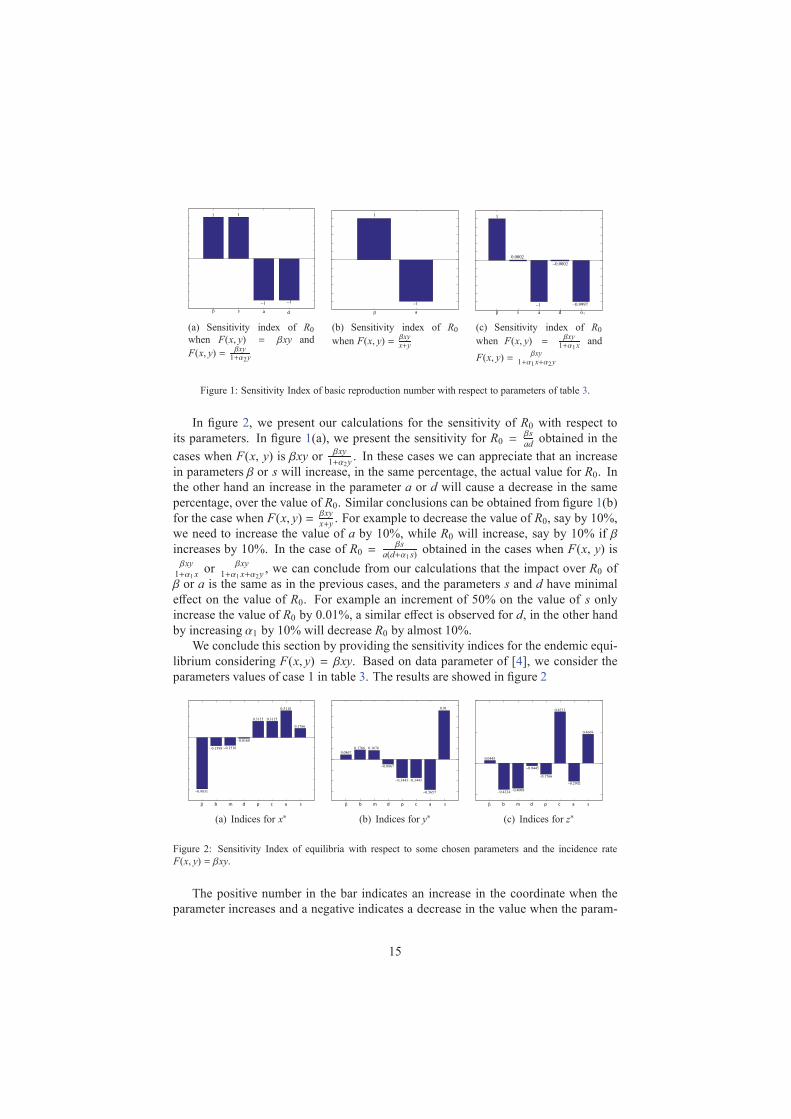
Figure 1: Sensitivity Index of basic reproduction number with respect to parameters of table 3.

In figure 2, we present our calculations for the sensitivity of R0 with respect to

its parameters. In figure 1(a), we present the sensitivity for R0 =βs

adobtained in the

cases when F(x, y) is βxy orβxy

1+α2y. In these cases we can appreciate that an increase

in parameters β or s will increase, in the same percentage, the actual value for R0. In

the other hand an increase in the parameter a or d will cause a decrease in the same

percentage, over the value of R0. Similar conclusions can be obtained from figure 1(b)

for the case when F(x, y) =βxy

x+y. For example to decrease the value of R0, say by 10%,

we need to increase the value of a by 10%, while R0 will increase, say by 10% if β

increases by 10%. In the case of R0 =βs

a(d+α1 s)obtained in the cases when F(x, y) is

βxy

1+α1xor

βxy

1+α1 x+α2y, we can conclude from our calculations that the impact over R0 of

β or a is the same as in the previous cases, and the parameters s and d have minimal

effect on the value of R0. For example an increment of 50% on the value of s only

increase the value of R0 by 0.01%, a similar effect is observed for d, in the other hand

by increasing α1 by 10% will decrease R0 by almost 10%.

We conclude this section by providing the sensitivity indices for the endemic equi-

librium considering F(x, y) = βxy. Based on data parameter of [4], we consider the

parameters values of case 1 in table 3. The results are showed in figure 2

β b m d p c a s

−0.9831

−0.1598 −0.1516

−0.0168

0.3115 0.3115

0.5118

0.1766

(a) Indices for x∗

β b m d p c a s

0.08670.1766 0.1676

−0.0867

−0.3443 −0.3443

−0.5657

0.91

(b) Indices for y∗

β b m d p c a s

0.0445

−0.4224−0.4008

−0.0445

−0.1766

0.8233

−0.2902

0.4669

(c) Indices for z∗

Figure 2: Sensitivity Index of equilibria with respect to some chosen parameters and the incidence rate

F(x, y) = βxy.

The positive number in the bar indicates an increase in the coordinate when the

parameter increases and a negative indicates a decrease in the value when the param-

15

eter increases. From figure 2 we can observe the following facts: for the value of x∗,

showed in (a), the parameter with more influence is the contact rate, β, which means

that the number of susceptible cells will decrease when the contact rate with the in-

fected cells increases. By increasing this parameter 10% the amount of susceptible

cells will decrease 9.8%, note that increasing the death rate of infected cells, a, the

number of susceptible cells also increases. From panel (b) we can note that the param-

eter with more influence is the source of susceptible cells and the number of infected

cells will decrease if their death rate increases. A similar analysis can be made from

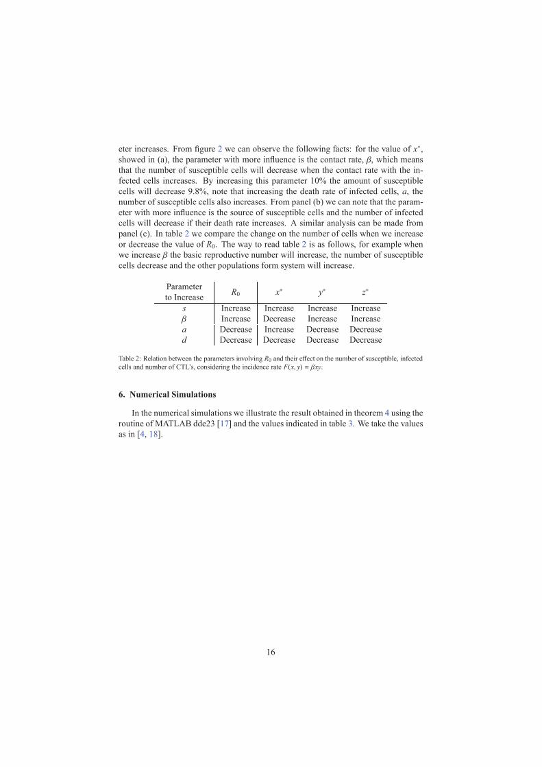
panel (c). In table 2 we compare the change on the number of cells when we increase

or decrease the value of R0. The way to read table 2 is as follows, for example when

we increase β the basic reproductive number will increase, the number of susceptible

cells decrease and the other populations form system will increase.

Parameter

to IncreaseR0 x∗ y∗ z∗

s Increase Increase Increase Increase

β Increase Decrease Increase Increase

a Decrease Increase Decrease Decrease

d Decrease Decrease Decrease Decrease

Table 2: Relation between the parameters involving R0 and their effect on the number of susceptible, infected

cells and number of CTL’s, considering the incidence rate F(x, y) = βxy.

6. Numerical Simulations

In the numerical simulations we illustrate the result obtained in theorem 4 using the

routine of MATLAB dde23 [17] and the values indicated in table 3. We take the values

as in [4, 18].

16

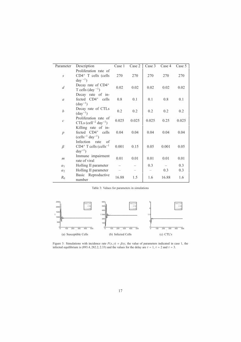
Parameter Description Case 1 Case 2 Case 3 Case 4 Case 5

s

Proliferation rate of

CD4+ T cells (cells

day −1)

270 270 270 270 270

dDecay rate of CD4+

T cells (day −1)0.02 0.02 0.02 0.02 0.02

a

Decay rate of in-

fected CD4+ cells

(day−1)

0.8 0.1 0.1 0.8 0.1

bDecay rate of CTLs

(day−1)0.2 0.2 0.2 0.2 0.2

cProliferation rate of

CTLs (cell−2 day−1)0.025 0.025 0.025 0.25 0.025

p

Killing rate of in-

fected CD4+ cells

(cells−1 day−1)

0.04 0.04 0.04 0.04 0.04

β

Infection rate of

CD4+ T cells (cells−1

day−1)

0.001 0.15 0.05 0.001 0.05

mImmune impairment

rate of viral0.01 0.01 0.01 0.01 0.01

α1 Holling II parameter – – 0.3 – 0.3

α2 Holling II parameter – – – 0.3 0.3

R0Basic Reproductive

number16.88 1.5 1.6 16.88 1.6

Table 3: Values for parameters in simulations

0 100 200 300 400 5000

500

1000

1500

2000

2500

t

x(t

)

τ =1

τ =2

τ =3

(a) Susceptible Cells

0 100 200 300 400 5000

100

200

300

400

500

600

t

y(t

)

τ =1

τ =2

τ =3

(b) Infected Cells

0 100 200 300 400 5001

2

3

4

5

t

z(t

)

τ =1

τ =2

τ =3

(c) CTL’s

Figure 3: Simulations with incidence rate F(x, y) = βxy, the value of parameters indicated in case 1, the

infected equilibrium is (893.4, 282.2, 2.33) and the values for the delay are τ = 1, τ = 2 and τ = 3.

17

0 100 200 300 400 5000

5000

10000

15000

t

x(t

)

τ =1

τ =2

τ =3

(a) Susceptible Cells

0 100 200 300 400 5000

50

100

150

200

t

y(t

)

τ =1

τ =2

τ =3

(b) Infected Cells

0 100 200 300 400 5001

2

3

4

5

t

z(t

)

τ =1

τ =2

τ =3

(c) CTL’s

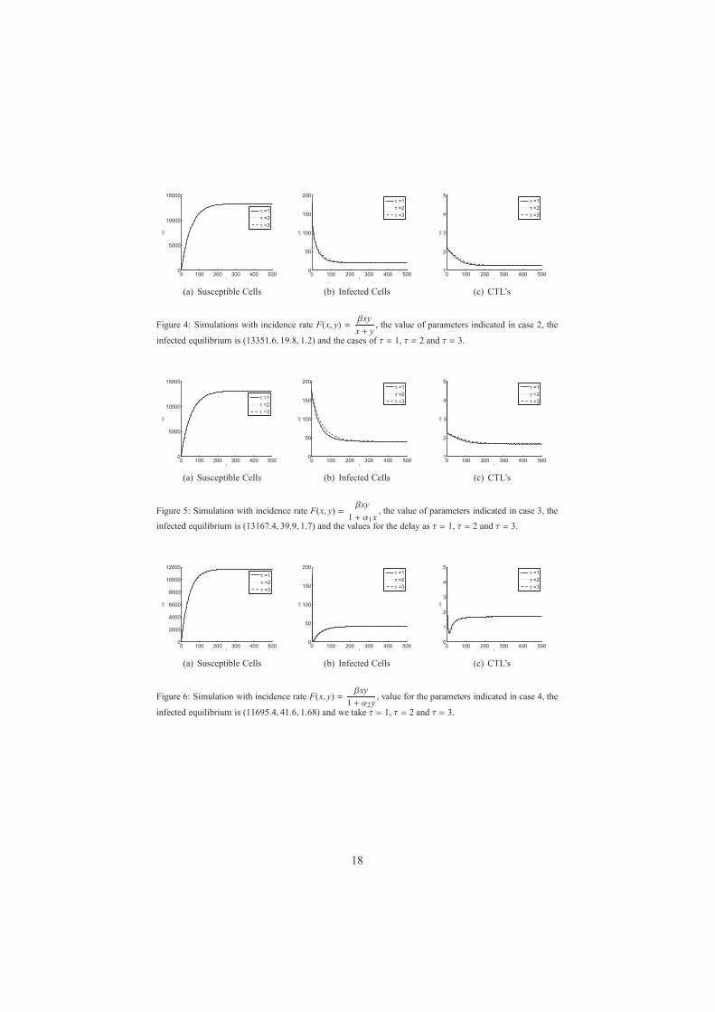
Figure 4: Simulations with incidence rate F(x, y) =βxy

x + y, the value of parameters indicated in case 2, the

infected equilibrium is (13351.6, 19.8, 1.2) and the cases of τ = 1, τ = 2 and τ = 3.

0 100 200 300 400 5000

5000

10000

15000

t

x(t

)

τ =1

τ =2

τ =3

(a) Susceptible Cells

0 100 200 300 400 5000

50

100

150

200

t

y(t

)

τ =1

τ =2

τ =3

(b) Infected Cells

0 100 200 300 400 5001

2

3

4

5

t

z(t

)

τ =1

τ =2

τ =3

(c) CTL’s

Figure 5: Simulation with incidence rate F(x, y) =βxy

1 + α1x, the value of parameters indicated in case 3, the

infected equilibrium is (13167.4, 39.9, 1.7) and the values for the delay as τ = 1, τ = 2 and τ = 3.

0 100 200 300 400 5000

2000

4000

6000

8000

10000

12000

t

x(t

)

τ =1

τ =2

τ =3

(a) Susceptible Cells

0 100 200 300 400 5000

50

100

150

200

t

y(t

)

τ =1

τ =2

τ =3

(b) Infected Cells

0 100 200 300 400 5000

1

2

3

4

5

t

z(t

)

τ =1

τ =2

τ =3

(c) CTL’s

Figure 6: Simulation with incidence rate F(x, y) =βxy

1 + α2y, value for the parameters indicated in case 4, the

infected equilibrium is (11695.4, 41.6, 1.68) and we take τ = 1, τ = 2 and τ = 3.

18

0 100 200 300 400 5000

5000

10000

15000

t

x(t

)

τ =1

τ =2

τ =3

(a) Susceptible Cells

0 100 200 300 400 5000

50

100

150

200

t

y(t

)

τ =1

τ =2

τ =3

(b) Infected Cells

0 100 200 300 400 5001

2

3

4

5

t

z(t

)

τ =1

τ =2

τ =3

(c) CTL’s

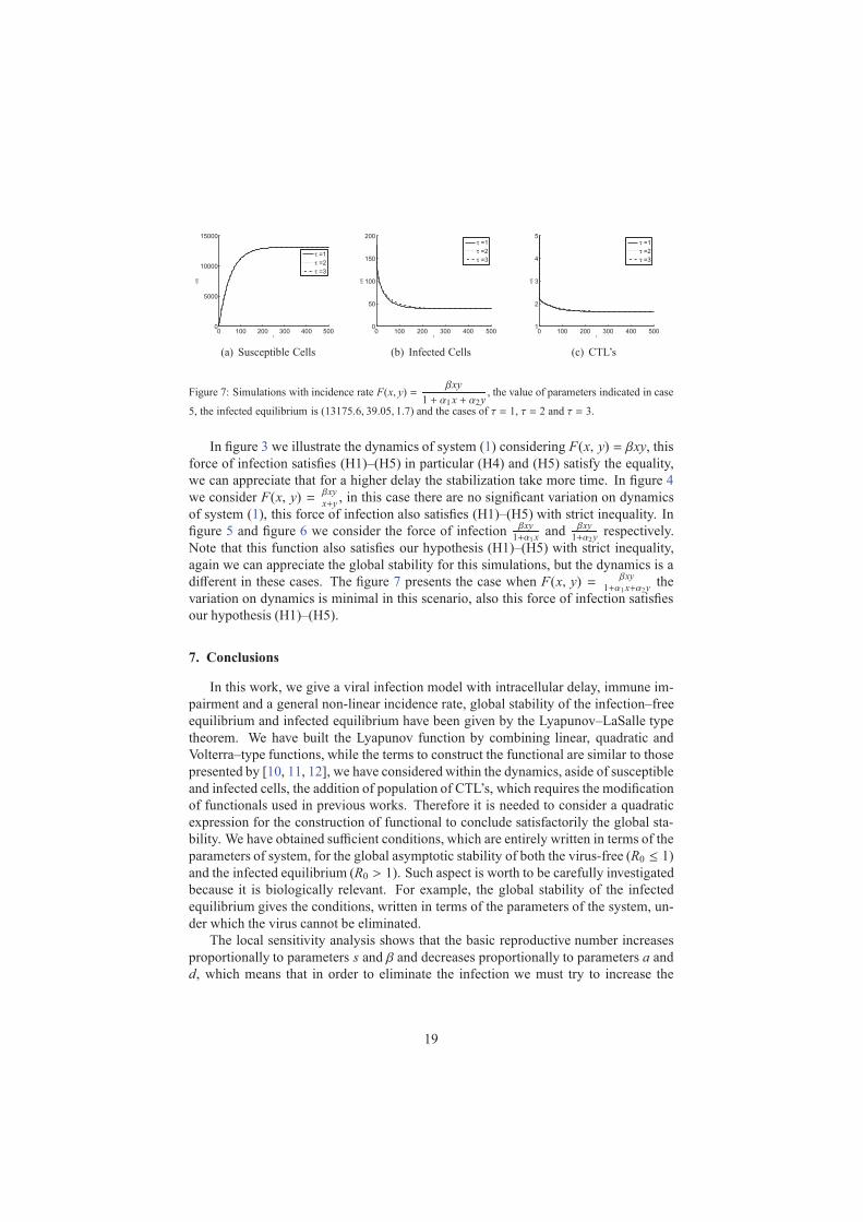
Figure 7: Simulations with incidence rate F(x, y) =βxy

1 + α1x + α2y, the value of parameters indicated in case

5, the infected equilibrium is (13175.6, 39.05, 1.7) and the cases of τ = 1, τ = 2 and τ = 3.

In figure 3 we illustrate the dynamics of system (1) considering F(x, y) = βxy, this

force of infection satisfies (H1)–(H5) in particular (H4) and (H5) satisfy the equality,

we can appreciate that for a higher delay the stabilization take more time. In figure 4

we consider F(x, y) =βxy

x+y, in this case there are no significant variation on dynamics

of system (1), this force of infection also satisfies (H1)–(H5) with strict inequality. In

figure 5 and figure 6 we consider the force of infectionβxy

1+α1xand

βxy

1+α2yrespectively.

Note that this function also satisfies our hypothesis (H1)–(H5) with strict inequality,

again we can appreciate the global stability for this simulations, but the dynamics is a

different in these cases. The figure 7 presents the case when F(x, y) =βxy

1+α1x+α2ythe

variation on dynamics is minimal in this scenario, also this force of infection satisfies

our hypothesis (H1)–(H5).

7. Conclusions

In this work, we give a viral infection model with intracellular delay, immune im-

pairment and a general non-linear incidence rate, global stability of the infection–free

equilibrium and infected equilibrium have been given by the Lyapunov–LaSalle type

theorem. We have built the Lyapunov function by combining linear, quadratic and

Volterra–type functions, while the terms to construct the functional are similar to those

presented by [10, 11, 12], we have considered within the dynamics, aside of susceptible

and infected cells, the addition of population of CTL’s, which requires the modification

of functionals used in previous works. Therefore it is needed to consider a quadratic

expression for the construction of functional to conclude satisfactorily the global sta-

bility. We have obtained sufficient conditions, which are entirely written in terms of the

parameters of system, for the global asymptotic stability of both the virus-free (R0 ≤ 1)

and the infected equilibrium (R0 > 1). Such aspect is worth to be carefully investigated

because it is biologically relevant. For example, the global stability of the infected

equilibrium gives the conditions, written in terms of the parameters of the system, un-

der which the virus cannot be eliminated.

The local sensitivity analysis shows that the basic reproductive number increases

proportionally to parameters s and β and decreases proportionally to parameters a and

d, which means that in order to eliminate the infection we must try to increase the

19

value of a or d. From table 2 a positive increment on the parameter a, will decrease the

number of infected cells and CTL’s and will increase the number of susceptible cells.

Our result establishes that no sustained oscillation regime exists which is similar to

the conclusion of paper [9] but quite different from the conclusion of paper [4], where

there are sustained oscillations. We think that if we introduce in model (1) a logistic

proliferation term for the uninfected cells we could get sustained oscillations as in [7].

Aknowledgements

We would like to thank the anonymous referees for their valuable comments ans

suggestions. This article was supported in part by Mexican SNI under grants 33365

and 15284.

References

References

[1] R. Regoes, D. Wodarz, M. A. Nowak. Virus dynamics: the effect to target cell

limitation and immune responses on virus evolution. J. Theor. Biol. 191 (1998),

451–462.

[2] R.J. De Boer, A.S. Perelson, Towards a general function describing T cell prolif-

eration, J. Theoret. Biol. 175 (1995) 567–576.

[3] R.J. De Boer, A.S. Perelson, Target cell limited and immune control models of

HIV infection: a comparison, J. Theoret. Biol. 190 (1998) 201–214.

[4] S. Wang, X. Song, Z. Ge. Dynamics analysis of a delayed viral infection model

with immune impairment. Appl. Math. Modelling, 35 (2011) 4877–4885.

[5] Z. Wang and X. Liu. A chronic viral infection model with immune impairment.

Journal of Theoretical Biology, 249 (2007), 532–542.

[6] Q. Xie, D. Huang, S. Zhang, and J. Cao, Analysis of a viral infection model with

delayed immune response, Applied Mathematical Modelling, vol. 34, no. 9, pp.

2388–2395, 2010.

[7] Z. Hu, J. Zhang, H. Wang, W. Ma and F. Liao. Dynamics of a delayed viral infec-

tion model with logistic growth and immune impairment. Applied Mathematical

Modelling (2013).

[8] X. Y. Song, S. L. Wang and J. Dong. Stability properties and Hopf bifurcation of

a delayed viral infection model with lytic immune response. J. Math. Anal. Appl.

373 (2011), 345–355.

[9] F. Song, X. Wang and X. Y. Song. Stability properties of a delayed viral infec-

tion model with lytic immune response. J. Appl. Math. and Informatics, Vol. 29

(2011), 1117–1127.

20

[10] G. Huang, Y. Takeuchi, W. Ma, D. Wei. Global Stability for Delay SIR and SEIR

Epidemic Models with Nonlinear Incidence Rate. Bulletin of Mathematical Biol-

ogy (2010) 72: 1192–1207

[11] A. Korobeinikov. Global Properties of Infectious Disease Models with Nonlinear

Incidence. Bulletin of Mathematical Biology (2007) 69: 1871–1886

[12] Y. Enatsu, Y. Nakata, Y. Muroya. Global stability of SIR epidemic models with

a wide class of nonlinear incidence rates and distributed delays. Discrete and

Continuous Dynamical Systems B 15 (2011) 61–74

[13] Y. Muroya, Y. Enatsu, H. Li. Global stability of a delayed HTLV–I infection

model with a class of non-linear incidence rates and CTLs immune response.

Applied Mathematics and Computation, 219 (2013) 10559–10573.

[14] M. Li, X. Liu. An SIR epidemic model with time delay and general non-linear

incidence rate. Abstract and Applied Analysis. Volume 2014, 1–7.

[15] Y. Kuang Delay Differential Equations With Applications In Population Dynam-

ics, Academic Press, 1993.

[16] Chitnis N., Hyman J. M., Cushing J. M., Determining important parameters in the

spread of malaria through the sensitivity analysis of a mathematical model. Bull.

Math. Biol., 70, 1272–1296 (2008).

[17] L. F. Shampine, S. Thompson, Solving DDEs in MATLAB, Appl. Numer. Math.

37 (2001) 441–458.

[18] K. Wang, W. Wang, X. Liu. Global Stability in a viral infection model with Lytic

and Nonlytic Immune Responses. Computers and Mathematics Applications. 51

(2006) 1593–1610.

[19] J. K. Hale, P. Waltman, Persistence in infinite-dimensional systems, SIAM J.

Math. Anal. 20 (1989) 388–396.

21