Packet Delivery Delay and ThroughputOptimization for Vehicular Networks

by

Ahmad Mostafa

A dissertation submitted in partial satisfaction of the

requirements for the degree of

Doctor of Philosophy

in

Computer Science and Engineering

in the

School of Computing Sciences and Informatics

of theCollege of Engineering

of the

UNIVERSITY OF CINCINNATI, OHIO

Committee:Professor Dharma P Agrawal, Chair

Professor Raj BhatnagarProfessor Chia-Yung HanProfessor John FrancoProfessor Yizong ChengProfessor Yiming Hu

January 2013

Abstract

Vehicular networking is a new emerging wireless technology concept that supports

communication amongst various nearby vehicles themselves and enables vehicles to

have access to the Internet. This networking technology provides vehicles with endless

possibilities of applications, including safety, convenience, and entertainment. Exam-

ples for these applications are safety messaging exchange, real-time tra�c information

sharing, route condition updates, besides a general purpose Internet access. The goal

of vehicular networks is to provide an e�cient, safe, and convenient environment for

vehicles on the road.

In vehicular networking technology, vehicles connect either through other vehicles

in an ad hoc multi-hop fashion or through road side units (infrastructure) which

connects them to the Internet. These approaches have their own advantages and

disadvantages. However, one of the main objectives of vehicular networking is to

achieve a minimal delay for message delivery, and encourage potential continuous

connectivity among vehicles.

This dissertation introduces a novel hybrid communication paradigm for achieving

seamless connectivity as Vehicular Ad Hoc NETworks (VANETs), wherein connectiv-

ity is often a↵ected by changes in vehicles’ speed, dynamic topology, as well as tra�c

density. Our proposed technique —named QoS-oriented Hybrid Vehicular Communi-

cations Protocol (QoSHVCP)— exploits both existing network infrastructure through

a Vehicle-to-Infrastructure (V2I) protocol, as well as a traditional Vehicle-to-Vehicle

(V2V), that satisfies Quality-of-Service requirements. We analyze time delay as a

performance metric, and determine delay propagation rates when vehicles are trans-

i

mitting high priority messages via QoSHVCP.

Focusing on V2V communication, we propose a reliable and low-collision packet-

forwarding scheme, based on a novel concept of probabilistic rebroadcasting. Our

proposed scheme, called Collision-Aware REliable FORwarding (CAREFOR), works

in a distributed fashion where each vehicle receiving a packet rebroadcasts based on

a predefined probability. The success of rebroadcast is determined based on allowing

the message to travel the furthest possible distance with the least amount of packet

collisions.

We also present a QoS-Aware node Selection Algorithm (QASA) for VANET

routing protocols. Our algorithm is focused on selecting the vehicle to forward the

message, where vehicles on the east (west) select from the west (east), and is achieved

by exploiting a useful notion of the bridging approach. The QoS metrics that are

being optimized include the throughput in the network and end-to-end delay for the

packets.

Finally, we exploit the use of autonomous vehicles in order to optimize the end-

to-end packet delivery delay. Our protocol introduces a dynamic metric that depends

on the vehicular density on the highway in order to control the inter-vehicle distance.

Our results show a great promise for their future use in the area of vehicular

technology.

ii

c� 2013All rights reserved

Contents

List of Figures vi

List of Tables x

1 Introduction 11.1 Scope of Applications . . . . . . . . . . . . . . . . . . . . . . . . . . . 2

1.1.1 Application Requirements . . . . . . . . . . . . . . . . . . . . 51.2 Vehicular Networking Technology . . . . . . . . . . . . . . . . . . . . 61.3 Vehicular Networking Initiatives . . . . . . . . . . . . . . . . . . . . . 61.4 Problem Specification . . . . . . . . . . . . . . . . . . . . . . . . . . . 7

1.4.1 Vehicular Networking Scenarios . . . . . . . . . . . . . . . . . 71.4.2 Network Connectivity . . . . . . . . . . . . . . . . . . . . . . 9

1.5 Contributions . . . . . . . . . . . . . . . . . . . . . . . . . . . . . . . 91.6 Research Scenario . . . . . . . . . . . . . . . . . . . . . . . . . . . . . 121.7 Dissertation Outline . . . . . . . . . . . . . . . . . . . . . . . . . . . 13

2 Vehicular Networking 152.1 Intelligent Transportation System . . . . . . . . . . . . . . . . . . . . 152.2 Characteristics of VANETs . . . . . . . . . . . . . . . . . . . . . . . . 162.3 VANET and Cellular Networks . . . . . . . . . . . . . . . . . . . . . 172.4 VANET versus MANET . . . . . . . . . . . . . . . . . . . . . . . . . 182.5 Vehicular Network Hardware . . . . . . . . . . . . . . . . . . . . . . . 19

2.5.1 Sensor Network . . . . . . . . . . . . . . . . . . . . . . . . . . 202.5.2 Communication Systems . . . . . . . . . . . . . . . . . . . . . 212.5.3 Sensor and Communication Applications . . . . . . . . . . . . 22

2.6 Vehicular Network Model . . . . . . . . . . . . . . . . . . . . . . . . . 222.6.1 Vehicle-to-Vehicle . . . . . . . . . . . . . . . . . . . . . . . . . 232.6.2 Vehicle-to-Infrastructure . . . . . . . . . . . . . . . . . . . . . 242.6.3 Hybrid Model . . . . . . . . . . . . . . . . . . . . . . . . . . . 24

2.7 V2V versus V2I . . . . . . . . . . . . . . . . . . . . . . . . . . . . . . 252.8 Vehicular Networking Initiatives . . . . . . . . . . . . . . . . . . . . . 26

iv

2.8.1 Congestion Initiative . . . . . . . . . . . . . . . . . . . . . . . 262.8.2 Next Generation 9-1-1 . . . . . . . . . . . . . . . . . . . . . . 262.8.3 Cooperative Intersection Collision Avoidance System . . . . . 272.8.4 Clarus . . . . . . . . . . . . . . . . . . . . . . . . . . . . . . . 272.8.5 Mobility Services for All Americans . . . . . . . . . . . . . . . 272.8.6 Rural Safety . . . . . . . . . . . . . . . . . . . . . . . . . . . . 27

2.9 Summary . . . . . . . . . . . . . . . . . . . . . . . . . . . . . . . . . 28

3 QoSHVCP: QoS-oriented Hybrid Vehicular Communications Proto-col 303.1 Related Work . . . . . . . . . . . . . . . . . . . . . . . . . . . . . . . 30

3.1.1 Delay Tolerant Networks . . . . . . . . . . . . . . . . . . . . . 313.1.2 Broadcasting Techniques . . . . . . . . . . . . . . . . . . . . . 323.1.3 Vehicle-to-Infrastructure . . . . . . . . . . . . . . . . . . . . . 343.1.4 Hybrid Model . . . . . . . . . . . . . . . . . . . . . . . . . . . 343.1.5 Analytical Models for Data Delivery Rates . . . . . . . . . . . 353.1.6 Load Sharing and Balancing . . . . . . . . . . . . . . . . . . . 36

3.2 Our QoSHVCP Approach . . . . . . . . . . . . . . . . . . . . . . . . 373.2.1 QoSHVCP Scheme . . . . . . . . . . . . . . . . . . . . . . . . 373.2.2 Delay-based Protocol Switching Mechanism in QoSHVCP . . 393.2.3 Load Balancing Mechanism in QoSHVCP . . . . . . . . . . . 41

3.3 Message Delivery Time Rates . . . . . . . . . . . . . . . . . . . . . . 443.3.1 Delay in Vehicle-to-Vehicle Communication . . . . . . . . . . . 44

3.4 Delay in Vehicle-to-Infrastructure Communication . . . . . . . . . . . 463.4.1 Connectivity Phases . . . . . . . . . . . . . . . . . . . . . . . 473.4.2 Average Propagation Time Delay . . . . . . . . . . . . . . . . 52

3.5 Simulation Results . . . . . . . . . . . . . . . . . . . . . . . . . . . . 523.5.1 Simulation setup . . . . . . . . . . . . . . . . . . . . . . . . . 533.5.2 Simulation results . . . . . . . . . . . . . . . . . . . . . . . . . 55

3.6 Summary . . . . . . . . . . . . . . . . . . . . . . . . . . . . . . . . . 64

4 CAREFOR for VANET 684.1 Introduction . . . . . . . . . . . . . . . . . . . . . . . . . . . . . . . . 694.2 Related Work . . . . . . . . . . . . . . . . . . . . . . . . . . . . . . . 704.3 Collision-Aware REliable FORwarding . . . . . . . . . . . . . . . . . 75

4.3.1 Reliable Forwarding . . . . . . . . . . . . . . . . . . . . . . . 754.3.2 Collision Probability . . . . . . . . . . . . . . . . . . . . . . . 794.3.3 Analytical Model . . . . . . . . . . . . . . . . . . . . . . . . . 814.3.4 CAREFOR algorithm . . . . . . . . . . . . . . . . . . . . . . 864.3.5 CAREFOR as two hop vs. three hop algorithm . . . . . . . . 89

4.4 Simulation Results . . . . . . . . . . . . . . . . . . . . . . . . . . . . 904.4.1 CAREFOR v/s IF . . . . . . . . . . . . . . . . . . . . . . . . 90

v

4.4.2 Two vs. Three Hops Prediction . . . . . . . . . . . . . . . . . 924.5 Summary . . . . . . . . . . . . . . . . . . . . . . . . . . . . . . . . . 93

5 QASA: QoS-Aware Node Selection Algorithm 1005.1 Introduction . . . . . . . . . . . . . . . . . . . . . . . . . . . . . . . . 1015.2 Related Work . . . . . . . . . . . . . . . . . . . . . . . . . . . . . . . 1035.3 QoS-Aware Node Selection Algorithm . . . . . . . . . . . . . . . . . . 105

5.3.1 Analytical Model . . . . . . . . . . . . . . . . . . . . . . . . . 1085.3.2 QASA Algorithm . . . . . . . . . . . . . . . . . . . . . . . . . 110

5.4 Simulation Results . . . . . . . . . . . . . . . . . . . . . . . . . . . . 1145.5 Summary . . . . . . . . . . . . . . . . . . . . . . . . . . . . . . . . . 119

6 QoS-Aware Routing for Autonomous Vehicles 1266.1 Introduction . . . . . . . . . . . . . . . . . . . . . . . . . . . . . . . . 1276.2 Related Work . . . . . . . . . . . . . . . . . . . . . . . . . . . . . . . 1296.3 Inter-vehicle Distance and Delay . . . . . . . . . . . . . . . . . . . . . 1316.4 Inter-vehicle Distance Manipulation for Autonomuos Vehicles (ID-MAV)1356.5 Simulation Results . . . . . . . . . . . . . . . . . . . . . . . . . . . . 1386.6 Summary . . . . . . . . . . . . . . . . . . . . . . . . . . . . . . . . . 138

7 Summary & Future Research Directions 1417.1 Summary . . . . . . . . . . . . . . . . . . . . . . . . . . . . . . . . . 1417.2 Future Research Directions . . . . . . . . . . . . . . . . . . . . . . . . 144

Bibliography 146

vi

List of Figures

1.1 Figure depicting applications available to vehicle through the vehicularnetwork technology . . . . . . . . . . . . . . . . . . . . . . . . . . . . 2

1.2 Breakdown of American and British Tra�c Causes in 1985 [1]. . . . 31.3 Highway model of a vehicular network . . . . . . . . . . . . . . . . . 81.4 City model of a vehicular network . . . . . . . . . . . . . . . . . . . . 8

2.1 Some examples of on-board vehicle sensors [2] . . . . . . . . . . . . . 212.2 Breakdown of standards and network layers for the vehicular commu-

nication technology [3] . . . . . . . . . . . . . . . . . . . . . . . . . . 222.3 The di↵erent communication models in a Vehicular network scenario [4] 23

3.1 Vehicular grid with an overlapping heterogeneous wireless network in-frastructure. . . . . . . . . . . . . . . . . . . . . . . . . . . . . . . . . 39

3.2 Percentage of channel utilization in a wireless network for HP messagesdelivery, and ⌫max = [40, 60, 80]). . . . . . . . . . . . . . . . . . . . . 43

3.3 Vehicular grid comprised of l-size virtual cells. The probability that avehicle is connected via V2V and V2I depends on the cells occupancyby the vehicles. . . . . . . . . . . . . . . . . . . . . . . . . . . . . . . 50

3.4 (a) Average message propagation delay for increasing vehicle density,and speed for Phase 1 (no connectivity) at di↵erent speeds (i.e., 15, 20,25 and 35 m/s). (b) Average message propagation delay for increasingthe vehicle density at di↵erent tra�c speeds using V2V communication. 56

3.5 (a) Average message propagation delay for increasing vehicle densityfor V2V, V2V Bridged and QoSHVCP at a fixed speed. (b) Aver-age message propagation delay for increasing vehicle density in pureinfrastructure communications at di↵erent uplink and downlink rates. 59

3.6 The e↵ect of the network overload on both V2V and V2I. . . . . . . . 603.7 Message propagation delay for High and Low Priority messages with

di↵erent probabilities of High Priority without load balancing mechanism. 61

vii

3.8 Message propagation delay for High and Low Priority messages withdi↵erent probabilities of High Priority with our load balancing mecha-nism. . . . . . . . . . . . . . . . . . . . . . . . . . . . . . . . . . . . . 62

3.9 Number of packets experiencing di↵erent message propagation delaysat the vehicle density of 65 [veh/km] and HP message probability of 0.2. 63

3.10 Number of packets experiencing di↵erent message propagation delaysat the vehicle density of 65 [veh/km] and high priority message prob-ability of 0.3. . . . . . . . . . . . . . . . . . . . . . . . . . . . . . . . 64

3.11 Number of packets experiencing di↵erent message propagation delaysat the vehicle density of 65 [veh/km] and high priority message prob-ability of 0.4. . . . . . . . . . . . . . . . . . . . . . . . . . . . . . . . 65

4.1 Schematic of RF approach in a vehicular network. The vehicle v0 isa source transmitting a packet to potential forwarding vehicles withinits transmission range (i.e., z). The basic assumption is that vehiclesmay have di↵erent transmission ranges (i.e., z00 < z0 < z), which a↵ectthe next-hop rebroadcast probability. . . . . . . . . . . . . . . . . . . 77

4.2 RF rebroadcast probability as a function of the distance between thereceiver vehicle and the transmitter. (a) Dependence on di↵erent val-ues of c, and ⇢. The solid lines are for z/z

i

= 2, while dotted lines arefor z/z

i

= 0.5 m; (b) dependence on increasing next-hop transmissionranges i.e., z

i

= 100, 200, 400 m, given c = 2, z = 200 m, and ⇢ = 0.02. 944.3 Analytical trends of (a) collision probability experienced by vehicles

within a z = 200 m source’s transmission range, and (b) collisionprobability threshold, vs. the vehicle density; for di↵erent next-hoptransmission ranges, n = 2, ⇢ = 0.04 and c = 5. . . . . . . . . . . . . 95

4.4 Comparison between IF and CAREFOR, in terms of collision prob-ability, as a percentage of the collisions part of the total number ofmessages in the system, vs. the vehicular density. Notice that thecollision reduction is provided by CAREFOR. . . . . . . . . . . . . . 96

4.5 Comparison between CAREFOR and IF in terms of throughput, as apercentage of messages arrived to a vehicle receiver and relative to thetotal number of messages exchanged in the system, vs. the vehiculardensity. The high performance with CAREFOR is due to the highreduction of broadcast messages. . . . . . . . . . . . . . . . . . . . . . 96

4.6 Comparison between CAREFOR and IF in terms of the percentageof successful transmissions vs.the vehicular density, w.r.t. the totalnumber of transmissions including the collided attempts. . . . . . . . 97

4.7 Collision Probability, as a percentage of the collisions part of the totalnumber of messages in the system, in both three and two hops CARE-FOR algorithm. A small increase of performance is provided by threehop CAREFOR approach. . . . . . . . . . . . . . . . . . . . . . . . . 97

viii

4.8 Throughput, as a percentage of messages arrived to a vehicle receiverand relative to the total number of messages exchanged in the system,in both three- and two-hops CAREFOR algorithm. Minor improve-ment is provided with the three-hop prediction. . . . . . . . . . . . . 98

4.9 Percentage of successful transmissions compared to the total numberof transmissions including the collided attempts, in both three- andtwo-hops CAREFOR algorithm. Minor improvement is provided withthe three-hop prediction. . . . . . . . . . . . . . . . . . . . . . . . . . 99

5.1 Schematic of a vehicular opportunistic network, with bridging approach.A source (blue) vehicle shall select a next-hop forwarder from the oppo-site lane, since the forward inter-vehicular gap is too large for allowingV2V communications (i.e., r(Tx)

i

> �ij

). The blue and black boxes rep-resent the source’s transmission range and the cluster size, respectively. 106

5.2 QASA technique main aspects. (12a) Dividing the transmission rangeof a source vehicle (i.e., the white vehicle) into smaller circular trans-mission domains (i.e., with C1 > C2 > C3) for next-hop selection. (12b)The scenario explains the trade-o↵ between time delay and throughputperformance with QASA technique. . . . . . . . . . . . . . . . . . . . 107(a) . . . . . . . . . . . . . . . . . . . . . . . . . . . . . . . . . . . . 107(b) . . . . . . . . . . . . . . . . . . . . . . . . . . . . . . . . . . . . 107

5.3 Scheme for next-hop forwarder selection algorithm based on the cov-erage crossing time calculation, �T [s]. Assuming each vehicle has anomnidirectional coverage, with radius R [m], (a) the red vehicle willexperience longest time connection with the blue vehicle, respect tothe green one, which is exiting the coverage area. (b) The coveragecrossing time is calculated as a time interval (i.e., from t

in

to tout

[s]). 120(a) . . . . . . . . . . . . . . . . . . . . . . . . . . . . . . . . . . . . 120(b) . . . . . . . . . . . . . . . . . . . . . . . . . . . . . . . . . . . . 120

5.4 E↵ect of bridging on the number of disconnected clusters on highway. 1215.5 Total communication time analysis for algorithm with di↵erent regions. 1225.6 Throughput analysis for algorithm with di↵erent regions. . . . . . . . 1225.7 Throughput for di↵erent ranges at lower tra�c densities. . . . . . . . 1235.8 Average time delay vs. the vehicular density for di↵erent ranges. . . . 1235.9 Average time delay vs. the vehicular density for di↵erent ranges with

a packet regeneration every 20 seconds. . . . . . . . . . . . . . . . . . 1245.10 E↵ect of FRP variable on total time communicated. . . . . . . . . . . 1245.11 E↵ect of FRP variable on total time communicated. . . . . . . . . . . 1255.12 E↵ect of FRP variable on throughput. . . . . . . . . . . . . . . . . . 125

6.1 3D figure presenting end-to-end packet delay for the di↵erent values of r.1326.2 2D figure presenting end-to-end packet delay for the di↵erent values of r.133

ix

6.3 Comparing the end-to-end delay in the case of controlling inter-vehicledistance vs not controlling. . . . . . . . . . . . . . . . . . . . . . . . . 134

6.4 3D figure presenting vehicle delay for the di↵erent values of r. . . . . 1356.5 2D figure presenting vehicle delay for the di↵erent values of r. . . . . 1366.6 E↵ect of the c value on the inter-vehicle distance versus vehicle density. 1376.7 End-to-end delay performance for c=6 vs the di↵erent inter-vehicle

distance values. . . . . . . . . . . . . . . . . . . . . . . . . . . . . . . 1396.8 Vehicle delay performance for c=6 vs the di↵erent inter-vehicle distance

values. . . . . . . . . . . . . . . . . . . . . . . . . . . . . . . . . . . . 140

x

List of Tables

1.1 Specific Research Contributions. . . . . . . . . . . . . . . . . . . . . . 11

2.1 Di↵erence between VANET and MANET technologies. . . . . . . . . 192.3 Di↵erent applications that require sensors and communication tech-

nologies. . . . . . . . . . . . . . . . . . . . . . . . . . . . . . . . . . . 282.2 A comparison between the di↵erent wireless technologies and the DSRC

technology [3] . . . . . . . . . . . . . . . . . . . . . . . . . . . . . . . 29

3.1 Parameter setup used in simulations. . . . . . . . . . . . . . . . . . . 54

4.1 Message exchanged classification and content. . . . . . . . . . . . . . 884.2 Simulation Parameters. . . . . . . . . . . . . . . . . . . . . . . . . . . 88

5.1 QASA message exchanged classification and content. . . . . . . . . . 1135.2 Simulation Parameters. . . . . . . . . . . . . . . . . . . . . . . . . . . 115

6.1 Simulation Parameters. . . . . . . . . . . . . . . . . . . . . . . . . . . 131

xi

Chapter 1

Introduction

The concept of vehicular technology has emerged due to advancements in wire-

less sensor networks as well as ad hoc networks. The progress in these fields has

allowed sensors placed at di↵erent location within the vehicles to communicate with

each other wirelessly. Ad hoc networks technology has allowed vehicles to commu-

nicate with other vehicles in its surrounding area. The combination of sensing and

communication enables the vehicles to respond to di↵erent request and provide many

useful services. For example, the vehicle brakes can respond when the vehicle senses

that there is a vehicle at a very close proximity or that the conditions of the road

cannot sustain the vehicle speed. Another example would be for the air bags and

pre-tension safety belts to be activated when detecting a potential for an accident.

Tra�c conditions on the road ahead can be communicated to the vehicles and provide

an alternative route that could shorten the length and duration of a trip. Internet

can be accessible to the vehicle occupants through the communication ability of well-

placed road side units. The Internet access can either be used for safety, or can be

utilized for entertainment purpose such as streaming movies or browsing the Internet.

1

Figure 1.1 depicts di↵erent services that can be provided to the vehicle through the

vehicular network technology.

Figure 1.1: Figure depicting applications available to vehicle through the vehicularnetwork technology

1.1 Scope of Applications

Vehicles have started playing an important role in peoples lives, and hence, enhanc-

ing them with software and hardware based intelligence would drastically improve the

passengers quality of life and experience [5]. To elaborate on the importance of vehic-

ular networks, it is worth mentioning that more than half of the accidents each year

2

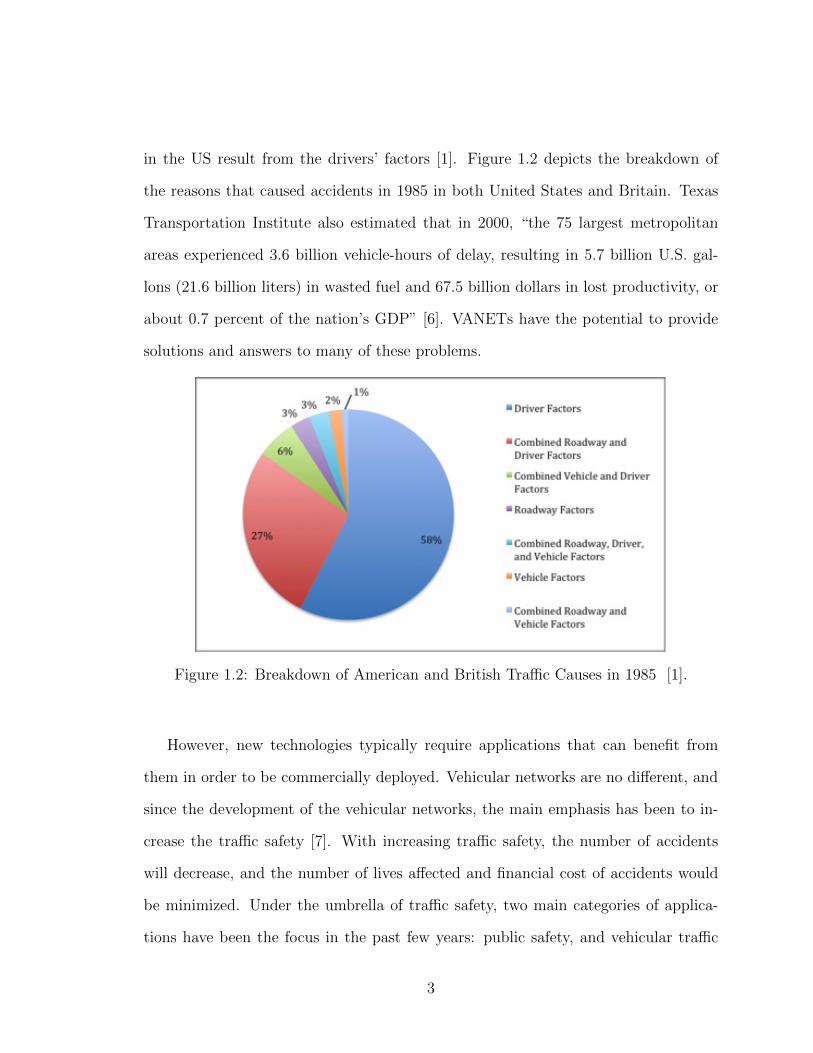
in the US result from the drivers’ factors [1]. Figure 1.2 depicts the breakdown of

the reasons that caused accidents in 1985 in both United States and Britain. Texas

Transportation Institute also estimated that in 2000, “the 75 largest metropolitan

areas experienced 3.6 billion vehicle-hours of delay, resulting in 5.7 billion U.S. gal-

lons (21.6 billion liters) in wasted fuel and 67.5 billion dollars in lost productivity, or

about 0.7 percent of the nation’s GDP” [6]. VANETs have the potential to provide

solutions and answers to many of these problems.

Figure 1.2: Breakdown of American and British Tra�c Causes in 1985 [1].

However, new technologies typically require applications that can benefit from

them in order to be commercially deployed. Vehicular networks are no di↵erent, and

since the development of the vehicular networks, the main emphasis has been to in-

crease the tra�c safety [7]. With increasing tra�c safety, the number of accidents

will decrease, and the number of lives a↵ected and financial cost of accidents would

be minimized. Under the umbrella of tra�c safety, two main categories of applica-

tions have been the focus in the past few years: public safety, and vehicular tra�c

3

coordination. An example for public safety applications would be collision avoidance,

while others that allow coordination of vehicles movement with each other would be

an example for vehicular tra�c coordination [7].

Considerable work has also been done to introduce and address usefulness that

relate to road tra�c management, as well as those that are for added comfort. Road

tra�c management purpose helps resolve issues such as tra�c congestion. This de-

creases the number of accidents during such congestions as well as aids in decreasing

the travel time. On the other hand, comfort applications provide entertainment and

relaxing experience to the drivers (viz., information from road-side units) and to the

accompanying passengers (such as Internet access or video-on-demand).

Vehicular networks are still in the phase of research, and hence, they are not yet

to be widely deployed. Many specific utilizations that are being considered in this

field are speculative and can be challenged [8]. Di↵erent initiatives lead to distinct

set of applications as their primary focus. However, there are three main categories

for use of vehicular network technologies:

1. Vehicle safety related applications: These focus on the safety of vehicles and

passengers. Collision avoidance are considered one of the most important ap-

plications in this category.

2. Tra�c conditions: These are aimed at improving the traveling experience by

helping the vehicle avoid tra�c congested area or by providing useful tra�c

information that helps in selecting an e↵ective routing.

3. Comfort applications: The goal is to provide comfort to the driver and the

vehicle passengers. This can be achieved through applications that allow the

user to communicate with the Internet, or allows for video streaming or mobile

4

o�ce applications.

1.1.1 Application Requirements

Each one of the three application categories has di↵erent requirements based on

the importance and required Quality of Service (QoS). The main goal of safety appli-

cations is to provide a safe environment for the occupants of the vehicle, the neighbor-

ing vehicles, the pedestrians, and the environment. This is usually achieved through

creating a connectivity mechanism between the neighboring vehicles that ensures

safety by avoiding any collision. In these types of endeavours, end-to-end message

propagation delay ought to be minimized. Messages that can not achieve this delay

requirement are discarded because of their irrelevance.

Tra�c and congestion control applications aim to minimize the trip duration

and avoid congested areas on the highway or on the roadway. The data for such

applications are gathered from di↵erent vehicles throughout the area of interest. This

data is not safety-sensitive; hence, the delay requirement can be slightly relaxed than

the data in the safety applications.

Finally, the internet and multimedia applications are those that allow the vehicle

occupants to have access to di↵erent context for the purpose of information and en-

tertainment. These applications require access to the infrastructure that can connect

them to the Internet. One of the main problems with this approach is the connectivity

between the infrastructure and the vehicles, i.e., the last mile problem.

Moreover, some of the underlying applications require only one hop communica-

tion (i.e., each vehicle needs to relay the information to the next hop only). However,

other applications require multi-hop communication (i.e., the information needs to

be relayed from the source in multiple hops). An example could be changing lane for

5

collision avoidance. In a lane changing step, each vehicle needs to inform only the

nearby vehicles merging from another lane and those are within its communication

range. However, for the collision avoidance applications, one of the worst accident

categories on the highway is that involves many vehicles rear-ending each other due

to significant reduction in speed of the first vehicle. In this case, if the first vehicle

could notify all multi-hop vehicles behind it of the sudden reduction in its speed, this

could help avoid the sequence of any potential read-ending crash.

1.2 Vehicular Networking Technology

A vehicular network is composed of two main components: sensing and commu-

nication. The sensor part has the capability of understanding the environment, the

vehicles, and the occupants of the vehicles. On the other hand, the communication en-

tity has the facility of relying this understanding to other vehicles or to infrastructure

on the side of the road (road side units).

The nature of vehicular networks is di↵erent than any other previously existing

wireless network due to the nature of the nodes that form the network. The di↵erence

is that the current communication technologies are not applicable to a vehicular envi-

ronment. Hence, new strategies are being introduced such as Wireless Access for Ve-

hicular Environment (WAVE) and Dedicated Short-Range Communication (DSRC).

These technologies are discussed in more detail in Chapter 2.

1.3 Vehicular Networking Initiatives

Due to the importance of the vehicular network and the potential impact of its

applications, many initiatives and projects have been undertaken all around the world

6

by the Government and the private sector. In the US, the Department of Transport

(USDOT) has introduced the IntelliDrive, which aims to leverage the communication

and sensing capabilities of vehicles in providing a safe and smart road transportation

service [9]. In Japan, a similar project has been introduced, namely Smartway, where

the goal is to expand on existing usefulness and introduce innovative ones, such as

navigation, safety, electronic automated toll payment, vehicle diagnostics, and others.

Other projects have been established such as E-ENOVA, Car-2-Car, PREVENT,

PATH, WATCH-OVER [10–14]. These projects cover diverse topics such as pedes-

trian security, intersection safety, and development of hardware specific infrastructure

targeted for risk-free vehicular network applications.

1.4 Problem Specification

Vehicular networks have emerged as a new paradigm that share some similarities

but di↵er greatly with other existing wireless networks. One of the main networks

that resemble the vehicular is the ad hoc networks. However, one of the fundamental

di↵erence is the very high mobility of the vehicles. In the following subsections, we

will discuss di↵erent scenarios and the network connectivity for a vehicular network

environment.

1.4.1 Vehicular Networking Scenarios

A vehicular network scenario is constrained by real-life models with traveling

vehicles on the roads and on the highways. These models are partitioned into either:

highway model, or city model. In the highway model, vehicles travel in a near straight

path with an almost constant speed which can best be characterized by the freeway

7

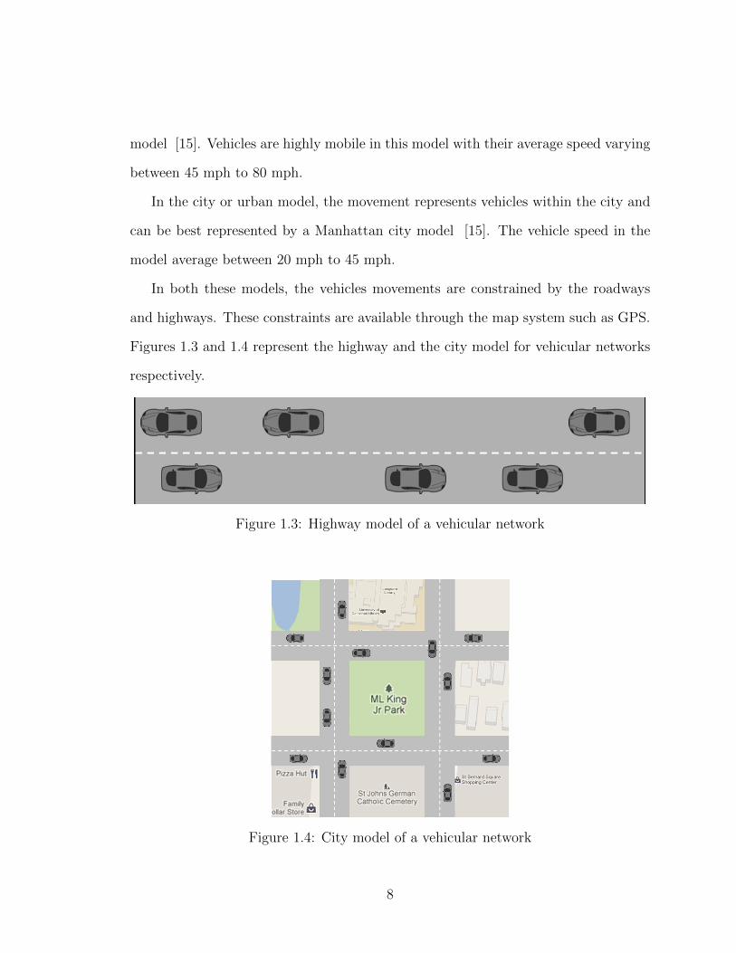
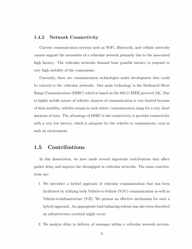
model [15]. Vehicles are highly mobile in this model with their average speed varying

between 45 mph to 80 mph.

In the city or urban model, the movement represents vehicles within the city and

can be best represented by a Manhattan city model [15]. The vehicle speed in the

model average between 20 mph to 45 mph.

In both these models, the vehicles movements are constrained by the roadways

and highways. These constraints are available through the map system such as GPS.

Figures 1.3 and 1.4 represent the highway and the city model for vehicular networks

respectively.

Figure 1.3: Highway model of a vehicular network

Figure 1.4: City model of a vehicular network

8

1.4.2 Network Connectivity

Current communication systems such as WiFi, Bluetooth, and cellular networks

cannot support the necessities of a vehicular network primarily due to the associated

high latency. The vehicular networks demand least possible latency to respond to

very high mobility of the components.

Currently, there are communication technologies under development that could

be catered to the vehicular networks. One main technology is the Dedicated Short

Range Communication (DSRC) which is based on the 802.11 IEEE protocol [16]. Due

to highly mobile nature of vehicles, chances of communication is very limited because

of their mobility, vehicles remain in each others’ communication range for a very short

duration of time. The advantage of DSRC is the connectivity it provides connectivity

with a very low latency, which is adequate for the vehicles to communicate, even in

such an environment.

1.5 Contributions

In this dissertation, we have made several important contributions that a↵ect

packet delay and improve the throughput in vehicular networks. The main contribu-

tions are:

1. We introduce a hybrid approach of vehicular communication that has been

facilitated by utilizing both Vehicle-to-Vehicle (V2V) communication as well as

Vehicle-to-Infrastructure (V2I). We present an e↵ective mechanism for such a

hybrid approach. An appropriate load balancing scheme has also been described

an infrastructure overload might occur.

2. We analyze delay in delivery of messages within a vehicular network environ-

9

ment on a highway. We have attempted to present a fairly complex model for

this delay in terms of many factors that a↵ect and influence this delay. Initially,

we present an analytical model that incorporates di↵erent connectivity phases of

the vehicle communication during a typical trip on the highway. This leads to a

realistic approach that resembles real-life connectivity among the vehicles. Our

goal is to utilize this analytical model so that the vehicles can make real-time

decisions for routing of its messages on the highway.

3. We simulate QoSHVCP protocol in a VANET scenario, and demonstrate the

relationship between message delivery delay and the vehicular density on the

highway. We also present the e↵ect of an infrastructure overload on the message

delivery delay, as well as discuss ways of improvements by incorporating a load

balancing mechanism.

4. We introduce probabilistic routing protocol (CAREFOR) that judiciously com-

bines multi-hop retransmission forecast with collision-aware constraints so that

the end-to-end packet delivery delay for V2V communications can be optimized

in vehicular networks. We present an analytical model for the rebroadcast prob-

ability, as well as simulation results showing better values from our protocol as

compared with other existing approaches.

5. In order to address the optimal vehicle selection in the bridging approach (V2B),

we present the QASA algorithm that improves the throughput of the VANET

and optimizes the packet delivery delay with the focus on V2B communication

(vehicles on the east lane of the highway communicating with vehicles on the

west lane, and vice-versa). We present an analytical model as well as simulation

results to demonstrate the e↵ectiveness of our approach.

10

6. We utilize autonomous vehicles in order to improve end-to-end packet delivery

delay and vehicle trip duration. By controlling the speed of the autonomous

vehicles, we can manipulate the distribution of vehicles on the highway. Simu-

lation results are presented to demonstrate the improvements by our protocol.

Table 1.1 summarizes the di↵erent aspects of our research. Briefly speaking, the

scope of this research is to analyze and present a sophisticated model for message

propagation delay in a VANET and introduce new approaches (overload balancing

mechanism, routing mechanism, hando↵ criterion, etc.) in order to reduce this delay,

as well as improve other QoS metrics.

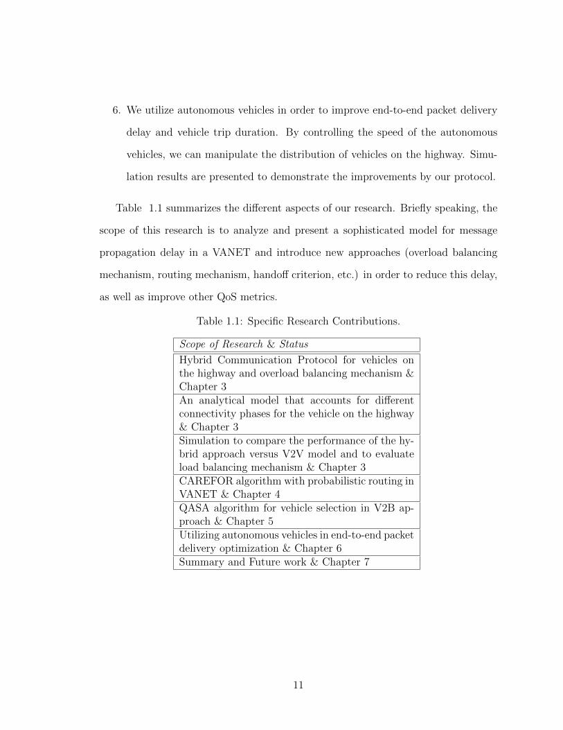
Table 1.1: Specific Research Contributions.

Scope of Research & Status

Hybrid Communication Protocol for vehicles onthe highway and overload balancing mechanism &Chapter 3An analytical model that accounts for di↵erentconnectivity phases for the vehicle on the highway& Chapter 3Simulation to compare the performance of the hy-brid approach versus V2V model and to evaluateload balancing mechanism & Chapter 3CAREFOR algorithm with probabilistic routing inVANET & Chapter 4QASA algorithm for vehicle selection in V2B ap-proach & Chapter 5Utilizing autonomous vehicles in end-to-end packetdelivery optimization & Chapter 6Summary and Future work & Chapter 7

11

1.6 Research Scenario

The research presented in this dissertation addresses the message delivery delay in

a highway scenario, where vehicles transmit their messages from the beginning of the

highway, and the messages propagate forward till they reach the end of the highway.

Note that the results presented in this research can be generalized for messages prop-

agating forward or backward on the highway. Since highways are composed of two

direction lanes moving in opposite direction, messages propagating forward for one

direction is considered propagating backward for the opposite direction. The focus

of this research is to calculate the message delivery delay and provide solutions for

minimizing this delay. However, this delay needs to be clearly expressed in terms

of what are the factors behind this, and then, present appropriate approaches that

could e↵ectively address it. This requires us to look into an analytical model that

helps us identify di↵erent components contributing to such a delay. Later on, this

model can be used as a real-time metric that could let the vehicles decide the route

to be taken in propagating the message throughout the highway. Following that, we

focus on developing di↵erent e↵ective routing protocols, and potential approaches for

reducing this delay.

A typical scenario used in this dissertation is a highway in a rural area, covered

by Wireless LAN units at di↵erent locations of the highway (i.e., Wireless LAN units

from the restaurants, homes on the side of the highway). However, most of these

Wireless LAN services may not be connected to the Internet or to a satellite system.

As it is a delay tolerant application, the messages and the data can permit some

delays in message delivery. In order for vehicles and Wireless LAN networks to be

connected to the Internet, they have to transmit their messages to a cellular network

located along the highway.

12

1.7 Dissertation Outline

The remainder of this dissertation is organized as follows:

• Chapter 2 presents di↵erent aspects of the vehicular network. It covers the con-

cept of Intelligent Transportation Systems (ITS) and the vision for the vehicular

networks in the future. The di↵erence between a VANET and a cellular network

as well as a MANET is presented. Inter-dependency between the architecture,

communication systems, applications are also discussed.

• Chapter 3 introduces the QoSHVCP, discusses related work in the vehicular

network research and delay tolerant networks. It also describes the e↵ect of

overload on the infrastructure network, presents a theoretical model for the

rate of message delivery time, and performance results for simulation of di↵erent

communication models.

• Chapter 4 presents the CAREFOR algorithm and the analytical probabilistic

rebroadcast model that attempts to minimize the number of packet collisions in

the network, as well as optimize end-to-end packet delivery delay. Simulation

results demonstrate the e↵ectiveness of CAREFOR.

• Chapter 5 presents the QASA protocol that focuses on vehicle selection in V2B

approach with an objective to optimize throughput between the vehicles, and

minimize end-to-end packet delivery delay.

• Chapter 6 introduces utilization of autonomous vehicles in optimizing end-to-

end packet delivery delay and the vehicle trip duration on the highway. Simu-

lation results indicate the e↵ectiveness of our approach.

13

• Chapter 7 concludes the dissertation with a summary of the contributions and

ideas for future research.

14

Chapter 2

Vehicular Networking

In this Chapter, we introduce di↵erent technologies that are used within the scope

of vehicular networks. The chapter starts with a brief introduction of the concept of

Intelligent Transportation System (ITS). Following that, we present characteristics of

a VANET, and di↵erence between a VANET, a cellular network, and a MANET. We

also discuss di↵erent aspects and technologies that form a real life vehicular network.

Finally, potential applications and current initiatives for the vehicle networks are

covered.

2.1 Intelligent Transportation System

Information and communication technology applicable to vehicles and transport

infrastructure are referred to as Intelligent Transportation System [17]. Tools en-

compassed in ITS include: concepts of tra�c engineering, software, hardware, and

telecommunication technologies. These tools are integrated together in order to pro-

vide services that improve the e�ciency and safety of transportation services and

vehicles. These services include: tra�c management, commercial vehicle operations,

15

transit management, and information access to travelers. ITS applications have the

potential to provide solutions for many problems caused by vehicles and transporta-

tion systems. For example, ITS can improve the tra�c flows by avoiding and reducing

the congestion of tra�c. It can help enhance the air quality by reducing the pollution

created by the exhaust system by simply minimizing the tra�c delay. The overall

safety of the vehicle, operator, and the environment can be improved by utilizing an

advance warning system that can be activated in case of a crash, or by minimizing

the environmental, road, or highway e↵ects that cause a crash. Economic e�ciencies

can also be achieved through ITS by reducing the fuel consumption, and avoiding the

dire expense due to tra�c collision and potential accident [18].

2.2 Characteristics of VANETs

VANET is a type of Ad Hoc Network with some unique characteristics, and re-

quirements. In the following, we discuss unique features of VANETs. Some of these

main qualities are [5]:

• Computing Powerand Battery Life: Vehicles have much higher reserve power

and computing capability than a typical cell-phone or a mobile computer.

• Node Size and Weight: Vehicles have significantly larger size and weight, and

hence, can support complex sensor applications with significant computing com-

ponent.

• Vehicle Speeds: Vehicles travel at speeds up to hundred miles per hours, which

results in the lack of continuous coherent communication links and could have

frequently changing topology.

16

• Vehicle Grid: Vehicles in the grid are few hops away from a Road Side Unit

(RSU) or the infrastructure.

2.3 VANET and Cellular Networks

Cellular networks provide many advantages for wireless communications. Some of

the main advantages include:

• Always-on connectivity,

• Rich multimedia services, and

• Provides exclusive bandwidth for users which help relieve associated congestion.

These advantages are important for vehicular communications and coverage. How-

ever, VANET is better than cellular services (viz., 3G) services in a vehicular envi-

ronment. This is mainly due to:

1. Vehicles are highly mobile, and many applications in the vehicular environment

require transmission of a large volume of data. 3G cannot support such massive

data due its bandwidth limitations.

2. Cellular networks are designed primarily for continuous coverage and every-

where availability to users at all the time. In order to establish a cellular

network specifically for a VANET, this could come with a very high cost that

exceeds hundreds of millions of dollars [19]. On the other hand, VANETs do

not require any extra cost for infrastructure besides the network interface cards

installed on each vehicle.

17

3. Current cellular networks cannot sustain an additional volume of data exchange

on their networks. This is particularly evident in the case of existing cellular

networks. Epecially after the introduction of smartphones, these networks have

become increasingly overloaded. An example would be At&T in which, “the

net result is dropped calls, spotty service, delayed text and voice messages

and glacial download speeds as AT&T’s cellular network strains to meet the

demand” [20]. This basically causes introduction of a new type of data category

to an already overloaded network that is less practical and almost infeasible.

Constant connectivity is not a requirement in many VANET applications. For

example, email, transfer of files, bulk downloads, etc. can sustain continuous disrup-

tions in the connectivity of the network. In other words, VANET is basically a Delay

Tolerant Network (DTN).

2.4 VANET versus MANET

Another technology that is typically very similar to a VANET is the Mobile

Ad Hoc Network (MANET). VANET is typically considered a special category of

a MANET in which the mobile nodes are vehicles. However, there are di↵erences be-

tween the two technologies that dont allow the adoption of the MANET technology

directly to VANET. Some of the main dissimilarities are:

1. Very high mobility speed: Vehicles in VANET move with a speed up to 100

m/s, and hence, there is a frequent change in the topology of the network.

Moreover, vehicles only get a very slim window in order to communicate with

each other. This results in a continuously disconnected and a highly dynamic

network topology.

18

2. Number of nodes in VANET: A VANET address a scenario where it is expected

that many vehicles will be equipped with the VANET interface card, and hence,

the node density is usually very large. Any VANET algorithm needs to be

salable to a very large number of nodes.

Table 2.1 provides a brief comparison between VANET and MANET [21]. These dif-

ferences result in a unique set of problems in the VANET, which need to be addressed

with new problem formulations, protocols, and algorithms.

Table 2.1: Di↵erence between VANET and MANET technologies.

Characteristic &MANET

VANET

Cost of production Cheap ExpensiveChange in networktopology

Slow Frequent and Fast

Mobility Low HighNode density Sparse Dense and frequently variableBandwidth Hundreds of kbps Thousands of kbpsRange Up to 100 m Up to 500 mLifetime Depends on power source Depends on vehicle lifetimeMulti-hop routing Available Weekly availableMoving pattern ofnodes

Random Regular

Position acquisition Using ultrasonic Using GPS, RADAR

2.5 Vehicular Network Hardware

In order to achieve the goals and the vision of ITS, the vehicles and highways are

equipped with di↵erent types of software and hardware. The hardware falls under

two main categories: sensors and communication systems. In the next subsections,

we will be giving a brief introduction to these categories.

19

2.5.1 Sensor Network

Sensors play a major role in vehicular technology since they provide the means

of understanding the environment, the vehicle, and the vehicle operator. Many sen-

sors are equipped within the vehicle, and along the road or highway. Vehicles also

can act as sensors themselves. Examples for the sensors that can be equipped in

the car include: Tire Pressure Monitoring Systems (TPMS), Vehicle Speed Sensor

(VSS), Traction Control System (TCS), Electronic Stability Control Systems (ESC),

Automated Collision Avoidance Systems (ACAS) and many more [22]. Vehicle man-

ufacturers are already including many sensors such as those mentioned previously

and more in the assembly of vehicles. Honda is introducing a Blind Spot Information

(BSI) sensor that informs the vehicle operator in case there are any neighboring ve-

hicle in his/her blind spot [23]. Ford has begun developing a heart rate monitoring

seat in its vehicles. The information gathered by the heart rate sensors is analyzed

by an on-board computer system and provides real-time health information or alerts

the vehicle operator [24]. Figure 2.1 presents examples of di↵erent types of sensors

in a vehicle.

Aside from on-board vehicle sensors, the vehicles themselves can be used as mobile

sensors. Applications that can utilize such approach include real-time update of tra�c

speeds, or updating digital road maps by utilizing GPS traces [25]. One example

for using vehicles as sensors is the OPTIS project implemented in Sewden [26]. In

order for the city to validate data gathered from cameras/loop detector systems, 220

vehicles reported their real-time speeds using cellular GPRS modems [26].

20

Figure 2.1: Some examples of on-board vehicle sensors [2]

2.5.2 Communication Systems

In order to communicate the data gathered from on-board sensors, vehicles are

also required to be equipped with communication tools. IEEE has defined the stan-

dards for communication amongst vehicles for Wireless Access in a Vehicular Environ-

ment (WAVE) and the Dedicated Short-Range Communications (DSRC) standards.

WAVE standard manages the network layers from the network layer up to the appli-

cation layer. The physical and data link layers are managed by the DSRC standard.

Figure 2.2 presents di↵erent layers managed by each standard.

Table 2.2 provides a comparison between the DSRC and other wireless technolo-

gies. As shown in the table, the main advantage for the DSRC wireless technology is

the very low latency as compared to other network technologies.

21

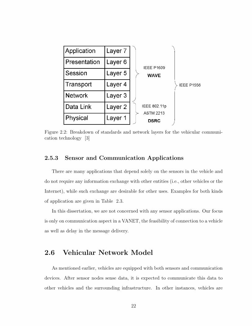
Figure 2.2: Breakdown of standards and network layers for the vehicular communi-cation technology [3]

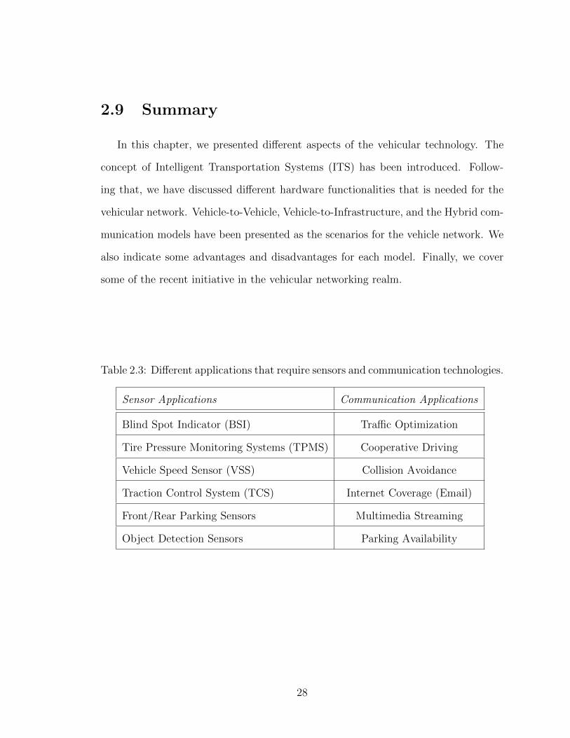
2.5.3 Sensor and Communication Applications

There are many applications that depend solely on the sensors in the vehicle and

do not require any information exchange with other entities (i.e., other vehicles or the

Internet), while such exchange are desirable for other uses. Examples for both kinds

of application are given in Table 2.3.

In this dissertation, we are not concerned with any sensor applications. Our focus

is only on communication aspect in a VANET, the feasibility of connection to a vehicle

as well as delay in the message delivery.

2.6 Vehicular Network Model

As mentioned earlier, vehicles are equipped with both sensors and communication

devices. After sensor nodes sense data, it is expected to communicate this data to

other vehicles and the surrounding infrastructure. In other instances, vehicles are

22

required to retrieve data from other vehicles, from the infrastructure, or from the

Internet. Vehicles themselves are considered as nodes in a large network. Due to the

nature of the vehicular network, these nodes are highly mobile. When vehicles travel

on the highway or in the city, they come in close proximity (within the communication

connectivity range) with other vehicles or with road side units (infrastructure). Hence,

we can assume that the communication infrastructure of vehicular networks is one of

three main models: Vehicle-to-Vehicle, Vehicle-to-Infrastructure, and Hybrid models.

Figure 2.3 presents di↵erent models in a vehicular network scenario.

Figure 2.3: The di↵erent communication models in a Vehicular network scenario [4]

2.6.1 Vehicle-to-Vehicle

In vehicle-to-vehicle (V2V) model, vehicles communicate with each other in an

ad hoc fashion. Vehicles that are in close proximity with each other, communicate

directly. Vehicles outside of this range communicate in a multi-hop fashion. One of

23

the main disadvantages of this model is that it depends heavily on the density of

vehicles on the road or a highway. When the vehicle density is high, vehicles can

communicate with each other in a multi-hop fashion. However, when the vehicle

density is low, this type of communication is not feasible. This model also overcomes

conventional centralized approach and avoids any fixed network size, or end-to-end

delay. End-to-end delay depends mainly on availability of intermediate vehicles that

can be used as hops to communicate or propagate the data.

2.6.2 Vehicle-to-Infrastructure

Vehicle-to-Infrastructure (V2I) model is when vehicles connect with an infrastructure-

based communication system. An infrastructure-based system is also referred to as

Road Side Unit (RSU) [27]. They can be cellular, WiMax, or 802.11 networks. The

advantage of these networks is that they are centralized and enable a vehicle access to

the Internet. One of the main disadvantages of this model is that the communication

infrastructure network could be easily overloaded, while the cost of using the network

could be substantially high.

2.6.3 Hybrid Model

The hybrid model combines the advantages of both the vehicle-to-vehicle model

and the vehicle-to-infrastructure model. In this hybrid model, vehicles communicate

by using either of the two models depending on a specific criteria and availability.

If other vehicles are absent in the vicinity, vehicles can communicate through the

infrastructure.

24

2.7 V2V versus V2I

It is a common expectation that a vehicular network should rely entirely on ”free”

V2V communications without any dependence on the Infrastructure [5]. However, due

to connectivity limitations of the vehicles in a V2V mode, an existing infrastructure

can be used as a complementary charged access service in case an application requires

a guaranteed service, or minimal delay. There are many types of infrastructure that

can be used such as cellular networks and WiFi. The main disadvantage for cellular

networks is that they are already overloaded, are not free, while their throughput is

relatively low. However, they have the advantage of covering almost all the highways

and the cities. On the other hand, WiFi has very small coverage area, while having

a very high throughput.

Another solution would be to install a totally new infrastructure system. This

is proposed by the Intelligence Transportation System (ITS) of the Department of

Transportation (DoT) [28]. The total cost for such an establishment is approximated

by 251 million dollars. Yet, this investment will not be adequate to cover all the

highways where V2V communications is still desirable. Therefore, this dissertation

calls for installation of infrastructure only at few key areas such as busy intersections,

urban locations, and interstate highways.

It is worth mentioning that according to the Department of Transportation (DoT),

V2V system helps avoid 79 percent of all vehicle crashes, while V2I systems could

help only 26 percent of the crashes. These two systems combined could address up

to 81 percent of the crashes [29].

25

2.8 Vehicular Networking Initiatives

Many initiatives have been undertaken around the world in order to develop the

vehicular networking technology. In Japan, Smartway is an initiative that creates a

platform to deploy infrastructure on the roads and enables vehicles to communicate

with the environment [30].

In Europe, many organizations have emerged with the goal of enhancing the Intel-

ligent Transportation System. Some of these organizations are: E-ENOVA, Car-2-Car

Communication Consortium, PREVENT, and PATH [10–12,14].

In the United States, the U.S. Department of Transportation (USDOT) has in-

troduced a comprehensive initiative that aims to enable a safe, wireless network that

continuously connects vehicles [31]. Under this initiative, many research goals have

been presented that utilize ITS, and are discussed in the following paragraphs.

2.8.1 Congestion Initiative

Paying Toll, Transition, Telecommuting, and Technology are four synergistic strate-

gies presented by the congestion initiative in order to minimize any urban accumula-

tion.

2.8.2 Next Generation 9-1-1

The goal of the NG9-1-1 initiative is to enable the Public Safety Answering Point

(PSAPs) and emergency responder networks to incorporate voice, data, and video

transmission from di↵erent communication devices.

26

2.8.3 Cooperative Intersection Collision Avoidance System

The Cooperative Intersection Collision Avoidance System aimed to find solutions

for intersection crash problems caused by stop sign movements, stop sign violations,

tra�c signal violations, and unprotected signalized left turn movements.

2.8.4 Clarus

This initiative delivers timely and reliable weather and road condition information

by integrating a wide variety of weather observing, forecasting, and data management

systems.

2.8.5 Mobility Services for All Americans

The main drawback of the public services is that they are fragmented, ine�cient

and unreliable. MSAA initiative attempts to provide the basic need of transportation

for the many Americans that use the public transportation services.

2.8.6 Rural Safety

The main goal of Rural Safety Innovation Program is to improve the rural road

safety. In order to achieve that, the Rural Safety initiative assists rural communi-

ties in addressing highway safety problems, increasing interest in rural safety issues,

and promoting the benefits of rural safety countermeasures that could reduce rural

accidents.

27

2.9 Summary

In this chapter, we presented di↵erent aspects of the vehicular technology. The

concept of Intelligent Transportation Systems (ITS) has been introduced. Follow-

ing that, we have discussed di↵erent hardware functionalities that is needed for the

vehicular network. Vehicle-to-Vehicle, Vehicle-to-Infrastructure, and the Hybrid com-

munication models have been presented as the scenarios for the vehicle network. We

also indicate some advantages and disadvantages for each model. Finally, we cover

some of the recent initiative in the vehicular networking realm.

Table 2.3: Di↵erent applications that require sensors and communication technologies.

Sensor Applications Communication Applications

Blind Spot Indicator (BSI) Tra�c Optimization

Tire Pressure Monitoring Systems (TPMS) Cooperative Driving

Vehicle Speed Sensor (VSS) Collision Avoidance

Traction Control System (TCS) Internet Coverage (Email)

Front/Rear Parking Sensors Multimedia Streaming

Object Detection Sensors Parking Availability

28

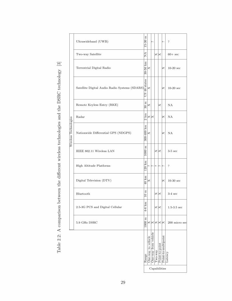
Tab

le2.2:

Acomparison

betweenthedi↵erentwirelesstechnologiesan

dtheDSRC

technology

[3]

WirelessTechnologies

5.9 GHz DSRC

2.5-3G PCS and Digital Cellular

Bluetooth

Digital Television (DTV)

High Altitude Platforms

IEEE 802.11 Wireless LAN

Nationwide Di↵erential GPS (NDGPS)

Radar

Remote Keyless Entry (RKE)

Satellite Digital Audio Radio Systems (SDARS)

Terrestrial Digital Radio

Two-way Satellite

Ultrawideband (UWB)

Capabilities

Range

1000m

4-6

km

10m

40km

120km

1000m

300-400km

2km

30m

US48

states

30-50km

NA

15-30m

One-way

toveh

icle

XX

?X

XX

XX

One-way

from

veh

icle

X?

X?

Two-w

ayX

XX

?X

XPoint-to-point

XX

X?

XX

XPoint-to-m

ultipoint

XX

?X

XX

X?

Latency

200 micro sec

1.5-3.5 sec

3-4 sec

10-30 sec

?

3-5 sec

NA

NA

NA

10-20 sec

10-20 sec

60+ sec

?

29

Chapter 3

QoSHVCP: QoS-oriented Hybrid

Vehicular Communications

Protocol

3.1 Related Work

Many factors can characterize a VANET topology and its dynamic behavior. Traf-

fic density (i.e., well-connected, sparsely connected, and totally disconnected neigh-

borhood), vehicles’ speed (i.e., low, medium, and high) and the heterogeneous net-

work environment (i.e., technologies of wireless networks around the VANET and

their deployment) are the main aspects depicting a VANET. The fast mobility of

vehicles make most traditional MANETs routing protocols ine�cient for VANETs

applications, mainly due to lack of any topology maintenance.

This section presents related work in specific areas of vehicular networking that

this dissertation expands on. Each subsection presents only one aspect. The first

30

subsection presents the concept of delay tolerant networks and its relation to vehic-

ular networks as well as the research done in this area. The following subsections

include research findings in broadcasting techniques for vehicular network, vehicle-

to-infrastructure communication model, and the hybrid model. Finally, we present

analytical models developed for data delivery rates in vehicular network, followed by

research findings in load sharing and balancing in vehicular networks.

3.1.1 Delay Tolerant Networks

Delay Tolerant Networks (DTNs) are networks that are composed of nodes that

are either static or dynamic and the network may not be connected at all times.

The DTN concept was initially introduced for the networks such as Military Ad-Hoc

Networks and Sensor and Sensor/Actuator Networks [32]. The main characteristic

of these networks is the frequent disconnection of the network. In sensor networks,

this is caused by limitations on the battery life of the sensor nodes which cause many

of them to be turned o↵ before they become dead. On the other hand, in vehicular

networks, this is caused by the high mobility of the vehicles.

In order to overcome the problem of connectivity, an approach called opportunis-

tic forwarding has been presented [33]. This approach is also extended to VANETs

in achieving connectivity between vehicles via V2V and opportunistically disseminate

useful information. It provides message propagation through building the links dy-

namically as a bridging technique, where any vehicle can be used as the next hop

temporary storage element and subsequently rebroadcast to forward the message to

the final destination whenever feasible. In [34], the authors define an opportunistic

forwarding technique in VANETs as an advanced information dissemination commu-

nication pattern, which has an objective to disseminate information among the vehi-

31

cles and enduring for a certain amount of time. Traditionally, schemes for advanced

information dissemination use single-hop broadcasts or store-and-forward technique,

and forward messages multiple times to all those vehicles unreachable because of an

existing network partitioning.

DTNs have the ability to tolerate a given amount of delay in delivering the message

to the destination. Many applications in VANET can accept such a delay, such as

tra�c information, email downloading, and many others. However, being an inherent

nature of a VANET, the scope of our research is to minimize the delay in the message

delivery so as to provide a better service to the users. Also, there are some applications

that require an upper limit of the delay, or else the information will be irrelevant

within a few seconds.

3.1.2 Broadcasting Techniques

Message and time delay propagation in a VANET via opportunistic networking

have been largely investigated in the literature, and di↵erent broadcasting techniques

have been proposed, many of which can be classified by distance, location, probabil-

ity and topology-based [35]. These methods are e↵ective only with V2V for dense

tra�c scenario. But, their use is very limited when vehicles constitute a low density

neighbourhood.

Distance and Location Based Approaches

The distance and location based approaches simply exploit the inter-vehicular dis-

tance and the vehicles’ positions by GPS devices in order to select the next hop to

forward a message further within the area. Beacon messages are implemented in many

location-based approaches, where vehicle’s position information is embedded either

32

through GPS or a-priori calculations. In [36], each vehicle has the knowledge of its

neighbors in term of both the numbers of neighbors and their relative positions. The

next hop selection involves the furthest vehicle within its communication range from

the source vehicle. In [37], a fast multi-hop broadcast technique has been proposed.

It estimates vehicles’ distance and provides a reduction on the number of needed hops

and associated delay required to forward a broadcast message throughout the area.

It is well known that a non-optimal number of hops, experienced by a message to be

forwarded to a destination vehicle, causes higher delays due to associated parameters

such as queuing delays, link quality, etc. and the network performance can be drasti-

cally a↵ected. However, the major drawback of position-based broadcasting approach

is the need for global information concerning the vehicular network topology, as well

as the geographical characteristics of the vehicular scenario. A huge quantity of data

information is needed which can be exchanged only by a dedicated logical channel.

Probability Based Approaches

In the probability-based broadcasting technique, probability of collision reduction

and hence, a decrease in required number of transmitted messages is assumed. Upon

message reception, each vehicle retransmits with a probability depending on the dis-

tance from the source vehicle [38]. It follows that greater the vehicle’s distance is from

the source (but within its communication range), higher will be the retransmission

probability. In [39], Resta et al. deal with multi-hop emergency message dissemi-

nation through a probabilistic approach and derive lower bounds on the probability

that a vehicle can correctly receives a message within a fixed time interval. Similarly,

in [40], Jiang et al. introduce an e�cient alarm message broadcast routing protocol

and estimate the receipt probability of alarm messages sent to the vehicles.

33

3.1.3 Vehicle-to-Infrastructure

Road-side infrastructure could represent a viable solution to extend the vehicular

connectivity support in scenarios where V2V fail which is only e↵ective in dense ve-

hicle scenario. However, they are dysfunctional in a low density area. Many authors

investigated novel techniques in order to allow vehicles to be seamlessly connected.

Such approaches rely on using portions of both V2V as well as V2I techniques. Such

a combination is commonly referenced as QoS oriented Hybrid Vehicular Communi-

cations Protocol (QoSHVCP).

V2V and V2I communication technologies have been developed as a part of the

Vehicle Infrastructure Integration (VII) initiative [41]. The use of a vehicular grid

along with an opportunistic infrastructure placed on the roads, can guarantee seam-

less connectivity in a dynamic vehicular scenario, as described in [42, 43]. In [44],

the authors propose a Cooperative Infrastructure Discovery Protocol, called CIDP,

which allows vehicles to gather information about encountered RSUs through direct

communication with the network infrastructure, and subsequent message exchanges

with neighboring vehicles via V2V. The authors show the e↵ectiveness of their ap-

proach. But, it seems to be limited to the message exchange about the infrastructure

discovery. In [45], Wedel et al. use QoSHVCP communications for an enhanced navi-

gation system which intelligently help drivers to circumnavigate congested roads and

avoid tra�c roadblocks. Their contribution highlights the advantages of QoSHVCP

communication protocols for numerous safety applications.

3.1.4 Hybrid Model

Finally, Seo et al. [46] analyze the performances of a general hybrid communication

protocol, based on the IEEE 802.11p WAVE (Wireless Access in Vehicular Environ-

34

ments) system. The authors focus on packet error rates for the proposed method,

while connectivity issues and reliability of vehicles have not been incorporated.

3.1.5 Analytical Models for Data Delivery Rates

Several studies have introduced analytical models for the data delivery rates and

delay time within vehicular networks. Some works have addressed propagation de-

lay for safety critical warning messages in a vehicular environment [47–49]. In [47],

the authors develop an analytical model that evaluates the message delivery delay

in critical safety applications and its relation to the bu↵ering and switching mecha-

nism within the WAVE protocol. The same problem has been considered in [48] by

the authors. However, they observe the tradeo↵ between the message delivery delay

versus the cluster size used by the vehicles travelling on the highway. Finally, in [49]

the authors present an analytical model and its dependence on vehicular density on

the highway. Our work concentrates on a di↵erent aspect of the VANET that repre-

sents a more realistic view of such networks. We present an analytical model when

the vehicular network appears as a partitioned network that incorporates di↵erent

connectivity phases a vehicle encounters during its trip on the highway.

Another work [50] has also developed an analytical model for the message delivery

delay in a VANET by exploring queuing theory in studying the vehicular connectivity

when the tra�c follows a unidirectional model. We generalize this by extending to

bidirectional tra�c on the highway in a typical dynamic network.

Finally, the authors in [51] derive an analytical model that characterizes the con-

nectivity of the VANET on a unidirectional road. We compute an expected delay for

the message delivery rather than simply considering the network connectivity aspect

only in a unidirectional tra�c scenario.

35

To our knowledge, our work is the first to introduce an analytical model that

includes delay from V2I communication as well as V2V.

3.1.6 Load Sharing and Balancing

In order to provide a more e�cient resource management and in an attempt to

satisfy soft real-time requirements in a distributed system, there has been a significant

number of works that looked at how to implement load sharing and load balancing

mechanism in a distributed system [52]. Most of the work focus on the distribution

and/or migration of the workload among many di↵erent servers [53, 54]. Some even

go as far as adapting the functionality of the clients in the system [55]. When there

is an option of re-distribution, load balancing could also be obtained by distributing

the tra�c generated among multiple paths and servers [56, 57]. However, such load

balancing mechanisms might not provide optimal resource management in a VANET

scenario due to the fact that there is often a lack of multiple resources, or routing

options are limited. In many cases, cars would be limited to either go through the

route using the infrastructure, or to use the formed ad hoc network.

36

3.2 Our QoSHVCP Approach

Network connectivity is one of the main challenges in the vehicular environment.

In this chapter, we investigate a hybrid approach for enhancing the connectivity

among vehicles. Our approach of a hybrid vehicular protocol, i.e. QoSHVCP, ap-

propriate switching is provided from V2V to V2I and relying on a vehicular grid

with a neighboring network infrastructure. The protocol switching enables seamless

connectivity and expected to be e↵ective independent of any specific tra�c scenar-

ios or vehicle speeds. It consists of a handover procedure from V2V to V2I (and

vice versa), resulting in improving the opportunistic connectivity with respect to the

traditional inter-vehicle communications. Our QoSHVCP also has a load balancing

component that considers two di↵erent classes of message priorities. It allows the net-

work to gracefully degrade, while still maintaining good performance for high priority

messages.

3.2.1 QoSHVCP Scheme

QoSHVCP scheme is a hybrid approach that provides a link between both vehi-

cles (i.e., V2V) and from vehicles to the infrastructure (i.e., V2I) communications.

The cooperation and coexistence of these two di↵erent methods can assure a good

connectivity in a VANET scenario, especially in sparsely connected neighborhoods

where V2V communications are not always feasible.

QoSHVCP is a broadcast protocol that reduces the time required by a message

to propagate from a source vehicle to the farthest vehicle within the communication

range inside a certain strip-shaped area-of-interest. QoSHVCP represents a smart

and realistic communication protocol, since vehicles can establish opportunistically

37

both V2V and V2I communications and reduce the message delivery time, as well as

avoid disconnections due to changed vehicle density that cause dynamic topological

changes.

Based on the estimation of the link utilization time (i.e., the message delivery

time for one hop) of vehicles, QoSHVCP is then used to reduce the amount of hops

needed to deliver the message. In a previous version of QoSHVCP [58], we assumed

a known and constant transmission range of vehicles. But, this limits the protocol

resulting in an unrealistic implementation of the algorithm. In this dissertation, we

adapt QoSHVCP to be a more pragmatic broadcast protocol where vehicles’ actual

transmission data rates are subjected to continuous changes due to physical obstacles,

vehicle density, speed, network overload, etc.

Apart from achieving seamless connectivity to a VANET through dynamic proto-

col switching, our proposed technique also guarantees message delivery with smaller

delay, specially for HP (high priority) messages. In particular, QoSHVCP reserves

HP messages (e.g., warning, safety, and soft-real time messages) to be forwarded via

V2I; while LP messages (e.g., delay-tolerant) via V2V. The main scope of QoSHVCP

is to exploit the connectivity with the network infrastructure for HP messages when-

ever available, as RSU (Road Side Unit) can forward a message to the next RSU,

resulting in quicker message propagation inside the vehicular grid.

In the following Subsection 3.2.2, we describe the QoSHVCP protocol switching

mechanism, while in Subsection 3.2.3 we introduce the QoS prioritization adopted in

QoSHVCP.

38

3.2.2 Delay-based Protocol Switching Mechanism in QoSHVCP

Let us consider the vehicular scenario depicted in Figure 3.1. Several RSUs of

di↵erent wireless technologies are deployed, partially covering a given area. The

local information —assumed as global— comprises the key data defining the network

scenario, since the tra�c density is directly inter-related to the vehicles density. Each

vehicle continuously monitors its local connectivity by storing their periodic HELLO

broadcast messages with piggyback information about neighbors. It is then able to

determine if it is within a group of vehicles called a cluster or is travelling alone on

the road. A vehicle will be aware of neighbouring wireless networks on the basis of

broadcast signalling messages sent by the Road Side Units (RSUs).

 

Figure 3.1: Vehicular grid with an overlapping heterogeneous wireless network infras-tructure.

The knowledge of RSUs’ presence in the range is indicated by a routing parameter,

defined as Infrastructure Connectivity (IC). This parameter gives information about

the ability of a vehicle to be directly connected with one or more RSUs. The IC

39

assumes two values, i.e., IC = {0, 1}, respectively corresponding to no RSU, and one

or more available RSUs. For instance, when a vehicle has IC = 1, it means that it

is driving inside the radio coverage of a wireless cell of an RSU and is potentially

able to directly connect to that RSU associated with the neighbouring wireless cell.

Otherwise, the value of IC is 0 when no wireless cell is available for such an access.

Let us consider a cluster C comprised of a set S of vehicles (i.e., S = {1, 2, . . . , n}).

Then, m RSUs (i.e., m < n) are displaced in the network scenario as depicted in

Figure 3.1. Each vehicle is able to communicate with all the other vehicles around

it via V2V. At the same time, we assume that only a limited subset of vehicles in

the cluster C, (i.e., S 0 = {1, 2, . . . , l} ⇢ S, with l < n), is able to connect to an

RSU via V2I. For example, not all the vehicles might have an appropriate network

interface card, and/or are not in the range of connectivity of an RSU. Analogously,

we assume that only k RSUs (i.e., k = {1, 2, . . . , h} with h < m) are available to V2I

communications.

For the connectivity link from the i-th to the j-th vehicle, we define link utilization

time q(i,j) [s] as the time needed to transmit a message of length L [bit] from the i-th

to the j-th vehicle, at an actual data rate f(i,j) [Mbit/s]. This is given by:

q(i,j) =L

f(i,j). (3.1)

For a direct link between i-th vehicle and k-th RSU, the data rate is computed by

the nominal data rate^

f (i,k) by applying a Data Rate Reduction (DRR) factor (i.e.,

⇢(i,k)) that depends on the distance from the vehicle to the RSU, namely f(i,k) =

⇢(i,k)^

f (i,k). The DRR factor increases when a vehicle is located within the bound of a

wireless cell corresponding to an RSU.

Let us define a path from i-th vehicle to k-th RSU, comprising of a sequence of

40

M hops, where a single hop represents a link between two neighboring vehicles. The

path length represents the number of hops M for a single path. It follows that the

maximum number of directed links from a vehicle to an RSU is ↵ = l · h, while the

maximum number of di↵erent paths that can connect i-th vehicle to k-th RSU is n ·↵.

From the definition of a path, we define the path utilization time Q(i,k) [s] from

the i-th vehicle to the k-th RSU as the sum of single link utilization time parameters

(i.e., q(i,j)), for each hop that constitutes the path as:

Q(i,k) = q(i,j) + q(j,x) + ...+ q(x,k) = LnP

i=1x2S

⇥f(i,x)

�1⇤. (3.2)

Among all possible paths, the optimal path will be the one with the minimized

time required by a path and can be given by:

mins=1,2,...,n↵

Q(s)(i,k) = L · min

s=1,2,...,n↵

nX

i=1x2S

hf(s)(i,x)

i�1

. (3.3)

Equation (3.3) is compared with the link utilization times in V2V communications

in order to detect the most appropriate transmission path.

3.2.3 Load Balancing Mechanism in QoSHVCP

QoSHVCP aims to guarantee connections either through V2V or through V2I on

the basis of minimizing path required time. However, in a VANET, various applica-

tions require di↵erent communication modes and QoS levels. For instance, two most

important safety applications are the Extended Emergency Brake Light (EEBL), and

the Cooperative Intersection Collision Avoidance System (CICAS) [59]. EEBL is

based on V2V communications, while CICAS exploits V2I mode [59]. Leveraging on

such consideration, we assume that two sets of vehicles are respectively transmitting

41

EEBL and CICAS safety messages. EEBL and CICAS messages are classified to have

Low and High Priority, respectively. QoSHVCP forces HP messages to be transmitted

via V2I, while LP messages are directed towards V2V.

As presented in the simulation results of section 3.5, when the tra�c density

increases, the message propagation delay decreases due to enhanced connectivity of

the vehicles and possibly larger size cluster. However, this is somehow unrealistic

due to the fact that when the tra�c density increases, the overload on the network

infrastructure also increases. This results in a decrease in the bandwidth available

for each vehicle, which could mean increased message propagation delays.

In order to avoid this tra�c overload in the network infrastructure, a load balancing

mechanism can be employed. We define the channel utilization, i.e., ⇢(⌫), as the

percentage of the tra�c load in a wireless network, where ⌫ is the number of vehicles

connected to the RSU inside a wireless cell. The channel utilization is expressed as:

⇢ (⌫) =

8><

>:

exph⌫�⌫

max

⌫

max

i, for ⌫ ⌫max

1, otherwise(3.4)

where ⌫max is the maximum number of vehicles which can be served by the RSU.

When ⌫ > ⌫max the tra�c load in the wireless cell will be maximum and new HP

messages cannot be served with success.

The analytical variation in the channel utilization is depicted in Figure 3.2. Notice

that ⌫max is a threshold which strictly depends on particular wireless network tech-

nology. It needs to be updated constantly and is expressed as ⌫max / (r, B), where

r [m] is the wireless radio coverage, and B [b/s] is the the bandwidth of a particular

wireless network.

The load balancing mechanism is enabled once the overload on the network infras-

42

Figure 3.2: Percentage of channel utilization in a wireless network for HP messagesdelivery, and ⌫max = [40, 60, 80]).

tructure exceeds a given threshold ⌫max. Before overload on the network exceeds this

threshold, any High Priority packets are routed via V2I communications 1, and any

Low Priority packets are routed using V2V. Once the overload exceeds the threshold,

regardless of their priority, any new packets are forced to communicate using V2V,

until the overload is reduced below the threshold.

1Due to minimal delay and guaranteed service V2I provides

43

3.3 Message Delivery Time Rates

In this section, we investigate the message delivery time delay that propagates in

a VANET within the network infrastructure. We breakdown the message propagation

delay according to the connectivity sequence of the vehicles. After we formulate the

message propagation delay within each phase, we can obtain the probability of the

vehicle being in that phase. Finally, we present a theorem that provides an average

message reception delay that incorporates all message propagated to the destination

vehicles using di↵erent technologies and possibly passing through alternate phases.

3.3.1 Delay in Vehicle-to-Vehicle Communication

It is important to note that RSUs are connected together using land-line as they

are placed at pre-defined physical locations. As depicted in Figure 3.1, vehicles move

in clusters in two separated lanes (i.e., left and right lanes), where north (i.e., N),

and south (i.e., S) respectively represent the directions of the left and the right lanes.

The message propagation is based on the number of vehicles involved in forwarding

and assumed to be N and vehicles are traveling at a constant speed c [m/s].

The time delay for a message propagating within a cluster C is d [s] which is

defined as the di↵erence between the time-stamps of message reception (i.e., tRx

) and

transmission rate (i.e., tTx

), respectively:

d = tRx

� tTx

. (3.5)

For a successful transmission of a message of length L [bit] between a couple of

vehicles (i, j), equation (3.5) can be also expressed as the link utilization time, i.e.,

d(i,j) [s], where i-th vehicle transmits a message to j-th vehicle at a transmission rate

44

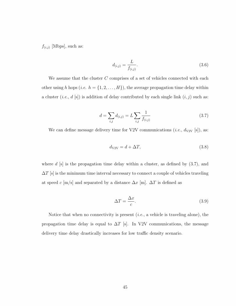
f(i,j) [Mbps], such as:

d(i,j) =L

f(i,j). (3.6)

We assume that the cluster C comprises of a set of vehicles connected with each

other using h hops (i.e. h = {1, 2, . . . , H}), the average propagation time delay within

a cluster (i.e., d [s]) is addition of delay contributed by each single link (i, j) such as:

d =X

i,j

d(i,j) = LX

i,j

1

f(i,j)(3.7)

We can define message delivery time for V2V communications (i.e., dV2V [s]), as:

dV2V = d+�T, (3.8)

where d [s] is the propagation time delay within a cluster, as defined by (3.7), and

�T [s] is the minimum time interval necessary to connect a couple of vehicles traveling

at speed c [m/s] and separated by a distance �x [m]. �T is defined as

�T =�x

c. (3.9)

Notice that when no connectivity is present (i.e., a vehicle is traveling alone), the

propagation time delay is equal to �T [s]. In V2V communications, the message

delivery time delay drastically increases for low tra�c density scenario.

45

3.4 Delay in Vehicle-to-Infrastructure Communi-

cation

Analogous to (3.6), let us consider dRSU [s] as the propagation time delay through

the network infrastructure to the destination as:

dRSU =L

fRSU, (3.10)

which is defined for the link between them-th and (m+1)-th RSU as the ratio between

the message length L [Bit], and the e↵ective data rate fRSU [b/s]. It represents the

time necessary to forward a message of length L between two consecutive RSUs at

rate fRSU [b/s]. Equation (3.10) represents the time delay propagation rate within

the preexisting network infrastructure.

Each RSU works as a relay node and forwards the message to vehicles crossing

its wireless cell. According to Figure 3.1, we shall also consider the propagation time

delay in uplink (downlink), when a vehicle sends a message to an RSU (and vice

versa), such as:

dUP =L

g(i,m), dDOWN =

L

g(m,i), (3.11)

where g(i,m) and g(m,i) are the e↵ective transmission data rate for the link (i,m)

(uplink), and (m, i) (downlink), respectively.

From relations (3.10) and (3.11), it follows that the propagation time delay consists

of propagation dV2I [s] for communication between vehicles and RSUs via V2I depends

only on the e↵ective transmission data rates in uplink and downlink (i.e., dUP and

dDOWN, respectively) and on the e↵ective data rate for intra-RSU communications

46

(i.e., dRSU) given by:

dV2I = dUP + dRSU + dDOWN =

= L⇣

1g

(i,m)

+ 1f

RSU

+ 1g

(m,i)

⌘.

(3.12)

3.4.1 Connectivity Phases

Using a generic vision, we can model the overall system as an alternating renewal

process where vehicular connectivity structure alternates between three phases as

follows:

1. Phase 1 (No connectivity): A vehicle is traveling alone in the vehicular grid. It

represents a typical totally-disconnected tra�c scenario where no connectivity

via V2V is available. Moreover, we assume that no connectivity via V2I is

assumed to be present during this phase (no network infrastructure).

2. Phase 2 (Short-range connectivity): A vehicle is traveling and forming a cluster

with other vehicles. V2V connectivity is available within the transmission range

of the sender/forwarder. No connectivity via V2I is assumed to be available

during this phase.

3. Phase 3 (Long-range connectivity): A vehicle is traveling and forming a cluster

with other vehicles. It enters a wireless cell and can connect with the associated

RSU via V2I. No connectivity via V2V is assumed to be available during this

phase. Vehicles are connected with an accessible network infrastructure.

47

Each phase is described as follows. During Phase 1, the vehicles are completely

disconnected due to very low vehicle density and no available network infrastructure.

Data packets are cached within a vehicle and traverse the network once a connectivity

link becomes available. Minimum time needed for a vehicle to get connected with a

neighbouring vehicle is �T [s], which depends on the inter-vehicle distance �x [m]

and the vehicle speed c [m/s], as expressed by (3.9).

When a vehicle is in Phase 2, the messages propagate in a multihop fashion via

V2V within the cluster. The transmission time delay to forward a message within a

cluster is d [s], which depends on the e↵ective transmission data rates for each hop

within the cluster, as defined by (3.7).

We assume that a traditional opportunistic networking in a VANET depends on

exploiting connectivity in both Phase 1 and Phase 2. In order to avoid disconnections,

the bridging technique connecting vehicles separated in Phase 1 from those in Phase

2. It follows that the message delivery time delay via V2V (i.e., dV2V [s]) respectively

comprises of both two components from Phase 1 (i.e., �T [s]), and Phase 2 (i.e.,

d [s]).

Finally, in Phase 3, time period necessary for a vehicle to transmit a message via

V2I to an RSU is dUP [s], which depends on the RSU’s wireless technology. End-to-end

time delay between two separated vehicles for communications via V2I comprises of

the uplink (i.e., dUP), the inter-RSU link (i.e., dRSU), and the downlink (i.e., dDOWN)

time delays.

By utilizing such assumptions, we shall define the average data transmission de-

livery time delay (i.e. davg

[s]) as the average time delay necessary to propagate a

message in a vehicular network, where vehicles are able to opportunistically communi-

cate either via V2V and/or V2I. Basically, the average time delay alternates between

48

(i) the time delay occurring in Phase 1 (i.e., �T [s]), (ii) the multihop time delay

in Phase 2 (i.e., d [s]), and (iii) the time delay in Phase 3 via V2I (i.e., dV2I [s]),

respectively. Let us denote T(n)⌧

with ⌧ = {1, 2, 3} the random amounts of time a

vehicle spends in one of the three phases during the n-th cycle. T (n)⌧

are independent

and identically distributed (i.i.d.) variable, due to the memory-less assumption on the

inter-vehicular distances, and the expected time spent in the ⌧ -th phase is EhT

(n)⌧

i.

It follows that the long-run fraction of time spent in each of these phases is:

p⌧

=E [T

⌧

]P⌧

E [T⌧

], (3.13)

where E [T⌧

] has been assumed to approximate EhT

(n)⌧

i.

We are now able to compute the average propagation time delay davg

, which occurs

in a vehicular scenario, where connectivity is alternating between three main phases:

davg

= p(⌧=1)�T + p(⌧=2)d+ p(⌧=3)dV2I. (3.14)

Each term in relation (3.14) represents the e↵ective delivery time delay which

occurs each time a vehicle is in a given connectivity phase, i.e., for ⌧ = {1, 2, 3}.

The probability that a vehicle lays in one of the three phases can be expressed as

the probability that a vehicle is not connected, connected with neighbors and RSUs,

respectively.

In order to determine the probability that a vehicle is connected with other vehicles

traveling in the same or opposing direction, it is useful to assume that vehicular grid

is discretized in terms of a number of cells, that is, the gap between two vehicles is

equivalent to N cells. Basically, we consider two bounds for the cell size, i.e., R an

upper bound, and R/2 a lower bound.

49

Figure 3.3 depicts how the vehicular grid is assumed to be composed of cells. Each

cell has a size l [m]. We consider a cell to be occupied if one or more vehicles are

positioned within that cell.

Figure 3.3: Vehicular grid comprised of l-size virtual cells. The probability that avehicle is connected via V2V and V2I depends on the cells occupancy by the vehicles.

For a vehicle traveling alone on the eastbound (westbound), the probability that

it will be connected in Phase 1 via multi-hop with a next vehicle on the eastbound

(westbound) depends on whether each of the N eastbound (westbound) cells within

the gap is occupied by at least one vehicle given by:

(pe,w

)N = (1� exp (��e,w

R))N , (3.15)

where �e,w

is the tra�c density distribution on eastbound (westbound). In this case,

the number of cell is N = 1 since the gap equals the minimum inter-vehicle distance,

i.e., G = R [m]. Equation (5.2) becomes

pe,w

= (1� exp (��e,w

R)) . (3.16)

50

Again, in Phase 2 the vehicles along eastbound (westbound) are connected via

V2V if each of the N westbound (eastbound) cells in the gap is occupied by at least

one vehicle. This is an event which occurs with the probability expressed by (5.2).

But, the number of cell N is equal to:

N =

�G

R

⌫, (3.17)

where G [m] is the gap between two separated vehicles. However, in the event that

not all of the N cells in the westbound direction are occupied, the vehicles along

eastbound are deemed to be disconnected. A message is then bu↵ered in the vehicle’s

cache until connectivity is again re-established.

Finally, in the Phase 3, probability that a vehicle traveling in the westbound

(eastbound) will be connected via V2I with a westbound (eastbound) next vehicle

depends on if each of the N westbound (eastbound) cells in the gap is occupied by

at least one RSU, such as:

(pw,e

)N = (1� exp (��w,e

R))N , (3.18)

where the number of cell N is:

N =

�G

K ·R.

⌫, (3.19)

Since we assumed the wireless networks have a larger cell size than that in the vehic-

ular grid, i.e., l = K ·R [m], with K > 0.

51

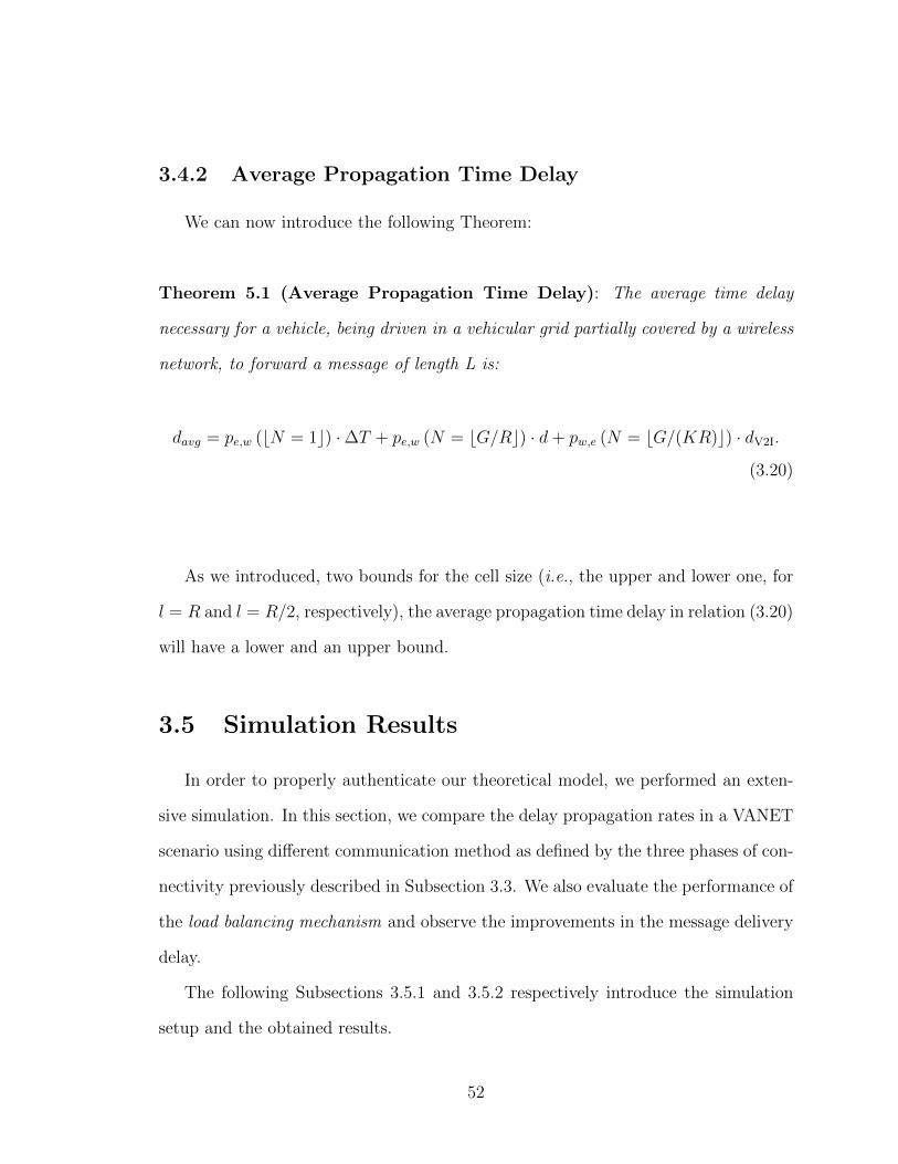
3.4.2 Average Propagation Time Delay

We can now introduce the following Theorem:

Theorem 5.1 (Average Propagation Time Delay): The average time delay

necessary for a vehicle, being driven in a vehicular grid partially covered by a wireless

network, to forward a message of length L is:

davg

= pe,w

(bN = 1c) ·�T + pe,w

(N = bG/Rc) · d+ pw,e

(N = bG/(KR)c) · dV2I.

(3.20)

As we introduced, two bounds for the cell size (i.e., the upper and lower one, for

l = R and l = R/2, respectively), the average propagation time delay in relation (3.20)

will have a lower and an upper bound.

3.5 Simulation Results

In order to properly authenticate our theoretical model, we performed an exten-

sive simulation. In this section, we compare the delay propagation rates in a VANET

scenario using di↵erent communication method as defined by the three phases of con-

nectivity previously described in Subsection 3.3. We also evaluate the performance of

the load balancing mechanism and observe the improvements in the message delivery

delay.

The following Subsections 3.5.1 and 3.5.2 respectively introduce the simulation

setup and the obtained results.

52

3.5.1 Simulation setup

We developed our own simulator, written using Java, which includes the highway

model scenario with 4 di↵erent car speeds. The simulator measures the data delivery

delay as the main performance metric. We considered both asymmetric and sym-

metric bidirectional tra�c flows, where the tra�c density on respective eastbound

and westbound tra�c is di↵erent and assumed equal. However, in this dissertation,

we assume a symmetric tra�c flow, that is a typical configuration, illustrating the

propagation behavior and message delivery performance when cars follow all the three

connectivity phases.

We simulated two typical safety applications, i.e., the Extended Emergency Brake

Light (EEBL), and the Cooperative Intersection Collision Avoidance System (CI-

CAS), corresponding to Low and High Priority messages, respectively. All messages

are being propagated in the vehicular grid. A large number of simulations have been

performed so as to decrease any random fluctuation. We assumed an idealistic perfect

conditions, assuming no dropped packets while contention or interference occurrence

are present. This ideal situation represents the first scenario to simulate in order to

understand how delay is a↵ected in the best case. The vehicle density on highways

is varied from as low as 1 vehicle per kilometer, up to 100 vehicles per kilometer,

and speed ranges from 15 up to 35 [m/s]. These values represent a typical highway

condition of a sparse, medium and heavy tra�c conditions on the roadways.

The vehicular tra�c has been generated using a random exponential distribution

which created the inter-vehicle distances on the highway. The exponential distribution

has been largely shown to be in a good agreement with real vehicular traces for

uncongested tra�c conditions, i.e., up to 1000 vehicles per hour. The inter-arrival

time of vehicles is calculated based on the vehicle density and the speed of vehicle over

53

the highway. For these reasons, the network connectivity is not always guaranteed.

Consequently, at any given time, there is a non-zero possibility that a partition may

exist in the network.

For each scenario, the simulation has been run for 10, 000 seconds, and the average

delay has been calculated from 200 di↵erent iterations to account for the randomness

of the simulation. Distance between RSUs is 500 [meters] and they are distributed

uniformly.

Following these parameters, the QoSHVCP technique has been simulated. Firstly,

the e↵ect of overload and the resulting channel utilization are considered in the tra�c

scenario. Packets introduced to the system are randomly assigned either High Priority

(HP) or Low Priority (LP). The fraction of HP packets of the total packets in the

system is controlled. This fraction is varied from 10% up to 40% of the total number

of messages.

Finally, the load balancing mechanism is included in the system. The message

reception delays for HP packets before and after the introduction of the load bal-

ancing are analyzed and compared. Complete details about the simulation setup are

presented in Table 3.1.

Table 3.1: Parameter setup used in simulations.

Parameter Value

Length of simulation 10000 secondsNumber of runs 200Estimated Vehicular Tx Range [0, 200] meterInfrastructure Tx Range 500 meterPacket size 400 bytesVehicle speeds 15 to 35 meter/sVehicle density 1 to 100 veh/kmLoad balancing threshold 40 veh

54

3.5.2 Simulation results

In this subsection, we begin by presenting the simulation results of the message

reception delay without any load balancing technique. This presents the propagation

delay rates versus di↵erent factors such as connectivity phase, vehicle speed, and

RSU throughput. The following subsection includes results that indicate the e↵ect

of overload on the message reception delay and the improvement after implementing

our overload balancing technique.

Propagation Delay vs Connectivity Phases

We compared the delay reception rates in three di↵erent connectivity phases for

typical safety applications (e.g. EEBL and CICAS) in VANETs. However, to better

understand and validate our simulator, we also included a “limited” Phase 2 that

allows transmission of a single direction only. So, the message propagates strictly in an

ad-hoc hop-to-hop fashion from vehicle to vehicle in a single direction of the highway.

This allows results to be analyzed in the light of (i) no connectivity; (ii) limited one-

directional communication; (iii) vehicle communication that allows transmissions to

both directions through bridging ; and finally (iv) our hybrid QoSHVCP model in

which a message can propagate using all possible transmission means. This may be

in ad-hoc mode or through an infrastructure, whenever available.

We use the following legends in the graphs: “V2V” represents the single-direction

message propagation; “V2V Bridged” represents Phase 2; and “QoSHVCP” our

hybrid model.

The results in Figure 3.4 (a) show that as the vehicle density increases, the delay

decreases. The delay also decreases as the vehicle speed increases. The graph rep-

resents a typical behavior anticipated in Phase 1. The delay in the no connectivity

55

0 10 20 30 40 50 60 70 80 90 10025

30

35

40

45

50

55

60

65

70

Vehicle density [veh/km]

Av

erag

e M

essa

ge

Pro

pag

atio

n D

elay

[s]

15m/s

20m/s

25m/s

35m/s

(a)

(b)

Figure 3.4: (a) Average message propagation delay for increasing vehicle density, andspeed for Phase 1 (no connectivity) at di↵erent speeds (i.e., 15, 20, 25 and 35 m/s).(b) Average message propagation delay for increasing the vehicle density at di↵erenttra�c speeds using V2V communication.

56

phase is the ratio of physical distance covered over the vehicle speed. Thus, the de-

lay is significantly large as compared to Phases 2 and 3. Notice that the reception

time delay in this phase does not depend on vehicles’ density, since no connectivity

is assumed.

Propagation delay also depends on the vehicles’ speed. To better understand

correlation between the delay and the vehicle speed, we have simulated vehicular

movement and the delay at four di↵erent speeds, relying solely on a single-direction

of communication. The simulation results unambiguously show that the delay re-

duces with an increase in the vehicle speed as illustrated in Figure 3.4 (b). As a

consequence, Figure 3.5 (a) depicts the average time delay propagation for a message

traveling at the vehicle speed, and the vehicle density is low. The time delay results

in an average delay smaller than that of Phase 1 with no connectivity. Moreover,

by varying the speeds of the vehicles, the maximum time delay also changes. As

the vehicle density increases, the average delay decreases. This is because when the

probability of connectivity among vehicles increases, the message travels faster than

the vehicle speed.

Figure 3.5 (a) shows that in a low density situation, the average delay follows an

increasing order. This is clearly expected and rea�rms correctness of our simulator.

The results show that under high density conditions, majority of the vehicles are

inter-connected and the message travels at the radio speed. Beyond this level, the

e↵ect of increasing vehicle density does not seem beneficial. Obviously, as vehicle

density increases, more and more vehicles are connected and majority of time, the

message can travel at the radio speed in ad-hoc mode.

In Figure 3.5 (b), we compare the message delivery delay for pure infrastructure

communications only, since it reflects the best and worst cases of delivery time delay.

57

As a matter of fact, infrastructure communication performance is not a↵ected by the

vehicle density since it does not rely on any multihop vehicle communications. It

is only a↵ected by variations in the uplink and downlink data rates of the network

infrastructure. The transmission rates used are a combination of the maximum up-

link and downlink rates for the infrastructure in order to demonstrate the impact of

di↵erent thresholds. The uplink data rate ranges from 0.2 Mbps to 2.7 Mbps, and

the downlink from 5 Mbps to 12.2 Mbps. Notice that infrastructure communication

shows the best (i.e., 5 s) and the worst (i.e., 48 s) time delays respectively for low

(i.e., uplink 0.2 Mbps and downlink 5 Mbps) and high (i.e., uplink 2.7 Mbps and

downlink 12.2 Mbps) values of data rates.

Comparing Figure 3.5 (a) and (b), we are able to establish thresholds for handover

between a purely infrastructure-based connection to any of the other options.

Propagation Delay and Overload Balancing

The performance of the V2V and the V2I, after incorporating the overload factor

on the network, is presented in Figure 3.6. As shown, V2V is not a↵ected by the

overload of the network 2. This is due to the increased connectivity coverage due to

increase in the vehicle density.

In Figure 3.7, we compare the message propagation delays for HP and LP mes-

sages versus di↵erent vehicle densities. As expected, when the probability of HP

messages increases, the message propagation delay increases for higher vehicle den-

sities. Figure 3.8 compares the message propagation delays for the same case after

introducing the load balancing mechanism. Figures 3.9, 3.10, and 3.11 present the

number of packets that experience di↵erent message delivery delays in both schemes

2We ignored the collision and contention due to increased number of packets

58

0 20 40 60 80 1000

10

20

30

40

50

Vehicle Density [Veh/km]

Av

erag

e M

essa

ge

Pro

pag

atio

n D

elay

[s]

V2V

V2V Bridged

QoSHVCP

(a)

0 10 20 30 40 50 60 70 80 90 1000

5

10

15

20

25

30

35

40

45

50

Vehicle Density [Veh/km]

Av

erag

e m

essa

ge

pro

pag

atio

n d

elay

[s]

Uplink 0.2Mbps, Downlink 12.2Mbps

Uplink 0.2Mbps, Downlink 5Mbps

Uplink 2.7Mbps, Downlink 5Mbps

Uplink 2.7Mbps, Downlink 12.2Mbps

(b)

Figure 3.5: (a) Average message propagation delay for increasing vehicle density forV2V, V2V Bridged and QoSHVCP at a fixed speed. (b) Average message propagationdelay for increasing vehicle density in pure infrastructure communications at di↵erentuplink and downlink rates.

59

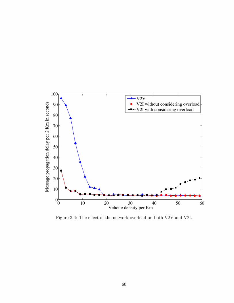
0 10 20 30 40 50 600

10

20

30

40

50

60

70

80

90

100

Vehcile density per Km

Mes

sage

pro

pag

atio

n d

elay

per

2 K

m i

n s

econds

V2V

V2I without considering overload

V2I with considering overload

Figure 3.6: The e↵ect of the network overload on both V2V and V2I.

60

0 10 20 30 40 50 60 700

10

20

30

40

50

60

70

80

90

100

Vehicle density per Km

Mes

sage

pro

pag

atio

n d

elay

per

2 K

m i

n s

econds

LP packets

HP packets with probability 0.1

HP packets with probability 0.2

HP packets with probability 0.3

HP packets with probability 0.4

Figure 3.7: Message propagation delay for High and Low Priority messages withdi↵erent probabilities of High Priority without load balancing mechanism.

61

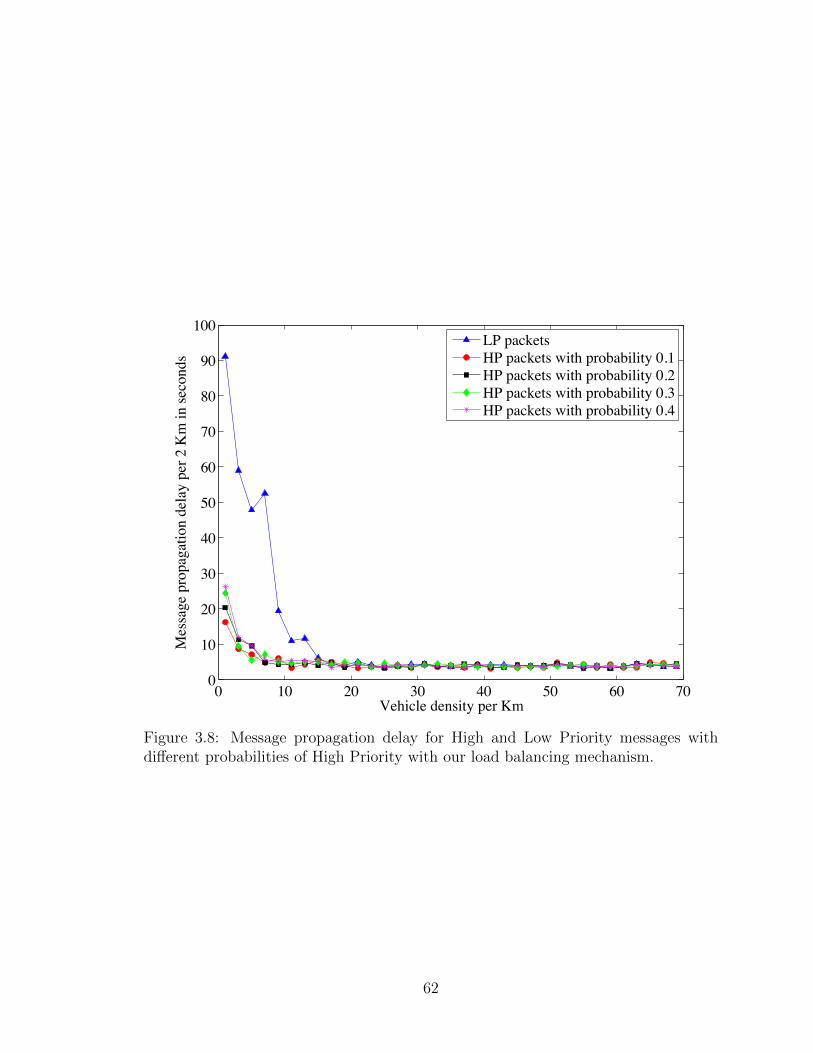
0 10 20 30 40 50 60 700

10

20

30

40

50

60

70

80

90

100

Vehicle density per Km

Mes

sag

e p

rop

agat

ion

del

ay p

er 2

Km

in

sec

on

ds

LP packets

HP packets with probability 0.1

HP packets with probability 0.2

HP packets with probability 0.3

HP packets with probability 0.4

Figure 3.8: Message propagation delay for High and Low Priority messages withdi↵erent probabilities of High Priority with our load balancing mechanism.

62

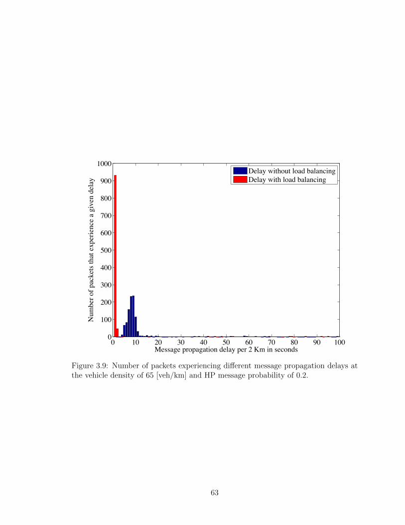
0 10 20 30 40 50 60 70 80 90 1000

100

200

300

400

500

600

700

800

900

1000

Message propagation delay per 2 Km in seconds

Nu

mb

er o

f p

ack

ets

that

ex

per

ien

ce a

giv

en d

elay

Delay without load balancing

Delay with load balancing

Figure 3.9: Number of packets experiencing di↵erent message propagation delays atthe vehicle density of 65 [veh/km] and HP message probability of 0.2.

63

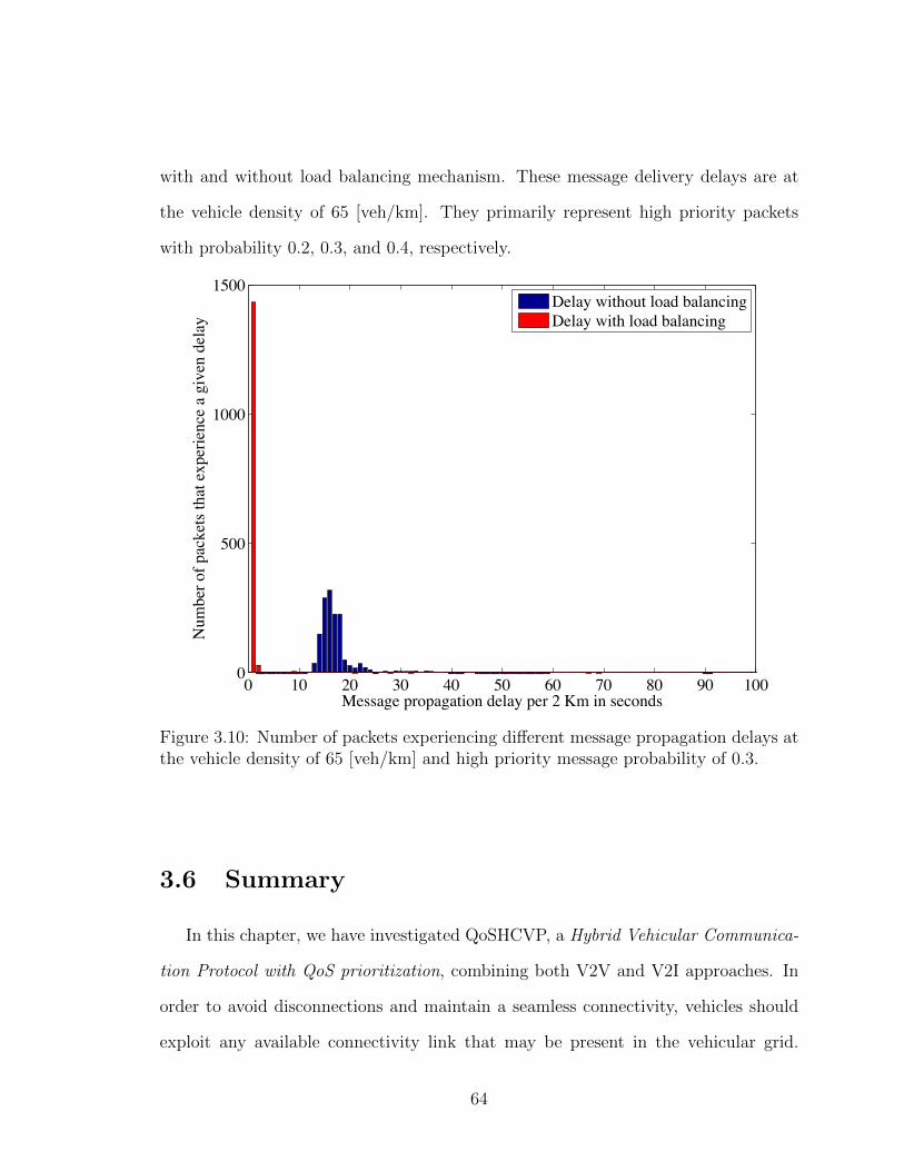
with and without load balancing mechanism. These message delivery delays are at

the vehicle density of 65 [veh/km]. They primarily represent high priority packets

with probability 0.2, 0.3, and 0.4, respectively.

0 10 20 30 40 50 60 70 80 90 1000

500

1000

1500

Message propagation delay per 2 Km in seconds

Nu

mb

er o

f p

ack

ets

that

ex

per

ien

ce a

giv

en d

elay

Delay without load balancing

Delay with load balancing

Figure 3.10: Number of packets experiencing di↵erent message propagation delays atthe vehicle density of 65 [veh/km] and high priority message probability of 0.3.

3.6 Summary

In this chapter, we have investigated QoSHCVP, a Hybrid Vehicular Communica-

tion Protocol with QoS prioritization, combining both V2V and V2I approaches. In

order to avoid disconnections and maintain a seamless connectivity, vehicles should

exploit any available connectivity link that may be present in the vehicular grid.

64

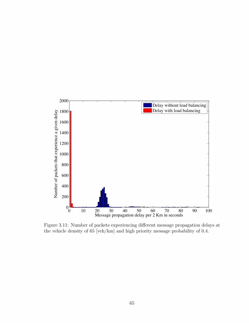
0 10 20 30 40 50 60 70 80 90 1000

200

400

600

800

1000

1200

1400

1600

1800

2000

Message propagation delay per 2 Km in seconds

Nu

mb

er o

f p

ack

ets

that

ex

per

ien

ce a

giv

en d

elay

Delay without load balancing

Delay with load balancing

Figure 3.11: Number of packets experiencing di↵erent message propagation delays atthe vehicle density of 65 [veh/km] and high priority message probability of 0.4.

65

Based on a delay-based decision criterion, our approach represents a handover mech-

anism between V2V and V2I.

We have illustrated the e↵ectiveness of such technique in terms of message delivery

time delay rates. Simulation results confirm our analytical work on how hybrid ap-

proach enhances the connectivity support, specially in high mobility and low density

vehicle scenarios as compared to traditional opportunistic V2V techniques for dense

areas.

The e↵ect of tra�c overload on the message propagation delay has also been

presented. The failure of achieving QoS requirements has been addressed with our

novel load balancing mechanism that decreases the message propagation delay of high

priority packets regardless of the network overload.

The main contributions presented in this chapter can be summarized as follows:

• A Hybrid protocol for vehicle communication on highway: We pre-

sented a hybrid protocol that utilizes both vehicle-to-vehicle communication

as well as vehicle-to-infrastructure communication in order to achieve a low

message delivery delay.

• An analytical model that formulates the end-to-end message propaga-

tion delay: In order to get this formula, we analyzed the vehicle connectivity

as one of three possible scenarios: vehicle travelling alone, vehicle travelling

along with other vehicles on the highway, and vehicle travelling within the cov-

erage of road side units (infrastructure). The average delay formula accounts

for di↵erent connectivity scenarios with the probability of the vehicle being in

each scenario.

• Infrastructure load analysis and a load balancing mechanism: We in-

66

troduced the e↵ect of increasing the load on the throughput of infrastructure.

We presented the impact of this overload on the end-to-end message delivery

delay. A load balancing mechanism was introduced to minimize the e↵ect of

this overload.

• Simulation results: We presented simulation results that analyzed end-to-end

message propagation delay versus the vehicle density in a highway scenario. We

simulated the e↵ect of the infrastructure overload on the message delivery delay.

We finally simulated the performance of our load balancing mechanism.

67

Chapter 4

CAREFOR for VANET

In this chapter, we introduce a novel reliable and low-collision packet-forwarding

scheme for vehicular ad hoc networks, based on a probabilistic rebroadcasting. Our

proposed scheme, called Collision-Aware REliable FORwarding (CAREFOR) works

in a distributed fashion where each vehicle receiving a packet, rebroadcasts it based

on a predefined probability. This probability is manipulated by di↵erent physical

factors derived from the vehicular environment, including density of the vehicles in

the vicinity, distance between transmitting and receiving vehicles, and finally, trans-

mission range of the next-hop. All these factors are combined into one probability

that enables each vehicle to evaluate whether there is another vehicle that ought

to be receiving this message and could be feasible if the message is rebroadcasted.

The success of rebroadcast is determined based on allowing the message to travel the

furthest possible distance with the least amount of packet rebroadcast collision.

CAREFOR is di↵erent from other existing techniques as it accounts for the e↵ect

of the next-hop transmission in the rebroadcast decision. Simulation results show the

e↵ectiveness of our approach in terms of limited number of rebroadcasts needed with

68

low collision probability as compared to existing techniques. Two and three-hops

message retransmissions are also considered.

4.1 Introduction

Frequent topological changes of a VANET makes it not very e�cient to rely on

existing MANET protocols. Rebroadcasting packets by multiple vehicles causes an

increase in redundant data, which leads to wasted bandwidth and misuse of radio

channels in the network. One of the main objectives of packet rebroadcasting in a

VANET is to minimize this redundancy while still guaranteeing packet delivery to all

relevant vehicles.

Due to these unique features of a VANET, several types of routing protocols have

been introduced in the literature [60]. These protocols are mainly defined taking

certain attributes of the VANET into account, such as (i) connectivity-based, (ii)

mobility-based, (iii) infrastructure-based, (iv) location-based, and (v) probability-

based routing protocols. Later on, many techniques are used to exploit probability

theory in systems’ dynamic, representing the likelihood of certain events, such as

the probability of link breakage at a given transmission power. Many such routing

protocols utilize a probability model to indicate the state of a wireless communication

link between two adjacent nodes, while using many di↵erent parameters (e.g., link

lifetime in the network) as a major routing parameter.

In this research, we propose a probability-based multi-hop broadcast protocol,

called Collision-Aware REliable FORwarding (CAREFOR) with an objective of re-

ducing the number of rebroadcasts in the network. This minimizes the number of

packets in the system which leads to a lower collision probability and eventually im-

69

proved throughput. CAREFOR achieves this by allowing the vehicles to compute the

probability of their successful transmission in case they are selected to rebroadcast

the packet if there exists no better candidate for rebroadcast. A better candidate

would be a vehicle that has a chance of delivering the packet for a larger number of

uncovered vehicles with fewer number of retransmissions and with minimum packet

collisions. Hence, the CAREFOR algorithm relies both on collision avoidance and re-

liable forwarding mechanism. By using both, CAREFOR is able to limit the number

of retransmissions while maintaining lower collision value.

The rest of this chapter is organized as follows. Subsection 4.2 discusses some re-

cent research on routing protocols for VANETs. We mainly highlight the work of [61],

which is the foundation of our CAREFOR technique. In Subsection 4.3, we describe

CAREFOR algorithm with details mainly covering the theoretical analysis of the

next-hop vehicle election probability, and the collision probability estimation. Con-

siderations on the use of two vs. three hops forward prediction are also investigated

in order to determine the optimal approach. The simulation results demonstrates the

e↵ectiveness of our technique and is presented in Subsection 4.4. Finally, conclusion

and future work are drawn in the last subsection.

4.2 Related Work

Many categories of routing protocols in VANETs have been described in the liter-

ature over the past few years. One of these schemes is the probability-based routing

protocol that avoids flooding of the network with duplicates of the same packet by

assessing availability of the links and reachability of the packet to the destination

through a given multi-hop route. Clearly, the advantage of such technique is to reduce

70

the overall required number of packets in the system that improves the performance

by minimizing the number of collisions. If each vehicle rebroadcasts probabilistically,

the number of duplicate packets could be considerably lowered in the system. This

type of routing protocols have been used in many papers. These techniques oppor-

tunistically select the next hop based on a given specific criteria. The most common

rule is the ability to retransmit the packet successfully. This is a↵ected by di↵erent

physical factors of the environment and the network. Examples for these physical

factors include: transmission power, received signal strength, vehicle density, vehicle

speed, etc.

In [62], authors presented a ticket-based technique as a routing protocol. These

tickets are control packets transmitted on selected links which is based on the met-

rics of stability, delay and cost. Ticket-based systems were initially introduced in

MANETs [63] with the objective of identifying a reliable route based on multiple

links that are selectively probed.

Jiang et al. [64] presented a routing algorithm defined as REAR, which considers

the reception probability of the alarm message and analyzes similar to a real wireless

channel model in a VANET. Particularly, the probability model takes into account

physical parameters, such as the received signal strength, the path loss as well as the

di↵raction loss factor. The receipt probability is computed by using the relationship

between the packet loss rate and the received signal strength. The links with highest

reception probability of additional vehicles are then selected for routing.

Sun et al. [65] proposed GVGrid algorithm to find a reliable routing path that

meets a given delay requirement. By assuming an equally spaced inter-vehicle gap

and a normally distributed vehicle speed, GVGrid computes the probability of link

lifetime as a function of link reliability. The proposed technique will select that path

71

with the highest reliability, and relatively smaller link delay as the routing path.

Common to all previous techniques, physical parameters play an important role

for the rebroadcast probability and the link selection. In [66], the authors present a

rebroadcast probability that is based on the inter-vehicle distance. This probability

is directly proportional to the distance from the transmitter. The larger the distance

is, higher will be the rebroadcast probability.

From [66], the rebroadcast probability is a function of inter-vehicle distance and

can be expressed as:

p =d

z, (4.1)

where d is the distance between receiving and transmitting vehicles, and z is the

transmission range. The rebroadcast probability follows a linear dependence that

increases with the distance.

Based on this technique, the authors in [61] present a protocol named Irresponsible

Forwarding (IF) which accounts for both the signal strength, as well as the statistical

distribution of the vehicles. The main idea behind IF is that each vehicle evaluates the

presence of other vehicles within the transmission range of the source vehicle. If the

receiving vehicle evaluation results in the likeliness of the presence of another vehicle

that is better qualified to rebroadcast the packet, the vehicle decides irresponsibly

to refrain from rebroadcasting the packet. A more qualified vehicle is the one that

will be able to cover a longer distance with one hop transmission if it is allowed to

rebroadcast the packet.

Therefore, a vehicle that receives a packet, should rebroadcast it only if the prob-

ability of finding a better qualified vehicle in the transmission range is very low. If

the probability is very low, then the vehicle should avoid rebroadcasting the packet.

In [61], the authors define the rebroadcast probability for a receiving vehicle as:

72

p = exp

�⇢ · (z � d)

c

�, (4.2)

where d is the inter-vehicle distance between the receiving and the transmitting ve-

hicles, ⇢ is the exponentially distributed inter-vehicle spacing [veh/m] with mean

value 1/⇢, and c 1 is a coe�cient which can be selected to shape the rebroadcast

probability (as a function of d).

It is clear from the equation that the larger the value of c, higher will be the re-

broadcast probability will be at any value of d. In the case that c = 1, the rebroadcast

probability is reduced to the probability of no vehicles in the range of (z � d).

The IF protocol is a very e↵ective approach in order to limit the number of re-

broadcasts in the system. However, it has one major limitation as it fails to account

for packet collision from the vehicle that rebroadcasts. Since IF is a probabilistic

approach, more than one vehicle may decide to rebroadcast the message, which will

cause packet collision, and hence, the loss of the packet. In order to overcome this

limitation, the authors in [67] leveraged the assumption that vehicles travel on the

highway within the cluster with high probability. The authors present a protocol in

which a cluster-head is elected within each cluster which is responsible for rebroad-

casting the packet, while other vehicles in the cluster refrain from rebroadcasting.

This avoids the occurrence of packet collisions within the cluster, and minimizes the

number of rebroadcasts in the network.

The main disadvantage of the cluster-based approach is that it is a centralized

protocol. While this can be feasible in MANETs, it is di�cult to generalize for a

VANET. The high mobility of a VANET makes creating clusters very di�cult on

the highway, since di↵erent vehicles are added and others leave the cluster within a

very short span of time. Moreover, cluster-based approach entails di↵erent security

73

weaknesses and adds to the existence of malicious nodes in the cluster.

Finally, the IF approach [61] relies mainly on the coverage range of the transmit-

ting vehicle, i.e., z [m]. IF only accounts for the probability of another vehicle being

present in the range (z � d) [m] at a distance d [m] from the transmitting vehicle.

If this probability yields to absence or a low chance of having any other vehicles in

this range, the vehicle will rebroadcast the packet. IF relies on the assumption that

all the vehicles have the same transmission range. Hence, the vehicle density metric

within the transmission range of any vehicle is dependent only on the distribution of

the vehicles on the highway. This assumption does not always hold good in a real

life scenario. In case this assumption is not true, this will result in a di↵erent vehicle

density within the transmission range of ever vehicle. This vehicle density will not

only depend on the vehicle distribution, but on the transmission range of the vehicle

as well. Another limitation in the IF protocol is the assumption of a collision-free

environment, which is not true in a VANET and ought to be relaxed in a realistic

protocol.

In this research, we consider IF approach as the foundation for our novel probability-

based protocol that minimizes the redundancy caused by the packet retransmission.

Moreover, this protocol aims to reduce the packet collisions in the system. The main

focus of CAREFOR is to enhance the performance, as observed by the simulation

results. We also present a thorough theoretical analysis, and investigate the e↵ect

of including two and three-hops information as factors in computing the rebroadcast

probability.

74

4.3 Collision-Aware REliable FORwarding

In this section, we introduce the CAREFOR technique, and discuss the main

rationale behind it, reliable forwarding and collision probability. The CAREFOR

protocol particularly exploits twofold probabilistic analysis, aiming (i) to limit the

number of packet collisions, and (ii) to select potential vehicle forwarder. CAREFOR

takes into consideration reduction in the packet collision probability by estimating

and selecting the next-hop forwarder for every single transmission as a method for

packet rebroadcasting. One of the main improvements of the CAREFOR algorithm

over other traditional approaches is that it accounts for more than one-hop neighbor

information as the traditional approaches do. CAREFOR relies on the probability

obtained from information extended to the next hop(s) (i.e., from two to three hops).

We discuss the reliable forwarding and the collision probability in Subsection 4.3.1

and Subsection 4.3.2, respectively. An analytical model for message rebroadcast prob-

ability has been developed in Subsection 4.3.3. In Subsection 4.3.4, the main features

of CAREFOR are presented in an algorithmic form. Finally, in Subsection 4.3.5 we

investigate the benefits of CAREFOR technique based on information from two and

three hops.

4.3.1 Reliable Forwarding

Before we introduce our proposed technique, we present an example that elab-

orates on the reason for considering two-hop (prediction) information in order to

compute the rebroadcast probability instead of the traditional one-hop method.

Consider Figure 4.1, with the vehicle has a transmission range of z [m]. We

make a basic assumption that each vehicle has the knowledge of its exact location

75

using a Global Positioning System (GPS), and that this location is piggybacked along

with the data packets to other vehicles in the vicinity. As shown in this example,

there are two vehicles (i.e., the dark (i.e., v1) and light colored (i.e., v2) vehicle in

Figure 4.1), within the transmission range of the source vehicle (i.e., v0). Both vehicles

are at a distance d0 [meter] and d00 [meter] respectively, where d00 > d0. Following the

traditional IF protocol [61], the rebroadcast probability for vehicle v2 is higher than

that for vehicle v1 since the probability is directly proportional to the distance from

the source vehicle v0. From this example, it is clear that the IF limits the rebroadcast

probability to control the one-hop transmission and reflect the inter-vehicle distance.

In the IF protocol, it is assumed that each vehicle has the same transmission

range. This assumption may not be true in real life and the transmission range could

vary from vehicle to vehicle due to di↵erent factors, including the transmission power,

as well as signal e↵ects such as multipath or fading. A practical algorithm should

incorporate these factors in computing the rebroadcast probability, since the objective

of a selected forwarding vehicle is to be able to forward the packet as fas as possible,

and hence, minimize the number of required packet rebroadcasts in order to reach all

the vehicles in the group.

Since the objective of any routing algorithm is to forward the packet to the destina-

tion through the most e�cient route, a successful forwarder should not be considered

based on the performance from only the one-hop transmission point of view. If pos-

sible, the e↵ect of the hops following, beyond the first hop ought to be considered

when selecting the first forwarder. In other words, the best routing protocol would

be able to aggregate the e↵ect of every hop from the source to the destination, and

select the first forwarder based on which one will provide the best overall coverage.

In our work, we investigate the e↵ect of relying on information from two hops as well

76

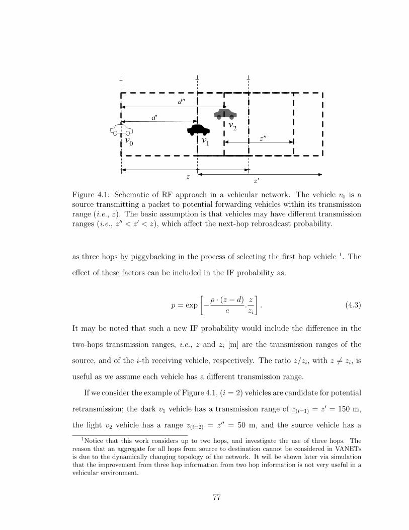
d'

zz'

d''

z''

v

0 v

1

v

2

Figure 4.1: Schematic of RF approach in a vehicular network. The vehicle v0 is asource transmitting a packet to potential forwarding vehicles within its transmissionrange (i.e., z). The basic assumption is that vehicles may have di↵erent transmissionranges (i.e., z00 < z0 < z), which a↵ect the next-hop rebroadcast probability.

as three hops by piggybacking in the process of selecting the first hop vehicle 1. The

e↵ect of these factors can be included in the IF probability as:

p = exp

�⇢ · (z � d)

c.z

zi

�. (4.3)

It may be noted that such a new IF probability would include the di↵erence in the

two-hops transmission ranges, i.e., z and zi

[m] are the transmission ranges of the

source, and of the i-th receiving vehicle, respectively. The ratio z/zi

, with z 6= zi

, is

useful as we assume each vehicle has a di↵erent transmission range.

If we consider the example of Figure 4.1, (i = 2) vehicles are candidate for potential

retransmission; the dark v1 vehicle has a transmission range of z(i=1) = z0 = 150 m,

the light v2 vehicle has a range z(i=2) = z00 = 50 m, and the source vehicle has a

1Notice that this work considers up to two hops, and investigate the use of three hops. The

reason that an aggregate for all hops from source to destination cannot be considered in VANETs

is due to the dynamically changing topology of the network. It will be shown later via simulation

that the improvement from three hop information from two hop information is not very useful in a

vehicular environment.

77

transmission range z = 200 m. As mentioned earlier, the traditional IF rebroadcast

probability is based on the distance between the source and the receiving vehicle, as

well as the vehicular density. Hence, based on (4.2), assuming that ⇢ = 0.02, c = 2

and d00 = 150 m, the traditional IF rebroadcast probability for the green vehicle will

be 0.6. If we assume that d0 = 100 m, the IF rebroadcast probability for the v1 dark

vehicle will be 0.36. Hence, the v2 light vehicle will be selected based on the higher

rebroadcast probability, while v1 will not rebroadcast.

If we relax the assumption that vehicles have the same transmission range, and if

we note that the objective of the routing protocol is to eventually transmit the packet

to the longest distance with the least number of rebroadcasts along the route, then

the vehicle that provides an overall largest aggregate transmission distance should be

selected. In this case, the v1 vehicle should be selected, since its next-hop transmission

range is larger than that of v2 vehicle (i.e., z0 > z00), resulting as the most e�cient

rebroadcaster. This allows the packet to potentially reach a larger number of vehicles

in a fewer number of rebroadcasts, and hence reducing the span of time. The RF

probability for the dark vehicle is 0.26, while for the light vehicle it is 0.13.

Allowing the vehicles to estimate the potential for future second hops vehicles

shifts the paradigm of the protocol from being irresponsible forwarding to be a stable

and reliable protocol. Hence, the new probability metric is named Reliable Forwarding

(RF). The behavior of the RF probability for two-hop forward transmission versus

di↵erent transmission ranges is depicted in Figure 4.2. It may be noticed from the

figure that the RF probability depends on the distance between the source and the

destination as well as the transmission range. The main advantage for RF over IF, is

that IF only considers one hop rebroadcast, while the RF introduced here considers

the two hops rebroadcast as well. It also can be observed from (4.3) that when the

78

transmission range of the receiving vehicle is equal to that of the source vehicle (i.e.,

z0 = z), the value of the RF probability is equal to that of the IF probability.

As it is shown in Figure 4.2, the RF probability allows a vehicle with a larger

transmission range to have a higher value for the RF probability. This results in

better chances of rebroadcasting the message and allowing the packet to reach an

increased number of vehicles due to the transmission range covering a larger distance.

The main disadvantage is that the larger the covered area, higher will be the number

of vehicles in the transmission range, which could result in a higher packet collision

probability. Hence, we address this issue in the following section.

4.3.2 Collision Probability

The authors in [68] define the collision probability as the probability that more

than one vehicle is transmitting at the same time. In order to model this probability,

Pcoll

, we initially need to analyze the probability that there is at least one vehicle

transmitting in the current time slot, Pbusy

. This can be defined by:

Pbusy

= 1� (1� p)(n�1), (4.4)

where p is the RF probability from (4.3), which is the probability that the vehicle

will decide to rebroadcast the packet in this instance, and n is the number of other

vehicles interfering with this transmission. As we assume that N is the number of

vehicles interfering in every hop, and our RF probability considers only two hops, the

total number of interfering vehicles will be n = 2N .

Based on Pbusy

, we can define another probability Pt

, which is the probability that

there is only one vehicle using in the channel at this time. The probability can be

79

given by:

Pt

=p · (1� p)(n�1)

Pbusy

. (4.5)

Based on (4.4) and (4.5), we can define the collision probability Pcoll

, which is the

probability that more than one vehicle is transmitting, causing the collision. Hence,

Pcoll

is:

Pcoll

= Pbusy

· (1� Pt

). (4.6)

In Figure 4.3 (a), we observe collision probabilities for di↵erent next-hop trans-

mission ranges (i.e., zi

= {100, 200, 400} m), in a forward packet transmission v/s the

transmission range of the source (i.e., z = 200 m). As expected, we can notice that a

larger next hop transmission range results in a higher collision probability. However,

this result is obtained against the RF probability, as depicted in Figure 4.2, since for

high next-hop transmission range, the RF probability increases for growing distance

from the source.

In order to decide which vehicle should be allowed to forward the packet due

to experiencing a low collision probability versus which vehicles are experiencing a

high collision probability, we need to define a threshold. This threshold is based on

di↵erent physical factors in the network, such as the next-hop transmission range i.e.,

zi

[m], and the number of vehicles—the vehicle density i.e., ⇢ [veh/m]. We define the

collision threshold as:

Thcoll

= 1� [exp (�⇢zi

)] . (4.7)

In Figure 4.3 (a), this threshold is presented by the horizontal line at 0.4. Note

80

that the threshold varies for di↵erent transmission ranges. As shown in the figure,

for transmission ranges of [100, 200, 400] m, the collision threshold of (i.e., 0.4) is at

distances [172, 143, 86] m respectively from the source. This means that any vehicle

with a transmission range of 100 m, and is at a distance smaller than 172 m from the

source, should be able to satisfy the collision probability threshold. The smaller the

transmission range, the higher the distance from the transmitter can be, hence, more

vehicles will have a collision probability lower than the threshold.

For a fixed source transmission range (i.e., z = {100, 200, 400} m), Figure 4.3 (b)

presents the behavior of the threshold for the collision versus the vehicle density. No-

tice that if the vehicle density is fixed, the collision threshold is indirectly proportional

with the transmission range.

4.3.3 Analytical Model

Let us consider the scenario where an information packet propagates forward from

a source vehicle, as previously depicted in Figure 4.1. The message direction is the

same as that of the vehicle speed, and we assume vehicles are being driven along the

lane following a Poisson distribution.

In such a scenario, we consider the average number of packets collectively being

rebroadcasted by the vehicles in the network. More specifically, we need to distinguish

how many packets are retransmitted by the other vehicles for each hop in the vehicular

network. This coincides with the average number of vehicles that rebroadcast the

packet transmitted by the source vehicle which experiences a low collision probability.

Obviously, we implicitly assume each vehicle rebroadcasts only one copy of each

received packet and then no more copies of the same packet need to be retransmitted

within the network.

81

As shown in Figure 4.1, following a Poisson distribution with parameter ⇢z we

assume there are Nz

vehicles in the transmission range z of the source vehicle. Each

vehicle in the range (0, z) m can rebroadcast a packet based on its RF probability

and this event can be represented by the following Bernoulli random variable:

Vi

=

8><

>:

1, if i�th vehicle rebroacasts

0, otherwise,(4.8)

with i = 1, 2, . . . , Nz

, as the i-th candidate vehicle for rebroadcasting. It follows

that the average number of vehicles in (0, z) which can rebroadcast the packet, is

represented by means of a random variable Mz

, as follows:

E [Mz

] =NzX

i=1

Vi

. (4.9)

Since Nz

follows a Poisson distribution with parameter ⇢z, by applying the law of

total probability and observing that

E [Mz

|Nz

= 0] = 0. (4.10)

Then, the average number in (4.9) can be rewritten as follows:

E [Mz

] =1X

n=1

E[Mz

|Nz

= n ]P {Nz

= n} =1X

n=1

E"

NzX

i=1

Vi

|Nz

= n

#P {N

z

= n} =

=1X

n=1

nX

i=1

E[Vi

|Nz

= n ]P {Nz

= n} =1X

n=1

e(�⇢z) (⇢z)n

n!

nX

i=1

E[Vi

]. (4.11)

Based on Bernoulli behavior of Vi

random variable, we can obtain the average number

82

of rebroadcasting vehicles based on the corresponding RF probability:

E [Vi

] = P {Vi

= 1} , (4.12)

where P {Vi

= 1} is the probability of rebroadcasting for the i-th vehicle (i.e., RF

probability). As per (4.3), this probability depends on both the distance di

= ⌧ of

the i-th vehicle from the source vehicle, as well as on the transmission range zi

= �

of the i-th vehicle:

P {Vi

= 1 |di

= ⌧, zi

= �} = exp

�⇢ · (z � ⌧)

c· z�

�. (4.13)

By applying the total probability theorem, (4.13) can be written as:

P {Vi

= 1} =

1Z

0

P {Vi

= 1 |di

= ⌧, zi

= �} fdi (⌧) fzi (�) d⌧d� =

=

zZ

0

�Z

z

exp

�⇢ (z � ⌧)

c

z

�

�fdi (⌧) fzi (�) d⌧d�, (4.14)

where fdi(·) and f

zi(·) are respectively the probability density functions (pdf) of the

distance di

[m] and the transmission range zi

[m] of the i-th vehicle.

Assuming that each vehicle is traveling along with a Poisson distribution within

the transmission range, following a linear path 2, then the distance di

can be expressed

as the sum of the distances of the vehicles behind the i-th vehicle in the range (0, z),

such as:

di

=i�1X

j=1

yj

, (4.15)

2We assume that the vehicles from 1 to Nz are in an increasing order of distance from the origin.

83

where yj

, with j = i� 1, is the distance from the j-th vehicle to the i-th vehicle. As-

suming the variables yj

are randomly independent and identically distributed (i.i.d.)

with exponential distribution with mean value 1/⇢, then di

follows Erlang distribution

with parameters i and ⇢ as:

fdi�Erlang

(⌧) =⇢e�⇢⌧ (⇢⌧)i�1

(i� 1)!U (⌧) , (4.16)

where U (⌧) is the unit-step function, limited to be lower than z. The pdf of the

distance di

from the source vehicle can be written as:

fdi (⌧) = f

di�Erlang

(⌧ |di

z ) =

8><

>:

fdi�Erlang(⌧)

FDi�Erlang(z), if 0 < d

i

z

0, otherwise, (4.17)

where FDi�Erlang

(z) is the cumulative distribution function (CDF) of an Erlang pdf

with parameters i and ⇢. In particular, it can be shown that

FDi�Erlang

(z) =� (i, ⇢z)

(i� 1)!, (4.18)

where � is the lower incomplete gamma function:

� (i, ⇢z) =

⇢zZ

0

ti�1e�tdt. (4.19)

Finally, (4.17) becomes

fdi (⌧) =

⇢e�⇢⌧ (⇢⌧)i�1

� (1, ⇢z)[U (⌧)� U (⌧ � z)] . (4.20)

Similar substitutions can be done for the fzi(·) pdf of the transmission range z

i

84

for the i-th vehicle. We distinguish two cases, i.e., (i) for zi

= z, and (ii) for zi

> z.

In the former case, we can write

zi

= z =NzX

j=1

yj

, (4.21)

and that follows:

fzi�Erlang

(�) =⇢e�⇢� (⇢�)i�1

(i� 1)!U (�) , (4.22)

with i = Nz

. The pdf of the transmission range fzi(·) can be expressed as:

fzi (�) = f

zi�Erlang

(zi

|� z ) =

8><

>:

fzi�Erlang(zi)

Fz�Erlang(z), if 0 < z

i

z

0, otherwise(4.23)

It follows as:

fzi (�| zi = z) =

⇢e�⇢�(⇢�)i�1

� (1, ⇢z)[U (�)� U (� � z)] . (4.24)

In the second case, for zi

> z, we can write:

zi

= z +�z =NzX

i=1

y(z)i

+N

�zX

j=1

y(�z)j

, (4.25)

fzi (�) = f

zi�Erlang

(zi

|� > z ) =

8><

>:

fzi�Erlang(zi)

Fz�Erlang(z), if z

i

> z

0, otherwise(4.26)

and then,

fzi (�| zi > z) =

⇢e(�⇢�) (⇢�)Nzi�1

(Nzi � 1)!

U (z) . (4.27)

By using (4.17) and (4.24) into (4.14), the RF probability becomes:

85

P {Vi

= 1} =

zZ

0

�Z

z

exp

�⇢

(z � ⌧)

c

z

�

�⇢ exp [�⇢⌧ ] (⇢⌧)i�1

� (i, ⇢z)· ⇢ exp [�⇢�] (⇢�)i�1

� (i, ⇢z)d⌧d� =

=⇢2

�2 (i, ⇢z)

zZ

0

�Z

z

exp

�⇢

(z � ⌧)

c

z

�� ⇢⌧ � ⇢�

�(⇢⌧)i�1 · (⇢�)i�1 d⌧d� =

=⇢2

�2 (i, ⇢z)

zZ

0

�Z

z

exp

⇢�z2 + ⌧z � c�⌧ � c�2

c�

�(⇢⌧)i�1 · (⇢�)i�1 d⌧d�. (4.28)

4.3.4 CAREFOR algorithm

In this subsection, we present the details of how the CAREFOR protocol can

actually work in a VANET environment. As mentioned earlier, the protocol includes

two main phases (i) Collision probability estimation, and (ii) Reliable forwarding.

CAREFOR considers a contention resolution procedure necessary for each vehicle

to estimate the collision threshold associated with the vehicle density and the actual

transmission ranges. The procedure follows in several steps which can be described

as follows:

• RTB transmission: In this step, the source vehicle broadcasts a Request-to-

Broadcast (RTB) control message to all the vehicles in its vicinity. The RTB

message is a MAC-broadcast packet which includes the GPS information of the

source node, the vehicle density around the source node (which can be found

out by ping messages), and finally, the transmission power level.

Notice that, since the transmission ranges are relatively short (i.e., lower than

400 meter), we assume that the local vehicular density can approximate the

global vehicular density within the transmission range. Moreover, the transmis-

86

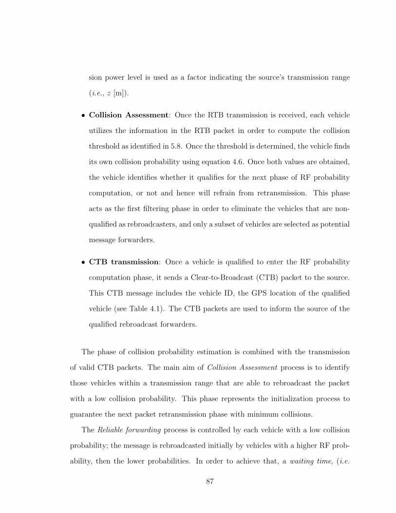
sion power level is used as a factor indicating the source’s transmission range

(i.e., z [m]).

• Collision Assessment: Once the RTB transmission is received, each vehicle

utilizes the information in the RTB packet in order to compute the collision

threshold as identified in 5.8. Once the threshold is determined, the vehicle finds

its own collision probability using equation 4.6. Once both values are obtained,

the vehicle identifies whether it qualifies for the next phase of RF probability

computation, or not and hence will refrain from retransmission. This phase

acts as the first filtering phase in order to eliminate the vehicles that are non-

qualified as rebroadcasters, and only a subset of vehicles are selected as potential

message forwarders.

• CTB transmission: Once a vehicle is qualified to enter the RF probability

computation phase, it sends a Clear-to-Broadcast (CTB) packet to the source.

This CTB message includes the vehicle ID, the GPS location of the qualified

vehicle (see Table 4.1). The CTB packets are used to inform the source of the

qualified rebroadcast forwarders.

The phase of collision probability estimation is combined with the transmission

of valid CTB packets. The main aim of Collision Assessment process is to identify

those vehicles within a transmission range that are able to rebroadcast the packet

with a low collision probability. This phase represents the initialization process to

guarantee the next packet retransmission phase with minimum collisions.

The Reliable forwarding process is controlled by each vehicle with a low collision

probability; the message is rebroadcasted initially by vehicles with a higher RF prob-

ability, then the lower probabilities. In order to achieve that, a waiting time, (i.e.

87

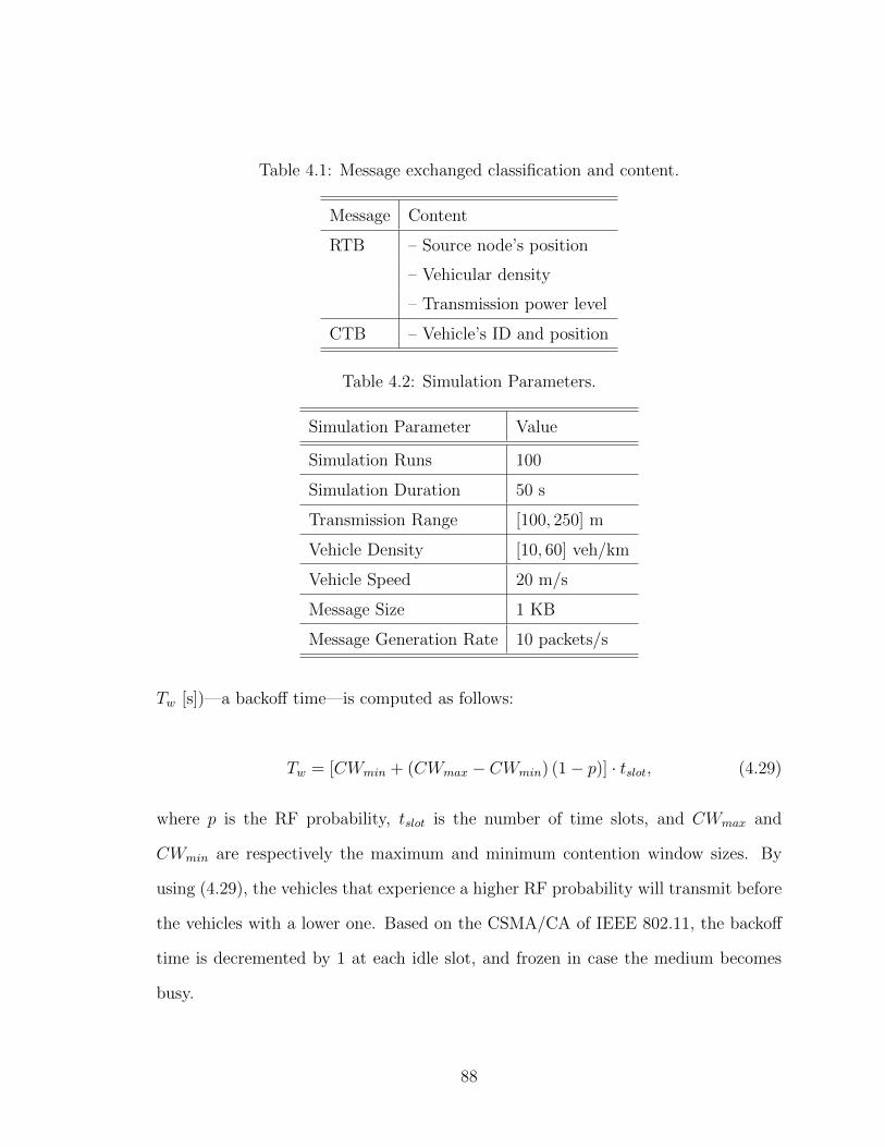
Table 4.1: Message exchanged classification and content.

Message Content

RTB – Source node’s position

– Vehicular density

– Transmission power level

CTB – Vehicle’s ID and position

Table 4.2: Simulation Parameters.

Simulation Parameter Value

Simulation Runs 100

Simulation Duration 50 s

Transmission Range [100, 250] m

Vehicle Density [10, 60] veh/km

Vehicle Speed 20 m/s

Message Size 1 KB

Message Generation Rate 10 packets/s

Tw

[s])—a backo↵ time—is computed as follows:

Tw

= [CWmin

+ (CWmax

� CWmin

) (1� p)] · tslot

, (4.29)

where p is the RF probability, tslot

is the number of time slots, and CWmax

and

CWmin

are respectively the maximum and minimum contention window sizes. By

using (4.29), the vehicles that experience a higher RF probability will transmit before

the vehicles with a lower one. Based on the CSMA/CA of IEEE 802.11, the backo↵

time is decremented by 1 at each idle slot, and frozen in case the medium becomes

busy.

88

4.3.5 CAREFOR as two hop vs. three hop algorithm

We further investigated the performance of the CAREFOR algorithm in a sce-

nario that takes in consideration information from three hops instead of only two.

Currently, the CAREFOR algorithm relies on the information from vehicles one hop

away from the source in order to indicate which vehicles pass the threshold for reliable

forwarding, and also relies on the second hop information in order to indicate which

of these vehicles has a low chance of collision when the packet is being forwarded. In

the three hop scenario, we considered one step further in which the collision proba-

bility of the two hop vehicle is taken into consideration, which is considered as the

three hop information obtained from piggybacking. The collision probability of the

third hop is averaged with the collision probability of the second hop, and both are

taken in consideration when making a decision whether the vehicle passes the collision

threshold requirement or not.

Feasibility of gathering three hops information in a VANET is rather tedious. This

is because of the rapid movement of the vehicles in such as a scenario. Information is

only valid for a very short period of time. Hence, for the locality and collision data to

propagate and be processed after the delay introduced by three hops will cease to be

valid quite frequently even though piggybacking can be used, in principal. A detailed

analysis on the comparison between two and three hops prediction in CAREFOR

is investigated in Subsection 4.4.2. This will show whether a three-hop approach

provides a major improvement over the current CAREFOR algorithm or not.

89

4.4 Simulation Results

In this section, we present results of extensive simulation to illustrate the per-

formance and the advantage of the CAREFOR over the previous IF algorithm. In

Subsection 4.4.1, we compare the collision probability, the percentage of successful

transmissions, and the total throughput in the system in the case of CAREFOR versus

the IF protocol. In Subsection 4.4.2, we show that for a two-hops prediction, CARE-

FOR works e�ciently and extending to a three-hops prediction does not provide any

e↵ective improvement.

For these results, we used our own simulator that we have developed before for

our previous work [69]. Each vehicle is assumed to be equipped with GPS device, as

well as a IEEE 802.11b network interface card. Vehicles move at a constant speed

of 20 m/s. Di↵erent parameters used in the simulation are given in Table 6.1. The

simulation starts when a given source vehicle transmits a message to neighbors within

its own transmission range.

4.4.1 CAREFOR v/s IF

In our simulations, we have compared the performance of the CAREFOR algo-

rithm with the IF to demonstrate the advantage of our algorithm. Intuitively, the

performance of the CAREFOR algorithm is expected to be better than IF, since

CAREFOR adds two extra filtering factors in order to select the best rebroadcast-

ing vehicle. This results in a lower number of overall packets in the system in the

case of CAREFOR as compared to IF (due to the lower number of rebroadcasters).

Furthermore, CAREFOR minimizes the number of rebroadcasts in the route to the

destination, since its selection algorithm elects the rebroadcasters that are able to

90

deliver the packet to a further location in a two-hop transmission with the least num-

ber of rebroadcasts. Hence, it is expected that CAREFOR will outperform the IF

technique. In order to compare both algorithms, both have been simulated after

considering the collisions in the case of CAREFOR since the IF algorithm does not

consider collisions.

In Figure 4.4, we compare the collision probability for CAREFOR and IF. We

calculated the collision probability as the percentage of collisions in the duration

of the simulation compared to the number of total attempted transmissions in the

system. As it is clear from the figure, CAREFOR performs better than IF at all

vehicle densities since CAREFOR considers minimizing the collision chances as part

of the algorithm. As expected, collision probability increases as the vehicle density

increases since more vehicles are present in the system.

We show the throughput for the CAREFOR and IF algorithms in Figure 4.5. We

compute the throughput as the percentage of packets that have been received at the

destination, compared to the total number of packets in the system which includes

the collided packets, the packets just generated in the vehicle bu↵er, and the packets

being transmitted through the system. Figure 4.5 illustrates the behaviour and the

decreasing slope as the vehicle density increases. This is expected since as the vehicle

density increase, the rate of increase in the number of the total packets in the system

is larger than the rate of receiving the packets at the destination. With regards to the

throughput in the system, it is expected that CAREFOR can perform better than

IF since CAREFOR minimizes the number of total packets in the system as well as

collisions by limiting the number of rebroadcasters, which is contrary to the IF.

Finally, in Figure 4.6, we compare the total number of successful transmissions for

both CAREFOR and IF. Again, the number of successful transmissions are compared

91

to the total number of vehicles in the system. As it is shown, CAREFOR performs

better than IF. Based on the previous results, it is clear that the CAREFOR algo-

rithm improves the throughput, minimizes the collisions, and increases the number of

successful transmissions as compared to the traditional IF. It is also worth mentioning

that these improvements are achieved using CAREFOR in minimum latency since all

one round trip for the control messages additional time is required.

4.4.2 Two vs. Three Hops Prediction

In order to validate the performance on CAREFOR further, we simulated the

performance of the algorithm in case it considers three-hop information instead of

just two-hops. First of all, feasibility of gathering three-hop information in VANET is

di�cult using a piggybacking scheme. This is because rapid movement of the vehicles

in the vehicular scenario, which has a short-lived connectivity links and causes fast

changes in the network. It follows that such information is valid only for few seconds.

Data and collision information have to be propagated and processed, as additional

delay is introduced by obtaining three-hop prediction and may make it to be invalid

by the time it is done, or it maybe at least highly questionable.

However, we investigated the improvement introduced by three-hop information

in order to validate the e↵ectiveness of the CAREFOR algorithm. Figure 4.7 depicts

the collision probability using the CAREFOR algorithm for two cases of two hop and

three hop information. Figure 4.8 and Figure 4.9 present respectively the throughput

and the percentage of successful transmission in both the scenarios. As it is expected,

including three hop information yields only marginal improvement. However, as the

simulation results show, this improvement is considerably small as compared to the

benefits from one hop information (i.e., IF) to two hop information (i.e., CAREFOR).

92

Hence, using two hop information algorithm in CAREFOR is more cost e�cient (in

terms of delay, and validity of data) than utilizing three-hop algorithm.

4.5 Summary

In this chapter, we presented a novel algorithm, Collision-Aware REliable FOR-

warding (CAREFOR), which is probabilistic rebroadcast scheme for VANETs. CARE-

FOR aims to improve the overall performance of the VANET system by minimizing

the number of rebroadcasts required in order for a packet to reach a destination. It

also relies on reducing the number of collisions using a distributed algorithm. CARE-

FOR is composed of two phases, a collision probability estimation phase, followed by

a reliable forwarding phase.

We tested our system, and compared CAREFOR to an already existing Irresponsi-

ble Forwarding (IF) algorithm, [61]. Our simulation results demonstrate superiority of

CAREFOR as compared to IF. This is clear from the performance of collision proba-

bility, the throughput, and the percentage of successful transmissions. Considerations

about how many hops are necessary in CAREFOR for rebroadcast probability esti-

mation have been also investigated, given that an end-to-end multi-hop approach is

not suitable in vehicular networks.

As a future work, we will address validation of CAREFOR in real urban tra�c

scenarios, also assuming the deployment of road side units (e.g., WiFi access points,

or base stations), as potential fixed nodes to forward messages.

93

0 50 100 150 200 2500

0.2

0.4

0.6

0.8

1

Distance from the source, [m]

Relia

ble

Forw

ardi

ng P

roba

bilit

y

ρ=0.04, c=2ρ=0.02, c=2ρ=0.02, c=5ρ=0.04, c=5

(a)

0 50 100 150 2000

0.1

0.2

0.3

0.4

0.5

0.6

0.7

0.8

0.9

1

Distance from the source, [m]

RF P

roba

bilit

y

100 m200 m400 m

Increasingtransmission range

(b)

Figure 4.2: RF rebroadcast probability as a function of the distance between thereceiver vehicle and the transmitter. (a) Dependence on di↵erent values of c, and ⇢.The solid lines are for z/z

i

= 2, while dotted lines are for z/zi

= 0.5 m; (b) dependenceon increasing next-hop transmission ranges i.e., z

i

= 100, 200, 400 m, given c = 2,z = 200 m, and ⇢ = 0.02.

94

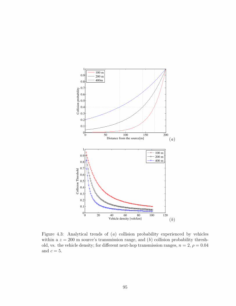
0 50 100 150 2000

0.1

0.2

0.3

0.4

0.5

0.6

0.7

0.8

0.9

1

Distance from the source[m]

Colli

sion

prob

abili

ty

100 m200 m400m

(a)

0 20 40 60 80 100 1200

0.1

0.2

0.3

0.4

0.5

0.6

0.7

0.8

0.9

1

Vehicle density [veh/km]

Colli

sion

Thre

shol

d

100 m200 m400 m

(b)

Figure 4.3: Analytical trends of (a) collision probability experienced by vehicleswithin a z = 200 m source’s transmission range, and (b) collision probability thresh-old, vs. the vehicle density; for di↵erent next-hop transmission ranges, n = 2, ⇢ = 0.04and c = 5.

95

10 20 30 40 50 600.7

0.75

0.8

0.85

0.9

0.95

1

Vehicle Density [veh/km]

Colli

sion

Prob

abili

ty

IFCAREFOR

Figure 4.4: Comparison between IF and CAREFOR, in terms of collision probability,as a percentage of the collisions part of the total number of messages in the system, vs.the vehicular density. Notice that the collision reduction is provided by CAREFOR.

10 20 30 40 50 600

0.02

0.04

0.06

0.08

0.1

0.12

0.14

0.16

Vehicular Density [veh/km]Thro

ughp

ut (%

of m

essa

ges a

t des

tinat

ion)

IFCAREFOR

Figure 4.5: Comparison between CAREFOR and IF in terms of throughput, as apercentage of messages arrived to a vehicle receiver and relative to the total numberof messages exchanged in the system, vs. the vehicular density. The high performancewith CAREFOR is due to the high reduction of broadcast messages.

96

10 20 30 40 50 600

0.02

0.04

0.06

0.08

0.1

0.12

0.14

Vehicular Density [veh/km]

Perc

enta

ge o

f Suc

cess

ful T

rans

miss

ions

IFCAREFOR

Figure 4.6: Comparison between CAREFOR and IF in terms of the percentage of suc-cessful transmissions vs.the vehicular density, w.r.t. the total number of transmissionsincluding the collided attempts.

20 25 30 35 40 45 500.8

0.82

0.84

0.86

0.88

0.9

0.92

0.94

Vehicular Density [veh/km]

Colli

sion

Prob

abili

ty

Three HopsTwo Hops

Figure 4.7: Collision Probability, as a percentage of the collisions part of the totalnumber of messages in the system, in both three and two hops CAREFOR algorithm.A small increase of performance is provided by three hop CAREFOR approach.

97

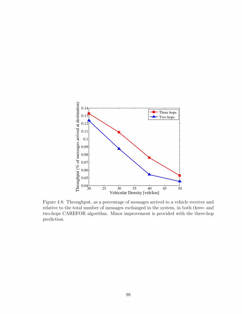
20 25 30 35 40 45 500.04

0.05

0.06

0.07

0.08

0.09

0.1

0.11

0.12

0.13

0.14

Vehicular Density [veh/km]Thro

ughp

ut (%

of m

essa

ges a

rrive

d at

des

tinat

ion)

Three hops Two hops

Figure 4.8: Throughput, as a percentage of messages arrived to a vehicle receiver andrelative to the total number of messages exchanged in the system, in both three- andtwo-hops CAREFOR algorithm. Minor improvement is provided with the three-hopprediction.

98

20 25 30 35 40 45 500.04

0.06

0.08

0.1

0.12

0.14

0.16

0.18

Vehicular Density [veh/km]

Perc

enta

ge o

f Suc

cess

ful T

rans

miss

ions

Three hopsTwo hops

Figure 4.9: Percentage of successful transmissions compared to the total number oftransmissions including the collided attempts, in both three- and two-hops CARE-FOR algorithm. Minor improvement is provided with the three-hop prediction.

99

Chapter 5

QASA: QoS-Aware Node Selection

Algorithm

In this chapter, we present a QoS-Aware node Selection Algorithm (QASA) for

routing protocols to be suitable for a particular class of opportunistic networks, i.e.,

the vehicular ad hoc networks. Our algorithm is focused on selecting the vehicle to

communicate with and is achieved by exploiting the bridging approach for message

forwarding (i.e., vehicles on the east (west) select from west (east)). The QoS metrics

that are being optimized are the throughput in the network, as well as end-to-end

delay for packets. In order to provide the best network performance, our algorithm

utilizes a probabilistic rebroadcasting scheme that is based on di↵erent network pa-

rameters including vehicle density, inter-vehicle distance, and the transmission range

for the vehicles. Moreover, QASA utilizes a transmission range based metric that

can be changed as per application requirements, whether it is high throughput or

minimum end-to-end delay. Simulation results show the e↵ectiveness of our approach

in terms of improved QoS metrics in di↵erent VANET scenarios.

100

5.1 Introduction

Opportunistic networking techniques allow mobile devices to exchange messages

by having knowledge of the mobility patterns and accordingly explore the use of store-

carry-and-forward approach. Following this technique, a message can be stored in a

node and then forwarded using available wireless link to other nodes, as soon as a con-

nection opportunity becomes feasible with a neighbouring device. Such occasionally

used next-hop forwards information towards a desired destination.

In opportunistic networks, the assumption of a complete path between a source

and a destination is relaxed, allowing mobile nodes to communicate with each other

even if a route connecting them may not currently exist or may break frequently.

Messages are cached in the network, and wait for an end-to-end path to be available.

Thus, additional delays in message delivery can occur. For this reason, opportunistic

networks belong to the class of Delay Tolerant Networks (DTN), since connectivity is

provided despite long link delays or frequent link breakage due to nodes moving out

of the range, or the environmental changes, or interference from other devices, etc.

Vehicular Ad hoc NETworks (VANETs) are a special kind of Mobile Ad hoc NET-

works (MANETs) in which packets are exchanged between mobile devices (vehicles)

travelling on constrained paths, in case of Vehicle-to-Vehicle (V2V) communications,

and between vehicles and road-side access points, i.e., Road-Side Units (RSUs), in

case of Vehicle-to-Infrastructure (V2I) communication.

Opportunistic forwarding is the main technique adopted in DTN [70], and has

also been extended in VANETs to achieve connectivity between vehicles via V2V so

as to disseminate tra�c information [39, 71, 72]. In particular, the authors in [72]

assume a bidirectional road, where vehicles’ clusters formed in one direction of the

highway come in intermittent contact with other clusters traveling in the opposite

101

direction. Such contacts can be opportunistically exploited as a bridging technique,

linking the partitioning that exists between clusters traveling in the same direction

of the roadway. As a result, the connectivity can be maintained along the road.

On the other hand, exploitation of RSUs together with inter-vehicle communica-

tions represents a viable solution to extend connectivity support in those scenarios

where vehicles are not able to directly communicate with each others. The use of

V2I communications can bridge the inherent network fragmentation that exists in

any multi-hop network in existing network infrastructure [73, 74]. As an analogy, a

vehicular grid together with an opportunistic infrastructure deployed on the roads,

can be a good solution to guarantee seamless connectivity in a dynamic vehicular

scenario [75, 76], as well as hybrid vehicular communication paradigm with inter-

mittent connectivity. In such an approach, connectivity can be provided by both

existing network infrastructure (i.e., RSUs) through a V2I protocol, and traditional

V2V networking [44, 45]. Such a combination is commonly referred to as V2X; the

cooperation and coexistence of V2V and V2I methods can ensure a good connectivity

for a VANET.

Based on the concept of bridging in a VANET, an open issue is the fact that

any vehicle traveling along one direction (e.g., east) can select any of the multiple

vehicles on the opposite side (e.g., west) of the roadway to carry the message. How

to choose a next-hop forwarder is a real challenge, as an optimum choice should

consider numerous factors such as the longest inter-vehicle distance, link connectivity

time, mobility pattern, and so on.

This research addresses the best way to select the next-hop forwarder node as-

suming the use of bridging approach not only when (i) there is no connectivity link

along one direction, but also when (ii) the network performance (i.e., link connec-

102

tivity time, and throughput) ought to be improved. Based on the Quality-of-Service

(QoS) requirement of a given application, we propose a routing protocol, which relies

on choosing an opportunistic node, named as QoS-Aware Node Selection Algorithm

(QASA).

This chapter is organized as follows. In Section 5.2, we provide a background on

existing routing protocols for vehicular networks which exploit opportunistic network-

ing. Then, in Section 5.3 we introduce our proposed QASA protocol, and describe the

main aspects through an analytical model, as well as the algorithm, respectively in

Subsections 5.3.1 and 5.3.2. The e↵ectiveness of QASA has been illustrated with sim-

ulation results, as covered in Section 5.4, specifically expressed in terms of throughput

and time delay. Finally, conclusions are drawn at the end of this chapter.

5.2 Related Work

For the past few years, routing protocols for vehicular networks have been a topic

of interest in the literature. These protocols are classified into di↵erent categories,

such as the probability-based routing protocol. Such a protocol rely on the algorithm

that allows selection of specific vehicles to communicate with amongst many vehicles

within the communication range of the source vehicle. As the main advantage, the

use of probability in selecting a routing protocol is based on avoiding the flooding

of the network with duplicates of the same packet. Clearly, this provides a signifi-

cant improvement in the performance of the network, since it reduces the number of

collisions, and hence improves the throughput, as well as reduces end-to-end delay.

Among various probabilistic routing protocols in the literature, we recall the ticket-

based techniques [62, 63], where the vehicle is selected based on stability, delay and

103

cost metrics. Authors in [64] presented REAR algorithm which considers reception

probability of the alarm messages and exploit physical parameters like received signal

strength measurements, the path loss and di↵raction loss factor, so that next-hop

vehicles can be selected. Another solution is the GVGrid algorithm [65] that is used

to find a reliable routing path satisfying specific delay requirement. The algorithm

determines the link lifetime based on the link reliability.

In [66], rebroadcast probability is a function of inter-vehicle distance, signal strength

and the statistical distribution of the vehicles [61, 77]. In [61], the authors introduce

Irresponsible Forwarding (IF) algorithm, so that each vehicle will refrain from broad-

casting whenever likelihood of other qualified vehicles is present to rebroadcast a

packet. Whether a vehicle is better qualified in IF is decided based on whether the

packet will travel for a longer distance in one hop or not. The main disadvantage for

IF stems from being a probabilistic approach, which results in more than one vehicle

rebroadcasting the packet.

In [77], the CAREFOR technique considers the vehicle selection based on the

probability that at least two vehicles will be qualified as the next-hop forwarders.

Basically, CAREFOR considers not only the rebroadcast probability for one hop, but

extends this probability up to two next-hops. This approach represents a two-hops

prediction in selecting a qualified vehicle as an e↵ective next-hop forwarder.

All these techniques are driven by reducing the replica of a packet within the ve-

hicular network. However, many applications have di↵erent QoS requirements, which

routing protocol should also maximize [78]. For example, throughput optimization

has been considered in the literature, specially when addressing the issue of content

distribution. In [79], authors developed CodeTorrent protocol that employs a net-

work coding based file swarming protocol. They also investigated the e↵ect of the

104

vehicular density and mobility on the performance of network coding. Authors in [80]

developed a similar collaborative content distribution approach, which used a multi-

hop randomized network coding in a decentralized approach. At the same time, low

end-to-end delay should be achieved for safety point of view (e.g. quick braking) [78].

In this research, we consider a QoS-oriented and probability-based routing proto-

col for vehicular network that maximizes the throughout while considering end-to-end

delay. The routing protocol is developed by selecting a vehicle from opposite side of

the highway. In other words, for vehicle on east side selects a vehicle on the west side

to communicate with and vice-versa. We investigate the e↵ectiveness of our algorithm

in two di↵erent vehicular scenarios (i.e., urban and highway).

5.3 QoS-Aware Node Selection Algorithm

In this section, we introduce the QoS-Aware Node Selection (QASA) algorithm,

and discuss the major aspects behind its usefulness. The reference scenario is a

vehicular network comprised of two lanes (i.e., lane E and W), where vehicles are

being driven in opposite directions, as depicted in Figure 5.1. Let us assume vehicles

on lane E (W) being driven to the east (west) direction. We consider the vehicular

network to have a highly dynamic topology due to di↵erent mobility patterns that

form vehicles’ clusters. As an instance, vehicles traveling on the roadway, along the

east and west directions, are characterized by frequent link breakages that strongly

hinder stable and durable V2V communications. In particular, a cluster formed in

one direction of the highway comes in intermittent contact with clusters of vehicles

travelling in the opposite direction. Such contacts can be opportunistically exploited

as a bridge, linking the partitions that exist between clusters travelling in the same

105

Figure 5.1: Schematic of a vehicular opportunistic network, with bridging approach.A source (blue) vehicle shall select a next-hop forwarder from the opposite lane, sincethe forward inter-vehicular gap is too large for allowing V2V communications (i.e.,

r(Tx)i

> �ij

). The blue and black boxes represent the source’s transmission range andthe cluster size, respectively.

direction of the roadway. This reflects typical bridging connectivity in a VANET.

In such a scenario, let us consider a source vehicle being driven on the E lane. V2V

communications along the E lane cannot occur since the inter-vehicular gap among

the i-th source vehicle and its j-th neighbours (i.e., �ij

[m]) is so large that the source

connectivity range (i.e., r(Tx)i

[m]) results in a very short time as compared to this

(i.e., r(Tx)i

> �ij

). Thus, the main aspect of QASA algorithm is to allow a source

vehicle on east side to be able to select the best candidate to be a receiver from the

opposite lane (i.e., the west side).

106

(a)

(b)

Figure 5.2: QASA technique main aspects. (a) Dividing the transmission range of asource vehicle (i.e., the white vehicle) into smaller circular transmission domains (i.e.,with C1 > C2 > C3) for next-hop selection. (b) The scenario explains the trade-o↵between time delay and throughput performance with QASA technique.

Consider Figure 5.2, when the vehicle on the east (i.e., vehicle v2) is getting ready

to transmit a message to the west side of the highway, it will have two candidate

107

vehicles as receivers on the west side within its transmission range (i.e., vehicle v1,

and v3). The best candidate would be able to o↵er the best QoS metrics in a VANET,

specifically (i) the best throughput, and (ii) the least packet transmission delay. If

vehicle v2 selects vehicle v1, the established connection will only last for a short time

due to v1 moving out of vehicle v2’s transmission range.

However, if vehicle v2 ends up selecting vehicle v3 instead, this will allow for the

connection to remain established for a longer period of time due to vehicle v3 being in

v1’s transmission range for a longer period. The shorter the time the connection lasts

a larger number of connections can be established within the same time duration.

The disadvantage of establishing a new connection lies in the overhead for Clear To

Broadcast (CTB)/ Ready To Broadcast (RTB) signals and backo↵ algorithm.

5.3.1 Analytical Model

In order to analyze selecting the best candidate vehicle, we divide the transmis-

sion range of the source vehicles into smaller circular domains 1. As demonstrated

in Figure 5.2, the domains correspond to actual transmission range (i.e., the full

transmission range, half the transmission range, and one quarter of the transmission

range). These domains are the di↵erent ranges from which the source (east) vehicle

can select a destination (west) vehicle. We investigate the performance of the VANET

with regards to the di↵erent ranges for the vehicle selection.

Let us assume that R1 is the radius for the circle C1; R2 for C2; and R3 for C3.

We develop an analytical model for the probability of the existence of a vehicle in

each circular domain. Vehicles are distributed on the highway following a Poisson

distribution model which is a common practice in the VANET literature [81].

1We assume each vehicle is equipped with an omnidirectional antenna.

108

The probability that a vehicle can be selected as a receiver depends on two events,

i.e., (i) the vehicle is within the transmission range, and (ii) the vehicle is expected

to have a large enough connectivity interval to guarantee enough time for packet

transmission and relay. Both conditions should be satisfied in order to select a vehicle

as the best packet forwarder. We express the probability that a vehicle will be a

receiver (i.e., prx

) as follows:

prx

= Pr [d⇤ Ri

] [ Pr [�T (Ri

) > ⌧ ] , (5.1)

where d⇤ [m] is the inter-vehicular distance from a potential receiver to a source,

�T (Ri

) [s] is the expected time interval the vehicle is within the coverage area Ri

,

and ⌧ [s] is a given threshold to guarantee a larger connectivity time interval. Notice

that �T (Ri

) depends on the radius Ri

in a given coverage area, since this can be

increased from the maximum distance between the source and the receiver within its

transmission range.

Let us consider Figure 5.2. The probability that a vehicle is laying at distance

d = d⇤ from a source vehicle follows the following equation:

Pr [d = d⇤] =�d

⇤ · exp (��)

d⇤!, (5.2)

where � [veh/km] is the tra�c density distribution on the highway, following a Poisson

distribution.

From (5.1), the probability that a vehicle, placed at distance d⇤ from a source

node, is inside the i-th coverage area Ci

with radius Ri

, for i = {1, 2, 3}, becomes:

Pr [d⇤ Ri

] =� (bd⇤ + 1c ,�)

bd⇤c! , (5.3)

109

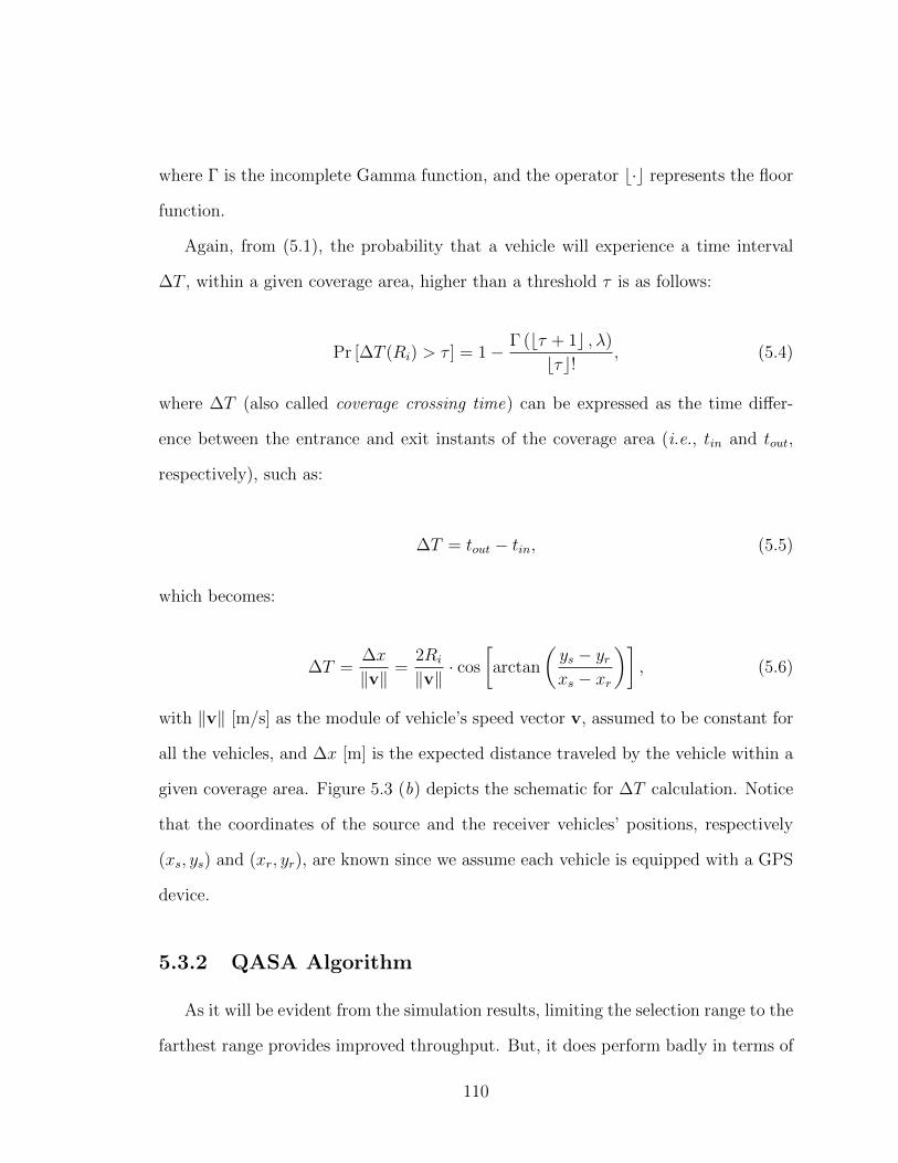
where � is the incomplete Gamma function, and the operator b·c represents the floor

function.

Again, from (5.1), the probability that a vehicle will experience a time interval

�T , within a given coverage area, higher than a threshold ⌧ is as follows:

Pr [�T (Ri

) > ⌧ ] = 1� � (b⌧ + 1c ,�)b⌧c! , (5.4)

where �T (also called coverage crossing time) can be expressed as the time di↵er-

ence between the entrance and exit instants of the coverage area (i.e., tin

and tout

,

respectively), such as:

�T = tout

� tin

, (5.5)

which becomes:

�T =�x

kvk =2R

i

kvk · cosarctan

✓ys

� yr

xs

� xr

◆�, (5.6)

with kvk [m/s] as the module of vehicle’s speed vector v, assumed to be constant for

all the vehicles, and �x [m] is the expected distance traveled by the vehicle within a

given coverage area. Figure 5.3 (b) depicts the schematic for �T calculation. Notice

that the coordinates of the source and the receiver vehicles’ positions, respectively

(xs

, ys

) and (xr

, yr

), are known since we assume each vehicle is equipped with a GPS

device.

5.3.2 QASA Algorithm

As it will be evident from the simulation results, limiting the selection range to the

farthest range provides improved throughput. But, it does perform badly in terms of

110

average time delay. However, QASA assumes that the closer the vehicle is, the worse

will be the expected throughput, while it provides reduced time delay.

Consider the scenario in Figure 5.2 (b), if vehicle v2 on the east selects the fur-

thest available vehicle in its transmission range on the west, QASA algorithm will

select vehicle v1. As will be observed from simulation results, this leads to a smaller

average time delay, but will result in a lower throughput. If vehicle v2 waits for a

short anticipated time 2, it will be able to select vehicle v3, which could result in a

higher throughput, but in a slightly increased time delay. The choice between vehi-

cles v1 and v3 can be decided by restricting the region from where the east vehicle

selects a west vehicle. This restriction should be defined solely based on the type of

application. Some vehicular network applications require minimum delay regardless

of the throughput, while other applications require maximum throughput but are

delay tolerant.

In order to overcome this trade-o↵, the algorithm needs to allow the vehicle to

select the furthest possible vehicle available in a specific area within the transmission

range. In the following subsection, we describe the QASA algorithm, which relies on

the CAREFOR protocol [77].

The QASA is a probabilistic forwarding routing protocol that ensures selection

of the farthest available vehicle in the transmission range that could forward the

packet (i.e., the next-hop forwarder). This algorithm attempts to improve the QoS

of routing protocols in a VANET by selecting the best candidates among the vehicles

on the opposite direction (i.e., on the lane west) to act as bridges for communication

between vehicles on the other side (i.e., the lane east). The QoS metrics of concern

behind QASA are both (i) the throughput of the network, as well as (ii) the average

2It is evident that vehicle v3 will enter the coverage area C1, in a short time.

111

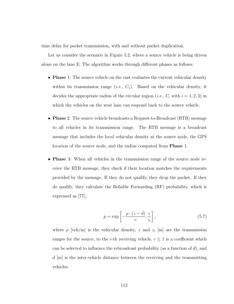
time delay for packet transmission, with and without packet duplication.

Let us consider the scenario in Figure 5.2, where a source vehicle is being driven

alone on the lane E. The algorithm works through di↵erent phases as follows:

• Phase 1: The source vehicle on the east evaluates the current vehicular density

within its transmission range (i.e., C1). Based on the vehicular density, it

decides the appropriate radius of the circular region (i.e., Ci

with i = 1, 2, 3) in

which the vehicles on the west lane can respond back to the source vehicle.

• Phase 2: The source vehicle broadcasts a Request-to-Broadcast (RTB) message

to all vehicles in its transmission range. The RTB message is a broadcast

message that includes the local vehicular density at the source node, the GPS

location of the source node, and the radius computed from Phase 1.

• Phase 3: When all vehicles in the transmission range of the source node re-

ceive the RTB message, they check if their location matches the requirements

provided by the message. If they do not qualify, they drop the packet. If they

do qualify, they calculate the Reliable Forwarding (RF) probability, which is

expressed as [77],:

p = exp

�⇢ · (z � d)

c.z

zi

�, (5.7)

where ⇢ [veh/m] is the vehicular density, z and zi

[m] are the transmission

ranges for the source, to the i-th receiving vehicle, c 1 is a coe�cient which

can be selected to influence the rebroadcast probability (as a function of d), and

d [m] is the inter-vehicle distance between the receiving and the transmitting

vehicles.

112

Table 5.1: QASA message exchanged classification and content.

Message Content

RTB 1) Source node’s position

2) Vehicular density

3) FRP

4) Transmission power level

CTB 1) Vehicle’s ID and position

The decision of packet retransmission is taken by each vehicle by comparing the

RF probability to a transmission threshold (i.e., Thcoll

). That means:

Thcoll

= 1� [exp (�⇢zi

)] , (5.8)

where zi

[m] is the transmission range of the i-th vehicle, and ⇢ [veh/m] is the

vehicular density. If calculated RF value is larger than the threshold, then the

vehicle broadcasts a CTB message. Otherwise, the vehicle refrains from any

rebroadcasting. The CTB message includes the GPS location of the vehicle.

• Phase 4: Once the source vehicle receives the CTB messages, it determines

which vehicle amongst those who responded is the furthest. Once that is de-

cided, the source vehicle transmits the packet with a destination address to the

vehicle selected from the west lanes. All vehicles which receive the packet, but

do not have their vehicle ID as the destination, simply drop the packet.

An explanation of each control message used in the algorithm is presented in

Table 5.1.

Di↵erent applications in vehicular networks can have varying QoS requirements.

Some applications require minimum delay regardless of the throughput, while others

113

require the opposite, and some applications may need a balance between throughput

and average time delay. In order for the algorithm to be functional for di↵erent

applications, we introduce a Full Range Portion (FRP) parameter that restricts the

performance of the network as per the QoS requirements.

The FRP parameter is a value larger than 0 but smaller or equal to 1, and rep-

resents the fraction of a full transmission range, from which a vehicle on the west

side can be selected by a vehicle from the east side. For example, in Figure 5.2,

C3 is selected using a FRP factor equal to 0.25; C2 using FRP equal to 0.5; while

FRP is equal to 1 for C1. The FRP factor is equal to 1 when the requirement is to

provide the minimum average delay regardless of the throughput. The smaller the

FRP variable is, better will be throughput the network experience, and the higher

will be the average time delay. However, if the FRP parameter becomes too small,

the region from which the west vehicle can be selected will be very restricted, and

may cause failure in establishing any connection. Hence, FRP parameter depends

mainly on the transmission range and the vehicle density in the network.

5.4 Simulation Results

In this section, we present simulation results for the QASA algorithm as well

as results to illustrate improvements in QoS. The metrics used in this simulation

are the throughput, total e↵ective communication time, and the average time delay.

The total e↵ective communication time is measured after excluding any time used

in setting up the connection or selecting the vehicles for communication. We use

our own VANET simulator [77, 82]. Di↵erent parameters used in our simulation are

presented in Table 6.1.

114

Table 5.2: Simulation Parameters.

Simulation Parameter Value

Simulation Runs 50

Simulation Duration 6000 s

Transmission Range 400 m

Vehicle Density [1, 65] veh/km

Vehicle Speed 20 m/s

Highway Length 3 km

Control Packet Size 2 KB

Message Size 32 KB

Message Generation Rate 20 packets/s

Bandwidth 10 MB/s

Figure 5.4 demonstrates the impact of the bridging approach on the vehicular

network performance. When vehicles on either side of the highway are allowed to

connect with vehicles on the opposite side of the highway, the overall network con-

nectivity is enhanced. For sake of readiness, we identify the bridging approach as a

“Vehicle-to-Bridge” (V2B), since a vehicle forms a bridge each time it communicates

with another vehicle driving in the opposite direction.

We present results by varying the number of disconnected clusters at di↵erent

vehicle densities with and without bridging (i.e., V2B used, and not used, respec-

tively). As expected, allowing bridging reduces the number of disconnected clusters

which enhances the connectivity between vehicles on the network, allows for enhanced

throughput, and reduces the average time delay experienced in the network.

In Figure 5.5, we present the total time communicated during the simulation runs,

which proves the e↵ectiveness of the concept of limiting the region within the trans-

mission area of the east vehicle from which a vehicle on the west can communicate.

115

The case where any vehicle on the west within the source vehicle’s transmission region

can communicate with the east vehicle is demonstrated for full range of variations,

and the diameter of the region are changed to 0.75, 0.5, and 0.25 respectively. We

observe that dynamically varying the transmission ranges in di↵erent regions can pro-

vide an enhancement of connectivity within the network. Note that all these regions

are located at the end of the transmission range. For example, in Figure 5.2, C3

represents the 0.25 of full range C1. Morevoer, in Figure 5.6, we show the throughput

analysis for the same region. Again, high performance are obtained with a reduction

of transmission range (e.g., for 0.5 and 0.25 of full range we reach maximum values

of throughput).

Figure 5.7 represents simulation results for throughput at a lower vehicular density

for di↵erent ranges (i.e., full transmission range, half transmission range, and one

quarter of the transmission range). Consider the scenario presented in Figure 5.2. If

the system uses a smaller range (i.e., C3 range) from which the west bridge vehicle

can be selected, and as there is no vehicle in this range, no vehicle will be selected.

Therefore, no connection will be established between the source vehicle and any other

vehicle from the west lane of the highway.

However, with the assumption of a continuously moving highway scenario, even

at lower vehicle densities, each vehicle on the east will get the chance to communicate

with each vehicle on the west regardless of the communication range restriction.

This is because QASA detects and selects a potential forwarder, based on both the

transmission range, as well as the longest inter-vehicles distance (i.e., the furthest

vehicle in a coverage area). In the light of such considerations, it can be easily

understood why at lower vehicular densities, the throughput is the same for di↵erent

values of the circular range.

116

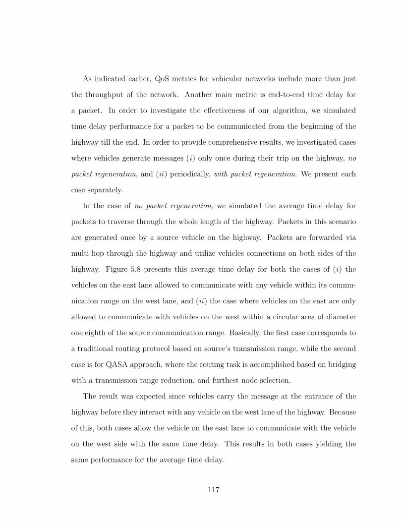
As indicated earlier, QoS metrics for vehicular networks include more than just

the throughput of the network. Another main metric is end-to-end time delay for

a packet. In order to investigate the e↵ectiveness of our algorithm, we simulated

time delay performance for a packet to be communicated from the beginning of the

highway till the end. In order to provide comprehensive results, we investigated cases

where vehicles generate messages (i) only once during their trip on the highway, no

packet regeneration, and (ii) periodically, with packet regeneration. We present each

case separately.

In the case of no packet regeneration, we simulated the average time delay for

packets to traverse through the whole length of the highway. Packets in this scenario

are generated once by a source vehicle on the highway. Packets are forwarded via

multi-hop through the highway and utilize vehicles connections on both sides of the

highway. Figure 5.8 presents this average time delay for both the cases of (i) the

vehicles on the east lane allowed to communicate with any vehicle within its commu-

nication range on the west lane, and (ii) the case where vehicles on the east are only

allowed to communicate with vehicles on the west within a circular area of diameter

one eighth of the source communication range. Basically, the first case corresponds to

a traditional routing protocol based on source’s transmission range, while the second

case is for QASA approach, where the routing task is accomplished based on bridging

with a transmission range reduction, and furthest node selection.

The result was expected since vehicles carry the message at the entrance of the

highway before they interact with any vehicle on the west lane of the highway. Because

of this, both cases allow the vehicle on the east lane to communicate with the vehicle

on the west side with the same time delay. This results in both cases yielding the

same performance for the average time delay.

117

As presented for the case with no packet regeneration, the average time delay

for QASA algorithm, as well as for the traditional forwarding case yields the same

result. However, this does not hold when vehicles generate message repeatedly during

their trip through the highway (i.e., periodically packet regeneration). With such an

assumption, the average time delay for both the case of the vehicles on the east lane

(i) are allowed to communicate with any vehicle within its communication range on

the west lane—i.e., R—, and (ii) are only allowed to communicate with vehicles

on the west within a reduced circular area of diameter three fourth of the source

communication range—i.e., 3/4R—, are presented in Figure 5.9.

To explain the result for the case vehicles regenerating packets, we consider the

scenario in Figure 5.2 (b) representing the instance at which the source (v2) vehicle

has just generated a new packet. At this instance, the vehicle will not be able to

communicate with vehicle v1, if its communication range is restricted to half of the

transmission range, and will also not be able to communicate with the vehicle v3,

since it is not in its transmission range yet. This will result in vehicle v2 to wait till

vehicle v3 enters its transmission range C2, which causes the average time delay to

increase in case of restricting the communication range at a low vehicle density.

As presented earlier, the use of FRP factor a↵ects the QoS requirements for dif-

ferent applications of the VANET. Figure 5.10 and Figure 5.11 present the e↵ect of

the FRP factor on the total communication time in the network at di↵erent vehicle

density. As expected, smaller the value of FRP, and higher the vehicular density,

larger will be the communication time. Figure 5.12 presents the same results for the

throughput in the network.

118

5.5 Summary

In this chapter, we have introduced QASA algorithm which is primarily a for-

warding node selection algorithm for routing protocols in an opportunistic vehicular

network. QASA allows vehicles on one side of the highway to successfully select a

vehicle from the opposite side that improves the QoS metrics for the network. The

QoS metrics used to analyze the algorithm are total communication time, throughput,

and packet end-to-end time delay.

We tested our system by extensive simulation and verified the importance and use-

fulness of bridging in vehicular networks. Furthermore, we compared the performance

of QASA with normal scenarios. The results have shown significant improvement by

QASA in terms of throughput, and end-to-end packet delay. Finally, we presented an

FRP parameter that will help provide better performance based on the QoS require-

ments for the VANET application.

119

(a)

x

s, y

s( )

x

r, y

r( )

!T tin

tout

R

i

C

i

(b)

Figure 5.3: Scheme for next-hop forwarder selection algorithm based on the coveragecrossing time calculation, �T [s]. Assuming each vehicle has an omnidirectionalcoverage, with radiusR [m], (a) the red vehicle will experience longest time connectionwith the blue vehicle, respect to the green one, which is exiting the coverage area. (b)The coverage crossing time is calculated as a time interval (i.e., from t

in

to tout

[s]).

120

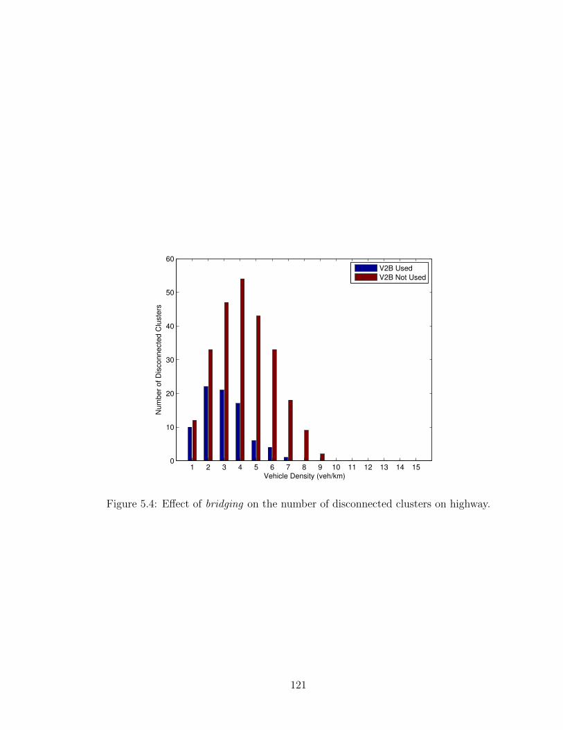
1 2 3 4 5 6 7 8 9 10 11 12 13 14 150

10

20

30

40

50

60

Vehicle Density (veh/km)

Num

ber

of D

isco

nnect

ed C

lust

ers

V2B UsedV2B Not Used

Figure 5.4: E↵ect of bridging on the number of disconnected clusters on highway.

121

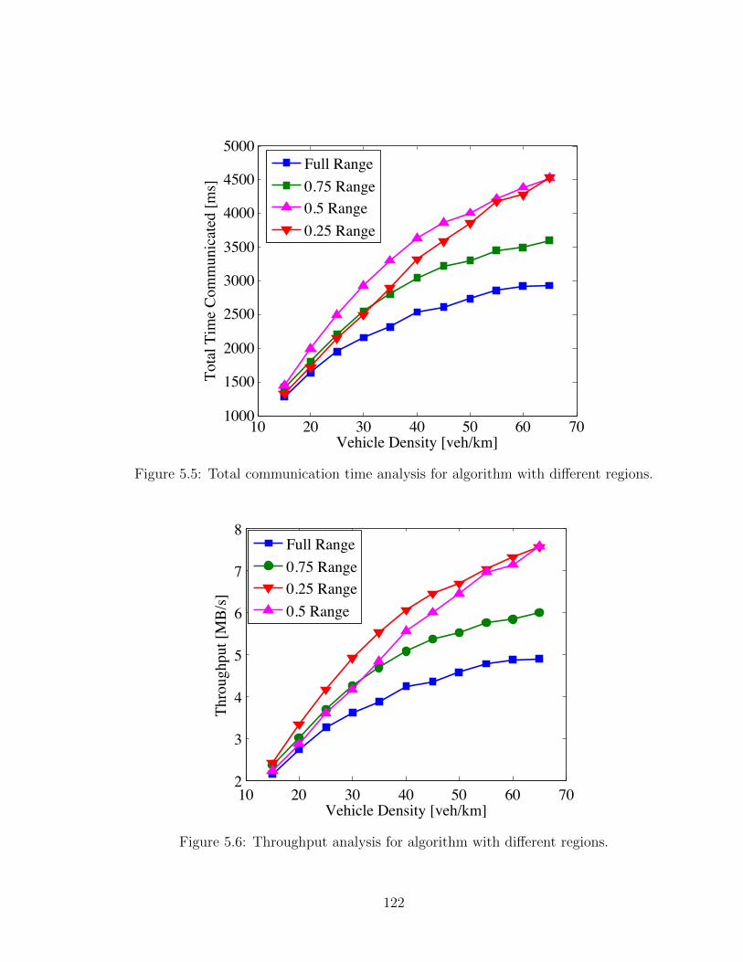
10 20 30 40 50 60 701000

1500

2000

2500

3000

3500

4000

4500

5000

Vehicle Density [veh/km]

Tota

l Tim

e Co

mm

unic

ated

[ms]

Full Range0.75 Range0.5 Range0.25 Range

Figure 5.5: Total communication time analysis for algorithm with di↵erent regions.

10 20 30 40 50 60 702

3

4

5

6

7

8

Vehicle Density [veh/km]

Thro

ughp

ut [M

B/s]

Full Range0.75 Range0.25 Range0.5 Range

Figure 5.6: Throughput analysis for algorithm with di↵erent regions.

122

2 3 4 5 60

200

400

600

800

1000

Vehicle Density [veh/km]

Tota

l tim

e co

mm

unic

ated

[ms]

Full Range0.75 Range0.5 Range

Figure 5.7: Throughput for di↵erent ranges at lower tra�c densities.

0 5 10 15 20 250

50

100

150

Vehicle Density [veh/km]

Ave

rage

Tim

e D

elay

[s]

Full Range0.75 Range0.5 Range0.25 Range

Figure 5.8: Average time delay vs. the vehicular density for di↵erent ranges.

123

0 5 10 15 20 250

5

10

15

20

25

Vehicle Density [veh/km]

Ave

rage

Tim

e D

elay

[s]

Full Range0.75 Range0.5 Range0.25 Range

Figure 5.9: Average time delay vs. the vehicular density for di↵erent ranges with apacket regeneration every 20 seconds.

020

4060

80100

00.2

0.40.6

0.810

2000

4000

6000

Vehicle Density [veh/km]Full Range Portion

Tota

l tim

e co

mm

unic

ated

[ms]

Figure 5.10: E↵ect of FRP variable on total time communicated.

124

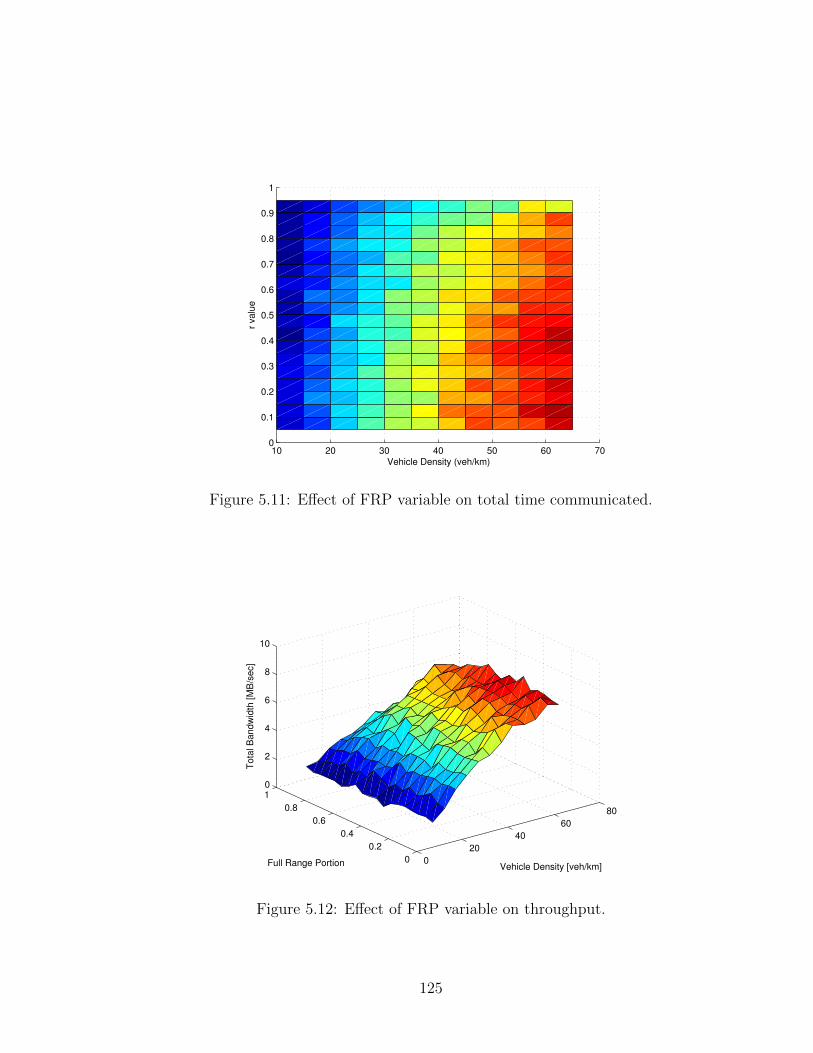
10 20 30 40 50 60 700

0.1

0.2

0.3

0.4

0.5

0.6

0.7

0.8

0.9

1

Vehicle Density (veh/km)

r va

lue

Figure 5.11: E↵ect of FRP variable on total time communicated.

0

20

40

60

80

0

0.2

0.4

0.6

0.8

10

2

4

6

8

10

Vehicle Density [veh/km]Full Range Portion

Tota

l Bandw

idth

[M

B/s

ec]

Figure 5.12: E↵ect of FRP variable on throughput.

125

Chapter 6

QoS-Aware Routing for

Autonomous Vehicles

In this chapter, we present a QoS-Aware routing protocol for autonomous (which

are driverless or sefl-driving vehicles capable of doing what a human being does) ve-

hicles on a highway. The ability to control the motion and location of autonomous

vehicles provide endless possibilities for the improvement of the performance of ve-

hicular networks. In this chapter, we focus on the end-to-end packet delivery delay

in vehicle-to-vehicle communication, and minimizing this delay by reorganizing and

controlling autonomous vehicles on highways. The scheme introduced is a dynamic

protocol that depends mainly on the vehicle density on the highway, and controls the

inter-vehicle distance. We investigate the performance of this protocol compared to

normal VANET scenario. The side e↵ects of this protocol are investigated mainly in

terms of the e↵ect on the vehicles trip travel time. A metric is introduced that is

scenario dependent to control the trade-o↵ between end-to-end delay, and the total

vehicle travel time on the highway.

126

6.1 Introduction

Over the last decade, great progress in computational power in terms of hardware

and software, as well as sensing capabilities have been achieved. These advancements

have facilitated the introduction of autonomous vehicles. With the help of the com-

putational power, vehicles are able to operate autonomously with a high degree of

reliability in environments that exhibit high degrees of dynamicity as well as un-

certainty. With deploying redundant sensitive sensors on the vehicle, it is able to

understand with great reliability the environment around it. This allows the vehicle

to respond accurately and in a timely fashion to environmental changes, such as the

existence of another vehicle, or as basic as changes in the road conditions.

The concept of autonomous vehicles is no longer just a research subject. It is

expected that in the next few years, autonomous vehicles may be introduced to be

used widely in normal highways and cities. Many car manufacturers have already

embarked on developing autonomous vehicles. BMW has started testing autonomous

vehicles since the year 2005 [83]. In 2011, General Motors (GM) created the Electric

Networked Vehicle (EN-V) in hope to have their autonomous vehicle in the market

by the year 2018 [84]. In 2011, Audi was able to send an autonomous vehicle TTS

to achieve close to race speeds at Pikes peak [85]. Many other manufacturers have

been working on their own autonomous vehicle as well [86]. Moreover, several states

have started to allow autonomous vehicles to be used on their roads. Nevada was the

first state to grant Google a license to test their driverless vehicles on the roads [87].

On October 29, 2012, California was the second state to grant Google the same

license [88]. More vehicle manufacturers are being granted similar license to test

their vehicles [89]. It is anticipated that by the year 2040, vehicle operators may not

be required to obtain a drivers license as the vehicles will be driven autonomously [90].

127

Many benefits are expected from a wider use of autonomous vehicles [86]. Those

benefits can be summarized as:

• Fewer tra�c collisions due to increased reliability of the vehicles in sensing and

reacting to the environmental tra�c changes [91].

• Reduced tra�c congestion due to absence of tra�c collisions, and required safety

gaps [91], as well as the development of algorithms that selects the best possible

path to the destination.

• Vehicles passengers no longer are required to drive and navigate the vehicle,

and hence can perform other chores while inside the vehicle.

• Higher speed limits can be granted to autonomous vehicles [92].

• Lack of restrictions on the passengers such as age, vision, impaired or intoxica-

tion.

• Improved fuel e�ciency [93].

With these benefits and advancements, vehicle operators will no longer be involved

in the manipulation or in the control of the vehicle speed, location, or direction.

Vehicle operators will only notify the vehicle of the destination they are heading to

and the vehicle will determine the path, speed, and direction to be used in order to

reach to the destination. Enabling the vehicle to autonomously select these variables

opens endless possibilities for potential innovation of new algorithms that will provide

the best possible experience for the vehicle passengers within limits of the surrounding

environment.

This chapter introduces the concept of utilizing autonomous vehicles in order to

improve end-to-end message delay which is achieved through intelligently adjusting

128

the inter-vehicle distance by controlling their speed and hence location. This chapter

is organized as follows: first, related work regarding routing protocols to manipulate

autonomous vehicles is introduced in Section 6.2. The e↵ect of inter-vehicle distance

on end-to-end packet delivery delay is introduced in Section 6.3. Section 6.4 intro-

duces our algorithm and approach. Finally, Section 6.5 introduces our simulation

results followed by the chapter summary.

6.2 Related Work

For many years, the problem of planning a path or a trajectory in a dynamic

environment or that is cluttered by obstacles has been the object of many researches in

the area of robotics and artificial intelligence [94]. Building on these research finding,

di↵erent algorithms have tailored them to be applicable to autonomous vehicles in

a VANET environment. The scope of those di↵erent algorithms have varied from

collision avoidance, to path selection, to fuel economy optimization.

Authors in [95] have introduced a collision avoidance system for autonomous ve-

hicles using cooperative motion control. The system introduced is composed of two

systems: collision prediction and avoidance. Collision prediction is achieved through

estimating the trajectory of objects, while collision avoidance is achieved through

controlling the speed of the vehicle or through modifying the path of the vehicle.

In [96], authors developed fuel-economy optimization system (FEOS), which gathers

input data from the vehicle as well as the environment, and mathematically computes

the optimum speed for the vehicle.

Many research publications focused specifically on path planning, or real-time

motion planning. Authors in [97], proposed an autonomous real-time driving motion

129

planner with trajectory optimization. The optimization is based on a set of cost func-

tions. Moreover, their framework reduces the planning time by 52 percent. In [98],

authors presented a method for vehicle guidance that is based on path relaxation to

compute critical points using a-priori information and sensor data along a desirable

path. The scope of this method is to provide a collision free path for the vehicle along

the desirable route.

To our knowledge, none of the presented algorithms in literature regarding the

control or manipulation of autonomous vehicles has had the goal of optimizing the

end-to-end route delay. This delay has been the focus of other research in the litera-

ture that considered regular vehicles, rather than autonomous vehicles.

In [62], Yan et al. presented a ticket-based technique as a routing protocol.

These tickets are control packets transmitted on selected links which indicate the

metrics of stability, delay and cost. Ticket-based systems were initially introduced

in MANETs [63] with the objective of identifying a reliable route based on multiple

links that are selectively probed.

Sun et al. [65] proposed the GVGrid algorithm to find a reliable routing path that

meets a given delay requirement. By assuming an equally spaced inter-vehicle gap,

and a normally distributed vehicle speed, GVGrid computes the probability of link

lifetime as the function of link reliability. The proposed technique can select a path

with the highest reliability, and relatively smaller link delay as the selected route.

Common to all previous techniques, physical parameters play an important role

for the rebroadcast probability and the link selection. In [66], the authors present a

rebroadcast probability that is based on the inter-vehicle distance. This probability

is directly proportional to the distance from the transmitter. The larger the distance

is, higher will be the rebroadcast probability.

130

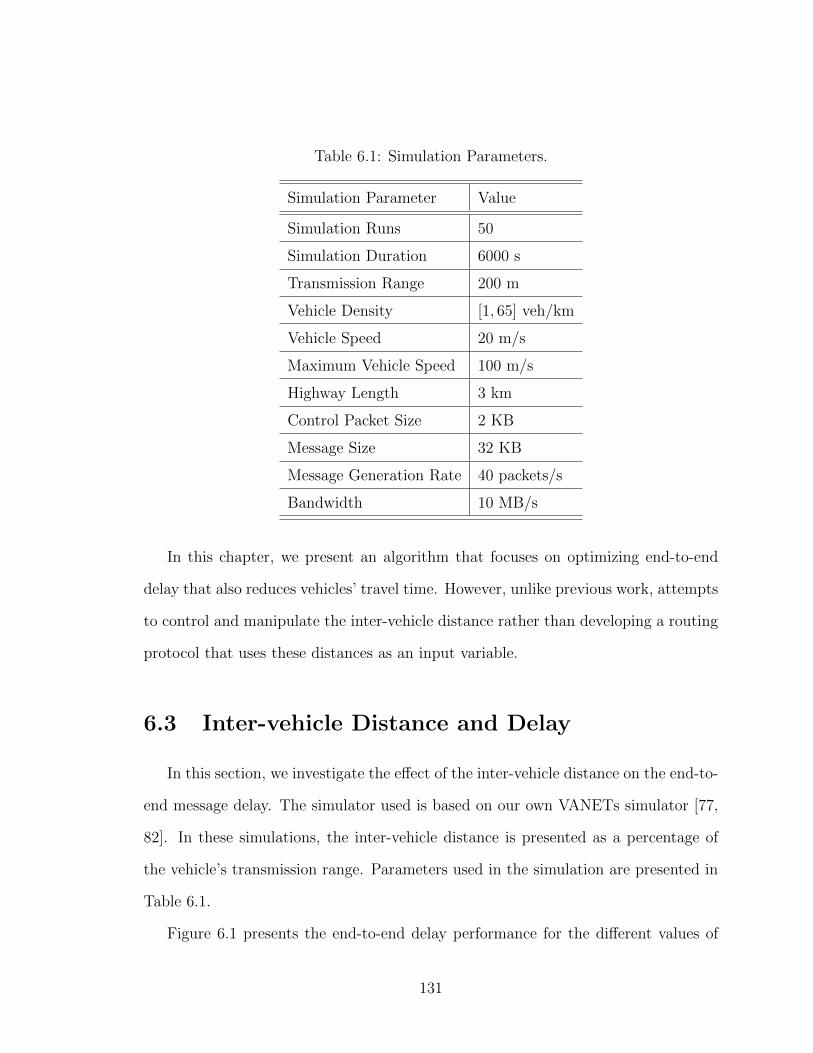
Table 6.1: Simulation Parameters.

Simulation Parameter Value

Simulation Runs 50

Simulation Duration 6000 s

Transmission Range 200 m

Vehicle Density [1, 65] veh/km

Vehicle Speed 20 m/s

Maximum Vehicle Speed 100 m/s

Highway Length 3 km

Control Packet Size 2 KB

Message Size 32 KB

Message Generation Rate 40 packets/s

Bandwidth 10 MB/s

In this chapter, we present an algorithm that focuses on optimizing end-to-end

delay that also reduces vehicles’ travel time. However, unlike previous work, attempts

to control and manipulate the inter-vehicle distance rather than developing a routing

protocol that uses these distances as an input variable.

6.3 Inter-vehicle Distance and Delay

In this section, we investigate the e↵ect of the inter-vehicle distance on the end-to-

end message delay. The simulator used is based on our own VANETs simulator [77,

82]. In these simulations, the inter-vehicle distance is presented as a percentage of

the vehicle’s transmission range. Parameters used in the simulation are presented in

Table 6.1.

Figure 6.1 presents the end-to-end delay performance for the di↵erent values of

131

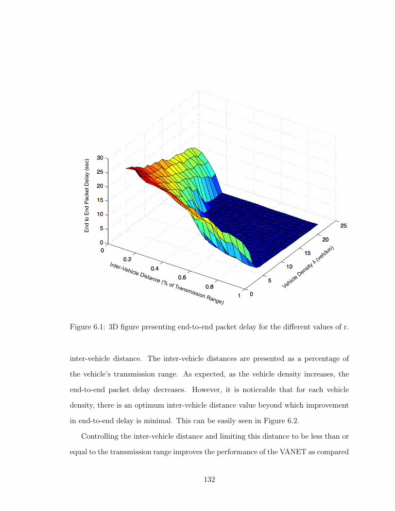
Figure 6.1: 3D figure presenting end-to-end packet delay for the di↵erent values of r.

inter-vehicle distance. The inter-vehicle distances are presented as a percentage of

the vehicle’s transmission range. As expected, as the vehicle density increases, the

end-to-end packet delay decreases. However, it is noticeable that for each vehicle

density, there is an optimum inter-vehicle distance value beyond which improvement

in end-to-end delay is minimal. This can be easily seen in Figure 6.2.

Controlling the inter-vehicle distance and limiting this distance to be less than or

equal to the transmission range improves the performance of the VANET as compared

132

Figure 6.2: 2D figure presenting end-to-end packet delay for the di↵erent values of r.

to not controlling this distance. In Figure 6.3, we present this improvement. As

presented in this figure, controlling the inter-vehicle distance always yields a smaller

end-to-end delay than the case of not controlling it, except the case of high vehicle

densities with the inter-vehicle distance being equal to 0.25 or lower. This explains

that in the case of controlling the vehicle to very small inter-vehicle distance with

a high vehicle density, yields the creation of di↵erent disconnected clusters on the

highway that takes time to interconnect them together. This introduces an added

delay than a regular scenario.

133

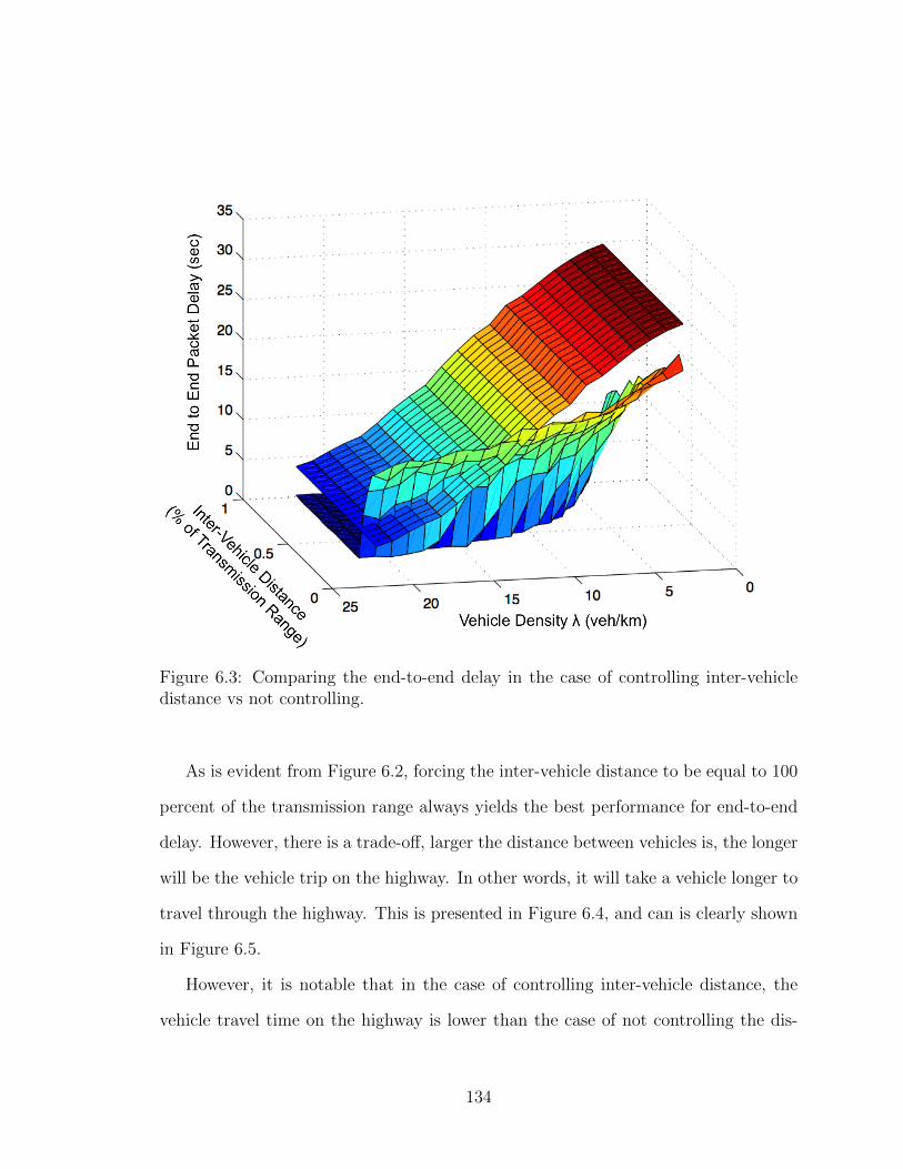
Figure 6.3: Comparing the end-to-end delay in the case of controlling inter-vehicledistance vs not controlling.

As is evident from Figure 6.2, forcing the inter-vehicle distance to be equal to 100

percent of the transmission range always yields the best performance for end-to-end

delay. However, there is a trade-o↵, larger the distance between vehicles is, the longer

will be the vehicle trip on the highway. In other words, it will take a vehicle longer to

travel through the highway. This is presented in Figure 6.4, and can is clearly shown

in Figure 6.5.

However, it is notable that in the case of controlling inter-vehicle distance, the

vehicle travel time on the highway is lower than the case of not controlling the dis-

134

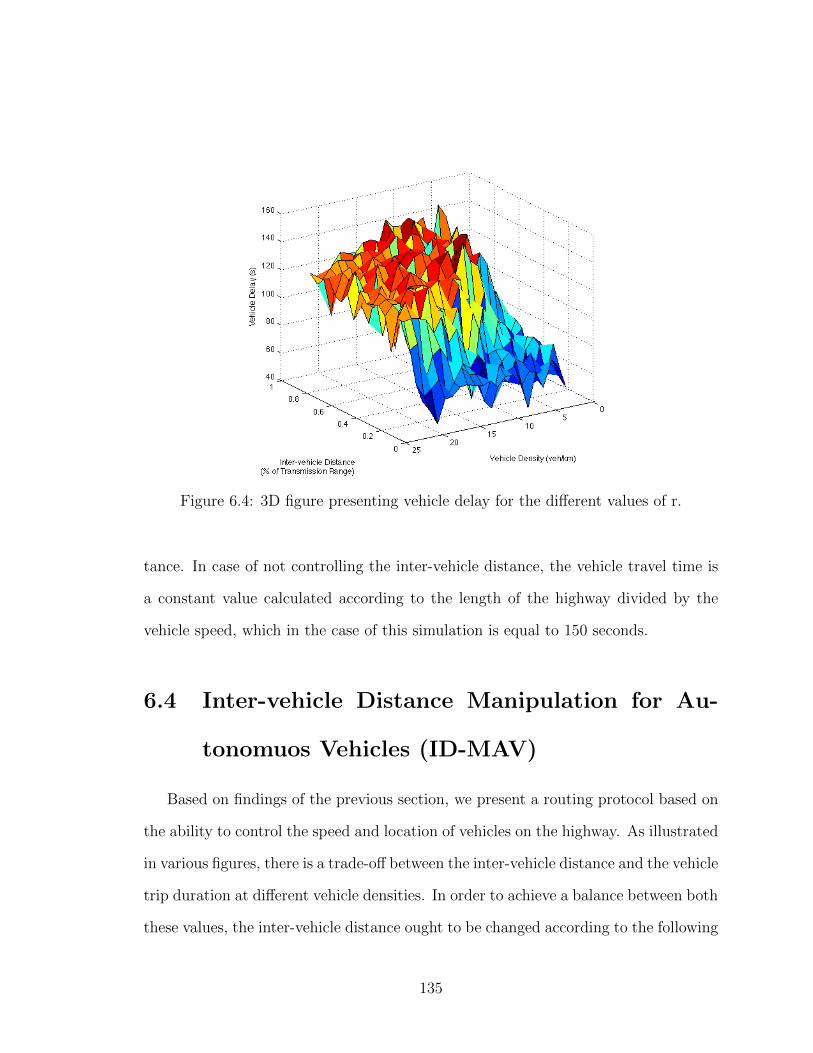
Figure 6.4: 3D figure presenting vehicle delay for the di↵erent values of r.

tance. In case of not controlling the inter-vehicle distance, the vehicle travel time is

a constant value calculated according to the length of the highway divided by the

vehicle speed, which in the case of this simulation is equal to 150 seconds.

6.4 Inter-vehicle Distance Manipulation for Au-

tonomuos Vehicles (ID-MAV)

Based on findings of the previous section, we present a routing protocol based on

the ability to control the speed and location of vehicles on the highway. As illustrated

in various figures, there is a trade-o↵ between the inter-vehicle distance and the vehicle

trip duration at di↵erent vehicle densities. In order to achieve a balance between both

these values, the inter-vehicle distance ought to be changed according to the following

135

Figure 6.5: 2D figure presenting vehicle delay for the di↵erent values of r.

equation:

d = r ⇤✓1� exp

✓�c

�� c

◆◆, (6.1)

where d is the inter-vehicle distance [m], r is transmission range of the vehicle [m],

� [veh/km] is the tra�c density on the highway, and c is a constant variable to

manipulate the trade-o↵ between end-to-end message delivery delay, and the vehicle

trip duration.

The protocol is presented in di↵erent phases:

• Phase 1. Each vehicle estimates the vehicle density on the highway through

computing the density in its communication range using ping messages.

• Phase 2. The constant variable c is pre-set according to the application require-

136

Figure 6.6: E↵ect of the c value on the inter-vehicle distance versus vehicle density.

ments. If an application does not require end-to-end delay to be the minimum

value, but requires the vehicle trip duration to be minimal, the variable c can

be relaxed. The e↵ect of the c value on the inter-vehicle distance versus the

di↵erent vehicle densities is presented in Figure 6.6.

• Phase 3. Each vehicle computes the inter-vehicle distance required per equa-

tion 6.1.

• Phase 4. Once the inter-vehicle density is calculated, each vehicle increases

or decreases its speed till it can be maintained at the inter-vehicle distance

desirable on the highway from the vehicle ahead of it. Note that we utilize a

maximum vehicle speed. This speed is the maximum speed any vehicle is al-

lowed to use in case it would like to increase it’s speed. Once the vehicle reaches

137

required inter-vehicle distance, its speed ought to be immediately adjusted equal

to the speed of the vehicle ahead of it.

6.5 Simulation Results

In this section, we present simulation results for the ID-MAV algorithm. We used

the same simulation setup as that presented in Table 6.1. Also, value for the variable

c used in these results is set to 6.

The performance of our algorithm for end-to-end packet delay and the di↵erent

inter-vehicle distance values are presented in Figure 6.7. The vehicle delay perfor-

mance is presented in Figure 6.8.

Note that the vehicle trip duration is always set at a lower value regardless of the

chosen inter-vehicle distance chosen as compared to conventional non-autonomous

vehicles. The main reason is that controlling the inter-vehicle distance forces the

vehicles to speed up till they reach required distance.

6.6 Summary

In this chapter, we have introduced ID-MAV algorithm which is a vehicle speed

manipulation algorithm for autonomous vehicles. The goal of the vehicle speed control

is to optimize end-to-end packet delivery delay. However, a downside of controlling the

speed of the vehicles is the e↵ect on the vehicle trip duration on the highway. Hence,

the ID-MAV is a dynamic algorithm that changes QoS requirement of vehicle trip

duration for di↵erent VANET applications of vehicle trip duration versus end-to-end

message delivery delay.

We tested our algorithm by verifying the e↵ect of inter-vehicle distance on both

138

Figure 6.7: End-to-end delay performance for c=6 vs the di↵erent inter-vehicle dis-tance values.

end-to-end message delivery delay, and on vehicle trip duration. We presented the

results of the ID-MAV algorithm and improvements on the VANET QoS.

Future work includes developing ID-MAV algorithm to deal with VANET scenar-

ios that include both autonomous and non-autonomous vehicles, and optimizing the

control of the autonomous vehicles to achieve QoS requirements in a hybrid VANET

application.

139

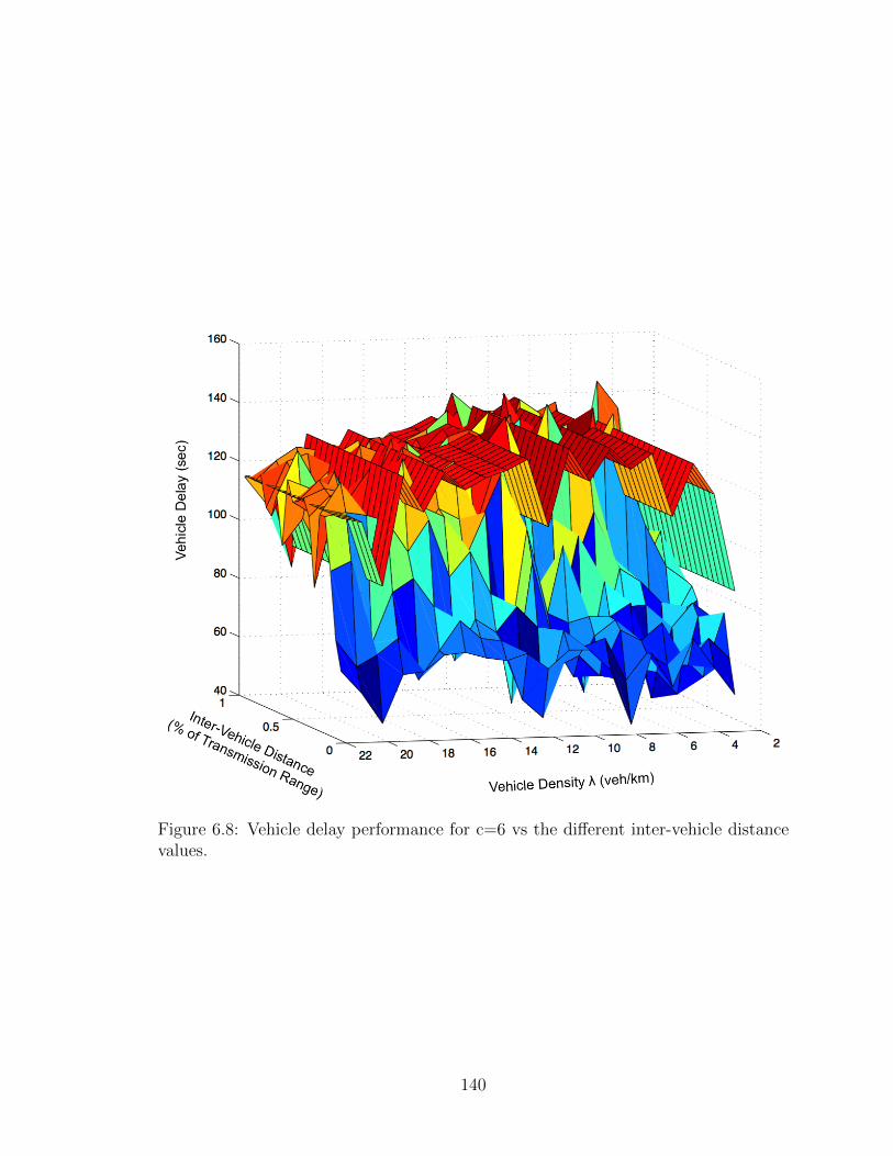
Figure 6.8: Vehicle delay performance for c=6 vs the di↵erent inter-vehicle distancevalues.

140

Chapter 7

Summary & Future Research

Directions

In this chapter, we present a summary of research contribution made in this

dissertation. Following that, we present future research directions that stems from

our findings and the results of this research.

7.1 Summary

In this dissertation, we addressed some important QoS issues in Vehicular Ad

Hoc Networks (VANETs). An introduction to VANET technology with di↵erent

aspects have also been given. Based on di↵erent communication schemes in a VANET,

average total message propagation delay has been analytically determined. In order

to optimize end-to-end message delivery delay, we presented a QoSHVCP hybrid

communication protocol. Moreover, we introduced CAREFOR algorithm which is a

probabilistic routing protocol for VANETs. In order to improve end-to-end message

delivery delay and the throughput in the VANET, we introduced the QASA vehicle

141

selection algorithm. Finally, we utilized the ability to control speed of autonomous

vehicles in order to manipulate the vehicle distribution on highway to minimize end-

to-end message delivery delay. We can summarize our research contributions in this

dissertation as follows:

• We introduced a hybrid approach for vehicular communication that utilizes

both Vehicle-to-Vehicle as well as Vehicle-to-Infrastructure communications.

We present simulation results to demonstrate end-to-end packet delivery de-

lay based on each communication model separately. Based on these findings,

we analyze the total average packet delivery delay using this protocol. Follow-

ing that, we investigated the improvements presented by our hybrid approach

by accounting for overloads in the infrastructure and the net e↵ect on the delay

of packet delivery. We present an analytical model for the delivery delay, and

simulation results to demonstrate the e↵ectiveness of our QoSHVCP protocol.

• We presented a probabilistic routing protocol (CAREFOR) that utilizes multi-

hop retransmission forecast with collision-aware constraints in order to optimize

end-to-end packet delivery delay for V2V communications in vehicular networks.

CAREFOR allows each vehicle to compute a rebroadcast probability that de-

cides whether the vehicle should be allowed to rebroadcast the packet, or refrain

from rebroadcasting. Decreasing the number of rebroadcasters helps minimize

the number of packet collisions due to smaller flooding of the network. The

vehicle with a higher rebroadcast probability is selected as a vehicle which has

a higher chance of forwarding the packet to the largest distance. We present an

analytical model for the rebroadcast probability, as well as simulation results

comparing our protocol to other existing approaches.

142

• We presented the QASA algorithm that considers improving the throughput

of the VANET and optimizing the packet delivery delay. The algorithm is

tailored specifically for vehicles communication using the V2B model. This

model allows vehicles from the east lane to communicate with vehicles on the

same lane through a bridge using vehicles from the opposite lane. The QASA

algorithm allows vehicles on the east to select the vehicles from the west that

will maximize the throughput. This introduces a trade-o↵ with end-to-end

packet delivery delay. We also presented a metric that is manipulated based on

the application QoS requirements. We have also included simulation results to

demonstrate the e↵ectiveness of our approach.

• We investigated utilization of autonomous vehicles in order to improve end-to-

end packet delivery delay and vehicle trip duration. The advantage presented

by autonomous vehicles is that they are automatically controlled and the driver

does not interfere or control the speed of the vehicle. By allowing the protocol to

control the speed of the vehicle, we can manipulate the distribution of vehicles

on the highway. This allows us to control the connectivity of vehicles on the

highway, and hence control the end-to-end packet delivery delay. A trade-o↵

is presented between the total time delay for the vehicle and vehicle speed

manipulation to travel the highway length. We present a metric to control

this trade-o↵ depending on the requirement of the application utilizing the

protocol. Simulation results are presented to demonstrate the improvements by

our protocol.

143

7.2 Future Research Directions

In this dissertation, we have investigated di↵erent approaches to optimize end-to-

end packet delivery delay as well as the throughput in the vehicular networks.

Many future research directions stem from the work presented in this dissertation.

Some of specific directions include:

• Routing Protocols: In this dissertation, we presented routing protocols, as

well as vehicle selection algorithms for vehicle-to-vehicle communication. How-

ever, throughout our analytical model and simulation, we assumed vehicles to

travel at a constant speed. A future research direction could investigate the ef-

fect of vehicles having di↵erent speeds and the changes required in the di↵erent

models and protocols.

• Tra�c Scenario: In the research presented in this dissertation, we have as-

sumed highway scenarios where vehicles travel in either one of two directions.

A future research direction would include developing the di↵erent models and

routing protocols for a city model, which includes road intersections, stop signs,

di↵erent speed limits, etc.

• Autonomous Vehicles: In this dissertation, we presented the idea of the uti-

lization of autonomous vehicles with the goal of minimizing end-to-end packet

delivery delay. However, in our scenario, we assumed all the vehicles to be

autonomous. In reality, this is not a practical assumption. Future research

direction should include developing a model for end-to-end packet delivery de-

lay for highways with hybrid vehicles (including both autonomous and regular

cars). The percentage of autonomous vehicles on the highway can be manip-

ulated, and a dynamic algorithm to manipulate the autonomous vehicle speed

144

can be based on the percentage of these vehicles on the highway. Moreover,

this problem can be modeled after adhoc networks that include both static

and mobile nodes, where regular vehicles are considered relatively static, while

autonomous vehicles can be considered as the mobile nodes.

145

Bibliography

[1] H. Lum and J. A. Reagan, “Interactive highway safety design model: Accident

predictive module,” in Public Roads Magazine, 1995.

[2] “Future cars: The word from GM at IDC’s Smart Technology World Confer-

ence,” 2011.

[3] N. H. T. S. Admin, “Vehicle Safety Communications Project Final Report,”

2006.

[4] M. E. Nowatkowski, Certificate revocation list distribution in vehicular ad hoc

networks. PhD thesis, Georgia Institute of Technology, 2010.

[5] M. Gerla, B. Zhou, Y. zhong Lee, F. Soldo, U. Lee, and G. Marfia, “Vehicular

Grid Communications: The Role of the Internet Infrastructure,” in Proceedings

of the 1st International Conference on Genetic Algorithms and their Applica-

tions, pp. 112–120, 2006.

[6] “Tra�c Congestion.” http://en.wikipedia.org/wiki/Traffic_congestion.

[7] H. Moustafa and Y. Zhang, Vehicular Networks: Techniques, Standards, and

Applications. Auerbach Publications, 2009.

146

[8] “Vehicular Communication Systems.” http://en.wikipedia.org/wiki/

Vehicular_communication_systems.

[9] “United States Department of Transport (US-DOT).”

[10] “E-enova.” http://www.eenova.de/, 2010.

[11] “Car 2 car communication consortium.” http://www.car-to-car.org, 2010.

[12] C. Tutor, “Ford proposes intelligent active safety system.” http://autoblog.

com/2007/09/25/ford-proposes-intelligent-active-safety-system/,

2007.

[13] “The partners for advanced transit and highway (path).”

[14] “Watch-over: Cooperative vulnerable road users.” http://www.watchover-eu.

org/, 2010.

[15] X. Hong, T. J. Kwon, M. Gerla, D. L. Gu, and G. Pei, “A mobility framework for

ad hoc wireless networks,” in Proceedings of the Second International Conference

on Mobile Data Management (MDM ’01), pp. 185–196, Springer-Verlag, 2001.

[16] “Dedicated short range communications project.”

[17] “Road network operations handbook,” World Road Association, 2002.

[18] M. A. Chowdhury and A. Sadek, Fundamentals of Intelligent Transportation

Systems Planning. Artech House, 2003.

[19] R. Karim, “VANET: superior system for content distribution in vehicular net-

work applications.” http://www.cs.rutgers.edu/.

147

[20] “Customers Angered as iPhones Overload ATT.” http://www.nytimes.com/

2009/09/03/technology/companies/03att.html.

[21] A. Dahiya and R. Chauhan, “A Comparative Study of MANET and VANET

environment,” Journal of Computing, vol. 2, July 2010.

[22] S. Sullivan, “Method and apparatus for powering of amphibious craft,”

[23] “Blind spot information system.” http://www.honda.com/, 2011.

[24] “Ford develops heart rate monitoring seat; adds new element to health

and wellness research.” http://corporate.ford.com/news-center/

press-releases-detail/pr-ford-develops-heart-rate-34664.

[25] D. N. Cottingham, Vehicular Wireless Communication. PhD thesis, University

of Cambridge, 2009.

[26] N. Karlsson, “Floating car data deployment and tra�c advisory services,” in

OPTIS Project, 2002.

[27] A. Agrawal, Analytical Modeling of Delay-Tolerant Data Dissemination In Ve-

hicular Networks. PhD thesis, Boston University, 2010.

[28] “Vehicle-Infrastructure Integration (VII) Initiative Benefit-Cost Analysis:

Pre-Testing Estimates.” http://www.its.dot.gov/research_docs/pdf/

8cost-analysis.pdf.

[29] “Frequency of Target Crashes for IntelliDrive Safety System.” http://www.

nhtsa.gov/.

[30] H. Makino, “Smartway project: Cooperative vehicle highway systems,” in Trans-

portation Research Board Annual Meeting, 2006.

148

[31] “Intelligent Transportation Services.” http://www.its.dot.gov/.

[32] K. Fall, “A delay-tolerant network architecture for challenged internets,” in Pro-

ceedings of the 2003 Conference on Applications, Technologies, Architectures,

and Protocols for Computer Communications (SIGCOMM ’03), pp. 27–34, ACM

Press, 2003.

[33] T. Spyropoulos, K. Psounis, and C. Raghavendra, “Spray and wait: An e�cient

routing scheme for intermittently connected mobile networks,” in Proc. of the

2005 ACM SIGCOMMWorkshop on Delay-Tolerant Networking, (PA, USA.),

2005.

[34] E. Schoch, F. Kargl, M. Weber, and T. Leinmuller, “Communication patterns in

vanets,” IEEE Communications Magazine, vol. 46, no. 11, 2008.

[35] S. Ni, Y. Tseng, Y. Cheng, and J. Sheu, “The broadcast storm problem in

a mobile ad hoc network,” in Proc. of ACM MobiCom, (Seattle, Washington,

USA), pp. 151–162, August 1999.

[36] K. Suriyapaobonwattana and C. Pomavalai, “An e↵ective safety alert broadcast

algorithm for vanet,” in Proc. of International Symposium on Communications

and Information Technologies, pp. 247–250, 2008.

[37] C. Palazzi, M. Roccetti, S. Ferretti, G. Oau, and M. Gerla, “Online games on

wheels: Fast game event delivery in vehicular ad-hoc networks,” in Proc. of 3rd

IEEE International Workshop on Vehicle-to-Vehicle Communications - IEEE

International Vehicles Symposium, IEEE Intelligent Transportation Systems So-

ciety, (Istanbul, Turkey), June 2007.

149

[38] S. Panichpapiboon and G. Ferrari, “Irresponsible forwarding,” in Proc. of IEEE

8th International Conference on Intelligent Transport System Telecommunica-

tions, (Phuket, Thailand), pp. 311–316, October 2008.

[39] G. Resta, P. Santi, and J. Simon, “Analysis of Multi-hop Emergency Message

Propagation in Vehicular Ad Hoc Networks,” in Proc. of the 8th ACM Intl. Symp.

on Mobile Ad Hoc Networking and Computing, (Montreal, Canada), pp. 140–149.

[40] H. Jiang, H. Guo, and L. Chen, “Reliable and E�cient Alarm Message Routing

in VANET,” in Proc. on the 28th Int. Conf. on Distributed Computing Systems

Workshops, pp. 186–191, 2008.

[41] X. Dong, K. Li, J. Misener, P. Varayia, and W. Zhang, “Expediting vehicle

infrastructure integration (evii),” tech. rep., California PATH Research Report,

UCB-ITS-PRR-2006-20, 2006.

[42] M. Gerla, B. Zhou, Y.-Z. Lee, F. Soldo, U. Lee, and G. Marfia, “Vehicular

grid communications: The role of the internet infrastructure,” in Proceeding of

Wireless Internet Conference, (Boston), Aug. 2006.

[43] G. Marfia, G. Pau, E. D. Sena, E. Giordano, and M. Gerla, “Evaluating vehi-

cle network strategies for downtown portland: Opportunistic infrastructure and

importance of realistic mobility models,” in Proceeding of MobiOpp 2007, (Porto

Rico), June, 2007.

[44] N. Mejri, F. Kamoun, and F. Filali, “Cooperative infrastructure discovery

through v2x communication,” in Proc. of the 9th IFIP Annual Mediterranean

Ad Hoc Networking Workshop, pp. 1–8, June 2010.

150

[45] J. Wedel, B. Schunemann, and I. Radusch, “V2X-based Tra�c Congestion

Recognition and Avoidance,” in Proc. of 10th Intl. Symp. on Pervasice Systems,

Algorithms and Networks, pp. 637–641, 2009.

[46] S. Jeongwook, P. Kyungwon, J. Wongi, J. Kwak, and K. Dong, “Performance

evaluation of v2x communications in practical small-scale fading models,” in

Proc. of IEEE 20th International Symposium on Personal, Indoor and Mobile

Radio Communications, pp. 2434–2438, September 2009.

[47] Ghada H. Badawy, Jelena V. Misic, Terence D. Todd, and Dongmei Zhao, “Per-

formance modeling of safety message delivery in vehicular ad hoc networks,”

in Proceedings of Sixth IEEE International Conference on Wireless and Mobile

Computing, Networking and Communications (WiMob 2011), pp. 188–195, 2011.

[48] K. Abboud and W. Zhuang, “Modeling and Analysis for Emergency Messag-

ing Delay in Vehicular Ad Hoc Networks,” in Proceedings of the IEEE Global

Communications Conference, Exhibition Industry Forum (GLOBECOM 2009),

pp. 1–6, 2009.

[49] R. Fracchia and M. Meo, “Analysis and Design of Warning Delivery Service

in Intervehicular Networks,” IEEE Transactions on Mobile Computing, vol. 7,

no. 7, 2008.

[50] S. Yousefi, E. Altman, E. El-Azouzi, and M. Fathy, “Analytical Model for Con-

nectivity in Vehicular Ad Hoc Networks,” Proceedings of IEEE Transactions on

Vehicular Technology (VTC 2008, vol. 57, pp. 3341–3356, 2008.

[51] S. Ukkusuri and L. Du, “Geometric Connectivity of Vehicular Ad hoc Networks:

151

Analytical Characterization,” Transportation Research Part C: Emerging Tech-

nologies, vol. 16, no. 5, pp. 615–634, 2008.

[52] T. C. K. Chou and J. A. Abraham, “Load balancing in distributed systems,”

IEEE Trans. Software Engineering, vol. 8, pp. 401–412, July 1982.

[53] Q.-T. Nguyen-Vuong, N. Agoulmine, and Y. Ghamri-Doudane, “Novel approach

for load balancing in heterogeneous wireless packet networks,” in Proceedings of

the 2008 Network Operations and Management Symposium Workshops, pp. 26–

31, 2008.

[54] J. Ha, J. Kim, J.-U. Kim, and S.-H. Kim, “Dynamic load balancing architecture

in heterogeneous wireless network environment,” in Proc. of the 9th Interna-

tional Conference on Communications and Information Technologies, ISCIT’09,

(Piscataway, NJ, USA), pp. 248–253, IEEE Press, 2009.

[55] A. D. Amis and R. Prakash, “Load-balancing clusters in wireless ad hoc net-

works,” in Proc. of the 3rd IEEE Symposium on Application-Specific Systems

and Software Engineering Technology (ASSET’00), ASSET ’00, (Washington,

DC, USA), pp. 25–32, IEEE Computer Society, 2000.

[56] H. Dai and R. Han, “A node-centric load balancing algorithm for wireless sensor

networks,” in Proc. of IEEE Global Telecommunications Conference (GLOBE-

COM 2003), pp. 548–552, December 1-5 2003.

[57] W. Jiang, Z. Li, C. Zeng, and H. Jin, “Load balancing routing algorithm for ad

hoc networks,” in Proc. of 5th International Conference on Mobile Ad-hoc and

Sensor Networks (MSN 2009), pp. 334–339, Dec. 2009.

152

[58] A. Mostafa, A. Vegni, R. Singoria, T. Oliveira, T. Little, and D. Agrawal, “A

v2x-based approach for reduction of delay propagation in vehicular ad-hoc net-

works,” in Proc. of Intl. Workshop on Seamless Connectivity in Vehicular Net-

works (SCVN 2011), part of the 11th IEEE International Conference on ITS

Telecommunications (ITST 2011), (Saint Petersburg, Russia), August, 23-25.

[59] S. Olariu, and M. C. Weigle (Eds.), Vehicular Networks: From Theory to Prac-

tice. CRC Press / Taylor & Francis, 2009.

[60] G. Yan, N. Mitton, and X. Li, “Reliable Routing in Vehicular Ad Hoc Networks,”

in IEEE 30th International Conference on Distributed Computing Systems Work-

shops (ICDCSW), pp. 263–269, June 21-25 2010.

[61] S. Panichpapiboon and G. Ferrari, “Irresponsible Forwarding,” in Proc. of 8th

International Conference on ITS Telecommunications, (Phuket), pp. 311–316,

October 2008.

[62] G. Yan, D. B. Rawat, and S. El-Tawab, “Ticket-based Reliable Routing in

VANET,” in IEEE 6th International Conference on Mobile Adhoc and Sensor

Systems (MASS ’09), pp. 609–614, October 12-15 2009.

[63] S. Chen and K. Nahrstedt, “Distributed Quality-of-Service Routing in Ad-

hoc Networks,” IEEE Journal on Selected Areas in Communications, vol. 17,

pp. 1488–1505, August 1999.

[64] H. Jiang, H. Guo, and L. Chen, “Reliable and e�cient alarm message routing in

vanet,” in Proc. of The 28th International Conference on Distributed Computing

Systems Workshops (ICDCSW), (Washington, DC, USA), pp. 186–191, 2008.

153

[65] W. Sun, H. Yamaguchi, and K. Yukimasa, “Gvgrid: A QoS Routing Protocol

for Vehicular ad-hoc Networks,” in Proc. of the Fourteenth IEEE International

Workshop on Quality of Service (IWQoS 2006), (Yale University, New Haven,

CT, USA), pp. 130–139, June 19-21 2006.

[66] J. Kim, Q. Zhang, and D. P. Agrawal, “Probabilistic broadcasting based on

coverage area and neighbor confirmation in mobile ad hoc networks,” in Proc.

IEEE Global Telecomm. Conf. (GLOBECOM), November 2004.

[67] S. Busanelli, G. Ferrarri, and S. Panichpapiboon, “Cluster-Based Irresponsible

Forwarding,” The Internet of Things, pp. 59–68, 2010.

[68] K.A. Hafeez and L. Zhao and Z. Liao, and B.N. Ma, “Performance Analysis of

Broadcast Messages in VANETs Safety Applications,” in Proc. of 2010 IEEE

Global Telecommunications Conference, pp. 1–5, December 6-10, 2010.

[69] A. Mostafa, A. M. Vegni, T. Oliveira, T. D. C. Little, and D. P. Agrawal,

“QoSHVCP: Hybrid Vehicular Communications Protocol with QoS Prioriza-

tion for Safety Applications,” ISRN Communications and Networking Journal,

vol. 2012, p. 14, 2012.

[70] T. Spyropoulos, K. Psounis, and C. Raghavendra, “Spray and Wait: An E�cient

Routing Scheme for Intermittently Connected Mobile Networks,” in Proc. of

ACM SIGCOMM Workshop on Delay-Tolerant Networking, (PA, USA), 2005.

[71] S. Yousefi, E. Altman, R. El-Azouzi, and M. Fathy, “Analytical Model for Con-

nectivity in Vehicular Ad Hoc Networks,” IEEE Trans. of Vehicular Technology,

vol. 57, no. 6, 2008.

154

[72] A. Agarwal and T. Little, “Access Point Placement in Vehicular Networking,”

in Proc. of 1st Intl. Conf. on Wireless Access in Vehicular Environments, (Troy,

MI), Dec. 2008.

[73] W.-L. Jin and H.-J. Wang, “Modeling Connectivity of Inter-Vehicle Communica-

tion Systems with Road-Side Stations,” The Open Transportation Journal, no. 2,

pp. 1–6, 2008.

[74] Vladimir Bychkovsky, Bret Hull, Allen K. Miu, Hari Balakrishnan, and Samuel

Madden, “A Measurement Study of Vehicular Internet Access using in situ Wi-

Fi Networks,” in Proc. of ACM Annual Intl. Conf. on Mobile Computing and

Networking, (Los Angeles, CA, USA), Sept. 2006.

[75] M. Gerla, B. Zhou, Y.-Z. Lee, F. Soldo, U. Lee, and G. Marfia, “Vehicular Grid

Communications: The Role of the Internet Infrastructure,” in Proc. of Wireless

Internet Conference, (Boston, MA), 2006.

[76] G. Marfia, G. Pau, E. D. Sena, E. Giordano, and M. Gerla, “Evaluating Vehicle

Network Strategies for Downtown Portland: Opportunistic Infrastructure and

Importance of Realistic Mobility Models,” in Proc. of MobiOpp, (Porto Rico),

2007.

[77] A. Vegni, A. Mostafa, and D. Agrawal, “CAREFOR: Collision-Aware REliable

FORwarding Technique for Vehicular Ad hoc Networks,” in Proc. of Intl. Conf.

on Computing, Networking and Communications (ICNC 2012), Mobile Comput-

ing & Vehicle Comm. Symp., (San Diego, CA, USA), January 28-31 2013.

[78] H. Hartenstein and K. Laberteaux, VANET: Vehicular Applications and Inter-

networking Technologies. Wiley & sons, Ltd., 2010.

155

[79] U. Lee, J.-S. Park, J. Yeh, G. Pau, and M. Gerla, “Code Torrent: Content

Distribution Using Network Coding in VANET,” in Proc. of First Intl. Workshop

on Decentralized Resource Sharing in Mobile Computing and Networking., (Los

Angeles, CA, USA), September 23-29 2006.

[80] L. D. N. Mark Johnson and K. Ramchandran, “Collaborative content distribu-

tion for vehicular ad hoc networks,” in Proc. of Allerton conference on commu-

nication, control, and computing., (Los Angeles, CA, USA), September 2006.

[81] D. Gerlough and A. Schuhl, Use of Poisson distribution in highway tra�c. Eno

Foundation for Highway Tra�c Control, 1955.

[82] A. Mostafa, A. Vegni, R. Singoria, T. Oliveira, T. Little, and D. Agrawal, “A

V2X-based approach for reduction of delay propagation in Vehicular Ad-Hoc

Networks,” in Proc. of Intl. Workshop on Seamless Connectivity in Vehicular

Networks, part of the 11th IEEE Intl. Conf. on ITS Telecommunications, (Saint-

Petersburg, Russia), August 23-25 2011.

[83] “An Automated Adventure at the Wheel of a driverless bmw.” http://www.

thenational.ae/.

[84] “En-v Electric Networked Car Concept by gm begins Pilot Testing.” http://

www.designboom.com/.

[85] “Rea�rmed Mission for Autonomous Audi tts Pikes Peak.” http://www.

audiusa.com/.

[86] “Autonomous Car.” http://en.wikipedia.org/wiki/Autonomous_car.

[87] “Google gets License to Operate Driverless cars in Nevada.” http://www.cnn.

com/.

156

[88] “Self-driving Cars now Legal in California.” http://www.cnn.com/.

[89] “More Autonomous Vehicles Headed to Nevada Roads.” http://www.wired.

com/.

[90] “You won’t need a driver’s license by 2040.” http://www.cnn.com/.

[91] “Can I See Your License, Registration and c.p.u.?.” http://www.nytimes.com/.

[92] “Get Ready for Automated Cars.” http://www.chron.com/.

[93] “How Vehicle Automation Will Cut Fuel Consumption.” http://www.

technologyreview.com/.

[94] E. Frazzoli, M. A. Dahleh, and E. Feron, “Real-time motion planning for agile

autonomous vehicles,” AIAA JOURNAL OF GUIDANCE, CONTROL, AND

DYNAMICS, vol. 25, pp. 116–129, 2000.

[95] A. P. P. Aguiar, J. F. Almeida, M. Bayat, B. Cardeira, R. Cunha, A. Hausler,

P. K. Maurya, A. Oliveira, A. Pascoal, A. A. Pereira, M. Rufino, L. Sebastiao,

C. Silvestre, and F. Vanni, “Cooperative control of multiple marine vehicles the-

oretical challenges and practical issues,” in Manoeuvering and Control of Marine

Craft, (Guaruja (SP), Brazil), Sep. 2009.

[96] C. Wu, G. Zhao, and B. Ou, “A fuel economy optimization system with applica-

tions in vehicles with human drivers and autonomous vehicles,” Transportation

Research Part D: Transport and Environment, vol. 16, no. 7, pp. 515 – 524, 2011.

[97] W. Xu, J. Wei, J. Dolan, H. Zhao, and H. Zha, “A real-time motion planner with

trajectory optimization for autonomous vehicles,” in Robotics and Automation

(ICRA), 2012 IEEE International Conference on, pp. 2061 –2067, May. 2012.

157

[98] B. Krogh and C. Thorpe, “Integrated path planning and dynamic steering control

for autonomous vehicles,” in Proceedings of 1986 IEEE International Conference

on Robotics and Automation (ICRA ’86), pp. 1664 – 1669, April 1986.

158