Towards Development of a Self-Healing Composite using a Mendable Polymer and Resistive Heating
Upload
khangminh22Category
view
0download
0
73
Analysis of a Composite Microlift-GliderWing Structure Using Finite Element Analysis and Manual Calculation*Análisis de la estructura alar de un planeador para microsustentación usando elementos finitos y cálculos analítico
R e c i b i d o : 2 d e d i c i e m b r e - A c e p t a d o : 2 d e s e p t i e m b r e d e 2 0 1 4
Jorge Eliécer Gaitán Aroca**
Harold Sánchez***
Jairo Niño****
* Artículo de investigación, producto derivado del proyecto de investigación Diseño del planeador atlas M2 Fase II, realizado en el grupo Aerotech de la Universidad de San Buenaventura, llevado a cabo entre el 20 de febrero 2012 y el 1 de junio de 2013.
** Ingeniero Aeronáutico. Especialista en Pedagogía y Docencia Universitaria. Docente Ingeniería Aeronáutica Universidad de San Buenaventura. Investigador grupo investigación Aerotech. Representante ante la red internacional Prideras de la Universidad de San Buenaventura.
*** Ingeniero Aeronáutico Universidad de San Buenaventura.**** Ingeniero Aeronáutico Universidad de San Buenaventura.
Para citar este artículo: J. Gaitán, H. Sánchez, J. Niño, «Analysis of a composite Microlift-glider wing structure using Finite element analysis and manual calculation», Ingenium, vol. 15, n.°30, pp. 73-94, octubre, 2014.
Abstract
The paper describes a project undertaken at the San Buenaventura University Bogota, Colombia branch to develop the structural design of a light motor-less glider focused on the wing structure based on wood and composites materials. In the first stage there where established the main constraints for post calculation, then it is proposed the main wing structure to be analyzed and as this is a small weight glider it was considered special composites materials. There is an analysis of the structure taking into account the maximum load factor developed during a normal flight; completes dates are available for each station of the wing; those date are compared with the same wing structure under the same loads analyzed using FEA
74
Revista de la Facultad de Ingeniería • Año 15 • n.° 30, Julio - Diciembre de 2014
Keywords
Design, analysis, finit element analysis, glider, wing structure, microlift.
Resumen
El artículo describe un proyecto en la Universidad de San Buenaventura, sede Bogotá, en el cual se desarrolla el diseño estructural del ala de un planeador, el cual se enfoca en materiales como la madera y materiales compuestos. En la primera etapa se establecen las cargas principales para un cálculo posterior, luego se propone la configuración de la estructura alar a analizar haciendo énfasis en materiales compuestos. Se tiene en cuenta en el análisis estructural el factor de carga máximo que se puede desarrollar durante un vuelo normal. Dichos cálculos se aplican a la misma estructura por medio de un análisis en elementos finitos con el fin de comparar datos.
Palabras clave
Diseño, análisis estructural, elementos finitos, planeador, estructura alar, microsus-tentación
1. Introduction
The work starts from a comparison of the data obtained under the geometric design of the glider as a function of the initial adjustment for gliders of different categories, the body of work provides critical operating conditions from current regulatory and accurate data, which gives the way for a series of proposals initially structural drawings of the aircraft and its support structure. This structural approach is modified depending on the operating conditions and sets the maximum aerodynamic loads that structure supports during a normal flight mission, by this way it is proceeded to apply this strength on the structure to find the maximum internal loads to find a material that mitigates these load conditions. So it is necessary to show a selection of materials used and the characterization of from ASTM standards, while preliminary proposals are given how to build such a structure.
2. Investigation Development
To give the design and analysis for a wing structure is it necessary to know the main requirements given by the mission profile of the sailplane, there are also dimensional parameters that must meet the final design, the aerodynamic characteristics must be known on the most critical conditions, once those requirements are well known it is needed to propose a structural disposition that support the most critical load at least 1,5 times. The analysis begin with an analytical calculation to be complemented with a software analysis.
The wing structure begins with the main characteristics of the saiplane.
Investigación
75
Analysis of a Composite Microlift-GliderWing Structure Using Finite Element Analysis and Manual Calculation • pp. 73-94
The airplane that operates from microlift conditions is called microlift glider, some of the main features are:
• To be considered a micro-glider lift its maximum takeoff weight must be less than 220 kg, and the maximum wing loading less than 18 kg / m2.
• Must be driven by a single occupant.
Parameters Resume
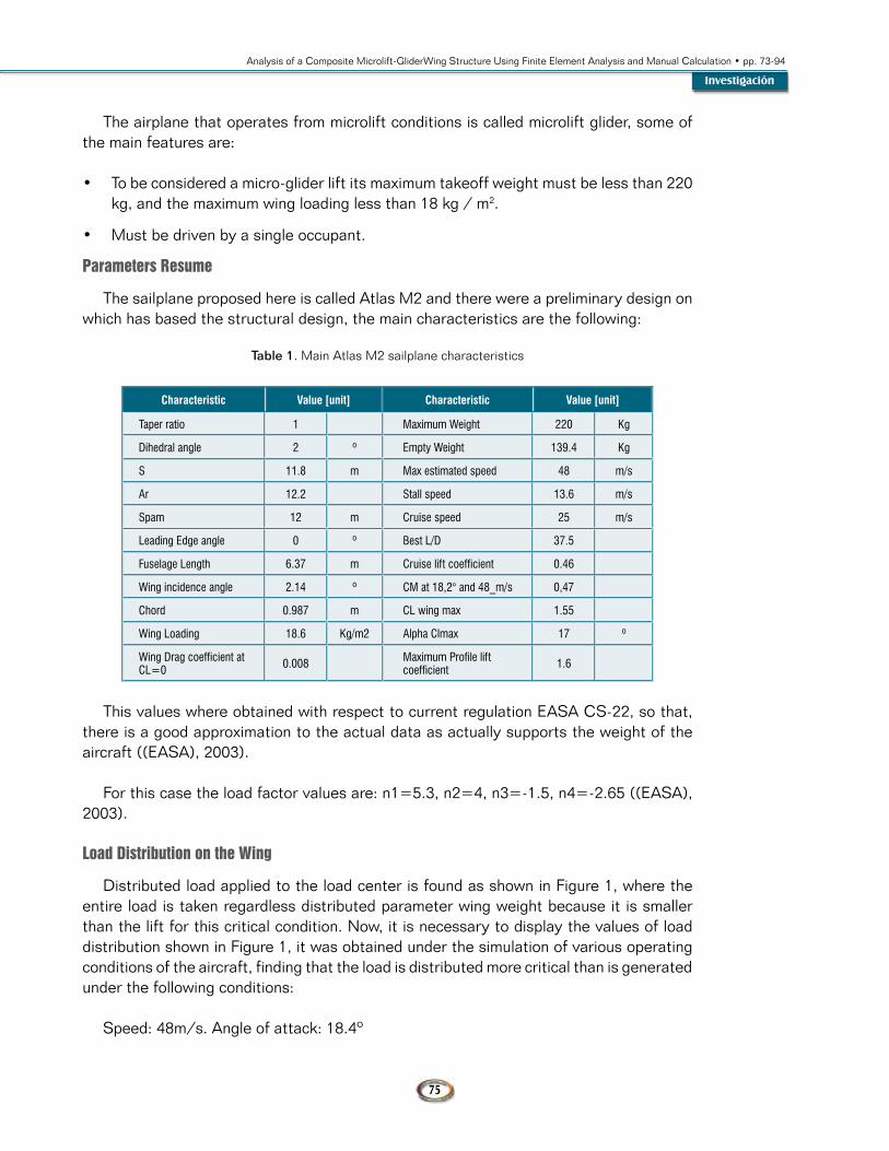
The sailplane proposed here is called Atlas M2 and there were a preliminary design on which has based the structural design, the main characteristics are the following:
Table 1. Main Atlas M2 sailplane characteristics
Characteristic Value [unit] Characteristic Value [unit]
Taper ratio 1 Maximum Weight 220 Kg
Dihedral angle 2 º Empty Weight 139.4 Kg
S 11.8 m Max estimated speed 48 m/s
Ar 12.2 Stall speed 13.6 m/s
Spam 12 m Cruise speed 25 m/s
Leading Edge angle 0 º Best L/D 37.5
Fuselage Length 6.37 m Cruise lift coefficient 0.46
Wing incidence angle 2.14 º CM at 18,2° and 48_m/s 0,47
Chord 0.987 m CL wing max 1.55
Wing Loading 18.6 Kg/m2 Alpha Clmax 17 º
Wing Drag coefficient at CL=0 0.008 Maximum Profile lift
coefficient 1.6
This values where obtained with respect to current regulation EASA CS-22, so that, there is a good approximation to the actual data as actually supports the weight of the aircraft ((EASA), 2003).
For this case the load factor values are: n1=5.3, n2=4, n3=-1.5, n4=-2.65 ((EASA), 2003).
Load Distribution on the Wing
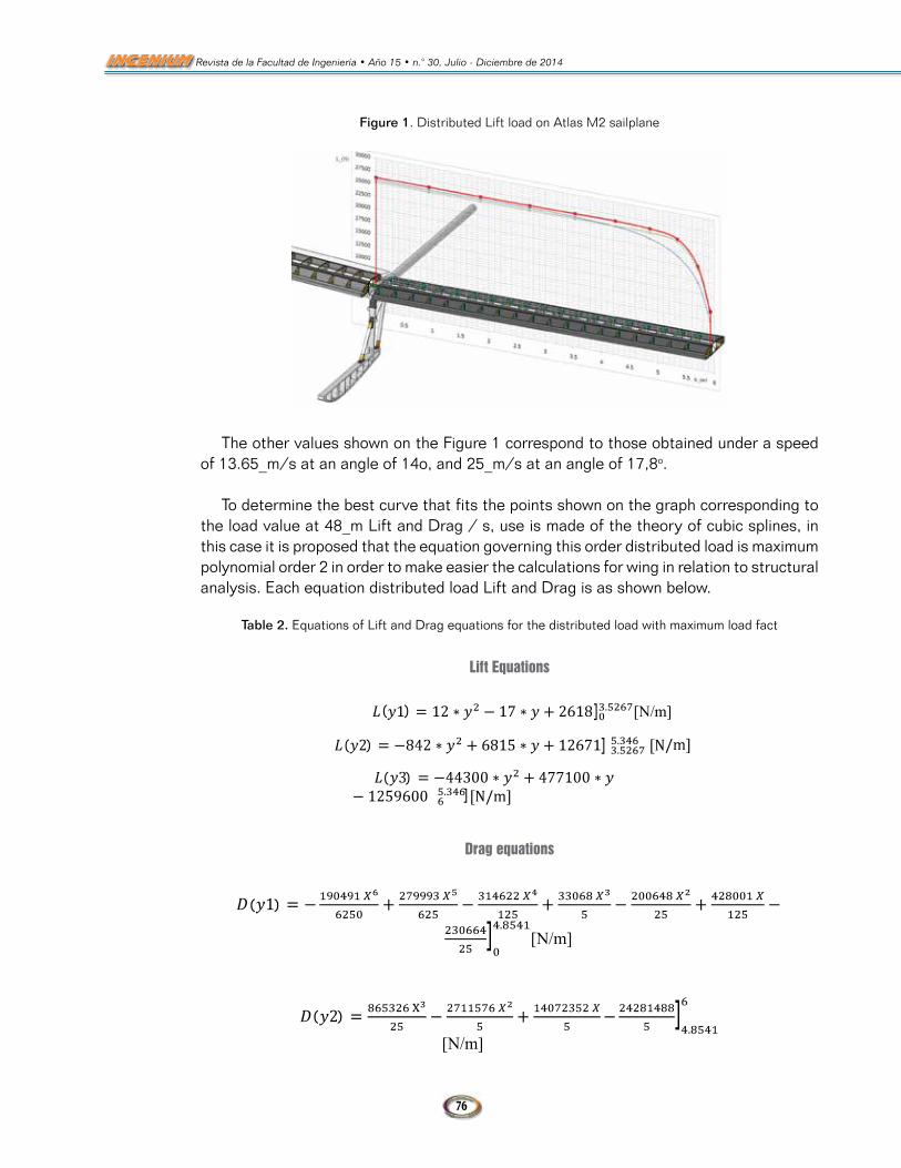
Distributed load applied to the load center is found as shown in Figure 1, where the entire load is taken regardless distributed parameter wing weight because it is smaller than the lift for this critical condition. Now, it is necessary to display the values of load distribution shown in Figure 1, it was obtained under the simulation of various operating conditions of the aircraft, finding that the load is distributed more critical than is generated under the following conditions:
Speed: 48m/s. Angle of attack: 18.4º
76
Revista de la Facultad de Ingeniería • Año 15 • n.° 30, Julio - Diciembre de 2014
Figure 1. Distributed Lift load on Atlas M2 sailplane
The other values shown on the Figure 1 correspond to those obtained under a speed of 13.65_m/s at an angle of 14o, and 25_m/s at an angle of 17,8o.
To determine the best curve that fits the points shown on the graph corresponding to the load value at 48_m Lift and Drag / s, use is made of the theory of cubic splines, in this case it is proposed that the equation governing this order distributed load is maximum polynomial order 2 in order to make easier the calculations for wing in relation to structural analysis. Each equation distributed load Lift and Drag is as shown below.
Table 2. Equations of Lift and Drag equations for the distributed load with maximum load fact
Lift Equations
The other values shown on the Figure 1 correspond to those obtained under a speed of 13.65_m/s at an angle of 14o, and 25_m/s at an angle of 17,8o.
To determine the best curve that fits the points shown on the graph corresponding to the load value at 48_m Lift and Drag / s, use is made of the theory of cubic splines, in this case it is proposed that the equation governing this order distributed load is maximum polynomial order 2 in order to make easier the calculations for wing in relation to structural analysis. Each equation distributed load Lift and Drag is as shown below.
Table 2. Equations of Lift and Drag equations for the distributed load with maximum load factor
Lift Equations
[N/m]
Drag equations
[N/m]
[N/m]
3. Analysis and Result Discussion
In the structural analysis it is necessary to know how the internal behavior of the structure is, but to do this it is necessary to propose a defined structure which supports the internal flight load. It must be known that the structural proposition is an iterative process due to the structural stresses which the structure will carried out, in this structure it was proposed a structure according to typical structures for similar wing structure. Once this has been proposed it is necessary to apply the loads the know the internal stress and strain condition on this structure
Equations for Internal Load Sustainability
Drag equations
The other values shown on the Figure 1 correspond to those obtained under a speed of 13.65_m/s at an angle of 14o, and 25_m/s at an angle of 17,8o.
To determine the best curve that fits the points shown on the graph corresponding to the load value at 48_m Lift and Drag / s, use is made of the theory of cubic splines, in this case it is proposed that the equation governing this order distributed load is maximum polynomial order 2 in order to make easier the calculations for wing in relation to structural analysis. Each equation distributed load Lift and Drag is as shown below.
Table 2. Equations of Lift and Drag equations for the distributed load with maximum load factor
Lift Equations
[N/m]
Drag equations
[N/m]
[N/m]
3. Analysis and Result Discussion
In the structural analysis it is necessary to know how the internal behavior of the structure is, but to do this it is necessary to propose a defined structure which supports the internal flight load. It must be known that the structural proposition is an iterative process due to the structural stresses which the structure will carried out, in this structure it was proposed a structure according to typical structures for similar wing structure. Once this has been proposed it is necessary to apply the loads the know the internal stress and strain condition on this structure
Equations for Internal Load Sustainability
Investigación
77
Analysis of a Composite Microlift-GliderWing Structure Using Finite Element Analysis and Manual Calculation • pp. 73-94
3. Analysis and Result Discussion
In the structural analysis it is necessary to know how the internal behavior of the structure is, but to do this it is necessary to propose a defined structure which supports the internal flight load. It must be known that the structural proposition is an iterative process due to the structural stresses which the structure will carried out, in this structure it was proposed a structure according to typical structures for similar wing structure. Once this has been proposed it is necessary to apply the loads the know the internal stress and strain condition on this structure
Equations for Internal Load Sustainability
From lift and drag equations it is possible to obtain the diagram shear and moment for each of the wing sections, it should be noted at this point that although it was not considered the influence of the wing torsion moment coefficient due to aerodynamic effects given.
Structural Wing Layout
It is appreciated that most of the location of the center of pressure falls to approximately 25% (Anderson, 2001) of the chord measured from the leading edge, and has a significant change in increase of 80.1% from the average size measured from the plane of symmetry of the aircraft.
This value has to be established, it is possible to estimate the position of the main beam along the rope. But for this case will take an approach to the location of the center of pressure along the chord, so you can make a simplification of the calculations without introducing significant changes in the results error.
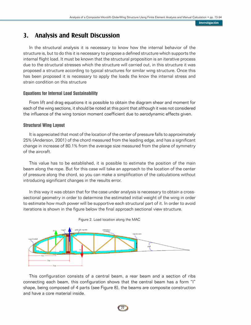
In this way it was obtain that for the case under analysis is necessary to obtain a cross-sectional geometry in order to determine the estimated initial weight of the wing in order to estimate how much power will be supportive each structural part of it. In order to avoid iterations is shown in the figure below the final approach sectional view structure.
Figure 2. Load location along the MAC
This configuration consists of a central beam, a rear beam and a section of ribs connecting each beam, this configuration shows that the central beam has a form “I” shape, being composed of 4 parts (see Figure 8), the beams are composite construction and have a core material inside.
78
Revista de la Facultad de Ingeniería • Año 15 • n.° 30, Julio - Diciembre de 2014
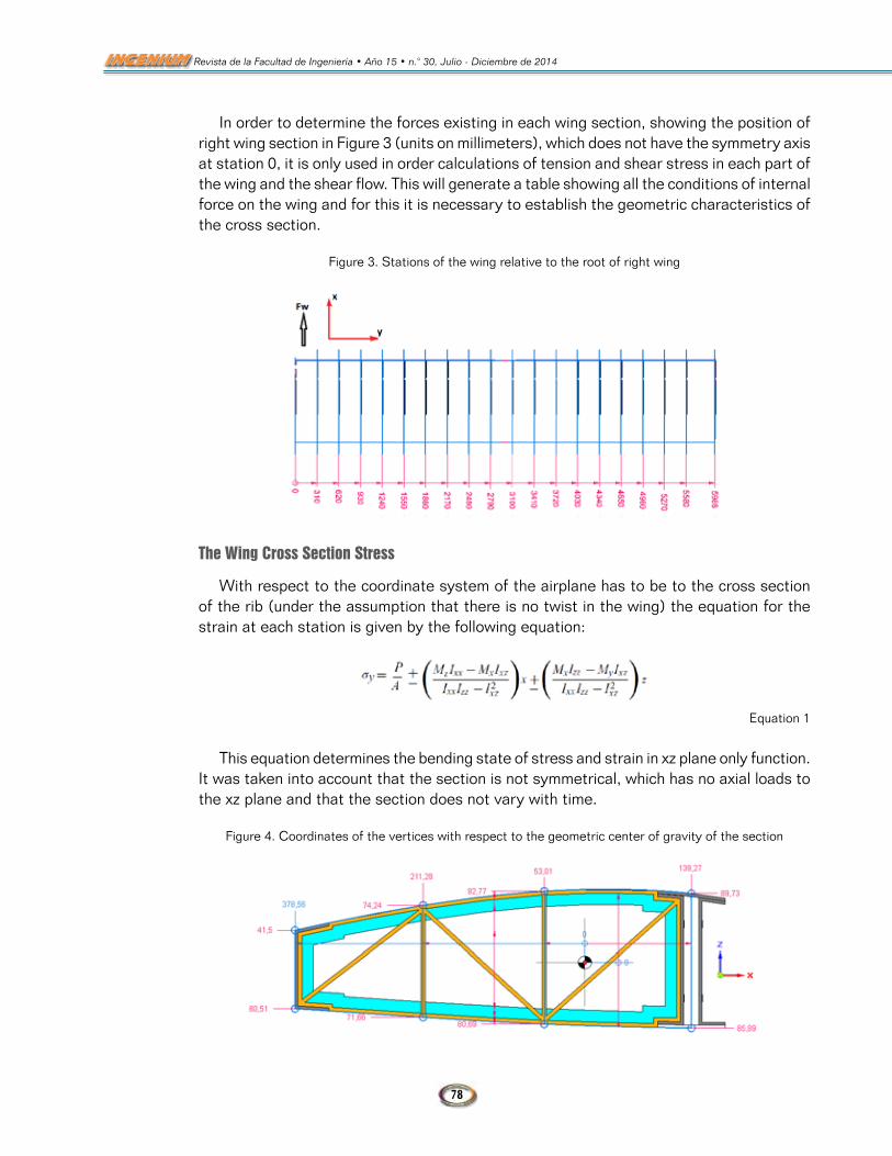
In order to determine the forces existing in each wing section, showing the position of right wing section in Figure 3 (units on millimeters), which does not have the symmetry axis at station 0, it is only used in order calculations of tension and shear stress in each part of the wing and the shear flow. This will generate a table showing all the conditions of internal force on the wing and for this it is necessary to establish the geometric characteristics of the cross section.
Figure 3. Stations of the wing relative to the root of right wing
The Wing Cross Section Stress
With respect to the coordinate system of the airplane has to be to the cross section of the rib (under the assumption that there is no twist in the wing) the equation for the strain at each station is given by the following equation:
7
The Wing Cross Section Stress
With respect to the coordinate system of the airplane has to be to the cross section of the rib (under the assumption that there is no twist in the wing) the equation for the strain at each station is given by the following equation:
Equation 1
This equation determines the bending state of stress and strain in xz plane only function. It was taken into account that the section is not symmetrical, which has no axial loads to the xz plane and that the section does not vary with time.
Figure 4. Coordinates of the vertices with respect to the geometric center of gravity of the section
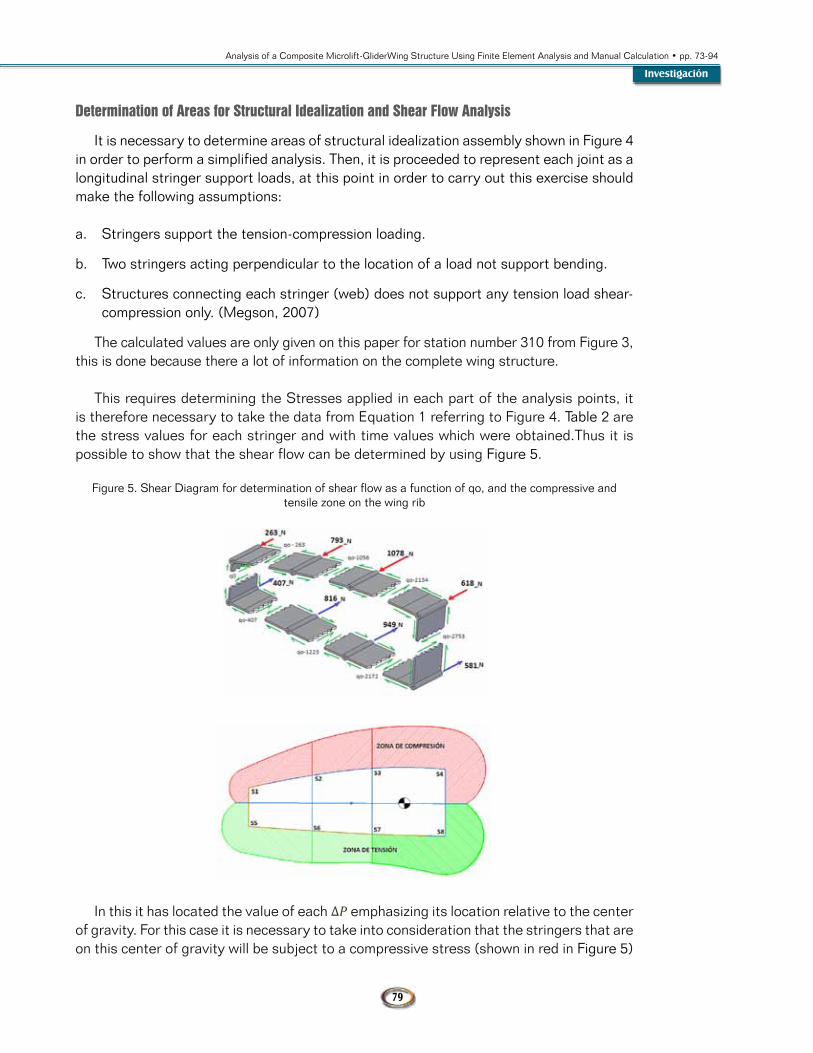
Determination of Areas for Structural Idealization and Shear Flow Analysis
It is necessary to determine areas of structural idealization assembly shown in
Figure 4 in order to perform a simplified analysis. Then, it is proceeded to represent each joint as a longitudinal stringer support loads, at this point in order to carry out this exercise should make the following assumptions:
a. Stringers support the tension-compression loading. b. Two stringers acting perpendicular to the location of a load not support bending. c. Structures connecting each stringer (web) does not support any tension load shear-compression
only. (Megson, 2007)
The calculated values are only given on this paper for station number 310 from Figure 3, this is done because there a lot of information on the complete wing structure.
This requires determining the Stresses applied in each part of the analysis points, it is therefore necessary to take the data from Equation 1 referring to
Figure 4. Table 2 are the stress values for each stringer and with time values which were obtained.Thus it is possible to show that the shear flow can be determined by using Figure 5.
Equation 1
This equation determines the bending state of stress and strain in xz plane only function. It was taken into account that the section is not symmetrical, which has no axial loads to the xz plane and that the section does not vary with time.
Figure 4. Coordinates of the vertices with respect to the geometric center of gravity of the section
Investigación
79
Analysis of a Composite Microlift-GliderWing Structure Using Finite Element Analysis and Manual Calculation • pp. 73-94
Determination of Areas for Structural Idealization and Shear Flow Analysis
It is necessary to determine areas of structural idealization assembly shown in Figure 4 in order to perform a simplified analysis. Then, it is proceeded to represent each joint as a longitudinal stringer support loads, at this point in order to carry out this exercise should make the following assumptions:
a. Stringers support the tension-compression loading.
b. Two stringers acting perpendicular to the location of a load not support bending.
c. Structures connecting each stringer (web) does not support any tension load shear-compression only. (Megson, 2007)
The calculated values are only given on this paper for station number 310 from Figure 3, this is done because there a lot of information on the complete wing structure.
This requires determining the Stresses applied in each part of the analysis points, it is therefore necessary to take the data from Equation 1 referring to Figure 4. Table 2 are the stress values for each stringer and with time values which were obtained.Thus it is possible to show that the shear flow can be determined by using Figure 5.
Figure 5. Shear Diagram for determination of shear flow as a function of qo, and the compressive and tensile zone on the wing rib
In this it has located the value of each
8
Figure 5. Shear Diagram for determination of shear flow as a function of qo, and the compressive and tensile zone on the wing rib
In this it has located the value of each emphasizing its location relative to the center of gravity. For this case it is necessary to take into consideration that the stringers that are on this center of gravity will be subject to a compressive stress (shown in red in Figure 5) and those under tensile force are located under it (this can be seen more clearly in Figure 5). q0 is the shear flow on the rear beam, thus the flow is supposed to be located between the 1st and 5th stringer termed q0 (Jones, 1999).
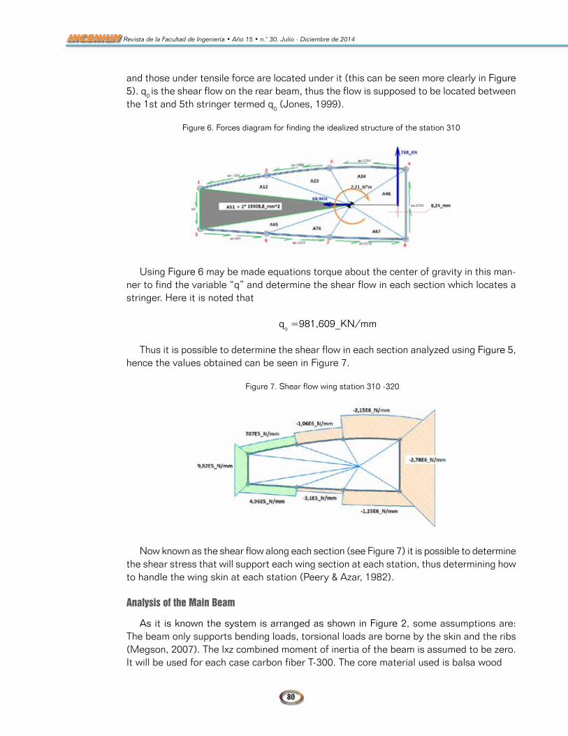
Figure 6. Forces diagram for finding the idealized structure of the station 310
Using Figure 6 may be made equations torque about the center of gravity in this manner to find the variable "q" and determine the shear flow in each section which locates a stringer. Here it is noted that
qo =981,609_KN/mm
Thus it is possible to determine the shear flow in each section analyzed using Figure 5, hence the values obtained can be seen in Figure 7.
Figure 7. Shear flow wing station 310 -320
emphasizing its location relative to the center of gravity. For this case it is necessary to take into consideration that the stringers that are on this center of gravity will be subject to a compressive stress (shown in red in Figure 5)
80
Revista de la Facultad de Ingeniería • Año 15 • n.° 30, Julio - Diciembre de 2014
and those under tensile force are located under it (this can be seen more clearly in Figure 5). q0 is the shear flow on the rear beam, thus the flow is supposed to be located between the 1st and 5th stringer termed q0 (Jones, 1999).
Figure 6. Forces diagram for finding the idealized structure of the station 310
Using Figure 6 may be made equations torque about the center of gravity in this man-ner to find the variable “q” and determine the shear flow in each section which locates a stringer. Here it is noted that
qo =981,609_KN/mm
Thus it is possible to determine the shear flow in each section analyzed using Figure 5, hence the values obtained can be seen in Figure 7.
Figure 7. Shear flow wing station 310 -320
Now known as the shear flow along each section (see Figure 7) it is possible to determine the shear stress that will support each wing section at each station, thus determining how to handle the wing skin at each station (Peery & Azar, 1982).
Analysis of the Main Beam
As it is known the system is arranged as shown in Figure 2, some assumptions are: The beam only supports bending loads, torsional loads are borne by the skin and the ribs (Megson, 2007). The Ixz combined moment of inertia of the beam is assumed to be zero. It will be used for each case carbon fiber T-300. The core material used is balsa wood
Investigación
81
Analysis of a Composite Microlift-GliderWing Structure Using Finite Element Analysis and Manual Calculation • pp. 73-94
Beam characteristics are as shown below; worth noting that in this case the cross section of the beam is not constant along the span, due to the arrangement of composite plies necessary to support loads of lift and drag, the plies quantity are lower the closer the tip. Thus section presented is an initial approximation that is expected to be the cross section of the wing at the root thereof (Allen & Haisler, 1985).
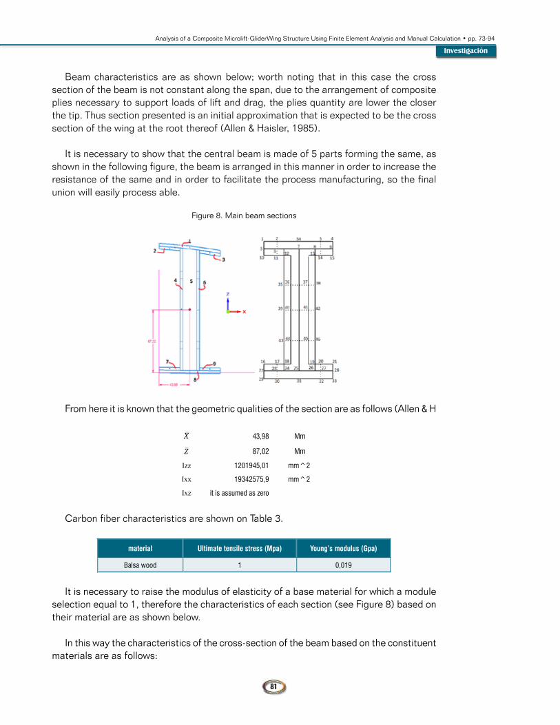
It is necessary to show that the central beam is made of 5 parts forming the same, as shown in the following figure, the beam is arranged in this manner in order to increase the resistance of the same and in order to facilitate the process manufacturing, so the final union will easily process able.
Figure 8. Main beam sections
From here it is known that the geometric qualities of the section are as follows (Allen & H
10
43,98 Mm 87,02 Mm
Izz 1201945,01 mm^2 Ixx 19342575,9 mm^2 Ixz it is assumed as zero
Carbon fiber characteristics are shown on
Table 3.
material Ultimate tensile stress (Mpa) Young’s modulus
(Gpa) Balsa wood 1 0,019
It is necessary to raise the modulus of elasticity of a base material for which a module selection equal to 1, therefore the characteristics of each section (see Figure 8) based on their material are as shown below.
In this way the characteristics of the cross-section of the beam based on the constituent materials are as follows:
Curved cross section beam
Plane cross section beam
0,000177214 m 0,177213718 mm -1,42278E-05 m -0,014227787 mm
Izz 6,03829E-07 m^4 603828,5125 mm^4 Ixx 1,93426E-05 m^5 19342575,9 mm^4
Iz´z´ 6,03827E-07 m^6 603827,3223 mm^4 Ix´x´ 1,93424E-05 m^7 19342391,26 mm^4 A* 1,173215663 m^2 1173215,663 mm^2 ´* 0,000410955 m 410,9552076 mm
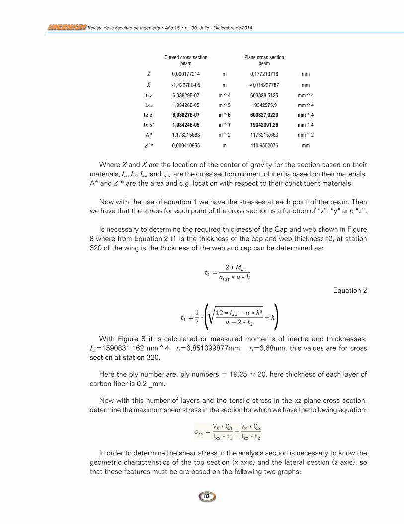
Where and are the location of the center of gravity for the section based on their materials, Izz, Ixx, Iz´z´ and Ix´x´ are the cross section moment of inertia based on their materials, A* and ´* are the area and c.g. location with respect to their constituent materials.
Now with the use of equation 1 we have the stresses at each point of the beam. Then we have that the stress for each point of the cross section is a function of "x", "y" and "z".
Is necessary to determine the required thickness of the Cap and web shown in Figure 8 where from Equation 2 t1 is the thickness of the cap and web thickness t2, at station 320 of the wing is the thickness of the web and cap can be determined as:
43,98 Mm
10
43,98 Mm 87,02 Mm
Izz 1201945,01 mm^2 Ixx 19342575,9 mm^2 Ixz it is assumed as zero
Carbon fiber characteristics are shown on
Table 3.
material Ultimate tensile stress (Mpa) Young’s modulus
(Gpa) Balsa wood 1 0,019
It is necessary to raise the modulus of elasticity of a base material for which a module selection equal to 1, therefore the characteristics of each section (see Figure 8) based on their material are as shown below.
In this way the characteristics of the cross-section of the beam based on the constituent materials are as follows:
Curved cross section beam
Plane cross section beam
0,000177214 m 0,177213718 mm -1,42278E-05 m -0,014227787 mm
Izz 6,03829E-07 m^4 603828,5125 mm^4 Ixx 1,93426E-05 m^5 19342575,9 mm^4
Iz´z´ 6,03827E-07 m^6 603827,3223 mm^4 Ix´x´ 1,93424E-05 m^7 19342391,26 mm^4 A* 1,173215663 m^2 1173215,663 mm^2
´* 0,000410955 m 410,9552076 mm
Where and are the location of the center of gravity for the section based on their materials, Izz, Ixx, Iz´z´ and Ix´x´ are the cross section moment of inertia based on their materials, A* and ´* are the area and c.g. location with respect to their constituent materials.
Now with the use of equation 1 we have the stresses at each point of the beam. Then we have that the stress for each point of the cross section is a function of "x", "y" and "z".
Is necessary to determine the required thickness of the Cap and web shown in Figure 8 where from Equation 2 t1 is the thickness of the cap and web thickness t2, at station 320 of the wing is the thickness of the web and cap can be determined as:
87,02 Mm
Izz 1201945,01 mm^2
Ixx 19342575,9 mm^2
Ixz it is assumed as zero
Carbon fiber characteristics are shown on Table 3.
material Ultimate tensile stress (Mpa) Young’s modulus (Gpa)
Balsa wood 1 0,019
It is necessary to raise the modulus of elasticity of a base material for which a module selection equal to 1, therefore the characteristics of each section (see Figure 8) based on their material are as shown below.
In this way the characteristics of the cross-section of the beam based on the constituent materials are as follows:
82
Revista de la Facultad de Ingeniería • Año 15 • n.° 30, Julio - Diciembre de 2014
Curved cross section beam
Plane cross section beam
10
43,98 Mm 87,02 Mm
Izz 1201945,01 mm^2 Ixx 19342575,9 mm^2 Ixz it is assumed as zero
Carbon fiber characteristics are shown on
Table 3.
material Ultimate tensile stress (Mpa) Young’s modulus
(Gpa) Balsa wood 1 0,019
It is necessary to raise the modulus of elasticity of a base material for which a module selection equal to 1, therefore the characteristics of each section (see Figure 8) based on their material are as shown below.
In this way the characteristics of the cross-section of the beam based on the constituent materials are as follows:
Curved cross section beam
Plane cross section beam
0,000177214 m 0,177213718 mm -1,42278E-05 m -0,014227787 mm
Izz 6,03829E-07 m^4 603828,5125 mm^4 Ixx 1,93426E-05 m^5 19342575,9 mm^4
Iz´z´ 6,03827E-07 m^6 603827,3223 mm^4 Ix´x´ 1,93424E-05 m^7 19342391,26 mm^4 A* 1,173215663 m^2 1173215,663 mm^2
´* 0,000410955 m 410,9552076 mm
Where and are the location of the center of gravity for the section based on their materials, Izz, Ixx, Iz´z´ and Ix´x´ are the cross section moment of inertia based on their materials, A* and ´* are the area and c.g. location with respect to their constituent materials.
Now with the use of equation 1 we have the stresses at each point of the beam. Then we have that the stress for each point of the cross section is a function of "x", "y" and "z".
Is necessary to determine the required thickness of the Cap and web shown in Figure 8 where from Equation 2 t1 is the thickness of the cap and web thickness t2, at station 320 of the wing is the thickness of the web and cap can be determined as:
0,000177214 m 0,177213718 mm
10
43,98 Mm 87,02 Mm
Izz 1201945,01 mm^2 Ixx 19342575,9 mm^2 Ixz it is assumed as zero
Carbon fiber characteristics are shown on
Table 3.
material Ultimate tensile stress (Mpa) Young’s modulus
(Gpa) Balsa wood 1 0,019
It is necessary to raise the modulus of elasticity of a base material for which a module selection equal to 1, therefore the characteristics of each section (see Figure 8) based on their material are as shown below.
In this way the characteristics of the cross-section of the beam based on the constituent materials are as follows:
Curved cross section beam
Plane cross section beam
0,000177214 m 0,177213718 mm -1,42278E-05 m -0,014227787 mm
Izz 6,03829E-07 m^4 603828,5125 mm^4 Ixx 1,93426E-05 m^5 19342575,9 mm^4
Iz´z´ 6,03827E-07 m^6 603827,3223 mm^4 Ix´x´ 1,93424E-05 m^7 19342391,26 mm^4 A* 1,173215663 m^2 1173215,663 mm^2
´* 0,000410955 m 410,9552076 mm
Where and are the location of the center of gravity for the section based on their materials, Izz, Ixx, Iz´z´ and Ix´x´ are the cross section moment of inertia based on their materials, A* and ´* are the area and c.g. location with respect to their constituent materials.
Now with the use of equation 1 we have the stresses at each point of the beam. Then we have that the stress for each point of the cross section is a function of "x", "y" and "z".
Is necessary to determine the required thickness of the Cap and web shown in Figure 8 where from Equation 2 t1 is the thickness of the cap and web thickness t2, at station 320 of the wing is the thickness of the web and cap can be determined as:
-1,42278E-05 m -0,014227787 mm
Izz 6,03829E-07 m^4 603828,5125 mm^4
Ixx 1,93426E-05 m^5 19342575,9 mm^4
Iz´z´ 6,03827E-07 m^6 603827,3223 mm^4
Ix´x´ 1,93424E-05 m^7 19342391,26 mm^4
A* 1,173215663 m^2 1173215,663 mm^2
10
43,98 Mm 87,02 Mm
Izz 1201945,01 mm^2 Ixx 19342575,9 mm^2 Ixz it is assumed as zero
Carbon fiber characteristics are shown on
Table 3.
material Ultimate tensile stress (Mpa) Young’s modulus
(Gpa) Balsa wood 1 0,019
It is necessary to raise the modulus of elasticity of a base material for which a module selection equal to 1, therefore the characteristics of each section (see Figure 8) based on their material are as shown below.
In this way the characteristics of the cross-section of the beam based on the constituent materials are as follows:
Curved cross section beam
Plane cross section beam
0,000177214 m 0,177213718 mm -1,42278E-05 m -0,014227787 mm
Izz 6,03829E-07 m^4 603828,5125 mm^4 Ixx 1,93426E-05 m^5 19342575,9 mm^4
Iz´z´ 6,03827E-07 m^6 603827,3223 mm^4 Ix´x´ 1,93424E-05 m^7 19342391,26 mm^4 A* 1,173215663 m^2 1173215,663 mm^2 ´* 0,000410955 m 410,9552076 mm
Where and are the location of the center of gravity for the section based on their materials, Izz, Ixx, Iz´z´ and Ix´x´ are the cross section moment of inertia based on their materials, A* and ´* are the area and c.g. location with respect to their constituent materials.
Now with the use of equation 1 we have the stresses at each point of the beam. Then we have that the stress for each point of the cross section is a function of "x", "y" and "z".
Is necessary to determine the required thickness of the Cap and web shown in Figure 8 where from Equation 2 t1 is the thickness of the cap and web thickness t2, at station 320 of the wing is the thickness of the web and cap can be determined as:
0,000410955 m 410,9552076 mm
Where Z and X are the location of the center of gravity for the section based on their materials, Izz, Ixx, Iz´z´ and Ix´x´ are the cross section moment of inertia based on their materials, A* and Z´* are the area and c.g. location with respect to their constituent materials.
Now with the use of equation 1 we have the stresses at each point of the beam. Then we have that the stress for each point of the cross section is a function of “x”, “y” and “z”.
Is necessary to determine the required thickness of the Cap and web shown in Figure 8 where from Equation 2 t1 is the thickness of the cap and web thickness t2, at station 320 of the wing is the thickness of the web and cap can be determined as:
11
Equation 2
With Figure 8 it is calculated or measured moments of inertia and thicknesses: =1590831,162 mm^4, , this values are for cross section at station 320.
Here the ply number are, ply numbers = 19,25 ≈ 20, here thickness of each layer of carbon fiber is 0.2 _mm.
Now with this number of layers and the tensile stress in the xz plane cross section, determine the maximum shear stress in the section for which we have the following equation:
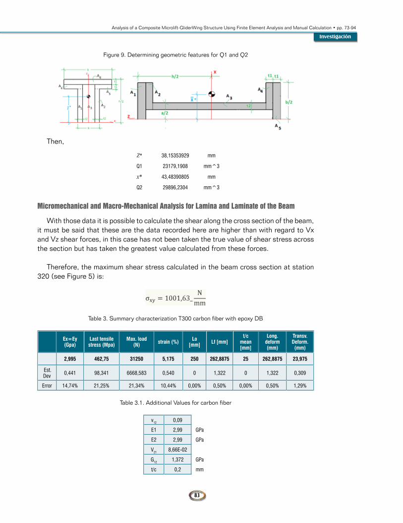
In order to determine the shear stress in the analysis section is necessary to know the geometric characteristics of the top section (x-axis) and the lateral section (z-axis), so that these features must be are based on the following two graphs:
Figure 9. Determining geometric features for Q1 and Q2
Then,
38,15353929 mm Q1 23179,1908 mm^3
43,48390805 mm Q2 29896,2304 mm^3
Micromechanical and Macro-Mechanical Analysis for Lamina and Laminate of the Beam
With those data it is possible to calculate the shear along the cross section of the beam, it must be said that these are the data recorded here are higher than with regard to Vx and Vz shear forces,
Equation 2
11
Equation 2
With Figure 8 it is calculated or measured moments of inertia and thicknesses: =1590831,162 mm^4, , this values are for cross section at station 320.
Here the ply number are, ply numbers = 19,25 ≈ 20, here thickness of each layer of carbon fiber is 0.2 _mm.
Now with this number of layers and the tensile stress in the xz plane cross section, determine the maximum shear stress in the section for which we have the following equation:
In order to determine the shear stress in the analysis section is necessary to know the geometric characteristics of the top section (x-axis) and the lateral section (z-axis), so that these features must be are based on the following two graphs:
Figure 9. Determining geometric features for Q1 and Q2
Then,
38,15353929 mm Q1 23179,1908 mm^3
43,48390805 mm Q2 29896,2304 mm^3
Micromechanical and Macro-Mechanical Analysis for Lamina and Laminate of the Beam
With those data it is possible to calculate the shear along the cross section of the beam, it must be said that these are the data recorded here are higher than with regard to Vx and Vz shear forces,
With Figure 8 it is calculated or measured moments of inertia and thicknesses: Ixx=1590831,162 mm^4, t1=3,851099877mm, t1=3,68mm, this values are for cross section at station 320.
Here the ply number are, ply numbers = 19,25 ≈ 20, here thickness of each layer of carbon fiber is 0.2 _mm.
Now with this number of layers and the tensile stress in the xz plane cross section, determine the maximum shear stress in the section for which we have the following equation:
11
Equation 2
With Figure 8 it is calculated or measured moments of inertia and thicknesses: =1590831,162 mm^4, , this values are for cross section at station 320.
Here the ply number are, ply numbers = 19,25 ≈ 20, here thickness of each layer of carbon fiber is 0.2 _mm.
Now with this number of layers and the tensile stress in the xz plane cross section, determine the maximum shear stress in the section for which we have the following equation:
In order to determine the shear stress in the analysis section is necessary to know the geometric characteristics of the top section (x-axis) and the lateral section (z-axis), so that these features must be are based on the following two graphs:
Figure 9. Determining geometric features for Q1 and Q2
Then,
38,15353929 mm Q1 23179,1908 mm^3
43,48390805 mm Q2 29896,2304 mm^3
Micromechanical and Macro-Mechanical Analysis for Lamina and Laminate of the Beam
With those data it is possible to calculate the shear along the cross section of the beam, it must be said that these are the data recorded here are higher than with regard to Vx and Vz shear forces,
In order to determine the shear stress in the analysis section is necessary to know the geometric characteristics of the top section (x-axis) and the lateral section (z-axis), so that these features must be are based on the following two graphs:
Investigación
83
Analysis of a Composite Microlift-GliderWing Structure Using Finite Element Analysis and Manual Calculation • pp. 73-94
Figure 9. Determining geometric features for Q1 and Q2
Then,
Z* 38,15353929 mm
Q1 23179,1908 mm^3
x* 43,48390805 mm
Q2 29896,2304 mm^3
Micromechanical and Macro-Mechanical Analysis for Lamina and Laminate of the Beam
With those data it is possible to calculate the shear along the cross section of the beam, it must be said that these are the data recorded here are higher than with regard to Vx and Vz shear forces, in this case has not been taken the true value of shear stress across the section but has taken the greatest value calculated from these forces.
Therefore, the maximum shear stress calculated in the beam cross section at station 320 (see Figure 5) is:
12
in this case has not been taken the true value of shear stress across the section but has taken the greatest value calculated from these forces.
Therefore, the maximum shear stress calculated in the beam cross section at station 320 (see Figure 5) is:
Table 3. Summary characterization T300 carbon fiber with epoxy DB
Ex=Ey (Gpa)
Last tensile stress (Mpa)
Max. load (N)
strain (%)
Lo [mm]
Lf [mm]
t/c mean [mm]
Long. defor
m (mm)
Transv. Deform.
(mm)
2,995 462,75 31250 5,175 250 262,8875 25 262,88
75 23,975
Est. Dev 0,441 98,341
6668,583 0,540 0 1,322 0 1,322 0,309
Error 14,74% 21,25%
21,34%
10,44%
0,00%
0,50% 0,00% 0,50% 1,29%
Table 3.1. Additional Values for carbon fiber
v12 0,09 E1 2,99 GPa
E2 2,99 GPa V21 8,66E-02
G12 1,372 GPa t/c 0,2 mm
Based on
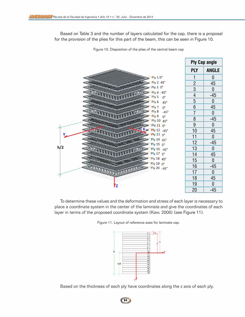
Table 3 and the number of layers calculated for the cap, there is a proposal for the provision of the plies for this part of the beam, this can be seen in Figure 10.
Figure 10. Disposition of the plies of the central beam cap
Table 3. Summary characterization T300 carbon fiber with epoxy DB
Ex=Ey (Gpa)
Last tensile stress (Mpa)
Max. load (N) strain (%) Lo
[mm] Lf [mm]t/c
mean [mm]
Long. deform (mm)
Transv. Deform. (mm)
2,995 462,75 31250 5,175 250 262,8875 25 262,8875 23,975
Est. Dev 0,441 98,341 6668,583 0,540 0 1,322 0 1,322 0,309
Error 14,74% 21,25% 21,34% 10,44% 0,00% 0,50% 0,00% 0,50% 1,29%
Table 3.1. Additional Values for carbon fiber
v12 0,09
E1 2,99 GPa
E2 2,99 GPa
V21 8,66E-02
G12 1,372 GPa
t/c 0,2 mm
84
Revista de la Facultad de Ingeniería • Año 15 • n.° 30, Julio - Diciembre de 2014
Based on Table 3 and the number of layers calculated for the cap, there is a proposal for the provision of the plies for this part of the beam, this can be seen in Figure 10.
Figure 10. Disposition of the plies of the central beam cap
Ply Cap angle
PLY ANGLE1 02 453 04 -455 06 457 08 -459 0
10 4511 012 -4513 014 4515 016 -4517 018 4519 020 -45
To determine these values and the deformation and stress of each layer is necessary to place a coordinate system in the center of the laminate and give the coordinates of each layer in terms of the proposed coordinate system (Kaw, 2006) (see Figure 11).
Figure 11. Layout of reference axes for laminate cap.
Based on the thickness of each ply have coordinates along the z axis of each ply.
Investigación
85
Analysis of a Composite Microlift-GliderWing Structure Using Finite Element Analysis and Manual Calculation • pp. 73-94
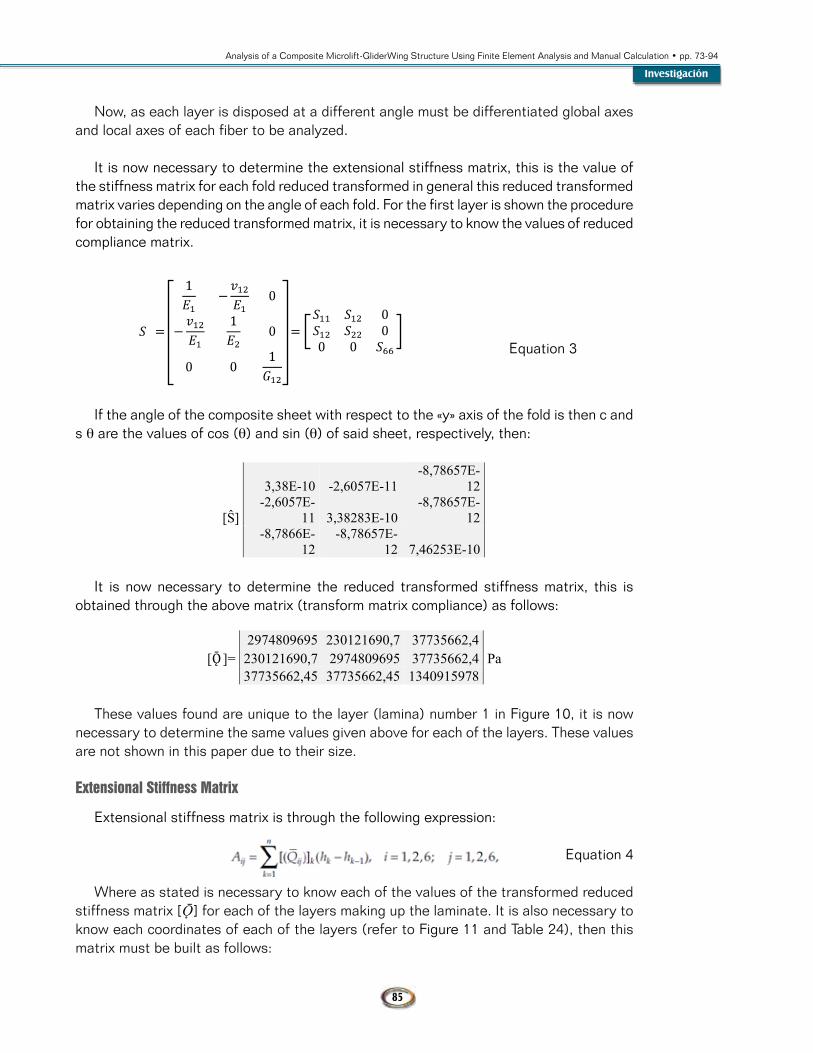
Now, as each layer is disposed at a different angle must be differentiated global axes and local axes of each fiber to be analyzed.
It is now necessary to determine the extensional stiffness matrix, this is the value of the stiffness matrix for each fold reduced transformed in general this reduced transformed matrix varies depending on the angle of each fold. For the first layer is shown the procedure for obtaining the reduced transformed matrix, it is necessary to know the values of reduced compliance matrix.
14
depending on the angle of each fold. For the first layer is shown the procedure for obtaining the reduced transformed matrix, it is necessary to know the values of reduced compliance matrix.
Equation 3
If the angle of the composite sheet with respect to the "y" axis of the fold is then c and s θ are the values of cos (θ) and sin (θ) of said sheet, respectively, then:
3,38E-10 -2,6057E-11
-8,78657E-12
[Ŝ] -2,6057E-
11 3,38283E-10 -8,78657E-
12
-8,7866E-12
-8,78657E-12 7,46253E-10
It is now necessary to determine the reduced transformed stiffness matrix, this is obtained through the above matrix (transform matrix compliance) as follows:
2974809695 230121690,7 37735662,4
[Ǭ ]= 230121690,7 2974809695 37735662,4 Pa
37735662,45 37735662,45 1340915978
These values found are unique to the layer (lamina) number 1 in Figure 10, it is now necessary to determine the same values given above for each of the layers. These values are not shown in this paper due to their size.
Extensional Stiffness Matrix
Extensional stiffness matrix is through the following expression:
Equation 4
] for each of the layers making up the laminate. It is also necessary to know each coordinates of each of the layers (refer to Figure 11 and Table 24), then this matrix must be built as follows:
Equation 3
If the angle of the composite sheet with respect to the «y» axis of the fold is then c and s θ are the values of cos (θ) and sin (θ) of said sheet, respectively, then:
14
depending on the angle of each fold. For the first layer is shown the procedure for obtaining the reduced transformed matrix, it is necessary to know the values of reduced compliance matrix.
Equation 3
If the angle of the composite sheet with respect to the "y" axis of the fold is then c and s θ are the values of cos (θ) and sin (θ) of said sheet, respectively, then:
3,38E-10 -2,6057E-11
-8,78657E-12
[Ŝ] -2,6057E-
11 3,38283E-10 -8,78657E-
12
-8,7866E-12
-8,78657E-12 7,46253E-10
It is now necessary to determine the reduced transformed stiffness matrix, this is obtained through the above matrix (transform matrix compliance) as follows:
2974809695 230121690,7 37735662,4
[Ǭ ]= 230121690,7 2974809695 37735662,4 Pa
37735662,45 37735662,45 1340915978
These values found are unique to the layer (lamina) number 1 in Figure 10, it is now necessary to determine the same values given above for each of the layers. These values are not shown in this paper due to their size.
Extensional Stiffness Matrix
Extensional stiffness matrix is through the following expression:
Equation 4
] for each of the layers making up the laminate. It is also necessary to know each coordinates of each of the layers (refer to Figure 11 and Table 24), then this matrix must be built as follows:
It is now necessary to determine the reduced transformed stiffness matrix, this is obtained through the above matrix (transform matrix compliance) as follows:
14
depending on the angle of each fold. For the first layer is shown the procedure for obtaining the reduced transformed matrix, it is necessary to know the values of reduced compliance matrix.
Equation 3
If the angle of the composite sheet with respect to the "y" axis of the fold is then c and s θ are the values of cos (θ) and sin (θ) of said sheet, respectively, then:
3,38E-10 -2,6057E-11
-8,78657E-12
[Ŝ] -2,6057E-
11 3,38283E-10 -8,78657E-
12
-8,7866E-12
-8,78657E-12 7,46253E-10
It is now necessary to determine the reduced transformed stiffness matrix, this is obtained through the above matrix (transform matrix compliance) as follows:
2974809695 230121690,7 37735662,4
[Ǭ ]= 230121690,7 2974809695 37735662,4 Pa
37735662,45 37735662,45 1340915978
These values found are unique to the layer (lamina) number 1 in Figure 10, it is now necessary to determine the same values given above for each of the layers. These values are not shown in this paper due to their size.
Extensional Stiffness Matrix
Extensional stiffness matrix is through the following expression:
Equation 4
] for each of the layers making up the laminate. It is also necessary to know each coordinates of each of the layers (refer to Figure 11 and Table 24), then this matrix must be built as follows:
These values found are unique to the layer (lamina) number 1 in Figure 10, it is now necessary to determine the same values given above for each of the layers. These values are not shown in this paper due to their size.
Extensional Stiffness Matrix
Extensional stiffness matrix is through the following expression:
Equation 4
Where as stated is necessary to know each of the values of the transformed reduced stiffness matrix [Ǭ] for each of the layers making up the laminate. It is also necessary to know each coordinates of each of the layers (refer to Figure 11 and Table 24), then this matrix must be built as follows:
14
depending on the angle of each fold. For the first layer is shown the procedure for obtaining the reduced transformed matrix, it is necessary to know the values of reduced compliance matrix.
Equation 3
If the angle of the composite sheet with respect to the "y" axis of the fold is then c and s θ are the values of cos (θ) and sin (θ) of said sheet, respectively, then:
3,38E-10 -2,6057E-11
-8,78657E-12
[Ŝ] -2,6057E-
11 3,38283E-10 -8,78657E-
12
-8,7866E-12
-8,78657E-12 7,46253E-10
It is now necessary to determine the reduced transformed stiffness matrix, this is obtained through the above matrix (transform matrix compliance) as follows:
2974809695 230121690,7 37735662,4
[Ǭ ]= 230121690,7 2974809695 37735662,4 Pa
37735662,45 37735662,45 1340915978
These values found are unique to the layer (lamina) number 1 in Figure 10, it is now necessary to determine the same values given above for each of the layers. These values are not shown in this paper due to their size.
Extensional Stiffness Matrix
Extensional stiffness matrix is through the following expression:
Equation 4
] for each of the layers making up the laminate. It is also necessary to know each coordinates of each of the layers (refer to Figure 11 and Table 24), then this matrix must be built as follows:
86
Revista de la Facultad de Ingeniería • Año 15 • n.° 30, Julio - Diciembre de 2014
15
[A] =
-6,04E
+08
-5,23E+
07 0,00E+
00 -
5,23E+07
-5,74E+
08 0,00E
+00
0,00E+00
0,00E+00
-2,74E
+08
+
-5,95E
+08
-4,60E+
07
-7,55E+
06
4,60E+07
-5,95E+
08
-7,55E+
06 -
7,55E+06
-7,55E+
06
-2,68E+
08
+
-6,04E+
08
-5,23E
+07 0,00E
+00 -
5,23E+07
-5,74E
+08 0,00E
+00
0,00E+00
0,00E+00
-2,74E
+08
+ …
[Ǭ ]*(h0-h1) laminate 1 [Ǭ ] *(h1-h2)
laminate 2 [Ǭ ] *(h2-h3) laminate 3 [Ǭ ] …
Thus,
-1,20E+10
-9,83E+08 0,00E+00
[A] =
-9,83E+08
-1,17E+10 0,00E+00 Pa
0,00E+00 0,00E+00
-5,43E+09
Engaging Stiffness Matrix
The coupling stiffness matrix is found by the following expression:
Equation 5
] for each of the component layers of the laminate. It is also necessary to know each coordinates of each of the layers (refer to Figure 11), then this matrix must be built as follows:
-8,81E+06
-6,29E+06
-1,51E+07
[B] =
-6,29E+06 2,14E+07
-1,51E+07 Pa
-1,51E+07
-1,51E+07
-6,29E+06
Bending Stiffness Matrix
The coupling stiffness matrix is found by the following expression:
Thus,
15
[A] =
-6,04E
+08
-5,23E+
07 0,00E+
00 -
5,23E+07
-5,74E+
08 0,00E
+00
0,00E+00
0,00E+00
-2,74E
+08
+
-5,95E
+08
-4,60E+
07
-7,55E+
06
4,60E+07
-5,95E+
08
-7,55E+
06 -
7,55E+06
-7,55E+
06
-2,68E+
08
+
-6,04E+
08
-5,23E
+07 0,00E
+00 -
5,23E+07
-5,74E
+08 0,00E
+00
0,00E+00
0,00E+00
-2,74E
+08
+ …
[Ǭ ]*(h0-h1) laminate 1 [Ǭ ] *(h1-h2)
laminate 2 [Ǭ ] *(h2-h3) laminate 3 [Ǭ ] …
Thus,
-1,20E+10
-9,83E+08 0,00E+00
[A] =
-9,83E+08
-1,17E+10 0,00E+00 Pa
0,00E+00 0,00E+00
-5,43E+09
Engaging Stiffness Matrix
The coupling stiffness matrix is found by the following expression:
Equation 5
] for each of the component layers of the laminate. It is also necessary to know each coordinates of each of the layers (refer to Figure 11), then this matrix must be built as follows:
-8,81E+06
-6,29E+06
-1,51E+07
[B] =
-6,29E+06 2,14E+07
-1,51E+07 Pa
-1,51E+07
-1,51E+07
-6,29E+06
Bending Stiffness Matrix
The coupling stiffness matrix is found by the following expression:
Engaging Stiffness Matrix
The coupling stiffness matrix is found by the following expression:
Equation 5
Where as stated is necessary to know each of the values of the transformed reduced stiffness matrix [Ǭ] for each of the component layers of the laminate. It is also necessary to know each coordinates of each of the layers (refer to Figure 11), then this matrix must be built as follows:
15
[A] =
-6,04E
+08
-5,23E+
07 0,00E+
00 -
5,23E+07
-5,74E+
08 0,00E
+00
0,00E+00
0,00E+00
-2,74E
+08
+
-5,95E
+08
-4,60E+
07
-7,55E+
06
4,60E+07
-5,95E+
08
-7,55E+
06 -
7,55E+06
-7,55E+
06
-2,68E+
08
+
-6,04E+
08
-5,23E
+07 0,00E
+00 -
5,23E+07
-5,74E
+08 0,00E
+00
0,00E+00
0,00E+00
-2,74E
+08
+ …
[Ǭ ]*(h0-h1) laminate 1 [Ǭ ] *(h1-h2)
laminate 2 [Ǭ ] *(h2-h3) laminate 3 [Ǭ ] …
Thus,
-1,20E+10
-9,83E+08 0,00E+00
[A] =
-9,83E+08
-1,17E+10 0,00E+00 Pa
0,00E+00 0,00E+00
-5,43E+09
Engaging Stiffness Matrix
The coupling stiffness matrix is found by the following expression:
Equation 5
] for each of the component layers of the laminate. It is also necessary to know each coordinates of each of the layers (refer to Figure 11), then this matrix must be built as follows:
-8,81E+06
-6,29E+06
-1,51E+07
[B] =
-6,29E+06 2,14E+07
-1,51E+07 Pa
-1,51E+07
-1,51E+07
-6,29E+06
Bending Stiffness Matrix
The coupling stiffness matrix is found by the following expression: Bending Stiffness Matrix
The coupling stiffness matrix is found by the following expression:
Equation 6
As the above is necessary to use the reduced transformed stiffness matrix [Ǭ] and the coordinate values of the layers (plies) with respect to the coordinate system that is in the middle of the laminate, so this matrix is determined as follows:
15
[A] =
-6,04E
+08
-5,23E+
07 0,00E+
00 -
5,23E+07
-5,74E+
08 0,00E
+00
0,00E+00
0,00E+00
-2,74E
+08
+
-5,95E
+08
-4,60E+
07
-7,55E+
06
4,60E+07
-5,95E+
08
-7,55E+
06 -
7,55E+06
-7,55E+
06
-2,68E+
08
+
-6,04E+
08
-5,23E
+07 0,00E
+00 -
5,23E+07
-5,74E
+08 0,00E
+00
0,00E+00
0,00E+00
-2,74E
+08
+ …
[Ǭ ]*(h0-h1) laminate 1 [Ǭ ] *(h1-h2)
laminate 2 [Ǭ ] *(h2-h3) laminate 3 [Ǭ ] …
Thus,
-1,20E+10
-9,83E+08 0,00E+00
[A] =
-9,83E+08
-1,17E+10 0,00E+00 Pa
0,00E+00 0,00E+00
-5,43E+09
Engaging Stiffness Matrix
The coupling stiffness matrix is found by the following expression:
Equation 5
] for each of the component layers of the laminate. It is also necessary to know each coordinates of each of the layers (refer to Figure 11), then this matrix must be built as follows:
-8,81E+06
-6,29E+06
-1,51E+07
[B] =
-6,29E+06 2,14E+07
-1,51E+07 Pa
-1,51E+07
-1,51E+07
-6,29E+06
Bending Stiffness Matrix
The coupling stiffness matrix is found by the following expression:
16
Equation 6
As the above is necessary to use the reduced transformed stiffness ] and the coordinate values of the layers (plies) with respect to the coordinate system that is in the middle of the laminate, so this matrix is determined as follows:
-1,60E+10
-1,31E+09 3,02E+06
[D] =
-1,31E+09
-1,56E+10 3,02E+06 Pa
3,02E+06 3,02E+06
-7,24E+09
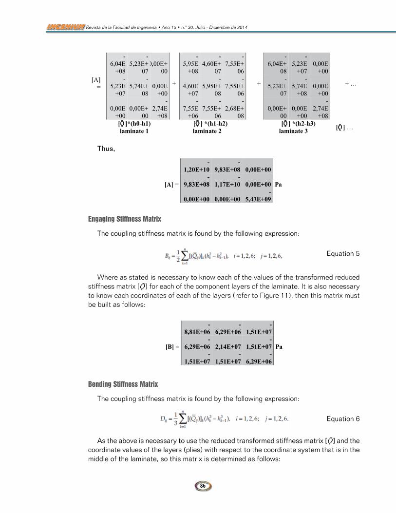
Deformation and Curvatures of Planes Media
Once you have the three matrices (matrix extensional stiffness matrix coupling and bending stiffness matrix) it is possible to consolidate an array containing these values, so we just need to determine the values located to the left of the equality in that equation. These are determined based on characteristics of shear and tensile stress and the laminate of time to be analyzed (Hollman, 1983), these can be seen in figure which follows:
Figure 12. Forces and moments resulting in the laminate
From: (Kaw, 2006) pag 321.
Given the values Nx cap, Mx are zero by inspection, but when considering equations each component has a correct answer on each one.
Then as the stress σx = 0 the values of Nx and Mx be equally zero, then,
Thus, the values are:
Ny= 1,03E+05 N/mm
Investigación
87
Analysis of a Composite Microlift-GliderWing Structure Using Finite Element Analysis and Manual Calculation • pp. 73-94
16
Equation 6
As the above is necessary to use the reduced transformed stiffness ] and the coordinate values of the layers (plies) with respect to the coordinate system that is in the middle of the laminate, so this matrix is determined as follows:
-1,60E+10
-1,31E+09 3,02E+06
[D] =
-1,31E+09
-1,56E+10 3,02E+06 Pa
3,02E+06 3,02E+06
-7,24E+09
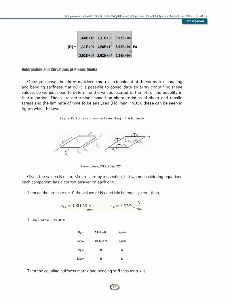
Deformation and Curvatures of Planes Media
Once you have the three matrices (matrix extensional stiffness matrix coupling and bending stiffness matrix) it is possible to consolidate an array containing these values, so we just need to determine the values located to the left of the equality in that equation. These are determined based on characteristics of shear and tensile stress and the laminate of time to be analyzed (Hollman, 1983), these can be seen in figure which follows:
Figure 12. Forces and moments resulting in the laminate
From: (Kaw, 2006) pag 321.
Given the values Nx cap, Mx are zero by inspection, but when considering equations each component has a correct answer on each one.
Then as the stress σx = 0 the values of Nx and Mx be equally zero, then,
Thus, the values are:
Ny= 1,03E+05 N/mm
Deformation and Curvatures of Planes Media
Once you have the three matrices (matrix extensional stiffness matrix coupling and bending stiffness matrix) it is possible to consolidate an array containing these values, so we just need to determine the values located to the left of the equality in that equation. These are determined based on characteristics of shear and tensile stress and the laminate of time to be analyzed (Hollman, 1983), these can be seen in figure which follows:
Figure 12. Forces and moments resulting in the laminate
16
Equation 6
As the above is necessary to use the reduced transformed stiffness ] and the coordinate values of the layers (plies) with respect to the coordinate system that is in the middle of the laminate, so this matrix is determined as follows:
-1,60E+10
-1,31E+09 3,02E+06
[D] =
-1,31E+09
-1,56E+10 3,02E+06 Pa
3,02E+06 3,02E+06
-7,24E+09
Deformation and Curvatures of Planes Media
Once you have the three matrices (matrix extensional stiffness matrix coupling and bending stiffness matrix) it is possible to consolidate an array containing these values, so we just need to determine the values located to the left of the equality in that equation. These are determined based on characteristics of shear and tensile stress and the laminate of time to be analyzed (Hollman, 1983), these can be seen in figure which follows:
Figure 12. Forces and moments resulting in the laminate
From: (Kaw, 2006) pag 321.
Given the values Nx cap, Mx are zero by inspection, but when considering equations each component has a correct answer on each one.
Then as the stress σx = 0 the values of Nx and Mx be equally zero, then,
Thus, the values are:
Ny= 1,03E+05 N/mm
From: (Kaw, 2006) pag 321.
Given the values Nx cap, Mx are zero by inspection, but when considering equations each component has a correct answer on each one.
Then as the stress σx = 0 the values of Nx and Mx be equally zero, then,
16
Equation 6
As the above is necessary to use the reduced transformed stiffness ] and the coordinate values of the layers (plies) with respect to the coordinate system that is in the middle of the laminate, so this matrix is determined as follows:
-1,60E+10
-1,31E+09 3,02E+06
[D] =
-1,31E+09
-1,56E+10 3,02E+06 Pa
3,02E+06 3,02E+06
-7,24E+09
Deformation and Curvatures of Planes Media
Once you have the three matrices (matrix extensional stiffness matrix coupling and bending stiffness matrix) it is possible to consolidate an array containing these values, so we just need to determine the values located to the left of the equality in that equation. These are determined based on characteristics of shear and tensile stress and the laminate of time to be analyzed (Hollman, 1983), these can be seen in figure which follows:
Figure 12. Forces and moments resulting in the laminate
From: (Kaw, 2006) pag 321.
Given the values Nx cap, Mx are zero by inspection, but when considering equations each component has a correct answer on each one.
Then as the stress σx = 0 the values of Nx and Mx be equally zero, then,
Thus, the values are:
Ny= 1,03E+05 N/mm
Thus, the values are:
Ny= 1,03E+05 N/mm
Nxy= 4006,5172 N/mm
My= 0 N
Mxy= 0 N
Then the coupling stiffness matrix and bending stiffness matrix is:
88
Revista de la Facultad de Ingeniería • Año 15 • n.° 30, Julio - Diciembre de 2014
0
=
-1,20E+10 -9,83E+08 0,00E+00 -8,81E+06 -6,29E+06 -1,51E+07
*
1,03E+05 -9,83E+08 -1,17E+10 0,00E+00 -6,29E+06 2,14E+07 -1,51E+07
4006,52 0,00E+00 0,00E+00 -5,43E+09 -1,51E+07 -1,51E+07 -6,29E+06
0 -8,81E+06 -6,29E+06 -1,51E+07 -1,60E+10 -1,31E+09 3,02E+06
0 -6,29E+06 2,14E+07 -1,51E+07 -1,31E+09 -1,56E+10 3,02E+06
0 -1,51E+07 -1,51E+07 -6,29E+06 3,02E+06 3,02E+06 -7,24E+09
Solving,
=
7,26E-07
-8,85E-06
-7,38E-07
mm/mm
4,78E-09
-1,21E-08
1,76E-08
1/mm
After a deflection and deformation in the structure, proceed to determine the safety factor, knowing the thickness of each layer of the material is 0.325 mm. These values were determined to be 5 layers were used which increase the thickness of 1.625 mm sandwich safety factors.
Table 4. Ply number, t/c and factor of safety.
Ply orientation Ply qx t/c Factor of safety
0 grados 20 1,625mm 1,601155856
Finite Element Analysis
According to the results of the calculation of composite materials, for the sizing of the main beam, we proceeded to modify the preliminary design and then to do a finite element analysis and obtain more specific behavior of both the wing and the aircraft structure.
Wing Analysis
After locating these boundary conditions starts the analysis process of the program, which throw the following results for the wing and its various components.
The analysis seeking core values: maximum stress and shear, total deformation, safety factor and value of the reactions that are present in the substrate in order to export these values to attached components and verify its durability.
In the Figure 13 it can be seen two forces, the supporting, the drag and the moment. Each of which was obtained from the initial analysis through CFD wing. It should be noted at this point that these values to be applied in the first step have been so evenly distributed, which simplifies the values.
Investigación
89
Analysis of a Composite Microlift-GliderWing Structure Using Finite Element Analysis and Manual Calculation • pp. 73-94
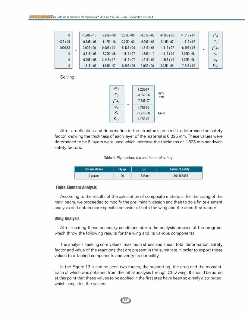
Figure 13. Loads on the wing
The value of the support has been added the value of the load factor of the aircraft under normal operating conditions (depending on the aircraft Vn diagram), ie the maximum value load factor equal to 5.3. This value is a multiplier for the lift, drag and moment of the wing.
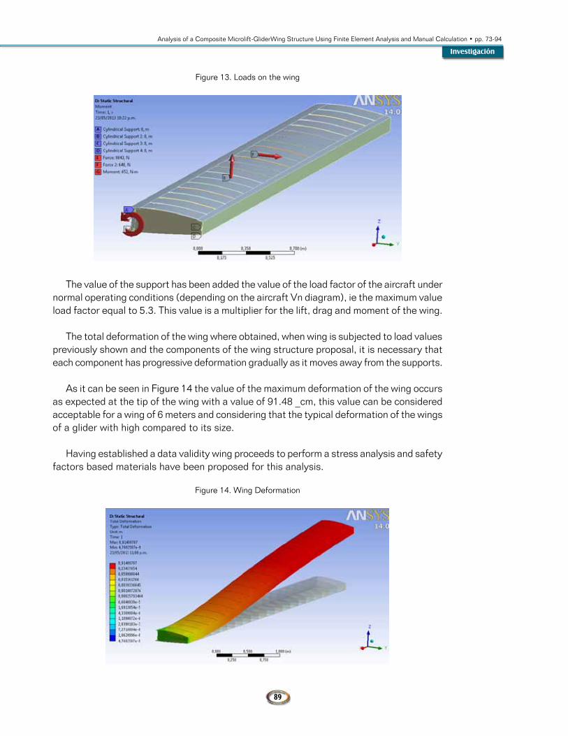
The total deformation of the wing where obtained, when wing is subjected to load values previously shown and the components of the wing structure proposal, it is necessary that each component has progressive deformation gradually as it moves away from the supports.
As it can be seen in Figure 14 the value of the maximum deformation of the wing occurs as expected at the tip of the wing with a value of 91.48 _cm, this value can be considered acceptable for a wing of 6 meters and considering that the typical deformation of the wings of a glider with high compared to its size.
Having established a data validity wing proceeds to perform a stress analysis and safety factors based materials have been proposed for this analysis.
Figure 14. Wing Deformation
90
Revista de la Facultad de Ingeniería • Año 15 • n.° 30, Julio - Diciembre de 2014
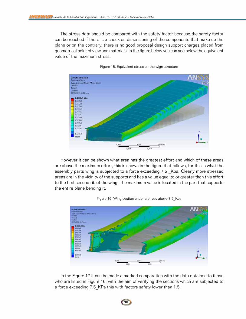
The stress data should be compared with the safety factor because the safety factor can be reached if there is a check on dimensioning of the components that make up the plane or on the contrary, there is no good proposal design support charges placed from geometrical point of view and materials. In the figure below you can see below the equivalent value of the maximum stress.
Figure 15. Equivalent stress on the wign structure
However it can be shown what area has the greatest effort and which of these areas are above the maximum effort, this is shown in the figure that follows, for this is what the assembly parts wing is subjected to a force exceeding 7.5 _Kpa. Clearly more stressed areas are in the vicinity of the supports and has a value equal to or greater than this effort to the first second rib of the wing. The maximum value is located in the part that supports the entire plane bending it.
Figure 16. Wing section under a stress above 7.5_Kpa
In the Figure 17 it can be made a marked comparation with the data obtained to those who are listed in Figure 16, with the aim of verifying the sections which are subjected to a force exceeding 7.5_KPa this with factors safety lower than 1.5.
Investigación
91
Analysis of a Composite Microlift-GliderWing Structure Using Finite Element Analysis and Manual Calculation • pp. 73-94
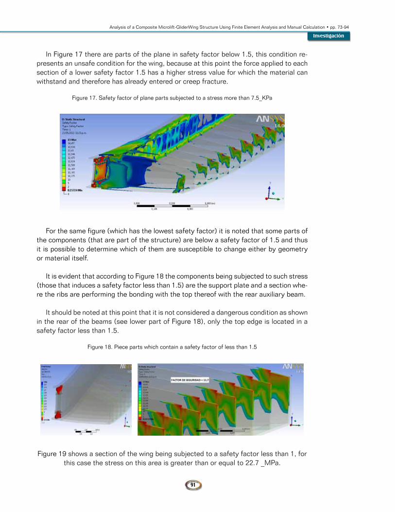
In Figure 17 there are parts of the plane in safety factor below 1.5, this condition re-presents an unsafe condition for the wing, because at this point the force applied to each section of a lower safety factor 1.5 has a higher stress value for which the material can withstand and therefore has already entered or creep fracture.
Figure 17. Safety factor of plane parts subjected to a stress more than 7.5_KPa
For the same figure (which has the lowest safety factor) it is noted that some parts of the components (that are part of the structure) are below a safety factor of 1.5 and thus it is possible to determine which of them are susceptible to change either by geometry or material itself.
It is evident that according to Figure 18 the components being subjected to such stress (those that induces a safety factor less than 1.5) are the support plate and a section whe-re the ribs are performing the bonding with the top thereof with the rear auxiliary beam.
It should be noted at this point that it is not considered a dangerous condition as shown in the rear of the beams (see lower part of Figure 18), only the top edge is located in a safety factor less than 1.5.
Figure 18. Piece parts which contain a safety factor of less than 1.5
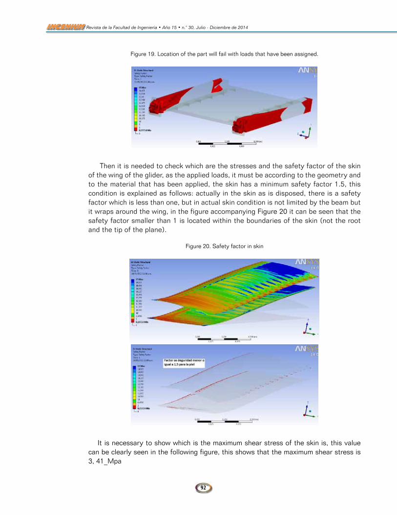
Figure 19 shows a section of the wing being subjected to a safety factor less than 1, for this case the stress on this area is greater than or equal to 22.7 _MPa.
92
Revista de la Facultad de Ingeniería • Año 15 • n.° 30, Julio - Diciembre de 2014
Figure 19. Location of the part will fail with loads that have been assigned.
Then it is needed to check which are the stresses and the safety factor of the skin of the wing of the glider, as the applied loads, it must be according to the geometry and to the material that has been applied, the skin has a minimum safety factor 1.5, this condition is explained as follows: actually in the skin as is disposed, there is a safety factor which is less than one, but in actual skin condition is not limited by the beam but it wraps around the wing, in the figure accompanying Figure 20 it can be seen that the safety factor smaller than 1 is located within the boundaries of the skin (not the root and the tip of the plane).
Figure 20. Safety factor in skin
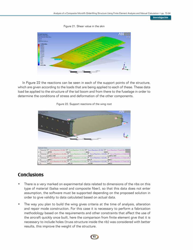
It is necessary to show which is the maximum shear stress of the skin is, this value can be clearly seen in the following figure, this shows that the maximum shear stress is 3, 41_Mpa
Investigación
93
Analysis of a Composite Microlift-GliderWing Structure Using Finite Element Analysis and Manual Calculation • pp. 73-94
Figure 21. Shear value in the skin
In Figure 22 the reactions can be seen in each of the support points of the structure, which are given according to the loads that are being applied to each of these. These data load be applied to the structure of the tail boom and from there to the fuselage in order to determine the conditions of stress and deformation of the other components.
Figure 22. Support reactions of the wing root
Conclusions
• There is a very marked on experimental data related to dimensions of the ribs on this type of material (balsa wood and composite fiber), so that this data does not enter assumption, the software must be supported depending on the proposed solution in order to give validity to data calculated based on actual data.
• The way you plan to build the wing gives criteria at the time of analysis, alteration and repair mode construction. For this case it is necessary to perform a fabrication methodology based on the requirements and other constraints that affect the use of the aircraft quickly once built, here the comparison from finite element give that it is necessary to include holes (truss structure inside the rib) was considered with better results, this improve the weight of the structure.
94
Revista de la Facultad de Ingeniería • Año 15 • n.° 30, Julio - Diciembre de 2014
• The use of composite materials give a variable cross section beam, decreasing total weight, analysis and method of manufacture of the part you want to elaborate on these materials is easy. But total structural analysis is high.
• According to the maximum stresses that occur in the beams, we determined the type of beams and materials, with a safety factor of 1.5, which ensures the smooth functioning of the structure for charge distributions presented.
• There is a strong needed between analytical and simulation methodologies, this increase the optimal results, and improve the behavior of the structure on the same given forces given by the mission profile.
ReferencesAllen, D. H., & Haisler, W. (1985). Introduction to Aerospace Structural Analysis. Canada: John Wiley & Sons.
Anderson, J. (2001). Fundamentals of Aerdynamics. New York: McGraw-Hill.
Hollman, M. (1983). Composite Aircraft Design. California: Aircraft Design Inc.
Jones, R. M. (1999). Mechanics of Composite Materials. Virginia: Taylor & Francis.
Kaw, A. K. (2006). Mechanics of Composite Materials. United States: Taylor & Francis.
Megson, T. H. (2007). An Introduction to Aircraft Structural Analysis. United States of America: ELSEVIER.
Peery, D., & Azar, J. (1982). Aircraft Structures. United States of America: McGraw-Hill.
Copyright © 2022 FDOKUMEN