Security Aspects, Attacks, Threats and Countermeasures - MDPI
Upload
khangminh22Category
view
2download
0
HAL Id: tel-03290140https://tel.archives-ouvertes.fr/tel-03290140
Submitted on 19 Jul 2021
HAL is a multi-disciplinary open accessarchive for the deposit and dissemination of sci-entific research documents, whether they are pub-lished or not. The documents may come fromteaching and research institutions in France orabroad, or from public or private research centers.
L’archive ouverte pluridisciplinaire HAL, estdestinée au dépôt et à la diffusion de documentsscientifiques de niveau recherche, publiés ou non,émanant des établissements d’enseignement et derecherche français ou étrangers, des laboratoirespublics ou privés.
Analysis and prevention of stealthy aging attacks : anapproach based on dynamical systems theory
Cédric Escudero
To cite this version:Cédric Escudero. Analysis and prevention of stealthy aging attacks : an approach based on dy-namical systems theory. Automatic. Université Grenoble Alpes [2020-..], 2021. English. NNT :2021GRALT025. tel-03290140

THÈSE
Pour obtenir le grade de
DOCTEUR DE L’UNIVERSITE GRENOBLE ALPES
Spécialité : AUTOMATIQUE - PRODUCTIQUE
Arrêté ministériel : 25 mai 2016
Présentée par
Cédric ESCUDERO Thèse dirigée par Eric ZAMAI, Professeur des Universités et codirigée par Paolo MASSIONI, Maître de Conférences préparée au sein du Laboratoire des Sciences pour la Conception, l’Optimisation et la Production de Grenoble dans l'École Doctorale Electronique, Electrotechnique, Automatique, Traitement du Signal (EEATS)
Analyse et prévention des attaques cachées de vieillissement : une approche basée sur la théorie des systèmes dynamiques Analysis and prevention of stealthy aging attacks: an approach based on dynamical systems theory
Thèse soutenue publiquement le 15 janvier 2021, devant le jury composé de :
Monsieur Jean-Marc THIRIET PROFESSEUR DES UNIVERSITES, Université Grenoble Alpes, Président du jury
Madame Mireille BAYART MERCHEZ PROFESSEURE DES UNIVERSITES, Université de Lille, Rapporteur
Monsieur Frédéric KRATZ PROFESSEUR DES UNIVERSITES, INSA Centre Val de Loire, Rapporteur
Monsieur Carlos MURGUIA RENDON PROFESSEUR ASSISTANT, Eindhoven University of Technology, Examinateur
Monsieur Stéphane DE FLEURIAU INGENIEUR, Direction Générale de l’Armement, Invité
Monsieur Franck SICARD DOCTEUR INGENIEUR, Naval Group, Invité
Monsieur Paolo MASSIONI MAITRE DE CONFERENCES, INSA de Lyon, Co-directeur de thèse
Monsieur Eric ZAMAI PROFESSEUR DES UNIVERSITES, INSA de Lyon, Directeur de thèse


i
Acknowledgments
The research works presented in this manuscript have been done at Laboratoire des Sci-ences pour la Conception, l'Optimisation et la Production (G-SCOP) in the researchteam Gestion et Conduite des Systèmes de Production (GCSP). That is why, I wouldlike to thank M. François Villeneuve, G-SCOP Research Laboratory Director, for havingwelcomed and allowed me to conduct my research works during these three years. Also,I would like to thank M. Bruno Allard and M. Eric Bideaux, respectively Director ofAmpère Research Laboratory and Head of the Department Méthodes pour l'Ingénieriedes Systèmes (MIS) at Ampère Research Laboratory, for having welcomed me as aninvited researcher for my last year.
First and foremost, I would like to express my gratitude to my PhD supervisor, M.Eric Zamaï, Full Professor at Institut National des Sciences Appliquées Lyon (INSALyon), for having accepted to supervise me. In addition to this, I would like to thankhim for the quality of his supervision, his availability and his advice.
I would like also to express my gratitude to my PhD co-supervisor, M. Paolo Mas-sioni, Associate Professor at INSA Lyon, for having accepted me to supervise me. Inaddition to this, I would like to thank him for the quality of his supervision and his advice.
I would like to thank M. Jean-Marc Thiriet, Full Professor at Université GrenobleAlpes (UGA), for having accepted to preside the jury of my PhD Defense.
I would like to thank Ms. Mireille Bayart Merchez, Full Professor at Université deLille, and M. Frédéric Kratz, Full Professor at INSA Centre Val de Loire, for the interestthey have shown on my research works and for having accepted to be reviewers of myresearch works.
I would like to thank M. Carlos Murguia Rendon, Assistant Professor at EindhovenUniversity of Technology, for having accepted to examine my research works and to par-ticipate to my PhD Defense.
I would like to thank M. Stéphane De Fleuriau, Engineer at Direction Générale del'Armement (DGA), and M. Franck Sicard, PhD-Engineer at Naval Group, for havingaccepted to participate to my PhD Defense.
I would like to thank M. Nouredine Hadjsaid, Director of Laboratoire de Génie Elec-trique de Grenoble (G2ELab), and M. Jean-Paul Jamont, Associate Professor at UGA,for having accepted to follow the progress of my PhD.
I would like also to thank the collaborators I worked with during these three years:M. Bertrand Raison, Full Professor at UGA, M. Quoc Bao Duong, research engineer atS.mart Grenoble-Alpes, M. Laurent Thibault, Lecturer at UGA, M. Romain Delpoux,Associate Professor at INSA Lyon, M. Vincent Léchappé, Associate Professor at INSA

ii
Lyon, M. Sébastien Henry, Associate Professor at IUT Lyon 1.I am also grateful to my close friends M. Iliasse Benbalaid and M. Lucas Mourey for
the time spent to read my papers.I would like to thank my beloved family and in particular my mother, my father, my
sister, my brother and my grand mother for having supported me. I would like also todedicate this thesis to my grand fathers.
Lastly, I would like to thank all my friends and in particular the ones with who Ispent most of my time during these three years: M. Akram Chergui, M. MouhamadouMansour Mbow, and Ms. Cléa Martinez.

Contents
List of Figures viii
List of Tables ix
List of Acronyms xi
List of Abbreviations xiii
List of Publications xv
Introduction 1
I General framework 5
1 Malevolence: a new root cause of failures in Industrial Control Systems 7
1.1 Introduction . . . . . . . . . . . . . . . . . . . . . . . . . . . . . . . . . . . 71.2 Industrial Control Systems . . . . . . . . . . . . . . . . . . . . . . . . . . . 8
1.2.1 General description . . . . . . . . . . . . . . . . . . . . . . . . . . . 81.2.2 Internal structure . . . . . . . . . . . . . . . . . . . . . . . . . . . . 81.2.3 Control system . . . . . . . . . . . . . . . . . . . . . . . . . . . . . 9
1.3 Responsiveness to faults . . . . . . . . . . . . . . . . . . . . . . . . . . . . 111.3.1 Failures in an ICS . . . . . . . . . . . . . . . . . . . . . . . . . . . 111.3.2 Root causes of failures . . . . . . . . . . . . . . . . . . . . . . . . . 121.3.3 Responsiveness of the control system . . . . . . . . . . . . . . . . . 13
1.4 Malevolence: an intentional root cause . . . . . . . . . . . . . . . . . . . . 141.4.1 Violation of the process integrity . . . . . . . . . . . . . . . . . . . 141.4.2 Malevolence . . . . . . . . . . . . . . . . . . . . . . . . . . . . . . . 15
1.5 Conclusion . . . . . . . . . . . . . . . . . . . . . . . . . . . . . . . . . . . . 17
2 Analysis of the malevolence and behavioral approach 19
2.1 Introduction . . . . . . . . . . . . . . . . . . . . . . . . . . . . . . . . . . . 192.2 Preliminary: detailed ICS functioning and penetration point . . . . . . . . 19
2.2.1 Functions of Control . . . . . . . . . . . . . . . . . . . . . . . . . . 192.2.2 Main digital devices . . . . . . . . . . . . . . . . . . . . . . . . . . 212.2.3 External devices . . . . . . . . . . . . . . . . . . . . . . . . . . . . 23
2.3 Analysis of the malevolence . . . . . . . . . . . . . . . . . . . . . . . . . . 242.3.1 Control-based attack model . . . . . . . . . . . . . . . . . . . . . . 242.3.2 Process integrity violation . . . . . . . . . . . . . . . . . . . . . . . 25
2.4 Application on Stuxnet attack . . . . . . . . . . . . . . . . . . . . . . . . . 282.5 Behavioral approaches to address the malevolence . . . . . . . . . . . . . . 31

iv Contents
2.6 Conclusion . . . . . . . . . . . . . . . . . . . . . . . . . . . . . . . . . . . . 33
3 Research problem 35
3.1 Introduction . . . . . . . . . . . . . . . . . . . . . . . . . . . . . . . . . . . 353.2 Process control with CVDS-controller . . . . . . . . . . . . . . . . . . . . 36
3.2.1 Description of the system in our focus of interest . . . . . . . . . . 363.2.2 Behavior of dynamical systems . . . . . . . . . . . . . . . . . . . . 36
3.3 Brief literature review of malevolence in dynamical system . . . . . . . . . 373.3.1 Methods based on the measurement signals . . . . . . . . . . . . . 383.3.2 Methods based on the control signals . . . . . . . . . . . . . . . . . 39
3.4 Observation of the anomaly . . . . . . . . . . . . . . . . . . . . . . . . . . 403.5 Aging of actuators . . . . . . . . . . . . . . . . . . . . . . . . . . . . . . . 413.6 Problem statement . . . . . . . . . . . . . . . . . . . . . . . . . . . . . . . 423.7 Scientic positioning . . . . . . . . . . . . . . . . . . . . . . . . . . . . . . 44
3.7.1 Set-theoretic methods in control . . . . . . . . . . . . . . . . . . . 443.7.2 Linear optimization . . . . . . . . . . . . . . . . . . . . . . . . . . 45
3.8 Scientic issues . . . . . . . . . . . . . . . . . . . . . . . . . . . . . . . . . 463.9 Conclusion . . . . . . . . . . . . . . . . . . . . . . . . . . . . . . . . . . . . 47
II Analysis and prevention of stealthy aging attacks 49
4 Background 51
4.1 Introduction . . . . . . . . . . . . . . . . . . . . . . . . . . . . . . . . . . . 514.2 Notations and conventions . . . . . . . . . . . . . . . . . . . . . . . . . . . 514.3 Matrix inequalities . . . . . . . . . . . . . . . . . . . . . . . . . . . . . . . 524.4 Sum Of Squares (SOS) . . . . . . . . . . . . . . . . . . . . . . . . . . . . . 534.5 The generalized S-procedure . . . . . . . . . . . . . . . . . . . . . . . . . . 554.6 Set-theory preliminaries . . . . . . . . . . . . . . . . . . . . . . . . . . . . 55
4.6.1 Convex functions and sets . . . . . . . . . . . . . . . . . . . . . . . 554.6.2 κ-sublevel sets . . . . . . . . . . . . . . . . . . . . . . . . . . . . . 564.6.3 Operations between sets . . . . . . . . . . . . . . . . . . . . . . . . 564.6.4 Ellipsoidal sets . . . . . . . . . . . . . . . . . . . . . . . . . . . . . 574.6.5 Hyperplanes and halfspaces . . . . . . . . . . . . . . . . . . . . . . 584.6.6 Distance between an ellipsoid and an hyperplane . . . . . . . . . . 58
4.7 Convex optimization problems . . . . . . . . . . . . . . . . . . . . . . . . . 584.7.1 Special cases of convex optimization problems . . . . . . . . . . . . 60
4.8 Lyapunov function . . . . . . . . . . . . . . . . . . . . . . . . . . . . . . . 614.9 Conclusion . . . . . . . . . . . . . . . . . . . . . . . . . . . . . . . . . . . . 63
5 Analysis and prevention: a subcase of stealthy aging attacks 65
5.1 Introduction . . . . . . . . . . . . . . . . . . . . . . . . . . . . . . . . . . . 655.2 Research question . . . . . . . . . . . . . . . . . . . . . . . . . . . . . . . . 66
5.2.1 Framework of the methods . . . . . . . . . . . . . . . . . . . . . . 675.2.2 Modeling considerations . . . . . . . . . . . . . . . . . . . . . . . . 67
5.3 Invariant set-based method . . . . . . . . . . . . . . . . . . . . . . . . . . 70
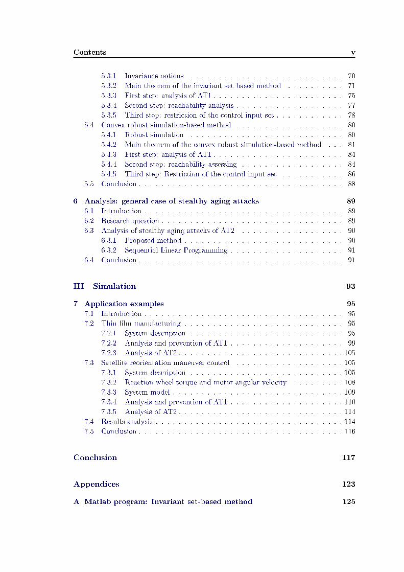
Contents v
5.3.1 Invariance notions . . . . . . . . . . . . . . . . . . . . . . . . . . . 705.3.2 Main theorem of the invariant set-based method . . . . . . . . . . 715.3.3 First step: analysis of AT1 . . . . . . . . . . . . . . . . . . . . . . . 755.3.4 Second step: reachability analysis . . . . . . . . . . . . . . . . . . . 775.3.5 Third step: restriction of the control input set . . . . . . . . . . . . 78
5.4 Convex robust simulation-based method . . . . . . . . . . . . . . . . . . . 805.4.1 Robust simulation . . . . . . . . . . . . . . . . . . . . . . . . . . . 805.4.2 Main theorem of the convex robust simulation-based method . . . 815.4.3 First step: analysis of AT1 . . . . . . . . . . . . . . . . . . . . . . . 845.4.4 Second step: reachability assessing . . . . . . . . . . . . . . . . . . 845.4.5 Third step: Restriction of the control input set . . . . . . . . . . . 86
5.5 Conclusion . . . . . . . . . . . . . . . . . . . . . . . . . . . . . . . . . . . . 88
6 Analysis: general case of stealthy aging attacks 89
6.1 Introduction . . . . . . . . . . . . . . . . . . . . . . . . . . . . . . . . . . . 896.2 Research question . . . . . . . . . . . . . . . . . . . . . . . . . . . . . . . . 896.3 Analysis of stealthy aging attacks of AT2 . . . . . . . . . . . . . . . . . . 90
6.3.1 Proposed method . . . . . . . . . . . . . . . . . . . . . . . . . . . . 906.3.2 Sequential Linear Programming . . . . . . . . . . . . . . . . . . . . 91
6.4 Conclusion . . . . . . . . . . . . . . . . . . . . . . . . . . . . . . . . . . . . 91
III Simulation 93
7 Application examples 95
7.1 Introduction . . . . . . . . . . . . . . . . . . . . . . . . . . . . . . . . . . . 957.2 Thin lm manufacturing . . . . . . . . . . . . . . . . . . . . . . . . . . . . 95
7.2.1 System description . . . . . . . . . . . . . . . . . . . . . . . . . . . 957.2.2 Analysis and prevention of AT1 . . . . . . . . . . . . . . . . . . . . 997.2.3 Analysis of AT2 . . . . . . . . . . . . . . . . . . . . . . . . . . . . . 105
7.3 Satellite reorientation maneuver control . . . . . . . . . . . . . . . . . . . 1057.3.1 System description . . . . . . . . . . . . . . . . . . . . . . . . . . . 1057.3.2 Reaction wheel torque and motor angular velocity . . . . . . . . . 1087.3.3 System model . . . . . . . . . . . . . . . . . . . . . . . . . . . . . . 1097.3.4 Analysis and prevention of AT1 . . . . . . . . . . . . . . . . . . . . 1107.3.5 Analysis of AT2 . . . . . . . . . . . . . . . . . . . . . . . . . . . . . 114
7.4 Results analysis . . . . . . . . . . . . . . . . . . . . . . . . . . . . . . . . . 1147.5 Conclusion . . . . . . . . . . . . . . . . . . . . . . . . . . . . . . . . . . . . 116
Conclusion 117
Appendices 123
A Matlab program: Invariant set-based method 125

vi Contents
B Matlab program: Robust convex simulation-based method 129
C Matlab program: Optimal attack input signal 137
Bibliography 145
Abstract 163
Résumé 163

List of Figures
1.1 General structure of ICS . . . . . . . . . . . . . . . . . . . . . . . . . . . . 91.2 Standard ICS architecture . . . . . . . . . . . . . . . . . . . . . . . . . . . 101.3 Request-reply procedure . . . . . . . . . . . . . . . . . . . . . . . . . . . . 11
2.1 Reduced ICS architecture - Main digital devices (bold), their vulnerablearchitecture layers (Hw., Fw., App.) studied (in black) and not studied(in grey), and their exchanged messages: decision (→), status feedback(→), and monitoring (↔) . . . . . . . . . . . . . . . . . . . . . . . . . . . 22
2.2 Map reading methodology . . . . . . . . . . . . . . . . . . . . . . . . . . . 262.3 Stuxnet attack propagation . . . . . . . . . . . . . . . . . . . . . . . . . . 29
3.1 Considered control system . . . . . . . . . . . . . . . . . . . . . . . . . . . 363.2 Considered control system with the corrupted channel (red) . . . . . . . . 44
5.1 Step 1 : Analysis of stealthy aging attacks . . . . . . . . . . . . . . . . . . 695.2 Step 2 : Reachability analysis of the abnormal aging set . . . . . . . . . . 705.3 Step 3 : Restriction of the input set to prevent such attacks . . . . . . . . 705.4 Invariant ellipsoid Ex . . . . . . . . . . . . . . . . . . . . . . . . . . . . . . 715.5 RQ1- Constrained invariant state set Ex (dot pattern) for the input set
Eu by applying Algorithm 3, the abnormal aging set Dx (red area), and(Ex ∩Dx) (red polygon) . . . . . . . . . . . . . . . . . . . . . . . . . . . . 78
5.6 RQ2- Largest restrained input set Eu with the corresponding constrainedinvariant state set Ex (dot pattern) in dotted lines by applying Algo-rithm 4, and RQ1 in solid lines, and the abnormal aging set Dx (red area) 80
5.7 Bounding state ellipsoid Ex(tf ) from Ex(t0) . . . . . . . . . . . . . . . . . 815.8 RQ1- Evolution of bounding state ellipsoids (dot pattern) over the time
interval [t0, tf ] for the input set Eu, the abnormal aging set Dx (red area),and (Ex(t) ∩Dx) (red polygon) by applying Algorithm 6 . . . . . . . . . . 86
5.9 RQ2- Restrained input set Eu with the corresponding evolution of bound-ing state ellipsoids (dot pattern) over the time interval [t0, tf ] in dottedlines by applying Algorithm 7, RQ1 in solid lines, and the abnormal agingset Dx (red area) . . . . . . . . . . . . . . . . . . . . . . . . . . . . . . . . 87
7.1 Film mfg. system (simplied from [Chen et al. 2004]) . . . . . . . . . . . . 967.2 Web tension [Chen et al. 2004] . . . . . . . . . . . . . . . . . . . . . . . . 977.3 Web speed . . . . . . . . . . . . . . . . . . . . . . . . . . . . . . . . . . . . 987.4 AT1 for the lm mfg. system with invariant-set based method - RQ1 -
constrained invariant state set Ex (green), service set Es (blue) coveringthe whole space for [τx,τy] (not drawn), abnormal aging set Dx (red),control input set Eu (magenta) . . . . . . . . . . . . . . . . . . . . . . . . 101

viii List of Figures
7.5 AT1 for the lm mfg. system with invariant-set based method - RQ2 -constrained invariant state set Ex (green), service set Es (blue) coveringthe whole space for [τx,τy] (not drawn), abnormal aging set Dx (red),restrained control input set Eu (magenta) . . . . . . . . . . . . . . . . . . 103
7.6 AT1 for the lm mfg. system with robust convex simulation-based method- RQ1 - Bounding state ellipsoids Ex(ti) at each 0.1ms from initial setEx(t0) (orange star) and nal set Ex(tf ) (green), abnormal aging set Dx
(red), control input set Eu (magenta) . . . . . . . . . . . . . . . . . . . . . 1047.7 AT1 for the lm mfg. system with robust convex simulation-based method
- RQ2 - Bounding state ellipsoids Ex(ti) at each 0.1ms from initial setEx(t0) (orange star) and nal set Ex(tf ) (green), abnormal aging set Dx
(red), restrained control input set Eu (magenta) . . . . . . . . . . . . . . . 1067.8 AT2 for the lm mfg. control: at the 28th iteration, the cost degradation
function is maximized (1st from bottom) with the degradation function(1st from top) for the optimal attack input signal (2nd from top) whiledelivering the desired service (2nd from bottom) . . . . . . . . . . . . . . . 107
7.9 AT1 for the satellite with robust convex simulation-based method - RQ1 -Bounding state ellipsoids Ex(ti) at each 0.1s from initial set Ex(t0) (orangestar) and nal set Ex(tf ) (green), abnormal aging set Dx (red), controlinput set Eu (magenta) . . . . . . . . . . . . . . . . . . . . . . . . . . . . . 112
7.10 AT1 for the satellite with robust convex simulation-based method - RQ2 -Bounding state ellipsoids Ex(ti) at each 0.1s from initial set Ex(t0) (orangestar) and nal set Ex(tf ) (green), abnormal aging set Dx (red), restrainedcontrol input set Eu (magenta) . . . . . . . . . . . . . . . . . . . . . . . . 113
7.11 AT2 for the satellite: at the 60th iteration, the cost degradation functionis maximized (1st from bottom) with the degradation function (1st fromtop) for the optimal attack input signal (2nd from top) while deliveringthe desired service (2nd from bottom) . . . . . . . . . . . . . . . . . . . . . 115

List of Tables
2.1 Reduced attacks propagation map for the case study . . . . . . . . . . . . 272.2 Attacks propagation map for an ICS arranged following the ISA95 - From
the corruption of a device architecture ( ) or of a communication ( ), thepotential manipulated FCs (?), the propagation path of anomalies ( ), the misbehaving FCs (), the process integrity ( ), the nottargeted FCs and device architecture (-); the Stuxnet attack propagation(letters and numbers) . . . . . . . . . . . . . . . . . . . . . . . . . . . . . 30

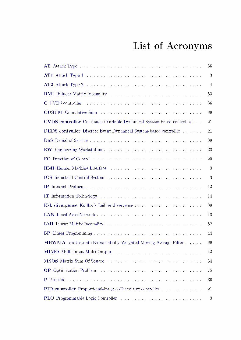
List of Acronyms
AT Attack Type . . . . . . . . . . . . . . . . . . . . . . . . . . . . . . . . . . . . 66
AT1 Attack Type 1 . . . . . . . . . . . . . . . . . . . . . . . . . . . . . . . . . . 3
AT2 Attack Type 2 . . . . . . . . . . . . . . . . . . . . . . . . . . . . . . . . . . 4
BMI Bilinear Matrix Inequality . . . . . . . . . . . . . . . . . . . . . . . . . . . 53
C CVDS controller . . . . . . . . . . . . . . . . . . . . . . . . . . . . . . . . . . . 36
CUSUM Cumulative Sum . . . . . . . . . . . . . . . . . . . . . . . . . . . . . . 39
CVDS controller Continuous-Variable Dynamical System-based controller . . . 21
DEDS controller Discrete Event Dynamical System-based controller . . . . . . 21
DoS Denial of Service . . . . . . . . . . . . . . . . . . . . . . . . . . . . . . . . . 38
EW Engineering Workstation . . . . . . . . . . . . . . . . . . . . . . . . . . . . . 23
FC Function of Control . . . . . . . . . . . . . . . . . . . . . . . . . . . . . . . . 20
HMI Human Machine Interface . . . . . . . . . . . . . . . . . . . . . . . . . . . 3
ICS Industrial Control System . . . . . . . . . . . . . . . . . . . . . . . . . . . . 3
IP Internet Protocol . . . . . . . . . . . . . . . . . . . . . . . . . . . . . . . . . . 13
IT Information Technology . . . . . . . . . . . . . . . . . . . . . . . . . . . . . . 14
K-L divergence Kullback-Leibler divergence . . . . . . . . . . . . . . . . . . . . 38
LAN Local Area Network . . . . . . . . . . . . . . . . . . . . . . . . . . . . . . . 13
LMI Linear Matrix Inequality . . . . . . . . . . . . . . . . . . . . . . . . . . . . 52
LP Linear Programming . . . . . . . . . . . . . . . . . . . . . . . . . . . . . . . . 44
MEWMA Multivariate Exponentially Weighted Moving Average Filter . . . . . 39
MIMO Multi-Input-Multi-Output . . . . . . . . . . . . . . . . . . . . . . . . . . 43
MSOS Matrix Sum Of Square . . . . . . . . . . . . . . . . . . . . . . . . . . . . 54
OP Optimization Problem . . . . . . . . . . . . . . . . . . . . . . . . . . . . . . 75
P Process . . . . . . . . . . . . . . . . . . . . . . . . . . . . . . . . . . . . . . . . 36
PID controller Proportional-Integral-Derivative controller . . . . . . . . . . . . 21
PLC Programmable Logic Controller . . . . . . . . . . . . . . . . . . . . . . . . 3

xii List of Acronyms
PWA Piecewise ane . . . . . . . . . . . . . . . . . . . . . . . . . . . . . . . . . 37
RQ Research Question . . . . . . . . . . . . . . . . . . . . . . . . . . . . . . . . . 67
SCADA Supervisory Control And Data Acquisition . . . . . . . . . . . . . . . . 22
SDP Semidenite Programming . . . . . . . . . . . . . . . . . . . . . . . . . . . 60
SLP Sequential or Successive Linear Programming . . . . . . . . . . . . . . . . . 91
SOS Sum Of Square . . . . . . . . . . . . . . . . . . . . . . . . . . . . . . . . . . 53
WO Work Order . . . . . . . . . . . . . . . . . . . . . . . . . . . . . . . . . . . . 12

List of Abbreviations
App. Application . . . . . . . . . . . . . . . . . . . . . . . . . . . . . . . . . . . 20
Com. Communication . . . . . . . . . . . . . . . . . . . . . . . . . . . . . . . . . 20
Fw. Firmware . . . . . . . . . . . . . . . . . . . . . . . . . . . . . . . . . . . . . 20
Hw. Hardware . . . . . . . . . . . . . . . . . . . . . . . . . . . . . . . . . . . . . 20


List of Publications
Journals:
C. Escudero, F. Sicard, A. Beaudet and E. Zamaï, E. Security of the Process
Integrity under Attacks Propagation in Industrial Control Systems: a Classication
of Control-based Methods. Reliability Engineering and System Safety (Reliab. Eng.
Syst. Saf.), (Submitted), pages 1-1, Sept. 2020
C. Escudero, P. Massioni, E. Zamaï and B. Raison. Control System Theory Meth-
ods to Analyze, Prevent and Design Stealthy Aging Attacks. IEEE Transaction on
Industrial Informatics (IEEE Trans. Ind. Informat.), (Submitted), pages 1-1,Sept. 2020
Conferences:
A. Beaudet, C. Escudero and E. Zamaï. Malicious Anomaly Detection Ap-
proaches Robustness in Manufacturing ICSs. In 2021 IFAC 17th Symposium onInformation Control Problems in Manufacturing (INCOM), (Submitted), pages1-8, Jun. 2021
C. Escudero, P. Massioni, G. Scorletti and E. Zamaï. Security of Control Systems:Prevention of Aging Attacks by means of Convex Robust Simulation Forecasts. In2020 IFAC World Congress, pages 1-8, Jul. 2020
E. M. Merouane, C. Escudero, F. Sicard and E. Zamaï. Aging Attacks against
Electro-Mechanical Actuators from Control Signal Manipulation. In 2020 IEEEInternational Conference on Industrial Technology (ICIT), pages 133-138, Feb.2020
A. Beaudet, F. Sicard, C. Escudero and E. Zamaï. Process-Aware Model-based
Intrusion Detection System on Filtering Approach: Further Investigations. In 2020IEEE International Conference on Industrial Technology (ICIT), pages 310-315,Feb. 2020
C. Escudero, and E. Zamaï. Prevention of Aging Attacks: Malicious Nature of
the Control Signal. In 2019 IEEE International Automatic Control Conference(CACS), pages 1-6, Nov. 2019
F. Sicard, C. Escudero, E. Zamaï and J.-M. Flaus. From ICS Attacks' Analysis
to the S.A.F.E. Approach: implementation of Filters based on behavioral models
and critical state distance for ICS cybersecurity. In 2018 IEEE 2nd Cyber Securityin Networking Conference (CSNet), pages 1-8, Oct. 2018

xvi List of Publications
C. Escudero, F. Sicard and E. Zamaï. Process-Aware Model based IDSs for In-
dustrial Control Systems Cybersecurity: Approaches, Limits and Further Research.In 2018 IEEE 23rd International Conference on Emerging Technologies and Fac-tory Automation (ETFA), volume 1, pages 605-612, Sep. 2018
Workshops:
C. Escudero and E. Zamaï. Sécurité des Systèmes Déterministes Linéaires: Com-posantes Malveillantes du Signal de Commande des Actionneurs. Extended ab-stract for the National Research Group Workshop Modélisation, Analyse et Con-duite des Systèmes dynamiques (GdR MACS), Jun. 2019

Introduction


Introduction
Industrial Control System (ICS) are architectures controlling a physical system to achievean industrial objective. They are present in various sectors including energy generationand distribution, water treatment, manufacturing production, aerospace and defense.Those architectures are equipped with various digital entities, including Human MachineInterface (HMI), Programmable Logic Controller (PLC), regulator, organized for reduc-ing the complexity of the control. Historically, ICSs have been designed to improve theproductivity, but the cybersecurity has not been considered. Due to this lack, ICSs arefacing cyberattacks. Plenty of them manipulating the architecture have been reportedin the literature. They aim to steal sensitive information or to violate the integrity ofthe physical system. The violation of the physical system integrity refers to an intendedalteration or destruction of the physical system through its control. It leads to a partialor complete failure of the services delivered by the physical system. Hence, cyberattacksare a new root-cause of failure, that we call the malicious acts. Those malicious actsaim to create and propagate anomalies in the architecture by exploiting vulnerabilitiesof the digital entities.
In this thesis, we address a new type of attack that aims to accelerate the agingof the actuators. The attacker is considered to manipulate the control signal sent tothem. The objective of this thesis is to develop methods for analyzing such attacks andpreventing them. The analysis consists in quantifying the potential impact a controlsignal manipulation could have on the process. The prevention consists in restrainingthe control signal such that stealthy aging attacks cannot occur.
This thesis addresses the following scientic issues:
Modeling the attack stealthiness in set theory,
Stability condition required from the invariant set theory,
Loss of the temporal variable in the invariant set theory.
This manuscript is organized in Part as follows.
Part 1 presents the general problematic of our research works. After having presentedthe general context about the malicious act acting on ICSs to reach the process integrity,we position our research works in the controllers. In particular, we focus on the continu-ous controllers. Then, the problem of anomaly observation is explained. It appears thatthe process integrity can be violated if the control signal is abnormal. Thus, we orientateour works on anomalies in the control signal. In particular, our interest concerns anoma-lies accelerating the aging of the actuators. After having briey reviewed the literature,we position our works on the set-theoretic methods and linear optimization.
Part 2 provides our contributions. First, the analysis and prevention of stealthyaging attacks are restrained to a subcase, denoted Attack Type 1 (AT1). AT1 consists
4 Introduction
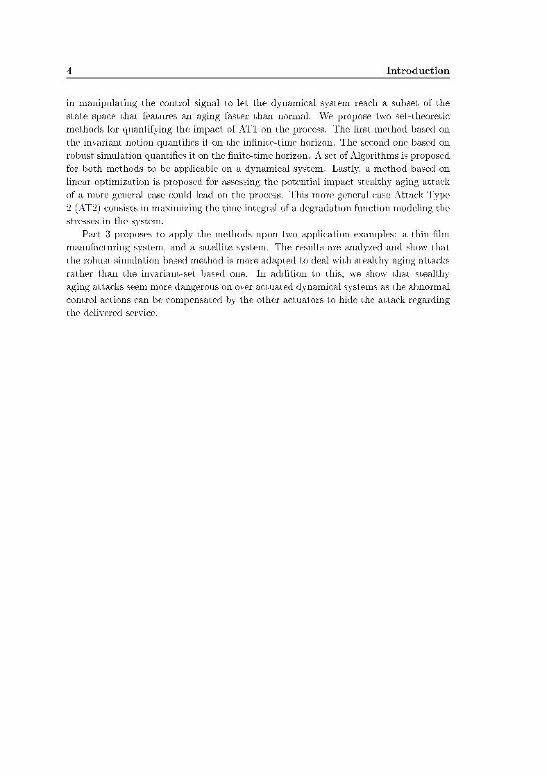
in manipulating the control signal to let the dynamical system reach a subset of thestate space that features an aging faster than normal. We propose two set-theoreticmethods for quantifying the impact of AT1 on the process. The rst method based onthe invariant notion quanties it on the innite-time horizon. The second one based onrobust simulation quanties it on the nite-time horizon. A set of Algorithms is proposedfor both methods to be applicable on a dynamical system. Lastly, a method based onlinear optimization is proposed for assessing the potential impact stealthy aging attackof a more general case could lead on the process. This more general case Attack Type2 (AT2) consists in maximizing the time integral of a degradation function modeling thestresses in the system.
Part 3 proposes to apply the methods upon two application examples: a thin lmmanufacturing system, and a satellite system. The results are analyzed and show thatthe robust simulation-based method is more adapted to deal with stealthy aging attacksrather than the invariant-set based one. In addition to this, we show that stealthyaging attacks seem more dangerous on over actuated dynamical systems as the abnormalcontrol actions can be compensated by the other actuators to hide the attack regardingthe delivered service.

Part I
General framework


Chapter 1
Malevolence: a new root cause of
failures in Industrial Control
Systems
Contents
1.1 Introduction . . . . . . . . . . . . . . . . . . . . . . . . . . . . . . . 7
1.2 Industrial Control Systems . . . . . . . . . . . . . . . . . . . . . . . 8
1.2.1 General description . . . . . . . . . . . . . . . . . . . . . . . . . . . 8
1.2.2 Internal structure . . . . . . . . . . . . . . . . . . . . . . . . . . . . 8
1.2.3 Control system . . . . . . . . . . . . . . . . . . . . . . . . . . . . . 9
1.3 Responsiveness to faults . . . . . . . . . . . . . . . . . . . . . . . . 11
1.3.1 Failures in an ICS . . . . . . . . . . . . . . . . . . . . . . . . . . . 11
1.3.2 Root causes of failures . . . . . . . . . . . . . . . . . . . . . . . . . 12
1.3.3 Responsiveness of the control system . . . . . . . . . . . . . . . . . 13
1.4 Malevolence: an intentional root cause . . . . . . . . . . . . . . . 14
1.4.1 Violation of the process integrity . . . . . . . . . . . . . . . . . . . 14
1.4.2 Malevolence . . . . . . . . . . . . . . . . . . . . . . . . . . . . . . . 15
1.5 Conclusion . . . . . . . . . . . . . . . . . . . . . . . . . . . . . . . . 17
1.1 Introduction
This Chapter presents the overall context of this thesis. It takes place in ICSs, whereheterogeneous industrial equipment and devices operate each other to control a physicalsystem. After having presented what is an ICS in Section 1.2, the problem of faults inICS is explained and the response given by the community is detailed in Section 1.3.This response has introduced a new problem in ICSs: the malevolence. In this thesis, wefocus on the malevolence that aim to violate the integrity of the physical system. Thatis why, the malevolence is studied in Section 1.4 with the viewpoint of the integrity ofthe physical system.

8
Chapter 1. Malevolence: a new root cause of failures in Industrial Control
Systems
1.2 Industrial Control Systems
Many sectors including critical ones [Rushby 1994] have quickly integrated automationof their industrial operations such as energy generation and distribution, water treat-ment, manufacturing production, aerospace and defense [Nozaic & Freese 2009, Stoueret al. 2015, Groover 2008]. This automation raise stems from the fact companies areconstantly chasing better performance. In the following subsection, a brief study of ICSsis given.
1.2.1 General description
ICSs are organized around workstations, mostly automated. The workstations performindustrial operations using industrial equipment, i.e. the physical system used to realizethe industrial operations. These workstations are interconnected with a control systemdevoted to the coordination of the control, and to the control of the workstations. Theautomated operations are often supported by manual interventions of operators. Thesemanual interventions are dedicated to auxiliary operations such as tools changing or theloading and unloading of workpieces in manufacturing productions, cleaning of screensin water treatment systems, or repair and replace activities.ICSs aim at:
Relieving the human of the tedious and dangerous tasks (e.g. operations in envi-ronment with high temperature or toxic gas) [Robla-Gómez et al. 2017, Cherubiniet al. 2016],
Performing complex industrial operations, almost impossible by the human (e.g.manufacturing precision in aerospace and defense),
Improving the productivity (e.g. production time, delivery times),
Reducing the production cost,
Optimizing energetic performance during the industrial operations.
To successfully achieve its objectives, an ICS requires exibility [Michalos et al. 2010].The exibility is the ability to easily adapt to changes. Industrial equipment exibilityallows exibility in the operations realizable by the equipment. This requirement plays amajor role to deal with failures in ICSs. However, the industrial equipment exibility isnot enough. In complementary, exibility in the control system is required to easily adaptto industrial objectives and failures. Both requirements allow the industrial equipmentand the control system to respond to industrial objectives changes, and failures in theICS [Zamai et al. 1998].
1.2.2 Internal structure
In general, an ICS has an internal structure split into three parts as illustrated in Fig-ure 1.1:

1.2. Industrial Control Systems 9
Figure 1.1: General structure of ICS
The plant represents the physical entities which are transformed to achieve theindustrial objectives such as displacement of a workpiece, water level in a tank,ow of power in power lines. These physical entities are often called raw materialsand represent respectively the workpiece, the water and the power in the previousexamples.
The operative part is the set of actuators and sensors, also called eld devices, orindustrial control and instrumentation devices. On the one hand, actuators receivedecisions from the control system and transform them into physical actuation (e.g.angular velocity, electrical current, electromagnetic torque, force, uid volumetricrate of ow). Physical actuation is applied on the plant to transform the physicalentities. To achieve this transformation, actuators use energy: electrical, pneu-matic, or hydraulic. On other hand, sensors measure physical quantities relatedto the entities transformation. These measurements are transmitted back to thecontrol system as status feedbacks. The operative part together with the plant isusually gathered into a single term: the process, being the physical system to becontrolled.
The control system coordinates the control of the process by transmitting deci-sions to the actuators in order to impose a desired behavior to the plant based onthe status feedbacks and the industrial objectives. The control system can transmitrelevant information about the process, or even itself to operators. The operatorsinterconnected with the control system monitor the control of the plant, and canmake decisions if required.
1.2.3 Control system
As seen previously, the control system is the core of an ICS as it coordinates the controland controls the process. However, the plant involves plenty of physical phenomenonwhich need to be considered by the control system in order to impose the desired behav-ior. Each physical phenomenon needs to be controlled through actuators, and monitored

10
Chapter 1. Malevolence: a new root cause of failures in Industrial Control
Systems
through sensors, thus the higher the number of physical phenomenon, the higher thenumber of actuators and sensors is. This complexity has increased in the past with morecomplex process to be controlled. From this raise, it quickly appeared that centralizedcontrol system was not anymore adapted. This major problem has been considered inthe past, and many architectures have emerged to deal with [Jones & Saleh 1989]. Oneof the most used architecture is the hierarchical and modular control system architec-ture, known under the name "Computer Integrated Manufacturing" [Williams 1990] andnormalized nowadays in the ISA95 [ISA ]. Although each sector has specic features,their architecture follows this conceptual architecture. It splits the control system intove levels of lower complexities as illustrated in Figure 1.2:
Level 5: Management information
Level 4: Production scheduling and operational management
Level 3: Supervisory control
Level 2: Control coordinator
Level 1: Local control
Levels 5 and 4 are dedicated to the production scheduling and management information,while the levels 3, 2, and 1 are devoted to the process control. These levels are intercon-nected together through communication levels. Throughout this thesis, only the levelsdevoted to the process control are of concern, i.e. levels 3, 2, and 1.
Figure 1.2: Standard ICS architecture
Each level has several modules, and each module is a digital device having a controlmission in the control system, as it will be detailed in Chapter 2. The operating prin-ciple of this control system architecture is based on a request-reply procedure [Jones &Saleh 1989], illustrated in Figure 1.3 and explained as follows. A module at a level ntransmits a decision to a module at a level n − 1. The latter module breaks down the

1.3. Responsiveness to faults 11
Figure 1.3: Request-reply procedure
decision into m other decisions, and transmits them to the lower layer, and so on untilthe decisions reach the process.
After the process has reacted to these decisions, m status feedbacks, corresponding tothe reaction response of the process to the m decisions, are propagated to the modules.These status feedbacks inform about the activity of the process. They can be eithernormal, or abnormal if the status feedback does not correspond to the expected one, i.e.expected activity, [Duong et al. 2013]. In the last case, this anomaly is commonly knownas a fault. Since ICSs are made of many industrial equipment ranging from dozens tohundreds of equipment, faults issue is a complex problem to deal with.
1.3 Responsiveness to faults
As this thesis concerns attacks leading to a fault in the operations of the ICS, faults inICS are presented in this section. First of all, the concept of failure commonly agreed inthe literature is presented.
1.3.1 Failures in an ICS
A failure of an entity is dened as the cessation of its ability to deliver its service. Afailure can lead to a fault in an entity. A fault of an entity is dened as its inability todeliver the service [Villemeur 1992]. A fault results in a deviation from a characteristicproperty or a property of the service to deliver [Isermann 1997][ISO13849-1 2015]. Thisdeviation is seen as an anomaly in the ICS. A failure can result from the occurrence ofother failures. The rst failure is the origin of failure.
The origin of failures are usually classied into two groups: external or internal, ofthe architecture. The external failures can come from:
The production scheduling and management information, i.e. levels 5 and 4, (e.g.industrial objectives changes, production rate changes).
The raw materials (e.g. not t with required specications).
The environment of the ICS (e.g. operators interacting with the ICS, energy usedby actuators).
The internal failures can come from:
12
Chapter 1. Malevolence: a new root cause of failures in Industrial Control
Systems
The digital entities of the ICS, i.e. digital devices and digital communication, (e.g.failure of a communication, design error in a control program).
The process: the failure of a sensor, of an actuator, or of the plant.
1.3.2 Root causes of failures
In ICSs, the root causes of failures are often classied into ve main root causes: Man,Equipment, Method and Recipe, Material, and Environment [Ishikawa 1990, Doggett 2004].The main root causes are explained below only with respect to facts related to the pro-cess control [Nguyen et al. 2016], as this is the interest of this thesis. Hence, the Manroot cause refers to the exploitation and maintenance of equipment, and the Equipmentrefers to an intrinsic deviation from its technical specications. In addition, as Methoddevotes to the recognition at work, so only the Recipe is studied. It concerns their char-acterization as this step is done without considering the current operations in the ICS,i.e. without the current stresses the equipment is subject to. The Material refers to thenon-compliance with required specications. Finally, the Environment is not consideredas it devotes to the well-being at work.
Man is, on the one hand, an irreplaceable stakeholder with adaptation and respon-siveness capabilities to deal with unpredictable events. It is particularly essentialin ICS with high variability such as electric power systems, or some manufactur-ing production systems (e.g. automotive assembly lines [Michalos et al. 2010],semiconductor manufacturing [Bouaziz 2012]). On the other hand, it can generatedisturbances because of whether a lack of information to make its decisions forresponding to a failure, or it is fallible in the tasks it realizes (e.g. negligence in themaintenance operations, tension variations causing paper web breaks due to con-trol design error [Hristopulos & Uesaka 2002]) [Kobbacy & Murthy 2008, Proctor& Zandt 2018].
Equipment is subject to an intrinsic aging process due to the various stresses itgoes through during its control. The aging process comes from the phenomenon ofwear and tear of the equipment's components [Dhillon 1999, Viveros et al. 2014].The failure of an equipment can be predicted by statistical and probabilistic meth-ods [Vrignat et al. 2015]. However, these methods usually consider normal condi-tions of equipment operation, often not satised in the ICS. Indeed, non-predictedfailure of equipment's components have been reported owing to abnormal oper-ations. Furthermore, [Isermann 2006] highlights the phenomenon of rapid tech-nological change, and the consequences of the lack of knowledge about the newequipment causing an increase in the number of failures.
Recipe is usually developed in the R&D department [Erickson & Hedrick 1999],and dened for dedicated equipment. A recipe species the industrial operationssuch as the equipment to be used, their setting parameters, and the starting andending date of operations. A set of recipes is usually associated with a WorkOrder (WO) [Muñoz et al. 2011]. A WO is a set of orders the control coordinatorlevel in the ICS architecture has to execute. A WO corresponds to a set of decisions

1.3. Responsiveness to faults 13
the operators have made in the supervisory control level as presented in Section 1.2.The recipes are usually developed in a dedicated environment without consideringthe stresses the equipment are subject to in current operations. Indeed, sometimesthe ICS equipment operates beyond its operating conditions, and then operatesin stress conditions. Therefore, the recipes can result in failures once they areexecuted by the control coordinator level [Muñoz et al. 2011]. In addition, thehigher the stressed equipment, the higher the number of failures can occur [Hubac& Zamaï 2013].
Material is the raw materials introduced in the ICS to realize industrial operationson it, as mentioned in Section 1.2. If the raw materials do not conform to requiredspecication standards, then they can produce failures on the physical entitiesto transform, i.e. the plant, (e.g. web breakage due to low paper properties innewsprint production [Haapala et al. 2010]) [Ahmad et al. 2018], and even onthe equipment transforming the raw materials (e.g. reactor accidents in chemicalprocess industry [Kidam & Hurme 2013]).
1.3.3 Responsiveness of the control system
As faults are many in an ICS, it appeared the control systems were not designed to dealwith. Indeed, the request-reply procedure was designed to optimize the operations in ICSby transmitting a decision, and waiting for its realization before transmitting anotherdecision. However, it was not designed to deal with faults. The lack of response to faultsin an ICS has appeared as the main cause of lack of performance in an ICS. As a result,ICSs have progressively evolved to improve its responsiveness, as detailed below.
In 1980, a rst observation was stated: the control system and the industrial controland instrumentation devices, i.e. level 1 and 0 of the ICS, communicate in a single-wayanalog communication with point-to-point connections. Besides the high installationand maintenance cost it leads to, i.e. a lot of electrical wirings, the need for a two-way digital communication appeared in order to improve the feedback of informationfor fault-detection purposes. Indeed, the analog communications limited the feedback ofinformation from the equipment to the control system in dierent aspects: the amount,the quality, and the cost of supplementary electrical wiring for the two-way communi-cation. This conducts the progressive replacement of the analog communication by aserial digital communication, called eldbus, so that more information can ow in bothdirections between the eld devices and the control system. The emergence of integratedcircuit in the same years has reinforced the need for digital processing capabilities in theactuators and sensors, so that they can transmit more information. These new digitalprocessing capabilities and the emergence of eldbuses have conducted progressively thereplacement of analog devices to digital ones [Thomesse 2005, Galloway & Hancke 2013].
In 2000, a second observation was stated: the dierent levels of the ICS communi-cate with incompatible networking concepts, i.e. eldbuses, and mostly Ethernet, andInternet Protocol (IP)-based Local Area Network (LAN) for the higher levels-. Due tothese incompatibility, integration problems were reported, and still are, and is used asone of the main arguments used to promote Ethernet on the eld level. Moreover, the

14
Chapter 1. Malevolence: a new root cause of failures in Industrial Control
Systems
spread of Ethernet on the lower levels is also supported by the paradigm of interoper-ability between the enterprise systems and the control systems to interconnect them ona same network [Sauter 2010].
Nowadays, a large number of ICSs operate with Ethernet networks on the lower lev-els. In addition to this, most of the devices in the control system are now based on adigital architecture. From now on, sensors and actuators are subject to a digitizationto improve the amount, the quality of feedback information, and on a side note theexibility. Furthermore, the paradigm of Industry 4.0 follows this trend by introducingadditional smart eld devices [Alcácer & Cruz-Machado 2019, Liu et al. 2019, Gungor& Hancke 2009, Vitturi et al. 2019].
To respond to the productivity problem, the responsiveness of ICS has been optimizedby improving the ow of information between the eld devices and the control system.This evolution has conducted the ICSs to have mostly a digital architecture closed to theInformation Technology (IT) systems on the communication and the devices, i.e. digitalentities. However, by introducing digital entities operating on standard architecturemostly IT-based inside the process control levels of the ICS, a new root cause of failurehas appeared: the Malevolence.
1.4 Malevolence: an intentional root cause
In this section, the malevolence is presented as a new root cause, that can lead to aprocess failure. This root cause is driven by an attacker with several objectives, andamong them the violation of the process integrity. Specic characteristics of this rootcause are then presented. First and foremost, attacks against ICS are briey explained,and the attacks objective of concern in this thesis is focused on.
1.4.1 Violation of the process integrity
Dierent attacks against ICSs have been reported [Hemsley & Fisher 2018a], and areclassied in two groups as follows [Gisel & Olejnik 2018]:
Information Operations encompass the activity of reconnaissance, surveillance,and exltration of data and information about the ICS. It includes (i) stealingand disclosing sensitive information, (ii) cyber frauding (e.g. illegitimate nancialtransfer), and (iii) collecting information about the ICS operations (e.g. espi-onnage) [OECD 2017] in order to launch Eects Operations.
Eects Operations encompass the activity of generating eects on the internalstructure of the ICS. It includes (i) tampering with data integrity (e.g. deletion,modication), (ii) aecting availability of the devices (e.g. disabling their oper-ations for short or prolonged periods of time), and (iii) causing physical eects(e.g. damaging the process leading potentially to human loss and environmentdamages). The Eect Operations are the attacks that violate the process integrity,as dened below.

1.4. Malevolence: an intentional root cause 15
In this thesis, only the attacks violating the process integrity of the ICS are of concern[Escudero et al. 2018]. As the internal structure controls a process as described inSection 1.2, attacks generating eects on the internal structure aect inherently theprocess control. Therefore, the process is controlled in a dierent way than the oneimposed by the control system. As shown in past ICS attacks [Sicard et al. 2018], theseattacks aim at damaging the process by violating the process integrity. In the contextof ICS attacks, we dene the process integrity violation as follows.
Denition 1. The process integrity violation is the intended alteration or destruction
of the physical system (e.g. robot, lathe, milling machine) through its control, such as for
example the intended transgression of physical constraints (e.g. space shared in mutual
exclusion between two robot arms, speed limit of an electric motor).
Violation of the process integrity leads to a fault in the process. Unlike the root causesof failures studied in the literature, and seen in Section 1.3, the root cause of this failureis intended. We propose to call this new root cause: Malevolence.
1.4.2 Malevolence
1.4.2.1 Malicious act
As shown in past ICS attacks [Sicard et al. 2018, Hemsley & Fisher 2018a], one of themajor threats the ICSs are facing is the capability for an attacker to penetrate andmanipulate the control system to violate the process integrity. This malicious act isproposed to be dened as follows.
Denition 2. A malicious act, commonly called an attack, is a set of intended actions
executed on the control system of an ICS. These intended actions are launched by an
organization, i.e. the attacker, with the primary objective of violating the process integrity
to cause a fault or a failure in the process. This fault can be classied into dierent degrees
of severity:
Degradation of the delivered service (fault): the process in whole or in part
partially delivers the desired service, i.e. the delivered service deviates from the de-
sired service, (e.g. constant bias or transient overshoot of desired angular velocities
[de Sá et al. 2017]).
Temporarily inability to deliver the service (failure): the process in whole or
in part temporarily loses its ability to deliver the service (e.g. intermittent failure of
communication with the equipment [Ylmaz et al. 2018, Long et al. 2005, Cetinkaya
et al. 2019, Amin et al. 2009]).
Permanent inability to deliver the service (failure): the process in whole or
in part permanently loses its ability to deliver the service (e.g. permanent failure
of communication with the equipment, permanent damage of the process leading to
permanent interruption of operations in the ICS).
To be realizable, the malicious act requires the penetration of the control systemdened as follows.

16
Chapter 1. Malevolence: a new root cause of failures in Industrial Control
Systems
Denition 3. The penetration of the control system is the corruption of one or
several digital entities of the control system.
The corruption of a digital entity can be considered as a failure of this entity because itsability to deliver its service is not anymore guaranteed. The root cause of this failure isthe malevolence. Nowadays, an attacker penetrates the control system by beneting fromthe digital entities left open for maintenance and reconguration purposes [Luiijf 2016,Fovino 2014]. Two proles of attacker can be pinpointed:
Insider threat is "a person with legitimate access to an company's computers andnetworks" [Peeger et al. 2010]. In the context of ICS attacks, it is an operatorwith a legitimate access to the control system allowing the attacker to penetrateit.
Outsider threat: the attacker penetrates the control system using various IT-based methods [Alladi et al. 2020] to get illegitimate access to it. Most of the time,these methods fool one or several operators to penetrate the control system (e.g.social engineering).
1.4.2.2 Characteristics of the malevolence
As the malevolence is an intended root cause of failure, it has unique characteristics. Wehave identied three main characteristics: the capability, the spread, and the propagationpath.
The capability of the malevolence is the ability of the malicious act to successfullyachieve its objective. The success of this objective clearly depends on its ability to violatethe process integrity, but also to remain stealthy during the period of attack. Otherwise,the attack could be detected and isolated before it violates the process integrity, leadingto a fail of the attack (e.g. Triton attack [Hemsley & Fisher 2018b]). Hence, the capabilitydepends on the knowledge of the attacker about the ICS. This begins rst and foremostwith the process of knowledge, being the attack goal. In addition, the knowledge aboutthe control system's modules is required to understand their interaction with the process.Indeed, one module can be directly interconnected with the process, or indirectly throughother modules as it will be shown in Chapter 2. Moreover, the knowledge about thedeployed detection systems is mandatory to guarantee the stealthiness of the attack.Clearly, the presence of detection systems limit the capability of the malevolence. Also,the quality of knowledge, i.e. incomplete, partial, complete, limit it and can even causea fail of the attack.
The spread of the malevolence is the place in the control system where the maliciousact can be performed. As the attacker targets the digital entities, the attack can hit allthe modules of the control system as they are now all digitized. The malevolence is thenwidely spread over the whole control system. Thus, higher the number of digital entitiesin the control system, higher the number of potential corrupted entities are. However,higher the level of the ICS the failure occurs, longer the propagation path to violate theprocess integrity is. This comes from the hierarchical organization of the control systemleading having upper modules than others.

1.5. Conclusion 17
The propagation path of the malevolence is the propagation path followed by theanomalies resulting from the failures of digital entities, i.e. their corruption. Unlikethe other root cause of failures, the intentional nature of the malevolence conducts theanomalies to be controlled by the attacker. In case of the primary objective is theviolation of the process integrity, the anomalies tend to descend in the control system toreach the process.
1.5 Conclusion
In this Chapter, the malevolence has been presented as a new-root cause of failuresthat aim to violate the process integrity. Unlike the other root-causes, the malevolenceis intentional. From this property, we have highlighted characteristics of this intendedroot-cause: the capability, the spread, and the propagation path to violate the processintegrity. In the next Chapter, the malevolence will be analyzed to understand howanomalies can be propagated over the control system in order to identify the digitaldevices that need to be secured. Obviously, this propagation intrinsically depends onthe characteristics of the malevolence. Finally, we will provide a general presentation ofthe behavioral approaches addressing the malevolence.


Chapter 2
Analysis of the malevolence and
behavioral approach
Contents
2.1 Introduction . . . . . . . . . . . . . . . . . . . . . . . . . . . . . . . 19
2.2 Preliminary: detailed ICS functioning and penetration point . . 19
2.2.1 Functions of Control . . . . . . . . . . . . . . . . . . . . . . . . . . 19
2.2.2 Main digital devices . . . . . . . . . . . . . . . . . . . . . . . . . . 21
2.2.3 External devices . . . . . . . . . . . . . . . . . . . . . . . . . . . . 23
2.3 Analysis of the malevolence . . . . . . . . . . . . . . . . . . . . . . 24
2.3.1 Control-based attack model . . . . . . . . . . . . . . . . . . . . . . 24
2.3.2 Process integrity violation . . . . . . . . . . . . . . . . . . . . . . . 25
2.4 Application on Stuxnet attack . . . . . . . . . . . . . . . . . . . . . 28
2.5 Behavioral approaches to address the malevolence . . . . . . . . 31
2.6 Conclusion . . . . . . . . . . . . . . . . . . . . . . . . . . . . . . . . 33
2.1 Introduction
This Chapter analyzes the malevolence with the aim to understand how anomalies canbe propagated over the control system to potentially violate the process integrity (Sec-tion 2.3). This Chapter shows that the controllers need to be hit by the maliciousact to violate the process integrity. This result is then shown on the Stuxnet attack(Section 2.4). Finally, a general presentation of the behavioral approaches addressingthe malevolence is presented (Section 2.5). First and foremost, the ICS functioning isdetailed based on the main digital devices (Section 2.2).
2.2 Preliminary: detailed ICS functioning and penetration
point
2.2.1 Functions of Control
Each digital entity of the control system processes several Functions of Control to achievetheir control mission. This functional view is inspired from the function blocks descrip-tion of distributed control systems [Dai & Vyatkin 2012, M-SYSTEM 1990]. We denea Function of Control as follows.

20 Chapter 2. Analysis of the malevolence and behavioral approach
Denition 4. A Function of Control (FC) is a high-level abstraction procedure pro-
cessed by a digital entity to achieve its control mission.
For instance, a PLC achieves its control mission by processing the following FCs[Bolton 2015]: reception of status feedbacks from sensors, computation of decisionsaccording to the PLC's control program, and transmission of the decisions to actuators.
In the following we study the FCs of both digital devices and digital communications,and their functioning. In addition, their digital architecture is considered to show thepenetration points.
2.2.1.1 Digital devices
A digital device operates on a digital architecture in which FCs are processed to achieveits control mission. The digital architecture comprises three layers: aHardware (Hw.),a Firmware (Fw.), and an Application (App.). These layers are further detailed in[Mano 1992]. The digital architectures are either (i) computer-based which is a standardIT architecture including a dedicated App. layer, or (ii) embedded-based with onlydedicated layers for the process control. In this thesis, only the layers dedicated to theprocess control are considered, so the Hw. and Fw. layers on computer-based systemsare not considered in this thesis.
The digital devices are the core elements of an ICS. They achieve their control missionby interacting with each other. Each digital device reacts to input decisions from itssupervisors, transmits output decisions to its subordinates, monitors their execution,and transmits status feedback to its supervisors [Jones & McLean 1986]. Each digitaldevice processes a set of FCs, belonging to the following list inspired from the functionsof distributed computer control systems [Steuslo 1984, Syrbe 1978, Kramer et al. 1984]:
rec is the function of receiving and delivering the content of messages coming fromother devices.
comp is the function of processing the content, and computing output decisions.
tran is the function of formatting and transmitting messages to other devices.
stor is the function of storing the variables representing the behavior of the processand/or the devices.
disp is the function of displaying valuable information to the operators and gettingtheir decisions, both about the behavior of the process and/or the devices.
2.2.1.2 Digital communications
The digital communications denoted Communication (Com.) gather multiple devices(e.g. gateway, switch, router) which are opaque from the process control: the functionof exchanging messages matters. Hence, the communications are a mean for exchangingmessages, i.e. decision and status feedback, between devices.

2.2. Preliminary: detailed ICS functioning and penetration point 21
The messages can be broken down into (i) ctrl for controlling the process (workorder, setpoint, command, request, instruction, sensor reading, status, response), and(ii) cnf for conguring the digital devices, i.e. architecture reconguration, change ofstatus. Both (ctrl) and (cnf) are the FCs of the communications.
2.2.1.3 Penetration points
As explained in Section 1.4, the malicious act requires the penetration of the controlsystem. Analysis of ICS attacks shows that this penetration consists in corrupting thearchitecture of a digital entity, i.e. a digital device or a digital communication, to gainaccess to the FCs. Note that for digital communications the corruption of the architectureof their devices are not studied as they are not concerned in this thesis. Additionalconsiderations will be stated later.
2.2.2 Main digital devices
To study how anomalies can be propagated over the control system, it is required todescribe in depth the ICS functioning based on the main digital devices in charge ofcontrolling the process. In the following, notice that the control coordinator (level 2)is merged with the supervisory control (level 3). Therefore, the ICS architecture inFigure 1.2 can be restated in Figure 2.1 with the main digital devices described asfollows.
2.2.2.1 Local control (level 1)
It includes cells of controllers containing Continuous-Variable Dynamical System-basedcontroller (CVDS controller) (e.g. Proportional-Integral-Derivative controller (PID controller)),Discrete Event Dynamical System-based controller (DEDS controller) (e.g. PLC), andHMI attached to them.
• CVDS controller (CVDS) is a continuous-variable controller receiving setpoints(rec) from a DEDS controller and/or an HMI to adjust the process behavior. It com-putes continuous-variable commands from its continuous-variable control law (comp),it transmits them to actuators (tran), it monitors their execution by receiving sensorreadings from sensors (rec), and it stores the sensor readings with its status in a sharedmemory (stor). For the monitoring purpose, it can receive requests (rec) from a DEDScontroller and/or an HMI to have access to its shared memory. In response, it reacts bytransmitting the requested variables (tran) or by making them available in its sharedmemory (stor). Usually, an estimator is also part of (comp) in order to overcome thelack of sensors for describing the process behavior [Hoo et al. 2003, Pivar£iová & Qaz-izada 2018, tefan Kozák 2014].The CVDS controller is an embedded-based system with a reprogrammable App., i.e.control program, including a control law (comp) and a shared memory management(stor). However, the Fw. is generally designed only once by the manufacturer itself.Hence, we assume that the Fw. cannot be corrupted.

22 Chapter 2. Analysis of the malevolence and behavioral approach
Figure 2.1: Reduced ICS architecture - Main digital devices (bold), their vulnerablearchitecture layers (Hw., Fw., App.) studied (in black) and not studied (in grey), andtheir exchanged messages: decision (→), status feedback (→), and monitoring (↔)
• DEDS controller (DEDS) is a discrete-variable controller receiving work orders(rec) from the Supervisory Control And Data Acquisition (SCADA) and/or HMI toadjust the process behavior. In reaction, it computes discrete-variable commands, i.e.command or setpoint, from its discrete-variable control law (comp), it transmits them towhether actuators or CVDS controllers (tran), it monitors their execution by receivingwhether sensor readings or CVDS controllers' variables (rec), and it stores them with itsstatus in a shared memory (stor). For the monitoring purpose, it can receive requests(rec) from a SCADA and/or an HMI to have access to its shared memory. In response,it reacts by transmitting the requested variables (tran) or by making them available inits shared memory (stor) [Bolton 2015].The DEDS controller is an embedded-based system with a reprogrammable App., i.e.control program, including a control law (comp) and a shared memory management(stor); and a reprogrammable Fw. being the interface between the App. and the Hw.(rec, comp, tran, stor) [Pavesi et al. 2019, Bradbury 2012, Gonzalez et al. 2019, Valentine& Farkas 2011]. In some cases, the DEDS controller is a computer-based system with areprogrammable App. embedding the control law [Milinkovi¢ & Lazi¢ 2012].

2.2. Preliminary: detailed ICS functioning and penetration point 23
• HMI (HMI) receives decisions (disp) from operators to adjust the process behavioror the controllers' status. In reaction, it computes the appropriate decisions, i.e. workorder or setpoint, (comp), and it transmits them to the appropriate controllers (tran).Moreover, the HMI continuously monitors the attached controllers by transmitting themrequests (tran), receiving their responses (rec), and storing the controllers' variables in adatabase (stor). Then, the HMI computes (comp) valuable information about the localbehavior of the process and of the local control, and displays it (disp) to the operators[Zolotová & Landryová 2000, Tendjaoui et al. 1991, Wucherer 2001].The HMI is a computer-based system with a reprogrammable App. which is a dedicatedprogram (comp, stor, disp). Often based on windows platforms, this type of device isconsidered highly vulnerable [Mcgrew 2013, McGrew & Vaughn 2009, Morris et al. 2013,Gonzalez et al. 2019]. As it is a computer-based system, the Hw. and Fw. are notconsidered in this manuscript.
2.2.2.2 Supervisory control (level 3)
• SCADA system receives instructions (rec) from operators or higher layers of ISA95(not studied in this manuscript) to adjust the process behavior or the controllers' status.In reaction, it computes the appropriate work orders (comp), and transmits them tothe appropriate controllers (tran). Moreover, the SCADA continuously monitors theattached controllers by transmitting them requests (tran), receiving their responses(rec), and storing the variables in a database (stor). Then, the SCADA computes(comp) valuable information for the operators about the global behavior of the processand the local control, and displays it (disp) [Daneels & Salter 1999]. Some ICSs wherethe controlled plant is a single entity (e.g. power grid) present specicities: (i) the controlof the process is mainly deported to the SCADA where the DEDS controllers serve mostlyas remote stations for transmitting the sensor readings to the SCADA, and thus (ii) anestimator is equipped in the SCADA (comp). The contributions depending on thesespecicities will be mentioned with the symbol after the citation [Prada 2013, JulianiCorrea de Godoy & Garcia 2017, Zolotová & Landryová 2000].The SCADA is a computer-based system with a reprogrammable App. (comp, stor, disp)[Kim 2012, Upadhyay et al. 2020, Shapiro et al. 2011, Cagalaban et al. 2010, Fovino 2014,Gonzalez et al. 2019, Samtani et al. 2016]. Often based on windows platforms, and fullyconnected to the enterprise network, this type of device is considered highly vulnerable(Fw. and Hw.). As it is a computer-based system, the Hw. and Fw. are not consideredin this manuscript.
2.2.3 External devices
Other devices are involved in the design or the monitoring of the ICS. They are externaldevices as they are not in charge of the process control.
2.2.3.1 Engineering Workstations (EWs)
Engineering Workstation (EW) are computer-based systems interconnected intermit-tently with the ICS to recongure the digital devices through conguration messages

24 Chapter 2. Analysis of the malevolence and behavioral approach
exchanged over a communication, often the Com.2-1.
2.2.3.2 Anomaly detectors
Most of the CVDS and the DEDS controllers, and the SCADA () are congured with ananomaly detector to detect faults in the process [Dorr et al. 1997, Combacau et al. 2000].The basic idea is to forecast the process behavior with an estimator. Then, hypothesistestings based on characteristics of the residual, i.e. dierence between the sensor read-ings and the estimation, are checked to establish either the presence of an anomaly or not.
2.3 Analysis of the malevolence
After having detailed the ICS functioning from a functional view of the main digitaldevices, the malevolence is analyzed. Owing to its intentional nature, anomalies arecontrolled by the attacker to successfully achieve its objective of violating the processintegrity. To understand how anomalies can be propagated over the control system toreach the attack objective, we propose a methodology. It is based on the FCs the digitalentities are processing, to ensure their control mission in the ICS.
2.3.1 Control-based attack model
From the past attacks analysis, we have established a control-based attack model. Thisattack model describes how the anomaly propagates once a device architecture or a com-munication is corrupted. This attack model is based on the FC presented in Section 2.2.
2.3.1.1 Denitions
The four stages of the malicious act are dened as follows.
- (I) Corruption is the modication of a device architecture (Hw., Fw., App.) or acommunication, after having gained access to it. The corruption allows the manipulationof one or several FCs by the attacker. This stage leads to a failure of the digital entityas it is not anymore able to achieve its control mission, i.e. its service.
In this analysis, we do not consider the Hw. corruption as it requires to have a physicalaccess to the ICS, which one has already a control access policy restraining such corrup-tion; we consider also that all the devices do not contain hidden functions at the time oftheir manufacture.
- (II) Manipulation is the modication of the normal processing of a corrupteddevice's FC by an attacker. The Manipulation of a FC results in an anomaly, i.e. a fault.
- (III) Propagation is the transmission of an anomaly from a device's FC to an-other device's FC through the ICS architecture.
- (IV) Misbehavior is the anomalous behavior of a device's FC resulting from thepropagation of an anomaly to this FC input. The Misbehavior of a FC results in a newanomaly in its output.

2.3. Analysis of the malevolence 25
2.3.1.2 Attack model explanations
The four stages of an attack take place as follows. Once an entity of the control system iscorrupted (I), the attacker can manipulate some of their FCs. A manipulation modiesthe normal processing of a FC, and it produces anomalies (II). The produced anomaliesare then propagated to other devices through the exchanged messages (III). The devices,that are exposed to these anomalies, misbehave from the propagation (IV). The normalprocessing of their FCs is not modied, but the received anomalies do produce newanomalies in the outcome of each exposed FC, as they are processing anomalous inputmessages. Then, these new anomalies propagate further following the same stages. Thefour stages are preceded and initiated by Information Operations attack to bring theattacker knowledge about the ICS architecture, the devices processing and the processbehavior.
The stages of the malicious act have been presented. In the following, propagationpaths of anomalies aiming at reach the process to violate its integrity are investigated.
2.3.2 Process integrity violation
In Section 2.2 the interactions between the devices have been modeled by consideringthe ICS is arranged following the ISA95 architecture. The attacks propagation mapproposed in Table 2.2 is built from (i) the vulnerable architectures of devices and theirprocessing, to dene the structure of the table (column and row labels); and (ii) theattack model combined with the interactions between the devices, to dene the contentof the Table. Indeed, the interactions between the devices are at the core of Table 2.2and of the following analysis since it denes where the anomaly can be propagated. Thistable gathers:
- The vulnerable devices architectures and communications in column labels
- The FCs of the devices and of the communications in row labels
For the sake of clarity in the table explanation, we dene by "item" a device architectureor a communication. To understand how to read the map in Table 2.2, the reader has toview it through the attack model presented above. The methodology is provided belowand the corresponding steps are presented in Figure 2.2:
- (I) Item corruption: this refers to the choice of the column label dening thecorrupted item. After having selected the column, the reader has to nd the internalprocessing of the corrupted item by crossing the rows and the column sharing the samelabel, i.e. grey font cells ( ). Note that which architecture is corrupted matters in theanalysis as multiple columns can match with the rows-column crossing: the reader hasto choose the right column regarding which architecture is corrupted illustrated witha black font cell ( ) and labeled at the column label. The internal processing informsabout which FCs can be manipulated if the corresponding item is corrupted.
- (II) Item's FCs manipulation: from the internal processing ( ), the FCs thatcan be manipulated are mentioned with (?). In the opposite, the ones that cannot bemanipulated have (-). The manipulation of a FC results in an anomaly on it.
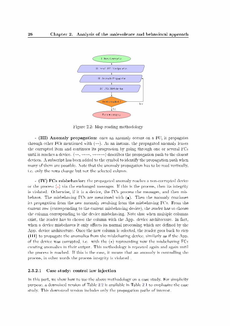
26 Chapter 2. Analysis of the malevolence and behavioral approach
I- Item Corruption
II- Item's FCs Manipulation
III- Anomaly Propagation
IV- FCs Misbehavior
Device reached ?
Process integrity
No
Yes
Figure 2.2: Map reading methodology
- (III) Anomaly propagation: once an anomaly occurs on a FC, it propagatesthrough other FCs mentioned with ( ). At an instant, the propagated anomaly leavesthe corrupted item and continues its progression by going through one or several FCsuntil it reaches a device. ( , , ) describes the propagation path to the closestdevices. A subscript has been added to the symbol to identify the propagation path whenmany of them are possible. Note that the anomaly propagation has to be read vertically,i.e. only the rows change but not the selected column.
- (IV) FCs misbehavior: the propagated anomaly reaches a non-corrupted deviceor the process ( ) via the exchanged messages. If this is the process, then its integrityis violated. Otherwise, if it is a device, the FCs process the messages, and then mis-behave. The misbehaving FCs are mentioned with (). Then the anomaly continuesits propagation from the new anomaly resulting from the misbehaving FCs. From thecurrent row (corresponding to the current misbehaving device), the reader has to choosethe column corresponding to the device misbehaving. Note that when multiple columnsexist, the reader has to choose the column with the App. device architecture. In fact,when a device misbehaves it only aects its normal processing which are dened by theApp. device architecture. Once the new column is selected, the reader goes back to step(III) to propagate the anomalies from the misbehaving device, similarly as if the App.of the device was corrupted, i.e. with the (?) representing now the misbehaving FCscreating anomalies in their output. This methodology is repeated again and again untilthe process is reached. If this is the case, it means that an anomaly is controlling theprocess, in other words the process integrity is violated-.
2.3.2.1 Case study: control law injection
In this part, we show how to use the above methodology on a case study. For simplicitypurpose, a downsized version of Table 2.2 is available in Table 2.1 to emphasize the casestudy. This downsized version includes only the propagation paths of interest.

2.3. Analysis of the malevolence 27
Consider an attacker that has corrupted the App. of a DEDS controller (e.g. PLC)by uploading a malicious control law to forge anomalous commands. Recalling that thecontrol law corresponds to the FC: (comp) (Section 2.2).
DEDS c CVDS c
App. c App. c
DEDS comp ? c
tran cApp.
Com.1-1
ctrl c
CVDS
rec c - c
comp c ? c
tran - c cstor c ? c
Com.1-0
ctrl - c c
Process - c cTable 2.1: Reduced attacks propagation map for the case study
(I) Starting from the corrupted item, the column label "DEDS App." is selected.Then, we search for its internal processing by choosing the row label of the cor-rupted item, and crossing them with the selected column. The internal processingis shown in ( ), and the corrupted architecture in ( ).
(II) The attacker has uploaded a malicious control law that manipulates the FC(comp), which is consistent with the table since this FC can be manipulated by anattacker (?). An anomaly results from this manipulation: anomalous computationis processed.
(III) The anomalous command propagates on the FC (tran) ( ) to be emitted tothe CVDS-controller. Then, the anomaly leaves the corrupted DEDS controller.Thereafter, the propagation continues over the Com.1-1 on the FC (ctrl) ( )until it reaches the CVDS-controller and its FC (rec) ( ). To keep simplicityin the analysis, we only analyze one propagation path over three in Table 2.2, i.e.corresponds to the one with the subscript (1).
(IV) The anomaly transported via the message is stored in the CVDS memory(stor) and is used for the computation (comp). Hence, both FCs (stor) and (comp)misbehave (). Since the CVDS misbehaves, it produces a new anomaly beingpropagated. To study the propagation path, we choose the column label whichcorresponds to the misbehaving device, i.e. CVDS, with the device architectureApp. From now on, the analysis is done from the CVDS App. column by goingback to step (III) of Figure 2.2.
(III) The anomaly goes through the FC (tran) ( ), and is transported via Com.1-0 on FC (ctrl) ( ). As before, only one propagation path is studied whichcorresponds to the one with the subscript (1) in Table 2.2.

28 Chapter 2. Analysis of the malevolence and behavioral approach
(IV) From the propagation path, the anomaly reaches the process ( ) whichmeans the violation of its integrity.
The attacks propagation map in Table 2.2 has been proposed and a methodologyto use and read it has been detailed in Figure 2.2. A case study has been studied toshow how to use the methodology with a reduced attacks propagation map. As seenin this Section, the attacks propagation map is relevant to study how the process canbe reached by an anomaly resulting from the corruption of a device architecture or ofa communication. As a remark, only the propagation path resulting to the processintegrity reachability has been detailed. However, by analyzing the other propagationpaths it is possible to nd out all the other devices that are misbehaving as we will seein the next part on past attacks analysis.
2.4 Application on Stuxnet attack
Apart from the case study, we describe and analyze in this part the application of the at-tacks propagation map in Table 2.2 on past attacks following the methodology presentedabove. It appears that such attacks tried to remain stealthy regarding the operatorsin front of the SCADA or the HMIs as an additional objective [Sicard et al. 2018]. Inaddition to the process integrity reachability, we use the methodology to analyze how theSCADA and/or the HMIs have been targeted. This is done by exploring the other prop-agation paths as stated in the remark above. From now on, we specify which messagecontent part, i.e. pl or md, are involved.
2.4.0.1 Stuxnet Attack
Stuxnet attack aimed to abnormally control the centrifuges velocities, i.e. to violate theprocess integrity, and to hide the abnormal values of variables related to the centrifugesvelocities from the operators in front of the SCADA and the HMIs. After a preliminaryreconnaissance of the targeted ICS control features, the attacker has corrupted the DEDSApp. by uploading a malicious control program from a corrupted EW. Such corruptionallowed the manipulation of (i) the FC (comp) to forge anomalous setpoints to violatethe process integrity, and (ii) the FC (stor) to store false variables representing a nor-mal process behavior, as it should be without any attacks, in order to remain stealthy[Langner 2011].
Figure 2.3 describes the attack propagation mentioned with a reference letter (A,B,C,D)and numbers, the asterisk symbol * refers to the propagation path. It is also reportedin Table 2.2 to guide the reader in the analysis. For visibility purposes, only the lastpropagation path's symbol is labeled in Table 2.2. Indeed, it is sucient for the readerto read the symbol's subscript to trace the propagation path backwards. The Stuxnetattack propagation follows four distinct steps which are illustrated sequentially in thestate ow (Figure 2.3). These four steps are detailed below:
1. Beforehand, the attacker has corrupted an EW (A), an external device (whitefont cell), to upload a malicious control program in the DEDS App. through theCom.2-1 (cnf-pl) (A*).

2.4. Application on Stuxnet attack 29
Corrupted EW (A)
DEDS (App) (B)
Corruption
DEDS (comp) (B1)
Manipulation
CVDS (C1)
Misbehavior
Process integrity (D1)
Violation
DEDS (stor) (B2)
Manipulation
HMI (C21)
Misbehavior
SCADA (C22)
Misbehavior
Upload control program
Com.2-1 (cnf)
Propagation
(A*)
Setpoint
Com.1-1 (ctrl)
Propagation
(B1*)
Command
Com.1-0 (ctrl)
Propagation
(C1*)
Variables
Com.1-1
(ctrl)
Propagation
(B21*)
Variables
Com.2-1
(ctrl)
Propagation
(B22*)
Figure 2.3: Stuxnet attack propagation

30
Chapter2.Analysis
ofthemalevolenceandbehavioralapproach
SCADA Com. DEDS B DEDS HMI Com. CVDS C1 Com. EW A
ccApp. 2-1 App. ccFw. ccApp. 1-1 cccApp. 1-0SCADA
rec - - (2) B22* (2) - - - - - -
comp ? - C22 - - - - - -
tran - - - - - - - - - -
stor ? - C22 - - - - - -
disp ? - C22 - - - - - -
App. - - - - - - - - - -
Com.2-1 cnf - ? - - - - - - - - (1)
ctrl - ? (2) (2) - - - - - -
DEDS
rec - ? - (2) (1) (1) A*
comp - ? B1 ? - -
tran - - - ? - - - - - -
stor - ? B2 ? - -
App. - - - - - - - - B
Fw. - - - - - - - -
HMI
rec - - - (3) B21* (3) - - - - -
comp - - - C21 ? - - - -
tran - - - - - - - - - -
stor - - - C21 ? - - - -
disp - - - C21 ? - - - -
App. - - - - - - - - - -
Com.1-1 cnf - - - - - - ? - - - (2)
ctrl - - - (1)(3) (1)(3) - ? (2) - -
CVDS
rec - - - (1) B1* (1) - (2)
comp - - - C1 - ? C1 -
tran - - - - - - - - - -
stor - - - C1 - ? C1 -
App - - - - - - - -
Com.1-0
ctrl - - - (4) (4) - - - (1) C1* ? -
Process - - - (4) (4) - - - (1) D1 (2) -
Table 2.2: Attacks propagation map for an ICS arranged following the ISA95 - From the corruption of a device architecture ( ) or of acommunication ( ), the potential manipulated FCs (?), the propagation path of anomalies ( ), the misbehaving FCs (),the process integrity ( ), the not targeted FCs and device architecture (-); the Stuxnet attack propagation (letters and numbers)

2.5. Behavioral approaches to address the malevolence 31
2. From now on, the DEDS is corrupted (B), i.e. the column and the rows change,and the attacker manipulates both (i) the DEDS (comp) (B1), and (ii) the DEDS(stor) (B2).
3. (i) The DEDS (comp) (B1) is manipulated:
(a) The attacker computes an anomalous setpoint which propagates throughCom.1-1 (ctrl-pl) (B1*) to make the CVDS controller misbehave (C1).
(b) From the misbehaving CVDS controller (C1), i.e. the column changes, anoma-lous commands are transmitted through Com.1-0 (ctrl-pl) (C1*) to the pro-cess.
(c) Hence, the process integrity is violated (D1).
4. In the meantime, (ii) the DEDS (stor) (B2) is manipulated:
(a) The attacker stores false variables about the behavior of the process and ofthe local control in the DEDS shared memory. Then, they are propagatedfrom the Com.1-1 (ctrl-pl) (B21*) to the HMI (C21), and from the Com.2-1(ctrl-pl) (B22*) to the SCADA (C22).
(b) Hence, the HMI and the SCADA misbehave (C21, C22) and mislead theoperators about the process and local control behaviors.
To conclude this section, the analysis of the malevolence highlights the following points:
Anomalies controlled by the malicious act follow a mandatory path to reach itsobjective.
The higher the level of the corrupted module in the ICS architecture, the longerthe propagation path is, i.e. various digital devices need to be crossed to reach theprocess.
In the past decade, the literature has proposed a large number of contributions toaddress the malevolence in ICS. One of the main approaches consists in modeling thenormal behavior of a digital entity with respect to the evolution of the process. Thenormal behavior corresponds to the behavior of the entity in the malevolence free case.The next section is devoted to the behavioral approaches.
2.5 Behavioral approaches to address the malevolence
In the previous section, the malevolence has been analyzed as a mean to create anintended failure in a digital entity, i.e. the Corruption. This failure creates in term anintended fault in the behavior of the digital entity, i.e. the Manipulation. The anomaliesare then propagated over the control system by misbehaving the digital devices, i.e. thePropagation and the Misbehavior.Literature focusing on the malevolence inherits the research works from the fault-detectionand the malware detection research elds, respectively for the fault created by the malev-olence and the intentional characteristic of malwares. Approaches can be split into two

32 Chapter 2. Analysis of the malevolence and behavioral approach
main groups [Vinod et al. 2009, Bazrafshan et al. 2013]: signature-based, and behav-ioral approaches [Sicard 2018]. In a nutshell, the signature-based approach establishesan abnormal pattern of the behavior of a digital entity representing its behavior in themalevolence case; whereas the behavioral approach models their normal behavior, i.e. inthe malevolence free case. This thesis contributes to the behavioral approach.
The basic idea behind the behavioral approach is the inspection of the behaviorof a digital entity, or of a digital entity with respect to the behavior of the process.Indeed, a digital entity is a module or a communication of the control system in chargeof coordinating the control and controlling the process. Therefore, any decision emittedby a digital entity is a reaction of a decision from an upper module or a status feedbackof a lower module about the process behavior.
Plenty of methods utilizing a behavioral approach to tackle the malevolence haveemerged in the literature. Inspired from the classication of fault-detection methods[Venkatasubramanian et al. 2003, Nguyen 2015], we propose to split these methods intothree categories:
Knowledge-based methods utilizes explicit knowledge about the behavior of adigital entity, or of a digital entity with respect to the behavior of the process. Thisknowledge can come from technical specications of the control system design, fromfunctional and structural analysis of the control system, or from the historical data.For instance, [Lin et al. 2013] [ctrl] models specications of the DNP3 protocolthat might be violated by the malevolence. Besides, [McLaughlin 2013] [DEDS-comp] models the PLC's control program to detect inconsistency in the computeddecisions if it is subject to malevolence. In [Carcano et al. 2009, Fovino et al. 2010][DEDS-tran] the process behavior is modeled with respect to the PLC behavior,to reveal inconsistency.
Data-driven-based methods utilizes learning techniques to associate a set ofdecisions and/or status feedback to the behavior of a digital entity. These tech-niques use data collected from the current ICS operations, or from historical data.For instance, [Linda et al. 2009, Kalech 2019] [ctrl] model the normal behavior ofcommunication exchanges including source-destination, size and periodicity of ex-changed packets, and their probability of occurrence from network properties (e.g.response time and loss of packets) in [Ponomarev & Atkison 2016] [ctrl]. Besides,[Hadziosmanovic et al. 2013] [DEDS-stor] models the normal range of the variablesstored in the PLC. Again on the PLC, [Rrushi & Kang 2009] [DEDS-stor] modelsits interaction with the process to describe the evolution of the stored variables.
Behavior-based methods utilizes physical knowledge about the process behav-ior to model it, or to model its interaction with other digital entities. In additionto this, it can utilize information knowledge about digital entities to model it. Forinstance, [Goldenberg & Wool 2013, Kleinmann & Wool 2017, Hahn & Govin-darasu 2013] [ctrl] model the communication exchanges between an HMI and aPLC including the size and periodicity of exchanged packets, and the data trans-ported. In [Erez & Wool 2015] the behavior of the variables stored in the PLC ismodeled.

2.6. Conclusion 33
From the model of the process behavior, [Hu et al. 2018b, Marelli et al. 2018] es-tablish properties of the status feedback characterizing the malevolence (e.g. non-randomness, distribution properties). [Koutsandria et al. 2014, Garcia et al. 2016,Caselli et al. 2015, Sicard et al. 2019] models the behavior of the process withrespect to the PLC behavior to detect if the transmitted decisions will conductto a violation of the process integrity. In addition, [Beaudet et al. 2020] proposesan implementation on a testbed for detecting anomaly in the control signal trans-mitted by a DEDS-controller [ctrl] Similarly with the CVDS-controller, [Sridhar& Govindarasu 2014] models the behavior of the process with respect to the con-troller behavior to detect malevolence based on the residual on the sensor readings[ctrl]. Dierently, [Koucham et al. 2018] extracts normal behavior features of thecommunication using a data mining method. It obtains temporal safety propertiesthat must be satised in the attack-free case [ctrl-pl]. With a similar model, [Mo &Sinopoli 2016a, Murguia et al. 2017, Murguia et al. 2020a] investigate the impact ofthe malevolence on the process integrity [ctrl]. [Yaseen & Bayart 2017] proposes tomonitor the CVDS-controller behavior from its input and its output. It allows thedetection of a control signal manipulation from a compromised controller. Lastly,[Thuillier et al. 2020] uses an Interval Finite Memory Observer allowing the esti-mation of states on an uncertain process over a temporal window. It provides anupper and lower bounds of estimate values due to the process uncertainties. Thiswork aims at detecting and correcting anomalous sensor readings. The detectionoccurs when the sensor readings are outside of the estimation bounds [CVDS-rec].
2.6 Conclusion
This Chapter has shown that multiple paths exist for the anomalies to reach the processintegrity. In addition, whatever the path taken, the anomalies must cross the controllers(DEDS or CVDS) to reach it. This analysis has then been shown on a real case, theStuxnet attack. Although this analysis shows the reachability, it does not provide formalmethods to prove it, neither to prevent anomalies to reach the process integrity. Thisthesis takes place within this framework. As we will see later, we provide formal methodsfor proving the reachability of the process integrity for a type of attacks. These methodsare then extended to nd restrictions on the control in order to guarantee the non-reachability of the process integrity. The methods allow the analysis and the preventionof malevolence.


Chapter 3
Research problem
Contents
3.1 Introduction . . . . . . . . . . . . . . . . . . . . . . . . . . . . . . . 35
3.2 Process control with CVDS-controller . . . . . . . . . . . . . . . . 36
3.2.1 Description of the system in our focus of interest . . . . . . . . . . 36
3.2.2 Behavior of dynamical systems . . . . . . . . . . . . . . . . . . . . 36
3.3 Brief literature review of malevolence in dynamical system . . . 37
3.3.1 Methods based on the measurement signals . . . . . . . . . . . . . 38
3.3.2 Methods based on the control signals . . . . . . . . . . . . . . . . . 39
3.4 Observation of the anomaly . . . . . . . . . . . . . . . . . . . . . . 40
3.5 Aging of actuators . . . . . . . . . . . . . . . . . . . . . . . . . . . . 41
3.6 Problem statement . . . . . . . . . . . . . . . . . . . . . . . . . . . 42
3.7 Scientic positioning . . . . . . . . . . . . . . . . . . . . . . . . . . 44
3.7.1 Set-theoretic methods in control . . . . . . . . . . . . . . . . . . . 44
3.7.2 Linear optimization . . . . . . . . . . . . . . . . . . . . . . . . . . 45
3.8 Scientic issues . . . . . . . . . . . . . . . . . . . . . . . . . . . . . . 46
3.9 Conclusion . . . . . . . . . . . . . . . . . . . . . . . . . . . . . . . . 47
3.1 Introduction
As we have seen in Chapter 2, there exist multiple paths for the anomaly to reach theprocess integrity. However, all the origin of these paths dier. It can come from thecorruption of the interaction with the controllers, i.e. SCADA, HMI, Com.2-1, Com.1-1, or from the corruption of the controllers itself and their respective communicationwith the process, i.e. Com.1-1. This thesis addresses the malevolence issue from thecontrollers, in particular the CVDS-controllers.
This Chapter is devoted to the research problem this thesis contributes. Section 3.2describes the control system we consider in this thesis and the mathematical modelutilized for describing the process behavior. Thereafter, Section 3.3 reviews briey theliterature to outline the main trends in analysis and prevention of anomalies. Then,Section 3.4 and Section 3.5 explains why our research problem is focused on anomalies inthe control signal. Section 3.6 presents our problems statement, and Section 3.7 presentsthe methods we derive to address our problem statement and the dierences with theliterature. Lastly, Section 3.8 highlights the scientic issues this thesis addresses.

36 Chapter 3. Research problem
3.2 Process control with CVDS-controller
3.2.1 Description of the system in our focus of interest
In this thesis, we consider a control system including a CVDS controller (C) that controlsa Process (P) via a transmission (tran) and reception (rec) channels. This control systemis coordinated by the upper modules of the ICS: it receives setpoints being the industrialobjectives. The controller imposes the desired service, often called the desired systemresponse, by transmitting a control signal u(t) to the process, and receives a partial orcomplete measure of the state x(t) to update the control input. In addition to this, atypical anomaly detector receives the measured state x(t) and the transmitted input u(t)
to detect a service degradation that could occur from a fault in the process. Theory ofautomatic control [Dorf & Bishop 2000] commonly represents this control system with ablock diagram representation in Figure 3.1.
Figure 3.1: Considered control system
In this representation, the digital entities, that can be subject to malevolence, are:the controller, and the transmission and reception channels. However, the anomalydetector is assumed as not attackable. The process to be controlled by the controller isconsidered to be a dynamical systems. A dynamical system is "a particle or ensembleof particles whose state varies over time and thus obeys dierential equations involvingtime derivatives" [Nature ].
3.2.2 Behavior of dynamical systems
In order to provide methods to tackle the issue of malevolence in the control of dynam-ical systems, this thesis focuses on quantitative mathematical models of the behavior ofdynamical system. Dynamical systems are represented mathematically by a set of simul-taneous dierential equations given in (3.1). It describes quantitatively the relationshipsbetween the system variables. They are obtained by using the physical laws governingthe process (e.g. mechanical, electrical, uid, thermodynamic).
x(t) = f(x, u, t) (3.1)
where t ∈ R is the time, x(t) ∈ X ⊂ Rn is the state, u ∈ U ⊂ Rm is the control input,and f is a function. Notice that R is the set of real numbers, Rn is the set of real nvector, and Rn×m is the set of real n×m matrices. This notation will be recall later inChapter 4.

3.3. Brief literature review of malevolence in dynamical system 37
In this thesis, we restrain our research works to dynamical systems modeled ascontinuous-time invariant ane system given in (3.2).
x(t) = Ax(t) +Bu(t) + a (3.2)
where x(t) ∈ Rn is the state, u(t) ∈ Rm is the input, A ∈ Rn×n is the state matrix,B ∈ Rn×m is the input matrix, and a ∈ Rn is the ane term.
An ane systems is a linear system with an ane term. In fact, the ane termcan be seen as a constant control input acting on the dynamical system. Thus, onecan extend the input u(t) to simplify the model in (3.2). Instead of this, the model isproposed to be simplied by extending the state in order to t with the formalism of theclass of Piecewise ane (PWA) systems [Hassibi & Boyd 1998] for future research works.By dening the extended state x(t) = [x>(t), 1]>, the model in (3.2) can be reformulatedas:
˙x(t) = Ax(t) + Bu(t) (3.3)
with
A =
[A a
01,n 0
], B =
[B
01,m
]. (3.4)
In this section, we have described our focus of interest: the malevolence in the controlof dynamical systems. From this control view, we are interested in the signals: themeasurement signals, and the control signals. In the next section, we review the literaturearound the malevolence in the control of dynamical systems.
3.3 Brief literature review of malevolence in dynamical sys-
tem
This section gives a brief literature review to outline the main trends in the literatureof malevolence in dynamical system with a state-space representation. Clearly, the ob-jective is not to provide an exhaustive list of methods, but show what is investigated inthe literature.
The literature contributions can be classied into three groups as follows.
Vulnerability assessment contribution explores control-based security weak pointsthat might be abused by the malicious act (e.g. impact of manipulation on theprocess integrity, design of attacks).
Prevention contribution provides design conditions to limit or avoid the mali-cious act feasibility (e.g. minimum set of sensor to secure to guarantee the statereconstruction in the attack case, conguration of anomaly detector to limit theattack impact).
Detection contribution aims at revealing the presence of anomalies in the currentoperations of the ICS (e.g. verication of signals properties such as randomness ofmeasurement signals, violated in the attack case).

38 Chapter 3. Research problem
This thesis contributes to vulnerability assessment and prevention groups. In the rest ofthis thesis, detection methods are thus not anymore considered.
The reviewed literature comes from the theory of automatic control. As seen previ-ously, it considers the problem as an interconnection of two systems, i.e. the controllerand the process, that reacts to signals. This systemic view leads to a lack of practicalimplementations of the proposed methods: for instance, measurement signals can be in-vestigated from the sensors, the reception channel [Com.1-0-ctrl], or the controller [rec,stor, comp], however the model does not explicitly consider it. Therefore, the methodsare classied either on the measurement signals or the control signals.
3.3.1 Methods based on the measurement signals
Vulnerability assessment
Three main trends appear in the literature: (i) quantication of the impact of sensorreading manipulation on the process state, (ii) design of stealthy sensor reading injectionattack, and (iii) design of stealthy sensor reading Denial of Service (DoS) attack.
(i) [Bai et al. 2017a] considers the manipulation of a single sensor reading. Froman information-theoretic approach, a graded notion of attack stealthiness is provided.Also, the fundamental limitations for the detection with an anomaly detector are given.Then, an optimal attack is designed to maximize the performance degradation for agiven stealthiness level. Finally, [Murguia et al. 2020b] proposes two security metrics toquantify the impact on the performance degradation, based on the reachable set of theprocess state.
(ii) [Guo et al. 2018] considers the stealthy manipulation of a single sensor readingas an ane function of its legitimate value. An optimal attack is designed to maximizethe performance degradation and to achieve the desired level of stealthiness expressedfrom the Kullback-Leibler divergence (K-L divergence) on the residue. Similarly, a moregeneral attack is proposed in [Li & Yang 2019]. Their attack achieves the largest per-formance degradation of the process control. In addition, [Guo et al. 2019] considersa similar attack but with an extra sensor reading for measuring the process behavior.The optimal attack is designed to evade a static Chi-squared anomaly detector. Besides,[Cheng et al. 2019] designs event-based stealthy sensor readings manipulations to maxi-mize the performance degradation under a xed average communication rate to remainstealthy.
(iii) [Zhang et al. 2016] designs an optimal DoS attack subject to energy-constraintto maximize the performance degradation of the process control. The proposal considersthe manipulation of a single sensor reading during a limited period of time. In fact, axed energy amount is consumed for each manipulation. Also, the impact on the controlloop stability is investigated. Under similar considerations, [Zhang et al. 2018] designs anoptimal DoS attack taking into account the energy allocation. In particular, a real-timealgorithm is provided to dynamically adjust the attack energy.
Prevention

3.3. Brief literature review of malevolence in dynamical system 39
Two main trends appear in the literature: (i) conditions to guarantee the integrity ofthe state estimator, and (ii) conguring anomaly detectors to mitigate stealthy sensorreading manipulation.
(i) [Fawzi et al. 2014] characterizes the fundamental limitations of an estimator tocorrect invariant sparse manipulated sensor readings. In particular, it is shown thatthe state reconstruction is not possible if more than half the sensor readings are ma-nipulated. An algorithm inspired from techniques in compressed sensing is provided tocorrect the manipulated sensor readings, when the number of manipulations is smallerthan a threshold. In addition, [Chang et al. 2018] considers a variant set of sparse ma-nipulated sensor readings. A secure estimator is proposed and the maximum numberof manipulated sensor readings that can be corrected by the estimator is proved. Inanother way, [Hu et al. 2018a] proposes a security criterion to guarantee the securityof the estimator, i.e. estimation error is bounded, when the number of manipulation issmaller than a threshold. Then, the set of normal sensor readings to guarantee the statereconstruction is provided.
(ii) [Umsonst et al. 2017] considers time-limited manipulations on the sensor readingsand the commands. The optimal stealthy attack to maximize the performance degrada-tion is designed for both stateless and stateful anomaly detectors. It is shown that thestateful one better mitigates the stealthy attack [rec]. Furthermore, [Umsonst & Sand-berg 2018] compares the performance degradation induced by sensor readings manipula-tions for stateless (Chi-squared) and stateful (Cumulative Sum (CUSUM), MultivariateExponentially Weighted Moving Average Filter (MEWMA)) anomaly detectors. It ispointed out that the MEWMA anomaly detector better mitigates the attack than theChi-squared anomaly detector. Dierently, [Murguia & Ruths 2019] proposes a system-atic procedure conguring a CUSUM anomaly detector based on statistical properties ofthe residual. The sucient conditions on the bias parameter are provided to guaranteethe CUSUM sequence being bounded. [Milo²evi£ et al. 2017] proposes a criterion toselect the best combination of sensors to be secured in order to mitigate sensor readingsmanipulations. The defender's objective is to guarantee an upper bound of the perfor-mance degradation. Besides, in the power grid domain, [Zhang et al. 2019a] investigatesthe impact of sensor readings manipulations on the microgrid system stability. A stableregion is dened and the sucient conditions to guarantee the system stability are given.
3.3.2 Methods based on the control signals
Vulnerability assessment
Three main trends appear in the literature: (i) quantication of the impact of controlsignal manipulation on the process state, (ii) design of stealthy control signal injectionattack, and (iii) design of stealthy sensor reading DoS attack.
(i) [Mo & Sinopoli 2016b] computes the inner and the outer-approximations of thereachable set of the process states by the means of invariant ellipsoids. Note that italso considers sensor reading manipulation. In addition, [Bai et al. 2017b] describesthe ability of an attacker to modify a single command; and provides conditions to havethe optimal performance degradation. [Milo²evi¢ et al. 2019] quanties the impact of

40 Chapter 3. Research problem
stealthy sensor readings/commands manipulations upon critical states. Two metrics arecomputed for describing the probability for some states to leave a safety region duringa period of time. Various types of attacks are evaluated (e.g. DoS, values permutation,sign alternation) in order to nd the one with the largest impact upon a set of criticalstates.
(ii) [Li et al. 2019] designs a two agents based attack applying the Least SquaresSupport Vector Machine (LSSVM). The CVDS controller is assumed to implement aProportional Integrate Derivative (PID) control law. On one hand, an attack agent es-timates the PID's parameters from the single sensor reading and the single command.Thereafter, the attack agent injects additional data to the command in order to deviatethe process steady-state. On the other hand, a covert agent uses the estimated PID'sparameters to mimic the normal steady-state by injecting additional data to the sensorreading. In addition, [Zhang et al. 2019b] investigates the manipulation of commands andsensor readings with a xed additional data at each time instant. An optimal stealthyattack to maximize the performance degradation is designed.
Prevention
Only one main trend appears in the literature: (i) the restriction of the control signal.(i) As far as we know, [Kafash et al. 2018] is the rst and only contribution with this
objective. The main idea is to quantify the impact of control signal manipulation on theprocess, analyze if the a dangerous zone can be reached, and restrain the control signalsuch that the dangerous zone cannot be reached. This work is based on the computationof the reachable set of the process. Thereafter, the same authors have extended theirwork in [Hadizadeh Kafash et al. 2018] to tackle the problem of control restriction. Infact, they have observed that by restraining the control input set, it results that thecontroller is too restrained to deliver the desired service.
3.4 Observation of the anomaly
As seen in the previous section, contributions focusing on the malevolence in controlsystems study anomalies either in the measurement signals, or in the control signals. InChapter 2, the malevolence has been analyzed, and it has been shown that anomaliesfollow specic propagation paths to violate the process integrity. We propose in thissection to study the issue of the anomaly observation for securing the process integrity,against a malicious act. We consider three scenarios where a single digital entity iscorrupted: (i) the controller, (ii) the transmission channel, and (iii) the reception channel.
In the scenario (i) where the controller is corrupted, the attacker can manipulatethe commands from the FCs (stor,comp). The abnormal command is then propagatedover the transmission channel to the actuators. The process is then transformed by theactuators, so its integrity is violated. Thereafter, abnormal measurements are then sentback to the controller about the process state.
In the scenario (ii) where the transmission channel is corrupted, the attacker can ma-nipulate the commands transmitted by the controller from the FC (ctrl). The abnormalcommand is then propagated to the actuators. The process is then transformed by the

3.5. Aging of actuators 41
actuators, so its integrity is violated. Thereafter, abnormal measurements are then sentback to the controller about the process state.
In the scenario (iii) where the reception channel is corrupted, the attacker can ma-nipulate the measurements received by the controller from the FC (ctrl). The abnormalmeasurements are then propagated to the controller. The controller misbehaves: itstores and computes abnormal commands. Then, the abnormal commands are propa-gated over the transmission channel to the actuators. The process is then transformedby the actuators, so its integrity is violated.
We state that the study of anomalies in the measurements is too late to detect aviolation of the process integrity. Indeed, the process integrity is already violated beforethe presence of anomalies in the measurements as seen in the scenarios (i) and (ii). Thus,abnormal measurements are the result of the malicious act on the process. In additionto this, presence of abnormal measurements do not systematically mean the violation ofthe process integrity. Indeed, it can also be the result of equipment failures, the mostcommon root cause of failures in ICSs. Therefore, the root cause of failure causing ab-normal measurements in the scenarios (iii) cannot be characterized. However, anomaliesin the commands systematically violate the process integrity, as seen in Chapter 2. Thisis why it is more appropriate to study anomalies in the commands, as we can see in thescenarios (i), (ii), and (iii). However, the characterization of the root cause is not easierwhen anomalies are present in the commands. Indeed, it can be the result of the otherroot causes presented in Chapter 1.
From this observation, this thesis focuses on anomalies in the commands transmittedby the controller to the actuators. In particular, the malicious act with the primaryobjective of violating the process integrity to cause a permanent inability to deliver theservice is focused on. To that end, we consider a malicious act that accelerates the agingof the actuators in order to cause premature failure in the process.
3.5 Aging of actuators
Aging of an actuator is a process changing the properties of the actuator with respectto the time. The type of aging of interest is the one associated with deterioration ofthe actuator's functional capability. Aging occurs owing to many physical stresses theactuator is subject to. They are categorized into internal and external and dened asfollows [Carfagno et al. 1980].
Internal are operational stresses meaning that they are inherent in the operationof the actuator (e.g. current, voltage, ohmic heating).
External are stresses originating in the environment of the actuator (e.g. ambienttemperature, vibration, humidity, oxidation) [Cox et al. 1995].
In this thesis, external stresses on an actuator are not considered as they cannot becontrolled from the control of the actuator. Theoretical relationships between a stressand a deterioration are known for some types of materials and components. However,

42 Chapter 3. Research problem
for actuator mixing materials and components is often more complex. Thus the relationof degradation to stress is based on empirical knowledge, or the observation of aging asa function of time and stress magnitude.
Physical stresses are usually classied into three categories: electrical, mechanical,and thermal. They are detailed in [IAE 1989, McNeill 1983], and some internal stressesare given as follows:
Electrical: electric elds, magnetic elds
Mechanical: vibration, mechanical shock, i.e. bump, acceleration
Thermal: temperature, temperature cycling, thermal shock, i.e. rapid change oftemperature
For instance, the electric power quality referring to the quality of voltage or currentis an important electrical stress (e.g. voltage and current transients, short- and long-duration voltage variation, voltage imbalance, voltage uctuation) in power systemsand electric machinery [Fuc 2008]. In the mechanical stresses, mechanical vibrationsand shocks play an important role in the aging of mechanical systems [Lalanne 2013].In particular, torsional vibration shaft due to torque harmonics has been studied inturbine-generators [Walker et al. 1981, Liu et al. 2014], and in electric machinery [Han& Palazzolo 2013, Holopainen et al. 2013]. In addition, mechanical overload causes anelectric drive to overheat leading to a failure [Atallah et al. 2007]. In the thermal stresses,some applications require high peak torque, beyond the operating conditions, achievedby supplying more current to the electric drive for limited time periods. As a result, themachine is thermally overloaded and the insulation system can be degraded [Sciasceraet al. 2016, Madonna et al. 2020]. Usually, aging is not only the cause of a single typeof stress, but a combination of electrical, mechanical, and thermal stresses as for thedegradation of the insulation system in electric machinery [Bartnikas & Morin 2004].
To conclude, this thesis is concerned about anomalies in the control signal that aimto accelerate the aging of the process's actuators [Merouane et al. 2020]. In the followingSections, the problem statement is presented and our research works are positionedaccording to the literature.
3.6 Problem statement
This thesis concerns the malevolence in the control of dynamical systems. Our interestis in malicious acts aiming at (i) accelerating the aging of a dynamical system, while (ii)delivering the desired service. (i) is the primary goal of the malicious act, i.e. violatingthe process integrity, and (ii) is to avoid any suspicion of fault from the anomaly detector.This is what we call a stealthy aging attack and is dened as follows:
Denition 5. A stealthy aging attack drives a targeted dynamical system as in (3.3)to operate outside of the normal aging conditions while delivering the desired service.
By accelerating the aging, a failure will occur prematurely in the dynamical system.As the malicious act focuses on the aging instead of the delivered service, the failure

3.6. Problem statement 43
could be misinterpreted and associated to a normal aging. Indeed, although reliabilitymethods, predicting the time of failure, have been improved, they still lack in successfullypredicting a failure in many cases as the aging mechanisms are complex to model anddepend on various operating conditions.
As far as we know, the only contribution motivated by the stresses in a dynamicalsystem to cause a failure is [de Sá et al. 2017]. It attempts to design an attack maximiz-ing the overshoot, i.e. the peak value of a state variable during the transient response,or the constant steady-state error of the controlled variable. It considers a corruptedtransmission channel and a corrupted reception channel where the malicious act manip-ulates the transmitted commands following an attack function. This work proposes adesign method of this function, considering the attacker is aware of the controller andthe process models.Three critical remarks can be stated on this work:
Firstly, it only concerns Single-Input-Single-Output dynamical systems with an input-output relationship in the frequency-domain. The design method utilizes the root locusmethod for designing the attack function to make the control system underdamped,i.e. to cause overshoot. However, the work can be easily extended on the Multi-Input-Multi-Output (MIMO) system with a time-domain representation using a typical pole-placement technique from the characteristic equation of the control system.
Secondly, the design method requires the controller model. Indeed, the design of theattack function requires both the controller and the process models. That is why, thereception channel is also considered as corrupted in order to perform a system identi-cation of both models. In a nutshell, the system identication collects the input andoutput signals of the system of interest to assess a tting model, i.e. applying the sameinputs, the same outputs result. But, system identication requires the structure of themodel that is the unknown coecients of the model. Both requirements on the corruptedchannels and the model structure are strong.
Thirdly, the stealthiness of the attack is not considered, with respect to an anomalydetector. Indeed, if an anomaly detector is placed, the overshoot or the constant biaswould be detected. By collecting the received measurement signals and the transmittedcontrol signals from the controller side, an abnormal residual would appear, resultingprobably to an alarm, i.e. depending on the hypothesis testing, [Cómbita et al. 2019].
This last remark is the most critical one, and clearly limits the application of theirproposal. We state that this kind of attacks can be stealthy if the states related to theaging are dierent from the state of the service to be delivered. Therefore, we focuson the MIMO dynamical system. In addition, we assume periodicity in the productionobjectives as it is the case in many ICSs. We consider an attacker with the followingconsiderations: (a) it has penetrated the control system, and corrupted the transmissionchannel; (b) it is aware of the process to be controlled, so it knows the process model, (c)it is aware of the periodicity in the production objectives, so that it knows the expecteddesired services, assuming the controller model does not change between two periodicoperations. The considered control system with the attacker is shown in Figure 3.2.
In practice, such considerations are reasonable: (a) it has been shown from pastICS attacks and the literature that communication channels can be corrupted mainlyfrom protocol vulnerabilities; (b) the process model is known by the ICS designer as

44 Chapter 3. Research problem
Figure 3.2: Considered control system with the corrupted channel (red)
it is required for designing the ICS and conguring the controller. As ICS applies atraceability policy, the process model should appear from the technical documentations.Thus, an attacker could gain access to it using Information Operations as preliminaryattack; (c) periodicity in the production objectives depends on the variability of theICS. Many ICSs have low variability (e.g. manufacturing production, papermill), andthus the production objectives do not change much. Hence, the attacker can performagain an Information Operations as preliminary attack to know the time evolution ofthe desired service. It can be known by collecting the control signals transmitted by thecontroller, and applying them on the process model known in (b) in order to computethe measurement signals. These measurement signals are those collected by the anomalydetector, and the state estimator of the controller, to check the hypothesis testings.This time evolution of the desired service can also be updated after having launchedthe stealthy aging attack. In fact, stealthy aging attacks accelerate the aging of theprocess by executing the attack periodically. Thus, it is reasonable to assume that inICSs with low variability, the computational time of a stealthy aging attack is lower thanthe industrial objectives changes.
3.7 Scientic positioning
In this thesis, two research problems are addressed: (i) the analysis of stealthy agingattacks for quantifying the impact on the process, and (ii) the prevention of stealthyaging attacks by restraining the control signal. For (i), we propose set-theoretic methodsderived from set theory to analyze the attacks feasibility. For (ii), those methods are usedfor restraining the control signal to make those attacks non-feasible. As we will see later,the latter has been done on a subcase of stealthy aging attacks. Thus, analysis of stealthyaging attacks (i) for the general case has been proposed with a Linear Programming (LP)method for computing the optimal abnormal input signal that maximizes the dynamicalsystem aging.
3.7.1 Set-theoretic methods in control
Set theory is a branch of mathematics investigating sets and their properties. Manycontrol problems can be formulated, analyzed, and solved in a set-theoretic context.Indeed, sets appear naturally when constraints, uncertainties, or design specications are

3.7. Scientic positioning 45
considered. Furthermore, sets are adapted to quantify system performances (e.g. eectof persistent noise in a feedback system, state estimation error) [Blanchini & Miani 2015].Set-theory appears in various areas of automatic control including constrained control,robust control, disturbance rejection, and robust estimation.
In this thesis, we are interested specically in set-theoretic methods for the analysisof dynamical systems. As part of these methods, reachable set computation are the basisof many control methods including target avoidance of an adversary in a game theoreticsetting [Mitchell et al. 2005], collision avoidance in unmanned aerial vehicles [Zhou &Baras 2015], or in fault detection for chemical reactors [Tulsyan & I. Barton 2016].In particular, the ellipsoidal set has been largely studied in many control problems tocompute reachable sets of linear systems [Blanchini 1999]. For instance, [Khlebnikovet al. 2011] uses invariant ellipsoids to analyze and design controller for linear time-invariant system subject to bounded exogenous disturbances.
For a dynamical system modeled as in (3.3), the reachable set is dened as follows.
Denition 6 (Reachable set, [Pecsvaradi & Narendra 1971]). A (nite-time) reachable
state set R(t1, X0) is the state set containing all the state trajectories of the dynamical
system at a time t1 from an initial state set X0 with a constrained input set U .
In the case of innite-time, i.e. t1 =∞, the innite-time reachable state setR(∞, X0)
is the set that captures all the nite time reachable state sets from an initial state setX0. Obviously to compute it, it is necessary for the system to be Lyapunov stable, aswe will detail later; otherwise R(∞, X0) is not bounded [Gayek 1991].
In the context of the malevolence, few research works have proposed methods basedon the reachable set. Our research works originate from the many works of the authorencompassed in [Murguia et al. 2020b] where it uses the innite-time reachable set forquantifying the impact of sensor reading or control signal manipulation on the process.Moreover, [Kafash et al. 2018] uses the innite-time reachable set for restraining thecontrol input set such that the impact of attacks avoids a dangerous set. Although thisidea is not novel as it is used in safety verication and control design, it is the rst contri-bution dealing with the malevolence. Our research work exploits this idea of restrainingthe control input set so that it avoids a dangerous set. However the system considereddiers from the one considered in [Murguia et al. 2020b, Kafash et al. 2018]: we consideronly the process without the controller, unlike the both contributions. Indeed, as seenin Chapter 2, the controller is subject to the malevolence as much as the communica-tion channels. Therefore, we are interested in quantifying the impact of control signalmanipulation by only considering the process. Thus, we search for preventing anomaliesin the control signal that can come from the control system.
3.7.2 Linear optimization
Linear optimization is a method to maximize a cost function in a mathematical modelwhose requirements are represented by linear relationships. It is used in control prob-lems such as path planning control to compute optimal control signals to minimize ormaximize an objective function representing for instance energy consumption or actuatorlimitations [Puglia 2012, Yang et al. 2012].

46 Chapter 3. Research problem
In the context of the malevolence, linear optimization has not been utilized surpris-ingly. Thus, the closest related works are [de Sá et al. 2017] computing an attack transferfunction maximizing the service degradation during the transient response; and [Teix-eira 2019], [Zhang & Venkitasubramaniam 2017], maximizing the service degradationwhile being stealthy with respect to a detector. However, those contributions considerthe controller in the optimization problem to escape the anomaly detector, as they de-grade the service. The main dierence in our work is that the attack objective is theaging of the system, instead of degrading the delivered service.
3.8 Scientic issues
In this thesis, we propose to analyze and prevent stealthy aging attacks dened in 5.The analysis consists in quantifying the impact of control signal manipulation on theprocess. As stated previously, we do not consider the controller model in our work, onlythe process model is considered.
Comparing with the literature, the rst novelty in this thesis is to model the stealth-iness of the attack by constraining the state to remain inside a set called the service set,as we will see in the next Chapters. In a nutshell, the state remains inside this service setwhen the controller controls the physical system, i.e. in the attack-free case. The stateconcerned with this constraint is the state that can reveal the attack. In particular, itincludes: (i) the state corresponding to the service that the physical system must deliver(e.g. tracking a position reference), (ii) the state measured by the sensors, providing afeedback to the controller.
We have developed two set-theoretic methods. The rst one is based on the invariantnotions for computing the constrained reachable set at the innite-time. The second oneis based on convex robust simulation for computing the constrained reachable set at thenite-time. Notice that those reachable sets are referred as constrained since they areconstrained by the service set. As we will see later, the second method has been developedto tackle the drawback of the invariant set-based method. In fact, as stated above, theinvariant set-based method requires a condition of stability for the dynamical systemof study. In our case, the system considered is the process only. But, the condition ofstability is often not satised without considering the controller.
In addition to this, invariant-set based method loses the temporal variable in theanalysis. The convex robust simulation-based method allows the presence of the temporalvariable and thus, can be used to quantify at which time the dangerous set can be reached.
To summarize, the following scientic issues are addressed in this thesis:
Modeling the attack stealthiness in set theory,
Stability condition required from the invariant set theory,
Loss of the temporal variable in the invariant set theory.

3.9. Conclusion 47
3.9 Conclusion
This Chapter has described the research problem addressed in this thesis. We contributein the vulnerability assessment and the prevention of stealthy aging attacks, a new typeof attack, launching on a process modeled as a dynamical system. In particular, wefocus on anomalies in the control signals that reach the actuators. It can come from acorruption of the CVDS-controller or of the Com.1-1 with the process. In the next Part,our methods for analyzing and preventing stealthy aging attacks are detailed.


Part II
Analysis and prevention of stealthy
aging attacks


Chapter 4
Background
Contents
4.1 Introduction . . . . . . . . . . . . . . . . . . . . . . . . . . . . . . . 51
4.2 Notations and conventions . . . . . . . . . . . . . . . . . . . . . . . 51
4.3 Matrix inequalities . . . . . . . . . . . . . . . . . . . . . . . . . . . . 52
4.4 Sum Of Squares (SOS) . . . . . . . . . . . . . . . . . . . . . . . . . 53
4.5 The generalized S-procedure . . . . . . . . . . . . . . . . . . . . . . 55
4.6 Set-theory preliminaries . . . . . . . . . . . . . . . . . . . . . . . . 55
4.6.1 Convex functions and sets . . . . . . . . . . . . . . . . . . . . . . . 55
4.6.2 κ-sublevel sets . . . . . . . . . . . . . . . . . . . . . . . . . . . . . 56
4.6.3 Operations between sets . . . . . . . . . . . . . . . . . . . . . . . . 56
4.6.4 Ellipsoidal sets . . . . . . . . . . . . . . . . . . . . . . . . . . . . . 57
4.6.5 Hyperplanes and halfspaces . . . . . . . . . . . . . . . . . . . . . . 58
4.6.6 Distance between an ellipsoid and an hyperplane . . . . . . . . . . 58
4.7 Convex optimization problems . . . . . . . . . . . . . . . . . . . . 58
4.7.1 Special cases of convex optimization problems . . . . . . . . . . . . 60
4.8 Lyapunov function . . . . . . . . . . . . . . . . . . . . . . . . . . . . 61
4.9 Conclusion . . . . . . . . . . . . . . . . . . . . . . . . . . . . . . . . 63
4.1 Introduction
The methods for analyzing and preventing stealthy aging attacks developed in this thesisare based on dynamical system theory. This theory allows the behavior descriptionof dynamical systems subject to input signals under some constraints. This Chapterprovides the sucient background in a compact manner to the reader for understandingthe rest of this thesis.
4.2 Notations and conventions
The notations and the conventions used in the manuscript are common for the controlsystem literature. Their description is provided in the following.
First of all, we present the notations for number sets and matrix sets. Let R be theset of real numbers, Rn be the set of real n vector, and Rn×m be the set of real n×mmatrices. Notice that Rn×n is the set of real n× n symmetric matrices. Given a vector

52 Chapter 4. Background
v ∈ Rn, vᵀ denotes its transpose. Given a matrix A, A> indicates its transpose, diag(A)
is the diagonal entries of the matrix A, In is the identity matrix of size n, 0n,m is thezero matrix of size n,m. The notation A ≥ 0 (A ≤ 0) indicates the positive (negative)semideniteness, i.e. all the eigenvalues of the symmetric matrix A are positive (negative)or equal to zero, whereas A > 0 (A < 0) indicates the positive (negative) deniteness,i.e. eigenvalues are strictly positive (negative). Finally, let Rm[t] be the set of real-valuedpolynomials of degree up to m in the variable t, and Rn×nm [t] be the set of symmetricmatrix-valued polynomials of degree up to m in the variable t of size n×n, with m ∈ N.
The following convention, classical in automatic control, must be recalled. Generally,the signals manipulated in this manuscript are in continous-time, for example x(t) ∈ Rn.Whenever this is not leading to confusions the time dependence will be dropped.
4.3 Matrix inequalities
As seen in the previous section, we focus on dynamical system described with a state-space representation using a matrix form. For this reason, it is important to recall somedenitions and properties related to matrices. The following denitions and propertiesare highlighted.
Denition 7 (Positive (negative) deniteness, [Boyd et al. 1994]). A symmetric
matrix P = P> ∈ Rn×n is called a negative denite matrix (respectively positive denite
matrix), denoted by P < 0 (resp. P > 0), if z>Pz < 0 (resp. z>Pz > 0) for all non-zero
vectors z with real entries (z ∈ Rn \ 0n).
Denition 8 (Positive (negative) semideniteness, [Boyd et al. 1994]). A symmet-
ric matrix P = P> ∈ Rn×n is called a negative semidenite matrix (respectively positive
semidenite matrix), denoted by P ≤ 0 (resp. P ≥ 0), if z>Pz ≤ 0 (resp. z>Pz ≥ 0)
for all non-zero vectors z with real entries (z ∈ Rn \ 0n)
The methods developed in this thesis are based on the search for symmetric matricessatisfying some constraints expressed in terms of Linear Matrix Inequality (LMI). LMIsare inequalities constraining the eigenvalues of a square symmetric matrix that dependsanely (linear plus a constant term) on the decision variables.
Denition 9 (Linear Matrix Inequality, [Boyd et al. 1994]). A Linear Matrix In-
equality (LMI) is dened by the following formulation:
F (x) = F0 +m∑i=1
xiFi > 0, (4.1)
where x = [x1, x2, · · · , xm]> ∈ Rm is the vector of decision variables, and Fi ∈ Rn×n, i =
0, · · · , n are given symmetric matrices, i.e. Fi = F>i . The components xi, i = 0, · · · ,m,
of this vector are called decision variables. The inequality means that F (x) is a positive
denite matrix, which can be rewritten as follows:
∀u ∈ Rn, u>F (x)u > 0, u 6= 0 (4.2)

4.4. Sum Of Squares (SOS) 53
Remark 1. The LMI in (4.1) is a convex constraint on x, i.e. the set x|F (x) > 0 isconvex.
In most control applications, LMIs are functions of matrix variables rather thanscalar valued decision variables. This means that we consider inequalities of the form(4.1) where the decision variables becomes X ∈ Rm1×m2 [Boyd et al. 1994]. As anexample, consider the well known Lyapunov inequality F (X) = A>X +XA < 0 whereA ∈ Rn×n is assumed to be given, and X ∈ Rn×n is a symmetric matrix variable. Thephrase "the LMI F (X) < 0 in X" means that the matrix X is a decision variable.Note that the LMI can be rewritten in the form of (4.1) as follows. Let X1, · · · , Pmbe a basis for symmetric n × n matrices (m = n(n + 1)/2). Then, take F0 = 0, andFi = −A>Pi − PiA.
The form of an LMI is very general and many inequalities can be expressed as LMIssuch that linear inequalities, convex quadratic inequalities, matrix norm inequalities, andvarious constraints from automatic control theory such as Lypaunov inequality as shownabove [Boyd et al. 1994].
In some cases, the matrix inequality can be a Bilinear Matrix Inequality (BMI), thatis a more general case than an LMI.
Denition 10 (Bilinear Matrix Inequality, [VanAntwerp & Braatz 2000]). A Bilin-
ear Matrix Inequality (BMI) is of the form:
F (x, y) = F0 +
m∑i=1
xiFi +
l∑j=1
yjGj +
m∑i=1
l∑j=1
xiyjHij > 0, (4.3)
where x = [x1, x2, · · · , xm]> ∈ Rm and y = [y1, y2, · · · , yl]> ∈ Rl are the vectors of
decision variables; and Fi ∈ Rn×n, ∀i = 0, · · · ,m, Gj ∈ Rn×n, ∀j = 1, · · · , l, Hij ∈Rn×n, ∀i = 1, · · · ,m and ∀j = 1, · · · , l are given symmetric matrices.
A BMI is an LMI in x for xed y, and an LMI in y for xed x; and so is convex inx and convex in y. But, the bilinear terms make the set not jointly convex in x and y[VanAntwerp & Braatz 2000].
In many automatic control problem, it is common to encounter the constraint thatsome functions be negative whenever some other functions are all negative. In some cases,this constraint can be expressed as an LMI, but in some others we can only approximatethis constraint by an LMI, which is more conservative than the initial constraint but isoften a useful approximation [VanAntwerp & Braatz 2000].
4.4 Sum Of Squares (SOS)
In this thesis, we are going to rely on a technique called Sum Of Square (SOS), whichallows casting several classes of polynomial problems into convex optimization problems.We recall here briey the basic notions that are necessary for understanding this thesis,the interested reader can then consult the references that are provided.

54 Chapter 4. Background
Denition 11 (SOS problems, [Parrilo 2003]). Let p(t) ∈ R2d[t]; we call Sum Of Squares
problem (SOS) the problem of nding whether there exists a nite number l of polynomials
πi(t) ∈ Rd[t] such that
p(t) =l∑
i=1
πi(t)2. (4.4)
If such an expression exists, then p(t) is a sum of squares (SOS), which implies that
p(t) > 0 for all t.
The class above can be extended to the class of Matrix Sum Of Square (MSOS).
Denition 12 (MSOS problems, [Chesi 2010]). Let P(t) ∈ Rn×n2d [t]; we call a Matrix
Sum Of Squares problem (MSOS) the problem of nding whether there exists a nite
number l of matrices of polynomials Πi(t) such that
P(t) =
l∑i=1
Πi(t)>Πi(t). (4.5)
If such a decomposition exists, then P (t) is a matrix sum of squares (MSOS), which
implies that P (t) 0 for all t.
The denitions above are restricted to univariate polynomials, as this is the case weconsider in this thesis. SOS and MSOS problems are convex problems. A derived classof problems is that of feasibility problems under SOS or MSOS constraints.
Denition 13 (SOS constraints feasibility, [Parrilo 2003]). Let pi(t, θ) ∈ R2d[t], ∀i ∈1, 2, ..., q, where θ ∈ Rρ is a vector of parameters or unknowns, with pi(t, θ) ane
with respect to the entries of θ. A feasibility problem under SOS constraints consists in
nding, if it exists, a value of θ = θ∗ for which
pi(t, θ∗) is SOS, for i = 1, ..., q. (4.6)
If such a θ∗ exists, then the problem is feasible; otherwise it is unfeasible.
Denition 14 (MSOS constraints feasibility, [Chesi 2010]). Let Pi(t, θ) ∈ Rn×n2d [t], ∀i ∈1, 2, ..., q, where θ ∈ Rρ is a vector of parameters or unknowns, and the matrices Pi(t, θ)are ane with respect to the entries of θ. A feasibility problem under SOS constraints
consists in nding, if it exists, a value of θ = θ∗ for which
Pi(t, θ∗) is MSOS, for i = 1, ..., q. (4.7)
If such a θ∗ exists, then the problem is feasible; otherwise it is unfeasible.
Feasibility problems under SOS and MSOS problems are convex optimization prob-lems, and they can be reformulated as linear matrix inequality (LMI) feasibility problems;this can either be done explicitly, or relying on automated procedures, like the one avail-able in the Yalmip toolbox [Löfberg 2009] under Matlab. Minimizing any single anefunction of the decision variables under SOS and/or MSOS constraints is also a convexoptimization problem.

4.5. The generalized S-procedure 55
4.5 The generalized S-procedure
The S-procedure allows restricting some classes of inequalities to a certain given subsetof the variables that are concerned [Boyd et al. 1994]. In this thesis, we rely on a generalexpression which can be specialized according to the cases.
Theorem 1. S-procedure
Let F (x), G(x) be (symmetric matrix) functions of the (vector) variable x; and let g(x)
be a scalar function of x.
If there exists λ ≥ 0 such that:
F (x)− λG(x) ≥ 0, ∀x (4.8)
Then, the following holds:
F (x) ≥ 0 for G(x) ≥ 0, ∀x (4.9)
Similarly, if there exists Λ ≥ 0 such that:
F (x)− Λg(x) ≥ 0, ∀x (4.10)
Then, the following holds:
F (x) ≥ 0 for g(x) ≥ 0, ∀x (4.11)
The terms Λ and λ are called multipliers, which can be chosen at one's convenience,
i.e. they are decision variables subject to the positivity constraints above. When used in
the context of polynomial problems as in this case, the lemma above is a direct consequence
of a lemma known as Positivstellensatz [Chesi 2010] or p-satz, of which several versions
exist in the literature. The multipliers can in this case have a polynomial dependence
on x, which allows satisfying the positivity constraints by means of either SOS or MSOS
constraints.
4.6 Set-theory preliminaries
Set theoretic-based methods are methods utilizing certain type of set to model a controlproblem (e.g. uncertainty, target objective, obstacle) [Blanchini & Miani 2015]. Inparticular, they exploit the structural property of convexity of functions and sets toformulate their problem as convex optimization problem. Main convex sets encounteredare: interval set, polyhedral set, zonotopic set, and ellipsoidal set [Blanchini 1999]. Theset theoretic-based methods developed in this thesis are based on ellipsoidal sets andhalfspaces, so their mathematical form will be detailed. First and foremost, some basicset denitions and operations are given.
4.6.1 Convex functions and sets
Denition 15 (Convex set, [Lucchetti 2006]). A set C ⊆ Rn is convex if, for all x, y
∈ C and for all λ ∈ [0, 1],
λx+ (1− λ)y ∈ C (4.12)

56 Chapter 4. Background
This means that if any two elements in C are taken, and a line segment is drawnbetween these two elements, then every points on that line segment also belongs to C.Note that the point λx+ (1− λ)y is called a convex combination of the points x and y.
The denition of convexity for functions is given below.
Denition 16 (Convex function, [Lucchetti 2006]). A function f : D → R is convex
if its domain D ⊆ Rn is a convex set and if for all x, y ∈ dom(f) and for all λ ∈ [0, 1]
the following holds:
f(λx+ (1− λ)y) ≤ λf(x) + (1− λ)f(y) (4.13)
This denition can be interpreted geometrically as follows: the line segment connecting(x, f(x)) to (y, f(y)) should sit above the graph of the function.
There are many attractive properties associated with convexity [Boyd & Vanden-berghe 2004]. Among others, a fundamental property given as follows leads many prob-lems to be solved with convex optimization.
Theorem 2. (Global minimum). Consider an optimization problem of the form:
minimizex∈S
f(x) (4.14)
where f is a convex function and S is a convex set. Then, any local minimum is also a
global minimum.
4.6.2 κ-sublevel sets
[κ-sublevel set, [Boyd & Vandenberghe 2004]] Convex functions give rise to an inter-esting type of convex set called a κ-sublevel set.
Denition 17. (κ-sublevel sets). Given a convex function f : Rn → R and a real
number κ ∈ R, the κ-sublevel set is dened as
x ∈ D(f)|f(x) ≤ κ (4.15)
In other words, the κ-sublevel set is the set of all points x such that f(x) ≤ κ.
Theorem 3. If a function f : Rn → R is convex, then all its sublevel sets are convex
sets.
Denition 18 (κ-level set, [Boyd & Vandenberghe 2004]). Given a convex function
f : Rn → R and a real number κ ∈ R, the κ-level set is dened as
x ∈ D(f)|f(x) = κ (4.16)
4.6.3 Operations between sets
Some basic operations between sets are necessary to understand the methods developedin this thesis. They are presented in the following.

4.6. Set-theory preliminaries 57
Denition 19. (Inclusion). A set X is included in a set Y , i.e. X ⊆ Y , if and only
if x ∈ Y , ∀x ∈ X. This means that X is a subset of Y .
Denition 20. (Intersection). The intersection of two sets X and Y is dened as
follows:
X ∩ Y = z| z ∈ X, z ∈ Y (4.17)
Denition 21. (Scaling). The scaling of a set X by a real λ ∈ R+ denoted λX is
dened as follows:
λX = z = λx| x ∈ X, λ ≥ 0 (4.18)
Some set operations preserve the convexity:
Theorem 4. Consider the convex set S1 scaled by a real λ, the scaled set is also convex,
i.e. λS1 is convex.
4.6.4 Ellipsoidal sets
Ellipsoidal sets also called ellipsoids is a class of convex sets widely used in the automaticcontrol of dynamical systems.
Denition 22. [Ellipsoid, [Blanchini & Miani 2015]] Given a strictly positive denite
matrix Q ∈ Rn×n, i.e. Q > 0 and Q = Q>, a real vector x ∈ Rn, and a strictly positive
real scalar ρ, the ellipsoid E(Q, x, ρ) is dened by the set:
E(Q, x, ρ) = x ∈ Rn| (x− x)>Q(x− x) ≤ ρ (4.19)
where Q is the shape matrix of the ellipsoid, x its center, and ρ its radius.
A normalized ellipsoid dened in (4.20) is often utilized instead of the general formin 4.19.
E(Q, x, 1) = E(Q, x) = x ∈ Rn| (x− x)>Q(x− x) ≤ 1 (4.20)
where Q is the shape matrix of the ellipsoid, and x its center.From now on, the term ρ is dropped out in the notation when we refer to a normalized
ellipsoid, as shown in (4.20).Normalized ellipsoids can also be rewritten with x = [x>, 1]> in the following quadratic
form:E(Q, x) = x ∈ Rn+1 | x>Qx ≤ 1 (4.21)
where
Q =
[Q −Qx−x>Q x>Qx
]∈ R(n+1)×(n+1). (4.22)
Note that if the center is set at zero, i.e. x = 0, then from the denition in 22 thequadratic form becomes:
E(Q, 0) = E(Q) = x ∈ Rn| x>Qx ≤ 1 (4.23)
From now on, the term x is dropped out in the notation when the center is null, as shownin (4.23).

58 Chapter 4. Background
4.6.5 Hyperplanes and halfspaces
Denition 23. [Hyperplane, [Kurzhanskiy & Varaiya 2006]] A hyperplane denoted
H(c, γ) ∈ Rn is the set dened as follows:
H(c, γ) = x ∈ Rn| c>x = γ (4.24)
where c 6= O ∈ Rn, and γ ∈ R are given.
A hyperplane denes two (closed) halfspaces:
S1 = x ∈ Rn| c>x ≤ γ (4.25)
and
S2 = x ∈ Rn| c>x ≥ γ (4.26)
To avoid confusion, we assume that a hyperplane H(c, γ) species the halfspace in(4.26). The other halfspace dened in (4.25) is never used in the remaining of thismanuscript.
4.6.6 Distance between an ellipsoid and an hyperplane
Denition 24. [Distance function, [Kurzhanskiy & Varaiya 2006]] Consider a (nor-
malized) ellipsoid E(Q, q) and a hyperplane H(c, γ). The distance from E(Q, q) to H(c, γ)
is given as follows:
dist(E(Q, q),H(c, γ)) =(c>Q−1c)1/2 − |γ − c>q|
(c>c)1/2(4.27)
where dist(E(Q, q),H(c, γ)) > 0 if the ellipsoid intersects the hyperplane; otherwise it is
negative.
Note that in the case when the distance function is equals to zero, this means thatthe hyperplane is a supporting hyperplane for the ellipsoid.
4.7 Convex optimization problems
In this thesis, the proposed methods are based on convex optimization problems. Fromthe denitions of convex functions and convex set, we present the convex optimizationproblems in this Section [Boyd & Vandenberghe 2004].
Denition 25. [Convex optimization problem] Formally, a convex optimization
problem is an optimization problem of the form
minimizex
f(x)
subject to x ∈ C

4.7. Convex optimization problems 59
where f is a convex function dening the cost function, , x ∈ Rm is the vector of decision
variables, and C is a convex set. From this formal denition of convex optimization
problem, we often rewrite is as
minimizex
f(x)
subject to gi(x) ≤ 0, i = 1, ...,m
hi(x) = 0, i = 1, ..., p
(4.28)
where f is a convex function dening the cost function, , gi are convex functions, and hiare ane functions, and x ∈ Rm is the vector of decision variables.
Remark 2. The direction of the inequalities in convex optimization problem of the form
(4.28) matters: a convex function gi must be less than zero. Indeed the 0-sublevel set of giis a convex set, thus the feasible region, i.e. the intersection of many convex sets dened
by gi, is also convex. If the constraint becomes gi ≥ 0 for some convex function gi, then
we are interested in 0-superlevel set, not 0-sublevel set. In this case, the feasible region
is no longer a convex set. Note that superlevel sets are convex for concave functions, i.e.
if f is a concave function and gi ≥ 0 then the feasible region is convex.
Remark 3. Only ane functions are allowed to be equality constraints. Indeed, an
equality constraint hi = 0 is equivalent to two inequality constraints hi ≥ 0 and hi ≤ 0.
However, this is only valid constraints if and only if hi is both convex and concave, i.e.
hi must be ane.
Before stating the main property of global optimality in convex optimization prob-lems, the concepts of local optima and global optima are dened.
Denition 26. (Locally optimal point). A point x is locally optimal if it is feasible,
i.e. it satises the constraints of the optimization problem, and if there exists some R > 0
such that all feasible points z with ||x− z||2 ≤ R satisfy f(x) ≤ f(z)
where ||.||2 is the Euclidean norm.
Denition 27. (Globally optimal point). A point x is globally optimal if it is feasible,
i.e. it satises the constraints of the optimization problem, and for all feasible points z,
f(x) ≤ f(z)
One of the main property in convex optimization problems is stated as follows.
Property 1. (Global optimality). For a convex optimization problem, all locally
optimal points are globally optimal.
As a nal note, convex optimization problems are often considered as the largest classof optimization problems for solving engineering problems [Boyd & Vandenberghe 2004].A short list of the main reasons is given below.
1. Broadest class of optimization problems one can solve eciently [Boyd & Vanden-berghe 2004];
2. Global optimality is an appealing property [Boyd & Vandenberghe 2004];

60 Chapter 4. Background
3. Automated procedures to solve them are available (e.g. Yalmip toolbox underMatlab) [Lofberg 2004];
4. Many solvers exist (e.g. Mosek, cvx) [Aps 2020, Boyd & Grant 2020];
5. Many engineering problems can be cast into convex optimization problems.
Note that solving convex optimization problem is often referred as convex programming.
Remark 4. All the convex optimization problems appearing in the methods presented
later in this thesis have been solved with Mosek solver with Yalmip toolbox on Matlab
R2019a.
4.7.1 Special cases of convex optimization problems
After having presented the general convex optimization problems, some special casesused in this thesis are presented in the following.
1. Linear Programming (LP) is a convex optimization problem in which both thecost function f and inequality constraints gi are ane functions. Hence, theseproblems have the form
minimizex
c>x+ d
subject to Gx ≤ h, Ax = b(4.29)
where x ∈ Rn is the vector of decision variables, and c ∈ Rn, d ∈ R, G ∈ Rm×n,h ∈ Rm, A ∈ Rp×n, b ∈ Rp are dened by the problem. Here, the operator '≥'denotes elementwise inequality, not semideniteness.
2. Semidenite Programming (SDP) is a convex optimization problem if it is ofthe form
minimizeX
Trace(CX)
subject to Trace(AiX) = bi, i = 1, ..., p
X ≥ 0
(4.30)
where the symmetric matrix X ∈ Rn×n is the decision variable, the symmetric
matrices C,A1,. . . , Ap ∈ Rn×n are dened by the problem, and the constraint
X ≥ 0 means that we are constraining X to be positive semidenite, i.e. it is anLMI.
To conclude, all these sections have presented the sucient background for understandingthe rest of this manuscript. In addition to this, Lyapunov functions are explained anddetailed in the next section. This is a fundamental background for our approach.

4.8. Lyapunov function 61
4.8 Lyapunov function
Lyapunov functions is a fundamental concept in the theory of stability of dynamical sys-tems. It is utilized in the famous second method of Lyapunov [Kalman & Bertram 1960,Lyashevskiy & Meyer 1995]. The principal idea of the second method is contained in thefollowing physical reasoning: "if the rate of change dE(x)
dt of the energy E(x) of an isolatedphysical system is negative for every possible state x, except for a single equilibrium statexe, then the energy will continually decrease until it nally assumes its minimum valueE(xe)" [Kalman & Bertram 1960]. This can be interpreted as follows: a system withthis property perturbed from its equilibrium state will always return to it. This is the socalled concept of Lyapunov stability. Unfortunately, there is no straightforward methodto dene the energy E(x) for a dynamical system, but the mathematical counterpart ofthe foregoing reasoning is the following theorem:
Denition 28 (Equilibrium state, [Kalman & Bertram 1960]). The state xe of a
system is the equilibrium state of a dynamical system as in (3.3) if and only if the time
derivative of x is zero, i.e. x(t) = 0.
Remark 5. For the autonomous system, the equilibrium state xe is expressed as
0 = Axe + a (4.31)
For the case of a system with a null ane term, it is trivial to show that xe = 0; and
xe 6= 0 for a 6= 0.
Denition 29 (Laypunov function, [Kalman & Bertram 1960]). A Lyapunov function
is any scalar function V (x) of the state with the properties:
1. V (x) ≥ 0, V (x) ≤ 0 when x(t) 6= xe
2. V (x) = V (x) = 0 when x(t) = xe
Theorem 5 (Lyapunov stability, [Kalman & Bertram 1960]). A dynamical system as
in (3.3) is Lyapunov stable if and only if there exists a Lyapunov function.
In this case we say that the system is Lyapunov stable, and its state returns to theequilibrium after a perturbation.
Remark 6. Unlike the energy E(x) of a system, the Lyapunov function V (x) is not
unique. The energy E(x) is not necessary a Lyapunov function: a system whose en-
ergy E(x) decreases on the average, but not at each instant, is stable but E(x) is not a
Lyapunov function as the requirement V (x) < 0, ∀x 6= xe is not satised at each instant.
The denition of a Lyapunov function and the Theorem above are usually statedfor the special case where the ane term is null with V (x) = x>Qx > 0 when x 6= 0.This can be shown as follows: consider the system in (3.3) and V (x) = x(t)>Qx(t) withQ ≥ 0 a Lyapunov function. From , recall that
V (x) = x(t)>Qx(t)↔ V (x) = (x− x)>Q(x− x) (4.32)
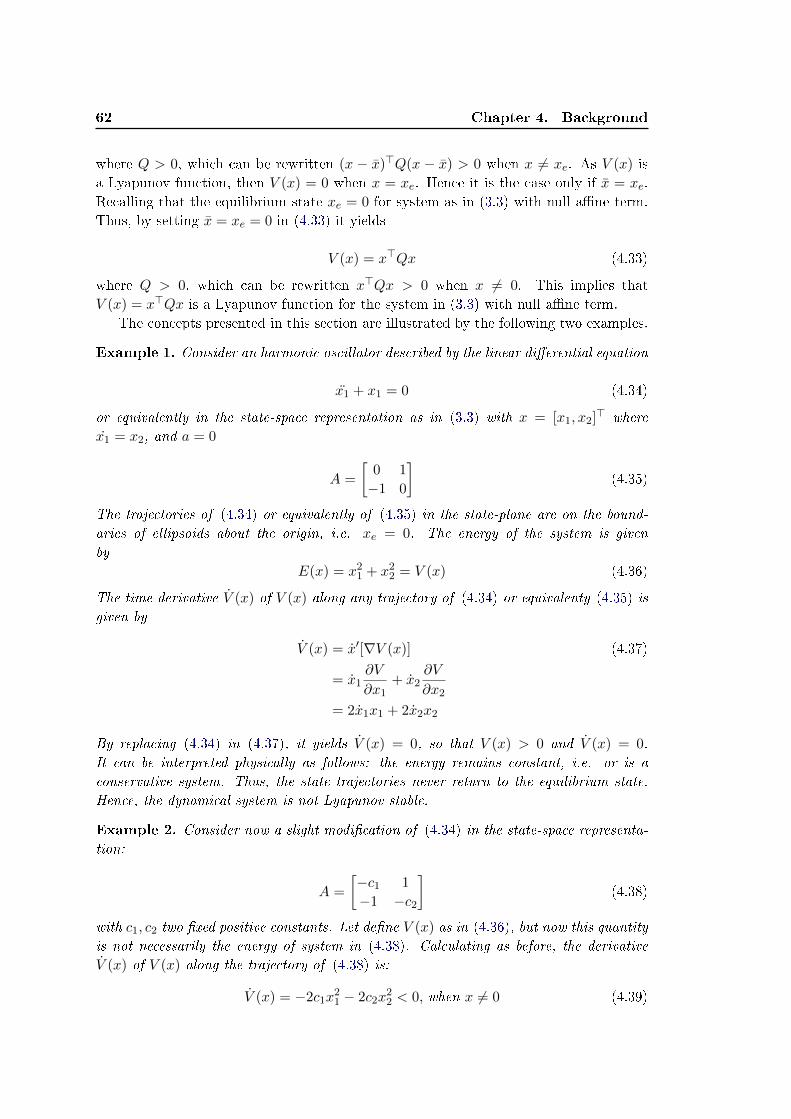
62 Chapter 4. Background
where Q > 0, which can be rewritten (x − x)>Q(x − x) > 0 when x 6= xe. As V (x) isa Lyapunov function, then V (x) = 0 when x = xe. Hence it is the case only if x = xe.Recalling that the equilibrium state xe = 0 for system as in (3.3) with null ane term.Thus, by setting x = xe = 0 in (4.33) it yields
V (x) = x>Qx (4.33)
where Q > 0, which can be rewritten x>Qx > 0 when x 6= 0. This implies thatV (x) = x>Qx is a Lyapunov function for the system in (3.3) with null ane term.
The concepts presented in this section are illustrated by the following two examples.
Example 1. Consider an harmonic oscillator described by the linear dierential equation
x1 + x1 = 0 (4.34)
or equivalently in the state-space representation as in (3.3) with x = [x1, x2]> where
x1 = x2, and a = 0
A =
[0 1
−1 0
](4.35)
The trajectories of (4.34) or equivalently of (4.35) in the state-plane are on the bound-
aries of ellipsoids about the origin, i.e. xe = 0. The energy of the system is given
by
E(x) = x21 + x2
2 = V (x) (4.36)
The time derivative V (x) of V (x) along any trajectory of (4.34) or equivalenty (4.35) isgiven by
V (x) = x′[∇V (x)] (4.37)
= x1∂V
∂x1+ x2
∂V
∂x2
= 2x1x1 + 2x2x2
By replacing (4.34) in (4.37), it yields V (x) = 0, so that V (x) > 0 and V (x) = 0.
It can be interpreted physically as follows: the energy remains constant, i.e. or is a
conservative system. Thus, the state trajectories never return to the equilibrium state.
Hence, the dynamical system is not Lyapunov stable.
Example 2. Consider now a slight modication of (4.34) in the state-space representa-
tion:
A =
[−c1 1
−1 −c2
](4.38)
with c1, c2 two xed positive constants. Let dene V (x) as in (4.36), but now this quantity
is not necessarily the energy of system in (4.38). Calculating as before, the derivative
V (x) of V (x) along the trajectory of (4.38) is:
V (x) = −2c1x21 − 2c2x
22 < 0, when x 6= 0 (4.39)

4.9. Conclusion 63
Hence, V (x) > 0 and V (x) < 0 when x 6= 0. This implies that V (x) is a Lyapunov
function for system (4.38); so the system is Lyapunov stable as a Lyapunov function
exists.
Notice that the state trajectory crosses the boundary ellipsoid dened by the κ-sublevel
set from the outside toward the inside until reaching the origin, i.e. the origin is asymp-
totically stable.
As a nal remark, the problem of existence of a quadratic Lyapunov function fora dynamical system as in (3.3) can be cast into a SDP feasability problem with LMIconstraints.
Find Q such thatV (x) ≥ 0
V (x) ≤ 0
⇔
Find Q such thatQ ≥ 0
−A>Q− QA ≥ 0
(4.40)
with
V (x) = ˙x>Qx+ x>Q ˙x (4.41)
= x>(A>Q+ QA)x (4.42)
4.9 Conclusion
This Chapter has presented the sucient background for understanding the methodsdeveloped in this thesis. In the following Chapters we will detail the methods of thisthesis for analyzing and preventing stealthy aging attacks.


Chapter 5
Analysis and prevention: a subcase
of stealthy aging attacks
Contents
5.1 Introduction . . . . . . . . . . . . . . . . . . . . . . . . . . . . . . . 65
5.2 Research question . . . . . . . . . . . . . . . . . . . . . . . . . . . . 66
5.2.1 Framework of the methods . . . . . . . . . . . . . . . . . . . . . . 67
5.2.2 Modeling considerations . . . . . . . . . . . . . . . . . . . . . . . . 67
5.3 Invariant set-based method . . . . . . . . . . . . . . . . . . . . . . 70
5.3.1 Invariance notions . . . . . . . . . . . . . . . . . . . . . . . . . . . 70
5.3.2 Main theorem of the invariant set-based method . . . . . . . . . . 71
5.3.3 First step: analysis of AT1 . . . . . . . . . . . . . . . . . . . . . . 75
5.3.4 Second step: reachability analysis . . . . . . . . . . . . . . . . . . . 77
5.3.5 Third step: restriction of the control input set . . . . . . . . . . . 78
5.4 Convex robust simulation-based method . . . . . . . . . . . . . . 80
5.4.1 Robust simulation . . . . . . . . . . . . . . . . . . . . . . . . . . . 80
5.4.2 Main theorem of the convex robust simulation-based method . . . 81
5.4.3 First step: analysis of AT1 . . . . . . . . . . . . . . . . . . . . . . 84
5.4.4 Second step: reachability assessing . . . . . . . . . . . . . . . . . . 84
5.4.5 Third step: Restriction of the control input set . . . . . . . . . . . 86
5.5 Conclusion . . . . . . . . . . . . . . . . . . . . . . . . . . . . . . . . 88
5.1 Introduction
As introduced in Chapter 3, our methods contribute in the analysis and prevention ofstealthy aging attacks. Among these attacks, two of them manipulating the controlsignal are considered in this thesis: (AT1) where the objective is to let the dynamicalsystem reach a subset of the state space featuring an abnormal aging; and (AT2) wherethe objective is to maximize the time integral of a degradation function modeling thestresses acting on the process. As we will see in the following Chapters, AT1 is a subcaseof AT2. This Chapter is devoted to the subcase of stealthy aging attacks (AT1).
Section 5.2 formally denes the subcase of stealthy aging attacks (AT1) to provide theframework of the problem the methods will solve. Thereafter, the methods for analyzingand preventing stealthy aging attacks of AT1 are detailed in Section 5.3 and Section 5.4.

66 Chapter 5. Analysis and prevention: a subcase of stealthy aging attacks
5.2 Research question
From the general denition of stealthy aging attacks in Denition 5, we restrain ourinvestigation to the following Attack Type (AT).
Denition 30. (Attack Type 1 (AT1)). The input u(t) is manipulated by an attacker
to let the dynamical system reach a subset Dx of the state space that we call abnormal
aging set, because it features an aging faster than normal for the dynamical system,
leading to lifetime reduction. In the meantime, the state trajectory is constrained to
remain in a set Xs we call service set, because this is the set the state trajectory visits
during the normal operation of the control system, i.e. the attack-free case.
As an interpretation of the Denition 30, if the state trajectory x(t) of the dynamicalsystem reaches the abnormal aging set Dx then the dynamical system operates outside ofthe normal aging conditions. In the meantime, the state trajectory remains in the serviceset Xs, where the delivered service is normal. If the state trajectory remains inside theservice set, we can consider that the service can be provided normally, such that nosuspicion of attack can arise. Clearly, AT1 is possible only if Xs ∩ Dx is non-empty,otherwise stealthy aging attacks of AT1 are not feasible.
The general idea to analyze and prevent such kind of attacks is summarized as follows.Consider a dynamical system as in (3.3) where u(t) is bounded at every time instant dueto physical input limitation (e.g. voltage, current, torque):
u(t) ∈ U , ∀t ≥ 0 (5.1)
where U is called the control input set, and it is a closed set.Note that we insist in the physical nature of the input limitation as it constrains
the attack capabilities. In fact, virtual limitation imposed by the controller could bebypassed by an attacker compromising the controller. It is important to note that noother conditions are imposed on the input u(t) (e.g. band-limited signal).
Consider X the state set of the dynamical system such that x(t) ∈ X , ∀t ≥ 0. Asthe attacker wants to remain stealthy regarding the delivered service, we may assumethat the control signal u(t) will be chosen carefully in order to not degrade the servicedelivered by the dynamical system. For this reason, we can assume that a part of thestate can be constrained to belong to Xs, the set that will not cause any suspicions ofattack to arise:
x(t) ∈ X ⊆ Xs, ∀t ≥ 0 (5.2)
As a consequence of this, the following assumption is made:
Assumption 1. There exists a control signal u(t) ∈ U such that x(t) ∈ Xs for all t ≥ 0
and for any initial conditions x(t0) ∈ X .
If the assumption above is not satised, it means that no stealthy aging attack canbe performed without being detected from the sensors measuring the delivered service,which put us on the safe side. This assumption will be rened later to be more specicfor each method, but the essence of the assumption remains.

5.2. Research question 67
From this problem, the following two Research Question (RQ) are addressed in thisChapter:
Denition 31. (RQ1). Are stealthy aging attacks of AT1 feasible for the given dynam-
ical system in (3.3), the control input set U , the service set Xs, and the abnormal aging
set Dx?
Denition 32. (RQ2). How the control input set U can be restrained to U such that
stealthy aging attacks of AT1 are not feasible, i.e. the answer to RQ1 is negative?
After having dened the Attack Type of stealthy aging attacks we consider, stated theproblem, and dened the research questions we answer in this Chapter, the frameworkof the developed methods for analyzing and preventing AT1 is presented.
5.2.1 Framework of the methods
From the physical input limitation U in (5.1), the proposed methods perform the follow-ing steps:
1. Computation of the reachable set under the given constraints, i.e. X . This analysisstep consists in quantifying the eect induced by AT1 on the dynamical system.
2. Reachability analysis of the abnormal aging set Dx. This consists in assessing if thestate trajectory can reach the abnormal aging set Dx, i.e. X ∩Dx 6= ∅. In the caseof X ∩Dx = ∅, it means that the state trajectory cannot reach the abnormal agingset, so stealthy aging attacks of AT1 are not feasible (RQ1); hence (RQ2) is alreadyanswered: the current physical input limitation U is sucient to prevent stealthyaging attacks. Otherwise, stealthy aging attacks of AT1 are feasible (RQ1), so(RQ2) is addressed with step 3.
3. Restraining the control input set U to U to make (RQ1) not feasible, with U ⊆ U .It consists in nding the largest control input set U such that the constrained stateset X does not intersect with the abnormal aging set Dx, i.e. X ∩ Dx = ∅ ifu(t) ∈ U , ∀t ≥ 0. This answers RQ2.
5.2.2 Modeling considerations
In order to make the problem solvable with convex optimization problems, the followingconsiderations are made:
The control input set U is modeled as an ellipsoid Eu(R, u), i.e. u(t) ∈ U ⊆ Eu, ∀t ≥0.
The constrained control input set U is modeled as an ellipsoid Eu, i.e. u(t) ∈ U ⊆Eu, ∀t ≥ 0.
The state set X is modeled as an ellipsoid Ex(Q, x), i.e. x(t) ∈ X ⊆ Ex, ∀t ≥ 0.
The service set Xs is modeled as an ellipsoid Es(Ξ, ξ), i.e. x(t) ∈ X ⊆ Ex, ∀t ≥ 0.
68 Chapter 5. Analysis and prevention: a subcase of stealthy aging attacks
The abnormal aging set Dx is modeled as the union of i number of halfspacesHi(ci, µi) dened by their boundary hyperplane:
Dx = x ∈ Rn :
p⋃i=1
c>i x(t) ≥ µi (5.3)
From the modeling considerations and before detailing the methods proposed in thisthesis, we express the constraints (5.1) and (5.2):
u(t) ∈ Eu(R, u)⇔ (u− u)>R(u− u) ≤ 1 (5.4)
x(t) ∈ Es(Ξ, ξ)⇔ (x− ξ)>Ξ(x− ξ) ≤ 1 (5.5)
Before reformulating the constraints, let
Γ> =
[0n,1
1
]Ξ =
[Ξ 0n,1
01,n 0,
], ξ =
[ξ
0
]. (5.6)
By introducing the vector[x
u
], it can be restated as follows.
(u− u)>R(u− u) ≤ 1⇔[x
u
]> [Γ>u>RuΓ −Γ>u>R
−RuΓ R
] [x
u
]≤ 1 (5.7)
(x− ξ)>Ξ(u− ξ) ≤ 1⇔[x
u
]> [Ξ− ΞξΓ− Γ>ξ>Ξ + Γ>ξ>ΞξΓ 0n+1,m
0m,n+1 0m,m
] [x
u
]≤ 1
(5.8)
Rewriting the matrix inequalities in (5.7) in the positive semidenite form (≥ 0), ityields: [
x
u
]> [−Γ>u>RuΓ −Γ>u>R
−RuΓ R
] [x
u
]+ 1 ≥ 0, (5.9)
[x
u
]> [−Ξ + ΞξΓ + Γ>ξ>Ξ− Γ>ξ>ΞξΓ 0n+1,m
0m,n+1 0m,m
] [x
u
]+ 1 ≥ 0 (5.10)
Note that Γ>Γ =
[0n,n 0n,101,n 1
], so that x>Γ>Γx =
[x
1
]> [0n,n 0n,101,n 1
] [x
1
]allows the
expression of the constant term. Therefore, the constraints can be restated as follows:
u(t) ∈ Eu(R, u)⇔ S ≥ 0 (5.11)
x(t) ∈ Es(Ξ, ξ)⇔ T ≥ 0 (5.12)
with
S =
[Γ>Γ− Γ>u>RuΓ Γ>u>R
RuΓ −R
]T =
[Γ>Γ− Ξ + ΞξΓ + Γ>ξ>Ξ− Γ>ξ>ΞξΓ 0n+1,m
0m,n+1 0m,m
]

5.2. Research question 69
The service set is dened as Ex(Ξ, ξ), where Ξ in general will be rank-decient, as itwill constrain only one part of the state, that is involved in the service to deliver by thephysical system; Ex(Ξ, ξ) can even coincide with Rn×n (formally by picking Ξ = 0).
Remark 7. If Ξ = 0 then the state trajectory is not constrained to belong to the service
set. This is the case of an open-loop system where the delivered service is not measured
by sensors neither operators.
After having expressed the constraints u(t) ∈ Eu and x(t) ∈ Es, ∀t ≥ 0, we present inthe next sections the two set theoretic methods we propose. The rst one called invariantset-based method is based on the invariance concept, while the second one called convexrobust simulation-based method is based on the simulation of a dynamical system toforecast its state set. Beforehand, the main steps of the proposed methods are picturedin the following gures.
Figure 5.1: Step 1 : Analysis of stealthy aging attacks

70 Chapter 5. Analysis and prevention: a subcase of stealthy aging attacks
Figure 5.2: Step 2 : Reachability analysis of the abnormal aging set
Figure 5.3: Step 3 : Restriction of the input set to prevent such attacks
5.3 Invariant set-based method
5.3.1 Invariance notions
In this method [Escudero & Zamaï 2019], we propose to exploit the property of positiveinvariance of an ellipsoid, dened as follows.
Denition 33 (Positive invariance, [Gayek 1991]). An ellipsoid Ex is positive invari-ant for a dynamical system as in (3.3) if from any initial conditions x(0) ∈ Ex and for
all u(t) ∈ Eu, x(t) ∈ Ex, ∀t ≥ 0.

5.3. Invariant set-based method 71
Figure 5.4: Invariant ellipsoid Ex
Remark 8. The role of the term "positive" is referred to the fact that the invariant
property regards the future. This term is commonly dropped and the ellipsoid is said to
be an invariant set or an invariant ellipsoid.
The property of invariance is then attractive: it allows the encapsulation of the stateset at the innite-time horizon of the dynamical system, i.e. X (∞, x(0)) ⊆ Ex whereEx is invariant. Hence, an invariant ellipsoid is an outer-approximation of X (∞, x(0)).This set X (∞, x(0)) often called the innite time reachable set of the dynamical systemstates is the set that captures all the state trajectory emanating from initial statesx(0). However, its analytic computation is generally not possible. Instead, invariantsets are computed as they benet from the fact that their family can be chosen at oneconvenience. The choice of the set family has an eect on the computational complexity,and the error of approximation of the reachable set.
The positive invariance notion has largely been utilized in the analysis and synthesisof controllers for dynamical systems. In particular, two relevant sets in the automaticcontrol can be pinpointed [Blanchini & Miani 2015]: the robustly (positively) invariantset, and the robust controlled (positively) invariant set. The robustly invariant set isthe set that encompasses the state trajectory while the dynamical system is subject todisturbance. The robustly controlled invariant set is the set that encompasses the statestrajectory while the dynamical system is subject to disturbance and a control inputcomputed from a controller.
5.3.2 Main theorem of the invariant set-based method
The main theorem of this method provides sucient conditions for computing the invari-ant state ellipsoid for a dynamical system as in (3.3) with the state trajectory constrainedto belong to the service set. This is what we call the constrained invariant state ellipsoid.This theorem will be subsequently employed in a set of algorithms, whose goal is theprediction and prevention of potential stealthy aging attack of AT1.

72 Chapter 5. Analysis and prevention: a subcase of stealthy aging attacks
This method is based on the search of a pseudo-Lyapunov function V (x) = x>Qx.The idea is to characterize a positive denite function
V (x) = x>Qx ≥ 0 ∀x 6= xe, (5.13)
such that
V (x, u) 6 0 for allx, u satisfying: (5.14)
V (x) ≥ 1, (3.3), (5.11) (5.15)
where Q ≥ 0 is a symmetric matrix.In the presence of a control input u(t), the time derivative V (x, u) of the Lyapunov
function V (x, u) dened in (5.13) is not (4.41), but it becomes:
V (x, u) =
[x
u
]> [A>Q+ QA QB
B>Q 0m,m
] [x
u
]. (5.16)
Notice that if V (x) 6 0 for all x, u satisfying V (x) ≥ 1, then V (x(t)) denes a time-invariant ellipsoidal κ-level set from which the state trajectory will never go out over theinnite-time horizon; so if the set of initial conditions is within this level set, the statetrajectory stemming from them will never exit this level set. In fact, to assure that thestate trajectory x(t) of the dynamical system in (3.3) does not leave the ellipsoid:
Ex(Q, x) = x ∈ Rn| (x− x)>Q(x− x) ≤ 1 (5.17)
it is sucient to require the fulllment of the inequality V (x(t)) ≥ 0, ∀x(t), u(t) satisfy-ing V (x(t)) ≤ 1, so that V (x(t)) decreases when V (x(t)) is outside the ellipsoid in (5.17).This condition can be rewritten as: V (x(t)) ≤ 0 for all x, u satisfying V (x(t)) ≥ 1. Itis obvious that this condition can be satised on the innite-time horizon if and only ifthe dynamical system is Lyapunov stable. If not Lyapunov stable the state trajectorywill not converge, as energy is added to the dynamical system from u(t).
In addition to this, the state trajectory is constrained to remain in the service setEs(Ξ, ξ), as aging attacks are launched while maintaining the desired service to guar-antee the stealthiness of the attack. Therefore, the constraint in (5.12) is added tothe requirement in (5.15), under the Assumption 1 that is specied for this method asfollows:
Assumption 2. There exists a control signal u(t) ∈ Eu(R, u) such that x(t) ∈ Es(Ξ, ξ)for all t ≥ 0 and for any initial conditions x(t0) ∈ Ex(Q(t0), x(t0)) .
Finally, the problem we want to solve can be summarized as follows:
P1
Find Q such thatV (x, u) ≤ 0 ∀x(t), u(t) satisfying:V (x) ≥ 1, u(t) ∈ Eu(R, u), x(t) ∈ Es(Ξ, ξ)under Assumption 2with Q ≥ 0
(5.18)

5.3. Invariant set-based method 73
Finally, Theorem 6 casts the problem P1 into a SDP feasability problem with LMIconstraints.
Theorem 6. Consider an ane time-invariant continuous-time dynamical system ac-
cording to (3.2) or equivalently (3.3), with matrices dened according to (3.4).If there exist Q ∈ R(n+1)×(n+1), and α, β, λ ∈ R for which the following constraints are
satised:
−M − αN − βS − λT ≥ 0, (5.19)
α, β, λ ≥ 0 (5.20)
with
M =
[A>Q+ QA QB
B>Q 0m,m
](5.21)
N =
[Q− Γ>Γ 0n+1,m
0m,n+1 0m,m
](5.22)
S =
[Γ>Γ− Γ>u>RuΓ Γ>u>R
RuΓ −R
](5.23)
T =
[Γ>Γ− Ξ + ΞξΓ + Γ>ξ>Ξ− Γ>ξ>ΞξΓ 0n+1,m
0m,n+1 0m,m
](5.24)
(5.25)
and Γ, Ξ, ξ dened as in (5.6), then
x(t0)>Qx(t0) 6 1⇒ x(t)>Qx(t) 6 1∀t ≥ t0, (5.26)
under the constraints ∀t ≥ t0, u(t) ∈ Eu(R, u), x(t) ∈ Es(Ξ, ξ).
Proof. Consider rst (5.19); left and right multiply by [x(t)>, u(t)>]>, and consider αN ,βS and λT as S-procedure terms by positive multiplier α, β and λ as in (5.20); thisimplies (Lemma 1):
[x>, u>] −M [x>, u>]> = −V (x, u) > 0⇔ V (x, u) 6 0 (5.27)
when[x>, u>]N [x>, u>]> = V (x)− 1 > 0⇔ V (x) > 1. (5.28)
[x>, u>]S [x>, u>]> > 0⇔ u(t) ∈ Eu(R, u). (5.29)
[x>, u>]T [x>, u>]> > 0⇔ x(t) ∈ Ex(Ξ, ξ), (5.30)
This means that the value of V (x) can only increase under the stated constraints, i.e.V (x(t0)) 6 1⇒ V (x(t)) 6 1 ∀t ≥ 0, which is the theorem statement.
Due to the product of α with Q, two unknown variables, the matrix inequality in(5.45) in Theorem 6 is not a LMI, but a BMI. To deal with it, the constrained invariantstate ellipsoid is computed iteratively for a x α ≥ 0 at each iteration.

74 Chapter 5. Analysis and prevention: a subcase of stealthy aging attacks
Ideally, we would like to design an iterative algorithm computing at each iterationthe optimal α minimizing the size of Ex, so that the iterative algorithm stops once theoptimal α converges. At least, we would like to impose an upper bound α on α to explorea nite interval.
Theorem 7. Consider the matrix of the constraint (5.19) in Theorem 6 restated in
(5.31)
−M − αN − βS − λT (5.31)
with α, β, γ ≥ 0, and matrices M , N , S, and T are dened in (5.21), (5.22), (5.23),(5.24).
For the special case Ξ = 0, it is a necessary condition for the satisfaction of the
constraint that
α ≤ −2λ(A) (5.32)
where λ(A) denotes the largest eigenvalue of A, with A = (A> + A)/2, and A is the
matrix of the dynamical system in (3.3)
Proof. Before starting with the proof, let us recall the following Lemmas.
Lemma 1. If a matrix Y is positive semidenite, the diagonal elements Ynn are non-
negative.
Lemma 2. If a matrix Y is positive (negative) semidenite, the trace is positive (nega-
tive).
For the matrix in (5.31) to be positive semidenite, it is necessary that the diagonalentries are nonnegative from Lemma 1. By expanding the vector [x>, u>] into [x>, 1, u>],matrices M , N , S, T in (5.19) can be rewritten:
M =
A>Q+QA • •• −a>Qx− x>Qa •• • 0m,m
N =
Q • •• x>Qx− 1 •• • 0m,m
S =
0n,n • •• 1− u>Ru •• • −R
T =
−Ξ • •• 1− ξΞξ •• • 0m,m
Thus, the necessary condition is:

5.3. Invariant set-based method 75
−A>Q−QA− αQ+ λΞ ≥ 0 (5.33)
⇔ A>Q+QA+ αQ− λΞ ≤ 0 (5.34)
From Lemma 2, it yields:
trace(A>Q+QA+ αQ− λΞ) ≤ 0 (5.35)
⇔ trace(A>Q+QA) ≤ trace(− αQ+ λΞ)
⇔ 2 trace(A>Q) ≤ −α trace(Q) + λtrace(Ξ)
As λn(A>)trace(Q) ≤ trace(A>Q) where λj(A) denotes the jth largest eigenvalue of Awith A> = (A> +A)/2 then, (5.35) is equivalent to
2λn(A>)trace(Q) ≤ −αtrace(Q) + λtrace(Ξ)
In the special case Ξ = 0, it yields
2λn(A>) ≤ −α⇔ α ≤ −2λn(A>)
Then, it implies that α ≤ α with α = −2λn((A> +A)/2) for the special case Ξ = 0,which is the theorem statement.
After having given the theorem providing sucient conditions for a constrained in-variant state ellipsoid in which the state remains over the innite-time horizon, the threesteps to analyze and prevent stealthy aging attacks are detailed, one for each subsec-tion. Given a dynamical system as in (3.3), the input limitation Eu(R, u), the service setEs(Ξ, ξ), and the abnormal aging set Dx the following steps are proposed.
5.3.3 First step: analysis of AT1
This rst step aims to analyze stealthy aging attacks of AT1. To do so, we proposecomputing the constrained invariant state ellipsoid Ex(Q, x) for the given dynamicalsystem in (3.3) and for a given control input set Eu(R, u). This constrained invariantstate ellipsoid encompasses the constrained innite time reachable set X (∞, x(0)) underthe condition of existence of a control input u(t) ∈ Eu(R, u) that can constrain the statetrajectory to remain inside the service set, x(t) ∈ Es(Ξ, ξ) (Assumption 2).
As invariant sets are outer-approximation of the innite-time reachable set X (∞, x(0)),there exist an innite number of sets being invariant for the dynamical system. However,we are interested in the smallest constrained invariant state ellipsoid to have the bestapproximation, i.e. as close as possible to X (∞, x(0)). In fact, the lower the approxima-tion error, the better the analysis of AT1 is. This can be obtained by maximizing thetrace of Q under Theorem 6 as stated in the convex Optimization Problem (OP) OP1.
OP1: maximizeQ,β,λ
trace(Q)
subject to (5.19), (5.20)

76 Chapter 5. Analysis and prevention: a subcase of stealthy aging attacks
Note that maximizing the trace does not guarantee to nd the tighest ellipsoid asthe trace(.) operator relates to the size of the semiaxes. Hence, Algorithm 1 is proposedfor nding the smallest constrained invariant state ellipsoid for the dynamical system in(3.3) with a control input set Eu(R, u) for a given α.
Algorithm 1 : [Q, x]=Alg1(α, R, u, Ξ, ξ, I1)
Input: α, R, u, Ξ, ξ, I1:=A, BInitial condition: -2. Solve OP1
3. [Q, x]=Normalize(Q)Output: Q, x
Remark 9. Notice that the numerical procedure will have a limited numerical precision,
for this reason a normalization step (step 3.) has been introduced; typically the ellipsoids
matrices might not t into the form of (4.22), with a non-matching lower-right entry thatcorresponds to dening a set v ∈ Rn | (v− v)>Ann(v− v) 6 ρ with ρ 6= 1. The function
Normalize(Ann) transforms a non-normalized (nn) ellipsoid dened as Ennv (Ann, v) =
v ∈ Rn | (v − v)>Ann(v − v) 6 ρ into a normalized one Ev(A, v) (ρ = 1).
Thereafter, Algorithm 2 is proposed for nding the smallest constrained invariantstate ellipsoid Ex for the dynamical system in (3.3) with a control input set Eu(R, u)
over a value interval for α. Recall that we are interested in the smallest Ex to have thebest approximation of X. The idea of Algorithm 2 is to recursively call Algorithm 1 tocompute the smallest constrained invariant state ellipsoid Ex(Q, x) for a given α (step1.1.). The size of the computed Ex(Q, x) is then compared with Ex(Qmin, xmin), thatis the smallest ellipsoids found over the value interval of α. If the computed ellipsoidis smaller (step 1.2.), then update Ex(Qmin, xmin) with the recently computed ellipsoid(step 1.2.1.). The Algorithm repeats the same process for another value of α over theinterval value. Note that ∆α is the α step at each iteration such that α is updatedat α + ∆α. After having explored the whole interval value of α, Algorithm 2 nallyprovides the smallest constrained invariant state ellipsoid Ex(Qmin, xmin) found at someα, if there exists. So, for the given dynamical system, x(t0) ∈ Ex(Qmin, xmin) impliesthat x(t) ∈ Ex(Qmin, xmin), ∀u(t) ∈ Eu(R, u) and forx(t) ∈ Es(Ξ, ξ), ∀t ≥ t0.
Remark 10. As previously mentioned, the choice of α for the general case, i.e. Ξ 6= 0,
is still an open problem. Then, one can choose it arbitrarily.

5.3. Invariant set-based method 77
Algorithm 2 : [Qmin, xmin]=Alg2(R, u, Ξ, ξ, I1, I2)
Input: α, α, ∆α, R, u, Ξ, ξ, I2:=α, α, ∆αInitial condition: Qmin = 0n,n, xmin = 0n,11. For α = α to α with a step ∆α
1.1. [Q, x]=Alg1(α, R, u, Ξ, ξ, I1)1.2. If trace(Q) > trace(Qmin)
1.2.1. Set Qmin = Q
Output: Qmin, xmin
5.3.4 Second step: reachability analysis
This second step aims to check if the state trajectory can reach the abnormal ag-ing set. This can be done by checking if the the constrained invariant state ellipsoidEx(Qmin, xmin) resulting from the rst step intersects with the abnormal aging set Dx.Instead of considering the intersection between both sets, we focus on the overlappingdistance between an ellipsoid and an hyperplane dened in (4.27), as Dx is dened bythe union of i number of hyperplane. Hence, we dene the function Hit(Qx,x,Hi) fordetermining if an ellipsoid Ev(A, v) hits the abnormal aging set Dx. This function veri-es that the distance from the ellipsoid to each hyperplane is negative. If it is, then theellipsoid does not intersect with the abnormal aging set; otherwise it does.
Denition 34. Function Hit: [hit]=Hit(Qx, x, Hi)
Input: Qx, x, HiInitial condition: -
1. For j = 1 to i
1.1. If dist(Ex(Qx, x),Hj(cj , µj)) ≥ 0
Set hit = True, Goto Output
1.2. Else Set hit = False, Goto Output
Output: hit
Algorithm 3 implements this boolean function Hit(A,v,Hiv) to check if the smallestconstrained invariant state ellipsoid intersects with the abnormal aging set (step 2.). Theoutput of the function and so the Algorithm 3 answers to RQ1 about the feasability ofstealhty aging attacks of AT1.
Figure 5.5 is an illustration of RQ1 on a projection of two states and two inputs. Theconstrained invariant state ellipsoid Ex (dot pattern) is obtained for a given Eu by apply-ing Algorithm 3. The intersection between Ex and the abnormal aging set Dx is studied(red polygon).
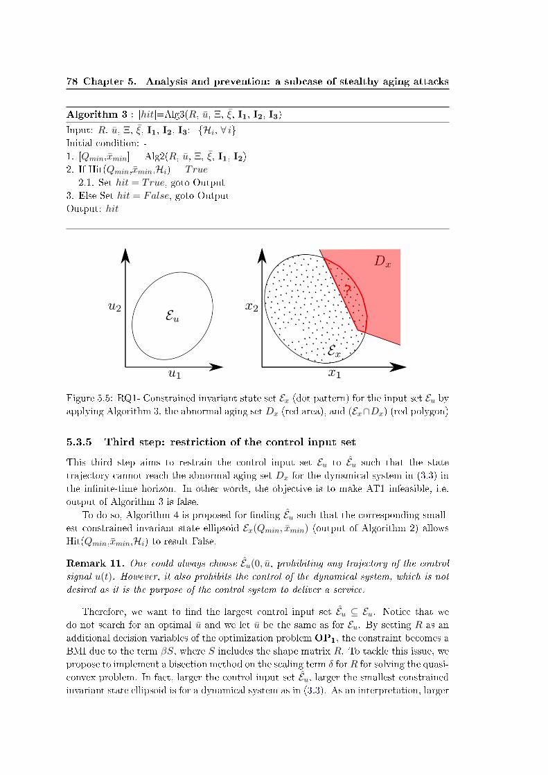
78 Chapter 5. Analysis and prevention: a subcase of stealthy aging attacks
Algorithm 3 : [hit]=Alg3(R, u, Ξ, ξ, I1, I2, I3)
Input: R, u, Ξ, ξ, I1, I2, I3:=Hi, ∀ iInitial condition: -1. [Qmin,xmin] = Alg2(R, u, Ξ, ξ, I1, I2)2. If Hit(Qmin,xmin,Hi) = True
2.1. Set hit = True, goto Output3. Else Set hit = False, goto OutputOutput: hit
Figure 5.5: RQ1- Constrained invariant state set Ex (dot pattern) for the input set Eu byapplying Algorithm 3, the abnormal aging set Dx (red area), and (Ex∩Dx) (red polygon)
5.3.5 Third step: restriction of the control input set
This third step aims to restrain the control input set Eu to Eu such that the statetrajectory cannot reach the abnormal aging set Dx for the dynamical system in (3.3) inthe innite-time horizon. In other words, the objective is to make AT1 infeasible, i.e.output of Algorithm 3 is false.
To do so, Algorithm 4 is proposed for nding Eu such that the corresponding small-est constrained invariant state ellipsoid Ex(Qmin, xmin) (output of Algorithm 2) allowsHit(Qmin,xmin,Hi) to result False.
Remark 11. One could always choose Eu(0, u, prohibiting any trajectory of the control
signal u(t). However, it also prohibits the control of the dynamical system, which is not
desired as it is the purpose of the control system to deliver a service.
Therefore, we want to nd the largest control input set Eu ⊆ Eu. Notice that wedo not search for an optimal u and we let u be the same as for Eu. By setting R as anadditional decision variables of the optimization problem OP1, the constraint becomes aBMI due to the term βS, where S includes the shape matrix R. To tackle this issue, wepropose to implement a bisection method on the scaling term δ for R for solving the quasi-convex problem. In fact, larger the control input set Eu, larger the smallest constrainedinvariant state ellipsoid is for a dynamical system as in (3.3). As an interpretation, larger
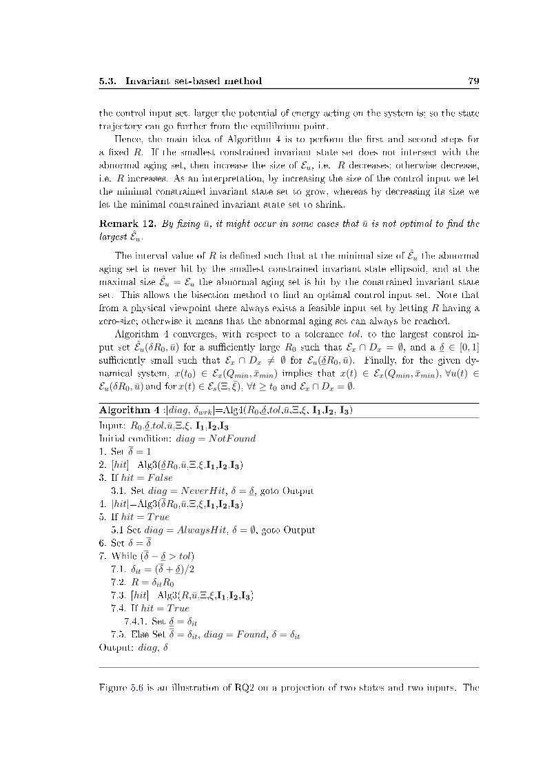
5.3. Invariant set-based method 79
the control input set, larger the potential of energy acting on the system is; so the statetrajectory can go further from the equilibrium point.
Hence, the main idea of Algorithm 4 is to perform the rst and second steps fora xed R. If the smallest constrained invariant state set does not intersect with theabnormal aging set, then increase the size of Eu, i.e. R decreases; otherwise decrease,i.e. R increases. As an interpretation, by increasing the size of the control input we letthe minimal constrained invariant state set to grow, whereas by decreasing its size welet the minimal constrained invariant state set to shrink.
Remark 12. By xing u, it might occur in some cases that u is not optimal to nd the
largest Eu.
The interval value of R is dened such that at the minimal size of Eu the abnormalaging set is never hit by the smallest constrained invariant state ellipsoid, and at themaximal size Eu = Eu the abnormal aging set is hit by the constrained invariant stateset. This allows the bisection method to nd an optimal control input set. Note thatfrom a physical viewpoint there always exists a feasible input set by letting R having azero-size; otherwise it means that the abnormal aging set can always be reached.
Algorithm 4 converges, with respect to a tolerance tol, to the largest control in-put set Eu(δR0, u) for a suciently large R0 such that Ex ∩ Dx = ∅, and a δ ∈ [0, 1]
suciently small such that Ex ∩ Dx 6= ∅ for Eu(δR0, u). Finally, for the given dy-namical system, x(t0) ∈ Ex(Qmin, xmin) implies that x(t) ∈ Ex(Qmin, xmin), ∀u(t) ∈Eu(δR0, u) and forx(t) ∈ Es(Ξ, ξ), ∀t ≥ t0 and Ex ∩Dx = ∅.
Algorithm 4 :[diag, δwrk]=Alg4(R0,δ,tol,u,Ξ,ξ, I1,I2, I3)
Input: R0,δ,tol,u,Ξ,ξ, I1,I2,I3Initial condition: diag = NotFound
1. Set δ = 1
2. [hit]=Alg3(δR0,u,Ξ,ξ,I1,I2,I3)3. If hit = False
3.1. Set diag = NeverHit, δ = δ, goto Output4. [hit]=Alg3(δR0,u,Ξ,ξ,I1,I2,I3)5. If hit = True
5.1 Set diag = AlwaysHit, δ = ∅, goto Output6. Set δ = δ
7. While (δ − δ > tol)7.1. δit = (δ + δ)/2
7.2. R = δitR0
7.3. [hit]=Alg3(R,u,Ξ,ξ,I1,I2,I3)7.4. If hit = True
7.4.1. Set δ = δit7.5. Else Set δ = δit, diag = Found, δ = δit
Output: diag, δ
Figure 5.6 is an illustration of RQ2 on a projection of two states and two inputs. The

80 Chapter 5. Analysis and prevention: a subcase of stealthy aging attacks
current input limitation Eu and the smallest constrained invariant state set Ex (dotpattern) of RQ1 are drawn in solide lines. The largest restrained input set Eu obtainedfrom Algorithm 4 such that constrained invariant state set Ex (dot pattern) does notintersect with the abnormal aging set Dx.
Figure 5.6: RQ2- Largest restrained input set Eu with the corresponding constrainedinvariant state set Ex (dot pattern) in dotted lines by applying Algorithm 4, and RQ1in solid lines, and the abnormal aging set Dx (red area)
One of the main limitation of the presented method is the necessary condition for thesystem to be Lyapunov stable. In many cases, the dynamical system is not Lyapunovstable without considering the closed-loop controller in the model in (3.3). The followingSection presents a set-theoretic method that tackle this limitation.
5.4 Convex robust simulation-based method
To address the limitation of the previous method, we have proposed in [Escudero et al. 2020a]has proposed a robust convex simulation-based method which relies on computing theevolution of bounding state ellipsoids with respect to the time by means of LMI theory.
5.4.1 Robust simulation
By robust simulation we mean simulation of a dynamical system for a whole set ofinitial conditions, under a certain number of constraints. Namely, the problem of robustsimulation consists in nding a bounding set for the state x(t) at a nal time tf , givena set of possible initial values for it at an initial time t0; this under the hypotheses ofa given dynamical equation and in the presence of additional constraints of dierentkind. The bounding state sets considered in this thesis are ellipsoids, denoted Ex(tf )
for the bounding set for the state x(t) at time tf . Therefore, bounding state ellipsoidsencapsulates the state trajectory of a dynamical system at the nite-time horizon froman initial state ellipsoid, i.e. R(tf , x(0)) ⊆ Ex(tf ), with x(0) ∈ Ex(t0).
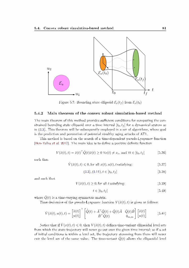
5.4. Convex robust simulation-based method 81
Figure 5.7: Bounding state ellipsoid Ex(tf ) from Ex(t0)
5.4.2 Main theorem of the convex robust simulation-based method
The main theorem of this method provides sucient conditions for computing the con-strained bounding state ellipsoid over a time interval [t0, tf ] for a dynamical system asin (3.3). This theorem will be subsequently employed in a set of algorithms, whose goalis the prediction and prevention of potential stealthy aging attacks of AT1.
This method is based on the search of a time-dependent pseudo-Lyapunov function[Ben-Talha et al. 2017]. The main idea is to dene a positive denite function
V (x(t), t) = x(t)>Q(t)x(t) ≥ 0 ∀x(t) 6= xe, and ∀t ∈ [t0, tf ] (5.36)
such thatV (x(t), t) 6 0, for all x(t), u(t), t satisfying: (5.37)
(3.3), (5.11), t ∈ [t0, tf ] (5.38)
and such thatV (x(t), t) ≥ 0, for all t satisfying: (5.39)
t ∈ [t0, tf ] (5.40)
where Q(t) is a time-varying symmetric matrix.Time derivative of the pseudo-Lyapunov function V (x(t), t) is given as follows:
V (x(t), u(t), t) =
[x(t)
u(t)
]> [ ˙Q(t) + A>Q(t) + Q(t)A Q(t)B
B>Q(t) 0m,m
] [x(t)
u(t)
](5.41)
Notice that if V (x(t), t) 6 0, then V (x(t), t) denes time-variant ellipsoidal level setsfrom which the state trajectory will never go out over the given time interval; so if a setof initial conditions is within a level set, the trajectory stemming from them will neverexit the level set of the same value. The time-variant Q(t) allows the ellipsoidal level

82 Chapter 5. Analysis and prevention: a subcase of stealthy aging attacks
sets to move and grow or shrink over time with the state trajectory, whether the statetrajectory is converging or not.
In order to make the search tractable, we are going to limit it to the set of matrix-valued polynomials, i.e. we will set Q(t) ∈ R(n+1)×(n+1)
2d [t] for an arbitrarily chosen integerd > 1. It is clear that specifying Q(t) in this way adds some conservatism, which can be
progressively reduced by increasing the degree of the matrix-valued polynomial. ˙Q(t) is
then its rst time-derivative, with ˙Q ∈ R(n+1)×(n+1)2d−1 [t].
As for the invariant-set based method, the state trajectory is constrained to remainin the service set by adding the constraint (5.12), under Assumption 1 that is speciedfor this method as follows:
Assumption 3. There exists a control input signal u(t) ∈ Eu(R, u) such that x(t) ∈Es(Ξ, ξ) for all t ∈ [t0, tf ] and for initial conditions x(t0) ∈ Ex(Q(t0), x(t0)) .
If the assumption above is not satised, it means that no aging attack can be per-formed without being detected, which put us on the safe side.Subsequently, the constraint of t ∈ [t0, tf ] can be expressed as follows
γ(t) = (tf − t)(t− t0) > 0 (5.42)
Finally, the problem we want to solve can be summarized as follows:
P2
Find Q(t) such that(i)V (x(t), t) ≥ 0 for t ∈ [t0, tf ],
(ii)V (x(t), u(t), t) ≤ 0 ∀x(t), u(t)satisfying:u(t) ∈ Eu(R, u), x(t) ∈ Es(Ξ, ξ), t ∈ [t0, tf ]
under Assumption 1with Q ≥ 0
(5.43)
Finally, Theorem 8 casts the problem P2 into a SDP feasability problem with LMIconstraints. Before formulating it, consider
I =
[In 0n,1
01,n 0
], Ξ =
[Ξ 0n,1
01,n 0,
], ξ =
[ξ
0
]. (5.44)
The main theorem is then stated as follows.
Theorem 8. Consider an ane time-invariant continuous-time system according to
(3.2) or equivalently (3.3), with matrices dened according to (3.4).
If for a given d > 1 there exist Q(t) ∈ R(n+1)×(n+1)2d [t], Z(t), X(t) ∈ R(n+1)×(n+1)
2d−2 [t]
α(t), β(t) ∈ R2d−2[t], and a scalar ε > 0 for which the following constraints are satised:
−W (t)− α(t)S − β(t)T − γ(t)Z(t) is MSOS, (5.45)
Q(t)− γ(t)X(t)− εI is MSOS (5.46)
Z(t), X(t) are MSOS (5.47)
α(t), β(t) are SOS (5.48)

5.4. Convex robust simulation-based method 83
with
W (t) =
[˙Q(t) + A>Q(t) + Q(t)A Q(t)B
B>Q(t) 0m,m
]
S =
[Γ>Γ− Γ>u>RuΓ Γ>u>R
RuΓ −R
]T =
[Γ>Γ− Ξ + ΞξΓ + Γ>ξ>Ξ− Γ>ξ>ΞξΓ 0n+1,m
0m,n+1 0m,m
]
and Γ, Ξ, ξ dened as in (5.6), and γ(t), I dened as in (5.42), (5.44), then
x(t0)>Q(t0)x(t0) 6 1⇒ x(t)>Q(t)x(t) 6 1 ∀t ∈ [t0, tf ], (5.49)
under the constraints ∀t ∈ [t0, tf ]u(t) ∈ Eu(R, u), x(t) ∈ Ex(Ξ, ξ).
Proof. Consider rst (5.46); left and right multiply by x(t), and consider γ(t)X(t) as anS-procedure term by positive multiplier X(t) as in (5.47); this implies (Lemma 1):
x(t)>Q(t)x(t) > ε||x(t)||2 (5.50)
when γ(t) > 0, i.e. V (x(t), t) = x(t)>Q(t)x(t) > 0 when x(t) 6= 0, t ∈ [t0, tf ]. Subse-quently, consider (5.45); left and right multiply by [x(t)>, u(t)>]>, and consider α(t)S,β(t)T and γ(t)Z(t) as S-procedure terms by positive multipliers α(t), β(t) and Z(t) asin (5.47) and (5.48); this implies (Lemma 1):
[x(t)>, u(t)>]W (t) [x(t)>, u(t)>]> = V (x(t), t) 6 0 (5.51)
when[x(t)>, u(t)>]S [x(t)>, u(t)>]> > 0⇔ u(t) ∈ Eu(R, u). (5.52)
[x(t)>, u(t)>]T [x(t)>, u(t)>]> > 0⇔ x(t) ∈ Ex(Ξ, ξ), (5.53)
and when γ(t) > 0, i.e. when t ∈ [t0, tf ]. This means that the value of V (x(t), t) canonly increase under the stated constraints, i.e. V (x(t0), t0) 6 1 ⇒ V (x(t), t) 6 1 in theconsidered interval, which is the theorem statement.
After having given the theorem providing sucient conditions for a bounding stateellipsoid at time tf in which the state trajectory remains at tf , the three steps to an-alyze and prevent stealthy aging attacks are detailed, one for each subsection. Givena dynamical system as in (3.3), the input limitation Eu(R, u), the service set Es(Ξ, ξ),and the abnormal aging set Dx the following steps are proposed. As both methods arebased on the same general idea described in Section 5.2.1, the algorithms we are goingto present are rather similar to the ones for the invariant set based method. Thus, wewill only present here the main dierences.
In this section, we are proposing algorithms involving Theorem 8 for analyzing andpreventing stealthy aging attacks over a given time interval. In other words, we want torestrain the input set Eu(R, u) into the set Eu(R, u), (Eu(R, u) ⊆ Eu(R, u)) such that adangerous set Dx is avoided over a time interval [t0, tf ].

84 Chapter 5. Analysis and prevention: a subcase of stealthy aging attacks
5.4.3 First step: analysis of AT1
This rst step aims to quantify the eect on the state trajectory x(t) induced by AT1 overa time interval [t0, tf ]. To do so, we propose to compute the constrained bounding stateellipsoid Ex(tf ) for the given dynamical system in (3.3) and for a given control inputset Eu(R, u). This constrained bounding state ellipsoid encompasses the constrainednite-time reachable set X(tf , x(0)) under the condition of existence of a control inputu(t) ∈ Eu(R, u) that can constrain the state trajectory to remain inside the service setEs(Ξ, ξ) over the time interval [t0, tf ], i.e. x(t) ∈ Es(Ξ, ξ) ∀t ∈ [t0, tf ], (Assumption 3).
There exists many constrained bounding state ellipsoids from Theorem 8, i.e. aconstrained bounding state ellipsoid is an outer-approximation of the constrained nite-time reachable set. Thus, we want to nd the smallest bounding state ellipsoid to havethe best approximation. As previously, this can be obtained by maximizing the traceof Q(tf ) under Theorem 8 with initial conditions (Q(t0),x(t0)) as stated in the convexoptimization problem in OP2. So, for the given dynamical system, if x(t0) ∈ Ex(t0)
dened with (Q(t0), x(t0)), then it implies that x(t) ∈ Ex(tf ) dened with (Q(tf ), x(tf )),∀t ∈ [t0, tf ], ∀u(t) ∈ Eu(R, u), and for x(t) ∈ Es(Ξ, ξ).
In order to give more degrees of freedom to the search of such ellipsoids and withoutloss of generality, let t0 be time 0 and split the nal time tf in N ∈ N time steps suchthat N = tf∆−1
t with ∆t a small time step, which simplies the computations. Hence,Algorithm 1 is proposed for nding the minimal bounding ellipsoid for system in (3.3)with a control input set Eu(R, u)) over the time interval [0,∆t] by using Theorem 8.Notice that (step 3.) is the normalization step due to limited numerical precision asdetailed previously in Remark 9.
OP2: maximizeQ∆t ,Z(t),X(t),α(t),β(t)
trace(Q∆t)
subject to (5.45), (5.46), (5.47), (5.48)
Algorithm 5 : [Q∆t , x∆t ]=Alg5(Q(t0),x(t0),R,u,Ξ,ξ, I1)
Input: Q(t0),x(t0),R,u, Ξ, ξ, I1:=A, B, ∆t, dInitial condition: Q0 = Q(t0), x0 = x(t0)
1. Set Q0 =
[Q0 −Q0x0
−x>0 Q0 x>0 Q0x0
],
Q(t) =∑2d
i=0 Qiti
2. Solve P1
3. [Q(∆t), x(∆t)]=Normalize(Q(∆t))Output: Q(∆t), x(∆t)
5.4.4 Second step: reachability assessing
This second step aims to check if the state trajectory can reach the abnormal aging setDx over the time interval [t0, tf ]. Algorithm 5.4.4, whose goal is to determine if andat which time t∩ (with t∩ ∈ 0,∆t, ..., N∆t) the bounding ellipsoid hits the abnormal
5.4. Convex robust simulation-based method 85
aging set Dx. Notice that t∩ could be exploited for further defensive strategies. The ideaof Algorithm 5.4.4 is to compute the evolution of the smallest bounding state ellipsoidsover the time interval [t0, tf ], and check if none of them intersects with Dx. To do so,Algorithm 2 implements an iterative procedure with N iterations that performs two stepsat each iterations i:
1. The computation of the nal (smallest) bounding state ellipsoid at time t0 + i∆t,Ex(t0 + i∆t) dened for (Q(t0 + i∆t),x(t0 + i∆t))
2. The computation of the distance between Ex(t0 + i∆t) and Dx from the booleanfunction Hit(.) already presented previously in Section 5.3.4.
Finally, Algorithm 5.4.4 provides two arrays hit and t∩ to know at which time thesmallest bounding state ellipsoid reaches the abnormal aging set. If all the element ofhit are set at False, it means that stealthy aging attacks of AT1 are not feasible overthe time interval [t0, tf ], otherwise they are (RQ1). In that last case, the third step isproposed to make AT1 not feasible.
Algorithm 6 : [hit, t∩]=Alg6(Q(t0),x(t0),R,u,Ξ,ξ, I1,I2)
Input: Q(t0),x(t0),R,u,Ξ,ξ, I1,I2 := Hix, tfInitial condition: Q0 = Q(t0), x0 = x(t0)
1. Set N = tf∆−1t
2. For j = 1 to N2.1. [Q∆t , x∆t ]=Alg5(Q0,x0,R,u,Ξ,ξ, I1,I2)2.2. If Hit(Q∆t ,x∆t ,Hix) = True
Set hit = True, t∩ = j∆t, Goto Output2.3. Set Q0 = Q∆t , x0 = x∆t
3. Set hit = False, t∩ = ∅Output: hit, t∩
Figure 5.8 is an illustration of RQ1 on a projection of two states and two inputs. Theevolution of bounding state ellipsoids over the time interval [t0, tf ] (dot pattern) areobtained for a given control input set Eu by applying Algorithm 6 with N = 2. At eachiteration i, the intersection between the ith bounding state ellipsoid and the abnormalaging set Dx is studied to determine the feasibility of stealthy aging attacks.

86 Chapter 5. Analysis and prevention: a subcase of stealthy aging attacks
Figure 5.8: RQ1- Evolution of bounding state ellipsoids (dot pattern) over the timeinterval [t0, tf ] for the input set Eu, the abnormal aging setDx (red area), and (Ex(t)∩Dx)(red polygon) by applying Algorithm 6
5.4.5 Third step: Restriction of the control input set
This third step aims to restrain the control input set Eu to Eu such that the statetrajectory cannot reach the abnormal aging set Dx for the dynamical system in (3.3)over the time interval [t0, tf ]. In other words, the objective is to make AT1 unfeasibleover the given time interval, i.e. output of Algorithm 5.4.4 is false for every element ofhit.
For the same reason stated previously, the objective is to nd the largest control inputset Eu such that the evolution of bounding state ellipsoids over the time interval [t0, tf ]
never hits the abnormal aging set Dx. By setting R as an additional decision variables ofthe optimization problem OP2 becomes a BMI due to the term α(t)S, where S includesthe shape matrix R. Similarly as previously, we propose to implement a bisection methodon the scaling term δ for R for solving the quasi-convex problem. Further details havealready been given previously in Section 5.3.5. Hence, Algorithm 5.4.5 is proposed. Itconverges with respect to a tolerance tol, to the largest control input set Eu(δR0, u) fora suciently large R0 such that Ex(t0 + i∆t) ∩ Dx = ∅, ∀i = 1, ..., N , and a δ ∈ [0, 1]
suciently small such that Ex(t0 + i∆t)∩Dx 6= ∅ for Eu(δR0, u) for at least an iterationi.

5.4. Convex robust simulation-based method 87
Algorithm 7 :[diag, δwrk]=Alg7(R0,δ,tol,Q(t0),x(t0),u,Ξ,ξ, I1,I2)
Input: R0,δ,tol,Q(t0),x(t0),u,Ξ,ξ, I1,I2Initial condition: diag = NotFound, Q0 = Q(t0), x0 = x(t0)
1. Set δ = 1
2. [hit, t∩]=Alg6(Q(t0),x(t0),δR0,u,Ξ,ξ,I1,I2)3. If hit = False
3.1. Set diag = NeverHit, δ = δ, Goto Output4. [hit, t∩]=Alg6(Q(t0),x(t0),δR0,u,Ξ,ξ,I1,I2)5. If hit = True
5.1 Set diag = AlwaysHit, δ = ∅, Goto Output6. Set δ = δ
7. While (δ − δ > tol)7.1. δit = (δ + δ)/2
7.2. R = δitR0
7.3. [hit, t∩]=Alg6(Q(t0),x(t0),R,u,Ξ,ξ,I1,I2)7.4. If hit = True, Set δ = δit7.4. Else, Set δ = δit, diag = Found, δ = δit
Output: diag, δ
Figure 5.9 is an illustration of RQ2 on a projection of two states and two inputs. Theevolution of bounding state ellipsoids over the time interval [t0, tf ] (dot pattern) for thecurrent input limitation Eu of RQ1 are drawn in solid lines. The restrained input set Euis computed by applying Algorithm 7 with N = 2 such that the evolution of boundingstate ellipsoids (dotted lines) do not hit with the abnormal aging set Dx.
Figure 5.9: RQ2- Restrained input set Eu with the corresponding evolution of boundingstate ellipsoids (dot pattern) over the time interval [t0, tf ] in dotted lines by applyingAlgorithm 7, RQ1 in solid lines, and the abnormal aging set Dx (red area)

88 Chapter 5. Analysis and prevention: a subcase of stealthy aging attacks
5.5 Conclusion
In this Chapter, we have proposed two set theoretic methods based on an outer-approximationof the reachable state set to answer RQ1 and RQ2 for stealthy aging attacks of AT1. Therst one based on invariant set theory is limited to Lyapunov stable system whereas thelast one based on robust convex simulation can be applied at any systems, i.e. Lyapunovstable or not. In the next Chapter, we will propose a method for analyzing stealthyaging attacks of a more general case (AT2).

Chapter 6
Analysis: general case of stealthy
aging attacks
Contents
6.1 Introduction . . . . . . . . . . . . . . . . . . . . . . . . . . . . . . . 89
6.2 Research question . . . . . . . . . . . . . . . . . . . . . . . . . . . . 89
6.3 Analysis of stealthy aging attacks of AT2 . . . . . . . . . . . . . . 90
6.3.1 Proposed method . . . . . . . . . . . . . . . . . . . . . . . . . . . . 90
6.3.2 Sequential Linear Programming . . . . . . . . . . . . . . . . . . . . 91
6.4 Conclusion . . . . . . . . . . . . . . . . . . . . . . . . . . . . . . . . 91
6.1 Introduction
In Chapter 5, we have detailed the methods for analyzing and preventing stealthy agingattacks of AT1. However, AT1 is a subcase of stealthy aging attacks. The general case isan attack that maximizes the time integral of a degradation function, instead of reachingan abnormal aging set. Hence, this Chapter proposes a method for analyzing stealthyaging attacks of AT2.
Section 6.2 formally denes the general case of stealthy aging attacks (AT1) to pro-vide the framework of the problem the method will solve. Thereafter, the method foranalyzing stealthy aging attacks (AT1) is detailed in Section 6.3.
6.2 Research question
From the general Denition 5 of stealthy aging attacks, our investigation concerns thefollowing Attack Type.
Denition 35. (Attack Type 2 (AT2)). The input u(t) is manipulated by an attacker
to maximize the time integral of a degradation function g(x(t), u(t)) while keeping the
state trajectory inside the service set Xs. The degradation function models the stresses
acting on the process.
After having dened the stealthy aging attacks of AT2 we consider in this Chapter, theproblem we address is explained in the following.

90 Chapter 6. Analysis: general case of stealthy aging attacks
Consider a discretized version of (3.3), namely:
xk+1 = Adxk +Bduk + ad (6.1)
where uk is a piecewise constant input, xk is a piecewise constant state; and Ad ∈ Rn×n,Bd ∈ Rn×m, ad ∈ Rn
Lastly, consider g(xk, uk) the discretized version of the degradation function g(x(t), u(t)).From this new type of attack, the following Research Question is answered in this Chap-ter:
Denition 36. (RQ3). How the control signal uk can be chosen to maximize the time
integral of the degradation function g(xk, uk), which we call cost degradation function,
while constraining the state xk to remain in the service set Xs.
This research question diers from the previous method answering RQ1. In fact, thismethod assesses what kind of control signal uk an attacker could replace to launch astealthy aging attack. This is an assessment method instead of a faisability method asthe previous ones.
For the same reason already presented in the previous Chapter, the input uk isassumed bounded at every time instant due to physical input limitation:
uk ∈ U , k ≥ 0 (6.2)
In addition to this, the state xk is constrained by the service set Xs to remain stealthy:
xk ∈ Xs, k ≥ 0 (6.3)
Remark 13. Stealthy aging attacks of AT1 are a special case of AT2: the objective is
to reach the abnormal aging set at some time instead of maximizing a cost degradation
function. It can be addressed by setting a piecewise function g with non zero positive
values only in the abnormal aging set Dx, and zero elsewhere.
The next section presents the method for analyzing stealthy aging attacks of AT2,which includes AT1 as a subcase.
6.3 Analysis of stealthy aging attacks of AT2
6.3.1 Proposed method
The analysis can be seen as a design method where the optimal control signal is searchedfor. Then, the optimal stealthy aging attack is formulated as an optimization problemmaximizing the time integral of the degradation function (6.4) while keeping the statesinside the stealthy set Xs during the attack period of M time instants. The idea isto guarantee that the error of the delivered service with respect to the desired one isbounded by a given threshold δ suciently low such that it is not perceptible from theservice state (e.g. measurements) (6.7), so that no detection occurs in the detector. Also,the input signal is constrained by the input limitations (6.6). After having launched the

6.4. Conclusion 91
attack, we want the dynamical system to return to its normal state in the attack-freecase. To do so, we impose initial and nal states to be equal to the normal ones.OP3: Optimal abnormal input signal
maximizeuk,xk+1
M−1∑k=0
g(xk, uk) (6.4)
subject to xk+1 = Adxk +Bduk + ad (6.5)
uk ≤ uk ≤ uk (6.6)
xdesk+1 − δ ≤ xk+1 ≤ xdesk+1 + δ (6.7)
x0 = xdes0 , xN = xdesN (6.8)
6.3.2 Sequential Linear Programming
One issue of the previous optimization problems is the non-linearity of the degradationfunction g(xk, uk). Indeed, aging of actuators involves most of the time a magnitude ofa state (e.g. torque magnitude, current magnitude) which increases the stresses of theactuator.To deal with the typical non-linearity of the degradation function g, we have proposed tosolve the optimization problem OP3 with Sequential or Successive Linear Programming(SLP). SLP is an iterative procedure that approaches the solution of the original non-linear problem by generating a sequence of solutions of linear subproblems approximatingit (LP problem) [Palacios-Gomez et al. 1982].
The main idea is to approximate the non-linear function g(xk, uk) of the optimiza-tion problem by its Taylor series linearization at the operating points denoted by 0
[Vukic 2003]. For the sake of clarity, we drop out the k-instant notation; at each SLPiteration g(x, u) is replaced by:
g(x0, u0) +n∑j=1
∂g(x, u)
∂xj
0
∆xj +m∑j=1
∂g(x, u)
∂uj
0
∆uj (6.9)
where ∆xj = x− x0 and ∆u = u− u0.This linearization is only accurate for ∆xj and ∆uj suciently small; so upper and lowerbounds are imposed as additional constraints in the optimization problem.Hence, the optimization problems are transformed into a succession of linear programsin which the operating point x0 and u0 at the iteration j are respectively equals to theoptimal x? and u? obtained at the iteration j − 1. The SLP stops once ∆x and ∆u
converges.
6.4 Conclusion
In this Chapter, we have proposed a method based on Linear Programming to answerRQ3 for stealthy aging attacks of AT2, which include AT1 as a subcase. In the next Part,we will apply the proposed methods for analyzing and preventing stealthy aging attacksof AT1 and AT2 upon two application After having detailed the methods for analyzing

92 Chapter 6. Analysis: general case of stealthy aging attacks
and preventing stealthy aging attacks, the next Chapter proposes to apply them upontwo application examples.

Part III
Simulation


Chapter 7
Application examples
Contents
7.1 Introduction . . . . . . . . . . . . . . . . . . . . . . . . . . . . . . . 95
7.2 Thin lm manufacturing . . . . . . . . . . . . . . . . . . . . . . . . 95
7.2.1 System description . . . . . . . . . . . . . . . . . . . . . . . . . . . 95
7.2.2 Analysis and prevention of AT1 . . . . . . . . . . . . . . . . . . . . 99
7.2.3 Analysis of AT2 . . . . . . . . . . . . . . . . . . . . . . . . . . . . 105
7.3 Satellite reorientation maneuver control . . . . . . . . . . . . . . . 105
7.3.1 System description . . . . . . . . . . . . . . . . . . . . . . . . . . . 105
7.3.2 Reaction wheel torque and motor angular velocity . . . . . . . . . 108
7.3.3 System model . . . . . . . . . . . . . . . . . . . . . . . . . . . . . . 109
7.3.4 Analysis and prevention of AT1 . . . . . . . . . . . . . . . . . . . . 110
7.3.5 Analysis of AT2 . . . . . . . . . . . . . . . . . . . . . . . . . . . . 114
7.4 Results analysis . . . . . . . . . . . . . . . . . . . . . . . . . . . . . 114
7.5 Conclusion . . . . . . . . . . . . . . . . . . . . . . . . . . . . . . . . 116
7.1 Introduction
In this Chapter, the proposed methods for analyzing and preventing stealthy aging at-tacks of AT1 and AT2 are applied upon two application examples: a thin lm manu-facturing control and a satellite reorientation maneuver control. As we will see in thisChapter, both applications are relevant to study the proposed methods. In fact, themodel of the thin lm manufacturing system is Lyapunov stable, so that both methodscan be applied and compared, whereas the satellite system is not Lyapunov stable andis over actuated. Besides, both applications exhibit a dierent system property: thesatellite system is an over-actuated system, unlike the other application.
7.2 Thin lm manufacturing
7.2.1 System description
Consider the lm mfg. system represented in Figure 7.1. It represents the manufactureof continuous webs such as paper products, plastic lms, or metal foils. In such manu-facture, the objective is to move the continuous web in each part of the lm mfg. systemto perform some operations. The control objective is to maintain the tension and the
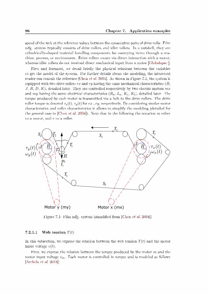
96 Chapter 7. Application examples
speed of the web at the reference values between the consecutive pairs of drive rolls. Filmmfg. system typically consists of drive rollers and idler rollers. In a nutshell, they arecylindrically-shaped material handling components for conveying items through a ma-chine, process, or environment. Drive rollers rotate via direct interaction with a motor,whereas idler rollers do not received direct mechanical input from a motor [Globalspec ].
First and foremost, we detail briey the physical relations between the variablesto get the model of the system. For further details about the modeling, the interestedreader can consult the reference [Chen et al. 2004]. As shown in Figure 7.1, the system isequipped with two drive rollers rx and ry having the same mechanical characteristics (B,J , R, D, K), detailed later. They are controlled respectively by two electric motors mxand my having the same electrical characteristics (Ra, La, Ke, Kt), detailed later. Thetorque produced by each motor is transmitted via a belt to the drive rollers. The driveroller torque is denoted τx(t), τy(t) for rx , ry, respectively. By considering similar motorcharacteristics and roller characteristics it allows to simplify the modeling (detailed forthe general case in [Chen et al. 2004]). Note that in the following the notation m refersto a motor, and r to a roller.
Figure 7.1: Film mfg. system (simplied from [Chen et al. 2004])
7.2.1.1 Web tension T (t)
In this subsection, we express the relation between the web tension T (t) and the motorinput voltage v(t).
First, we express the relation between the torque produced by the motor m and themotor input voltage vm. Each motor is controlled in torque and is modeled as follows[Archela et al. 2018]:

7.2. Thin lm manufacturing 97
τm(t) = −RaLaτm(t)− KeKt
Laωm(t) +
Kt
Lav(t) (7.1)
where τm(t) is the motor torque [Nm], ωm(t) is the motor angular velocity [rad/s], v(t)
is the motor input voltage [V], and Ra is the armature resistance [Ω], La is the armatureinductance [H],Ke is the back electromotive constant [V/rad/s],Kt is the torque constant[Nm/A].
Then, we express the relation between the motor torque τm(t) and the drive rollertorque τr(t). To that end, we consider the subsystem (motor, belt, drive roller) aspictured in Figure 7.2. Assume that (i) there is no loss of transmission via the belt, and(ii) the radius of the drive belt (motor side) is equal to the radius of the driven belt(roller side). From those both assumptions, the drive roller torque τr(t) and velocityωr(t) are equal to the motor torque τm(t) and velocity ωm(t), i.e.
τr(t) = τm(t), ωr(t) = ωm(t) (7.2)
Figure 7.2: Web tension [Chen et al. 2004]
Lastly, we express the relation between the drive roller torque τr(t) and the webtension T (t). According to Newton's law of motion, this relation can be expressed asfollows:
Jωr(t) = τr(t) +RTb(t)−RTa(t)−Bωr(t)= τr(t) +R(Tb(t)− Ta(t))−Bωr(t) (7.3)
where Ta(t), Tb(t) is the web tension of zone a, b respectively [N], and J is the sum of theinertia of motor, belt, drive roller [kg.m2], B is the viscous friction coecient [N.m.s].
For an idler roller, equation (7.3) becomes (7.4) since it is not controlled by a motor,and under some other assumptions detailed in [Chen et al. 2004].
Itωt(t) = R(Tb(t)− Ta(t)) (7.4)
where It is the rotation inertia [kg.m2].

98 Chapter 7. Application examples
7.2.1.2 Web speed V (t)
In this subsection, we express the relation between the web tension T (t) and the rollerangular velocities. Consider Figure 7.3 where two rollers r1, r2 transport the web. S(t)
represents the web length [m] that depends on the web variation generated by the rollers
S(t) = S0 +
∫ t
t0
Rωr1(ζ) dζ −∫ t
t0
Rωr2(ζ) dζ (7.5)
Figure 7.3: Web speed
Then, the web tension at a zone i can be modeled in (7.6).
Ti(t) = KS(t) +DS(t) (7.6)
where K and D represent the spring constant [N/m] and the damping constant [Ns/m]of the web, respectively. They are properties of the material.
Hence, (7.6) can be rewritten as
T (t) = K(Rωr1(t)−Rωr2(t)) +D(Rωr1(t)−Rωr2(t)) (7.7)
Equation (7.7) establishes the relation between the web speed and the web tension.
7.2.1.3 System model
From the relation between the variables in (7.1), (7.3), (7.4), (7.7), the system can bemodeled by the set of dierential equations in (7.8).
τx(t) = −RaLaτx(t)− KeKt
Laωx(t) + Kt
Lavx(t)
τy(t) = −RaLaτy(t)− KeKt
Laωy(t) + Kt
Lavy(t)
Jωx(t) = τx(t)−Bωx(t) +R(T1(t)− T3(t))
Jωy(t) = τy(t)−Bωy(t) +R(T3(t)− T2(t))
Itωt(t) = R(T2(t)− T1(t))
T1(t) = K(Rωt(t)−Rωx(t)) +D(Rωt(t)−Rωx(t))
T2(t) = K(Rωy(t)−Rωt(t)) +D(Rωy(t)−Rωt(t))T3(t) = K(Rωx(t)−Rωy(t)) +D(Rωx(t)−Rωy(t))
(7.8)
The system in (7.8) can be rewritten in the matrix form in (3.3) with x(t) =
[x1, x2, x3, x4, x5, x6, x7]> = [τx(t), τy(t), ωx(t), ωy(t), ωt(t), ωx(t)+ 1DRT1(t), wy(t)− 1
DRT2(t)]>,where T3(t) = −(T1(t) + T2(t); and u(t) = [vx(t), vy(t)]
>. Note that the state x(t) ischosen such that the system is completely controllable [Chen et al. 2004].

7.2. Thin lm manufacturing 99
A =
−RaLa
0 −KeKtLa
0 0 0 0
0 −RaLa
0 −KeKtLa
0 0 01J 0 −B+2DR2
JDR2
J 0 2DR2
J −DR2
J
0 1J
DR2
J −B+2DR2
J 0 −DR2
J2DR2
J
0 0 DR2
ItDR2
It0 −DR2
It−DR2
It
0 0 DR2
It− K
DDRIt
KD −DR2
It−DR
It
0 0 DRIt
DR2
It− K
DKD −DR
It−DR2
It
, B =
KtLa
0
0 KtLa
0 0
0 0
0 0
0 0
0 0
, a = 07
(7.9)where Ra = 4.74, La = 344× 10−6, Ke = 2.4× 10⁻², Kt = 4.2× 10⁻², R = 2× 10⁻²,
J = It = 8× 10⁻⁴, D = 2, K = 3.69× 10².In [Chen et al. 2004], the objective is to control the tension and speed of the
web dened by T (t) = DR(−x3(t) + x4(t) + x6(t) − x7(t)) and V (t) = Rx3(t) re-spectively. To achieve this, the system is equipped with sensors measuring the state[wx(t), wy(t), T1(t), T2(t)]. Note that x6(t) and x7(t) can be computed from the mea-surement of wx(t), T1(t), and wy(t), T2(t) respectively. Hence, the tension T (t) and thespeed V (t) is the service to deliver, and by extension [wx(t), wy(t), T1(t), T2(t)] are thestates that must belong to the service set. In addition, notice that the system in (7.9) isLyapunov stable.
Consider the input limitation dened by Eu(R, u) with
R = diag(10−2, 10−2), u = 02. (7.10)
7.2.2 Analysis and prevention of AT1
Let the service set Es(Ξ, ξ) be dened for
Ξ = diag(1× 10⁻⁸, 1× 10⁻⁸, 1× 10⁻², 1× 10⁻², 1× 10⁻⁸, 2.5× 10⁻¹, 2.5× 10⁻¹),
ξ = 07 (7.11)
with [wx(t), wy(t), T1(t), T2(t)] the state corresponding to the service to deliver, so thatit is constrained by Es, whereas [τx(t), τy(t), ωt(t)] is the free state.Lastly, consider the objective of stealthy aging attacks of AT1 to accelerate the motoraging by controlling them outside of their normal torque levels [Sikanen et al. 2018]:|τx| ≥ 1Nm, |τy| ≥ 1Nm. Hence, the abnormal aging set Dx is dened in (7.12).
c1 =[1 0>n−1
]>, c2 =
[−1 0>n−1
]>, c3 =
[0 1 0>n−2
]>, c4 =
[0 −1 0>n−2
]>,
(7.12)
µ = 1 (7.13)
From the system model in (7.9), the actuator limitation (7.10), the service set (7.11),we want to verify if the physical integrity of the system, i.e. actuator aging, can beviolated by an attacker (RQ1). If it is possible, we want to restrain the control inputset E(R, u) into Eu(R, u) to prevent potential stealthy aging attacks of AT1 (RQ2). RQ1and RQ2 are rstly answered with the invariant set-based method, and then with theconvex robust simulation-based method.

100 Chapter 7. Application examples
7.2.2.1 Invariant set-based method
First-second step: From this rst step, we want to quantify the eect induced bystealthy aging attacks of AT1. To do so, Algorithm 2 is applied with the inputs: (7.10),(7.11), (7.9), α = 0, α = 15, ∆α = 1× 10⁻³. It gives in output the smallest constrainedinvariant state ellipsoid Ex dened with Qx and x in (7.14). It is obtained for α = 14.99,β = 1.1× 10⁻³, and λ = 3.21× 10⁻⁴.
Q = 10−3 ×
215.18 0.02 −8.39 −0.05 7.58 −2.03 −0.04
0.02 215.18 −0.05 −8.39 7.58 −0.04 −2.03
−8.39 −0.05 93.25 0.56 −83.81 22.59 0.45
−0.05 −8.39 0.56 93.25 −83.81 0.45 22.59
7.58 7.58 −83.91 −83.81 165.49 −23.37 −23.37
−2.03 −0.04 22.59 0.45 −23.37 13.73 0.22
−0.04 −2.03 0.45 22.59 −23.37 0.22 13.73
, x = 07
(7.14)
The result is shown graphically in Figure 7.4 where the smallest constrained invariantstate ellipsoid Ex is in green, the service ellipsoid Es constraining the state is in blue, theabnormal aging set Dx is the red area, and the control input set Eu is in magenta. Asan interpretation, if the control signal u(t) remains inside the control input set Eu∀t ≥t0, then the state x(t) remains inside the constrained invariant state ellipsoid Ex forany initial condition x(t0) inside this constrained invariant state ellipsoid Ex and underAssumption 2. From the left- to the right-hand side and from the top to the bottom, thestate [ωx(t), ωy(t)], [T1(t), T2(t)], [V (t), T (t)], [τx(t), τy(t)], and the input [ux(t), uy(t)] areprojected. Notice that the service set has not been drawn for [τx(t), τy(t)] for visibilitypurpose, but the service set covers the whole space as τx(t) and τy(t) are two free states.One can notice that the state τx(t) and τy(t) can reach the abnormal aging set Dx inred, i.e. Ex ∩ D 6= ∅. Recall that this observation is indeed computed by Algorithm 3Thus, stealthy aging attacks can potentially occur if one manipulates the control signalu(t). This answers RQ1, and leads to the next research question RQ2.
Third step: As stealthy aging attacks are feasible for the given control input set Eu, wewant to restrain it such that stealthy aging attacks cannot occur. Algorithm 4 is appliedwith the inputs: R0 = Im, δ = 1 × 10⁻², tol = 1 × 10⁻³. It converges, with respectto the tolerance tol, to the largest control input set Eu(R, u) with R = δR0 dened forδ = 4.9× 10⁻²
R = 10−2 ×[4.09 0
0 4.09
], u = 02 (7.15)
such that the smallest constrained invariant state ellipsoid Ex obtained for α = 14.99
over the interval α = 15 with a step ∆α = 0.01 with β = 13.37, λ = 1.62

7.2. Thin lm manufacturing 101
(a) Figure A
(b) Figure B
(c) Figure B
Figure 7.4: AT1 for the lm mfg. system with invariant-set based method - RQ1 -constrained invariant state set Ex (green), service set Es (blue) covering the whole spacefor [τx,τy] (not drawn), abnormal aging set Dx (red), control input set Eu (magenta)

102 Chapter 7. Application examples
Q = 10−3×
1013.87 0.02 −19.59 −0.23 16.17 −2.16 −0.09
0.02 1013.87 −0.23 −19.59 16.17 −0.09 −2.16
−19.59 −0.23 218.63 2.57 −178.49 23.94 0.99
−0.23 −19.59 2.57 218.63 −178.49 0.99 23.94
16.17 16.17 −178.49 −178.49 338.80 −26.18 −26.18
−2.16 −0.09 23.94 0.99 −26.18 9.95 0.07
−0.09 −2.16 0.99 23.94 −26.18 0.07 9.95
, u = 07
(7.16)does not intersect with the abnormal aging set Dx.
The result is graphically shown in Figure 7.5 where the smallest constrained invariantstate ellipsoid Ex is in green, the service ellipsoid Es constraining the state is in blue,the abnormal aging set Dx is the red area, and the restrained control input set Eu isin magenta. As we can observe in Figure 7.5, the abnormal aging set is guaranteedunreachable for u(t) ∈ Eu, ∀t ≥ t0. Therefore, stealthy aging attacks are prevented byrestraining the control input u(t) to the restrained input set.
7.2.2.2 Convex robust simulation-based method
Notice that in this application, we have considered Q(t) MSOS of degree 4 (d = 2);Z(t), X(t) are matrices (MSOS of degree 0); α(t) SOS of degree 4 (d = 2); and β(t) anunknown scalar (SOS of degree 0).First-second step:
The analysis of stealthy aging attacks of AT1 is now studied on the nite time horizonwith the convex robust simulation-based method. Instead of stopping the simulationonce a constrained bounding ellipsoid at time t = j∆t in Algorithm 6 hits with theabnormal aging set, we stop it once the bounding ellipsoids converge, in this case fortf = 1s. We apply Algorithm 6 with the inputs: Q(t0) = diag(10, 10, 10, 10, 10, 10, 10),x(t0) = [0, 0, 0, 0, 0, 0, 0]>, ∆t = 0.1ms, tf = 1s. The result is graphically shown inFigure 7.6, where the nal bounding state ellipsoid Ex(tf ) is in green, the bounding stateellipsoids Ex(ti) with ti = t0, ..., tf −∆t are not lled, i.e. only their bound is drawn,the service ellipsoid Es constraining the state is in blue, the abnormal aging set Dx is thered area, and the input ellipsoid Eu is in magenta. Recall that the state starting from abounding state ellipsoid Ex(ti) remains inside Ex(ti + ∆t) for u(t) ∈ Eu and for x(t) ∈ Es,∀t ∈ [ti, ti + ∆t] under Assumption 1.
The bounding state ellipsoid hits for the rst time the abnormal aging set at t∩ =
9.5ms, i.e. Ex(9.5ms) ∩ Dx 6= ∅ that corresponds to the j = 95th iterations in Algo-rithm 6. From this analysis, we can conclude that the physical integrity of the systemcan be violated over the time interval [0, 1s] by an attacker manipulating the controlsignal u(t). Thus, stealthy aging attacks are feasible which answers RQ1, and leads tothe prevention step (third step).
Third step: In the third step, we want to restrain the control input set Eu such thatstealthy aging attacks are not feasible. To do so, we apply Algorithm 7 with the inputs:R0 = I2, δ = 1 × 10⁻², tol = 1 × 10⁻³, Q(t0) = diag(10, 10, 10, 10, 10, 10, 10), x(t0) =

7.2. Thin lm manufacturing 103
Figure 7.5: AT1 for the lm mfg. system with invariant-set based method - RQ2 -constrained invariant state set Ex (green), service set Es (blue) covering the whole spacefor [τx,τy] (not drawn), abnormal aging set Dx (red), restrained control input set Eu(magenta)
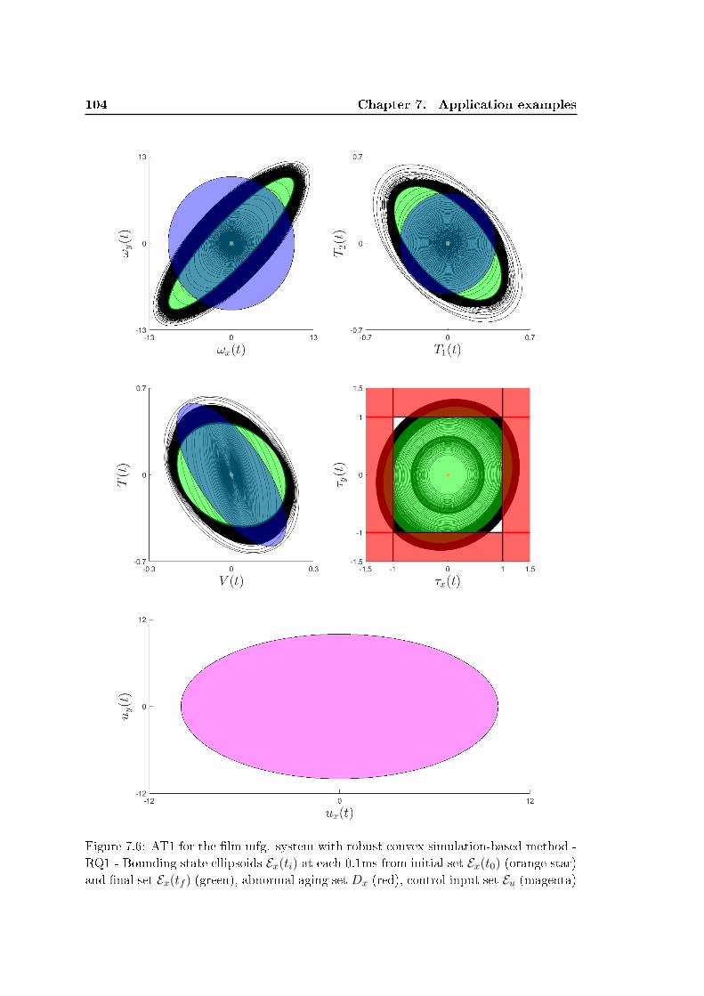
104 Chapter 7. Application examples
Figure 7.6: AT1 for the lm mfg. system with robust convex simulation-based method -RQ1 - Bounding state ellipsoids Ex(ti) at each 0.1ms from initial set Ex(t0) (orange star)and nal set Ex(tf ) (green), abnormal aging set Dx (red), control input set Eu (magenta)

7.3. Satellite reorientation maneuver control 105
[0, 0, 0, 0, 0, 0, 0]>, ∆t = 0.1ms, tf = 1s. The largest restrained control input set Eu(R, u)
is given from the output δ = 0.0168 of Algorithm 7 and computed as R = δR0
R = 10−2 ×[1.68 0
0 1.68
], u = 02 (7.17)
The result is graphically shown in Figure 7.7 where the bounding ellipsoids Ex(ti)
are the ones for the restrained input set Eu. We can observe that none of the boundingellipsoids intersect with the abnormal aging set, so stealthy aging attacks are preventedfor any input u(t) ∈ Eu.
7.2.3 Analysis of AT2
In this subsection, stealthy aging attacks of AT2 is analyzed. The system model in (7.9)is discretized with the Tustin method with a sampling time Te = 1ms.
Consider the attacker aims to maximize the thermomechanical stresses [Sikanenet al. 2018] (e.g. heat) due to the torque square in the motor x. Hence, the degra-dation function is expressed as gk = τ2
x,k. Recall that the attacker can manipulate thecontrol signal, and it knows the desired service at each time instant k. Thus and beforeanalyzing the attack, a preliminary computation is required to get the normal signals(norm) that a controller should produce in the attack-free case. The signal of interest inthe normal signals are the ones that belong to the service set, so that Xs can be dened.Then, the attack input signal uk is computed with the SLP method to maximize the costdegradation function while keeping the service states [x3, x4, x6, x7] inside Xs given fora δ = 10−4 error around the normal service. At the 28th iteration of the SLP, the costdegradation function converges as shown in Fig. 7.8.
7.3 Satellite reorientation maneuver control
In this section, we propose to show the relevance of the proposed methods for AT1 andAT2 upon a satellite reorientation maneuver control.
7.3.1 System description
Consider an attitude controlled satellite, featuring four reaction wheels as actuators[Wie 2008]. The control objective is to slightly re-orientate it at the orientation referencevalues. The Euler angles α, β, γ [rad] characterize the orientation of the coordinatesystem. The satellite is equipped with four reaction wheels wi with i = 1, 2, 3, 4 havingthe same characteristics: an inertia Jw. Each of them is controlled by an electrical motormi, having the same characteristics: an armature resistance Ra, an electric constant ke,a torque constant kt. As in the previous application, we will not detail the modelinggiven in [Wie 2008], but explain the physical relations between the variables.
7.3.1.1 Euler angles
The total angular momentum of the satellite is dened in (7.18).

106 Chapter 7. Application examples
Figure 7.7: AT1 for the lm mfg. system with robust convex simulation-based method -RQ2 - Bounding state ellipsoids Ex(ti) at each 0.1ms from initial set Ex(t0) (orange star)and nal set Ex(tf ) (green), abnormal aging set Dx (red), restrained control input set Eu(magenta)

7.3. Satellite reorientation maneuver control 107
0 500 1000 1500 2000 2500 30000
1
2
310-3
0 500 1000 1500 2000 2500 3000
0
2
4
6
Time (10-5
s)
Time (10-5
s)
0 500 1000 1500 2000 2500 30000
0.01
0.02
0
0.04
0.08
1 15 283.250
3.255
3.259
0 1000 2000 3000-2
-1
0
1
2
Time (10-5
s)
Time (10-5
s)
Figure 7.8: AT2 for the lm mfg. control: at the 28th iteration, the cost degradationfunction is maximized (1st from bottom) with the degradation function (1st from top)for the optimal attack input signal (2nd from top) while delivering the desired service(2nd from bottom)

108 Chapter 7. Application examples
Hs(t) = Isωs(t) + hw(t) (7.18)
where ωs(t) = [α(t), β(t), γ(t)]> is the satellite angular velocity in body frame with α, β,γ the Euler angular rates [rad/s], hw(t) is the angular momentum of the reaction wheels,and Is is the inertia matrix of the satellite.The angular momentum of the reaction wheels hw(t) can be described in body frame in(7.19).
hw(t) = LwIwωw(t) (7.19)
where ωw(t) = [ωw1(t), ωw2(t), ωw3(t), ωw4(t) is the angular velocity of the reactionwheels, and Lw is the reaction wheel distribution matrix, Iw = diag(Iw1, Iw2, Iw3, Iw4) isthe reaction wheel diagonal inertia matrix.
Assuming the reaction wheels have a pyramid conguration, then the moments ac-tuated on the satellite are dened by
Ts(t) = LwTw(t),with Lw =
−√
3/3√
3/3√
3/3 −√
3/3
−√
3/3 −√
3/3√
3/3√
3/3√3/3
√3/3
√3/3
√3/3
(7.20)
where Ts(t) = [τα(t), τβ(t), τγ(t)]> the torque actuating on each axes of the body frame,and Tw(t) = [τw1(t), τw2(t), τw3(t), τw4(t)]> is the torque generated by each reactionwheel wi. From the moment equations of Euler represented by the angular momentumrate with respect to the body frame, the dynamics of the satellite can be described in(7.21), assuming no disturbance torque.
Hs(t) = −ωs(t)×Hs(t) (7.21)
Then, we neglect the term ωs(t)×Hs(t), which yields Hs(t) = 0.The rst time derivative of (7.18) yields to
Hs(t) = Isωs(t) + hw(t) (7.22)
Hence, (7.21) can be rewritten from the rst time (7.22) as follows:
Isωs(t) = −hw(t) (7.23)
Each reaction wheel produces an angular momentum which is transferred to thesatellite, so hw(t) = Ts(t) = LwTw(t).
7.3.2 Reaction wheel torque and motor angular velocity
In this subsection, we express the relation between the reaction wheel torque τwn(t) andthe motor input voltage vmn(t). This is expressed for a motor mn and reaction wheelwn as is validate for all the motors and reaction wheels of the application.
As the reaction wheel is xed to the rotor shaft, then the reaction wheel and themotor have same angular velocity and acceleration, i.e. ωwn(t) = ωmn(t), ωwn(t) =

7.3. Satellite reorientation maneuver control 109
˙omegamn(t). Consider a motor controlled in torque similar to the previous application.From [Archela et al. 2018], the armature current can be expressed in (7.24).
Laimn(t) = Keωmn(t)−Raimn(t) + vmn(t) (7.24)
τmn(t) = Ktimn(t) (7.25)
As the dynamic of the current is very fast compared to the satellite dynamic, thecurrent dynamic is neglected. Hence equation (7.24) is restated at the equilibrium statein (7.26).
imn(t) =Ke
Raωmn(t) +
1
Ravmn(t) (7.26)
The moment balance of the motor shaft is given in (7.27).
Imnωmn(t) = τmn(t)−Bωmn(t)− τwn(t) (7.27)
where τwn(t) = Iwnωwn(t) as the load torque is the reaction wheel xed on the rotorshaft, and B is the viscous friction coecient [N.m.s] of the motor, Imn is the momentof inertia of the motor.
Thus, as ωwn(t) = ωw(t), (7.27) can be rewritten
(Imn + Iwn)ωwn(t) = τmn(t)−Bωmn(t) (7.28)
It is reasonable to assume that Iwn >> Imn, thus equation (7.28) becomes (7.29).
Iwnωwn(t) ≈ τmn(t)−Bωmn(t) (7.29)
Lastly, by substituting equation (7.26) into (7.29) with (7.25), the motor angularvelocity ωwn(t) can be expressed in (7.30).
Iwnωmn(t) ≈ (KtKe
Ra−B)ωmn(t) +
Kt
Ravmn(t) (7.30)
Then, we express the satellite angular acceleration ωs(t) in by substituting (7.29)into (7.23).
Isωs(t) = −LwI4(KtKe
Ra−B)ωm(t)− LwI4
Kt
Ravm(t) (7.31)
7.3.3 System model
From the relation between the variables in (7.30), (7.31), the system can be modeled bythe set of dierential equations in (7.32).
ωm(t) = I−1wn(KtKe
Ra−B)ωmn(t) + I−1
wnKtRavmn(t)
ωs(t) = −I−1s LwI4(KtKe
Ra−B)ωm(t)− I−1
s LwI4KtRavm(t)
(7.32)
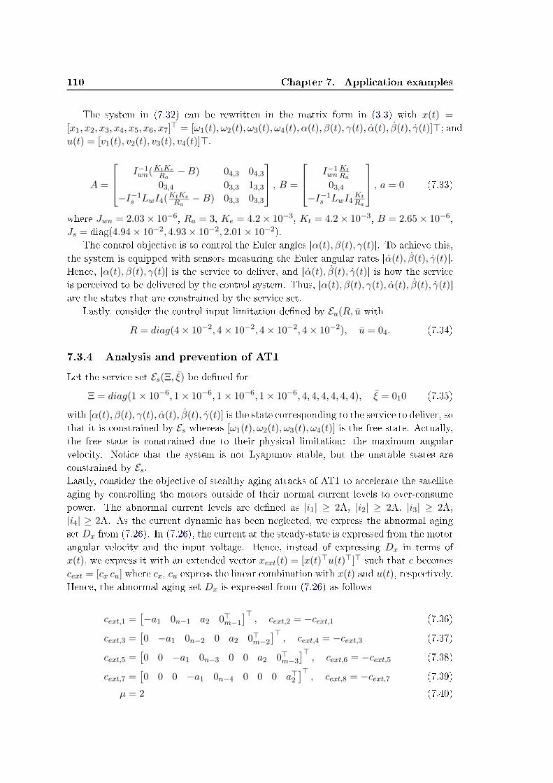
110 Chapter 7. Application examples
The system in (7.32) can be rewritten in the matrix form in (3.3) with x(t) =
[x1, x2, x3, x4, x5, x6, x7]> = [ω1(t), ω2(t), ω3(t), ω4(t), α(t), β(t), γ(t), α(t), β(t), γ(t)]>; andu(t) = [v1(t), v2(t), v3(t), v4(t)]>.
A =
I−1wn(KtKe
Ra−B) 04,3 04,3
03,4 03,3 13,3
−I−1s LwI4(KtKe
Ra−B) 03,3 03,3
, B =
I−1wn
KtRa
03,4
−I−1s LwI4
KtRa
, a = 0 (7.33)
where Jwn = 2.03× 10⁻⁶, Ra = 3, Ke = 4.2× 10⁻³, Kt = 4.2× 10⁻³, B = 2.65× 10⁻⁶,Js = diag(4.94× 10⁻², 4.93× 10⁻², 2.01× 10⁻²).
The control objective is to control the Euler angles [α(t), β(t), γ(t)]. To achieve this,the system is equipped with sensors measuring the Euler angular rates [α(t), β(t), γ(t)].Hence, [α(t), β(t), γ(t)] is the service to deliver, and [α(t), β(t), γ(t)] is how the serviceis perceived to be delivered by the control system. Thus, [α(t), β(t), γ(t), α(t), β(t), γ(t)]are the states that are constrained by the service set.
Lastly, consider the control input limitation dened by Eu(R, u with
R = diag(4× 10⁻², 4× 10⁻², 4× 10⁻², 4× 10⁻²), u = 04. (7.34)
7.3.4 Analysis and prevention of AT1
Let the service set Es(Ξ, ξ) be dened for
Ξ = diag(1× 10⁻⁶, 1× 10⁻⁶, 1× 10⁻⁶, 1× 10⁻⁶, 4, 4, 4, 4, 4, 4), ξ = 010 (7.35)
with [α(t), β(t), γ(t), α(t), β(t), γ(t)] is the state corresponding to the service to deliver, sothat it is constrained by Es whereas [ω1(t), ω2(t), ω3(t), ω4(t)] is the free state. Actually,the free state is constrained due to their physical limitation: the maximum angularvelocity. Notice that the system is not Lyapunov stable, but the unstable states areconstrained by Es.Lastly, consider the objective of stealthy aging attacks of AT1 to accelerate the satelliteaging by controlling the motors outside of their normal current levels to over-consumepower. The abnormal current levels are dened as |i1| ≥ 2A, |i2| ≥ 2A, |i3| ≥ 2A,|i4| ≥ 2A. As the current dynamic has been neglected, we express the abnormal agingset Dx from (7.26). In (7.26), the current at the steady-state is expressed from the motorangular velocity and the input voltage. Hence, instead of expressing Dx in terms ofx(t), we express it with an extended vector xext(t) = [x(t)>u(t)>]> such that c becomescext = [cx cu] where cx, cu express the linear combination with x(t) and u(t), respectively.Hence, the abnormal aging set Dx is expressed from (7.26) as follows
cext,1 =[−a1 0n−1 a2 0>m−1
]>, cext,2 = −cext,1 (7.36)
cext,3 =[0 −a1 0n−2 0 a2 0>m−2
]>, cext,4 = −cext,3 (7.37)
cext,5 =[0 0 −a1 0n−3 0 0 a2 0>m−3
]>, cext,6 = −cext,5 (7.38)
cext,7 =[0 0 0 −a1 0n−4 0 0 0 a>2
]>, cext,8 = −cext,7 (7.39)
µ = 2 (7.40)

7.3. Satellite reorientation maneuver control 111
Because the system is not completely controllable, it is transformed with the transfor-mation matrix Z such that x(t) = Zx(t), with x(t) = [x1, x2, x3, x4, x5, x6, x7]> the new(controllable) state, and Es, D are the transformed sets of Es, Dx respectively.
In the following, we apply the robust convex simulation-based method on the systemto analyze and prevent stealthy aging attacks of AT1. Since the system is not Lyapunovstable, the invariant set-based method cannot be applied.
7.3.4.1 Robust convex simulation-based method
Notice that in this application, we have considered Q(t) MSOS of degree 6 (d = 3);Z(t), X(t) are matrices (MSOS of degree 0); α(t) SOS of degree 6 (d = 3); and β(t) anunknown scalar (SOS of degree 0).
The analysis of stealthy aging attacks of AT1 on the nite time horizon is studied.Similarly as previously, we stop the simulation once the bounding ellipsoids converge.In this case, it converges at tf = 4s. Algorithm 6 is applied with the inputs: Q(t0) =
diag(100, 100, 100, 100, 100, 100, 100), ˘x(t0) = [0, 0, 0, 0, 0, 0, 0]>, ∆t = 0.1s, tf = 4s.The result is graphically shown in Figure 7.9, where the nal bounding state ellipsoidEx(tf ) is in green, the bounding state ellipsoids Ex(ti) with ti = t0, ..., tf −∆t are notlled, i.e. only their bound is drawn, the service ellipsoid Es constraining the state is inblue, the abnormal aging set Dx is the red area, and the input ellipsoid Eu is in magenta.
The bounding ellipsoid hits for the rst time the abnormal aging set at t∩ = 100ms,i.e. Ex(100ms) ∩ Dx 6= ∅ that corresponds to the j = 1st iteration in Algorithm 6.Therefore, the physical integrity of the system can be violated over the time interval[0, 4s] by an attacker manipulating the control signal u(t). Thus, stealthy aging attacksare feasible which answers RQ1, and leads to the prevention step (third step).Third step: In the third step, we want to restrain the control input set Eu such thatstealthy aging attacks are not feasible. Algorithm 7 is applied with the inputs: R0 = I2,δ = 1 × 10⁻², tol = 1 × 10⁻², Q(t0) = diag(100, 100, 100, 100, 100, 100, 100), ˘x(t0) =
[0, 0, 0, 0, 0, 0, 0]>, ∆t = 0.1ms, tf = 4s. The largest restrained control input set Eu(R, u)
is given from the output δ = 0.1338 of Algorithm 7 and computed as R = δR0
R = 10−1 ×
1.34 0 0 0
0 1.34 0 0
0 0 1.34 0
0 0 0 1.34
, u = 04 (7.41)
The result is graphically shown in Figure 7.10 where the bounding ellipsoids Ex(ti)
are the ones for the restrained input set Eu. We can observe that none of the boundingellipsoids intersect with the abnormal aging set, so stealthy aging attacks are preventedfor any input u(t) ∈ Eu.
Remark 14. In Figure 7.9 and 7.10, we can observe that the bounding state ellipsoids
grows until they are constrained by the service set. This comes from the stability of the
dynamical system: as it is not Lyapunov stable, then the state x(t) does not return to
the equilibrium state after a perturbation, i.e. the control input u(t) in this case. A
physical interpretation is given as follows. By controlling the motors, the satellite moves
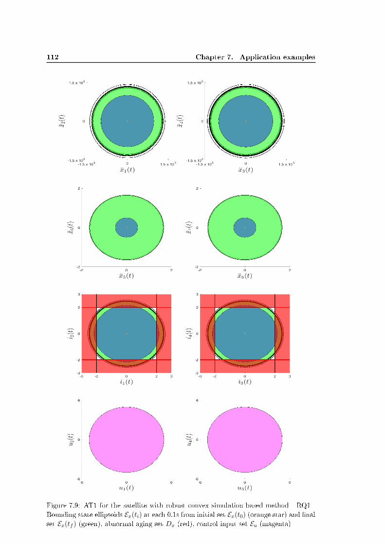
112 Chapter 7. Application examples
Figure 7.9: AT1 for the satellite with robust convex simulation-based method - RQ1 -Bounding state ellipsoids Ex(ti) at each 0.1s from initial set Ex(t0) (orange star) and nalset Ex(tf ) (green), abnormal aging set Dx (red), control input set Eu (magenta)

7.3. Satellite reorientation maneuver control 113
Figure 7.10: AT1 for the satellite with robust convex simulation-based method - RQ2- Bounding state ellipsoids Ex(ti) at each 0.1s from initial set Ex(t0) (orange star) andnal set Ex(tf ) (green), abnormal aging set Dx (red), restrained control input set Eu(magenta)

114 Chapter 7. Application examples
according to the Euler angles. Recalling no external torque actuating on the satellite has
been considered and another term in the dynamics of the satellite, then Hs(t) = 0. In
other words, we do not considered the dynamics of the satellite. Thus, the Euler angular
rate never returns to 0, unless if a motor actuates oppositely. That is why the bounding
state ellipsoid grows as the state always grow, but they are constrained by the service set.
7.3.5 Analysis of AT2
In this subsection, we propose to analyze stealthy aging attacks of AT2. The systemmodel in (7.33) is discretized with the Tustin method with a sampling time Te = 10ms.
Consider the attacker aims to maximize the power consumption of the satellite. Thedegradation function is expressed as gk =
∑4i=1 pi,k, pi,k = ii,kui,k. In preliminary,
the normal signals are computed in order to know the service set at each time instantk. Then, the attack input signal uk is computed with the SLP to maximize the costdegradation function while keeping the service states [x5, x6, x7, x8, x9, x10] inside Xs
given for a δ = 10−4 error around the normal service. At the 60th iteration of the SLP,the cost degradation function converges as shown in Figure. 7.11. It shows that the costdegradation function raises by 3.25 times from the normal signals.
7.4 Results analysis
For the AT1 on the lm mfg. system, we can observe that the robust convex simulation-based method provides better results: the restrained input set Eu is larger, allowinglarger control actions. This observation might come from a tighter outer-approximationof the reachable set with the robust convex simulation-based method. In fact, it is lessconservative than the invariant set based method as it allows the search for a symmet-ric matrix-valued polynomials Q(t) rather than a symmetric matrix Q. However, thismethod consumes more computational resources.
By comparing the AT2 on both applications, we can notice that stealthy aging attackshave more capabilities on the satellite application, as the cost degradation function raisesmore. This observation might come from the physical system type: the satellite onecomprises four motors, each of them acting on the three Euler angular rates, and thenthe Euler angles; whereas the lm mfg. system comprises two motors, each of themacting on either T1 or T2, with T depending on T1 and T2. This analysis reveals thatthe satellite application is an over-actuated system. Note that it is over-actuated onpurpose to tackle a potential (not intended) failure of a motor or reaction wheel. Thestealthy aging attacks benet from it by compensating the control action of one actuatorwith another one to deliver the desired service as shown in Figure. 7.11 (2nd from top).However, for the not over-actuated type (lm mfg. system), we can note that stealthyaging attacks benet from the dynamic of the service to perform the attacks. In fact, themotor torque having a faster dynamic than the motor angular velocities, i.e. electricaland mechanical dynamic, it is possible to fastly change the control input u(t) such thatit is ltered by the motor angular velocity dynamic to remain stealthy.

7.4. Results analysis 115
0 200 400 600 800 10100
6
12
0 200 400 600 800 1010-5
0
5
Time (10-2
s)
Time (10-2
s)
0 200 400 600 800 10100
0.15
0.3
Angle
s
0
0.016
0.032
Angula
r ra
tes
0 20 40 602
4.26
6.5
0 500 1010-2
-1
0
1
2
Time (10-2
s)
Time (10-2
s)
Figure 7.11: AT2 for the satellite: at the 60th iteration, the cost degradation functionis maximized (1st from bottom) with the degradation function (1st from top) for theoptimal attack input signal (2nd from top) while delivering the desired service (2nd frombottom)

116 Chapter 7. Application examples
7.5 Conclusion
In this Chapter, we have applied our methods upon two application examples. We haveshown that the robut convex simulation-based method is more general and providesbetter results. However, the computational time is higher than the one with the invariantset-based method. In particular, we have observed that stealthy aging attacks seem moredangerous against dynamical systems exhibiting an over actuation as abnormal controlactions can be compensated by the other actuators to hide the attacks regarding thedelivered service.

Conclusion


Conclusion
The research works presented in this manuscript address the analysis and the preventionof stealthy aging attacks. Such attacks aim to accelerate the aging of the actuators, whilethe process continues to deliver the desired service. In particular, these research worksconsiders an attacker that can manipulate the control input. Thus, their objective is toviolate the process integrity.
The problem has been split into two cases of stealthy aging attacks: on one hand,a subcase of attacks (AT1) is considered. AT1 aims to let the dynamical system reachan abnormal aging set featuring an aging faster than normal. For AT1, the contributionof the methods resides in (i) proving the feasibility of such attacks, i.e. can they reachthe process integrity? If they are feasible, (ii) restraining the control input set to makethem unfeasible, i.e. the process integrity cannot be reached. On the other hand, thegeneral case of stealthy aging attacks (AT2) is considered. AT2 aims to maximize thetime integral of a degradation function, modeling the stresses acting on the dynamicalsystem. The contribution of the method resides in (i) analyzing the potential aging anattacker could lead to the actuators.
On one hand, the methods for AT1 are based on the search of a pseudo-Lyapunovfunction for the dynamical system. This function denes κ-level set from which thestate trajectory of the dynamical system will never go out. This allows the proof of thefeasibility of such attacks. Two methods have been proposed: one based on the invari-ance concept, called the invariant set based method; and the other based on the robustsimulation of the dynamical system, called the convex robust simulation-based method.The rst method allows the analysis of stealthy aging attacks on an innite-time hori-zon, while the second one allows it on a nite-time horizon. Thereafter, the methodssearch for a restrained control input set to make stealthy aging attacks unfeasible. Bothmethods solve a SDP problem with LMI constraints.
On the other hand, the method for AT2 is based on the construction of a control sig-nal maximizing the time integral of a degradation function, modeling the stresses actingon the actuators. The idea is to nd an optimal control signal under some constraintsrelated to AT2. It allows the analysis of the impact stealthy aging attacks of AT2 couldcause against a process. Since the degradation function is intrinsically nonlinear, thenthe method solves a SLP problem.
From a theoretical analysis of the methods, for AT1 the convex robust simulation-based one is more adapted to deal with stealthy aging attacks. Indeed, no condition onthe Lyapunov stability is required for this method, unlike the invariant set-based one.Moreover, the invariant set-based-method has a computational drawback: the multiplierα needs to be xed, but it is unbounded. As a result, one can search for an pseudo-Lyapunov function, but there is no guarantee that this is the optimal one. In addition,

120 Conclusion
the convex robust simulation-based method is less conservative. In fact, the methodsolves a Matrix SOS (MSOS) problem giving more degree of freedom. However, thismethod consumes more computational resources. About the method for AT2, it allowsthe analysis of potential impact of such attacks in the general case, but does not provethe feasibility of such attacks.
Lastly, the methods for AT1 and AT2 have been applied upon two applications: onefrom the manufacturing area, and another from the aerospace one. The results con-rm the theoretical analysis: the convex robust simulation-based method provides a lessrestrictive condition on the control input set to guarantee the non-feasibility of AT1.About AT2, the results show that the optimal control signal maximizing the stressescan exploit (i) the dynamic property of the system to hide the attack, i.e. mechanicaldynamic is slower than the electrical dynamic; (ii) the over-actuated property of thesystem to hide the attack.
This thesis has addressed the following scientic issues:
Modeling the attack stealthiness in set theory,
Stability condition required from the invariant set theory,
Loss of the temporal variable in the invariant set theory.
From these research works, several research axes for pursuing these three years ofresearch are proposed.In the short term:
From the aging of actuators, it seems relevant to map which stresses can occur fromthe control signals, and at which level it accelerates the aging of the actuator. Infact, the proposed methods are relevant only if one is able to describe the dangerousstresses, otherwise our methods cannot be applied. Furthermore, recalling thatthe stresses can be internal meaning that they are inherent in the operation ofthe actuator; or external meaning that they originate in the environment of theactuator. From this, it appears that both stresses need to be investigated. Indeed,an attacker might control another part of the process in order to increase theexternal stresses of an actuator.
From the methods for AT1, the prevention of attacks consists in restraining thecontrol input set. Such restriction has been formulated in terms of the controlinput set size, i.e. the trace of the shape matrix. However, the center has notbeen considered as a decision variable, otherwise the constraint becomes a BMI.By xing the center, we nd the largest restrained control input set for the xedcenter, but this center is not guaranteed to give the largest set. Thus, this issuewill be investigated.
The methods for AT1 and AT2 will be applied on two testbeds to validate themethods. Two testbeds are available in our research lab: (i) a dc motor (drive)

Conclusion 121
interconnected with another dc motor (load) producing a load torque, and (ii) adrone with two dc motors. Those two testbeds are relevant as they share similarproperties than the ones of the Applications studied in this thesis.
In the mid term:
As a complement with the validation on a testbeds, it is common that the modeldoes not t with the real system owing to the modeling assumptions and the ex-ternal disturbances acting on the process (input disturbance, output disturbance).So, the methods will be extended to a model with uncertainties.
As seen in this thesis, the attacker requires to know the desired service, i.e. serviceset, in order to launch a stealthy aging attacks. We have stated in this thesisthat the attacker can assess the expected service from the process model and thecontrol signal transmitted by the controller. Thus, we will conduct research aboutthe quality of knowledge the attacker has about the service set. Recalling thatthe detector in the controller side is based on a state estimator, can the attackerfrom the communication side compute the expected service around a small errorcompared to the one computed by the state estimator? This small error mustguarantee the stealthiness of the attack.
This thesis provides methods for analyzing and preventing stealthy aging attacks,but does not contribute to the detection of anomalies in the control signal. Fromthe proposed methods, the convex robust simulation could be derived for detectionpurpose. In fact, it could be possible to place the detection system close to theprocess, i.e. after the transmission channel, and collect the control signal in real-time. Then, starting from an initial bounding state ellipsoid, the system checksif the bounding state ellipsoid at a future time will violate the process integrity.Obviously, it will require further conditions that might be strong such as (i) thecontrol signal does not change during the computational time of the method, (ii)the computation time is guaranteed to be lower than the dynamic of the process.
As presented in this thesis, the malevolence can be seen as a new root cause offailures in ICSs. It is intended and aims to reach the process integrity. However, thedetection of an anomaly leads the detection system to assess the root cause. Thisleads to the problem of anomaly characterization. This is a crucial problem: if themalevolence is miscategorized and considered as another classical root cause by thedetection system, then inappropriate actions will be take by the operators, withoutremoving the malevolence. In a worst case, an attack could exploit it to inducefailures at dierent period of times to be miscategorized in an intentional manner.We think that the characterization needs to focus on the specic characteristics ofthe malevolence. As stated in this thesis, the intentional characteristic combinedwith analysis of the propagation path could be an entry point to deal with. Noticethat the propagation path of an anomaly needs a tracking of the anomaly whichcould be done by detecting anomalies in all the potential propagation paths aspresented in this thesis. Obviously, this will lead further research works about
122 Conclusion
the eect in the anomaly characterization if some propagation paths taken by theanomaly are missing. About this, we think that the works in the condence of thedata based on Bayesian Network model could be appropriate.
In the long term:
The methods for AT1 have a limit: they search for an ellipsoid that encompassesthe state under some constraints. However, ellipsoid might not be the appropriateset for being the smallest set. Other sets exist as mentioned in this thesis. Furtherresearch works will develop methods with the same objective, but with other sets.These research works will develop a method searching for various sets, includingthe ellipsoids presented in this thesis. By denition all the sets we will nd containthe state trajectory, thus the set resulting from the intersection of all the setscontains also the state trajectory. A tighter outer-approximation of the state setcould result from this approach.
As seen in this thesis, with the methods for AT1 one can prove the feasibilityof stealthy aging attacks and prevent them to occur by computing the largestrestrained control input set. However, it has not been extended to the general caseAT2. Future research works will investigate it.
In future works we will extend our methods to the class of PWA system. In fact,it allows a description of a physical system that follows an ane time-invariantmodel for some regions of the state. This extension is important as it allows,among others, the modeling of the physical entity that deliver the energy to theactuator, called the pre-actuator (e.g. power converter, pneumatic distributor). Infact, their model is often non-linear.
The design of any system (e.g. controller, detector) requires a model of the process.This model is obtained under some modeling assumptions to simplify the problem.Those modeling assumptions are validated in particular cases. However, no systemchecks if those modeling assumptions are satised in realtime. So, our futureresearch work will concern it around two main questions: can an attacker exploitthe modeling assumptions to launch stealthy aging attacks? and how can wedesign detection system to verify in realtime that those modeling assumptions aresatised?

Appendices

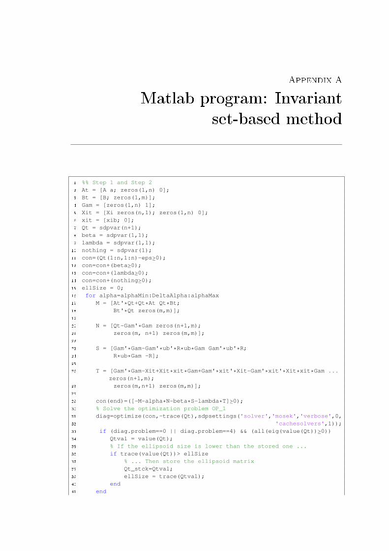
Appendix A
Matlab program: Invariant
set-based method
1 %% Step 1 and Step 22 At = [A a; zeros(1,n) 0];3 Bt = [B; zeros(1,m)];4 Gam = [zeros(1,n) 1];5 Xit = [Xi zeros(n,1); zeros(1,n) 0];6 xit = [xib; 0];7 Qt = sdpvar(n+1);8 beta = sdpvar(1,1);9 lambda = sdpvar(1,1);
10 nothing = sdpvar(1);11 con=(Qt(1:n,1:n)-eps≥0);12 con=con+(beta≥0);13 con=con+(lambda≥0);14 con=con+(nothing≥0);15 ellSize = 0;16 for alpha=alphaMin:DeltaAlpha:alphaMax17 M = [At'*Qt+Qt*At Qt*Bt;18 Bt'*Qt zeros(m,m)];19
20 N = [Qt-Gam'*Gam zeros(n+1,m);21 zeros(m, n+1) zeros(m,m)];22
23 S = [Gam'*Gam-Gam'*ub'*R*ub*Gam Gam'*ub'*R;24 R*ub*Gam -R];25
26 T = [Gam'*Gam-Xit+Xit*xit*Gam+Gam'*xit'*Xit-Gam'*xit'*Xit*xit*Gam ...zeros(n+1,m);
27 zeros(m,n+1) zeros(m,m)];28
29 con(end)=([-M-alpha*N-beta*S-lambda*T]≥0);30 % Solve the optimization problem OP_131 diag=optimize(con,-trace(Qt),sdpsettings('solver','mosek','verbose',0,32 'cachesolvers',1));33 if (diag.problem==0 || diag.problem==4) && (all(eig(value(Qt))≥0))34 Qtval = value(Qt);35 % If the ellipsoid size is lower than the stored one ...36 if trace(value(Qt))> ellSize37 % ... Then store the ellipsoid matrix38 Qt_stck=Qtval;39 ellSize = trace(Qtval);40 end41 end

126 Appendix A. Matlab program: Invariant set-based method
42 end43 % Extract the ellipsoid matrix and the center44 Qn=Qt_stck;45 xn_out = -Qn([1:n],[1:n])\Qn([1:n],n+1);46 % Normalization47 Qn_out = Qn([1:n],[1:n])/(1-Qn(n+1,n+1)+xn_out'*Qn([1:n],[1:n])*xn_out);
1 %% Step 32 At = [A a; zeros(1,n) 0];3 Bt = [B; zeros(1,m)];4 Gam = [zeros(1,n) 1];5 Xit = [Xi zeros(n,1); zeros(1,n) 0];6 xit = [xib; 0];7 % Parameters of the bisection method8 R_ov = ∆_ov*R0; %Should not hit9 R_und = ∆_und*R0; %Should hit
10 % Start the bisection method11 ∆_wrk = ∆_ov;12 while(∆_ov-∆_und > tol)13 ∆ = (∆_ov+∆_und)/214 R = ∆*R0; % Value of R at the first iteration15 bool = 0; %0 if no hit, otherwise 116 eps = 10^-8;17 Qt = sdpvar(n+1);18 beta = sdpvar(1,1);19 lambda = sdpvar(1,1);20 nothing = sdpvar(1);21 con=(Qt(1:n,1:n)-eps≥0);22 con=con+(beta≥0);23 con=con+(lambda≥0);24 con=con+(nothing≥0);25 ellSize = 0;26 for alpha=alphaMin:DeltaAlpha:alphaMax27 M = [At'*Qt+Qt*At Qt*Bt;28 Bt'*Qt zeros(m,m)];29
30 N = [Qt-Gam'*Gam zeros(n+1,m);31 zeros(m, n+1) zeros(m,m)];32
33 S = [Gam'*Gam-Gam'*ub'*R*ub*Gam Gam'*ub'*R;34 R*ub*Gam -R];35
36 T = ...[Gam'*Gam-Xit+Xit*xit*Gam+Gam'*xit'*Xit-Gam'*xit'*Xit*xit*Gam ...zeros(n+1,m);
37 zeros(m,n+1) zeros(m,m)];38
39 con(end)=([-M-alpha*N-beta*S-lambda*T]≥0);40 % Solve the optimization problem OP_141 diag=optimize(con,-trace(Qt),sdpsettings('solver','mosek',42 'verbose',0,'cachesolvers',1));43 if (diag.problem==0 || diag.problem==4) && (all(eig(value(Qt))≥0))44 Qtval = value(Qt);

127
45 % If the ellipsoid size is lower than the stored one ...46 if trace(value(Qt))> ellSize47 % ... Then store the ellipsoid matrix48 Qt_stck=Qtval;49 ellSize = trace(Qtval);50 end51 end52 end53 % Extract the ellipsoid matrix and the center54 Qn=Qt_stck;55 xn_out = -Qn([1:n],[1:n])\Qn([1:n],n+1);56 % Normalization57 Qn_out = ...
Qn([1:n],[1:n])/(1-Qn(n+1,n+1)+xn_out'*Qn([1:n],[1:n])*xn_out);58 % Verify if the ellipsoid hits with the abnormal aging set (259 % halfspaces in this case)60 check1 = (sqrt(cHyp1'*(Qn_out\cHyp1))-abs(mu-cHyp1'*xn_out))/61 (sqrt(cHyp1'*cHyp1));62 check2 = (sqrt(cHyp2'*(Qn_out\cHyp2))-abs(mu-cHyp2'*xn_out))/63 (sqrt(cHyp2'*cHyp2));64 % If it hits ...65 if (check1>0 || check2>0)66 % ... Then reduce the size of R67 ∆_und = ∆;68 else69 % ... Otherwise increase the size of R70 ∆_ov = ∆;71 ∆_wrk = ∆;72 % Store the ellipsoid matrix and the center73 Qn_out_wrk = Qn_out74 xn_out_wrk = xn_out75 end76 % Clear memory77 yalmip('clear');78 % Define decision variables for the next iteration step79 nothing = sdpvar(1);80 end81 % Output: state and input ellipsoid matrices and centers82 Qn_out_opt = Qn_out_wrk;83 xn_out_opt = xn_out_wrk;84 R = ∆_wrk * R0;85 ub


Appendix B
Matlab program: Robust convex
simulation-based method
1 %% Step 1 and Step 22 Atil = [A, ab; zeros(1,n), 0];3 Btil = [B; zeros(1,m)];4 Gam = [zeros(1,n) 1];5 Xit = [Xi zeros(n,1); zeros(1,n) 0];6 xit = [xib; 0];7 Qsi_org = Xi;8 qsi_org = xib;9 Qsitil = [Qsi_org, zeros(n,1);
10 zeros(1,n) 0];11 qsitil = [qsi_org; 0];12 Itil = eye(n);13
14 % Initial condition Eps_x(E0,c0)15 E0 = Eini;16 c0 = cini;17
18 % Time parameters19 tf = 0.5; % Total simulation time [s]20 Delta_t = 0.001; % Time step [s]21 N = tf/(Delta_t); % Number of iterations22
23 % Initialization24 E([1:n],[1:n]) = E0;25 c([1:n],1) = c0;26
27 % To store the hit28 ck=zeros(1,round(N));29
30 % Verify if at initial time it hits the abnormal aging set31 check1 = (sqrt(cHyp1'*(E0\cHyp1))-abs(mu-cHyp1'*c0))/(sqrt(cHyp1'*cHyp1));32 check2 = (sqrt(cHyp2'*(E0\cHyp2))-abs(mu-cHyp2'*c0))/(sqrt(cHyp2'*cHyp2));33 if(check1>0 || check2>0)34 ck(1) = 1;35 disp('error')36 pause();37 else38 ck(1)=0;39 end40
41 % Time SOS degree 042 t=sdpvar(1);
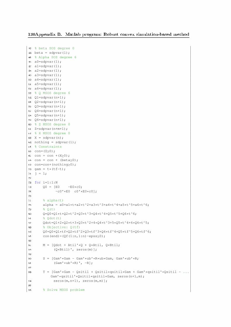
130Appendix B. Matlab program: Robust convex simulation-based method
43 % beta SOS degree 044 beta = sdpvar(1);45 % Alpha SOS degree 646 a0=sdpvar(1);47 a1=sdpvar(1);48 a2=sdpvar(1);49 a3=sdpvar(1);50 a4=sdpvar(1);51 a5=sdpvar(1);52 a6=sdpvar(1);53 % Q MSOS degree 654 Q1=sdpvar(n+1);55 Q2=sdpvar(n+1);56 Q3=sdpvar(n+1);57 Q4=sdpvar(n+1);58 Q5=sdpvar(n+1);59 Q6=sdpvar(n+1);60 % Z MSOS degree 061 Z=sdpvar(n+m+1);62 % X MSOS degree 063 X = sdpvar(n);64 nothing = sdpvar(1);65 % Constraints66 con=(Z≥0);67 con = con +(X≥0);68 con = con + (beta≥0);69 con=con+(nothing≥0);70 gam = t*(tf-t);71 j = 1;72
73 for i=1:1:N74 Q0 = [E0 -E0*c0;75 -c0'*E0 c0'*E0*c0];76
77 % alpha(t)78 alpha = a0+a1*t+a2*t^2+a3*t^3+a4*t^4+a5*t^5+a6*t^6;79 % Q(t)80 Q=Q0+Q1*t+Q2*t^2+Q3*t^3+Q4*t^4+Q5*t^5+Q6*t^6;81 % Qdot(t)82 Qdot=Q1+2*Q2*t+3*Q3*t^2+4*Q4*t^3+5*Q5*t^4+6*Q6*t^5;83 % Objective: Q(tf)84 Qf=Q0+Q1*tf+Q2*tf^2+Q3*tf^3+Q4*tf^4+Q5*tf^5+Q6*tf^6;85 con(end)=(Qf(1:n,1:n)-epss≥0);86
87 M = [Qdot + Atil'*Q + Q*Atil, Q*Btil;88 (Q*Btil)', zeros(m)];89
90 S = [Gam'*Gam - Gam'*ub'*R*ub*Gam, Gam'*ub'*R;91 (Gam'*ub'*R)', -R];92
93 T = [Gam'*Gam - Qsitil + Qsitil*qsitil*Gam + Gam'*qsitil'*Qsitil - ...Gam'*qsitil'*Qsitil*qsitil*Gam, zeros(n+1,m);
94 zeros(m,n+1), zeros(m,m)];95
96 % Solve MSOS problem
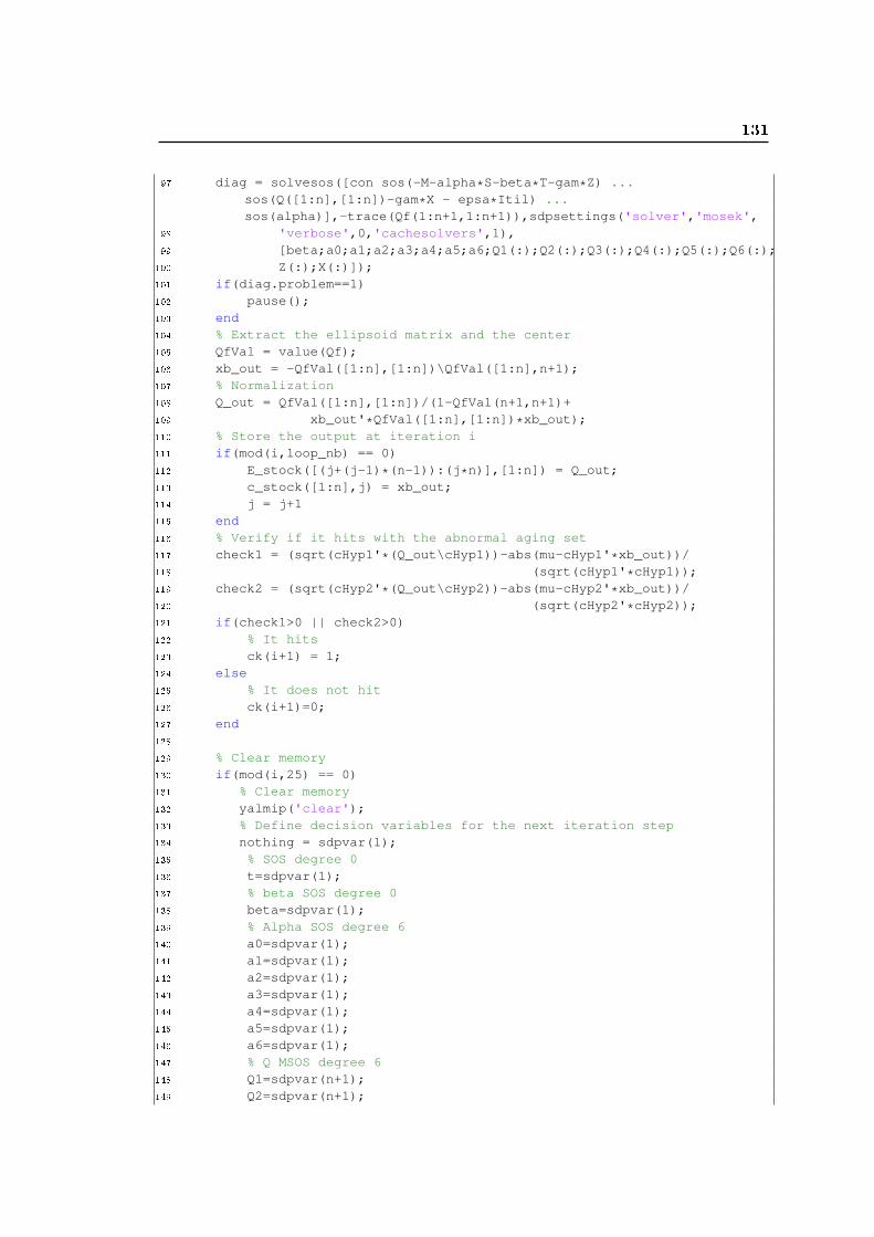
131
97 diag = solvesos([con sos(-M-alpha*S-beta*T-gam*Z) ...sos(Q([1:n],[1:n])-gam*X - epsa*Itil) ...sos(alpha)],-trace(Qf(1:n+1,1:n+1)),sdpsettings('solver','mosek',
98 'verbose',0,'cachesolvers',1),99 [beta;a0;a1;a2;a3;a4;a5;a6;Q1(:);Q2(:);Q3(:);Q4(:);Q5(:);Q6(:);
100 Z(:);X(:)]);101 if(diag.problem==1)102 pause();103 end104 % Extract the ellipsoid matrix and the center105 QfVal = value(Qf);106 xb_out = -QfVal([1:n],[1:n])\QfVal([1:n],n+1);107 % Normalization108 Q_out = QfVal([1:n],[1:n])/(1-QfVal(n+1,n+1)+109 xb_out'*QfVal([1:n],[1:n])*xb_out);110 % Store the output at iteration i111 if(mod(i,loop_nb) == 0)112 E_stock([(j+(j-1)*(n-1)):(j*n)],[1:n]) = Q_out;113 c_stock([1:n],j) = xb_out;114 j = j+1115 end116 % Verify if it hits with the abnormal aging set117 check1 = (sqrt(cHyp1'*(Q_out\cHyp1))-abs(mu-cHyp1'*xb_out))/118 (sqrt(cHyp1'*cHyp1));119 check2 = (sqrt(cHyp2'*(Q_out\cHyp2))-abs(mu-cHyp2'*xb_out))/120 (sqrt(cHyp2'*cHyp2));121 if(check1>0 || check2>0)122 % It hits123 ck(i+1) = 1;124 else125 % It does not hit126 ck(i+1)=0;127 end128
129 % Clear memory130 if(mod(i,25) == 0)131 % Clear memory132 yalmip('clear');133 % Define decision variables for the next iteration step134 nothing = sdpvar(1);135 % SOS degree 0136 t=sdpvar(1);137 % beta SOS degree 0138 beta=sdpvar(1);139 % Alpha SOS degree 6140 a0=sdpvar(1);141 a1=sdpvar(1);142 a2=sdpvar(1);143 a3=sdpvar(1);144 a4=sdpvar(1);145 a5=sdpvar(1);146 a6=sdpvar(1);147 % Q MSOS degree 6148 Q1=sdpvar(n+1);149 Q2=sdpvar(n+1);

132Appendix B. Matlab program: Robust convex simulation-based method
150 Q3=sdpvar(n+1);151 Q4=sdpvar(n+1);152 Q5=sdpvar(n+1);153 Q6=sdpvar(n+1);154 % Z MSOS degree 0155 Z=sdpvar(n+m+1);156 % X MSOS degree 0157 X = sdpvar(n);158 % Constraints159 con=(Z≥0);160 con = con +(X≥0);161 con = con + (beta≥0);162 con=con+(nothing≥0);163 gam = t*(tf-t);164 end165 % Final ellipsoid at iteration i is then the initial ellipsoid at i+1166 E0 = Q_out;167 c0 = xb_out;168 end
1 %% Step 32 Atil = [A, ab; zeros(1,n), 0];3 Btil = [B; zeros(1,m)];4 Gam = [zeros(1,n) 1];5 Xit = [Xi zeros(n,1); zeros(1,n) 0];6 xit = [xib; 0];7 Qsi_org = Xi;8 qsi_org = xib;9 Qsitil = [Qsi_org, zeros(n,1);
10 zeros(1,n) 0];11 qsitil = [qsi_org; 0];12 Itil = eye(n);13
14 % Initial condition Eps_x(E0,c0)15 E0 = Eini;16 c0 = cini;17
18 % Time parameters19 tf = 0.5; % Total simulation time [s]20 Delta_t = 0.001; % Time step [s]21 N = tf/(Delta_t); % Number of iterations22
23 % Initialization24 E([1:n],[1:n]) = E0;25 c([1:n],1) = c0;26
27 % To store the hit28 ck=zeros(1,round(N));29
30 % Verify if at initial time it hits the abnormal aging set31 check1 = (sqrt(cHyp1'*(E0\cHyp1))-abs(mu-cHyp1'*c0))/(sqrt(cHyp1'*cHyp1));32 check2 = (sqrt(cHyp2'*(E0\cHyp2))-abs(mu-cHyp2'*c0))/(sqrt(cHyp2'*cHyp2));33 if(check1>0 || check2>0)

133
34 ck(1) = 1;35 disp('error')36 pause();37 else38 ck(1)=0;39 end40
41 % Time SOS degree 042 t=sdpvar(1);43 % beta SOS degree 044 beta = sdpvar(1);45 % Alpha SOS degree 646 a0=sdpvar(1);47 a1=sdpvar(1);48 a2=sdpvar(1);49 a3=sdpvar(1);50 a4=sdpvar(1);51 a5=sdpvar(1);52 a6=sdpvar(1);53 % Q MSOS degree 654 Q1=sdpvar(n+1);55 Q2=sdpvar(n+1);56 Q3=sdpvar(n+1);57 Q4=sdpvar(n+1);58 Q5=sdpvar(n+1);59 Q6=sdpvar(n+1);60 % Z MSOS degree 061 Z=sdpvar(n+m+1);62 % X MSOS degree 063 X = sdpvar(n);64 nothing = sdpvar(1);65 % Constraints66 con=(Z≥0);67 con = con +(X≥0);68 con = con + (beta≥0);69 con=con+(nothing≥0);70 gam = t*(tf-t);71
72 % Parameters of the bisection method73 R_ov = ∆_ov*R0; %Should not hit74 R_und = ∆_und*R0; %Should hit75
76 % Start the bisection method77 ∆_wrk = ∆_ov;78 while(∆_ov-∆_und > tol)79 ∆ = (∆_ov+∆_und)/280 R = ∆*R0;81 i = 1;82 j = 1;83 bool = 0; %0 if no hit, otherwise 184 E0 = Eini;85 c0 = cini;86
87 % Compute the evolution of state ellipsoids for the N iterations while88 % none ellipsoid hits with the abnormal aging set
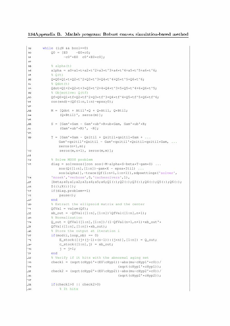
134Appendix B. Matlab program: Robust convex simulation-based method
89 while (i≤N && bool==0)90 Q0 = [E0 -E0*c0;91 -c0'*E0 c0'*E0*c0];92
93 % alpha(t)94 alpha = a0+a1*t+a2*t^2+a3*t^3+a4*t^4+a5*t^5+a6*t^6;95 % Q(t)96 Q=Q0+Q1*t+Q2*t^2+Q3*t^3+Q4*t^4+Q5*t^5+Q6*t^6;97 % Qdot(t)98 Qdot=Q1+2*Q2*t+3*Q3*t^2+4*Q4*t^3+5*Q5*t^4+6*Q6*t^5;99 % Objective: Q(tf)
100 Qf=Q0+Q1*tf+Q2*tf^2+Q3*tf^3+Q4*tf^4+Q5*tf^5+Q6*tf^6;101 con(end)=(Qf(1:n,1:n)-epss≥0);102
103 M = [Qdot + Atil'*Q + Q*Atil, Q*Btil;104 (Q*Btil)', zeros(m)];105
106 S = [Gam'*Gam - Gam'*ub'*R*ub*Gam, Gam'*ub'*R;107 (Gam'*ub'*R)', -R];108
109 T = [Gam'*Gam - Qsitil + Qsitil*qsitil*Gam + ...Gam'*qsitil'*Qsitil - Gam'*qsitil'*Qsitil*qsitil*Gam, ...zeros(n+1,m);
110 zeros(m,n+1), zeros(m,m)];111
112 % Solve MSOS problem113 diag = solvesos([con sos(-M-alpha*S-beta*T-gam*Z) ...
sos(Q([1:n],[1:n])-gam*X - epsa*Itil) ...sos(alpha)],-trace(Qf(1:n+1,1:n+1)),sdpsettings('solver',
114 'mosek','verbose',0,'cachesolvers',1),115 [beta;a0;a1;a2;a3;a4;a5;a6;Q1(:);Q2(:);Q3(:);Q4(:);Q5(:);Q6(:);116 Z(:);X(:)]);117 if(diag.problem==1)118 pause();119 end120 % Extract the ellipsoid matrix and the center121 QfVal = value(Qf);122 xb_out = -QfVal([1:n],[1:n])\QfVal([1:n],n+1);123 % Normalization124 Q_out = QfVal([1:n],[1:n])/(1-QfVal(n+1,n+1)+xb_out'*125 QfVal([1:n],[1:n])*xb_out);126 % Store the output at iteration i127 if(mod(i,loop_nb) == 0)128 E_stock([(j+(j-1)*(n-1)):(j*n)],[1:n]) = Q_out;129 c_stock([1:n],j) = xb_out;130 j = j+1;131 end132 % Verify if it hits with the abnormal aging set133 check1 = (sqrt(cHyp1'*(E0\cHyp1))-abs(mu-cHyp1'*c0))/134 (sqrt(cHyp1'*cHyp1));135 check2 = (sqrt(cHyp2'*(E0\cHyp2))-abs(mu-cHyp2'*c0))/136 (sqrt(cHyp2'*cHyp2));137
138 if(check1>0 || check2>0)139 % It hits

135
140 ck(i+1) = 1;141 bool=1;142 else143 % It does not hit144 ck(i+1)=0;145 end146
147 % Clear memory148 if(mod(i,25) == 0)149 % Clear memory150 yalmip('clear');151 % Define decision variables for the next iteration step152 nothing = sdpvar(1);153 % SOS degree 0154 t=sdpvar(1);155 % beta SOS degree 0156 beta=sdpvar(1);157 % Alpha SOS degree 6158 a0=sdpvar(1);159 a1=sdpvar(1);160 a2=sdpvar(1);161 a3=sdpvar(1);162 a4=sdpvar(1);163 a5=sdpvar(1);164 a6=sdpvar(1);165 % Q MSOS degree 6166 Q1=sdpvar(n+1);167 Q2=sdpvar(n+1);168 Q3=sdpvar(n+1);169 Q4=sdpvar(n+1);170 Q5=sdpvar(n+1);171 Q6=sdpvar(n+1);172 % Z MSOS degree 0173 Z=sdpvar(n+m+1);174 % X MSOS degree 0175 X = sdpvar(n);176 % Constraints177 con=(Z≥0);178 con = con +(X≥0);179 con = con + (beta≥0);180 con=con+(nothing≥0);181 gam = t*(tf-t);182 end183 % Final ellipsoid at iteration i is then the initial ellipsoid ...
at i+1184 E0 = Q_out;185 c0 = xb_out;186 i = i+1;187 end188 % If it hits ...189 if (check1>0 || check2>0)190 % ... Then reduce the size of R191 ∆_und = ∆;192 else193 % ... Otherwise increase the size of R

136Appendix B. Matlab program: Robust convex simulation-based method
194 ∆_ov = ∆;195 ∆_wrk = ∆;196 % Store the evolution of state ellipsoids197 Q_out_wrk = Q_out;198 xb_out_wrk = xb_out199 E_out_wrk(:,:) = E_stock(:,:);200 c_out_wrk(:,:) = c_stock(:,:);201 end202 % Clear memory203 yalmip('clear');204 % Define decision variables for the next iteration step205 nothing = sdpvar(1);206 % SOS degree 0207 t=sdpvar(1);208 % beta SOS degree 0209 beta=sdpvar(1);210 % Alpha SOS degree 6211 a0=sdpvar(1);212 a1=sdpvar(1);213 a2=sdpvar(1);214 a3=sdpvar(1);215 a4=sdpvar(1);216 a5=sdpvar(1);217 a6=sdpvar(1);218 % Q MSOS degree 6219 Q1=sdpvar(n+1);220 Q2=sdpvar(n+1);221 Q3=sdpvar(n+1);222 Q4=sdpvar(n+1);223 Q5=sdpvar(n+1);224 Q6=sdpvar(n+1);225 % Z MSOS degree 0226 Z=sdpvar(n+m+1);227 % X MSOS degree 0228 X = sdpvar(n);229 % Constraints230 con=(Z≥0);231 con = con +(X≥0);232 con = con + (beta≥0);233 con=con+(nothing≥0);234 gam = t*(tf-t);235 end236 % Output: state and input ellipsoid matrices and centers237 E_stock = E_out_wrk;238 c_stock = c_out_wrk;239 R = ∆_wrk*R0;240 ub

Appendix C
Matlab program: Optimal attack
input signal
1 %% Step 1 : Discretization2 At = [A a; zeros(1,n) 0];3 Bt = [B; zeros(1,m)];4 sys = ss(At,Bt,C,D);5 % Discretization6 Te = 0.001; % Sampling time7 opt = c2dOptions('Method','tustin');8 sysd = c2d(sys,Te,opt);9 % Transformation for having Cd = eye(ns)
10 T = inv(eye(n+1))*sysd.C;11 sysd = ss2ss(sysd,T);12 At = sysd.A;13 Bt = sysd.B;14 C = sysd.C;15 D = sysd.D;16 save model.mat At Bt C D Te n m out
1 %% Step 2 : Parametrization2 clear all;3 load model_presentation.mat;4
5 N=2000; % Total number of time instants6 gtemp = 50; % Number of time instants stored in a matrix (reduces ...
computational time)7 Nb=N/gtemp;8 F=sparse(N*(n+1),n+1);9 for i=1:N
10 F([(i-1)*(n+1)+1:i*(n+1)],:)=At^i;11 end12 temp = sparse(n+1,N*m);13 i=0;14 while i<N15 i=i+1;16 temp(:,[m*(i-1)+1:m*i])=At^(N-i)*Bt;17 end18 for j=1:Nb19 j20 Gtemp = sparse(gtemp*(n+1),N*m);21 for i=1:gtemp22 Gtemp([(i-1)*(n+1)+1:i*(n+1)],[1:m*(i+(j-1)*gtemp)])=

138 Appendix C. Matlab program: Optimal attack input signal
23 temp(:,[end-m*(i+(j-1)*gtemp)+1:end]);24 end25 if j6=126 G = [G; Gtemp];27 else28 G=Gtemp;29 end30 end31
32 save param_model_presentation.mat F G N -v7.3 % Added
1 %% Step 3 : Verify if the normal trajectories satisfy the constraints2 yalmip('clear');3 clear all;4 close all;5 load model_presentation.mat;6 load param_model_presentation.mat;7
8 H = sparse(N*(n+1),N*(n+1));9 I = sparse(N*(n+1),N*m);
10 for i =1:N11 for j=1:n+112 H(j+(n+1)*(i-1),j+(n+1)*(i-1)) = 1;13 end14 I([1+(n+1)*(i-1):i*(n+1)],[1+m*(i-1):i*m]) = D;15 end16
17 x=sdpvar((n+1)*N,1);18 y = sdpvar((n+1)*N,1);19 u=sdpvar(m*N,1);20 xi = [zeros(n,1);1];21
22 con=(x(:)==F*xi+G*u);23 con=con+(y(:)==H*[xi;x(1:end-(n+1))]+I*u);24
25 for i=1:(n+1)*N26 if mod(i,3)==027 x(i)=1;28 end29 end30
31 con=con+(u(:)≤uh);32 con=con+(u(:)≥ul);33
34 disp('In progress')35
36 obj=0;37 u = out.control_normal(2:end,2);38 j=2;39 k=2;40 for i=1:(n+1)*N41 if mod(i,3)==142 y(i) = out.velocity_normal(j,2);

139
43 j=j+1;44 elseif mod(i,3)==245 y(i) = out.current_normal(k,2);46 k=k+1;47 elseif mod(i,3)==048 y(i) = 1;49 end50 end51 j=optimize(con,obj,sdpsettings('solver','mosek','verbose',1,52 'cachesolvers',1));53 uopt=value(u);54 xopt=value(x);55 yopt=value(y);56 save sol_model_presentation.mat xopt yopt uopt xi H I57
58 % Extract value59 X=zeros(n+1,N);60 Y=zeros(n+1,N);61 U=zeros(m,N);62 for i=1:N63 X(:,i) = xopt((i-1)*(n+1)+1:i*(n+1));64 Y(:,i) = yopt((i-1)*(n+1)+1:i*(n+1));65 U(:,i) = uopt((i-1)*m+1:i*m);66 end
1 %% Step 4 : Compute a feasible attack2 yalmip('clear');3 clear all;4 close all;5 load model_presentation.mat;6 load param_model_presentation.mat;7 load sol_model_presentation.mat;8
9 nbServ = 1;10 x=sdpvar((n+1)*N,1);11 y = sdpvar((n+1)*N,1);12 u=sdpvar(m*N,1);13 ybnd = sdpvar(nbServ*N,1);14 bnd_h=sparse(nbServ*N,1);15 bnd_l=sparse(nbServ*N,1);16 diff = 1e-1; % Trajectory error17 bndFix=[diff NaN]';18
19 con=(x(:)==F*xi+G*u);20 con=con+(y(:)==H*[xi;x(1:end-(n+1))]+I*u);21
22 for i=1:(n+1)*N23 if mod(i,3)==024 x(i)=1;25 end26 end27 j=1;28 for i =1:N*(n+1)

140 Appendix C. Matlab program: Optimal attack input signal
29 if(mod(i,3)==1)30 ybnd(j,1)=x(i);31 bnd_h(j,1)=xopt(i)+bndFix(1);32 bnd_l(j,1)=xopt(i)-bndFix(1);33 j=j+1;34 end35 end36 con=con+(ybnd≤bnd_h);37 con=con+(ybnd≥bnd_l);38 M = 1; % Time step instant between each manipulation of the control signal39 if(M>1)40 temp=ceil(N/M)-1;41 conAttck=sdpvar(temp*(M-1)*m+((N-1)-temp*M+1)*m,1);42 ucon=sdpvar(temp*m+(N-1)-temp*M,1);43
44 for i=1:temp45 for j=1:M-146 conAttck(m*(i-1)*(M-1)+(j-1)*m+1:m*(i-1)*47 (M-1)+(j-1)*m+m,1)=u(m*(i-1)*M+1:m*(i-1)*M+m);48 ucon(m*(i-1)*(M-1)+(j-1)*m+1:m*(i-1)*49 (M-1)+(j-1)*m+m,1)=u((i-1)*M*m+j*m+1:(i-1)*M*m+j*m+m);50 end51 end52 j=1;53 for i=temp*M:N-154 conAttck(m*(temp-1)*(M-1)+(M-1-1)*m+m+(j-1)*m+1:m*(temp-1)*55 (M-1)+(M-1-1)*m+m+j*m)=u(temp*M*m+1:temp*M*m+m);56 ucon(m*(temp-1)*(M-1)+(M-1-1)*m+m+(j-1)*m+1:m*(temp-1)*57 (M-1)+(M-1-1)*m+m+j*m)=u(i*m+1:i*m+m);58 j=j+1;59 end60 con=con+(ucon==conAttck);61 end62 con=con+(u(:)≤uh);63 con=con+(u(:)≥ul);64 obj=u'*u; % Whatever objective cost because the objective is to find ...
feasible attack signals65
66 j=optimize(con,obj,sdpsettings('solver','mosek','verbose',1,67 'cachesolvers',1));68 ufeas=value(u);69 xfeas=value(x);70 yfeas=value(y);71 objfeas = value(obj);72 save sol_pre_presentation.mat xfeas yfeas ufeas objfeas M bndFix73
74 % Extract value75 X=zeros(n+1,N);76 Y=zeros(n+1,N);77 U=zeros(m,N);78 for i=1:N79 X(:,i) = xfeas((i-1)*(n+1)+1:i*(n+1));80 Y(:,i) = yfeas((i-1)*(n+1)+1:i*(n+1));81 U(:,i) = ufeas((i-1)*m+1:i*m);82 end

141
1 %% Step 5 : Compute the optimal attack signals2 yalmip('clear');3 clear all;4 close all;5 load model_presentation.mat;6 load param_model_presentation.mat;7 load sol_model_presentation.mat;8 load sol_pre_presentation.mat;9
10 nbServ = 1;11 x=sdpvar((n+1)*N,1);12 y=sdpvar((n+1)*N,1);13 u=sdpvar(m*N,1);14 xbnd = sdpvar(nbServ*N,1);15 bnd_h=sparse(nbServ*N,1);16 bnd_l=sparse(nbServ*N,1);17 con=(x(:)==F*xi+G*u);18 con=con+(y(:)==H*[xi;x(1:end-(n+1))]+I*u);19
20 for i=1:(n+1)*N21 if mod(i,3)==022 x(i)=1;23 end24 end25
26 vecA = sdpvar(N1,1);27 for i=1:N128 vecA(i) = y(end-(n+1)*i+1);29 end30 con=con+(vecA==ones(N1,1)*yopt(end-(n+1)*i+1);31
32 j=1;33 for i =1:N*n34 if(mod(i,2)==1)35 ybnd(j,1)=y(i);36 bnd_h(j,1)=yopt(i)+bndFix(1);37 bnd_l(j,1)=yopt(i)-bndFix(1);38 j=j+1;39 end40 end41 con=con+(ybnd≤bnd_h);42 con=con+(ybnd≥bnd_l);43
44 M=1;45 if(M>1)46 temp=ceil(N/M)-1;47 conAttck=sdpvar(temp*(M-1)*m+((N-1)-temp*M+1)*m,1);48 ucon=sdpvar(temp*m+(N-1)-temp*M,1);49
50 for i=1:temp51 for j=1:M-152 conAttck(m*(i-1)*(M-1)+(j-1)*m+1:m*(i-1)*53 (M-1)+(j-1)*m+m,1)=u(m*(i-1)*M+1:m*(i-1)*M+m);54 ucon(m*(i-1)*(M-1)+(j-1)*m+1:m*(i-1)*

142 Appendix C. Matlab program: Optimal attack input signal
55 (M-1)+(j-1)*m+m,1)=u((i-1)*M*m+j*m+1:(i-1)*M*m+j*m+m);56 end57 end58 j=1;59 for i=temp*M:N-160 conAttck(m*(temp-1)*(M-1)+(M-1-1)*m+m+(j-1)*m+1:m*(temp-1)*61 (M-1)+(M-1-1)*m+m+j*m)=u(temp*M*m+1:temp*M*m+m);62 ucon(m*(temp-1)*(M-1)+(M-1-1)*m+m+(j-1)*m+1:m*(temp-1)*63 (M-1)+(M-1-1)*m+m+j*m)=u(i*m+1:i*m+m);64 j=j+1;65 end66 con=con+(ucon==conAttck);67 end68
69 for it=1:20070 % Evolution of uit constraint to have a linearized cost function close71 % to the true cost function72 con(end-1)=(u≤uit+0.1);73 con(end)=(u≥uit-0.1);74 % Objective function75 for i=1:N76 currentit(i) = xit(1+(n+1)*(i-1));77 current(i) = x(1+(n+1)*(i-1));78 end79 objit=sum(currentit.^2);80 objEvol(it) = objit;81 obj=objit+sum(2*(current-currentit).*currentit);82 j=optimize(con,-obj,sdpsettings('solver','mosek','verbose',1,83 'cachesolvers',1));84 if(j.problem6=0)85 disp('Value of diag:');86 j87 pause();88 end89 yit=value(y);90 uit=value(u);91
92 % Initialize93 if(mod(jinst,25) == 0)94 % Clear memory95 yalmip('clear');96 x=sdpvar((n+1)*N,1);97 y=sdpvar((n+1)*N,1);98 u=sdpvar(m*N,1);99 xbnd = sdpvar(nbServ*N,1);
100 bnd_h=sparse(nbServ*N,1);101 bnd_l=sparse(nbServ*N,1);102 con=(x(:)==F*xi+G*u);103 con=con+(y(:)==H*[xi;x(1:end-(n+1))]+I*u);104 for i=1:(n+1)*N105 if mod(i,3)==0106 x(i)=1;107 end108 end109

143
110 vecA = sdpvar(N1,1);111 for i=1:N1112 vecA(i) = y(end-(n+1)*i+1);113 end114 con=con+(vecA==ones(N1,1)*yopt(end-(n+1)*i+1);115 j=1;116 for i =1:N*n117 if(mod(i,2)==1)118 ybnd(j,1)=y(i);119 bnd_h(j,1)=yopt(i)+bndFix(1);120 bnd_l(j,1)=yopt(i)-bndFix(1);121 j=j+1;122 end123 end124 con=con+(ybnd≤bnd_h);125 con=con+(ybnd≥bnd_l);126
127 if(M>1)128 temp=ceil(N/M)-1;129 conAttck=sdpvar(temp*(M-1)*m+((N-1)-temp*M+1)*m,1);130 ucon=sdpvar(temp*m+(N-1)-temp*M,1);131
132 for i=1:temp133 for j=1:M-1134 conAttck(m*(i-1)*(M-1)+(j-1)*m+1:m*(i-1)*135 (M-1)+(j-1)*m+m,1)=u(m*(i-1)*M+1:m*(i-1)*M+m);136 ucon(m*(i-1)*(M-1)+(j-1)*m+1:m*(i-1)*137 (M-1)+(j-1)*m+m,1)=u((i-1)*M*m+j*m+1:(i-1)*M*m+j*m+m);138 end139 end140 j=1;141 for i=temp*M:N-1142 conAttck(m*(temp-1)*(M-1)+(M-1-1)*m+m+(j-1)*m+1:m*(temp-1)*143 (M-1)+(M-1-1)*m+m+j*m)=u(temp*M*m+1:temp*M*m+m);144 ucon(m*(temp-1)*(M-1)+(M-1-1)*m+m+(j-1)*m+1:m*(temp-1)*145 (M-1)+(M-1-1)*m+m+j*m)=u(i*m+1:i*m+m);146 j=j+1;147 end148
149 con=con+(ucon==conAttck);150 end151 con=con+(u(:)≤uh);152 con=con+(u(:)≥ul);153 con=con+(u≤uit+.1);154 con=con+(u≥uit-.1);155 end156
157 end

Bibliography
[Ahmad et al. 2018] S. Ahmad, A. Badwelan, A. M. Ghaleb, A. Qamhan, M. Sharaf,M. Alate and A. Moohialdin. Analyzing Critical Failures in a Production Pro-
cess: Is Industrial IoT the Solution? Wireless Communications and MobileComputing, 2018. (Cited on page 13.)
[Alcácer & Cruz-Machado 2019] V. Alcácer and V. Cruz-Machado. Scanning the Indus-try 4.0: A Literature Review on Technologies for Manufacturing Systems. Engi-neering Science and Technology, an International Journal, vol. 22, no. 3, pages899 919, 2019. (Cited on page 14.)
[Alladi et al. 2020] T. Alladi, V. Chamola and S. Zeadally. Industrial Control Systems:Cyberattack trends and countermeasures. Computer Communications, vol. 155,pages 1 8, 2020. (Cited on page 16.)
[Amin et al. 2009] Saurabh Amin, Alvaro A. Cárdenas and S. Shankar Sastry. Safe andSecure Networked Control Systems under Denial-of-Service Attacks. In RupakMajumdar and Paulo Tabuada, editors, Hybrid Systems: Computation and Con-trol, pages 3145, Berlin, Heidelberg, 2009. Springer Berlin Heidelberg. (Citedon page 15.)
[Aps 2020] Mosek Aps. Mosek optimization toolbox for Matlab - Release 9.2.29. Technicalreport, 2020. (Cited on page 60.)
[Archela et al. 2018] A. Archela, D. G. Toginho and L. F. d. Melo. Torque Control
of a DC Motor With a State Space Estimator and Kalman Filter for Vehicle
Traction. In 2018 13th IEEE International Conference on Industry Applications(INDUSCON), pages 763769, 2018. (Cited on pages 96 and 109.)
[Atallah et al. 2007] K. Atallah, S. D. Calverley and D. Howe. A Brushless Permanent
Magnet Motor With Integrated Torque-Limiter. IEEE Transactions on Magnetics,vol. 43, no. 6, pages 24982500, 2007. (Cited on page 42.)
[Bai et al. 2017a] Cheng-Zong Bai, Vijay Gupta and Fabio Pasqualetti. On Kalman Fil-
tering with Compromised Sensors: Attack Stealthiness and Performance Bounds.IEEE Trans. Autom. Control, vol. 62, no. 12, pages 66416648, December 2017.(Cited on page 38.)
[Bai et al. 2017b] Cheng-Zong Bai, Fabio Pasqualetti and Vijay Gupta. Data-injectionattacks in stochastic control systems: Detectability and performance tradeos.Automatica, vol. 82, pages 251260, August 2017. (Cited on page 39.)
[Bartnikas & Morin 2004] R. Bartnikas and R. Morin. Multi-stress aging of stator bars
with electrical, thermal, and mechanical stresses as simultaneous acceleration fac-
tors. IEEE Transactions on Energy Conversion, vol. 19, no. 4, pages 702714,2004. (Cited on page 42.)

146 Bibliography
[Bazrafshan et al. 2013] Z. Bazrafshan, H. Hashemi, S. M. H. Fard and A. Hamzeh.A survey on heuristic malware detection techniques. In The 5th Conference onInformation and Knowledge Technology, pages 113120, 2013. (Cited on page 32.)
[Beaudet et al. 2020] A. Beaudet, F. Sicard, C. Escudero and E. Zamaï. Process-AwareModel-based Intrusion Detection System on Filtering Approach: Further Investi-
gations. In 2020 IEEE International Conference on Industrial Technology (ICIT),pages 310315, 2020. (Cited on page 33.)
[Beaudet et al. 2021] A. Beaudet, C. Escudero and E. Zamaï. Malicious Anomaly De-
tection Approaches Robustness in Manufacturing ICSs. In Proc. INCOM, (Sub-mitted), pages 18, Budapest, June 2021. (Not cited.)
[Ben-Talha et al. 2017] H. Ben-Talha, P. Massioni and G. Scorletti. Robust simulation of
continuous-time systems with rational dynamics. International Journal of Robustand Nonlinear Control, vol. 27, no. 16, pages 30973108, 2017. (Cited on page 81.)
[Blanchini & Miani 2015] Franco Blanchini and Stefano Miani. Springer InternationalPublishing, Cham, 2015. (Cited on pages 45, 55, 57 and 71.)
[Blanchini 1999] F. Blanchini. Set invariance in control. Automatica, vol. 35, no. 11,pages 1747 1767, 1999. (Cited on pages 45 and 55.)
[Bolton 2015] W. Bolton. Programmable logic controllers (sixth edition). Newnes,Boston, sixth edition édition, 2015. (Cited on pages 20 and 22.)
[Bouaziz 2012] E. Bouaziz M.-F.and Zamaï. Equipment Health Factor prediction for
complex semiconductor manufacturing facility. IFAC Proceedings Volumes,vol. 45, no. 6, pages 1005 1010, 2012. 14th IFAC Symposium on InformationControl Problems in Manufacturing. (Cited on page 12.)
[Boyd & Grant 2020] Stephen Boyd and Michael C. Grant. The CVX users' guide -
Release 2.2. Technical report, 2020. (Cited on page 60.)
[Boyd & Vandenberghe 2004] Stephen Boyd and Lieven Vandenberghe. Convex opti-mization. Cambridge University Press, USA, 2004. (Cited on pages 56, 58 and 59.)
[Boyd et al. 1994] S.P. Boyd, L. El Ghaoui, E. Feron and V. Balakrishnan. Linear matrixinequalities in system and control theory, volume 15. SIAM, 1994. (Cited onpages 52, 53 and 55.)
[Bradbury 2012] Danny Bradbury. SCADA: a critical vulnerability. Computer Fraud &Security, vol. 2012, no. 4, pages 11 14, 2012. (Cited on page 22.)
[Cagalaban et al. 2010] Giovanni Cagalaban, Taihoon Kim and Seoksoo Kim. ImprovingSCADA Control Systems Security with Software Vulnerability Analysis. In Pro-ceedings of the 12th WSEAS International Conference on Automatic Control,Modelling & Simulation, page 409414, Stevens Point, Wisconsin, USA, 2010.World Scientic and Engineering Academy and Society (WSEAS). (Cited onpage 23.)

Bibliography 147
[Carcano et al. 2009] Andrea Carcano, Igor Nai Fovino, Marcelo Masera and AlbertoTrombetta. State-based network intrusion detection systems for SCADA pro-
tocols: a proof of concept. In International Workshop on Critical InformationInfrastructures Security, pages 138150. Springer, 2009. (Cited on page 32.)
[Carfagno et al. 1980] S.P. Carfagno, R.J. Gibson, Franklin Research Center and ElectricPower Research Institute. A review of equipment aging theory and technology.EPRI. Electric Power Research Institute, 1980. (Cited on page 41.)
[Caselli et al. 2015] Marco Caselli, Emmanuele Zambon and Frank Kargl. Sequence-
aware Intrusion Detection in Industrial Control Systems. In Proceedings of the1st ACM Workshop on Cyber-Physical System Security, pages 1324, New York,NY, USA, 2015. ACM. (Cited on page 33.)
[Cetinkaya et al. 2019] Ahmet Cetinkaya, Hideaki Ishii and Tomohisa Hayakawa. An
Overview on Denial-of-Service Attacks in Control Systems: Attack Models and
Security Analyses. Entropy, vol. 21, page 210, 02 2019. (Cited on page 15.)
[Chang et al. 2018] Young Hwan Chang, Qie Hu and Claire J. Tomlin. Secure estimationbased Kalman Filter for cyberphysical systems against sensor attacks. Automat-ica, vol. 95, pages 399412, September 2018. (Cited on page 39.)
[Chen et al. 2004] Chieh-Li Chen, Kuo-Ming Chang and Chih-Ming Chang. Modeling
and control of a web-fed machine. Appl. Math. Model., vol. 28, no. 10, pages 863 876, Oct. 2004. (Cited on pages vii, 96, 97, 98 and 99.)
[Cheng et al. 2019] P. Cheng, Z. Yang, J. Chen, Y. Qi and L. Shi. An event-based stealthy
attack on remote state estimation. IEEE Trans. Autom. Control, pages 11, 2019.(Cited on page 38.)
[Cherubini et al. 2016] Andrea Cherubini, Robin Passama, André Crosnier, AntoineLasnier and Philippe Fraisse. Collaborative manufacturing with physical hu-
manrobot interaction. Robotics and Computer-Integrated Manufacturing,vol. 40, pages 1 13, 2016. (Cited on page 8.)
[Chesi 2010] G. Chesi. LMI techniques for optimization over polynomials in control: a
survey. IEEE Transactions on Automatic Control, vol. 55, no. 11, pages 25002510, 2010. (Cited on pages 54 and 55.)
[Cómbita et al. 2019] L. F. Cómbita, Á. A. Cárdenas and N. Quijano. Mitigating Sensor
Attacks Against Industrial Control Systems. IEEE Access, vol. 7, pages 9244492455, 2019. (Cited on page 43.)
[Combacau et al. 2000] M. Combacau, P. Berruet, E. Zamai, P. Charbonnaud andA. Khatab. Supervision and Monitoring of Production Systems. In Proc. IFACMCPL (IFAC Proceedings Volumes), volume 33, pages 849 854, 2000. (Citedon page 24.)

148 Bibliography
[Cox et al. 1995] D.F. Cox, K.L. McElhaney and R.H. Staunton. Aging and service wearof air-operated valves used in safety-related systems at nuclear power plants.Number 6016 de NUREG Series. International Atomic Energy Agency, UnitedStates, 1995. (Cited on page 41.)
[Dai & Vyatkin 2012] W. Dai and V. Vyatkin. Redesign Distributed PLC Control Sys-
tems Using IEC 61499 Function Blocks. IEEE Trans. Autom. Sci. Eng, vol. 9,no. 2, pages 390401, 2012. (Cited on page 19.)
[Daneels & Salter 1999] A. Daneels and W. Salter. What is SCADA? In D. Bulfoneand A. Daneels, editors, 7th International Conference on Accelerator and LargeExperimental Physics Control Systems (ICALEPCS 99), volume 991004, pages339343, 1999. (Cited on page 23.)
[de Sá et al. 2017] A. O. de Sá, L. F. R. d. C. Carmo and R. C. S. Machado. Covert
Attacks in Cyber-Physical Control Systems. IEEE Trans. Ind. Informat., vol. 13,no. 4, pages 16411651, Aug. 2017. (Cited on pages 15, 43 and 46.)
[Dhillon 1999] B.S. Dhillon. Design reliability: Fundamentals and applications. CRCPress, 1999. (Cited on page 12.)
[Doggett 2004] A. M. Doggett. A Statistical Comparison of Three Root Cause Analysis
Tools. Journal of Industrial Technology, vol. 20, no. 2, pages 2 9, 2004. (Citedon page 12.)
[Dorf & Bishop 2000] Richard C. Dorf and Robert H. Bishop. Modern control systems.Prentice-Hall, Inc., USA, 9th édition, 2000. (Cited on page 36.)
[Dorr et al. 1997] R. Dorr, F. Kratz, J. Ragot, F. Loisy and J. . Germain. Detection,
isolation, and identication of sensor faults in nuclear power plants. IEEE Trans-actions on Control Systems Technology, vol. 5, no. 1, pages 4260, 1997. (Citedon page 24.)
[Duong et al. 2013] Quoc-Bao Duong, Eric Zamai and Khoi-Quoc Tran-Dinh. Con-
dence estimation of feedback information for logicdiagnosis. Engineering Appli-cations of Articial Intelligence, vol. 26, no. 3, pages 1149 1161, 2013. (Citedon page 11.)
[Erez & Wool 2015] Noam Erez and Avishai Wool. Control variable classication, mod-eling and anomaly detection in Modbus/TCP SCADA systems. InternationalJournal of Critical Infrastructure Protection, vol. 10, pages 5970, September2015. (Cited on page 32.)
[Erickson & Hedrick 1999] K.T. Erickson and J.L. Hedrick. Plantwide process control.Wiley Series in Chemical Engineering. Wiley, 1999. (Cited on page 12.)
[Escudero & Zamaï 2019] C. Escudero and E. Zamaï. Prevention of Aging Attacks: Ma-
licious Nature of the Control Signal. In 2019 International Automatic ControlConference (CACS), pages 16, Nov 2019. (Cited on page 70.)

Bibliography 149
[Escudero et al. 2018] C. Escudero, F. Sicard and E. Zamai. Process-Aware Model based
IDSs for Industrial Control Systems Cybersecurity: Approaches, Limits and Fur-
ther Research. In 2018 IEEE 23rd International Conference on Emerging Tech-nologies and Factory Automation (ETFA), volume 1, pages 605612, Sep. 2018.(Cited on page 15.)
[Escudero et al. 2020a] C. Escudero, P. Massioni, G. Scorletti and E. Zamaï. Security
of Control Systems: Prevention of Aging Attacks by means of Convex Robust
Simulation Forecasts. Proc. IFAC WC (IFAC-PapersOnLine), pages 1 1, Jul.2020. (Cited on page 80.)
[Escudero et al. 2020b] C. Escudero, P. Massioni, E. Zamaï and B. Raison. Control
System Theory Methods to Analyze, Prevent and Design Stealthy Aging Attacks.IEEE Transaction on Industrial Informatics, (Submitted), pages 1 1, Sept.2020. (Not cited.)
[Escudero et al. 2020c] C. Escudero, F. Sicard, A. Beaudet and E. Zamaï. Security of
the Process Integrity under Attacks Propagation in Industrial Control Systems: a
Classication of Control-based Methods. Reliab. Eng. Syst. Saf., (Submitted),pages 1 1, Sept. 2020. (Not cited.)
[Fawzi et al. 2014] Hamza Fawzi, Paulo Tabuada and Suhas Diggavi. Secure Estimationand Control for Cyber-Physical Systems Under Adversarial Attacks. IEEE Trans.Autom. Control, vol. 59, no. 6, pages 14541467, June 2014. (Cited on page 39.)
[Fovino et al. 2010] I. N. Fovino, A. Carcano, T. D. L. Murel, A. Trombetta andM. Masera. Modbus/DNP3 State-Based Intrusion Detection System. In 201024th IEEE International Conference on Advanced Information Networking andApplications, pages 729736, April 2010. (Cited on page 32.)
[Fovino 2014] Igor Nai Fovino. Scada system cyber security, pages 451471. SpringerNew York, New York, NY, 2014. (Cited on pages 16 and 23.)
[Fuc 2008] Chapter 1 - Introduction to Power Quality. In E. F. Fuchs and M. A.S.Masoum, editors, Power Quality in Power Systems and Electrical Machines, pages1 54. Academic Press, Burlington, 2008. (Cited on page 42.)
[Galloway & Hancke 2013] B. Galloway and G. P. Hancke. Introduction to Industrial
Control Networks. IEEE Communications Surveys & Tutorials, vol. 15, no. 2,pages 860880, 2013. (Cited on page 13.)
[Garcia et al. 2016] L. Garcia, S. Zonouz, Dong Wei and L. P. de Aguiar. Detecting
PLC control corruption via on-device runtime verication. In 2016 ResilienceWeek (RWS), pages 6772, August 2016. (Cited on page 33.)
[Gayek 1991] J. E. Gayek. A survey of techniques for approximating reachable and con-
trollable sets. In Proc. CDC, pages 17241729, Dec. 1991. (Cited on pages 45and 70.)

150 Bibliography
[Gisel & Olejnik 2018] L. Gisel and L. Olejnik. The potential human cost of cyber op-
erations. Technical report, International Committee of the Red Cross ExpertMeeting, Nov. 2018. (Cited on page 14.)
[Globalspec ] Globalspec. Drive rollers and idler rollers information. https:
//www.globalspec.com/learnmore/material_handling_packaging_
equipment/material_handling_equipment/conveyor_rollers. [Online;accessed 19-November-2020]. (Cited on page 96.)
[Goldenberg & Wool 2013] Niv Goldenberg and Avishai Wool. Accurate modeling of
Modbus/TCP for intrusion detection in SCADA systems. International Journalof Critical Infrastructure Protection, vol. 6, no. 2, pages 6375, June 2013. (Citedon page 32.)
[Gonzalez et al. 2019] D. Gonzalez, F. Alhenaki and M. Mirakhorli. Architectural Secu-rity Weaknesses in Industrial Control Systems (ICS) an Empirical Study Based
on Disclosed Software Vulnerabilities. In 2019 IEEE International Conference onSoftware Architecture (ICSA), pages 3140, 2019. (Cited on pages 22 and 23.)
[Groover 2008] M.P. Groover. Automation, production systems, and computer-integrated manufacturing. Prentice Hall, 2008. (Cited on page 8.)
[Gungor & Hancke 2009] V. C. Gungor and G. P. Hancke. Industrial Wireless Sen-
sor Networks: Challenges, Design Principles, and Technical Approaches. IEEETransactions on Industrial Electronics, vol. 56, no. 10, pages 42584265, 2009.(Cited on page 14.)
[Guo et al. 2018] Ziyang Guo, Dawei Shi, Karl Henrik Johansson and Ling Shi. Worst-
case stealthy innovation-based linear attack on remote state estimation. Automat-ica, vol. 89, pages 117124, March 2018. (Cited on page 38.)
[Guo et al. 2019] Ziyang Guo, Dawei Shi, Karl H. Johansson and Ling Shi. Worst-
case Innovation-based Integrity Attacks with Side Information on Remote State
Estimation. IEEE Control Netw. Syst., vol. 6, no. 1, pages 4859, March 2019.(Cited on page 38.)
[Haapala et al. 2010] Antti Haapala, Henrikki Liimatainen, Mika Körkkö, Jaakko Ek-man, Mirja Sinikka Salkinoja-Salonen and Jouko Niinimäki. Web defects in
newsprint production a mill case study. Appita Journal, vol. 63, no. 5, pages358364, 2010. (Cited on page 13.)
[Hadizadeh Kafash et al. 2018] S. Hadizadeh Kafash, N. Hashemi, C. Murguia andJ. Ruths. Constraining Attackers and Enabling Operators via Actuation Lim-
its. In 2018 IEEE Conference on Decision and Control (CDC), pages 45354540,Dec 2018. (Cited on page 40.)
[Hadziosmanovic et al. 2013] Dina Hadziosmanovic, Robin Sommer, Emmanuele Zam-bon and Pieter Hartel. Through the eye of the PLC: towards semantic security

Bibliography 151
monitoring for industrial control systems. International Computer Science Insti-tute, Berkeley, 2013. (Cited on page 32.)
[Hahn & Govindarasu 2013] Adam Hahn and Manimaran Govindarasu. Model-based In-
trustion Detection for the Smart Grid (MINDS). In Proceedings of the EighthAnnual Cyber Security and Information Intelligence Research Workshop, pages27:127:4, New York, NY, USA, 2013. ACM. (Cited on page 32.)
[Han & Palazzolo 2013] X. Han and A. B. Palazzolo. VFD Machinery Vibration Fatigue
Life and Multilevel Inverter Eect. IEEE Transactions on Industry Applications,vol. 49, no. 6, pages 25622575, 2013. (Cited on page 42.)
[Hassibi & Boyd 1998] A. Hassibi and S. Boyd. Quadratic stabilization and control of
piecewise-linear systems. In Proceedings of the 1998 American Control Conference(ACC), volume 6, pages 36593664 vol.6, 1998. (Cited on page 37.)
[Hemsley & Fisher 2018a] K. E. Hemsley and R. E. Fisher. History of Industrial ControlSystem Cyber Incidents. Technical report, Idaho National Laboratory, Dec. 2018.(Cited on pages 14 and 15.)
[Hemsley & Fisher 2018b] Kevin Hemsley and Ronald Fisher. A History of Cyber Inci-
dents and Threats Involving Industrial Control Systems. In Jason Staggs and Su-jeet Shenoi, editors, Critical Infrastructure Protection XII, pages 215242, Cham,2018. Springer International Publishing. (Cited on page 16.)
[Holopainen et al. 2013] T. P. Holopainen, P. Jorg, J. Nïiranen and D. Andrea. ElectricMotors and Drives in Torsional Vibration Analysis and Design. In Proceedingsof the 42nd Turbomachinery Symposium, 2013. (Cited on page 42.)
[Hoo et al. 2003] K. A. Hoo, M. J. Piovoso, P. D. Schnelle and D. A. Rowan. Process
and controller performance monitoring: overview with industrial applications. In-ternational Journal of Adaptive Control and Signal Processing, vol. 17, no. 7-9,pages 635662, 2003. (Cited on page 21.)
[Hristopulos & Uesaka 2002] D.T. Hristopulos and T. Uesaka. A model of machine-
direction tension variations in paper webs with runnability applications. Journalof Pulp and Paper Science, vol. 28, no. 12, pages 389 394, Dec. 2002. (Cited onpage 12.)
[Hu et al. 2018a] Liang Hu, Zidong Wang, Qing-Long Han and Xiaohui Liu. State esti-mation under false data injection attacks: Security analysis and system protection.Automatica, vol. 87, pages 176183, January 2018. (Cited on page 39.)
[Hu et al. 2018b] Yan Hu, Hong Li, Tom H. Luan, An Yang, Limin Sun, Zhiliang Wangand Rui Wang. Detecting stealthy attacks on industrial control systems using a
permutation entropy-based method. Future Generation Computer Systems, Au-gust 2018. (Cited on page 33.)

152 Bibliography
[Hubac & Zamaï 2013] S. Hubac and E. Zamaï. Politiques de maintenance équipement
en ux de production stressant. Techniques de l'ingénieur Méthodes de produc-tion, vol. base documentaire : TIB521DUO., 2013. (Cited on page 13.)
[IAE 1989] Safety aspects of nuclear power plant ageing (state of the art report). Number540 de TECDOC Series. International Atomic Energy Agency, Vienna, 1989.(Cited on page 42.)
[ISA ] ISA. ISA 95 Standard. https://isa-95.com/. [Online; accessed 19-November-2020]. (Cited on page 10.)
[Isermann 1997] R. Isermann. Supervision, fault-detection and fault-diagnosis methods
An introduction. Control Engineering Practice, vol. 5, no. 5, pages 639 652,1997. (Cited on page 11.)
[Isermann 2006] R. Isermann. Fault-diagnosis systems: An introduction from fault de-tection to fault tolerance. Springer-Verlag Berlin Heidelberg, 2006. (Cited onpage 12.)
[Ishikawa 1990] K. Ishikawa. Introduction to quality control. Taylor & Francis, 1990.(Cited on page 12.)
[ISO13849-1 2015] ISO13849-1. 13849-1:2015: Safety of machinery, safety related partsof control systems, part 1: General principles for design. 3rd edition. InternationalOrganization for Standardization, 2015. (Cited on page 11.)
[Jones & McLean 1986] Albert T. Jones and Charles R. McLean. A proposed hierarchical
control model for automated manufacturing systems. J. Manuf. Syst., vol. 5, no. 1,pages 15 25, 1986. (Cited on page 20.)
[Jones & Saleh 1989] A. Jones and A. Saleh. A multi-layer/multi-level control architec-
ture for computer integrated manufacturing systems. In 15th Annual Conferenceof IEEE Industrial Electronics Society, pages 519525 vol.3, 1989. (Cited onpage 10.)
[Juliani Correa de Godoy & Garcia 2017] Rodrigo Juliani Correa de Godoy and ClaudioGarcia. Plantwide Control: A Review of Design Techniques, Benchmarks, and
Challenges. Industrial & Engineering Chemistry Research, vol. 56, no. 28, pages78777887, 2017. (Cited on page 23.)
[Kafash et al. 2018] S. H. Kafash, J. Giraldo, C. Murguia, A. A. Cardenas and J. Ruths.Constraining Attacker Capabilities Through Actuator Saturation. In Proc. ACC,pages 986991, Milwaukee, WI, Jun. 2018. (Cited on pages 40 and 45.)
[Kalech 2019] Meir Kalech. Cyber-attack detection in SCADA systems using temporal
pattern recognition techniques. Computers & Security, vol. 84, pages 225238,July 2019. (Cited on page 32.)

Bibliography 153
[Kalman & Bertram 1960] R.E. Kalman and J.E. Bertram. Control system analysis and
design via the second method of Lyapunov: Continuous-time systems. Journal ofBasic Engineering, vol. 82, no. 2, pages 371393, 1960. (Cited on page 61.)
[Khlebnikov et al. 2011] M. V. Khlebnikov, B. T. Polyak and V. M. Kuntsevich. Op-
timization of linear systems subject to bounded exogenous disturbances: The in-
variant ellipsoid technique. Autom Remote Control, vol. 72, no. 11, pages 2227 2275, 2011. (Cited on page 45.)
[Kidam & Hurme 2013] K. Kidam and M. Hurme. Analysis of equipment failures as
contributors to chemical process accidents. Process Safety and EnvironmentalProtection, vol. 91, no. 1, pages 61 78, 2013. (Cited on page 13.)
[Kim 2012] HyungJun Kim. Security and Vulnerability of SCADA Systems over IP-
Based Wireless Sensor Networks. International Journal of Distributed SensorNetworks, vol. 8, no. 11, page 268478, 2012. (Cited on page 23.)
[Kleinmann & Wool 2017] Amit Kleinmann and Avishai Wool. Automatic Construc-
tion of Statechart-Based Anomaly Detection Models for Multi-Threaded Indus-
trial Control Systems. ACM Trans. Intell. Syst. Technol., vol. 8, no. 4, pages55:155:21, February 2017. (Cited on page 32.)
[Kobbacy & Murthy 2008] Khairy A. H Kobbacy and D. N. P Murthy. Complex sys-tem maintenance handbook. Springer London, 1st ed. édition, 2008. (Cited onpage 12.)
[Koucham et al. 2018] Oualid Koucham, Stéphane Mocanu, Guillaume Hiet, Jean-MarcThiriet and Frédéric Majorczyk. Ecient Mining of Temporal Safety Properties
for Intrusion Detection in Industrial Control Systems. In Proc. IFAC SAFEPRO-CESS, volume 51, pages 1043 1050, Warsaw, Aug. 2018. (Cited on page 33.)
[Koutsandria et al. 2014] G. Koutsandria, V. Muthukumar, M. Parvania, S. Peisert,C. McParland and A. Scaglione. A hybrid network IDS for protective digital
relays in the power transmission grid. In 2014 IEEE International Conferenceon Smart Grid Communications (SmartGridComm), pages 908913, November2014. (Cited on page 33.)
[Kramer et al. 1984] J. Kramer, J. Magee and M. Sloman. A software architecture for
distributed computer control systems. Automatica, vol. 20, no. 1, pages 93 102,1984. (Cited on page 20.)
[Kurzhanskiy & Varaiya 2006] A. A. Kurzhanskiy and P. Varaiya. Ellipsoidal toolbox.EECS Department, University of California, Berkeley, Tech. Rep., 2006. (Citedon page 58.)
[Lalanne 2013] C. Lalanne. Mechanical vibration and shock analysis, fatigue damage.Mechanical Vibration and Shock Analysis. Wiley, 2013. (Cited on page 42.)
[Langner 2011] R. Langner. Stuxnet: Dissecting a Cyberwarfare Weapon. IEEE SecurPriv, vol. 9, no. 3, pages 4951, 2011. (Cited on page 28.)

154 Bibliography
[Li & Yang 2019] Yi-Gang Li and Guang-Hong Yang. Optimal Stealthy False Data Injec-tion Attacks in Cyber-Physical Systems. Inform. Sciences, vol. 481, pages 474490,May 2019. (Cited on page 38.)
[Li et al. 2019] W. Li, L. Xie and Z. Wang. Two-Loop Covert Attacks Against Constant
Value Control of Industrial Control Systems. IEEE Trans. Ind. Informat., vol. 15,no. 2, pages 663676, Feb 2019. (Cited on page 40.)
[Lin et al. 2013] Hui Lin, Adam Slagell, Catello Di Martino, Zbigniew Kalbarczyk andRavishankar K. Iyer. Adapting Bro into SCADA: Building a Specication-based
Intrusion Detection System for the DNP3 Protocol. In Proceedings of the EighthAnnual Cyber Security and Information Intelligence Research Workshop, CSI-IRW '13, pages 5:15:4, New York, NY, USA, 2013. ACM. (Cited on page 32.)
[Linda et al. 2009] O. Linda, T. Vollmer and M. Manic. Neural Network based Intrusion
Detection System for critical infrastructures. In 2009 International Joint Confer-ence on Neural Networks, pages 18271834, June 2009. (Cited on page 32.)
[Liu et al. 2014] C. Liu, D. Jiang and J. Chen. Coupled Torsional Vibration and Fatigue
Damage of Turbine Generator Due to Grid Disturbance. Journal of Engineeringfor Gas Turbines and Power, vol. 136, Jun. 2014. (Cited on page 42.)
[Liu et al. 2019] Y. Liu, M. Kashef, K. B. Lee, L. Benmohamed and R. Candell. Wireless
Network Design for Emerging IIoT Applications: Reference Framework and Use
Cases. Proceedings of the IEEE, vol. 107, no. 6, pages 11661192, 2019. (Citedon page 14.)
[Lofberg 2004] J. Lofberg. YALMIP : a toolbox for modeling and optimization in MAT-
LAB. In 2004 IEEE International Conference on Robotics and Automation (IEEECat. No.04CH37508), pages 284289, 2004. (Cited on page 60.)
[Löfberg 2009] J. Löfberg. Pre- and post-processing sum-of-squares programs in practice.IEEE Transactions on Automatic Control, vol. 54, no. 5, pages 10071011, 2009.(Cited on page 54.)
[Long et al. 2005] M. Long, Chwan-Hwa Wu and J. Y. Hung. Denial of service attacks
on network-based control systems: impact and mitigation. IEEE Transactions onIndustrial Informatics, vol. 1, no. 2, pages 8596, 2005. (Cited on page 15.)
[Lucchetti 2006] Roberto Lucchetti. Convex sets and convex functions: the fundamen-tals, pages 119. Springer New York, New York, NY, 2006. (Cited on pages 55and 56.)
[Luiijf 2016] E. Luiijf. Threats in industrial control systems, pages 6993. SpringerInternational Publishing, 2016. (Cited on page 16.)
[Lyashevskiy & Meyer 1995] S. Lyashevskiy and A. U. Meyer. Control system analysis
and design upon the Lyapunov method. In Proceedings of 1995 American ControlConference - ACC'95, volume 5, pages 32193223 vol.5, 1995. (Cited on page 61.)

Bibliography 155
[M-SYSTEM 1990] M-SYSTEM. SC100/200 Series Function Block Application Manual
EM-6460-C Rev.1. Technical report, 1990. (Cited on page 19.)
[Madonna et al. 2020] V. Madonna, P. Giangrande, L. Lusuardi, A. Cavallini, C. Geradaand M. Galea. Thermal Overload and Insulation Aging of Short Duty Cycle,
Aerospace Motors. IEEE Transactions on Industrial Electronics, vol. 67, no. 4,pages 26182629, 2020. (Cited on page 42.)
[Mano 1992] M. Morris Mano. Computer system architecture (3rd edition), pages 14.Prentice Hall, 3 édition, 1992. (Cited on page 20.)
[Marelli et al. 2018] Damián Marelli, Tianju Sui and Minyue Fu. Statistical Approach toDetection of Attacks for Stochastic Cyber-Physical Systems. IFAC-PapersOnLine,vol. 51, no. 25, pages 178183, January 2018. (Cited on page 33.)
[McGrew & Vaughn 2009] Robert Wesley McGrew and Rayford B. Vaughn. Discoveringvulnerabilities in control system humanmachine interface software. Journal ofSystems and Software, vol. 82, no. 4, pages 583 589, 2009. (Cited on page 23.)
[Mcgrew 2013] Robert Wesley Mcgrew. Vulnerability Analysis Case Studies of Control
Systems Human Machine Interfaces. PhD thesis, USA, 2013. (Cited on page 23.)
[McLaughlin 2013] Stephen McLaughlin. CPS: Stateful Policy Enforcement for Control
System Device Usage. In Proceedings of the 29th Annual Computer SecurityApplications Conference, ACSAC '13, pages 109118, New York, NY, USA, 2013.ACM. (Cited on page 32.)
[McNeill 1983] H McNeill. Environmental qualication of essential safety-related equip-
ment for nuclear power plants. Nucl. Saf., vol. 24:5, pages 658670, Oct. 1983.(Cited on page 42.)
[Merouane et al. 2020] E. M. Merouane, C. Escudero, F. Sicard and E. Zamai. Aging
Attacks against Electro-Mechanical Actuators from Control Signal Manipulation.In 2020 IEEE International Conference on Industrial Technology (ICIT), pages133138, 2020. (Cited on page 42.)
[Michalos et al. 2010] G. Michalos, S. Makris, N. Papakostas, D. Mourtzis and G. Chrys-solouris. Automotive assembly technologies review: challenges and outlook for a
exible and adaptive approach. CIRP Journal of Manufacturing Science and Tech-nology, vol. 2, no. 2, pages 81 91, 2010. (Cited on pages 8 and 12.)
[Milinkovi¢ & Lazi¢ 2012] S. A. Milinkovi¢ and L. R. Lazi¢. Industrial PLC security
issues. In 2012 20th Telecommunications Forum (TELFOR), pages 15361539,2012. (Cited on page 22.)
[Milo²evi£ et al. 2017] Jezdimir Milo²evi£, Takashi Tanaka, Henrik Sandberg andKarl Henrik Johansson. Analysis and Mitigation of Bias Injection Attacks Against
a Kalman Filter. In Proc. IFAC World Congress, pages 83938398, July 2017.(Cited on page 39.)

156 Bibliography
[Milo²evi¢ et al. 2019] J. Milo²evi¢, H. Sandberg and K. H. Johansson. Estimating
the Impact of Cyber-Attack Strategies for Stochastic Networked Control Systems.IEEE Control Netw. Syst., pages 11, 2019. (Cited on page 39.)
[Mitchell et al. 2005] I. M. Mitchell, A. M. Bayen and C. J. Tomlin. A time-dependent
Hamilton-Jacobi formulation of reachable sets for continuous dynamic games.IEEE Transactions on Automatic Control, vol. 50, no. 7, pages 947957, 2005.(Cited on page 45.)
[Mo & Sinopoli 2016a] Y. Mo and B. Sinopoli. On the Performance Degradation of
Cyber-Physical Systems Under Stealthy Integrity Attacks. IEEE Transactions onAutomatic Control, vol. 61, no. 9, pages 26182624, September 2016. (Cited onpage 33.)
[Mo & Sinopoli 2016b] Yilin Mo and Bruno Sinopoli. On the Performance Degradation
of Cyber-Physical Systems Under Stealthy Integrity Attacks. IEEE Trans. Autom.Control, vol. 61, no. 9, pages 26182624, September 2016. (Cited on page 39.)
[Morris et al. 2013] Thomas H. Morris, Rayford B. Vaughn and Elena Sitnikova. Ad-
vances in the Protection of Critical Infrastructure by Improvement in Industrial
Control System Security. In Proceedings of the Eleventh Australasian InformationSecurity Conference - Volume 138, page 6773, 2013. (Cited on page 23.)
[Muñoz et al. 2011] E. Muñoz, E. Capón-García, M. Moreno-Benito, A. Espuña andL. Puigjaner. Scheduling and control decision-making under an integrated infor-
mation environment. Computers & Chemical Engineering, vol. 35, no. 5, pages774 786, 2011. (Cited on pages 12 and 13.)
[Murguia & Ruths 2019] C. Murguia and J. Ruths. On model-based detectors for lin-
ear time-invariant stochastic systems under sensor attacks. IET Control TheoryAppl., vol. 13, no. 8, pages 10511061, May 2019. (Cited on page 39.)
[Murguia et al. 2017] Carlos Murguia, Nathan van de Wouw and Justin Ruths. Reach-able Sets of Hidden CPS Sensor Attacks: Analysis and Synthesis Tools. IFAC-PapersOnLine, vol. 50, no. 1, pages 20882094, July 2017. (Cited on page 33.)
[Murguia et al. 2020a] Carlos Murguia, Iman Shames, Justin Ruths and Dragan Ne²i¢.Security metrics and synthesis of secure control systems. Automatica, vol. 115,page 108757, May 2020. (Cited on page 33.)
[Murguia et al. 2020b] Carlos Murguia, Iman Shames, Justin Ruths and Dragan Ne²i¢.Security metrics and synthesis of secure control systems. Automatica, vol. 115,page 108757, May 2020. (Cited on pages 38 and 45.)
[Nature ] Nature. Dynamical systems. https://www.nature.com/subjects/
dynamical-systems. [Online; accessed September 15, 2020]. (Cited on page 36.)
[Nguyen et al. 2016] D. T. Nguyen, Q. B. Duong, E. Zamaï and Muhammad KashifShahzad. Fault diagnosis for the complex manufacturing system. Proc Inst MechEng O J Risk Reliab, vol. 230, no. 2, pages 178194, 2016. (Cited on page 12.)

Bibliography 157
[Nguyen 2015] Dang-Trinh Nguyen. Diagnostic en ligne des systèmes à événements dis-
crets complexes : approche mixte logique/probabiliste. PhD thesis, 2015. Thèse dedoctorat dirigée par Zamaï, Eric Automatique et productique Université Greno-ble Alpes (ComUE) 2015. (Cited on page 32.)
[Nozaic & Freese 2009] DJ Nozaic and SD Freese. Process Design Manual For Small
Wastewater Works. Technical report, Water Research Commission, Apr. 2009.(Cited on page 8.)
[OECD 2017] OECD. Enhancing the Role of Insurance in Cyber Risk Management.Technical report, Dec. 2017. (Cited on page 14.)
[Palacios-Gomez et al. 1982] F. Palacios-Gomez, L. Lasdon and M. Engquist. NonlinearOptimization by Successive Linear Programming. Management Science, vol. 28,no. 10, pages 11061120, 1982. (Cited on page 91.)
[Parrilo 2003] P.A. Parrilo. Semidenite programming relaxations for semialgebraic prob-lems. Mathematical programming, vol. 96, no. 2, pages 293320, 2003. (Cited onpage 54.)
[Pavesi et al. 2019] Jaime Pavesi, Thamara Villegas, Alexey Perepechko, EleazarAguirre and Lorena Galeazzi. Validation of ICS Vulnerability Related to TCP/IP
Protocol Implementation in Allen-Bradley Compact Logix PLC Controller. InMiguel Felix Mata-Rivera, Roberto Zagal-Flores and Cristian Barría-Huidobro,editors, Telematics and Computing, pages 355364, Cham, 2019. Springer Inter-national Publishing. (Cited on page 22.)
[Pecsvaradi & Narendra 1971] Thomas Pecsvaradi and Kumpati S. Narendra. Reachablesets for linear dynamical systems. Information and Control, vol. 19, no. 4, pages319 344, 1971. (Cited on page 45.)
[Peeger et al. 2010] S. L. Peeger, J. B. Predd, J. Hunker and C. Bulford. Insiders
Behaving Badly: Addressing Bad Actors and Their Actions. IEEE Transactionson Information Forensics and Security, vol. 5, no. 1, pages 169179, 2010. (Citedon page 16.)
[Pivar£iová & Qazizada 2018] E. Pivar£iová and M. E. Qazizada. Applications of processcontrol system with (SCADA) and PID controller. In 2018 ELEKTRO, pages 16,2018. (Cited on page 21.)
[Ponomarev & Atkison 2016] S. Ponomarev and T. Atkison. Industrial Control SystemNetwork Intrusion Detection by Telemetry Analysis. IEEE Transactions on De-pendable and Secure Computing, vol. 13, no. 2, pages 252260, March 2016.(Cited on page 32.)
[Prada 2013] Cesar de Prada. Overview: Control hierarchy of large processing plants,pages 19. Springer London, London, 2013. (Cited on page 23.)
[Proctor & Zandt 2018] R. Proctor and T. Zandt. Human factors in simple and complexsystems. CRC Press, 3rd édition, 2018. (Cited on page 12.)

158 Bibliography
[Puglia 2012] Luiz Vasco Puglia. LINEAR PROGRAMMING FOR THE OPTIMAL
CONTROL OF A ONE-DEGREE-OF-FREEDOM OVERHEAD CRANE SYS-
TEM. 2012. (Cited on page 45.)
[Robla-Gómez et al. 2017] S. Robla-Gómez, V. M. Becerra, J. R. Llata, E. González-Sarabia, C. Torre-Ferrero and J. Pérez-Oria. Working Together: A Review on
Safe Human-Robot Collaboration in Industrial Environments. IEEE Access, vol. 5,pages 2675426773, 2017. (Cited on page 8.)
[Rrushi & Kang 2009] Julian Rrushi and Kyoung-Don Kang. Detecting Anomalies in
Process Control Networks. In Charles Palmer and Sujeet Shenoi, editors, CriticalInfrastructure Protection III, pages 151165. Springer Berlin Heidelberg, March2009. (Cited on page 32.)
[Rushby 1994] John Rushby. Critical system properties: survey and taxonomy. Reliab.Eng. Syst. Saf., vol. 43, no. 2, pages 189 219, 1994. (Cited on page 8.)
[Samtani et al. 2016] S. Samtani, S. Yu, H. Zhu, M. Patton and H. Chen. Identify-
ing SCADA vulnerabilities using passive and active vulnerability assessment tech-
niques. In 2016 IEEE Conference on Intelligence and Security Informatics (ISI),pages 2530, 2016. (Cited on page 23.)
[Sauter 2010] T. Sauter. The Three Generations of Field-Level NetworksEvolution and
Compatibility Issues. IEEE Transactions on Industrial Electronics, vol. 57, no. 11,pages 35853595, 2010. (Cited on page 14.)
[Sciascera et al. 2016] C. Sciascera, M. Galea, P. Giangrande and C. Gerada. Lifetime
consumption and degradation analysis of the winding insulation of electrical ma-
chines. In 8th IET International Conference on Power Electronics, Machines andDrives (PEMD 2016), pages 15, 2016. (Cited on page 42.)
[Shapiro et al. 2011] Rebecca Shapiro, Sergey Bratus, Edmond Rogers and Sean Smith.Identifying Vulnerabilities in SCADA Systems via Fuzz-Testing. In JonathanButts and Sujeet Shenoi, editors, Critical Infrastructure Protection V, pages 5772, Berlin, Heidelberg, 2011. (Cited on page 23.)
[Sicard et al. 2018] F. Sicard, C. Escudero, E. Zamaï and J.-M. Flaus. From ICS attacks'
analysis to the S.A.F.E. approach: implementation of lters based on behavioral
models and critical state distance for ICS cybersecurity. In Proc. CSNet, pages18, Paris, October 2018. (Cited on pages 15 and 28.)
[Sicard et al. 2019] Franck Sicard, Éric Zamaï and Jean-Marie Flaus. An approach based
on behavioral models and critical states distance notion for improving cybersecu-
rity of industrial control systems. Reliability Engineering & System Safety, March2019. (Cited on page 33.)
[Sicard 2018] Franck Sicard. Prise en compte des risques de cyber-attaques dans le do-
maine de la sécurité des systèmes cyber-physiques : proposition de mécanismes

Bibliography 159
de détection à base de modèles comportementaux. Theses, Université GrenobleAlpes, October 2018. (Cited on page 32.)
[Sikanen et al. 2018] Eerik Sikanen, Janne Nerg, Janne E. Heikkinen, MohammadGerami Tehrani and Jussi Sopanen. Fatigue life calculation procedure for the
rotor of an embedded magnet traction motor taking into account thermomechan-
ical loads. Mech. Syst. Signal Pr., vol. 111, pages 36 46, Oct. 2018. (Cited onpages 99 and 105.)
[Sridhar & Govindarasu 2014] Siddharth Sridhar and Manimaran Govindarasu. Model-
Based Attack Detection and Mitigation for Automatic Generation Control. IEEETransactions on Smart Grid, vol. 5, no. 2, pages 580591, March 2014. (Cited onpage 33.)
[Steuslo 1984] H. U. Steuslo. Advanced Real-Time Languages for Distributed Indus-
trial Process Control. Computer, vol. 17, no. 2, page 3746, Feb. 1984. (Cited onpage 20.)
[Stouer et al. 2015] K. Stouer, V. Pillitteri, S. Lightman, M. Abrams and A. Hahn.Guide to Industrial Control Systems (ICS) Security. Technical report, NationalInstitute of Standards and Technology, May 2015. (Cited on page 8.)
[Syrbe 1978] M. Syrbe. Basic Principles of Advanced Process Control System Structures
and a Realization with Distributed Microcomputers. IFAC Proceedings Volumes,vol. 11, no. 1, pages 393 401, 1978. 7th Triennial World Congress of the IFACon A Link Between Science and Applications of Automatic Control, Helsinki,Finland, 12-16 June. (Cited on page 20.)
[tefan Kozák 2014] tefan Kozák. State-of-the-art in control engineering. Journal ofElectrical Systems and Information Technology, vol. 1, no. 1, pages 1 9, 2014.(Cited on page 21.)
[Teixeira 2019] A. M. H. Teixeira. Optimal stealthy attacks on actuators for strictly
proper systems. In Proc. CDC, pages 43854390, Nice, Dec. 2019. (Cited onpage 46.)
[Tendjaoui et al. 1991] Mustapha Tendjaoui, Christophe Kolski and Patrick Millot. Anapproach towards the design of intelligent man-machine interfaces used in process
control. International Journal of Industrial Ergonomics, vol. 8, no. 4, pages 345 361, 1991. (Cited on page 23.)
[Thomesse 2005] J. P. Thomesse. Fieldbus Technology in Industrial Automation. Pro-ceedings of the IEEE, vol. 93, no. 6, pages 10731101, 2005. (Cited on page 13.)
[Thuillier et al. 2020] Julien Thuillier, David Delouche, Jacques Fantini and FrédéricKratz. Detection of integrity loss in networked control systems using an interval
nite memory observer. Int. J. Control, vol. 0, no. 0, pages 110, Feb. 2020.(Cited on page 33.)

160 Bibliography
[Tulsyan & I. Barton 2016] Aditya Tulsyan and Paul I. Barton. Reachability-based fault
detection method for uncertain chemical ow reactors. IFAC-PapersOnLine,vol. 49, no. 7, pages 1 6, 2016. 11th IFAC Symposium on Dynamics andControl of Process SystemsIncluding Biosystems DYCOPS-CAB 2016. (Cited onpage 45.)
[Umsonst & Sandberg 2018] David Umsonst and Henrik Sandberg. Anomaly Detector
Metrics for Sensor Data Attacks in Control Systems. In Proc. ACC, pages 153158, Milwaukee, WI, June 2018. (Cited on page 39.)
[Umsonst et al. 2017] David Umsonst, Henrik Sandberg and Alvaro A. Cardenas. Secu-rity analysis of control system anomaly detectors. In Proc. ACC, pages 55005506,Seattle, WA, May 2017. (Cited on page 39.)
[Upadhyay et al. 2020] Darshana Upadhyay, Srinivas Sampalli and Bernard Plourde.Vulnerabilities' Assessment and Mitigation Strategies for the Small Linux Server,
Onion Omega2. Electronics, vol. 9, no. 6, 2020. (Cited on page 23.)
[Valentine & Farkas 2011] S. Valentine and C. Farkas. Software security: Application-
level vulnerabilities in SCADA systems. In 2011 IEEE International Conferenceon Information Reuse Integration, pages 498499, 2011. (Cited on page 22.)
[VanAntwerp & Braatz 2000] Jeremy G. VanAntwerp and Richard D. Braatz. A tutorial
on linear and bilinear matrix inequalities. Journal of Process Control, vol. 10,no. 4, pages 363 385, 2000. (Cited on page 53.)
[Venkatasubramanian et al. 2003] Venkat Venkatasubramanian, Raghunathan Ren-gaswamy, Surya N. Kavuri and Kewen Yin. A review of process fault detection
and diagnosis: Part III: Process history based methods. Computers & ChemicalEngineering, vol. 27, no. 3, pages 327 346, 2003. (Cited on page 32.)
[Villemeur 1992] A. Villemeur. Reliability, availability, maintainability and safety assess-ment, assessment, hardware, software and human factors. Wiley, 1992. (Cited onpage 11.)
[Vinod et al. 2009] P. Vinod, V. Laxmi and M. S. Gaur. Survey on Malware Detection
Methods. In Workshop on Computer and Internet Security, page 7379, 2009.(Cited on page 32.)
[Vitturi et al. 2019] S. Vitturi, C. Zunino and T. Sauter. Industrial Communication
Systems and Their Future Challenges: Next-Generation Ethernet, IIoT, and 5G.Proceedings of the IEEE, vol. 107, no. 6, pages 944961, 2019. (Cited on page 14.)
[Viveros et al. 2014] P. Viveros, E. Zio, C. Nikulin, R. Stegmaier and G. Bravo. Resolvingequipment failure causes by root cause analysis and theory of inventive problem
solving. Proc Inst Mech Eng O J Risk Reliab, vol. 228, no. 1, pages 93111, 2014.(Cited on page 12.)

Bibliography 161
[Vrignat et al. 2015] P. Vrignat, M. Avila, F. Duculty and F. Kratz. Failure Event Predic-tion Using Hidden Markov Model Approaches. IEEE Transactions on Reliability,vol. 64, no. 3, pages 10381048, 2015. (Cited on page 12.)
[Vukic 2003] Z. Vukic. Nonlinear control systems. Automation and Control Engineering.Taylor & Francis, 2003. (Cited on page 91.)
[Walker et al. 1981] D. N. Walker, S. L. Adams and R. J. Placek. Torsional Vibration
and Fatigue of Turbine-Generator shafts. IEEE Transactions on Power Apparatusand Systems, vol. PAS-100, no. 11, pages 43734380, 1981. (Cited on page 42.)
[Wie 2008] B. Wie. Space vehicle dynamics and control, second edition. 2008. (Citedon page 105.)
[Williams 1990] T.J. Williams. A Reference Model for Computer Integrated Manufac-
turing from the Viewpoint of Industrial Automation. IFAC Proceedings Volumes,vol. 23, no. 8, Part 5, pages 281 291, 1990. 11th IFAC World Congress on Au-tomatic Control, Tallinn, 1990 - Volume 5, Tallinn, Finland. (Cited on page 10.)
[Wucherer 2001] Klaus Wucherer. HMI, The Window to the Manufacturing and Process
Industry. 8th IFAC Symposium on Analysis, Design and Evaluation of Human-Machine Systems (HMS 2001) (IFAC Proceedings Volumes), vol. 34, no. 16, pages101 108, 2001. (Cited on page 23.)
[Yang et al. 2012] Liying Yang, Juntong Qi and Jianda Han. Path planning methods
for mobile robots with linear programming. pages 641646, 01 2012. (Cited onpage 45.)
[Yaseen & Bayart 2017] Amer Atta Yaseen and Mireille Bayart. Attack-tolerant net-
worked control system: an approach for detection the controller stealthy hijacking
attack. Journal of Physics: Conference Series, vol. 783, page 012022, jan 2017.(Cited on page 33.)
[Ylmaz et al. 2018] E. N. Ylmaz, B. Ciylan, S. Gönen, E. Sindiren and G. Karacaylmaz.Cyber security in industrial control systems: Analysis of DoS attacks against
PLCs and the insider eect. In 2018 6th International Istanbul Smart Grids andCities Congress and Fair (ICSG), pages 8185, 2018. (Cited on page 15.)
[Zamai et al. 1998] E. Zamai, A. Chaillet-Subias and M. Combacau. An architecture for
control and monitoring of discrete events systems. Computers in Industry, vol. 36,no. 1, pages 95 100, 1998. (Cited on page 8.)
[Zhang & Venkitasubramaniam 2017] R. Zhang and P. Venkitasubramaniam. Stealthy
Control Signal Attacks in Linear Quadratic Gaussian Control Systems: De-
tectability Reward Tradeo. IEEE Trans. Inf. Forensics Security, vol. 12, no. 7,pages 15551570, Jul. 2017. (Cited on page 46.)
[Zhang et al. 2016] Heng Zhang, Peng Cheng, Ling Shi and Jiming Chen. Optimal DoSAttack Scheduling in Wireless Networked Control System. IEEE Trans. ControlSyst. Technol., vol. 24, no. 3, pages 843852, May 2016. (Cited on page 38.)

162 Bibliography
[Zhang et al. 2018] H. Zhang, Y. Qi, J. Wu, L. Fu and L. He. DoS Attack Energy
Management Against Remote State Estimation. IEEE Control Netw. Syst., vol. 5,no. 1, pages 383394, March 2018. (Cited on page 38.)
[Zhang et al. 2019a] Heng Zhang, Wenchao Meng, Junjian Qi, Xiaoyu Wang andWei Xing Zheng. Distributed Load Sharing Under False Data Injection Attack
in an Inverter-Based Microgrid. IEEE Trans. Ind. Informat., vol. 66, no. 2, pages15431551, February 2019. (Cited on page 39.)
[Zhang et al. 2019b] Q. Zhang, K. Liu, Y. Xia and A. Ma. Optimal Stealthy Deception
Attack Against Cyber-Physical Systems. IEEE Trans. Cybern., pages 110, 2019.(Cited on page 40.)
[Zhou & Baras 2015] Y. Zhou and J. S. Baras. Reachable set approach to collision avoid-
ance for UAVs. In 2015 54th IEEE Conference on Decision and Control (CDC),pages 59475952, 2015. (Cited on page 45.)
[Zolotová & Landryová 2000] Iveta Zolotová and Lenka Landryová. SCADA/HMI Sys-
tems and Emerging Technologies. IFAC Workshop on Programmable Devices andSystems (PDS 2000) (IFAC Proceedings Volumes), vol. 33, no. 1, pages 17 20,2000. (Cited on page 23.)

Abstract: Industrial Control Systems (ICSs) are architectures controlling a physi-cal system to achieve an industrial objective. They are present in various sectors in-cluding energy generation and distribution, water treatment, manufacturing production,aerospace and defense. Those architectures are equipped with various digital entities(e.g. HMI, PLC, regulator) organized for the decrease in complexity of the control.Historically, ICSs have been designed to improve the productivity, but the cybersecu-rity has not been considered. Due to this lack, ICSs are facing cyberattacks. Plentyof them manipulating the architecture have been reported in the literature. They aimto steal sensitive information or to violate the integrity of the physical system. Theviolation of the physical system integrity refers to an intended alteration or destructionof the physical system through its control. It leads to a partial or complete failure of theservices delivered by the physical system. Hence, cyberattacks are a new root-cause offailure, that we call the malicious acts. Those malicious acts aim to create and propagateanomalies in the architecture by exploiting vulnerabilities of the digital entities.
The research works developed in this thesis contribute in the prevention of the ma-licious acts in the ICS architectures. In particular, the contributions focus on the pre-vention of attacks targeting the controllers, of type of industrial regulator (e.g. PIDcontroller). The type of attacks we address aim to accelerate the aging of the actuatorsthrough the control signal. Thus, this thesis considers this type of attacks by assumingan attacker who can modify the control signal.
About the contributions, they can be gathered in two propositions. Firstly, we pro-pose to analyze those attacks. A rst method of analysis aims to demonstrate thefeasibility of such attacks by designing the control signal an attacker could inject toaccelerate the aging of the actuators. It consists in solving an optimization problemwith Sequential Linear Programming (SLP). A second method of analysis, based on aset theoretic approach, is developed to prove the feasibility of such attacks. It consistsin quantifying the eect of those attacks on the physical system. Secondly, we proposeto prevent the occurrence of those attacks. This method is derived from the previousone based on a set theoretic approach. It consists in restraining the control signal tomake those attacks unfeasible. The main idea of the set theoretic-based methods is tosearch for a pseudo Lyapunov function. Two cases are considered: the quanticationof the eects on an innite-time horizon based on the concepts of positive invariance,and the quantication of the eects on a nite time horizon based on techniques fromthe robust convex simulation. In both cases, the methods consist in solving an opti-mization problem with semidenite programming (SDP) under constraints expressed interms of Linear Matrix Inequalities (LMI). Lastly, the proposed methods are validatedon experiments.
Keywords: Stealthy attacks, Cybersecurity, Industrial Control Systems, Set-theoreticmethods, Reachability analysis, Convex optimization

Résumé: Les systèmes de contrôle-commande industriels (ICSs) sont des architec-tures permettant de piloter un système physique an de satisfaire un objectif industrielxé. Ils sont présents dans de nombreux secteurs tels que la production et la distri-bution d'énergie, le traitement des eaux usés, le manufacturier, l'aérospatial ou encorela défense. Ces architectures ICSs s'appuient sur de nombreuses entités numériques(IHM, API, régulateurs, etc.) organisées pour maîtriser la complexité du pilotage dusystème physique considéré. Historiquement, ces ICSs ont été conçus an d'améliorer laproductivité, mais sans considérer nativement la cybersécurité. Cette absence de priseen compte conduit aujourd'hui les ICSs à être exposés à des cyberattaques ; nombred'entre-elles manipulant le système de commande ont été révélées dans la littérature.Parmi ces attaques, certaines visent le vol de données condentielles, d'autres visent àvioler l'intégrité du système physique ; on parlera alors d'altération ou de destructionintentionnelle du système physique au travers de sa commande, entrainant de fait undysfonctionnement partiel ou total des services rendus par le système physique. Les cy-berattaques constituent ainsi de nouvelles causes racines de défaillances ; nous parleronsd'actes de malveillance. Ces actes de malveillance exploitent les vulnérabilités des entitésnumériques an de créer et de propager des anomalies au sein de l'architecture ICS.
Les travaux développés dans cette thèse se proposent d'apporter leurs contributionsdans le domaine de la prévention d'actes de malveillance envers les architectures decontrôle-commande industriel. Ils se focalisent en particulier sur la proposition d'uneapproche de prévention d'attaques ciblant les contrôleurs de type régulateurs industriels.Le type d'attaque adressé par ses travaux concerne celles qui accélèrent le vieillissementdes actionneurs au travers du signal de commande. Cette thèse se place ainsi dans lecadre de ce type d'attaque en considérant un attaquant capable de modier le signal decommande.
Sur le plan des contributions, les travaux développés s'articulent autour de deuxpropositions. Dans un premier temps, nous proposons d'analyser ces attaques. Unepremière méthode d'analyse vise à démonter leur faisabilité par la construction d'unsignal de commande malveillant à injecter pour accélérer le vieillissement. Elle consisteà résoudre un problème d'optimisation exprimée sous forme de programmation linéaireséquentielle (SLP). Une seconde méthode d'analyse, basée sur une approche ensembliste,est développée quant à elle pour prouver la faisabilité de ces attaques. Elle consiste àquantier l'eet de ces attaques sur le système physique. Dans un second temps, nousproposons d'empêcher l'occurrence de ces attaques. La méthode reprend la précédentesur la quantication de l'eet des attaques sur le système physique. Elle consiste à re-streindre le signal de commande an de les rendre infaisables. L'idée générale de cesméthodes basées sur une approche ensembliste consiste en la recherche d'une pseudo-fonction de Lyapunov. Deux cas sont considérés: la quantication des eets sur unhorizon de temps inni à partir des concepts d'invariance positive, et la quanticationdes eets sur un horizon de temps ni à partir de techniques basées sur la simulationrobuste convexe. Dans ces deux cas, les méthodes consistent à résoudre un problème

Résumé 165
d'optimisation Semi-Dénie Positive (SDP) avec des contraintes formulées en inégalitésmatricielles linéaires (LMI). Enn, des expérimentations sont proposées an de validerl'ensemble des propositions théoriques proposées.
Mots clefs: Attaques cachées, Cybersécurité, Système de contrôle-commande in-dustriel, Méthodes ensemblistes, Analyse d'atteignabilité, Optimisation convexe
Copyright © 2022 FDOKUMEN