Analysis and interpretation of the first monochromatic X-ray tomography data collected at the...

research papers

728 doi:10.1107/S0909049512023618 J. Synchrotron Rad. (2012). 19, 728–750

Journal of

SynchrotronRadiation

ISSN 0909-0495

Received 16 March 2012

Accepted 23 May 2012

We dedicate this paper to the memory of

Dr A. McL. Mathieson, BSc (Aberdeen), PhD

(Glasgow), DSc (Melbourne), Hon DSc

(St Andrews), FAA, FRACI (1920–2011): a great

mentor, colleague and friend, sadly missed.

Sandy passed away peacefully in Melbourne on

Tuesday 30 August 2011 at age 91 years. This

was, in fact, the final day of the International

Union of Crystallography’s (IUCr) XXII Congress

and General Assembly being held in Madrid;

rather poignant given Sandy’s staunch support of

and significant contributions to the IUCr over

many years. Sandy is widely recognized as the

‘father of X-ray crystallography in Australia’.

# 2012 International Union of Crystallography

Printed in Singapore – all rights reserved

Analysis and interpretation of the firstmonochromatic X-ray tomography datacollected at the Australian SynchrotronImaging and Medical beamline

Andrew W. Stevenson,a* Christopher J. Hall,b Sheridan C. Mayo,a

Daniel Hausermann,b Anton Maksimenko,b Timur E. Gureyev,a

Yakov I. Nesterets,a Stephen W. Wilkinsa,c and Robert A. Lewisd

aCSIRO, Materials Science and Engineering, Private Bag 33, Clayton South, Victoria 3169,

Australia, bAustralian Synchrotron, 800 Blackburn Road, Clayton, Victoria 3168, Australia, cSchool

of Physics, Monash University, Melbourne, Victoria 3800, Australia, and dDepartment of Medical

Imaging and Radiation Sciences, Monash University, Melbourne, Victoria 3800, Australia.

E-mail: [email protected]

The first monochromatic X-ray tomography experiments conducted at the

Imaging and Medical beamline of the Australian Synchrotron are reported. The

sample was a phantom comprising nylon line, Al wire and finer Cu wire twisted

together. Data sets were collected at four different X-ray energies. In order to

quantitatively account for the experimental values obtained for the Hounsfield

(or CT) number, it was necessary to consider various issues including the point-

spread function for the X-ray imaging system and harmonic contamination of

the X-ray beam. The analysis and interpretation of the data includes detailed

considerations of the resolution and efficiency of the CCD detector, calculations

of the X-ray spectrum prior to monochromatization, allowance for the response

of the double-crystal Si monochromator used (via X-ray dynamical theory), as

well as a thorough assessment of the role of X-ray phase-contrast effects.

Computer simulations relating to the tomography experiments also provide

valuable insights into these important issues. It was found that a significant

discrepancy between theory and experiment for the Cu wire could be largely

resolved in terms of the effect of the point-spread function. The findings of this

study are important in respect of any attempts to extract quantitative

information from X-ray tomography data, across a wide range of disciplines,

including materials and life sciences.

Keywords: X-ray tomography; monochromatic; resolution; point-spread function;harmonic contamination; phase contrast.

1. Introduction

The first experiments conducted on the Imaging and Medical

beamline (IMBL) at the Australian Synchrotron were

reported by Stevenson et al. (2010), and related to both

qualitative and quantitative X-ray imaging/tomography

studies with a (filtered) white beam. The present paper reports

the first results of quantitative tomography experiments

conducted on the IMBL with monochromatic X-rays.

The beginning of ‘tomography’ is generally associated with

the landmark paper of Radon (1917), although it could be

argued otherwise. Tomography is not of course confined to

X-rays and indeed can be said to go from ‘A’ (atom-probe

tomography, e.g. Miller, 2000) to ‘Z’ (Zeeman–Doppler

tomography, e.g. Donati et al., 2008). X-ray tomography is,

however, certainly the most prevalent and well known of these

techniques. The origins of practical approaches to X-ray

tomography, in the form of working prototypes, can be traced

back to the 1930s [e.g. Vallebona (1931), Ziedses Des Plantes

(1932) and Kieffer (1938) in connection with ‘stratigraphy’,

‘planigraphy’ and ‘laminagraphy’, respectively] and others had

applied for patents as early as 1921. ‘Computed tomography’

(CT) was developed by Sir Godfrey Hounsfield in 1972, while

working as an engineer at EMI laboratories in England, and

independently by physicist Allan Cormack, for which they

shared (equally) the 1979 Nobel Prize in Physiology or

Medicine [see, for example, Hounsfield (1973) and Cormack

(1964)]. The first commercial CT system from a major medical

http://scripts.iucr.org/cgi-bin/cr.cgi?rm=pdfbb&cnor=pp5023&bbid=BB105

http://crossmark.crossref.org/dialog/?doi=10.1107/S0909049512023618&domain=pdf&date_stamp=2012-07-11

equipment company (Siemens)

appeared on the market in May 1974.

Reconstructed CT images are in

reality maps of the linear absorption

coefficient �. However, this information

is often expressed, especially for

medical applications, in terms of the CT

number, specified in Hounsfield units

(HU). We will employ the following

definition,

CT number ¼�� water

�water � �air

� 1000;

ð1Þ

so that water has a value of 0 HU and

air �1000 HU, independent of X-ray energy E. The CT

number can also be expressed, in the same basic form as (1),

with � replaced by �, the imaginary component of the complex

X-ray refractive index,

n ¼ 1� �� i�; ð2Þ

where � = 4��/� = 2k� and the phase shift per unit length ’ =

�2��/� = �k�, with � being the X-ray wavelength and k the

vacuum wavenumber (E = hc/�, with h being Planck’s constant

and c the speed of light).

Manufacturers of medical CT equipment do not usually

recommend using measured CT-number values as a basis for

differentiating healthy and diseased tissue, and improving the

accuracy of CT numbers is an ongoing challenge [see, for

example, Merritt & Chenery (1986) and Hsieh (2009)]. To

illustrate the potential, for example, Albert et al. (1984) have

studied the reliability of using CT numbers in the diagnosis of

Alzheimer’s disease. Rho et al. (1995) have investigated the

relationship of mechanical properties with CT number and

density for human bone, and Nuzzo et al. (2002) have used

synchrotron-based tomography to obtain quantitative

measurements of the degree of bone mineralization. In other

fields too, the accuracy of CT numbers can be of considerable

importance, for example in geology for quantitative studies of

sediment cores (Orsi et al., 1994) and for the discrimination of

certain mineral phases in complex systems (Tsuchiyama et al.,

2005), in environmental science for testing the impact of

ground water on waterproof membranes (Yang et al., 2010a),

and in materials science for ‘data-constrained modelling’

approaches to predicting compositional microstructures (Yang

et al., 2010b). A key aspect of such studies is the non-

destructive nature of X-ray tomography. One cannot in

general, unfortunately, make the analogous statement for

medical CT as this technique does involve a relatively high

radiation dose to the patient. The undoubted benefits of

medical CT must therefore be balanced against the inherent

risks involved and the debate continues as to what protocols

should be adopted [see, for example, Golding & Shrimpton

(2002) and McNitt-Gray (2002)].

In this context and in conjunction with commissioning of

the IMBL, we report on the first monochromatic X-ray

tomography experiments. In order to reconcile the experi-

mentally determined CT-number values with theoretical

values we consider a number of effects including phase-

contrast effects, the point-spread function (PSF) for the

X-ray imaging system, and harmonic contamination of the

X-ray beam. Given the increasing emphasis being placed on

using X-ray tomography for quantitative, rather than just

qualitative, materials characterization in a range of disci-

plines, it is timely that we present a comprehensive and

objective assessment of those factors which need to be

considered.

2. Experimental

X-ray tomography experiments were performed in the IMBL’s

second hutch (1B), with a source-to-sample distance (R1) of

23.4 m and a sample-to-detector distance (R2) of 52 cm

[experimental magnification M = (R1 + R2)/R1 = 1:02_22]. A

schematic diagram of the experimental configuration is shown

in Fig. 1. The current insertion device is an Advanced Photon

Source (APS) type A permanent-magnet wiggler, with 28 �

8.5 cm periods (total length 2.4 m), which was operated with

a gap of 25 mm. The field is approximately 0.838 T, the

deflection parameter K is 6.65 and the critical energy Ec is

5.0 keV (see Lai et al., 1993; http://www.aps.anl.gov/Science/

Publications/techbulletins/content/files/aps_1401727.pdf).1

The RMS electron beam size in the straight sections at the

Australian Synchrotron is 320 mm horizontally and 16 mm

vertically (1% coupling), with a distributed dispersion of

0.1 m. These values correspond to Gaussian FWHMs of

754 mm and 38 mm, respectively. The electron-beam deviation

caused by the field of the APS wiggler is small in comparison

with the electron-beam size and so it is the latter which

dictates the X-ray source size [see also Stevenson et al.

(2010)]. The synchrotron was operated at 3 GeV and 200 mA

during the present experiments, with beam decay to about

150 mA in the 12 h between injections. The X-ray beam was

filtered by, allowing for all filters, windows (including for

ionization chambers) and beam paths: 0:5ffiffiffi2p

+ 0.35 = 1.06 mm

research papers

J. Synchrotron Rad. (2012). 19, 728–750 Andrew W. Stevenson et al. � X-ray tomography at the Australian Synchrotron 729

Figure 1Schematic diagram of the experimental configuration used for the X-ray tomography experimentsat IMBL. The arrow at the monochromator shows the direction of increasing Bragg angle(decreasing X-ray energy), and the arrow at the sample shows the direction of positive rotation fortomography acquisition.

1 Magnetic field measurements performed for this wiggler (14.5, 15.5 and23.0 mm gaps) in July 2006, prior to shipping to Australia, suggest that a fieldvalue of 0.78 T might be more accurate, for a gap of 25 mm. In this case K = 6.2and Ec = 4.7 keV.

Be; 1:5ffiffiffi2p

= 2.12 mm graphite; 0:5ffiffiffi2p

= 0.707 mm Al; 1 mm

kapton; 2 m He; 2.5 m air. The appearance of the factorffiffiffi2p

here reflects the fact that these filters were at 45� to the X-ray

beam (in the horizontal plane) in the in-vacuum filter vessels

in hutch 1A.

A float-zone Si monolithic (+,�) double-crystal mono-

chromator was used (in hutch 1B; 21.6 m from the source) with

a vertical plane of diffraction; the doubly diffracted X-ray

beam being horizontal and higher than the incident beam. This

monochromator is part of a diffraction-enhanced imaging

system which has been transferred to Monash University, for

use at the IMBL, from Daresbury SRS (station 9.4). The first

crystal face is water cooled and approximately 11 cm wide

(across the X-ray beam) by 8 cm long (parallel to the X-ray

beam, when Bragg angle �B = 0�), and 27 mm thick. When �B =

0� there is a 5 mm gap between the first and second crystal

faces in the vertical direction, and no gap in the direction of

the X-ray beam, and the second crystal face (10 mm thick and

the same width as first face) is approximately 12 cm long

(parallel to the X-ray beam). The two, symmetric, Si 111 Bragg

reflections were used to select four X-ray energies: 12.66,

18.00, 25.52 and 30.49 keV. The calibrations of the angular

position of the monochromator for each of these X-ray

energies was achieved by scanning through the K-edge of Se,

Zr, Ag and Sb filters, respectively, and monitoring the signal

with an ionization chamber.

The CCD system used was a 20 MHz 12-bit VHR2 32M

camera supplied by Photonic Science. The camera design

incorporates multi-stage Peltier cooling, secondary air cooling,

and was operated at 258 K for these experiments. The CCD

system has a single (P43) Tb-doped Gadox (gadolinium

oxysulphide) input phosphor [surface density (also known as

‘phosphor concentration’) �s = 10 mg cm�2] viewed by two

separate chips, each with 4872 � 3248 (horizontal � vertical)

12 mm pixels, via lenses and plane mirrors. The CCD control

software performs the ‘stitching’ of the two individual images

and corrects for barrel distortion associated with the lenses,

yielding a final single image which has 8800� 3100 (horizontal

� vertical) pixels. In fact, all of the X-ray images recorded in

the present study were restricted to an area associated with

just one of the CCD chips. These images were pre-processed in

conjunction with flat-field and dark-current images, i.e. images

without a sample and without X-rays, respectively.

The sample used for the tomography experiments was a

three-component phantom comprising monofilament nylon

line, Al wire and Cu wire of approximate diameters 1.2 mm,

0.83 mm and 60 mm, respectively. The three components were

twisted together as shown in Fig. 2. The tomography data were

collected using 0.18� steps about the vertical sample-rotation

axis over 180�, i.e. 1001 individual images2 were recorded. The

flat-field images were recorded every ten steps by translating

the sample out of the X-ray beam (horizontally). The exposure

time per image was 1, 0.1, 0.5 and 1 s for the 12.66, 18.00, 25.52

and 30.49 keV data sets, respectively.

3. Results

Fig. 3 shows examples of pre-processed images (individual

frames from each of the tomographic data sets) for the four

X-ray energies used. These images are all presented on the

same grey-scale range, where a normalized intensity level of

0.0 is black and an intensity level of 1.15 is white. In the

absence of a sample we would have an intensity level of unity.

After the initial data-processing steps had been completed, a

research papers

730 Andrew W. Stevenson et al. � X-ray tomography at the Australian Synchrotron J. Synchrotron Rad. (2012). 19, 728–750

Figure 2Three-component phantom (nylon line, Al wire and Cu wire) used forX-ray tomography experiments at the IMBL.

Figure 3Examples of pre-processed X-ray images obtained for the three-component phantom at X-ray energies of: (a) 12.66 keV; (b) 18.00 keV;(c) 25.52 keV; (d) 30.49 keV. The field-of-view is 7.0 mm horizontally.Further details are provided in the text.

2 The X-ray images were collected for a selected region-of-interest for eachdata set as the full CCD field-of-view was far too large.

standard parallel-beam filtered back-projection reconstruc-

tion algorithm was used for each of the four data sets. The

versatile X-TRACT (version 4) software package (http:// ts-

imaging.net/Services/) was employed for these tasks. Fig. 4

shows a typical reconstructed xz (horizontal) slice for the

25.52 keV data set, a typical yz (vertical) slice for the

12.66 keV data set, and a volume-rendered view for the

12.66 keV data set. Fig. 5 provides the experimental values of

CT number in graphical form, and Table 1 shows the resulting

average experimental values of CT number, for each of the

three sample components and each of the four data sets. The

size of the monochromatic X-ray beam in the vertical (y)

direction decreases with increasing X-ray energy (as is

apparent in Fig. 3) and therefore so does the number of

reconstructed (xz) slices. The experimental CT numbers in

Fig. 5 were determined by averaging reconstructed �-values in

circular regions within each component region, for each slice.

These circular regions were in the centre and had approxi-

mately half the cross-sectional area of each component. The

error bars correspond to �, where is the estimated stan-

dard deviation for the average (we refer to these as ‘intra-

slice’ errors). For reasons of clarity of presentation only every

tenth error bar is shown in the graphs in Fig. 5. In the case of

the Cu component, the circular regions used to determine the

displayed CT-number values only contained nine data points.

Even for this small set of data points it was apparent that this

region encompassed a peak. We will discuss this aspect in

more detail in the next section, but show the Cu CT-number

values for just the central data points, for the reconstructed

slices between the pairs of vertical dashed lines, in each case in

Fig. 5 (see the grey ‘plus’ symbols; only every tenth such point

is shown for clarity).

The experimental CT-number values in Table 1 are

obtained by averaging all of the associated values between the

pairs of vertical dashed lines in Fig. 5 (for Cu we use the values

obtained from the nine data points, not the central data point

alone, for reasons of consistency). The values in Fig. 5 can be

used to obtain an overall intra-slice error in each case, and an

‘inter-slice’ error can also be generated when evaluating the

average over the individual CT-number values associated with

each slice. The errors quoted in Table 1 are the averages of the

associated intra- and inter-slice errors, the former being the

larger in all cases. It should be pointed out that the seemingly

large errors quoted in Table 1, for nylon in particular, are in

part due to the form of the numerator in (1), i.e. the relative

errors for the CT-number values are significantly larger than

those for the � values (and the relative errors for the derived

� values are in general larger for lower-density and/or thinner

materials anyway). Theoretical values of CT number, calcu-

lated using the mass-absorption-coefficient parameterizations

provided by Zschornack (2007)3, are also included in Table 1.

The experimental and theoretical values of CT number for

nylon and Al in Table 1 are in excellent agreement, the

differences being significantly smaller than the associated

error values for each of the four X-ray energies. The nylon

values are all negative and, as expected, fall in between the

theoretical values for air and water. The Al values are of

research papers


Figure 4(a) A typical reconstructed xz (horizontal) slice for the 25.52 keV dataset; (b) a typical yz (vertical) slice for the 12.66 keV data set; (c) a view ofthe volume-rendered 12.66 keV data set. Rendering software used for (c):Drishti (Limaye, 2006).

Table 1Experimental values of CT number in HU for each of the samplecomponents and each of the X-ray energies.

Theoretical values are given in bold italics. Further details are provided inthe text.

12.66 keV 18.00 keV 25.52 keV 30.49 keV

Nylon �255 (208) �257 (227) �185 (477) �116 (691)�392 �308 �195 �128

Al 12100 (700) 11000 (400) 8250 (540) 6680 (800)12200 11100 8340 6840

Cu 19200 (1000) 57700 (3800) 55900 (3200) 57900 (4300)395000 390000 311000 252000

3 These data include total, not just photoelectric, cross-sections and alsocontribute to the experimental values of CT number inasmuch as they are thesource of the required values of �water and �air. The composition and densityof air was taken from ICRU (1989).

course considerably larger than the nylon values. The values of

CT number for these two components generally decrease in

magnitude with increasing X-ray energy. In stark contrast,

however, there are very large discrepancies between experi-

ment and theory in the case of Cu. The experimental values,

whilst being larger than those for nylon and Al as expected,

are all very much smaller than predicted. The next section (x4)

is devoted to the consideration of various effects which might,

at least in part, be responsible for this discrepancy.

4. Analysis

The artefacts which can occur in reconstructed tomography

data are well documented, e.g. Barrett & Keat (2004) and

Vidal et al. (2005). Beam hardening of polychromatic X-ray

beams is a common source of tomography artefacts (such as

‘cupping’) and various approaches have been taken to incor-

porate corrections [see, for example, Hsieh et al. (2000)]. One

of the key motivations for performing tomography with

monochromatic X-ray beams is to avoid beam-hardening

effects.

When the imaging detector used for tomography possesses

individual pixels with abnormal responses, ‘ring’ artefacts can

result, e.g. Sijbers & Postnov (2004). In cases where the

amount of data collected is insufficient (either within indivi-

dual projections or as a result of there being too few projec-

tions), ‘aliasing’ artefacts or streaks can occur, e.g. Galigekere

et al. (1999). This ‘undersampling’ can be quantified via the

Nyquist–Shannon sampling theorem (Nyquist, 1928; Shannon,

1949). Streaking can also occur as a result of sample move-

ment, e.g. Yang et al. (1982). ‘Bright-band’ artefacts can occur

in reconstructed data at peripheral positions when regions of

the sample extend outside of the field-of-view during the

tomography scan, e.g. Ohnesorge et al. (2000). Another

research papers


Figure 5Experimental values of CT number as a function of vertical (y) position on the sample: (a) 12.66 keV data; (b) 18.00 keV data; (c) 25.52 keV data;(d) 30.49 keV data. Further details are provided in the text.

common artefact is the so-called ‘partial volume effect’ [see,

for example, Glover & Pelc (1980)], where sharp boundaries

between two dissimilar materials can appear blurred (such as a

case for which �1t1 ’ �2t2 but �1 >> �2 and t1 << t2, where t is

the thickness and the subscripts denote the two materials).

X-ray scatter can be a very significant effect in conventional

cone-beam X-ray tomography and is a well known cause of

artefacts, e.g. Siewerdsen & Jaffray (2001). It can also have a

pronounced impact on the derived values of CT number, e.g.

Joseph & Spital (1982). Kyriakou et al. (2008) have recently

performed a detailed comparison of coherent and incoherent

scattering contributions in the medical context, via a hybrid

(analytical/Monte Carlo) simulation model. However, in the

present (synchrotron, parallel-beam) case, with an incident

X-ray beam of very low divergence, the effects of scatter,

whilst still worthy of consideration, are reduced. As already

mentioned, the mass absorption coefficients used for calcula-

tions in the present work (Zschornack, 2007) are based on

total, not just photoelectric, interaction cross-sections.

We have carefully considered various artefacts, including

those discussed above, in respect of the discrepancies in

Table 1 (results for Cu) but cannot reconcile such effects with

the nature and magnitude of differences between experiment

and theory. One additional artefact type which can arise is

radial streaking emanating from isolated highly absorbing

features in the sample; these are sometimes referred to as

‘starburst’ artefacts. In the clinical context such artefacts often

occur at the site of joint implants, dental fillings, metal elec-

trodes in cochlear implants, or pace-makers. Some methods or

algorithms for reducing starburst artefacts have been devel-

oped [see, for example, Glover & Pelc (1981) and Robertson et

al. (1988)]. Thus far, starburst artefacts, at the site of the Cu

wire, have only appeared to a quite minor extent [see, for

example, Fig. 4(b)]. We will, however, return to the issue of

starburst artefacts in x5. It has been implicit in our analysis of

the experimental tomography data that, whilst phase-contrast

effects may be present, they will not significantly affect the

derived values of CT number. In the following subsection

(x4.1) we will discuss the validity of this hypothesis.

4.1. X-ray phase-contrast effects

A detailed discussion of phase-contrast effects is beyond the

scope of the present study; however, some consideration of the

role of propagation-based phase contrast in the tomography

data collected here is timely. Propagation-based phase-

contrast imaging (PB-PCI) was first demonstrated and

discussed in the laboratory context by Wilkins et al. (1996),

and with synchrotron radiation by Snigirev et al. (1995).

PB-PCI is typically characterized by its ability to provide

improved contrast for weakly absorbing features and, being a

differential technique4, its enhancement of edge features. The

advantages of using PB-PCI in laboratory-based tomography

have been described by, for example, Mayo et al. (2003) and

Donnelly et al. (2007), and in synchrotron-based tomography

by, for example, Spanne et al. (1999) and Rustichelli et al.

(2004). Bronnikov (2002) and Gureyev et al. (2006) have

detailed tomographic reconstruction algorithms for PB-PCI

which incorporate the phase-retrieval step. The X-TRACT

software used here is also capable of performing phase

retrieval with a number of different algorithms, although this

was not undertaken in connection with the results reported

in x3. Phase retrieval also has the property of reducing the

influence of noise, thereby enhancing the tomographic

reconstruction results.

The two-dimensional X-ray wavefunction in the spherical-

wave case can be obtained, after making certain small-angle

approximations, from the Fresnel–Kirchhoff formula (Cowley,

1975; Snigirev et al., 1995) as

sðx; yÞ ’i

�

Z1

�1

Z1

�1

exp �ikR1 1þ X2þY2

2R21

� �h iR1

qðX;YÞ

�

exp �ikR2 1þ ðX�xÞ2þðY�yÞ2

2R22

� �h iR2

dX dY; ð3Þ

where (X, Y) are coordinates in the sample plane and (x, y) in

the image plane. q(X, Y) is the sample transmission function,

including both absorption and phase (or refraction) effects,

qðX;YÞ ¼ exp �½�t�ðX;YÞ

2� i½’t�ðX;YÞ

� �; ð4Þ

where t is the sample thickness; if there is no sample q(X, Y) is

unity for all (X, Y) and (3) takes a considerably simpler form.

The two-dimensional intensity distribution Is(x, y) (i.e. the

X-ray image) can be obtained in the usual manner, from �s s.

Unfortunately, analytical solutions for Is(x, y) cannot in

general be obtained, even for samples with simple geometry.

However, it is quite straightforward to use a technique such as

Gauss–Legendre quadrature, and, if we recognize that (3) is in

fact a two-dimensional convolution, solutions can readily be

obtained by using fast-Fourier transforms. It is also possible to

take advantage of the simpler formulae which result for the

analogous plane-wave case [to yield Ip(x, y)], as a straight-

forward transformation between Is(x, y) and Ip(x, y) can

readily be derived.

If we consider the case of a sample transmission function

which is independent of Y (such as for a straight edge parallel

to Y), it can be shown that, for a weak pure phase sample

(Pogany et al., 1997),

IpðxÞ ’ 1þ 2=�1 = ½’t�ðxÞ� �

sinð��R2u2Þ

; ð5Þ

where = represents a Fourier transform and u is the associated

variable in Fourier space. If the argument of the sin term in (5)

is sufficiently small it can be shown that

IpðxÞ ’ 1��R2

2�r

2x ½’t�ðxÞ� �

: ð6Þ

Using the approach of Guigay (1977) [see also Guigay et al.

(1971)] it can be shown that, in the case of a pure (but not

necessarily weak) phase sample, (5) is actually valid for

research papers


4 Wilkins et al. (1996) showed that, to a first approximation, the imagestructure for a pure phase sample depends on the Laplacian of the projectedelectron-number density r2

x;y

R�eðx; y; zÞ dz.

j½’t�ðxÞ � ½’t�ðx� �R2uÞj << 1, which is less restrictive than the

more usual, weak-phase, condition j½’t�ðxÞj << 1.

In the case of a pure phase sample represented by a

Gaussian-blurred edge the X-ray image will typically have a

characteristic black–white fringe and we can use (5) to obtain

IpðxÞ ¼ 1� 2’t�R2

R10

u sinc �R2u2ð Þ exp �2�22bu2

� sinð2�uxÞ du; ð7Þ

where b is the standard deviation for the (normalized)

Gaussian, and sinc() = sin(�)/(�), i.e. the normalized

version of the sinc function. The integral in (7) cannot be

solved analytically: if the approximation made in obtaining (6)

from (5) is also applied in (7), the sinc term will be unity and

IpðxÞ ’ 1�’t�R2x

ð2�Þ3=23b

exp �x2

22b

� �: ð8Þ

Alternatively, a more reasonable approximation is to replace

the sinc term by a Gaussian {exp½��R2u2=ð22fitÞ�}; the use of a

Gaussian approximation to the sinc function has been used

successfully in various applications, e.g. Gaskill (1978) and

Nakajima (2007).5 The value of fit which provides the best fit

to the sinc function is 0.56 (0.01)6 and (7) can then be solved.

The result has the same form as (8) but with the following

substitution,

b ! 2b þ ��R2

1=2; ð9Þ

where � ¼ 1=ð4�22fitÞ = 0.081. This new term is associated with

diffraction and in the current context is negligibly small.

However, under some circumstances this term can be impor-

tant and so we will retain it for completeness.

If we use (8) and (9) (with � = 0.081) and convert to the

spherical-wave case, we get

IsðxÞ ¼ 1�’t�R0x

ð2�2b þ 0:16��R0Þ

3=2exp �

�x2

ð2�2b þ 0:16��R0Þ

� �;

ð10Þ

where R 0 = R1R2 /(R1 + R2) = R2 /M is the effective propagation

or ‘defocus’ distance (R 0 ’ R2 when R1 >> R2, such as is often

the case with plane-wave geometry at synchrotron sources;

R 0 ’ R1 when R1 << R2, such as can be the case with spherical-

wave geometry and laboratory-based microfocus X-ray

sources).

In order to include the effects of the source emissivity

(‘source size’) and detector PSF or resolution we can convo-

lute (10) with normalized Gaussian distributions (assuming an

incoherent X-ray source). Given that (10) is with reference to

the sample plane rather than the detector plane, the respective

standard deviations, s and d, must be multiplied by the

appropriate factors involving M. The final result is obtained by

replacing b in (10) by tot, where

2b ! 2

tot ¼ 2b þ

2sys ð11Þ

and

2sys ¼ ðM � 1Þ22

s =M2þ 2

d=M2: ð12Þ

sys combines the source and detector contributions and can

be thought of as being associated with a ‘system’ PSF (referred

to the sample plane).

The contrast is given by the difference between the

maximum and minimum intensity values divided by their sum.

The resolution is given by the difference in position between

these maximum and minimum intensity values, referred to the

sample plane. It can be shown using (10)–(12) that the contrast

is given by

C ¼ �2’t�R0

�ð2�eÞ1=2ð42

tot þ 0:32�R0Þ; ð13Þ

and the resolution by

R ¼ 42tot þ 0:32�R0

1=2: ð14Þ

It must be remembered that ’ is negative for X-rays and so the

value of C from (13) will be positive. It should also be pointed

out that the minimum and maximum intensity values (which

form the characteristic black–white fringe) are disposed

symmetrically about x = 0, with the latter being on the side

corresponding to a vacuum. As expected, large values of R

(‘poor’ resolution) accompany small values of C (‘low’

contrast), whereas ‘good’ resolution is concomitant with ‘high’

contrast. It is convenient to discuss the limiting cases of (13)

and (14) in terms of the Fresnel number, defined as NF =

k2tot=R0 = 2�2

tot=ð�R0Þ. In the ‘near-Fresnel’ region, where

NF >> 1, R = 2tot and C = �0:242’t=NF. In the ‘far-Fresnel’ or

‘Fraunhofer’ region, where NF << 1, R = 0:568ð�R0Þ1=2 and C =

�0:477’t. These results for contrast and resolution are in

excellent agreement with the corresponding ones obtained in

the more comprehensive study by Gureyev et al. (2008), with

the exception of the value of R in the latter case. This value is

expected to be ð�R0Þ1=2, which represents the width of the first

Fresnel zone, e.g. Cosslett & Nixon (1953). The discrepancy

can be attributed to the approximations made, in particular

the need to replace the sinc term by a Gaussian in (7). If

instead we apply the conditions NF >> 1 and NF << 1 at the

outset, there is no necessity to make this substitution in either

case, and the results for the ‘near-Fresnel’ region remain

unchanged. In the case of the ‘far-Fresnel’ region, however,

the analogous expression to (10) is then IsðxÞ = 1 �

research papers


5 The analogous expression to (7) for a Gaussian-blurred cylinder of diameter tinvolves multiplying the integral by ��, replacing sinð2�uxÞ by cosð2�uxÞ, andincluding an extra factor J1ð�tuÞ (the Bessel function of the first kind of orderone) in the integral. Whilst there are various representations of andapproximations to the Bessel function [see, for example, Gross (1995)], thesedo not provide an analytical solution for IpðxÞ. The familiar series expansion,whilst converging for all values of the argument, does not start to convergeuntil the number of terms considered is very much greater than the absolutevalue of the argument. If we do use this series expansion for the Besselfunction, and one of the above-mentioned approximations to the sinc term,the resulting expression for IpðxÞ will involve a sum of integrals; these integralscan be solved analytically [see, for example, Gradshteyn & Ryzhik (1965)],with the solutions expressed in terms of Hermite polynomials, but there willstill be the concomitant convergence issues.6 This value was determined by using a modified Levenberg–Marquardtalgorithm (Levenberg, 1944; Marquardt, 1963) for solving non-linear least-squares problems, which avoids the need for explicit derivatives.

https://www.researchgate.net/publication/210269765_Table_of_Integrals_Series_and_Products?el=1_x_8&enrichId=rgreq-e6764b0c-f885-4316-b442-21750793c7c5&enrichSource=Y292ZXJQYWdlOzIzMDY4NTUxNDtBUzo5NzY1MjE2NzQxMzc3NkAxNDAwMjkzNDk5ODk3

’t ½FCfffiffiffi2p

x=ð�R0Þ1=2g � FSf

ffiffiffi2p

x=ð�R0Þ1=2g�, where the two

functions in the square brackets are the Fresnel cosine and

Fresnel sine integrals. We have adopted the definitions of

these transcendental functions given by, for example, Abra-

mowitz & Stegun (1965) [rather than those of, for example,

Gradshteyn & Ryzhik (1965)]. It can then be shown that R =

ð�R0Þ1=2 and C = �½FCð1=

ffiffiffi2pÞ � FSð1=

ffiffiffi2pÞ�’t = �0.488’t.

If we examine (11)–(13), neglecting the diffraction term,

with R1 + R2 held fixed, it can be shown that the optimum

magnification (for maximum contrast) is given by

1þ ½ð2b þ

2dÞ=ð

2b þ

2s Þ�

1=2, which is less than 2 for 2s > 2

d,

equal to 2 for 2s = 2

d, and greater than 2 for 2s < 2

d. The

situation for (14), neglecting the diffraction term, is that the

optimum magnification, for a minimum value of R, is

(2s þ

2dÞ=

2s , which satisfies the same relationships mentioned

above (in connection with the optimum magnification for

maximum contrast)7. We will discuss the values of 2s and 2

d

for the present case in detail below but it suffices to point out

that our value of M (1:02_22) is significantly smaller than the

optimum value (for maximum phase contrast), especially in

the vertical direction, where 2s < 2

d (in the horizontal direc-

tion 2s > 2

d).

In the present case of course, the individual components of

the phantom are neither pure phase samples nor are they

blurred edges. We can, however, gain some valuable insights

by considering certain ‘back-of-the-envelope’ calculations. For

a weakly absorbing edge sample (and no phase effects), we

can use the Beer–Lambert law to show that the associated

absorption contrast, in analogy to (13), is simply �t/2. Whilst

�/� is often used as a convenient quantity in discussions of

phase- and absorption-contrast effects, it does not itself give a

convenient measure of the relative magnitudes of these two

effects in X-ray images. If we take the ratio of (13), neglecting

the diffraction term, and �t/2 we obtain the result R =

(A/E)(�/�), representing the phase contrast relative to

absorption contrast, where A combines various constants and

depends on R1, R2 and tot. If we assume that tot = 40 mm (b =

0 mm and sys = 40 mm; this will be justified below) then A ’

15 eV, with E in units of keV. Table 2 gives values of both �/�and R for each of the three sample components and each of

the four X-ray energies. The source of data for calculation of

�-values has already been described above. The �-values were

calculated with the aid of data from McMaster et al. (1970) and

Brennan & Cowan (1992). The material properties of the

components are taken to be as follows: nylon, nylon 6-6,

C12H22N2O2, � = 1.13 g cm�3; Al, � = 2.698 g cm�3; Cu, � =

8.960 g cm�3. None of the components has any absorption

edges in the X-ray energy range covered and, based on

photoelectric cross-sections alone, we would expect �/� to vary

as E2 and R as E. The fact that the data follow these trends

reasonably closely for Al and Cu, and show a significant

departure for nylon, is due to greater importance of the other

interaction cross-sections in the case of the lighter elements

and higher X-ray energies. Our rather crude prediction of the

ratio of phase- to absorption-contrast effects in the X-ray

images suggests: that we would not expect to see the former

for Cu; it is marginal for Al; and there should be quite

significant phase-contrast effects for nylon. Very close

inspection of the pre-processed X-ray images (prior to

tomographic reconstruction), such as those in Fig. 3, does

suggest the presence of weak phase-contrast effects for the

nylon component at each of the four X-ray energies (and not

for Al and Cu). However, the more compelling such evidence

comes from the actual reconstructed slices [see, for example,

Figs. 4(a) and 4(b)]. This observation is in part a consequence

of the ‘dose fractionation theorem’ (Hegerl & Hoppe, 1976;

McEwen et al., 1995), but also the inherent nature of the two

data forms [this will be demonstrated in the next subsection

(x4.2)].

In Fig. 6 we present the results of taking radial profiles

through the nylon, Al and Cu regions, for each of the four

X-ray energies. These profiles have been obtained by using all

of the reconstructed slices with a value of y between �0.5 mm

and 0.5 mm (see the pairs of vertical dashed lines in Fig. 5).

The step size for these profiles is the pixel size of the CCD,

referred to the object plane, i.e. 11.74 mm. The useful range of

pole angles (for which the presence of other components does

not obtrude) is approximately 255� for nylon, 260� for Al, and

100� for Cu. As a result of difficulties in ascertaining the

central reference position for each component, and departures

from circularity of the component’s cross-section (particularly

in the case of Al8), we obtained radial profiles for sectors (nine

for nylon and Al, and just one for Cu) within each recon-

structed slice. These individual radial profiles were then

correlated prior to averaging, to yield the final radial profile

for each component. In order to obtain the positional shifts

from the correlations of profiles, we first smoothed these

profiles by using a ‘running average’ over ten data points. In

the cases of nylon and Al, where the profiles start within the

component itself, the correlations are actually performed with

the derivatives of profiles due to the nature of curves and the

need to fulfil periodic boundary conditions for the Fourier

research papers


Table 2Theoretical values of the dimensionless quantities �/� (top rows) and R(bottom rows; bold italics) for each of the sample components and each ofthe X-ray energies.

Further details are provided in the text.

12.66 keV 18.00 keV 25.52 keV 30.49 keV

Nylon 1260 2010 2570 26601.51 1.70 1.53 1.32

Al 123 243 466 6210.148 0.205 0.277 0.309

Cu 12.8 23.8 44.2 61.10.0154 0.0201 0.0263 0.0304

7 A more complicated set of conditions (which are too detailed to be presentedhere) prevail when the diffraction terms in (13) and (14) are significant.

8 Given that the nylon line is essentially parallel to the sample rotation axisand the Cu wire has such a small diameter, the Al wire is the main issue here,e.g. see Fig. 4. The typical reconstructed xz (horizontal) slice shown in Fig. 4(a)shows a rather distorted/somewhat elliptical cross-section for the Al wire. Thisis entirely consistent with this wire actually having a circular cross-section,when allowance is made for the ‘pitch’ involved (see Fig. 2).

methods employed. In the Cu case the profiles encompass

most of the component and the correlations can be performed

without the need to take derivatives. It should be noted that

the background values are very close to �1000 HU (as

expected for air); see, also, more detailed discussions in the

next subsection (x4.2). We also note that, as expected, the peak

values for the Cu data are in excellent accord with the values

in Fig. 5 (on average) which correspond to the central data

points in each reconstructed slice, rather than those corre-

sponding to an average over nine data points.

The experimental results presented in Fig. 6 show that

phase-contrast effects are indeed significant for the nylon

component, but not for the Al and Cu components. There is,

however, a slight indication of the presence of such effects for

Al [see Figs. 6(a) and 6(d) in particular]: it must also be

remembered that the actual geometry of the Al wire and its

associated pitch will result in these effects being, on average,

reduced experimentally (and dependent on the pole angle),

relative to any theoretical expectations for a truly straight

cylindrical wire. The experimental values of CT number,

derived using data from the central part of the component

regions and avoiding the edges, will not, in any event, be

affected by phase-contrast effects and, in particular, do not

provide an explanation for the discrepancy between theory

and experiment for the Cu data. The Cu results presented in

Fig. 6 do, however, suggest that the role of the system PSF

should be investigated.

4.2. The role of the point-spread function

The profiles shown in Fig. 6 may provide an important clue

as to the source of the discrepancy for Cu. In the case of nylon

we have a flat plateau in the centre and the distinctive black–

white fringe associated with phase contrast at the edge; for Al,

just the plateau; and for Cu, a highly peaked, almost triangular

distribution. In the absence of phase-contrast effects we would

expect a PSF whose width is small compared with the diameter

of the component, to have the effect of ‘rounding the corners’

of the top-hat-like CT-number profile, as exemplified by the

Al results. However, if the width of the PSF is comparable with

that of the component, a distribution such as that obtained

with the Cu results may well be produced.

research papers


Figure 6Experimental values of CT number (grey data points) as a function of radial distance from the centre of each component for: (a) 12.66 keV; (b)18.00 keV; (c) 25.52 keV; (d) 30.49 keV. Further details are provided in the text. The solid curves are the result of numerical image simulations which arediscussed in detail in x4.2.

The system PSF, as given by (12), is dependent on the X-ray

source emissivity distribution (essentially the source size) and

the detector resolution. The PSF has already been shown to be

important in connection with PB-PCI and we will show in this

section that it is of more general significance. The nominal

X-ray source size in the current context is 320 mm horizontally

[s (horiz)] and 16 mm vertically [s (vert)]; Stevenson et al.

(2010) determined the former to be 346 (14) mm, in good

agreement with the nominal value. We will use the latter value

of s (horiz) and the nominal value of s (vert) in our further

analysis of the experimental tomography data.

Stevenson et al. (2010) determined the value of d to be

19.2 (0.5) mm for a Photonic Science 10 MHz 16M FDI-VHR

CCD camera with a (P43) Tb-doped Gadox phosphor (5 mg

cm�2) and 7.4 mm pixels. The CCD for the present study

(described in x2) is from the same manufacturer and has �s =

10 mg cm�2 phosphor and 12 mm pixels. The thickness of the

phosphor can be calculated using the formula �s = �ptGadox,

where � is the (bulk) density and p is the packing fraction; for

Gadox � = 7.34 g cm�3 and p is typically close to 0.5 [see, for

example, Graafsma & Martin (2008)], giving tGadox = 27 mm.

A number of rules-of-thumb have been suggested for CCD

resolution [see, for example, Meyer (1998)] and a common

theme is that they involve a linear combination of phosphor

thickness (the grain size can also be a significant factor) and

pixel size. Given that, assuming the same packing fraction, the

phosphor for the CCD used here will be twice the thickness of

that used by Stevenson et al. (2010) and that the pixels are also

roughly twice the size (12 mm/7.4 mm’ 1.6), it is reasonable to

assume that d = 2 � 19.2 mm = 38.4 mm for the present study.

Thus the value of Msys (horiz) would be 39.2 mm [using (12)]

and for Msys (vert) 38.4 mm, and hence the adoption of a two-

dimensional Gaussian PSF (referred to the detector plane,

hence the inclusion of the factor M) with Msys = 40 mm both

vertically and horizontally is a reasonable starting point for

this study. It should be noted that we are able to treat sys

(horiz) and sys (vert) as being equal to a good approximation

because M is very close to unity in the present case and so the

associated large demagnification of the X-ray source ensures

that the PSF is dominated by the (isotropic) detector resolu-

tion, e.g. if M were increased to 1.2 we would have Msys

(horiz) = 79.1 mm and Msys (vert) = 38.5 mm, with the

anisotropic source size having a significant impact.

Stevenson et al. (2010) did, however, point out that the

value they obtained for d was larger than expected and may

reflect that ‘some factor not accounted for in our model is

causing an apparent degradation of the detector resolution’.

This factor could, for example, be the result of extraneous

X-ray scatter reaching the CCD. It would therefore seem

prudent to consider the detector resolution for the current

CCD detector in more detail. To this end we collected X-ray

images (at 20 keV) for a Leeds type 18d line-pair phantom

placed on the front of the CCD, thereby ensuring that the

effect of the source size is negligible and reducing the effects

of any unwanted scatter. This phantom has a range of periodic

line structures from 1.0 to 20.0 line-pairs mm�1, with the lines

being 30 mm-thick Pb (the transmission for which is approxi-

mately 5% at 20 keV). Fig. 7 shows part of one of these X-ray

images, plus the profile through the periodic structures.

If we represent the line-pair periodic structures by a square

wave which varies from 0 to 1 and has period T, we can use the

Fourier-series expansion and convolute term-by-term with a

line-spread function (LSF)9:

1

2þ

2

�

X1n¼1

fð2n� 1Þ�w

T

� �sin

2ð2n� 1Þ�x

T

� �=ð2n� 1Þ; ð15Þ

where w is the FWHM for the LSF and

f ½� ¼ exp �2=ð4 ln 2Þ �

; ð16aÞ

f ½� ¼ expð�Þ ð16bÞ

or

f ½� ¼ sinðÞ=: ð16cÞ

Equations (16a), (16b) and (16c) apply, respectively, to a

normalized Gaussian LSF [w = ð8 ln 2Þ1=2], a normalized

Lorentzian (Cauchy) LSF and a normalized top-hat LSF. It

should be noted that in the case of a Gaussian or a top-hat

LSF, PSF(x, y) = LSF(x)LSF(y), the PSF has the same func-

tional form (in two dimensions) as the LSF (in one dimen-

sion), and the associated widths are the same in x and y. These

statements do not hold for a Lorentzian LSF; its inclusion in

our analysis was thought to be important, however, as scat-

tering effects within the CCD phosphor and beyond often lead

to PSFs with long ‘tails’ [see, for example, Naday et al. (1994)].

Consideration of more general functional forms for the LSF or

PSF is beyond the scope of the present study but it is worth

pointing out that a Pearson VII function (Pearson, 1916)

[often used to describe powder-diffraction peak profiles (both

X-ray and neutron); see, for example, Hall et al. (1977)] may

well merit investigation. Such a PSF can be written as

PSFðx; yÞ ¼ PSFð0; 0Þ 1þ4ðx2 þ y2Þ

w 0 2

� ��; ð17Þ

research papers


Figure 7X-ray image (20 keV) and corresponding profile for a line-pair phantom.

9 To be rigorous we refer here to the line-spread function, which is the‘projection’ (see later in this section) of the two-dimensional PSF onto onedimension.

where w 0 is related to the width [the FWHM is given by

w 0ð21=� � 1Þ1=2, which is equal to w 0 when � = 1], and � is a

shape factor, largely responsible for the rate at which the

function’s tails will decrease. Interestingly, (17) is used quite

extensively to describe stellar images in astronomy and is

known as the (circular) Moffat function (Moffat, 1969); in this

field � is known as the ‘atmospheric scattering coefficient’. If

� = 1, (17) is a Lorentzian and, in the limit of � ! 1, a

Gaussian results [see, for example, Trujillo et al. (2001)]. In

between these extremes we have the ‘intermediate’ Lorent-

zian (� = 1.5) and the ‘modified’ Lorentzian (� = 2) [see, for

example, Young & Wiles (1982)].

We can obtain experimental values of the peak-to-trough

ratio for each line-pair structure from the X-ray images and

then compare these with the results of calculations using (15),

(16a), (16b) and (16c). In performing the calculations we used

N = 100 terms in the summation in (15) in order to ensure that

the approximation to the original square wave was accurate. In

addition, we have included an extra factor in the summation,

sincfð2n� 1Þ=½2ðN þ 1Þ�g, which is often referred to as a

Lanczos factor (Lanczos, 1956) and has the effect of miti-

gating the ringing artefacts which can occur at the ‘corners’ of

the square wave [such artefacts are usually referred to as the

‘Gibbs phenomenon’; see Gibbs (1898, 1899)]. The experi-

mental peak-to-trough ratios for the four line-pair structures

in Fig. 7 are, from left to right, 1.5, 2.3, 4.8 and 11. If we

perform calculations based on a Lorentzian LSF [(15) and

(16b)] the four values of w are, from left to right in Fig. 7, 36,

29, 21 and 13 mm, i.e. there is quite poor consistency. In the

case of a top-hat LSF [(15) and (16c)] the values are 51, 58, 68

and 87 mm, which also show rather poor agreement. Finally,

for the Gaussian LSF [(15) and (16a)], the values are 44, 46, 49

and 53 mm, which may still display some systematic trend, but

are certainly the most consistent. We might, rather simplisti-

cally, suppose that the most appropriate LSF is somewhere in

between a Lorentzian and a Gaussian, and closer to the latter.

If we adopt the Gaussian LSF (and therefore PSF) results, the

average of the associated w-values is 48 (4) mm and we have a

value of d of 20 (2) mm.10 In this case, for the tomography

experiment, Msys (horiz) = 21 mm and Msys (vert) = 20 mm;

thus Msys = 20 mm both vertically and horizontally represents

the smallest PSF which it would be reasonable to consider in

the present study.

We will now proceed to describe the results of numerical

simulations undertaken with a view to better understanding

the remaining discrepancy between theory and experiment in

respect of CT numbers, i.e. the Cu results in particular. We will

use (3) and (4) to calculate X-ray images with the experi-

mental conditions already described and then convolute these

with two-dimensional Gaussian PSFs, referred to the detector

plane (Msys with a typical value of 40 mm, and a minimum

value of 20 mm; remembering that sys is referred to the

sample plane). These images are then used to form simulated

tomographic data sets, which can be subjected to the same

reconstruction procedures as applied to the original experi-

mental data. We have experimented with different amounts of

Poisson-distributed noise in the original calculated images

and, whilst the reconstructed data display the effects of this

noise, there was no significant difference in the derived values

of the average CT number apart from in the associated esti-

mated standard deviations (e.s.d.s), as expected.

In the case of a cylinder we cannot assume that any Gaus-

sian blur which we might wish to include, as characterized by

b, can be simply added to sys in quadrature [as was the case

in (11) for a Gaussian-blurred edge]. In the context of (4) we

consider the pathlength t(X, Y) t(X), for a cylinder whose

axis is vertical (parallel to Y), to be given by

tðXÞ ¼R1�1

SðX;ZÞ dZ; ð18Þ

where the Z-axis is (anti-)parallel to the optic axis or X-ray

beam direction, and S(X, Z) is a mask with a value of 0 outside

the cylinder and 1 inside the cylinder. If there is no blurring of

the cylinder, S(X, Z) is simply a filled circle of diameter t and

t(X) is 0 for jXj > t/2 and ðt2 � 4X2Þ1=2 for jXj t/2. When

S(X, Z) is convoluted with a (normalized) two-dimensional

Gaussian and then (18) is used we obtain curves such as those

in Fig. 8.11 We have normalized both axes (and b) by t so that

the curves are in some sense ‘universal’. It is worth noting that

we are implicitly assuming the validity of the ‘projection

approximation’ [see, for example, Paganin (2006)], and

Morgan et al. (2010) have recently provided a detailed

consideration of this approximation in the context of PB-PCI

for a cylinder edge. Based on our experience with other

phantoms we have chosen to use b = 5 mm for each of the

three components being considered. This value is reasonable

for these cylindrical components and the accuracy of b is not

critical here as its role is subsidiary to that of sys.

research papers


10 Compare with one of the most frequently employed rules-of-thumb fordetector resolution alluded to above, that the FWHM resolution is twice thepixel size plus half the phosphor thickness, i.e. d = 16 mm in the present case.

11 We can think of (18) as defining a ‘projection’ of S(X, Z) onto onedimension to yield t(X). It can be shown that, when S(X, Z) is to be convolutedwith a two-dimensional blurring function, an equivalent approach to obtainingt(X) is to ‘project’ these two two-dimensional functions and then convolute theresulting one-dimensional functions, i.e. the convolution and projectionoperations commute [see, for example, Natterer (2001)]. The projection of atwo-dimensional Gaussian can easily be shown to be a one-dimensionalGaussian, and similarly the projection of a two-dimensional top-hatdistribution is a one-dimensional top-hat distribution. The case of a two-dimensional Lorentzian, however, is not as straightforward: firstly, the(double-)integral of a two-dimensional Lorentzian over all of X–Z spacediverges and so the function cannot be normalized; secondly, whilst theintegral arising from the application of (18) is otherwise easily evaluated, theresulting one-dimensional function is not a Lorentzian. The first point is borneout by the fact that, in order to normalize the function in (17), it can be shownthat PSF(0,0) = 4(� � 1)/(�w 02); this result is only valid for � > 1, a conditionimposed in solving one of the integrals involved (see Gradshteyn & Ryzhik,1965): thus for a Lorentzian, where � = 1, (17) cannot be normalized. On thesecond point, the application of (18) to an ‘intermediate’ two-dimensionalLorentzian produces a one-dimensional Lorentzian, and for a ‘modified’ two-dimensional Lorentzian we get a one-dimensional ‘intermediate’ Lorentzian.Put more generally (the validity condition here is � > 1/2), the projection, asdefined in (18), of a two-dimensional Pearson VII function with shape factor �will be a one-dimensional Pearson VII function with shape factor � � 1/2, andthis statement still holds in the limit of � ! 1 where a two-dimensionalGaussian is projected to a one-dimensional Gaussian as noted above.

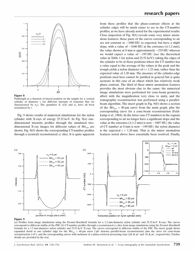
Fig. 9 shows results of numerical simulations for the nylon

cylinder with X-rays of energy 25.52 keV. In Fig. 9(a) one-

dimensional intensity profiles through the simulated two-

dimensional X-ray images for different values of Msys are

shown. Fig. 9(b) shows the corresponding CT-number profiles

through a (central) reconstructed xz slice. It is quite apparent

from these profiles that the phase-contrast effects at the

cylinder edges will be much easier to see in the CT-number

profiles, as we have already noted for the experimental results.

Close inspection of Fig. 9(b) reveals some very minor anom-

alous features: those parts of the curves corresponding to air

are not constant at �1000 HU as expected, but have a slight

slope, with a value of �1040 HU at the extremes (�1.2 mm);

the value shown at 0 mm is approximately �219 HU whereas

we would expect a value of �195 HU (see the theoretical

value in Table 1 for nylon and 25.52 keV); taking the edges of

the cylinder to be at those positions where the CT number has

a value equal to the average of the values at the peak and the

trough yields a nylon diameter of t = 1.23 mm, rather than the

expected value of 1.20 mm. The measure of the cylinder-edge

positions used here cannot be justified in general but is quite

accurate in this case of an object which has relatively weak

phase contrast. The third of these minor anomalous features

provides the most obvious clue to the cause: the numerical

image simulations were performed for cone-beam geometry,

albeit with the magnification very close to unity, and the

tomographic reconstruction was performed using a parallel-

beam algorithm. The insert graph in Fig. 9(b) shows a section

of the Msys = 40 mm curve from the main graph, plus the

corresponding curve for a cone-beam reconstruction (Feld-

kamp et al., 1984). In the latter case CT numbers in the regions

corresponding to air no longer have a significant slope and the

value at the extremes (�1.2 mm) is now �1007 HU; the value

of CT number at 0 mm is now �199 HU; the nylon diameter

is the expected t = 1.20 mm. That is, the minor anomalous

features noted above have essentially been resolved. Finally,

research papers


Figure 9(a) Profiles from image simulations using the Fresnel–Kirchhoff formula for a 1.2 mm-diameter nylon cylinder and 25.52 keV X-rays. The curvescorrespond to different widths of the PSF. (b) CT-number profiles through a reconstructed xz slice from image simulations using the Fresnel–Kirchhoffformula for a 1.2 mm-diameter nylon cylinder and 25.52 keV X-rays. The curves correspond to different widths of the PSF. The insert graph showsexpanded detail at one cylinder edge for the Msys = 40 mm curve (‘pb’ denotes parallel-beam reconstruction) plus the curve for cone-beamreconstruction (‘cb’), and the corresponding curves with inclusion of a phase-retrieval processing step (‘pb & pr’ and ‘cb & pr’, respectively). Furtherdetails are provided in the text.

Figure 8Pathlength as a function of lateral position on the sample for a verticalcylinder of diameter t, for different amounts of Gaussian blur (ascharacterized by b). The quantities X, t(X) and b have all beennormalized by t.

the insert graph also includes the corresponding curves for the

case where the original simulated images are subjected to

phase retrieval prior to the formation of sinograms. This

phase-retrieval step was performed using the algorithm

developed by Paganin et al. (2002), which utilizes the ‘trans-

port-of-intensity’ equation (Teague, 1983) and assumes a

homogeneous object (required input parameters are �/� =

�2’/� = 2570 for nylon and 25.52 keV, and R 0 = 50.9 cm). In

this case (see the ‘cb & pr’ curve) the form of the CT-number

profile relates directly to the cylinder geometry, without what

is essentially an artefact (the characteristic black–white fringe)

resulting from phase-contrast effects. The application of this

phase-retrieval algorithm to the experimental data is compli-

cated by the fact that we have three quite distinct materials

present rather than just one. As we will see below, we are able

to use the phase-contrast artefacts present in the recon-

structed CT-number data to considerable advantage and so

we will not further pursue the use of phase retrieval here.

However, the recent algorithm developed by Beltran et al.

(2010) might well be applied to such experimental data.

Fig. 10 shows the analogous curves to those in Fig. 9, for the

Cu cylinder with X-rays of energy 25.52 keV. In this case the

sensitivity of the curves, and the CT-number value at the peak

in particular, to the width of the PSF is quite apparent. If we

vary the value of Msys (whilst holding b fixed at 5 mm) to

obtain the ‘best’ agreement with each of the experimental

radial profiles in Fig. 6 (separately), we obtain the solid curves

included in Fig. 6. Table 3 provides the values of Msys so

obtained. The agreement between theoretical and experi-

mental profiles in Fig. 6, which is generally very good, was

optimized in terms of a single quantity: for nylon, the differ-

ence between the values of CT number at the peak and

trough. In the case of Cu this quantity was the value of CT

number at the peak. There was no convenient quantity in the

case of Al, given the shape of the associated experimental

profiles, and so the corresponding theoretical profiles in Fig. 6

are based on the averages of the optimum Msys values for

nylon and Cu, at each X-ray energy. The theoretical Al profiles

in Fig. 6 contain some, albeit small, indications of phase

contrast which are not present in the experimental profiles (or

are much less obvious). This may be a reflection of the Al wire

‘surface quality’ being poorer than we have modelled it to be,

but is most likely a consequence of the geometrical effect

discussed in x4.1 [which gives rise to the distinctly non-circular

Al-wire cross-section in reconstructed (xz) slices].

The magnitude of the values of Msys in Table 3 are quite

consistent with our detailed considerations above. It is parti-

cularly encouraging that the values obtained independently for

nylon and Cu are reasonably consistent at each X-ray energy.

Although we have not explicitly addressed the point thus far,

it is of course quite possible for Msys to be energy dependent,

and so we cannot necessarily expect the values to be in

agreement from one X-ray energy to another. Bourgeois et al.

(1994), for example, have used synchrotron radiation to

measure the FWHM of the PSF for several X-ray imaging

systems as a function of energy, the range encompassing the

X-ray energies employed in the present study. Whilst the

X-ray imaging systems studied are quite different from the

research papers


Figure 10(a) Profiles from image simulations using the Fresnel–Kirchhoff formulafor a 60 mm-diameter Cu cylinder and 25.52 keV X-rays. The curvescorrespond to different widths of the PSF. (b) CT-number profilesthrough a reconstructed xz slice from image simulations using theFresnel–Kirchhoff formula for a 60 mm-diameter Cu cylinder and25.52 keV X-rays. The curves correspond to different widths of thePSF. Further details are provided in the text.

Table 3Values of Msys (mm) which provide the best agreement between theexperimental and theoretical profiles in Fig. 6 for each of the samplecomponents and each of the X-ray energies.

The values for Al are in brackets and italicized because they are just theaverages of the values for nylon and Cu. Further details are provided in thetext.

12.66 keV 18.00 keV 25.52 keV 30.49 keV

Nylon 46 38 38 38Al (48) (39) (40) (38)Cu 50 41 43 39

CCD used here, the closest, an image intensifier/CCD with a

Be window, has a PSF whose FWHM is almost constant with

energy (there is in fact a very slight decrease with increasing

energy). Whilst certainly not highly compelling evidence in

favour of, this trend is at least consistent with, the results in

Table 3.

We now have the situation where we can quite accurately

account for all of the quantitative experimental X-ray tomo-

graphy data. The remaining question relates to our acceptance

of the relatively larger values of Msys, especially for Cu, at

12.66 keV. In the event that this behaviour is deemed to be

anomalous, we still need to account for this effect in terms

of some additional, hitherto unidentified, energy-dependent

phenomenon which predominates for Cu. A likely candidate

would seem to be harmonic contamination and we will

investigate this possibility in detail in the next subsection

(x4.3). Tran et al. (2003), for example, in connection with

accurate measurements of X-ray absorption coefficients using

synchrotron data, have undertaken a quantitative determina-

tion of the effect of harmonic contamination. If we consider

the case where we have a primary X-ray beam incident on

the sample which is composed of 99% 12.66 keV photons

(fundamental) and 1% 37.98 keV photons (�/3 harmonic),

then the transmitted beam would have: essentially the same

composition after traversing 1.2 mm of nylon; only 86%

fundamental, plus 14% �/3 harmonic after traversing 0.83 mm

of Al; just 19% fundamental, plus 81% �/3 harmonic after

traversing 60 mm Cu. This is, of course, a form of beam

hardening and provides an indication of why harmonic

contamination could manifest itself preferentially in the Cu

results. The figures quoted correspond to the case of a perfect

imaging system (Msys = 0) and the impact of harmonic

contamination will be considerably less dramatic when

allowance is made for the real PSF (this will be demonstrated

in x4.3). The fact that harmonic contamination is not expected

to have any significant effect in the case of the nylon results,

and that the value of Msys in Table 3 for nylon at 12.66 keV is

larger than for the other X-ray energies, suggests that we are

seeing a ‘real’ energy dependence in the PSF width. However,

this cannot be stated categorically, and the value of Msys at

12.66 keV being slightly larger for Cu compared with nylon

indicates that further investigation is justified.

In terms of the effects of harmonic contamination as a

function of X-ray energy, a number of factors need to be

considered, including the quantum efficiency and response of

the CCD, e.g. the quantum efficiency will decrease from 72%

at 12.66 keV to 11% at 30.49 keV; however, the presence of

the Gd K-edge at 50.24 keV for the Gadox phosphor means

that all harmonics (for example, the lowest-energy �/4

harmonic at 50.64 keV) will then have a somewhat enhanced

quantum efficiency except for the lowest-energy �/3 harmonic

(37.98 keV).

4.3. Contributions due to harmonic contamination

Fig. 11 displays the results of numerical image simulations

for the 60 mm Cu cylinder and 12.66 keV (fundamental)

research papers


Figure 11Intensity and CT-number profiles from image simulations using theFresnel–Kirchhoff formula for a 60 mm-diameter Cu cylinder and12.66 keV X-rays, allowing for different levels of harmonic (�/3)contamination. The curves correspond to (a) Msys = 20 mm; (b) Msys

= 30 mm; (c) Msys = 40 mm. Further details are provided in the text.

X-rays, with different levels of harmonic (�/3) contamination

(0, 1, 2 and 5%). In Fig. 11(a) we have used Msys = 20 mm, in

Fig. 11(b) Msys = 30 mm, and in Fig. 11(c) Msys = 40 mm (all

with b = 5 mm). In each figure there are one-dimensional

intensity profiles (top) through the simulated two-dimensional

X-ray images, and the corresponding CT-number profiles

(bottom) through a (central) reconstructed xz slice. The range

covered in the image plane has been limited to 80 mm (80/M =

78.3 mm at the sample). As alluded to in x4.2, the effects of

harmonic contamination are most significant for smaller

values of Msys.

We will now describe the detailed calculations we have

performed in order to estimate the harmonic contamination

contributions as accurately as possible. The angular flux

density was calculated (ignoring, for the present, the presence

of the monochromator) at the CCD (24 m) as a function of

X-ray energy from 1 to 150 keV in steps of 0.1 keV using the

program SPECTRA8.1 (Tanaka & Kitamura, 2001; http://

radiant.harima.riken.go.jp/spectra/). The storage-ring para-

meter values for the Australian Synchrotron were taken from

http://radiant.harima.riken.go.jp/spectra/asp.prm. The wiggler

field was initially taken to be 0.838 T (see x2 for further

details). Fig. 12 shows the resulting flux-density curve (solid).

When allowance is made for all of the filters, windows and

beam paths we get the dotted curve in Fig. 12. It is then

necessary to make allowance for the quantum efficiency and

response of the CCD. The former is accomplished by including

the multiplicative factor 1� expð��m�sÞ, where �m is the

energy-dependent mass absorption coefficient. The CCD

response takes account of the fact that the number of visible

photons produced is not only directly proportional to the

number of incident X-ray photons but also to their energy, e.g.

the CCD detector signal associated with a single 60 keV X-ray

photon is three times that for a single 20 keV X-ray photon.

The short-dashed curve in Fig. 12 shows the result of including

the detector efficiency and response. The nature of the

detector response results in this curve being on a relative,

rather than an absolute, flux-density scale (we have scaled the

curve so that the response at the peak is unity). Finally, the

long-dashed curve in Fig. 12 is the same as the short-dashed

curve except that the wiggler field is 0.78 T instead of 0.838 T

(see x2 for further details). The vertical (up) arrows show the

positions of the four (fundamental) X-ray energies used. The

horizontal arrows correspond to the �/3 harmonics, and the

vertical (down) arrows to the �/4 harmonics. The weighted-

average X-ray energies for the curves in Fig. 12 are 9.6, 23.8,

21.7 and 21.1 keV, respectively.

In order to ascertain the peak reflectivity of the Si mono-

lithic double-crystal monochromator for the fundamental

X-ray energies and harmonics we use the perfect-crystal

dynamical theory of X-ray diffraction. The two Si components

are assumed to be perfectly flat, effectively infinite thickness,

with sufficiently extended surfaces to intercept the entire

X-ray beam, and with symmetric (111) surfaces. The dyna-

mical-theory formulation is simplified by the fact that we only

need to consider the normal () component of polarization

(polarization factor is unity), that Si possesses the centro-

symmetric12 diamond crystal structure, and that we will only

be concerned with symmetric hhh Bragg reflections, i.e. those

for which the Miller indices are all equal to integer h. If we

neglect bonding effects and anharmonic thermal vibrations, it

can be shown that the conventional X-ray structure factor is

given by

Fhð�Þ ¼ f0ðhÞ þ f 0ð�Þ þ if 00ð�Þ �

TðhÞ�ðhÞ

F 0hð�Þ þ iF 00h ð�Þ; ð19Þ

where f0ðhÞ is the free-atom spherical scattering factor for Si,

f 0ð�Þ and f 00ð�Þ are the anomalous dispersion corrections for

Si, and TðhÞ is the harmonic temperature factor for Si. f0ðhÞ is

also dependent on the Si lattice parameter (5.4309 A; NBS,

1976) and we use the atomic scattering-factor parameteriza-

tion of Doyle & Turner (1968). The values of the anomalous

dispersion corrections were calculated with the aid of data

from Brennan & Cowan (1992). TðhÞ also depends on the

lattice parameter and the Si Debye–Waller factor (0.45 A2;

Prager, 1971). The value of �ðhÞ is 8 if h 0ðmod 8Þ, �4ffiffiffi2p

if

h �1ðmod 8Þ, 0 if h �2ðmod 8Þ, 4ffiffiffi2p

if h �3ðmod 8Þ,

and�8 if h 4ðmod 8Þ. We will not be directly concerned with

the modulus of the structure factor here, but, for complete-

ness,

Fhð�Þ�� ¼ f0ðhÞ þ f 0ð�Þ

�2þ f 00ð�Þ½ �

2n o1=2

TðhÞ �ðhÞ��

F 0hð�Þ �2

þ F 00h ð�Þ �2

n o1=2

: ð20Þ

research papers


Figure 12Angular-flux-density calculations, including the effects of filters, windowsand beam paths, and the quantum efficiency and response of the CCD.One curve is for a wiggler field of 0.78 T, and the others for 0.838 T. Thearrows indicate the position of the fundamental X-ray energies andharmonics. Further details are provided in the text.

12 The diamond structure (space group Fd�33m) is not centrosymmetric aboutthe conventional unit-cell origin [where the eight atom positions are (0, 0, 0)plus the three equivalent face-centred cubic (f.c.c.) sites and (1/4, 1/4, 1/4) plusthree f.c.c. sites]. However, there is a centre of symmetry at the mid-point ofeach nearest-neighbour bond, such as (1/8, 1/8, 1/8), and so we choose thisposition as the origin and have new atom positions of�(1/8, 1/8, 1/8) plus f.c.c.sites instead.

Equation (20) shows that the Bragg reflec-

tions for which h is odd (e.g. 111 and 333)

will in general be reasonably strong (j�ðhÞj= 4

ffiffiffi2p

) and those for which h is even and an

even multiple of two (e.g. 444 and 888) will

in general be (relatively) stronger still

( �ðhÞ�� = 8). However, if h is even and an

odd multiple of two (e.g. 222 and 666) the

Bragg reflection is ‘forbidden’, remem-

bering that we have explicitly neglected the

small contributions due to bonding effects

and anharmonic thermal vibrations in the

present study [see, for example, the detailed

(temperature-dependent) X-ray study of

both effects performed by Roberto &

Batterman (1970) in respect of the 222

reflection in Si].

The X-ray susceptibility (or polariz-

ability) can then be expressed as

hð�Þ ¼ 0hð�Þ þ i 00h ð�Þ; ð21aÞ

where

0hð�Þ ¼ �re�

2

�VF 0hð�Þ ð21bÞ

and

00h ð�Þ ¼ �re�

2

�VF 00h ð�Þ; ð21cÞ

and re is the classical electron radius and V the unit-cell

volume. For a non-centrosymmetric crystal structure 0hð�Þand 00h ð�Þ can themselves be complex, but for the present case

of a centrosymmetric crystal structure these components are

both real.

Using the dynamical-theory formalism of Cole & Stemple

(1962) [see also Zachariasen (1945)] the reflectivity curve

(reflecting power) is given by

R ¼ L� ðL2� 1Þ1=2; ð22Þ

where

L ¼y2 þ g2 þ ðy2 � g2 � 1þ p2Þ

2þ 4ðgy� pÞ

2 �1=2

1þ p2; ð23Þ

y ¼ 00ð�Þ þ ð� � �BÞ sin 2�B

0hð�Þ; ð24Þ

g ¼ 000 ð�Þ= 0hð�Þ ð25Þ

and

p ¼ 00h ð�Þ= 0hð�Þ; ð26Þ

with � being the angle between the incident X-ray beam and

the Bragg planes. Certain important quantities which result

from the dynamical theory of X-ray diffraction include [see,

for example, Matsushita & Hashizume (1983) and Authier

(2001)], for the present study, the extinction distance

�h ¼ � cos �B= h

�� ; ð27Þ

the intrinsic or Darwin width of the Bragg reflection

!h ¼ 2 0h�� =sin 2�B ð28Þ

and the deviation from the exact Bragg angle due to refraction

effects

��h ¼ � 00=sin 2�B: ð29Þ

It can easily be shown, using Bragg’s Law, that the relative

wavelength spread associated with the Darwin width is given

by

��

�

� �h

¼ ��E

E

� �h

¼ !h cot �B ¼ 0h��

sin2�B

: ð30Þ

Given that the X-ray wavelengths or energies considered in

this study are well removed from the Si absorption edges it can

be shown that, for a particular Bragg reflection, �h varies as

��1 to a good approximation, !h as �, and ð��=�Þh remains

constant [��h also varies as � for a particular Bragg reflection

and, additionally, varies as �2 (or h�2) for a series of harmonics

(where �B is constant)]. Table 4 provides the calculated values

of these quantities for the relevant Bragg reflections and X-ray

wavelengths.

The IMBL front-end mask defines an X-ray beam of

divergence 5.0 mrad horizontally and 0.3 mrad vertically. The

water-cooled primary slits (hutch 1A), defining the beam in

the horizontal and vertical directions, are at 13.7 m and 14.0 m

from the source, respectively. The horizontal-defining slits had

an opening of approximately 6 mm and the vertical-defining

slits 1.0 mm (precisely determined). These slit sizes represent

a quite significant aperturing of the primary X-ray beam, and

were verified by exposures taken with Gafchromic film (HD-

810; ISP Inc.) placed on the CCD (with the monochromator

out of the primary beam). We are particularly concerned with

the vertical-defining slit since this dictates the beam diver-

gence (��d) in the plane of diffraction (vertical) for the

monochromator (this slit subtends an angle of 0.071 mrad or

research papers


Table 4Values of certain parameters and calculated quantities for relevant Bragg reflections and X-raywavelengths.

Rows with the same typeface belong to the same group of fundamental/harmonics. Further details areprovided in the text.

hhh E (keV) � (A) �B (�) �h (mm) !h (arcsec) ��h (arcsec) ð��=�Þh

111 12.66 0.9795 8.986 30.14 4.292 4.064 1.316 �� 10�4

111 18.00 0.6889 6.307 43.34 2.985 2.824 1.309 �� 10�4

111 25.52 0.4859 4.444 61.95 2.088 1.976 1.302 � 10�4

111 30.49 0.4067 3.718 74.19 1.744 1.658 1.301 � 10�4

333 37.98 0.3265 8.986 163.7 0.2634 0.4472 8.075 �� 10�6

333 54.00 0.2296 6.307 235.0 0.1834 0.3126 8.046 �� 10�6

333 76.56 0.1620 4.444 334.4 0.1290 0.2189 8.045 � 10�6

333 91.47 0.1356 3.718 400.3 0.1077 0.1833 8.038 � 10�6

444 50.64 0.2449 8.986 216.0 0.1497 0.2514 4.591 �� 10�6

444 72.00 0.1722 6.307 311.2 0.1039 0.1757 4.557 �� 10�6

444 102.1 0.1215 4.444 442.1 0.07316 0.1234 4.564 � 10�6

444 122.0 0.1017 3.718 528.6 0.06120 0.1033 4.566 � 10�6

555 63.30 0.1959 8.986 562.5 0.04599 0.1611 1.410 �� 10�6

777 88.62 0.1399 8.986 1706 0.01083 0.08222 3.320 �� 10�7

15 arcsec at the source). It is easily shown geometrically that a

source of size s and a slit of size a, separated by a distance d1,

will produce a beam size at distance d2 from the slit of

jM0ðs� aÞ � sj, where M 0 = ðd1 þ d2Þ=d1 is the simple

geometric magnification factor, and the upper sign is for the

penumbra and the lower sign for the umbra. In the limiting

case where s� a, the sizes of the umbra and penumbra are

equal, with a value M 0a. At the other limit, where s� a, they

are also equal, but with a value ðM 0 � 1Þs.13 In the present

case, and taking s to have the (-) values mentioned in x4.2,

the sizes of X-ray beam umbra and penumbra at the CCD

differ by only 1.3% in the vertical direction, and by 4.9% in the

horizontal direction. The corresponding figures when we use

FWHM values for s are 3.2% and 11.7%, respectively. This

is consistent with the quite anisotropic nature of the source

having a significant impact on the X-ray beam profile, and the

effects are clearly visible when the sharpness of the horizontal

and vertical edges of the Gafchromic-film exposures are

compared.

We have used SPECTRA8.1 to calculate profiles of the

angular flux density at the CCD (24 m; without mono-

chromator) as a function of vertical and horizontal position,

about the centre of the X-ray beam (wiggler field 0.838 T).

These calculations have been performed for all the X-ray

energies of concern, including harmonics, with vertical and

horizontal step sizes of 100 mm and 1 mm, respectively. The

results for an X-ray energy of 12.66 keV, and all its harmonics

up to �/7, are shown in Figs. 13(a) and 13(b) (horizontal and

vertical positions, respectively), the profiles having been

normalized for ease of presentation; the absolute angular-flux-

density values at 0 mm are those plotted in the uppermost

curve of Fig. 12. The limits of the X-ray beam, as defined by

the primary slits, are shown as vertical lines for both the umbra

(solid lines) and penumbra (dashed lines); their calculated

positions are based on FWHM-values for s. The increase of

‘roll-off’ of the angular flux density with increasing X-ray

energy is quite apparent, especially in the vertical direction,

and we will make allowance for this effect in our calculations

of harmonic contamination (see below).

The differential form of Bragg’s law [ð��=�Þ = �� cot �B;

used to obtain (30)] yields a maximum value of �� corre-

sponding to the beam divergence associated with the X-ray

beam represented in Fig. 13(b), of ð��Þd = 0.45 mA for the

Bragg reflections in Table 4. This value is significantly larger

than any of the values associated with the Darwin width,

ð��Þh = �ð��=�Þh, obtained from Table 4, which lie in the

range from essentially zero up to 0.13 mA. That is, the

wavelength spread associated with the divergence of the

primary X-ray beam will in general dominate over that asso-

ciated with the Darwin width for the monochromator Bragg

reflections we are considering here. A convenient way of

considering these issues is via the use of DuMond diagrams

(DuMond, 1937). The DuMond diagram provides a versatile

and intuitive graphical approach to understanding the corre-

lations imposed by X-ray optical elements, such as slits and

monochromators, in angle–wavelength (�–�) space. In the case

of a double-crystal monochromator one normally needs to

consider a separate DuMond diagram for each crystal.

However, in the present case of a monolithic (+, �) mono-

chromator which has two rigidly linked crystal elements with

parallel sets of Bragg planes (the so-called ‘non-dispersive

research papers


Figure 13(Normalized) angular-flux-density calculations for a wiggler field of0.838 T and a (fundamental) X-ray energy of 12.66 keV plus harmonics inthe (a) horizontal direction, (b) vertical direction. The vertical lines markthe edges of the X-ray beam as defined by the primary slits (solid lines forumbra and dashed lines for penumbra). The �/2 and �/6 harmonics areshown in grey because they relate to ‘forbidden’ Bragg reflections (222and 666, respectively). Further details are provided in the text.

13 Similarly, the beam divergence can be shown to be js� aj=d1, which has thevalues, equal for both umbra and penumbra, of a=d1 and s=d1 for the limitingcases of s� a and s� a, respectively. In the present case, s < a, bothhorizontally and vertically, and we have calculated the beam divergence to bethe angle subtended by the penumbral beam at the true (not the effective,point) source position, a value which lies in between the values obtained whenconsidering umbral and penumbral beam sizes in conjunction with theirrespective effective point-source positions.

parallel configuration’), these two DuMond diagrams exactly

overlap and we need consider just one.14

Fig. 14(a) shows the full DuMond diagram corresponding

to the 12.66 keV case, and including harmonics up to �/7.

Figs. 14(b) and 14(c) show magnified (by a factor of 104)

versions of the DuMond diagram in the vicinity of the

fundamental (�) and �/3 harmonic, respectively. In such small

regions of �–� space, the differential form of Bragg’s law can

be applied directly and the curve treated as a straight line of

gradient � cot �B. The effect of refraction is to move this line

by an amount ��h [see (29)] parallel to the horizontal (�) axis;

see the dashed lines, parallel to and displaced from the original

lines. The lightly shaded region about the dashed line, in each

case, has a width, parallel to �, of !h [see (28)], corresponding

to the extent of the effect associated with the Darwin width.

The lightly shaded region with sides parallel to both the � and

� axes corresponds to the effect of the X-ray beam divergence

and has a width of ��d. Both of these lightly shaded regions

have effectively infinite extent in the � direction, but our

concern will be with the region where the two intersect,

research papers


Figure 14DuMond diagrams corresponding to the 12.66 keV case. (a) The full DuMond diagram and including harmonics up to �/7. (b) Magnified (by a factor of104) version in the vicinity of the fundamental (�). (c) Magnified (by a factor of 104) version in the vicinity of the �/3 harmonic. The effects of the Darwinwidth and the beam divergence are incorporated and the intersection of the associated lightly shaded regions, represented by the darkly shadedparallelogram, will be the focus of our attention. The effect of refraction is also included in the diagrams. In (a) the �/2 and �/6 harmonics are shown ingrey because they relate to ‘forbidden’ Bragg reflections (222 and 666, respectively). In (c) we have included an insert graph with an enlarged view forclarity. Further details are provided in the text.

14 This statement should not, however, be taken to mean that the reflectivitycurves for a single such crystal and for the double-crystal monochromator arethe same. As a simple example we can consider two points on the single-crystalreflectivity curve for a single X-ray wavelength and a single beam divergenceangle. One point is on the peak and has a value of 0.9, and one is on a tail andhas a value of 0.1. The reflectivity values for the corresponding double-crystalmonochromator we are considering in the present study would have values of(0.9)2 = 0.81 and (0.1)2 = 0.01, respectively. This simple example also serves todemonstrate the well known effect, first demonstrated by Bonse & Hart(1965), of using multiple Bragg reflections in a channel-cut monochromator topreferentially reduce the tails, i.e. compare 0.9/0.1 = 9 with 0.81/0.01 = 81.

represented by the darkly shaded parallelogram. In the case of

Fig. 14(c), the values of ��h and !h are quite small compared

with ��d and so we have included an insert graph with an

enlarged view for clarity. Important properties of this paral-

lelogram, for a particular fundamental and associated

harmonics, are as follows:

(i) Area:

��d!hð�0=nÞ�0 cot �B=n; ð31aÞ

(ii) Abscissa of centre:

� � �B ¼ ��hð�0Þ; ð31bÞ

(iii) Ordinate of centre:

�� ð�0=nÞ ¼ �0 cot �B ��hð�0Þ � ��hð�0=nÞ �

=n

’4�3

0Zre

�Vsin2�B

1

n1�

1

n2

� �; ð31cÞ

where n denotes the number of the harmonic [for the funda-

mental n = 1, and the ordinate corresponds to � = �0 as

expected; see Fig. 14(b)]. The approximate expression in (31c)

is obtained by replacing, for Si, F 00ð�Þ by 8Z [see (19) and

(21b)], where Z is the atomic number (14 for Si), i.e. we are

neglecting the real anomalous dispersion correction f 0ð�Þ. The

centre of the parallelogram, given by (31b) and (31c), is

marked by a small circle in Figs. 14(b) and 14(c) and it is

apparent that, whilst �0=3 = 0.3265 A is within the range of

those wavelengths which make a contribution, it is not actually

at the centre of this wavelength band (which is [0.32646,

0.32661] A). This is a consequence of the fact that the size of

the deviation from the exact Bragg angle due to refraction

effects is different for the fundamental and its harmonics. The

centre of the parallelogram for the fundamental is determined

by the fact that we initially calibrated our �0 values with

reference to the K-edges of certain filters (see x2).

We have performed extensive dynamical-theory calcula-

tions for each of the cases given in Table 4 using (19) and

(21a)–(26), for the monolithic double-crystal monochromator.

The results of individual reflectivity-curve calculations for

values of � and � covering a particular DuMond-diagram

parallelogram are combined to yield the final results. Whilst

the � values sampled must fall within the range dictated by the

divergence of the X-ray beam, we can choose (for conve-

nience) to map the full rectangle, with vertical and horizontal

sides, which bounds the parallelogram, without compromising

the calculation results. However, the area of this rectangle is

ð!h þ ��dÞ=!h times larger than that of the parallelogram and

whilst this factor is less than 5 for the 12.66 keV fundamental

it will exceed 103 for the corresponding �/7 harmonic (see

Table 4 for the !h values). Thus, in the interests of avoiding

issues of undersampling or lengthy computation times, we

have ensured that our computer program has the flexibility to

map a parallelogram in �–� space. In the interests of being

conservative, and allowing for the fact that individual reflec-

tivity curves have tails extending beyond the angular range

associated with the Darwin width, we have considered paral-

lelograms which are twice the prescribed ‘thickness’ in �, i.e.

2ð��Þh [resulting in an overall range in � for the parallelogram

of ð��Þd þ 2ð��Þh]. Individual reflectivity-curve calculations

were performed for a regular grid of (�, �) points covering

each parallelogram, with 101 equally spaced points along each

line parallel to the � axis, and the same along each line parallel

to the � axis. The number of such calculations varied from

approximately 1.8 � 104 (for the 12.66 keV case) to approxi-

mately 6.9 � 106 (for the 88.62 keV case). The variation of

angular flux density with X-ray wavelength within the

DuMond diagrams being considered here amounts to a less-

than-1% effect in all cases, and so we have used top-hat

distributions as a function of �. However, in order to allow for

the roll-off of the angular flux density as a function of � in the

vertical direction we have included a �-dependent weighting

factor at each point. The value of this weighting factor was

obtained by performing least-squares fits to curves such as

those shown in Fig. 13(b) for each X-ray energy. Whilst the

overall shape of these curves is not Gaussian, we found that

we could obtain excellent Gaussian fits within the vertical

divergence range of concern here, i.e. between the vertical

dashed lines in Fig. 13(b), calculated to span 14.96 arcsec. The

third column in Table 5 lists the values of the refined para-

meter, the FWHM of the Gaussian [the peak height for the

Gaussian fit to the (normalized) angular-flux-density curve

was also refined, but the value obtained was always unity].

In the approach which we have adopted here it is implicit

that we are treating the double-crystal monochromator as an

X-ray optical element which does not itself alter the spatial

distribution of the beam which illuminates the sample (apart

from the obvious displacement vertically) but rather acts like a

special ‘filter’. We have not concerned ourselves with corre-

lations, at the sample position, between wavelength, direction

of propagation and x–y position for the incident X-rays. This

is quite justifiable for the imaging/tomographic study being

reported here; however, if the X-ray beam after the mono-

chromator was being used for certain diffraction-based

experiments for example, a more detailed approach may need

to be considered. The DuMond-diagram approach adopted

here can be extended [see, for example, Xu & Li (1988) and

Servidori et al. (2001)], alternatively the phase-space method

can be used [see, for example, Hastings (1977) and Pianetta &

Lindau (1977)], or a combination of both can be applied [see,

for example, Matsushita et al. (1978) and Matsushita &

Kaminaga (1980)]. It should also be pointed out that we will

not attempt to allow for the variation of harmonic contam-

ination from point to point across the monochromated X-ray

beam, although results such as those presented in Fig. 13 could

form the basis for such an undertaking. This variation is,

however, accounted for in an average sense, in our consid-

eration of the tomographic data sets.

The dynamical-theory calculations yield a factor, shown in

the fourth column of Table 5, which, when multiplied by the

angular flux density from Fig. 12, will provide us with the value

of the integrated flux in the ‘monochromatic’ beam for the

associated X-ray energy. Before applying this factor we need

to allow for the roll-off of the angular flux density with � in the

horizontal direction. As shown in Fig. 13(a), this effect is not

research papers


especially large in the present context and a relatively crude

correction factor is sufficient. To this end we have performed

Gaussian least-squares fits to the (normalized) angular-flux-

density curves in the same manner as for the vertical direction.

An expression for the correction factor (Rhoriz) can then be

obtained by deriving the average (ordinate-)value of the

Gaussian within the region corresponding to the horizontal

beam divergence (calculated to be 95.60 arcsec),

Rhoriz ¼�1=2

2ðln 2Þ1=2�erf ðln 2Þ1=2� �

; ð32Þ

where erf is the conventional error function and � is the

(dimensionless) ratio of the beam divergence to the refined

FWHM-value from the Gaussian fit to the angular-flux-density

curve. The values of Rhoriz are provided in the fifth column of

Table 5. The last four columns in Table 5 provide the resulting

integrated flux values corresponding to each of the curves

presented in Fig. 12. In those cases where the integrated flux

for the fundamental is not 100.0% of the group of funda-

mental/harmonics, we have indicated the actual percentage in

brackets, and, correspondingly, the values for the associated

harmonics when they are not 0.0%. It is clear that the

12.66 keV fundamental is the only one for which harmonic

contamination is of any significance. If there were no filters

present and we had a perfect CCD, we predict just 0.1% of �/3,

as the fundamental and all harmonics are on the high-energy

side of the peak in the angular-flux-density curve in Fig. 12.

Once the X-ray beam is hardened as a result of the presence of

the filters, the 12.66 keV fundamental and its �/3 harmonic lie

on opposite sides of the peak in the corresponding angular-

flux-density curve in Fig. 12 and the �/3 amounts to 4.2%, with

the �/4 being 0.3% (helped by the 444 being a strong Bragg

reflection). In this case, where we have allowed for the

filtration of the X-ray beam, the 18.00 keV fundamental is

very nearly at the peak of the angular-flux-density curve.

When we allow for the energy-dependent efficiency of the

CCD, the apparent extent of the harmonic contamination is

reduced. However, this effect is offset to some extent by the

energy-dependent response of the CCD, as discussed at the

beginning of this subsection. This results in a 1.2% �/3

contribution and a 0.2% �/4 contribution; the latter, whilst

being small, has been enhanced somewhat as a result of the

X-ray energy being optimum with respect to the jump in the

CCD efficiency which results from the presence of the Gd K-

edge [see the previous subsection (x4.2)]. Finally, as discussed

in x2, there is a possibility that the actual magnetic field in the

insertion device is somewhat lower than the nominal value for

an APS type A wiggler and the last column in Table 5 corre-

sponds to this case. Whilst the exact value of the wiggler field,

for a gap of 25 mm, is an important factor, it is clear that we

are dealing with an apparent �/3 component of approximately

1%. It should be emphasized that the extent of the harmonic

contamination in the X-ray beam from the double-crystal

monochromator is predicted to be significantly larger (see the

third last column in Table 5), but the harmonic contamination

as seen by the CCD is lower. In interpreting our experimental

tomography data, inclusion of the performance of the CCD

as a function of X-ray energy is an important factor when

discussing harmonic contamination.

In summary, we have shown that there will indeed be a

significant presence of harmonic contamination in the X-ray

beam which is incident on the sample, but only for the lowest

(fundamental) X-ray energy used (12.66 keV). This is exactly

the type of effect we alluded to at the end of the previous sub-

section (x4.2). However, it is apparent from Fig. 11 [Fig. 11(c)

in particular] that the magnitude of the effect associated with

1% harmonic contamination, for Cu, is still quite small. Thus

the value of Msys = 50 mm, for Cu and 12.66 keV, in Table 3

would not be expected to decrease significantly as a result of

research papers


Table 5Results of dynamical-theory calculations, made in connection with estimating the extent of harmonic contamination, for relevant Bragg reflections andX-ray wavelengths.

It should be noted that the values of integrated flux in the last two columns are on a relative rather than an absolute scale (the percentage values in brackets areabsolute) due to the allowance for the CCD response. Rows with the same typeface belong to the same group of fundamental/harmonics. Further details areprovided in the text.

Integrated flux (photons s�1)

hhh E (keV)

GaussianFWHM(arcsec)

Dynamical-theoryfactor (mrad2 0.1%bandwidth) Rhoriz

No filtersPerfect CCD(0.838 T)

FiltersPerfect CCD(0.838 T)

FiltersReal CCD(0.838 T)

FiltersReal CCD(0.78 T)

111 12.66 35.78 4.099 �� 10�3 0.9884 3.85 �� 1012 (99.9%) 6.12 �� 1010 (95.5%) 3.01 �� 1010 (98.6%) 2.71 �� 1010 (99.1%)111 18.00 28.59 4.192 �� 10�3 0.9813 1.86 �� 1012 3.74 �� 1011 1.42 �� 1011 1.18 �� 1011

111 25.52 23.24 4.142 � 10�3 0.9710 5.59 � 1011 2.75 � 1011 6.68 � 1010 4.99 � 1010

111 30.49 21.01 4.092 � 10�3 0.9645 2.40 � 1011 1.44 � 1011 2.71 � 1010 1.87 � 1010

333 37.98 18.60 2.455 �� 10�4 0.9546 3.96 �� 109 (0.1%) 2.70 �� 109 (4.2%) 3.68 �� 108 (1.2%) 2.27 �� 108 (0.8%)333 54.00 15.44 2.336 �� 10�4 0.9344 2.10 �� 108 1.59 �� 108 5.83 �� 107 2.84 �� 107

333 76.56 12.94 2.179 � 10�4 0.9075 2.93 � 106 2.33 � 106 4.84 � 105 1.69 � 105

333 91.47 11.85 2.084 � 10�4 0.8904 1.66 � 105 1.35 � 105 2.10 � 104 5.83 � 103

444 50.64 15.97 1.343 �� 10�4 0.9384 2.23 �� 108 1.68 �� 108 (0.3%) 6.75 �� 107 (0.2%) 3.47 �� 107 (0.1%)444 72.00 13.34 1.253 �� 10�4 0.9128 3.98 �� 106 3.15 �� 106 7.23 �� 105 2.70 �� 105

444 102.1 11.24 1.147 � 10�4 0.8787 1.20 � 104 9.83 � 103 1.27 � 103 3.03 � 102

444 122.0 10.32 1.091 � 10�4 0.8579 2.50 � 102 2.06 � 102 1.99 � 101 3.55 � 100

555 63.30 14.24 3.940 �� 10�5 0.9228 6.36 �� 106 4.94 �� 106 1.40 �� 106 5.96 �� 105

777 88.62 12.03 8.587 �� 10�6 0.8936 1.17 �� 104 9.51 �� 103 1.55 �� 103 4.53 �� 102

allowance for 1% harmonic contamination, i.e. we do not

believe that this value of Msys was artificially increased to

any significant extent in order to compensate for the un-

acknowledged presence of a �/3 component. We thus conclude

that the slightly higher values of Msys at 12.66 keV in Table 3

reflect an underlying dependence of the PSF on X-ray energy.

5. Discussion and conclusions

It is clear from the results we have obtained in x4 that the

accurate characterization of the system PSF is crucial for any

highly quantitative studies. The optimization of this PSF (for

example, via the selection and operation of the X-ray imaging

detector, or the choice of the wiggler gap and thereby the

magnetic field which prevails in the insertion device) will be a

key factor in the success of future experiments. There will of

course always be some remaining (unwanted) contributions

impacting adversely on the PSF, associated with the practi-

calities and limitations of any hardware or software involved

in such experiments.

An obvious aspect of the present study which we have not

addressed as yet is the possibility of deconvoluting the PSF we

have established, from the X-ray images collected, prior to the

tomographic reconstruction. Our ability to account, quanti-

tatively, for the experimental results reported has relied, in

part, on the use of computer simulations which have incor-

porated different theoretical PSFs through the procedure of

convolution. This valuable opportunity has been afforded us

by virtue of dealing with a well characterized phantom as the

sample. In the case of a ‘real-world’ sample which we might

wish to characterize, the possibility of being able to decon-

volute the, independently determined, PSF from the experi-

mental data is a very attractive one. Unfortunately, and unlike

convolution, the inverse problem of deconvolution is in

general mathematically ‘ill-posed’. A detailed consideration of

this ‘ill-posedness’ is beyond the scope of the present study

and there is a wealth of literature on the subject [see, for

example, Tikhonov & Arsenin (1977)]. In fact, as an opera-

tion, deconvolution does not have a direct definition in

rigorous mathematical terms, but rather is defined as the

inverse of the operation of convolution. In the present context

it suffices to say that the solution of a given deconvolution

problem may not exist, or may not be unique. A solution may

also be quite unstable with respect to noise in the experi-

mental data or quite sensitive to the precise description of

the PSF.

In the present study, noise makes a significant contribution

to the experimental X-ray images, and we also have the

situation of the width of the PSF being comparable in size with

certain key sample features (especially the Cu wire).

Graafsma & de Vries (1999), for example, have demonstrated

the utility of the maximum-entropy method for the deconvo-

lution of PSFs from experimental X-ray images and Laue

diffraction patterns. We have investigated both the

Richardson–Lucy algorithm (Richardson, 1972; Lucy, 1974)

and regularized Wiener deconvolution [see Wiener (1949)],

as implemented in the X-TRACT software, and will report

briefly on results of the latter here. As indicated earlier we do

not expect the CT-number values already reported for nylon

and Al (see Table 1) to change as a result of considerations of

the role of the PSF. Table 6 provides the experimental values

of CT number for the Cu component at each of the four X-ray

energies, resulting from the application of regularized Wiener

deconvolution to the pre-processed images prior to tomo-

graphic reconstruction. We used the Gaussian PSFs as speci-

fied by the values of Msys given in italics in Table 3, and

assumed the average signal-to-noise ratio to be 100. As

expected, this deconvolution step did result in the presence of

quite pronounced artefacts in the resulting X-ray images.

These were clearly evident in the reconstructed slices and in

fact such effects were exacerbated by the fact that, with the

Cu component now demonstrating something approaching the

true degree of absorption, the starburst artefacts mentioned in

x4 have become quite prominent. In performing these tomo-

graphic reconstructions we tried a number of different filters

(for example, Hamming, Hann, cosine, Shepp–Logan) with a

view to reducing the impact of these artefacts, but there was

no definitive improvement and the results reported here are

for the (default) linear-ramp filter (which we have used

previously). The experimental CT-number values in Table 6

represent the averages of the maximum values for the five

central reconstructed (xz) slices in each case and can thus be

compared most directly with the grey ‘plus’ symbols in Fig. 5.

The ’s given in brackets in Table 6 are thus ‘inter-slice’ errors

in the terminology we adopted in x3. We have included CT-

number values based on both parallel-beam and cone-beam

reconstructions in light of the results obtained earlier for

simulations [see x4.2, and the insert graph in Fig. 9(b) in

particular].15 Whilst these experimental CT-number values are

still smaller than the theoretical values, the discrepancies are

greatly reduced (note that the factor by which the experi-

mental value for 12.66 keV has increased is well over an order

of magnitude). Given the issues associated with the decon-

volution of the PSF from the X-ray images, these results are

most encouraging.

In this paper we have performed a detailed analysis of

the first monochromatic X-ray tomography data collected

at IMBL, Australian Synchrotron. In order to account quan-

research papers


Table 6Experimental values of CT number in HU for the Cu component of thesample and each of the X-ray energies.

Theoretical values from Table 1 are also included for convenience. Furtherdetails are provided in the text.

12.66 keV 18.00 keV 25.52 keV 30.49 keV

Parallel-beamreconstruction

294000 338000 202000 196000(24000) (7000) (4000) (4000)

Cone-beamreconstruction

307000 347000 212000 201000(16000) (5000) (3000) (8000)

Theory 395000 390000 311000 252000

15 The CT-number values for nylon and Al also increase, by approximately3%, when cone-beam rather than parallel-beam reconstructions areperformed. This does not change the excellent agreement between theoryand experiment seen in Table 1 nor alter any of the discussion or conclusions.

titatively for the experimental results obtained for a simple

three-component phantom at four different X-ray energies, we

have considered in detail the role of harmonic contamination,

phase-contrast effects and the system PSF. All three of these

aspects have been shown to be significant, but it is the way in

which the PSF affects the derived values of CT number, for the

Cu component in particular, which is most relevant and

pronounced. This Cu wire is the most highly absorbing of the

three components and its diameter of just 60 mm is compar-

able in size with the width of the system PSF.

The use of a phantom which comprises simple features of

known dimensions and material properties has enabled us to

gain considerable insights into the capabilities and perfor-

mance of the key beamline components such as the wiggler-

based X-ray source itself, the double-crystal monochromator

and the CCD detector. Such knowledge is of crucial impor-

tance to any quantitative analysis and interpretation of X-ray

imaging/tomography data collected in the future for more

complex samples consisting of unknown or poorly character-

ized materials. Such applications will occur in a variety of

areas from materials science to the life sciences, with parti-

cular emphasis on medical and biomedical studies. Some

aspects of the present investigations also have the potential

to inform the conduct of and results obtained from other

experiments performed at IMBL and other X-ray facilities,

e.g. the need to accurately characterize the primary X-ray

beam used for planned radiotherapy studies.

The CSIRO-affiliated authors are grateful to XRT Ltd for

their encouragement, and to the CSIRO Computational and

Simulation Science and Advanced Materials Transformational

Capability Platforms and the CSIRO Materials Science and

Engineering Capability Development Fund for support of this

work. One of us (AWS) would like to thank Dr Jeff Crosbie

for stimulating conversations related to the importance of

some aspects of this work to X-ray beam characterization at

IMBL for radiation-therapy applications. Two of us (AWS and

TEG) are most grateful to Associate Professor David Paganin

for valuable discussions relating to certain aspects of the

functional form of the PSF. We also acknowledge the many

staff members at the Australian Synchrotron who have helped

to make these experiments possible.

References

Abramowitz, M. & Stegun, I. A. (1965). Handbook of MathematicalFunctions with Formulas, Graphs and Mathematical Tables, 1st ed.New York: Dover.

Albert, M., Naeser, M. A., Levine, H. L. & Garvey, A. J. (1984). Arch.Neurol. 41, 1264–1269.

Authier, A. (2001). Dynamical Theory of X-ray Diffraction, IUCrMonographs on Crystallography, No. 11, 1st ed. Oxford UniversityPress.

Barrett, J. F. & Keat, N. (2004). Radiography, 24, 1679–1691.Beltran, M. A., Paganin, D. M., Uesugi, K. & Kitchen, M. J. (2010).

Opt. Express, 18, 6423–6436.Bonse, U. & Hart, M. (1965). Appl. Phys. Lett. 7, 238–240.Bourgeois, D., Moy, J. P., Svensson, S. O. & Kvick, A. (1994). J. Appl.

Cryst. 27, 868–877.

Brennan, S. & Cowan, P. L. (1992). Rev. Sci. Instrum. 63, 850–853.Bronnikov, A. V. (2002). J. Opt. Soc. Am. A, 19, 472–480.Cole, H. & Stemple, N. R. (1962). J. Appl. Phys. 33, 2227–2233.Cormack, A. M. (1964). J. Appl. Phys. 34, 2722–2727.Cosslett, V. E. & Nixon, W. C. (1953). J. Appl. Phys. 24, 616–623.Cowley, J. M. (1975). Diffraction Physics, 1st ed. Amsterdam: North-

Holland.Donati, J.-F., Morin, J., Petit, P., Delfosse, X., Forveille, T., Auriere,

M., Cabanac, R., Dintrans, B., Fares, R., Gastine, T., Jardine, M. M.,Lignieres, F., Paletou, F., Ramirez Velez, J. C. & Theado, S. (2008).Mon. Not. R. Astron. Soc. 390, 545–560.

Donnelly, E. F., Price, R. R., Lewis, K. G. & Pickens, D. R. (2007).Med. Phys. 34, 3165–3168.

Doyle, P. A. & Turner, P. S. (1968). Acta Cryst. A24, 390–397.DuMond, J. W. M. (1937). Phys. Rev. 52, 872–883.Feldkamp, L. A., Davis, L. C. & Kress, J. W. (1984). J. Opt. Soc. Am.

A, 1, 612–619.Galigekere, R. R., Wiesent, K. & Holdsworth, D. W. (1999). Med.

Phys. 26, 896–904.Gaskill, J. D. (1978). Linear Systems, Fourier Transforms and Optics.

New York: Wiley.Gibbs, J. W. (1898). Nature (London), 59, 200.Gibbs, J. W. (1899). Nature (London), 59, 606.Glover, G. H. & Pelc, N. J. (1980). Med. Phys. 7, 238–248.Glover, G. H. & Pelc, N. J. (1981). Med. Phys. 8, 799–807.Golding, S. J. & Shrimpton, P. C. (2002). Br. J. Radiol. 75, 1–4.Graafsma, H. & de Vries, R. Y. (1999). J. Appl. Cryst. 32, 683–691.Graafsma, H. & Martin, T. (2008). In Advanced Tomographic

Methods in Materials Research and Engineering, ch. 10, 1st ed.,edited by J. Banhart. Oxford University Press.

Gradshteyn, I. S. & Ryzhik, I. M. (1965). Table of Integrals, Series andProducts. New York: Academic Press.

Gross, F. B. (1995). IEEE Trans. Antennas Propag. 43, 904–907.Guigay, J. P. (1977). Optik, 49, 121–125.Guigay, J. P., Wade, R. H. & Delpla, C. (1971). Electron Microscopy

and Analysis, edited by W. C. Nixon, pp. 238–239. London: Instituteof Physics.

Gureyev, T. E., Nesterets, Ya. I., Stevenson, A. W., Miller, P. R.,Pogany, A. & Wilkins, S. W. (2008). Opt. Express, 16, 3223–3241.

Gureyev, T. E., Paganin, D. M., Myers, G. R., Nesterets, Ya. I. &Wilkins, S. W. (2006). Appl. Phys. Lett. 89, 034102.

Hall Jr, M. M., Veeraraghavan, V. G., Rubin, H. & Winchell, P. G.(1977). J. Appl. Cryst. 10, 66–68.

Hastings, J. B. (1977). J. Appl. Phys. 48, 1576–1584.Hegerl, R. & Hoppe, W. (1976). Z. Naturforsch. Teil A, 31, 1717–

1721.Hounsfield, G. N. (1973). Br. J. Radiol. 46, 1016–1022.Hsieh, J. (2009). Computed Tomography: Principles, Design,

Artifacts, and Recent Advances, 2nd ed. Washington: SPIE/JohnWiley and Sons.

Hsieh, J., Molthen, R. C., Dawson, C. A. & Johnson, R. H. (2000).Med. Phys. 27, 23–29.

ICRU (1989). International Commission on Radiation Units andMeasurements Report No. 44. Bethesda: ICRU.

Joseph, P. M. & Spital, R. D. (1982). Med. Phys. 9, 464–472.Kieffer, J. (1938). Am. J. Roentgenol. 39, 497–513.Kyriakou, Y., Meyer, M. & Kalender, W. A. (2008). Phys. Med. Biol.

53, N175–N185.Lai, B., Khounsary, A. & Gluskin, E. (1993). Technical Bulletin ANL/

APS/TB-11. Argonne National Laboratory/Advanced PhotonSource, Argonnne, IL, USA.

Lanczos, C. (1956). Applied Analysis. Princeton: Van Nostrand.Levenberg, K. (1944). Q. Appl. Math. 2, 164–168.Limaye, A. (2006). Drishti – Volume Exploration and Presentation

Tool. Poster presentation at the 2006 IEEE VisualizationConference, Baltimore, MD, USA (see also http://anusf.anu.edu.au/Vizlab/drishti/index.shtml).

Lucy, L. B. (1974). Astron. J. 79, 745–754.

research papers




















































































McEwen, B. F., Downing, K. H. & Glaeser, R. M. (1995).Ultramicroscopy, 60, 357–373.

McMaster, W. H., Del Grande, N. K., Mallett, J. H. & Hubbell, J. H.(1970). Report No. UCRL-50174. LLNL, Livermore, CA, USA.

McNitt-Gray, M. F. (2002). Radiography, 22, 1541–1553.Marquardt, D. W. (1963). SIAM J. Appl. Math. 11, 431–441.Matsushita, T. & Hashizume, H. (1983). In Handbook on Synchrotron

Radiation, Vol. 1, edited by E. E. Koch, ch. 4. Amsterdam: North-Holland.

Matsushita, T. & Kaminaga, U. (1980). J. Appl. Cryst. 13, 472–478.Matsushita, T., Kaminaga, U. & Kohra, K. (1978). Jpn. J. Appl. Phys.

17(Suppl. 2), 449–452.Mayo, S. C., Davis, T. J., Gureyev, T. E., Miller, P. R., Paganin, D.,

Pogany, A., Stevenson, A. W. & Wilkins, S. W. (2003). Opt. Express,11, 2289–2302.

Merritt, R. B. & Chenery, S. G. (1986). Phys. Med. Biol. 31, 55–63.Meyer, M. (1998). PhD thesis, University of Lausanne, Switzerland.Miller, M. K. (2000). Atom Probe Tomography: Analysis at the

Atomic Level. New York: Kluwer Academic/Plenum.Moffat, A. F. J. (1969). Astron. Astrophys. 3, 455–461.Morgan, K. S., Siu, K. K. W. & Paganin, D. M. (2010). Opt. Express,

18, 9865–9878.Naday, I., Ross, S., Kanyo, M., Westbrook, E. & Westbrook, M.

(1994). Nucl. Instrum. Methods Phys. Res. A, 347, 534–538.Nakajima, N. (2007). Phys. Rev. Lett. 98, 223901.Natterer, F. (2001). The Mathematics of Computerized Tomography.

Philadelphia: SIAM.NBS (1976). Monograph 25, Section 13, p. 35. National Bureau of

Standards, Washington, DC, USA.Nuzzo, S., Peyrin, F., Cloetens, P., Baruchel, J. & Boivin, G. (2002).

Med. Phys. 29, 2672–2681.Nyquist, H. (1928). Trans. AIEE, 47, 617–644.Ohnesorge, B., Flohr, T., Schwarz, K., Heiken, J. P. & Bae, K. T.

(2000). Med. Phys. 27, 39–46.Orsi, T. H., Edwards, C. M. & Anderson, A. L. (1994). J. Sediment.

Res. 64, 690–693.Paganin, D. M. (2006). Coherent X-ray Optics, Oxford Series on

Synchrotron Radiation, No. 6. New York: Oxford University Press.Paganin, D., Mayo, S. C., Gureyev, T. E., Miller, P. R. & Wilkins, S. W.

(2002). J. Microsc. 206, 33–40.Pearson, K. (1916). Philos. Trans. R. Soc. London Ser. A, 216, 429–

457.Pianetta, P. & Lindau, I. (1977). J. Electron. Spectrosc. Relat. Phenom.

11, 13–38.Pogany, A., Gao, D. & Wilkins, S. W. (1997). Rev. Sci. Instrum. 68,

2774–2782.Prager, P. R. (1971). PhD thesis, University of Melbourne, Australia.Radon, J. H. (1917). Ber. Verh. Konigl. Sachs. Akad. Wiss. (Reports

on the Proceedings of the Saxony Academy of Science), 69, 262–277.[Translation by Parks, P. C. (1986). IEEE Trans. Med. Imag. 5, 170–176.]

Rho, J. Y., Hobatho, M. C. & Ashman, R. B. (1995). Med. Eng. Phys.17, 347–355.

Richardson, W. H. (1972). J. Opt. Soc. Am. 62, 55–59.Roberto, J. B. & Batterman, B. W. (1970). Phys. Rev. B, 2, 3220–3226.Robertson, D. D., Weiss, P. J., Fishman, E. K., Magid, D. & Walker,

P. S. (1988). J. Comput. Assist. Tomogr. 12, 236–241.Rustichelli, F., Romanzetti, S., Dubini, B., Girardin, E., Raven, C.,

Snigirev, A. & Rizzi, G. (2004). J. Mater. Sci. Mater. Med. 15, 1053–1057.

Servidori, M., Cembali, F. & Milita, S. (2001). Appl. Phys. A, 73, 75–82.

Shannon, C. E. (1949). Proc. IRE, 37, 10–21.Siewerdsen, J. H. & Jaffray, D. A. (2001). Med. Phys. 28, 220–231.Sijbers, J. & Postnov, A. (2004). Phys. Med. Biol. 49, N247–N253.Snigirev, A., Snigireva, I., Kohn, V., Kuznetsov, S. & Schelokov, I.

(1995). Rev. Sci. Instrum. 66, 5486–5492.Spanne, P., Raven, C., Snigireva, I. & Snigirev, A. (1999). Phys. Med.

Biol. 44, 741–749.Stevenson, A. W., Mayo, S. C., Hausermann, D., Maksimenko, A.,

Garrett, R. F., Hall, C. J., Wilkins, S. W., Lewis, R. A. & Myers, D. E.(2010). J. Synchrotron Rad. 17, 75–80.

Tanaka, T. & Kitamura, H. (2001). J. Synchrotron Rad. 8, 1221–1228.Teague, M. R. (1983). J. Opt. Soc. Am. 73, 1434–1441.Tikhonov, A. N. & Arsenin, V. Y. (1977). Solution of Ill-Posed

Problems. New York: Halsted.Tran, C. Q., Barnea, Z., de Jonge, M. D., Dhal, B. B., Paterson, D.,

Cookson, D. J. & Chantler, C. T. (2003). X-ray Spectrosc. 32, 69–74.

Trujillo, I., Aguerri, J. A. L., Cepa, J. & Gutierrez, C. M. (2001). Mon.Not. R. Astron. Soc. 328, 977–985.

Tsuchiyama, A., Uesugi, K., Nakano, T. & Ikeda, S. (2005). Am.Mineral. 90, 132–142.

Vallebona, A. (1931). Radiol. Med. 17, 1090–1097.Vidal, F. P., Letang, J. M., Peix, G. & Cloetens, P. (2005). Nucl.

Instrum. Methods Phys. Res. B, 234, 333–348.Wiener, N. (1949). Extrapolation, Interpolation and Smoothing of

Stationary Time Series. New York: Wiley.Wilkins, S. W., Gureyev, T. E., Gao, D., Pogany, A. & Stevenson, A. W.

(1996). Nature (London), 384, 335–338.Xu, S. & Li, R. (1988). J. Appl. Cryst. 21, 213–217.Yang, C.-K., Orphanoudakis, S. C. & Strohbehn, J. W. (1982). Phys.

Med. Biol. 27, 51–61.Yang, Q. X., Xu, P. & Zheng, S. F. (2010a). Sci. China Tech. Sci. 53,

512–518.Yang, Y. S., Gureyev, T. E., Tulloh, A., Clennell, M. B. & Pervukhina,

M. (2010b). Meas. Sci. Tech. 21, 047001.Young, R. A. & Wiles, D. B. (1982). J. Appl. Cryst. 15, 430–438.Zachariasen, W. H. (1945). Theory of X-ray Diffraction in Crystals.

New York: Wiley.Ziedses Des Plantes, B. G. (1932). Acta Radiol. 13, 182–192.Zschornack, G. (2007). Handbook of X-ray Data. Berlin: Springer.

research papers








































































































Analysis and interpretation of the first monochromatic X-ray tomography data collected at the...

Documents

Transcript of Analysis and interpretation of the first monochromatic X-ray tomography data collected at the...