CERN–2005–01212 November 2005

ORGANISATION EUROPÉENNE POUR LA RECHERCHE NUCLÉAIRE

CERN EUROPEAN ORGANIZATION FOR NUCLEAR RESEARCH

CERN Accelerator School

Synchrotron radiation and free-electron lasers

Brunnen, Switzerland2 – 9 July 2003

Proceedings

Editor: D. Brandt

GENEVA2005

CERN–290 copies printed–November 2005

Abstract

These proceedings present the lectures given at the seventeenth specialized course organized by the CERNAccelerator School (CAS), the topic being ‘Synchrotron Radiation and Free-Electron Lasers’. Similar courseshave already been given at Chester, UK, in 1989 and at Grenoble, France, in 1996, with the proceedingspublished as CERN 90–03 and CERN 98–04, respectively. However, progress in this field was so rapid that itbecame imperative to produce a revised version of the course. After basic recapitulation of beam dynamics, thephysics and dynamics of electrons is then addressed. Following this introductory part, a more global overviewof the field is introduced, including insertion devices, beam current and brightness limits, dedicated lattices,current limitations, beam lifetime and quality, diagnostics and beam stability. Finally, lectures on linac free-electron lasers and energy recovery linacs are presented. Special emphasis is given throughout to reviewing theactual state of the art and highlighting the latest developments in the field.

iii

iv

Foreword

The aim of the CERN Accelerator School (CAS) to collect, preserve, and disseminate the knowledge ac-cumulated in the world’s accelerator laboratories applies not only to general accelerator physics, but also torelated sub-systems, equipment, and technologies. This wider aim is achieved by means of specialized courses.For 2003, the topic of this course was Synchrotron Radiation and Free-Electron Lasers and it was held at theSeehotel Waldstaetterhof, Brunnen, Switzerland, from 2–9 July 2003.

‘Synchrotron Radiation and Free-Electron Lasers’ have already been treated twice in the framework of CAScourses, namely in 1989 (Chester, UK) and 1996 (Grenoble, France). However, with the enormous progress inthe design of sources and in their range of applications, it was unanimously felt that there was an urgent needto present an updated version of the previous courses. This is particularly true when considering the number ofsources operated around the world, the intensity and the brightness achieved, the latest developments applied toinsertion devices and, last but not least, the large number of projects dedicated to the use of free-electron lasers.

This course was made possible by the active support of several laboratories and many individuals. Inparticular, the help and encouragement of the Paul Scherrer Institute (PSI) management and staff, especiallythe Director, Prof. R. Eichler, and the Chairman of the Local Organizing Committee, Dr. L. Rivkin, were mostinvaluable.

The generous financial support provided by PSI allowed CAS and the Local Organizing Committee to offerscholarships to highly deserving young students, who would otherwise not have been able to attend the school.

As always, the backing of the CERN management, the guidance of the CAS Advisory and ProgrammeCommittees, the attention to detail of the Local Organizing Committee and the management and staff of theSeehotel Waldstaetterhof ensured that the school was held under optimum conditions.

Very special thanks must go to the lecturers for the enormous task of preparing, presenting, and writing uptheir topics.

Finally, the enthusiasm of the participants who came from more than 20 different countries around theworld was convincing proof of the usefulness and success of the course.

This school in Brunnen was my first contribution to the CAS series. I really appreciated it and would liketo thank most sincerely all the persons who helped me to make it a success, including the team of the CERNDesktop Publishing Service for their dedication and commitment to the production of this document.

Daniel BrandtCERN Accelerator School

v

June

200

3PR

OG

RA

MM

E

SYN

CH

RO

TR

ON

RA

DIA

TIO

N A

ND

FR

EE

-EL

EC

TR

ON

LA

SER

S (B

RU

NN

EN

2-9

Jul

y 20

03)

T

ime

Wed

nesd

ay

2 Ju

ly

Thu

rsda

y 3

July

Fr

iday

4

July

Sa

turd

ay

5 Ju

ly

Sund

ay

6 Ju

ly

Mon

day

7 Ju

ly

Tue

sday

8

July

W

edne

sday

9

July

08

:30

09

:30

08:3

0 –

09:0

0

Ope

ning

Tal

k

Elec

tron

Dyn

amic

s II

L.

Riv

kin

Bea

m

Inst

abili

ties I

A

. Hof

man

n

Dia

gnos

tics I

M. M

inty

Dia

gnos

tics I

I

M. M

inty

Bea

m

Dia

gnos

tics w

ith

S.R

. A

. Hof

man

n 09

:30

10:3

0

09:0

0 –

10:0

0 In

trodu

ctio

n to

R

elat

ivity

E. W

ilson

Inse

rtion

D

evic

es I

P.

Elle

aum

e

Life

time

and

Bea

m Q

ualit

y II

C

. Boc

chet

ta

Life

time

and

Bea

m Q

ualit

y II

I C

. Boc

chet

ta

Lina

c FE

Ls II

J. R

ossb

ach

Sem

inar

III

Shin

ing

Ligh

t on

Mat

ter

F.

van

der

Vee

n

CO

FFE

E

CO

FFE

E

CO

FFE

E

11:0

0 12

:00

10:3

0 –

11:3

0 Tr

ansv

erse

Fo

cusi

ng

E.

Wils

on

Life

time

and

Bea

m Q

ualit

y I

C

. Boc

chet

ta

Inse

rtion

D

evic

es II

P. E

lleau

me

Bea

m

Inst

abili

ties I

I

A. H

ofm

ann

ERLs

S. W

erin

Stud

ents

Fe

edba

ck a

nd

Clo

sing

Tal

k

L

UN

CH

P S I

LU

NC

H/P

OST

ER

LU

NC

H

14:0

0 15

:00

Phas

e St

abili

ty

J.

Le D

uff

Latti

ces a

nd

Emitt

ance

s II

A

. Stre

un

14:0

0 –

14:4

5 O

rbit

Feed

back

M

. Boe

ge

Inse

rtion

D

evic

es II

I

P. E

lleau

me

Lina

c FE

Ls I

J.

Ros

sbac

h

New

Idea

s for

Fu

ture

Sou

rces

T. S

hint

ake

15:0

0 16

:00

Phys

ics o

f S.R

.

L. R

ivki

n

Intro

to B

eam

In

stab

ilitie

s

A. H

ofm

ann

14:4

5 –

15:3

0 V

acuu

m

Asp

ects

L. S

chul

z

Tut

oria

l El

ectro

n D

ynam

ics

Tut

oria

l La

ttice

s and

Em

ittan

ces

Tut

oria

l In

stab

ilitie

s

TE

A

TEA

16

:30

17:3

0

Elec

tron

Dyn

amic

s I

L. R

ivki

n

Sem

inar

I Ex

perim

ents

with

Sy

n. R

ad.:

Bas

ic

Facts

& C

halle

nges

fo

r Acc

. Sci

ence

G

. Mar

garit

ondo

16:0

0 –

16:4

5 M

echa

nica

l A

spec

ts

S.

Zel

enik

a

Cur

rent

and

B

right

ness

Li

mits

V. S

ulle

r

Sem

inar

II

Fun

with

Fo

rmul

as

W

. Joh

o

Smal

l Em

ittan

ce

Sour

ces/

Gun

s

T.Sh

inta

ke

17:3

0 18

:15

Gui

ded

Stud

y El

ectro

n D

ynam

ics

Gui

ded

Stud

y La

ttice

s and

Em

ittan

ces

Gui

ded

Stud

y In

stab

ilitie

s D

emo

SR

Sim

ulat

or

18

:30

Latti

ces a

nd

Emitt

ance

s I

A

. Stre

un

POST

ER

S

19:1

5 C

ockt

ail

19:3

0 D

INN

ER

D

INN

ER

D

inne

r on

the

way

bac

k to

B

runn

en

DIN

NE

R

E X C U R S I O N

SPE

CIA

L

DIN

NE

R

vi

Contents

ForewordD. Brandt . . . . . . . . . . . . . . . . . . . . . . . . . . . . . . . . . . . . . . . . . . . . . . . . . . . . . . . . . . . . . . . . . . . . . . . . . . . . . . . . . . . . . . v

Special relativityE.J.N. Wilson . . . . . . . . . . . . . . . . . . . . . . . . . . . . . . . . . . . . . . . . . . . . . . . . . . . . . . . . . . . . . . . . . . . . . . . . . . . . . . . . . . . 1

Transverse motionE.J.N. Wilson . . . . . . . . . . . . . . . . . . . . . . . . . . . . . . . . . . . . . . . . . . . . . . . . . . . . . . . . . . . . . . . . . . . . . . . . . . . . . . . . . . 17

Phase stabilityJ. Le Duff . . . . . . . . . . . . . . . . . . . . . . . . . . . . . . . . . . . . . . . . . . . . . . . . . . . . . . . . . . . . . . . . . . . . . . . . . . . . . . . . . . . . . 41

Lattices for light sourcesA. Streun . . . . . . . . . . . . . . . . . . . . . . . . . . . . . . . . . . . . . . . . . . . . . . . . . . . . . . . . . . . . . . . . . . . . . . . . . . . . . . . . . . . . . . 55

Insertion devicesP. Elleaume . . . . . . . . . . . . . . . . . . . . . . . . . . . . . . . . . . . . . . . . . . . . . . . . . . . . . . . . . . . . . . . . . . . . . . . . . . . . . . . . . . . 83

Introduction to current and brightness limitsV.P. Suller . . . . . . . . . . . . . . . . . . . . . . . . . . . . . . . . . . . . . . . . . . . . . . . . . . . . . . . . . . . . . . . . . . . . . . . . . . . . . . . . . . . . 121

Beam instabilitiesA. Hofmann . . . . . . . . . . . . . . . . . . . . . . . . . . . . . . . . . . . . . . . . . . . . . . . . . . . . . . . . . . . . . . . . . . . . . . . . . . . . . . . . . . 139

Linac-based free-electron laserJ. Rossbach . . . . . . . . . . . . . . . . . . . . . . . . . . . . . . . . . . . . . . . . . . . . . . . . . . . . . . . . . . . . . . . . . . . . . . . . . . . . . . . . . . 187

Energy recovery linacsS. Werin . . . . . . . . . . . . . . . . . . . . . . . . . . . . . . . . . . . . . . . . . . . . . . . . . . . . . . . . . . . . . . . . . . . . . . . . . . . . . . . . . . . . . 227

DiagnosticsM. Minty . . . . . . . . . . . . . . . . . . . . . . . . . . . . . . . . . . . . . . . . . . . . . . . . . . . . . . . . . . . . . . . . . . . . . . . . . . . . . . . . . . . . . 239

Diagnostics with synchrotron radiationA. Hofmann . . . . . . . . . . . . . . . . . . . . . . . . . . . . . . . . . . . . . . . . . . . . . . . . . . . . . . . . . . . . . . . . . . . . . . . . . . . . . . . . . . 295

Vacuum aspectsL. Schulz . . . . . . . . . . . . . . . . . . . . . . . . . . . . . . . . . . . . . . . . . . . . . . . . . . . . . . . . . . . . . . . . . . . . . . . . . . . . . . . . . . . . . 325

Mechanical aspects of the design of third-generation synchrotron-light sourcesS. Zelenika . . . . . . . . . . . . . . . . . . . . . . . . . . . . . . . . . . . . . . . . . . . . . . . . . . . . . . . . . . . . . . . . . . . . . . . . . . . . . . . . . . . 337

List of Participants . . . . . . . . . . . . . . . . . . . . . . . . . . . . . . . . . . . . . . . . . . . . . . . . . . . . . . . . . . . . . . . . . . . . . . . . . . . . . . 363

vii

viii

SPECIAL RELATIVITY

E. J. N. Wilson CERN, Geneva

Abstract Particles in the beams of modern accelerators travel close to the velocity of light. A working knowledge of the Einstein’s theory of special relativity is essential if one is to understand their behaviour. The essentials of Special Relativity are presented in this paper in the order in which they were discovered – from the questions raised by Maxwell’s theory and the Michelson Morley experiment to their final resolution in Einstein’s theory which is one of the cornerstones of modern physics.

INTRODUCTION

If you ask a random collection of first year students, “What do you know about relativity?” the answers might be:

“All is relative?” “It all depends on your frame of reference.” “You will never measure an absolute velocity unless you look into space.” “Wasn’t it invented by the same guy that gave us the atom bomb?” Of course none of these answers are correct and if we turn to Einstein’s rather

philosophical definition it does not give us a clue as to how to apply the principle. The laws of physics in two systems moving with a relative velocity one to another are equivalent. The speed of light is finite and independent of the motion of the source. The principle of relativity, coming after Maxwell’s equations and before quantum

theory is one of the three great discoveries upon which modern physics is based. The best way to understand it is to follow the series of puzzles which confronted physics at the end of the eighteenth century and see how this principle pointed to their solution.

OBSERVERS AND THEIR FRAMES OF REFERENCE Before plunging back into history we should have a clear idea of what is meant by a “frame of reference” and imagine the definition of the world as seen by two observers each using their own frame of reference. It helps to think of these observers as real people with eyes and ears and carrying clocks and rulers to measure and observe in their respective frames of reference. We shall call them, Joe, an observer in the “laboratory” frame of reference or coordinate system which to us appears to us stationary, and Moe, a moving observer rooted in a frame of reference whose relative velocity to Joe is a

1

vector,υ . In Figure 1 we have chosen the case where the motion is parallel to the x axis of both coordinate systems. Of course Moe thinks his frame of reference is stationary and would see Joe as moving with velocity, υ− . If both Joe and Moe were to describe the position of the same point, P, in their frames of reference, Joe in the lab would write down three numbers zyx ,, while moving Moe would write down zyx ′′′ ,, .

Fig 1:. Joe is an observer in the laboratory while Moe is traveling to the right with a velocity,u . They describe the same point P with different coordinates zyx ,, and

zyx ′′′ ,,

Fig 2:. The Michelson and Morley experiment

E.J.N. WILSON

2

HISTORY

In the late eighteenth century a Scottish mathematician, Maxwell, discovered the laws of electromagnetism which allowed physicists to formulate a wave equation for light and other electromagnetic radiation. They jumped to the conclusion that light, like sound and other waves must be propagated in a medium which they called the ether.

Michelson and Morley devised an experiment which would measure the velocity of the earth in its orbit relative to the ether. Figure 2 shows the experiment. Light from a source is split by a half silvered mirror, B . Half the light is reflected back from a mirror, C , and the other half from E and from the back side of B to recombine with the light from C. The distances to each of the mirrors is adjusted to be equal so that the interference fringes from the two paths reinforce each other. If the apparatus is traveling with the ether the distances BC and BE are then both equal to L . The velocity of the light waves along each leg is, c . But. suppose that the whole apparatus is moving parallel to the earths orbit with velocity u . We show this situation dotted in Figure 2.

Eighteenth century physicists knew about sound waves which always propagate with the same velocity with respect to their source and would expect the light waves to have velocity, c along each let of their journey. However in the time, t , taken for the lithe to travel to E , it has moved to E ′ and the path length must be, utL + . If

utLct +=

then the time for the outward journey is:

ucLt−

=

and for the return journey is:

ucLt+

=

the time for the total journey is :

( )222

ucLc−

.

If we now look at the path taken to C and back we find that the light must travel

along the hypotenuse of a triangle and the total time is:

( )22

2uc

Lc−

.

SPECIAL RELATIVITY

3

The eighteenth century physicists believed that the difference in these times would be a measure of u and that the fringes would move out of register if the apparatus was rotated to point towards the sun rather than tangential to the earths orbit. The number of fringes counted would determine u and tell them the earth’s velocity in space. To their disappointment and consternation the fringes did not change and there was no satisfactory explanation for this other than perhaps that there was no such thing as ether - or perhaps the distance BE had shrunk so that :

( )22 ucLL BC

BE−

.

Some years after the experiment, Lorentz, who had taken upon himself the task of

tidying up Maxwell’s equations and casting them in the elegant form we now use, found a transformation of time and space coordinates which predicted just such a contraction of space. However this idea was thought to be a mathematical fudge and not treated with the respect it deserved. It took an even greater mind, that of Einstein, to realise that this was part of a far reaching theory of special relativity.

THE LIGHT CLOCK AND THE DILATION OF TIME

While our thoughts are buzzing with such things it is a good time to understand another of the transformations that Lorentz had discovered: the dilation of time. To understand this phenomenon we imagine a clock as seen by our two observers Joe and Moe. Moe has taken his clock in a spaceship while Joe observes the clock from his stationary laboratory on earth. We see Joe’s view in the upper diagram of Figure 3. The clock relies upon a light wave or photon, generated by a photodiode or flashtube, traveling to a mirror where it reflected back to a photocell which generates an electrical signal which, in turn, produces an audible “tick”. If the mirror is a distance, D , from the diode the interval between ticks will be

cD /2

Joe observes that the mirror and receiver move during the time the reflection takes and that the distance traveled by the photon is longer. This is exactly the problem we have solved in the side leg of the Michelson and Morley experiment where we found the time to travel back and forth observed by Joe in the lab was

222 )/(1/)/(2/2 cucLucLc −=− .

The rate of ticking observed by Joe will therefore be slower by a factor

γ=β−=− 22 1/1)/(1/1 cu .

E.J.N. WILSON

4

Fig. 3: The light clock as seen by Moe in a spaceship (a) and, (b) by Joe from his

laboratory on earth.

Here we have taken the opportunity to define two parameters cu /=β and γ which we shall see are fundamental in the notation of special relativity. However we are in danger of losing the historical thread and should now return to the concept of Newton and see the impact that Maxwell’s unification of electricity and magnetism had upon physics.

TRANSFORMATIONS

The laws of physics and in particular Newton’s Law of Motion had always been held to be independent of the velocity of the observer. We would now say “independent under a transformation between observers with relative velocity,u .” The transformation they

SPECIAL RELATIVITY

5

applied in Newton’s day, the Galilean transformation, can be expressed by four equations which take us from Joe’s world into that of Moe

.

,,

x x uty yz zt t

′ = −′ =′ =′ =

Then in 1880 came the discovery by Maxwell of four equations which defined a new law of physics uniting electricity and magnetism

0,

,

=⋅∇ρ=⋅∇

∂∂+=×∇

∂∂−=×∇

BD

DJH

BE

t

t

which had the untidy quality of not being invariant under a Galilean transformation. When converted from Joe’s world to Moe’s they became a mess and predicted effects which were just not observed. Then, around 1900, Lorentz hit upon a transformation which did leave Maxwell’s equations (and Newton’s) unchanged for Moe. The Lorentz transformation is

2 2

2

2 2

1

.1

,

,,

/

x utxu v

y yz z

t ux ctu v

−′ =−

′ =′ =

−′ =−

Lorentz had in fact made a major leap towards special relativity and offered his

transformation to explain the Michelson and Morley experiment, but this suggestion was rejected by the world as a mere mathematical artifact.

In order to fall in line with current convention we shall redefine the unprimed and

primed coordinate of Joe and Moe with suffices 1 and 2 respectively so that the Lorentz transformation becomes

22

211

2121222

112

1

/ , , ,1 cv

cvxttzzyycv

vtxx−

−===

−

−= .

E.J.N. WILSON

6

We have also taken the liberty of putting c where Lorentz had used v and have redefined the relative velocity between Joe and Moe to be, v .

We can imagine that this appears simpler in the notation of special relativity

which defines

γ=β− 21

1 .

LORENTZ CONTRACTION

We are now in a position to think clearly about Lorentz’ explanation of the Michelson and Morley experiment. In the lower diagram of Figure 4 we imagine how Joe lays down a ruler of length 0l to measure a distance from the origin to 1x . Moe (upper diagram) sees this but the point 2x in his coordinates is transformed by

22

121

1 cv

vtxx−

−=

and if all this happens at a time 021 == tt

2212 1 cvxx −=

Fig. 4: The two views of a measurement of length. Joe lays down a ruler in (b) and Moe

(a) sees it as shorter.

In the lower figure we have Joe’s view as he lays down a ruler length: 2l . In the

upper figure we see that Moe who is moving , compares the position of the ends at the same time ( t=0 in both systems) with marks on his bench (perhaps by a photo) and concludes Joe’s ruler is shorter:

γ=−= /1 122

12 lcvll . This effect is called Lorentz contraction.

SPECIAL RELATIVITY

7

TIME DILATION

We can move on immediately to see how the Lorentz transformation explains the light clock. In Figure 5 Moe’s view is above and Joe’s below. Moe has one clock while Joe has two, one at the origin and the other at a point 1x that Moe’s clock passes at a time which appears to be 2t ( 0T in the diagram). The aim of what follows is to find out what time 1t this event seems to occur on Joe’s second clock. All three clocks start at the same instant when Moe’s clock passes the first of Joe’s.

Fig. 5: Moe’s view is above and Joe’s below. Moe has one clock while Joe has two

In order to simplify the process we arbitrarily choose

221

11 cv

vtx−

=

then

22

211

21

/

cv

cvxtt−

−=

and this gives

222

21

1t

cv

tt γ=

−= .

It seems to Joe that the moving clock of Moe is running slow. To find a physical

demonstration of this one only has to observe that muons from cosmic ray interactions with the upper atmosphere survive to reach ground level even though the life time at rest of the muon is much shorter than the time it would take to this distance at the velocity of light. The clocks of the cosmic muons telling them when to decay seem to an earth bound observer to run slow.

E.J.N. WILSON

8

FOUR VECTOR OF SPACE-TIME

Most of us are familiar with the simple transformation that rotates a point, , ( )11, yx by an angle θ about the origin to lie at coordinates, ( )22 , yx .

2 1 1

2 1 1

cos sinsin cos .

,x x yy x y

= θ + θ= − θ + θ

This transformation may be thought of as a rotation of a vector of constant length

22 yx + .

The Lorentz transformation:

22

211

2121222

112

1

/ , , ,1 cv

cvxttzzyycv

vtxx−

−===

−

−=

rotates the 4-vector: ),,,( ctzyx − so that its “length” is an invariant

22222 tczyx +++ . This is our first example of a quantity that is invariant under a change to the

moving coordinate system. It is a step towards restoring physics to the nice situation where one could apply a Galilean transformation to Newton’s “metric” as it is called and find the laws of motion were unchanged. Quantities that are invariant under Lorentz transformation are at the heart of physics. To find that something is invariant or to find a transformation that preserves invariance of a physical law gives enormous confidence in its validity. It also provides a shortcut to solving physical problems as we shall see in the case of synchrotron radiation later.

LORENTZ MATRIX The Lorentz transformation can be written in a very compact form as a four by four matrix operating on a column vector ( )ctzyx −,,,

12 10001000010

001

⎟⎟⎟⎟⎟

⎠

⎞

⎜⎜⎜⎜⎜

⎝

⎛

−⎟⎟⎟⎟⎟

⎠

⎞

⎜⎜⎜⎜⎜

⎝

⎛

β

β

γ=

⎟⎟⎟⎟⎟

⎠

⎞

⎜⎜⎜⎜⎜

⎝

⎛

− ctzyx

ctzyx

where cv /=β and 21

1β−

=γ .

SPECIAL RELATIVITY

9

This will transform from the lab (Joe) to moving (Moe) coordinates while the inverse matrix

21 10001000010

001

⎟⎟⎟⎟⎟

⎠

⎞

⎜⎜⎜⎜⎜

⎝

⎛

−⎟⎟⎟⎟⎟

⎠

⎞

⎜⎜⎜⎜⎜

⎝

⎛

β−

β−

γ=

⎟⎟⎟⎟⎟

⎠

⎞

⎜⎜⎜⎜⎜

⎝

⎛

− ctzyx

ctzyx

transforms an observation of position and time in the moving system to predict what the observer in the lab records.

TRANSFORMING A VELOCITY

The relative velocity is now written, υ , to distinguish it from the observed velocity of a point in the laboratory 1v . We first express a component of the velocity in the laboratory frame as the product of two differentials

1

2

2

1

1

11 dt

dtdtdx

dtdxvx == .

We now refer back to the equations of the Lorentz transformation.. The first of these when applied to a transformation from Moe to Joe becomes

22

221

1 cv

txx−

υ+= .

Thus the first of the two differentials is

( ) ( ) ( )υ+γ=υ+γ=υ+−

= xvtxdtdtx

dtd

cvdtdx

2222

222

222

1

1

1 .

Next we differentiate the fourth Lorentz equation

22

211

21

/ cv

cxtt−

υ−= .

to obtain

( )[ ] ( )[ ]xvcxctdtd

dtdt

12

12

111

2 1 υ−γ=υ−γ= .

Finally after forming the product of the two differentials and solving for xv1 we have

E.J.N. WILSON

10

( )21

21 1 cv

vv

x

xx υ+

υ+= and

( )β−β−

=x

xx vc

cvcv

1

12 .

It is interesting to note that if β= cv x1 then 02 =xv and if c=υ then cv x =2 for all values of υ .

A SMALL STEP TO REDEFINE MOMENTUM AND ENERGY

The above equations for transformation of velocities do not at first appear impressive but they may be used to reveal how the fundamental quantities of dynamics, energy and momentum should be transformed. It was one of Einstein’s crucial contributions to o defined a particles momentum and energy

vmvm

cv

vmmvp γ=

β−=

−== 02

0

2

0 1

)/(1

2

02

02

20

2

20 T

1

)/(1cmcm

cm

cv

cmE γ=+=

β−=

−=

where 0m is the mass of the particle when at rest in the laboratory, v is the velocity of the particle with respect to the laboratory observer , cv /=β and T is the kinetic energy of the particle.

Applying the rule for transformation of velocity we find that the three momenta and the total energy are four elements of a vector which obeys the Lorentz transformation which we applied to space and time coordinates.

21 100001000000

⎟⎟⎟⎟⎟

⎠

⎞

⎜⎜⎜⎜⎜

⎝

⎛

−−−

⎟⎟⎟⎟⎟

⎠

⎞

⎜⎜⎜⎜⎜

⎝

⎛γβγ−βγ−γ

=

⎟⎟⎟⎟⎟

⎠

⎞

⎜⎜⎜⎜⎜

⎝

⎛

−−−

cpcpcp

E

cpcpcp

E

z

y

x

z

y

x .

The reader will note that the components of the momentum have been multiplied

by –c to make them fit the transformation. Moreover there is a quantity

( ) )( 220

22 cmpcE =−

which is invariant as we move from one moving frame to another as is the law of motion

Fp =dtd

of a particle under the influence of a force F .

SPECIAL RELATIVITY

11

Other useful relationships emerge:

00 / ,/ ,/ EpcEpcEE =βγ=β=γ .

MOVING FROM NEWTON TO EINSTEIN The first two of these last equations are plotted below to illustrate that, while in the classical Newtonian regime the energy increase with the square of the velocity, and while by accelerating particles we can increase their energy parameter, γ , indefinitely, their velocity “saturates” approaching that of c (or 1=β ) more slowly and asymptotically.

Fig. 6: Variation of velocity of a moving particle with increasing energy

The shape of this curve is defined

111 ,1

1 2

220

⇒⎟⎠⎞⎜

⎝⎛

γ−=ββ−

=γ=cm

E .

E.J.N. WILSON

12

TRANSFORMING ACCELERATION AND FORCE COMPONENTS Having earlier understood how to transform velocities we can use a similar procedure to deduce how to transform an acceleration. This is somewhat tedious and the reader may prefer to skip this and the transformation of a force which follow. However it is important to note that the transformations of forces and accelerations in the directions transverse to the direction of motion of the moving frame depend on γ . This is the reason why synchrotron radiation and its distribution in the laboratory are so strongly dependent on γ .

To pursue the analysis we can differentiate to find the acceleration

1

2

2

1

1

11 dt

dtdtdv

dtdv

a xxx == .

Again after using two partial differentials we obtain for

[ ]321

3

12

1 cv

aa

x

xx

υ−γ=

[ ] ⎭⎬⎫

⎩⎨⎧

υ−υ

+υ−γ

= xx

yz

x

z avc

va

cva 1

12

1122

122

11

[ ] ⎭⎬⎫

⎩⎨⎧

υ−υ

+υ−γ

= xx

yy

x

y avc

va

cva 1

12

1122

122

11 .

We can also express a force as three components (X, Y, Z) which transform as:

( )11111

212 ZvYvvc

XX zyx

+υ−

υ−=

[ ]221

12

1 cv

YYxυ−γ

=

[ ]221

12

1 cv

ZZxυ−γ

= .

WHY IS SYNCHROTRON RADIATION SO γ DEPENDENT? Synchrotron radiation is simply dipole radiation from a moving charge like an electron circulating in a magnetic field. Larmor solved this problem and it is easy to calculate that the power radiated is :

SPECIAL RELATIVITY

13

( )23

2

061 z

ceP

πε= .

Here we see the acceleration of the charge, z , which is in the transverse direction

as shown in Figure 7.

Fig. 7: This shows the particle motion and that of the transverse force and acceleration.

If we look at the transformations of acceleration above (the za component

corresponds to z and is the only component of acceleration present) and imagine that xv1=υ we find that

yy aa 1221γ

= .

We suddenly realise that z2γ is an invariant under Lorentz transformation and by putting it in Larmor’s classical formula instead of 2γ we have a law of physics which will be valid in any frame of reference:

( ) 423

2

061 γπε

= zceP .

We have just done something rather “grown up” in physics and by expressing a

classical law in the invariant coordinates of special relativity produced a new law of physics that applies whatever the relative velocity of the particle or observer. Another example of this method is to be found in the field of synchrotron radiation.

In Figure 8 the diagram on the left shows how we expect the radiation to be rather

isotropic around a slowly moving particle while on the right we see that it is concentrated

E.J.N. WILSON

14

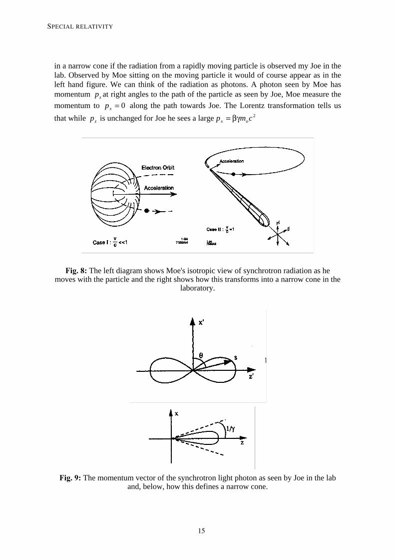
in a narrow cone if the radiation from a rapidly moving particle is observed my Joe in the lab. Observed by Moe sitting on the moving particle it would of course appear as in the left hand figure. We can think of the radiation as photons. A photon seen by Moe has momentum zp at right angles to the path of the particle as seen by Joe, Moe measure the momentum to 0=xp along the path towards Joe. The Lorentz transformation tells us that while zp is unchanged for Joe he sees a large 2cmp ox βγ=

Fig. 8: The left diagram shows Moe's isotropic view of synchrotron radiation as he moves with the particle and the right shows how this transforms into a narrow cone in the

laboratory.

Fig. 9: The momentum vector of the synchrotron light photon as seen by Joe in the lab

and, below, how this defines a narrow cone.

SPECIAL RELATIVITY

15

Figure 9 shows above the momentum vector of the photon (labeled s) seen by Joe

in the lab and below how the isotropic distribution of photons in the moving system appears as a forward cone of opening angle γ/1 to Joe in his lab.

TRANSFORMING ELECTRIC AND MAGNETIC FIELDS Finally and to be complete we include the transformation matrix for a six vector whose components are the three components of electric field and those of magnetic field multiplied (in MKS notation) by c.

⎟⎟⎟⎟⎟⎟⎟⎟

⎠

⎞

⎜⎜⎜⎜⎜⎜⎜⎜

⎝

⎛

⎟⎟⎟⎟⎟⎟⎟⎟

⎠

⎞

⎜⎜⎜⎜⎜⎜⎜⎜

⎝

⎛

γγβγγβ−

γβ−γγβγ

=

⎟⎟⎟⎟⎟⎟⎟⎟

⎠

⎞

⎜⎜⎜⎜⎜⎜⎜⎜

⎝

⎛

z

y

x

z

y

x

z

y

x

z

y

x

cBcBcBEEE

cBcBcBEEE

2

2

2

2

2

2

1

1

1

1

1

1

000000000010000000

0000000001

.

CONCLUSIONS

This is really as far as one needs to go to understand special relativity and apply it to particle accelerators. Once one gets used to using invariant quantities and the laws of physics in invariant form it is often simple to solve a problem in the moving system of the particle and transform the solution into the lab or vice versa. We already have found this in dealing with synchrotron radiation. Another example is that of space charge which is particularly simple in the frame of reference of the mobbing bunch where fields are simply electrostatic.

E.J.N. WILSON

16

1

TRANSVERSE MOTION E. J. N. Wilson CERN, Geneva

Abstract Transverse dynamics lies at the heart of modern synchrotron design. Considerable economies are to be had by intelligent choice of the arrangement of focusing magnets: the lattice. In this lecture we concentrate on the description of the magnetic focusing systems of a synchrotron. The effect of momentum spread on the beam’s central orbit (dispersion) and the change in betatron oscillation frequency with momentum (chromaticity) are also analysed. We leave the effect of synchrotron radiation emission and the beam growth and damping to later lectures.

1. DESCRIPTION OF MOTION

Fig. 1 Charged particle orbit in a magnetic field.

The bending fields of a synchrotron are usually vertically directed, causing the particle to follow a curved path in the horizontal plane (Fig. 1). The force acting on the particle is horizontal and is given by:

F = e v × B where: v is the velocity of the charged particle in the direction tangential to its path

and B is the magnetic guide field.

If the guide field is uniform, the ideal motion of the particle is simply a circle of radius of curvature, ρ. but we can also define a local radius of curvature, ρ(s), to describe motion in a non-uniform field. We shall suppose that it is possible to find an orbit or curved path for the particle which closes on itself around the synchrotron which we call the equilibrium orbit. The machine is usually designed with this orbit at the centre of its vacuum chamber.

17

2

2. BENDING MAGNETS AND MAGNETIC RIGIDITY Let us now examine how a particle is deflected in a simple dipole bending

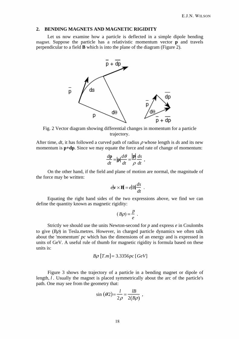
magnet. Suppose the particle has a relativistic momentum vector p and travels perpendicular to a field B which is into the plane of the diagram (Figure 2).

Fig. 2 Vector diagram showing differential changes in momentum for a particle

trajectory.

After time, dt, it has followed a curved path of radius ρ whose length is ds and its new momentum is p+dp. Since we may equate the force and rate of change of momentum:

dpdt

= pdθdt

=pρ

dsdt

,

On the other hand, if the field and plane of motion are normal, the magnitude of the force may be written:

e v × B = e B

dsdt

.

Equating the right hand sides of the two expressions above, we find we can define the quantity known as magnetic rigidity:

Bρ( ) =

pe

.

Strictly we should use the units Newton-second for p and express e in Coulombs to give (Bρ) in Tesla.metres. However, in charged particle dynamics we often talk about the 'momentum' pc which has the dimensions of an energy and is expressed in units of GeV. A useful rule of thumb for magnetic rigidity is formula based on these units is:

Bρ T.m[ ]= 3.3356pc [GeV]

Figure 3 shows the trajectory of a particle in a bending magnet or dipole of length, l . Usually the magnet is placed symmetrically about the arc of the particle's path. One may see from the geometry that:

sin θ/2( )=l

2ρ=

lB2 Bρ( )

,

E.J.N. WILSON

18

3

and if θ << π/2

θ ≈lBBρ( )

The bending magnet aperture must be wide enough to contain the sagitta of the beam which is the distance between the apex of the arc and the chord:

l = ±ρ 1−cos θ /2( )( )≈ ±ρθ2

8≈

lθ8

.

Fig. 3 Geometry of a particle trajectory in a bending magnet of length, l

The ends of bending magnets are often parallel but in some machines are

designed to be normal to the beam. There is a focusing effect at the end which depends on the angle of these faces. We will come back to this later. 3. FOCUSING 3.1 Displacement and divergence

A beam of particles enters the machine as a bundle of trajectories spread about the ideal orbit. At any instant a particle may be displaced horizontally by x and vertically by z from the ideal position and may also have divergence angles horizontally and vertically:

′ x = dx / ds and ′ z = dz / ds . and we see how divergence is defined in the left half of Figure 6.

Such mis-steering would cause particles to leave the vacuum pipe were it not for the carefully shaped field which restores them back towards the beam centre so that

TRANSVERSE MOTION

19

4

they oscillate about the ideal orbit. The design of the restoring fields determines the transverse excursions of the beam and the size of the cross section of the magnets and is therefore of crucial importance to the cost of a project. 3.2 Weak Focussing

The first generation of synchrotrons upon the curved shape of the field at the open side of their “C” shaped magnets to provide vertical focusing forces to restore particles towards the mid-plane of the synchrotron. The curvature of the lines ensured that the force on circulating particles had a vertical component – deflecting downward above the mid-plane and upward below. (Figure 4)

Fig. 4. Cross section of a constant gradient synchrotron ring illustrating focusing The curvature was enhanced by tapering the pole gap towards the outside to

produce a constant field gradient both across the aperture and around the machine. Horizontal focusing was provided by the effect of an imbalance between the force due to the guide field and the smaller radial acceleration of a particle in an outer and larger radius orbit. The acceleration towards the reference orbit, radius ρ , is just:

1ρ2 x

Unfortunately the field gradient, though focusing in the vertical plane produces a defocusing effect in the horizontal direction and could easily swamp this weak horizontal focusing effect. Thus the focusing forces had to be kept rather weak, which led to large amplitudes of oscillation of particles about the centre line of the machine. The cross section of the vacuum chamber and the magnet gap had to be often 20 cm by 100 cm.

Nevertheless this kind of machine has the virtue that it is easy to understand the motion of particles as they oscillate about the axis in a uniform focussing environment. 3.3 The gutter analogy

Fig. 5 Two views of a sphere rolling down a gutter as it is focused by the walls.

E.J.N. WILSON

20

5

It is important to start with a tangible concept of focusing and so we consider an analogy to the focusing system of the weak focusing synchrotron. We suppose that a particle oscillates in this focusing system like a small sphere rolling down a slightly inclined gutter with constant speed. Figure 5 shows two views of this motion and from the right hand view we recognise the motion as a sine wave. Note too that the sphere makes four complete oscillations along the gutter. In the language of accelerators we shall learn to characterise this aspect of its motion by the wave number, Q = 4.

Now let us extend this analogy by bending the gutter into a circle rather like the brim of a hat. Suppose we provide the necessary instrumentation to measure the displacement of the sphere from the centre of the gutter each time it passes a given mark on the brim and we also have a means to measure its transverse velocity. With the aid of a computer, we might convert this information into the divergence angle shown in Fig. 6:

x' =dxds

=v⊥

v||

.

Suppose also that we make the brim of a hat out of a slightly different length of gutter than is shown so that Q is not an integer. We can plot a point (x, ′ x ) each time the sphere makes a turn of the brim in what we call a ‘phase space diagram’ of transverse motion. The sphere has a large transverse velocity as it crosses the axis of the gutter and has almost zero transverse velocity as it reaches its maximum displacement.

The locus of these ‘observations’ will be an ellipse (Fig. 6) and the phase of the motion (the angle subtended at the origin) will advance by Q revolutions each time the particle returns to the detector. Of course, only the fractional part of Q may be deduced from our observations since we are blind to what happens round the rest of the hat’s brim – a situation we shall find is common in the real life of accelerators.

Fig. 6 The elliptical locus of a particle's history in phase space as it circulates in a

synchrotron.

In order to establish concepts which will take us from the gutter analogy to real synchrotrons we have to define some of the transverse beam dynamical quantities

TRANSVERSE MOTION

21

6

more rigorously. The area of the ellipse is a measure of how much the particle departs from the ideal trajectory which in the diagram is represented by the origin:

Area = πε [mm.rad] .

In accelerator notation we use ε, the product of the semi-axes of the ellipse as a measure of the area called the emittance. The emittance is usually quoted in units of π mm.mradians.

The maximum excursion in displacement, the major axis, of the ellipse defined:

εβ=x

and hence ˆ ′ x = ε /β

Note that the aspect ratio of the ellipse is just β. We will return to these

quantities when we have studied more about the alternating gradient focusing systems in which the steepness of the sides of the gutter varies as we go around the ring and can even change sign. We shall see that in these circumstances β varies around the ring and becomes an envelope with in which the oscillating particles are constrained. 3.4 Alternating gradient focusing

The discovery of alternating gradient focusing (Courant et al. 1958) was a major break-through in the design of synchrotrons which allowed designers to use much stronger focusing forces in both vertical and horizontal planes. It happened almost by accident as E. Courant, then working on the effect that the modulation of the “constant” gradient would produce when some of the magnets of weak focusing Cosmotron were reversed in gradient. To his surprise he found the effect to be strikingly beneficial. Taking this gradient reversal to the extreme allowed much stronger focusing systems to be used with considerable savings in the space needed for the beam cross section.

Fig. 7 Optical analogy in which an alternating pattern of lenses.

The principle of this alternating gradient focusing is illustrated in Fig. 7 where we see an optical system in which each lens is concave in one plane while convex in

E.J.N. WILSON

22

7

the other. It is possible, even with lenses of equal strength, to find a ray which is always on axis at the D lenses in the horizontal plane and therefore only sees the F lenses. The spacing of the lenses has to be twice their focal length, f. If the ray is also central in the lenses which are vertically defocusing, the same condition will apply simultaneously in the vertical plane. At least one particular particle or trajectory corresponding to this ray will be contained indefinitely.The alternating gradient idea will work even when the rays in the D lenses do not pass dead centre and the lenses are not spaced by exactly 2f. In fact it is sufficient for the particle trajectories to tend to be closer to the axis in D lenses than in F lenses as shown in Fig. 8.

Fig. 8 The paths of particles within a FODO lattice are within the envelope of

betatron motion and, like the rays of Fig. 7, are always closer in the D quadrupoles.

By suitable choice of strength and spacing of the lenses the envelope function, which was constant for the gutter which we used as an analogy for representing a weak focussing machine, now varies around the ring and the parameter β is a function: β(s). Symmetry tells us it will be periodic and by suitable choice of lens strength we can ensure that it is large at all F quadrupoles and small at all D's. The picture will be in the vertical plane but displaced by the distance between quadrupoles. Particles oscillating within this envelope will always tend to be further

TRANSVERSE MOTION

23

8

off axis in F quadrupoles than in D quadrupoles and there will therefore be a net focusing action. We have already seen that β is the aspect ratio of the phase space ellipse. At F quadrupoles the ellipse will be squat and at D quadrupoles it will be tall. We shall go on to define this envelope or betatron amplitude more rigorously and establish how to calculate it for a given lattice of focusing magnets. See also Schmüser (1987) and Rossbach et al. (1992). 3.5 Quadrupole magnets

Fig. 9 Components of field and force in a magnetic quadrupole. Positive ions

approach the reader on paths parallel to the s axis. (Livingood 1961).

The lenses elements in a modern alternating gradient synchrotron are quadrupole magnets. The poles are truncated rectangular hyperbolae and alternate in polarity. Figure 9 shows a particle's view of the fields and forces in the aperture of a quadrupole as it passes through normal to the plane of the paper. The field shape is such that it is zero on the axis of the device but its strength rises linearly with distance from the axis. This can be seen from a superficial examination of Fig. 9 if we remember that the product of field and length of a field line joining the poles is a constant. Symmetry tells us that the field is vertical in the median plane (and purely horizontal in the vertical plane of asymmetry). The field must be downwards on the left of the axis if it is upwards on the right.

This last observation ensures that the horizontal focusing force, - evBz, has an inward direction on both sides and, like the restoring force of a spring, rises linearly with displacement, x. The strength of the quadrupole is characterised by its gradient dBz/dx normalised with respect to magnetic rigidity:

k =1

Bρ( )dBz

dx.

The angular deflection given to a particle passing through a short quadrupole of length, and strength, k , at a displacement x is therefore:

(This is just another application for the formula we derived for deflection in a bending magnet.) Compare this with a converging lens in optics:

Δ ′ x = −x / f

Δ ′ x =Bl

(Bρ)= kl

E.J.N. WILSON

24

9

and we see that the focal length of a horizontally focusing quadrupole is f = −1/(kl)

The particular quadrupole shown in Fig. 9 would focus positive particles

coming out of the paper or negative particles going into the paper in the horizontal plane. A closer examination reveals that such a quadrupole deflects particles with a vertical displacement away from the axis – vertical displacements are defocused. This can be seen this if Fig. 9 is rotated through 90 degrees. It was this feature that discouraged the use of quadrupoles for focussing until the discovery of alternating gradient focussing. 4. BETATRON ENVELOPES During the design phase of an accelerator project a considerable amount of calculation and discussion centres around the choice of the transverse focusing system. The pattern of bending and focusing magnets, called the lattice, has a strong influence on the aperture of the bending and focusing magnets which are usually the most expensive single system in the accelerator and which, in turn can have an important effect on the design of almost all other systems in the synchrotron.

Fig. 10 One cell of the CERN SPS representing 1/108 of the circumference. The pattern of dipole (B) magnets and quadrupole (F and D) lenses is shown above.

A modern synchrotron consists of pure bending magnets and quadrupole magnets or lenses which provide focusing. These are interspersed among the bending magnets of the ring in a pattern called the lattice. In Fig. 10 we see an example of such a magnet pattern which is one cell, or about 1% of the circumference, of the 400 GeV SPS at CERN. Although the SPS is now considered a rather old fashioned machine, its

TRANSVERSE MOTION

25

10

simplicity makes it an excellent example for teaching purposes. For obvious reasons this focusing structure is called FODO and in this pattern half of the quadrupoles focus, while the other half, defocus the beam. The envelope of these oscillations follows a function β s( ) which has waists near each defocusing magnet and has a maximum at the centres of F quadrupoles. Since F quadrupoles in the horizontal plane are D quadrupoles vertically, and vice versa, the two functions βh s( ) and β v s( ) are one half-cell out of register in the two transverse planes. The function β has the dimensions of length but the units bear no relation at this stage to physical beam size. The reader should be clear that particles do not follow the β s( ) curves but oscillate within them in a form of modified sinusoidal motion whose phase advance is described by φ(s). The phase change per cell in the example shown, is close to π/2 but the rate of phase advance is modulated throughout the cell. 5. THE EQUATION OF MOTION

In the last section we derived an expression for the change in divergence of a particle passing through the quadrupole. The strength of the quadrupole is characterised by its gradient dBz / dx , normalised with respect to magnetic rigidity:

k =

1Bρ( )

dBzdx

If k is negative, the quadrupole is horizontally focusing and vertically defocusing. We first look at the vertical plane. The angular deflection given to a particle passing through a short quadrupole of length ds and strength k at a displacement z is therefore:

d ′ z = −kzds We can deduce from this a differential equation for the motion

′ ′ z + k(s)z = 0 .

This is called Hill's Equation, a second order linear equation with a periodic coefficient, k(s) which describes the distribution of focusing strength around the ring. The above form of Hill’s equation applies to motion in the vertical plane while in the horizontal plane:

′ ′ x +1

ρ(s)2 − k(s)⎡

⎣ ⎢ ⎢

⎤

⎦ ⎥ ⎥ x = 0

Here the sign before k(s) is reversed so that the quadrupole defocuses. We

include an extra focusing term due to the curvature of the orbit which we found was the only horizontal focussing mechanism in weak focusing synchrotrons. We include this term since it can be significant in small radius rings. 6. SOLUTION OF HILL'S EQUATION Hill’s equation is reminiscent of simple harmonic motion but has a restoring constant k(s) which varies around the accelerator. In order to arrive at a solution we must first assume that k(s) is periodic on the scale of one turn of the ring. The period can also be a smaller unit, the cell, from which the ring is built. The solution, like the differential equation itself, is reminiscent of simple harmonic motion:

x = β(s)ε cos φ(s)+φ0[ ]

E.J.N. WILSON

26

11

In simple harmonic motion the amplitude is a constant but here we see that in addition to ε , which can be considered an arbitrary constant, there is another amplitude component, the function β s( ) . Another difference from harmonic motion is that phase, φ(s), does not advance linearly with time and with distance, s , around the ring. Both these functions of s must have the same periodicity as the lattice and they are linked by the condition:

′ ϕ =1 / β or ϕ = ds / β∫

.

We shall later show that this condition is necessary if Hill's Equation is to be satisfied but for the moment let us just accept it. By simple differentiation we can then find

x = β(s)ε cos φ(s) +φ0[ ]′ x = − ε / β(s) sin φ(s) +φ0[ ]+ ′ β (s) /2[ ] ε /β (s) cos φ(s) +φ0[ ]

We look at this function at points of symmetry, mid-way through an F or D quadrupole where ′ β s( ) is zero and hence where the second term in the divergence equation is zero. We then find that the locus of a particles motion returning to this observation point is an ellipse with semi-axis in the x - direction βε , and in the

′ x - direction ε / β s( ) (Fig. 6). Its area is πε , where ε is an invariant of the motion for a single particle or the emittance of a beam of many particles. 6.1 Smooth approximation

Older accelerators, constant gradient machines simple harmonic motion is a very close approximation to reality. In the vertical plane the particles obey the differential equation

d2zds2 + kx = 0

If we think of this as analogous to a travelling wave

d2zds2 +

2πλ

⎛ ⎝ ⎜ ⎞

⎠ ⎟

2z = 0

The solution of such an equation is a wave whose length is λ namely:

z = z0 sin 2π λ( )s = z0 sinφ . We can see that the derivative of phase is:

′ φ = 2π λ( )

but earlier we mentioned that to find a solution to Hill’s equation the phase derivative must be 1 / β to be equal to this derivative. We can therefore argue that β is a local wavelength (multiplied by 2π) of the oscillation. This may help us to understand the way in which β and φ vary in the cells of a FODO lattice. 6.2 Q-value

Let us now look at the definition of a quantity, Q , the betatron wave number. Suppose, we again consider a constant gradient machine. The particle with the largest

TRANSVERSE MOTION

27

12

amplitude in the beam, βε , starts off with phase φ0 , and after one turn its phase has increased by

Δϕ = ds β∫ = 2πR β

.

It has been round the ellipse Δϕ / 2π times. The number of such betatron oscillations per turn to be Q , the betatron wave number. Using the above relation we see that for a constant gradient machine

Q =

Δϕ2π

=Rβ

or β = R Q

This is approximately true for alternating gradient machines as well, and is often used in juggling machine parameters at the design stage because the choice of Q determines β and hence beam size.

It is very important that Q is not be a simple integer or vulgar fraction, otherwise, over one or more paths around the ellipse, the particle will repeat its path in the machine and see the same field imperfections. These will then build up into a resonant growth. The condition to be avoided is nQ = p (where n and p are integers). This can be done by tuning the restoring gradients of the quadrupoles.

7. MATRIX DESCRIPTION From now on we deal only with alternating gradient (AG) machines in which the ring is a repetitive pattern of focusing fields, the lattice. Each lattice element may be expressed by a matrix.

Whole sections of the ring which transport the beam from place to place may also be represented as a matrix. Any linear differential equation, like Hill's Equation, has solutions which can be traced from one point, s1 , to another, s2 , by a 2 × 2 matrix: the transport matrix:

y(s2)′ y (s2)

⎛

⎝ ⎜ ⎜

⎞

⎠ ⎟ ⎟ =

a bc d⎛

⎝ ⎜

⎞

⎠ ⎟

y(s1)′ y (s1)

⎛

⎝ ⎜ ⎜

⎞

⎠ ⎟ ⎟ = M21

y(s1)′ y (s1)

⎛

⎝ ⎜ ⎜

⎞

⎠ ⎟ ⎟

.

There are two ways of thinking of these transport matrices. First of all there is the matrix fro one turn of the accelerator ring (or for one period that repeats) which we call the Twiss matrix. We shall show that each term in M21 is a simple function of β s( ) and φ s( ) . As an alternative description of the ring wee can also write down rather simple forms for the matrices of each quadrupole, bending magnet and drift length which we can write down as simple numbers depending on the length and strength of each component. The functions β s( ) and φ s( ) may be calculated by comparing the numerical result of multiplying the individual matrices for quadrupoles and drift lengths in the ring with what we know must be the general form of each element. But we are moving too fast. Our first job is to derive the general form of a periodic transport matrix.

E.J.N. WILSON

28

13

7.1 The Twiss matrix

We shall simplify the notation by dropping the explicit dependence of β and ϕ on s from the expressions - we will just have to remember that they vary with s. We also introduce a new quantity:

w = β

In this new notation we can write the solution of the Hill Equation:

y = ε1/2w cos ϕ + φ0( ) . By taking the derivative and substituting ′ ϕ = 1/ β = 1/ w2 we have:

( ) ( )0

2/1

02/1 φϕεφϕε +−+′=′ sin cos

wwy

.

The next step is to substitute these explicit expressions for y and ′ y in both sides of the matrix equation. We do this first with the initial condition on the right hand side, ϕ0 = 0 , This is the so-called ‘cosine’ solution. Writing the matrix equation in “long hand” we find we have two equations – for y after the matrix operation and the other for ′ y . We can do this again starting from the ‘sine’ solution with

ϕ0 = π / 2 . This is exactly equivalent to tracing the paraxial and central rays through an optical lens system. We write φ2 −φ1 =φ for each case. Thus we obtain two more equations making in all four simultaneous equations which can be solved to find the four transport matrix elements, a, b, c, d in terms of w, w', and ϕ . The result, for anyone with the patience to pursue this process, is the most general form of the transport matrix which will take you from any point in the ring to another:

M12 =

w2w1

cos ϕ − w2 ′ w 1 sin ϕ w1w2 sin ϕ

− 1+w1 ′ w 1w2 ′ w 2w1w2

sin ϕ − ′ w 1w2

− w2w1

⎛

⎝ ⎜ ⎜

⎞

⎠ ⎟ ⎟ cos ϕ w1

w2cosϕ + w1 ′ w 2 sin ϕ

⎛

⎝

⎜ ⎜ ⎜ ⎜ ⎜

⎞

⎠

⎟ ⎟ ⎟ ⎟ ⎟ .

At first glance this seems to have complicated the issue but we still have some constraints to apply. The first of these is to restrict M to be between two identical points in successive turns or cells of a periodic structure. This forces w2 = w1

′ w 2 = ′ w 1 and ϕ to become μ , the phase advance per cell. Then:

M =cos μ − w ′ w sin μ w2sin μ

− 1+w2 ′ w 2

w2 sin μ cos μ +w ′ w sin μ

⎛

⎝

⎜ ⎜ ⎜

⎞

⎠

⎟ ⎟ ⎟

The next simplification is to invent some new functions of β or

α = −w ′ w = −′ β

2β = w2

γ =1 + w ′ w ( )2

w2 = 1+ α 2

β

⎫

⎬

⎪ ⎪ ⎪

⎭

⎪ ⎪ ⎪

TRANSVERSE MOTION

29

14

These functions (which are nothing to do with special relativity!) are a complete and compact description of the dynamics. The matrix now becomes even simpler:

M =

cos μ + α sin μ , β sin μ−γ sin μ, cos μ − α sin μ

⎛ ⎝ ⎜

⎞ ⎠ ⎟

=

a bc d⎛ ⎝ ⎜

⎞ ⎠ ⎟

.

This is the Twiss matrix. It is the basic matrix for periodic lattices and should be memorized.

7.2 Transport matrices for the components of a period Now let us explore the alternative matrix approach – that of multiplying a large

number of component matrices together. The simplest of these component matrices is the one for an empty space or drift length. Figure 11 (a) shows the analogy between a particle trajectory and a diverging ray in optics. The angle of the ray and the divergence of the trajectory are related:

θ = tan−1 ′ x ( ) .

The effect of a drift length in phase space is a simple horizontal translation from (x, x') to ( )xxx ′′+ , and can therefore be written as a matrix:

x2

′ x 2

⎛

⎝ ⎜ ⎜

⎞

⎠ ⎟ ⎟ =

1 l0 1

⎛

⎝ ⎜ ⎜

⎞

⎠ ⎟ ⎟

x1

′ x 1

⎛

⎝ ⎜ ⎜

⎞

⎠ ⎟ ⎟ .

Fig. 11 The effect of (a) a drift length and (b) a thin quadrupole seen in real space as an optical ray and a particle trajectory then plotted in phase space and expressed as a

transport matrix. The next simplest case is that of a thin quadrupole magnet of infinitely small

length but finite integrated gradient:

lk =1

(Bρ)∂Bz

∂x

E.J.N. WILSON

30

15

Figure 11(b) illustrates the optical analogy of a thin quadrupole with a converging lens. A ray, diverging from the focal point arrives at the lens at a displacement, x, and is turned parallel by a deflection:

θ ≈1f

⋅ x .

In fact this deflection will be the same for any ray at displacement x irrespective of its divergence. This behaviour can be expressed by a simple matrix, the thin lens matrix:

x2

′ x 2

⎛

⎝ ⎜ ⎜

⎞

⎠ ⎟ ⎟ =

1 0−1/ f 1

⎛

⎝ ⎜ ⎜

⎞

⎠ ⎟ ⎟

x1

′ x 1

⎛

⎝ ⎜ ⎜

⎞

⎠ ⎟ ⎟ .

A quadrupole has a a similar property. A particle arriving at a displacement x obeys Hill's equation

′ ′ x + kx = 0 hence the small deflection, θ , is just:

Δ ′ x == −klx We see that lk = 1/f and is the power of the lens and that the matrix, for a thin lens,

can be written: 1 0

−kl 1

⎛

⎝ ⎜ ⎜

⎞

⎠ ⎟ ⎟

The lenses of a synchrotron are not normally short compared to their focal length. One must therefore use the matrices for a long quadrupole when one comes to compute the final machine:

MF =cos l k 1

ksin l k

- k sin l k cos l k

⎛

⎝

⎜ ⎜ ⎜

⎞

⎠

⎟ ⎟ ⎟

and

MD =cosh l k 1

ksinh l k

k sinh l k cosh l k

⎛

⎝

⎜ ⎜ ⎜

⎞

⎠

⎟ ⎟ ⎟

These correspond to the solutions of Hill's equations in F and D cases:

z = z0cos l k +′ z 0k

sin l k

x = x0coshl k +′ x 0k

sinh l k

In this model we have ignored the bending that takes place in dipole magnets and these are thought of as drift lengths in a first approximation. However, an exact calculation must include the focusing effect of their ends. A pure sector magnet, whose ends are normal to the beam will give more deflection to a ray which passes at a displacement x away from the centre of curvature (Fig. 12). This particle will have a longer trajectory in the magnet. The effect is exactly like a lens which focuses horizontally but not vertically.

TRANSVERSE MOTION

31

16

The matrices for a sector magnet are:

MH =cos θ ρ sin θ

− 1 / ρ( ) sin θ cos θ⎛

⎝ ⎜ ⎜

⎞

⎠ ⎟ ⎟

MV =1 ρθ0 1⎛ ⎝ ⎜

⎞ ⎠ ⎟ .

Fig. 12 The focusing effect of trajectory length in a pure sector dipole magnet.

Most bending magnets are not sector magnets but have end faces which are parallel. It is easier to stack laminations this way than on a curve. The entry and exit angles are therefore, θ/2, and the horizontal focusing effect is reduced but there is an additional focusing effect for a particle whose trajectory is displaced vertically. In the computer model one may convert a pure sector magnet into a parallel faced magnet by simply adding two thin lenses at each face. They are horizontally defocusing and vertically focusing and their strength is:

There are further effects from the azimuthal shape of end fields which can be included analytically.

7.3 Comparing the two matrices to obtain the Twiss parameters Having two independent ways of describing the matrix for a turn the time has

come to compare them. We must first choose the starting point, the location, s, where we wish to know β and the other Twiss parameters. By starting at that point in the ring and multiplying the element matrices together for one turn we are able to find a, b, c, d numerically for that point. Examining the Twiss matrix and comparing with the numbers a, b, c, d we can write

cos μ =TrM

2=

a + d2

β = b / sin μ > 0

α =a − b

2 sin μγ = −c / sin μ

lk = −tan θ /2( )

ρ

E.J.N. WILSON

32

17

Solving these four equations to will the Twiss parameters and in particular β and μ. If the machine has a natural symmetry in which there are a number of identical periods, it is sufficient to do the multiplication up to the corresponding point in the next period. The values of α, β, and γ would be the same if we went on for the whole ring. Then by choosing different starting points we can trace β(s) and α(s) throughout a period.

Fortunately we have computers to help when we come to multiply these elements together to form the matrix for a ring or a period of the lattice (Servranckx et al. 1984; Garren et al. 1985; Schachinger and Talman 1985). A lattice program such as MAD (Iselin and Grote 1991) does all the matrix multiplication to obtain (a, b, c, d) from each specified point, s, and back again. It prints out β and ϕ and other lattice variables in each plane, and we can plot the result to find the beam envelope around the machine. This is the way machines are designed. Lengths, gradients, and numbers of FODO normal periods are varied to match the desired beam sizes and Q values.

It is nevertheless an interesting exercise for the student to multiply the five matrices of the FODO lattice together starting at the mid plane of the F lens and show that for lenses of focal length , f¸ spaced by a distance, L :

cos μ =1− L2 /2 f 2

sin μ/2( ) = l / 2 f

⎫ ⎬ ⎪

⎭ ⎪

β = 2L1∓ sin μ/2( )[ ]

sin μ

⎫ ⎬ ⎪

⎭ ⎪

α x,z = 0

.

8. LIOUVILLE'S THEOREM

Fig. 13 Liouville's theorem applies to this ellipse.

TRANSVERSE MOTION

33

18

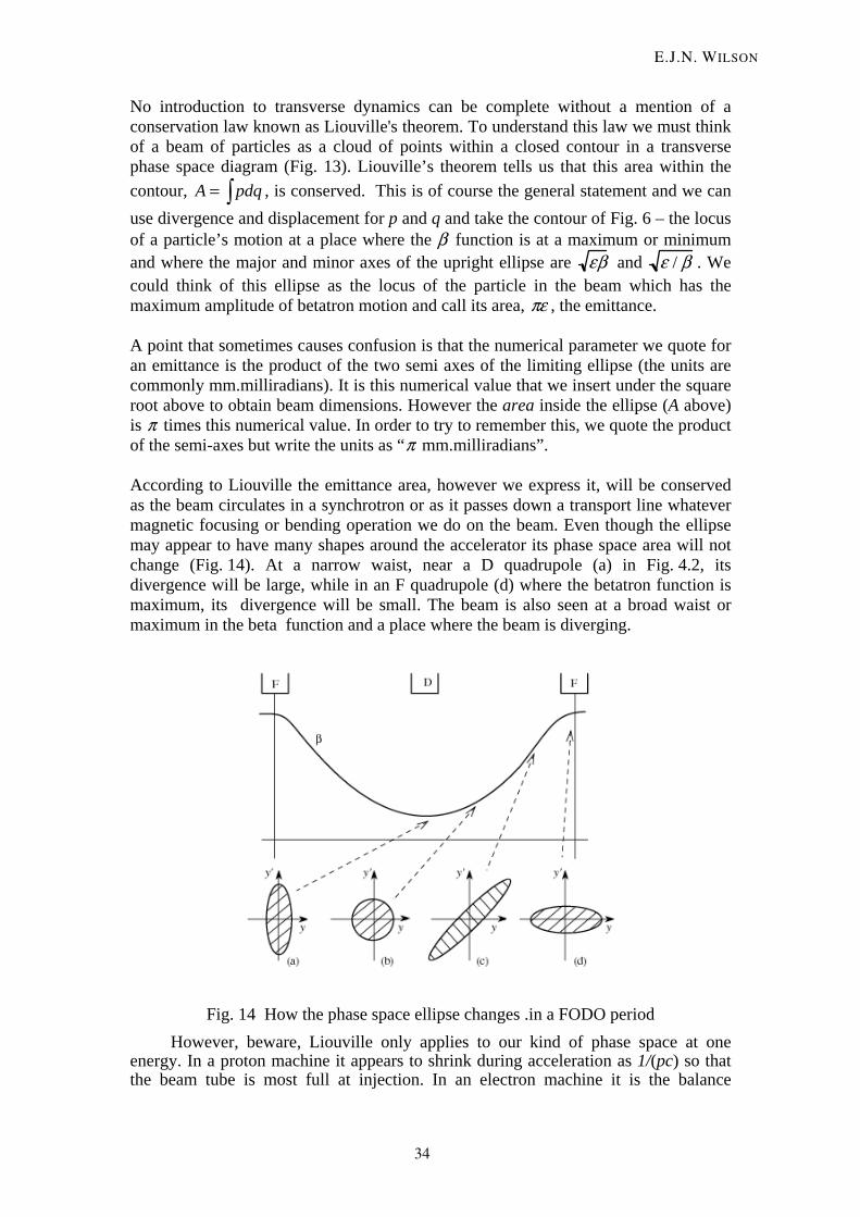
No introduction to transverse dynamics can be complete without a mention of a conservation law known as Liouville's theorem. To understand this law we must think of a beam of particles as a cloud of points within a closed contour in a transverse phase space diagram (Fig. 13). Liouville’s theorem tells us that this area within the contour, A = pdq∫ , is conserved. This is of course the general statement and we can use divergence and displacement for p and q and take the contour of Fig. 6 – the locus of a particle’s motion at a place where the β function is at a maximum or minimum and where the major and minor axes of the upright ellipse are εβ and ε / β . We could think of this ellipse as the locus of the particle in the beam which has the maximum amplitude of betatron motion and call its area, πε , the emittance. A point that sometimes causes confusion is that the numerical parameter we quote for an emittance is the product of the two semi axes of the limiting ellipse (the units are commonly mm.milliradians). It is this numerical value that we insert under the square root above to obtain beam dimensions. However the area inside the ellipse (A above) is π times this numerical value. In order to try to remember this, we quote the product of the semi-axes but write the units as “ π mm.milliradians”. According to Liouville the emittance area, however we express it, will be conserved as the beam circulates in a synchrotron or as it passes down a transport line whatever magnetic focusing or bending operation we do on the beam. Even though the ellipse may appear to have many shapes around the accelerator its phase space area will not change (Fig. 14). At a narrow waist, near a D quadrupole (a) in Fig. 4.2, its divergence will be large, while in an F quadrupole (d) where the betatron function is maximum, its divergence will be small. The beam is also seen at a broad waist or maximum in the beta function and a place where the beam is diverging.

Fig. 14 How the phase space ellipse changes .in a FODO period However, beware, Liouville only applies to our kind of phase space at one

energy. In a proton machine it appears to shrink during acceleration as 1/(pc) so that the beam tube is most full at injection. In an electron machine it is the balance

E.J.N. WILSON

34

19

between the radiation damping and quantum excitation that determines the emittance at any energy and in most machines although it will be conserved around the ring it will grow with energy. 9. DISPERSION 9.1 Closed orbit

The bending field of a synchrotron is matched to some ideal (synchronous) momentum p0 . A particle of this momentum and of zero betatron amplitude will pass down the centre of each quadrupole, be bent by exactly 2π by the bending magnets in one turn of the ring and remain synchronous with the r.f. frequency. Its path is called the central (or synchronous) momentum closed orbit. In Fig. 8. this ideal orbit was the horizontal axis. We see particles executing betatron oscillations about it but these oscillations do not replicate every turn. In contrast the synchronous orbit closes on itself so that x and x' remain zero. It is not at first obvious that such a closed orbit exists for a particle of slightly different momentum. One might think perhaps of a spiral. However we will show that there is an orbit, displaced from the axis, which closes on itself and whose shape is defined by the “dispersion” function. 9.2 Orbit of a low momentum particle

Fig. 15 Orbits in a bending magnet

. Figure 5 shows a particle with a lower momentum Δp/p < 0 and which therefore is consistently bent horizontally more in each dipole of a FODO lattice.

We might argue that the total deflection, being more than 2π would cause it to spiral in. But let us take a bird's eye view as in Figure 16. The smaller arrows represent the extra inward bending force on the low momentum particle as it passes through the dipoles but the particular orbit we have drawn passes systematically

further off axis in the F quadrupoles than in the D quadrupoles and while each quadrupole exerts a deflection

the outward deflections at the F quadrupoles predominate and, if the displacement of the orbit is large enough will compensate the extra bend at each dipole. We may describe the shape of this new closed orbit for a particle of unit Δp/p by a dispersion function D(s) which is the displacement of the orbit per unit momentum error. Thus we take the product D(s) Δp/p to obtain the displacement of the closed orbit. Note that the orbit shape is periodic like the lattice and betatron oscillations will now take place with reference to this new closed orbit.

( ) xkB

B ==ρ

ΔθΔ

TRANSVERSE MOTION

35

20

Fig.16

This clearly means the beam will be wider if it has momentum spread and the

minimum semi-aperture required for the beam will be:

av = βvεv , aH = β Hε H + D s( )Δpp

10. CHROMATICITY

Fig. 17 SPS working diamond.

E.J.N. WILSON

36

21

The operators of synchrotrons must be continually aware of the Q value of the machine in each plane and make adjustments to the focusing and defocusing quadruples to adjust Q to avoid integer values or values that are fractions like 1/3 ¼ 1/5 etc. Such values spell danger from resonant condition in which the pattern minute errors over several turn can repeat driving the beam out of the machine. Seen in a plot of both vertical and horizontal Q values these danger values appear as a forest of lines (Figure 17) which must be avoided.Unfortunately different momentum [particles will have different Q values so that the “working point” or area of the diagram covered by the population of all particles in the beam may be so large that is impossible to steer between the resonance lines..

This momentum dependence of Q is exactly equivalent to the chromatic aberration in a lens. It is defined as a quantity Q'

ΔQ = ′ Q Δpp

.

The chromaticity (Guiducci 1992) arises because the focusing strength of a quadrupole has (Bρ) in the denominator and is therefore inversely proportional to momentum:

k =1

Bρ( )dBz

dx.

A small spread in momentum in the beam, ±Δp/p, causes a spread in focusing strength:

Δkk

= −Δpp .

Fig. 18 Measurement of variation of Q with momentum made by changing the r.f.

frequency.

TRANSVERSE MOTION

37

22

An equation, which we have not the space here to derive, describes the effect of such a focussing error

ΔQ =

14π

β s( )∫ δk s( ) ds .

enables us to calculate Q' rather quickly:

ΔQ =14π

β s( )∫ δk s( )ds =−14π

β s( )∫ k s( )ds⎡ ⎣ ⎢

⎤ ⎦ ⎥

Δpp

.

The chromaticity Q' is just the quantity in square brackets. To be clear, this is called the natural chromaticity. For most alternating gradient machines, its value is about -1.3Q. Of course there are two Q values relating to horizontal and vertical oscillations and therefore two chromaticities.

One way to correct this is to introduce some focusing which gets stronger for the high momentum orbits near the outside of the vacuum chamber – a quadrupole whose gradient increases with radial position is needed. A sextupole magnet has just such a field configuration:

Bz =B"2

x2

and, in a place where there is dispersion it will introduce a normalised focusing

correction:

Δk =

B" DBρ( )

Δpp

.

The effect of this Δk on Q is:

ΔQ =14π

′ ′ B s( )β s( )D s( )dsBρ( )∫

⎡

⎣ ⎢ ⎢

⎤

⎦ ⎥ ⎥

Δpp .

To correct chromaticity we have to make the quantity in the square bracket balance the chromaticity. There are of course two chromaticities, one affecting QH, the other QV and we must therefore arrange for the sextupoles to cancel both. For this we use a trick which is common and will crop up again in other contexts. Sextupoles near F-quadrupoles where β x is large affect mainly the horizontal Q, while those near D-quadrupoles where βz is large influence Qv . The effects of two families like this are not completely orthogonal but by inverting a simple 2 x 2 matrix one can find two sextupole sets which do the job.

11. CONCLUSIONS

We have now covered the transverse dynamics of particles in a rudimentary way in preparation for more detailed lectures which follow on the effect of synchrotron radiation of the dynamics, the link with longitudinal dynamics and the effect of imperfection in the construction. We have also still to understand how a modern synchrotron may be equipped with special long straight sections for injection, accelerating systems and, for a storage ring, collision.

E.J.N. WILSON

38

23

12. REFERENCES

Courant, E. D. and Snyder, H. S. (1858), Theory of the alternating-gradient synchtrotron. Annals of Physics, 3,1-48

Schmüser, P. (1987). Basic course on accelerator optics. Proceedings of the 1986 CERN Accelerator School, CERN 87-10

Rossbach ,J. and Schmüser, P. (1992). Basic course on accelerator optics. Proceedings of the 1986 CERN Accelerator School, Jycaskyla, Finland, CERN 87-10

Livingood, J J, (1961) Principles of cyclic particle accelerators. Von Nostrand, New York.

Servranckx, R. and Brown, K. L. (1984). DIMAD, SLAC Report 270 UC-288

Garren, A, A., Kenney, A. S., Courant, E. D., and Syphers, M. J. (1985) SYNCH, Fermilab Report FN 420

Schachinger, L., and and Talman, R. (1985). TEAPOT, SSC-52

Iselin, F. C., and Grote, H. G. (1991). The MAD Program, Version 8.4, CERN/SL/90–13

Guiducci, S. (1992) Chromaticity Proceedings of the 1986 CERN Accelerator School, Jycaskyla, Finland, CERN 87-10

TRANSVERSE MOTION

39

PHASE STABILITY

J. Le Duff LAL, Orsay, France

Abstract The principle of phase stability was established independently and almost simultaneously by V. Veksler [1] and E.M. McMillan [2]. The first electron synchrotron which was designed by McMillan and built at the University of California came to full energy (320 MeV) operation early 1949.

1. INTRODUCTION

The phase stability occurs in synchronous accelerators where the acceleration is made by using radio-frequency electric fields. If successive accelerating gaps (radio-frequency cavities) are arranged such that a given particle always sees the same RF phase and gets the same energy gain, that particle is called synchronous particle. In the case of a synchrotron a single cavity will be successively traversed by the particles turn after turn and for the particular case of ultra-relativistic electrons a fixed RF frequency can fit the revolution frequency.

Other particles, either deviated in phase or in energy from the synchronous one, will oscillate in phase and energy with respect to the synchronous particle (also called reference particle) and this is the mechanism of phase stability. However stability requires specific input conditions as it will be seen in the present lecture.

2. RADIO FREQUENCY ACCELERATION

2.1 Energy gain

In relativistic dynamics the total energy ( ), the rest energy ( ) and the momentum (

2mcE = 200 cmE =

mvp = ) satisfy:

2220

2 cpEE += which by differentiation gives:

vdpdE = From Newton-Lorentz force:

zeEdzdE

dzdpvdt

dp ===

and the energy gain due to the electric field component Ez is:

∫ ==∆ eVdzEeE z where V is the voltage across the accelerating gap.

Considering an oscillating accelerating electric field ( TM mode in a cavity) one can write:

)(sinˆsinˆ tEtEE zRFzz φω ==

Neglecting the transit time through the gap one can also write:

41

φsinVeE =∆

∫= dzEV zˆˆ

and φ represents the RF phase as seen by the particle while going through the gap.

2.2 Principle of phase stability

Considering now periodic gap crossings and a reference particle for which the synchronism condition is satisfied for an entrance phase sφ , the energy gain in each gap can be represented by the RF signal shown on Fig. 1.

Fig. 1 Energy gain versus RF phase during gap crossing.

There are two possible synchronous phases ( sφ and sφπ − ) per half accelerating periods, which repeat every period. Particles P1, P2 …Pn are called synchronous particles and at each gap they get the amount of energy that bring them to the next gap with an identical phase.

As for other particles which are deviated from the synchronous ones they will get a different story. For example particle M1 which has arrived later in time in the first gap is getting more energy gain so it will run faster (assuming right now that an increase in energy, followed by an increase in velocity, reduces the time it takes to reach the next gap) and it will get closer to the synchronous particle at the next gap and so on. Particle N1 arriving earlier in the first gap is getting less energy gain, hence will slow down compare to the synchronous one and get also closer to it at the next gap. It gets clear that the tendency for non synchronous particles is to oscillate in phase and energy around the synchronous one. That is true on the positive slope of the RF signal but the same type of approach made for particles M2 and N2 shows the reverse process as they tend, gap after gap, to go further away from P2.

The capture phenomena which occurs around P1 is called “phase stability” and is similar to a focusing effect where the focusing force is just the slope of the RF signal. Since it applies on the phase and energy variables it can be called “longitudinal focusing” by analogy with magnetic focusing in the transverse plane.

J. LE DUFF

42

2.3 Consequence of phase stability

Noticing that a particle which is behind the reference one ( 0<∆z ) arrives later in the accelerating gap ( ); hence the positive RF slope which gives stability is translated into a negative slope when changing variable:

0>∆ t

00 <∂∂→>∂

∂z

EtV z

According to Maxell’s equations:

0=∇E

r

leading to:

0>∂∂

+∂∂

yE

xE yx

showing that one or another (or both) of these two gradients has to be positive leading to a transverse defocusing.

3. THE ELECTRON SYNCHROTRON

3.1 Principle of operation

The synchrotron, as sketched on Fig.2, is a synchronous circular accelerator and the reference (synchronous) particle, at nominal energy, travels on a fixed closed orbit. In order to do so, while ramping in energy, the synchronous particle is such that its synchronous RF phase provides the exact amount of energy gain, at each turn, that fits the increase of the magnetic fields.

The cavity located in a straight section will give a synchronousenergy gain:

sVeE φsinˆ=∆

In order to stay on the given circumference C Rπ2= , where Ris defined as the physical radius, the following relation needs tobe satisfied:

peB =ρ

where B is the bending field, ρ the bending radius and p the particle momentum.

Fig. 2 The synchrotron

Ramping in energy, while ρ remains constant, also means:

Bedtdp &ρ=

where dtdBB =& .

PHASE STABILITY

43

Since generally the revolution period, T , and the momentum gained per turn, , are rather small quantities one can approximate as follows:

r ( )turnp∆

( ) vBReTBep rturn

&& ρπρ 2=≈∆

where is the particle velocity. v

Since: pvE ∆=∆

one gets the relationship between the required synchronous phase and the ramping rate of the magnetic field:

sVBR φπρ sinˆ2 =&

which can be fulfilled if V is sufficiently large. ˆ

Let’s also mention that since, in general, the synchronism requires a constant phase sφ at each turn, the RF frequency needs to be an integer multiple of the revolution frequency ( rRF hωω = ). In practice the RF frequency needs to be varied to follow the increase of the particle velocity. However in the case of electrons ,which are ultra-relativistic, their velocity will remain constant ( ) during the energy ramping and consequently the RF frequency will be kept constant.

cv =

3.2 Dispersion effects due to the bending magnets

Since bending magnets, like spectrometers, will analyze particle energies, any particle which is slightly shifted in energy (or momentum) with respect to the reference particle will perform a different orbit. Fig. 3, though the sketch is very rough, is intended to show the change in circumference due to an energy deviation.

It is usual to introduce two parameters to describe the dispersion effects. The “momentum compaction factor” gives, to first order, the relative change in the circumference due to a relative momentum deviation:

dpdR

Rp=α

while the parameter “η ” gives the corresponding relative change in the revolution frequency, which takes also account of the change in velocity:

dpdf

fp r

r=η

Fig. 3 Orbit versus energy

3.2.1 Momentum compaction Consider two particles, with different energies, going through a bending magnet as shown on Fig. 4. To a momentum deviation corresponds an orbit shifted by an amount in the plane of curvature. The corresponding relative change in path length is:

dp )( 0sx

J. LE DUFF

44

ρx

dsdsds

dsdl =−=

0

0

0

Integrating over the whole circumference gives:

∫ ∫ ===m

xdsdsxdRdl 0012 ρρπ ∫

leading to:

mxdR >=< where the subscript « m » tells that the integral is performed only in the bending magnets where ρ is finite.Introducing the dispersion function , property of the lattice arrangement:

xD

pdpDx x=

Fig. 4 Orbits in bending magnets

the momentum compaction simply becomes:

RD mx ><=α

3.2.2 Revolution frequency versus momentum

Since Rcfr π

β2= , with c

v=β , a relative change in the revolution frequency can be expressed as:

RdRd

fdf

r

r −= ββ

Expressing the momentum:

cEmvp 0βγ==

one gets for its relative change:

( )( )

( ) βββ

β

βββ ddd

pdp 12

21

2

21

21

1

1 −

−

−

−=−

−+=

and finally:

pdp

fdf

r

r

−= αγ 2

1

PHASE STABILITY

45

From the definition of the parameter η one gets:

αγη −= 21

showing that there is an energy, called “transition energy”, for which the synchrotron gets isochronous ( 0=η ):

αγ 1=tr

3.3 Phase stability in an electron synchrotron

Since in an electron synchrotron γ is generally very large, one can easily assume that αη −≈ . Since all operating electron synchrotrons have a positive momentum compaction they do have η < 0 and so they stand above transition energy.

In such conditions a small positive momentum deviation ( > 0 ) will be followed by a small negative revolution frequency change ( < 0 ), or in other words by a longer revolution time. This is explained by the fact that the velocity of the particle is no longer depending on the energy (

dp

rdfcv ≈ )

and then the revolution time only depends on the circumference, which indeed gets longer for a small increase in energy.

Back to Fig. 1, if P1 still represents a synchronous particle for the synchrotron, then particle M1 which arrives later in the cavity will have a higher energy gain, hence a longer revolution period, and will be delayed even more with respect to the reference particle; as for particle N1, a similar story will happen and it will get more and more deviated from P1 as they travel around the synchrotron. Clearly P1 has become an unstable reference point.

It is straightforward to demonstrate that the reverse process will occur around P2 , which turns out to be the stable reference now. In other words the phase stability in an electron synchrotron is obtained on the negative slope of the RF signal. The stable synchronous phase has become sφπ − .

4. LONGITUDINAL DYNAMICS

4.1 Energy and phase variables

The RF acceleration process clearly emphasizes the correlation between the RF phase experienced by a particle and its energy gain. Since by definition there is a well defined synchronous particle which always feel the same RF phase at each turn, and which has the nominal energy, it is then sufficient to follow other particles with respect to that reference particle. Consequently, in what follows, one will make use of reduced variables:

Revolution frequency: rsrr fff −=∆ Particle RF phase: sφφφ −=∆ Particle momentum : sppp −=∆

Particle energy : sEEE −=∆ Azimuthal angle : sθθθ −=∆

J. LE DUFF

46

4.2 First energy-phase equation

The azimuthal variable θ ( Fig. 5 ) is defined such that θRdds =0 , where is the position along the nominal circumference

0sRπ2r

, no matter if the synchrotron is a pure circle or not. Introducing the angular revolution frequency rfπω 2= , one can write: ∫= dtrωθ

Since in the electron case ( ): cv ≈

Assuming the RF frequency is an integer multiple of the revolution frequency, rsRF hωω = , h being the harmonic number, then the RF phase will rotate h times faster than the azimuthal angle. Distance between two particles can now be either expressed through one or another variable:

θφ ∆−=∆ h where the – sign just shows that a particle behind ( 0<∆θ ) arrives later in the cavity ( 0>∆φ ). For any particle with respect to the reference, one can write:

( ) ( ) φφθω &hdt

dhdt

dr

11 −=∆−=∆=∆

Fig. 5 Azimuthal variable

αωω

ωωη −≈

=

=

s

r

rs

s

s

r

rs

s

dEdE

dpdp

one gets a first order differential equation that relates the relative energy deviation to the time derivative of the phase deviation:

φαφ

αω&

hcR

dtd

hEE

rss==∆ 1

knowing that the synchronous phase is a constant.

4.3 Second energy-phase equation

The energy gained by a particle at each turn is , and when compare to the reference’s one it becomes:

φsinVe

( ) ( )sturn VeE φφ sinsinˆ −=∆

The rate of relative energy gain can be approximated to first order:

( ) ( ) ( )srsturn VeR

cfEdtEd φφπ sinsinˆ

2 −=∆≈∆

leading to the second first order differential equation that relates the time derivative of the relative energy deviation to the phase deviation:

PHASE STABILITY

47

( )sss RE

VecEE

dtd φφπ sinsin2

ˆ−=

∆

where it is assumed that is either constant or slow varying. sE

Note that in the case of an electron synchrotron the synchronous phase will be always finite, to compensate for the energy losses due to synchrotron radiation, even if is kept constant ( ). sE 0=B&

4.4 Small amplitude oscillations

Considering small phase deviations from the reference particle one can expand the trigonometric function in the previous differential equation:

φπφ ∆≈

∆

s

s

s REVec

EE

dtd

2cosˆ

By differentiating the first energy-phase equation one gets:

∆=

sEE

dtd

Rhcαφ&&

keeping in mind that ( ) φφ &&=∆2

2

dtd since sφ is constant. Combining the above two equations leads to

a second order equation for the phase motion:

02 =∆Ω+ φφ s&&

s

ss E

VehRc

πφα

2cosˆ2

2

−=Ω

Provided is a real and positive number the equation will describe a simple harmonic

oscillation. Since

2sΩα is positive, a stable oscillation needs cos 0<sφ , which corresponds to the

negative slope of the RF signal ( πφπ << s2 ), as already mentioned before. Note that sin 0>sφ is

the choice previously made for having an acceleration.

Since the first derivative of the phase is proportional to the energy , the energy will oscillate

around the nominal one with a 2π phase difference as compared to the phase oscillation. In other

words, when the phase deviation is at maximum the energy deviation is zero and vice versa.

4.5 Large amplitude oscillations

For large phase deviations the second order equation is non linear:

( ) 0sinsincos2

=−Ω+ ss

s φφφφ&&

Multiplying by and integrating leads to an invariant of the motion: φ&

J. LE DUFF

48

( ) Iss

s =+Ω− φφφφφ sincoscos2

22&

which, for small phase deviations, reduces to the quadratic form:

( ) Is =∆Ω+ 22

22

2 φφ&

Since sEE∆∝φ& , the invariant represents a closed trajectory in the phase space (

sEE∆∆ ,φ ). These

trajectories are ellipses for the small amplitude case but they change shape as the amplitude gets larger and need to be numerically calculated. The corresponding curves, also known as Bohm and Foldy

diagram [3], with normalized variables ( φφ ,sΩ&

), are shown on Fig. 6 for the particular case

0150=sφ .

Fig. 6 Bohm & Foldy Diagram

In the second order equation of phase motion it can be seen that when the phase φ reaches the

value sφπ − , the driving force goes to zero and beyond it changes sign and become a defocusing type force.

Hence sφπ − represents an extreme amplitude for stable motion and the corresponding curve in the phase space is called the separatrix ( the outer curve on Fig. 6 ). Inside the area described by the separatrix the trajectories are closed curves. Outside they slip in phase showing that particles get out of synchronism ( Fig. 7 ) and in practice will be lost.

The equation of the separatrix is simply obtained by injecting one known point of the curve into

the general equation to find the corresponding value of the invariant. This point is ( sφπ −,0 ) leading to:

PHASE STABILITY

49

( ) ( ) ( ) ssss

ss

s

s φφπφπφφφφφφ sincoscossincoscos2

222

−+−Ω−=+Ω−&

where the right hand side represent the maximum value of the invariant for stable oscillations. The second value mφ , where the separatrix crosses the horizontal axis is obtained by solving the trigonometric equation:

( ) ( ) ssssmm φφπφπφφφ sincossincos −+−=+

4.6 Energy acceptance

From the equation of motion it is seen that reaches a maximum when , which corresponds to φ& 0=φ&&

sφφ = . Introducing this value into the equation of the separatrix gives:

( ) sss φπφφ tan222 22max −+Ω=&

Using the first energy-phase equation gives the maximum acceptable energy deviation:

( )21

max

ˆ

−±=

∆

sss

GhEVe

EE φπα

( ) ( )[ ]ssssG φπφφφ sin2cos2 −+=

This “RF acceptance” strongly depends on sφ and plays an important role for the electron

capture at injection and for the beam lifetime. Fig 7 shows, for an electron synchrotron, the drastic reduction of the stable area when sφ

approaches the value 2π . This fact can be understood from the slope of the RF signal which vanishes

at 2π and no restoring force is then available for stable oscillations.

Note that the vertical coordinate which is shown on Fig. 7 has the following meaning:

rs

EW ωπ ∆= 2

and is often used in the literature.

The stable area limited by the separatrix is often called “bucket” and is maximum for πφ =s , which corresponds to no acceleration. However, such a case does not happen in an electron synchrotron since particles radiate part of their energy at each turn, while going through the bending magnets, which is automatically compensated by the RF system. The synchronous particle in this case is the one which enters the cavity at an RF phase which provides the necessary energy gain to compensate for the loss per turn. The above treatment remains valid for any other particles.

The height of the bucket increases with increasing RF voltage, which allows the capture of

larger energy spread from injected bunches.

J. LE DUFF

50

The bucket also shows the phase extension of captured particles (bunch) and there will be h such bunches, equally spaced, circulating around the synchrotron. The distance between bunches equal the RF wavelength.

Fig 7 RF acceptance versus synchronous phase angle

5. FROM SYNCHROTRON TO LINAC

In an electron linac there are no bending magnets, hence there are no dispersion effects and 0=α . Provided the accelerating cavities are periodically spaced to fulfill the synchronism condition, the longitudinal dynamics treatment remains valid and one ends up with a phase oscillation frequency

. In other words the distance in phase between particles is frozen, while the energy increases, which is simply due to a frozen velocity v

0=Ωs

c= .

In an ultra-relativistic electron linac it is then important to concentrate the injected bunches on the crest of the RF signal such that all particles will get the same energy.

However at small kinetic energies, where v c≠ , which is the case for heavier particles

(protons, ions) or electrons generated at the gun voltage, the term 21γ which appears in the definition

of the η parameter, can not be neglected anymore. Then, phase and energy oscillations will exist with

γ −23

∝Ωs (neglecting the contribution from cv=β ). Note that in a linac the distance between

accelerating gaps will be mostly equal to an RF wavelength, which is more efficient, and then h=1.

PHASE STABILITY

51

6. ADIABATIC DAMPING

Though there are many physical processes that can damp the longitudinal oscillations, one of them appears to be directly generated by the acceleration process itself. It will happen in the electron synchrotron when ramping from injection energy to operating energy, but not in the ultra-relativistic linac.

As a matter of fact when varies with time, one needs to be more careful when combining the two first order energy-phase equations into one second order equation:

sE

( ) φφ ∆Ω−= sss EEdtd 2&

02 =∆Ω++ φφφ ssss EEE &&&&

which after dividing by : sE

02 =∆Ω++ φφφ ss

s

EE &&

&&

shows the existence of a damping coefficient proportional to the energy ramping rate and from the formula giving the angular oscillation frequency one has:

s

s

s

s

EE

ΩΩ−=&&

2

This shows that the phase amplitude of the oscillation will be damped during acceleration, and

the bunch length will be reduced provided all other parameters remain untouched.

Considering an adiabatic ramping, which means slow enough compared to the longitudinal oscillation period, it can be shown that the area in the phase space remains constant which finally tells that the bunch energy spread will grow during acceleration, but not the relative energy spread.

However this adiabatic damping of the longitudinal oscillations can hardly compete with the

radiation damping that is generated by the synchrotron radiation in electron synchrotrons.

REFERENCES

[1] V. Veksler, Compt. Rend. Acad. Sci. U.S.S.R., 43:444 (1944); 44:393 (1944);

J. Phys. (U.S.S.R.), 9:153 (1945).

[2] E. M. Mc Millan, Phys. Rev., 68 :143 (1945)

[3] D. Bohm and L. Foldy, Phys. Rev., 70:249 (1946) and 72:649 (1947)

J. LE DUFF

52

BIBLIOGRAPHY

M.Stanley Livingston, John P. Blewett, Particle Accelerators, Mc Graw-Hill, Book Company, INC. N.Y.,1962

H. Bruck, Accelerateurs Circulaires de Particules, Presses Universitaires de France, Paris 1966

E. Persico, E. Ferrari, S.E. Segre, Principles of Particle Accelerators, W.A. Benjamin, INC N.Y. 1968

M. Sands, The Physics of Electron Storage Rings, SLAC Report 121 (1970); also in Proceedings of the International School of Physics (Enrico Fermi), Varenna 1969, B. Touschek, Editor, Academic Press N.Y. 1971

B.W. Montague, RF Acceleration, Proceedings of the first course of the International School of Particle Accelerators, Erice, CERN 77-13, 19 July 1977

J. Le Duff, Longitudinal Beam Dynamics in Circular Accelerators, Proceedings of the CERN Accelerator School (Fifth General Accelerator Physics Course), University of Jyvaskyla, Finland, 7-18 September 1992, CERN 94-01, Vol. 1

PHASE STABILITY

53

Lattices for light sources

A. StreunPaul Scherrer Institut, CH-5232 Villigen PSI

AbstractThis paper provides guidelines on how to design the lattice (i.e., the magnet ar-rangement) of a high-brightness light source. In the introduction we look at thegeneral design framework, clarify the steps in the design process and the tech-nical engineering interfaces that the lattice designer has to take into account.Section 2 examines the lattice building-blocks, i.e., the magnets. A short de-tour through magnet design helps explain the limitations of magnet strength.This paper is not an introduction to beam dynamics. All formula relevant tounderstanding subsequent sections are summarized in Section 3 without anyderivation. Section 4 focuses on emittance and how to build a lattice to ob-tain low emittance. This is explained intuitively, then the theoretical minimumemittance and deviations from the minimum conditions are calculated in de-tail. The final section dealing with the problem of acceptance considers therequirements for beam life-time and injection efficiency. Physical acceptanceswill be discussed in some detail, whereas the broad subject of dynamic accep-tance optimization was the subject of a lecture in Zeuthen, Germany and isonly briefly summarized here.

1 Introduction1.1 Global requirementsSynchrotron light users’ demands specify the layout of a new light source:

– The highest photon energy to be obtained from the most advanced insertion devices available (interms of period length and harmonic content) sets the electron energy of the storage ring.

– The target performance in terms of brightness defines the natural, horizontal emittance of theelectron beam, and — considering diffraction-limited experiments in the X-ray range — emittancecoupling, in other words the ratio of vertical to horizontal emittance.

– The number and types of planned beamlines define the shape of the machine, i.e., the number andlength of straight sections and the symmetry of the lattice.

– Experiments expect micron photon beam stability at the location of the probe to be analysed.Thermal stability of the beamline is maintained by constant photon heat load, i.e., by constantbeam current. This requires a long beam lifetime and/or operation with top-up injection (i.e., veryfrequent refill).

– Low radiation background to the experiments also calls for long-beam lifetime and for efficientinjection into the machine, particularly in top-up operations. Both constraints require large accep-tances of the machine in order to keep particles deviating in longitudinal and transverse momentaafter scattering with residual gas atoms or each other, and in order to safely capture injected beams.

– The available area for building the machine and the beamlines limits the circumference of thelattice. This makes it more challenging to accommodate the required number of straight sectionswhile achieving the desired performance, and defines the type of magnetic arc to be used.

– Every light source needs operational flexibility and some upgrade potential for new and unfore-seeable future experiments.

– Finally, budgetary constraints on construction and operation call for simple and efficient solutions(in terms of number of magnets and magnet families, power consumption, etc.).

55

1.2 Lattice design phases and toolsThe lattice design process may be divided into four phases:

1. Preparation: Definition of performance issues and boundary conditions. Acquisition of informa-tion on available building blocks (magnets) for composing the lattice (their properties and technicallimitations).

2. Linear lattice layout: Arrangement of linear building blocks (quadrupoles and bending magnets)to obtain the desired global (i.e., concerning the lattice as a whole) quantities such as circum-ference, emittance, etc. This phase deals with the concepts of periodic cells, matching sections,insertions etc.

3. Nonlinearities: Introduction of sextupoles and RF cavities for particle stabilization with momen-tum deviations. Because of the nonlinearity of these elements, dynamic acceptance, i.e., stabilitylimits for transverse and longitudinal deviations from the reference orbit becomes the main designissue.

4. Errors: Investigation of lattice performance with magnet misalignments, multipolar errors, vibra-tions etc. and development of correction schemes. The final design phase ends with a significantprediction on the performance of the machine, and the respective tolerance requirements for thecomponents.

Not much lattice design can be done analytically, most tasks require a computer code. During the linearlayout, the designer needs a visual, dialogue-oriented code to ‘play’ with lattices and optimize theminteractively, whereas in the later design stages the exact modelling including nonlinearities and errorsis crucial to obtain predictive results. Typically, work proceeds by alternating fast, creative steps usingreduced models, and slow, consolidating runs based on more complete models. Usually one code isinsufficient to fulfil all of the tasks and switching between two or more is required. Here are somekeywords for lattice development code requirements:

– Model: complete set of elements, correct methods for tracking and concatenation, well-documentedapproximations.

– Elementary functions: beta functions and dispersions, periodic solutions, closed-orbit finder, en-ergy variations, tracking, matching.

– Toolbox: Fourier transforms of particle data (see resonance analysis), minimizaton routines (seedynamic aperture optimization, coupling suppression), linear algebra package (see orbit correc-tion).

– User convenience: editor functions, graphical user interface, editable text files.– Extended functionality: RF dimensioning, geometry plots, lifetime calculations, injection design,

alignment errors, multipolar errors, ground vibrations.– Connectivity: database access, control system access (see real machine operation).

1.3 InterfacingLattice design provides an empty machine that illustrates how single particles move around the ring andwhat equilibrium will form for an ensemble of particles. However, prediction of performance in terms ofbrightness for light sources includes the maximum beam-current to be stored. This is a complex subjectincorporating beam dynamics, vacuum and RF departments. In this paper it is assumed as given and notconsidered further. However, the lattice designer has to stay in contact with his/her colleagues from otherdepartments for several reasons:

– Vacuum: Impedance of the vacuum chamber affects maximum beam-current; pressure affectslifetime; pumps, absorbers and flanges require space.

A. STREUN

56

Fig. 1: Lattice sections as seen by the lattice designer (top) and the design engineer (bottom). Note how the spacebetween ideal magnets is consumed by coils, beam-position monitors, absorbers, pumps, etc.

– Radiofrequency: RF parameters determine momentum acceptance and other parameters directlyaffecting the lattice design.

– Diagnostics: Beam-position monitors have to be inserted at the appropriate locations (betatronphases) and also require space.

– Magnet design: Technological limits and geometrical properties of magnets determine the maxi-mum magnet strength to be used in lattice design; magnet coils need space; multipolar errors affectthe acceptance.

– Alignment: Misalignments cause orbit distortions affecting the performance and requiring correc-tion schemes.

– Mechanical engineering: Grouping magnets on stiff girders improves the robustness of the latticeto misalignments and vibrations.

– Construction: The design engineer’s blueprint shows all the devices to be installed by variousdepartments. Any conflict should be apparent in the blueprint.

The lattice designer must include the space requirements for all devices from the beginning. Fig-ure 1 illustrates this by comparing the lattice designer’s and the design engineer’s view of a lattice section.

1.4 Conventions and approximationsA curvilinear coordinate system is commonly used for describing particle motion in a storage ring, wherethe axis x points radially to the ring outside, the s-axis is the tangent to the ring, pointing forward, andthe y-axis points up. Some authors define it as a right-handed system x; y; s [1], other authors as aright-handed system x; s; y [2, 3] (which could be viewed as a left-handed x; y; s system!). Thesecond convention has the advantages that particles in the storage ring rotate mathematically positive(i.e., counter clockwise seen from above), and that for constant radius of curvature ρ the system maps toa cylindrical coordinate system r; θ; z with r = ρ+ x, θ = s/ρ, z = y [4].

Positive particles require a negative magnetic field ~B = −|By| ~y to get the appropriate Lorentzforce to form the storage ring. Since the radius of curvature of a curve in space is always positive bydefinition, the product of magnetic field and radius of curvature, also called magnetic rigidity (Bρ) [seeEq. (2) below] has to be negative.

For the practical design of a low-emittance light source usually an idealized subset of the theoret-ical beam dynamics formalism is sufficient and obtained by introducing the following approximations:

LATTICES FOR LIGHT SOURCES

57

– Highly relativistic beam, i.e., v = c, E = pc.– Small deviations from the reference axis (x, y ρ, x′, y′ 1) for validity of linear beam dynam-

ics using betatron amplitudes, emittance, betafunctions, betatron phases, etc.– Decoupling of subspaces: Synchrotron motion, i.e., dynamics in (δ,∆s) subspace is slow and thus

treated as a constant parameter over the timescales of betatron motion (‘adiabatic approximation’).Coupling between horizontal (x,x′) and vertical (y,y′) subspaces is considered to be small.

– Non-linearities are treated as perturbations.

2 Building blocksBending magnets and quadrupoles for guiding and focusing the beam are elementary building blocks forlinear lattice design. The non-linear lattice design includes sextupoles used for correcting the quadrupoles’chromatic aberrations. The real lattice, with alignment and other errors, includes small corrector dipolesand skew quadrupoles and beam-position monitors. In addition, every ring needs injection devices (kick-ers and septa), and one or more RF cavities for acceleration and longitudinal focusing. Light sources alsocontain wigglers and undulators for the production of highest flux, and synchrotron radiation brightness.

2.1 Lattice composition: local↔ globalIt is important to make a clear distinction between local properties of the building blocks and globalproperties of the lattice as noted by Forest and Hirata [5]:

“A quantity is called local if it is derivable from the individual magnet irrespective of themagnet position in the ring and even irrespective of the ring itself. For example a trajectoryof a particle through the magnet is local. [. . . ] Global information, on the contrary, isderivable only after the full ring is produced. For example the dynamic aperture has nomeaning whatsoever if we cannot iterate the one-turn map (i.e., circulate particles in themachine).”

Concatenation of building blocks is done by coordinate transformations, i.e., translations and ro-tations. For example, a vertical bending magnet can be described by a horizontal bending preceded bya 90 rotation around the longitudinal axis.

A building block may have any coordinate system, however, in practice it is either a Cartesiangeometry with parallel entrance and exit planes (x,y planes, perpendicular to s) and length L or acylindric geometry with an angle φ between the entrance and axis planes and arc length L. Obviouslycylindric geometry is more convenient for the description of bending magnets and Cartesian geometryfor other magnet types and drift spaces.

After assembling the building blocks and closing the ring, the one-turn map can be calculated: Itis the mapping of the particle vector ~X = (x, x′, y, y′, δ,∆s) from one turn to the next ~Xn

map−→ ~Xn+1

with the order of the map corresponding to the highest power in the coordinates. Thus the closed orbit isa fixed point of the one-turn map and the transfer matrix is a linearization of the one-turn map around theclosed orbit. The so-called ‘design orbit’ is just a coincidence of the closed orbit with (most) magnets’symmetry axis for the ideal lattice but is not defined a priori.

Finally, any lattice design has to be tested by tracking particles through the lattice. Trackingconcatenates all local transformation of the particle vector from block entrance to block exit includingthe coordinate transformations between blocks and implicitly applies the full one-turn map.

A. STREUN

58

2.2 Magnet multipole definitionIn the local coordinate system of a magnet the field is given as multipole expansion around the localreference axis (x=y=0) by

By(x, s, y) + iBx(x, s, y) = (Bρ)∑

n

(ian(s) + bn(s))(x+ iy)n−1 (1)

with n the multipole order and 2n the number of poles in the magnet, i.e., n = 1, 2, 3, . . . indicatingdipole, quadrupole, sextupole, etc. The bn are the regular multipoles (Bx = 0 for x = 0) and an the skewmultipoles, obtained through a rotation around the s-axis by 90/n.

The quantity (Bρ) is called the magnetic rigidity. From the Lorentz force equation it is directlyderived as the ratio of momentum over charge:

(Bρ) = −pq

= −βE/enec

≈ 3.3356E [GeV] for relativistic electrons (ne = −1) (2)

with ne the number of elementary charges per particle and β = v/c. By differentiation of Eq. (1) weobtain a useful expression for a pure, regular multipole:

bn =1

Bρ

1

(n− 1)!

∂(n−1)By(x, y)

∂xn−1

∣∣∣∣∣y=0

. (3)

The radius of a cylinder around the symmetry axis touching the magnet poles is called the pole inscribedradius or magnet aperture radiusR. In the case of dipoles the full gap g = 2R is used for characterization.The poletip field of a regular magnet is then given from Eqs. (1) and (3) by

Bpt = (Bρ) bnRn−1 =

Rn−1

(n− 1)!

∂(n−1)By(x, y)

∂xn−1

∣∣∣∣∣y=0

. (4)

Following the conventions explained in Section 1.4, a positive dipole moment b1 bends both positive andnegative charged particles to the ring inside because the polarity is contained in (Bρ), in other words, b1

is always positive, otherwise we have no ring with a coordinate system x; s; y oriented as describedabove. Consequently, a positive quadrupole moment b2 focuses all particles horizontally.

Unfortunately, there are different definitions of multipole strengths: The quadrupole strength,mostly called k, is usually defined as k = −b2, however, k = +b2 is also found. For the sextupole (andhigher multipole) strength, called m or ks or other, definitions with and without the factorial are used:m = ∓b3 or m = ∓2b3.

2.3 The general bending magnetThe bending magnet is a block of cylindrical symmetry with a reference radius of curvature ρ ref, anarc length L, and a bending angle Φ = L/ρref. The dipole moment b1 = By/(Bρ) provides a radiusρ = 1/b1 of the curvature of a particle’s trajectory. The magnetic field is adjusted so that ρ = ρref forthe particular energy of the reference particle. The trajectories’ curvatures do not match the coordinatesystem’s curvature, for particles at other energies they leave the bend off-axis even if they enter on-axis,an effect called dispersion. It is important not to confuse ρref, given by geometry, and ρ, a function ofmagnet current and particle energy.

The general magnet may contain a gradient (quadrupole moment) b2 called a combined functionmagnet, because it provides both bending and focusing. The transfer matrix for propagating a vector of

LATTICES FOR LIGHT SOURCES

59

local coordinates from the entry plane to the exit plane is given by

xx′

yy′

δ

out

=

cx1√Ksx 0 0 b1

K (1− cx)

−√K sx cx 0 0 b1√

Ksx

0 0 cy1√−b2 sy 0

0 0 −√−b2 sy cy 00 0 0 0 1

·

xx′

yy′

δ

in

(5)

with the abbreviations

cx[sx] = cos [sin](√K L), cy[sy] = cos [sin](

√−b2 L), and K = b2

1 + b2, δ = ∆p/po .

For 0 > b2 > −b21 the gradient bend provides horizontal and vertical focusing, for lower values ofb2 it becomes horizonally defocusing, for positive b2 vertically defocusing. (Note: cos ix = cosh x,sin ix = i sinhx.) Focusing means negative matrix elements m21 and m43, i.e., a positive value of x ory provides a negative increment to x′ or y′)

For b2 = 0, i.e., no gradient, it is a pure sector dipole magnet. For b1 = 0, it is a quadrupole (forb1 → 0, ρ → ∞ the cylindrical symmetry becomes Cartesian) and will not produce any dispersion. Ifb1 = 0 and b2 = 0 it is just a drift space.

Weak focusing synchrotrons used combined function magnets, the ‘field index’ definition

n = − ρ

By

∂By∂x

= −b2b21

(6)

stems from these times. Later on, combined function magnets with strong gradients (|b2| b21) recov-ered their attraction for low emittance lattices [6].

In a pure sector bend the entrance and exit edges of the magnet are orthogonal to the arc, in ageneral case the edges may be rotated by angles ζ1, ζ2. Rectangular bends have parallel entrance andexit edges, ζ1 = ζ2 = Φ/2. Laminated magnets, similar to those used in synchrotrons for eddy-currentsuppression, are always rectangular since they are manufactured by stacking the laminates.

2.4 Magnet designA brief detour into magnet design is required to include limitations on magnet strengths and requirementsfor distances between magnets in the lattice design process:

Length The effective length Leff of the field of an iron-dominated magnet of yoke length Liron isapproximately

Leff :=

∫B(s) ds

Bo≈ Liron +

2R

n

where Bo is the maximum field in the magnet’s centre, R the pole inscribed radius, and n the multipoleorder. Leff and Bo are the relevant quantities for beam optics. For the total length Ltotal the coil sizehas to be added to the iron length. For example, consider the dipole magnet shown in Fig. 2: Therequired coil cross-section area is given by A = Bg/(2jcµo). A conservative value for the gross averagecurrent density in a water cooled coil (including water channels, insulation, etc.) is jc ≈ 2 . . . 3 A/mm2.Assuming a realistic bending magnet of 1.5 T field and 40 mm gap, the cross-section is A ≈ 100 cm2

and the coil might be quadratic with 10 cm width and height. The iron length will be shorter than theeffective length by Liron ≈ (Leff − gap), but the coil in our example would add 16 cm to the effectivemagnet length as used in lattice design. The same consideration applies to quadrupoles and sextupoles.Figure 1 shows the spaces required by the coils. Table 1 lists some data for the effective coil width, i.e.,(Ltotal − Leff)/2 needing to be added in advance on both sides of a magnet as free space.

A. STREUN

60

g

L total

L

L

iron

eff

coilS iron

A

Fig. 2: Iron-dominated dipole magnet. Integrating Maxwell’s equation∮Hds =

∫ ∫j da along the path as shown

at the left gives the cross-section area A of the coils required to create the field B: A = B/(2jc)[Siron/(µoµr) +

g/µo] with jc the current density in the coil. Since the iron permeability µr 1 this simplifies to A ≈Bg/(2jcµo). The figure on the right shows the distinction between effective magnet length, iron length, andtotal length due to the addition of coil width to iron length.

Maximum poletip field Some data for the maximum poletip field for normal-conducting iron-dominated magnets are also given in Table 1. The poletip field is limited because of saturation effectssomewhere in the iron. Although magnet iron saturates fully around 2.2 T, it already becomes nonlinearat lower fields. In order to maintain the high field homogeneity required for modern machines and toensure predictability and reproducability, the magnet design should try to avoid saturation. The limits onpoletip fields for quadrupoles and sextupoles are lower than those for bending magnets since flux linesare compressed because of the pole geometry and higher field values appear somewhere else in the yoke.Saturation of a 2n-pole will create a parasitic 6n-pole.

Magnet apertures Calculations in Fig. 2 can be done for any iron-dominated multipole and leadto the result that the required current per coil expressed as (windings × current) NI or (current density× coil cross section) jcA is proportional to (poletip field× aperture radius) BptR. Keeping the multipolestrength constant, we thus obtain from Eq. (4) a proportionality of NI ∝ Rn, i.e., quadrupole currentsincrease with the square of aperture. The proportionality is the same for the power if we assume constantcurrent density jc. Thus from the magnet design point of view the apertures should be as small aspossible.

On the other hand, the apertures have to be large enough to allow efficient injection and sufficientbeam lifetime, and sufficient cross sections for pumping. Since the poletip field is the limiting quantity,the larger aperture decreases the maximum acceptable multipole strength. With a larger aperture, aquadrupole has to be longer to maintain the integrated focusing strength, when the maximum poletipfield has been reached. This way, the whole machine size increases with magnet apertures. Some datafor pole inscribed radii are listed in Table 1.

In particular, a light source in its final configuration will run with several undulators of rathernarrow vertical gap (few mm). Consequently, the storage ring could be built using bending magnets of

Table 1: Some data for effective coil width, maximum poletip fields, and aperture inscribed radii obtained from asurvey on existing light source magnets

Eff. coil width Max. poletip field Aperture radiusBending magnets: 6.5 . . . 15 cm 1.5 T 20. . . 35 mm (=gap/2)Quadrupoles: 4 . . . 7 cm 0.75 T 30. . . 43 mmSextupoles: 4 . . . 8 cm 0.6 T 30. . . 50 mm

LATTICES FOR LIGHT SOURCES

61

correspondingly small aperture in order to reduce operating costs. On the other hand, a narrow vacuumchamber gives rise to resistive-wall instability. For a light source design, the best choice of verticalaperture has to be carefully considered.

3 Lattice propertiesFor an introduction to linear transverse dynamics see Refs. [3, 4, 7, 8] covering the linear Hamiltonian ofbetatron motion with appropriate approximations (small curvature, paraxial motion, piecewise constantfields), the equations of motion, Hill’s equation and introduction of beta functions, betatron phases anddispersion, and how to obtain these quantities from a transfer matrix. These references also give examplesof transfer matrices for particular magnets and of basic lattice cells like a triplet, a FODO cell, etc.,obtained by multiplication of the concatenated magnets’ transfer matrices.

For our practical approach to lattice design only the essential formulae needed for the understand-ing of the following sections are summarized here.

3.1 Beta function and emittanceFor a linear lattice with negligible transverse coupling and ‘slow’ longitudinal dynamics, the beta-function β(s) is introduced for the following motivations:

– Seen from a practical point of view, the r.m.s. beam size (assuming Gaussian particle distributionsas they result from the quantum structure of synchrotron radiation), can be expressed as

σx =√

Beta function β︸ ︷︷ ︸magnet structure

×√

Emittance ε︸ ︷︷ ︸particle ensemble

.

The beta function is completely defined by the magnetic fields whether there are particles in themachine or not, only the reference energy has to be specified. The emittance, however, describesthe invariant phase space volume of the particles no matter which focusing forces act on them. (Ofcourse, in the long term (thousands of turns), emittance is determined by the magnet structure, seeSection 4.)

– From a theoretical point of view, the single particle Hamiltonian of the betatron oscillation iscanonically transformed from coordinates x, px (with px ≈ x′po) to action-angle variables, namelythe invariant amplitude 2J and the betatron phase φ(s):

H =p2x

2+b2(s)x2

2−→ H =

J

β(s), ε = 〈J〉 .

Here the beta function describes the variation of the Hamiltonian along the lattice, and the emit-tance turns out to be the average particle amplitude [3, 8], (Section 4.1).

3.2 The betatron oscillationThe linear betatron motion of a particle is described by

x(s) =√

2Jx · βx(s) cosφx(s) +D(s) · δ (7)

with D = Dx the dispersion function describing the orbit translation for relative momentum deviationsδ = ∆p/po. The same equation applies to the vertical y, with Dy(s) ≡ 0 in case of a flat lattice (i.e., novertical bending magnets).

A. STREUN

62

σx

χ’

ε

ε

σx’

A=πε

x

x’

χ0 0

00

Fig. 3: Gaussian particle distribution in transverse phase space in normalized coordinates χ, χ′ (left) and realcoordinates x, x′ (right).

The Twiss parameters α, β, γ— not to be confused with relativistic parameters — are related toeach other and the betatron phase by

φ(s) =

∫1

β(s)ds α(s) = −1

2

dβ(s)

dsγ(s) =

1 + α(s)2

β(s). (8)

The angle x′(s) is obtained by differentiation of Eq. (7) using the relations of Eq. (8):

x′(s) =

√2Jxβx(s)

(sinφx(s) + αx(s) cosφx(s)) +D′(s) · δ . (9)

3.3 Circle transformationThe Poincare plot x, x′ at some location s paints an ellipse in phase space during subsequent turns(perhaps with a dispersive offset of the origin). This ellipse can be converted into a circle of radius

√2J

by the geometric transformation (see Fig. 3)

(χχ′

)= T

(xx′

)with T =

(1√βx

0αx√βx

√βx

)(10)

=⇒(

χχ′

)=√

2Jx

(cosφxsinφx

) [+

1√βx

(D

αxD + βxD′

)· δ]. (11)

3.4 Transfer matrixThe general transfer matrixMa→b from some location a to another location b in the lattice is convenientlydescribed by a circle transformation at location a, followed by a rotation in phase space by the betatronphase advance ∆φ = φb − φa and by a back transformation at location b:

Ma→b = T−1b

(cos ∆φ sin ∆φ− sin ∆φ cos ∆φ

)Ta . (12)

LATTICES FOR LIGHT SOURCES

63

Multiplication gives

Ma→b =

√βbβa

(cos ∆φ+ αa sin ∆φ)√βaβb sin ∆φ

(αa−αb) cos ∆φ−(1+αaαb) sin ∆φ√βaβb

√βaβb

(cos ∆φ− αb sin ∆φ)

. (13)

For a periodic structure, i.e., b = a, this simplifies to the one-turn matrix

Ma =

(cos 2πQ+ αa sin 2πQ βa sin 2πQ−γa sin 2πQ cos 2πQ− αa sin 2πQ

)(14)

with Q the machine tune i.e., the number of betatron oscillations per revolution. This matrix furthersimplifies when considering a symmetry point of the machine where α = 0.

The global transfer matrix is usually obtained numerically by multiplication of the local elementmatrices. However, this method is dangerous since it works only where the elements are in perfectalignment, so that the beam travels along the symmetry axis of each element. This example is usuallygiven in the linear-lattice design phase and it does work, although it is not the correct procedure. Inthe general case, mentioned in Section 2.1, the transfer matrix is a linearization around the closed orbitwhich can be anywhere after concatenation of the elements.

3.5 Twiss parameter propagationThe transformation of Twiss parameters along the lattice is given by a 3×3 matrix composed of elementsof Ma→b, expressed here in terms of sine and cosine type solutions:

βαγ

b

=

C2 −2SC S2

−CC ′ S′C + SC ′ −SS′C ′2 −2S′C ′ S′2

·

βαγ

a

with Ma→b =

(C SC ′ S′

). (15)

3.6 Example: drift

Consider the most simple example, a drift space, the [(x, x′) sub-] matrix given by(

1 s0 1

)[see Eq. (5)

for b1 = 0, b2 = 0]. From a focus, where β = βo, α = 0 and thus γ = 1/β [see Eq. (8)], the betafunction propagates [see Eq. (15)] as

β(s) = βo +s2

βo. (16)

The phase advance of a drift space extending from −L to +L with a focus in the centre, is given byintegration of Eq. (8) (left):

φ = 2 arctanL

βo

βo→0−→ 180 =1

22π . (17)

The maximum betatron phase advance of a sharp beam focus thus is limited to 180, or to 0.5 in tune.

4 Low emittance lattice developmentFor light sources, low emittance is the design criterion, because the brightness of the synchrotron ra-diation scales quadratically with the inverse emittance in the X-ray region and at least linearly in the[diffraction-limited] VUV region [9].

A. STREUN

64

4.1 Emittance definition and conventionsIn an electron storage ring, the two competing synchrotron-radiation effects of quantum noise excitationand classical radiation damping lead to a 6-dimensional Gaussian particle distribution with standarddeviations σx, σy called the [r.m.s.] beam radii, σx′ , σy′ the beam divergences, σδ the relative energyspread, and σs the bunch length. Betatron oscillations are rotations in the transverse 2-dimensionalx, x′ and y, y′ sub phase spaces, which are usually considered as decoupled from each other andadiabatically decoupled from the slow synchrotron oscillation in the longitudinal δ,∆s sub phasespace.

Figure 3 (right) shows particles in horizontal phase space with a strong and variable correlationbetween x and x′ depending on the local Twiss parameters. By means of the circle transformationEq. (10), normalized coordinates χ, χ′ are introduced as shown in Fig. 3 (left): The correspondingGaussian distributions have standard deviations given by σχ = σχ′ =

√ε. Obviously, the phase space

area containing particles up to one standard deviation is given by A = πε. This remains true for the realcoordinates, since the transformation conserves phase-space area (|T | = 1). Actually, the emittance isinvariant to the betatron motion and projects locally varying beam radii and divergences and correlationsof both. In normalized coordinates, the distribution function for the particles is simply

% (χ, χ′) =1

2π εe−(χ2+χ′2)/(2 ε) .

Going back to real coordinates by the inverse transformation T −1 [see Eq. (10)], a correlation termappears

% (x, x′) =1

2π εe−(γx2+2αxx′+βx′2)/(2 ε) .

The observable, 1-dimensional spatial distribution is obtained by

% (x) =

∫ +∞

−∞%(x, x′) dx′ =

1√2π σx

e−x2/(2 σ2

x) with σx =√εβ .

Transforming into action-angle variables J and φ through Eq. (11) we get

% (J, φ) =1

2π εe−J/ε .

It follows that emittance is the average betatron amplitude of a Gaussian distributed particle ensemble:

〈J〉 =

∫ ∞

0

∫ 2π

0J %(J, φ) dφ dJ = ε .

There are various conventions for emittance. Electron storage rings quote the 1-sigma emittance asintroduced here. The corresponding area of phase space (grey circle/ellipse in Fig. 3) contains only39.3% of the particles. An interval of [−σ,+σ] in one dimension, however, confines 68.3% of theparticles since it implies integration of the other coordinates over ]−∞,∞[.

Note: For proton machines, a 2-sigma emittance is quoted, which is four times larger and confines86.5% of the particles. This fraction is rather independent of the type of distribution, thus making the2-sigma emittance a more robust quantity for protons, which are not always Gaussian distributed.

There are different opinions as to whether the phase-space area A as shown in Fig. 3 is givenF = πε or by F = ε. In the latter case, the factor π is included in the emittance unit, measuring it inπ·m·rad, whereas here we measure emittance in units of m·rad, or, since emittance is very small in lightsources, in nm·rad.

Finally, normalized emittance ε refers to true phase space in canonical coordinates x; px. Forsub-relativistic beams with large spread of momentum, the difference may be substantial, but for a lightsource, the simple conversion ε = mocγε is usually justified.

LATTICES FOR LIGHT SOURCES

65

References [10–12] give a deeper understanding of emittance, why it is an invariant, the connec-tion to Liouville’s theorem, its statistical interpretation, and the formation of the synchrotron radiationequilibrium.

4.2 Equilibrium emittanceNo matter what has been injected into a storage ring, the synchrotron radiation effects will reach anequilibrium and shape the particle ensemble to Gaussian distributions within a few milliseconds. Thenatural horizontal emittance, the most relevant of these equilibrium values for a light source, is solelydetermined by the lattice structure, and for a flat lattice (i.e., only horizontal bending magnets) in practicalunits given by [12]

εxo [nm·rad] = 1470 (E [GeV])2 〈H/ρ3〉Jx〈1/ρ2〉 (18)

with 〈. . . 〉 an average over the lattice, and H the so-called ‘lattice invariant’ or ‘dispersion emittance’[actually it is the betatron amplitude of the dispersion see Eq. (11)],

H(s) = γx(s)D(s)2 + 2αx(s)D(s)D′(s) + βx(s)D′(s)2. (19)

The horizontal damping partition number Jx discussed in Section 4.5, is mostly close to unity, it issometimes pushed up to values of ≈ 2 to halve the emittance.

In the case of an isomagnetic lattice, i.e., all magnets having the same bending radius, Eq. (18)simplifies to

εxo [nm·rad] = 1470 (E [GeV])2 〈H〉mag

ρJx(20)

with 〈. . . 〉mag an average taken over the magnets only.

A cursory glance at Eq. (19) shows that a rather sharp horizontal focus of the beam in each bendingmagnet’s centre is the path to low emittance: With αx = D′ = 0 defining a focus and a low value ofdispersion at the focus, H will be small everywhere inside the bending magnets.

Building a low-emittance light-source lattice will be explained from an intuitive point of view,before examining H systematically in Section 4.4 to learn how to obtain minimum emittance.

4.3 Building a latticeTo work on periodic structures, consider a cell providing a bending angle of 360

N and imagine that it isrepeated N times to give a ring. With appropriate horizontal and vertical focusing, there is a solution forthe beta function. Figure 4 provides a step-by-step approach to light-source-lattice construction.a. Weak focusing: The simplest cell is a combined function magnet from Eq. (5). However, the range

of gradients allowed for bounded motion in both transverse planes is restricted to small, negativenumbers of b2. Therefore focusing is weak and beta functions and dispersions will be large re-sulting in large emittance of the beam. However, this type of lattice works well for simple andcompact industrial light sources requiring flux and not brightness for irradiation of materials [13].

b. Strong focusing: The next simple cell consists of two quadrupoles of opposite polarity: they do notcancel each other, but provide focusing in both planes (this is easy to show by multiplication of thematrices). This is the principle of alternating gradient (AG) or strong focusing, a term to expressopposition to weak focusing of single combined-function magnets. The quadrupole gradients areorders of magnitude larger than the gradients of weak-focusing combined-function magnets fromthe previous example, thus they provide strong variation of beta functions and sharp foci.

c. The FODO cell: However, a series of quadrupoles does not give a ring. So the next simple cellwould consist of alternating quadrupoles with dipole magnets between them. The dipoles have aminor influence on the beam compared to the focusing forces from the quadrupoles, which mainly

A. STREUN

66

a b c

d

g h

e f

ij

b x

Db y

Fig. 4: Building a low-emittance light-source lattice. The lenses are quadrupoles, convex if focusing horizontally.The blocks are bending magnets, with an empty lens overplotted if they have a gradient. Dispersion, horizontalbeta and vertical beta are indicated by the solid, dashed and dotted lines. See text for further explanation.

determine the solution for the beta functions. This is the classical FODO cell: [horizontally]focusing quadrupole (F), dipole (no gradient, negligible focusing, 0), defocusing quadrupole (D),dipole (0). FODO cells do not allow low emittance but can be built rather densely, they are mainlyused for high-energy physics machines and booster synchrotrons.

d. Separated-function low-emittance cell: The emittance in the FODO lattice is limited because thebeam has its horizontal focus in the D-quadrupoles and not in the bending magnets. So anothertype of cell is required, which could be called FDODF. With the bending magnet in the symmetrypoint, the horizontal focus is moved to its centre and the emittance can become very low, if theF-quadrupoles are strong enough. Several cells of this type forming a ring would provide a low-emittance light source.

LATTICES FOR LIGHT SOURCES

67

e. Combined-function low-emittance cell: As an alternative to the previous example, vertical focus-ing may be provided by the bending magnet, making it a combined-function magnet again. Thiscell is more compact and requires fewer elements; also, as explained in Section 4.5, the horizontaldamping partition number Jx in Eq. (18) may be increased by the appropriate choice of gradient.

f. Low-emittance FODO cell: To expand on the previous example, strong horizontal focusing maybe provided by a combined-function magnet. With clever distribution of bending angle, lengthand gradients on the two types of magnets, it is possible to achieve low emittance and appro-priate damping partitioning with a very simple lattice [6]. However, since the magnet gradientsare usually realized by the pole profiles and are therefore non-adjustable, lack of flexibility is adisadvantage.

g. Dispersion matching: Highest-brightness synchrotron light is obtained from undulators and notbending magnets. These devices usually have negligible focusing, but they are rather long andrequire suitable empty–straight sections for installation, preferably without dispersion in order tohide any energy fluctuation from the users and avoid increase of the source size due to the beam’senergy spread. Thus a transition has to be constructed from the periodically oscillating dispersionto zero dispersion. The periodic separated function cell in graph d of Fig. 4, shows that in thebending magnet’s centre the dispersion D is close to zero and D ′ = 0 by symmetry. Thus theperiodic cell may be split in the centre, leaving a half-bending magnet. Suppressing the dispersioncompletely to D = 0 while keeping D′ = 0 can be carried out by adjusting the strengths of the Fand D quadrupoles, or by increasing the distance between the last quadrupole and the half-bendingmagnet, or by a combination of both.

h. Matching cell: The dispersion-suppressing cell is no longer periodic. It is a matching cell, with finalparameters obtained from initial parameters. In order to insert this matching cell in to a latticewithout disturbing the periodic solution, a symmetry point (D ′ = 0, αx = 0, αy = 0) has tobe created at its exit. Furthermore, the undulator has to be accommodated in the straight section.The two additional constraints αx = αy = 0 require two more degrees of freedom, i.e., two morequadrupoles. If a particular value of beta function (for maximum acceptance, see Section 5.4) orphase advance (for reasons of dynamic aperture optimization, see Section 5.6) is required, three orfour quadrupoles are necessary. Graph h in Fig. 4 shows a triplet solution to match the beam to thestraight section, including the undulator. Appending the mirror image of this complete matchingcell M will then form a structure [M | −M ] which matches the periodic solution from the cell [P ]of graph d Fig. 4 at the transition points (entry and exit). It can be inserted anywhere in a seriesof periodic cells: [. . . P |P |P |M | −M |P |P . . . ]. With periodic cells [P ] and matching cells [M ]different types of lattices can be composed.

i. Double-bend achromat: The structure [−M |M ] is called a double-bend achromat (DBA), becauseit contains two bending magnets. The first one builds up dispersion and the second one suppressesit, making the whole structure achromatic. Most light sources are of the DBA type, for example,the ESRF, ELETTRA, and SOLEIL among others.

j. Triple-bend achromat: The structure [−M |P |M ] is called a triple-bend achromat (TBA). It is morecompact than a DBA lattice of the same emittance, however, it provides fewer straight sections.The TBA can be modified further by making the half-bending magnets at the ends somewhat longerat the expense of the centre bending magnet in order to obtain the best emittance. Light sourceswith TBA structure are ALS, PLS and SLS.[−M |P |P |M ] is a quadruple-bend achromat (QBA) [14], and so on. Any number of [P ] cellscould be inserted between [−M | and |M ], however, this option is used for damping rings morethan for light sources, because the number of straight sections becomes too small.

Figure 5 gives the European Synchrotron-Radiation Facility (ESRF) and the Swiss Light Source(SLS) as examples for DBA and TBA lattices:

A. STREUN

68

DBA example: ESRF

high beta low betastraight sections DBA cell

@ 6 GeV

@ 2.4 GeV

4 m straight11.5 m straight 7 m straight

TBA example: SLS

beta−xbeta−y

beta−y beta−x

Dispersion

Dispersion

Fig. 5: ESRF and SLS lattices provide examples for DBA and TBA structures

LATTICES FOR LIGHT SOURCES

69

D

β

D β

βc

Dc

βf

sfLFig. 6: Requirements to obtain minimum emittance from a centre bend (left) or from an end bend (right)

The ESRF lattice in its original, dispersion-free mode shown in the figure, can be described as16 × [−MH |ML|| − ML|MH ] with two types of matching cells for high and low beta functions inthe straight sections. With 5.625 bending angle for each of the 64 magnets, it provides an emittanceof 8.17 nm·rad at 6 GeV beam energy and has a circumference of 846 m.

The structure 3 × [−ML|P |MS || − MS |P |MM || − MM |P |MS || − MS |P |ML] describes thelattice of (SLS). Three types of matching cells are used for long, medium, and short straight sections.As a modification to the basic TBA of graph j Fig. 4, the ‘half’ bends of the matching cells had beenincreased at the expense of the centre full bend during optimization for lowest emittance. With 8 forthe 24, and 14 for the 12 centre bends, the lattice provides an emittance of 5.03 nm·rad at 2.4 GeV beamenergy and has a circumference of 288 m.

4.4 Minimum emittanceSolving the integral over H from Eqs. (19) and (20) and minimizing the result of values αx, βx, D, andD′ at the magnet centre or entrance gives the theoretical minimum emittance [14–17].

Assuming there are identical cells with only one type of bending magnet with deflection angle Φ,and further assuming that Φ/2 1, which is valid for most light sources (Φ < 20 gives < 1% error),the emittance can be written

εxo [nm·rad] = 1470(E [GeV])2

Jx

Φ3F

12√

15(21)

with Φ the deflection angle per bending magnet in radians and F ≥ 1 a factor depending on the latticetype. The theoretical minimum emittance is achieved for F = 1. Table 2 gives the F values for someexisting high-brightness light sources: The region of operation is generally given by F > 3.

Note that emittance is independent of the bending radius and the magnetic field, but increasescubically with the angle per bending magnet. That is why light sources have many cells with relativelyshort bending magnets.

For two basic situations shown in Fig. 6, the constraints on beta function and dispersion for ob-taining lowest emittance and the minimum factor F can be calculated:

– Centre bending magnet: The beam has a focus (αxc = D′c = 0) at the magnet centre, dispersionand beta function are symmetric to the bend centre and the dispersion is non zero everywhere.Then we get with the magnet length L = ρΦ:

βxc =1

2√

15L Dc =

1

24ρL2 =⇒ F = 1 .

A. STREUN

70

Table 2: Some high-brightness light sources in operation. Nmag is the number of bending magnets in the lattice,εxo [nm · rad] is the natural horizontal emittance, and F is the ratio of emittance to its theoretical minimum, seeEq. (21)

.

Name Country E [GeV] Nmag εxo [nm · rad] F

ALS USA 1.5 36 3.4 8.9MAX-2 Sweden 1.5 20 8.7 (+D) 3.9BESSY-2 Germany 1.7 32 5.2 7.5ELETTRA Italy 2.0 24 7.0 3.1PLS S. Korea 2.0 36 12 18SLS Switz. 2.4 36 5.0 5.1ESRF Europe 6.0 64 4.0 (+D) 3.7APS USA 7.0 80 8.2 11Spring-8 Japan 8.0 96 5.6 9.6(+D) indicates dispersive beams in undulators

– End bending magnet: The beam enters the bending magnet with zero dispersion. Then we get aconstraint for the distance sf of the focus (where αx = 0) from the entrance edge and for the betafunction at that focus:

sf =3

8L βxf =

√3

320L =⇒ F = 3 .

It is interesting to note the following:

– Zero dispersion in the centre of a bending magnet does not provide the minimum emittance.– A lattice consisting only of centre bends with dispersion everywhere provides the lowest possible

emittance; it is three times lower than in a (double-bend achromat) DBA lattice where each cell ismade from two end bending-magnets. As a consequence, DBA lattices starting with dispersion-free straights are sometimes tuned into a dispersive mode later to further reduce emittance. How-ever, the local effective emittance relevant for the brightness has to include the projection of mo-mentum spread σδ to the horizontal dimension via dispersion and is given by

εx,eff(s) =√ε2xo + εxoH(s)σ2

δ . (22)

– In TBA and higher bend achromats the end magnets should be made shorter by a factor 3√

3 inorder to compensate for the factor 3 larger value of F [18].

– FODO lattices are unsuitable for light sources since F ≈ 100, except for modern structures withrather different types of combined function magnets used for the F- and D-magnets as shown ingraph f of Fig. 4.

– As seen in Table 2, ELETTRA operates almost at minimum emittance for a DBA lattice withdispersion-free straight sections. MAX-2 and ESRF, with low F values, have slightly dispersivestraights.

Deviations from the ideal emittance condition will now be investigated [19] in lattices with centre bendsas shown in Fig. 6 (left). Defining dimensionless parameters

b =βxc

βxc,mind =

Dc

Dc,min

LATTICES FOR LIGHT SOURCES

71

using index min, which denotes the ideal values to obtain the minimum F = 1, and introducing them intoH, after some algebra, leads to the equation of an ellipse

5

4(d− 1)2 + (b− F )2 = F 2 (23)

shown in Fig. 7. To learn more about the cell providing a factor F , we impose constraints on periodicity,i.e., αx = D′ = 0 at the cell entrance and exit. On account of symmetry βx andD have the same entranceand exit values. In the approximation of small deflection angle Φ/2 1, the matrix B transformingx, x′ from the centre to the exit of the bending magnet is given by

B =

(1 L/2 ρφ2/80 1 φ/2

)

with the third column describing the dispersion production [a submatrix from Eq. (5) containing theelements relating x, x′, δ]. The rest of the cell, from bend exit to cell exit, may now be described by amatrix M from which it is known that it contains no other bending magnet and is of course symplectic,i.e., |M | = 1. Starting with the optical parameters described by b and d in the magnet centre, the matrixM ·B has to zero αx and D′, otherwise the solution would not be periodic. This provides constraints forM . The detailed structure of M is less interesting than the full-cell betatron phase advance Ψ, which iscalculated from

cos Ψ = 12Trace

(M · B

(1 00 −1

)(M ·B)−1

(1 00 −1

))

since the first half of the cell is the mirror image of the second half. The result is found as

Ψ = 2 arctan

(6√15

b

(d− 3)

). (24)

This equation describes lines of constant Ψ value in the (b, d) plane intersecting at d=3, b=0, as shownin Fig. 7. Reaching the minimum emittance requires a phase advance per cell of 284.5. Ideal latticesbased on these cells have been studied [20]. They require ‘empty cells’ alternating with the magnetcells to accommodate the additional focus for high-phase advance. An example of a minimum-emittancecell is shown in Fig. 8. Existing light sources operate at Ψ < 180 and accept a larger emittance ofF ≈ 3 . . . 5, see Table 2.

4.5 Damping partitions and energy spreadIn Eq. (18) the quantity Jx appears as another possible way to reduce the emittance. The dampingpartition numbers are given by

Jx = 1−D Jy = 1 Js = 2 +D with D =1

2π

∫

magD(s)(b1(s)2 + 2b2(s)) ds . (25)

The integral is only to be taken over the bending magnets where b1 6= 0. If the bending magnets uselarge gradients, as in some low-emittance lattice concepts [6], the gradients have to be carefully adjustedto ensure damping in all dimensions: −2 < D < 1. In a separate-function light-source lattice withno gradient in the bends, D ≈ 1. Note that

∑Ji = 4, i.e., the damping may be shifted between the

dimensions but the sum is limited. In other words, the damping times depend on the energy loss per turnU and on the partition numbers:

τi =2CE

cUJiwith U [keV] = 26.5(E [GeV])3 B [T] (26)

A. STREUN

72

180°

135°

284°

225°

F=1

F=2

F=3

F=4

F=5d

b

Fig. 7: Ellipses of constant ratios F of emittance to minimum emittance as a function of the deviation from idealdispersion and βx values for obtaining minimum emittance. Lines are also shown indicating the phase advance percell [19].

D

β

β x

y

QD QF QDQFBend

Fig. 8: Minimum-emittance cell. The 10gradient-free sector-bending magnet with optimum beta functions anddispersion in centre (b=d=1) creates the minimum emittance (Ex) of 1.5 nm·rad at 3 GeV. The tune advance (Qx)of 0.7902 corresponds to the ideal phase advance of Ψ = 360 ·∆Qx = 284.5.

for an isomagnetic lattice (neglecting undulator radiation and wake-field losses).

The r.m.s. energy (or momentum) spread of the beam is relevant for effective emittance accordingto Eq. (22) if undulators are placed in dispersive sections. In practical units it is given by

σδ = 6.64 · 10−4 ·√B[T]E[GeV]

Js. (27)

Thus something should be left for Js when shifting the partitions around.

LATTICES FOR LIGHT SOURCES

73

4.6 Vertical emittance and beam sizesIdeally, a flat lattice (i.e., no vertical bending magnets) has no vertical emittance, as is clear from Eq. (18)with Hy = 0 everywhere. In reality, however, spurious vertical dispersion and linear coupling create afinite vertical emittance.

Vertical dispersion is caused by roll errors of bending magnets and by vertically misalignedquadrupoles. Linear coupling between horizontal and vertical betatron oscillations is introduced by skewquadrupole fields from vertically misaligned sextupoles or from quadrupoles with roll errors.

If coupling is the main source, the emittance ratio g = εy/εx, to be calculated from an integralover skew quadrupolar fields [21], tells how the natural horizontal emittance from Eq. (18) is dividedinto horizontal and vertical emittance:

εx =1

1 + gεxo εy =

g

1 + gεxo . (28)

Careful orbit correction, including beam-based alignment of quadrupoles, suppresses vertical dispersion,and dedicated skew quadrupole corrector magnets minimize linear coupling. Exploiting these two meth-ods, emittance ratios g < 10−3 can be obtained. However, for VUV and soft X-ray experiments, thephoton diffraction phase space may be larger than the vertical emittance. Therefore only hard X-rayexperiments benefit from the lowest g-values. On the other hand, Touschek lifetime (see Section 5.1) isproportional to the bunch volume and scales with

√g. Therefore, a moderate rather than the minimum

achievable value of g is often preferred.

With low coupling and negligible vertical dispersion, the beam will appear as an upright (i.e., nottilted or sheared) elliptical spot with Gaussian profiles and r.m.s. beam radii given by

σx(s) =√εx βx(s) + (σδD(s))2 σy(s) =

√εy βy(s) . (29)

For further reading on coupling and beam sizes see Refs. [21–23].

4.7 ChromaticityFrom Eqs. (2) and (3) we see that the multipole strength bn is a function of momentum deviation δ,

bn = bnopop

=bn

1 + δ≈ bno (1− δ) .

As a consequence, the quadrupoles set to produce sharp foci in all bending magnets for the sake oflow emittance do not provide the same focusing strength for particles with momentum deviation. Thusthe machine tune (total phase advance around the ring) will vary with momentum. The ratio is calledchromaticity and given by [11]

ξx :=dQxdδ

= − 1

4π

∮

Cb2(s)βx(s) ds ξy :=

dQydδ

=1

4π

∮

Cb2(s)βy(s) ds . (30)

Chromaticity is naturally negative, i.e., the tunes decrease with energy as the quadrupoles becomeweaker. Strong quadrupoles at large beta functions contribute most to chromaticity. Light sources there-fore suffer from large negative horizontal chromaticity as a resuit of strong focusing. This must not betolerated for two reasons:

– Momentum acceptance: Some variation of momentum has to be accepted by the storage ringbecause of beam lifetime (see Section 5.1). The machine tune has to stay away from integer orhalf-integer numbers, otherwise field or gradient errors will amplify coherently and destroy thebeam. Thus even in the optimum case of frac (Q) = 0.25 the momentum acceptance is restrictedto |δ| < 1/(4ξ) giving an unacceptably small number for most machines.

A. STREUN

74

– Head–tail instability: Negative chromaticity excites the fundamental mode of the head–tail insta-bility, a collective oscillation of electrons at the head and tail of the bunch leads to very fast beamloss. Suppression of the fundamental mode requires non-negative chromaticity [24].

Sextupoles in dispersive regions of the lattice are used to compensate chromaticity. Since a sextupolehas a parabolic field [By ∼ x2, see Eq. (1)], it may be considered like a quadrupole in the vicinity ofa point xd by using the tangent: b2(xd) ≈ 2b3xd. In a dispersive region, the particles are horizontally‘ordered’ by momentum, i.e., xd = Dδ. Thus the appropriate combination of dispersion and sextupolestrength will compensate the chromatic errors introduced by the quadrupole. Finally, the chromaticitiesof a storage ring including sextupoles (but neglecting [small] contributions from bending magnets) aregiven by [3, 11]

ξx =1

4π

∮

C(2b3(s)D(s)− b2(s))βx(s) ds ξy = − 1

4π

∮

C(2b3(s)D(s)− b2(s))βy(s) ds . (31)

To correct both chromaticities, two families of sextupoles with opposite polarities are required. To pre-vent the two families from neutralizing each other, the sextupoles for horizontal chromaticity should belocated at locations of large βx and low βy and vice versa. Of course, all sextupoles should be located atlarge dispersion.

4.8 Other lattice parametersWhile trying to obtain a lattice for lowest emittance, constraints on other lattice parameters have to betaken into account or side-effects have to be minimized:

Circumference: Ideally, to save space and building costs, one would like to make a compactmachine. However, a small circumference is not always best in terms of lattice performance and cost.Inserting some space may relax the optics and improve acceptance, etc. From day one of lattice design,all kinds of spaces required for magnet coils, beam-position monitors, corrector magnets, absorbers,pumps, flanges, etc. have to be taken into account as indicated in Fig. 1.

The circumference must be an integer multiple of the RF wavelength C = hλrf , h is the harmonicnumber. h could have a nice prime factor decomposition giving different filling patterns.

Periodicity: Periodicity is the number Nper of identical supercells making up the total lattice (16for ESRF, 3 for SLS as shown in Fig. 5). High periodicity has fundamental advantages:

– simplicity: most optics calculations are based on the simple supercell;– stability: few systematic resonances (see below), better dynamic acceptance;– cost saving: larger series of a few different components.

Periodicity of existing machines ranges from 1 in DORIS to 40 in APS.

Working point: The Qx,Qy space, called the tune diagram, is covered with resonances appear-ing as lines described by aQx + bQy = p as shown in Fig. 9. The resonance order is given by a+ |b|. Ifp is an integer multiple of Nper the resonance is systematic, i.e., amplified by the cell structure, otherwiseit is inhibited by periodicity. Even b identifies regular and odd b skew resonances. The magnets in a flatlattice are all of regular type, thus neither skew nor non-systematic resonances appear in the ideal lattice,but show up in the real lattice with multipolar and misalignment errors (see Fig. 9). There are manylimitations to be respected when placing the working point.

– To avoid closed-orbit instability due to dipole errors, it must not be at integer.– To avoid beam blow-up due to gradient errors, it must not be at half integer.– To avoid mutual amplification of horizontal and vertical betatron oscillations, it must not be at a

2nd order sum resonance.

LATTICES FOR LIGHT SOURCES

75

Fig. 9: Tune diagram for an ideal (left) and real (right) period-3 lattice. Solid lines are systematic, dashed linesnon-systematic and dotted-lines skew resonances. Larger thickness corresponds to the lower order. Resonancesup to 4th order are shown. The curved line is the tune walk for a wide range of momentum deviations. In thisexample, the working point at 20.82/8.28 turned out to be too close to the Qx + Qy = 29 sum resonance for thereal machine and had to be changed.

– It has to avoid sextupolar resonances (see Section 5.6).– Multiturn injection requires a fractional tune that is not too close to integer, (|frac(Q)| > 0.2) in

the plane of injection in order for the injected satellite to clear the septum in the turn followinginjection (see Fig. 10).

– Resistive-wall instability requires a tune above rather than below an integer.

Generally the fractional part of the tune is more important than the integer, but the flexibility of the latticeto move the tunes independently in the tune diagram is the most important. This flexibility is ensured bythe lattice design, since the best working point is not found until operation.

Momentum compaction factor The relative difference in path length travelled by a particle at agiven relative momentum deviation δ within one revolution of the reference particle is expressed by themomentum compaction factor α:

∆s

C= α δ , α =

∮

C

D(s)

ρds (32)

with C the machine circumference. Low-emittance light sources have rather low values of α < 10−3

due to the low dispersion inside the bending magnets. They may even become isochronous, i.e., α = 0by introducing partially negative dispersion. At very low or even zero α, the quadratic variation of pathlength with energy has to be taken into account. It can be controlled by means of sextupoles in order toobtain longitudinal stability, i.e., a closed RF bucket again.

5 AcceptanceClosed-orbit stability is not enough. The lattice has to accept particles with some deviations from theideal orbit in all six coordinates x, x′, y, y′, δ and ∆s in order to provide sufficient beam lifetime andto allow filling of the machine to the desired current. Accumulation of beam current requires horizontalacceptance, and increasing the lifetime requires vertical and momentum acceptance.

A. STREUN

76

stored beam

injected beam

acceptancehorizontal

SeptumTURN 0

TURN 2

TURN 1

TURN 4

Fig. 10: Injection scheme for accumulation of beam current shown in horizontal phase space (x to the right, x′ up)for subsequent turns

5.1 LifetimePerformance in terms of brightness is only useful if the beam lifetime is sufficiently long to keep the beamcurrent approximately constant and the background from lost particles low enough to do the experiments.This requirement is only partially relieved when running top-up injections, because bad lifetime will stilllead to enhanced background and to activation of injection elements. The most important processes ofparticle losses in light sources are:

– Touschek effect, scattering of particles within the bunch, leads to a transfer of transverse to longi-tudinal momentum exceeding the momentum acceptance. The loss rate is inversely proportionalto the bunch volume, thus light sources with low-emittance beams suffer most from the Touschekeffect.

– Elastic scattering on residual gas nuclei leads to a transverse deflection and subsequent loss inregions of low aperture, which are usually the narrow vertical gaps of the undulators.

– Bremsstrahlung on residual gas nuclei leads to a change of electron momentum and also requiressufficient momentum acceptance, however, the dependency is much weaker than for Touschekscattering.

The three relevant lifetimes have the following, approximate scalings:

Tt ∼γ3σsIsb

εxo√g 〈 [δacc(s)]

2...3 β(s) . . . 〉C Tel ∼ γ2AyP

Tbs ∼δ∼0.2

acc

P

with δacc the relative momentum acceptance [see Eq. (38)], σs the r.m.s. bunch length, Isb the singlebunch current, εxo the natural emittance from Eq. (18), g the emittance ratio from Eq. (28), P the residualgas pressure, and Ay the vertical acceptance [see Eq. (35)], assuming Ay Ax in any case due to thepresence of narrow-gap undulators in a light source lattice.

LATTICES FOR LIGHT SOURCES

77

Touschek lifetime is defined as the beam half-lifetime, since Touschek scattering is a space-chargeeffect, i.e., a two-particle process leading to a hyperbolic beam decay. The residual gas lifetimes aredefined as decay of beam current to 1/e of its initial value, since these effects are single-particle processesleading to an exponential decay. For more information on lifetime see Refs. [25–29].

5.2 InjectionIn order to achieve a large beam current in the storage ring, many beams (≈ 100 . . . 1000) delivered bythe linac/booster injection complex have to be accumulated in the storage ring. In order to keep storedparticles while bringing in new particles, the injection scheme in Fig. 10 is applied: A closed bump of thestored beam brings it close to a current septum shielding a dipole field for inflecting the injected beamfrom the stored beam region. Because of technical limitations, the bump has a typical duration of a fewmicroseconds corresponding to a few turns. Beyond the end of the septum, stored and injected beamspropagate in parallel. The bump is closed for the stored beam, whereas the injected beam performsa betatron oscillation around the stored-beam orbit. This oscillation continues until radiation dampingmerges the injected beam into the stored beam. With damping times in the order of milliseconds, thistakes some 1000 turns. During this time the injection beam requires a certain amount of horizontalacceptance as shown by the large ellipses in Fig. 10.

5.3 Acceptance definitionWe distinguish physical acceptances, determined by the beam pipe diameters, and dynamic acceptances,defined by the onset of chaotic or unstable motion and particle loss beyond some critical amplitude dueto nonlinear resonances. Generally, acceptance is defined by the 6-dimensional phase-space volumewhere particles are stable, i.e., where they perform bounded oscillations. In most machines the cou-pling between the subspaces is not too strong so we may separate horizontal, vertical, and longitudinalacceptance as projections from 6D to 2D-spaces.

Then the acceptances are invariants of the lattice such as the Courant–Snyder invariant in case oflinear uncoupled betatron motion. Local projections of the transverse acceptance to real space x, y givethe dynamic apertures, which are not invariants but depend on the local beta functions. The transverseacceptance is usually measured in mm·mrad, the aperture in mm.

It is unusual to mention the two-dimensional longitudinal acceptance of the RF bucket, instead itsprojection to the axis of relative momentum deviation δ, called RF momentum acceptance, is quoted. Thecorresponding lattice momentum acceptance defines the δ-range where non-zero transverse acceptancesstill exist.

Determination of dynamic acceptance is not trivial, since the equations of motion are nonlinearand thus not integrable in most cases. Stability of motion has to be proven by simulation, i.e., probingpoints in 6D-space on stability by tracking. A test particle is considered to be stable if it survives thetracking, i.e., its amplitudes stay within some limits. Of course this depends on the number of turns to betracked. Electrons fortunately ‘forget’ their history due to radiation damping, so tracking one dampingtime is usually enough (103 . . . 104 turns).

A general criterion for lattice performance is that pure dynamic acceptance, i.e., the phase spaceseparatrix, calculated excluding the cut-off beyond the beam pipe, should be larger than the physicalacceptance. Furthermore, the dynamic acceptance should have little non-linear distortion, otherwisethe actual available acceptance given as the dynamic acceptance, including physical limitations, will bereduced.

5.4 Physical acceptanceAn initial lattice design composed of ideal quadrupoles and bending magnets has a purely linear dynamic,and the dynamic acceptance is infinitely wide. (Actually this is not exactly true, since the equations of

A. STREUN

78

motion had been derived assuming paraxial motion, i.e., ‘small’ deviations from the closed orbit.)

A particle will be lost if |x(s)| ≥ ax(s) where ax(s) is the half-width of the vacuum chamber.The linear betatron motion x(s) of a particle is given by Eq. (7). Since we consider many turns wedrop the betatron phase and find the physical acceptance as the maximum possible betatron amplitude,A = 2Jmax, by identifying x(s) with its limit ax(s) and taking the minimum from all locations in thelattice:

Ax = min

((ax(s)− |D(s) · δ|)2

βx(s)

). (33)

Since Ax is an invariant of the linear betatron motion we get the local projection of the acceptance, i.e.,the minimum and maximum x-values a particle can reach from Eq. (7):

x(s) = ±√Ax · βx(s) +D(s) · δ . (34)

Owing to the absence of vertical dispersion, the corresponding equations for vertical acceptance aresimpler:

Ay = min

(ay(s)

2

βy(s)

)y(s) = ±

√Ay · βy(s) . (35)

5.5 Momentum acceptanceMomentum and phase acceptance as provided by the RF bucket height and length can be considered likelongitudinal physical acceptances, although they are in fact dynamic since they are almost constant alongthe lattice and decoupled from the transverse dynamics. But momentum acceptance is restricted by thetransverse acceptance of the lattice. From Eq. (33) we see that Ax disappears for momentum deviations|δ| > min(ax(s)/|D(s)|), i.e., when the closed orbit hits the vacuum chamber.

Momentum acceptance of the lattice is relevant for the Touschek beam lifetime (see Section 5.1):The scattering events cause a sudden change in particle momentum while leaving the transverse coordi-nates almost constant. After the event, the two interacting particles’ vectors are given by (≈ 0,≈ 0,≈0,≈ 0,±δ, 0) since the scattered particles come from the beam core where the transverse coordinates arevery small. Now the particle will start a betatron oscillation relative to the dispersive closed orbit. For alinear lattice the amplitude of this oscillation is given by

Ax = γxo(Doδ)2 + 2αxo(Doδ)(D

′oδ) + βxo(D

′oδ)

2 = Hoδ2 (36)

with αxo, βxo, γxo the Twiss parameters at location ‘0’ where the scattering event occurred, Do, D′o the

dispersion and its slope, and Ho the lattice invariant from Eq. (19).

The particles perform oscillations according to Eq. (7) resulting at another location s in the maxi-mum excursion

x(s) =√Axβx(s) +D(s)δ =

(√Hoβx(s) +D(s)

)· δ . (37)

As in the derivation of Eq. (33) we identify x with ax as loss criterion and get the local momentumacceptance for location ‘0’ as

δacc(so) = ±min

(ax(s)√

Hoβx(s) + |D(s)|

). (38)

Thus the momentum acceptance provided by the lattice varies for different locations. From Eq. (38) itcan be easily shown that the lattice momentum acceptance at the location of maximum dispersion is halfof its value for the dispersion-free region.

Finally, the local momentum acceptance is the minor of the values from Eq. (38) and the mo-mentum acceptance provided by the RF system, i.e., the height of the RF bucket. The RF momentum

LATTICES FOR LIGHT SOURCES

79

acceptance does not vary along the lattice and is given by

δRFacc =

√2Uλrf

πEαC(cotϕs + ϕs − π/2) (39)

with sinϕs = U/Vrf and λrf, Vrf RF wavelength and peak voltage, and U the energy loss per turn fromEq. (26). Beam lifetime calculations have to integrate scattering rates and momentum acceptance alongthe lattice [27].

5.6 Dynamic acceptanceThe sextupoles to be installed for chromaticity correction (see Section 4.7) have dramatic side-effects,because they apply a parabolic, i.e., a non-linear field. Thus the equations of motion become non-linearand cannot usually be integrated any longer. As a consequence, beyond some transverse amplitude themotion will become unstable thus defining finite dynamic acceptances.

Finding a distribution of sextupoles for correcting the large chromaticity and leaving sufficientdynamic acceptance, is the most challenging task in light source design. How to attack this problemsystematically is described elsewhere [30, 31]. Here we give only a brief outline of the approach.

Analysis of the sextupole Hamiltonian reveals nine terms of first order in sextupole strength af-fecting the equations of motion. Two of them, chromaticities, are independent of betatron phases, i.e.,quadrupoles and sextupoles contribute additively as expressed by Eq. (31). The seven other terms arephase dependant and show a resonant behaviour. Kicks from single sextupoles to particles may partiallycancel due to their different phase advances, however, any residual kick may be amplified more or less,depending on the machine tune. Therefore, the sextupolar resonances will be excited (see Fig. 9): Thereare two terms driving integer resonances of type Qx, one term driving third integer resonances 3Qx, twoterms driving coupling resonances Qx ± 2Qy , and two terms driving chromatic half-integer resonances2Qx, 2Qy for off-momentum particles.

Quadrupoles contribute to four of the nine terms: They are the source of the two chromaticities,i.e., the variation of tunes with momentum, and they also contribute to the 2Qx, 2Qy terms, which causevariation of the beta functions with momentum and subsequently higher-order chromaticities. Clearly,the ideal distribution of sextupoles in a lattice would compensate the four chromatic quadrupole termswhile maintaining a total cancellation of the five adverse sextupole terms through appropriate phaseadvances.

Since all nine terms are of first order (i.e., linear) in sextupole strength, they form a linear system ofequations. If we have M sextupole families, a procedure like singular-value decomposition (SVD) wouldreturn the M -vector of sextupole strengths for the optimum sextupole pattern. Basically, for M ≥ 9 asolution should exist that corrects all chromatic effects while not exciting any resonances.

In practice, however, the linear system tends to degenerate in low-emittance light sources, becausethe horizontal betatron phase advance per cell is close to 180 due to strong horizontal focusing to achievelow emittance (see Fig. 7). Thus the individual sextupole contributions to the phase-dependent 2Qx termadd up coherently, and no solution will be found for the sextupole pattern. Instead appropriate phaseadvances have to be inserted into the machine, mainly by exploiting the straight sections of the storagering, to create a sextupole pattern (in terms of betatron phases) that shows less degeneracy and may havea chance of finding a set of strengths that work. Clearly, manipulating the straights for the sake of phaseadvances has a large impact on the general machine layout and performance. The following guidelineemerges: for lattices with large chromaticities, linear and non-linear lattice design are not decoupled.The sextupole pattern has to be taken into account at the initial stage of the lattice design. The bendingmagnet and quadrupole arrangement have to be designed before the sextupoles are added.

Another complication arises from the crosstalk between sextupoles causing higher order effects. Ifthe sextupoles are rather strong, as is the case in a low-emittance light source, the second order sextupole

A. STREUN

80

Physical Aperture

only chromaticity correction(2 sextupole families)

(beampipe)

Dynamic aperture:

1st and 2nd order optimization(9 sextupole families)

required for injection

X[mm]

Y [mm]

Fig. 11: Dynamic aperture of the Swiss Light Source (SLS): Recovery of dynamic aperture is indispensable formachine operation because otherwise it would be impossible to inject. (Dynamic aperture-tracking has physicallimitation.)

Hamiltonian has to be considered. It consists of 13 terms causing tune shifts with amplitude, secondorder chromaticities, and excitation of octupolar resonances. Any light source design has, as a mini-mum requirement, to consider the amplitude-dependent tune shifts in order to achieve sufficient dynamicacceptance.

In practice, a minimization procedure will vary the vector of sextupole family strengths to suppressa penalty function constructed by the application of suitable weighting factors to first and second orderterms. Results achieved during this procedure have to be checked by tracking calculations.

Figure 11 gives an example of successful dynamic acceptance recovery through minimization ofthe 9 first order and 13 second order sextupole terms by means of 9 sextupole families.

References[1] K. L. Brown, A first and second order matrix theory for the design of beam transport systems and

charged particle spectrometers, SLAC report No.75, (1967).[2] Cern Accelerator School Convention, report CERN 85–19, p. xv or CERN 87–03, p. 3.[3] R. D. Ruth, Single particle dynamics in circularar accelerators, AIP Conf. Proc. 153 (1987) 150.[4] K. Steffen, Basic course on accelerator optics, report CERN 85–19, p. 25 (1985).[5] E. Forest and K. Hirata, A contemporary guide to beam dynamics, Internal report KEK 92–12,

KEK August 1992.[6] G. Mulhaupt, A few design considerations for injector synchrotrons for synchrotron light sources,

Internal Report ESRF/MACH-INJ/94-13, ESRF (1994).[7] J. Rossbach and H.Schmuser, Basic Course on Accelerator Optics, report CERN–94–01, p. 17.[8] E. J. N. Wilson, Nonlinearities and resonances, CERN 95–06 (1995), p. 15.[9] W. Joho, Radiation properties of an undulator, Internal report SLS-TME-TA-1995-0004, (PSI,

1995).[10] J. Buon, Beam phase space and emittance, report CERN–94–01, p. 89.[11] E. D. Courant and H. S. Snyder, The alternating gradient synchrotron, Ann. Phys. (N. Y.)

3 (1958) 1.

LATTICES FOR LIGHT SOURCES

81

[12] M. Sands, The physics of electron–positron storage rings, report SLAC-121 (Stanford, 1970).[13] T. Hori, 10 years of compact synchrotron light source (AURORA, Proc. PAC’99, New York, 1999),

p. 2400.[14] D. Einfeld and M. Plesko, A modified QBA optics for low emittance storage rings, Nucl. Instrum.

Methods, A 335 (1993) 402.[15] A. Ropert, Low emittance lattices, CERN 95–06 p.147 (1995).[16] L. C. Teng, Minimum emittance lattice for synchrotron radiation storage rings,

Internal report LS-17, (ANL, 1985).[17] D. Trbojevic and E. Courant, Low emittance lattices for electron storage rings revisited,

Proc. EPAC’94, p. 1000.[18] S. Y. Lee, Emittance optimization in three and multiple bend achromats, Phys. Rev. E 54 (1996)

1940.[19] W. Joho, private communication.[20] D. Einfeld et al., A lattice design to reach the theoretical minimum emittance in a storage ring,

Proc. EPAC’96, p. 638.[21] G. Guignard, Betatron coupling with radiation, report CERN–87–03, p. 203.[22] A. W. Chao, Evaluation of beam distribution parameters in an electron storage ring,

J. Appl. Phys. 50 (1979) 595.[23] F. Willeke and G. Ripken, Methods of beam optics, Internal report DESY 88-114 (DESY, 1988).[24] A. W. Chao, Coherent instabilities of a relativistic bunched beam, AIP Conf. Proc. 105 (1982) 353.[25] H. Nesemann, Teilchenverlust und Lebensdauer (DESY, 1970).[26] A. Ropert, Lifetime issues for third generation light sources, Proc. EPAC’98, p. 62.[27] A. Streun, Momentum acceptance and Touschek lifetime, Internal report SLS-Note 18/97 (PSI,

1997).[28] A. Wrulich, Single beam lifetime, report CERN–94–01, p. 409 (1994).[29] M.S. Zisman et al., ZAP user’s manual, Internal report LBL-21270 (LBL, 1986).[30] J. Bengtsson et al., Increasing the energy acceptance of high brightness synchrotron light storage

rings Nucl. Instrum. Methods, A 404 (1998) 237.[31] A. Streun, Nonlinearities in light sources, in Proceedings of CERN & DESY Course on Accelerator

Physics, Zeuthen, Germany 2003.

A. STREUN

82

INSERTION DEVICES

P. Elleaume European Synchrotron Radiation Facility, Grenoble, France

Abstract The characteristics of the synchrotron radiation generated by an electron beam in bending magnets, planar undulators and wiggler magnets are derived, with emphasis on the spectral flux, brilliance, and power densities. The interaction of the electron beam with the insertion device field is discussed in terms of closed orbit distortion, tune shift and non-linear effect. The technology of permanent magnet insertion devices is presented. A brief mention is made of the insertion devices used to generate circularly polarized radiation as well as undulators for free electron lasers.

1 Introduction In the 1970s it was known that the large flux of VUV and X-ray synchrotron radiation available from the bending magnets of the first generation of storage rings dedicated to research in high-energy physics could have a large impact on many other domains of science. This radiation is indeed the most intense and powerful available at wavelengths shorter than those attainable by laser technology. The effort made to optimize the source of such radiation naturally lead to the idea of wigglers and undulators, generally called insertion devices. An insertion device can be viewed as a sequence of bending magnets of opposite polarity driving the beam in an oscillatory motion. The radiation from each bend therefore accumulates in a preferential direction producing very high spectral flux. It was very quickly recognized that the radiation from each pole interferes with the other resulting in emission spectra made of narrow peaks and peak intensity growing like the square of the number of periods. Insertion devices which are optimized to make use of the enhanced spectral flux due to the interference are now called undulators. They are built with short periods and medium fields as opposed to wigglers, which are usually optimized for large magnetic fields resulting in longer periods with negligible enhancement by interference. A review article covering the early phase of development is given in [1]. Nowadays, insertion devices are not only used to provide higher flux compared to bending magnet sources, but also to produce radiation with different polarization characteristics.

Section 2 defines the formalism used to compute synchrotron radiation properties. Sections 3, 4 and 5 apply this formalism to the cases of bending magnet radiation, undulator radiation and wiggler radiation. Section 6 deals with the perturbations induced by the magnetic field of an insertion device on the electron beam dynamics in a storage ring. Section 7 presents a short review of the engineering issues encountered with permanent magnet undulators and wigglers. Section 8 introduces two special cases of exotic undulators built either for generating an arbitrary type of polarization or for a free electron laser experiment.

This lecture is largely inspired from a multi-author book edited by the author [2]. The reader must consider this lecture as a basic introduction and should refer to [2] for a more complete and detailed presentation. One should also mention another lecture on the same topics made by R.P. Walker in a previous CERN Accelerator School [3]. The content of the present lecture has been organized to be a complement of this lecture rather than a duplication. Another detailed presentation of the characteristics of synchrotron radiation has been given by K.J. Kim [4].

83

2 Generalities on synchrotron radiation Synchrotron radiation is emitted by ultra-relativistic electrons as they propagate in a magnetic field. The analytical derivation of its electric and magnetic field can be made by means of the so-called retarded potentials. The derivation is rather lengthy and technical, it can be found in text books [5]. We shall not reproduce it in this lecture but rather emphasize some important results. We assume an ultra-relativistic electron of energy 2mcγ with 1γ >> . We also assume the so-called far field approximation for which the electron emitting the radiation is far away enough from the observer so that the unit vector n directing between the electron and the observer is a constant during the electron motion. This approximation is largely justified in the large majority of cases of interest. We shall further assume for the moment that the radiation is produced by a filament and mono-energetic electron beam of current I.

Let ˆ ˆ( , , )/

d n ud d

ωω ωΦ

Ω be the number of photons emitted per second in a direction defined by

n , at the frequency ω with a polarization described by the complex unit vector u . In the following,

we shall commonly call /

dd dω ω

ΦΩ

the angular spectral flux. It can be expressed as:

2*ˆ ˆ ˆ ˆ( , , ) ( , )

/d In u H n u

d d eω α ω

ω ωΦ =

Ω (1)

where 204 1/137e hcα πε= = is the fine structure constant, *u is the complex conjugate of u and

ˆ( , )H n ω is a dimensionless field vector which is expressed as [6]:

ˆˆ ˆ ˆ( , ) ( ) exp ( )

2nRH n n n i dc

ωω ϑ ω τ τπ

∞

−∞

⎛ ⎞= × × −⎜ ⎟

⎝ ⎠∫ (2)

where R and ϑ are the position and electron velocity of an electron at time .τ ˆ( , )H n ω is a two dimensional vector always perpendicular to n . The expressions of R and ϑ are obtained by solving the Lorentz Force equation in the magnetic field B :

,d dRm e Bd dϑγ ϑ ϑτ τ

= × = (3)

where e and m are the charge and mass of an electron and 2 21 1 cγ ϑ= − is the relativistic

factor. The vector ˆ( , )H n ω encapsulates the information on the magnetic field producing the radiation. It is computed through (2). All spectral properties of the radiation such as the near field and far field spectral flux, and spectral brilliance, are derived from ˆ( , )H n ω [6]. The two-dimensional complex unit vector u describing the polarization is expressed in the space orthogonal to n , it is equal to (1,0) for a polarization corresponding to a horizontal electric field and (0,1) for a vertical electric field. A planar polarization with electric field inclined by the angle a with respect to the horizontal is described by the vector (cos( ),sin( ))a a . Finally the right and left circular polarizations

are described by the vectors (1, ) / 2i and (1, ) / 2i− . In the following we shall derive close

expressions of ˆ( , )H n ω for the particular magnetic field geometries of a bending magnet, undulator

and wiggler. For ultrarelativistic electrons ( 1γ ), the expression of ˆ( , )H n ω is only appreciable for

P. ELLEAUME

84

a direction of emission n making a small angle with the electron veolicity. Then n can be approximated as:

2 2

ˆ ( , ,1 )2

x zx zn θ θθ θ += − (4)

and (1) can be rewritten as

2*ˆ ˆ( , , , ) ( , , )

/ x z x zd Iu H u

d d eθ θ ω α θ θ ω

ω ωΦ =

Ω . (5)

A thick electron beam is described by a density ( , )x zρ θ θ of electron travelling in the direction ( , )x zθ θ . The angular spectral flux generated by a thick electron beam is the angular convolution of

2*ˆ( , , )x zI H ue

α θ θ ω (angular spectral flux from a filament electron beam) with the electron

distribution ( , )x zρ θ θ .

In synchrotron sources, another important quantity is the spectral brilliance or simply brilliance (some people use brightness instead of brilliance). It can be assimilated with the number of photons with transverse position ( , )y x z= propagating in the direction ' ( , )x zy θ θ= with frequency ω and polarization u . Such brilliance is observed at a longitudinal position s from the source. The brilliance B generated by a filament electron beam is expressed as a function of the dimensionless field vector H by means of the so-called Wigner distribution function [4,6]:

2 * *

2

ˆ ˆ ˆ( , , , , ) ( ) ( ( 2, ) )( ( 2, ) )2

exp( ( ) )

∞ ∞

−∞ −∞

′ ′ ′ ′ ′= + −

′ ′ ′× − −

∫ ∫IB y y s u H y u H y u

c e

i y sy dc

ωω α ξ ω ξ ωπ

ω ξ ξ (6)

For a thick electron beam described by a 4-dimensional density ( , )′y yρ , the brilliance is a 4 dimensional convolution (in y and ′y ) of the electron density ( , )′y yρ with the brilliance generated by a filament beam expressed by (6).

3 Radiation from bending magnets In a uniform magnetic field, the electron trajectory follows a helix. Neglecting the axial velocity parallel to the magnetic field, the motion becomes a circle with a radius of curvature eB mcρ γ= . Let θ be the angle between the direction of observation and the plane of the circle. The unit vector n , the velocity ( )ϑ τ and the position ( )R τ are described by:

2

2 20

0

2 2 3 3 2

ˆ (0, ,1 )2

( ) ( ,0,1 )2

( ) ( / 2 ,0, / 6 )

n

R c c c

θθ

ω τϑ τ β ω τ

τ τ ρ β τ τ ρ

= −

= − −

= − −

(7)

where 0 eB mω γ= is the angular frequency of the circular motion. Replacing (7) in (2), one obtains:

INSERTION DEVICES

85

2 22/ 3

2 21/3

3 (1 ) ( )2

3 (1 ) ( )2

xc

zc

H i K

H K

ω γ γ θ ξω π

ω γ γθ γ θ ξω π

= +

= + (8)

with

3/ 2 3

22

1 3,3 2c

cc

ωρ γξ θ ωγ ρ⎛ ⎞

= + =⎜ ⎟⎝ ⎠

. (9)

Replacing (8) in (1), one obtains in practical units [photons/s/mrad2/0.1% bandwidth]:

( )2 2 2213 2 2 2 2 2

2/3 1/32 21.327 10 [GeV] [A] 1 ( ) ( )/ 1c

d E I K Kd d

ω γ θγ θ ξ ξω ω ω γ θ

⎛ ⎞ ⎡ ⎤Φ = × + +⎜ ⎟ ⎢ ⎥Ω +⎣ ⎦⎝ ⎠ . (10)

The critical wavelength cλ and critical photon energy cε associated to cω are given in practical units:

22

18.6[A] , [keV] 0.665 [T] [GeV][T] [GeV]c c B E

B Eλ ε= = . (11)

The vertical angular divergence of both horizontal and vertical field components depends on the photon energy (Fig. 1). At a photon energy close to the critical energy, the horizontal component 2

xH is reasonably well approximated by a Gaussian distribution with a standard deviation '

Rσ given by [7]:

0.425

' 0.565R

c

ωσγ ω

−⎛ ⎞

≈ ⎜ ⎟⎝ ⎠

. (12)

Fig. 1: Angular distribution of 2xH , (solid line), and 2

zH , (dashed lines), the horizontal and vertical polarized radiation as a function of the normalized vertical angle for various photon energies. The dotted line is the expression given by Eq. (12). For each photon energy an identical normalization has been applied to both 2

xH

and 2zH in such a way that 2

x .H θ = 1) = 1( Illustration from Ref. [7].

P. ELLEAUME

86

On axis 0θ = , only the horizontal polarization exists and (10) is rewritten as:

13 22

0

1.327 10 [GeV] [A] ( )/ c

d E I Hd d θ

ωω ω ω=

Φ = ×Ω

(13)

with 2 22 2/3( ) ( )

2yH y y K= . Figure 2 shows the function 2 ( )H y , which peaks at 0.83

c c

ω εω ε

= = .

Fig. 2: The functions 2 ( )H y and 1( ).G y Illustration from Ref. [7].

It results from (8) that zH is real while xH is imaginary; as a result the polarization is elliptical out of the orbit plane. At large angles both components have similar amplitude and the polarization is fully circularly polarized right (left) handedly above (below) the orbit plane respectively.

Integrating the flux /

dd dω ω

ΦΩ

over the vertical angle θ , one obtains the photon flux per

relative bandwidth per unit horizontal angle:

1312.457 10 [GeV] [ ] ( )

/Φ = ×

Ω c

d E I A Gd d

ωω ω ω

(14)

where the function 1 5/3( ) ( )∞

′ ′= ∫y

G y y K y dy is presented in Fig. 2. Integrating (10) over all

frequencies, one derives the power density in practical units:

( ) ( )

2 22 4

5/ 2 2 22 2

1 5[W/mrad ] 5.42 [GeV] [T] [A] 17 11

dP E B Id

γ θγ θγ θ

⎡ ⎤⎢ ⎥= +

Ω +⎢ ⎥+ ⎣ ⎦ (15)

The first (second) term in the brackets corresponds to horizontally (vertically) polarized radiation. This distribution is well approximated by a Gaussian with standard angular deviation σ [7]:

INSERTION DEVICES

87

0.608σ

γ= . (16)

Integrating (15) over the vertical angle, one obtains the Power per unit horizontal angle:

3[W/mrad] 4.221 [GeV] [T] [A]x

dP E B Idθ

= . (17)

One can show that half of the angular power given by (17) corresponds to photon energies below and above the critical energy cε . The total power generated in all bending magnets is obtained by multiplying (17) by 2000 .π It is clear from the previous results that the power and power densities are a steep function of the electron energy. As an illustration, Table 1 presents the power and power densities from three very different electron storage rings with energies ranging from 0.8 to 6 GeV.

Table 1: Main parameters of synchrotron radiation facilities of three typical energies. The power is the total power generated in all bending magnets along the circumference. Both the power and power density are strongly dependent on the electron energy.

Ring Energy [GeV]

Field [T]

cε [keV]

Current [A]

Power [kW]

dP dΩ [W/mrad2]

SuperACO 0.8 1.57 0.67 0.4 8.5 1.4 ELETTRA 2 1.2 3.2 0.3 76 31.2 ESRF 6 0.85 20.3 0.2 974 1194

4 Radiation from planar undulators In the following we shall use the following notation:

( , , )x z sA A A A= (18)

where xA , zA and sA are respectively the horizontal, vertical and longitudinal components of the field vector A . An undulator field will be described as a vertical field with sinusoidal dependence on the longitudinal coordinate s:

0

ˆ0, sin(2 ),0sB B πλ

⎛ ⎞= −⎜ ⎟⎝ ⎠

. (19)

Let us consider an electron propagating along the s axis and injected inside the undulator with no initial velocity, then integrating the Lorentz force equation (3) gives the velocity ϑ and position :R

0

0

0

1cos(2 ),0,1 ( )

1sin(2 ),0, ( )2

K s o

K sR s o

ϑ πγ λ γ

λ ππγ λ γ

⎛ ⎞= +⎜ ⎟⎝ ⎠⎛ ⎞

= +⎜ ⎟⎝ ⎠

(20)

where s cτ≈ is the longitudinal coordinate of the electron. 1( )oγ

is a quantity of an order smaller

than 1γ

. K is the deflection parameter expressed as:

P. ELLEAUME

88

00

ˆ ˆ0.0934 [T] [mm] .2eBK B

mcλ λ

π= = (21)

The periodicity of the trajectory allows the rewriting of the field vector (2) as:

( 1) / 2

1

( 1) / 2 1

1

sin( )( , , ) ( , , ) exp(2 ) ( , , )

sin( )

N

x z x z x zq N

NH h i q Nh

N

ωπωωθ θ ω θ θ ω π θ θ ω ωω πω

−

=− −

⎛ ⎞= =⎜ ⎟

⎝ ⎠∑ (22)

where ( , , )x zh θ θ ω is formally identical to the function ( , , )x zH θ θ ω but the time integration in (2) is limited to the motion over a single undulator period and N is the number of undulator periods. The frequency 1ω and its associated wavelength 1λ are expressed as:

2 2

2 2 2 201 1 22

2 2 2 2 10

4 2, 12 2

12

x z

x z

c c KK

λπ γ πω λ γ θ γ θω γλ γ θ γ θ

⎛ ⎞= = = + + +⎜ ⎟⎛ ⎞ ⎝ ⎠+ + +⎜ ⎟

⎝ ⎠

. (23)

The associated photon energy 1E can be expressed in dimensionless units:

2

11 2

0

[GeV][keV] 0.952 [cm](1 )

2

= =+

h EEK

ωπ λ

. (24)

Figure 3 presents the variation of 1

1

sin( )sin( )

NN

π ω ωπ ω ω

as a function 1ω ω . Since the spectral flux scales

like the modulus square of ( , , )x zH θ θ ω , it clearly appears that the radiation spectrum is concentrated on the frequency 1ω and its harmonics.

Fig. 3: Function 1

1

sin( )sin( )

NN

π ω ωπ ω ω

as a function of 1ω ω in the particular case of 40N = periods

INSERTION DEVICES

89

In the limit of a large number of periods ,N one can approximate:

( 1)1 1

1,2...1 1

sin( ) sin( )( 1)sin( ) sin( )

n N

n

N N nN N n

π ω ω π ω ωπ ω ω π ω ω

∞−

=

−≈ −−∑ (25)

and one approximates the field vector ( , , )x zH θ θ ω as:

( 1) 1

1 1

sin( )( , , ) ( 1) ( , )sin( )

n Nx z n x z

n

N nH N hN n

π ω ωθ θ ω θ θπ ω ω

∞−

=

−≈ −−∑ (26)

where 1( , ) ( , , )n x z x zh h nθ θ θ θ ω= . Replacing (20) into (2) and performing an integration over a single

period, one derives the following expression for ( , ):n x zh θ θ

00

1 0

20 0

2 2 2 2 20

cos(2 )( , )

2 sin(2 ) ( 4)sin(4 ))exp 2 (2 (1 2 )

⎡ ⎤−⎢ ⎥= ×⎢ ⎥−⎢ ⎥⎣ ⎦

⎛ ⎞− +× +⎜ ⎟+ + +⎝ ⎠

∫ xn x z

z

x

x z

K snh

K s K ssi nK

λ π λ θγθ θ

λ θ

γθ π λ π λπλ π γ θ γ θ

(27)

Replacing (26) into (1), one derives the angular spectral flux ˆ ˆ( , , )/

d n ud d

ωω ωΦ

Ω:

2

22 * 1

1 1

sin( )ˆ ˆ( , , , ) ( , )/ sin( )x z n x z

n

N nd Iu N h ud d e N n

π ω ωθ θ ω α θ θω ω π ω ω

∞

=

−Φ ≈Ω −∑ . (28)

Figure 4 presents the variation of ˆ ˆ( , , )/

d n ud d

ωω ωΦ

Ω versus 1ω ω computed for a 20N = period

undulator. The spectrum is made up of a series of harmonics. The angular spectral flux /

ndd dω ω

ΦΩ

at

the top of the nth peak is given by:

22 *ˆ( , )

/n

n x zd I N h u

d d eα θ θ

ω ωΦ ≈

Ω . (29)

P. ELLEAUME

90

Fig. 4: Angular spectral flux /

ΦΩ

dd dω ω

as a function of 1ω ω for N = 20 a periods undulator

The height of each harmonic is therefore proportional to 2*ˆnh u . The harmonics have a relative

narrow spectral width 1 1 nNω ωΔ ∼ . The shape of the harmonic n is determined by the function 2

1

1

sin( )sin( )

N nN n

π ω ωπ ω ω

−−

. The fact that the spectrum is made up of a series of harmonics is a consequence

of the periodicity of the undulator field. The details of the undulator field over one period enters in the expression of the resonant frequency 1ω and in the relative emission on each harmonic by means of

the quantity 2*ˆnh u . Figure 5 presents a plot of

2*ˆnh u as a function of the normalized horizontal and

vertical angle of observation xγθ and zγθ . The computation is made on the first three harmonics n = 1, 2 and 3 and for a K = 2 undulator. The plain contour lines correspond to the horizontal polarization

2*ˆn xh u while the dash contour corresponds to the vertical polarization 2*ˆn zh u . The intensity in the

vertical polarization is typically 5–10 times weaker than in the horizontal polarization. Harmonics 1 and 3 (and all odd harmonics) have a peak of emission on axis [ ( , ) (0,0)x zθ θ = ]. In this direction, the radiation is fully linearly polarized with a horizontal electric field. Harmonics 2 (and all even harmonics) have a minimum of emission on axis. Using the expression (27) of ( , ),n x zh θ θ one can

also show that the higher the harmonic number, the higher the number of lobes in 2*ˆn xh u and

2*ˆn zh u .

INSERTION DEVICES

91

Fig. 5: Contour plot of 2*ˆn xh u (plain) and

2*ˆn zh u (dashed) as a function of xγθ and zγθ for K = 2.

P. ELLEAUME

92

The expression of (0,0)nh on axis of the undulator is of great importance since it corresponds to the maximum in the angular spectral flux. It is derived from (27) and, for an odd harmonic n, it can be expressed as:

2 2

( 1) 2 ( 1) 22 2 2ˆ(0,0) ( ) ( )1 2 4 2 4 2n x n n

nK nK nKh u J JK K K

γ + −⎡ ⎤

= −⎢ ⎥+ + +⎣ ⎦ (30)

while (0,0) 0nh = for an even harmonic n. Replacing (30) in (29), one obtains the angular spectral flux on axis on harmonics n

2 2 ( ) , with 1,3,5.../

0 , with 2,4,6.../

nn

n

d I N F Kd d e

dd d

α γω ω

ω ω

Φ ≈ =Ω

Φ ≈ =Ω

(31)

or in dimensionless units for an odd harmonic:

2 14 2 2[Photons / s / 0.1% / mrad ] 1.744 10 [GeV] [A] ( )/

Φ ≈ ×Ω

nn

d N E I F Kd dω ω

(32)

The dimensionless quantity ( )nF K is given by

( )

22 2 2 2

( 1) 2 ( 1) 22 2 22( ) ( ) ( )

4 2 4 21 2n n n

n K nK nKF K J JK KK

+ −⎡ ⎤

= −⎢ ⎥+ +⎣ ⎦+ (33)

where ( )nJ x is the usual Bessel function of order n. Figure 6 presents a plot of ( )nF K as a function of K for n = 1,3,5 and 7.

Fig. 6: Plot of ( )nF K as a function of K for n = 1,3,5 and 7

INSERTION DEVICES

93

Assuming a small angle ( , 1x zγθ γθ << ), and a large number of periods ( 1N >> ), and a not too high

harmonic number n, the dependence of 1

1

sin( )sin( )

N nN n

π ω ωπ ω ω

−−

versus xθ , zθ ω is much more rapid than

that of ( , )n x zh θ θ and (26) can be rewritten neglecting the variations of ( , )n x zh θ θ :

( 1)

1

sin( )( , , ) ( 1) ( , )n Nx z n x z

nH N hθ θ ω θ θ

∞−

=

Γ≈ −Γ∑ (34)

with

2 2

1

1

(0)( )2 (0)

x z Ln N nθ θ λπ πλ λ

+Γ = + − (35)

where the on-axis wavelength 1(0)λ is:

2

01 2(0) 1

2 2Kλλ

γ⎛ ⎞

= +⎜ ⎟⎝ ⎠

. (36)

The angular width of an harmonic peak around the axis can be derived from (35)and (36) to be

21 1 2K

nNθ

γ+Δ ∼ . (37)

In other words, when observed at the wavelength 1(0)λ given by (36), the peaks observed on axis of the undulator are not only narrow in frequency but they are also generated over a narrow cone of

emission. The angular width of the peaks of undulator emission is typically 21 2K

nN+

narrower than

the angular divergence of bending magnet radiation. Let us define the angle integrated spectral

flux /d

dω ωΦ

as:

ˆ ˆ( , ) ( , , , )/ / x z x z

d du u d dd d d

ω θ θ ω θ θω ω ω ω

+∞ +∞

−∞ −∞

Φ Φ=Ω∫ ∫ . (38)

In general, its detailed expression is rather involved. If one restricts the frequency ω to the most interesting case of the on-axis frequency 1(0,0)n nω ω= , assuming N >> 1, one can make use of (34) and (35) to obtain:

2*ˆ ˆ( , ) ( )

/ /n

n n xd d Iu N Q K u u

d d eω πα

ω ω ω ωΦ Φ= ≈ (39)

It is linearly polarized in the horizontal plane. It can be written in dimensionless units:

14[Photons / s / 0.1%] 1.431 10 [A] ( )/

Φ ≈ ×nn

d NI Q Kdω ω

(40)

where the dimensionless quantity ( )nQ K is expressed as

P. ELLEAUME

94

22 2 2

2( 1) 2 ( 1) 22 2 2

( )( ) (1 2) ( ) ( )1 2 4 2 4 2

nn n n

F K nK nK nKQ K K J Jn K K K+ −

⎡ ⎤= + = −⎢ ⎥+ + +⎣ ⎦

. (41)

Figure 7 presents a plot of ( )nQ K versus K for several odd harmonic numbers n.

Fig. 7: Plot of ( )nQ K vs. K

So far we have assumed a filament mono-energetic electron beam. In view of the very narrow peaks of the undulator emission (in both energy and angle), one can expect that the shape and width of the peaks can be strongly affected by the electron energy spread and the angular divergence of the electron beam. In addition, in a real experiment, an observer integrates the spectral flux over a finite aperture and the size of the aperture defines a spread in the direction in which the radiation is collected. For similar reasons, the electron beam sizes contribute to the broadening of the radiation. The precise computation of the undulator peaks broadened by the electron energy spread, angular divergence and beam sizes is best carried out using numerical tools. Figure 8 presents such a spectrum computed for an ESRF undulator observed through a slit:

Fig. 8: Spectrum through a slit produced by an undulator of the ESRF

INSERTION DEVICES

95

It is clear from Fig. 8 that the broadening affects each peak in a non-symmetrical fashion. The tails are longer on the low energy side. This can be traced to the dependence of 1ω on

122 2 2 21

2 x zK γ θ γ θ

−⎛ ⎞

+ + +⎜ ⎟⎝ ⎠

which shifts 1ω toward lower values whenever xθ and zθ deviates from 0.

The shape of the profile of the high-energy side of the peak is determined by the electron energy spread and the undulator field errors. Since the energy of the peak of the undulator emission scales proportionally to the square of the electron energy, it appears that even a filament electron beam, but with a non-zero energy spread, introduces a broadening of the peaks. The undulator magnetic field contains a number of errors which also broaden the spectrum. Since high harmonic numbers are naturally narrow ( 1 nN∼ ), the higher the harmonics the more sensitive they are to the energy spread, electron beam emittance and field errors.

We have seen that one of the main features of the undulator emission is its small divergence and spectral width. A typical figure of merit of undulator radiation is the spectral brightness or spectral brilliance. The brilliance was introduced in Section 2, it is the number of photons emitted per unit spectral bandwidth, per unit solid angle and per unit source size. Of most importance is the brilliance on axis on odd harmonics which can be approximated as:

( )2

' '

/2

n

nx x z z

ddB ω ω

π

Φ

≈Σ Σ Σ Σ

(42)

where /

nddω ω

Φ is the angle integrated spectral flux expressed by (39) and xΣ and 'xΣ ( zΣ and 'zΣ )

are the horizontal (vertical) r.m.s. photon beam size and divergence. Their expression is the convolution of a contribution from the electron beam as well as a so-called diffractive contribution which comes from the wave nature of the radiation. Their expressions are:

2 2 2 2

' ' ' '2 2 2 2 2 2

2 , 2

8 , 8x x z z

x x z z

L L

L L

σ λ σ λσ λ π σ λ π

Σ ≈ + Σ ≈ +

Σ ≈ + Σ ≈ + (43)

in which xσ and 'xσ ( zσ and 'zσ ) are the horizontal (vertical) electron beam size and divergence. By changing the peak magnetic field of an undulator, one modifies the K values and therefore the energy of the harmonics. A classical way to summarize the undulator performance on a particular machine is to plot the on-axis brilliance nB as a function of the photon energy for each harmonic. Figure 9 presents such a plot. According to the photon energy of interest, a user would select one or the other harmonics. For some beamlines it is important to cover a wide photon energy range continuously. This can be done if one uses an undulator with maximum K value larger than 2.2.

P. ELLEAUME

96

Fig. 9: Brilliance produced by a 5 m long undulator having a period of 42 mm and a maximum K of 2.4 installed on a high-beta straight section of the ESRF ring

We have given expressions for the angular flux, angle integrated flux and brilliance of the undulator emission. For reasons of completeness, one must mention the expression of the power density of the radiation. Such quantities are also of prime importance in the design of the absorbers and beamlines optical components. We shall simply give its expression. For a filament electron beam,

the power density dPdΩ

emitted in a direction ( , )x zθ θ is given by [8]:

0

0

2 22 4 22 20

02 3 50 0 2

( cos(2 ))2 4 1( , ) 4 sin (2 )4

xx z

K sdP e I NK s dsd e d d

λ

λ

γθ π λγ πθ θ π λπε π λ −

⎛ ⎞−= −⎜ ⎟Ω ⎝ ⎠∫ (44)

where d is expressed as:

( ) ( )2 201 cos(2 )x zd K sγθ π λ γθ= + − + . (45)

Integrating ( , )x zdPd

θ θΩ

over all angles ( , )x zθ θ , one obtains the total power P:

2

20

0

26NKP ecZ Iπ γ

λ= (46)

with 0 377Z = ohm. In practical units:

2 2ˆ[kW] 0.633 [GeV] [T] [m] [A]P E B L I= (47)

the on-axis power density can be expressed as

221(0,0) ( )

16dP P G Kd K

γπ

=Ω

(48)

or in practical units

2 4ˆ(0,0)[W mrad ] 10.84 [T] [GeV] [A] ( )dP B E I NG Kd

=Ω

(49)

INSERTION DEVICES

97

with ( )G K defined as:

6 4 2

2 7 2

24 7 4 16 7( )(1 )

K K KG K KK

+ + +=+

. (50)

In this section we have described in some detail the various steps of the analytical derivation of the spectral characteristics of undulator radiation. A number of people have been addressing the question for many years both analytically and numerically. As a result there exists several computer codes available for accurately computing undulator radiation. Here are some of them: B2E [9], SPECTRA [10], SRW [11], URGENT [12], XOP [13].

5 Radiation from wigglers In the previous section we described the characteristics of the radiation generated by an electron beam travelling in the periodic magnetic field of an undulator. For large field and/or large period undulators, K is large and the energy of the fundamental drops to a low value. The radiation spectrum from such a device presents a large number of harmonics. The number n of harmonics can be estimated by comparing the equation for the wavelength of the harmonics (24) with that of the critical wavelength

cλ associated with the peak magnetic field (11). This gives rise to the following expression for the harmonic number n corresponding to a wavelength :λ

23 1 2

4 c

Kn Kλ λ+= . (51)

The radiation generated by a 5K = (10) undulator observed at the wavelength cλ corresponds to an harmonic number 50 (383). As discussed in the previous section, the line width of each harmonic is degraded by the electron energy spread, the emittance and the volume of phase space over which the radiation is integrated. At a sufficiently high harmonic number, the spectrum of an harmonic n overlaps with that of the harmonic 1n − and 1n + . This is illustrated in Fig. 10 for a K = 5 device.

Fig. 10: Spectral flux of a K = 5 device calculated using the undulator radiation method and with the wiggler method (smooth curve). The electron energy is 2 GeV, the number of periods is 10N = and the period 100 mm. The radiation is integrated over a total acceptance angle of +/- 0.2 mrad. Illustration from Ref. [7].

P. ELLEAUME

98

The low-energy part of the spectrum presents an undulator-type spectrum with well-defined harmonics while at high energy the harmonic peaks overlap each other to produce a continuous spectrum. The higher the energy, the smoother the spectrum. Superimposed to the exact computation, Fig. 10 presents an approximation called the wiggler approximation. The wiggler approximation consists in approximating the spectrum by that of a bending magnet, the field of which is equal to the peak field B multiplied by 2 ,N where N is the number of periods. In other words, in the wiggler model the device is approximated as a series of 2N source points. There are two source points per period. Each source point takes place at a longitudinal position s such that the electron velocity is pointing towards the observer. We have seen [see (19) and (20)] that if the vertical field is a sine function of the longitudinal coordinate s, the horizontal velocity is a cosine function. As a result the electron trajectory can be represented in a field versus velocity diagram as a circle. This is illustrated in Fig. 11.

Fig. 11: Diagram of vertical field versus electron horizontal angle. In this representation, an electron makes one circle every period. The electron velocity points towards an observer in a direction 0θ twice per period. This

takes place at longitudinal coordinates such that the magnetic field is equal to 0B and 0B− as shown.

The maximum angle is equal to K γ and is reached for a zero magnetic field. On the other

hand, the maximum field is B and is reached when the angle is zero. If one observes the radiation at some non-zero angle 0θ , one sees an electron twice per period at places where the magnetic fields are

0B and 0B− (see Fig. 11). Using (19) and (20), the field of the source point 0B can be expressed as a function of the horizontal angle 0θ :

2

0 01ˆB

KBγθ⎛ ⎞= − ⎜ ⎟⎝ ⎠

. (52)

To conclude, a wiggler spectrum is computed as the one produced by 2N bending magnets but with a critical energy that varies with the angle of observation in the horizontal plane according to (52). The polarization of the wiggler radiation can also be deduced from the polarization of bending magnet radiation. There is nevertheless one important particularity. Since there are two source points per period with equal and opposite fields, the left handed and right handed circular polarization generated above and below the orbit planes cancel each other to the point that no circularly polarized radiation is

INSERTION DEVICES

99

generated from a wiggler. Indeed the polarization of the radiation is evolving from nearly 100% linearly polarized when observed in the orbit plane to fully depolarized when observed far above or below the orbit plane. In an arbitrary direction the radiation is partially linearly polarized and partially depolarized.

The detailed computation of the brilliance generated by a wiggler is out of the scope of this lecture. We summarize the main results here, namely the on-axis brilliance of wiggler radiation can be approximated [7] as:

'

'2 '2 2 2 2 '2 2 2 '20/ 2 12 12z

R

z R x x z z

NdBd d a L Lθ

σω ω π σ σ σ σ σ σ=

Φ≈Ω + + + +

(53)

where:

0/z

dd d θω ω =

ΦΩ

is the angular spectral flux produced in the orbit plane generated by a filament

electron beam in a bending magnet with field B . It is given by Eq. (13).

'Rσ is the r.m.s. standard deviation of the bending magnet radiation approximated by (12);

0L Nλ= is the wiggler length;

' ', , ( , )x x z zσ σ σ σ are the horizontal (vertical) r.m.s. electron beam size and divergence;

0

2Ka λ

π γ= is the amplitude of the sinusoidal motion of the electron in the horizontal plane.

Note that this expression only applies on axis and assumes ' '4 , 2 , , 2z x x z RL L aβ β σ σ σ≤ ≤ ≤ ≤ . If one observes the radiation off axis in the horizontal plane, the 2N source points appear laterally displaced. More precisely, if one tries to refocus some bending magnet radiation generated off axis in a direction xθ , one observes a spread of all 2N source points horizontally over a distance equal to

xLθ .

6 Effects on the beam

6.1 Perturbation to the lattice, synchrotron radiation integrals There is a particular difficulty with insertion devices in a storage ring. Contrary to the other lattice magnets (dipoles, quadrupoles, sextupoles), it is of prime importance for the users to vary the field in order to tune the spectral characteristics of the radiation to their particular need. It is therefore necessary for a synchrotron light source to operate with a large number of insertion devices the fields of which are changed randomly under the full control of the users. This change in field generates perturbations to the stored beam which may affect the other users. In this section we shall discuss these perturbations.

Many global characteristics of the electron beam dynamics can be deduced from the so-called synchrotron radiation integrals [14] :

P. ELLEAUME

100

2 3 32

2 2

4 5 33

1 1

2 ' '(1 2 )C C

x x x

C C

I ds I ds

nI ds I ds

ρ ρ

γ η α ηη β ηηρ ρ

= =

+ +−= =

∫ ∫

∫ ∫ (54)

where xβ is the horizontal betatron function, 12

xx

ddsβα = − and

21 xx

x

αγβ+= . η is the dispersion

function and ' ddsηη = . The integrals are computed over the ring circumference. ρ is the radius of

curvature which is deduced from the magnetic field B by means of the Lorentz force equation (3):

1 eB

mcρ γ= . (55)

A very important physical quantity derived from the 2I integral is the energy loss per turn 0U :

4 20 2

23 eU r mc Iγ= . (56)

The damping partition numbers iJ which enter in the damping times and in the electron beam sizes, are given by:

4 4

2 2

1 1 2x zI IJ J JI Iε= − = = + . (57)

The damping times iτ which also enter in the electron beam sizes, are given by:

03

2

3 , ,ii e

T i x zJ r I

τ δγ

= = . (58)

The horizontal r.m.s. emittance xε and the relative r.m.s. energy spread δσ :

2 2

25 3

2 2x q q

x

I IC CJ I J Iδ

δ

γ γε σ= = (59)

where 0T is the revolution time of an electron, 15 m2.82 10−= ×er is the classical radius of an electron

and 133.84 10qC −= × m.

In general, the contribution of the insertion device magnetic field to these is a small perturbation compared to those produced by the storage ring bending magnets. On a ring like the ESRF, all insertion devices contribute less than 10% to the energy loss per turn 0U ; the remaining 90% is generated in the dipole magnets. On the contrary, high field superconducting wigglers installed on a low-energy ring may dramatically affect the lattice and bring modifications to the synchrotron radiation integrals. A particular sort of wiggler, called damping wiggler, is sometimes installed on a straight section of a ring in the aim of strongly modifying the synchrotron radiation integrals. To be efficient such wigglers must increase 2I by, say, more than a factor 2 over the contributions from all bending magnets. As a result, damping wigglers must have a high field and/or be very long and/or the

INSERTION DEVICES

101

bending magnet must have a low field. Damping wigglers increase the energy loss per turn and shrink the damping time, thereby reducing the sensitivity to instabilities. If they are placed in a straight section with no dispersion, they contribute to a reduction of the emittance, which is of prime interest to the users. Nevertheless, damping wigglers are rarely implemented because of a lack of space. The practical interest of damping wigglers is mainly linked with large circumference rings originally designed for high-energy physics having a low magnetic field in the bending magnets such as the LEP ring at CERN, or the PETRA ring at DESY in view of its re-conversion as a synchrotron source.

6.2 Beam deflection and focusing Another important class of effects come from the deflection and focusing induced by the field of an insertion device. In a fixed orthogonal reference frame Ox, Oz, Os, the electron trajectory can be described by the functions ( )x s and ( )z s describing the horizontal and vertical position as a function of the longitudinal coordinate .s ( )x s and ( )z s satisfy the following equation that can be derived from the Lorentz force (3):

2 2 2

2 2 2

'' 1 ' ' ' (1 ' ) ' '

'' 1 ' ' ' (1 ' ) ' '

s z x

s x z

ex x z z B x B x z Bmc

ez x z x B z B x z Bmc

γ

γ

⎡ ⎤= − + + − + +⎣ ⎦

⎡ ⎤= + + − + +⎣ ⎦

(60)

where ' dxxds

= and 2

2" d xxds

= and , ,x z sB B B are the horizontal, vertical and longitudinal

components of the magnetic field. Integrating (60) over the length L of the insertion device to the second order in the inverse of the electron energy 1 γ , and making use of the fact that the magnetic

field satisfies the Maxwell Equations in free space ( 0B∇ = , 0B∇× = ) gives [14]:

22

0 0

22

0 0

1 1( ) (0) ( ) ( )2

1 1( ) (0) ( ) ( )2

L L

z

L L

x

dx dx e eL B ds ds ods ds mc mc x

dz dz e eL B ds ds ods ds mc mc z

γ γ γ

γ γ γ

∂Φ= + − +∂

∂Φ= − − +∂

∫ ∫

∫ ∫ (61)

where the insertion device magnetic field extends in a domain of s going from 0 to L and 2

1( )oγ

is a

function of order 31 γ or higher and the function ( , , )x z sΦ is given by:

2 2

0 0

( , , ) ( , , ') ' ( , , ') 's s

x zx z s B x z s ds B x z s ds⎛ ⎞ ⎛ ⎞

Φ = +⎜ ⎟ ⎜ ⎟⎝ ⎠ ⎝ ⎠∫ ∫ . (62)

Let xθ , zθ be the horizontal and vertical deflecting angles experienced by an electron when passing through an insertion device. It is clear from (61) that at first order in 1 γ , xθ , zθ are expressed as:

0 0

L L

x z z xe eB ds B dsmc mc

θ θγ γ

= = −∫ ∫ . (63)

P. ELLEAUME

102

In a storage ring, an electron passes through the same insertion device every turn. Each turn its trajectory is bent by the angles xθ , zθ . The overall result is a distortion of the closed orbit over the whole ring circumference, which in the horizontal plane can be expressed as [14]:

cos( ( ) )

( ) ( )2sin( )

IDx x xID

x x xx

sx s s

πυ φ φδ θ β β

πυ− −

= (64)

where ( ),x sδ ( )x sβ , ( )x sφ are the orbit displacement, horizontal beta function and betatron phase at

the position s along the circumference. IDxβ , ID

xφ are the horizontal beta function and betatron phase at the location of the insertion device. xυ is the horizontal betatron tune. Similarly the vertical deflecting angle zθ is responsible for a vertical closed orbit distortion which is given by (64) replacing the horizontal betatron function and tune by the vertical ones. In a synchrotron light source, the orbit stability is of prime importance. Any deviation with time of the position of the closed orbit generates mismatching in the beamlines and therefore undesirable discontinuities in the recorded data. A common specification is to maintain the r.m.s. closed orbit distortion within 1/10th of the r.m.s. beam size. Taking the example of the ESRF, this results in a specification for the vertical (horizontal) field integral of ~ 40 (20) Gcm. This is usually sufficient for most beamline users. Nevertheless, several facilities report a few experiments that can be disturbed by an electron beam motion of the order of 1/100th of the r.m.s. beam size. It is therefore of prime importance to correct the variation of field integrals generated when the user varies the peak field B .

Differentiating xθ , zθ with respect to x and z, one derives the focusing induced by an insertion device which involves two independent focal lengths F and cF :

0 0

0 0

1

1 .

L Lx xz z

L Lx xz z

c

B Be eds dsF z x mc z mc x

BBe eds dsF z x mc z mc x

θθγ γ

θ θγ γ

∂ ∂∂ ∂= − = = =∂ ∂ ∂ ∂

∂ ∂∂ ∂= = = = −∂ ∂ ∂ ∂

∫ ∫

∫ ∫ (65)

The focal lengths F and cF are associated with a conventional normal and skew focusing component identical in nature to those generated by a quadrupole. Higher order derivatives of xθ , zθ in x and z give sextupolar, octupolar, ect. field components.

The focusing elements of the transport (quadrupole, bending magnet with gradient, etc.) maintain a so-called betatron oscillation in both the horizontal and vertical planes. In a storage ring, this oscillation is characterized by the horizontal and vertical betatron tunes xν and zν which are defined as the number of oscillations taking place over the circumference. The additional focusing induced by an insertion device generate at first order a betatron tune shifts xδν and zδν given by [14]:

1 1 1

4 4 4x zx z

x z ccF F F

β ββ βδν δν δνπ π π (66)

INSERTION DEVICES

103

where xβ and zβ are the unperturbed horizontal and vertical beta functions averaged over the length of the insertion device. The skew focal length cF is responsible for a coupling of the horizontal and vertical betatron oscillation characterized by the coupling tune cδν . A detailed analysis of this tune shift can be traced to the occurrence of a small oscillation of the beta functions (beta beat) over the

whole circumference which relative amplitude x

x

ββ

Δ, z

z

ββ

Δ is expressed as:

2 2

sin(2 ) sin(2 )x x z z

x x z z

β πδυ β πδυβ πυ β πυ

Δ Δ= = . (67)

Such tune shifts are undesirable. It may bring the tune closer to some resonance where the beam becomes excited. The variation of the beta function also generates an undesirable change of the beam sizes and divergences on each beamline. Higher derivatives of the field integrals vs. x and z may result in increased chromaticity or additional non-linearities in the betatron motion. In the worst case such additional non-linearities may reduce the dynamic aperture and reduce the lifetime of the stored beam. The magnet lattice of modern low emittance third generation sources has a precise compensation for the non-linearities induced by the sextupole magnets. A small modification of the beta functions produced by a single insertion device may break this compensation and again reduce the dynamic aperture and the lifetime.

For the reasons developed above, it is important to eliminate such field integrals and their derivatives vs. x and z . Indeed, almost all insertion devices can be designed with zero field integrals. It is a matter of properly designing the field terminations and of correcting the field errors induced by magnetic imperfections in the permanent magnet blocks or those due to positioning errors of the individual blocks in the full assembly. This is done by carefully measuring and tuning the field either by displacing blocks or by adding iron sheets at the surface of the assembly. The process is called multipole shimming. Ultimately, when performed with sufficient care, the multipole shimming removes most the variations of the deflections xθ , zθ vs. x and z, leaving a residual constant offset which can be corrected using small coils located at each extremity of the device. Unfortunately, this is not the end of the story. So far we have discussed the contributions linear to 1 γ in (61). Closed orbit distortions, focusing and beta beat are also induced at second order in 1 γ . Such effects are numerically computed through the function ( , , )x z sΦ by means of equations (61) and (62). The deflecting angles at second order in 1 γ are deduced from (61):

2

02

0

12

1 .2

L

x

L

z

e dsmc x

e dsmc z

θγ

θγ

⎛ ⎞ ∂Φ= − ⎜ ⎟ ∂⎝ ⎠

⎛ ⎞ ∂Φ= − ⎜ ⎟ ∂⎝ ⎠

∫

∫ (68)

The derivatives of the deflective angle determine the focusing effects characterized by the three focal lengths xF , zF and cF :

P. ELLEAUME

104

22

20

22

20

22

0

1 1 ( )2

1 1 ( )2

1 1 ( ) .2

Lx

x

Lz

z

Lx z

c

e dsF x mc x

e dsF z mc z

e dsF z x mc x z

θγ

θγ

θ θγ

∂ ∂ Φ= = −∂ ∂

∂ ∂ Φ= = −∂ ∂

∂ ∂ ∂ Φ= = = −∂ ∂ ∂ ∂

∫

∫

∫

(69)

The numerical computation of xθ , zθ and its derivatives with respect to x and z largely depend on the nature of the function ,Φ which is itself a function of the transverse components of the magnetic field expressed by (62). At this stage, we will limit the discussion to the conventional planar insertion which presents a symmetry axis (the normal beam axis) such that:

0x xz zx

B BB BBx z z x

∂ ∂∂ ∂= = = = =∂ ∂ ∂ ∂

. (70)

Replacing (70) into (61), one derives:

2 2

0

22 2

20 0 0 0

00

1 1 ( )

1 ( ) ' '

1 0 .

==

+ =

⎛ ⎞∂= −⎜ ⎟∂⎝ ⎠

=

∫

∫ ∫ ∫ ∫

x

z

L

zx z

L L s szz z

z

c

e B dsF F mc

Be B ds ds B ds dsF mc x

F

θθ

γ

γ

(71)

In the particular case where 2

2 0zBx

∂ =∂

, one then obtains

2 2

0

1 ( )

1 1 0 .

L

zz

x c

e B dsF mc

F F

γ=

= =

∫ (72)

In other words, a conventional planar undulator essentially produces a vertical focusing proportional to the integral of the square of the field and inversely proportional to the electron energy. In real undulators and wigglers, the vertical field is at its maximum on axis of the device and decays slowly in the medium plane away from the axis. As a result, there is a small horizontal defocusing effect on axis expressed by (71). The deflection and focusing properties described above have been derived in a somewhat abstract way by means of solving the differential equation (60) . One can understand the focusing produced by an undulator as follows. At first order in 1 γ , the vertical field create a sinusoidal horizontal velocity and trajectory. Applying again the Lorentz force equation and making the vector product of the 1 γ horizontal velocity with the longitudinal component of the field generates a vertical force and therefore an angular deflection linear in 21 γ . In the median plane, the longitudinal component of the field is zero, and there is no vertical deflection in 21 γ . The

INSERTION DEVICES

105

longitudinal component of the field appears only away from the median plane linearly in z. As a result the vertical deflection is linear to z which makes a vertical focusing. Contrary to the focusing proportional to 1 γ that can be locally corrected, such types of focusing cannot be removed without removing the main magnetic field. Note also that it cannot be simply compensated locally by means of a quadrupole-type lens placed at the extremity because such a lens would only remove the vertical focusing by adding some horizontal defocusing. Most synchrotron light sources operate at a sufficiently high electron energy meaning that such focusing is usually small and simply requires a global adjustment of the tunes.

7 Insertion device technology

7.1 2D analytical field computation There are only two sources of magnetic field available to magnet engineers, namely currents and permanent magnet materials. Embedding them into an iron yoke allows the generation of a higher magnetic field and/or a better control of the field pattern. The simplest type of undulator that one can imagine is an array of current carrying elements with current flowing alternatively in opposite directions. This is schematized in Fig. 12:

Fig. 12: Array of current carrying elements generating an undulator type magnetic field. The beam passes in the median plane along Os

Assuming infinitely long conductors, the vertical field experienced not, by an electron travelling in the median plane along Os at equal distance between the upper and lower conductor arrays is a periodic function of the period 0λ expressed by [16]:

0 0 0

1,3,5 0 0 0 0 0

4 sin( ) sinh( )( ) exp( ) sin(2 ) ,=

+= −∑ s zzz

n s z

I n t n tg t sB s n nn t n t

μ π λ π λπ πλ λ π λ π λ λ

(73)

where I is the total current in each conductor, g is the magnetic gap between the upper and lower arrays of conductors and zt and st are the conductor dimensions as defined in Fig. 12. In most cases of interest, the harmonic n = 1 dominates and the field is nearly sinusoidal. Similarly, a common and straightforward method of generating a periodic field using permanent magnets is to assemble them as shown in Fig. 13.

P. ELLEAUME

106

Fig. 13: Array of permanent magnets generating an undulator type magnetic field. The electron beam passes in the median plane along Os. The arrow defines the direction of the magnetization. Assuming infinitely long permanent magnets in the direction perpendicular to the figure, one derives the vertical field seen by the beam in the median plane [17]:

00

1,5,9,.. 0

0 0

sin( (1 4 ))( ) 2 exp( )4

(1 exp( 2 ))sin(2 )

zn

ngB s M nn

t sn n

π δ λμ πλ π

π πλ λ

=

−= −

× − −

∑ (74)

where M is the magnetization of the permanent magnet material, g is the gap between the upper and lower magnet array, 0λ is the period and t ,δ are defined in Fig. 13. Again for practical values for the gap and period, the field is dominated by the fundamental n = 1 component. In the typical case where 0δ = and 0 2t λ= , the field of the first harmonic reduces to

00 0

( ) 1.72 exp( )sin(2 )zg sB s Mμ π πλ λ

= − . (75)

Increasing the thickness t of the magnet beyond 0 2λ to infinity only gives 4% more field on the fundamental. A typical permanent magnet material needed to build an undulator requires a high remanent field rB as well as a high coercivite field. These properties are achieved by the NdFeB alloys which present a typical rB of 1.2–1.3 T. The Sm2Co17 alloy is also used sometimes. It has a lower rB around 1.05 T, but presents a higher Curie temperature resulting in a remanent field less sensitive to temperature variations. Sm2Co17 is also less sensitive to radiation damage. Both materials, when magnetized, have a small relative permeability around their operating point resulting in

rM B .

INSERTION DEVICES

107

Let ˆIB be the peak field created by a current undulator (as in Fig. 12) and ˆ

MB the peak field created by a permanent magnet undulator (as in Fig. 13) of same period and gap and similar dimension 0 2s zt t t λ= = = . Their ratio is deduced from (74) and (75):

00

0

ˆ0.45 0.11ˆ

I

rM

JB IM BB

λμλ

= ≈ (76)

where 0μ is the vacuum permeability, J is the current density in the conductor and rB is the remanent field of the permanent magnet material. For a 30 mm period undulator and a NdFeB material with a remanent field rB of 1.2 T, one requires a current density of more than 280 A/mm2 to reach the same field. Such a current density can only be achieved using superconducting technology. In common room-temperature electromagnet undulators, one reinforces the field by using an iron yoke, but staying with current densities below 5 A/mm2, which is, in most cases, insufficient to compete with permanent magnets. One is now in a position to understand why the large majority of undulators and wigglers are built with permanent magnets rather than current and yoke. Indeed the magnetic structure presented in Fig. 13 has been selected for a very large number of undulators. To obtain more fields one can also use hybrid technology in which narrow pieces of iron are inserted between the magnets as shown in Fig. 14:

Fig. 14: The two most popular magnet structures used to build undulators and wigglers. On the right is the Pure Permanent Magnet (PPM) structure. On the left is the hybrid structure where pieces of iron are inserted between the blocks of permanent magnets. The arrows indicate the direction of magnetisation. The electron beam passes in the middle of the gap between the upper and lower magnet arrays.

7.2 3D field computation The magnetic field produced by a hybrid structure is slightly larger than that produced by a pure permanent magnet structure. Figure 15 presents a comparison of the peak field and the first harmonic of the Fourier decomposition for a pure permanent magnet device, a hybrid structure with poles made from an ARMCO steel (inexpensive steel) and a hybrid device with poles made of Vanadium Permendur (highest performance). It appears from Fig. 15 that the first harmonic deviates only slightly

P. ELLEAUME

108

from the peak field. The pure permanent magnet array saturates its peak field with a lower volume of magnets as compared to the hybrid. The advantage in peak field of the hybrid over the pure permanent magnet array really occurs if a large volume of magnets is used.

Fig. 15: Peak field (dash curves) and first harmonic (plain curves) of the field as a function of the total permanent magnet volume in units of 3

0Nλ for a pure permanent magnet array and hybrid type structure with poles made either of ARMCO or Vanadium Permendur. In all three cases, the horizontal width of the block has been set to 02λ and the ratio of the gap/period is 0.314. For each magnet volume all free parameters are optimised to maximize the peak field.

Finally, Fig. 16 presents a comparison of peak field and first harmonic as a function of the gap/period ratio. For a large gap the advantage of the hybrid technology is marginal while with a small gap, the most difference is seen with an increasing contribution from the harmonics higher than 1.

Fig. 16: Peak field and first harmonic as a function of the ratio of the magnetic gap to period for a pure permanent magnet structure and a hybrid structure with pole made of Vanadium Permendur. In both cases the horizontal width of the magnets is equal to twice the period, and the volume of magnet per period is equal to

302λ . For gap/period, and within the constraint of a limited volume and fixed horizontal dimension, the

dimensions of the magnets and blocks have been optimized to maximize the peak field.

INSERTION DEVICES

109

Figures 15 and 16 have been computed using the 3D magnetostatic code RADIA [18] which makes use of the so-called volume integral method. Similar computations can be made from the various commercially available packages making use of finite elements such as TOSCA [19], FLUX3D [20], MAXWELL [21], ANSYS [22]. As discussed above, most undulators and wigglers are made of permanent magnets. In order to vary the peak field of such a device, the only method is to change the magnetic gap. In the particular case of the pure permanent magnet arrays, (74) allows a precise estimation of the peak field at any gap and period. In most situations where the fundamental dominates, (75) is much simpler to use. There is no such universal and simple formula as (75) for a hybrid structure that relates the peak field or the fundamental as a function of period and gap. The following empirical relationship is often used to estimate the achievable peak field B based on a series of 2D calculations with optimized poles and magnet dimensions :

2

0 0

ˆ exp ( )g gB a b cλ λ

⎛ ⎞= − +⎜ ⎟

⎝ ⎠ (77)

where a = 3.33, b = 5.47 , c = 1.8 for a SmCo5 material with Br = 0.9 T [23] and a = 3.44, b = 5.08 , c = 1.54 for NdFeB material with Br = 1.1 T [24] . Such formula has been established for

0

0.07 0.7gλ

≤ ≤ The formula expressed in (77) is handy to obtain a rough estimate of the achievable

peak field. It is not precise since a, b and c depend on the magnet coercivity, remanent field and overall volume of magnetic material. In addition it does not give any information on the harmonic content. Indeed, contrary to the pure permanent magnet undulator which contains harmonic 1.5.9, in the field, the hybrid undulator contains all odd harmonics : 1,3,5,… Finally this formula does not apply if one optimizes an undulator at some gap and wants to estimate the field that such undulator would produce at a larger gap. Such formulas were more useful ten years ago when 3D magnetostatic computation were imprecise due to the lack of software and CPU power. Nowadays, most designers derive the peak field as well as the field harmonic content numerically using one of the software packages mentioned above.

7.3 Variable-gap support structures The large field generated by an undulator results in a large magnetic force between the upper and lower arrays. For a sinusoidal field undulator or wiggler, the force F can be derived by integrating the Maxwell Tensor over the undulator median plane. It yields:

2

0

1 ˆ4

F B LWμ

(78)

where L is the length of the undulator and W is the horizontal width of the magnet array. For a 2 m long device with a 100 mm horizontal width and a 1 Tesla peak field, this force amounts to 40 000 N! As a result, a strong support structure is needed to guide the gap motion. In addition, it is clear from (75) that the field is highly sensitive to the gap and one must minimize the gap variation along the length of the structure if one needs a constant peak field along the structure. This is particularly important for undulators for which the spectrum of the radiation is made up of a set of narrow peaks the energy of which varies with K and therefore with the field and therefore with the gap. A large gap variation along the structure would broaden the peaks. In other words the supporting structure holding the magnet arrays must be stiff enough to minimize the deflection under the heavy magnetic load. Figure 17 presents such a support structure in use for the many insertion devices at the ESRF. It is a so-called C type structure in which the rigid frame holding both girders occupies only a single side of the magnet array. Such a C type structure allows the installation or removal of an insertion device

P. ELLEAUME

110

without having to break the vacuum of the ring. The alternative is an H type structure where the supporting takes place on both sides and generates a lower deflection. H type structures are usually only preferred for very high field devices generating large magnetic forces. The installation of H type structures requires breaking the vacuum in the straight section upon installation. The gap change on such a structure is carried out by powering one or two high torque motors equipped with proper demultiplication.

Fig. 17: ESRF support structure holding the magnet arrays and capable of tuning the magnetic gap over a range of 300 mm with a resolution of 1 μm while withstanding magnetic forces as high as 100 000 N with limited deformation of the girder. The permanent magnet arrays are fixed to the rigid girders by means of the dovetail profile.

A recent evolution of undulator technology has been to reach very small magnetic gaps. This pressure is drawn from the requirement to push the fundamental photon energy of an undulator spectrum to higher energy. A typical undulator system is 5 m long and is operated with a magnetic gap close to 10 mm. The magnet blocks are located in the air outside of a narrow aperture and flat and thin wall vacuum chamber where the electron beam circulates in ultra high vacuum. This chamber is usually made of aluminium with wall thickness less than 1 mm leaving less than an 8mm vertical aperture to the electron beam. The narrow aperture and the long length of the undulator results in a poor vacuum, which is undesirable since it generates bremsstrahlung in the associated beamline. Pumping is either made by a ribbon of Non Evaporable Getter (NEG) material placed along the chamber close to the beam in a so-called anti-chamber (APS type chamber), or by evaporating a thin

INSERTION DEVICES

111

film of NEG material on the internal wall of the chamber (ESRF type chambers). In both cases the NEG needs to be activated to a higher temperature in order to ensure the correct pumping speed.

7.4 In-vacuum undulators If a smaller magnetic gap is required, then one must use the so-called in-vacuum undulator technology developed at NSLS [25], Bessy [26], Photon factory [27], SPring-8 [28] and ESRF [29]. Several years ago this technology was considered as somewhat adventurous. Nowadays, though still tricky, it has become mature and is now commercially available following the large-scale implementation on the Spring-8 storage ring. The magnet blocks are placed inside the vacuum chamber. To be compatible with the ultra high vacuum, the magnet blocks need to be coated with a ultra high vacuum compatible material such as Nickel or TiN. The magnet surface is covered by a thin sheet (~0.1 mm) of a sandwich of copper and nickel. The copper conducts the return current from the beam and avoids excessive heatload deposition in the blocks while the nickel adds a constant attraction force of the sheet towards the magnet array and maintains the sheet in contact with the magnets. Figure 18 presents a 3D view of such an in-vacuum undulator as built at the ESRF.

Fig. 18: 3D view of an ESRF in-vacuum undulator. Illustration from Ref. [9].

7.5 Phase errors The magnetic field from undulators and wigglers must satisfy three types of specifications. The first types of specifications are the user specifications, which are the field geometry, period and number of periods. These must be selected in order to reach the desired photon energy range with the desired flux and brilliance within the heatload constraints that the beamline is capable of handling. The second class of specifications concerns the integrated multipole components (both normal and skew) that must be sufficiently small in order to prevent closed orbit distortion, tune shifts and possible reduction of dynamic aperture (see section above). The third class of specifications concerns only undulators, the peak field and period of which must be stable to a fraction of a per cent along the length of the

P. ELLEAUME

112

device if one wants to keep narrow high harmonic peaks in the spectrum. To address this question more quantitatively, let us define the phase advance pΦ of the pth pole of the magnetic field at the wavelength λ :

2 2 22 1 ( ( ) ( ))p x z

Pole p

s s dsπ γ ϑ ϑλγ

⎡ ⎤Φ = + +⎢ ⎥

⎢ ⎥⎣ ⎦∫ (79)

where ( )x sϑ and ( )x sϑ are the horizontal electron velocities defined as

( ) ( ) ( ) ( )s s

x z z xe es B s ds s B s dsmc mc

ϑ ϑγ γ−∞ −∞

= = −∫ ∫ . (80)

The whole range of longitudinal coordinates is partitioned into a number of consecutive poles. The partition points are defined as the points where the 2 2( ) ( )x zs sϑ ϑ+ reach a local minimum as a function of s. The naming of the pole can be traced to the case of an ideal hybrid undulator for which the partition points fall exactly in the middle of an iron pole. Equations (1) and (2) can be expressed as :

2

/pi

p

d ed dω ω

ΦΦ ∝Ω ∑ (81)

If the wavelength λ is equal to the fundamental undulator wavelength and if the field is an ideal

sinewave then all pΦ are equal to π and 2

24pi

pe NΦ =∑ . Field errors generate some fluctuations

of pΦ from one period to the next. Assuming that the phase errors are independent and uncorrelated

from one pole to the next with an r.m.s. fluctuation σ Φ (also called phase error), then the angular spectral flux given by (81) is reduced to:

2

2 24 exp( )/

pi

p

d e Nd d

σω ω

ΦΦ

Φ ∝ = −Ω ∑ . (82)

Both the phases pΦ and phase errors σ Φ scale like 1 λ , therefore the reduction of the angular spectral flux due to the phase errors induced by magnetic imperfections are strongly dependent on the harmonic number. The higher the harmonic the higher the reduction. Table 2 presents a computation of

2

e σ Φ− as a function of harmonic number for two different cases of r.m.s. phase errors of 1° and 6° degrees computed on the fundamental wavelength 1λ . A phase error of 6° corresponds to a typical undulator assembled from permanent magnets without any particular precautions for correcting such phase errors, while a 1° phase error corresponds to a specially shimmed undulator (see below). Clearly, undulators used on the fundamental are rather insensitive to phase errors. On the other hand, operating an undulator on a high harmonic with high flux and brilliance requires special care in removing phase errors.

INSERTION DEVICES

113

Table 2: Reduction of the angular spectral flux as a function of harmonics and r.m.s. phase error.

Harmonic # 6°Φ =σ 1°Φ =σ 1 0.99 1 5 0.76 0.99 9 0.41 0.98

13 0.16 0.95 Contrary to the dipole or quadrupole magnets, permanent magnet undulators are not iron-

dominated magnets. This is not only true for pure permanent magnet undulators but also for hybrid undulators in which the major part of the field is not created by the magnetized iron but by the permanent magnet material itself. As a consequence, the precise field profile is very sensitive to the variation of magnetization from one magnet block to the next as well as to the precise position of each block in the array. In addition, while all magnetic blocks are specified identically, the magnetization is usually not 100% uniform in the block: depending on the manufacturing process, there can be significant non-uniformities. While the manufacturer of an iron-dominated magnet must essentially be careful with regard to the precision of machining of the yoke (the non-uniform magnetic permeability is usually low), the manufacturer of a permanent magnet undulator or wiggler must limit the deviations from one magnet block to another. The blocks must usually be measured one by one in an effort to cancel their variations of magnetization by suitable pairing during the assembly process. If done with the utmost rigour this work is enormous (typical undulators such as the 100 period undulator include 800 magnet blocks), although it is rarely carried through to the required precision. In addition small random position errors during assembly add new types of errors. As a result an assembled undulator is rarely within the desired specifications in terms of both multipole errors and phase errors. Some further shimming must be carried out. Shimming can be achieved either by displacing some of the blocks or by adding small thin pieces of iron (50 microns typical) on the surface of the blocks as shown in Fig. 19. In general it is preferable to tune the field errors by displacing magnet blocks or a pole whenever possible rather than adding iron shims that always shortcut some of the flux generated by the blocks.

Fig. 19: Multipole and spectrum (phase) shims on a pure permanent magnet array (PPM) or a hybrid array (HYB)

P. ELLEAUME

114

8 Insertion devices for circular polarization So far we have discussed the properties and engineering of conventional insertion devices with a planar, nearly sinusoidal magnetic field. These undulators and wigglers essentially produce linearly polarized radiation with an electric field perpendicular to the plane of the undulator magnetic field. For some scientific applications, it is important to produce circularly polarized radiation. There exists a number of different types of insertion design optimised to generate such radiation. We shall not review them extensively. The reader interested in more detail should consult Refs. [3,30]. We shall only discuss in more detail the most successful of such undulators known as Apple II [31]-[33]. Apple II undulators are now present in almost all synchrotron light sources. The magnet array of an Apple II undulator is shown in Fig. 20.

Fig. 20: Magnet array of an Apple II undulator

The magnet array can be described as a pure permanent magnet array where the upper and lower arrays have been cut into two independent arrays, the longitudinal position of which can be changed with respect to each other. Let us number the magnet arrays as A1, A2, A3 and A4 as shown in Fig. 20. Let us first consider the situation in which the A2 and A4 magnet arrays stay in position while the A1 and A3 arrays are moved longitudinally by the same quantity δ . One can then show that the transverse components of the magnetic field seen by the beam is, in general, ellipsoidal:

0

0

00

( ) 4 cos( )cos(2 )2 2

( ) 4 sin( )sin(2 )2 2

z z

x x

sB s B

sB s B

ϕ ϕπλ

ϕ ϕπλ

= +

= − + (83)

where 0

2 δϕ πλ

= and 0zB and 0xB vary with the magnetic gap between the upper and lower magnet

arrays. Depending on the displacement δ , the field can be linear vertical, ellipsoidal, circular or linear horizontal. The three most important limiting cases are:

INSERTION DEVICES

115

00

00

0

10 0

0 0 0

0 [ ( ), ( )] [4 cos(2 ),0] vertical field

[ ( ), ( )] [0, 4 sin(2 )] horizontal field2

tan ( ) [ ( ), ( )] cos(2 ), sin(2 ) helical field2 2

z x z

z x x

xz x

z

sB s B s B

sB s B s B

B s sB s B s BB

δ πλ

λδ πλ

λ ϕ ϕδ π ππ λ λ

−

= ⇒ =

= ⇒ = −

⎡ ⎤= ⇒ = + − +⎢ ⎥

⎣ ⎦

(84)

If, on the other hand, one displaces the A1 and A3 magnet arrays in opposite directions but with the same quantity δ , then the magnetic field seen by the beam is:

2 20 0

0

[ ( ), ( )] 4 cos ( ), 4 sin ( ) cos(2 )2 2z x z x

sB s B s B Bϕ ϕ πλ

⎡ ⎤= −⎢ ⎥⎣ ⎦ (85)

This defines a linearly polarized magnetic field with orientation continuously rotating from vertical to

horizontal as 0

2 δϕ πλ

= varies from 0 to π .

As just discussed, the magnetic field generated by an Apple II is extremely flexible. One can show that for a given gap and period the field in whichever polarization state is close to the highest that one can design. These properties of flexible polarization and field efficiency are the reason for the success of the Apple II undulator. Contrary to a conventional planar device where only the gap is a free parameter, an Apple II undulator is built with three degrees of freedom, namely the magnetic gap and the longitudinal positions of both the A1 and A3 magnet arrays. From the engineering point of view the field tuning of an Apple II undulator is more tricky since the integrated multipoles must be insensitive to any of the three degrees of freedom. Apple II undulators also present a variation of the second order focusing (focusing inversely proportional to the inverse of the square of the electron energy, see Section 6) as a function of the longitudinal position of the A1 and A3 magnet arrays. This requires special attention, especially on a low-energy storage ring.

9 Undulators for free electron lasers Finally it is difficult to conclude this lecture on insertion devices without briefly mentioning the special kind of undulators needed for the new free electron laser projects. The most ambitious Free Electron Lasers (FELs) are based on the Self Amplified Spontaneous Emission (SASE). In a SASE FEL, the synchrotron radiation produced in the entrance of the undulator is re-amplified as the electrons travels further inside the undulator. The process saturates at a very large field and the SASE radiation generated can be more monochromatic and brilliant than synchrotron radiation also called (by analogy with classical lasers) spontaneous emission.

In order to have enough gain and to saturate the laser power over a limited length of undulator, ultra short electron bunches with low energy spread and emittance are needed. Such electron beam characteristics are not available from a storage ring; but from a linear accelerator injected with recently developed ultra low emittance electron guns. Nevertheless the undulators need to be long. The shorter the targeted wavelength, the higher the electron energy and the longer the undulator. For an ultimate 0.1 nm wavelength FEL (LCLS project at SLAC and XFEL project at DESY), one estimates that the electron energy will need to be in the 15-20 GeV range and the undulator will be 100 to 200 m long. Such long undulators need to be split into segments of few metres length as shown in Fig. 21. The undulator can either be of the planar type or helical. The amplification per unit length of undulator (also called the growth length) is higher in a helical undulator than in a planar undulator.

P. ELLEAUME

116

This makes the total length of a helical undulator shorter. Nevertheless many projects still rely on the planar type permanent magnet based structure which is the best known and mastered.

Fig. 21: 3D conceptual design of the XFEL undulator. A large number of variable gap vertical field undulators of about 3 m length are separated by diagnostic stations.

The undulator segments are spaced a few tens of centimetres from each other. The sections between undulators include:

- quadrupole focusing for maintaining a small electron beam size all along the device, - steerers to align the electron beam in each undulator section, - three-pole phasing section to delay the electron bunch and ensure a proper phasing of the

undulator sections, - electron-beam-position monitors.

Contrary to storage ring type undulators, the magnetic specification of the SASE undulator segments are quite relaxed both in terms of integrated multipoles and phase errors. This is due to the fact that electrons only pass once in the undulator and that only the fundamental of the spectrum is really amplified. One of the challenging issues is the required alignment of the electron beam axis to the radiation beam to a precision of a few micrometers over the full 100-200 m length. Such an alignment requires sophisticated electron and photon beam based alignment techniques. Another challenging issue is the organization of the series production and measurement and tuning of such undulator segments by industry. The reader interested in more information concerning the design and manufacture of very long SASE undulators should consult Refs. [34]-[39].

References [1] Winick, H., R.H. Helm, Nucl. Instrum. Meth. 152 (1978) 9.

[2] Undulators, Wigglers and Their Applications, Editor H. Onuki, P. Elleaume, Taylor & Francis, London 2003.

[3] Walker, R.P., Insertion Device: Undulators and Wigglers, CERN Accelerator School: Synchrotron Radiation and Free Electron Lasers, Grenoble, France, 22 - 27 Apr 1996, p 129.

[4] Kim, K. J., Characteristics of Synchrotron Radiation, AIP Conference Proceedings 184, p. 567 (American Institute of Physics, New York, 1989). vol. 1,

[5] Jackson, J.D., Classical Electrodynamics, (John Wiley & Sons Inc., New York, 1962) Chapter 14.

INSERTION DEVICES

117

[6] Elleaume P., Ref. [2], Chapter 2.

[7] Walker, R.P. Ref. [2], Chapter 4.

[8] Elleaume P., Ref. [2], Chapter 3.

[9] B2E, available from http://www.esrf.fr/machine/groups/insertion_devices/Codes/software.html

[10] SPECTRA, available from http://www.spring8.or.jp/e/facility/bl/insertion/Softs/index.html

[11] SRW, available from http://www.esrf.fr/machine/groups/insertion_devices/Codes/software.html

[12] Walker, R.P. and B. Diviacco, Rev. Sci. Instrum. 63 (1992) 392.

[13] XOP, available from http://www.esrf.fr/computing/scientific/xop/

[14] Farvacque L., Ref. [2], Chapter 1.

[15] Elleaume P., Proc EPAC 92 Conference, Berlin.

[16] Elleaume P., Ref. [2], Chapter 5.

[17] Halbach, K., Nucl. Instrum. Meth. 187 (1981) 109-117.

[18] P. Elleaume, O. Chubar, J. Chavanne, “Computing 3D Magnetics Fields from Insertion Devices”, Proceedings of the PAC97 Conference, May 1997, pp. 3509-3511. O. Chubar, P. Elleaume, J. Chavanne, "A 3D Magnetostatics Computer Code for Insertion devices", Synchr. Rad. 5 (1998) 481-484

[19] TOSCA, Vector Fields Limited, Oxford, England, see “http://www.vectorfields.co.uk/”

[20] FLUX3D, Cedrat S.A., see http://www.cedrat-grenoble.fr/

[21] MAXWEL, Ansoft Corporation, see “http://www.ansoft.com/”

[22] ANSYS, Engineering Analysis System, Swanson Analysis System Inc. see http://www.ansys.com/

[23] Halbach, K, J. de Physique C1 44 (1984) 211.

[24] 6 GeV Synchrotron X-ray source, Conceptual Design report, Supplement A, LS-52 , March 1986, Argonne National Laboratory.

[25] H. Hsieh, S. Krinsky, A. Luccio, C. Pellegrini, A. Van Steenbergen, Nucl. Instrum. Meth. A208 (1983) 79-90, P.M. Stefan et al., J. Synchr. Rad. 5 (1998) 417-419, see also P.M. Stefan et al. Nucl. Instr. and Methods A412 (1998) 161.

[26] W. Gudat, J. Pfluegher, J. Chatzipetros, W. Peatman, Nucl. Instrum. Meth. A246 (1986) p. 50-53.

[27] S. Yamamoto, T. Shioya, M. Hara, H. Kitamura, X. Zhang, T. Mochizuki, H. Sugiyama, M. Ando, Rev. Sci. Instrum. 63 (1992) 400.

[28] T. Hara, T. Tanaka, T. Tanabe, X.M. Marechal, S. Okada, H. Kitamura, J. Synchr. Rad. 5 (1998) 403-405.

[29] J. Chavanne, P. Elleaume, P. Van Vaerenbergh, Proc. of the 1999 Particle Accelerator Conference, p. 2662.

[30] Onuki, H., Ref. [2] , Chapter 6.

[31] Sasaki, S., K. Miyata and T. Takada, Jpn. J. Appl. Phys. 31 (1992) L1794.

[32] Sasaki, S., K. Kakuno, T. Takada, T. Shimada, K. Yanagida and Y. Miyahara, Nucl. Instrum. Meth. A331 (1993) 763.

P. ELLEAUME

118

[33] Sasaki, S., T. Shimada, K. Yanagida, H. Kobayashi and Y. Miyahara, Nucl. Instrum. Meth. A347 (1994) 87.

[34] S. Caspi, R. Schlueter, R. Tatchyn, Proceedings of the PAC95 Conference, Dallas, TX, pp. 1441-1443.

[35] R. Schlueter, Nucl. Instr. and Meth. A 358 (1995) 44.

[36] Pflueger, J., Proc. 1999 Particle Accelerator Conference.

[37] Elleaume, P., Chavanne, J., Faatz, B., Nucl. Instum. Meth., A455 (2000) 503-523.

[38] I.B. Vasserman, S. Sasaki, R.J. Dejus, E.R. Moog, E. Trakhtenberg, O. Makarov, N. Vinokurov, Proceedings of the 24th International Free Electron Laser Conference and 9th Annual FEL User Workshop, Argonne, IL, USA, 9-13 Sep 2002.

[39] TESLA -XFEL, Technical Design report, http://tesla.desy.de/new_pages/tdr_update/supplement.html

INSERTION DEVICES

119

INTRODUCTION TO CURRENT AND BRIGHTNESS LIMITS V. P. Suller CLRC, Daresbury Laboratory, Daresbury, Warrington, Cheshire WA4 4AD, United Kingdom 1. INTRODUCTION Current and brightness limits are potentially serious concerns for synchrotron light sources because in effect they can impose a limit on the usefulness of the source and the experimental science programmes they can cover. As will be seen, the expression for brightness contains the beam current so any limit in current automatically limits the brightness. We will present some very simple ideas relating to beam current in electron storage rings and give an impression of the magnitudes involved by taking some examples from a range of different storage rings. Using simple expressions it will be demonstrated how the electro-magnetic fields associated with beam currents can significantly interact with the structures surrounding the beam to produce effects which can limit the current. Then the basic equations for the brightness of synchrotron light will be stated and the factors which may limit the brightness will be explained. The brightness of two different types of source will be evaluated (for ESRF dipoles and undulators) to illustrate these factors. 2. BEAM CURRENT MEASUREMENT AND TYPICAL VALUES The beam current in an accelerator is defined in the same way as a normal electric current, that is, the rate at which charge passes a fixed point. It can be measured by two different techniques, as shown in fig 1:-

Particles

Ammeter

Faraday cup

Ejected beam

Particles

Ammeter

Transformer

(a) (b)

Fig 1 (a) DC current transformer (this measures the magnetic field produced by the current)[ 1 ] (b) Faraday cup (this measures the total beam charge and needs the beam to be ejected)[ 2 ] Notice that the two methods will give greatly differing results for the same number of particles (see below). If there are N particles of charge q moving with velocity v in a circular accelerator of circumference 2πR, the current transformer will indicate a circulating beam current I0

121

I 0 =Nqv2πR

If we restrict our view to synchrotron radiation sources with electrons at relativistic (v = c) velocity this expression becomes

I 0 =Nec2πR

or = Nef0

where e is the electronic charge and f0 is the orbit frequency. Note that if the same beam were ejected into a Faraday Cup it would indicate

I fc = Nefrep where frep is the repetition rate of the accelerator.

I0

I fc

=f0

frep

This ratio is typically a very large number since f0 is usually MHz and frep is Hz, so that in the example of the ISIS[ 3 ] spallation source accelerator where a high current of 800 MeV protons is ejected at 50 Hz, the faraday cup indicates an average current of 200 µA whereas a current transformer would show 6 Amperes for the circulating beam current. The circulating beam current is determined both by the number of electrons and by the circumference, as is seen in these examples:-

2πR(m) I0 mA N HELIOS[ 4 ] 9.6 300 6.0 1010 ESRF[ 5 ] 844 200 3.5 1012 LEP[ 6 ] 26.7 103 6 (8x 3/4 mA) 3.3 1012

The small circumference of HELIOS produces a relatively high current with few electrons, whilst even the large number of electrons in the large circumference of LEP does not produce a big current. The beam current transformer measures the average current as if the electrons were uniformly spread around the circumference. In reality they are in a bunch train imposed by the Radio Frequency accelerating system. The harmonic number h is the maximum number of bunches around the circumference.

h =2πRλ rf

=f rf

f 0

V.P. SULLER

122

The bunches typically have a gaussian structure in time, as shown in fig 2, where the length of the bunches is often described by the full width at half maximum (fwhm) of the peak. This may be conveniently expressed in terms of a fraction k of the period of the RF [7 ]

fwhm = 2.36σ t = k1frf

Normally k will have a value between 0.01 and 0.1, depending on the storage ring design. From the well known properties of gaussians we can relate the peak current Ipk to the average I0

2πσ t I pk =I0

f rf

Ipk=0.94I0

k

Current ( i )

Time ( t )

Ipk

1 frf

fwhm

Fig 2 Time structure of the bunches

With the value for k in storage rings typically being between 0.1 and 0.01 it can be easily seen that the peak current can be 10 to 100 times higher than the average current. Even higher peak currents are produced when electron storage rings operate, as is often the case, with the beam current concentrated in a single (or few) bunches. The current transformer will still register a reading I0(sb) as though the electrons are spread around the circumference, but the peak current is increased by a factor of the harmonic number h because now:-

2πσ t I pk =I0(sb)

f0

I pk = 0.94hI0(sb)

k

Consider these examples of peak currents in storage rings operated in single or few bunch mode, from which it can be seen that peak currents can easily reach values of hundreds of amperes.

INTRODUCTION TO CURRENT AND BRIGHTNESS LIMITS

123

I0(sb)(mA) k fo h N Ipk Amps SRS[ 8 ] 100 0.11 3.1 106 160 2.0 1011 136 ESRF[9] 10 0.03 3.5 105 992 1.8 1011 310 LEP[ 10 ] 3/4 0.025 1.1 104 31360 4.3 1011 885

It is not surprising that the electro-magnetic fields associated with these very high peak currents can produce effects which destabilise the electron bunches and produce current limitations. 3. FOURIER COMPONENTS OF THE BEAM CURRENT Consider the time structure of the beam current in more detail. The train of bunches in the beam current, as shown in fig 2, can be expressed as a Fourier series:-

i(t) =a 0

2+ a nn=1

∞∑ cosnωt + b nn=1

∞∑ sin nωt

To allow the coefficients of this series to be estimated by inspection, a simplifying assumption can be made that the bunches are rectangular in time with length k/frf and height Ipk and by setting the origin of the time axis at the centre of a bunch, all the coefficients bn are zero. The interval between bunches 1/f is (yet) an unspecified number of rf periods.

The coefficients of the series are evaluated

a n =1π

i(t)cos nωt.d(ωt)o

2 π

∫

and describe the amplitudes of the different frequencies present in the beam current. We evaluate a0 with n = 0 thus

a 0 ≈1π

Ipk 2πfkfrf

≈ 2Ipkkffrf

≈ 2I0

and a0/2 gives the expected amplitude for the steady component of the beam current. The question "Which value of n gives a zero for the coefficient an ?" can be answered approximately by inspecting the product of the beam current function and the cosine term in the integral. It will give an indication of the highest frequency component present. The coefficient will be zero when

nωk

2frf

= π

V.P. SULLER

124

n =1k

frf

f

The value of f is determined by the interbunch spacing and we can consider two limiting situations.

In multibunch f = frf In singlebunch f = f0

But in both these cases the actual frequency nf at which the coefficient goes to zero is the same, namely

=frf

k

The beam current spectrum is therefore a series extending to at least 10 to 100 times the radio frequency. In multibunch the series (n = 1/k) is at intervals of frf but in singlebunch there are many more harmonics (n = h/k), at intervals of the orbit frequency f0. Some limitations of beam current and brightness arise from the interaction between the components of this spectrum and the accelerator environment in which the beam current circulates. 4. FIELDS OF RELATIVISTIC ELECTRONS

Consider the fields surrounding an electron. If the electron is stationary there is only a uniformly symmetric electric field shown in fig 3. At a radius r the magnitude of the electric field can quickly be calculated using Gauss’ Law

E.ds =∫eε0

ε0 is the permittivity of free space

E

r

Fig 3 Electric field surrounding a stationary electron

The integral is made over the surface of a sphere at radius r, thus

INTRODUCTION TO CURRENT AND BRIGHTNESS LIMITS

125

E.4πr2 =eε0

E =1

4πε 0

er2

If the electron is moving relativistically with respect to an observer the electric field suffers a relativistic contraction along the line of motion. For an electron moving with velocity βc with

121

−−= βγ the electric field seen by the observer at rest is as shown in fig 4.

EEx

Ey

θvelocity = βc

Fig 4 Electric field of a relativistic electron

The x direction is along the axis of the electron’s motion, while the y direction is perpendicular to it. The general expressions for the electric field components are [11]

E x =γ cos θ

(1 + (γ 2 − 1) cos2 θ)3/ 2 .e

4πε 0 r2

E y =γ sin θ

(1 + (γ 2 − 1) cos2 θ)3 / 2 .e

4πε 0 r2

If these expressions are examined for two extreme values of θ Along the axis of motion at θ = 0

Ey = 0, E x =1γ 2

e4πε 0 r2

Within a small angle to the normal to the axis of motion at θ =

π2

−1γ

E y =γ

23/ 2 .e

4πε0 r2 E x =1

23/ 2 .e

4πε0 r2

V.P. SULLER

126

Because γ has a large value for relativistic electrons, it can be seen that the only significant

field component is within ±1γ

of the normal to the electron motion. Thus the electric field is

concentrated into a disc of angular thickness ±1γ

at right angles to the electron’s motion as

shown in fig 5

velocity = βc

E 2 γ

Fig 5 The electric field of a relativistic electron is concentrated into a disc at right angles to the velocity.

Using this concept of the field concentrated into a disc we can quickly confirm (approximately) the result above by using Gauss’ Law over the edge of the disc

0

2.2εγ

π errEdsE y =≈∫

E y = γe

4πε 0 r2 (compare to the exact treatment

above)

The moving charge also appears as a current i to the stationary observer. If we consider this current to be the passage of charge e in the time

2rγc

which the disc edge takes to pass the

observer, then i =

eγc2r

Using Ampere’s law for the magnetic field surrounding a current

Bdl∫ = μ 0i μ0 is the permeability of free space

B2πr = μ 0eγc2r

INTRODUCTION TO CURRENT AND BRIGHTNESS LIMITS

127

B =γμ 0

4πr2 ec

Since ε 0μ 0 =1c2 , we have the expected relation between the magnetic and electric fields;

B = E/c 5. EFFECTS DUE TO THE VACUUM CHAMBER WALLS It has been shown that a relativistic electron has its electric field concentrated into a disc. When the electron is moving within the conducting vacuum chamber of an accelerator the disc must terminate at the chamber wall on an opposite sign image charge moving along with the electron. If the walls are not perfectly conducting the image charge will dissipate energy in the walls; this is a resistive wall effect. However, the energy dissipation is usually negligible. For example, a 1000 m circumference accelerator with a vacuum chamber made of stainless steel would have a resistance of about 1 Ω. Applying Ohm's Law to a 300 mA image current flowing in this resistance gives a dissipation of only 0.1 W. The high frequency components of the beam current see a higher resistance due to the skin effect but again the dissipation is usually not important. The resistive loss in the chamber walls can be pictured as a longitudinal drag force on an electron bunch and as such does not cause any stability problems for the bunch. If the bunch is not aligned transversely with the axis of the vacuum chamber the transverse asymmetry of the electric field disc can be expected to produce a transverse force component and this can lead to an instability. This is called the transverse resistive wall instability [12]. In addition to resistance the vacuum chamber walls can show other [13] electrical impedance properties, that is, capacitance or inductance. These arise from changes in the geometrical shape of the vacuum chamber, as seen by the fields surrounding the beam. As the beam moves at relativistic velocity from a region with one shape of the chamber to another, both the fields and the image currents become distorted and can even be left in these shape changes ‘ringing’ behind the beam. These residual fields can then interact with the tail of the bunch, or with beam bunches which pass later (even with the same bunch on a later orbit), and are the principal reason for the existence of beam current and brightness limitations. Even though the capacitances and inductances resulting from shape changes in the vacuum chamber are quite small (a 10 mm step in a 100 mm diameter pipe contributes an inductance of order 0.01 μHenries [14]) it must be remembered that the peak current in the bunch may exceed hundreds of amperes. In the chamber impedance such a bunch can produce fields equivalent to hundreds of volts and this is sufficient to affect the stability of the bunches. When the field from the head of a bunch affects the tail of the same bunch this is called a single bunch effect. [15] When the field of a bunch affects later bunches this is called a multi bunch effect. [15]

V.P. SULLER

128

The observable effects may be: 1. Bunch position oscillations (transverse or longitudinal) 2. Bunch shape oscillations ( “ “ ) 3. Bunch size changes ( “ “ ) All these effects, which originate in the electromagnetic fields generated by the beam in the vacuum chamber, may be described by a general impedance function. [13] This is usually expressed as an impedance containing two different contributions: I. A broadband impedance (hence low Q-factor) representing the total effect of the wall

resistance (including skin effects) together with capacitive and inductive terms arising from all the geometrical effects of dimension changes, branches, tees, slots, etc.

II. Several (perhaps many) narrow band (hence high Q-factor) impedances due to

resonant structures in the chamber such as RF cavities. The broadband resonator impedance is a shunt arrangement shown in fig 6 representing the longitudinal chamber impedance ZII.

C

L

R

Fig 6 Components of the broadband longitudinal chamber impedance ZII.

The most useful formula used is:

Z II =R

1+ jQω res

ω−

ωω res

⎛ ⎝ ⎜ ⎞

⎠ ⎟

ω res LC=

1, Q = R

CL

Remembering that the beam spectrum extends up to many times the RF, and that at a frequency of several Ghz most vacuum chambers start to propagate like a waveguide, it is to be expected that ωres will be in the Ghz region.

INTRODUCTION TO CURRENT AND BRIGHTNESS LIMITS

129

To obtain a suitably broadband response over this range Q must be of the order ~1. For Q=1, ZII has the following Real and Imaginary parts, as shown in fig 7.

0

0.5

1.0

-0.5

0.5 1.0 1.5 2.0 ω ωres

Real part

Imaginary part

ZII

R

__

Fig 7 Real and Imaginary components of the broadband impedance. The important Impedance parameter in single bunch instabilities is

Z II

n, where n =

ωω o

This effectively normalises between accelerators of different circumference. For modern light source accelerators which need to operate with good beam quality at several hundred mA it is generally accepted that the magnitude [16]

Z II

n≤1 Ω

Examples of measured Z II

n in light sources:

SRS 1.8 ± 0.6 Ω [ 8 ] ALS 0.2 Ω [17] LEP 0.25-0.5 Ω [18] It is intuitively apparent that a beam moving off centre down the vacuum chamber will generate different fields than a beam which is centred. This must imply that there is a transverse component Z⊥ to the chamber impedance, although it is closely related to the longitudinal impedance ZII. The generally used approximate relationship between them is [19]:

V.P. SULLER

130

Z ⊥ =ZII

n2Rb2

where R is the accelerator average radius and b is the radius of the vacuum chamber aperture. Note that the dimensions of Z⊥ are Ω/m. The mathematical treatment of instabilities is well beyond the scope of this paper. The concepts which have already been introduced, however, can be appreciated for the role that they play in the behaviour of instabilities. An expression for the growth rate of some coordinate of a theoretical test particle within the beam can be derived [19], which is related to the beam current and the chamber impedance. An instability will not necessarily develop on all occasions because there are often damping mechanisms (by synchrotron radiation emission [20] or by Landau damping [21], for example) which stifle the instability because the damping rate exceeds the growth rate. But since the growth rate is related to the beam current, above some threshold current the instability will grow. Even then the growth may stabilise at a new equilibrium because of frequency shifts with amplitude and Landau damping. Thus below the instability threshold current the beam will exhibit its theoretical dimensions, whereas above the threshold the beam may grow to an increased size, or oscillate, or suffer an intensity reduction until it restabilises below the threshold. All these behaviours are obviously important to users of synchrotron radiation facilities. 6. BRIGHTNESS OF A SYNCHROTRON RADIATION SOURCE The usefulness of a synchrotron radiation source may be judged by an experimenter primarily in terms of how many photons per second can be directed onto the sample. The relevant factors which influence this are the emission properties of the source and the acceptance parameters of the beamline, the optics, the detectors and the sample itself. Ideally there should be a good match between the emission and the acceptance. The long established radiometric parameter which describes this emission property of a source of radiation is called the Brightness, although the term Radiance or Illuminance may sometimes be used.[22] Spectral Brightness is defined at a particular photon wavelength as the radiated flux per unit area of the source and per unit solid angle of emission.

Spectral Brightness = d4 F

dxdz dθdϕ photons/sec/mm2/mr2/0.1%bandwidth

where dF is the radiated photon flux in a narrow 0.1% bandwidth, over which it can be assumed that the flux does not vary. The coordinates are as defined in fig 8.

INTRODUCTION TO CURRENT AND BRIGHTNESS LIMITS

131

dϕ

dθ

z

x

orbit

beam cross section

Fig 8 Coordinates used in defining source properties. Notice that Brightness, as defined above, in Europe is sometimes referred to as Brilliance [23], with an accompanying incorrect use of the term brightness for the Spectral Flux Intensity. The author prefers to avoid confusion by using the established radiometric definitions as given above, which is also the practice in the USA. If dF is integrated over all wavelengths a simple expression gives the total power in the synchrotron radiation spectrum:-

Power(kW) = 88.5 E 4 (GeV)I0 (A)

R(m)

where E is electron energy, Io is beam current (average) and R is bending radius Examples:

E(GeV) I0(A) R(m) Power(kW) HELIOS[24] 0.7 0.3 0.52 12.3 SRS[25] 2.0 0.3 5.55 76.5 ESRF[26] 6.0 0.2 23.3 985 LEP[10] 50.0 0.006 3096 1072

The synchrotron radiation spectrum is described with reference to a characteristic (often called 'critical') wavelength λc, or photon energy εc

λ c (Ao) =

5.59R(m)E3(GeV)

=18.6

B(Tesla)E2 (GeV)

ε c(keV) =12.39

λ c (Ao

)

V.P. SULLER

132

where B is the bending magnetic field. Examples:

E(GeV) R(m) B(T) λc(Å) εc(keV)

BESSY-I[27] 0.8 1.78 1.5 19.4 0.64 HELIOS[28] 0.7 0.52 4.5 8.5 1.5 SRS[25] 2.0 5.55 1.2 3.9 3.2 ESRF[29] 6.0 23.3 0.86 0.60 20.7 LEP[30] 50.0 3096 0.054 0.14 88.5

When the radiation at a given wavelength is integrated over all angles of vertical emission the resultant Spectral Flux Density is given by

dFdθ

= 2.46 1013 I0 (A)E(GeV)λλ c

⎛ ⎝ ⎜ ⎞

⎠ ⎟

2

Gλλ c

⎛ ⎝ ⎜ ⎞

⎠ ⎟ photons/sec/mr/0.1% bandwidth

where Gλλ c

⎛ ⎝ ⎜ ⎞

⎠ ⎟ [31] is a numerical factor which essentially governs the shape of the spectrum.

Note that source Brightness as defined above is a function whose value depends on the source density distribution and on the observation angle. It is often more convenient to use, as a figure of merit, an average brightness which for dipole sources is defined [32]:

Average Spectral Brightness =

dFdθ

2.36σ x 2.36σz 2.36σ γ/

where dFdθ

is the vertically integrated flux, 2.36σx is the fwhm of the horizontal electron beam

size, 2.36σz is the fwhm of the vertical electron beam size, and 2.36σγ/ is the fwhm of the

photon emission angle in the vertical plane. The latter is a combination of the electron beam vertical divergence and the photon emission angle thus

σγ/ = σz

/ 2+ 0.41

λλ c

⎛ ⎝ ⎜ ⎞

⎠ ⎟ 1

γ 2

INTRODUCTION TO CURRENT AND BRIGHTNESS LIMITS

133

As an example let us calculate the Average Brightness of a dipole magnet in the ESRF [23] General data Source point data Electron beam data At λ = λc

E = 6 GeV

I0= 200 mA βx = 1.0 m σx = 0.07 mm λc = 0.6 Å

εx= 4 10-9 m.rads βz = 25.0 m σz = 0.032 mm σγ/ = 0.055 mr

εz= 4 10-11 m.rads η = 0.03 m σz/ = 0.0013 mr

σE = 10-3

dFdθ

= 2.46 1013 0.2 6 0.65 at λ = λc

= 1.9 1013 photons/sec/mr/0.1% band

Dipole Average Spectral Brightness = 1.91013

2.363 0.07 0.032 0.055

= 1.2 1016 photons/sec/mm2/mr2/0.1% band

The brightness performance of an undulator is calculated slightly differently. The flux in the central cone of an undulator Fn at a specified wavelength is averaged over the emission angle of that cone to give the Average On-axis Brightness. Because of the usually very small source size and divergence in an undulator diffraction effects must be taken into account. [33]

Average On-axis Brightness = Fn

2.364 σ γx σγx/ σ γzσ γz

/ photons/sec/mm2/mr2/0.1% band

where σγz, σγz are the photon source sizes in both planes and σγz/, σγz

/ are the photon source divergence in both planes, taking into account diffraction effects.

σγx,z = σx,z2 +σ γ

2 σγ =14π

λnL

σγx,z/ = σx,z

/ 2 +σ γ/ 2 σγ

/ =λ n

L

where L = undulator length, λu = undulator period

V.P. SULLER

134

The standard expression for the radiation produced in the nth harmonic in an undulator is

λ n =λu

n2γ 2 1 +k2

2⎛ ⎝ ⎜ ⎞

⎠

where the deflection parameter k = 93.4 λu(m)Bo(Tesla)

and the flux in the central cone is [34] Fn=1.43 1014 Lλ u

I0 Qn(k) photons/sec/0.1% bandwidth

where

Q n (k) = 1+k2

2⎛ ⎝ ⎜ ⎞

⎠ fn

n

and fn is a numerical factor, related to k. [35] As an example let us calculate the On-axis Brightness of an ESRF undulator [36] General data Source point data Electron beam data Photon data σγ = 0.0016 mm λu = 46 mm βx = 0.5 m σx = 0.06 mm σγ

/ = 0.012 mr N = 36 βz = 4.0 m σx

/ = 0.12 mr σγx = 0.06 mm

L = 1.66 m η = 0.04m σz = 0.013 mm σγx/ = 0.12 mr

γ = 1.17 104 σz/ = 0.003 mr σγz = 0.013 mm

σγz/ = 0.012 mr

Consider k = 1, then the wavelength of the fundamental is

λ =46 10−3

2 1.17104( )2 1 +12

⎛ ⎝

⎞ ⎠ = 2.5 10−10 m

Fn =1.431014 36 0.232

0.37

= 5.71014 photons / sec/ 0.1%band

On-axis Brightness = 5.71014

2.364 0.06 0.013 0.12 0.012

= 1.6 1019 photons/sec/mm2/mr2/0.1% band

INTRODUCTION TO CURRENT AND BRIGHTNESS LIMITS

135

7. BRIGHTNESS LIMITATIONS It has been shown that the brightness of a synchrotron radiation source depends on the beam current and the cross sectional dimensions of the beam itself. Both these quantities may be degraded by effects arising from the impedance behaviour of the beam vacuum chamber; the beam may be limited to a threshold current; or above it the beam dimensions may increase. The end result is to limit the brightness properties of the source. These are what might be called technological limitations, which may be overcome by appropriate designs to ensure a suitably low impedance. Alternatively, feedback systems may be employed to counteract specific instabilities. But as the technological design of synchrotron sources moves steadily towards the achievement of yet smaller beam dimensions, the ultimate limit will then be reached when, no matter how small the beam is, diffraction effects predominate. Until that happy day for experimentalists is reached, there remains much to be done by accelerator theorists, scientists and technicians. REFERENCES [1] K Unser; IEEE Trans Nuc Sci, NS-16,p934, (1969) [2] KL Brown and GW Tautfest; Rev Sci Instr, 27, p696, (1956) [3] ISK Gardner; Proc 1st European Part Accel Conf, Rome 1988, p65 [4] VC Kempson et al; Proc 4th European Part Accel Conf, London 1994, p594 [5] JM Filhol; Proc 4th European Part Accel Conf, London 1994, p8 [6] E Keil; Proc 3rd European Part Accel Conf, Berlin 1992, p22 [7] RP Walker; Proc CERN Accel School, Juvaskula 1992, CERN 94-01, p485 [8] JA Clarke; Proc USA Part Accel Conf, Dallas 1995, p3128 [9] JL Revol and E Plouviez; Proc 4th European Part Accel Conf, London 1994, p1506 [10] B Zotter; Proc 3rd European Part Accel Conf, Berlin 1992, p273 [11] Richtmeyer, Kennard and Lauritsen; Introduction to Modern Physics, 5th edition, p73, McGraw-Hill 1955

V.P. SULLER

136

[12] LJ Laslett et al; Rev Sci Instr, 36, p436, (1965) [13] M Furman et al; Chapter 12 in Synchrotron Radiation Sources, a Primer; H Winick(ed), World Scientific 1994 [14] SA Heifets and SA Kheifets; Revs Mod Phys, 63, p631, (1991) [15] A Hofmann; Proc 11th Int Conf High Energy Accel, p540, Geneva 1980 [16] M Cornacchia; Proc CERN Accel School, Chester 1989, CERN 90-03, p68 [17] JM Byrd and JN Corlett; Proc 4th European Part Accel Conf, London 1994, p1069 [18] D Brandt et al; Proc 2nd European Part Accel Conf, Nice 1990, p240 [19] JL Laclare; Proc 11th Int Conf High Energy Accel, p526, Geneva 1980 [20] RP Walker; Proc CERN Accel School, Juvaskula 1992, CERN 94-01, p461 [21] HG Hereward; Proc CERN Accel School, Oxford 1985, CERN 87-03, p255 [22] Jenkins and White; Fundamentals of Optics, 3rd edition, p108, McGraw-Hill 1957 [23] JM Lefebvre; Proc 5th European Part Accel Conf, Sitges 1996, p67 [24] RJ Anderson et al; Proc 3rd European Part Accel Conf, Berlin 1992, p187 [25] VP Suller et al; Proc 1st European Part Accel Conf, Rome 1988, p418 [26] A Ropert; Proc 3rd European Part Accel Conf, Berlin 1992, p35 [27] D Einfeld and G Muelhaupt; Nuc Instr Meth , 172, p55, (1980) [28] MN Wilson; Proc 2nd European Part Accel Conf, Nice 1990, p295 [29] M Lieuvin et al; Proc 3rd European Part Accel Conf, Berlin 1992, p1347 [30] K Huebner; Proc CERN Accel School, Chester 1989, CERN 90-03, p32 [31] GK Green; Brookhaven National Laboratory Report, BNL 50522, 1976 [32] KJ Kim; Nuc Instr Meth Phys Res,A246, p71, (1986) [33] S Krinsky; IEEE Trans Nuc Sci, NS-30, p3078, (1983) [34] KJ Kim; Section 4 in X-Ray Data Booklet, Lawrence Berkeley Laboratory report, PUB-490, 1985

INTRODUCTION TO CURRENT AND BRIGHTNESS LIMITS

137

[35] European Science Foundation report 'European Synchrotron Radiation Facility; supplement II, The Machine', p56, (1979) [36] L Farvacque et al; Proc 5th European Part Accel Conf, Sitges 1996, p632

V.P. SULLER

138

BEAM INSTABILITIES

A. HofmannCERN, Geneva, Switzerland

AbstractWe start with longitudinal instabilities of bunched beams and in-troduce first the concept of impedance by approximating a cavityresonance with a RLC-circuit. The response of such a resonatorto a pulse excitation gives the wake potential or Green functionwhile a harmonic excitation reveals the concept and properties ofthe impedance. The interaction of a stationary circulating bunchwith an impedance leads to an energy loss and a shift of the inco-herent synchrotron frequency. The spectrum of a bunch, executinga synchrotron oscillation, has revolution harmonics with side bandsspaced by the synchrotron frequency. The voltage induced by thesespectral lines in a narrow band impedance has a memory and canact back later on the same or an other bunch. This can lead toa coupled bunch instability, also called Robinson instability. Itsgrowth rate is determined by the impedance values at the upperand lower side bands. This can be generalized for a more compli-cated impedance, for the case of many bunches and also for highermodes of longitudinal oscillations. A broad band impedance withonly short memory does not cause coupled bunch instabilities butproduces some single passage effects like frequency shifts and bunchlengthening. To treat the corresponding instabilities of betatron os-cillations we introduce the transverse impedance in which the beaninduces a deflecting field. Using the same formalism as for the lon-gitudinal case, we get the growth rate of the transverse instability.The tune dependence on energy deviation, called chromaticity, pro-duces a phase shift of the betatron oscillations between front andback of the bunch which can lead to an instability, called head-taileffect.

1 INTRODUCTION

The motion of a single particle in a storage ring is determined by the external guidefields created by the dipole and quadrupole magnets and the RF-system, and also by initialconditions and synchrotron radiation. The many particles contained in a high intensitybeam represent a sizeable charge and current which act as sources of electromagnetic fieldscalled self fields. They are modified by the boundary conditions imposed by the beam

........

........

........

................................................................

......................

.............................

..................................................................................................................................................................................................................................................................................................................................................................................................................................................................................................................................................

..................................................................................................................................................................................................................

cavity

........................................................... ...............

bunch

.................................................................

.........

.................................................................................

........

........

.

.........

.................................................................................

........

........

.

................................................................................................................................................................................................................................................................................................................................................................................................................................................................................................................................................ .......................

........

........

........

........

........

........

.........

.........

.........

.........

.........

.........

.........

.........

.........

.........

.........

.........

......................

...............

............. ............. ............. ............. ............. ............. ............. ............. ............. ............. ............. ............. ............. ............. ............. ............. ............. ............. ............. .................................................................................................................. ..............................................................................................................

turn 2turn 1

Vcavity(t)

t

..............................................................................................................................................................................................................................................................................................................................................................................................................................................................................................................................................................................................................

....................................................................................................................................................................................................................................

.......................................................................................................................................................................

...................................................................................................................

Figure 1: Induced field acting on the bunch the next turn

139

surroundings (vacuum chambers, cavities, etc.) and act back on the beam. This can leadto a frequency shift (change of the betatron or synchrotron frequency), to an increaseof a small initial disturbance, an instability, or a change of the particle distribution, e.g.bunch lengthening. These phenomena are called collective effects since they are causedby a common action of the many particles in the beam.

As an introductory example we consider a bunch circulating in a storage ring andgoing through a passive cavity where it induces electromagnetic fields, Fig. 1. These fieldsoscillate and decay slowly. In the next turn the bunch might find some field left, having aphase such that a small initial synchrotron oscillation amplitude is increased, leading toan exponentially growing instability.

In most cases the fields created by the beam are small compared to the guide fieldsand their effects can be treated as a perturbation. This is done in three steps:

• First, the motion in the guide field and the stationary particle distribution areestablished.

• A small disturbance of the bunch from its stationary motion is considered (betatronor synchrotron oscillation). The fields caused by this disturbance are determinedtaking the boundary condition imposed by the beam surroundings (impedance) intoaccount.

• The effect of these fields on the initial disturbance is investigated. If its amplitudeis increased we have an instability, if it is decreased we have damping, or, if thefrequency of the oscillation mode is changed, we have a frequency shift.

For the case of small self-fields, considered here, the particle distribution in thebunch is given by external conditions (machine parameter, initial condition, synchrotronradiation) and is usually Gaussian in electron machines. As disturbances of the stationarydistribution we consider some modes of oscillation which are orthogonal (independent ofeach other) and investigate their stability.

Strong self-fields, however, modify the particle distribution and also the modes ofoscillation, such that they are no longer independent. A self consistent solution has to befound, which is usually only attempted for the case of bunch lengthening.

We distinguish between single and multi-traversal collective effects. For the firstkind no memory of the induced field over the time interval between the bunch passages isrequired. An example of a single-traversal effect is bunch lengthening. For multi-traversaleffects the impedance needs a memory to make an interaction between bunches or turnspossible which can be provided by cavity-like objects with a large quality factor Q.

Finally, we have longitudinal effects involving synchrotron oscillations and longitu-dinal impedances, and transverse effects involving betatron oscillations and transverseimpedances. In both cases the longitudinal particle distribution (bunch length) is impor-tant, because it can be “resolved” by the impedance, while the transverse distribution isusually not resolved and does not affect the instability.

The most important longitudinal single traversal effects are synchrotron frequencyshifts and bunch lengthening. In the transverse case the effect of the chromaticity isimportant which can lead to head-tail instabilities.

2 IMPEDANCES, WAKES AND LONGITUDINAL DYNAMICS

2.1 Cavity resonance

Impedances and wake potentials are treated extensively in the literature, e.g. [1].We illustrate here some of their essential properties based on the simple example of acavity resonance.

Cavity-like devices are the most important objects which can cause coupled-bunchmode instabilities, because the induced fields oscillate for a relatively long time and pro-

A. HOFMANN

140

............................................................................................bunch

...................................................................................................................................................................................................................................................................................................................................................................................

...................................................................................................................................................................................................................................................................................................................................................................................

...................

......

.........................

...........................................

...........................................

~E............................................................................................

........

.......................................

............................................................................................................

.......................................................................................................................

....................................

............................................................................... ...............................................................................

............................................................................... ...............................................................................

............................................................................................

L

RsC..........................................................................................................................

........

........

.....

...............................................................................................................................................

...............................................................................................................................................

...............................................................................................................................................

...........................

.....................................................................................

................................................................................................................................

.............................................................................................................................................................................................................................

...................

Figure 2: Cavity resembling an RLC-circuit

...............................................................

...............................................................

...............................................................IR IC IL

LRs

CI......................................................................................

.......................................

................................................................................................

......................................................................................

........

........

........

........

........

........

........

.........

.........

.........

........

.........

.........

.........

.........

.........

..........................................................................................................................................................................................................................................................................................................................................................

..................................................................................................................................................................................................................................................................................................................................................................................................................................................................................................

........

........

........

........

..................................................................................................................................................................................................................................................................................

..................................................................................................................................................................................................................................................................................................................

................................................................................................................................................................................................................................

............. ............. ............. ............. .............

............. ............. ............. ............. .............

........................................................................................................................................................................................................................................................................................................................................................................................................................................................................................................

V

.......................................................... ...............I

.............................................................................................................................................................................................................................................................................................................................................................................................................................................................................................................................................................

VR = IRRs

VC =1

C

∫ICdt

VL = LdIL

dt

Figure 3: RLC-circuit equivalent to a cavity resonance

vide a memory over the time interval between bunch passages. Such a cavity can be ofa form which resembles an RLC-circuit as shown in Fig. 2, and can be treated as such.The RLC-circuit has a shunt impedance Rs, an inductance L and a capacity C, Fig. 3.In a real cavity these three parameters cannot easily be separated. For this reason we usesome other related parameters which can be measured directly: The resonance frequencyωr, the quality factor Q and the damping rate α:

ωr =1√LC

, Q = Rs

√C

L=

Rs

Lωr

= RsCωr , α =ωr

2Q, C =

Q

ωrRs

, L =Rs

ωrQ.

If this circuit is driven by a current I the voltages across each element are

VR = IRRs , VC =1

C

∫ICdt , VL = L

dIL

dt

and have the relations

VR = VC = VL = V , IR + IC + IL = I.

Differentiating with respect to t gives

I = ˙IR + ˙IC + IL =V

Rs

+ CV +V

L.

Using L = Rs/(ωrQ) and C = Q/(ωrRs) gives the differential equation

V +ωr

QV + ω2

rV =ωrRs

QI.

BEAM INSTABILITIES

141

The solution of the homogeneous equation is a damped oscillation

V (t) = V e−αt cos

(ωr

√1 − 1

4Q2+ φ

)

or

V (t) = e−αt

(A cos

(ωr

√1 −

1

4Q2t

)+ B sin

(ωr

√1 −

1

4Q2t

)).

2.2 Wake potential

We now calculate the response of the RLC-circuit shown in Fig. 3, representing acavity resonance, to a delta function pulse (very short bunch)

I(t) = qδ(t)

The charge q induces a voltage in the capacity

V (0+) =q

C=

ωrRs

Qq.

The resulting energy stored in the capacity

U =q2

2C=

ωrRs

2Qq2 =

V (0+)

2q = kpm0q

2,

must be equal to the energy lost by the charge. Here we introduced the parasitic modeloss factor for a point charge

kpm0 =U

q2=

ωrRs

2Q

which is the energy loss normalized for the charge q. The charged capacitor C willdischarge first through the resistor Rs and then also through the inductance L

V (0+) = −˙q

C= −IR

C= − 1

C

V (0+)

Rs

= −ω2rRs

Q2q = −2ωrkpm0

Qq.

The voltage in this resonance circuit has now the initial conditions

V (0+) = 2kpm0q and V (0+) =2ωrkpm0

Qq.

We take the solution of the homogeneous differential equation and its derivative

V (t) = e−αt

(A cos

(ωr

√1 − 1

4Q2t

)+ B sin

(ωr

√1 − 1

4Q2t

))

V (t) = e−αt

((−Aα + Bωr

√1 − 1

4Q2

)cos

(ωr

√1 − 1

4Q2t

)

−(Bα + Aωr

√1 − 1

4Q2

)sin

(ωr

√1 − 1

4Q2t

))

and satisfy the above initial conditions by

A = 2kpm0q and − Aα + Bωr

√1 − 1

4Q2= −2ωrkpm0

Qq.

A. HOFMANN

142

........

........

........

........

........

........

........

.........

.........

.........

.........

.........

.........

.........

........

.........

.........

.........

.........

.......................

...............

................................................................................................................................................................................................................................................................................................................................................................................................................................................................................................................................................................................................................................................................................................................................................................................................................ ...............

wake potential

G(t)

2kpm0

t

.....................

q

•q′

1

.............

.............

.............

.....................................................................................................................................................................................................................................................................................................................................................................................................................................................................................................................................................

.................................................................................................................................................................................................................................................................................................

..............................................................................................................................................................................................................................................................

................................................................................................................................................................................................................................

longitudinal field

........

........

........

........

.........

.........

........

........

........

........

........

........

.........

.........

.........

...................

...............

................................................................................................................................................................................................................................................................................................................................................................................................................................................................................................................................................................................................................................................................................................................................................................................................................ ...............

t

〈Ez〉t(t)

.......................................................................................................

q

•q′.......................................

.....................................................................................................................................................................................................................................................................................................................................................................................

......................................................................................................................................................................................................................................................................................................................

..............................................................................................................................................................................................................................................................................

...............................................................................................................................................................................................................................................

............................................................................................................

Figure 4: Wake potential and longitudinal field

The voltage in a resonator circuit excited at the time t = 0by a δ-pulse I(t) = qδt becomes

V (t) = 2qkpm0e−αt

cos

(ωr

√1 − 1

4Q2t

)−

sin(ωr

√1 − 1

4Q2 t)

2Q√

1 − 14Q2

.

This voltage induced by charge q at t = 0 is seen by a second point charge q′

traversing the cavity at t and loosing or gaining an energy U = q′V (t) as shown inFig. 4. This energy gain/loss per unit source and probe charges is called point chargewake potential or Green function G(t). For our resonator (cavity resonance), we have

G(t) = 2kpm0e−αt

cos

(ωr

√1 −

1

4Q2t

)−

sin(ωr

√1 − 1

4Q2 t)

2Q√

1 − 14Q2

.

For a high quality factor, Q 1, this simplifies to

G(t) ≈ 2kpm0e−αt cos (ωrt)

The wake potential is related to the longitudinal field Ez by a field integral overthe object length. Since the field changes during the traversal, this integration has tofollow a particle going with nearly the speed of light through the object and taking themomentary field value

V = −∫ z2

z1

Ez(z, t)dz = −ft

∫ z2

z1

Ez(z)dz = −〈Ez〉t∆z

with the transit time factor ft correcting the instantaneous integral over z. We use a wakepotential being positive where the particle loses energy consistent with the sign used forresistors.

2.3 Impedance

We use now a harmonic excitation of the circuit in Fig. 3 with a current I = I cos(ωt)which is described by the differential equation

V +ωr

QV + ω2

rV = −ωrRs

QIω sin(ωt).

BEAM INSTABILITIES

143

The solution of the homogeneous equation is a damped oscillation which disappears aftersome transient time and we are left with the particular solution of the form V (t) =A cos(ωt) + B sin(ωt). Inserting this into the differential equation and separating cosineand sine terms gives

(ω2r − ω2)A +

ωrω

QB = 0 and (ω2

r − ω2)B − ωrω

QA = −ωrωRs

QI.

The voltage induced by the harmonic excitation of the resonator becomes

V (t) = IRs

cos(ωt) − Qω2r−ω2

ωrωsin(ωt)

1 − Q2(

ω2−ω2r

ωrω

)2 .

This voltage has a cosine term which is in phase with the exciting current. It can absorbenergy and is called the resistive term. The sine term of the voltage is out of phase withthe exciting current and does not absorb energy, it is called the reactive term. The ratiobetween the voltage and current is called impedance. It is a function of frequency ω andhas a resistive part Zr(ω) and a reactive part Zi(ω)

Zr(ω) = Rs

1

1 + Q2(

ω2r−ω2

ωrω

)2 , Zi(ω) = Rs

Qω2r−ω2

ωrω

1 + Q2(

ω2r−ω2

ωrω

)2 .

The resonance can be excited either by a current I(t) = I cos(ωt) or I(t) = I sin(ωt)resulting in the voltages V (t)

I(t) = I cos(ωt) → V (t) = I (Zr(ω) cos(ωt) − Zi(ω) sin(ωt)) ,

I(t) = I sin(ωt) → V (t) = I (Zr(ω) sin(ωt) + Zi(ω) cos(ωt)) .

2.4 Complex notation

We have used a harmonic excitation of the form

I(t) = I cos(ωt) = Iejωt + e−jωt

2with 0 ≤ ω ≤ ∞,

using positive frequencies only. A complex notation

I(t) = Iejωt with −∞ ≤ ω ≤ ∞

involving positive and negative frequencies leads to more compact expressions and is oftenconvenient. The real solution can be obtained after, by taking half the sum of the solutionsfor e±ωt. We take the differential equation

V +ωr

QV + ω2

r =ωrRs

QI

of the resonator voltage with the excitation I(t) = I exp(jωt) and seek a solution of theform V (t) = V0 exp(jωt), where V0 is in general complex and get

−ω2V0ejωt + j

ωrω

QV0e

jωt + ω2rV0e

jωt = jωrωRs

QIejωt.

A. HOFMANN

144

The impedance, defined as the ratio V/I , is given by

Z(ω) =V0

I= Rs

j ωrωQ

ω2r − ω2 + jQωrω

Q

= Rs

1 − jQω2−ω2r

ωωr

1 + Q2(

ω2−ω2r

ωωr

)2 = Zr(ω) + jZi(ω)

and has a real and an imaginary part. For a large quality factor Q the impedance is onlylarge for ω ≈ ωr or |ω − ωr|/ωr = |∆ω|/ωr 1 and can be simplified

Z(ω) ≈ Rs

1 − j2Q∆ωωr

1 + 4Q2(

∆ωωr

)2 .

The resonator impedance has some specific properties:

ω = ωr → Zr(ωr) has a maximum while Zi(ωr) = 0

|ω| < ωr → Zi(ω) > 0 (inductive) (1)

|ω| > ωr → Zi(ω) < 0 (capacitive)

and some properties which apply to any impedance or wake potential

Zr(ω) = Zr(−ω) , Zi(ω) = −Zi(−ω),

Z(ω) =∫ ∞

−∞G(t)e−jωtdt , G(t) =

1

2π

∫ ∞

−∞Z(ω)ejωtdω, (2)

t < 0, → G(t) = 0 no fields before particle arrives. (3)

Impedance and Green function are related by a Fourier transform with a factor unityor 1/(2π) in front of the integral instead of the factor 1/

√2π used elsewhere. Caution;

sometimes one uses I(t) = Ie−iωt instead of I(t) = Iejωt, this reverses the sign Zi(ω).In Fig. 5 the Green functions and impedances are shown for two resonators of dif-

ferent quality factors.

2.5 Review of the longitudinal dynamics

A particle with a momentum deviation ∆p has a different closed orbit which isradially displaced by ∆x = Dx∆p/p with Dx being the dispersion. As a result the orbitlength L, the revolution time T0 and the revolution frequency ω0 are changed

∆L

L= αc

∆p

p,

∆ω0

ω0= −

∆T0

T0= −

(αc −

1

γ2

)∆p

p= −ηc

∆p

p

with αc being the momentum compaction and ηc = αc−1/γ2. There is a transition energyET = m0c

2γT with γT = 1/α2c for which the dependence of the revolution frequency on

momentum (or energy) changes sign

E > ET →1

γ2< αc → ηc > 1 → ω0 decreases with ∆E

E < ET → 1

γ2> αc → ηc < 1 → ω0 increases with ∆E.

We will assume in most cases that the particles are ultra-relativistic in which case ∆p/p ≈∆E/E = ε and ηc ≈ αc.

BEAM INSTABILITIES

145

........

.........

.........

........

........

........

........

........

........

........

.........

........

........

........

........

........

........

........

.........

........

........

........

........

........

........

........

.........

........

........

........

........

........

........

........

.........

........

........

........

........

........

........

........

.........

........

........

........

........

........

........

.........

.........

.........

.........

.........

........

........

........

........

........

........

........

.........

........

........

........

........

........

........

........

.........

........

........

........

........

........

........

.........

.........

.........

.........

.........

........

........

........

........

........

........

........

.........

........

........

........

........

........

........

........

.........

........

........

........

........

.............................................................................................................................................................................................................................................................................................................................................................................................................................................................................................................................................................................................................................................................................................................................................................................................................................................................................................................................................................................................................................................................................................................................................................................................................................................................................................................................................................................................................................................................................................................................................................................................................................................................................................................................................................................................................................................................................................................................................................................................................................................................................................................................................................................................................................................................................................................................................................................................................................................................................................................................................................................................................................................................................................................................................................................................................................................................................................................................................................................

................................................................................................................................................................................................................................................................................................................................................................................................................................................................................................................................................................................................................................................................................................................................................................................................................................................................................................................................................................................................................................................

........

.........

.........

........

........

........

........

........

........

........

.........

........

........

........

........

........

........

........

.........

........

........

........

........

........

........

........

.........

........

........

........

........

........

........

........

.........

........

........

........

........

........

........

........

.........

........

........

........

........

........

........

.........

.........

.........

.........

.........

........

........

........

........

........

........

........

.........

........

........

........

........

........

........

........

.........

........

........

........

........

........

........

.........

.........

.........

.........

.........

........

........

........

........

........

........

........

.........

........

........

........

........

........

........

........

.........

........

........

........

........

........

................................................................................................................................................................................................................................................................................................................................................................................................................................................................................................................................................................................................................................................................................................................................................................................................................................................................................................................................................................................................................................................

Q = 3.0 Q = 15.0

...................................................................................................................................................................................................................................................................................................................................................................................................................................................................... .......................

.........

.........

.........

.........

.........

.........

.........

.........

.........

.........

.........

.........

........

.........

.........

.........

.........

.........

.................

...............

Green functionG(t)2kpm0

ωr/2π0

...........1 ............................................................................................................................................................................................................................................................................................................................................................................................................................

.......................................................................................................................

....................................................................................................................................................................

1......

2......

3......

4......

................................................................................................................................................................................................................................................................................................................................................................................................................................................................ ........................................................................................................................................................................................................................

Impedance

ω/ωr0

Z(ω)Rs

ZR(ω)

ZI(ω)

1−1

1

........

................

........

....

..........

.............................................................

.........................................................................................................................................................................................................................................................................................................................................

.......................................................................................................................................................................................................................................................................................

................................

.....................

.............................................................................................................

..........................

.......................

.......................................................................................................................

.........................

.................

...................................................................................................................................................................................................................................................................................................................................................................................................................................................................... .......................

.........

.........

.........

.........

.........

.........

.........

.........

.........

.........

.........

.........

........

.........

.........

.........

.........

.........

.................

...............

Green functionG(t)

2kpm0

ωr/2π0

...........1 ...........1 ...............................................................................................................................................................................................................................................................................................................................................................................................................................................................................................................................................................................................................................................

............................................................................................................................................................................................................................................................................................................................

.........................................................................................................................................................................................................................................................................

..............................................................................................................................................................................................................................

..

1......

2......

3......

4......

................................................................................................................................................................................................................................................................................................................................................................................................................................................................ ........................................................................................................................................................................................................................

Impedance

ω/ωr0

Z(ω)Rs

ZR(ω)

ZI (ω)

1−1

1

........

................

........

....

..........

.............................................................................................................................................................................................................................................................................................................................................................................................................................................................................................

.......................................................................................................................................................................................................................................................................................................................................................

....................................................................................................................................................

...........................................................................

.........................................................................................................................................................

...........................

Figure 5: Green function and impedance of a resonance

........................................................................................................................................................................................................................................................................................................................................................................................................................................................................................................................................................................................................................................................................................ .......................

........

........

........

........

........

.........

.........

.........

.........

.........

........

........

........

........

........

........

........

........

.........

........

........

........

........

........

........

........

........

.........

........

........

........

........

........

........

........

........

.........

.........

........

........

........

........

........

........

................

...............

......................................................................................................................................................................................................................................................................................................................................................................................................................

......................................

...............................................................................................................................................................................................................................................................................................................................................................................................................................................................................................................................................................

............. ............. ............. ............. ............. ............. ............. ............. ............. ............. ............. ............. ........

............. ............. ............. ............. ............. ............. ............. ............. ............. ............. ............. ............. ............. ............. ............. ............. ............. ............. ............. ............. .............

........

........

........

........

.........

........

.........

.........

........

.........

.........

.........

.........

.........

.........

.........

........

.........

.........

.........

.........

...

................................................................................................................................................................................................................................................................................................................................................................................................................................................................................................................................................ ............... .................................................. ...............

.......................................................................................................................

.................................................................................................

V (t)

V

Us/e

ts τ

tbunch

Figure 6: Longitudinal beam dynamics

In the presence of an RF-system and an energy loss per turn U due to synchrotronradiation or an impedance, a circulating particle has according to Fig. 6 each turn a gainor loss δE in energy of

δE = eV sin(hω0(ts + τ )) − U

A. HOFMANN

146

or in relative energy δE/E = δε

δE

E= δε =

eV sin(ω0h(ts + τ ))

E− U

E.

with ts being the synchronous arrival time of the particle in the cavity and τ = t − ts thedeviation from it. We introduce the synchronous phase angle φs = ω0hts and assumeτ T0 which allows us to develop the trigonometric function

δε =eV sin(φs)

E+

ω0heV cos φs

Eτ − U

E.

The energy gain per turn is usually very small, δE E, and we can make a smoothapproximation

δε =δE

E= εT0 = ε

2π

ω0

ε =ω0eV sinφs

2πE+

ω20heV cos φs

2πEτ −

ω0

2π

U

E. (4)

The energy loss U suffered by a particle is in general a function of its deviations ε and τfrom the nominal energy and synchronous time and can be developed to first order as

U(ε, τ ) ≈ U0 +∂U

∂E∆E +

∂U

∂tτ.

This leads to an expression for the time derivative of the energy loss

ε =ω0eV sinφs

2πE+

ω20heV cos φs

2πEτ −

ω0

2π

U0

E−

ω0

2π

dU

dEε −

ω0

2π

1

E

dU

dtτ.

To have equilibrium for the synchronous particle, ε = 0 , τ = 0, we must have

U0 = eV sinφs.

With this and using τ = ω0∆T0/2π = ηcε we get a system of two first order differentialequations

ε = ω20

heV cos φs

2πEτ − ω0

2π

dU

dEε − ω0

2π

1

E

dU

dtτ

τ = ηcε .

They can be combined into one second-order equation

τ +ω0ηc

2π

dU

dEτ −

ω20hηceV cos φs

2πEτ −

ω0ηc

2πE

dU

dtτ = 0

which describes a damped oscillation. Using the unperturbed synchrotron frequency ωs0

and the damping rate αs

ω2s0 = −ω2

0

hηceV cos φs

2πE, αs =

1

2

ω0η

2π

dU

dE, (5)

seeking a solution of the form ejωt, with complex ω and assuming αs ωs0 we get

−ω2 + j2ωαs + (ω2s0 +

ω0

2π

ηc

E

dU

dt) = 0

BEAM INSTABILITIES

147

ω = jαs ±√

(ω2s0 +

ω0

2π

ηc

E

dU

dt) − α2

s ≈ jαs ± (ωs0 +1

2

ω0

2π

ηc

ωs0E

dU

dt) .

Calling

∆ωr =1

2

ω0

2π

ηc

ωs0E

dU

dt

gives

ε = A(e(−αs+j(ωs0+∆ωr)t + Be(−αs−j(ωs0+∆ωr)t

).

For the initial conditions ε(t) = ε, ε(0) = −αsε we get A = B = ε/2 and

ε(t) = ε e−αst cos((ωs0 + ∆ωr)t).

In the absence of any energy loss U we have

ε(t) = ε cos(ωs0t + φ)

with

ω2s0 = −ω2

0

hηceV cos φs

2πE

In order to get a stable oscillation we need ω2s0 > 0 which leads to the conditions

E > ET ηc < 0 → cos φs < 0 , E < ET ηc > 0 → cos φs > 0.

For stability in the presence of an energy loss U we need in addition

αs =1

2

ω0η

2π

dU

dE> 0.

In other words, the energy loss U has to increase for a positive energy deviation of theparticle.

3 A STATIONARY BUNCH INTERACTING WITH AN IMPEDANCE

3.1 Spectrum of a stationary bunch

We consider now a bunch in a single traversal with the current I(t) time and I(ω)in frequency domain

I(ω) =1√2π

∫ ∞

−∞I(t)e−jωtdt. (6)

We assume the bunch form to be symmetric

I(−t) = I(t)

which leads to a Fourier transform having only a real part and being symmetric in ω

I(−ω) = I(ω).

This assumption is not necessary but is here used for convenience to reduce the numberof terms which have to be carried along in some calculations. Since, in most practicalapplications, the bunches are to a good approximation symmetric, this represents a mi-nor restriction which could easily be removed. The current of a bunch with Gaussiandistribution as a function of time and frequency is illustrated in Fig. 7 and given by theexpressions

I(t) =q√2πσt

e− t2

2σ2t ; I(ω) =

q√2π

e− ω2

2σ2ω (7)

A. HOFMANN

148

......................................................................................................................................................................................................................................................................................................................................................................................................................................................................................................................................................................................................... .......................

........

........

........

........

........

........

........

........

.........

........

.........

.........

.........

.........

........

.........

.....................

...............

........................................................................ ...............σt

time domainI(t)

t0.............................................................................

..............................................................................................................................................................................

...................................................................................................................................................

..................................................................................................................................................................................................................................................................................................................................................

......................................................................................................................................................................................................................................................................................................................................................................................................................................................................................................................................................................................................... ........................

........

.........

.........

.........

........

.........

.........

.........

........

.........

.........

.........

.........

........

.........

.......................

...............frequency domain

ω0

I(ω)

........................................................................................................ ...............σω

.........

....

........

.....

........

.....

.........

....

........

.....

........

....

.....................................................................................................................

......................................

.................................................................................................................

..................................................

............................................................................................................................................................................................................................................................................................................................

Figure 7: Single passage of a bunch in time and frequency domain

where q = Nbe is the total charge of the Nb particles in a bunch. The RMS width of thebunch and its spectrum are σt and σω which are related by

σt =1

σω

.

Next we investigate the case of a circulating bunch having repetitive passages at agiven location with frequency ω0 = 2π/T0. For a stationary bunch, having no synchrotronoscillations, the observed current can be written in this, slightly unusual form

Ik(t) =∞∑

k=−∞I(t − kT0). (8)

which is not convenient for applications. Since the current is periodic it is natural toexpress it in a Fourier series using either a complex notation with positive and negativefrequencies or trigonometric functions involving positive frequencies only

Ik(t) =∞∑

−∞Ipe

jpω0 = I0 + 2∞∑

1

Ip cos(pω0t) (9)

with

Ip =1

T0

∫ T0/2

−T0/2I(t)e−jpω0t =

1

T0

∫ T0/2

−T0/2I(t) (cos(pω0t) − j sin(pω0t))dt (10)

where the sine term vanishes for our symmetric bunch passages. The bunch currentcomponent at zero frequency is just its average value

I0 = 〈I〉 =1

T0

∫ T0/2

−T0/2I(t)dt =

q

T0. (11)

The multiple bunch passage is illustrated in Fig. 8 in time domain on the top, andin frequency domain in the middle using positive and negative frequencies and on thebottom with positive frequencies only. For the latter the current components are twiceas large except for the one at zero frequency.

Comparing the Fourier transform (6) with the terms of the Fourier series (10) wefind the relation

Ip =ω0√2π

I(pω0).

For a Gaussian bunch (7) we get

Ip = I0e−

p2ω20

2σ2ω .

At low frequencies pω0 σω we have Ip ≈ I0.

BEAM INSTABILITIES

149

................................................................................................................................................................................................................................................................................................................................................................................................................................................................................................................................................................................................................................................................................................................................................................................................................ .......................

.........

.........

.........

.........

.........

........

........

........

........

........

........

........

........

.........

.........

.........

.........

........

........

........

........

........

........

........

........

.........

.................

............... time domainIk(t)

t0−T0 T0

................................................................................................................................................................................................................................................................................ ............... ...............................................................................................................................................................................................................................................................................................

T0

I(t + T0)

........

.....

........

.....

........

.....

........

.....

........

.....

........

.....

........

.....

........

.....

.....

.................................................................................................................................................................................................................................................................................................................................................................................................................................................................................................................

I(t)

......................................... ...............

σt

........

.....

........

.....

........

.....

........

.....

........

.....

........

.....

........

.....

........

.....

.....

.................................................................................................................................................................................................................................................................................................................................................................................................................................................................................................................

I(t − T0)

........

.....

........

.....

........

.....

........

.....

........

.....

........

.....

........

.....

........

.....

.....

.................................................................................................................................................................................................................................................................................................................................................................................................................................................................................................................

frequency domain

−∞ < ω < ∞

........................................................................................................................................................................................................................................................................................................................................................................................................................................................................................................................................................................................................................................................................................................................................................................ .......................

........

........

........

........

........

.........

.........

.........

.........

.........

.........

.........

.........

.........

.........

.........

.........

........

.........

.........

.........

.........

.........

.........

...................

...............Ip(ω)

ω0

ω0

.....

...................................... ............... .....................................................

................................................................................................................................. ...............σω

.. .. .. ... .............

.............................

........................

.................................

..........................................

....................................................

..............................................................

........................................................................

...............................................................................

....................................................................................

......................................................................................

....................................................................................

...............................................................................

........................................................................

..............................................................

....................................................

..........................................

.................................

.........................................

.................... ..... ... .. .. ..

frequency domain

0 ≤ ω < ∞

........................................................................................................................................................................................................................................................................................................................................................................................................................................................................................................................................................................................................................................................................................................................................................................ ...............

........

........

........

........

........

........

...................

...............

Ip(ω)

ω0

ω0

.........

............................................................. ............... ............................................................................

................................................................................................................................................................................................................................................... ...............σω

......................................................................................

........................................................................................................................................................................

..............................................................................................................................................................

...............................................................................................................................................

............................................................................................................................

........................................................................................................

....................................................................................

.................................................................

................................................

..................................

........................................

.......... ...... .... .. ..

Figure 8: Multiple passage of a bunch in time and frequency domain

3.2 Voltage induced by the stationary bunch

In the presence of a cavity resonance, or any general impedance Z(ω), the circulatingstationary bunch induces a voltage. Using the Fourier series (9) of the bunch current wehave to multiply each frequency component with the corresponding impedance

Vk(t) =∞∑

p=−∞IpZ(pω0)e

jpω0t =∞∑

p=−∞Ip(Zr(pω0) + jZi(pω0)e

jpω0t.

By combining positive and negative frequencies and observing the symmetry conditionsZr(−ω) = Zr(ω) , Zi(−ω) = −Zi(ω) and the fact that Z(0) = 0, we get a real expression

Vk(t) = 2∞∑

p=1

Ip (Zr(pω0) cos(pω0t)− Zi(pω0) sin(pω0t)) . (12)

We calculate the induced voltage 〈V 〉, averaged over all particles in the bunch

〈V 〉 =1

I0T0

∫ T0/2

−T0/2Ik(t)Vk(t)dt.

With the expressions (9) for the current and (12) for the voltage we get

〈V 〉 =4

I0T0

∞∑

p=1

∞∑

p′=1

I ′pIp

(Zr(pω0

∫ T0/2

−T0/2cos(p′ω0t) cos(pω0t)dt − Zr(pω0)

∫ T0/2

−T0/2cos(p′ω0t) sin(pω0t)dt

).

A. HOFMANN

150

The first integral vanishes except for p′ = p in which case it has the value T0/2, and thesecond integral always vanishes. This leads to

〈V 〉 =1

I0

∞∑

p=−∞|Ip|2Zr(pω0) =

2

I0

∞∑

p=1

|Ip|2Zr(pω0). (13)

Only the resistive impedance Zr(ω) contributes to this average voltage while the voltagesinduced in the reactive impedance Zi(ω) averages out.

We will also need the average voltage slope⟨

dV

dt

⟩=

1

I0T0

∫ T0/2

−T0/2Ik(t)

dVk(t)

dtdt.

In this case the contribution induced in the resistive impedance averages out to zero andthe average voltage slope is determined by the reactive impedance only. Using the samemethod as above for the average voltage we obtain the averaged voltage slope

⟨dV

dt

⟩= −ω0

I0

∞∑

p=−∞p|Ip|2Zi(pω0) = −2ω0

I0

∞∑

p=1

p|Ip|2Zi(pω0).

3.3 Energy loss per turn of a stationary circulating bunch

The energy Wb lost by the whole circulating stationary bunch in one turn due tothe impedance Z(ω) can be obtained from the average voltage (13)

Wb = q〈V 〉 =2q

I0

∞∑

p=1

|Ip|2Zr(pω0)

where q = eNb is the total charge of the bunch. The average energy loss U per particlein the bunch is

U =Wb

Nb

=2e

I0

∞∑

p=1

|Ip|2Zr(pω0) =2T0

Nb

∞∑

p=1

|Ip|2Zr(pω0).

We can normalize the loss Wb by the square of charge (the charge inducing the voltageand the same charge suffering an energy loss) to get the so-called parasitic mode lossfactor of a bunch

kpm =Wb

q2=

U

eq=

2T0

q2

∞∑

p=1

|Ip|2Zr(pω0) =T0

q2

∞∑

p=−∞|Ip|2Zr(pω0)..

This parameter depends on the bunch length. For a short bunch the spectrum extends tohigher frequencies. The parameter kpm is therefore expected to increase with decreasingbunch length.

If the impedance is broad band and does not contain resonances of bandwidth smallerthan the revolution frequency, the above sum can be approximated by an integral

kpm ≈1

q2

∫ ∞

−∞|I(ω)|2Zr(ω)dω.

The above relation is often used to measure the resistive impedance of a ring. Byobserving the change of the synchronous phase φs with current the energy loss U , andtherefore the loss factor kpm, can be determined from the relation

U = eV sinφs.

This gives a a convolution between impedance and power spectrum of the bunch. Bydoing this experiment for different bunch lengths, we get information of the impedance.

BEAM INSTABILITIES

151

3.4 Incoherent synchrotron frequency shift

We take now the case of a stationary bunch in the presence of an impedance Z(ω) =Zr(ω) + jZi(ω). As we saw before, the bunch induces an average voltage in the resistivepart of the impedance

〈V 〉 =2

I0

∞∑

p=1

|Ip|2Zr(pω0) (14)

and an averaged voltage slope in the reactive part⟨

dV

dt

⟩= −2ω0

I0

∞∑

p=1

p|Ip|2Zi(pω0), (15)

both being independent of the energy deviation ε. We have to include these voltages inthe equation of the synchrotron motion

ε =eV sinφsω0

2πE+

ω20heV cos φs

2πEτ − ω0

2π

e〈V 〉E

− ω0e

2πE

⟨dV

dt

⟩τ.

With the condition eV sin φs = e〈V 〉 we find

ε = ω20

heV cos φs

2πEτ +

ω0e

2πE

⟨dV

dt

⟩τ

τ = ηcε ,

or, combined into a second-order equation,

ε −(

ω20hηceV cos φs

2πE+

ηc

E

ω0

2πe

⟨dV

dt

⟩)ε = 0.

ω2s = ω2

s0 −2ω2

0ηce

2πEI0

∞∑

p=1

p|Ip|2Zi(pω0)

= ω2s0

1 +

2

hV cos φsI0

∞∑

p=1

p|Ip|2Zi(pω0)

. (16)

where we used the unperturbed synchrotron frequency given in (5). There is a shift ofthe incoherent synchrotron frequency. For a small effect this shift can be expressed as

∆ωsi

ωs0

=1

I0hV cos φs

∞∑

p=1

pI2p Zi(pω0)

=1

2I0hV cos φs

∞∑

p=−∞pI2

pZi(pω0). (17)

For a predominately inductive impedance Zi(ω) > 0 this frequency shift is negative abovetransition energy cos φs < 0 and positive bellow transition energy. The longitudinalfocusing is reduced in the first case and increased in the second case. This leads to achange of the bunch length being to first order for electrons

∆σs

σs= −

∆ωsi

ωs0

A. HOFMANN

152

and for protons∆σs

σs= −

√∆ωsi

ωs0

We have taken an average slope to calculate this tune shift. In reality the inducedvoltage is not linear and will make this incoherent tune shift amplitude dependent leadingto a spread in synchrotron frequencies.

4 ROBINSON INSTABILITY, QUALITATIVE

4.1 Introduction

The interaction of a bunch executing a synchrotron oscillation with a narrow cavityresonance can lead to a growing amplitude, called Robinson instability, [2]. We will treatit here in some detail because it can be generalized to describe all multi-turn instabilitiesin storage rings. In order to gain some understanding of the physics involved we startwith some qualitative treatment and proceed later to the quantitative investigation whichinvolves some lengthy derivations.

4.2 Qualitative treatment

4.2.1 Modulation of the revolution frequency of an oscillating bunch

.................................................................................................................................................................................................................................................................................................................................................................................................................................................................................................................................... ..............................................................................................................................................................

............................................

.................................

........................................................................................................................................................................................................................................................................................................................................................................................................................................................................................................................................

........

........

.........

.........

.........

.........

........

.........

.........

.........

.........

.........

........

.........

.........

........

........

.....

........

.....

........

.....

........

.....

........

.....

........

.....

........

.....

........

.....

........

.....

........

.....

........

.....

........

.....

............................................................. ............... ............................................................................

ZR(ω)

ωωr pω0

.................................................................................................................................................................................................................................................................................................................................................................................................................................................................................................................................... ..............................................................................................................................................................

............................................

.................................

........................................................................................................................................................................................................................................................................................................................................................................................................................................................................................................................................

........

........

.........

.........

.........

.........

........

.........

.........

.........

.........

.........

........

.........

.........

........

........

.....

........

.....

........

.....

........

.....

........

.....

........

.....

........

.....

........

.....

........

.....

........

.....

........

.....

........

.....

......................................................................................................................................... ...............

ZR(ω)

ωωrpω0

Figure 9: Qualitative treatment of the Robinson instability

We consider a single bunch circulating in a storage ring with revolution frequencyω0. Its harmonic pω0 excites a narrow cavity with resonance frequency ωr ≈ pω0 andimpedance Z(ω) of which we consider only the resistive part Zr as shown in Fig. 9.

The revolution frequency ω0 of the circulating bunch depends on its relative energydeviation ∆E/E = ε

∆ω0

ω0

= −ηc∆E

E= −ηcε or ω0 = ω0 (1 − ηcε) .

While the bunch is executing a coherent dipole mode oscillation ε(t) = ε cos(ωst) itsrevolution frequency is modulated. Above transition the revolution frequency ω0 is smallwhen the energy is high and ω0 is large when the energy is small. If the cavity is tuned toa resonant frequency slightly smaller than the revolution frequency harmonic ωr < pω0,as shown in Fig. 9 on the left, the bunch sees a higher impedance and loses more energywhen it has an energy excess and it loses less energy when it has a lack of energy. Thisleads to a damping of the oscillation. If ωr > pω0 this is reversed, as shown in Fig. 9on the right, and leads to an instability. Below transition energy the dependence of therevolution frequency is reversed which changes the stability criterion.

BEAM INSTABILITIES

153

4.2.2 Effect of the fields induced by the side bands

turn k................................................................................................................................................................................................................................................................................................................................................................................................................................................................................................................................................................................................................................................................................ ............... ...............................................................................................................................................................................................................................................................................................................................................................................................................................................................................................................................................................................................................................................................................................

T0

Oscillating bunch(Qs = 0.25)

≈.........................................................................................

...............................................................................

....................................................................................................

.........................................................................................................................................................................................................................

..................................................................τ

............................................................................................................................................................................................................................................................................................................ .......................

........

........

........

........

........

........

........

........

........

........

.........

.........

................

............... Ik(t)

t

Stationary bunch

+...........................................................

.................................................................................

................................................................................................................................................................................................................................................................................................................................................................................................................................................................................................................................................................................................... .......................

.........

.........

.........

........

.........

.........

.........

........

.........

.........

.........

.................

............... I(t)

t

................................................... ...............

σ

Perturbation

........

.....

........

.....

........

.....

........

.....

.......

.................................................................................

....................................................................................................................................................

..........................................

......................................................................................................................................................................................................................................................................................................................................................... ........................................................................................................................................................ I1(t)

t

turn k+1

........

.....

........

.....

........

.....

........

.....

........

.....

........

.....

........

...

...............................................................................

....................................................................................................

................................................................................................................................................................................................................................................................................................................................................................................................................................................................................................. ........................................................................................................................................................ Ik(t)

t

.........

....

........

.....

........

.....

.........

....

.......

.................................................................................

................................................................................................................................................................................................................................................................................................................................................................................................................................................................................................................................................................................................... .......................

.........

.........

.........

........

.........

.........

.........

........

.........

.........

.........

.................

............... I(t)

t

................................................... ...............

σ

........

.....

........

.....

........

.....

........

.....

.......

............................................................................................................................................................................................................................................................................................................ .......................

........

.........

........

.........

.........

.........

........

.........

.........

.........

........

...................

............... I1(t)

tBunch oscillation represented by a perturbation

.........

....

........

.....

.........

....

........

.....

................................

.................................

.............................................

........................................................................................................................................................................................................................

.................................

.................................

....................................................................................................................................................................................................................................

..................................

.................................

.............................................

.............................................

..................................................................................................................................................................................................................................................................................................................................................................................................................................................................................................................................................................................................................................................................................................................................................................................................................................................................................................... .......................

........

........

........

........

........

........

................

...............

t

Ez ωr = (2 + Qs)ω0

.........

....

........

.....

.........

....

........

.....

.......................................

.........................................

........................................................

..............................................................................................................................................................................................................................................................................

........................................

........................................

..............................................................................................................................................................................................................................................................................................

..

..................................................................................................................................................................................................................................................................................................................................................................................................................................................................................................................................................................................................................................................................................................................................................................................................................................................................................................... .......................

........

........

........

........

........

........

................

...............

t

Ez ωr = (2 − Qs)ω0

Cavity field induced by the two side bands

γ > γT...........................

.....................................................................................................................................................................................................•...............

.........

....................

..................................................................................................................... ε

....................................................................................... ...............τ

.........................................

.......................................................................................................................................................................................

•............................................ ...............

........

.........

........

........

........

........

........

........

......................

............... ε

....................................................................................... ...............τ

........

...................

.....................................................................................................................................................................................................•...........................................................

........

........

........

.........

.........

.........

.........

.........

..................

............... ε

....................................................................................... ...............τ γ < γT

Phase motion of the bunch center

........

................................

........................................................................................................................................................................................

•............................................ ...............

........

........

........

.........

.........

.........

.........

.........

..................

............... ε

....................................................................................... ...............τ

Figure 10: Qualitative understanding from the voltages induced by the two side bands

The simple picture of energy exchange between the oscillating beam and the narrowband impedance and the resulting stability condition illustrates the underlying physics.However, it can not easily be extended to a quantitative treatment. The use of revolutionfrequency which changes in time represents a mixture of time and frequency domainwhich is not easily treated by the standard mathematical methods. A bunch executinga synchrotron oscillation is presented in frequency domain by a spectrum consisting ofharmonics pω0 of the revolution frequency with side bands spaced by ±ωs around them.This will be discussed later in detail.

The oscillating bunch creates frequency components of the current at the carrierpω0 with side bands at ±ωs which excite the cavity resonance. The latter is assumed to

A. HOFMANN

154

be sufficiently narrow such that only one value of p has to be considered. We take asan example a bunch with Qs = ωs/ω0 = 0.25 and show its oscillation on top of Fig. 10on two successive turns. This oscillation can be presented as a stationary bunch plus aperturbation. This perturbation induces a voltage in the cavity impedance which will actback on the bunch. It is shown in the center for p = 2 and the frequencies ω = (2±Qs)ω0corresponding to the upper or lower side band. After one turn the first one results ina positive and the lower frequency gives in a negative field. At the bottom the bunchmotion is presented in the phase space coordinates ε and τ . Taking the first case γ > γT

above transition energy the bunch has a positive energy deviation after one turn. The fieldinduced by the upper side band is positive leading to an increase of this energy deviationand therefore to a growing oscillation. The field due to the lower side band is negativeand reduces the energy deviation leading to damping of the oscillation. Below transitionenergy, γ < γT the bunch rotates in phase space in the opposite direction which reversesthe stability condition. Obviously the special value Qs = 0.25 was chosen to make thestability situation already visible after one turn. For a more realistic smaller value forQs the oscillation would have to be followed over several turns making the picture morecomplicated.

5 ROBINSON INSTABILITY, QUANTITATIVE

5.1 Spectrum of an oscillating bunch

We consider a bunch which executes a rigid synchrotron oscillation with frequencyωs = ω0Qs. This means that the bunch as a whole executes this oscillation withoutchanging its longitudinal distribution. It results in a modulation of its passage time tk ata cavity in successive turns k as illustrated in Fig. 11

tk = kT0 + τk , τk = τ cos(2πQsk),

where k is the revolution number and τ the amplitude of the modulation. The currentrepresented by this oscillating bunch is given in time domain by

Ik(t) =∞∑

k=−∞I(t− kT0 − τk) =

∞∑

k=−∞I(t− kT0 − τ cos(2πQsk)). (18)

This resembles much a phase oscillation and we expect a spectrum having side bands at±ω0Qs of the revolution harmonics pω0. However, here the modulation does not occurwith respect to time t but to the turn number k. This makes a minute difference whichcould be neglected without much loss in accuracy. However, we will use here the correcttreatment which will lead to a result being easier to compute.

We assume the oscillation to be small τ T0 and consider it as a perturbationmaking the approximation

Ik(t) =∞∑

k=−∞I(t− kT0 − τk) ≈

∞∑

k=−∞

(I(t − kT0) −

dI(t− kT0)

dtτk

)

as illustrated on the top of Fig. 10. The form of this expression is not very useful forapplication. The current Ik(t) is not periodic but it consists of a periodic function witha modulation and can be expressed as Fourier series giving a spectrum having lines atpω0 with side bands at ±Qsω0 around them. As mentioned before the modulation occursnot in time but with respects to turns k which makes the following calculation somewhatcomplicated.

To express the approximate equation describing an oscillating bunch in a moretransparent way we need two properties of the Fourier transform.

BEAM INSTABILITIES

155

time domain

..................................................................................................................................................................................................................................................................................................................................................................................................................................................................................................................................................................................................................................................................................................................................................................................................................................................................................................... .......................

........

........

........

........

.........

.........

.........

.........

.........

.........

.........

.........

........

........

........

........

........

........

........

........

.........

.........

.........

.........

........

.......................

...............

Ik(t)

t0 T0 2T0 3T0

..................................................................................................................................................................................................................................... ............... ......................................................................................................................................................................................................................................................................................................................................................................................................................................................................................... ............... .................................................................................................................................................................................................................................................... ..................................................................................................................................................................................................................................... ............... ....................................................................................................................................................................................................................................................

T0 T0T0....................................................................................................................................

...........

...........

...........

...........

...........

...........

...........

...........

...........

...........

...........

...............................................................................................................................................

........

...

........

...

........

...

........

...

........

...

.........

..

........

...

........

...

........

...

........

...

I(t − τ0)

..................................... ...............τ0

........

........

........

........

........

........

.........

.........

.........

.........

.........

.........

.........

.........

.........

.........

.........

.........

.........

.........

.........

.....

.......................................................................................................................................................................................................................................................................................................................................................................................................................................................................................................................................

I(t − T0 − τ1)

.......................................................... ...............τ1

..................................... ...............σt

........

........

........

........

........

........

.........

.........

.........

.........

.........

.........

.........

.........

.........

.........

.........

.........

.........

.........

.........

.....

.......................................................................................................................................................................................................................................................................................................................................................................................................................................................................................................................................

I(t − 2T0 − τ2)

..................................... ...............τ2

........

........

........

........

........

........

.........

.........

.........

.........

.........

.........

.........

.........

.........

.........

.........

.........

.........

.........

.........

.....

.......................................................................................................................................................................................................................................................................................................................................................................................................................................................................................................................................

I(t − 3T0 − τ3)

....................................................τ3

........

........

........

........

........

........

.........

.........

.........

.........

.........

.........

.........

.........

.........

.........

.........

.........

.........

.........

.........

.....

....................................................................................................................................................................................................................................................................................................................................................................................................................................................................................

frequency domain0 ≤ ω < ∞

......................................................................................................................................................................................................................................................................................................................................................................................................................................................................................................................................................................................................................................................................................................................................................................................................................................................................................................................................... ...............

........

........

........

....I(ω)

ω0 ω0ωs

........ ....................................................................................... ............... ......................................................................................................................................................... ............... ..................................................................

................................................................................................................................................................................................................................................................................................................................................................................... ...............σω

........................................................................

............................................................................................................................................

....................................................................................................................................

.......................................................................................................................

........................................................................................................

.......................................................................................

......................................................................

......................................................

........................................

.............................

.................................

........

....................

............................

.......................................

...................................................

................................................................

...........................................................................

....................................................................................

.......................................................................................

...................................................................................

........................................................................

.....................................................

....................................

............................

.....................................................

........................................................................

...................................................................................

.......................................................................................

....................................................................................

...........................................................................

................................................................

...................................................

.......................................

............................

....................

Figure 11: Oscillating bunch in time and frequency domain

First, the shift theorem relates the Fourier transform of a time delayed function tothe one of the function itself

f(ω) =1√2π

∫ ∞

−∞f (t)e−jωtdt

fτ (ω) =1√2π

∫ ∞

−∞f (t− τ )e−jωtdt =

e−jωτ

√2π

∫ ∞

−∞f (t− τ )e−jω(t−τ )d(t − τ ) = e−jωτ f (ω).

The delay introduces a phase factor exp(−jωτ ).Second, the Fourier transform of the time derivative of a function can be obtained

with an integration by parts and related to the one of the function itself

1√2π

∫ ∞

−∞

dI(t)

dte−jωtdt =

1√2π

∫ ∞

−∞U ′V dt =

1√2π

(UV |∞−∞ −

∫ ∞

−∞UV ′

)dt

with U ′(t) = dI(t)/dt, U(t) = I(t), V (t) = exp(−jωt), V ′(t) = −jω exp(−jωt). Using

also I(±∞) = 0 we get for the Fourier transform of the derivative

dI

dt(ω) =

1√2π

∫ ∞

−∞

dI(t)

dte−jωtdt = jω

1√2π

∫ ∞

−∞I(t)e−jωtdt = jωI (ω).

With this we obtain the Fourier transform of the current (18) representing an oscil-lating bunch

Ik(ω) = I(ω)∞∑

k=−∞e−jωkT0 (1 − jωτ cos(2πQsk))

= I(ω)∞∑

k=−∞

[e−jωkT0 − j

ωτ

2

(e−jkT0(ω−ωs) + e−jkT0(ω+ωs)

)]

A. HOFMANN

156

with ωs = ω0Qs being the synchrotron frequency. It consists of lines at revolution fre-quency harmonics pω0 caused by the stationary bunch motion and of side bands causedby the bunch oscillation. This is expected since this oscillation resembles a phase modu-lation. The sums over exponentials appearing above ad up to infinite if the exponent isof the form j2πn, with n being an integer, and average out to zero otherwise. This leadsto the relation between sum over exp (jkx) and a repetitive δ-function (comb function)

∞∑

k=−∞ejkx =

∞∑

k=−∞e−jkx = 2π

∞∑

p=−∞δ(x − 2πp)

Using also the property δ(ax) = δ(x)/a of the δ-function gives

Ik(ω) = ω0I(ω)∞∑

p=−∞

[δ(ω − pω0) − j

ωτ

2(δ(ω − pω0 − ωs) + δ(ω − pω0 + ωs))

]. (19)

We get this current in time domain by an inverse Fourier transform

Ik(t) =1√2π

∫ ∞

−∞Ik(ω)ejωtdω (20)

giving the current of a rigid bunch oscillation

Ik(t) =ω0√2π

∞∑

p=−∞

[I(pω0)e

jpω0t−

jω0τ

2

((p − Qs)I((p − Qs)ω0)e

j(p−Qs)ω0t + (p + Qs)I((p + Qs)ω0)ej(p+Qs)ω0t

)].

To make the equation more compact we introduce the abbreviations for the frequen-cies, current components and impedances at the harmonics pω0 and their side bands

ωp = pω0 ω(p±Q) = (p ± Qs)ω0

Ip =ω0√2π

I(pω0) I(p±Q) =ω0√2π

I((p ± Q)ω0)

Zp = Z(pω0) Z(p±Q) = Z((p + Q)ω0)Zrp = Zr(pω0) Zr(p±Q) = Zr((p ± Q)ω0)Zip = Zi(pω0) Zi(p±Q) = Zi((p ± Q)ω0)

(21)

This gives the current of the oscillating bunch in complex and, by combining terms withpositive and negative values of p, with I(ω) = I(−ω), also in real presentation

Ik(t) =∞∑

p=−∞

[Ipe

jωpt − jτ

2

((p − Q)ω0I(p−Q)e

j(p−Q)ω0t + (p + Q)ω0I(p+Q)ej(p+Q)ω0t

)].

Ik(t) = I0 + 2∑

ω>0

[Ip cos(pω0t)+ (22)

ω0τ

2

((p − Qs)I(p−Q) sin((p − Q)ω0t) + (p + Qs)I(p+Q) sin((p + Q)ω0t)

)].

The latter spectrum is shown at the bottom of Fig. 11.

BEAM INSTABILITIES

157

5.2 Voltage induced by an oscillating bunch

We calculate the voltage induced by the current Ik(t) in an impedance Z(ω). TheFourier transform of this voltage is given by

Vk(ω) = Ik(ω)Z(ω).

and the corresponding expression in time domain is obtained from (22) in complex andreal notation

Vk(t) =∞∑

p=−∞

[IpZpe

jωpt (23)

−jω0τ

2

((p − Qs)I(p−Q)Z(p−Q)e

j(p−Q)ω0t + (p + Qs)I(p+Q)Z(p+Q)ej(p+Q)ω0t

)]

Vk(t) = 2∑

ω>0

[Ip (Zrp cos(ωpt)− Zip sin(ωpt)) + (24)

ω0τ

2

((p − Qs)I(p−Q)Zr(p−Q) sin((p − Q)ω0t) + (p + Qs)I(p+Q)Zr(p+Q) sin((p + Q)ω0t) +

(p − Qs)I(p−Q)Zi(p−Q) cos((p − Q)ω0t) + (p + Qs)I(p+Q)Zi(p+Q) cos((p + Q)ω0t))]

The real notation (24) can also been obtained from the complex one (23) by combining

terms with positive and negative values of p and observing the symmetry relations I(ω) =I(−ω), Zr(ω) = Zr(−ω) and Zi(ω) = −Zi(−ω). The current of an oscillating bunch andthe voltage induced in the resistive and reactive part of a narrow band impedance areshown in Fig. 12 in frequency domain.

This voltage Vk(t) has been induced in the impedance by the bunch current overmany turns. We calculate now its effect on the bunch itself in a single traversal duringturn k and calculate the resulting energy exchange ∆W of the whole rigid bunch

∆W =∫ ∞

−∞I(t− kT0 − τk)Vk(t)dt ≈

∫ ∞

−∞

(I(t− kT0)Vk(t)− τk

dI(t − kT0)

dtVk(t)

)dt.

Since here voltage and current can be in phase or out of phase with respect to each other∆W has to be understood as a generalized energy transfer which might contain a reactivepart. We wrote this single traversal integral as one with infinite limits since due to thefinite bunch length I(t) vanishes outside an interval smaller than ±T0/2. For the voltageVk(t) we can use either the complex (23) or the real (24) notation. We chose the first andencounter integrals of the form

∫ ∞

−∞I(t − kT0)e

jpω0tdt =√

2πI(−pω0) =2π

ω0

Ip

∫ ∞

−∞I(t − kT0)e

j(p−Q)ω0tdt =√

2πe−jk2πQs)I(−(p − Q)ω0) =2π

ω0e−k2πQsI(p−Q)

∫ ∞

−∞I(t − kT0)e

j(p+Q)ω0tdt =√

2πejk2πQs)I(−(p + Q)ω0) =2π

ω0

ejk2πQsI(p+Q)

∫ ∞

−∞

dI(t − kT0)

dtτke

jωptdt = −j√

2πωpτk I(ωp) = −j2π

ω0

τkωpIp.

We neglect terms of higher order than linear in τ or τk and get for the generalized energyexchange during the turn k

∆W = T0

∞∑

p=−∞

[|Ip|2Zrp − 2τkωp|Ip|2Zp+ (25)

jω0τk

2

((p − Qs)|I(p−Q)|2Z(p−Q)e

−jk2πQs + (p + Qs)|I(p+Q)|2Z(p+Q)ejk2πQs

)]

A. HOFMANN

158

Collecting terms with positive and negative values for p and satisfying the symmetryrelation for the impedance we can express this in real notation

∆W = 2T0

∑

ω>0

[|Ip|2Zrp −

ω0τ

2

(2p|Ip|2Zip cos(2πQs)+ (26)

((p − Qs)|I(p−Q)|2Zi(p−Q) + (p + Qs)|I(p+Q)|2Zi(p+Q)

)cos(2πQs)−

((p − Qs)|I(p−Q)|2Zr(p−Q) − (p + Qs)|I(p+Q)|2Zr(p+Q)

)sin(2πQs)

)]

We started with a synchrotron motion expressed as a function of turns

τk = τ cos(2πQsk).

We make now a smooth approximation and express this motion as a function of time2πQsk ≈ ωst with ωs = ω0Qs and get for the synchrotron motion

τ cos(2πQsk) ≈ τ cos(ωst) = τ (t) , τ sin(2πQsk) ≈ τ sin(ωst) = − τ (t)

ωs

.

We divide the energy loss ∆W of the whole bunch by the total bunch charge q = T0I0 toget the average voltage per particle 〈V 〉 due to the impedance

〈V 〉 =∆W

T0I0

=2

I0

∑

ω>0

|Ip|2Zrp (27)

− τω0

ωsI0

∑

ω>0

((p − Q)|I(p−Q)|2Zr(p−Q) − (p + Q)|I(p+Q)|2Zr(p+Q)

)

−τω0

I0

∑

ω>0

[2pI2

p Zip −((p − Q)|I(p−Q)|2Zr(p−Q) + (p + Q)|I(p+Q)|2Zr(p+Q)

)]

= 〈V 〉0 +τω0

ωs〈V 〉r + τω0〈V 〉i

with

〈V 〉 =2

I0

∑

ω>0

|Ip|2Zrp =1

I0

∞∑

p=−∞|Ip|2Zrp

〈V 〉r = − 1

I0

∑

ω>0

((p − Q)|I(p−Q)|2Zr(p−Q) − (p + Q)|I(p+Q)|2Zr(p+Q)

)

=1

I0

∞∑

p=−∞(p + Q)|I(p+Q)|2Zr(p+Q) (28)

〈V 〉i =1

I0

∑

ω>0

[−2p|Ip|2Zip +

((p − Q)|I(p−Q)|2Zi(p−Q) + (p + Q)|I(p+Q)|2Zi(p+Q)

)]

=1

I0

∞∑

p=−∞

[−p|Ip|2Zip + (p + Q)|I(p+Q)|2Zi(p+Q)

]

This induced average voltage has a first term 〈V 〉0 which is independent of theoscillation and leads to an energy loss of the stationary bunch we treated before. Thenext term τω0/ωs〈V 〉r is proportional to τ , which leads to a growth or damping of theoscillation as will be shown later. The last term τω0〈V 〉i is proportional to τ and can leadto a change of frequency. The first part of this term depends only on the impedance atthe revolution harmonics pω0. This voltage is induced by the stationary bunch and leadsto an incoherent frequency shift we discussed before.

BEAM INSTABILITIES

159

.............................................................................................................................................................................................................................................................................................................................................................................................................................................................................................................................................................................................................................................................................................................................................................................................................................................................................................................................................................. .......................

........

........

........

........

........

.........

.........

.........

.........

.........

.........

.........

.........

.........

.......................

...............

ω

pω0

ZR(ω)ZR(ω)

........

.....

........

.....

.........

....

........

.....

........

.....

.........

...ωr

........

........

........

........

........

.........

........

......

........

........

........

........

.........

.........

.........

........

........

........

........

.

........

........

........

........

....

........................................................................................................................................................................................................................................................................................................................................................................

..............................................................................................................................................................................................................................................................................................................................................................................................................................................................................................................................................................................................................................

.............................................................................................................................................................................................................................................................................................................................................................................................................................................................................................................................................................................................................................................................................................................................................................................................................................................................................................................................................................. .......................

........

........

........

........

........

.........

.........

.........

........

........

................

...............ZI (ω)ZI(ω)

ω...............................................................

..............................................

.....................................................

........

.....

........

.....

........

.....

........

.....

........................................................................................................................................................................................................................................................................................................

................................................................

........................................

....................................................................................................................................................................................

...........................................................

..............................................................................................................................................................................................................................................................................

...................................

.............................................................................................................................................................................................................................................................................................................................................................................................................................................................................................................................................................................................................................................................................................................................................................................................................................................................................................................................................................. .......................

........

........

........

........

........

.........

.........

..................

............... I(ω)

........

........

........

.........

.........

.........

.

........

........

........

.....

........

........

........

.....

........

........

........

.........

.........

.........

.

........

........

........

.....

........

........

........

.....

........

........

........

.........

.........

.........

.

........

........

........

.....

........

........

........

..... ω

pω0(p+1)ω0 (p−1)ω0

.............................................................................................................................................................................................................................................................................................................................................................................................................................................................................................................................................................................................................................................................................................................................................................................................................................................................................................................................................................. .......................

.........

........

.........

.........

.........

.........

.......................

............... VR(ω)

........

........

........

........

........

........

....

........

........

........

........

........

......

........

........

...... ........ ..

ω

pω0

.............................................................................................................................................................................................................................................................................................................................................................................................................................................................................................................................................................................................................................................................................................................................................................................................................................................................................................................................................................. .......................

........

........

........

........

........

.........

.........

..................

............... VI (ω)

....................................................

.......................

...........................

.............................

....... ......

ωpω0

Figure 12: Voltage induced by an oscillating bunch in a narrow band impedance

5.3 Robinson instability due to a narrow cavity resonance

We consider now first the interaction of the oscillating bunch with a single cavityresonance which is sufficiently narrow such that only one revolution harmonic p with itsside band pair induce a voltage as shown in Fig. 12. In this case the above equation doesnot contain a summation but only a single value for p.

The bunch executes a synchrotron oscillation which is approximately described asτ = τ cos(ωst) and produces side bands to the revolution frequency harmonics of thebunch. The average voltage

〈V 〉 = 〈V 〉0 +τω0

ωs

〈V 〉r + τω0〈V 〉i

seen by the bunch, due to its interaction with this impedance, is now given by a singlesummation index p of the expression (27). It contributes to the energy loss of the particlein the bunch and we include this induced voltage in the equation (4) for the energy gainand loss.

ε =ω0eV sinφs

2πE+

ω20heV cos φs

2πEτ −

ω0e

2πE〈V 〉

τ = ηcε.

Using the equilibrium condition

eV sin φs = e〈V 〉0 =2I2

pZrp

I0

A. HOFMANN

160

and combining the two equations gives

τ = −ω2

0ηce

2πEωs〈V 〉rτ +

(ω2

0ηcheV cos φs

2πE−

ω20ηce

2πE〈V 〉i

)τ.

With the unperturbed synchrotron frequency ωs0

ω2s0 = −ω2

0

ηcheV cos φs

2πE

we get the second-order equation

τ +ωs0

2hV cos φs

〈V 〉rτ + ω2s0

(1 − 1

hV cos φs

〈V 〉i)

τ = 0.

Its solution is an oscillationε = εe−αst cos(ωst + φ)

with damping or growing rate αs and frequency square ω2s

αs =ωs0

2hV cos φs

〈V 〉r , ω2s = ω2

s0

(1 − 1

hV cos φs

〈V 〉i)

. (29)

We express the average voltage component 〈V 〉r and 〈V 〉i with their expressions (28)taking only a single value of the harmonics p and get

αs =ωs0

((p + Qs)|I(p+Q)|2Zr(p+Q) − (p − Qs)|I(p−Q)|2Zr(p−Q))

)

2I0hV cos φs

(30)

ω2s = ω2

s0

1 +

2pI2pZip

I0hV cos φs

−

((p + Qs)|I(p+Q)|2Zi(p+Q) + (p − Qs)|I(p−Q)|2Zi(p−Q)

)

I0hV cos φs

.

The growth rate of the Robinson instability is given by the difference of the resistiveimpedance at the upper and lower synchrotron side band, Fig. 13. Above transition energywe have cos φs < 0 and αs > 0, i.e. stability if Zr(p−Q) > Zr(p+Q) as we found alreadyfrom qualitative arguments.

The RF-cavity itself has a narrow-band impedance around hω0 which can drive aninstability. Since the bunch length is usually much shorter than the RF wavelength wehave I(p+Q) ≈ I(p−Q) ≈ Ip = Ih ≈ I0 so that

αs ≈ωs0I0(Zr(p+Q) − Zr(p−Q))

2V cos φs

.

The shifted synchrotron frequency shift (30), due to the reactive part of the im-pedance, has a second term which only depends on the impedance at the revolutionharmonic pω0 and not on the one at the side bands. It is present also in the absence ofa coherent motion and produces a change of the incoherent synchrotron frequency whichwill be discussed later in more detail

ω2si = ω2

s0

(1 +

2p|Ip |2Zp

I0hV cos φs

).

BEAM INSTABILITIES

161

....................................................................................................................................................................................................................................................................................................................................................................................................................................................................................................................................................................................................................................................................................................................................................................................................................................................... ..............................................................................................................................................................................................................................................

...............................................

.......................................

.................................

..............................

..............................................................................................................................................................................................................................................................................................................................

...................................................................................................................................................................................................................................................................................................................................................................................................................................................................................................

........

.........

.........

.........

.........

.........

.........

.........

.........

.........

........

.........

.........

.........

.........

.........

.........

.........

.........

.........

.........

.........

.........

.........

...

........

........

........

........

........

........

........

........

........

........

........

........

........

........

........

........

........

........

........

........

........

........

........

........

........

........

........

........

........

........

•

•

Zr(p+Q)

Zr(p+Q)

....................................................................... ...............

Zr(ω)

ωωr

ωs

hω0

Figure 13: Quantitative treatment of the Robinson instability

The coherent synchrotron motion produces a further shift compared to ωsi

ω2s =

ω2

si − ω2s0

((p + Qs)|I(p+Q)|2Zi(p+Q) + (p − Qs)|I(p−Q)|2Zi(p−Q)

)

I0hV cos φs

.

For a small effect, the shift of the coherent frequency with respect to the incoherent one∆ωr = ωs − ωsi is given by

∆ωs

ωs0

≈ −

((p + Qs)|I(p+Q)|2Zi(p+Q) + (p − Qs)|I(p−Q)|2Zi(p−Q)

)

2I0hV cos φs

.

5.4 General impedance

So far we assumed a narrow, resonant type impedance which covers the side bandpair (p ± Qs)ω0 of a single harmonic p of the revolution frequency. If the impedance ismore broad it can cover several side band pairs as shown in Fig. 14. The oscillating bunchinduces now voltages in each such side band which have to be included to calculate theireffect on the bunch. The growth rate and frequency are now obtained from (29) by usingthe complete expression (28) for the average voltage 〈V 〉r.

This gives the growth (or damping) rate of the instability containing a kind ofconvolution between power spectrum and impedance expressed with positive frequenciesonly and both side bands

αs =ω0Qs0

2hI0V cos φs

∑

ω>0

((p + Qs)|I(p+Q)|2Z(p+Q) − (p − Qs)|I(p−Q)|2Z(p−Q)

)

as shown in Fig. 14, or with positive and negative frequencies but only upper side bands

αs =ω0Qs0

2hI0V cos φs

∞∑

p=−∞(p + Qs)|I(p+Q)|2Zr(p+Q)) (31)

=ω2

0Qs0

4πhI0V cos φs

∞∑

p=−∞(p + Qs)ω0

∣∣∣I((p + Qs)ω0)∣∣∣2Zr(ω0(p + Qs)ω0)

as shown in Fig. 15.

A. HOFMANN

162

Since the growth rate depends on the difference in resistive impedance between theupper and lower side band, a smooth broad band impedance will not result in a stronginstability. This is consistent with the time domain picture which demands a memory ofthe fields between bunch passages

We also find the synchrotron frequency for this broad band impedance by using thesummation in (30)

ω2s = ω2

si −ω2

s0

I0hV cos φs

∞∑

p=1

((p + Qs)|I(p+Q)|2Zi(p+Q) + (p − Qs)|I(p−Q)|2Zi(p−Q)

)(32)

with the incoherent synchrotron frequency ωsi now given by

ω2si = ω2

s0

1 +

1

I0hV cos φs

∞∑

p=−∞p|Ip |2Zip

,

∆ωsi

ωs0

≈ 1

2I0hV cos φs

∞∑

p=−∞p|Ip|2Zip. (33)

It should be noted that this incoherent frequency was derived before (16) for a stationarybunch in the presence of a reactive impedance.

Assuming a small effect due to the impedance we get for the coherent synchrotronfrequency shift ∆ωr = ωs − ωsi

∆ωr = − ω0Qs0

2I0hV cos φs

∑

ω>0

((p + Qs)|I(p+Q)|2Zi(p+Q) + (p − Qs)|I(p−Q)|2Zi(p−Q)

)

= − ω0Qs0

2I0hV cos φs

∞∑

p=−∞(p + Qs)|I(p+Q)|2Zi(p+Q) (34)

= − ω20Qs0

4πhI0V cos φs

∞∑

p=−∞(p + Qs)ω0

∣∣∣I((p + Qs)ω0)∣∣∣2Zi((p + Qs)ω0)

A broad band impedance changes little between the side bands and we can approx-imate Zi(p−Q) ≈ Zi(p+Q) ≈ Zip. Furthermore, also the current components are about thesame at these three frequencies I(p−Q) ≈ I(p+Q) ≈ Ip and Qs p. In this case we canapproximate the coherent frequency shift ∆ωr

∆ωr

ωs0

≈ − 1

2I0hV cos φs

∞∑

p=−∞p|Ip|2Zip ≈ −∆ωsi

ωs0

. (35)

For a broad band reactive impedance the incoherent and coherent frequency shift are ofopposite sign but of about the same magnitude. This results in a coherent frequencybeing not or only little different from the unperturbed one, ωs ≈ ωs0, but in a separationbetween coherent and incoherent frequencies.

5.5 Complex notation

Some times the growth rate αs given in (31) and coherent frequency shift ∆ωr givenin (34) are combined into a complex frequency shift

∆ω = ∆ωr + jαs =ωs0

2I0hV cos φs

∞∑

p=−∞(p + Qs)|I(p+Q)|2(jZr(p+Q) − jZi(p+Q))

to obtain a more compact formula. This frequency shift is put into the general solutionof the synchrotron oscillation in the presence of an impedance

τ (t) = τejωt = τej(ωsi+∆ω)t = τej(ωsi+∆ωr+jαs)t.

BEAM INSTABILITIES

163

............................................................................................................................................................................................................................................................................................................................................................................................................................................................................................................................................................................................................................................................................................................................................................................................................................................................................................................................................................................................................ ...............

........

........

........

........

........

........

.........

.........

........

........

........

........

........

........

.........

.....................

...............

|I(ω)|2

ω

p = ω/ω00 1 2 3 5 6 7 10 11 12ω0ωs

............................................................................................. ............... ..................................................................................................................................................... ............... .................................................................

........

........

........

........

........

........

................

........

........

........

................

........

........

........

...........

........

........

................

........

........

........

................

........

........

........

................

........

........

........

................

........

........

................

........

........

........

................

........

....

........

................

........

........

........

........

........

........

........

................

........

........

........

........

........

.....

........

........

........

...

........

........

....

........

.................

........ ...... ..............

................

........................

..................................

...............................................

.............................................................

............................................................................

..........................................................................................

....................................................................................................

........................................................................................................

....................................................................................................

......................................................................................

...............................................................

...........................................

..................................

...............................................................

......................................................................................

....................................................................................................

........................................................................................................

....................................................................................................

..........................................................................................

............................................................................

.............................................................

...............................................

..................................

........................................

.................................................................................................................................................................................................................................................................................................................................................................................................................................................................................................................................... ............................................................................................................................

.......................................................

.....................................

...........................................................................................................................................................

......................................................................................................................................................................................................................................................................................................

Zr(ω)

ωωr

Figure 14: Convolution of power spectrum and general impedance using positive frequen-cies with upper and lower side bands

............................................................................................................................................................................................................................................................................................................................................................................................................................................................................................................................................................................................................................................................................................................................................................................................................................................................................................................................................................................................................ ...............

........

........

........

........

........

.........

.........

........

.........

........

.........

........

.........

.................

...............

|I(ω)|2

ω

p = ω/ω00 1 2 3 5 6 7 10−14 ω0ωs

........................................................... ............... .................................................................................................. ............... ................................................

........

........

........

................

........

........

........

........

................

........

........

........

........

........

............

........

........

........

........

........

........

........

........

..........

........

................

.......

........

........

........

........

..........

........

..................

........ ........ ..... ... ..

........

........

........

................

........

........

........

........

................

........

........

........

........

........

............

........

........

........

........

........

........

........

........

..........

........

................

.......

........

........

........

........

..........

........

..................

..........................

Ip

........

..................

........

........

........

........

........

........

........

..

........

........

........

........

........

.......

........

........

........

........

........

........

...

........

........

........

........

........

........

...

........

........

.........

........

.........

.........

........

........

.........

........

.........

.........

........

........

........

.........

.........

.........

........

........

........

.........

........

........

...

........

........

.........

........

.........

.........

........

........

........

........

........

........

...

........

........

........

........

...........

..................................

...............................................................

......................................................................................

....................................................................................................

........................................................................................................

....................................................................................................

..........................................................................................

............................................................................

.............................................................

...............................................

..................................

........................................

I(p+Q)

.......................................................................................................................................................................................................................................................................... ............................................................................................................................

.............................................................................................................................................................................................................................................................................................................................................................................

Zr(ω)

ωωr

.......................................................................................................................................................................................................................................................................... ............................................................................................................................

.............................................................................................................................................................................................................................................................................................................................................................................

Zr(ω)

ω−ωr

Figure 15: Convolution of power spectrum and a general impedance using positive andnegative frequencies with upper side bands only

Combining the solution for positive and negative frequencies e±ωt we get

τ (t) = τe−αst cos((ωsi + ∆ωr)t).

Using also the complex impedance Z = Zr + jZi we can express the complex frequencyshift

∆ω = ∆ωr + jαs = jωs0

2I0hV cos φs

∞∑

p=−∞(p + Qs)|I(p+Q)|2Z(p+Q)

which contains growth rate and coherent frequency shift in a compact form.

A. HOFMANN

164

5.6 Many bunches

........

........

........

........

........

........

........

........

........

.........

....................

...............

...........................................................................................................................................................................................................................................................................................................................................................................................................................................................................................................................................................................................................................................................................................................................................................................................................................................................................................................................................................................................................................................................................................................................................................................................................................................................................................................................................................................................................................................................................................................................................................................................................................................................................................................................................................................................................................................................................................................................................................................................................................................................................................................................................................................................................................................................................................................................................................................................................................................................................................................................................................................................................................................................................................................................................................................................................................................................................................................................

........

........

.........

........

........

........

........

........

........

........

.........

.........

........

........

........

........

........

........

........

.........

.........

........

........

........

........

........

........

........

.........

.........

........

........

........

........

........

........

........

.........

.........

........

........

........

........

........

........

........

.........

.........

........

........

........

........

........

........

........

.........

.........

.........

........

........

........

........

........

........

........

.........

.........

........

........

........

........

........

........

........

.........

.........

........

........

........

........

........

........

........

.........

.........

........

........

........

........

........

........

........

.........

.........

........

........

........

.....

....................................................................................................................................................................................................................................................................................................................................................................................................................................................................................................................................................................................................................................................................................................................................................................................................................................................................................................................................................................................................................................

....................................................................................................................................................................................................................................................................................................................................................................................................................................................................................................................................................................................................................................................................................................................................................................................................................................................................................................................................................................................................................................

∆E

s

Global view of frozen motion

•

•

•

•

•

........

........

........

....................

..........................................................................

............................................................................................................................................................................................................................................................................................................ ...............

bunch: 1 2 3 4 1

........

........

........

........

........

........

0 1 2

............................................................................................................................................................................................................................................................................................................................................................................................................................................................................................................................................................................................................................................................................................................................................................................................................................................ ...............

............................................................................................................................................................................................................................................................................................................................................................................................................................................................................................................................................................................................................................................................................................................................................................................................................................................ ........................

........

.........

.........

.........

.........

.........

.........

.........

.....................

...............

Motion observed at a fixed location vs. time

∆E

t

turn k

••

• •

•

• •

••

•

•..................................................................................................................................................................................................................................................................................

.................................................................................................................................................................................................

.......................................................................................................................................................................................................................................................................................................................

..................................................................................................................................................

......................................................................................................

...............

.....

........

.......................................

..........................

.............................................

.....................................................................................

..............................................................................

.......................................

.......................................

...........................................................................

...

.............

......................................................................................................................................................................................

.......................................

.............

.............

..........................................

..........

.............

....................................................

.........................................................................................................................................................................

..........................

.......................................

..........................

....................................................

bunch: 1 2 3 4 1 2 3 4 1 2 3

.......................................................................................................................................................................................................................................................................................................................................................................................................................................................................................................................................................................................................................................................................................................................... .................................................................. ...............Qs

Spectrum

ω/ω00 1 2 3 4....................................

........

........

........

........

....

........

........

........

.

........

........

........

.

........

........

......

........

........

......

........

........

......

Figure 16: Robinson instability extended to many bunches

With M circulating, equidistant bunches there are M independent modes of coupledbunch oscillations, labeled with 0 ≤ n ≤ M − 1 being related to the oscillation phasedifference ∆φ between adjacent bunches n = ∆φ/(2πM). Each mode n has one pair ofside bands in each frequency range of Mω0

ω(p±n,Q) = ω0(pM ± (n + Qs))

The growth rate of each mode n is given by a sum over the impedance differences of eachside band pair, [4, 5].

αs =ωs

2hI0V cos φsω0

∑

p

(ω(p+n,Q)I

2(p+n,Q)Zr(p+n,Q) − ω(p−n,Q)I

2p−n,Q)Zr((p−n,Q)

).

In contrast to the one bunch case, the side bands of a multi-bunch mode n can be separatedby more than a revolution frequency. Even for a relatively broad band impedance therecan now be a significant difference in impedance at these frequencies resulting in a largegrowth rate. Again, this is consistent with the time domain picture that the memoryof the impedance has to last now only for a bunch spacing and not for a revolutiontime. This is illustrated at the bottom of Fig. 16 where the values M = 4, n = 1 andQs = ωs/ω0 = 0.25 have been chosen as example. It is interesting that for the modesn = 0 and n = 2 the side bands are close together making an instability less likely.

BEAM INSTABILITIES

165

5.7 Bunch shape oscillations

So far, we considered only dipole oscillations where the bunch makes a rigid oscil-lation around the nominal phase without changing the form. There are higher modes ofoscillation, called bunch-shape oscillations, which can be classified as quadrupole (m = 2),sextupole (m = 3), octupole (m = 4), etc. modes with frequencies

ωp± = ω0(pM ± (n + mQs)).

Each mode has a spectrum with side bands at a distance mωs from the revolution har-monics. Again, to calculate the stability of these modes we have to sum the products ofimpedance times the square of the current components over these side bands.

5.8 Further generalization of the Robinson instability

We have assumed that the effect of the impedance is relatively weak such that thechanges in synchrotron frequency and growth rate are small compared to the synchrotronfrequency itself. For very narrow-band cavities with high shunt impedance, e.g. super-conducting cavities, this might no longer be true. In this case we have to evaluate theimpedance not at the unperturbed side band ωs0 but at the shifted synchrotron frequencyωs. Furthermore, if we are interested in the growth rate we have to consider the cavityimpedance for a growing oscillation which is different as soon as the growth time of theoscillation becomes comparable to the filling time of the cavity. Taking this into accountone arrives at a 4th-order equation for the frequency shift and growth rate resulting in amore general stability criterion, often called the second Robinson criterion [2].

We have considered stability only for the case of an infinitesimally small oscillationand we have calculated its initial growth or damping time. If, however, the oscillation am-plitude becomes large, some non-linear effects should be included. The modulation indexof the phase oscillation will become large leading to side bands at twice the synchrotronfrequency. They have to be included in the sum over the impedance contributions. Thiscan lead to a situation where the beam is unstable for small oscillation amplitudes butbecomes stable again at large amplitudes. In practice, such cases have bunches oscillatingwith finite but more or less constant amplitudes [6, 7].

6 BUNCH LENGTHENING

6.1 Broadband impedance

A ring impedance consists often of many resonances with frequencies ωr, shuntimpedance Rs and quality factors Q. At low frequencies, ω < ωr, their impedances aremainly inductive

Z(ω) = Rs

1 − jQω2−ω2r

ωωr

1 +(Qω2−ω2

r

ωωr

)2 ≈ jRsω

Qωr

+ .....

The sum impedance at low frequencies of all these resonances divided by the mode numbern = ω/ω0 is called ∣∣∣∣

Z

n

∣∣∣∣0

=∑

k

Rskω0

Qkωrk

= Lω0.

with L being the inductance.

A. HOFMANN

166

........

.........

.........

.........

.........

.........

........

........

........

........

........

........

.........

.........

.........

.........

.........

........

........

........

........

........

........

.........

.........

.........

.........

.........

........

........

........

........

..................

...............

......................................................................................................................................................................................................................................................................................................................................................................................................................................... ....................................................................................................................................................................................................................................................................................

...............................................................................................................................................................................................................................................................................................................................................

...................................................................................................................................................................................................................................................................................................................................................................................................

........

.........

.........

.........

.........

.........

........

........

........

........

.......

..............................................

........

.....

........

.....

........

.....

........

.....

........

.....

........

.....

........

.....

........

.....

........

.....

........

.....

.........

....

............. ............. ............. ............. ............. ............. ............. ............. .....

τ0 τ

Ib(τ )

dIb/dτ

Figure 17: Current and its derivative of a parabolic bunch

6.2 Synchrotron frequency shift and potential well lengthening of a parabolicbunch

A bunch with current Ib(t) induces a voltage Vi = −LdIb/dt which is added to theRF-voltage

V (t) = V sin(hω0t) − LdIb

dt.

Developing around ts, calling τ = t − ts, φs = hω0ts and using a parabolic bunch, shownin Fig. 17, of half length τ at the base, average current I0, peak current I of the form

Ib(τ ) = I

(1 −

τ 2

τ 20

)=

3πI0

2ω0τ0

(1 −

τ 2

τ 20

),

dIb

dτ= −

3πI0τ

ω0τ 30

and Fourier transform

I(ω) =6πI0√2πω0

sin(τ0ω) − τ0ω cos(τ0ω)

(τ0ω)3.

The total voltage becomes

V (τ ) = V sin φs + V cos φshω0τ

(1 +

3π|Z/n|0I0

hV cos φs(ω0τ0)3

).

It has a linear dependence on τ and leads to a new synchrotron frequency given by

ω2s = ω2

0

hηcV cos φs

2πE

(1 +

3π|Z/n|0I0

hV cos φs(ω0τ )3

)= ω2

s0

(1 +

3π|Z/n|0I0

hV cos φs(ω0τ )3

). (36)

Assuming a small change of the synchrotron frequency ωs = ωs0 + ∆ωs we make a linearapproximation to the above equation

∆ωs

ωs0≈

3π|Z/n|0I0

2hV cos φs(ω0τ0)3. (37)

Above transition energy, cos φs < 0, the inductive impedance reduces the synchrotronfrequency of the particles inside the bunch; below transition energy, cos φs > 0, thisfrequency is increased.

BEAM INSTABILITIES

167

We compare this result with the incoherent frequency shift obtained earlier withthe Robinson formalism (33). We use the relation Ip = ω0I(pω0)/

√2π, replace the line

spectrum with a continuous one and the sum by an integral

∆ωsi

ωs0=

1

2I0hV cos φs

∞∑

p=−∞p|Ip|2Zip ≈

1

4πI0hV cos φs

∫ ∞

−∞ω|I(ω)|2Zi(ω)dω.

We assume an inductive impedance which can be expressed as Zi(ω) = ωL = |Z/n|ω/ω0

and get for the frequency shift

∆ωsi

ωs0

=|Z/n|

4πω0I0hV cos φs

∫ ∞

−∞ω2|I(ω)|2dω.

Using also the expression for I(ω) we get

∆ωsi

ωs0

=9I0|Z/n|

2hV cos φs(ω0τ0)3

∫ ∞

−∞

sin(τ0ω) − τ0ω cos(τ0ω)

(τ0ω)3d(τ0ω) =

3πI0|Z/n|2hV cos φs(ω0τ0)3

which agrees with (37).

.......................................................................................................................................................................................................................................................................................................................................................................................................................................................................................................................................................................................................................................................................................................................................................................................................................................................................................... .......................

........

.........

.........

.........

.........

........

........

........

........

........

........

........

.........

........

........

........

........

........

........

........

.........

.........

........

........

........

........

........

................

...............

........................................................................................................................................................ ............... .......................................................................................................................................................................

...............................................................................................................................................................................................................................

..............................................................................................................................................................................................................................................................................................

..........................

..................................................................

..............................................................................................................................................................................................................

.........................................................................................................................................................................................................................................

.............................................................................. ...........

.............................................................................. ...........

..............................................................................

............. ............. ............. ............. ............. ............. ............. ............. .....

........

.....

.........

....

........

.....

........

.....

.............

.............

.............

.............

.............

.............

......................................................

........

....

..............

........................................................................................

................................................................................

V (t)

V

t

bunch

Figure 18: Vanishing frequency shift of a coherent bunch oscillation

The above frequency change (decrease for γ > γT , increase for γ < γT ) applies only to theincoherent motion of individual particles. The coherent dipole (rigid bunch) mode is notaffected since it carries the induced voltage with it, as shown in Fig. 18. This separatesthe coherent synchrotron frequency from the incoherent distribution and leads to a lossof Landau damping. We found this result already before, (35), but here we give a morephysical explanation for it.

The reduction of longitudinal focusing leads also to a change of the bunch length. Forprotons, with negligible emitted synchrotron radiation, the phase space area is conserved,σsσε = constant. This gives a relation between the change in bunch length and synchrotronfrequency and a linearized bunch lengthening (37)

τ0

τ00

=

√ωs0

ωs

,∆τ0

τ00

≈ −3π|Z/n|0I0

4hV cos φs(ω0τ0)3.

For electrons, the energy spread is determined and fixed by synchrotron radiation, leadingto the corresponding relations

τ0

τ00

=ωs0

ωs

,∆τ0

τ00

≈ − 3π|Z/n|0I0

2hV cos φs(ω0τ0)3.

A. HOFMANN

168

−3 −2 −1 0 1 2 30.0

0.1

0.2

0.3

0.4

..........................................

.........................................................................................................................................................................................................................................................................................................................................................................................................................................................................................................................

........................................................................................................................................................................................................................................................................................................................................................................................................................................................................................................................................................................................................................... ................ ....

.... ................................................................................................................................................................................................................................................ .

....... ........ ........ ........ ........ ........................................................................................................................................................................................................................................ ................ ........ ........ ..................................................

................................................................................................................................................................................................................................................................................................................................................................................

......................................................................

......................................................................................................................................................................................................................................................................................................................................................................................................................................................................................................................................................................................................

ξ = 0

ξ = 0.8

ξ = 1.6

τ/στ0

I(τ )

Figure 19: Potential well lengthening of a bunch with Gaussian energy spread

If the effect is stronger we have to go back to the accurate expression (36) for thechange of synchrotron frequency which leads to a 4th-order equation for protons

(τ0

τ00

)4

+3π|Z/n|0I0

hV cos φs(ω0τ00)3

(τ0

τ00

)− 1 = 0

and to a 3rd-order expression for electrons

(τ0

τ00

)3

−τ0

τ00

+3π|Z/n|0I0

hV cos φs(ω0τ00)3= 0

6.3 Potential well lengthening of a bunch with a Gaussian energy distribution

The above bunch lengthening expressions are based on a parabolic bunch form andare therefore only approximations for electrons which have Gaussian bunches at vanishingimpedance. An inductance leads to bunch lengthening but contrary to a parabolic bunchthe Gaussian form is altered. A self consistent distribution for electron bunches with aGaussian energy distribution can be obtained [8] leading to an implicit and transcendentequation

I(φ)eξI(φ)/I0(0) = I(0)eξI(0)/I0(0)e−φ2/2σ2φ0 (38)

where σφ0 is the RMS bunch length expressed in RF-phase and I0(0) the peak current,both in the absence of impedance, while ξ is a parameter giving the strength of the effect

σφ0 =(

Qs

αch

)2

σε , I0(0) =

√2πhI0

σφ0

, ξ =

√2πh2I0|Z/n|V cos φsσ3

φ0

.

The above equation (38) determines the self-consistent current distribution I(φ) for aGaussian energy distribution in the presence of an inductive impedance. It has to besolved numerically and the bunch form is plotted in Fig. 19 for 3 values of the strengthparameter ξ.

BEAM INSTABILITIES

169

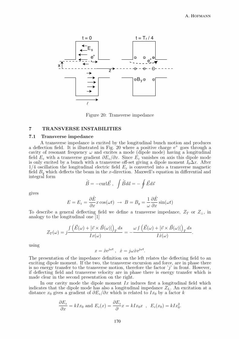
Figure 20: Transverse impedance

7 TRANSVERSE INSTABILITIES

7.1 Transverse impedance

A transverse impedance is excited by the longitudinal bunch motion and producesa deflection field. It is illustrated in Fig. 20 where a positive charge e+ goes through acavity of resonant frequency ω and excites a mode (dipole mode) having a longitudinalfield Ez with a transverse gradient ∂Ez/∂x. Since Ez vanishes on axis this dipole modeis only excited by a bunch with a transverse off-set giving a dipole moment Ib∆x. After1/4 oscillation the longitudinal electric field Ez is converted into a transverse magneticfield By which deflects the beam in the x-direction. Maxwell’s equation in differential andintegral form

~B = −curl ~E ,∫

~Bd~a = −∮

~Ed~s

gives

E = Ez =∂E

∂xx cos(ωt) → B = By =

1

ω

∂E

∂xsin(ωt)

To describe a general deflecting field we define a transverse impedance, ZT or Z⊥, inanalogy to the longitudinal one [1]

ZT (ω) = j

∫ ( ~E(ω) + [~v × ~B(ω)])

Tds

Ix(ω)= −

ω∫ ( ~E(ω) + [~v × ~B(ω)]

)T

ds

Ix(ω).

usingx = xejωt , x = jωxejωt.

The presentation of the impedance definition on the left relates the deflecting field to anexciting dipole moment. If the two, the transverse excursion and force, are in phase thereis no energy transfer to the transverse motion, therefore the factor ’j’ in front. However,if deflecting field and transverse velocity are in phase there is energy transfer which ismade clear in the second presentation on the right.

In our cavity mode the dipole moment Ix induces first a longitudinal field whichindicates that the dipole mode has also a longitudinal impedance ZL. An excitation at adistance x0 gives a gradient of ∂Ez/∂x which is related to Ix0 by a factor k

∂Ez

∂x= kIx0 and Ez(x) =

∂Ez

∂x = kIx0x , Ez(x0) = kIx2

0.

t = 0 t = T / 4r

E

B

xz

e+

e+

s

y

A. HOFMANN

170

The longitudinal impedance of this mode is

ZL(x0) = −∫

Ez(x0)dz

I= kx2

0`

` is the cavity length. With Maxwell’s equation

∫ ˙~Bd~a = −

∮~Ed~s

we obtain a relation between the electric field gradient and the deflecting magnetic fieldit is transformed into

Byx` = −x`∂Ez

∂x.

With I(t) = Iejωt we get for the fields

By(t) = Bjωejωt = −∂Ez(t)

∂x= −

∂Ez

∂xejωt , By(t) = Bye

jωt = j1

ω

∂Ez(t)

∂x= j

1

ω

∂Ez

∂xejωt.

With this we have a relation between the electric field gradient and the deflecting magneticfield which can be applied to the two impedances

ZT (ω) = j

∫ ( ~E(ω) + [~v × ~B(ω)])

Tds

Ix(ω)= −j

Byc`

Ix0

=c

ωk` =

2c

ω

d2ZL

dx2.

Our transverse impedance is related to the second derivative of the longitudinal belongingto the same mode. From this we get the symmetry relations

longitudinal : Zr(−ω) = Zr(ω) Zi(−ω) = −Zi(ω)transverse : ZTr(−ω) = −ZTr(ω) ZTi(−ω) = ZTi(ω)

While the above accurate relation applies to the same mode of oscillation thereexists also an approximate relation for the two impedances belonging to different modes.Taking some average of different oscillation modes in the same vacuum chamber of radiusb and ring circumference of 2πR one obtains the approximate but very useful relation [9]

ZT (ω) ≈ 2R

b2

Z(ω)

(ω/ω0)

7.2 Transverse dynamics

The transverse focusing provided by the quadrupoles keeps the beam in the vicinityof the nominal orbit. A particle executes a betatron motion around this orbit. Thismotion has the form of an oscillation which is not harmonic but has a phase advanceper unit length which varies around the ring. Often this is approximated by a smoothfocusing given by

x + ω20Q

2xx = 0

with ω0 being the revolution frequency and Qx the horizontal tune, i.e. the number ofbetatron oscillation executed per turn.

A stationary observer, or impedance, sees the particle position xk only at one loca-tion each turn k as indicated by the points in Fig. 21, and has no information of what theparticle does in the rest of the ring . Therefore, we have no information about the integer

BEAM INSTABILITIES

171

0 1 2 3 4 5 6 7 8 9 10

................................................................................................................................................................................................................................................................................................................................................................................................................................................................................................................................................................................................................................................................................................................................................ ...............

................................................................................................................................................................................................................................................................................................................................................................................................................................................................................................................................................................................................................................................................................................................................................ .......................

........

........

.........

.........

.........

.........

........

........

........

.......................

...............

t

turn k

xk••

••

••

••

••

•

.......................................................................................................................................................................................................................................................................................

...............................................................................................................................................

.........................................................................................................................................................................................................................................................................................................

.......................................

................................................................. ..........

..........................................

..........................

................................................................

..................................................... .............

..................................................................................................................................

..................................................................................................................................

.....................................................................................................................

.................................................... ..........

..........................................

..........................

................................................................

..................................................... .............

..................................................................................................................................

...........................

................................................................................................................................................................................................................................................................................................................................................................................................................................................................................................................................................................................................................................................................................................................................................ .......................

........

........

........

........

........

........

........

.........

......................

............... spectrum

........

........

.......

........

........

.......

........

........

.......

........

........

.......

........

........

.......

........

........

........

........

........

........

........

.

........

........

........

........

........

........

........

.

0 1 2 ω/ω0

Figure 21: Betatron oscillation observed at one location in time and frequency domain

part of the tune Qx = integer + q but only about the fractional part q with determinesthe phase

xk = x cos(2πqk) , x′k = −

x

βxsin(2πqk).

We observe this motion as a function of turn k. We can make a harmonic fit, i.e. aFourier analysis, Fig. 21. For a single bunch circulating in the machine we find at therevolution harmonic pω0 an upper and lower side band. The distance of the side band isgiven by the fractional part q because the integer part cannot be observed. For a veryshort bunch these side bands will extend up to very high frequencies, for longer bunchesthey will get smaller and vanish with increasing frequencies. A transverse impedance (ora position monitor) is sensitive to the dipole moment I ·x of the current and does not seethe revolution harmonics.

In general the betatron tune depends on the momentum deviation ∆p of a particlewhich is quantified by the chromaticity

∆Q = Q′∆p

p≈ Q′∆E

E.

A finite chromaticity will influence the motion of a particle executing at the same timebetatron and synchrotron oscillations and make certain modes of oscillations complicated.This will be discussed later while in this and the next section we assume Q′ = 0.

8 TRANSVERSE INSTABILITIES WITH Q′ = 0

8.1 Qualitative treatment

We consider a positive charge e+ going at t = 0 through a cavity and exciting adeflecting mode as with frequency ωr = 2π/Tr, as illustrated in Fig. 22. At first, t = 0, thismode consists of a longitudinal field with a gradient ∂Ez/∂x which is later, at t = Tr/4,converted into a magnetic field B = −By, pointing in the negative y-direction. A positivecharge going in the z-direction will obtain a Lorentz force in the positive x-direction. Aftera further quarter cavity oscillation, at t = Tr/2, we have again a longitudinal electric fieldwith a gradient but of opposite sign compared to the beginning. At t = 3Tr/4 this will beconverted into a magnetic field pointing in the positive y-direction. The Lorentz force on apositive charge going in the z-direction is now in the negative x-direction. The interactionof a bunch with this cavity depends on the relation between its fractional tune q and thefrequency of the cavity. For the latter also only its fractional part is of importance, asan integer number k′ of oscillations executed while the bunch is not in the cavity, has noinfluence.

We discuss now the interaction between the bunch and the cavity and make somesimple choices to facilitate the illustration. For the fractional tune we take q = 1/4. For

A. HOFMANN

172

..................................................................................................................... ...............

τ

................................

.................................

................................

..................................................x

........

........

........

.........

.........

........

........

........

........

........

........

........

.........

.........

................

...............y

..................................................................................... ...............

.............................................................. ...................................................... ...........

....

......................................................

................................

.............................................

................................

.................................

...................................

Ez

t = Tr/2

............. ............. ............. ............. .............

..........................

..........................

.............

•e+............................................... ...........

....

..................................................................................................................... ...............

τ

................................

.................................

................................

..................................................x

........

........

........

.........

.........

........

........

........

........

........

........

........

.........

.........

................

...............y

...............................

.................................

....................................

................................

.............................................

......................................................

....................................... ...............

.............................................................. ..........................................................................

Ez

t = 0

............. ............. ............. ............. .............

..........................

..........................

............. e[~v × ~B]................................

.........................................................

..................................................................................................................... ...............

τ

................................

.................................

................................

..................................................x

........

........

........

.........

.........

........

........

........

........

........

........

........

.........

.........

................

...............

.......................................................................................

y

~B

t = Tr/4

A

............. ............. ............. ............. .............

..........................

..........................

............. e[~v × ~B] ..........................................................................

...............

..................................................................................................................... ...............

τ

................................

.................................

................................

..................................................x

........

........

........

.........

.........

........

........

........

........

........

........

........

.........

.........

................

...............

........

........

........

........

........

........

........

................

...............

y

~B

t = 3Tr/4

B

............. ............. ............. ............. .............

..........................

..........................

.............

Figure 22: Illustration of a bunch interacting with a deflecting cavity mode

.........................................................................................................................................................................................................................................................................................................................................................................................................................................................................................................................................................................................................................................................................

........

........

.........

.........

.........

.........

.........

.........

.........

.........

.........

.........

.........

........

...

.................

4

.................

3.................

2.................

1

.................

0 turn

.....................................................................................................................................................................................................................................................................................................................................................................................................................................

..............................................................................................................................................................................................................................................................................

.......................................... −Ex

........

........

........

........

.........

.........

...................

...............

....................................................................................

........

........

........

.........

........

........

........

........

........

........

........

........

.........

........

........

........

........

........

...................

...............

........

........

........

.........

.........

.........

.........

.........

.........

.......................

...............x

−Ez

~F

~F

••

••

• x............. ............. ............. ............. ............. ............. ............. ............. ............. ............. ............. ............. ............. ............. ............. ..........................

..........................

.......................... ............. ............. .............

Figure 23: Interaction with the cavity tuned to the upper side band

..........................................................................................................................................................................................................................................................................................................................................................................................................................................................................................................................................................................................................................................................................

........

........

........

........

........

........

........

........

.........

.........

.........

.........

.........

.........

.......

.................

4

.................

3

.................

2.................

1.................

0 turn

.....................................................................................................................................................................................................................................................................................................................................................................................................................................................................................................................................................................................................................................................................................................................................................................

.............................................................................................................................................................................................................................................................................................................................................................................................................................................................................................

...................................................................................................................................................................................................................... −Ex

........

........

........

........

........

........

.....................

...............

....................................................................................

........

........

........

........

........

........

........

.........

.........

.........

.........

.........

.........

.........

........

........

........

......................

...............

........

........

........

........

........

........

........

........

.........

.........

...................

...............x

−Ez

~F

~F

••

••

• x............. ............. ............. ............. ............. ............. ............. ............. ............. ............. ............. ............. ............. ............. ............. ..........................

..........................

.......................... ............. ............. .............

Figure 24: Interaction with the cavity tuned to the lower side band

the cavity frequency we consider two cases: First, ωr = (k′ + 1/4)ω0, in which case thebunch having excited the cavity will find it after one turn in the situation ‘A’ as shownin Fig. 23. Here, the Lorentz force is opposite to the particle velocity and reduces theoscillation which leads to damping. Second, ωr = (k′+3/4)ω0 = (k′+1−1/4)ω0 , the bunchfinds the cavity after one turn in the situation ‘B’ shown in Fig. 24 where the Lorentzforce is in the direction of the transverse particle velocity and increases the oscillationwhich leads to an instability. As a result we find for one circulating bunch stability if thecavity is tuned to the upper side-band.

The resistive impedance at the upper side band damps, the one at the lower sideband excites the oscillation. If we have a more general impedance extending over severalside bands ω0(p + q) and ω0(p − q) we expect that the growth or damping rate of theoscillation is given by an expression of the form

1

τs

∝∑

p

(|I(p+q)|2ZTr(ω(p+q)) − |I(p−q)|2ZTr(ω(p−q))

)with ω(p±q) = ω0 (p ± q)

where Ip± is the Fourier component of the beam current at the upper or lower side band.It appears here as the square I2

p since the instability is driven by the energy transfer fromthe longitudinal to the transverse motion.We can estimate some properties of the proportionality factor missing in the above equa-tion. The product I2

pZT = P/y represents a power transfer per unit length. To get a

BEAM INSTABILITIES

173

growth rate we have to divide this by the energy of the bunch having Nb particles whichcan be related to the average current of the bunch I0 = eNbω0/2π

1

τs

∝P

m0c2γN0

=eω0P

2πm0c2γI0

.

8.2 Quantitative treatment

We consider a transverse impedance ZT (ω) which interacts with a bunch executinga rigid transverse oscillation with a tune Qx = integer+q. For convenience we assume theimpedance to be in a symmetry point with β ′

x = 0. We consider now a transverse rigidbunch executing a betatron oscillation with the center-of-mass position and angle at theimpedance location as a function of turn number k of the form

xk = x cos(2πqk) , x′k = −

x

βxsin(2πqk).

This motion in time (turn) and frequency domain is shown in Fig. 21.To get the fields induced in the impedance we also have to consider the longitudinal

distribution and motion of the bunch treated before. In a single traversal it is (6)

I(t) , I(ω) =1√2π

∫ ∞

−∞I(t)e−jωtdt.

and illustrated in Fig. 7. For a stationary circulating bunch the current in time domainexpressed directly or as a Fourier series is according to (8) and (9)

Ik(t) =∞∑

−∞I(t − kT0) = I0 + 2

∞∑

p=1

Ip cos(pω0t).

and shown in Fig. 8.

The dipole moment of an oscillating bunch at turn k and as function of t is

Dk = xkIk , Dk(t) = x∞∑

k=−∞cos(2πqk)I(t − kT0) (39)

To express this in a series we form the Fourier transform of Ik(t)

Ik(ω) =1√2π

∫ ∞

−∞

∞∑

k=−∞I(t− kT0)e

−jωtdt

=1√2π

∑e−kωT0

∫ ∞

−∞I(t− kT0)e

−jω(t−kT0)dt = I(ω)∞∑

k=−∞e−jkωT0

The Fourier transform of the dipole moment is

Dx(ω) = xI(ω)∞∑

−∞cos(2πqk)e−jkωT0

=xI(ω)

2

∞∑

−∞

[e−jk(ωT0+2πq) + e−jk(ωT0−2πq)

]

The sums become ∞ if the exponent is of form 2πp and vanish otherwise

∞∑

k=−∞e−jkx = 2π

∞∑

p=−∞δ(x − 2πp) and δ(ax) =

1

aδ(x) gives

A. HOFMANN

174

Dk(ω) = xω0I(ω)

2

∞∑

−∞[δ(ω − (p − q)ω0) + δ(ω − (p + q)ω0)] (40)

The inverse Fourier transform gives the oscillating dipole in time domain

Dk(t) =ω0x

2√

2π

∞∑

−∞

[I((p + q)ω0)e

j((p+q)ω0t) + I((p − q)ω0)ej((p−q)ω0t)

]

Using

(p + q)ω0 = (p + q)ω0, (p − q)ω0 = (p − q)ω0, I(p±q) =ω0√2π

I((p ± q)ω0) gives

Dk(t) =x

2

∞∑

p=−∞

[I(p+q)e

j(t(p+q)ω0) + I(p−q)ej(t(p−q)ω0)

].

Combining terms p > 0 from the first, p < 0 from second the part and vice versa, andusing I(ω) = I(−ω) gives

Dk(t) = x∞∑

ω>0

[I(p+q) cos((p + q)ω0t) + I(p−q) cos((p − q)ω0t)].

A charge e going through the impedance element at turn k is exposed to a transverseforce changing its momentum ∆pke = FT ∆t ≈ FT∆s/c

∆pke =e

c

∫ [~E(ω) + [~v × ~B(ω)]

]T

ds =−jeDk(t)ZT

c.

We get the momentum change of the whole bunch by a convolution between its chargedistribution given by the single traversal current I(t) and the deflecting field in turn k

∆pk = −j1

c

∫ ∞

−∞I(t)Dk(t + kT0)ZTdt

= −jx

2c

∞∑

p=−∞

∫ ∞

−∞I(t)

[I(p+q)ZT ((p + q)ω0)e

j(p+q)ω0(t+kT0)+

I(p−q)ZT ((p − q)ω0)ej(p−q)ω0(t+kT0)

]dt

This contains integrals of the form

∫ ∞

−∞I(t)e−j(t+kT0)(p+q)ω0dt =

√2πe−jT0k(p+q)ω0I((p + q)ω0) =

2π

ω0

e−j2πqkI(p+q)

giving

∆pk = −jcT0

2c

∞∑

−∞

[|I(p+q)|2ZT ((p + q)ω0)e

−j2πqk + |I(p−q)|2ZT ((p − q)ω0)ej2πqk

].

Combining terms p > 0 from the first, p < 0 from the second part and vice versa, usingrelations ZTr(ω) = ZTr(−ω), ZTi(ω) = ZTi(−ω) gives

BEAM INSTABILITIES

175

∆pk = −T0

c

∑

ω>0

[(|I(p+q)|2ZTr((p + q)ω0) − |I(p−q)|2ZTr((p − q)ω0)

)x sin(2πqk)

−(|I(p+q)|2ZTi((p + q)ω0) + |I(p−q)|2ZTi((p − q)ω0)

)x cos(2πqk)

].

using the form of the betatron oscillation we started from

xk = x cos(2πqk) , x′k = − x

βx

sin(2πqk) , xk = cx′k = − xc

βx

sin(2πqk)

∆pk =T0

c2

∑

ω>0

[(|I(p+q)|2ZTr((p + q)ω0) − |I(p−q)|2ZTr((p − q)ω0)

)βxxk

+(|I(p+q)|2ZTi((p + q)ω0) + |I(p−q)|2ZTi((p − q)ω0)

)cxk

].

The transverse velocity and angle change with the transverse momentum

∆x′k =

∆xk

c=

∆pk

N0m0γc=

e∆pk

m0γcI0T0

∆xk =e

m0c2γI0

∑

ω>0

[(|I(p+q)|2ZTr((p + q)ω)) − |I(p−q)|2ZTr((p − q)ω0)

)βxxk

+(|I(p+q)|2ZTi(p+q) + |I(p−q)|2ZTi(p−q)

)cxk

].

The velocity change has a component proportional to velocity and resistive impedance andone proportional to displacement and reactive impedance. The first leads to exponentialgrowth or damping, the second to a change of the betatron frequency.We start with the first part alone and a smooth approximation and get an accelerationx = ∆xω0/2π which we ad to the one due to focusing by beam optics

x + 2αsx + Q2xω

20 = 0, solution: x = x0e

−αst cos(Qxω0t + φ) if a Qxω0

αs =1

τ=

eω0βx

4πm0c2γI0

∑

ω>0

(|I(p+q)|2ZTr(p+q) − |I(p−q)|2ZTr(p−q)

). (41)

using (p − q)ω0 = −(−p + q)ω0 for p < 0 and ZTr(ω) = −ZTr(−ω) gives a sum withpositive and negative frequencies

αs =1

τ=

eω0βx

4πm0c2γI0

∞∑

p=−∞|I(p+q)|2ZTr(p+q). (42)

The growth rate is given by a convolution between the power spectrum components andthe impedance at the betatron side bands.

The reactive impedance alone gives an angular change ∆x′k = ∆xk/c proportional

to xk. This represents a focusing element of strength

1

f= −

∆x′k

xk

= −e

m0c2γI0

∑

ω±>0

(|I(p+q)|2ZTi(p+q) + |I(p−q)|2ZTi(p−q))

)xk

A. HOFMANN

176

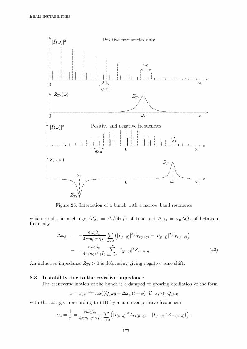
Positive frequencies only

............................................................................................................................................................................................................................................................................................................................................................................................................................................................................................................................................................................................................................................................................................................................................................................................................................................................................................................................................................................................................ .......................

........

........

........

........

........

........

........

.........

.........

.........

.........

.........

.........

.........

.........

.........

.........

.........

.........

.........

.........

.........

.........

.........

.........

.........

.........

.........

.....................

...............

|I (ω)|2

ω0

ω0

..........

.................................................................................... ............... ...................................................................................................

........................................................................................................................

........................................................................................................................

................................................................................................................

......................................................................................................

.........................................................................................

.........................................................................

............................................................

...............................................

....................................

........................

..............................

........ ..................................................................

............................................................ qω0

..................................................

.................................................

..............................................

..........................................

.....................................

...............................

............................................

........................ ....... ..... ... ..

.................................................

..............................................

..........................................

.....................................

...............................

............................................

........................ ....... ..... ... ..

............................................................................................................................................................................................................................................................................................................................................................................................................................................................................................................................................................................................................................................................................................................................................................................................................................................................................................................................................................................................................ .......................

........

........

........

........

.........

.........

.........

.........

.........

.........

.........

.........

.......................

............... ZTr(ω)

ω0.................................................................

........................................................................................................................................

....................................................................................................................................................................................................................................................................................................................................................................

ZTr

ωr

............................................................................................................................................................................................................................................................................................................................................................................................................................................................................................................................................................................................................................................................................................................................................................................................................................................................................................................................................................................................................ .......................

........

.........

.........

.........

.........

.........

.........

.........

.........

.........

.........

.........

.........

.........

.................

............... Positive and negative frequencies|I(ω)|2

ω0

ω0

.....

.................................................. ............... .................................................................

.... ............

......................

..................

........................

..............................

.....................................

.............................................

....................................................

........................................................

............................................................

............................................................

............................................................

........................................................

....................................................

.............................................

.....................................

..............................

........................

..............................

................ ...... ..................................................

..............................................qω0

.. ... ..... .................

.................................

.........................

...............................

.....................................

..........................................

..............................................

.................................................

..................................................

.................................................

..............................................

..........................................

.....................................

...............................

............................................

........................ ....... ..... ... .... ... ..... .......

........................

...................

.........................

...............................

.....................................

..........................................

..............................................

.................................................

..................................................

.................................................

..............................................

..........................................

.....................................

...............................

............................................

........................ ....... ..... ... ..

............................................................................................................................................................................................................................................................................................................................................................................................................................................................................................................................................................................................................................................................................................................................................................................................................................................................................................................................................................................................................ .......................

........

........

........

........

........

........

.........

.........

.........

.........

.........

........

........

........

........

.................

.

ZTr(ω)

ω0..... ........

.....

........

.....

........

.....

........

.....

........

.....

......................................................................

..........................................................................................................................................................................................................................................................

ZTr

ωr

.............

.............

.............

.............

.............

..........................................................................................................................................................................................................................................................................

......................................................

ZTr

ωr

Figure 25: Interaction of a bunch with a narrow band resonance

which results in a change ∆Qx = βx/(4πf ) of tune and ∆ωβ = ω0∆Qx of betatronfrequency

∆ωβ = −eω0βx

4πm0c2γI0

∑

ω>0

(|I(p+q)|2ZTi(p+q) + |I(p−q)|2ZTi(p−q)

)

= −eω0βx

4πm0c2γI0

∞∑

p=−∞|I(p+q)|2ZTi(p+q). (43)

An inductive impedance ZTi > 0 is defocusing giving negative tune shift.

8.3 Instability due to the resistive impedance

The transverse motion of the bunch is a damped or growing oscillation of the form

x = x0e−αst cos((Qxω0 + ∆ωβ)t + φ) if αs Qxω0

with the rate given according to (41) by a sum over positive frequencies

αs =1

τ=

eω0βx

4πm0c2γI0

∑

ω>0

(|I(p+q)|2ZTr(p+q) − |I(p−q)|2ZTr(p−q))

).

BEAM INSTABILITIES

177

............................................................................................................................................................................................................................................................................................................................................................................................................................................................................................................................................................................................................................................................................................................................................................................................................................................................................................................................................................................................................ .......................

........

........

........

........

........

........

........

.........

.........

........

.........

.........

.........

.........

.........

.........

.........

.........

.........

.........

.........

.........

.........

.........

.....................

...............

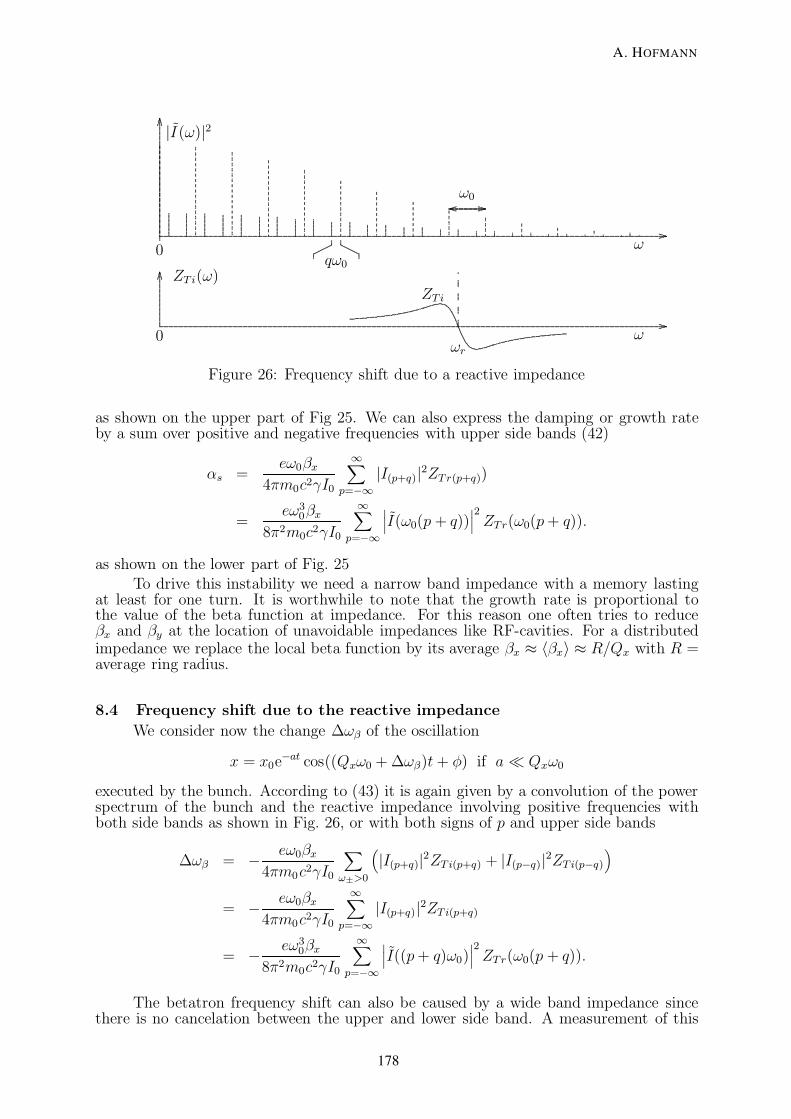
|I (ω)|2

ω0

ω0

.........

.................................................................................... ............... ...................................................................................................

.......................................................................................................

......................................................................................................

................................................................................................

.......................................................................................

............................................................................

................................................................

....................................................

.........................................

..............................

......................

............................

...... ...............................................................

......................................................... qω0

...........................................

..........................................

........................................

....................................

...............................

..........................

......................................

..................... ...... .... ... ..

..........................................

........................................

....................................

...............................

..........................

......................................

..................... ...... .... ... ..

............................................................................................................................................................................................................................................................................................................................................................................................................................................................................................................................................................................................................................................................................................................................................................................................................................................................................................................................................................................................................ .......................

........

........

........

........

........

........

........

........

.........

.........

.........

...................

............... ZTi(ω)

ω0.......................................................

...........................................................................................................................

.......................................................................................................................................................................................................

...................................................................................

...........................................................

ZTi

ωr

Figure 26: Frequency shift due to a reactive impedance

as shown on the upper part of Fig 25. We can also express the damping or growth rateby a sum over positive and negative frequencies with upper side bands (42)

αs =eω0βx

4πm0c2γI0

∞∑

p=−∞|I(p+q)|2ZTr(p+q))

=eω3

0βx

8π2m0c2γI0

∞∑

p=−∞

∣∣∣I(ω0(p + q))∣∣∣2ZTr(ω0(p + q)).

as shown on the lower part of Fig. 25To drive this instability we need a narrow band impedance with a memory lasting

at least for one turn. It is worthwhile to note that the growth rate is proportional tothe value of the beta function at impedance. For this reason one often tries to reduceβx and βy at the location of unavoidable impedances like RF-cavities. For a distributedimpedance we replace the local beta function by its average βx ≈ 〈βx〉 ≈ R/Qx with R =average ring radius.

8.4 Frequency shift due to the reactive impedance

We consider now the change ∆ωβ of the oscillation

x = x0e−at cos((Qxω0 + ∆ωβ)t + φ) if a Qxω0

executed by the bunch. According to (43) it is again given by a convolution of the powerspectrum of the bunch and the reactive impedance involving positive frequencies withboth side bands as shown in Fig. 26, or with both signs of p and upper side bands

∆ωβ = − eω0βx

4πm0c2γI0

∑

ω±>0

(|I(p+q)|2ZTi(p+q) + |I(p−q)|2ZTi(p−q)

)

= − eω0βx

4πm0c2γI0

∞∑

p=−∞|I(p+q)|2ZTi(p+q)

= − eω30βx

8π2m0c2γI0

∞∑

p=−∞

∣∣∣I((p + q)ω0)∣∣∣2ZTr(ω0(p + q)).

The betatron frequency shift can also be caused by a wide band impedance sincethere is no cancelation between the upper and lower side band. A measurement of this

A. HOFMANN

178

........

........

........

........

...................

...............

................................................................................................................................................................................................................................................................................................................................................................................................................................................................................................................................................................................................................................................................................................................................................................................................................................................................................................................................................................................................................................................................................................................................................................................................................................................................................................................................................................................................................................................................................................................................................................................................................................................................................................................................................................................................................................................................................................................................................................................................................................................................................................................................................................................................................................................................................................................................................................................................................................................................................................................................................................................................................................................................................................................................................................................................................................................................................................................................................................................................................................................................................................................................................................

........

........

........

........

........

........

........

.........

........

........

........

........

........

........

.........

.........

.........

.........

.........

........

........

........

........

........

........

.........

.........

.........

.........

.........

........

........

........

........

........

........

.........

.........

.........

.........

.........

........

........

........

........

........

........

.........

.........

.........

.........

........

........

........

........

........

........

........

.........

........

........

........

........

........

........

........

.........

........

........

........

........

........

........

.........

.........

.........

.........

.........

........

........

........

........

........

........

.........

.........

.........

.........

........

........

........

........

........

........

........

.........

........

........

........

........

........

.........

........

.........

.........

.........

.........

........

........

........

........

........

........

........

.........

........

........

........

........

........

........

.........

.........

......

....................................................................................................................................................................................................................................................................................................................................................................................................................................................................................................................................................................................................................................................................................................................................................................................................................................................................................................................................................................................................................................

....................................................................................................................................................................................................................................................................................................................................................................................................................................................................................................................................................................................................................................................................................................................................................................................................................................................................................................................................................................................................................................

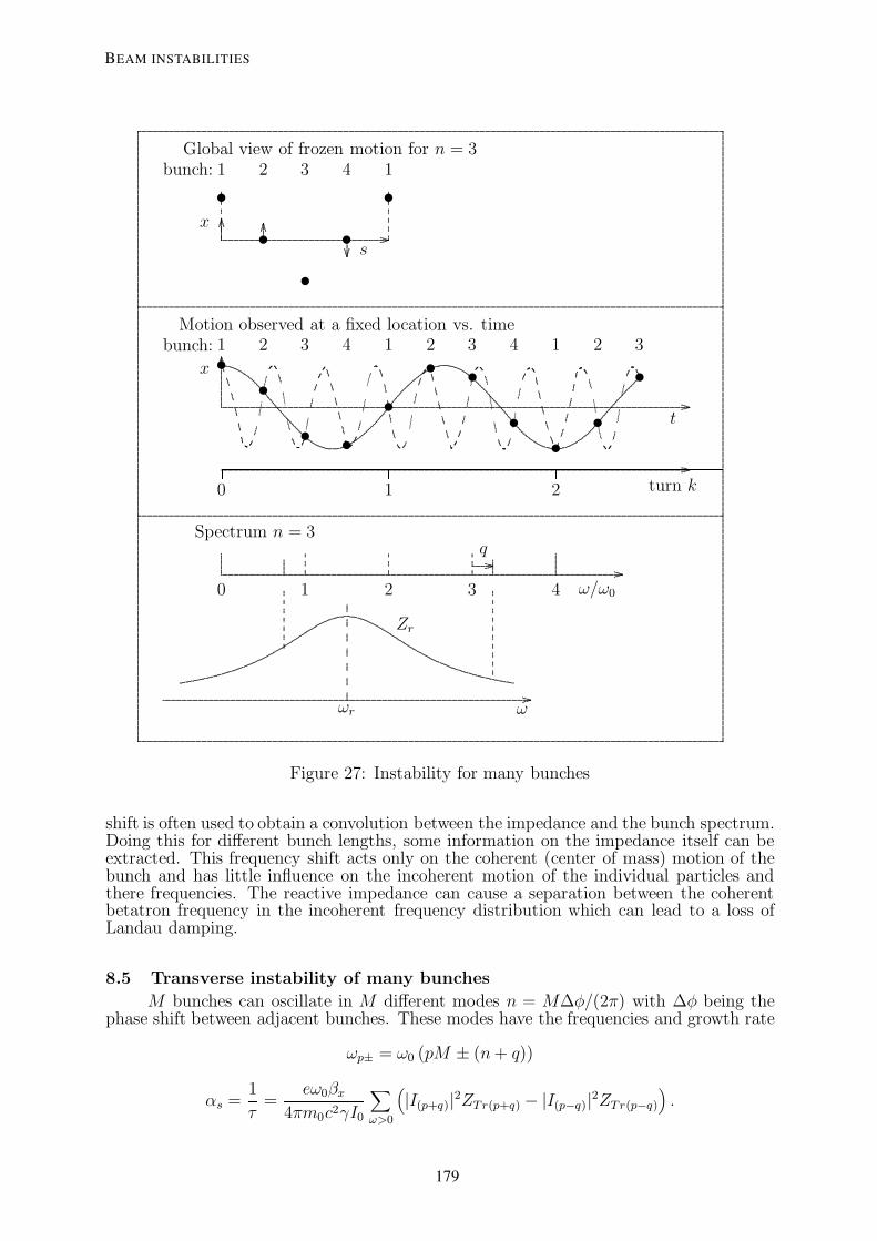
x

s

Global view of frozen motion for n = 3

•

•

•

•

•

........

........

........

....................

..........................................................................

............................................................................................................................................................................................................................................................................................................ ...............

bunch: 1 2 3 4 1

........

........

........

........

........

........

........

........

........

........

........

........

0 1 2

............................................................................................................................................................................................................................................................................................................................................................................................................................................................................................................................................................................................................................................................................................................................................................................................................................................ ...............

............................................................................................................................................................................................................................................................................................................................................................................................................................................................................................................................................................................................................................................................................................................................................................................................................................................ .......................

........

........

........

........

........

........

........

.........

.........

...................

...............

Motion observed at a fixed location vs. time

x

t

turn k

••

• •

•

• •

••

•

•..................................................................................................................................................................................................................................................................................

.................................................................................................................................................................................................

.......................................................................................................................................................................................................................................................................................................................

..................................................................................................................................................

.....................................................................................................

................

.....

........

.......................................

..........................

.............................................

.....................................................................................

..............................................................................

.......................................

.......................................

...........................................................................

...

.............

......................................................................................................................................................................................

.......................................

.............

.............

..........................................

..........

.............

....................................................

.........................................................................................................................................................................

..........................

.......................................

..........................

....................................................

bunch: 1 2 3 4 1 2 3 4 1 2 3

.......................................................................................................................................................................................................................................................................................................................................................................................................................................................................................................................................................................................................................................................................................................................... .................................................................. ...............q

Spectrum n = 3

ω/ω00 1 2 3 4....................................

........

........

........

........

....

.......

........

........

..

.......

........

........

..

........

........

......

........

........

......

........

........

......

........

........

........

................

........

........

........

........

........

................

........

........

........

................

................................................................................................................................................................................................................................................................................................................................................................................................................................................................................................................................................................................................................................................................. ..........................................................................................................

............................................................................

.................................................

.....................................

.................................

..............................

...............................

.................................................

...........................................................................................................................................................................................................................................................................................................................

Zr

ωωr

Figure 27: Instability for many bunches

shift is often used to obtain a convolution between the impedance and the bunch spectrum.Doing this for different bunch lengths, some information on the impedance itself can beextracted. This frequency shift acts only on the coherent (center of mass) motion of thebunch and has little influence on the incoherent motion of the individual particles andthere frequencies. The reactive impedance can cause a separation between the coherentbetatron frequency in the incoherent frequency distribution which can lead to a loss ofLandau damping.

8.5 Transverse instability of many bunches

M bunches can oscillate in M different modes n = M∆φ/(2π) with ∆φ being thephase shift between adjacent bunches. These modes have the frequencies and growth rate

ωp± = ω0 (pM ± (n + q))

αs =1

τ=

eω0βx

4πm0c2γI0

∑

ω>0

(|I(p+q)|2ZTr(p+q) − |I(p−q)|2ZTr(p−q)

).

BEAM INSTABILITIES

179

.......................................................................................................................................................................................................................................................................................................................................................................................................................................................................................................................................................................................................................................................................................................................................................................................................................................................................................................................................................................................... .................................................................. ...............q

General mode number n for M = 4

ω/ω00 1 2 3 4

........

........

........

........

....

........

........

........

........

....

........

........

........

.

........

........

........

.

........

........

........

.

........

........

........

.

........

........

........

.

........

........

........

.

........

........

........

.

........

........

........

.

........

........

........

.

........

........

........

.

........

........

........

.

........

........

........

.

........

........

........

.

5 6

n 0 1 2 3 0123 0 1 23......................

........

........

......

........

........

......

........

........

......

........

........

......

Figure 28: side bands of all modes

9 HEAD-TAIL INSTABILITY

9.1 Head-tail mode oscillations

The longitudinal synchrotron motion in energy and time deviation, ∆E and τ , canalso influence the transverse motion. Particles executing a vertical betatron oscillationmove at the same time frome the head to the tail of the bunch and vice-versa and gothrough some deviations ∆E from the nominal energy as shown in Fig. 29. If the chro-maticity Q′ = dQ/(dp/p) vanishes the betatron tune does not depend on energy and thereis no systematic betatron phase shift between head and tail of the bunch as shown on theleft of the figure. However, for Q′ 6= 0 the betatron frequency is different for the positiveand negative energy deviation the particle goes through. A particle can accumulate aphase shift going from head to tail via ∆E > 0 which is again lost going back to thehead as shown on the right of the figure. For γ > γT it has an excess energy movingfrom head to tail and an energy lack moving from tail to head. For Q′ > 0, this gives aphase advance in the first and a phase lag in the second step and vice versa for Q′ < 0 orγ < γT .

The head-tail mode oscillation is shown in Fig. 30. On the left half we have Q′ = 0.The motion of the bunch y(t) is shown on the very left which consists just of a rigidup-and-down motion. In the next row this motion is multiplied with the bunch currentgiving the dipole moment y · I(t) which induces the voltage in the transverse impedance.On the right the same quantities are plotted for the case of Q′ 6= 0 which clearly show thephase shift between head and tail. An experimental verification of this motion has beendone [10] and is shown in Fig. 31. For relatively long bunches this mode can be observeddirectly with a fast position monitor giving a signal being proportional the instantaneousdipole moment x(t) · I(t). Several superimposed traces on the scope are shown, eachcorresponding to a turn of the oscillating bunch passing through the monitor. On theleft we have Q′ = 0, on the right Q′ > 0. This figure shows the same behavior as thecalculated plotted in Fig. 30.

9.2 Head-tail instability

A broad band impedance is excited by oscillating particles A at the bunch headwhich in turn excite particles B at the tail with a phase shifted by ∆φ compared to thehead. Half a synchrotron oscillation later particles B are at the head and while particlesA are at the tail oscillating with phase −∆φ compared to B (assuming Q′ = 0). Theexcitation by the head has the wrong phase to keep oscillation growing unless Q′ 6= 0producing a phase shift during a motion from head to tail or vice versa. The wake fieldexcited by the head of the bunch will affect the tail later. The tail oscillates therefore witha phase lag compared to the tail. To keep the oscillation growing the head particle mustundergo a relative phase delay while moving to the tail and the tail particle a relativephase advance moving to the head. We expect a possible instability if Q′ < 0 for γ > γT

or if Q′ > 0 for γ < γT . The ’wiggle’ of the head-tail motion is seen by a stationaryobserver (impedance) as an oscillation with the chromatic frequency ωξ which has to beconsidered in calculating the head-tail instability.

∆p/p = ∆p/p sin(ωst) , τ = −τ cos(ωst) with τ =ωs

ηc

∆p

p

A. HOFMANN

180

................................................................................................. ...............

.................................

................................

...............................................

........

........

.........

........

.........

........

.........

.........

........

...................

...............

..........................

..........................

..........................

..........................

..........................

..........................

..............

∆E

τ

z

................................................................................. ...............

.................................

................................

...............................

4 β osc.

4 β osc.

head

tail

Q′ = 0

..................

...............................................................................

...............

...................

.........................

....................................................................................................................................................................................................................................................................................................................................................................................................................................

.........................

....

...............................................................................................................................................................................

............................................................................................

.....................................................................................................

......................

........................

....................................................................................................................................................

............................

................................................................................................................................................................................................................................................................

.............................................................................................................................................................................................................................................................................................................................

.....................................................................................•

•

••

•

•

••

•

................................................................................................. ...............

.................................

................................

...............................................

........

........

.........

........

.........

........

.........

.........

........

...................

...............

..........................

..........................

..........................

..........................

..........................

..........................

..............

∆E

τ

z

................................................................................. ...............

.................................

................................

...............................

3.5 β osc.

4.5 β osc.

head

tail

Q′ < 0

.................................................................................................

...............

...................

.........................

....................................................................................................................................................................................................................................................................................................................................................................................................................................

.........................

....

..................................................................................................................................................................................................................................

.......................................................................................................................................

........................................................................................................................................................

.......................................................................

......................................................................................................................................................................................................

............................................................................................................................................................................................

.........................

.......................

........................

...................................................................................................................................................................

..............................

..............•

•

•

••

•

•

••......................................................

........

........

.....................

...............

....................................................

......................................................

....................................................

........

........

.....................

...............

Figure 29: Combined betatron and synchrotron motion

........

........

........

........

........

........

........

........

........

........

........

.................

...............

................................................................................................................................................ ...............

y

τ

t = 0 bunch

displacement y

......................................................................................................................................................................................................................

................................................................................................................................................................................................................................................................................................................................................................................................................................................................................................................................................................................................................................................................................................................................................................

........

........

........

........

........

........

.........

........

........

........

........

........

........

........

.........

.........

.........

........

........

........

........

........

........

........

........

........

........

.........

........

.........

.........

......................

...............

................................................................................................................................................ ...............

y

τ

t = Tβ/8

......................................................................................................................................................................................................................

................................................................................................................................................................................................................................................................................................................................................................................................................................................................................................................................................................................................................................................................................................................................................................

........

........

.........

.........

.........

.........

.........

........

........

........

........

........

........

........

.........

.........

.........

.........

........

........

...

........

.........

.........

........

.........

.........

........

.........

.........

.........

..................

...............

................................................................................................................................................ ...............

y

τ

t = Tβ/4

......................................................................................................................................................................................................................

.................................................................................................................................................................................................................................................................................................................................................................................................................................................................................................................................................................................................................................................................................................................................................................

.........

.........

.........

........

........

........

........

........

........

........

.........

.........

.........

........

........

........

........

........

........

........

.....

........

........

........

........

........

........

........

........

.........

.........

.......................

...............

................................................................................................................................................ ...............

y

τ

t = 3Tβ/8

......................................................................................................................................................................................................................

................................................................................................................................................................................................................................................................................................................................................................................................................................................................................................................................................................................................................................................................................................................................................................

........

........

........

........

.........

........

........

........

........

........

........

........

.........

.........

.........

........

........

........

........

........

........

........

........

........

.........

.........

........

.........

.........

.........

........

....................

...............

................................................................................................................................................ ...............

y

τ

t = Tβ/2

bunch......................................................................................................................................................................................................................

................................................................................................................................................................................................................................................................................................................................................................................................................................................................................................................................................................................................................................................................................................................................................................

.........

.........

.........

.........

.........

........

........

........

........

........

........

........

.........

.........

.........

........

........

........

........

........

....

........

........

........

........

........

........

........

........

........

........

........

.................

...............

................................................................................................................................................ ...............

y · I

τ

t = 0bunch

dipole moment yI

....................................................

...........................................

....................................................................................................................................................

................................................................................................................................................................................................................................................................................................................................................................................................................................................................................................................................................................................................................................................................................................................................................................

........

........

........

........

........

........

.........

........

........

........

........

........

........

........

.........

.........

.........

........

........

........

........

........

........

........

........

........

........

.........

........

.........

.........

......................

...............

................................................................................................................................................ ...............

y cdotI

τ

t = Tβ/8

...............................

...............................................

.......................................................................................................................................................

................................................................................................................................................................................................................................................................................................................................................................................................................................................................................................................................................................................................................................................................................................................................................................

........

........

.........

.........

.........

.........

.........

........

........

........

........

........

........

........

.........

.........

.........

.........

........

........

...

........

.........

.........

........

.........

.........

........

.........

.........

.........

..................

...............

................................................................................................................................................ ...............

y · I

τ

t = Tβ/4

......................................................................................................................................................................................................................

.................................................................................................................................................................................................................................................................................................................................................................................................................................................................................................................................................................................................................................................................................................................................................................

.........

.........

.........

........

........

........

........

........

........

........

.........

.........

.........

........

........

........

........

........

........

........

.....

........

........

........

........

........

........

........

........

.........

.........

.......................

...............

................................................................................................................................................ ...............

y · I

τ

t = 3Tβ/8

............................................................................................................................................................................................

..................................

.......

................................................................................................................................................................................................................................................................................................................................................................................................................................................................................................................................................................................................................................................................................................................................................................

........

........

........

........

.........

........

........

........

........

........

........

........

.........

.........

.........

........

........

........

........

........

........

........

........

........

.........

.........

........

.........

.........

.........

........

....................

...............

................................................................................................................................................ ...............

y · I

τ

t = Tβ/2

bunch

........................................................................................................................................................................................

...........................................................

................................................................................................................................................................................................................................................................................................................................................................................................................................................................................................................................................................................................................................................................................................................................................................

.........

.........

.........

.........

.........

........

........

........

........

........

........

........

.........

.........

.........

........

........

........

........

........

....

........

........

........

........

........

........

........

........

........

........

........

.................

...............

................................................................................................................................................ ...............

y

τ

t = 0

bunch

displacement y

..................................................................................................................................................................................................................................................

................................................................................................................................................................................................................................................................................................................................................................................................................................................................................................................................................................................................................................................................................................................................................................

........

........

........

........

........

........

.........

........

........

........

........

........

........

........

.........

.........

.........

........

........

........

........

........

........

........

........

........

........

.........

........

.........

.........

......................

...............

................................................................................................................................................ ...............

y

τ

t = Tβ/8

..................................................................................................................................................................................................................................................

................................................................................................................................................................................................................................................................................................................................................................................................................................................................................................................................................................................................................................................................................................................................................................

........

........

.........

.........

.........

.........

.........

........

........

........

........

........

........

........

.........

.........

.........

.........

........

........

...

........

.........

.........

........

.........

.........

........

.........

.........

.........

..................

...............

................................................................................................................................................ ...............

y

τ

t = Tβ/4

.........................................................

...........................................

..............................................................................................................................................

.................................................................................................................................................................................................................................................................................................................................................................................................................................................................................................................................................................................................................................................................................................................................................................

.........

.........

.........

........

........

........

........

........

........

........

.........

.........

.........

........

........

........

........

........

........

........

.....

........

........

........

........

........

........

........

........

.........

.........

.......................

...............

................................................................................................................................................ ...............

y

τ

t = 3Tβ/8

..............................

....................................................................................

...................................

.............................................................................................

................................................................................................................................................................................................................................................................................................................................................................................................................................................................................................................................................................................................................................................................................................................................................................

........

........

........

........

.........

........

........

........

........

........

........

........

.........

.........

.........

........

........

........

........

........

........

........

........

........

.........

.........

........

.........

.........

.........

........

....................

...............

................................................................................................................................................ ...............

y

τ

t = Tβ/2bunch

..........................................................

...............................

...................................................................................

.....................................

.................................

................................................................................................................................................................................................................................................................................................................................................................................................................................................................................................................................................................................................................................................................................................................................................................

.........

.........

.........

.........

.........

........

........

........

........

........

........

........

.........

.........

.........

........

........

........

........

........

....

........

........

........

........

........

........

........

........

........

........

........

.................

...............

................................................................................................................................................ ...............

y · I

τ

t = 0

bunch

dipole moment yI

.........................................

...........................................................................................................................................................................................

.................

................................................................................................................................................................................................................................................................................................................................................................................................................................................................................................................................................................................................................................................................................................................................................................

........

........

........

........

........

........

.........

........

........

........

........

........

........

........

.........

.........

.........

........

........

........

........

........

........

........

........

........

........

.........

........

.........

.........

......................

...............

................................................................................................................................................ ...............

y · I

τ

t = Tβ/8

......................................................................

.............................................................................................................................................................................

................................................................................................................................................................................................................................................................................................................................................................................................................................................................................................................................................................................................................................................................................................................................................................

........

........

.........

.........

.........

.........

.........

........

........

........

........

........

........

........

.........

.........

.........

.........

........

........

...

........

.........

.........

........

.........

.........

........

.........

.........

.........

..................

...............

................................................................................................................................................ ...............

y · I

τ

t = Tβ/4

...........................................

..........................................

............................................................................................................................................................

.................................................................................................................................................................................................................................................................................................................................................................................................................................................................................................................................................................................................................................................................................................................................................................

.........

.........

.........

........

........

........

........

........

........

........

.........

.........

.........

........

........

........

........

........

........

........

.....

........

........

........

........

........

........

........

........

.........

.........

.......................

...............

................................................................................................................................................ ...............

y · I

τ

t = 3Tβ/8

.....................................................................................

.............................

.................................................................................................................................

................................................................................................................................................................................................................................................................................................................................................................................................................................................................................................................................................................................................................................................................................................................................................................

........

........

........

........

.........

........

........

........

........

........

........

........

.........

.........

.........

........

........

........

........

........

........

........

........

........

.........

.........

........

.........

.........

.........

........

....................

...............

................................................................................................................................................ ...............

y · I

τ

t = Tβ/2

bunch........................................................................................

...........................................................................

..................................................................................

................................................................................................................................................................................................................................................................................................................................................................................................................................................................................................................................................................................................................................................................................................................................................................

.........

.........

.........

.........

.........

........

........

........

........

........

........

........

.........

.........

.........

........

........

........

........

........

....

Figure 30: Head-tail mode observed in steps of its period Tβ/8, left: Q′ = 0, right: Q′ 6= 0

ωs = Qsω0 is the synchrotron frequency and ηc = αc − 1/γ2 with αc = momentumcompaction. The relative betatron phase shift of a particle executing part of a synchrotronoscillation is

∆φβ = ω0

∫ t2

t1∆Qdt = ω0Q

′∆p

p

∫ t2

t1sin(ωst)dt

BEAM INSTABILITIES

181

Q′ = 0 Q′ > 0

Figure 31: Head-tail mode m = 0 for vanishing and finite chromaticity

= −ω0Q′∆p

p(cos(ωst2) − cos(ωst2)) =

ω0Q′

ηc

(τ2 − τ1)

This gives for the chromatic frequency

ωξ =∆φβ

∆τ=

ω0Q′

ηc

.

This ‘wiggle’ of the head-tail mode shifts the envelope of the side bands by the chromaticfrequency ωξ = Q′ω0/ηc as shown in Fig. 32. This results in current components

I(p+q+ξ) =ω0√2π

I((p + q)ω0 + ωξ) , I(p−q−ξ) =ω0√2π

I((p − q)ω0 − ωξ)

which can be very different for adjacent side bands. Since now the difference betweenupper and lower side band is large even a broad band impedance can lead to an instabilitywith growth (or damping) rate [11]

α =eω0βx

4πm0c2γI0

∑

ω>0

[|I(p+q+ξ)|2ZTr((p + q)ω0 + ωξ) − |I(p−q−ξ)|2ZTr((p − q)ω0 − ωξ)

].

9.3 Higher head-tail modes

So far we considered a head tail mode in which for vanishing chromaticity all particlemove in phase up and down. It is also possible that oscillation of the head and tail oscillatewith opposite phase as shown in Fig. 33. Here, the particles move up and down with aphase which depends on their longitudinal position resulting in a difference of π betweenheat and tail. There are now two modes possible. In one the particle ahead has a phaselag, shown on the left, in the other a phase advance, shown on the right of the figure.The two modes are labeled by m = ±1. Their frequency is different, in the first case anextra betatron oscillation is subtracted, in the second case added per synchrotron period,resulting in a frequency ωβ = (p ± q ± Qs)ω0.

The projected position y(τ ) and dipole moment y · I(τ ) of this head-tail modem = ±1 is shown in Fig. 34 in steps of Tβ/8. It should be noted that the project position

A. HOFMANN

182

............................................................................................................................................................................................................................................................................................................................................................................................................................................................................................................................................................................................................................................................................................................................................................................................................................................................................................................................................................................................................ .......................

........

.........

.........

.........

.........

.........

.........

.........

.........

.........

.........

........

........

........

....................

...............y · Ip(ω)Q′ = 0

ω0

ω0

.....

.................................................. ............... .................................................................

.... ............

......................

..................

........................

..............................

.....................................

.............................................

....................................................

........................................................

............................................................

............................................................

............................................................

........................................................

....................................................

.............................................

.....................................

..............................

........................

..............................

................ ...... ..................................................

..............................................qω0

.. ... ..... .................

.................................

.........................

...............................

.....................................

..........................................

..............................................

.................................................

..................................................

.................................................

..............................................

..........................................

.....................................

...............................

............................................

........................ ....... ..... ... .... ... ..... .......

........................

...................

.........................

...............................

.....................................

..........................................

..............................................

.................................................

..................................................

.................................................

..............................................

..........................................

.....................................

...............................

............................................

........................ ....... ..... ... ..

............................................................................................................................................................................................................................................................................................................................................................................................................................................................................................................................................................................................................................................................................................................................................................................................................................................................................................................................................................................................................ .......................

........

........

........

........

........

........

.........

.........

.........

.........

.........

.........

.........

.........

......................

............................................................................................................................................. ...............

ωξy · Ip(ω)Q′ > 0

ω0

ω0

.....

.................................................. ............... .................................................................

.... ............

......................

..................

........................

..............................

.....................................

.............................................

....................................................

........................................................

............................................................

............................................................

............................................................

........................................................

....................................................

.............................................

.....................................

..............................

........................

..............................

................ ...... ...... ... ..... .......

........................

...................

.........................

...............................

.....................................

..........................................

..............................................

.................................................

..................................................

.................................................

..............................................

..........................................

.....................................

...............................

............................................

........................ ....... ..... ... .....................................................................................................................................

.....................................................................................................................

.................................................................................................

......................................................................................................................................................................................................................................................................................................................................................................................................................................................................................................................................................................

............................................................................................................................................................................................................................................................................................................................................................................................................................................................................................................................................................................................................................................................................................................................................................................................................................................................................................................................................................................................................ .......................

.........

.........

.........

........

........

........

........

........

........

........

.........

........

........

........

........

........

........

.........

.........

.........

.........

........

........

........

........

...................

............y · Ip(ω)

ω0

Q′ > 0ω0

..........

.................................................................................... ............... ...................................................................................................

........................................................................................................................

........................................................................................................................

................................................................................................................

......................................................................................................

.........................................................................................

.........................................................................

............................................................

...............................................

....................................

........................

..............................

........ .................................

.................................

.........................

...............................

.....................................

..........................................

..............................................

.................................................

..................................................

.................................................

..............................................

..........................................

.....................................

...............................

............................................

........................ .......

................................................................................................................................................................................................................................................................................................................................................................................................................................................................................................................................................................................................................................................................. ..........................................................................................

.......................................................................................

.......................................................

.........................................

....................................

......................................

.........................................................................................................................................................................................................................................................................................................................................................

Zr

ωωr

Figure 32: Head-tail mode spectrum; top: Q′ = 0, middle: Q′ > 0 positive and negativefrequencies, bottom: Q′ > 0 with positive frequencies only

in the center τ = 0 vanishes always forming a node. Obviously the individual particlestill move at this position but their phases are opposite for ±∆p resulting in a vanishingprojection.

There are higher head tail modes with the general frequencies

ωβ = ω0(p ± q ± mQs)

shown in Fig. 35

BEAM INSTABILITIES

183

................................................................................................. ...............

.................................

................................

...............................................

........

........

.........

........

.........

.........

........

.........

........

...................

...............

..........................

..........................

..........................

..........................

..........................

..........................

..............

∆E

τ

z

................................................................................. ...............

.................................

................................

...............................

3.5 β-osc.

3.5 β-osc.

m = −1

t = 0

fit

head

tail...........

......................................................................................

...............

...................

.........................

....................................................................................................................................................................................................................................................................................................................................................................................................................................

.........................

....

.............................................................................................................................................................................................................................................

......................................................................................

.......................

......................

.............................

...................................................................................................................................................................

.....................................................................................................................................................................................................................................................................................................

............................................................................................................................................................................

................................................................................................................................................................•

•

••

•

•

••

................................................................................................. ...............

.................................

................................

...............................................

........

........

.........

........

.........

.........

........

.........

........

...................

...............

..........................

..........................

..........................

..........................

..........................

..........................

..............

∆E

τ

z

................................................................................. ...............

.................................

................................

...............................

4.5 β-osc.

4.5 β-osc.

m = 1

t = 0

fit

head

tail...........

......................................................................................

...............

...................

.........................

....................................................................................................................................................................................................................................................................................................................................................................................................................................

.........................

....

.................................................................................................................................

......

.......

........

........

........

........

.........

........

........

.......................................................

...........................................................................

................................................................................................................

......................

........................

.............................................................................................................................................

........................................................................................................................................

...............................................................................................................................................................................................................................................................

...........................................................................................................................................................

...........................................................................................................................................•

•

••

•

•

••

•

................................................................................................. ...............

................................

.................................

...............................................

........

........

........

........

........

.........

........

.........

.........

....................

...............

..........................

..........................

..........................

..........................

..........................

..........................

..............

∆E

τ

z

................................................................................. ...............

................................

.................................

...............................

3.5 β-osc.

3.5 β-osc.

t = Tβ/4

fit

head

tail...........

......................................................................................

...............

...................

.........................

......................................................................................................................................................................................................................................................................................................................................................................................................................................

.........................

..................................................................................................................................................................

........................................................................................................

..............................................................................................................

........................

...........................

....................................................................................................................................................................................

........................................................................................................................................................................................................................................................................................

......................................

................................................................................................................................................................................................................................

......................................•

•

••

•

•

••

•

................................................................................................. ...............

................................

.................................

...............................................

........

........

........

........

........

.........

........

.........

.........

....................

...............

..........................

..........................

..........................

..........................

..........................

..........................

..............

..................

......................................................................................

................

......................

....................................

..............................................................................................................................................................................................................................................................................................................................................................................................................

.........................

.........................................................................................................................................................................................................................................................................................................

........................................................................

..............................................................................................................................

.........................

..................................................................................................................................................

............................................................................................................................................

................................................................................................................................................................................................................................................................................

.............................................................................................................................................................

..............................................................................................................•

•

•••

•

•• •

∆E

τ

z

................................................................................. ...............

................................

.................................

...............................

4.5 β-osc.

4.5 β-osc.

t = Tβ/4

fit

head

tail

Figure 33: Higher head-tail mode m = ±1 for Q′ = 0

........

........

........

........

........

........

........

........

.....................

...............

............................................................................................................................................................................................................................ ...............

y

τ

t = 0

bunch

...............................................................................................................................................................................................................................................................................................................................................................

..................................................................................................................................................................................................................................................................................................................................................................................................................................................................................................................................................................................................................................................................................................................................................................................................................................................................................................................................................................................................................................................................................................................................................

........

........

........

........

........

.........

........

.........

.........

.........

.........

.........

.........

.........

.........

...

........

........

........

........

........

........

........

........

.....................

...............

............................................................................................................................................................................................................................ ...............

y

τ

t = Tβ/8...........................................................................................................................................................................................................................................................................................................................................................

..................................................................................................................................................................................................................................................................................................................................................................................................................................................................................................................................................................................................................................................................................................................................................................................................................................................................................................................................................................................................................................................................................................................................................

........

........

........

.........

.........

.........

.........

.........

.........

.........

.........

.........

.........

.........

.........

........

........

........

........

........

........

........

.........

....................

...............

............................................................................................................................................................................................................................ ...............

y

τ

t = Tβ/4

......................................................................................................................................................................................................................................................................................................................................................

..................................................................................................................................................................................................................................................................................................................................................................................................................................................................................................................................................................................................................................................................................................................................................................................................................................................................................................................................................................................................................................................................................................................................................

.........

.........

.........

.........

.........

.........

.........

.........

.........

.........

.........

.........

.........

.........

......

.........

........

........

.........

........

.........

........

.........

.................

...............

............................................................................................................................................................................................................................ ...............

y

τ

t = 3Tβ/8

................................................................................................

...................................................................................................

....................................................................................................

....................................................

..................................................................................................................................................................................................................................................................................................................................................................................................................................................................................................................................................................................................................................................................................................................................................................................................................................................................................................................................................................................................................................................................................................................................................

........

........

........

........

........

........

.........

.........

.........

.........

.........

.........

.........

.........

.........

...

........

........

........

........

........

........

........

........

.....................

...............

............................................................................................................................................................................................................................ ...............

y

τ

t = Tβ/2

bunch..................................

.......................................................................

........................................................................

.......................................................................

........................................................................

...............................

..................................................................................................................................................................................................................................................................................................................................................................................................................................................................................................................................................................................................................................................................................................................................................................................................................................................................................................................................................................................................................................................................................................................................................

........

........

........

.........

.........

.........

.........

.........

.........

.........

.........

.........

.........

.........

.........

........

........

........

........

........

........

........

........

.....................

...............

............................................................................................................................................................................................................................ ...............

y · I

τ

t = 0

bunch....................................................

..........................................................................................................................................................................................................................................................................................................

.................................

..................................................................................................................................................................................................................................................................................................................................................................................................................................................................................................................................................................................................................................................................................................................................................................................................................................................................................................................................................................................................................................................................................................................................................

........

........

........

........

........

.........

........

.........

.........

.........

.........

.........

.........

.........

.........

...

........

........

........

........

........

........

........

........

.....................

...............

............................................................................................................................................................................................................................ ...............

y · I

τ

t = Tβ/8

.............................

.........................................................................................................................................................................................................................................................................................................

......................................

..................................................................................................................................................................................................................................................................................................................................................................................................................................................................................................................................................................................................................................................................................................................................................................................................................................................................................................................................................................................................................................................................................................................................................

........

........

........

.........

.........

.........

.........

.........

.........

.........

.........

.........

.........

.........

.........

........

........

........

........

........

........

........

.........

....................

...............

............................................................................................................................................................................................................................ ...............

y · I

τ

t = Tβ/4

......................................................................................................................................................................................................................................................................................................................................................

..................................................................................................................................................................................................................................................................................................................................................................................................................................................................................................................................................................................................................................................................................................................................................................................................................................................................................................................................................................................................................................................................................................................................................

.........

.........

.........

.........

.........

.........

.........

.........

.........

.........

.........

.........

.........

.........

......

.........

........

........

.........

........

.........

........

.........

.................

...............

............................................................................................................................................................................................................................ ...............

y · I

τ

t = 3Tβ/8

.........................................................................................................................................................

............................................

................................................

.......................................................................................................................

..................................................................................................................................................................................................................................................................................................................................................................................................................................................................................................................................................................................................................................................................................................................................................................................................................................................................................................................................................................................................................................................................................................................................................

........

........

........

........

........

........

.........

.........

.........

.........

.........

.........

.........

.........

.........

...

........

........

........

........

........

........

........

........

.....................

...............

............................................................................................................................................................................................................................ ...............

y · I

τ

t = Tβ/2

bunch..............................................................................................................................

.....................................

.................................

.................................

............................................

..............................................................................................................

..................................................................................................................................................................................................................................................................................................................................................................................................................................................................................................................................................................................................................................................................................................................................................................................................................................................................................................................................................................................................................................................................................................................................................

........

........

........

.........

.........

.........

.........

.........

.........

.........

.........

.........

.........

.........

.........

Figure 34: Head-tail mode m = ±1, Q′ = 0 seen in steps of Tβ = T0/q, left displacementy(τ ), right: dipole moment y · I(τ )

A. HOFMANN

184

................................................................................................................................................................................................................................................................................................................................................................................................................................................................................................................................................................................................................................................................................................................................................................................................................................................................................................................................................................................ ...............

................................................................................................................................................................................................................................................................................ ...............

q

......

......

......

.....

.......

........

........

.......

........

........

.......

........

........

.......

........

........

.......

........

........

.......

........

........

................................................ ............... ...............................................................

Qa

.......

........

........

.......

........

........

.......

........

........

.......

........

........

p ω/ω0

m -2 -1 0 1 2 -2 -1 0 1 2

Figure 35: Detailed spectrum of higher head-tail modes ω = ω0(p ± q ± Qs)

References

[1] B. Zotter, S Kheifets, “Impedances and Wakes in High-Energy Particle Accelerators”,World Scientific 1997.

[2] K.W. Robinson, “Stability of beam in radio frequency systems”, Cambridge ElectronAccel. CEAL-1010 (1964).

[3] A. Hofmann, “Physics of beam instabilities”, Proc. of a Topical Course ‘Frontiersof Particle Beams’ held by the Joint US-CERN School on Particle Accel. at SouthPadre Island, Texas, Oct. l986, ed. M. Month and S. Turner, Lecture notes in Physics296. Springer (l988) 99.

[4] F. Sacherer, “A longitudinal stability criterion for bunched beams”; Proc. of the 1977Particle Accel. Conf., IEEE Trans. on Nucl. Sci. NS 20-3 (1973) 825.

[5] J.L. Laclare, “Bunched beam coherent instabilities”; CAS CERN Accelerator School,Advanced Accelerator Physics, 1985; ed. S. Turner. CERN 87-03, p. 264.

[6] F. Pedersen, CERN, Private communication.

[7] S. Krinsky, “Saturation of a longitudinal instability due to nonlinearity of the wakefield”; Proc. of the 1985 Particle Accel. Conf., IEEE Trans. on Nucl. Sci. NS 32-5(1985) 2320.

[8] A. Hofmann, “Kinetic theory”, CAS CERN Accelerator School, 5th advanced accel.phys. course, held 1993 in Rhodos and published as CERN 95-06.

[9] W. Schnell, “A relation between longitudinal and transverse instability thresholdsfor a coasting beam traversing a resonant cavity”, CERN-ISR-RF/70-7 (1970).

[10] J. Gareyte and F. Sacherer, “Head-tail instabilities in the CERN PS and booster”,Proc. 9th Int. Conf. on High Energy Accel., Stanford 1974, p. 341.

[11] A. Hofmann, K. Hubner, B. Zotter, “A computer code for the calculation of beaminstabilities in circular electron machines”, Proc. 1979 Particle Accel. Conference,IEEE Trans. on Nucl. Sci. NS 26-3 (1979) p. 3514.

BEAM INSTABILITIES

185

LINAC-BASED FREE-ELECTRON LASER

J. Rossbach Universität Hamburg, Hamburg, Germany

Abstract A basic treatment of the principle of the linac-driven free-electron laser (FEL) is given. The first part of the paper describes the FEL in low-gain approximation, the second part gives the high-gain FEL theory. The majority of the treatment describes FELs in one-dimensional approximation. Only in the final section are a few remarks made on the effects by diffraction of radiation and by electron beam emittance. The ambition of this paper is to make a clear presentation of basic FEL theory concepts with explicit derivation of the formulae from first principles, and it does not aspire to postulate any progress in FEL theory.

1 Introduction The basic theory of linac-driven free-electron lasers (FEL) in this paper is based on lectures given at the CERN Accelerator School on ‘Synchrotron Radiation and Free Electron Lasers’ 2–9 July 2003 in Brunnen, Switzerland. This paper is neither a report on progress in FEL theory nor a complete and in-depth treatment of the subject. It presents the basic concepts of linac-based FELs starting from first principles and deriving formulae step-by-step so that students can follow without doing long derivations and calculations. In the interest of simplicity, the FEL theory is given in one-dimensional approximation, i.e. only longitudinal electron motion is considered and diffraction effects of radiation are neglected. This approximation is particularly justified for FELs operating in the VUV- or X-ray wavelength regime because of the suppression of space-charge effects at ultra-relativistic energies typical for these kinds of radiation sources.

The paper covers the material presented during the two one-hour lectures. It includes a few useful comments for the student. The MKSA (or ‘practical’) system of units and a right-handed Cartesian coordinate system (with z being the longitudinal coordinate) are used throughout the paper [1,2].

2 The free-electron laser in low-gain approximation

2.1 Radiation power of a point-like electron distribution moving at ultra-relativistic speed

An FEL is basically a classical device; with very few exceptions, all features can be derived and described by classical electrodynamics and relativistic kinematics. Thus, as an introduction to the principle of FELs, it is useful to recall some basics of classical electrodynamics [3].

Consider an electric charge q moving at ultra-relativistic speed with respect to the laboratory system. Classical electrodynamics says that any accelerated charge emits electromagnetic radiation. The radiation power Pγ emitted by a charge q accelerated at v∗ is given by

( )2 2

30

6

qP v Pc

∗ ∗γ γ= =

πε, (1)

187

where ε0 is the electric permittivity of vacuum and c is the speed of light. The asterisk * means that the respective quantity is to be evaluated in a system * moving along with the charge such that its velocity v∗ is much smaller than c.

Equation (1) states that the power Pγ observed in any system is the same as the power P ∗γ

calculated in the co-moving system in Eq. (1). This makes it easy to calculate the radiation power observed in the laboratory system in terms of quantities measured in the laboratory system: We just have to express the acceleration v∗ by quantities measured in the laboratory system. This is accomplished by the Lorentz transformation of acceleration given by (see Ref. [3] p. 47 ff)

* 3 * 2 * 2x , , z y xz yv v v v v vγ γ γ= = = (2)

with 201/ 1 and /v cγ β β= − = . The velocity 0v of the moving system * with respect to the

laboratory system is assumed to be in the z direction, see Fig. 1.

Y Y*

Z

Z*

V0 V*

Fig 1: Definition of a coordinate system denoted with an asterisk * moving with speed 0v with respect to the laboratory system

It is important to realize from Eq. (1) that the component zv of acceleration parallel to the velocity of the moving system transforms in a different way than the components perpendicular to it. Acceleration perpendicular to the relativistic motion of the electron beam is the only one of practical relevance, because it is achieved by the motion of the electrons in the presence of an external magnetic field. In the case of vertical acceleration, for example, Eq. (1) reads

2

4 23

06 yq

P vcγ γ

πε= , (3)

indicating that one gains a large increase in radiation power when accelerating the electron beam to ultra-relativistic (i.e. γ >> 1) energies.

In terms of the FEL principle, the most important consequence of Eq. (1) is that the radiation power scales quadratically with the charge. Taking into account that, in practice, the charge consists of a large number N of electrons with elementary charge e0, Eq. (3) can be written in the form

2

4 23

0

20

6 yP vc

N eγ γ

πε= . (4)

Obviously, the radiation power per electron is Pγ (each electron) 4 22 30 0/ ( /6 ) yP vN Ne cγ γπε= = , i.e. it is

N times larger than the radiation power of a single electron (i.e. not accompanied by many others)

J. ROSSBACH

188

Pγ (single electron) 4 22 30 0( /6 ) yve c γπε= . This is because the electrons moving in a bunch have to

perform work against the electric field generated by the co-moving electrons. This can be considered the classical analogue to stimulated emission.

The main condition for Eq. (4) to hold is that all N electrons have to make up a ‘point-like’ charge distribution. For a radiating bunch of electrons moving at ultra-relativistic speed this means that the longitudinal dimension of the bunch must be shorter than the radiated wavelengths. For wavelengths much shorter than the visible, this is difficult (or impossible) to achieve. In conventional synchrotron radiation sources like electron storage rings, for instance, the radiation wavelength attractive for users is in the nanometre range (or below), while the size of electron bunches in storage rings is typically a few millimetres. As a consequence, the radiation power of a bunch of N electrons in a storage ring is only N Pγ⋅ (single electron). Electrons radiate independently from one another (incoherent radiation). Obviously, there is a huge N factor to be regained. The FEL principle provides a mechanism to rearrange the electrons on the scale of the optical wavelength.

Figure 2 shows the key components of a free-electron laser using an electron beam accelerated by a linear accelerator.

Fig. 2: A linac-driven free-electron laser. Major components are i) a source of electron bunches of high charge density, ii) a linear accelerator (superconducting technology is preferable to achieve a high duty cycle, but is not a must), iii) a long undulator magnet generating periodically alternating deflection of the electron beam, and iv) a bending magnet separating the FEL radiation generated in the undulator from the electron beam.

2.2 Electron motion in the undulator field

In the present paper, we restrict ourselves to helical undulators, because this simplifies calculations. Extension to planar undulators can be found in the literature. It modifies some quantitative results but it does not change essentials.

In the vicinity of the axis of a helical undulator with period length λu, the magnetic field can be expressed (to first order in the distance r to the axis) by

LINAC-BASED FREE-ELECTRON LASER

189

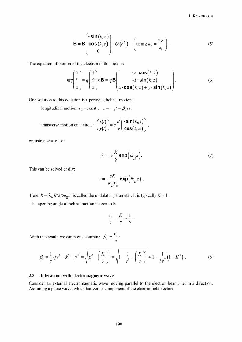
( )( ) ( )2 2 using 0

u

u uu

k zk z O r k π

λ

⎛ ⎞⎛ ⎞⎜ ⎟= + =⎜ ⎟⎜ ⎟⎝ ⎠⎜ ⎟

⎝ ⎠

- sinB B cos . (5)

The equation of motion of the electron in this field is

( )( )

( ) ( )

u

u

u u

x x z k zm y q y q z k z

z z x k z y k z

⎛ ⎞⋅⎛ ⎞ ⎛ ⎞⎜ ⎟⎜ ⎟ ⎜ ⎟γ = × = ⋅⎜ ⎟⎜ ⎟ ⎜ ⎟

⎜ ⎟ ⎜ ⎟ ⎜ ⎟⋅ + ⋅⎝ ⎠ ⎝ ⎠ ⎝ ⎠

- cosB B - sin

cos sin . (6)

One solution to this equation is a periodic, helical motion:

longitudinal motion: = const., v z v t ctz z zβ= = ;

( )( )transverse motion on a circle:

k zx t K ucy t k zuγ

=⎛ ⎞⎛ ⎞⎜ ⎟⎜ ⎟

⎝ ⎠ ⎝ ⎠

- sin( )( ) cos

,

or, using w x iy= +

( )Kw ic ik zuγ= exp . (7)

This can be solved easily:

( ) .cKw ik zuk vu z=γ

exp

Here, = /2 is called the undulator parameter. It is typically 1 . 0The opening angle of helical motion is seen to be

K e B m c Kuλ π ≈

1v Kc⊥ = ≈

γ γ .

With this result, we can now determine zz

vc

=β :

( )2 2

2 2 2 2 22 2

1 1 1 1 1 12z

K Kv x y Kc

β βγ γ γ γ

⎛ ⎞ ⎛ ⎞= − − = − = − − ≈ − +⎜ ⎟ ⎜ ⎟⎝ ⎠ ⎝ ⎠

. (8)

2.3 Interaction with electromagnetic wave

Consider an external electromagnetic wave moving parallel to the electron beam, i.e. in z direction. Assuming a plane wave, which has zero z component of the electric field vector:

J. ROSSBACH

190

( )( )

0

0 0

0

cosE E sin

L L

L L L

t k zt k z

⎛ ⎞− −⎜ ⎟= − −⎜ ⎟⎜ ⎟⎝ ⎠

ω ϕω ϕ , (9)

with the magnetic field given by: (1/ )L L Lcω=B E . Here, Lω is the angular frequency of the electromagnetic ‘light’ wave and the index L stands for ‘light’. It is unnecessary to mention that this frequency does not need to be in the visible range. 2 /L Lk π λ= is the wave number. Again, complex

notation is very useful, because we have to deal with only two components of LE . We define a complex electric field given by

( )0 0, ,E E E E expL L x L y L Li i t k z= + = − −ω ϕ .

We now calculate the change of the electron’s energy in the combined presence of the undulator and the electromagnetic field. It is well known that a charged particle does not gain energy in any magnetic field, since the Lorentz force is always perpendicular to the particle’s velocity. Thus we have to consider only the electric field. As the electromagnetic wave has nothing but electric field components perpendicular to the mean electron beam (z) direction, we now recognize the important role of the undulator field: It generates velocity components of the electrons in the direction of the electric field vector, i.e. in the x and y direction making energy transfer between the electromagnetic wave and the electron beam possible. The electron’s energy E is changed at a rate

( ) ( )

( )

2

0 00 .

L L x L y L

u L L

dΕ dmc v F q v q x y q wdt dt

K Kqc k k z t qc

γ

ω ϕγ γ

∗= = ⋅ = ⋅ ⋅ = + = ℜ =

= − + − + = − Ψ

, ,E E E E

E Esin sin

We have used Eq. (7) and the ‘ponderomotive phase’ defined as ( ) 0u L Lk k z tΨ = + − +ω ϕ . If we use z zz v t ct= = β , we can write

( ) 0L

u Lz

zk k z

cω ϕβ

Ψ = + − + (10)

and 0E sinz

q KdΕdz γβ= − Ψ . (11)

The energy dE is taken from or transferred to the radiation field. For most frequencies, dE/dt oscillates very rapidly. A significant energy transfer will only be accumulated if the phase difference between particle motion and electromagnetic wave stays constant with time. Thus, there is a resonance condition give by

const. 0Lu L

z

d k kdz c

ωβ

ΨΨ = → = + − =( ) .

Using cL Lkω = yields

LINAC-BASED FREE-ELECTRON LASER

191

0Lu L

z

kk k

β+ − = .

Solving for 2

LLkπλ = we get the resonance condition

( ) ( )22

1 1 12

uzL u u z

z

Kλβλ λ λ ββ γ−= ≈ − ≈ + . (12)

It is important to realize that the resonant wavelength Lλ is identical to the on-axis, first harmonic wavelength spontaneously radiated by the undulator. With Eq. (12) we have achieved a condition for continuous energy transfer from the electron beam to the electromagnetic wave. However, even if all electrons had exactly the right energy to fulfil this condition when they entered the undulator, they would leave the resonance energy quickly because of the energy transfer to (or from) the wave. Thus, we need to investigate what happens to electrons with energies slightly off resonance. For particles slightly off resonance, the phase Ψ will slip. In order to understand by how much, we note that in Eq. (10) only 2 21 1/2 1z Kβ γ≈ − +( ) depends on energy. Writing resγ γ γ= + Δ we get

( )

2

32 res

2res

2

3res res

1

112

1 2 .

L L Lu L u L

z res

Lu

d Kk k k kdz c cKc

K kc

ω ω ω γβ γ γ

γ γ

ω γ γγ γ

Ψ += + − ≈ + − + Δ =⋅⎛ ⎞+⎜ ⎟−

⎜ ⎟+ Δ⎝ ⎠+= Δ = Δ

( )( )

(13)

Deriving once more with respect to z yields 2

2res

2u

d dkdzdzγ

γΨ = .

Using Eq. (11) in the form 02

0

E sinz

q Kddz m cγ

γβ= − Ψ we finally get

2

2 20 02 2 2 2 2

0 0

2 2 with E Esin sinu u

res z res z

Kk Kkd q qdz m c m cγ β γ βΨ = − Ψ = −Ω Ψ Ω = . (14)

This is pendulum equation in the γΔ –Ψ phase space: electrons with little deviation from resonance energy or from synchronous phase perform periodic oscillations, see Fig. 2. This is equivalent to the synchrotron oscillations in storage rings, except that the ‘bucket’ length is now the optical wavelength. Similarly, in synchrotron oscillation, particles within the separatrix get bunched.

The energy lost (or gained) by an electron increases (or decreases) the field energy. Thus, as seen from Eq. (11) and illustrated in Fig. 3, there is gain or loss in field energy per undulator passage depending on where the electron starts in the γΔ –Ψ phase space.

J. ROSSBACH

192

Fig. 3: In the presence of the undulator and electromagnetic field, buckets are formed where electrons perform periodic oscillation if the deviation from resonance energy and from synchronous phase is small. In contrast to synchrotron oscillation buckets, the longitudinal size of our buckets is very small, i.e., the optical wavelength.

2.3.1 The separatrix

In order to determine the parameters of the separatrix, we look for a first integral of Eq. (14):

Multiplying 2 sin′′Ψ = −Ω Ψ by 2 ′Ψ on both sides and using ( )22 = ddz

′ ′′ ′Ψ Ψ Ψ yields

( )2 2 2 22 2 2 2 const.dz dz d′ ′′ ′ ′Ψ Ψ = Ψ = Ω ΨΨ = −Ω Ψ Ψ = Ω Ψ +∫ ∫ ∫sin sin cos .

With 2

ures

k γγ

′Ψ = Δ this reads 2

22 2 const.ures

k γγ

⎛ ⎞Δ = Ω Ψ +⎜ ⎟

⎝ ⎠cos , thus

( )2 02

0

const .u z

q Km c k

γβ

Δ − Ψ =E cos , (15)

with const. determined by initial conditions.

There are two cases to be distinguished:

Case 1: const. 02

0 u z

q Km c k β

< E. Then, 0

20

const.u z

q Km c k

γβ

Δ = + ΨE cos has real solutions only within a

limited range of phases. This is the case of rotation within the separatrix.

Case 2: const. 02

0 u z

q Km c k β

> E. In this case all phases are possible, but 0Δγ = cannot be reached. As a

consequence, the electron performs ‘libration’ outside the separatrix. The separatrix is defined by the

limiting case: const. 02

0 u z

q K=m c k β

E. Thus, the separatrix is defined by the equation

LINAC-BASED FREE-ELECTRON LASER

193

( ) ( )2 02

0

1E cos

u z

q Km c k

γβ

Δ = + Ψ . (16)

The height of the separatrix is given by: 02

0

2max min

Eu z

q Km c k

γ γβ

Δ − Δ = , (17)

i.e. it is determined by the strengths of both the external electromagnetic wave 0E and of the undulator field (through K).

2.3.2 Power gain

In practice, an electron beam consists of many particles distributed smoothly throughout the phases, it is unclear from the previous analysis whether a significant overall amplification of the electromagnetic wave can take place. To determine the ‘power gain’ of the FEL in the presence of the entire beam, our most important assumption is that the amplitude of the electromagnetic wave changes little during one passage of the electron beam: i.e. the power gain (as defined below) is much smaller than unity: |G| < 1. This is the ‘low-gain approximation’, the subject of this section. We also assume an initially monoenergetic beam with some deviation γΔ from resonance energy. Let us define the power gain iG due to a particle identified by the index i by

( )

( ) ( )( )

2

200

2res res

20 0

0gain of field energy produced by electron total field energy

20

[using Eq. (13) ] .2

i u ii

i u i

u u

mc z LiGV

mc z LVk k

γ γε

γ γγε

− = −= =

⋅

′ ′− Ψ = −Ψ′= Δ = Ψ

⋅

( ) ( )

E

E

(18)

The undulator length is uL . Calculation of iG requires solution of the pendulum equation (14) 2 sin′′Ψ = −Ω Ψ for ( )zΨ . This is done iteratively. Start with the ansatz

( ) ( )0 0z z zδ′Ψ = Ψ + Ψ ⋅ + Ψ , (19)

where ( )zδΨ is the higher order term.

Step 1: ( ) 0zδΨ = .

Using the ansatz, a first integral of Eq. (14) is then:

( ) ( )1 2 20 0 0 0 0 0 0

00

1( ) sin cos cosz

z dz z′ ′ ′ ′ ′⎡ ⎤Ψ = Ψ −Ω Ψ + Ψ ⋅ = Ψ −Ω Ψ − Ψ + Ψ ⋅⎣ ⎦′Ψ∫ (20)

The gain of the entire beam (consisting of pN particles) is given by

0ii i p

iG G G N

Ψ= = ⋅∑ (21)

Averaging with respect to the initial phases is denoted by 0iΨ

and yields

J. ROSSBACH

194

( )0

0

1 20 0 0 0

0

1 0 ( ) cos cos zΨ

Ψ

′ ′ ′⎡ ⎤Ψ −Ψ = −Ω Ψ − Ψ + Ψ ⋅ =⎣ ⎦′Ψ. (22)

The important result is that, in first order, the average gain G is zero!

Step 2: ( ) 0zδΨ ≠ , calculating ( )zδΨ using the results of step 1, Eq. (20).

( ) ( )

( )

20 0 0

0 0

20 0 0 0

0 0 0

1

1 1 1 .

z

z z dz

z z

δ ′⎡ ⎤Ψ = −Ω Ψ − Ψ + Ψ ⋅ =⎣ ⎦′Ψ

⎡ ⎤′= −Ω ⋅ Ψ − Ψ + Ψ ⋅ + Ψ⎢ ⎥′ ′ ′Ψ Ψ Ψ⎣ ⎦

∫ cos cos

cos sin sin (23)

Using the ansatz again, the first integral of Eq. (14) now reads

( )( )

( ) ( ) ( )

2 20 0 0

0

20 0 0 0

0

.

z

z

z z dz

z z z dz

δ

δ

′ ′ ′Ψ − Ψ = −Ω Ψ + Ψ ⋅ + Ψ ≈

′ ′⎡ ⎤≈ −Ω Ψ + Ψ ⋅ + Ψ + Ψ ⋅ Ψ⎣ ⎦

∫

∫

( ) sin

sin cos

The approximation is valid for ( )zδΨ π , keep this in mind when using the results.

Plugging in ( )zδΨ and averaging with respect to phases yields

( ) ( )

( ) ( )

0

0

2 4 2 20 0 0 0 0 02

0 0

4

0 0 020 0

1

.2

Lu

Lu

z z z dz

z z z dz

ΨΨ

′ ′ ′ ′ ′⎡ ⎤Ψ −Ψ = Ω Ψ Ψ ⋅ Ψ ⋅ − Ψ ⋅ Ψ ⋅ =⎣ ⎦′Ψ

Ω ′ ′ ′⎡ ⎤= Ψ Ψ ⋅ − Ψ ⋅⎣ ⎦′Ψ

∫

∫

( ) cos cos sin sin

cos sin

( ) ( )Here we used 0α

α β α β+ + =cos sin 2 21 1and ; and 2 2α α

α α= =cos sin .

By partial integration as follows

0 0 0 0 0 0 00 00 0

1 1cos( ) sin( ) | sin( )u u

u

L LL

vu u uv v

z z dz z z z dz′ ′

′ ′ ′ ′ ′ ′Ψ Ψ = Ψ Ψ − Ψ Ψ′ ′Ψ Ψ∫ ∫ ,

LINAC-BASED FREE-ELECTRON LASER

195

( ) ( )

( ) ( )( )

0

2

42

0 0 020 0

4

0 020 0

4 20 0 02 3

0 0

(using 2 2 and 2 1 2 )

we get 22

12 12

1 2 .2 2 2

Lu

u u

u u u

u u uu

x x x x x

L L z dz

L L L

L L LL

Ψ

= − = −

⎡ ⎤Ω′ ′ ′ ′Ψ −Ψ = Ψ − Ψ ⋅ =⎢ ⎥′Ψ ⎣ ⎦⎡ ⎤Ω ′ ′= Ψ + Ψ − =⎢ ⎥′ ′Ψ Ψ⎣ ⎦

⎛ ⎞′ ′ ′Ψ Ψ Ψ= Ω −⎜ ⎟′ ′Ψ Ψ⎝ ⎠

∫( )

sin sin cos cos sin

sin sin

sin cos

sin cos sin

The latter expression can also be put in the form 0

2 0

2 40 2

0 0

d 2 .d

uL

Ψ

′Ψ⎧ ⎫⎪ ⎪

′ ′Ψ −Ψ = Ω ⎨ ⎬′ ′Ψ Ψ⎪ ⎪⎩ ⎭

( )sin

With Eqs. (18) and (21), the gain can be written

( ) ( )( ) 2 02 2res 4

2 2 20 0 0 0 0 0

0 d 2 .d

u

i u i res pp

u u

Lmc z L mc N

G NVk Vk

γ γε ε

′Ψ ⋅⎧ ⎫′ ′− Ψ = − Ψ ⎪ ⎪

= = − Ω ⎨ ⎬′ ′⋅ ⋅ Ψ Ψ⎪ ⎪⎩ ⎭

sin

E E

Using the abbreviations 0 2

, pup

NLn

Vξ

′Ψ ⋅= = , u u uL N λ= (with uN the number of

undulator periods) and get the final result 1

2

2 3 2 2 2

2 30

dd

u u pq N K nG

mcπ λ ξ

ξ ξε γ⎧ ⎫⎪ ⎪⎨ ⎬⎪ ⎪⎩ ⎭

= − sin . (24)

The functions 2

2sin ξξ

and 2

2dd

sin ξξ ξ⎧ ⎫⎪ ⎪⎨ ⎬⎪ ⎪⎩ ⎭

are plotted in Fig. 4.

To summarize, the key assumptions based on this result are a helical undulator, perfect overlap of electron and radiation field, perfect electron beam (zero emittance and no momentum spread). Note that the approximations do not assume that the beam is located inside the separatrix, i.e. the external electromagnetic field may be so weak that the separatrix covers only a small fraction of the gain curve.

For the interpretation of Eq. (24) it is useful to express ξ in the form

0 22

u u uu

res res

L k LN

γ γξ πγ γ

′Ψ ⋅ Δ Δ= = = (25)

1 Using the same volume V in the definition of the particle density as in the expression for the total field energy [see Eq. (18)] means that we assume perfect overlap of electron beam and electromagnetic field.

J. ROSSBACH

196

Fig. 4: In low-gain approximation, the dependency of power gain on the initial momentum (right) can be written as the derivative of the line-shape function (left) of the spontaneous undulator radiation

Thus, we can interpret the result as follows: There is no net gain (G = 0), to first order in the iteration, because phase-space motion is (almost) symmetric. In other words, the same amount of particles move up as move down. In second order, however, for positive γΔ , the particle motion with positive phase goes downwards more rapidly than the motion of the others goes upwards, i.e. there is positive gain if the electron energy is slightly above resonance energy ( 0γΔ = ). This is illustrated in Fig. 5. There is no gain for particles precisely on resonance energy ( 0γΔ = ). For 0,γΔ < the gain is negative, this means the beam extracts energy from the electromagnetic wave, and is accelerated. A device accelerating electrons by an electromagnetic wave using this mechanism is called an ‘inverse FEL’.

Fig. 5: If the electron energy is slightly above resonance energy (red broken line), some particles lose, while some gain energy. On average, electron energy is pumped into the electromagnetic wave (positive power gain), this is a second-order effect.

2.3.3 Madey theorem

Another interpretation of Eq. (24) uses the relation [see Eq. (12)] res/2 = / resω ω γ γΔ Δ connecting γΔ to the deviation of the angular frequency ωΔ from its resonance value resω . Using this relation, we can write

LINAC-BASED FREE-ELECTRON LASER

197

2

res2

res

2

2

2 2

0.

14 u

u

u u pN

dd

N

KK

q N nG

mc

ωπω

ω ωπω

π λε γ

Δ

Δ

⎛ ⎞⎜ ⎟⎝ ⎠

+ ⎛ ⎞⎜ ⎟⎝ ⎠

= −sin

( )

The expression

2

res2

res

sin u

u

N

N

ωπω

ωπω

Δ

Δ

⎛ ⎞⎜ ⎟⎝ ⎠

⎛ ⎞⎜ ⎟⎝ ⎠

is just the spectral line-shape function of spontaneous radiation of an undulator with uN periods in the vicinity of the first harmonic resonance frequency resω , see the left-hand side of Fig. 4. The following statement is called the Madey-theorem [5]:

The gain function of low-gain FEL emission is the derivative of the line-shape function of spontaneous undulator radiation.

2.3.4 The optical cavity

The amount of radiation energy produced per undulator passage isΔ = ⋅ iE G E , where iE represents the radiation energy before the electron bunch passes the undulator. One might think that a power gain of a few per cent (i.e. a low-gain FEL) is of no interest. However, it is important to realize that the gain is independent of the strength of the initial, external electromagnetic field, for example whatever the initial field, it will be amplified by this gain factor. The radiation produced can be accumulated successively with a pair of mirrors arranged to form an optical cavity as shown in Fig. 6, if on each round trip of radiation a fresh electron bunch is available. After N round trips, the total power gain is Gtotal = GN , which may be a very large number, even if G is not much larger than unity.

At the end of this process, there is a great deal of radiation energy stored in the optical cavity, so that amplification of this energy by even a few per cent is a large quantity in terms of absolute numbers. In other words, the electrons are stimulated to emit radiation because of the presence of the existing field. In fact, the amplification process in the FEL can be described quantum-mechanically in terms of emission and absorption of radiation quanta (photons), and with the properties of FEL radiation like coherence and many photons per coherence volume –– it justifies the notion of a ‘laser’. Many of the early FEL papers were written in a quantum mechanics context which explains the generous use of quantum-based terminology in the FEL community. Nevertheless, the description of FELs in terms of classical physics is, with a few rare exceptions, perfectly correct. The FEL is a ‘classical device’.

A fraction of the radiation energy gained is extracted through one of the semi-transparent mirrors. Of course, the mirror transparency must be arranged so that the total power losses of the optical cavity by extraction or absorption do not exceed the power gain.

J. ROSSBACH

198

Fig. 6: A free-electron laser in oscillator mode (R. Bakker). Large radiation power can be generated if the radiation field can be stored in an optical cavity, and if many electron bunches pass the cavity with timing synchronized to the round-trip of radiation within the oscillator: even if there is only a few per cent field gain per passage of an electron bunch (low-gain FEL). If the power gain exceeds the accumulated mirror losses (including the semi-transparent mirror for extraction), the stored power increases passage-by-passage in an exponential way until saturation is reached.

2.3.5 Saturation

If the change of electron energy within one undulator passage becomes comparable with /2res uNγ π , the phase advance per undulator passage becomes large according to Eq. (13), so that the assumption ( )zδΨ π made for our gain calculation is violated. Also, the assumption of a quasi-monoenergetic

electron beam is violated, i.e. the parameter ξ defined in Eq. (25) varies significantly during the undulator passage, depending on the longitudinal position within the separatrix. Thus, Eq. (24) becomes a useless calculation tool for overall gain because, based on violated assumptions, it is now inaccurate. In this case, the gain must be calculated numerically.

According to Eq. (17), the height of the separatrix grows with the radiation energy stored in the cavity. More and more electrons get trapped within the separatrix, providing an efficient mechanism for longitudinal bunching of the electron beam at the optical wavelength (an effect called ‘micro-bunching’, to be distinguished from longitudinal bunching of the entire electron bunch). The gain process saturates if most of the electrons get micro-bunched, i.e. if the electron density is almost completely modulated at the resonance wavelength. According to Eq. (4) and the explanations thereof, the undulator radiation power exceeds spontaneous radiation power by a large factor N comparable to the number of electrons per resonance wavelength.

This section only solves the kinematic problem of an electron beam in the combined presence of a given electromagnetic wave and an undulator field where the gain of radiation power was derived from an energy conservation argument. The kinetic energy taken from the electron must go into the radiation energy –– where else? It is obvious that, for a more thorough analysis, one has to solve both the kinematic problem and the electrodynamical problem (i.e. the generation of radiation by a modulated charge according to Maxwell’s equations) simultaneously. Such a detailed analysis of the

LINAC-BASED FREE-ELECTRON LASER

199

FEL oscillator, including the analysis of saturation, can be found in the literature, [2]. The next section presents this kind of treatment for the high-gain, single-pass FEL. Indeed, the low-gain results in this section can be derived from the general result as a special case, low-gain approximation, which with hindsight justifies the low-gain treatment given above.

Although storage-ring FELs are beyond the scope of this article, we conclude this section with a remark on FEL oscillators driven by electron bunches in a storage ring. This kind of arrangement is very attractive, since the electron bunch can be used many times (i.e. once per revolution), and reliable operation can be expected on account of the inherent stability of storage rings in terms of timing and bunch population. However, there are inherent drawbacks: As the same electron bunch is used many times, the electron-beam dynamics in the storage ring must be taken into account. As described above, the energy width of the electron beam is considerably increased close to saturation at each passage of the FEL. This energy broadening accumulates from turn-to-turn. It is somewhat compensated by radiation damping, but the saturation process remains drastically determined by this effect [6]. Even if one considered using the beam of a storage ring only once per damping time, there is a fundamental issue making such an electron bunch unattractive in some cases: The product of bunch length and energy width (longitudinal emittance) is determined by quantum fluctuation effects in a storage ring and cannot be made as small as in a linear accelerator.

2.3.6 Start-up from noise

In order to achieve maximum gain, ξ should be ~ +1, i.e. Δγ ≈ + γ/2πΝu. The electron-beam energy should be above resonance energy by that amount. This is easy to achieve if the initial electromagnetic field is provided by an external source. The external wavelength determines, together with the undulator parameters, the resonance energy γres of the electron beam. Therefore, we simply have to set the electron-beam energy to γres + Δγ.

What happens if there is no external radiation source? The FEL can still work, if the spontaneous radiation of the undulator is used. With two mirrors, this radiation has to be reflected back to the entrance of the undulator, and it must be synchronized longitudinally with the next electron bunch for overlap in the undulator (see Fig. 6).

Unfortunately, if we want to use the centre of the spectrum of the spontaneous undulator radiation as the ‘external wave’, there will be no FEL gain, because this wavelength, and the beam energy, fulfill the resonance condition exactly. It is helpful that the spontaneous spectrum has the same width [see Eq. (24) and Fig. 4] as the gain curve, therefore there is always significant power at a wavelength with high gain.

This can happen in two ways:

1. If the bandwidth of the optical resonator formed by the two mirrors is very large, then the FEL will ‘automatically’ amplify only that part of the spectrum with positive gain. This will happen with the lower frequency part of the spontaneous spectrum. For this wavelength to be resonant, the beam energy would have to be smaller than it actually is, so the actual beam energy will be slightly above resonance, as it should be for positive gain.

2. If the bandwidth of the optical resonator is small (normal case), it should be tuned below the centre frequency of the spontaneous spectrum (same argument as before). This is illustrated in Fig. 7.

J. ROSSBACH

200

Fig. 7: When starting from noise, the spontaneous radiation of the undulator serves as an ‘external electromagnetic wave’ to be amplified in the FEL. For optimum gain, the electron energy should be chosen so that it samples the gain curve where it is positive and maximum. Since the gain curve is centred with respect to the resonance energy (rather than w.r.t. the beam energy), this condition can be met if the resonant wavelength of the optical cavity (yellow line) is tuned below the electron beam energy. Then, only the low-frequency wing of the undulator spectrum gets amplified, but it is guaranteed by the strict relation between the width of the spectrum and the width of the gain curve (see section 2.3.3) that there is sufficient radiation power in this portion of the spectrum to serve as input signal.

3 The high-gain free-electron laser If the radiation power gained within a single passage of the electron beam through the undulator is comparable or much larger than the input radiation power, the low-gain approximation is not applicable any more. In this case, we have to take into account the time-dependence of the increasing electromagnetic wave as determined by the motion of the electrons in the beam. On the other hand, just this motion is determined by the electromagnetic field amplitude at any point in time and space. Thus, we need to treat the evolution of electron kinematics and electromagnetic field amplitude in a self-consistent manner.

The purpose of this section is to derive the key equations from first principles, motivating the approximations and providing some realistic numbers for illustration. The treatment follows closely the one given in Ref. [2].

3.1 Generation of electromagnetic fields by the electron beam

We start with a derivation of the wave equation for the electric field from Maxwell’s equations. From

Maxwell’s equation rott

∂= −∂BE we get 2

0rot rot grad div rot HE E Et∂= −∇ = −μ∂

. (26)

Next, we derive Maxwell’s equation 0rot EH jt∂= + ε∂

once more with respect to time and get

2

0 2rot H Ejt t t∂ ∂ ∂= + ε∂ ∂ ∂

.

If we further use Maxwell’s equations 0divε = ρE , Eq. (26) can be written in the form

LINAC-BASED FREE-ELECTRON LASER

201

22

0 0 0 20

1 EE jgradt t∂ ∂ρ −∇ = −μ − ε μ

ε ∂ ∂ .

Using 0 0 2

1c

μ ε = , this reads

22

02 20

1E jtc t

⎛ ⎞∂ ∂∇ − = μ + ∇ρ⎜ ⎟ ∂ ε∂⎝ ⎠, (27)

which is the well-known wave equation for the electric field. In the following approximation, we restrict ourselves to a one-dimensional treatment of the FEL, i.e. we consider a purely transverse electromagnetic field. This means that we neglect diffraction effects, which is certainly questionable for long wavelengths. With this approximation, Eq. (27) reads

2 2

02 2 20

1 1E E jtz c t

⊥ ⊥ ⊥⊥

∂ ∂ ∂− = μ + ∇ ρ

∂ ε∂ ∂, (28)

with the index ⊥ denoting the vector component perpendicular to the direction of electron propagation. The term 01/ ⊥ε ∇ ρ in Eq. (28) can be neglected because its contribution to radiation generation is small in all practical cases.2 The transverse electric field ⊥E of the electromagnetic wave can be written in the form

0

0 0

0

cos( )E E sin( )

L L

L L

t k zt k z⊥

ω − − ϕ⎛ ⎞⎜ ⎟= ω − − ϕ⎜ ⎟⎜ ⎟⎝ ⎠

.

The magnetic field of the electromagnetic wave is then 1B E

Lc⊥ ⊥=ω

.

In analogy to the previous section, we take advantage of the fact that we have to deal with only two components of E and define a complex electric field given by

0 0x y L Li i t k zω ϕ⊥ ⊥= + = − −, ,E E E E exp ( ) . The only difference from the low-gain case is now

that the amplitude 0E and the phase 0ϕ (which we will call Eψ now) may vary with z (though slowly compared to Ltω ). We thus separate the slow part from the rapidly oscillating part by

writing: 0 0E E ( )exp ( ) E ( )exp ( )L L E L Lz i t k z z i t k z∗= ω − −ψ = ω − , with the slow part

0 0E ( ) E ( )exp Ez z i= ψ and 0E ( )z∗ its complex conjugate (c.c.). Equation (28), re-written for

0, ,E E E ( )exp ( )x y L Li z i t k z∗⊥ ⊥+ = ω − reads

2 For a more detailed justification, see Ref. [2], section 4.1.

J. ROSSBACH

202

2 2

2 2 2

2 2

0 02 2 2

0 0

02

1

1

1

, , , ,(E E ) (E E )

E ( )exp ( ) E ( )exp ( )

E ( ) exp ( ) exp ( ) E ( )

E ( ) exp ( ) exp ( )

x y x y

L L L L

L L L L

L L L L

i i

z c t

z i t k z z i t k zz c t

z i t k z i t k z zz z z

z i t k z i t k zt tc

⊥ ⊥ ⊥ ⊥

∗ ∗

∗ ∗

∗

∂ + ∂ +− =

∂ ∂∂ ∂= ω − − ω − =∂ ∂∂ ∂ ∂⎡ ⎤ω − + ω − −⎢ ⎥∂ ∂ ∂⎣ ⎦

∂ ∂ ∂ω − + ω −∂ ∂ ∂

…

… 0E (zt

∗

20 0

2

0 02

021

)

(E ( )) ( )exp ( ) E ( )( )exp ( )

( )exp ( ) E ( ) exp ( ) E ( )

(E ( )) exp ( )

L L L L L L

L L L L L

L L L

z ik i t k z z k i t k zz

ik i t k z z i t k z zz z

z i i t k ztc

∗ ∗

∗ ∗

∗

⎡ ⎤=⎢ ⎥

⎣ ⎦∂ ⋅ − ω − + − ω − +∂

∂ ∂− ω − + ω − −∂ ∂

∂ ⋅ ω ω −∂

…

… …

… 202

1 0E ( )( )exp ( )L L Lz i t k zc

∗− −ω ω − +

where we have made use of our assumption that the complex field amplitude does depend on the

longitudinal coordinate z, but not (explicitly) on time t, i.e. 00 zt∂ ∗ =∂

E ( ) . We further neglect the

second derivative of the field amplitude with respect to z because it is assumed to vary only slowly and get:

2 2

2 2 2

22

0 0 02

0 0 0

i i1

2i i i i

i K2i i i i

x y x y

LL L L L L L L L

x yL L L u

z c t

k z t k z k z t k z z t k zz c

j jk z t k z k z

z t

⊥ ⊥ ⊥ ⊥

∗ ∗ ∗

⊥ ⊥∗

∂ + ∂ +− =

∂ ∂−ω∂⎡ ⎤= − ω − − ω − − ω − =⎢ ⎥∂⎣ ⎦

∂ + ⋅ ∂∂⎡ ⎤= − ω − = μ = μ⎢ ⎥∂ ∂ γ⎣ ⎦

, , , ,

, ,

(E E ) (E E )

( )E ( ) exp ( ) E ( )exp ( ) E ( )exp ( )

( )E ( ) exp ( ) exp( ) . (29)zj

t∂Here we made use of / = L Lc kω . Also, we were able to relate the transverse components of the current density to its longitudinal component, since we know from Eq. (7) how electrons move in the presence of the helical undulator: Namely, because of j rv= , we were able to write

x x(j [see Eq.(7)] = i i zy y u z u z

z z

j c K Ki j v i v e ik z j e ik z jv v

+ ⋅ = + ⋅ = ≈γ γ

) ( ) xp( ) xp( ) .

Collecting the rapidly oscillating term and using ( )u L Lk k z tΨ = + − ω , Eq. (29) re-writes:

0 0 0K K2 i iE ( ) exp ( ) expz z

L u L Lj j

k z k z k z tz t t

∗ Ψ∂ ∂∂⎡ ⎤− = μ + −ω = μ⎢ ⎥∂ γ ∂ γ ∂⎣ ⎦

. (30)

The message of the equation is pretty simple: The electromagnetic field amplitude is generated by the time-dependent current density.

To proceed further, we have to say something about the current density zj .

LINAC-BASED FREE-ELECTRON LASER

203

3.2 Kinematics of electrons in phase space

The term zj is determined by the initial charge distribution and its evolution in the presence of the electromagnetic field and the undulator field. We know that electron dynamics is governed by the Hamiltonian

( ) ( )1 22 22 2 4

/( , , )z z z uH p z t p c qA q A A m c q⊥

⎡ ⎤= − + + + + φ⎣ ⎦ ,

with uA describing the undulator field, and zA , φ the space charge. Applying a canonical transformation, we can change from the canonical pair of coordinates z/ zp to /Ψ γ (actually, the pair

is 20/m c⊥ω Ψ γ⋅ / , but 2

0/m c⊥ω is constant), with ( )u L Lk k z tΨ = + − ω and 20m cγ the kinetic

energy of the electron. A consequence of Hamiltonian mechanics is Liouville’s theorem, stating that phase space density f along the particle’s motion is constant. Phase space motion must be described in any pair of canonically conjugate variables, and we choose /Ψ γ . In coordinates z, γ ,Ψ , this theorem reads3

0df f f fdz z z z

∂ ∂ ∂Ψ ∂ ∂γ= + + =∂ ∂Ψ ∂ ∂γ ∂

, (31)

which is also called ‘Vlasov equation’.

We have seen from Eq. (11) how the electron energy changes in the presence of an electromagnetic field and an undulator field. In addition to Eq. (11), we now include the energy gain due to the presence of a longitudinal space charge field Ez :

( )02 2

0 0 0

E Esin zE

z

q K qddz m c m cγ = − Ψ + ψ +

γ β.

Of course, we have to understand that the electrical field strength 0E is no longer constant. Therefore, we also allow for a slowly varying phase of the electromagnetic field, described by Eψ . Note d dzΨ / can be determined from Eq. (13):

2

30 0

1( )

L Lu L

z

d Kk kdz c c

ω ωΨ += + − + Δγβ γ ⋅ γ

,

where Δγ denotes the deviation from 0γ . In general, we allow 0γ to deviate slightly from resonance energy resγ described by the detuning parameter

( )( )

Lu L

z

C k kc

ωγ = + −

β γ ⋅, i.e. 0( )resC γ = .

(Note: You may ask why the deviation from resonance energy is split into two terms, 0γ and Δγ . The reason will become clear below, where we use Δγ to describe the energy distribution of the beam

3 We use the longitudinal coordinate z as independent variable instead of time t, which in fact means another canonical transformation.

J. ROSSBACH

204

around the centre 0γ .) We get:

2

30

1Ld KCdz c

ωΨ += + Δγγ

.

Equation (31) now reads

( )2

03 2 20 0 0 0

1 0sinL zE

qE K qEf K f fCz c m c m c

⎛ ⎞ ⎛ ⎞ω∂ + ∂ ∂+ + Δγ + − Ψ + ψ + =⎜ ⎟ ⎜ ⎟∂ ∂Ψ ∂γγ γ⎝ ⎠ ⎝ ⎠. (32)

Note that from now on we use z 1β ≈ . For the phase space density f we make the ansatz 0 1 0( , , ) ( ) ( , )cos( )f z f f zγ Ψ = γ + γ Ψ + ψ , i.e. we assume a density modulation at the optical

wavelength, growing with z (not get calculated), see Fig. 8 for illustration. The phase of this modulation is allowed to slowly depart from Ψ by 0ψ (which is, general differently from Eψ ). In complex notation:

1 10 0 1 01 0 2 2 12 c.c. c.c.f fi i i i iff z e e ee f z eΨ+ψ − Ψ+ ψψ Ψ Ψγγ Ψ + ψ = + = + = +( ) ( )( , )co ) , )s ((

The complex amplitude 1 01 2( , ) f if z e ψγ = of density modulation contains the slowly varying phase

0ψ . A similar ansatz is made for the space charge field Ez :

iz z s zE z z e c.c.Ψ= Ψ + ψ = +E ( )cos( ) E ( ) ,

again with its own slowly varying phase sψ . Vlasov’s equation (32) can now be written:

( )

20

3 2 20 0 0 0

2i i i1 1

1 130

i i i i i0 0 12 2

0 0 0

1

1 i i

i2

( ) ( )

E E( ) ( sin( ) )

( )( )

E (E E )E E

L zE

iL

z z

q K qf K f fCz c m c m c

f f Ke e C f e f ez z c

q K f fqe e e e em c m c

∗Ψ − Ψ Ψ ∗ − Ψ

Ψ+ψ − Ψ+ψ Ψ ∗ − Ψ Ψ

ω∂ + ∂ ∂+ + Δγ + − Ψ + ψ + =∂ ∂Ψ ∂γγ γ

∂ ∂ ω += + + + Δγ − +∂ ∂ γ

⎡ ⎤ ∂ ∂ ∂+ − + + + +⎢ ⎥

∂γ ∂γ⎢ ⎥γ⎣ ⎦

i1

i0 0

20 01

13 2 20 0 0 0i

i i i i0 12 2

0 0 0

(using )

1i i2

0

i2

( ) ( )

E E

E( ) ( E )

. .E ( ) (E E )

E

E E

Lz

z z

fe

e

q K ff K qC fz c m c m c

e c cq K fqe e e em c m c

∗− Ψ

ψ

Ψ

Ψ+ψ − Ψ+ψ Ψ ∗ − Ψ

⎛ ⎞⎜ ⎟ =⎜ ⎟∂γ⎝ ⎠

=

⎧ ⎫∂∂ ω ++ + Δγ + + +⎪ ⎪∂ ∂γγ γ⎪ ⎪⎪ ⎪= + =⎨ ⎬⎡ ⎤ ∂⎪ ⎪− + +⎢ ⎥⎪ ⎪∂γ⎢ ⎥γ⎪ ⎪⎣ ⎦⎩ ⎭

For this equation to hold for all phases Ψ , the expression in brackets must vanish. Our next step in approximation assumes that the modulation amplitude does not depend on energy (see Fig. 7):

LINAC-BASED FREE-ELECTRON LASER

205

1 0f∂=

∂γ. Then:

0

20 01

13 2 20 0 0

1i i 02

( )( , )

E( , ) ( ) ( E )Lzz

q K ff z qKC fz c m c m c

γγ

∂∂ γ ω ++ + Δγ + + =∂ ∂γγ γ

. (33)

Fig. 8: Illustration of a possible phase space density function fulfilling the assumptions made here: The density modulation amplitude f1 observed at an arbitrary location z does not depend on energy γ, and the amount of modulation in the core of the beam is small compared to the total density.

Equation (33) is a differential equation in z of the type ( ) ( ) ( )df z i f z g z

dz+ α = , which is solved by

[ ]0

( ) ( )exp ( )z

f z g z i z z dz′ ′ ′= α −∫ . Thus:

20 0

1 2 2 30 0 0 00

12E ( ) ( )( , ) E ( ) exp ( )( )

zL

zq z K fq Kf z dz i z i C z z

cm c m c⎡ ⎤′ ⎡ ⎤∂ γ ω +′ ′ ′γ = + + Δγ −⎢ ⎥ ⎢ ⎥∂γγ γ⎣ ⎦⎣ ⎦

∫ (34)

and 1 c.c.f z∗ γ =( , ) We can now calculate the current density:

0 1

0 1 1 1

1

1,with , etc.

i iz z

i i

j v c qc f z d qc f d e qc e qc fj j e j e j q

f z d z df z dc

Ψ − Ψ ∗

Ψ ∗ − Ψ

= ρ ≈ ρ = γ Ψ γ = γ γ + + == + + =

γ γ γ γγ γ

∫ ∫ ∫ ∫∫

( , ) ( , )( , )

( , , ) ( )

With these definitions, Eq. (30) reads

( )0 1 10 0 0

0 0

K K2 E ( )i i

i izL

j j e j ejk z e e

z t t

Ψ ∗ − Ψ∗ Ψ Ψ

∂ + +∂∂⎡ ⎤− = μ = μ⎢ ⎥∂ γ ∂ γ ∂⎣ ⎦.

We use ( )u L Lk k z tΨ = + − ω and assume that 1j is ‘almost’ independent of time.

J. ROSSBACH

206

Then:

( ) ( ) ( )i i 2i0 0 1 1 0 1 1 0 1

0 0 0

K KK2 i i iE ( ) i L LL L Lk z j e i j e e j e j j

z∗ Ψ ∗ − Ψ Ψ Ψ ∗ ∗ω ω∂⎡ ⎤ ⎡ ⎤− ≈ μ − ω + ω = μ − + ≈ μ⎣ ⎦⎢ ⎥∂ γ γ γ⎣ ⎦

(neglecting the rapidly term 2i1j e Ψ ). Equally, ( )0 1 0

0

Kiμ 2 EL

Lj k zz

ω ∂=γ ∂

. (35)

3.3 Self-consistent description of electromagnetic field and electron distribution

We can now combine the ‘field equation’ (35) and the ‘kinematic equation’ (34) to find a self-consistent description of the evolution of the electromagnetic field and the electron density distribution:

20 0

0 1 10 0 1

2 20 0 0

2 2 30 0 0 0 01 0

i i2 2

1i i i( .2 2

zL

z

cK Kqcz j f z dz

Kqc q z K fq Kd dz z C z zm c m c c

∞

∞

μ μ∂ = = γ γ =∂ γ γ

⎡ ⎤ ⎡ ⎤′μ ∂ γ ω +′ ′ ′γ + + Δγ −⎢ ⎥ ⎢ ⎥γ γ ∂γ γ⎣ ⎦⎣ ⎦

∫

∫ ∫

E ( ) ( , )

E ( ) ( )E ( ) exp )( ) (36)

The problem with this equation is that it contains not only the desired complex transverse field amplitude 0E , but also the longitudinal space charge field zE . Fortunately, Ez can be related to 0E in

the following way: For our assumption of the space charge field ( ) c.c.iz z z e Ψ= +E E , the

longitudinal component of the first Maxwell equation reads (note / x = / y = 0∂ ∂ ∂ ∂ in our 1D treatment):

( ) 00 Ez zzH j

t∂∇× = = + ε∂

or

( ) 20Ez zz c j

t∂ = −μ∂

,

thus

( )2

01

iEzL

cz j

μ≈ −

ω.

With Eq. (35) this is related to the transverse electromagnetic field:

( )01 0

0

2i Ej z

cK zγ ∂= −

μ ∂,

thus

( )00

2E ( ) EzL

cz z

K zγ ∂≈ −ω ∂

.

LINAC-BASED FREE-ELECTRON LASER

207

Therefore Eq. (36) becomes:

( )2 2 2 2 2

0 0 00 0 02 2 2 3

0 0 01 0

4 1i i i(C4

( )E ( ) E ( ) E exp )( )z

L

L

q K c c f Kz d dz z z z zz z cm c K

∞ ⎡ ⎤ ⎡ ⎤μ γ ∂ γ ω∂ ∂ +′ ′ ′ ′= γ − + Δγ −⎢ ⎥ ⎢ ⎥′∂ ∂ ∂γγ ω γ⎣ ⎦ ⎣ ⎦∫ ∫

This is an integro-differential equation for the complex amplitude of the electromagnetic field. Only for few non-trivial model functions of the initial energy distribution 0f can the solution be found analytically, using Laplace transform techniques. We restrict ourselves to the most simple case, a monoenergetic (‘cold’) beam: 0 0 0( ) ( )f nγ = δ γ − γ , i.e. = 0Δγ , with charge density 0qn , i.e.

0 0 0 0( )j qc n d qcn∞

−∞

= δ γ − γ γ =∫ .

Integration over energy can then be executed, using partial integration:

[ ]00 01

1 1

d ( ) ( )( ) ( ) ( ) ( ) dFF d F dd d

∞ ∞∞δ γ − γ γγ γ = δ γ − γ γ − δ γ − γ γ

γ γ∫ ∫ ,

thus

2 2 2

0 0 02 3 30 00 1

2 20 0

0 20 0

2 2 2 20 0 0

0 05 20 0 0

4 1 1i i i(C

i4

1 4i4

zL L

L

zL

L

c K Kdz d z z z z z z

K z c c

n q Kzz m

n q K K cdz z zm c K z

∞ ω ωγ ∂ + +′ ′ ′ ′ ′γδ γ − γ − − + Δγ −′ω ∂ γ γ

μ∂ = ×∂ γ

⎛ ⎞ ⎡ ⎤⎡ ⎤=⎜ ⎟ ⎢ ⎥⎢ ⎥

⎣ ⎦ ⎝ ⎠ ⎣ ⎦⎡ ⎤μ + ω γ ∂′ ′ ′= − −⎢ ⎥′γ ω ∂⎣ ⎦

∫ ∫

∫

( ) E ( ) E ( ) ( ) exp )( )

E ( )

( ) E ( ) E ( ) [ ]

[ ]2

30 03

0

iC

i iC , (37)z

p

z z z z

kdz z z z z z z

z

′ ′− − =

⎡ ⎤∂′ ′ ′ ′ ′= −Γ − − −⎢ ⎥′Γ ∂⎢ ⎥⎣ ⎦∫

( )exp ( )

E ( ) E ( ) ( )exp ( )

with abbreviations:

0

0

2 2 2 2 23 0 0 0

5 50 0 0

2 22 30

3 20

Γ is called the gain parameter

417 kA is the 'Alven current'

is the wave number of longitudinal

1 1 4

4 1 4

A

L L

A

p pA L

m cI

q

n q K K j K Km c I c

j K ck kI K

π= =

μ

μ + ω π + ωΓ = =γ γ

π + γ= = Γγ ω

( ) ( )

( )plasma oscillation

.

Note that kp is the only reminder of taking longitudinal space charge into account. We have ended with an ordinary integro-differential equation (37) for 0E . We now derive Eq. (37) with respect to z:

[ ]22

30 0 0 02 3

0

=-iC i iCE E E ( ) E ( ) exp ( )z

pkd d ddz z z z zdz dzdz

⎡ ⎤′ ′ ′ ′+ Γ − −⎢ ⎥′Γ⎢ ⎥⎣ ⎦

∫ ,

J. ROSSBACH

208

where

0 0 0

( ) ( ) ( ) ( ) ( ) ( ) ( ) ( )z z zd d ddz g z h z g z dz h z g z dz h z g z h z

dz dz dz⎡ ⎤

′ ′ ′ ′ ′ ′= = +⎢ ⎥⎣ ⎦

∫ ∫ ∫ )

was used.

Finally, we derive once more and get:

[ ]

3

03

2 223 3

0 0 0 0 02 3 30

22 23

0 0 0 0 02 3 2

23

0 02

=

=-iC i i i iC

=-iC i i iC

-2iC i

zp p

p

ddz

k kd d dz z C dz z z z zdz dz dz

kd d d dz z Cdz dz dz dz

ddz

⎡ ⎤ ⎡ ⎤′ ′ ′ ′+ Γ − − Γ − − =⎢ ⎥ ⎢ ⎥′Γ Γ⎢ ⎥ ⎢ ⎥⎣ ⎦ ⎣ ⎦

⎡ ⎤+ Γ − − + =⎢ ⎥Γ⎢ ⎥⎣ ⎦

= + Γ

∫

E

E E ( ) E ( ) E ( ) E ( ) exp ( )

E E ( ) E ( ) ( E E )

E E (2

20 03 C .pk d dz z

dz dz⎡ ⎤

− +⎢ ⎥Γ⎢ ⎥⎣ ⎦) E ( ) E

Rearranging, we arrive at our final result: An ordinary linear third-order differential equation for the complex field amplitude 0E :

( )3 2

2 2 30 0 0 03 22iC + C iE E E E ( )p

d d dk zdzdz dz

+ − = Γ . (38)

At the end of this derivation, Fig. 9 illustrates the major steps and approximations taking us to the final result in Eq. (38).

Fig. 9: Major steps to derive the 3rd order differential Eq. (38) for the high-gain free-electron laser

LINAC-BASED FREE-ELECTRON LASER

209

3.4 Solution of the high-gain FEL equation

For the solution of Eq. (38) we make the ansatz ( )0E expA z= Λ and get the ‘characteristic equation’:

( ) ( ) ( )23 2 2 2 2 2 2 2 3+2iC + C = 2iC C i ip p pk k C k⎡ ⎤Λ Λ − Λ Λ Λ + Λ − + = Λ Λ + + = Γ⎣ ⎦ . (39)

Equation (39) has three roots, and the general solution of Eq. (38) is constructed from three independent partial solutions:

( ) ( ) ( )0 1 1 2 2 3 3E ( ) exp exp expz A z A z A z= Λ + Λ + Λ . (40)

The amplitudes 1 2 3, , A A A are determined by the initial conditions. Since there are three free parameters, we need three independent conditions. The most practical way to specify these conditions is to specify

( ) ( ) ( )2

0 0 020 0 0E , E , Ed dz z zdz dz

= = = ,

or, taking into account Eq. (35): 0 1( / )d dz j∝E , to specify

( ) ( ) ( )0 1 10 0 0E , , dz j z j zdz

= = = .

We write Eq. (40) in the form ( ) ( ) ( ) ( )0 1 1 2 2 3 3E E E Ez A z A z A z= + + , with ( ) ( )1 1E expz z= Λ ,

etc., and we write ( / )d dz ′=E E , etc. (note we will omit the index 0 to 0E in the following). The general solution, including its first and second derivatives, can then be written in a matrix form:

1 2 3 1

1 2 3 2

31 2 3

AAA

z z

⎛ ⎞ ⎛ ⎞ ⎛ ⎞⎜ ⎟ ⎜ ⎟ ⎜ ⎟′ ′ ′ ′= ⋅⎜ ⎟ ⎜ ⎟ ⎜ ⎟⎜ ⎟ ⎜ ⎟ ⎜ ⎟⎜ ⎟ ⎜ ⎟′′ ′′ ′′ ′′ ⎝ ⎠⎝ ⎠ ⎝ ⎠

E E E EE E E EE E E E

,

where the index z means that the matrix elements are taken at longitudinal position z. Since 1 2 3Λ , Λ , Λ are known from the characteristic equation (39), all matrix elements are known. Writing

the initial condition in the form

0

,

z=

⎛ ⎞⎜ ⎟′⎜ ⎟

⎜ ⎟⎜ ⎟′′⎝ ⎠

EEE

we can calculate 1 2 3, ,A A A from

J. ROSSBACH

210

1

1 2 31

2 1 2 3

3 1 2 3 0 0

E E E EE E E EE E E E

z z

AAA

−

= =

⎛ ⎞ ⎛ ⎞⎛ ⎞ ⎜ ⎟ ⎜ ⎟⎜ ⎟ ′ ′ ′ ′= ⋅⎜ ⎟ ⎜ ⎟⎜ ⎟ ⎜ ⎟ ⎜ ⎟⎜ ⎟ ⎜ ⎟ ⎜ ⎟′′ ′′ ′′ ′′⎝ ⎠ ⎝ ⎠ ⎝ ⎠

.

Thus,

1

1 2 3 1 2 3

1 2 3 1 2 3

1 2 3 1 2 3 0 0z z z z

−

= =

⎛ ⎞ ⎛ ⎞ ⎛ ⎞ ⎛ ⎞⎜ ⎟ ⎜ ⎟ ⎜ ⎟ ⎜ ⎟′ ′ ′ ′ ′ ′ ′ ′= ⋅ ⋅⎜ ⎟ ⎜ ⎟ ⎜ ⎟ ⎜ ⎟

⎜ ⎟ ⎜ ⎟ ⎜ ⎟ ⎜ ⎟⎜ ⎟ ⎜ ⎟ ⎜ ⎟ ⎜ ⎟′′ ′′ ′′ ′′ ′′ ′′ ′′ ′′⎝ ⎠ ⎝ ⎠ ⎝ ⎠ ⎝ ⎠

E E E E E E E EE E E E E E E EE E E E E E E E

or, using ( ) ( ) ( ) ( )1 1 1 1 1 E exp , E exp ,z z z z′= Λ = Λ Λ etc.,

11 2 3

1 2 3 1 2 32 2 21 2 31 2 3 0

1 1 1E E E E EE E E E EE E E E E

z z z

−

=

⎛ ⎞ ⎛ ⎞ ⎛ ⎞⎛ ⎞⎜ ⎟ ⎜ ⎟ ⎜ ⎟⎜ ⎟′ ′ ′ ′ ′= ⋅ Λ Λ Λ ⋅⎜ ⎟ ⎜ ⎟ ⎜ ⎟⎜ ⎟⎜ ⎟ ⎜ ⎟ ⎜ ⎟⎜ ⎟Λ Λ Λ⎜ ⎟ ⎜ ⎟ ⎜ ⎟′′ ′′ ′′ ′′ ′′⎝ ⎠⎝ ⎠ ⎝ ⎠ ⎝ ⎠

. (41)

Using the explicit expression for the inverse matrix, Eq. (41) reads

( )( ) ( ) ( ) ( )( )

( )( ) ( )( ) ( )( )

( )( ) ( )( ) ( )( )

2 3 2 3

1 2 1 3 1 2 1 3 1 2 1 31 2 3

1 3 1 31 2 3

2 1 2 3 2 1 2 3 2 1 2 31 2 3

2 1 2 1

3 2 3 1 3 2 3 1 3 2 3 1

1

1

1z z

⎛ Λ Λ Λ + Λ−⎜ Λ − Λ Λ − Λ Λ − Λ Λ − Λ Λ − Λ Λ − Λ⎜⎛ ⎞ ⎛ ⎞⎜ ⎟ ⎜ ⎟ Λ Λ Λ + Λ′ ′ ′ ′= ⋅ −⎜ ⎟ ⎜ ⎟

Λ − Λ Λ − Λ Λ − Λ Λ − Λ Λ − Λ Λ − Λ⎜ ⎟ ⎜ ⎟⎜ ⎟ ⎜ ⎟′′ ′′ ′′ ′′⎝ ⎠ ⎝ ⎠ Λ Λ Λ + Λ−Λ − Λ Λ − Λ Λ − Λ Λ − Λ Λ − Λ Λ − Λ⎝

E E E EE E E EE E E E

0

.

z=

⎞⎟⎟ ⎛ ⎞

⎜ ⎟ ⎜ ⎟′⎜ ⎟ ⋅ ⎜ ⎟

⎜ ⎟ ⎜ ⎟⎜ ⎟′′⎜ ⎟ ⎝ ⎠⎜ ⎟⎜ ⎟

⎠

EEE

(42)

3.5 Solution for the case C = kp = 0

To be more specific, we now investigate the most simple case. No detuning, i.e. all the electrons have the same energy, and this energy meets exactly the resonance condition: C = 0. Also, we assume negligible impact of space charge, i.e.

22 0

30

4 10

( )p

A

j Kk

Iπ +

= →γ

.

The validity of this latter condition is a little more difficult to verify and should be considered with care for each individual case. This condition tends to be valid at very high beam energy 0γ . With these assumptions, the three roots of Eq. (39) are:

3 31 2 3

i 3 i 3i i ; ; 2 2+ −Λ = Γ ⇒ Λ = − Γ Λ = Γ Λ = Γ . (43)

The general solution is thus:

LINAC-BASED FREE-ELECTRON LASER

211

( ) ( ) ( ) ( ) ( ) ( ) ( )

( )

1 1 2 2 3 3 1 1 2 2 3 3

1 2 3i 3 i 3i .

2 2

z A z A z A z A z A z A z

A z A z A z

= + + = Λ + Λ + Λ

⎛ ⎞ ⎛ ⎞+ −= − Γ + Γ + Γ⎜ ⎟ ⎜ ⎟⎜ ⎟ ⎜ ⎟⎝ ⎠ ⎝ ⎠

E E E E exp exp exp

exp exp exp

Obviously, all contributions to this solution either vanish with increasing z, or they oscillate, except

for the one containing 23

2expA z

⎛ ⎞Γ⎜ ⎟⎜ ⎟

⎝ ⎠. For an undulator much longer than 1/Γ, this part of the

solution will dominate.

Using 1 2 3, ,Λ Λ Λ from Eq. (43), Eq. (42) reads now (note 1+i 3 2 i3

exp π= ):

2

1 2 3

1 2 3 2

1 2 3 0

2

1 i 13 3 31 1 1i i ,3 3 6 3 31 1 1i i3 3 6 3 3

z z z=

⎛ ⎞−⎜ ⎟

Γ Γ⎛ ⎞ ⎛ ⎞ ⎛ ⎞⎜ ⎟⎜ ⎟ ⎜ ⎟ ⎜ ⎟⎜ ⎟π π⎛ ⎞ ⎛ ⎞′ ′ ′ ′ ′= ⋅ − − ⋅⎜ ⎟ ⎜ ⎟ ⎜ ⎟⎜ ⎟⎜ ⎟ ⎜ ⎟Γ Γ⎝ ⎠ ⎝ ⎠⎜ ⎟ ⎜ ⎟ ⎜ ⎟⎜ ⎟⎜ ⎟ ⎜ ⎟ ⎜ ⎟′′ ′′ ′′ ′′ ′′⎜ ⎟⎝ ⎠ ⎝ ⎠ ⎝ ⎠− π π⎛ ⎞ ⎛ ⎞

⎜ ⎟⎜ ⎟ ⎜ ⎟Γ Γ⎝ ⎠ ⎝ ⎠⎝ ⎠

E E E E EE E E E exp exp EE E E E E

exp exp

(44)

which we will evaluate in the following for two different initial conditions.

3.5.1 Seeding by external electromagnetic wave at the undulator entrance

First, we consider the case of an external (‘seeding’) electromagnetic wave (with amplitude Eext ) existing at the undulator entrance, but no initial longitudinal modulation of the electron beam, i.e. ( )1 0 0j z = = . Consequently,

( ) ( ) ( )1 1

0

0 , 0 0 0 0 00

E EE , E

E

ext

ext

z

dz E j z j zdz

=

⎛ ⎞ ⎛ ⎞⎜ ⎟ ⎜ ⎟′= = = = = = → =⎜ ⎟ ⎜ ⎟⎜ ⎟ ⎜ ⎟⎜ ⎟′′ ⎝ ⎠⎝ ⎠

.

Thus:

2

1 2 3 1 2 3

1 2 3 2

1 2 3

2

1 13 3 31 1 1 03 3 6 3 3

01 1 13 3 6 3 3

ext

z z

i

i i

i i

⎛ ⎞−⎜ ⎟

Γ Γ⎛ ⎞ ⎛ ⎞ ⎜ ⎟ ⎛ ⎞⎜ ⎟ ⎜ ⎟ ⎜ ⎟π π⎛ ⎞ ⎛ ⎞ ⎜ ⎟′ ′ ′ ′ ′= ⋅ − − ⋅ =⎜ ⎟ ⎜ ⎟ ⎜ ⎟⎜ ⎟ ⎜ ⎟ ⎜ ⎟Γ Γ⎝ ⎠ ⎝ ⎠⎜ ⎟ ⎜ ⎟ ⎜ ⎟⎜ ⎟⎜ ⎟ ⎜ ⎟′′ ′′ ′′ ′′ ⎝ ⎠⎜ ⎟⎝ ⎠ ⎝ ⎠ − π π⎛ ⎞ ⎛ ⎞⎜ ⎟⎜ ⎟ ⎜ ⎟Γ Γ⎝ ⎠ ⎝ ⎠⎝ ⎠

E E E E E E EEE E E E exp exp EE E E E

exp exp

( ) ( ) ( )( ) ( ) ( )( )

1 2 3

1 2 3

1 2 3 1 2 3

1 2 3 1 1 2 2 3 321 1 21 2 3

131313

1 13 3

ext

ext

zext

ext ext

z z zz z zz

⎛ ⎞⎜ ⎟⎛ ⎞ ⎜ ⎟⎜ ⎟ ⎜ ⎟′ ′ ⋅⎜ ⎟ ⎜ ⎟⎜ ⎟ ⎜ ⎟⎜ ⎟′′ ′′ ′′⎝ ⎠ ⎜ ⎟⎜ ⎟⎝ ⎠

⎛ ⎞+ + Λ + Λ + Λ⎜ ⎟′ ′ ′= + + = Λ Λ + Λ Λ + Λ Λ⎜ ⎟

⎜ ⎟ Λ Λ + Λ⎜ ⎟′′ ′′ ′′+ +⎝ ⎠

E

E E EE E E

E

E E E exp exp expE E E E E exp exp exp

expE E E ( ) ( )2 22 3 3z z

⎛ ⎞⎜ ⎟⎜ ⎟⎜ ⎟Λ + Λ Λ⎝ ⎠exp exp

J. ROSSBACH

212

Explicitly, the solution for ( )E z is

( )1 i 3 i 3i3 2 2

E( ) E exp exp expextz z z z⎡ ⎤⎛ ⎞ ⎛ ⎞+ −= − Γ + Γ + Γ⎢ ⎥⎜ ⎟ ⎜ ⎟⎜ ⎟ ⎜ ⎟⎢ ⎥⎝ ⎠ ⎝ ⎠⎣ ⎦

.

As mentioned before, for 1z Γ , the solution with 2Λ dominates:

1 i 33 2

E( ) E expextz z⎛ ⎞+= Γ⎜ ⎟⎜ ⎟⎝ ⎠

. (45)

The power gain, defined by 2

2

E

Eext

G = , is calculated from Eq. (45) and results in:

2

2

1 3 3 31 49 2 2 2

Ecosh cosh cos

Eext

G z z z⎡ ⎤⎛ ⎞

= = + Γ Γ + Γ⎢ ⎥⎜ ⎟⎜ ⎟⎢ ⎥⎝ ⎠⎣ ⎦. (46)

For 1z Γ , this simplifies to

1 39

expG z= Γ . (47)

The factor 1/9 describes the efficiency at which the incoming (‘seeding’) electromagnetic field couples to the FEL gain process. Figure 10 shows a plot of Eqs. (46, 47) as a function of zΓ , indicating that, indeed, the gain grows exponentially according to Eq. (47) for 1z Γ . The e-folding length of radiation power is called (power) gain length GL :

135

2 20

1 113 3A

GL

I cLj K K

⎛ ⎞γ= = ⎜ ⎟π + ωΓ ⎝ ⎠( ).

Using 2

2

41( )L

u

cK

π γω =λ +

and expressing the current density 0 2

ˆ

r

Ij ≈πσ

in terms of peak current I and

beam cross section 2rπσ , this can be written

13 2 3

2

143A r u

GIL

IK⎛ ⎞γ σ λ= ⎜ ⎟π⎝ ⎠ˆ . (48)

Note that some authors use the e-folding length for the field amplitude which is 2 GL . Another parameter widely used is the dimensionless ‘FEL-parameter’ :ρ

LINAC-BASED FREE-ELECTRON LASER

213

1 1 14 4 3 4 3

u u

G GainL Nλ Γ λ

ρ = = =π π π

. (49)

Within one power gain length GainN is the number of undulator periods.

0 1 2 3 4 51

0

1

2

3

4

log g Γz( )( )( )

log h Γz( )( )

Γz Fig. 10: Plot of the power gain of a high-gain FEL, starting with a seeding electromagnetic wave, see Eq. (46). The dotted line is the asymptotic solution Eq. (47) for 1z Γ . The vertical scale is logarithmic.

3.5.2 Initial longitudinal modulation of electron-beam density

As a second example, consider when instead of an external electromagnetic wave at the undulator entrance there is a longitudinal current modulation of the electron beam at the radiation wavelength, which is assumed to be stationary at the beginning:

( ) ( ) ( )1 10 =0, 0 0 , 0 0E dz j z j zdz

= = ≠ = = .

Thus:

( ) ( ) ( )0 10

cK0 0 , 0 02

E Ez i j z z′ ′′= = μ = = =γ

and 0 1 00

00

0 0cK2

00

EE EE

zz

i j

==

⎛ ⎞⎛ ⎞ ⎛ ⎞⎜ ⎟⎜ ⎟ ⎜ ⎟⎜ ⎟′ ′= μ =⎜ ⎟ ⎜ ⎟⎜ ⎟γ⎜ ⎟ ⎜ ⎟⎜ ⎟ ⎜ ⎟′′ ⎜ ⎟ ⎝ ⎠⎝ ⎠ ⎝ ⎠

. (50)

Therefore:

2

1 2 3 1 2 3

1 2 3 02

1 2 3 0z

2

1 i 13 3 3 01 1 1i i3 3 6 3 3

01 1 1i i3 3 6 3 3

zz =

⎛ ⎞−⎜ ⎟

Γ Γ⎛ ⎞ ⎛ ⎞ ⎜ ⎟⎛ ⎞⎜ ⎟ ⎜ ⎟ ⎜ ⎟⎜ ⎟π π⎛ ⎞ ⎛ ⎞′ ′ ′ ′ ′ ′= − − =⎜ ⎟ ⎜ ⎟ ⎜ ⎟⎜ ⎟⎜ ⎟ ⎜ ⎟Γ Γ⎝ ⎠ ⎝ ⎠⎜ ⎟ ⎜ ⎟ ⎜ ⎟⎜ ⎟⎜ ⎟ ⎜ ⎟′′ ′′ ′′ ′′ ⎝ ⎠⎜ ⎟⎝ ⎠ ⎝ ⎠ − π π⎛ ⎞ ⎛ ⎞

⎜ ⎟⎜ ⎟ ⎜ ⎟Γ Γ⎝ ⎠ ⎝ ⎠⎝ ⎠

E E E E E E EE E E E exp exp EE E E E

exp exp

0

1 2 3 0

1 2 3

0

i3

1 i .3 6

1 i3 6

z

⎛ ⎞′⎜ ⎟

Γ⎛ ⎞ ⎜ ⎟⎜ ⎟ ⎜ ⎟π⎛ ⎞′ ′ ′−⎜ ⎟ ⎜ ⎟⎜ ⎟Γ ⎝ ⎠⎜ ⎟ ⎜ ⎟⎜ ⎟′′ ′′ ′′ ⎜ ⎟⎝ ⎠ π⎛ ⎞ ′−⎜ ⎟⎜ ⎟Γ ⎝ ⎠⎝ ⎠

E

E E E exp EE E E

exp E

J. ROSSBACH

214

Explicitly, the solution for ( )E z is

( ) ( ) ( ) ( )0 1 2 31z = i z i z i z

3 6 6E E exp exp exp exp exp⎡ ⎤π π⎛ ⎞ ⎛ ⎞′ Λ + − Λ − Λ⎜ ⎟ ⎜ ⎟⎢ ⎥Γ ⎝ ⎠ ⎝ ⎠⎣ ⎦

. (51)

Again, for 1z Γ , the solution with 2Λ dominates:

1 i 32

E( ) expz z⎛ ⎞+∝ Γ⎜ ⎟⎜ ⎟Γ ⎝ ⎠

,

i.e. we get an exponential growth with the same e-folding length as in the seeding case. The main point is that we do not need any input seeding electromagnetic wave: a current modulation at the optical, resonant wavelength is as good for starting the process, no matter how small the current modulation.

From Eq. (50), the radiation power as a function of z is calculated:

2 3 3 3 33 32 2 2 2

( ) E( ) cos cosh sin sinh coshP z z z z z z z∝ ∝ Γ ⋅ Γ − Γ ⋅ Γ + Γ . (52)

The asymptotic behaviour for 1z Γ is 3( ) expP z z∝ Γ , very much like in the seeding case. Figure 11 illustrates both Eq. (52) and its asymptotic behaviour.

It is interesting to note that, like in the seeding case, the exponential growth of the electromagnetic field starts only after approximately three gain lengths, a distance often called ‘lethargy regime’.

0 1 2 3 4 50

1

2

3

4

log Power Γz( )( )

log Asympt Γz( )( )

Γz Fig. 11: Plot of the power gain of a high-gain FEL, starting with a longitudinal current modulation of the electron beam at the radiation wavelength, see Eq. (50). The dotted line is the asymptotic solution for 1z Γ . The vertical scale is logarithmic.

LINAC-BASED FREE-ELECTRON LASER

215

3.6 Resonance width

In the previous section we assumed the electrons all had the same energy, which meets exactly the resonance condition 0C = . Analysis of the characteristic equation (39) for 0pk = and 0C ≠ is straightforward algebra.

1. Maximum gain occurs for ON-resonance operation (i.e. for 0C = ). It is important to point out that this behaviour is fundamentally in contrast to the low-gain case, where initially no gain was found for particles on resonance energy, see Fig. 4.

2. The gain drops significantly when C is increased to values corresponding to Δγ = ργ

.

Because of 2

1Lλ ∝

γ, this means the bandwidth of a high-gain FEL is

2 2L

L

Δλ Δγ= = ρλ γ

. (53)

Particles outside this energy window do not contribute to the gain process constructively. Therefore, the relative energy spread with the electron bunch should be smaller thanρ :

Δγ ≤ ργ

.

This requirement is a serious technical challenge for FELs operating at low ρ -values. This is the case for very short wavelength Lλ in tendency. For instance, for the LCLS X-ray FEL presently under

construction at SLAC, ρ is approximately 410− . A comparison of the theoretically expected bandwidth with measurements taken at the short-wavelength FEL at DESY is illustrated in Fig. 10.

Fig. 12: Wavelength spectrum of the central radiation cone measured at the high-gain FEL at DESY [7], called TTF FEL. The dotted line represents the theoretically expected line width.

J. ROSSBACH

216

The same facts can be formulated differently. A high-gain FEL acts as a narrow-band amplifier

with bandwidth 2Δω ≤ ρω

.

3.7 Laser saturation

The exponential growth of radiation power will not proceed forever. It comes to an end when the electron beam current is perfectly modulated at the optical wavelength. The precise behaviour of the high-gain FEL in this saturation regime cannot be treated within our analysis because our linear

approximation is based on the assumption 1

0

1jj

. Some typical features of the saturation regime

follow. The electrons lose so much energy that they fall out of the resonance condition. Bunching and motion in phase space may even cause the electromagnetic field to pump back some energy to the electron beam. A potential cure for this is undulator tapering, i.e. increasing the K parameter to compensate for the loss of electron energy. Also, the energy spread of the electron beam increases (thus the frequency spread of radiation). In any case, the analysis of the non-linear saturation behaviour needs numerical simulation and is beyond the scope of this paper.

However, we are able to perform a simple estimate of the radiation power at saturation: Let us assume 1 0j j= , i.e. full modulation. With Eq. (35) we estimate the field amplitude at saturation with

the assumption that the major part of radiation is generated within the last gain length:

( ) ( )0 0 0 002

E EG G G Gd cKz L L L j Ldz

= ≈ × ≈ μγ

.

Plugging GL in from Eq. (48) yields

232 22 20 0 0

r2 2 120ˆ

E Er uAsat sat

c c c I I KP Area⎛ ⎞⎜ ⎟⎜ ⎟⎝ ⎠

ε ε σ μ λ= × ≈ ≈σ

. (54)

It is interesting to note that, within this approximation, the saturation power depends neither on beam energy γ nor on radiation wavelength Lλ , very much in contrast with the power of spontaneous undulator radiation. Typical numbers may be:

r = 1000 A, K = 1, = 0.03 m, = 0.1 mm 2 GWu satI Pλ σ → ≈ˆ .

Figure 13 illustrates the onset of FEL saturation at a power level of 1 GW observed at the TTF FEL at DESY, Hamburg, with parameters close to these values.

LINAC-BASED FREE-ELECTRON LASER

217

Fig. 13: Since SASE FELs start from shot noise, the output radiation spectrum is expected to be noisy. In the extreme case of the numerical simulation shown on the left-hand side, there is a very large number of spikes (large number of ‘longitudinal modes’) which fluctuate from electron bunch to electron bunch in intensity within the bandwidth of the FEL. The plot on the right-hand side shows measurement at TTF FEL of a single shot spectrum with mode number M ≈ 6. The envelope of this spectrum corresponds to about / 0.015ph phΔλ λ ≈ , in agreement with Fig. 12.

The amount of electron beam power converted to FEL output radiation is called power efficiency and is given by:

20

ˆo

sat sat

beam m c I qP P

P γ= ≈ ρ ,

i.e. it is just given by the FEL parameter ρ. As a rule of thumb, saturation occurs after 20 power gain lengths. For the most challenging high-gain FEL projects aiming at sub-nanometre wavelengths (e.g. LCLS/SLAC, and the European XFEL/DESY), satL will be as long as 100–200 m.

3.8 Start-up from noise: Self-Amplified Spontaneous Emission (SASE)

Section 3.5.2 demonstrates that a small arbitrary current modulation of the electron beam current at the entrance of the undulator will suffice to start the exponential FEL process. Of course, this modulation must be at the resonant radiation wavelength Lλ , determined by the electron energy and undulator parameters λ , u K , see Eq. (12). For very short wavelengths (micrometres or nanometres), this is very difficult to achieve. In fact, because of the narrow-bandpass property described in the previous section, it would be sufficient if the longitudinal electron bunch profile contained Fourier components at Lλ . However, for normal electron bunch lengths of some 1 mm and Lλ well below a micrometre, this is (practically) not the case.

Making use of the fact that the electron beam is actually made up of many point-like charges (i.e. electrons) randomly distributed in space and time provides a very elegant way around this4. Such a random distribution generates a white noise spectrum of current modulation, which always contains

4 There is simple proof that this random distribution really exists: It is the basis for spontaneous undulator radiation. As long as the observed characteristics of spontaneous undulator radiation agree with theoretical expectations, we can safely assume that electrons are distributed randomly.

J. ROSSBACH

218

some spectral contribution within the FEL bandwidth. This principle was first proposed by Kondratenko and Saldin in 1980 [8] and is widely known as the ‘Self-Amplified Spontaneous Emission’ mode (SASE) of high-gain FELs. It is most attractive for very short wavelengths, where no mirrors are available to construct an optical cavity, and no external lasers are available to produce a sufficiently powerful input wave. Tuning FEL output wavelength is extremely simple in the SASE mode: Just change the electron energy (or, if you prefer, the undulator K parameter) accordingly, and the SASE process ‘automatically’ selects the correct modulation wavelength from shot noise.

A characteristic property of SASE FELs is a noisy output radiation spectrum, because the FEL amplifies a part of the shot noise spectrum. Figure 13 illustrates an extreme case of a noisy output spectrum. The frequency width Δω of the individual spikes in the output spectrum is determined by the length of the electron bunch bunchl according to 2 / bunchc lΔω = π , i.e. the Fourier transform limit given by the bunch length.

Another important quantity is the number /c G un L= λ of undulator periods within one gain length. Since the radiation pulse slips by one wavelength per undulator period with respect to the electron bunch, it is this quantity cn that determines the number of wavelengths where coherence is expected within the FEL process. The quantity coh c Ll n≈ ⋅λ is called coherence length. Using Eq. (49), it can be written /coh Ll ≈ λ πρ (note the factor π comes from a more detailed analysis, Ref. [2]). We would expect that the quantity /L cohlλ ≈ πρ determine the relative bandwidth of the FEL, which is indeed the case, see Eq. (53). If this quantity is larger than Δω , it determines the envelope spectrum containing M spikes in statistical average. In terms of cohl , it is the number of the coherence lengths cohl within the bunch length that determines the average number /bunch cohM l l= of spikes within the FEL output spectrum. M is called the number of longitudinal modes.

How can we calculate the initial conditions the FEL process is subjected to by the shot noise? One way is to estimate the effective current modulation within the bandwidth / 2ph phΔλ λ = ρ and use this value as ‘initial longitudinal current modulation’ in the analysis described in Section 3.5.2. Another way is to calculate the equivalent input power generated within the first gain length by shot noise and use this value as an external ‘seed wave’ in Section 3.5.1. This ‘effective input power’

shP of shot noise can be estimated at

3lnsh beam

c c

P PN N

≈ ρπ

(55)

(see Ref. [2], Eq. (6.95)). Here, beamP is the electron beam power and cN is 0.5 times the number of electrons within the coherence length. The power gain of a SASE FEL at saturation can be estimated from Eqs. (54) and (55) as:

13

lnsat beamsat c c

sh sh

P PG N NP P

ρ= = ≈ π ,

i.e. it is roughly given by the number of electrons in the cooperation length. The quantity shP is relevant in two ways:

1. An available estimate for shP allow us to compare the theoretical SASE model with measurements. Figure 14 shows the exponential gain observed at the SASE FEL at DESY. Within the first five gain lengths, the measured radiation power is dominated by the spontaneous undulator radiation, so that the start-up process and the lethargy regime cannot be observed directly. However, if the exponential gain curve is (exponentially) extrapolated down to the beginning of the undulator, it hits the vertical axis at a value very much in

LINAC-BASED FREE-ELECTRON LASER

219

agreement with Eq. (55). Since shP is the power amplified by the high-gain FEL, Fig. 14 indicates a total power gain by 8 orders of magnitude, about the number of electrons in the cooperation length. This does not mean that the FEL output power exceeds the power of spontaneous undulator radiation by this factor. In contrast, the power of spontaneous undulator radiation may even be comparable to FEL saturation power, but is radiated into a much wider spectrum and opening angle.

2. If one plans to improve the spectral purity of the FEL by using a seeding laser, Eq. (55) provides a lower limit of its required power. If the seed laser power does not exceed shP , the output radiation will still be determined by shot noise rather than by the seed laser spectrum.

Fig. 14: Energy in the radiation pulse as a function of longitudinal position in the undulator measured at the SASE FEL at DESY at λL = 98 nm (dots). The vertical scale is logarithmic. The solid line is the theoretical expectation. If the exponential gain curve is (exponentially) extrapolated down (blue arrow) to the beginning of the undulator, it hits the vertical axis at a value very much in agreement with Eq. (55).

3.9 3D effects

Analysis of effects due to the finite transverse size of both the radiation and the electron beam goes beyond the scope of this article. However, sone 3D effects have a tremendous practical relevance and will be summarized here in a semi-quantitative way.

3.9.1 Transverse overlap between electron beam and electromagnetic radiation

The most prominent 3D issue is that the FEL gain process requires complete transverse overlap between the electron beam and the radiation beam during the complete passage of the undulator to ensure that the interaction between electromagnetic wave and the electron beam takes place as described. Taking into account that the transverse r.m.s. beam size is 100 μm or less (see below) for a short-wavelength FEL, the electron orbit must not depart from a perfectly straight line by more than

J. ROSSBACH

220

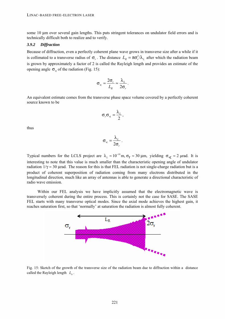
some 10 μm over several gain lengths. This puts stringent tolerances on undulator field errors and is technically difficult both to realize and to verify.

3.9.2 Diffraction

Because of diffraction, even a perfectly coherent plane wave grows in transverse size after a while if it is collimated to a transverse radius of rσ . The distance 2/R r LL = πσ λ after which the radiation beam is grown by approximately a factor of 2 is called the Rayleigh length and provides an estimate of the opening angle σ of the radiation (Fig. 15):

22

r L

R rLσ λσ ≈ ≈

σ.

An equivalent estimate comes from the transverse phase space volume covered by a perfectly coherent source known to be

2L

rλσ σ = ,

thus

2L

r

λσ =σ

.

Typical numbers for the LCLS project are 1010 m, 30 m,rL−λ ≈ σ ≈ μ yielding 2 μrad.σ ≈ It is

interesting to note that this value is much smaller than the characteristic opening angle of undulator radiation 1/ 30 rad.γ ≈ μ The reason for this is that FEL radiation is not single-charge radiation but is a product of coherent superposition of radiation coming from many electrons distributed in the longitudinal direction, much like an array of antennas is able to generate a directional characteristic of radio wave emission.

Within our FEL analysis we have implicitly assumed that the electromagnetic wave is transversely coherent during the entire process. This is certainly not the case for SASE. The SASE FEL starts with many transverse optical modes. Since the axial mode achieves the highest gain, it reaches saturation first, so that ‘normally’ at saturation the radiation is almost fully coherent.

Fig. 15: Sketch of the growth of the transverse size of the radiation beam due to diffraction within a distance called the Rayleigh length RL .

LINAC-BASED FREE-ELECTRON LASER

221

3.9.3 Emittance of the electron beam

The emittance of the electron beam introduces a longitudinal velocity spread in the electron beam very much as energy spread does. Thus, in terms of FEL gain, electron emittance is equivalent to additional energy spread. The equivalent energy spread is

( )2

21eff KΔγ γ ε≈γ β +

(β is the Twiss parameter of electron focusing). With the condition /Δγ γ < ρ derived from Eq. (53) this gives a limit for the beam emittance:

( ) ( )2 2

2 2

1 1

2èff

K Kβ + β +Δγε ≈ < ργ γ γ

, (56)

where the factor 2 makes sure the emittance contributes less than 50% of the total energy spread budget.

A second condition comes from the diffraction effect: We want to maintain both complete overlap of electron beam and radiation (calling for long RL thus large rσ ) AND maximum possible gain (calling for small rσ , thus small RL ). The best compromise is R gL L≈ , thus

2 14 3

urR G

L L

L L λπσ πβε= = ≈ =λ λ ρπ

.

With the help of Eq. (46), ρ can be eliminated, yielding

44 3ph phλ λ

ε < ≈ππ

.

4phλ

ε <π

is a rather challenging condition for Lλ in the nanometer range.

3.10 Velocities

When we introduced the complex field amplitude 0 0E ( ) E ( )exp Ez z i= ψ in Section 3.1, we intentionally introduced an additional phase Eψ . This slowly varying phase describes the slippage of the electromagnetic phase with respect to a free wave propagating at phase velocity c. We can determine cos Eψ by (see. Fig. 16):

( ) 322 2

3 3 31 42 2 2

cos cos coshEcos

Ecosh cosh cos

E

zz z

z z z

⎛ ⎞Γ⎛ ⎞Γ + ⋅ Γ⎜ ⎟⎜ ⎟⎝ ⎠ℜ ⎝ ⎠ψ = =

⎛ ⎞+ Γ Γ + Γ⎜ ⎟

⎝ ⎠

.

J. ROSSBACH

222

For 1/z Γ this reads

E

i 3 z2 i z= z

2 2i 3 z2

expEcos exp cos

Eexp

⎛ ⎞+ℜ Γ⎜ ⎟ℜ Γ⎛ ⎞⎝ ⎠ψ = = ℜ Γ =⎜ ⎟⎛ ⎞ ⎝ ⎠+ Γ⎜ ⎟

⎝ ⎠

,

i.e. for 12

/Ez zΓψ = Γ .

0 1 2 3 4 5 60

1

2

33

0

phase Γz( )

phaselimit Γz( )

60 Γz

Fig. 16: Development of the slowly varying phase Eψ as a function of the longitudinal coordinate z, normalized tio the gain parameter Γ. Eψ describes the slippage of the electromagnetic phase with respect to a free wave propagating at phase velocity c.

We can now calculate the phase velocity of the electromagnetic wave during the FEL process:

2

ph

L

vk k

ω ω= = Γ+,

i.e. is reduced by

12 2ph

L L L

c v c ck k k

⎛ ⎞ω Γ Γ− ≈ − − =⎜ ⎟⎝ ⎠

with respect to a free electromagnetic wave.

Similarly, we can calculate the phase velocity of density modulation. With Eq. (35), and using Eq. (44):

LINAC-BASED FREE-ELECTRON LASER

223

( )i i00 1 0 2 2

0

0

2 1c.c. i c.c.3

3const. i c.c.2 2

z ext

u L

j j j e j z ecK

zj k k z t

Ψ Ψγ= + + = − Λ Λ + =μ

⎡ ⎤Γ Γ⎛ ⎞= + ⋅ + + − ω +⎜ ⎟⎢ ⎥⎝ ⎠⎣ ⎦

E exp

exp exp

Thus, the phase velocity of the density modulation is given by

1 22

jeff u L L

u L

v ck k k kk k

ω ω ω Γ= = ≈ −Γ ++ +.

Since / u Lk kω + is the mean longitudinal velocity of the resonant electrons, it is seen that the growing density modulation slowly slips backwards with respect to the bunch centre.

Finally, the group velocity of electromagnetic wave packets during the FEL process is of interest. Analysing how 2Λ depends on c shows that

2

g 20

113

d Kv cdk

⎛ ⎞ω += ≈ −⎜ ⎟γ⎝ ⎠ .

In conclusion, we can distinguish four characteristic velocity slippages with respect to c in the high-gain FEL:

2

20

2

20

with the phase velocity of on electromagnetic wave during the gain process.

with the group velocity of on electromagnetic wave during the gain process.

2

1 3

12

phL

g

z

vph

vg

c v ck

Kc v c

Kc v c

Γ− =

+− =γ

+− =γ

1

2

1 20

with the longitudinal velocity of the electron bunch

(i.e. of resonant particles, 'kinematical slippage').

with the phase velocity of

1 2 2j

L

vz

v jKc v c

k⎛ ⎞+ Γ− = +⎜ ⎟γ⎝ ⎠

density modulation during the gain process.

From these relations, we can calculate the slippage g zv v− of radiation wave packages (‘spikes’ in the time domain) with respect to the electron bunch. It is three times smaller than the kinematic slippage:

13

g z

z

v vc v−

=−

.

ACKNOWLEDGEMENTS The author acknowledges with pleasure numerous valuable discussions with his colleagues G. Hoffstätter, E.L. Saldin, E.A. Schneidmiller, and M.V. Yurkov. Unpublished lecture notes by G. Hoffstätter have been used for the chapter on low-gain FELs.

J. ROSSBACH

224

REFERENCES [1] K. Wille, Introduction to Accelerator Physics (Teubner Studienbücher, 1992).

[2] E.L. Saldin, E.A. Schneidmiller M.V. Yurkov The Physics of Free-Electron Lasers (Springer, 2000).

[3] J.D. Jackson, Classical Electrodynamics (De Gruyter, 1980).

[4] P. J. Duke, Synchrotron Radiation (Oxford Science Publications, 2000).

[5] J.M.J. Madey, Relationship between mean radiated energy and spontaneous power spectrum in a free electron laser, Nuovo Cimento B50 (1979) 64.

[6] A. Renieri, Nuovo Cim. 53B (1979) 160.

[7] J. Andruszkow et al., First observation of Self-Amlified Spontaneous Emission in a Free-Electron Laser at 109 nm Wavelength, Phys. Rev. Lett. 85 (2000) 3825.

[8] A. M. Kondratenko and E. L. Saldin, Generation of coherent radiation by a relativistic electron beam in an undulator, Part. Accelerators, 10 (1980) 207.

LINAC-BASED FREE-ELECTRON LASER

225

ENERGY RECOVERY LINACS

S. Werin MAX-lab, Lund University, Sweden

Abstract Energy Recovery Linacs (ERL) is a technique that makes use of the fact that linear accelerators can provide electron beam qualities which in some respects are superior to storage rings, without having to pay the price of unacceptable power consumption. The limitations to this statement, what the ERL is, and its advantages and disadvantages are discussed.

1 PATH OF DEVELOPMENT

Over the last few years there has been a running discussion on what will become the fourth-generation light source. At the moment there is no definite answer. New storage rings are being constructed but will they be fourth-generation sources? Free electron lasers have unique capabilities which no other source can beat. Energy Recovery Linacs (ERLs) come in between, having most of the good qualities of a storage ring and many of the good qualities of an FEL. So, will the ERL be the fourth-generation light source? We do not know. We do not even know how to define a fourth-generation light source. What special quality defines the fourth-generation source? Coherence, pulse length, diffraction-limited, etc.

The first-generation synchrotron light sources operated parasitically on high-energy physics machines. No real optimization was done to improve the generation of light. The second-generation sources were built to generate synchrotron radiation from bending magnets, and the third-generation sources were optimized for generating synchrotron radiation in undulators. This is where we are today.

Soleil in Paris and Diamond in Oxford are improving on almost all details of the radiation from current sources, but is that enough to call them fourth-generation sources? I do not think so and prefer to call them three-and-a-half-generation sources.

The FEL is able to generate coherent, powerful, tunable, diffraction-limited radiation in truly femtosecond pulses. This perhaps qualifies them technically as fourth-generation sources, but will they be available for everyone? A few large facilities will be built, each one of them providing a handful of parallel beamlines. A small number of key experiments which can not be performed elsewhere will be performed here, but the majority of science will be done on other sources.

Will the ERL become the fourth-generation source? Many aspects tell us yes, but there are also question marks. We shall see.

2 WHAT IS AN ERL

In a storage ring, electrons emitting light come back turn after turn, we can say that they are re-used. This has certain disadvantages as the electron beam characteristics are defined by an equilibrium that is found after a large number of turns.

In the ERL it is not the electrons that are re-used, but only their energy. Thus the electron emitting light at this moment, is not the same one as during the last turn. This is favourable as the equilibrium electron beam has not been created and a ‘one-time-use’ beam can be made with a smaller emittance both transversally and longitudinally.

227

Fig. 1: Step one of an ERL – acceleration

In the first step of an ERL, electrons from the injector are accelerated (Fig. 1). The electron beam is then conducted to the experimental area where the synchrotron radiation is extracted.

Fig. 2: Step two of an ERL – deceleration

In the second stage of the ERL, the electron beam is directed back to the accelerating structure but with a phase change of 180 degrees. Thus the electrons are decelerated instead of accelerated, and after the deceleration they are extracted at low energy and dumped (Fig. 2).

Fig. 3: Alternative layout of an ERL – acceleration and deceleration over several turns

An alternative way of operating the ERL is to run acceleration over several turns, using the same accelerating structure more than once (Fig. 3). In the final (outermost) turn the generation of synchrotron radiation takes place and the electrons arrive in the subsequent turns in the decelerating phase. Thus passing the same orbits in reverse order until they are slowed down to the injection energy and can be dumped.

The energy recovery in this process takes place in the accelerating structure. The energy taken from the electron beam in the decelerating phase is ‘stored’ in the accelerating structure and can be

Linac

injection

S. WERIN

228

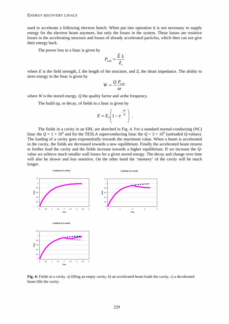
used to accelerate a following electron bunch. When put into operation it is not necessary to supply energy for the electron beam anymore, but only the losses in the system. These losses are resistive losses in the accelerating structure and losses of already accelerated particles, which then can not give their energy back.

The power loss in a linac is given by

walls

E LPZ

=

where E is the field strength, L the length of the structure, and Zs the shunt impedance. The ability to store energy in the linac is given by

wallQ PWω

=

where W is the stored energy, Q the quality factor and ω the frequency.

The build up, or decay, of fields in a linac is given by

⎟⎟⎠

⎞⎜⎜⎝

⎛−=

−Q

t

eEEω

10 .

The fields in a cavity in an ERL are sketched in Fig. 4. For a standard normal-conducting (NC) linac the Q = 1 × 104 and for the TESLA superconducting linac the Q = 3 × 109 (unloaded Q-values). The loading of a cavity goes exponentially towards the maximum value. When a beam is accelerated in the cavity, the fields are decreased towards a new equilibrium. Finally the accelerated beam returns to further load the cavity and the fields increase towards a higher equilibrium. If we increase the Q-value we achieve much smaller wall losses for a given stored energy. The decay and change over time will also be slower and less sensitive. On the other hand the ‘memory’ of the cavity will be much longer.

Loading of a cavity

0

0.2

0.4

0.6

0.8

1

1.2

0 0.5 1 1.5 2 2.5 3 3.5 4

Time

Fiel

d

Loading of a cavity

0

0.2

0.4

0.6

0.8

1

1.2

0 1 2 3 4

Time

Fiel

d

Loading of a cavity

0

0.2

0.4

0.6

0.8

1

1.2

0 0.5 1 1.5 2 2.5 3 3.5 4

Time

Fiel

d

Fig. 4: Fields in a cavity. a) filling an empty cavity, b) an accelerated beam loads the cavity, c) a decelerated beam fills the cavity.

ENERGY RECOVERY LINACS

229

3 BRILLIANCE, EMITTANCE, DIFFRACTION LIMIT, AND PULSE LENGTH

With these machines the aim is of course to produce radiation with the best quality possible. What quality actually means can be fairly arbitrary, but when looking at your experiment you are normally interested in how many ‘good’ photons you get on your sample. That would mean the number of photons at a certain wavelength, with a certain polarization, within a time window. This can be given as flux (normally: photons/(second * 0.1% bandwidth * A electron beam). Unfortunately, the flux for one machine will not tell you much when comparing the flux with the one you will get with another machine.

3.1 Brilliance

The ability to control your photon beam and focus it on your sample is given by the flux divided by the phase space of the radiation, this is called brilliance (or brightness) (flux / mm2 × mrad2 ). Brilliance is a unit possible to compare between different sources.

yyxx

FluxBrilliance′′ ΣΣΣΣ

= 24π

where Σ is the width of the distribution, x defines the horizontal plane, and y the vertical. Σx refers to size and Σx´ to angle.

The Σ contains one contribution from the electron beam (the source) and one from the radiation field, giving

2 2 2 2 x x r x x rσ σ σ σ′ ′ ′Σ = + Σ = +

for the horizontal direction, and similar for the vertical direction.

The electron beam quality is given by the electron beam emittance, defined by

xx ′= σσε

where ε is the emittance of the electron beam.

Regarding the photon beam the emittance is given by

πλσσε

2== ′rr .

Exactly what you will find in the denominator depends on which reference you read, if you look at fields or powers etc. What is quite clear is that the emittance of the photon beam is a fundamental of the wavelength and we can not do much about it.

3.2 Diffraction limit

We can tailor the electron beam emittance with the optics of the storage ring or the emittance of our linac source. If we can make the σx and σx´ smaller than the σr and σr´ then it is no use going any further because we can not gain anything more in brilliance. In this case we call our accelerator ‘diffraction-limited’.

From Fig. 5 we can see that if we want to generate diffraction-limited radiation at 1 keV we need an emittance a bit below 1 nm rad. This is lower than what the thind-generation storage rings can make today, but a few of the rings under construction and design can do it. The reason is that the emittance of a storage ring is given by the equilibrium emittance which is the fight between excitation through emission of radiation and damping.

S. WERIN

230

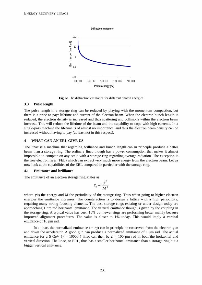
Diffraction emittance -

0,01

0,1

1

10

100

0,0E+00 5,0E+02 1,0E+03 1,5E+03 2,0E+03

Photon energy (eV)

Emitt

ance

(nm

Rad

)

Fig. 5: The diffraction emittance for different photon energies

3.3 Pulse length

The pulse length in a storage ring can be reduced by playing with the momentum compaction, but there is a price to pay: lifetime and current of the electron beam. When the electron bunch length is reduced, the electron density is increased and thus scattering and collisions within the electron beam increase. This will reduce the lifetime of the beam and the capability to cope with high currents. In a single-pass machine the lifetime is of almost no importance, and thus the electron beam density can be increased without having to pay (at least not in this respect).

4 WHAT CAN AN ERL GIVE US

The linac is a machine that regarding brilliance and bunch length can in principle produce a better beam than a storage ring. The ordinary linac though has a power consumption that makes it almost impossible to compete on any scale with a storage ring regarding average radiation. The exception is the free electron laser (FEL) which can extract very much more energy from the electron beam. Let us now look at the capabilities of the ERL compared in particular with the storage ring.

4.1 Emittance and brilliance

The emittance of an electron storage ring scales as 2

h 3Mγε ∝

where γ is the energy and M the periodicity of the storage ring. Thus when going to higher electron energies the emittance increases. The counteraction is to design a lattice with a high periodicity, requiring many strong-focusing elements. The best storage rings existing or under design today are approaching 1 nm rad horizontal emittance. The vertical emittance though is given by the coupling in the storage ring. A typical value has been 10% but newer rings are performing better mainly because improved alignment procedures. The value is closer to 1% today. This would imply a vertical emittance of 10 pm rad.

In a linac, the normalized emittance ( = εγ) can in principle be conserved from the electron gun and down the accelerator. A good gun can produce a normalized emittance of 1 µm rad. The actual emittance for a 5 GeV (γ = 10000 ) linac can then be ε = 100 pm rad in both the horizontal and vertical direction. The linac, or ERL, thus has a smaller horizontal emittance than a storage ring but a bigger vertical emittance.

ENERGY RECOVERY LINACS

231

The brilliance can be enhanced either by increasing the flux or by decreasing the emittance until the diffraction limit is reached. Development is ongoing but the ERL will not be significantly better than the storage rings as regards emittance or brilliance.

4.2 Bunch length

The ERL bunch length can be achieved in a number of ways. As the equilibrium situation from a storage ring will not have time to develop, the bunch length can be tailored at the electron gun and maintained through the system. There is also the possibility to compress the bunch at certain locations around the machine.

The electron gun normally consists of an RF-gun structure with a photocathode onto which a laser beam is focused. A typical RF structure operates around 3 GHz and such a gun creates a bunch of a few ps length if left free-running. If a short laser pulse is used, a shorter window can be created in the femtosecond range. Lasers providing 100 fs pulses are available, but not trivial to construct.

Compression of an electron bunch is done by letting the bunch pass an accelerating structure slightly off-crest. The head and the tail will thus receive slightly different energies and will follow paths with different lengths in a dispersive section. The tail can catch up with the head and thus compress the bunch. The result is a bunch that in principle can reach below 100 fs, which is far below what can be achieved in a storage ring. The price is paid in increased energy spread of the bunch.

An obstacle though is that a short bunch will generate coherent synchrotron radiation (see below).

4.3 Energy savings

The name Energy Recovery Linac cries out for an investigation of the energy savings that are possible. The first important concept is to actually recover the already accelerated beam. In the existing ERL systems, as at Jefferson Lab, efficiencies up to 99.97% have been achieved. One can thus assume energy recovery works, there are savings to be made.

An important fact is that a 100 mA 5 GeV beam that is used only once means a power of 500 MW. It is impossible to spend this amount in any realistic project, and thus ways of reducing the consumption have to be made. The easiest way is to reduce the average current, but then the average brilliance falls equally fast. Another way is, of course, to recover the energy.

To make the most efficient energy recovery system, one normally considers the superconducting linac technology as superior. In the LBL LUX proposal [1] the two alternatives of superconducting or normal-conducting linacs have been investigated (Table 1). (Four passes through a 600 MeV linac generating 2.4 GeV and a repetition rate of 10 kHz.)

Table 1: Comparison of power consumption: normal-conducting v. superconducting linac for the LBL LUX

NC SC RF-power peak 240 MW 0.288 MW RF-power average 6 MW 0.288 MW Cooling power 0 ~3.5 MW Total 6 MW 3.8 MW

It is obvious that for peak power, the normal-conducting linac can never compete with the superconducting alternative. On the other hand, we are most interested in average power in this case. To get a full picture we also have to add the cooling power of the superconducting system. The final figure is still better for the superconducting technology, but only by a factor of two. This has to be compared with the added complexity of such a system. If the repetition rate could be increased to 100 kHz the SC would be outstanding.

S. WERIN

232

Let us compare an ERL with a storage ring (Table 2). The Cornell ERL-2 [2] will operate at 5 GeV with a current of 100 mA. This is comparable to the ESRF (at 5 GeV and 200 mA).

Table 2: Comparison of RF power consumption ERL vs. storage ring

Cornell ESRF RF-power peak 1.1 MW 2.6 MW RF-power average 1.1 MW 2.6 MW Cooling power 16.4 MW 0 Total 17.5 MW 2.6 MW

The cooling power of the superconducting ERL consumes more than the storage ring RF power, and thus there is no gain. On the other hand, the electron beam power is 500 MW for the Cornell machine, and thus the ERL is a solution if the unique beam of a linac source is desired.

One can argue whether these comparisons are correct, but what is obvious is that the ERL does not always save energy.

4.4 Radiation savings

By continuously dumping a high-current beam there is a large potential of generating radiation. A storage ring slowly loses its current over several hours and the total number of electrons is fairly low, thus the ‘dumped’ power is very low. In a single-pass machine the power might get very large.

A 100 mA beam which is dumped at 5 GeV would mean dumping 500 MW. This is of course impossible on account of energy considerations, but also the generated radiation would be a severe problem. Decelerating the beam down to below 10 MeV reduces the dump power to 1 MW. What is also important is that by going below 10 MeV with an electron beam means that one comes below the neutron production threshold and thus it is easier to shield the radiation dump. For a single-pass machine, like an ERL, energy recovery is important to reduce the radiation hazards.

A storage ring like the ESRF ( 200 mA, 5 GeV, 24 hours lifetime) generates 30 mW in ‘dump’ power.

5 ACCELERATOR PHYSICS ISSUES, LIMITATIONS

The ERL is built with either one recirculation or with several passages through the linac systems. In one passage there are a number of key issues to take into account (Fig. 6).

Fig. 6: Beam issues in a one-recirculation ERL

Beam loss / ”halo loss”

CSR BBUCSR

RF focusingInjection energy phase slip

Multi energy focusing

ENERGY RECOVERY LINACS

233

5.1 Coherent Synchrotron Radiation (CSR)

A short electron bunch can radiate synchrotron radiation coherently at wavelengths that are longer than the length of the bunch. In this case all electrons radiate in phase. This can be used to generate powerful infrared radiation, but the radiation emitted from the back end of the bunch can also overtake the head of the bunch which then will be influenced by the electromagnetic field. This can cause both a change of energy and a displacement, and thus the energy spread and the emittance can be destroyed. The effect is most prominent for short bunches at low energies. Thus a sub picosecond bunch just after the gun is very sensitive, and so are the bunches after hard compression later in the system. The effect can be reduced by having larger radii in the bending magnets and, in some cases, by small diameters on the vacuum vessel that shields the CSR.

5.2 Phase slip

It is important to find a proper balance between the accelerated and decelerated beam to match the energy taken and deposited. A low-energy beam will slip in phase relative to the linac phase differently than a high-energy beam. Choosing a low injection and extraction energy makes the problem worse, though this is the choice that is good for the efficiency of the recovery process.

5.3 Multi-energy beam focusing

As beams with different energies pass through the same focusing elements, special care has to be taken in the design. Proper focusing of the lower energies, which is the normal way, will give too-weak focusing for higher energy beams. The contrary would mean over-focusing of the low-energy beams and is less favourable.

The focusing of multi-energy beams is even more difficult as there is a larger span in the different energies and they must pass the same elements going in and out from the accelerating structure. In addition, there is also the problem of dividing and merging the beams in the arcs of the recirculation.

5.4 RF focusing

The linac itself focuses the electron beam both horizontally and vertically. This focusing is dependent on the beam energy and energy gain.

5.5 Beam loss

A loss of the beam will first generate heating-up and activation of the components where it is lost. Another effect is that the balance of the fields in the linac system will not be correct. A larger power has to be supplied by the klystron to the linac. The balance between the different fields can be seen in Fig. 6. If the decelerated particles suddenly become fewer, a new equilibrium point will be found and thus the energy in the process will change.

The loss of particles can be due either to the design of the system, where the aperture is not large enough, or to instabilities. What is more of a problem are ‘halo particles’. These are particles in the beam but very far out from the centre, normally disregarded when discussing the emittance of the beam.

5.6 Beam break-up (BBU)

If the beam does not pass in the centre of the accelerating cavity it will induce fields of other modes in the cavity. The reason for not passing in the middle could be either misalignments of the accelerator, or misplacements of the beam itself. The induced fields can oscillate in the cavities if they fit a cavity mode. Such modes other than the main mode are called higher-order modes (HOM). A subsequent electron bunch, or the same bunch after one turn, will sense these fields and instabilities can be induced (Fig. 7).

S. WERIN

234

Fig. 7: Beam break-up (BBU)

The BBU effect can be treated by a good damping of the unwanted modes in the cavity and a good alignment of the accelerator. In the existing and earlier ERLs this effect has been a limiting factor on the achieved maximum current. The MUSL ERL in Illinois [3] never became stable and at Jefferson Lab IR-demo [4] the current limit is around 10 mA.

In a multiturn machine the complexity of the BBU is increased as there will be a larger number of turns and sensitivity for longer range modes in the cavity.

5.7 Challenges

There are several challenges for the future development of ERLs. The first is the construction of continuous electron guns. The gun not only has to operate CW, but to make use of the capabilities of an ERL the emittance has to be very small. To achieve the small emittance, the most common route is to use a photocathode RF gun. A laser is focused onto the cathode surface extracting the wanted electrons. The cathode sits inside an RF cell which gives the initial acceleration immediately. This kind of device can produce very small emittances. Problems lie mainly in the areas of high-repetition-rate lasers and on making the RF structures superconducting, and maintaining them cold while shining into them with a laser. Alternative solutions would be thermionic guns, where the cathode is heated to continuously emit electrons. The emittance of such guns though is poorer.

Controlling HOMs in superconducting cavities is a key topic to be able to reach high average currents.

The optics of recovery lines and especially the systems where multi-energy beams are envisioned is a true challenge. The splitting and joining of beams also poses significant problems. These problems have to be solved and effects diluting the emittance, like CSR, have to be taken into account.

6 THE CURRENT SITUATION

In 1965 Mauro Tigner published the first ideas for an ERL [5]. It took a number of years until the ideas were put into realisation at the University of Illinois in the MUSL accelerator in 1977. Unfortunately, stability was not attained and we had to wait another 10 years until T. Smith in 1986 operated the SCA at Stanford in energy recovery mode [6] (Fig. 8).

Fig. 8: The SCA at Stanford 1986 [6]

ENERGY RECOVERY LINACS

235

Following the Stanford development the S-DALINAC [7] in Darmstadt, Germany, came into operation in 1990. It is built from a 10 MeV injector and three passes through a 40 MeV superconducting linac, making a maximum energy of 130 MeV.

The most intense development has been done at Jefferson lab [4] in the US. In 1995 the CEBAF [4] came into operation. It is a continuous 6 GeV accelerator for nuclear physics. Today there are plans to upgrade this machine up to 12 GeV.

At Jefferson lab there is also an infrared FEL that has been in operation since 1999 and is now being upgraded to a 160 MeV 10 mA machine [4]. A comparable machine to the Jlab FEL, but at lower energy, is the JAERI-ERL and FEL in Japan [8]. Looking into the future there are a number of laboratories with intense activities and development. One of the most thrilling concepts was presented by G. Kulipanov et al. in Novosibirsk [9], the MARS (Multipass Accelerator Recuperator Source) (Fig. 9).

Fig. 9: The MARS concept [9]

To overcome some of the problems of accelerating low- and high-energy beams in the same structures and being able to optimize the optics, the system is divided into two accelerating linacs.

There are three further proposals for synchrotron radiation sources in the US.

The LUX at LBL is a 3 GeV racetrack-shaped machine [10] (Fig. 10). In the first stage it wiil not operate in energy recovery mode; this option is being kept for a second step. This is because of the problems of stability at higher currents. The main objective of the project is to create short femtosecond pulses of radiation.

Fig. 10: Layout of the LBL LUX proposal [1]

S. WERIN

236

Another proposal is the joint Jefferson lab–Cornell ERL [11]. The first step consists of a 100 MeV ring-like machine operating with one pass. A second step would be to build the full-scale machine which is a 5 GeV ERL for synchrotron radiation.

At Brookhaven on Long Island the NSLS is proposing the PERL project which is a 2.7 GeV recirculated linac for synchrotron radiation [12].

In Europe we have the 4 GLS in Daresbury UK [13]. This is the ‘accelerator physicists dream’, a machine that can do almost anything. One part of the project is a 600 MeV superconducting linac capable of running in energy recovery mode.

At the university of Erlangen in Germany there is an ambitious proposal for a 3.5 GeV energy recovery linac for synchrotron radiation [14], the ERLSYN.

Finally, there is, of course, also a Japanese proposal from KEK for a 2.5–5 GeV energy recovery linac [15].

Table 3: Overview of ERL machines

Operation Type Energy Form Purpose MUSL 1977 unstable multiturn SCA 1986 ERL 50 MeV ring SR+FEL

S-Dalinac 1990 ERL 130 MeV multiturn SR+FEL CEBAF 1995 ERL 6–12 GeV multiturn nuclear Jlab FEL 1999 ERL 40–160 MeV ring FEL

JAERI-ERL 199? ERL 17 MeV ring FEL

MARS idea ERL 6 GeV 2×multiturn SR LUX prop linac 3 GeV multiturn SR

Cornell-ERL prop ERL 100 MeV–5 GeV ring SR PERL prop ERL 2.7 GeV ring SR 4 GLS prop ERL 600 MeV ring SR+FEL

ERLSYN prop ERL 3.5 GeV ring SR KEK-ERL prop ERL 2.5–5 GeV ring SR

7 SUMMARY

Energy recovery linacs have been operated in lower energy applications for several years. Experiments proving the principle and achieving very high recovery rates have been done. Today, several proposals for new large projects are being put forward around the world, but especially in the US.

The ERLs beat storage rings in horizontal emittance and short (fs) pulses. They can not compete with the FELs in peak power or coherence (if not the ERL is used as an FEL driver). The vertical emittance of a modern storage ring is better than both the ERL and the FEL, and if this is properly used in the beam line design, the diffraction limit is reached and there is no need for smaller beams. Thus the main advantage of the ERL is to provide fs pulses to many users on undulator beam lines.

A superconducting ERL will be able to operate almost in CW mode (several KHz to MHz), thus leaving warm systems behind. They will also be an important way of reducing the radiation hazards of linac systems. The SC ERL will also be able to efficiently drive a CW FEL.

On the other hand, no direct energy savings are made. Some applications will only be possible by energy recovery, but comparing the final radiation to power consumption will show that energy savings is a relative term.

Many problems still remain to be solved and worked on. The instabilities limiting higher currents and the higher order modes (HOM) in the linac structures are key areas.

ENERGY RECOVERY LINACS

237

The question of the fourth-generation light source still has to be solved. As the situation looks today, we can expect a number of different sources providing different capabilities. A few of them will most probably be Energy Recovery Linacs.

Table 4: Pros and cons for some machines

Diffraction limit

Coherence fs pulses Multi user

Brilliance, average

Brilliance, peak

Rep. rate

Storage ring

-hor, +vert – – + 0 – +

FEL 0 + + 0 0 + – ERL 0 – + + 0 – 0

REFERENCES [1] LBL LUX feasibility study: http://jncorlett.lbl.gov/FsX-raySource/FeasibilityStudy02/ . [2] Cornell ERL, I. Bazarov et al., EPAC 2002, Paris. [3] P. Axel, L.S. Cardman, H.D. Graef, A.O. Hanson, R.A. Hoffswell, D. Jamnik, D.C. Sutton and

R.H. Taylor, ‘Operating experience with MUSL-2’, IEEE Trans. Nucl. Sci. NS-26 (1979) 3143. [4] http://www.jlab.org [5] M. Tigner, Nuovo Cimento 37 (1965)1228. [6] T.I. Smith et al., NIM A 259 (1987) 1–7. [7] M. Platz et. al., EPAC 2002, Paris. [8] N. Nishimori et al., EPAC 2002, Paris. [9] G. Kulipanov, SRI 2001, ERL Workshop and D.A. Kayran et al., MARS - a project of the

diffraction limited fourth generation X-ray source, apac 98, Tsukuba, 1998. [10] http://jncorlett.lbl.gov/FsX-raySource. [11] D. Bilderback, Synchr. Rad. News 2/27/01. [12] J. Murphy, PERL, SRI 2001, ERL Workshop. [13] http://www.4gls.ac.uk and M.W. Poole, et al., Proceedings of the European Particle Accelerator

Conference, Paris, 2002, p. 733. [14] http://www.erlsyn.uni-erlangen.de/ and Feasibility study of the Erlangen synchrotron light

source, D. E. Berkaev, et al., Proceedings of EPAC 2002, Paris. [15] K. Harada, JSPS Asian Science Seminar Synchrotron Radiation Science, 2002, Jordan

http://conference.kek.jp/JASS02/23_harada.pdf .

S. WERIN

238

1

DIAGNOSTICS

M. Minty Deutsches Elektronen Synchrotron (DESY), Hamburg, Germany

Abstract The beam diagnostics considered here concentrate on those with most frequent application in synchrotron radiation and free electron laser facilities. Focus is placed on the description of the experimental hardware in the immediate vicinity of the beam. We describe the various instruments used for determining the most easily measured moments of the beam distribution, namely, the beam charge, the beam positions, the transverse and longitudinal beam sizes, and the bunch energy spread. Common algorithms for determining the transverse beam emittances are also outlined.

1. INTRODUCTION

Optimum accelerator performance depends critically on the ability to carefully measure and control the properties of the particle beams. As the demands for higher beam currents, smaller beam emittances, and tighter tolerances on the beam parameters have increased in recent years, the types of problems encountered in practice have evolved and the diagnostics used to characterize the beams have correspondingly been improved and refined.

The rapid evolution of developments in beam instrumentation has resulted in numerous published reports, only a portion of which are cited here. A selection of classic references, from which I have greatly profited, include “Diagnostics” by J. Borer and R. Jung [1], a comprehensive report including signal processing techniques and schematics and photographs of many detectors used at CERN; “Beam Instrumentation” by R. Littauer [2]; “Beam Diagnostics and Applications by A. Hofmann [3], which details many high-level applications using beam diagnostics; and “Bunched Beam Diagnostics” [4] and “Spectral Analysis of Relativistic bunched Beams” [5] by R.H. Siemann, which provide an excellent introduction to frequency domain analysis including application to the study of beam instabilities. More recently, several excellent tutorials in beam diagnostics have been published in the proceedings of the beam instrumentation workshops (BIW) and in the invited talks of the diagnostics conferences (DIPAC).

For the purpose of these lectures, we consider beam diagnostics to consist of:

i) the measurement device (the focus of this lecture);

ii) the associated electronics and processing hardware (the subject of numerous publications and internal reports, which are often application specific);

iii) high-level applications (for example by A. Hofmann [3]).

Personally I find the topic of beam diagnostics and their applications to be not only extremely interesting per se (i.e. studying limits on the ultimately achievable resolution of a particular measurement diagnostic), but also, on a day-to-day basis, relevant for defining, diagnosing, and solving problems related to the control of particle beams. It has often been my experience that the design of a good experiment and the interpretation and analysis of the experimental data demand a thorough understanding of the measurement device itself. As an example, suppose ion-related phenomena are suspected to be the cause of observed emittance growth or beam

239

2

instability. For diagnosis, one might consider using beam position monitor electrodes as clearing electrodes. To do so these questions might be relevant: “what kind of beam position monitors can be appropriately biased to clear the suspected ions?” or (in the study of beam instabilities) “what should the frequency spectra look like without instabilities”. To address these questions, an understanding of the diagnostics themselves is often required.

In these lectures we describe the hardware used for measurements of the beam charge and intensity (section 3) and the beam position (section 4). Methods for determining the transverse beam emittance are described together with the apparatus used for the required measurements of the transverse beam size (section 5). Techniques are also presented for measurements of the beam energy spread (section 6) and the bunch length (section 7). A summary is given in section 8. The presented methods focus on applications in linac-based free electron lasers and synchrotron radiation facilities. Examples of beam diagnostics measurements from existing facilities are given throughout the text.

2. DETECTOR SENSITIVITY

The electric field of a relativitic particle in a smooth vacuum chamber is depicted in Fig. 1. The field lines are relativistically contracted into a “Lorentz-contracted pancake”. These induce a wall current iw(t) which has opposite sign of the beam current ib(t): ib(t)=-iw(t).

From the point of view of a beam detector, which detects properties of the charged particle beam, the wall current may be viewed as a current source. With infinite output impedance, the wall current iw will therefore flow through any impedance placed in its path. Many “classical” beam detectors consist of a modification of the walls through which the currents will flow.

Fig. 1 Beam (ib) and wall (iw) current induced by the electric field E of the bunch of charge q.

In the following, we will refer to the sensitivity S(ω) of the detector. For measurement of the beam charge,

(1)

(in units of Ω) which is the ratio of the signal size developed V(ω) to the wall current Iw(ω). For measurement of the beam position,

(2)

(in units of Ω/m) which is the ratio of the signal size developed to the dipole mode of the distribution, given by D(ω)=I(ω)z, with z=x,y in the horizontal (x) and vertical (y) plane respectively.

M. MINTY

240

3

3. BEAM CHARGE AND INTENSITY 3.1 Beam Charge – the Faraday Cup

Measurements of the beam charge using a Faraday cup [6-8] are usually invasive and typically used only at low beam energies (up to a few hundred MeV). In such applications, the cup is inserted directly into the path of the beam which may consist of a single bunch or of a train of bunches. Compared to other types of beam charge monitors, the calibration of the Faraday Cup does not depend on the time structure of the beam.

A conceptual view of a Faraday cup is shown in Fig. 2. The cup itself consists of a thick or series of thick conducting materials (e.g. Cu, C, Pb. Ta) of sufficient area to fully intercept the beam. The constituency and thickness L of the intercepting material, which are chosen depending on the beam energy E, is such that the energy of the particles in the beam is completely absorbed: E=(dE/dx)L, where the energy loss per unit length dE/dx depends on the absorber material [9]. For example, ~0.4 m of copper is sufficient to stop 1 GeV electrons. The beam charge is converted into a corresponding current. The voltage V measured across a resistor R to ground provides a measure of the instantaneous current absorbed. In practice, a direct current (dc) bias is often applied to the cup to retain the electrons produced by secondary emission. Impedance matching is essential and termination is usually made into 50Ω. The detector is typically bandwidth limited to ~1 GHz due to the capacitance to ground.

Fig. 2 Conceptual view of a Faraday cup.

Shown in Fig. 3 is a schematic of the Faraday cup used in the injector linac for KEKB [10,11]. The cylindrically symmetric structure contains lead, iron, and carbon blocks. In this application, the thickness of the lead block corresponds to about 35 radiation lengths so that the beams are fully absorbed by the block. The carbon and ion blocks serve to suppress electromagnetic showers generated in the lead block. The bias voltage (several hundred Volts) is supplied to suppress both secondary emission from the target material and secondary electrons generated in the residual gas of the vacuum environment.

Fig. 3 Schematic of the Faraday cup used for in the KEKB injector linac (courtesy T. Suwada, 2003).

DIAGNOSTICS

241

4

3.2 Beam Intensity - Toroids

The choice of design of transformers for measuring the beam intensity using toroids reflects the time structure of the beam. For beams with no time-dependent structure (true dc beams), second harmonic detectors, also refered to as direct-current current transformers are used1. In storage rings or in linear accelerators with pulsed beam currents, conventional current transformers are used, usually to obtain the dc-component (i.e. total charge) of the beam. In FEL linacs and light sources with multiple closely spaced bunches, integrating current transformers are often used to measure the single-bunch charge. In the latter two cases, these magnetic detectors sense the change in the magnetic flux caused by the electromotive force (emf) induced in response to the beam’s azimuthal magnetic field.

Consider a magnetic ring (e.g. ferrite, iron, or a tape-wound core) surrounding the beam, as shown in Fig. 4a. From Ampere’s law,

where the integration over the field B and length element dl is taken over the magnetic path length (e.g. the circumferential length of the magnetic core), μ is the permeability of the core (=μrμ0, where μr is the magnetic permeability of the medium and μ0=4π× 10-7 [H/m] is the permeability of free space), and I is the intercepting beam current. If the radius r0 is much greater than the thickness of the toroid (as is typical by design) and if the beam is centered in the toroid, then the field B may be approximated by the average value of the field in the magnetic core <Bn> and is given by

Here the subscript n denotes the component of the magnetic field normal to the cross sectional area the core. The induced electromotive voltage ε, is related to the magnetic flux φ through a cross-sectional area element of the coil da by

where A is the cross-sectional area of the magnetic ring. If now an N-turn coil is additionally wound around the core, as depicted in Fig. 4b, this coil senses the induced electromotive force (emf), which acts to oppose the magnetic field induce by the beam. In the classical sense, the N-turn coil serves as a primary/secondary winding of a current transformer while the intercepting beam acts as a secondary/primary winding, respectively. By loading the circuit with an series impedance R, the observed voltage across the resistor is by Lenz’s law, a scaled (by the turns ratio N) replica of the beam current: Vr=IrR=(Ib/N)R.

The bandwidth characteristics, not taking into account limitations from the processing electronics, are determined by the inductance L which is given by L=N2/Rh, where the reluctance 1 The phrase DCCT is also used particularly by the storage ring community to describe bunched beam current transformers which detect the DC component (total current) of the stored beam.

(3)

(4)

(5)

M. MINTY

242

5

of the magnetic path is Rh=l/μ·A in H-1 and l is the length of the magnetic path (i.e. the mean circumference of the toroid). Then

Modeled as an idealized parallel R-L circuit, the sensitivity is

(7)

where the low frequency cutoff ωl is ωl=R/L.

Fig. 4 Conceptual sketches of a beam current transformer for which the beam acts as a primary winding (left) while an N-turn coil serves as the secondary winding (right).

When a measure of the total beam current of interest, the cutoff frequency should be small. This may be achieved by making L~N2 large or R small. However, the voltage across the resistor is

(8)

so that the detected voltage is small if N is large or R is small. Therefore a trade-off between bandwidth and signal amplitude must be made.

For detection of single-bunch beam currents, if the bunch spacing is small compared to the response time of the electronics, so-called “pile-up” effects (for which the detected signal amplitude does not decay to zero between bunches) may introduce systematic offsets. To minimize the effect of such distortions, care is taken to increase the high frequency cutoff, which arises ultimately from the stray capacitance of the windings.

A photograph of a commercially available current transformer is shown in Fig. 5. This beam charge monitor from Bergoz Precision Beam Instrumentation [12], which is based on K. Unser’s design of a bunch-by-bunch monitor for LEP [13,14] at CERN, features the ability to detect single pulses in linacs or transfer lines with a resolution of 3×106 particles and in storage rings, a resolution of 10 nA for the circulating beam current.

Shown in Fig. 6 is a schematic of a toroidal transformer designed for beam intensity monitoring for use in the machine protection system at the TESLA test facility (TTF) at DESY [15]. For this application the total beam current (consisting of a train of pulses of up to 800 μs

(6)

DIAGNOSTICS

243

6

total train length of maximum intensity of 8 mA with variable repetition frequency of up to 10 Hz) is of interest. By comparing the signals from two such detectors placed at different locations in the linac, any beam loss between the transformers could be detected and, if present, used to trigger the beam inhibit system.

Fig. 5 (One of many) current transformers available from Bergoz Precision Beam Instrumentation (courtesy J. Bergoz, 2003).

Fig. 6 Mechanical drawing of the toroidal transformer for use at the TESLA test facility showing iron (A), μ-metal (B), and copper (C) shields, the toroid itself (D) made from “Supermalloy”, distributed by BF1 Electronique, France with μ=8×104, an electron shield (E), and a ceramic gap (F) (courtesy M. Jablonka, 2003).

M. MINTY

244

7

Another example of a current transformer for the detection of single-bunch beam currents recently developed for use in the TTF at DESY is shown in Fig. 7. As can be seen in the photograph, the detector consists of 2 iron halves, which has the advantage that installation does not require opening the vacuum chamber. On the other hand, the low cutoff frequency is substantially increased due to the gaps between the two detector halves.

Fig. 7 Photograph of the fast toroid developed for the TESLA Test Facility (left) and measurement setup (right) showing the iron toroid, the 50 Ω effective output impedance, four bronze secondary windings, two additional calibration windings, and ferrite rings, which were added for suppression of a high frequency resonance (Courtesy D. Noelle, L. Schreiter, and M. Wendt, 2003).

4. BEAM POSITION MONITORS (BPMS)

Consider an array of “pickups” (to be described in detail in the next sections) placed symmetrically within the vacuum chamber. These may be used to measure both the total charge passing between them (the so-called “sum” signal) and the beam position (the “difference” signal). Due to the extra electronics required, BPM sum signals are not always available. However, the additional effort is especially worthwhile to allow for intensity-independent beam position information or, even without normalization, to localize beam losses in transport lines or at injection into a storage ring provided that the BPMs have single-turn readout capabilities.

A cross-sectional, conceptual view of a BPM is shown2 in Fig. 8. The four pickups are label “U” for up, “D” for down, “L” for left, and “R” for right as seen from the point of view of the accelerated particles, for example. Denoting the induced voltage provided by each pickup by V, then for the geometry shown in Fig. 8, the relative beam positions are given by VR-VL in the horizontal plane (x) and VU-VD in the vertical plane (y). By “relative” is emphasized that the dipole moment (current times position) is measured. The beam intensity may be formed, for this example, by summing the voltages detected on two opposing pickups or by summing all pickups: VR+VL , Vu+VD, or VR+VL +Vu+VD. The intensity-independent beam position is given by normalizing the measured dipole moments to the measured beam intensity; for example, the horizontal position x is given by x = VR-VL / VR+VL. While elementary in principle, we will

2 In e+/e- storage rings, the assembly is usually tilted by 45 degrees to avoid synchrotron radiation from striking the electrodes. Processing of the beam position information must take into account the modified geometry.

DIAGNOSTICS

245

8

show that there are higher-order nonlinearities, depending on the pickup design, that must considered particularly in the case of non-perfectly steered (far off-axis) beams.

Fig. 8 Conceptual view of a beam position monitor used for detecting the horizontal (x) and vertical (y) beam positions.

4.1 Beam Position – Wall Gap Monitor (WGM)

Consider the simple geometry shown in Fig. 9. Here a portion of the vacuum chamber has been removed and replaced with some resistive material with effective impedance Z (representing the effective output impedance seen by the beam). When the bunch passes the detector, a wall current flows in the opposite direction. Detection of the voltage across the impedance then gives a direct measurement of the beam current since V = iw(t)Z = -ib(t)Z. In practice, the removed portion of the vacuum chamber is replaced with a nonconducting (for example, ceramic) material with resistors mounted across the gap to provide a path for the wall current. While simple in concept, this design is susceptible to environmental factors including electromagnetic pickup from pulsed devices (such as injection and extraction kickers and septa) and to ground loops (because the vacuum chamber is nominally grounded, not only does the wall current, but also power supply and/or vacuum pump return and leakage currents, for example, may flow directly through the resistors).

Fig. 9 Sketch of a simple wall gap monitor.

M. MINTY

246

9

Typical refinements, as depicted in Fig. 10, include the addition of high permeability ferrite around the beam axis and a high-inductance metal enclosure (to protect from stray electromagnetic fields and to increase the impedance at high frequencies thus forcing the signal through the resistor), and perhaps multiple resistors (across which the voltage is to be measured) mounted usually in a cylindrically symmetric fashion. In the sketch of Fig. 10 (right), which shows an alternate topology, one of the resistors has been replaced by a coaxial line of equal impedance to be used for the signal processing. Such a device was used at CERN in the SPS accelerator [1] with eight 50 Ω resistors placed in parallel to form an equivalent impedance of 12.5 Ω.

Fig. 10 Conceptual view of a wall gap monitor for two different geometries.

The sensitivity of the wall gap monitor, shown in Fig. 11, is considered from the idealized circuit model for the WGM consisting of a parallel RLC circuit with effective impedance Z:

(9)

Fig. 11 Impedance of a resistive wall gap monitor with L=100 μH, C=5 pF, and R=40 Ω.

DIAGNOSTICS

247

10

The high frequency response is determined by the capacitance C:

with (10)

while the low frequency response is determined by the inductance L:

with (11)

In the intermediate regime, R/L < ω < 1/RC. For high bandwidth therefore, L should be large while the resistance R and the capacitance C should be small. We remark that this simplified model does not take into account the fact that the shield may act as a resonant cavity (which is of importance for high-current storage rings in the context of impedances).

4.2 Beam Position – Electrostatic Monitors

Electrostatic monitors offer better immunity from environmental noise and may be used for detection of both the beam current and the beam position. These detectors consist of electrodes of length l upon which a voltage V is generated by the passing beam. A simple cylindrical capacitive monitor is shown in Fig. 12. The electrode is rigidly mounted and electrically isolated using insulating “standoffs”. The vacuum chamber wall and the electrode act as a capacitor of capacitance Ce so the voltage generated on the electrode is V=Q/ Ce where Q=iwt=iwl/c with c the speed of light in vacuum. The capacitive monitor can be represented by a series RCe circuit. In the frequency domain, the detector sensitivity is constant in log ω for ω<ωC=1/RCe and equal to R at higher frequencies.

Fig. 12 Idealized sketch of a simple electrostatic monitor.

Since the capacitance Ce scales with electrode length l, then for fixed l, the output signal is determined by the input impedance R and the bunch length. For a pulse that is long (ω>ωC) compared to the electrode length, the electrode becomes fully charged during the bunch passage. The output signal is therefore differentiated (dV/dt=V/RCe). That is, the frequency response is limited by the detector bandwidth so the output pulse is broad and bipolar for frequencies ω<ωC. In this case, the signal is often coupled out using a coaxial line attached to the electrode. The coupling impedance is Z=1/Cec. For a coaxial line Ce=lC and Z0=sqrt(L/C), where C and L are respectively the capacitance and inductance per unit length. Since c=1/sqrt(LC), Z0=Z so, as expected, the impedance of the coaxial line should be made equal to the coupling impedance Z.

M. MINTY

248

11

If the bunch length is short compared to the electrode length, then the induced voltage is usually directly detected through a high impedance amplifier. The impedance is chosen to be large so as to bleed the charge off the electrode. The output voltage rises rapidly and has amplitude proportional to the induced charge. This signal is followed by an extended negative tail (the dc component of the signal is zero). For very short bunches (less than about 1 cm), the signal may be bandwidth limited due to the processing of the signal. Typically high frequency cables (bandwidth ~20 GHz) are required and the signal should be viewed close to the source to minimize degradation of the signal due to the frequency-dependent attenuation in the cable.

In the following two examples, we consider, for simplicity, the case of termination into high output impedance so that the influence of geometrical considerations in detector design may be best illustrated.

4.2.1 Split-Plate Monitor

To obtain beam position information, the cylinder in Fig. 12 may be replaced by curved electrodes spanning an azimuth 2ψ. The azimuth is usually small to best suppress signal contributions from offsets in the plane not of interest. The detector is shown schematically in Fig. 13. The angle subtended by the electrodes is 2ψ and the electrodes have length l.

Fig. 13 Sketch of a split-plate capacitive monitor.

To determine the detector sensitivity, the induced voltage on each electrode must be determined. From Poisson’s equation, using the polar coordinates (r and ϕ), the surface charge density σ due to a line charge λ collinear to the split plate at (r0, ϕ0) is

(12)

where a is the radial distance from the center of the monitor to the electrode. The current on each plate (IL on the left and IR on the right) is given by integrating the charge density over the entire area of the electrode:

(13)

DIAGNOSTICS

249

12

and

(14)

The voltage or current on a single electrode depends on the detector geometry through the radius a, the length l, and the azimuthal angle subtended by the electrode 2ψ.

If, in the study of beam instabilities for example, the voltage of a single electrode is input into a frequency analyzer, higher harmonics (which have nothing to do with the nature of possible beam instabilities) will arise due to the nonlinearities inherent in this detector design.

Taking the difference of the currents times the impedance R gives the voltage to second order in the displacement x0 and y0

(15)

and the sensitivity S, to second order, is

(16)

which is large if the azimuthal coverage is large or the radius is small. For example, with 2ψ=25º, R=50 Ω, and a=2.5 cm, the maximum sensitivity is about 0.5 Ω/mm.

4.2.2 Split-Cylinder Monitor

The geometry-dependent higher order contributions may be eliminated by clever design [1]. One such example is shown in Fig. 14. The charge induced on each detector half is again found by integrating the surface charge density:

(17)

where λ is the linear charge density, L is the total length of the detector, and φ0 is the angular position of the charge relative to x=0. The angle θ denotes the angle of the cut measured from the vertical. The sensitivity of the split cylinder monitor is again determined by first evaluating the induced voltage. For long bunches, for which the signal is coupled out using a coaxial line, the capacitance Ce of the detector is Ce=C/2 where C=L/Z0c and Z0 is the impedance of the coaxial line. With iw=λc and since Δx=r0cosϕ0, the detected voltage is

(18)

and the sensitivity is given by

M. MINTY

250

13

(19)

The capacitive split cylinder is a linear detector; there are no geometry-dependent higher order contributions to the position sensitivity. The sensitivity is maximum for a cut angle of θ=π/4.

Fig. 14 Sketch of a split-cylinder capacitive monitor.

4.2.3 Button Monitors

Buttons are used frequently in sychrotron light sources and are usually terminated into a characteristic impedance consisting of a coaxial cable with an impedance of 50 Ω. A photograph of a button electrode for use between the undulators of the SASE FEL in the TESLA test facility is shown in Fig. 15 (from which it is clear from where buttons derive their name). A cross-sectional view of the BPM assembly used in the DORIS synchrotron light facility at DESY is shown in Fig. 16, which consists of 4 button electrodes. The design, which is similar to that used in the B-factories at SLAC and KEK, reflects geometrical constraints imposed by the vacuum chamber geometry (ease of vacuum chamber design). The nonlinear response for off-axis beams is often corrected for in software using simulations of the detector response.

Fig. 15 Button electrode from the Tesla Test Facility at DESY (courtesy D. Noelle and M. Wendt, 2003).

DIAGNOSTICS

251

14

Fig. 16 Sketch of the BPM assembly from the DORIS synchrotron light facility at DESY (courtesy O. Kaul, 2003).

4.3 Beam Position – Stripline / Transmission Detectors

Transmission line detectors, often referred to by nature of their geometry as stripline detectors or in the literature occasionally as “wall-gap” monitors, are commonly used in both linear accelerators and storage rings. Two types of transmission line detectors are shown in Fig. 17. The darkened surfaces flush with the beam pipe represent the electrodes. The design concept relies on the coaxial structure of the beam pipe in which the electrode acts like the inner conductor of a coaxial line while the shield resembles the grounded outer conductor. The impedance of the coaxial line so formed3 is Z0. In Fig 17a, for example, the electrode is shorted to ground on the downstream end. Physically, the electrode may be welded to the vacuum chamber. The impedances (which are located physically outside of the vacuum chamber) denoted by RL and RR represent the output impedance of the detector. In Fig. 17b the electrode is appears to be suspended. In practice the electrodes are supported using nonconducting “stand-offs” or ceramics). A picture of a stripline BPM viewed from on-end is shown in Fig. 18.

In the following we calculate the sensitivity of the transmission line detector. The general case shown in Fig. 17b is analyzed followed by consideration of limiting cases. To determine the voltage generated at each resistor (RL or RR) the propagation of the beam-induced voltage along the electrode must be considered. We recall the following properties for the propagation of a signal through a characteristic impedance Z0 terminated in a resistor R as sketched in Fig. 19. The reflection coefficient ρ is:

3 This impedance is not to be confused with the impedance of output coupling, which may also consist of a coaxial cable, the impedance of which will be designated here by R.

M. MINTY

252

15

Fig. 17 Transmission line detector terminated on the right hand side to ground (a) and terminated into a matched impedance (b).

Fig. 18 Photograph of a stripline BPM from the HERA accelerator at DESY (courtesy M. Wendt, 2004).

Z0 RL

RL RR

Z0

DIAGNOSTICS

253

16

(20)

while the transmission coefficient Γ is given by Γ=sqrt(1-ρ2).

Fig. 19 Conceptual sketch of a coaxial line of impedance Z0 terminated into an impedance R.

The equivalent circuit diagram for the terminated transmission line detector [16] is shown in Fig. 20. The voltage appearing across the resistors is evaluated by analyzing the current flow due to each gap. The problem will be simplified by assuming that the velocity of the wall current is equal to the velocity of the beam, which is approximately true in the absence of dielectrics and/or magnetic materials for relativistic beams. The time required for the beam to traverse the monitor is denoted by Δt (=L/c with L the electrode length and c the speed of light), which, in this approximation, is equal to the time required for the induced pulse to traverse the electrode. The notation used will be of the form VRL,gL which represents the voltage in RL due to the signal generated at the left gap gL. We assume that the beam travels from left to right as shown in Fig. 17.

Fig. 20 Equivalent circuit for a transmission line detector.

The voltage appearing across RL has two contributions arising from the contributions from each of the two gaps. The voltage generated by the first gap is

(21)

M. MINTY

254

17

Where the first term is generated by the initial passage of the beam across the gap and the second term is the contribution from the first gap after the wave has propagated to the second gap and has been reflected back to the first gap (hence the factor of two for the total delay of 2Δt). In Eq. (21) we have for simplicity dropped the terms which are of higher order in the reflection coefficients (with time delays of 4,6,8,… times Δt) representing multiple reflections at the terminating impedances. The voltage appearing across RL has also contributions arising from signals generated by the second gap:

(22)

Here, the factor to the left of the square brackets (with time delay Δt) represents the current induced by the beam after having traversed the electrode. The remaining factor represents the transmission coefficient of the signal generated at the first gap (also with delay Δt). The total voltage appearing across RL is VRL= VRL,gL + VRL,gR .

Using the same logic as above, the voltage across RR has two contributions. The voltage generated at the first gap is

(23)

where the first factor reflects the delay of the signal in reaching the gap and the second factor represents the transmission coefficient of the signal induced there. The voltage generated at the second gap is

(24)

where the first factor represents the delay of the beam, the first term in brackets gives the signal generated, and the second term in brackets corresponds to this signal after having been reflected back and forth from RL. The total voltage appearing across RR is VRR= VRR,gL + VRR,gR .

We consider now special cases (with Δt=L/c):

(a) transmission line shorted to ground (RL=Z0=R, RR=0) as in Fig. 17a

(25)

(b) transmission line terminated in a matched line (RL=RR=ZL) as in Fig. 17b

(26)

DIAGNOSTICS

255

18

(c) transmission line with RL=RR≠ZL . In this case, the solutions for the voltages are the

same as in (b) to second order in the reflection coefficient

Of the above cases, the transmission line shorted to ground is perhaps easiest to fabricate (the welds ensure better collinearity of the electrodes to the beam) and is most common. The transmission line terminated in a matched impedance, however, conveys directional information. In the example above, with the beam traveling from from gap 1 to gap 2, the right going wave from gap 1 cancels the left going wave from gap 2 at R2. Likewise, for a beam traveling from gap 2 to gap 1 a voltage is detected at R2 and not at R1. Such a design was used at CERN in the SPS, which featured counter-rotating beams sharing a common vacuum chamber [1].

The sensitivity of the transmission line detector (single electrode) is given by

(27)

As depicted in Fig. 21 for the case of an electrode of length L=10 cm. The signal peaks at an amplitude given by R at

(28)

that is, for an electrode length of λ/4 (which shows why such detectors are often referred to as “quarter-wave” detectors). The spacing between zeros is ωΔt=nπ with integer n. We remark, that as before, the high frequency response in particular may be limited by the bandwidth of the signal processing electronics or, in this case, by the shunt capacitance of the resistors. Furthermore, in practice, bandpass filters are often added to reduce the power into the signal processors.

Fig. 21 Sensitivity of a quarter-wave transmission line detector with an electrode length of l=10 cm.

A photograph of a stripline monitor used at the LEUTL facility at Argonne is shown in Fig. 22. This shorted, S-band (2856 MHz), quarter-wave, four-plate detector was specially designed to enhance port isolation (using a short Tantalum ribbon to connect the stripline to the Molybdenum feedthrough connector) and to reduce reflections [17]. The electrode length is 28 mm (the electrical length used in circuit models, based on the measured response, was ~7% longer than the theoretical quarter-wavelength) and Z0=50 Ω.

M. MINTY

256

19

Fig. 22 Photograph of the shorted S-band quarter-wave four-plate stripline BPM used at in the SASE FEL facility LEUTL at Argonne (courtesy R. Lill, 2003).

4.4 Beam Position - Cavity BPMs [18]

Recently, resonant cavities have been developed for sub-micron measurements of the beam position in linear accelerators (as resonant devices, cavity BPMs are not suited for storage rings since signal amplitudes would be excessive). The growing interest in cavity BPMs is partially due to the proliferation of applications in microwave, as opposed to tranmission wave, technologies in industry. Pioneering experiments using 3 C-band “RF BPMS” placed sequentially, performed at the final focus test beam facility at Stanford, demonstrated a position resolution of 25 nm (at 1 nC bunch charge) [19,20], which exceeds substantially the sensitivity obtainable with the monitors described in the previous sections (comparison with the example of split-plate capacitive monitor terminated into 50 Ω, the cavity BPM offers a factor of 103 improved resolution).

The principle of the cavity BPM is excitation of discrete modes, which depend on the cavity geometry, the bunch charge q, the beam position δx, and the spectrum of the beam, which in turn depends on the bunch length, the bunch shape, and the spacing between bunches. A sketch of the measured electric fields generated in a simple pill-box type cavity is shown in Fig. 23 (left), from Ref. [18,21]. Shown are the fundamental mode (TM010 of amplitude A010 at frequency f010), which is to be suppressed4 by the processing electronics, and the dipole mode (TM110 of amplitude A110 at frequency f110), e.g. position times charge, which is excited by an off-axis beam. Assuming perfect detector symmetry, the amplitude of the dipole mode is proportional to the beam offset. Representative signal amplitudes are shown in Fig. 23 (right). The signal is detected, in this example, using two antennas per plane of interest.

As before, the BPM sum and difference signals are used to determine the beam intensity and position. Assuming perfect detector symmetry, the BPM sum signal, with two antennas, is

V1 + V2 = 2 × A010 (29)

4 see also Shintake, “common-mode-free BMPS” [22]

DIAGNOSTICS

257

20

= 0 × A110

while the difference signal gives

V1 - V2 = 0 × A010 (30)

= 2 × A110

Fig. 23 Idealized sketch of excited fields in a cavity BPM due to an off-axis beam (left) and the corresponding frequency response (right) in a pill-box cavity BPM (from Ref. [18,20]).

Depending on the quality factor Q of the cavity, the detected signal may also contain information about (that is, be diluted by) the bunch structure (for cavities with high Q the signal decays slowly with decay time τ=2Q/ω); the cavity BPM is therefore best suited for widely separated bunches. On the other hand, the inherent symmetry of cavity BPMs offers better accuracy of absolute position (i.e. as compared to stripline monitors, geometrical defects during manufacture are less likely due to the improved mechanical rigidity) and so is the preferred choice of the SASE FEL of the LCLS facility to be built at Stanford [23], which is based on normal conducting cavities (with closely spaced, non-distinguishable bunches). For the European XFEL under consideration at DESY, which uses superconducting cavities for acceleration of the beam (thus allowing well separated bunches) so-called reentrant cavity BPMs (see next section) offering good sensitivity are being considered and have the advantage of resolving the position of every bunch.

Evaluation of the expected detector sensitivity is based, in the simplified case of the pill-box cavity, on solving Maxwell’s equations for a cylindrical waveguide with perpendicular plates on the two ends [18]. In the following, we cite the results of Ref. [18,21]. Then issues of practical interest, based on the experiences at the Final Focus Test Facility at SLAC and the Tesla Test Facility at DESY, will be discussed. For the cylindrically symmetric pill-box BPM terminated into 50 Ω, the detected voltage V110

out is related to the induced voltage V110in (both of mode 110 at

frequency f110) by [18]

(31)

where δx is the transverse (in this case horizontal) position displacement, (R/Q)110 is a geometrical factor depending on the impedance R and quality factor of mode 110, and QL is the

M. MINTY

258

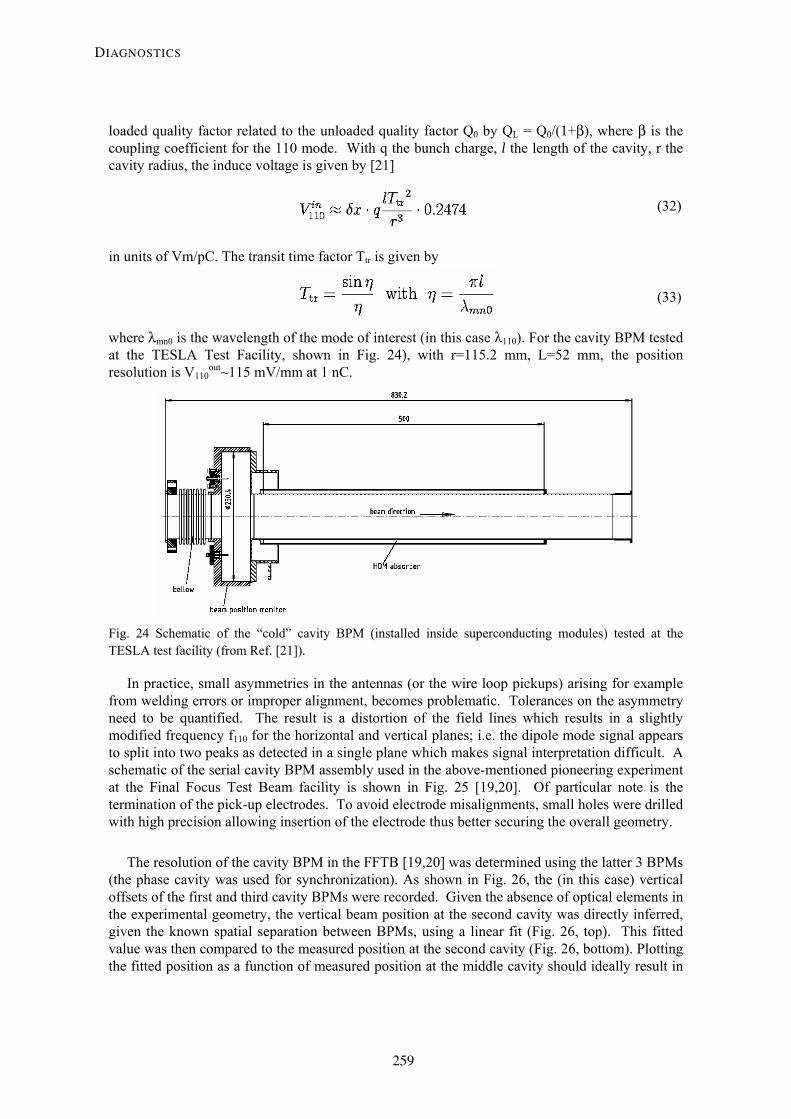
21

loaded quality factor related to the unloaded quality factor Q0 by QL = Q0/(1+β), where β is the coupling coefficient for the 110 mode. With q the bunch charge, l the length of the cavity, r the cavity radius, the induce voltage is given by [21]

(32)

in units of Vm/pC. The transit time factor Ttr is given by

(33)

where λmn0 is the wavelength of the mode of interest (in this case λ110). For the cavity BPM tested at the TESLA Test Facility, shown in Fig. 24), with r=115.2 mm, L=52 mm, the position resolution is V110

out~115 mV/mm at 1 nC.

Fig. 24 Schematic of the “cold” cavity BPM (installed inside superconducting modules) tested at the TESLA test facility (from Ref. [21]).

In practice, small asymmetries in the antennas (or the wire loop pickups) arising for example from welding errors or improper alignment, becomes problematic. Tolerances on the asymmetry need to be quantified. The result is a distortion of the field lines which results in a slightly modified frequency f110 for the horizontal and vertical planes; i.e. the dipole mode signal appears to split into two peaks as detected in a single plane which makes signal interpretation difficult. A schematic of the serial cavity BPM assembly used in the above-mentioned pioneering experiment at the Final Focus Test Beam facility is shown in Fig. 25 [19,20]. Of particular note is the termination of the pick-up electrodes. To avoid electrode misalignments, small holes were drilled with high precision allowing insertion of the electrode thus better securing the overall geometry.

The resolution of the cavity BPM in the FFTB [19,20] was determined using the latter 3 BPMs (the phase cavity was used for synchronization). As shown in Fig. 26, the (in this case) vertical offsets of the first and third cavity BPMs were recorded. Given the absence of optical elements in the experimental geometry, the vertical beam position at the second cavity was directly inferred, given the known spatial separation between BPMs, using a linear fit (Fig. 26, top). This fitted value was then compared to the measured position at the second cavity (Fig. 26, bottom). Plotting the fitted position as a function of measured position at the middle cavity should ideally result in

DIAGNOSTICS

259

22

a straight line with a 45º slope crossing through zero. The scatter of the resulting data points projected along this 45º axis gives a distribution with an rms value equal related to the BPM resolution as shown (corrected by a geometrical factor). With 1 nC bunch charge, these C-band cavity “RF BPMs” yielded a position resolution of a mere 25 nm. Perhaps of significance is the evidenced non-zero crossing of the fitted line which suggests a relative alignment error or electrical asymmetry.

Fig. 25 Mechanical drawing of the triplet RF-BPM set (refered in this text as cavity BPMs) from the Final Focus Test Beam Facility (courtesy T. Shintake, 2003).

Fig. 26 Illustration of the C-band cavity BPM geometry used in the FFTB experiment at SLAC (top) and the method used to infer the resolution of the cavity BPM (bottom).

M. MINTY

260

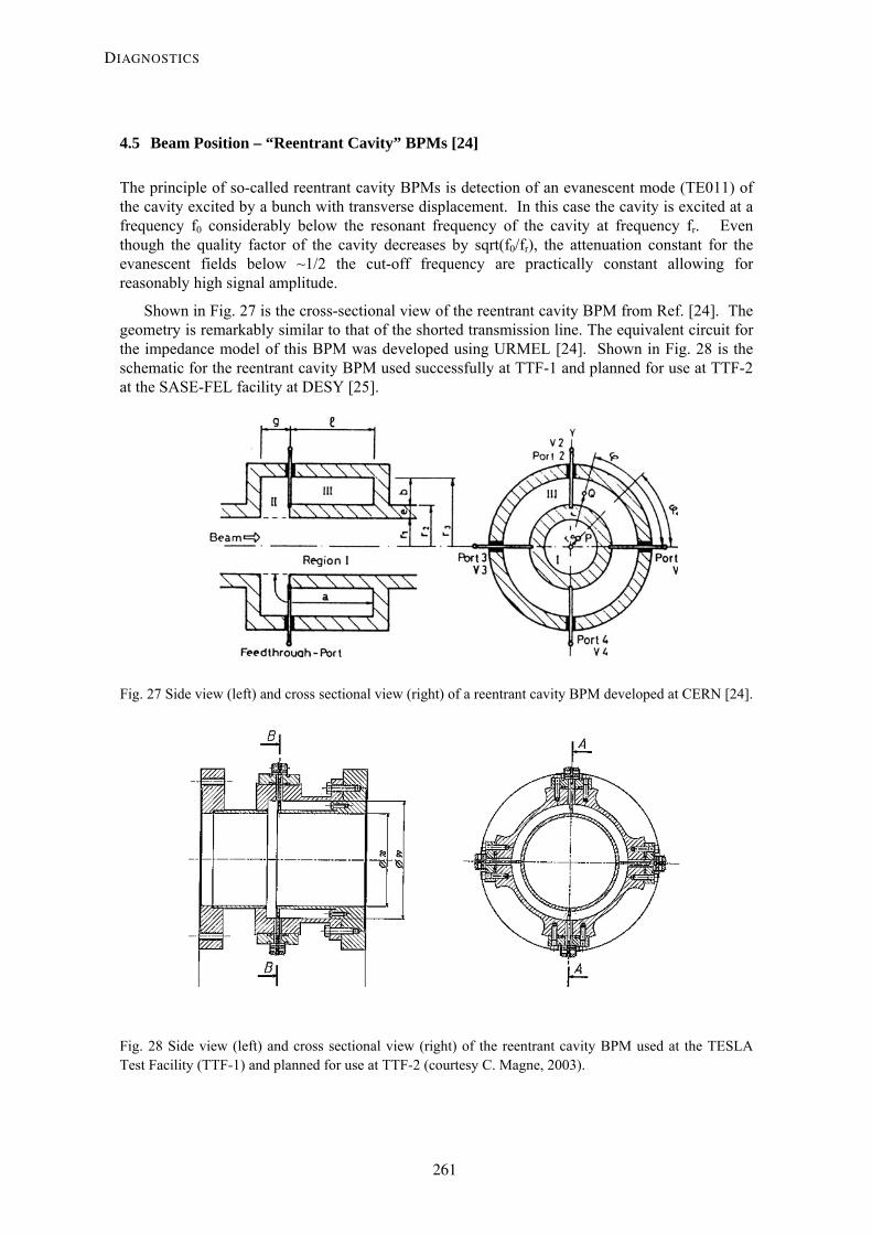
23

4.5 Beam Position – “Reentrant Cavity” BPMs [24]

The principle of so-called reentrant cavity BPMs is detection of an evanescent mode (TE011) of the cavity excited by a bunch with transverse displacement. In this case the cavity is excited at a frequency f0 considerably below the resonant frequency of the cavity at frequency fr. Even though the quality factor of the cavity decreases by sqrt(f0/fr), the attenuation constant for the evanescent fields below ~1/2 the cut-off frequency are practically constant allowing for reasonably high signal amplitude.

Shown in Fig. 27 is the cross-sectional view of the reentrant cavity BPM from Ref. [24]. The geometry is remarkably similar to that of the shorted transmission line. The equivalent circuit for the impedance model of this BPM was developed using URMEL [24]. Shown in Fig. 28 is the schematic for the reentrant cavity BPM used successfully at TTF-1 and planned for use at TTF-2 at the SASE-FEL facility at DESY [25].

Fig. 27 Side view (left) and cross sectional view (right) of a reentrant cavity BPM developed at CERN [24].

Fig. 28 Side view (left) and cross sectional view (right) of the reentrant cavity BPM used at the TESLA Test Facility (TTF-1) and planned for use at TTF-2 (courtesy C. Magne, 2003).

DIAGNOSTICS

261

24

5. TRANSVERSE BEAM EMITTANCE

In this section we describe techniques for measuring the transverse emittances of the particle beam. We begin with a review of three equivalent and complementary methods for characterizing the second moments of the beam distribution and will refer to these later in the context of each application. The principles for measurement of the transverse beam emittance will be described for the (invasive) single quadrupole scan and for the (nominally noninvasive) method utilizing a minimum of 3 beam size measurements with illustrative examples from the SLC5. These methods rely on accurate beam size measurements. Measurement techniques for determining the beam size will be reviewed next with numerous examples from the Accelerator Test Facility (ATF) at KEK and the SLC.

5.1 Introduction The determination of the transverse beam emittances may be characterized using at least 3 different equivalent formalisms: using the single-particle point-to-point transfer matrices, the transport of the Twiss parameters, or the transport of the so-called “beam matrix”. In all cases we consider the ideal case of uncoupled motion (the horizontal and vertical degrees of freedom are independent of one another and of motion in the longitudinal plane).

(i) The transformation of the phase space coordinates (x, x’) of a single particle from an initial to a final location (denoted by subscripts i and f, respectively) separated by some distance may be represented by a transport matrix, R as Xf=RXi:

(34)

where R is the point-to-point transfer matrix (obtained by multiplying the matrix representations of all elements between the initial and final observation points) and x is taken here to represent motion in either the horizontal or vertical plane. Averaging over all particles within the bunch, assuming that all the particles in the bunch move independently of one another, the first moment of the distribution <x> gives the mean position while the second moment of the distribution <x2> gives the transverse beam size since σx=<x2>1/2.

The first two moments of the distribution are given by:

and (35)

where f(x) is the intensity distribution of the beam (which for lepton beams is usually taken to be Gaussian). 5 The examples presented could be particularly useful for those involved in programming code as a performance check.

M. MINTY

262

25

(ii) Equivalently, the Twiss parameters (α,β, and γ), which define the beam ellipse, obey (36) where in both cases above, the elements of the transfer matrix R are given generally by (37) If the initial (i) and final (f) observation points are the same, as for storage ring applications, then the matrix R is given by the one-turn-map Rotm as (38) where μ is the one-turn phase advance: μ =2πQ, where Q is the transverse betatron tune. Obtaining the beam size given the Twiss parameters will be shown after first introducing the beam matrix. (iii) The beam matrix Σbeam may be expressed either in terms of the Twiss parameters or in terms of the moments of the beam distribution as (39) The transformation of an initial beam matrix Σbeam,0 to the desired observation point is (40) where R is again the transfer matrix given in Eq. (34). Neglecting the mean of the distribution, that is, disregarding the static position offset of the core of the beam; i.e. <x>=0, then (41)

DIAGNOSTICS

263

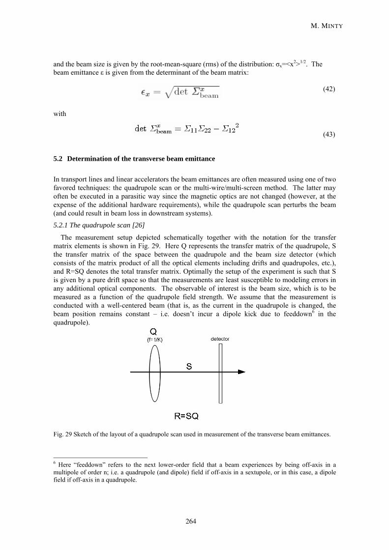
26

and the beam size is given by the root-mean-square (rms) of the distribution: σx=<x2>1/2. The beam emittance ε is given from the determinant of the beam matrix: (42) with

(43)

5.2 Determination of the transverse beam emittance

In transport lines and linear accelerators the beam emittances are often measured using one of two favored techniques: the quadrupole scan or the multi-wire/multi-screen method. The latter may often be executed in a parasitic way since the magnetic optics are not changed (however, at the expense of the additional hardware requirements), while the quadrupole scan perturbs the beam (and could result in beam loss in downstream systems).

5.2.1 The quadrupole scan [26]

The measurement setup depicted schematically together with the notation for the transfer matrix elements is shown in Fig. 29. Here Q represents the transfer matrix of the quadrupole, S the transfer matrix of the space between the quadrupole and the beam size detector (which consists of the matrix product of all the optical elements including drifts and quadrupoles, etc.), and R=SQ denotes the total transfer matrix. Optimally the setup of the experiment is such that S is given by a pure drift space so that the measurements are least susceptible to modeling errors in any additional optical components. The observable of interest is the beam size, which is to be measured as a function of the quadrupole field strength. We assume that the measurement is conducted with a well-centered beam (that is, as the current in the quadrupole is changed, the beam position remains constant – i.e. doesn’t incur a dipole kick due to feeddown6 in the quadrupole).

Fig. 29 Sketch of the layout of a quadrupole scan used in measurement of the transverse beam emittances.

6 Here “feeddown” refers to the next lower-order field that a beam experiences by being off-axis in a multipole of order n; i.e. a quadrupole (and dipole) field if off-axis in a sextupole, or in this case, a dipole field if off-axis in a quadrupole.

M. MINTY

264

27

Using a thin-lens approximation for the quadrupole with K=±1/f, where f is the focusing strength of the quadrupole (- for focusing and + for defocusing), then and [ (44)

Expanding the position function from Eq. (34), the (11)-element of the beam transfer matrix, Eq. (41), after some algebra, is found to be quadratic in the field strength K: [45] (45)

Measurements of the beam size versus quadrupole field strength from the SLC are shown in Fig. 30 taken from the transfer line between the electron damping ring and the main linac.

Fig. 30 Measurements of the transverse beam emittance at the SLC using the method of the quadrupole scan.

DIAGNOSTICS

265

28

The parabolic fitting function in Fig. 30 is of the form

(46)

Equating terms in Eqs. (45) and (46) and dropping the ‘o’ subscipts, we have

(47)

which represents 3 equations with 3 unknowns given by the fit parameters A, B, and C. Solving for the elements of the beam matrix,

(48)

The beam emittance, given by the determinant of the beam matrix, Eq. (42), is then obtained directly from the fit parameters:

(49)

Likewise, using the definition of the Twiss parameters in terms of the beam matrix elements, Eq. (39), the 3 Twiss parameters, and hence the orientation of the beam in phase space, as shown in Fig. 31, are known. Namely,

(50)

As a useful check, the beam-ellipse parameters should satisfy the fundamental relationship for the Twiss parameters: (βγ-1)=α2. If this relationship does not hold given the Twiss parameters derived from the fit, then reasons must be investigated. A likely source for discrepancy (as

M. MINTY

266

29

experienced in practice) is the error introduced by the thin-lens approximation for the quadrupole7.

Fig. 31 Beam ellipse in transverse phase space in terms of the Twiss parameters.

5.2.2 Multiple wire (or screen) measurement of the beam emittance [27,28]

The measurement geometry for measuring the beam emittance using multiple measurements of the beam size is depicted in Fig. 32. The syntax used is: superscripts to denote the “measurement number”, or location, and subscripts to designate the matrix elements for the transfer matrix of interest.

Fig. 32 Geometry of the multiple wire/screen method for measurement of the transverse beam emittances.

7 The exact matrix representation for a quadrupole, obtained by solving Hill’s equation, may be found in Ref. [28], for example.

DIAGNOSTICS

267

30

Referring to Fig. 32, with fixed optics and multiple (total of n) measurements of the horizontal beam size σx at the different locations along the beamline, we may write:

(51)

The optimum wire locations for maximum sensitivity are such that the separation between wires corresponds to a difference in betatron phase advance i(180º/(n+1)) where the number of measurement n must be at least 3 (to solve for the 3 unknowns) and i=0,1,…,n.

Using the symbol definitions shown in Eq. (51), the matrix equation to be solved is

(52)

The solution for the vector with the Twiss parameters is given by minimizing the sum (this is a least squares fit)

(53)

Where σΞx( ) denotes the error of Ξx

( )=(σx( ))2 (i.e. this is the error in the Gaussian fit for wire l).

Forming a symmetric n x n covariance matrix

(54)

the least-squares solution to Eq. (54) is

(55)

with dimension of (3 by 1) independent of the number of measurements. Equation (55) yields the Twiss parameters of interest in terms of the measured beam sizes and the beam optics, which are assumed to be known. Here the ‘hats’ show the weighting used in the normalization so that the rms error is 1:

and (56)

o Ξx B

M. MINTY

268

31

Once the components of the vector with the Twiss parameters is known, the emittance and Twiss parameters are given by

(57)

and γ=(1+ α2)/β. Raw beam size data obtained using wire scanners in the injector linac of the SLC are shown in Fig. 33. We intentionally show this particularly poor set of data to illustrate the usefulness of a graphical summary (see below) of the measurement as shown in Fig. 34.

Fig. 33 Wire scanner data measured in 4 different locations in the injector linac at the SLC.

DIAGNOSTICS

269

32

The beam size measurements in Fig. 33 are clearly non-Gaussian. This is usually not the case for measurements in a transport line (or linear accelerator) following a storage ring but is not unusual in low energy linear accelerators. The fits in the case shown are “bi-Gaussian”; that is, each side of the profile is fitted independently with a Gaussian (giving standard deviations σL on the left and σR on the right). For insertion into the Ξ-matrix above the mean, σ=(σL +σR)/2, is used. This fitted σ therefore, while ‘representative’ of the distribution, is not equivalent to the true rms of the distribution (which one would have with perfect Gaussian profiles). However, experience has shown that even an approximate way of characterizing the data is useful for either monitoring purposes or in efforts aimed towards improving the beam quality.

The data may be represented graphically in the following convenient way as shown in Fig. 34. Since the Twiss parameters at the point of interest are known, the ellipse in phase space (x, x’) as in Fig. 31 may be reconstructed. Alternatively, the ellipse may be plotted in normalized phase space (x, px=αxx+βxx’) where px is canonically conjugate to x. A further refinement is to normalize both coordinates to the square root of the beta function at the reference point for the beam ellipse of interest so that the design ellipse has unity radius in these coordinates. That is, for the graphical representation, plot the design ellipse and the measured ellipse as represented by

(58)

In addition, it is of interest to plot the wires mapped back to the observation point using

(59)

For example, two measurements separated by 90º phase advance would be instantly visible as two lines intersecting also at a 90º angle.

Fig. 34. Graphical representation of the emittance measurement.

M. MINTY

270

33

The utility of the graphical representation is now clear: 1) The fact that the design ellipse (circle in this normalized phase space) and the measured ellipse are not both round indicates what is refered to as a “mismatch”8 [29]; 2) At a glance, the phase space coverage of the beam size measurements is immediately clear: we observe, for the case of the horizontal plane shown on the left, phase advances of 0º, ~45º, ~67.5º , and ~(90+22.5º); 3) whereas only 3 measurements are required to determine the Twiss parameters, a fourth measurement has been included (in the case of the measurement of the horizontal emittance). However, we observe that 1 of the 4 wires does not touch the measured beam ellipse thus indicating an optical error (in this case the data from this wire is best omitted when determining the Twiss parameters, as was done for the vertical beam emittance measurement). In the text display of Fig. 31 is included also for convenience the design beam sizes and the design Twiss parameters at the point of interest as well as the beam intensity (in units of particles per bunch, ppb) and the goodness of fit indication, the χ2.

Lastly we remark, that in the design of a multiple wire or screen emittance station, by clever choice of the optical parameters at the location of the measurements, even more information could be inferred from the graphical representation. For example, suppose that the design β-functions at two of the wires are equal and that the measured beam sizes are different. In the absence of an optical error, this could indicate a dispersive contribution to the beam size.

5.3 Measurements of the transverse beam size

The emittance measurements described in the preceding section rely on accurate measurements of the beam size. In this section we describe the hardware used for measuring the beam size including directly intercepting screens, transition radiation (favored conventionally in transport lines and linear accelerators), conventional wire scanners and laser wire scanners (applicable in linear lattices or circular accelerators). To complement the lectures presented by A. Hoffmann, various measurements based on measurements of the emitted synchrotron radiation in storage rings are described.

5.3.1 Measurement of the transverse beam size using screens

A schematic view of a vacuum chamber and hardware associated with beam size measurement utilizing a screen is shown [30] in Fig. 35. The intercepting screen (composed for example of Al2O3Cr possibly with a phosphorescent coating) is inserted, usually at a 45º angle (to simplify the vacuum chamber geometry) into the path of the beam. The image is then viewed by a camera allowing direct observation in the horizontal and vertical planes (x-y) in locations of zero dispersion (η=0) for which the beam position is independent of beam energy, or in the energy and vertical planes (δ-y) in regions of nonzero dispersion (η≠ 0). Orientation of the camera for head-on viewing of the screen is advisable in order to avoid corrections (path-length dependent aberrations in the camera lenses) as illustrated by the orientation of the view port in Fig. 35.

R. Jung et al, in Ref [31] have defined the following characteristics9 of light emission from the screen: fluorescence – referring to light emitted on short time scales (t~10 ns) as the atoms in the screen excited by the beam decay back to their ground state, phosphorescence – light continues to be emitted (t~μs) after the exciting mechanism has ceased10, and luminescence – a combination of both processes. 8 The mismatch parameter denoted in the text of Fig. 34 by Bmag is unity for perfectly matched beams or >1 if mismatched. The physical interpretation is that the beam, if allowed to filament completely after propagating through identical lattice sections, would have an emittance then equal to Bmagε, where ε denotes the emittance just measured. 9 The definitions are useful given that the words fluorescence, phosphorescence, and luminescence seem to be used somewhat randomly in the literature. 10 For example, “afterglow” in analogue oscilloscopes.

DIAGNOSTICS

271

34

In the beam size measurement utilizing screens, the image is digitized, projected onto orthogonal axes, and fitted with a Gaussian function. A “background image” (obtained without beam) is subtracted from the data (here line-locking of the camera may be important). The calibration may be most easily obtained using as reference grid lines etched directly on the screen or from drilled calibration holes either of which has a known spacing.

Special concerns for beam size measurements utilizing screens include the special resolution (of typically 20-30 μm) given by the phosphor grain size and transparency, the temporal resolution given by the decay time, radiation hardness of the screen and camera, and the dynamic range (i.e. saturation of the screen at high beam currents).

At the SLC the beam sizes at the end of the 50 GeV lepton linac were routinely monitored using screens [32]. Rather than inserting a screen directly into the beam path, fast kicker magnets (2 per plane) were used to deflect the bunch of interest onto dedicated screens. An example of such measurements is shown in Fig. 36.

Fig. 35 Beam size measurement assembly utilizing a screen (courtesy P. Tenenbaum, 2003).

Fig. 36 Beam size monitoring using screens at the end of the SLC linac (courtesy F.J.-Decker, 2004).

M. MINTY

272

35

5.3.2 Measurement of the transverse beam size using optical transition radiation (OTR)

When a charged particle crosses between two materials of different dielectric constant (for example, between vacuum and a conductor), transition radiation is generated. The time dependence of the photon emission is short (~1 ps) allowing for temporal resolution of closely spaced bunches. Beam profiling using OTR are reviewed, for example, in Refs. [33-35].

The radiation from the foil is emitted in both the forward and backward directions as shown [36] in Fig. 37 for the case of a foil oriented at 45º with respect to the incident beam. Represented schematically are lobes of peak intensity (strongest electric field of the emitted photon beam). These lobes are centered about the direction of the beam for the case of forward transition radiation and about an axis that obeys Snell’s law (of equal angle of incidence and reflection) for the backward transition radiation. While the optimum viewing angle for minimum systematic distortion is such that the camera lenses are flush with the screen, the radiation emitted at a 90º angle with respect to the beam is often viewed since there the light intensity is highest. Aberrations in the camera lenses must in such a case be taken into account. In certain applications, the image plane of the camera is tilted to avoid such aberrations.

Typical compositions of the foil for OTR measurements are Al, Be, Si, or Si with an Al coating. Similarly to beam size measurements using screens, the images obtained are digitized and fitted using typically a Gaussian distribution and the calibration is often obtained using etched lines of known spacing.

Fig. 37 Conceptual view of emitted optical transition radiation generated by a beam striking a thin foil (courtesy K. Honkavaara, 2003).

Issues related to beam size measurements using optical transition radiation include the special resolution (the upper limit of which was thought, based on literature, to be higher than that recently demonstrated, see below, but is widely considered to be ~5 μm), damage to the radiator, particularly in the case of small beam sizes, and as mentioned, geometrical depth-of-field effects resulting from the geometry associated with imaging the backward transition radiation. As in the case with normal screens, background subtraction is also of critical importance.

Recently, a resolution of 1 μm was demonstrated [37] in an OTR measurement at the accelerator test facility (ATF) at KEK. The vertical beam size of about 5 μm was measured at the exit of the low-emittance damping ring in the downstream transfer line. The measurement setup

DIAGNOSTICS

273

36

is shown in Fig. 38 and includes a Cu target, a 1 mm exit window (with a surface flatness given by the pressure differential across the window of about λ/4), and an imaging system with a triggered CCD camera (with a pixel size of 10 μm). The geometry was optimized, within the mechanical constraints and at the expense of intensity, to try to achieve normal incidence of the camera on the target. To minimize the possible systematic error resulting from the change in focal depth with position on the target, rather than tilting the image plane of the camera, the field of view was made to be narrow. An example of the beam size measured using this SLAC-built OTR station at the ATF [37] is shown in Fig. 39.

Fig. 38 Photograph of the optical transition radiation hardware for measurement of the beam size as mounted in the extraction line of the ATF damping ring (courtesy M. Ross, 2003).

Fig. 39 Beam size measurement at the ATF using optical transition radiation (courtesy M. Ross, 2003).

M. MINTY

274

37

5.3.3 Measurement of the transverse beam size using (conventional) wire scanners

Wire scanner measurements (see for example Refs. [38-39]) may be used usually noninvasively in both linear and circular lepton accelerators. The wire is mounted rigidly on a shaft which is moved using a precision stage with a precision encoder. Usually the wire (e.g. of material C, Be, or W) is moved across the beam. In certain cases, the beam is moved across the wire (which no longer constitutes a noninvasive measurement if the change in beam position is not compensated for downstream). A typical support structure for wires is shown in Fig. 40 for the scanner assembly in the extraction line of the accelerator test facility at KEK [40]. With the scanner mounted at 45º with respect to the beamline, the horizontal/vertical wire is used for measurements of the vertical/horizontal beam sizes respectively. The wire mounted at 45º is used to infer the coupling (with 45º optimal for the case of a round beam). The precision of the stepper-motor in this assembly was 0.5 μm. The optimum velocity of the wire passage through the beam depends on the desired interpoint spacing and on the bunch repetition frequency (as constrained possibly by beam-induced heating).

Fig. 40 Wire scanner mount from the ATF (courtesy H. Hayano, 2003).

The interaction of the beam with the wire may be detected in many ways: 1) by the change in voltage on the wire induced by secondary emission; 2) by detection of hard Bremsstrahlung whereby the forward detected photons are separated from the beam via an applied magnetic field (e.g. a normal bending dipole in a storage ring), converted to e+/e- pairs in the vacuum chamber wall, and detected with a Cerenkov counter or photomultiplier tube (PMT) after conversion back to photons in the front end of the detector; 3) via detection of delta-rays at 90º using Cerenkov counters or PMTs; 4) by detection of scattering and electromagnetic showers using PMTs; 5) and novelly, by the detection of the change in tension of the wire. Of the above methods, option 4 finds most widespread use in high energy accelerators. In this case, the amplitude of the PMT signal is recorded as a function of the calibrated position of the wire.

Particular concerns of wire scanners include the dynamic range of the detectors (trade-off between good signal-to-noise characteristics and possible saturation for high single-bunch beam currents), vibrations of the wire, single-pulse beam heating (the instantaneous temperature in the wire should not exceed the melting point of the wire material), the wire thickness which adds in quadrature with the measured beam size (and should therefore be small), and, particularly in

DIAGNOSTICS

275

38

circular accelerators, higher-order modes introduced by the vacuum chamber geometry surrounding the wire and the wire itself.

The wire scanner assembly and an example beam size measurement from the ATF [40] are shown in Figs. 41 and 42. These measurements together with data from a laser wire located in the damping ring are used routinely in the demonstration of record small vertical beam emittances at the ATF.

Fig. 41 Wire scanner assembly in the extraction line of the ATF damping ring (courtesy H. Hayano, 2003).

Fig. 42 Vertical beam size measured in the ATF extraction line using a wire scanner (courtesy H. Hayano, 2003).

M. MINTY

276

39

5.3.4 Measurement of the transverse beam size using laser wires

At the expense of increased cost and complexity, the use of a laser as the interaction medium allows for a noninvasive measurement of the beam sizes. Moreover, as opposed to measurements with screens or conventional wires, the wire itself (in this case the laser) is (advantageously) non-destructable. A schematic of the laser wire system as installed [41] in PETRA at DESY and planned for use in PETRA-3, a third generation light source, is shown in Fig. 43. The system consists of a high-power laser, the optical transport line, the laser-lepton interaction region, and detectors. Measurement of the horizontal beam size is made using the optical path containing the deflector while the vertical beam size is measured using the optical path of the beam in the deflected arm of the beam splitter. The laser-beam interaction is detected using either the forward-scattered Compton photons or, after deflection by a magnetic field, the lower-energy scattered leptons of the particle beam.

Fig. 43 Geometry of the laser-wire system for PETRA-3 at DESY (courtesy S. Schreiber, 2003).

A close-up view of the interaction region optics is shown in Fig. 44 from the pioneering laser wire experiment [42] performed in the SLC at SLAC. As with all applications of laser wires to date (at the SLC, the ATF, and at PETRA-3) experience has shown the following issues to be of importance: the size of the laser waist (in practice, the minimum waist size is on the order of the laser wavelength), background sources and background subtraction, the depth of focus, temporal synchronization of the laser with the beam (for the case of pulsed lasers), and, particularly for measurements of small beam sizes, accelerator reproducibility (which influences the time required to establish overlap of the laser with the beam).

In the laser wire facility in the ATF at KEK [43] the intensity of the laser is amplified using an optical cavity as shown in Fig. 45. Here the optical cavity is pumped by a CW laser with a mirror reflectivity exceeding 99%. A measurement of the vertical beam size in the ATF damping ring is shown in Fig. 46. As with normal wires, the wire size and additive contributions due to the vertical dispersion ηy (for the case of the vertical beam size measurement shown in Fig. 45) must be taken into account [43]. The correction for the wire size is

(60)

where ω0 is the 2σ wire thickness. The correction for the vertical dispersion is given, as usual, by

DIAGNOSTICS

277

40

(61)

where σp/p denotes the momentum spread of the particle beam. This state-of-the-art beam size measurement verified the exceedingly small design vertical emittance as required for a future linear collider.

Fig. 44 Interaction region optics for the SLC laser wire (courtesy M. Ross, 2003).

Fig. 45 Schematic of the laser wire at the ATF using an optical cavity (courtesy H. Sakai and J. Urakawa, 2003).

M. MINTY

278

41

Fig. 46 Vertical beam size measurement from the ATF using a laser wire (courtesy H. Sakai and J. Urakawa, 2003).

5.3.5 Measurement of the transverse beam size using synchrotron radiation

In this section we describe one of many methods used for measuring properties of the lepton beam in a circular accelerator using synchrotron radiation. Not includes in this lecture, yet of great significance, are among others, measurements made using pin-hole cameras [44], interferometric methods [45], or measurements based on the angular distribution of the photon beam [46]. In the examples presented, it is attempted to discuss is some detail special concerns of measurements utilizing direct imaging and the variety of ways in which a single (relatively low-cost) experimental setup utilizing screens (in this case for the photon beam) can be used to gain information about the circulating lepton beam.

We recall from the lectures of A. Hoffmann [46], that measurement of the synchrotron radiation emitted by accelerated leptons can be categorized as direct imaging (for which the beam size is directly measured) or as direct observation (for which the angular spread of the beam is measured). These principles are illustrated schematically in Fig. 47. In the first case of direct imaging, the radiation emitted from a bending magnet is focused onto the detector using optical lenses. In the second case, the angular spread of the emitted radiation is observed directly.

Considering the first case, for which the radiation is emitted in a bending magnet, “depth of field” effects [47] must be taken into account. This refers to the fact that the photons are emitted continuously as they are bent (accelerated transversely) in the deflecting field of the magnet. The geometry is illustrated in Fig. 48 (top) from which can be seen that the photons are collected in the detector, located nominally to view the tangentially emitted radiation, not only from the ideal source emission point, but along the path of the lepton beam. The undesired contributions depend on the acceptance of the detector or on aperture restrictions given by the optical elements between the emission points and the detector. Viewed in the reference frame of the photon beam phase space, as shown in Fig. 48 (bottom), the particle beam emits a “swath” of radiation with a

DIAGNOSTICS

279

42

curvature related to the curvature of the orbit. For example, referring to Fig. 48 (top), the beam emits radiation at +x for emission both before and after the nominal source-point emission location and has a point-source emission angle of +/- x’. The width of the “swath” is given by the transverse size of the lepton beam. Also shown in Fig. 48 (bottom) are the effects of limiting apertures (i.e. lens diameters or the camera acceptance). Here a is the half-width of the limiting aperture and l is the distance to this defining aperture.

Fig. 47 Conceptual diagrams illustrating direct imaging (left) or direct observation of the angular spread of the emitted synchrotron radiation (right) for determination of the transverse beam size (courtesy A. Hoffmann, these lecture series, 2003).

Fig. 48 Geometry of emitted synchrotron radiation in the horizontal plane illustrating contributions due to depth-of-field and the phase space coordinates of the photon beam (a) and the phase space of the photon beam assuming a bending radius of ρ=2 m, a beam size of σ=100 μm, and limiting apertures defined by the half-width a=1 cm and the distance to the aperture of l=1.46 m (b) [47,48].

M. MINTY

280

43

The measured photon beam centroid <x> and beam size σr,x correspond to a projection of the photon phase space (see Fig. 48b) onto the horizontal axis:

(62)

and

(63)

where I(x) denotes the intensity of the photon beam distribution. From Fig. 48 it is clear that depth-of-field effects may be minimized (at the cost of reduced light intensity) by reducing the size of the limiting aperture (the two parallel lines in Fig. 48b move closer together). With large apertures, the projection (and hence the measured image) would evidence a one-sided “tail” in the distribution and hence be non-Gaussian.

In the following is presented data taken in the SLC damping rings using direct imaging of synchrotron radiation. While the initial goal of the experiment was accurate determination of the transverse damping times [48], since these are perhaps not of foremost interest in the synchrotron radiation facility community, instead, the additional measurements of the beam emittance and matching at injection (which may be of concern in synchrotron light facilities to maximize injection efficiency) will be presented [49]. The layout of the optical system is shown in Fig. 49. In this case, the radiation was extracted from the vacuum chamber using a water-cooled Molybdenum mirror. The 1.33 m achromatic lens was used to produce parallel rays for transport to a remote location, which was necessary to avoid the high background radiation levels in the accelerator tunnel and was desired in order to have the camera accessible during normal operations. Special care was taken to avoid distortions of the beam image resulting from air currents generated between the (warm) tunnel and (cooler) room containing the optical table. At the remote location, the light was focused and then split using a pellicle. The image was viewed by two cameras, a “normal camera” for continuous monitoring of the beam and by a fast-gated camera used for turn-by-turn imaging of the lepton beam. The fast shutter was used to protect the delicate fast-gated camera from dangerous light levels when data were not being acquired. The polarized filters were used to filter out the contributions from the (bi-modal) transverse polarization of the photon beam. The location of the image focus was determined experimentally by translating the cameras along the optical path to obtain a minimum image size.

Shown in Fig. 50 is a close-up view of the camera apparatus. To remove scrolling (as seen on a camera “lines” that sweep vertically with time) resulting from electromagnetic interference the line-locked normal camera was used to supply composite synchronization to the gated camera. The video amplifier was used to boost the voltage level of the synchronized signal. The controller was used to adjust the gain and phase of the output video signal. A video digitizer clock interface (VDCI) and a transient wave form recorder (TWR) were used as in the previously existing automated emittance measurement systems at SLAC.

DIAGNOSTICS

281

44

Fig. 49 Light optics used to produce parallel rays for transport to a remote location for direct imaging of the synchrotron radiation in the damping rings at the SLC. The overview is not to scale.

Fig. 50 Synchronization scheme using an additional “normal” camera.

In Fig. 51 is depicted the raw data showing turn-by-turn transverse beam profiles acquired at injection (with each image representing an average over 8 different beam pulses). The data were obtained by advancing the camera trigger by one revolution for each snapshot. A background image was subtracted from all snapshots and nearest-neighbor pixel averaging (smoothing) was performed to more clearly distinguish the intensity contours. As can be seen, the beam

M. MINTY

282

45

distribution varied dramatically from turn-to-turn. After the beam filamented (after ~10 μs/100 ns = 100 turns), the beam image was seen to be elliptical with a Gaussian distribution. It is worth mentioning that the accelerator was operated on the coupling resonance with Qx~Qy=0.25 so that one might expect that every fourth turn result in an identical beam image (i.e. along every row). The differences in images along a given row may be partly attributable to amplitude-dependent tune shifts (arising from non-centered orbits in the sextupole magnets).

Quantitative information of the beam distribution was obtained, as in the case of transverse beam size measurements utilizing screens or wires, by digitizing the image, subtracting a background image, projecting the distributions along two normal axes, and fitting the results with a Gaussian distribution. An example is shown in Fig. 52.

Fig. 51 Transverse beam profiles (in the x-y plane) using direct imaging as a function of turn number in the SLC damping ring.

DIAGNOSTICS

283

46

As in the case of the wire scanner data presented previously one is confronted with the difficulty of qualitatively characterizing the measured profiles. As discussed previously one can apply a fit (either Gaussian or bi-Gaussian) and postulate that the fitted σ is fairly representative of the true rms of the distribution. While this parametrization is clearly not strictly true, it was found to be useful for further beam optimization. This is illustrated by the measurement results of Figs. 53 and 54. Plotted in both cases, on the left is the measured beam size squared (in the horizontal and vertical planes) measured turn-by-turn at injection. On the right are shown the Fourier transform of these data. In the case of perfect matching of the optical functions between the injection line and the downstream circular accelerator, the beam sizes would be constant from turn-to-turn. Given a mismatch peaks in the Fourier spectrum are discernible at frequencies of 2Q for a betatron mismatch (Δβ) and at Q for a dispersion mismatch (Δη) [49]. Figure 53 shows the measurement results before optimizing the injection match (evidencing prominent peaks due to the mismatches in β and η). The data obtained after correction are shown in Fig. 54. The optimization was performed empirically, using as a diagnostic the fitted beam size measured after the beam had fully filamented, by varying the strength of the quadrupoles at the end of the injection line.

Fig. 52 Processed data from direct imaging. Shown is the 3-dimensional digitized image after background subtraction (top) and the projections together with the Gaussian fits (bottom).

The amplitude of the aberrant peaks gives qualitative information about the optical errors [49]. Considering for illustration purposes the case of a pure betatron mismatch, following the convention of M. Sands [29], the amplitude of the mismatch parameter B can be quantified. Denoting A1 as the amplitude of the peak at zero frequency (dc) and A2 the amplitude of the peak at twice the betatron frequency, it can be shown that A1=Bε0, where ε is the beam emittance in the plane of interest and A2=ε•sqrt(B2-1). Denoting the measured ratio of the amplitude of the peaks at dc and at twice the betatron frequency as ρ, the amplitude of the mismatch parameter can be solved for independent of knowledge of the β-function at the source emission point: B=1/sqrt(1-ρ-2). For the case of complete filamentation without damping mechanisms, the beam emittance after the number of turns required for complete filamentation would be ε=Bε0. If the β-function at the source emission point is known (or measured using, for example, a quadrupole

M. MINTY

284

47

scan) and if the matching is perfect (B=1), then the amplitude of the DC component of the Fourier transform of σ2 gives directly the beam emittance: σ=sqrt(A1β).

Fig. 53 Turn-by-turn measurement of the transverse beam sizes (left) and the Fourier spectrum of the beam shape oscillations (right) before injection matching.

Fig. 54 Turn-by-turn measurement of the transverse beam sizes (left) and the Fourier spectrum of the beam shape oscillations (right) after injection matching.

DIAGNOSTICS

285

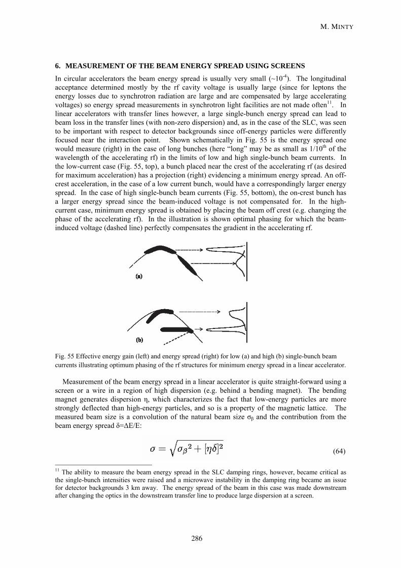
48

6. MEASUREMENT OF THE BEAM ENERGY SPREAD USING SCREENS

In circular accelerators the beam energy spread is usually very small (~10-4). The longitudinal acceptance determined mostly by the rf cavity voltage is usually large (since for leptons the energy losses due to synchrotron radiation are large and are compensated by large accelerating voltages) so energy spread measurements in synchrotron light facilities are not made often11. In linear accelerators with transfer lines however, a large single-bunch energy spread can lead to beam loss in the transfer lines (with non-zero dispersion) and, as in the case of the SLC, was seen to be important with respect to detector backgrounds since off-energy particles were differently focused near the interaction point. Shown schematically in Fig. 55 is the energy spread one would measure (right) in the case of long bunches (here “long” may be as small as 1/10th of the wavelength of the accelerating rf) in the limits of low and high single-bunch beam currents. In the low-current case (Fig. 55, top), a bunch placed near the crest of the accelerating rf (as desired for maximum acceleration) has a projection (right) evidencing a minimum energy spread. An off-crest acceleration, in the case of a low current bunch, would have a correspondingly larger energy spread. In the case of high single-bunch beam currents (Fig. 55, bottom), the on-crest bunch has a larger energy spread since the beam-induced voltage is not compensated for. In the high-current case, minimum energy spread is obtained by placing the beam off crest (e.g. changing the phase of the accelerating rf). In the illustration is shown optimal phasing for which the beam-induced voltage (dashed line) perfectly compensates the gradient in the accelerating rf.

Fig. 55 Effective energy gain (left) and energy spread (right) for low (a) and high (b) single-bunch beam currents illustrating optimum phasing of the rf structures for minimum energy spread in a linear accelerator.

Measurement of the beam energy spread in a linear accelerator is quite straight-forward using a screen or a wire in a region of high dispersion (e.g. behind a bending magnet). The bending magnet generates dispersion η, which characterizes the fact that low-energy particles are more strongly deflected than high-energy particles, and so is a property of the magnetic lattice. The measured beam size is a convolution of the natural beam size σβ and the contribution from the beam energy spread δ=ΔE/E:

(64)

11 The ability to measure the beam energy spread in the SLC damping rings, however, became critical as the single-bunch intensities were raised and a microwave instability in the damping ring became an issue for detector backgrounds 3 km away. The energy spread of the beam in this case was made downstream after changing the optics in the downstream transfer line to produce large dispersion at a screen.

M. MINTY

286

49

By proper selection of location for the screen/wire behind the bending magnet, the dispersive contribution should be made to be large in comparison with the contribution from the natural beam size.

The layout of the TESLA Test Facility (TTF) is shown in Fig. 56. Measurements of the beam energy spread were made using an OTR screen at the end of the linac following the energy spectrometer. Single-bunch energy spreads as a function of the phase of the downstream accelerating module are shown in Fig. 57 measured with moderate single-bunch beam currents. Comparison with Fig. 55 shows good compensation of the beam-induced voltage at an rf phase angle of about +7º and poor phasing at an rf phase of -14º, for example. The substructure observed within a single bunch [50] has been attributed [51] to coherent synchrotron radiation generated in the bunch compressor, which was used nominally to compress the bunch length by about a factor of 4 (from 2 mm to 0.5 mm).

Fig. 56 Layout of the TESLA Test Facility (TTF-1).

Fig. 57 Measurements of the single-bunch energy spread at the end of the TTF-1 linac (courtesy F. Stulle, 2003).

DIAGNOSTICS

287

50

7. MEASUREMENT OF THE BUNCH LENGTH

The FEL community is challenged by resolution limitations for measurements of single-bunch bunch lengths. Recent theoretical analyses of the beam dynamics at the SASE FEL at the TESLA test facility have shown that only a small fraction (~50 fs) of the bunch contributed to the lasing process [52] and imply that all methods used to date (e.g. streak camera measurements, electro-optical sampling, interferometry, etc) were in this application resolution limited. While each and every R&D effort warrants further elaboration, since at the time of this writing the conclusions of these advanced efforts are still in flux, we opt to describe rather the conventional method of bunch length determination using streak cameras which is a primary tool for storage ring facilities.

7.1 Measurement of the bunch length using a streak camera

As shown in Fig. 58, photons (generated e.g. by synchrotron radiation, optical transition radiation, or from an FEL) after collimation and optics adjustment are converted into electrons in the photocathode of the streak camera. These electrons are accelerated by a biasing field and deflected using a time-synchronized, ramped electric field. In this way those particles within the bunch arriving latest (at the tail of the bunch) experience the highest deflection so that the temporal properties of the beam are visible in the transverse plane. The electron beam signal is sometimes further amplified using a multiple channel plate detector (MCP). The electrons are converted back into photons (via a phosphor screen) and detected using an imager (i.e. CCD array) which converts the light signal into a voltage.

Fig. 58 Principle of a streak camera [53].

Practical issues that arise in streak camera measurements include the energy spread of the electrons from the photocathode (time dispersion), space charge effects immediately after the photocathode, and chromatic effects which change the particle arrival time in an energy-correlated way arising, for example, in the windows that separate the vacuum system from air.

Streak camera images taken at the Pohang light source are shown in Fig. 59. These data were acquired in study of fast-ion instabilities predicted [54] to arise in electron storage rings when ions in the residual gas are attracted resonantly to the passing bunches of an electron beam. In the figure, time decreases towards the bottom of each sub-plot (the most recent data are at the bottom of each plot). The horizontal axis is the temporal coordinate. Visible are the bunch lengths of six bunches (top left plot). As the residual gas pressure was intentionally increased, the bunches

M. MINTY

288

51

were observed to begin to oscillate coherently in a manner consistent with that expected from the fast-ion instability [55].

Fig. 59 Streak camera images from the Pohang light source evidencing beam oscillations arising from the fast-ion instability (courtesy M. Kwon, 2000).

7.2 Bunch length measurements using a transverse-mode deflecting cavity and screens

Based on a concept used at SLAC in 1965 [56], use of transverse-mode deflecting cavities has gained recent interest now applied to bunch length measurements in FEL facilities [57-59]. The deflecting cavity, which has a large TM11-mode so that a bunch with a transverse displacement receives a large deflection, is used to “sweep” the beam (just like in the case of a streak camera),

DIAGNOSTICS

289

52

which is then detected using standard profile monitors. The concept is illustrated schematically in Fig. 60.

Fig. 60 Principle of the transverse mode cavity as installed and tested at SLAC (courtesy R. Akre, 2003).

The image detected on the screen is as usual projected and fitted with a Gaussian distribution (after background subtraction). Measurement of the bunch length, presented as the square of the measured bunch length versus applied voltage of the cavity are shown in Fig. 61. The deviation of the minimum bunch length measured from zero applied voltage has been attributed to evidence of an incoming tilt of the bunch [59].

Fig. 61 Measured bunch length (squared) versus applied voltage in the transverse-mode deflecting cavity in measurements at SLAC (courtesy R. Akre, 2003).

M. MINTY

290

53

8. SUMMARY

In these lectures were described the hardware applied for determining the most commonly measured moments of the beam distribution with focus on those devices used most frequently in synchrotron radiation and free electron laser facilities. In the first lecture, measurements of the zeroth and first order moments were discussed. Beam diagnostics were described as used for measuring the beam charge (using Faraday cups) and intensity (using toroidal transformers and BPM sum signals) and the beam position measured with wall gap monitors, electrostatic monitors (including buttons), stripline/transmission detectors, and resonant cavities. Equivalent circuit models were presented which were however often simplistic. In practice these models are often tailored to match observation given direct measurement or using computer models. Impedances in the electronics used to process the signals (which were not described) must also be taken into account as they often limit the bandwidth of the measurement. Nonetheless, the fundamental design features of the detectors presented were discussed thus highlighting the importance of detector geometries and impedance matching as required for high measurement sensitivity.

The second lecture focused on measurement of the second moments of the beam distribution. Multiple, equivalent methods for describing the transport of beam parameters between two points were reviewed. Two methods for measuring the transverse beam emittance were outlined in detail: the method of the quadrupole scan, an invasive measurement during which the accelerator optic (e.g. quadrupole field strength) is varied and measurements are made at a single location, and the fixed-optics method, which requires at least three independent beam size measurements and assumes that the optics between measurements is known. Experimental hardware applied in measurements of the beam size were reviewed including the use of screens, transition radiation, conventional and laser wire scanners, and direct imaging of synchrotron radiation. Measurements of the beam energy spread using screens and the bunch length using streak cameras and transvers-mode deflecting cavities were reviewed.

ACKNOWLEDGEMENTS

In preparation of these lectures, I have profitted enourmously from recent insightful conversations with M. Dohlus, K. Honkavaara, R. Neumann, D. Noelle, S. Schreiber, L. Schreiter, T. Shintake, M. Werner, and M. Wendt. For their enthusiasm, insights, and furthering of my education in the subject of beam diagnostics, I would like especially to thank W. Kriens, R. Pollock, M.C. Ross, and R.H. Siemann.

REFERENCES

[1] J. Borer and R. Jung, Diagnostics, CERN LEP-BI/84-14 (1984); CERN Accel. School on

Antiprotons for Colliding Beam Facilities (Geneva, Switzerland, 1984) 385.

[2] R. Littauer, Beam instrumentation, Proc. Physics of High Energy Particle Accelerators (Stanford, CA, 1982); AIP Conf. Proc. 105 (1982) 869.

[3] A. Hofmann, Beam diagnostics and applications, Proc. Beam Instr. Wkshp. BIW98 (Stanford, CA, 1998); AIP Conf. Proc. 451 (1998) 3.

[4] R.H. Siemann, Bunched beam diagnostics, Proc. Physics of Part. Accel. (Batavia, IL, 1987) 430.

[5] R.H. Siemann, Spectral analysis of relativistic bunched beams, Proc. Beam Instr. Wkshp. BIW96 (Argonne, IL, 1996) 3.

DIAGNOSTICS

291

54

[6] R. Talman, Beam current monitors, Proc. Acc. Instr. Wkshp. (Dallas, TX, 1989); AIP Conf. Proc. 212 (1989) 1.

[7] R.C. Webber, Tutorial on beam current monitoring, Proc. Beam Instr. Wkshp., BIW00 (Oak Ridge, TN, 2000); AIP Conf. Proc. 546 (2000).

[8] J.A. Hinkson, Beam current measurements, in Handbook of Accelerator Physics and Engineering, A.W. Chao and M. Tigner (eds.) (World Scientific, 1999).

[9] see for example the Particle Properties Data Booklet: L. Montanet et al., Phys. Rev. D50, 1173 (1994).

[10] T. Suwada, S. Ohsawa, K. Furukawa, N. Akasake, Absolute beam-charge measurement for single-bunch electron beams, Jpn. Jour. Appl. Phys. 39 (2000) 628.

[11] T. Suwada et al, Recalibration of a wall-current monitor using a Faraday cup for the KEKB injector linac, Proc. 1999 Part. Acc. Conf. (New York, NY,1999) 2238.

[12] Bergoz Precision Beam Instrumentation – www.bergoz.com

[13] K. Unser, Beam current transformer with DC to 200 MHz range, IEEE Trans. on Nucl. Sci., Vol. NS-16, No. 2 (1969).

[14] K. Unser, A toroidal dc current transformer with high resolution, IEEE Trans. on Nucl. Sci., Vol. NS-28, No. 3 (1981).

[15] J. Fusellier, J.M. Joly, Beam intensity monitoring and machine protection by toroidal transformers on the TESLA test facility, Proc. 5th Eur. Part. Acc. Conf. (Sitges, Spain, 1996) 1591.

[16] D. Boussard, Schottky noise and BTF diagnostics, CERN Accel. School on Advanced Accelerator Physics (Rhodes, Greece, 1993) 749.

[17] A.J. Gorski and R. M. Lill, Construction and measurment techniques for the APS LEUTL project rf beam position monitors, Proc. 1999 Part. Acc. Conf. (New York, NY,1999) 1411.

[18] R. Lorentz, Cavity beam position monitors, Proc. Beam Instr. Wkshp., BIW98 (Stanford, CA, 1998); AIP Conf. Proc. 451 (1998) 53.

[19] T. Shintake, Development of nanometer resolution RF-BPMs, given at the 17th Intl. Conf. on High-Energy Acc. HEACC98 (Dubna, Russia, 1998); KEK-preprint-98-1998.

[20] T. Slaton, G. Mazaheri, and T. Shintake, Development of nanometer resolution C band radio frequency beam position monitors in the final focus test beam, Proc. 19th Intl. Linear Acc. Conf., Linac98 (Chicago, IL,1998) 911.

[21] C. Magne and M. Wendt, Beam position monitors for the TESLA accelerator complex, DESY-TESLA-2000-41 (2000).

[22] Alternatively the undesired common-mode may be damped by clever design of the BPM. See, for example, S.C. Hartman, T. Shintake, and N. Akasaka, Nanometer resolution BPM using damped slot resonator, Proc. 1995 Part. Acc. Conf. (Dallas, TX,1995) 2655.

[23] J. Arthur et al, Linac coherent light source (LCLS) conceptual design report, SLAC-R-593 (2002).

[24] R. Bossart, High precision beam position monintor using a re-entrant coaxial cavity, Proc. 17th Intl. Linear Acc. Conf., Linac94 (Tsukuba, Japan,1994) 851.

M. MINTY

292

55

[25] C. Magne et al, High resolution BPM for future colliders, Proc. 19th Intl. Linear Acc. Conf., Linac98 (Chicago, IL,1998) 323.

[26] M.C. Ross et al, Automated emittance measurements at the SLC, Proc. 1987 Part. Acc. Conf. (Washington, D.C., 1987) 725.

[27] H. Wiedemann, Particle accelerators physics: basic principles and linear beam dynamics (Springer Verlag, Berlin 1993).

[28] M. Minty and F. Zimmermann, Measurement and control of charged particle beams, (Springer Verlag, Berlin 2003).

[29] M. Sands, A beta mismatch parameter, SLAC-AP-085 (1991).

[30] P. Tenenbaum and T. Shintake, Measurement of small electron beam spots, Ann. Rev. Nucl. Part. Sci. 49 (1999) 125.

[31] R. Jung, G. Ferioli, S. Hutchins, Single pass optical profile monitoring, 6th Eur. Wkshp. on Beam Diagnostics and Instr. for Part. Acc., DIPAC2003 (Mainz, Germany, 2003).

[32] F.-J. Decker, R. Brown, and J.T. Seeman, Beam size measurements with noninterceptive off-axis screens, Proc. 1993 Part. Acc. Conf. (Washington, DC, 1993) 2507.

[33] J. Bosser et al, Optical transition radiation proton beam profile monitor, Nucl. Instrum. Meth. A238 (1985) 45.

[34] D.W. Rule and R.B. Fiorito, Beam profiling with optical transition radiation, Proc. 1993 Part. Acc. Conf. (Washington, DC, 1993) 2453.

[35] R. Jung, G. Ferioli, and S. Hutchins, Single pass optical profile monitoring, Proc. DIPAC 2003 (Mainz, Germany, 2003)

[36] K. Honkavaara, New beam diagnostics at TTF, Proc. DESY Beschleuniger-Betriebsseminar (Grömitz, Germany, 2000); DESY M 00-05 (2000) 110.

[37] M. Ross et al, A very high resolution optical transition radiation beam profile monitor, Proc. Beam Instr. Wkshp. BIW02 (Upton, NY, 2002); AIP Conf. Proc. 648 (2003) 237.

[38] M.C. Ross, Wire scanner systems for beam size and emittance measurements at the SLC, Proc. of Acc. Instr. Conf. (Batavia, IL, 1990) 88.

[39] M.C. Ross et al, Wire scanners for beam size and emittance measurements at the SLC, Proc. 1991 Part. Acc. Conf. (San Fransisco, CA, 1991) 1201.

[40] H. Hayano, Wire scanners for small emittance beam measurements in ATF, Proc. 20th Intl. Linac Conf, Linac 2000; eConf C000821:MOc01,2000 (Monterey, CA, 2000) 146.

[41] T. Kamps et al, R&D towards a laser based beam size monitor for the future linear collider, Proc. 8th Eur. Part. Acc. Conf. (Paris, France, 2002) 1912.

[42] R. Alley et al, A laser based beam profile monitor for the SLC/SLD interaction region, Nucl. Instrum. Meth. A379 (1996) 363.

[43] H. Sakai et al, Measurement of a small vertical emittance with a laser wire beam profile monitor, Phys. Rev. ST Accel. Beams 5:122801 (2002).

[44] see for example J. Safranek and P.M. Stefan, Emittance measurement at the NSLS X-Ray Ring, Proc. 5th Eur. Part. Acc. Conf. (Sitges, Spain, 1996) 1573 ; C. Limborg et al, A pinhole camera for SPEAR 2, Proc. 7th Eur. Part. Acc. Conf. (Vienna, Austria, 2000) 1774.

DIAGNOSTICS

293

56

[45] see for example T. Mitsuhashi and T. Naito, Measurement of beam size at the ATF damping ring with the sr interferometer, Proc. 6th Eur. Part. Acc. Conf. (Stockholm, Sweden, 1998) 1565 ; T. Shintake et al, Experiments of nanometer spot size monitor at FFTB using laser interferometry, Proc. 1995 Part. Acc. Conf., PAC95 (Dallas, TX, 1995) 2444.

[46] A. Hofmann (in this lecture series), Beam diagnostics with synchrotron radiation, to be published in Proc. CERN Accel. School on Synchrotron Radiation and Free-Electron Lasers (Brunnen, Switzerland, 2003).

[47] A.P. Sabersky, The geometry and optics of synchrotron radiation, Part. Accel. 5 (1973) 199; SLAC-PUB-1245 (1973).

[48] M. Minty et al, Using a fast gated camera for measurements of the transverse beam distributions and damping times, Proc. 1992 Acc. Instr. Wkshp. (Berkeley, CA, 1992) 158.

[49] M. Minty and W.Spence, Injection envelope matching in storage rings, Proc. 1995 Part. Acc. Conf. and Intl. Conf. on High Energy Accel (Dallas, TX, 1995) 536.

[50] M. Huening et al, Observation of longitudinal phase space fragmentation at the TESLA test facility free electron laser, Nucl. Instrum. Meth. A475 (2001) 348.

[51] T. Limberg et al, An analysis of longitudinal phase space fragmentation at the TESLA test facility, Nucl. Instrum. Meth. A475 (2001) 353.

[52] V. Ayvazian et al, Generation of GW radiation from a VUV free electron laser operating in the femtosecond regime, Phys. Rev. Lett. 88:104802 (2002).

[53] M. Geitz, Bunch length measurements, Proc. DIPAC99 (Daresbury Laboratory, UK, 1999) 18.

[54] T.O. Raubenheimer and F. Zimmermann, Phys. Rev. E 52 (1995) 5487.

[55] J.Y. Huang et al, Study of the fast beam-ion instability in the Pohang light source, Proc. 6th Eur. Part. Acc. Conf. (Stockholm, Sweden, 1998) 276.

[56] G.A. Loew and O.H. Altenmueller, Design and application of rf deflecting structures at SLAC, PUB-135 (1965); R.H. Miller et al, The SLAC injector, IEEE Trans. Nucl. Sci. (1965) 804.

[57] X.-J. Wang, Producing and measuring small electron bunches, Proc. 1999 Part. Acc. Conf. (New York, NY, 1999) 229.

[58] R. Akre et al, A transverse RF deflecting structure for bunch length and phase space diagnostics, Proc. 2001 Part. Acc. Conf. (Chicago, IL, 2001) 2353.

[58] R. Akre et al, Bunch length measurements using a transverse rf deflecting structure in the SLAC linac, Proc. 8th Eur. Part. Acc. Conf. (Paris, France, 2002) 1882.

M. MINTY

294

DIAGNOSTICS WITH SYNCHROTRON RADIATION

A. Hofmann,CERN, Geneva, Switzerland

AbstractSynchrotron radiation is used mainly to measure the dimensions ofan electron beam. The transverse size is obtained by forming an im-age of the beam cross section by means of the emitted synchrotronradiation. The obtained resolution is limited by diffraction. Theangular spread of the particles in the beam can be obtained by di-rect observation of the radiation. Here, the natural opening angleof the emitted light sets a limit to the resolution. Measuring both,beam cross section and angular spread, gives the emittance of thebeam. In most cases only one of the two parameters is observed andthe other obtained from the known properties of the particle optics.The longitudinal particle distribution is directly obtained from theobserved time structure of the emitted radiation. In most cases theobserved radiation is emitted in long bending magnets. However,short magnets and undulators are also useful sources for some mea-surements. For technical reasons the beam diagnostics is carriedout using visible or ultraviolet light. This part of the spectrum isfar below the critical frequency and corresponding approximationscan be applied for the radiation properties. Synchrotron radiationis an extremely useful tool for diagnostics in electron (or positron)rings.

1 INTRODUCTION

There are mainly three types of measurement made with synchrotron radiation:imaging to measure the beam cross section, direct observation to measure the angularspread of the particles and observation of the longitudinal structure of the radiation toobtain the bunch length.

For the most common measurement the radiation, emitted tangentially in the bend-ing magnet, is extracted from the vacuum chamber through a window. A lens is thenused to form an image of the source point on a screen. This is illustrated in Fig. 1.

It is also possible to observe the synchrotron radiation directly without using focus-ing elements as shown in Fig. 2. In this case one measures the angular distribution of theparticles in the beam. If a horizontal bending magnet serves as source of the radiation,only the vertical angles can be measured. The resolution is limited by the natural openingangle of the radiation itself.

The bunch length can be measured by observing the time structure of the emit-ted radiation. Since the light pulse observed from each individual particle is very shortthe time distribution of the radiation reflects directly the longitudinal bunch shape asindicated in Fig. 3. A fast photon detector is needed to measure this distribution.

2 PROPERTIESOF SYNCHROTRON AND UNDULATOR RADIATION

The properties of synchrotron radiation has been treated in this and earlier schoolsand can be found in many publications. However, for convenience we summarize here themost important results and refer for derivation to an earlier CAS lecture [1].

295

.........................................................................................................................................

.............

.............

..........................

............. .............

.............

.............

.............

.............

.............

.............

.............

.............

.............

.

.............................................................................................................................................................................................................................................................................................

............................................................................................................................

...........................................................................................................................................................................................................................................................................................................................................................

+B...............................................................................................................................................................................................................

............

...........

............

.................

............

............

...........

............

.................

............

.................

............

.................

............

............

...........

............

.......................................................................................................................................................................................................................................................................................................................................................

e

..........................................................

...............

............. ............. ............. ............. ............. ............. ............. ............. ............. ............. ............. ..........

.............

.............

.............

.............

.............

.............

.............

.............

.............

..........................

............. ............

lens

detector

..........................................................................................................................................................................................................................................................................................................................................................................................................................................................................................................................................................................................

............................................................................................................................................................................................................................................................................................................................................................................................................................................................................................................................................................................................

............................................................................................................................................................................................................................................................................................................................................................................................................................................................................................................................................................................................

..

..

..

..

..

..

..

..

..

..

..

..

..

..

..

..

..

..

..

..

..

..

..

..

..

..

..

..

.

..

..

..............................................................................................................................................

Figure 1: Imaging of the beam cross section with synchrotron radiation

............. ............. ............. ............. ............. ............. ............. ............. ............. ............. ............. ............. ............. ............. ............. ............. ............. ............. ............. ............. ............. ............. ............. ............. ............. ............. ............. ............. ............. ............. ............. ............. .............

..

..

..

..

..

..

.

..

..

..

..

..

..

.

..

..

..

..

..

..

.

..

..

..

..

..

..

.

..

..

..

..

..

..

.

..

..

..

..

..

..

.

..

..

..

..

..

..

.

..

..

..

..

..

..

.

.............................................................................................................................................................................................................................................................................................................................................................................................................................................................................................................................................................................................................................................................................................................................................................

.........

........ ........ ........ ........ ........ ........ ........ ........ ........ ........ ........ ........ ........ ........ ........ ........ ........ ........ ........ ........ ........ ........ ........ ........ ........ ........ ........ ........ ........ ........ ........ ........ ........ ........ ........ ........ ........ ........ ........ ........ ........ ........ ........ ........ ........ ........ ........ ........

................

................

................

................

................

................

................

................

................

................

................

................

................

................

................

................

................

................

................

................

................

................

................

................

........ ........ ........ ........ ........ ........ ........ ........ ........ ........ ........ ........ ........ ........ ........ ........ ........ ........ ........ ........ ........ ........ ........ ........ ........ ........ ........ ........ ........ ........ ........ ........ ........ ........ ........ ........ ........ ........ ........ ........ ........ ........ ........ ........ ........ ........ ........ ........ ........

........ ........ ........ ........ ........ ........ ........ ........ ........ ........ ........ ........ ........ ........ ........ ........ ........ ........ ........ ........ ........ ........ ........ ........ ........ ........ ........ ........ ........ ........ ........ ........ ........ ........ ........ ........ ........ ........ ........ ........ ........ ........ ........ ........ ........ ........ ........

..................................

....................................

.................

...............

.......................

.......................

.......................

...................

...............

......................................................................................................

.............................................................................................

.........

..

..

..

..

..

..

..

..

..

..

..

..

..

..

..

..

..

..

..

..

..

..

..

..

..

..

..

..

..

..

..

..

..

..

..

..

..

..

..

..

..

..

..

..

..

..

..

..

..

..

..

..

..

..

..

..

..

..

..

..

..

..

..

..

..

..

..

..

..

..

..

..

..

..

..

..

..

..

..

..

..

..

..

..

..

..

..

..

..

..

..

..

..

..

..

..

..

..

..

..

..

..

..

..

..

..

..

..

..

..

..

..

..

..

..

..

..

..

..

..

..

..

..

..

..

..

..

..

..

..

..

..

..

..

..

..

..

..

..

..

..

..

..

..

..

..

..

..

..

..

..

..

..

..

..

..

..

..

..

..

..

..

..

..

..

..

..

..

..

..

..

..

..

..

..

..

..

..

..

..

..

..

..

..

..

..

..

..

..

..

..

..

..

..

..

..

..

..

..

..

..

..

..

..

..

..

..

..

..

..

..

..

..

..

..

..

..

..

..

..

..

..

..

..

..

..

..

..

..

..

..

..

..

..

..

..

..

..

..

..

................

...............

..............................................................................................................

.........

..............................................................................................................................................................................................................................................................................................................................................................................................................................................................

..

..

..

..

..

..

..

..

..

..

..

..

..

..

..

..

..

..

..

..

..

..

................

............... y0

..

..

..

..

..

..

..

..

..

..

..

..

..

..

..

..

..

..

..

..

..

..

..

..

..

..

..

..

..

..

..

..

..

..

..

..

..

..

..

..

..

..

..

..

..

..

..

..

..

..

..

..

..

..

..

..

..

..

..

..

..

..

..

..

..

..

..

..

..

..

..

..

..

..

..

..

..

..

.

..

..

..

..

..

..

..

..

..

..

..

..

..

..

..

..

..

..

..

..

..

..

..

..

..

..

..

..

..

..

..

..

..

..

..

..

..

..

..

..

..

..

..

..

..

..

..

..

..

..

..

..

..

................

...............

B

y = y0R

P (y)

e

R

intensitydistribution

Figure 2: Direct observation of synchrotron radiation

.............................................

..............................................................................................................................................

.............................................

....................

...............

............

.................

..............................................................................

................................................... ...............

..

..

..

..

..

..

..

..

..

..

..

..

..

..

..

..

..

..

..

..

..

..

..

..

..

..

..

..

..

..

..

..

..

..

..

..

..

..

..

..

..

..

..

..

..

..

..

..

..

..

..

..

..

..

..

..

..

..

..

..

..

..

..

..

..

..

..

..

..

..

..

..

..

..

..

..

..

..

..

..

..

..

..

..

..

..

..

..

..

....................................................................................................................................................................................

.............

.............

.............

.............

.............

.............

.............

.............

.............

.............

.............

.............

.............

.............

............. ..........................

..........................

..........................

..........................

..........................

..........................

.......................................

..........................

..........................

..........................

..........................

..........................

..........................

..........................

.............

.............

.............

.............

.............

.............

.............

.............

.............

.............

.............

.............

.............

.............

e

lens

........................................................................

detector

............................................................................................................................................................................................................................................................................................................

...........

....

..

..

..

..

..

..

..

..

..

..

..

..

..

..

..

..

..

..

..

..

..

..

..

..

..

..

..

..

..

..

..

..

..

..

..

..

..

..

..

..

..

..

..

..

..

..

..

..

..

..

..

..

..

................

...............

t

P (t)averagedintensity

............................................

...............

........................

............................................................................................................................................................................................................................................................................................................................... ......

..

..

.

.

.

.

.

..

..

..

..

..

..

..

..

..

..

..

..

..

..

..

..

..

..

.

.

..

........

.

.

.........................................................

..

..

.

.

.

.

.

..

..

..

..

..

..

..

..

..

..

..

..

..

..

..

..

..

..

.

.

..

........

.

.

.........................................................

..

..

.

.

.

.

.

..

..

..

..

..

..

..

..

..

..

..

..

..

..

..

..

..

..

.

.

..

........

.

.

................................................... ......

..

..

.

.

.

.

.

..

..

..

..

..

..

..

..

..

..

..

..

..

..

..

..

..

..

.

.

..

........

.

.

.........................................................

..

..

.

.

.

.

.

..

..

..

..

..

..

..

..

..

..

..

..

..

..

..

..

..

..

.

.

..

........

.

.

...................................................

Figure 3: Observation of the synchrotron radiation time structure to measure bunchlength

2.1 Qualitative treatment of the radiation

We start with a qualitative treatment of the synchrotron radiation emitted in longmagnets, in short magnets and in undulators.

We consider an electron moving in the laboratory frame F on a circular orbit andemitting synchrotron radiation, Fig. 4. In a frame F ′, which moves at one instant withthe same velocity, v = βc, as the electron, the particle trajectory has the form of acycloid with a cusp where the electron undergoes an acceleration in the −x′ direction.Like any accelerated charge it will emit radiation which is in this frame F ′ approximatelyuniformly distributed. Going now back to the laboratory frame F , by applying a Lorentz

A. HOFMANN

296

Figure 4: Opening angle of synchrotron radiation caused by the moving source

transformation, this radiation will be peaked forward. A photon emitted along the x′-axisin the moving frame F ′ will appear at an angle 1/γ in the laboratory frame F . Thetypical opening angle of synchrotron radiation is therefore expected to be of order 1/γ.For ultra-relativistic particles, γ 1, the radiation is confined to very small angles aroundthe direction of the electron motion.

Next we try to estimate the typical frequency of the emitted synchrotron radiationspectrum and consider an electron going through a long magnet where it emits radiation,which reaches an observer P , Fig. 5. We ask ourselves how long the pulse of radiationwill last. Due to the small opening angle this observer and the velocities of electron andphoton being close, will see the light for a rather short time only. The radiation seen firstis emitted at the point A, where the electron trajectory has an angle of 1/γ with respectto the direction towards the observer, and the last time at point A′ where this angle is−1/γ. The length of the radiation pulse seen by the observer is just the difference intravel time between the electron and the photon in going from point A to point A′

∆t = te − tγ =2ρ

βγc− 2ρ sin(1/γ)

c.

For the ultra-relativistic case we consider here, γ 1, we can expand the trigonometricfunction

∆t ∼2ρ

βγc

(1 − β +

β

6γ2

)∼

2ρ

γc

(1

2γ2+

1

6γ2

)=

4

3

ρ

cγ3,

where we used the approximation

1 − β =1 − β2

1 + β∼ 1

2γ2.

The typical frequency is approximately

ωtyp ∼2π

∆t∼ cγ3

ρ.

This frequency is proportional to γ3. A factor γ2 comes from the difference in velocitybetween electron and photon and another factor of γ is due to the difference in trajectorylength of the two in the magnet.

We consider now the radiation emitted in a short magnet having a length L < 2ρ/γ.An observer will receive the radiation emitted during the whole passage of the electron

DIAGNOSTICS WITH SYNCHROTRON RADIATION

297

.......................................................................................................................................................................

.........................................

...................................................................................................................................................................................................................................................................................................................................................................................................................

...............

........................................................................................................

...................................................................................................

..

..

..

..

..

..

..

..

..

..

..

..

..

..

..

..

..

..

..

..

..

..

..

..

..

..

..

..

..

..

..

..

..

..

..

..

..

..

..

..

..

..

..

..

..

..

..

..

..

..

..

..

..

..

..

..

..

..

..

..

..

..

..

..

........................................................................................................................................................................................................................................................................................................................................................................................................................................................................................................................................................................................................................................................................................................................................................................................................................................................................................................................................................................................................................

............. ............. ............. ............. ............. ............. ............. ............. ............. ............. ............. ............. ............. ............. ............. ............. ............. ............. ............. ............. ............. ............. ............. ............. ..........................

.............

.............

.............

.............

.............

.............

.............

.............

.............

.............

.............

.............

.............

.............

.............

.............

..

.............

.............

.............

.............

.............

.............

.............

.............

.............

.............

.............

.............

.............

.............

.............

.............

.............

..

.............

.............

.............

.............

.............

.............

.............

.............

.............

.............

.............

.............

.............

.............

.............

.............

.............

..

..

..

..

..

..

..

..

..

..

..

..

..

..

..

..

..

..

..

..

..

..

..

..

..

..

..

..

..

..

..

..

................

...............

................................................

...........................

...............

..........................................................................................

...................................... ...............

..........................................................................................................................................................................................

...............

............................................................................................................

........

.....................................................................................................

...............

.......................................................................................................................................................................................... ...............

............................................................................................................

........

.....................................................................................................

...............

A A0

S

S

e

B

1=

1=

1=

............................................................

............................................................................................................................................................................................................................

observer

P

......................................................................................................................................................................................................................................................................................

.........

..

..

..

..

..

..

..

..

..

..

..

..

..

..

..

..

..

..

..

..

..

..

..

..

..

..

..

..

..

..

..

..

..

..

..

..

..

..

..

..

..

..

..

..

..

..

..

..

..

..

..

..

..

..

..

..

..

..

..

.................

...............

E(t)

t

pulse shape

......................................................................................................................................................................................................................................................................................

.........

..

..

..

..

..

..

..

..

..

..

..

..

..

..

..

..

..

..

..

..

..

..

..

..

..

..

..

..

..

..

..

..

..

..

..

..

..

..

..

..

..

..

..

..

..

..

..

..

..

..

..

..

..

..

..

..

..

..

..

.................

...............

~E(!)

!

spectrum

......................................................................................................................................................................................................................................................................

..............................

.............................................................................................................................................................................................................................................

Figure 5: Spectrum of synchrotron radiation emitted in a long magnet

through this magnet, Fig. 6. The duration of the received pulse is now determined by thelength L of the deflecting magnet. Again, the length of the radiated pulse is given by thedifference in traveling times of the electron and photon through the magnet

∆tsm =L

βc−L

c=L(1 − β)

βc≈

L

2cγ2,

and the typical frequency is

ωsm ≈ 4πcγ2

L. (1)

This frequency contains only a factor γ2 since the difference in trajectory length is smallif the magnet is sufficiently short.

An interesting source of synchrotron radiation is an undulator. It consists of spatiallyperiodic magnetic fields with period length λu in which the particles move on a sinusoidalorbit, Fig. 7. Each of the periods represents a source of radiation. These contributionsemitted towards an observer at an angle θ will interfere with each other. We get maximumintensity at a wavelength λ for which the contributions from different undulator periodsare in phase. The time difference ∆T between the arrival of adjacent contributions is

∆T =λuβc

−λu cos θ

c=λu(1 − β cos θ)

βc.

For a relativistic particle the angle θ at which radiation of reasonable intensity can beobserved is small; θ ≈ 1/γ. We can approximate cos θ ≈ 1 − θ2/2.

∆T ≈ λuβc

(1 − β +

θ2

2

)≈ λu

2cγ2(1 + γ2θ2). (2)

The frequency for which we get constructive interference is just ω = 2π/∆T

ω =4πcγ2

λu(1 + γ2θ2).

Harmonics of this frequency might also be emitted.

A. HOFMANN

298

........................

.............................................................................................................................

.........................................

...............................

...............................

.....................

...............................

................

.........................................

...............................

.............................

...............

...........................................................................................................................................................................

..................................................................................................... ...............

...........................................................................................................................................................................................................................................

.........

..........................................................................................................................

...............

.......................................................................................................................... ...............

..

..

..

..

..

..

..

..

..

..

..

..

..

..

..

..

..

..

..

..

..

..

..

..

..

..

..

..

..

..

..

..

..

..

..

..

..

..

..

..

..

..

..

..

..

..

..

..

..

..

..

..

..

..

..

..

..

..

..

..

..

..

..

..

............................................................................................................................................................................................................................................................................................................................................................................................................................................

............. ............. ............. ............. ............. ............. ............. ............. ............. ............. ............. ............. ............. ............. ............. ............. ............. ............. ............. ....

.............

.............

.............

.............

.............

.............

.............

.............

.............

.............

.............

.............

.............

.............

.............

.............

.............

..

.............

.............

.............

.............

.............

.............

.............

.............

.............

.............

.............

.............

.............

.............

.............

.............

.............

..

.............

.............

.............

.............

.............

.............

.............

.............

.............

.............

.............

.............

.............

.............

.............

.............

.............

..

.............................................

.....................................................

S

e B

1=

.............

.............

.............

.............

.............

.............

.............

..

..

..

..

..

..

..

..

..

..

..

..

..

..

..

..

..

..

..

..

..

..

.

..

..

..

..

..

.................

............... ............................................................

............................................................................................................................................................................................................................

observer

P

......................................................................................................................................................................................................................................................................................

.........

..

..

..

..

..

..

..

..

..

..

..

..

..

..

..

..

..

..

..

..

..

..

..

..

..

..

..

..

..

..

..

..

..

..

..

..

..

..

..

..

..

..

..

..

..

..

..

..

..

..

..

..

..

..

..

..

..

..

..

.................

...............

E(t)

t

eld pulse

......................................................................................................................................................................................................................................................................................

.........

..

..

..

..

..

..

..

..

..

..

..

..

..

..

..

..

..

..

..

..

..

..

..

..

..

..

..

..

..

..

..

..

..

..

..

..

..

..

..

..

..

..

..

..

..

..

..

..

..

..

..

..

..

..

..

..

..

..

..

.................

...............

~E(!)

!

spectrum

...........................................................................................................................................................................................................................................

....................................................................................................................................................................................................................................

Figure 6: Spectrum of synchrotron radiation emitted in a short magnet

........................................................................................................................................................................................

.....................................................................................................................

.....................................................................................................................

.................................................

.....................................................................................................................

...........................................................................

...........................................................................

.................................

.............................................................................................................................................................................................................................................................................................................................................................................................................................................................................................................................................................

................................................................................................................

................................................

................................................

............................................................................................................................................................

e..........................................................

............

...

..

..

..

..

..

..

..

..

..

..

..

..

..

..

..

..

..

..

..

..

..

..

..

..

..

..

..

..

..

..

..

..

..

..

..

..

..

..

..

..

..

..

..

..

..

..

..

..

..

..

..

................

...............

..

..

..

..

..

..

..

..

..

..

..

..

..

..

..

..

..

..

..

..

..

..

..

..

..

..

..

..

..

..

..

..

..

..

..

..

..

..

..

..

..

..

..

..

..

..

..

..

..

..

..

................

...............

............. ............. ............. ............. ............. ............. ............. ............. ............. ............. .............

............. ............. ............. ............. ............. ............. ............. ............. ............. ............. .......................... ............. ............. ..............................

.......

............. ..............................

......

.............

.............

.............

.............

.............

.............

.............

.............

.............

.............

.............

.............

.............

.............

.............

.............

.............

.............

.............

.............

.............

.............

.............

.............

.............

.............

.............

.............

.............

.............

.............

........

..

..

..

..

..

..

..

..

..

..

..

..

..

..

..

..

..

..

..

..

.......................................................................

...............

.......................................................................

...............

..............................................................................................................

............... ..............................................................................................................

...............

.............

...................................................................................................................................

.............

................................................................................................................

........

...............

u cos

............. ............. ............. ............. ............. ............. ........................................................

..

..

.................

...............

............. ............. ............. ............. ............. ............. ............. ............. ............. ............. ............. ............. ............. ............. ............. ............. ............. ............. ............. ............. ............. ............. ............. ............. ..........................

.............

.............

.............

.............

.............

.............

.............................................................................

...............

0

E

E

t

t

.........................................................................

.........

...................................................................

...............

...............................................

.........

.........................................

...............

()

(0)

eld at = 0

eld at angle

Figure 7: Spectrum of synchrotron radiation emitted in an undulator

3 RADIATION EMITTED BY A RELATIVISTIC CHARGE

3.1 The time scales for emission and observation of the radiation

Synchrotron radiation is emitted by a moving charge and received by a stationaryobserver. To describe these processes one uses two time scales: the time t′ of emissionand the time t of observation. This is shown in Fig. 8 where the charge q moves on atrajectory R(t′) emitting radiation which is received by an observer P , being at a distancer(t′) = |r(t′)|, at the later time t

t = t′ +r(t′)

c.

The vectors R(t′) and rp, pointing from the origin to the charge and the observer re-spectively, and the vector r(t′), pointing from the charge to the observer, are relatedby

R(t′) + r(t′) = rp.

We differentiate this with respect to the time t′ and use the expression for the particlevelocity and the unit vector pointing from the charge to the observer

dR(t′)

dt′= v = βc = −dr

dt′, n =

r(t′)

r(t′)

to get the scalar time derivative of r(t′) which we multiply with r

rdr

dt′=

1

2

d(r2)

dt′= r

dr

dt′= −r · v ,

dr

dt′= −n · v ,

dr

dt′= −v = −βc.

DIAGNOSTICS WITH SYNCHROTRON RADIATION

299

Figure 8: Particle trajectory and radiation geometry

From this we obtain the relation between increments of the observation time t and theemission time t′

dt = (1 − n · β)dt′.

This relation is important for many aspects of synchrotron radiation and appears invarious expressions. In the forward direction, where n and β are nearly parallel, theobservation time interval is in the relativistic case much shorter than the emission timeinterval. This compaction in time leads to the very high frequencies observed in syn-chrotron radiation.

3.2 The fields of a moving, accelerated charge

One starts from the potentials of a moving charge and gets the field from Maxwell’sequation taking the relation between the two time scales into consideration. As a resultwe obtain the Lienard-Wiechert equation for the electric and magnetic field of a movingand accelerated charge [2, 1],

E(t) =q

4πε0

(1 − β2)(n− β)

r2(1 − n · β)3+

[n× [(n− β) × β]

]

cr(1 − n · β)3

ret.

(3)

B(t) =[n× E]

c.

These equations are the basis for calculating the radiation emitted in long and shortmagnets as well as in undulators. The index ‘ret.’ indicates that the expression insidethe bracket has to be evaluated at the time t′ of emission in order to get the field receivedat the time t by the observer. For a general motion of a charge the relation between thetime scales can be very complicated.

The expression for the electric field has two terms. The first one, proportional to1/r2, does not contain the acceleration and can be reduced to a Coulomb field by a Lorentztransformation. Therefore, it does not contribute to the radiated power. The second termis proportional to the acceleration and to 1/r. It will dominate at large distances and isfor this reason often referred to as ‘far-field’. We will from now on concentrate on thisfar-field and use

E(t) ≈ Efar−field =q

4πε0c

[n× [(n− β) × β]

]

r(1 − n · β)3

ret.

. (4)

This is fine as long as we use the field to discuss the polarization properties and tocalculated the radiation power. It should however be noted out that the ‘far-field’ alonedoes not satisfy Maxwell’s equations.

A. HOFMANN

300

3.3 The power radiated by the particle

The power flux of this field is determined by the Poynting vector S

S =1

µ0

[E×B] =1

µ0c[E× [n×E]] =

1

µ0c

(E2n− (n · E)E

).

For the far field we have (n · E) = 0 and therefore

S =E2n

µ0c.

It represents the energy passing through a unit area per unit time t of observation. Toget the power P radiated by the particle into a unit solid angle we have to consider theenergy W emitted by the charge per unit time t′ of emission

dP

dΩ=

d2W

dΩdt′= (n · S)

dt

dt′r2 = S(1 − n · β)r2 =

r2E2

µ0c(1 − n · β), (5)

where S = |S| is the absolute value of the Poynting vector and Ω is the solid angle. Tocalculate the power distribution we use a coordinate system (x, y, z) in which the particleis momentarily at the origin moving in the z−direction and express the three componentswith the angles θ and φ of the corresponding spherical coordinate system. The unit vectorn pointing from the particle to the observer and the normalized velocity vector β are

n = (sin θ cos φ, sin θ sinφ, cos θ) and β = β (0, 0, 1) .

We take now the case of an acceleration being perpendicular to the velocity and pointingin the −x direction. This corresponds to synchrotron radiation emitted by an elemen-tary charge q = e going through a magnetic field By with a curvature and normalizedacceleration

1

ρ=

eB

βγm0c, β =

β2c

ρ(−1, 0, 0) .

The distribution of the power radiated by the particle is

dP

dΩ=

e2

(4π)2ε0c

[n× [(n− β) × β]

]2

(1 − n · β)5

=cr0m0c

2β4

4πγ2ρ2

(γ2(1 − β cos θ)2 − sin2 θ cos2 φ

(1 − β cos θ)5

), (6)

where we introduced the classical particle radius.

r0 =e2

4πε0m0c2=

2.818 10−15 m for electrons1.535 10−18 m for protons

.

Integrating (6) over the solid angle gives the total power radiated by the particle

P0 =2r0cm0c

2β4γ4

3ρ2≈ 2r0cm0c

2γ4

3ρ2=

2r0e2c3 (m0c

2γ)2B2

3 (m0c2)3 (7)

where we approximated for an ultra-relativistic particle. If the orbit is a closed circle weget the energy Us lost per turn by multiplying the power by the revolution time T = 2πρ/c

Us =4πr0m0c

2γ4

3ρ=

4πr0ec(m0c2γ2)3B

3 (m0c2)3 .

DIAGNOSTICS WITH SYNCHROTRON RADIATION

301

This expression is also valid for a ring having all magnets of the same strength and field-free straight sections in between.

For the instantaneous angular distribution (6) we assume the ultra-relativistic caseβ ≈ 1, γ 1 for which the radiation is peaked forward and confined to a cone of openingangle θ ∼ 1/γ. We use the corresponding approximations and the expression for the totalpower P0 to obtain

dP

dΩ= P0

3γ2

π

(1 + 2γ2θ2(1 − 2 cos2 φ) + γ4θ4

(1 + γ2θ2)5

).

3.4 Fourier transformed radiation field and angular spectral power density

We derived the electric and magnetic radiation fields emitted by a moving chargeq = e as a function of time (4). As we said before, the difficulty to calculate these fieldslies in the fact that the expressions involving the particle motion have to be evaluated atthe earlier time t′ which has, in general, a rather complicated relation to the time t ofobservation. For this reason it is often easier to calculate directly the Fourier transformE(ω) of the electric field

E(ω) =e√2π

∫ ∞

−∞E(t)e−iωtdt.

This integration involves the time t since we are interested in the spectrum of the radiationas seen by the observer. We can however make a formal substitution of the integrationvariable t by t = t′ + r(t′)/c , dt = (1 − n · β)dt′ and get

E(ω) =q

4πcε0

1√2π

∫ ∞

−∞

[n× [(n− β) × β]

]

r(1 − n · β)2

e−iω(t′+r(t′)/c)dt′. (8)

We omitted in the above equation the index ‘ret’ since the integration variable is anywaythe time t′ at which the expressions are evaluated. By partial integration we obtained in[1] the Fourier transformed electric field

E(ω) =iωe

4π√

2πε0cr

∫ ∞

−∞[n× [n× β]] e−iω(t′−r(t′)/c)dt′ (9)

which is an easier equation to deal with than (4) giving the field in time domain. However,we should remember the expression (9) involves some approximations.

Based on this Fourier transformed field the angular spectral energy density, i.e. theenergy radiated per unit solid angle and frequency band, has been calculated [1]

d2W

dΩdω=

2r2∣∣∣E(ω)

∣∣∣2

µ0c. (10)

The factor 2 on the right hand side indicates that the spectral energy density is takenat positive frequencies only, contrary to the field which is taken at positive and negativefrequencies. This is common practice since power can be measured directly but the signof the frequency cannot be observed during such measurements. The field, however, israrely accessible to direct measurements.

Sometimes one likes to give the power radiated per unit solid angle and frequencyband, called the angular spectral power density. This only makes sense if this power canbe averaged over some interval. In the case of synchrotron radiation emitted on a closedcircular orbit of radius ρ and revolution frequency ω0 = βc/ρ ≈ c/ρ the observer receives

A. HOFMANN

302

.........................................................................................

..

..

..

..

..

..

..

..

..

..

..

..

..

..

..

..

..

..

..

..

..

..

..

..

..

..

...........................................................................................

...........

..............

....................

...............................................................................................................................................................................................................................................................................................................................................................................................................................................................................................................................................

.......................................................................................................................................................................................

..................................................................................................................................................................................................................................................................................................................................................................................................................................

..

..

..

..

..

..

..

..

..

..

..

..

..

..

..

..

..

..

..

..

..

..

..

..

..

..

..

..

..

.

..

..

..

..

..

..

..

...

...........

.................................

..................

.............

.............

.............

.............

.............

.............

.............

.............

.............

.............

.............

.............

.............

.............

.............

.............

.............

.............

.............

.............

.............

..........................

z

..................................................................................................................................................................................................................................................................................................................................................................................................................................................

...........

...........

..........................................................................

...............

..

..

..

..

..

..

..

..

..

..

..

..

..

..

..

..

..

..

..

..

..

..

..

..

..

..

..

..

..

..

..

.................

...............y

x

e

radiation

Figure 9: Geometry used to describe the synchrotron radiation

c/2πρ such flashes per second from the particle and an average spectral angular powerdensity

d2P

dΩdω=

2r2∣∣∣E(ω)

∣∣∣2

2πµ0ρ. (11)

This expression (11) gives the average received power which is also the power radiatedby the particle. For a magnet of finite length Lu, like an undulator, radiation is emittedduring the whole traversal time ∆t′ = Lu/c which reaches the observer. The averagepower emitted per solid angle during this traversal is

d2P

dΩdω=

2r2∣∣∣E(ω)

∣∣∣2

µ0Lu. (12)

4 SYNCHROTRON RADIATION

4.1 The synchrotron radiation field

We consider now the radiation emitted by a charge which moves momentarily witha constant ultra-relativistic speed on a circular trajectory of bending radius ρ as shownin Fig. 9. This is the case of ordinary synchrotron radiation emitted by a charge q = e ina bending magnet where the curvature is

1

ρ=

eB

m0cβγ≈ eBc

m0c2γ.

Using the expression (9) one obtains the horizontal and vertical field components

Ex(ω) =eγ√

2πε0cr

(3ω

4ωc

)1/3

Ai′((

3ω4ωc

)2/3(1 + γ2ψ2)

)

(13)

Ey(ω) =ieγ√2πε0cr

(3ω

4ωc

)2/3

γψAi((

3ω4ωc

)2/3(1 + γ2ψ2)

)

where we used the Airy function Ai(z) and its derivative Ai′(z) and introduce the criticalfrequency ωc

ωc =3cγ3

2ρ. (14)

DIAGNOSTICS WITH SYNCHROTRON RADIATION

303

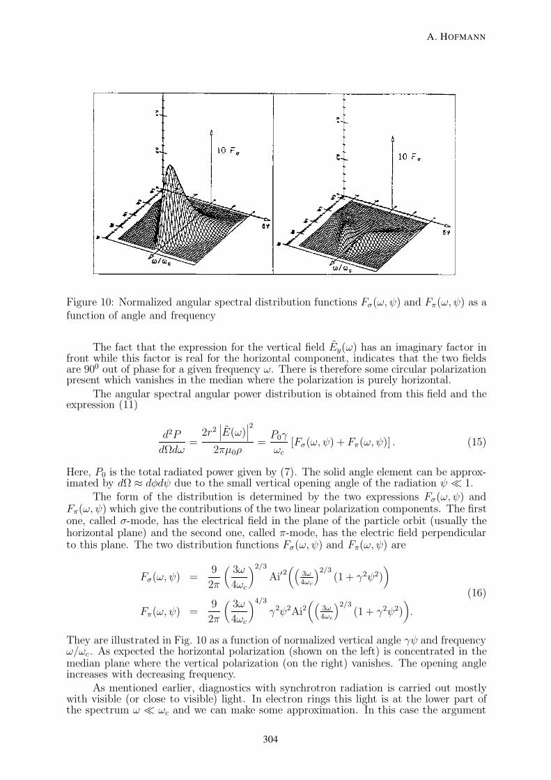
Figure 10: Normalized angular spectral distribution functions Fσ(ω, ψ) and Fπ(ω, ψ) as afunction of angle and frequency

The fact that the expression for the vertical field Ey(ω) has an imaginary factor infront while this factor is real for the horizontal component, indicates that the two fieldsare 900 out of phase for a given frequency ω. There is therefore some circular polarizationpresent which vanishes in the median where the polarization is purely horizontal.

The angular spectral angular power distribution is obtained from this field and theexpression (11)

d2P

dΩdω=

2r2∣∣∣E(ω)

∣∣∣2

2πµ0ρ=P0γ

ωc[Fσ(ω, ψ) + Fπ(ω, ψ)] . (15)

Here, P0 is the total radiated power given by (7). The solid angle element can be approx-imated by dΩ ≈ dφdψ due to the small vertical opening angle of the radiation ψ 1.

The form of the distribution is determined by the two expressions Fσ(ω, ψ) andFπ(ω, ψ) which give the contributions of the two linear polarization components. The firstone, called σ-mode, has the electrical field in the plane of the particle orbit (usually thehorizontal plane) and the second one, called π-mode, has the electric field perpendicularto this plane. The two distribution functions Fσ(ω, ψ) and Fπ(ω, ψ) are

Fσ(ω, ψ) =9

2π

(3ω

4ωc

)2/3

Ai′2((

3ω4ωc

)2/3(1 + γ2ψ2)

)

(16)

Fπ(ω, ψ) =9

2π

(3ω

4ωc

)4/3

γ2ψ2Ai2((

3ω4ωc

)2/3(1 + γ2ψ2)

).

They are illustrated in Fig. 10 as a function of normalized vertical angle γψ and frequencyω/ωc . As expected the horizontal polarization (shown on the left) is concentrated in themedian plane where the vertical polarization (on the right) vanishes. The opening angleincreases with decreasing frequency.

As mentioned earlier, diagnostics with synchrotron radiation is carried out mostlywith visible (or close to visible) light. In electron rings this light is at the lower part ofthe spectrum ω ωc and we can make some approximation. In this case the argument

A. HOFMANN

304

0 1 20.00

0.02

0.04

0.06

0.08

0.10

...................................................................................................................................................................................................................................................................................................................................................................................................................................................................................................................................................................................................................................................................................................................................................................................................................................................................................................... ......................

...........

...........

.................................

...........

...........

.................................

...........

...........

...................... ........... ...........

......................

......................

......................

......................

......................

......................

...................... ........... ........... ........... ........... ........... ........... ........... ........... .

.........................

..............

.............

.............

.............

.............

.............

.............

............. ..........................

.............

.............

.............

.............

.............

.............

.............

.............

.............

.............

.............

.............

.............

.............

.............

.............

.............

.............

..........................

.......................... ............. ............. ............. ......

F

F

F

(3!=4!c)1=3 = (!=2c)1=3

F (2=9)(4!c=3!)1=3

Figure 11: Vertical distribution of synchrotron radiation at low frequencies ω ωc

of the Airy function or its derivative in (13) is small except if γ2ψ2 becomes very large.Therefore, we make a small error by replacing (1 + γ2ψ2) by γ2ψ2 inside the argument ofthe Airy functions. Using the expression (14) for the critical frequency we get then forthe argument of the Airy functions

(3ω

4ωc

)2/3

(1 + γ2ψ2) ≈(

3ω

4ωc

)2/3

γ2ψ2 =(ωρ

2c

)2/3

ψ2.

With this we get for the electric field (13) and spectral angular distribution (15) at smallfrequencies ω ωc

E(ω) =e√

2πε0cr

(ωρ

2c

)1/3[Ai′((

ρω2c

) 23 ψ2

), i(ωρ

2c

)1/3

ψAi((

ρω2c

) 23 ψ2

)](17)

and

d2P

dΩdω=

2r0m0c2

πρ

[(ρω

2c

)23

Ai′2((

ρω2c

) 23 ψ2

)+ ψ2

(ρω

2c

) 43

Ai2((

ρω2c

) 23 ψ2

)]. (18)

It is interesting to note that these expressions do not depend on γ. At low frequencies theproperties of synchrotron radiation are independent of the particle energy and dependonly on the radius ρ of curvature. This fact is important for diagnostics applicationswhich usually uses the lower part of the spectrum. The angular power distribution forthis case is plotted in Fig. 11.

The RMS opening angle of synchrotron radiation can be calculated [1] which givesfor the low frequency part of the spectrum ω ωc

ψσ−RMS ∼

√√√√ 5

12

Ai(0)

−Ai′(0)

(c

ρω

)1/3

= 0.4097

(λ

ρ

)1/3

ψπ−RMS ∼

√√√√ 9

12

Ai(0)

−Ai′(0)

(c

ρω

)1/3

= 0.5497

(λ

ρ

)1/3

(19)

ψRMS ∼

√√√√ 6

12

Ai(0)

−Ai′(0)

(c

ρω

)1/3

= 0.4488

(λ

ρ

)1/3

.

4.2 Undulator radiation

An undulator is a spatially periodic magnetic structure designed to produce quasi-monochromatic radiation from relativistic particles. We consider here a plane harmonic

DIAGNOSTICS WITH SYNCHROTRON RADIATION

305

.............

.............

.............

.............

.............

.............

.............

.............

.............

.............

.............

.....................................................................................................................................................................................................................................................................................................................................................................................................................................................................................................................................................................................................................................

..

..

..

..

..

..

..

..

..

..

..

..

..

..

..

..

..

..

..

..

..

..

..

..

..

..

..

..

..

..

..

..

..

..

..

..

..

..

..

..

..

..

..

..

..

..

..

..

..

..

..

..

..

..

..

..

.................

...............

.................................................................................................................................

...............x

y

z

.......................................................................................................................................................................................................................................................................................................................................................................................................................................................................................................................................................................................................................................................................................................................................................................................................................................................................................................................................................

e

observer

..

..

..........................................................................................

....................................................

........................................................

........................................................................................................................................................................................................................................................................................................................................................................................................................................................................................... ...............

r

rp

0..........................................................

.....................

......................

......................

......................

......................

......................

......................

......................

......................

......................

......................

......................

......................

................................. ...........

.............

.............

.......

.............

.............

.......

.....................................................................................................................................................................

.....................................................................................................................................................................

u

........ ........ ........ ........ ........ ........ ........ ........ ........

................................................................

0

Figure 12: Geometry of undulator radiation

undulator with period length λu, Fig. 12. It has in the median plane (y = 0) a magneticfield of the form

B(z) = By(z) = B0 cos(kuz)

with the wave number ku = 2π/λu. If the field is not too strong the trajectory of a particlegoing along the axis is of the form

x(z) = a cos(kuz) , a =eB0

m0cγk2u

anddx

dz= −ψ0 sin(kuz) , ψ0 =

eB0

m0cγku=K

γ.

Here, we introduced the undulator parameter

K =eB0

m0cku= γψ0

which gives the ratio between the maximum deflecting angle ψ0 and the natural openingangle of the radiation 1/γ. For the case K < 1 the emitted light is deflected by angleψ0 smaller than the natural opening angle. An observer will receive a weakly modulatedfield which is quasi-monochromatic. However, for K > 1 the deflection is larger than thenatural opening angle and the observer will receive strongly modulated light containingharmonics of the basic modulation frequency.

The Fourier transformed electric field of the undulator radiation has been derived[1] to be

E(ω) =4r0cB0γ

3

√2πrp

[1 − γ2θ2 cos(2φ), γ2θ2 sin(2φ)]

(1 + γ2θ2)3

πNu

ω1

sin(

(ω−ω1)πNu

ω1

)

(ω−ω1)πNu

ω1

(20)

were we assume that the undulator has many periods Nu 1 and introduced the fre-quency

ω1 = kuc2γ2

1 + γ2θ2=

ω10

1 + γ2θ2.

The angular spectral power distribution of a weak undulator is obtained from theabove field

d2PudΩdω

= Puγ2 (Fuσ(θ, φ) + Fuπ(θ, φ))fN (∆ω),

A. HOFMANN

306

Figure 13: Normalized angular power distribution of undulator radiation; left: horizontal,right: vertical polarization

where Pu is the total radiated power and the two function Fuσ and Fuσ determine thecontributions of the two polarization modes

Fuσ(θ, φ) =3

π

(1 − γ2θ2 cos(2φ))2

(1 + γ2θ2)5 , Fuφ(θ, φ) =

3

π

(γ2θ2 sin(2φ))2

(1 + γ2θ2)5 .

They are shown in Fig. 13 which clearly illustrates that the horizontal polarization (onthe left) is concentrated in the forward direction while the vertical one (on the right)vanishes on the axis itself as well as in the horizontal and vertical plane.

The function fN (∆ω) gives the spectral distribution at a given angle θ which dependson the number Nu of undulator periods

fN(∆ω) =Nu

ω1

sin(

∆ωπNu

ω1

)

∆ωπNu

ω1

2

with ∆ω = ω − ω1.

This function is normalized and approaches the Dirac delta function for a large numberNu of periods

∫ ∞

−∞fN (∆ω)dω = 1 , fN (∆ω) → δ(∆ω) for Nu → ∞.

In this latter case the radiation is monochromatic at each observation angle θ with thefrequency ω1.

4.3 Generalized undulators – weak magnets

We consider now a magnet which is sufficiently short and weak that the deflectionit produces for the beam stays within an angle smaller than 1/γ. We assume that theparticle trajectory lies in the x, z-plane and follows closely the z-axis and give the magneticfield in the form

By = By(z).

DIAGNOSTICS WITH SYNCHROTRON RADIATION

307

Within this approximation and using the geometry shown in Fig. 12 the particle trajectoryis determined by

1

ρ=

eBc

m0c2γ≈ −

1

c2d2x

dt′2= −

β

c.

It can be regarded as a weak undulator with a generalized field By(z) having a Fouriertransform

B(ksm) =1√2π

∫ ∞

−∞By(z)e

−iksmzdz.

The radiation observed at frequency ω and angle θ is determined by the Fourier componentB(ksm) of the magnetic field. We get for the radiation in frequency domain [3]

E(ω) =2r0γ

rp

[1 − γ2θ2 cos(2φ), γ2θ2 sin(2φ)]

(1 + γ2θ2)2By(ksm) (21)

=2r0γ

rp

[1 − γ2θ2 cos(2φ), γ2θ2 sin(2φ)]

(1 + γ2θ2)2B

(1 + γ2θ2

2cγ2ω

)

and the angular spectral energy distribution is obtained from the relation

dW 2

dΩdω=

2r2p|E(ω)|2

µ0c

giving

d2W

dΩdω=

2r0ce2(m0c

2γ)2

π(m0c2)3

[(1 − γ2θ2 cos(2φ))2 + (γ2θ2 sin(2φ))2]

(1 + γ2θ2)4(22)

∣∣∣∣∣B(

1 + γ2θ2

2cγ2ω

)∣∣∣∣∣

2

.

This expression gives the radiation from a general magnet provided that the deflection isweak and nowhere exceeds an angle of 1/γ.

A special case of a short magnet is an undulator having a harmonic field which ismodulated by a Lorentz function

B(z) = B0cos(kuz)

1 + (z/z0)2=K0m0cku

e

cos(kuz)

1 + (z/z0)2.

For the case of many periods Nu within its characteristic length 2z0 the total energyradiated by an electron is

Wu =πr0(m0c

2γ)2K20k

2uz0

6m0c2.

We treat this undulator as a short magnet and filter out the frequency component ω10

from the radiationω = ω10 = kuc2γ

2

which is given by the spacial Fourier component at

ksm = ω10

1 + γ2θ2

2γ2= ku(1 + γ2θ2).

Using (21) we get for the radiation field

E(ω) =

√2πr0m0c

2γK0kuz0rpec

[1, 0]e−πNuγ2θ2 (23)

A. HOFMANN

308

where we are left with the horizontal polarization mode only. From (10) we obtain emittedangular spectral energy distribution

d2Wu

dΩdω= Wu

6z0π

e−2πNuγ2θ2 . (24)

The radiation from this Lorentz modulated undulator, filtered at ω10, has a Gaussianangular energy distribution with RMS values for the polar angle θ and the two Cartesianangles x′ and y′

θRMS =1

γ√

2πNu

, x′RMS = y′RMS =1

2γ√πNu

.

5 IMAGING WITH SR — QUALITATIVE TREATMENT

5.1 Diffraction of radiation emitted in long magnets

We use synchrotron radiation from a long magnet to form an image of the beam crosssection with an arrangement shown in Fig. 14. For simplicity a single lens is consideredto form a 1:1 image. This is no restriction since we could also use a magnification andthen project the image back to the source to get the resolution in terms of beam size.Since the vertical opening angle of the radiation σ′γ is small, only the central part of thelens is illuminated. The situation is therefore similar to optical imaging with a limitedlens aperture. This case is known to lead to a limitation of the resolution by diffraction[4]

d ≈ λ

2D/R, (25)

where d is the half size of an image from a point source and D is the full lens aperture.For synchrotron radiation observed at the low frequency part of the spectrum we foundfor the horizontal polarization an RMS opening angle (19) which is

σ′γ = ψσ−RMS ≈ 0.41(λ/ρ)1/3

for the σ-mode. Relating this to (25) we take D ≈ 4σγR since the lens represents the fullaperture which we approximate with ±2ψσ−RMS to get

d ≈ 0.3(λ2ρ)1/3.

We find that the resolution improves with shorter wavelength and with smaller radiusof curvature. Due to the latter dependence synchrotron radiation monitors have a poorresolution in large machines as indicated in the examples shown in Table 1. A wavelengthas short as possible can help to improve the resolution. Special magnets with strongcurvature could help to improve the resolution but the weak dependence on ρ makes thisapproach not very attractive.

Diffraction represents often a serious limitation of the resolution for large machines.It is caused by the small opening angle of synchrotron radiation. Sometimes the questionarises if a large angular spread of the particles in the beam helps the resolution since alarger part of the lens is now illuminated. This is not the case since the diffraction resultsin a finite size image of each particle. The radiation originating from different particleshas no phase relation and does not produce the corresponding diffraction pattern.

5.2 Depth of field effect for the radiation emitted in long magnets

We consider now the effect of the depth of field on the resolution of an image of thebeam cross section. The situation is illustrated in Fig. 15. We discussed at the beginningthe length of orbit from which radiation can be received by an observer, Fig. 5. There, we

DIAGNOSTICS WITH SYNCHROTRON RADIATION

309

............. ............. ............. ............. ............. ............. ............. ............. ............. ............. ............. ............. ............. ............. ............. ............. ............. ............. ............. ............. ............. ............. ............. ............. ............. ............. ............. ............. ............. ............. ............. ............. .............

.....................................................................................................................................................................................................................................................................................

........................................................................................................................................................................................................................................................................................................................................................................................................................................................................................................................................................................................................................................................................

...............

...................................................................................................................................................................................................................................................................................................................................................................................

...............

...................................................................................................................................................................................................................................................................................................................................................................................

...............

...................................................................................................................................................................................................................................................................................................................................................................................

...............

..

..

..

..

..

..

..

................

...............

........................................................................................................................................................................................................................................................................................................................................................................................................................................................................................................................................................................................................................................................................................................................................................................................................................................................................................................................................................................................................................................................................................................................................................................................................................................................................................................................................................................................................................................................................................................................................................

.......................................................................................

..

..

..

..

..

..

.

..

..

..

..

..

..

.

..

..

..

..

..

..

.

..

..

..

..

..

..

.

..

..

..

..

..

..

.

..

..

..

..

..

..

.

..

..

..

..

..

..

.

..

..

..

..

..

..

.

..

..

..

..

..

..

.

..

..

..

..

..

..

.

..

..

..

..

..

..

.

..

..

..

..

..

..

..

..

..

..

..

..

..

..

..

..

..

..

..

..

..

..

..

..

..

..

..

..

..

..

..

..

..

..

..

..

..

..

..

..

..

..

..

..

..

..

..

..

..

..

..

..

..

..

..

..

..

..

..

..

..

..

..

..

..

..

..

..

..

..

..

..

..

..

..

..

..

..

..

..

..

..

..

..

..

..

..

..

..

..

..

..

..

..

..

..

..

..

..

..

..

..

..

..

..

..

..

..

..

..

..

..

..

..

..

..

..

..

.................

...............

......................................................................................................................................................................................................................................

..

..

..

..

..

..

.

..

..

..

..

..

..

..

.

..

..

..

..

..

..

..

..

..

..

..

..

..

..

..

..

..

..

..

..

..

..

..

..

..

..

..

..

..

..

..

..

..

..

..

..

..

..

..

..

..

..

..

..

................

...............

........................................................................................................

...............

........................................................................................................................................................................................................

..

..

..

..

..

..

..

..

..

..

..

..

..

..

..

..

..

..

..

..

..

..

..

..

..

..

..

..

..

..

..

..

..

..

..

..

..

..

..

..

..

..

..

..

..

..

..

..

..

..

..

..

..

..

..

..

..

..

..

..

..

..

..

..

..

..

..

..

..

..

..

..

..

..

..

..

..

..

.

............. ............. .............

............. ............. .............

y

P (y)

lens

e

0

R R

D

diractionpattern

Figure 14: Imaging the beam cross section with synchrotron radiation

machine ρ λ σ′γ dm nm m rad mm

EPA (CERN) 1.43 400 2.7 0.018LEP (CERN) 3096 400 0.21 0.24

Table 1: Resolution for imaging with synchrotron radiation in different machines

assumed an opening angle of ±1/γ for the radiation. In forming the image of the beamwe use σ-mode of the low frequency part of the spectrum for which the opening angle isσ′γ ≈ 0.41(λ/ρ)1/3. The part of the orbit from which radiation of wavelength λ can reachthe observer has therefore a length of about ±2σ′γρ. We consider now three points A, Band C along this orbit where B is located at the nominal distance R = 2f from the lenshaving a focal length f and the other points deviate by ±2σ′γρ from it. For a 1:1 imageand assuming σγρ R we find that the images A′ and C ′ have also about the spacing±2σ′γ from the central image B ′. At this central point the radiation from A and B hasan extension

d ≈ σ′γ2ρ = 0.34(λ2ρ)1/3.

It is interesting that the resolution limitation due to the depth of field effect has the sameparameter dependence as the one caused by diffraction.

............. ............. ............. ............. ............. ............. ............. ............. ............. ............. ............. ............. ............. ............. ............. ............. ............. ............. ............. ............. ............. ............. ............. ............. ............. ............. ............. ............. ............. ............. ............. ............. ............. ............. ............. ............. ............. ............. ............. .............

.....................................................................................................................................................................................................................................................................................

........................................................................................................................................................................................................................................................................................................................................................................................................................................................................................................................................................................................................................................................................

...............

...................................................................................................................................................................................................................................................................................................................................................................................

...............

...................................................................................................................................................................................................................................................................................................................................................................................

...............

...................................................................................................................................................................................................................................................................................................................................................................................

...............

.................

...............

A A0B B0C C 0

........................................................................................................................................................................................................

...............

........................................................................................................................................................................................................ ...............

.................................................................................................................................................................................................................................................................................................................................................................................................................................................................................................................................................................................................................................................................................................................................................................................................................................................................................................................................................................................................................................................................................................................................................................................................................................................................................................................................................................................................................................................................................................................................... .....

...........................................................................................................................................................

................

................

................

................

................

................

................

................

................

................

................

................

................

................

................

................

................

................

................

................

................

................

.

........ ................ ........ ........................................................................

........................................................................................................................

................................................................

.........

................

................

................

................

................

................

................

................

................

................

................

................

................

................

................

................

................

................

................

................

................

................

................

................

................

................

................

................

................

................

................

................

................

................

................

................

................

................

................

................

................

................

................

................

................

................

................

................

................

................

................

................

................

................

................

................

................

............

.

.

.

.

.

.

.........................................................

..

..

..

..

..

..

.

..

..

..

..

..

..

.

..

..

..

..

..

..

.

..

..

..

..

..

..

.

..

..

..

..

..

..

.

..

..

..

..

..

..

.

..

..

..

..

..

..

.

..

..

..

..

..

..

.

..

..

..

..

..

..

.

..

..

..

..

..

..

.

..

..

..

..

..

..

.

..

..

..

..

..

..

.

..

..

..

..

..

..

.

..

..

..

..

..

..

..

..

..

.........

........

.......................................................................................

...............

.......................................................................................

...............

.......................................................................................

...............

.......................................................................................

...............

20

20

d

lens

e 0

R R

Figure 15: Depth of field effect

A. HOFMANN

310

5.3 Diffraction and depth of field effect for undulator radiation

We derived the radiation from a weak undulator in frequency domain (20)

E(ω) =4r0cB0γ

3

√2πrp

(1 − γ2θ2 cos(2φ), γ2θ2 sin(2φ))

(1 + γ2θ2)3

πNu

ω1

sin(

(ω−ω1)πNu

ω1

)

(ω−ω1)πNu

ω1

.

with

ω1 =ω10

1 + γ2θ2=

2γ2kuc

1 + γ2θ2.

We filter now the frequency ω = ω10 to use it for imaging the beam and get for the spectralfunction

πNu

ω1

sin(

(ω−ω1)πNu

ω1

)

(ω−ω1)πNu

ω1

=πNu(1 + γ2θ2)

ω10

sin(γ2θ2πNu)

γ2θ2πNu.

This equation contains the function sin x/x which has a maximum value of unity at x = 0and is small for large values of x. It has a first zero at x = π which corresponds to theangle

θzero =1

γ√Nu

. (26)

We assume now an undulator with many periods Nu 1 for which the radiation atω = ω10 is concentrated within an angle much smaller than 1/γ. We can then approximatein (20) for 1 + γ2θ2 ≈ 1 and get a radiation field containing only an x-component

Ex(ω10) ≈4r0cB0γ

3

√2πrp

πNu

ω10

sin(γ2θ2πNu)

γ2θ2πNu

(27)

From this we obtain the angular spectral power distribution for which we make an expo-nential approximation for reasons explained below

d2P (ω10)

dΩdω≈ Puγ

2 3

π

Nu

ω10

(sin(γ2θ2πNu)

γ2θ2πNu

)2

≈ Puγ2 3

π

Nu

ω10

e−(πNuγ2θ2)2/3. (28)

which is plotted in Fig. 16.For the evaluation of the diffraction we would like to use the RMS width of this

angular power distribution. However, the variance of function (sinx/x)2 diverges. Thisis due to the unphysical undulator field which is harmonic within ±Lu/2 but vanishesabruptly outside this range. This produces high frequency tails which appear also atrelatively large angles θ. To still get an estimate for the resolution limitation by diffractionwe use the variance of the exponential fit to get the RMS-value

σ′γ ≈4√

3π

πγ√Nu

= 0.561√Nu

.

With this we get the approximate size of the diffraction spot form (25)

d ≈ λ10

2D/R≈ λ10

4σ′γ≈ 0.45γλ10

√Nu , σγ ≈ d

2≈ 0.27λ10

√Nu = 0.19

√λ10Lu.

Since the resolution is proportional to√Lu one would like to work with a short undulator.

However, we obtained the above expression with the assumption Nu 1. A more detailed

DIAGNOSTICS WITH SYNCHROTRON RADIATION

311

0 1 2 30.0

0.2

0.4

0.6

0.8

1.0 .................................................................................................................................................................................................................................................................................................................................................................................................................................................................................................................................................................................................................................................................................................................................................................................................................................................

............................

.........................................................................

............. ............. ............. ..........................

.............

.............

.............

.............

.............

.............

.............

.............

.............

.............

.............

.............

.............

.............

.............

.............

.............

.............

.............

.............

.............

.......................... ............. .........

d2P (; !10)

dd!

pNu

exp(( 22Nu)2=3)

Figure 16: Angular power distribution of undulator radiation at ω10

calculation is necessary to treat the more general case of an undulator having few periodsor of a short magnet.

We can also investigate the depth of field effect by replacing the source length 2σ′γρby the undulator length Lu and σ′γ by θzero in Fig. 15

d ≈ θzeroLuLu

=

√λ10Lu√

2.

Again, diffraction and depth of field effect have the same parameter dependence and areof similar magnitude.

5.4 Resolution for imaging with short magnet radiation

We treated the radiation from short magnets before and obtained the angular spec-tral power distribution (22) for a general, but weak field B(z). Without knowing thedetails of this field we can estimate the opening angle of the radiation from the lengthLsm of the source. Considering two points, one at the beginning and one at the end ofthe short magnet, emitting radiation with the wavelength λ for which we get positiveinterference in the forward direction

λ

c=Lsmβc

− Lsmc

=Lsmβc

(1 − β) ≈ Lsm2cγ2

,

or

λ =Lsm2γ2

.

We look now for the angle θ for which we get destructive interference

3λ

2c=Lsmβc

− Lsm cos θ

c=Lsmβc

(1 − β cos θ) ≈ Lsm(1 + γ2θ2)

2cγ2,

A. HOFMANN

312

or

1 + γ2θ2 =3

2→ θ =

1√2γ.

The radiation emitted at wavelength λ has a first minimum at the above angle. Of coursethis is a rough estimate since we should also take the radiation emitted in between theend point of the magnet into account. Using this angle σ′γ = 1/(

√2γ) we get for the

resolution

d ≈ λ

2D/R≈

√2λγ

2=

1

2

√λLsm.

Using this very general argument we find a similar resolution to the one obtained for anundulator.

6 IMAGING WITH SR — FRAUNHOFER APPROXIMATION

6.1 Fraunhofer diffraction

We treat now the diffraction in a more quantitative way and consider an imageformed with synchrotron radiation as illustrated in Fig. 17. We form a 1:1 image witha single lens at a distance R from the source. The emitted Fourier transformed fieldcomponents have a horizontal and vertical angular distribution of the form

Ex = Ex(x′γ , y

′γ) , Ey = Ey(x

′γ , y

′γ).

At the lens this is converted into a spacial distribution

Ex(x, y) = Ex(Rx′γ , Ry

′γ) , Ey(x, y) = Ex(Rx

′γ , Ry

′γ).

The point source in the figure is imaged on to the image point at a distance R from thelens. In this case all rays between source and image points have the same optical length.The dashed circular arc with radius R around the image point, shown in the figure,represents therefore a cut through an equi-phase surface. Using Huygens’s principle weconsider each point on this surface as a source of a radiation field of strength proportionalto (Ex(x, y), Ey(x, y)). We restrict ourselves to a scalar field E which can stand for eitherthe horizontal or vertical field components. From this secondary source point (x, y, z) thisfield propagates towards the image plane (X, Y ) in the form of a wave

δE(X, Y ) ∝ E(x, y)e(kr−ωt), (29)

where k = 2π/λ is the wave number of the radiation and r the distance between thesecondary source and the observation point in the image plane

r2 = (R− z)2 + (x −X)2 + (y − Y )2.

On the equi-phase surface we have (R− z)2 = R2 − (x2 + y2) which gives

r =√R2 − 2xX − 2yY + X2 + Y 2 ≈ R

(1 + −

xX

R2−yY

R2+X2

R2+Y 2

R2...

).

The small opening angle of synchrotron radiation and the limited extension of the imagepermit to use an approximation and we neglect from now on higher order terms in (X/R)and (Y/R).

We get the field in the image plane by integrating the contribution (29) from eachsurface element of the secondary source

E(X, Y ) ∝ e−iωt∫ ∞

−∞

∫ ∞

−∞E(x, y)ei(kR−kxX

R −kyYR )dxdy.

DIAGNOSTICS WITH SYNCHROTRON RADIATION

313

............. ............. ............. ............. ............. ............. ............. ............. ............. ............. ............. ............. ............. ............. ............. ............. ............. ............. ............. ............. ............. ............. ............. ............. ............. ............. ............. ............. ............. ............. ............. ............. ............. ............. ............. ..

...........................................................................................................................................................................................................................................................................................................

.....................................................................................................................................................................................................................................................................................................................................................................................................................................................................................................................................................................................................................................................................................................................................................

...............

..............................................................................................................................................................................................................................................................................................................................................................................................................................

...............

..............................................................................................................................................................................................................................................................................................................................................................................................................................

...............

..............................................................................................................................................................................................................................................................................................................................................................................................................................

...............

............................................................................................................................................................................................................................................................................................................................................................................................................................................................................................................................................................................................................................................................................................................................................................................................................................................................................................................................................................................................................................................................................................................................................................................................................................................................................................................................................................................................................................................................................................................................................................................................................................................................................................................................................

.................

............

.................

............

...........

............

...........

............

.................

............

...........

............

...........

............

...........

............

.................

............

...........

............

...........

............

.................

............

...........

............

...........

............

.................

............

...........

............

..................................................................................................................................................................................................................................................................................................................................................................................................................................................

......................................................................................................................................................................................................................................................................................................................................................................................................................................................................................................................................................................................................................................................................................................................................................................................................................................................................

..................................................................................................

..

..

..

..

..

..

..

..

................

...............

..

..

..

..

..

..

..

..

..

..

..

..

..

..

..

..

..

..

..

..

..

..

..

..

..

..

..

..

..

..

..

..

..

..

..

..

..

..

..

..

..

..

..

..

..

..

..

..

..

..

..

..

..

..

..

..

..

..

..

..

..

..

..

..

..

..

..

..

..

..

..

..

..

..

..

..

..

..

..

.................

...............

x

..

..

..

..

..

..

..

..

..

..

..

..

..

..

..

..

..

..

..

..

..

..

..

..

..

..

..

..

..

..

..

..

..

..

..

..

..

..

..

..

..

..

..

..

..

..

..

..

..

.................

...............

...........................................................................................................................................................

...............

...............................................................................................................................................................................................................................................................

..

..

..

..

..

..

..

..

..

..

..

..

..

..

..

..

..

..

..

..

..

..

..

..

..

..

..

..

..

..

..

..

..

..

..

..

..

..

..

..

..

..

..

..

..

..

..

..

..

..

..

..

..

..

..

..

..

..

..

..

..

..

..

..

..

..

..

..

..

..

..

..

..

..

..

..

..

..

..

..

..

..

..

..

..

..

..

.. X

E(X)

lens

pointsource

0

x

R R

E(x)

diraction

pattern

.........................................................................................................................................................................................................................

..........................................................................................................................................................................................................................................................................................................................

........

........

........

........

........

........

........

........

........

........

........

..

..

..

..

..

..

..

..

..

..

..

..

..

..

..

..

..

..

..

..

..

..

..

..

..

..

..

..

..

..

..

..

..

..

..

..

..

..

..

..

..

..

..

..

..

..

..

..

..

..

..

..

r

equi-phase

Figure 17: Diffraction in imaging with synchrotron radiation

We omit the oscillatory term as well as fixed phase term exp (ikR) which are both of nointerest and replace the coordinates (x, y) at the lens by the angles (x′, y′) at which theradiation is emitted

E(X, Y ) ∝∫ ∞

−∞

∫ ∞

−∞E(x, y)e−i(x

′kX+y′kY )dx′dy′. (30)

This integral represents a Fourier transform. In other words, the field distribution E(X, Y )in the image plane is just proportional to the two dimensional Fourier transform of thefield distribution at the lens, or of the angular distribution of the emitted radiation

E(kX, kY ) ∝ FE(x′, y′).

Instead of the source angles x′ and y′ we can use a spherical coordinate system(R, φ, θ) having the origin at the source and the relations

x = R sin θ cos φ ≈ Rθ cos φ; , y = R sin θ sinφ ≈ Rθ sin φ.

We also express the image coordinates X, Y by polar coordinates (RΦ) with the relations

X = R cosΦ , Y = R sinΦ

and get

E(R,Φ) ∝∫ ∞

−∞

∫ 2π

0E(θ, φ)e−ikθRcos(φ−Φ)θdθdφ.

In some cases the emitted radiation is independent of the azimuthal angle φ whichleads also to the same symmetry for the diffraction pattern at the image plane. Theintegration over φ becomes

E(Θ,Φ) ∝∫ ∞

−∞

∫ 2π

0E(R)e−ikθRcos(φ−Φ)θdθdφ = 2π

∫ ∞

0E(R)J0(kRθ)θdθ (31)

where we used the integral representation of the Bessel function

J0(z) =1

π

∫ π

0eiz cos ξdξ.

In all these calculations of the diffraction we assumed a point source located at thedistance R from the lens. This is an approximation for the case of synchrotron radiation.In the treatment of the depth of field we said that the length of the source is ±2σ′γρ

A. HOFMANN

314

and used for the RMS opening angle σ′γ ≈ 0.41(λ/ρ). If we take the finite longitudinalextension of the source into account the sphere of radius R around the image centeris no longer an equi-phase surface. The calculation becomes more complicated and theexponent in the integral (30) will contain quadratic terms of coordinates x and y at thelens. This leads to the case of Fresnel diffraction which is not covered here but can befound in more profound treatments [5, 6]. Since we found before that the depth of fieldeffect is of the same order as the diffraction we expect the improved treatment to makea sizable correction. However, we will in the following still use the Fraunhofer diffractionto illustrate some of the underlying physics.

6.2 Diffraction of synchrotron radiation emitted in long magnets

We use here synchrotron radiation from a long magnet to image the cross sectionof the beam. The radiation depends only on the vertical emission angle y′ which wecalled y′ = ψ before. The Fourier transformed electric field in the approximation of smallfrequencies ω ωc is

E(ψ, λ) =e√

2ε0cr

(πρ

λ

) 13

(Ai′

(ψ2(πρ

λ

)23

), ψ

(πρ

λ

) 13

Ai

(ψ2(πρ

λ

) 23

)).

The corresponding power distribution is proportional to the square of this field and isplotted in Fig. 18. To get the image given by Fraunhofer diffraction we have to use theexpression (30). The field distribution in the horizontal direction is uniform by natureand will be terminated by some aperture limitation due to a slit or lens size. Since thisaperture will determine the horizontal diffraction one does not want to make it too small.On the other hand, by making it too large we will increase the depth of field effect. Asa compromise one makes the horizontal angular acceptance comparable to the naturalvertical distribution. Considering that the horizontal limitation has a sharp edge a valueof the order |x′| ≤ 2σ′γ is a reasonable compromise. We restrict ourselves here to thevertical resolution and integrate (30) only over the vertical coordinate and get for thecorresponding distribution of the image field

E(Y, λ) ∝∫ ∞

−∞E(ψ, λ)e−i(ψkY )dψ.

This integration has to be done numerically. The corresponding image power is propor-tional to |E(Y, λ)|2 and is plotted in Fig. 19 for the horizontal and vertical polarizationas well as for the total radiation. The RMS values of the image power are

σY,σ = 0.206(λ2ρ)1/3 , σY,π(λ2ρ)1/3 , σY,total = 0.279(λ2ρ)1/3. (32)

From the figure it is evident that the image is narrowest for the σ-mode of the radiation.Using a horizontal polarizing filter will therefore improve the resolution of the image byabout 25%.

6.3 Diffraction for the undulator having a Gaussian angular distribution

We discussed an undulator with a Lorentz modulation having a magnetic field ofthe form

B(z) = B0

cos(kuz)

1 + (z/z0)2

giving a radiation field at the frequency ω10 which has for a large number of periods onlyan x-component (23)

Ex(ω10) =

√2πr0m0c

2γK0kuz0rpec

e−πNuγ2θ2

DIAGNOSTICS WITH SYNCHROTRON RADIATION

315

0.0 0.2 0.4 0.6 0.8 1.0 1.2 1.4

0.0

0.2

0.4

0.6

0.8

1.0

1.2

1.4

..................................................................................................................................................................................................................................................................................................................................................................................................................................................................................................................................................................................................................................................................................................................................................................................................................................................................................................................................................................................................................................................................................................................................................................................................................................................................................................................................................................................................................................................................................................................................................................................................................................................................................................................................

................

................

........

........

........

........

........

........

........

........

........

................ ........

........

........

........

........

........

........

........

........

........

........

........

........

........

........

........

........

........

........

........

........

........

........

........

........

........

........

........

........

........

........

........

........

........

........

........

................

................

........ ........ ........ ........ ........ ........ ........ ........ ........ ........ .........

..

..

..

..

..

..

..

..

..

..

..

..

..

..

..

..

..

..

..

..

..

..

..

..

..

..

..

..

..

..

..

..

..

..

..

..

..

..

..

..

..

..

..

..

..

..

..

..

..

..

..

..

..

..

..

..

..

..

..

..

..

..

..

..

..

..

..

..

..

..

..

..

..

..

..

..

..

..

..

..

..

..

..

..

..

..

..

..

..

..

..

..

..

..

..

..

..

..

..

..

..

..

..

..

..

..

..

..

..

..

..

..

..

..

..

..

..

..

..

..

..

..

..

..

..

..

..

..

..

..

..

..

..

..

..

..

..

..

..

..

..

..

..

..

..

..

..

..

..

..

..

..

..

..

..

..

..

..

..

..

..

..

..

..

..

..

..

..

..

..

..

..

..

..

..

..

..

..

..

..

..

..

..

..

..

..

..

..

..

..

..

..

..

..

..

..

..

..

..

..

..

..

..

..

..

..

..

..

..

..

..

..

..

..

..

..

..

..

..

..

..

..

..

..

..

..

..

..

..

..

..

..

..

..

..

..

..

..

..

..

..

..

..

.............................................................................................................................................................................................................................

...............

.........................................................................................................................................................................................................................................................................................................

...........

....

..................................................................................................................................................................................................................................................

...............

total

rms-

rms-

rms-total

d2P

dd!

1=3

Figure 18: Vertical distribution of synchrotron radiation from long magnets

0.0 0.2 0.4 0.6 0.8 1.00.0

0.2

0.4

0.6

0.8

1.0 ................................................................................................................................................................................................................................................................................................................................................................................................................................................................................................................................................................................................................................................................................................................ ..................................................................................................................

...................................................................................................................................

..................................................................................................................................................................................................................................................................

......................................................................................................................................................................................................................................................................................................................................................................................................................................................................................

........ ................

........

........

........

........

........

........

........

........

........

........

........

........

........

........

........

........

........

........

........

........

........

........

........

........

........

........

........

........

........

........

........

........

........

........

........

........

........

................

................

................

................

........ ........ ........ ........ ........ ........ ........ ........ ........ ........ ........ .............

..

..

..

..

..

..

..

..

..

..

..

..

..

..

..

..

..

..

..

..

..

..

..

..

..

..

..

..

..

..

..

..

..

..

..

..

..

..

..

..

..

..

..

..

..

..

..

..

..

..

..

..

..

..

..

..

..

..

..

..

..

..

..

..

..

..

..

..

..

..

..

..

..

..

..

..

..

..

..

..

..

..

..

..

..

..

.

..

..

..

..

..

..

..

..

..

..

..

..

..

..

..

..

..

..

..

..

..

..

..

..

..

..

..

..

..

..

..

..

..

..

..

..

..

..

..

..

..

..

..

..

..

..

..

..

..

..

..

..

..

..

..

..

..

..

..

..

..

..

..

..

..

..

..

..

..

..

..

..

..

..

..

..

..

..

..

..

..

..

..

..

..

..

..

..

..

..

..

..

..

..

..

..

..

..

..

..

..

..

..

..

..

..

..

..

..

..

..

..

..................................................................................................................................................................

...............

.........................................................................................................................................................................................................................................................................................................................................

...............

......................................................................................................................................................................................................................

...............

total

rms-

rms-

rms-total

P (Y )

Y

(2)1=3

Figure 19: Fraunhofer diffraction for synchrotron radiation from long magnets

A. HOFMANN

316

and the emitted angular spectral energy distribution (24)

d2W

dΩdω= W0

6z0π

e−2πNuγ2θ2

with the RMS opening angle

θRMS =1

2γ√πNu

.

To calculate the diffraction for the field distribution we make use of its azimuthalsymmetry and use the relation (31)

E(R) ∝∫ ∞

0e−πNuγ2θ2J0(kRθ)θdθ =

1

πNuγ2e− k2R2

4γ2πNu .

The integral appearing above can be found in [7]. The energy distribution of the diffractionpattern has the form

dW

RdRdω (ω10) ∝ e− k2R2

2γ2πNu .

It is also Gaussian with an RMS width

σR =

√2πNuγλ

2π, σX = σY =

√πNuγλ

2π.

7 DIRECT OBSERVATION OF SR

Instead of forming an image of the beam cross section we can observe the synchrotronradiation directly and measure its angular distribution. This experiment can determinethe angular spread of the particles in the beam. The resolution is clearly limited by thenatural opening angles of the synchrotron light, as shown in Fig. 20. In order to correctfor this it is advantageous to use quasi-monochromatic light for which the distributionand the sensitivity of the detector is well known. The angular spread of the particles canthen be obtained by a deconvolution.

The angular spread and the dimension of the particle beam in a ring are related byan invariant emittance ε. It is defined as the RMS phase space area divided by π. Atlocations where the beam size has a maximum or minimum the emittance is simply givenby the product of RMS beam size and angular spread ε = σσ′ . At other locations thephase space area forms a tilted ellipse and the relation is more complicated and determinedby the local particle beam optics described by the lattice function β(s), α(s), γ(s) in thetwo planes. At the location of maximal or minimal beam size the ratio between size andangular spread is simply given by σ/σ′ = β. A convenient method has been developed [8]to use the lattice functions at the source to treat the photon beam distribution measuredon a screen at a distance s from the source. If the lattice functions are known at thesource s = 0 we can calculate their propagation in a drift space being free of focusingelements to get the values at a distance s

β(s) = β(0) − 2α(0)s + γ(0)s2.

Apart from the finite opening angle we can treat the synchrotron radiation emitted inthe forward direction like particles and describe their propagation by the same latticefunctions. We can therefore define a beta function for the photon beam at the screenβγ(R) = β(R). Neglecting the finite opening angle of the radiation the photon beam sizeσR on the screen is determined by the emittance of the electron beam ε and the betafunction β(R)

σε =√εβγ (R).

DIAGNOSTICS WITH SYNCHROTRON RADIATION

317

............. ............. ............. ............. ............. ............. ............. ............. ............. ............. ............. ............. ............. ............. ............. ............. ............. ............. ............. ............. ............. ............. ............. ............. ............. ............. ............. ............. ............. ............. ............. ............. .............

..

..

..

..

..

..

.

..

..

..

..

..

..

.

..

..

..

..

..

..

.

..

..

..

..

..

..

.

..

..

..

..

..

..

.

..

..

..

..

..

..

.

..

..

..

..

..

..

.

..

..

..

..

..

..

.

.......................................................................................................................................................................................................................................................................................................................................................................................................................................................................................................................................................................................................................................................................................................................................................

...........

....

................

................

................

................

................

................

................

................

................

................ ........

................

................

................

................

................

................

................

................

................

................

................ ........

................

................

..

..

..

..

........

........

................

................

................

................

................

................

................

................

................

................

................

................

................

................

................

................

................

................

................

................

................

................

................

................

........ ........ ........ ........ ........ ........ ........ ........ ........ ........ ........ ........ ........ ........ ........ ........ ........ ........ ........ ........ ........ ........ ........ ........ ........ ........ ........ ........ ........ ........ ........ ........ ........ ........ ........ ........ ........ ........ ........ ........ ........ ........ ........ ........ ........ ........ ........ ........ ........

........ ........ ........ ........ ........ ........ ........ ........ ........ ........ ........ ........ ........ ........ ........ ........ ........ ........ ........ ........ ........ ........ ........ ........ ........ ........ ........ ........ ........ ........ ........ ........ ........ ........ ........ ........ ........ ........ ........ ........ ........ ........ ........ ........ ........ ........ ........

......................

.........................

........................

........................

.........................

........................

........................

........................

.........................

........................

........................

........................

.........................

........................

........................

........................

.........................

........................

........................

........................

.........................

........................

........................

........................

.........................

........................

........................

........................

.........................

...............

.............................................................................................................................................................................................................................................................................................................................................................................................................................................................................................................................................................................................................................................................................................................................................

...........................................................................................................................................................................................................................................................................................................................................................................................................................................................................................................................................................................................................................................................................................................................................................

..........................................................................................................................................................................................................................................................................................................................................................................................................................................................................................................................................................................................................................................................................................................................

.....................................

.........................................

........................................

........................................

........................................

.........................................

........................................

........................................

........................................

.........................................

........................................

........................................

........................................

.........................................

........................................

........................................

........................................

.................................

.......................

......................

......................

......................

.......................

......................

......................

......................

.......................

......................

......................

.......................

......................

......................

......................

.......................

......................

......................

......................

.......................

......................

......................

......................

.......................

......................

......................

.......................

......................

......................

......................

.......................

....................

........................................................................................................................................................................................................................................................................................................................................................................................................................................................................................................................................................................................................................................................................................................................................................

..............................................................................................................................................................................................................................................................................................................................................................................................................................................................................................................................................................................

............................................................................................................................................

............................

..............................

.............................

...............

........................................................................................

...............

......................................................................................................

.......................................................................................

...............

..

..

..

..

..

..

..

..

..

..

..

..

..

..

..

..

..

..

..

..

..

..

..

..

..

..

..

..

..

..

..

..

..

..

..

..

..

..

..

..

..

..

..

..

..

..

..

..

..

..

..

..

..

..

..

..

..

..

..

..

..

..

..

..

..

..

..

..

..

..

..

..

..

..

..

..

..

..

..

..

..

..

..

..

..

..

..

..

..

..

..

..

..

..

..

..

..

..

..

..

..

..

..

..

..

..

..

..

..

..

..

..

..

..

..

..

..

..

..

..

..

..

..

..

..

..

..

..

..

..

..

..

..

..

..

..

..

..

..

..

..

..

..

..

..

..

..

..

..

..

..

..

..

..

..

..

..

..

..

..

..

..

..

..

..

..

..

..

..

..

..

..

..

..

..

..

..

..

..

..

..

..

..

..

..

..

..

..

..

..

..

..

..

..

..

..

..

..

..

..

..

..

..

..

..

..

..

..

..

..

..

..

..

..

..

..

..

..

..

..

..

..

..

..

..

..

..

..

..

..

..

..

..

..

..

..

..

..

..

..

................

...............

........................................................................................................

...............

..............................................................................................................................................................................................................................................................................................................................................................................................................................................................

..

..

..

..

..

..

..

..

..

..

..

..

..

..

..

..

..

..

..

..

..

..

................

............... y0

..

..

..

..

..

..

..

..

..

..

..

..

..

..

..

..

..

..

..

..

..

..

..

..

..

..

..

..

..

..

..

..

..

..

..

..

..

..

..

..

..

..

..

..

..

..

..

..

..

..

..

..

..

..

..

..

..

..

..

..

..

..

..

..

..

..

..

..

..

..

..

..

..

..

..

..

..

..

.

..

..

..

..

..

..

..

..

..

..

..

..

..

..

..

..

..

..

..

..

..

..

..

..

..

..

..

..

..

..

..

..

..

..

..

..

..

..

..

..

..

..

..

..

..

..

..

..

..

..

..

..

..

................

...............

B

y = y0R

P (y)

e

R

averagedintensity

distribution

...........................................................................

...........................................................................

...........................................................................

...........................................................................

Figure 20: Limitation of the angular spread measurement by the natural opening angleof synchrotron radiation

To take into account the effect of the RMS opening angle σγ of the emitted synchrotronradiation we just have to de-convolution the picture on the screen with this photon dis-tribution. In many cases we can approximate all distributions by a Gaussian and obtainthe relation

σ2 = σ2γ + σ2

ε .

Of course in an actual measurement there are other contributions to the beam size likethe limited resolution of the radiation detector or the energy spread of the particle beamin case of a finite dispersion at the source, etc.

The finite opening angle of the radiation limiting the resolution of this direct obser-vation is smaller for a shorter wavelength. For radiation from long magnets the verticalRMS opening angle of the σ-mode at the lower part of spectrum ω ωc is

ψσ−RMS = 0.41

(λ

ρ

)1/3

.

For a Lorentz modulated undulator with the distribution Gaussian with the RMS values

θRMS =1

γ√

2πNu

, σ′x = σ′y =1

2γ√πNu

.

Because the direct observation does not involve any focusing elements we can chose shortwavelength radiation, like x-rays.

8 EMITTANCE MEASUREMENTS

We investigated the radiation emitted by a relativistic charge in long magnets andin undulators which can be used to form an image of the beam cross section and to getits dimension σ or to obtain the angular spread σ′ of the particles. Concentrating forsimplicity on locations at which the beam size has a maximum or minimum, the productof these two quantiles is the emittance which is an invariant around the ring, and theirratio is given by the beta function which depends on the local focusing properties

ε = σσ′ =σ2

β= σ′2β ,

σ

σ′= β. (33)

A. HOFMANN

318

Source σγ σ′γ εγ

Long magnet (y) 0.206 3√λ2ρ 0.41 3

√λ/ρ 1.06λ/4π

Undulator (x, y) ≈ 0.27λγ√Nu) ≈ 0.56/(γ

√Nu) ≈ 2λ/4π

Lorentz undulator (x, y) λγ√πNu/(2π) 1/(2γ

√πNu λ/4π

Table 2: Fraunhofer diffraction, natural opening angle and emittance of different radiationsources

We can determine the emittance using synchrotron radiation by measuring both,σ and σ′ . In the first case diffraction σγ limits the resolution, in the second case it isthe natural opening angle σ′γ of the radiation. We can define the product of these twolimitations as the effective emittance of the photon beam εγ = σγσ

′γ which represents some

measure of the limitation with which the particle beam can be measured. We comparenow in Table 2 two different sources of radiation with respect to their resolution. Forundulators the angular spread can be measured in both planes while the radiation fromlong magnets can only give the vertical angles. In all cases we consider only the horizontalpolarization component (σ-mode) which gives a better resolution.

The photon beam from the Lorentz modulated undulator has a Gaussian angulardistribution and gives the smallest emittance. It is shown in optics that there is no otherdistribution resulting in a smaller emittance than the Gaussian which is the minimumemittance of a photon beam

εx/y =λ

4π.

. Of course these photon beam emittances do not represent a hard limit for measuringthe particle beam. The measured data can be corrected for the known size and angularspread of the radiation leading to a considerably better resolution.

In most cases one does not measure both, the beam dimension and the angularspread, of a beam with synchrotron radiation. It is often better to measure either thebeam size or the angular spread and use the relations (33) to find the emittance. Tomeasure the beam size it is best to chose as source a location of high beta function wherethe beam size is large for a given emittance. For direct observation a small beta functionis advantageous since it gives large spread

σ =√εβ , σ′ =

√ε

β.

For such measurements involving only one of two parameters the beta function has to beknown to deduce the emittance.

9 MEASUREMENT EXAMPLES

9.1 Introduction

In the following we discuss some beam observations carried out with synchrotronradiation. Such measurements are done at all electron storage rings and the ones selectedhere represent just some typical examples. In all cases either the beam size or the angularspread was measured and the emittance was calculated from the lattice function at thesource. In most storage rings these functions are not too well known locally. Focusingerrors produce beta beating around the machine. It is recommended to provide somemeasurements of the beta function at the source point. This could be realized by makinga small change of a neighboring quadrupole and measure the resulting variation of thebetatron tune.

DIAGNOSTICS WITH SYNCHROTRON RADIATION

319

9.2 Imaging with synchrotron radiation in LEP

Figure 21: Telescope for imaging the beam cross section in LEP

Figure 22: Presentation of the beam cross section for eight successive revolutions

The electron positron storage ring LEP has operated at an energy exceeding 100 GeVper beam. To minimize the power radiated by synchrotron radiation this ring has a largebending radius in the dipole magnets of ρ = 3096 m. There are monitors which imagethe beam cross section using the synchrotron radiation from these magnets [9]. Theyconsists of telescopes of the kind shown in Fig. 21 looking at the beam at locations havingdifferent values for the dispersion function. To get a good resolution they can operate withultra-violet light of a wavelength λ = 200 nm. We expect a vertical resolution limitationby Fraunhofer diffraction (32) if only the horizontal polarization is used

σY (σ) = 0.206(λ2ρ)1/3 = 0.1mm.

A. HOFMANN

320

A more detailed calculation of the effect of diffraction, depth of field and instrumentaleffects has been carried out giving a resolution which is about twice as large.

We have to compare this resolution with the actual size of the beam. For physicsexperiments LEP is operating either at 46 GeV per beam to produce Z0-particles or atabout 90 GeV to create W+, W−-pairs. At the lower energy the horizontal beam emittancedetermined by synchrotron radiation in a 900 FODO lattice is Ex ≈ 12 nm rad. At thehigher energy it is larger. The vertical emittance is not well determined since it is dueto coupling and residual dispersion. After careful correction of these effects an emittanceratio of about 0.5 % can be obtained giving Ey ≈ 0.06 nm rad. The vertical beta functionsat the synchrotron radiation monitors are 78.6 m and 137.1 m giving RMS beam sizesof σy = 0.07 mm and σy = 0.09 mm respectively. These values are somewhat smallerthan the resolution. However, the instrument can make a correction for the diffractionand is able to measure beams down to an emittance of about 0.1 nm rad. The horizontalresolution of the instrument is optimized by limiting the horizontal acceptance. It isa little larger than the vertical resolution but does not represent a limitation since thehorizontal beam size is large.

The image of the beam cross section is measured with a CCD camera and memorized.It can now be presented as a horizontal and vertical profile or as a three dimensional plot.It is also possible get this information for successive revolutions and thereby observe fastbunch shape oscillation as shown in Fig. 22.

9.3 Imaging an electron beam with an x-ray pin-hole camera

Figure 23: Measuring the beam cross section with an x-ray pin-hole camera to evaluateand compensate coupling

Since the diffraction limited resolution of the image is proportional to λ2/3 it can beimproved by going to a shorter wavelength. However, lenses and other optical elementsare not readily available for ultra-violet light or x-rays. It is possible to obtain an imageusing x-rays and a simple pin-hole camera. Such a measurement was carried out for

DIAGNOSTICS WITH SYNCHROTRON RADIATION

321

the electron-positron storage ring CEA [10]. The lay-out of this experiment is shown inFig. 23. The radiation originates in a bending magnet having ρ = 26.2 m, reaches at adistance of 8 m a pin-hole of 0.07 mm diameter and is detected 16 m further down streamon a film. The x-rays had to pass through 1.3 mm of Al and about 6 m of air which cutmost of the radiation with λ > 0.1 nm. Taking also the spectral sensitivity of the film intoaccount it is estimated that radiation with λ ≈ 0.05 nm contributed mostly to the picture.For this wavelength and the pin-hole size used the diffraction contributes less than 0.01mm to the resolution while the direct effect of the finite pin-hole size gives about 0.07mm. Taking also the resolution of the film into account we estimate an overall resolutionof about 0.1 mm. The lower part of the Fig. 23 shows two measured cross sections ofthe beam. The left picture indicates some strong coupling which is reduced by poweringa quadrupole which separates the horizontal and vertical tunes, as shown by the flatterbeam on the right side.

9.4 Measurement of the angular spread with undulator radiation

A direct measurement of the synchrotron radiation distribution gives the angularspread of the particles in the beam. The resolution is limited by the natural opening angleof the emitted radiation. Such a measurement has been carried out to measure the beamin the electron-positron storage ring PEP at SLAC [11]. An undulator has been used asa radiation source which permits to measure the vertical and horizontal angular spreadin the beam. A wavelength of the emitted radiation is selected by a monochromator andobserved on a screen at a distance L from the source as shown in Fig. 24. The measuredundulator spectrum and photon beam pictures taken at two different selected wavelengthsare shown in Fig. 25. The first picture is within the fundamental peak of the undulatorspectrum (but unfortunately not quite at its maximum). It shows an elliptic distributionof the radiation around the axis. This distribution was scanned with a pinhole to get ahorizontal and a vertical cut through the distribution with the RMS widths σx and σy atthe screen. The second measurement was only taken for comparison at shorter wavelengthand shows that the second undulator harmonic has a distribution with vanishing intensityon axis θ = 0.

To analyze the measurement we have to consider the other effects which influencethe measured photon beam size at the screen. The pinhole used for scanning had theform of a square of side a = 0.5 mm which corresponds to σpinhole = a/

√12 = 0.144

mm. The energy spread together with the dispersion and its derivative at the sourcegive a contribution σD = (D(0) + D′(0)L)σE/E at the screen. For the natural angulardistribution of the photon beam at the fundamental frequency ω10 we take the one givenby (28) and plotted in Fig. 16 valid for a weak field undulator as an approximation for ourexperiment which uses a somewhat stronger field. We said before that this distributionhas a diverging variance for the opening angle θ. However, in this experiment cuts in thex and y-direction were made for which we find

σγ =L

γ

√3

4πNu.

Finally the emittance of the beam gives the contribution we want to measure. We showedin section 7 that we can define a beta function β(L) for a photon beam on the screen andget the relation between its size and the emittance ε of the electron beam

σε =√εβγ(L).

The measured size σ of the photon beam on the screen is therefore composed of thecontributions

σ2 = σ2D + σ2

pinhole + σ2γ + σ2

ε

from which the emittance can be obtained. Its value in this measurement was about 35%larger than expected, probably due to the limited accuracy with which the beta functionis known.

A. HOFMANN

322

Figure 24: Direct angular distribution measurement of the monochromatized undulatorradiation

Figure 25: Measured undulator spectrum and photon beam picture

References

[1] A. Hofmann; “Characteristics of Synchrotron Radiation”, lectures at this school.

[2] A. Lienard, ‘Champ electrique et magnetique produit par une charge electrique con-centree en un point et animee d’un mouvement quelquonque, (Electic and magnetic

field of a point charge undergoing a general motion)’, L’Eclairage Electrique 16, 5(1898).

[3] R. Coısson, ‘On Synchrotron Radiation in Non-Uniform Magnetic Fields”, OpticsCommunications 22 (1977) p. 135.

[4] A. Hofmann, F. Meot; “Optical Resolution of Beam Cross-Section Measurements bymeans of Synchrotron Radiation”, Nucl. Instr. and Meth. 203 483 (1982).

DIAGNOSTICS WITH SYNCHROTRON RADIATION

323

[5] O. Chubar; “Resolution Improvement in Beam Profile Measurements with SynchrotronLight”, Proc. of the IEEE Part. Accel. Conf. PAC-93, (1993) p. 2510.

[6] A. Andersson, M. Ericsson, O. Chubar; “Beam Profile Measurements with VisibleSynchrotron Light on Max-II”, Proc. EPAC 1996, Sitges (Barcelona) p. 1689.

[7] M. Abramowitz, I. Stegun; “Handbook of Mathematical Functions”, 11.4.28; Dover1970.

[8] M. Placidi; private communication 1986.

[9] C. Bovet, G. Burtin, R.J. Colchester, B. Halvarsson, R. Jung, S. Levitt, J.M. Vouillot,“The LEP Synchrotron Light Monitors”, CERN SL/91-25 and 1991 IEEE ParticleAccelerator Conference, p. 1160.

[10] A. Hofmann, K.W. Robinson; “Measurement of the Cross Section of a High-EnergyElectron Beam by means of the X-Ray Portion of the Synchrotron Radiation”, Proc.1971 Particle Accel. Conference, IEEE Trans. on Nucl. Sci. NS 18-3 (1971) p. 973.

[11] M. Brendt, G. Brown, R. Brown, J. Cerino, J. Christensen, M. Donald, B. Graham,R. Gray, El Guerra, C. Harris, A. Hofmann. C. Hollosi, T. Jones, J. Jowett, R. Liu, P.Morton, J.M. Paterson, R. Pennacchi, L. Rivkin, T. Taylor, T. Troxel, F. Turner, J.Turner, P. Wang, H. Wiedemann, H. Winick; “Operation of PEP in a Low EmittanceMode”, Proc. of the 1987 IEEE Particle Accelerator Conference, p. 461.

A. HOFMANN

324

VACUUM ASPECTS

L. Schulz Paul Scherrer Institute, Villigen, Switzerland

Abstract The vacuum system is an important ingredient of a synchrotron light source. This article focuses on some vacuum aspects of storage-ring-based light sources.

1 Introduction The vacuum system has to provide vacuum pressure of about 1 nTorr for storage ring light sources to achieve beam lifetimes longer than 10 hours at the maximum beam current. Elastic and inelastic scattering contribute mainly to the vacuum-dependent beam lifetime.

With elastic scattering, beam particles are scattered by the molecules of the residual gas and deflected transversally. When the scattered particles exceed the aperture of the vacuum chamber they get lost. This is one of the most sensitive effects of synchrotron light sources in the low and medium energy range on account of the narrow gaps of the insertion devices.

With inelastic scattering, beam particles can lose energy when scattered with residual gas molecules. Particles get lost when the momentum change exceeds the RF acceptance. Along with the restriction of the beam lifetime, a high level of bremsstrahlung is generated, leading to a high background radiation in the experimental hall.

For more information on lifetime see Refs. [1],[2].

2 Desorption The main gas sources of a general vacuum system are desorption, permeation, vaporization, and leaks [3]. In the Ultra High Vacuum (UHV) regime, special designs using all metal techniques for the vacuum chambers are required to avoid permeation, vaporization, and leaks. In a well-designed UHV system, the pressure is determined by residual gas molecules desorbed from all inner parts of the vacuum chamber.

The two desorption processes, thermal and photo desorption, determine the pressure in the vacuum system of a synchrotron light source.

2.1 Thermal desorption

The vacuum chamber surfaces are covered with several layers of molecules of different gas species, that are either chemically or physically adsorbed. The thermal desorption rate QTH is the product of the specific desorption rate q and the vacuum chamber surface area A.

THQ q A= × (1)

The specific desorption rates depend on the chamber material, its history, and how the surfaces are cleaned.

For clean stainless steel chambers, specific outgassing rates of q = 1×10-12 Torr l s-1 cm-2 are achieved after bake-out at 250°C. In unbaked systems the rate is 5 to 10 times higher.

325

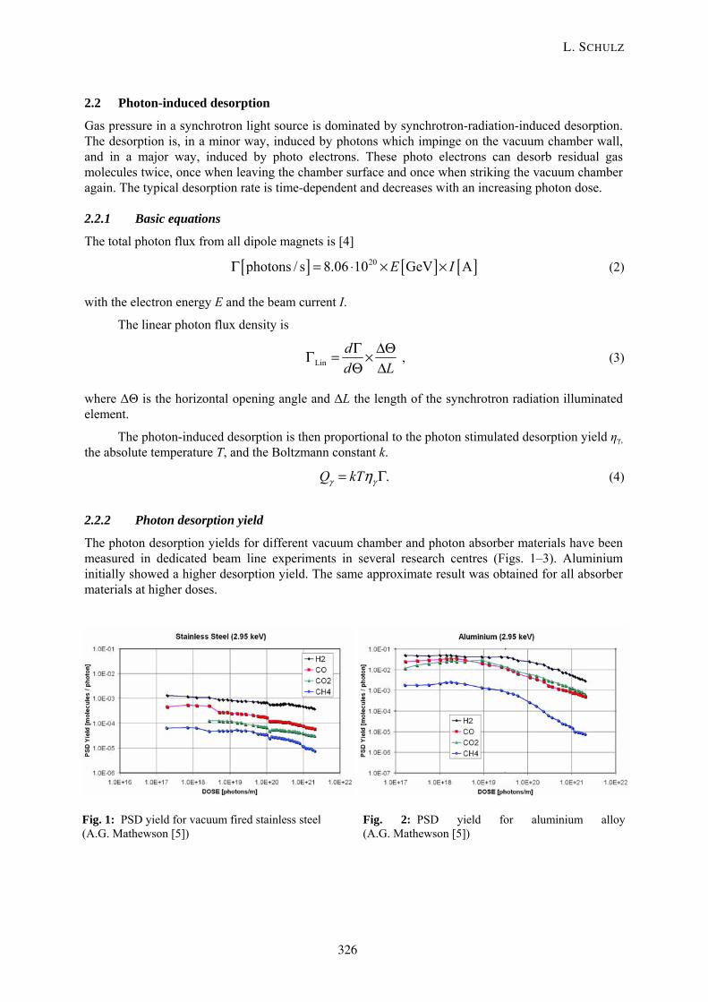
2.2 Photon-induced desorption

Gas pressure in a synchrotron light source is dominated by synchrotron-radiation-induced desorption. The desorption is, in a minor way, induced by photons which impinge on the vacuum chamber wall, and in a major way, induced by photo electrons. These photo electrons can desorb residual gas molecules twice, once when leaving the chamber surface and once when striking the vacuum chamber again. The typical desorption rate is time-dependent and decreases with an increasing photon dose.

2.2.1 Basic equations

The total photon flux from all dipole magnets is [4]

[ ] [ ] [ ]20photons / s 8.06 10 GeV AE IΓ = ⋅ × × (2)

with the electron energy E and the beam current I.

The linear photon flux density is

Lindd L

Γ ΔΘΓ = ×Θ Δ

, (3)

where ΔΘ is the horizontal opening angle and ΔL the length of the synchrotron radiation illuminated element.

The photon-induced desorption is then proportional to the photon stimulated desorption yield ηγ, the absolute temperature T, and the Boltzmann constant k.

.Q kTγ γη= Γ (4)

2.2.2 Photon desorption yield

The photon desorption yields for different vacuum chamber and photon absorber materials have been measured in dedicated beam line experiments in several research centres (Figs. 1–3). Aluminium initially showed a higher desorption yield. The same approximate result was obtained for all absorber materials at higher doses.

Fig. 1: PSD yield for vacuum fired stainless steel (A.G. Mathewson [5])

Fig. 2: PSD yield for aluminium alloy (A.G. Mathewson [5])

L. SCHULZ

326

Fig. 3: PSD yield for OFHC copper (V. Anashin [6])

O.B. Malyshev uses the following model for his calculations of dynamic desorption processes in a beam vacuum chamber [7] (see Fig. 4).

Fig. 4: Photon stimulated desorption yield for CO for unbaked and baked vacuum chambers

The pre-baked vacuum chamber was baked at 200°C for 24 hours (but not baked in situ) [8],[9]. The yields for doses higher then 1023 photons/m are extrapolations.

3 UHV pumps Capture pumps, which trap the pumped gas molecules in the pump body, are the predominate pumps in the UHV region of synchrotron light sources. The advantage of capture pumps is that they form a closed vacuum system with the vacuum chamber of the accelerator; additional complicated valve interlocks are unnecessary; there are no moving parts in the pump, and no vibrations are transmitted to the magnet lattice.

Chemical transformation triggers the principal pumping mechanism that combines gases chemically into solid compounds with very low vapour pressure. At UHV conditions, a surface can hold large quantities of gases compared to the amount of gas present in the volume.

VACUUM ASPECTS

327

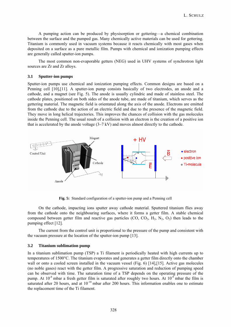
A pumping action can be produced by physisorption or gettering—a chemical combination between the surface and the pumped gas. Many chemically active materials can be used for gettering. Titanium is commonly used in vacuum systems because it reacts chemically with most gases when deposited on a surface as a pure metallic film. Pumps with chemical and ionization pumping effects are generally called sputter-ion pumps.

The most common non-evaporable getters (NEG) used in UHV systems of synchrotron light sources are Zr and Zr alloys.

3.1 Sputter-ion pumps

Sputter-ion pumps use chemical and ionization pumping effects. Common designs are based on a Penning cell [10],[11]. A sputter-ion pump consists basically of two electrodes, an anode and a cathode, and a magnet (see Fig. 5). The anode is usually cylindric and made of stainless steel. The cathode plates, positioned on both sides of the anode tube, are made of titanium, which serves as the gettering material. The magnetic field is orientated along the axis of the anode. Electrons are emitted from the cathode due to the action of an electric field and due to the presence of the magnetic field. They move in long helical trajectories. This improves the chances of collision with the gas molecules inside the Penning cell. The usual result of a collision with an electron is the creation of a positive ion that is accelerated by the anode voltage (3–7 kV) and moves almost directly to the cathode.

Fig. 5: Standard configuration of a sputter-ion pump and a Penning cell

On the cathode, impacting ions sputter away cathode material. Sputtered titanium flies away from the cathode onto the neighbouring surfaces, where it forms a getter film. A stable chemical compound between getter film and reactive gas particles (CO, CO2, H2, N2, O2) then leads to the pumping effect [12].

The current from the control unit is proportional to the pressure of the pump and consistent with the vacuum pressure at the location of the sputter-ion pump [13].

3.2 Titanium sublimation pump

In a titanium sublimation pump (TSP) a Ti filament is periodically heated with high currents up to temperatures of 1500°C. The titanium evaporates and generates a getter film directly onto the chamber wall or onto a cooled screen installed in the vacuum vessel (Fig. 6) [14],[15]. Active gas molecules (no noble gases) react with the getter film. A progressive saturation and reduction of pumping speed can be observed with time. The saturation time of a TSP depends on the operating pressure of the pump. At 10-8 mbar a fresh getter film is saturated after roughly two hours. At 10-9 mbar the film is saturated after 20 hours, and at 10-10 mbar after 200 hours. This information enables one to estimate the replacement time of the Ti filament.

L. SCHULZ

328

Fig. 6: Titanium sublimation pump

Most standard TSP have three Ti filaments, i.e. spares to replace the burnt-out filament. Under normal operating conditions this enables operation for a long period of time.

3.3 Non-evaporable getter pumps

Non-evaporable getters (NEGs) using zirconium alloy powder are pressed onto a strip or sintered into disks. Gas molecules can be sorbed by a chemical reaction when they impinge on the clean metal surface of the NEG material. After pumpdown, the NEG material is covered with a passivation layer. The oxide layer must be removed in an activation process to achieve a clean metal surface. The getter must be heated to a particular temperature to achieve this (Fig. 7). During activation, the passivation layer diffuses into the bulk material. The metal surface saturates with cumulative sorption of gas molecules and a new oxide layer is created. The NEG must be reactivated to achieve full pumping speed.

Fig. 7: Working principle of a NEG pump (courtesy of SAES Getters SpA)

3.3.1 NEG strips

SAES Getters SpA produce all NEG pumps on the market. Several materials are available. In synchrotron light sources, ST707 NEG strips are often used. They can be activated by heating up the strips to 400°C for one hour. Figure 8 shows the ST707 NEG strips installed in the APS undulator vessel with a vertical electron channel aperture of 5 mm [16]. A high linear pumping speed with resulting low pressure can be achieved in this strong conductance limited configuration.

VACUUM ASPECTS

329

Fig. 8: NEG strips installed into the ante chamber of the APS undulator vessel

3.3.2 NEG coating

NEG film coatings are sputtered in thin films directly onto the inside of the vacuum chamber walls. Many coatings have been tested at CERN to find an alloy which can be activated at low temperatures [17],[18]. With Ti-Zr-V, an alloy was found which can be activated at 200°C, comparable with standard vacuum vessel bake-out temperatures.

Coating the chamber leads to a high pumping speed and a reduced degassing rate; thus a very low pressure can be achieved. Figure 9 shows the performance of a NEG-coated stainless steel undulator vessel at ESRF [19]. The data are taken at the ESRF D31 beamline. At first, the desorption yield under photon bombardment was measured without activating the NEG coating. At a beam dose of 100 mA h, the NEG film was activated by heating the chamber at 250°C for about 20 hours. After activation, a decrease of the desorption yield by a factor of 380 was observed.

Fig. 9: Total molecular desorption yield η (N2 equivalent) of a Ti-Zr-V coated stainless steel chamber as a function of the accumulated dose before and after activation

L. SCHULZ

330

4 Pressure distribution The vacuum system of a synchrotron light source has limited general conductance. When designing the vacuum system, it is important to calculate the pressure distribution expected, and to specify the size and location of pumps. Several computer programs are available for this task. Simulations can be done with Monte Carlo calculations [20] or by using finite element programs.

O. Malyshev calculated the pressure distribution for the Diamond storage ring using the commercial mathematical package, Mathcad [7].

5 Chamber design

5.1 Vacuum chamber materials

Aluminium or stainless steel are the most-common materials used for vacuum chambers of synchrotron light sources. Copper is not often used as chamber material, but it is the main material for photon absorbers. Table 1 shows the main properties of stainless steel, aluminium, and OFHC copper.

Table 1:Properties of stainless steel, aluminium, and copper

Stainless Steel 316 LN

Aluminium Al Mg 4.5 Mn

Copper OFHC/GlidcopTM

Yield stress [MN m-2] 20°C/250°C

315/200 215 63/ 55 332/255

Therm. cond. [W m-1 K-1] 20°C

15 109 391/345

Electr. cond. [μΩ m]-1 20°C

1.4 36 58/54

Modulus of elast. [GN m-2] 20°C

200 71 117/126

Chamber fabrication deep drawn edge bending

extrusions solid blocks

(extrusions)

Joining technique TIG welding e-beam welding very easy

TIG welding brazing e-beam welding

Stainless steel has good mechanical and vacuum properties. The vacuum chamber fabrication, based on deep draw and edge bending techniques, is easy [21].

The thermal properties of aluminium are very high. It has advantages for long vacuum chambers with uniform cross sections that can be fabricated from extrusions [22],[23].

Copper has excellent thermal properties. The fabrication of vacuum chambers from copper is very tricky, examples where copper is used as chamber material for a synchrotron light source are rare [24],[25]. The main application for copper is in photon absorption. Water-cooled OFHC copper is the standard material for photon absorbers. Dispersion-strengthened copper (GlidCop® [26]) with higher yield strength at high temperatures is used [27] for absorbers with very high photon power.

Stainless steel has very poor thermal conductivity compared with aluminium and copper. This explains why copper is used for photon absorbers in stainless steel vacuum systems. The electrical conductivity value is very low. This contributes to the resistive wall effects and can pose a real problem in undulator vessels with very small gaps [28].

VACUUM ASPECTS

331

On the other hand, low electrical conductivity results in low eddy-current effects, a fact that has to be taken into account when the global closed-orbit correction system works at frequencies of 100 Hz and higher.

5.2 Vacuum chambers

A characteristic feature of vacuum chamber designs for 3rd generation synchrotron light sources is the use of the antechamber design [29]. The vacuum chamber consists of an electron beam chamber and an antechamber. The electron chamber is open on the side of the antechamber. The synchrotron radiation can pass through to the antechamber where discrete crotch-absorbers intercept the photons that are not used.

In general, vacuum chamber designs for synchrotron light sources can be classified in two groups. In the first group, the antechamber design is used only in the dipole chamber where the photon beam has the highest intensity. In the straight chambers, where the photon intensity is lower, the synchrotron radiation hits on distributed absorbers in the chamber wall (see Fig. 10).

Fig. 10: Antechamber design only in the bending magnet (ANKA)

In the second group, the vacuum chamber has an antechamber that is full around the ring (see Fig. 11). With a full antechamber design, the area exposed to synchrotron radiation is minimized, and the photons are concentrated on the crotch absorbers. This leads to a higher rate of conditioning, and reduces the thermal stress on the chamber, which may lead to less current-dependent chamber movements.

Fig. 11: Full antechamber design (SLS)

L. SCHULZ

332

6 Vacuum conditioning Several procedures are necessary for vacuum chamber conditioning. Obviously, a clean environment preceded by several cleaning steps is necessary. When the fabrication process is finished, the vacuum chamber is cleaned chemically. To avoid polluting the environment, it is preferable to use detergents to clean UHV applications rather that solvents [30],[31].

The question of in situ bake-out for the vacuum system of synchrotron light sources is a controversial issue in the community. A classical in situ bake-out system for the vacuum chambers of a light source consists of resistive heaters with electrical and thermal insulation. This raises the costs for the vacuum system and other accelerator components.

A new bake-out method has been performed at the SLS and CLS. An external bake-out system was used for the vacuum conditioning of the vacuum vessels. All vacuum chambers for the magnet sections were baked in a bake-out oven at a temperature of 250°C, and installed into the storage ring under vacuum [32]. The adjacent straight sections were evacuated and baked in the tunnel with a movable and modular bake-out oven.

Fig. 12: Dynamic average pressure (N2 equiv.) versus accumulated beam dose for SLS at 2.4 GeV

However, in spite of careful preparation of the vacuum system the design pressure of a synchrotron light source can only be achieved with beam cleaning. And the time involved for this process depends on the design and preconditioning of the vacuum system. For example, Fig. 12 shows the evolution of the dynamic average pressure dp/dI as a function of the accumulated beam dose of the SLS storage ring. The design pressure of 2 × 10-9 mbar at a beam current of 400 mA could be achieved after an accumulated beam dose of 100 Ah. Other machines that started commissioning without in situ bake-out have needed much more time.

Experience at SLS has also shown that if the venting of single vacuum sections for the change of vacuum components is carried out under a dry nitrogen purge, the recovery of the vacuum system can be accomplished without in situ bake-out. Beam lifetimes of about 10 hours are back after one week of operation.

VACUUM ASPECTS

333

REFERENCES [1] C. Bocchetta, Lifetime and beam quality, CERN Accelerator School, Brunnen, Switzerland,

2003.

[2] A. Wrulich, Single-beam lifetime, CERN Accelerator School, Jyväskyla, Finland, 1992.

[3] R. Reid, Gas load origins in synchrotron light sources, CLRC Daresbury Laboratory, VDN/10/96.

[4] O. Gröbner et al., Vacuum 33, No. 7 (1983).

[5] A. G. Mathewson et al., Comparison of synchrotron-radiation-induced gas desorption from Al, stainless steel, and Cu chambers, American Institute of Physics Conference Proceedings No. 236 (American Vacuum Society, Series 12, Argonne, IL, 1990), p. 313.

[6] V. Anashin et al., Photodesorption and power testing of the SR crotch-absorber for BESSY II, EPAC 1998.

[7] O.B. Malyshev et al., Pressure distribution for Diamond storage ring, EPAC 2002.

[8] C.L. Foerster et al., Photon-stimulated desorption yields from stainless steel and copper plated beam tubes with various pretreatments, J. Vac. Sci. Technol. A8 (1990) 2856.

[9] C. Herbeaux et al., Photon stimulated desorption of an unbaked stainless steel chamber by 3.75 keV critical energy photons, J. Vac. Sci. Technol. A17 (1999) 635.

[10] F.M. Penning, Philips Tech. Rev. 2 (1937) 201.

[11] W. Schuurman, Investigation of a low pressure Penning discharge, Physica, 36 (1967) 136.

[12] L. Schulz, Sputter ion pumps, CERN Accelerator School, Vacuum Technology, Snekersten, Denmark, 1999.

[13] F. Giacuzzo, and J. Miertusova, Total pressure measurements in the ELETTRA storage ring according to the performance of the sputter-ion pumps, EPAC 1996.

[14] C. Benvenuti, Molecular surface pumping: The getter pumps, CERN Accelerator School, Vacuum Technology, Snekersten, Denmark, 1999.

[15] P.A. Redhead et al., The Physical Basis of Ultrahigh Vacuum (American Inst. of Physics, New York, 1993).

[16] E. Trakhtenberg, Argonne National Laboratory, private communication.

[17] C. Benvenuti et al., A novel route to extreme vacua: the non evaporable getter thin film coatings, Vacuum 53 (1999) 219.

[18] C. Benvenuti et al., Nonevaporable getter films for ultrahigh vacuum applications, J. Vac. Sci. Technol. A 16 (1998) 148.

[19] P. Chiggiato, R. Kersevan, Synchrotron-radiation-induced desorption from a NEG-coated vacuum chamber, Vacuum 60 (2001) 62.

[20] R. Kersevan, MOLFLOW user’s guide, Sincrotrone Trieste Technical Report, ST/M-91/17 (1991).

[21] E. Huttel, Materials for accelerator vacuum systems, CERN Accelerator School, Vacuum Technology, Snekersten, Denmark, 1999.

[22] G. A. Goeppner, APS storage ring vacuum chamber fabrication, American Institute of Physics Conference Proceedings No. 236 (American Vacuum Society, Series 12, Argonne, IL 1990), 124.

L. SCHULZ

334

[23] E. Trakhtenberg et al., The vacuum system for insertion devices at the Advanced Photon Source, PAC 1995.

[24] N. R. Kurita et al., Overview of the SPEAR3 vacuum system, PAC 1999.

[25] D. Berger et al., Mechanical and thermal design of vacuum chambers for a 7 T multipole wiggler for BESSY II, EPAC 2002.

[26] GlidCop is a registered trademark of OMG Americas Corp., Research Triangle Park, N.C., USA.

[27] A. Alp, Thermal-stress analysis of the high heat-load crotch absorber at the APS, 2nd International Workshop on Mechanical Engineering Design of Synchrotron Radiation Equipment (MEDSI02), 2002.

[28] R. Nagaoka, Impact of resistive-wall wake fields generated by low-gap chambers on the beam at the ESRF, PAC 2001

[29] L. Schulz, Stainless steel vacuum chambers, 25th ICFA Advanced Beam Dynamics Workshop, Shanghai Symposium on Intermediate-energy Light Sources, SSILS 2002.

[30] C. Benvenuti et al., Surface cleaning efficiency for UHV applications, Vacuum 53 (1999) 317.

[31] R.J. Reid, Cleaning for vacuum service, CERN Accelerator School, Vacuum Technology, Snekersten, Denmark, 1999.

[32] L. Schulz et al., SLS vacuum system, PSI Scientific Report VII (2000).

BIBLIOGRAPHY Vacuum Design of Advanced and Compact Synchrotron Light Sources, American Institute of Physics Conference Proceedings No. 171 (American Vacuum Society, Series 5, Upton, NY, 1990).

Vacuum Design of Synchrotron Light Sources, American Institute of Physics Conference Proceedings No. 236 (American Vacuum Society, Series 12, Argonne, IL, 1990).

Vacuum Technology, CERN Accelerator School Proceedings, Snekersten, Denmark, 1999.

VACUUM ASPECTS

335

MECHANICAL ASPECTS OF THE DESIGN OF THIRD-GENERATION SYNCHROTRON-LIGHT SOURCES

S. Zelenika Paul Scherrer Institute, Villigen, Switzerland

Abstract In storage rings of third-generation synchrotron radiation facilities, the positioning tolerances of the elements of the machine are constantly reduced to achieve lower emittance and increased lifetime. This implies increasing positioning and alignment precision that must be preserved over long time-spans. The mechanical engineering approach to meet these requirements is described. The design of the Swiss Light Source storage ring support, positioning and position monitoring systems, the tests done on the respective prototypes, the quality assurance and installation procedures, and the operational experience with these systems are discussed in depth. The applicability of the developed arrangement to beam-based alignment is also illustrated.

1 Introduction In the design of third-generation synchrotron-light sources and related experimental infrastructure, there is a wide range of mechanical engineering tasks to satisfy. Therefore, the mechanical engineering crew is confronted with several topics related to these designs [1–3]:

- ultra-high-precision positioning of optical and other elements with resolutions, accuracies and precisions in the nanometric and μrad ranges;

- high-precision machining with tolerances of the produced pieces of equipment in the micrometre range;

- vibration measurement and suppression, with maximum allowed vibration amplitudes often limited to the nanometre range;

- high-heat-load problems, with pieces of equipment subject to specific heat loads approaching 1 GW/m2 [4, 5], i.e., considerably higher than those on the surface of the sun where 7×107 W/m2 are reached;

- high and ultra-high vacuum issues (with the respective limits imposed, for example, on the use of materials or types of positioning mechanisms), where the ultimate pressures reached are in the low 10-10 mbar range;

- radiation compatibility, with stringent limits on the available selection of materials and components used;

- experimental technologies pertaining to all of the above fields;

- innovative, analytical and numerical methods needed to satisfy the technical challenges cited;

- use of advanced computer-aided engineering systems [computer-aided design (CAD) and manufacturing (CAM), finite-element methods (FEM), database management tools, etc.].

In the design of synchrotron accelerator complexes, increasing attention is dedicated to the proper mechanical design of the storage ring support, positioning and position monitoring systems. The sources of beam instabilities causing orbit distortions, and the effects generated by ground motion

337

(ground settlement, seasonal changes, and temperature effects) and by dynamic excitation sources (local machinery, water cooling, and near-by roads) have to be minimized [5–8] to attain the required beam quality (high brightness, i.e. low emittance) and lifetimes.

Fig. 1: View of the interior of the SLS building during its construction

In this paper an approach to deal effectively with these challenges is illustrated using the example of the mechanical design of the Swiss Light Source (SLS) machine (Fig. 1) at the Paul Scherrer Institute (PSI, Villigen, Switzerland). SLS is the first medium-energy-range synchrotron facility of hard X-rays that uses the higher spectral harmonics of in-vacuum undulators with a short period and a small gap. The main goal at the SLS was to achieve a very high photon-beam quality, which is, in turn, determined by the electron-beam quality. Since the remaining space for the optimization of the lattices is limited, the positioning, re-positioning and alignment precision of the magnets by mechanical means were considered extremely important to attain the low emittances required and to reduce orbit distortions before switching on the correction dipoles [9]. Hence, in order to meet the high-quality requirements, provisions for accurate positioning, as well as dynamic minimization of ground motions and thermal effects, were foreseen from the very beginning of the SLS storage ring design.

2 Aims of the work Considering these arguments, the mechanical design goals for the SLS storage ring support, alignment and disturbances compensation systems are to

- support the storage ring magnets, vacuum chambers, diagnostics devices and position measurement systems (horizontal positioning system––HPS, and hydrostatic levelling system––HLS);

- obtain one large, rigid, pre-assembled item not necessitating fiducialization of individual magnets or items other than the support itself;

- provide high-precision reference surfaces for the magnets both in the horizontal and in the vertical direction (out of the total alignment tolerances, only 30 μm are ‘at disposal’ for the manufacturing tolerances of the supports);

- provide a simple and reliable mechanical design allowing easy mounting and alignment;

- provide a kinematic support (number of constrains balances the number of the needed degrees of freedom––DOFs);

- provide means of compensating for thermal and geological horizontal and vertical disturbances with large time constants;

- provide smooth, hysteresis-free and remotely controllable motion at micrometric levels;

S. ZELENIKA

338

- guarantee the stiffness (dynamic stability) of the support structures with magnets mounted onto them such that the residual r.m.s. beam jitter––including optics amplification––remains smaller than 10% of the r.m.s. beam sigmas (i.e., considering a 1% emittance coupling, the jitter should not exceed 1 μm vertically and 10 μm horizontally) [10].

3 Basic design

3.1 Support system

Various solutions have been adopted at synchrotron light and other accelerator facilities around the world to support the elements of the machine [11]. The individual support stands are generally used when the accelerator components are spread out, while girders are the preferred solution when a set of components has to be mounted on a common platform. The latter solution avoids the ground settlement of individual components, permits the vacuum chambers to be supported on the same structure thus guaranteeing the tolerances needed between the magnets and the vacuum system, and the girders can be pre-assembled. Moreover, as shown below, random displacements of girders with several magnets mounted onto them generate a lesser impact on orbit distortion than do individually supported quadrupoles.

Given that these advantages, fulfil the requirements perfectly, a girder-based support system was adopted in the SLS case. The cross section of the girders was then determined based on the optimization of their mechanical characteristics, with the intention of minimizing the cross sectional area (which is directly proportional to the costs and the mass of the structure), while concurrently maximizing the stiffness of the girders. It can be shown [12] that for bending loads the optimal shape to meet these goals is either an ‘I’ or a hollow-square-cross-section. In the case of torsion loads, the optimum is reached with closed hollow shapes, possibly with ribs along the length of the structure.

Based on these considerations, a welded, stress-relieved (annealed), hollow-square girder structure with internal ribs was adopted as the basic support unit of the SLS storage ring elements (Fig. 2). The girder design included an extensive optimization process based on the numerical sensitivity analysis of the main design parameters (such as longitudinal distance between the support points, their vertical position relative to the centre of mass of the girder/magnet assembly, wall thickness of the girder structure) so as to maximize the static and dynamic stiffness of the girder assemblies [13].

Fig. 2: The SLS storage ring support, alignment and disturbances compensation systems

MECHANICAL ASPECTS OF THE DESIGN OF THIRD-GENERATION SYNCHROTRON-LIGHT SOURCES

339

In total, 48 girders are used of which 30 are 4.5 m in length and 18 are 3.7 m in length. Four girders are placed in each of the 12 triple-bend achromats (TBAs––four TBAs then form one superperiod containing a 11.8 m, a 7 m, and two 4 m long straight sections) of the SLS storage ring. The upper part of the girders is designed to provide ground horizontal and vertical reference surfaces with a precision of ≤ ± 15 μm (Fig. 3) onto which the magnets (whose reference surfaces were also given narrow tolerances so as to achieve the global goal of keeping the total mechanical tolerances to within ± 50 μm) are laid and fixed via suitably designed clamps.

vertical reference surfaces

horizontal reference surfaces

Fig. 3: Reference planes for positioning the storage ring elements on the girders

Kinematically supported dipole magnets (the conventional flat-V-cone kinematic mount balances the six DOFs) overlap adjacent girders establishing, together with the HPS foreseen and HLS systems (see below), a virtual ‘train link’ scheme with joints near the centres of the dipoles.

Continuous monitoring and correction of girder location is required to compensate for girder misalignment relative to the ideal position due to geological and thermal drifts, and to guarantee sufficient dynamic apertures.

3.2 Positioning system

Alignment and disturbance compensation targets have also been met at various accelerator facilities using different approaches [11]. At the European Organization for Nuclear Research (CERN), the Stanford Linear Accelerator Center (SLAC) and the Deutsches Elektronen-Synchrotron (DESY), the positioning in the horizontal and vertical plane is separate. The vertical system, based on shim stacks, threaded rods, wedge jacks or screw jacks is constituted by three standoffs allowing the heave, the roll and the pitch to be adjusted. The horizontal system constitutes one or two sliding plates with a push–push screw or a turnbuckle push–pull rail-slide-based system. Obviously in this case the alignment procedure is iterative, often leading to a coupled motion in more DOFs, thus resulting in considerable time loss.

Therefore, at the Advanced Light Source (ALS), the ‘six-strut system’ constituted by length-adjustable bars with spherical joints at the ends has been developed. Three of the bars are used for the adjustment in the vertical plane (heave, roll and pitch), while the remaining three lie in the horizontal plane and are used to adjust the sway, surge and jaw of the structure under consideration. However, the six-strut system still presents the disadvantages of rather limited load capacity, residual coupling of

S. ZELENIKA

340

the DOFs because of the cosine effect, intermittent motion due to stick-slip effects at the strut fixations, as well as several sources of backlash all leading to reduced accuracy.

A motorized Kelvin clamp-based kinematic positioning system was recently developed at SLAC [14]. The positioning is obtained via eccentric cam-shaft support drives (‘movers’) driven via stepping motors, with a linear variable differential transformer (LVDT)-based feedback system. The system allows simultaneous remotely controllable multi-DOF movements to be performed, while minimizing friction and hysteresis by substituting conventional sliding with pure rolling motions (only the inner eccentric shaft rotates, while the outer part of the cam remains in contact with the girder body). As a result, the required smooth incremental motions can be obtained using conventional (low-cost) mechanical components. In the proposed configuration, however, the range of motion of the system was limited to ±2 mm, while the loading capacity was limited to roughly 1 ton.

Based on these experiences, SLS adopted a pre-alignment, push–push, screw arrangement mounted on the four pedestals underneath each girder, and for the final micrometric-range alignment, the mover system (Fig. 4). However, several design modifications have been introduced to the original SLAC mover design:

- the range of motions of the movers was increased to ±5 mm to suit SLS needs;

- costly stepping motors were replaced by simple d.c. motors;

- in the feedback loop the LVDTs were replaced by absolute rotary encoders, avoiding the necessity of lengthy LVDT mounting and calibration procedures [14];

- instead of ball bearings, commercially available (SKF) spherical roller bearings were press-fitted onto the precisely machined cam-shafts, thus providing means for adaptation to small misalignments between the bearings and the respective seats on the girders, but also, given the larger contact area, increasing the load-carrying capacity (the SLS girder-magnet assembly weighs up to 9 tons) and stiffness.

Fig. 4: Mover system

MECHANICAL ASPECTS OF THE DESIGN OF THIRD-GENERATION SYNCHROTRON-LIGHT SOURCES

341

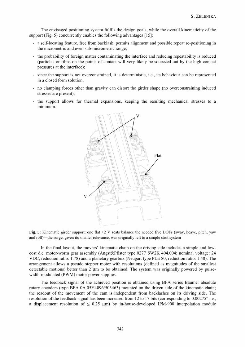
The envisaged positioning system fulfils the design goals, while the overall kinematicity of the support (Fig. 5) concurrently enables the following advantages [15]:

- a self-locating feature, free from backlash, permits alignment and possible repeat re-positioning in the micrometric and even sub-micrometric range;

- the probability of foreign matter contaminating the interface and reducing repeatability is reduced (particles or films on the points of contact will very likely be squeezed out by the high contact pressures at the interface);

- since the support is not overconstrained, it is deterministic, i.e., its behaviour can be represented in a closed form solution;

- no clamping forces other than gravity can distort the girder shape (no overconstraining induced stresses are present);

- the support allows for thermal expansions, keeping the resulting mechanical stresses to a minimum.

V

V

Flat

Fig. 5: Kinematic girder support: one flat +2 V seats balance the needed five DOFs (sway, heave, pitch, yaw and roll)––the surge, given its smaller relevance, was originally left to a simple strut system

In the final layout, the movers’ kinematic chain on the driving side includes a simple and low-cost d.c. motor-worm gear assembly (Angst&Pfister type 0277 SW2K 404.004; nominal voltage: 24 VDC; reduction ratio: 1:78) and a planetary gearbox (Neugart type PLE 80; reduction ratio: 1:40). The arrangement allows a pseudo stepper motor with resolutions (defined as magnitudes of the smallest detectable motions) better than 2 μm to be obtained. The system was originally powered by pulse-width-modulated (PWM) motor power supplies.

The feedback signal of the achieved position is obtained using BFA series Baumer absolute rotary encoders (type BFA 0A.05Y4096/503463) mounted on the driven side of the kinematic chain; the readout of the movement of the cam is independent from backlashes on its driving side. The resolution of the feedback signal has been increased from 12 to 17 bits (corresponding to 0.00275° i.e., a displacement resolution of ≤ 0.25 μm) by in-house-developed IPM-900 interpolation module

S. ZELENIKA

342

interfaces based on SSI I/O units. The electronics can down-load the acquired data directly to the SLS control system through a VME output channel, integrating the girder positioning system fully into the SLS EPICS-based control system [16].

The adopted arrangement also allows the inclusion of motion bounding via precision Baumer Electric My-Com F75/S35 limit switches, and provides additional (i.e., redundant––the motion is already bounded by the design geometry of the eccentric cams as well as by software interlocks) security in the preservation of the integrity of the vacuum chamber.

3.3 Position-monitoring systems (HLS and HPS)

The necessity to continuously monitor the positioning stability of the girders, because of the long time deterioration of their initially aligned location, is met by using the hydrostatic levelling system (HLS) and the horizontal positioning system (HPS); both have micrometric-range accuracies (Fig. 6).

HPS referencepole

HPS armswith sensors

HLS potsHLS piping network

HLS potsHPS arms

with sensors

HPS referencepole

Fig. 6: A 30° sector of the SLS storage ring

The HLS consists of cylindrical stainless steel pots (φ = 10 cm) developed in collaboration with the Edi Meier & Partner AG company (Fig. 7). The pots are connected by a half-filled stainless steel pipe (outer diameter: 25 mm, inner diameter: 22 mm) around the ring; this configuration allows the problems associated with differential thermal expansion of the working fluid in different pots to be avoided. For easy of installation, localized Tygothane (radiation hardened poly-urethane) inserts are used, compensating for the small thermal and other misalignments of the piping network. With such an arrangement, a single reference altimetric level is obtained (Fig. 6).

Originally, de-mineralized water was the working fluid in the system since it has well-known properties, is easy to handle, and environmentally friendly and cheap.

The sensing elements are capacitive proximity gauge-based and linked to the SLS EPICS-based global control system. The non-contact measurement principle allows corrosion due to moistening or wetting of the contact points, as well as mineral deposits on the sensors, to be avoided. Moreover, the temperature of the sensor is kept above that of the water, avoiding condensation effects (which would cause corrosion and mineral deposits on the sensor); the temperature in each pot is constantly monitored to avoid temperature-induced apparent level changes (see, for example, Ref. [17]). The position of the sensors in the pots, as well as the dimensions of the pot itself, have been optimized to minimize the influence of the surface meniscus effect on the measurements and the capillary wall effects. An O-ring protects the electronics from corrosion. To keep wiring costs low, all the analog (± 10 V) signals of one storage ring girder are multiplexed and digitized in a local HLS electronics. Each pot is equipped with a touch sensor; this feature allows a remote recalibration of the sensor by raising the water level up to it [18].

The resolution of the system is better than 2 μm, with the specified absolute accuracy and repeatability better than 10 μm. The maximum range of the sensors is 14 mm, while the range measurement used is ±2.5 mm.

Four pots are installed on each girder (Fig. 6) allowing its vertical position (heave) as well as pitch and roll to be measured (in fact, three pots would be sufficient, with the fourth one giving

MECHANICAL ASPECTS OF THE DESIGN OF THIRD-GENERATION SYNCHROTRON-LIGHT SOURCES

343

statistical data for increasing the precision, as well as covering possible failures). The pots are installed on the girder brackets so that both the ground movements and eventual differential dilatations of the girder supports can be taken into account. Each storage ring TBA (four girders) can be valved-off for maintenance purposes, thus lowering the settling times at refilling. The filling system restores the water level in the network after changes due to evaporation. The signals of the sensors next to the inner filling station are used to control the filling and emptying valves, respectively.

38

φ 25

φ 100

de-mineralizedH2O

guard

sensor plate

touching point

O-ring

ceramic plate

heating element

electrical circuits

Fig. 7: The HLS pot (a) and the layout of its interior structure (b)

The horizontal positioning system (HPS) monitors horizontal girder movements and is constituted by pairs of lever arms under the girder surface equipped with optical encoders (Fig. 8). By extending the system in a ‘train link’ arrangement (Fig. 6), the relative horizontal displacements of adjacent girders can be correlated with respect to artificially created references (reference poles) at the beginning and at the end of each TBA (Fig. 9––there is no absolute reference as in the HLS). The position of the reference poles is determined by the accuracy of the conventional alignment methods, which is better than 100 μm.

Fig. 8: The HPS system mounted on girders

S. ZELENIKA

344

Fig. 9: An HPS reference pole

The four girders of a single TBA can be treated as either a self-contained system (‘partial train link’) or as part of the whole SLS storage ring (‘full train link’). Using the artificial references as starting points, any motion of individual girders can be detected and traced back via a 2N dimensional linear system of equations––N being the number of girders taken into consideration in the calculation––with the girder transversal displacements (sways) and yaws as the unknowns. Since roll and pitch also affect the readouts of the HPS sensors, they have to be measured in advance via the HLS system [19].

The measuring sensor used for the HPS system is a Renishaw type RGH24Z50A00A absolute linear encoder with a 0.5 μm resolution and a working range of ± 2.5 mm; eight encoders are used in each TBA of the SLS storage ring. An in-house-developed encoder counter module (RHC 900) is employed to acquire the data, serialize them, and send them to the global SLS control system [20].

4 Beam-based alignment For diagnostic purposes, it was envisaged that the SLS storage ring beam trajectory be measured using 72 high-precision BPMs [21] located between the magnets. Encoders similar to those used for the HPS system are then employed for monitoring the positions of the BPMs with respect to adjacent quadrupole magnets; the resulting readings are taken into account when the final electron-beam position is calculated. These data can be used to remotely align the girders using the mover system described, thus obtaining beam-based alignment. In fact, the girder mover system can be used like the corrector magnets to obtain closed-orbit and even coupling correction via the correction matrix, which correlates the BPM readings to the girder re-alignment motions needed (in the correction matrix, the girder misalignments are treated as correctors in the classical beam dynamics approach).

MECHANICAL ASPECTS OF THE DESIGN OF THIRD-GENERATION SYNCHROTRON-LIGHT SOURCES

345

The beam-tracing simulations performed have shown that the static vertical closed-orbit corrections can be completely covered by girder alignment, while in the horizontal direction proper selection of the girders to be re-positioned via the movers allows the corrector magnet strength used to be reduced by a factor 4 (Fig. 10). This kind of alignment can take over most of the static orbit correction and leave the corrector strengths for the dynamic correction (active orbit feedback) and local bump creation for matching the beamline acceptances or for machine studies. Since beam-based girder alignment is a dynamic method and, in principle, may be done on-line with the stored beam, it appears to be a superior substitute for magnet sorting [19].

Fig. 10: Maxima of corrector magnet strengths before (dashed) and after (full line) closed-orbit correction through girder alignment. Two hundred random misalignment seeds were generated and corrected. The random errors assumed partial train links over four girders with r.m.s. (2σ cut) displacement errors of 300 μm for the (virtual) girder joints, 100 μm for the joint play (i.e. errors in the HPS and HLS readings), and 50 μm for magnets and BPMs positioning tolerances relative to the surfaces of the girders.

5 Tests on prototypes

5.1 Girder system

The delivery of the girder prototypes prompted an extensive design review and measurement campaign. In particular, the following tests have been carried out:

- The dimensional checks of the main components were carried out at the PSI laboratories via a Renishaw 3D coordinate measuring machine with micrometric range precisions. It was established that the design tolerances were met.

- The straightness accuracy of the reference surfaces was assessed using the HP 5529A Michelson-type heterodyne laser interferometric system. In the optical configuration used (Fig. 11), the measurement principle is based on an interferometer with a Wollaston prism. The prism is slid along the girder and has a different refractive index for each of the two polarized components of the laser beam; these are deviated by two equal and opposite angles towards a fixed retro-reflector. The reflector contains two plane mirrors that reflect the beam components back along their respective paths. The difference in optical paths of the two beam components is proportional

S. ZELENIKA

346

to the displacements perpendicular to the incoming beam, and the value of the girder surface quality (indicated with ‘a’ on Fig. 11) will be obtained simply by multiplying the interferometric measurement by a constant (1/[2 sin(Φ/2)]). In this case, given the range of measurement (4.5 m), the resolution of the optical set-up is 100 nm.

- The measurement system illustrated proved that the very tight tolerances (± 15 μm) on the reference surfaces of the girders were met, and proved the deflection of the girders under the weight of the magnets to be smaller than 20 μm.

- The mounting and alignment procedures were reviewed. As a result, several alignment reference points have been added both to the mover supports and to the girder bodies. Also, the vertical and horizontal degrees of freedom have been completely decoupled, further contributing to the ease of the alignment procedure.

Fig. 11: Straightness measurement principle

5.2 Mover system

- The tests on the mover system proved its functionality.

- An 85 000 cycles fatigue test of the mover-to-girder interface under full load was performed. The electron microscopy analysis of the surfaces involved showed some fretting of the mover surface (Fig. 12), implying the need to change the material of the cam and increase its surface hardness to 60 HRC.

- The measured resolution and repeatability of a single mover proved to be better than the specified ±2 μm while the resolution of the whole girder was within ± 3–5 μm. The positioning repeatability (also called precision, i.e., the range of deviations in the output position that occur for the same input command) of the system in the whole common working window proved to be better than the specified ±10 μm, with the relative errors (difference between the (mean) actual component motion and its ideal motion) below 5% for ‘small’ range (up to 0.1 mm and 0.1 mrad) 5 DOF motions, and below 1% for bigger ones [22].

- Software allowing full operational control of the mover system, and creating all the pre-conditions for easy and reliable alignment of the SLS storage ring, when coupled with the diagnostics equipment, for beam-based girder alignment (see above), has been optimized [19] and tested proving its functionality. In fact, the geometric relations coupling the girder position to the

MECHANICAL ASPECTS OF THE DESIGN OF THIRD-GENERATION SYNCHROTRON-LIGHT SOURCES

347

movers’ angles of rotations are rather complex, and positioning requires a control unit to make the respective calculations.

- The development of this algorithm also allowed the simulation of girder behaviour. It was established that, when one misalignment at a time is compensated for, the mover working windows would cover a range of ±5–7 mm for linear motions and of ±5–7.5 mrad (±3.5–7 in the case of the 4.5 m long girder) for the angular ones, a combination of misalignments reduces these ranges to a common 5-dimensional region limited by one cubical and four hyper-hyper cubical regions, resulting in a common working window of ±1.4 mm for linear displacements and ±1–1.5 mrad for angular motions [19].

- Inverse software to calculate the girder displacements from the angles of the movers was developed to interpret the encoder feedback in metric units and check the convergence of the movements performed to the respective reference positions.

- The mover power supply and control systems, originally a self-standing unit, have been integrated into the global SLS EPICS-based control system.

(a) (b)

Fig. 12: Electron microscopy of the cam surface after the fatigue test: (a) 40 and (b) 1000 times magnification

5.3 Hydrostatic levelling system

The analog output of the HLS pots is a non-linear voltage signal. A suitable calibration procedure had to be developed for the pots readings, i.e., the determination of the correlation of the output voltage to the water level in the pots. Several pots were placed on a horizontal plate, whose planarity was checked via a high-precision inclinometer, and then connected by a tube. A reference pot, calibrated by observing the touching position of a micrometer device to its water surface, was used. The water level in the common piping network was then slowly raised while concurrently measuring the output voltage of the reference and the pots being calibrated. An automatic algorithm was employed to determine the calibration constants, i.e., to fit the measured output voltage of the pots being calibrated to the water level data of the reference pot. A third-order polynomial fit can then be used to correct the eventual non-linearities of the measurements; however, if the measurement range is kept reasonably small, the conversion formula can be simplified to [18]:

21 2 3volt volt= ⋅ + ⋅ +mm C C C (1)

where C1, C2 and C3 are the calibration constants being determined, and volt is the output signal of the pots.

S. ZELENIKA

348

Preliminary results obtained with a prototype installation of the HLS system onto the girders established that:

- The repeatability of the measurements for long range motions (/1 mm) is better than ±10 μm, while for motions limited to 100 μm it is better than ±3 μm. Given the mounting onto the girder, this measurement also included inaccuracies incurred through moving, which indicates that the repeatability of the HLS system itself is much better.

- The measurement on the girder installation also established that the settling times are very short after filling. In fact, a further measurement on a 100 m piping network (Fig. 13) with HLS pots mounted every 20 m, and with one pot mounted on a movable support (so that a precise vertical motion could be imposed on it), showed [23] that even with extreme perturbations the settling time for the attainment of the precision needed is shorter than that reported in previous installations [24] (Fig. 14).

- The stability of the measurements in both test set-ups proves the vibration influence on the measurements to be negligible, making unnecessary the mechanical (inserts to cut surface waviness and reduce waves) or software (scan of all or individual sensors with high data rates, with an application of FFT or spline fits to estimate undisturbed reference planes) vibration filtering, considered as a possible option.

- A test, heating one of the pots by ±2°C, performed on the same set-up in Fig. 13 indicated that the resulting difference in the readings was limited to ±1 μm, i.e., that the temperature effects have a small influence on the overall system stability [23]

Fig. 13: A 100 m piping HLS experimental set-up

MECHANICAL ASPECTS OF THE DESIGN OF THIRD-GENERATION SYNCHROTRON-LIGHT SOURCES

349

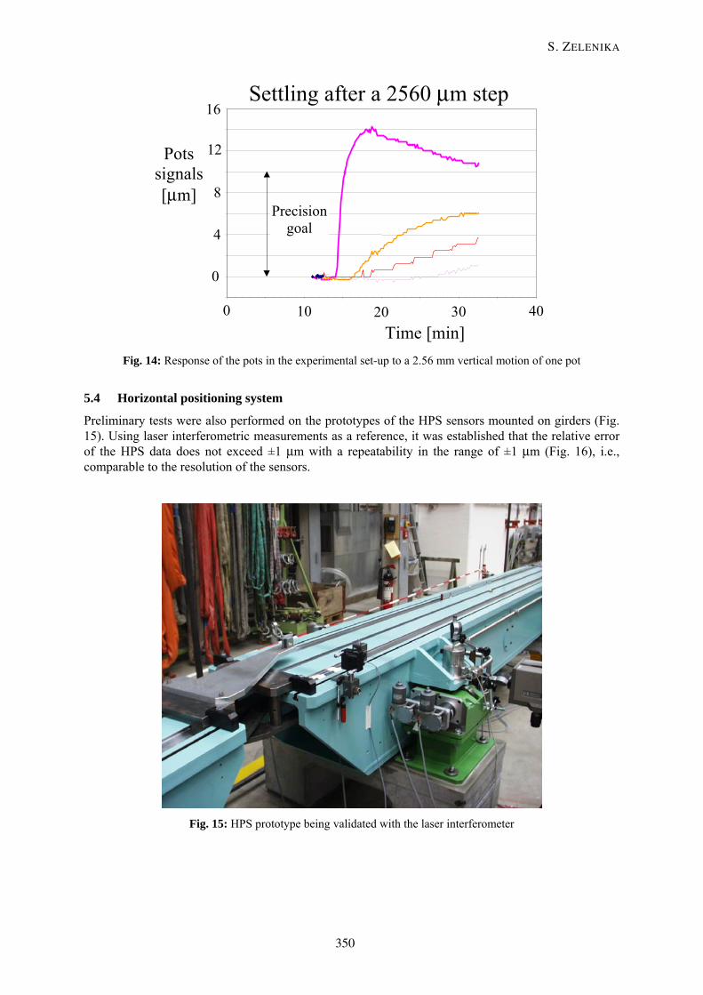
0

4

8

12

16

0 10 20 30 40 Time [min]

Precision goal

Settling after a 2560 μm step

Pots signals [μm]

Fig. 14: Response of the pots in the experimental set-up to a 2.56 mm vertical motion of one pot

5.4 Horizontal positioning system

Preliminary tests were also performed on the prototypes of the HPS sensors mounted on girders (Fig. 15). Using laser interferometric measurements as a reference, it was established that the relative error of the HPS data does not exceed ±1 μm with a repeatability in the range of ±1 μm (Fig. 16), i.e., comparable to the resolution of the sensors.

Fig. 15: HPS prototype being validated with the laser interferometer

S. ZELENIKA

350

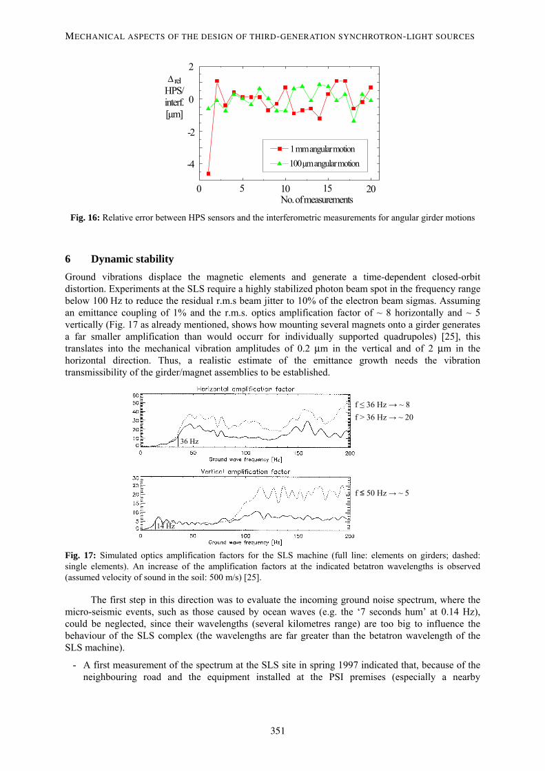
0 5 10 15 20-5000

-4000

-3000

-2000

-1000

0

1000

2000

1 mm (Anguar Motion)

0.1 mm (AnguarMotion)Re

lativ

e Er

ror H

PS/L

aser

Inte

rf.

(nm

)

Number of Measurements

2

-2

-4

0 5 10 15 20No. of measurements

1 mm angular motion100 μm angular motion

Δ relHPS/interf.[μm]

0

Fig. 16: Relative error between HPS sensors and the interferometric measurements for angular girder motions

6 Dynamic stability Ground vibrations displace the magnetic elements and generate a time-dependent closed-orbit distortion. Experiments at the SLS require a highly stabilized photon beam spot in the frequency range below 100 Hz to reduce the residual r.m.s beam jitter to 10% of the electron beam sigmas. Assuming an emittance coupling of 1% and the r.m.s. optics amplification factor of ~ 8 horizontally and ~ 5 vertically (Fig. 17 as already mentioned, shows how mounting several magnets onto a girder generates a far smaller amplification than would occurr for individually supported quadrupoles) [25], this translates into the mechanical vibration amplitudes of 0.2 μm in the vertical and of 2 μm in the horizontal direction. Thus, a realistic estimate of the emittance growth needs the vibration transmissibility of the girder/magnet assemblies to be established.

f ≤ 36 Hz → ~ 8f > 36 Hz → ~ 20

f ≤ 50 Hz → ~ 5

36 Hz

14 Hz

Fig. 17: Simulated optics amplification factors for the SLS machine (full line: elements on girders; dashed: single elements). An increase of the amplification factors at the indicated betatron wavelengths is observed (assumed velocity of sound in the soil: 500 m/s) [25].

The first step in this direction was to evaluate the incoming ground noise spectrum, where the micro-seismic events, such as those caused by ocean waves (e.g. the ‘7 seconds hum’ at 0.14 Hz), could be neglected, since their wavelengths (several kilometres range) are too big to influence the behaviour of the SLS complex (the wavelengths are far greater than the betatron wavelength of the SLS machine).

- A first measurement of the spectrum at the SLS site in spring 1997 indicated that, because of the neighbouring road and the equipment installed at the PSI premises (especially a nearby

MECHANICAL ASPECTS OF THE DESIGN OF THIRD-GENERATION SYNCHROTRON-LIGHT SOURCES

351

compressor working at a 12.3 Hz frequency), significant excitations could be induced in the frequency range below 40 Hz. In fact, under ‘natural’ excitations, amplitudes of up to 20 nm in the vertical and 40 nm in the horizontal direction were measured, while under ‘random’ events, such as weights dropped from a crane, and explosions in a nearby quarry, the maximum measured amplitudes went up to 100 or more.

- In a second phase (end 1998), a thorough vibration measurement campaign was performed on the girder prototypes checking the influence of the number of contact points and of the type of the concrete pedestal-to-metal support interface. For this purpose, the system was excited in the frequency range of man-induced vibrations (traffic, machinery, in the 10–50 Hz region) by an eccentric mass driven by a d.c. motor (Fig. 18). The results obtained with PCB Piezotronics (USA) ICP accelerometers were analysed using the corresponding mono-dimensional analytical model. Once an estimate of the stiffness and damping of the system was obtained, the transmissibility of the excitation from the ground to the system was assessed considering the theory of the vibration response of a mechanical system to the vibrations of its basement. It was thus established that, although there are some resonance peaks in the frequency range considered (mostly in the horizontal direction), the transmissibility of the system is such (< 10) that the amplitudes of the vibrations under ‘natural’ excitations should remain in the acceptable range.

- Based on the experimental results, the parameters of the numerical (FEM, Fig. 19) model mentioned were tuned, enabling further design variables (screw types at the concrete-to-metal interface, grouting of the supports, ribs in the girder body) to be investigated. It was proved that, from a dynamic point of view, the system configuration with a kinematic support arrangement, grouted supports, and with a proper fixing of the magnets onto the girder body efficiently fulfils the design goals.

- In summer 1999, measurement of the new SLS building indicated the ground motion amplitudes under natural excitations to be below 10 nm.

- In spring 2000, a vibration measurement campaign established the dynamic response of the girder system under the natural excitation coming from the ground floor in the storage ring tunnel (Fig. 20) under real operating conditions. These included the operation of the cooling and conditioning units, the crane unit, machinery in the experimental area, i.e. all equipment that could introduce additional excitation. At this stage, a thorough measurement campaign of a girder excited by an impulse hammer also allowed its eigenfrequencies and mode shapes to be accurately determined. This provided evidence that the transmissibility of the girder/magnet assembly existed [10], while its dynamics were greatly influenced by the dipoles on its ends (and the ‘cross-talk’ between neighbourhood girders) see Fig. 21. Some significant girder eigenfrequencies in the range of excitations produced by the technical devices, which are present at and around the SLS premises, have been found––especially in the 25–40 Hz range. Nevertheless, the resulting amplitudes were, in the worst case-scenario, still in the 10–30 nm range, and hence an order of magnitude below those needed to produce significant perturbations of the storage ring performances.

- In the horizontal direction, more relaxed tolerances have been given lower relevance, the vibration amplitudes of the girder assemblies are higher than those in the vertical plane, but still an order of magnitude lower than that required (Fig. 22).

- Subsequent measurements of the SLS building vibrations at various locations have clearly confirmed the very quiet conditions for the machine and the experimental floor. The vibration amplitude levels are such that the building would be suitable for tunnel electron microscopy (TEM) and scanning electron microscopy (SEM) equipment. What is clearly visible, however, is the influence of the crane, which raises the vibration amplitudes in the entire lower frequency range. On the other hand, the influence of the infrastructure equipment is negligible.

S. ZELENIKA

352

DUMMY MAGNETS

SPECTRUM ANALYSER

EXCITATION SOURCE(DC MOTOR + ECCENTRIC MASS)

ACCELEROMETERS

GIRDER BODY

orientation ofmode shape vector

Fig. 18: Experimental set-up for vibration measurements Fig. 19: FEM modal model of the girder system

Fig. 20: Spectrum of the storage ring tunnel Fig. 21: Eigenmode of the girder/magnets assembly floor and of the girder/magnet assembly evidencing the influence of the dipoles on under natural excitation – vertical plane the dynamic response

MECHANICAL ASPECTS OF THE DESIGN OF THIRD-GENERATION SYNCHROTRON-LIGHT SOURCES

353

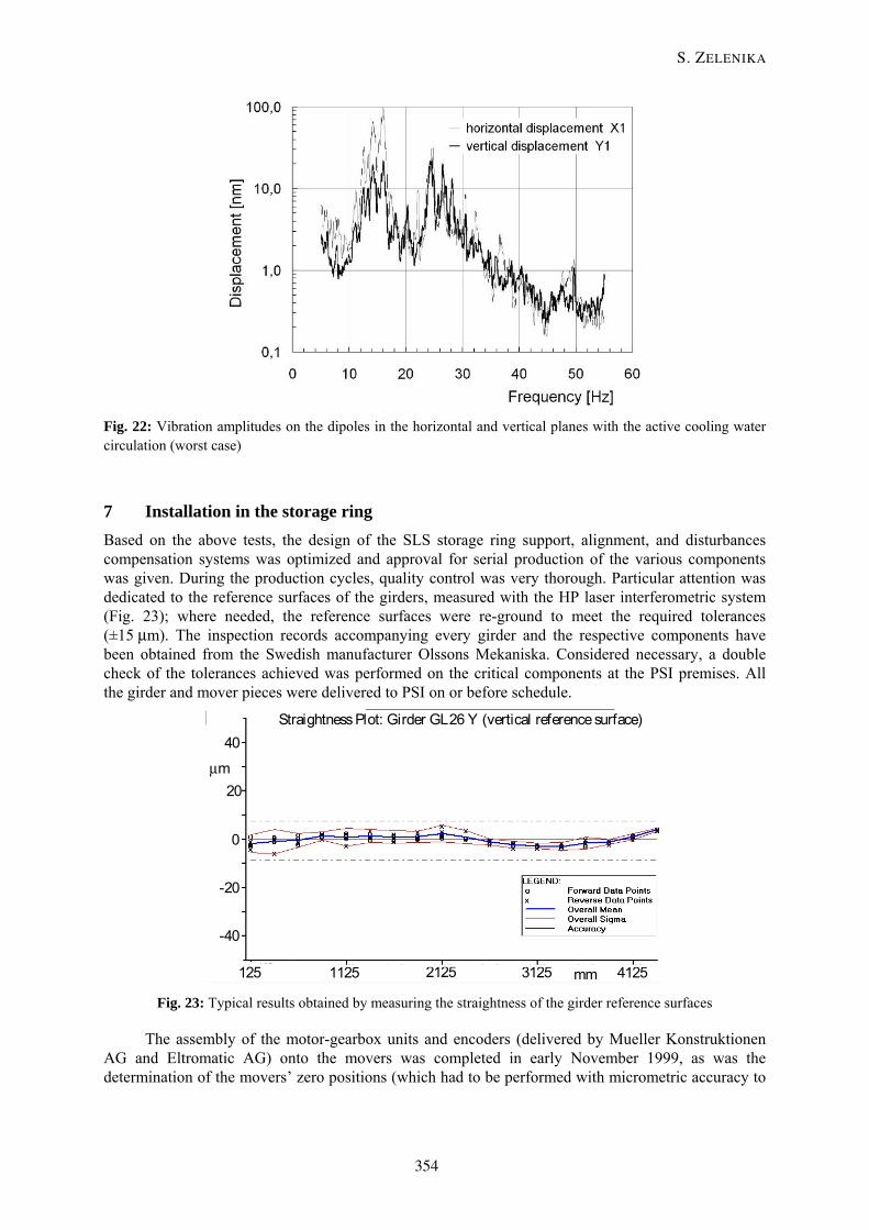
Fig. 22: Vibration amplitudes on the dipoles in the horizontal and vertical planes with the active cooling water circulation (worst case)

7 Installation in the storage ring Based on the above tests, the design of the SLS storage ring support, alignment, and disturbances compensation systems was optimized and approval for serial production of the various components was given. During the production cycles, quality control was very thorough. Particular attention was dedicated to the reference surfaces of the girders, measured with the HP laser interferometric system (Fig. 23); where needed, the reference surfaces were re-ground to meet the required tolerances (±15 μm). The inspection records accompanying every girder and the respective components have been obtained from the Swedish manufacturer Olssons Mekaniska. Considered necessary, a double check of the tolerances achieved was performed on the critical components at the PSI premises. All the girder and mover pieces were delivered to PSI on or before schedule.

40Straightness Plot: Girder GL26 Y (vertical reference surface)

μm

0

20

-20

-40

mm125 1125 2125 3125 4125 Fig. 23: Typical results obtained by measuring the straightness of the girder reference surfaces

The assembly of the motor-gearbox units and encoders (delivered by Mueller Konstruktionen AG and Eltromatic AG) onto the movers was completed in early November 1999, as was the determination of the movers’ zero positions (which had to be performed with micrometric accuracy to

S. ZELENIKA

354

allow for the proper usage of the respective software––the tools needed were developed in-house). The steel girder pedestals were concurrently mounted and grouted onto the concrete blocks, and then the movers were mounted onto the pedestals thus enabling cabling of the respective d.c. motors and of the encoders.

Towards the end of 1999 magnet delivery began. The storage ring magnets comprise 36 dipoles and 174 quadrupoles for bending and focusing, and 120 sextupoles for chromaticity correction (72 of the sextupoles have additional horizontal and vertical dipole windings for closed-orbit correction).

In each TBA there are two 0.8 m long magnets, each providing 8° of bend, and one 1.4 m long magnet bending the trajectory by 14°; the dipoles were manufactured by Tesla Engineering. Each was measured with a Hall array magnetic measurement bench showing a small spread between the magnets of each type; a full field map of a few dipoles was also obtained and used to calibrate the series measurements and the 3-D field model of the magnets [26].

The multipoles were manufactured at the Budker Institute of Nuclear Physics (BINP), Russia. Stringent requirements were placed on the location of the magnetic axes, as well as on the field quality. Each magnet was measured on a rotating coil magnetic measurement bench. After the initial measurement, the magnet pedestals were machined to bring the magnetic axe positions within the specified tolerance of ± 30 μm. After delivery to PSI, the multipoles were re-measured following the same procedure [26], see Fig. 24.

Fig. 24: BINP specialist at the SLS rotating coil magnetic measurement bench

After completion of the magnetic measurements, the magnets were mounted onto the girders and the first TBA was installed in the SLS storage ring on 9 December 1999 using a specially designed lifting tool (Fig. 25).

MECHANICAL ASPECTS OF THE DESIGN OF THIRD-GENERATION SYNCHROTRON-LIGHT SOURCES

355

Fig. 25: Mounting of the first girder/magnet assembly onto its place in the SLS storage ring

The network-based pre-alignment of the girder/magnet assemblies was carried out using the Leica Geosystems LTD500 laser tracker [27] (the SLS storage ring tunnel has 155 network reference points).

The upper parts of the yokes were removed, and the first 18 m stainless steel vacuum chambers, corresponding to one storage ring TBA or girder sector, were installed (Fig. 26). The chambers have an antechamber and contain discrete water-cooled copper absorbers to intercept most of the synchrotron radiation not transmitted to the beamlines (as the main source of gas load, the absorbers are positioned close to the pumps). It is worth noting that the vacuum chamber pieces that form one sector were initially vacuum fired up to 950°C at CERN and DESY. The vacuum sectors (including diagnostic elements and lumped pumps) with gate valves at both ends were assembled in the clean room on the SLS experimental hall, and finally baked-out for roughly a week at 250°C. No in situ bake-out and no bellows are used in the vacuum sectors (for impedance reduction reasons). For details about the SLS vacuum system refer to Ref. [28].

Fig. 26: Vacuum chamber transport from the bake-out oven to the storage ring tunnel

S. ZELENIKA

356

The installation of all the storage ring girder/magnet assemblies (including the respective water and electrical connections) and the vacuum chambers was completed in early summer 2000. In parallel to mounting the TBAs, mounting, assembly, as well as cabling and piping of the elements of the girder position monitoring systems (HPS, HLS) were carried out. To comply with safety requirements, all the HLS, HPS cabling and mover systems were completed with halogen-free cables (Fig. 27).

For the HLS, whose development was considered critical given its innovative design, a LabView-based control unit was installed in the technical gallery proving its functionality; an Oracle database to download the data acquired and its storage into the global SLS control system was successfully completed. The installation of the automatic filling station allowed the on-line filling procedure to be tested and optimized. A new series of tests was performed in the SLS storage ring. The results, obtained compared to laser-tracker and mover-encoder measurements, showed that the HLS allows reliable micrometric accuracy data with relative errors in the 1% range to be achieved. The only drawback was the relatively long settling time needed to achieve the correct readings on the heave, since in this case the water contained in the HLS pots of the moved girders has to flow in/out from the whole storage ring. In the case of pitch and roll motions, the water is basically redistributed only in the pots of the moved girder, limiting the settling times to a range of a few minutes [29].

Fig. 27: View of the SLS tunnel after installation of the storage ring elements

8 Operational experience

8.1 Girder and mover system

During the final alignment phase of the storage ring it was clear that the strut-based longitudinal girder fastening originally foreseen did not allow the desired positioning accuracies to be attained and maintained as a result of the breakage of frictional contacts. New roller bearing-based, backlash-free fastenings were developed and mounted in a very short time. These allow simple and repeatable positioning of the 9 ton girder-magnet assemblies on the micrometric scale.

A further problem encountered during alignment was electrical noise generated in the mover cables by the PWM motor power supplies adopted. This hindered the proper functionality of movers

MECHANICAL ASPECTS OF THE DESIGN OF THIRD-GENERATION SYNCHROTRON-LIGHT SOURCES

357

furthest from the mover electronics. Stabilized d.c. Kepco Bipolar Operational Power Supplies/Amplifiers BOP 36-6M (±36 V, ±6 A) have since been adopted, efficiently solving the problem.

With these two minor modifications to the original arrangement, the final alignment of the SLS storage ring allowed the positioning of whole TBAs (4 girders with up to 28 magnets mounted onto them) with micrometric accuracies within 1 to 2 days. The beam-based measurements performed during machine commissioning allowed the achievement of the required machining (girder and magnet total tolerances within ±50 μm) as well as alignment tolerances to be confirmed. In fact, SLS is probably one of the very few synchrotron radiation facilities where the very first turn of the electron beam in the storage ring was achieved with all the correctors turned off [30].

8.2 Horizontal positioning system (HPS)

The HPS has worked reliably ever since it was commissioned, allowing the correlation of beam current temperature stability in the storage ring tunnel with respect to beam stability to be assessed [31].

8.3 Hydrostatic levelling system (HLS)

Despite the excellent commissioning results cited above, the HLS readings showed millimetre range drifts on several pots after a few weeks of operation with longer time scales (Fig. 28). Some of these drifts have been traced back to poor fixing and alignment of the piping network which, with the rather high water level in the pipes at the time, led to the creation of Bernoulli tube effects (monitoring of local pressure differences between the created tube sections). However, even when additional supports were added (especially at the interface between the HLS pots and the pipes––Fig. 29), considerably improving the alignment of the piping network, the problems encountered, which were completely randomly distributed in space and time, persisted.

-0.1-0.05

00.05

0.10.15

0.20.25

0.3

1 33 65 97 129 161Pot number

Δ po

ts' r

eadi

ngs [

mm

]

Fig. 28: Relative change of the readings on all pots of the SLS storage ring during three weeks in spring 2001

S. ZELENIKA

358

Fig. 29: Additional piping fastenings at the HLS pots

It was assumed that the phenomena observed were due to the formation of a foggy layer above the water level, which could influence the respective dielectric constant. A thorough study of the theoretical aspects of the air-water mixtures has excluded this as the possible cause of the problem.

A humidity build-up at the guard-to-sensor interface of the HLS pots, inducing a parasitic capacitance, was thus postulated. Changing the material of the insulator plate with glass, quartz and different types of ceramics and inducing electronic compensation of the drifts, proved unsuccessful. Only the introduction of an O-ring between the guard and the sensor plate (hindering the humidity path to the upper parts of the pot) led to stable readings within ±10 μm over several weeks. After a few months, however, roughly half of the pots started drifting again [32].

After several attempts to tackle this problem (with very large time constants needed to attain any meaningful results) [32], a satisfactory solution was eventually obtained by adding 30% of an antibacterial fluid and alcohol solution to the HLS working fluid. Seemingly, this has killed the my-cells of the fungi observed under a microscope on the surfaces of the sensors and the guards [Fig. 30(a)], which could have been creating ‘water channels’ that induced the parasitic capacitances observed [18]. This theory cannot explain all the phenomena observed.

Nevertheless, since the adoption of the fungicide (January 2002), the HLS readings are stable to a point at which the Earth’s tides can be observed. The normal environmental variations in the SLS machine tunnel induce effects limited to 2–3 μm on the behaviour of the system. Regular shutdowns, opening of the storage ring tunnel roof to install new equipment, and human presence in the tunnel do introduce larger perturbations [Fig. 30(b)].

The recent full integration of the HLS into the SLS EPICS-based control system will now allow the study of any residual ‘parasitic’ effects, as well as the correspondence of the HLS readings with long-term survey data.

MECHANICAL ASPECTS OF THE DESIGN OF THIRD-GENERATION SYNCHROTRON-LIGHT SOURCES

359

SENSORPLATE

O-RING

MY-CELLS

Data Relative to Average of Sect. 1, 4, 7, 10

-0.06

-0.04

-0.02

0

0.02

0.04

0.06

12.1.03 26.1.03 9.2.03 23.2.03 9.3.03 23.3.03Date

Lev

el [m

m]

HLS1-1G3HLS1-4G3HLS1-7G3HLS1L-10G4

Shut-down Shut-downShut-down

(a) (b)

Fig. 30: My-cells observed on the HLS pots (a) and the results obtained after the adoption of a fungicide (b)

8.4 Dynamic stability

Beam-based measurements performed using the digital BPMs mentioned confirmed the girder eigenfrequency shown above and corresponding vibration amplitude measurements [33]. Furthermore, a vibration measurement campaign performed at the end of 2002 as part of a CERN PhD thesis confirmed the data (Fig. 31). Thanks to the low transmissibility of the girder structures (< 10 in the vertical and < 20 in the horizontal direction), the installation of new beamline equipment, including several additional excitation sources, did not induce any meaningful perturbations to the storage ring optics or to the photon beam [34].

Fig. 31: Vibration amplitudes on the storage ring elements obtained late 2002

9 Conclusions Although some minor upgrades have been necessary, the SLS storage ring support, positioning and position monitoring systems, optimized by thorough analytical, numerical, and experimental assessments, have been successfully installed and commissioned, allowing a significant reduction of the alignment time spans to be obtained. The system’s effective and sophisticated design has so far given excellent results at the SLS. This has led to the creation of all the preconditions for beam-based storage ring dynamic alignment (allowing the potential optimized use of the corrector magnet) when

S. ZELENIKA

360

linked to the diagnostics data. The design is further validated by the high degree of interest shown by other synchrotron radiation facilities (SLAC, DIAMOND, CLS, SOLEIL, APS, ELISA, etc.) to adopt similar solutions.

In the end, it is important to note that the role of mechanical engineering at the synchrotron light sources extends much further than storage-ring support, positioning, and position monitoring systems [35]. In the case of the SLS project, the Mechanical Engineering Group had to design several beamline components or whole beamlines (e.g., diagnostic beamline X05DA), organize the design, production and follow-up of several critical machines (e.g., third harmonic superconducting RF system), insertion device (including in-vacuum devices) and beamline components (the first set of four SLS insertion devices and beamlines had very active involvement of the SLS Mechanical Engineering) outsourced to external companies. In this process, the group has mastered the skills to deal with complex tasks, such as:

- advanced design of ultra-high vacuum (UHV) and radiation compatible, high-heat load and high-precision equipment and instrumentation;

- analytical and numerical modelling of structural (static and dynamic, as well as modal), thermal, non-linear (buckling, contact, large displacements), and transient problems;

- experimental techniques such as the Michelson-type heterodyne laser interferometric measurements mentioned in the linear (resolution down to 10 nm), angular (resolution: 0 05. ′′ ) and straightness (resolution: 10 nm) optical configurations, as well as vibration measurements on machine and beamline (including optical) components;

- a key competence, original approaches to the analytical modelling and experimental assessment of the performances of UHV-compatible, ultra-high precision devices.

Such skills are proving to be very valuable in the upgrades of the machine (e.g., the femto-second project) as well as for the development of new SLS beamlines.

Although the role of ‘non-physics’ (vacuum, alignment, mechanical, electrical) experts in the development of new synchrotron radiation facilities is sometimes underrated, all of the above clearly proves that such complex projects require an interdisciplinary approach, where the expertise of all the personnel involved is of vital importance.

Acknowledgements The author would like to thank all the members of the PSI crew as well as external personnel and suppliers that have helped with the ideas, development, manufacturing, assembly and commissioning of the systems described.

References [1] Proc. 1st Int. Workshop Mech. Eng. Des. SR Equip. Instr. (MEDSI 2000), Villigen, 2000.

[2] Proc. 2nd Int. Workshop Mech. Eng. Des. SR Equip. Instr. (MEDSI 2002), Argonne, 2002.

[3] Proc. 3rd Int. Workshop Mech. Eng. Des. SR Equip. Instr. (MEDSI 2004), Grenoble, 2004.

[4] G. Margaritondo, Experiments with synchrotron radiation: basic facts and challenges for accelerator science, these Proceedings.

[5] P. Elleaume, Present limits and future developments of storage ring synchrotron sources, Proc. 8th Int. Conf. SR Instr. (SRI 03), San Francisco, 2003.

[6] C. J. Bocchetta, Beam quality and lifetime, these Proceedings.

MECHANICAL ASPECTS OF THE DESIGN OF THIRD-GENERATION SYNCHROTRON-LIGHT SOURCES

361

[7] C. J. Bocchetta, Closed orbit stability, these Proceedings.

[8] A. Streun, Lattices and emittances, these Proceedings.

[9] A. F. Wrulich, Proc. 1999 Part. Accel. Conf. (PAC 99), New York, 1999, p. 192.

[10] M. Böge, Paul Scherrer Institut Sci. Rep. 1998, Vol. VII, 1999, p. 15.

[11] R. E. Ruland, Proc. 4th Int. Workshop Accel. Align., Tsukuba, 1995, p. II/233.

[12] J. Brnic, Nauka o cvrstoci, University of Rijeka, Rijeka, 1991.

[13] M. Böge et al., Proc. 6th Eur. Accel. Conf. (EPAC 98), Vol. 1, Stockholm, 1998, p. 644.

[14] G. Bowden et al., SLAC-PUB-95-61326132, 1995.

[15] A. H. Slocum and A. Donmez A., Prec. Eng. 10 No. 3 (1988) 115.

[16] R. Kramert, Girder Mover Encoder Readout - Technical Specification, PSI Publ., 2000.

[17] D. Roux, Proc. 1st Int. Workshop Accel. Align., Stanford, 1989, p. 37.

[18] E. Meier et al., Hydrostatic Levelling System – Service Guide, E. Meier & Partner, Switzerland 2002.

[19] A. Streun, Swiss Light Source-TME-TA-2000-0152, 2000.

[20] V. Schlott, Paul Scherrer Institut Sci. Rep. 1998, Vol. VII, 1999, p. 19.

[21] V. Schlott, Paul Scherrer Institut Sci. Rep. 1999, Vol. VII, 2000, p. 25.

[22] P. Wiegand, Swiss Light Source-TME-TA-2000-0145, 2000.

[23] E. Meier, Messresultate 100 m Test, E. Meier & Partner, 2000.

[24] D. Roux, A New Alignment Design - Application of ESRF Storage Ring, ESRF Publ.

[25] M. Böge et al., Proc. 1999 Part. Accel. Conf. (PAC 99), New York, 1999, p. 1542.

[26] L. Rivkin, Paul Scherrer Institut Sci. Rep. 1999, Vol. VII, 2000, p. 13.

[27] F. Q. Wei et al., Paul Scherrer Institut Sci. Rep. 1999, Vol. VII, 2000, p. 30.

[28] L. Schulz, Vacuum aspects, these Proceedings.

[29] S. Zelenika et al., Paul Scherrer Institut Sci. Rep. 2000, Vol. VII, 2001, p. 30.

[30] A. Streun, Paul Scherrer Institut Sci. Rep. 2000, Vol. VII, 2001, p. 12.

[31] V. Schlott, Paul Scherrer Institut Sci. Rep. 2001, Vol. VII, 2002, p. 28.

[32] S. Zelenika, Paul Scherrer Institut Sci. Rep. 2001, Vol. VII, 2002, p. 30.

[33] V. Schlott et al., Proc. 2001 Part. Accel. Conf. (PAC 01), Chicago, 2001, p. 2397.

[34] J. Krempansky and M. Dehler, Paul Scherrer Institut Sci. Rep. 2002, Vol. VI, 2003, p. 38.

[35] S. Zelenika et al., Mechanical engineering at the Swiss Light Source, 3rd SLS Users’ Meeting, Villigen, Switzerland, 2002.

S. ZELENIKA

362

Participants

ALESINI, D. INFN-LNF, Frascati, IT

BAILEY, C. Diamond Light Source Ltd., Didcot, GB

BALDWIN, A. Diamond Light Source Ltd., Didcot, GB

BOKSBERGER, H.U. Paul Scherrer Institut, Villigen, CH

BOSCOLO, M. INFN-LNF, Frascati, IT

CANDEL, A. ETHZ, Zurich, CH

CHAN, C.K. NSRRC, Hsinchu, TW

CHIADRONI, E. Univ. of Rome ‘Tor Vergata’, Rome, IT

CHOUHAN, S. FKZ GmbH, Karlsruhe, DE

CHRISTOU, C. Diamond Light Source, Didcot, GB

DI MITRI, S. Sincrotrone Trieste S.C.p.A., Trieste, IT

FACCHINI, M. CERN, Geneva, CH

FUSCO, V. INFN-LNF, Frascati, IT

GASPAR, M. Paul Scherrer Institut, Villigen, CH

GEORGSON, M. Danfysik A/s, Jyllinge, DK

GOUGH, C. Paul Scherrer Institut, Villigen, CH

GRIMM, O. DESY, Hamburg, DE

HOBL, A. ACCEL Instruments GmbH, Bergisch-Gladbach, DE

DE JENSEN, M. Diamond Light Source Ltd, Didcot, GB

KAZIMI, R. Thomas Jefferson National Accelerator Facility, Newport News, US

KELLER, A. Paul Scherrer Institut, Villigen, CH

KNAPIC, C. Sincrotrone Trieste S.C.p.A., Trieste, IT

KORHONEN, T. Paul Scherrer Institut, Villigen, CH

KOUBYCHINE, I. Tech. Univ. of Catalonia, Barcelona, ES

KREMPASKY, J. Paul Scherrer Institut, Villigen, CH

KUBSKY, S. ACCEL Instruments GmbH, Bergisch-Gladbach, DE

LEEMANN, S.C. Paul Scherrer Institut, Villigen, CH

LUCAS, J. CERN, Geneva, CH

MARCOUILLE, O. Synchrotron SOLEIL, Gif-sur-Yvette, FR

MARGOTO, E. Thales Electron Devices, Velizy, FR

MILTCHEV, V. DESY, Zeuthen, DE

363

MIRALLES, L. Laboratorio Luz Sincrotron, Cerdanyola del Valles, ES

MORGAN, A. Diamond Light Source Ltd., Didcot, GB

MORNACCHI, G. CERN, Geneva, CH

PAPAPHILIPPOU, I. ESRF, Grenoble, FR

PARALIEV, M. Paul Scherrer Institut, Villigen, CH

PEDROZZI, M. Paul Scherrer Institut, Villigen, CH

PERRON, T. ESRF, Grenoble, FR

POTTIN, B. Synchrotron SOLEIL, Gif-sur-Yvette, FR

PRADO DE ABREU, N. CRNS, Campinas, BR

PUGACHOV, D. DESY, Hamburg, DE

QUAST, T. BESSY GmbH, Berlin, DE

RAGUIN, J.-Y. Paul Scherrer Institut, Villigen, CH

REHM, G. Diamond Light Source Ltd., Didcot, GB

ROLLASON, A. Keele University, Newcastle-under-Lyme, GB

SCHWERG, N. TU Berlin, Berlin, DE

SERAYDARYAN, H. CANDLE, Yerevan, AM

SERRIERE, V. ESRF, Grenoble, FR

SETSHEDI, R. Univ. of Witwatersrand, Mafikeng, ZA

SILZER, R. Canadian Light Source, Saskatoon, CA

SUETTERLIN, D. Paul Scherrer Institut, Villigen, CH

TANNER, R. Canadian Light Source, Saskatoon, CA

TARAWNEH, H. Lund University, Lund, SE

THOMAS-MADEC, C. Synchrotron SOLEIL, Gif-sur-Yvette, FR

TROVO, M. Sincrotrone Trieste, Basovizza, IT

VARLEY, J. CCLRC Daresbury Laboratory, Warrington, GB

WERBER, R. Inst. f. Biophysik, Koeflach, AT

WYLES, N. CLRC Daresbury Laboratory, Warrington, GB

364