At

Aa

b

a

ARRAA

KWMPPC

1

itpqvhpcmtabtd

0d

Analytica Chimica Acta 660 (2010) 8–21

Contents lists available at ScienceDirect

Analytica Chimica Acta

journa l homepage: www.e lsev ier .com/ locate /aca

nalysis and assessment of Madeira wine ageing over an extended time periodhrough GC–MS and chemometric analysis

na C. Pereiraa,b, Marco S. Reisa, Pedro M. Saraivaa, José C. Marquesb,∗

Departamento de Engenharia Química, Universidade de Coimbra, Pólo II, Rua Sílvio Lima, 3030-790 Coimbra, PortugalCentro de Química da Madeira, Departamento de Química, Universidade da Madeira, Campus Universitário da Penteada, 9000-390 Funchal, Portugal

r t i c l e i n f o

rticle history:eceived 7 August 2009eceived in revised form 4 November 2009ccepted 5 November 2009vailable online 12 November 2009

eywords:ine ageingultivariate analysis

rincipal component analysisartial least squares discriminant analysislassification

a b s t r a c t

Wine is one of the world’s higher value agricultural products. The present work is centred on Madeirawine, a fine and prestigious example among Portuguese liqueur wines,with the main goal to deepenour understanding of relevant phenomena going on during the winemaking process, in particular duringageing of “Malmsey” Madeira wine.

In this paper we present the results obtained from the chemical characterization of how its aroma com-position evolves during ageing, and the development of a robust framework for analyzing the identity ofaged Madeira wines. An extended ageing period was considered, covering a time frame of twenty years,from which several samples were analyzed in terms of their aromatic composition. The multivariate struc-ture of this chemical information was then processed through multivariate statistical feature extractiontechniques such as principal component analysis (PCA) and partial least squares discriminant analysis(PLS-DA), in order to identify the relevant patterns corresponding to trends associated with wine ageing.

Classification methodologies for age prediction were developed, using data from the lower dimensionalsub-spaces obtained after projecting the original data to the latent variable spaces provided by PCA orPLS-DA. Finally, the performance for each classification methodology developed was evaluated accord-ing to their error rates using cross-validation methodologies (Leave-One-Out and k-fold Monte Carlo).Results obtained so far show that quite interesting classification performances can indeed be achieved,despite the natural variability present in wine products. These results also provide solid bases which can

ble fr

be used to build up availa

. Introduction

The wine industry needs analytical tools to verify the authentic-ty of its high value products in order to protect wine brands. Theseools ideally should allow for a rapid and inexpensive analysis at anyoint in the distribution chain [1,2]. In the particular case of highuality wines, they are required to warrant origin and identity, pro-iding means for analytical control focused on protecting consumerealth and prevent fraud. The latter phase of the wine productionrocess—ageing, deserves special attention and calls for strict pro-ess control. Most wines are consumed after a period of ageing thatay take place in different reservoirs, such as wooden casks, bot-

les, or both, during which the wine’s identity is established. This

geing process implies a significant financial overhead that muste recovered in the final price of the wine [3]. Moreover, nowadayshe typical wine consumer is increasingly more knowledgeable andemanding, requiring the wine to be fully documented and authen-

∗ Corresponding author. Tel.: +351 291705103; fax: +351 291705149.E-mail address: marques@uma.pt (J.C. Marques).

003-2670/$ – see front matter © 2009 Elsevier B.V. All rights reserved.oi:10.1016/j.aca.2009.11.009

ameworks which assist quality monitoring and identity assurance tasks.© 2009 Elsevier B.V. All rights reserved.

ticated with respect to its production and ageing process. Giventhese premises, it should be now clear how the development ofmethods to classify aged wines becomes of central importance. Inorder to develop such methods, reliable techniques for the analysesof several chemical and physical parameters should be optimized,followed by the application of proper multivariate statistical anal-ysis methods, namely those usually falling under the heading ofchemometrics [4–9]. In fact, the relatively large number of studiescarried out in the scope of the present investigation, underlines thecentral importance of multivariate statistical analysis in order toachieve a better understanding of the process, enabling its analysis,improvement and monitoring.

“Malmsey” Madeira wine is a well known fortified wine distin-guished for its superior quality which results from the “MalvasiaCandida” grape variety attributes, and from the peculiar wine pro-cess used. This is a sweet fortified wine (residual sugar above

96.1 mg L−1 and alcohol content ranging from 17 to 21%, v/v) whichundergoes a long oxidative ageing period during which some aromacompounds that play an outstanding role in its sweet aroma notesare developed. Among the recommended grape varieties used inMadeira Island, “Malvasia Candida” assumes a prominent position.

a Chimica Acta 660 (2010) 8–21 9

Ispitsuathwh

ehswmtMcuwpi[scawicifstlbmfrvao

aowmtac2ottmidcafttau

Table 1Wine samples analyzed and respective notation used.

Harvest year Samples Notation Harvest year Samples Notation

1988 A 88A 2000 A 00AB 88B B 00B

1990 A 90A C 00CB 90B 2002 A 02A

1992 A 92A B 02BB 92B C 02C

1994 A 94A 2004 A 04AB 94B B 04BC 94C C 04C

1996 A 96A 2006 A 06AB 96B B 06B

A.C. Pereira et al. / Analytic

t was one of the first varieties to be planted in Madeira Island andtill being produced. Growing on steep terraces all over the island,referentially at lower altitudes, its early harvest grape-gathering

s mostly done manually. The wine making process is similar tohat used in the production of other fortified wines (fermentationtopped according to the desired residual sugar), followed by a mat-ration period in wooden casks. The best wines and all the vintagesre treated with the Canteiro method which basically consists ofransferring the casks containing the young fortified wine to theigher floor (under the roof), where it will be exposed to naturalarmth (temperatures ranging between 30 and 35 ◦C) and highumidity levels (70–75%).

Notwithstanding the significant amount of empirical knowl-dge about Madeira wine production, the increasing demand forigher quality in the current global markets calls for studies thatupport the necessary quality improvement activities, consistentith the prestigious position achieved by Madeira wines, whichakes it a product of high economic value. Therefore, in this study,

he research goals focus on two important issues related to theadeira wine ageing process, namely: (i) to analyze the aroma

omposition and its evolution through this phase, and then (ii) tose such information in order to develop a classification frame-ork which will allow for the proper assessment of the wine ageingeriod. In this context, it is widely recognized that the wines’ aroma,

s a major contributor to the overall perception of wine features10], being a complex result of contributions arising from manyources, such as: grape variety, yeast population and microbiologi-al fermentation and post-fermentation treatments, including oakgeing and bottle storage. There are several good reviews available,hich provide detailed information on the chemical components

nvolved in wine flavour [11]. In this research study, wine aromaompounds were chosen to establish the criteria of genuinenessn order to characterize and differentiate Madeira wines producedrom “Malvasia Candida” at different ageing periods. Among all theets of variables that could be considered, wine volatile composi-ion has been pointed as a primary choice, because it includes aarge amount of information obtained inexpensively and fast, andecause it is related to the wine flavour characteristics. Further-ore, the wine volatile composition is also influenced by numerous

actors, reflecting in some sense the whole history of the wine, aseported extensively in the literature [12–14]. To sum up, wineolatile composition is a rich source of information for establishingconsistent control of authenticity, allowing the proper assessmentf the origin or grape variety of very different wine samples [15].

Finding the natural ‘tracers’ of ageing, i.e., those subsets of vari-bles strongly dependent on ageing time and almost independentf other factors, is far from being a trivial task, and in this paper,e present the results obtained in the development of an analyticalethodology coupled with the analysis of the large amounts of data

hus generated, in order to come up with a robust framework fornalyzing the identity of aged Madeira wines. Extraction of chemi-al information is described in Sections 2.2 and 2.3. Next, in Section.4 a description of pattern recognition techniques is provided, inrder to understand the relationships between chemical data struc-ure and the samples under study, and furthermore to establish howhe extracted features may be used in the context of a classification

ethodology. Section 3, is devoted to the illustration and compar-son of the obtained results. First, in Section 3.1, the exploratoryata analysis carried out is presented; next, in Section 3.2, principalomponent analysis and partial least squares discriminant analysisre applied as feature extraction methods, and data analysis per-

ormed on their outcomes; classification models resulting from theransformed variables (principal components) and from sampleshat constitute the training set are presented in Section 3.3. Finally,nd in the absence of a test set, the developed models are validatedsing cross-validation methodologies (‘Leave-One-Out’ and k-fold

C 96C C 06C1998 A 98A

B 98B

Monte Carlo), in order to evaluate their predictive reliability of theclassification models achieved.

2. Experimental

2.1. Wine samples

A total of 26 wine samples of known ageing periods, kept undersimilar conditions during and after the wine making process, wereanalyzed. The harvest years cover a time frame of twenty years,ranging from 1988 until 2006, in intervals of 2 years. The wineswere produced with the Malvasia grape variety, and were collecteddirectly from cellars, to ensure that they do consist of a single grapevariety. Table 1 presents all samples analysed and the respectivenotation used in this text. Samples are denoted by harvest year andby a letter to distinguish different wines from the same harvestyear. To further distinguish the replicates analysis carried out, weuse the numbers 1 and 2 at the end of these words. Each harvestyear consists of a class label, for classification purposes. Therefore,we are addressing a 10 class classification problem, which mightbe a quite demanding data analysis task, given the relatively lowratio of samples per class.

2.2. Chemical analysis and analytical methods employed

The analysis of volatile compounds such as aromas is a contin-uous challenge in the food and beverage industry. Several studieshave been carried out in order to develop, test and optimize sam-ple extraction and preparation procedures prior to instrumentalanalysis depending on the matrix and analyte, as well as on therequired accuracy (quantitative or qualitative). The complexity ofthe volatile fraction of Madeira wine, the high alcohol content andthe likely low concentration levels for its key odorants do require anoptimized sample preparation, not only to reduce the time taken toprocess them, but because each step adds a potential source of error.Of different isolation and pre-concentration possibilities, solidphase extraction has been reported as being able to analyze com-pounds present at relatively high concentrations in a single run, ofover 0.1 mg L−1 (such as higher alcohols and some of their acetates,fatty acids and their ethyl esters) and also compounds present atlow concentration levels, between 0.1 �g L−1 and 0.1 mg L−1 (forexample, volatile phenols, some lactones, vanillin derivates, someminor esters and nor-isoprenoids) [16,17]. The great enrichmentof the aromatic compounds in the extract by using a small quan-

tity of organic solvent, the possibility of selecting the most adequatesolid phase according to the analytes under study, and the ability toextract several samples simultaneously, consubstantiate its choicewhen the screening of wine aroma is intended [18,19]. Therefore,in this study, the screening of volatile compounds was carried out

1 a Chim

u[Miazptosts1t(dw

2

giioawtru((p

tlmc

2

tToictasMcamarchina

pdr

0 A.C. Pereira et al. / Analytic

sing the solid phase extraction method proposed by López et al.16], which was also later used in a quantitative chemical study of

adeira wine aimed at providing an odorant classification accord-ng to their potential sensory role [20]. In accordance with theforementioned method, the polymer of poly-(styrene-divinyl ben-ene) was selected as a reverse phase sorbent, of which 120 mg wasacked in a 6 mL cartridge and, in the extraction unit, were condi-ioned with 4 mL of dichloromethane, 4 mL of methanol and 4 mLf a ethanol–water solution mixture (18%, v/v). Then 50 mL of winepiked with 25 �L of 3-octanol (internal standard) were passedhrough the sorbent approximately at 2 mL min−1, followed using amall flow of air. Finally, analytes were recovered upon elution with.3 mL of dichloromethane/methanol solution (75%:25%), in ordero ensure that some characteristics of Madeira wine compoundssuch as furanic aldehydes) were retained. The extract was thenried with sodium sulphate and kept at −20 ◦C until the analysisas done.

.3. Gas chromatography–mass spectrometry analysis

The extracts were injected into 6890N (Palo Alto, CA, USA)as chromatograph equipped with an Agilent 5975 quadrupolenert mass selective detector. 1 �L of extract was vaporized in thenjector port maintained at 220 ◦C in splitless mode (1 min). Theven temperature was raised from 40 ◦C to 220 ◦C at 3 ◦C min−1

nd finally kept at 220 ◦C for 10 min. A 30–300 m/z mass rangeas recorded in full-scan mode. The quadrupole ion source and

ransfer line temperatures were maintained at 150 and 250 ◦C,espectively, and the ionisation energy was set to 70 eV. The col-mn (30 m × 0.25 mm i.d., and 0.25 �m film thickness) was a BP-20WAX) from SGE (Austin, TX, USA). The carrier gas was heliumhelium N60, Air Liquid, Portugal) at 1 mL min−1 (column-headressure of 13 psi).

The identification of compounds was made by comparison ofhe mass spectra obtained with those present in the NIST05 MSibrary database, using the Kovats indexes. A C8–C20 n-alkanes

ixture (Sigma, St. Louis, MO, USA) was analysed under the samehromatographic conditions to calculate Kovats indexes.

.4. Data analysis

In this stage, a large amount of data is available as a result ofhe analytical measurements carried out over the wine samples.heir structure call for adequate multivariate data analysis meth-ds, in order to find and summarize typical trends and patternsn the observations (samples) and variables (compounds). In thisontext, apart from the always important interpretation of pat-erns extracted during the preliminary stage of exploratory datanalysis, there are two central goals to be addressed in this work,pecifically regarding our statistical classification framework: (i)odel selection – to estimate the performance of different classifi-

ation methodologies in order to choose the most promising onesnd (ii) final model assessment – in which the performance of theodels, namely their estimated classification error rates (gener-

lization error rates), are computed, in order to establish a finalanking of the methods studied, regarding their reliability in thelassification of wine ageing periods. In fact, despite the relativelyigh number of variables, we are not in a data-rich situation regard-

ng the number of samples, and to reach the aforementioned goals,amely the second one, it is necessary to adopt a cross-validation

pproach (to be described in more detail later on in the text).

All data analysis tasks were performed in the computationallatform MatLab (version 7.6, The Mathworks, Inc.), and will beetailed in the next section, along with the presentation of theesults achieved.

ica Acta 660 (2010) 8–21

2.4.1. Feature extraction methodsThe great amount of information produced by modern analyti-

cal instruments and the need for compressing and extracting theirinformation content, in order to retain what is essential, is recurrentproblem, for which several statistical and computational method-ologies are currently available. Looking at data sets or examiningone variable at a time, are not valid alternatives for analyzing datatables such as those generated in food quality assessment, finger-printing, profiling, authentication and detection of adulteration,among others. This happens to be so, because much of the infor-mation that is useful for understanding the essential features ofthe systems, is found in the variables correlations, and therefore oneshould avoid blindly discarding data, or analyzing variables one-by-one, or selecting sub-sets of variables using univariate criteria [21].The selected methodologies must be able to extract the system-atic information about the system, while handling multicollinearityproblems and unwanted variation (noise). Several multivariate sta-tistical methods are well suited for dealing with these features andthereby reducing the risk of incorrect inferences in a large data set,some of which will be employed in this work, and will be describedin the next paragraphs.

In order to extract patterns from complex multivariate data sets,a preliminary step of dimension reduction is often required, wherean unsupervised learning methodology such as principal compo-nent analysis (PCA) is applied to transform and reduce the originalnumber variables. PCA is an effective tool for identifying system-atic patterns such as clusters and time trends hidden in the originalhigh-dimensional variables space, being also useful for establish-ing a new set of variables, the principal components, to be subjectof further modelling efforts. Alternatively, the structure of highdimensional data sets can also be explored with supervised learningmethodologies such as partial least squares for discriminant anal-ysis (PLS-DA) and Fisher discriminant analysis (FDA), where priorinformation such as class membership of the samples, is requiredin order to compress the original dimensional space, through newvariables with enhanced discriminating characteristics.

2.4.1.1. Principal component analysis. Principal component analy-sis forms the basis for multivariate data analysis. In PCA, raw dataconsist of a matrix X(n × m), is represented in a new co-ordinatesystem defined by the principal components (PC). The direction invariables space exhibiting most of the data variability defines thelocation of the first PC. The second PC will coincide with the direc-tion of largest variability, which is orthogonal to the direction offirst PC. New PCs can be extracted in this way, until only a residualpart of the original data variability is left to be explained by theset of computed PCs. Each PC (with index say, a) consists of a score(ta) and loading vector (pa), in such a way that the variability in Xis summarized as a product of two low-dimensional space matri-ces T(n × m) and P(m × A), given by Eq. (1) (A is the number of PCsretained), which may be overviewed and used.

X = t1pT1 + t2pT

2 + · · · + tApTA + E = TPT + E (1)

Mathematically, this procedure relies on an eigenvector decom-position of the correlation matrix (or covariance matrix, accordingto the scaling option), ˙x, through which the loading matrix isobtained from the eigenvectors thus obtained, sorted according toa decreasing order of magnitude of the eigenvalues (�a, 1:m)

˙xpa = �apa (2)

The score vector (ta) correspond to the linear combination of the

original X data defined by (pa) (orthonormal)

ta = ˙xpa (3)

All score vectors form together an orthogonal set [22–24]. Thepart of the data matrix not explained by the PC model is contained

a Chim

itws

2wdpdiwditfomacitWdssa

X

Y

U

Ip

(

(

(

(

(

(

(

baoi

p

w

t

A.C. Pereira et al. / Analytic

n the residual matrix E(n × m), which contains information abouthe distance from each observation to the estimated PCA model,hich is easily obtained by taking the square root of the sum of

quares of the elements in each row.

.4.1.2. Partial least squares for discriminant analysis. Although PLSas not inherently designed for problems of classification andiscrimination, it is routinely used with some success for such pur-oses [25,26]. In its simplest form, PLS is a method for relating twoata matrices, say X and Y, through a linear multivariate model. The

dea is to relate a response variable (y) or a matrix of responses Yith the predictor variables of the X matrix. Matrix X is successivelyeflated as in PCA, but now, instead of finding those directions max-

mizing data variability in the X-space, PLS seeks the directions inhe X- and Y-spaces corresponding to the maximum covariance. PLSorms “new X-variables” (ta) as linear combinations of the originalnes, which will then be related to the Y-scores through a linearodel. For each component (a), the parameters (ta), (ua), (w∗

a), (pa),nd (ca) are determined by the PLS algorithm, but they can also beomputed from the matrix (XTY)(YTX) [24,27]. The PLS algorithm,nitially developed by Herman Wold and called nonlinear itera-ive partial least squares (NIPALS), was later on modified by Svante

old and Harald Martens to better handle the large ill-conditionedata sets found in chemistry and related fields. In this case, PLS alsotands for projections to latent structures, by means of partial leastquares, first modelling X and Y (outer relations, Eqs. (4) and (5)),nd then predicting Y from X (inner relation, Eq. (6)):

= t1pT1 + t2pT

2 + · · · + tmpTm = TPT + E (4)

= u1qT1 + u2qT

2 + · · · + umqTm = UCT + F (5)

= BT (6)

NIPALS does not calculate all of the linear combinations at once.n order to improve the inner relationship the strategy encom-asses the following steps:

1) ustart = some yj; (7)

2) wT = tTX

tTt; (8)

3) wTnew = wT

new∥∥wTold

∥∥ ; (9)

4) t = Xw

wTw; (10)

5) qT = tTY

tTt; (11)

6) qTnew = qT

old∥∥qTold

∥∥ ; (12)

7) u = Yq

q′q; (13)

These steps are performed iteratively, until the differenceetween successive t’s in steps (2) and (4) becomes smaller thanuser specified tolerance. Note that this algorithm does not give

rthogonal t values. If such is intended, an extra loop could bencluded in which wT are replaced by pT [23,26–30]:

T = tTXT

being pTnew = pT

old∥T

∥ and tTnew = tT

old∥T

∥ (14)

t t ∥pold

∥ ∥told∥

ith

old = Xp

pTp(15)

ica Acta 660 (2010) 8–21 11

PLS-DA is an extension of PLS, with the objective of extending itsapplication from a regression scenario, to a classification one, wherea model is sought that separates the several classes of observationson the basis of their X values. In PLS-DA, the Y matrix (n × g) encodesclass membership by a set of “dummy” variables, in such way that, ifthe ith observation belongs to class k, then there will be a “1” in thekth column “0” in all the others. A regular PLS model is then fittedbetween X and the artificial Y matrix, and in this way dicriminantdirections can be found in the X-scores, in which their observationsappear well separated according to class membership [21,30–32].

2.4.2. Classification methodologiesClassification is one of the fundamental methodologies used in

pattern recognition problems, aiming to find a mathematical modelcapable of recognizing the membership of each object under analy-sis. Once a classification model has been obtained, the membershipof new objects to one of the defined classes can be predicted. Sev-eral multivariate classification methods have been proposed in theliterature. With the purpose of discriminating among classes andto build a model with all the categories concerned in the discrimi-nation, a parametric methodology as well as a non-parametric onewere applied in this study, namely the linear discriminant analysis(LDA, or linear classifier) and k-nearest neighbours (kNN), respec-tively.

Being a parametric technique linear discriminant analysis, relieson the estimation of statistical parameters for the assumed classdistributions of objects (a normal distribution is assumed), leadingto the derivation of a linear decision function aTX that maximizesthe ratio of between-class variance to within-class variance, whenthe covariance matrices of the class dependent distributions areassumed to be equal:

âT(∑k

i=1(xi − x)(xi − x)T)â

âT[∑k

i=1

∑nij=1(xij − xi)(xij − xi)

T]â= âTBâ

âTWâ, (16)

where xi (p × 1) is the sample mean vector of classe i and x themean vector of the combined kclasses. The mth linear discrim-inants are given by m ≤ min(k − 1,p) eigenvectors correspondingto nonzero m eigenvalues of W−1B. LDA also hypothesizes thatthe variance–covariance matrices of the classes established can bepooled. Consequently,

W

n1 + n2 + · · · + ng − g= Spooled, (17)

so that âTBâ/âTSpooledâ also maximizes âTBâ/âTWâ.If the linear function between two classes involves two or more

independent variables (p) the linear function correspond to a planeinstead of a straight line. In both cases, an observation x is allocatedto class k if

r∑

j=1

[âTj (x − xk)]

2 ≤r∑

j=1

[âTj (x − xi)]

2(18)

The non-parametric methodology of k Nearest Neighboursclassification (kNN), do not assume any underlying probability dis-tribution for the observations. kNN employs a metric of distancefor selecting the k nearest objects to the sample to be classified,and once the k nearest objects are found the sample is classified tothe category in which the majority of objects selected belong [33].Usually the Euclidean distance is used (Eq. (19)), but for stronglycorrelated variables, correlation-based measures are preferred.

DE = [(xi − �k)2]0.5

(19)

In this context, the classification scheme adopted can be basedupon the Mahalanobis distance measure, which allows the incorpo-ration of variability and correlations across the different variables.

1 a Chim

Tc

D

3

3

afqdtiAdacdrthor

adrvtAwaaTif

F(

2 A.C. Pereira et al. / Analytic

he Mahalanobis distance of observation xi to the cluster centre �kharacterized by a covariance matrix ˙k = ˙k′ /= k = ˙, is given by:

M =[(xi − �k)T˙−1(xi − �k)

]0.5(20)

. Results and discussion

.1. Exploratory data analysis

As mentioned in Section 2.2, chemical data were obtained byvalidated analytical method. A total of 128 volatile compounds

or the set of 26 samples analyzed in duplicate were identified anduantified in terms of relative area with respect to the internal stan-ard. Samples analyzed cover a time frame of twenty years in ordero take into account the natural variation, in such a way the general-zation of the models to not-yet measured data becomes possible.lthough PCA and PLS-DA, as dimensional reduction techniques,o extract information on the directionality of maximum variationnd discrimination, respectively, a pre-selection of variables wasarried out, aiming to find and eliminate those noisy variables thatefinitely do not convey any relevant contribution to class sepa-ation. In this way, better classification models can be obtained,hat are not disturbed by irrelevant variables to the problem inands. The computational complexity of the classification meth-ds also diminishes as the number of variables under analysis iseduced.

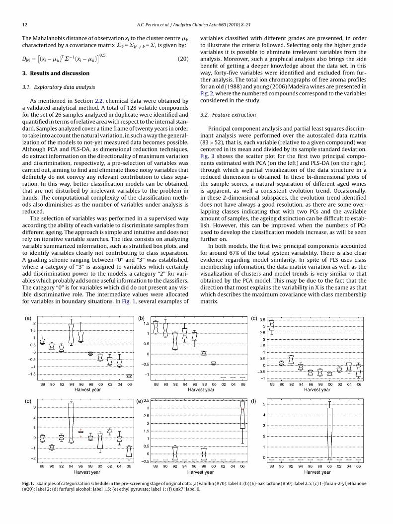
The selection of variables was performed in a supervised wayccording the ability of each variable to discriminate samples fromifferent ageing. The approach is simple and intuitive and does notely on iterative variable searches. The idea consists on analyzingariable summarized information, such as stratified box plots, ando identify variables clearly not contributing to class separation.

grading scheme ranging between “0” and “3” was established,here a category of “3” is assigned to variables which certainly

dd discrimination power to the models, a category “2” for vari-bles which probably add some useful information to the classifiers.he category “0” is for variables which did do not present any vis-ble discriminative role. The intermediate values were allocatedor variables in boundary situations. In Fig. 1, several examples of

ig. 1. Examples of categorization schedule in the pre-screening stage of original data. (a) v#20): label 2; (d) furfuryl alcohol: label 1.5; (e) ethyl pyruvate: label 1; (f) unk7: label 0.

ica Acta 660 (2010) 8–21

variables classified with different grades are presented, in orderto illustrate the criteria followed. Selecting only the higher gradevariables it is possible to eliminate irrelevant variables from theanalysis. Moreover, such a graphical analysis also brings the sidebenefit of getting a deeper knowledge about the data set. In thisway, forty-five variables were identified and excluded from fur-ther analysis. The total ion chromatographs of free aroma profilesfor an old (1988) and young (2006) Madeira wines are presented inFig. 2, where the numbered compounds correspond to the variablesconsidered in the study.

3.2. Feature extraction

Principal component analysis and partial least squares discrim-inant analysis were performed over the autoscaled data matrix(83 × 52), that is, each variable (relative to a given compound) wascentered in its mean and divided by its sample standard deviation.Fig. 3 shows the scatter plot for the first two principal compo-nents estimated with PCA (on the left) and PLS-DA (on the right),through which a partial visualization of the data structure in areduced dimension is obtained. In these bi-dimensional plots ofthe sample scores, a natural separation of different aged winesis apparent, as well a consistent evolution trend. Occasionally,in these 2-dimensional subspaces, the evolution trend identifieddoes not have always a good resolution, as there are some over-lapping classes indicating that with two PCs and the availableamount of samples, the ageing distinction can be difficult to estab-lish. However, this can be improved when the numbers of PCsused to develop the classification models increase, as will be seenfurther on.

In both models, the first two principal components accountedfor around 67% of the total system variability. There is also clearevidence regarding model similarity. In spite of PLS uses classmembership information, the data matrix variation as well as the

visualization of clusters and model trends is very similar to thatobtained by the PCA model. This may be due to the fact that thedirection that most explains the variability in X is the same as thatwhich describes the maximum covariance with class membershipmatrix.

anillin (#70): label 3; (b) (E)-oak lactone (#50): label 2.5; (c) 1-(furan-2-yl)ethanone

A.C. Pereira et al. / Analytica Chimica Acta 660 (2010) 8–21 13

Fig. 2. Total ion chromatogram from aroma profile of Madeira wine samples obtained by SPE/GC–MS. (a) “Malmsey” Madeira wine from 1988 harvest. (b) “Malmsey”Madeira wine from 2006 harvest. (1) Ethyl butanoate; (2) 2-methylpropan-1-ol; (3) 2-methylbutan-1-ol + 3-methylbutan-1-ol; (4) ethyl hexanoate; (5) unk1; (6) unk2; (7)3-hydroxybutanone; (8) ethyl 2-ethoxyacetate; (9) ethyl 3-ethoxy propanoate; (10) ethyl 2-hydroxypropanoate; (11) hexen-1-ol; (12) (Z)-3-hexen-1-ol; (13) (Z)-hex-2-en-1-ol; (14) ethyl 2-hydroxyacetate; (15) ethyl 2-hydroxyisovalerate; (16) cis-Linalool oxide; (17) acetic acid; (18) cis-dioxane; (19) acid formic; (20) 1-(furan-2-yl)ethanone; (21)benzaldehyde; (22) (S)-2,3-butanediol; (23) ethyl dl-2-hydroxycaproate; (24) unk5; (25) 2-methyl propanoic acid; (26) isoamyl lactate; (27) 5-methylfuran-2-carbaldehyde(28) (R)-2,3-butanediol; (29) unk6; (30) trans-dioxalane; (31) ethyl pentanoate; (32) butyrolactone; (33) butanoic acid; (34) ethyl methyl succinate; (35) diethyl methylsuccinate; (36) isovaleric acid; (37) trans-dioxane; (38) diethyl succinate; (39) 3-methyl-2,5-furandione; (40) unk8; (41) ethyl 2-phenylacetate; (42) cis-dioxalane; (43)caproic acid; (44) unk9; (45) phenylmethanol; (46) (Z)-oak-lactone; (47) 2-phenylethanol; (48) acethoxymethyl-2-furaldehyde; (49) unk11; (50) (E)-oak-lactone; (51)2-hexenoic acid; (52) 2H-pyran-2,6(3H)dione; (53) methyl furan-2-carboxylate; (54) dl diethyl malate; (55) 1H-pyrrole-carboxaldehyde; (56) 3-hydroxy hexanoic acid,ethyl ester; (57) diethyl malate (58) unk13; (59) nerol; (60) vinylguaiacol; (61) �-carboethoxy-�-butyrolactone; (62) unk15; (63) glycerol; (64) tartaric acid, diethyl ester; (65)

14 A.C. Pereira et al. / Analytica Chimica Acta 660 (2010) 8–21

Fig. 3. PC1 versus PC2 scores for the global signature of the “Malmsey” Madeira wines cov(a) PCA (explaining 67.075% of total variance) and (b) PLS-DA (explaining 67.045% of tota

Fs

cdtdti

ticomdCctcg

ma(p

ig. 4. PC1 versus PC2 loading values relative to the global signature for the “Malm-ey” Madeira wines.

In both models an evolution trend regarding the ageing pro-esses is identified across the 1st PC, which develops across twoifferent paths in the second PC: first samples evolve throughhe positive direction of the 2nd PC, and then, in the negativeirection of the 2nd PC. Then, loading information was analyzedo understand which variables are important in the directionsdentified.

By looking to the loading vectors (Fig. 4), it is possible to analyzehe variables that are responsible for score behaviors and get morensight into the nature of identified trends. A detailed discussionannot be given here, due to space restrictions, but one can pointut, for instance that the ethyl ester and acetal families are theost prominent compounds on the first PC. The role of ethyl esters

uring barrel-ageing of wines has also been reported by Garde-

erdán et. al. [5] who raises the hypothesis that such compoundsan be considered as ageing markers. In “Malmsey” Madeira wineshis family of compounds organizes under two groups: one whichontribute for ageing trends during the first 10 years, and anotherroup more important for older wines, including the ethyl esters

onoethyl succinate; (66) benzenecarboxilic acid; (67) ethyl citrate; (68) 5-(hydroxymcid, monoethyl ester; (72) 2-pyrrolidinecarboxylic acid-5-oxo, ethyl ester; (73) ethyl h76) 2,4-dihydroxy-3-methoxyacetophenone + benzoic acid, 2-hydroxy; (77) unk19; (78)araben; (81) unk20; (82) benzeneethanol 4-hydroxy; (83) unk21.

ering an extended time period of 20 years according to the samples listed in Table 1.l variance) (samples are listed in Table 1).

of diprotic acids, namely ethyl 2-hydroxypropanoate (ethyl lac-tate #10) ethyl methyl succinate (#34), diethyl succinate (#38) andmonoethyl succinate (#65). With regard to the acetal compounds(formed from acetaldehyde and glycerol) they have been pointedout as possible ageing markers and of fundamental importance dur-ing oxidative ageing monitoring [34]. The weight and position ofcis/trans dioxane (#18, #37) and dioxalane (#30, #42) in loadingsplots demonstrate also they role in the identified ageing trends.Therefore, special attention should be devoted in future work touncover their role in establishing possible focused Madeira winechemical based ageing markers.

The oxidative reactions that take place in wines stored in bar-rels increase the aldehyde and methyl ketone content [34]. Inthe particular case of furanic compounds (1-(furan-2-yl)ethanone(#20), 5-methylfuran-2-carbaldehyde (#27), acethoxymethyl-2-furaldehyde (#48), methyl furan-2-carboxylate (#53) and 5-(hydroxymethyl)-2-furaldehyde (HMF) (#68)) the positive valuesof loads regarding the 2nd PC indicate that they may be importantduring the first years of ageing. The content of these compoundstends to rise during ageing and their high reactivity, which rapidlyevolves into other compounds and differences in the accumulationkinetics [6] can justify their major impact during the first yearsof ageing. Other aldehyde compounds such as vanillin (#70) ethylhomovanilatte (#73); ethyl vanillate + acetovanillone (74) and lac-tone compounds (#50 and #61) also show a similar trend in theprincipal component subspace. According to this brief analysis,aldehyde compounds should be taken into account to distinguishthe two identified phases of ageing.

To conclude, the alcohols trends for the loadings interpreta-tion regarding the bi-dimensional model described above shouldbe noted. These are preferentially located in the negative quadrant,weighing in the location of 1988 samples.

To find the natural grouping purposed by the first two principalcomponents, an hierarchical cluster analysis (HCA) was performedusing an agglomerative technique, namely ‘complete’ linkage clus-tering. The ‘single’ and ‘average’ linkage criteria clustering werealso tested. The results reached by the latter were very similar to

ethyl)-2-furaldehyde (HMF); (69) benzeneacetic acid; (70) vanillin; (71) hexenoicomovanilatte; (74) ethyl vanillate + acetovanillone; (75) benzoic acid, dimethoxy;4-hydroxy-3,5-dimethoxybenzaldehyde; (79) benzaldehyde, 4-hydroxy; (80) ethyl

A.C. Pereira et al. / Analytica Chimica Acta 660 (2010) 8–21 15

F onentt

‘c

wbimdPotfIqaw

3

latmTs

TG

ig. 5. Dendrogram with “complete linkage” method for 1st and 2nd principal compo evaluate similarities among samples (samples are listed in Table 1).

complete’ linkage. Both perform well, forming naturally distinctlumps in principal component data space.

In HCA, samples are grouped according to their similarities,ithout taking into account the information about their class mem-

ership. This technique is based on the idea that similarity isnversely related to the distance between samples. Two similarity

etrics were tested, the Euclidean distance and the Mahalanobisistance, and results are present in Fig. 5. The results obtained forCA and PLS-DA scores are quite similar, this being the reason whynly the case of PLS-DA is reported in Fig. 5. In this representa-ion, a solid line indicates that the node contains only samplesrom the same class underneath. Otherwise, a dash line is used.t can be seen that the results obtained with both metrics are alsouite similar. Using Mahalanobis distance, the first dubious divisionppears a lower level of similarity, therefore Mahalanobis distanceas selected to carry out similar subsequent analysis.

.3. Model assessment and evaluation

In the previous section, the data analysis carried out in theatent variable subspaces reveals some interesting ageing trends

nd information on which chemical compounds are contributing tohem. We will now focus on the assessment and validation of the

odels obtained using the adopted feature extraction techniques.he reliability of LDA and kNN is also analyzed in terms of their con-istency (ability to correctly classify the members of the training

able 2lobal classification error rate using linear and kNN classifiers for PCA and PLS-DA scores

Model 1LV 2LV 3LV 4LV

Linear PCA 0.3472 0.1731 0.1731 0.076PLSDA 0.2885 0.1538 0.0769 0.076

kNN PCA 0.0000 0.0000 0.0000 0.000PLSDA 0.0000 0.0000 0.0000 0.000

Similarity measure Angle (◦) 20.59 20.59 20.58 12.00fs 0.18 0.15 0.24 0.29

s obtained by PLS-DA using: (a) “Euclidean” distance and (b) “Mahalanobis” distance

set) and generalization ability (ability to correctly classify future,never-seen samples).

3.3.1. Model evaluation—consistencyIt is expected that the classification ability for a training set will

be improved when the number of latent variables increases. Thequestion is to decide a suitable number of components to considerin the model, avoiding an over-fitted model. “Suitable” implies thatthe model describes the systematic variation in the data and not thenoise. Table 2, shows that adding more than 6 and 7 latent variablesrespectively to PLS-DA and PCA models does not provide a signifi-cant improvement in the results. A measure of similarity betweenboth subspaces, for a specified number of latent variables, is alsopresented in Table 2. Their values indicate that indeed subspacesare similar and thus, the classification ability obtained does not dif-fer much. The procedure carried out for comparison models basedon the angle between subspaces and the Krzanowski similarity fac-tor (ranging from 0 (no similarity) to 1 (exact similarity)) [35,36].It is worth underlining that the error free performance of kNN canbe due to the presence of replicates in the data set. The reason whywe have not excluded one of the replicates from our analysis or,

for example, do not consider the mean value of replicates, is dueto the low number of samples available, and also to enable severalcomparisons with LDA. However, if we consider the scenario wherereplicates are left out from the analysis, together with the sampleunder consideration, the performance of kNN at training reaches a

, with different numbers of retained latent variables (LV).

5LV 6LV 7LV 8LV 9LV 10LV

9 0.0769 0.0385 0.0192 0.0385 0.0385 0.03859 0.0577 0.0000 0.0192 0.0192 0.0000 0.0000

0 0.0000 0.0000 0.0000 0.0000 0.0000 0.00000 0.0000 0.0000 0.0000 0.0000 0.0000 0.0000

12.09 11.99 12.11 9.0392 8.68 7.810.32 0.29 0.31 0.89 0.89 0.89

16 A.C. Pereira et al. / Analytica Chimica Acta 660 (2010) 8–21

F e traia

mr

rtmfitbbtbbgtcmwaosbtP

ig. 6. Recognition ability for all possible combinations among latent variables in thnd (b) latent variables from PLS-DA.

inimum classification rate of 0.15 and 0.09 for PCA and PLS-DA,espectively

The selection of the number of latent variables is essential ineaching the optimal model. Too few latent variables imply thathere is still relevant discriminating information left out of the

odel, but choosing too many components may lead to model over-tting and to an inferior predictive ability for future objects, dueo the modeling of unstructured variability. Moreover, it shoulde taken into account that the number of latent variables whichest classify are not necessarily those resulting from incorporatinghe first scores. Therefore, the strategy to decide the best num-er of latent variables to use in the model was accomplished herey the first finding the best combination of latent variables for aiven subgroup size. One way of doing this consists in evaluatinghe classification ability (consistency) associated with all possibleombinations of latent variables for a given subgroup size (for aodel defined by T latent variables in a subgroup size of Z, thereill be Z!/T!(Z − T)! such combinations). All of these combinations

re represented in Fig. 6, and for each subgroup size (number

f latent variables) it was pointed out the latent variables corre-ponding to the best combination. It is possible to verify that for ai-dimensional model, the best classifier is not defined for the firstwo latent variables but defined by the 1st and 4th scores for theCA model and 1st and 6th scores for PLS-DA. The results obtained

ning phase, using linear discriminant rules. (a) Latent variables extracted from PCA

with linear discriminant and kNN classifiers, lead to very low mis-classification scores. Note that k is assumed to be one for kNN, andthe Euclidean and Mahalanobis distances were tested as metricto evaluate the nearest neighbor distances, leading equal results.Comparing these results with those presented in Table 2, in whichthe selection of the best latent variable combinations are not takeninto account, it should be noted that with this selection methodol-ogy the number of latent variables required to establish a classifierwithout misclassifications cases is significantly lower. However,this way of establishing a classification methodology, without con-sidering never-seen samples or a test set, is too optimistic, eventhough it is useful and important as a preliminary consistency testthat all methodologies must pass.

3.3.2. Model validation—testing phaseThis section provides a more realistic basis for assessing the clas-

sification frameworks developed. From the many ways available forassessing a classification model, perhaps the best one would be touse a large external validation set (the test set), not involved in the

model building (training) stage. However, such situation is quiteoften not possible due to limitations in data availability, and alter-native was must then be adopted. In this context, cross-validation(CV) provides a valid alternative. It allows to perform a number ofrounds where observations are successively separated into training

A.C. Pereira et al. / Analytica Chimica Acta 660 (2010) 8–21 17

F variaL .

stmtv

3vttaiotp

ifv

ig. 7. ‘Leave-one-out’ cross-validation concerning the best combination of latentatent variables extracted from PCA and (b) latent variables extracted from PLS-DA

ets (used to estimate the classifiers) and test sets (used to evaluateheir performance), after which the overall classification perfor-

ance is computed. Several variants of cross-validation exist. Inhis study we will confine ourselves to the ‘Leave-One-Out’ cross-alidation and k-fold Monte Carlo cross-validation.

.3.2.1. Leave-one-out cross-validation. In ‘Leave-One-Out’ cross-alidation, the strategy consists of discarding one observation ofhe reference group, and estimate the classification model withhe other observations. The observation left out is then used tossess the performance on the classifier and the whole processs repeated for all other samples, until each one is left asidene time. In the end, the global average accuracy or classifica-ion error rates are computed in order to assess the classifiers

erformance.

Fig. 7 shows the performance of LDA and kNN classifiers regard-ng the best combination of latent variables in the preliminaryeature extraction stage. Note that, for a model defined with latentariables, all possible combinations were also tested. Analysing the

bles in testing phase using linear discriminant (a1, b1) and kNN (a2, b2) rules. (a)

global error rate, which corresponds to the overall percentage ofmembers of the test set that were misclassified, it could be con-cluded that kNN shows better performance when combined witha feature extraction methodology. When PCA is used, both theEuclidean and Mahalanobis distances lead to similar performances(therefore, only one is represented in Fig. 7a1). As for PLS-DA, theEuclidean distance is associated with better classification scores. Inconsequence, the Euclidean distance was adopted. In relation to theLDA classifier, the minimum error rate achieved is about 4% when5 latent variables are selected from the PLS-DA feature extractionmethodology (Fig. 7b2).

Using two latent variables, the performance of kNN is verysimilar for both PCA and PLS-DA. In this case, Fig. 8 enables a visu-alization about which samples are contributing to the computed

error rate of 11%.

3.3.2.2. k-fold Monte Carlo cross-validation. Even though leave-one-out cross-validation already addresses the issue of assessingthe predictive classification in a coherent way, it still provides

18 A.C. Pereira et al. / Analytica Chim

FeP

uBvpespsttaarecow

brsc

FaT

ig. 8. kNN applied to 1st and 2nd latent variables (best variable combination)xtracted from principal component analysis (similar results are obtained throughLS-DA).

sually rather optimistic estimate of the method error rates.etter estimates can usually be obtained using alternative cross-alidation methodologies, such as based on a Monte Carlorocedure, which was implemented here. PCA and PLS-DA mod-ls were estimated 100 times, each time with a randomly selectedubset of objects for the training set. This random selection waserformed in a stratified manner, that is, each test set was repre-ented at least by two samples of each class, chosen randomly. Then,he corresponding test data sets were submitted to both classifica-ion methods selected in this study (LDA and kNN). This procedurellows for a sufficient number of samples in the training set andrepresentative number of members among the test set (the 100

epetitions also ensure that all of the samples were included in thevaluation). Consequently, the global error rate concerning a spe-ific latent variables combinations correspond to the mean valuef all 100 resampling computed, for which the standard deviationas also calculated.

The results of this resampling scheme were analyzed for theest ten latent variable combinations regarding the global errorates and its standard error for classification. These results are pre-ented in Table 3. Fig. 9 also shows the results regarding the bestombination of latent variables. Once again it is possible to ver-

ig. 9. Monte Carlo cross-validations concerning the best combination of latent vari-bles in testing phase using PLS-DA latent variables and kNN as classifier (solid line).he dotted lines correspond to remaining methods analyzed.

ica Acta 660 (2010) 8–21

ify that the kNN was the classifier showing better performancein relation to the global error rate, which is usually lower thanthe rate obtained with LDA. In case of the latent variables arisingfrom feature extraction with PCA, the performance of both clas-sifiers becomes similar when 6 latent variables are used to buildthe model, worsening with an increase in the number componentsretained, indicating that after this point data is being overfitted.However, with kNN, the performance improves when one morevariable is included, and only after that, the classification scoresstart to degrade. Concerning the best latent variables combina-tion, the difference between global error rates obtained from eachclassifiers rank from 2 to 4.4%, achieving better performances formodels built up from PLS-DA latent variables. In this case, clas-sifiers assume an equal error rate when 5 latent variables areretained. Such a similar error rate is maintained until they reachtheir best performance (3.4%), when 8 latent variables are used.Note that kNN were tested for two different metrics—“Euclidean”and “Mahalanobis” distance, the first one leading to the bestresults.

As described above, the 10 best combinations of variables werealso analyzed in similar manner. Concerning the best PCA model(defined by 6 LV) for both classifiers, the latent variables that leadto the best performance are the same: 1, 4, 5, 6, 7 and 10. It isworth noting that the 1st and 4th latent variables, are the only onesthat are present in all of the best 10 combinations, which revealstheir importance in the ageing phenomena. Note that this fact hasalready been seen as a possibility during the training stage, andis now confirmed. The 5th and 6th variables are also very impor-tant for both classifiers, being the 2nd one also very important incase of using the kNN classifier. In the case of the PLS-DA model,also comparing classifiers performance with 6 LV, the 1stand 4thcomponents also play a key role, but not the 1st and 6th com-ponents. Regarding the best combinations for achieve the lowesterror rates, the following sequences were identified: 1-2-3-4-5-7-9-10 for LDA; 1-3-4-5-6-7-8-10 for kNN. However, the same typeof comments, regarding the impact of the presence of replicatesin kNN performance, made for the training phase, are also validhere.

3.4. Classification model refinement

Monte Carlo cross-validation allows us to establish the modelthat best predicts unknown aged “Malmsey” Madeira wine sam-ples. The kNN classifier using eight latent variables extracted fromthe PLS-DA methodology revealed to be the best approach. How-ever, some class overlapping exists, and if the required resolutionregarding ageing prediction can be relaxed a bit, a simplifiedmodel can be established. This can be accomplished by coalesc-ing or aggregating the overlapping classes into single classes. Thisapproach improves classification performance at the expense ofdecreasing the classification model resolution. As shown in Table 4,considering 9 classes instead of the original 10, a classifier with anerror rate of lower than 1% can be established using only five latentvariables. In this case, the samples from the 1992 and 1994 harvestswere aggregated into one class. This decision was taken accordingto the misclassification regions found in the best 10-class classifiers,in particular through the analysis of the natural groups formed inthe hierarchical cluster tree (using ‘complete’ linkage method and‘Euclidean’ distance as the distance measure). Samples from the1998 and 2000 harvests also tend to cluster together. In this case,taking into account the 8 classes thus obtained, the ideal classifier

(without misclassifications cases) was achieved using 8 latent vari-ables. The samples from the 1996 harvest also cluster together with1992 and 1994 samples. The model built under such circumstancesonly requires five latent variables to achieve the best performance(Table 4).

A.C.Pereira

etal./A

nalyticaChim

icaA

cta660 (2010) 8–21

19

Table 3Mean and standard deviation global error rates using linear and kNN classifiers with PCA and PLS-DA latent variable regarding 100 simulations carried out, along with the 10 best latent variable combinations.

1LV 2LV 3LV 4LV 5LV 6LV 7LV 8LV 9LV 10LV

Linear Best LV 0.4125 ± 0.0869a 0.2365 ± 0.0923a 0.1465 ± 0.0715a 0.0930 ± 0.0659a 0.0865 ± 0.0602a 0.0650 ± 0.0571a 0.0760 ± 0.0505a 0.0725 ± 0.0596a 0.0790 ± 0.0565a 0.0795 ± 0.0616a

1st 1 1-4 1-4-6 1-4-6-7 1-4-5-6-7 1-4-5-6-7-10 1-2-4-5-6-7-9 1-2-4-5-6-7-9-10 1-3-4-5-6-7-8-9-10 1-2-3-4-5-6-7-8-9-102nd 2 1-3 1-4-7 1-5-6-7 1-2-4-6-7 1-4-5-6-7-8 1-3- 4-5-6-7-10 1-4-5-6-7-8-9-10 1-2-3-5-6-7-8-9-10 1-2-3-4-5-6-7-8-9-103rd 4 1-7 1-6-7 1-3-6-7 1-4-6-7-10 1-3-4-6-7-10 1-3-4-5-6-7- 8 1-3-4-5-6-7-8-10 1-2-4-5-6-7-8-9-10 1-2-3-4-5-6-7-8-9-104th 7 1-6 1-2-6 1-3-5-7 1-4-6-7-9 1- 4-6-7-9-10 1-3-4-5-6-7-9 1 -3-4-5-6-7-9 10 1-2-3-4-5-6-7-8-9 1-2-3-4-5-6-7-8-9-105th 6 1-2 1-3-6 1-2-4-6 1-3-4-6-7 1-4-6-7-8-10 1-2-4-6-7-8-10 1-2-4-5-6-7-8-10 1-2-3-4-6-7-8-9-10 1-2-3-4-5-6-7-8-9-106th 3 1-5 1-3-7 1-4-5-7 1-4 -6-7-8 1-3-4-5-6-7 1-2-4-5-6 -7-10 1-3-4-5-6-7-8-9 1-2-3-4-5-6-7-9-10 1-2-3-4-5-6-7-8-9-107th 5 1-10 1-3-4 1-2-6-7 1-2-5-6-7 1-4-5-6-7-9 1-4-5-6-7- 9-10 1-2-4-5-6-7-8-9 1-2-3-4-5-6-7-8-10 1-2-3-4-5-6-7-8-9-108th 8 1-8 1-2-7 1-3-4-6 1-3-5-6-7 1-2-4-6-7-10 1-2-4-6-7-9-10 1-2-4-6-7-8-9-10 1-2-3-4-5- 6-8-9-10 1-2-3-4-5-6-7-8-9-109th 10 1-9 1-2-4 1-4-7-9 1-5 -6-7-8 1-2-4-5-6-8 1-4-5-6-7-8-9 1-2-3-4-5-6-7-10 2-3-4-5-6-7-8-9-10 1-2-3-4-5-6-7-8-9-1010th 8 2-3 1-4-5 1-4-6-10 1-3-6-7-9 1-3-4-5-7-9 1-3-5-6-7-9-10 1-3-5-6-7-8-9-10 1-2-3-4-5-7-8-9-10 1-2-3-4-5-6-7-8-9-10

Best LV 0.3755 ± 0.0889b 0.19955 ± 0.0862b 0.1200 ± 0.0603b 0.0715 ± 0.0660b 0.0530 ± 0.0550b 0.0495 ± 0.0562b 0.0435 ± 0.0558b 0.0340 ± 0.0512b 0.0560 ± 0.0596b 0.0695 ± 0.0618b

1st 1 1-4 1-4-7 1-4-7- 9 1-2-4-5-9 1-2-4-5-7-9 1-2-4-5-7-9-10 1-2-3-4-5-7-9-10 1-2-3-4-5-7-8-9-10 1-2-3-4-5-6-7-8-9-102nd 2 1-5 1-2-5 1-4-5-8 1-2-4-7-9 1-4-5-6-7-10 1-2-4-5-6-7-9 1-3-4-5-7-8-9-10 1-3-4-5-6-7-8-9-10 1-2-3-4-5-6-7-8-9-103rd 3 1-3 1-5-6 1-4-5-6 1-4-5-6-9 1-3-4-5-7-10 1-2-3-4-5-7-9 1-2-3-4-5-7-8-9 1-2-3-4-5-6-7-8-10 1-2-3-4-5-6-7-8-9-104th 7 1-7 1-4-6 1- 4-6-7 1-4-5-6-8 1-4-5-7-8-10 1-2-4-5-7-8-9 1-2-4-5-7-8-9-10 1-2-3-4-5-6-7-9-10 1-2-3-4-5-6-7-8-9-105th 4 1-6 1-4-5 1-2-5-10 1-2-5-6-9 1-2-4-5-7-10 1-3-4-5-7-8-9 1-3-4-5-6-7-9-10 1-2-3-4-5-6-7-8-9 1-2-3-4-5-6-7-8-9-106th 5 1-2 1-5-8 1-2-5-9 1-4-5-7-9 1-2-4-5-9-10 1-3-4-5-7-8-10 1-2-3-5-7-8-9-10 1-2-3-5-6-7-8-9-10 1-2-3-4-5-6-7-8-9-107th 8 2-3 1-4-8 1-4-6-9 1-4-5-7-10 1-3-4-5-7-8 1-2-3-4-5-9-10 1-3-4-5-6-7-8-10 1-2-3-4-5-6-8-9-10 1-2-3-4-5-6-7-8-9-108th 6 1-8 1-3-9 1-4-5-7 1-4-6-7-9 1-4-5-6-7 -9 1-2-4-5-8-9-10 1-2-3-4-5-7-8-10 1-2-4-5-6-7-8-9-10 1-2-3-4-5-6-7-8-9-109th 9 1-9 1-4-9 1-2-5-6 1-4-5-7-8 1-4-5-7-9-10 1-3-4-5-8-9-10 1-3-4-5-6-7-8-9 2-3-4-5-6-7-8-9-10 1-2-3-4-5-6-7-8-9-1010th 10 2-5 1-3-8 1-4-5-9 1-4-5-6-7 1-2-4-5-8-9 1-2-3-5-7-9-10 1-2-4-5-6-7-9-10 1-2-3-4-6-7-8-9-10 1-2-3-4-5-6-7-8-9-10

kNN Best LV 0.3959 ± 0.0866a 0.148 ± 0.0735a 0.0930 ± 0.0735a 0.0590 ± 0.0676a 0.0620 ± 0.0578a 0.0625 ± 0.0572a 0.0475 ± 0.0524a 0.0545 ± 0.0524a 0.0565 ± 0.0491a 0.0505 ± 0.0500a

1st 1 1-2 1-2-4 1-2-4-6 1-2-4-7-10 1-4-5-6-7-10 1-4-5-6-7-9-10 1-2-4-5-6-7-8-10 1-3-4-5-6-7-8-9-10 1-2-3-4-5-6-7-8-9-102nd 2 1-4 1-2-6 1-2-4-10 1-2-4-5-7 1-2-4-5-6-10 1-2-4-5-6-7-10 1-2-4-5-6-7-9-10 1-2-4-5-6-7-8-9-10 1-2-3-4-5-6-7-8-9-103rd 4 1-7 1-2-5 1-2-4-5 1-2-4-5-10 1-4-5-6-7-9 1-4-5-6-7-8-9 1-2-4-5-6-7-8-9 1-2-3-4-6-7-8-9-10 1-2-3-4-5-6-7-8-9-104th 6 1-3 1-2-7 1-2-4-9 1-2-4-5-6 1-2-4-5-6-7 1-4-5-6-7-8-10 1-2-4-5-6-8-9-10 1-2-3-4-5-6-8-9-10 1-2-3-4-5-6-7-8-9-105th 3 2-5 1-2-10 1-2-4-8 1-2-4-6-7 1-2-4-5-6-9 1-2-4-5-6-7-9 1-2-4-6-7-8-9-10 1-2-3-4-5-6-7-9-10 1-2-3-4-5-6-7-8-9-106th 5 1-6 1-4-5 1-2-4-7 1-2-4-6-9 1- 2-4-5-7-10 1-2-4-5-7-9-10 1-4-5-6-7-8-9-10 1-2-3-4-5-7-8-9-10 1-2-3-4-5-6-7-8-9-107th 7 1-5 1-2-8 1-2-5-6 1-2-4-6-10 1-2-4-5-6-8 1-2-4-6-7-9-10 1-2-4-5-7-8-9-10 1-2-3-4-5-6 -7-8-9 1-2-3-4-5-6-7-8-9-108th 9 2-6 1-4-6 1-2-6-7 1-4-5-6-7 1-2-4-6-7-10 1-2- 4-5-6-7-8 1-3-4-5-6-7 -8-10 1-2-3-4-5-6 -7-8-10 1-2-3-4-5-6-7-8-9-109th 10 2-3 1-4-7 1-4-5-6 1-2-4-6-8 1-2-4-5-7-8 1-2-4-5-6-8-10 1-2-3-4-5-6 -7-10 1-2-3-5-6-7-8-9-10 1-2-3-4-5-6-7-8-9-1010th 8 2-5 1-2-9 1-2-6-10 1-2-4-9-10 1-4-5-6-7-8 1-2-4-5-6-8-9 1-2-3-4-5-6-8-10 2-3-4-5-6-7-8-9-10 1-2-3-4-5-6-7-8-9-10

Best LV 0.4090 ± 0.0845b 0.1375 ± 0.0786b 0.0770 ± 0.0543b 0.0525 ± 0.0548b 0.0515 ± 0.0534b 0.0495 ± 0.0474b 0.0455 ± 0.0498b 0.0340 ± 0.0481b 0.0430 ± 0.0537b 0.0430 ± 0.0582b

1st 1 1-2 1-2-4 1-2-4-6 1-2-4-7-10 1-4-5- 6-7-10 1-4-5-6-7-9-10 1-2-4-5-6-7-8-10 1-3-4-5-6-7-8-9-10 1-2-3-4-5-6-7-8-9-102nd 2 1-5 1-5-6 1-4-5-6 1-3-5-6-9 1-3-5-6-7-9 1-3-4-5-7-8-9 1-2-3-4-5-6-7-10 1-2-3-4-5-6-7-9-10 1-2-3-4-5-6-7-8-9-103rd 5 2-3 1-2-4 1-2-3-5 1-2-3-5-9 1-4-5-6-7-8 1-2-4-5-6-7-9 1-3-4-5-6-7-9-10 1-2-3-4-5-6-7-8-9 1-2-3-4-5-6-7-8-9-104th 4 1-6 2-3-5 1-5-6-8 1-4-5-6-8 1-4-5-7-8-9 1-2-3-5-6-7-10 1-3-4-5-6-7-8-9 1-2-3-4-5-6-7-8-9 1-2-3-4-5-6-7-8-9-105th 3 1-4 1-4-5 1-3-5-8 1-4-5-6-9 1-3-4-5-7-8 1-4-5-6-7-8-9 1-2-3-5-6-7-8-10 1-2-3-4-5-6-8-9-10 1-2-3-4-5-6-7-8-9-106th 8 1-3 1-5-8 1-2-5-6 1-3-5-7-9 1-2-4-5-7-9 1-3-4-5-6-7-9 2-3-4-5-6-7-8-10 1-2-3-5-6-7-8-9-10 1-2-3-4-5-6-7-8-9-107th 7 1-7 1-2-3 1-4-5-8 1-2-3-4-5 1-2-3-5-7-8 1-4-5-6-7-8-10 1-2-4-5-6-7-8-10 1-2-3-4-5-7-8-9-10 1-2-3-4-5-6-7-8-9-108th 6 1-8 1-2-7 1-2-5-8 1-2-3-5-6 1-2-4-5-7-8 1-3-5-6-7-8-9 2-3-4-5-6-7-8-9 2-3-4-5-6-7-8-9-10 1-2-3-4-5-6-7-8-9-109th 9 2-5 1-4-8 1-2-5-7 1-2-3-6-9 1-4-5-6-7-9 1-2-3-4-5-6-10 1-2-3-4-5-6-7-9 1-2-3-4-6-7-8-9-10 1-2-3-4-5-6-7-8-9-1010th 10 2-6 1-3-5 1-3-5-6 2-3-6-7-9 1-2-3-6-7-9 1-2-4-5-6-7-10 1-2-3-4-5-7-8-10 1-2-4-5-6-7-8-9-10 1-2-3-4-5-6-7-8-9-10

a PCA.b PLS-DA

20 A.C. Pereira et al. / Analytica Chim

Tab

le4

Mea

nan

dst

and

ard

dev

iati

ongl

obal

erro

rra

tes

usi

ng

akN

Ncl

assi

fier

wit

hPL

S-D

Ala

ten

tva

riab

les

rega

rdin

g10

0si

mu

lati

ons,

alon

gw

ith

corr

esp

ond

ing

resu

lts,

wh

end

ata

clas

ses

are

coal

esce

d.

1LV

2LV

3LV

4LV

5LV

6LV

7LV

8LV

9LV

10LV

9cl

asse

sEr

ror

rate

0.38

00±

0.09

100.

0983

±0.

0665

0.04

06±

0.04

790.

0161

±0.

0356

0.00

61±

0.01

930.

0033

±0.

0133

0.00

50±

0.01

780.

0022

±0.

0109

0.00

33±

0.01

030.

0128

±0.

0334

Bes

tLV

11-

21-

2-4

1-3-

5-6

1-2-

3-4-

7-8

1-4-

5-6-

7-8

1-3-

4-5-

6-7-

81-

4-5-

6-7-

8-9-

101-

3-4-

5-6-

7-8-

9-10

1-2-

3-4-

5-6-

7-8-

9-10

8cl

asse

sEr

ror

rate

0.38

00±

0.09

760.

0881

±0.

0635

0.00

94±

0.03

00.

0025

±0.

0123

0.00

13±

0.08

80.

0013

±0.

088

0.00

13±

0.08

80.

0000

±0.

088

0.00

00±

0.08

80.

0000

±0.

088

Bes

tLV

11-

21-

2-4

1-2-

4-5

1-3-

4-5-

7-8

1-4-

5-6-

7-8

1-3-

4-5-

6-7-

81-

2-3-

4-5-

6-7-

81-

2-3-

4-5-

7-8-

9-10

1-2-

3-4-

5-6-

7-8-

9-10

7cl

asse

sEr

ror

rate

0.30

07±

0.08

690.

0486

±0.

0555

0.00

79±

0.03

190.

0021

±0.

0159

0.00

00±

0.00

00.

0000

±0.

000

0.00

00±

0.00

00.

0007

±0.

007

0.00

07±

0.00

70.

0014

±0.

0010

Bes

tLV

11-

21-

2-4

1-2-

4-8

1-2-

3-4-

7-8

1-2-

3-4-

6-7-

81-

3-4-

5-6-

7-8

1-3-

4-5-

6-7-

8-10

1-2-

3-4-

5-6-

7-8-

101-

2-3-

4-5-

6-7-

8-9-

10

[[[

[

[[[[[[[

[

[[[[

[[[[

ica Acta 660 (2010) 8–21

4. Conclusions

In this paper, approaches for performing ageing classificationon a particular type of Madeira wine were presented and dis-cussed. Two multivariate feature extraction methodologies wereemployed, principal component analysis and partial least squaresfor discriminant analysis. These were properly combined withtwo classifiers, representative from the parametric (LDA) andnon-parametric (kNN) families of classification methodologies.Selection of the number of features to retain (latent variables) wasproperly addressed in several alternatives, namely using differ-ent cross-validation approaches, such as leave-one-out and k-foldMonte Carlo cross-validation. The classifiers consistency was alsoevaluated, as a necessary condition (but not sufficient) for their usein future applications.

Results achieved show that it is advisable to use kNN onlatent features obtained through PLS-DA. The model performanceachieved in this scenario has an error rate of 4% which can beimproved by decreasing the classification resolution. This method-ology will be applied in the feature to richer data sets, containingmore chemical information about the samples, in order to improvethe current performance of the classifiers.

Acknowledgements

A.C. Pereira acknowledges the Portuguese Fundacão para aCiência e Tecnologia for the financial support through PhD grantSFRH/BD/28660/2006. The authors also acknowledge MadeiraWine Company for kindly supplying all the wine samples used inthis work.

References

[1] L. Liu, D. Cozzolino, W.U. Cynkar, R.G. Dambergs, L. Janik, B.K. O’Neill, C.B. Colby,M. Gishen, Food Chem. 106 (2008) 781.

[2] V. Parra, Á.A. Arrieta, J.A.F. Escudero, M. Íniguez, M.L. Rodríguez-Méndez, J.A.D.Saja, Anal. Chim. Acta 563 (2006) 229.

[3] D.A. Guilleän, M. Palma, R.N. Natera, R. Romero, C.G. Barroso, J. Agric. FoodChem. 53 (2005) 2412.

[4] M. Aznar, R. López, J. Cacho, V. Ferreira, J. Agric. Food Chem. 51 (2003)2700.

[5] T. Garde-Cerdán, C. Lorenzo, J.M. Carot, J.M. Jabaloyes, M.D. Esteve, M.R. Salinas,Food Chem. 111 (2008) 1025.

[6] F. Masino, F. Chinnici, G.C. Franchini, A. Ulrici, A. Antonelli, Food Chem. 92(2005) 673.

[7] G. González, E.M. Pena-Méndez, Eur. Food Res. Technol. 212 (2000) 100.[8] S. Preys, E. Vigneau, G. Mazerolles, V. Cheynier, D. Bertrand, Chemom. Intell.

Lab. Syst. 87 (2007) 200.[9] R.M. Alonso-Salces, S. Guyot, C. Herrero, L.A. Berrueta, J.F. Drilleau, B. Gallo, F.

Vicente, Anal. Bioanal. Chem. 379 (2004) 464.10] P. Polásková, J. Herszage, S. Ebeler, Chem. Soc. Rev. 37 (2008) 2478.11] S.E. Ebeler, Food Rev. Int. 17 (2001) 45.12] I.S. Arvanitoyannis, M.N. Katsota, E.P. Psarra, E.H. Souferos, S. Kallithrakay,

Trends Food Sci. Technol. 10 (1999) 321.13] M.S. Pérez-Coello, P.J. Martín-Álvarez, M.D. Cabezudo, Z. Lebensm. Unters.

Forsch. 208 (1999) 408.14] V.A. Watts, C.E. Butzke, R.B. Boulton, J. Agric. Food Chem. 51 (2003) 7738.15] V. Ferreira, P. Fernández, J.F. Cacho, Lebens. Wissen. Technol. 29 (1996) 251.16] R. López, M. Aznar, J. Cacho, V. Ferreira, J. Chromatogr. A 966 (2002) 167.17] K. Ridgway, S.P.D. Lalljie, R.M. Smith, J. Chromatogr. A 1153 (2007) 36.18] C. Domínguez, D.A. Guillén, C.G. Barroso, Anal. Chim. Acta 458 (2002) 95.19] Z. Pineiro, M. Palma, C.G. Barroso, Anal. Chim. Acta 513 (2004) 209.20] E. Campo, V. Ferreira, A. Escudero, J.C. Marques, J. Cacho, Anal. Chim. Acta 563

(2006) 180.21] L. Eriksson, E. Johansson, N. Kettameh-Wold, S. Wold, Multi- and Megavariate

Data Analysis—Principles and Applications, Umetrics, Sweeden, 2001.22] I.T. Jolliffe, Principal Component of Analysis, Springer–Verlag, New York, 2002.23] B.M. Wise, N.B. Gallagher, J. Proc. Cont. 6 (1996) 329.24] T. Kourti, J.F. MacGregor, Chemom. Intell. Lab. Syst. 28 (1995) 3.

25] M.C. Ortiz, L.A. Sarabia, C. Symington, F. Santamaria, M. Iniguez, Analyst 121

(1996) 1009.26] M. Barker, W. Rayens, J. Chemom. 17 (2003) 166.27] S. Wold, M. Sjöström, L. Eriksson, Chemom. Intell. Lab. Syst. 58 (2001) 109.28] J. Gabrielsson, N.-O. Lindberg, T. Lundstedt, J. Chemom. (2002) 141.29] P. Geladi, B.R. Kowalski, Anal. Chim. Acta 185 (1986) 1.

a Chim

[

[

[

A.C. Pereira et al. / Analytic

30] L.A. Berrueta, R.M. Alonso-Salces, K. Héberger, J. Chromatogr. A 1158 (2007)196.

31] R. Rousseau, B. Govaerts, M. Verleysen, B. Boulanger, Chemom. Intell. Lab. Syst.91 (2008) 54.

32] T. Rajalahtia, R. Arneberg, F.S. Bervend, K.-M. Myhr, R.J. Ulvikd, O.M. Kvalheim,Chemom. Intell. Lab. Syst. 95 (2009) 35.

[

[

[[

ica Acta 660 (2010) 8–21 21

33] T. Hastie, R. Tibshirani, J. Friedman, The Elements of Statistical Learning—DataMining, Inference, and Prediction, Springer, New York, 2001.

34] A.C.D.S. Ferreira, J.-C. Barbe, A. Bertrand, J. Agric. Food Chem. 50 (2002)2560.

35] A.C. Raich, CinarF A., Chemom. Intell. Lab. Syst. 30 (1995) 37.36] M.C. Johannesmeyer, A. Singhal, D.E. Seborg, AIChE J. 48 (2002) 2022.