Department of EconomicsWorking Paper 2014:10

Analysing Mechanisms for Meeting Global Emissions Target - A Dynamical Systems Approach

Shyam Ranganathan and Ranjula Bali Swain

Department of Economics Working paper 2014:10Uppsala University November 2014P.O. Box 513 ISSN 1653-6975 SE-751 20 UppsalaSwedenFax: +46 18 471 14 78

Analysing Mechanisms for Meeting Global EmissionsTarget - A Dynamical Systems Approach

Shyam Ranganathan and Ranjula Bali Swain

Papers in the Working Paper Series are published on internet in PDF formats. Download from http://www.nek.uu.se or from S-WoPEC http://swopec.hhs.se/uunewp/

Analysing Mechanisms for Meeting Global Emissions

Target - A Dynamical Systems Approach

By Shyam Ranganathan and Ranjula Bali Swain∗

31 October 2014

Global emissions beyond 44 gigatonnes of carbondioxide

equivalent (GtCO2e) in 2020 can potentially lead the world to

an irreversible climate change. Employing a novel dynamical

system modeling approach, we predict that in a business-as-

usual scenario, it will reach 61 GtCO2e by 2020. Testing esti-

mated parameters, we find that limiting the burden of emis-

sion reduction to the top 25 global emitters, does not increase

their encumbrance. In absence of emission cuts, technology

and preferences for environmental quality have to improve by

at least 2.6 percent and 3.5 percent if the emission target has

to be met by 2020.

JEL: C51, C52, C53, C61, Q01, Q50

Keywords: Sustainable Development Goals, dynamical sys-

tems, Bayesian, greenhouse gases

∗ This work was funded by ERC grant 1DC-AB and Swedish Research Council grantD049040. Shyam Ranganathan: Uppsala University, Sweden, shyam@math.uu.se. BaliSwain: Uppsala University, Sweden, ranjula.bali@nek.uu.se.

1

I. Introduction

Increased production of goods and services lead to growth of Green House

Gas (GHG) emissions, particularly carbon dioxide (Granados, Ianides and

Carpintero, 2012; Raupach et al., 2007; Quadrelli and Peterson, 2007; Roca

and Alcantara, 2001; Tol et al., 2009), which is one of the strongest pre-

dictors of temperature increase. Scientists agree that unless this global

temperature increase is capped to under 2 degree Celsius, irreversible cli-

mate change will occur, leading to crisis, conflicts and large losses in GDP

(IPCC, 2007). Recognising this the Copenhagen Accord, 2009, agreed to

cooperation in peaking (stopping from rising) the global and national green-

house gas emissions but it was in Cancun at the COP/16/CMP6 in 2010,

that the United Nations Framework Convention on Climate Change (UN-

FCCC)Parties agreed to limit a rise in global average temperature to 2

degrees Celsius above the pre-industrial levels. United Nations Environ-

ment Program (2011) estimates that to achieve this GHGs should be re-

duced to less than 44 gigatonnes of carbon dioxide equivalent (GtCO2e) by

2020. With the Sustainable Development Goals (SDGs) 1 for the post-2015

development agenda still under formulation and the slow pace of global en-

vironmental strategy - meeting this target by 2020 would be challenging

unless some drastic measures are introduced.

1The SDGs broadly aims at reducing the global greenhouse gas emissions, achiev-ing a more equitable and sustainable management and governance of natural resourceswhile promoting dynamic and inclusive economic and human development. Instead ofbeing prescriptive in terms of specific development strategies or policies, this integratedpost-2015 UN framework suggests enablers that overlap between the fundamental prin-ciples of Sustainability and the four core dimensions. These core dimensions include:sustainable use of natural resources; managing disaster risk and improving disaster re-sponse; affordable access to technology and knowledge; providing sustainable energy forall; coherent macroeconomic and development policies supportive of inclusive and greengrowth; sustainable food and nutrition security; managing demographic dynamics; andconflict prevention and mediation (UN 2012).

Our objective in this paper is to quantify the gap between the scientifi-

cally stipulated target of 44 GtCO2e and the predicted GHG emissions by

2020, if the business-as-usual scenario persists. We also identify and test

mechanisms to suggest policy options to reduce this gap.

Without making any a priori assumptions, we use an innovative dynamical

system modeling approach, to identify interactions between GHG emissions

and Gross Domestic Product per capita (we use GDP per capita in interna-

tional dollars, fixed 2005 prices and measure it in the log scale and represent

it by GDP or G through the rest of this paper) by analysing data for 134

countries for 1990-2005. First, we fit equations for the rate of change of each

indicator as a function of the level of the indicator itself and the level(s) of

other indicator(s). The non-linear dynamics and effects are captured by

the polynomial terms that cover diverse linearities and nonlinearities (Ran-

ganathan et al., 2014). The intention here is to use the theoretical litera-

ture as a guide to identify relationships and variables, and investigate all

the plausible interactions. Second, we use the best-fit model to predict the

total GHG emissions for the year 2020. Third, based on our best-fit model,

we test and identify mechanisms which may be used to suggest options to

achieve the 44 GtCO2 equivalent target by 2020.

The main contribution of our paper is that the model we present provides

robust predictions for the business-as-usual scenario based on the available

data and the interacting variables. Further, the model also provides clear

mechanisms for reducing emissions by controlling different factors such as

technology and environmental quality preferences. The best-fit model thus

enables us to test the effects of adopting legally binding reductions for coun-

tries or the influence of economic prosperity in people’s environmental pref-

erences and delivers policy suggestions that may be implemented to reach

global emission reduction targets.

We find three main results. First, our best-fit model shows that GHG

emission decreases as the product of GDP and GHG emissions increases.

This could be attributed to the greater awareness, education or preference

for better environmental quality in countries, as the GDP rises (or con-

versely, concern for the environment due to increasing emissions beyond

a certain level). It thus suggests that GHG emissions might be brought

down through mechanisms of better technology/efficiency and by bringing

about greater changes in the education/awareness or preferences of citizens

towards better environmental quality. We also find a non-linear effect of

GHG emission on itself. This is in line with recent literature that does not

find supportive evidence for the Environmental Kuznets Curve (EKC) that

suggests that after a country reaches a certain economic level, its environ-

mental degradation begins to reduce. Based on the fact that a majority of

the developing countries are in their initial phase of development our results

suggest that countries will continue to have a greater increase in emissions.

Second, our analysis shows that if we continue with the business-as-usual

scenario the predicted global GHG emissions will be nearly 61 GtCO2e by

2020. This is 17 GtCO2e above the recommended 44 GtCO2e to keep the

increase in temperature under 2 degrees Celsius in this century. (These

numbers are not absolute and there are minor revisions in recent IPCC

reports but we use the 44 GtCO2e as a useful target in this paper).

Third, based on our data and estimated parameters, we test and suggest

various policy options that may work in the short run to achieve the im-

pending targets for reduction in GHG emissions by 2020. Our results show

that a democratically equal cut in emissions by all countries would require

an overall reduction of about 27.6% . We also demonstrate that this bur-

den in emissions reduction would not change much if we focus on the 25

most polluting countries. In the absence of any emission cuts, our model

suggests that the technology should improve by at least 2.6 percent and the

tastes and preferences should improve by 3.5 percent, if the global emissions

reduction target is to be met.

The paper is organized as follows. In the following section we present

the theory and literature on the relationship between economic growth and

environment. Section 3 presents the analytical tools and methods that we

use to capture the relation between our indicators. We then discuss the data

that we use in the next section. Section 5 presents the empirical results

with the best-fitted model and discusses its implications for the relationship

between economic performance and GHGs. It also makes the prediction for

the global GHG emission in 2020, based on the business-as-usual scenario.

Section 6 tests options to achieve the 44 GtCO2e GHG emissions target.

Section 7 concludes with a discussion of the results and suggested policies.

II. Theory and empirical evidence

The relationship between economic growth and environmental degrada-

tion is complex and a thorough study needs to include an understanding of

various other factors that affect these two factors. Clearly any attempt to

mitigate environmental damage has direct effects on the economic growth

of countries, which in turn might lead to changes in their environmental

policies. A comprehensive model needs to account for these complex feed-

backs. However, we can try to isolate the two key indicator variables - total

greenhouse gas emissions and GDP - and try to build a model using these

to isolate the basic mechanisms through which these variables affect each

other.

While our methodology is different from the analysis done in the Envi-

ronmental Kuznets Curve (EKC) literature, we use the extensive work EKC

researchers have already done to motivate our ideas. The EKC theorists

hypothesize that an inverted U-shaped relationship between income growth

and environmental degradation. This has been supported by a lot of em-

pirical research but the theory has also expanded to include more complex

factors. According to the EKC hypothesis, during the initial stage of devel-

opment, a certain amount of environmental degradation is inevitable, but

as income rises there are greater incentives and preferences to improve envi-

ronmental quality (Grossman and Krueger, 1991, 1995; Shafik and Bandy-

opadhyay, 1992; Panatayou,1993; see Dinda 2004 for a survey; World Bank,

1992).2

Based on various assumptions researchers have theoretically derived the

EKC relationship between environmental quality and income(Dinda, 2002;

John and Pecchenino, 1994; Selden and Song, 1995; Stokey, 1998). A few

theoretical studies such as Lopez (1994) argue that income growth is driven

by accumulation of production factors, which increase firms’ demand for

polluting inputs. Simultaneously, demand for environmental quality rises

with income, as the willingness to pay for a clean environment increases.

2Some researchers argue that increase in environmental deterioration is transient andwith greater economic growth, environmental quality will improve (Beckerman, 1992;Lomborg, 2001; Barlett, 1994; Bhagwati, 1993).

Others insist that trade liberalization re-distributes pollution from rich countries topoor countries, as the pollution-intensive industries move to developing countries (Suriand Chapman, 1998; Ekins, 1997). Arrow et al.(1995) believe that economic growth isneither a necessary nor a sufficient factor to induce environmental improvement.

From a basic comparative static analysis of the costs and benefits for an

improved environmental quality, the EKC can be derived from the techno-

logical link between consumption of a desired good and abatement of the

’bad’ produced as a by-product (Andreoni and Levinson, 2001).

Specifically, we know that GDP growth is largely unaffected by the emis-

sions, though there may be a negative effect due to the imposition of ‘green

technologies.’ The change in the total GHG emissions of a country is affected

by the economic state of the country - its GDP. The yearly change in the

total GHG emissions depends on: the GDP; on its current emissions level;

the efficiency in technology; and also on the current ‘taste’ or environmental

concerns of the population.

Empirical estimation of the EKC soon recognised that in such a reduced

form model, income proxies for too many other determinants, for example,

level of economic activity, regulatory capability and incentives etc. (Stern,

2004, 2007; Dijkgraaf and Vollebergh, 1998, 2005; Holtz-Eakin and Selden,

1995; Richmond and Kaufmann, 2006; Fuller-Furstenberger and Wagner,

2007; He, 2007; Hossain, 2011). There was therefore a potential for bias

arising from variables omitted from the model (Galeotti et. al, 2009). This

recognition led to attempts to extend the model by including variables re-

lating to the structure of the economy, energy prices, trade openness and

occasionally political rights and civil liberties (Dasgupta and Maler, 1995;

Barrett and Graddy, 2000; Harbaugh et al., 2002; Narayan and Narayan,

2010).

Bi-directional causality between income and carbon dioxide emission has

also been found by several empirical studies (Coondoo and Dinda, 2002; He,

2006; Shen, 2006). Over 100 studies published in the last 25 years show the

following three effects. The scale effect (all else equal, an increase in output

means an equi-proportionate increase in pollution), the composition effect

(all else equal, if the sectors with high emission intensities grow faster than

sectors with low emission intensities, then composition changes will result in

an upward pressure upon emission), and the technical effects that describe

the decrease of sector emission intensities as resulting from the use of more

efficient production and abatement technologies (Grossman and Krueger,

1991; Antweiler et al., 2001; Stern, 2002; Brock and Taylor, 2005).

More recent literature shows that increase in world output leads to an

increase in carbon dixide emission (Granados, Ianides and Carpintero, 2012;

Raupach et al., 2007; Quadrelli and Peterson, 2007; Roca and Alcantara,2001;

Tol et al., 2009). For instance, Raupach et al. (2007) estimate that the CO2

global emissions increased at an annual rate of 1.1% in 1990s to that of

over 3% in 2000-2004. Most EKC empirical studies use cross-country data.

Others use multi-function system estimation methods for panel data that

enables them to assign country-specific random coefficients to the income

and the squared income terms (List and Gallet, 1999; Koope and Tole, 1999;

Halkos, 2003). Country specific EKC derived from international experience

are deemed “descriptive statistics” by Stern et al. (1996), who suggests that

the relationship between economic growth and environmental impact should

be analysed by examining the historical experience of individual countries,

using econometrics and qualitative historical analysis. Only a few studies

have done this (Roca et al., 2001; Friedl and Getzner, 2003; Lindmark,

2002).

Motivated by this theoretical and empirical work on the relationship be-

tween emissions and economic growth, we try to build a parsimonious model

that identify common patterns in the available data for countries over time,

in terms of their economic performance and GHG emissions.

III. Methods

We use a novel data-driven mathematical modelling approach to anal-

yse dynamic relationships in the yearly changes of the indicators of interest

(Ranganathan et al., 2014). Our main intent is to understand the inter-

actions between indicators in terms of the change in one variable between

times t and t+1 as a function of all included model variable(s) at time t.

We use a Bayesian model selection approach to identify the best model.

In our approach ordinary differential equations are fit to country-level data

on indicators. For instance, consider the indicators log GDP per capita (G)

and total GHG emissions (E). We attempt to find the best-fit model for

changes dG and dE as a function of G and E, that is,

dG

dt= f1(G,E)(1)

dE

dt= f2(G,E)(2)

We restrict our model space (defined by the possible functions f1, f2 to

comprise polynomials in G and E with the interacting terms, that capture

various linear and nonlinear effects. In order to test a wide range of possible

interactions, we fit models of the form:

f(G,E) = a0 +a1G

+a2E

+ a3G+ a4E +a5GE

+a6E

G+a7G

E+ a8GE +

+a9G2 + a10E

2 +a11G2

+a12E2

Selecting a specific model is equivalent to choosing a subset of non-zero

coefficients a0, ..., a12 and the corresponding terms while setting the other

coefficients to zero. If we allow m polynomial terms in our model specifica-

tion, we get a total of(13m

)models. Note that due to our choice of model

terms the number of models we have to evaluate computationally is suffi-

ciently small while the terms comprising products of variables and higher

order terms capture non-linearities in the system. These higher order terms

typically result in multi-stable states for the dynamical system, which are

characteristic of the realistic socio-economic systems.

Also, each of the terms lends itself to interpretation in terms of actual eco-

nomic factors. For instance, the term GE

may be interpreted as the emission

efficiency of a country’s economic output and its inverse EG

then corresponds

to the emission inefficiency of the economy. The EG term (and its inverse)

may be interpreted as the environmental concern or environmental prefer-

ence variable.

A model’s complexity is defined in terms of the number of terms in it and

we use a two-stage fitting algorithm to select the least complex model that

fits the data well. In the first stage of the model selection algorithm, we find

the maximum-likelihood model for each possible number of terms m. We fit

the changes in the indicator variables using multiple linear regression over

all 8, 192 possible models f1(G,E) (and similarly for f2(G,E)). We find the

models with the greatest likelihood value as a function of number of terms

in the model. Thus M1,M2, ... represent the best models with 1 term, 2

terms and so on.

The log-likelihood value of the best fit for dG models with m terms is

given by

(3) LG(m) = logP (dG|G,E, φ∗i,m)

where dG,G,E are all the observations from the dataset and φ∗G,m is the

set of unique parameter values obtained for the model with the highest

log-likelihood value among all models with m terms.

The ranking of the models according to log-likelihood values shows us

which models best fit the data. However, there is an overfitting effect where

more complex models (more terms in the model) rank high on this scale

but are not the most robust for the available dataset. This is because

the maximum log-likelihood value increases monotonically with additional

terms, since each term allows an extra degree of freedom on curve fitting

but there is a diminishing returns effect once the essential information from

the dataset has already been captured by a model. Thus reliance on the

log-likelihood value alone can lead to overfitting the data by selecting too

many terms. Accepting a model may accurately fit the existing data but

this may generalise poorly to unseen data and hence have little predictive

power.

To address this problem we use the Bayesian approach (Jeffreys, 1939;

Berger, 1985) to evaluate the fit of these models in the second stage of

our model selection algorithm. We calculate the Bayes factor also called

the Bayesian marginal likelihood (MacKay, 2003). The Bayes factor com-

pensates for the increase in the dimensions of the model search space by

integrating over all parameter values, i.e.,

(4) BG(m) =

∫φG,m

P (dG|G,E, φG,m)π(φG,m)dφG,m

The Bayes factor is thus the likelihood value averaged over the parame-

ter space with a prior distribution defined by π(φG,m). We choose a non-

informative prior distribution (Ley and Steel, 2009). For example, π(φi,m)

can be chosen to be uniform over the range of feasible parameter values. In

our method, this range of values is chosen to include most feasible values

(we test this numerically by looking at the parameters that maximise the

log-likelihood value and then choose a large enough range around this value)

but also to be small enough for the integral to be computed using Monte

Carlo methods.

IV. Data

The data used in the paper has primarily been taken from the World Bank

‘World Development Indicators’ dataset. This contains data for nearly 200

countries for a period of more than 50 years. Specifically, to obtain the value

of total GHG emissions in kt of CO2 equivalent, we add the values given for

CO2 emissions, the other greenhouse gas emissions, HFC, PFC and SF6 (kt

CO2 equivalent), Methane emissions (kt CO2 equivalent) and Nitrous oxide

emissions (kt CO2 equivalent). The corresponding per capita emissions data

is also available in the same dataset.We have this data for 134 countries for

the years from 1990 to 2005 in this dataset. The CO2 emissions dataset is

more complete (we also have CO2 emissions data for years before 1990 for

many countries). For other gases we have to rely on interpolations to get

yearly values.

The data in the World Bank indicators set is itself sourced from Car-

bon Dioxide Information Analysis Center, Environmental Sciences Division,

Oak Ridge National Laboratory, Tennessee, United States and the Interna-

tional Energy Agency statistics, according to notes in this publicly available

dataset. We use the data from the 2009 dataset in this study.

We decided to use total emissions data in our models to test the model

predictions against the global targets set by the IPCC. In addition, we also

tested models using total emissions per capita but the model parameter es-

timation was distorted by the presence of outliers in the form of sparsely

populated and/or oil-producing countries which had extremely high emis-

sions per capita.

For the economic indicator, we use the GDP per capita (in international

dollars, fixed 2005 prices) from the publicly available Gapminder dataset,

which itself uses publicly available data and uses extrapolation methods to

provide GDP values for certain countries from the beginning of the nine-

teenth century. Documentation for this is provided at www.gapminder.org.

In the years of interest for us (roughly 1950-2009), the data is virtually

identical to the World Bank dataset.

The data clearly shows that while there is a small increase in the median

values of both the total emissions and the GDP per capita, much of it is

driven by large outliers. In the case of total emissions, in which we are

especially interested, the outliers are mainly the United States of Amer-

ica, China, India and a few other countries. In fact, the top 5 emitters

contributed more than 50 per cent in every year in the dataset3. This con-

tribution went from nearly 53 per cent in 1990 to around 51 per cent in

1992-1993, which was its lowest, before increasing again. In the last 4 years

(2002-2005) the proportional contribution has been increasing nearly expo-

nentially. China overtook the United States as the highest emitter in 2005,

and India bypassed Russia as the third largest emitter in 1998. There has

also been a significant movement within the top 10 emitters as countries

such as Mexico, Indonesia, Brazil improve their economy and emit more.

V. Results

A. Economic Growth and Greenhouse gas emissions

An important consideration in the sustainable development paradigm is

the effect of economic growth on the environment. A large body of literature

has grown on this subject both in economics and ecology but it is still not

clear if a specific mechanism may be attributed to the interaction between

the key indicator variables - GDP and total greenhouse gas emissions. Given

the set of all possible two variable models relating GDP (G) and greenhouse

gas emissions (E) to the rate change in GDP and the rate of change in

greenhouse gas emissions, we find that the model with the largest Bayes

factor is (coefficients rounded off):

(5)dG

dt= 0.014

3In 2005 the top 5 total emitters were China, United States, India, Russian Federationand Japan.

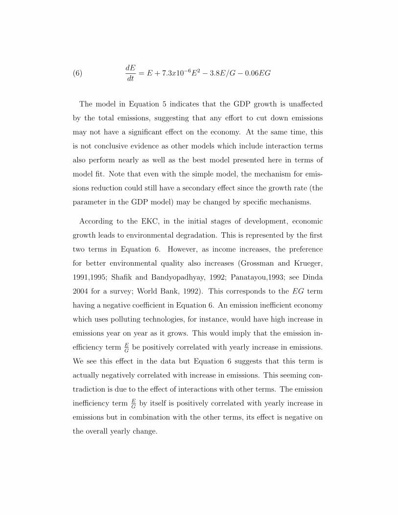
(6)dE

dt= E + 7.3x10−6E2 − 3.8E/G− 0.06EG

The model in Equation 5 indicates that the GDP growth is unaffected

by the total emissions, suggesting that any effort to cut down emissions

may not have a significant effect on the economy. At the same time, this

is not conclusive evidence as other models which include interaction terms

also perform nearly as well as the best model presented here in terms of

model fit. Note that even with the simple model, the mechanism for emis-

sions reduction could still have a secondary effect since the growth rate (the

parameter in the GDP model) may be changed by specific mechanisms.

According to the EKC, in the initial stages of development, economic

growth leads to environmental degradation. This is represented by the first

two terms in Equation 6. However, as income increases, the preference

for better environmental quality also increases (Grossman and Krueger,

1991,1995; Shafik and Bandyopadhyay, 1992; Panatayou,1993; see Dinda

2004 for a survey; World Bank, 1992). This corresponds to the EG term

having a negative coefficient in Equation 6. An emission inefficient economy

which uses polluting technologies, for instance, would have high increase in

emissions year on year as it grows. This would imply that the emission in-

efficiency term EG

be positively correlated with yearly increase in emissions.

We see this effect in the data but Equation 6 suggests that this term is

actually negatively correlated with increase in emissions. This seeming con-

tradiction is due to the effect of interactions with other terms. The emission

inefficiency term EG

by itself is positively correlated with yearly increase in

emissions but in combination with the other terms, its effect is negative on

the overall yearly change.

As countries like China, India, Brazil and Indonesia develop, their total

emissions continue to increase the total emissions (as captured by the E and

E2 terms). With the increase in their GDP per capita, the EG

interaction

term implies a decline in the decrease in the change in the total carbon

dioxide emissions. This might be due to the choice of technology, efficiency,

institutions, macro policies as also several social and political factors. As

these countries will continue on their economic development path our model

suggests that the EG interaction term kicks in with greater taste and pref-

erence for better environmental quality. The result of these two terms taken

together is that first there is an increase in emissions with increasing GDP

followed by a decrease due to the preference term.

We can see from the data phase portrait Fig. 1 that countries with higher

GDP per capita have more GHG emissions and vice versa. Fig. 2 shows the

phase portrait of the dynamical system given by our model in Equations 5

and 6. We can see that the two phase portraits are similar, confirming that

the model predicts the data reasonably well.

B. Model Validation and GHG emission projection in the short run

The system of equations 5 and 6 provide the description of the most

probable dynamics between economic growth and GHG emissions, in 1990-

2005. If the patterns of growth that were current until 2005 were to continue

with a business-as-usual scenario, our global projections for GHGs show that

the GHGs rise from around 35.7 GtCO2e to nearly 61 GtCO2e equivalent in

2020 (Fig. 3). Our projections are very close to the UNEP (2011) business-

as-usual projections. According to UNEP the global emissions could reach

around 56 GtCO2e in 2020.

6 9 120

5000

10000

log GDP per capita

Tota

l E

mis

sio

ns in G

t C

O2 e

quiv

ale

nt

ChinaUSASweden

IndiaBrazilKenya

RussiaSouth AfricaQatar

Figure 1. : Total emissions against log GDP per capita for all countriesfrom 1990-2005. The black vector lines show the average yearly changes(magnitude and direction) in log GDP and total emissions as a functionof current log GDP and total emissions. The coloured vector lines showrepresentative country trajectories in the same time period.

6 9 120

5000

10000

log GDP per capita

Tota

l E

mis

sio

ns in G

t C

O2 e

quiv

ale

nt

ChinaUSASweden

IndiaBrazilKenya

RussiaSouth AfricaQatar

Figure 2. : The model predictions for total emissions against log GDP percapita for all countries from 1990-2005. The coloured vector lines show thepredicted country trajectories starting from 1990 initial conditions for thesame time period.

Figure 3. : Predicted Total Emissions with the IPCC target for 2020 to keepglobal temperature increase below 2 degrees C

We test the robustness of our best-fit model by checking the predictions

for 2008 and 2010, against the actual data. Our model predictions for

the total emissions are 39.70 GtCO2e in 2008, while the actual recorded

value was 41.12 GtCO2e. In 2010, the predicted total emissions are 42.73

GtCO2e while the actual total emissions were 40.84 GtCO2e. Investigat-

ing the country-wise prediction we find that United States, for example,

will emit less than what the model predicts (about 7.6 GtCO2e in 2010

is predicted by the model) whereas historically, since 2005, it has reduced

emissions (actual in 2010 is 6.61 GtCO2e). We find similar evidence for the

developed countries. On the other hand, fast growing developing economies

like China, emit more than what our model predicts (actual emission in

2010 was 10.7 GtCO2e, predicted: 9.94 GtCO2). Overall these effects bal-

ance each other globally to an extent and our model leads to a somewhat

conservative estimate that nearly reflects the actual emissions.

Even if we go by the more conservative target (target-band) of 44 GtCO2e

(range: 39-44 GtCO2e) by 2020, the projected business-as-usual scenario in

our model leaves a gap of 17 GtCO2e with the IPCC target in the global

emissions. What makes the task of reducing this gap challenging is that

the reduction in the GHG needs to be achieved while enhancing access to

energy. About 1.4 billion people lack modern energy services (UNEP 2011).

Add to that the energy demands of the fast growing economies, like China

and India, and the task becomes even more difficult.

VI. Testing ways to Reduce Greenhouse Gas Emissions

Many proposals have been suggested to reduce emissions to acceptable

levels. Our model allows us to test different scenarios based on changes to

the different model parameters. We also test options by imposing the global

target of 44 GtCO2e and find the set of model parameters that can achieve

this target.

A. Proportional Reduction in Emissions

One simple option to achieve emissions reduction is to impose a propor-

tional reduction in emissions on all countries. In this regime, we know that

our global business-as-usual projection for total emissions is 60.77 GtCO2e,

which is 16.77 GtCO2e above the 44 GtCO2e target. To eliminate this emis-

sion gap, each country could aim for a total reduction in 2020 of 27.6% of

its predicted emissions.

One objection to this “democratic” scheme of reducing emissions across

different countries is that the poorer countries need to reduce emissions in

the same proportion as the more developed countries. This may set back

their development as the initial stages of economic development present ad-

ditional challenges and reducing energy consumption and hence greenhouse

gas emission might be a difficult proposition to achieve. On the other hand,

emissions per capita numbers show that some developed countries (when

we exclude very under-populated countries such as Aruba or the Caribbean

islands, for instance) have a much larger share of emissions relative to the

population they support. Some developing countries such as China and In-

dia, even though they support huge populations, also contribute very heavily

to the global emissions.

Of the total predicted emissions of 60.77 GtCO2e, the top 25 emitters

which includes rapidly developing countries such as China, India, Brazil,

Indonesia, Mexico, Turkey etc. and developed countries such as the United

States, the United Kingdom, Canada, Japan, Germany, Italy etc. contribute

54.5 GtCO2e, or nearly 90% of the total emissions. If the load of reducing the

16.77 GtCO2e in 2020 is shared only by the top 25 emitters, then they have

to reduce their emissions by 30.8% each while the others can continue along

their historical trajectories. Table 4 presents the predicted 2020 emissions

for the top 10 emitters. Regime I presents the reduction in GtCO2e if all

countries democratically reduce their emissions in the same proportion to

achieve the global target of 44 GtCO2e. In contrast, Regime II presents

the same proportional reduction in the emissions by the top 25 emitters in

the world, in order to meet the global targets. According to our prediction

estimates, with the exception of China, for other countries this would not

result in a significant increase in the required reduction to meet the global

targets in the short run. Thus, one possible strategy could be to focus on

the top GHG emitters.

Figure 4. : Table showing the top 10 emitters in 2005 and their predictedemissions in 2020 based on model predictions. Regime I reductions corre-spond to proportionally equal reductions for all countries based on estimatedovershoot of 16.77 Gt CO2 equivalent in 2020. Regime II reductions corre-spond to the top 25 emitters of 2020 sharing the burden of reducing all theexcess emissions.

B. Effect of Emission Cuts, Technology and Preferences in Business as

Usual Scenario

The model parameters in Equations 5 and 6 represent the business-as-

usual scenario. If policy changes are allowed, they are reflected by changes

in the model parameters. In general, we can rewrite the two equations as

(7)dG

dt= 0.014× δ

(8)dE

dt= α(E + 7.3× 10−6E2)− β × 3.8E/G− γ × 0.06EG

where changes in the estimated coefficients in the original model due to

policy interventions are represented by changes in the parameters α, β, γ, δ.

Here δ represents changes in economic growth rate, α represents the cutoff

rates of emission imposed on countries, β is the improvement in technology

and γ is the change in environmental preference.

If only one parameter can be changed, we see that total emissions decreases

when α decreases and when β and γ increase.

In the real world scenario policymakers make multiple interventions simul-

taneously. It is therefore more interesting to look at combinations of policy

interventions where two or more parameters are simultaneously changed.

This analysis enables us to identify the most effective combination among

the imposed reductions, technological change and change in environmental

preference, and to choose the best option to invest in among them.

(a) (b) (c)

Figure 5. : Predicted total global emissions in 2020 shown as a function ofchanging two of the parameters α, β and γ while keeping the third parameterconstant at 1. The mapping of colour to amount of emissions is shown asa colourbar in units of tonnes of CO2 equivalent. The dashed line in eachsub-figure represents the desired target of 44 GtCO2e.

The three sub-figures in Fig. 5 show the predicted emissions as a function

of changes in two of the parameters keeping the third constant at 1 which

corresponds to the business-as-usual scenario for that variable. Instead of

using a 3-D plot, we use a heatmap to show the predicted emissions in 2020

as a function of the two parameters while the third is constant at 1. The

mapping of colour to amount of emissions is shown in the colour bar in units

of mega tonnes of CO2 equivalent. The grading is such that darker shades of

gray (and black) corresponds to low values while lighter shades (and white)

correspond to high values. Since we are not concerned here with the exact

values for every set of parameters but only those parameter values that yield

the desired target (shown by the red lines on the plots), the heatmap is an

efficient way to condense the information. Note that the scales are different

in the three sub-figures and so the same shade represents slightly different

value of predicted emissions.

We see from the figure that different parameter combinations yield the

same predicted emissions (same shades on the heatmap). Specifically, the

dashed lines on the three sub-figures show the values of the parameters for

which predicted emissions in 2020 is 44 GtCO2e. Numerical simulations

are used to obtain these heatmaps and hence the dashed lines represent the

numerically closest values to 44 GtCO2e. Mathematically we can see that

the curves of constant predicted emissions on these planes are straight lines.

The region below the dashed lines in sub-figures a) and b) and the region

above the dashed line in sub-figure c) are the desirable set of parameters

which will lead to achieving the target of less than 44 GtCO2e in 2020.

It is clear from sub-figure a) that if the environmental quality preference

is business-as-usual, improvements in technology will be required to meet

the desired target even if emissions are cut-down. For instance, a global-

emissions cut of 4 percent would still require a 5 percent improvement in

technology by 2020 to meet the required target. If however, the technology

scenario remains business-as-usual (sub-figure b), meeting the global emis-

sions target for 2020 would be impossible without improvements in prefer-

ences for environmental quality. This is already a sign of the difficult task

ahead in controlling emissions. A result that is supported by the literature

that shows that the developing countries have a harder time improving en-

vironmental quality (for example,compare the results in Stern and Common

2001 and Selden and Song 1994; Cole et al. 1997 and Kauffman et al. 1998).

The model provides clear directives on how to attain global emission tar-

gets if no clear emission cuts are agreed upon and implemented by countries,

especially the top emitters. In such a business-as-usual scenario (sub-figure

c), we would require an improvement of about 3.5 percent in preference for

better environmental quality and about 2.6 percent improvement in tech-

nology. It is worth emphasising that changes below these thresholds will not

result in desired outcomes.

VII. Discussion and Conclusions

In the post-2015 scenario, the scientific evidence pointing towards the

imminent dire consequences of GHG emissions need to be translated into

actionable goals that may be globally implemented with immediate effect.

These SDGs need to be simple, clear, achievable and easily monitored. We

use dynamical systems models to investigate the interaction between GHGs

and GDP and test some intuitively plausible options that can potentially

be formulated into SDGs. Predicting the total GHG emissions for the year

2020 our best-fit model suggests that the emissions might be brought down

through mechanisms of better technology/efficiency and by bringing about

greater changes in the education/awareness or preferences of citizens towards

better environmental quality. According to our estimation, the business as

usual global GHG emission prediction is about 61 GtCO2e by 2020. This is

nearly 17 GtCO2e above the recommended 44 GtCO2e for 2020 to keep the

increase in temperature under 2 degree in this century.

We test and suggest three potential SDGs. The first SDG option is a

democratic equal reduction in the total emissions of all countries. This

would imply a total reduction in 2020 of 27.6% of its predicted emissions

between now and 2020. The second SDG option is to focus on the top emit-

ters. Rapidly developing countries such as China, India, Brazil, Indonesia,

Mexico, Turkey etc. and developed large economies such as the United

States, the United Kingdom, Canada, Japan, Germany, Italy etc. account

for the majority of the future global emissions till 2020. We find that if the

top 25 emitters bear the full load of meeting the global emissions reduction

target, their burden in reducing emissions does not change by much. Thus,

focussing on a few key global emitters in the short-run might be a more

effective strategy.

Our results from Figure 7 suggest that under a business-as-usual scenario

where no global emission cuts are implemented, the world would have to see

an improvement in its emission-reduction technology by atleast 2.6 percent

and also alter its tastes and preferences by about 3.5 percent. This provides

us with the third SDG option, as any improvements below these thresholds

would not be sufficient to achieve the desirable emissions target by 2020.

While our best-fit model provides us insights into setting of SDGs, the real

world is fraught with political, social and institutional hurdles. A suggestion

to focus on the set of most 25 polluting countries in the very short run might

make logical sense but in terms of implementation might turn out to be a

political and diplomatic mine-field. At best, the suggestions in this paper

may be treated as normative directives to identify the immediate threat of

the process of economic growth and global GHG emissions and insights into

how they may be effectively contained, at least in the very short run.

References

Adams, R., Rosenzweig,C., Peart, R.M., Ritchie, J.T., McCarl, B., Glyer,

D.J., Curry, B., Jones, J.W., Boote, K.J., Allen Jr., L.H. 1990. Global Cli-

mate Change and US Agriculture, Nature, 345, pp. 219-224.

Anderson, D., Cavandish, W., 2001. Dynamic simulation and environmen-

tal policy analysis: beyond comparative statics and environmental Kuznets

curve. Oxford Economic Papers 53, 721– 746.

Andreoni, J., Levinson, A., 2001. The simple analytics of the Environ-

mental Kuznets Curve. Journal of Public Economics, 80 (2), 269– 286.

Antweiler, W., B. R. Copeland and M.S. Taylor. 2001. Is Free Trade

Good for The Environment?, American Economic Review 91(4): 877-908.

Arrow, K., B. Bolin, R. Costanza, P. Dasgupta, C.Folke, C. S. Holling,

B.O. Jansson, S. Levin, K.G. Maler, C. Perrings and D. Pimentel. 1995.

Economic growth, carrying capacity, and the environment. Ecological Eco-

nomics 15( 2): 91-95.

Barrett, S. and K. Graddy. 2000, “Freedom, growth, and the environ-

ment”, Environment and Development Economics 5:433-456.

Bartlett, A. 1994. Reflections on Sustainability, Population Growth and

the Environment. Population and Environment 16(1): 5-35.

Beckerman, W. 1992. Economic Growth and the Environment: Whose

Growth? Whose Environment? World Development 20(4): 481-296.

Berger, J.O. 1985. Statistical Decision Theory and Bayesian Analysis.

Springer-Verlag, New York.

Bhagawati, J., 1993. The case for free trade. Scientific American, 42-49.

Bimonte, S. 2002. Information access, income distribution and the envi-

ronmental Kuznets curve. Ecological Economics 4: 145-156.

Cole, M.A., A.J. Rayner and J.M. Bates. 1997. The environmental

Kuznets curve: an empirical analysis. Environment and Development Eco-

nomics 2: 401-416.

Coondoo, D. and S. Dinda. 2002. Causality between income and emis-

sion: a country group-specific econometric analysis. Ecological Economics

40: 351-367.

Clemens, M.A. Kenny, C.J.and Moss, T. 2007. The Trouble with the

MDGs: Confronting, Expectations of Aid and Development Success, World

Development 35, (5). 735-751.

Dasgupta, P. and K.-G. Maler. 1995. Poverty, institutions, and the envi-

ronmental resource-base”, In: Behrman, J. and T.N.Srinivaan (Eds.), Hand-

book of Development Economics, vol. 3A. Elsevier Science, Amsterdam.

Dell, M., Jones, B.F., Olken, B.A. 2012. Temperature Shocks and Eco-

nomic Growth: Evidence from the Last Half Century, American Economic

Journal: Macroeconomics, 4 (3), pp. 66-95.

den Elzen, M.G.J., van Vuuren, D.P. and van Vliet, J. 2010. Postponing

emission reductions from 2020 to 2030 increases climate risks and long-term

costs, Climate Change, 99 (1-2), 313-320.

Deschenes, O. and Greenstone, M. 2007. The Economic Impact of Climate

Change: Evidence from Agricultural Output and Random Fluctuations in

Weather, American Economic Review, 97, pp. 354-385.

Deschenes, O. and Moretti, E. 2010. Extreme Weather Events, Mortality,

and Migration, Review of Economics and Statistics, 91(4), pp. 659-681.

Dijkgraaf, E., Vollebergh, H.R.J. 2005. A test for parameter heterogene-

ity in CO2 panel EKC estimations. Environmental Resource Economics, 32,

pp.229-239.

Dijkgraaf, E., Vollebergh, H.R.J. 1998. Environmental Kuznets Revisited:

Time-Series Versus Panel Estimation: The CO2 Case (OCFEB Research

Memorandum 9806).

Dinda, S., 2002. A theoretical basis for Environmental Kuznets Curve.

Economic Research Unit, Indian Statistical Institute, Kolkata. Mimeo.

Dinda, S., 2003. Economic growth with environmental and physical capi-

tal: a convergence approach. Mimeo.

Dinda, S. 2004. Environmental Kuznets Curve Hypothesis: A Survey.

Ecological Economics, 49, pp. 431-455.

Ekins, P. 1997. The Kuznets curve for the environment and economic

growth: examining the evidence. Environment and Planning A. 29: 805-

830.

Easterly, W. 2007. How the Millennium Development Goals are Unfair

to Africa, Brookings Global Economy and Development Working Paper 14,

November 2007.

Friedl, B. and M. Getzner. 2003. Determinants of CO2 emissions in a

small open economy. Ecological Economics 45:133-148.

Field, S. 1992. The Effect of Temperature on Crime, The British Journal

of Criminology, 32, pp. 340-351.

Galeotti, M., Manera, M. and Lanza, A. 2009. On the Robustness of

Robustness Checks of the Environmental Kuznets Curve Hypothesis, Envi-

ronmental and Resource Economics, 42 (4), pp. 551-574.

Granados, J.A. T, Ionides, E.L., and Carpintero, O. 2012. Climate change

and the world economy: short-run determinants of atmospheric CO2, Envi-

ronmental Science and Policy, 21, pp. 50-62.

Grossman, G. M., & Krueger, A. B. (1995). Economic growth and the

environment, Quarterly Journal of Economics, 110 (2), pp. 353-377.

Halkos, G.E. 2003. Environmental Kuznets Curve for Sulfur : Evidence

using GMM estimation and random coefficient panel data model. Environ-

ment and Development Economics, 8:581-601.

Harbaugh, W., Levinson, A., Wilson, D.M., 2002. Re-examining the em-

pirical evidence for an Environmental Kuznets Curve. The Review of Eco-

nomics and Statistics 84 (3), 541-551.

He, J. 2006. Pollution haven hypothesis and Environmental impacts of

foreign direct investment: The Case of Industrial Emission of Sulfur Diox-

ide (SO2) in Chinese provinces, Ecological Economics, 60:228-245.

He, J. 2007. Is the Environment Curve hypothesis valid for developing

countries? A survey. Cahier de recherche Working Paper 07-03, Universite

de Sherbrooke, Canada.

Hilton, F.F.H. and A. Levinson. 1998. Factoring the environmental

Kuznets curves: Evidence from automotive lead emissions. Journal of En-

vironmental Economics and Management 36: 126-141.

Holtz-Eakin, D., Selden, T., 1995. Stocking the fires? CO2 emissions and

economic growth. Journal of Public Economics 57, 85-101.

Hossain, M.S. 2011. Panel estimation for CO2 emissions, energy consump-

tion, economic growth, trade openness and urbanization of newly industri-

alized countries, Energy Policy 39, pp. 6991-6999.

Hsiang, S.M. 2010. Temperatures and Cyclones Strongly Associated with

Economic Production in the Caribbean and Central America, Proceedings

of the National Academy of Sciences.

IPCC. 2007. Climate Change 2007: Synthesis Report, Cambridge, UK

and New York, USA: Intergovernmental Panel on Climate Change.

Jaynes, R.T. 2003. Probability Theory: The Logic of Science. Cambridge

University Press, Cambridge.

Jeffreys, H. 1939. Theory of Probability, Oxford University Press, Oxford.

John, A., Pecchenino, R., 1994. An overlapping generations model of

growth and the environment. Economic Journal 104, 1393-1410.

Kaufmann, R., B. Davidsdottir, S. Garnham and P. Pauly. 1998. The

Determinants of Atmospheric SO2 Concentrations: Reconsidering the En-

vironmental Kuznets Curve. Ecological Economics 25:209-220.

Komen, R., Gerking, S., Folmer, H., 1997. Income and environmental

R&D: empirical evidence from OECD countries. Environment and Devel-

opment Economics 2, 505-515.

Koop, G., Tole, L. 1999. Is there an environmental Kuznets curve for

deforestation? Journal of Development Economics 58: 231-244.

Kuznets, S. 1955. Economic growth and income inequality. American

Economic Review 45, 1-28.

Labys, W.C., Wadell, L.M. 1989. Commodity lifecycles in US materials

demand. Resources Policy 15, 238-252.

Ley, E., Steel, M.F.J. 2009. On the effect of prior assumptions in Bayesian

Model Averaging with applications to growth regression. Journal of Applied

Econometrics, 24: 651-674.

Lindmark, M. 2002. An EKC-pattern in historical perspective: carbon

dioxide emissions, technology, fuel prices and growth in Sweden, 1870-1997.

Ecological Economics, 42: 333-347.

List, J.A. and C. A. Gallet. 1999. The environmental Kuznets Curve:

Dose One Size Fit All ? Ecological Economics, 31:409-423.

Lomborg, B. 2001. The Skeptical Environmentalist: Measuring the Real

State of the World. Cambridge, UK: Cambridge University Press.

Lopez, R., 1994. The environment as a factor of production: the effects of

economic growth and trade liberalization. Journal of Environmental Eco-

nomics and management, 27, 163-184.

Mackay, D.J.C. 2003. Information Theory, Inference and Learning Algo-

rithms. Cambridge University Press, Cambridge.

Magnani, E. 2000. The environmental Kuznets Curve, environmental pro-

tection policy and income distribution. Ecological Economics 32: 431-443.

Narayan,P.K., Narayan,S. 2010. Carbon dioxide and economic growth:

panel data evidence from developing countries. Energy Policy, 38,661-666.

Panayotou, T., 1993. Empirical tests and policy analysis of environmental

degradation at different stages of economic development, ILO, Technology

and Employment Programme, Geneva.

Panayotou, T., 1997. Demystifying the environmental Kuznets curve:

turning a black box into a policy tool. Environment and Development Eco-

nomics 2, 465-484.

Panayotou, T., 1999. The economics of environments in transition. Envi-

ronment and Development Economics 4 (4), 401-412.

Piontek et al, 2013. Multisectoral climate impact hotspots in a warming

world. Proceedings of the National Academy of Sciences. DOI: 10.1073/pnas.1222471110

Quadrelli, R., Peterson, S., 2007. The energy–climate challenge: recent

trends in CO2 emissions from fuel combustion. Energy Policy 35, 5938-5952.

Ranganathan, S., Spaiser, V., Mann, R.P., and Sumpter, D. 2014. Bayesian

Dynamical Systems Modelling in the Social Sciences. PLoS ONE.

Ranger, V., Gohar, L., Lowe, J., Bowen, A. and Ward, R. 2010. Miti-

gating climate change through reduction in greenhouse gas emissions:is it

possible to limit global warming to no more than 1.5o C? – Policy brief.

Grantham Research Institute.

Raupach, M.R., Marland, G., Ciais, P., Le Que´re´ , C., Canadell, J.G.,

Klepper, G., Field, C.B., 2007. Global and regional drivers of accelerating

CO2 emissions. Proceedings of National Academy of Science, 104, 10288-

10293.

Roberts, J. T. and P. Grimes. 1997. Carbon Intensity and Economic De-

velopment 1962-1991 : A Brief Exploration of the Environmental Kuznets

Curve. World Development 25:191-198.

Roca, J., Alcantara, V., 2001. Energy intensity, CO2 emissions and the

environmental Kuznets curve. The Spanish case. Energy Policy 29, 553-556.

Roca, J., E. Padilla, M. Farre and V. Galletto. 2001. Economic growth

and atmospheric pollution in Spain: Discussion the environmental Kuznets

hypothesis. Ecological Economics 39: 85-99.

Selden T. M. and D. Song. 1994. Environmental Quality and Develop-

ment: Is there a Kuznets Curve for Air Pollution Emission? Journal of

Environmental Economics and Management 27: 147-162.

Shen, J. 2006. A simultaneous estimation of Environmental Kuznets

Curve: Evidence from China. China Economic Review, 17(2006):383-394.

Steinacher et al. 2013. Allowable carbon emissions lowered by multiple

climate targets. Nature. DOI: 10.1038/nature12269

Stern, D. I. 2002. Explaining changes in global sulfur emissions: an econo-

metric decomposition approach, Ecological Economics, vol. 42, pp. 201-220.

Stern, D.I., 2004. The rise and fall of the environmental Kuznets curve.

World Development, 32, 1419-1439.

Stern, D.I. and M.S. Common. 2001. Is there an environmental Kuznets

curve for sulfur? Journal of Environmental Economics and Management 41:

162-178.

Stern, N. 2007. The Economics of Climate Change: The Stern Review,

Cambridge, England: Cambridge University Press.

Stokey, N.L., 1998. Are there limits to growth? International Economic

Review, 39 (1), 1-31.

Suri, V. and D. Chapman. 1998. Economic growth, trade and energy:

implications for the environmental Kuznets curve. Ecological Economics

25(2): 195-208.

Swain, A., Bali Swain, R., Themner, A., and Krampe, F. 2011. Climate

Change, Natural Resource Governance and Conflict Prevention in Africa:

A Scoping Study of the Zambezi River, Global Crisis Solutions, Pretoria,

South Africa.

Tol, R.S.J., Pacala, S.W., Socolow, R.H. 2009. Understanding long-term

energy use and carbon dioxide emissions in the USA. Journal of Policy Mod-

eling, 31, 425-445.

Torras, M. and J. K. Boyce. 1998. Income, Inequality and Pollution: A

Reassessment of the Environmental Kuznets Curve. Ecological Economics,

25:147-160.

Unruh, G. C. and W. R. Moomaw. 1998. An Altenative Analysis of Ap-

parent EKC-Type Transitions. Ecological Economics 25:221-229.

United Nations. 2012. Realizing the Future We Want for All: Report to

the Secretary-General, UN System Task Team on the Post-2015 UN Devel-

opment Agenda, New York.

UNEP. 2011. The Emissions Gap Report: Are the Copenhagen Accord

Pledges Sufficient to Limit Global Warming to 2o C or 1.5oC?, A prelim-

inary assessment, Full Report, United Nations Environment Programmme

(UNEP).

UNEP. 2012. Submission of the United Nations Environment Programme

(UNEP) to the Ad Hoc Working Group on the Durban Platform for En-

hanced Action (AWG-DPEA), submitted 27 February 2012.

Vandemoortele, Jan. 2007. The MDGs: ‘M’ for Misunderstood?, WIDER

Angle, United Nations World Institute for Development Economics Re-

search. 6-7.

Wagner, M., 2008. The carbon Kuznets curve: a cloudy picture emitted

by bad econometrics? Resource Energy Economics 30, pp. 388-408.

World Bank. 1992. World development report: environment and devel-

opment. New York: Oxford University Press.

WORKING PAPERS* Editor: Nils Gottfries 2013:1 Jan Pettersson and Johan Wikström, Peeing out of poverty? Human fertilizer

and the productivity of farming households. 43 pp. 2013:2 Olof Åslund and Mattias Engdahl, The value of earning for learning:

Performance bonuses in immigrant language training. 52 pp. 2013:3 Michihito Ando, Estimating the effects of nuclear power facilities on local

income levels: A quasi-experimental approach. 44 pp. 2013:4 Matz Dahlberg, Karin Edmak and Heléne Lundqvist, Ethnic Diversity and

Preferences for Redistribution: Reply. 23 pp. 2013:5 Ali Sina Önder and Marko Terviö, Is Economics a House Divided? Analysis

of Citation Networks. 20 pp. 2013:6 Per Engström and Eskil Forsell, Demand effects of consumers' stated and

revealed preferences. 27 pp. 2013:7 Che-Yuan Liang, Optimal Inequality behind the Veil of Ignorance. 26 pp. 2013:8 Pia Fromlet, Monetary Policy Under Discretion Or Commitment? -An

Empirical Study. 57 pp. 2013:9 Olof Åslund and Mattias Engdahl, Open borders, transport links and local

labor markets. 41 pp. 2013:10 Mohammad Sepahvand, Roujman Shahbazian and Ranjula Bali Swain, Time

Investment by Parents in Cognitive and Non-cognitive Childcare Activities. 31 pp.

2013:11 Miia Bask and Mikael Bask, Social Influence and the Matthew Mechanism:

The Case of an Artificial Cultural Market. 13 pp 2013:12 Alex Solis, Credit access and college enrollment. 54 pp 2013:13 Alex Solis, Does Higher Education Cause Political Participation?: Evidence

From a Regression Discontinuity Design. 48 pp. 2013:14 Jonas Kolsrud, Precaution and Risk Aversion: Decomposing the Effect of

Unemployment Benefits on Saving. 37 pp. 2013:15 Helena Svaleryd, Self-employment and the local business cycle. 28 pp. 2013:16 Tobias Lindhe and Jan Södersten, Distortive Effects of Dividend Taxation.

22 pp. 2013:17 Jonas Poulsen, After Apartheid: The Effects of ANC Power. 42 pp.

* A list of papers in this series from earlier years will be sent on request by the department.

2013:18 Magnus Gustavsson, Permanent versus Transitory Wage Differentials and

the Inequality-Hours Hypothesis. 11 pp. 2013:19 Lovisa Persson, Consumption smoothing in a balanced budget regim. 35 pp. 2013:20 Linuz Aggeborn, Voter Turnout and the Size of Government. 50 pp. 2013:21 Niklas Bengtsson, Stefan Peterson and Fredrik Sävje, Revisiting the

Educational Effects of Fetal Iodine Deficiency. 48 pp 2013:22 Michihito Ando, How Much Should We Trust Regression-Kink-Design

Estimates? 69 pp. 2013:23 Bertil Holmlund, What do labor market institutions do? 25 pp. 2014:1 Oscar Erixson and Henry Ohlsson, Estate division: Equal sharing as choice,

social norm, and legal requirement. 45 pp. 2014:2 Eva Mörk, Anna Sjögren and Helena Svaleryd, Parental unemployment and

child health. 35 pp. 2014:3 Pedro Carneiro, Emanuela Galasso and Rita Ginja, Tackling Social

Exclusion: Evidence from Chile. 87 pp. 2014:4 Mikael Elinder och Lovisa Persson, Property taxation, bounded rationality

and housing prices. 38 pp. 2014:5 Daniel Waldenström, Swedish stock and bond returns, 1856–2012. 51 pp. 2014:6 Mikael Carlsson, Selection Effects in Producer-Price Setting. 34 pp. 2014:7 Ranjula Bali Swain and Fan Yang Wallentin, The impact of microfinance on

factors empowering women: Differences in regional and delivery mechanisms in India’s SHG programme. 28 pp.

2014:8 Ashim Kumar Kar and Ranjula Bali Swain, Competition, performance and

portfolio quality in microfinance markets. 33 pp. 2014:9 Shyam Ranganathan, Ranjula Bali Swain and David J.T. Sumpter, A

DYNAMICAL SYSTEMS APPROACH TO MODELING HUMAN DEVELOPMENT. 42 pp.

2014:10 Shyam Ranganathan and Ranjula Bali Swain, Analysing Mechanisms for

Meeting Global Emissions Target - A Dynamical Systems Approach. 40 pp. See also working papers published by the Office of Labour Market Policy Evaluation http://www.ifau.se/ ISSN 1653-6975