Model-based Robust Fault Diagnosis forSatellite Control Systems Using Learning and

Sliding Mode ApproachesQing Wu, Mehrdad Saif

School of Engineering Science, Simon Fraser University, Vancouver, BC, CanadaEmail: {qingw, saif}@ensc.sfu.ca

Abstract— In this paper, our recent work on robust model-based fault diagnosis (FD) for several satellite controlsystems using learning and sliding mode approaches aresummarized. Firstly, a variety of nonlinear mathematicalmodels for these satellite control systems are described andanalyzed for the purpose of fault diagnosis. These satellitecontrol systems are classified into two classes of nonlineardynamical systems. Then, several fault diagnostic observersusing sliding mode and learning approaches are presented.Sliding mode with time-varying switching gains, second or-der sliding mode, and high order sliding mode differentiatorsare respectively used in the proposed diagnostic observersto deal with modeling uncertainties. Neural model-basedand iterative learning algorithms-based online learning es-timators are respectively used in the diagnostic observersfor the purpose of isolating and estimating faults. Finally,conclusions and future work on the health monitoring andfault diagnosis for satellite control systems are provided.

Index Terms— fault diagnosis, observer, sliding mode, learn-ing, satellite control systems

I. INTRODUCTION

With the development of space technologies, differentclasses of satellites have been constructed and utilized forvarious space missions, such as global positioning, Earthobservation, atmosphere data collection, space science,and communication. The dynamics of satellite controlsystems have the following characteristics: i) The safetyand reliability of the satellite control systems are so essen-tial that fault diagnosis (FD) strategies are indispensablefor them. ii) Various linear and nonlinear mathematicalmodels of the satellite control systems are available for thedesign and analysis of controllers and/or state observers.Although linear models can represent the attitude dynam-ics at local vertical local horizontal (LVLH) orientation,inherently, the satellite dynamics is nonlinear. Especiallywhen a satellite make a large angle maneuver, or it hasflexible appendages, or multiple satellites are deployed,different nonlinear models must be applied to describethese dynamics. iii) The satellites in space are subject tointernal modeling uncertainties and external disturbances,such as gravity-gradient torque, aerodynamics torque, and

This paper is based on “An Overview of Robust Model-based FaultDiagnosis for Satellite Systems Using Sliding Mode and LearningApproaches,” by Q. Wu and M. Saif, which appeared in the Proceedingsof the IEEE Conference on Systems, Men, and Cybernetics, Montreal,Canada, October, 2007. c© 2007 IEEE.

Earth magnetic torque, etc. iv) In order to ensure thenormal operation, real-time fault diagnosis is necessaryto provide information for the satellites to accommodatethe fault in time.

In the last three decades, model-based robust faultdiagnosis schemes for nonlinear dynamic systems havebeen significantly investigated. Many contributions havebeen summarized in the books [3] and [4]. For non-linear systems, a class of FD schemes using learningmethodologies, which use neural networks [5], [6], [7],iterative learning observers, [8], or adaptive observers[9], [10], [11], have received great deal of attention. Toachieve robust fault diagnosis, dead-zone operators areadopted in the learning methodologies to make the faultapproximator insensitive to the error signal under a certainthreshold which is considered to be caused by modelinguncertainties [12], [13], [14]. However, two issues in thisclass of methodologies still need further studies. One isthat, in all likelihood, the dead-zone operators may reducethe accuracy of the fault approximation. The other issueis that the projection operators, which can confine theparameter estimation vectors to a predefined compact andconvex region, have to be used to bound parameters inthe presence of modeling uncertainties and approximationerrors.

Moreover, due to the inherent robustness to systemuncertainties, traditional and high order sliding mode havebeen studied in system observation (e.g. [15], [16], [17],[18], [20], [21], [22]) and robust fault diagnosis (e.g.[23], [24], [25], [26]), [27] for many years. One FDmethod based on sliding mode is that the estimationdynamics maintain a sliding motion even in the presenceof fault, and the fault is reconstructed by manipulating theequivalent output injection signal. Another approach is todesign an observer in such a way that the sliding motionis destroyed in the presence of fault [28]. In this case,additional online estimators are needed to approximatethe fault.

In this paper, we summarize our recent study on therobust fault diagnosis for a variety of satellite controlsystems using sliding mode and learning approaches. Ourobjective is to take advantages of these two methodologiesand create novel and practical model-based robust faultdiagnosis schemes for various satellite control systems.In Section II, the satellite control systems in our study

1022 JOURNAL OF COMPUTERS, VOL. 4, NO. 10, OCTOBER 2009

© 2009 ACADEMY PUBLISHER

are presented and summarized. Then, these systems aredescribed by two families of mathematical formula inSection III. After that, Section IV proposes three kindsof observers using sliding mode and learning approaches.Fault detection, isolation, and estimation schemes basedon these diagnostic observers are formulated in SectionV and VI. Finally, conclusion is given in Section VII.

II. SATELLITE MODELS

In mathematical model-based fault diagnosis schemes,a model for the plant is built first. Then diagnosticresiduals are generate through comparing the output ofthe practical system with the output of the model. Next,the residuals are used to diagnose faults.

An important assumption for the model-based faultdiagnosis schemes is that the mathematical models areable to represent the practical systems with sufficientaccuracy. Otherwise, the mismatch between the practicalsystems and their models as well as disturbances mightcause the proposed fault diagnosis schemes unreliable.As aerospace technologies develop, different models forsatellites are available for system analysis and controllerdesign. The satellite models become more and moresophisticated if they are used to represent the real satellitesystems precisely. Hence, more complex models shouldalso be used in the model-based robust FD for satellitecontrol systems.

A. Nonlinear Model for Rigid-body Satellite AttitudeControl Systems

In many research literatures, a satellite is modeled asa rotary rigid body, and its dynamics is described usingthe following equation of motion [29],

Iω + ω×Iω = 3ω20ζ×Iζ + u + Td (1)

and the following relation between ω and pitch angle θ1,yaw angle θ2, and roll angle θ3:

ω =

⎡⎣ω1

ω2

ω3

⎤⎦ =

⎡⎣ (ω0 + θ1) sin θ2 + θ3

(ω0 + θ1) cos θ2 cos θ3 + θ2 sin θ3

−(ω0 + θ1) cos θ2 sin θ3 + θ2 cos θ3

⎤⎦

=

⎡⎣ sin θ2 0 1

cos θ2 cos θ3 sin θ3 0− cos θ2 sin θ3 cos θ3 0

⎤⎦

⎡⎣ θ1

θ2

θ3

⎤⎦

+

⎡⎣ ω0 sin θ2

ω0 cos θ2 cos θ3

−ω0 cos θ2 sin θ3

⎤⎦

= R(θ)θ + ωc(θ) (2)

where ω0 is the orbital angular velocity of the satellite,θ = [θ1 θ2 θ3]� is Euler angle vector, u = [u1, u2, u3]�

is the control torque vector, and Td represents the externaldisturbance torques. Ii, (i = 1, 2, 3) are the principal axismoments of inertia of the satellite. The term ζ is

ζ =

⎡⎣ − sin θ1 cos θ2

cos θ1 sin θ3 + sin θ1 sin θ2 cos θ3

cos θ1 cos θ3 − sin θ1 sin θ2 sin θ3

⎤⎦ (3)

The notation ω× stands for a skew symmetric matrix

ω× =

⎡⎣ 0 −ω3 ω2

ω3 0 −ω1

−ω2 ω1 0

⎤⎦

For the dynamic system represented by (1) and (2), onlyθ1, θ2, θ3 are measurable.

B. Linear Model for Rigid-body Satellite Attitude Systems

For small attitude deviation from LVLH orientation,the nonlinear dynamics of the satellite attitude controlsystems can be linearized around its equilibrium point,and a linear model is given in [30] as

I1θ3 − w0(I1 − I2 + I3)θ2 + 4w0(I2 − I3)θ1 = u1 + Td1

I2θ1 + 3w20(I1 − I3)θ1 = u2 + Td2 (4)

I3θ2 + w0(I1 − I2 + I3)θ3 + w20(I2 − I1)θ2 = u3 + Td3

This linear model is important, since it can represent aclass of micro-satellites that have wide applications. Manycontrol algorithms can be designed based on this linearmodel. Moreover, for this linear time invariant systems,fault diagnosis based on linear models can be completelysolved, provided the considered system is observable.

C. Quaternion-based Model for Satellite Attitude Systems

Quaternions were invented as a result of searchingfor hypercomplex numbers that could be represented bypoints in three dimensional space. Quaternions have noinherent geometric singularity as do Euler angles. More-over, quaternions are well suitable for onboard real-timecomputation because only products and no trigonometricrelations exist in the quaternion kinematic differentialequations. Thus, spacecraft orientation is now commonlyrepresented in terms of quaternions. The motion equationsof the satellite are described in [31] as

Iω = −S(ω)Iω + Td + u (5)

q =12(q4I + S(q)) (6)

q4 = −12q�ω (7)

where I is still the moment of inertia matrix, ω is the an-gular velocity of the satellite, Td denotes the disturbancetorque, u is also the control torque, q = [q1, q2, q3]�, andq4 constitute the quaternions of the satellite, which satisfyq�q+q2

4 = 1. The quaternions are the output of the system(5)-(7). The notation S(ω) is the skew symmetric matrix.

D. Model for Flexible Satellite Attitude Systems

As the second generation of satellites appear, flexiblesatellites have been deployed. The model of a flexiblesatellite consists of a rigid central hub, which representsthe satellite body, and two flexible appendages, whichare usually solar arrays, antennas, or any other flexiblestructures.

JOURNAL OF COMPUTERS, VOL. 4, NO. 10, OCTOBER 2009 1023

© 2009 ACADEMY PUBLISHER

Spatial discretization method has ever been used toderive a group of ordinary differential equations to de-scribe the motion of satellite, although the vibration of theappendages is formulated by partial differential equations.Hence, the appendage deflections are expressed in termsof a set of admissible or shape functions as

δ(l, t) =N∑

i=1

Ψi(l − r)pi(t) (8)

where pi(t) are the generalized coordinates associatedwith these functions, l is the distance from a point on theappendage to the center of the hub, and r is the radius ofthe hub. Here, we assume that N modes are sufficient forthe computation of elastic deformation. Ψi are the shapefunctions that satisfy the geometric and physical boundaryconditions. The shape functions are given in [32] that

Ψi(l − r) = 1 − cos(

iπ(l − r)L

)

+12(−1)i+1

(iπ(l − r)

L

)2

(9)

A simplified formulation of the governing equations ofthis class of satellites is given in [33][

Jt m�ψp

mψp Mpp

] [ψp

]+

[0 00 Cpp

] [ψp

]

+[0 00 Kpp

] [ψp

]=

[ut

0

]+

[h1

h2

](10)

where

Jt = J + 2J1

h1 = −3ω20J1 sin(2ψ) − 3ω2

0 cos(2ψ)m�ψpp

h2 = (ψ2 + 2ψω0 + 3ω20 sin2 ψ)Mppp − 3

2ω2

0 sin 2ψmψp

where ψ is the pitch angle, p = [p1, · · · , pN ]� is the vec-tor of appendage flexibility generalized coordinates, ω0 isthe orbital rate, J and J1 are the mass moments of inertiaof the central hub and each appendage, respectively, ut

is the control torque, and Mpp, mψp, Cpp and Kpp arethe following modal integrals [33] as

[Mpp]i,j = 2∫ r+L

r

Ψi(l − r)Ψj(l − r)dl

[mψp]i,j = 2r

∫ r+L

r

lΨi(l − r)dl

[Cpp]i,j = 2∫ r+L

r

CIΨ′′i (l − r)Ψ′′

j (l − r)dl

[Kpp]i,j = 2∫ r+L

r

EIΨ′′i (l − r)Ψ′′

j (l − r)dl (11)

where Ψ′′i = (∂2Ψi/∂l2), C and E are the damping

coefficient and modulus of elasticity of the appendages,respectively, and I is the sectional area moment of inertiawith respect to the appendage bending axis.

E. Model for Satellite Orbital Control SystemsThe above model A, B and C are all about attitude

dynamics of satellites. When we consider the orbitalbehavior of a satellite, it can be treated as a point mass,which flies in a plane, subject to an inverse square lawforce field with potential energy k/r and both radial andtangential thrusts u1 and u2, respectively. The orbitaldynamics of a point mass satellite is given by [34]

r = v r(0) = r0

v = rw2 − k

mr2+

u1

mv(0) = 0

φ = w φ(0) = 0

ω = −2vω

r+

u2

mrω(0) = ω0

(12)

where m is the mass of the satellite, (r, φ) are the polarcoordinates of the satellite, v is the radial speed, and ωis the angular speed. The control objective is to track rand ω to their reference values.

F. Model for Multiple Satellites Formation Flying SystemOne key technology in aerospace engineering is to

distribute functionality of a large spacecraft to a group ofsmaller, low-cost, cooperative spacecraft. Flying two ormore satellites in a specific formation is usually referredto as multiple satellite formation flying (MSFF).

MSFF is a cluster of interdependent micro-satellitesthat communicate with each other and share payload, data,and missions. In the simplest case, the MSFF fleet iscomposed of a leader satellite and a follower satellite. Theleader satellite provides the reference motion trajectoryand the follower satellite navigates in the neighborhoodof the leader satellite according to a desired relativetrajectory.

The nonlinear position dynamics of the follower satel-lite relative to the coordinate frame of the leader satelliteis [35]

mf q + Cq + N + Td = u (13)

where C(ω) denotes the following Coriolis-like matrix:

C = 2mfω

⎡⎣0 −1 0

1 0 00 0 0

⎤⎦ (14)

and N(q, ω, ρ, ul) denotes the following nonlinear vector

N =

⎡⎢⎣

mfMG qx

‖ρ+q‖3 − mfω2qx + mf

mlulx

mfMG(

qy+‖ρ‖‖ρ+q‖3 − 1

‖ρ‖2

)− mfω2qy + mf

mluly

mfMG qz

‖ρ+q‖3 + mf

mlulz

⎤⎥⎦

and Td ∈ �3 is the total disturbance vector.In (13), ml, and mf denote the masses of the leader and

follower satellite, respectively, and ul(t) = [ulx uly ulz],and uf (t) denote the control input vectors of the leaderand follower satellite, respectively, M is the mass of theEarth, and G represents the universal gravity constant,ρ(t) ∈ �3 denotes a position vector from the originof the inertial coordinate to the leader satellite, q(t) =[qx qy qz]� is the relative position vector, which is to becontrolled to track the desired relative position trajectory.

1024 JOURNAL OF COMPUTERS, VOL. 4, NO. 10, OCTOBER 2009

© 2009 ACADEMY PUBLISHER

G. Summary of Satellite Models

From above various satellite models, we can seethat firstly, no single mathematical model can representall classes of satellite dynamics, especially, when thesatellite can not be simply described as a rigid body.Secondly, mathematical description of the investigatedsatellite control systems are classified and summarized.Thirdly, the main problems in controller and/or observerdesign for satellite systems are nonlinearity, modelinguncertainties and disturbances, which in practice are themoment-of-inertia variation and space environmental dis-turbances. For example, gravity-gradient torque, aerody-namic torque, and Earth magnetic torque are the primaryenvironmental disturbances for satellite in low-Earth orbitwithin 1000 km [30]. Hence, nonlinearity and robustnessshould be carefully considered when we design faultdiagnosis schemes.

Moreover, gas jet and momentum wheel are two mainactuators in satellite systems. In our research, the innermechanism of the actuator is hidden by its outside controltorque. So far, we focus on robust fault diagnosis forprocess fault in satellite systems, which may occur in theactuator or system components of the satellite.

III. SYSTEM FORMULATIONS

The above satellite control systems dynamics A-F , canbe described by two families of nonlinear systems. Thefirst class of nonlinear systems with modeling uncertain-ties and process faults can be described as

x1 = x2 (15)x2 = f(x1, x2, t) + ξ(x, u, t) + η(x, u, t)

+B(t − Tf )fa(t) (16)y(t) = x1 (17)

where x1 ∈ �p and x2 ∈ �p constitute the state vector,u ∈ �m is the control input, y ∈ �p is the output vector,respectively, f : �n × �+ → �n, ξ : �n × �m × �+ →�n, η : �n×�m×�+ → �n, and fa : �n×�+ → �n areall smooth vector fields. The nonlinear function η(x, u, t)represents modeling uncertainties and disturbances in thesystem dynamics. The term B(t−Tf ) is a time function,which is one if t > Tf , otherwise is zero. The nonlinearvector fa(t) denotes the changes in system dynamics dueto additive state faults, which are probably caused in theactuators and/or in the system components.

Remark 1: The dynamic system (15) can representa family of systems which have triangular input form.Satellite control systems B, D, E, and F have thisstructure. Many mechanical or equivalent systems can beclassified into (15) because usually only displacementsor angles are measurable. For such class of systems, itis possible to design an observer which does not usethe input derivative. In real applications such as satellitejet control or AC motor with PWM control, the exactinformation of the input derivative is hard to obtained[19].

The satellite attitude control systems A and C can bedescribed by another class of nonlinear systems, which ispresented as

x1 = h(x1, x2) (18)x2 = f(x1, x2) + Bu(t) + η(t) + B(t − Tf )fa(t)(19)x2 = h†(x1, x1) (20)y = x1 (21)

where x1 ∈ �n, x = [x�1 , x�

2 ]� is the vector ofthe system state, u(t) = [u1, · · · , um]� and y(t) arethe system input and output vectors. Function vec-tors f(x1, x2) = [f1(x1, x2), · · · , fn(x1, x2)]� andh(x1, x2) = [h1(x1, x2), · · · , hn(x1, x2)]� describe thesystem state and output dynamics, respectively, η(t) =[η1(t), · · · , ηn(t)]� denotes the uncertainty vector, andfa(t) = [f (1)

a (t), · · · , f(n)a (t)]� is the fault function

vector. Moreover, B ∈ �n×m is the control matrix, and,in (20), h† is a pseudo-inverse function of (18), whichimplies the state x2 can be described as a nonlinearfunction of the system output and its derivative.

For nonlinear systems, a general theory of globallyconvergent observers is not known yet, with the exceptionof some theoretical cases. We have to design ad hoc non-linear observers. Moreover, the purpose of fault diagnosisdoes not confine to the judgment of the occurrence of faultand localization of the fault. Accurate fault informationcan be useful for fault tolerant purpose. Therefore, in ourresearch, fault estimation or identification is also supposedto be realized.

IV. DIAGNOSTIC OBSERVERS

A. Diagnostic Observer Design Using Sliding Mode

In the robust fault diagnosis schemes for nonlinearsystems using sliding mode observer, one method is totreat fault in the same way as uncertainties, both of whichare eliminated by sliding mode [23]. In this approach,fault can be constructed through suitable matrix manip-ulation. Another fault diagnosis scheme using slidingmode observer is to separate the modeling uncertaintiesfrom faults in terms of their magnitude. The fault signalwith magnitude above a threshold is approximated by anadditional online estimator.

In order to realize fault detection, isolation, and es-timation, we proposed a class of nonlinear observers,which combine sliding mode observer with various on-line estimators. The sliding mode observer is to achieverobust state estimation, which reduces the effect of initialstate estimation error and modeling uncertainties on thestate estimation. The successful state estimation providesmore accurate information on the process fault, which isestimated by the online estimator.

The dynamic system (15) represents a class of systemswhich have triangular input form. Sliding mode observersfor this class of systems have been studied [20]. Intheir methods, the states are stabilized one by one in arecursive way within a finite time. A constant switchinggain in their sliding mode observer is acceptable because

JOURNAL OF COMPUTERS, VOL. 4, NO. 10, OCTOBER 2009 1025

© 2009 ACADEMY PUBLISHER

their objective is only to observe the states. However,when there is a need to eliminate the effect of modelinguncertainties and for the sliding motion to be destroyedas a fault occurs, a time-varying sliding mode gain ispreferred.

Thus, a nonlinear diagnostic observer was proposed in[37]

˙x1 = x2 + g1(t)sign(Γ1s1(t)) + B(t − Te)M1(t) (22)˙x2 = f(x1, x2, t) + ξ(x, u, t) + g2(t)sign(Γ2s2(t))

+B(t − Te)M2(t) (23)y = Cx (24)

where x1 ∈ �p and x2 ∈ �p are the states of the observer,and y ∈ �p is the output of the observer. The term ”sign”represents signum function, and M1(t) and M2(t) areonline estimators to specify the process fault, which willbe discussed in the next section. In order to separate theroles of the sliding mode observer and the online faultestimator, we disable the estimator before all the statesare stabilized by the sliding mode, and a fault is assumedto occur after the estimators are activated, i.e., Te < Tf .

The terms Γ1 ∈ �p×p and Γ2 ∈ �p×p are both sym-metric positive definite matrices, which are useful for thetheoretical proof. The terms s1(t) = [s1,1, · · · , s1,p]� ∈�p, and s2(t) = [s2,1, · · · , s2,p]� ∈ �p are namedequivalent state estimation errors, which are computedaccording to the anti-peaking structure as follows,⎧⎪⎪⎨

⎪⎪⎩s1(t) = x1(t) − x1(t)s2(t) = (g1(t)sign(Γ1s1(t)))eq

if x1(t) = 0 and ˙x1(t) = 0= 0 otherwise

(25)

where the (g1(t)sign(Γ1s1(t)))eq , named equivalent out-put injection, is the average value of the discontinuousterm in sliding mode, which itself is enough to keepx1 on the sliding manifold. The switching gain g1(t) =diag{g1,1, · · · , g1,p} and g2(t) = diag{g2,1, · · · , g2,p}are two diagonal matrices.

The principle of the anti-peaking structure is that theoutput estimation error is not used to construct the stateestimation error before reaching the sliding manifold [20].Hence, the output estimation error x1 = x1 − x1 reachesthe sliding manifold prior to x2 = x2−x2. From (25), thestate estimation error x2 is constructed by the equivalentoutput injection as

x2(t) = (g1(t)sign(Γ1x1(t)))eq (26)

after x1(t) reaches the sliding manifold.The equivalent output injection can be calculated by

using a low pass filter [17] or replace the discontinuoussignum function by a continuous function [23].

For sliding mode observers, a large switching gainwould enable the state estimation errors to approach thesliding manifold more quickly, but it may also cause un-necessary high-frequency chattering. Furthermore, sincethe sliding mode observer in our work is used onlyto eliminate the effect of modeling uncertainties, the

switching gain can not be too large since in that case theeffect of the fault will also be destroyed by the slidingmode term. On the contrary, when a fault occurs, thesliding motion should be destroyed immediately, and thenthe online estimators specify the fault. Therefore, a time-varying switching gain is more desirable.

In our research, two iterative methods were used toupdate the switching gain of the sliding mode observer[37].

1) Iterative Learning Update Law: A P-type iterativelearning update law was designed to update the switchinggain [37] as

Gj+1(t) = Gj(t) + Φ(t)|Sj(t)|sign(Sj(t)Sj−1(t)) (27)

where matrix S = diag{s1,1, · · · , s1,p, s2,1, · · · , s2,p}is composed of equivalent state estimation error, and jindicates the jth iteration at time t. Φ(t) ∈ �n×n is apositive definite iterative learning coefficient matrix whichdetermines the rate of update. The operator | · | takesabsolute value of each element of a vector or a matrix.

The purpose of above update law (27) is to searchan optimal switching gain G∗(t) at each time t, whichcan sufficiently minimize the state estimation error. Itshows that if the state estimation error has not reached thesliding manifold (the switching gain should be larger), theelement of sign(Sj(t)Sj−1(t)) is +1, and the switchinggain will increase correspondingly. If the state estimationerror crosses the sliding manifold (the switching gainshould be reduced), the element of sign(Sj(t)Sj−1(t))is -1, and the gain will decrease correspondingly.

In an ideal case, the optimal switching gain at each timet is obtained through iteratively updating the switchinggain to drive Sj(t) to the sliding manifold. In practicalcomputation, a maximum iteration number is used to pre-vent a long-time update. This maximum iteration numberis set to a large value in order to ensure the convergenceof the switching gain to its optimal value.

2) Iterative Fuzzy Logic Update Law: In the aboveiterative learning update algorithm, the constant coeffi-cient matrix Φ(t) determines the changing speed of theswitching gain. In order to obtain a better performance,we consider to use fuzzy logic to update the coefficientmatrix Φi,i(j) iteratively, which is given in [37] as:

Gi,i(j + 1) = Gi,i(j) + Φi,i(j)|Si,i(j)| (28)

where j still denotes iteration number, and the subscript(i, i) represents the ith diagonal element of a matrix.

According to the analysis in previous section, whentuning the switching gain, not only do we need to considerthe magnitude of the estimation error, but also we needto consider its position relative to the sliding manifold.Therefore, Φi,i(j) is determined based on the values ofSi,i(j − 1) and Si,i(j).

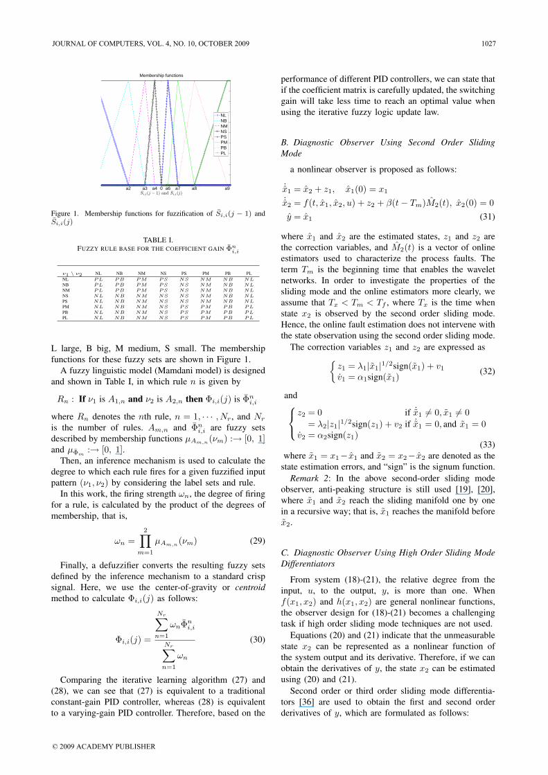
Firstly, the inputs of the fuzzy model are defined asν1 = Si,i(j − 1) and ν2 = Si,i(j). Then, in fuzzificationof these two inputs, we map the crisp values of Si,i(j−1)and Si,i(j) into several fuzzy sets: NL, NB, NM, NS,PS, PM, PB, PL, where N stands for negative, P positive,

1026 JOURNAL OF COMPUTERS, VOL. 4, NO. 10, OCTOBER 2009

© 2009 ACADEMY PUBLISHER

a2 a3 a4 0 a6 a7 a8 a9Si,i(j − 1) and Si,i(j)

Membership functions

NLNBNMNSPSPMPBPL

Figure 1. Membership functions for fuzzification of Si,i(j − 1) andSi,i(j)

TABLE I.FUZZY RULE BASE FOR THE COEFFICIENT GAIN Φn

i,i

ν1 \ ν2 NL NB NM NS PS PM PB PLNL P L P B P M P S NS NM NB NLNB P L P B P M P S NS NM NB NLNM P L P B P M P S NS NM NB NLNS NL NB NM NS NS NM NB NLPS NL NB NM NS NS NM NB NLPM NL NB NM NS P S P M P B P LPB NL NB NM NS P S P M P B P LPL NL NB NM NS P S P M P B P L

L large, B big, M medium, S small. The membershipfunctions for these fuzzy sets are shown in Figure 1.

A fuzzy linguistic model (Mamdani model) is designedand shown in Table I, in which rule n is given by

Rn : If ν1 is A1,n and ν2 is A2,n then Φi,i(j) is Φni,i

where Rn denotes the nth rule, n = 1, · · · , Nr, and Nr

is the number of rules. Am,n and Φni,i are fuzzy sets

described by membership functions µAm,n(νm) :→ [0, 1]

and µΦm:→ [0, 1].

Then, an inference mechanism is used to calculate thedegree to which each rule fires for a given fuzzified inputpattern (ν1, ν2) by considering the label sets and rule.

In this work, the firing strength ωn, the degree of firingfor a rule, is calculated by the product of the degrees ofmembership, that is,

ωn =2∏

m=1

µAm,n(νm) (29)

Finally, a defuzzifier converts the resulting fuzzy setsdefined by the inference mechanism to a standard crispsignal. Here, we use the center-of-gravity or centroidmethod to calculate Φi,i(j) as follows:

Φi,i(j) =

Nr∑n=1

ωnΦni,i

Nr∑n=1

ωn

(30)

Comparing the iterative learning algorithm (27) and(28), we can see that (27) is equivalent to a traditionalconstant-gain PID controller, whereas (28) is equivalentto a varying-gain PID controller. Therefore, based on the

performance of different PID controllers, we can state thatif the coefficient matrix is carefully updated, the switchinggain will take less time to reach an optimal value whenusing the iterative fuzzy logic update law.

B. Diagnostic Observer Using Second Order SlidingMode

a nonlinear observer is proposed as follows:

˙x1 = x2 + z1, x1(0) = x1

˙x2 = f(t, x1, x2, u) + z2 + β(t − Tm)M2(t), x2(0) = 0y = x1 (31)

where x1 and x2 are the estimated states, z1 and z2 arethe correction variables, and M2(t) is a vector of onlineestimators used to characterize the process faults. Theterm Tm is the beginning time that enables the waveletnetworks. In order to investigate the properties of thesliding mode and the online estimators more clearly, weassume that Tx < Tm < Tf , where Tx is the time whenstate x2 is observed by the second order sliding mode.Hence, the online fault estimation does not intervene withthe state observation using the second order sliding mode.

The correction variables z1 and z2 are expressed as{z1 = λ1|x1|1/2sign(x1) + v1

v1 = α1sign(x1)(32)

and⎧⎨⎩

z2 = 0 if ˙x1 �= 0, x1 �= 0= λ2|z1|1/2sign(z1) + v2 if ˙x1 = 0, and x1 = 0

v2 = α2sign(z1)(33)

where x1 = x1− x1 and x2 = x2− x2 are denoted as thestate estimation errors, and “sign” is the signum function.

Remark 2: In the above second-order sliding modeobserver, anti-peaking structure is still used [19], [20],where x1 and x2 reach the sliding manifold one by onein a recursive way; that is, x1 reaches the manifold beforex2.

C. Diagnostic Observer Using High Order Sliding ModeDifferentiators

From system (18)-(21), the relative degree from theinput, u, to the output, y, is more than one. Whenf(x1, x2) and h(x1, x2) are general nonlinear functions,the observer design for (18)-(21) becomes a challengingtask if high order sliding mode techniques are not used.

Equations (20) and (21) indicate that the unmeasurablestate x2 can be represented as a nonlinear function ofthe system output and its derivative. Therefore, if we canobtain the derivatives of y, the state x2 can be estimatedusing (20) and (21).

Second order or third order sliding mode differentia-tors [36] are used to obtain the first and second orderderivatives of y, which are formulated as follows:

JOURNAL OF COMPUTERS, VOL. 4, NO. 10, OCTOBER 2009 1027

© 2009 ACADEMY PUBLISHER

1) Second Order Sliding Mode Differentiator

z0 = v0

v0 = −λ0|z0 − y|2/3sign(z0 − y) + z1

z1 = v1

v1 = −λ1|z1 − v0|1/2sign(z1 − v0) + z2

z2 = −λ2sign(z2 − v1). (34)

2) Third Order Sliding Mode Differentiator

z0 = v0

v0 = −λ0|z0 − y|3/4sign(z0 − y) + z1

z1 = v1

v1 = −λ1|z1 − v0|2/3sign(z1 − v0) + z2

z2 = v2

v2 = −λ2|z2 − v1|1/2sign(z2 − v1) + z3

z3 = −λ3sign(z3 − v2) (35)

where λ0, λ1, λ2, and λ3 are diagonal positive coeffi-cient matrices.

The parameters of the differentiator can be easilyadjusted because the estimation accuracy is not verysensitive to their values. However, a tradeoff exists: thelarger the parameters, the faster the convergence andthe higher sensitivity to input noises and the samplinginterval.

It has been proved that if no measurement noise existsand all the coefficients are chosen properly, then, within afinite time, both the 2nd-order and 3rd-order sliding modedifferentiators can guarantee

z0 = y; z1 = y; z2 = y. (36)

If measurement noise exists with a magnitude less thanε, and all the coefficients are chosen properly, the highorder sliding mode differentiators can ensure

|zi − y(i)| ≤ µiε(n−i+1)/(n+1), i = 0, 1, · · · , n

|vi − y(i+1)| ≤ νiε(n−i)/(n+1), i = 0, 1, · · · , n − 1(37)

where µi and νi are positive constants which are onlydependent on the parameters of the differentiators [36].

A diagnostic observer using the second order or thirdorder sliding mode differentiators is designed as follows,

˙x2 = f(y, x2) + Bu + β(t − Tm)M2(t)x2D = h†(y, yD)

x2(0) = x2D(0) (38)

where x2 ∈ �n is the estimated state, yD is the first-order derivative of y computed via the high order slidingmode differentiators, and x2D is the calculated state usingy and yD. If the high order sliding mode differentiatorscan exactly compute the derivative of y, then x2D iscompletely equal to x2. Moreover, we assume that theonline fault estimator M2(t) is activated after all the statesare estimated via HOSMDs, but before the occurrence ofany fault. This assumption guarantees the performance ofthe neural adaptive estimators.

V. FAULT DIAGNOSIS SCHEMES

In model-based fault diagnosis study, a residual isusually generated to detect and diagnose faults. Due tothe universal existence of modeling uncertainties anddisturbances, robust diagnosis strategies are necessaryto avoid false alarm. One robust FD approach uses adead-zone operator in the parameter update algorithmwhich hopes the estimator only to specify the signal withmagnitude above a threshold. However, this method mayaffect the accuracy of fault estimation. Another way torealize robust fault detection is to set a nonzero thresholdfor the residual when making diagnostic decision.

In this work, the measurable output estimation error canbe considered as the residual for robust fault detection.After the sliding mode term forces all the state estimationerrors to reach the sliding manifold,⎧⎪⎪⎨⎪⎪⎩

No fault has occured, M1(t), M2(t) are set to zeroif ‖y(t)‖ < εf

Fault has occurred, M1(t), M2(t) are activatedif ‖y(t)‖ ≥ εf

(39)However, due to the compensation of the online es-

timators, ‖y(t)‖ will return to zero shortly after theoccurrence of a fault. In order to achieve fault isolationand estimation, we need to use the output signals ofthe estimators M1(t) and M2(t), which are designed toidentify the location and magnitude of the fault.

VI. ONLINE FAULT ESTIMATORS

In the nonlinear diagnostic observer (22), online es-timators M1(t) and M2(t) are used to characterize thefault. There exists a large number of online estimators,e.g., neural networks, fuzzy models and so on, which canapproximate universal bounded nonlinear functions undercertain conditions. However, considering the requirementof online real-time realization, the FD scheme should beable to be implemented as quickly as possible. As thealgorithm becomes more complicated, the approximationperformance may be better, however, the computationtime probably increases as well. Hence, There is a trad-off between the simplification of FD scheme and theimprovement of estimation performance.

In our recent studies, several online estimators weredesigned to achieve online fault estimation. These esti-mators can be classified into two classes, one is neural-based estimators and the other is iterative learning-basedestimators.

A. Neural-based Estimators

1) Neural Adaptive Estimator: Instead of using amulti-layer feed-forward neural networks [7], we designeda neural adaptive estimator, which has the followingstructure [38]:

Mi,j(t) = Wi,j(t)σ(Vi,j(t)Ii,j(t)) (40)

where Mi,j(t), (i = 1, 2; j = 1, · · · , p) is the(i, j)th element of M(t). Wi,j(t) and Vi,j(t) =

1028 JOURNAL OF COMPUTERS, VOL. 4, NO. 10, OCTOBER 2009

© 2009 ACADEMY PUBLISHER

[V (1)i,j (t), · · · , V

(p+q)i,j (t)]� are the parameters of Mi,j(t)

at time t, and Ii,j(t) = [Mi,j(t − τ), · · · , Mi,j(t −pτ), xi,j(t−τ), · · · , xi,j(t−qτ)]�, where τ here denotesthe sampling time interval, xi,j is the (i, j)th state estima-tion error which is obtained via the sliding mode observer.The term σ(x) = (1 − e−x)/(1 + e−x) is a hyperbolictangent activation function.

The estimator is recursively updated by previous p stepestimator outputs and previous q step state estimationerrors. The choice of tapped delay p and q is basedon a heuristic or called trial-and-error method. Althoughusing large p and q probably guarantees convergenceand increases approximation accuracy, it may spend morecomputation time and cause unnecessary time delay.

2) Neural State Space Model-based Estimator: Neuralstate space (NSS) model is a special kind of recurrentneural networks, which not only has the same universalapproximation ability as neural networks, but also hasa similar structure with linear state space model. Thisfeature makes the theoretical analysis of NSS model-based system more conveniently.

The dynamics of the neural state space model-basedestimator is [39]

˙Mi,j(t) = W

(1)i,j (t)Mi,j(t) + W

(2)i,j (t)σ

(W

(3)i,j (t)Mi,j(t)

+W(4)i,j (t)xi,j(t)

)(i = 1, · · · , p)(41)

where W(l)i,j (i = 1, 2; j = 1, · · · , p; l = 1, · · · , 4) are the

parameters of the NSS model.3) Wavelet Networks: Some studies have proved that

in some cases, a simple-structure wavelet network canat least provide the same approximation ability as tradi-tional neural networks [40]. This feature implies waveletnetwork can also be used as the estimator.

We proposed a three-layer wavelet network that iscomposed of an input layer (the i layer), a wavelet layer(the ij layer), and an output layer (the o layer) [41]. Theschematic of this wavelet network is shown in Fig. 2.The inputs of the wavelet network are the state estimationerrors obtained from the sliding mode observer and thedifference between the network input and output. Theoutput of the wavelet network is the estimation of thefault.

The input-output relation for node i of the input layeris

net1i = nii, no1i = f1

i (net1i ) = net1i , i = 1, · · · , p(42)

where nii is the input of the wavelet network in whichni1 = xi,j , and ni2 = ni1 − Mi,j . Moreover, in thewavelet layer, a family of wavelets is established bypreforming translations and dilations on a single fixedfunction called the mother wavelet. In this study, the firstderivative of a Gaussian function φ(x) = −x exp(−x2/2)is selected as the mother wavelet. This mother waveletfunction has a universal approximation ability, since it canbe regarded as a differentiable version of the Haar motherwavelet, just as the sigmoid is a differentiable version of

∑

1ni 2ni

3

ono

−

ijoW

Input Layer

Wavelet

Layer

Output

Layer

ij

i

m mmm

m

−+

)(⋅φ )(⋅φ )(⋅φ )(⋅φ )(⋅φ )(⋅φ

Figure 2. Structure of the three-layer wavelet network

a step function. For the ijth node in the wavelet layer,we have

net2ij =no1

i − ci,j

σij(43)

no2ij = φij(net2ij)

= −net2ij exp( − (net2ij)

2/2), j = 1, · · · , q (44)

where cij and σij are the translation and dilation in thejth term of the ith input no1

i to the node of motherwavelet layer, respectively, and q is the total number ofthe wavelets with respect to the corresponding input node.

In the output layer, the single node o is labeled as∑

,which adds all input signals together.

net3o =∑ij

W 3ijono2

ij (45)

no3o = f3

o (net3o) = net3o, o = 1 (46)

where no3o = Mi,j is the output of the wavelet network;

the connection weight W 3ijo is the output action strength

of the oth output associated with the ijth wavelet, andno2

ij is denoted as the ijth input to the node of outputlayer.

B. Fault Estimators Using Iterative Learning Algorithms

Although neural-based estimators can approximate thefault with high accuracy in a short time, there inevitablyexists overshoot and transient process in the fault esti-mation, because the estimator needs time to update itsparameters to track an abrupt change. Accordingly, weproposed several kinds of iterative learning estimators,which have the following characteristics: i) The trackingtrajectory becomes time-varying but iteration-invariant.ii) The parameters of the estimator are updated in theiteration domain rather than in the time domain. ii) Whenthe convergence of the update process in iteration domainis guaranteed, the overshoot and transient process in faultestimation are eliminated.

JOURNAL OF COMPUTERS, VOL. 4, NO. 10, OCTOBER 2009 1029

© 2009 ACADEMY PUBLISHER

1) PID-type Iterative Learning Estimator: Inspired bythe structure of the single neuron PID controller [42],the proposed PID-type iterative learning estimator is de-scribed as,

Mi,j(t) =K · ∑3

l=1 ω(l)i,j (t)z

(l)i,j (t − τ)∑3

l=1 ω(l)i,j (t)

(47)

where K is the learning coefficient, ω(l)i,j (t), (i =

1, 2, ; j = 1, · · · , p; l = 1, · · · , 3) are the three parametersof the (i, j)th M(t), and τ is the sampling time interval inthe iteration domain. Three exogenous inputs are chosenas ⎧⎪⎨

⎪⎩z(1)i,j (t) = xi,j(t)

z(2)i,j (t) = z

(1)i,j (t) − Mi,j(t)

z(3)i,j (t) = ∆z

(2)i,j (t) = z

(2)i,j (t) − z

(2)i,j (t − τ)

(48)

Since this estimator is a linear network, some adaptivealgorithms can be used to update its parameters [43].

2) Iterative Neuron PID Estimator: The above PID-type iterative learning estimator is actually a linear com-bination of previous information of state estimation errorand fault estimation error. In order to accelerate theconvergence speed, the nonlinear activation function isused and formulate an iterative neuron PID estimator in[44] as,

Mi,j(t) = Mi,j(t − τ) + Wi,j(t)σ(V

(1)i,j (t)z(1)

i,j (t)

+V(2)i,j (t)z(2)

i,j (t) + V(3)i,j (t)z(3)

i,j (t))

(49)

where Mi,j(t) is the (i, j)th element of M(t). Wi,j andV

(l)i,j , (l = 1, 2, 3) are the parameters of the estimator. The

term σ(·) is still the hyperbolic tangent activation func-tion. Defining ei,j(t) = xi,j(t) − Mi,j(t), the exogenousinputs of Mi,j(t) are chosen as⎧⎪⎪⎪⎨

⎪⎪⎪⎩z(1)i,j (t) = ei,j(t)

z(2)i,j (t) = ∆ei,j(t) = ei,j(t) − ei,j(t − τ)

z(3)i,j (t) = ∆2ei,j(t)

= ei,j(t) − 2ei,j(t − τ) + ei,j(t − 2τ)

For the parameter update of this estimator, four robustparameter update laws were proposed in [44]. In addi-tion to the traditional parameter update law for neuralnetworks, like gradient descent algorithm and extendedKalman filtering algorithm, two iterative learning algo-rithms were designed, which use the fault estimation errorat current and previous iterations.

C. Parameter Update LawFor above online fault estimators, in order to char-

acterize the fault as soon as possible, the parametersare supposed to be updated using some optimizationalgorithms. The parameter update algorithms for recurrentneural networks are all suitable for above estimators,for example, dynamic back-propagation method, extendedKalman filtering algorithm, etc. Moreover, two robustiterative learning algorithms were designed to update theparameters in the iterative neuron PID estimators [44].

VII. CONCLUSION

In this paper, we summarized our research work onrobust fault diagnosis for satellite control systems usingsliding mode and learning approaches in recent years.Firstly, mathematical models for a variety of satellitecontrol systems were summarized and analyzed. Thesesatellite control systems can be classified into two classesof nonlinear dynamics, which were used to design dif-ferent robust fault diagnosis schemes. In our proposedrobust FD schemes, sliding mode observer was integratedwith online learning estimators for the purpose of faultdetection, isolation, and estimation. The sliding modeobserver with time-varying switching gain estimate thestates as soon as possible before the occurrence of anyfault. Then, the online learning estimators were used toidentify the fault from the state estimation error withsufficient accuracy. In order to simplify the FD algorithmunder the guarantee of fault estimation performance, someneural-based estimators and iterative learning estimatorswere designed.

In practical applications, single FD scheme for asatellite system might be not able to reach the sameperformance as that in simulation due to the complexsituation in space. Hence, using multiple FD algorithmsin a distribute and simultaneous way, we can achievesoftware redundancy to reduce fault false alarm.

Moreover, in our above research, state observers weredesigned only for a specific class of nonlinear systems,which can not describe a few classes of satellites. There-fore, for general nonlinear satellite systems, we needto design other state observers for the purpose of faultdetection, isolation and estimation.

ACKNOWLEDGMENT

This research was supported by Natural Sciences andEngineering Research Council (NSERC) of Canada andthe Canadian Space Agency (CSA) under a joint multi-university project entitled Intelligent Autonomous SpaceVehicles (IASV): Health monitoring, fault diagnosis andrecovery.

REFERENCES

[1] R.J. Patton, P.M. Frank and R.N. Clark, Fault Diagnosisin Dynamic Systems: Theory and Applications, Prentice-Hall, Englewood Cliffs, NJ; 1989.

[2] J.J. Gertler, Fault Detection and Diagnosis in EngineeringSystems, Marcel Dekker, NY; 1998.

[3] J. Chen and R.J. Patton Robust Model-Based Fault Diag-nosis for Dynamic Systems, Kluwer Academic Publishers,Boston; 1999.

[4] R.J. Patton, R. Clark, and R.N. Clark, Issues of Fault Di-agnosis for Dynamic Systems, Springer-Verlag, London;2000.

[5] S. Naidu, E. Zafirou, and T.J. Mcavoy, “Use of Neural-Networks for Failure Detection in A Control System,”IEEE Control Syst. Mag., vol. 10, 1990, pp. 49-55.

[6] T. Marcu, and L. Mirea, “Robust Detection and Isolationof Process Faults Using Neural Networks,” IEEE ControlSyst. Mag. vol. 17, 1997, pp. 72-79.

1030 JOURNAL OF COMPUTERS, VOL. 4, NO. 10, OCTOBER 2009

© 2009 ACADEMY PUBLISHER

[7] A.B. Trunov, and M.M. Polycarpou, “Automated FaultDiagnosis in Nonlinear Multivariable Systems Using ALearning Methodology,” IEEE Trans. Neural Networks,vol. 11, 2000, pp. 91-101.

[8] W. Chen, and M. Saif, 2006, “An Iterative LearningObserver for Fault Detection and Accommodation inNonlinear Time-Delay Systems,” Int. J. Robust and Non-linear Contr., vol. 16, 2006, pp. 1-19.

[9] B. Jiang, and M. Staroswiecki, 2002, “Adaptive ObserverDesign for Robust Fault Estimation,” Int. J. Syst. Sci.,vol. 33, 2002, pp. 767-775.

[10] A. Alessandri, “Fault Diagnosis for Nonlinear SystemsUsing A Bank of Neural Estimators,” Computers inIndustry, vol. 52, 2003, pp. 271-289.

[11] A. Xu, and Q. Zhang, “Nonlinear System Fault Diagnosisbased on Adaptive Estimation,” Automatica, vol. 40,2004, pp. 1181-1193.

[12] M.M. Polycarpou, and A.J. Helmicki, “Automated FaultDetection and Accommodation: A Learning Systems Ap-proach,” IEEE Trans. Syst., Man, and Cybern., vol. 25,1995, pp. 1447-1458.

[13] A.T. Vemuri, and M.M. Polycarpou, “Robust NonlinearFault Diagnosis in Input-output Systems,” Int. J. Contr.,vol. 68, 1997, pp. 343-360.

[14] M.A. Demetriou, and M.M. Polycarpou, “Incipient FaultDiagnosis of Dynamical Systems Using Online Approxi-mators,” IEEE Trans. Automat. Contr., vol. 43, 1998, pp.1612-1617.

[15] C. Edwards, and S.K. Spurgeon, “On the Development ofDiscontinuous Observers,” Int. J. Contr., vol. 59, 1994,pp. 1211-1229.

[16] S. Drakunov, and V. Utkin, “Sliding Mode Observers.Tutorial,” In Proeedings of the 34th Conference on De-cision and Control, Dec. 1995; New Orleans, LA, USA.pp. 3376-3378.

[17] I. Haskara, U. Ozguner, and V. Utkin, “On SlidingMode Observers via Equivalent Control Approach,” Int.J. Contr., vol. 71, 1998, pp. 1051-1067.

[18] F. Floret-Ponetet, and F. Lamnabhi-Lagarrigue, “Para-metric Identification Methodology Using Sliding ModesObserver,” Int. J. Contr., vol. 74, 2001, pp. 1743-1753.

[19] J.P. Barbot, and T. Boukhobza and M. Djemai, “SlidingMode Observer for Triangular Input Form,” Proceedingsof the 35th Conference on Decision and Control, 1996,pp. 1489-1490.

[20] Y. Xiong, and M. Saif. “Sliding Mode Observer forNonlinear Uncertain Systems,” IEEE Trans. Automat.Contr., vol. 46, 2001, pp. 2012-2017.

[21] T. Boukhobza, and J.P. Barbot, “High Order SlidingModes Observer,” In Proceedings of the 37th IEEEConference on Decision and Control Dec. 1998; TampaFlorida, USA. pp. 1912-1917.

[22] J. Davila, L. Fridman, and A. Levant, “Second-orderSliding Mode Observer for Mechanical Systems,” IEEETrans. on Automat. Contr., vol. 50, 2005, pp. 1785-1789.

[23] C. Edwards, S.K. Spurgeon, and R.J. Patton, “SlidingMode Obsevers for Fault Detection and Isolation,” Au-tomatica, vol. 36, 2000, pp. 541-553.

[24] C.P. Tan, and C. Edwards, “Sliding Mode Observers forDetection and Reconstruction of Sensor Faults,” Automat-ica, vol. 38, 2002, pp. 1815-1821.

[25] W. Chen, and M. Saif, “Robust Fault Detction andIsolation in Constrained Nonlinear Systems via A SecondOrder Sliding Mode Observer,” In Proc. of the 15thTriennial World Congress of IFAC, Barcelona Spain, July2002.

[26] T. Floquet, J.P. Barbot, et al, “On the Robust FaultDetection via A Sliding Mode Disturbance Observer,” Int.J. Contr., vol. 77, 2004, pp. 622-629.

[27] C. Edwards, and L. Fridman, and M-W.L. Thein, “FaultReconstruction in a Leader/Follower Spacecraft SystemUsing Higher Order Sliding Mode Observers,” Proceed-ings of the American Control Conference, New York, July2007, pp. 408-413.

[28] Q. Wu and M. Saif, “Robust Fault Diagnosis for aSatellite System Using a Neural Sliding Mode Observer,”in Proc. of the 44th IEEE Conference on Decision andControl, and European Control Conference ECC 2005(CDC-ECC’05), Seville, Spain, December 12-15, 2005,pp. 7668-7673.

[29] A.A. Anchev, “Equilibrium Attitude Transitions of aThree Rotor Gyrostat in a Circular orbit,” Journal of theAmerican Institute of Aeronautics and Astronautics, vol.11, 1973, pp. 467-472.

[30] C.D. Yang, and Y.P. Sun, Mixed H2/H∞ Sate-feedbackDesign for Micorsatellite Attitude Control, Control Engi-neering Practice, vol. 10, 2002, pp. 951-970.

[31] B. Wie, Space Vehicle Dynamics and Control, AmericanInstitute of Aeronautics and Astronautics Inc., Reston,1998.

[32] S.N. Singh and R. Zhang, “Adaptive Output FeedbackControl of Spacecraft with Flexible Appendages by Mod-eling Error Compensation,” Acta Astronautica, vol. 54,2004, pp. 229-243.

[33] K. Karray, A. Grewal, et al, “Stiffening Control of aClass of Nonlinear Affine Systems,” IEEE Trans. Aerosp.Electron. Syst., vol. 33, 1997, pp. 473-484.

[34] R. Marino, and P. Tomei, Nonlinear Control Design,Geometric, Adaptive and Robust, Prentice Hall, UK,1995.

[35] W.E. Dixon, A.Behal et al, Nonlinear Control ofEngineering Systems–A Lyapunov-Based Approach,Birkhauser, 2003.

[36] A. Levant, “Robust Exact Differentiation via SlidingMode Technique”, Automatica, vol. 34, No. 3, 1998, pp.379-384.

[37] Q. Wu, and M. Saif, “Robust Fault Detection and Diag-nosis in a Class of Nonlinear Systems Using a NeuralSliding Mode Observer,” Accepted by the InternationalJournal of Systems Science-Special Issue on Advances inSliding Mode Observation and Estimation, 207.

[38] Q. Wu and M. Saif, “Neural Adaptive Observer BasedFault Detection and Identification for Satellite AttitudeControl Systems,” in Proc. of the 2005 American ControlConference, June 8-10, Portland, Oregon, USA, 2005, pp.1054-1059.

[39] Q. Wu and M. Saif, “Robust Fault Diagnosis for SatelliteAttitude Systems Using Neural State Space Models,” inProc. of the International Conference on Systems Manand Cybernetics, Hawaii, USA, October 10-12, 2005, pp.1955-1960.

[40] Q. Zhang, and A. Benveniste, “Wavelet Networks,” IEEETrans. Neural Networks, vol. 3, 1992, pp. 889-898.

[41] Q. Wu and M. Saif, “Robust Fault Detection and Diagno-sis for a Multiple Satellite Formation Flying System Us-ing Second Order Sliding Mode and Wavelet Networks,”Accepted by the 2007 American Control Conference, NewYork, USA, July 11-13, 2007.

[42] Z. Li, R. Zhao Y. Li and D. Sun, “Real-Time PredictableControl Based on Single-Neuron PSD Controller,” inProc. of the Second Internatioal Conference on MachineLearning and Cybernetics, Xi’an, Nov., 2003, pp. 720-725.

[43] Q. Wu and M. Saif, “Observer-Based Robust ProcessFault Detection and Diagnosis for a Satellite System withFlexible Appendages,” in Proc. of the 45th Conference onDecision and Control, San Diego, CA, USA, Dec. 13-15,2006, pp. 2183-2188.

JOURNAL OF COMPUTERS, VOL. 4, NO. 10, OCTOBER 2009 1031

© 2009 ACADEMY PUBLISHER

[44] Q. Wu and M. Saif, “Robust Fault Diagnosis for aSatellite Large Angle Attitude System Using an IterativeNeuron PID (INPID) Observer,” in Proc. of the 2006American Control Conference, Minneapolis, MinnesotaUSA, June 14-16, 2006, pp. 5710-5715.

Qing Wu is currently an embedded software engineer at CriticalEnvironment Technologies Canada Inc., Delta, BC, Canada. Hereceived his PhD degree in Engineering Science from SimonFraser University, Vancouver, BC, Canada in 2008, MS andBS degrees in Control Theory and Engineering from HuazhongUniversity of Science and Technology, Wuhan, China in 1999and 2002, respectively. His research interests include faultdiagnosis, computational intelligence, control systems, sensors,etc.

Mehrdad Saif received B.S. in 1982, M.S. in 1984, and PhDin 1987 all in Electrical Engineering. During his graduatestudies he worked on research projects sponsored by NASALewis (now Glenn) Research Center, as well as ClevelandAdvanced Manufacturing Program (CAMP). In 1987 he joinedthe School of Engineering Science at Simon Fraser Universityas an Assistant Professor. He is currently a Full Professorand Director of the same School. From 1993-1994 Saif was aVisiting Scholar at General Motors North American Operation(NAO) R & D Center in Warren, MI. At GM he was a memberof the Powertrain Control Group in the Electrical and ElectronicsResearch Department where he worked on engine control andon-board engine diagnostic problems.

Saif’s research interests are in estimation and observer theory,model based fault diagnostics, and application of these toautomotive, power, and other complex engineering systems. Hehas published over 150 refereed journal and conference papersplus an edited book in these areas. Saif has been a consultant toa number of industries and agencies such as GM, NASA, B.C.Hydro, Ontario Council of Graduate Studies, etc. He served twoterms (1995,1997) as the Chairman of the Vancouver Section ofthe IEEE Control Systems Society, and is currently a member ofthe editorial board of the IEEE Systems Journal, InternationalJournal of Control and Computers, IEEE CDC, and ACC. Saif isSenior Member of IEEE and a Registered Professional Engineerin British Columbia.

1032 JOURNAL OF COMPUTERS, VOL. 4, NO. 10, OCTOBER 2009

© 2009 ACADEMY PUBLISHER