An Optimal Product Mix for Hedging Longevity Risk in Life Insurance Companies: The Immunization...
25
C The Journal of Risk and Insurance, 2010, Vol. 77, No. 2, 473-497 DOI: 10.1111/j.1539-6975.2009.01325.x AN OPTIMAL PRODUCT MIX FOR HEDGING LONGEVITY RISK IN LIFE INSURANCE COMPANIES: THE IMMUNIZATION THEORY APPROACH Jennifer L. Wang H.C. Huang Sharon S. Yang Jeffrey T. Tsai ABSTRACT This article investigates the natural hedging strategy to deal with longevity risks for life insurance companies. We propose an immunization model that incorporates a stochastic mortality dynamic to calculate the optimal life insurance–annuity product mix ratio to hedge against longevity risks. We model the dynamic of the changes in future mortality using the well-known Lee–Carter model and discuss the model risk issue by comparing the results between the Lee–Carter and Cairns–Blake–Dowd models. On the basis of the mortality experience and insurance products in the United States, we demonstrate that the proposed model can lead to an optimal product mix and effectively reduce longevity risks for life insurance companies. INTRODUCTION In the past decade, annuity premiums in the United States have accounted for more than 50 percent of life insurers’ premium income, with an average growth rate of 10.2 percent from 1988 to 2005 (American Council of Life Insurers, 2005). However, longevity risk 1 —or uncertainty about long-term trends in mortality rates and the impact on the long-term probability of survival of an individual—represents a critical threat to private insurers because it increases the payout period and the liability costs of providing annuities. In particular, human mortality has declined globally Jennifer L. Wang is a professor at National Cheng-chi University. H.C. Huang is an asso- ciate professor at National Cheng-chih University. Sharon S. Yang is an associate professor at National Central University. Jeffrey T. Tsai is an assistant professor at National Tsing Hua University. Jennifer L. Wang can be contacted via e-mail: [email protected]. 1 To differentiate mortality risk from longevity risk, Cairns, Blake, and Dowd (2006a) define the latter as uncertainty in the long-term trend in mortality rates and the former as uncertainty in future mortality rates. 473
-
Upload
independent -
Category
Documents
-
view
1 -
download
0
Transcript of An Optimal Product Mix for Hedging Longevity Risk in Life Insurance Companies: The Immunization...
C© The Journal of Risk and Insurance, 2010, Vol. 77, No. 2, 473-497DOI: 10.1111/j.1539-6975.2009.01325.x
AN OPTIMAL PRODUCT MIX FOR HEDGINGLONGEVITY RISK IN LIFE INSURANCE COMPANIES:THE IMMUNIZATION THEORY APPROACHJennifer L. WangH.C. HuangSharon S. YangJeffrey T. Tsai
ABSTRACT
This article investigates the natural hedging strategy to deal with longevityrisks for life insurance companies. We propose an immunization model thatincorporates a stochastic mortality dynamic to calculate the optimal lifeinsurance–annuity product mix ratio to hedge against longevity risks. Wemodel the dynamic of the changes in future mortality using the well-knownLee–Carter model and discuss the model risk issue by comparing the resultsbetween the Lee–Carter and Cairns–Blake–Dowd models. On the basis ofthe mortality experience and insurance products in the United States, wedemonstrate that the proposed model can lead to an optimal product mixand effectively reduce longevity risks for life insurance companies.
INTRODUCTION
In the past decade, annuity premiums in the United States have accounted for morethan 50 percent of life insurers’ premium income, with an average growth rate of10.2 percent from 1988 to 2005 (American Council of Life Insurers, 2005). However,longevity risk1—or uncertainty about long-term trends in mortality rates and theimpact on the long-term probability of survival of an individual—represents a criticalthreat to private insurers because it increases the payout period and the liabilitycosts of providing annuities. In particular, human mortality has declined globally
Jennifer L. Wang is a professor at National Cheng-chi University. H.C. Huang is an asso-ciate professor at National Cheng-chih University. Sharon S. Yang is an associate professorat National Central University. Jeffrey T. Tsai is an assistant professor at National Tsing HuaUniversity. Jennifer L. Wang can be contacted via e-mail: [email protected] differentiate mortality risk from longevity risk, Cairns, Blake, and Dowd (2006a) define thelatter as uncertainty in the long-term trend in mortality rates and the former as uncertainty infuture mortality rates.
473
474 THE JOURNAL OF RISK AND INSURANCE
over the course of the twentieth century.2 As Willets (2004) points out, mortalityimprovements do not occur in a smooth upward fashion but rather exhibit a “cohorteffect.”3 Recent medical discoveries may increase human life spans even beyond thecurrently projected mortality table used by insurance companies. These issues havemade it far more difficult for insurance actuaries to price annuity products correctly,and the resulting inaccurate mortality assumptions lead to major risks. Therefore,hedging longevity risks has taken on an increasingly important role for life insurancecompanies.
When considering how to hedge longevity risks, most prior research investigatesmortality risk and pricing issues for annuity products (Friedman and Warshawsky,1990; Frees, Carriere, and Valdez, 1996; Brown, Mitchell, and Poterba, 2000; Mitchellet al., 2001). More recent studies focus on the impact of stochastic mortality changeson life insurance and annuities (Marceau and Gaillardetz, 1999; Wilkie, Waters, andYang, 2003; Cairns, Blake, and Dowd, 2006a). In addition, many financial vehicles,such as mortality derivatives and survivor bonds, have been proposed to reduceor hedge the longevity risks of annuity. Blake and Burrows (2001) first proposedthat issuing survivor bonds4 could help a pension fund insure against the longevityrisk, and more recent studies also extend the issue of securitization of longevityrisk (e.g., Dowd, 2003; Blake, Cairns, and Dowd, 2006; Blake, Cairns, Dowd, andMacMinn, 2006; Lin and Cox, 2005; Cox, Lin, and Wang, 2006; Denuit, Devolder,and Goderniaux, 2007). Dowd et al. (2006) suggest that a survivor swap can serveas a more advantageous survivor derivative than a survivor bond, because it can bearranged at a lower transaction cost and does not require a liquid market.5
Similar to the concept of survivor swap, insurers can hedge longevity risks internallybetween their own business products (life insurance and annuity), which are sensitivein opposing ways to the changes in mortality rates. This approach provides a so-callednatural hedging strategy. If the future mortality of a cohort improves relative to currentexpectations, life insurers gain a profit because they can pay the death benefit laterthan initially expected, whereas annuity insurers suffer losses because they must payannuity benefits for longer than they initially expected. Therefore, life insurance canserve as a dynamic hedge vehicle against unexpected mortality risk. Yet relatively fewacademic papers have investigated the issue of natural hedging. Cox and Lin (2007)suggest that natural hedging is appealing but may be too expensive to be effectivein the context of internal life insurance and annuity products. They instead proposea pricing model for a mortality swap and provide empirical evidence to show thatinsurers that exploit natural hedging by using a mortality swap can charge a lower
2Benjamin and Soliman (1993), McDonald (1997), and McDonald et al. (1998) confirm that anunprecedented improvement in population longevity has occurred both in the United Statesand worldwide.
3Willets (2004) suggests mortality improvements exhibit cyclical patterns, in which some co-horts enjoy better improvements than others.
4Unlike the mortality bond that links the bond payments to mortality deviations, survivorbonds (or longevity bonds) link coupon payments to the survivor index (Cairns, Blake, andDowd, 2006b).
5Survivor swaps are more flexible and can be tailored to suit diverse circumstances for counter-parties (usually life insurance companies), which enables them to transfer their death exposurewithout heavy regulations.
THE IMMUNIZATION THEORY APPROACH 475
risk premium than others. However, no discussion so far addresses product strategiesfor natural hedging. This article attempts to fill this gap.
To help life insurers achieve a better natural hedging effect, we propose an immuniza-tion model that incorporates a stochastic mortality dynamic to calculate the optimallevel of a product mix that includes both life insurance and annuities and therebyeffectively reduces longevity risks for insurance companies. Our article differs fromCox and Lin’s (2007) in two aspects. First, whereas Cox and Lin propose a pricingmodel for a mortality swap for natural hedging, we propose an immunization modeland calculate the optimal product mix ratio for natural hedging. Second, Cox andLin illustrate the natural hedging strategy by using the 1995 U.S. Society of Actu-aries (SOA) basic age last table for life and annuity to measure the market price ofrisk. However, their model does not consider the future dynamic of mortality. Tobetter capture the stochastic mortality pattern, we estimate the parameters in boththe Lee–Carter (LC) and Cairns–Blake–Dowd (CBD) models to reflect the age effectby fitting historical U.S. mortality experience. Our numerical results demonstrate thatthe proposed model indicates the optimal product mix and thus can effectively reducelongevity risks.
The remainder of this article is organized as follows: In the section “Immunizationfor Natural Hedging” section we introduce our proposed immunization models fora natural hedging strategy for life insurers. In the next section “Modeling LongevityRisk” section we discuss drivers of the mortality curve and model the future mor-tality using the LC model with U.S. mortality experience. We demonstrate how toimplement our proposed model to calculate natural hedging product mix ratios forvarious products and analyze some related issues with numerical examples in thesubsequent section. We discuss the model risk by comparing the results between theLC model and the CBD model for natural hedging strategies in the following section,and then we conclude in the last section.
IMMUNIZATION STRATEGY FOR NATURAL HEDGING
Natural hedging employs the interaction of life insurance and annuities in response toa change in mortality to stabilize the cash flow for insurers. Compared with externalhedging tools, natural hedging does not require the insurer to find counterparties anddemands no transaction costs. As an internal vehicle, natural hedging not only helpsinsurance companies diversify their mortality risk but also provides other advan-tages. Cox and Lin (2007) show that insurers that utilize natural hedging can charge alower risk premium, which may increase their market share. However, in practice, itmay be difficult to implement natural hedging strategies for several reasons. First, thedurations of these two products cannot be matched easily to achieve proper hedgesbecause annuities generally are purchased by older consumers, whereas life insurancepolicies are purchased by the young. Second, effective hedging may require insurancecompanies to change their business composition, which could introduce additionalexpenses or increase operational risks. To achieve an optimal hedging strategy, insur-ers may need to reduce or increase the price of their annuity or life insurance productsto make them more or less attractive.6 The result of this price adjustment also could
6We thank the referees for pointing out this important issue.

476 THE JOURNAL OF RISK AND INSURANCE
reduce the effect of natural hedging. In addition, some specialized insurers may be in-duced to change their business composition internally by switching production linesbetween life insurance and annuities.7 To help life insurers achieve a better naturalhedging effect, we propose an immunization model that incorporates a stochasticmortality dynamic to calculate the optimal level of a product mix that includes bothlife insurance and annuities.
Assume an insurer sells two types of products: life insurance and annuity. The totalliability (V) of the insurer equals the sum of the liabilities for the different businesses,as in Equation (1)
V = Vlife + Vannuity, (1)
where Vlife is the expected liability of life insurance policies, and Vannuity is theexpected liability of annuity policies.
On the basis of the concept of modified duration,8 we posit that the effect of a mortalityrate change on insurance total liability (V), under a constant force of mortality rate(μ) assumption, can be measured by mortality duration, as in Equation (2)
DVμ = dV
dμ· 1
V. (2)
We extend the immunization theory proposed by Redington (1952) to deal withlongevity risk because the effect of mortality changes on the liability of life insurersis similar to that of an interest rate change. The effect of mortality changes on totalliability can be expressed by the Taylor expansion, as follows:
�V =(
dVlife
dμ+ dVannuity
dμ
)�μ + 1
2
(d2Vlife
dμ2 + d2Vannuity
dμ2
)(�μ)2 + · · · (3)
To achieve the immunization strategy for the mortality change, we can obtain theoptimal product mix by setting Equation (3) equal to zero, such that �V = 0. Whenconsidering the first-order approximation, the immunization strategy can be achievedby Equation (4):
(dVlife
dμ+ dVannuity
dμ
)�μ = 0. (4)
We further denote the mortality duration of liability for life insurance as Dlifeμ = dVlife
dμ ·1
Vlife and the mortality duration of liability for annuity as Dannuityμ = − dVannuity
dμ· 1
Vannuity .
7With regard to this limitation, Dowd et al. (2006) propose the possible use of survivor swaps.8To hedge the interest rate risk, under a constant force of interest rate (δ) assumption, the effectof an interest rate change on the liability (V) of the insurer can be measured by modifiedduration as DV = − dV
dδ· 1
V .
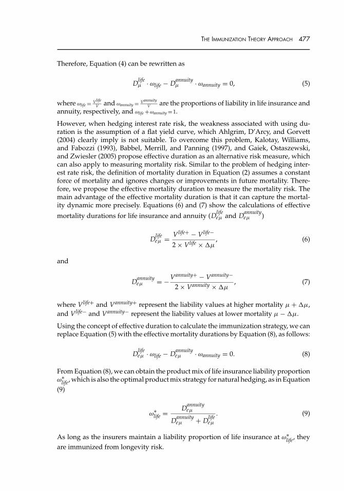
THE IMMUNIZATION THEORY APPROACH 477
Therefore, Equation (4) can be rewritten as
Dlifeμ · ωlife − Dannuity
μ · ωannuity = 0, (5)
where ωlife = VlifeV and ωannuity = Vannuity
V are the proportions of liability in life insurance andannuity, respectively, and ωlife +ωannuity = 1.
However, when hedging interest rate risk, the weakness associated with using du-ration is the assumption of a flat yield curve, which Ahlgrim, D’Arcy, and Gorvett(2004) clearly imply is not suitable. To overcome this problem, Kalotay, Williams,and Fabozzi (1993), Babbel, Merrill, and Panning (1997), and Gaiek, Ostaszewski,and Zwiesler (2005) propose effective duration as an alternative risk measure, whichcan also apply to measuring mortality risk. Similar to the problem of hedging inter-est rate risk, the definition of mortality duration in Equation (2) assumes a constantforce of mortality and ignores changes or improvements in future mortality. There-fore, we propose the effective mortality duration to measure the mortality risk. Themain advantage of the effective mortality duration is that it can capture the mortal-ity dynamic more precisely. Equations (6) and (7) show the calculations of effective
mortality durations for life insurance and annuity (Dlifeeμ and Dannuity
eμ )
Dlifeeμ = Vlife+ − Vlife−
2 × Vlife × �μ, (6)
and
Dannuityeμ = − Vannuity+ − Vannuity−
2 × Vannuity × �μ, (7)
where Vlife+ and Vannuity+ represent the liability values at higher mortality μ + �μ,and Vlife− and Vannuity− represent the liability values at lower mortality μ − �μ.
Using the concept of effective duration to calculate the immunization strategy, we canreplace Equation (5) with the effective mortality durations by Equation (8), as follows:
Dlifeeμ · ωlife − Dannuity
eμ · ωannuity = 0. (8)
From Equation (8), we can obtain the product mix of life insurance liability proportionω∗
life, which is also the optimal product mix strategy for natural hedging, as in Equation(9)
ω∗life = Dannuity
eμ
Dannuityeμ + Dlife
eμ
. (9)
As long as the insurers maintain a liability proportion of life insurance at ω∗life, they
are immunized from longevity risk.
478 THE JOURNAL OF RISK AND INSURANCE
In addition, the effect of convexity plays an important role in dealing with interestrate risk or mortality risk, especially when it encounters a big shock. In other words,the second-order approximation is needed. When considering the second-order ap-proximation, the calculation of optimal product mix includes the effect of convexity.The effect of mortality changes on insurance liability can be measured by mortalityconvexity, as in Equation (10)
CVμ = d2V
dμ2 · 1V
. (10)
Therefore, the effective mortality convexity for life insurance and annuity (Clifeeμ and
Cannuityeμ ), as in Equations (11) and (12), should be utilized
Clifeeμ = Vlife− + Vlife+ − 2Vlife
Vlife(�μ)2, (11)
and
Cannuityeμ = Vannuity− + Vannuity+ − 2Vannuity
Vannuity(�μ)2 . (12)
Thus, the change of total liability (�V) by considering both effective mortality dura-tion and effective mortality convexity is as follows:
�V = (Dlife
eμ · ωlife − Dannuityeμ · ωannuity
)�μ + 1
2
(Clife
eμ · ωlife + Cannuityeμ · ωannuity
)(�μ)2.
(13)
By setting Equation (13) equal to 0,9 we can obtain the product mix of life insurance
liability proportions, ω∗life = Dannuity
eμ + �μ2 Cannuity
eμ
Dannuityeμ +Dlife
eμ + �μ2 (Cannuity
eμ −Clifeeμ )
, which is the optimal prod-
uct mix strategy for natural hedging after considering both effects of duration andconvexity.
We conduct further numerical analyses in the section “Numerical Analysis for NaturalHedging Strategy.” For the case of a small change in mortality (10 percent mortalityshift), we use the concept of effective duration for the immunization strategy and
calculate the optimal product mix ω∗life = Dannuity
eμ
Dannuityeμ +Dlife
eμunder the first-order approxi-
mation. For the case of a big change in mortality (22.5 percent and 25 percent shifts),we further include the concept of effective convexity for the immunization strat-
egy and calculate the optimal product mix, ω∗life = Dannuity
eμ + �μ2 Cannuity
eμ
Dannuityeμ +Dlife
eμ + �μ2 (Cannuity
eμ −Clifeeμ )
, under
9For hedging longevity risk, we assume that the insurers’ objective is to maintain the totalliability unchanged, which is the conception of immunization.

THE IMMUNIZATION THEORY APPROACH 479
second-order approximations. In summary, as long as the insurers maintain a liabilityproportion of life insurance at ω∗
life, they are immunized from longevity risk.
MODELING LONGEVITY RISK
In traditional insurance pricing and reserve calculation, an actuary treats mortalityrates as constant over time, which means unanticipated mortality improvements cancause serious financial burdens or even bankruptcy for life insurers. In actuarialliterature, the question of how to model mortality rates dynamically continues torepresent an important issue. Earlier developments of stochastic mortality modelingrely on the one-factor model and pioneering work by Lee and Carter (1992), whoseLC model is easily applied and provides fairly accurate mortality estimations andpopulation projections. Renshaw, Haberman, and Hatzoupoulos (1996) and Renshawand Haberman (2003) offer further analysis of the LC model.
In addition, more recent works develop two-factor mortality LC models. The mostdistinguishing feature of previous models is the consideration of a cohort effect inmortality modeling. Renshaw and Haberman (2003) apply a cohort effect, and Currie(2006) introduces an Age-Period-Cohort (APC) model. More recently, Cairns, Blake,and Dowd (2006b) allow not only for a cohort effect but also for a quadratic age effectin their CBD model. Cairns et al. (2007) extend Cairns, Blake, and Dowd (2006b) bycomparing an analysis of eight stochastic models based in England and Wales withthe U.S. mortality experience.
Other developments in two-factor models (e.g., Mileysky and Promislow, 2001; Dahl,2004; Dahl and Møller, 2005; Miltersen and Persson, 2005; Luciano and Vigna, 2005;Biffis, 2005; Schrager, 2006) employ a continuous-time framework and thus offeran important means to understand pricing of mortality-linked securities. Followingthe most recent literature on mortality modeling, we employ stochastic mortality toimplement the optimal natural hedging strategy for life insurers.
Stochastic Mortality ModelsWe adopt the most cited stochastic mortality model, the LC model, as our primarymethod to analyze natural hedging strategies. Moreover, we discuss model risk bycomparing the results of the LC model with the recent developed mortality model ofCBD model in the section “Impact of Model on Natural Hedging Strategy.”
We first give a brief overview of the LC model. Lee and Carter (1992) propose thefollowing mortality model for the central death rate mx,t for a person aged x at time t
ln(mx,t) = αx + βx kt + εx,t , (14)
where the parameter αx describes the average age-specific mortality, kt represents thegeneral mortality level, and the decline in mortality at age x is captured by βx. Theterm εx,t denotes the deviation of the model from the observed log-central death ratesand should be white noise with zero and relatively small variance (R. D. Lee, 2000).Once the parameters are estimated, we are able to forecast age-specific death ratesusing extrapolated kt and fixed αx and βx . In this article, we assume that the force ofmortality remains constant over each year of integer age and over each calendar year,
480 THE JOURNAL OF RISK AND INSURANCE
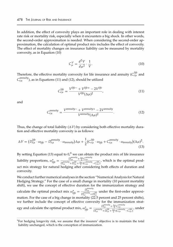
FIGURE 1Trend of Probabilities of Death for 10-Year Age Group, 1959–2002
1960 1965 1970 1975 1980 1985 1990 1995 20000
0.02
0.04
0.06
0.08
0.1
0.12
0.14
0.16
Calander year
Dea
th r
ate
age group 50-59
age group 60-69age group 70-79
age group 80-90
1960 1965 1970 1975 1980 1985 1990 1995 20000
0.02
0.04
0.06
0.08
0.1
0.12
0.14
0.16
Calander year
Dea
th r
ate
age group 50-59
age group 60-69age group 70-79
age group 80-90
(Left: male; Right: female)
not that the force of mortality is constant for all ages. Thus, our prediction capturesthe mortality improvements among different age cohorts (i.e., the effect of mortalitychanges as people get older). Let μx,t denote the force of mortality for a person agedx at integer time t. Thus, the survival probability (px,t) for a person aged x at time tfor the next year can be calculated as px,t = exp[−μx,t] = exp[−mx,t].
Empirical Patterns of MortalityTo generate appropriate future mortality dynamics of the LC model, we analyzeU.S. mortality experience and the relevant data provided by the human mortalitydatabase (HMD, 2005).10 We provide the empirical patterns of U.S. mortality data inFigures 1 and 2. Figure 1 depicts the average probability of death for each 10-year agegroup of men and women aged 50–90 years from 1959 to 2002. The patterns clearlyshow a decreasing trend in death probabilities for each age group, and the mortalityimprovement trend is more significant for older age groups. For example, in the groupof men aged 80–89 years, the probability of death is 0.1526 in 1959 and 0.1061 in 2002.Among men in the 50–59 age group, the probability of death is 0.0140 in 1959 and0.0075 in 2002. For women 80–89 years of age, the probability of death declines from0.1202 in 1959 to 0.0770 in 2002, and for those aged 50–59 years, the probability ofdeath is 0.0073 in 1959 and 0.0045 in 2002.
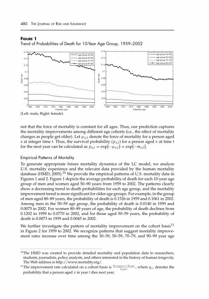
We further investigate the pattern of mortality improvement on the cohort basis11
in Figure 2 for 1959 to 2002. We recognize patterns that suggest mortality improve-ment rates increase over time among the 30–39, 50–59, 70–79, and 90–99 year age
10The HMD was created to provide detailed mortality and population data to researchers,students, journalists, policy analysts, and others interested in the history of human longevity.The Web address is http://www.mortality.org/.
11The improvement rate calculated on a cohort basis is qx+1,year+1−qx,yearqx,year
, where qx,t denotes theprobability that a person aged x in year t dies next year.
THE IMMUNIZATION THEORY APPROACH 481
FIGURE 2Average Mortality Change Rate for 10-Year Age Cohorts, 1959–2002
1960 1965 1970 1975 1980 1985 1990 1995 2000 2005
-0.4
-0.3
-0.2
-0.1
0
0.1
0.2
Calander year
Pro
port
ion
chan
ge o
f dea
th r
ate
Cohort ages from 1959-2002
age group 30-39age group 50-59age group 70-79age group 90-99
1960 1965 1970 1975 1980 1985 1990 1995 2000 2005
-0.4
-0.3
-0.2
-0.1
0
0.1
0.2
Calander year
Pro
port
ion
chan
ge o
f dea
th r
ate
Cohort ages from 1959-2002
age group 30-39age group 50-59age group 70-79age group 90-99
(Left: male; Right: female)
cohorts, with the exception of the male, 30–39 group. We also find that the mortalityimprovement in recent years is more significant for the male, 50–59 group.
Estimation of ParametersTo better capture future stochastic mortality, we estimate the parameters in the LCmodel by fitting historical U.S. mortality data from 1959 to 2002 with the HMD data.12
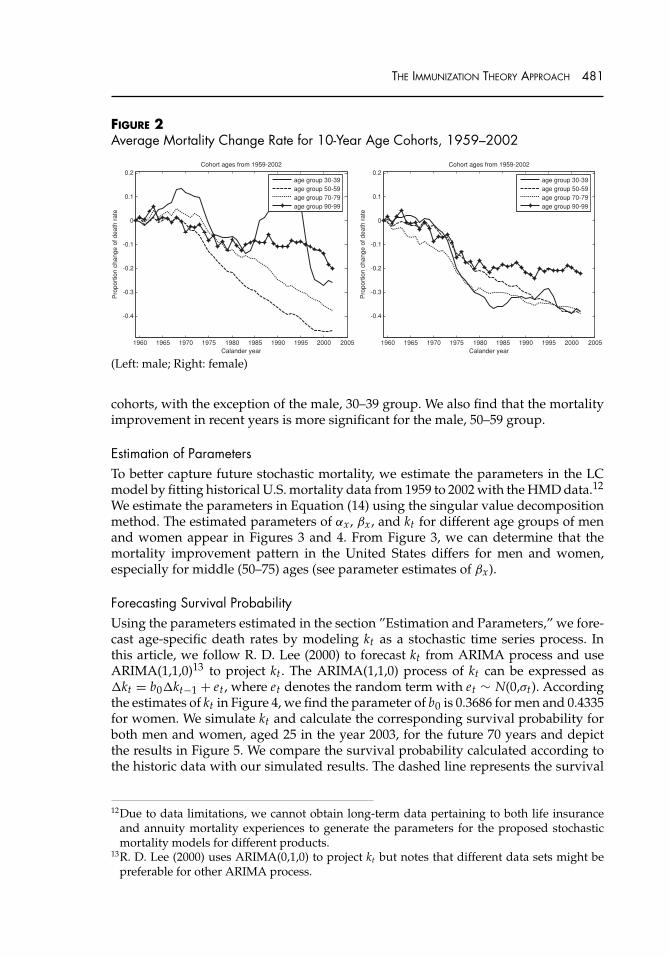
We estimate the parameters in Equation (14) using the singular value decompositionmethod. The estimated parameters of αx , βx , and kt for different age groups of menand women appear in Figures 3 and 4. From Figure 3, we can determine that themortality improvement pattern in the United States differs for men and women,especially for middle (50–75) ages (see parameter estimates of βx).
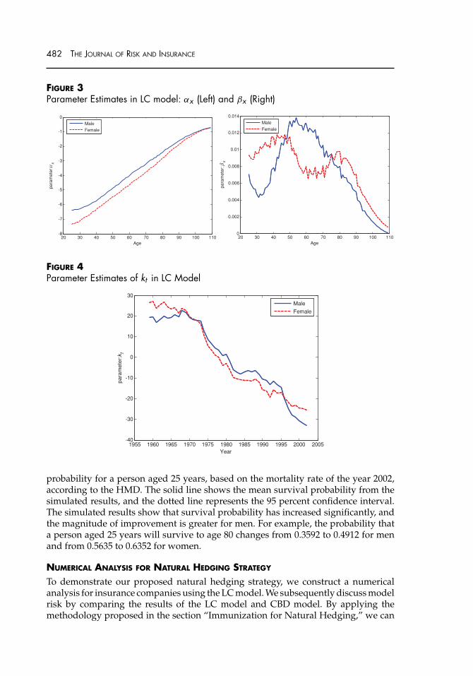
Forecasting Survival ProbabilityUsing the parameters estimated in the section ”Estimation and Parameters,” we fore-cast age-specific death rates by modeling kt as a stochastic time series process. Inthis article, we follow R. D. Lee (2000) to forecast kt from ARIMA process and useARIMA(1,1,0)13 to project kt . The ARIMA(1,1,0) process of kt can be expressed as�kt = b0�kt−1 + et , where et denotes the random term with et ∼ N(0,σt). Accordingthe estimates of kt in Figure 4, we find the parameter of b0 is 0.3686 for men and 0.4335for women. We simulate kt and calculate the corresponding survival probability forboth men and women, aged 25 in the year 2003, for the future 70 years and depictthe results in Figure 5. We compare the survival probability calculated according tothe historic data with our simulated results. The dashed line represents the survival
12Due to data limitations, we cannot obtain long-term data pertaining to both life insuranceand annuity mortality experiences to generate the parameters for the proposed stochasticmortality models for different products.
13R. D. Lee (2000) uses ARIMA(0,1,0) to project kt but notes that different data sets might bepreferable for other ARIMA process.
482 THE JOURNAL OF RISK AND INSURANCE
FIGURE 3Parameter Estimates in LC model: αx (Left) and βx (Right)
20 30 40 50 60 70 80 90 100 110-8
-7
-6
-5
-4
-3
-2
-1
0
Age
para
met
er:α
x
MaleFemale
20 30 40 50 60 70 80 90 100 1100
0.002
0.004
0.006
0.008
0.01
0.012
0.014
Age
para
met
er: β
x
MaleFemale
FIGURE 4Parameter Estimates of kt in LC Model
1955 1960 1965 1970 1975 1980 1985 1990 1995 2000 2005-40
-30
-20
-10
0
10
20
30
Year
para
met
er:k
t
Male
Female
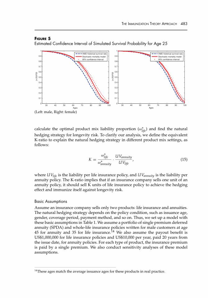
probability for a person aged 25 years, based on the mortality rate of the year 2002,according to the HMD. The solid line shows the mean survival probability from thesimulated results, and the dotted line represents the 95 percent confidence interval.The simulated results show that survival probability has increased significantly, andthe magnitude of improvement is greater for men. For example, the probability thata person aged 25 years will survive to age 80 changes from 0.3592 to 0.4912 for menand from 0.5635 to 0.6352 for women.
NUMERICAL ANALYSIS FOR NATURAL HEDGING STRATEGY
To demonstrate our proposed natural hedging strategy, we construct a numericalanalysis for insurance companies using the LC model. We subsequently discuss modelrisk by comparing the results of the LC model and CBD model. By applying themethodology proposed in the section “Immunization for Natural Hedging,” we can
THE IMMUNIZATION THEORY APPROACH 483
FIGURE 5Estimated Confidence Interval of Simulated Survival Probability for Age 25
30 40 50 60 70 80 90 1000
0.1
0.2
0.3
0.4
0.5
0.6
0.7
0.8
0.9
1
Ages
(x-2
5)P
25
HMD historical survival rate
Stochastic mortality model95% confidence interval
30 40 50 60 70 80 90 1000
0.1
0.2
0.3
0.4
0.5
0.6
0.7
0.8
0.9
1
Ages
(x-2
5)P
25
HMD historical survival rate
Stochastic mortality model95% confidence interval
(Left: male, Right: female)
calculate the optimal product mix liability proportion (ω∗life) and find the natural
hedging strategy for longevity risk. To clarify our analysis, we define the equivalentK-ratio to explain the natural hedging strategy in different product mix settings, asfollows:
K =ω∗
life
ω∗annuity
· UVannuity
UVlife, (15)
where UVlife is the liability per life insurance policy, and UVannuity is the liability perannuity policy. The K-ratio implies that if an insurance company sells one unit of anannuity policy, it should sell K units of life insurance policy to achieve the hedgingeffect and immunize itself against longevity risk.
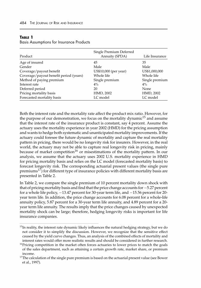
Basic AssumptionsAssume an insurance company sells only two products: life insurance and annuities.The natural hedging strategy depends on the policy condition, such as issuance age,gender, coverage period, payment method, and so on. Thus, we set up a model withthese basic assumptions in Table 1. We assume a portfolio of single premium deferredannuity (SPDA) and whole-life insurance policies written for male customers at age45 for annuity and 35 for life insurance.14 We also assume the payout benefit isUS$1,000,000 for life insurance policies and US$10,000 per year, paid 20 years fromthe issue date, for annuity policies. For each type of product, the insurance premiumis paid by a single premium. We also conduct sensitivity analyses of these modelassumptions.
14These ages match the average issuance ages for these products in real practice.
484 THE JOURNAL OF RISK AND INSURANCE
TABLE 1Basis Assumptions for Insurance Products
Single Premium DeferredProduct Annuity (SPDA) Life Insurance
Age of insured 45 35Gender Male MaleCoverage/payout benefit US$10,000 (per year) US$1,000,000Coverage/payout benefit period (years) Whole life Whole lifeMethod of paying premium Single premium Single premiumInterest rate 4% 4%Deferred period 20 NonePricing mortality basis HMD, 2002 HMD, 2002Forecasted mortality basis LC model LC model
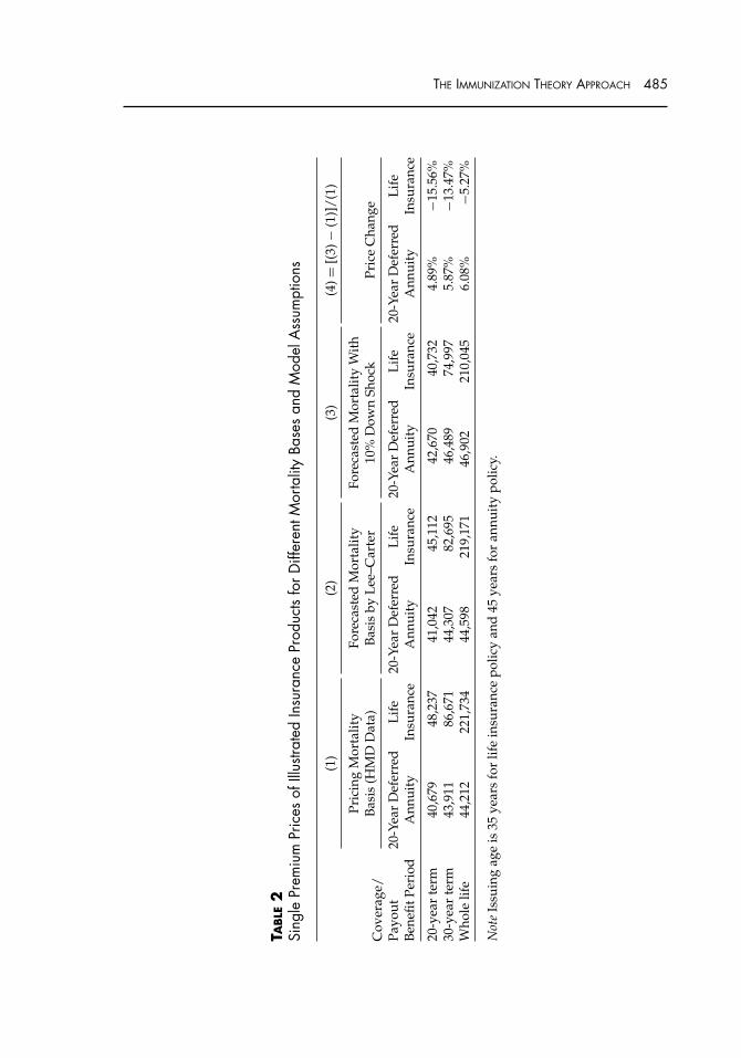
Both the interest rate and the mortality rate affect the product mix ratio. However, forthe purpose of our demonstration, we focus on the mortality dynamic15 and assumethat the interest rate of the insurance product is constant, say 4 percent. Assume theactuary uses the mortality experience in year 2002 (HMD) for the pricing assumptionand wants to hedge both systematic and unanticipated mortality improvements. If theactuary could foresee the future dynamic of mortality and capture the real mortalitypattern in pricing, there would be no longevity risk for insurers. However, in the realworld, the actuary may not be able to capture real longevity risk in pricing, mainlybecause of market competition16 or misestimations of the mortality pattern. In ouranalysis, we assume that the actuary uses 2002 U.S. mortality experience in HMDfor pricing mortality basis and relies on the LC model (forecasted mortality basis) toforecast longevity risk. The corresponding actuarial present values (the single purepremiums17) for different type of insurance policies with different mortality basis arepresented in Table 2.
In Table 2, we compare the single premium of 10 percent mortality down shock withthat of pricing mortality basis and find that the price change accounts for −5.27 percentfor a whole life policy, −13.47 percent for 30-year term life, and −15.56 percent for 20-year term life. In addition, the price change accounts for 6.08 percent for a whole-lifeannuity policy, 5.87 percent for a 30-year term life annuity, and 4.89 percent for a 20-year term life annuity. The results imply that the price changes caused by unexpectedmortality shock can be large; therefore, hedging longevity risks is important for lifeinsurance companies.
15In reality, the interest rate dynamic likely influences the natural hedging strategy, but we donot consider it to simplify the discussion. However, we recognize that the sensitive effectcaused by the yield curve changes. Thus, an analysis of the combined effects of mortality andinterest rates would offer more realistic results and should be considered in further research.
16Pricing competition in the market often forces actuaries to lower prices to match the goalsof the sales department, such as attaining a certain growth rate, market share, or premiumincome.
17The calculation of the single pure premium is based on the actuarial present value (see Boweret al., 1997).
THE IMMUNIZATION THEORY APPROACH 485
TABLE
2Si
ngle
Prem
ium
Pric
esof
Illus
trate
dIn
sura
nce
Prod
ucts
forD
iffer
entM
orta
lity
Base
san
dM
odel
Ass
umpt
ions
(1)
(2)
(3)
(4)=
[(3)
−(1
)]/
(1)
Pric
ing
Mor
talit
yFo
reca
sted
Mor
talit
yFo
reca
sted
Mor
talit
yW
ith
Bas
is(H
MD
Dat
a)B
asis
byL
ee–C
arte
r10
%D
own
Shoc
kPr
ice
Cha
nge
Cov
erag
e/Pa
yout
20-Y
ear
Def
erre
dL
ife
20-Y
ear
Def
erre
dL
ife
20-Y
ear
Def
erre
dL
ife
20-Y
ear
Def
erre
dL
ife
Ben
efitP
erio
dA
nnui
tyIn
sura
nce
Ann
uity
Insu
ranc
eA
nnui
tyIn
sura
nce
Ann
uity
Insu
ranc
e
20-y
ear
term
40,6
7948
,237
41,0
4245
,112
42,6
7040
,732
4.89
%−1
5.56
%30
-yea
rte
rm43
,911
86,6
7144
,307
82,6
9546
,489
74,9
975.
87%
−13.
47%
Who
lelif
e44
,212
221,
734
44,5
9821
9,17
146
,902
210,
045
6.08
%−5
.27%
Not
eIs
suin
gag
eis
35ye
ars
for
life
insu
ranc
epo
licy
and
45ye
ars
for
annu
ity
polic
y.

486 THE JOURNAL OF RISK AND INSURANCE
TABLE 3Product Mix Proportion (ω∗
life) and K-Ratio: Men, Single Premium
Coverage/Payout Benefit Period 20-Year Term Life Whole Life
20-year term SPDA 30.1% 49.5%(0.364) (0.180)
30-year term SPDA 34.6% 54.6%(0.481) (0.238)
Whole-life SPDA 35.5% 55.6%(0.504) (0.249)
Note: Figures in parentheses represent the K-ratios.
Hedging Strategy for Two ProductsIn this section, we illustrate how insurers can use our proposed product mix strategyto hedge against unexpected mortality shock. For demonstration purposes, we discussthree different cases of mortality shocks: (1) the base case with a 10 percent mortalityshift for both annuity and insurance policies, (2) a sudden big shock with a 25 percentmortality shift for both annuity and insurance policies, and (3) a sudden big shock witha 25 percent mortality shift for annuity and 22.5 percent mortality shift for insurancepolicies. According to our numerical findings, the effect of convexity is not significantfor a small mortality shock. Therefore, in the case of the 10 percent mortality shift,we use only the effective durations (i.e., Equations (6) and (7)) to measure mortalityrisk and ignore the effect of convexity.18 However, for the 22.5 percent and 25 percentmortality shifts, we include the effect of convexity by using Equation (13) to measuremortality risk in our analyses.
We calculate both the optimal product mix proportion (ω∗life) and the K-ratio in
different product settings under our basic assumptions and report the results inTable 3. According to Table 3, the optimal product mix proportion for natural hedg-ing of a whole-life insurance product is 55.6 percent for men. Therefore, as long as theliability for life insurance accounts for 55.6 percent of the total liability, the insurer canachieve a natural hedging effect. The corresponding K-ratio for such product mix is0.249. In other words, if the insurance company sells one unit of whole-life SPDA to acohort of men, it should sell 0.249 units of whole life insurance to hedge its longevityrisk.
In Table 3, we observe that the optimal product mix proportion becomes smallerand the K-ratio higher as the coverage period of a life insurance become shorter.For example, for a product mix that contains a whole-life SPDA and 20-year termlife, the corresponding optimal product mix proportion is 35.5 percent (smaller than55.6 percent for whole life), and the K-ratio is 0.504 (higher than 0.249 for wholelife). As mentioned in the section “Immunization Strategy for Natural Hedging,”
18The impact of ignoring the effect of convexity on the value of both product mix proportionand K-ratio under the case of 10 percent mortality shift in Table 3 is less than 0.002.

THE IMMUNIZATION THEORY APPROACH 487
the optimal product mix of the life insurance proportion is ω∗life = Dannuity
eμ
Dannuityeμ +Dlife
eμ. Thus,
when the coverage period of life insurance becomes shorter, the optimal product mixproportion decreases because the effective duration of the life insurance increases andthe effective duration of the annuity remains the same. The results of the K-ratio inour numerical analysis imply that compared with its sale of whole-life policies, theinsurer will require more units of term-life policies to hedge against the longevity riskassociated with whole-life annuity contracts.
In contrast, both the optimal product mix proportion and the K-ratio decrease as thecoverage period of SPDA becomes shorter in Table 3. For example, for a productmix with a 20-year term SPDA and whole-life product, the optimal product mixproportion is 49.5 percent (smaller than 55.6 percent for whole-life SPDA), and theK-ratio is 0.18 (lower than 0.249 for whole-life SPDA); with a 30-year term SPDAand whole-life product, the optimal product mix is 54.6 percent and the K-ratio is0.238, again smaller than the whole-life SPDA. In these cases, the optimal productmix proportion decreases because the effective duration of life insurance remainsthe same and the effective duration of the annuity becomes smaller. The results ofthe K-ratio in our numerical analysis imply that compared with a short-term annuitypolicy, a long-term policy requires more life insurance policy units to achieve a naturalhedging effect.
In Table 4, we report the corresponding calculated results for women, whose patternsof optimal product mix proportion and K-ratios are similar. In most cases,19 thecorresponding optimal product mix proportion for women is smaller and the K-ratiohigher than those for men. For example, for a product mix containing a whole-lifeSPDA and whole-life insurance, the optimal product mix proportion for women is49.3 percent (less than 55.6 percent for men), and the corresponding K-ratio for womenis 0.279 (higher than 0.249 for men). From the section “Modeling Longevity Risk,” weknow that the survival probability of both men and women has increased significantlybut the magnitude of improvement is greater for men. Thus, compared with those formen, the optimal product mix proportions of women are smaller because the effectiveduration of life insurance is larger, and the effective duration of the annuity smaller
than those for men.20 The K-ratio (K = ω∗life
ω∗annuity
· UVannuityUVlife
) of women in most cases is
higher because the liability ratios of annuity to life insurance per policy (UVannuity
UVlife)
for women are generally higher than those of men. We also find that the K-ratio forwomen in the case of a term-life policy is almost 30–50 percent higher than that ofmen. The result implies that women have longer life expectancies, so the insurer mayneed to sell more life insurance policies to hedge for its longevity risks for women inour numerical examples.
19For the product mix with 20-year term annuity and whole life, both the corresponding optimalproduct mix proportion and the K-ratio for women are smaller than those for men.
20In the setting of our example, the mortality improvement has greater impact on the liabilityof annuity than on life insurance. Thus, the optimal product mix proportion of women issmaller than that of men.
488 THE JOURNAL OF RISK AND INSURANCE
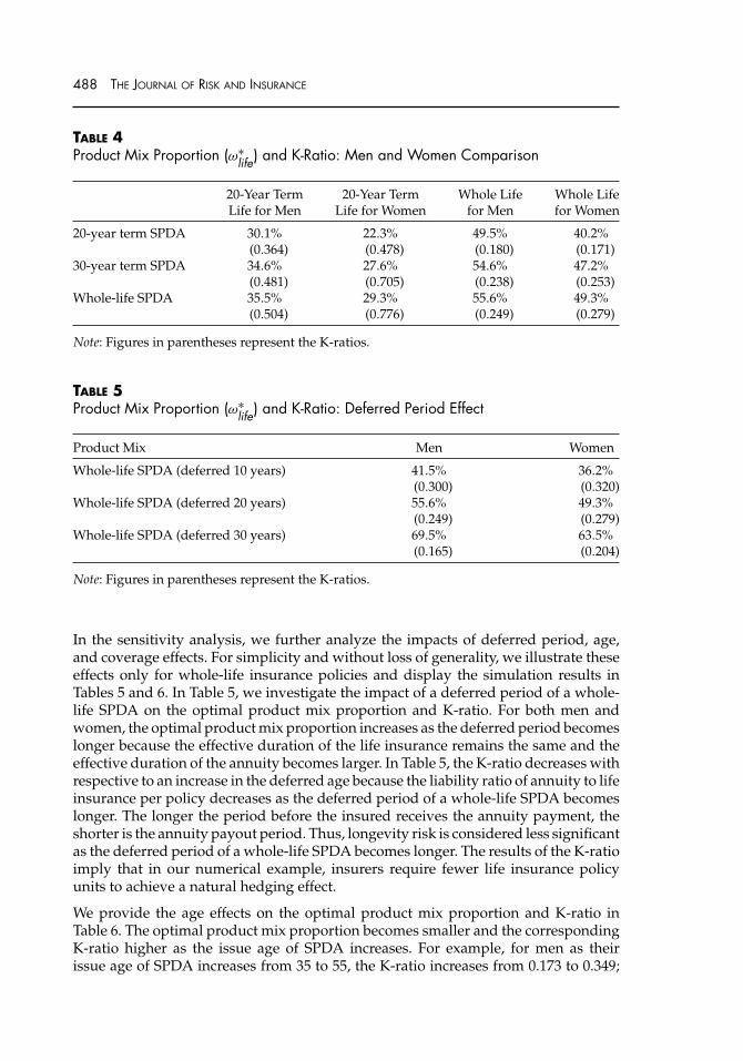
TABLE 4Product Mix Proportion (ω∗
life) and K-Ratio: Men and Women Comparison
20-Year Term 20-Year Term Whole Life Whole LifeLife for Men Life for Women for Men for Women
20-year term SPDA 30.1% 22.3% 49.5% 40.2%(0.364) (0.478) (0.180) (0.171)
30-year term SPDA 34.6% 27.6% 54.6% 47.2%(0.481) (0.705) (0.238) (0.253)
Whole-life SPDA 35.5% 29.3% 55.6% 49.3%(0.504) (0.776) (0.249) (0.279)
Note: Figures in parentheses represent the K-ratios.
TABLE 5Product Mix Proportion (ω∗
life) and K-Ratio: Deferred Period Effect
Product Mix Men Women
Whole-life SPDA (deferred 10 years) 41.5% 36.2%(0.300) (0.320)
Whole-life SPDA (deferred 20 years) 55.6% 49.3%(0.249) (0.279)
Whole-life SPDA (deferred 30 years) 69.5% 63.5%(0.165) (0.204)
Note: Figures in parentheses represent the K-ratios.
In the sensitivity analysis, we further analyze the impacts of deferred period, age,and coverage effects. For simplicity and without loss of generality, we illustrate theseeffects only for whole-life insurance policies and display the simulation results inTables 5 and 6. In Table 5, we investigate the impact of a deferred period of a whole-life SPDA on the optimal product mix proportion and K-ratio. For both men andwomen, the optimal product mix proportion increases as the deferred period becomeslonger because the effective duration of the life insurance remains the same and theeffective duration of the annuity becomes larger. In Table 5, the K-ratio decreases withrespective to an increase in the deferred age because the liability ratio of annuity to lifeinsurance per policy decreases as the deferred period of a whole-life SPDA becomeslonger. The longer the period before the insured receives the annuity payment, theshorter is the annuity payout period. Thus, longevity risk is considered less significantas the deferred period of a whole-life SPDA becomes longer. The results of the K-ratioimply that in our numerical example, insurers require fewer life insurance policyunits to achieve a natural hedging effect.
We provide the age effects on the optimal product mix proportion and K-ratio inTable 6. The optimal product mix proportion becomes smaller and the correspondingK-ratio higher as the issue age of SPDA increases. For example, for men as theirissue age of SPDA increases from 35 to 55, the K-ratio increases from 0.173 to 0.349;
THE IMMUNIZATION THEORY APPROACH 489
TABLE 6Product Mix Proportion (ω∗
life) and K-Ratio: Age Effect
Product Mix Men Women
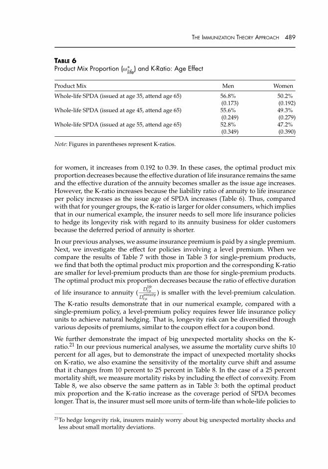
Whole-life SPDA (issued at age 35, attend age 65) 56.8% 50.2%(0.173) (0.192)
Whole-life SPDA (issued at age 45, attend age 65) 55.6% 49.3%(0.249) (0.279)
Whole-life SPDA (issued at age 55, attend age 65) 52.8% 47.2%(0.349) (0.390)
Note: Figures in parentheses represent K-ratios.
for women, it increases from 0.192 to 0.39. In these cases, the optimal product mixproportion decreases because the effective duration of life insurance remains the sameand the effective duration of the annuity becomes smaller as the issue age increases.However, the K-ratio increases because the liability ratio of annuity to life insuranceper policy increases as the issue age of SPDA increases (Table 6). Thus, comparedwith that for younger groups, the K-ratio is larger for older consumers, which impliesthat in our numerical example, the insurer needs to sell more life insurance policiesto hedge its longevity risk with regard to its annuity business for older customersbecause the deferred period of annuity is shorter.
In our previous analyses, we assume insurance premium is paid by a single premium.Next, we investigate the effect for policies involving a level premium. When wecompare the results of Table 7 with those in Table 3 for single-premium products,we find that both the optimal product mix proportion and the corresponding K-ratioare smaller for level-premium products than are those for single-premium products.The optimal product mix proportion decreases because the ratio of effective duration
of life insurance to annuity ( Dlifeeμ
Dannuityeμ
) is smaller with the level-premium calculation.
The K-ratio results demonstrate that in our numerical example, compared with asingle-premium policy, a level-premium policy requires fewer life insurance policyunits to achieve natural hedging. That is, longevity risk can be diversified throughvarious deposits of premiums, similar to the coupon effect for a coupon bond.
We further demonstrate the impact of big unexpected mortality shocks on the K-ratio.21 In our previous numerical analyses, we assume the mortality curve shifts 10percent for all ages, but to demonstrate the impact of unexpected mortality shockson K-ratio, we also examine the sensitivity of the mortality curve shift and assumethat it changes from 10 percent to 25 percent in Table 8. In the case of a 25 percentmortality shift, we measure mortality risks by including the effect of convexity. FromTable 8, we also observe the same pattern as in Table 3: both the optimal productmix proportion and the K-ratio increase as the coverage period of SPDA becomeslonger. That is, the insurer must sell more units of term-life than whole-life policies to
21To hedge longevity risk, insurers mainly worry about big unexpected mortality shocks andless about small mortality deviations.
490 THE JOURNAL OF RISK AND INSURANCE
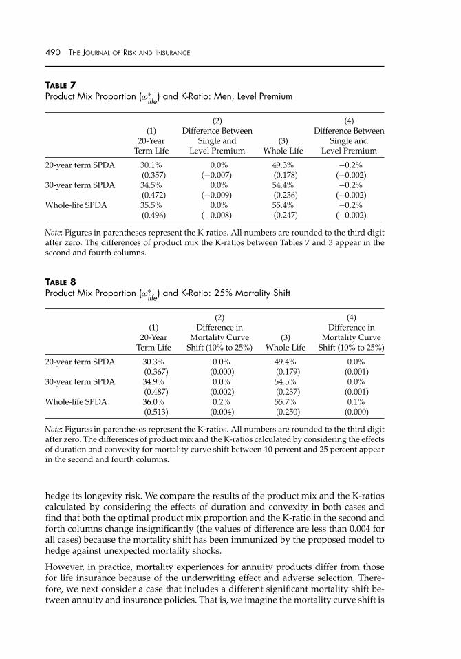
TABLE 7Product Mix Proportion (ω∗
life) and K-Ratio: Men, Level Premium
(2) (4)(1) Difference Between Difference Between
20-Year Single and (3) Single andTerm Life Level Premium Whole Life Level Premium
20-year term SPDA 30.1% 0.0% 49.3% −0.2%(0.357) (−0.007) (0.178) (−0.002)
30-year term SPDA 34.5% 0.0% 54.4% −0.2%(0.472) (−0.009) (0.236) (−0.002)
Whole-life SPDA 35.5% 0.0% 55.4% −0.2%(0.496) (−0.008) (0.247) (−0.002)
Note: Figures in parentheses represent the K-ratios. All numbers are rounded to the third digitafter zero. The differences of product mix the K-ratios between Tables 7 and 3 appear in thesecond and fourth columns.
TABLE 8Product Mix Proportion (ω∗
life) and K-Ratio: 25% Mortality Shift
(2) (4)(1) Difference in Difference in
20-Year Mortality Curve (3) Mortality CurveTerm Life Shift (10% to 25%) Whole Life Shift (10% to 25%)
20-year term SPDA 30.3% 0.0% 49.4% 0.0%(0.367) (0.000) (0.179) (0.001)
30-year term SPDA 34.9% 0.0% 54.5% 0.0%(0.487) (0.002) (0.237) (0.001)
Whole-life SPDA 36.0% 0.2% 55.7% 0.1%(0.513) (0.004) (0.250) (0.000)
Note: Figures in parentheses represent the K-ratios. All numbers are rounded to the third digitafter zero. The differences of product mix and the K-ratios calculated by considering the effectsof duration and convexity for mortality curve shift between 10 percent and 25 percent appearin the second and fourth columns.
hedge its longevity risk. We compare the results of the product mix and the K-ratioscalculated by considering the effects of duration and convexity in both cases andfind that both the optimal product mix proportion and the K-ratio in the second andforth columns change insignificantly (the values of difference are less than 0.004 forall cases) because the mortality shift has been immunized by the proposed model tohedge against unexpected mortality shocks.
However, in practice, mortality experiences for annuity products differ from thosefor life insurance because of the underwriting effect and adverse selection. There-fore, we next consider a case that includes a different significant mortality shift be-tween annuity and insurance policies. That is, we imagine the mortality curve shift is
THE IMMUNIZATION THEORY APPROACH 491
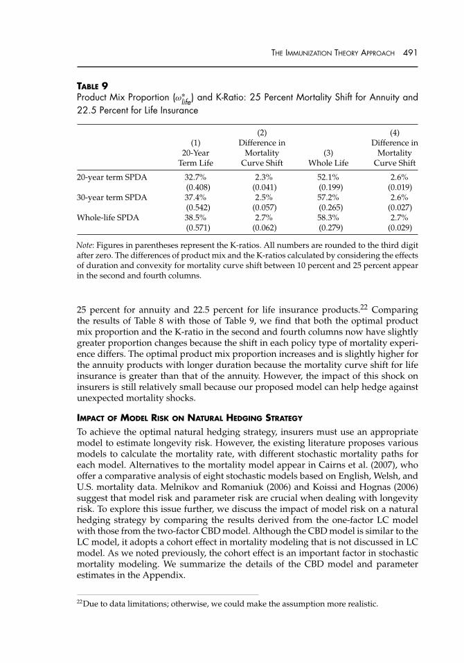
TABLE 9Product Mix Proportion (ω∗
life) and K-Ratio: 25 Percent Mortality Shift for Annuity and22.5 Percent for Life Insurance
(2) (4)(1) Difference in Difference in
20-Year Mortality (3) MortalityTerm Life Curve Shift Whole Life Curve Shift
20-year term SPDA 32.7% 2.3% 52.1% 2.6%(0.408) (0.041) (0.199) (0.019)
30-year term SPDA 37.4% 2.5% 57.2% 2.6%(0.542) (0.057) (0.265) (0.027)
Whole-life SPDA 38.5% 2.7% 58.3% 2.7%(0.571) (0.062) (0.279) (0.029)
Note: Figures in parentheses represent the K-ratios. All numbers are rounded to the third digitafter zero. The differences of product mix and the K-ratios calculated by considering the effectsof duration and convexity for mortality curve shift between 10 percent and 25 percent appearin the second and fourth columns.
25 percent for annuity and 22.5 percent for life insurance products.22 Comparingthe results of Table 8 with those of Table 9, we find that both the optimal productmix proportion and the K-ratio in the second and fourth columns now have slightlygreater proportion changes because the shift in each policy type of mortality experi-ence differs. The optimal product mix proportion increases and is slightly higher forthe annuity products with longer duration because the mortality curve shift for lifeinsurance is greater than that of the annuity. However, the impact of this shock oninsurers is still relatively small because our proposed model can help hedge againstunexpected mortality shocks.
IMPACT OF MODEL RISK ON NATURAL HEDGING STRATEGY
To achieve the optimal natural hedging strategy, insurers must use an appropriatemodel to estimate longevity risk. However, the existing literature proposes variousmodels to calculate the mortality rate, with different stochastic mortality paths foreach model. Alternatives to the mortality model appear in Cairns et al. (2007), whooffer a comparative analysis of eight stochastic models based on English, Welsh, andU.S. mortality data. Melnikov and Romaniuk (2006) and Koissi and Hognas (2006)suggest that model risk and parameter risk are crucial when dealing with longevityrisk. To explore this issue further, we discuss the impact of model risk on a naturalhedging strategy by comparing the results derived from the one-factor LC modelwith those from the two-factor CBD model. Although the CBD model is similar to theLC model, it adopts a cohort effect in mortality modeling that is not discussed in LCmodel. As we noted previously, the cohort effect is an important factor in stochasticmortality modeling. We summarize the details of the CBD model and parameterestimates in the Appendix.
22Due to data limitations; otherwise, we could make the assumption more realistic.
492 THE JOURNAL OF RISK AND INSURANCE
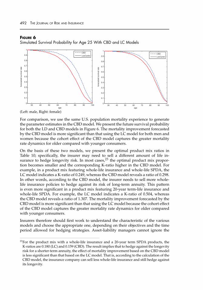
FIGURE 6Simulated Survival Probability for Age 25 With CBD and LC Models
30 40 50 60 70 80 90 1000
0.1
0.2
0.3
0.4
0.5
0.6
0.7
0.8
0.9
1
age
fore
cast
ed s
urvi
val r
ate
CBD
LeeCarter
30 40 50 60 70 80 90 1000
0.1
0.2
0.3
0.4
0.5
0.6
0.7
0.8
0.9
1
age
fore
cast
ed s
urvi
val r
ate
CBD
LeeCarter
(Left: male, Right: female)
For comparison, we use the same U.S. population mortality experience to generatethe parameter estimates in the CBD model. We present the future survival probabilityfor both the LD and CBD models in Figure 6. The mortality improvement forecastedby the CBD model is more significant than that using the LC model for both men andwomen because the cohort effect of the CBD model captures the greater mortalityrate dynamics for older compared with younger consumers.
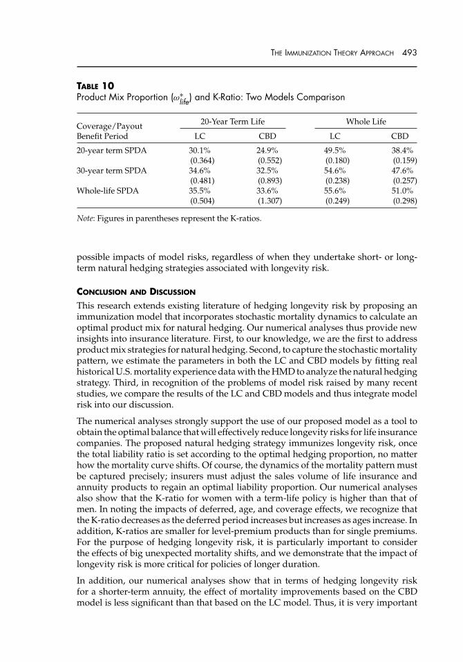
On the basis of these two models, we present the optimal product mix ratios inTable 10; specifically, the insurer may need to sell a different amount of life in-surance to hedge longevity risk. In most cases,23 the optimal product mix propor-tion becomes smaller and the corresponding K-ratio higher in the CBD model. Forexample, in a product mix featuring whole-life insurance and whole-life SPDA, theLC model indicates a K-ratio of 0.249, whereas the CBD model reveals a ratio of 0.298.In other words, according to the CBD model, the insurer needs to sell more whole-life insurance policies to hedge against its risk of long-term annuity. This patternis even more significant in a product mix featuring 20-year term-life insurance andwhole-life SPDA. For example, the LC model indicates a K-ratio of 0.504, whereasthe CBD model reveals a ratio of 1.307. The mortality improvement forecasted by theCBD model is more significant than that using the LC model because the cohort effectof the CBD model captures the greater mortality rate dynamics for older comparedwith younger consumers.
Insurers therefore should first work to understand the characteristic of the variousmodels and choose the appropriate one, depending on their objectives and the timeperiod allowed for hedging strategies. Asset-liability managers cannot ignore the
23For the product mix with a whole-life insurance and a 20-year term SPDA products, theK-ratios are 0.180 (LC) and 0.159 (CBD). The result implies that to hedge against the longevityrisk for a shorter-term annuity, the effect of mortality improvement based on the CBD modelis less significant than that based on the LC model. That is, according to the calculation of theCBD model, the insurance company can sell less whole-life insurance and still hedge againstits longevity.
THE IMMUNIZATION THEORY APPROACH 493
TABLE 10Product Mix Proportion (ω∗
life) and K-Ratio: Two Models Comparison
20-Year Term Life Whole LifeCoverage/PayoutBenefit Period LC CBD LC CBD
20-year term SPDA 30.1% 24.9% 49.5% 38.4%(0.364) (0.552) (0.180) (0.159)
30-year term SPDA 34.6% 32.5% 54.6% 47.6%(0.481) (0.893) (0.238) (0.257)
Whole-life SPDA 35.5% 33.6% 55.6% 51.0%(0.504) (1.307) (0.249) (0.298)
Note: Figures in parentheses represent the K-ratios.
possible impacts of model risks, regardless of when they undertake short- or long-term natural hedging strategies associated with longevity risk.
CONCLUSION AND DISCUSSION
This research extends existing literature of hedging longevity risk by proposing animmunization model that incorporates stochastic mortality dynamics to calculate anoptimal product mix for natural hedging. Our numerical analyses thus provide newinsights into insurance literature. First, to our knowledge, we are the first to addressproduct mix strategies for natural hedging. Second, to capture the stochastic mortalitypattern, we estimate the parameters in both the LC and CBD models by fitting realhistorical U.S. mortality experience data with the HMD to analyze the natural hedgingstrategy. Third, in recognition of the problems of model risk raised by many recentstudies, we compare the results of the LC and CBD models and thus integrate modelrisk into our discussion.
The numerical analyses strongly support the use of our proposed model as a tool toobtain the optimal balance that will effectively reduce longevity risks for life insurancecompanies. The proposed natural hedging strategy immunizes longevity risk, oncethe total liability ratio is set according to the optimal hedging proportion, no matterhow the mortality curve shifts. Of course, the dynamics of the mortality pattern mustbe captured precisely; insurers must adjust the sales volume of life insurance andannuity products to regain an optimal liability proportion. Our numerical analysesalso show that the K-ratio for women with a term-life policy is higher than that ofmen. In noting the impacts of deferred, age, and coverage effects, we recognize thatthe K-ratio decreases as the deferred period increases but increases as ages increase. Inaddition, K-ratios are smaller for level-premium products than for single premiums.For the purpose of hedging longevity risk, it is particularly important to considerthe effects of big unexpected mortality shifts, and we demonstrate that the impact oflongevity risk is more critical for policies of longer duration.
In addition, our numerical analyses show that in terms of hedging longevity riskfor a shorter-term annuity, the effect of mortality improvements based on the CBDmodel is less significant than that based on the LC model. Thus, it is very important

494 THE JOURNAL OF RISK AND INSURANCE
for insurers to understand the characteristic of the various models and choose anappropriate one, according to their objectives and the time period of their hedgingstrategies. Asset-liability managers also cannot ignore the possible impacts of modelrisks.
Is natural hedging really cheaper than other external hedging instruments, such asmortality derivatives and survivor bonds? Due to a lack of suitable price data forvarious insurance products, we are unable to analyze the actual natural hedging costin real practice for insurance companies. Furthermore, mortality experiences maydiffer for life insurance and annuity products, but because of our data limitations, wecannot obtain sufficiently long life insurance and annuity mortality experiences togenerate the parameters for the proposed stochastic mortality models from the U.S.mortality data in the HMD. However, we believe insurers can make use of their ownmortality experience to revise the parameters in the mortality models and apply ourproposed mythology to find their natural hedging strategy. Finally, some ongoingimportant issues for insurance research and practice clearly deserve more investi-gation. For example, studies of alternative mortality models could use the insurer’sactual mortality experience with different products and immunization strategies withcertain assumptions about the future dynamics of nonparallel mortality shifts. We il-lustrate the hedging strategy with a term structure force of mortality, but we do notconsider the effect of dynamic interest rates. Therefore, an analysis of the combinedeffects of mortality and interest rates would offer more realistic results and should beconsidered by further research.
APPENDIX: CBD MORTALITY MODEL
The ModelThe CBD mortality model we use was proposed in Cairns, Blake, and Down (2006b).They suggest a two-factor model for modeling initial mortality rates instead of centralmortality rate. The mortality rate for a person aged x in year t (q (t,x)) is modeled asfollows:
logit q (t, x) = β1t k1
t + β2t k2
t (A1)
where k1t and k2
t reflect period-related effects.
This model can be presented in a simple parametric form by setting β1t equal to 1 and
β2t = x − x̄. Thus, the mortality rate can be modeled as in Equation (A2)
logit q (t, x) = k1t + k2
t (x − x̄), (A2)
where x̄ is the mean age. For other generalizations of CBD model, see Cairns et al.(2007).
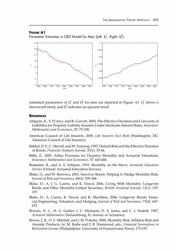
The Parameter EstimatesTo investigate the model risk, we also estimate the parameters in the CBD modelby fitting historical U.S. mortality data from 1959 to 2002 with the HMD data. The
THE IMMUNIZATION THEORY APPROACH 495
FIGURE A1Parameter Estimates in CBD Model for Men (Left: k1
t , Right: k2t )
1960 1965 1970 1975 1980 1985 1990 1995 2000-3.2
-3.1
-3
-2.9
-2.8
-2.7
-2.6
-2.5
year
kt
1960 1965 1970 1975 1980 1985 1990 1995 2000
0.075
0.08
0.085
0.09
0.095
0.1
year
kt
estimated parameters of k1t and k2
t for men are depicted in Figure A1. k1t shows a
downward trend, and k2t indicates an upward trend.
REFERENCES
Ahlgrim, K., S. D’Arcy, and R. Gorvett, 2004, The Effective Duration and Convexity ofLiabilities for Property-Liability Insurers Under Stochastic Interest Rates, Insurance:Mathematics and Economics, 29: 75-108.
American Council of Life Insurers, 2000, Life Insurers Fact Book (Washington, DC:American Council of Life Insurers).
Babbel, D. F., C. Merrill, and W. Panning, 1997, Default Risk and the Effective Durationof Bonds, Financial Analysts Journal, 33(1): 35-44.
Biffis, E., 2005, Affine Processes for Dynamic Mortality and Actuarial Valuations,Insurance: Mathematics and Economics, 37: 443-468.
Benjamin, B., and A. S. Soliman, 1993, Mortality on the Move, Actuarial EducationService (Oxford: Actuarial Education Service).
Blake, D., and W. Burrows, 2001, Survivor Bonds: Helping to Hedge Mortality Risk,Journal of Risk and Insurance, 68(2): 339-348.
Blake, D., A. J. G. Cairns, and K. Dowd, 2006, Living With Mortality: LongevityBonds and Other Mortality-Linked Securities, British Actuarial Journal, 12(1): 153-197.
Blake, D., A. Cairns, K. Dowd, and R. MacMinn, 2006, Longevity Bonds: Finan-cial Engineering, Valuation, and Hedging, Journal of Risk and Insurance, 73(4): 647-672.
Bowers, N. L., H. U. Gerber, J. C. Hickman, D. A. Jones, and C. J. Nesbitt, 1997,Actuarial Mathematics (Schaumburg, IL: Society of Actuaries).
Brown, J. R., O. S. Mitchell, and J. M. Poterba, 2000, Mortality Risk, Inflation Risk andAnnuity Products, in: M. Bodie and P. B. Hammond, eds., Financial Innovations inRetirement Income (Philadelphia: University of Pennsylvania Press), 175-197.

496 THE JOURNAL OF RISK AND INSURANCE
Cairns, A. J. G., D. Blake, and K. Dowd, 2006a, Pricing Death: Frameworks for theValuation and Securitization of Mortality Risk, ASTIN Bulletin, 36: 79-120.
Cairns, A. J. G., D. Blake, and K. Dowd, 2006b, A Two-factor Model for StochasticMortality With Parameter Uncertainty: Theory and Calibration, Journal of Risk andInsurance, 73: 687-718.
Cairns, A. J. G., D. Blake, K. Dowd, G. D. Goughlan, D. Epstein, A. Ong, and I. Balevich,2007, A Quantitative Comparison of Stochastic Mortality Models Using Data FromEngland and Wales and the United States, Pensions Institute Discussion Paper I-0701Available at: http://www.pensions-institute.org/workingpapers/wp0701.pdf (ac-cessed May 2006).
Cox, S. H., Y. Lin, and S. Wang, 2006, Multivariate Exponential Tilting and Pric-ing Implications for Mortality Securitization. Journal Risk and Insurance, 73(4): 719-736.
Cox, S. H. and Y. Lin, 2007, Natural Hedging of Life and Annuity Mortality Risks,North American Actuarial Journal, 11(3): 1-15.
Currie, I. D., 2006, Smoothing and Forecasting Mortality Rates With P-splines. Pre-sentation, Institute of Actuaries, June 2006.
Dahl, M., 2004, Stochastic Mortality in Life Insurance: Market Reserves and Mortality-Linked Insurance Contracts, Insurance: Mathematics and Economics, 35: 113-136.
Dahl, M., and T. Møller, 2005, Valuation and Hedging of Life Insurance Liabilities WithSystematic Mortality Risk, in Proceedings of the 15th International AFIR Colloquium,Zurich.
Denuit, M., P. Devolder, and A. C. Goderniaux, 2007, Securitization of Longevity Risk:Pricing Survivor Bonds With Wang Transform in the Lee-Carter Framework, Journalof Risk and Insurance 74(1): 87-113.
Dowd, K., 2003, Survivor Bonds: A Comment on Blake and Burrows, Journal of Riskand Insurance, 70(2): 339-348.
Dowd, K., D. Blake, A. J. G. Cairns, and P. Dawson, 2006, Survivor Swaps, Journal ofRisk and Insurance, 1: 1-17.
Frees, E., W. J Carriere, and E. Valdez, 1996, Annuity Valuation With DependentMortality, Journal of Risk and Insurance, 63(2): 229-261.
Friedman, B., and M. Warshawsky, 1990, Annuity Prices and Saving Behavior in theUnited States, in: A. Bodie, J. Shoven, and D. A. Wise, eds., Pension in the U.S.Economy (Chicago: University of Chicago Press), 53-77.
Gaiek, L., K. Ostaszewski, and H. -J. Zwiesler, 2005, A Primer on Duration, Convexity,and Immunization, Journal of Actuarial Practice, 12: 59-82.
Human Mortality Database, 2005. Available at: http://www.mortality.org (accessedMay 2006).
Kalotay, A. J., G. O. Williams, and F. J. Fabozzi, 1993, A Model for Valuing Bonds andEmbedded Options, Financial Analysts Journal, 49: 35-46.
Koissi, S., and Hognas, 2006, Evaluating and Extending the Lee–Carter Model forMortality Forecasting: Bootstrap Confidence Interval, Insurance: Mathematics andEconomics, 26: 1-20.
THE IMMUNIZATION THEORY APPROACH 497
Lee, P. J., 2000, A General Framework for Stochastic Investigations of Mortality andInvestment Risks, Presented to Wilkiefest, Heriot-watt University, March 2000.
Lee, R. D., 2000, The Lee-Carter Method for Forecasting Mortality, With VariousExtensions and Applications, North American Actuarial Journal, 4(1): 80-93.
Lee, R. D., and L.R. Carter, 1992, Modeling and Forecasting U. S. Mortality, Journal ofthe American Statistical Association, 87: 659-671.
Lin, Y., and Cox, S.H., 2005, Securitization of Mortality Risks in Life Annuities, Journalof Risk and Insurance, 72: 227-252.
Luciano, E., and E. Vigna, 2005, Non Mean Reverting Affine Processes for Stochas-tic Mortality, International Centre for Economic Research, Working Paper No. 4/2005.
Marceau, E., and P. Gaillardetz, 1999, On Life Insurance Reserve in a Stochastic Mor-tality and Interest Rates Environment, Insurance: Mathematics and Economics, 25(3):261-80.
McDonald, A. S., 1997, The Second Actuarial Study of Mortality in Europe (Oxford:Oxford University Press).
McDonald, A. S., A. J. G. Cairns, P. L. Gwilt, and K. A. Miller, 1998, An InternationalComparison of Recent Trends in the Population Mortality, British Actuarial Journal,3: 3-141.
Melnikov, A., and Y. Romaniuk, 2006, Evaluating the Performance of Gompertz,Makeham and Lee-Carter Mortality Models for Risk Management, Insurance: Math-ematics and Economics, 39: 310-329.
Mileysky, M. A., and S. D. Promislow, 2001, Mortality Derivatives and the Option toAnnuities, Insurance: Mathematics and Economics, 29: 299-318.
Mitchell, O. S, J. M. Poterba, M. J. Warshawky, and J. R. Brown, 2001, New Evidenceon the Money’s Worth of Individual Annuities: The Role of Annuity Markets in FinancingRetirement (Cambridge, MA: MIT Press).
Miltersen, K. R., and S.-A. Persson, 2005, Is Mortality Dead? Stochastic Forward Forceof Mortality Determined by No Arbitrage, Working Paper, University of Bergen.
Redington, F. M., 1952, Review of the Principle of Life Office Valuation, Journal of theInstitute of Actuaries, 23: 286-340.
Renshaw, A. E., S. Haberman, and P. Hatzoupoulos, 1996, The Modeling of RecentMortality Trends in United Kingdom Male Assured Lives, British Actuarial Journal,2: 229-277.
Renshaw, A. E., and S. Haberman, 2003, Lee-Carter Mortality Forecasting with AgeSpecific Enhancement, Insurance: Mathematics and Economics, 33: 255-272.
Schrager, D. F., 2006, Affine Stochastic Mortality, Insurance: Mathematics and Economics,38: 81-97.
Wilkie, A. D., H. R. Waters, and S. S. Yang, 2003, Reserving, Pricing and Hedging forPolicies With Guaranteed Annuity Options, British Actuarial Journal, 9: 263-425.
Willets, R. C., 2004, The Cohort Effect: Insights and Explanations, British ActuarialJournal, 10: 833-877.