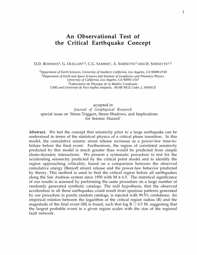
1

An Observational Test ofthe Critical Earthquake Concept

D.D. BOWMAN1, G. OUILLON2,3, C.G. SAMMIS1, A. SORNETTE3 AND D. SORNETTE2,3

1Department of Earth Sciences, University of Southern California, Los Angeles, CA 90089-07402Department of Earth and Space Sciences and Institute of Geophysics and Planetary Physics

University of California, Los Angeles, CA 90095-15673Laboratoire de Physique de la Matière Condensée

CNRS and Université de Nice-Sophia Antipolis, 06108 NICE Cedex 2, FRANCE

accepted inJournal of Geophysical Research

special issue on 'Stress Triggers, Stress Shadows, and Implicationsfor Seismic Hazard'

Abstract. We test the concept that seismicity prior to a large earthquake can beunderstood in terms of the statistical physics of a critical phase transition. In thismodel, the cumulative seismic strain release increases as a power-law time-to-failure before the final event. Furthermore, the region of correlated seismicitypredicted by this model is much greater than would be predicted from simpleelasto-dynamic interactions. We present a systematic procedure to test for theaccelerating seismicity predicted by the critical point model and to identify theregion approaching criticality, based on a comparison between the observedcumulative energy (Benioff strain) release and the power-law behavior predictedby theory. This method is used to find the critical region before all earthquakesalong the San Andreas system since 1950 with M ≥ 6.5. The statistical significanceof our results is assessed by performing the same procedure on a large number ofrandomly generated synthetic catalogs. The null hypothesis, that the observedacceleration in all these earthquakes could result from spurious patterns generatedby our procedure in purely random catalogs, is rejected with 99.5% confidence. Anempirical relation between the logarithm of the critical region radius (R) and themagnitude of the final event (M) is found, such that log R ∝ 0.5 M, suggesting thatthe largest probable event in a given region scales with the size of the regionalfault network.

2

Introduction

Many investigators have attempted to use the methods of statistical physicsto understand regional seismicity [Rundle, 1988a,b; Rundle, 1989a,b; Smalley et al.,1985]. One approach has been to model the earthquake process as a criticalphenomenon, culminating in a large event that is analogous to a kind of criticalpoint [Allègre and Le Mouel, 1994; Allègre et al., 1982; Chelidze, 1982; Keilis-Borok,1990; Saleur et al., 1996a; Saleur et al., 1996b; Sornette and Sornette, 1990; Sornetteand Sammis, 1995]. Attempts to link earthquakes and critical phenomena findsupport in the recent demonstration that rupture in heterogeneous media is acritical phenomenon [Herrmann and Roux, 1990; Vanneste and Sornette, 1992;Sornette et al., 1992; Lamaignere et al., 1996; Andersen et al., 1997]. Alsoencouraging is the often reported observation of increased intermediatemagnitude seismicity before large events [Ellsworth et al., 1981; Jones, 1994; Keilis-Borok et al., 1988; Knopoff et al., 1996; Lindh, 1990; Mogi, 1969; Raleigh et al., 1982;Sykes and Jaumé, 1990; Tocher, 1959]. Because these precursory events occur overan area much greater than is predicted for elasto-dynamic interactions, they are notconsidered to be classical foreshocks [Jones and Molnar, 1979]. While the observedlong-range correlations in seismicity can not be explained by simple elasto-dynamic interactions, they can be understood by analogy to the statisticalmechanics of a system approaching a critical point for which the correlation lengthis only limited by the size of the system [Wilson, 1979].

How does one test the critical point hypothesis for earthquakes? One of thefundamental predictions of this approach is that large earthquakes follow periodsof accelerating seismicity. Previous investigators [Bufe et al., 1994; Bufe andVarnes, 1993; Saleur et al., 1996a; Sammis et al., 1996; Sornette and Sammis, 1995;Sykes and Jaumé, 1990] have attempted to predict the time of the ensuingmainshock by quantifying the accelerating seismicity predicted by statisticalphysics. However, these works have all been case studies of individual eventswhich may have been chosen precisely because they followed a period ofaccelerating seismicity. Knopoff et al. [1996] have conducted a systematic study thatcan be seen as a preliminary test of the critical point hypothesis. They found thatall 11 earthquakes in California since 1941 with magnitudes greater than 6.8 wereassociated with anomalously high levels of intermediate (M ≥ 5.1) earthquakeactivity. However, the five-year running- window method they used does notallow one to quantitatively test the existence of an acceleration in the seisimicity, ifany. The spatial partition was made a priori between northern, central andsouthern California and no attempt was made to identify the regions which wereapproaching criticality. The purpose of the present paper is to test the existence of,and quantify the acceleration of, seismicity of intermediate earthquakes and toidentify the critical region associated with each earthquake. Failure to observe aregion of accelerating seismicity before these events would invalidate the criticalpoint hypothesis.

It is important to note that the central prediction of the critical pointhypothesis is that large earthquakes only occur when the system is in a criticalstate. The word "critical" describes a system at the boundary between order and

3

disorder, and is characterized by both extreme susceptibility to external factors andstrong correlation between different parts of the system. Examples of such systemsare liquids and magnets, where the system progressively orders under smallexternal changes. Critical behavior is fundamentally a cooperative phenomenon,resulting from the repeated interactions between "microscopic" elements whichprogressively "phase up" and construct a "macroscopic" self-similar state. Here,the important observation is the appearence of many different scales involved inthe construction of the macroscopic rupture of a large earthquake.

The question now arises: how is this critical state related to the postulatedself-organized criticality of the earth’s crust [Sornette and Sornette, 1989;Bak andTang, 1989; Ito and Matsuzaki, 1990; Scholz, 1991; Sornette, 1991; Geller et al., 1997;Main, 1997]? Huang et al. [1998] have shown that these two concepts addressdifferent questions and describe properties of the crust at different time scales.Critical rupture occurs when the applied force reaches a critical value beyondwhich the system moves globally and abruptly, while self-organized criticalityneeds a slow driving velocity and describes the jerky steady-state of the system atlarge time scales. Thus, the critical rupture associated with large earthquakesconstitutes a small fraction of the total history described by self-organizedcriticality. In their hierarchical model fault network, Huang et al. [1998] found thatthe critical nature of the large model-earthquakes emerges from the interplaybetween the long-range stress-stress correlations of the self-organized critical stateand the hierarchical geometrical structure: a given level of the hierarchicalrupture is like a critical point to all the lower levels, albeit with a finite size. Thefinite size effects are thus intrinsic to the process. Pushing this reasoning by takinginto account the special role played by plate boundaries, Sammis and Smith [1997]have suggested that regional fault networks may not be in a state of continuousself-organized criticality. Rather, their analysis, performed on the same model asHuang et al. [1998], suggests that a large event may move the network away fromcriticality. A period of accelerating seismicity is then the signature of the approachback to the critical state. Furthermore, the large earthquake need not correspondexactly with the critical point. A large earthquake which is not immediatelypreceded by a period of accelerating seismicity may represent a region which hadpreviously reached a state of self-organized criticality, but has not yet had anearthquake large enough to perturb the system away from the critical state.Alternatively, a region of accelerating seismicity which is not followed by a largeearthquake is interpreted as a system which has achieved criticality, but in which alarge event has not yet nucleated. The observation of accelerating seismicity isindirect evidence that the system has approached criticality and is therefore capableof producing a large earthquake. Grasso and Sornette [1997] have proposedanother approach to test for criticality, which is to monitor the response of thecrust to perturbations leading to induced seismicity. In this case, one tests directlythe large "critical" susceptibility of the crust which should be present in the criticalstate.

For simplicity, in this paper it is implicitly assumed that large earthquakesoccur at a time close to the critical point. We will test the critical point hypothesisby searching for a region of accelerating seismicity (i.e. a critical region) for all

4

earthquakes stronger than magnitude 6.5 in California between the latitudes of40°N (the northern extent of the San Andreas fault) and 32.5° N (the southernlimit of the Southern California Seismic Network). The critical region is selectedby optimizing the residue of the fit of the cumulative Benioff strain by a powerlaw. We limit our study to events after 1950 in order to minimize artifacts in thedata due to modifications of the seismic networks, such as the installation of theSouthern California network in 1932. We also present detailed synthetic tests thathave been performed in order to check the statistical significance of our results.While the acceleration pattern found for each single earthquake could be the resultof chance with a probability close to 1/2, when taking all together, we find that ourresults reject the null hypothesis that the seismic acceleration is due to chancewith a confidence level better than 99.5%. As a bonus, we find that the criticalregion size scales with the magnitude of the final event. Although the regionalstudy defined above is complete for all events meeting the study criteria, theearthquakes cover a very limited magnitude range (6.5 ≤ M ≤ 7.5). In order tostudy the relationship between critical region size and the magnitude of the finalevent, we have extended the magnitude window by analyzing four additionalevents outside of the previously defined space/time/magnitude limits. Theseearthquakes, which include two large and two small events, help define thescaling region over a broader magnitude range (4.7 ≤ M ≤ 8.6). The proposedscaling law reinforces the critical point hypothesis, but will demand the analysis ofmany more cases to be put on a firm statistical basis.

The approach to criticality

Bufe and Varnes, [1993] and Bufe et al., [1994] found that the clustering ofintermediate events before a large shock produces a regional increase incumulative Benioff strain, ε(t), which can be fit by a power-law time-to-failurerelation of the form

ε(t)=A+B(tc-t)m (1)

where tc is the time of the large event, B is negative and m is usually about 0.3. Ais the value of ε(t) when t = tc, i.e. the final Benioff strain up to and including thelargest event. The cumulative Benioff strain at time t is defined as

ε(t) =

12

iE (t)i=1

N(t)

∑ , (2)

where Ei is the energy of the ith event and N(t) is the number of events at time t.In calculating the energy release by an event, we follow the formulation ofKanamori and Anderson [1975], where

log10E = 4.8 + 1.5Ms. (3)

5

Bufe and Varnes, [1993] justified (1) in terms of a simple damage mechanics model.However, Sornette and Sammis, [1995] pointed out that a power-law increase inthe cumulative seismic strain release can also be expected for heterogeneousmaterials if the rupture process is analogous to a critical phase transition. In thisapproach, small and intermediate earthquakes are associated with the growingcorrelation length of the regional stress field prior to a large event. The final eventin the cycle is viewed as being analogous to the critical point in a chemical ormagnetic phase transition, occurring when the regional stress field is correlated atlong wavelengths. Within this framework, the renormalization group methodhas been applied as a powerful tool for understanding the earthquake process interms of the growing correlation length of the regional stress field [Saleur et al.,1996a,b].

The renormalization group method introduces the concept of a scalingregion in the time and space before a large rupture. The essence of therenormalization group is to assume that the failure process at a small spatial scalelength and temporally far from global failure (i.e. t « tc) can be remapped(renormalized) to the process at a larger length scale and closer to the failure time.Thus, the damage mechanics model described above can be recognized as a mean-field approximation to the regional renormalization group (see Saleur et al,1996a,b for a discussion of the application of the renormalization group to regionalseismicity).

The regional clustering of intermediate events prior to a large earthquakecan be understood in terms of the growing correlation length of the regional stressfield. Here, “correlation length” refers to the capacity of the system to sustain arupture. Early in the earthquake cycle (i.e., following an earlier large earthquake),the correlation length is short, reflecting a stress field which is very rough on theregional scale. Simply put, this implies that the distribution of stress on theregional scale is highly heterogeneous, and that the physical dimensions of regionscapable of producing a rupture are smaller than the physical dimensions of theindividual faults which are capable of producing a rupture. Thus, when anearthquake nucleates, it will reach the edge of the highly stressed patch before itcan grow to become a large event. As these events occur, they smooth the stressfield at long length scales by redistributing stress to neighboring regions, whileroughening the stress field at short length scales through aftershocks. The processof smoothing the stress field at long wavelengths while roughening it at shortwavelengths increases the correlation length of the regional stress field withoutshutting off small events. As the process continues, the growing correlation of thestress field allows ruptures in the smoothed stress field to grow to greater lengths,smoothing the stress field at even longer length scales. Thus, earthquakes whichnucleate later in the cycle, and therefore in a more correlated stress field, are able torupture barriers which would have halted the earthquake in an earlier, lesscorrelated stress field. Only when criticality is reached is the stress field correlatedon all scale lengths up to and including the largest possible event for the givenfault network.

In addition to the accelerating seismic release in (1), the renormalizationgroup approach makes observable predictions of the influence of local geology on

6

the regional rate of seismic energy release. Sornette and Sammis [1995] pointedout that if the regional fault network is a discrete hierarchy, then the criticalexponent m in (1) is complex, such that

ε(t) = Re[A + B(tf-t)m+im’] = A + B(tf-t)m

1+C cos

2π 

log (tf-t)log λ  + ψ (4)

where A, B, and C are constants, λ describes the wavelength of the oscillations inlog-space, and ψ is a phase shift which depends on the units of the timemeasurement. Note that the portion of the equation outside the square brackets isjust a simple power-law. The expression within the square brackets in (4) is acorrection due to the expansion of the imaginary component, and is a second-order effect which modulates the power-law.

Another implication of the critical point model is that small earthquakesare the agents by which longer stress correlations are established - they effectivelysmooth the stress field at larger scale lengths, as originally proposed by Andrews,[1975]. Also, the final catastrophic event in the sequence may occur in a systemwhich does not have a single fault large enough to support the rupture. In such ascenario, the long range correlation of the stress field allows the final event toconnect neighboring faults, as in the 1992 Landers earthquake. Alternatively, anetwork without a single largest element may be moved away from criticality by acluster of intermediate magnitude events.

Finally, it is noteworthy that (1) contains no inherent spatial information.From a strictly theoretical viewpoint, the correlation length of the stress fieldcould continue to grow up to the absolute physical size of the system. Thus it canbe argued that this process is ultimately limited only by the size of the earth. Amore physical limit is imposed by the size of the “local” fault network. Forexample, the physical extent of transform faulting along the Pacific-NorthAmerican plate margin places a reasonable upper limit on the scale for which thisprocess may occur in western North America. In a region with a more spatiallyextended network of faulting (e.g. China), the process could be expected tocontinue to even greater scales. Indeed, different domains within the plate marginmay become critical independently of each other, each with their own scalingregion in time and space. While these domains do have physical constraints ontheir size, they still are much larger than might be expected for actual triggering asan elastic process. The large length scales suggested by this process do not imply anactual triggering mechanism. Rather, they describe the evolution of a systemwhich is sympathetic to increasingly large ruptures. The extreme length scalesimplied by this process make identification of the critical region difficult, and areone of the prime reasons why precursory increases in regional seismicity have notbeen widely recognized until recently.

Spatial Identification of Critical Regions

A fundamental prediction of the critical point model is that the seismicityin a region which is preparing for a large earthquake increases as power-law of the

7

time to failure (Equation 1). Therefore, in the context of the critical point model,we can identify a region which is approaching criticality by optimizing the fit to (1).Initially, we will neglect the proposed log-periodic corrections to the power-law.Log-periodicity is a second-order phenomena related to the presence of a structuralhierarchy, and is not a necessary condition for the definition of the critical region.However, we will qualitatively show that for most of the earthquakes we haveconsidered in this study, log-periodicity is only observed in regions where thepower-law is optimized.

We have developed a region optimization algorithm which identifiesdomains of accelerating seismicity. The seismicity in a test domain is fit to thepower-law time-to-failure equation (1) and to a straight line corresponding to thenull hypothesis that the seismicity rate is constant. Because the physics ofcriticality requires seismicity to be accelerating prior to the mainshock, we imposethe conditions B<0 and 0<m<1 in (1). The critical exponent, m, is furtherconstrained to be less than 0.8, because for 0.8 ≤ m ≤ 1 the curvature of the power-law is virtually indistinguishable from that of a straight line over the time scaleswe consider. Finally, the date and magnitude of the final earthquake are assumedto be known quantities, which fixes the values of tf and A in (1) and allows a moreaccurate determination of the critical region.

In order to quantify the degree of acceleration in the seismicity, we define acurvature parameter C, where

C = power-law fit root-mean-square errorlinear fit root-mean-square error . (5)

Therefore when the data is best characterized by a power-law curve, the RMS errorfor the power-law fit will be small compared to the RMS error of the linear fit, andC will be small. Conversely, if the seismicity is linearly increasing then the power-law fit will be statistically indistinguishable from a linear fit, and the parameter Cwill be at or near unity. Because the critical exponent is constrained to be less than0.8, a region of linearly increasing seismicity will have a power-law fit whose RMSerror is slightly greater than the error of the linear fit. This effect is greatest forregions of decelerating seismicity, which will have a power-law RMS much greaterthan that of the linear fit, corresponding to C much greater than unity.

The optimization procedure begins by isolating earthquakes within a smallcircle centered on the epicenter of the large earthquake under consideration. Thissmallest region is always chosen to include at least four events, so that the power-law can be uniquely determined. Within this region, the seismicity is fit to astraight line as well as the power-law, and the parameter C is calculated. Theradius of the circle defining the current region of interest is then repeatedlyincreased by an arbitrary increment, and a new value of C is calculated at each step.After a predetermined number of steps, the curvature parameter C is plotted as afunction of region size. The optimal radius of the critical region corresponds tothe minimum value of C. An error estimate for the region determination can befound by measuring the width of the minimum in the plot of C.

8

For this study, we explore the region approaching criticality before historicearthquakes. We shall focus our study on all events in California withmagnitudes greater than 6.5 between 32° N and 40°N latitude (Figure 1). Becausethe method is dependent on a complete catalog at small to intermediatemagnitudes, we shall focus on events since 1950. The catalog used in this studywas the Council of the National Seismic System (CNSS) Worldwide EarthquakeCatalog, which is accessible via the World Wide Web at the Northern CaliforniaEarthquake Data Center (http://quake.geo.berkeley.edu/cnss), and includescontributions from the member networks of the CNSS, including the SouthernCalifornia Seismic Network, the Seismographic Station of the University ofCalifornia at Berkeley, and the Northern California Seismic Network. To avoidambiguities in catalogs at small magnitudes, the lower cutoff of the catalogs in thisstudy is 2 units below the magnitude of the final event. In regions where thecatalog is known to be complete to lower magnitudes, the cutoff is adjustedaccordingly.

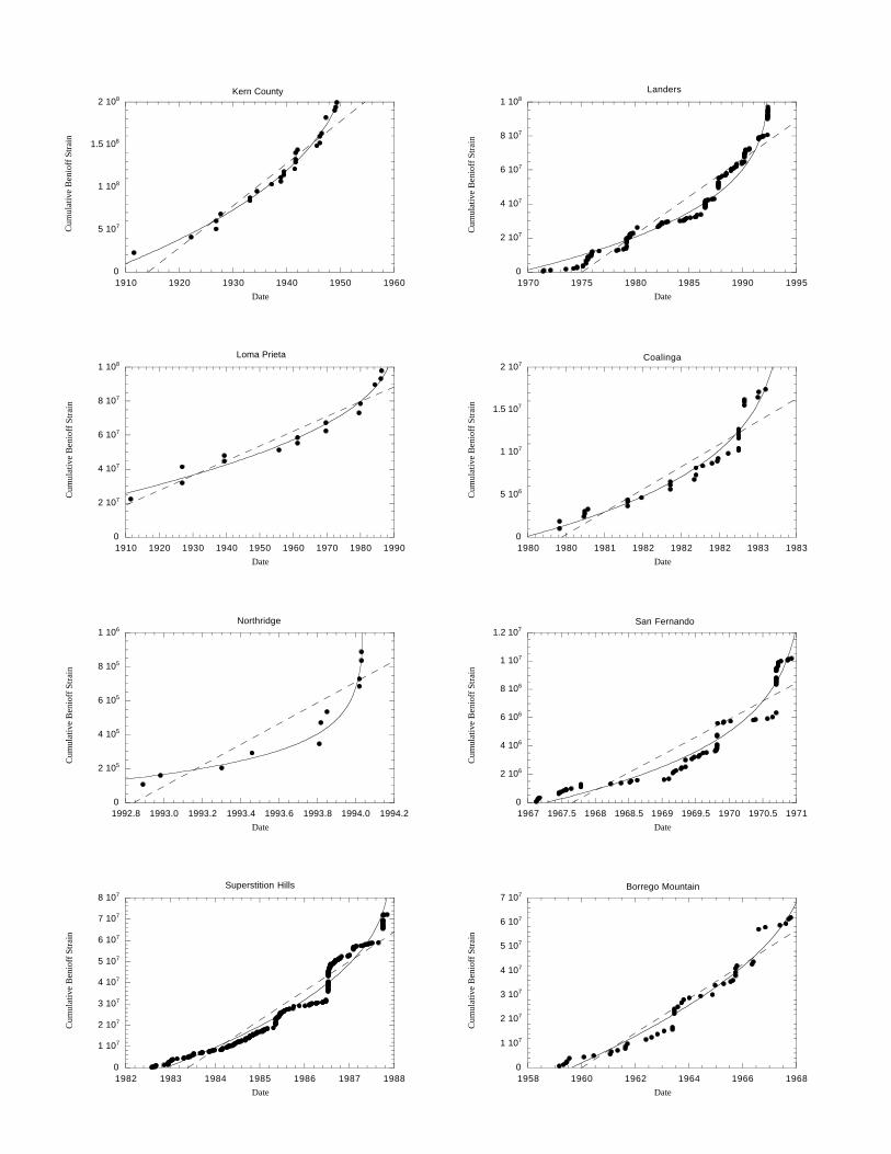
To illustrate our methodology, we now analyze the 1952 Kern Countyearthquake (Figure 2). Figure 3 shows the cumulative Benioff strain release for thethree regions in Figure 2 and, for comparison, all of California. Figure 4 shows thecorresponding plot of the optimum curvature parameter versus region size. Theseismicity prior to the Kern County event was analyzed beginning in 1910. Toaccount for changes in and variations between the seismic networks recording thecatalogs, a lower magnitude threshold for seismicity prior to this event wasimposed at M=5.5. At a radius of less than 200 km, there is not enough seismicityto obtain a statistically significant curve-fit. However, at a radius of 325 km, theseismicity produces a well-defined power-law. As the region expands, the patterndegrades. By 600 km the energy release is essentially a linear function of time.Thus, we conclude that the critical region is delimited by a circle with a radius of325 km centered at 35°N, 119°W (Figure 2). The positive and negative errors onthe region determination are defined as the radii where C is greater than 25% of 1-Cmin. Note that the seismicity for all of California during the same time period(Figure 3d) shows no acceleration in activity; the power-law time-to-failurebehavior is only observed within the critical region. Furthermore, notice that thecumulative seismicity has a structure which suggests log-periodic oscillation aboutthe power-law in the 325 km radius region (Figure 3b), while the other regionsshow less organized fluctuations. For all of the earthquakes analyzed in this study,log-periodicity was only identifiable within the critical regions defined by the best-fitting power-law.

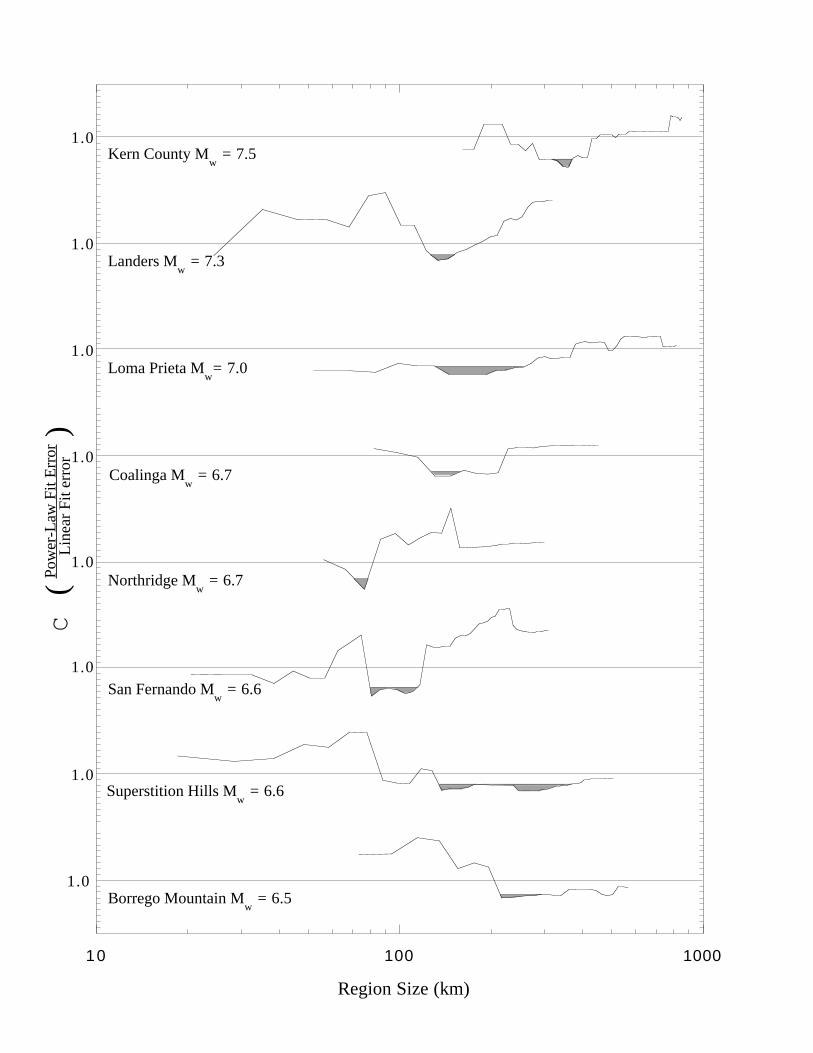
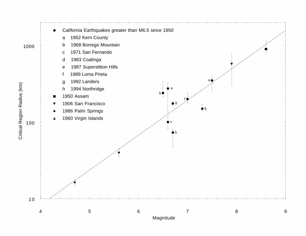
The procedure described above was repeated for all earthquakes greater thanmagnitude 6.5 since 1950 along the San Andreas system (Table 1a). Figure 5 andFigure 6 show the curvature versus region size for each earthquake and thecorresponding cumulative Benioff strain release for each event’s optimal region.There seems to be a weak correlation between the magnitude of an earthquake andthe size of its associated critical region (Figure 7, circles). While there is significantscatter in the region sizes, large earthquakes tend to be preceded by larger criticalregions than for small events. However, the relatively narrow range of

9

magnitudes included in the study (6.5 ≤ M ≤ 7.5) make this observation rathertenuous.

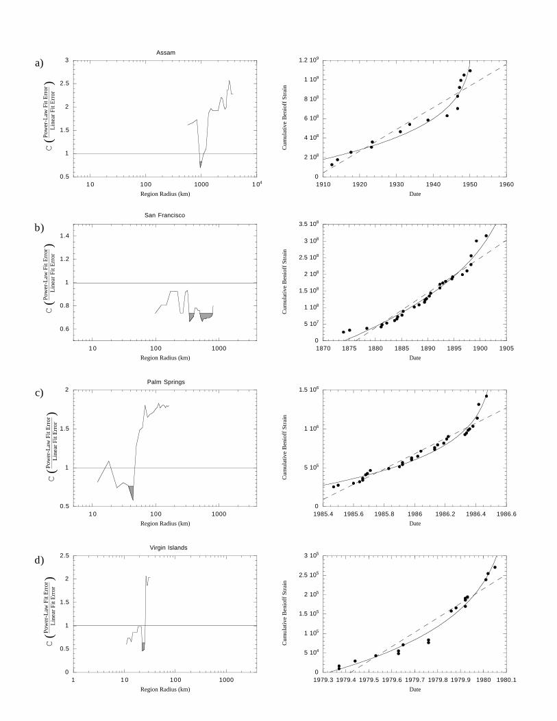
To further explore the scaling of the critical region, we have analyzed asmall set of earthquakes outside the space-time window of our study. Theseevents span a wide range of magnitudes, and include the 1950 Mw=8.6 Assamearthquake [Triep and Sykes, 1997], the 1906 Mw=7.9 San Francisco earthquake[Sykes and Jaumé, 1990] 1986 ML=5.6 Palm Springs earthquake, and the 1980 Mb=4.8Virgin Islands earthquake [Varnes and Bufe, 1996].

Notice that the Assam, San Francisco and Virgin Islands earthquakes eachcorrespond probably to the upper levels of the corresponding regional hierarchy ofearthquakes. This is the most favorable situation to clearly qualify a criticalbehavior as shown in Huang et al., [1998]. For smaller earthquakes down thehierarchy, the relative size of the fluctuations of the Benioff strain is larger due tothe influence of the (preparatory stages of) earthquakes at the upper levels of thehierarchy. Critical behavior is also expected to describe the maturation ofintermediate earthquakes, such as the Palm Springs earthquake, however withincreasing uncertainty due to the shadow cast by the larger events. This is ourjustification for not presenting a systematic study of the many intermediateearthquakes, which is left for a future work. Each of these events were analyzedwith the above procedure using the CNSS Catalog (Figure 8, Table 1b). Theseearthquakes, which cover a much larger magnitude range (4.8 ≤ M ≤ 8.6), show avery well defined trend for large events to correspond with large region sizes(Figure 7).

Statistical tests on synthetic catalogsBy its very definition, our procedure will identify a specific pattern (the

power law acceleration of seismicity measured by the Benioff strain) in a complexspatio-temporal set using an optimization procedure. The question arises whetherthis optimization would pick up a power-law pattern in any random set ofearthquakes. In other words, a power-law acceleration might always be foundprovided that we give sufficient flexibility (here in the size R of the region) in theselection of the subset of the random set. Loosely speaking, Ramsey's theoremstates that it is always possible to find any pattern we want in a sufficiently largerandom set [Graham and Spencer, 1990; Graham et al., 1990]. For instance, thistheorem explains why the ancients found recognizable everyday life structures instar constellations. Could it thus be that the observed acceleration in all of theseearthquakes results from spurious patterns generated by our procedure?

In order to test this null hypothesis, we have generated 1000 syntheticcatalogs, each containing 100 earthquakes. Each catalog corresponds to a givenseismic history culminating in a main shock. The (intermediate) earthquakes areplaced at random and uniformly within a square [-1000;1000] by [-1000;1000]. Eachevent occurs at a random time uniformly taken in the interval [0, 1000], and ischaracterized by a magnitude taken in the interval [5.5; 7.5] according to theGutenberg-Richter law (log N = a - b M) with b=1. Finally, the main shock ispositioned at the center (0,0) of the square in space and at the end of the timewindow tc=1000. We have considered two magnitudes for the main shock (7.5 and

10

8.5) in order to test the sensitivity of our results with respect to this parameter. Weuse the above optimization procedure and construct the cumulative Benioff strainwhich is fit to equation (1), with A fixed, tc fixed and the exponent m constrainedbetween 0 and 1.

Figure 9 shows the cumulative number N(C) of synthetic catalogs whosebest curvature parameter over all possible radii R is smaller than or equal to C(N(C) is thus a conditional probability). The inset shows the full range of C-valueswhile the main figure focuses on the most interesting values of C smaller than 1,which qualify that the power law (1) provides a better fit and therefore signals anacceleration. The two curves correspond to the two choices for the magnitude ofthe main shock and show the sensitivity of the results with respect to fixing theparameter A in equation (1) in the selection of the region. To compare with thegenuine catalogs, we choose the case where the optimal C is always found smallerthan or equal to 0.7. The probability that a random catalog gives an optimal Csmaller than 0.7 is seen in Figure 9 to be slightly smaller than 0.5 for the mainshock magnitude equal to 7.5 and smaller than 0.4 for the main shock magnitudeequal to 8.5. This result confirms our suspicion that the application of anoptimization procedure on a single catalog has close to 1/2 probability to generate aspurious acceleration out of pure randomness. However, the joint probability thateight earthquakes, chosen arbitrarily (i.e. without picking them a priori), all exhibitan optimal C less than or equal to 0.7 is less than (1/2)8 ≤ 0.004. This shows that thenull hypothesis that the observed acceleration in all these eight earthquakes couldresult from spurious patterns generated by our procedure in purely randomcatalogs is rejected at a confidence better than 99%.

Finally, we note that the procedure proposed here and our statistical test aredesigned solely to test for periods of accelerating seismicity before largeearthquakes. The results of this study show that the space-time distribution ofseismicity is not purely random, as has been implied by models of self-organizedcriticality (e.g. Bak and Tang [1989], Main [1997], and Geller et al. [1997]). Rather, wehave observed a systematic, non-spurious deviation from random behavior.While this observation does not constitute proof of the critical earthquakehypothesis, it is consistent with the conceptual model originally proposed bySornette and Sammis [1995].

DiscussionIt is important to examine the influence of the constraints that we have

used in the fits. Fixing A as given by the main shock is justified a priori by thebetter quality of the fit and the fewer number of fitting parameters. However, inprinciple, one would like to free A and thus be able to estimate the magnitude ofthe main shock (which is directly related to A) from the accelerated seismicity. Wehave thus tested the influence of removing the constraint on A and on theexponent m. For Kern County, we find the smallest curvature parameter for alarger optimal radius 800±100 km instead of 325 ± 75 km (see table 1a) with anexponent around 1.5 (thus larger than 1). This reflects a decelerating trend insteadof an acceleration, a result which holds when taking into account the intermediateearthquakes above magnitude 5.5. If we move the lower threshold for the selection

11

of precursors to magnitude 6, we recover the results of table 1a with the sameoptimal radius and the same exponent. This shows the sensitivity of the threeparameter fit with such sparse data. Similarly, for the Landers earthquake we findan optimal radius of 300±50 km instead of 150±15 km (table 1a), again with anexponent close to 1.5. However, in this case there are not enough events toincrease the threshold magnitude as was done for Kern County.

We conclude that, at this stage of exploratory research, the sparseness of thecatalogs prevents the realization of the full program which would consists in"predicting" completely the main shock properties (magnitude from A, time ofoccurrence from tc and position by varying the position of the circle). This wouldlead to fits with too many parameters to give robust results. The proceduredeveloped above is thus justified by the minimization of the number of fittingparameters to test in the most robust possible way the critical earthquakehypothesis. Some previous works [Sornette and Sammis, 1995; Bufe and Varnes,1996] have been more ambitious and have fit the cumulative Benioff strain to thelog-periodic equation (4), which contains even more fitting parameters. But thiswas done only on a few case studies and no systematics were obtained. It is possiblethat equation (4) might provide better results than are reported here because,notwithstanding the larger number of parameters, the log-periodic structuresprovide stringent constraints on the fits. This is currently being investigated andwill be reported elsewhere.

We now turn to a possible interpretation of figure 7, which suggests that thelogarithm of the critical region radius scales directly with the magnitude of the

final event in the sequence. A line with a slope of 1

2 gives an excellent fit to the

data. Dobrovolsky et al. [1979] and Keilis-Borok and Kossobokov [1990] report asimilar scaling log R = 0.43 M for the maximum distance between an earthquakeand its precursors, based on a completely different procedure, namely theoptimization of pattern recognition techniques [Gelfand et al, 1976]. However, isthere a theoretical justification for such a relationship? One simple possibility isthat the energy of the final event scales with the volume of the crust approachingcriticality, such that

R3 ∝ E (6)

where E is the energy of the final event and R is the radius of the critical region.

Kanamori and Anderson [1975] showed that log E ∝ 3

2 Ms, so that

log R3 = 3 log R ∝ log E ∝ 3

2 M, (7)

which yields

log R ∝ 1

2 M. (8)

12

However, an implicit assumption of this derivation is that the radius of the criticalregion is equal to or less than the thickness of the seismogenic crust. While thismay be an acceptable assumption for small earthquakes, events larger thanapproximately magnitude 6 rupture the entire crust. For these events, the radiusof the critical region is much larger than the thickness of the seismogenic zone,and the process must be treated as approximately 2 dimensional. Thus, for large

events the scaling in (6) should be R2 ∝ E, which yields a slope of 3

4, much higher

than the observed slope of 1

2.

The critical point hypothesis suggests another explanation for the slope of 1

2

observed in Figure 7. In this model, the correlation length of the regional stressfield is not constrained by elastic interactions, but rather by the physicaldimensions of the system. Thus, it might be expected that the critical region iscontrolled by the size of the regional fault network, rather than by the transfer ofelastic energy to the fault plane. Assuming that fault networks are self-similar[Hirata, 1989; King, 1986; King et al., 1988; Ouillon et al., 1996;Robertson et al., 1995;Turcotte, 1986], then the linear dimension of the fault network should scale withthe length of its largest member (L), i.e. R ∝ L. This relation of proportionalitydoes not mean that R and L are similar in order of magnitude, but only that R isproportional to L. In practice, R can be ten times larger than L or more. If thelargest event occurs on the largest coherent element of the network, then Ms ∝ 2log L [Kanamori and Anderson, 1975], so that

2 log R ∝ 2 log L ∝ M (9)and

log R ∝ 1

2 M. (10)

While the critical point model implies a slope of 1

2 in Figure 7, a least-

squares fit to the region size-magnitude plot gives a slope of 0.44. There is alsoconsiderable scatter about this best-fit line, particularly among the intermediatemagnitude events (M ≈ 6.5). This may be in part due to the simplified dataanalysis procedures that were used in this study and also to the expected cross-overbetween 2D to 3D expected around this magnitude. Our study indicates that the 2D-3D cross-over is not only dictated by the comparison of the main shock rupturesize to the seismogenic thickness. Our finding suggests another important scale,namely the size R of the critical region in which the maturation of the main shockoccurs. Since R is significantly larger than L, the cross-over should be very smoothand extend over a large magnitude range. This seems to be confirmed by a recentcareful reanalysis of the Gutenberg-Richter law for Southern California whichfound no cross-over up to the largest magnitude 7.5 [Sornette et al., 1996].

13

The present work can be improved in many ways. First, there is no physicalreason for the critical region to be a perfect circle centered on the epicenter of thefinal event. We have already extended this analysis to use elliptical regions ratherthan circles, with no significant modification of the results. A better approachwould be to use the natural clustering of the seismicity to define the regions. Theseismicity could also be much more accurately characterized by incorporating thesecond-order log-periodic corrections in (4). These fluctuations permit a moreprecise characterization of the precursory seismicity, which would consequentlyenable a more accurate determination of the critical region. Such procedures areclearly more computationally intensive, and are reserved for a later study. Finally,this study has made the explicit assumption that the final earthquake occurs assoon as the system achieves criticality. Some of the uncertainty in fitting equation(1) could be removed by incorporating an arbitrary time delay into the equationdescribing the accelerating seismicity.

In spite of these simplifications, it is encouraging that all of the events onthe San Andreas fault system greater than magnitude 6.5 in the last half centurywere preceded by an identifiable region of accelerating seismicity which follows apower-law time-to-failure. Furthermore, the derived region size seems to follow aphysically reasonable scaling with the magnitude of the final event which can beunderstood within the framework of the critical point model.

AcknowledgementsWe would like to acknowledge the helpful comments by the reviewers

Peter Mora and Jim Brune, as well as the Associate Editor, Ruth Harris. We wouldalso like to thank Bernard Minster and Nadya Williams for their comments onthe manuscript. This work was funded by NSF grant #EAR-9508040 (DDB),partially supported by NSF EAR9615357 (DS) and by the Southern CaliforniaEarthquake Center (CGS). SCEC is funded by NSF Cooperative Agreement EAR-8920135 and USGS Cooperative Agreement 14-08-0001-A0899 and 1434-HQ-97AG01718. This paper is SCEC contribution # 417 and IGPP contribution #XXXX.

14

ReferencesAllègre, C.J., and J.L. Le Mouel, Introduction of scaling techniques in brittle failure

of rocks, Phys. Earth Planet Inter., 87, 85-93, 1994.Allègre, C.J., J.L. Le Mouel, and A. Provost, Scaling rules in rock fracture and

possible implications for earthquake predictions, Nature, 297, 47-49, 1982.Andersen, J.V., D. Sornette and K.-T. Leung, Tri-critical behavior in rupture

induced by disorder, Phys. Rev. Lett. 78, 2140-2143, 1997.Andrews, D.J., From antimoment to moment: Plane-strain models of earthquakes

that stop, Bull. Seismol. Soc. Am., 65, 163-182, 1975.Bak, P., and C. Tang, Earthquakes as a self-organized critical phenomenon, J.

Geophys. Res., 94, 15635-15637, 1989.Bufe, C.G., S.P. Nishenko, and D.J. Varnes, Seismicity trends and potential for large

earthquakes in the Alaska-Aleutian region, PAGEOPH, 142, 83-99, 1994.Bufe, C.G., and D.J. Varnes, Predictive modelling of the seismic cycle of the greater

San Francisco bay region, J. Geophys. Res., 98, 9871-9883, 1993.Chelidze, T.L., Percolation and fracture, Phys. Earth Planet. Int., 28, 93-101, 1982.Dobrovolsky, I.R., S.I. Zubkov and V.I. Miachkin, Estimation of the size of

earthquake preparation zones, Pure and Applied Geophys. 117, 1025-1044, 1979.Ellsworth, W.L., A.G. Lindh, W.H. Prescott, and D.J. Herd, The 1906 San Francisco

earthquake and the seismic cycle, in Earthquake Prediction: An InternationalReview, Maurice Ewing Ser.,Maurice Ewing Series,4, edited by D.W. Simpson,and P.G. Richards, pp. 126-140, AGU, Washington, D.C., 1981.

Gelfand, I.M., S.A. Guberman, V.I. Keilis-Borok, L. Knopoff, F. Press, I.Y.Ranzman, I.M. Rotwain and A.M. Sadovsky, Pattern recognition applied toearthquake epicenters in California, Phys. Earth and Planet. Int. 11, 227-283, 1976.

Geller, R.J., D.D. Jackson, Y.Y. Kagan, and F. Mulargia, Earthquakes cannot bepredicted, Science, 275, 1616-1617, 1997.

Graham, R.L., B.L. Rothschild and J.H. Spencer, Ramsey theory, 2nd ed. New York: Wiley, 1990.

Graham, R.L., and J.H. Spencer, Ramsey theory, Scientific American 263, 112-117,July 1990.

Grasso, J.R., and D. Sornette, Testing self-organized criticality by inducedseismicity, J. Geophys.Res. in press , 1998.

Herrmann, H.J. and S. Roux, eds., Statistical models for the fracture of disorderedmedia (Elsevier, Amsterdam, 1990).

Hirata, T., Fractal dimension of fault systems in Japan: Fractal structure inrock fracture geometry at various scales, PAGEOPH, 131, 157-170, 1989.

Huang, Y., H. Saleur, C. G. Sammis, D. Sornette, Precursors, aftershocks,criticality and self-organized criticality, Europhysics Letters 41, 43-48 (1998)

Ito K. and M. Matsuzaki, Earthquakes as self-organized critical phenomena, J. Geophys. Res. B 95, 6853-6860, 1990.Jones, L.M., Foreshocks, aftershocks, and earthquake probabilities: Accounting for

the Landers earthquake, Bull. Seismol. Soc. Am., 84, 892-899, 1994.Jones, L.M., and P. Molnar, Some characteristics of foreshocks and their possible

relationship to earthquake prediction and premonitory slip on faults, J .Geophys. Res., 84, 3596-3608, 1979.

15

Kanamori, H., and D.L. Anderson, Theoretical basis of some empirical relations inseismology, Bull. Seismol. Soc. Am., 65, 1073-1095, 1975.

Keilis-Borok, V., The lithosphere of the Earth as a large nonlinear system, in QuoVadimus: Geophysics for the Next Generation,Geophys. Monogr. Ser.,60, editedby G.D. Garland, and J.R. Apel, pp. 81-84, AGU, Washington DC, 1990.

Keilis-Borok, V.I., L. Knopoff, I.M. Rotwain, and C.R. Allen, Intermediate-termprediction of occuerrence times of strong earthquakes, Nature, 335, 690-694,1988.

Keilis-Borok, V.I. and V.G. Kossobokov, Premonitory activation of earthquakeflow: algorithm M8, Phys. Earth and Planet. Int. 61, 73-83, 1990.

King, G.C.P., Speculations on the geometry of the initiation and terminationprocesses of earthquake rupture and its relation to morphology and geologicalstructure, PAGEOPH, 124, 567-585, 1986.

King, G.C.P., R.S. Stein, and J.B. Rundle, The growth of geological structures byrepeated earthquakes 1. Conceptual framework, J. Geophys. Res., 93, 13307-13318,1988.

Knopoff, L., T. Levshina, V.I. Keilis-Borok, and C. Mattoni, Increased long-rangeintermediate-magnitude earthquake activity prior to strong earthquakes inCalifornia, J. Geophys. Res., 101, 5779-5796, 1996.

Lamaignère, L., F. Carmona and D. Sornette, Experimental realization of criticalthermal fuse rupture, Phys. Rev. Lett. 77, 2738-2741, 1996.

Lindh, A.G., The seismic cycle pursued, Nature, 348, 580-581, 1990.Main, I., Long odds on prediction, Nature, 385, 19-20, 1997.Mogi, K., Some features of recent seismic activity in and near Japan {2}: Activity

before and after great earthquakes, Bull. Eq. Res. Inst. Univ. Tokyo, 47, 395-417,1969.

Ouillon, G., B. Castaing and D. Sornette, Hierarchical scaling of faulting, J .Geophys. Res. 101, 5477-5487, 1996.

Raleigh, C.B., K. Sieh, L.R. Sykes, and D.L. Anderson, Forecasting southernCalifornia earthquakes, Science, 217, 1097-1104, 1982.

Robertson, M.C., C.G. Sammis, M. Sahimi, and A.J. Martin, Fractal analysis ofthree-dimensional spatial distributions of earthquakes with a percolationinterpretation, J. Geophys. Res., 100, 609-620, 1995.

Rundle, J.B., A physical model for earthquakes, 1. Fluctuations and interactions, J.Geophys. Res., 93, 6237-6254, 1988a.

Rundle, J.B., A physical model for earthquakes, 2. Application to southernCalifornia, J. Geophys. Res., 93, 6255-6274, 1988b.

Rundle, J.B., Derivation of the complete Gutenberg-Richter magnitude frequencyrelation using the principle of scale invariance, J. Geophys. Res., 94, 12,337-12,342, 1989a.

Rundle, J.B., A physical model for earthquakes: 3. Thermodynamical approach andits relation to nonclassical theories of nucleation, J. Geophys. Res., 94 , J.Geophys. Res., 1989b.

Saleur, H., C.G. Sammis, and D. Sornette, Discrete scale invariance, complex fractaldimensions, and log-periodic fluctuations in seismicity, J. Geophys. Res., 101,17,661-17,677, 1996a.

16

Saleur, H., C.G. Sammis, and D. Sornette, Renormalization group theory ofearthquakes, Nonlinear Processes in Geophysics, 3, 102-109, 1996b.

Sammis, C.G., D. Sornette, and H. Saleur, Complexity and earthquake forecasting,in Reduction and Predictability of Natural Disasters,SFI Studies in the Sciencesof Complexity,vol. XXV, edited by J.B. Rundle, W. Klein, and D.L. Turcotte, pp.143-156, Addison-Wesley, Reading, MA, 1996.

Sammis, C.G., and S. Smith, A fractal automaton model for regional seismicity, inpreparation.

Scholtz C.H., Earthquakes and Faulting: self-organized critical phenomena withcharacteristic dimension.; in Triste and D. Sherrington (eds), Spontaneousformation of space-time structures and criticality, Kluwer Academic Publishers,Netherlands, 41-56, 1991.

Smalley, R.F., D.L. Turcotte, and S.A. Solla, A renormalization group approach tothe stick-slip behavior of faults, J. Geophys. Res., 90, 1894-1900, 1985.

Sornette D., Self-organized criticality in plate tectonics, in the proceedings of theNATO ASI "Spontaneous formation of space-time structures and criticality",Geilo, Norway 2-12 april 1991, edited by T. Riste and D. Sherrington, KluwerAcademic Press, p.57-106, 1991.

Sornette, A. and D. Sornette, Self-organized criticality and earthquakes,Europhys.Lett. 9, 197 (1989)

Sornette, A., and D. Sornette, Earthquake rupture as a critical point : Consequencesfor telluric precursors, Tectonophysics, 179, 327-334, 1990.

Sornette, D., C. Vanneste and L. Knopoff, Statistical model of earthquakeforeshocks,Phys.Rev.A 45 , 8351-8357, 1992.

Sornette, D., and C.G. Sammis, Complex critical exponents from renormalizationgroup theory of earthquakes : Implications for earthquake predictions, J. Phys. I.,5, 607-619, 1995.

Sykes, L.R., and S. Jaumé, Seismic activity on neighboring faults as a long-termprecursor to large earthquakes in the San Francisco Bay Area, Nature, 348, 595-599, 1990.

Tocher, D., Seismic history of the San Francisco region, in San FranciscoEarthquakes of 1957G.B. Oakeshott, pp. 39-48, CDMG Special Report 57, 1959.

Triep, E.G., and L.R. Sykes, Frequency of occurrence of moderate to greatearthquakes in intracontinental regions: Implications for changes in stress,earthquake prediction, and hazards assessments, J. Geophys. Res., 102, 9923-9948,1997.

Turcotte, D.L., A fractal model for crustal deformation, Tectonophys., 132, 261-269,1986.

C. Vanneste and D. Sornette, Dynamics of rupture in thermal fuse models, J.Phys.IFrance 2, 1621-1644, 1992.

Varnes, D.J., and C.G. Bufe, The cyclic and fractal seismic series preceding anMb=4.8 earthquake on 1980 February 14 near the Virgin Islands, Geophys. J. Int.,

124, 149-158, 1996.Wilson, K.G. , Problems in physics with many scales of length, Scientific American

241, August, 158-179, 1979.

17

Figure Captions

Figure 1. All earthquakes in California since 1950 with M ≥ 6.5 and with epicentersbetween 32° N and 40°N latitude. (1) 1952 Mw=7.5 Kern County. (2) 1968 Mw=6.5Borrego Mountain. (3) 1971 Mw=6.6 San Fernando. (4) 1983 Mw=6.7 Coalinga. (5)1987 Mw=6.6 Superstition Hills. (6) 1989 Mw=7.0 Loma Prieta. (7) 1992 Mw=7.3Landers. (8) 1994 Mw=6.7 Northridge.

Figure 2. Three examples of the regions tested for accelerating seismicity before the1952 Kern County earthquake. The optimal critical region is the dark circle at aradius of 325 km.

Figure 3. Cumulative Benioff strain (Equation 2) before the 1952 Kern Countyearthquake. (a) Seismicity within a 200 km radius. The power-law and linear fitsboth fit the data equally well. (b) Seismicity within a 325 km radius. The power-law fits the significantly better than a line. Note the suggestion of log-periodicfluctuations about the power-law. (c) Seismicity within 600 km radius. Neitherthe power-law nor the linear fit adequately describe the seismicity. (d) Seismicityfor all of California. The seismicity is linearly increasing.

Figure 4. Curvature paramter C as a function of region radius for the Kern Countyearthquake. Smaller values of C reflect a better power-law fit. The range of radiiwith the best power-law fit are shaded. The minimum is at a radius of 325 km.

Figure 5. Curvature paramter C as a function of region radius for all of the eventsmeeting the study criteria (see Figure 1).

Figure 6. Cumulative Benioff strain release for the optimum regions in Figure 5.

Figure 7. Optimal region radius as a function of the magnitude of the final event.The best fitting line has a slope of 0.44.

Figure 8. Curvature parameter C as a function of region radius and cumulativeBenioff strain for the optimal region for (a) 1950 Mw=8.6 Assam, (b) 1906 Mw=7.9San Francisco, (c) 1986 ML=5.6 North Palm Springs, and (d) 1980 ML=4.8 VirginIslands earthquakes.

Figure 9: Cumulative number N(C) of synthetic catalogs whose best curvatureparameter over all possible radii R is smaller than or equal to C. The inset showsthe full range of C-values while the main figure focuses on the most interestingvalues of C smaller than 1, which qualify that the power law (1) provides a betterfit and therefore signals an acceleration. Circles: Main shock magnitude is 7.5;Squares: main shock magnitude is 8.5.

124˚W

124˚W

122˚W

122˚W

120˚W

120˚W

118˚W

118˚W

116˚W

116˚W

114˚W

114˚W

32˚N 32˚N

34˚N 34˚N

36˚N 36˚N

38˚N 38˚N

40˚N 40˚N

42˚N 42˚N

1

2

3

4

5

6

78

Table 1a

Earthquake Date Magnitude Region Radius(km)

m

Kern County 7/21/52 7.5 325±75 0.3Landers 6/28/92 7.3 150 ±15 0.18Loma Prieta 10/18/89 7.0 200±30 0.28Coalinga 5/2/83 6.7 175±10 0.18Northridge 1/17/94 6.7 73±17 0.1San Fernando 2/9/71 6.6 100±20 0.13Superstition Hills 11/24/87 6.6 275±95 0.43Borrego Mountain 4/8/68 6.5 240±60 0.55

Table 1b

Assam 8/15/50 8.6 900±175 0.22San Francisco 4/18/06 7.7 575±240 0.49Palm Springs 7/8/86 5.6 40±5 0.12Virgin Islands 2/14/80 4.8 24±2 0.11

124˚W

124˚W

122˚W

122˚W

120˚W

120˚W

118˚W

118˚W

116˚W

116˚W

114˚W

114˚W

32˚N 32˚N

34˚N 34˚N

36˚N 36˚N

38˚N 38˚N

40˚N 40˚N

42˚N 42˚N

200km

600km

325km

0

1 104

2 104

3 104

4 104

5 104

6 104

7 104

1910 1920 1930 1940 1950 1960

Radius = 350 km

Cum

ulat

ive

Ben

ioff

Str

ain

Date

5000

1 104

1.5 104

2 104

1910 1920 1930 1940 1950 1960

Radius = 200 km

Cum

ulat

ive

Ben

ioff

Str

ain

Date

0

2 104

4 104

6 104

8 104

1 105

1.2 105

1.4 105

1.6 105

1910 1920 1930 1940 1950 1960

Cum

ulat

ive

Ben

ioff

Str

ain

Date

Radius = 600 km

0

5 104

1 105

1.5 105

2 105

2.5 105

3 105

1910 1920 1930 1940 1950 1960

Cum

ulat

ive

Ben

ioff

Str

ain

Date

a)

b)

c)

d)

0.4

0.6

0.8

1

1.2

1.4

1.6

100 200 300 400 500 600 700 800 900

Region Radius (km)

CPo

wer

-Law

Fit

Err

orL

inea

r Fi

t Err

or(

)

10 100 1000

Kern County Mw

= 7.5

Landers Mw

= 7.3

Loma Prieta Mw

= 7.0

Coalinga Mw

= 6.7

Northridge Mw

= 6.7

San Fernando Mw

= 6.6

Superstition Hills Mw

= 6.6

Borrego Mountain Mw

= 6.5

CPo

wer

-Law

Fit

Err

orL

inea

r Fi

t err

or(

)

1.0

1.0

1.0

1.0

1.0

1.0

1.0

1.0

Region Size (km)

0

5 107

1 108

1.5 108

2 108

1910 1920 1930 1940 1950 1960

Kern County

Cum

ulat

ive

Ben

ioff

Str

ain

Date

0

2 107

4 107

6 107

8 107

1 108

1970 1975 1980 1985 1990 1995

Landers

Cum

ulat

ive

Ben

ioff

Str

ain

Date

0

2 107

4 107

6 107

8 107

1 108

1910 1920 1930 1940 1950 1960 1970 1980 1990

Loma Prieta

Cum

ulat

ive

Ben

ioff

Str

ain

Date

0

5 106

1 107

1.5 107

2 107

1980 1980 1981 1982 1982 1982 1983 1983

Coalinga

Cum

ulat

ive

Ben

ioff

Str

ain

Date

0

2 105

4 105

6 105

8 105

1 106

1992.8 1993.0 1993.2 1993.4 1993.6 1993.8 1994.0 1994.2

Northridge

Cum

ulat

ive

Ben

ioff

Str

ain

Date

0

2 106

4 106

6 106

8 106

1 107

1.2 107

1967 1967.5 1968 1968.5 1969 1969.5 1970 1970.5 1971

San Fernando

Cum

ulat

ive

Ben

ioff

Str

ain

Date

0

1 107

2 107

3 107

4 107

5 107

6 107

7 107

8 107

1982 1983 1984 1985 1986 1987 1988

Superstition Hills

Cum

ulat

ive

Ben

ioff

Str

ain

Date

0

1 107

2 107

3 107

4 107

5 107

6 107

7 107

1958 1960 1962 1964 1966 1968

Borrego Mountain

Cum

ulat

ive

Ben

ioff

Str

ain

Date

10

100

1000

4 5 6 7 8 9

California Earthquakes greater than M6.5 since 1950

a 1952 Kern County

b 1968 Borrego Mountain

c 1971 San Fernando

d 1983 Coalinga

e 1987 Superstition Hills

f 1989 Loma Prieta

g 1992 Landers

h 1994 Northridge

1950 Assam

1906 San Francisco

1986 Palm Springs

1960 Virgin Islands

Crit

ical

Reg

ion

Rad

ius

(km

)

Magnitude

a

g

fd

h

c

eb

0.5

1

1.5

2

2.5

3

1 0 100 1000 1 04

Assam

Region Radius (km)

C(Po

wer

-Law

Fit

Err

orL

inea

r Fi

t Err

or)

0

2 108

4 108

6 108

8 108

1 109

1.2 109

1910 1920 1930 1940 1950 1960

Cum

ulat

ive

Ben

ioff

Str

ain

Date

0.6

0.8

1

1.2

1.4

1 0 100 1000

San Francisco

Region Radius (km)

C(Po

wer

-Law

Fit

Err

orL

inea

r Fi

t Err

or)

0

5 107

1 108

1.5 108

2 108

2.5 108

3 108

3.5 108

1870 1875 1880 1885 1890 1895 1900 1905

Cum

ulat

ive

Ben

ioff

Str

ain

Date

0.5

1

1.5

2

1 0 100 1000

Palm Springs

Region Radius (km)

C(Po

wer

-Law

Fit

Err

orL

inea

r Fi

t Err

or)

0

5 105

1 106

1.5 106

1985.4 1985.6 1985.8 1986 1986.2 1986.4 1986.6

Cum

ulat

ive

Ben

ioff

Str

ain

Date

0

0.5

1

1.5

2

2.5

1 1 0 100 1000

Virgin Islands

Region Radius (km)

C(Po

wer

-Law

Fit

Err

orL

inea

r Fi

t Err

or)

0

5 104

1 105

1.5 105

2 105

2.5 105

3 105

1979.3 1979.4 1979.5 1979.6 1979.7 1979.8 1979.9 1980 1980.1

Cum

ulat

ive

Ben

ioff

Str

ain

Date

a)

b)

c)

d)

Mag main=7.5Mag main=8.5

Mag main=7.5Mag main=8.5

0.0 2.0 4.0 6.00.0

0.2

0.4

0.6

0.8

1.00.6

0.5

0.4

0.3

0.2

0.1

0.00.0 0.1 0.2 0.3 0.4 0.5 0.6 0.7 0.8 0.9 1.0

C

Prob

abili

ty o

f fi

ndin

g a

curv

atur

e ≤ C

from

a r

ando

m c

atal

ogN

(C)

-