Design of Observational Studies (Springer Series in Statistics)
382
-
Upload
khangminh22 -
Category
Documents
-
view
0 -
download
0
Transcript of Design of Observational Studies (Springer Series in Statistics)


Springer Series in Statistics
Advisors:P. Bickel, P. Diggle, S. Fienberg,U. Gather, I. Olkin, S. Zeger
For other titles published in this series, go tohttp://www.springer.com/series/692

Paul R. Rosenbaum
Design of ObservationalStudies
123

Paul R. RosenbaumStatistics DepartmentWharton SchoolUniversity of PennsylvaniaPhiladelphia, PA [email protected]
ISBN 978-1-4419-1212-1 e-ISBN 978-1-4419-1213-8DOI 10.1007/978-1-4419-1213-8Springer New York Dordrecht Heidelberg London
Library of Congress Control Number: 2009938109
c© Springer Science+Business Media, LLC 2010All rights reserved. This work may not be translated or copied in whole or in part without the writtenpermission of the publisher (Springer Science+Business Media, LLC, 233 Spring Street, New York,NY 10013, USA), except for brief excerpts in connection with reviews or scholarly analysis. Use inconnection with any form of information storage and retrieval, electronic adaptation, computersoftware, or by similar or dissimilar methodology now known or hereafter developed is forbidden.The use in this publication of trade names, trademarks, service marks, and similar terms, even ifthey are not identified as such, is not to be taken as an expression of opinion as to whether or notthey are subject to proprietary rights.
Printed on acid-free paper
Springer is a part of Springer Science+Business Media (www.springer.com).

For Judy

“Simplicity of form is not necessarily simplicity of experience.”
Robert Morris, writing about art.
“Simplicity is not a given. It is an achievement.”
William H. Gass, writing about literature.
“Simplicity . . . is a very important matter which must be constantlyborne in mind.”
Sir David Cox, writing about experiments.

Preface
An observational study is an empiric investigation of effects caused by treatments
when randomized experimentation is unethical or infeasible. The quality and
strength of evidence provided by an observational study is determined largely by
its design. Excellent methods of analysis will not salvage a poorly designed study.
The line between design and analysis is easier to draw in practice than it is in the-
ory. In practice, the design of an observational study consists of all activities that
precede the examination or use of those outcome measures that will be the basis
for the study’s conclusions. Unlike experiments, in some observational studies, the
outcomes may exist as measurements prior to the design of the study; it is their ex-
amination and use, not their existence, that separates design from analysis. Aspects
of design include the framing of scientific questions to permit empirical investiga-
tion, the choice of a context in which to conduct the investigation, decisions about
what data to collect, where and how to collect it, matching to remove bias from
measured covariates, strategies and tactics to limit uncertainty caused by covariates
not measured, and sample splitting to guide design using individuals who will not
be included in the final analysis. In practice, design ends and analysis begins when
outcomes are examined for individuals who will be the basis of the study’s conclu-
sions. An observational study that begins by examining outcomes is a formless,
undisciplined investigation that lacks design.
In theory, design anticipates analysis. Analysis is ever present in design, as any
goal is ever present in any organized effort, as a goal is necessary to organize effort.
One seeks to ask questions and collect data so that results will be decisive when
analyzed. To end well, how should we begin?
Philadelphia, PA Paul Rosenbaum5 August 2009
ix

Acknowledgments
I am in debt to many people: to Jeff Silber, Dylan Small, and Ruth Heller for re-
cent collaborations I describe here in detail; to my teacher, adviser, and coauthor
Don Rubin, from whom I learned a great deal; to Ben Hansen, Bo Lu and Robert
Greevy for making network optimization algorithms for matching generally accessi-
ble inside R; to colleagues, coauthors or former students Katrina Armstrong, Susan
Bakewell-Sachs, Lisa Bellini, T. Behringer, Avital Cnaan, Shoshana Daniel, Gabriel
Escobar, Orit Even-Shoshan, Joe Gastwirth, Robert Greevy, Sam Gu, Amelia Hav-
iland, Robert Hornik, Abba Krieger, Marshall Joffe, Yunfei Paul Li, Scott Lorch,
Bo Lu, Barbara Medoff-Cooper, Lanyu Mi, Andrea Millman, Kewei Ming, Dan
Nagin, Dan Polsky, Kate Propert, Tom Randall, Amy Rosen, Richard Ross, Sandy
Schwartz, Tom Ten Have, Richard Tremblay, Kevin Volpp, Yanli Wang, Frank Yoon,
and Elaine Zanutto, for collaborations I describe more briefly; to Judith McDonald,
John Newell, Luke Keele, Dylan Small, and anonymous reviewers for comments on
drafts of the book; to Joshua Angrist, David Card, Susan Dynarski, Alan Krueger,
and Victor Lavy for making micro-data from their research available in one form or
another.
Parts of this book were written while I was on sabbatical. The hospitality of
the Department of Statistics at Columbia University and the Department of Eco-
nomics and the Statistics Program at the National University of Ireland at Galway
are gratefully acknowledged. The work was supported in part by the Methodology,
Measurement and Statistics Program of the U.S. National Science Foundation.
Of course, my greatest debts are to Judy, Sarah, Hannah, and Aaron.
xi

Contents
Part I Beginnings
1 Dilemmas and Craftsmanship . . . . . . . . . . . . . . . . . . . . . . . . . . . . . . . . . . . 3
1.1 Those Confounded Vitamins . . . . . . . . . . . . . . . . . . . . . . . . . . . . . . . . . 3
1.2 Cochran’s Basic Advice . . . . . . . . . . . . . . . . . . . . . . . . . . . . . . . . . . . . . 4
1.2.1 Treatments, covariates, outcomes . . . . . . . . . . . . . . . . . . . . . . . 5
1.2.2 How were treatments assigned? . . . . . . . . . . . . . . . . . . . . . . . . 5
1.2.3 Were treated and control groups comparable? . . . . . . . . . . . . . 5
1.2.4 Eliminating plausible alternatives to treatment effects . . . . . . 6
1.2.5 Exclusion criteria . . . . . . . . . . . . . . . . . . . . . . . . . . . . . . . . . . . . 6
1.2.6 Exiting a treatment group after treatment assignment . . . . . . 7
1.2.7 Study protocol . . . . . . . . . . . . . . . . . . . . . . . . . . . . . . . . . . . . . . . 7
1.3 Maimonides’ Rule . . . . . . . . . . . . . . . . . . . . . . . . . . . . . . . . . . . . . . . . . . 7
1.4 Seat Belts in Car Crashes . . . . . . . . . . . . . . . . . . . . . . . . . . . . . . . . . . . . 9
1.5 Money for College . . . . . . . . . . . . . . . . . . . . . . . . . . . . . . . . . . . . . . . . . 10
1.6 Nature’s ‘Natural Experiment’ . . . . . . . . . . . . . . . . . . . . . . . . . . . . . . . . 11
1.7 What This Book Is About . . . . . . . . . . . . . . . . . . . . . . . . . . . . . . . . . . . . 13
1.8 Further Reading . . . . . . . . . . . . . . . . . . . . . . . . . . . . . . . . . . . . . . . . . . . . 18
References . . . . . . . . . . . . . . . . . . . . . . . . . . . . . . . . . . . . . . . . . . . . . . . . . . . . . 18
2 Causal Inference in Randomized Experiments . . . . . . . . . . . . . . . . . . . . . 21
2.1 Two Versions of the National Supported Work Experiment . . . . . . . . 21
2.1.1 A version with 185 pairs and a version with 5 pairs . . . . . . . . 21
2.1.2 Basic notation . . . . . . . . . . . . . . . . . . . . . . . . . . . . . . . . . . . . . . . 23
2.2 Treatment Effects in Randomized Experiments . . . . . . . . . . . . . . . . . . 25
2.2.1 Potential responses under alternative treatments . . . . . . . . . . . 25
2.2.2 Covariates and outcomes . . . . . . . . . . . . . . . . . . . . . . . . . . . . . . 26
2.2.3 Possible treatment assignments and randomization . . . . . . . . 27
2.2.4 Interference between units . . . . . . . . . . . . . . . . . . . . . . . . . . . . . 28
2.3 Testing the Null Hypothesis of No Treatment Effect . . . . . . . . . . . . . . 29
2.3.1 Treated−control differences when the null hypothesis is true 29
xiii

xiv Contents
2.3.2 The randomization distribution of the mean difference . . . . . 31
2.3.3 The randomization distribution of Wilcoxon’s statistic . . . . . 36
2.4 Testing Other Hypotheses; Confidence Intervals; Point Estimates . . . 40
2.4.1 Testing a constant, additive treatment effect . . . . . . . . . . . . . . 40
2.4.2 Confidence intervals for a constant, additive effect . . . . . . . . 41
2.4.3 Hodges-Lehmann point estimates of effect . . . . . . . . . . . . . . . 43
2.4.4 Testing general hypotheses about treatment effects . . . . . . . . 44
2.4.5 Multiplicative effects; Tobit effects . . . . . . . . . . . . . . . . . . . . . 46
2.5 Attributable Effects . . . . . . . . . . . . . . . . . . . . . . . . . . . . . . . . . . . . . . . . . 49
2.6 Internal and External Validity . . . . . . . . . . . . . . . . . . . . . . . . . . . . . . . . 56
2.7 Summary . . . . . . . . . . . . . . . . . . . . . . . . . . . . . . . . . . . . . . . . . . . . . . . . . 57
2.8 Further Reading . . . . . . . . . . . . . . . . . . . . . . . . . . . . . . . . . . . . . . . . . . . . 57
2.9 Appendix: Randomization Distribution of m-statistics . . . . . . . . . . . . 58
References . . . . . . . . . . . . . . . . . . . . . . . . . . . . . . . . . . . . . . . . . . . . . . . . . . . . . 61
3 Two Simple Models for Observational Studies . . . . . . . . . . . . . . . . . . . . . 65
3.1 The Population Before Matching . . . . . . . . . . . . . . . . . . . . . . . . . . . . . . 65
3.2 The Ideal Matching . . . . . . . . . . . . . . . . . . . . . . . . . . . . . . . . . . . . . . . . . 66
3.3 A Naıve Model: People Who Look Comparable Are Comparable . . 70
3.4 Sensitivity Analysis: People Who Look Comparable May Differ . . . 76
3.5 Welding Fumes and DNA Damage . . . . . . . . . . . . . . . . . . . . . . . . . . . . 79
3.6 Bias Due to Incomplete Matching . . . . . . . . . . . . . . . . . . . . . . . . . . . . . 85
3.7 Summary . . . . . . . . . . . . . . . . . . . . . . . . . . . . . . . . . . . . . . . . . . . . . . . . . 86
3.8 Further Reading . . . . . . . . . . . . . . . . . . . . . . . . . . . . . . . . . . . . . . . . . . . . 87
3.9 Appendix: Exact Computations for Sensitivity Analysis . . . . . . . . . . 88
References . . . . . . . . . . . . . . . . . . . . . . . . . . . . . . . . . . . . . . . . . . . . . . . . . . . . . 90
4 Competing Theories Structure Design . . . . . . . . . . . . . . . . . . . . . . . . . . . . 95
4.1 How Stones Fall . . . . . . . . . . . . . . . . . . . . . . . . . . . . . . . . . . . . . . . . . . . 95
4.2 The Permanent-Debt Hypothesis . . . . . . . . . . . . . . . . . . . . . . . . . . . . . . 98
4.3 Guns and Misdemeanors . . . . . . . . . . . . . . . . . . . . . . . . . . . . . . . . . . . . 100
4.4 The Dutch Famine of 1944–1945 . . . . . . . . . . . . . . . . . . . . . . . . . . . . . 100
4.5 Replicating Effects and Biases . . . . . . . . . . . . . . . . . . . . . . . . . . . . . . . . 101
4.6 Reasons for Effects . . . . . . . . . . . . . . . . . . . . . . . . . . . . . . . . . . . . . . . . . 104
4.7 The Drive for System . . . . . . . . . . . . . . . . . . . . . . . . . . . . . . . . . . . . . . . 108
4.8 Further Reading . . . . . . . . . . . . . . . . . . . . . . . . . . . . . . . . . . . . . . . . . . . . 109
References . . . . . . . . . . . . . . . . . . . . . . . . . . . . . . . . . . . . . . . . . . . . . . . . . . . . . 110
5 Opportunities, Devices, and Instruments . . . . . . . . . . . . . . . . . . . . . . . . . . 113
5.1 Opportunities . . . . . . . . . . . . . . . . . . . . . . . . . . . . . . . . . . . . . . . . . . . . . . 113
5.2 Devices . . . . . . . . . . . . . . . . . . . . . . . . . . . . . . . . . . . . . . . . . . . . . . . . . . . 116
5.2.1 Disambiguation . . . . . . . . . . . . . . . . . . . . . . . . . . . . . . . . . . . . . . 116
5.2.2 Multiple control groups . . . . . . . . . . . . . . . . . . . . . . . . . . . . . . . 116
5.2.3 Coherence among several outcomes . . . . . . . . . . . . . . . . . . . . . 118
5.2.4 Known effects . . . . . . . . . . . . . . . . . . . . . . . . . . . . . . . . . . . . . . . 121

Contents xv
5.2.5 Doses of treatment . . . . . . . . . . . . . . . . . . . . . . . . . . . . . . . . . . . 124
5.2.6 Differential effects and generic biases . . . . . . . . . . . . . . . . . . . 128
5.3 Instruments . . . . . . . . . . . . . . . . . . . . . . . . . . . . . . . . . . . . . . . . . . . . . . . . 131
5.4 Summary . . . . . . . . . . . . . . . . . . . . . . . . . . . . . . . . . . . . . . . . . . . . . . . . . 140
5.5 Further Reading . . . . . . . . . . . . . . . . . . . . . . . . . . . . . . . . . . . . . . . . . . . . 140
References . . . . . . . . . . . . . . . . . . . . . . . . . . . . . . . . . . . . . . . . . . . . . . . . . . . . . 141
6 Transparency . . . . . . . . . . . . . . . . . . . . . . . . . . . . . . . . . . . . . . . . . . . . . . . . . . 147
References . . . . . . . . . . . . . . . . . . . . . . . . . . . . . . . . . . . . . . . . . . . . . . . . . . . . . 149
Part II Matching
7 A Matched Observational Study . . . . . . . . . . . . . . . . . . . . . . . . . . . . . . . . . 153
7.1 Is More Chemotherapy More Effective? . . . . . . . . . . . . . . . . . . . . . . . . 153
7.2 Matching for Observed Covariates . . . . . . . . . . . . . . . . . . . . . . . . . . . . 154
7.3 Outcomes in Matched Pairs . . . . . . . . . . . . . . . . . . . . . . . . . . . . . . . . . . 157
7.4 Summary . . . . . . . . . . . . . . . . . . . . . . . . . . . . . . . . . . . . . . . . . . . . . . . . . 159
7.5 Further Reading . . . . . . . . . . . . . . . . . . . . . . . . . . . . . . . . . . . . . . . . . . . . 161
References . . . . . . . . . . . . . . . . . . . . . . . . . . . . . . . . . . . . . . . . . . . . . . . . . . . . . 161
8 Basic Tools of Multivariate Matching . . . . . . . . . . . . . . . . . . . . . . . . . . . . . 163
8.1 A Small Example . . . . . . . . . . . . . . . . . . . . . . . . . . . . . . . . . . . . . . . . . . 163
8.2 Propensity Score . . . . . . . . . . . . . . . . . . . . . . . . . . . . . . . . . . . . . . . . . . . 165
8.3 Distance Matrices . . . . . . . . . . . . . . . . . . . . . . . . . . . . . . . . . . . . . . . . . . 168
8.4 Optimal Pair Matching . . . . . . . . . . . . . . . . . . . . . . . . . . . . . . . . . . . . . . 172
8.5 Optimal Matching with Multiple Controls . . . . . . . . . . . . . . . . . . . . . . 175
8.6 Optimal Full Matching . . . . . . . . . . . . . . . . . . . . . . . . . . . . . . . . . . . . . . 179
8.7 Efficiency . . . . . . . . . . . . . . . . . . . . . . . . . . . . . . . . . . . . . . . . . . . . . . . . . 183
8.8 Summary . . . . . . . . . . . . . . . . . . . . . . . . . . . . . . . . . . . . . . . . . . . . . . . . . 184
8.9 Further Reading . . . . . . . . . . . . . . . . . . . . . . . . . . . . . . . . . . . . . . . . . . . . 184
References . . . . . . . . . . . . . . . . . . . . . . . . . . . . . . . . . . . . . . . . . . . . . . . . . . . . . 185
9 Various Practical Issues in Matching . . . . . . . . . . . . . . . . . . . . . . . . . . . . . 187
9.1 Checking Covariate Balance . . . . . . . . . . . . . . . . . . . . . . . . . . . . . . . . . 187
9.2 Almost Exact Matching . . . . . . . . . . . . . . . . . . . . . . . . . . . . . . . . . . . . . 190
9.3 Exact Matching . . . . . . . . . . . . . . . . . . . . . . . . . . . . . . . . . . . . . . . . . . . . 192
9.4 Missing Covariate Values . . . . . . . . . . . . . . . . . . . . . . . . . . . . . . . . . . . . 193
9.5 Further Reading . . . . . . . . . . . . . . . . . . . . . . . . . . . . . . . . . . . . . . . . . . . . 194
References . . . . . . . . . . . . . . . . . . . . . . . . . . . . . . . . . . . . . . . . . . . . . . . . . . . . . 194
10 Fine Balance . . . . . . . . . . . . . . . . . . . . . . . . . . . . . . . . . . . . . . . . . . . . . . . . . . . 197
10.1 What Is Fine Balance? . . . . . . . . . . . . . . . . . . . . . . . . . . . . . . . . . . . . . . 197
10.2 Constructing an Exactly Balanced Control Group . . . . . . . . . . . . . . . . 198
10.3 Controlling Imbalance When Exact Balance Is Not Feasible . . . . . . . 201
10.4 Fine Balance and Exact Matching . . . . . . . . . . . . . . . . . . . . . . . . . . . . . 203
10.5 Further Reading . . . . . . . . . . . . . . . . . . . . . . . . . . . . . . . . . . . . . . . . . . . . 204

xvi Contents
References . . . . . . . . . . . . . . . . . . . . . . . . . . . . . . . . . . . . . . . . . . . . . . . . . . . . . 204
11 Matching Without Groups . . . . . . . . . . . . . . . . . . . . . . . . . . . . . . . . . . . . . . 207
11.1 Matching Without Groups: Nonbipartite Matching . . . . . . . . . . . . . . 207
11.1.1 Matching with doses . . . . . . . . . . . . . . . . . . . . . . . . . . . . . . . . . 209
11.1.2 Matching with several groups . . . . . . . . . . . . . . . . . . . . . . . . . . 210
11.2 Some Practical Aspects of Matching Without Groups . . . . . . . . . . . . 211
11.3 Matching with Doses and Two Control Groups . . . . . . . . . . . . . . . . . . 213
11.3.1 Does the minimum wage reduce employment? . . . . . . . . . . . . 213
11.3.2 Optimal matching to form two independent comparisons . . . 214
11.3.3 Difference in change in employment with 2 control groups . 218
11.4 Further Reading . . . . . . . . . . . . . . . . . . . . . . . . . . . . . . . . . . . . . . . . . . . . 220
References . . . . . . . . . . . . . . . . . . . . . . . . . . . . . . . . . . . . . . . . . . . . . . . . . . . . . 220
12 Risk-Set Matching . . . . . . . . . . . . . . . . . . . . . . . . . . . . . . . . . . . . . . . . . . . . . 223
12.1 Does Cardiac Transplantation Prolong Life? . . . . . . . . . . . . . . . . . . . . 223
12.2 Risk-Set Matching in a Study of Surgery for Interstitial Cystitis . . . . 224
12.3 Maturity at Discharge from a Neonatal Intensive Care Unit . . . . . . . . 228
12.4 Joining a Gang at Age 14 . . . . . . . . . . . . . . . . . . . . . . . . . . . . . . . . . . . . 231
12.5 Some Theory . . . . . . . . . . . . . . . . . . . . . . . . . . . . . . . . . . . . . . . . . . . . . . 232
12.6 Further Reading . . . . . . . . . . . . . . . . . . . . . . . . . . . . . . . . . . . . . . . . . . . . 233
References . . . . . . . . . . . . . . . . . . . . . . . . . . . . . . . . . . . . . . . . . . . . . . . . . . . . . 234
13 Matching in R . . . . . . . . . . . . . . . . . . . . . . . . . . . . . . . . . . . . . . . . . . . . . . . . . 237
13.1 R . . . . . . . . . . . . . . . . . . . . . . . . . . . . . . . . . . . . . . . . . . . . . . . . . . . . . . . . 237
13.2 Data . . . . . . . . . . . . . . . . . . . . . . . . . . . . . . . . . . . . . . . . . . . . . . . . . . . . . . 238
13.3 Propensity Score . . . . . . . . . . . . . . . . . . . . . . . . . . . . . . . . . . . . . . . . . . . 240
13.4 Covariates with Missing Values . . . . . . . . . . . . . . . . . . . . . . . . . . . . . . . 240
13.5 Distance Matrix . . . . . . . . . . . . . . . . . . . . . . . . . . . . . . . . . . . . . . . . . . . . 242
13.6 Constructing the Match . . . . . . . . . . . . . . . . . . . . . . . . . . . . . . . . . . . . . . 243
13.7 Checking Covariate Balance . . . . . . . . . . . . . . . . . . . . . . . . . . . . . . . . . 244
13.8 College Outcomes . . . . . . . . . . . . . . . . . . . . . . . . . . . . . . . . . . . . . . . . . . 246
13.9 Further Reading . . . . . . . . . . . . . . . . . . . . . . . . . . . . . . . . . . . . . . . . . . . . 247
13.10 Appendix: A Brief Introduction to R . . . . . . . . . . . . . . . . . . . . . . . . . 248
13.11 Appendix: R Functions for Distance Matrices . . . . . . . . . . . . . . . . . 250
References . . . . . . . . . . . . . . . . . . . . . . . . . . . . . . . . . . . . . . . . . . . . . . . . . . . . . 252
Part III Design Sensitivity
14 The Power of a Sensitivity Analysis and Its Limit . . . . . . . . . . . . . . . . . . 257
14.1 The Power of a Test in a Randomized Experiment . . . . . . . . . . . . . . . 257
14.2 Power of a Sensitivity Analysis in an Observational Study . . . . . . . . 265
14.3 Design Sensitivity . . . . . . . . . . . . . . . . . . . . . . . . . . . . . . . . . . . . . . . . . . 269
14.4 Summary . . . . . . . . . . . . . . . . . . . . . . . . . . . . . . . . . . . . . . . . . . . . . . . . . 272
14.5 Further Reading . . . . . . . . . . . . . . . . . . . . . . . . . . . . . . . . . . . . . . . . . . . . 272
Appendix: Techincal Remarks and Proof of Proposition 14.1 . . . . . . . . . . . 272

Contents xvii
References . . . . . . . . . . . . . . . . . . . . . . . . . . . . . . . . . . . . . . . . . . . . . . . . . . . . . 274
15 Heterogeneity and Causality . . . . . . . . . . . . . . . . . . . . . . . . . . . . . . . . . . . . . 275
15.1 J.S. Mill and R.A. Fisher: Reducing Heterogeneity or Introducing
Random Assignment . . . . . . . . . . . . . . . . . . . . . . . . . . . . . . . . . . . . . . . . 275
15.2 A Larger, More Heterogeneous Study Versus a Smaller, Less
Heterogeneous Study . . . . . . . . . . . . . . . . . . . . . . . . . . . . . . . . . . . . . . . 277
15.3 Heterogeneity and the Sensitivity of Point Estimates . . . . . . . . . . . . . 281
15.4 Examples of Efforts to Reduce Heterogeneity . . . . . . . . . . . . . . . . . . . 282
15.5 Summary . . . . . . . . . . . . . . . . . . . . . . . . . . . . . . . . . . . . . . . . . . . . . . . . . 284
15.6 Further Reading . . . . . . . . . . . . . . . . . . . . . . . . . . . . . . . . . . . . . . . . . . . . 284
References . . . . . . . . . . . . . . . . . . . . . . . . . . . . . . . . . . . . . . . . . . . . . . . . . . . . . 284
16 Uncommon but Dramatic Responses to Treatment . . . . . . . . . . . . . . . . . 287
16.1 Large Effects, Now and Then . . . . . . . . . . . . . . . . . . . . . . . . . . . . . . . . . 287
16.2 Two Examples . . . . . . . . . . . . . . . . . . . . . . . . . . . . . . . . . . . . . . . . . . . . . 290
16.3 Properties of a Paired Version of Salsburg’s Model . . . . . . . . . . . . . . . 292
16.4 Design Sensitivity for Uncommon but Dramatic Effects . . . . . . . . . . 294
16.5 Summary . . . . . . . . . . . . . . . . . . . . . . . . . . . . . . . . . . . . . . . . . . . . . . . . . 296
16.6 Further Reading . . . . . . . . . . . . . . . . . . . . . . . . . . . . . . . . . . . . . . . . . . . . 297
16.7 Appendix: Sketch of the Proof of Proposition 16.1 . . . . . . . . . . . . . . . 297
References . . . . . . . . . . . . . . . . . . . . . . . . . . . . . . . . . . . . . . . . . . . . . . . . . . . . . 298
17 Anticipated Patterns of Response . . . . . . . . . . . . . . . . . . . . . . . . . . . . . . . . 299
17.1 Using Design Sensitivity to Evaluate Devices . . . . . . . . . . . . . . . . . . . 299
17.2 Coherence . . . . . . . . . . . . . . . . . . . . . . . . . . . . . . . . . . . . . . . . . . . . . . . . 299
17.3 Doses . . . . . . . . . . . . . . . . . . . . . . . . . . . . . . . . . . . . . . . . . . . . . . . . . . . . 303
17.4 Example: Maimonides’ Rule . . . . . . . . . . . . . . . . . . . . . . . . . . . . . . . . . 308
17.5 Further Reading . . . . . . . . . . . . . . . . . . . . . . . . . . . . . . . . . . . . . . . . . . . . 309
17.6 Appendix: Proof of Proposition 17.1 . . . . . . . . . . . . . . . . . . . . . . . . . . 309
References . . . . . . . . . . . . . . . . . . . . . . . . . . . . . . . . . . . . . . . . . . . . . . . . . . . . . 310
Part IV Planning Analysis
18 After Matching, Before Analysis . . . . . . . . . . . . . . . . . . . . . . . . . . . . . . . . . 315
18.1 Split Samples and Design Sensitivity . . . . . . . . . . . . . . . . . . . . . . . . . . 315
18.2 Are Analytic Adjustments Feasible? . . . . . . . . . . . . . . . . . . . . . . . . . . . 317
18.3 Matching and Thick Description . . . . . . . . . . . . . . . . . . . . . . . . . . . . . . 322
18.4 Further Reading . . . . . . . . . . . . . . . . . . . . . . . . . . . . . . . . . . . . . . . . . . . . 324
References . . . . . . . . . . . . . . . . . . . . . . . . . . . . . . . . . . . . . . . . . . . . . . . . . . . . . 324
19 Planning the Analysis . . . . . . . . . . . . . . . . . . . . . . . . . . . . . . . . . . . . . . . . . . . 327
19.1 Plans Enable . . . . . . . . . . . . . . . . . . . . . . . . . . . . . . . . . . . . . . . . . . . . . . . 327
19.2 Elaborate Theories . . . . . . . . . . . . . . . . . . . . . . . . . . . . . . . . . . . . . . . . . 329
19.3 Three Simple Plans with Two Control Groups . . . . . . . . . . . . . . . . . . . 330
19.4 Sensitivity Analysis for Two Outcomes and Coherence . . . . . . . . . . . 339

xviii Contents
19.5 Sensitivity Analysis for Tests of Equivalence . . . . . . . . . . . . . . . . . . . . 341
19.6 Sensitivity Analysis for Equivalence and Difference . . . . . . . . . . . . . . 343
19.7 Summary . . . . . . . . . . . . . . . . . . . . . . . . . . . . . . . . . . . . . . . . . . . . . . . . . 345
19.8 Further Reading . . . . . . . . . . . . . . . . . . . . . . . . . . . . . . . . . . . . . . . . . . . . 345
19.9 Appendix: Testing Hypotheses in Order . . . . . . . . . . . . . . . . . . . . . . . . 346
References . . . . . . . . . . . . . . . . . . . . . . . . . . . . . . . . . . . . . . . . . . . . . . . . . . . . . 350
Summary: Key Elements of Design . . . . . . . . . . . . . . . . . . . . . . . . . . . . . . . . . . . 353
Solutions to Common Problems . . . . . . . . . . . . . . . . . . . . . . . . . . . . . . . . . . . . . . 355
References . . . . . . . . . . . . . . . . . . . . . . . . . . . . . . . . . . . . . . . . . . . . . . . . . . . . . 358
Symbols . . . . . . . . . . . . . . . . . . . . . . . . . . . . . . . . . . . . . . . . . . . . . . . . . . . . . . . . . . . 359
Acronyms . . . . . . . . . . . . . . . . . . . . . . . . . . . . . . . . . . . . . . . . . . . . . . . . . . . . . . . . . 361
Glossary of Statistical Terms . . . . . . . . . . . . . . . . . . . . . . . . . . . . . . . . . . . . . . . . . 363
Some Books . . . . . . . . . . . . . . . . . . . . . . . . . . . . . . . . . . . . . . . . . . . . . . . . . . . . . . . 369
References . . . . . . . . . . . . . . . . . . . . . . . . . . . . . . . . . . . . . . . . . . . . . . . . . . . . . 369
Suggested Readings for a Course . . . . . . . . . . . . . . . . . . . . . . . . . . . . . . . . . . . . . 371
References . . . . . . . . . . . . . . . . . . . . . . . . . . . . . . . . . . . . . . . . . . . . . . . . . . . . . 371
Index . . . . . . . . . . . . . . . . . . . . . . . . . . . . . . . . . . . . . . . . . . . . . . . . . . . . . . . . . . . . . 373

Part IBeginnings

Chapter 1Dilemmas and Craftsmanship
Abstract This introductory chapter mentions some of the issues that arise in obser-
vational studies and describes a few well designed studies. Section 1.7 outlines the
book, describes its structure, and suggests alternative ways to read it.
1.1 Those Confounded Vitamins
On 22 May 2004, the Lancet published two articles, one entitled “When are ob-
servational studies as credible as randomized trials?” by Jan Vandenbroucke [53],
the other entitled “Those confounded vitamins: What can we learn from the differ-
ences between observational versus randomized trial evidence?” by Debbie Lawlor,
George Smith, Richard Bruckdorfer, Devi Kundu, and Shah Ebrahim [32]. In a
randomized experiment or trial, a coin is flipped to decide whether the next person
is assigned to treatment or control, whereas in an observational study, treatment as-
signment is not under experimental control. Despite the optimism of the first title
and the pessimism of the second, both articles struck a balance, perhaps with a slight
tilt towards pessimism. Vandenbroucke reproduced one of Jim Borgman’s political
cartoons in which a TV newsman sits below both a banner reading “Today’s Ran-
dom Medical News” and three spinners which have decided that “coffee can cause
depression in twins.” Dead pan, the newsman says, “According to a report released
today. . . .” The cartoon reappeared in a recent report of the Academy of Medical
Sciences that discusses observational studies in some detail [43, page 19].
Lawlor et al. begin by noting that a large observational study published in the
Lancet [30] had found a strong, statistically significant negative association between
coronary heart disease mortality and level of vitamin C in blood, having used a
model to adjust for other variables such as age, blood pressure, diabetes, and smok-
ing. Adjustments using a model attempt to compare people who are not directly
comparable — people of somewhat different ages or smoking habits — removing
these differences using a mathematical structure that has elements estimated from
the data at hand. Investigators often have great faith in their models, a faith that
3P.R. Rosenbaum, Design of Observational Studies, Springer Series in Statistics, DOI 10.1007/978-1-4419-1213-8_1, © Springer Science+Business Media, LLC 2010

4 1 Dilemmas and Craftsmanship
is expressed in the large tasks they expect their models to successfully perform.
Lawlor et al. then note that a large randomized controlled trial published in the
Lancet [20] compared a placebo pill with a multivitamin pill including vitamin C,
finding slightly but not significantly lower death rates under placebo. The random-
ized trial and the observational study seem to contradict one another. Why is that?
There are, of course, many possibilities. There are some important differences be-
tween the randomized trial and the observational study; in particular, the treatments
are not really identical, and it is not inconceivable that each study correctly answered
questions that differ in subtle ways. In particular, Khaw et al. emphasize vitamin C
from fruit and vegetable intake rather than from vitamin supplements. Lawlor et al.
examine a different possibility, namely that, because of the absence of randomized
treatment assignment, people who were not really comparable were compared in
the observational study. Their examination of this possibility is indirect, using data
from another study, the British Women’s Heart and Health Study, in which several
variables were measured that were not included in the adjustments performed by
Khaw et al. Lawlor et al. find that women with low levels of vitamin C in their
blood are more likely to smoke cigarettes, to exercise less than one hour per week,
to be obese, and less likely to consume a low fat diet, a high fiber diet, and daily
alcohol. Moreover, women with low levels of vitamin C in their blood are more
likely to have had a childhood in a “manual social class,” with no bathroom or hot
water in the house, a shared bedroom, no car access, and to have completed full time
education by eighteen years of age. And the list goes on. The concern is that one
or more of these differences, or some other difference that was not measured, not
the difference in vitamin C, is responsible for the higher coronary mortality among
individuals with lower levels of vitamin C in their blood. To a large degree, this
problem was avoided in the randomized trial, because there, only the turn of a coin
distinguished placebo and multivitamin.
1.2 Cochran’s Basic Advice
The planner of an observational study should always ask himself the question, ‘How wouldthe study be conducted if it were possible to do it by controlled experimentation?’
William G. Cochran [9, page 236]
attributing the point to H.F. Dorn.
At the most elementary level, a well designed observational study resembles,
as closely as possible, a simple randomized experiment. By definition, the resem-
blance is incomplete: randomization is not used to assign treatments in an observa-
tional study. Nonetheless, elementary mistakes are often introduced and opportuni-
ties missed by unnecessary deviations from the experimental template. The current
section briefly mentions these most basic ingredients.

1.2 Cochran’s Basic Advice 5
1.2.1 Treatments, covariates, outcomes
Randomized experiment: There is a well-defined treatment, that began at a well-
defined time, so there is a clear distinction between covariates measured prior to
treatment, and outcomes measured after treatment.
Better observational study: There is a well-defined treatment, that began at a
well-defined time, so there is a clear distinction between covariates measured
prior to treatment, and outcomes measured after treatment.
Poorer observational study: It is difficult to say when the treatment began, and
some variables labeled as covariates may have been measured after the start of
treatment, so they might have been affected by the treatment. The distinction
between covariates and outcomes is not clear. See [34].
1.2.2 How were treatments assigned?
Randomized experiment: Treatment assignment is determined by a truly random
device. At one time, this actually meant coins or dice, but today it typically
means random numbers generated by a computer.
Better observational study: Treatment assignment is not random, but circum-
stances for the study were chosen so that treatment seems haphazard, or at least
not obviously related to the outcomes subjects would exhibit under treatment or
under control. When investigators are especially proud, having found unusual
circumstances in which treatment assignment, though not random, seems unusu-
ally haphazard, they may speak of a ‘natural experiment.’
Poorer observational study: Little attention is given to the process that made
some people into treated subjects and others into controls.
1.2.3 Were treated and control groups comparable?
Randomized experiment: Although a direct assessment of comparability is pos-
sible only for covariates that were measured, a randomized trial typically has a
table demonstrating that the randomization was reasonably effective in balancing
these observed covariates. Randomization provides some basis for anticipating
that many covariates that were not measured will tend to be similarly balanced.
Better observational study: Although a direct assessment of comparability is pos-
sible only for covariates that were measured, a matched observational study typ-
ically has a table demonstrating that the matching was reasonably effective in
balancing these observed covariates. Unlike randomization, matching for ob-
served covariates provides absolutely no basis for anticipating that unmeasured
covariates are similarly balanced.
Poorer observational study: No direct assessment of comparability is presented.
6 1 Dilemmas and Craftsmanship
1.2.4 Eliminating plausible alternatives to treatment effects
Randomized experiment: The most plausible alternatives to an actual treatment
effect are identified, and the experimental design includes features to shed light
on these alternatives. Typical examples include the use of placebos and other
forms of sham or partial treatment, or the blinding of subjects and investigators
to the identity of the treatment received by a subject.
Better observational study: The most plausible alternatives to an actual treatment
effect are identified, and the design of the observational study includes features
to shed light on these alternatives. Because there are many more plausible al-
ternatives to a treatment effect in an observational study than in an experiment,
much more effort is devoted to collecting data that would shed light on these
alternatives. Typical examples include multiple control groups thought to be af-
fected by different biases, or a sequence of longitudinal baseline pretreatment
measurements of the variable that will be the outcome after treatment. When
investigators are especially proud of devices included to distinguish treatment
effects from plausible alternatives, they may speak of a ‘quasi-experiment.’
Poorer observational study: Plausible alternatives to a treatment effect are men-
tioned in the discussion section of the published report.
1.2.5 Exclusion criteria
Randomized experiment: Subjects are included or excluded from the experiment
based on covariates, that is, on variables measured prior to treatment assignment
and hence unaffected by treatment. Only after the subject is included is the
subject randomly assigned to a treatment group and treated. This ensures that
the same exclusion criteria are used in treated and control groups.
Better observational study: Subjects are included or excluded from the experi-
ment based on covariates, that is, on variables measured prior to treatment assign-
ment and hence unaffected by treatment. The same criteria are used in treated
and control groups.
Poorer observational study: A person included in the control group might have
been excluded if assigned to treatment instead. The criteria for membership in
the treated and control groups differ. In one particularly egregious case, to be
discussed in §12.1, treatment was not immediately available, and any patient who
died before the treatment became available was placed in the control group; then
came the exciting news that treated patients lived longer than controls.

1.3 Maimonides’ Rule 7
1.2.6 Exiting a treatment group after treatment assignment
Randomized experiment: Once assigned to a treatment group, subjects do not
exit. A subject who does not comply with the assigned treatment, or switches
to another treatment, or is lost to follow-up, remains in the assigned treatment
group with these characteristics noted. An analysis that compares the groups as
randomly assigned, ignoring deviations between intended and actual treatment,
is called an ‘intention-to-treat’ analysis, and it is one of the central analyses
reported in a randomized trial. Randomization inference may partially address
noncompliance with assigned treatment by viewing treatment assignment as an
instrumental variable for treatment received; see §5.3 and [18].
Better observational study: Once assigned to a treatment group, subjects do not
exit. A subject who does not comply with the assigned treatment, or switches to
another treatment, or is lost to follow-up, remains in the assigned treatment group
with these characteristics noted. Inference may partially address noncompliance
by viewing treatment assignment as an instrumental variable for treatment re-
ceived; see §5.3 and [22].
Poorer observational study: There is no clear distinction between assignment to
treatment, acceptance of treatment, receipt of treatment, or switching treatments,
so problems that arise in experiments seem to be avoided, when in fact they are
simply ignored.
1.2.7 Study protocol
Randomized experiment: Before beginning the actual experiment, a written pro-
tocol describes the design, exclusion criteria, primary and secondary outcomes,
and proposed analyses.
Better observational study: Before examining outcomes that will form the basis
for the study’s conclusions, a written protocol describes the design, exclusion
criteria, primary and secondary outcomes, and proposed analyses; see Chapter
19.
Poorer observational study: If sufficiently many analyses are performed, some-
thing publishable will turn up sooner or later.
1.3 Maimonides’ Rule
In 1999, Joshua Angrist and Victor Lavy [3] published an unusual and much ad-
mired study of the effects of class size on academic achievement. They wrote [3,
pages 533-535]:
[C]ausal effects of class size on pupil achievement have proved very difficult to measure.Even though the level of educational inputs differs substantially both between and within

8 1 Dilemmas and Craftsmanship
schools, these differences are often associated with factors such as remedial training orstudents’ socioeconomic background . . . The great twelfth century Rabbinic scholar, Mai-monides, interprets the Talmud’s discussion of class size as follows: ‘Twenty-five childrenmay be put in charge of one teacher. If the number in the class exceeds twenty-five but isnot more than forty, he should have an assistant to help with instruction. If there are morethan forty, two teachers must be appointed.’ . . . The importance of Maimonides’ rule forour purposes is that, since 1969, it has been used to determine the division of enrollmentcohorts into classes in Israeli public schools.
In most places at most times, class size has been determined by the affluence or
poverty of a community, its enthusiasm or skepticism about the value of educa-
tion, the special needs of students for remedial or advanced instruction, the obscure,
transitory, barely intelligible obsessions of bureaucracies, and each of these deter-
minants of class size clouds its actual effect on academic performance. However,
if adherence to Maimonides’ rule were perfectly rigid, then what would separate a
school with a single class of size 40 from the same school with two classes whose
average size is 20.5 is the enrollment of a single student.
Maimonides’ rule has the largest impact on a school with about 40 students in
a grade cohort. With cohorts of size 40, 80, and 120 students, the steps down in
average class size required by Maimonides’ rule when an additional student enrolls
are, respectively, from 40 to 20.5, from 40 to 27, and from 40 to 30.25. For this
reason, we will look at schools with fifth grade cohorts in 1991 with between 31
and 50 students, where average class sizes might be cut in half by Maimonides’
rule. There were 211 such schools, with 86 of these schools having between 31 and
40 students in fifth grade, and 125 schools having between 41 and 50 students in the
fifth grade.
Adherence to Maimonides’ rule is not perfectly rigid. In particular, Angrist and
Lavy [3, page 538] note that the percentage of disadvantaged students in a school
“is used by the Ministry of Education to allocate supplementary hours of instruction
and other school resources.” Among the 211 schools with between 31 and 50 stu-
dents in fifth grade, the percentage disadvantaged has a slightly negative Kendall’s
correlation of −0.10 with average class size, which differs significantly from zero
(P-value = 0.031), and it has more strongly negative correlations of −0.42 and
−0.55, respectively, with performance on verbal and mathematics test scores. For
this reason, 86 matched pairs of two schools were formed, matching to minimize to
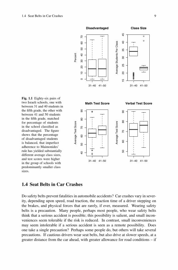
total absolute difference in percentage disadvantaged. Figure 1.1 shows the paired
schools, 86 schools with 31 and 40 students in fifth grade, and 86 schools with be-
tween 41 and 50 students in the fifth grade. After matching, the upper left panel
in Figure 1.1 shows that the percentage of disadvantaged students was balanced;
indeed, the average absolute difference within a pair was less than 1%. The upper
right panel in Figure 1.1 shows Maimonides’ rule at work: with some exceptions,
the slightly larger schools had substantially smaller class sizes. The bottom panels
of Figure 1.1 show the average mathematics and verbal test performance of these
fifth graders, with somewhat higher scores in the schools with between 41 and 50
fifth graders, where class sizes tended to be smaller.
1.4 Seat Belts in Car Crashes 9
Fig. 1.1 Eighty-six pairs oftwo Israeli schools, one withbetween 31 and 40 students inthe fifth grade, the other withbetween 41 and 50 studentsin the fifth grade, matchedfor percentage of studentsin the school classified asdisadvantaged. The figureshows that the percentageof disadvantaged studentsis balanced, that imperfectadherence to Maimonides’rule has yielded substantiallydifferent average class sizes,and test scores were higherin the group of schools withpredominantly smaller classsizes.
31−40 41−50
010
2030
4050
6070
Disadvantaged
Per
cent
●
●●
●●●
●●●●
●●●
●
●
●●
●●
●
●
31−40 41−50
1520
2530
3540
45
Class Size
Ave
rage
Stu
dent
s P
er C
lass
●●
●●
●●
31−40 41−50
4050
6070
8090
Math Test Score
Ave
rage
Tes
t Sco
re
31−40 41−50
5060
7080
90
Verbal Test Score
Ave
rage
Tes
t Sco
re
1.4 Seat Belts in Car Crashes
Do safety belts prevent fatalities in automobile accidents? Car crashes vary in sever-
ity, depending upon speed, road traction, the reaction time of a driver stepping on
the brakes, and physical forces that are rarely, if ever, measured. Wearing safety
belts is a precaution. Many people, perhaps most people, who wear safety belts
think that a serious accident is possible; this possibility is salient, and small incon-
veniences seem tolerable if the risk is reduced. In contrast, small inconveniences
may seem intolerable if a serious accident is seen as a remote possibility. Does
one take a single precaution? Perhaps some people do, but others will take several
precautions. If cautious drivers wear seat belts, but also drive at slower speeds, at a
greater distance from the car ahead, with greater allowance for road conditions – if

10 1 Dilemmas and Craftsmanship
Table 1.1 Crashes in FARS 1975–1983 in which the front seat had two occupants, a driver and apassenger, with one belted, the other unbelted, and one died and one survived.
Driver Not Belted BeltedPassenger Belted Not Belted
Driver Died Passenger Survived 189 153Driver Survived Passenger Died 111 363
risk-tolerant drivers do not wear seat belts, drive faster and closer, ignore road con-
ditions – then a simple comparison of belted and unbelted drivers may credit seat
belts with effects that reflect, in part, the severity of the crash.
Using data from the U.S. Fatal Accident Reporting System (FARS), Leonard
Evans [14] looked at crashes in which there were two individuals in the front seat,
one belted, the other unbelted, with at least one fatality. In these crashes, several
otherwise uncontrolled features are the same for driver and passenger: speed, road
traction, distance from the car ahead, reaction time. Admittedly, risk in the pas-
senger seat may differ from risk in the driver seat, but in this comparison there are
belted drivers with unbelted passengers and unbelted drivers with belted passengers,
so this issue may be examined. Table 1.1 is derived from Evans’ [14] more detailed
tables. In this table, when the passenger is belted and the driver is not, more often
than not, the driver dies; conversely, when the driver is belted and the passenger is
not, more often than not, the passenger dies.
Everyone in Table 1.1 is at least sixteen years of age. Nonetheless, the roles
of driver and passenger are connected to law and custom, for parents and children,
husbands and wives, and others. For this reason, Evans did further analyses, for
instance taking account of the ages of driver and passenger, with similar results.
Evans [14, page 239]wrote:
The crucial information for this study is provided by cars in which the safety belt use ofthe subject and other occupant differ . . . There is a strong tendency for safety belt use ornon-use to be the same for different occupants of the same vehicle . . . Hence, sample sizesin the really important cells are . . . small . . .
This study is discussed further in §5.2.6.
1.5 Money for College
To what extent, if any, does financial aid increase college attendance? It would not
do to simply compare those who received aid with those who did not. Decisions
about the allocation of financial aid are often made person by person, with consider-
ation of financial need and academic promise, together with many other factors. A
grant of financial aid is often a response to an application for aid, and the decision
to apply or not is likely to reflect an individual’s motivation for continued education
and competing immediate career prospects.
1.6 Nature’s ‘Natural Experiment’ 11
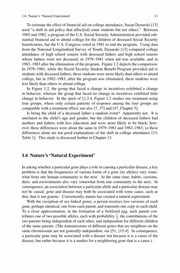
To estimate the effect of financial aid on college attendance, Susan Dynarski [13]
used “a shift in aid policy that affect[ed] some students but not others.” Between
1965 and 1982, a program of the U.S. Social Security Administration provided sub-
stantial financial aid to attend college for the children of deceased Social Security
beneficiaries, but the U.S. Congress voted in 1981 to end the program. Using data
from the National Longitudinal Survey of Youth, Dynarski [13] compared college
attendance of high school seniors with deceased fathers and high school seniors
whose fathers were not deceased, in 1979–1981 when aid was available, and in
1982–1983 after the elimination of the program. Figure 1.2 depicts the comparison.
In 1979–1981, while the Social Security Student Benefit Program provided aid to
students with deceased fathers, these students were more likely than others to attend
college, but in 1982–1983, after the program was eliminated, these students were
less likely than others to attend college.
In Figure 1.2, the group that faced a change in incentives exhibited a change
in behavior, whereas the group that faced no change in incentives exhibited little
change in behavior. In the spirit of §1.2.4, Figure 1.2 studies one treatment using
four groups, where only certain patterns of response among the four groups are
compatible with a treatment effect; see also [7, 37] and [47, Chapter 5].
Is being the child of a deceased father a random event? Apparently not. It is
unrelated to the child’s age and gender, but the children of deceased fathers had
mothers and fathers with less education and were more likely to be black; how-
ever, these differences were about the same in 1979–1981 and 1982–1983, so these
differences alone are not good explanations of the shift in college attendance [13,
Table 1]. This study is discussed further in Chapter 13.
1.6 Nature’s ‘Natural Experiment’
In asking whether a particular gene plays a role in causing a particular disease, a key
problem is that the frequencies of various forms of a gene (its alleles) vary some-
what from one human community to the next. At the same time, habits, customs,
diets, and environments also vary somewhat from one community to the next. In
consequence, an association between a particular allele and a particular disease may
not be causal: gene and disease may both be associated with some cause, such as
diet, that is not genetic. Conveniently, nature has created a natural experiment.
With the exception of sex-linked genes, a person receives two versions of each
gene, perhaps identical, one from each parent, and transmits one copy to each child.
To a close approximation, in the formation of a fertilized egg, each parent con-
tributes one of two possible alleles, each with probability 12 , the contributions of the
two parents being independent of each other, and independent for different children
of the same parents. (The transmissions of different genes that are neighbors on the
same chromosome are not generally independent; see [51, §15.4]. In consequence,
a particular gene may be associated with a disease not because it is a cause of the
disease, but rather because it is a marker for a neighboring gene that is a cause.)

12 1 Dilemmas and Craftsmanship
Several strategies use this observation to create natural experiments that study
genetic causes of a specific disease. Individuals with the disease are identified.
Richard Spielman, Ralph McGinnis, and Warren Ewens [49] used genetic informa-
tion on the diseased individual and both parents in their Transmission/Disequilibrium
Test (TDT). The test compares the diseased individuals to the known distributions
of alleles for the hypothetical children their parents could produce. David Curtis
[12], Richard Spielman and Warren Ewens [50], and Michael Boehnke and Carl
Langefeld [5] suggested using genetic information on the diseased individual and
one or more siblings from the same parents, which Spielman and Ewens called the
sib-TDT. If the disease has no genetic cause linked to the gene under study, then
the alleles from the diseased individual and her siblings should be exchangeable.
The idea underlying the sib-TDT is illustrated in Table 1.2, using data from
Boehnke and Langefeld [5, Table 5], their table being derived from work of Mar-
garet Pericak-Vance and Ann Saunders; see [44]. Table 1.2 gives the frequency
of the ε4 allele of the apolipoprotein E gene in 112 individuals with Alzheimer
disease and in an unaffected sibling of the same parents. Table 1.2 counts sib-
ling pairs, not individuals, so the total count in the table is 112 pairs of an af-
Fig. 1.2 College attendanceby age 23 in four groups:before (1979–1981) and af-ter (1982–1983) the end ofthe Social Security StudentBenefit Program for childrenwhose fathers were deceased(FD) or not deceased (FND).Values are proportions withstandard errors (se).
1979 1980 1981 1982 1983
0.3
0.4
0.5
0.6
Attending College by Age 23
Years: 1979−1981 vs 1982−1983
Pro
port
ion
Atte
ndin
g
FDFNDse

1.7 What This Book Is About 13
Table 1.2 Alzheimer disease and the apolipoprotein E ε4 allele in 112 sibling pairs, one withAlzheimer disease (affected), the other without (unaffected). The table counts pairs, not individ-uals. The rows and columns of the table indicate the number (0, 1, or 2) of ApoE alleles for theaffected and unaffected sibling.
Unaffected Sib# ApoEε4 Alleles 0 1 2
0 23 4 0Affected Sib 1 25 36 2
2 8 8 6
fected and an unaffected sibling. Each person can receive 0, 1, or 2 copies of
the ε4 allele from parents. For any one pair, write (aff,unaff) for the number of
ε4 alleles possessed by, respectively, the affected and unaffected sibling. In Ta-
ble 1.2, there are 25 pairs with (aff,unaff) = (1,0). If Alzheimer disease had no
genetic link with the apolipoprotein E ε4 allele, then nature’s natural experiment
implies that the chance that (aff,unaff) = (2,0), say, is the same as the chance that
(aff,unaff) = (0,2), and more generally, the chance that (aff,unaff) = (i, j) equals
the chance that (aff,unaff) = ( j, i), for i, j = 0,1,2. In fact, this does not appear
to be the case in Table 1.2. For instance, there are eight sibling pairs such that
(aff,unaff) = (2,0) and none such that (aff,unaff) = (0,2). Also, there are 25 pairs
such that (aff,unaff) = (1,0) and only 4 pairs such that (aff,unaff) = (0,1).A distribution with the property
Pr{(aff,unaff) = (i, j)} = Pr{(aff,unaff) = ( j, i)} for all i, j
is said to be exchangeable. In the absence of a genetic link with disease, na-
ture’s natural experiment ensures that the distribution of allele frequencies in af-
fected/unaffected sib pairs is exchangeable. This creates a test, the sib transmission
disequilibrium test [50] that is identical to a certain randomization test appropriate
in a randomized experiment [31].
1.7 What This Book Is About
Basic structure
Design of Observational Studies has four parts, ‘Beginnings,’ ‘Matching,’ ‘Design
Sensitivity,’ and ‘Planning Analysis,’ plus a brief summary. Part I, ‘Beginnings,’ is
a conceptual introduction to causal inference in observational studies. Chapters 2,
3, and 5 of Part I cover concisely, in about one hundred pages, many of the ideas
discussed in my book Observational Studies [38], but in a far less technical and less
general fashion. Parts II–IV cover material that, for the most part, has not previously
appeared in book form. Part II, ‘Matching,’ concerns the conceptual, practical, and
computational aspects of creating a matched comparison that balances many ob-

14 1 Dilemmas and Craftsmanship
served covariates. Because matching does not make use of outcome information,
it is part of the design of the study, what Cochran [9] called “setting up the com-
parisons”; that is, setting up the structure of the experimental analog. Even if the
matching in Part II is entirely successful, so that after matching, matched treated and
control groups are comparable with respect to all observed covariates, the question
or objection or challenge will inevitably be raised that subjects who look compa-
rable in observed data may not actually be comparable in terms of covariates that
were not measured. Chapters 3 and 5 and Parts III and IV address this central con-
cern. Part III, ‘Design Sensitivity,’ discusses a quantitative tool for appraising how
well competing designs (or data generating processes) resist such challenges. In
part, ‘Design Sensitivity’ will provide a formal appraisal of the design strategies
introduced informally in Chapter 5. Part IV discusses those activities that follow
matching but precede analysis, notably planning the analysis.
Structure of Part I: Beginnings
Observational studies are built to resemble simple experiments, and Chapter 2 re-
views the role that randomization plays in experiments. Chapter 2 also introduces
elements and notation shared by experiments and observational studies. Chapter
3 discusses two simple models for observational studies, one claiming that adjust-
ments for observed covariates suffice, the other engaging the possibility that they
do not. Chapter 3 introduces the propensity score and sensitivity analysis. Obser-
vational studies are built from three basic ingredients: opportunities, devices and
instruments. Chapter 5 introduces these ideas in an informal manner, with some of
the formalities developed in Part III and others developed in [38, Chapters 4, 6–9].
My impression is that many observational studies dissipate either by the absence
of a focused objective or by becoming mired in ornate analyses that may overwhelm
an audience but are unlikely to convince anyone. Neither problem is common in
randomized experiments, and both problems are avoidable in observational studies.
Chapter 4 discusses the first problem, while Chapter 6 discusses the second. In a
successful experiment or observational study, competing theories make conflicting
predictions; this is the concern of Chapter 4. Transparency means making evidence
evident, and Chapter 6 discusses how this is done.
Structure of Part II: Matching
Part II, entitled ‘Matching,’ is partly conceptual, partly algorithmic, partly data an-
alytic. Chapter 7 is introductory: it presents a matched comparison as it might (and
did) appear in a scientific journal. The basic tools of multivariate matching are de-
scribed and illustrated in Chapter 8, and various common practicalities are discussed
in Chapter 9. Later chapters in Part II discuss specific topics in matching, including
fine balance, matching with multiple groups or without groups, and risk-set match-
ing. Matching in the computer package R is discussed in Chapter 13.

1.7 What This Book Is About 15
Structure of Part III: Design Sensitivity
In Chapter 3, it is seen that some observational studies are sensitive to small unob-
served biases, whereas other studies are insensitive to quite large unobserved biases.
What features of the design of an observational study affect its sensitivity to bias
from covariates that were not measured? This is the focus of Part III.
Chapter 14 reviews the concept of power in a randomized experiment, then de-
fines the power of a sensitivity analysis. Design sensitivity is then defined. Design
sensitivity is a number that defines the sensitivity of an observational study design
to unmeasured biases when the sample size is large. Many factors affect the design
sensitivity, including the issues discussed informally in Chapter 5. Chapter 15 re-
vives a very old debate between John Stuart Mill and Sir Ronald Fisher about the
relevance to causal inference of the heterogeneity of experimental material. Mill
believed it mattered quite a bit; Fisher denied this. Sometimes a treatment has lit-
tle effect on most people and a dramatic effect on some people. In one sense, the
effect is small — on average it is small — but for a few people it is large. Is an
effect of this sort highly sensitive to unmeasured biases? Chapter 16 provides the
answer. Chapter 17 takes up themes from Chapter 5, specifically coherence and
dose-response, and evaluates their contribution to design sensitivity.
Structure of Part IV: Planning Analysis
The sample has been successfully matched — treated and control groups look com-
parable in terms of measured covariates — and Part IV turns to planning the analy-
sis. Chapter 18 concerns three emprical steps that aid planning the analysis: sample
splitting to improve design sensitivity, checking that analytical adjustments are fea-
sible, and thick description of a few matched pairs. After reviewing Fisher’s advice
— “make your theories elaborate” — Chapter 19 discusses planning the analysis of
an observational study.
A less technical introduction to observational studies
The mathematician Paul Halmos wrote two essays, “How to write mathematics” and
“How to talk mathematics.” In the latter, he suggested that in a good mathematical
talk, you don’t prove everything, but you do prove something to give the flavor of
proofs for the topic under discussion. In the spirit of that remark, ObservationalStudies [38] writes about statistics, where Design of Observational Studies talks
about statistics. This is done in several ways.
We often develop an understanding by taking something apart and putting it back
together. In statistics, this typically means looking at an unrealistically small ex-
ample in which it is possible to see the details of what goes on. For this reason,
I discuss several unrealistically small examples in parallel with real examples of
practical size. For instance, Chapter 2 discusses two versions of a paired random-

16 1 Dilemmas and Craftsmanship
ized experiment, one with five pairs, the other with 185 pairs. The five pairs are a
random sample from the 185 pairs. With 5 pairs, there are 25 = 32 possible treat-
ment assignments, and it is possible to see what is happening. With 185 pairs, there
are 2185 = 4.9× 1055 possible treatment assignments, and it is not possible to see
what is happening, although nothing new is happening beyond what you saw hap-
pening with five pairs. The larger experiment is just larger, somewhat awkward to
inspect, but no different conceptually. In a similar way, Chapter 7 discusses the
construction of 344 pairs matched for many covariates, while Chapter 8 discusses
the construction of 21 pairs matched for three covariates. With 21 pairs, you can
see what is happening, whereas with 344 pairs you cannot see as much, but nothing
new is happening.
Chapter 2 discusses a number of very old, very central concepts in statistics.
These include: the role of randomization in experiments, the nature of randomiza-
tion tests, obtaining confidence intervals by inverting hypothesis tests, building an
estimator using an estimating equation, and so on. This material is so old and central
to the subject that an article in a statistical journal might reduce the entire chapter
to a paragraph, and that would be fine for someone who had been around this track
a few times. My goal in Chapter 2 is not concise expression. My goal in Chapter 2
is to take you around this track a few times.
To prove something, not everything, I develop statistical theory only for the case
of matched pairs with continuous responses. The case of matched pairs is the sim-
plest nontrivial case. All of the important concepts appear in the case of matched
pairs, but most of the technical issues are easy. Randomization distributions for
matched pairs are little more than a series of independent coin flips. Everybody can
do coin flips. In a randomized experiment, the coin flips are fair, but in a sensitiv-
ity analysis, the coin flips may be biased. The matching methods in Part II are not
restricted to pair matching — matching with multiple controls, matching with vari-
able controls, full matching, risk set matching are all there — however, if you want
to work through the derivations of the associated statistical analyses for continuous,
discrete, censored, and multivariate responses, you will need to turn to [38] or the
references discussed in ‘Further Reading.’
Focusing the theoretical presentation on matched pairs permits discussion of key
concepts with the minimum of mathematics. Unlike statistical analysis, research de-
sign yields decisions rather than calculations — decisions to ask certain questions,
in certain settings, collecting certain data, adding certain design elements, attending
to certain patterns — and for such decisions, the concepts are more important than
details of general computations. What is being left out by focusing on matched
pairs? For one thing, sensitivity analyses in other cases are easy to do but require
more mathematical machinery to justify. Some of this machinery is aesthetically
pleasing, for instance exact results using Holley’s inequality [1, 6, 25] in I. R. Sav-
age’s [45] finite distributive lattice of rank orders or samples; see [35, 36] and [38,
§4]. Some of this machinery uses large sample approximations or asymptotics that
work easily and well even in small samples, but discussion of these approximations
means a step up in the level of technical detail; see [16] and [38, §4]. To get a
feeling for the difference between the paired case and other cases, see [39], where

1.7 What This Book Is About 17
both cases are discussed in parallel, one right after the other. If you need to do a
sensitivity analysis for a situation other than matched pairs, see [38, §4] or other
references in Further Reading. Another item that is left out of the current discus-
sion is a formal notation and model for multiple groups, as opposed to a treated and
a control group; see [38, §8] for such a notation and model. Such a model adds
more subscripts and symbols with few additional concepts. The absence of such a
notation and model has a small effect on the discussion of multiple control groups
(§5.2.2), differential effects (§5.2.6), the presentation of the matching session in Rfor a difference-in-differences example in Chapter 13, and the planned analysis with
two control groups (§19.3); specifically, these topics are described informally with
reference to the literature for formal results.
Dependence among chapters
Design of Observational Studies is highly modular, so it is not necessary to read
chapters in order. Part II may be read before or after Part I or not at all; Part II is
not needed for Parts III and IV. Part III may be read before or after Part IV.
In Part I, Chapter 5 depends on Chapter 3, which in turn depends on Chapter 2.
The beginning of Chapter 2, up through §2.4.3, is needed for Chapters 3 and 5, but
§2.5 is not essential except for Chapter 16, and the remainder of Chapter 2 is not
used later in the book. Chapters 4 and 6 may be read at any time or not at all.
In Part II, most chapters depend strongly on Chapter 8 but only weakly on each
other. Read the introductory Chapter 7 and Chapter 8; then, read what you like in
Part II.
The situation is similar in Part III. All of the chapters of Part III depend upon
Chapter 14, which in turn depends on Chapter 5. The remaining chapters of Part III
may be read in any order or not at all.
The two chapters in Part IV may be read out of sequence, and both depend upon
Chapter 5.
At the back of the book, there is a list of symbols and a glossary of statistical
terms. In the index, a bold page number locates the definition of a technical term
or symbol.
Some books (e.g., [38]) contain practice problems for you to solve. My sense
is that the investigator planning an observational study has problems enough, so
instead of further problems, at the back of the book there is a list of solutions.
As a scholar at a research university, I fall victim to periodic compulsions to make
remarks that are largely unintelligible and totally unnecessary. These remarks are
found in appendices and footnotes. Under no circumstances read them. If you read
a footnote, you will suffer a fate worse than Lot’s wife.1
1 She turned into a pillar of salt when she looked where her husband instructed her not to look.Opposed to the story of Lot and his wife is the remark of Immanuel Kant: “Sapere aude” (Dare toknow) [27, page 17]. You are, by the way, off to a bad start with these footnotes.

18 1 Dilemmas and Craftsmanship
1.8 Further Reading
One might reasonably say that the distinction between randomized experiments and
observational studies was introduced by Sir Ronald Fisher’s [15] invention of ran-
domized experimentation. Fisher’s book [15] of 1935 is of continuing interest. As
noted in §1.2, William Cochran [9] argued that observational studies should be un-
derstood in relation to experiments; see also the important paper in this spirit by
Donald Rubin [41]. A modern discussion of quasi-experiments is given by William
Shadish, Thomas Cook , and Donald Campbell [47], and Campbell’s [8] collected
papers are of continuing interest. See also [17, 33, 54]. Natural experiments in
medicine are discussed by Jan Vandenbroucke [53] and the report edited by Michael
Rutter [43], and in economics by Joshua Angrist and Alan Kruger [2], Timothy
Besley and Anne Case [4], Daniel Hamermesh [19], Bruce Meyer [33], and Mark
Rosenzweig and Kenneth Wolpin [40]. Natural experiments are prominent also in
recent developments in genetic epidemiology [5, 12, 31, 49, 50]. The papers by Jerry
Cornfield and colleagues [11], Austin Bradford Hill [23] , and Mervyn Susser [52]
remain highly influential in epidemiology and are of continuing interest. Miguel
Hernan and colleagues [22] illustrate the practical importance of adhering to the
experimental template in designing an observational study. For a general discussion
of observational studies, see [38].
References
1. Anderson, I.: Combinatories of Finite Sets. New York: Oxford University Press (1987)2. Angrist, J.D., Krueger, A.B.: Empirical strategies in labor economics. In: Ashenfelter, O.,
Card, D. (eds.) Handbook of Labor Economics, Volume 3, pp. 1277–1366. New York: Else-vier (1999)
3. Angrist, J.D., Lavy, V.: Using Maimonides’ rule to estimate the effect of class size on scholas-tic achievement. Q J Econ 114, 533–575 (1999)
4. Besley, T., Case, A.: Unnatural experiments? Estimating the incidence of endogenous poli-cies. Econ J 110, 672–694 (2000)
5. Boehnke, M., Langefeld, C.D.: Genetic association mapping based on discordant sib pairs:The discordant alleles test. Am J Hum Genet 62, 950–961 (1998)
6. Bollobas, B.: Combinatorics. New York: Cambridge University Press (1986)7. Campbell, D.T.: Factors relevant to the validity of experiments in social settings. Psychol Bull
54, 297–312 (1957)8. Campbell, D.T.: Methodology and Epistemology for Social Science: Selected Papers.
Chicago: University of Chicago Press (1988)9. Cochran, W.G.: The planning of observational studies of human populations (with Discus-
sion). J Roy Statist Soc A 128, 234–265 (1965)10. Cook, T.D., Shadish, W.R.: Social experiments: Some developments over the past fifteen
years. Annu Rev Psychol 45, 545–580 (1994)11. Cornfield, J., Haenszel, W., Hammond, E., Lilienfeld, A., Shimkin, M., Wynder, E.: Smoking
and lung cancer: Recent evidence and a discussion of some questions. J Natl Cancer Inst 22,173–203 (1959)
12. Curtis, D.: Use of siblings as controls in case-control association studies. Ann Hum Genet 61,319–333 (1997)

References 19
13. Dynarski, S.M.: Does aid matter? Measuring the effect of student aid on college attendanceand completion. Am Econ Rev 93, 279–288 (2003)
14. Evans, L.: The effectiveness of safety belts in preventing fatalities. Accid Anal Prev 18, 229–241 (1986)
15. Fisher, R.A.: Design of Experiments. Edinburgh: Oliver and Boyd (1935)16. Gastwirth, J.L., Krieger, A.M., Rosenbaum, P.R.: Asymptotic separability in sensitivity anal-
ysis. J Roy Statist Soc B 62, 545–555 (2000)17. Greenstone, M., Gayer, T.: Quasi-experimental and experimental approaches to environmental
economics. J Environ Econ Manag 57, 21–44 (2009)18. Greevy, R., Silber, J.H., Cnaan, A., Rosenbaum, P.R.: Randomization inference with imper-
fect compliance in the ACE-inhibitor after anthracycline randomized trial. J Am Statist Assoc99, 7–15 (2004)
19. Hamermesh, D.S.: The craft of labormetrics. Indust Labor Relat Rev 53, 363–380 (2000)20. Heart Protection Study Collaborative Group.: MRC/BHF Heart Protection Study of an-
tioxidant vitamin supplementation in 20,536 high-risk individuals: A randomised placebo-controlled trial. Lancet 360, 23–33 (2002)
21. Heckman, J.J.: Micro data, heterogeneity, and the evaluation of public policy: Nobel lecture.J Polit Econ 109, 673–748 (2001)
22. Hernan, M.A., Alonso, A., Logan, R., Grodstein, F., Michels, K.B., Willett, W.C., Manson,J.E., Robins, J.M.: Observational studies analyzed like randomized experiments: an ap-plication to postmenopausal hormone therapy and coronary heart disease (with Discussion).Epidemiology 19,766–793 (2008)
23. Hill, A.B.: The environment and disease: Association or causation? Proc Roy Soc Med 58,295–300 (1965)
24. Holland, P.W.: Statistics and causal inference. J Am Statist Assoc 81, 945–960 (1986)25. Holley, R.: Remarks on the FKG inequalities. Comm Math Phys 36, 227–231 (1974)26. Imbens, G.W., Wooldridge, J.M.: Recent developments in the econometrics of program eval-
uation. J Econ Lit 47, 5–86 (2009)27. Kant, I.: What is enlightenment? In: I. Kant, Toward Perpetual Peace and Other Writings.
New Haven, CT: Yale University Press (1785, 2006)28. Katan, M.B.: Apolipoprotein E isoforms, serum cholesterol, and cancer. Lancet 1, 507–508
(1986) Reprinted: Int J Epidemiol 33, 9 (2004)29. Katan, M.B.: Commentary: Mendelian randomization, 18 years on. Int J Epidemiol 33, 10–11
(2004)30. Khaw, K.T., Bingham, S., Welch, A., Luben, R., Wareham, N., Oakes, S., Day, N.: Relation
between plasma ascorbic acid and mortality in men and women in EPIC-Norfolk prospectivestudy. Lancet 357, 657–663 (2001)
31. Laird, N.M., Blacker, D., Wilcox, M.: The sib transmission/disequilibrium test is a Mantel-Haenszel test. Am J Hum Genet 63, 1915 (1998)
32. Lawlor, D.A., Smith, G.D., Bruckdorfer, K.R., Kundo, D., Ebrahim, S.: Those confoundedvitamins: What can we learn from the differences between observational versus randomizedtrial evidence? Lancet 363, 1724–1727 (2004)
33. Meyer, B.D.: Natural and quasi-experiments in economics. J Business Econ Statist 13, 151–161 (1995)
34. Rosenbaum, P.R.: The consequences of adjustment for a concomitant variable that has beenaffected by the treatment. J Roy Statist Soc A 147, 656–666 (1984)
35. Rosenbaum, P.R.: On permutation tests for hidden biases in observational studies: An appli-cation of Holley’s inequality to the Savage lattice. Ann Statist 17, 643–653 (1989)
36. Rosenbaum, P.R.: Quantiles in nonrandom samples and observational studies. J Am StatistAssoc 90, 1424–1431 (1995)
37. Rosenbaum, P.R.: Stability in the absence of treatment. J Am Statist Assoc 96, 210–219(2001)
38. Rosenbaum, P.R.: Observational Studies (2nd ed.). New York: Springer (2002)39. Rosenbaum, P.R.: Sensitivity analysis for m-estimates, tests, and confidence intervals in
matched observational studies. Biometrics 63, 456–464 (2007)

20 1 Dilemmas and Craftsmanship
40. Rosenzweig, M.R., Wolpin, K.I.: Natural ‘natural experiments’ in economics. J Econ Lit 38,827–874 (2000)
41. Rubin, D.B.: Estimating causal effects of treatments in randomized and nonrandomized stud-ies. J Educ Psychol 66, 688–701 (1974)
42. Rubin, D.B.: The design versus the analysis of observational studies for causal effects: Paral-lels with the design of randomized trials. Statist Med 26, 20–36 (2007)
43. Rutter, M.: Identifying the Environmental Causes of Disease: How Do We Decide What toBelieve and When to Take Action? London: Academy of Medical Sciences (2007)
44. Saunders, A.M., Strittmatter, W.J., Schmechel, D., et al.: Association of apolipoprotein E al-lele epsilon 4 with late-onset familial and sporadic Alzheimer’s disease. Neurology 43, 1467–1472 (1993)
45. Savage, I.R.: Contributions to the theory of rank order statistics: Applications of lattice theory.Rev Int Statist Inst 32, 52–63 (1964)
46. Sekhon, J.S.: Opiates for the matches: Matching methods for causal inference. Annu Rev PolSci 12, 487-508 (2009)
47. Shadish, W. R., Cook, T. D., Campbell, D.T.: Experimental and Quasi-Experimental Designsfor Generalized Causal Inference. Boston: Houghton-Mifflin (2002)
48. Shadish, W. R., Cook, T. D.: The renaissance of field experimentation in evaluating interven-tions. Annu Rev Psychol 60, 607–629 (2009)
49. Spielman, R.S., McGinnis, R.E., Ewens, W.J.: Transmission test for linkage disequilibrium.Am J Hum Genet 52, 506–516 (1993)
50. Spielman, R.S., Ewens, W.J.: A sibship test for linkage in the presence of association: The sibtransmission/disequilibrium test. Am J Hum Genet 62, 450–458 (1998)
51. Strachan, T., Read, A.P.: Human Molecular Genetics. New York: Garland (2004)52. Susser, M.: Epidemiology, Health and Society: Selected Papers. New York: Oxford Univer-
sity Press (1987)53. Vandenbroucke, J.P.: When are observational studies as credible as randomized trials? Lancet
363, 1728–1731 (2004)54. West, S.G., Duan, N., Pequegnat, W., Gaist, P., Des Jarlais, D.C., Holtgrave, D., Szapocznik, J.,
Fishbein, M., Rapkin, B., Clatts, M., Mullen, P.D.: Alternatives to the randomized controlledtrial. Am J Public Health 98, 1359–1366 (2008)

Chapter 2Causal Inference in Randomized Experiments
Abstract An observational study is an empiric investigation of treatment effects
when random assignment to treatment or control is not feasible. Because observa-
tional studies are structured to resemble simple randomized experiments, an under-
standing of the role randomization plays in experiments is important as background.
As a prelude to the discussion of observational studies in later chapters, the current
chapter contains a brief review of the logic of causal inference in a randomized ex-
periment. Only one simple case is discussed in detail, namely a randomized paired
experiment in which subjects are paired before randomization and one subject in
each pair is picked at random to receive treatment, the other receiving control. Al-
though a foundation for later chapters, much of the material in this chapter is quite
old, dating from Sir Ronald Fisher’s work in the 1920s and 1930s, and it is likely to
be familiar from other contexts, such as a course in the design of experiments.
2.1 Two Versions of the National Supported Work Experiment
2.1.1 A version with 185 pairs and a version with 5 pairs
Though discussed daily in the newspaper, unemployment is a curious phenomenon.
Defined abstractly, it implies that someone entered an active labor market intending
to sell their labor but was unable to find a buyer, often for long periods of time. Of
course, the abstract definition leaves out most of what is happening.
Robert LaLonde [30] reviews several decades of
public sector sponsored employment and training programs . . . [intended to] enhance par-ticipants’ productive skills and, in turn, increase their future earnings and tax payments andreduce their dependence on social welfare benefits. [. . . The] primary recipients of publicsector sponsored training [have been] economically disadvantaged or dislocated workers.[30, page 149]
21P.R. Rosenbaum, Design of Observational Studies, Springer Series in Statistics, DOI 10.1007/978-1-4419-1213-8_2, © Springer Science+Business Media, LLC 2010
22 2 Causal Inference in Randomized Experiments
The National Supported Work Demonstration (NSW) included a randomized ex-
periment evaluating the effects of one such program [7, 24]. Kenneth Couch writes:
The NSW provided work experiences primarily in service occupations for females and con-struction for males. The jobs were designed to be consistent with a concept known asgraduated stress. Stress within the working environment increased gradually during thetraining period until it simulated the workplace norms of the private sector. At that point,not more than 18 month after entry, individuals who received services provided by the NSWhad to attempt a transition to unsubsidized employment. Screening criteria for the NSWlimited participation to individuals severely handicapped in the labor market. . . . Afterscreening by a local social service agency and referral into the program, each participantwas randomly assigned to a treatment (experimental) or control group. Treatments receivedthe services offered by the NSW. Controls continued enrollment in other available socialprograms [7, pages 381–382].
The current chapter will use pieces of the NSW experiment to illustrate the logic
of randomized experimentation. A reader interested not in randomized experimen-
tation but rather in the full NSW program and its effects might begin with Couch’s
[7] study of the program’s long term effects. The NSW became important in think-
ing about methodology for observational studies in economics because of a series
of studies [12, 19, 29, 57], beginning with LaLonde’s 1986 study [29], in which
the randomized control group was set aside and various analytical methods were
applied to nonrandomized controls from survey data.
Because the goal is to discuss the logic of randomized experiments in a manner
that prepares for the discussion of observational studies in later chapters, several ad-
justments and simplifications were made. First, the data set is what Rajeev Dehejia
and Sadek Wahba [12, Table 1] call the “RE74 subset,” which in turn is a subset
of the data used by LaLonde [29]. The subset consists of males who were ran-
domized to treatment or control after December 1975 and who had left the program
before January 1978, with annual earnings recorded in 1974, 1975 and 1978. Be-
cause of these requirements, earnings in 1974 and 1975 are pretreatment covariates
unaffected by the NSW program, and earnings in 1978 is an outcome that may be af-
fected by treatment. Furthermore, to emphasize the parallel with matched observa-
tional studies, the randomized treated and control groups were matched: specifically,
all 185 treated men were matched to 185 untreated controls using eight covariates,
forming 185 matched pairs. 1
For the 185 matched pairs, Table 2.1 shows the distribution of the eight covari-
ates. Before treatment, the treated and control groups looked fairly similar.
1 As mentioned in Chapter 1, to keep the theoretical technicalities to a minimum, statistical theoryis developed only for the case of matched pairs, so I have slightly reshaped the NSW experimentinto a matched pair study. Randomization inference for unmatched randomized experiments issimilar and is discussed in [44, Chapter 2]. The matching used precisely the methods describedlater in §8.4, using a penalty function to implement calipers on the propensity score, with the rank-based Mahalanobis distance used within calipers. Multivariate matching before randomizationcan improve the efficiency of a randomized experiment; see [17]. For illustration only in thisexpository chapter, the matching is done after random assignment, which entails discarding someof the randomized controls, something I would not do if the goal were to perform the most efficientanalysis of the NSW experiment.

2.1 Two Versions of the National Supported Work Experiment 23
Table 2.1 Pretreatment covariates for 185 matched pairs from the NSW randomized experiment.For age and years of education, means, median (50%) and quartiles (25% and 75%) are given. Forearnings, the mean of all earnings (including zero earnings) and the percentage of zero earningsare given. For binary variables, the percentage is given.
Covariate Group Mean 25% 50% 75%
Age Treated 25.82 20 25 29Control 25.70 20 25 29
Years of Treated 10.35 9 11 12Education Control 10.19 9 10 11
Covariate Group Mean Percent $0
Earnings in $ Treated 2096 71%in 1974 Control 2009 75%
Earnings in $ Treated 1532 60%in 1975 Control 1485 64%
Covariate Group Percent
Black Treated 84%Control 85%
Hispanic Treated 6%Control 5%
Married Treated 19%Control 20%
No High School Treated 71%Degree Control 77%
Figure 2.1 displays the earnings in 1978 after treatment for the 185 matched pairs
of men. In the boxplot of 185 matched pair differences, the dotted lines are at 0 and
±5000. It appears that treated men earned somewhat more.
In general, in this book, I will use small examples to illustrate the details of what
goes on, and examples of practical size to illustrate analysis and interpretation. In
that spirit, Table 2.2 is a random sample of five of the 185 pairs; it will be used to
illustrate the details of randomization inference. The sample happens to consist of
pairs 15, 37, 46, 151, and 181 of the 185 pairs.
2.1.2 Basic notation
Table 2.2 exemplifies notation that will be used throughout the book. The index
of the pair is i, i = 1,2, . . . ,5 = I, and the index of the person in the pair is j, j =1,2. In Table 2.2 and throughout the book, Z indicates treatment, Z = 1 for treated,
Z = 0 for control, x is an observed covariate — there are eight covariates, xi jk, k =1, . . . ,8 = K, in Table 2.2 — and R indicates a response, in this case, earnings after
the end of treatment in 1978. The first pair in Table 2.2 consists of two unmarried,
young black men with seven or eight years of education and no earnings in 1974
and 1975, before the start of treatment; after treatment, in 1978, the treated man
earned more. The treated-minus-control matched pair difference in 1978 earnings

24 2 Causal Inference in Randomized Experiments
●●
●
●
●
●
●●
Treated Control
010
000
3000
050
000
1978 Earnings
1978
Ear
ning
s
●
●
●●
●
●
●
−20
000
010
000
3000
050
000
Treated−Control Difference
Diff
eren
ce in
197
8 E
arni
ngs
Fig. 2.1 Earnings in 1978, after treatment, for 185 pairs of men in the NSW randomized experi-ment. The dotted lines are at −$5000, $0, and $5000.
Table 2.2 Five pairs sampled at random from the 185 pairs in the NSW randomized experiment.The variables are: id = pair number among the 185 pairs; pairs 1 to 5; person 1 or 2 in a pair; treat=1if treated, 0 if control; age in years; edu=education in years; black=1 if black, 0 otherwise; hisp=1if hispanic, 0 otherwise; married=1 if married, 0 otherwise; no degree=1 if no high school degree, 0otherwise; and re74, re75, and re78 are earnings in dollars in 1974, 1975, and 1978. Also, in pair i,Yi is the treated-minus-control matched pair difference in 1978 earnings, Yi = (Zi1−Zi2)(Ri1−Ri2).
treat age edu black hisp married nodegree re74 re75 re78id i j Zi j xi j1 xi j2 xi j3 xi j4 xi j5 xi j6 xi j7 xi j8 Ri j Yi15 1 1 1 17 7 1 0 0 1 0 0 3024 145615 1 2 0 18 8 1 0 0 1 0 0 1568
37 2 1 1 25 5 1 0 0 1 0 0 6182 398837 2 2 0 24 7 1 0 0 1 0 0 2194
46 3 1 1 25 11 1 0 1 1 0 0 0 −4546 3 2 0 25 11 1 0 1 1 0 0 45
151 4 1 1 28 10 1 0 0 1 0 2837 3197 −2147151 4 2 0 22 10 1 0 0 1 0 2175 5344
181 5 1 1 33 12 1 0 1 0 20280 10941 15953 3173181 5 2 0 28 12 1 0 1 0 10585 5551 12780
is Yi = (Zi1 −Zi2)(Ri1 −Ri2), so Y1 = (1−0)(3024−1568) = $1456 for the first
pair of men.
It is convenient to have a symbol that represents the K covariates together, and
vector notation does this, so xi j =(xi j1, . . . ,xi jK
)Tcontains the K covariate values
for the jth person or unit in the ith pair. If you are not familiar with vector notation,
it will not be a problem here. Vectors and vector notation have many uses, but for
2.2 Treatment Effects in Randomized Experiments 25
the most part, in the current book they are used simply to give concise names to
arrays of data. For instance, in Table 2.2, x11 = (17,7,1,0,0,1,0,0)T contains the
covariate values for the first man in the first pair.
In the same way, Z indicates the treatment assignments for all 2I subjects in
the I matched pairs, Z = (Z11,Z12,Z21, . . . ,ZI2)T . For the I = 5 pairs in Table 2.2,
Z = (1,0,1,0,1,0,1,0,1,0)T . The notation is slightly redundant, because Zi2 =1−Zi1, so that, now and then, when compact expression is needed, only the Zi1’s
are mentioned. Also, R = (R11,R12, . . . ,RI2)T and Y = (Y1,Y2, . . . ,YI)
T .
It is possible to match for observed covariates, but not for a covariate that was not
observed. There is an important sense in which a failure to match or control for an
unobserved covariate presents no special problem in a randomized experiment but
can present substantial problems in an observational study. Clarification of this dis-
tinction is one goal of the current chapter. For this purpose, it is convenient to give
a name, ui j, to the unobserved covariate. In the current chapter, which is focused
on inference in randomized experiments, ui j could be any unmeasured covariate (or
any vector containing several unmeasured covariates). Success in finding and keep-
ing a job may depend on aspects of personality, intelligence, family and personal
connections, and physical appearance; then, in this chapter in connection with the
NSW experiment, ui j could be a vector of measurements of these attributes, a vector
that was not measured by the investigators. Also, u = (u11,u12, . . . ,uI2)T .
To aid in reading the table, subject j = 1 is always the treated subject and subject
j = 2 is always the control subject; however, strictly speaking, one should not do
this. Strictly speaking, i j is the ‘name’ of a unique person; that person had his name,
i j, before treatments were randomly assigned. In a paired randomized experiment,
Zi1 is determined by I independent flips of a fair coin, so Z11 = 1 happens with
probability 12 and Z11 = 0 happens with probability 1
2 ; then Zi2 = 1−Zi1. That is, in
Table 2.2, Zi1 is 1 and Zi2 is 0 for every i, but this would happen by chance in a paired
randomized experiment with I = 5 pairs with probability(
12
)5 = 132 = 0.03125.
Strictly speaking, some of the Zi1’s should be 1 and some of the Zi2’s should be 1.
Quantities in statistical computations, such as the treated-minus-control difference
in responses, Yi = (Zi1 −Zi2)(Ri1 −Ri2), are unaffected by the ordering of the table.
So there is a small inconsistency between the logic of random assignment and the
form of a readable table. Having mentioned this once, I will adhere to the logic of
random assignment in theoretical discussions, present tables in readable form, and
ignore the small inconsistency.
2.2 Treatment Effects in Randomized Experiments
2.2.1 Potential responses under alternative treatments
In Table 2.2, the first man, (i, j) = (1,1), was randomly assigned to treatment,
Z11 = 1, and had earnings of R11 = $3024 in 1978, but things might have been

26 2 Causal Inference in Randomized Experiments
different. Had the coin fallen differently, the first man, (i, j) = (1,1), might have
been randomly assigned to control, Z11 = 0, and in this case his earnings in 1978
might have been different. We will never know what this first man’s earnings would
have been had the coin fallen differently, had he been assigned to control. Perhaps
the treatment was completely ineffective, and perhaps this first man would have held
the same job, with the same earnings, namely $3024, had he been assigned to con-
trol. Or perhaps the treatment raised his earnings, and his earnings under control
would have been lower. We will never know about this one man, but with 370 men
in 185 pairs, half randomly assigned to treatment, the others to control, we can say
something about what would have happened to the 370 men under treatment and
under control.
Not only the first man but each man (i, j) has two potential responses, a level
of earnings he would exhibit in 1978 if assigned to treatment, rTi j, and a level of
earnings he would exhibit in 1978 if assigned to control, rCi j. We see one of these.
Specifically, if (i, j) were assigned to treatment, Zi j = 1, we would see rTi j, but if
(i, j) were assigned to control, Zi j = 0, we would see rCi j. The response, Ri j, we
actually observe from (i, j) — that is, the 1978 earnings actually recorded in Table
2.2 — equal rTi j if Zi j = 1 or rCi j if Zi j = 0; that is, in a formula, Ri j = Zi j rTi j +(1−Zi j) rCi j. Also, rT = (rT 11,rT 12, . . . ,rT I2)
T and rC = (rC11,rC12, . . . ,rCI2)T .
To say that the treatment has no effect on this response from (i, j) is to say rCi j =rTi j. To say that the treatment caused (i, j)’s earnings to increase by $1000 is to
say rTi j = rCi j + 1000 or rTi j − rCi j = 1000. We will never be in a position to
confidently assert either of these things about a single man. It is, however, a very
different thing to assert that all 370 men were unaffected by the treatment — to
assert that rCi j = rTi j for i = 1,2, . . .185, j = 1,2; in a randomized experiment, we
may be in a position to confidently deny that. The hypothesis that the treatment had
no effect on anyone, namely H0 : rCi j = rTi j for i = 1,2, . . .185, j = 1,2, is known
as Ronald Fisher’s [13] sharp null hypothesis of no effect. This hypothesis may be
written compactly as H0 : rT = rC.
The notation that expresses treatment effects as comparisons of potential re-
sponses under alternative treatments was introduced into the design of experiments
by Jerzy Neyman [35] in 1923 and was used to solve various problems in random-
ized experiments; e.g., [62, 64, 9, 40] and [28, § 8.3]. Donald Rubin [50] first
advocated use of this notation in observational studies.
2.2.2 Covariates and outcomes
In §1.2, the distinction between covariates and outcomes was emphasized. A co-
variate, such as xi j or ui j, is a pretreatment quantity, so there is only one version
of a covariate. A response or outcome has two potential values,(rTi j, rCi j
), one of
which is observed, namely Ri j, depending upon the treatment assignment Zi j, that
is, Ri j = Zi j rTi j +(1−Zi j) rCi j.

2.2 Treatment Effects in Randomized Experiments 27
Notice that(rTi j, rCi j, xi j, ui j
)do not change when treatments are assigned at
random, that is, when Zi j is determined by a coin flip or a random number, but in
general the observed response, Ri j, does change. It is convenient to have a symbol
that represents the quantities that are not changed when treatments are randomized.
Let F denote the array of quantities{(
rTi j, rCi j, xi j, ui j), i = 1,2, . . . , I, j = 1,2
}that do not change when Zi j is determined. (These quantities are fixed in Fisher’s
theory of randomization inference; hence, the symbol is F .)
2.2.3 Possible treatment assignments and randomization
The observed treatment assignment in Table 2.2 is Z = (1,0,1,0,1,0,1,0,1,0)T ,
but random assignment of treatments within pairs might have picked a different
assignment. Write Z for the set of the 2I possible values of Z; that is, z ∈Z if and
only if z = (z11,z12, . . . ,zI2)T with zi j = 0 or zi j = 1 and zi1 +zi2 = 1 for each i, j. For
Table 2.2, there are 2I = 25 = 32 possible values z ∈ Z . Generally, if A is a finite
set, then |A| is the number of elements of A, so that, in particular, |Z | = 2I . Table
2.3 lists, in abbreviated form, the 32 possible treatment assignments for Table 2.2;
the abbreviation consists in listing zi1 but not zi2 because zi2 = 1−zi1. The observed
treatment assignment, Z = (1,0,1,0,1,0,1,0,1,0)T in Table 2.2, corresponds with
the first row of Table 2.3. In the second row of Table 2.3, the treatment assignment
for the fifth pair in Table 2.2 has been reversed, so the second man, not the first man,
in that pair is assigned to treatment.
For the I = 185 pairs in Table 2.1, the set Z of possible treatment assignments
contains 2I = 2185 .= 4.9× 1055 possible treatment assignments, z ∈ Z . It would
be inconvenient to list them.
What does it mean to randomly assign treatments? At an intuitive level, one as-
signment z ∈ Z is picked at random, each having probability 2−I , or 2−5 = 132 =
0.03125 for Table 2.3. For instance, one might flip a fair coin independently five
times to determine Z in Table 2.3. The intuition is that randomization is making a
statement about how Z alone was determined, that is, about the marginal distribu-
tion of Z. This intuition is not quite correct; in an important way, randomization
means more than this. Specifically, in a randomized experiment, the information
in(rTi j, rCi j, xi j, ui j
)(or in F ) is of no use in predicting Zi j. That is, the coin is
fair not just in coming up heads half the time, independently in different pairs, but
more importantly the coin knows nothing about the individual and is impartial in
its treatment assignments. The design of the paired randomized experiment forces
Z to fall in Z — that is, it forces the event Z ∈ Z to occur — which is denoted
concisely by saying the event Z occurs. Randomization in the paired randomized
experiment means:
Pr(Z = z |F ,Z ) =1
|Z | =1
2I for each z ∈ Z . (2.1)
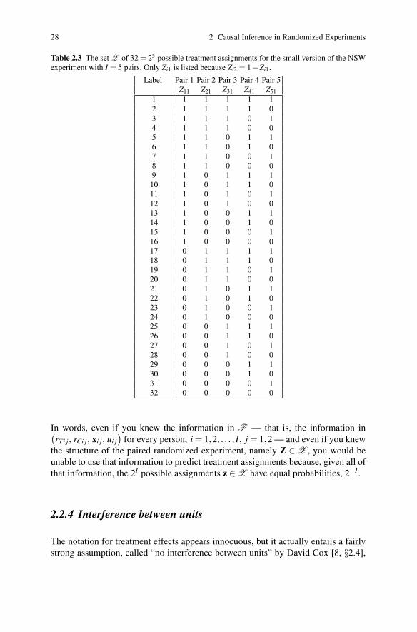
28 2 Causal Inference in Randomized Experiments
Table 2.3 The set Z of 32 = 25 possible treatment assignments for the small version of the NSWexperiment with I = 5 pairs. Only Zi1 is listed because Zi2 = 1−Zi1.
Label Pair 1 Pair 2 Pair 3 Pair 4 Pair 5Z11 Z21 Z31 Z41 Z51
1 1 1 1 1 12 1 1 1 1 03 1 1 1 0 14 1 1 1 0 05 1 1 0 1 16 1 1 0 1 07 1 1 0 0 18 1 1 0 0 09 1 0 1 1 1
10 1 0 1 1 011 1 0 1 0 112 1 0 1 0 013 1 0 0 1 114 1 0 0 1 015 1 0 0 0 116 1 0 0 0 017 0 1 1 1 118 0 1 1 1 019 0 1 1 0 120 0 1 1 0 021 0 1 0 1 122 0 1 0 1 023 0 1 0 0 124 0 1 0 0 025 0 0 1 1 126 0 0 1 1 027 0 0 1 0 128 0 0 1 0 029 0 0 0 1 130 0 0 0 1 031 0 0 0 0 132 0 0 0 0 0
In words, even if you knew the information in F — that is, the information in(rTi j, rCi j, xi j, ui j
)for every person, i = 1,2, . . . , I, j = 1,2 — and even if you knew
the structure of the paired randomized experiment, namely Z ∈ Z , you would be
unable to use that information to predict treatment assignments because, given all of
that information, the 2I possible assignments z ∈ Z have equal probabilities, 2−I .
2.2.4 Interference between units
The notation for treatment effects appears innocuous, but it actually entails a fairly
strong assumption, called “no interference between units” by David Cox [8, §2.4],

2.3 Testing the Null Hypothesis of No Treatment Effect 29
namely “that the observation on one unit should be unaffected by particular assign-
ment of treatments to other units.” There would be interference between units in
Table 2.2 if switching man (i, j) = (2,1) — i.e., the first man in the second pair —
from treatment to control would affect the earnings of the man we discussed be-
fore, (i, j) = (1,1), that is, the first man in the first pair. Interference is probably not
widespread in the NSW experiment, but it cannot be entirely ruled out. For instance,
a potential employer might hire two subsidized workers under NSW, but retain for
unsubsidized permanent employment only the better of the two employees. In this
case, switching the treatment for one man might cause another man to gain or lose a
job. The two-outcomes notation makes no provision for interference between units;
each unit or man has only two potential responses depending exclusively on his own
treatment assignment. If there were interference between units, the response of each
man would depend upon all of the treatment assignments, (Z11,Z12, . . . ,ZI2). In Ta-
ble 2.2, there are two ways to assign treatments in each of five pairs, so there are
32 = 25 possible treatment assignments. If there were interference between units,
each man would have not two potential responses but 32 potential responses, de-
pending upon all of the treatment assignments, (Z11,Z12, . . . ,Z52).Interference between units is likely to be very limited in the NSW experiment
because most men don’t interfere with each other. The situation is different when
the same person is studied repeatedly under different treatments in a randomized
order. For instance, this is common in many experiments in cognitive neuroscience,
in which a person’s brain is watched using functional magnetic resonance imaging
while she performs different cognitive tasks [36]. In this case, an experimental
unit is one time for one person. In experiments of this kind, interference between
different times for the same person is likely.
In randomized experiments with interference between units, inference is possible
but requires additional care [26, 47, 58]. There is considerable simplification if
only units in the same pair interfere with one another [46, §6].
2.3 Testing the Null Hypothesis of No Treatment Effect
2.3.1 Treated−control differences when the null hypothesis is true
What would happen if the null hypothesis of no effect were true?
As discussed in §2.2.1, the null hypothesis of no treatment effect says each person
would exhibit the same response whether assigned to treatment, Zi j = 1, or to con-
trol, Zi j = 0; that is, the hypothesis asserts H0 : rCi j = rTi j for all i, j, or concisely
H0 : rT = rC. In Table 2.2, if H0 : rT = rC were true, then the first man in the
first pair would have earned $3024 in 1978 whether he was assigned to treatment
or to control. Similarly, if H0 : rT = rC were true, the second man in the first pair
would have earned $1568 whether he was assigned to treatment or control. This null

30 2 Causal Inference in Randomized Experiments
hypothesis is not implausible; it might be true. Many treatments you or I receive
during the course of a year do not change our earnings during the course of the year:
we work at the same job, receive the same pay. Then again, the NSW might have
had a beneficial effect, raising the earnings for treated men; in this case, H0 : rT = rCwould be false. A basic question is: To what extent do the data from the randomized
experiment provide evidence against the null hypothesis of no treatment effect?
If the null hypothesis of no treatment effect, H0 : rT = rC, were true, then de-
pending upon the fall of the coin for the first pair in Table 2.2, the treated-minus-
control difference in 1978 earnings in the first pair, namely Y1, would be either
3024−1568 = 1456 or 1568−3024 = −1456. In other words, if the null hypoth-
esis of no treatment effect were true, then the treatment does not do anything to
the responses, and it affects the treated-minus-control difference in responses only
by labeling one man as treated, the other as control. Recall that the observed re-
sponse for man j in pair i is Ri j = Zi j rTi j + (1−Zi j) rCi j and the treated-minus-
control difference in responses in pair i is Yi = (Zi1 −Zi2)(Ri1 −Ri2). If the treat-
ment had no effect, so that rTi j = rCi j for all i, j, then Yi = (Zi1 −Zi2)(Ri1 −Ri2)is Yi = (Zi1 −Zi2)(rCi1 − rCi2) which equals rCi1 − rCi2 if (Zi1,Zi2) = (1,0) or
−(rCi1 − rCi2) if (Zi1,Zi2) = (0,1). If the treatment has no effect, randomization
just randomizes the labels ‘treated’ and ‘controls’; however, it does not change any-
body’s earnings, and it simply changes the sign of the treated-minus-control differ-
ence in earnings.
What experimental results might occur if the null hypothesis of no effect weretrue?
Under the null hypothesis of no treatment effect, H0 : rT = rC, Table 2.4 displays
the possible treatment assignments Zi1 and possible treated-minus-control differ-
ences in responses Yi for the five pairs in Table 2.2. Each row of Table 2.4 is one
possible outcome of the experiment when the null hypothesis, H0, is true. The ran-
dom numbers actually gave us the first row of Table 2.4, but had the coins fallen
differently, another row would have occurred. If H0 were true, each row of Table
2.4 has probability 125 = 1
32 of turning out to be the results of the experiment: flip
the five coins and you get one row of Table 2.4 as your experiment. We know this
without assumptions. We know that each of the 32 treatment assignments in Table
2.3 has probability 125 = 1
32 because we randomized: Z was determined by the in-
dependent flips of five fair coins. We know ‘if H0 were true, each row of Table 2.4
has probability 125 = 1
32 ,’ because if H0 were true, then different Z’s simply change
the signs of the Yi’s as in Table 2.4. Nothing is assumed.

2.3 Testing the Null Hypothesis of No Treatment Effect 31
Table 2.4 The set Z of 32 = 25 possible treatment assignments and the corresponding possibletreated-minus-control differences in responses Yi = (Zi1 −Zi2)(Ri1 −Ri2) under the null hypothe-sis of no treatment effect, H0 : rT = rC , for the small version of the NSW experiment with I = 5pairs. Only Zi1 is listed because Zi2 = 1−Zi1. Under the null hypothesis, different treatment assign-ments relabel men as treated or control, but do not change their earnings, so the sign of Yi changesaccordingly.
Label Pair 1 Pair 2 Pair 3 Pair 4 Pair 5 Pair 1 Pair 2 Pair 3 Pair 4 Pair 5Z11 Z21 Z31 Z41 Z51 Y1 Y2 Y3 Y4 Y5
1 1 1 1 1 1 1456 3988 −45 −2147 31732 1 1 1 1 0 1456 3988 −45 −2147 −31733 1 1 1 0 1 1456 3988 −45 2147 31734 1 1 1 0 0 1456 3988 −45 2147 −31735 1 1 0 1 1 1456 3988 45 −2147 31736 1 1 0 1 0 1456 3988 45 −2147 −31737 1 1 0 0 1 1456 3988 45 2147 31738 1 1 0 0 0 1456 3988 45 2147 −31739 1 0 1 1 1 1456 −3988 −45 −2147 3173
10 1 0 1 1 0 1456 −3988 −45 −2147 −317311 1 0 1 0 1 1456 −3988 −45 2147 317312 1 0 1 0 0 1456 −3988 −45 2147 −317313 1 0 0 1 1 1456 −3988 45 −2147 317314 1 0 0 1 0 1456 −3988 45 −2147 −317315 1 0 0 0 1 1456 −3988 45 2147 317316 1 0 0 0 0 1456 −3988 45 2147 −317317 0 1 1 1 1 −1456 3988 −45 −2147 317318 0 1 1 1 0 −1456 3988 −45 −2147 −317319 0 1 1 0 1 −1456 3988 −45 2147 317320 0 1 1 0 0 −1456 3988 −45 2147 −317321 0 1 0 1 1 −1456 3988 45 −2147 317322 0 1 0 1 0 −1456 3988 45 −2147 −317323 0 1 0 0 1 −1456 3988 45 2147 317324 0 1 0 0 0 −1456 3988 45 2147 −317325 0 0 1 1 1 −1456 −3988 −45 −2147 317326 0 0 1 1 0 −1456 −3988 −45 −2147 −317327 0 0 1 0 1 −1456 −3988 −45 2147 317328 0 0 1 0 0 −1456 −3988 −45 2147 −317329 0 0 0 1 1 −1456 −3988 45 −2147 317330 0 0 0 1 0 −1456 −3988 45 −2147 −317331 0 0 0 0 1 −1456 −3988 45 2147 317332 0 0 0 0 0 −1456 −3988 45 2147 −3173
2.3.2 The randomization distribution of the mean difference
Randomization test of no effect using the mean as the test statistic
In general, the null distribution of a statistic is its distribution if the null hypothe-
sis were true. A P-value or significance level is computed with reference to a null
distribution. This section considers the null distribution of the sample mean differ-
ence; it was considered by Fisher [13, Chapter 3] in the book in which he introduced
randomized experimentation.
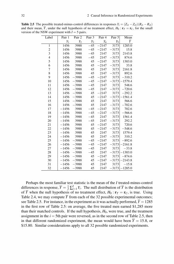
32 2 Causal Inference in Randomized Experiments
Table 2.5 The possible treated-minus-control differences in responses Yi = (Zi1 −Zi2)(Ri1 −Ri2)and their mean, Y , under the null hypothesis of no treatment effect, H0 : rT = rC , for the smallversion of the NSW experiment with I = 5 pairs.
Label Pair 1 Pair 2 Pair 3 Pair 4 Pair 5 Mean
Y1 Y2 Y3 Y4 Y5 Y1 1456 3988 −45 −2147 3173 1285.02 1456 3988 −45 −2147 −3173 15.83 1456 3988 −45 2147 3173 2143.84 1456 3988 −45 2147 −3173 874.65 1456 3988 45 −2147 3173 1303.06 1456 3988 45 −2147 −3173 33.87 1456 3988 45 2147 3173 2161.88 1456 3988 45 2147 −3173 892.69 1456 −3988 −45 −2147 3173 −310.2
10 1456 −3988 −45 −2147 −3173 −1579.411 1456 −3988 −45 2147 3173 548.612 1456 −3988 −45 2147 −3173 −720.613 1456 −3988 45 −2147 3173 −292.214 1456 −3988 45 −2147 −3173 −1561.415 1456 −3988 45 2147 3173 566.616 1456 −3988 45 2147 −3173 −702.617 −1456 3988 −45 −2147 3173 702.618 −1456 3988 −45 −2147 −3173 −566.619 −1456 3988 −45 2147 3173 1561.420 −1456 3988 −45 2147 −3173 292.221 −1456 3988 45 −2147 3173 720.622 −1456 3988 45 −2147 −3173 −548.623 −1456 3988 45 2147 3173 1579.424 −1456 3988 45 2147 −3173 310.225 −1456 −3988 −45 −2147 3173 −892.626 −1456 −3988 −45 −2147 −3173 −2161.827 −1456 −3988 −45 2147 3173 −33.828 −1456 −3988 −45 2147 −3173 −1303.029 −1456 −3988 45 −2147 3173 −874.630 −1456 −3988 45 −2147 −3173 −2143.831 −1456 −3988 45 2147 3173 −15.832 −1456 −3988 45 2147 −3173 −1285.0
Perhaps the most familiar test statistic is the mean of the I treated-minus-control
differences in response, Y = 1I ∑I
i=1 Yi. The null distribution of Y is the distribution
of Y when the null hypothesis of no treatment effect, H0 : rT = rC, is true. Using
Table 2.4, we may compute Y from each of the 32 possible experimental outcomes;
see Table 2.5. For instance, in the experiment as it was actually performed, Y = 1285
in the first row of Table 2.5: on average, the five treated men earned $1,285 more
than their matched controls. If the null hypothesis, H0, were true, and the treatment
assignment in the i = 5th pair were reversed, as in the second row of Table 2.5, then
in that different randomized experiment, the mean would have been Y = 15.8, or
$15.80. Similar considerations apply to all 32 possible randomized experiments.

2.3 Testing the Null Hypothesis of No Treatment Effect 33
In fact, Tables 2.5 and 2.6 give the null randomization distribution of the mean
difference Y . That is, the tables give the distribution of Y derived from the random
assignment of treatments and the null hypothesis, H0, that the treatment is without
effect. Table 2.5 lists the results in the order of Table 2.3, while Table 2.6 sorts Table
2.5 into increasing order of the possible values of Y . It is the same distribution,
but Table 2.6 is easier to read. In both tables, each possible outcome or row has
probability 125 = 1
32 = 0.03125. The tail probability, Pr(
Y ≥ y∣∣F ,Z
), used in
computing significance levels or P-values, is also given in Table 2.6. The one-
sided P-value for testing no treatment effect in Table 2.2 is Pr(
Y ≥ 1285∣∣F ,Z
)=
0.1875 = 632 because 6 of the 32 random assignments produce means Y of 1285 or
more when the null hypothesis of no effect is true. The two-sided P-value is twice
this one-sided P-value,2 or 2×Pr(
Y ≥ 1285∣∣F ,Z
)= 0.375 = 12
32 , which equals
Pr(
Y ≤−1285∣∣ F ,Z
)+ Pr
(Y ≥ 1285
∣∣ F ,Z)
for the distribution in Table 2.6
because the distribution is symmetric about zero.
The reasoned basis for inference in experiments
Fisher [13, Chapter 2] spoke of randomization as the “reasoned basis” for causal
inference in experiments. By this, he meant that the distribution in Table 2.6 for the
mean difference Y and similar randomization distributions for other test statistics
provided a valid test of the hypothesis of no effect caused by the treatment. More-
over, these tests required no assumptions whatsoever. Fisher placed great emphasis
on this, so it is worthwhile to consider what he meant and why he regarded the issue
as important.
The distribution in Table 2.6 was derived from two considerations. The first
consideration is that the experimenter used coins or random numbers to assign treat-
ments, picking one of the 32 treatment assignments in Table 2.3, each with probabil-
ity 1/32. Provided the experimenter is not dishonest in describing the experiment,
there is no basis for doubting this first consideration. The first consideration is not
an assumption; it is a fact describing how the experiment was conducted. The sec-
ond consideration is the null hypothesis of no treatment effect. Table 2.6 is the null
distribution of the mean difference, Y ; that is, Table 2.6 is the distribution Y wouldhave if the null hypothesis of no treatment effect were true. The null hypothesis
may well be false — perhaps the experiment was undertaken in the hope of showing
it is false — but that is beside the point because Table 2.6 is the distribution Y would
2 In general, if you want a two-sided P-value, compute both one-sided P-values, double the smallerone, and take the minimum of this value and 1. This approach views the two-sided P-value as acorrection for testing twice [10]. Both the sample mean in the current section and Wilcoxon’ssigned rank statistic in the next section have randomization distributions under the null hypothesisthat are symmetric, and with a symmetric null distribution there is little ambiguity about the mean-ing of a two-sided P-value. When the null distribution is not symmetric, different definitions ofa two-sided P-value can give slightly different answers. As discussed in [10], the view of a two-sided P-value as a correction for testing twice is one sensible approach in all cases. For relatedresults, see [55].

34 2 Causal Inference in Randomized Experiments
Table 2.6 The randomization distribution of the sample mean Y of I = 5 matched pair differencesin 1978 earnings under the null hypothesis of no treatment effect in the NSW experiment. Becausethe observed value of Y is $1285, the one-sided P-value is 0.1875 and the two-sided P-value istwice that, or 0.375. With I = 5 pairs, the difference would be significant at the conventional 0.05level in a one-sided test only if all five differences were positive, in which case Y = 2161.8 and theone-sided P-value is 0.03125. Notice the that null distribution of Y is symmetric about zero.
y Pr(
Y = y∣∣ F ,Z
)Pr
(Y ≥ y
∣∣ F ,Z)
2161.8 0.03125 0.031252143.8 0.03125 0.062501579.4 0.03125 0.093751561.4 0.03125 0.125001303.0 0.03125 0.156251285.0 0.03125 0.18750
892.6 0.03125 0.21875874.6 0.03125 0.25000720.6 0.03125 0.28125702.6 0.03125 0.31250566.6 0.03125 0.34375548.6 0.03125 0.37500310.2 0.03125 0.40625292.2 0.03125 0.43750
33.8 0.03125 0.4687515.8 0.03125 0.50000
−15.8 0.03125 0.53125−33.8 0.03125 0.56250
−292.2 0.03125 0.59375−310.2 0.03125 0.62500−548.6 0.03125 0.65625−566.6 0.03125 0.68750−702.6 0.03125 0.71875−720.6 0.03125 0.75000−874.6 0.03125 0.78125−892.6 0.03125 0.81250
−1285.0 0.03125 0.84375−1303.0 0.03125 0.87500−1561.4 0.03125 0.90625−1579.4 0.03125 0.93750−2143.8 0.03125 0.96875−2161.8 0.03125 1.00000
have if the null hypothesis of no treatment effect were true. One tests a null hy-
pothesis using Y by contrasting the actual behavior of Y with the behavior Y would
have if the null hypothesis were true. A small P-value indicates that the behavior
Y actually exhibited would have been remarkably improbable if the null hypothesis
were true. In this sense too, the second consideration, the null hypothesis, is not an
assumption. One does not assume or believe the null hypothesis to be true when
testing it; rather, certain logical consequences of the null hypothesis are worked out
for the purpose of evaluating its plausibility. In brief, nothing was assumed to be

2.3 Testing the Null Hypothesis of No Treatment Effect 35
true in working out the distribution in Table 2.6, that is, in testing the hypothesis
that the treatment caused no effect.
You sometimes hear it said that “You cannot prove causality with statistics.” One
of my professors, Fred Mosteller, would often say: “You can only prove causality
with statistics.” When he said this, he was referring to randomization as the rea-
soned basis for causal inference in experiments.
Some history: Random assignment and Normal errors
Concerning Table 2.6, one might reasonably ask how this null randomization dis-
tribution of the mean treated-minus-control difference, Y , compares with the t-distribution that might be used if the Yi were assumed to be Normally distributed
with constant variance. The null distribution in Table 2.6 made no assumption
that the Yi were Normal with constant variance; rather, it acknowledged that the
experimenter did indeed randomize treatment assignments. Questions of this sort
received close attention in early work on randomization inference; see, for instance,
[62]. This attention focused on the moments of the distributions and their limit-
ing behavior as the number, I, of pairs increases. Generally, the two approaches to
inference gave similar inferences for large I when the(rCi j,rTi j
)were sufficiently
well-behaved, but could diverge in other situations. In early work [13, 62], this
was often understood to mean that randomization formed a justification for infer-
ences based on Normal models without requiring the assumptions of those models
to be true. However, it was not long before attention focused on the divergences be-
tween randomization inference and Normal theory, so the concern ceased to be with
justifying Normal theory when applied to well-behaved data from a randomized
experiment; instead, concern shifted to inferences that would be valid and efficient
whether or not the data are well-behaved.3 This leads to the randomization distribu-
tion of statistics other than the mean difference, Y , because the mean was found to
be one of the least efficient statistics for responses that are not so well-behaved [1].
Two such statistics will be discussed: Frank Wilcoxon’s signed rank statistic [63]
in §2.3.3 and the randomization distribution of the statistics used in Peter Huber’s
m-estimation [25, 33] in §2.9. The close connection between rank statistics and m-
estimates is developed in detail in [27]. Sections 2.3.3 and 2.9 play different roles
in this book, and it is not necessary to read §2.9. The signed rank statistic will be
discussed at many points in the book. In contrast, m-estimation is mentioned here
to emphasize that the basic issues discussed here and later are not tied to any one
statistic and may be developed for large classes of statistics in an entirely parallel
way.
3 I write ‘Normal’ distribution rather than ‘normal’ distribution because Normal is the name, notthe description, of a distribution, in the same way that ‘Sitting Bull’ is the name of a man, nota description of that man. The exponential distribution is exponential, the logistic distribution islogistic, but the Normal distribution is not normal. Under normal circumstances, data are not Nor-mally distributed.

36 2 Causal Inference in Randomized Experiments
2.3.3 The randomization distribution of Wilcoxon’s statistic
Computing the randomization distribution under the null hypothesis of noeffect
Among robust alternatives to the mean treated-minus-control difference, Y , by far
the most popular in practice is Wilcoxon’s signed rank statistic, T ; see [63] or [32,
§3.2]. As with Y , Wilcoxon’s statistic uses the treated-minus-control differences in
responses, Yi = (Zi1 −Zi2)(Ri1 −Ri2), in the I pairs. First, the absolute differences
|Yi| are calculated; then these absolute differences are assigned ranks qi from small-
est to largest, from 1 to I; then Wilcoxon’s signed rank statistic, T , is the sum of
those ranks qi for which Yi is positive. With Y1 = 1456, Y2 = 3988, Y3 = −45,
Y4 = −2147, Y5 = 3173 in Table 2.2, the absolute differences are |Y1| = 1456,
|Y2| = 3988, |Y3| = 45, |Y4| = 2147, |Y5| = 3173, with ranks q1 = 2, q2 = 5, q3 = 1,
q4 = 3, and q5 = 4, and Y1, Y2, Y5 are positive, so T = q1 +q2 +q5 = 2+5+4 = 11.
In general, Wilcoxon’s signed rank statistic is T = ∑Ii=1 sgn(Yi) · qi, where
sgn(a) = 1 if a > 0, sgn(a) = 0 if a ≤ 0, and qi is the rank of |Yi|.As in §2.3.2 and Table 2.5, if the null hypothesis of no treatment effect, H0 :
rT = rC, were true then Yi = (Zi1 −Zi2)(rCi1 − rCi2), and randomization simply
changes the signs of the Yi, as in Table 2.4. For each row of Table 2.4, Wilcoxon’s
signed rank statistic, T , may be computed, and this is done in Table 2.7. Under
the null hypothesis of no treatment effect, H0 : rT = rC, each row of Table 2.7 has
a probability of 125 = 1
32 of becoming the observed experimental results in the five
pairs, and 7 rows produce values of T that are 11 or more, so the one-sided P-
value is Pr(T ≥ 11| F ,Z ) = 732 = 0.21875. Table 2.8 reorganizes Table 2.7, sort-
ing by the possible values of the test statistic and removing repetitions of values
that occur several times. In parallel with §2.3.2, the two-sided P-value is twice
this one-sided P-value4, or 2 × Pr(T ≥ 11| F ,Z ) = 1432 = 0.4375 which equals
Pr(T ≤ 4| F ,Z ) + Pr(T ≥ 11 | F ,Z ) for the distribution in Table 2.7 because
the distribution is symmetric about its expectation I (I +1)/4 = 5(5+1)/4 = 7.5.
The null distribution of Wilcoxon’s T is, in many ways, a very simple distri-
bution. In Table 2.7, as the signs change, the absolute values |Yi| stay the same,
so the ranks of the absolute values also stay the same; see the bottom of Table
2.7. That is, if H0 : rT = rC, were true, then the |Yi| = |rCi1 − rCi2| and qi are
4 In practice, statistical software is used to do the calculations. In the statistical package R, thecommand wilcox.test(.) is used. Consider, first, the I = 5 matched pair differences in 1978 earningsin Table 2.7, which are contained in the vector dif5.
> dif5[1] 1456 3988 -45 -2147 3173> wilcox.test(dif5)Wilcoxon signed rank testdata: dif5V = 11, p-value = 0.4375In the case of I = 5, wilcox.test performs calculations that exactly reproduce the value
T = 11 and the two-sided P-value of 0.4375. By adjusting the call to wilcox.test, either ofthe two one-sided P-values may be obtained.
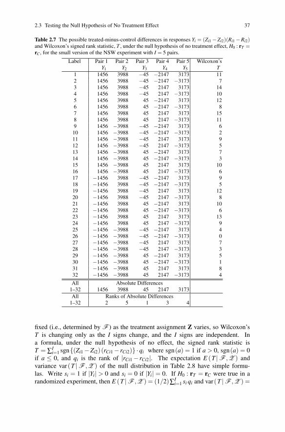
2.3 Testing the Null Hypothesis of No Treatment Effect 37
Table 2.7 The possible treated-minus-control differences in responses Yi = (Zi1 −Zi2)(Ri1 −Ri2)and Wilcoxon’s signed rank statistic, T , under the null hypothesis of no treatment effect, H0 : rT =rC , for the small version of the NSW experiment with I = 5 pairs.
Label Pair 1 Pair 2 Pair 3 Pair 4 Pair 5 Wilcoxon’sY1 Y2 Y3 Y4 Y5 T
1 1456 3988 −45 −2147 3173 112 1456 3988 −45 −2147 −3173 73 1456 3988 −45 2147 3173 144 1456 3988 −45 2147 −3173 105 1456 3988 45 −2147 3173 126 1456 3988 45 −2147 −3173 87 1456 3988 45 2147 3173 158 1456 3988 45 2147 −3173 119 1456 −3988 −45 −2147 3173 6
10 1456 −3988 −45 −2147 −3173 211 1456 −3988 −45 2147 3173 912 1456 −3988 −45 2147 −3173 513 1456 −3988 45 −2147 3173 714 1456 −3988 45 −2147 −3173 315 1456 −3988 45 2147 3173 1016 1456 −3988 45 2147 −3173 617 −1456 3988 −45 −2147 3173 918 −1456 3988 −45 −2147 −3173 519 −1456 3988 −45 2147 3173 1220 −1456 3988 −45 2147 −3173 821 −1456 3988 45 −2147 3173 1022 −1456 3988 45 −2147 −3173 623 −1456 3988 45 2147 3173 1324 −1456 3988 45 2147 −3173 925 −1456 −3988 −45 −2147 3173 426 −1456 −3988 −45 −2147 −3173 027 −1456 −3988 −45 2147 3173 728 −1456 −3988 −45 2147 −3173 329 −1456 −3988 45 −2147 3173 530 −1456 −3988 45 −2147 −3173 131 −1456 −3988 45 2147 3173 832 −1456 −3988 45 2147 −3173 4
All Absolute Differences1–32 1456 3988 45 2147 3173
All Ranks of Absolute Differences1–32 2 5 1 3 4
fixed (i.e., determined by F ) as the treatment assignment Z varies, so Wilcoxon’s
T is changing only as the I signs change, and the I signs are independent. In
a formula, under the null hypothesis of no effect, the signed rank statistic is
T = ∑Ii=1 sgn{(Zi1 −Zi2)(rCi1 − rCi2)} · qi where sgn(a) = 1 if a > 0, sgn(a) = 0
if a ≤ 0, and qi is the rank of |rCi1 − rCi2|. The expectation E (T | F ,Z ) and
variance var(T | F ,Z ) of the null distribution in Table 2.8 have simple formu-
las. Write si = 1 if |Yi| > 0 and si = 0 if |Yi| = 0. If H0 : rT = rC were true in a
randomized experiment, then E (T | F ,Z ) = (1/2)∑Ii=1 si qi and var(T | F ,Z ) =

38 2 Causal Inference in Randomized Experiments
Table 2.8 The randomization distribution of Wilcoxon’s signed rank statistic, T , for I = 5 matchedpair differences in 1978 earnings under the null hypothesis of no treatment effect in the NSWexperiment. Count is the number of treatment assignments that yield T = t; for instance, thereare two ways to obtain T = 12. Because the observed value of T is 11, the one-sided P-valueis 0.21875 and the two-sided P-value is twice that, or 0.4375. With I = 5 pairs, the differencewould be significant at the conventional 0.05 level in a one-sided test only if all five differenceswere positive, in which case T = 15 and the one-sided P-value is 0.03125. Notice the that nulldistribution of T is symmetric about its expectation, I(I +1)/4 = 5(5+1)/4 = 7.5.
t Count Pr(T = t | F ,Z ) Pr(T ≥ t | F ,Z )15 1 0.03125 0.0312514 1 0.03125 0.0625013 1 0.03125 0.0937512 2 0.06250 0.1562511 2 0.06250 0.2187510 3 0.09375 0.31250
9 3 0.09375 0.406258 3 0.09375 0.500007 3 0.09375 0.593756 3 0.09375 0.687505 3 0.09375 0.781254 2 0.06250 0.843753 2 0.06250 0.906252 1 0.03125 0.937501 1 0.03125 0.968750 1 0.03125 1.00000
(1/4)∑Ii=1 (si qi)
2. When there are no ties, these formulas simplify because the
ranks are then 1, 2, . . . , I. If there are no ties, in the sense that |Yi|> 0 for all i and all
of the |Yi| are distinct, then the formulas simplify to E (T | F ,Z ) = I (I +1)/4 and
var(T | F ,Z ) = I (I +1)(2I +1)/24; see [32, §3.2] Moreover, under very mild
conditions, as I → ∞, the null distribution of {T −E (T | F ,Z )}/√
var(T | F ,Z )converges in distribution to the standard Normal distribution [32].
Testing no effect with all I = 185 matched pairs
If Wilcoxon’s test is applied to all I = 185 matched pairs in Figure 2.1, then the
two-sided P-value for testing no effect is 0.009934. When all I = 185 pairs are con-
sidered, the difference in 1978 earnings in Figure 2.1 appears to be an effect caused
by the intervention. The difference in 1978 earnings is too large and systematic to
be due to chance, the flip of the coin that assigned one man to treatment, the next to
control.5
5 Performing the calculations in R is straightforward. The I = 185 paired differences in 1978earnings are contained in the vector dif.
> length(dif)[1] 185> dif[1:6][1] 3889.711 -4733.929 18939.192 7506.146 -6862.342 -8841.886

2.3 Testing the Null Hypothesis of No Treatment Effect 39
The procedure used in Table 2.5 for the mean, Y , and in Table 2.7 for Wilcoxon’s
statistic, T , are entirely parallel and work in a similar way for any test statistic.6
The null distribution of Wilcoxon’s T in Table 2.8 has a curious property not
shared by the null distribution of the mean difference, Y , in Table 2.6. The null
distribution of Y in Table 2.6 depends on the numeric values of Yi, so this distribution
could not have been written down before the experiment was conducted. You need
to have the Yi’s to construct Table 2.6. In contrast, the distribution of T in Table
2.8 does not depend upon the differences in earnings, the Yi’s, provided the |Yi| are
nonzero and different (or untied) so that they can be ranked 1, 2, 3, 4, 5 and each
Yi is either positive or negative. Provided the I = 5 earnings differences are untied,
the null distribution in Table 2.8 could be written down before the experiment is
conducted, and indeed the distribution in Table 2.8 appears at the back of many
textbooks.
Ties and distribution-free statistics
What happens to Wilcoxon’s T when some |Yi| are tied? If several |Yi| are equal, it
does not seem reasonable to assign them different ranks, so instead they are assigned
the average of the ranks they would have had if they had differed ever so slightly. If
|Y4| = |Y5| and they would have had ranks 3 and 4 had they not been tied, then they
are both assigned rank 3.5. Under the null hypothesis of no effect, if |Yi| = 0 then
Yi = 0 no matter how treatments are assigned, and pair i contributes 0 to Wilcoxon’s
T for every treatment assignment. With ties, the null distribution of T is determined
as has been done twice before in Tables 2.5 and 2.7; however, the null distribution
now depends not only on the sample size I but also on the specific pattern of ties, so
the distribution is not known in advance of the experiment.
The phrase ‘distribution-free statistic’ is used in a variety of related but slightly
distinct senses. In one of these senses, both the sample mean, Y , and Wilcoxon’s
signed rank statistic, T , always have randomization distributions, as computed in
Tables 2.5 and 2.7, and if there are no ties among the |Yi|, then T is distribution-free,
in the sense that its null distribution does not depend upon the values of the Yi.
> wilcox.test(dif)Wilcoxon signed rank test with continuity correction
data: difV = 9025, p-value = 0.009934alternative hypothesis: true location is not equal to 0Now, with I = 185 pairs, the statistic is T = 9025 and the two-sided P-value is 0.009934. In
computing this P-value, R has taken appropriate account of ties of both kinds and has made use of aNormal approximation to the null distribution of T . It has also employed a ‘continuity correction’intended to improve the accuracy of approximate P-values obtained from the Normal distribution.6 This statement is true conceptually. That is, the statement would be true if we had an infinitelyfast computer. As a practical matter, producing a table like Table 2.5 for large I is quite tedious,even for a computer, so randomization distributions are obtained either with clever algorithms [37]or with the aid of large sample approximations [32]. It is not necessary to focus on these technicaldetails in a chapter whose focus is on concepts. In understanding concepts, we can pretend for themoment that we have an infinitely fast computer.

40 2 Causal Inference in Randomized Experiments
2.4 Testing Other Hypotheses; Confidence Intervals; PointEstimates
2.4.1 Testing a constant, additive treatment effect
Section 2.3 tested Fisher’s [13] sharp null hypothesis of no treatment effect, which
asserts that each subject would exhibit the same response whether assigned to treat-
ment or control, that is, H0 : rTi j = rCi j for i = 1, . . . , I, j = 1,2, or equivalently
H0 : rT = rC. This test for no effect quickly provides the basis for testing any hy-
pothesis that specifies an effect, and from this to confidence intervals.
The simplest case is considered first, namely a constant, additive treatment ef-
fect, τ , in which rTi j = rCi j + τ for i = 1, . . . , I, j = 1,2, or equivalently rT =rC + 1τ , where 1 = (1,1, . . . ,1)T . In this case, the observed response, Ri j =Zi j rTi j +(1−Zi j) rCi j from the jth subject in pair i becomes Ri j = Zi j
(rCi j + τ
)+
(1−Zi j) rCi j = rCi j + τZi j, that is, the observed response, Ri j, equals the response
to control, rCi j, plus the treatment effect τ if i j is assigned to treatment, Zi j = 1. Of
course, Ri j and Zi j are observed, but rCi j and τ are not.
The hypothesis of a constant, additive effect is not strictly plausible for any τ �= 0
in the NSW study in §2.1. For instance, in Table 2.2, the j = 1st man in the i = 3rd
pair was treated but earned $0.00 in 1978. Because earnings are positive, the only
positive constant effect τ that can yield $0.00 for a treated man is τ = 0. Indeed,
in Figure 2.1, a quarter of the controls had $0.00 of earnings in 1978. Moreover,
even if negative earnings were possible, the boxplots in Figure 2.1 for all 185 pairs
of men strongly suggest the treatment effect is not an additive constant. In a very
large randomized experiment with an additive, constant effect τ , the two boxplots of
responses, Ri j, on the left in Figure 2.1 would look the same, except that the treated
boxplot would be shifted up by τ , and the boxplot of pair differences, Yi, on the right
in Figure 2.1 would be symmetric about τ . In fact, neither of these two conditions
appears to be true in Figure 2.1. After illustrating the most commonly used methods
for an additive effect, three alternative approaches will be considered for the NSW
study: a multiplicative effect, a truncated additive effect similar to that found in a
Tobit model, and ‘attributable effects’ of various kinds. As will be seen, although
the hypothesized effects are different, the method of inference is much the same.
Suppose that we hypothesized that the additive effect τ is some particular num-
ber, τ0. For instance, in §2.1, a rather extreme hypothesis says that the NSW pro-
gram increases earnings by $5000, or H0 : τ = 5000, or H0 : τ = τ0 with τ0 = 5000.
It will soon be seen that this hypothesis is quite implausible. If this hypothesis
were true, the observed response would be Ri j = rCi j + τ0 Zi j = rCi j + 5000Zi j,
so rCi j could be computed from the observed (Ri j,Zi j) together with the sup-
posedly true hypothesis, H0 : τ = 5000, as rCi j = Ri j − τ0 Zi j = Ri j − 5000Zi j.
Moreover, the matched treated-minus-control difference in observed earnings is
Yi = (Zi1 −Zi2)(Ri1 −Ri2), so if the hypothesis H0 : τ = τ0 were true,
Yi = (Zi1 −Zi2)(Ri1 −Ri2)

2.4 Testing Other Hypotheses; Confidence Intervals; Point Estimates 41
Table 2.9 Five matched pair differences from the NSW experiment adjusted for the hypothesisH0 : τ = 5000.
i 1 2 3 4 5
Yi 1456 3988 −45 −2147 3173τ0 = 5000 5000 5000 5000 5000 5000
Yi − τ0 −3544 −1012 −5045 −7147 −1827
= (Zi1 −Zi2){(rCi1 + τ0 Zi1)− (rCi2 + τ0 Zi2)}= τ0 +(Zi1 −Zi2)(rCi1 − rCi2) ,
and Yi − τ0 = (Zi1 −Zi2)(rCi1 − rCi2). In other words, if H0 : τ = τ0 were true with
τ0 = 5000, then the observed difference in earnings, Yi, in pair i, less τ0 = 5000,
would equal ±(rCi1 − rCi2) depending upon the random treatment assignment Zi1 −Zi2 in pair i. In particular, if H0 : τ = 5000 were true, then the sign of Yi − 5000
would be determined by a coin flip, and we would expect about half of the Yi−5000
to be positive, half to be negative. If H0 : τ = 5000 were true for the five pairs in
Table 2.2, then, for pair i = 1, the adjusted difference is rC11 − rC12 = Y1 − 5000
= 1456 − 5000 = −3544. The five adjusted differences are listed in Table 2.9.
Even with just the five pairs in Table 2.9, the hypothesis H0 : τ = 5000 does not
look plausible: all five adjusted differences are negative, whereas if the hypothesis
were true, the signs would be ±1 independently with probability 12 . Only one of
the 32 treatment assignments z ∈ Z would give negative signs to all five adjusted
responses, and that one assignment has probability 1/32 = .03125 in a randomized
experiment. If H0 : τ = 5000 were true, to produce Table 2.9 would require quite a
bit of bad luck when Z is picked at random from Z .
Table 2.10 displays all 32 treatment assignments, z ∈ Z , together with all pos-
sible adjusted responses, Yi − τ0 = (Zi1 −Zi2)(rCi1 − rCi2), when H0 : τ = 5000 is
true, together with Wilcoxon’s signed rank statistic T computed from these adjusted
responses. In the first row, for the actual treatment assignment, T = 0 because
all five differences are negative. From Table 2.10, Pr(T ≤ 0| F ,Z ) = 1/32 =.03125 if H0 : τ = 5000 is true, and the two-sided P-value is Pr(T ≤ 0| F ,Z )+Pr(T ≥ 15| F ,Z ) = 2/32 = .0625.
2.4.2 Confidence intervals for a constant, additive effect
If the treatment has an additive effect, rTi j = rCi j + τ for i = 1, . . . , I, j = 1,2, then
a 95% confidence set for the additive treatment effect, τ , is formed by testing each
hypothesis H0 : τ = τ0 and retaining for the confidence set the values of τ0 not
rejected at the 5% level. In general, a 1−α confidence set is the set of hypothesized
values of a parameter not rejected by a level α test [31, §3.5]. If the parameter is a
number, such as τ , then a 1−α confidence interval is the shortest interval containing
the 1−α confidence set, and this interval may be a half-line or the entire line. For

42 2 Causal Inference in Randomized Experiments
Table 2.10 Using Wilcoxon’s signed rank statistic T to test the null hypothesis that the trainingprogram increased wages by an additive constant of $5000, that is, H0 : rTi j = rCi j + 5000 for alli, j.
Label Pair 1 Pair 2 Pair 3 Pair 4 Pair 5 Pair 1 Pair 2 Pair 3 Pair 4 Pair 5Z11 Z21 Z31 Z41 Z51 Y1 − τ0 Y2 − τ0 Y3 − τ0 Y4 − τ0 Y5 − τ0 T
1 1 1 1 1 1 −3544 −1012 −5045 −7147 −1827 02 1 1 1 1 0 −3544 −1012 −5045 −7147 1827 23 1 1 1 0 1 −3544 −1012 −5045 7147 −1827 54 1 1 1 0 0 −3544 −1012 −5045 7147 1827 75 1 1 0 1 1 −3544 −1012 5045 −7147 −1827 46 1 1 0 1 0 −3544 −1012 5045 −7147 1827 67 1 1 0 0 1 −3544 −1012 5045 7147 −1827 98 1 1 0 0 0 −3544 −1012 5045 7147 1827 119 1 0 1 1 1 −3544 1012 −5045 −7147 −1827 110 1 0 1 1 0 −3544 1012 −5045 −7147 1827 311 1 0 1 0 1 −3544 1012 −5045 7147 −1827 612 1 0 1 0 0 −3544 1012 −5045 7147 1827 813 1 0 0 1 1 −3544 1012 5045 −7147 −1827 514 1 0 0 1 0 −3544 1012 5045 −7147 1827 715 1 0 0 0 1 −3544 1012 5045 7147 −1827 1016 1 0 0 0 0 −3544 1012 5045 7147 1827 1217 0 1 1 1 1 3544 −1012 −5045 −7147 −1827 318 0 1 1 1 0 3544 −1012 −5045 −7147 1827 519 0 1 1 0 1 3544 −1012 −5045 7147 −1827 820 0 1 1 0 0 3544 −1012 −5045 7147 1827 1021 0 1 0 1 1 3544 −1012 5045 −7147 −1827 722 0 1 0 1 0 3544 −1012 5045 −7147 1827 923 0 1 0 0 1 3544 −1012 5045 7147 −1827 1224 0 1 0 0 0 3544 −1012 5045 7147 1827 1425 0 0 1 1 1 3544 1012 −5045 −7147 −1827 426 0 0 1 1 0 3544 1012 −5045 −7147 1827 627 0 0 1 0 1 3544 1012 −5045 7147 −1827 928 0 0 1 0 0 3544 1012 −5045 7147 1827 1129 0 0 0 1 1 3544 1012 5045 −7147 −1827 830 0 0 0 1 0 3544 1012 5045 −7147 1827 1031 0 0 0 0 1 3544 1012 5045 7147 −1827 1332 0 0 0 0 0 3544 1012 5045 7147 1827 15
many simple statistics, including Wilcoxon’s signed rank statistic, the confidence
set and the confidence interval for τ are the same [32, Chapter 4].
The five pairs in Table 2.10 cannot reject at the 5% level any two-sided hypothe-
sis using Wilcoxon’s statistic, T , because the smallest two-sided significance level is
Pr(T ≤ 0| F ,Z )+Pr(T ≥ 15| F ,Z ) = 2/32 = .0625. However, a 1− .0625 =93.75% confidence interval for τ may be constructed. The endpoints of the confi-
dence interval are determined in Table 2.11, where Wilcoxon’s signed rank statistic,
T , rejects hypotheses below H0 : τ =−2147 and above H0 : τ = 3988 in a two-sided,
0.0625 level test, and the 93.75% confidence interval for τ is [−2147, 3988].

2.4 Testing Other Hypotheses; Confidence Intervals; Point Estimates 43
Table 2.11 The endpoints of the 93.75% confidence interval for an additive treatment effect τ infive pairs from the NSW experiment. Wilcoxon’s signed rank statistic T takes steps at −2147 and3988, which define the endpoints of the two-sided confidence interval, [−2147, 3988].
τ0 −2147.0001 −2147 3987.9999 3988T 15 14 1 0
P-value .0625 0.1250 0.1250 .0625
With the full sample of I = 185 pairs, the 95% confidence interval for τ is
[391, 2893] or between $391 and $2893, a long interval but one that excludes zero
treatment effect.7
2.4.3 Hodges-Lehmann point estimates of effect
In §2.4.1, the hypothesis of an additive treatment effect, H0 : rTi j = rCi j + τ0 for
i = 1, . . . , I, j = 1,2, was tested by applying Wilcoxon’s signed rank statistic to the
adjusted pair differences, Yi − τ0, which equal (Zi1 −Zi2)(rCi1 − rCi2) if H0 is true.
In §2.4.2, a 1−α confidence interval for an additive effect was formed by testing
every value τ0 and retaining for the interval all values not rejected by the Wilcoxon
test at level α . The same logic was used by Joseph Hodges and Erich Lehmann
[21, 32] to create a point estimate. They asked: What value τ0 when subtracted
from Yi makes Wilcoxon’s statistic T computed from Yi − τ0 behave the way we
expect Wilcoxon’s statistic to behave with a true hypothesis? As noted in §2.3.3,
when Wilcoxon’s signed rank statistic T is computed from (Zi1 −Zi2)(rCi1 − rCi2),it has expectation E (T | F ,Z ) = I (I +1)/4 provided |rCi1 − rCi2|> 0 for all i. In-
tuitively, one finds a value, τ , such that Wilcoxon’s statistic T equals I (I +1)/4
when T is computed from Yi − τ . The intuition does not quite work, because the
7 Continuing the discussion from Note 5, calculating the confidence interval in R is straightforward:the call to wilcox.test(.) includes the option conf.int=T.
>wilcox.test(dif,conf.int=T)Wilcoxon signed rank test with continuity correctiondata: difV = 9025, p-value = 0.009934alternative hypothesis: true location is not equal to 095 percent confidence interval:391.359 2893.225sample estimates:(pseudo)median1639.383
In addition to the confidence interval, R supplies the Hodges-Lehmann point estimate 1639.383of τ , as discussed in §2.4.3. In the R output, the Hodges-Lehmann estimate is labeled a (pseudo)median.
In calculating this confidence interval, R makes use of various computational short-cuts. Be-cause these computational shortcuts do not change the confidence interval, because they make thesubject seem more complex than it is, and because they do not generalize to other situations, I donot discuss such shortcuts in this book.
44 2 Causal Inference in Randomized Experiments
Wilcoxon statistic is discrete, taking on a finite number of values, so it may never
equal I (I +1)/4 or it may equal I (I +1)/4 for an interval of values of τ0. So
Hodges and Lehmann added two very small patches. If the signed rank statis-
tic never equals I (I +1)/4, then there is a unique value of τ0 where T passes
I (I +1)/4, and that unique value is the Hodges-Lehmann estimate, τ . If the
signed rank statistic equals I (I +1)/4 for an interval of values of τ0, then the mid-
point of that interval is the Hodges-Lehmann estimate, τ . In Table 2.2, I = 5,
so I (I +1)/4 = 5(5+1)/4 = 7.5. Wilcoxon’s T is T = 8 if computed from
Yi − 1455.9999, but it is T = 7 if computed from Yi − 1456.0001, so τ = $1456.
For all I = 185 pairs, the point estimate8 of the increase in earnings is τ = $1639.
Although τ is one of the two well-known estimates that are called ‘Hodges-
Lehmann (HL) estimates,’ Hodges and Lehmann [21] had actually proposed a gen-
eral method for constructing estimates from tests of no treatment effect. The test
statistic need not be the Wilcoxon statistic, and the parameter need not be an addi-
tive treatment effect. One equates a test statistic to its null expectation and solves
the resulting equation for the point estimate. The method is applicable with other
statistics. In a mildly dull way, if you take the sample mean of Yi − τ0 as a test
statistic, as in §2.3.2, then the mean of Yi − τ0 has expectation zero when H0 is true,
so the estimating equation is (1/I)∑(Yi − τ) = 0 with solution τ = Y ; that is, the
Hodges-Lehmann estimate derived from the mean is the mean of the Yi. Almost,
but not quite, the same thing happens with the randomization distribution of m-tests
in §2.9. In §2.4.5 there are Hodges-Lehmann estimates of a multiplicative effect [2]
and a Tobit effect.
2.4.4 Testing general hypotheses about treatment effects
Any hypothesis that specifies the 2I treatment effects, rTi j − rCi j, may be tested
using the same reasoning as in §2.4.1. Let τ0i j be 2I specific numbers, and let
θ0 = (τ011,τ012, . . . ,τ0I2)T collect them into a vector of dimension 2I. Consider
the hypothesis H0 : rTi j = rCi j + τ0i j for i = 1, . . . , I and j = 1,2, or equivalently
H0 : rT = rC + θ0. Any specific hypothesis about effects may be expressed in this
way.
For instance, a basic hypothesis of this form entails interaction between the treat-
ment and a covariate, or so-called ‘effect-modification.’ In Table 2.1, one might
entertain a hypothesis in which there are two values of τ0i j depending upon whether
the jth man in the ith pair has or does not have a high school degree. The hypothesis
might assert that τ0i j = $1000 if i j has a high school degree and τ0i j = $2000 if i jdoes not have such a degree, so the program has a larger benefit for men without a
degree.
The logic of §2.4.1 barely changes. If H0 : rT = rC +θ0 were true, the observed
response Ri j = Zi j rTi j +(1−Zi j) rCi j from the jth person in pair i would be Ri j =
8 To compute the Hodges-Lehmann estimate in R, see Note 7.

2.4 Testing Other Hypotheses; Confidence Intervals; Point Estimates 45
rCi j + Zi j τ0i j, so that the observable data, (Ri j,Zi j), together with the hypothesis
permit the computation of rCi j = Ri j −Zi j τ0i j, in parallel with §2.4.1. Indeed, using
the fact that Zi2 = 1−Zi1, if H0 : rT = rC +θ0 were true, the treated-minus-control
matched-pair difference in responses is
Yi = (Zi1 −Zi2)(Ri1 −Ri2)= (Zi1 −Zi2){(rCi1 + τ0i1 Zi1)− (rCi2 + τ0i2 Zi2)}= (Zi1 −Zi2)(rCi1 − rCi2)+(τ0i1 Zi1 + τ0i2 Zi2)
so the adjusted difference
Yi − (τ0i1 Zi1 + τ0i2 Zi2) = (Zi1 −Zi2)(rCi1 − rCi2) (2.2)
is ±(rCi1 − rCi2) depending upon the random assignment of treatments Zi1 − Zi2.
The rest of the argument in §2.4.1 is as before, with a statistic, such as Wilcoxon’s
signed rank statistic, T , computed from the the adjusted differences (2.2), and com-
pared to its randomization distribution formed from all 2I assignments of signs to
(Zi1 −Zi2)(rCi1 − rCi2).In abstract principle, a 95% confidence set for θ = (rT 11 − rC11, . . . ,rT I2 − rCI2)
T
could be constructed by testing every hypothesis H0 : rT = rC +θ0 and retaining for
the confidence set the values of θ0 that are not rejected by some 5% level test. In
practice, such a confidence set would not be intelligible, for it would be a subset
of 2I-dimensional space. In the NSW data in §2.1, the confidence set would be a
subset of 2I = 2×185 = 370 dimensional space and would be beyond human com-
prehension. In brief, it is straightforward to make valid statistical inferences that
are so complex, so faithful to the minute detail of reality, that they are unintelligible
and of no practical use whatsoever. The 1-dimensional confidence interval for the
single (scalar) constant effect τ in §2.4.2 provides insight into the 2I-dimensional
confidence set for θ because the constant model rT = rC + 1τ defines a line in
2I-dimensional space as τ varies over the real numbers. If all the tests were per-
formed using the same test statistic, say Wilcoxon’s signed rank statistic T , then τ0
is excluded from the 1-dimensional confidence interval for an additive effect if and
only if θ0 = (τ0,τ0, . . . ,τ0)T is excluded from the 2I-dimensional confidence set for
θ ; after all, it is the same hypothesis tested by the same test. In this sense, a 1-
dimensional model for the 2I dimensional effect, such as the constant effect model,
may be understood as an attempt to glean insight into the 2I dimensional confidence
set for θ while recognizing that any 1-dimensional model, indeed any intelligible
model, is to some degree an oversimplification. Understanding of θ is often aided
by contrasting several intelligible models, rather than discarding them. Two other
1-dimensional effects are considered in §2.4.5. Arguably, the joint consideration
of three 1-dimensional models for the 2I-dimensional parameter θ provides more
humanly accessible insight into θ than would a 2I-dimensional confidence set.
An alternative approach to understanding the 2I-dimensional confidence set for
θ uses ‘attributable effects.’ In typical practice, an attributable effect provides a 1-
46 2 Causal Inference in Randomized Experiments
dimensional summary statement about the 2I-dimensional θ , but this summary does
not determine θ uniquely. Attributable effects are discussed in §2.5.
2.4.5 Multiplicative effects; Tobit effects
A constant multiplicative effect β
As noted in §2.4.1, the hypothesis of a positive, constant additive effect, H0 : rTi j =rCi j + τ for i = 1, . . . , I, j = 1,2, has the disagreeable property that it implies that a
man with zero earnings under treatment would have negative earnings under con-
trol. In this section, two other 1-dimensional families of hypotheses for the 2I-
dimensional effect θ = (rT 11 − rC11, . . . ,rT I2 − rCI2)T are considered; they do not
produce negative earnings.
The first hypothesis asserts that the effect is a constant multiplier rather than a
constant addition, H0 : rTi j = β0 rCi j for i = 1, . . . , I, j = 1,2 with β0 ≥ 0. This
hypothesis avoids the implication of negative earnings under one of the treatments.
The multiplicative effect hypothesis is a special case of the hypothesis in §2.4.4,
namely the hypothesis H0 : rT = rC + θ0 with τ0i j = rTi j − rCi j = β0 rCi j − rCi j =(β0 −1) rCi j.
For an additive effect, the treatment effect is removed by subtraction, but for a
multiplicative effect, the effect is removed by division [2]. If H0 : rTi j = β0 rCi j
were true for all i j, then Ri j/β Zi j0 = rCi j; that is, if Zi j = 0 then Ri j = rCi j and
β Zi j0 = 1, while if Zi j = 1, then Ri j = rTi j, β Zi j
0 = β0 and Ri j/β Zi j0 = rTi j/β0 =
rCi j. The hypothesis H0 : rTi j = β0 rCi j is tested by applying Wilcoxon’s signed
rank statistic to the I adjusted, treated-minus-control matched pair differences,
(Zi1 −Zi2)(
Ri1/β Zi10 −Ri2/β Zi2
0
), which equal (Zi1 −Zi2)(rCi1 − rCi2) if the hy-
pothesis is true. The set of values of β0 not rejected in a 5%-level test is a 95%
confidence set for a constant multiplicative effect β .
In the NSW experiment with I = 185 pairs, the two-sided, 95% confidence in-
terval for β is [1.08, 1.95], or between an 8% increase and a 95% increase. The
Hodges-Lehmann point estimate is β = 1.45.
Although a multiplicative effect avoids the implication of negative earnings, it
has peculiarities of its own. If the effect is multiplicative, then a man who has rCi j =0 earnings under control also has rTi j = β rCi j = 0 earnings under treatment. Many
controls did have zero earnings in 1978; see Figure 2.1. Among its several goals,
the NSW program intended to bring into employment men who would otherwise be
out of work, and a multiplicative effect says this cannot happen. This leads to the
consideration of a ‘Tobit effect.’

2.4 Testing Other Hypotheses; Confidence Intervals; Point Estimates 47
Tobit effects
Two men with the same positive earnings, rCi j, under control in 1978 have some-
thing in common: the labor market attached the same dollar value to their labor.
Two men with zero earnings under control in 1978 have less in common: the labor
market declined to attach a positive value to the labor they might supply. One might
entertain the thought that two unemployed men are unequally unemployed: perhaps
the market attaches negative but unequal values to the labor they might supply. Ex-
pressed in operational terms, the subsidy that an employer would require before
employing the two unemployed men might be different because one man could sup-
ply labor of greater net value to the employer than the other. In a simple economic
model, workers are paid the values of the marginal products of their labor, and a
worker is unemployed if the marginal product of his labor is negative. (We have
all known people like that.) ‘Tobit effects,’ named for James Tobin [60], attempt to
express this idea.
Suppose the NSW program raises the marginal value of every worker’s labor by
the same constant, τ0, but the worker is employed, with positive earnings, only if
the marginal value of the labor is positive. In this case, if the jth man in the ithpair would have earnings of rTi j in the NSW program, and if rTi j ≥ τ0, then rCi j =rTi j − τ0, but if rTi j < τ0 then rCi j = 0; that is, in general, rCi j = max(rTi j − τ0,0).This hypothesis is another special case of the general hypothesis in §2.4.4.
If the hypothesis, H0 : rCi j = max(rTi j − τ0,0) for i = 1, . . . , I, j = 1,2, were
true, then max(Ri j − τ0 Zi j, 0) = rCi j. The hypothesis rCi j = max(rTi j − τ0,0) may
be tested by applying Wilcoxon’s signed rank test to the I adjusted treated-minus-
control differences, (Zi1 −Zi2){
max(Ri j − τ0 Zi j, 0)−max(Ri j − τ0 Zi j, 0)}
,which
equal (Zi1 −Zi2)(rCi1 − rCi2) if the hypothesis is true. The test is the same as before;
see §2.4.4.
For the Tobit effect rCi j = max(rTi j − τ,0), the 95% confidence interval for τ is
[$458, $3955], and the Hodges-Lehmann point estimate is τ = $2114.
Comparing the three effects: additive, multiplicative, tobit
Figure 2.2 compares an additive effect, rCi j = rTi j −τ , a multiplicative effect, rCi j =rTi j/β , and a Tobit effect, rCi j = max(rTi j − τ,0). In each of the three panels of
Figure 2.2, the 1978 earnings of the 185 treated men (Zi j = 1) and the 185 control
men (Zi j = 0) are displayed after removing the estimated treatment effect from the
earnings of the treated men. In each case, the Hodges-Lehmann estimate is used
to estimate the treatment effect. For an additive effect, Ri j − τZi j is plotted; for a
multiplicative effect, Ri j/β Zi j is plotted; for a Tobit effect, max(Ri j − τ Zi j, 0) is
plotted. If the number I of pairs were large, then the pair of treated-control boxplots
would look the same with an effect of the correct form. The boxplots for an additive
effect suggest the effect is not, in fact, additive, in part because the boxplots look
quite different, and in part because negative earnings are produced. The boxplots
for the multiplicative effect look better, although the lower quartile for the treated

48 2 Causal Inference in Randomized Experiments
●
●
●
●
●
●
●●
Treated Control
010
000
2000
030
000
4000
050
000
6000
0Additive Effect
1978
Ear
ning
s A
djus
ted
for
Effe
ct
●
●
●
●
●
●
●●
Treated Control
010
000
2000
030
000
4000
050
000
6000
0
Multiplicative Effect
1978
Ear
ning
s A
djus
ted
for
Effe
ct
●
●
●
●
●
●
●
●
●●
Treated Control
010
000
2000
030
000
4000
050
000
6000
0
Tobit Effect
1978
Ear
ning
s A
djus
ted
for
Effe
ct
Fig. 2.2 Earnings in 1978 after adjustment to remove three possible treatment effects, an additiveeffect of $1639, a multiplicative effect of 1.45, and a Tobit effect of $2114. If the correct effectwere removed, the two boxplots would look similar, differing only by chance.
group is positive while for the control group it is zero. The boxplots for the Tobit
effect are better than for the additive effect, and the lower quartile in both groups is
now zero. Although the Tobit effect is, arguably, the best of the three, it misses the
long right tail in the treated group: a handful of treated men earned much more than
is accounted for by the Tobit effect. This was clearly visible in Figure 2.1 as well.
More will be said about the tail in §2.5.

2.5 Attributable Effects 49
2.5 Attributable Effects
Why use attributable effects?
As seen in §2.4.4, it is straightforward to test a hypothesis that specifies all 2Itreatment effects, rTi j − rCi j, say the hypothesis H0 : rTi j = rCi j + τ0i j for i =1, . . . , I and j = 1,2, or equivalently the hypothesis H0 : rT = rC + θ0 with θ0 =(τ011,τ012, . . . ,τ0I2)
T . We were barred from using such a test to produce a con-
fidence set for θ = (rT 11 − rC11, . . . ,rT I2 − rCI2)T in part by our inability to make
practical sense of a confidence set that is a subset of 2I-dimensional space. In §2.4.5,
some insight into θ was gleaned by contrasting three 1-dimensional effects, that is,
three paths or curves through the 2I-dimensional space of possible effects. By con-
trast, ‘attributable effects’ make summary statements about θ without restricting
the form of θ in any way. Attributable effects are a general concept [42, 43] but, in
the current section, only the case of matched pairs is considered using Wilcoxon’s
signed rank statistic [46] and an extension of it by W. Robert Stephenson [59, 49].
The discussion is simplified by assuming that there are no ties of any kind and dis-
cussing ties separately at the end.
Aligned responses: Shifting attention from pairs to individuals
If no simplifying form is imposed upon θ = (rT 11 − rC11, . . . ,rT I2 − rCI2), then it
is easiest to understand a treatment effect on one man, rTi j − rCi j, rather than on
the matched pair difference between two men. In simple cases, such as an additive
effect, the difference of two matched men has a simple relationship with the sepa-
rate responses of the two individual men (§2.4.1), but in general this is not so. At
the same time, the men were carefully matched for important characteristics, such
as education, age and pretreatment earnings, and it seems wise to retain the com-
parison of two similar men. These two considerations lead to ‘aligned responses,’
introduced by Hodges and Lehmann [20] in an extension of Wilcoxon’s signed rank
statistic. With matched pairs, the aligned response for the jth man in the ith pair
is the difference between his observed response, Ri j, and the average response in
his pair, Ri = (Ri1 +Ri2)/2, so the aligned response is Ri j −Ri. Talk about aligned
responses is, in a sense, talk about one man while taking account of the pairing.
Of course, the treated-minus-control pair difference of aligned responses Ri j −Riequals the treated-minus-control difference in the responses Ri j themselves because
Ri appears twice and cancels. If Wilcoxon’s signed rank statistic were computed
from the aligned responses, it would equal Wilcoxon’s signed rank statistic com-
puted from the responses themselves. So far, the switch to aligned responses is a
switch in the way we talk rather than a switch in what we calculate.9
9 At this point, we part company with Hodges and Lehmann [20]. They were interested in creatinga generalization of Wilcoxon’s signed rank statistic so that the matched sets were no longer pairsand might, for example, include several controls. Their statistic, the aligned rank statistic, ranks

50 2 Causal Inference in Randomized Experiments
If the null hypothesis of no treatment effect, H0 : rTi j = rCi j for i = 1, . . . , I and
j = 1,2, were true, then the pair of aligned responses in pair i would be(rCi1 − rCi1 + rCi2
2, rCi2 − rCi1 + rCi2
2
)(2.3)
no matter how treatments were assigned. In contrast, if the treatment has an effect,
then the pair of aligned responses in pair i would be(rTi1 − rTi1 + rCi2
2, rCi2 − rTi1 + rCi2
2
)(2.4)
if the first man were the treated man, Zi1 = 1, Zi2 = 0, and the aligned responses
would be (rCi1 − rCi1 + rTi2
2, rTi2 − rCi1 + rTi2
2
)(2.5)
if the second man were the treated man, Zi1 = 0, Zi2 = 1, so in either case the pair
of aligned responses is
(Ri1 −Ri, Ri2 −Ri
)= Zi1
(rTi1 − rTi1 + rCi2
2, rCi2 − rTi1 + rCi2
2
)(2.6)
+Zi2
(rCi1 − rCi1 + rTi2
2, rTi2 − rCi1 + rTi2
2
). (2.7)
For instance, it might happen that rTi1 − (rTi1 + rCi2)/2 = $1000 in (2.4) and
rTi2 − (rCi1 + rTi2)/2 = $5000 in (2.5), so the effect in pair i is positive and sub-
stantial but far from constant; rather it depends upon which man is treated. Can
Wilcoxon’s statistic (and Stephenson’s generalization) help to draw inferences about
effects that vary in size from person to person?
Thinking about heterogeneous effects by focusing on small groups of pairs
To think about effects that are not constant, that are heterogeneous, it is natural to
look at several pairs at once. If the effect varies, variations in effect have to part
of the story. Let I ⊆ {1, . . . , I} be a subset of m pairs of the I pairs. Wilcoxon’s
statistic looks at pairs m = 2 at a time, so I = {i, i′} for i �= i′, 1 ≤ i < i′ ≤ I.
the aligned responses (not the absolute differences) and sums the ranks of treated subjects. Formatched pairs, they would rank the Ri j −Ri from 1 to 2I and sum the I ranks for the I treatedsubjects. Hodges and Lehmann [20] show that, for matched pairs, Wilcoxon’s signed rank statisticand the aligned rank statistic produce virtually the same inferences. Can you see why? In pairs,how are Ri1 −Ri and Ri2 −Ri related? Think about the pair with largest Ri j −Ri, the pair thatcontains the aligned response that gets the largest aligned rank. How is that pair related to the pairthat has the largest |Ri1 −Ri2|, the one that has the largest rank in Wilcoxon’s statistic?

2.5 Attributable Effects 51
Stephenson [59] suggested using other values of m, 1 ≤ m ≤ I. For the moment,
focus on one subset I , perhaps I = {1,2}; later, the statistic will average over all
subsets.
Among the m pairs in I , there are 2m men, or 2m = 4 men for Wilcoxon’s
statistic. Which one man among these 2m men seems to have the most exceptionally
positive earnings, in the sense that his observed aligned response, Ri j −Ri, is the
largest, the most positive, of the 2m aligned responses? That one man seems to
be an interesting man, deserving special attention, because he entered or reentered
the workforce with high earnings in 1978 relative to someone else of similar age,
education and so forth. This man is the most interesting of 2m men. Now that we
have focused on one interesting man, it is time to ask: was he a treated man? We
ought to tally one success for the NSW treatment if this man — the man with the
highest aligned earnings among the 2m men in I — is a treated man. So write
HI = 1 if indeed he is a treated man, and HI = 0 if he is a control.
Even if the treatment had no effect, so that the aligned responses were always
(2.3), the random assignment of treatments would grant a success, HI = 1, to the
treatment with probability 12 . One of the two values in the pair (2.3) is positive, and
even if the treatment is without effect, randomization picks the positive entry for
treatment half the time. That is true for each pair, so it is true for the pair i ∈ Iwith the largest rCi j − (rCi1 + rCi2)/2 in (2.3). Evidently, some work needs to be
done to distinguish apparent successes that are merely due to luck of the random
assignment and successes that were actually caused by the treatment.
To distinguish successes caused by treatment from successes that happen by luck,
a new quantity, HCI , is introduced. Imagine, for a brief moment, that we could ob-
serve the response to control, rCi j, for all 2I subjects, so that, in particular, we could
calculate the pair of aligned control responses in (2.3). In point of fact, we observe
only half of the rCi j because half of the men receive treatment, so we observe (2.4)
or (2.5) not (2.3). If we could calculate (2.3), we could calculate a quantity HCI
which is similar to HI , but is computed from the aligned control responses in (2.3).
Specifically, with (2.3) in hand, we could find the man with the largest, most pos-
itive of the 2m aligned responses to control (2.3) for the m pairs i ∈ I and score
HCI = 1 if that man was a treated man and HCI = 0 if that man was a control.
Like HI , the quantity HCI depends on the random assignment of treatments, Z, so
HI and HCI are random variables; however, HI is observed but HCI is not.
If HI −HCI = 1−0 = 1, then in the set I an effect of the treatment caused a
success to be tallied that would not have been tallied if all 2m men had received the
control. If HI −HCI = 0− 1 = −1, then in the set I an effect of the treatment
prevented a success from being tallied that would have been tallied if all 2m men
had received the control. If HI −HCI = 0, then in the set I the effects of the
treatment did not change whether a success was tallied. One might say, with some
imprecision, that HI gives credit for successes that occur by chance, but HI −HCI
does not. We cannot calculate quantities like HI −HCI because we see HI but
not HCI ; however, if we could calculate HI −HCI , we would know whether a
success or failure was attributable to effects caused by the treatment. That we never
see HCI turns out to be less of a problem than one might suppose.

52 2 Causal Inference in Randomized Experiments
It seems arbitrary to focus on just the 2m men in I when there are data on 2Imen. For Wilcoxon’s statistic, with m = 2, this would mean focusing on 2m = 4
men when there are 2I = 370 men to consider. To drive out the arbitrary element
of what otherwise seems to be a promising idea, it is natural to consider every sub-
set I of m distinct pairs, to compute HI for each one, and to tally up the total
number of successes for the treatment in all of these comparisons. So let K be
the collection of all subsets I of m distinct pairs. For Wilcoxon’s statistic, with
m = 2, the collection is K contains {1,2}, {1,3}, {2,3}, . . . , {I −1, I}. In general,
K contains |K |= I!/{m!(I −m)!} subsets, or 17,020 subsets of two pairs for the
Wilcoxon statistic in the NSW experiment. The statistic T = ∑I∈K HI tallies up
the successes for the treatment in all possible comparisons of m distinct pairs.10 In
a parallel, the unobservable quantity TC = ∑I∈K HCI tallies the success for the
treatment that would have occurred had all 2I men received the control. Finally,
A = T − TC = ∑I∈K HI −HCI tallies the number of successes attributable to
effects of the treatment, that is, the net increase in successes due to effects of the
treatment. If the treatment has no effect, then HI = HCI for every I ∈ K and
A = 0. In general, A is an integer between −|K | and |K |. It is often convenient
to think of the proportions, T/ |K |, TC/ |K |, and A/ |K | rather than the counts.
Computations; null distribution
Computing T sounds as if it would be an enormous amount of work: even for
m = 2, there are 17,020 terms HI for the I = 185 pairs in the NSW exper-
iment. Actually, it is easy. Stephenson [59] wrote T in the form of a signed
rank statistic, similar to the form for Wilcoxon’s T in §2.3.3, specifically T =∑I
i=1 sgn{(Zi1 −Zi2)(rCi1 − rCi2)} · qi, where sgn(a) = 1 if a > 0, sgn(a) = 0 if
a ≤ 0, and qi is a new quantity that will be defined in just a moment. With pairs, it
is always true that Ri1 −Ri = −Ri2 + Ri, so∣∣Ri1 −Ri
∣∣ =∣∣Ri2 −Ri
∣∣. Rank the pairs
from 1 to I based on the value of∣∣Ri1 −Ri
∣∣; therefore, pair i gets rank qi where this
rank qi is the same as the rank qi in §2.3.3 of |Yi| that appears in Wilcoxon’s signed
rank statistic. The pairs with ranks qi = 1, qi = 2, . . . , qi = m− 1, never contain
the largest observed aligned response Ri j −Ri in a subset of m pairs, so set qi = 0
for these pairs. The pair with rank qi = m contains the largest observed aligned
response Ri j −Ri in exactly one subset of m pairs, so set qi = 1 for this pair. The
pair with rank qi = m+1 contains the largest observed aligned response Ri j −Ri in
exactly m subsets I of m pairs, so set qi = m for this pair. In general, the pair with
rank qi contains the largest aligned response in exactly qi pairs, where
10 A statistic built in this way is known as a U-statistic, a type of statistic invented by Wassily Ho-effding [22], and for m = 2, the statistic T is the U-statistic that most closely resembles Wilcoxon’ssigned rank statistic; see [32, Chapter 4] or [39, §3.5]. Wilcoxon’s statistic T does not quite equalT , but the behavior of the two statistics is virtually identical when I is large. If Wilcoxon hadranked the I pairs from 0 to I −1, he would have produced T rather than T [39, §3.5]. If the col-lection K were expanded to include the I self-pairs, (1,1), (2,2), . . . , (I, I), then T would equal T[32, Chapter 4].
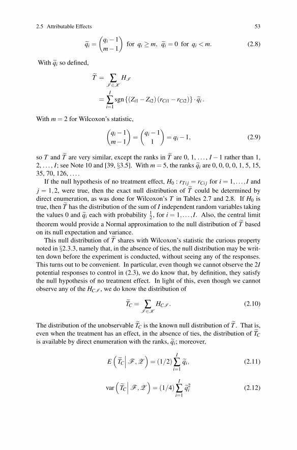
2.5 Attributable Effects 53
qi =(
qi −1
m−1
)for qi ≥ m, qi = 0 for qi < m. (2.8)
With qi so defined,
T = ∑I∈K
HI
=I
∑i=1
sgn{(Zi1 −Zi2)(rCi1 − rCi2)} · qi .
With m = 2 for Wilcoxon’s statistic,(qi −1
m−1
)=
(qi −1
1
)= qi −1, (2.9)
so T and T are very similar, except the ranks in T are 0, 1, . . . , I −1 rather than 1,
2, . . . , I; see Note 10 and [39, §3.5]. With m = 5, the ranks qi are 0, 0, 0, 0, 1, 5, 15,
35, 70, 126, . . . .
If the null hypothesis of no treatment effect, H0 : rTi j = rCi j for i = 1, . . . , I and
j = 1,2, were true, then the exact null distribution of T could be determined by
direct enumeration, as was done for Wilcoxon’s T in Tables 2.7 and 2.8. If H0 is
true, then T has the distribution of the sum of I independent random variables taking
the values 0 and qi each with probability 12 , for i = 1, . . . , I. Also, the central limit
theorem would provide a Normal approximation to the null distribution of T based
on its null expectation and variance.
This null distribution of T shares with Wilcoxon’s statistic the curious property
noted in §2.3.3, namely that, in the absence of ties, the null distribution may be writ-
ten down before the experiment is conducted, without seeing any of the responses.
This turns out to be convenient. In particular, even though we cannot observe the 2Ipotential responses to control in (2.3), we do know that, by definition, they satisfy
the null hypothesis of no treatment effect. In light of this, even though we cannot
observe any of the HCI , we do know the distribution of
TC = ∑I∈K
HCI . (2.10)
The distribution of the unobservable TC is the known null distribution of T . That is,
even when the treatment has an effect, in the absence of ties, the distribution of TCis available by direct enumeration with the ranks, qi; moreover,
E(
TC
∣∣∣ F ,Z)
= (1/2)I
∑i=1
qi, (2.11)
var(
TC
∣∣∣ F ,Z)
= (1/4)I
∑i=1
q2i (2.12)

54 2 Causal Inference in Randomized Experiments
and the distribution of{
TC −E(
TC
∣∣∣ F ,Z)}
/
√var
(TC
∣∣∣ F ,Z)
converges in
distribution to the standard Normal distribution as I → ∞ with m fixed. Using this
known distribution of TC, find the smallest value tα such that Pr(
TC ≤ tα∣∣∣ F ,Z
)≥
1−α . For large I, the critical value tα is approximately
E(
TC
∣∣∣ F ,Z)
+Φ−1 (1−α)√
var(
TC
∣∣∣ F ,Z)
(2.13)
where Φ−1 (·) is the standard Normal quantile function, or
E(
TC
∣∣∣ F ,Z)
+1.65
√var
(TC
∣∣∣ F ,Z)
(2.14)
for α = 0.05.
Our interest is in the number A = T − TC of successes attributable to effects of
the treatment, where T can be calculated from the data and TC is not observed.
It is easy to see that Pr(
A ≥ T − tα∣∣∣ F ,Z
)≥ 1−α , where T − tα is something
that can be calculated, so A ≥ T − tα may be asserted with 1−α confidence.11 In
terms of proportions of successes rather than counts, the confidence statement is
A/ |K | ≥(
T − tα)
/ |K |.
Ties
Ties are a minor inconvenience. Among the I = 185 pairs in the NSW experi-
ment, there are 14 ties among the |Yi|, all with |Yi| = 0. Briefly, ties make the
procedure conservative, so A ≥ T − tα occurs with probability at least 1−α for
large I. Specifics follow. Although the distribution of TC is known in the absence
of ties, it is not known if ties occur, because the pattern of ties in the unobserv-
able (2.3) affects the distribution. For the observable T , it is natural to use av-
erage ranks, averaging the qi for pairs with tied |Yi|, and setting sgn(a) = 1 for
a > 0, sgn(a) = 12 for a = 0, sgn(a) = 0 for a < 0. Speaking informally, a tie for
the highest Ri1 −Ri for i ∈ I means one success is shared as a fractional success
equally among the tied values. The same thing cannot be done for TC because the
ties in (2.3) are not observed. Suppose that the unobserved TC allowed for ties in
the manner proposed for the observed T , but the distribution used to determine tαignored ties, using instead the ranks qi in (2.8) for qi = 1, 2, . . . , I; then the ex-
pectation is correct, E(
TC
∣∣∣ F ,Z)
= (1/2)∑Ii=1 qi or E
(TC/ |K |
∣∣∣ F ,Z)
= 12 ,
11 To see this, observe that: Pr(
A ≥ T − tα∣∣∣ F ,Z
)= Pr
(T − TC ≥ T − tα
∣∣∣ F ,Z)
=
Pr(
TC ≤ tα∣∣∣ F ,Z
)≥ 1−α by the definition of tα . The assertion A ≥ T − tα is a confidence
interval for an unobservable random variable. Confidence sets for random variables are less famil-iar than confidence sets for parameters, but they are hardly new; see, for instance, Weiss [61].
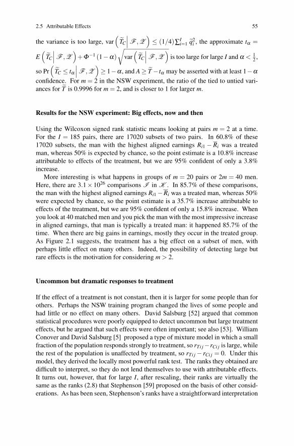
2.5 Attributable Effects 55
the variance is too large, var(
TC
∣∣∣ F ,Z)≤ (1/4)∑I
i=1 q2i , the approximate tα =
E(
TC
∣∣∣ F ,Z)
+Φ−1 (1−α)√
var(
TC
∣∣∣ F ,Z)
is too large for large I and α < 12 ,
so Pr(
TC ≤ tα∣∣∣ F ,Z
)≥ 1−α , and A ≥ T − tα may be asserted with at least 1−α
confidence. For m = 2 in the NSW experiment, the ratio of the tied to untied vari-
ances for T is 0.9996 for m = 2, and is closer to 1 for larger m.
Results for the NSW experiment: Big effects, now and then
Using the Wilcoxon signed rank statistic means looking at pairs m = 2 at a time.
For the I = 185 pairs, there are 17020 subsets of two pairs. In 60.8% of these
17020 subsets, the man with the highest aligned earnings Ri1 − Ri was a treated
man, whereas 50% is expected by chance, so the point estimate is a 10.8% increase
attributable to effects of the treatment, but we are 95% confident of only a 3.8%
increase.
More interesting is what happens in groups of m = 20 pairs or 2m = 40 men.
Here, there are 3.1× 1026 comparisons I in K . In 85.7% of these comparisons,
the man with the highest aligned earnings Ri1 −Ri was a treated man, whereas 50%
were expected by chance, so the point estimate is a 35.7% increase attributable to
effects of the treatment, but we are 95% confident of only a 15.8% increase. When
you look at 40 matched men and you pick the man with the most impressive increase
in aligned earnings, that man is typically a treated man: it happened 85.7% of the
time. When there are big gains in earnings, mostly they occur in the treated group.
As Figure 2.1 suggests, the treatment has a big effect on a subset of men, with
perhaps little effect on many others. Indeed, the possibility of detecting large but
rare effects is the motivation for considering m > 2.
Uncommon but dramatic responses to treatment
If the effect of a treatment is not constant, then it is larger for some people than for
others. Perhaps the NSW training program changed the lives of some people and
had little or no effect on many others. David Salsburg [52] argued that common
statistical procedures were poorly equipped to detect uncommon but large treatment
effects, but he argued that such effects were often important; see also [53]. William
Conover and David Salsburg [5] proposed a type of mixture model in which a small
fraction of the population responds strongly to treatment, so rTi j−rCi j is large, while
the rest of the population is unaffected by treatment, so rTi j − rCi j = 0. Under this
model, they derived the locally most powerful rank test. The ranks they obtained are
difficult to interpret, so they do not lend themselves to use with attributable effects.
It turns out, however, that for large I, after rescaling, their ranks are virtually the
same as the ranks (2.8) that Stephenson [59] proposed on the basis of other consid-
erations. As has been seen, Stephenson’s ranks have a straightforward interpretation

56 2 Causal Inference in Randomized Experiments
in terms of attributable effects. This subject is developed in detail in Chapter 16 and
[49]. In short, the methods described in this section are well adapted to the study
of uncommon but dramatic responses to treatment of the type that seem to have
occurred in the NSW experiment.
2.6 Internal and External Validity
In Fisher’s theory of randomized experiments, the inference is from the responses
the 2I subjects did exhibit under the treatments they did receive, and it is to the
2I unobserved responses these same individuals would have exhibited had they re-
ceived the alternative treatment. In brief, the inference concerns the unobservable
causal effects rTi j − rCi j for the 2I individuals in the experiment. See, for instance,
Welch [62].
A distinction is often made between ‘internal’ and ‘external’ validity [54]. A
randomized experiment is said to have a high level of ‘internal validity’ in the sense
that randomization provides a strong or ‘reasoned’ basis for inference about the
effects of the treatment, rTi j − rCi j, on the 2I individuals in the experiment. Causal
inference is challenging even if one were only interested in these 2I individuals,
and randomization meets that specific challenge. Often, one is interested not just
in these 2I people, but in people generally, people on other continents, people who
will be born in the future. ‘External’ validity refers to the effects of the treatment
on people not included in the experiment.
For instance, suppose that four large hospitals, say in Europe and the United
States, cooperated in a randomized trial of two forms of surgery, with sixty day
mortality as the outcome. Properly conducted, the trial would provide a sound basis
for inference about the effects of the two forms of surgery on the 2I patients in this
one clinical trial. One might plausibly think that similar effects would be found
at other large hospitals in Europe and the United States, Canada, Japan and other
countries, but nothing in a statistical analysis based on four hospitals provides a
warrant for this plausible extrapolation. The extrapolation sounds plausible because
of what we know about surgeons and hospitals in these countries, not because data
from four cooperating hospitals provides a sound basis for extrapolation. Would
similar effects be found at the small ambulatory surgical centers that are increasingly
common in the United States and elsewhere? Will the same effects be found at large
hospitals ten years from now as other technologies improve? Statistical analysis of
a clinical trial at four large hospitals provides no warrant for these extrapolations,
although surgeons may be able to offer an informed guess. These questions refer to
the degree of external validity of the clinical trial.
The common view [54], which I share, is that internal validity comes first. If
you do not know the effects of the treatment on the individuals in your study, you
are not well-positioned to infer the effects on individuals you did not study who live
in circumstances you did not study. Randomization addresses internal validity. In
actual practice, external validity is often addressed by comparing the results of sev-

2.8 Further Reading 57
eral internally valid studies conducted in different circumstances at different times.
These issues also arise in observational studies, and so will be discussed at various
points later on.
2.7 Summary
The goal of causal inference in the NSW experiment is not to say that the earnings of
treated and control men differed systematically, but rather that the treatment was the
cause of the difference, so that if the treatment had been withheld from the treated
men, there would have been no systematic difference between the two groups. Many
statistical procedures can recognize a systematic difference, providing the sample
size is sufficiently large. Randomization plays a key role in experiments that study
the effects actually caused by a treatment.
The current chapter has done several things. It has introduced many elements
that randomized experiments and observational studies have in common, such as
treatment effects, treatment assignments and pretreatment covariates unaffected by
treatment. The chapter has discussed the large role played by random treatment
assignment in experiments in justifying, or warranting, or being the ‘reasoned ba-
sis’ for inference about effects caused by treatment. Without random assignment, in
observational studies, this justification or warrant or reasoned basis is absent. There-
fore, the chapter has framed the problem faced in an observational study, where the
goal is again to draw inferences about the effects caused by treatment, but treatments
were not assigned at random [4].
2.8 Further Reading
Randomized experimentation is due to Sir Ronald Fisher [13], whose book of 1935
is of continuing interest. David Cox and Nancy Reid [11] present a modern dis-
cussion of the theory of randomized experiments. For randomized clinical trials in
medicine, see [16, 38], and for experiments in the social sciences, see [3, 6]. Among
books that discuss permutation and randomization inferences, Erich Lehmann’s [32]
book is especially careful in distinguishing properties that follow from random as-
signment and properties that involve sampling a population. For causal effects as
comparisons of potential outcomes under alternative treatments, see the papers by
Jerzy Neyman [35], B.L. Welch [62] and Donald Rubin [50]. Donald Rubin’s paper
[50] is the first parallel, formal discussion of causal effects in randomized and obser-
vational studies. For three important illustrations of the enhanced clarity provided
by this approach, see [14, 15, 51]. Fisher [13], Welch [62], Kempthorne [28], Wilk
[64], Cox [9], Robinson [40], and many others viewed sampling models as approx-
imations to randomization inferences. Randomization inference is, of course, not

58 2 Causal Inference in Randomized Experiments
limited to matched pairs [32, 44] and it may be used in conjunction with general
forms of covariance adjustment [45, 56].
In labor economics, the National Supported Work experiment became a small
laboratory for methods for observational studies when Robert LaLonde [29] set
aside the randomized control group and replaced it with a nonrandomized control
group drawn from a survey; see [12, 18, 19, 29, 57] for discussion.
2.9 Appendix: Randomization Distribution of m-statistics
Giving observations controlled weight using a ψ function
Sections 2.3.2 and 2.3.3 were similar in structure, even though the sample mean Yand Wilcoxon’s signed rank statistic are not similar as statistics. It was suggested in
§2.3.3 that randomization inference is very general and virtually any statistic could
be handled in a parallel manner. This is illustrated using another statistic, an m-test,
that is, a test associated with Peter Huber’s [25] m-estimates. The discussion here
derives from a paper by J. S. Maritz [33]; see also [34, 48]. It should be emphasized
that the statistics used in m-tests differ in small but consequential ways from the
statistics used in m-estimation, and the description that follows is for m-tests.12
As in Huber’s m-estimation of a location parameter, Maritz’s test statistic in-
volves a function ψ (·) that gives weights to scaled observations. Rather than ‘re-
ject outliers’ from a statistical analysis, a suitable ψ-function gradually reduces the
weight of observations as they become increasingly extreme. Because we want an
observation that is high by 3 units to pull up as strongly as an observation that is
low by 3 units pulls down, the function ψ (·) is required to be an odd function,
meaning ψ (−y) = −ψ (y) for every y ≥ 0, so in particular ψ (−3) = −ψ (3) and
ψ (0) = 0. For testing and confidence intervals, it is wise to insist that ψ (·) be
monotone increasing, so y < y′ implies ψ (y) ≤ ψ (y′). One such function, similar
to a trimmed mean, was proposed by Huber; it has ψ (y) = max{−1,min(y, 1)}, so
that ψ (y) = −1 for y < −1, ψ (y) = y for −1 ≤ y ≤ 1, and ψ (y) = 1 for y > 1. In
effect, the mean Y has a ψ (·) function of ψ (y) = y.
Consider using the treated-minus-control differences in paired responses, Yi =(Zi1 −Zi2)(Ri1 −Ri2), in testing the hypothesis of an additive treatment effect, H0 :
rTi j = τ0 + rCi j, for all i j, where τ0 is a specified number. When τ0 = 0, this is
12 The difference involves the scaling factor. In estimation, the scaling factor might be the medianabsolute deviation from the sample median. In testing, the scaling factor might be the medianabsolute deviation from the hypothesized median, which for testing no effect is zero. In testinga hypothesis, one can presume the hypothesis is true for the purpose of testing it. By using thehypothesized median rather than the sample median, the scaling factor becomes fixed as the treat-ment assignments vary — as illustrated later — with the consequence that Maritz’s statistic has anull randomization distribution that is the sum of independent bounded random variables, and thisgreatly simplifies the creation of a large sample approximation to the null randomization distribu-tion. This small difference has various consequences that should be considered before designing anew m-test; see [33, 48] for discussion.
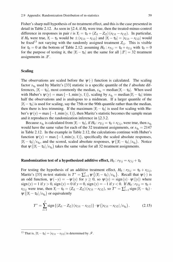
2.9 Appendix: Randomization Distribution of m-statistics 59
Fisher’s sharp null hypothesis of no treatment effect, and this is the case presented in
detail in Table 2.12. As seen in §2.4, if H0 were true, then the treated-minus-control
difference in responses in pair i is Yi = τ0 +(Zi1 −Zi2)(rCi1 − rCi2). In particular,
if H0 were true, Yi − τ0 would be ±(rCi1 − rCi2) and |Yi − τ0| = |rCi1 − rCi2| would
be fixed13 not varying with the randomly assigned treatment Zi j. This is visible
for τ0 = 0 at the bottom of Table 2.12: assuming H0 : rTi j = τ0 + rCi j with τ0 = 0
for the purpose of testing it, the |Yi − τ0| are the same for all |Z | = 32 treatment
assignments in Z .
Scaling
The observations are scaled before the ψ (·) function is calculated. The scaling
factor sτ0used by Maritz’s [33] statistic is a specific quantile of the I absolute dif-
ferences, |Yi − τ0|, most commonly the median, sτ0= median |Yi − τ0|. When used
with Huber’s ψ (y) = max{−1,min(y, 1)}, scaling by sτ0= median |Yi − τ0| trims
half the observations and is analogous to a midmean. If a larger quantile of the
|Yi − τ0| is used for scaling, say the 75th or the 90th quantile rather than the median,
then there is less trimming. If the maximum |Yi − τ0| is used for scaling with Hu-
ber’s ψ (y) = max{−1,min(y, 1)}, then Maritz’s statistic becomes the sample mean
and it reproduces the randomization inference in §2.3.2.
Because sτ0is calculated from |Yi − τ0|, if H0 : rTi j = τ0 +rCi j, were true, then sτ0
would have the same value for each of the 32 treatment assignments, or sτ0= 2147
in Table 2.12. In the example in Table 2.12, the calculations continue with Huber’s
function ψ (y) = max{−1,min(y, 1)}, specifically the scaled absolute responses,
|Yi − τ0|/sτ0, and the scored, scaled absolute responses, ψ
(|Yi − τ0|/sτ0
). Notice
that ψ(|Yi − τ0|/sτ0
)takes the same value for all 32 treatment assignments.
Randomization test of a hypothesized additive effect, H0 : rTi j = rCi j + τ0
For testing the hypothesis of an additive treatment effect, H0 : rTi j = τ0 + rCi j,
Maritz’s [33] m-test statistic is T ∗ = ∑Ii=1 ψ
{(Yi − τ0)/sτ0
}. Recall that ψ (·) is
an odd function, ψ (−y) = −ψ (y) for y ≥ 0, so ψ (y) = sign(y) · ψ (|y|) where
sign(y) = 1 if y > 0, sign(y) = 0 if y = 0, sign(y) =−1 if y < 0. If H0 : rTi j = τ0 +rCi j were true, then Yi − τ0 = (Zi1 −Zi2)(rCi1 − rCi2), so T ∗ = ∑I
i=1 sign(Yi − τ0) ·ψ
(|Yi − τ0|/sτ0
)or equivalently
T ∗ =I
∑i=1
sign{(Zi1 −Zi2)(rCi1 − rCi2)} ·ψ(|rCi1 − rCi2|/sτ0
). (2.15)
13 That is, |Yi − τ0| = |rCi1 − rCi2| is determined by F .

60 2 Causal Inference in Randomized Experiments
Table 2.12 The possible treated-minus-control differences in adjusted responses Yi − τ0 = (Zi1 −Zi2)(rCi1 − rCi2) and Huber-Maritz m-statistic, T ∗, under the null hypothesis of an additive treat-ment effect, H0 : rTi j = rCi j + τ0, for τ0 = 0 for the small version of the NSW experiment withI = 5 pairs.
Label Pair 1 Pair 2 Pair 3 Pair 4 Pair 5 Huber-MaritzY1 − τ0 Y2 − τ0 Y3 − τ0 Y4 − τ0 Y5 − τ0 T ∗
1 1456 3988 −45 −2147 3173 1.662 1456 3988 −45 −2147 −3173 −0.343 1456 3988 −45 2147 3173 3.664 1456 3988 −45 2147 −3173 1.665 1456 3988 45 −2147 3173 1.706 1456 3988 45 −2147 −3173 −0.307 1456 3988 45 2147 3173 3.708 1456 3988 45 2147 −3173 1.709 1456 −3988 −45 −2147 3173 −0.34
10 1456 −3988 −45 −2147 −3173 −2.3411 1456 −3988 −45 2147 3173 1.6612 1456 −3988 −45 2147 −3173 −0.3413 1456 −3988 45 −2147 3173 −0.3014 1456 −3988 45 −2147 −3173 −2.3015 1456 −3988 45 2147 3173 1.7016 1456 −3988 45 2147 −3173 −0.3017 −1456 3988 −45 −2147 3173 0.3018 −1456 3988 −45 −2147 −3173 −1.7019 −1456 3988 −45 2147 3173 2.3020 −1456 3988 −45 2147 −3173 0.3021 −1456 3988 45 −2147 3173 0.3422 −1456 3988 45 −2147 −3173 −1.6623 −1456 3988 45 2147 3173 2.3424 −1456 3988 45 2147 −3173 0.3425 −1456 −3988 −45 −2147 3173 −1.7026 −1456 −3988 −45 −2147 −3173 −3.7027 −1456 −3988 −45 2147 3173 0.3028 −1456 −3988 −45 2147 −3173 −1.7029 −1456 −3988 45 −2147 3173 −1.6630 −1456 −3988 45 −2147 −3173 −3.6631 −1456 −3988 45 2147 3173 0.3432 −1456 −3988 45 2147 −3173 −1.66
All Absolute Differences |Yi − τ0|1–32 1456 3988 45 2147 3173
All Scaled Absolute Differences |Yi − τ0|/sτ0
1–32 0.68 1.86 0.02 1.00 1.48
All Scored, Scaled Absolute Differences ψ(|Yi − τ0|/sτ0)
1–32 0.68 1.00 0.02 1.00 1.00
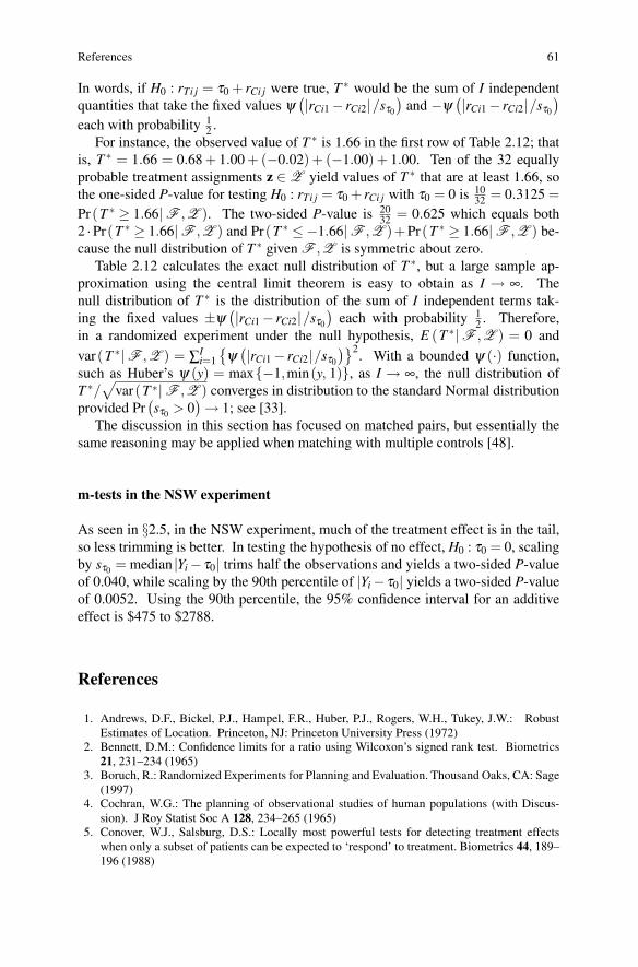
References 61
In words, if H0 : rTi j = τ0 + rCi j were true, T ∗ would be the sum of I independent
quantities that take the fixed values ψ(|rCi1 − rCi2|/sτ0
)and −ψ
(|rCi1 − rCi2|/sτ0
)each with probability 1
2 .
For instance, the observed value of T ∗ is 1.66 in the first row of Table 2.12; that
is, T ∗ = 1.66 = 0.68 + 1.00 + (−0.02) + (−1.00) + 1.00. Ten of the 32 equally
probable treatment assignments z ∈ Z yield values of T ∗ that are at least 1.66, so
the one-sided P-value for testing H0 : rTi j = τ0 + rCi j with τ0 = 0 is 1032 = 0.3125 =
Pr(T ∗ ≥ 1.66| F ,Z ). The two-sided P-value is 2032 = 0.625 which equals both
2 ·Pr(T ∗ ≥ 1.66| F ,Z ) and Pr(T ∗ ≤ −1.66| F ,Z )+Pr(T ∗ ≥ 1.66| F ,Z ) be-
cause the null distribution of T ∗ given F ,Z is symmetric about zero.
Table 2.12 calculates the exact null distribution of T ∗, but a large sample ap-
proximation using the central limit theorem is easy to obtain as I → ∞. The
null distribution of T ∗ is the distribution of the sum of I independent terms tak-
ing the fixed values ±ψ(|rCi1 − rCi2|/sτ0
)each with probability 1
2 . Therefore,
in a randomized experiment under the null hypothesis, E (T ∗| F ,Z ) = 0 and
var(T ∗| F ,Z ) = ∑Ii=1
{ψ
(|rCi1 − rCi2|/sτ0
)}2. With a bounded ψ (·) function,
such as Huber’s ψ (y) = max{−1,min(y, 1)}, as I → ∞, the null distribution of
T ∗/√
var(T ∗| F ,Z ) converges in distribution to the standard Normal distribution
provided Pr(sτ0
> 0) → 1; see [33].
The discussion in this section has focused on matched pairs, but essentially the
same reasoning may be applied when matching with multiple controls [48].
m-tests in the NSW experiment
As seen in §2.5, in the NSW experiment, much of the treatment effect is in the tail,
so less trimming is better. In testing the hypothesis of no effect, H0 : τ0 = 0, scaling
by sτ0= median |Yi − τ0| trims half the observations and yields a two-sided P-value
of 0.040, while scaling by the 90th percentile of |Yi − τ0| yields a two-sided P-value
of 0.0052. Using the 90th percentile, the 95% confidence interval for an additive
effect is $475 to $2788.
References
1. Andrews, D.F., Bickel, P.J., Hampel, F.R., Huber, P.J., Rogers, W.H., Tukey, J.W.: RobustEstimates of Location. Princeton, NJ: Princeton University Press (1972)
2. Bennett, D.M.: Confidence limits for a ratio using Wilcoxon’s signed rank test. Biometrics21, 231–234 (1965)
3. Boruch, R.: Randomized Experiments for Planning and Evaluation. Thousand Oaks, CA: Sage(1997)
4. Cochran, W.G.: The planning of observational studies of human populations (with Discus-sion). J Roy Statist Soc A 128, 234–265 (1965)
5. Conover, W.J., Salsburg, D.S.: Locally most powerful tests for detecting treatment effectswhen only a subset of patients can be expected to ‘respond’ to treatment. Biometrics 44, 189–196 (1988)

62 2 Causal Inference in Randomized Experiments
6. Cook, T.D., Shadish, W.R.: Social experiments: Some developments over the past fifteenyears. Annu Rev Psychol 45, 545–580 (1994)
7. Couch, K.A.: New evidence on the long-term effects of employment training programs. JLabor Econ 10, 380–388. (1992)
8. Cox, D.R.: Planning of Experiments. New York: Wiley (1958)9. Cox, D.R.: The interpretation of the effects of non-additivity in the Latin square. Biometrika
45, 69–73. (1958)10. Cox, D.R.: The role of significance tests. Scand J Statist 4, 49–62 (1977)11. Cox, D.R., Reid, N.: The Theory of the Design of Experiments. New York: Chapman and
Hall/CRC (2000)12. Dehejia, R.H., Wahba, W.: Causal effects in nonexperimental studies: Reevaluating the eval-
uation of training programs. J Am Statist Assoc 94, 1053–1062 (1999)13. Fisher, R.A.: Design of Experiments. Edinburgh: Oliver and Boyd (1935)14. Frangakis, C.E., Rubin, D.B.: Principal stratification in causal inference. Biometrics 58, 21–
29 (2002)15. Freedman, D.A.: Randomization does not justify logistic regression. Statist Sci 23, 237–249
(2008)16. Friedman, L.M., DeMets, D.L., Furberg, C.D.: Fundamentals of Clinical Trials. New York:
Springer (1998)17. Greevy, R., Lu, B., Silber, J.H., Rosenbaum, P.R.: Optimal matching before randomization.
Biostatistics 5, 263–275 (2004)18. Hamalainen, K., Uusitalo, R., Vuori, J.: Varying biases in matching estimates: Evidence from
two randomized job search training experiments. Labour Econ 15, 604–618 (2008)19. Heckman, J.J., Hotz, V.J.: Choosing among alternative nonexperimental methods for estimat-
ing the impact of social programs: The case of manpower training (with Discussion). J AmStatist Assoc 84, 862–874 (1989)
20. Hodges, J.L., Lehmann, E.L.: Rank methods for combination of independent experiments inanalysis of variance. Ann Math Statist 33, 482–497 (1962)
21. Hodges, J.L., Lehmann, E.L.: Estimates of location based on ranks. Ann Math Statist 34,598–611 (1963)
22. Hoeffding, W.: A class of statistics with asymptotically normal distributions. Ann Math Statist19, 293–325 (1948)
23. Holland, P.W.: Statistics and causal inference. J Am Statist Assoc 81, 945–960 (1986)24. Hollister, R., Kemper, P., Maynard, R., eds.: The National Supported Work Demonstration.
Madison: University of Wisconsin Press (1984)25. Huber, P.J.: Robust estimation of a location parameter. Ann Math Statist 35, 73–101 (1964)26. Hudgens, M.G., Halloran, M.E.: Toward causal inference with interference. J Am Statist Assoc
482, 832–842 (2008)27. Jureckova, J., Sen, P.K.: Robust Statistical Procedures. New York: Wiley (1996)28. Kempthorne, O.: Design and Analysis of Experiments. New York: Wiley (1952)29. LaLonde, R.J.: Evaluating the econometric evaluations of training programs with experimental
data. Am Econ Rev 76, 604–620 (1986)30. LaLonde, R.J.: The promise of public sector-sponsored training programs. J Econ Perspec 9,
149–168 (1995)31. Lehmann, E.L.: Testing Statistical Hypotheses. New York: Wiley (1959)32. Lehmann, E.L.: Nonparametrics. San Francisco: Holden-Day (1975)33. Maritz, J.S.: A note on exact robust confidence intervals for location. Biometrika 66, 163–166
(1979)34. Maritz, J.S.: Distribution-Free Statistical Methods. London: Chapman and Hall (1995)35. Neyman, J.: On the application of probability theory to agricultural experiments: Essay on
principles, Section 9. In Polish, but reprinted in English with Discussion by T. Speed and D.B. Rubin in Statist Sci 5, 463–480 (1923, reprinted 1990)
36. Nichols, T.E., Holmes, A.P.: Nonparametric permutation tests for functional neuroimaging.Human Brain Mapping 15, 1–25.

References 63
37. Pagano, M., Tritchler, D.: On obtaining permutation distributions in polynomial time. J AmStatist Assoc 78, 435–440 (1983)
38. Piantadosi, S.: Clinical Trials. New York: Wiley (2005)39. Pratt, J.W., Gibbons, J.D.: Concepts of Nonparametric Theory. New York: Springer (1981)40. Robinson, J.: The large sample power of permutation tests for randomization models. Ann
Statist 1, 291–296 (1973)41. Rosenbaum, P.R.: The consequences of adjustment for a concomitant variable that has been
affected by the treatment. J Roy Statist Soc A 147, 656–666 (1984)42. Rosenbaum, P.R.: Effects attributable to treatment: Inference in experiments and observational
studies with a discrete pivot. Biometrika 88, 219–231 (2001)43. Rosenbaum, P.R.: Attributing effects to treatment in matched observational studies. J Am
Statist Assoc 97, 183–192 (2002)44. Rosenbaum, P.R.: Observational Studies (2nd ed.). New York: Springer (2002)45. Rosenbaum, P.R.: Covariance adjustment in randomized experiments and observational stud-
ies (with Discussion). Statist Sci 17, 286–327 (2002)46. Rosenbaum, P.R.: Exact confidence intervals for nonconstant effects by inverting the signed
rank test. Am Statistician 57,132–138 (2003)47. Rosenbaum, P.R.: Interference between units in randomized experiments. J Am Statist Assoc
102, 191–200 (2007)48. Rosenbaum, P.R.: Sensitivity analysis for m-estimates, tests, and confidence intervals in
matched observational studies. Biometrics 63, 456-464 (2007)49. Rosenbaum, P.R.: Confidence intervals for uncommon but dramatic responses to treatment.
Biometrics 63, 1164–1171 (2007)50. Rubin, D.B.: Estimating causal effects of treatments in randomized and nonrandomized stud-
ies. J Educ Psychol 66, 688–701 (1974)51. Rubin, D.B., Stuart, E.A., Zanutto, E.L.: A potential outcomes view of value-added assessment
in education. J Educ Behav Statist 29, 103–116 (2004)52. Salsburg, D.S.: Alternative hypotheses for the effects of drugs in small-scale clinical studies.
Biometrics 42, 671–674 (1986)53. Salsburg, D.S.: The Use of Restricted Significance Tests in Clinical Trials. New York:
Springer (1992)54. Shadish, W. R., Cook, T. D., Campbell, D. T.: Experimental and Quasi-Experimental Designs
for Generalized Causal Inference. Boston: Houghton-Mifflin (2002)55. Shaffer, J.P.: Bidirectional unbiased procedures. J Am Statist Assoc 69, 437–439 (1974)56. Small, D., Ten Have, T.R., Rosenbaum, P.R.: Randomization inference in a group-randomized
trial of treatments for depression: covariate adjustment, noncompliance and quantile effects.J Am Statist Assoc 103, 271-279 (2007)
57. Smith, J.A., Todd, P.E.: Does matching overcome LaLonde’s critique of nonexperimental es-timators? J Econometrics 125, 305–353 (2005)
58. Sobel, M.E.: What do randomized studies of housing mobility demonstrate?: Causal inferencein the face of interference. J Am Statist Assoc 476, 1398–1407 (2006)
59. Stephenson, W.R.: A general class of one-sample nonparametric test statistics based on sub-samples. J Am Statist Assoc 76, 960–966 (1981)
60. Tobin, J.: Estimation of relationships for limited dependent variables. Econometrica 26, 24–36 (1958)
61. Weiss, L.: A note on confidence sets for random variables. Ann Math Statist 26, 142–144(1955)
62. Welch, B.L.: On the z-test in randomized blocks and Latin squares. Biometrika 29, 21–52(1937)
63. Wilcoxon, F.: Individual comparisons by ranking methods. Biometrics 1, 80–83 (1945)64. Wilk, M.B.: The randomization analysis of a generalized randomized block design.
Biometrika 42, 70–79 (1955)
Chapter 3Two Simple Models for Observational Studies
Abstract Observational studies differ from experiments in that randomization is
not used to assign treatments. How were treatments assigned? This chapter intro-
duces two simple models for treatment assignment in observational studies. The first
model is useful but naıve: it says that people who look comparable are comparable.
The second model speaks to a central concern in observational studies: people who
look comparable in the observed data may not actually be comparable; they may
differ in ways we did not observe.
3.1 The Population Before Matching
In the population before matching, there are L subjects, � = 1, 2, . . . , L. Like
the subjects in the randomized experiment in Chapter 2, each of these L subjects
has an observed covariate x�, an unobserved covariate u�, an indicator of treat-
ment assignment, Z�, where Z� = 1 if the subject receives treatment or Z� = 0 if
the subject receives the control, a potential response to treatment, rT �, which is
seen if the subject receives treatment, Z� = 1, a potential response to control, rC�,
which is seen if the subject receives the control, Z� = 0, and an observed response,
R� = Z� rT � + (1−Z�) rC�. Now, however, treatments Z� are not assigned by the
equitable flip of a fair coin.
In the population before matching, we imagine that subject � received treatment
with probability π�, independently of other subjects, where π� may vary from one
person to the next and is not known. More precisely,
π� = Pr(Z� = 1 | rT �, rC�, x�, u�) , (3.1)
Pr(Z1 = z1, . . . ,ZL = zL|rT 1, rC1, x1, u1, . . . ,rT L, rCL, xL, uL)
= πz11 (1−π1)
1−z1 · · ·πzLL (1−πL)1−zL = Π L
�=1 πz�� (1−π�)
1−z� .
65P.R. Rosenbaum, Design of Observational Studies, Springer Series in Statistics, DOI 10.1007/978-1-4419-1213-8_3, © Springer Science+Business Media, LLC 2010

66 3 Two Simple Models for Observational Studies
It is natural to ask whether very little or a great deal has just been assumed.
One might reasonably worry if a great deal has just been assumed, for perhaps the
central problems in observational studies have just been assumed away. Addressing
difficult problems by assuming they are not there is one of the less reliable tactics,
so it is reasonable to seek some assurance that this has not just happened. Indeed,
it has not. Actually, because of the delicate nature of unobserved variables, nothing
at all has been assumed: there is always an unobserved u� that makes all of this
true, and true in a fairly trivial way. Specifically, if we set u� = Z�, then π� =Pr(Z� = 1 | rT �, rC�, x�, u�) is Pr(Z� = 1 | rT �, rC�, x�, Z�) which is, of course, π� = 1
if Z� = 1 and π� = 0 if Z� = 0; moreover, with π� so defined, Π L�=1 πz�
� (1−π�)1−z� is
1 for the observed treatment assignment and 0 for all other treatment assignments,
and
Pr(Z1 = z1, . . . ,ZL = zL|rT 1, rC1, x1, u1, . . . ,rT L, rCL, xL, uL)
= Pr(Z1 = z1, . . . ,ZL = zL|rT 1, rC1, x1, Z1, . . . ,rT L, rCL, xL, ZL)
is also 1 for the observed treatment assignment and 0 for all other treatment as-
signments; so it’s all true, in a trivial way, with u� = Z�. Until something is done to
restrict the behavior of the unobserved covariate u�, nothing has been assumed: (3.1)
is a representation, not a model, because there is always some u� that makes (3.1)
true. A representation, such as (3.1), is a manner of speaking; it does not become a
model until it says something that may be false.
3.2 The Ideal Matching
Imagine that we could find two subjects, say k and �, such that exactly one was
treated, Zk + Z� = 1, but they had the same probability of treatment, πk = π�, and
we made those two subjects into a matched pair.1 Obviously, it is something of a
challenge to create this matched pair because we do not observe uk and u�, and we
observe either rT k or rCk but not both, and either rT � or rC� but not both. It is a chal-
lenge because we cannot create this pair by matching on observable quantities. We
could create this pair by matching on the observable x, so xk = x�, and then flipping
a fair coin to determine (Zk,Z�), assigning one member of the pair to treatment, the
other to control; that is, we could create this pair by conducting a randomized paired
experiment, as in Chapter 2. Indeed, with the aid of random assignment, matching
on x may be prudent [27], but is not necessary to achieve πk = π� because the π’s
are created by the experimenter. If randomization is infeasible or unethical, then
1 The alert reader will notice that the supposition that there could be two subjects, k and �, withZk + Z� = 1 but πk = π� is already a step beyond the mere representation in (3.1), because itprecludes setting ui = Zi for all i and instead requires 0 < πi < 1 for at least two subjects.

3.2 The Ideal Matching 67
how might one attempt to find a treated-control pair such that the paired units have
the same probability of treatment, πk = π�?
Return for a moment to the study by Joshua Angrist and Victor Lavy [3] of class
size and educational test performance, and in particular to the I = 86 pairs of Israeli
schools in §1.3, one with between 31 and 40 students in the fifth grade (Z = 0), the
other with between 41 and 50 students in the fifth grade (Z = 1), the pairs being
matched for a covariate x, namely the percentage of disadvantaged students. Strict
adherence to Maimonides’ rule would require the slightly larger fifth grade cohorts
to be taught in two small classes, and the slightly smaller fifth grade cohorts to be
taught in one large class. As seen in Figure 1.1, adherence to Maimonides’ rule
was imperfect but strict enough to produce a wide separation in typical class size.
In their study, (rT , rC) are average test scores in fifth grade if the fifth grade co-
hort was a little larger (Z = 1) or a little smaller (Z = 0). What separates a school
with a slightly smaller fifth grade cohort (Z = 0, 31–40 students) and a school with a
slightly larger fifth grade cohort (Z = 1, 41–50 students)? Well, what separates them
is the enrollment of a handful of students in grade 5. It seems reasonably plausible
that whether or not a few more students enroll in the fifth grade is a relatively hap-
hazard event, an event not strongly related to the average test performance (rT , rC)that the fifth grade would exhibit with a larger or smaller cohort. That is, building
a study in the way that Angrist and Lavy did, it does seem reasonably plausible that
πk and π� are fairly close in the I = 86 matched pairs of two schools.
Properly understood, a ‘natural experiment’ is an attempt to find in the world
some rare circumstance such that a consequential treatment was handed to some
people and denied to others for no particularly good reason at all, that is, hap-
hazardly [2, 7, 31, 47, 58, 83, 92, 96, 102, 106]. The word ‘natural’ has various
connotations, but a ‘natural experiment’ is a ‘wild experiment’ not a ‘wholesome
experiment,’ natural in the way that a tiger is natural, not in the way that oatmeal is
natural. To express the same thought differently: to say that ‘it does seem reason-
ably plausible that πk and π� are fairly close’ is to say much less than ‘definitely,
πk = π� by the way treatments were randomly assigned.’ Haphazard is a far cry
from randomized, a point given proper emphasis by Mark Rosenzweig and Ken
Wolpin [92] and by Timothy Besley and Anne Case [7] in reviews of several natural
experiments.
Nonetheless, it does seem reasonable to think that πk and π� are fairly close for
the 86 paired Israeli schools in Figure 1.1. This might be implausible in some other
context, say in a national survey in the United States where schools are funded by
local governments, so that class size might be predicted by the wealth or poverty
of the local community. Even in the Israeli schools, the claim that πk and π� are
plausibly close depended upon: (i) matching for the percentage of students who
were disadvantaged, xk, and (ii) defining Zk in terms of cohort size rather than class
size. In the pair of boxplots on the upper right of Figure 1.1 depicting class size and
cohort size, there is considerable adherence to Maimonides’ rule, but there are a few
deviations: in particular, two large fifth grade cohorts that strict adherence to the rule
would have divided, and several small cohorts that were taught in smaller classes
than strict adherence to the rule would have permitted. Small variations in the size

68 3 Two Simple Models for Observational Studies
of the fifth grade cohort are plausibly haphazard, but deviations from Maimonides’
rule may have been deliberate, considered responses to special circumstances, and
hence not haphazard. As defined in Figure 1.1, Zk reflects the haphazard element,
namely susceptibility to Maimonides’ rule based on cohort size, rather than realized
class size. Defining Zk in this way is analogous to an ‘intention-to-treat’ analysis
(§1.2.6) in a randomized experiment.2
Suppose indeed we could find two subjects, k and �, with the same probability
of treatment, πk = π�, where the common value of πk and π� is typically unknown.
What would follow from this? From (3.1),
Pr(Zk = zk, Z� = z�|rT k, rCk, xk, uk, rT �, rC�, x�, u�) (3.2)
= πzkk (1−πk)
1−zk πz�� (1−π�)
1−z� (3.3)
= πzk+z�� (1−π�)
(1−zk)+(1−z�) because πk = π�, (3.4)
which is, so far, of limited use, because π� is unknown. Suppose, however, that we
found two subjects, k and �, with the same probability of treatment, πk = π�, with
precisely the additional fact that exactly one was treated, Zk + Z� = 1. Given that
one of these subjects was treated, the chance that it was k and not � would be
Pr(Zk = 1, Z� = 0 |rT k, rCk, xk, uk, rT �, rC�, x�, u�,Zk +Z� = 1)
=Pr(Zk = 1, Z� = 0 |rT k, rCk, xk, uk, rT �, rC�, x�, u�)
Pr(Zk + Z� = 1 |rT k, rCk, xk, uk, rT �, rC�, x�, u�)
=π1+0
� (1−π�)(1−1)+(1−0)
π1+0� (1−π�)
(1−1)+(1−0) +π0+1� (1−π�)
(1−0)+(1−1)
=π� (1−π�)
π� (1−π�)+π� (1−π�)=
1
2
which, unlike (3.2), would be immensely useful. If we could find among the L sub-
jects in the population a total of 2I different subjects matched in I pairs in just this
way, then we would have reconstructed the distribution of treatment assignments
Z in the paired, randomized experiment, and inference about the effects caused by
treatments would be straightforward; indeed, the methods of Chapter 2 would be
applicable.3 Keep in mind that we are speaking here about mere imaginings, sup-
positions, hopes, aspirations and attempts, as distinct from simple, undeniable facts
created by randomization in Chapter 2. In the words of the proverb: “If wishes were
horses, beggars would ride.”
2 As in §1.2.6, this definition of Zk leaves open the possibility of using cohort size Zk as an in-strument for the actual size of the class, and indeed Angrist and Lavy [3] reported instrumentalvariable analyses.3 The argument just presented is the simplest version of a general argument developed in [69].

3.2 The Ideal Matching 69
Where do things stand? As has been seen, the ideal matching would pair indi-
viduals, k and �, with different treatments, Zk + Z� = 1, but the same probability of
treatment, πk = π�. If we could do this, we could reconstruct a randomized exper-
iment from observational data; however, we cannot do this. The wise attempt to
find ‘natural experiments’ is the attempt to move towards this ideal. That is what
you do with ideals: you attempt to move towards them. No doubt, many if not most
‘natural experiments’ fail to produce this ideal pairing [7, 92]; moreover, even if one
‘natural experiment’ once succeeded, there would be no way of knowing for sure
that it had succeeded. A second attempt to approach the ideal is to find a context in
which the covariates used to determine treatment assignment are measured covari-
ates, xk, not unobserved covariates, u�, and then to match closely for the measured
covariates, xk.4 Matching for observed covariates is the topic of Part II of this book.
Although we cannot see πk and π� and so cannot see whether they are fairly close,
perhaps there are things we can see that provide an incomplete and partial check
on the closeness of πk and π�. This leads to the devices of ‘quasi-experiments’
[10, 12, 58, 97] mentioned in §1.2.4, such as multiple control groups [51, 75, 78],
‘multiple operationalism’ or coherence [12, 36, 63, 82, 105], ‘control constructs’
and known effects [57, 77, 78, 97, 110], and one or more pretreatment measures of
what will become the response.5 Even when it ‘seems reasonably plausible that πk
4 See, for instance, the argument made by David Gross and Nicholas Souleles, quoted in §4.2 fromtheir paper [29]. The example in Chapter 7 attempts to use both approaches, although it is, per-haps, not entirely convincing in either attempt. In Chapter 7, the dose of chemotherapy receivedby patients with ovarian cancer is varied by comparing two types of providers of chemotherapy,gynecological oncologists (GO) and medical oncologists (MO), where the latter treat more inten-sively. The most important clinical covariates are measured, including clinical stage, tumor grade,histology, and comorbid conditions. Despite these two good attempts, it is far from clear that theGO-vs-MO assignment is haphazard, even after adjustments, and it quite likely that the oncologistknew considerably more about the patient than is recorded in electronic form.5 Figure 1.2 is an example of quasi-experimental reasoning. Instead of comparing college atten-dance in two groups, say the children of deceased fathers in 1979–1981, when the benefit programwas available, and the children of deceased fathers in 1982–1983, after the program was with-drawn, Figure 1.2 follows Susan Dynarski’s [20] study in comparing four groups. Figure 1.2shows at most a small shift in college attendance by the group of children without deceased fa-thers, who were never eligible for the program. This is a small check, but a useful one: it suggeststhat the comparison of children of deceased fathers in 1979–1981 and 1982–1983, though totallyconfounded with time, may not be seriously biased by this confounding, because a substantial shiftin college attendance by unaffected groups over this time is not evident. The quasi-experimentaldesign in Figure 1.2 is widely used, and is known by a variety of not entirely helpful names,including ‘pretest-posttest nonequivalent control group design’ and ‘difference-in-differences de-sign.’ Kevin Volpp and colleagues [108] used this design in a medical context to study the possibleeffects on patient mortality of a reduction, to 80 hours per week, of the maximum number of hoursthat a medical resident may work in a hospital. See [1, 5, 6, 11, 84] for discussion in general terms.
The study by Garen Wintemute and colleagues [112], as discussed in §4.3, contains another ex-ample of quasi-experimental reasoning using a ‘control construct,’ that is, an outcome thought tobe unaffected by the treatment. They were interested in the possible effects of a change in guncontrol laws on violent crimes using guns. One would not expect a change in gun control lawsto have a substantial effect on nonviolent, nongun crimes, and so the rate of such crimes is theircontrol construct or unaffected outcome. See §4.3. An example with two control groups subjectto different biases is discussed in §11.3.

70 3 Two Simple Models for Observational Studies
and π� are fairly close,’ we will need to ask about the consequences of being close
rather than equal, about the possibility they are somewhat less close than we had
hoped, about the possibility that they are disappointingly far apart. Answers are
provided by sensitivity analysis; see §3.4.
3.3 A Naıve Model: People Who Look Comparable AreComparable
Assigning treatments by flipping biased coins whose unknown biases aredetermined by observed covariates
The first of the two models in the title of this chapter asserts, rather naıvely, that
people who look comparable in terms of measured covariates, xk, actually are com-
parable, and to a nontrivial extent, an element of luck determined every treatment
assignment. Most observational studies report, perhaps briefly or perhaps at length,
at least one analysis that tentatively assumes that the naıve model is true. Most of
the controversy and skepticism associated with observational studies is a reference
of one sort or another to this model’s naıvete.
The naıve model restricts the representation (3.1) in two quite severe ways. First,
it says that treatment assignment probabilities, π� = Pr(Z� = 1 | rT �, rC�, x�, u�), that
condition on (rT �, rC�, x�, u�) may depend upon the observed covariates x� but not
upon the potential responses (rT �, rC�) or the unobserved covariate u�. Second, the
model says 0 < π� < 1 for all �, so that every person � has a chance of receiving
either treatment, Z� = 1, or control, Z� = 0. Putting this together with (3.1), the
naıve model says:
π� = Pr(Z� = 1 | rT �, rC�, x�, u�) = Pr(Z� = 1 | x�) (3.5)
and
0 < π� < 1, � = 1,2, . . . ,L, (3.6)
with
Pr(Z1 = z1, . . . ,ZL = zL|rT 1, rC1, x1, u1, . . . ,rT L, rCL, xL, uL) (3.7)
=L
∏�=1
πz�� (1−π�)
1−z� . (3.8)
The naıve model would be true if treatments Z� were assigned by independent
flips of a fair coin: then π� = 12 for � = 1,2, . . . ,L, and all of (3.5)–(3.8) is true. In-
deed, the naıve model would be true if treatments Z� were assigned by independent
flips of a group of biased coins, where the same biased coin is used whenever two
people, k and �, have the same observed covariate, xk = x�, and no coin has proba-
bility 1 or 0 of a head; then all of (3.5)–(3.8) is true. For (3.5)–(3.8) to be true, it is
not necessary that the biases of these coins be known, but it is necessary that the bias

3.3 A Naıve Model: People Who Look Comparable Are Comparable 71
depend on x� alone. The first feature of the model (3.5)–(3.8) says treatment assign-
ment Z is conditionally independent of (rT , rC,u) given x, or in Phillip Dawid’s [17]
notation, Z | | (rT , rC, u)∣∣∣ x. In [67], Donald Rubin and I gave the name ‘strongly
ignorable treatment assignment given x’ to this naıve model (3.5)–(3.8).6
As will be seen in a moment, it would be very convenient if the naıve model
(3.5)–(3.8) were true. If (3.5)–(3.8) were true, causal inference in an observational
study would become a mechanical problem, so that if the sample size were large, and
you followed certain steps, and you did not make mistakes in following the steps,
then a correct causal inference would result; a computer could do it. So it would
be convenient if (3.5)–(3.8) were true. To believe that something is true because it
would be convenient if it were true is a fair definition of naıvete.
The ideal match and the naıve model
If the naıve model were true, then the ideal match of §3.2 could be produced sim-
ply by matching treated and control subjects with the same value of the observed
covariate x. This follows immediately from (3.5)–(3.8) and the discussion in §3.2.
If the naıve model were true, one could reconstruct the distribution of treatment as-
signments Z in a randomized paired experiment from observational data simply by
matching for the observed covariates, x. Conventional methods of statistical anal-
ysis — the paired t-test, Wilcoxon’s signed rank test, m-estimates, etc. — would
work if (3.5)–(3.8) were true, and are quite likely to fail if (3.5)–(3.8) is false in a
nontrivial way.
6 Techincally, strongly ignorable treatment assigment given x is Z | | (rT , rC)∣∣∣ x and 0 <
Pr(Z = 1 | x) < 1 for all x, or in a single expression, 0 < Pr(Z = 1 | rT , rC, x) = Pr(Z = 1 | x) < 1for all x; that is, no explicit reference is made to an unobserved covariate u. I introduce u here,rather than in §3.4 where it is essential, to simplify the transition between §3.3 and §3.4. The re-mainder of this footnote is a slightly technical discussion of the formal relationship between (3.5)and the condition as given in [67]; it will interest only the insanely curious.
In a straightforward way [17, Lemma 3], condition (3.5) implies Z | | (rT , rC)∣∣∣ x and 0 <
Pr(Z = 1 | x) < 1 for all x. Also, in a straightforward way [17, Lemma 3], if (3.5) is true then (i)
Z | | (rT , rC)∣∣∣ (x,u), (ii) 0 < Pr(Z = 1 | x) < 1 for all x, and (iii) Z | | u
∣∣∣ x are true. Moreover,
(ii) and (iii) together imply (iv) 0 < Pr(Z = 1 | x,u) < 1 for all (x,u). In words, condition (3.5)implies both strong ignorability given x and also strong ignorability given (x,u). Now, conditions(i) and (iv), without condition (iii), are the key elements of the sensitivity model in §3.4: they say,that treatment assignment would have been strongly ignorable if u had been measured and includedwith x; so the failure to measure u is the source of our problems. Moreover, if condition (iii) weretrue in addition to (i) and (iv), then (3.5) and strong ignorability given x follow. In brief, strongignorability given x is implied by the addition of condition (iii) to strong ignorability given (x,u).In words, one can reasonably think of the naive model §3.3 as the sensitivity model of §3.4 together
with the irrelevance of u as expressed by Z | | u∣∣∣ x in condition (iii).

72 3 Two Simple Models for Observational Studies
What is the propensity score?
So far, the talk has been of matching exactly for x as if that were easy to do. If
x contains many covariates, then matching treated and control subjects with the
same or similar x will be difficult if not impossible. Imagine, for instance, that
x contains 20 covariates. Then any one subject, �, might be above or below the
median on the first covariate (two possibilities), above or below the median on the
second covariate (two more possibilities, making 2 × 2 = 4 possibilities so far),
and so on. Just in terms of being above or below the median on each covariate,
there are 2× 2× ·· · × 2 = 220 = 1,048,576 possibilities, or more than a million
possibilities. With thousands of subjects, it will often be difficult to find two subjects
who even match in the limited way of being on the same side of the median for all
20 covariates. This turns out to be less of a problem than it might seem at first,
because of a device called the ‘propensity score’ [67].
In a sample of L subjects from an infinite population, the propensity score [67]
is the conditional probability of treatment Z = 1 given the observed covariates x, or
e(x) = Pr(Z = 1 | x). Several aspects of this definition deserve immediate empha-
sis. The propensity score is defined in terms of the observed covariates, x, whether
or not the naıve model (3.5)–(3.8) is true, that is, whether or not the ‘ideal match’ of
§3.2 can be produced by matching on the observed covariates x. The form of (3.5)–
(3.8) correctly suggests that the propensity score e(x) = Pr(Z = 1 | x) will be more
useful when (3.5)–(3.8) is true; however, the propensity score is defined in terms
of the observable quantities, Z and x, whether or not (3.5)–(3.8) is true. In a ran-
domized experiment, the propensity score is known because of random assignment.
In contrast, in an observational study the propensity score is typically unknown;
however, because e(x) = Pr(Z = 1 | x) is defined in terms of observable quantities,
namely treatment assignment Z and observed covariates, x, it is straightforward to
estimate the propensity score in an observational study. In a randomized experi-
ment, π� in (3.1) is known and in an observational study π� is unknown, but because
π� depends upon the unobservable (rT , rC, u) as well as x, it is not possible to es-
timate π� in an observational study. Of course, if the naıve model (3.5)–(3.8) were
true, then π� = e(x�); indeed, this is virtually the defining feature of that model.
Balancing property of the propensity score
The propensity score has several useful properties. The first property, the balancing
property, is always true, whether or not the naıve model (3.5)–(3.8) is true. The bal-
ancing property [67] says that treated (Z = 1) and control (Z = 0) subjects with the
same propensity score e(x) have the same distribution of the observed covariates, x,
Pr{x | Z = 1, e(x)} = Pr{x | Z = 0, e(x)} (3.9)
or equivalently
Z | | x∣∣∣ e(x) , (3.10)

3.3 A Naıve Model: People Who Look Comparable Are Comparable 73
so treatment Z and observed covariates x are conditionally independent given the
propensity score.7
Because of the balancing property (3.10), if you pair two people, k and �, one
of whom is treated, Zk +Z� = 1, so that they have the same value of the propensity
score, e(xk) = e(x�), then they may have different values of the observed covariate,
xk �= x�, but in this pair, the specific values of the observed covariate (xk,x�) will
be unrelated to the treatment assignment (Zk,Z�). If you form many pairs in this
way, then the distribution of the observed covariates x will look about the same in
the treated (Z = 1) and control (Z = 0) groups, even though individuals in matched
pairs will typically have different values of x. Although it is difficult to match on 20
covariates at once, it is easy to match on one covariate, the propensity score e(x),and matching on e(x) will tend to balance all 20 covariates.
In the randomized NSW experiment in Chapter 2, Table 2.1 displayed balance on
observed covariates, x. Randomization alone tends to balance observed covariates,
x, and Table 2.1 combined randomization and matching. In an observational study,
it is often possible to match on an estimate e(x) of the propensity score e(x) and to
produce balance on observed covariates x similar to the balance in Table 2.1; see,
for example, Chapter 7.
Randomization is a much more powerful tool for balancing covariates than
matching on an estimate of the propensity score. The difference is that the propen-
sity score balances the observed covariates, x, whereas randomization balances
observed covariates, unobserved covariates, and potential responses, (rT , rC, x, u).This difference is not something you can see: randomization makes a promise about
something you cannot see. Stated formally, if you match on e(x), then Z | | x∣∣∣ e(x),
but if you assign treatments by flipping fair coins, then Z | | (rT , rC, x, u) . Random-
ization provides a basis for believing that an unobserved covariate u is balanced, but
matching on propensity scores provides no basis for believing that.
Part II of this book discusses the practical aspects of matching, and an estimate
e(x) of the propensity score e(x) is one of the tools used; see §8.2.8 In common
practice, the estimate of the propensity score, e(x), is based on a model, such as a
logit model, relating treatment assignment, Z, and observed covariates, x. The logit
model may include interactions, polynomials, and transformations of the covariates
in x, so it need not be a linear logit model narrowly conceived. Logit models for
e(x) are used for convenience; other methods can and have been used instead [56].
7 The proof is easy [67]. Recall the following basic facts about conditional expecta-tions: if A, B and C are random variables, then E (A) = E {E (A | B)} and E (A | C ) =E {E (A | B,C ) |C}. From the definition of conditional independence, to prove (3.10), it sufficesto prove Pr{Z = 1 | x, e(x)} = Pr{Z = 1 | e(x)}. Because e(x) is a function of x, conditioningon x fixes e(x), so Pr{Z = 1 | x, e(x)} = Pr(Z = 1 | x) = e(x). Because Z = 0 or Z = 1, for anyrandom variable D, we have Pr(Z = 1 | D) = E (Z | D). With A = Z, B = x, C = e(x), we havePr{Z = 1 | e(x)} = E {Z | e(x)} = E {E {Z | x, e(x)}| e(x)} = E {Pr{Z = 1 | x, e(x)}| e(x)}= E { e(x) | e(x)} = e(x) = Pr(Z = 1 | x), which is what we needed to prove.8 Part II makes use of a stronger version of the balancing property than stated in (3.10). Specif-ically, if you match on e(x) and any other aspect of x, say h(x), you still balance x, that is,
Z | | x∣∣∣ {e(x) , h(x)} for any h(x). See [67] for the small adjustments required in the proof.

74 3 Two Simple Models for Observational Studies
After matching, balance on observed covariates is checked by comparing the dis-
tributions of observed covariates in treated and control groups, as in Tables 2.1 and
7.1; for general discussion, see §9.1. Because (3.10) is known to be true for the true
propensity score, e(x), a check on covariate balance, as in Table 7.1, is a diagnostic
check of the model that produced the estimated propensity score, e(x), and may
lead to a revision of that model.
In most but not all cases, when you substitute an estimate, say e(x), for the un-
known true parameter, e(x), the estimate performs somewhat less well than the true
parameter would perform. In fact, this is not true for propensity scores: estimated
scores, e(x), tend to work slightly better than true scores, e(x). Estimated scores
tend to slightly overfit, producing slightly better than chance balance on observed
covariates, x, in the data set used to construct the score. Estimated scores produce
‘too much covariate balance,’ but because propensity scores are used to balance
covariates, ‘too much covariate balance’ is just fine.9
Propensity scores and ignorable treatment assignment
The balancing property of propensity scores (3.10) is always true, but a second
property of propensity scores would follow if the naıve model (3.5)–(3.8) were true.
Recall that if (3.5)–(3.8) were true, then the ‘ideal match’ of §3.2 could be produced
simply by matching for the observed covariate x. Recall also that it may be difficult
to match closely for every one of the many covariates in x, but it is easy to match on
one variable, the propensity score, e(x), and doing that balances all of x. The second
property closes this loop. It says: if (3.5)–(3.8) were true, then the ‘ideal match’ of
§3.2 could be produced by matching on the propensity score, e(x), alone [67]. The
proof is very short: the ‘ideal match’ is to match on π� = Pr(Z� = 1 | rT �, rC�, x�, u�),but if the naıve model (3.5)–(3.8) were true, then π� = e(x�), so matching on the
propensity score is matching on π�. In words, if it suffices to match for the observed
covariates, x, then it suffices to match for the propensity score, e(x).The issue just discussed concerns a second property of propensity scores that
holds when the naıve model (3.5)–(3.8) is true. This second property may be ex-
pressed in a different way. The naıve model (3.5)–(3.8) assumes
Z | | (rT , rC, u)∣∣∣ x , (3.11)
and the second property says that (3.11) implies
Z | | (rT , rC, u)∣∣∣ e(x) (3.12)
9 Theoretical arguments also show that estimated propensity scores can have better properties thantrue propensity scores; see [69, 76].

3.3 A Naıve Model: People Who Look Comparable Are Comparable 75
so the single variable e(x) may be used in place of the many observed covariates in
x.10
Summary: Separating two tasks, one mechanical, the other scientific
If the naıve model (3.5)–(3.8) were true, then the distribution of treatment assign-
ments Z in a paired randomized experiment could be produced in an observational
study by simply matching on observed covariates, x. That might be a challenge
if x contains many observed covariates, but in fact, matching on one covariate, the
propensity score, e(x), will balance all of the observed covariates, x, and if (3.5)–
(3.8) were true, this match would also produce the distribution of treatment assign-
ments Z in a paired randomized experiment. Better still, it is straightforward to
check whether matching has balanced the observed covariates; one simply checks
whether matched treated and control groups are similar in terms of x.
The naıve model (3.5)–(3.8) is important, but not because it is plausible; it is not
plausible. The controversy and skepticism that almost invariably attends an observa-
tional study almost invariably refers back to this model’s naıvete. Rather, the naıve
model (3.5)–(3.8) is important because it cleanly divides inference in observational
studies into two separable tasks. One is a fairly mechanical task that typically can be
completed successfully, and can be seen to have been completed successfully, before
the second task is engaged. This first task can take the form of matching treated and
control subjects so that observed covariates are seen to be balanced. The first task
is to compare treated and control subjects who look comparable prior to treatment.
The second task engages the concern that people who look comparable may not be
comparable. If people were not randomly assigned to treatments, then perhaps there
are reasons they received the treatments they did, but those reasons are not visible
to us because the observed covariates x provide an incomplete picture of the situ-
ation prior to treatment. The second task is not a mechanical but rather a scientific
task, one that can be controversial and difficult to bring to a rapid and definitive
closure; this task is, therefore, more challenging, and hence more interesting. The
clever opportunities of natural experiments, the subtle devices of quasi-experiments,
the technical tools of sensitivity analysis that extract information from nonidentified
models — each of these is an attempt to engage the second task.
10 In technical terms, if treatment assignment is strongly ignorable given x, then it is stronglyignorable given e(x). The proof of this version is also short [67]. In Note 7, we saw thatPr{Z = 1 | e(x)}= Pr(Z = 1 | x). Condition (3.11) says Pr(Z = 1 | rT , rC, x, u) = Pr(Z = 1 | x).Together they say Pr(Z = 1 | rT , rC, x, u) = Pr{Z = 1 | e(x)}, which implies (3.12).
76 3 Two Simple Models for Observational Studies
3.4 Sensitivity Analysis: People Who Look Comparable MayDiffer
What is sensitivity analysis?
If the naıve model (3.5)–(3.8) were true, the distribution of treatment assignments
Z in a randomized paired experiment could be reconstructed by matching for the
observed covariate, x. It is common for a critic to argue that, in a particular study,
the naıve model may be false. Indeed, it may be false. Typically, the critic accepts
that the investigators matched for the observed covariates, x, so treated and control
subjects are seen to be comparable in terms of x, but the critic points out that the
investigators did not measure a specific covariate u, did not match for u, and so are
in no position to assert that treated and control groups are comparable in terms of
u. This criticism could be dismissed in a randomized experiment — randomization
does tend to balance unobserved covariates — but the criticism cannot be dismissed
in an observational study. This difference in the unobserved covariate u, the critic
continues, is the real reason outcomes differ in the treated and control groups: it is
not an effect caused by the treatment, but rather a failure on the part of the inves-
tigators to measure and control imbalances in u. Although not strictly necessary,
the critic is usually aided by an air of superiority: “This would never happen in my
laboratory.”
It is important to recognize at the outset that our critic may be, but need not be,
on the side of the angels. The tobacco industry and its (sometimes distinguished)
consultants criticized, in precisely this way, observational studies linking smoking
with lung cancer [103]. In this instance, the criticism was wrong. Investigators and
their critics stand on level ground [8].
It is difficult if not impossible to give form to arguments of this sort until one
has a way of speaking about the degree to which the naıve model is false. In an
observational study, one could never assert with warranted conviction that the naıve
model is precisely true. Trivially small deviations from the naıve model will have a
trivially small impact on the study’s conclusions. Sufficiently large deviations from
the naıve model will overturn the results of any study. Because these two facts are
always true, they quickly exhaust their usefulness. Therefore, the magnitude of the
deviation is all-important. The sensitivity of an observational study to bias from an
unmeasured covariate u is the magnitude of the departure from the naıve model that
would need to be present to materially alter the study’s conclusions.11
The first sensitivity analysis in an observational study concerned smoking and
lung cancer. In 1959, Jerry Cornfield and his colleagues [15] asked about the mag-
nitude of the bias from an unobserved covariate u needed to alter the conclusion
11 In general, a sensitivity analysis asks how the conclusion of an argument dependent upon as-sumptions would change if the assumptions were relaxed. The term is sometimes misused to referto performing several parallel statistical analyses without regard to the assumptions upon whichthey depend. If several statistical analyses all depend upon the same assumption — for instance,the naıve model (3.5) — then performing several such analyses provides no insight into conse-quences of the failure of that assumption.
3.4 Sensitivity Analysis: People Who Look Comparable May Differ 77
from observational studies that heavy smoking causes lung cancer. They concluded
that the magnitude of the bias would need to be enormous.
The sensitivity analysis model: Quantitative deviation from randomassignment
The naıve model (3.5)–(3.8) said that two people, k and �, with the same observed
covariates, xk = x�, have the same probability of treatment given (rT , rC, x, u), i.e.,
πk = π�, where πk = Pr(Zk = 1 | rT k, rCk, xk, uk) and π� = Pr(Z� = 1 | rT �, rC�, x�, u�).The sensitivity analysis model speaks about the same probabilities in (3.1), saying
that the naıve model (3.5)–(3.8) may be false, but to an extent controlled by a pa-
rameter, Γ ≥ 1. Specifically, it says that two people, k and �, with the same observed
covariates, xk = x�, have odds12 of treatment, πk/(1−πk) and π�/(1−π�), that dif-
fer by at most a multiplier of Γ ; that is, in (3.1),
1
Γ≤ πk/(1−πk)
π�/(1−π�)≤ Γ whenever xk = x� . (3.13)
If Γ = 1 in (3.13), then πk = π�, so (3.5)–(3.8) is true; that is, Γ = 1 corresponds
with the naıve model. In §3.1, expression (3.1) was seen to be a representation
and not a model — something that is always true for suitably defined u� — but
that representation took π� = 0 or π� = 1, which implies Γ = ∞ in (3.13). In other
words, numeric values of Γ between Γ = 1 and Γ = ∞ define a spectrum that begins
with the naıve model (3.5)–(3.8) and ends with something that is hollow in the
sense that it is always true, namely (3.1). The hollow statement that is always true,
namely (3.1), is the statement that ‘association does not imply causation,’ that is,
a sufficiently large departure from the naıve model can explain away as noncausal
any observed association.
If Γ = 2, and if you, k , and I, �, look the same, in the sense that we have the
same observed covariates, xk = x�, then you might be twice as likely as I to receive
the treatment because we differ in ways that have not been measured. For instance,
if your πk = 2/3 and my π� = 1/2, then your odds of treatment rather than control
are πk/(1−πk) = 2 or 2-to-1, whereas my odds of treatment rather than control
are π�/(1−π�) = 1 or 1-to-1, and you are twice as likely as I to receive treatment,
{πk/(1−πk)}/{π�/(1−π�)} = 2 in (3.13).13
12 Odds are an alternative way of expressing probabilities. Probabilities and odds carry the sameinformation in different forms. A probability of πk = 2/3 is an odds of πk/(1−πk) = 2 or 2-to-1.Gamblers prefer odds to probabilities because odds express the chance of an event in terms of fairbetting odds, the price of a fair bet. It is easy to move from probability πk to odds ωk = πk/(1−πk)and back again from odds ωk to probability πk = ωk/(1+ωk).13 Implicitly, the critic is saying that the failure to measure u is the source of the problem, or that(3.5) would be true with (x,u) in place of x, but is untrue with x alone. That is, the critic is sayingπ� = Pr(Z� = 1 | rT �, rC�, x�, u�) = Pr(Z� = 1 | x�, u�). As in §3.1, because of the delicate natureof unobserved variables, this is a manner of speaking rather than a tangible distinction. If theformalities are understood to refer to π� = Pr(Z� = 1 | rT �, rC�, x�, u�), then it is not necessary to
78 3 Two Simple Models for Observational Studies
Sensitivity analysis model when pairs are matched for observed covariates
The sensitivity analysis model (3.13) is quite general in its applicability [85, Chap-
ter 4], but here its implications for matched pairs are developed [74]. Suppose
that two subjects, k and �, with the same observed covariates, xk = x�, are paired,
with precisely the additional fact that one of them is treated and the other control,
Zk + Z� = 1. Then in the representation (3.1), the chance that k is treated and � is
control is:
Pr(Zk = 1, Z� = 0 |rT k, rCk, xk, uk, rT �, rC�, x�, u�,Zk +Z� = 1) =πk
πk +π�. (3.14)
If in addition the sensitivity model (3.13) were true in (3.1), then simple algebra
yields1
1+Γ≤ πk
πk +π�≤ Γ
1+Γ. (3.15)
In words, the condition (3.13) becomes a new condition (3.15) on paired individuals
where one is treated and the other control, Zk +Z� = 1. If Γ = 1, then all three terms
in (3.15) equal 12 , as in the randomized experiment in Chapter 2. As Γ → ∞, the
lower bound in (3.13) tends to zero and the upper bound tends to one.
Instead of pairing just two individuals, k and �, suppose we pair 2I distinct indi-
viduals of the L individuals in the population in just this way, insisting that within
each pair the two subjects have the same observed covariates and different treat-
ments. Renumber these paired subjects into I pairs of two subjects, i = 1, 2, . . . , I,
j = 1,2, so xi1 = xi2, Zi1 = 1−Zi2 in each of the I pairs.14 If (3.1) and (3.13) are
true, then the distribution of treatment assignments in the I pairs satisfies
Zi1, i = 1, . . . , I are mutually independent, (3.16)
Zi2 = 1−Zi1, i = 1, . . . , I, (3.17)
1
1+Γ≤ πi1
πi1 +πi2≤ Γ
1+Γ, i = 1, . . . , I. (3.18)
This is very similar in form to the distribution of treatment assignments in a ran-
domized paired experiment in Chapter 2, except that in the experiment (3.14) was 12
insist that π� = Pr(Z� = 1 | x�, u�). Conversely, if (3.1) and (3.13) were true as they stand, thenthere is an unobserved covariate u� such that (3.1) and (3.13) are true with π� = Pr(Z� = 1 | x�, u�);simply take u� = π� = Pr(Z� = 1 | rT �, rC�, x�, u�).14 In a fussy technical sense, the numbering of pairs and people within pairs is supposed to conveynothing about these people, except that they were eligible to be paired, that is, they have the sameobserved covariates, different treatments, with 2I distinct people. Information about people issupposed to be recorded in variables that describe them, such as Z, x, u, rT , rC , not in their positionin the data set. You can’t put your brother-in-law in the last pair just because of that remark hemade last Thanksgiving; you have to code him in an explicit brother-in-law variable. Obviously,it is easy to make up subscripts that meet this fussy requirement: number the pairs at random, thennumber the people in a pair at random. The fussy technical point is that, in going from the L peoplein (3.1) to the 2I paired people, no information has been added and tucked away into the subjectnumbers — the criteria for pairs are precisely xi1 = xi2 , Zi1 +Zi2 = 1 with 2I distinct individuals.

3.5 Welding Fumes and DNA Damage 79
for i = 1, . . . , I, whereas in (3.16)–(3.18) the treatment assignment probabilities may
vary from pair to pair, are unknown, but are bounded by 1/(1+Γ ) and Γ /(1+Γ ).If Γ = 1.0001, then (3.14) would differ trivially from a randomized paired experi-
ment, but as Γ → ∞ the difference can become arbitrarily large.
Suppose that we had calculated a P-value or a point estimate or confidence inter-
val from a paired observational study matched for observed covariates x, by simply
applying conventional statistical methods, that is, the methods in Chapter 2 for a ran-
domized paired experiment. Those inferences would have their usual properties if
the naıve model (3.5)–(3.8) were true, that is, if Γ = 1. How might those inferences
change if Γ were some specific number larger than 1, indicating some bias due to
failure to control for u? Using (3.16)–(3.18) and a few calculations, we can often
deduce the range of possible P-values or point estimates or confidence intervals for
a specified Γ . Consider, for instance, the P-value for testing the null hypothesis of
no treatment effect. If the naıve model, Γ = 1, led to a P-value of, say, 0.001, and if
Γ = 2 yields a range of possible P-values from 0.0001 to 0.02, then a bias of mag-
nitude Γ = 2 creates greater uncertainty but does not alter the qualitative conclusion
that the null hypothesis of no effect is not plausible. If the critic is thinking in terms
of a moderately large deviation from a randomized trial, in which similar looking
people may differ by a factor of Γ = 2 in their odds of treatment, then the critic is
simply mistaken: the bias would have to be considerably larger than Γ = 2 to make
no treatment effect plausible.
Every study is sensitive to sufficiently large biases. There is always a value of
Γ such that, for that value and larger values of Γ , the interval of possible P-values
includes small values, perhaps 0.0001, and large values, perhaps 0.1. A sensitivity
analysis simply displays how the inference changes with Γ . For smoking and lung
cancer, the bias would have to be enormous, Γ = 6; see [85, Chapter 4]. The ques-
tion answered by a sensitivity analysis is: how large does Γ have to be before one
must concede that the critic’s criticism might be correct?
It is time to consider an example.
3.5 Welding Fumes and DNA Damage
Sensitivity analysis when testing the hypothesis of no treatment effect
The fumes produced by electric welding contain chromium and nickel and have
been judged genotoxic in laboratory tests [39]. Werfel and colleagues [111] looked
for evidence of DNA damage in humans by comparing 39 male welders to 39 male
controls matched for age and smoking habits. Table 3.1 displays the comparability
of the two groups with respect to the three covariates used in matching. Clearly,
Table 3.1 is a rather limited demonstration of comparability.
Werfel et al. [111] presented several measures of genetic damage, including the
measurement of DNA single strand breakage and DNA-protein cross-links using
elution rates through polycarbonate filters with proteinase K. Broken strands are

80 3 Two Simple Models for Observational Studies
Table 3.1 Covariate balance in 39 matched welder-control pairs. Covariates are gender, smokingand age.
Welders Controls
Male 100% 100%Smokers 69% 69%
Age Mean 39 39Minimum 23 23
Lower Quartile 34 32Median 38 36
Upper Quartile 46 46Maximum 56 59
expected to pass through filters more quickly, at a higher rate. Figure 3.1 depicts the
elution rates and their matched pair differences. The differences are mostly positive,
with higher elution rates for welders, and the differences are fairly symmetric about
their median, with longer tails than the Normal distribution.
Table 3.2 is the sensitivity analysis for the one-sided P-value using Wilcoxon’s
signed rank statistic to test the null hypothesis of no treatment effect against the
alternative that exposure to welding fumes caused an increase in DNA damage. The
first row, Γ = 1, is the usual randomization inference, which would be appropriate
if the 78 men had been paired for age and smoking and randomly assigned to their
careers as a welder or a nonwelder. In the first row, the range of possible P-values
is a single number, 3.1× 10⁻⁷, because there would be no uncertainty about the
distribution of treatment assignments, Z, in a randomized experiment. The naıve
model (3.5)–(3.8) would also lead to Γ = 1 and the single P-value in the first row of
Table 3.2. If this had been a randomized experiment, there would have been strong
evidence against the null hypothesis of no effect. However, it was not a randomized
experiment. The P-value in the first row of Table 3.2 says that it is implausible that
the difference seen in Figure 3.1 is due to chance, the flip of a coin that assigned
one man to treatment, another to control. The P-value in the first row of Table
3.2 does not speak to the critic’s concern that the difference seen in Figure 3.1 is
neither due to chance nor due to an effect caused by welding, but reflects instead
some way that the matched welders and controls are not comparable. A small P-
value, here 3.1×10⁻⁷, computed assuming either randomization or equivalently the
naıve model (3.5)–(3.8) does nothing to address the critic’s concern. It is, however,
possible to speak to that concern.
The second row permits a substantial departure from random treatment assign-
ment or (3.5)–(3.8). It says that two men of the same age and smoking status — the
same x — may not have the same chance of a career as a welder: one such man may
be twice as likely as another to choose a career as a welder, Γ = 2, because they dif-
fer in terms of a covariate u that was not measured. This introduces a new source of
uncertainty beyond chance. Using (3.16)–(3.18), we may determine every possible
P-value that could be produced when Γ = 2, and it turns out that the smallest pos-
sible P-value is 3.4×10⁻¹² and the largest possible P-value is 0.00064. Although

3.5 Welding Fumes and DNA Damage 81
●
●
Welders Controls
01
23
4Welders and Matched Controls
DN
A e
lutio
n ra
te w
ith p
rote
inas
e K
●
●
●
●
−3
−2
−1
01
23
Pair Differences
Diff
eren
ce in
DN
A e
lutio
n ra
te
●
●
●
●
●
●
●
●
●
●●●
●
●
●
●
●
●
●
●
●
●
●●
●
●
●
●
●
●
●
●
●
●
●
●
●
●
●
−2 −1 0 1 2
−3
−2
−1
01
23
Normal Quantile Plot
Normal Quantiles
Diff
eren
ce in
DN
A e
lutio
n ra
te
Fig. 3.1 DNA elution rates through polycarbonate filters with proteinase K for 39 male weldersand 39 male controls matched for age and smoking. This assay is a measure of DNA single strandbreakage and DNA-protein cross-links. In the boxplot of differences, there is a line at zero. In theNormal quantile plot, the line is fitted to the median and quartiles.
Table 3.2 Sensitivity analysis for the one-tailed P-value for testing the null hypothesis of no treat-ment effect on DNA elution rates with proteinase K in 39 pairs of a male welder and a male controlmatched for age and smoking. The table gives the lower (min) and upper (max) bounds on the one-sided P-value for departures from random assignment of various magnitudes, Γ . For Γ = 1, thetwo P-values are equal to each other and equal to the randomization P-value from Chapter 2. ForΓ > 1, there is a range [Pmin, Pmax] of possible P-values. This study is sensitive only to very largebiases, for instance Γ = 5, because at this point the range includes both small and large, significantand insignificant, P-values.
Γ Pmin Pmax
1 3.1×10⁻⁷ 3.1×10⁻⁷
2 3.4×10⁻¹² 0.00064
3 < 10−15 0.011
4 < 10−15 0.047
5 < 10−15 0.108

82 3 Two Simple Models for Observational Studies
a bias of magnitude Γ = 2 would introduce greater uncertainty, there would be no
real doubt that the null hypothesis of no treatment effect is not plausible.
As seen in Table 3.2, all possible P-values are less than 0.05 for departures from
randomization as large as Γ = 4. A bias of Γ = 4 is a very large departure from
a randomized experiment. In a randomized experiment, each man in each pair has
probability 12 of receiving treatment. If Γ = 4, then in a matched pair, one man
might have probability Γ /(1+Γ ) = 4/5 of treatment and the other might have
probability 1/(1+Γ ) = 1/5; however, even such a large departure from a random-
ized experiment is quite unlikely to produce the difference seen in Figure 3.1.
By Γ = 5, the situation has changed. Now the range of possible P-values in-
cludes some that are much smaller than the conventional 0.05 level and others that
are considerably higher, the range being from < 10−15 to 0.108. A very large de-
parture from random assignment of magnitude Γ = 5 could produce the difference
seen in Figure 3.1 even if welding has no effect on DNA elution rates.
Computations
The P-values in Table 3.2 are exact: in principle, they could be produced by direct
enumeration analogous to those in §2.3.3, except that, now, different treatment as-
signments Z have different probabilities constrained by (3.16)–(3.18). The actual
exact computations are done more efficiently; see Appendix §3.9.
Look back at (3.16)–(3.18) and consider how to set the probabilities to make Tas large or as small as possible. In the absence of ties, the upper bound in Table
3.2 is obtained by comparing Wilcoxon’s signed rank statistic to the distribution of
a random variable, T , which is the sum of I independent random variables, i = 1, 2,
. . . , I, that take the value i with probability Γ /(1+Γ ) or the value 0 with probability
1/(1+Γ ). In parallel, the lower bound in Table 3.2 is obtained by comparing
Wilcoxon’s signed rank statistic to the distribution of a random variable, T , which
is the sum of I independent random variables, i = 1, 2, . . . , I, that take the value iwith probability 1/(1+Γ ) or the value 0 with probability Γ /(1+Γ ).
Although exact computation is quite feasible for moderate sample sizes, I, a large
sample approximation is easier and typically adequate. In Table 3.2, Wilcoxon’s
signed rank statistic is T = 715 and there are no ties. In the absence of ties, for a
specified Γ , the largest null distribution15 of T subject to (3.16)–(3.18) has expec-
15 What does it mean to speak of the ‘largest distribution’? One random variable, A, is said tobe stochastically larger than another random variable, B, if Pr(A ≥ k) ≥ Pr(B ≥ k) for every k.That is, A is more likely than B to jump over a bar at height k, no matter how high k the baris set. Because this must be true for every k, it is a rather special relationship between randomvariables. For instance, it might happen that Pr(A ≥−1.65) = 0.95, Pr(A ≥ 1.65) = 0.05 whilePr(B ≥−1.65) = 0.80, Pr(B ≥ 1.65) = 0.20, so neither A nor B is stochastically larger than theother. For instance, this is true if A is Normal with mean zero and standard deviation 1, andB is Normal with mean zero and standard deviation 2. The intuition is overwhelmingly strongthat the largest null distribution of Wilcoxon’s signed rank statistic is obtained by driving thechance of a positive difference up to its maximum, namely Γ /(1+Γ ) in (3.18), and this intuitionturns out to be correct. It takes a small amount of effort in this case to show the distribution is

3.5 Welding Fumes and DNA Damage 83
tation
E(
T∣∣∣ F ,Z
)=
Γ1+Γ
· I (I +1)2
(3.19)
and variance
var(
T∣∣∣ F ,Z
)=
Γ(1+Γ )2
I (I +1)(2I +1)6
. (3.20)
For Γ = 1, formulas (3.19) and (3.20) reduce to the formulas for randomiza-
tion inference in §2.3.3, namely E (T | F ,Z ) = I (I +1)/4 and var(T | F ,Z ) =I (I +1)(2I +1)/24. For Γ = 3, the expectation is
E(
T∣∣∣ F ,Z
)=
3
(1+3)· 39(39+1)
2= 585 (3.21)
in (3.19) and the variance is
var(
T∣∣∣ F ,Z
)=
3
(1+3)2
39(39+1)(2 ·39+1)6
= 3851.25 (3.22)
in (3.20). For large I, the standardized deviate,
T −E(
T∣∣∣ F ,Z
)√
var(
T∣∣∣ F ,Z
) =715−585√
3851.25= 2.0948 (3.23)
is compared to the standard Normal cumulative distribution, Φ (·), to yield the ap-
proximate upper bound on the one-sided P-value, 1−Φ (2.0948) = 0.018, which
is close to the exact value of 0.011 in Table 3.2. The lower bound is obtained in a
parallel manner, with
E(
T∣∣ F ,Z
)=
1
1+Γ· I (I +1)
2(3.24)
and var(
T∣∣ F ,Z
)= var
(T
∣∣∣ F ,Z)
given again by (3.20).
Ties are a minor inconvenience. In the notation of §2.3.3, the expectations be-
come
E(
T∣∣∣ F ,Z
)=
Γ1+Γ
I
∑i=1
si qi, (3.25)
actually stochastically largest; see [85, Chapter 4]. In other cases, the same result is availablewith somewhat more effort. In still other cases, one can speak of a ‘largest distribution’ onlyasymptotically, that is, only in large samples; see [26] or [85, Chapter 4]. This presents no problemin practice, because the asymptotic results are quite adequate and easy to use [85, Chapter 4];however, it does make the theory of the paired case simpler than, say, the theory of matching withseveral controls matched to each treated subject. To see a parallel discussion of the paired caseand the case of several controls, see [89].

84 3 Two Simple Models for Observational Studies
Table 3.3 Sensitivity analysis for the one-sided 95% confidence interval for a constant, additivetreatment effect τ on DNA elution rates. As usual, the hypothesis of a constant effect H0 : τ = τ0
is tested by testing no effect on Yi − τ0 for the given value of Γ . The one-sided 95% confidenceinterval is the set of values of τ0 not rejected in the one-sided, 0.05 level test. As Γ increases,there is greater potential deviation from random treatment assignment in (3.13), and the confidenceinterval grows longer. For instance, a treatment effect of τ0 = 0.30 would be implausible in arandomized experiment, Γ = 1, but not in an observational study with Γ = 2.
Γ 1 2 395% Interval [0.37, ∞) [0.21, ∞) [0.094, ∞)
E(
T∣∣ F ,Z
)=
1
1+Γ
I
∑i=1
si qi, (3.26)
while the variance becomes
var(
T∣∣ F ,Z
)= var
(T
∣∣∣ F ,Z)
=Γ
(1+Γ )2
I
∑i=1
(si qi)2 . (3.27)
The remaining calculations are unchanged.
Sensitivity analysis for a confidence interval
Table 3.3 is the sensitivity analysis for the one-sided 95% confidence interval for an
additive, constant treatment effect discussed in §2.4.2. As in a randomized experi-
ment, the hypothesis that H0 : rTi j = rCi j +τ0 is tested by testing the null hypothesis
of no treatment effect on the adjusted responses, Ri j − τ0 Zi j, or equivalently on the
adjusted, treated-minus-control pair differences, Yi − τ0. The one-sided 95% con-
fidence interval is the set of values of τ0 not rejected by a one-sided, 0.05 level
test.
From Table 3.2, the hypothesis H0 : τ = τ0 for τ0 = 0 is barely rejected for Γ = 4
because the maximum possible one-sided P-value is 0.047. For Γ = 3, the max-
imum possible one-sided P-value is 0.04859 for τ0 = .0935 and is 0.05055 for
τ0 = .0936, so after rounding to two significant digits, the one-sided 95% confi-
dence interval is [0.094, ∞).
Sensitivity analysis for point estimates
For each value of Γ ≥ 1, a sensitivity analysis replaces a single point estimate,
say τ , by an interval of point estimates, say [τmin, τmax] that are the minimum and
maximum point estimates for all distributions of treatment assignments satisfying
(3.16)–(3.18). Unlike a test or a confidence interval, and like a point estimate, this
interval [τmin, τmax] does not reflect sampling uncertainty; however, it does reflect
uncertainty introduced by departures from random treatment assignment in (3.13)
or (3.16)–(3.18).

3.6 Bias Due to Incomplete Matching 85
Table 3.4 Sensitivity analysis for the Hodges-Lehmann (HL) point estimate for a constant, addi-tive treatment effect τ on DNA elution rates.
Γ 1 2 3HL Estimate [0.51, 0.51] [0.36, 0.69] [0.27, 0.81]
In a randomized experiment in §2.4.3, the Hodges-Lehmann point estimate of a
constant, additive treatment effect, τ , was obtained by computing Wilcoxon’s signed
rank statistic T from Yi − τ0 and solving for the estimate, τ , as the value of τ0 that
brings T as close as possible to its null expectation, I (I +1)/4. It is not difficult to
show16 the interval of point estimates, [τmin, τmax], is obtained by finding the value
τmin such that when Wilcoxon’s T is computed from Yi − τmin it is as close as pos-
sible to (3.19), and the value τmax such that when T is computed from Yi − τmax
it is as close as possible to (3.24). For example, with Γ = 2, the maximum ex-
pectation in (3.19) is {Γ /(1+Γ )} I (I +1)/2 or {2/(1+2)}39(39+1)/2 = 520.
When Wilcoxon’s T is computed from Yi − .35550001 it is T = 519, but when it is
computed from Yi − .35549999 it is T = 521, so τmin = 0.3555.
Table 3.4 displays [τmin, τmax] for three values of Γ . For Γ = 1, there is a single
point estimate, τ = 0.51, the value that would be obtained in a randomized experi-
ment. A large departure from random assignment of magnitude Γ = 3 could reduce
that by almost half, to τmin = 0.27.
3.6 Bias Due to Incomplete Matching
Chapter 3 has followed Chapter 2 in focusing on internal validity, as discussed in
§2.6. That is, the focus has been on inference about treatment effects for the 2Imatched individuals, not on whether the same treatment effects would be found in
the population of L individuals. When treatment effects vary from person to person,
as seemed to be the case in §2.5, changing the individuals under study may change
the magnitude of the effect.
Although not required for internal validity, it is common in practice to match all
of the treated subjects in the population, so that the number of matched pairs, I,
equals the number of treated subjects ∑Z� in the available population of L individ-
uals. The goal here is an aspect of external validity, specifically the ability to speak
about treatment effects in the original population of L individuals. If the population
of L individuals were itself a random sample from an infinite population, and if all
treated subjects were matched, then under the naıve model (3.5)–(3.8), the average
treated-minus-control difference in observed responses, (1/I)∑Yi, would be unbi-
ased for the expected treatment effect on people who typically receive the treatment,
namely E ( rT − rC | Z = 1); however, this is typically untrue if some treated subjects
are deleted, creating what is known as the ‘bias due to incomplete matching’ [72].
16 See [80] or [85, Chapter 4].

86 3 Two Simple Models for Observational Studies
Unless explicitly instructed to do otherwise, the matching methods in Part II will
match all treated subjects.
If some treated subjects, �, in the population have propensity scores near 1,
e(x�) ≈ 1, they will be very difficult to match. Virtually everyone with this x� will
receive treatment. Rather than delete individuals one at a time based on extreme
propensity scores, e(x�), it is usually better to go back to the covariates themselves,
x�, perhaps redefining the population under study to be a subpopulation of the orig-
inal population of L subjects. A population defined in terms of e(x�) is likely to
have little meaning to other investigators, whereas a population defined in terms of
one or two familiar covariates from x� will have a clear meaning. In this redefined
population, all treated subjects are matched. For instance, in a study of the effects of
joining a gang at age 14 on subsequent violence [33, 34], a handful of the most ex-
tremely violent, chronically violent boys at age 13 all joined gangs at age 14. These
few extremely violent boys had no plausible controls — all of the potential controls
were substantially less violent than these few boys prior to age 14. Disappointing
as this may be, there is no plausible way to estimate the effect of a treatment in a
subpopulation that always receives the treatment. Using violence prior to age 14,
the study population was redefined to exclude the extremely chronically violent sub-
population, with no claim that similar effects would be found in that subpopulation.
See §12.4 for further discussion of the gang study.
3.7 Summary
Two simple models for treatment assignment in observational studies have been
discussed. The two models define and divide the two tasks faced by the investigator.
The first model is naıve: it says that two people who look comparable in terms of
observed covariates x� are comparable. People who look comparable in terms of x�
are said to be ‘ostensibly comparable’; on the surface, they appear to be comparable,
but they may not be so. If the naıve model were true, it would suffice to match
treated and control subjects for the observed covariates x�. More precisely, if the
naıve model were true, and treated and control subjects were matched so that xi j =xik for different subjects j and k in the same matched set i, then this alone would
reproduce the distribution of treatment assignments in a randomized experiment.
The key difficulty in an observational study is that there is usually little or no reason
to believe the naıve model is true.
The sensitivity analysis model says people who look comparable in terms of
observed covariates x� may differ in terms of one or more covariates u� that were
not measured. The sensitivity analysis model says that two subjects, j and k, who
look comparable in terms of observed covariates, and so might be placed in the
same matched set i — that is, two subjects with xi j = xik — may differ in their
odds of treatment by a factor of Γ ≥ 1. When Γ = 1, the sensitivity analysis model
reduces to the naıve model, yielding the distribution of treatment assignments in a
randomized experiment. When Γ > 1, the treatment assignment probabilities are

3.8 Further Reading 87
unknown, but unknown to a bounded degree. For each fixed value of Γ ≥ 1, there
is a range of possible inferences, for instance an interval of possible P-values or
point estimates. For Γ = 1, the interval is a single point, namely the randomization
inference. As Γ → ∞, the interval widens until, at some point, it is so long as to be
uninformative, for instance, including both small and large P-values. The sensitivity
analysis determines the magnitude of bias, measured by Γ , that would need to be
present to qualitatively alter the conclusions of the study, that is, to produce an
interval so long that it is uninformative. There is always such a Γ , but the numerical
value of Γ varies dramatically from one observational study to the next. The naıve
model assumes Γ = 1. The phrase ‘association does not imply causation’ refers to
letting Γ → ∞. The sensitivity analysis determines the value of Γ that is relevant in
light of the data at hand.
The two models define and divide the two tasks in an observational study. The
first task is to compare people who look comparable. The first task can be done
somewhat mechanically and completed: we may reach a stage where we are all
forced to agree that the people who are being compared under alternative treatments
do indeed look comparable in terms of observed covariates x. At this point, the
first task is done. Part II of this book discusses the first task, namely matching
for observed covariates. The second task is to address the possibility that differing
outcomes in treated and control groups are not effects caused by the treatment, but
instead reflect some way in which treated and control groups are not comparable in
terms of covariates that were not measured. The second task is not a mechanical
task, not one that could be handed over to a computer. The second task, being at-
tended by controversy, is more challenging, and hence more interesting. Sensitivity
analysis, the tactics in Chapter 5, and the concepts in Parts III and IV are aimed at
the second task.
3.8 Further Reading
In this book, see Chapter 8 for further discussion of propensity scores, and see Chap-
ter 5 and Parts III and IV for further discussion of sensitivity analysis. Propensity
scores originate in [67] and are discussed in [16, 18, 30, 37, 35, 41, 56, 52, 54, 64,
65, 69, 70, 71, 76, 86, 93, 94, 95, 107] and [85, §3]. The method of sensitivity anal-
ysis described here is not restricted to matched pairs and is discussed in [74, 79, 80,
81, 26, 86, 89] and [85, §4]; see also [48]. That one-parameter sensitivity analysis
may be reexpressed in terms of two parameters, one describing the relationship be-
tween Z and u, the other describing the relationship between rC and u; see [91]. The
one-parameter and two-parameter analyses are numerically the same, but the latter
may aid in interpreting the former. Other approaches to sensitivity analysis are dis-
cussed in [13, 14, 15, 24, 25, 28, 42, 68, 53, 54, 55, 50, 66, 68, 73, 113, 99, 59]. For
a few applications of sensitivity analysis, see [60, 19, 49, 100].

88 3 Two Simple Models for Observational Studies
3.9 Appendix: Exact Computations for Sensitivity Analysis
Exact sensitivity distribution of Wilcoxon’s statistic
For small to moderate I, the exact upper bound on the distribution of Wilcoxon’s
signed rank statistic may be obtained quickly in R as the convolution of I proba-
bility generating functions. Only the situation without ties is considered. Pagano
and Tritchler [62] observed that permutation distributions may often be obtained in
polynomial time by applying the fast Fourier transform to the convolution of char-
acteristic functions or generating functions. Here, probability generating functions
are used along with the R function convolve.
The distribution of T is the distribution of the sum of I independent random
variables, i = 1,2, . . . , I, taking the value i with probability Γ /(1+Γ ) and the value
0 with probability 1/(1+Γ ). The ith random variable has probability generating
function
hi (x) =1
1+Γ+
Γ xi
1+Γ, (3.28)
and T has generating function Π Ii=1hi (x). In R, the generating function of a random
variable taking integer values 0, 1, . . . , B is represented by a vector of dimension
B + 1 whose b + 1 coordinate gives the probability that the random variable equals
b. For instance, h3 (x) is represented by(1
1+Γ, 0, 0,
Γ1+Γ
). (3.29)
The distribution of T is obtained by convolution as a vector with 1 + I (I +1)/2
coordinates representing Π Ii=1hi (x) and giving the Pr
(T = b
)for b = 0, 1, . . . ,
I (I +1)/2 where I (I +1)/2 = ∑ i.
The 39 matched pair differences are
> dif[1] 0.148 0.358 1.572 2.526 0.287 -0.271 0.494[8] 0.716 0.411 0.988 1.073 1.097 0.491 0.294[15] 0.062 0.417 -0.886 0.314 0.178 0.867 0.539[22] 1.791 -0.001 -0.067 0.779 0.113 0.729 0.374[29] 0.610 2.277 0.303 -0.326 0.527 1.203 0.854[36] 0.269 0.683 -0.190 0.778
For Γ = 2 in Table 3.2, the upper bound on the one sided P-value is
> senWilcoxExact(dif,gamma=2)pval T ties[1,] 0.0006376274 715 0
The R functions that compute this exact P-value follow.

3.9 Appendix: Exact Computations for Sensitivity Analysis 89
> senWilcoxExactfunction(d,gamma=1){a<-abs(d)rk<-rank(a)s<-(d>0)*1tie<-1*(d==0)sgn<-s+tie/2wt<-sum(sgn*rk)out<-matrix(NA,1,3)colnames(out)<-c("pval","T","ties")out[1,3]<-sum(tie)out[1,2]<-wtout[1,1]<-wilcsenexacttail(floor(wt),length(d),gamma=gamma)out
}> wilcsenexacttailfunction(k,n,gamma=1){#Upper tail probability for Wilcoxon’s signed rank statistic#Prob(T>=k) in n pairs with specified gamma1-sum(wilcsenexact(n,gamma=gamma)[1:k])}> wilcsenexactfunction(n,gamma=1){#Computes the upper bound distribution of#Wilcoxon’s signed rank statistic with n pairs#Returns a vector g of length 1+sum(1:n)#where g[k+1] is the probability the statistic#equals k, for k in 0:sum(1:n)#Uses gconvp<-gamma/(1+gamma)g<-c(1-p,p)for (i in 2:n){gi<-rep(0,i+1)gi[1]<-1-pgi[i+1]<-pg<-gconv(g,gi)}g
}> gconvfunction(g1,g2){#convolution of g1 and g2convolve(g1,rev(g2),type="o")}

90 3 Two Simple Models for Observational Studies
References
1. Abadie, A.: Semiparametric difference-in-differences estimators. Rev Econ Stud 72, 1–19(2005)
2. Angrist, J.D., Krueger, A.B.: Empirical strategies in labor economics. In: Ashenfelter, O.,Card, D. (eds.) Handbook of Labor Economics, Volume 3, pp. 1277–1366. New York: Else-vier (1999)
3. Angrist, J. D., Lavy, V.: Using Maimonides’ rule to estimate the effect of class size onscholastic achievement. Q J Econ 114, 533–575 (1999)
4. Angrist, J., Hahn, J.: When to control for covariates? Panel asymptotics for estimates oftreatment effects. Rev Econ Statist 86, 58–72 (2004)
5. Athey, S., Imbens, G.W.: Identification and inference in nonlinear difference-in-differencesmodels. Econometrica 74, 431–497 (2006)
6. Bertrand, M., Duflo, E., Mullainathan, S.: How much should we trust difference-in-differences estimates? Q J Econ 119, 249–275 (2004)
7. Besley, T., Case, A.: Unnatural experiments? Estimating the incidence of endogenous poli-cies. Econ J 110, 672–694 (2000)
8. Bross, I.D.J.: Statistical criticism. Cancer 13, 394–400 (1961)9. Bross, I.D.J.: Spurious effects from an extraneous variable. J Chron Dis 19, 637–647 (1966)
10. Campbell, D.T.: Factors relevant to the validity of experiments in social settings. Psych Bull54, 297–312 (1957)
11. Campbell, D.T.: Reforms as experiments. Am Psychol 409–429 (1969)12. Campbell, D.T.: Methodology and Epistemology for Social Science: Selected Papers.
Chicago: University of Chicago Press (1988)13. Copas, J.B., Li, H.G.: Inference for non-random samples. J Roy Statist Soc B 59, 55–77
(1997)14. Copas, J.B., Eguchi, S.: Local sensitivity approximations for selectivity bias. J Roy Statist
Soc B 63, 871–896 (2001)15. Cornfield, J., Haenszel, W., Hammond, E., Lilienfeld, A., Shimkin, M., Wynder, E.: Smoking
and lung cancer: Recent evidence and a discussion of some questions. J Natl Cancer Instit22, 173–203 (1959)
16. D’Agostino, R.B.: Propensity score methods for bias reduction in the comparison of a treat-ment to a non-randomized control group. Statist Med 17, 2265–2281 (1998)
17. Dawid, A.P.: Conditional independence in statistical theory (with Discussion). J Roy StatistSoc B 41, 1–31 (1979)
18. Dehejia, R.H., Wahba, S.: Propensity score-matching methods for nonexperimental causalstudies. Rev Econ Statist 84, 151–161 (2002)
19. Diprete, T.A., Gangl, M.: Assessing bias in the estimation of causal effects. Sociolog Method34, 271–310 (2004)
20. Dynarski, S.M.: Does aid matter? Measuring the effect of student aid on college attendanceand completion. Am Econ Rev 93, 279–288 (2003)
21. Fenech, M., Changb, W.P., Kirsch-Voldersc, M., Holland, N., Bonassie, S., Zeiger, E.:HUMN project: Detailed description of the scoring criteria for the cytokinesis-block mi-cronucleus assay using isolated human lymphocyte cultures. Mutat Res 534, 65–75 (2003)
22. Foster, E.M., Bickman, L.: Old wine in new skins: The sensitivity of established findings tonew methods. Eval Rev 33, 281–306 (2009)
23. Frangakis, C.E., Rubin, D.B.: Principal stratification in causal inference. Biometrics 58,21–29 (2002)
24. Gastwirth, J.L.: Methods for assessing the sensitivity of comparisons in Title VII cases toomitted variables. Jurimetrics J 33, 19–34 (1992)
25. Gastwirth, J.L., Krieger, A.M., Rosenbaum, P.R.: Dual and simultaneous sensitivity analysisfor matched pairs. Biometrika 85, 907–920 (1998)
26. Gastwirth, J.L., Krieger, A.M., Rosenbaum, P.R.: Asymptotic separability in sensitivity anal-ysis. J Roy Statist Soc B 62, 545–555 (2000)

References 91
27. Greevy, R., Lu, B., Silber, J.H., Rosenbaum, P.R.: Optimal matching before randomization.Biostatistics 5, 263–275 (2004)
28. Greenland, S.: Basic methods of sensitivity analysis. Int J Epidemiol 25, 1107–1116 (1996)29. Gross, D.B., Souleles, N.S.: Do liquidity constraints and interest rates matter for consumer
behavior? Evidence from credit card data. Q J Econ 117, 149–185 (2002)30. Hahn, J.Y.: On the role of the propensity score in efficient semiparametric estimation of
average treatment effects. Econometrica 66, 315–331 (1998)31. Hamermesh, D.S.: The craft of labormetrics. Indust Labor Relat Rev 53, 363–380 (2000)32. Hansen, B.B.: The prognostic analogue of the propensity score. Biometrika 95, 481–488
(2008)33. Haviland, A., Nagin, D.S., Rosenbaum, P.R.: Combining propensity score matching and
group-based trajectory analysis in an observational study. Psych Methods 12, 247–267(2007)
34. Haviland, A.M., Nagin, D.S., Rosenbaum, P.R., Tremblay, R.E.: Combining group-basedtrajectory modeling and propensity score matching for causal inferences in nonexperimentallongitudinal data. Devel Psych 44, 422–436 (2008)
35. Hirano, K., Imbens, G.W., Ridder, G.: Efficient estimation of average treatment effects usingthe estimated propensity score. Econometrica 71, 1161–1189 (2003)
36. Hill, A.B.: The environment and disease: Association or causation? Proc Roy Soc Med 58,295–300 (1965)
37. Hill, J.L., Waldfogel, J., Brooks-Gunn, J., Han, W.J.: Maternal employment and child devel-opment: A fresh look using newer methods. Devel Psychol 41, 833–850 (2005)
38. Ho, D.E., Imai, K., King, G., Stuart, E.A.: Matching as nonparametric preprocessing forreducing model dependence in parametric causal inference. Polit Anal 15, 199–236 (2007)
39. International Agency for Research on Cancer: IARC Monographs on the Valuation of Car-cinogenic Risks of Chemicals to Humans: Chromium, Nickel and Welding, Volume 49, pp.447–525. Lyon: IARC (1990)
40. Imai, K.: Statistical analysis of randomized experiments with non-ignorable missing binaryoutcomes: an application to a voting experiment. Appl Statist 58, 83–104 (2009)
41. Imbens, G.W.: The role of the propensity score in estimating dose response functions.Biometrika 87, 706–710 (2000)
42. Imbens, G.W.: Sensitivity to exogeneity assumptions in program evaluation. Am Econ Rev93, 126–132 (2003)
43. Imbens, G.W.: Nonparametric estimation of average treatment effects under exogeneity: Areview. Rev Econ Statist 86, 4–29 (2004)
44. Imbens, G.W., Wooldridge, J.M.: Recent developments in the econometrics of program eval-uation. J Econ Lit 47, 5–86 (2009)
45. Joffe, M.M., Ten Have, T.R., Feldman, H.I., Kimmel, S.E.: Model selection, confoundercontrol, and marginal structural models: Review and new applications. Am Statistician 58,272–279 (2004)
46. Johnson, B.A., Tsiatis, A.A.: Estimating mean response as a function of treatment durationin an observational study, where duration may be informatively censored. Biometrics 60,315–323 (2004)
47. Katan, M.B.: Commentary: Mendelian randomization, 18 years on. Int J Epidemiol 33, 10–11 (2004)
48. Keele, L.J.: Rbounds: An R Package for Sensitivity Analysis with Matched Data.http://www.polisci.ohio-state.edu/faculty/lkeele/rbounds.html
49. Lee, M.J., Lee, S.J.: Sensitivity analysis of job-training effects on reemployment for Koreanwomen. Empiric Econ 36, 81–107 (2009)
50. Lin, D.Y., Psaty, B.M., Kronmal, R.A.: Assessing sensitivity of regression to unmeasuredconfounders in observational studies. Biometrics 54, 948–963 (1998)
51. Lu, B., Rosenbaum, P.R.: Optimal matching with two control groups. J Comput Graph Statist13, 422–434 (2004)
52. Manski, C.: Nonparametric bounds on treatment effects. Am Econ Rev 80, 319–323 (1990)

92 3 Two Simple Models for Observational Studies
53. Manski, C.F.: Identification Problems in the Social Sciences. Cambridge: Harvard UniversityPress (1995)
54. Manski, C.F., Nagin, D.S.: Bounding disagreements about treatment effects: a case study ofsentencing and recidivism. Sociol Method 28, 99–137 (1998)
55. Marcus, S.M.: Using omitted variable bias to assess uncertainty in the estimation of an AIDSeducation treatment effect. J Educ Behav Statist 22, 193–201 (1997)
56. McCaffrey, D.F., Ridgeway, G., Morral, A.R.: Propensity score estimation with boosted re-gression for evaluating causal effects in observational studies. Psych Meth 9, 403–425 (2004)
57. McKillip, J.: Research without control groups: A control construct design. In: Methodolog-ical Issues in Applied Social Psychology, F. B. Bryant, et al., eds., New York: Plenum Press,pp. 159–175 (1992)
58. Meyer, B.D.: Natural and quasi-experiments in economics. J Business Econ Statist 13, 151–161 (1995)
59. Mitra, N. Heitjan, D.F.: Sensitivity of the hazard ratio to nonignorable treatment assignmentin an observational study. Statist Med 26, 1398–1414 (2007)
60. Normand, S-L., Landrum, M.B., Guadagnoli, E., Ayanian, J.Z., Ryan, T.J., Cleary, P.D., Mc-Neil, B.J.: Validating recommendations for coronary angiography following acute myocar-dial infarction in the elderly: A matched analysis using propensity scores. J Clin Epidemiol54, 387–398 (2001)
61. Normand, S-L., Sykora, K., Li, P., Mamdani, M., Rochon, P.A., Anderson, G.M.: Readersguide to critical appraisal of cohort studies: 3. Analytical strategies to reduce confounding.Brit Med J 330, 1021–1023 (2005)
62. Pagano, M., Tritchler, D.: On obtaining permutation distributions in polynomial time. J AmStatist Assoc 78, 435–440 (1983)
63. Reynolds, K.D., West, S.G.: A multiplist strategy for strengthening nonequivalent controlgroup designs. Eval Rev 11, 691–714 (1987)
64. Robins, J.M., Mark, S.D., Newey, W.K.: Estimating exposure effects by modeling the expec-tation of exposure conditional on confounders. Biometrics 48, 479–495 (1992)
65. Robins, J.M., Ritov, Y.: Toward a curse of dimensionality appropriate (CODA) asymptotictheory for semi-parametric models. Statist Med 16, 285–319 (1997)
66. Robins, J.M., Rotnitzky, A., Scharfstein, D.: Sensitivity analysis for selection bias and un-measured confounding in missing data and causal inference models. In: Statistical Models inEpidemiology, E. Halloran and D. Berry, eds., pp. 1–94. New York: Springer (1999)
67. Rosenbaum, P.R., Rubin, D.B.: The central role of the propensity score in observationalstudies for causal effects. Biometrika 70, 41–55 (1983)
68. Rosenbaum, P. R., Rubin, D.B.: Assessing sensitivity to an unobserved binary covariate inan observational study with binary outcome. J Roy Statist Soc B 45, 212–218 (1983)
69. Rosenbaum, P.R.: Conditional permutation tests and the propensity score in observationalstudies. J Am Statist Assoc 79, 565–574 (1984)
70. Rosenbaum, P.R., Rubin, D.B.: Reducing bias in observational studies using subclassificationon the propensity score. J Am Statist Assoc 79, 516–524 (1984)
71. Rosenbaum, P.R., Rubin, D.B.: Constructing a control group by multivariate matched sam-pling methods that incorporate the propensity score. Am Statistician 39, 33–38 (1985)
72. Rosenbaum, P. R., Rubin, D.B.: The bias due to incomplete matching. Biometrics 41, 106–116 (1985)
73. Rosenbaum, P.R.: Dropping out of high school in the United States: An observational study.J Educ Statist 11, 207–224 (1986)
74. Rosenbaum, P.R.: Sensitivity analysis for certain permutation inferences in matched obser-vational studies. Biometrika 74, 13–26 (1987)
75. Rosenbaum, P.R.: The role of a second control group in an observational study (with Discus-sion). Statist Sci 2, 292–316 (1987)
76. Rosenbaum, P.R.: Model-based direct adjustment. J Am Statist Assoc 82, 387–394 (1987)77. Rosenbaum, P.R.: The role of known effects in observational studies. Biometrics 45, 557–
569 (1989)

References 93
78. Rosenbaum, P.R.: On permutation tests for hidden biases in observational studies. AnnStatist 17, 643–653 (1989)
79. Rosenbaum, P.R., Krieger, A.M.: Sensitivity analysis for two-sample permutation inferencesin observational studies. J Am Statist Assoc 85, 493–498 (1990)
80. Rosenbaum, P.R.: Hodges-Lehmann point estimates in observational studies. J Am StatistAssoc 88, 1250–1253 (1993)
81. Rosenbaum, P.R.: Quantiles in nonrandom samples and observational studies. J Am StatistAssoc 90, 1424–1431 (1995)
82. Rosenbaum, P.R.: Signed rank statistics for coherent predictions. Biometrics 53, 556–566(1997)
83. Rosenbaum, P.R.: Choice as an alternative to control in observational studies (with Discus-sion). Statist Sci 14, 259–304 (1999)
84. Rosenbaum, P.R.: Stability in the absence of treatment. J Am Statist Assoc 96, 210–219(2001)
85. Rosenbaum, P.R.: Observational Studies (2nd ed.). New York: Springer (2002)86. Rosenbaum, P.R.: Covariance adjustment in randomized experiments and observational stud-
ies (with Discussion). Statist Sci 17, 286–327 (2002)87. Rosenbaum, P.R.: Design sensitivity in observational studies. Biometrika 91, 153–164
(2004)88. Rosenbaum, P. R.: Heterogeneity and causality: Unit heterogeneity and design sensitivity in
observational studies. Am Statistician 59, 147–152 (2005)89. Rosenbaum, P.R.: Sensitivity analysis for m-estimates, tests, and confidence intervals in
matched observational studies. Biometrics 63, 456–464 (2007)90. Rosenbaum, P.R., Silber, J.H.: Sensitivity analysis for equivalence and difference in an ob-
servational study of neonatal intensive care units. J Am Statist Assoc 104, 501–511 (2009)91. Rosenbaum, P.R., Silber, J.H.: Amplification of sensitivity analysis in observational studies.
J Am Statist Assoc, to appear.92. Rosenzweig, M.R., Wolpin, K.I.: Natural ‘natural experiments’ in economics. J Econ Lit 38,
827–874 (2000)93. Rotnitzky, A., Robins, J.M.: Semiparametric regression estimation in the presence of depen-
dent censoring. Biometrika 82, 805–820 (1995)94. Rubin, D.B., Thomas, N.: Characterizing the effect of matching using linear propensity score
methods with normal distribution. Biometrika 79, 797–809 (1992)95. Rubin, D.B., Thomas, N.: Combining propensity score matching with additional adjustments
for prognostic covariates. J Am Statist Assoc 95, 573–585 (2000)96. Rutter, M.: Identifying the Environmental Causes of Disease: How Do We Decide What to
Believe and When to Take Action? London: Academy of Medical Sciences (2007)97. Shadish, W.R., Cook, T.D., Campbell, D. T.: Experimental and Quasi-Experimental Designs
for Generalized Causal Inference. Boston: Houghton-Mifflin (2002)98. Shadish, W. R., Cook, T. D.: The renaissance of field experimentation in evaluating inter-
ventions. Annu Rev Psychol 60, 607–629 (2009)99. Shepherd, B.E., Gilbert, P.B., Mehrotra, D.V.: Eliciting a counterfactual sensitivity parame-
ter. Am Statistician 61, 56–63 (2007)100. Silber, J.H., Rosenbaum, P. R., Trudeau, M.E., Chen, W., Zhang, X., Lorch, S.L., Rapaport-
Kelz, R., Mosher, R.E., Even-Shoshan, O.: Preoperative antibiotics and mortality in theelderly. Ann Surg 242, 107–114 (2005)
101. Small, D., Rosenbaum, P.R.: War and wages: The strength of instrumental variables andtheir sensitivity to unobserved biases. J Am Statist Assoc 103, 924–933 (2008)
102. Spielman, R.S., Ewens, W.J.: A sibship test for linkage in the presence of association: Thesib transmission/disequilibrium test. Am J Hum Genet 62, 450–458 (1998)
103. Stolley, P.D.: When genius errs — R.A. Fisher and the lung cancer controversy. Am J Epi-demiol 133, 416–425 (1991)
104. Stone, R.: The assumptions on which causal inferences rest. J Roy Statist Soc B 55, 455–466(1993)

94 3 Two Simple Models for Observational Studies
105. Trochim, W.M.K.: Pattern matching, validity and conceptualization in program evaluation.Eval Rev 9, 575–604 (1985)
106. Vandenbroucke, J.P.: When are observational studies as credible as randomized trials? Lancet363, 1728–1731 (2004)
107. VanderWeele, T.: The use of propensity score methods in psychiatric research. Int J MethodsPsychol Res 15, 95–103 (2006)
108. Volpp, K.G., Rosen, A.K., Rosenbaum, P.R., Romano, P.S., Even-Shoshan, O., Wang, Y.,Bellini, L., Behringer, T., Silber, J.H.: Mortality among hospitalized Medicare beneficiariesin the first 2 years following ACGME resident duty hour reform. J Am Med Assoc 298,975–983 (2007)
109. Wang, L.S., Krieger, A.M.: Causal conclusions are most sensitive to unobserved binarycovariates. Statist Med 25, 2257–2271 (2006)
110. Weiss, N.S.: Can the “specificity” of an association be rehabilitated as a basis for supportinga causal hypothesis? Epidemiology 13, 6–8 (2002)
111. Werfel, U., Langen, V., Eickhoff, I., Schoonbrood, J., Vahrenholz, C., Brauksiepe, A.,Popp, W., Norpoth, K.: Elevated DNA single-strand breakage frequencies in lymphocytesof welders. Carcinogenesis 19, 413–418 (1998)
112. Wintemute, G.J., Wright, M.A., Drake, C.M., Beaumont, J.J.: Subsequent criminal activityamong violent misdemeanants who seek to purchase handguns: risk factors and effectivenessof denying handgun purchase. J Am Med Assoc 285, 1019–1026 (2001)
113. Yu, B.B., Gastwirth, J.L.: Sensitivity analysis for trend tests: Application to the risk of radi-ation exposure. Biostatistics 6, 201–209 (2005)
114. Zanutto, E., Lu, B., Hornik, R.: Using propensity score subclassification for multiple treat-ment doses to evaluate a national antidrug media campaign. J Educ Behav Statist 30, 59–73(2005)

Chapter 4Competing Theories Structure Design
Abstract In a well designed experiment or observational study, competing theories
make conflicting predictions. Several examples, some quite old, are used to illus-
trate. Also discussed are: the goals of replication, empirical studies of reasons for
effects, and the importance of systemic knowledge in eliminating errors.
About thirty years ago there was much talk that geologists ought only to observe and nottheorise; and I well remember some one saying that at this rate a man might as well go into agravel-pit and count the pebbles and describe the colours. How odd it is that anyone shouldnot see that all observation must be for or against some view if it is to be of any service.
Charles Darwin 1861 [16]
Letter to Henry Fawcett
What goes on in science is not that we try to have theories that accommodate our experi-ences; it’s closer that we try to have experiences that adjudicate among our theories.
Jerry Fodor [21, pages 202–203]
It takes a theory to kill a theory . . . given our need to have a systematic way of thinkingabout complicated reality.
Paul A. Samuelson [55, page 304]
4.1 How Stones Fall
In his Physics, Aristotle claimed a heavy object falls faster than a light one. Much
in daily experience confirms this, or seems to. Stones fall faster than feathers, for
instance. Everyone has seen this. How can you doubt what you and everyone else
have seen?
95P.R. Rosenbaum, Design of Observational Studies, Springer Series in Statistics, DOI 10.1007/978-1-4419-1213-8_4, © Springer Science+Business Media, LLC 2010

96 4 Competing Theories Structure Design
Galileo doubted that Aristotle had it right. In his dialogue1 Two New Sciences[25], Galileo proposed a thought experiment, perhaps the most famous of all thought
experiments. Suppose Aristotle were correct, says Galileo, and suppose we con-
nected a large stone to a small one. Would the two connected stones fall faster or
slower than the large stone falling alone? In Galileo’s words [25, pages 66–67]:
Salviati: But without other experiences, by a short and conclusive demonstration, we canprove clearly that it is not true that a heavier moveable is moved more swiftly than another,less heavy, these being of the same material, and in a word, those of which Aristotle speaks.. . . if we had two moveables whose natural speeds were unequal, it is evident that were weto connect the slower to the faster, the latter would be partly retarded by the slower, and thiswould be partly speeded up by the faster. Do you not agree with me in this opinion?Simplicio: It seems to me that this would undoubtedly follow.Salviati: But if this is so, and it is also true that a large stone is moved with eight degreesof speed, for example, and a smaller one with four degrees, then joining both together, theircomposite will be moved with a speed less than eight degrees. But the two stones joinedtogether make a larger stone than that first one which was moved with eight degrees ofspeed; therefore this greater stone is moved less swiftly than the lesser one. But this iscontrary to your assumption. So you see how, from the supposition that the heavier body ismoved more swiftly than the less heavy, I concluded that the heavier moves less swiftly.Simplicio: I find myself in a tangle . . .
Galileo develops his own theory involving a ‘law of uniformly accelerated mo-
tion:’ [25, page 166]:
Proposition II. Theorem II: If a moveable descends from rest in uniformly acceleratedmotion, the spaces run through in any times whatever are . . . as the squares of those times.
In later Newtonian terms, if an object is acted upon by a single, constant force,
namely gravity, its acceleration will be constant in time, its velocity will increase
linearly with time, and the distance it travels will increase with the square of the
time spent traveling.2 Galileo’s proposition concerns a theory that asserts that the
instantaneous velocity of a falling stone is ever increasing at a constant rate of in-
crease, is never the same for two distinct instants. Instantaneous velocity is not
measurable, but the proposition says the theory has a measurable consequence, a
relationship between distance traveled and time spent traveling.
Naturally, Galileo set up an experiment to test the testable consequence of his
theory. Or, at least, it seems natural to us, though it was something of a new idea
at the time. Things fall quickly, making measurement difficult, so Galileo began by
slowing the speed of the fall. Harre [29, pages 79–81] writes:
The experiment involved cutting and polishing a groove in a wooden beam and lining thegroove with parchment. A polished bronze ball was let roll down the groove when the
1 The full title is “Discourses and Mathematical Demonstrations Concerning Two New SciencesPertaining to Mechanics and Local Motions” by Galileo Galilei, chief philosopher and mathe-matician to the most serene Grand Duke of Tuscany. It was written while Galileo was under housearrest for teaching the Copernican theory. Galileo could not publish it in Italy, and it was publishedby Elzevir in Leyden in 1638.2 This is, of course, a simple calculus problem. Then again, calculus was invented, in part, with aview to making this a simple problem.

4.1 How Stones Fall 97
beam was set on an incline . . . Variations in time for many runs of the same descent werevery small. The theoretically derived relation between distances and times for uniformlyaccelerating motion was tested by letting the ball roll a quarter, then half, then two-thirdsand so on, of the length of the groove, measuring the times for the journey in each case.The ball did indeed take half the time required for a full descent to reach the quarter waypoint.
Much is instructive in Galileo’s approach.
• Galileo develops his theory in dialogue with, in opposition to, existing theories.3
• Everyday impressions that might casually be taken to support Aristotle’s theory
are immediately challenged, not as false impressions, but as providing no support
to Aristotle’s theory. Galileo turns attention to a “heavier moveable . . . of the
same material.” If stones fall faster than feathers, but heavy, larger stones fall
no faster than lighter, smaller stones of the same material, then that is evidence
against, not evidence in favor of Aristotle’s theory, for it says that something
besides weight causes stones and feathers to fall at different rates.4 Repeatedly,
either by abstraction in argument or by experimental procedure — “polishing
a groove . . . lining the groove with parchment . . . a polished bronze ball” —
disturbing influences are removed so that weight and weight alone varies.5
• The case Galileo makes is neither strictly theoretical nor strictly empirical. Using
a thought experiment, he argues that Aristotle’s theory contradicts itself, that it
is necessarily false without reference to any particular experimental observation.
The thought experiment is not totally convincing: if an actual experiment failed to
reproduce the thought experiment, we would be puzzled rather than certain that
the actual experiment erred. Nonetheless, Galileo’s theoretical argument creates
a space for competing theories and their experimental evaluation.6
• Galileo introduces a competing theory, a beautiful theory, in terms of constant ac-
celeration. In point of fact, this theory speaks about things that cannot be seen or
measured, namely instantaneous velocity and how it changes. Galileo develops
an observable, testable consequence of this theory. The testable consequence
involves very precise predictions concerning the relationship between distance
traveled and time spent traveling.
3 The importance of working with several theories at once is often stressed. Paul Feyerabendwrites: “You can be a good empiricist only if you are prepared to work with many alternativetheories rather than with a single point of view and ‘experience.’ . . . Theoretical pluralism isassumed to be an essential feature of all knowledge that claims to be objective . . . [19, pages 14–15] [T]he evidence that might refute a theory can often be unearthed only with the help of anincompatible alternative [20, page 29].” See also [11, 45].4 Robert Nozick [42, pages 261–263], Peter Achinstein [1], and Kent Staley [59] argue that whetheror not E consitutes evidence for T is a matter itself open to empirical challenge and investigation.5 The systematic exclusion of sources of variation besides the one cause under study is familiar inevery scientific laboratory, and it was named the ‘method of difference’ by John Stuart Mill [38];see Chapter 15.6 Thomas Kuhn [34] and J.R. Brown [5] present perspectives on the role of thought experimentsin scientific work. In particular, Kuhn writes [34, page 264]: “By transforming felt anomaly toconcrete contradiction, the thought experiment [. . . provided the. . . ] first clear view of the misfitbetween experience and implicit expectation . . . .”

98 4 Competing Theories Structure Design
• The experiment is limited in scope and is atypical of situations in which objects
fall. The descent is slowed by a beam set on an incline, permitting precise mea-
surements to be compared with a theory that makes precise predictions. The ob-
ject, a polished bronze ball, is atypical of falling objects. And so on. No attempt
is made to survey the falls of all of the world’s falling objects, because those
comparisons would be subject to innumerable disturbing influences that would
obscure the issue under examination. Laura Fermi and Gilberto Bernardini [18,
page 20] write that Galileo’s experiments “reproduced the essential elements of
the phenomenon under controlled and simplified conditions.”
• Galileo conducted a severe test of his theory, but did little to demonstrate that
it is always true: perhaps the theory is correct only for one bronze ball, on one
inclined beam, with suitable parchment, in Italy, in the 1600s.7
4.2 The Permanent-Debt Hypothesis
In his permanent income hypothesis, Milton Friedman argued that personal con-
sumption today is guided by expected long-term income, not current income or cash
on hand.8 Much in daily experience confirms this, or seems to. At a business school,
doctoral students receive tuition and a stipend but spend modestly, while MBAs pay
tuition with no stipend, yet spend less modestly. This is consistent with the perma-
nent income hypothesis: MBAs expect to earn more in the long run. Whatever may
be the ultimate fate of the permanent income hypothesis, it embodies a plausible
claim: a rational person would anticipate future income in deciding about current
consumption.9
The permanent income hypothesis has been challenged in various ways. David
Gross and Nicholas Souleles [27, page 149] write:
The canonical Permanent-Income Hypothesis (PIH) assumes that consumers have certainty-equivalent preferences and do not face any liquidity constraints. Under these assumptionsthe marginal propensity to consume (MPC) out of liquid wealth depends on model parame-ters, but generally averages less than 0.1. The MPC out of predictable income or ‘liquidity’(e.g., increases in credit limits), which do not entail wealth effects, should be zero. Theleading alternative view of the world is that liquidity constraints are pervasive. Even when
7 The notion that scientific theories are testable but not demonstrable is thematic in the work of SirKarl Popper [48]. He writes: “Theories are not verifiable, but they can be ‘corroborated’ . . . [W]eshould try to assess what tests, what trials, [the theory] has withstood [48, page 251] . . . [I]t is notso much the number of corroborating instances which determines the degree of corroboration as theseverity of the various tests to which hypothesis can be, and has been, subjected [48, page 267].”Obviously, if you doubted Galileo, you could polish a bronze ball . . .8 Friedman discusses his permanent income hypothesis in his A Theory of the Consumption Func-tion [23]. A concise, simplified version of the permanent income hypothesis is given in a couple ofpages by Romer [51, Chapter 7]. Zellner [72, III.C] and Friedman [24, Chapter 12] reprint sectionsof Friedman’s A Theory of the Consumption Function.9 Perhaps there is a certain similarity between a rational person and a polished bronze ball: bothare uncommon in nature, but their behavior is of interest nonetheless.
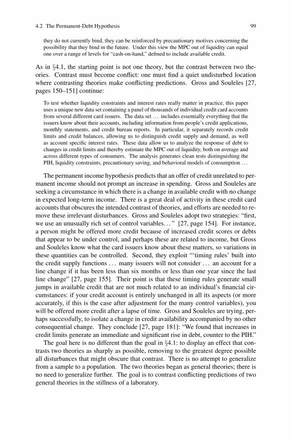
4.2 The Permanent-Debt Hypothesis 99
they do not currently bind, they can be reinforced by precautionary motives concerning thepossibility that they bind in the future. Under this view the MPC out of liquidity can equalone over a range of levels for “cash-on-hand,” defined to include available credit.
As in §4.1, the starting point is not one theory, but the contrast between two the-
ories. Contrast must become conflict: one must find a quiet undisturbed location
where contrasting theories make conflicting predictions. Gross and Souleles [27,
pages 150–151] continue:
To test whether liquidity constraints and interest rates really matter in practice, this paperuses a unique new data set containing a panel of thousands of individual credit card accountsfrom several different card issuers. The data set . . . includes essentially everything that theissuers know about their accounts, including information from people’s credit applications,monthly statements, and credit bureau reports. In particular, it separately records creditlimits and credit balances, allowing us to distinguish credit supply and demand, as wellas account specific interest rates. These data allow us to analyze the response of debt tochanges in credit limits and thereby estimate the MPC out of liquidity, both on average andacross different types of consumers. The analysis generates clean tests distinguishing thePIH, liquidity constraints, precautionary saving, and behavioral models of consumption . . .
The permanent income hypothesis predicts that an offer of credit unrelated to per-
manent income should not prompt an increase in spending. Gross and Souleles are
seeking a circumstance in which there is a change in available credit with no change
in expected long-term income. There is a great deal of activity in these credit card
accounts that obscures the intended contrast of theories, and efforts are needed to re-
move these irrelevant disturbances. Gross and Souleles adopt two strategies: “first,
we use an unusually rich set of control variables. . . ” [27, page 154]. For instance,
a person might be offered more credit because of increased credit scores or debts
that appear to be under control, and perhaps these are related to income, but Gross
and Souleles know what the card issuers know about these matters, so variations in
these quantities can be controlled. Second, they exploit “‘timing rules’ built into
the credit supply functions . . . many issuers will not consider . . . an account for a
line change if it has been less than six months or less than one year since the last
line change” [27, page 155]. Their point is that these timing rules generate small
jumps in available credit that are not much related to an individual’s financial cir-
cumstances: if your credit account is entirely unchanged in all its aspects (or more
accurately, if this is the case after adjustment for the many control variables), you
will be offered more credit after a lapse of time. Gross and Souleles are trying, per-
haps successfully, to isolate a change in credit availability accompanied by no other
consequential change. They conclude [27, page 181]: “We found that increases in
credit limits generate an immediate and significant rise in debt, counter to the PIH.”
The goal here is no different than the goal in §4.1: to display an effect that con-
trasts two theories as sharply as possible, removing to the greatest degree possible
all disturbances that might obscure that contrast. There is no attempt to generalize
from a sample to a population. The two theories began as general theories; there is
no need to generalize further. The goal is to contrast conflicting predictions of two
general theories in the stillness of a laboratory.

100 4 Competing Theories Structure Design
4.3 Guns and Misdemeanors
The 1968 Federal Gun Control Act prohibits the purchase of guns by felons. Be-
ginning in 1991, California prohibited the purchase of handguns by individuals con-
victed of violent misdemeanors, including assault or brandishing a firearm. It is not
clear whether such prohibitions are effective at reducing gun-related violence. On
one theory, it is fairly easy to purchase a handgun illegally, for instance by purchas-
ing the gun from someone who can buy it legally, so the prohibitions deter only
those who wish to avoid illegal activity, perhaps not the best target for deterrence.
On a different theory, legal prohibitions backed by punishment deter individuals
who wish to avoid punishment.
The two theories are plain enough, but contrasting them is not so easy. Under
what circumstances do the two theories make conflicting predictions? Under both
theories, it would not be surprising if violent men remain violent, with or without re-
strictions on handgun purchases. The laws restrict purchases by violent individuals;
these individuals cannot be compared with unrestricted, nonviolent individuals.
The effects of California’s law were investigated by Garen Wintemute, Mona
Wright, Christiana Drake, and James Beaumont [71] in the following way. They
compared two groups of Californians who had been convicted of violent misde-
meanors of the sort that would have prevented a legal purchase of a handgun be-
ginning in 1991. One group consisted of individuals who had applied to purchase a
handgun in 1989 or 1990, before the law took effect. The second group consisted of
individuals who applied to purchase a handgun in 1991 and whose application was
denied. These two groups may not be perfectly comparable, but at least both groups
had been convicted of violent misdemeanors and both groups sought to purchase
a handgun. In terms of demographics and previous convictions, the two groups
looked fairly similar [71, Table 1].
If California’s law were effective, one expects to see a lower rate of gun and vio-
lent crime in the group denied a handgun purchase, with no difference in nongun or
nonviolent crime. If the law were ineffective, one expects to see similar rates of gun
and violent crime in both groups. With or without adjustments for demographics
and previous convictions, Wintemute et al. [71, Tables 2 and 3] found lower rates of
gun and violent crime in the group denied a handgun purchase, with little indication
of a difference in the rate of other crimes.
The reasoning here is much the same as in §4.1 and §4.2. Admittedly, the two
theories are quite plain: one says the policy works, the other denies this. And yet,
because the policy is targeted at offenders, care is needed to identify circumstances
in which these theories make conflicting predictions.
4.4 The Dutch Famine of 1944–1945
Does malnutrition in utero reduce mental performance at age 19? The two theories
are straightforward: it does or it doesn’t. It is not straightforward, however, to iden-

4.5 Replicating Effects and Biases 101
tify circumstances in which these theories lead to different predictions. Reliable
information is needed about mental performance at age 19 and about mother’s diet
20 years prior to that. Controls are needed whose mothers were not malnourished
but who were otherwise similar in background, education, social class, etc. Neither
such information nor such controls are commonly available.
Zena Stein, Mervyn Susser, Gerhart Saenger and Francis Marolla [61] found
what was needed in the Dutch famine of 1944–1945. They wrote [61, page 708]:
On 17 September 1944 British paratroops landed at Arnhem in an effort to force a bridge-head across the Rhine. At the same time, in response to a call from the Dutch government-in-exile in London, Dutch rail workers went on strike. The effort to take the bridgeheadfailed, and the Nazis in reprisal imposed a transport embargo on western Holland. A se-vere winter froze the barges in the canals, and soon no food was reaching the large cities. . . At their lowest point the official food rations reached 450 calories per day, a quarter ofthe minimum standard. In cities outside the famine area, rations almost never fell below1300 calories per day. . . . The Dutch famine was remarkable in three respects: (i) Faminehas seldom if ever struck where extensive, reliable and valid data allow the effects to beanalyzed within specified conditions of social environment. (ii) The famine was sharplycircumscribed in both time and place. (iii) The type and degree of nutritional deprivationduring the famine were known with a precision unequaled in any large human populationbefore or since.
To know a child’s date and place of birth is to know whether the mother was affected
by the famine. So Stein et al. defined famine and control regions in Holland, as
well as a cohort of children born just before the start of the famine, several cohorts
exposed to the famine at various times in utero, and a cohort conceived after the
famine ended. In these cohorts, virtually all males received medical examinations
and psychological testing, including an IQ test, in connection with induction into
the military. For 1700 births at two hospitals, one in a famine region (Rotterdam)
and one in a control region (Heerlan), birth weights were available. Stein et al. [61,
page 712] concluded: “Starvation during pregnancy had no detectable effects on the
mental performance of surviving male offspring.”
Subsequent studies used the Dutch famine to examine other outcomes, includ-
ing schizophrenia, affective disorders, obesity, and breast cancer; see [35, 63] for
reviews of these studies. For studies that have taken a similar approach in other
situations, see [3, 57].
The Dutch famine was unrepresentative both of typical in utero development and
typical famines, and it was useful for studies of development precisely in the ways it
was unrepresentative. In representative situations, famine is confounded with other
factors that obscure the effects caused by malnutrition in utero.
4.5 Replicating Effects and Biases
The randomized experiment in its idealized, perhaps unattainable, form is subject
to a single source of uncertainty — that stemming from a finite sample size. In
this ideal, biases of every sort have been eliminated by blocking and randomization;

102 4 Competing Theories Structure Design
therefore, the sole function of replication is to increase the sample size. Actual ex-
periments are a step or two removed from the ideal, and observational studies are
several steps removed from that. In an observational study, even an excellent one,
there is the possibility that can never be entirely eliminated: treated and control sub-
jects who look comparable may not actually be comparable, so differing outcomes
may not be treatment effects.10 In observational studies, the principal and important
function of replication is to shed some light on biases of this sort.
Here, too, there are two theories. The first theory asserts that previous studies
have produced estimates of treatment effects without much bias. The competing
theory denies this, asserting instead that previous studies were biased in certain
particular ways, and if those biases were removed, then the ostensible treatment
effect would be removed with them. The replication does not repeat the original
study; rather, it studies the same treatment effect in a context that is not subject to
particular biases claimed by the competing theory. Replication is not repetition: the
issue at hand is whether the ostensible effect can be reproduced if a conjectured bias
is removed.
An example is David Card and Alan Krueger’s [9, 10] replication of their earlier
study [8] of the effects of the minimum wage on employment11; see also §11.3. On
1 April 1992, New Jersey raised its minimum wage by about 20%, whereas neigh-
boring Pennsylvania left its minimum wage unchanged. In their initial study, Card
and Krueger [8] used survey data to examine changes in employment at fast food
restaurants, such as Burger King and Wendy’s, in New Jersey and eastern Pennsyl-
vania, before and after the increase in New Jersey’s minimum wage. They found
“no evidence that the rise in New Jersey’s minimum wage reduced employment at
fast food restaurants in the state.” Their careful and interesting study received some
critical commentary; e.g., [41]. One of several issues was the quality of the employ-
ment data obtained by a telephone survey, and another was simply that New Jersey
and Pennsylvania differ in many ways relevant to employment change, not just in
their approach to the minimum wage. In 1996, the minimum wage as set by the
U.S. Federal Government was raised, forcing up the minimum wage in Pennsylva-
nia, without forcing changes in New Jersey whose state minimum wage was already
above the new Federal minimum wage. Card and Krueger [9, 10] then replicated the
original study with the roles of New Jersey and Pennsylvania now reversed, using
employment data from payroll records for Unemployment Insurance made available
by the U.S. Bureau of Labor Statistics. Their findings were similar. The replication
does not eliminate all concerns raised about the original study, but it does make two
specific concerns less plausible.
10 In an observational study, an increase in sample size ensures only that the estimator is closer towhatever the estimator estimates. Typically, the estimator estimates the sum of a treatment effectand a bias whose unknown magnitude does not decrease as the sample size increases. When a biasof this sort is not zero, as the sample size increases, confidence intervals shrink in length to excludethe true treatment effect, and hypothesis tests are ever more likely to reject the true hypothesis. It isa mistake to attach great importance to an increase in the sample size (or to an increase in statisticalefficiency) when substantial biases of fixed size are present or likely.11 For a brief survey of the economics of the minimum wage, see [6, §12.1].

4.5 Replicating Effects and Biases 103
Mervyn Susser writes:
The epidemiologist [. . . seeks. . . ] consistency of results in a variety of repeated tests . . .Consistency is present if the result is not dislodged in the face of diversity in times, places,circumstances, and people, as well as of research design [65, page 88] . . . The strength ofthe argument rests on the fact that diverse approaches produce similar results [64, page 148].
Susser’s careful statement is easily, perhaps typically, misread. Mere consistency
upon replication is not the goal. Mere consistency means very little. Rather, the
goal is “consistency . . . in a variety of . . . tests” and “consistency . . . not dislodged
in the face of diversity.” The mere reappearance of an association between treat-
ment and response does not convince us that the association is causal — whatever
produced the association before has produced it again. It is the tenacity of the as-
sociation — its ability to resist determined challenges — that is ultimately convinc-
ing. For a similar view with examples from physics, see Allan Franklin and Colin
Howson [22]. For a similar view with examples from mathematics in a Bayesian
formulation, see Georg Polya [47, especially pages 463–464].
To illustrate, consider two sequences of studies, one sequence involving the ef-
fectiveness of treatments for drug addiction, the other involving the effects of ad-
vertising on prices. The first sequence increases the sample size, but the bias of
greatest concern remains the same. The second sequence asks the same question in
very different contexts.
Several nonexperimental studies of the effects of treatments for heroin or co-
caine addiction have found that people who remain in treatment for at least three
months are more likely to remain drug-free than people who drop out of treatment
before three months. These studies had involved the Drug Abuse Reporting Pro-
gram (DARP) and the Treatment Outcomes Prospective Study (TOPS). In a third
study using a different source of data, Hubbard et al. [31, page 268] wrote:
The general finding from DARP and TOPS that treatment duration of at least three monthsis associated statistically and clinically with more positive outcomes supports the inferenceof treatment effectiveness. The following analysis retests this hypothesis . . .
In their new study, Hubbard et al. [31] found, again, that people who dropped out of
treatment went on to use more illegal drugs than people who remained in treatment.
Is this an effect caused by treatment? Or is it simply that a person who has little
enthusiasm for ending his addiction is both more likely to drop out of treatment and
more likely to use illegal drugs? A summary report of the National Academy of
Sciences [36, page 17] was understandably skeptical:
Depending on the process by which users are selected into treatment programs and thedeterminants of dropout from such programs . . . the data may make treatment programsseem more or less cost-effective than they actually are.
These three studies are all open to the same question: Is a comparison of people
who remain in treatment and people who drop out revealing an effect caused by the
treatment, or is it revealing something about the people who stay in treatment and
those who drop out? Because the same question can be asked of each study, the

104 4 Competing Theories Structure Design
replications increase the sample size — which was large from the start, and never
much at issue — but they do not make progress towards answering a basic concern.
What is the effect of advertising on prices? More precisely, what is the effect on
prices of imposing or removing a restriction on the advertising of prices? One study
by Amihai Glazer [26] made use of a strike from 10 August 1978 to 5 October 1978
that shut down three daily New York City newspapers, the New York Times, the
New York Post, and the Daily News. The strike reduced advertising of retail food
prices in New York City. Glazer looked at changes in retail food prices in Queens,
the eastern borough of New York City, comparing Queens with adjacent Nassau
County, outside the City, where the major newspaper, Newsday, was unaffected by
the strike. A second study by Jeffrey Milyo and Joel Waldfogel [39] examined
changes in liquor prices in Rhode Island before and after the U.S. Supreme Court
struck down Rhode Island’s ban on liquor advertising, comparing Rhode Island with
adjacent areas of Massachusetts that were unaffected by the Court decision. In a
third study, C. Robert Clark [12] examined the effect on the prices of children’s
breakfast cereals of Quebec’s ban on advertising aimed at children under the age of
13. Clark compared the prices of cereals for children and cereals for adults in Que-
bec and in the rest of Canada. Each situation — the newspaper strike in New York,
the Supreme Court decision in Rhode Island, the ban on advertising to children in
Quebec — has idiosyncrasies that might be mistaken for an effect of advertising
on prices, but there is no obvious reason why these idiosyncrasies should align to
reproduce the same association between advertising and prices. Unlike the studies
of treatments for drug addiction, where one alternative explanation suffices for three
studies, in the advertising studies, three unrelated idiosyncrasies would have to pro-
duce similar associations. That could happen, but it seems less and less plausible as
more and more studies are designed to replicate an effect, if it is a real effect, but to
avoid replicating biases.
The goal in replication is to study the same treatment effect in a new context that
removes some plausible bias that may have affected previous studies [53].
4.6 Reasons for Effects
To suppose universal laws of nature capable of being apprehended by the mind and yethaving no reason for their special forms, but standing inexplicable and irrational, is hardlya justifiable position. Uniformities are precisely the sort of facts that need to be accountedfor. . . . Law is par excellence the thing that wants a reason.
Charles Sanders Peirce [44]
The Architecture of Theories
There is an obvious distinction between empirical evidence in support of a theory
and a reasoned argument in support of a theory, but as is often the case with obvious
distinctions, this one becomes less obvious upon close inspection. It is, after all,
common to argue that what was taken as empirical evidence in support of a theory is

4.6 Reasons for Effects 105
not evidence at all.12 It is equally common to cast doubt upon a reasoned argument
with the aid of empirical evidence. To offer a reasoned argument in support of the
claim that a treatment does or should or would have a certain effect is to create a
new object for empirical investigation, namely the argument itself.13 Consider an
example.
In an effort to reduce gun violence, various municipalities have created programs
to buy handguns from their owners. For instance, Milwaukee did this in 1994-1996,
offering $50 for a workable gun. Buyback programs are popular because they are
voluntary: they do not meet the same resistance that a coercive program might meet.
However, voluntary programs may also be less effective than coercive programs. Do
voluntary buyback programs work to reduce gun violence?
One could argue that buybacks have to work: whenever a gun is destroyed, that
gun cannot be used in a future homicide or suicide. One could argue that the pro-
gram can’t really work: a rational person would turn in a gun for $50 only if he
does not plan to use it, so the program is buying guns that would otherwise rest
harmlessly in the attic. One could argue that buybacks work because people aren’t
rational: many gun deaths are accidents, and others stem from impulsive responses
to rage or depression, so buying guns from people who do not plan to use them helps
people to adhere to their peaceful plans. (See Ainslie [2] or Rachlin [50] for cogent
general discussions of rational control of irrational impulses.) One could argue that
buybacks can’t really work because many violent individuals do not have peaceful
plans and will not sell their guns, intending to thwart their own violent inclinations:
“[T]he self-images of violent criminals are always congruent with their violent crim-
inal actions,” wrote Athens [4, page 68] in a careful, perceptive study. In short, it is
not difficult to offer a variety of reasons in support of a variety of possible effects.
Whatever the strengths or weakness of these arguments as arguments for or against
particular effects, the arguments create objects for empirical investigation, namely
the validity of the arguments themselves.
Basic to each of these arguments is the question: Do buyback programs buy the
guns that would otherwise be used in gun violence? One aspect of this question
is: Do buyback programs typically buy the types of guns typically used in gun vi-
olence? A second aspect is: Do buyback programs buy guns in sufficient quantity
to affect gun violence? Evelyn Kuhn and colleagues [33] addressed the first aspect
and a report of the U.S. National Academy of Sciences [69, pages 95–96] addressed
the second.
Table 4.1 is Kuhn et al.’s [33] comparison of the caliber of repurchased guns
and homicide guns. To a dramatic degree, with an odds ratio of ten or more, re-
12 See §4.1 and Note 4.13 Dretske [17, pages 20–22] writes: “More often than not a reason, or the giving of reasons,supplies a recipe . . . for the possible falsification of the statement or statements for which thereason is given. By this I mean that although some statements, considered in isolation, may appearirrefutable, they lose this invulnerability when taken in the context provided by evidential support.. . . If Q is a reason for believing P true, then although P need not be true, Q must be. We can, andoften do, give reasons — sometimes very good reasons — for believing something that is not true. . . [A]ny challenge to the truth of Q is simultaneously a challenge to the acceptability of Q as areason.”

106 4 Competing Theories Structure Design
Table 4.1 Homicide and buyback handguns in Milwaukee by caliber. As the odds ratios indicate,homicide and buyback guns are quite different.
Caliber Buyback Homicide Odds Ratio
Small: .22, .25, .32 719 75 1.0Medium: .357, .38, 9mm 182 202 10.6
Large: .40, .44, .45 20 40 19.2
Total 941 369
purchased guns are small caliber and homicide guns are large caliber. Kuhn et al.
make several similar comparisons, finding that repurchased guns tended to be small,
obsolete revolvers, whereas homicide guns tended to be large, inexpensive, semiau-
tomatic pistols. They found similar but not identical results for suicide guns. The
buyback programs are buying types of guns infrequently used in gun violence.
The report of the U.S. National Academy of Sciences makes this same point and
two others [69, pages 95–96]:
The theory on which gun buy-back programs is based is flawed in three respects. First,the guns that are typically surrendered in gun buy-backs are those that are least likely tobe used in criminal activities . . . Second, because replacement guns are relatively easilyobtained, the actual decline in the number of guns on the street may be smaller than thenumber of guns that are turned in. Third, the likelihood that any particular gun will be usedin a crime in a given year is low. In 1999, approximately 6,500 homicides were committedwith handguns. There are approximately 70 million handguns in the United States. Thus,if a different handgun were used in each homicide, the likelihood that a particular handgunwould be used to kill an individual in a particular year is 1 in 10,000. The typical buy-backprogram yields less than 1,000 guns.
In brief, their third point claims that the scale of buyback programs is too small to
have a meaningful effect.
Table 4.1, related results in [33], and the arguments in the quoted paragraph from
[69, pages 95–96] are intended to undermine the reasoning that justifies gun buyback
programs, but they provide no direct evidence about the effects of such programs on
violence. In [33], violence is not measured. Table 4.1 and the quoted paragraph
attack the idea that gun buyback programs could work by buying the guns used in
gun violence, because the programs buy the wrong types of guns and too few of
them. It is, nonetheless, not entirely inconceivable that gun buyback programs do
work to reduce violence, but do this in some other way. Imagine a highly publicized
buyback program, in which, each night, the television news interviews someone who
turned in a gun, reporting the accumulated total of guns repurchased, accompanied
by comments from civic leaders about how the city is “getting rid of its guns and
ridding itself of violence.” Even if the program bought the wrong guns and too few
of them, it is not entirely inconceivable that the publicity, fanciful though it may
be, would affect public sentiment in a way that ultimately affected the level of gun
violence. Of course, in arguing for a new policy, one might hope to say more than:
‘it is not entirely inconceivable that the policy might work.’
In the discussion here, a precise distinction is intended between ‘direct evidence
of a treatment effect’ and a ‘reason for a treatment effect.’ The distinction does not

4.6 Reasons for Effects 107
refer to the presence or absence of empirical evidence: empirical evidence is present
in some form in most scientific work. Nor does the distinction refer to the strength
or quality of the evidence: in the case of gun buybacks, the evidence against the
reasons for an effect may be more compelling than the direct evidence of ineffec-
tiveness [69, pages 95–96]. ‘Direct evidence of a treatment effect’ means a study
of the relevant treatment, on the relevant subjects or units, measured in terms of the
relevant outcome. A randomized experiment or an observational study may provide
direct evidence of an effect in this sense, and the evidence is likely to be stronger
if it comes from a well-conducted randomized experiment. In contrast, an empiri-
cal study of a ‘reason for an effect’ is a study that is a step removed; it provides a
reason for thinking the relevant treatment would have a particular effect were it to
be applied to the relevant subjects measured in terms of the relevant response, but
one or more of these elements is not actually present. In the case of gun buybacks
in Table 4.1 and in [33], the relevant outcome is the level of gun violence, which is
not measured; instead, the results refer to the types of guns that are repurchased. In
the paragraph above quoted from [69, pages 95–96], the relevant outcome is again
gun violence, but the results refer to the number of guns repurchased. Dafna Kanny
and colleagues [32] studied the effects on helmet use of a law requiring bicyclists
to wear helmets: this provides a plausible reason for thinking the law reduced ac-
cidents, but it is a step removed, because helmet use rather than accident reduction
is the outcome. In the 1964 U.S. Surgeon General’s Report, Smoking and Health,
it is noted that [60, page 143] “there is evidence from numerous laboratories that
tobacco smoke condensates and extracts of tobacco are carcinogenic for several an-
imal species.” This is a reason for thinking that tobacco is carcinogenic in humans,
but it is a step removed, because the subjects are not human. Much laboratory work
in the biomedical sciences studies reasons for effects in humans by examining ef-
fects on animals or cell cultures or molecules. The use of surrogate outcomes in
medicine is the study of a reason for an effect in the sense defined here; for exam-
ple, the use of colonic polyps as a surrogate for mortality from colorectal cancer
[56]. Laboratory style experimentation in economics studies reasons for effects
when small experimental incentives are proxies for incentives faced in actual eco-
nomic decisions [46]. A theoretical argument about what effect would appear in a
tidy and simple theoretical world may constitute a reason for an effect in the untidy
and complex world we actually inhabit; see, for instance, §11.3.
There is no substitute for direct evidence of the effect of a treatment. And yet,
evidence about reasons for an effect remains important. Evidence about reasons for
an effect may either strengthen or undermine direct evidence of an effect, and either
outcome is constructive [54, 67].

108 4 Competing Theories Structure Design
4.7 The Drive for System
A good scientific theory is under tension from two opposing forces: the drive for evidenceand the drive for system. Theoretical terms should be subject to observable criteria, themore the better; and they should lend themselves to systematic laws, the simpler the better,other things being equal. If either of these drives were unchecked by the other, it wouldissue in something unworthy of the name of scientific theory: in the one case a mere recordof observations, and in the other a myth without foundation.
W.V.O. Quine [49, page 90]
[I]mpersonal knowledge . . . has a special commitment to reasons. Bodies of knowledge areessentially, if to varying degrees with different subjects, systematic. There is both a pureand an applied reason for this. Pure, because the aim is not just to know but to understand,and in scientific cases at least understanding necessarily implies organization and economy.Applied, because a body of knowledge will only be freely extensible and open to criticismif rationally organized. . . . So knowledge, in this sense, must have reasons.
Bernard Williams [70, page 56]
The first paragraph of Chapter 1 recalled Borgman’s political cartoon in which a
TV newsman presents “Today’s Random Medical News” that “according to a report
released today . . . coffee can cause depression in twins.” The cartoon accurately de-
picts a popular misconception. It is often thought, incorrectly, that a scientific study
has a clear and stable interpretation on the day it is published, and that interpretation
is ‘news.’ In fact, the considered judgment about a scientific study hardens slowly,
like cement, as the study is subjected to critical commentary, reconciled with other
studies, both past and future, and integrated into a systemic understanding of the
larger topic to which the study is a contribution. The science of the undergraduate
classroom — that is, the science that is presented simply as the way things are — is
not a list of findings from a sequence of individually decisive studies, but rather the
systemic reconciliation and integration of many, perhaps conflicting, studies. The
study of ‘reasons for effects’ in §4.6 is part of this systemic reconciliation. Gaps and
conflicts in systemic knowledge provoke new investigations aimed at closing gaps,
resolving conflicts. In this sense, there is no ‘science news.’ On the day of its re-
lease, the new report faces a fate that is far too uncertain to constitute news. By the
time a systemic understanding has hardened, by the time today’s report has found a
resting place in that understanding, both the report and the systemic understanding
are far too old to constitute news.
Consider, for instance, Steven Clinton and Edward Giovannucci’s [13] review in
1998 of the possibility that diet affects the risk of prostate cancer. Their review
attempted to organize, reconcile, and lend systematic form to 193 scientific reports.
The following excerpts indicate the flavor of their review.
Studies of prostate cancer have yielded inconsistent results concerning the relationship be-tween various measurements of adult body mass or obesity and risk [of prostate cancer,citing 11 studies, which are then contrasted in detail] [13, page 422]. . . . An association be-tween prostate cancer incidence and tobacco use has been inconsistent . . . Additional stud-ies focusing on the critical timing of smoking during the life cycle . . . are necessary [13,

4.8 Further Reading 109
page 419]. . . . The relationship between alcohol consumption and risk of prostate cancerhas been evaluated in a series of studies. No strong evidence has emerged for an association[citing 4 studies] [13, page 424]. . . . Reports of a correlation between diets rich in meat ordairy products and risk of prostate cancer are frequent [citing 12 studies] [13, page 425].. . . [Citing Giovannucci’s own study, in which a nutrient, lycopene, found in tomatoes, wasstudied:] men in the highest quintile of lycopene intake experienced a 21% lower risk [. . .but . . . ] investigators should use caution in assuming that lycopene mediates a relationshipbetween consumption of tomato products and lower risk of prostate cancer [13, page 429].. . . A recent study was designed to examine the effects of selenium supplementation on re-currence of skin cancer in a high-risk population [citing a randomized clinical trial]. Sele-nium treatment did not influence the risk of skin cancer, although selenium-treated patientshad a nonsignificant reduction in total cancer mortality, as well as a lower risk of prostatecancer. Additional studies are necessary . . . [13, pages 429–30]
The serious, evenhanded, cautious tone of Clinton and Giovannucci’s review is in
marked contrast to the presentation of diet and health in the popular press. Clinton
and Giovannucci’s calls for additional studies are often cited by subsequent stud-
ies [40, 43]. An updated review six years later reports some progress but many
questions still open [37].
Most scientific fields seek a systemic understanding that: (i) contrasts and rec-
onciles past studies, (ii) guides future studies towards promising gaps in the current
understanding, and (iii) integrates theoretical and empirical work. For an example
from economics, see Jonathan Gruber’s [28] review of the economic issues related
to providing health insurance to the uninsured. For an example from criminology,
see the report by Charles Wellford and colleagues [69] concerning firearms and vio-
lence. For an example from the epidemiology of dementia emphasizing methodol-
ogy as the origin for inconsistent results, see the review by Nicola Coley, Sandrine
Andrieu, Virginie Gardette, Sophie Gillette-Guyonnet, Caroline Sanz, Bruno Vellas,
and Alain Grand [14].
The drive for system plays a key role in eliminating scientific error, but it also
plays a key role in deciding what to study next. A new experiment or observational
study contributes to an extant understanding, one that is partly systematic, partly
incomplete, partly conflicting, and doubtless partly, perhaps substantially, in error.
A new study is judged by its contribution to organizing, completing, reconciling, or
correcting that understanding.
4.8 Further Reading
Karl Popper [48], Georg Polya [47], John Platt [45], and Paul Feyerabend [19] offer
abstract discussions relevant to the current chapter; see also [52]. The material in
§4.5 and §4.6 is discussed in greater detail in [53] and [54], respectively.

110 4 Competing Theories Structure Design
References
1. Achinstein, P.: Are empirical evidence claims a priori? Brit J Philos Sci 46, 447–473 (1995)2. Ainslie, G.: Breakdown of Will. New York: Cambridge University Press (2002)3. Almond, D.: Is the 1918 influenza pandemic over? Long-term effects of in utero influenza
exposure in the post-1940 US population. J Polit Econ 114, 672–712 (2006)4. Athens, L.: Violent Criminal Acts and Actors Revisited. Urbana: University of Illinois Press
(1997)5. Brown, J. R.: The Laboratory of the Mind: Thought Experiments in the Natural Sciences.
New York: Routledge (1991)6. Cahuc, P., Zylberberg, A.: Labor Economics. Cambridge, MA: MIT Press (2004)7. Card, D.: The causal effect of education. In: Handbook of Labor Economics, O. Ashenfelter
and D. Card, eds. New York: North-Holland (2001)8. Card, D., Krueger, A.: Minimum wages and employment: A case study of the fast-food indus-
try in New Jersey and Pennsylvania. Am Econ Rev 84, 772–793 (1994)9. Card, D., Krueger, A.: A reanalysis of the effect of the New Jersey minimum wage increase on
the fast-food industry with representative payroll data. NBER Working Paper 6386. Boston:National Bureau of Economic Research (1998)
10. Card, D., Krueger, A.: Minimum wages and employment: A case study of the fast-food indus-try in New Jersey and Pennsylvania: Reply. Am Econ Rev 90, 1397–1420 (2000)
11. Chamberlin, T.C.: The method of multiple working hypotheses. Science 15, 92 (1890),reprinted Science 148, 754–759 (1965)
12. Clark, C.R.: Advertising restrictions and competition in the children’s breakfast cereal indus-try. J Law Econ 50, 757–780 (2007)
13. Clinton, S.K., Giovannucci, E.: Diet, nutrition, and prostate cancer. Annu Rev Nutr 18, 413–440 (1998)
14. Coley, N., Andrieu, S., Gardette. V., Gillette-Guyonnet, S., Sanz, C., Vellas, B., Grand, A.:Dementia prevention: Methodological explanations for inconsistent results. Epidemiol Rev35–66 (2008)
15. Coulibaly, B., Li, G.: Do homeowners increase consumption after the last mortgage payment?An alternative test of the permanent income hypothesis. Rev Econ Statist 88, 10–19 (2006)
16. Darwin, C.: Letter to Henry Fawcett, 18 September 1861. (1861)17. Dretske, F.I.: Reasons and falsification. Philos Q 15, 20–34 (1965)18. Fermi, L., Bernardini, G.: Galileo and the Scientific Revolution. New York: Basic Books
(1961), reprinted New York: Dover (2003)19. Feyerabend, P.: How to be a good empiricist — a plea for tolerance in matters epistemological.
In: Nidditch, P.H., ed. The Philosophy of Science, New York: Oxford University Press (1968)20. Feyerabend, P.: Against Method. London: Verso. (1975)21. Fodor, J.A.: The dogma that didn’t bark. Mind 100, 201-220 (1991)22. Franklin, A., Howson, C.: Why do scientists prefer to vary their experiments? Stud Hist Philos
Sci 15, 51-62 (1984)23. Friedman, M.: A Theory of the Consumption Function. Princeton, NJ: Princeton University
Press (1957)24. Friedman, M.: The Essence of Friedman. Stanford, CA: Hoover Institution Press (1987)25. Galileo, G.: Two New Sciences (1638). Madison: University of Wisconsin Press (1974)26. Glazer, A.: Advertising, information and prices. Econ Inquiry 19, 661-671 (1981)27. Gross, D.B., Souleles, N.S.: Do liquidity constraints and interest rates matter for consumer
behavior? Evidence from credit card data. Q J Econ 117, 149–185 (2002)28. Gruber, J.: Covering the uninsured in the United States. J Econ Lit 46, 571-606 (2008)29. Harre, R.: Great Scientific Experiments. London: Phaidon Press (1981), reprinted New York:
Dover (2002)30. Ho, D.E., Imai, K.: Estimating causal effects of ballot order from a randomized natural exper-
iment: The California alphabet lottery, 1978–2002. Public Opin Q 72, 216–240 (2008)

References 111
31. Hubbard, R.L., Craddock, S.G., Flynn, P.M., Anderson, J., Etheridge, R.M.: Overview of 1-year follow-up outcomes in the Drug Abuse Treatment Outcome Study (DATOS). PsycholAddict Behav 11, 261-278 (1997)
32. Kanny, D., Schieber, R.A., Pryor, V., Kresnow, M.: Effectiveness of a state law mandating useof bicycle helmets among children. Am J Epidemiol 154, 1072–1076 (2001)
33. Kuhn, E.M., Nie, C.L., O’Brien, M.E., Withers, R.L., Wintemute, G.J., Hargarten, S.W.: Miss-ing the target: A comparison of buyback and fatality related guns. Inj Prev 8, 143–146 (2002)
34. Kuhn, T.: A function for thought experiments. In: Kuhn, T., The Essential Tension: SelectedStudies in Scientific Tradition and Change, pages 240–265. Chicago: University of ChicagoPress. (1979)
35. Lumey, L.H., Stein, A.D., Kahn, H.S., van der Pal-de Bruin, K.M., Blauw, G.J., Zybert, P.A.,Susser, E.S.: Cohort profile: The Dutch hunger winter families study. Int J Epidemiol 36,1196–1204 (2007)
36. Manski, C.F., Pepper, J.V., Thomas, Y.F. (eds): Assessment of Two Cost-Effectiveness Studieson Cocaine Control Policy. Washington, DC: National Academies Press (1999)
37. McCullough, M.L., Giovannucci, E.L.: Diet and cancer prevention. Oncogene 23, 6349–6364(2004)
38. Mill, J.S.: A System of Logic: The Principles of Evidence and the Methods of Scientific In-vestigation. Indianapolis: Liberty Fund (1867)
39. Milyo, J., Waldfogel, J.: The effect of price advertising on prices: Evidence in the wake of 44Liquormart. Am Econ Rev 89, 1081-1096 (1999)
40. Mitrou, P.N., Albanes, D., Weinstein, S.J., Pietinen, P., Taylor, P.R., Virtamo, J., Leitzmann,M.F.: A prospective study of dietary calcium, dairy products and prostate cancer risk. Int JCancer 120, 2466–2473 (2007)
41. Neumark, D., Wascher, W.: Minimum wages and employment: A case study of the fast-foodindustry in New Jersey and Pennsylvania: Comment. Am Econ Rev 90, 1362–1396 (2000)
42. Nozick, R.: Philosophical Explanations. Cambridge, MA: Harvard University Press (1981)43. Park, S.Y., Murphy, S.P., Wilkens, L.R., Stram, D.O., Henderson, B.E., Kolonel, L.N.: Cal-
cium, vitamin D, and dairy product intake and prostate cancer risk — The multiethnic cohortstudy. Am J Epidemiol 166, 1259–1269 (2007)
44. Peirce, C.S.: The architecture of theories. In: Charles Sanders Peirce: Selected Writings. NewYork: Dover (1958)
45. Platt, J.: Strong inference. Science 146, 347–353 (1964)46. Plott, C.R., Smith, V.L. (eds): Handbook of Experimental Economics Results. New York:
North Holland (2008)47. Polya, G.: Heuristic reasoning and the theory of probability. Am Math Month 48, 450–465
(1941)48. Popper, K.R.: The Logic of Scientific Discovery. New York: Harper and Row (1935 in Ger-
man, 1959 in English)49. Quine, W.V.O.: What price bivalence? J Philos 78, 90–95 (1981)50. Rachlin, H.: Self-control: Beyond commitment (with Discussion). Behav Brain Sci 18, 109–
159 (1995)51. Romer, D.: Advanced Macroeconomics. New York: McGraw-Hill/Irwin (2005)52. Rosenbaum, P.R.: Choice as an alternative to control in observational studies (with Discus-
sion). Statist Sci 14, 259–304 (1999)53. Rosenbaum, P.R.: Replicating effects and biases. Am Statistician 55, 223–227 (2001)54. Rosenbaum, P.R.: Reasons for effects. Chance 5–10 (2005)55. Samuelson, P.A.: Schumpeter as economic theorist. In: P.A. Samuelson, Collected Papers,
Volume 5, pages 201-327. Cambridge, MA: MIT Press (1982, 1986)56. Schatzkin, A., Gail, M.: The promise and peril of surrogate end points in cancer research.
Nature Rev Cancer 2, 19–27 (2002)57. Sparen, P., Vagero, D., Shestov, D.B., Plavinskaja, S., Parfenova, N., Hoptiar, V., Paturot,
D., Galanti, M.R.: Long term mortality after severe starvation during the siege of Leningrad:prospective cohort study. Br Med J 328, 11-14 (2004)

112 4 Competing Theories Structure Design
58. Souleles, N.S.: The response of household consumption to income tax refunds. Am Econ Rev89, 947–958 (1999)
59. Staley, K.W.: Robust evidence and secure evidence claims. Philos Sci 71, 467–488. (2004)60. Surgeon General’s Advisory Committee: Smoking and Health. Princeton, NJ: Van Nostrand
(1964)61. Stein, Z., Susser, M., Saenger, G., Marolla, F.: Nutrition and mental performance. Science
178, 708–713 (1972)62. Stigler, G.J.: The economics of minimum wage legislation. Am Econ Rev 36, 358–365 (1946)63. Susser, E., Hoek, H.W., Brown, A.: Neurodevelopmental disorders after prenatal famine: the
story of the Dutch famine study. Am J Epidemiol 147, 213–216 (1998)64. Susser, M.: Causal Thinking in the Health Sciences: Concepts and Strategies in Epidemiology.
New York: Oxford University Press (1973)65. Susser, M.: Falsification, verification and causal inference in epidemiology: Reconsideration
in the light of Sir Karl Popper’s philosophy. In: Susser, M., ed., Epidemiology, Health andSociety: Selected Papers, pp. 82–93, New York: Oxford University Press (1987)
66. Urmson, J.O.: Aristotle’s Ethics. Oxford: Blackwell (1988)67. Weed, D.L., Hursting, S.D.: Biologic plausibility in causal inference: current method and prac-
tice. Am J Epidemiol 147, 415–425 (1998)68. Weiss, N.S.: Can the “specificity” of an association be rehabilitated as a basis for supporting
a causal hypothesis? Epidemiology 13, 6–8 (2002)69. Wellford, C.F., Pepper, J.V., Petrie, C.V., and the Committee to Improve Research and Data
on Firearms: Firearms and Violence. Washington, DC: National Academies Press (2004)70. Williams, B.: Knowledge and reasons. In: Williams, B., Philosophy as a Humanistic Disci-
pline, pages 47–56. Princeton, NJ: Princeton University Press. (2006)71. Wintemute, G.J., Wright, M.A., Drake, C.M., Beaumont, J.J.: Subsequent criminal activity
among violent misdemeanants who seek to purchase handguns: Risk factors and effectivenessof denying handgun purchase. J Am Med Assoc 285, 1019–1026 (2001)
72. Zellner, A. Readings in Economic Statistics and Econometrics. Boston: Little, Brown (1968)

Chapter 5Opportunities, Devices, and Instruments
Abstract What features of the design of an observational study affect its ability to
distinguish a treatment effect from bias due to an unmeasured covariate ui j? This
topic, which is the focus of Part III of the book, is sketched in informal terms in the
current chapter. An opportunity is an unusual setting in which there is less confound-
ing with unobserved covariates than occurs in common settings. One opportunity
may be the base on which one or more natural experiments are built. A device is in-
formation collected in an effort to disambiguate an association that might otherwise
be thought to reflect either an effect or a bias. Typical devices include: multiple con-
trol groups, outcomes thought to be unaffected by the treatment, coherence among
several outcomes, and varied doses of treatment. An instrument is a relatively hap-
hazard nudge towards acceptance of treatment where the nudge itself can affect the
outcome only if it prompts acceptance of the treatment. Although competing the-
ories structure design, opportunities, devices, and instruments are ingredients from
which designs are built.
5.1 Opportunities
The well-ordered world
. . . a nostalgia for caprice and chaos . . .E.M. Cioran [23, Page 2]
In a well-ordered world, a rationally ordered world, each person would have no
choice but to receive the best treatment for that person, the decision being based on
undisputed knowledge and expert deliberation. That well-ordered world would be
the antithesis of a randomized experiment, in which people receive treatments for
no reason at all, simply the flip of a fair coin, the experimental design reflecting
our acknowledged ignorance about the best treatment and our determined efforts
113P.R. Rosenbaum, Design of Observational Studies, Springer Series in Statistics, DOI 10.1007/978-1-4419-1213-8_5, © Springer Science+Business Media, LLC 2010

114 5 Opportunities, Devices, and Instruments
to reduce that ignorance. In that well-ordered world, it would be difficult to learn
anything new. In that world, policy has settled into the “deep slumber of decided
opinion” [59, page 42]. Happily for the investigator planning an observational study,
we do not live in that well-ordered world.
An observational study may begin with an opportunity, an arbitrary, capricious,
chaotic disruption of the ordered world of everyday. The investigator may ask:
How can this disruption be put to use? Is there a pair of scientific theories that on
an average day do not yield conflicting predictions, but today, just because of this
disruption, do yield conflicting predictions? In Chapter 2, randomness was found
to be useful. Following Richard Sennett [93], we may ask: Is disorder useful?
Questions
I. Does a low level of ambient light cause auto accidents? It would not do to com-
pare shoppers driving at 11:00 am, commuters driving at dusk, party-goers driving
home at 3:00 am; their rates of accidents might differ for reasons other than the dif-
ference in ambient light. It would not do to compare the rates of accidents at 5:00
pm in Helsinki and Tel Aviv, because a difference in ambient light is one difference
among many others. What would you compare?
II. If murderers, rapists, and armed robbers condemned to death were not executed,
would they do greater injury to other inmates and prison staff than is done by others
incarcerated for violent crimes? What would you compare?
III. At present in the United States, married couples pay taxes jointly on the sum of
their incomes, where the total income matters, but the division of income between
husband and wife does not. Also, the tax rates are progressive, with higher tax rates
at higher incomes. Under such a system, if a husband and wife have very different
incomes, the tax disincentives to work may be quite different than if they were not
married. It is natural to ask: What effect does joint taxation have on the labor supply
of husbands and wives? How would you study the effects of joint taxation on labor
supply given that the whole country is subject to joint taxation?
IV. Does growing up in a poor neighborhood depress later adult earnings? The
question asks for a separation of the effects of the neighborhood from any attributes
of the individual’s own family circumstances. What would you compare?
Solutions
I. You are looking for a change in ambient light with no other consequential change.
When does that happen? It happens twice a year with the switch into and out of day-
light savings time. John Sullivan and Michael Flannagan [102] looked at change
in fatal auto accident rates at dawn and dusk in the weeks before and after the dis-
continuity in ambient light produced by the switch into and out of daylight savings
time.

5.1 Opportunities 115
Does increased or reduced sleep affect auto accident rates? In a different use of
the change into or out of daylight savings time, Mats Lambe and Peter Cummings
[51] looked at Mondays before and after the switch, noting that on the Monday
immediately after the switch, people often have added or subtracted an hour of sleep.
The use of daylight savings time to vary either ambient light or sleep duration
is an example of a discontinuity design, in which a treatment shifts abruptly and
discontinuously on some dimension, here time, while the sources of bias that are of
greatest concern are likely to shift gradually and continuously, so the bias in esti-
mating the treatment effect is small near the discontinuity. Donald Thistlethwaite
and Donald Campbell [105] were the first to see discontinuities as opportunities for
observational studies; see also [11, 12, 15, 25, 34, 46].
II. Generally, it is not easy to study the behavior that a person would have exhib-
ited had they not been executed. In the case of Furman v. Georgia in 1972, the
U.S. Supreme Court found that the then current methods of implementing the death
penalty were ‘cruel and unusual’ and therefore in violation of the U.S. Constitu-
tion, invalidating the death sentences of more than 600 prisoners facing execution.
Marquart and Sorensen [56] looked at 47 Texas inmates whose sentences were com-
muted to life imprisonment, examining their behavior from 1973 to 1986, compared
with a cohort of similar violent offenders not on death row.
Supreme Court decisions are not infrequently seen as opportunities; e.g., [60].
For present purposes, it makes little difference whether we view the Supreme Court
as capricious in striking down legislation or legislators as capricious in ignoring the
strictures of the Constitution; not wisdom, but sharp abrupt change is sought.
III. Today, the U.S. tax code is well-ordered in the limited sense that the whole
country is subject to joint taxation, but it was not always so. Prior to the Revenue
Act of 1948, married couples paid joint taxes on their combined incomes in states
with community property laws and separate taxes on their individual incomes in
states without such laws. Sara LaLumia [50] compared the change in the labor
supplied by husbands and wives, from before the Revenue Act of 1948 to after, in
states with and without community property laws.
IV. The public housing program in Toronto assigned families to locations based
on vacancies at the time a family reached the top of the waiting list, and Philip
Oreopoulos [62] used this relatively haphazard arrangement to study neighborhood
effects on adult earnings. He wrote:
This paper is the first to examine the effects of the neighborhood on the long-run labormarket outcomes of adults who were assigned as children to different residential housingprojects in Toronto . . . All families in the Toronto program were assigned to various housingprojects throughout the city at the time they reach the top of the waiting list . . . [F]amiliescannot specify a preference . . . The Toronto housing program also permits comparisonacross a wide variety of subsidized housing projects . . . [some located] in central downtown,while others are in middle-income areas in the suburbs.
The Toronto housing program is an opportunity to the extent that position on a wait-
ing list predicts earnings later in life only because it affects the assigned neighbor-
hood. The Toronto housing program is an opportunity to the extent that something

116 5 Opportunities, Devices, and Instruments
consequential (your neighborhood) was determined by something inconsequential
(your position on a waiting list).
5.2 Devices
5.2.1 Disambiguation
In his President’s Address to the Royal Society of Medicine, Sir Austin Bradford
Hill [38] asked:
Our observations reveal an association between two variables, perfectly clear-cut and be-yond what we would care to attribute to the play of chance. What aspects of that associationshould we especially consider before deciding that the most likely interpretation of it is cau-sation?
Association does not imply causation: an association between treatment and out-
come is ambiguous, possibly an effect caused by the treatment, possibly a bias from
comparing people who are not comparable despite looking comparable. ‘Disam-
biguate’ is a word with an ugly sound but the right attitude. Ambiguity is opposed,
perhaps ultimately defeated, by activity specifically targeted at resolving ambigu-
ity.1 Devices enlarge the set of considered associations with a view to disambiguat-
ing the association between treatment and outcome. Donald Campbell’s paper [18]
of 1957 was one of the first to systematically consider the role of devices.
5.2.2 Multiple control groups
In the absence of random assignment, the mere fact that controls escaped treatment
is prima facie evidence that they are not comparable to treated subjects. How did
they escape treatment? Perhaps the controls were denied treatment, or declined
the offer of treatment, or lived too far away to receive treatment, or were studied
before treatment became available. Depending upon the context, these reasons for
escaping treatment may appear consequential or innocuous. How might one obtain
relevant evidence to supplement mere appearances?
If there are several ways to escape treatment, then several control groups are pos-
sible. Direct evidence about bias from unmeasured covariates is sometimes avail-
able, depending upon the context, by using more than one control group in an ob-
servational study. For instance, one control group might consist of people who
declined treatment and another control group of people who were denied treatment.
For example, in 2005, Majan Bilban and Cvetka Jakopin [14] asked whether lead
and zinc miners exposed to radon gas and heavy metals were suffering from ex-
1 Citing Bentham, the Oxford English Dictionary writes: “‘disambiguate’: verb, to remove ambi-guity from.”

5.2 Devices 117
Table 5.1 Comparison of micronuclei frequency among lead-zinc miners and two control groups.The two-sample unpooled t-statistics are given together with the standard errors (SE) of the means.
Group Label n Mean SE t vs LP t vs SR
Local population LP 57 6.005 0.377 − −0.98Slovene residents SR 61 6.400 0.143 0.98 −
Mine workers MW 67 14.456 0.479 13.87 16.13
cess levels of genetic damage. They compared 70 Slovene lead-zinc miners at one
mine with two control groups, one consisting of local residents close to the mine,
the other consisting of other Slovene residents who lived at a considerable distance
from the mine. The mine itself was a source of lead pollution in the local environ-
ment. Bilban and Jakopin looked at several standard measures in genetic toxicology,
including the frequency of micronuclei. In this assay [29], a blood sample is drawn
and blood lymphocytes are cultured. In a normal cell division, the genetic mate-
rial in one cell divides to become the genetic material in the two nuclei of two new
separate cells. If this process does not go well, each new cell may not have a sin-
gle nucleus, but may have bits of genetic material scattered in several micronuclei.
The frequency of micronuclei (MN) is the measure of genetic damage; specifically,
Bilban and Jakopin looked at 500 binuclear cells per person and recorded the total
number of micronuclei in the 500 cells.
Table 5.1 displays Bilban and Jakopin’s [14, Table IV] data for micronuclei
among miners and the two control groups. It is clear that the miners have higher fre-
quencies of micronuclei than both control groups, which do not differ greatly from
each other.2 Another example using two control groups is discussed in §11.3.
The advantages and limitations of multiple control groups may be developed in
formal statistical terms, but several issues are fairly clear without formalities. First,
if two control groups have differing outcomes after adjustment for observed covari-
ates, then that cannot be due to an effect caused by the treatment, and it must indicate
that at least one and perhaps both control groups are not suitable as control groups,
perhaps that they differ with respect to unmeasured covariates. If the two control
groups differ from each other with respect to relevant unmeasured covariates, then
at least one of the two control groups must differ from the treated group with respect
to these covariates.
Second, two control groups can be useful only if they differ in some useful way.
If having two control groups were of value merely because there are two instead
2 The analysis as I have done it in Table 5.1 is unproblematic because the situation is so dramatic,with t’s either above 10 or below 1. In less dramatic situations, this analysis is not appropriate,for several reasons. First, a more powerful test for effect would use both control groups at once.Second, Table 5.1 performs several tests with no effort to control the rate of misstatements bythese tests. Third, Table 5.1 takes the absence of a difference between the two control groups assupporting their comparability, but the failure to reject a null hypothesis is not evidence in favorof that hypothesis. For instance, the two control groups might not differ significantly becauseof limited power, or else they might differ significantly but the differences might be too small toinvalidate their usefulness in the main comparison with the treated group. These issues will bediscussed with greater care in §19.3.

118 5 Opportunities, Devices, and Instruments
of one, then any one control group could be divided in half at random to produce
two groups, but of course that would provide no new information about unmeasured
covariates. The two control groups in Table 5.1 help to indicate that there is noth-
ing special about the region immediately around the mine; only miners, not local
residents, have elevated MN levels. Donald Campbell [19] argued that it is wise
to select two control groups so they differ with respect to a covariate that, though
unmeasured, is known to differ substantially in the two groups. Similar outcomes in
two such control groups provide evidence that imbalances in the unmeasured covari-
ate are not responsible for treatment-vs-control differences in outcomes; see [69, 71]
for discussion of this in terms of the power and unbiasedness of tests for bias from
unmeasured covariates. Following M. Bitterman, Campbell refers to this as ‘control
by systematic variation:’ the unmeasured covariate is systematically varied without
producing substantial variation in the outcome.
Third, similar outcomes in two control groups do not ensure that treatment-
versus-control comparisons are unbiased. The two control groups may both be bi-
ased in the same way. For instance, if a willingness to work in a lead-zinc mine is
associated with a general lack of concern about health hazards, one might discover
that miners are more prone to tolerate other health hazards, say cigarette smoke
and excessive alcohol, than are other Slovenes living near or far from the mine. A
comparison of two control groups may have considerable power to detect certain
specific biases — biases from covariates that have been systematically varied —
and virtually no power to detect other biases — biases that are present in a similar
way in both control groups [69, 71]. This is a very simple case of a general issue
discussed carefully by Dylan Small [96].
5.2.3 Coherence among several outcomes
Austin Bradford Hill [38] in the quotation in §5.2.1 argued that there were aspects
of the observed association that might aid in distinguishing an actual treatment ef-
fect from mere failure to adjust for some covariate that was not measured. Section
5.2.2 considered multiple control groups. In §3.4, it was seen that studies vary
in their sensitivity to bias from unmeasured covariates: small biases, measured by
Γ , could explain the observed association between treatment and outcome in some
studies, but only large biases do so in other studies. So the degree of sensitivity
to unmeasured biases is another aspect of the observed association that is relevant
to distinguishing treatment effects and biases. Are there additional aspects to con-
sider?
Table 5.2 displays data for the fifth grade for four of the 86 pairs of Israeli schools
in Figure 1.1 from Angrist and Lavy’s [3] study of academic test performance and
class size manipulated by Maimonides’ rule. Recall from §1.3 that schools were
paired for the percentage of disadvantaged students in the school, x, and the out-
comes were the average math and verbal test scores for the fifth grade. The mid-
dle portion of Table 5.2 shows Maimonides’ rule in imperfect operation. School

5.2 Devices 119
Table 5.2 Four of the 86 pairs of two Israeli schools in Angrist and Lavy’s study of test perfor-mance and class size manipulated using Maimonides’ rule. Pair j = 3 violated Maimonides’ rule,dividing the cohort for school j = 2 which had a cohort size of 40.
Pair School Percentage Cohort Size Number of Class Average Averagei j Disadvantaged x Classes Size Math Score Verbal Score
1 1 9 46 2 23.0 72.1 81.11 2 8 40 1 40.0 63.1 79.4
2 1 1 45 2 22.5 78.5 85.52 2 1 32 1 32.0 68.1 75.7
3 1 0 47 2 23.5 78.1 80.03 2 0 40 2 20.0 64.4 80.4
4 1 1 45 2 22.5 76.4 82.94 2 1 33 1 33.0 67.0 84.0
(i, j) = (1,1) had 46 students in the fifth grade and was divided to form two classes
with an average size of 23, while school (i, j) = (1,2) had 40 students in the fifth
grade and was not divided, yielding one class with 40 students. Pair i = 3 violates
Maimonides’ rule because the cohort of size 40 in school (i, j) = (3,2) was divided.
Table 5.2 suggests several questions. The first question, discussed in the current
section, concerns ‘coherence.’3 As is often the case, the most compelling argument
in support of the importance of ‘coherence’ comes from considering ‘incoherence.’
Suppose that larger cohorts divided into smaller classes had decidedly superior re-
sults in mathematics when compared with smaller cohorts taught in larger classes,
but also decidedly inferior results in the verbal test. That result would be incoherent.
Faced with an incoherent result of this sort, the investigator would be hard-pressed
to argue that smaller classes produce superior academic achievement. In fact, Fig-
ure 1.1 suggests gains in both math and verbal test scores, a coherent result. If
incoherence presents a substantial obstacle to a claim that the treatment caused its
ostensible effects, then the absence of incoherence — that is, coherence — should
entail some strengthening of that claim. Can this intuition be formalized?
Recall from §2.4.1 the hypothesis of an additive treatment effect. If indeed the
treatment had additive effects, τmath on the math test, τverb on the verbal test, then a
claim that smaller class sizes improve test performance is the claim that τmath ≥ 0
and τverb ≥ 0 with at least one strict inequality. To say that smaller classes cause
a decisive improvement in both mathematics and verbal test performance is to say
that both τmath and τverb are substantially positive. A gain in math and a loss in
verbal test performance, τmath > 0 and τverb < 0, is not logically impossible, but it
would not be compatible with the anticipated benefit from smaller class sizes. The
policy question is whether smaller classes confer benefits commensurate with their
unambiguously higher costs, and for that the relevant question is whether both τmathand τverb are substantially positive. Viewed geometrically, a gain in mathematics
3 Hill [38] used the attractive term ‘coherence’ but did not give it a precise meaning. Campbell[20] used the term ‘multiple operationalism’ in a more technical sense, one that is quite consistentwith the discussion in the current section. Trochim [106] uses the term ‘pattern matching’ in asimilar way. Reynolds and West [66] present a compelling application.

120 5 Opportunities, Devices, and Instruments
is half of the line, τmath > 0, but a gain in both mathematics and verbal scores is a
quarter of the plane, (τmath,τverb) > (0,0), so the latter is a more focused hypothesis.
In the previous paragraph I have made an argument that a relevant treatment
effect has a certain specific form. You may or may not have found that argument
compelling. No matter. For present purposes, the issue is not whether the argument
in the previous paragraph is compelling to you in this particular case, but rather
that any claim of coherence or incoherence depends, explicitly or implicitly, on
an argument of this sort. A claim is made that an actual treatment effect, or a
policy-relevant treatment effect, or a useful treatment effect must have a certain
form. Coherence then means a pattern of observed associations compatible with
this anticipated form, and incoherence means a pattern of observed associations
incompatible with this form. Claims of coherence or incoherence are arguable to
the extent that the anticipated form of treatment effect is arguable.
A simple way to look for an increase in both math and verbal scores is to add
together the two signed rank statistics for the math and verbal scores;4 this is one
instance of the ‘coherent signed rank statistic’ [76] and [81, §9]. Although discussed
in technical terms in §17.2, the intuition behind the coherent signed rank statistic is
clear without technical details. If larger cohorts divided in half tend to have better
math and verbal scores than smaller cohorts, both signed rank statistics will tend to
be large, and the coherent statistic will be extremely large. If gains in math scores
are offset by losses in verbal scores, the sum of the two signed rank statistics will
not be especially large.
We may conduct a sensitivity analysis for the coherent signed rank statistic. See
[76] and [81, §9]. The intuition here is that a coherent result will be judged less
sensitive to unobserved bias if the coherent signed rank statistic is used, whereas
an incoherent result will be more sensitive to unobserved bias. Section 17.2 will
develop some of the formalities that justify this intuition. The computations are
very similar in form to those in §3.5 and equally simple to perform; see [76] and
[81, §9].
Table 5.3 shows the sensitivity analysis for the signed rank statistic applied to
the math score alone, to the verbal score alone, and to the coherent signed rank
statistic that combines them. Table 5.3 presents the upper bound on the one-sided
P-value for testing the null hypothesis of no treatment effect against an increase in
test performance. The lower bound on the P-value is highly significant in all cases
and is not presented. The math score becomes sensitive to unobserved bias at about
Γ = 1.45, the verbal score at a little more than Γ = 1.55 and the coherent statistic
at about Γ = 1.70. In brief, a noticeably larger bias, Γ , would need to be present to
explain away the coherent pattern of associations than would be needed to explain
4 In an obvious way, in adding the two signed rank statistics, one is committing oneself to a par-ticular direction of effect for the two outcomes. If one anticipated gains in math scores togetherwith declines in verbal scores, one might replace the verbal score by their negation before sum-ming the signed rank statistics. Because the two outcomes are ranked separately, approximatelyequal weight is being given to each of the outcomes. The coherent signed rank statistic may beused with more than two oriented outcomes. It may also be adjusted to include varied doses oftreatment [76].

5.2 Devices 121
Table 5.3 Sensitivity analysis and coherence in Angrist and Lavy’s study of academic test perfor-mance and class size manipulated by Maimonides’ rule. The table gives the upper bound on theone-sided P-value for the math test score, the verbal test score and their coherent combination.In this instance, a larger bias, say Γ = 1.7, is needed to explain away the coherent association,whereas the association with the math test score could be explained by Γ = 1.45.
Γ Math Verbal Coherent
1.00 0.0012 0.00037 0.000181.40 0.043 0.020 0.0111.45 0.057 0.027 0.0151.55 0.092 0.047 0.0261.65 0.138 0.075 0.0431.70 0.164 0.092 0.054
away the ostensible effect on either math or verbal scores taken in isolation. See
§19.4 for further discussion of this analysis.
The results in Table 5.3 for Israeli schools are more sensitive to unobserved biases
than the results in Table 3.2 for welders. That is an unambiguous fact clearly visible
in the two sets of data. However, the contexts are different, and the contexts are
relevant to thinking about what biases are plausible. Angrist and Lavy [3] worked
hard to prevent unmeasured biases: the treated and control schools in Figure 1.1 and
Table 5.2 were selected to be similar in terms of percentage disadvantaged, x, and to
differ slightly in fifth grade cohort size on opposite sides of Maimonides’ cutpoint
of 40 students. Could this comparison omit a covariate u strongly predictive of
both math and verbal test performance and about 1.7 times more common among
schools with a slightly larger fifth grade cohort? Certainly, that remains a logical
possibility, but Angrist and Lavy’s results in Figure 1.1 are not extremely fragile
given the magnitude of bias that seems plausible here.
5.2.4 Known effects
Unaffected outcomes or control outcomes
In §5.2.3, coherence referred to the possibility that the treatment was thought to
affect several outcomes in known directions. It may happen, however, that we think
a treatment will affect one outcome and not affect another, and we wish to exploit
the anticipated absence of effect to provide information about unmeasured biases
[57, 66, 67, 70, 71, 110, 25]. A control group is a group of subjects known to be
unaffected by the treatment; by analogy, an outcome known to be unaffected by
the treatment is sometimes called a ‘control outcome’ or a ‘control construct.’ A
control outcome is sometimes linked to Hill’s [38] notion of the ‘specificity’ of a

122 5 Opportunities, Devices, and Instruments
treatment effect [70, 110].5 In particular, McKillip [57] argues that under some
circumstances, a control outcome might suffice in the absence of a control group.
An argument involving a control outcome appeared in §4.3 in the study by Win-
temute and colleagues [112] of the effects in California of the introduction of a law
in 1991 denying handguns to individuals convicted of violent misdemeanors. Recall
that they compared individuals who had convictions for violent misdemeanors and
who applied to purchase a handgun in either 1989-1990, before the law, or 1991,
after the law had taken effect. Also, recall that they found lower rates of gun and
violent crime when the law was in effect. Is this an effect caused by the law? Over
time, there could be shifts in crime rates with, say, shifts in demographics or eco-
nomic conditions. It is not clear how or why restrictions on handgun purchases
would affect nonviolent crimes. Wintemute et al. [112] also looked at rates of non-
violent and nongun crime, finding little change in these rates following the change
in law. In their study, where an effect is plausible, treatment and outcome are asso-
ciated; where an effect is not particularly plausible, treatment and outcome are not
associated.
In a similar manner, Sadik Khuder and colleagues [49] study the impact of a
smoking ban in workplaces and in public areas on the rate of hospital admission
for coronary heart disease. As a control outcome, they used admissions for non-
smoking related diseases.
Although the role of known effects may be developed in formal terms, the main
issues are fairly clear without technical detail. To be useful, an unaffected outcome
must have certain properties. If an unaffected outcome were useful merely because
it is unaffected, then such an outcome could always be created artificially using
random numbers; however, that could not provide insight into unmeasured biases.
To be useful, an unaffected outcome must be associated with some unmeasured
covariate. Plausibly, trends in nonviolent crime or nongun crime are associated
with general trends in lawless behavior, and therefore are useful in distinguishing
an effect of the law from a general increase or decrease in crime. It is not difficult
to show that an unaffected outcome can provide a consistent and unbiased test6 of
5 Specificity of a treatment effect in Hill’s sense [38] is sometimes understood as referring tothe number of outcomes associated with the treatment, but more recent work has emphasized theabsence of associations with outcomes the treatment is not expected to affect [70, 110].6 Consistency and unbiasedness are two concepts of minimal competence for a test of a null hy-pothesis H0 against an alternative hypothesis HA. Consistency says the test would work if thesample size were large enough. Unbiasedness says the test is oriented in the correct direction insamples of all sizes. One would be hard pressed to say the test is actually a test of H0 against HAif consistency and unbiasedness failed in a material way. To be a 5% level test of H0, the chanceof a P-value less than 0.05 must be at most 5% when H0 is true. The power of a test of a null hy-pothesis, H0, against an alternative hypothesis, HA, is the probability that H0 will be rejected whenHA is true. If the test is performed at the 5% level, then the power of the test is the probability ofa P-value less than or equal to 0.05 when H0 is false and HA is true instead. We would like thepower to be high. The test is consistent against HA if the power increases to 1 as the sample sizeincreases — that is, rejection of H0 in favor of HA is nearly certain if HA is true and the sample sizeis large enough. The test is an unbiased test of H0 against HA if the power is at least equal to thelevel whenever HA is true. If the test is performed at the 5% level, then it is unbiased against HA ifthe power is at least 5% when HA is true.

5.2 Devices 123
imbalance in an unmeasured covariate with which it is associated; see [70, 71] and
[81, §6]. A substantial imbalance in an unmeasured covariate may yield only a
faint echo in an unaffected outcome if the association between them is weak.7 An
unaffected outcome may guide the scope of a sensitivity analysis [74].
Bias of known direction
Claims to know the direction of the bias induced by an unmeasured covariate are
common in discussions of the findings of observational studies. To the extent that
such claims are warranted, they may disambiguate certain associations between
treatment and outcome.
Did adherence to the gold standard lengthen the Great Depression? Building
upon work by Milton Friedman and Anna Schwartz [30] about the United States,
studies by E.U. Choudhri and L.A. Kochin [22] and B. Eichengreen and J. Sachs
[26] compared nations that were not on the gold standard, that left the gold standard
at various times, or that remained on the gold standard. Discussing these studies,
Benjamin Bernanke [13] wrote:
[B]y 1935 countries that had left gold relatively early had largely recovered from the De-pression, while Gold Block countries remained at low levels of output and employment. . . .If choices of exchange-rate regime were random, these results would leave little doubt . . .Of course, in practice the decision about whether to leave the gold standard was endoge-nous to a degree . . . In fact, these results are very unlikely to be spurious . . . [A]ny biascreated by endogeneity of the decision to leave gold would appear to go the wrong way,as it were, to explain the facts: The presumption is that economically weaker countries, orthose suffering the deepest depressions, would be the first to devalue or abandon gold. Yetthe evidence is that countries leaving gold recovered substantially more rapidly and vigor-ously than those who did not. Hence, any correction for endogeneity . . . should tend tostrengthen the association of economic expansion and the abandonment of gold.
Bernanke’s claim is typical of claims to know the direction of a particular bias. The
claim is not put forward in the language of absolute certainty. Rather the claim is put
forward as a clarification of the logical and yet somewhat implausible consequences
of the claim that the association between treatment and outcome was produced by
a bias of a particular kind. To assert the claimed bias is to assert also its necessary
but implausible implications.
A fairly risky but sometimes compelling study design exploits a claim to know
that the most plausible bias runs counter to the claimed effects of the treatment.
In this design, two groups are compared that are known to be incomparable, but
incomparable in a direction that would tend to mask an actual effect rather than
create a spurious one. The logic behind this design is valid: if the bias runs counter
to the anticipated effect, and the bias is ignored, inferences about the effect will be
conservative, so the bias will not lead to spurious rejection of no effect in favor of
the anticipated effect; see [70, 71] and [81, §6]. Nonetheless, the design is risky
7 More precisely, the Kullback-Leibler information in the unaffected outcome is never greater, andis typically much smaller, than the information in the unmeasured covariate itself [70].

124 5 Opportunities, Devices, and Instruments
because a bias in one direction combined with an effect in the other may cancel, so
an actual effect is missed. Moreover, the claim to know the direction of the bias
may be disputed.
Does disability insurance discourage work? In one study exploiting unmeasured
biases of known direction, John Bound [16] compared successful and unsuccess-
ful applicants for U.S. Social Security disability insurance. His premise was that
successful applicants were often more severely disabled than unsuccessful appli-
cants, that is, that the U.S. Social Security Administration was employing some
reasonable criteria in sorting the applications into two piles. In this case, the incen-
tive to not work was given to individuals who were, presumably, less able to work.
Presumably, the difference in work behavior between successful and unsuccessful
applicants overstates the effect of the incentive, because it combines the impact of
the incentive and greater disability. In fact, Bound [16] found that relatively few
of the unsuccessful applicants returned to work, and on that basis claimed that the
incentive effects were not extremely large.
Do laws that prevent handgun purchases by convicted felons prevent violent
crimes? What would be a suitable control group for comparison with convicted
felons? Mona Wright, Garen Wintemute, and Frederick Rivara [113] conducted a
study exploiting a bias of known direction. They compared convicted felons whose
attempt to purchase a handgun was denied with persons arrested for felonies but not
convicted whose purchase was permitted. Presumably, some of those arrested but
not convicted were innocent, so presumably the group of purchasers in their study
contains fewer individuals who have previously committed felony offenses. Though
the most plausible bias works in the opposite direction, Wright et al. found that, ad-
justing for age, purchasers were 13% more likely than denied felons to be arrested
for gun crimes in the following three years [113, relative risk 1.13 in Table 1].
5.2.5 Doses of treatment
Does a dose-response relationship strengthen causal inference?
Much has been written about doses of treatment and their relationship to claims of
cause and effect. Many such claims contradict other related claims, or appear to.
Section 17.3 will attempt to sort out some of these claims in formal terms. Here,
some of the claims are mentioned and an example (guided by §17.3) is presented.
(A different aspect of doses is discussed in §11.3.)
The most familiar claim is due to Austin Bradford Hill in the paper quoted pre-
viously. Hill [38, page 298] wrote:
[I]f the association is one which can reveal a biological gradient, or dose-response curve,then we should look most carefully for such evidence. For instance, the fact that the deathrate from cancer of the lung rises linearly with the number of cigarettes smoked daily, addsa very great deal to the simpler evidence that cigarette smokers have a higher death rate thannon-smokers.

5.2 Devices 125
Hill’s claim is often disputed. Kenneth Rothman [90, page 18] wrote:
Some causal associations, however, show no apparent trend of effect with dose; an exampleis the association between DES and adenocarcinoma of the vagina . . . Associations that doshow a dose-response trend are not necessarily causal; confounding can result in such atrend between a noncausal risk factor and disease if the confounding factor itself demon-strates a biologic gradient in its relation with disease.
In a subtle reinterpretation of Hill’s notion of dose and response, Noel Weiss [109,
page 488] says much the same:
[O]ne or more confounding factors can be related closely enough to both exposure anddisease to give rise to [a dose response relationship] in the absence of cause and effect.
These remarks speak of a dose-response relationship as something that is present
or absent, with contributions to the strength of evidence that are correspondingly
present or absent. Is this the best way to speak about either a dose-response re-
lationship or the strength of evidence? We might ask: would an analysis that took
account of doses of treatment exhibit less sensitivity to unmeasured biases? The an-
swer is accessible by analytical means in any one study [83], and the answer varies
from one study to the next. Hill makes a positive reference to smoking and can-
cer of the lung, and Rothman makes a negative reference to DES and cancer of the
vagina, but the existence of both positive and negative examples is consistent with
the notion that doses sometimes reduce sensitivity to unobserved biases.
Cochran [24] argued that observational studies should be patterned after simple
experiments, and the good, standard advice about clinical trials is to compare two
treatments that are as different as possible; see Peto, Pike, Armitage, Breslow, Cox,
Howard, Mantel, McPherson, Peto, and Smith [64, page 590]. Of course, this entails
widely separated doses with no attempt to discover a graduated continuum of dose
and response. Is a graduated continuum the relevant issue? Or is it simply important
to anticipate negligible effects among treated subjects receiving negligible doses?
The issue turns out to be quite unambiguous; see §17.3 and [84].
Doses may be suspect in one sense or another. In Angrist and Lavy’s [3] study
of class size and educational test performance, cohort size was thought to be hap-
hazard, but class size — the dose of treatment — was thought to be haphazard only
to the extent that it was determined by cohort size using Maimonides’ rule. The
distinction between treated and control may be free of error, while the dose magni-
tudes may be subject to errors of measurement [86, 98]. In both instances, suspect
doses require instruments if bias is to be avoided; see §5.3.
It is time to consider an example.
Genetic damage from paint and paint thinners
Professional painters are exposed to a variety of potential hazards in paint and paint
thinners, including organic solvents and lead. Do such exposures cause genetic
damage? Pinto, Ceballos, Garcıa and colleagues [65] compared male professional
painters in Yucatan, Mexico, with male clerks, matched for age, with respect to the

126 5 Opportunities, Devices, and Instruments
●
●●
●
●
●
●
●
●
●
●
●
●
●
●
●●
●
●
●
●
●
0 1 2 3 4 5 6 7
01
23
45
Log, base 2, of Years as a Painter
Mic
ronu
clei
Per
100
0 C
ells
●
●
● ●
●
●●●
●
●
●
●●●
●
●
●
●
● ●
●
●
●
●
PainterControl
PainterControlYears = 4
Fig. 5.1 Micronuclei in 22 male painters and 22 male controls matched for age plotted againstlog2(years) where years is the number of years of employment as a painter for the painter in eachmatched pair. The two curves are lowess smooths. The vertical line is at the median of 4 years orlog2(years) = 2.
frequency of micronuclei in 3000 oral epithelial cells scraped from the cheek. See
§5.2.2 for a discussion of the micronucleus assay. The painters were public build-
ing painters who worked without masks or gloves, and the dose di of their expo-
sure8 is the number of years of employment as a painter, recorded on a logarithmic
scale, specifically log2 (years), so log2
(2k
)= k, and in particular, log2 (4) = 2 and
log2 (32) = 5. Pinto et al. [65]’s data appear in Table 5.4 and Figure 5.1. Obviously,
age and years as a painter are highly correlated, but the controls are closely matched
8 When F was introduced in Chapter 2, treatment was applied at a single dose, and so doses werenot mentioned. In general, if there are fixed doses, one dose di for each pair i, then the doses arealso part of F . Because previous discussions involving F had a single dose, we may adopt thenew definition that includes doses in F without altering the content of those previous discussions.

5.2 Devices 127
Table 5.4 Micronnuclei per 1000 cells in 22 male painters and 22 male clerks matched for age.For painters, the number of years worked as a painter is recorded, along with its logarithm to thebase of 2. Pairs are sorted by increasing years. A line separates painters with less than four yearsof work as a painter.
Pair Painter Control Years Painter ControlAge Age Painting log2(years) Micronuclei Micronuclei
1 18 18 1.6 0.68 0.32 0.002 20 20 1.6 0.68 0.00 0.003 40 39 1.6 0.68 0.00 0.004 29 29 1.8 0.85 0.32 0.325 20 18 2.0 1.00 0.00 0.656 26 27 2.0 1.00 0.00 0.007 23 23 3.0 1.58 0.95 0.008 30 30 3.0 1.58 0.00 0.629 31 31 3.5 1.81 0.33 1.96
10 52 51 3.6 1.85 1.99 0.00
11 22 22 4.0 2.00 0.99 0.3312 47 47 4.0 2.00 1.54 0.0013 40 39 4.6 2.20 0.33 0.0014 22 22 4.7 2.23 0.66 0.0015 23 23 5.0 2.32 0.00 0.0016 42 42 5.0 2.32 1.63 0.6617 35 36 8.0 3.00 0.65 0.0018 48 49 8.0 3.00 1.64 0.6419 60 58 8.6 3.10 4.84 0.0020 62 64 11.0 3.46 5.35 1.3021 41 40 25.0 4.64 1.99 1.3322 60 63 40.0 5.32 2.89 0.32
for age. In Figure 5.1, painters have higher frequencies of micronuclei, and the
difference between painters and matched controls increases with log2 (years).Recall from §2.3.3 that Wilcoxon’s signed rank statistic is T = ∑I
i=1 sgn(Yi) · qiwhere sgn(a) = 1 if a > 0, sgn(a) = 0 if a ≤ 0, and qi is the rank of |Yi|. The dose-
weighted signed rank statistic [76, 83, 108] with doses di, i = 1, . . . , I, is similar
except it weights the pairs i by the doses di, Tdose = ∑Ii=1 sgn(Yi) · qi · di. An alter-
native statistic is the signed rank statistic applied to the subset of pairs with large
doses, say di ≥ d, that is,
Thigh = ∑{i:di≥d}
sgn(Yi) ·qi. (5.1)
In the example, d is set at the median dose, here, four years or d = log2 (4) = 2; see
the vertical line in Figure 5.1. The sensitivity analysis for these statistics is easy to
perform and closely parallels the sensitivity analysis for the signed rank statistic in
§3.5; see [76, 83].
Table 5.5 asks whether the dose-response pattern in Figure 5.1 reduced sensitiv-
ity to bias from failure to adjust for an unmeasured covariate ui j. In this instance,
weighting by doses, Tdose, is marginally less sensitive to unmeasured bias than ig-

128 5 Opportunities, Devices, and Instruments
Table 5.5 Did a dose-response relationship reduce sensitivity to unmeasured covariates? Testsof the null hypothesis of no treatment effect on micronuclei frequency in 22 male painters and22 male clerks matched for age. Comparison of the upper bounds on the one-sided P-value us-ing Wilcoxon’s signed rank statistic, the dose-weighted signed rank statistic, and the signed rankstatistic applied to high dose pairs. The dose, di, is log2(years). The signed rank statistic applied tothe high-dose pairs used 12 of the 22 pairs in which the painter had worked for at least four yearsas a painter, di = log2(years) ≥ 2, discarding ten pairs.
Ignoring Weighting Using only the 12Γ doses, T by doses, Tdose high-dose pairs, Thigh
1 0.0032 0.0025 0.00122 0.064 0.038 0.0162.5 0.12 0.067 0.0283.3 0.22 0.12 0.048
noring doses, T , but using only the 12 pairs with high doses, Thigh, is substantially
less sensitive to unmeasured bias. Specifically, a bias of Γ = 2 could just explain the
association between professional painting and micronuclei frequency if that associ-
ation is measured ignoring doses using Wilcoxon’s signed rank statistic, T , because
the upper bound on the one-sided P-value is 0.064. A bias of Γ = 2.5 could just
explain the association between treatment and response if the dose-weighted signed
rank statistic, Tdose, is used. In contrast, even a bias of Γ = 3.3 could not explain
the high levels of micronuclei in the 12 pairs with at least four years of work as a
painter, because the upper bound on the one-sided significance level is 0.048.
A dose-response relationship reduces sensitivity to bias from unmeasured covari-
ates in some studies but not in others [83]. A mere upward trend in a plot or table
does not decide the issue, whereas Table 5.5 is decisive. The relative performance
of T , Tdose, and Thigh are examined further in §17.3 and [88]; see also [84].
5.2.6 Differential effects and generic biases
What are differential effects?
If there are two treatments, say A and B, each of which may be applied or withheld,
then there is a 2×2 factorial arrangement of treatments in four cells. Extending the
notation of Chapter 3, person � falls in one of four cells: (i) neither A nor B (ZA� = 0,
ZB� = 0), (ii) A but not B, (ZA� = 1, ZB� = 0), (iii) B but not A, (ZA� = 0, ZB� = 1),
and (iv) both A and B, (ZA� = 1, ZB� = 1). If subjects � were randomized to the cells
of this 2× 2 design, with ZA� and ZB� independently determined by the flips of a
fair coin, then there are several comparisons or contrasts that may be examined, and
because randomization would prevent bias in all such comparisons, the choice of
comparison would reflect only our interests or considerations of parsimony. When
randomization is not used, the situation is different. Depending upon the context,

5.2 Devices 129
it may happen that certain comparisons are less susceptible than others to certain
types of biases.
The differential effect [87] of the two treatments is the effect of giving one treat-
ment in lieu of the other. It is a comparison of two of the cells of the 2×2 factorial
design, but not one of the most familiar comparisons. Specifically, the differential
effect compares cells (ii) and (iii) above, that is, A but not B, (ZA� = 1, ZB� = 0) ver-
sus B but not A, (ZA� = 0, ZB� = 1). In a randomized experiment, there is no more
interest in this comparison than in other comparisons. In an observational study, it
may happen that an unmeasured bias that promotes A also promotes B, and in this
case the differential effect may be less biased, or even unbiased, when other factorial
contrasts are severely biased.
Whether the differential effect is of interest will depend upon the context. Obvi-
ously, the differential effect of A versus B is not the effect of A versus not-A; it may
happen that A and B have substantial but similar effects, so their differential effect is
small; in this case, the differential effect of A versus B reveals little about the effect
of A. In other cases, the differential effect of A versus B may reveal quite a bit about
the effect A versus not-A.
Examples of differential effects in observational studies
The study by Leonard Evans [14] in §1.4 is a skillful and fairly compelling use of
differential effects to disambiguate treatment effects and unmeasured biases. Table
1.1 describes fatal accidents in which precisely one person in the front seat wore
seat belts and precisely one of these two people died. There are, of course, many
fatal accidents in which both people in the front seat wore seat belts and many oth-
ers in which neither person wore seat belts. In other words, Table 1.1 describes
the differential comparison, belted-driver-with-unbelted-passenger versus unbelted-
driver-with-belted-passenger, which comprises two cells of a 2× 2 factorial. As
discussed in §1.4, the worry is that wearing seat belts is a precaution that may be
accompanied by other precautions, driving at slower speeds or driving at a greater
distance from the car ahead. A comparison that used the other cells of the 2× 2
factorial — twice belted or twice unbelted — might be extremely biased, with use
of seat belts taking the credit for cautious driving that occurred in unmeasured ways.
In contrast, Table 1.1 compares two people in the same car, in the same accident,
one belted, the other not, with the unbelted person at greater risk regardless of po-
sition. In a strict sense, Table 1.1 refers to the differential effect of belting with
an unbelted companion, and that effect might be different from, say, belting with a
belted companion: an unbelted companion may be hurled about the car and become
a hazard to others. And yet, in this context, the beneficial differential effect of belt-
ing is strongly suggestive of a beneficial main effect of belting, and the differential
effect is plausibly less affected by unmeasured biases.
Does regular use of nonsteroidal anti-inflammatory drugs (NSAIDs), such as the
pain reliever ibuprofen, reduce the risk of Alzheimer disease? Several studies had
found a negative association, but in a review of the subject, in ’t Veld et al. [47] raised

130 5 Opportunities, Devices, and Instruments
Table 5.6 Attributes of the mothers who used marijuana, crack, neither or both in the U.S. NationalInstitute on Drug Abuse’s study of live births in the District of Columbia. Mothers who used eithermarijuana or crack but not both are more similar to each other than either group is to mothers whoused neither drug.
Neither Marijuana Crack BothNumber of Babies 931 11 39 5
Cigarette use during pregnancy (%) 22 100 92 100Alcohol use during pregnancy (%) 23 64 74 100
Late or no prenatal care (%) 10 27 48 40Less than high school education (%) 23 54 49 60
Married (%) 34 0 3 0Did not want to get pregnant (%) 32 46 59 80
the possibility that people who are in the early stages of cognitive impairment might
be less aware of pain or less active in seeking treatment for pain, thereby depressing
their use of pain relievers. That is, perhaps the early stages of Alzheimer disease
cause a reduction in the use of NSAIDs, rather than NSAIDs reducing the risk of
Alzheimer disease. James Anthony and colleagues [6] addressed this possibility in
the following way. Acetaminophen is a pain reliever that is not an NSAID. An-
thony et al. [6, Table 2] found that the risk of Alzheimer disease among users of just
NSAID pain relievers was about half that of users of just analgesic compounds that
were not NSAIDs. A generic tendency to be less aware of pain could explain a neg-
ative association between Alzheimer disease and NSAIDs, but it does not explain
the differential association that a preference for NSAIDs over other pain relievers is
negatively associated with Alzheimer disease. Plausibly, Alzheimer disease causes
people to be passive in the face of pain, but it is far less plausible that Alzheimer
disease causes people to reach for acetaminophen rather than ibuprofen. The differ-
ential effect of acetaminophen versus ibuprofen is not plausibly affected by certain
biases that plausibly affect the main effect of ibuprofen.
In practical cases it is not possible to demonstrate that differential effects are less
affected than main effects by certain unobserved biases, precisely because the biases
are not observed. It is possible, in an impractical way, to illustrate this phenomenon
by pretending for a moment that certain observed covariates are not observed. Table
5.6 compares four groups of mothers in the National Institute on Drug Abuse [61]
study of babies born alive in eight hospitals in Washington, D.C. None of these
mothers reported using heroin during pregnancy, and the mothers are classified by
whether they used marijuana, crack, neither or both during pregnancy. In terms of
several variables, such as cigarette and alcohol use and prenatal care, mothers who
used either drug are more similar to each other than they are to mothers who used
neither drug. The differential effect of marijuana versus cocaine on the health of
newborn babies may or may not be of interest; that depends upon the context. What
Table 5.6 suggests is that this differential effect is likely to be less biased than either
main effect formed by comparing with mothers who abstained from narcotics; see
[87] for further discussion.

5.3 Instruments 131
What are generic biases?
A ‘generic unobserved bias’ is one that promotes the use of both treatments [87].
The following definition from [87] makes this precise.
Definition 5.1. There is only generic unobserved bias in the assignment of two treat-
ments, A and B, if
Pr(ZA� = 1, ZB� = 0 | rT �, rC�, x�, u�)Pr(ZA� = 0, ZB� = 1 | rT �, rC�, x�, u�)
= ϑ (x�) , � = 1, . . . ,L, (5.2)
for some (typically unknown) function ϑ (x�).
Condition (5.2) says that the odds of receiving treatment A in lieu of treatment
B may depend on observed covariates, x�, but not on (rT �, rC�, u�). Condition
(5.2) is considerably weaker than the naıve model’s condition (3.5). That is, (5.2)
may be true when quantities such as Pr(ZA� = 1 | rT �, rC�, x�, u�) do depend upon
(rT �, rC�, u�). For instance, in [6], (5.2) says that the odds of taking acetaminophen
rather than ibuprofen does not depend upon the unobservable (rT �, rC�, u�), but the
chance of taking ibuprofen at all may depend upon (rT �, rC�, u�). In brief, (5.2) may
be true when the naıve model is false.
It is possible to show [87] that a generic bias of the form (5.2) does not bias
the differential effect of treatment A versus treatment B, although it may bias the
main effects of A and of B. Specifically, suppose (5.2) is true with 0 < ϑ (x�) < ∞,
and I matched pairs are formed, matching exactly for x�, in such a way that each
pair contains one subject who received treatment A but not B and one subject who
received treatment B but not A. Then the distribution of assignments to A in lieu of
B within these matched pairs is the randomization distribution in Chapter 2; see [87]
for proof. If (5.2) is false, then it is possible to conduct a sensitivity analysis that
is concerned only with the degree of violation of (5.2) and not with other violations
of the naıve model, and this sensitivity analysis closely resembles the sensitivity
analysis in Chapter 3; see [87].
5.3 Instruments
What is an instrument?
An instrument is a random nudge to accept a treatment, where the nudge may or
may not induce acceptance of the treatment, and the nudge can affect the outcome
only if it does succeed in inducing acceptance of the treatment. Paul Holland [40]
offered the ‘encouragement design’ as a prototype of an instrument; see also the im-
portant paper by Joshua Angrist, Guido Imbens, and Donald Rubin [2]. In a paired,
randomized encouragement design, individuals are paired based on measured pre-
treatment covariates, and for each pair, a coin is flipped to decide which member of

132 5 Opportunities, Devices, and Instruments
the pair will be encouraged to accept the treatment. In an encouragement design,
the experimenter hopes that encouraged individuals will accept the treatment and
individuals who are not encouraged will decline the treatment; however, some in-
dividuals may in fact decline the treatment despite encouragement, and others may
take the treatment in the absence of encouragement. A typical context would be
encouragement to diet or exercise, or other similar settings in which a voluntary
change in behavior is essential to the treatment.
There is, however, more to an instrument than randomly assigned encourage-
ment. The encouragement itself must have no effect on the outcome besides its
effect on acceptance of the treatment. This is often called the ‘exclusion restric-
tion.’ Consider encouragement to exercise with weight loss as an outcome. To be
an instrument, randomized encouragement to exercise must affect weight loss only
by inducing exercise. Suppose you are indeed randomly selected and strongly en-
couraged to exercise. At the end of each week, you are told yet again that you are a
failure and embarrassment for not exercising during the week, but despite this, you
will not exercise; instead, with all that good ‘encouragement,’ you fall into a deep
depression, stop eating, and your weight drops. In this case, encouragement to ex-
ercise is not an instrument for exercise: it changed your weight, but not by inducing
you to exercise.
Violations of the exclusion restriction are no small matter. If violation of the
exclusion restriction is ignored in the exercise example, your weight loss will be
attributed to exercise, though it was produced by depression instead.
Instruments are rare, but valuable when they exist.
Example: Noncompliance in a double-blind randomized trial
Randomized encouragement to accept either an active drug or a double-blind
placebo is the experimental design that most closely approximates an instrument.
In this case, encouragement is actually randomized. Also, because of the double-
blind placebo, neither the subject nor the investigator knows what the subject is
being encouraged to do. In this case, there are few opportunities for encouragement
to affect a clinical outcome without shifting the amount of active drug consumed;
that is, the exclusion restriction is likely to be satisfied. Even this situation is im-
perfect to the extent that side effects of the active drug alert the investigator or the
subject to the identity of the treatment.
An example is from Jeffrey Silber and colleagues’ [95] randomized, double-blind
clinical trial of the drug enalapril to protect the hearts of children who had received
an anthracycline as part of cancer chemotherapy. Briefly, this is the ‘AAA trial’ for
the ‘ACE-inhibitor after anthracycline randomized trial.’ Anthracyclines are fairly
effective at curing certain childhood cancers, but they may damage a child’s heart.
The study focused on children, teens mostly, whose cancer appeared to have been
cured, but who showed signs of cardiac decline. The AAA trial randomized 135
children to enalapril or a double-blind placebo and measured cardiac function over
several years. Although the children were encouraged to take a specific dose of

5.3 Instruments 133
drug or placebo, some children took less than that dose. It is likely that neither the
child, nor the child’s parents, nor the attending physician knew whether the child
was taking less than a full dose of enalapril or less than a full dose of placebo
[95], so it is likely that any effect of encouragement on cardiac function is a conse-
quence of biological effects of the quantity of enalapril consumed. In this context,
randomized encouragement is an instrument for the amount of enalapril actually
consumed. Because it is an instrument, it provides a principled solution to the prob-
lem of noncompliance, that is, a principled answer to the question: How effective is
the prescribed dose of drug on subjects willing to take that dose, despite the refusal
of some subjects to take the prescribed dose? An instrumental variable analysis
of noncompliance in the AAA trial is discussed by Robert Greevy, Jeffrey Silber,
Avital Cnaan, and me [33].
Example: Maimonides’ rule
Recall from §1.3 and §5.2.3 the study by Angrist and Lavy [3] of academic test
performance and class size manipulated by Maimonides’ rule. In that study, small
variations in the size of the fifth grade cohort often produced large variations in class
size for cohorts whose size was close to the cutpoint of 40 students; see Figure 1.1.
In Figure 1.1, some schools had class sizes in defiance of Maimonides’ rule; there
is some noncompliance. Focus on schools with cohort sizes near 40, that is, the
schools in Figure 1.1. In this case, small variations in cohort size are presumably
haphazard, while class size, not cohort size, is presumably what affects academic
performance. If these two presumptions were actually correct for the schools in
Figure 1.1, then whether or not the cohort size exceeds 40 is an instrument for class
size. In Table 5.2, in pair #3, there is noncompliance: in violation of Maimonides’
rule, both schools in this pair had two small classes.
Notation for an instrument in a paired encouragement design
In a paired, randomized encouragement design, one person in pair i is picked at ran-
dom and encouraged, denoted Zi j = 1; the other person in the pair is not encouraged,
denoted Zi j = 0, so Zi1 + Zi2 = 1. The jth subject in pair i has two potential doses
of treatment, dose dTi j if encouraged to accept the treatment, Zi j = 1, or dose dCi j if
not encouraged to accept the treatment, Zi j = 0. We observed either dTi j if Zi j = 1
or dCi j if Zi j = 0, but the pair(dTi j,dCi j
)is not jointly observed for any subject i j.
The dose of treatment actually received is dTi j if Zi j = 1 or dCi j if Zi j = 0, so it is
Di j = Zi j dTi j +(1−Zi j) dCi j in either case. The doses may be continuous, ordinal,
or binary.9 In Angrist and Lavy’s [3] study, Di j is the observed average class size,
so D11 = 23 and D12 = 40 for the first pair in Table 5.2.
9 As in Note 8, when F was defined in Chapter 2, the potential doses(dTi j,dCi j
)were always
equal to (1,0) and so were not mentioned. In general, if there are potential doses,(dTi j,dCi j
),
then they are part of F . Because previous discussions involving F had a single dose, we may

134 5 Opportunities, Devices, and Instruments
In Silber’s AAA trial [33, 95], while on-study, a child assigned to placebo,
Zi j = 0, took no enalapril, dCi j = 0, and a compliant child assigned to enalapril,
Zi j = 1, took the full assigned dose of enalapril, dTi j = 1; however, many chil-
dren were somewhat noncompliant and took somewhat less than the full dose, so
dTi j < 1 for many children i j. The decision by the experimenter to assign a child
to enalapril or placebo, Zi j, is randomized. The decision by the child to be compli-
ant,(dTi j = 1,dCi j = 0
), or not compliant,
(dTi j < 1,dCi j = 0
), is the child’s deci-
sion, doubtless influenced by the child’s parents. Quite possibly, compliant children,(dTi j = 1,dCi j = 0
), differ from noncompliant children,
(dTi j < 1,dCi j = 0
). Most
of the children in the experiment were teens, newly engaging or rejecting sports,
alcohol, tobacco and narcotics. Perhaps compliant and noncompliant children are
equally likely to smoke or engage in binge drinking, but perhaps not. Randomiza-
tion has ensured that encouraged children are similar to unencouraged children, that
the assignment to enalapril or placebo is equitable, but there is nothing to ensure
that compliant children are comparable to less compliant children.
The paired randomized experiment in Chapter 2 is the special case in which en-
couragement is always perfectly decisive for a binary dose. Specifically, the paired
randomized experiment is the special case with(dTi j,dCi j
)= (1,0) for all i and j,
so Di j = Zi j. In other words, people take the full dose of treatment, Di j = 1, if
encouraged to do so, Zi j = 1, and they take none of the treatment, Di j = 0, if not
encouraged to accept the treatment, Zi j = 0.
An instrument is said to be ‘strong’ if dTi j is much larger than dCi j for most or all
individuals i j; in this case, encouragement strongly shifts the dose received by most
subjects. Figure 1.1 depicts a strong instrument: in many schools, average class size
shifted decisively downward when enrollment passed 40 students. An instrument
is said to be ‘weak’ if dTi j is close to or equal to dCi j for most or all individuals i j;in this case, most individuals ignore encouragement. The most popular method of
analysis using an instrument, namely two-stage least squares, tends to give incorrect
inferences when an instrument is weak [17]: confidence intervals that claim 95%
coverage may cover only 85% of the time. The confidence intervals and tests using
an instrument in this book do not have this problem [45]: 95% intervals cover 95%
of the time with weak and strong instruments.
An ‘intention-to-treat analysis’ compares the encouraged group, Zi j = 1, to the
unencouraged group, Zi j = 0, ignoring compliance behavior. It compares the in-
tended treated group to the intended control group, ignoring actual treatment. The
advantage of such an analysis is that it is fully justified by the random assignment
of encouragement, Zi j; that is, the groups being compared are comparable. The dis-
advantage is that ‘intention-to-treat analysis’ estimates the effect of encouragement
to accept the treatment, not the effect of the treatment itself. Both effects are inter-
esting, but they can be quite different. Quitting smoking might be highly beneficial
to your health, but difficult to do. Encouragement to quit smoking might be highly
ineffective, because most people do not comply by quitting, but quitting itself might
be highly effective. Both effects are important — the effects of encouragement to
adopt the new definition that includes doses in F without altering the content of those previousdiscussions.
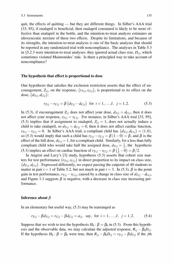
5.3 Instruments 135
quit, the effects of quitting — but they are different things. In Silber’s AAA trial
[33, 95], if enalapril is beneficial, then enalapril consumed is likely to be more ef-
fective than enalapril in the bottle, and the intention-to-treat analysis estimates an
idiosyncratic mixture of these two effects. Despite its limitations, and because of
its strengths, the intention-to-treat analysis is one of the basic analyses that should
be reported in any randomized trial with noncompliance. The analyses in Table 5.3
in §5.2.3 were intention-to-treat analyses: they ignored actual class size, Di j, which
sometimes violated Maimonides’ rule. Is there a principled way to take account of
noncompliance?
The hypothesis that effect is proportional to dose
One hypothesis that satisfies the exclusion restriction asserts that the effect of en-
couragement, Zi j, on the response,(rTi j,rCi j
), is proportional to its effect on the
dose,(dTi j,dCi j
):
rTi j − rCi j = β(dTi j −dCi j
)for i = 1, . . . , I, j = 1,2. (5.3)
In (5.3), if encouragement Zi j does not affect your dose, dTi j = dCi j, then it does
not affect your response, rTi j = rCi j. For instance, in Silber’s AAA trial [33, 95],
(5.3) implies that if assignment to enalapril, Zi j = 1, does not actually induce a
child to take enalapril, so dTi j = dCi j = 0, then it does not affect cardiac function,
rTi j − rCi j = 0. In Silber’s AAA trial, a compliant child has(dTi j,dCi j
)= (1,0),
so (5.3) would imply that such a child has rTi j − rCi j = β (1−0) = β , and β is the
effect of the full dose, dTi j = 1, for a compliant child. Similarly, for a less than fully
compliant child who would take half the assigned dose, dTi j = 12 , the hypothesis
(5.3) implies an effect on cardiac function of rTi j − rCi j = β(
12 −0
)= β/2.
In Angrist and Lavy’s [3] study, hypothesis (5.3) asserts that cohort size mat-
ters for test performance(rTi j,rCi j
)in direct proportion to its impact on class size,(
dTi j,dCi j). Expressed differently, we expect passing the cutpoint of 40 students to
matter in pair i = 1 of Table 5.2, but not much in pair i = 3. In (5.3), β is the point
gain in test performance, rTi j − rCi j, caused by a change in class size of dTi j −dCi j,
and Figure 1.1 suggests β is negative, with a decrease in class size increasing per-
formance.
Inference about β
In an elementary but useful way, (5.3) may be rearranged as
rTi j −βdTi j = rCi j −βdCi j = ai j, say, for i = 1, . . . , I, j = 1,2. (5.4)
Suppose that we wish to test the hypothesis H0 : β = β0 in (5.3). From this hypoth-
esis and the observable data, we may calculate the adjusted response, Ri j −β0Di j.
If the hypothesis H0 : β = β0 were true, then Ri j −β0Di j = rTi j −βdTi j if the jth
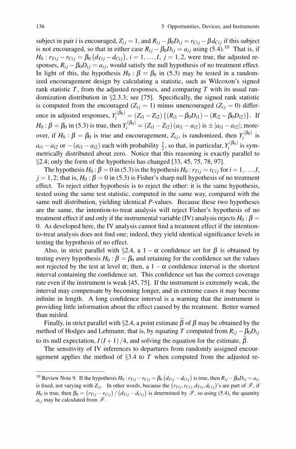
136 5 Opportunities, Devices, and Instruments
subject in pair i is encouraged, Zi j = 1, and Ri j −β0Di j = rCi j −βdCi j if this subject
is not encouraged, so that in either case Ri j −β0Di j = ai j using (5.4).10 That is, if
H0 : rTi j − rCi j = β0
(dTi j −dCi j
), i = 1, . . . , I, j = 1,2, were true, the adjusted re-
sponses, Ri j −β0Di j = ai j, would satisfy the null hypothesis of no treatment effect.
In light of this, the hypothesis H0 : β = β0 in (5.3) may be tested in a random-
ized encouragement design by calculating a statistic, such as Wilcoxon’s signed
rank statistic T , from the adjusted responses, and comparing T with its usual ran-
domization distribution in §2.3.3; see [75]. Specifically, the signed rank statistic
is computed from the encouraged (Zi j = 1) minus unencouraged (Zi j = 0) differ-
ence in adjusted responses, Y (β0)i = (Zi1 −Zi2){(Ri1 −β0Di1)− (Ri2 −β0Di2)}. If
H0 : β = β0 in (5.3) is true, then Y (β0)i = (Zi1 −Zi2)(ai1 −ai2) is ±|ai1 −ai2|; more-
over, if H0 : β = β0 is true and encouragement, Zi j, is randomized, then Y (β0)i is
ai1 −ai2 or −(ai1 −ai2) each with probability 12 , so that, in particular, Y (β0)
i is sym-
metrically distributed about zero. Notice that this reasoning is exactly parallel to
§2.4; only the form of the hypothesis has changed [33, 45, 75, 78, 97].
The hypothesis H0 : β = 0 in (5.3) is the hypothesis H0 : rTi j = rCi j for i = 1, . . . , I,
j = 1,2; that is, H0 : β = 0 in (5.3) is Fisher’s sharp null hypothesis of no treatment
effect. To reject either hypothesis is to reject the other: it is the same hypothesis,
tested using the same test statistic, computed in the same way, compared with the
same null distribution, yielding identical P-values. Because these two hypotheses
are the same, the intention-to-treat analysis will reject Fisher’s hypothesis of no
treatment effect if and only if the instrumental variable (IV) analysis rejects H0 : β =0. As developed here, the IV analysis cannot find a treatment effect if the intention-
to-treat analysis does not find one; indeed, they yield identical significance levels in
testing the hypothesis of no effect.
Also, in strict parallel with §2.4, a 1−α confidence set for β is obtained by
testing every hypothesis H0 : β = β0 and retaining for the confidence set the values
not rejected by the test at level α; then, a 1−α confidence interval is the shortest
interval containing the confidence set. This confidence set has the correct coverage
rate even if the instrument is weak [45, 75]. If the instrument is extremely weak, the
interval may compensate by becoming longer, and in extreme cases it may become
infinite in length. A long confidence interval is a warning that the instrument is
providing little information about the effect caused by the treatment. Better warned
than misled.
Finally, in strict parallel with §2.4, a point estimate β of β may be obtained by the
method of Hodges and Lehmann; that is, by equating T computed from Ri j −β0Di j
to its null expectation, I (I +1)/4, and solving the equation for the estimate, β .
The sensitivity of IV inferences to departures from randomly assigned encour-
agement applies the method of §3.4 to T when computed from the adjusted re-
10 Review Note 9. If the hypothesis H0 : rTi j −rCi j = β0
(dTi j −dCi j
)is true, then Ri j −β0Di j = ai j
is fixed, not varying with Zi j . In other words, because the(rTi j,rCi j,dTi j,dCi j
)’s are part of F , if
H0 is true, then β0 =(rTi j − rCi j
)/(dTi j −dCi j
)is determined by F , so using (5.4), the quantity
ai j may be calculated from F .

5.3 Instruments 137
sponses Ri j −β0Di j; see [75, 78, 97]. Weak instruments are invariably sensitive to
small departures from random assignment of encouragement [97].
Example: IV analysis for Maimonides’ rule
In Angrist and Lavy’s [3] study of academic test performance and class size manip-
ulated by Maimonides’ rule, the hypothesis H0 : β = β0 in (5.3) with β0 = −0.1 for
the math test asserts that a one-student increase in class size produces a decrease of110 point in the average math score. At the cutpoint of 40 students, Maimonides’
rule reduces the average class size by about 20 students, so if H0 : β = −0.1 were
true, that reduction would increase average math test scores by about 2 points. Is
that hypothesis plausible?
To test this hypothesis, apply Wilcoxon’s signed rank test to
Y (β0)i = (Zi1 −Zi2){(Ri1 −β0Di1)− (Ri2 −β0Di2)} (5.5)
with β0 = −0.1. For instance, in Table 5.2, in pair i = 1,
Y (−0.1)1 = (Z11 −Z12){(R11 −β0D11)− (R12 −β0D12)} (5.6)
= (1−0) [{72.1− (−0.1) ·23.0}−{63.1− (−0.1) ·40.0}] = 7.3. (5.7)
Applying Wilcoxon’s signed rank test to the I = 86 adjusted differences, Y (−0.1)i ,
yields a one-sided P-value of 0.00909, suggesting that β < β0 = −0.1, and yields a
two-sided P-value of 2×0.00909 = 0.01818. In Figure 1.1, if cohort size were an
instrument for class size — that is, if cohort size were random and influenced math
scores only by influencing class size through (5.3) — then it would be quite clear
that a one-student increase in class size depresses average math scores by more than1
10 of a point.
A confidence interval is built by inverting the hypothesis test; see §2.4. Test-
ing every hypothesis H0 : β = β0 in (5.3) in this way, retaining those not re-
jected by the two-sided 0.05 level test, yields the 95% confidence interval for β of
[−0.812, −0.151]. For instance, the one-sided P-value for testing H0 : β =−0.1515
is 0.0252, so this hypothesis is barely not rejected in a two-sided, 0.05 level test,
whereas the one-sided P-value for testing H0 : β = −1.51 is 0.0249, so this hypoth-
esis is barely rejected. Under Maimonides’ rule, for a 20 student increase in class
size as the cohort size goes from 41 to 40, the confidence interval for the change in
average math scores 20β is 20× [−0.812, −0.151] or [−16.24, −3.02] points.
A point estimate is obtained from the test by the method of Hodges and Lehmann;
see §2.4. With I = 86 pairs of schools, the null expectation of Wilcoxon’s signed
rank statistic T is I (I +1)/4 = 86(86+1)/4 = 1870.5. If T is computed from
Y (−0.4518)i , it yields T = 1871, a little too high, but if T is computed from Y (−0.4519)
i ,
it yields T = 1870, a little too low, so upon rounding to three digits, the Hodges-

138 5 Opportunities, Devices, and Instruments
Lehmann point estimate β of β in (5.3) is β = −0.452 or 20β = −9.04 math score
points for a 20 student increase in class size.
If cohort size were truly an instrument for class size and if (5.3) were true as well,
then Y (β )i would be symmetric about zero. Figure 5.2 plots the ‘residuals,’ that is
the differences in test performance adjusted for the estimated effect of class size,
Y
(β
)i = Y (−0.452)
i . The residuals Y
(β
)i do not deviate noticeably from symmetry
about zero.
−30 −20 −10 0 10 20 30
Boxplot of IV Residuals
Difference in math scores adjusted for estimated treatment effect
Histogram of IV Residuals
Difference in math scores adjusted for estimated treatment effect
Fre
quen
cy
−30 −20 −10 0 10 20 30
05
1015
Fig. 5.2 IV residuals of math test scores, Y (β0)i with β0 = −0.452, in I = 86 pairs of two Israeli
schools. If cohort size were in fact an instrument for class size in these schools, and if β =−0.452,then these residuals would be symmetric about zero. The residuals look approximately symmetricabout zero, with a mean of −0.03.
As discussed in §5.2.3, for the 86 pairs of schools in Figure 1.1 with fifth grade
cohorts between 30 and 50, cohort size may not be completely random, so that
cohort size is not actually an instrument for class size. Because of the nature of the

5.3 Instruments 139
comparison, very large biases may seem implausible, but no matter how carefully
a nonrandomized comparison is structured, it is never possible to completely rule
out the possibility of small biases. As in §3.4 and §5.2.3, a sensitivity analysis may
be conducted; see [75, 78] and [81, §5]. In fact, the math test results in Table 5.3
are the sensitivity analysis for the hypothesis H0 : β = 0. For Γ = 1.1 or Γ = 1.2,
the maximum one sided P-values for testing H0 : β =−0.1 are, respectively, 0.0238
and 0.0508. For Γ ≥ 1, there is an interval[βmin, βmax
]of possible point estimates
of β where, as we have seen, for Γ = 1, the single estimate is β = βmin = βmax =−0.452. As Γ increases, βmin decreases and βmax increases. For Γ = 1.83, βmax =−0.1, whereas for Γ = 2.21, βmax = 0. In brief, from Table 5.3, rejection of no
effect of class size is insensitive to small biases, Γ ≤ 1.4, and a point estimate of no
effect, βmax = 0, requires Γ = 2.21. Again, the qualitative conclusions reached by
Angrist and Lavy [3] are not extremely fragile; small deviations from a truly random
instrument would not alter their qualitative conclusions.
When and why are instruments valuable?
At first glance, the use of instruments seems unattractive. A natural experiment
seeks a consequential treatment to which people are exposed in a haphazard way.
In contrast, an instrument requires both a haphazard exposure and additionally the
exclusion restriction — that is, the exposure must affect the outcome only by af-
fecting the treatment. If a natural experiment rests on one doubtful assumption, a
study using an instrument rests on two doubtful assumptions. At first glance, the
step towards instruments seems to be a step in the wrong direction.
This first impression is reinforced by a second. In reading the scientific literature,
many claimed instruments seem implausible as instruments, perhaps because they
are clearly not random, perhaps because the exclusion restriction seems implausible,
or perhaps because the authors treat these central issues in a glib and superficial
manner. The examples from Angrist and Lavy [3] and Silber and colleagues [33, 95]
are atypical in that they are at least plausible as instruments.
Given these two impressions, why seek instruments? When are they particu-
larly valuable? When are they not needed? Instruments are of greatest value when
any straightforward comparison of treated and control subjects is almost inevitably
affected by the same bias, a bias that will recur whenever and wherever a straight-
forward comparison is made [45, §1]. A typical example is the effect of additional
education on earnings. Almost inevitably, students who obtain post-secondary de-
grees have performed well in school during the ages of compulsory education, have
greater motivation, better standardized test scores, typically greater financial re-
sources, and so on, than students who leave school at an earlier stage. Repeatedly
finding that people with more education earn more does little to isolate the effects
actually caused by education; that is, the biases replicate with the same consistency
that — perhaps with greater consistency than — the effects replicate [79]. In such a
situation, it may be possible to find haphazard nudges that, at the margin, enable or

140 5 Opportunities, Devices, and Instruments
discourage additional education, such as discontinuities in admission or aid criteria,
proximity to affordable education, shifts in the cost or availability of aid. These
nudges may be biased in various ways, but there may be no reason for them to be
consistently biased in the same direction, so similar estimates of effect from studies
subject to different potential biases gradually reduce ambiguity about what part is
effect and what part is bias [79]. In this vein, David Card [21] surveys the many var-
ied techniques used to estimate the economic returns actually caused by additional
education.
5.4 Summary
Although structured by competing theories that make conflicting predictions, obser-
vational studies are built from opportunities, devices, and instruments.
Opportunities are special circumstances in which competing theories may be
contrasted with unusual clarity. In these circumstances, the theories make sharply
different predictions and the most common or plausible unmeasured biases are re-
duced or absent.
The association between a treatment and an outcome is ambiguous when treat-
ments are not assigned at random. The association may be produced by an effect
caused by the treatment or by a comparison of people who are not truly comparable.
Devices are the tools of disambiguation, the active effort to reduce ambiguity.
Certain treatments are consistently assigned in the same biased way, so that
straightforward comparisons of treated and control groups inevitably reproduce the
same bias. There is no direct opportunity to separate the bias from the treatment ef-
fect. In these cases, it may be possible to find haphazard nudges towards treatment,
pushes that tilt but do not control treatment assignment. To the extent that these
nudges are assigned at random and affect outcomes only through acceptance of the
treatment, they form instruments that may permit the isolation of treatment effects.
Instruments are rare, but useful when they exist.
5.5 Further Reading
Part III of this book and Chapters 6 through 9 of [81] are ‘further reading’ for
this chapter. Part III discusses ‘design sensitivity’ which measures the degree to
which different designs or data generating processes produce results that are in-
sensitive to unmeasured biases. In contrast, Chapters 6 through 8 of [81] discuss
the circumstances under which known effects or multiple control groups can detect
unmeasured biases, presenting technical results about these topics, while Chapter
9 of [81] discusses some technical aspects of coherence; alternatively, for articles
covering similar material, see [69, 70, 71, 72, 76]. Multiple control groups are dis-
cussed in [9, 10, 19, 41, 53, 63, 69, 71] and [81, §8]; see also §11.3 and §19.3.

References 141
Known effects are discussed in [57, 66, 70, 71, 110, 25] and [81, §6]. Differential
effects and generic biases are discussed in [87] where further results and examples
may be found; see also the related, interesting but different design used by Rahul
Roychoudhuri and colleagues [91]. The view of instruments as a bridge between
randomized experiments and observational studies is developed in various ways in
[2, 7, 8, 28, 33, 31]. The link between instruments and randomization inference is
developed in [33, 45, 75, 78, 82]. General discussions of ‘opportunities’ are found
in [4, 35, 58, 77, 89, 92, 103, 107]. Lotteries often present ‘opportunities;’ see, for
instance, [5, 8, 39, 43].
References
1. Abadie, A., Gardeazabal, J.: Economic costs of conflict: A case study of the Basque Country.Am Econ Rev 93, 113–132 (2003)
2. Angrist, J.D., Imbens, G.W., Rubin, D.B.: Identification of causal effects using instrumentalvariables (with Discussion). J Am Statist Assoc 91, 444–455 (1996)
3. Angrist, J.D., Lavy, V.: Using Maimonides’ rule to estimate the effect of class size on scholas-tic achievement. Quart J Econ 114, 533–575 (1999)
4. Angrist, J.D., Krueger, A.B.: Empirical strategies in labor economics. In: Ashenfelter, O.,Card, D. (eds.), Handbook of Labor Economics, Volume 3, pp. 1277–1366. New York: Else-vier (1999)
5. Angrist, J., Lavy, V.: New evidence on classroom computers and pupil learning. Econ J 112,735–765 (2002)
6. Anthony, J.C., Breitner, J.C., Zandi, P.P., Meyer, M.R., Jurasova, I., Norton, M.C., Stone,S.V.: Reduced prevalence of AD in users of NSAIDs and H2 receptor antagonists. Neurology54, 2066–2071 (2000)
7. Barnard, J., Du, J.T., Hill, J.L., Rubin, D.B.: A broader template for analyzing broken ran-domized experiments. Sociol Methods Res 27, 285–317 (1998)
8. Barnard, J., Frangakis, C.E., Hill, J.L., Rubin, D.B.: Principal stratification approach to bro-ken randomized experiments: A case study of School Choice vouchers in New York City. JAm Statist Assoc 98, 299–311 (2003)
9. Battistin, E., Rettore, E.: Ineligibles and eligible non-participants as a double comparisongroup in regression-discontinuity designs. J Econometrics 142, 715–730 (2008)
10. Behrman, J.R., Cheng, Y., Todd, P.E.: Evaluating preschool programs when length of expo-sure to the program varies: A nonparametric approach. Rev Econ Statist 86, 108-132 (2004)
11. Berk, R.A., Rauma, D.: Capitalizing on nonrandom assignment to treatments: A regression-discontinuity evaluation of a crime-control program. J Am Statist Assoc 78, 21–27 (1983)
12. Berk, R.A., de Leuuw, J.: An evaluation of California’s inmate classification system using aregression discontinuity design. J Am Statist Assoc 94, 1045–1052 (1999)
13. Bernanke, B.S.: The macroeconomics of the Great Depression: a comparative approach. JMoney Cred Bank 27, 1–28 (1995) Reprinted: Bernanke, B.S. Essays on the Great Depres-sion, Princeton, NJ: Princeton University Press (2000)
14. Bilban, M., Jakopin, C.B.: Incidence of cytogenetic damage in lead-zinc mine workers ex-posed to radon. Mutagenesis 20, 187–191 (2005)
15. Black, S.: Do better schools matter? Parental valuation of elementary education. Q J Econ114, 577–599 (1999)
16. Bound, J.: The health and earnings of rejected disability insurance applicants. Am Econ Rev79, 482–503 (1989)
17. Bound, J., Jaeger, D.A., Baker, R.M.: Problems with instrumental variables estimation whenthe correlation between the instruments and the endogenous explanatory variable is weak. JAm Statist Assoc 90, 443–450 (1995)

142 5 Opportunities, Devices, and Instruments
18. Campbell, D.T.: Factors relevant to the validity of experiments in social settings. PsycholBull 54, 297–312 (1957)
19. Campbell, D.T.: Prospective: artifact and control. In: Rosenthal, R. and Rosnow, R. (eds.),Artifact in Behavioral Research, pp. 351–382. New York: Academic Press (1969)
20. Campbell, D.T.: Methodology and Epistemology for Social Science: Selected Papers.Chicago: University of Chicago Press (1988)
21. Card, D.: The causal effect of education. In: Ashenfelter, O., Card, D., (eds.) Handbook ofLabor Economics. New York: North Holland (2001)
22. Choudhri, E.U., Kochin, L.A.: The exchange rate and the international transmission of busi-ness cycle disturbances: Some evidence from the Great Depression. J Money Cred Bank 12,565–574 (1980)
23. Cioran, E.M.: History and Utopia. Chicago: University of Chicago Press (1998)24. Cochran, W.G.: The planning of observational studies of human populations (with Discus-
sion). J Roy Statist Soc A 128, 234–265 (1965)25. Cook, T.D.: Waiting for life to arrive: a history of the regression-discontinuity designs in
psychology, statistics and economics. J Econometrics 142, 636–654 (2007)26. Eichengreen, B., Sachs, J.: Exchange rates and economic recovery in the 1930’s. J Econ Hist
45, 925–946 (1985)27. Evans, L.: The effectiveness of safety belts in preventing fatalities. Accid Anal Prev 18,
229–241 (1986)28. Frangakis, C.E., Rubin, D.B.: Addressing complications of intention-to-treat analysis in the
combined presence of all-or-none treatment noncompliance and subsequent missing out-comes. Biometrika 86, 365–379 (1999)
29. Fenech, M., Changb, W.P., Kirsch-Voldersc, M., Holland, N., Bonassie, S., Zeiger, E.:HUMN project: Detailed description of the scoring criteria for the cytokinesis-block mi-cronucleus assay using isolated human lymphocyte cultures. Mutat Res 534, 65–75 (2003)
30. Friedman, M., Schwartz, A.J.: A Monetary History of the United States. Princeton, NJ:Princeton University Press (1963)
31. Goetghebeur, E., Loeys, T.: Beyond intent to treat. Epidemiol Rev 24, 85–90 (2002)32. Gould, E. D., Lavy, V., Paserman, M. D.: Immigrating to opportunity: Estimating the effect
of school quality using a natural experiment on Ethiopians in Israel. Q J Econ 119, 489–526(2004)
33. Greevy, R., Silber, J.H., Cnaan, A., Rosenbaum, P.R.: Randomization inference with im-perfect compliance in the ACE-inhibitor after anthracycline randomized trial. J Am StatistAssoc 99, 7–15 (2004)
34. Hahn, J., Todd, P., Van der Klaauw, W.: Identification and estimation of treatment effectswith a regression-discontinuity design. Econometrica 69, 201–209 (2001)
35. Hamermesh, D.S.: The craft of labormetrics. Indust Labor Relat Rev 53, 363–380 (2000)36. Hawkins, N.G., Sanson-Fisher, R.W., Shakeshaft, A., D’Este, C., Green, L.W.: The multi-
ple baseline design for evaluating population based research. Am J Prev Med 33, 162–168(2007)
37. Heckman, J., Navarro-Lozano, S.: Using matching, instrumental variables, and control func-tions to estimate economic choice models. Rev Econ Statist 86, 30–57 (2004)
38. Hill, A.B.: The environment and disease: Association or causation? Proc Roy Soc Med 58,295–300 (1965)
39. Ho, D.E., Imai, K.: Estimating the causal effects of ballot order from a randomized naturalexperiment: California alphabet lottery, 1978-2002. Public Opin Q 72, 216–240 (2008)
40. Holland, P.W.: Causal Inference, path analysis, and recursive structural equations models.Sociolog Method 18, 449–484 (1988)
41. Holland, P.W.: Choosing among alternative nonexperimental methods for estimating the im-pact of social programs: comment. J Am Statist Assoc 84, 875–877 (1989)
42. Imbens, G.W.: The role of the propensity score in estimating dose response functions.Biometrika 87, 706–710 (2000)

References 143
43. Imbens, G.W., Rubin, D.B., Sacerdote, B.I.: Estimating the effect of unearned income onlabor earnings, savings, and consumption: Evidence from a survey of lottery players. AmEcon Rev 91, 778-794 (2001)
44. Imbens, G.W.: Nonparametric estimation of average treatment effects under exogeneity: Areview. Rev Econ Statist 86, 4–29 (2004)
45. Imbens, G., Rosenbaum, P.R.: Robust, accurate confidence intervals with a weak instrument:Quarter of birth and education. J Roy Statist Soc A 168, 109–126 (2005)
46. Imbens, G.W., Lemieux, T.: Regression discontinuity designs: A guide to practice. J Econo-metrics 142, 615–635 (2008)
47. in ’t Veld, B.A., Launer, L.J., Breteler, M.M.B., Hofman, A., Stricker, B.H.C.: Pharmacologicagents associated with a preventive effect on Alzheimer’s disease. Epidemiol Rev 2, 248-268(2002)
48. Joffe, M.M., Colditz, G.A.: Restriction as a method for reducing bias in the estimation ofdirect effects. Statist Med 17, 2233–2249 (1998)
49. Khuder, S.A., Milz, S., Jordan, T., Price, J., Silvestri, K., Butler, P.: The impact of a smokingban on hospital admissions for coronary heart disease. Prev Med 45, 3–8 (2007)
50. LaLumia, S.: The effects of joint taxation of married couples on labor supply and non-wageincome. J Public Econ 92, 1698-1719 (2008)
51. Lambe, M., Cummings, P.: The shift to and from daylight savings time and motor vehiclecrashes. Accid Anal Prev 32, 609–611 (2002)
52. Li, F., Frangakis, C.E.: Polydesigns and causal inference. Biometrics 62, 343–351 (2006)53. Lu, B., Rosenbaum, P.R.: Optimal matching with two control groups. J Comput Graph Statist
13, 422–434 (2004)54. Ludwig, J., Miller, D.L.: Does Head Start improve children’s life chances? Evidence from a
regression discontinuity design. Q J Econ 122, 159–208 (2007)55. Manski, C.: Nonparametric bounds on treatment effects. Am Econ Rev 319–323 (1990)56. Marguart, J.W., Sorensen, J.R.: Institutional and postrelease behavior of Furman-commuted
inmates in Texas. Criminology 26, 677–693 (1988)57. McKillip, J.: Research without control groups: A control construct design. In: Bryant, F.B.,
et al., (eds.), Methodological Issues in Applied Social Psychology, pp. 159–175. New York:Plenum Press (1992)
58. Meyer, B.D.: Natural and quasi-experiments in economics. J Business Econ Statist 13, 151–161 (1995)
59. Mill, J.S.: On Liberty. New York: Barnes and Nobel (1859, reprinted 2004)60. Milyo, J., Waldfogel, J.: The effect of price advertising on prices: evidence in the wake of 44
Liquormart. Am Econ Rev 89, 1081–1096 (1999)61. NIDA: Washington DC Metropolitan Area Drug Study (DC*MADS), 1992. U.S. National
Institute on Drug Abuse: ICPSR Study No. 2347. http://www.icpsr.umich.edu (1999)62. Oreopoulos, P.: Long-run consequences of living in a poor neighborhood. Q J Econ 118,
1533–1575 (2003)63. Origo, F.: Flexible pay, firm performance and the role of unions: New evidence from Italy.
Labour Econ 16, 64–78 (2009)64. Peto, R., Pike, M., Armitage, P., Breslow, N., Cox, D., Howard, S., Mantel, N., McPherson,
K., Peto, J., Smith, P.: Design and analysis of randomised clinical trials requiring prolongedobservation of each patient, I. Br J Cancer 34, 585–612 (1976)
65. Pinto, D., Ceballos, J.M., Garcıa, G., Guzman, P., Del Razo, L.M., Gomez, E.V.H., Garcıa,A., Gonsebatt, M.E.: Increased cytogenetic damage in outdoor painters. Mutat Res 467,105–111 (2000)
66. Reynolds, K.D., West, S.G.: A multiplist strategy for strengthening nonequivalent controlgroup designs. Eval Rev 11, 691–714 (1987)
67. Rosenbaum, P.R.: From association to causation in observational studies. J Am Statist Assoc79, 41-48 (1984)
68. Rosenbaum, P.R.: Sensitivity analysis for certain permutation inferences in matched obser-vational studies. Biometrika 74, 13–26 (1987)

144 5 Opportunities, Devices, and Instruments
69. Rosenbaum, P.R.: The role of a second control group in an observational study (with Discus-sion). Statist Sci 2, 292–316 (1987)
70. Rosenbaum, P.R.: The role of known effects in observational studies. Biometrics 45, 557–569 (1989)
71. Rosenbaum, P.R.: On permutation tests for hidden biases in observational studies. AnnStatist 17, 643–653 (1989)
72. Rosenbaum, P.R.: Some poset statistics. Ann Statist 19, 1091–1097 (1991)73. Rosenbaum, P.R.: Hodges-Lehmann point estimates in observational studies. J Am Statist
Assoc 88, 1250–1253 (1993)74. Rosenbaum, P.R.: Detecting bias with confidence in observational studies. Biometrika 79,
367–374 (1992)75. Rosenbaum, P.R.: Comment on a paper by Angrist, Imbens, and Rubin. J Am Statist Assoc
91, 465–468 (1996)76. Rosenbaum, P.R.: Signed rank statistics for coherent predictions. Biometrics 53, 556–566
(1997)77. Rosenbaum, P.R.: Choice as an alternative to control in observational studies (with Discus-
sion). Statist Sci 14, 259–304 (1999)78. Rosenbaum, P.R.: Using quantile averages in matched observational studies. Appl Statist 48,
63–78 (1999)79. Rosenbaum, P.R.: Replicating effects and biases. Am Statistician 55, 223–227 (2001)80. Rosenbaum, P.R.: Stability in the absence of treatment. J Am Statist Assoc 96, 210–219
(2001)81. Rosenbaum, P.R.: Observational Studies (2nd ed.). New York: Springer (2002)82. Rosenbaum, P.R.: Covariance adjustment in randomized experiments and observational stud-
ies (with Discussion). Statist Sci 17, 286–327 (2002)83. Rosenbaum, P.R.: Does a dose-response relationship reduce sensitivity to hidden bias? Bio-
statistics 4, 1–10 (2003)84. Rosenbaum, P.R.: Design sensitivity in observational studies. Biometrika 91, 153–164
(2004)85. Rosenbaum, P. R.: Heterogeneity and causality: Unit heterogeneity and design sensitivity in
observational studies. Am Statist 59, 147–152 (2005)86. Rosenbaum, P.R.: Exact, nonparametric inference when doses are measured with random
errors. J Am Statist Assoc 100, 511–518 (2005)87. Rosenbaum, P.R.: Differential effects and generic biases in observational studies. Biometrika
93, 573–586 (2006)88. Rosenbaum, P.R.: What aspects of the design of an observational study affect its sensitivity
to bias from covariates that were not observed? Festschrift for Paul W. Holland. Princeton,NJ: ETS (2009)
89. Rosenzweig, M.R., Wolpin, K.I.: Natural ‘natural experiments’ in economics. J Econ Lit 38,827–874 (2000)
90. Rothman, K.J.: Modern Epidemiology. Boston: Little, Brown (1986)91. Roychoudhuri, R., Robinson, D., Putcha, V., Cuzick, J., Darby, S., Møller, H.: Increased
cardiovascular mortality more than fifteen years after radiotherapy for breast cancer: apopulation-based study. BMC Cancer, Jan 15, 7–9 (2007)
92. Rutter, M.: Identifying the Environmental Causes of Disease: How Do We Decide What toBelieve and When to Take Action? London: Academy of Medical Sciences. (2007)
93. Sennett, R.: The Uses of Disorder. New Haven, CT: Yale University Press (1971, 2008)94. Shadish, W.R., Cook, T.D.: The renaissance of field experimentation in evaluating interven-
tions. Annu Rev Psychol 60, 607–629 (2009)95. Silber, J.H., Cnaan, A., Clark, B.J., Paridon, S.M., Chin, A.J., et al.: Enalapril to prevent
cardiac function decline in long-term survivors of pediatric cancer exposed to anthracyclines.J Clin Oncol 5, 820–828 (2004)
96. Small, D.S.: Sensitivity analysis for instrumental variables regression with overidentifyingrestrictions. J Am Statist Assoc 102, 1049–1058 (2007)

References 145
97. Small, D.S., Rosenbaum, P.R.: War and wages: the strength of instrumental variables andtheir sensitivity to unobserved biases. J Am Statist Assoc 103, 924–933 (2008)
98. Small, D.S., Rosenbaum, P.R.: Error-free milestones in error-prone measurements. Ann ApplStatist, to appear (2009)
99. Sobel, M.E.: An introduction to causal inference. Sociol Methods Res 24, 353–379 (1996)100. Sommer, A., Zeger, S.L.: On estimating efficacy from clinical trials. Statist Med 10, 45–52
(1991)101. Stuart, E.A., Rubin, D.B.: Matching with multiple control groups with adjustment for group
differences. J Educ Behav Statist 33, 279–306 (2008)102. Sullivan, J.M., Flannagan, M.J.: The role of ambient light level in fatal crashes: Inferences
from daylight saving time transitions. Accid Anal Prev 34, 487–498 (2002)103. Summers, L.H.: The scientific illusion in empirical macroeconomics (with Discussion).
Scand J Econ 93, pp. 129–148 (1991)104. Tan, Z.: Regression and weighting methods for causal inference using instrumental variables.
J Am Statist Assoc 101, 1607–1618 (2006)105. Thistlethwaite, D.L., Campbell, D.T.: Regression-discontinuity analysis. J Educ Psychol 51,
309–317 (1960)106. Trochim, W.M.K.: Pattern matching, validity and conceptualization in program evaluation.
Eval Rev 9, 575–604 (1985)107. Vandenbroucke, J.P.: When are observational studies as credible as randomized trials? Lancet
363, 1728-1731 (2004)108. van Eeden, C.: An analogue, for signed rank statistics, of Jureckova’s asymptotic linearity
theorem for rank statistics. Ann Math Statist 43, 791–802 (1972)109. Weiss, N.: Inferring causal relationships: Elaboration of the criterion of dose-response. Am
J Epidemiol 113, 487–490 (1981)110. Weiss, N.: Can the ‘specificity’ of an association be rehabilitated as a basis for supporting a
causal hypothesis? Epidemiol 13, 6–8 (2002)111. West, S.G., Duan, N., Pequegnat, W., Gaist, P., Des Jarlais, D.C., Holtgrave, D., Szapoc-
znik, J., Fishbein, M., Rapkin, B., Clatts, M., Mullen, P.D.: Alternatives to the randomizedcontrolled trial. Am J Public Health 98, 1359–1366 (2008)
112. Wintemute, G.J., Wright, M.A., Drake, C.M., Beaumont, J.J.: Subsequent criminal activityamong violent misdemeanants who seek to purchase handguns: risk factors and effectivenessof denying handgun purchase. J Am Med Assoc 285, 1019–1026 (2001)
113. Wright, M.A., Wintemute, G.J., Rivara, F.P.: Effectiveness of denial of handgun purchaseto persons believed to be at high risk for firearm violence. Am J Public Health 89, 88–90(1999)

Chapter 6Transparency
Abstract Transparency means making evidence evident. An observational study
that is not transparent may be overwhelming or intimidating, but it is unlikely to be
convincing. Several aspects of transparency are briefly discussed.
The beliefs we have most warrant for, have no safeguard to rest on, but a standing invitationto the whole world to prove them unfounded. If the challenge is not accepted, or is acceptedand the attempt fails, we are far enough from certainty still; but we have done the best theexisting state of human reason admits of. . . ˙ This is the amount of certainty attainable by afallible being, and this is the sole way of attaining it.
John Stuart Mill [4, page 21]
The objectivity of all science, including mathematics, is inseparably linked with its criticiz-ability.
Karl R. Popper [6, page 137]
Transparency means making evidence evident. An experiment, and by analogy
an observational study, is not a private experience, not the source of some private
conviction. In the absence of transparency, evidence, argument, and conclusions
are not fully available for critical evaluation. Critical discussion, the standing invi-
tation to undermine evidence or argument, is, for John Stuart Mill, the sole safeguard
of our most warranted beliefs. For Karl Popper, critical discussion is inseparably
linked with the objectivity of science and mathematics. To the extent that trans-
parency is needed for critical discussion, transparency is no small issue.
David Cox [2, page 8] writes:
An important aspect of analysis, difficult to achieve with complex methods, is transparency.That is, in principle, the pathway between the data and the conclusions should be as clearas is feasible. This is partly for the self-education of the analyst and also is for protectionagainst errors. . . . It is also important for presenting conclusions. . . . Transparency stronglyencourages the use of the simplest methods that will be adequate.
147P.R. Rosenbaum, Design of Observational Studies, Springer Series in Statistics, DOI 10.1007/978-1-4419-1213-8_6, © Springer Science+Business Media, LLC 2010

148 6 Transparency
See also Cox [1, page 11].
In addition to the “use of the simplest methods that will be adequate,” trans-
parency is aided by the following considerations. Introducing a felicitous phrase,
Mervyn Susser [8, page 74] writes: “A main object of research design is thus to
simplify the conditions of observation.” In a chapter with that title, Susser [8, Chap-
ter 7] discusses: (i) limiting observations to the relevant segment of the population
to “isolate the hypothetical causal variable and permit study of its effects alone” [8,
page 74], (ii) “selecting suitable situations” [8, page 76], and (iii) matching to re-
move bias from observed covariates. Concerning (i), see also Joffe and Colditz [3],
who use the term ‘restriction.’ In discussing the design of clinical trials, Richard
Peto et al. [5, page 590] write: “A positive result is more likely, and a null result
is more informative, if the main comparison is of only 2 treatments, these being as
different as possible.”
Modularity aids transparency. If a study addresses several issues, each poten-
tially contentious, but the study is composed of separable, simple modular com-
ponents, then there is the realistic prospect that the scope of contention will be
constructively focused. Modularity limits leakage: controversy remains contained
within the region of contention. Here are three modular questions that arise in most
observational studies. Do the treated and untreated populations overlap sufficiently
with respect to observed covariates to permit the construction of a comparable con-
trol group, or do the populations need to be restricted before such a comparison is
attempted? Has matching succeeded in balancing observed covariates, so matched
treated and control groups are comparable with respect to these observed covariates?
Is it plausible that differing outcomes in treated and control groups are produced by
imbalances in a specific unmeasured covariate? If these questions are separated and
addressed one at a time, the first two questions may be settled with little contro-
versy before engaging the inevitably more contentious third question. If the three
questions are addressed simultaneously in one grand analysis, little conviction or
consensus may develop even about the first two questions.
To Cox’s good list of reasons for seeking transparency, I would add one more [7,
Chapter 12]. If smaller issues are permitted to become unnecessarily complex, then
the analysis may collapse under the weight of these complexities before engaging
larger issues. In observational studies, if the adjustment for observed covariates be-
comes unnecessarily complex, as sometimes happens, then the analysis may never
engage the fundamental issue, namely possible biases from covariates that were not
measured. Like a good card trick, unnecessarily complex adjustments for observed
covariates may distract attention from the fundamental issue in observational stud-
ies, but they are unlikely to shed much light on it.
An empirical study that is not transparent may be published or cited, but it is less
likely to undergo serious critical discussion and therefore less likely to receive the
implicit endorsement of surviving such discussion largely unscathed. Conversely,
if critical discussion of a transparent study reveals potential ambiguities or alterna-
tive interpretations, that discussion may stimulate a replication that eliminates the
ambiguities (§4.5). If a study has unambiguous faults, they are more likely to be

References 149
discovered if the study is transparent, and hence there is greater reason to trust the
conclusions of a transparent study when no such faults are identified.
References
1. Cox, D.R.: Planning of Experiments. New York: Wiley (1958)2. Cox, D.R.: Applied statistics: a review. Ann Appl Statist 1, 1–16 (2007)3. Joffe, M.M., Colditz, G.A.: Restriction as a method for reducing bias in the estimation of direct
effects. Statist Med 17, 2233–2249 (1998)4. Mill, J.S.: On Liberty. New York: Barnes and Nobel (1859, reprinted 2004)5. Peto, R., Pike, M., Armitage, P., Breslow, N., Cox, D., Howard, S., Mantel, N., McPherson,
K., Peto, J., Smith, P. Design and analysis of randomised clinical trials requiring prolongedobservation of each patient, I. Br J Cancer 34, 585–612 (1976)
6. Popper, K.R.: Objective Knowledge. Oxford: Oxford University Press (1972)7. Rosenbaum, P.R.: Observational Studies. New York: Springer (2002)8. Susser, M.: Causal Thinking in the Health Sciences. New York: Oxford University Press (1973)

Part IIMatching

Chapter 7A Matched Observational Study
Abstract As a prelude to several chapters describing the construction of a matched
control group, the current chapter presents an example of a matched observational
study as it might (and did) appear in a scientific journal. When reporting a matched
observational study, the matching methods are described very briefly in the Methodssection. In more detail, the Results section presents tables or figures showing that
the matching has been effective in balancing certain observed covariates, so that
treated and control groups are comparable with respect to these specific variables.
The Results section then compares outcomes in treated and control groups. Because
matching has arranged matters to compare ostensibly comparable groups, the com-
parison of outcomes is often both simpler in form and more detailed in content than
it might be if separate adjustments were required for each aspect of each outcome.
Treated and control groups that appear comparable in terms of a specific list of mea-
sured covariates – groups that are ostensibly comparable – may nonetheless differ
in terms of covariates that were not measured. Though not discussed in the current
chapter, the important issue of unmeasured covariates in this example is discussed
in Part III.
7.1 Is More Chemotherapy More Effective?
Jeffrey Silber, Dan Polsky, Richard Ross, Orit Even-Shoshan, Sandy Schwartz, Ka-
trina Armstrong, Tom Randall, and I [6, 8] asked how the intensity of chemother-
apy for ovarian cancer affected patient outcomes. We thought that greater intensity
might prolong survival, perhaps at the cost of increased toxicity. What evidence
bears on this question?
There is a basic difficulty in studying the intended effects of medical treat-
ments outside of randomized controlled clinical trials [9]. In virtually all areas
of medicine, most of the variation in treatment occurs in thoughtful and deliberate
response to variation in the health, prognosis or wishes of patients. That is, treat-
ment assignment is very far from being determined ‘at random.’ Ovarian cancer is
153P.R. Rosenbaum, Design of Observational Studies, Springer Series in Statistics, DOI 10.1007/978-1-4419-1213-8_7, © Springer Science+Business Media, LLC 2010

154 7 A Matched Observational Study
unusual in this regard because there is a meaningful source of variation in treat-
ment that is not a response to the patient. Chemotherapy for ovarian cancer is pro-
vided by two distinct specialties, namely medical oncologists (MOs), who provide
chemotherapy for cancers of all kinds, and gynecologic oncologists (GOs), who pri-
marily treat cancers of the ovary, uterus and cervix. Medical oncologists typically
have a residency in internal medicine, followed by a fellowship emphasizing the ad-
ministration of chemotherapy and the management of its side effects. Gynecologic
oncologists typically complete a residency in obstetrics and gynecology, followed
by a fellowship in gynecologic oncology, that includes training in surgical oncol-
ogy and chemotherapy administration for gynecologic cancers. Unlike gynecologic
oncologists, who are trained in surgery, medical oncologists are almost invariably
not surgeons, so medical oncologists provide chemotherapy after someone else has
performed surgery. We anticipated, as turned out to be the case, that MOs would
use chemotherapy more intensively than GOs, both at the time of initial diagnosis
and several years later if the cancer has spread from its site of origin. Is the greater
intensity of chemotherapy found in the practice of MOs of benefit to patients?
The study was based on data that linked the Surveillance, Epidemiology and End
Results (SEER) program of the U.S. National Cancer Institute to Medicare claims.
The SEER data are collected at SEER sites in the United States, where some SEER
sites are cities (e.g., Detroit) and others are states (e.g., New Mexico). The SEER
data include clinical stage and tumor grade. The study used data on women older
than 65 with ovarian cancer who were diagnosed between 1991 and 1999 and had
appropriate surgery and at least some chemotherapy; see [8] for details. There were
344 such women who received chemotherapy from a GO, and 2011 such women
who received chemotherapy from an MO.
7.2 Matching for Observed Covariates
We matched each GO patient to an MO patient, producing 344 matched pairs of two
similar patients. Table 7.1 describes several of the covariates used in the matching.
Was the matching successful in producing GO and MO groups that were reasonably
comparable in terms of observed covariates?
The first group of variables in Table 7.1 describes the type of surgeon. Gyneco-
logic oncologists are specialists in surgery for gynecologic cancers, but surgery is
often performed by gynecologists or general surgeons. Not surprisingly, this vari-
able is substantially out of balance before matching: a patient who has surgery per-
formed by a GO is more likely to have chemotherapy provided by a GO. After
matching, the distributions of surgeon types are almost identical.
Clinical stage is usually thought to be the most important predictor of survival
in ovarian cancer. Perhaps because there is no particular reason for patients to seek
chemotherapy from an MO or a GO, stage was not greatly out of balance before
matching. For stage, the balance after matching is quite close.

7.2 Matching for Observed Covariates 155
Table 7.1 Comparability at baseline for patients with ovarian cancer: all 344 patients of a gyneco-logic oncologist (GO), 344 matched patients of a medical oncologist (MO), and all 2011 patients ofmedical oncologists. Values are in percent, unless labeled as means. Also included in the matching,but not in this table, were additional comorbid conditions, including anemia, angina, arrhythmia,asthma, coagulation disorder, electrolyte abnormality, hepatic dysfunction, hyperthyroidism, pe-ripheral vascular disease, and rheumatoid arthritis. Notice that surgeon type, SEER site, and yearof diagnosis were substantially out of balance prior to matching, but were in reasonable balanceafter matching.
GO matched-MO all-MOn = 344 n = 344 n = 2,011
Surgeon GO 76 75 33Type Gyn 15 16 39
General 8 8 28
Stage I 9 9 9II 11 9 9
III 51 53 47IV 26 26 31
Missing 3 2 3
Tumor 1 5 4 4Grade 2 16 13 17
3 52 55 474 9 8 11
Missing 18 20 21
Demographics Age, mean 72.2 72.2 72.8White 91 94 94Black 8 5 3
Selected COPD 15 12 13Comorbid Hypertension 48 46 42
Conditions Diabetes 11 8 8CHF 2 2 4
SEER Site Connecticut 18 18 15Detroit 26 26 12
Iowa 17 17 17New Mexico 7 7 3
Seattle 9 9 16Atlanta 9 9 7
Los Angeles 12 12 19San Francisco 1 1 9
Year of Diagnosis 1991 4 4 91992 7 7 141993 10 9 141994 11 11 121995 11 13 121996 10 9 121997 16 15 101998 13 15 91999 18 17 9
Propensity Score e(x), mean 0.23 0.21 0.14

156 7 A Matched Observational Study
In fact, whenever possible, we matched exactly for surgeon type and stage. This
means that, whenever possible, a stage III patient whose surgery was performed by
a gynecologist was paired with a stage III patient whose surgery was performed
by a gynecologist. As seen in the marginal distributions in Table 7.1, this was not
always possible. Naive intuition suggests that one should match exactly for every
variable, but a moment’s thought reveals this to be impossible. If there were just
30 binary variables, there would be 230 or about a billion types of patients, so it
is highly unlikely that one would find exact matches on all 30 variables for almost
all of the patients. Nonetheless, the balance on the covariates in Table 7.1 is quite
good, even though, unlike stage and surgeon type, most variables in Table 7.1 are
not exactly matched. Section 9.1 will discuss covariate balance in greater detail. In
practice, exact matching, if used at all, is reserved for one or two critically important
variables.
Surgeon type and clinical stage are connected. A surgeon who is trained specif-
ically in cancer surgery, such as a GO, is likely to combine an effort at curative
surgery with extensive node sampling. In consequence, a cancer surgeon may find
more cancer than a general surgeon, and may assign a patient to a higher clinical
stage [2]. That is, a patient who is classified as stage II by a general surgeon might
have been classified as stage III by a GO. The very meaning of one variable, clinical
stage, depends upon another variable, surgeon type. However, because almost all
of the pairs are matched exactly for stage and surgeon type, in almost all pairs, the
two patients received the same stage from the same category of surgeon.
Tumor grade, demographics, and selected comorbid conditions are seen to be
reasonably well balanced, and the same is true for other comorbid conditions men-
tioned in the caption of Table 7.1. Comorbid conditions matter both because they
may pose a direct risk to the patient’s survival and may also complicate and limit
the administration of chemotherapy.
Gynecologic oncologists are unevenly spread through the United States, and the
profession has been growing over time. For this reason, before matching, both
SEER site and year of diagnosis were often quite different for the patients of GOs
and MOs. For patients of GOs at SEER sites, 26% were in Detroit and only 1%
in San Francisco, while for all MO patients, 12% were in Detroit and 9% in San
Francisco. Expressed in terms of odds ratios, a woman is almost 20 times as likely
to be treated by a GO in Detroit than in San Francisco. Although ovarian can-
cer is, presumably, much the same disease in Detroit and San Francisco, there are
differences in wealth, demographics, and health services that might affect patient
outcomes. After matching, the distributions of SEER sites are the same. Similarly,
GO patients were more likely to have been diagnosed recently, simply because there
are more GOs recently. Although ovarian cancer itself may not have changed much
through the 1990s, the chemotherapies did improve [3], so a substantial imbalance
in year of diagnosis would compare patients who received different drugs. After
matching, the proportion of patients diagnosed in three time intervals, 1991–1992,
1993–1996, and 1997–1999, were identical, with only small imbalances for indi-
vidual years inside these intervals. In fact, although this is not visible in Table 7.1,
the joint behavior of the three time intervals and the SEER site is exactly balanced;

7.3 Outcomes in Matched Pairs 157
Table 7.2 Weeks with chemotherapy, in year 1 and in years 1 through 5, for 344 matched pairs.Values are the mean, quartiles, minimum, and maximum. Two-sided P-values are from Wilcoxon’ssigned rank test.
Period Group Mean Min 25% 50% 75% Max P-value
Year 1 GO 6.63 1 5 6 8 19 0.0022Year 1 MO 7.74 1 5 6 10 42
Years 1-5 GO 12.07 1 5 9 16 70 0.00045Years 1-5 MO 16.47 1 6 11 21 103
for instance, the number of GO patients in 1991–1992 from Iowa equals the number
of matched MO patients in 1991–1992 from Iowa. The balance on SEER site and
year of diagnosis was obtained using “fine balance” [5, 6], a technique discussed in
Chapter 10.
The large imbalances before matching in surgeon type, year of diagnosis, and
SEER site, and the much smaller imbalances before matching in clinical stage,
grade and comorbid conditions are somewhat encouraging. They hint at the pos-
sibility that the chemotherapy provider type reflects the relative availability of MOs
and GOs more than it reflects attributes of the patient’s disease. In any event, the
measured covariates are reasonably well balanced after matching.
The final variable in Table 7.1 is the propensity score. It is an estimate of the con-
ditional probability of receiving chemotherapy from a GO rather than an MO given
the observed covariates. Propensity scores are a basic tool when matching on many
variables [4]. Propensity scores were discussed conceptually in §3.3, and their role
in multivariate matching is discussed further in Chapter 8. In Table 7.1, the mean
propensity score is fairly similar in the two matched groups; indeed, the balance on
many covariates is produced by balancing the propensity score; see (3.10).
7.3 Outcomes in Matched Pairs
As anticipated, many MOs often used chemotherapy more intensely than did GOs,
both in the first year following diagnosis and in the first five years following diag-
nosis; see Table 7.2 and Figure 7.1. The difference at the medians is not large, but
it is quite noticeable at the upper quartiles. Was greater intensity of treatment by
MOs beneficial?
Despite a difference in intensity, survival was virtually identical for the patients
of MOs and GOs; see Table 7.3. The standard test comparing paired censored sur-
vival times is the Prentice-Wilcoxon test [7]; it gives a two-sided P-value of 0.45.
Table 7.3 also lists the number of patients at risk at the beginning of each of the
first five years, that is, the number of patients alive and uncensored at the start of
the year. The number of patients at risk is also very similar for matched patients of
MOs and GOs.

158 7 A Matched Observational Study
●
●●●●●●●●●●●
●●●
●
●●●
●
●
●
●
●
●●●●
●
●
●
●
GO MO
010
2030
4050
Year 1 Chemotherapy
Che
mot
hera
py W
eeks
●●
●
●
●
●
●●
●●●●
●●
●●
●●
●●●
●
●
●
●
●
●
●●●
●
●
●
●
●
●
●●
●●
GO MO
010
2030
4050
Year 1 Toxicity
Tox
icity
Wee
ks
●
●
●●
●●●●●
●
●●●●●●●
●
●
●
●
●●●
●
●
●
●
●
●
●●
●
●
●●●●
●
●
●
●
GO MO
020
4060
8012
0
Years 1−5 Chemotherapy
Che
mot
hera
py W
eeks
●
●
●●
●
●
●●●
●
●●
●
●
●
●●
●
●
●
●
●●●
●
●
●
●
●
●●
●●●●
●
●
●
●
●
●
●
●
●
●
●
●
●
●●
●
GO MO
020
4060
8012
0Years 1−5 Toxicity
Tox
icity
Wee
ks
Fig. 7.1 Chemotherapy and toxicity in 344 pairs of patients with ovarian cancer, one treated by aGO, the other by an MO.
Patients of MOs had more weeks of toxicity than did patients of GOs; see Table
7.4 and Figure 7.1. In Table 7.4, both in year 1 and in years 1 to 5, the upper
quartiles for MO patients are double those for GO patients.
The difference in intensity was associated with the difference in toxicity; see
Figure 7.2. In Figure 7.2, the 344 matched pair differences in toxicity weeks, MO-
minus-GO, are plotted against the 344 matched pair differences in chemotherapy
weeks. Points project horizontally into the marginal boxplot of the differences in
toxicity weeks. The curve is a lowess smooth [1, pages 168–180] as implemented
in the statistical package R. Kendall’s rank correlation between toxicity differences
and chemotherapy differences is 0.39 and is significantly different from zero, with
a two-sided significance level less than 10−10.
In brief, it appears that MOs often treated more intensively than GOs, often with
more toxicity, but survival was no different.

7.4 Summary 159
Table 7.3 Survival and number at risk in 344 matched pairs of one GO patient and one MO patient.The two-sided P-value of 0.45 is from the Prentice-Wilcoxon test [7] comparing paired survivaltimes.
GO Patients MO Patients
Median (Years) 3.04 2.9895% CI [2.50, 3.40] [2.69, 3.67]
1 Year Survival % 86.6 87.595% CI [83.0, 90.2] [84.0, 90.1]
2 Year Survival % 64.8 66.995% CI [59.8, 69.9] [61.9, 71.8]
5 Year Survival % 35.1 34.295% CI [30.0, 40.2] [29.2, 39.3]
Number at Risk Year 0 344 344Number at Risk Year 1 298 301Number at Risk Year 2 223 230Number at Risk Year 3 173 172Number at Risk Year 4 133 128
Table 7.4 Weeks with chemotherapy-associated toxicity, in year 1 and in years 1 through 5, for344 matched pairs. Values are the mean, quartiles, minimum, and maximum. Two-sided P-valuesare from Wilcoxon’s signed rank test. Chemotherapy-associated toxicity refers to inpatient or out-patient diagnoses for anemia, neutropenia, thrombocytopenia, diarrhea, dehydration or mucositis,and neuropathy.
Period Group Mean Min 25% 50% 75% Max P-value
Year 1 GO 3.61 0 0 2 5 26 0.00000089Year 1 MO 6.67 0 1 3 10 51
Years 1-5 GO 8.89 0 1 5 11 111 0.000000026Years 1-5 MO 16.29 0 2 7 22 136
An obvious question is whether the patterns exhibited in Tables 7.2-7.4 and Fig-
ures 7.1 and 7.2 could be the result not of differences in intensity of chemotherapy
applied to similar patients, but rather of unmeasured pretreatment differences be-
tween the patients themselves. Table 7.1 showed that, prior to matching, many
covariates were substantially out of balance in the GO and MO groups. It is cer-
tainly possible that some other covariate, a covariate that was not measured, was
also out of balance before matching, and because that variable was not controlled
by matching, it is certainly possible that the variable is still out of balance in Tables
7.2–7.4 and Figures 7.1 and 7.2. This concern is central to Part III, where there will
be further analysis of the ovarian data.
7.4 Summary
This chapter is an introduction to Part II. A matched comparison has been presented
as it might be, and was, presented in a scientific journal [8], with little reference to
the procedures used to construct the matched sample [6]. Matching procedures are

160 7 A Matched Observational Study
●●●● ●●
●
●
●● ●●
●●
●
●
●●
●●●
●
● ●●
●
●
●
●●●
●●
●
●
●
●● ●
●● ●
●●
●
●
●
●
●
●
●
●●
●
●●
●
●
●●●
●
●
●
●
● ●
●
●
●●●
●● ●● ●●
●
●
●
●●
●
●
●●●
●
●
●
●
●
●
●
●
●
●●
●●
●
●
●
●
●●
●
●
●
●
●
● ●●
●
●●
●●
●
●
●●
●●
●
●
●●●
●
●
●
●
●●
●●
●
●
●
●
●●●●●●
●●
●
●●
● ●●
●
●
●
●
●
●
●
●
●
●
●
●
●
●
●
●
●
●
●
●●
●
●
●
●
●
●
●
●
●●
●
●●
●
●
●
●
●
●
●
●
●
●
●
●
●
●
●
●
●
●
●
●
●
●
●
● ●●
●
●●
●●● ●
●●
●
●
●
●
●
●
●
●●
●
●
●
● ●●●●
●
●
●
●
●
●
●●
●●●
●
●
●
●
●
●
●
●
●
●
●
●
●
●
●
●
●
●
●
●●
●
●
●
●
●
●
●
●
●
●
● ●
●
●
● ●
●
●●
●
●
●
●●
●
●●
●
●
●
●
●●
●
●
●
●
●
●
●
●
● ●
●
●
●
●
●●
●
●
●
●
●
●●●
●
●
●
●
●
●●●
●
●
●
●
−150 −100 −50 0 50 100 150
−15
0−
100
−50
050
100
150
344 MO−GO Matched Pair Differences
MO−GO Weeks of Chemotherapy, Years 1−5
MO
−G
O W
eeks
of T
oxic
ity, Y
ears
1−
5
●
●
●
●
●
●
●
●
●
●
●
●
●
●
●
●●●●
●
●
●
●
●
●
●
●●
●
●
●
●
●
●
●
●
●
●
−15
0−
100
−50
050
100
150
Toxicity
MO
−G
O W
eeks
of T
oxic
ity, Y
ears
1−
5
Fig. 7.2 Matched pair differences, MO−GO, in toxicity plotted against differences in chemother-apy. The curve is a lowess smooth.
the focus of Part II. The current chapter has made three basic points. First, match-
ing on many observed covariates is often feasible; see Table 7.1. Second, the reader
may examine the degree to which matched groups are comparable with respect to
observed covariates, as well as which covariates are not among the observed covari-
ates, without getting involved in the procedures used to construct the matched sam-
ple; again, see Table 7.1. Finally, straightforward analyses sufficed to take a close
look at several outcomes — here, survival, chemotherapy, toxicity in Tables 7.2-7.4
and Figures 7.1-7.2 — because those analyses compared two matched groups that
looked similar prior to treatment with respect to observed covariates. More pre-
cisely, analyses conducted under the naıve model for treatment assignment (§3.3)
are straightforward. The possibility that the naıve model is not true is taken up in
Part III.

References 161
7.5 Further Reading
The remainder of Part II is further reading for this chapter. The ovarian cancer study
is discussed in detail by Jeffrey Silber and colleagues [6, 8].
References
1. Cleveland, W.S.: The Elements of Graphing Data. Summit, NJ: Hobart Press.2. Mayer, A.R., Chambers, S.K., Graves, E., et al: Ovarian cancer staging: Does it require a gyne-
cologic oncologist? Gynecol Oncol 47, 223–337 (1992)3. McGuire, W.P., Bundy, B., Wenzel, L., et al.: Cyclophosphamide and cisplatin compared with
paclitaxel and cisplatin in patients with stage III and stage IV ovarian cancer. N Engl J Med334, 1–6 (1996)
4. Rosenbaum, P.R., Rubin, D.B.: The central role of the propensity score in observational studiesfor causal effects. Biometrika 70, 41–55 (1983)
5. Rosenbaum, P.R.: Optimal matching in observational studies. J Am Statist Assoc 84, 1024–1032 (1989)
6. Rosenbaum, P.R., Ross R.N., Silber, J.H.: Minimum distance matched sampling with fine bal-ance in an observational study of treatment for ovarian cancer. J Am Statist Assoc 102, 75–83.(2007)
7. O’Brien, P.C., Fleming, T.R.: A paired Prentice-Wilcoxon test for censored paired data. Bio-metrics 43, 169–180 (1987)
8. Silber, J.H., Rosenbaum, P.R., Polsky, D., Ross, R.N., Even-Shoshan, O., Schwartz, S., Arm-strong, K.A., Randall, T.C.: Does ovarian cancer treatment and survival differ by the specialtyproviding chemotherapy? J Clin Oncol 25, 1169–1175 (2007); related editorial 25, 1157–1159(2007); related letters and rejoinders 25, 3552–3558 (2007)
9. Vandenbroucke, J.P.: When are observational studies as credible as randomized trials? Lancet363, 1728–1731 (2004)

Chapter 8Basic Tools of Multivariate Matching
Abstract The basic tools of multivariate matching are introduced, including the
propensity score, distance matrices, calipers imposed using a penalty function, op-
timal matching, matching with multiple controls and full matching. The tools are
illustrated with a tiny example from genetic toxicology (n = 46), an example that is
so small that one can keep track of individuals as they are matched using different
techniques.
8.1 A Small Example
The mechanics of matching are best illustrated with a very small example, not be-
cause such an example is representative but because it is possible to inspect the
details of what goes on. The example considered here has 47 subjects and three
covariates. Typical examples have many more subjects and many more covariates.
Welders are exposed to chromium and nickel, substances that can cause inappro-
priate links between DNA and proteins, which in turn may disrupt gene expression
or interfere with replication of DNA. Costa, Zhitkovich, and Toniolo [10] mea-
sured DNA-protein cross-links in samples of white blood cells from 21 railroad arc
welders exposed to chromium and nickel and 26 unexposed controls. All 47 sub-
jects were male. In their data in Table 8.1, there are three covariates, namely age,
race and current smoking behavior. The response is a measure of DNA-protein
cross-links.
Summary measures describing the covariates appear at the bottom of Table 8.1.
The welders are about five years younger than the controls on average, have rela-
tively fewer African Americans, and more smokers. For what it is worth, the differ-
ence in age between welders and controls is significant as judged by the t-test, with
a t of −2.25 and a two-sided significance level of 0.03. The two binary variables
yield t’s of −0.94 for race and 1.2 for smoking, and are neither significant by that
standard nor by Fisher’s exact test for a 2× 2 table. In an experiment, random as-
signment leads to the expectation that one covariate in 20 will exhibit an imbalance
163P.R. Rosenbaum, Design of Observational Studies, Springer Series in Statistics, DOI 10.1007/978-1-4419-1213-8_8, © Springer Science+Business Media, LLC 2010

164 8 Basic Tools of Multivariate Matching
Table 8.1 Unmatched data for 21 railroad arc welders and 26 potential controls. Covariates areage, race (C=Caucasian , AA=African American), current smoker (Y=yes, N=no). Response isDPC = DNA-protein cross-links in percent in white blood cells. All 47 subjects are male.
Welders Controls
ID Age Race Smoker DPC ID Age Race Smoker DPC
1 38 C N 1.77 1 48 AA N 1.082 44 C N 1.02 2 63 C N 1.093 39 C Y 1.44 3 44 C Y 1.104 33 AA Y 0.65 4 40 C N 1.105 35 C Y 2.08 5 50 C N 0.936 39 C Y 0.61 6 52 C N 1.117 27 C N 2.86 7 56 C N 0.988 43 C Y 4.19 8 47 C N 2.209 39 C Y 4.88 9 38 C N 0.88
10 43 AA N 1.08 10 34 C N 1.5511 41 C Y 2.03 11 42 C N 0.5512 36 C N 2.81 12 36 C Y 1.0413 35 C N 0.94 13 41 C N 1.6614 37 C N 1.43 14 41 AA Y 1.4915 39 C Y 1.25 15 31 AA Y 1.3616 34 C N 2.97 16 56 AA Y 1.0217 35 C Y 1.01 17 51 AA N 0.9918 53 C N 2.07 18 36 C Y 0.6519 38 C Y 1.15 19 44 C N 0.4220 37 C N 1.07 20 35 C N 2.3321 38 C Y 1.63 21 34 C Y 0.97
22 39 C Y 0.6223 45 C N 1.0224 42 C N 1.7825 30 C N 0.9526 35 C Y 1.59
Mean AA Smoker Mean AA SmokerAge % % Age % %
38 10 52 43 19 35
that is statistically significant at the 0.05 level, at least when the comparison is based
on an appropriate randomization test, such as Fisher’s exact test. 1
A pair matching would form 21 pairs of a welder and a control, discarding five
potential controls, in the process altering the marginal distribution of the three co-
variates in the control group. Pair matching is, perhaps, not the most attractive
method in this particular example. In part, the removal of five controls can have
only a moderate impact on the distribution of covariates. In part, in such a small
example, it is not entirely comfortable to discard five controls. Then again, the old-
est control, #2, is 63 years old, which is ten years older than the oldest welder, #18,
1 Cochran [8] discusses the relationship between the magnitude of a t-statistic for covariate im-balance and the coverage rate of a confidence interval for a treatment effect when no adjustmentis made for the covariate. He concludes that problems begin to occur before the conventional0.05 level of significance is reached, and that attention should be given to covariates exhibiting at-statistic of 1.5 in absolute value.

8.2 Propensity Score 165
Table 8.2 Limitations of pair matching for age in the welder data. Even the 21 youngest of the26 controls are, on average, slightly older than the welders, so even a pair matching that focusedexclusively on one covariate, age, could not entirely eliminate the age difference. The discrepancyis not large in this example but can be large in some studies. Other forms of matching besides pairmatching can make further progress.
Mean Min Q1 Median Q3 Max
All 26 Controls 42.7 30 36 42 48 6321 Youngest Controls 39.6 30 35 40 44 50
21 Welders 38.2 27 35 38 39 53
and at least 19 years older than all other welders; arguably, some controls are not
suitable for comparison.
As Rubin [38] observes, there is a definite limit to what pair matching can ac-
complish. In many cases, what is needed falls well within this attainable limit; in
other cases it does not. Importantly, to a large extent, this limit is not shared by more
flexible matching strategies, such as ‘full matching’ [35]. One can see the limits of
pair matching in Table 8.2. The mean age of the 21 welders is 38.2 years, while
the mean age of the 26 controls is 42.7 years. Even if the only consideration were
reducing the mean age in the control group, in this example, pair matching will fall
slightly short of the goal, because the mean age of the 21 youngest of the 26 con-
trols is 39.6 years. In parallel, for smoking, 11 of the 21 welders are smokers, while
only 9 of the 26 potential controls are smokers, so pair matching can at most select
all nine smoking controls, and cannot perfectly balance smoking. Moreover, the 21
youngest controls include only eight of the nine smokers. Furthermore, although
pair matching can eliminate the imbalance in race, if it does this, it cannot use all
nine smoking controls. The discrepancies are not large, and hence are perhaps tol-
erable in this example, but in other studies, a matching strategy more flexible than
pair matching may be needed.
Before matching, there are L = 47 subjects in Table 8.1, � = 1,2, . . . ,L. In
the example, for subject �, the observed covariate, x�, is three-dimensional, x� =(x�1,x�2,x�3)
T , where (i) x�1 is the age of subject �, (ii) x�2 encodes race, x�2 = 1 if �is African American, x�2 = 0 if � is Caucasian, (iii) x�3 encodes smoking, x�3 = 1 if �is a current smoker, x�3 = 0 otherwise. For instance, x1 = (38,0,0)T . The variable
Z� distinguishes treated subjects from potential controls: Z� = 1 for a treated subject,
here a welder; Z� = 0 for a potential control.
8.2 Propensity Score
As discussed in §3.3, the propensity score is the conditional probability of exposure
to treatment given the observed covariates, e(x) = Pr(Z = 1 | x). The propensity
score is defined in terms of the observed covariates, x, even though there is in-
variably concern about other covariates that were not measured. Properties of the
propensity score are discussed in §3.3 and [30, 31, 33, 36].

166 8 Basic Tools of Multivariate Matching
In the simplest randomized experiment, with treatments assigned by independent
flips of a fair coin, the propensity score is e(x) = Pr(Z = 1 | x) = 12 for all values of
the covariate x. In this case, the covariate x is not useful in predicting the treatment
that a subject will receive. In such a completely randomized experiment, smokers
are just as likely as nonsmokers to receive the treatment — the chance is 12 for
smokers and 12 for nonsmokers — so smokers tend to show up in the treated group
just about as often as they do in the control group, and any difference in smoking
frequency is due to chance, the flip of a coin that assigned one subject to treatment,
another to control.
Brief examination of Table 8.1 suggested that at least age, x1, and possibly race
and smoking, x2 and x3, could be used to predict treatment assignment Z, so that the
propensity score is not constant. Saying that welders tend to be somewhat younger
than controls is much the same as saying that the chance of being a welder is lower
for someone who is older, that is, e(x) is lower when x1 is higher.
If two subjects have the same propensity score, e(x), they may have different
values of x. For instance, a younger nonsmoker and an older smoker might have the
same propensity score, e(x), because welders are often younger smokers. Imagine
that we have two individuals, a welder and a control, with the same propensity score
e(x) but different covariates x. Although these two individuals differ in terms of x,
this difference in x will not be helpful in guessing which one is the welder, because
e(x) is the same. If subjects were matched for e(x), they may be mismatched for x,
but the mismatches in x will be due to chance and will tend to balance, particularly
in large samples. If young nonsmokers and old smokers have the same propensity
score, then a match on the propensity score may pair a young nonsmoking welder to
an old smoking control, but it will do this about as often as it pairs an old smoking
welder to a young nonsmoking control.
In brief, matching on e(x) tends to balance x; see (3.10) in §3.3 or [30]. More
precisely, treatment assignment Z is conditionally independent of observed covari-
ates x given the propensity score e(x). Moreover, the propensity score is the coars-
est function of x with this balancing property, so if the propensity score e(x) is
not balanced, then the observed covariates x will continue to be useful in predict-
ing treatment Z. Expressed differently, ignoring chance imbalances, as we might in
sufficiently large samples, balancing the propensity score e(x) is sufficient to bal-
ance the observed covariates x but also necessary to balance x. It is important to
understand that this is a true statement about observed covariates x, and only about
observed covariates, whether or not treatment assignment also depends on covari-
ates that were not measured. On the negative side, success in balancing the observed
covariates, x, provides no assurance that unmeasured covariates are balanced. On
the positive side, balancing observed covariates — comparing groups that, at least,
look comparable in terms of the observed x — is a discrete task that can be success-
fully completed without reference to possible imbalances in covariates that were
not measured. For the men in Table 8.1, imagine that having a father who worked
as a welder is associated with a much higher chance that the son also will work as
a welder, so father’s occupation is an unmeasured covariate that could be used to
predict treatment Z; then success in matching on the propensity score e(x) would

8.2 Propensity Score 167
Table 8.3 Estimated propensity scores e(x) for 21 railroad arc welders and 26 potential controls.Covariates are age, race (C=Caucasian, AA=African American), current smoker (Y=yes, N=no).
Welders Controls
ID Age Race Smoker e(x) ID Age Race Smoker e(x)1 38 C N 0.46 1 48 AA N 0.142 44 C N 0.34 2 63 C N 0.093 39 C Y 0.57 3 44 C Y 0.474 33 AA Y 0.51 4 40 C N 0.425 35 C Y 0.65 5 50 C N 0.236 39 C Y 0.57 6 52 C N 0.207 27 C N 0.68 7 56 C N 0.158 43 C Y 0.49 8 47 C N 0.289 39 C Y 0.57 9 38 C N 0.4610 43 AA N 0.20 10 34 C N 0.5411 41 C Y 0.53 11 42 C N 0.3812 36 C N 0.50 12 36 C Y 0.6413 35 C N 0.52 13 41 C N 0.4014 37 C N 0.48 14 41 AA Y 0.3515 39 C Y 0.57 15 31 AA Y 0.5516 34 C N 0.54 16 56 AA Y 0.1317 35 C Y 0.65 17 51 AA N 0.1218 53 C N 0.19 18 36 C Y 0.6419 38 C Y 0.60 19 44 C N 0.3420 37 C N 0.48 20 35 C N 0.5221 38 C Y 0.60 21 34 C Y 0.67
22 39 C Y 0.5723 45 C N 0.3224 42 C N 0.3825 30 C N 0.6326 35 C Y 0.65
Mean AA Smoker Mean Mean AA Smoker MeanAge % % e(x) Age % % e(x)38 10 52 0.51 43 19 35 0.39
tend to balance age, race and smoking, but there is no reason to expect it to balance
father’s occupation. In short, (i) matching on e(x) is often practical even when
there are many covariates in x because e(x) is a single variable, (ii) matching on
e(x) tends to balance all of x, and (iii) failure to balance e(x) implies that x is not
balanced.
The propensity score is unknown, but it can be estimated from the data at hand.
In the example, the propensity score is estimated by a linear logit model
log
{e(x�)
1− e(x�)
}= ζ0 +ζ1 x�1 +ζ2 x�2 +ζ3 x�3, (8.1)
and the fitted values e(x�) from this model are the estimates of the propensity score.
The estimates of the propensity score, e(x�), are displayed in Table 8.3. Control #2,
a 63-year-old, Caucasian nonsmoker, has e(x�) = 0.09, only a 9% estimated chance
of being a welder. In contrast, control #12, a 36-year-old smoker, has e(x�) = 0.64,

168 8 Basic Tools of Multivariate Matching
a 64% chance of being a welder, so this control actually has covariates that are
atypical of controls and more typical of welders. Welders #10 and #18 have similar
estimated propensity scores e(x�) but different patterns of covariates x�.
The limitations of pair matching, illustrated for age in §8.1, apply with any vari-
able, including the propensity score. The mean of the 21 largest e(x)’s in the con-
trol group is 0.46, somewhat less than the mean of e(x) in the treated group, namely
0.51, so no pair matching can completely close that gap.
8.3 Distance Matrices
In its simplest form, a distance matrix is a table with one row for each treated subject
and one column for each potential control. For the welder data in Table 8.3, the
distance matrix would have 21 rows and 26 columns; it would be 21×26. The value
in row i and column j of the table is the ‘distance’ between the ith treated subject
and the jth potential control. This ‘distance’ is a nonnegative number2 or infinity,
∞, which measures the similarity of two individuals in terms of their covariates x.
Two individuals with the same value of x would have distance zero. An infinite
distance in row i and column j is used to forbid matching the ith treated subject to
the jth potential control.
For the welder data in Table 8.3, Table 8.4 displays all 21 rows and the first 6 of
26 columns on one such distance matrix. The distance is the squared difference in
the estimated propensity score, e(x). The first welder has e(x) = 0.46 and the first
control has e(x) = 0.14, so the distance in the first row and first column of Table
8.4 is (0.46−0.14)2 = 0.10. If the only concern were to obtain close matches on
e(x), then this might be a reasonable distance. The disadvantage is that two controls
with the same propensity score, e(x), may have different patterns of covariates, x,
and this is ignored in Table 8.4. For example, in the first row and third and fourth
columns of Table 8.4, the distance is zero to two decimal places. Looking back at
Table 8.3, the distances between welder #1 and potential controls #3 and #4 are,
respectively, (0.46−0.47)2 = 0.0001 and (0.46−0.42)2 = 0.0016, so control #3 is
ever so slightly closer to welder #1. However, in terms of the details of x, control
#4 looks to be the better match, a nonsmoker with a two-year difference in age, as
opposed to control #3, a smoker with a six-year difference in age. Because younger
smokers are more common in the welder group, the propensity score is indifferent
between a younger nonsmoker and an older smoker, but the details of x suggest that
control #4 is a better match for welder #1 than is control #4.
An alternative distance [32] insists that individuals be close on the propensity
score, e(x), but once this is achieved, the details of x affect the distance. With a
caliper of width w, if two individuals, say k and �, have propensity scores that differ
by more than w — that is, if |e(xk)− e(x�)| > w — then the distance between these
2 The distance need not be, and typically is not, a distance in the sense that the word is used inmetric space topology: it need not satisfy the triangle inequality.

8.3 Distance Matrices 169
Table 8.4 Squared differences in propensity scores between welders and controls. Rows are the21 welders and columns are for the first 6 of 26 potential controls.
Welder Control 1 Control 2 Control 3 Control 4 Control 5 Control 6
1 0.10 0.13 0.00 0.00 0.05 0.062 0.04 0.06 0.02 0.01 0.01 0.023 0.19 0.23 0.01 0.02 0.12 0.144 0.13 0.18 0.00 0.01 0.08 0.095 0.26 0.32 0.03 0.06 0.18 0.206 0.19 0.23 0.01 0.02 0.12 0.147 0.29 0.35 0.05 0.07 0.20 0.238 0.12 0.16 0.00 0.01 0.07 0.089 0.19 0.23 0.01 0.02 0.12 0.14
10 0.00 0.01 0.07 0.05 0.00 0.0011 0.15 0.19 0.00 0.01 0.09 0.1112 0.13 0.17 0.00 0.01 0.07 0.0913 0.14 0.19 0.00 0.01 0.08 0.1014 0.11 0.15 0.00 0.00 0.06 0.0815 0.19 0.23 0.01 0.02 0.12 0.1416 0.16 0.20 0.01 0.02 0.10 0.1117 0.26 0.32 0.03 0.06 0.18 0.2018 0.00 0.01 0.08 0.05 0.00 0.0019 0.20 0.25 0.02 0.03 0.13 0.1520 0.11 0.15 0.00 0.00 0.06 0.0821 0.20 0.25 0.02 0.03 0.13 0.15
individuals is set to ∞, whereas, if |e(xk)− e(x�)| ≤ w, the distance is a measure
of proximity of xk and x�. The caliper width, w, is often taken as a multiple of the
standard deviation of the propensity score, e(x), so that by varying the multiplier,
one can vary the relative importance given to e(x) and x. In Table 8.3, the standard
deviation of e(x) is 0.172. Tables 8.5 and 8.6 illustrate two distance matrices using a
caliper on the propensity score, in which the caliper is half of the standard deviation
of the propensity score, or 0.172/2 = 0.086.
In problems of practical size, a caliper of 20% of the standard deviation of the
propensity score is more common, and even that may be too large. A reasonable
strategy is to start with a caliper width of 20% of the standard deviation of the
propensity score, adjusting the caliper if needed to obtain balance on the propensity
score.
In both Tables 8.5 and 8.6, welder #1 has a propensity score that differs from
potential controls #1 and #2 by more than 0.086 in absolute value, so the distance
is infinite. There is a finite distance between welder #1 and potential controls #3
and #4, because their propensity scores are close, but in both Tables 8.5 and 8.6,
the distance is much smaller for potential control #4, because this control is closer
to welder #1 in age and smoking behavior. Control #2, who is 63 years old, is at
infinite distance from all 21 welders. Experience [32] and simulation [13] suggest
that matching on the propensity score e(x) alone often suffices to balance the dis-
tribution of covariates, but the individual pairs may be quite different in terms of
x, as in the case of welder #1 and potential control #3; whereas, minimum distance

170 8 Basic Tools of Multivariate Matching
Table 8.5 Mahalanobis distances within propensity score calipers. Rows are the 21 welders andcolumns are for the first 6 of 26 potential controls. An ∞ signifies that the caliper is violated.
Welder Control 1 Control 2 Control 3 Control 4 Control 5 Control 6
1 ∞ ∞ 6.15 0.08 ∞ ∞2 ∞ ∞ ∞ 0.33 ∞ ∞3 ∞ ∞ ∞ ∞ ∞ ∞4 ∞ ∞ 12.29 ∞ ∞ ∞5 ∞ ∞ ∞ ∞ ∞ ∞6 ∞ ∞ ∞ ∞ ∞ ∞7 ∞ ∞ ∞ ∞ ∞ ∞8 ∞ ∞ 0.02 5.09 ∞ ∞9 ∞ ∞ ∞ ∞ ∞ ∞
10 0.51 ∞ ∞ ∞ 10.20 11.1711 ∞ ∞ 0.18 ∞ ∞ ∞12 ∞ ∞ 7.06 0.33 ∞ ∞13 ∞ ∞ 7.57 ∞ ∞ ∞14 ∞ ∞ 6.58 0.18 ∞ ∞15 ∞ ∞ ∞ ∞ ∞ ∞16 ∞ ∞ 8.13 ∞ ∞ ∞17 ∞ ∞ ∞ ∞ ∞ ∞18 9.41 ∞ ∞ ∞ 0.18 0.0219 ∞ ∞ ∞ ∞ ∞ ∞20 ∞ ∞ 6.58 0.18 ∞ ∞21 ∞ ∞ ∞ ∞ ∞ ∞
matching within sufficiently narrow propensity score calipers also tends to balance
the distribution of covariates but confers the added benefit of closer individual pairs,
as in the case of welder #1 and potential control #4.
In Table 8.5, within the caliper, the distance is the Mahalanobis distance [24, 39],
which generalizes to several variables the familiar notion of measuring distance
in units of the standard deviation. Speaking very informally, in the Mahalanobis
distance, a difference of one standard deviation counts the same for each covariate
in x. Even as an informal description, this is not quite correct. The Mahalanobis
distance takes account of the correlations among variables. If one covariate in xwere weight in pounds rounded to the nearest pound and another were weight in
kilograms rounded to the nearest kilogram, then the Mahalanobis distance would
come very close to counting those two covariates as a single covariate because of
their high correlation.
If Σ is the sample covariance matrix of x, then the estimated Mahalanobis dis-
tance [24, 39] between xk and x� is (xk −x�)T Σ−1 (xk −x�). In the welder data in
Table 8.3, x� = (x�1,x�2,x�3)T where x�1 is age, x�2 is a binary indicator of race, and
x�3 is a binary indicator of smoking, and the sample variance covariance matrix is
Σ =
⎡⎣ 54.04 0.39 −0.94
0.39 0.13 0.02
−0.94 0.02 0.25
⎤⎦ (8.2)
with inverse

8.3 Distance Matrices 171
Σ−1 =
⎡⎣ 0.021 −0.077 0.084
−0.077 8.127 −1.009
0.084 −1.009 4.407
⎤⎦ . (8.3)
The Mahalanobis distance was originally developed for use with multivariate
Normal data, and for data of that type it works fine. With data that are not Normal,
the Mahalanobis distance can exhibit some rather odd behavior. If one covariate
contains extreme outliers or has a long-tailed distribution, its standard deviation
will be inflated, and the Mahalanobis distance will tend to ignore that covariate
in matching. With binary indicators, the variance is largest for events that occur
about half the time, and it is smallest for events with probabilities near zero and
one. In consequence, the Mahalanobis distance gives greater weight to binary vari-
ables with probabilities near zero or one than to binary variables with probabilities
closer to one half. In the welder data, two individuals with the same age and race
but different smoking behavior have a Mahalanobis distance of 4.407, whereas two
individuals with the same age and smoking behavior but different race have a Maha-
lanobis distance of 8.127, so a mismatch on race is counted as almost twice as bad
as a mismatch on smoking. Two people who differed by 20 years in age with the
same race and smoking would have a Mahalanobis distance of 0.021×202 = 8.4, so
a difference in race counts about as much as a 20-year difference in age. In a differ-
ent context, if there were binary indicators for the states of the United States, then
the Mahalanobis distance would regard matching for Wyoming as vastly more im-
portant than matching for California, simply because fewer people live in Wyoming.
In many contexts, rare binary covariates are not of overriding importance, and out-
liers do not make a covariate unimportant, so the Mahalanobis distance may not be
appropriate with covariates of this kind.
A simple alternative to the Mahalanobis distance (i) replaces each of the covari-
ates, one at a time, by its ranks, with average ranks for ties, (ii) premultiplies and
postmultiplies the covariance matrix of the ranks by a diagonal matrix whose di-
agonal elements are the ratios of the standard deviation of untied ranks, 1, . . . ,L,
to the standard deviations of the tied ranks of the covariates, and (iii) computes
the Mahalanobis distance using the ranks and this adjusted covariance matrix. Call
this the ‘rank-based Mahalanobis distance.’ Step (i) limits the influence of outliers.
After step (ii) is complete, the adjusted covariance matrix has a constant diagonal.
Step (ii) prevents heavily tied covariates, such as rare binary variables, from having
increased influence due to reduced variance. In the welder data, two individuals
with the same age and race but different smoking behavior have a rank-based Ma-
halanobis distance of 3.2, whereas two individuals with the same age and smoking
behavior but different race have a rank-based Mahalanobis distance of 3.1, so a
mismatch on race is counted as about equal to a mismatch on smoking.
Tables 8.5 and 8.6 contrast the Mahalanobis distance and the rank-based Maha-
lanobis distance for the welder data. In both tables, in row #18 and column #1,
there is the distance between a 53-year-old, Caucasian, nonsmoking welder and a
48-year-old, African American, nonsmoking control. In Table 8.5, the distance is
9.41, while in Table 8.6 the distance is 3.33. In fact, the four largest finite distances

172 8 Basic Tools of Multivariate Matching
Table 8.6 Rank-based Mahalanobis distances within propensity score calipers. Rows are the 21welders and columns are for the first 6 of 26 potential controls. An ∞ signifies that the caliper isviolated.
Welder Control 1 Control 2 Control 3 Control 4 Control 5 Control 6
1 ∞ ∞ 5.98 0.33 ∞ ∞2 ∞ ∞ ∞ 0.47 ∞ ∞3 ∞ ∞ ∞ ∞ ∞ ∞4 ∞ ∞ 10.43 ∞ ∞ ∞5 ∞ ∞ ∞ ∞ ∞ ∞6 ∞ ∞ ∞ ∞ ∞ ∞7 ∞ ∞ ∞ ∞ ∞ ∞8 ∞ ∞ 0.04 3.92 ∞ ∞9 ∞ ∞ ∞ ∞ ∞ ∞
10 0.25 ∞ ∞ ∞ 3.72 4.0111 ∞ ∞ 0.28 ∞ ∞ ∞12 ∞ ∞ 7.61 0.98 ∞ ∞13 ∞ ∞ 9.02 ∞ ∞ ∞14 ∞ ∞ 6.83 0.64 ∞ ∞15 ∞ ∞ ∞ ∞ ∞ ∞16 ∞ ∞ 10.61 ∞ ∞ ∞17 ∞ ∞ ∞ ∞ ∞ ∞18 3.33 ∞ ∞ ∞ 0.05 0.0119 ∞ ∞ ∞ ∞ ∞ ∞20 ∞ ∞ 6.83 0.64 ∞ ∞21 ∞ ∞ ∞ ∞ ∞ ∞
in Table 8.5 are the four distances between Caucasians and African Americans,
whereas race and smoking are about equally important in Table 8.6.
In short, a sturdy choice for a distance is the rank-based Mahalanobis distance
within calipers on the propensity score, with the caliper width w adjusted to ensure
good balance on the propensity score.
8.4 Optimal Pair Matching
An ‘optimal pair matching’ pairs each treated subject with a different control to
minimize the total distance within matched pairs [34]. In the welder data in Table
8.3, this means forming 21 pairs using 21 different controls from the 26 potential
controls so that the sum of the 21 distances within pairs is minimized. The problem
is not trivial because the closest control to one treated subject may also be the closest
control to another treated subject. For instance, in Table 8.4, many treated subjects
are close to potential control #3, but control #3 will be paired to only one of them.
As seen in Table 8.7, a best-first or greedy algorithm will not generally find an
optimal pair matching.
Finding an optimal pair matching is known as the ‘assignment problem’ and was
solved by Kuhn [22] in 1955. One of the fastest algorithms for the assignment
problem was proposed by Bertsekas [4], who offers free Fortran code at his website

8.4 Optimal Pair Matching 173
Table 8.7 A small example showing that a greedy algorithm, or a best-first algorithm, does notsolve the optimal matching problem. A greedy algorithm would pair treated #1 with control #1,and then would be forced to pair treated #2 with control #2 for a total distance of 0+1000, but it ispossible to obtain a match with a total distance of 0.01+0.01.
Control 1 Control 2
Treated 1 0.00 0.01Treated 2 0.01 1000.00
Table 8.8 Optimal pair match using the squared difference in the propensity score. Covariatesare age, race (C=Caucasian , AA=African American), current smoker (Y=yes, N=no), and theestimated propensity score e(x).
Welders Matched Controls
Pair Age Race Smoker e(x) Age Race Smoker e(x)1 38 C N 0.46 45 C N 0.322 44 C N 0.34 47 C N 0.283 39 C Y 0.57 39 C Y 0.574 33 AA Y 0.51 41 C N 0.405 35 C Y 0.65 34 C Y 0.676 39 C Y 0.57 31 AA Y 0.557 27 C N 0.68 35 C Y 0.658 43 C Y 0.49 41 AA Y 0.359 39 C Y 0.57 34 C N 0.5410 43 AA N 0.20 50 C N 0.2311 41 C Y 0.53 44 C Y 0.4712 36 C N 0.50 42 C N 0.3813 35 C N 0.52 40 C N 0.4214 37 C N 0.48 44 C N 0.3415 39 C Y 0.57 35 C N 0.5216 34 C N 0.54 38 C N 0.4617 35 C Y 0.65 36 C Y 0.6418 53 C N 0.19 52 C N 0.2019 38 C Y 0.60 36 C Y 0.6420 37 C N 0.48 42 C N 0.3821 38 C Y 0.60 30 C N 0.63
mean %AA %Y mean mean %AA %Y mean38 10 52 0.51 40 10 38 0.46
at MIT. Hansen’s [16] pairmatch function in his optmatch package makes
Bertsekas’ code available from inside the statistical package R; see [28] for free
access to R, and see [25] for a general textbook about R. Dell’Amico and Toth
[11] provide a recent review of the literature on the assignment problem. A Fortran
implementation of Kuhn’s Hungarian Method is available from the Association for
Computing Machinery (ACM) as implemented by Carpaneto and Toth [7]. The
SAS program proc assign also solves the assignment problem.
For the welder data, Table 8.8 displays an optimal match using the propensity
score distances in Table 8.4. As the discussion in §8.3 led us to expect, the marginal
means at the bottom of Table 8.8 are fairly well balanced, but the individual pairs
are often not matched for race or smoking.

174 8 Basic Tools of Multivariate Matching
Table 8.9 Optimal pair match using the Mahalanobis distance within propensity score calipers.The caliper is half the standard deviation of the propensity score, or 0.172/2 = 0.086. Covari-ates are age, race (C=caucasian , AA=African American), current smoker (Y=yes, N=no) and theestimated propensity score e(x).
Welders Matched Controls
Pair Age Race Smoker e(x) Age Race Smoker e(x)1 38 C N 0.46 44 C N 0.342 44 C N 0.34 47 C N 0.283 39 C Y 0.57 36 C Y 0.644 33 AA Y 0.51 41 AA Y 0.355 35 C Y 0.65 35 C Y 0.656 39 C Y 0.57 39 C Y 0.577 27 C N 0.68 30 C N 0.638 43 C Y 0.49 45 C N 0.329 39 C Y 0.57 36 C Y 0.6410 43 AA N 0.20 48 AA N 0.1411 41 C Y 0.53 44 C Y 0.4712 36 C N 0.50 41 C N 0.4013 35 C N 0.52 40 C N 0.4214 37 C N 0.48 42 C N 0.3815 39 C Y 0.57 35 C N 0.5216 34 C N 0.54 38 C N 0.4617 35 C Y 0.65 34 C Y 0.6718 53 C N 0.19 52 C N 0.2019 38 C Y 0.60 34 C N 0.5420 37 C N 0.48 42 C N 0.3821 38 C Y 0.60 31 AA Y 0.55
mean %AA %Y mean mean %AA %Y mean38 10 52 0.51 40 14 38 0.45
Although it is not obvious from Tables 8.3, 8.5, and 8.6, because of competi-
tion for controls, there is no pair matching in which the caliper on the propensity
score, |e(xk)− e(x�)| ≤ w with w = 0.086, is respected for all 21 matched pairs.
This is true because of competition among welders for the same controls, despite
the fact that each welder has a propensity score within w = 0.086 of at least one
potential control. For this reason, the infinities in Tables 8.5 and 8.6 are not used;
they are replaced by the addition of a ‘penalty function,’ which exacts a large but
finite penalty for violations of the constraint; see, for instance, [2, pages 372–373]
or [21, Chapter 6]. The penalty used here is 1000×max(0, |e(xk)− e(x�)|−w),so if |e(xk)− e(x�)| ≤ w then the penalty is zero, but if |e(xk)− e(x�)| > w then
the penalty is 1000× (|e(xk)− e(x�)|−w). For instance, the penalty for match-
ing welder #1 to potential control #1 is 1000× (|.4587−0.1437|−0.0860) = 229.
This penalty is added to the Mahalanobis distance or rank-based Mahalanobis dis-
tance for the corresponding pair. Optimal matching will try to avoid the penalties
by respecting the caliper, but when that is not possible, it will prefer to match so the
caliper is only slightly violated for a few matched pairs.
Table 8.9 displays the optimal match using the Mahalanobis distances within
propensity score calipers from Table 8.5. Again, the calipers are implemented not

8.5 Optimal Matching with Multiple Controls 175
Table 8.10 Optimal pair match using the rank-based Mahalanobis distance within propensity scorecalipers. The caliper is half the standard deviation of the propensity score, or 0.172/2 = 0.086.Covariates are age, race (C=Caucasian , AA=African American), current smoker (Y=yes, N=no),and the estimated propensity score e(x).
Welders Matched Controls
Pair Age Race Smoker e(x) Age Race Smoker e(x)1 38 C N 0.46 44 C N 0.342 44 C N 0.34 47 C N 0.283 39 C Y 0.57 36 C Y 0.644 33 AA Y 0.51 41 AA Y 0.355 35 C Y 0.65 35 C Y 0.656 39 C Y 0.57 39 C Y 0.577 27 C N 0.68 30 C N 0.638 43 C Y 0.49 45 C N 0.329 39 C Y 0.57 35 C N 0.5210 43 AA N 0.20 48 AA N 0.1411 41 C Y 0.53 44 C Y 0.4712 36 C N 0.50 41 C N 0.4013 35 C N 0.52 40 C N 0.4214 37 C N 0.48 42 C N 0.3815 39 C Y 0.57 36 C Y 0.6416 34 C N 0.54 38 C N 0.4617 35 C Y 0.65 34 C Y 0.6718 53 C N 0.19 52 C N 0.2019 38 C Y 0.60 31 AA Y 0.5520 37 C N 0.48 42 C N 0.3821 38 C Y 0.60 34 C N 0.54
mean %AA %Y mean mean %AA %Y mean38 10 52 0.51 40 14 38 0.45
with ∞’s but rather with a penalty function. Table 8.10 is similar, except the optimal
match uses the rank-based Mahalanobis distance within propensity score calipers in
Table 8.6, again using the penalty function to implement the calipers. The matches
in Table 8.9 and Table 8.10 are similar to each other and better than Table 8.8 in the
specific sense that inside individual pairs the matched individuals are closer.
8.5 Optimal Matching with Multiple Controls
In matching with multiple controls, each treated subject is matched to at least one,
and possibly more than one, control. To match in a fixed ratio is to match each
treated subject to the same number of controls; for instance, pair matching in §8.4
matches in a ratio of 1-to-1, while matching each treated subject to two controls is
matching in a ratio of 1-to-2. To match in a variable ratio is to allow the number of
controls to vary from one treated subject to another. In the welder data in Table 8.3,
there are too few potential controls to match in a 1-to-2 fixed ratio, but it is possible
to match with multiple controls in a variable ratio, and in particular to use all of the

176 8 Basic Tools of Multivariate Matching
controls. The decision to match in fixed or variable ratio is a substantial one that
affects both the quality of the matching and the analysis and presentation of results.
These issues are sketched at the end of this section, following a variable match for
the welder data.
Imagine for a moment that there were 42 or more potential controls in the welder
data in Table 8.3; then it would be possible to match in a fixed 1-to-2 ratio, producing
21 matched sets, each containing one welder and two controls, where all 42 controls
are different. An optimal matching with a fixed ratio of 1-to-2 would minimize the
sum of the distances within matched sets between treated subjects and their matched
controls, or the sum of 42 distances. Similar considerations apply to matching in a
fixed ratio of 1-to-3, 1-to-4, and so on.
Matching with a variable number of controls is slightly more complex. The
optimization algorithm decides not only who is matched to whom, but also how
many controls to assign to each treated subject. So matching with a variable number
of controls has more choices to make, but these choices must be constrained in some
reasonable way to avoid trivial results. If all the distances were positive, and no
constraints were imposed, the minimum distance matching with variable numbers
of controls would always be a pair matching. A simple constraint is to insist that a
certain number of controls be used. For instance, in the welder data, one might insist
that all 26 controls be used. Alternatively, one might insist that 23 controls be used,
which would permit, but not require, the algorithm to discard the three potential
controls who are older than all of the welders. An attractive feature of fixing the
total number of controls is that the total distance is then a sum of a fixed number of
distances. In addition to constraining the total number of controls, a different type
of constraint permits a treated subject to have, say, at least one but at most three
controls. Given some set of constraints on the matching, an optimal matching with
variable controls minimizes the total distance between treated subjects and controls
inside matched sets.
For the welder data, Table 8.11 is an optimal matching with variable controls,
using all 26 controls, based on the Mahalanobis distances with propensity score
calipers. The calipers again use the penalty function in §8.4. The match consists
of 19 pairs, one welder matched to three controls, and one welder matched to four
controls. Matched set #10 consists of older African Americans. Matched set #18
consists of older Caucasian nonsmokers. Both groups were overrepresented in the
control group. As might be expected from the discussion in §8.3, a variable match
using the rank-based Mahalanobis distance (not shown) is generally similar, but
gives about equal emphasis to race and smoking, as opposed to the emphasis on
race in Table 8.11.
In a matched pair, a welder is compared with his matched control. For instance,
in matched pair #1 in Table 8.11, the welder is 38 years old, the matched control is
44 years old, and the difference in age is 38− 44 = −6 years. In matched set #10,
the welder is compared with the average of the three matched controls. In this way,
the comparison in matched set #10 is just slightly less variable than it would be if
one of the three controls were used and the other two were discarded. For instance,
in set #10, the welder is 43 years old, the three matched controls have average age

8.5 Optimal Matching with Multiple Controls 177
Table 8.11 Optimal match with multiple controls using the Mahalanobis distance within propen-sity score calipers. The caliper is half the standard deviation of the propensity score, or 0.172/2 =0.086. Covariates are age, race (C=caucasian, AA=African American), current smoker (Y=yes,N=no) and the estimated propensity score e(x).
Welders Matched Controls
Matched Set Age Race Smoker e(x) Age Race Smoker e(x)1 38 C N 0.46 44 C N 0.34
2 44 C N 0.34 47 C N 0.28
3 39 C Y 0.57 36 C Y 0.64
4 33 AA Y 0.51 41 AA Y 0.35
5 35 C Y 0.65 35 C Y 0.65
6 39 C Y 0.57 36 C Y 0.64
7 27 C N 0.68 30 C N 0.63
8 43 C Y 0.49 45 C N 0.32
9 39 C Y 0.57 35 C N 0.52
10 43 AA N 0.20 51 AA N 0.1210 56 AA Y 0.1310 48 AA N 0.14
11 41 C Y 0.53 44 C Y 0.47
12 36 C N 0.50 41 C N 0.40
13 35 C N 0.52 40 C N 0.42
14 37 C N 0.48 42 C N 0.38
15 39 C Y 0.57 39 C Y 0.57
16 34 C N 0.54 38 C N 0.46
17 35 C Y 0.65 34 C Y 0.67
18 53 C N 0.19 63 C N 0.0918 56 C N 0.1518 52 C N 0.2018 50 C N 0.23
19 38 C Y 0.60 34 C N 0.54
20 37 C N 0.48 42 C N 0.38
21 38 C Y 0.60 31 AA Y 0.55
mean %AA %Y mean mean %AA %Y mean38 10 52 0.51 40 14 40 0.45
(51+56+48)/3 = 51.7, so the difference in age in that set is 43− 51.7 = −8.67
years. Similarly, in set #18, the welder is 53 years old, the four matched controls
have average age (63+56+52+50)/4 = 55.25, so the difference in age in that
set is 53− 55.25 = −2.25 years. The ‘average difference in age’ is the average
of these 21 differences. Similarly, the ‘average age’ in the control group is the
average of these 21 average ages of controls. Implicitly, the control in matched set
#1 counts as one person, but each of the controls in matched set #10 counts as 13 of
a person. In this way, although all controls are used, they are weighted to describe
a younger, more Caucasian population with more smokers, that is, a population like
the 21 welders. Weighted in this way, the mean age among the matched controls
is 40, about two years older than the mean age of 38 for the welders. The same
process is applied to a binary variable, such as smoking, to obtain a 40% smoking
rate among controls. Although all controls are used in Table 8.11, the balance in

178 8 Basic Tools of Multivariate Matching
the covariate means is similar to pair matching in §8.4 which discarded five controls.
This process of weighting is known as ‘direct adjustment,’ and it is one of the basic
differences between matching with a fixed ratio and matching with a variable ratio.3
When matching with a fixed ratio — for instance, with pair matching in §8.4 —
each matched control has the same weight.
The principal advantage of matching in a fixed ratio, such as 1-to-3 matching,
is that summary statistics, including those that might be displayed in graphs, may
be computed from treated and control groups in the usual way, without using direct
adjustment to give unequal weights to observations. For instance, one might dis-
play boxplots or Kaplan-Meier survival curves for treated and control groups. This
advantage will weigh heavily when potential controls are abundant and the biases
that must be removed are not large. A smaller issue is statistical efficiency, which in
nominal terms, though often not in practical terms, slightly favors matching in fixed
ratio over matching with a variable ratio [26].
There are several advantages to matching with a variable ratio [26, 34]. First,
the matched sets will be more closely matched, in the following precise sense. If
one finds the minimum distance match with, say, an average of three controls per
treated subject and two to four controls for each treated subject, the total distance
within matched sets will never be larger, and will typically be quite a bit smaller,
than in fixed ratio matching with three controls.4 This is visible in Table 8.11:
the two welders with low propensity scores were matched to the seven controls
with low propensity scores, and trying to allocate these seven more evenly among
welders would have produced a larger mismatch on these propensity scores. Sec-
ond, matching in fixed ratio requires the number of controls to be an integer multiple
of the number of treated subjects, and this restriction may be inconvenient or unde-
sirable for any of a variety of reasons; for instance, for the welder data in Table
8.3, the only possible matching in fixed ratio is pair matching. Third, just as §8.1
discussed definite limits to what can be accomplished with pair matching, there are
also definite limits to what can be accomplished by matching with multiple controls,
but these limits are better when matching with a variable ratio [26].
Finding an optimal match with variable controls is equivalent to solving a par-
ticular minimum-cost flow problem in a network [34]. In the statistical package R,
Hansen’s [16] fullmatch function in his optmatch package will determine an
optimal match with variable controls from a distance matrix by setting his parame-
ter min.controls to equal 1 rather than its default value of 0; the user will often
3 Direct adjustment can be applied to pretty much anything, not just means and proportions. Inparticular, an empirical distribution function is little more than a sequence of proportions, and itis clear how to apply direct adjustment to proportions. From the weighted empirical distributionfunction, pretty much anything else can be computed; for instance, medians and quartiles. In [17],medians and quartiles from directly adjusted empirical distribution functions are used to constructdirectly adjusted boxplots. In the weighted empirical distribution function, the 44-year-old controlin matched set #1 has mass 1/21, whereas the 63-year-old control in matched set #18 has mass1/(4×21).4 This is true because, when the number of controls matched is the same, optimal matching withvariable controls solves a less constrained optimization problem than matching with a fixed ratio,yet the two problems have the same objective function, so the optimum is never worse.

8.6 Optimal Full Matching 179
Table 8.12 A distance matrix showing that the best full matching can be much better than the bestpair matching or the best matching with variable controls. The best full matching is (1,a,b) and(2,3,c) with a distance of 0.01 + 0.01 + 0.01 + 0.01 = 0.04. A best pair matching is (1,a), (2,b),(3,c), with a distance of 0.01+1000.00+0.01 = 1000.02. Because the number of potential controlsequals the number of treated subjects, every matching with variable controls is a pair matching, sovariable matching can do no better than pair matching.
Control a Control b Control c
Treated 1 0.01 0.01 1000.00Treated 2 1000.00 1000.00 0.01Treated 3 1000.00 1000.00 0.01
wish to adjust the parameter max.controls, which limits the number of con-
trols matched to each treated subject, and the parameter omit.fraction which
determines the number of controls to use. An alternative approach is to use the as-
signment algorithm in §8.4 but with an altered and enlarged distance matrix [27]; for
instance, this can be done with proc assign in SAS. For a textbook discussion
of network optimization, see [1, 5, 9].
Statistical analysis is not difficult when matching with multiple controls, whether
in fixed or variable ratios; see [23, pages 132–145], [12, pages 384–387] or [37,
pages 135–139]. For an illustration, in [17, 18], a study of gang violence among
teenage boys is analyzed twice, first as a study matched with a fixed ratio of 1-
to-2, and second as a study with two strata matched separately, one matched with
between two and seven controls and an average of five controls, the other matched
with between one and six controls with an average of three controls.
8.6 Optimal Full Matching
In matching with a variable number of controls in §8.5, a treated subject could be
matched to one or more controls. In full matching, the reverse situation is permitted
as well: one control may be matched to several treated subjects [35]. Table 8.12
shows that full matching can be vastly better than pair matching or matching with
a variable number of controls. Because full matching includes as special cases all
of the matching procedures considered in §8.4-§8.5, the optimal full matching will
produce matched sets that are at least as close as these procedures.
Table 8.13 is an optimal full match for the welder data in Table 8.3, using all 26
controls, and the Mahalanobis distance within propensity score calipers, with the
calipers implemented using the penalty function in §8.4. Matched set #1 is a pair.
Matched set #2 has one welder and seven controls. Matched set #3 has one control
and seven welders. Within each matched set, the welders and controls look similar.
As in matching with variable controls, summary statistics for the control group
in full matching must be directly adjusted. In parallel with §8.5, the welder in
matched set #2 is compared with the average of the seven controls, so these controls
implicitly have weight 17 . In matched set #3, each of the seven welders is compared

180 8 Basic Tools of Multivariate Matching
Table 8.13 Optimal full match using Mahalanobis distance within propensity score calipers. Thecaliper is half the standard deviation of the propensity score, or 0.172/2 = 0.086. Covariates areage, race (C=Caucasian, AA=African American), current smoker (Y=yes, N=no), and the esti-mated propensity score e(x).
Welders Matched Controls
Matched Set Age Race Smoker e(x) Age Race Smoker e(x)1 38 C N 0.46 40 C N 0.42
2 44 C N 0.34 47 C N 0.282 45 C N 0.322 44 C N 0.342 41 AA Y 0.352 42 C N 0.382 42 C N 0.382 41 C N 0.40
3 41 C Y 0.53 39 C Y 0.573 39 C Y 0.573 39 C Y 0.573 39 C Y 0.573 39 C Y 0.573 38 C Y 0.603 38 C Y 0.60
4 33 AA Y 0.51 31 AA Y 0.55
5 35 C Y 0.65 35 C Y 0.655 34 C Y 0.67
6 27 C N 0.68 30 C N 0.63
7 43 C Y 0.49 44 C Y 0.47
8 43 AA N 0.20 51 AA N 0.128 56 AA Y 0.138 48 AA N 0.14
9 36 C N 0.50 35 C N 0.529 35 C N 0.52
10 37 C N 0.48 38 C N 0.4610 37 C N 0.48
11 34 C N 0.54 34 C N 0.54
12 35 C Y 0.65 36 C Y 0.6412 36 C Y 0.64
13 53 C N 0.19 63 C N 0.0913 56 C N 0.1513 52 C N 0.2013 50 C N 0.23
mean %AA %Y mean mean %AA %Y mean38 10 52 0.51 39 10 55 0.50
with the same control, so this control implicitly has weight 7. As seen at the bottom
of Table 8.13, after weighting or direct adjustment, the means in the control group
are quite similar to the means in the welder group.
Although the matched sets in Table 8.13 are quite homogeneous, the quite un-
equal set sizes can lead to some inefficiency. Tables 8.14 and 8.15 are two of many
possible variations on the same theme. In Table 8.14, the matched sets can be pairs
or triples, and only 21 of the 26 controls are used, in parallel pair matchings in §8.4.

8.6 Optimal Full Matching 181
Table 8.14 Optimal full match with sets of size 2 or 3 and 21 controls using the Mahalanobisdistance within propensity score calipers. The caliper is half the standard deviation of the propen-sity score, or 0.172/2 = 0.086. Covariates are age, race (C=Caucasian, AA=African American),current smoker (Y=yes, N=no) and the estimated propensity score e(x).
Welders Matched Controls
Matched Set Age Race Smoker e(x) Age Race Smoker e(x)1 38 C N 0.46 42 C N 0.381 42 C N 0.38
2 44 C N 0.34 45 C N 0.322 44 C N 0.34
3 39 C Y 0.57 36 C Y 0.643 38 C Y 0.60
4 33 AA Y 0.51 31 AA Y 0.55
5 35 C Y 0.65 35 C Y 0.65
6 39 C Y 0.57 39 C Y 0.576 39 C Y 0.57
7 27 C N 0.68 30 C N 0.63
8 43 C Y 0.49 44 C Y 0.478 41 C Y 0.53
9 43 AA N 0.20 51 AA N 0.129 48 AA N 0.14
10 36 C N 0.50 35 C N 0.5210 35 C N 0.52
11 37 C N 0.48 41 C N 0.4011 38 C N 0.46
12 39 C Y 0.57 36 C Y 0.6412 38 C Y 0.60
13 34 C N 0.54 34 C N 0.54
14 35 C Y 0.65 34 C Y 0.67
15 53 C N 0.19 56 C N 0.1515 52 C N 0.20
16 37 C N 0.48 40 C N 0.42
mean %AA %Y mean mean %AA %Y mean38 10 52 0.51 39 10 52 0.50
In Table 8.15, all 26 controls are used, with at most two welders or at most three
controls in any matched set. In Tables 8.14 and 8.15, welders and controls in the
same matched set are reasonably similar, and the (weighted) means in the control
group are closer to the welder means than for the several pair matchings in §8.4.
In one specific sense, an optimal full matching is an optimal design for an ob-
servational study [35]. Specifically, define a stratification to be a partitioning of the
subjects into groups or strata based on the covariates with the one requirement that
each stratum must contain at least one treated subject and at least one control. The
quality of a stratification might reasonably be judged by a weighted average of all
the within strata distances between treated subjects and controls. For instance, if a
stratum contained two treated subjects and three controls, then the average distance
between the treated and control subjects in this stratum is an average of the 6 = 2×3
distances between two treated and three control subjects. The stratum-specific av-
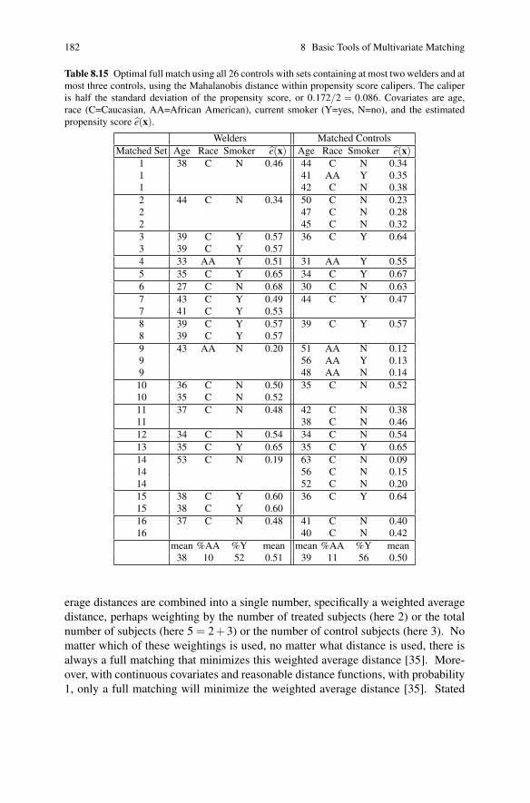
182 8 Basic Tools of Multivariate Matching
Table 8.15 Optimal full match using all 26 controls with sets containing at most two welders and atmost three controls, using the Mahalanobis distance within propensity score calipers. The caliperis half the standard deviation of the propensity score, or 0.172/2 = 0.086. Covariates are age,race (C=Caucasian, AA=African American), current smoker (Y=yes, N=no), and the estimatedpropensity score e(x).
Welders Matched Controls
Matched Set Age Race Smoker e(x) Age Race Smoker e(x)1 38 C N 0.46 44 C N 0.341 41 AA Y 0.351 42 C N 0.38
2 44 C N 0.34 50 C N 0.232 47 C N 0.282 45 C N 0.32
3 39 C Y 0.57 36 C Y 0.643 39 C Y 0.57
4 33 AA Y 0.51 31 AA Y 0.55
5 35 C Y 0.65 34 C Y 0.67
6 27 C N 0.68 30 C N 0.63
7 43 C Y 0.49 44 C Y 0.477 41 C Y 0.53
8 39 C Y 0.57 39 C Y 0.578 39 C Y 0.57
9 43 AA N 0.20 51 AA N 0.129 56 AA Y 0.139 48 AA N 0.14
10 36 C N 0.50 35 C N 0.5210 35 C N 0.52
11 37 C N 0.48 42 C N 0.3811 38 C N 0.46
12 34 C N 0.54 34 C N 0.54
13 35 C Y 0.65 35 C Y 0.65
14 53 C N 0.19 63 C N 0.0914 56 C N 0.1514 52 C N 0.20
15 38 C Y 0.60 36 C Y 0.6415 38 C Y 0.60
16 37 C N 0.48 41 C N 0.4016 40 C N 0.42
mean %AA %Y mean mean %AA %Y mean38 10 52 0.51 39 11 56 0.50
erage distances are combined into a single number, specifically a weighted average
distance, perhaps weighting by the number of treated subjects (here 2) or the total
number of subjects (here 5 = 2+3) or the number of control subjects (here 3). No
matter which of these weightings is used, no matter what distance is used, there is
always a full matching that minimizes this weighted average distance [35]. More-
over, with continuous covariates and reasonable distance functions, with probability
1, only a full matching will minimize the weighted average distance [35]. Stated

8.7 Efficiency 183
informally but briefly, a stratification that makes treated subjects and controls as
similar as possible is always a full matching.5
An optimal full match can be found as a minimum cost flow problem in a network
[35, 15]. In the statistical package R, starting with a distance matrix, Hansen’s
[16] fullmatch function in his optmatch package will find an optimal full
matching. In SAS, proc netflow can find an optimal full matching, although
it requires quite a bit of coaxing. Bertsekas [5] provides Fortran code for network
optimization at his web page at MIT; this code is called by Hansen’s optmatchpackage in R. Implementation in R is illustrated in Chapter 13.
8.7 Efficiency
Efficiency is a secondary concern in observational studies; the primary concern is
biases that do not diminish as the sample size increases [8]. If there is a bias of fixed
size, then as the sample size increases it quickly dominates the mean square error,6
so one has a highly efficient estimate of the wrong answer. Despite its secondary
role, there is an important fact about efficiency with multiple controls that deserves
close attention.
Imagine that we will match in fixed ratio, k controls matched to each treated
subject in each of I matched sets. Imagine further that the situation satisfies the as-
sumptions associated with the paired t-test. That is: (i) each matched set has a pair
parameter that is eliminated by differencing, (ii) there is an additive treatment effect,
τ , (iii) beyond the pair effect, there are independent Normally distributed errors with
expectation zero, constant variance ω2. If the matching were perfect, exactly con-
trolling all bias from observed and unobserved covariates, then the treated-minus-
control difference in means is unbiased for τ with variance (1+1/k)ω2/I. Table
8.16 displays the variance multiplier, (1+1/k), for several choices of k. Matching
with k = 2 substantially reduces the variance of the mean difference, from 2 to 1.5,
taking it halfway to k = ∞. The gains after that are much smaller, from 1.5 to 1.25
by going from k = 2 to k = 4, from 1.1 to 1 by going from k = 10 to k = ∞. See [18]
for informal presentation of related results. Detailed efficiency results are found in
[17, 26].
There is abundant evidence from theory [26] and from case studies [45] suggest-
ing that Table 8.16 exaggerates the gain from additional controls. The reason is
simple: the best k = 2 controls will be more closely matched for observed covari-
ates than the best k = 10 controls, and the quality of the match affects both bias and
5 Although the proofs of these claims require some attention to detail, the underlying techniquemay be described briefly. Specifically, if a stratification is not a full match, then some stratumcan be subdivided without increasing, and possibly decreasing, its average distance. Subdividingrepeatedly terminates in a full match.6 There is a sense in which Pitman’s asymptotic relative efficiency isn’t well-defined (or isn’tmeaningful) when there is a bias whose magnitude does not diminish with increasing sample size.See Chapter 15 where this subject is developed in a precise sense.

184 8 Basic Tools of Multivariate Matching
Table 8.16 Variance ratio 1 + 1/k when matching k controls to each treated subject. Here, k = ∞is only slightly better than k = 6, which is slightly better than k = 4.
Number of Controls 1 2 4 6 10 ∞Variance Multiplier 2 1.50 1.25 1.17 1.10 1
variance. The premise of Table 8.16 is that the quality of the match does not change
as more controls are used, and that premise is false.
If large numbers of close potential controls are available without cost, use of
k = 2 controls is definitely worthwhile, and k = 4 or k = 6 may yield some further
improvement. In a precise, quantifiable sense, the issue of design sensitivity in Part
III is far more important than using every available control, and the considerations
discussed there will often encourage use of some controls and not others; see in
particular Chapter 15 and §17.3.
8.8 Summary
Matching on one variable, the propensity score, tends to produce treated and control
groups that, in aggregate, are balanced with respect to observed covariates; however,
individual pairs that are close on the propensity score may differ widely on specific
covariates. To form closer pairs, a distance is used that penalizes large differences
on the propensity score, and then finds individual pairs that are as close as possible.
Pairs or matched sets are constructed using an optimization algorithm. Matching
with variable controls and full matching combine elements of matching with ele-
ments of direct adjustment. Full matching can often produce closer matches than
pair matching.
8.9 Further Reading
Matching for propensity scores is discussed in [30, 32]. Optimal matching is dis-
cussed in [34]. Matching with variable controls is discussed in [26], where it is
shown that matching with variable controls can remove more bias than matching in
fixed ratio. The optimality of full matching is proved in [35]. See the paper by Ben
Hansen and Stephanie Olsen Klopfer [15] for the best algorithmic results on full
matching. For examples of optimal pair matching, see [41, 43, 44]; for matching
in fixed ratio, see [45, 18]; for variable matching, see [17], and for full matching,
see the papers by Ben Hansen [14], Elizabeth Stuart and K.M. Green [46] , and
Ruth Heller, Elisabetta Manduchi, and Dylan Small [19]. For a detailed result on
the statistical efficiency of alternative designs, see the appendix of [17].

References 185
References
1. Ahuja, R.K., Magnanti, T.L., Orlin, J.B.: Network Flows: Theory, Algorithms, and Applica-tions. Upper Saddle River, NJ: Prentice Hall (1993)
2. Avriel, M.: Nonlinear Programming. Upper Saddle River, New Jersey: Prentice Hall. (1976)3. Bergstralh, E.J., Kosanke, J.L., Jacobsen, S.L.: Software for optimal matching in observa-
tional studies. Epidemiology 7, 331–332 (1996)4. Bertsekas, D.P.: A new algorithm for the assignment problem. Math Program 21, 152–171
(1981)5. Bertsekas, D.P.: Linear Network Optimization. Cambridge, MA: MIT Press (1991)6. Braitman, L.E., Rosenbaum, P.R.: Rare outcomes, common treatments: Analytic strategies
using propensity scores. Ann Intern Med 137, 693–695 (2002)7. Carpaneto, G., Toth, P.: Algorithm 548: Solution of the Assignment Problem [H]. ACM Trans
Math Software 6, 104–111 (1980)8. Cochran, W.G.: The planning of observational studies of human populations (with Discus-
sion). J Roy Statist Soc A 128, 234–265.9. Cook, W.J., Cunningham, W.H., Pulleyblank, W.R., Schrijver, A.: Combinatorial Optimiza-
tion. New York: Wiley (1998)10. Costa, M., Zhitkovich, A., Toniolo, P.: DNA-protein cross-links in welders: Molecular impli-
cations. Cancer Res 53, 460–463 (1993)11. Dell’Amico, M. and Toth, P.: Algorithms and codes for dense assignment problems: the state
of the art. Discrete App Math 100, 17–48 (2000)12. Fleiss, J.L., Levin, B., Paik, M.C.: Statistical Methods for Rates and Proportions. New York:
Wiley (2001)13. Gu, X.S., Rosenbaum, P.R.: Comparison of multivariate matching methods: Structures, dis-
tances, and algorithms. J Comput Graph Statist 2, 405–420 (1993)14. Hansen, B.B.: Full matching in an observational study of coaching for the SAT. J Am Statist
Assoc 99, 609–618 (2004)15. Hansen, B.B., Klopfer, S.O.: Optimal full matching and related designs via network flows. J
Comp Graph Statist 15, 609–627 (2006)16. Hansen, B.B.: Optmatch: Flexible, optimal matching for observational studies. R News 7,
18–24 (2007)17. Haviland, A.M., Nagin, D.S., Rosenbaum, P.R.: Combining propensity score matching and
group-based trajectory analysis in an observational study. Psychol Methods 12, 247–267(2007)
18. Haviland, A.M., Nagin, D.S., Rosenbaum, P.R., Tremblay, R.: Combining group-based tra-jectory modeling and propensity score matching for causal inferences in nonexperimental lon-gitudinal data. Dev Psychol 44, 422–436 (2008)
19. Heller, R., Manduchi, E., Small, D.: Matching methods for observational microarray studies.Bioinformatics 25, 904–909 (2009)
20. Ho, D., Imai, K., King, G., Stuart, E.A.: Matching as nonparametric preprocessing for reduc-ing model dependence in parametric causal inference. Polit Anal 15, 199–236 (2007)
21. Karmanov, V.G.: Mathematical Programming. Moscow: Mir.22. Kuhn, H.W.: The Hungarian method for the assignment problem. Naval Res Logist Quart 2,
83–97 (1955)23. Lehmann, E.L.: Nonparametrics. San Francisco: Holden Day (1975)24. Mahalanobis, P.C.: On the generalized distance in statistics. Proc Natl Inst Sci India 12, 49–55
(1936)25. Maindonald, J., Braun, J.: Data Analysis and Graphics Using R. New York: Cambridge Uni-
versity Press (2005)26. Ming, K., Rosenbaum, P. R. Substantial gains in bias reduction from matching with a variable
number of controls. Biometrics 56, 118–124 (2000)27. Ming, K., Rosenbaum, P.R.: A note on optimal matching with variable controls using the
assignment algorithm. J Comp Graph Statist 10, 455–463 (2001)

186 8 Basic Tools of Multivariate Matching
28. R Development Core Team.: R: A Language and Environment for Statistical Computing. Vi-enna: R Foundation, http://www.R-project.org (2007)
29. Papadimitriou, C.H., Steiglitz, K.: Combinatorial Optimization: Algorithms and Complexity.Englewood Cliffs, NJ: Prentice-Hall (1982)
30. Rosenbaum, P.R., Rubin, D.B.: The central role of the propensity score in observational studiesfor causal effects. Biometrika 70, 41–55 (1983)
31. Rosenbaum, P.R.: Conditional permutation tests and the propensity score in observationalstudies. J Am Statist Assoc 79, 565–574 (1984)
32. Rosenbaum, P.R., Rubin, D.B.: Constructing a control group by multivariate matched sam-pling methods that incorporate the propensity score. Am Statistician 39, 33–38 (1985)
33. Rosenbaum, P.R.: Model-based direct adjustment. J Am Statist Assoc 82, 387–394 (1987)34. Rosenbaum, P.R.: Optimal matching in observational studies. J Am Statist Assoc 84, 1024–
1032 (1989)35. Rosenbaum, P.R.: A characterization of optimal designs for observational studies. J Roy Statist
Soc B 53, 597–610 (1991)36. Rosenbaum, P.R.: Covariance adjustment in randomized experiments and observational stud-
ies (with Discussion). Statist Sci 17, 286–327 (2002)37. Rosenbaum, P.R.: Observational Studies. New York: Springer (2002)38. Rubin, D.B.: Matching to remove bias in observational studies. Biometrics 29,159–183 (1973)39. Rubin D.B.: Bias reduction using Mahalanobis metric matching. Biometrics 36, 293–298
(1980)40. Sekhon, J.S.: Opiates for the matches: Matching methods for causal inference. Annu Rev Pol
Sci 12, 487-508 (2009)41. Silber, J.H., Rosenbaum, P.R., Trudeau, M.E., Even-Shoshan, O., Chen, W., Zhang, X.,
Mosher, R.E.: Multivariate matching and bias reduction in the surgical outcomes study. Med-ical Care 39, 1048–1064 (2001)
42. Silber, J.H., Rosenbaum, P.R., Trudeau, M.E., Chen, W., Zhang, X., Lorch, S.L., Rapaport-Kelz, R., Mosher, R.E, Even-Shoshan, O.: Preoperative antibiotics and mortality in the elderly,Ann Surg 242, 107–114 (2005)
43. Silber, J.H., Rosenbaum, P.R., Polsky, D., Ross, R.N., Even-Shoshan, O., Schwartz, S., Arm-strong, K.A., Randall, T.C.: Does ovarian cancer treatment and survival differ by the specialtyproviding chemotherapy? J Clin Oncol 25, 1169–1175 (2007)
44. Silber, J.H., Lorch, S.L., Rosenbaum, P.R., Medoff-Cooper, B., Bakewell-Sachs, S., Millman,A., Mi, L., Even-Shoshan, O., Escobar, G.E.: Additional maturity at discharge and subsequenthealth care costs. Health Serv Res 44, 444–463 (2009)
45. Smith, H.L.: Matching with multiple controls to estimate treatment effects in observationalstudies. Sociol Method 27, 325–353 (1997)
46. Stuart, E.A., Green, K.M.: Using full matching to estimate causal effects in nonexperimentalstudies: Examining the relationship between adolescent marijuana use and adult outcomes.Dev Psychol 44, 395–406 (2008)
Chapter 9Various Practical Issues in Matching
Abstract Having constructed a matched control group, one must check that it is sat-
isfactory, in the sense of balancing the observed covariates. If some covariates are
not balanced, then adjustments are made to bring them into balance. Three adjust-
ments are almost exact matching, exact matching, and the use of small penalties.
Exact matching has a special role in extremely large problems, where it can be used
to accelerate computation. Matching when some covariates have missing values is
discussed.
9.1 Checking Covariate Balance
Although a table such as Table 7.1 in Chapter 7 may suffice to describe covariate
balance in a scientific paper [15], somewhat more is typically needed when con-
structing a matched sample. Checks on covariate balance in matching are informal
diagnostics, not unlike residuals in a regression. They aid in thinking about whether
the treated and control groups overlap sufficiently to be matched, and whether the
match currently under consideration has achieved reasonable balance or whether
some refinements are required. The study of ovarian cancer [15] in Chapter 7 is
used to illustrate.
One common measure of covariate imbalance is a slightly unusual version of
an absolute standardized difference in means [12]. The numerator of the standard-
ized difference is simply the treated-minus-control difference in covariate means
or proportions, and it is computed before and after matching. The first variable,
surgeon-type-GO, in Table 7.1 is a binary indicator, which is 1 if a GO performed
the surgery and is 0 if someone else performed the surgery. Before matching,
the difference in means is 0.76 − 0.33 = 0.43, or 43%, and after matching it is
0.76− 0.75 = 0.01 or 1%. Write xtk, xck, xcmk for the means of covariate k in, re-
spectively, the treated group, the control group before matching, and the matched
control group, so xt1 = 0.76, xc1 = 0.33, and xcmk = 0.75 for the first covariate in
Table 7.1. It is the denominator that is just slightly unusual in two ways. First, the
187P.R. Rosenbaum, Design of Observational Studies, Springer Series in Statistics, DOI 10.1007/978-1-4419-1213-8_9, © Springer Science+Business Media, LLC 2010
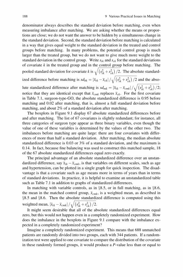
188 9 Various Practical Issues in Matching
denominator always describes the standard deviation before matching, even when
measuring imbalance after matching. We are asking whether the means or propor-
tions are close; we do not want the answer to be hidden by a simultaneous change in
the standard deviation. Second, the standard deviation before matching is calculated
in a way that gives equal weight to the standard deviation in the treated and control
groups before matching. In many problems, the potential control group is much
larger than the treated group, but we do not want to give much more weight to the
standard deviation in the control group. Write stk and sck for the standard deviations
of covariate k in the treated group and in the control group before matching. The
pooled standard deviation for covariate k is√(
s2tk + s2
ck
)/2. The absolute standard-
ized difference before matching is sdbk = |xtk − xck|/√(
s2tk + s2
ck
)/2 and the abso-
lute standardized difference after matching is sdmk = |xtk − xcmk|/√(
s2tk + s2
ck
)/2;
notice that they are identical except that xcmk replaces xck. For the first covariate
in Table 7.1, surgeon-type-GO, the absolute standardized difference is 0.95 before
matching and 0.02 after matching, that is, almost a full standard deviation before
matching, and about 2% of a standard deviation after matching.
The boxplots in Figure 9.1 display 67 absolute standardized differences before
and after matching. The list of 67 covariates is slightly redundant; for instance, all
three categories of surgeon type appear as three binary variables, even though the
value of one of these variables is determined by the values of the other two. The
imbalances before matching are quite large: there are four covariates with differ-
ences of more than half a standard deviation. After matching, the median absolute
standardized difference is 0.03 or 3% of a standard deviation, and the maximum is
0.14. In fact, because fine balancing was used to construct this matched sample, 18
of the 67 absolute standardized differences equal zero exactly.
The principal advantage of an absolute standardized difference over an unstan-
dardized difference, say xtk − xcmk, is that variables on different scales, such as age
and hypertension, can be plotted in a single graph for quick inspection. The disad-
vantage is that a covariate such as age means more in terms of years than in terms
of standard deviations. In practice, it is helpful to examine an unstandardized table
such as Table 7.1 in addition to graphs of standardized differences.
In matching with variable controls, as in §8.5, or in full matching, as in §8.6,
the mean in the matched control group, xcmk, is a weighted mean, as described in
§8.5 and §8.6. Then the absolute standardized difference is computed using this
weighted mean, |xtk − xcmk|/√(
s2tk + s2
ck
)/2.
It might seem desirable that all of the absolute standardized differences equal
zero, but this would not happen even in a completely randomized experiment. How
does the imbalance in the boxplots in Figure 9.1 compare with the imbalance ex-
pected in a completely randomized experiment?
Imagine a completely randomized experiment. This means that 688 unmatched
patients are randomly divided into two groups, each with 344 patients. If a random-
ization test were applied to one covariate to compare the distribution of the covariate
in these randomly formed groups, it would produce a P-value less than or equal to

9.1 Checking Covariate Balance 189
0.05 with probability 0.05; in fact, it would produce a P-value less than or equal to
α with probability α for every α between zero and one.1 Fisher’s exact test for a
2×2 table is one such randomization test, and Wilcoxon’s rank sum test is another.
With 688 patients, it suffices to use the large sample approximations to these tests.
●●
●
●
●
●
●
Before After
0.0
0.2
0.4
0.6
0.8
Imbalance in Covariate Means
|Sta
ndar
dize
d D
iffer
ence
|
●●●●●
●●●●●●
●●
●●
●●●●
●●●●●
●
●●
●●●●●●●●
●●●●●●●●●●●
●
●●
●
●●●●●●●●●●●●●●●●●
0.0 0.2 0.4 0.6 0.8 1.0
0.0
0.2
0.4
0.6
0.8
1.0
QQ−Plot of P−values
Uniform Distribution
Sor
ted
P−
valu
es
Fig. 9.1 Balance checks for 67 covariates in the study of ovarian cancer. The boxplots show ab-solute values of standardized differences in means between the GO and MO groups. The quantile-quantile plot compares the 67 two-sample P-values with the uniform distribution, with the line ofequality. The boxplot shows that the imbalances in covariates were greatly reduced by match-ing, while the quantile-quantile plot shows the imbalance on observed covariates after matchingis somewhat better than expected for a completely randomized experiment with patients randomlyassigned to GO or MO. Balance on observed covariates does not imply balance on covariates thatwere not observed.
1 This statement is not exactly correct, owing to the discreteness of a randomization distribution,but it is close enough.

190 9 Various Practical Issues in Matching
The quantile-quantile plot in Figure 9.1 compares the 67 two-sample P-values
with the uniform distribution. A quantile-quantile plot compares the quantiles in a
sample with the quantiles in a probability distribution to see how they compare [2,
pages 143–149]. If the sample looks like the distribution, the points will fall close
to the line of equality. In Figure 9.1 the points fall above the line of equality. This
means that the two-sample p-values for the 688 patients tend to be larger than they
would be if they came from the uniform distribution. In other words, matching on
these 67 covariates has produced more balance on these 67 covariates than we would
have expected if we had not matched these patients, but instead had assigned them
to treatment or control at random. Of course, randomization has the key benefit that
it tends to balance variables that were not measured, whereas matching can only be
expected to balance observed covariates.
9.2 Almost Exact Matching
If there are a few covariates of overriding importance, each taking just a few values,
then one may wish to match exactly on these covariates whenever this is possible.
For instance, in Table 7.1, for reasons discussed in §7.2, an effort was made to
match exactly on both surgeon type and stage, although this was not possible in
every instance. The procedure is similar to the use of penalties in §8.4. If subjects
k and � do not have the same values on these few key covariates, then a substantial
penalty is added to the distance between them as recorded in the distance matrix.
If the penalty is large enough, optimal matching will avoid the penalties whenever
possible, and when avoiding all of the penalties is not possible, it will minimize the
number of matches that incur the penalty. That is, if an exact match is possible, one
will be produced; if not, the match will be as close to exact as possible. In either
case, once the match is as exact as possible, the best such match is selected using
other considerations represented in the distance matrix. The approach is flexible: it
may be used with pair matching (§8.4), matching with variable controls (§8.5), or
full matching (§8.6).
Obviously, as the distance matrix increasingly emphasizes these key covariates,
it also de-emphasizes the other covariates, perhaps resulting in poor matches on the
other covariates. This is the principal disadvantage of all methods that emphasize
exact matching: gains in one area are paid for by losses in another, and sometimes
the price is high. In contrast, methods that emphasize balancing covariates, such as
propensity scores (§8.2) and fine balance (Chapter 10), may produce gains in one
area without losses in another.
To illustrate, in the welder data in Table 8.3, there were 11 smokers among the
21 welders and 9 smokers among the 26 potential controls. In pair matching, an
exact match on smoking is not possible: at most 9 of the 11 smoking welders can be
matched to smoking controls. In fact, none of the three pair matches in Tables 8.8-
8.10 had used all nine smoking controls. Table 9.1 is an optimal pair match using the
Mahalanobis distance within propensity score calipers with almost exact matching

9.2 Almost Exact Matching 191
Table 9.1 Optimal pair match using the Mahalanobis distance within propensity score caliperswith almost exact matching for smoking. The caliper is half the standard deviation of the propen-sity score, or 0.172/2 = 0.086. Covariates are age, race (C=Caucasian , AA=African American),current smoker (Y=yes, N=no), and the estimated propensity score e(x).
Welders Matched Controls
Pair Age Race Smoker e(x) Age Race Smoker e(x)1 38 C N 0.46 44 C N 0.342 44 C N 0.34 45 C N 0.323 39 C Y 0.57 36 C Y 0.644 33 AA Y 0.51 41 AA Y 0.355 35 C Y 0.65 35 C Y 0.656 39 C Y 0.57 39 C Y 0.577 27 C N 0.68 30 C N 0.638 43 C Y 0.49 56 AA Y 0.139 39 C Y 0.57 36 C Y 0.6410 43 AA N 0.20 48 AA N 0.1411 41 C Y 0.53 44 C Y 0.4712 36 C N 0.50 41 C N 0.4013 35 C N 0.52 40 C N 0.4214 37 C N 0.48 42 C N 0.3815 39 C Y 0.57 35 C N 0.5216 34 C N 0.54 38 C N 0.4617 35 C Y 0.65 34 C Y 0.6718 53 C N 0.19 52 C N 0.2019 38 C Y 0.60 34 C N 0.5420 37 C N 0.48 42 C N 0.3821 38 C Y 0.60 31 AA Y 0.55
mean %AA %Y mean mean %AA %Y mean38 10 52 0.51 40 19 43 0.45
for smoking. Specifically, the distance matrix for the match in Table 8.5 was used;
however, if there was a mismatch on smoking between a welder and a potential
control, a penalty was added to the distance between them. This penalty, 5322, was
ten times the largest distance in the previous distance matrix used for Table 8.5,
where the previous distance matrix already contained penalties to implement the
caliper on the propensity score, as described in §8.4.
In Table 9.1, all nine smoking controls are used, unlike Tables 8.8–8.10. Each
of the nine smoking controls is matched to a welder who smokes. Inevitably, two
smoking welders are matched to nonsmoking controls; they are #15 and #19. In the
means at the bottom of Table 9.1, the balance on smoking is slightly better than in
Tables 8.8–8.10, but the balance on race is worse.
Almost exact matching is sometimes useful when there is interest in estimating
the treatment effect separately in several subgroups, say for smokers and nonsmok-
ers in Table 9.1. For the ovarian cancer study in Chapter 7, in [15, Table 5], results
were reported separately for the 263 pairs in which both patients had stage III or
stage IV cancer. Because the matching was ‘almost exact’ for stage, only 10 of 344
pairs had a stage III or IV cancer matched to another stage or missing stage, and so
could not be used straightforwardly in such a subgroup analysis.

192 9 Various Practical Issues in Matching
Table 9.2 Is exact matching feasible in the welder data? The 2x2 contingency tables show thatexact matching is feasible for race, but not for smoking. Covariates are race (C=Caucasian,AA=African American), and current smoker (Y=yes, N=no)
.
Smoker Nonsmoker
Welder 11 10Potential Control 9 17
AA C
Welder 2 19Potential Control 5 21
Almost exact matching adds large penalties to a distance matrix when treated and
control subjects differ on a key covariate. Sometimes a covariate is uncomfortably
out of balance but not of overriding importance. In this case, small penalties for
mismatches are sometimes used. There is, at present, little theory to guide the use
of small penalties; nonetheless, they often work. The Mahalanobis distance between
two randomly selected individuals from a single multivariate Normal population has
expectation equal to twice the number of covariates, so adding a penalty of 2 to a
Mahalanobis distance may be viewed informally as doubling the importance of that
one covariate.
9.3 Exact Matching
Almost exact matching, as in §9.2, will result in an exact match whenever one
is available, so for many purposes a separate discussion of exact matching is not
needed. Nonetheless, there are computational reasons to distinguish exact and al-
most exact matching.
A simple contingency table will indicate whether an exact match is possible. For
the welder data, Table 9.2 shows that exact matching is feasible for race (because
5 ≥ 2 and 21 ≥ 19) but not feasible for smoking (because 9 < 11), although ‘almost
exact matching’ is feasible for smoking, as illustrated in §9.2.
When feasible, an exact match can be found by subdividing the matching prob-
lem into several smaller problems and piecing the answers together. For instance,
knowing from Table 9.2 that an exact match for race is feasible, the match can be
divided into two separate problems, namely matching the two African American
welders and matching the 19 Caucasian welders.
In small problems, there is no advantage to such a subdivision, but in extremely
large matching problems, there can be a useful reduction in computational effort,
both in required memory storage and in speed of computation. For instance, suppose
that there is a nominal covariate with five categories, each containing m treated
subjects and n potential controls, so that there are 5m + 5n subjects in total. A
distance matrix for all 5m+5n subjects is 5m×5n with 25mn entries, whereas each
of the five subdivided matching problems has a distance matrix that is m× n with
mn entries, so it is 1/25th as large. The worst-case time bound for the assignment

9.4 Missing Covariate Values 193
problem grows as the cube of the number of subjects [4, page 147], here 5m + 5n,
so the reduction to a problem of size m + n is expected to substantially accelerate
computation.
If a critically important covariate is continuous, it may enter the matching in two
versions, one continuous, the other discrete. For instance, a nominal variable can be
formed by cutting at quantiles of the continuous variable, and this nominal variable
may be used to subdivide the problem for exact matching. The only reasons to do
this is to save computer memory or accelerate computation. Within each subdivi-
sion, the continuous variable may be used in a distance, such as the Mahalanobis
distance, or with a caliper, as described in §8.4.
A large sample size should be a luxury, not a hindrance. To enjoy that luxury
when matching, consider exact matching on one or two important covariates, subdi-
viding the matching problem into several smaller problems.
9.4 Missing Covariate Values
A covariate has missing values if it is recorded for many people but not for some
people. The pattern of missing data refers to which values are missing and which
values are present, so you observe the pattern of missing data, though you do not
observe the missing values. The constant worry with missing values is that what you
cannot see may differ in important ways from what you can see. If a manuscript
is missing certain words, it makes all the difference whether the manuscript was
damaged by rain or edited by a censor. If edited by a censor, and if you know what
motivates the censor, then the fact that a word is missing speaks volumes about
what the word must have been, even though you still do not know the word. If a
high school student reports his mother’s level of education in a survey but not his
father’s, you might wonder whether he ever met his father. The pattern of missing
data may or may not say something about the values that are missing, but knowing
the pattern does not tell you the missing values.
The propensity score e(x) is the conditional probability of treatment given the
observed covariates, e(x) = Pr(Z = 1 | x), and matching on e(x) tends to balance
x; see §3.3 or [10, Theorems 1 and 2]. If a coordinate of x is sometimes miss-
ing, think of that coordinate as being a number if it is not missing or * if it is
missing. When some covariates have missing values, the propensity score remains
well-defined: it refers to the conditional probability of treatment given x, that is
e(x) = Pr(Z = 1 | x), where now some of the coordinates may equal *. It only
takes a moment to review the proof of the balancing property of the propensity
score to realize that the proof cares not a bit whether the coordinates of x take only
numeric values or sometimes take the value *; see [11, Appendix B] for an explicit
and detailed discussion. This says something useful, but alas something less than
one might hope. It says that matching on e(x) will tend to balance the observed
covariates and the pattern of missing covariates; however, the missing values them-

194 9 Various Practical Issues in Matching
selves may or may not be balanced. The subject is easiest to discuss in the context
of an example, which will happen in §13.4.
The usual way to estimate e(x) when some covariates are missing is to (i) append
indicator variables for the pattern of missing data, (ii) for each covariate, plug in an
arbitrary but fixed value for each *, and (iii) fit a logit model with these variables,
taking the fitted probabilities from the model as the estimates e(x). It is not difficult
to verify that the presence of the missing value indicators means that the arbitrary
values in step (ii) do not affect e(x), though they do affect the coefficients of the
model.2 Such a logit model is a specific parametric form for a conditional probabil-
ity e(x) = Pr(Z = 1 | x) relating two observed quantities, namely Z and x with its
*’s. As is always true with any such model, it may or may not correctly represent
the form of Pr(Z = 1 | x) — perhaps there should be an interaction linking the miss-
ing value indicator for variable #7 with the indicator for variable #19 — however,
the issues here are no different from any other attempt to model a conditional prob-
ability of one observable given another. Again, see [11, Appendix B] for additional
detail.
Further discussion is aided by an example; see §13.4.
9.5 Further Reading
For further discussion of checks on covariate balance, see the brief discussion in
Cochran’s paper [3], and the longer discussions in the papers by Ben Hansen and
Jake Bowers [5], Ben Hansen [6], Kosuke Imai, Gary King, and Elizabeth Stuart
[7] , and Sue Marcus and colleagues [9]. Propensity scores with missing data are
discussed in [11, Appendix B]. The use of penalty functions in optimization is fairly
standard; see [1, 8].
References
1. Avriel, M.: Nonlinear Programming. Englewood Cliffs, NJ: Prentice Hall (1976)2. Cleveland, W.S.: The Elements of Graphing Data. Summit, NJ: Hobart Press.3. Cochran, W.G.: The planning of observational studies of human populations (with Discus-
sion). J Roy Statist Soc A 128, 234–265.4. Cook, W.J., Cunningham, W.H., Pulleyblank, W.R., Schrijver, A.: Combinatorial Optimiza-
tion. New York: Wiley (1998)5. Hansen, B.B., Bowers, J.: Covariate balance in simple, stratified and clustered comparative
studies. Statist Sci 23, 219–236 (2008)6. Hansen, B.B.: The essential role of balance tests in propensity-matched observational studies.
Statist Med 12, 2050–2054 (2008)7. Imai, K., King, G., Stuart, E.A.: Misunderstandings between experimentalists and observa-
tionalists about causal inference. J Roy Statist Soc A 171, 481–502 (2008)
2 Technically, the fitted probabilities in logit regression are invariant under affine transformationsof the predictors.

References 195
8. Karmanov, V.G.: Mathematical Programming. Moscow: Mir.9. Marcus, S.M., Siddique, J., Ten Have, T.R., Gibbons, R.D., Stuart, E., Normand, S-L. T.
Balancing treatment comparisons in longitudinal studies. Psychiatric Ann 38, 12 (2008)10. Rosenbaum, P.R., Rubin, D.B.: The central role of the propensity score in observational studies
for causal effects. Biometrika 70, 41–55 (1983)11. Rosenbaum, P.R., Rubin, D.B.: Reducing bias in observational studies using subclassification
on the propensity score. J Am Statist Assoc 79, 516–524 (1984)12. Rosenbaum, P.R., Rubin, D.B.: Constructing a control group by multivariate matched sam-
pling methods that incorporate the propensity score. Am Statist 39, 33–38 (1985)13. Rosenbaum, P.R.: Optimal matching in observational studies. J Am Statist Assoc 84, 1024–
1032 (1989)14. Rosenbaum, P.R., Ross R.N., Silber, J.H.: Minimum distance matched sampling with fine
balance in an observational study of treatment for ovarian cancer. J Am Statist Assoc 102,75–83. (2007)
15. Silber, J.H., Rosenbaum, P.R., Polsky, D., Ross, R.N., Even-Shoshan, O., Schwartz, S., Arm-strong, K.A., Randall, T.C.: Does ovarian cancer treatment and survival differ by the specialtyproviding chemotherapy? J Clin Oncol 25, 1169–1175 (2007)

Chapter 10Fine Balance
Abstract Fine balance means constraining a match to balance a nominal variable,
without restricting who is matched to whom, when matching to minimize a distance
between treated and control subjects. It may be applied to: (i) a nominal variable
with many levels that is difficult to balance using propensity scores, (ii) a rare bi-
nary variable that is difficult to control using a distance, or (iii) the interaction of
several nominal variables. The fine balance constraint and the distance can empha-
size different covariates. When exact balance is unobtainable, fine balance can be
used to obtain a specific pattern of imbalances.
10.1 What Is Fine Balance?
Fine balance is a constraint on an optimal matching that forces a nominal variable
to be balanced [5, 6]. Fine balance is explicitly aimed at covariate balance, and it
makes no effort to match exactly for this nominal variable. The pairing can focus
on other covariates with the knowledge that this nominal variable will be balanced.
In the study of ovarian cancer in Chapter 7 and [7], the eight SEER sites
and three intervals 1991–1992, 1993–1996, and 1997–1999 for year of diagnosis
were finely balanced, as was their 24 = 8×3 category interaction. In other words,
the number of patients diagnosed in 1991–1992 in Connecticut, for instance, was
exactly the same for GO patients and the matched control group of MO patients,
although these patients were not typically matched to each other. As you may recall
from Table 7.1, SEER site and year of diagnosis were substantially out of balance
prior to matching, but they are not usually viewed as extremely important by clini-
cians. For this reason, the distance and various penalties used in this match sought
individual pairs with the same clinical stage from the same surgeon type with similar
propensity scores, and paid no explicit attention to SEER site, yet the fine balance
constraint ensured SEER site was balanced in aggregate.
Propensity scores use probability to balance covariates [4], appealing to the law
of large numbers [2, Chapter 10]; in effect, if a coin is flipped sufficiently often,
197P.R. Rosenbaum, Design of Observational Studies, Springer Series in Statistics, DOI 10.1007/978-1-4419-1213-8_10, © Springer Science+Business Media, LLC 2010

198 10 Fine Balance
the number of heads tends to balance the number of tails. Although they work well
in many contexts, propensity scores may not balance covariates when the number
of trials (or flips) is effectively small. For instance, if the data record little or no
information about income, education, pollution, and so on, but do record postal zip
code, then one might think to match for zip code as a proxy for various unmeasured
variables. In many contexts, there will be only a handful of people from any one zip
code, so matching exactly for Zip Code will yield poor matches for other covariates;
moreover, the law of large numbers is of no help. In such a context, fine balancing
can balance zip code, without matching people from the same zip code to one an-
other. Similar considerations apply if there are several binary covariates in which
one category is rarely seen; these can be combined into one nominal variable with
several rare levels and one common level, and this amalgamated covariate can be
finely balanced. More generally, if several important nominal variables are thought
to interact with each other, fine balancing may be used to exactly balance the many
categories formed from their interaction (i.e., their direct product).
10.2 Constructing an Exactly Balanced Control Group
As in Chapter 8, fine balance is best understood with the aid of a small example.
For the welder data [1] in Chapter 8, it was clear from Tables 8.3 and 9.2 that it was
possible to balance race but not smoking. Section 10.2 finds a match that finely bal-
ances race, while §10.3 finds a match that controls the nature of the joint imbalance
in race and smoking.
In Tables 8.3 and 9.2, among the potential controls, there are five African Amer-
icans where two are needed for balance, and there are 21 Caucasians, where 19 are
needed for balance, so three African Americans and two Caucasians must be re-
moved to obtain balance. This is done by expanding the distance matrix, adding
five rows. Table 10.1 adds five rows to Table 8.5, which recorded the Mahalanobis
distances within propensity score calipers for the first 6 of 26 potential controls.
The five extra rows are E1 to E5, making the distance matrix square, 26×26. The
first two of these extra rows, E1 and E2, will take away two Caucasians, while the
last three of the extra rows, E3, E4, and E5, will take away three African Ameri-
cans. Because control #1 in column 1 of Table 10.1 is African American, he is at
infinite distance from the two Caucasian extras and at zero distance from the three
African American extras. Because controls #2–#6 in columns 2 to 6 of Table 10.1
are Caucasian, they are at zero distance from the two Caucasian extras and at infi-
nite distance from the three African American extras. A similar pattern occurs in
the remaining 20 columns of the distance matrix.
With a distance matrix patterned as in Table 10.1, an optimal match is found, and
the extras and their matched controls are discarded. To avoid the infinite distances,
three African American and two Caucasian controls must be matched to the extras,
and the match that remains is balanced.

10.2 Constructing an Exactly Balanced Control Group 199
Table 10.1 Mahalanobis distances within propensity score calipers with extra rows to finely bal-ance race. Rows are the 21 welders plus five extras (E), and columns are for the first 6 of 26potential controls. An ∞ signifies that the caliper is violated.
Welder Control 1 Control 2 Control 3 Control 4 Control 5 Control 6
1 ∞ ∞ 6.15 0.08 ∞ ∞2 ∞ ∞ ∞ 0.33 ∞ ∞3 ∞ ∞ ∞ ∞ ∞ ∞4 ∞ ∞ 12.29 ∞ ∞ ∞5 ∞ ∞ ∞ ∞ ∞ ∞6 ∞ ∞ ∞ ∞ ∞ ∞7 ∞ ∞ ∞ ∞ ∞ ∞8 ∞ ∞ 0.02 5.09 ∞ ∞9 ∞ ∞ ∞ ∞ ∞ ∞
10 0.51 ∞ ∞ ∞ 10.20 11.1711 ∞ ∞ 0.18 ∞ ∞ ∞12 ∞ ∞ 7.06 0.33 ∞ ∞13 ∞ ∞ 7.57 ∞ ∞ ∞14 ∞ ∞ 6.58 0.18 ∞ ∞15 ∞ ∞ ∞ ∞ ∞ ∞16 ∞ ∞ 8.13 ∞ ∞ ∞17 ∞ ∞ ∞ ∞ ∞ ∞18 9.41 ∞ ∞ ∞ 0.18 0.0219 ∞ ∞ ∞ ∞ ∞ ∞20 ∞ ∞ 6.58 0.18 ∞ ∞21 ∞ ∞ ∞ ∞ ∞ ∞E1 ∞ 0 0 0 0 0E2 ∞ 0 0 0 0 0E3 0 ∞ ∞ ∞ ∞ ∞E4 0 ∞ ∞ ∞ ∞ ∞E5 0 ∞ ∞ ∞ ∞ ∞
Table 10.2 displays the minimum distance finely balanced match. Race is per-
fectly balanced, but the pairs are not exactly matched for race. In one sense, Table
10.2 is a slight improvement over Table 8.9 because the control group means for
age and smoking are the same, while the means for race and the propensity score
are slightly closer to the welder means. Notice that the finely balanced match se-
lected two African American smokers, even though a nonsmoker was available as a
control for pair #10.
The general procedure is essentially the same. If there is a nominal covariate
for which balance is required, then (i) cross-tabulate that covariate with treatment,
as in Table 9.2; (ii) determine the number of controls that must be removed from
each category of the covariate to achieve balance; (iii) add one row for each control
that must be removed, with zero distance to its own category and infinite distance
to other categories; (iv) find an optimal match for this new, square distance matrix;
(v) discard the extra rows and their matched controls. The nominal covariate that is
balanced may be formed by combining several other nominal covariates or intervals
that cut a continuous variable.

200 10 Fine Balance
Table 10.2 Optimal pair match using the Mahalanobis distance within propensity score calipers,with fine balance for race. This match is constrained to balance race. The caliper is half the standarddeviation of the propensity score, or 0.172/2 = 0.086. Covariates are age, race (C=Caucasian ,AA=African American), current smoker (Y=yes, N=no), and the estimated propensity score e(x).
Welders Matched Controls
Pair Age Race Smoker e(x) Age Race Smoker e(x)1 38 C N 0.46 44 C N 0.342 44 C N 0.34 47 C N 0.283 39 C Y 0.57 36 C Y 0.644 33 AA Y 0.51 41 AA Y 0.355 35 C Y 0.65 35 C Y 0.656 39 C Y 0.57 36 C Y 0.647 27 C N 0.68 30 C N 0.638 43 C Y 0.49 45 C N 0.329 39 C Y 0.57 39 C Y 0.5710 43 AA N 0.20 50 C N 0.2311 41 C Y 0.53 44 C Y 0.4712 36 C N 0.50 41 C N 0.4013 35 C N 0.52 40 C N 0.4214 37 C N 0.48 42 C N 0.3815 39 C Y 0.57 35 C N 0.5216 34 C N 0.54 38 C N 0.4617 35 C Y 0.65 34 C Y 0.6718 53 C N 0.19 52 C N 0.2019 38 C Y 0.60 34 C N 0.5420 37 C N 0.48 42 C N 0.3821 38 C Y 0.60 31 AA Y 0.55
mean %AA %Y mean mean %AA %Y mean38 10 52 0.51 40 10 38 0.46
To match two controls to each treated subject with fine balance, stack two copies
of the distance matrix, one on top of the other, and then add extras as before to
remove imbalances in the nominal covariate. In this way, the number of columns
or controls does not change, but each treated subject is represented twice, once in
each of two rows. In an optimal match, one control is paired with the first copy
of a treated subject and a different control is paired with the second copy, yielding
a 2-to-1 match. (Obviously, this cannot be done with the welder data, because at
least 42 potential controls are needed, and only 26 are available.) The procedure for
k-to-1 finely balanced matching is similar, but with k copies of the distance matrix
rather than two. If needed, a precise algorithmic description is given in [6, §4.2].
It is easy to prove that a minimum distance match with this enlarged distance
matrix is a minimum distance match subject to the fine balance constraint, and that
the minimum distance match has infinite total distance if and only if the latter prob-
lem is infeasible [6, Proposition 1]. In particular, in the statistical package R, the
pairmatch function in Hansen’s [3] optmatch package may be used, whereas
in SAS proc assign may be used. Alternatively, the minimum distance finely
balanced match may be determined directly as a minimum-cost flow in a network
[5, §3.2].

10.3 Controlling Imbalance When Exact Balance Is Not Feasible 201
Table 10.3 Table of treatment groups by (race × smoking) for the welder data, with race asC=caucasian , AA=African American, and current smoker coded as Y=yes or N=no.
Smoker Yes Yes No NoRace AA C AA C Total
Welder 1 10 1 9 21Control 3 6 2 15 26
10.3 Controlling Imbalance When Exact Balance Is Not Feasible
When exact balance is not possible, the fine balance procedure can be used to obtain
any specified, possible imbalance. The procedure is essentially the same as in §10.2,
except that one must choose an acceptable imbalance from those that are possible.
Table 10.3 displays the options for race and smoking in the welder data. The
obstacle to balance on the joint distribution of these two variables is a deficit of
smoking, Caucasian controls: there are six, where ten are needed. That is, from
the four categories given by the columns of Table 10.3, we would like to select
controls with frequencies (1,10,1,9) to agree with the welder group, but the sec-
ond entry is limited to six, so for a pair match some other entries must increase
to compensate. One attractive choice is (3,6,0,12), because this choice uses all
nine smoking controls, where 11 would be needed for balance, and is only slightly
imbalanced for race, with three African Americans where two would produce bal-
ance on race. This choice presumes that smoking is more important than race, as
is likely in genetic toxicology, and it provides no information about a treatment-by-
race-by-smoking interaction. In any event, for this purely illustrative example, the
important point that is fine balance can produce any specified possible imbalance,
such as (3,6,0,12).To produce the imbalance (3,6,0,12), one notices that: no controls are to be
removed from the first two columns of Table 10.3, two are to be removed from the
third column, and three are to be removed from the fourth column. So five rows
are added to Table 8.5, two at zero distance from nonsmoking African Americans,
three at zero distance from nonsmoking Caucasians, with the other entries set to ∞;
see Table 10.4. The first control in Table 8.3 is an African American nonsmoker,
and so in column 1 of Table 10.4, he is at zero distance from both of the first two
extra rows. The second control in Table 8.3 is a Caucasian nonsmoker, and so, in
column 2 of Table 10.4, he is at zero distance from the last three extra rows. The
third control in Table 8.3 is a Caucasian smoker, and cannot be eliminated, and so,
in column 3 of Table 10.4, he is at infinite distance from all five rows. As in §10.2,
one finds an optimal pair matching in the extended square 26× 26 distance matrix
and discards the extras and their matched controls.
Table 10.5 is the result. It achieves the prescribed imbalance, (3,6,0,12), and
subject to that constraint it minimizes the distance among all pair matchings. No-
table in Table 10.5 is the use of all nine smoking controls without a large imbal-
ance in race. This was produced by matching welder #10, a nonsmoking African

202 10 Fine Balance
Table 10.4 Mahalanobis distances within propensity score calipers with extra rows to finely bal-ance race and smoking. Rows are the 21 welders plus five extras (E), and columns are for the first6 of 26 potential controls. An ∞ signifies that the caliper is violated.
Welder Control 1 Control 2 Control 3 Control 4 Control 5 Control 6
1 ∞ ∞ 6.15 0.08 ∞ ∞2 ∞ ∞ ∞ 0.33 ∞ ∞3 ∞ ∞ ∞ ∞ ∞ ∞4 ∞ ∞ 12.29 ∞ ∞ ∞5 ∞ ∞ ∞ ∞ ∞ ∞6 ∞ ∞ ∞ ∞ ∞ ∞7 ∞ ∞ ∞ ∞ ∞ ∞8 ∞ ∞ 0.02 5.09 ∞ ∞9 ∞ ∞ ∞ ∞ ∞ ∞
10 0.51 ∞ ∞ ∞ 10.20 11.1711 ∞ ∞ 0.18 ∞ ∞ ∞12 ∞ ∞ 7.06 0.33 ∞ ∞13 ∞ ∞ 7.57 ∞ ∞ ∞14 ∞ ∞ 6.58 0.18 ∞ ∞15 ∞ ∞ ∞ ∞ ∞ ∞16 ∞ ∞ 8.13 ∞ ∞ ∞17 ∞ ∞ ∞ ∞ ∞ ∞18 9.41 ∞ ∞ ∞ 0.18 0.0219 ∞ ∞ ∞ ∞ ∞ ∞20 ∞ ∞ 6.58 0.18 ∞ ∞21 ∞ ∞ ∞ ∞ ∞ ∞E1 0 ∞ ∞ ∞ ∞ ∞E2 0 ∞ ∞ ∞ ∞ ∞E3 ∞ 0 ∞ 0 0 0E4 ∞ 0 ∞ 0 0 0E5 ∞ 0 ∞ 0 0 0
American, to a smoker, even though a nonsmoking African American control was
available.
In Tables 8.5, 10.1 and 10.4, it was convenient for display to use ∞ to indicate
the penalties. In computation, large numerical penalties are used. Table 10.6 shows
the numerical penalties used in producing the match in Table 10.5. Recall that
the caliper on the propensity score in Chapter 8 imposed no penalty if the caliper
was respected, a small penalty for small violations of the caliper, and a dramatic
penalty for large violations of the caliper; this is seen in the first 21 rows of Table
10.6. The caliper on the propensity score was 0.086, and control #2 in Table 8.3,
with e(x) = 0.09, violated the caliper for all 21 welders. For welders #10 and #18,
with e(x) = 0.20 and e(x) = 0.19, respectively, the violation is not large, and the
penalties in column 2 and rows 10 and 18 of Table 10.6 are not extremely large. To
give greater emphasis to the fine balance constraint than to the calipers, the penalties
for the extra rows in Table 10.6 are five times the largest distance in the first 21 rows
and 26 columns.

10.4 Fine Balance and Exact Matching 203
Table 10.5 Optimal pair match using the Mahalanobis distance within propensity score calipers,with fine balance for race and smoking. The caliper is half the standard deviation of the propensityscore, or 0.172/2 = 0.086. Covariates are age, race (C=Caucasian , AA=African American), cur-rent smoker (Y=yes, N=no), and the estimated propensity score e(x). This match is constrained touse all three AA smokers, all six C smokers, neither AA nonsmoker, and 12 C nonsmokers.
Welders Matched Controls
Pair Age Race Smoker e(x) Age Race Smoker e(x)1 38 C N 0.46 44 C N 0.342 44 C N 0.34 47 C N 0.283 39 C Y 0.57 36 C Y 0.644 33 AA Y 0.51 41 AA Y 0.355 35 C Y 0.65 35 C Y 0.656 39 C Y 0.57 36 C Y 0.647 27 C N 0.68 30 C N 0.638 43 C Y 0.49 45 C N 0.329 39 C Y 0.57 35 C N 0.5210 43 AA N 0.20 56 AA Y 0.1311 41 C Y 0.53 44 C Y 0.4712 36 C N 0.50 41 C N 0.4013 35 C N 0.52 40 C N 0.4214 37 C N 0.48 42 C N 0.3815 39 C Y 0.57 39 C Y 0.5716 34 C N 0.54 38 C N 0.4617 35 C Y 0.65 34 C Y 0.6718 53 C N 0.19 52 C N 0.2019 38 C Y 0.60 31 AA Y 0.5520 37 C N 0.48 42 C N 0.3821 38 C Y 0.60 34 C N 0.54
mean %AA %Y mean mean %AA %Y mean38 10 52 0.51 40 14 43 0.45
10.4 Fine Balance and Exact Matching
Fine balance can produce exact balance on a nominal covariate without matching
exactly for that covariate. Nonetheless, the two techniques may be combined. In
parallel with §9.3, this is one way to implement fine balance in extremely large
matching problems: the problem is divided into a few smaller problems.
In fact, this was done in the study of ovarian cancer in Chapter 7 and [7]. Three
separate matches were constructed, one for each of the three intervals 1991–1992,
1993–1996, and 1997–1999 of year of diagnosis, with fine balance for SEER sites.
We did this not primarily for computational reasons but because we had originally
envisioned an additional analysis, not reported in [7], that would have compared
the speed with which GOs and MOs adopted new chemotherapies for ovarian can-
cer. The three time intervals 1991–1992, 1993–1996, and 1997–1999 correspond
with innovations in chemotherapy for ovarian cancer, and for that analysis it would
have been convenient to have pairs matched for the time interval. That is, in each
pair, the same chemotherapies would have been available, so it would make sense
to ask who used what. Although the matching procedure worked well, we never

204 10 Fine Balance
Table 10.6 Mahalanobis distances within propensity score calipers with extra rows to finely bal-ance race and smoking. Rows are the 21 welders plus five extras (E), and columns are for the first6 of 26 potential controls. This table displays the numerical penalties rather than ∞’s.
Welder Control 1 Control 2 Control 3 Control 4 Control 5 Control 6
1 237.66 293.68 6.15 0.08 141.69 171.852 115.36 166.78 50.06 0.33 17.98 47.653 358.16 408.89 20.23 75.94 259.61 289.354 287.20 361.09 12.29 18.96 206.61 237.165 439.02 492.83 101.71 156.10 341.41 371.486 358.16 408.89 20.23 75.94 259.61 289.357 467.74 532.22 141.84 184.10 374.36 405.428 273.83 321.48 0.02 5.09 174.33 203.749 358.16 408.89 20.23 75.94 259.61 289.35
10 0.51 45.85 193.46 134.45 10.20 11.1711 316.15 365.34 0.18 34.28 217.12 246.7012 280.67 338.23 7.06 0.33 185.17 215.5013 302.27 360.61 7.57 20.03 207.01 237.4214 259.11 315.90 6.58 0.18 163.37 193.6115 358.16 408.89 20.23 75.94 259.61 289.3516 323.84 382.94 8.13 41.42 228.81 259.3017 439.02 492.83 101.71 156.10 341.41 371.4818 9.41 15.61 196.03 142.97 0.18 0.0219 378.88 430.37 41.10 96.48 280.55 310.3820 259.11 315.90 6.58 0.18 163.37 193.6121 378.88 430.37 41.10 96.48 280.55 310.38
E1 0 2661.08 2661.08 2661.08 2661.08 2661.08E2 0 2661.08 2661.08 2661.08 2661.08 2661.08E3 2661.08 0 2661.08 0 0 0E4 2661.08 0 2661.08 0 0 0E5 2661.08 0 2661.08 0 0 0
determined whether GOs or MOs were quicker in adopting new chemotherapies.
Instead, we determined that GOs and MOs are both much quicker in adopting new
chemotherapies than Medicare is in creating a code for new chemotherapies.
10.5 Further Reading
Matching with fine balance is discussed in detail in [6]. The network algorithm
in [5, §3.2] will be of interest primarily to programmers because it can be more
efficient in its use of space than the procedure described here and in [6].
References
1. Costa, M., Zhitkovich, A., Toniolo, P.: DNA-protein cross-links in welders: Molecular implica-tions. Cancer Res 53, 460–463 (1993)

References 205
2. Feller, W.: An Introduction to Probability Theory and Its Applications, Volume 1. New York:Wiley (1968)
3. Hansen, B.B.: Optmatch: Flexible, optimal matching for observational studies. R News 7, 18–24 (2007)
4. Rosenbaum, P.R., Rubin, D.B.: The central role of the propensity score in observational studiesfor causal effects. Biometrika 70, 41–55 (1983)
5. Rosenbaum, P.R.: Optimal matching in observational studies. J Am Statist Assoc 84, 1024–1032 (1989)
6. Rosenbaum, P.R., Ross R.N., Silber, J.H.: Minimum distance matched sampling with fine bal-ance in an observational study of treatment for ovarian cancer. J Am Statist Assoc 102, 75–83(2007)
7. Silber, J.H., Rosenbaum, P.R., Polsky, D., Ross, R.N., Even-Shoshan, O., Schwartz, S., Arm-strong, K.A., Randall, T.C.: Does ovarian cancer treatment and survival differ by the specialtyproviding chemotherapy? J Clin Oncol 25, 1169–1175 (2007)

Chapter 11Matching Without Groups
Abstract Optimal matching without groups, or optimal nonbipartite matching, of-
fers many additional options for matched designs in both observational studies and
experiments. One starts with a square, symmetric distance matrix with one row
and one column for each subject recording the distance between any two subjects.
Then the subjects are divided into pairs to minimize the total distance within pairs.
The method may be used to match with doses of treatment, or with multiple con-
trol groups, or as an aid to risk-set matching. An extended discussion of Card and
Krueger’s study of the minimum wage is used to illustrate.
11.1 Matching Without Groups: Nonbipartite Matching
What is nonbipartite matching?
In previous chapters, treated subjects were matched to controls. That is, there were
two groups, treated and control, which existed before the matching began, and mem-
bers of these two groups were placed in pairs or sets to minimize the distance be-
tween treated and control subjects in the same pair or set. The optimization algo-
rithm solved the so-called assignment problem or bipartite matching problem, where
‘bipartite’ makes reference to ‘two parts.’ A different optimization problem begins
with a single group and divides it into pairs to minimize the distance between paired
units; this is called by the awkward name ‘nonbipartite’ matching. For textbook dis-
cussions of the contrast between these two matching problems, see [5, Chapter 5]
or [21, Chapter 11]. Nonbipartite matching is highly flexible, and it substantially
enlarges the collection of matched designs for observational studies.
In Chapter 8, the distance matrix had one row for each treated subject and one
column for each potential control. In contrast, in nonbipartite matching, the distance
matrix is square, with one row and one column for every subject. Table 11.1 is a
small, artificial example with six subjects, so it is 6× 6. The distance matrix is
symmetric because the distance from k to � in row k and column � is the same as the
207P.R. Rosenbaum, Design of Observational Studies, Springer Series in Statistics, DOI 10.1007/978-1-4419-1213-8_11, © Springer Science+Business Media, LLC 2010

208 11 Matching Without Groups
Table 11.1 A 6 × 6 distance matrix for nonbipartite matching for six units. Unlike treatment-control matching, every unit appears as both a row and a column of this distance matrix. Theoptimal nonbipartite matching (1,2), (3,6), (4,5) is shown in bold with a minimum total distanceof 106+25+34 = 165.
ID 1 2 3 4 5 6
1 0 106 119 231 110 1012 106 0 207 126 192 683 119 207 0 156 247 254 231 126 156 0 34 675 110 192 247 34 0 2126 101 68 25 67 212 0
distance from � to k in row � and column k. Every subject is at zero distance from
itself, but of course a subject cannot be paired with itself.
In Table 11.1, an optimal nonbipartite match would pair the six units into three
pairs to minimize the total distance within pairs. The optimal match is shown in
bold type: it is (1,2), (3,6), and (4,5) for a total distance of 106 + 25 + 34 = 165.
Notice that subject 1 is closer to subject 6 than to subject 2, but if 1 were matched to
6, then the match for 3 would be much worse. Optimal nonbipartite matching may
be done in the statistical package R.1
Treatment-control matching using an algorithm for nonbipartite matching
Generally, one should not use a nonbipartite matching algorithm to perform bipar-
tite matching because the former requires a larger distance matrix and is somewhat
slower. Nonetheless, it is instructive to do it once. Imagine that the first three sub-
jects in Table 11.1 were treated and the last three were controls. To force treated
subjects to be matched to controls, infinite distances are placed among treated sub-
jects and among controls, as in Table 11.2. An optimal nonbipartite match in Table
11.2 avoids the infinite distances and pairs (1,5), (2,4), and (3,6), so treated subjects
1
Fortran code by Derigs [9] has been made available inside R by Bo Lu [19] through a functionnonbimatch(n,d), where d is the vector form of an n×n symmetric matrix of nonnegativeinteger distances.
> dm1 2 3 4 5 6
1 0 106 119 231 110 1012 106 0 207 126 192 683 119 207 0 156 247 254 231 126 156 0 34 675 110 192 247 34 0 2126 101 68 25 67 212 0> nonbimatch(6,as.vector(dm))[1] 2 1 6 5 4 3This says that unit 1 is paired with unit 2, unit 2 is paired with unit 1, unit 3 is paired with unit
6, unit 4 is paired with unit 5, unit 5 is paired with unit 4, and unit 6 is paired with unit 3.

11.1 Matching Without Groups: Nonbipartite Matching 209
Table 11.2 Using nonbipartite matching to perform treatment-versus-control matching (or bi-partite matching). Subjects 1, 2, and 3 are treated, and infinite distances prevent them frombeing matched to each other. Subjects 4, 5, and 6 are controls, and infinite distances preventthem from being matched to each other. The optimal match is (1,5), (2,4), (3,6) with distance110 + 126 + 25 = 261. Use of a bipartite matching algorithm would have required only a 3× 3distance matrix and be expected to run somewhat more quickly.
ID 1 2 3 4 5 6
1 0 ∞ ∞ 231 110 1012 ∞ 0 ∞ 126 192 683 ∞ ∞ 0 156 247 254 231 126 156 0 ∞ ∞5 110 192 247 ∞ 0 ∞6 101 68 25 ∞ ∞ 0
are paired with controls. In this sense, nonbipartite matching is a generalization of
bipartite matching. Of course, the bipartite matching could have been performed
with a 3×3 distance matrix rather than the 6×6 distance matrix in Table 11.2.
11.1.1 Matching with doses
Suppose that we do not have treated subjects and controls but rather individuals
who received various doses of treatment. In this case, we might wish to form pairs
of individuals who are similar in terms of covariates but quite different in terms of
doses. As an illustration, imagine that the six individuals 1, 2, . . . , 6 in Table 11.1
received the treatment at doses 1, 2, . . . , 6, respectively. In this case, we might wish
to match so that pairs differ in dose by at least 2; this would preclude matching 1
with 2, for instance.
In Table 11.3, an infinite distance appears whenever two subjects have doses that
differ by less than 2. Unlike Table 11.1, the infinite distances constrain who may
be matched to whom. Unlike Table 11.2, these constraints are not the sort that can
be addressed with a bipartite matching algorithm; that is, the pattern of ∞’s in Table
11.3 does not divide the six units into two nonoverlapping groups. The optimal
match in Table 11.3 pairs (1,5), (2,4), and (3,6): that is, this minimizes the distance
subject to the constraint that pairs differ in doses by at least 2.
A practical example of matching with doses was given by Bo Lu, Elaine Zanutto,
Robert Hornik, and me [17] in a study of a national media campaign against drug
abuse. The dose was the degree of exposure to the media campaign. Another prac-
tical example is discussed in §11.3.

210 11 Matching Without Groups
Table 11.3 A 6× 6 distance matrix for matching with doses of treatment. For simplicity in thisartificial illustration, the doses equal the ID numbers, and the requirement is that paired individualshave doses that differ by at least 2. Where the dose difference is less than 2, the distance is set to∞. The optimal match is (1,5), (2,4), (3.6).
ID 1 2 3 4 5 6
1 0 ∞ 119 231 110 1012 ∞ 0 ∞ 126 192 683 119 ∞ 0 ∞ 247 254 231 126 ∞ 0 ∞ 675 110 192 247 ∞ 0 ∞6 101 68 25 67 ∞ 0
Table 11.4 A 6× 6 distance matrix for matching with three groups. Subjects 1 and 2 are in thesame group, as are subjects 3 and 4 and subjects 5 and 6. Because subjects in the same group cannotbe matched to one another, there is an infinite distance between them. The optimal match is (1,3),(2,6), (4,5) with a total distance of 119+68+34 = 221. This is a very small balanced incompleteblock design in the sense that every group is paired with every other group exactly once.
ID 1 2 3 4 5 6
1 0 ∞ 119 231 110 1012 ∞ 0 207 126 192 683 119 207 0 ∞ 247 254 231 126 ∞ 0 34 675 110 192 247 34 0 ∞6 101 68 25 67 ∞ 0
11.1.2 Matching with several groups
Suppose that we do not have a treated and control group but rather several groups.
In this case, we might wish to pair similar individuals from different groups. For
instance, in Table 11.1, suppose that subjects 1 and 2 are in one group, 3 and 4 are
in a second group, and 5 and 6 are in a third group. In Table 11.4, individuals in the
same group are at infinite distance from one another. The optimal match is (1,3),
(2,6), and (4,5). In the optimal match, each individual is paired with an individual
from another group to minimize the distance within matched pairs.
The optimal match in Table 11.4 has an additional property. In a balanced in-
complete block design, each pair of treatment groups appears together in the same
block with the same frequency; see [4, Chapter 11] or [7, §4.2]. The optimal match
in Table 11.4 is a very small balanced incomplete block design in the sense that each
of the three groups is paired with each of the other groups exactly once. There is a
certain equity to a balanced incomplete block design: the number of pairs offering
a direct comparison of two groups is the same for every pair of two groups. Bo
Lu and I [18] showed how, with three groups, a balanced incomplete block design
may be constructed using optimal nonbipartite matching. See [18] for a practical
example, and see §11.2 for a few specifics.

11.2 Some Practical Aspects of Matching Without Groups 211
Table 11.5 Matching with an odd number of subjects. With five subjects, a sink is added at zerodistance to all subjects. One subject is paired with the sink and discarded. In this case, the optimalmatch is (1,2), (4,5), (3,6) with a distance of 106+34+0 = 140 and subject 3 is discarded.
ID 1 2 3 4 5 sink
1 0 106 119 231 110 02 106 0 207 126 192 03 119 207 0 156 247 04 231 126 156 0 34 05 110 192 247 34 0 0
sink 0 0 0 0 0 0
11.2 Some Practical Aspects of Matching Without Groups
An odd number of subjects
An odd number of subjects cannot be paired. Suppose that we had only the first five
subjects in Table 11.1. Then only two pairs may be constructed, with one individual
discarded. The best choice of a subject to discard is the one who will make the
remaining pairs as close as possible. Beginning with the 5× 5 distance matrix for
the first five subjects, a ‘sink’ is added at zero distance from all five subjects, making
a 6× 6 distance matrix; see Table 11.5. When optimal nonbipartite matching is
applied to this 6×6 distance matrix, one subject is paired to the sink and discarded.
Because any one subject may be discarded at a cost of 0, the matching discards the
subject who most improves the total distance for the remaining four subjects within
two pairs.
Discarding some subjects
Closer matches may be obtained by discarding some subjects. This is done by in-
troducing one ‘sink’ for each subject to be discarded. The sinks are at zero distance
from each subject and at infinite distance from one another. The infinite distances
prevent sinks from being matched to each other. Optimal nonbipartite matching
discards and pairs subjects to minimize the distance within the pairs that remain.
The process is illustrated in Table 11.6. Two sinks remove two subjects to form
two pairs. As seen in this small example, discarding the subjects who are most
difficult to match can leave behind closely matched pairs.
When there are several groups, as in Table 11.4, one may wish to discard a spe-
cific number of subjects from each group, perhaps two subjects from group one,
seven subjects from group two, etc. To do this, one introduces sinks in the specified
numbers that are at zero distance from the specified groups and at infinite distance
from other groups. To discard two subjects from group one, two sinks are introduced
at zero distance from subjects in group one and at infinite distance from subjects in
other groups. As always, sinks are at infinite distance from one another. In this

212 11 Matching Without Groups
Table 11.6 Optimal choice of two pairs from six subjects discarding two subjects. The 8×8 dis-tance matrix introduces two sinks at zero distance from each subject and at infinite distance fromeach other. Two subjects are matched to sinks and discarded. The optimal match is (1,8), (2,7),(3,6), (4,5) with a distance of 0+0+25+34 = 59. Subjects 1 and 2 discarded.
ID 1 2 3 4 5 6 sink sink
1 0 106 119 231 110 101 0 02 106 0 207 126 192 68 0 03 119 207 0 156 247 25 0 04 231 126 156 0 34 67 0 05 110 192 247 34 0 212 0 06 101 68 25 67 212 0 0 0
sink 0 0 0 0 0 0 0 ∞sink 0 0 0 0 0 0 ∞ 0
way, the required subjects in each group are paired with sinks and discarded, and
the pairs that remain are as close as possible; see [18] for a proof and an example.
Balanced incomplete block designs with three groups
The procedure indicated in Table 11.4 and discussed in §11.1 suffices to form
matched pairs from several groups. In general, the groups will be paired to min-
imize the distance within pairs, and the pairing may be far from balanced. For
instance, group one might always be paired with group two, while group three is
always paired with group four. Whether an unbalanced comparison is undesirable
depends upon the context; it may be sensible given the distribution of covariates in
the various groups.
In some contexts, one may prefer to force some degree of balance, or even to have
a balanced incomplete block design, in which every group is paired equally often
with every other group. With three groups, it is possible to control the number of
subjects from one group who are paired to subjects from another group, within the
limits of arithmetic. Indeed, with the three groups, by simple algebra, the number
of subjects used from each group determines the number of subjects in one group
paired with another group; see [18, Expression (2.1)]. For instance, in the example
in [18, §3.2], 56 subjects were retained in each of three groups, which produced a
balanced incomplete block design of minimum distance with 28 pairs of group one
with group two, 28 pairs of group one with group three, and 28 pairs of group two
with group three.
Propensity scores for several groups
There are several generalizations of the propensity score for use with doses or with
several groups. These generalizations depend upon additional assumptions and
yield a variety of properties. One generalization uses an ordinal logit model for
ordered doses, and matching on the linear portion of this score tends to balance ob-

11.3 Matching with Doses and Two Control Groups 213
served covariates when the model is correct; see [15, page 331]. Scores of this form
have been used in nonbipartite matching [17, §2.3]. Another generalization uses
several binary logit models as a device for weighting observations [14]. Multivari-
ate models yielding multidimensional scores are also possible; see [15, page 331]
and [13].
11.3 Matching with Doses and Two Control Groups
11.3.1 Does the minimum wage reduce employment?
The example uses data from David Card and Alan Krueger’s [2, 3] study of the
effects on employment of increasing the minimum wage; see also §4.5. It is often
said by economists that minimum wage laws harm the people the laws are intended
to benefit. For instance, in 1946, George Stigler [26] wrote:
Each worker receives the value of his marginal product under competition. If a minimumwage is effective, it must therefore have one of two effects: first, workers whose servicesare worth less than the minimum wage are discharged . . . ; or, second the productivity oflow-efficiency workers is increased.
After arguing that the second effect is not plausible, Stigler continues: “The higher
the minimum wage, the greater will be the number of covered workers who are
discharged.” To my mind, Stigler is discussing a ‘reason for an effect,’ in the sense
of §4.6, rather than presenting direct evidence of an effect. For a modern textbook
discussion of the minimum wage, see Pierre Cahuc and Andre Zylberberg [1, §12.1].
In one of the many empirical studies of the effects of the minimum wage on
employment, Card and Krueger [2] looked at changes in employment at fast food
restaurants, such as Burger King and Kentucky Fried Chicken, in the adjacent U.S.
states of New Jersey and Pennsylvania after New Jersey increased its state mini-
mum wage from $4.25 to $5.05 per hour on 1 April 1992. Did the increase in the
minimum wage in New Jersey reduce employment at fast food restaurants?
The increase in the minimum wage in New Jersey from $4.25 to $5.05 is expected
to have its largest effect on New Jersey restaurants whose starting wage before the
increase was at or near the old minimum, namely $4.25, with little or no effect on
restaurants in Pennsylvania where the minimum wage did not increase, and with
reduced effect on restaurants in New Jersey having a higher starting wage before
the increase. For instance, a New Jersey restaurant paying $4.25 an hour before the
increase would need to raise its starting wage by $0.80 whereas one paying $4.75
an hour would comply with the new law by raising its wage by $0.30; presumably,
the latter restaurant is less affected by the law. The theory that the minimum wage
depresses employment then yields two predictions, one about a comparison of New
Jersey and Pennsylvania, the other about a comparison within New Jersey.

214 11 Matching Without Groups
11.3.2 Optimal matching to form two independent comparisons
There are 351 restaurants with both starting wages and employment data both before
and after the wage increase. They will be divided into 175 pairs of two restaurants,
discarding one restaurant, where 351 = 2×175+1. In 65 pairs, there is one Penn-
sylvania restaurant and one New Jersey restaurant. In the remaining 110 pairs, there
are two New Jersey restaurants, one with a low starting wage before the increase,
the other with a high starting wage before the increase.
The matching used a 351× 351 distance matrix comparing every restaurant to
every other restaurant. The distances were a combination of distances on covariates
and penalties to force an appropriate comparison. There were five covariates: three
binary indicators to distinguish the four restaurant chains (BK = Burger King, KFC
= Kentucky Fried Chicken, RR = Roy Rogers, W = Wendy’s), a binary indicator
of whether or not the restaurant was company owned, and the number of hours the
restaurant was open each day.2 The rank based Mahalanobis distance was calculated
from these five covariates; see §8.3.
A 66×66 submatrix of the 351×351 distance matrix refers to distances among
Pennsylvania restaurants. We do not wish to match Pennsylvania restaurants to one
another, so the entries in this 66× 66 submatrix were increased by adding a large
number, specifically 20 times the largest of the covariate distances, m = 37.44, or
20×37.44 = 748.8. Any sufficiently large penalty would suffice.
If we match a Pennsylvania restaurant to a New Jersey restaurant, we would like
the two matched restaurants to have similar starting wages before the wage increase.
A caliper of $0.20 was used, and it was implemented with a penalty function; see
§8.4. Specifically, if a New Jersey restaurant k and a Pennsylvania restaurant � had
starting wages before the increase of wk and w�, respectively, then the distance be-
tween them was increased by adding the penalty 100×m×max(0, |wk −w�|−0.2).If |wk −w�| ≤ $0.20, the penalty is zero. If |wk −w�| = $0.21, the penalty is
|wk −w�| = 100× 37.44× 0.01 = 37.4, whereas if |wk −w�| = $0.25, the penalty
is 100×37.44×0.05 = 187.2. As discussed in §8.4, the advantage of a graduated
penalty function over a single large penalty is that slight violations of the penalty
2 Card and Krueger’s [2, 3] data are at http://www.irs.princeton.edu/links/.Restaurants were interviewed twice, once in February 1992, before New Jersey increasedits minimum wage, and once in November 1992, after New Jersey increased its minimumwage. Card and Krueger define full-time equivalent employment as the number of managersplus the number of full-time employees plus half the number of part-time employees, whichis NMGRS+EMPFT+EMPPT/2 in their first interview and NMGRS2+EMPFT2+EMPPT2/2in the second, and the change in employment is the difference between these two quanti-ties, November−minus−February. The price of a full meal refers to the sum of the priceof a soda, fries and an entree, or PSODA+PFRY+PENTREE in the first interview andPSODA2+PFRY2+PENTREE2 in the second, and the change in price is the difference of thesetwo quantities. The starting wage before the increase in the minimum wage is WAGE ST from thefirst interview. Other variables used are the restaurant chain (CHAIN), whether the restaurant wascompany-owned (CO OWNED), and hours open (HRSOPEN). There are 410 restaurants, but theanalysis here uses the 351 restaurants with complete data on employment and starting wage. Thevariable SHEET is Card and Krueger’s identification number for a restaurant.

11.3 Matching with Doses and Two Control Groups 215
Table 11.7 Distance matrix for 6 restaurants. Covariates are: (i) Chain = restaurant chain (BK =Burger King, KFC = Kentucky Fried Chicken, RR = Roy Rogers, W = Wendy’s); CO = companyowned (Yes, No); and HRS = number of hours open per day. Other variables are State (NJ = NewJersey, PA = Pennsylvania); Wage = starting wage before the wage increase in dollars per hour;and Sheet = Card and Krueger’s identification number. The last six columns contain the distancesbetween these six restaurants.
Chain CO HRS State Wage Sheet 301 310 477 434 208 253
KFC Yes 10.5 NJ 5.00 301 - 7.4 2067.6 2065.5 233.5 698.0W No 11.5 NJ 4.25 310 7.4 - 7.3 4.7 254.8 6.4BK No 16.5 PA 4.25 477 2067.6 7.3 - 749.5 641.2 1583.1BK No 16.0 PA 4.25 434 2065.5 4.7 749.5 - 642.5 1579.7RR Yes 17.0 NJ 4.62 208 233.5 254.8 641.2 642.5 - 475.7RR Yes 13.0 NJ 4.87 253 698.0 6.4 1583.1 1579.7 475.7 -
are preferred to large violations. When the matching was completed, among the
65 matched pairs of a restaurant in New Jersey with a restaurant in Pennsylvania,
the median difference, wk −w�, NJ−minus−PA, was $0.00, the median absolute
difference, |wk −w�| was $0.00, the mean absolute difference was $0.07, and the
maximum absolute difference was $0.25, so the $0.20 caliper was violated a few
times, but not by much.
If we match a New Jersey restaurant to another New Jersey restaurant, we would
like the two matched restaurants to have had very different starting wages before the
increase. This too was implemented using a penalty function, with a penalty for a
difference less than $0.50. For two New Jersey restaurants, k and �, with starting
wages before the increase of wk and w�, the distance between them was increased by
adding the penalty 50×max(0,0.5−|wk −w�|). If |wk −w�| ≥ $0.50, the penalty
is zero, but if |wk −w�|= $0.40, the penalty is 187.2. When the matching was com-
pleted, among the 110 pairs of a high-wage and a low-wage New Jersey restaurant,
the high−minus−low differences in starting wages before the increase ranged from
$0.25 to $1.50, with a mean of $0.58 and a median of $0.50.
The left side of Table 11.7 shows the baseline information for six of the 351
restaurants, while the right side of Table 11.7 shows the 6 × 6 portion of the
351×351 distance matrix for these six restaurants. Restaurants with Sheet or iden-
tification numbers 301 and 310 are at a distance of 7.4, with no penalties applied,
because they are two New Jersey restaurants with very different starting wages be-
fore the increase; however, they are not close on the covariates because one is a KFC,
the other a Wendy’s, one is company owned and the other is not. A large penalty
prevents restaurants 301 and 477 from being matched because one is in New Jersey,
the other in Pennsylvania, and their starting wages differ by $0.80. And so on.
An odd number of restaurants cannot be paired. The 351×351 distance matrix
is increased in size to 352×352 by adding a row and column of zeros. The added
‘sink’ is at a distance of zero from all actual restaurants. One restaurant — the one
restaurant that is hardest to match — is matched to the sink for a cost of zero, and
the remaining 350 restaurants are paired into 175 pairs. If 51 sinks were added
instead of one sink, with zero distances between restaurants and sinks and infinite
distances between one sink and another, then optimal nonbipartite matching would

216 11 Matching Without Groups
Table 11.8 Balance on one covariate, hours open per day, in All 175 pairs of a more affected anda less affected restaurant, in 65 NJ-vs.-PA pairs, and in 110 NJ-vs.-NJ pairs. In addition to thisone covariate, the pairs were also matched for restaurant chain, with 88% matched exactly, andfor company owned, with 93% matched exactly. The NJ-vs.-PA pairs had similar starting wagesbefore the increase in the NJ minimum wage. The NJ-vs.-NJ pairs had quite different startingwages before the increase, the less affected restaurant having a higher starting wage.
Group Type Minimum Lower Quartile Median Upper Quartile Maximum
More Affected All 7.0 11.5 15.5 16.0 24.0Less Affected All 8.0 12.0 16.0 16.5 24.0
More Affected NJ-vs.-PA 7.0 11.5 16.0 16.5 19.0Less Affected NJ-vs.-PA 8.0 12.0 16.0 16.5 24.0
More Affected NJ-vs.-NJ 10.0 11.5 15.0 16.0 24.0Less Affected NJ-vs.-NJ 9.5 12.0 15.0 16.0 24.0
Table 11.9 Comparison of starting wages in New Jersey, before the increase in the minimum wage,for the 110 pairs of a low-wage (more affected) restaurant and a high-wage (less affected) restau-rant. The minimum wage was increased to $5.05, so the less affected restaurants were, on average,forced to raise the starting wage by $0.14, while the more affected restaurants were, on average,forced to raise the starting wage by $0.72. If raising the minimum wage reduces employment, onewould expect it to have a larger effect on the more affected restaurants.
Group Type Mean Min Lower Quartile Median Upper Quartile Max
More Affected NJ-vs.-NJ 4.33 4.25 4.25 4.25 4.5 4.50Less Affected NJ-vs.-NJ 4.91 4.50 4.75 4.83 5.0 5.75
Difference NJ-vs.-NJ 0.58 0.24 0.50 0.58 0.50 1.25
pair 51 restaurants with sinks, leaving 300 restaurants to be paired with each other
to form 150 pairs. Use of additional sinks would discard some restaurants, which
would be unfortunate, but it would produce closer matches on the pairs that remain.
In the current example, one sink was used and one restaurant was discarded.3
The optimal nonbipartite matching algorithm was applied to the 352× 352 dis-
tance matrix to pair the restaurants to minimize the total distance within pairs. Im-
plicitly, the algorithm decides: (i) which one restaurant to discard, (ii) which New
Jersey restaurants should be paired with Pennsylvania restaurants and which should
be paired with other New Jersey restaurants, (iii) which individual restaurants should
be paired.
For the optimal match, Table 11.8 describes the covariates. In Table 11.8, ‘more
affected’ refers to the New Jersey restaurant in a NJ-vs.-PA pair, and it refers to the
restaurant with the lower starting wage before the increase in a NJ-vs.-NJ pair. Of
course, ‘less affected’ refers to the other restaurant in the same pair. In 88% of the
pairs, the restaurants were the same restaurant chain, and in 93% of the pairs, they
were the same in terms of company ownership. In addition, the distribution of hours
open was similar, as seen in Table 11.8.
For the optimal match, Figure 11.1 and Table 11.9 show the distribution of start-
ing wages before the wage increase. As was intended, the distribution of starting
3 As it turned out, the discarded restaurant was a company-owned Pennsylvania KFC open 10hours per day and paying a starting wage before the increase of $5.25. It was Sheet #481.

11.3 Matching with Doses and Two Control Groups 217
NJ PA
4.5
5.0
5.5
65 NJ−PA Pairs
Sta
rtin
g W
age
in $
Bef
ore
the
Incr
ease
●
●●
●
●●
●
Low High
4.5
5.0
5.5
110 Low−vs−High NJ Pairs
Sta
rtin
g W
age
in $
Bef
ore
the
Incr
ease
Fig. 11.1 Starting wages in dollars per hour in February 1992, before New Jersey increased itsminimum wage on April 1, 1992. In the 65 pairs of a New Jersey (NJ) and a Pennsylvania (PA)restaurant, restaurants were matched to have similar starting wages, restaurant chains, companyownership, and hours open in February 1992. In the 110 pairs of two New Jersey restaurants, thematching selected one restaurant with a low starting wage and another with a high starting wage,so the low-wage restaurant was required to raise wages by a larger amount to comply with the newNJ minimum wage. The horizontal dashed lines are at the old minimum wage of $4.25 and thenew minimum wage of $5.05.
wages was quite similar in the 65 NJ-vs.-PA pairs, and it was very different in the
110 NJ-vs.-NJ pairs. On average, the more affected restaurant in a NJ-vs.-NJ pair
would have to raise the starting wage by $0.73 to comply with the increase in the
minimum wage to $5.05, whereas the less affected restaurant would need an increase
of just $0.14.

218 11 Matching Without Groups
●
●
●
●
NJ PA
−40
−30
−20
−10
010
2030
65 NJ−PA Pairs
Cha
nge
in F
TE
Em
ploy
ees
●
●●
●
●
●
●
●
●
●
●●
●
●
●
●
●
●
●
●
Low High
−40
−30
−20
−10
010
2030
110 Low−vs−High NJ Pairs
Cha
nge
in F
TE
Em
ploy
ees
Fig. 11.2 Change in full-time-equivalent employment (FTE), after−minus−before, from beforethe increase in New Jersey’s minimum wage to after the increase. If increasing the minimum wagetended to decrease employment at fast-food restaurants, one might reasonably expect to see largerdeclines in employment in the 65 New Jersey restaurants in the 65 NJ-vs.-PA pairs and in the 110lower-wage New Jersey restaurants in the 110 NJ-vs.-NJ pairs; however, there is no sign of this.
11.3.3 Difference in change in employment with 2 control groups
Did the increase in New Jersey’s minimum wage reduce employment in more
affected restaurants in the 175 pairs? The outcome is the change in full-time-
equivalent employment (FTE) following the wage increase, after−minus−before.
In the discussion that follows, a ‘worker’ or an ‘employee’ refers to one FTE worker,
even if that means two people each working half time. The typical restaurant had
about 20 workers. A change of −1 means one less worker in a restaurant after the
wage increase. Table 11.10 and Figure 11.2 display the distribution of changes. A
few of the changes look implausibly large, whether positive or negative, perhaps

11.3 Matching with Doses and Two Control Groups 219
Table 11.10 Change in full-time-equivalent employment, after-minus-before, in All 175 pairs ofa more affected and a less affected restaurant, in 65 NJ-vs.-PA pairs, and in 110 NJ-vs.-NJ pairs.The NJ-vs.-PA pairs had similar starting wages before the increase in the NJ minimum wage. TheNJ-vs.-NJ pairs had quite different starting wages before the increase, the less affected restauranthaving a higher starting wage.
Group Type Minimum Lower Quartile Median Upper Quartile Maximum
More Affected All −20.0 −3.0 0.0 4.2 28.0Less Affected All −41.5 −5.0 0.0 4.0 23.5
More Affected NJ-vs.-PA −18.5 −4.0 0.5 4.0 15.5Less Affected NJ-vs.-PA −41.5 −7.0 −0.5 4.0 22.8
More Affected NJ-vs.-NJ −20.0 −2.2 0.0 4.4 28.0Less Affected NJ-vs.-NJ −34.0 −3.5 1.0 4.0 23.5
Table 11.11 Difference-in-differences estimates for FTE employment and the price of a full meal.The matched pair difference in after-minus-before changes is examined using Wilcoxon’s signedrank test and the associated Hodges-Lehmann point estimate and confidence interval. The pointestimates suggest an increase, not the predicted decrease, in employment in more affected restau-rants, but none of the differences in employment is significantly different from zero at the 0.05level. There is slight evidence for an increase in the price of a full meal, but it, too, is not signifi-cantly different from zero at the 0.05 level, and the magnitude of the increase in price is estimatedto be less than 5 cents.
Outcome Type HL-estimate 95% CI P-value
Employment All 1.00 [−0.62, 2.63] 0.22Employment NJ-vs.-PA 1.25 [−1.38, 4.25] 0.40Employment NJ-vs.-NJ 0.88 [−1.00, 2.87] 0.38
Price All 0.040 [−0.005, 0.085] 0.07Price NJ-vs.-PA 0.025 [−0.045, 0.115] 0.47Price NJ-vs.-NJ 0.045 [−0.005, 0.105] 0.08
due to some form of measurement error, but most values are plausible. The median
change in both more and less affected restaurants was zero.
Table 11.11 compares the changes in more versus less affected restaurants. These
are differences-in-differences: matched pair differences, more-minus-less affected
restaurants, in the change, after-minus-before. The upper half of Table 11.11 refers
to employment and the lower half to the price of a full meal, meaning soda, fries,
and entree. Inferences use Wilcoxon’s signed rank test, the associated confidence
interval for an additive effect, and the Hodges-Lehmann point estimate of an additive
effect; see Chapter 2. Although Stigler [26] predicted that increases in the minimum
wage reduce employment, the point estimates for employment in Table 11.11 are
positive, not negative, and none is significantly different from zero at the 0.05 level.
In the ‘All’ pairs comparison, a 1-employee decline falls outside the 95% confidence
interval. There is slight evidence of a small increase in prices in more affected
restaurants, but the point estimate is less than five cents, and it is not significantly
different from zero at the 0.05 level.

220 11 Matching Without Groups
11.4 Further Reading
Statistical uses and applications of optimal nonbipartite matching are discussed
in [11, 17, 18, 19, 23, 24, 25]. As these references indicate, Bo Lu has played
an important role in advancing the use of nonbipartite matching in statistics; see
[11, 17, 18, 19] and Note 1. The specific method in §11.3 illustrates both matching
with doses [17] and matching with two control groups [18]. Optimal nonbipartite
matching is also useful in ‘risk-set’ matching which is discussed in Chapter 12 and
in [16, 19, 24, 25]. Nonbipartite matching permits matching before randomiza-
tion in randomized experiments [11]. Tapered matching is discussed by Shoshana
Daniel and colleagues [8]; it has been used for research into the causes of disparities.
Jack Edmonds [10] developed some of the results used in algorithms for optimal
nonbipartite matching. See [21, §11.3] and [5, §5.3] for textbook discussions and
[6] for a survey article. Ulrich Derigs [9] provides an implementation in Fortran
that Bo Lu [19] has made accessible from within the statistical package R. An
implementation in C is also available [6].
Section 11.3 uses data and ideas from the fine study by Card and Krueger [2].
References
1. Cahuc, P., Zylberberg, A.: Labor Economics. Cambridge, MA: MIT Press (2004)2. Card, D., Krueger, A.B.: Minimum wages and employment: A case study of the fast-food
industry in New Jersey and Pennsylvania. Am Econ Rev 84, 772–793 (1994)3. Card, D., Krueger, A.B.: Myth and Measurement: The New Economics of
the Minimum Wage. Princeton, NJ: Princeton University Press (1995) Data:http://www.irs.princeton.edu/
4. Cochran, W.G., Cox, G.M.: Experimental Designs. New York: Wiley (1957)5. Cook, W.J., Cunningham, W.H., Pulleyblank, W.R., Schrijver, A.: Combinatorial Optimiza-
tion. New York: Wiley (1998)6. Cook, W., Rohe, A.: Computing minimum-weight perfect matchings. INFORMS J Comput
11, 138–148 (1999) Software: http://www2.isye.gatech.edu/˜wcook/7. Cox, D.R., Reid, N.: The Theory of the Design of Experiments. New York: Chapman and
Hall/CRC (2000)8. Daniel, S., Armstrong, K., Silber, J.H., Rosenbaum, P.R.: An algorithm for optimal tapered
matching, with application to disparities in survival. J Comput Graph Statist 17, 914–924(2008)
9. Derigs, U.: Solving nonbipartite matching problems by shortest path techniques. Ann OperatRes 13, 225–261 (1988)
10. Edmonds, J.: Matching and a polyhedron with 0-1 vertices. J Res Nat Bur Stand 65B, 125–130(1965)
11. Greevy, R., Lu, B., Silber, J.H., Rosenbaum, P.R.: Optimal matching before randomization.Biostatistics 5, 263–275 (2004)
12. Hornik, R., Jacobsohn, L., Orwin, R., Piesse, A., Kalton, G.: Effects of the national youthanti-drug media campaign on youths. Am J Public Health 98, 2229–2236 (2008)
13. Imai, K., van Dyk, D.A.: Causal inference with general treatment regimes: generalizing thepropensity score. J Am Statist Assoc 99, 854–866 (2004)
14. Imbens, G.W.: The role of the propensity score in estimating dose-response functions.Biometrika 87, 706–710 (2000)

References 221
15. Joffe, M.M., Rosenbaum, P.R.: Propensity scores. Am J Epidemiol 150, 327–333 (1999)16. Li, Y.F.P., Propert, K.J., Rosenbaum, P.R.: Balanced risk set matching. J Am Statist Assoc 96,
870–882 (2001)17. Lu, B., Zanutto, E., Hornik, R., Rosenbaum, P.R.: .Matching with doses in an observational
study of a media campaign against drug abuse. J Am Statist Assoc 96, 1245–1253 (2001)18. Lu, B., Rosenbaum, P.R.: Optimal matching with two control groups. J Comput Graph Statist
13, 422–434 (2004)19. Lu, B.: Propensity score matching with time-dependent covariates. Biometrics 61, 721–728
(2005) http://cph.osu.edu/divisions/biostatistics/20. Lu, B., Greevy, R., Xu, X., Beck, C.: Optimal nonbipartite matching and its statistical appli-
cations. Manuscript. (2009)21. Papadimitriou, C.H., Steiglitz, K.: Combinatorial Optimization: Algorithms and Complexity.
Englewood Cliffs, NJ: Prentice Hall (1982)22. R Development Core Team.: R: A Language and Environment for Statistical Computing. Vi-
enna: R Foundation, http://www.R-project.org (2007)23. Rosenbaum, P.R.: An exact, distribution free test comparing two multivariate distributions
based on adjacency. J Royal Statist Soc B 67, 515–530 (2005)24. Rosenbaum, P.R., Silber, J.H.: Sensitivity analysis for equivalence and difference in an obser-
vational study of neonatal intensive care units. J Am Statist Assoc 104, 501–511 (2009)25. Silber, J.H., Lorch, S.L., Rosenbaum, P.R., Medoff-Cooper, B., Bakewell-Sachs, S., Millman,
A., Mi, L., Even-Shoshan, O., Escobar, G.E.: Additional maturity at discharge and subsequenthealth care costs. Health Serv Res 44, 444–463 (2009)
26. Stigler, G.J.: The economics of minimum wage legislation. Am Econ Rev 36, 358–365 (1946)

Chapter 12Risk-Set Matching
Abstract When a treatment may be given at various times, it is important to form
matched pairs or sets in which subjects are similar prior to treatment but avoid
matching on events that were subsequent to treatment. This is done using risk-set
matching, in which a newly treated subject at time t is matched to one or more con-
trols who are not yet treated at time t based on covariate information describing
subjects prior to time t.
12.1 Does Cardiac Transplantation Prolong Life?
In the late 1960s and early 1970s, heart transplantation was a new surgical pro-
cedure. In 1972, Mitchell Gail [5] published a brief but influential and insightful
critique of two empirical studies from that time that evaluated cardiac transplan-
tation. Hearts were not immediately available for transplantation; a candidate for
a heart had to wait until one became available. In “Does cardiac transplantation
prolong life? A reassessment,” Gail wrote:
Two recent reports of experience with cardiac transplantation conclude that this procedureappears to prolong life . . . [however] the observed differences can be explained in termsof probable selection bias. . . . In both [studies] the patient is assigned to the nontransplantgroup by default. That is, a potential transplant recipient becomes a member of the non-transplant group because no suitable donor becomes available before the potential recipientdies . . . [T]his assignment method biases the results in favor to the transplanted group.[5, page 815] . . . [T]he survival time of the nontransplanted group is shorter than wouldhave been observed with a random assignment method, because the method used assigns anunfair proportion of the sicker patients to this group . . . [and] the survival time of the trans-planted group is longer than would have been observed with a random assignment methodfor two reasons. First, an unfairly large number of good risk patients have been assigned tothis group, introducing a bias. Second, the patients in this group are guaranteed (by defi-nition) to have survived at least until a donor was available, and this grace period has beenimplicitly added into the survival time of the transplanted group. [5, page 816]
223P.R. Rosenbaum, Design of Observational Studies, Springer Series in Statistics, DOI 10.1007/978-1-4419-1213-8_12, © Springer Science+Business Media, LLC 2010

224 12 Risk-Set Matching
If you die early, before a heart becomes available, you are a ‘control.’ If you sur-
vive long enough for a heart to become available for you, then you become a treated
subject. In an experiment, exclusion criteria are applied before random treatment
assignment, ensuring that the same exclusion criteria are applied to treated and con-
trol groups (§1.2.5), but here, dying early causes you to be included in the control
group and excluded from the treatment group. The term “immortal time bias” has
sometimes been used to describe this situation [20]; see also [17].
The difficulty is created by the delay, waiting for a suitable heart. Gail then
suggested a design for a randomized experiment that removes this difficulty. When
a heart becomes available, the two living individuals most compatible with that heart
are identified, paired, and then one is selected at random to receive it, the other
becoming a control, with survival measured from that date of randomization [5,
page 817]. This randomized experiment addresses the problem that hearts are not
immediately available, yet creates an appropriate randomized control group, one
that could be used in randomization inference.
A similar but slightly different randomized experiment would begin as Gail’s
hypothetical experiment begins, pairing individuals when a heart becomes available,
assigning the heart at random to one member of the pair; however, unlike Gail’s
experiment, the control, who did not receive the newly available heart, would remain
eligible to receive a suitable heart if one became available at a later time.
In general, this slightly different experiment would estimate the effect of delay,
that is, the effect of treating now as opposed to waiting and possibly treating later.
There are contexts, common in medicine, in which this is the practical choice: treat
now or wait and see; there is the option of treating later if treatment is delayed.
Is treating immediately advantageous? Does it improve outcomes? Or is waiting
better? Would delay lead to a better decision about who to treat? Would delay
eliminate unnecessary treatment without harming outcomes? Or is treatment in-
evitable? If treatment is inevitable, is delay pointless or harmful? A randomized
experiment of this form could answer such questions. Risk set matching creates an
observational study analogous to this randomized experiment.
12.2 Risk-Set Matching in a Study of Surgery for InterstitialCystitis
Interstitial cystitis (IC) is a chronic urologic disorder characterized by bladder pain
and irritative voiding, similar to the symptoms of urinary tract infection but without
evidence of infection. In an effort to better understand the disorder and its treat-
ment, the National Institute of Diabetes, Digestive and Kidney Diseases created the
Interstitial Cystitis Data Base (ICDB) [15]. In [9], Paul Li, Kathleen Propert, and I
proposed risk-set matching as a method for studying the effects of a surgical inter-
vention, cystoscopy and hydrodistention, on symptoms of interstitial cystitis using
data from the ICDB. Aspects of this study are described here.

12.2 Risk-Set Matching in a Study of Surgery for Interstitial Cystitis 225
To enter the ICDB, a patient must have symptoms of IC for at least the previous
six months. Patients are evaluated upon entry into the ICDB and at approximately
three month intervals thereafter. Three quantities were measured regularly: pain and
urgency, both recorded on scale of 0 to 9, where higher numbers indicate greater in-
tensity; and nocturnal frequency of voiding. Periodically, an additional patient was
treated with the surgical procedure, cystoscopy and hydrodistention. For brevity
in what follows, cystoscopy and hydrodistention is described as ‘surgery’ or ‘the
treatment.’
Patients were not selected at random for surgery. Presumably, a patient who
finds current symptoms to be intolerable is more likely to opt for surgery. This
presents a problem. One cannot reasonably compare all patients in the ICDB who
received surgery with all those who did not, because to know that a patient never
received surgery is to have reason to suspect the patient’s symptoms never became
intolerable. Implicitly, to know that a patient never received surgery is to know a
bit about the patient’s entire course of symptoms. We would like to create pairs
of patients who were similar up to the moment that one of them received surgery,
but without any knowledge of their subsequent symptoms. Matching should make
pairs comparable prior to treatment; what happens later is an outcome. Therefore, a
new surgical patient is paired with a control patient with similar symptoms up to the
point of surgery for the surgical patient; however, this control may receive surgery
at a later time. This paired comparison estimates the effect of surgery now versus
delaying surgery into the indefinite future, with the possibility that surgery will never
be performed. It estimates the effect of the choice that patients and surgeons keep
facing.
Whenever a patient received surgery, that patient was paired with a patient who
had not yet received surgery but who had similar symptoms at baseline, upon entry
into the ICDB, and also at the time of surgery for the surgical patient. Based on
their symptoms at baseline and just prior to surgery, it would have been difficult
to guess which patient would receive surgery because their symptoms at that time
were similar. By definition, this control patient did not receive surgery in the three
month recording interval following surgery for the treated patient, but the control
might have surgery at any time thereafter.1
Figure 12.1 depicts both the baseline symptoms used for matching and the same
symptoms six months after the date of surgery for the surgical patient. In Figure
12.1, baseline refers to the time of entry into the ICDB, time 0 months refers to
the time just prior to surgery for the surgical patient, and 3 months refers to three
months after surgery. For instance, if a patient was treated surgically nine months
after entry into the ICDB, then for the pair that includes this patient, time 0 is nine
months after entry into the ICDB, and time 3 months is 12 months after entry into
the ICDB for both patients. In Figure 12.1, the matching appears to have been suc-
cessful in the specific sense that surgical patients and their matched risk-set controls
1 The matching algorithm used a distance as in §8.3, but with an important change. The distancebetween a patient who received surgery at time t and a patient who had not yet received surgery attime t was computed from the covariates for these two patients up to time t, without reference toinformation obtained after time t.

226 12 Risk-Set Matching
●
●
●
●
●
●
●
●
●●●●●
●
Baseline 0 Months 3 Months
05
1015
Treated, Frequency
Fre
quen
cy
●
●
●
●
●
●
●
●
●
Baseline 0 Months 3 Months
05
1015
Risk Set Controls, Frequency
Fre
quen
cy
Baseline 0 Months 3 Months
02
46
810
Treated, Pain
Pai
n S
cale
Baseline 0 Months 3 Months
02
46
810
Risk Set Controls, Pain
Pai
n S
cale
Baseline 0 Months 3 Months
02
46
810
Treated, Urgency
Urg
ency
Sca
le
Baseline 0 Months 3 Months
02
46
810
Risk Set Controls, Urgency
Urg
ency
Sca
le
Fig. 12.1 Frequency, urgency, and pain at baseline, at treatment, and three months after treatmentfor treated patients and their matched not-yet-treated risk-set controls.
had similar distributions of symptoms at baseline and prior to the surgical patient’s
date of surgery. There is a very slight uptick in the distribution of pain prior to
surgery, but matching has ensured that the uptick is present for both surgical pa-
tients and matched controls. Indeed, the symptoms of the two matched individuals
were similar over time. Specifically, the correlations between the symptoms of the
two matched individuals were high: at baseline, for frequency, pain, and urgency,
the Spearman rank correlations were, respectively, 0.92, 0.94, and 0.87, whereas at
time 0 they were 0.92, 0.91 and 0.92.
In Figure 12.1, pain and urgency scores improved three months after surgery for
surgical patients, but they improved by just about the same amount for matched
controls. In Figure 12.1, frequency improved somewhat for surgical patients but
not for controls.

12.2 Risk-Set Matching in a Study of Surgery for Interstitial Cystitis 227
●
●
−10
−5
05
10Frequency
Pai
red
Diff
eren
ce in
Cha
nge
−10
−5
05
10
Pain
Pai
red
Diff
eren
ce in
Cha
nge
●●
●
●
−10
−5
05
10
Urgency
Pai
red
Diff
eren
ce in
Cha
nge
Fig. 12.2 Treated-minus-control difference in changes in frequency, urgency and pain.
Figure 12.2 sharpens this comparison. For each of the three symptoms, fre-
quency, pain, and urgency, for each patient, the change is computed between the
measurement at three months and the average of the measurements at baseline and
at time zero. Figure 12.2 depicts the treated-minus-control matched pair difference
in these differences. For pain and urgency, the median difference in the changes is
zero, suggesting little effect of surgery. For frequency, the median difference in the
changes is −0.75, a fairly small change. Table 12.1 applies Wilcoxon’s signed rank
test to the matched pair differences in changes, where the difference in frequency is
significantly different from zero at the 0.05 level.

228 12 Risk-Set Matching
Table 12.1 Inferences about the matched pair differences in changes in IC symptoms. The two-sided P-value is from Wilcoxon’s signed rank test and tests the null hypothesis that the differencesare symmetric about zero. Associated with the signed rank test is the Hodges-Lehmann (HL) pointestimate of the center of symmetry and the 95% confidence interval (CI) formed by inverting thetest.
Frequency Pain Urgency
P-value 0.004 0.688 0.249HL-estimate −0.50 0.00 −0.5095% CI [−1.00, 0.00) [−0.50, 0.75] [−1.0, 0.25]
12.3 Maturity at Discharge from a Neonatal Intensive Care Unit
A premature baby is kept in the neonatal intensive care unit (NICU) until it has ma-
tured sufficiently to go home [1]. Once babies have matured sufficiently to go home,
they typically stay a few more days, just to be sure, and the number of days included
in these ‘few more days’ can vary considerably from one baby to the next. Recently,
Jeffrey Silber, Scott Lorch, Barbara Medoff-Cooper, Susan Bakewell-Sachs, Andrea
Millman, Lanyu Mi, Orit Even-Shoshan, Gabriel Escobar, and I asked [18, 19]: Does
a longer stay in the NICU after maturity benefit the babies who receive it?
We looked at 1402 premature infants born in five hospitals of the Northern Cal-
ifornia Kaiser-Permanente Medical Care Program between 1998 and 2002. The
relevant age for a premature baby is not age from birth but rather postmenstrual age
or PMA, and gestational age refers to the age at birth. All 1402 babies in this study
were born with a gestational age of 34 weeks or less and were discharged from the
hospital alive. Using risk-set matching [9, 10], we divided the 1402 babies into 701
pairs of two babies, an ‘early baby’ and a ‘late baby,’ in such a way that the two
babies were similar on the day, the PMA, that the early baby was discharged, but
the late baby stayed a few more days.2 As anticipated, the late baby was not only
older on its day of discharge but also heavier and had maintained various measures
of maturity for a longer period of time. Did the late baby benefit from a few more
days to grow older, heavier, and more mature inside the NICU? Or would the quite
substantial cost of those extra days be better spent improving outpatient services for
such babies?
The matching balanced the variables in Table 12.2. In Table 12.2, the first three
groups of variables do not vary with time. In consequence, their values are the same
in the last two columns of Table 12.2. The first group of covariates describes the
babies at birth. On average, they were 31 weeks old at birth and weighed about 1.7
kilograms (3.75 pounds). The second group of variables describes the baby’s history
of significant health problems. The third group of covariates describes mom.
The fourth group of variables measures maturity, so they do vary with time; they
differ in the last two columns of Table 12.2. Aspects of maturity include: (i) mainte-
nance of body temperature, (ii) coordinated sucking, (iii) sustained weight gain, and
(iv) maturity of cardiorespiratory function. Six dimensions of maturity were scored
2 The matching was an optimal nonbipartite matching; see Chapter 11.

12.3 Maturity at Discharge from a Neonatal Intensive Care Unit 229
Table 12.2 Balance on fixed and time-dependent covariates after risk-set matching for 1402 pre-mature babies in 701 matched pairs. Matching ensured that paired babies were similar on the daythe early baby was discharged home from the neonatal intensive care unit, but the late baby wasmore mature (older, heavier) on the later day of discharge for the late baby. Of course, the fixedcovariates are the same on both days; only the time-dependent covariates change.
Covariate Covariate Early Baby at Late Baby at Late Baby atGroup Early Baby Early Baby Late Baby
Discharge Discharge Discharge
Number of Babies 701 701 701
Baby at Gestational Age (weeks) at birth 31.1 31.1 31.1Birth Weight at birth (grams) 1669 1686 1686
(fixed) SNAP-II 20 to 59 0.15 0.13 0.13SNAP-II 10 to 19 0.18 0.20 0.20SNAP-II 0 to 9 0.67 0.67 0.67
Male Sex 0.51 0.52 0.52
Baby’s Bronchopulmonary Dysplasia 0.09 0.11 0.11Health Necrotizing Enterocolitis 0.01 0.01 0.01History Retinopathy Stage ≥ 2 0.06 0.06 0.06(fixed) Intraventricular Hemorrhage ≥ 3 0.02 0.01 0.01
Mom Maternal Age (years) 29.9 30.3 30.3(fixed) Marital Status Single 0.24 0.24 0.24
Other children = 0 0.40 0.37 0.37Other children = 1 0.34 0.37 0.37Other children ≥ 2 0.26 0.26 0.26
Income $ 59,517 59,460 59,460White Race 0.47 0.48 0.48
Black 0.10 0.09 0.09Asian 0.20 0.23 0.23
Hispanic 0.22 0.18 0.18
Baby’s Time Postmenstrual Age (days) 247.4 247.4 250.9Dependent Propensity to discharge 0.67 0.64 1.33Variables Apnea smoothed score 0.04 0.05 0.03
Brady smoothed score 0.06 0.07 0.04Methyl smoothed score 0.04 0.03 0.02Oxygen smoothed score 0.11 0.11 0.07Gavage smoothed score 0.22 0.23 0.10
Incubator smoothed score 0.15 0.15 0.08Combined maturity score 0.62 0.63 0.34
Current weight 2153 2148 2231Current weight < 1700 grams 0.02 0.03 0.01
1700 ≤ weight < 1800 0.06 0.06 0.02Current weight ≥ 1800 grams 0.92 0.91 0.97
daily as binary variables, 1 indicating that this dimension had not yet been achieved,
and 0 indicating that it had been achieved. In almost all cases, babies had six zeros
on their day of discharge, so the relevant question is how long the baby had a zero
score before discharge. We measured this by applying exponential smoothing [2] to
the binary variables, so that the smoothed scores were between 0 and 1, and a score
near 0 indicated that the baby had achieved and maintained a zero score for quite
a few days. In Table 12.2, these are the Apnea, Brady, Methyl, Oxygen, Gavage

230 12 Risk-Set Matching
Table 12.3 Absolute difference in covariate means in units of the standard deviation for 20 fixedcovariates and 13 time-dependent covariates. For the time-dependent covariates, two values arereported, one comparing the babies on the day the early baby was discharged, the other comparingthe babies on their own days of discharge. The babies are quite similar on the day the early baby wasdischarged, but quite different on the day of their own discharge. On their own day of discharge,three of 13 variables had absolute standardized differences above 0.6, namely the time-dependentpropensity score, the combined maturity score, and the smoothed gavage score.
Quantile min 25% 50% 75% max
Fixed 0.00 0.01 0.04 0.06 0.09Time-Dependent at Early Discharge 0.00 0.01 0.02 0.06 0.09Time-Dependent at Own Discharge 0.09 0.16 0.19 0.34 0.75
and Incubator smoothed scores; notice that these are similar on the day the early
baby went home, but somewhat closer to zero for the late baby on the day the late
baby went home. Another time-dependent covariate is the baby’s current weight,
which is recorded in several forms in Table 12.2; the late baby went home weigh-
ing about 100 grams more. Also, there is the baby’s current age or PMA; the late
baby was about 3.5 days older at discharge. The time-dependent propensity score
[9, 10] was based on Cox’s [3] proportional hazards model using both the fixed and
time-dependent variables; it is the linear portion or log-hazard of discharge from the
model, and it varies from day to day.
Table 12.3 summarizes Table 12.2 in terms of standardized differences; see §9.1.
For the covariates in Table 12.2, absolute standardized differences in means are
displayed in Table 12.3. Although the babies were similar on the day the early
baby was discharged, the late baby was substantially more mature on its own day
of discharge. For three time-dependent variables, the difference is more than 0.6
standard deviations.
A detailed analysis of outcomes appears in [18, 19]; see also §18.2 and §19.6.
Here, it suffices to say that the early and late babies had similar experiences after
discharge, so there was little indication of benefit or harm from the extra days in the
NICU. Of course, the extra days were quite expensive.
The matching was implemented as follows. As noted, the proportional hazards
model contributed a time-dependent propensity score [9, 10]. Then a 1402×1402
distance matrix was computed comparing the babies to one another. If the baby in
row i and the baby in column j were discharged on the same day (the same PMA),
then the distance between them was infinite. Otherwise, one baby was discharged
earlier than the other, and the distance in row i and column j describes both babies on
the day the earlier baby was discharged. The distance used a penalty to implement
a caliper on the time-dependent propensity score (§8.4) and a Mahalanobis distance
using the current values of the time-dependent covariates, with small penalties to
improve balance on recalcitrant variables. Optimal nonbipartite matching was ap-
plied to this distance matrix to divide the 1402 babies into 701 pairs so that the
total distance within pairs was minimized; see Chapter 11. The computations used
Fortran code developed by Derigs [4] that Lu [10] has made available inside R.

12.4 Joining a Gang at Age 14 231
12.4 Joining a Gang at Age 14
Is joining a gang at age 14 a major turning point in a boy’s life? Does it initi-
ate a life of violence, a violent career? Amelia Haviland, Daniel Nagin, Richard
Tremblay, and I [8] examined this question using data from the Montreal Longitu-
dinal Study of Boys [21], which followed a cohort of boys in kindergarten in 1984
through 1995 when their average age was 17. The boys were from 53 schools in
low socioeconomic areas of Montreal, Canada, and all were white, born in Canada
to French-speaking parents. The data in the study are based on assessments by par-
ents, teachers, peers, self-reports, and records from schools and the juvenile court.
Violence was scored as a weighted count of violent incidents [8, page 425]. It should
be mentioned at the outset that Montreal is not one of earth’s most violent places,
and the boys we studied were not the most violent boys in the Montreal Longitudinal
Study; see [8] for a detailed description of the group under study.
The study looked at boys who had not joined a gang prior to age 14 and who
were not part of a small group of exceptional boys with very high and consistent
violence prior to age 14. Among these boys, 59 joined a gang at age 14. The 59
joiners were quite different from the typical boy in this group prior to age 14: they
were more violent prior to age 14, less popular, more aggressive, more oppositional,
more sexually active, and their mothers were younger. Each joiner (J) was matched
to two controls (C) from the same group who did not join a gang at age 14. In the
59 matched sets, the 59 joiners did not differ greatly from the 2×59 = 118 matched
controls in terms of the covariates. The matching used the techniques described
in Chapter 8 together with Nagin’s [24] latent trajectory groups fitted to violence
prior to age 14. This is the simplest form of risk-set matching because the risk-set
is defined at a single time, namely age 14.
Figure 12.3 depicts the results at various ages for joiners (J) and their matched
controls (C). The upper portion of the figure depicts violence, while the lower por-
tion depicts gang membership. By definition of the study group, none of these boys
were in gangs at ages 12 and 13, and all of the joiners and none of the matched
controls were in gangs at age 14. Because of the matching, the boys were similar
in terms of violence at ages 12 and 13. For joiners, there is a step up in violence at
age 14 that is smaller at age 15 and is no longer significantly different from zero at
ages 16 and 17. Most of the joiners had quit the gang by age 15, and a few of the
controls had joined. By ages 16 and 17, the difference in the percentage of gang
membership between joiners and controls is quite small. Only four of 59 joiners
were in gangs in all four years, ages 14–17.
In this cohort, joining a gang at age 14 does not appear to launch a violent career:
most joiners soon quit without a permanent elevation in violence, and controls often
subsequently joined and quit gangs. Appearances suggest that joining a gang has
highly transient effects. A conclusion of this sort is possible only if individuals
who were similar at a certain point in time are followed forward through time; that
is, the groups are not defined by what happened to individuals subsequently. One
could imagine an analysis that sliced boys into boy-years, counting a boy as a gang
member in years of membership and as a control in other years, but such an analysis

232 12 Risk-Set Matching
●
J C
02
46
810
Age 12
Vio
lenc
e
J C
Age 12
Gan
g P
erce
nt
020
4060
8010
0
●●
●
●
●●●
●
●●
J C
02
46
810
Age 13
Vio
lenc
e
J C
Age 13
Gan
g P
erce
nt
020
4060
8010
0
●
●●
●●
●
●
J C
02
46
810
Age 14
Vio
lenc
e
J C
Age 14
Gan
g P
erce
nt
020
4060
8010
0
●
●●
●
J C0
24
68
10
Age 15
Vio
lenc
e
J C
Age 15
Gan
g P
erce
nt
020
4060
8010
0
●
●●
●
●●
J C
02
46
810
Age 16
Vio
lenc
e
J C
Age 16
Gan
g P
erce
nt
020
4060
8010
0
●
●
●
●
●
●
●
●●
●
●
●
●
●
●
J C
02
46
810
Age 17
Vio
lenc
e
J C
Age 17
Gan
g P
erce
nt
020
4060
8010
0
Fig. 12.3 Gang violence and gang membership for 59 boys who joined gangs for the first time atage 14 and for two risk-set controls who had not joined gangs through age 14.
could easily miss the highly transient nature of gang membership in the lives of
intact boys.
12.5 Some Theory
The theory of risk-set matching is not difficult and is developed in about four pages
in [9, §4]. A brief, informal sketch of this theory follows.
You are waiting for an event to occur, but you do not know when it will occur.
In the most common medical applications, the event is death, but in risk-set match-
ing, the event is the start of treatment, perhaps surgery, or discharge from a neonatal
intensive care unit, or joining a gang. At any moment, given that the event has not

12.6 Further Reading 233
yet occurred, there is a small chance it will occur in the next moment. Given that
you are alive reading this sentence, there is a small chance you will not live to read
its last word. These small chances, divided by the length of the moment, are called
hazards.3 If an event has not yet occurred, up to the current instant, for both of two
people, and those two people have the same hazard of this event, and if the event
occurs for exactly one of them, then each of the two people has an equal chance, 12 ,
of being the recipient of this event. This logic, expanded in various ways, underlies
much of what is done with hazards, including much of Cox’s proportional hazards
model [3]. Suppose that two people are identical up to a certain time with regard
to certain measured time-varying covariates, such as pain in §12.2, and suppose that
the hazard of treatment depends only on these measured covariates, and suppose,
finally, that exactly one of them is treated in the next moment; then they each have
equal chance, 12 , of treatment, not unlike the ‘slightly different experiment’ dis-
cussed at the end of §12.1. That ‘slightly different randomized experiment’ is built
in an unusual way, but the essential properties of its randomization inferences are
about the same as those in Chapter 2. Under the suppositions just mentioned, exact
risk-set matching for time-varying covariates recreates the randomization distribu-
tion of treatment assignments in the ‘slightly different randomized experiment;’ in
essence, it recreates the naive model of Chapter 3. The supposition that we have
measured all of the covariates that affect the hazard of treatment is no small sup-
position; indeed, it is not especially plausible. We might imagine that there is an
unmeasured time varying-covariate that affects the hazard of treatment and that was
not controlled by risk-set matching for the observed covariates. With only a little
structure, it is possible to show that matching for the observed time-varying covari-
ates then reproduces the sensitivity analysis model of Chapter 3. In other words,
risk-set matching for measured covariates brings us back to the two simple models
of Chapter 3. Again, the technical details are not difficult and are developed in a
few pages in [9, §4].
12.6 Further Reading
Cardiac transplantation has advanced since the 1970s, but Mitchell Gail’s [5] short
paper is of continuing methodological interest. Risk set matching refers to match-
ing from the set of people who are at risk of receiving the treatment. The theory
of risk-set matching is related to hazard models, such as David Cox’s [3] propor-
tional hazards model, where a time-varying hazard of treatment acts in a manner
similar to the propensity score; the theory is discussed in [9, §4]. Bo Lu [10] de-
velops the balancing properties of time-dependent propensity scores, and studies
their use in conjunction with nonbipartite matching. Sue Marcus, Juned Siddique,
3 This is actually a calculus notion: the moments of time grow in number while becoming shorterand shorter in duration, so the chance that anything happens in such a short interval is shrinking,but the time interval is shrinking as well, so perhaps the ratio, the hazard, tends to a limit; if so, thelimit is the instantaneous hazard function at a specific time.
234 12 Risk-Set Matching
Tom Ten Have, Robert Gibbons, Liz Stuart, and Sharon-Lise Normand [11] discuss
balancing covariates in longitudinal studies. In risk-set matching, sensitivity of
conclusions to bias from unmeasured time-varying covariates is discussed in [9].
The examples in §12.2–§12.4 are discussed in greater detail in [8, 9, 18, 19]. An
alternative approach to matching in the Montreal Longitudinal Study of Boys is dis-
cussed in [7], where many more controls are used by matching a variable number of
controls to each joiner; see also §8.5. Paul Nieuwbeerta, Daniel Nagin, and Arjan
Blokland [14] used risk-set matching in a study of the possible effects of first im-
prisonment on the development of a criminal career. Wei Wu, Stephen West, and
Jan Hughes [24] study the effects of retention in first grade by matching retained
students to students who appeared to be similar at the end of first grade but were
promoted to second grade, following them forward for several years. Jamie Robins
and colleagues [16] have developed a general approach to treatments that evolve
over time; see the book by Mark van der Laan and Jamie Robins [22] for detailed
discussion of this approach.
References
1. American Academy of Pediatrics.: Hospital discharge of the high-risk neonate – proposedguidelines. Pediatrics 102, 411–17 (1998)
2. Cox, D.R.: Prediction by exponentially weighted moving averages and related methods. J RStatist Soc B 23, 414–422 (1961)
3. Cox, D.R.: Regression models and life-tables. J Roy Statist Soc B 34, 187–220.4. Derigs, U.: Solving nonbipartite matching problems by shortest path techniques. Ann Operat
Res 13, 225–261 (1988)5. Gail, M.H.: Does cardiac transplantation prolong life? A reassessment. Ann Intern Med 76,
815–817 (1972)6. Haviland, A.M., Nagin, D.S.: Causal inferences with group based trajectory models, Psy-
chometrika 70, 557–578 (2005)7. Haviland, A.M., Nagin, D.S., Rosenbaum, P.R.: Combining propensity score matching and
group-based trajectory analysis in an observational study. Psychol Methods 12, 247–267(2007)
8. Haviland, A.M., Nagin, D.S., Rosenbaum, P.R., Tremblay, R.E.: Combining group-basedtrajectory modeling and propensity score matching for causal inferences in nonexperimentallongitudinal data. Dev Psychol 44, 422–436 (2008)
9. Li, Y.F.P., Propert, K.J., Rosenbaum, P.R.: Balanced risk set matching. J Am Statist Assoc 96,870–882 (2001)
10. Lu, B.: Propensity score matching with time-dependent covariates. Biometrics 61, 721–728(2005)
11. Marcus, S.M., Siddique, J., Ten Have, T.R., Gibbons, R.D., Stuart, E., and Normand, S-L.:Balancing treatment comparisons in longitudinal studies. Psychiatric Ann 38, 805–812 (2008)
12. Messmer, B.J., Nora, J.J., Leachman, R.D., et al: Survival-times after cardiac allografts.Lancet 1, 954–956 (1969)
13. Nagin, D.S.: Group-Based Modeling of Development. Cambridge, MA: Harvard UniversityPress (2005)
14. Nieuwbeerta, P., Nagin, D.S., Blokland, A.A.J.: The relationship between first imprisonmentand criminal career development: A matched samples comparison. J Quant Criminol, to ap-pear.

References 235
15. Propert. K.J., Schaeffer, A.J., Brensinger, C.M., Kusek, J.W., Nyberg, L.M., Landis, J.R.: Aprospective study of interstitial cystitis: Results of longitudinal followup of the interstitialcystitis data base cohort. J Urol 163, 1434–1439. (2000)
16. Robins, J.M., Blevins, D., Ritter, G., Wulfsohn, M.: G-estimation of the effect of prophylaxistherapy for pneumocystis carinii pneumonia on the survival of AIDS patients. Epidemiology3, 319–336.
17. Rosenbaum, P.R.: The consequences of adjustment for a concomitant variable that has beenaffected by the treatment. J Roy Statist Soc A 147, 656–666 (1984)
18. Rosenbaum, P.R., Silber, J.H.: Sensitivity analysis for equivalence and difference in an obser-vational study of neonatal intensive care units. J Am Statist Assoc 104, 501–511 (2009)
19. Silber, J.H., Lorch, S.L., Rosenbaum, P.R., Medoff-Cooper, B., Bakewell-Sachs, S., Millman,A., Mi, L., Even-Shoshan, O., Escobar, G.E.: Additional maturity at discharge and subsequenthealth care costs. Health Serv Res 44, 444–463 (2009)
20. Suissa, S.: Immortal time bias in pharmacoepidemiology. Am J Epidemiol 167, 492–499(2008)
21. Tremblay, R.E., Desmarais-Gervais, L., Gagnon, C., Charlebois, P.: The preschool behaviorquestionnaire: Stability of its factor structure between culture, sexes, ages, and socioeconomicclasses. Int J Behav Devl 10, 467–484 (1987)
22. van der Laan, M., Robins, J.: Unified Methods for Censored Longitudinal Data and Causality.New York: Springer (2003)
23. Wermink, H., Blokland, A., Nieubeerta, P., Nagin, D., Tollenaar, N.: Comparing the ef-fects of community service and imprisonment on recidivism: A matched samples approach.Manuscript.
24. Wu, W., West, S.G., Hughes, J.N.: Effect of retention in first grade on children’s achievementtrajectories over 4 years: A piecewise growth analysis using propensity score matching. JEduc Psychol 100, 727–740 (2008)

Chapter 13Matching in R
Abstract The statistical package R is used to construct several matched samples
from one data set. The focus is on the mechanics of using R, not on the design of
observational studies. The process is made tangible by describing it in detail, closely
inspecting intermediate results; however, essentially, three steps are involved, (i) cre-
ating a distance matrix, (ii) adding a propensity score caliper to the distance matrix,
and (iii) finding an optimal match. One appendix contains a short introduction to R.
A second appendix contains short R functions used to create distance matrices used
in matching.
13.1 R
Multivariate matching is easy to do in the statistical package R, as is illustrated in
the current chapter. It is convenient to use one data set to illustrate various types of
matching. For that reason, and for that reason only, four matched samples will be
constructed from Susan Dynarski’s [9] fine study of the termination in 1982 of the
Social Security Student Benefit Program, which provided tuition assistance to the
children of deceased Social Security beneficiaries; this study was discussed in §1.5.
The construction of one of the four matched samples is presented in step-by-step
detail. Outcomes are briefly compared in §13.8, but the focus is on constructing
matched control groups in R. The chapter is structured to illustrate various aspects
of R, not to produce a recommended analysis for Dynarski’s [9] study.
The favorite statistical package of research statisticians, R is distributed free at
http://cran.r-project.org/ by the Comprehensive R Archive Network
(CRAN). Although there is also free documentation at that webpage, beginners
often find a book helpful, e.g., [15]. See the first appendix to this chapter for a brief
introduction to R.
Matching is easy in R, largely due to the efforts of Ben Hansen [11], who cre-
ated an R function, fullmatch, to do optimal matching from Fortan code created
237P.R. Rosenbaum, Design of Observational Studies, Springer Series in Statistics, DOI 10.1007/978-1-4419-1213-8_13, © Springer Science+Business Media, LLC 2010

238 13 Matching in R
by Demetri Bertsekas [3, 4]. To use fullmatch, you will need to install the
optmatch package; see the first appendix.
Statistical methodology changes slowly, but software changes rapidly. This
chapter is intended to give a sense of matching in R, but R changes constantly, so
you should look inside R for updates and new developments.
13.2 Data
The first match, the only one considered in detail, concerns seniors in the period
1979–1981, when the Social Security Student Benefit Program was still in opera-
tion; see the left half of Figure 1.2. During this period, a child of a deceased Social
Security beneficiary might receive a substantial tuition benefit from the program.
Eight covariates are used in the match.1 They are: family income (faminc),
income missing (incmiss), black, hispanic, the Armed Forces Qualifications Test
(afqtpct), mother’s education (edm), mother’s education missing (edmissm)
and gender (female);2 these are contained in Xb with 2820 rows and eight
columns. The treatment indicator zb is a vector with a 1 for a senior whose fa-
ther is deceased and 0 for other seniors. The first 20 of 2820 rows of the treatment
indicator, zb and covariates Xb are displayed in Table 13.1. In R, a variable such
as faminc in a data.frame such as Xb is referred to as Xb$faminc.
Mother’s education but not father’s education was used because one group was
defined by a deceased father. The AFQT is the only educational measure among the
covariates. The AFQT was missing for less than 2% of subjects, and these subjects
are not used in the matching. With this restriction,3 there are 131 high school seniors
with deceased fathers and 2689 other high school seniors in the 1979–1981 cohort,
before the Social Security Student Benefit Program ended in 1982; see Table 13.2.
Also, 131+2689 = 2820. In consequence, R finds:
1 Dynarski [9, Table 2] presents two analyses, one with no covariates, the other with many morecovariates, obtaining similar estimates of effect from both analyses. That is a reasonable approachin the context of her paper. In constructing a matched control group in this chapter, I have omitteda few of the covariates that Dynarski used, including ‘single-parent household’ and ‘father attendedcollege,’ from a comparison involving a group defined by a deceased father. In general, if one wantsto present parallel analyses with and without adjustment for a particular covariate, say ‘single-parent household,’ then one should not match on that covariate, but should control for it in one ofthe parallel analyses using analytical techniques; e.g., §18.2 or [10, 23, 28, 29] and [27, §3.6].2 In detail, the covariates used in the match are (i) faminc: family income in units of $10,000; (ii)incmiss: income missing (incmiss=1 if family income is missing, incmiss=0 otherwise);(iii) black (black=1 if black, black=0 otherwise), (iv) hispanic (hispanic=1 if his-panic, hispanic=0 otherwise), (v) afqtpct: Armed Forces Qualifcations Test (AFQT), (vi)edmissm: mother’s education missing (edmissm=1 if missing, edmissm=0 otherwise), (vii)edm: mother’s education (edm=1 for less than high school, edm=2 for high school, edm=3 forsome college, edm=4 for BA degree or more), (viii) female (female=1 for female, female=0for male).3 Because of this restriction, the counts of seniors in various groups are slightly different than in[9].

13.2 Data 239
Table 13.1 For the first 20 people in the 1979–1981 cohort, the treatment zb and the eight covari-ates Xb are listed. Here, zb is 1 if the father is deceased, and zb is 0 otherwise. In R, this table isdisplayed by cbind(zb,Xb)[1:20,], which instructs R to bind the vector zb and the matrixXb as columns, and to display rows 1 to 20 and all columns. The id numbers (actually rownamesin R) are not consecutive because zb and Xb contain only the 1979–1981 cohort, before the can-cellation of the Social Security Student Benefit Program in 1982. As discussed in Chapter 9, whenmissing value indicators are used in matching (here incmiss and edmissm), the missing valuesin the variables themselves are arbitrary. Here, faminc is set to 2 when incmiss is 1 indicatingthat faminc is missing, and edm is set to 0 when edmissm is 1 indicating that edm is missing.Had different values been filled in, the matching would have been the same.
id zb faminc incmiss black hisp afqtpct edmissm edm female1 0 5.3 0 0 0 71.9 0 2 02 0 2.5 0 0 0 95.2 0 2 14 0 9.5 0 0 0 95.8 0 2 15 0 0.4 0 0 0 90.6 0 2 16 0 10.4 0 0 0 81.8 0 2 07 0 6.3 0 0 0 97.9 0 4 010 1 3.2 0 0 0 61.9 0 2 111 0 9.5 0 0 0 20.4 0 2 112 0 2.7 0 0 0 57.2 0 1 014 0 2.0 1 0 0 8.3 0 1 115 0 7.1 0 0 0 50.9 0 2 116 0 7.8 0 0 0 71.1 0 2 117 0 12.5 0 0 0 74.9 0 2 018 0 2.0 1 0 0 98.4 0 2 121 0 9.4 0 0 0 98.7 0 4 123 0 2.0 1 0 0 99.7 0 4 024 0 2.0 1 0 0 73.3 0 3 129 0 2.0 1 1 0 1.8 0 1 031 0 2.0 1 0 0 42.9 0 2 134 1 2.6 0 0 0 99.6 0 2 0
Table 13.2 Frequency table showing the number of seniors available and the number used inmatching. In 1979–1981 and 1982–1983, seniors whose fathers were deceased are matched toten seniors whose fathers were not deceased, yielding, respectively, 131 and 54 matched sets of 11seniors each. Also, 1038 pairs of seniors whose fathers are not deceased are found, with one from1979–1981 and the other from 1982–1983. Among seniors with deceased fathers, a variable matchis also found, using all 54+131 seniors, with 54 matched sets containing one senior in 1982–1983and between 1 and 4 seniors in 1979–1981.
1979–1981 1982–1983 Matched 1979–1981
Father Deceased (FD) 131 54 131Father Not Deceased (FND) 2689 1038 1038Matched FND (10 controls) 1310 540

240 13 Matching in R
> length(zb)[1] 2820
> dim(Xb)[1] 2820 8
> sum(zb)[1] 131
> sum(1-zb)[1] 2689
The 131 seniors with deceased fathers will each be matched to 10 controls whose
fathers were not deceased.
13.3 Propensity Score
The propensity score is estimated using a logit model. In R, logit models are fitted
using the metaphor of generalized linear models [16]; however, if logit models are
familiar and generalized linear models are unfamiliar, then you may think of this
as R’s syntax for logit regression because it is the same logit regression. In R, the
estimated propensity scores are the fitted probabilities of a deceased father given
the eight covariates, and one obtains these as the $fitted.values in a gener-
alized linear model glm with the family=binomial. Specifically, the vector pcontains the 2820 estimated propensity scores, e(x�), � = 1,2, . . . ,2820:
> p<-glm(zb˜Xb$faminc+Xb$incmiss+Xb$black+Xb$hisp+Xb$afqtpct+Xb$edmissm+Xb$edm+Xb$female,family=binomial)$fitted.values
It is reasonable to work to improve this model, perhaps including interaction
terms or transformations or polynomials or whatnot, but this chapter will take a
rather minimal approach, seeking an acceptable match in a few simple steps.
Figure 13.1 displays the estimated propensity scores for the 131 seniors with de-
ceased fathers and the other 2689 high school seniors. The difference between the
two distributions is substantial: (i) the standardized difference in means (§9.1) of
e(x�) is 0.67, or 23 of a standard deviation, and (ii) in Figure 13.1, the median e(x�)
in the treated group is about equal to the upper quartile among potential controls.
Nonetheless, the distributions in Figure 13.1 overlap substantially, so matching ap-
pears to be possible.
13.4 Covariates with Missing Values
Missing covariate values are discussed in §9.4; please review that discussion. The
situation with missing covariate values is a common source of misunderstanding.

13.4 Covariates with Missing Values 241
●
●
●●
●
●
●
●●●
●
●
●
●●
●
●
●
●
●
●
●●●
●●●
●
●
●
●●
●●
●
●
●
●
●●
●●●
●●
●
●
●
●
●●●●
●●
●●
●
●
●●
●
●
●
●
Father Deceased, n=131 Father Not Deceased, n=2689
0.00
0.05
0.10
0.15
0.20
Propensity Scores for 1979−1981 Cohort
Est
imat
ed P
rope
nsity
Sco
re
Fig. 13.1 Estimated propensity scores for 131 seniors with deceased fathers and 2689 other seniorsin the 1979–1981 cohort, before the Social Security Student Benefit Program was eliminated.
As in §9.4, missing covariate values are filled-in with an arbitrary but fixed num-
ber; then, missing value indicators are appended as additional covariates; see Table
13.1 and the logit model for the propensity score in §13.3. If the missing values
for family income, faminc, or mother’s education, edm, had been filled in with
different constants, the estimated propensity scores e(x�) would have been the same
because of the presence of the missing value indicators, incmiss and edmissm.
The coefficients in the logit model would change if different values had been used,
but they change to compensate for the change in the filled-in values, keeping e(x�)unchanged.4 To prevent round-off error in the computer’s arithmetic work, it makes
sense to fill in values that are not wild — a family income of −9999 is not recom-
4 Technically, the fitted probabilities in logit regression are invariant under affine transformationsof the predictors.

242 13 Matching in R
Table 13.3 First five rows and columns of the 131× 2689 distance matrix using the rank-basedMahalanobis distance. Notice that the 131 rows and 2689 columns are labeled with distinct num-bers � = 1,2, . . . ,2820 = 131+2689.
� Control 1 Control 2 Control 3 Control 4 Control 5
Treated 7 3.86 2.61 5.06 6.86 6.72Treated 20 3.47 3.03 7.58 6.23 5.82Treated 108 9.60 19.47 20.02 24.62 13.03Treated 126 6.81 8.05 12.93 10.74 9.88Treated 145 8.70 15.09 17.74 18.86 12.37
mended — but aside from round-off error, the value filled in does not matter. To
emphasize, the missing values are still missing. The propensity score is estimat-
ing the probability that a senior will have a deceased father when that senior has
certain specific measured covariates and a specific pattern of missing covariates; it
is not guessing what the missing covariate values might be. That is, the propen-
sity score is estimating a particular conditional probability about observable events,
because the patterns of missing data (but not the missing values themselves) are
observable. Matching or stratifying on this particular conditional probability relat-
ing observables tends to balance those observables, that is, the observed covariates
and the pattern of missing data, but there is no basis for expecting it to balance the
missing values [21, Appendix]. Specifically, a successful match should produce
a similar distribution of observed family incomes (faminc, when incmiss=0)
in treated and control groups and a similar percent of seniors with missing family
incomes (incmiss=1); however, whether or not the missing incomes themselves
(faminc, when incmiss=1) are similar is not known. With regard to missing co-
variates, the propensity score succeeds in its ambitions only because its ambitions
are quite limited, namely balancing observable quantities.
13.5 Distance Matrix
The distance matrix is constructed in two steps. The first step computes the rank-
based Mahalanobis distance in §8.3. The function smahal(·,·), which is given
in the second appendix to this chapter, creates the 131×2689 distance matrix. The
first five rows and columns of dmat are given in Table 13.3.
> dmat<-smahal(zb,Xb)> dim(dmat)
[1] 131 2689
The second step adds the caliper on the propensity score in §8.4. The function
addcaliper(·,·,·), which is given in the second appendix to this chapter, takes
dmat and adds a penalty when the propensity scores differ by more than 0.2 times
the standard deviation of e(x). In the welder data in Chapter 8, the caliper was set at
0.5 times the standard deviation of e(x), but aside from very small problems, a value

13.6 Constructing the Match 243
Table 13.4 First five rows and columns of the 131×2689 distance matrix after adding the propen-sity score calipers. The caliper was at 0.2×sd(e(x)). Only two of these 25 entries were unaffectedby the caliper.
� Control 1 Control 2 Control 3 Control 4 Control 5
Treated 7 18.60 20.64 42.04 79.91 46.10Treated 20 46.32 3.03 72.66 51.18 73.30Treated 108 82.94 47.40 115.60 39.07 111.01Treated 126 57.81 13.64 86.16 47.54 85.51Treated 145 8.70 54.51 33.32 113.31 30.34
of 0.1 to 0.25 is more common. The result is a new 131×2689 distance matrix. The
first five rows and columns of the revised dmat are given in Table 13.4. Among
these 25 entries, only two respected the caliper and did not incur a penalty.
> dmat<-addcaliper(dmat,zb,p)> dim(dmat)
[1] 131 2689
13.6 Constructing the Match
From the distance matrix, dmat, the match is obtained using Hansen’s [11] fullmatchfunction in his optmatch package. After optmatch is installed, you must load
it, either using the packages menu or with the command
> library(optmatch)
We wish to match ten controls to each senior with a deceased father. The
fullmatch function needs to know the distance matrix, here dmat, the mini-
mum number of controls, here 10, the maximum number of controls, here 10, and
the fraction of controls to omit, here (2689− 10× 131)/2689 = 0.51283. That is,
matching 10-to-1 means 10×131 will be used, omitting 2689−10×131, which is
51%.
> 2689-10*131[1] 1379
> 1379/2689[1] 0.51283
With these quantities determined, we do the match:
> m<-fullmatch(dmat,min.controls=10,max.controls=10,omit.fraction=1379/2689)
After a few seconds, R places the match in m. There is an entry in m for each of
the 2820 seniors.
> length(m)

244 13 Matching in R
[1] 2820
The first ten entries in m are
> m[1:10]m.34 m.10 m.01 m.87 m.02 m.26 m.1 m.03 m.17 m.117
This says that the first senior of the 2820 seniors is in matched set #34 and the
second senior is in matched set #10. The third senior was one of the 1379 unmatched
controls; this is the meaning of the zero in m.01. The fourth senior is in matched
set #87, the fifth is unmatched, and so on. The function matched(·) indicates
who is matched. The first ten entries of matched(m) are
> matched(m)[1:10]TRUE TRUE FALSE TRUE FALSE TRUE TRUE FALSE TRUE TRUE
which says, again, that the first two seniors were matched but the third was not,
and so on. There are 1441 matched seniors, where 1441 = 131× 11, because the
131 seniors with deceased fathers were each matched to ten controls, making 131
matched sets each of size 11.
> sum(matched(m))[1] 1441
> 1441/11[1] 131
The first three matched sets are in Table 13.5. The first match consists of 11
female high school seniors, neither black nor hispanic, whose mothers had a high
school education, with family incomes between $30,000 and $40,000, mostly with
test scores between 59% and 77%. In the second matched set, incomes were lower
but test scores were higher. And so on.
Having constructed the match, the remaining work is done with standard R func-
tions.
13.7 Checking Covariate Balance
Three other matches were constructed: a 10-to-1 match for the period 1982–1983,
after the Social Security Student Benefit Program had ended, a 1-to-1 match of
seniors with fathers who were not deceased in 1982–1983 and in 1979–1981,
and a variable match (§8.5) for all seniors whose fathers were deceased, with 54
matched sets containing one senior from 1982–1983 and between one and four se-
niors from 1979–1981; see Table 13.2. In producing the variable match, the call to
fullmatch set min.controls=1, max.controls=4, omit.fraction=0,
which says that all 131 potential controls are to be used. The small variable-match
is included for illustration.

13.7 Checking Covariate Balance 245
Table 13.5 The first three of 131 matched sets, each set containing one treated subject and tenmatched controls.
id set zb faminc incmiss black hisp afqtpct edmissm edm female10 1380 1 3.22 0 0 0 61.92 0 2 1
350 1380 0 3.56 0 0 0 59.58 0 2 1365 1380 0 3.60 0 0 0 61.24 0 2 1465 1380 0 3.56 0 0 0 56.37 0 2 1518 1380 0 3.79 0 0 0 67.01 0 2 1550 1380 0 3.79 0 0 0 63.50 0 2 1
1294 1380 0 3.56 0 0 0 67.31 0 2 12072 1380 0 3.79 0 0 0 64.98 0 2 12082 1380 0 3.79 0 0 0 63.62 0 2 12183 1380 0 3.97 0 0 0 76.52 0 2 13965 1380 0 3.76 0 0 0 72.58 0 2 1
396 1381 1 2.37 0 0 0 88.51 0 2 12 1381 0 2.46 0 0 0 95.16 0 2 1
147 1381 0 2.27 0 0 0 77.09 0 2 1537 1381 0 2.60 0 0 0 95.96 0 2 1933 1381 0 2.85 0 0 0 96.11 0 2 1974 1381 0 1.90 0 0 0 99.60 0 3 1987 1381 0 2.13 0 0 0 81.18 0 2 1
1947 1381 0 2.05 0 0 0 91.45 0 3 12124 1381 0 2.30 0 0 0 72.40 0 2 12618 1381 0 2.21 0 0 0 68.92 0 2 13975 1381 0 2.37 0 0 0 90.74 0 2 1
3051 1382 1 3.41 0 0 1 62.87 0 1 0606 1382 0 4.18 0 0 1 81.74 0 1 0664 1382 0 4.39 0 0 1 91.57 0 1 0884 1382 0 2.85 0 0 1 48.77 0 1 0995 1382 0 3.13 0 0 1 55.12 0 1 0
1008 1382 0 3.32 0 0 1 51.61 0 1 01399 1382 0 3.44 0 0 1 90.02 0 2 02908 1382 0 3.80 0 0 1 80.28 0 1 03262 1382 0 3.79 0 0 1 57.28 0 1 03400 1382 0 2.93 0 0 1 80.88 0 2 03624 1382 0 3.32 0 0 1 74.08 0 1 1
Table 13.6 and Figure 13.1 display the imbalance in the eight covariates and
the propensity score in these four comparisons, before and after matching. For the
variable match, the means in the control group are weighted; see §8.5.
The four pairs of two groups were quite different before matching but were much
closer after matching. The family income of seniors with deceased fathers was
lower, they were more often black, and their mothers had less education. Between
1979–1981 and 1982–1983, AFQT test scores decline. The imbalances are much
smaller after matching.

246 13 Matching in R
Table 13.6 Balance on covariates before and after matching for four matched comparisons. FD= father deceased and FND = father not deceased. For covariate k, xtk is the mean in the firstgroup in the comparison, xck is the mean in the second group in the comparison, and xmck is themean in the matched comparison group formed from the second group. As in Chapter 9, sdbk isthe standardized difference in means before matching and sdmk is the standardized difference inmeans after matching; they have the same denominator but different numerators. The largest of 36standardized differences before matching was 0.80, compared with 0.19 after matching.
13.8 College Outcomes
A treatment effect should enhance college attendance in the one group that received
an incentive to attend, namely seniors in 1979–1981 whose fathers were deceased.
If the other groups differ substantially from each other after matching for observed
covariates, then this cannot be an effect of the treatment, and must indicate that
matching has failed to render the groups comparable [5, 20, 26] and [30, Chapter 5].
Table 13.7 compares three measures of college attendance in four matched com-
parisons. In Table 13.7, the Mantel-Haenszel test and odds ratio are reported [10,
§13.3] and percentages in the variable match are weighted see §8.5.
In 1979–1981, when the Social Security Student Benefit Program provided tu-
ition aid to students of a deceased Social Security beneficiary, seniors with deceased
fathers were more likely to attend college and complete one year of college than
were matched controls, with an odds ratio of about 1.65, but there is no sign of
this in 1982–1983 after the program ended. Among seniors whose fathers were not
deceased, college outcomes were slightly but not significantly better in 1982–1983
than among matched controls in 1979–1981. Seniors with deceased fathers in 1982–
1983 (n = 54) and their variably matched seniors with deceased fathers in 1979–
Comparison set e(x) faminc incmiss black hisp afqtpct edmissm edm female
1979–1981 xtk 0.07 2.78 0.15 0.35 0.15 49.58 0.08 1.62 0.49
FD vs. FND xcmk 0.06 2.77 0.15 0.34 0.15 49.10 0.04 1.61 0.50
xck 0.05 4.58 0.19 0.29 0.15 52.39 0.04 1.91 0.50
131 sets sdbk 0.67 0.71 0.11 0.13 0.02 0.10 0.19 0.33 0.03
10-to-1 sdmk 0.09 0.00 0.00 0.02 0.03 0.02 0.19 0.02 0.02
1982–1983 xtk 0.08 2.31 0.30 0.46 0.15 37.41 0.04 1.56 0.46
FD vs. FND xmck 0.07 2.53 0.33 0.41 0.13 39.13 0.03 1.62 0.49
xck 0.05 4.31 0.24 0.30 0.16 43.81 0.06 1.83 0.47
54 sets sdbk 0.76 0.80 0.12 0.35 0.04 0.22 0.11 0.34 0.02
10-to-1 sdmk 0.18 0.09 0.08 0.11 0.06 0.06 0.03 0.07 0.05
FND xtk 0.30 4.31 0.24 0.30 0.16 43.81 0.06 1.83 0.47
1982–1983 xcmk 0.30 4.33 0.24 0.29 0.15 44.06 0.05 1.81 0.47
vs 1979–1981 xck 0.27 4.58 0.19 0.29 0.15 52.39 0.04 1.91 0.50
1038 sdbk 0.37 0.09 0.12 0.01 0.03 0.30 0.10 0.09 0.06
pairs sdmk 0.02 0.01 0.00 0.01 0.02 0.01 0.05 0.03 0.00
FD xtk 0.35 2.31 0.30 0.46 0.15 37.41 0.04 1.56 0.46
1982–1983 xcmk 0.33 2.49 0.25 0.43 0.15 38.55 0.06 1.65 0.43
vs 1979–1981 xck 0.27 2.78 0.15 0.35 0.15 49.58 0.08 1.62 0.49
54 sets sdbk 0.67 0.24 0.35 0.23 0.01 0.43 0.20 0.09 0.05
variable sdmk 0.16 0.09 0.12 0.07 0.00 0.04 0.12 0.12 0.06

13.9 Further Reading 247
●
●
●
●
Unmatched Matched
0.0
0.2
0.4
0.6
0.8
1979−1981: FD vs FND
Abs
olut
e S
tand
ardi
zed
Diff
eren
ce
●●
●
Unmatched Matched
0.0
0.2
0.4
0.6
0.8
1982−1983: FD vs FND
Abs
olut
e S
tand
ardi
zed
Diff
eren
ce
●
●
●
Unmatched Matched
0.0
0.2
0.4
0.6
0.8
FND: 1982−1983 vs 1979−1981
Abs
olut
e S
tand
ardi
zed
Diff
eren
ce
●
Unmatched Matched
0.0
0.2
0.4
0.6
0.8
FD: 1982−1983 vs 1979−1981
Abs
olut
e S
tand
ardi
zed
Diff
eren
ce
Fig. 13.2 Standardized differences in covariate means before and after matching in three matchedcomparisons. Each boxplot displays standardized differences in means, for the nine covariates andthe propensity score.
1981 (n = 131) did not differ significantly on any outcome, but the sample size is
small, and the point estimates are not incompatible with reduced college attendance
in 1982–1983, when the tuition benefit was withdrawn. There was no indication of
a difference in completion of four years of college for any comparison.
13.9 Further Reading
Susan Dynarski’s [9] fine study is very much worth reading. The reanalysis pre-
sented here was intended just to illustrate many aspects of matching in R, not as a
recommended analysis for a study of this form. Because of the several sample sizes

248 13 Matching in R
Table 13.7 College outcomes by age 23: attended, completed a year, and completed four years.In matched groups, the table gives percentages, the Mantel-Haenszel odds ratio, and the two-sidedP-value from the Mantel-Haenszel test. Percents for the variable match are weighted.
Outcome Comparison Group 1 % Group 2 % MH–odds ratio p-value
Attend College 1979–1981: FD vs. FND 53 43 1.67 0.0191982–1983: FD vs. FND 35 37 0.90 0.853
FND: 1982–1983 vs. 1979–1981 43 39 1.21 0.070FD: 1982–1983 vs. 1979–1981 35 46 0.63 0.264
Complete Any 1979–1981: FD vs. FND 50 40 1.65 0.022College 1982–1983: FD vs. FND 31 34 0.87 0.798
FND: 1982–1983 vs. 1979–1981 40 37 1.20 0.100FD: 1982–1983 vs. 1979–1981 31 36 0.81 0.369
Complete 1979–1981: FD vs. FND 15 14 1.03 0.9154 Years 1982–1983: FD vs. FND 09 12 0.70 0.630
FND: 1982–1983 vs. 1979–1981 14 13 1.13 0.460FD: 1982–1983 vs. 1979–1981 9 12 0.88 0.805
in Dynarski’s [9] study, several different forms of matching could be used with one
data set.
Ben Hansen’s fullmatch function is well described in Hansen [11]. Docu-
mentation about R is available at http://cran.r-project.org/. See also
[13]. Four good books about R, in order of increasing difficulty, are [8, 15, 1, 7].
If you want to know what fullmatch is doing, see [12, 24, 25], but if you re-ally want to know what fullmatch is doing, see [3, 4]. If you plan to use procassign in SAS, see [17].
13.10 Appendix: A Brief Introduction to R
This chapter is not intended to teach R, although I do teach it in the classroom. My
impression is that R is easy to learn, and the only obstacle is that, in a world of
menu-driven software, R is not menu-driven, so you need to know keywords. Once
you know a few keywords, it is easy to learn more, but the first 20 minutes with
R can cause heart palpitations in people who are easily frustrated. You install Rby going to the website http://cran.r-project.org/ and following the
instructions. Once R is installed, the following comments may help with those first
twenty minutes.
You find keywords with apropos. For instance, if you were looking for
Wilcoxon’s signed rank test, you might type
> apropos("wilc")and get back
[1] "dwilcox" "pairwise.wilcox.test" "pwilcox"[4] "qwilcox" "rwilcox" "wilcox.test"Here, wilcox.test looks promising, so you type
> help(wilcox.test)

13.10 Appendix: A Brief Introduction to R 249
and receive instructions about Wilcoxon’s test.
If you’d like to mess around with any old data, type
> help(data)and
> data()where, yes, there is nothing inside the ().
Some keywords to learn early include data.frame, NA, ls, rm, summary,
plot, and boxplot. For instance, type
> help(data.frame)Speaking informally, a data.frame is an object that resides in your workspaceand contains data with variables as columns and subjects as rows. Missing values
are coded as NA. When you use an R function, you should check its help to see
what it does with NA’s; here, you will find the solution to many otherwise mysterious
events. If you type ls(), then you will see a list of the objects in your current
workspace. Keep a tidy workspace. Remove an unwanted object named
unwanted with rm(unwanted). R is not Windows: it will not ask you “Are
you absolutely sure you want to discard unwanted forever?” Save copies of any-
thing that is important using SAVE WORKSPACE on the file menu. Save different
research projects in different workspace’s. The command summary(object)provides an appropriate description for many different types of object.
A key feature of R is that you can download packages from the Web. You can
search the Web using help.search. For instance,
> help.search("match")produces lots of things, some of them related to the current chapter, whereas
help.search("fullmatch")guides you to Ben Hansen’s [11] fullmatch function, which is used in the current
chapter.
To use a package from the Web, you must install it, which is most easily done
using the packagesmenu, clicking on install package(s). For the current
chapter, you will want to install Hansen’s [11] optmatch package, then type
> library(optmatch)> help(fullmatch)and you are good to go.
At some point, you will want to use R with your own data. A basic command is
read.table, so type
> help(read.table)When reading data from files created by other statistical packages, a helpful package
is foreign. For instance, to read a stata file, install foreign, and type
> library(foreign)> help(read.dta)
To read a SAS file, install foreign, and type
> library(foreign)> help(read.xport)
Although read.table is the basic command and read.dta is an exten-
sion, reading a file that has already been formatted – say, reading a stata file

250 13 Matching in R
with read.dta – often turns out to be easier than reading a numeric file with
read.table, where you may have more details to attend to.
Most of the data sets that inhabit R that are listed by data() are not obser-
vational studies. The web page for Jeffrey Woodridge’s nice book [31] includes
stata files for several interesting observational studies published in economics
journals. David Card and Alan Krueger have made the data from their study [6] of
the minimum wage data available at http://www.irs.princeton.edu/.
Several versions of the NSW experiment in Chapter 2 are available in downloadable
packages in R, but you need to identify each version with a different paper from the
large literature spawned by Robert LaLonde’s [14] study. The data from Angrist
and Lavy’s study [2] are available from Joshua Angrist on his webpage at MIT.
13.11 Appendix: R Functions for Distance Matrices
This appendix contains several simple R functions that do the arithmetic involved in
creating a distance matrix or adding a penalty. The functions perform a few steps
of vector arithmetic. In all of these functions, z is a vector of length(z)=nwith z[i]=1 for treated and z[i]=0 for control, X is an n×k matrix of co-
variates, dmat is a distance matrix created by mahal or smahal, p is a vector
of length(p)=n typically containing a propensity score, and f is a vector of
length(f)=n with a few values used in almost exact matching.
The function mahal creates a distance matrix using the Mahalanobis distance;
see §8.3. It requires that the MASS package has been installed.
> mahalfunction(z,X){X<-as.matrix(X)n<-dim(X)[1]rownames(X)<-1:nk<-dim(X)[2]m<-sum(z)cv<-cov(X)out<-matrix(NA,m,n-m)Xc<-X[z==0,]Xt<-X[z==1,]rownames(out)<-rownames(X)[z==1]colnames(out)<-rownames(X)[z==0]library(MASS)icov<-ginv(cv)for (i in 1:m) {out[i,]<-mahalanobis(Xc,Xt[i,],icov,inverted=T)}
out}

13.11 Appendix: R Functions for Distance Matrices 251
The function smahal creates a distance matrix using the rank-based Maha-
lanobis distance; see §8.3. It requires the MASS package has been installed.
> smahalfunction(z,X){# Rank based Mahalanobis distance.X<-as.matrix(X)n<-dim(X)[1]rownames(X)<-1:nk<-dim(X)[2]m<-sum(z)for (j in 1:k) X[,j]<-rank(X[,j])cv<-cov(X)vuntied<-var(1:n)rat<-sqrt(vuntied/diag(cv))cv<-diag(rat)%*%cv%*%diag(rat)out<-matrix(NA,m,n-m)Xc<-X[z==0,]Xt<-X[z==1,]rownames(out)<-rownames(X)[z==1]colnames(out)<-rownames(X)[z==0]library(MASS)icov<-ginv(cv)for (i in 1:m) {out[i,]<-mahalanobis(Xc,Xt[i,],icov,inverted=T)}
out}The function addcaliper adds a penalty to a distance matrix dmat for vi-
olations of the caliper on p; see §8.4 for discussion of this penalty function. The
default caliper width is 0.2*sd(p). The magnitude of the penalty is penaltymultiplied by the magnitude of the violation, where penalty is set to 1000 by
default.
> addcaliperfunction(dmat,z,p,caliper=0.2,penalty=1000){sdp<-sd(p)adif<-abs(outer(p[z==1],p[z==0],"-"))adif<-(adif-(caliper*sdp))*(adif>(caliper*sdp))dmat<-dmat+adif*penaltydmat
}

252 13 Matching in R
The function addalmostexact adds a penalty to a distance matrix dmatfor failure to match exactly on f; see §9.2. The magnitude of the penalty is multmultiplied by the largest value in dmat.
> addalmostexactfunction(dmat,z,f,mult=10){penalty<-mult*max(dmat)mismatch<-outer(f[z==1],f[z==0],"!=")dmat<-dmat+mismatch*penaltydmat
}
References
1. Aitkin, M., Francis, B., Hinde, J., Darnell, R.: Statistical Modelling in R. New York: OxfordUniversity Press (2009)
2. Angrist, J.D., Lavy, V.: Using Maimonides’ rule to estimate the effect of class size on scholas-tic achievement. Quart J Econ 114, 533–575 (1999)
3. Bertsekas, D.P.: A new algorithm for the assignment problem. Math Program 21, 152–171(1981)
4. Bertsekas, D.P.: Linear Network Optimization. Cambridge, MA: MIT Press (1991)5. Campbell, D.T.: Factors relevant to the validity of experiments in social settings. Psychol Bull
54, 297–312 (1957)6. Card, D., Krueger, A.: Minimum wages and employment: A case study of the fast-food
industry in New Jersey and Pennsylvania. Am Econ Rev 84, 772–793 (1994) Data:http://www.irs.princeton.edu/
7. Chambers, J.: Software for Data Analysis: Programming with R. New York: Springer (2008)8. Dalgaard, P.: Introductory Statistics with R. New York: Springer (2002)9. Dynarski, S.M.: Does aid matter? Measuring the effect of student aid on college attendance
and completion. Am Econ Rev 93, 279–288 (2003)10. Fleiss, J.L., Levin, B., Paik, M.C.: Statistical Methods for Rates and Proportions. New York:
Wiley (2001)11. Hansen, B.B.: Optmatch: Flexible, optimal matching for observational studies. R News 7,
18–24 (2007)12. Hansen, B.B., Klopfer, S.O.: Optimal full matching and related designs via network flows. J
Comp Graph Statist 15, 609–627 (2006)13. Ho, D., Imai, K., King, G., Stuart, E.A.: Matching as nonparametric preprocessing for reduc-
ing model dependence in parametric causal inference. Polit Anal 15, 199–236 (2007)14. LaLonde, R.J.: Evaluating the econometric evaluations of training programs with experimental
data. Am Econ Rev 76, 604–620 (1986)15. Maindonald, J., Braun, J.: Data Analysis and Graphics Using R. New York: Cambridge Uni-
versity Press (2001)16. McCullagh, P., Nelder, J.A.: Generalized Linear Models. New York: Chapman and Hall/CRC
(1989)17. Ming, K., Rosenbaum, P.R.: A note on optimal matching with variable controls using the
assignment algorithm. J Comput Graph Statist 10, 455–463 (2001)18. R Development Core Team.: R: A Language and Environment for Statistical Computing. Vi-
enna: R Foundation, http://www.R-project.org (2007)19. Rosenbaum, P.R., Rubin, D.B.: The central role of the propensity score in observational studies
for causal effects. Biometrika 70, 41–55 (1983)

References 253
20. Rosenbaum, P.R.: From association to causation in observational studies. J Am Statist Assoc79, 41–48 (1984)
21. Rosenbaum, P.R., Rubin, D.B.: Reducing bias in observational studies using subclassificationon the propensity score. J Am Statist Assoc 79, 516–524 (1984)
22. Rosenbaum, P.R., Rubin, D.B.: Constructing a control group by multivariate matched sam-pling methods that incorporate the propensity score. Am Statistician 39, 33–38 (1985)
23. Rosenbaum, P.R.: Permutation tests for matched pairs with adjustments for covariates. ApplStatist 37, 401–411 (1988) (Correction: [27, §3])
24. Rosenbaum, P.R.: Optimal matching in observational studies. J Am Statist Assoc 84, 1024–32(1989)
25. Rosenbaum, P.R.: A characterization of optimal designs for observational studies. J Roy StatistSoc B 53, 597–610 (1991)
26. Rosenbaum, P.R.: Stability in the absence of treatment. J Am Statist Assoc 96, 210–219(2001)
27. Rosenbaum, P.R.: Observational Studies (2nd ed.). New York: Springer (2002)28. Rosenbaum, P.R.: Covariance adjustment in randomized experiments and observational stud-
ies (with Discussion). Statist Sci 17, 286–327 (2002)29. Rubin, D.B.: Using multivariate matched sampling and regression adjustment to control bias
in observational studies. J Am Statist Assoc 74, 318–328 (1979)30. Shadish, W. R., Cook, T. D., Campbell, D.T.: Experimental and Quasi-Experimental Designs
for Generalized Causal Inference. Boston: Houghton-Mifflin (2002)31. Wooldridge, J.M.: Econometric Analysis of Cross Section and Panel Data. Cambridge, MA:
MIT Press. (2002)

Part IIIDesign Sensitivity

Chapter 14The Power of a Sensitivity Analysis and Its Limit
Abstract In an experiment, power and sample size calculations anticipate the out-
come of a statistical test that will be performed when the experimental data are
available for analysis. In parallel, in an observational study, the power of a sensitiv-
ity analysis anticipates the outcome of a sensitivity analysis that will be performed
when the observational data are available for analysis. In both cases, it is imagined
that the data will be generated by a particular model or distribution, and the out-
come of the test or sensitivity analysis is anticipated for data from that model. Cal-
culations of this sort guide many of the decisions made in designing a randomized
clinical trial, and similar calculations may usefully guide the design of an observa-
tional study. In experiments, the power in large samples is used to judge the relative
efficiency of competing statistical procedures. In parallel, the power in large sam-
ples of a sensitivity analysis is used to judge the ability of design features, such as
those in Chapter 5, to distinguish treatment effects from bias due to unmeasured co-
variates. As the sample size increases, the limit of the power of a sensitivity analysis
is a step function with a single step down from power 1 to power 0, where the step
occurs at a value Γ of Γ called the design sensitivity. The design sensitivity is a
basic tool for comparing alternative designs for an observational study.
14.1 The Power of a Test in a Randomized Experiment
What is the power of a test?
The power of a statistical test anticipates the judgment that the test will issue when
the test is put to use. Conceptually, the power of a test is the probability that the
test will recognize that a false null hypothesis is indeed false and reject it. If the
test will reject the null hypothesis when the P-value is less than or equal to, say, the
conventional 0.05 level, then the power of the test is the probability that the P-value
will be less than or equal to 0.05 when the null hypothesis is indeed false.
257P.R. Rosenbaum, Design of Observational Studies, Springer Series in Statistics, DOI 10.1007/978-1-4419-1213-8_14, © Springer Science+Business Media, LLC 2010

258 14 The Power of a Sensitivity Analysis and Its Limit
If the test is a valid test of its null hypothesis, and if the null hypothesis were
true, the probability that the P-value would be less than or equal to 0.05 is itself less
than or equal to 0.05. This is the defining property of a valid test or P-value. The
P-value is unlikely to be less than or equal to 0.05 if the null hypothesis is true —
it happens in only one experiment in 20. Having defined a test so that rejection of
a true null hypothesis is improbable, we now want to make rejection of a false null
hypothesis highly probable; that is, we would like to have a powerful test.
The power of a test depends upon many things. First and foremost, it depends
upon what is true. If the null hypothesis is false, something else is true instead. If
the null hypothesis is false but barely so, the power is likely to be little better than
chance, 0.05. If the null hypothesis is far from the truth, the power is likely to be
much higher. The power depends also upon the sample size, the duration of follow-
up, the specifics of the experimental design, and the procedures used in statistical
analysis.
Power is a basic tool in designing a randomized experiment. How many patients
are needed? Well, calculate the power with 100, 200 and 300 patients. Is it better
to study the survival of 200 patients for five years or 300 patients for three years?
Calculate the power in each situation. The new treatment is expensive and difficult
to apply. To reduce cost, the experimenter is considering randomizing one-third of
the patients to treatment and two-thirds to control. Will this design be substantially
inferior to randomizing half the patients to treatment and half to control? Calculate
the power for both designs. There are two ways to measure the response, one pre-
cise but expensive, the other imprecise but inexpensive. If the inexpensive device is
used, the money saved will permit a larger sample size. For fixed total cost, which
is better, more precision with fewer patients, or less precision with more patients?
Calculate the power in both situations. With 20 schools, it would be convenient to
randomly assign ten schools to treatment, the rest to control, and to use the same
treatment for the hundreds of students in each school. Is that a terrible idea? Would
it be vastly better to randomize the many hundreds of students as individuals? Cal-
culate the power for the two designs.
Power is also a basic tool in evaluating the statistical methods that are used to
analyze the results of a randomized experiment. Faced with the same data from
the same statistical models, two different tests will typically have different power.
The power of two different tests in a variety of circumstances is often the basis for
choosing which test to use. The t-test has slightly better power than the Wilcoxon
test for data from a Normal distribution, but substantially inferior power for distri-
butions with longer tails, which is a basic reason that the Wilcoxon test is preferred;
its power is robust.
The remainder of this section briefly reviews the idea of power and its compu-
tation for Wilcoxon’s signed rank statistic when used in a randomized experiment.
The concept of power is important throughout Part III. The details of the computa-
tion of power are relevant to the details of the discussion in Part III, but the concepts
of Part III should be accessible if the concept of power is clear.

14.1 The Power of a Test in a Randomized Experiment 259
A pep talk about statistical power
Design sensitivity and the power of a sensitivity analysis are simple but useful exten-
sions of two other concepts, namely sensitivity analysis and the power of a statistical
test. The concept of a sensitivity analysis was introduced in §3.4 and §3.5, and this
might be a good moment to take a second look at those sections. The power of a
statistical test will be very familiar to some readers and less so to others. If power
is very familiar, please skip the next few paragraphs, continuing with the subsection
“Computing power in a randomized experiment: The two steps.”
For people to whom statistical power is less familiar, let me mention a common
source of discomfort and misunderstanding. In testing a null hypothesis, we ten-
tatively suppose that the null hypothesis is true, simply to push through the logic
of hypothesis testing. That is, we say, ‘suppose the null hypothesis were true.’ If
it were true, what is the chance of data as inconsistent with the null hypothesis as
the data we observed? That chance is the P-value, and if the P-value is small, then
we begin to doubt the supposition that the null hypothesis is true. That is the logic
of hypothesis testing. In computing the power, we suppose that the null hypothesis
isn’t true after all, and we ask about the probability of a small P-value when the null
hypothesis is false. This second question, the one about power, can seem perfectly
reasonable at one moment and incoherent the next, not unlike certain unstable op-
tical illusions. The reason is that a power calculation supposes two contradictory
things — that the null hypothesis is true and that it isn’t — and that can seem rea-
sonable if the suppositions occur at different levels and incoherent if they collapse
into a single contradictory supposition.
Rather than talk about power, let’s talk about fishing. Suppose that I go fishing
in a lake, but suppose there are no fish in the lake. Will I catch any fish? One
perfectly reasonable answer is ‘no’: if there are no fish in the lake, I won’t catch
any fish. Another answer is: if I supposed there were no fish in the lake, I would
not go fishing in that lake; perhaps I would fish in some other lake, and then yes,
perhaps I would catch a fish. The first answer was willing to suppose a situation in
which I supposed something false, namely it supposed that I supposed there were
fish in the lake, hence went fishing in the lake, but my supposition was false. In the
second answer, the two levels of supposing have collapsed into one, and the idea
of going fishing in a lake with no fish seems incoherent. The fish-in-lake situation
is clear enough, but add some technical concepts, a few Greek symbols, a little
jargon, and suppositional collapse can seem quite puzzling. In a power calculation,
I suppose the null hypothesis is false, but I also suppose that I am ignorant of the
fact that it is false, so I test it, and in my ignorance, in the process of testing the
null hypothesis, I suppose it to be true. To think about the possibility of error, I
must make suppositions at two levels: I must suppose something is true, and I must
suppose that I can be ignorant of that truth. If the concept of power ever feels
incoherent, go back to fish in a lake. In our ignorance, we scientists spend a lot of
time fishing in lakes with no fish, and you need to get the basic concepts down.
In an analogous way, when in §14.2 we compute the power of a sensitivity analy-
sis, we suppose that there is a treatment effect and there is no bias from unmeasured

260 14 The Power of a Sensitivity Analysis and Its Limit
covariates, but we are ignorant of these facts, so we perform a sensitivity analysis
when an omniscient investigator would not.1 Again, there is the danger of mis-
understanding from suppositional collapse. The sensitivity analysis entertains the
possibility of no treatment effect and a bias of magnitude Γ , for several values of
Γ , but the power of the sensitivity analysis is computed under the supposition of a
treatment effect and no bias. The power of a sensitivity analysis asks: If the treat-
ment worked, and there was no bias from unobserved covariates, then how would
the sensitivity analysis turn out? This is parallel to the power of a test of no effect
in a randomized experiment that asks: If the treatment worked, then how would the
test of no effect turn out?
Think about what you want a sensitivity analysis to do. In an observational study,
if you are looking at a treatment effect without bias, then you will not know this from
the data, but you want the sensitivity analysis to report that the ostensible effects of
the treatment are highly insensitive to unobserved bias. Perhaps that will happen,
perhaps not. The power of the sensitivity analysis is the probability that it will
happen when, indeed, there is a treatment effect without bias. Again, it is important
to avoid suppositional collapse. You are imagining that the world is a certain way,
but you are ignorant of this, and you are performing a statistical analysis, in this
case a sensitivity analysis, in a state of ignorance. You want to know: Under what
circumstances will a sensitivity analysis do what you want it to do? Under what
circumstances will the analysis sort things out correctly?
Formulas for power are needed to produce numerical results and to prove asser-
tions. If you are okay with formulas, then that is fine, but if not, take the assertions
and numerical results as true, focus on conceptual issues, and move on quickly to
Chapter 15 rather than getting bogged down here with a formula. For instance, right
now, look ahead to Figure 14.1 and realize that this figure is intelligible without ref-
erence to the technical material that precedes and produces it. Figure 14.1 says that,
in a randomized experiment, the power is greater if the treatment effect is larger
(τ = 1/2 rather than τ = 1/4), and the power increases to 1 as the sample size Iincreases. Figure 14.1 captures the way we think about randomized experiments.
Figures 14.2 and 14.3 are also intelligible without reference to the technical material
that precedes and produces them; look at them now. Figures 14.2 and 14.3 capture
the key difference between power in a randomized experiment and power in an ob-
servational study. Figures 14.2 and 14.3 say that the power of a sensitivity analysis
increases to 1 as the sample size I increases for small values of Γ and decreases
to 0 for large values of Γ , the dividing point being a quantity, Γ , called the design
sensitivity (which is Γ = 3.171 in Figure 14.2). Here, Γ is an aspect of your analysis
and Γ is an aspect of the world; they cannot coexist at the same suppositional level.
1 The omniscient investigator would not test hypotheses. Then again, the omniscient investigatorwould not run a laboratory or collect data. So, the omniscient investigator would be unable topublish, and would be denied tenure. The omniscient investigator would protest the denial oftenure on the grounds that the university routinely grants tenure to investigators who remain fallibledespite their expensive laboratories. The omniscient investigator would end up in an asylum. Becontent that you are not an omniscient investigator, and instead try to objectively and publiclycontrol the probability of error.

14.1 The Power of a Test in a Randomized Experiment 261
If you understand Figures 14.1–14.3, then you understand most of the concepts of
this chapter, even if you do not know how to produce these figures.
Computing power in a randomized experiment: The two steps
The power of Wilcoxon’s signed rank statistic, T , in a randomized experiment is
computed in two steps. First, for a particular α , conventionally α = 0.05, one finds
the critical value, ζα , such that the chance that T ≥ ζα if the null hypothesis is true is
α .2 The null hypothesis would be rejected in a one-sided 0.05 level test if T ≥ ζ0.05
because the one-sided P-value would be less than or equal to 0.05. Second, one
computes the power as the probability that T ≥ ζα when the null hypothesis is false
and something else is true instead. The power is then the probability of rejecting the
null hypothesis with a P-value less than or equal to 0.05 when the null hypothesis
is, in fact, false.
Step 1: Determining the critical value assuming the null hypothesis is true
Consider the first step, the behavior of Wilcoxon’s signed rank statistic, T , in a
paired randomized experiment with I pairs when the null hypothesis of no treatment
effect is true. It is convenient to assume there are no ties.3 Recall from §2.3.3 that
if the null hypothesis of no effect is true, then the expectation and variance of T are
given by
E (T | F ,Z ) =I (I +1)
4, (14.1)
var(T | F ,Z ) =I (I +1)(2I +1)
24, (14.2)
and, after subtracting the expectation and dividing by the standard deviation, the
distribution of T is well approximated by the standard Normal distribution if the
2 This statement is correct in concept, but it omits a small technical detail. The distribution ofWilcoxon’s statistic, T , is discrete, so its distribution attaches dollops of probability to the possibleinteger values of T , namely 0, 1, . . . , I (I +1)/2. In consequence, there may be no value ζ0.05 suchthat Pr(T ≥ ζ0.05|F ,Z ) = 0.05. In consequence, the best feasible value, ζ0.05, is used, that is, thesmallest value such that Pr(T ≥ ζ0.05|F ,Z ) ≤ 0.05 when the null hypothesis is true. With thisvalue, ζ0.05, the probability of rejection of a true hypothesis is less than or equal to 0.05 — that is,the test has level 0.05 — but the probability of false rejection may be slightly below 0.05 — that is,the test has size slightly less than 0.05. In moderately large samples, I, the dollops of probability atinteger values of T are very small, so this technical detail may be ignored for conceptual purposes.When an appeal is made to the central limit theorem as I → ∞ to justify an approximate Normalnull distribution for T , the technical detail disappears.3 Power will be computed for various continuous distributions of the responses, such as a Normaldistribution, and for continuous distributions ties never occur; that is, the probability of a tie iszero. As has been seen several times, ties are a minor inconvenience, easy to address in practice,but they tend to clutter theoretical arguments. As is typically done, ties are assumed absent until acircumstance arises in which it actually becomes important to address the issue.

262 14 The Power of a Sensitivity Analysis and Its Limit
number of pairs I is moderately large, that is, the standardized deviate converges in
distribution to the standard Normal distribution,
T −E (T | F ,Z )√var(T | F ,Z )
−→ N (0,1) as I → ∞ ; (14.3)
see Lehmann [3, §3.2]. Recall also that the standard Normal cumulative distribution
function is denoted Φ (·) and its inverse, the quantile function, is denoted Φ−1 (·),so that, for instance, Φ (1.65) = 0.95 and Φ−1 (0.95) = 1.65.
With I = 100 pairs, compute E (T | F ,Z ) = I (I +1)/4 as 100(100+1)/4 =2525, var(T | F ,Z ) = I (I +1)(2I +1)/24 as 100(100+1)(2×100+1)/24 =84587.5. Using (14.3) to approximate the probability that T ≥ 3005, we calculate
(3005−2525)/√
84587.5 = 1.65, and Pr(T ≥ 3005| F ,Z ) .= 1−Φ (1.65) = 1−0.95 = 0.05. In §2.3.3, computations along these lines yielded approximate one-
sided P-values for Wilcoxon’s statistic. More generally, under the null hypothesis
H0, for any fixed ζ ,
Pr(T ≥ ζ | F ,Z ) .= 1−Φ
{ζ −E (T | F ,Z )√
var(T | F ,Z )
}. (14.4)
The Normal approximation works increasingly well as the sample size increases,
I → ∞; however, I = 100 is quite adequate for most practical uses of (14.4).
For power calculations, we do not want the realized P-value computed in §2.3.3
from (14.4), but rather the quantile, ζα , of the distribution of T that corresponds
with a P-value less than or equal to α , conventionally α = 0.05. Rearranging (14.4)
yields Pr(T ≥ ζα | F ,Z ) .= α if
ζα.= E (T | F ,Z )+Φ−1 (1−α)
√var(T | F ,Z ). (14.5)
For instance, with I = 100 pairs and α = 0.05, Φ−1 (1−0.05) = 1.645, so the
critical value ζ0.05 is computed as approximately 2525 + 1.645√
84587.5 = 3005.
Of course, (14.4) and (14.5) agree that Pr(T ≥ 3005| F ,Z ) .= 0.05 for I = 100
pairs, but (14.5) reverses the computation in (14.4) determining ζα from α . With
I = 100 pairs in a randomized experiment, we would reject the null hypothesis of
no treatment effect in a one-sided α = 0.05 level test if T turned out to be at least
ζ0.05 = 3005.
Wilcoxon’s signed rank statistic T has the convenient property that the quantiles
ζα of its null distribution are determined by α and I without reference to F . See the
discussion of ‘distribution free’ statistics in §2.3.3. In particular, the approximation
(14.5) is computed from α and I using the standard Normal distribution Φ (·) and
(14.1) and (14.2).

14.1 The Power of a Test in a Randomized Experiment 263
Step 2: Determining the power assuming the null hypothesis is false
Consider now the second step, determining the power as the probability that T ≥ ζαwhen the null hypothesis is false. If the null hypothesis is false, then something
else is true, and the power depends upon what is, in fact, true. One way to proceed
would be to specify in detail what is true, that is to specify F , in particular to specify
the responses,(rTi j,rCi j
), each subject i j would exhibit under treatment and under
control. This specification would permit the calculation of the conditional power
given F , that is, the conditional probability that T ≥ ζα given F ,Z . Somewhat
more precisely, the conditional power is Pr(T ≥ ζα | F ,Z ) for some specific Ffor which there is a nonzero treatment effect. Computing the conditional power for
I = 100 pairs of two subjects would entail specifying(rTi j,rCi j
)for two hundred
individuals, which sounds like a thankless task. Instead, we imagine that F was
generated by a stochastic model, and compute the unconditional power — invari-
ably just called ‘the power’ — as the probability that T ≥ ζα for all random F ’s
generated by this model. That is, the (unconditional) power for Wilcoxon’s statistic
is Pr(T ≥ ζα | Z ) which is the expectation of Pr(T ≥ ζα | F ,Z ) over the specified
model generating F ’s.
In principle, with a sufficiently fast computer, the problem of computing the
power is now ‘solved.’ That is, (i) simulate an F from the specified model, (ii)
randomize treatments in the I pairs, (iii) compute Wilcoxon’s T from the treated-
minus-control differences in observed responses, Yi, (iv) score a 1 if T ≥ ζα , score
a 0 if T < ζα , and (v) repeat steps (i)–(iv) many times, estimating the power as the
proportion of 1’s. In practice, it is often helpful to work a little harder and obtain an
expression for the power, Pr(T ≥ ζα | Z ).
A simple case: constant effect with random errors
This definition of power is quite flexible, and its flexibility is put to use in later
chapters, but to make things tangible, consider the simplest nontrivial case, though
nonetheless an important case. In the simplest case, the treated-minus-control dif-
ferences in observed responses, Yi = (Zi1 −Zi2)(Ri1 −Ri2), are independent and
identically distributed (iid) observations drawn from a distribution F (·). For in-
stance, a simple model to generate F has differences in responses to control,
rCi1 − rCi2, that are iid observations from a Normal distribution with expectation
0 and variance ω2 — that is, rCi1 − rCi2 ∼iid N(0,ω2
)— and an additive constant
treatment effect, rTi j− rCi j = τ for all i j. Then, in a randomized experiment, the
treated-minus-control difference in observed responses, Yi = (Zi1 −Zi2)(Ri1 −Ri2),is Yi = τ + (Zi1 −Zi2)(rCi1 − rCi2), where given F and Z , the quantity Zi1 − Zi2is ±1 with equal probabilities, so Yi ∼iid N
(τ,ω2
). The power in this case is the
chance that T ≥ ζα when Wilcoxon’s signed rank statistic is computed from I inde-
pendent observations drawn from N(τ,ω2
).
When computing the power for differences Yi that are sampled independently
from a continuous distribution F (·), Lehmann [3, §4.2] gives an approximation to

264 14 The Power of a Sensitivity Analysis and Its Limit
the power of Wilcoxon’s signed rank statistic, T . The approximation appeals to the
central limit theorem twice as the sample size I increases, I → ∞, once to obtain the
critical value ζα in step 1 as has already been done, and the second time to approx-
imate the behavior of T when the null hypothesis is false. For Yi ∼iid F (·), define
p = Pr(Yi > 0), p′1 = Pr(Yi +Yi′ > 0) and p
′2 = Pr(Yi +Yi′ > 0 and Yi +Yi′′ > 0) with
i < i′ < i′′. Then Lehmann shows that the expectation μF of Wilcoxon’s T when the
null hypothesis is false and the Yi are sampled independently from F (·) is
μF =I (I −1) p
′1
2+ I p , (14.6)
the variance of T is
σ2F = I (I −1)(I −2)
(p′2 − p
′1
2)
(14.7)
+I (I −1)
2
{2(
p− p′1
)2+3p
′1
(1− p
′1
)}+ I p(1− p) , (14.8)
and that the central limit theorem yields approximate power as Pr(T ≥ ζα | Z ) .=1−Φ {(ζα −μF)/σF}.4
The required quantities p, p′1, and p
′2 are determined by the distribution F (·).
For the Normal distribution, p and p′1 have simple expressions, while p
′2 may be
obtained by numerical integration or simulation. For any F (·), it is easy to estimate
p, p′1, and p
′2 very precisely by simulating one very large sample of Yi’s drawn from
F (·).5For instance, if Yi ∼iid N
(τ,ω2
)with τ = 1
4 and ω = 1 (or more generally
with τ/ω = 14 ), then p = 0.599, p
′1 = 0.638, p
′2 = 0.482. For I = 100, we found
earlier that ζ0.05.= 3005. For I = 100 pairs, μF = 3217.16, σ2
F = 76400.5, and
Pr(T ≥ ζα | Z ) .= 1−Φ {(ζα −μF)/σF} = 0.78. In other words, if the null hy-
pothesis of no effect is false in a randomized experiment in such a way that the
treated-minus-control differences in observed outcomes are Normal with expec-
tation equal to one quarter of their standard deviation, then the probability that
the null hypothesis will be rejected at the 0.05 level in a one-sided test is about
78% when there are 100 pairs. In the same way, with τ = 12 and ω = 1 (or more
generally with τ/ω = 12 ) and I = 100 pairs, μF = 3834.67, σ2
F = 57041.2, and
Pr(T ≥ ζα | Z ) .= 1−Φ {(ζα −μF)/σF} = 0.999.
Figure 14.1 plots the power of Wilcoxon’s test for Yi ∼iid N (τ,1) with τ = 14 or
τ = 12 for I = 20, . . .200 pairs. With I = 50 pairs, the power is above 95% if the
4 This is expression (4.28) in Lehmann [3, §4.2] except for the exclusion of the continuity correc-tion.5 The probability p
′1 = Pr(Yi +Yi′ > 0) will turn out to be the most important of the three probabili-
ties. Notice that in (14.6), the quantity p′1 dominates the expectation of T , because p
′1 is multiplied
by I (I +1)/2 while p is multiplied by I, so in large samples, as I → ∞, the dominant role is played
by p′1. Looking back to §2.5, we see that p
′1 is the expectation of HI for I = {i, i′}. As seen in
§2.5, the quantity HI is highly interpretable, and the interpretation carries over to p′1.
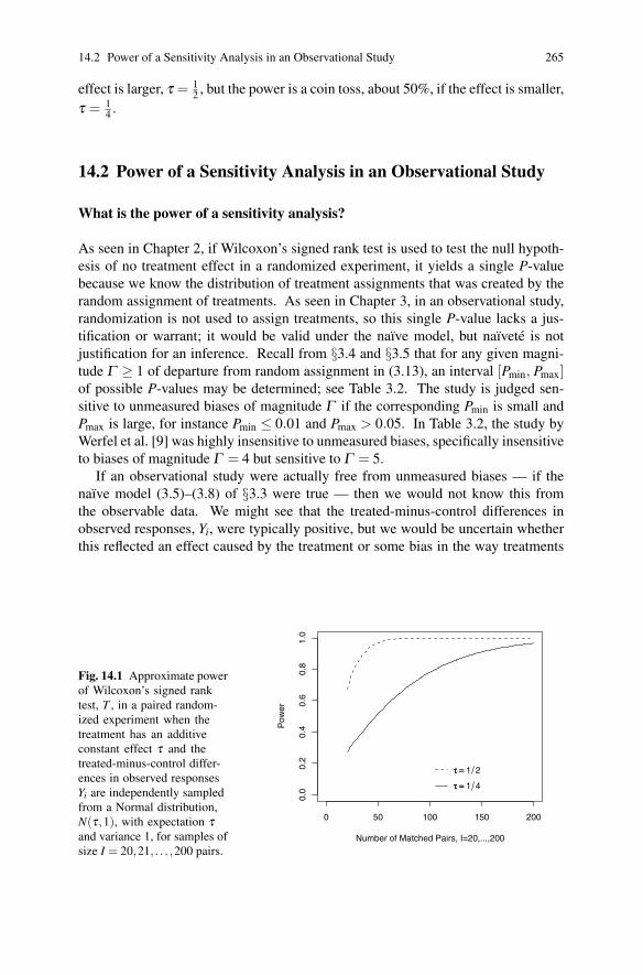
14.2 Power of a Sensitivity Analysis in an Observational Study 265
effect is larger, τ = 12 , but the power is a coin toss, about 50%, if the effect is smaller,
τ = 14 .
14.2 Power of a Sensitivity Analysis in an Observational Study
What is the power of a sensitivity analysis?
As seen in Chapter 2, if Wilcoxon’s signed rank test is used to test the null hypoth-
esis of no treatment effect in a randomized experiment, it yields a single P-value
because we know the distribution of treatment assignments that was created by the
random assignment of treatments. As seen in Chapter 3, in an observational study,
randomization is not used to assign treatments, so this single P-value lacks a jus-
tification or warrant; it would be valid under the naıve model, but naıvete is not
justification for an inference. Recall from §3.4 and §3.5 that for any given magni-
tude Γ ≥ 1 of departure from random assignment in (3.13), an interval [Pmin, Pmax]of possible P-values may be determined; see Table 3.2. The study is judged sen-
sitive to unmeasured biases of magnitude Γ if the corresponding Pmin is small and
Pmax is large, for instance Pmin ≤ 0.01 and Pmax > 0.05. In Table 3.2, the study by
Werfel et al. [9] was highly insensitive to unmeasured biases, specifically insensitive
to biases of magnitude Γ = 4 but sensitive to Γ = 5.
If an observational study were actually free from unmeasured biases — if the
naıve model (3.5)–(3.8) of §3.3 were true — then we would not know this from
the observable data. We might see that the treated-minus-control differences in
observed responses, Yi, were typically positive, but we would be uncertain whether
this reflected an effect caused by the treatment or some bias in the way treatments
Fig. 14.1 Approximate powerof Wilcoxon’s signed ranktest, T , in a paired random-ized experiment when thetreatment has an additiveconstant effect τ and thetreated-minus-control differ-ences in observed responsesYi are independently sampledfrom a Normal distribution,N(τ,1), with expectation τand variance 1, for samples ofsize I = 20,21, . . . ,200 pairs.
0 50 100 150 200
0.0
0.2
0.4
0.6
0.8
1.0
Number of Matched Pairs, I=20,...,200
Pow
er
ττ == 1 2
ττ == 1 4

266 14 The Power of a Sensitivity Analysis and Its Limit
were assigned or a combination of the two. The best we could hope to say in this
favorable situation is that the treatment appears to work and that this appearance
is highly insensitive to unmeasured biases, that is, only a very large value of Γcould produce this appearance from bias alone. Speaking informally, the power of
a sensitivity analysis is the probability that our hopes will be realized.
Somewhat more precisely, define the ‘favorable situation’ as a treatment that ac-
tually causes meaningful effects in an observational study that is free of unmeasured
biases. Specifically, in the favorable situation, the null hypothesis of no effect is
false, and not merely false but the treatment effect is large enough to be interesting
and substantively important. Also, in the favorable situation, the study is free of
unmeasured biases, people who look comparable are comparable, in the sense that
(3.5)–(3.8) are true. That is, the treated-minus-control differences in responses, Yi,
are not centered at zero because the treatment worked in the absence of bias. If we
were in the favorable situation, we would not know it from the observable data. It is
in this favorable situation that we would like to report a high degree of insensitivity
to unmeasured biases.
In testing the null hypothesis of no treatment effect at level α , conventionally
α = 0.05, rejection of the null hypothesis is insensitive to a bias of magnitude Γ if
Pmax ≤ α; see, again, the example in Table 3.2. In the favorable situation, the power
of a sensitivity analysis conducted with a specified α and Γ is the probability that
Pmax ≤ α . That is, if the treatment had an effect and there is no unmeasured bias,
then the power of the sensitivity analysis for specified α and Γ is the probability
that we will be able to say that a bias of magnitude Γ would not lead to acceptance
of the null hypothesis of no effect when tested at level α . In Table 3.2, it was found
that Pmax ≤ 0.05 for Γ = 4; the power is the probability of such an event computed
before the data are examined. For Γ = 1, this is the power of a test of no effect in a
randomized experiment as computed in §14.1.
Computing the power of a sensitivity analysis: The two steps
As in §14.1, the computations leading to the power of a sensitivity analysis are
done in two steps. As in §14.1, the first step is to compute a critical value, now
ζΓ ,α , so that Pr(T ≥ ζΓ ,α | F ,Z ) ≤ α for all treatment assignment probabilities
that satisfy (3.16)–(3.18) when the null hypothesis of no treatment effect is true.6 If
we observed T ≥ ζΓ ,α , then we would report that the upper bound on the one-sided
P-value for testing no effect is at most α for all biases of magnitude at most Γ ; see
again Table 3.2. The second step is to compute the probability that T ≥ ζΓ ,α in the
‘favorable situation’ in which the treatment has an effect and there is actually no
bias from unmeasured covariates. It is in this favorable situation that we hope to
report a high degree of insensitivity to unmeasured bias, and if T ≥ ζΓ ,α then we
will be able to report that rejection of the null hypothesis is insensitive to a bias of
magnitude Γ .
6 To be precise, we seek the smallest ζΓ ,α such that Pr(T ≥ ζΓ ,α | F ,Z ) ≤ α .

14.2 Power of a Sensitivity Analysis in an Observational Study 267
As in §14.1, the computation of the critical value is little more than a rearrange-
ment of the computation of the P-value for a one-sided test. Specifically, rearrang-
ing the computation (3.23) in §3.5 yields
ζΓ ,α.= E
(T∣∣∣F ,Z
)+Φ−1 (1−α)
√var
(T∣∣∣F ,Z
)(14.9)
so that using (3.19) and (3.20) yields
ζΓ ,α.=
Γ1+Γ
· I (I +1)2
+Φ−1 (1−α)
√Γ
(1+Γ )2
I (I +1)(2I +1)6
. (14.10)
For Γ = 1 in a randomized experiment, expressions (14.9) and (14.10) reduce to
(14.5).
Continuing the numerical illustration from §14.1, with I = 100 pairs, α = 0.05,
and Γ = 2, the critical value ζ2,0.05 is approximately
2
1+2· 100(100+1)
2+1.645
√2
(1+2)2
100(100+1)(2 ·100+1)6
(14.11)
or ζ2,0.05 = 3817.7, which is noticeably higher than ζ0.05 = ζ1,0.05.= 3005 for a ran-
domized experiment Γ = 1 in §14.1. In words, with I = 100 pairs, if T ≥ 3817.7then the maximum possible P-value is ≤ 0.05 for all treatment assignment proba-
bilities that satisfy (3.16)–(3.18) with Γ = 2. This completes the first step.
Step 2: Determining the power when the null hypothesis is false and there isno unobserved bias
Again, we wish to compute the power of the sensitivity analysis — the chance that
T ≥ ζΓ ,α — in the favorable situation in which there is no bias from unmeasured
covariates and the treatment has an effect. It is in this situation that we hope to report
that the treatment appears to work and the appearance is insensitive to moderately
large biases.
More precisely, the naıve model (3.5)–(3.8) is assumed to hold, or equivalently
(3.16)–(3.18) holds with Γ = 1, and the data F were generated by a stochastic
model with a treatment effect, and we wish to determine Pr(T ≥ ζΓ ,α | Z ) aver-
aging Pr(T ≥ ζΓ ,α | F , Z ) over the model that generates F . This is, of course,
identical to the second step in §14.1 for a randomized experiment except the critical
value, ζΓ ,α , has changed. In consequence, the second step is performed in the same
way as in §14.1 with the new critical value. As in §14.1, the second step may in
general be performed by simulating many sets of data F from the model, determin-
ing the proportion with T ≥ ζΓ ,α , and in particular cases the power of the sensitivity
analysis may be determined analytically.
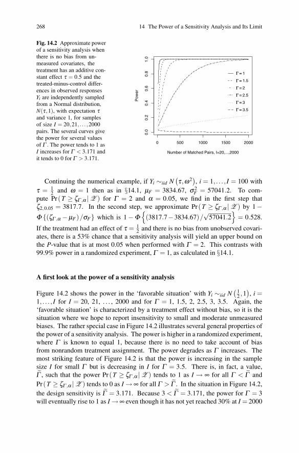
268 14 The Power of a Sensitivity Analysis and Its Limit
Fig. 14.2 Approximate powerof a sensitivity analysis whenthere is no bias from un-measured covariates, thetreatment has an additive con-stant effect τ = 0.5 and thetreated-minus-control differ-ences in observed responsesYi are independently sampledfrom a Normal distribution,N(τ,1), with expectation τand variance 1, for samplesof size I = 20,21, . . . ,2000pairs. The several curves givethe power for several valuesof Γ . The power tends to 1 asI increases for Γ < 3.171 andit tends to 0 for Γ > 3.171.
0 500 1000 1500 20000.
00.
20.
40.
60.
81.
0
Number of Matched Pairs, I=20,...,2000
Pow
er
ΓΓ == 1
ΓΓ == 1.5
ΓΓ == 2
ΓΓ == 2.5
ΓΓ == 3
ΓΓ == 3.5
Continuing the numerical example, if Yi ∼iid N(τ,ω2
), i = 1, . . . , I = 100 with
τ = 12 and ω = 1 then as in §14.1, μF = 3834.67, σ2
F = 57041.2. To com-
pute Pr(T ≥ ζΓ ,α | Z ) for Γ = 2 and α = 0.05, we find in the first step that
ζ2,0.05 = 3817.7. In the second step, we approximate Pr(T ≥ ζΓ ,α | Z ) by 1 −Φ {(ζΓ ,α −μF)/σF} which is 1 − Φ
{(3817.7−3834.67)/
√57041.2
}= 0.528.
If the treatment had an effect of τ = 12 and there is no bias from unobserved covari-
ates, there is a 53% chance that a sensitivity analysis will yield an upper bound on
the P-value that is at most 0.05 when performed with Γ = 2. This contrasts with
99.9% power in a randomized experiment, Γ = 1, as calculated in §14.1.
A first look at the power of a sensitivity analysis
Figure 14.2 shows the power in the ‘favorable situation’ with Yi ∼iid N(
12 ,1
), i =
1, . . . , I for I = 20, 21, . . . , 2000 and for Γ = 1, 1.5, 2, 2.5, 3, 3.5. Again, the
‘favorable situation’ is characterized by a treatment effect without bias, so it is the
situation where we hope to report insensitivity to small and moderate unmeasured
biases. The rather special case in Figure 14.2 illustrates several general properties of
the power of a sensitivity analysis. The power is higher in a randomized experiment,
where Γ is known to equal 1, because there is no need to take account of bias
from nonrandom treatment assignment. The power degrades as Γ increases. The
most striking feature of Figure 14.2 is that the power is increasing in the sample
size I for small Γ but is decreasing in I for Γ = 3.5. There is, in fact, a value,
Γ , such that the power Pr(T ≥ ζΓ ,α | Z ) tends to 1 as I → ∞ for all Γ < Γ and
Pr(T ≥ ζΓ ,α | Z ) tends to 0 as I → ∞ for all Γ > Γ . In the situation in Figure 14.2,
the design sensitivity is Γ = 3.171. Because 3 < Γ = 3.171, the power for Γ = 3
will eventually rise to 1 as I →∞ even though it has not yet reached 30% at I = 2000

14.3 Design Sensitivity 269
in Figure 14.2. In a sufficiently large sample, I, the ‘favorable situation’ with Yi ∼iidN(
12 ,1
), i = 1, . . . , I can be distinguished from bias of magnitude Γ < Γ = 3.171,
but not from biases of magnitude Γ > Γ = 3.171. Think of this statement as the
quantitative replacement for the statement ‘association does not imply causation.’ In
the ‘favorable situation’ with Yi ∼iid N(
12 ,1
), i = 1, . . . , I, the association between
treatment Z and response Y can be distinguished from biases less than Γ but not
from biases greater than Γ .
It is time to consider the design sensitivity, Γ , in greater detail.
14.3 Design Sensitivity
A first look at design sensitivity
In many simple settings, the power of a sensitivity analysis tends to 1 as the sample
size I increases if the analysis is performed with a sufficiently small value of Γ , but
the power tends to 0 if the analysis is performed with a sufficiently large value of Γ .
The switch occurs at a value, Γ , called the design sensitivity [5]. In the situation
in Figure 14.2, the design sensitivity was Γ = 3.171. It would be natural to seek a
design that results in a larger design sensitivity and to avoid designs that result in
a smaller design sensitivity. It would be natural to appraise the performance of the
methods in Chapter 5 in terms of their impact on design sensitivity.
Figure 14.2 plotted the power as a function of the sample size for several values
of Γ . Although such a plot resembles the familiar plot of power for a randomized
experiment (e.g., Figure 14.1), it is actually less instructive than plotting the power
as a function of Γ for several sample sizes I. Figure 14.3 plots power against Γ for
samples of size I = 200, 2000, 20000 in the ‘favorable situation’ in which there is a
treatment effect but no unmeasured bias, with Yi ∼iid N (τ,1), i = 1, . . . , I, for τ = 12
and τ = 1.
The first thing to notice about Figure 14.3 is that, as the sample size I increases,
the power viewed as a function of Γ is tending to a step function with a single step
down from power 1 to power 0, with the step located at the design sensitivity, Γ .
For τ = 12 , the step is at Γ = 3.171, whereas for τ = 1 the step is at Γ = 11.715.
For all sample sizes, I, there is negligible power for Γ > Γ .
The six power curves in Figure 14.3 refer to three sample sizes, I = 200, 2000,
20000, and two design sensitivities, Γ = 3.171 (for τ = 12 ) and Γ = 11.715 (for τ =
1). In this specific 3×2 array of power curves, the difference in design sensitivities
matters more than the difference in sample sizes, although sample size does have a
substantial effect on power. For instance, at Γ = 5, the power is close to 1 for I =200 pairs with τ = 1 but the power is close to zero with I = 20000 pairs and τ = 1
2 . A
bias of magnitude Γ = 5 could explain the observed association between treatment
and outcome if τ = 12 no matter how large the sample size becomes, whereas a mere
I = 200 pairs could eliminate bias of magnitude Γ = 5 as a plausible explanation
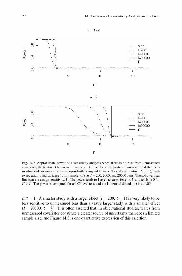
270 14 The Power of a Sensitivity Analysis and Its Limit
5 10 15
0.0
0.4
0.8
ττ == 1 2
ΓΓ
Pow
er
0.05I=200I=2000I=20000ΓΓ~
5 10 15
0.0
0.4
0.8
ττ == 1
ΓΓ
Pow
er
0.05I=200I=2000I=20000ΓΓ~
Fig. 14.3 Approximate power of a sensitivity analysis when there is no bias from unmeasuredcovariates, the treatment has an additive constant effect τ and the treated-minus-control differencesin observed responses Yi are independently sampled from a Normal distribution, N(τ,1), withexpectation τ and variance 1, for samples of size I = 200, 2000, and 20000 pairs. The solid verticalline is at the design sensitivity, Γ . The power tends to 1 as I increases for Γ < Γ and tends to 0 forΓ > Γ . The power is computed for a 0.05 level test, and the horizontal dotted line is at 0.05.
if τ = 1. A smaller study with a larger effect (I = 200, τ = 1) is very likely to be
less sensitive to unmeasured bias than a vastly larger study with a smaller effect
(I = 20000, τ = 12 ). It is often asserted that, in observational studies, biases from
unmeasured covariates constitute a greater source of uncertainty than does a limited
sample size, and Figure 14.3 is one quantitative expression of this assertion.

14.3 Design Sensitivity 271
A formula for design sensitivity
Design sensitivity is a general concept applicable to many statistics, not just Wilcoxon’s
signed rank statistic, and to many sampling situations, not just matched pairs [5].
However, in the case of Wilcoxon’s signed rank statistic for matched pairs, there is
a simple explicit formula for the design sensitivity [1, 8], which is given in Propo-
sition 14.1. Notice that this explicit form uses the quantity p′1 = Pr(Yi +Yi′ > 0),
which was encountered in §14.1 in connection with Lehmann’s formula for the ap-
proximate power of Wilcoxon’s signed rank statistic when applied in a randomized
experiment.7
Proposition 14.1. In I pairs matched exactly for observed covariates, xi j , supposethat the treated-minus-control matched pair differences in outcomes, Yi, i = 1, . . . , I,are independently sampled from a distribution F (·) and there is no bias from un-measured covariates in the sense that treatments are actually assigned by the naıvemodel (3.5)–(3.8). For a sensitivity analysis applied to Wilcoxon’s signed rankstatistic T in a one-tailed α-level test of no effect with α > 0, the power of thesensitivity analysis Pr(T ≥ ζΓ ,α | Z ) satisfies
Pr(T ≥ ζΓ ,α | Z ) → 1 as I → ∞ for Γ < Γ (14.12)
andPr(T ≥ ζΓ ,α | Z ) → 0 as I → ∞ for Γ > Γ , (14.13)
where
Γ =p′1
1− p′1
with p′1 = Pr(Yi +Yi′ > 0) , i �= i′. (14.14)
The proof is given in the appendix to this chapter.
Computing design sensitivity with additive effects and iid errors
If the Yi, i = 1, . . . , I, are independently sampled from a distribution F (·), then it
is always easy to determine p′1 = Pr(Yi +Yi′ > 0), i �= i′, and hence also Γ , by
simulation. In the case of an additive effect τ with Normal or Cauchy errors,
explicit formulas are available. Recall that Φ (·) is the standard Normal cumula-
tive distribution, N (0,1), and write ϒ (·) for the cumulative Cauchy distribution.
As in [3, pages 166–167], if Yi ∼iid N(τ,ω2
)then (Yi − τ)/ω ∼iid N (0,1) and
(Yi +Yi′ −2τ)/√
2ω2 ∼ N (0,1), so
Pr(Yi +Yi′ > 0) = Pr
(Yi +Yi′ −2τ
ω√
2>
−2τω√
2
)= Φ
(√2
τω
). (14.15)
7 See also Note 5 in §14.1.

272 14 The Power of a Sensitivity Analysis and Its Limit
For instance, if Yi ∼iid N(
12 ,1
), as in Figures 14.2 and 14.3, then Pr(Yi +Yi′ > 0) =
Φ(√
2 · 12
)= 0.76025 and Γ = 0.76025/(1−0.76025) = 3.171. If (Yi − τ)/ω ∼
ϒ (·), then {(Yi − τ)/ω +(Yi′ − τ)/ω}/2 ∼ϒ (·), so
Pr(Yi +Yi′ > 0) = Pr
(Yi +Yi′
2> 0
)= Pr
(Yi +Yi′ −2τ
2ω>
−2τ2ω
)= ϒ
( τω
).
(14.16)
For instance, if Yi − 12 ∼ ϒ (·), then Pr(Yi +Yi′ > 0) = ϒ
(12
)= 0.64758 and Γ =
0.64758/(1−0.64758) = 1.838.
14.4 Summary
As seen in Figure 14.3 and Proposition 14.1, no matter how large the sample size Ibecomes, a study will be sensitive to bias of magnitude Γ if Γ > Γ where Γ is the
design sensitivity. More precisely, when testing the null hypothesis of no effect, the
power of a sensitivity analysis will tend to 1 as I → ∞ for all Γ < Γ and to 0 for
all Γ > Γ . In this sense, Γ measures the limit of the ability of a particular study
design to distinguish a treatment effect from a bias due to failure to control for an
unmeasured covariate ui j. For this reason, the design sensitivity Γ is a natural nu-
merical measure for comparing design strategies that hope to distinguish treatment
effects from unmeasured biases, such as the strategies discussed in Chapter 5. The
remainder of Part III will make such comparisons.
14.5 Further Reading
The remainder of Part III is further reading for this chapter. Design sensitivity was
introduced in [5] and is developed further in [1, 6, 7, 8].
Appendix: Technical Remarks and Proof of Proposition 14.1
This appendix contains a proof of Proposition 14.1 in §14.3. The formula and proof
[1, 8] for Wilcoxon’s signed rank statistic are a special case of a general result [5,
§3] with the attractive feature that the design sensitivity Γ has an explicit closed
form (14.14).
The approximate power is Pr(T ≥ ζΓ ,α | Z ) .= 1−Φ {(ζΓ ,α −μF)/σF}, where
μF is the expectation of T in the ‘favorable situation.’ An intuitive, heuristic deriva-
tion [5, 8] uses the notion that if ζΓ ,α > μF , then in large samples, as I → ∞, the
signed rank statistic T eventually will be less than ζΓ ,α , whereas if ζΓ ,α < μF then
T will eventually be greater than ζΓ ,α . So the heuristic equates ζΓ ,α in (14.10) and

14.5 Further Reading 273
μF in (14.6) and solves for Γ . It is slightly better to equate ζΓ ,α/μF to 1, let I → ∞,
ignore terms that are small compared with I2, and solve for Γ ,
ζΓ ,α
μF
.=
Γ I(I+1)2(1+Γ ) +Φ−1 (1−α)
√Γ I(I+1)(2I+1)
6(1+Γ )2
I (I −1) p′1/2+ I p
(14.17)
.=Γ
p′1 (1+Γ )
, (14.18)
where 1 = Γ /{
p′1 (1+Γ )
}has solution Γ = p
′1/(
1− p′1
)as in (14.14). The
heuristic is attractive because it uses only the expectation μF of T in the favorable
situation, so the calculation is simple. Alas, the heuristic is ‘heuristic’ precisely be-
cause the power depends on (ζΓ ,α −μF)/σF , not on ζΓ ,α −μF , and the heuristic ig-
nores σF , hoping that things will work out. Indeed, things do work out, as the proof
that follows demonstrates [1]. The general result in [5, §3] shows that the heuristic
calculation works quite generally, but the proof that follows is self-contained and
does not depend upon the general result.
Proof. For large I, the power, Pr(T ≥ ζΓ ,α | Z ), is approximately equal to 1 −Φ {(ζΓ ,α −μF)/σF}, so the power tends to 1 as I → ∞ if (ζΓ ,α −μF)/σF →−∞and the power tends to 0 as I → ∞ if (ζΓ ,α −μF)/σF → ∞. Write κ = Γ /(1+Γ ).Using the expressions for μF and σ2
F from (14.6) and (14.7) in §14.1 and the expres-
sion for ζΓ ,α from (14.10) in §14.2 yields
ζΓ ,α −μF
σF= (14.19)
κI (I +1)/2+Φ−1 (1−α)√
κ (1−κ) I (I +1)(2I +1)/6− I (I −1) p′1/2− I p√
I (I −1)(I −2)(
p′2 − p′
1
2)
+ I(I−1)2
{2(
p− p′1
)2 +3p′1
(1− p′
1
)}+ I p(1− p)
.
(14.20)
Expression (14.20) looks untidy at first. Notice however that every term in the nu-
merator and denominator of (14.20) involves I, and I → ∞. So divide the numerator
and denominator of (14.20) by I√
I, and let I → ∞. The last term in the numerator,
−I p, becomes −I p/(I√
I)→ 0 as I → ∞, whereas the first term in the numerator,
κI (I +1)/2, becomes κI (I +1)/(2I√
I) ≈ √
Iκ/2 in the sense that their ratio is
tending to 1 as I → ∞. Continuing in this way, we find that
ζΓ ,α −μF
σF≈
√I(
κ − p′1
)2
√p′
2 − p′1
2as I → ∞, (14.21)
in the sense that the ratio of the left and right sides of (14.21) tends to 1 as I → ∞provided κ �= p
′1. If κ > p
′1, then (14.21) tends to ∞ as I → ∞, so the power tends to

274 14 The Power of a Sensitivity Analysis and Its Limit
0. If κ < p′1 then (14.21) tends to −∞ as I → ∞, so the power tends to 1. Moreover,
κ = Γ /(1+Γ ) > p′1 if and only if Γ > p
′1/(
1− p′1
).
References
1. Heller, R., Rosenbaum, P.R., Small, D.: Split samples and design sensitivity in observationalstudies. J Am Statist Assoc 104, to appear (2009)
2. Hodges, J.L., Lehmann, E.L.: Estimates of location based on ranks, Ann Math Statist 34, 598–611 (1963)
3. Lehmann, E.L.: Nonparametrics, San Francisco: Holden Day (1975). Reprinted New York:Springer (2006)
4. Rosenbaum, P. R.: Hodges-Lehmann point estimates of treatment effect in observational stud-ies. J Am Statist Assoc 88 1250–1253 (1993)
5. Rosenbaum, P. R.: Design sensitivity in observational studies. Biometrika 91, 153–164 (2004)6. Rosenbaum, P. R.: Heterogeneity and causality: Unit heterogeneity and design sensitivity in
observational studies. Am Statistician 59, 147–152 (2005)7. Rosenbaum, P.R.: What aspects of the design of an observational study affect its sensitivity to
bias from covariates that were not observed? Festshrift for Paul W. Holland. Princeton, NJ:ETS (2009)
8. Small, D., Rosenbaum, P. R.: War and wages: The strength of instrumental variables and theirsensitivity to unobserved biases. J Am Statist Assoc 103, 924–933 (2008)
9. Werfel, U., Langen, V., Eickhoff, I., Schoonbrood, J., Vahrenholz, C., Brauksiepe, A., Popp,W., Norpoth, K.: Elevated DNA single-strand breakage frequencies in lymphocytes of welders.Carcinogenesis 19, 413–418 (1998)

Chapter 15Heterogeneity and Causality
Abstract Before R.A. Fisher introduced randomized experimentation, the literature
on causal inference emphasized reduction of heterogeneity of experimental units.
To what extent is heterogeneity relevant to causal claims in observational studies
when random assignment of treatments is unethical or infeasible?
15.1 J.S. Mill and R.A. Fisher: Reducing Heterogeneity orIntroducing Random Assignment
In his System of Logic: Principles of Evidence and Methods of Scientific Inves-tigation, John Stuart Mill [11] proposed “four methods of experimental inquiry,”
including the “method of difference”:
If an instance in which the phenomenon . . . occurs and an instance in which it does not . . .have every circumstance save one in common . . . [then] the circumstance [in] which alonethe two instances differ is the . . . cause or a necessary part of the cause . . . [Mill wanted]“two instances . . . exactly similar in all circumstances except the one” [under study] [11,III, §8]
Notice Mill’s emphasis on a complete absence of heterogeneity: “have every circum-
stance save one in common;” that is, on treated and control units that are identical
but for the treatment. In the modern biology laboratory, nearly identical, geneti-
cally engineered mice are compared under treatment and control; this is a modern
expression of Mill’s ‘method of difference.’ It is clear from the quote that Mill
believed, rightly or wrongly, that heterogeneity of experimental units is directly rel-
evant to causal claims, and does not refer simply to reducing the standard error of
an estimate.
Ronald Fisher [3, Chapter 2] took a starkly different view. In 1935, in Chapter
2 of his Design of Experiments, Fisher introduced randomized experimentation for
the first time in book form, discussing his famous experiment of the lady tasting tea.
Fisher was directly critical of the ‘method of difference’:
275P.R. Rosenbaum, Design of Observational Studies, Springer Series in Statistics, DOI 10.1007/978-1-4419-1213-8_15, © Springer Science+Business Media, LLC 2010

276 15 Heterogeneity and Causality
It is not sufficient remedy to insist that “all the cups must be exactly alike” in every respectexcept that to be tested. For this is a totally impossible requirement in our example, andequally in all other forms of experimentation . . . These are only examples of the differencesprobably present; it would be impossible to present an exhaustive list of such possible dif-ferences . . . because [they] . . . are always strictly innumerable. When any such cause isnamed, it is usually perceived that, by increased labor and expense, it could be largely elim-inated. Too frequently it is assumed that such refinements constitute improvements to theexperiment . . . [3, page 18]
In the first omission, “. . . ,” in this quote, Fisher discussed the many ways two cups
of tea may differ.
Fisher is, of course, engaged in an enormously important task: he is introduc-
ing the logic of randomized experimentation to a broad audience for the first time.
Moreover, it would be reasonable to say that Fisher was correct and Mill was wrong
in certain critical respects. In a randomized clinical trial conducted in a hospital,
the patients are heterogeneous and not much can be done about it. There is no
opportunity to replace the hospital’s patients by genetically engineered, nearly iden-
tical patients. And yet it is possible to randomly assign treatments to heterogeneous
patients and draw valid causal inferences in just the manner that Fisher advocated.
Despite this, one senses that there is at least something that is sensible in Mill’s
method of difference, something that is sensible in the fanatical efforts of the basic
science laboratory to eliminate heterogeneity, in the use of nearly identical mice.
One senses that Fisher, in his understandable enthusiasm for his new method, has
gone just a tad too far in his criticism of Mill’s drive to eliminate heterogeneity.
Indeed, the issue may be particularly relevant in observational studies where random
assignment of treatments is either unethical or infeasible.
Some care is required in discussing heterogeneity. Heterogeneity is itself het-
erogeneous; there are several kinds of heterogeneity. In the biology laboratory, it is
often wise to use several different strains or species of genetically engineered, nearly
identical laboratory animals, making sure that each strain or species is equally repre-
sented in treated and control groups, to verify that any conclusion is not a peculiarity
of a single strain. It is uncontrolled rather than controlled heterogeneity that is the
target for reduction or elimination. Controlled heterogeneity has numerous uses.1
See Paul Holland’s [8] essay “Statistics and causal inference” for further con-
trasts of the views of Mill and Fisher.
1 Recall the related discussion of Bitterman’s concept of “control by systematic variation” in§5.2.2, where some factor is demonstrated to be irrelevant by systematically varying that factor.

15.2 A Larger, More Heterogeneous Study Versus a Smaller, Less Heterogeneous Study 277
15.2 A Larger, More Heterogeneous Study Versus a Smaller,Less Heterogeneous Study
Large I or small σ : Which is better?
To explore the issue raised in §15.1, consider the following simple situation. There
are I matched pairs in an observational study with treated-minus-control differences
in outcomes Yi, i = 1, . . . , I. Because it is an observational study, not a randomized
experiment, we cannot assume that matching for observed covariates has removed
all bias from nonrandom assignment — we cannot assume the naıve model of Chap-
ter 3, and will report a sensitivity analysis. Although we cannot know this from the
observed data, the situation is, in fact, the ‘favorable situation,’ in which there is
a treatment effect and the matching has succeeded in removing bias, so the naıve
model is correct and treatment assignment is effectively randomized within matched
pairs; see §14.2. In this favorable situation, the investigator hopes to report that the
treatment appears to be effective and that appearance is insensitive to small and
moderate biases. Indeed, the situation is simpler still: the treatment has an additive,
constant effect, τ = rTi j − rCi j, so that Yi = τ +(2Zi1 −1)(rCi1 − rCi2); see §2.4.1.
Moreover, the rCi1 − rCi2 are independent and identically distributed observations
drawn from a continuous distribution symmetric about zero; see §14.1. Because
this is the favorable situation, 2Zi1 −1 =±1, each with probability 12 independently
of rCi1 − rCi2, so Yi − τ itself has this same continuous distribution symmetric about
zero.
The investigator faces a choice between a larger study with more heterogeneous
responses or a smaller study with less heterogeneous responses, both in the ‘favor-
able situation.’ In §15.1, Mill would have advocated the smaller, less heterogeneous
study. Is there any merit to Mill’s claim? The heterogeneity here refers to hetero-
geneity that remains after matching for observed covariates, that is, heterogeneity
within pairs; heterogeneity between pairs is not at issue. Specifically, the investi-
gator faces the following admittedly stylized choice: observe either 4I pairs with
additive effect τ and (rCi1 − rCi2)/ω ∼ F (·), where F (·) is a continuous distribu-
tion symmetric about zero, or alternatively observe I pairs with additive effect τand (rCi1 − rCi2)/(ω/2) ∼ F (·). In words, the choice is between 4I pairs with dis-
persion ω or I pairs with dispersion ω/2. The choice is stylized in the following
sense. If F (·) were the standard Normal distribution, then the sample mean differ-
ence, Y = (1/I)∑Ii=1 Yi, would be Normally distributed Y ∼ N
{τ, ω2/(4I)
}with
expectation τ and variance ω2/(4I) in both the larger, more heterogeneous study
and the smaller less heterogeneous study. If ω were known in a randomized ex-
periment, the larger more heterogenous study and the smaller less heterogeneous
study would barely be worth distinguishing, because the sufficient statistic, Y , has
the same distribution in both studies.
Of course, this is not a randomized experiment. Does that matter for this choice?
If so, how does it matter?

278 15 Heterogeneity and Causality
A simulated example
Figure 15.1 depicts a simulated example of the choice between a smaller, less het-
erogeneous study (SL) with Yi ∼ N{
τ, (ω/2)2}
for i = 1, . . . , I = 100, and a larger,
more heterogeneous study (LM) with Yi ∼ N{
τ, ω2}
for i = 1, . . . , I = 400. In Fig-
ure 15.1, τ = 1/2, ω = 1. The boxplots for SL and LM have 100 and 400 pairs,
respectively.
If SL and LM were analyzed as if they were randomized experiments, the infer-
ences would be very similar. In SL, the mean difference is Y = 0.487 with estimated
standard error 0.054, while in LM the mean difference is Y = 0.485 with estimated
standard error 0.049; however, the true standard error is 0.05 in both SL and LM.
Using Wilcoxon’s signed rank statistic to test the null hypothesis of no effect yields
a very small P-value in both SL and LM, less than 10−10. The Hodges-Lehmann
point estimate τ of τ is τ = 0.485 for SL and τ = 0.489 for LM. The 95% confidence
interval from the randomization distribution of Wilcoxon’s statistic is [0.374, 0.600]from SL and [0.390, 0.587] from LM. If the choice were between two randomized
experiments with the distributions SL and LM yielding Figure 15.1, there would be
little reason to prefer one over the other.
Suppose, however, that SL and LM came from observational studies, so the be-
havior of the Yi might reflect either a treatment effect or an unmeasured bias or a
combination of the two. How sensitive are the conclusions from SL and LM to
departures from the naıve model (3.5)-(3.8) that underlies the inferences in the pre-
vious paragraph?
Fig. 15.1 A simulated exam-ple of the choice between asmaller, less heterogeneousstudy (SL) and a larger, moreheterogeneous study (LM). InSL there are I = 100 indepen-dent matched pair differences,Yi, that are Normal with ex-pectation τ and standarddeviation ω = 1/2. In LMthere are I = 400 independentmatched pair differences, Yi,that are Normal with expecta-tion τ and standard deviationω = 1. The horizontal dottedline is at 1/2.
●
●●
SL LM
−4
−2
02
4
Yi
I == 100 I == 400
ττ == 1 2 ττ == 1 2
ωω == 1 2 ωω == 1

15.2 A Larger, More Heterogeneous Study Versus a Smaller, Less Heterogeneous Study 279
Table 15.1 Sensitivity analysis for the larger, more heterogeneous study (LM) and the smaller, lessheterogeneous study (SL). Upper bounds on the one-sided P-value from Wilcoxon’s signed ranktest when testing the null hypothesis of no treatment effect are given. Although the randomizationinferences are similar (Γ = 1), the smaller, less heterogeneous study is much less sensitive to biasfrom unmeasured covariates (Γ ≥ 3).
Γ 1 2 3 4 5
LM < 10−10 0.00046 0.39 0.97 1.00
SL < 10−10 0.000016 0.0021 0.022 0.083
Table 15.2 Sensitivity analysis for the larger more heterogeneous study (LM) and the smallerless heterogeneous study (SL). For Γ = 1, the table gives the value of the Hodges-Lehmann pointestimate τ of the treatment effect, τ . For Γ = 2, the table gives the interval of possible pointestimates, [τmin, τmax], and the length of that interval, τmax − τmin. For a bias of magnitude Γ = 2,the range of possible point estimates is much longer for the larger, more heterogeneous study thanfor the smaller, less heterogeneous study.
Γ = 1 Γ = 2 Γ = 2τ [τmin, τmax] τmax − τmin
LM 0.489 [0.19, 0.79] 0.60SL 0.485 [0.32, 0.66] 0.34
Table 15.1 displays two sensitivity analyses, one for LM, the other for SL, giving
the upper bound on the one-sided P-value for testing the hypothesis of no treatment
effect using Wilcoxon’s signed rank statistic; see §3.4. As noted above, the random-
ization inferences (Γ = 1) are quite similar for LM and SL. In sharp contrast, the
smaller, less heterogeneous study, SL, is much less sensitive to bias from an unmea-
sured covariate. A bias of Γ = 3 could produce a boxplot similar to the LM boxplot
in Figure 15.1 (the upper bound on the P-value is 0.39), but a bias of Γ = 3 is very
unlikely to produce the boxplot for SL (the upper bound on the P-value is 0.0021).
To put this in context, SL is just slightly more sensitive to unmeasured bias than
Hammond’s [5] study of heavy smoking as a cause of lung cancer (see [14, §4]),
one of the least sensitive observational studies, whereas LM is much more sensitive.
In parallel with Table 3.4, Table 15.2 displays two sensitivity analyses, one for
LM, the other for SL, giving the interval of possible point estimates, [τmin, τmax],of the treatment effect τ . For Γ = 1, the interval is a point, namely the Hodges-
Lehmann point estimate, τmin = τmax = τ , and it is about the same for LM and SL.
For Γ = 2, the interval for LM, namely [0.19, 0.79], is considerably longer than the
interval for SL, namely [0.32, 0.66].In Tables 15.1 and 15.2, the smaller, less heterogeneous study is better than the
larger, more heterogeneous study, better in the sense of being less sensitive to un-
measured biases. It is important to keep in mind that Figure 15.1 depicts two ‘fa-
vorable situations,’ that is, treatment effects without unmeasured biases. Because
these are observational studies, the investigator does not know when she is in the
‘favorable situation,’ and so she cannot assert that Figure 15.1 depicts effects, not
biases. The investigator can, however, assert that a bias of magnitude Γ = 4 is too
small to explain away as unmeasured bias the ostensible effect in the smaller, less

280 15 Heterogeneity and Causality
Table 15.3 Power of a sensitivity analysis for a larger, more heterogeneous study (LM, 4I pairs,ω = 1), and a smaller, less heterogeneous study, (SL, I pairs, ω = 1/2), with the same additive,constant treatment effect, τ = 1/2, in the favorable situation with {rCi1 − rCi2}/ω ∼iid F(.). Thepower is similar when Γ = 1, but is higher for SL when Γ is larger.
Study Distribution Number Dispersion PowerF (·) of Pairs ω Γ = 1 Γ = 1.5 Γ = 2
LM Normal 120 1 1.00 0.96 0.60
SL Normal 30 12 1.00 1.00 0.96
LM Logistic 120 1 0.93 0.31 0.04
SL Logistic 30 12 0.93 0.61 0.32
LM Cauchy 200 1 0.98 0.32 0.02
SL Cauchy 50 12 0.95 0.60 0.28
heterogeneous study, but could not assert this about the larger, more heterogeneous
study.
Power comparisons with Normal, logistic and Cauchy errors
Table 15.3 contrasts the larger, more heterogeneous study (LM) and the smaller, less
heterogeneous study (SL) in terms of the power of the sensitivity analysis. Table
15.3 refers to a one-sided, 0.05 level test of the null hypothesis of no treatment
effect. The power is the probability that the upper bound on the one-sided P-value
is at most 0.05. The power is calculated as in §14.2.
The power of the randomization test (Γ = 1) is similar for LM and SL, but for
larger Γ , particularly for Γ = 2, the power is higher for the smaller, less heteroge-
neous study (SL). The pattern seen in Table 15.1 is not a peculiarity of one simula-
tion; rather, it is the anticipated pattern based on a comparison of the powers of LM
and SL.
Design sensitivity
Proposition 14.1 and expressions (14.15) and (14.16) may be used to determine the
design sensitivity Γ of the larger, more heterogeneous study (LM) and the smaller,
less heterogeneous study (SL) as
Γ =Φ(√
2 τω
)1−Φ
(√2 τ
ω
) (15.1)
for Normal errors and as
Γ =ϒ( τ
ω)
1−ϒ( τ
ω) (15.2)

15.3 Heterogeneity and the Sensitivity of Point Estimates 281
for Cauchy errors. For Normal errors with τ = 1/2, the designs LM (ω = 1) and SL
(ω = 1/2) have design sensitivities Γ of 3.171 and 11.715, respectively. In light of
this, the power of both designs with Normal errors tends to 1 as I → ∞ for the values
of Γ in Table 15.3, but for Γ = 5 the power of LM would tend to 0 while the power
of SL would tend to 1. In parallel, for Cauchy errors with τ = 1/2, the designs LM
(ω = 1) and SL (ω = 1/2) have design sensitivities Γ of 1.838 and 3, respectively.
In light of this, with Cauchy errors, for Γ = 2 in Table 15.3, the power of SL tends
to 1 as I → ∞ while the power of LM tends to 0.
15.3 Heterogeneity and the Sensitivity of Point Estimates
In the current chapter, the treatment has an additive constant effect, τ = rTi j − rCi j,
and in a randomized experiment, the Hodges-Lehmann estimate τ is a consistent es-
timate of τ . For a given deviation Γ from randomized treatment assignment, Tables
3.4 and 15.2 displayed the interval of possible Hodges-Lehmann point estimates
[τmin, τmax] of τ , where τmin = τmax = τ for Γ = 1; see §3.5 and [13]. As the sample
size increases, I → ∞, the endpoints of this interval converge in probability to the
endpoints of a fixed interval, [τmin, τmax]; this interval reflects the uncertainty about
τ that is due to a potential bias of magnitude Γ when there is no longer any sampling
uncertainty.
In the ‘favorable situation,’ with errors having Normal Φ (·) or Cauchy ϒ (·) cu-
mulative distributions, the following proposition gives the form of this limiting in-
terval. See [16, Appendix] for proof of Proposition 15.1.2
Proposition 15.1. If (Di − τ)/ω ∼iid Φ (·) then [τmin, τmax] is τ ±ω Φ−1 (κ)/√
2,where κ = Γ /(1+Γ ). If (Di − τ)/ω ∼iid ϒ (·) then [τmin, τmax] is τ ±ωϒ−1 (κ).
Proposition 15.1 is consistent with Mill’s view that heterogeneity of experimen-
tal units, ω , is directly relevant to causal claims. In Proposition 15.1, there is no
sampling variability, because Proposition 15.1 refers to the limit as I → ∞. The
uncertainty addressed in Proposition 15.1 is quantified by the length of the limiting
interval, τmax − τmin, and despite the absence of sampling variability, the length of
that interval is directly proportional to ω .
Proposition 15.1 does not contradict Fisher’s view, but it does emphasize that this
view is applicable only when biases from nonrandom treatment assignment have
been avoided by randomization. Reducing heterogeneity ω and increasing sample
2 Although the proof has a few details, it is simple in concept. The lower endpoint τmin of theinterval of possible point estimates is obtained by equating Wilcoxon’s signed rank statistic Tcomputed from Yi − τ0, say Tτ0
, to the maximum null expectation of T , namely E(
T∣∣∣F ,Z
)=
Γ I (I +1)/{2(1+Γ )} from (3.19) and solving the equation for τmin. Dividing the equation byI (I +1)/2 yields the equivalent equation 2Tτ0
/{I (I +1)} = Γ /(1+Γ ). If (Yi − τ)/ω ∼ Φ (·)or (Yi − τ)/ω ∼ϒ (·) then as I → ∞, the left side of the equation, 2Tτ0
/{I (I +1)}, converges inprobability to a function of (τ − τ0)/ω , and the rest of the proof is detail devoted to showing thatequation can be solved to give the solutions in the statement of Proposition 15.1.

282 15 Heterogeneity and Causality
size I compete for resources in a randomized experiment because bias is known to
have been avoided, so the analysis can be conducted with Γ = 1. More precisely,
in Proposition 15.1, if it were known that Γ = 1, then κ = 1/2, so Φ−1 (κ)/√
2 =Φ−1 (1/2)/
√2 = 0 and ϒ−1 (κ) = ϒ−1 (1/2) = 0, and the length of the limiting
interval is τmax − τmin = 0 for every value of ω .
The length of the interval is also affected by the magnitude of potential bias,
Γ , though κ = Γ /(1+Γ ). The two components determine the length τmax − τmin
of the limiting interval in a multiplicative manner; for the Normal, τmax − τmin =2ω Φ−1 (κ)/
√2. A given magnitude Γ of deviation from a randomized experi-
ment does more harm when the units are more heterogeneous, that is, when ω is
larger. If you were deceptively trying to bias a randomized trial by covertly tilting
the treatment assignment probabilities by a magnitude of Γ in (3.16)-(3.18), then
you could do more harm if the units were the heterogeneous patients in a clinical
trial than if they were the homogeneous genetically engineered mice in a laboratory
experiment.
In the ‘favorable situation’ in an observational study, increasing the sample size
I reduces the standard error, but it does not materially reduce sensitivity to unmea-
sured biases. In contrast, in this situation, reducing the heterogeneity of experimen-
tal units, ω , reduces both the standard error and sensitivity to unmeasured biases.
In an observational study, LM and SL of Figure 15.1 are not at all the same: SL is
much better.
15.4 Examples of Efforts to Reduce Heterogeneity
Twins
What are the economic returns to additional education? You cannot compare the
mid-life earnings of surgeons and high school dropouts — they differed in the mid-
dle of high school before the dropout left school. Not in every case, but typically, the
child who went on to become a surgeon was receiving better grades and standard-
ized test scores in high school, was more strongly motivated for school studies, had
better educated, wealthier parents, and not inconceivably differed in some relevant
genes. You would like to compare two children of the same parents with differ-
ent education growing up at the same time in the same home with the same genes.
Ashenfelter and Rouse [1] compared the earnings of identical twins with differing
education, estimating about a 9% increase in earnings per year of additional educa-
tion.
The use of twins is the canonical example of trading sample size for reduced
heterogeneity. Twin pairs are quite heterogeneous between pairs and in several
important respects fairly homogeneous within pairs, so the use of twins reflects the
type of heterogeneity discussed in this chapter.

15.4 Examples of Efforts to Reduce Heterogeneity 283
Road hazards
What permanent features of a road affect the risk of collisions with roadside ob-
jects? Road hazards are a fairly small part of accident risk. Also relevant are: the
driver’s sobriety, skill and risk tolerance; ambient light; the weather — ice, snow,
rain and fog; safety equipment — use of seat belts, quality and condition of brakes,
tires, air bags, traction and stability control devices. These factors are related. The
risk-averse driver will drive near the legal speed limit, but will also invest in safety
devices and wear seat belts. In the rain or snow, one drives on the highway to work
but not on the dirt road to the picnic area, so weather and road hazards vary to-
gether. Sobriety is more common at noon than at midnight, so sobriety and ambient
light vary together. You would like to compare different road hazards with the same
driver, in the same car, in the same weather, with the same ambient light, in the same
state of sobriety, with seat belts in the same state of use. Is this possible?
Using a simple, clever study design, Wright and Robertson [22] did just that.
They compared 300 fatal roadside collisions in Georgia in 1974–1975 to 300 nonac-
cidents involving the same driver, in the same car, in the same ambient light, and so
on. The nonaccidents occurred one mile back from the crash site, a location passed
without incident by the driver just moments before the crash. At crash sites, Wright
and Robertson found a substantial excess of roads that curved more than 6 degrees
with downhill gradients of greater than 2%. (Technically, this is a ‘case-crossover’
study of the type proposed by Malcolm Maclure [10], except that it is defined by ge-
ography rather than time; see also the ‘case-specular’ design of Sander Greenland
[4].)
The genetically engineered mice of microeconomics
Many businesses that provide products or services over large regions adopt a strat-
egy known as ‘replication’ in which nearly identical outlets are reproduced at high
speed in diverse locations [21]. Starbucks and Tesco are two of the many such
businesses. This strategy confers various benefits to businesses that use it, but it
also creates nearly identical copies of a business in locations that may have adopted
different regulations, taxes or other policies. For instance, Card and Kreuger’s [2]
study of the minimum wage and employment compared Burger Kings in New Jer-
sey to Burger Kings in Pennsylvania, KFCs in New Jersey to KFCs in Pennsylvania,
etc., and in this way eliminated one of several sources of extraneous variation be-
tween the two states; see §4.5 and §11.3 for further discussion of this study.
Motorcycle helmets
Do helmets reduce the risk of death in motorcycle crashes? Crashes occur at differ-
ent speeds with different forces, and neither speeds nor forces are likely to be mea-
sured. Motorcyclists hit different objects — pedestrians or Hummers — in dense or

284 15 Heterogeneity and Causality
light traffic, with emergency services near or far away. One would like to compare
two people, one with a helmet, the other without, on the same type of motorcycle,
driving at the same speed, crashing into the same object, in the same traffic, with
equal proximity to medical aid. Is that possible?
It is when two people ride one motorcycle, one with a helmet, the other without.
Norvell and Cummings [12] looked at such crashes, finding about 40% lower risk
associated with helmet use.
15.5 Summary
In a randomized experiment, an unbiased estimate of treatment effect is available,
so increasing the sample size, I, or reducing the unit heterogeneity, ω , both serve
to reduce the standard error of an unbiased estimate. The situation is strikingly
different in an observational study. In the ‘favorable situation’ in an observational
study, the treatment is effective and there are no unmeasured biases. If the favor-
able situation arose, the investigator would not know it, and at best would hope to
report that the treatment appears to be effective and that appearance is insensitive
to small and moderate biases. In this situation, reducing heterogeneity, even purely
random heterogeneity, ω , confers benefits that cannot be obtained by increasing the
sample size, I. Specifically, reducing heterogeneity reduces sensitivity to unmea-
sured biases. Several cleverly designed studies have illustrated efforts to reduce
heterogeneity.
15.6 Further Reading
This chapter is based on [16], where additional discussion may be found.
References
1. Ashenfelter, O., Rouse, C.: Income, schooling and ability: Evidence from a new sample ofidentical twins. Q J Econ 113, 253–284 (1998)
2. Card, D., Krueger, A.: Minimum wages and employment: A case study of the fast-food indus-try in New Jersey and Pennsylvania. Am Econ Rev 84, 772–793 (1994)
3. Fisher, R.A.: Design of Experiments. Edinburgh: Oliver and Boyd (1935)4. Greenland, S.: A unified approach to the analysis of case-distribution (case-only) studies.
Statist Med 18, 1–15 (1999)5. Hammond, E.C.: Smoking in relation to mortality and morbidity. J Natl Cancer Inst 32, 1161–
1188 (1964)6. Heller, R., Rosenbaum, P.R., Small, D.: Split samples and design sensitivity in observational
studies. J Am Statist Assoc 104, to appear (2009)7. Hodges, J.L., Lehmann, E.L.: Estimates of location based on ranks, Ann Math Statist 34,
598–611 (1963)

References 285
8. Holland, P.W.: Statistics and causal inference. J Am Statist Assoc 81, 945–960 (1986)9. Lehmann, E.L.: Nonparametrics, San Francisco: Holden Day (1975) Reprinted New York:
Springer (2006)10. Maclure, M.: The case-crossover design: A method for studying transient effects on the risk
of acute events. Am J Epidemiol 133, 144–152 (1991)11. Mill, J.S.: A System of Logic: The Principles of Evidence and the Methods of Scientific In-
vestigation. Indianapolis: Liberty Fund (1867)12. Norvell, D.C., Cummings, P.: Association of helmet use with death in motorcycle crashes: A
matched-pair cohort study. Am J Epidemiol 156, 483–487 (2002)13. Rosenbaum, P.R.: Hodges-Lehmann point estimates of treatment effect in observational stud-
ies. J Am Statist Assoc 88, 1250–1253 (1993)14. Rosenbaum, P.R.: Observational Studies (2nd ed.). New York: Springer (2002)15. Rosenbaum, P. R.: Design sensitivity in observational studies. Biometrika 91, 153–164 (2004)16. Rosenbaum, P. R.: Heterogeneity and causality: Unit heterogeneity and design sensitivity in
observational studies. Am Statistician 59, 147–152 (2005)17. Rosenbaum, P.R.: What aspects of the design of an observational study affect its sensitivity
to bias from covariates that were not observed? In: Festshrift for Paul W. Holland. Princeton,NJ: ETS (2009)
18. Salsburg, D.: The Lady Tasting Tea. San Francisco: Freeman (2001)19. Small, D., Rosenbaum, P.R.: War and wages: The strength of instrumental variables and their
sensitivity to unobserved biases. J Am Statist Assoc 103, 924–933 (2008)20. Werfel, U., Langen, V., Eickhoff, I., Schoonbrood, J., Vahrenholz, C., Brauksiepe, A., Popp,
W., Norpoth, K.: Elevated DNA single-strand breakage frequencies in lymphocytes. Carcino-genesis 19, 413–418 (1998)
21. Winter, S.G., Szulanski, G.: Replication as strategy. Organizat Sci 12, 730–743 (2001)22. Wright, P.H., Robertson, L.S.: Priorities for roadside hazard modification. Traffic Eng 46, 24–
30 (1976)

Chapter 16Uncommon but Dramatic Responses toTreatment
Abstract Large effects in moderate to large studies are typically insensitive to small
and moderate unobserved biases, but the concept of a ‘large effect’ is vague. What
if most subjects are not much affected by treatment, but a small fraction, perhaps
10% or 20% of subjects, are strongly affected? On average, such an effect may be
small, but not at all small for the affected fraction. Is such an effect insensitive to
small and moderate unobserved biases?
16.1 Large Effects, Now and Then
Are large but rare effects insensitive to unmeasured biases?
In §2.5, in the National Supported Work Experiment, depicted in Figure 2.1, many
men appear to have received little or no benefit from the treatment, but the few men
with high earnings were fairly consistently in the treated group. In §2.5, if pairs
of men were examined two at a time (i.e., four men), then 61% of the time, the
man with the highest aligned earnings was a treated man, where 50% is expected
by chance, but if pairs were examined 20 at a time (i.e., 40 men), 86% of the time
the man with the highest aligned earnings was a treated man, where again 50% is
expected by chance. Big gains in earnings are consistently in the treated group.
A similar pattern is seen for toxicity in Chapter 7 in Figure 7.1 in connection
with Jeffrey Silber et al.’s [14] study of intensity of chemotherapy in I = 344 pairs
of women with ovarian cancer: the median level of toxicity is not very different
in the MO and GO groups, but high levels are more common in the MO group. If
pairs of women are examined two at a time (i.e., 4 women), then in 65% of pairs, the
woman with the highest aligned toxicity was treated by an MO, but if we look at 20
pairs at a time (i.e., 40 women), then 90% of the time, the woman with the highest
aligned toxicity was treated by an MO. Figure 16.1 depicts the distribution of the
MO-minus-GO differences, Yi, in toxicity. In Figure 7.1 and Figure 16.1, it appears
287P.R. Rosenbaum, Design of Observational Studies, Springer Series in Statistics, DOI 10.1007/978-1-4419-1213-8_16, © Springer Science+Business Media, LLC 2010

288 16 Uncommon but Dramatic Responses to Treatment
●● ●●● ●●● ●● ●● ● ●●●●● ● ●●●●
−40 −20 0 20 40
MO−GO Difference in Weeks with Toxicity in Year 1
−40 −20 0 20 40
0.00
0.04
Yi
MO−GO Difference in Weeks with Toxicity in Year 1
Den
sity
Fig. 16.1 Boxplot and density estimate of the MO-GO difference Yi in weeks with toxicity in year1 for I = 344 pairs of women with ovarian cancer; see Chapter 7 and [14]. The vertical dotted lineis at zero difference. The density estimate uses the default settings in R.
that many MOs and GOs treat with similar intensity producing similar toxicity, but
a fraction of MOs treat more intensively producing more toxicity.
In these cases, the hypothesis of a constant effect, τ = rTi j − rCi j for all i, j,does not look plausible. As discussed in §2.5, a more plausible hypothesis is that
rTi j − rCi j is zero or small for many subjects i, j, but rTi j − rCi j is large for some
subjects i, j. David Salsburg [11] argued that effects of this sort are fairly common,
are often important, and that we tend to miss them because our methodology tends
to focus on typical effects, but in this context large effects do occur but are not
typical. The question addressed in the current chapter is whether an effect of this
kind is highly sensitive to unmeasured biases. In both Figure 2.1 and Figure 7.1,
the typical difference in outcomes is not large, yet the distributions of outcomes are
quite different.

16.1 Large Effects, Now and Then 289
Review of §2.5: Measuring large but uncommon effects
Building upon certain technical results by Eric Lehmann [2, (6.1)], David Salsburg
[11] and William Conover and Salsburg [1] made a strong argument that, in the
comparison of unmatched treated and control groups, the pattern of large, uncom-
mon effects is not properly associated with ‘transformations’ or ‘outliers’ or other
similar concepts of data analysis, because the pattern may be seen in the ranks: the
extremely high ranks are consistently in the treated group. In outline in §2.5 and in
detail in [7], it was found that the highly interpretable rank scores, qi in (2.8), pro-
posed by W. Robert Stephenson [15] approximate the locally optimal rank scores
of Conover and Salsburg [1]. For example, the statement about 20 pairs of men
in the first paragraph of this Chapter was obtained in §2.5 by an interpretation of
Stephenson’s ranks.
Fig. 16.2 Stephenson’sranks qi from (2.8) form = 2,5,10,20 and for theI = 344 matched pairs inSilber et al.’s [14] study ofintensity of chemotherapy forovarian cancer; see Chapter 7.Wilcoxon’s ranks are essen-tially the same as m = 2. Form = 5, the smallest 100 or so|Yi| are almost ignored. Form = 20, the smallest 300 or so|Yi| are almost ignored.
0 50 100 150 200 250 300 350
0.0
0.2
0.4
0.6
0.8
1.0
Ranks, i=1,...,344
Ste
phen
son'
s ra
nks
scal
ed to
[0,1
]
m=2m=5m=10m=20
Recall that Stephenson’s ranks score pairs m at a time, and are essentially the
same as Wilcoxon’s ranks for m = 2; see §2.5. For I = 344 matched pairs, as in
Silber et al.’s [8, 14] study in Chapter 7, Figure 16.2 depicts Stephenson’s ranks, qiin (2.8), sorted into increasing order and scaled to be between 0 and 1 as qi/max q j,
for m = 2, 5, 10, 20. With m = 20, one looks at 20 pairs simultaneously, counting
a ‘success’ if the largest of the 40 aligned responses in the 20 pairs is the response
of a treated subject. For m = 10 in Figure 16.2, Stephenson’s qi largely ignore the
smallest 200 of the 344 absolute differences in responses |Yi|, judging the treatment
effect by the remaining 144 pairs. Salsburg and Conover suggested the equivalent
of m = 5 for the applications that they discussed.

290 16 Uncommon but Dramatic Responses to Treatment
16.2 Two Examples
Chemotherapy intensity and toxicity in ovarian cancer
Table 16.1 compares four sensitivity analyses for the ovarian cancer study [8, 14]
in Chapter 7. The four sensitivity analyses are each conducted using Stephenson’s
[15] signed rank test, with four values of m, that is, with the absolute ranks in Figure
16.2. Wilcoxon’s ranks are similar to Stephenson’s ranks with m = 2. The ranks
with m = 20 are concerned with the largest aligned response of 40 women in 20
pairs, so that they emphasize the fairly high levels of toxicity experienced by some
women.
Table 16.1 reports upper bounds on the one-sided P-value testing the null hy-
pothesis of no treatment effect. Wilcoxon’s statistic (m = 2) becomes sensitive to a
bias of magnitude Γ = 1.5, but Stephenson’s statistic with m = 20 is insensitive to a
bias of magnitude Γ = 3.5. In this one example, the degree of sensitivity to bias is
strongly affected by whether the analysis emphasizes typical effects or less common
but larger effects. Small biases could not produce the large but uncommon effects
in Figure 16.1.
Table 16.1 Using Stephenson’s statistic with several values of m, upper bounds are given on theone-sided P-value testing the null hypothesis of no treatment effect in the ovarian cancer data ofChapter 7 and [14]. For m = 2, Stephenson’s ranks closely resemble Wilcoxon’s ranks, but forlarger values of m, Stephenson’s ranks place greater emphasis on large |Yi|’s. In this instance, theresults are much less sensitive with m = 20 than with m = 2.
Γ m = 2 m = 5 m = 10 m = 20
1 9.0×10⁻⁷ 5.2×10⁻⁹ 1.1×10⁻⁸ 1.1×10⁻⁶
1.5 0.051 0.00017 0.000024 0.000192 0.71 0.016 0.0010 0.00202.5 0.14 0.0087 0.00813 0.035 0.0213.5 0.088 0.041
The calculations to produce Table 16.1 closely parallel the calculations for
Wilcoxon’s signed rank statistic, except that Stephenson’s ranks, qi, are used in
place of Wilcoxon’s ranks, qi. The null expectation and variance of Stephenson’s
statistic T = ∑sgn(Yi) qi are bounded by expressions (3.25)-(3.26) with qi in place
of qi, and the standardized deviates are compared to the Normal distribution in par-
allel with (3.23).
DNA adducts among aluminum production workers
Bernadette Schoket, David Phillips, Alan Hewer, and Istvan Vincze [13] compared
DNA adducts in the lymphocytes of aluminum production workers and unexposed
controls. Figure 16.3 shows 25 matched pairs of an aluminum production worker

16.2 Two Examples 291
● ●
●●●●
● ●●●●●
●●●●●●
●
●● ●
●
●
●
0 1 2 3 4 5 6
01
23
45
6
DNA adducts for Controls
DN
A a
dduc
ts fo
r A
lum
inum
Wor
kers
●
0 1 2 3 4 5 6
DNA adducts for Controls
●
01
23
45
6
DN
A a
dduc
ts fo
r A
lum
inum
Wor
kers
Fig. 16.3 DNA adducts per 108 nucleotides for 25 aluminum production workers and 25 controlsmatched for age and cigarettes-per-day [13]. The central plot is a quantile-quantile plot that ignoresthe pairing. The dotted line is the x = y line. There appears to be little or no difference at lowerquantiles, with a sharp rise at upper quantiles.
and a control matched for age and cigarettes smoked per day. The noticeable feature
of Figure 16.3 is that there appears to be little or no difference in DNA adducts at
lower quantiles, with a substantial divergence at upper quantiles.1
Table 16.2 displays two sensitivity analyses using Stephenson’s signed rank
statistic, one with m = 2 which is similar to Wilcoxon’s statistic, and one with m = 5.
(With just I = 25 pairs, it does not seem reasonable to compare m = 20 pairs at a
time to determine the largest aligned response.) The table displays upper bounds
on the one-sided P-value for testing the null hypothesis of no treatment effect. As
Figure 16.3 might lead us to anticipate, the results are less sensitive for m = 5 than
for m = 2.
1 The paired data for the 25 pairs are listed in [7].

292 16 Uncommon but Dramatic Responses to Treatment
Table 16.2 Upper bounds on the one-sided P-values from Stephenson’s test for m = 2 and m = 5for the 25 pairs of an aluminum production worker and a matched control depicted in Figure 16.3.The results are less sensitive to bias for m = 5, presumably because the difference in the distributionof DNA adducts is apparent only at upper quantiles.
Γ m = 2 m = 5
1 0.0076 0.00781.5 0.054 0.0301.8 0.10 0.0482 0.14 0.061
16.3 Properties of a Paired Version of Salsburg’s Model
David Salsburg [11] proposed a model for treatment effects in unmatched groups in
which a fraction 0 ≤ λ ≤ 1 of the treated subjects experience a substantial treatment
effect and the rest experience no effect at all. The following model is a slight modi-
fication for matched pairs of Salsburg’s model for unmatched groups. Each pair i is
characterized by a fixed pair parameter, ηi, which accounts for dependence within
pairs, and is eliminated when matched pair differences Yi are calculated. Then the
rCi j −ηi are sampled from a continuous distribution G(·) with density g(·), and the
rTi j −ηi are sampled from (1−λ )G(·)+λ {G(·)}ν where 0 ≤ λ ≤ 1 and ν ≥ 2 is
a positive integer. Responses from distinct subjects are mutually independent.2
The model has a simple interpretation. The model says, in effect, that a frac-
tion, 1− λ , of treated subjects experience no treatment effect — their responses
are sampled from G(·) which is the distribution of responses to control. A frac-
tion λ of treated subjects do experience an effect. Instead of having a response
drawn from G(·), the affected fraction have a response rTi j − ηi drawn from
{G(·)}ν = G(·)× ·· · ×G(·). If you sampled ν independent rCi j −ηi’s from the
distribution G(·) and took the maximum of these, that maximum would have the
distribution {G(·)}ν . As intuition suggests, {G(·)}ν is a ‘larger’ distribution3 than
G(·) in the sense that {G(r)}ν ≤ G(r) for all r, because ν ≥ 2; that is, the chance,
namely {G(r)}ν , that the maximum of ν independent observations from G(·) is
less than r is less than or equal to the chance, namely G(r), that one observation
from G(·) is less than r, and this is true for all r. Figure 16.4 depicts the two prob-
ability densities that are mixed with weights λ and 1−λ to form the density of the
2 The density of rTi j −ηi is (1−λ ) g(r)+ λ ν g(r) {G(r)}ν−1. In the favorable situation, treat-ment assignment Zi1 −Zi2 is ±1 with probability 1/2 independently of (rCi1,rTi1,rCi2,rTi2), andYi = (Zi1 −Zi2)(Ri1 −Ri2) is distributed as the difference of two independent observations, onedrawn from (1−λ )G(·)+ λ {G(·)}ν and the other drawn from G(·). The matched pair differ-ence Yi has probability density∫
g(r)[(1−λ ) g(r + y)+λ ν g(r + y) {G(r + y)}ν−1
]dr
which is easy to evaluate by numerical integration. In the calculations presented graphically, G(·)is the standard Normal cumulative distribution Φ (·).3 It is stochastically larger; see Note 15 in Chapter 3.

16.3 Properties of a Paired Version of Salsburg’s Model 293
treated response, rTi j −ηi, for ν = 20, when G(·) is the standard Normal cumula-
tive distribution G(·) = Φ (·). In Figure 16.4, a fraction 1−λ of treated subjects
have a response rTi j −ηi drawn from the standard Normal density φ (r), the dashed
curve, and a fraction λ of treated subjects have a response rTi j −ηi drawn from the
the density ν φ (r) Φ (r)ν−1 of the maximum of ν = 20 independent observations
from a standard Normal distribution, the solid curve. The treated-minus-control
difference Yi in pair i is the difference of a treated response rTi j −ηi formed from
this mixture and a control response rCi j −ηi independently drawn from the standard
Normal density φ (r).In the unmatched two sample problem, Eric Lehmann [2, (6.1)] studied this
model for ν = 2 showing that Wilcoxon’s ranks, with m = 2, perform well for small
λ in large samples. William Conover and David Salsburg [1] showed that for gen-
eral ν , ranks similar to Stephenson’s ranks perform well if m = ν for small λ in
large samples.4
With G(·) equal to the standard Normal distribution, G(·) = Φ (·), Figure 16.5
depicts the distribution of matched pair differences, Yi, under Salsburg’s model with
λ = 0.2 and ν = 50. For comparison, Figure 16.5 also displays a Normal distri-
bution with the same expectation and variance. Visually, the distinction between
the two distributions is quite subtle: Salsburg’s model has a slight skew to the right,
with an expectation slightly to the right of its mode. Conceptually, the distributions
are very different. In Salsburg’s model, 1−λ = 80% of treated subjects experience
no treatment effect: their treated responses, rTi j −ηi, are sampled from the same
Normal distribution as responses to control, rCi j −ηi. In Salsburg’s model, only
λ = 20% of treated subjects experience a nonzero effect, and their responses are the
maximum of ν = 20 independent observations from a Normal distribution, rather
than one observation from a Normal distribution. In Figure 16.4, the affected group
had a much higher distribution of responses, but this is twice hidden in Figure 16.5,
once because only a fraction λ of treated subjects experienced a treatment effect,
and a second time by the need to compare treated subjects to controls to eliminate
ηi by differencing to form the matched pair difference, Yi. Figure 16.6 is similar to
Figure 16.5, except λ = 0.1 and ν = 1000; here, the difference is more noticeable,
but still quite subtle. Compare Figure 16.6 to the estimated density in Figure 16.1.
Are the effects in Figures 16.5 and 16.6 highly sensitive to unmeasured biases?
On the one hand, the affected group in Figure 16.4 is strongly affected. On the other
hand, that strong effect is twice hidden in the observable distribution of Yi in Figure
16.5. In Tables 16.1 and 16.2, effects were judged fairly sensitive by Wilcoxon’s
statistic (m = 2), which emphasizes typical effects, but were noticeably less sensitive
4 Somewhat more precisely, Conover and Salsburg found the locally most powerful rank test forfixed ν as λ → 0 for the two-sample problem as the sample size increased. It is shown in [7]that these locally most powerful ranks are almost the same as Stephenson’s [15] ranks in largesamples, although the latter are easier to interpret in terms of the magnitude of the treatment effect.Stephenson and Ghosh [16] discuss the use of Stephenson’s ranks in the unmatched two sampleproblem. The two sample model comparing (1−λ )G(·)+λ {G(·)}ν and G(·) is an instance of a‘Lehmann alternative’ in the sense that the distribution of the ranks depends upon ν and λ but noton G(·); see [2]. Reference [7] is not restricted to matched pairs, but in the current book, only thepaired case is discussed.

294 16 Uncommon but Dramatic Responses to Treatment
−6 −4 −2 0 2 4 6
0.0
0.2
0.4
0.6
0.8
rTij −− ννi
dens
ity
φφ((x))ννφφ((x))ΦΦ((x))νν−−1
νν == 20
Fig. 16.4 The two densities that are mixed in Salsburg’s model to form the distribution of rTi j −ηi,with ν = 20. The dashed density function is the standard Normal density. The solid density functionis the density of the maximum of ν = 20 independent observations from the standard Normaldistribution.
to bias when Stephenson’s statistic was used with larger values of m. Is the pattern
in Tables 16.1 and 16.2 something that can be expected under Salsburg’s model?
16.4 Design Sensitivity for Uncommon but Dramatic Effects
Design sensitivity of Stephenson’s test
To answer this question, the design sensitivity Γ of Stephenson’s [15] test is deter-
mined in general. Then Γ is calculated for Salsburg’s model.

16.4 Design Sensitivity for Uncommon but Dramatic Effects 295
Fig. 16.5 Salsburg’s model(solid line) for the matchedpair difference Yi with λ = 0.2and ν = 50 in the treatedgroup. For comparison, aNormal density (dashed line)of Yi with the same expecta-tion and variance is plotted.The vertical dotted line is attheir shared expectation.
−6 −4 −2 0 2 4 6
0.0
0.1
0.2
0.3
0.4
Yi
Pro
babi
lity
dens
ity o
f Pai
r D
iffer
ence
λλ == 0.2νν == 50 ((1 −− λλ))ΦΦ ++ λλΦΦνν
Normal
Treated Cumulative distribution
Fig. 16.6 Salsburg’s model(solid line) for the matchedpair difference Yi with λ = 0.1and ν = 1000 in the treatedgroup. For comparison, a Nor-mal density (dashed line) ofYi with the same expectationand variance is plotted. Thevertical dotted line is at theirshared expectation.
−6 −4 −2 0 2 4 6
0.0
0.1
0.2
0.3
0.4
Yi
Pro
babi
lity
dens
ity o
f Pai
r D
iffer
ence
λλ == 0.1νν == 1000 ((1 −− λλ))ΦΦ ++ λλΦΦνν
Normal
Treated Cumulative distribution
As in Chapter 14, the favorable situation is assumed, so there is a treatment ef-
fect without unmeasured biases, and therefore one hopes to report that rejection of
the null hypothesis of no treatment effect is insensitive to small and moderate un-
measured biases. Therefore, suppose that the Yi are independent observations from
some continuous distribution H (·) and there are no unmeasured biases, in the sense
that treatments were assigned by the naıve model (3.5)-(3.8).
Consider m independent observations Yi drawn from H (·). One of these m ob-
servations, say Y�, has the largest value of |Yi|; that is, |Y�| = max1≤i≤m |Yi|. Define

296 16 Uncommon but Dramatic Responses to Treatment
pm as the probability that the one Y� among these m with the largest value of |Yi| is
positive, Y� > 0.
The first thing to notice about pm is that we have already made extensive use of p2
in Chapter 14 because p2 = p′1 = Pr(Yi +Yi′ > 0); that is, for i �= i′, the sign of Yi +Yi′
is determined by Yi if |Yi| > |Yi′ | and by Yi′ if |Yi| < |Yi′ |. Indeed, by Proposition
14.1, the design sensitivity Γ of Wilcoxon’s statistic (m = 2) is, p′1/(
1− p′1
)=
p2/(1− p2). The second thing to notice about pm is that it can be easily calculated
by simulation for any distribution H (·).The following proposition generalizes Proposition 14.1.
Proposition 16.1. In I pairs matched exactly for observed covariates, xi j , supposethat the treated-minus-control matched pair differences in outcomes, Yi, i = 1, . . . , I,are independently sampled from a distribution H (·) and there is no bias from un-measured covariates in the sense that treatments are actually assigned by the naıvemodel (3.5)-(3.8). A sensitivity analysis is performed using Stephenson’s signedrank statistic T with a specific value of m and Γ . The power of this sensitivity anal-ysis for one-tailed α-level test of no effect with α > 0 tends to 1 as I → ∞ for Γ < Γand the power tends to 0 for Γ > Γ where
Γ =pm
1− pm. (16.1)
The proof of Proposition 16.1 is similar to the proof of Proposition 14.1 in Chap-
ter 14 and is given in detail in [9] and is sketched in the appendix to this chapter.
Design sensitivity of Stephenson’s test under Salsburg’s model
Table 16.3 reports design sensitivities Γ for Stephenson’s [15] signed rank statistic
when applied to the paired version of Salsburg’s [11] model. In Table 16.3, either
λ = 10% or λ = 20% of treated subjects are affected by the treatment, receiving
either the maximum of ν = 50 or ν = 1000 independent responses from the control
distribution G(·), with G(·) equal to either the Normal or Cauchy distributions. The
densities of two of these distributions were shown in Figures 16.5 and 16.6.
If only a small fraction of treated subjects respond to treatment, then the use of
Wilcoxon’s ranks (m = 2) is a mistake. In this case, much larger values of the design
sensitivity Γ are obtained by using a test that focuses attention on large values of
|Yi|. This conclusion is specific to the situation in which many treated subjects are
unaffected by treatment and a small fraction are strongly affected.
16.5 Summary
A treatment may affect some subjects and not others. In this case, the typical ef-
fect may be small, despite large effects for some subjects. Conventional statisti-

16.7 Appendix: Sketch of the Proof of Proposition 16.1 297
Table 16.3 Design sensitivity of Stephenson’s test based on subsets of m pairs for Salsburg’s modelin which only a fraction λ of treated subjects are affected by the treatment, having a response thatis the maximum of ν observations from the distribution of responses to control, G(.), for G(.) equalto the Normal or Cauchy distributions.
Normal Normal Cauchy Cauchyλ = 0.2, ν = 50 λ = 0.1, ν = 1000 λ = 0.2, ν = 50 λ = 0.1, ν = 1000
m = 2 1.8 1.4 2.0 1.5m = 5 2.6 2.0 3.3 2.3
m = 10 3.4 3.0 4.7 4.4m = 20 4.4 4.9 5.7 11.5
cal methods look for typical treatment effects and may miss dramatic effects for a
small subset of affected subjects. The issue arises in both randomized clinical trials
[1, 11, 12] and observational studies [7, 9]. When the treatment has an effect of
this form in an observational study, an analysis focused on detecting such an effect,
for instance using Stephenson’s [15] test, may be substanially less sensitive to un-
measured bias than an analysis focused on typical effects. The issue is relevant to
planning statistical analyses as discussed in Part IV.
16.6 Further Reading
This chapter is built from components found in papers by Eric Lehmann [2, (6.1)],
W. Robert Stephenson [15], David Salsburg [11, 12, 1], and William Conover [1];
see also [7, 9] for discussion of the use of these components in observational studies.
An alternative approach emphasizes the possibility that the magnitude of the
treatment effect rTi j − rCi j is not constant but rather increasing in rCi j — a so-called
dilated treatment effect — and estimates the effect at different quantiles of rCi j; see
[3, 5, §5]. With a dilated treatment effect, the effect at upper quantiles may be less
sensitive to bias than the effect at lower quantiles.
16.7 Appendix: Sketch of the Proof of Proposition 16.1
As in the proof of Proposition 14.1 in Chapter 14, there are two versions of the
proof. One version uses the heuristic and appeals to the general fact from [6, §3]
that the heuristic works quite generally. The other version is complete as it stands
and parallels the proof in Chapter 14. In either case, one starts with the observation
from Stephenson [15] that in the favorable situation a scaled version of T converges
in probability to pm, specifically
m!(I −m)!I!
T → pm.

298 16 Uncommon but Dramatic Responses to Treatment
One then checks that under the sensitivity analysis model, the maximum null ex-
pectation of T after scaling in the same way equals Γ /(1+Γ ). Equating pm =Γ /(1+Γ ) and solving completes the heuristic derivation. If no appeal is made
to [6, §3], the detailed proof must again verify that if pm �= Γ /(1+Γ ) then the
difference in expectations overwhelms the variance terms as I → ∞.
References
1. Conover, W.J., Salsburg, D.S.: Locally most powerful tests for detecting treatment effectswhen only a subset of patients can be expected to ‘respond’ to treatment. Biometrics, 44,189–196 (1988)
2. Lehmann, E.L.: The power of rank tests. Ann Math Statist 24, 23–43 (1953)3. Rosenbaum, P.R.: Reduced sensitivity to hidden bias at upper quantiles in observational stud-
ies with dilated treatment effects. Biometrics 55, 560–564 (1999)4. Rosenbaum, P.R.: Effects attributable to treatment: Inference in experiments and observational
studies with a discrete pivot. Biometrika 88, 219–231 (2001)5. Rosenbaum, P.R.: Observational Studies (2nd ed.). New York: Springer (2002)6. Rosenbaum, P.R.: Design sensitivity in observational studies. Biometrika 91, 153–164 (2004)7. Rosenbaum, P.R.: Confidence intervals for uncommon but dramatic responses to treatment.
Biometrics 63, 1164–1171 (2007)8. Rosenbaum, P.R., Ross R.N., Silber, J.H.: Minimum distance matched sampling with fine
balance in an observational study of treatment for ovarian cancer. J Am Statist Assoc 102,75–83 (2007)
9. Rosenbaum, P.R.: What aspects of the design of an observational study affect its sensitivity tobias from covariates that were not observed? Festshrift for Paul W. Holland. Princeton, NJ:ETS (2009)
10. Rosenbaum, P.R., Silber, J.H.: Amplification of sensitivity analysis in observational studies. JAm Statist Assoc, to appear (2009)
11. Salsburg, D.S.: Alternative hypotheses for the effects of drugs in small-scale clinical studies.Biometrics 42, 671–674 (1986)
12. Salsburg, D.S.: The Use of Restricted Significance Tests in Clinical Trials. New York:Springer (1992)
13. Schoket, B., Phillips, D.H., Hewer, A., Vincze, I.: 32P-Postlabelling detection of aromaticDNA adducts in peripheral blood lymphocytes from aluminum production plant workers. Mu-tation Res 260, 89–98 (1991)
14. Silber, J.H., Rosenbaum, P.R., Polsky, D., Ross, R.N., Even-Shoshan, O., Schwartz, S., Arm-strong, K.A., Randall, T.C.: Does ovarian cancer treatment and survival differ by the specialtyproviding chemotherapy? J Clin Oncol 25, 1169–1175 (2007)
15. Stephenson, W.R.: A general class of one-sample nonparametric test statistics based on sub-samples. J Am Statist Assoc 76, 960–966 (1981)
16. Stephenson, W.R., Ghosh, M.: Two sample nonparametric tests based on subsamples. Com-mun Statist 14, 1669–1684 (1985)
17. Wilcoxon, F.: Individual comparisons by ranking methods. Biometrics 1, 80–83 (1945)

Chapter 17Anticipated Patterns of Response
Abstract Design sensitivity is used to quantify the effectiveness of devices dis-
cussed in Chapter 5. Several of those devices anticipate a particular pattern of re-
sults, perhaps coherence among several outcomes, or a dose-response relationship.
To what extent do these considerations reduce sensitivity to unmeasured biases?
17.1 Using Design Sensitivity to Evaluate Devices
In §5.2, several devices used to study unmeasured biases made reference to an an-
ticipated pattern of responses. In §5.2.3, it was anticipated that several outcomes
would be affected in a similar way, the pattern of coherence. In §5.2.5, it was an-
ticipated that larger doses of treatment would yield larger responses, the pattern of
dose-response. If such a pattern is anticipated, and if the anticipation is realized in
the observed data, will the sensitivity to unmeasured biases be reduced? This did
occur in particular examples in Tables 5.3 and 5.5. Under what circumstance should
similar results be expected?
17.2 Coherence
Notation with several responses
In §5.2.3, the coherent signed rank statistic ([5] and [6, §9]) was simply the sum
of the several signed rank statistics for several outcomes oriented in the anticipated
direction. For instance, in Table 5.3, the signed rank statistics for the Math and
Verbal test scores were added together, creating a statistic that would react strongly
to improvements in both Math and Verbal scores, and weakly to, say, an increase in
Math scores together with a decline in Verbal scores.
299P.R. Rosenbaum, Design of Observational Studies, Springer Series in Statistics, DOI 10.1007/978-1-4419-1213-8_17, © Springer Science+Business Media, LLC 2010

300 17 Anticipated Patterns of Response
The coherent signed rank statistic so defined has advantages in analysis: the sep-
arate ranking of each outcome is one robust method for standardizing the outcomes,
giving about equal weight to each of the outcomes. In studying design sensitivity
for coherence, it is easiest if a slightly different statistic is used: Wilcoxon’s signed
rank statistic is applied to a weighted combination of the outcomes. In the first ap-
proach, weights are applied to the separate signed rank statistics, while in the second
approach a single signed rank statistic is computed from a weighted combination of
the outcomes. If the second approach is adopted, then in the multivariate Normal
situation, there is an explicit formula for the design sensitivity for given weights,
an explicit formula for the optimal weights, and so on. In analysis, data are not
typically multivariate Normal, and the second approach leaves the investigator with
the task of finding an appropriate, robust standardization of the outcomes. It is pos-
sible to compute the design sensitivity for both approaches, but the first approach
requires some unenlightening Monte Carlo work; however, when this is done, simi-
lar results are found for both approaches. Ruth Heller, Dylan Small and I [2] looked
at both approaches in quite a bit of detail; see also [8]. Here, a few of the simpler
results from [2] are presented, and the reader may turn to [2] and [8] for additional
approaches and numerical results.1
Instead of a single observed response Ri j from the jth person in pair i, that person
now has M observed responses, Ri j =(Ri j1, . . . ,Ri jM
)T. In Table 5.3, M = 2, and
Ri j1 was the Math score, while Ri j2 was the Verbal score. Wilcoxon’s signed rank
statistic will be applied to a weighted combination of the responses, ∑Mm=1 λm Ri jm,
where the weights λm are selected before the data are collected. More precisely,
Wilcoxon’s signed rank statistic, T , is computed from the treated-minus-control dif-
ference in combined responses,
Yi = (Zi1 −Zi2)
(M
∑m=1
λm Ri1m −M
∑m=1
λm Ri2m
)(17.1)
=M
∑m=1
λm Yim (17.2)
where
Yim = (Zi1 −Zi2)(Ri1m −Ri2m) . (17.3)
1 Why are simpler results available if the signed rank statistic is applied to a weighted combinationof results, rather than applying weights to several signed rank statistics? As discussed in §2.3.3,the signed rank statistic is distribution-free; that is, its null distribution can be determined beforeany data are collected. In contrast, the coherent signed rank statistic is a randomization test in arandomized experiment, but, like the sample mean in Chapter 2, it is not distribution-free: its ran-domization distribution depends upon features of the observed data. When thinking about design,with no data on hand, it is convenient that the null distribution of the test statistic is known and doesnot depend upon the data you do not have. On the other hand, in principle, the design sensitivityis well defined in either case, but more Monte Carlo work may be needed to determine its value.See [2] for some comparisons.

17.2 Coherence 301
Again, this differs slightly from Table 5.3 where weights λ1 = 1 and λ2 = 1 were
applied to two signed rank statistics, one computed from Ri j1, the other from Ri j2.
Responses with a multivariate Normal distribution
As in Chapter 14, design sensitivity is computed in the ‘favorable situation’ in which
there is a treatment effect and no bias from unmeasured covariates. It is in the
favorable situation that we hope to report that rejection of the hypothesis of no
effect is insensitive to unmeasured biases.
The results are particularly simple for multivariate Normal Ri j.2 The multi-
variate Normal distribution may be defined in various equivalent ways, but one
definition is that ∑Mm=1 λm Ri jm has some Normal distribution for every choice of
weights, λ = (λ1, . . . ,λM)T . In particular, it is assumed that each response Ri jm is
affected by an additive treatment effect τm, so Ri jm = rCi jm +Zi j τm, with the expecta-
tions, variances, covariances and correlations among the Yim’s given by E (Yim) = τm,
var(Yim) = ω2m, cov(Yim,Yim′) = ωmm′ and corr(Yim,Yim′) = ρmm′ = ωmm′/(ωm ωm′),
so ω2m = ωmm. The covariance matrix Ω is an M×M array with ωmm′ in row m and
column m′. In this case, Yi = ∑Mm=1 λm Yim is Normally distributed with expectation
μλ = ∑Mm=1 λm τm and variance ω2
λ = ∑Mm=1 ∑M
m′=1 λm λm′ωmm′ . Wilcoxon’s signed
rank statistic is calculated from the Yi.
The situation is now the same as in Chapter 14, and the design sensitivity is
Γ =p′1
1− p′1
(17.4)
where, for i �= i′,
p′1 = Pr(Yi +Yi′ > 0) = Pr
⎛⎝Yi +Yi′ −2μλ√
2ω2λ
>−2μλ√
2ω2λ
⎞⎠= Φ
(√2μλωλ
). (17.5)
Moreover, the optimal value, say λopt , of λ with the largest design sensitivity Γoptis given by a simple formula involving the inverse of the covariance matrix, say Ω ;
specifically, λopt is any vector proportional to Ω−1τ where τ = (τ1, . . . ,τM)T ; see
[2].3
2 A good reference for basic facts about the multivariate Normal distribution and associated matrixmanipulations is C.R. Rao’s text [4].3 The proportionality constant cancels in (17.5). If λopt = Ω−1τ is replaced by 2λopt , then bothμλ and ωλ are multiplied by 2, and (17.5) is unchanged. For this reason, it is often attractive tomultiply λopt by a constant so that the values are easy to consider. Where possible, λopt is givenas a vector of integers.

302 17 Anticipated Patterns of Response
Table 17.1 Design sensitivity with bivariate Normal outcomes and an additive treatment effect.Four design sensitivities are given: for optimal weights, for outcome 1 alone, for outcome 2 alone,and for equal weights. The optimal weights are also given.
Case Standard Correlation Effects Optimal Optimal Outcome Outcome EqualDeviation Weights 1 2 Weights
(ω1, ω2) ρ12 (τ1, τ2) λopt Γopt Γ1 Γ2 Γ=A (1, 1) 0 (0.5, 0.5) (1, 1) 5.3 3.2 3.2 5.3B (1, 1) 0.25 (0.5, 0.5) (1, 1) 4.4 3.2 3.2 4.4C (1, 1) 0.5 (0.5, 0.5) (1, 1) 3.8 3.2 3.2 3.8D (1, 0.5) 0 (0.5, 0.5) (1, 4) 16.6 3.2 11.7 8.7E (1, 0.5) 0.25 (0.5, 0.5) (1, 7) 12.9 3.2 11.7 7.1F (1, 0.5) 0.5 (0.5, 0.5) (0, 1) 11.7 3.2 11.7 6.0G (1, 1) 0 (0.75, 0.25) (3, 1) 6.6 5.9 1.8 5.3H (1, 1) 0.25 (0.75, 0.25) (11, 1) 6.0 5.9 1.8 4.4I (1, 1) 0.5 (0.75, 0.25) (5, −1) 6.1 5.9 1.8 3.8
Numerical results for bivariate Normal responses
Table 17.1 computes the design sensitivities for bivariate Normal responses (M = 2),
with an additive treatment effect (τ1, τ2), standard deviations (ω1, ω2) and correla-
tion ρ12; see also [2, 8] where M > 2 and other cases are considered. The table
calculates four design sensitivities: (i) Γ1 and Γ2 are the design sensitivities for the
two outcomes Yi1 and Yi2 used alone; (ii) Γ= is the design sensitivity with equal
weights, λ = (1,1), analogous to the coherent signed rank statistic used in Table
5.3; (iii) Γopt is the optimal design sensitivity and λopt are the weights that produce
the optimal design sensitivity. It should be kept in mind that the investigator does
not know λopt , and so the investigator can hope to get closer to Γopt in one way or
another, but is unlikely to reach Γopt .
In cases A–C, the effects (τ1, τ2) and standard deviations (ω1, ω2) are equal for
the two outcomes and the optimal weights are equal, so Γ1 = Γ2 ≤ Γopt = Γ=. The
advantage of using both outcomes with equal weights is substantial for uncorrelated
outcomes, ρ12 = 0, and the advantage disappears as ρ12 → 1.
Cases D–F resemble the situation in Chapter 15 in that the effects are equal, τ1 =τ2, but the standard deviation of Yi2 is half that of Yi1; here, however, the investigator
does not have to choose one outcome with a change in sample size, but can use
both outcomes with the full sample size. In these cases, Γ1 ≤ Γ= ≤ Γ2 ≤ Γopt and
Γ2 = Γopt for ρ12 = 12 . The optimal procedure does not use the first outcome when
ρ12 = 12 .
Cases G–I have equal standard deviations but unequal effects, τ1 = 34 , τ2 = 1
4 , so
τ1 + τ2 is the same as in cases A–C, but τ1 is larger. In these cases, Γ2 ≤ Γ= ≤ Γ1 ≤Γopt , and the optimal procedure attaches negative weight to Yi2 for ρ12 = 1
2 .
By definition, Γopt is always the largest design sensitivity. In all the cases con-
sidered in A–I, equal weights were better than the inferior of the two outcomes,
min(
Γ1, Γ2
)≤ Γ=. Equal weights, Γ=, were sometimes better and sometimes worse

17.3 Doses 303
than the better of the two outcomes, that is, max(
Γ1, Γ2
). The optimal weights, Γopt ,
were sometimes much better than the second best alternative, max(
Γ1, Γ2, Γ=
), and
sometimes no better. The design sensitivities vary considerably in cases A-I, from
1.8 to 16.6, so knowing which circumstance will arise and how to adapt the analysis
to that circumstance will materially affect the design sensitivity.
Cases A–I in Table 17.1 have various practical implications. In favorable circum-
stances, a coherent statistic with equal weights can yield materially less sensitivity
to unmeasured covariates than an analysis that focuses on a single outcome; how-
ever, not all circumstances are favorable in this sense. Similar results in [2] show
that, in favorable circumstances, the gains in Γ from using an equally weighted co-
herent statistic can increase substantially with additional outcomes, M > 2, and that
the sturdier, more practical coherent signed rank statistic (§5.2.3, [5] and [6, §9])
exhibits performance similar to the simpler but less practical statistic evaluated in
Table 17.1. At the same time, in Table 17.1, the optimal weights diminish the impor-
tance of an outcome that is either unstable (i.e., larger ω) or only slightly affected
(i.e., smaller τ), perhaps ignoring such an outcome with zero weight, or perhaps
even attaching negative weight to such an outcome; see Chapter 15 for a different
but related phenomenon. Finally, the substantial variability in design sensitivities in
cases A–I, from 1.8 to 16.6, suggests that a correct plan for analysis may materially
affect the sensitivity of results to unmeasured biases, so time and resources should
be allocated to planning the analysis; see §18.1 and [2] for one practical approach
based on split samples.
17.3 Doses
Recall from §5.2.5 that there are conflicting claims in the literature about whether or
not dose-response relationships are important in appraising evidence about effects
caused by a treatment. Also, recall the example in Table 5.5 in which doses did
seem to reduce sensitivity to unmeasured biases. Calculations of design sensitivity
in the current section will shed light on the various conflicting claims. In these
calculations, the Yi will be drawn from a continuous distribution, so ties do not
occur.
Another way to write a signed rank statistic
Wilcoxon’s signed rank statistic is T = ∑Ii=1 sgn(Yi) qi, where qi is the rank of |Yi|,
and the dose-weighted signed rank statistic [5, 7, 13] is Tdose = ∑Ii=1 sgn(Yi) qi di,
where di > 0 is the dose of treatment applied to the treated subject in pair i.4 In cal-
culating the design sensitivity, Γ , it is helpful to express T and Tdose in an equivalent
4 Recall Note 8 of §5.2.5.

304 17 Anticipated Patterns of Response
but slightly different form. The reason for this is that the expectation of Tdose will
be needed in the ‘favorable situation,’ and the expectation has a simple form when
Tdose is written in a different form.
Write
Wik ={
1 if |Yi| ≥ |Yk| and Yi > 0
0 otherwise.(17.6)
It takes only a moment to realize that the dose-weighted signed rank statistic, Tdose =∑I
i=1 sgn(Yi) qi di, is equal to ∑Ii=1 ∑I
k=1 diWik.5 When all of the doses, di, equal 1,
this simplifies to say that Wilcoxon’s signed rank statistic T = ∑Ii=1 sgn(Yi) qi equals
∑Ii=1 ∑I
k=1 Wik. The advantage of writing Tdose in this way is that it yields a simple
formula for E (Tdose), namely E (Tdose) = ∑Ii=1 ∑I
k=1 E (diWik).Another similar quantity, Vik, is also needed. Write
Vik ={
1 if |Yi| ≥ |Yk|0 otherwise.
(17.7)
Unlike Wik in (17.6), the quantity Vik ignores the sign of Yi. In takes only another
moment to realize that qi = ∑Ik=1 Vik and di qi = ∑I
k=1 diVik.6 Obviously, Wik ≤Vik.
The favorable situation with doses
As in Chapter 14, we ask: Will we be in a position to report that the conclusions are
insensitive to unmeasured bias when, indeed, the treatment did have an effect and
there was no bias from unmeasured covariates? It is in this situation that we hope to
report that the results are insensitive to small and moderate biases. In other words,
it is assumed that subjects who look comparable in terms of observed covariates,
xi j, are indeed comparable, so the naıve model (3.5)-(3.8) is correct. In addition,
a model is needed in which there is a treatment effect. Two such models will be
considered, one a special case of the other more general case.
In the general case of the ‘favorable situation,’ there are L ≥ 1 possible positive
doses, δ1, . . . ,δL. Of course, L = 1 represents the situation ‘without doses’ in the
sense that every treated subject receives the same dose. The I doses di for the Imatched pairs are independently sampled from the L possible doses, δ1, . . . ,δL with
probabilities Pr(di = δ�) = ϕ� for � = 1, . . . ,L; in effect, the doses are determined by
sampling a multinomial distribution with L categories. Conditionally given that di =δ�, the treated-minus-control difference in observed responses is Yi = τ� + εi where
εi are independently sampled from a continuous distribution F� (·) that is symmetric
5 To see this, compare di sgn(Yi) qi to ∑Ik=1 di Wik. If Yi ≤ 0, then sgn(Yi) = 0 so di sgn(Yi) qi = 0,
but also di Wik = 0 for every k, so 0 = ∑Ik=1 di Wik. If Yi > 0, then sgn(Yi) = 1, so di sgn(Yi) qi = di qi
is di times the rank qi of |Yi|. Also di ∑Ik=1 Wik is di times the number of |Yk| such that |Yi| ≥ |Yk|,
which is, of course, just di times the rank qi of |Yi|. So for every i, di sgn(Yi) qi = ∑Ik=1 di Wik. This
shows that Tdose = ∑Ii=1 ∑I
k=1 diWik. If you set di = 1 for all i, then this becomes T = ∑Ii=1 ∑I
k=1 Wik.
6 As in the previous footnote, ∑Ik=1 Vik is the number of |Yk| that are less than or equal to |Yi|, which
is just the rank qi of |Yi|.

17.3 Doses 305
about zero. That is, for each fixed dose, the ‘favorable situation’ is the same as
in Chapter 14, namely an additive constant treatment effect τ� with independent,
identically distributed symmetric, continuous errors, εi; in particular, with L = 1
dose, the situation is identical to that in Chapter 14. The new element is that the
size of the treatment effect, τ�, may vary with the dose, di = δ�, and so may the
error distribution, F� (·). The model as just described first samples doses, di = δ�,
then samples outcome differences, Yi, conditionally given doses, but this implies
a joint sampling scheme in which the dose outcome pairs (di,Yi) are independent,
identically distributed bivariate measurements (iid).
In this general model, two quantities, Ψ and Λ , will now be defined that are
important for the design sensitivity, Γ . Pick an i and a k with i �= k. Because
the bivariate (di,Yi) are iid, it makes no difference which i and k are used, pro-
vided they are different. Define Ψ = E (diWik) and Λ = E (diVik), where Wik is
defined in (17.6) and Vik is defined in (17.7). For specified δ1, . . . ,δL, τ1, . . . ,τL, and
F1 (·) , . . . ,FL (.), the quantities Ψ and Λ are well defined; for instance, they could
be determined by Monte Carlo.7 Because diWik ≤ diVik, it follows that Ψ ≤ Λ ;
moreover, if Pr(Yi > 0) < 1 then Ψ < Λ .
In addition to this general model, it is helpful to have a more tangible, more
specific model to permit tabulation of a few numerical results. In this model, the
doses are δ1 = 1, δ2 = 2, . . . , δL = L, and they have equal probabilities, ϕ� = 1/Lfor � = 1, . . . ,L. Then the expected and median dose are both (L+1)/2. Also,
the effect is linear in the dose, τ� = βδ� and the error distribution F� (·) is the same
F (·) for all �. The median treatment effect is then β (L+1)/2, and this is also
the expected treatment effect if F (·) has finite expectation. If the median effect,
β (L+1)/2, is held fixed, we may ask: Is it better to have more dose categories,
L? If you could choose between a somewhat larger median effect, β (L+1)/2,
with L = 1 dose category, or a somewhat smaller median effect, β (L+1)/2, with
several dose categories (larger L), which would be the better choice? How, if at all,
does the sample size, I, affect these choices? Before looking at numerical results,
in speculating about these questions, one might look again at the example in Table
5.5.
A formula for the design sensitivity with doses
The following proposition gives the design sensitivity of the dose weighted signed
rank statistic Tdose. The proof is in the appendix to this chapter. Recall that Λ ≥Ψwith equality if and only if Pr(Yi > 0) = 1.
Proposition 17.1. Suppose that (i) doses di in the I pairs are independently sam-pled from a discrete distribution with L ≥ 1 possible positive doses, δ1, . . . ,δL with
7 You can write Ψ or Λ as a weighted sum over the L2 possible dose combinations in pairs iand k, and in simple situations the individual terms in this sum either have closed forms or canbe evaluated numerically. For some details, see [10]. These forumlas are an aid to numericalcomputation, but they provide no insights, so they are not presented here.

306 17 Anticipated Patterns of Response
Pr(di = δ�) = ϕ�, � = 1, . . . ,L; (ii) there is no bias from unmeasured covariates inthe sense that conditions (3.5)-(3.8) are true, (iii) conditionally given that di = δ�,the treated-minus-control difference in observed responses is Yi = τ� + εi where εiare independently sampled from a continuous distribution F� (·) which is symmet-ric about zero. Then, as I → ∞, the power of a sensitivity analysis using the doseweighted signed rank statistic, Tdose, tends to 1 for Γ < Γ and to 0 for Γ > Γ where
Γ =Ψ
Λ −Ψ, (17.8)
Ψ = E (diWik), and Λ = E (diVik) with i �= k.
Proposition 17.1 generalizes Proposition 14.1 of Chapter 14 in the following
sense. Consider the case of a single dose, L = 1, with di = 1 for all i. With such a
single dose, the dose-weighted signed rank statistic Tdose equals Wilcoxon’s signed
rank statistic T . In this case, Λ = 1/2 and Ψ = p′1/2 = Pr(Yi +Yk > 0)/2; so Propo-
sition 17.1 implies Proposition 14.1 when there is a single dose.8
Recall that Λ ≥Ψ with equality if and only if Pr(Yi > 0) = 1; in this case, cor-
rectly, Γ = ∞ in (17.8).
Numerical evaluation of the design sensitivity
Table 17.2 provides numerical values of the design sensitivity Γ from (17.8) in the
case of L equally probable, equally spaced integer doses, δ1 = 1, . . . , δL = L, effect
τ� = β δ� at dose δ� with errors that are Normal, logistic, or Cauchy. The median
treatment effect is β (L+1)/2.
In cases A through D in Table 17.2, the median treatment effect is β (L+1)/2 =1/2, but the number of dose levels varies from 1 in case A to 9 in case D. That is,
the dose and the effect are constant at 1/2 in case A, but the doses range from 1 to 9
in case D, with a median effect of 1/2, and effects that vary from 1/10 at dose 1 to
9/10 at dose 9. The dose-weighted signed rank statistic, Tdose, gives greater weight
to pairs with larger doses, but in case A it equals Wilcoxon’s signed rank statistic
because there is only one dose. With the median dose fixed, there is some advantage
to having several dose levels, but the advantage is not extremely large.
In cases E through G, there is a single dose, with a slightly larger median effect.
A single dose with a median effect of 0.60 is comparable in terms of design sen-
sitivity to L = 5 doses with a median effect of 0.50. A single dose with a median
effect of 0.75 or 0.83 in cases F and G produces larger design sensitivities Γ than
are found in cases A–D. Faced with a choice between a single larger dose or a con-
8 To see this, assume that di = 1 for every i. Observe that with continuously distributed Yi, thereis zero probability that |Yi| = |Yk| with i �= k. Because Yi and Yk are two independent observationsfrom the same continuous distribution, Pr(|Yi| > |Yk|) = Pr(|Yi| < |Yk|) = 1/2. Therefore, becausedi = 1, Λ = E (diVik) = E (Vik) = 1/2. Also, Yi +Yk > 0 can occur in two mutually exclusive ways,either |Yi| > |Yk| and Yi > 0 or |Yk| > |Yi| and Yk > 0, and each of these possibilities has the same
probability, namely E (Wik) = E (Wki) which equals Ψ if di = dk = 1. This shows Ψ = p′1/2.
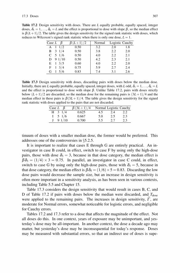
17.3 Doses 307
Table 17.2 Design sensitivity with doses. There are L equally probable, equally spaced, integerdoses, δ1 = 1, . . ., δL = L and the effect is proportional to dose with slope β , so the median effectis β (L+1)/2. The table gives the design sensitivity for the signed rank statistic with doses, whichreduces to Wilcoxon’s signed rank statistic when there is only one dose, L = 1.
Case L β β (L+1)/2 Normal Logistic Cauchy
A 1 1/2 0.50 3.2 2.0 1.8B 3 1/4 0.50 3.8 2.2 2.0C 5 1/6 0.50 4.0 2.2 2.1D 9 1/10 0.50 4.2 2.3 2.1E 1 3/5 0.60 4.0 2.2 2.0F 1 3/4 0.75 5.9 2.7 2.4G 1 5/6 0.83 7.4 3.1 2.6
Table 17.3 Design sensitivity with doses, discarding pairs with doses below the median dose.Initially, there are L equally probable, equally spaced, integer doses, with L odd, δ1 = 1, . . ., δL = Land the effect is proportional to dose with slope β . Unlike Table 17.2, pairs with doses strictlybelow (L + 1)/2 are discarded, so the median dose for the remaining pairs is (3L + 1)/4 and themedian effect in these pairs is β (3L + 1)/4. The table gives the design sensitivity for the signedrank statistic with doses applied to the pairs that are not discarded.
Case L β β (3L+1)/4 Normal Logistic Cauchy
H 3 1/4 0.625 4.5 2.4 2.2I 5 1/6 0.667 5.0 2.5 2.3J 9 1/10 0.700 5.5 2.7 2.3
tinuum of doses with a smaller median dose, the former would be preferred. This
addresses one of the controversies in §5.2.5.
It is important to realize that cases E through G are entirely practical. An in-
vestigator in case B could, in effect, switch to case F by using only the high-dose
pairs, those with dose δ3 = 3, because in that dose category, the median effect is
βδ3 = (1/4)× 3 = 0.75. In parallel, an investigator in case C could, in effect,
switch to case G by using only the high-dose pairs, those with δ3 = 5, because in
that dose category, the median effect is βδ5 = (1/6)×5 = 0.83. Discarding the low
dose pairs would decrease the sample size, but an increase in design sensitivity is
often more important in a sensitivity analysis, as has been seen in various contexts,
including Table 5.5 and Chapter 15.
Table 17.3 considers the design sensitivity that would result in cases B, C, and
D of Table 17.2 if pairs with doses below the median were discarded, and Tdose
were applied to the remaining pairs. The increases in design sensitivity, Γ , are
moderate for Normal errors, somewhat noticeable for logistic errors, and negligible
for Cauchy errors.
Tables 17.2 and 17.3 refer to a dose that affects the magnitude of the effect. Not
all doses do this. In one context, years of exposure may be unimportant, and yes-
terday’s dose may be all-important. In another context, the dose a decade ago may
matter, but yesterday’s dose may be inconsequential for today’s response. Doses
may be measured with substantial errors, so that an indirect use of doses is supe-

308 17 Anticipated Patterns of Response
Table 17.4 High, lower and mixed dose pairs in Angrist and Lavy’s study of class size manipulatedby Maimonides’ rule. The table describes matched pair differences, larger-cohort-minus-smaller-cohort. The tabled values are trimeans, a robust location estimate that is twice the median plus thequartiles divided by four.
86 High-Dose Pairs 49 Lower-Dose Pairs 135 Mixed-Dose Pairs
Class Size −10.88 −5.33 −7.38Math Test 3.97 3.47 3.66Verbal Test 2.98 1.45 2.55
rior to their direct incorporation in a test statistic [9, 12]. The wrong dose may be
measured or the right one may be measured poorly.
Arguably, Tables 17.2 and 17.3 speak not to the value of doses taken in isolation,
but rather to the value of treated subjects who experienced only small effects when
treatment effects are heterogeneous. When doses are actually indicative of the mag-
nitude of the effect, they serve to identify treated subjects who will experience small
effects. Here and in Chapter 16, design sensitivity is greater if little weight is given
to subjects experiencing negligible effects.
17.4 Example: Maimonides’ Rule
Recall from §1.3 and §5.2.3 the study by Angrist and Lavy [1] of class size manip-
ulated by Maimonides’ rule. So far, the discussion has considered only the 86 pairs
in Figure 1.1 in which a school with between 41 and 50 students in the fifth grade
was paired with a school with between 31 and 40 students in fifth grade. These are
the ‘high-dose’ pairs, in that adherence to Maimonides’ rule would cut a class of
40 students into two classes of average size 20.5 if one additional student enrolled.
In Figure 1.1, adherence to Maimonides’ rule is imperfect, so the typical reduction
in class size is smaller than 20 students. Table 17.4 considers the addition of 49
more pairs, for schools with between 70 and 90 students in the fifth grade. These
are the ‘lower-dose’ pairs, in that adherence to Maimonides’ rule would cut two
classes of 40 students into three classes of average size 27 if one additional stu-
dent enrolled. Table 17.4 gives the typical difference in class size and test scores in
matched pairs, larger-cohort-minus-smaller-cohort, for the 86 ‘high-dose’ pairs, the
49 ‘lower-dose’ pairs, and the 135 ‘mixed-dose’ pairs formed by pooling the pairs,
135 = 86 + 49. In Table 17.4, the typical difference in class size is larger for the
‘high-dose’ pairs, −10.9 students, than for the ‘lower-dose’ pairs, −5.3 students,
and the difference in verbal test scores is also larger.
Table 17.5 compares the sensitivity analysis in Table 5.3 with two additional sen-
sitivity analyses. One analysis uses Wilcoxon’s signed rank statistic and the coher-
ent signed rank statistic applied to the 135 ‘mixed-dose’ pairs. The other analysis
uses the dose-weighted signed rank statistic and the coherent version of that statistic
[5] applied to the 135 ‘mixed-dose’ pairs with doses of 2 and 1 for ‘high-dose’ and
‘lower-dose’ pairs, respectively. In this one example, the coherent statistic using the

17.6 Appendix: Proof of Proposition 17.1 309
Table 17.5 Sensitivity analysis and coherence in Angrist and Lavy’s study of academic test per-formance and class size manipulated by Maimonides’ rule. The table gives upper bounds on theone-sided P-values. The sensitivity analysis from Table 5.3 in §5.2.3 is the analysis for the 86‘high-dose’ pairs. The remaining analyses add 49 ‘lower-dose’ pairs to make 135 ‘mixed-dose’pairs. One analysis uses the signed rank statistic giving all pairs equal weights. The other analysisgives the ‘high-dose’ pairs twice the weight of the ‘lower-dose’ pairs. At Γ = 1.65, the only upperbound that is < 0.05 is for coherence with the 86 ‘high-dose’ pairs.
86 High-Dose Pairs 135 Mixed Dose Pairs 135 Dose-Weighted PairsΓ Math Verbal Coherent Math Verbal Coherent Math Verbal Coherent
1.00 0.0012 0.00037 0.00018 0.00034 0.00023 0.000081 0.00034 0.00014 0.0000501.45 0.057 0.027 0.015 0.058 0.046 0.015 0.049 0.029 0.0131.65 0.138 0.075 0.043 0.170 0.142 0.078 0.145 0.096 0.051
86 ‘high-dose’ pairs is marginally less sensitive than the other analyses to departures
from random treatment assignment. One should not make too much of individual
examples, such as Tables 5.5 and 17.5; however, the results in those tables are not
incompatible with the theoretical results about design sensitivity in this chapter.
17.5 Further Reading
Coherence and doses were discussed in Chapter 5, where general references may
be found. The relationship between design sensitivity and coherence is discussed
in [2, 8, 10]. The relationship between design sensitivity and doses is discussed in
[8, 10]. Closely related issues are discussed in [5, 7] and [6, §9]. An alternative
formulation of coherence is given by K. Joreskog and Arthur Goldberger [3]. Dose
errors are discussed in [9, 12]. Christopher Wild [14] surveys the many types of
doses that arise in modern cancer epidemiology. The proof in the appendix is from
[10].
17.6 Appendix: Proof of Proposition 17.1
Proof. Define Ψ1 = E (diWii) and Λ1 = E (diVii) = E (di). In the favorable situation
in the statement of Proposition 17.1, the expectation of Tdose is
E (Tdose) = E
(I
∑i=1
I
∑k=1
diWik
)=
I
∑i=1
E (diWii)+I
∑i=1
∑k �=i
E (diWik)
= IΨ1 + I (I −1)Ψ .
In the sensitivity analysis for Tdose, the upper bound on the one-sided P-value is
obtained by comparing Tdose to the distribution of the sum, TΓ ,dose, of I independent
random variables, i = 1, . . . , I, taking the value di qi with probability θ = Γ /(1+Γ )
310 17 Anticipated Patterns of Response
and the value 0 with probability 1−θ , so E(
TΓ ,dose
∣∣∣F)= θ ∑I
i=1 di qi; see [5, 7].
Because di qi = ∑Ik=1 diVik,
E(
TΓ ,dose
∣∣∣F ,Z)
= θI
∑i=1
di qi = θI
∑i=1
I
∑k=1
diVik,
so that
E(
TΓ ,dose
)= E
{E(
TΓ
∣∣∣F ,Z)}
= θI
∑i=1
I
∑k=1
E (diVik)
= θ {IΛ1 + I (I −1)Λ} .
Using the result in [8, §3], the design sensitivity, Γ , is the limit, as I → ∞, of the
solutions to E (Tdose) = E(
TΓ ,dose
), or equivalently to
Γ1+Γ
=IΨ1 + I (I −1)ΨIΛ1 + I (I −1)Λ
, (17.9)
where the right side of (17.9) tends to Ψ/Λ as I → ∞, yielding (17.8).
References
1. Angrist, J.D., Lavy, V.: Using Maimonides’ rule to estimate the effect of class size on scholas-tic achievement. Q J Econ 114, 533–575 (1999)
2. Heller, R., Rosenbaum, P.R., Small, D.: Split samples and design sensitivity in observationalstudies. J Am Statist Assoc 104, to appear (2009)
3. Joreskog, K.G., Goldberger, A.S.: Estimation of a model with multiple indicators and multiplecauses of a single latent variable. J Am Statist Assoc 70, 631–639 (1975)
4. Rao, C.R.: Linear Statistical Inference and Applications. New York: Wiley (1973)5. Rosenbaum, P.R.: Signed rank statistics for coherent predictions. Biometrics 53, 556–566
(1997)6. Rosenbaum, P.R.: Observational Studies (2nd edition). NY: Springer (2002)7. Rosenbaum, P.R.: Does a dose-response relationship reduce sensitivity to hidden bias? Bio-
statistics 4, 1–10 (2003)8. Rosenbaum, P.R.: Design sensitivity in observational studies. Biometrika 91, 153–164 (2004)9. Rosenbaum, P.R.: Exact, nonparametric inference when doses are measured with random er-
rors. J Am Statist Assoc 100, 511–518 (2005)10. Rosenbaum, P.R.: What aspects of the design of an observational study affect its sensitivity
to bias from covariates that were not observed? In: Festshrift for Paul W. Holland. Princeton,NJ: ETS (2009)
11. Small, D., Rosenbaum, P.R.: War and wages: The strength of instrumental variables and theirsensitivity to unobserved biases. J Am Statist Assoc 103, 924–933 (2008)
12. Small, D.S., Rosenbaum, P.R.: Error-free milestones in error-prone measurements. Ann AppStatist, to appear (2009)
13. van Eeden, C.: An analogue, for signed rank statistics, of Jureckova’s asymptotic linearitytheorem for rank statistics. Ann Math Statist 43, 791–802 (1972)

References 311
14. Wild, C.P.: Environmental exposure measurement in cancer epidemiology. Mutagenesis 24,117–125 (2009)

Part IVPlanning Analysis

Chapter 18After Matching, Before Analysis
Abstract Three design tasks may usefully follow matching and precede planning of
the analysis. Splitting the sample of I pairs into a small planning sample and a large
analysis sample may aid in planning the analysis in a manner that increases the de-
sign sensitivity. If there will be analytic adjustments for some unmatched variables,
it is prudent to check that the matched samples exhibit sufficient overlap on un-
matched variables to permit analytic adjustments. Quantitative analysis of matched
samples may usefully be combined with qualitative examination and narrative de-
scription of a few closely matched pairs.
18.1 Split Samples and Design Sensitivity
In Chapters 14–17, the sensitivity of the design of an observational study to un-
measured biases, Γ , was found to depend upon many things: unit heterogeneity,
coherence among outcomes, doses, uncommon but dramatic responses to treatment,
the strength of instrumental variables, among others. In some contexts, these con-
siderations may be difficult to evaluate during design, prior to the examination of
outcomes. An interesting option with good properties entails splitting the sample
at random into a small planning sample and a large analysis sample, making some
design decisions based on the planning sample, applying those decisions in the anal-
ysis sample. This section discusses the matter in brief outline based upon a paper
by Ruth Heller, Dylan Small, and me [14].
Sample splitting is most familiar from cross-validation [31]. In cross-validation,
a sample is split, usually at random, and a prediction is developed in one portion and
tested in the other. Often the process is repeated with many random splits in an effort
to develop an honest appraisal of the performance of some method of prediction.
Less familiar is the use of sample splitting to decide what question to ask, which
hypothesis to test. David Cox [6] examined the use of split samples as an alternative
to corrections for multiple testing in randomized experiments, such as corrections
based on the Bonferroni inequality. Instead of testing many hypotheses, the sample
315P.R. Rosenbaum, Design of Observational Studies, Springer Series in Statistics, DOI 10.1007/978-1-4419-1213-8_18, © Springer Science+Business Media, LLC 2010
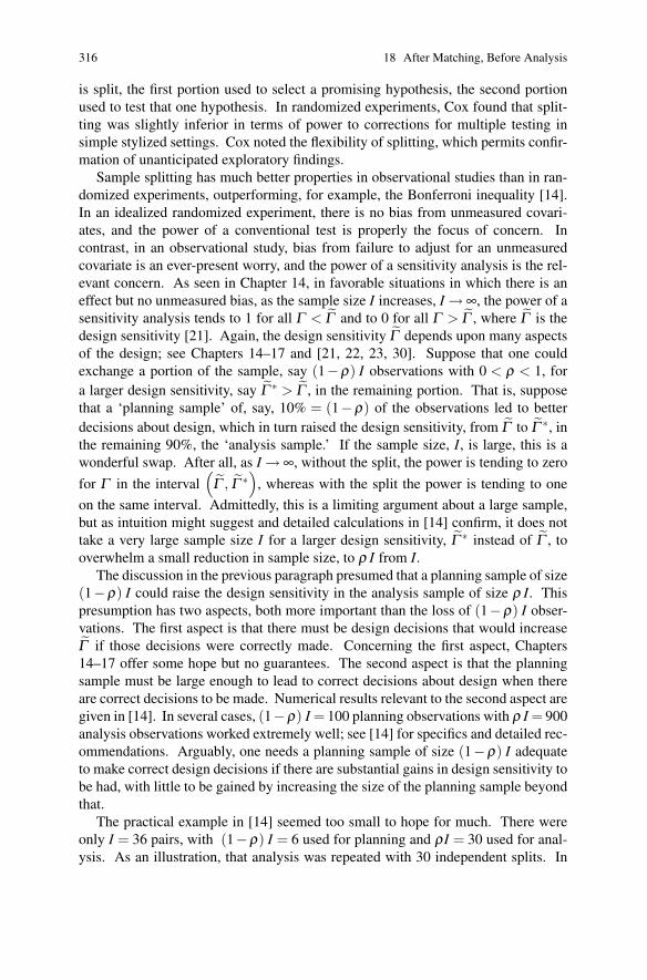
316 18 After Matching, Before Analysis
is split, the first portion used to select a promising hypothesis, the second portion
used to test that one hypothesis. In randomized experiments, Cox found that split-
ting was slightly inferior in terms of power to corrections for multiple testing in
simple stylized settings. Cox noted the flexibility of splitting, which permits confir-
mation of unanticipated exploratory findings.
Sample splitting has much better properties in observational studies than in ran-
domized experiments, outperforming, for example, the Bonferroni inequality [14].
In an idealized randomized experiment, there is no bias from unmeasured covari-
ates, and the power of a conventional test is properly the focus of concern. In
contrast, in an observational study, bias from failure to adjust for an unmeasured
covariate is an ever-present worry, and the power of a sensitivity analysis is the rel-
evant concern. As seen in Chapter 14, in favorable situations in which there is an
effect but no unmeasured bias, as the sample size I increases, I → ∞, the power of a
sensitivity analysis tends to 1 for all Γ < Γ and to 0 for all Γ > Γ , where Γ is the
design sensitivity [21]. Again, the design sensitivity Γ depends upon many aspects
of the design; see Chapters 14–17 and [21, 22, 23, 30]. Suppose that one could
exchange a portion of the sample, say (1−ρ) I observations with 0 < ρ < 1, for
a larger design sensitivity, say Γ ∗ > Γ , in the remaining portion. That is, suppose
that a ‘planning sample’ of, say, 10% = (1−ρ) of the observations led to better
decisions about design, which in turn raised the design sensitivity, from Γ to Γ ∗, in
the remaining 90%, the ‘analysis sample.’ If the sample size, I, is large, this is a
wonderful swap. After all, as I → ∞, without the split, the power is tending to zero
for Γ in the interval(
Γ , Γ ∗)
, whereas with the split the power is tending to one
on the same interval. Admittedly, this is a limiting argument about a large sample,
but as intuition might suggest and detailed calculations in [14] confirm, it does not
take a very large sample size I for a larger design sensitivity, Γ ∗ instead of Γ , to
overwhelm a small reduction in sample size, to ρ I from I.
The discussion in the previous paragraph presumed that a planning sample of size
(1−ρ) I could raise the design sensitivity in the analysis sample of size ρ I. This
presumption has two aspects, both more important than the loss of (1−ρ) I obser-
vations. The first aspect is that there must be design decisions that would increase
Γ if those decisions were correctly made. Concerning the first aspect, Chapters
14–17 offer some hope but no guarantees. The second aspect is that the planning
sample must be large enough to lead to correct decisions about design when there
are correct decisions to be made. Numerical results relevant to the second aspect are
given in [14]. In several cases, (1−ρ) I = 100 planning observations with ρ I = 900
analysis observations worked extremely well; see [14] for specifics and detailed rec-
ommendations. Arguably, one needs a planning sample of size (1−ρ) I adequate
to make correct design decisions if there are substantial gains in design sensitivity to
be had, with little to be gained by increasing the size of the planning sample beyond
that.
The practical example in [14] seemed too small to hope for much. There were
only I = 36 pairs, with (1−ρ) I = 6 used for planning and ρI = 30 used for anal-
ysis. As an illustration, that analysis was repeated with 30 independent splits. In
18.2 Are Analytic Adjustments Feasible? 317
every one of the 30 splits, the six planning observations correctly guided the one im-
portant design decision that materially affected the sensitivity to unmeasured biases.
That is too much to expect in general from six observations, but in larger studies,
sample splitting has much to offer.
18.2 Are Analytic Adjustments Feasible?
In an observational study, matching sets up certain comparisons, sets up a certain
analogous experiment: it builds adjustments for observed covariates into the design
of an observational study. In Mervyn Susser’s phrase, matching “simplifies the
conditions of observation,” aiding transparency (see Chapter 6).
Adjustments built into the design cannot be easily removed later. Under certain
circumstances, one may plan two analyses, one with an adjustment for a certain
variable, the other without that adjustment. In this case, the variable is not controlled
by matching but is controlled in the statistical analysis. An aspect of the design
of an observational study entails verifying that both analyses are feasible. This
means checking that an unmatched variable exhibits sufficient overlap in treated and
control groups that analytical adjustments are an interpolation, not an extrapolation
or a fabrication.
Typically, one leaves unmatched a variable of ambiguous status. In that way, dif-
ferent analyses may assign the variable different roles [4]. If a concomitant variable
is not truly a covariate, if it may have been affected by the treatment, then an adjust-
ment for it may introduce a bias that would not otherwise have been present [15].
That said, a variable may have an ambiguous status, perhaps slightly affected by the
treatment, but plausibly standing in as a surrogate for an important covariate that
was not measured. For instance, two studies in 1982, by James Coleman, Thomas
Hoffer, and Sally Kilgore [5] and Arthur Goldberger and Glen Cain [13], asked
whether Catholic and other private high schools did more than public schools to in-
crease the cognitive test performance of their students. Important covariates in this
context are cognitive test scores before high school, but these were not available.
Both studies make various comparisons of sophomore and senior test scores, with
the view that sophomore test scores, though possibly affected by public-vs.-private
schooling, might serve in one way or another as a proxy for the unmeasured covari-
ates of test scores prior to high school. An important variable with an ambiguous
status does not necessarily imply an ambiguous conclusion: perhaps the conclusion
is unchanged by changing the status of the variable. If a variable of ambiguous
status is left unmatched, analyses may examine issues of this sort.
Another type of variable of ambiguous status exhibits ‘seemingly innocuous con-
founding.’ That is, the covariate predicts a substantial fraction of the variation in
treatment assignment, but seems fairly innocuous, without obvious importance to
the outcomes under study. At the same time that the treatment is observed to be
confounded with something innocuous, it may also be confounded with unmea-
sured covariates that are not innocuous. In certain circumstances, the innocuous

318 18 After Matching, Before Analysis
confounding — the devil you know, in the words of the proverb — may seem less
worrisome than confounding with unmeasured covariates — the devil you don’t.1
Should ‘seemingly innocuous confounding’ be removed? Perhaps. Perhaps it is
not innocuous, and only seems so. And yet, if all the innocuous confounding is
removed, then perhaps the haphazard aspect of treatment assignment is removed as
well, and the remaining aspects of treatment assignment are governed by biases from
relevant unmeasured covariates. Again, when a variable has an ambiguous status,
conclusions may be firmer if shown to be untouched by this ambiguity. Consider
an example.
Recall from §12.3 the study by Jeffrey Silber and colleagues [24, 29] of slightly
earlier or slightly later discharges of 1402 premature infants from five neonatal in-
tensive care units (NICUs) in the Northern California Kaiser-Permanente Medical
Care Program between 1998 and 2002. The babies were paired into 701 pairs so
that the two babies looked similar in terms of measured (time-dependent) covariates
on the day the first baby, the early baby, was discharged, while the other baby, the
late baby, stayed in the NICU for a few more days, growing older and more mature.
Some of the variation in discharge day seems to have been governed by the day of
the week: reach maturity on Thursday and you go home on Friday; reach maturity on
Saturday and you go home on Tuesday, or so it appeared. There were five hospitals
in the Northern California Kaiser-Permanente Medical Care Program that provided
data for this study, and hence five NICUs, one at each hospital. Some of the variation
in discharge day seems to reflect styles of practice at the different NICUs: some are
faster than others. You could make a case, of course, that these sources of variation
are not innocuous. You could make a case that the baby discharged Friday morning
was judged healthier by the attending neonatologist than the baby held until Tues-
day, observed covariates to the contrary not withstanding. Although these were all
Kaiser-Permanente moms in hospitals run by Kaiser-Permanente, you could make
a case that the moms at certain hospitals or the hospitals themselves were not really
the same. Counter to this, you could make a case that the variation in discharge day
predicted by the identity of the NICU or the day of the week is less worrisome than
unexplained variation. Should we speculate and argue, or should we look and see?
Let’s look and see.
Table 18.1 shows the distribution of the 701 pairs of two babies at the five NICUs.
The table counts pairs, not babies, so the total count is 701 pairs, not 1402 babies.
Of the 701 pairs, 233 fall on the diagonal: the early and late baby are in the same
NICU. Some NICUs discharge earlier than others: NICU C contributed more late
babies than early babies, while NICU D did the opposite. On the other hand, despite
the trend, there are many early babies from NICU C, specifically 95, and many late
babies from NICU D, specifically 89. The variation between NICUs in discharge
rate accounts for part but not all of the variation in discharge day; therefore, the
variation due to the NICU can be removed analytically. In this way, we will see the
situation both with innocuous confounding and without.
1 Erasmus: “Nota res mala optima (an evil thing known is best)” [8, #85, page 123].

18.2 Are Analytic Adjustments Feasible? 319
Table 18.1 Pairs classified by the neonatal intensive care unit (NICU, A–E) of the early baby andthe late baby for 701 matched pairs. The table counts pairs, so the total count is 701. NICU C had161 late babies and 95 early babies, for a Late/Early ratio of 161/95 = 1.69, while NICU D had 89late babies and 165 early babies, for a Late/Early ratio of 89/165 = 0.54. Percentages are rounded.
Late Baby Late/EarlyEarly Baby A B C D E Total Percent Ratio
A 18 23 31 13 29 114 16 0.79B 20 65 24 17 36 162 23 0.93C 10 19 30 12 24 95 14 1.69D 26 24 41 36 38 165 24 0.54E 16 19 35 11 84 165 24 1.28
Total 90 150 161 89 211 701Percent % 13 21 23 13 30 100
Table 18.1 is part of the design. There is no information about outcomes in Table
18.1. The pattern in Table 18.1 reveals that it is safe to leave NICU unmatched;
within these 701 pairs matched for many characteristics of baby and mom, there is
enough overlap in the NICUs to permit adjustments. We may perform two analyses,
one that ignores the NICU, viewing the NICU as an innocent source of variation in
the day of discharge, the other analysis removing entirely the variation in discharge
day that can be predicted from the NICU. Deciding whether to match for the NICU
is part of the design, and Table 18.1 is part of that decision.
As will be discussed in detail in §19.6, one of the outcomes in Silber et al.’s
[24, 29] study concerned sick-baby services in an interval approximately six months
long following the discharge of the late baby, when both babies were home. Did
early discharge prompt a greater need for sick-baby services after discharge? Well-
baby services, such as checkups, were not included. Sick-baby costs include both
minor events with minor costs, and major events, such as readmission to the NICU,
with enormous costs. Services were converted to dollar amounts according to a
fixed schedule, so that babies who received the same services had the same dollar
score for those services. Here, postdischarge sick-baby cost is serving as a measure
of the severity of the health problem, for which it is not a bad proxy. See §19.6 and
[24, 29] for specifics and additional outcomes.
Table 18.2 is a letter value display [32] of the 701 matched pair differences, late-
minus-early, in postdischarge sick baby costs. Five deaths are recorded as infinite
costs, three among the early babies, two among the late babies; see §19.6 and [29]
for more about the deaths. The median difference in cost is $5 and the average of
the quartiles is $32. The distribution is extremely long-tailed relative to the Normal
distribution, as is seen from the pseudo-spreads in Table 18.2, which would be ap-
proximately constant for a very large sample from a Normal distribution. There is
no sign of increased postdischarge costs for early babies.
One analysis ignores the NICU. It allows the variation in practice style at differ-
ent NICUs to influence the day of discharge. A baby who happened to be born in
NICU C might stay a few extra days, and one born in NICU D may be discharged a
few days early. For two babies with the same matched covariates in §12.3, this anal-

320 18 After Matching, Before Analysis
Table 18.2 Letter value display of difference in postdischarge sick-baby costs in dollars in 701pairs of a late and an early baby. The difference is late-minus-early. Various quantiles are displayed,together with their averages (the mids), differences (the spreads), and the ratio of the spreads tothe corresponding spreads of the standard Normal distribution. Five deaths are recorded as infinitecosts, three among the early babies, two among the late babies; see §19.6 for detailed discussionof the deaths.
Quantile % ‘Letter’ Lower Upper Mid Spread Pseudo-spread
50 1/2 5 5 5 025 1/4 −223 287 32 510 378
12.5 1/8 −1063 2313 625 3376 14676.25 1/16 −4089 4956 433 9045 29483.125 1/32 −9893 12944 1526 22836 6130
ysis views the NICU as irrelevant to outcomes except to the extent that it accelerates
or retards discharge. Ignoring the NICU, procedures associated with Wilcoxon’s
signed rank statistic (§2.4) give a point estimate of an additive effect τ of $17 and a
95% confidence interval of [−$20, $56]; see §19.6 for additional analyses ignoring
the NICU, including a sensitivity analysis.
The analysis using Wilcoxon’s statistic viewed all 2701 possible treatment as-
signments in the 701 pairs as equally probable. Table 18.1 suggests they are not
equally probable; rather, they are predictable using the NICU. For instance, look
at row D and column C of Table 18.1 in comparison with row C and column D.
In those two cells of Table 18.1 are 41 + 12 = 53 pairs of two babies, one born at
NICU ‘C,’ the other at NICU ‘D.’ In those 53 pairs, the odds that the early baby
is at NICU D are estimated at 41/12 = 3.4 to 1. The alternative analysis ([17] and
[20, §3]) does not consider all 2701 possible treatment assignments, but rather a sub-
set of treatment assignments that exhibits the same imbalance as observed in Table
18.1. For instance, in the 53 pairs with one baby at NICU C and another at NICU
D, Wilcoxon’s statistic considers all 253 = 9×10¹⁵ possible treatment assignments
as equally probable and uses them all, but the alternative procedure considers only
the 53!/(41!12!) = 2.7× 10¹¹ treatment assignments that keep 12 early babies in
NICU C and 41 late babies in NICU ‘C.’ For the 233 pairs on the diagonal in Ta-
ble 18.1, all possible treatment assignments are considered, but for the off-diagonal
pairs, the observed imbalance is preserved. The distribution of Wilcoxon’s statis-
tic, or any other statistic, is compared to this restricted or conditional permutation
distribution.2
The alternative analysis that adjusts for the NICU yields a point estimate of an
additive effect τ of −$6 and a 95% confidence interval of [−$36, $53]. Some of
the variation in day of discharge can be predicted from the NICU, a seemingly
2 When is this analysis appropriate? Suppose the NICUs are included among the observed covari-ates and after including the NICUs, (3.5)–(3.8) is then true. Suppose further that the NICUs enterthe propensity score as additive constants on the logit scale. Then the conditioning just describedeliminates the additive NICU parameters, leaving behind a known distribution of treatment assign-ments that gives the remaining assigments equal probabilities. The distribution of the Wilcoxonstatistic is then approximated using its easily computed moments. See [17] and [20, §3] for thepaired case, as here, and see [16, 19] and [20, §3] for the general case.

18.2 Are Analytic Adjustments Feasible? 321
innocuous form of confounding. Two analyses were performed, one that ignored
the predictable variation, the other that removed the predictable variation. The two
analyses produce similar inferences about τ . Although the status of the NICU is
ambiguous, the conclusion is less so. Indeed the pair of analyses provides some
reassurance: different sources of variation in the day of discharge produce similar
estimates of the effect of slightly delayed discharge.
Is it safe to leave a covariate unmatched? Will analytic adjustments be feasible
for that covariate? Is there sufficient overlap on an unmatched covariate? Will ana-
lytic adjustments require an interpolation, not an extrapolation or a fabrication? In
the design of an observational study, a table such as Table 18.1 recording treatment
assignment and unmatched covariates provides answers to these questions.
Tapered matching
An alternative to leaving an ambiguous covariate unmatched is to construct matched
triples, one treated subject and two controls, so that one control is matched for the
covariate and the other is not. This ensures that both analyses are feasible, and pro-
vides a formal test as to whether their answers differ, as well as a confidence state-
ment about the magnitude of the difference. The matching is implemented using
‘optimal tapered matching’, as discussed by Shoshana Daniel, Katrina Armstrong,
Jeffrey Silber, and me [7]. In optimal tapered matching, a single control group is
optimally partitioned into two types of controls and optimally matched to treated
subjects. The procedure is easy to implement. A distance matrix is computed be-
tween each treated subject and each control, ignoring the ambiguous covariate, with
one row for each treated subject and one column for each control, as in Chapter 8. A
second distance matrix is computed between each treated subject and each control
including the ambiguous covariate in the distances. These two distance matrices
are stacked, one on top of the other, so the number of rows is doubled but the num-
ber of columns is unchanged. An optimal pair match is determined for this stacked
distance matrix. Each control is then used at most once, but each treated subject is
used twice. In this way, each treated subject is paired with two controls, one close
in terms of the first distance, the other close in terms of the second distance, and
the two control groups do not overlap, so they may be compared using conventional
methods, such as Wilcoxon’s signed rank test. The procedure is not restricted to
matched triples, and may use more than one control from either group, or may have
more than two control groups. Tapered matching was originally developed in con-
nection with research on disparities, where the concept of a covariate is inherently
ambiguous. The paper [7] discusses an example in detail, demonstrates a certain
optimal property of the procedure, and discusses some of the subtleties involved in
the choice of distance.

322 18 After Matching, Before Analysis
18.3 Matching and Thick Description
Matching and thick description
Matching compares groups of treated and control subjects, often pairs of treated and
control subjects, who look comparable in terms measured covariates xi j. A constant
worry is that subjects who look comparable may not be comparable, that they look
comparable only because important distinctions are omitted in the observed covari-
ates xi j, distinctions that are to be found only in unobserved covariates ui j for which
subjects are not matched.
In matching, people remain intact as people. In contrast, in model-based adjust-
ments, the people themselves disappear or recede into the background to be replaced
by features of a model. Where there were once people, there are now parameters in
a model. A relatively neglected but potentially important aspect of matching is the
possibility of taking a close look at a few well-matched pairs of people, providing
a narrative account of these pairs.3 That is, one might provide a ‘thick description’
of a small subset of pairs. Jeffrey Silber and I tried this in a study of mortality af-
ter surgery in the Medicare population in Pennsylvania, and the current section is a
brief summary of the resulting paper [18].
It is a staple of professional education — in medicine, in business, in law — that
a narrative account of a few well-chosen cases is often enlightening and instructive.
For instance, in this spirit, the New England Journal of Medicine often publishes
its “Case Reports from the Massachusetts General Hospital”; see also the essay by
Jan Vandenbroucke [33]. The professions do not believe that broad generalizations
can be warranted by examination of a few cases; rather, they believe that to be-
come acquainted with generalizations without engaging particular cases to which
those generalizations are supposed to apply is to run the risk of developing a fairly
scholastic perspective.
In certain social sciences, there is a division of labor, with some investigators,
sometimes called ‘qualitative researchers,’ creating narrative accounts from a few
cases, and other investigators, sometimes called ‘quantitative researchers,’ creat-
ing analyses from data describing many people. Matching provides a framework
within which qualitative and quantitative research can usefully interact within a sin-
gle investigation. A narrative account of a few pairs could go hand in hand with a
statistical analysis of many pairs.
3 As has been discussed several times, modern matching methods try to balance high-dimensionalobserved covariates in treated and control groups, viewing close individual matched pairs as asecondary concern. In light of this, treated and control groups may be balanced with respect toobserved covariates using many pairs that are not individually close on observed covariates. Themethodology discussed in the current section is most appropriate for the subset of matched pairsin which the individual pairs are closely matched. Typically, there will be many such pairs, evenif many other pairs contribute to covariate balance without being closely matched as pairs withrespect to covariates. If a distance, such as the Mahalanobis distance, is used in matching (seeChapter 8), then a closely matched pair will be recognizable by a small distance within the pair.

18.3 Matching and Thick Description 323
What is thick description?
The term ‘thick description’ was introduced by a philosopher, Gilbert Ryle [25,
page 479], and was made popular by an anthropologist, Clifford Geertz [11]; see [18,
pages 221-222] for quotes from Ryle and Geertz that give a brief sense of the nature
of their concerns. The aim of thick description according to Geertz [12, page 152] is
“to render obscure matters intelligibly by providing them with an informing context”
[12, p. 152]. The importance of an informing context is conveyed by the following
passage by Howard Becker [2, page 58]:
[I]f we don’t find out from people what meanings they are actually giving to things, we willstill talk about those meanings. In that case, we will, of necessity, invent them, reasoningthat the people we are writing about must have meant this or that, or they would not havedone the things they did. But it is inevitably epistemologically dangerous to guess at whatcould be observed directly. The danger is that we will guess wrong, that what looks reason-able to us will not be what looked reasonable to them. This happens all the time, largelybecause we are not those people and do not live in their circumstances.
It is quite easy to misinterpret data from a large electronic data set [10]. The
attempt to create a narrative account of a few cases may serve to test interpretations
of data and the concepts in which those interpretations are cast. An example follows.
Example: Mortality after surgery
Silber and colleagues’ [26, 27, 28] study of mortality after surgery used (inexpen-
sive) administrative data to create a matched sample from the Medicare popula-
tion in Pennsylvania, which was followed by (expensive) chart abstraction for the
matched sample. In this study, deaths shortly following surgery were matched to
ostensibly similar survivors based on administrative data from Medicare. Although
the best data would come from chart abstraction for the matched sample, it was im-
portant to have a reasonable match based on administrative data, so that charts for
suitable patients would be abstracted.
In [18], a preliminary matched sample was constructed, and Medicare records
for a handful of well-matched pairs were contrasted with far more detailed informa-
tion in the hospital chart. The preliminary match looked reasonable in terms of the
measured variables from Medicare’s administrative records. However, even though
only a few cases were examined, it was immediately clear from chart data that the
initial match was not adequate and that many definitions that we created to interpret
the administrative records required revision. Many of the mistakes we unearthed
were obvious mistakes when viewed from the step-by-step narrative perspective of
a hospital chart, but were not obvious from the perspective of computerized admin-
istrative records, or at least not obvious to us.
For instance, we generally wanted to avoid matching on events that were subse-
quent to surgery, because these might be outcomes of surgery or of subsequent care.
Although that principle is sound, our initial use of it was mechanical and thought-
less. For instance, if surgery reveals that a patient has metastatic cancer, that cancer

324 18 After Matching, Before Analysis
existed prior to the surgery that discovered it. Metastatic cancer is, of course, im-
portant to the patient’s prognosis and to proper interpretation of the care the patient
subsequently received. In light of this, we changed our definitions related to cancer
and several other medical conditions that could not have begun during a hospital
stay. No one would make this mistake faced with a narrative account describing an
individual patient, but it is less obvious in computerized administrative records, and
it might not be easily discerned from the coefficients of a model. If some mistakes
are difficult to make when a situation is viewed from a narrative perspective, then
that constitutes a good reason for expending the time and effort required to view the
situation from a narrative perspective.
We also redefined “died shortly after surgery.” One of the examined charts de-
scribed a patient who had ‘survived after surgery’ by our original definition, but
after a long stay had died without leaving the hospital. This case prompted us to re-
examine the administrative data, only to discover that the fate of this one patient was
sufficiently common to merit a different definition of “died shortly after surgery.”
For additional examples and further discussion, see [18]. The example in [18] is
a fairly limited use of matching in conjunction with narrative description, but exten-
sive use is possible. For three compelling examples of extended narrative accounts
(without matching), see [1, 3, 9].
18.4 Further Reading
Section 18.1 is a brief outline of a paper by Ruth Heller, Dylan Small and me [14].
The method of adjustment in §18.2 is from [17]. Although the method is described
correctly and in detail in [17], there is a misstatement of one of the assumptions,
which is corrected in [20, §3] and in Note 2 of the current chapter. The method of
§18.2 is the simplest case of a general method discussed in [16, 19]. Section 18.3
is derived from a paper with Jeffrey Silber [18] that contains further discussion and
additional references. The literature on thick description, ethnography, and quali-
tative research is vast. The books by Lonnie Athens [1], Charles Bosk [3] and Sue
Estroff [9] are fine examples of ethnography touching upon criminology, surgery,
and psychiatry, and the volume containing Becker’s essay [2] contains many other
interesting essays as well.
References
1. Athens, L.: Violent Criminal Acts and Actors Revisited. Urbana, Illinois: University of IllinoisPress (1997)
2. Becker, H.S.: The epistemology of qualitative research. In: R. Jessor, A. Colby, R. Shweder(eds.), Ethnography and Human Development, pp. 53–72. Chicago: University of ChicagoPress (1996)

References 325
3. Bosk, C.L.: Forgive and Remember: Managing Medical Failure. Chicago: University ofChicago Press (1981)
4. Cochran, W.G.: Analysis of covariance: Its nature and uses. Biometrics 13, 261–281 (1957)5. Coleman, J., Hoffer, T., Kilgore, S.: Cognitive outcomes in public and private schools. Soc
Educ 55, 65–76 (1982)6. Cox, D.R.: A note on data-splitting for the evaluation of significance levels. Biometrika 62,
441–444 (1975)7. Daniel, S., Armstrong, K., Silber, J.H., Rosenbaum, P.R.: An algorithm for optimal tapered
matching, with application to disparities in survival. J Comput Graph Statist 17, 914–924(2008)
8. Erasmus: The Collected Works of Erasmus, Volume 34, Adages IIvii1 to IIIiii100. Toronto:University of Toronto Press (1992)
9. Estroff, S.E.: Making It Crazy: An Ethnography of Psychiatric Clients in an American Com-munity. Berkeley: University of California Press (1985)
10. Bittner, E., Garfinkel, H.: ‘Good’ organizational reasons for ‘bad’ organizational records. In:H. Garfinkel, Studies in Ethnomethodology, pp. 186–207. Englewood Cliffs, NJ: PrenticeHall (1967).
11. Geertz, C.: Thick description: toward an interpretative theory of culture. In: C. Geertz, TheInterpretation of Cultures, pp. 3–30. New York: Basic Books (1973)
12. Geertz, C.: Local Knowledge. New York: Basic Books (1983)13. Goldberger, A.S., Cain, G.S.: The causal analysis of cognitive outcomes in the Coleman, Hof-
fer and Kilgore report. Soc Educ 55, 103–122 (1982)14. Heller, R., Rosenbaum, P. R., Small, D.: Split samples and design sensitivity in observational
studies. J Am Statist Assoc 104, to appear (2009)15. Rosenbaum, P.R.: The consequences of adjustment for a concomitant variable that has been
affected by the treatment. J Roy Statist Soc A 147, 656–666 (1984)16. Rosenbaum, P.R.: Conditional permutation tests and the propensity score in observational
studies. J Am Statist Assoc 79, 565–574 (1984)17. Rosenbaum, P.R.: Permutation tests for matched pairs with adjustments for covariates. Appl
Statist 37, 401–411 (1988) (Correction: [20, §3])18. Rosenbaum, P.R., Silber, J.H.: Matching and thick description in an observational study of
mortality after surgery. Biostatistics 2, 217–232 (2001)19. Rosenbaum, P.R.: Covariance adjustment in randomized experiments and observational stud-
ies (with Discussion). Statist Sci 17, 286–327 (2002)20. Rosenbaum, P.R.: Observational Studies (2nd ed). New York: Springer (2002)21. Rosenbaum, P.R.: Design sensitivity in observational studies. Biometrika 91, 153–164 (2004)22. Rosenbaum, P.R.: Heterogeneity and causality: Unit heterogeneity and design sensitivity in
observational studies. Am Statistician 59, 147–152 (2005)23. Rosenbaum, P.R.: What aspects of the design of an observational study affect its sensitivity
to bias from covariates that were not observed? In: Festshrift for Paul W. Holland. Princeton,NJ: ETS (2009)
24. Rosenbaum, P.R., Silber, J.H.: Sensitivity analysis for equivalence and difference in an obser-vational study of neonatal intensive care units. J Am Statist Assoc 104, 501–511 (2009)
25. Ryle, G.: Collected Papers, Volume 2. London: Hutchinson (1971)26. Silber, J.H., Rosenbaum, P.R., Trudeau, M.E., Even-Shoshan, O., Chen, W., Zhang, X.,
Mosher, R.E.: Multivariate matching and bias reduction in the surgical outcomes study. MedCare 39, 1048–1064 (2001)
27. Silber, J.H., Rosenbaum, P. R., Trudeau, M.E., Chen, W., Zhang, X., Lorch, S.L., Rapaport-Kelz, R., Mosher, R.E, Even-Shoshan, O.: Preoperative antibiotics and mortality in the elderly.Ann Surg 242, 107–114 (2005)
28. Silber, J.H., Rosenbaum, P.R., Zhang, X., Even-Shoshan, O.: Estimating anesthesia and surgi-cal time from medicare anesthesia claims. Anesthesiology 106, 346–355 (2007)
29. Silber, J.H., Lorch, S.L., Rosenbaum, P.R., Medoff-Cooper, B., Bakewell-Sachs, S., Millman,A., Mi, L., Even-Shoshan, O., Escobar, G.E.: Additional maturity at discharge and subsequenthealth care costs. Health Serv Res 44, 444–463 (2009)

326 18 After Matching, Before Analysis
30. Small, D.S., Rosenbaum, P.R.: War and wages: The strength of instrumental variables andtheir sensitivity to unobserved biases. J Am Statist Assoc 103, 924–933 (2008)
31. Stone, M.: Cross-validatory choice and assessment of statistical predictions. J Roy Statist SocB 36, 111–147 (1974)
32. Tukey, J.W.: Exploratory Data Analysis. Reading, MA: Addison-Wesley (1977)33. Vandenbroucke, J.: In defence of case reports and case series. Ann Intern Med 134, 330–334
(2001)

Chapter 19Planning the Analysis
Abstract “Make your theories elaborate” in observational studies, argued R.A.
Fisher, so that the many predictions of such a theory may disambiguate the asso-
ciation between treatment and outcome. How should one plan the analysis of an
observational study to check the predictions of an elaborate theory?
19.1 Plans Enable
A randomized clinical trial follows a protocol that describes the design of the trial
and a plan for its analysis. The plan for analysis will identify a primary endpoint
or outcome, possibly secondary endpoints, describe the comparisons that will be
made, and so forth. The plan for a clinical trial is reviewed by a funding agency
and, for large important trials, the plan may be published before the trial begins. In
this sense, the plan is a public plan. There is no barrier to planning the analysis of
an observational study, and there is much to gain from planning.
Plans enable. In all aspects of life, much can be done with a plan that cannot be
done without one.
A study that follows a public plan is more convincing than a study that emerges
ambiguously from a fog of data. A public plan is subject to public scrutiny before
the study begins, so criticism that would otherwise surface after the fact arises before
the fact, perhaps leading to a better study more resistant to legitimate criticism. If
there is a public plan, and if the critic raises no objection to the plan, then criticism
that could have been raised to the plan rings hollow when raised for the first time
after a particular conclusion is announced.
A planned analysis is more transparent than an unplanned analysis. As discussed
in Chapter 6, transparency means making evidence evident. If there is a public plan
for analysis, then the investigators either followed their plan or they deviated from
it. If they deviated from the plan, they will be obligated to explain and justify the
deviation. Perhaps the deviation will be judged appropriate, perhaps more appro-
327P.R. Rosenbaum, Design of Observational Studies, Springer Series in Statistics, DOI 10.1007/978-1-4419-1213-8_19, © Springer Science+Business Media, LLC 2010

328 19 Planning the Analysis
priate in light of events than adherence to the plan. No matter. What was done and
why it was done are open to view.
Without a plan, an analysis will first use the methods that are most familiar, most
ready to hand, then suffer a disorganized retreat to appropriate methods when un-
foreseen but foreseeable dilemmas arise. Even if appropriate methods are ultimately
used, such an analysis looks like what it is: a dubious circular meander around data,
methods, and conclusions. Here is a common example. We are all more familiar
with tests and confidence intervals for differences than with tests and intervals for
near equivalence, although there is sound, straightforward, standard methodology
available for both tasks [6]. Meandering through a data set, we therefore apply tests
for difference indiscriminately, then remember that tests for difference make a mud-
dle of attempts to demonstrate near equivalence, then retreat to appropriate methods
in a manner that rarely convinces us, much less anyone else. And yet a moment’s
thought before the fact would have revealed that to provide evidence for a certain
conclusion means finding a difference here and near equivalence there. A moment’s
thought before the fact is readily available; it just takes a moment’s thought. This
dilemma is not in the data but in the absence of a plan.1
A plan does not preclude unplanned analyses. A plan distinguishes planned and
unplanned analyses.2
Admittedly, you cannot plan an ornate and delicate analysis. You can plan the
analysis of a randomized trial because randomization has done the heavy lifting
of ensuring that comparable people are compared; ornate analysis is not needed.
You can plan the analysis of an observational study if matching in the design has
done the heavy lifting of ensuring that ostensibly comparable people are compared;
ornate adjustments of outcomes for observed covariates are not essential.3 Properly
performed, matching is done without examining outcomes; it is, therefore, part of
design. To say that you cannot plan an ornate and delicate analysis is to offer a
telling argument against ornate and delicate analyses.
Novelty and originality may be acceptable in a plan, but soundness, not novelty
or originality, is the mark of excellence in a planned analysis. The analysis of a
standard design may follow a standard plan.
1 See, for instance, Note 2 in Chapter 5, where I deliberately did the meandering analysis I intendto correct in the current chapter.2 John Tukey: “We do not dare either give up exploratory data analysis or make it our sole interest”[36, page 72]. “We often forget how science and engineering function. Ideas come from previousexploration more often than from lightning strokes. Important questions can demand the mostcareful planning for confirmatory analysis” [35, page 23].3 By ‘ostensibly comparable,’ I mean comparable in terms of measured covariates, x, leaving openthe question of whether people who look comparable in terms of x are actually comparable in termsof unmeasured covariates u. ‘Ostensibly comparable’ is an abbreviation.

19.2 Elaborate Theories 329
19.2 Elaborate Theories
R.A. Fisher’s Advice
In his paper, “The planning of observational studies of human populations,” William
Cochran [9, §5] wrote:
About 20 years ago, when asked in a meeting what can be done in observational studies toclarify the step from association to causation, Sir Ronald Fisher replied: ‘Make your theorieselaborate.’ The reply puzzled me at first, since by Occam’s razor, the advice usually givenis to make theories as simple as is consistent with known data. What Sir Ronald meant, assubsequent discussion showed, was that when constructing a causal hypothesis one shouldenvisage as many different consequences of its truth as possible, and plan observationalstudies to discover whether each of these consequences is found to hold.. . . [T]his multi-phasic attack is one of the most potent weapons in observational studies.
Fisher’s advice fits closely with the devices in §5.2 that disambiguate causal asso-
ciations [26], and with the reduction in sensitivity to unmeasured biases that may
follow from an anticipated pattern of treatment effects in Chapter 17. In Fisher’s
advice, the temporal order is important: one envisions consequences of a causal hy-
pothesis and then plans the study to discover whether the consequences hold. There
is no value in an elaborate theory built after the fact to fit unanticipated patterns in
the data.
A simple example, discussed in §5.2.2 and §11.3, is the use of two control groups.
If the treatment is the cause of its ostensible effects, the anticipated pattern with two
control groups is clear: the treated group differs substantially from the two control
groups, which do not differ substantially from each other. The prediction here is for
two substantial differences and one near equivalence. What plan is appropriate for
the analysis?
A second simple example discussed in § 5.2.3 and §17.2 concerns coherence of
two outcomes, for instance an increase in both math and verbal test scores associated
with smaller class sizes prompted by Maimonides’ rule. There is the hypothesis of a
coherent association and hypotheses about two outcomes. What plan is appropriate
for the analysis?
What should a planned analysis accomplish?
An elaborate theory makes an elaborate prediction, and in Chapter 17 it was seen
that certain forms of compatibility with an elaborate theory may make the study
less sensitive to unmeasured biases. The investigator hopes that the use of two
control groups rather than one, or the search for coherence among two outcomes,
will enlarge what can legitimately be said, not diminish it, but there are pitfalls for
the unwary.
In the first instance, the data may confirm part of the elaborate theory, refute
another part, with a third part left in an ambiguous state. A binary ‘confirm’ or
‘otherwise’ is not appropriate. The evaluation of an elaborate theory will, therefore,
330 19 Planning the Analysis
involve more than one comparison. If several comparisons are made using statistical
procedures, then each comparison runs a risk of error, with the resulting possibility
that a series of small risks of error accumulate to a risk of error that is no longer
small. If a correction for multiple testing were made to control this accumulation
of error, say using the Bonferroni inequality, then the investigator might discover,
to her shock and dismay, that if she had used the first control group alone, it would
have had outcomes significantly different from the treated group, and if she had
used the second control group alone, it too would have had outcomes significantly
different from the treated group, but because she used both control groups and did
two tests, neither difference is significant after correcting for multiple testing. This,
too, is not appropriate.
Moreover, if the elaborate theory makes predictions of near equivalence, and if
tests for difference are performed where tests for near equivalence are needed, then
successes may be misclassified as failures and failures as successes. In a large study,
two control groups might have nearly equivalent outcomes, yet differ significantly;
this is a success that might be mistaken for a failure. Conversely, two control groups
may have outcomes that do not differ significantly, and yet because of low power
may provide no evidence that the outcomes are similar in the two groups; this is a
failure that might be mistaken for a success. A test for near equivalence is one that
can reject substantial inequivalence.
So a plan for analysis must do several things. To be a legitimate statistical analy-
sis at all, it must control, in some appropriate sense, the risk of incorrect inferences.
It must do this while making several comparisons, resulting in a graduated assess-
ment of compatibility with the elaborate theory, rather than a simple ‘yes’ or ‘no’.
If some comparisons have priority over others, then the analysis should respect that
priority: the most important comparisons should come first, in some sense, and not
be hindered by added interest in other comparisons, as seemed to be the case above
in connection with the Bonferroni inequality.
To be credible in their respective roles, an elaborate theory and priorities for
its assessment must appear in a plan that precedes examination of outcomes. The
elaborate theory is intended to make predictions, but it isn’t making predictions if it
is built to fit the data that will be used to assess those predictions. Priorities can aid
in controlling the risk of incorrect inferences only if they shape the analysis rather
than being shaped by it.
19.3 Three Simple Plans with Two Control Groups
The simplest plan for analysis with two control groups
To examine the logic of the simplest plan in a practical case, consider again Table
5.1 from the study by Bilban and Jakopin [7] of genetic damage among lead-zinc
miners compared with two control groups. This simplest plan is, in fact, too simple

19.3 Three Simple Plans with Two Control Groups 331
even for this most basic situation. Better plans will be considered soon. The focus,
for the moment, is on the logic of the plan, not yet on finding a good plan.
Let us imagine that Bilban and Jakopin originally planned to use one control
group, say the Slovene residents far from the mine. Let us imagine further that they
added the second control group of local residents near the mine who were not miners
in response to concerns that pollution in the area of the mine, not the mine itself,
might be responsible for greater genetic damage among miners. This second control
group is a reasonable response to that specific concern. Finally, let us suppose that
they wanted to give priority to the first of these two control groups.
Consider the following analytic plan. Test the hypothesis of equality of micronu-
clei frequencies among miners and the first control group, say at level 0.05. If that
hypothesis is not rejected, stop. If that hypothesis is rejected, declare it rejected
and test the second hypothesis of equality of micronuclei frequencies among min-
ers and the second control group, also at level 0.05, declaring it rejected or not as
appropriate.
Admittedly, as analytic plans go, this is not much of a plan. It does nothing to
investigate the magnitude of the effect, which is surely important, and it does noth-
ing to appraise the comparability of the two control groups, which is also important.
The issue of sensitivity to unmeasured biases is not mentioned. This plan, such as it
is, does not plan much. Perhaps what it plans is less important than what it ignores.
No matter. The plan exemplifies a certain principle in the simplest possible setting.
In Table 5.1 from [7], the first test yields a t-statistic of 16.13, the second a t-statistic of 13.87. If the distributions of micronuclei were independent and Normal
with expectations μt , μc1 and μc2 and standard deviations ωt , ωc1, and ωc2 in the
treated group and the two control groups, with c1 referring to Slovene residents and
c2 referring to local residents, then, at the 0.05 level, the plan would reject the first
hypothesis, then test and reject the second.4
Notice first that, under this plan, the addition of a second control group costs
the investigators nothing. If the hypothesis of no difference between miners and
the first control group would have been rejected without the second control group,
it would also be rejected by this plan in the presence of the second control group.
So the situation is different from correcting for multiple testing using the Bonferroni
inequality as described above. The second control group may allow more to be said,
but less will not be said.
The second thing to notice is that the plan controls the probability of at least one
false rejection in two tests provided the two separate tests do their separate jobs of
controlling the probability of a false rejection. It is important to understand what is
being claimed, then why the claim is true. The claim is that if each test has level
4 In Table 5.1, it appears that ωt , ωc1, and ωc2 are not equal, so a pooled standard deviation is notused, and the ‘t-statistics’ are not actually distributed with a t-distribution. Because the degrees offreedom are fairly large, the separate standard errors are used, and the ‘t-statistics’ are comparedwith the standard Normal distribution, both here and in all calculations from Table 5.1. Althoughthis is an imperfect approach, the largest imperfection in my analysis is in assuming the data areNormal merely because only means and standard deviations were reported. This example is beingused to illustrate certain concepts while minimizing incidentals unrelated to those concepts.

332 19 Planning the Analysis
0.05, falsely rejecting one time in 20, then the two-step plan tests two hypotheses but
makes at least one false rejection with probability at most 0.05. It is like buying two
lottery tickets rather than one without increasing your chance of winning, though not
quite like that. Something has prevented an accumulation of risk of false rejection.
What is that something? Consider the logic.
There are two null hypotheses, H0 and H0. To be specific, the one sided null
hypotheses are H0 : μt ≤ μc1 and H0 : μt ≤ μc2. Here, H0 refers to the first control
group and H0 refers to the second, but it doesn’t really matter what they refer to;
they could be any two hypotheses about anything. The plan is to test H0, and only
if H0 is rejected to test H0. Consider the cases, one at a time. If H0 and H0 are both
false, then you cannot falsely reject anything, so there is no risk of false rejection;
any rejection is a correct rejection. If H0 is false but H0 is true, then you cannot
falsely reject H0, so to falsely reject anything you have to, among other things,
falsely reject H0, but the chance of this is at most 0.05. If H0 and H0 are both true,
then you commit a false rejection if and only if you reject H0, and the chance of this
is at most 0.05. So no matter which case is true, the chance of falsely rejecting at
least one true hypothesis is at most 0.05.5
This first bit of logic ramifies in many useful directions [3, 15, 17, 29]. This logic
is discussed explicitly in the context of clinical trials by Gary Koch and S.A. Gansky
[17] and Peter Bauer [3], but appears to have been understood 20 years earlier by
Ruth Marcus, Eric Peritz, and K. R. Gabriel [22], who were doing something related
but subtler. The logic also has links to multiparameter tests [5, 18, 20] and has been
combined in an interesting way with the Bonferroni inequality [14, §3].
There is a second piece to the logic.
A symmetric plan for analysis with two control groups
An awkward feature of the first plan is that the investigators had to give priority to
one of the control groups. Can the two control groups be viewed symmetrically?
Consider a second plan. Test at level 0.05 the hypothesis that H0 : μt ≤(μc1 + μc2)/2, which says that the expected level of micronuclei in the treated group
is no higher than in the average of the two control groups. If H0 is not rejected, stop.
If H0 is rejected, declare it rejected and test at the 0.05 level both H0 : μt ≤ μc1 and
H0 : μt ≤ μc2, rejecting neither, either, or both as appropriate.
5 In his PhD thesis, Frank Yoon [38] improves upon this plan in a sensible way. Suppose thatwe can specify a ‘meaningful difference’ (sometimes called a ‘clinically significant difference’)of τmf ≥ 0. The notion is that a difference smaller than τmf may exist but be too small to merit
attention. Yoon suggests testing H(τ)0 : μt − τ ≤ μc1 in order [29] at level α for τ ∈ (−∞, τmf],
stopping with the smallest H(τ)0 that is not rejected, say τnr, declaring with 1−α confidence that
μt − μc1 ≥ τnr; however, if all τ ∈ (−∞, τmf] are rejected, declaring with 1−α confidence that
μt −μc1 ≥ τmf and continuing to test H(τ)0 : μt −τ ≤ μc2, in order at level α for τ ∈ (−∞, τmf], with
a parallel interpretation. His method tries to establish a meaningful difference for the first controlgroup and, if that is successful, tries to establish a meaningful difference for the second controlgroup. See Yoon [38] for detailed discussion with an example.

19.3 Three Simple Plans with Two Control Groups 333
This second plan is little better than the first, but it does exemplify a second
piece of the logic in the simplest case. Here, the two control groups are handled
symmetrically, and if the control groups are similar, there is likely to be more power
in testing H0 than in testing either H0 or H0, because in testing H0 all the controls
are used at once.
If each of the tests is done with level 0.05, then the chance of at least one false
rejection is at most 0.05, even though three tests may be performed. To see this,
consider the possible cases. If H0 is true, then you falsely reject at least one true
hypothesis if and only if you reject H0, and the chance of this is at most 0.05. Now
suppose H0 is false. Then you cannot falsely reject H0; any rejection of H0 is a
correct rejection. Moreover, if H0 is false, then μt > (μc1 + μc2)/2, so H0 : μt ≤ μc1
and H0 : μt ≤ μc2 cannot both be true; either H0 or H0, or both, are false. If both H0
and H0 are false, then a false rejection is impossible. If exactly one of H0 and H0
is true, then to falsely reject at least one hypothesis you must falsely reject that one
true hypothesis, and the chance of this is at most 0.05.
In Table 5.1 from the study by Bilban and Jakopin [7], the hypothesis H0 is tested
by estimating the contrast 1×μt −(
12
)×μc1 −(
12
)×μc2 as 8.25 using the sample
means in place of the population means, with estimated standard error
0.519 =
√(12) ·0.479+
(−1
2
)2
·0.143+(−1
2
)2
·0.377, (19.1)
yielding a ‘t-statistic’ of 8.25/0.519 = 15.9, so H0 is rejected, and both H0 and H0
are tested, with t-statistics of 16.1 and 13.9 as in Table 5.1, so all three hypotheses
are rejected.
Where the first plan added a second control group at no cost, the second plan
may confer a gain, because the sample size is increased in the first step by using
both control groups at once. Perhaps H0 will be rejected when neither H0 nor H0
is rejected. If the treated group is judged to produce responses that, on average, are
higher than the two control groups, then the investigation continues by testing the
two control groups one at a time.
The first bit of logic concerned testing hypotheses in an order of priority. The
second bit of logic, which was just illustrated, concerned the possibility that some
hypotheses preclude one another, so in testing several hypotheses you may know
that they cannot all be true simultaneously, even though you do not know which one
is true. The second bit of logic is used in building confidence intervals: then you
test infinitely many hypotheses, but only one hypothesis is true, so no correction for
multiple testing is needed. The second bit of logic shows up in a certain form in
two methods for testing several hypotheses, specifically the method of Ruth Marcus,
Eric Peritz, and K.R. Gabriel [22] and the method of Julliet Popper Shaffer [32] , to-
gether with a large literature developing from these two papers. In the specific form
used above to compare two control groups, H0 and H0 do not preclude one another,
but they do preclude one another if H0 is false, and in this case⟨
H0,{
H0, H0
}⟩is called a ‘sequentially exclusive partition’ of the three hypotheses, H0, H0, H0, in

334 19 Planning the Analysis
the sense that a set of hypotheses in the sequence, here{
H0, H0
}, contains at most
one true hypothesis if all previous hypotheses in the sequence, here H0, are false;
see [29].
Before developing a serious plan for an analysis with two control groups, one
more bit of logic is needed, this time about equivalence tests.
Are the two control groups nearly equivalent?
The current section is concerned with demonstrating that the two control groups are
nearly equivalent in their responses, that is, with an equivalence test [6]. To assert
that the two control groups are close in their responses is to assert that |μc1 −μc2|is small, say |μc1 −μc2| < δ , for some specified δ > 0. To reject the hypothesis
that H(δ )�= : |μc1 −μc2| ≥ δ is to provide a basis for asserting |μc1 −μc2| < δ ; that
is, to reject the hypothesis H(δ )�= of inequivalence is to be in a position to assert
equivalence, |μc1 −μc2|< δ . Moreover, H(δ )�= : |μc1 −μc2| ≥ δ is true if either
←−H (δ )0 :
μc1 − μc2 ≤ −δ or−→H (δ )
0 : μc1 − μc2 ≥ δ is true; that is, H(δ )�= is the union of two
hypotheses [5, 20], and the set comprised of these two hypotheses,{←−H (δ )
0 ,−→H (δ )
0
},
is exclusive in the sense that at most one of the two hypotheses is true [29].
Suppose that we adopt the plan of testing both←−H (δ )
0 and−→H (δ )
0 in one-sided, 0.05
level tests, rejecting each hypothesis if the corresponding P-value is less than 0.05,
rejecting H(δ )�= if both
←−H (δ )0 and
−→H (δ )0 are rejected. In brief, two tests are performed,
each at level 0.05, with four possible outcomes: (i) no rejections, (ii) reject←−H (δ )
0 but
not−→H (δ )
0 , (iii) reject−→H (δ )
0 but not←−H (δ )
0 , (iv) reject←−H (δ )
0 ,−→H (δ )
0 , and H(δ )�= . What
is the chance of falsely rejecting at least one true hypothesis? The chance is at
most 0.05. To see this, recall that{←−H (δ )
0 ,−→H (δ )
0
}is exclusive: at most one of
←−H (δ )0
and−→H (δ )
0 is true. If neither←−H (δ )
0 nor−→H (δ )
0 is true, then there is no true hypothesis to
falsely reject, and the chance of a false rejection is zero. If←−H (δ )
0 is true, then−→H (δ )
0 is
false, and a false rejection occurs if and only if←−H (δ )
0 is rejected, which happens with
probability at most 0.05. If−→H (δ )
0 is true, then←−H (δ )
0 is false, and a false rejection
occurs if and only if−→H (δ )
0 is rejected, which happens with probability at most 0.05.
With δ = 2 in Table 5.1 from [7], two ‘t-statistics’ are computed as
←−t =(6.400−6.005)+2√
0.1432 +0.3772= 5.9 and −→t =
(6.400−6.005)−2√0.1432 +0.3772
= −4.0, (19.2)
where←−H (δ )
0 : μc1 − μc2 ≤ −δ is rejected for large values of ←−t and−→H (δ )
0 : μc1 −μc2 ≥ δ is rejected for small values of −→t . Here, both ←−t ≥ 1.65 and −→t ≤ −1.65,
where Φ (−1.65) = 0.05 and 1−Φ (1.65) = 0.05 give the approximate one-sided

19.3 Three Simple Plans with Two Control Groups 335
critical values from the Normal distribution. So we are in a position to assert that
|μc1 −μc2| < δ = 2 having rejected the two alternatives to this assertion.
How should one define equivalence? That is, how should one pick a δ? In fact,
there is no need to pick a single δ . Start with δ = ∞, which corresponds with ←−t = ∞and −→t = −∞, continuing to test smaller values of δ until a value δ ∗ is encountered
such that either←−H (δ )
0 or−→H (δ )
0 is not rejected; then assert with 95% confidence that
|μc1 −μc2| ≤ δ ∗. In Table 5.1, δ ∗ = 1.06, so with 95% confidence, the frequency
of micronuclei in the two control groups differs by at most 1.06.
The reasoning here closely parallels the reasoning behind the TOST, or two-one-
sided tests procedure for equivalence testing [6, 31, 37] and the associated confi-
dence interval [2, 16].6 It is also closely related to the intersection-union principle;
see [5, 6].
An elementary plan for analysis with two control groups
With two control groups, an elementary plan for analysis follows. The plan is stated
in terms of rejection at the conventional level α = 0.05, but any level α may be used
instead.
Step 1: Test H0 : μt ≤ (μc1 + μc2)/2. If the P-value is greater than 0.05, stop;
otherwise, reject H0 and perform Step 2.
Step 2: Test both H0 : μt ≤ μc1 and H0 : μt ≤ μc2, rejecting H0 if its P-value is at
most 0.05, rejecting H0 if its P-value is at most 0.05. If either P-value is above
0.05, stop. If both P-values are at most 0.05, perform Step 3.
Step 3: Starting with δ = ∞ and proceeding to smaller values of δ , test both←−H (δ )
0 : μc1 − μc2 ≤ −δ and−→H (δ )
0 : μc1 − μc2 ≥ δ . If the P-value for←−H (δ )
0 is at
most 0.05, reject←−H (δ )
0 , and if the P-value for−→H (δ )
0 is at most 0.05, reject−→H (δ )
0 .
If either P-value is greater than 0.05, stop testing and assert with 95% confidence
that |μc1 −μc2| ≤ δ . If both P-values are at most 0.05, then continue testing
smaller values of δ .
This three step plan may reach a variety of conclusions. It may decide that there
is insufficient evidence to reject H0, so that even when combining the sample sizes
from the two control groups, the treated group cannot be confidently asserted to have
higher responses than the average of the two control groups. If H0 is rejected in Step
6 Alternatively, if somewhat unconventionally, one may view this as testing hypotheses in order
[29] with an infinite sequentially exclusive partition of hypotheses,{←−H (δ )
0 ,−→H (δ )
0
}, δ ∈ (0,∞) ,
where{←−H (δ )
0 ,−→H (δ )
0
}is ‘before’
{←−H (δ ′)
0 ,−→H (δ ′)
0
}if δ > δ ′. Notice this ordering: extreme hy-
potheses are tested first. This slightly unconventional view has two advantages in the currentdiscussion. First, it allows equivalence tests to be embedded in other forms of sequentially exclu-sive partitions without requiring a separate formalism. This will be done in a moment. Second,
for a single δ , it permits rejection of either←−H (δ )
0 or−→H (δ )
0 when both hypotheses cannot be rejected,something that is not always explicitly stated in discussions of TOST.

336 19 Planning the Analysis
1, then with 95% confidence one may assert μt > (μc1 + μc2)/2. In Step 2, neither,
either, or both of H0 and H0 may be rejected; that is, one may be confident that
the treated group has higher responses than neither control group, than one control
group but not the other, or than both control groups. If H0 and H0 are both rejected
in Step 2, then Step 3 provides a confidence statement for the degree of equivalence
of the outcomes in the two control groups.
As we have already seen, when applied to Table 5.1 from [7], the three step
procedure rejects H0, rejects both H0 and H0, and rejects both←−H (δ )
0 and−→H (δ )
0 for
all δ > 1.06. With 95% confidence, the procedure asserts that the treated responses
are above the responses in both control groups and the two control group means
differ by |μc1 −μc2| ≤ 1.06.
The chance that this three-step procedure tests and falsely rejects at least one
true hypothesis is at most 0.05. Perhaps this is intuitive now, having previously
considered the steps in isolation, one at a time. A proof of a general kind is given
in the appendix to this chapter. It uses the simple fact that⟨H0,
{H0, H0
},{←−H (δ )
0 ,−→H (δ )
0
}, δ ∈ (0,∞)
⟩(19.3)
is a sequentially exclusive partition of hypotheses, with{←−H (δ )
0 ,−→H (δ )
0
}placed be-
fore
{←−H (δ ′)0 ,
−→H (δ ′)0
}whenever δ > δ ′; that is, as one proceeds forward in this
sequence of sets of hypotheses, at most one hypothesis in a set is true when all
the hypotheses in earlier sets are false. This is true because if H0 is false, then at
most one hypothesis in{
H0, H0
}is true, and for all δ , at most one hypothesis in{←−H (δ )
0 ,−→H (δ )
0
}is true. Intuitively, in the three-step procedure, whenever two hy-
potheses are tested at once, at most one of them is true, so you are taking only one
0.05 chance, not two 0.05 chances, of a false rejection.
An alternative plan for analysis with two control groups
A weakness of the analysis plan just described is that it might reject H0 : μt ≤ μc1 and
H0 : μt ≤ μc2 in Step 2, even though the treated group is close to one of the control
groups, in the sense that μt −max(μc1, μc2) is small, and the two control groups
are far apart, in the sense that max(μc1, μc2)−min(μc1, μc2) is large. One might
reasonably argue that a difference between the control groups is problematic unless
it is a small difference compared with the difference between the treated group and
both control groups. We are not so interested in whether the difference between
the two control groups is significantly different from zero, but rather whether the
magnitude of bias needed to explain any difference between the control groups is
far smaller than the magnitude of bias needed to explain the difference between the
treated group and both control groups. More precisely, for some fixed number, τ ,
one might wish to assert

19.3 Three Simple Plans with Two Control Groups 337
(μt − τ)−max(μc1, μc2) > max(μc1, μc2)−min(μc1, μc2) (19.4)
and one would have grounds for asserting this if one had rejected the hypothesis
H(τ)� : (μt − τ)−max(μc1, μc2) ≤ max(μc1, μc2)−min(μc1, μc2) . (19.5)
For instance, rejection at level 0.05 of H(τ)� with τ = 0 asserts with 95% confidence
that the treated mean, μt , exceeds the means, μc1 and μc2, in both control groups by
more than the control groups differ from each other.
The following procedure from [29] tests H(τ)� .
Step 1a: Test H(τ)0 : (μt − τ)≤ (μc1 + μc2)/2. If the P-value is greater than 0.05,
stop; otherwise, reject H(τ)0 and perform Step 2.
Step 2a: Test both H(τ)0 : (μt − τ) ≤ μc1 and H(τ)
0 : μt − τ ≤ μc2, rejecting H(τ)0 if
its P-value is at most 0.05, rejecting H(τ)0 if its P-value is at most 0.05. If either
P-value is above 0.05, stop. If both P-values are at most 0.05, perform Step 3.
Step 3a: Test both H(τ)� : (μt − τ)− μc1 ≤ μc1 − μc2 and H(τ)
� : (μt − τ)− μc2 ≤μc2 − μc1, rejecting H(τ)
� if its P-value is at most 0.05 and rejecting H(τ)� if its
P-value is at most 0.05. If either P-value is above 0.05, stop. Otherwise, if both
P-values are at most 0.05, reject H(τ)� .
For τ = 0, Steps 1a and 2a are the same as Steps 1 and 2, so the conclusions about
H0, H0, and H0 are the same. In Step 3a, two cases need to be distinguished, namely
max(μc1, μc2) = μc1 and max(μc1, μc2) = μc2. If max(μc1, μc2) = μc1, then H(τ)�
and H(τ)� are the same. Conversely, if max(μc1, μc2) = μc2, then H(τ)
� and H(τ)� are
the same. Therefore, H(τ)� is false if both H(τ)
� and H(τ)� are false; so, in Step 3a, H(τ)
�is rejected if both H(τ)
� and H(τ)� are rejected.
In Table 5.1 from the study by Bilban and Jakopin [7], the five hypotheses in
Steps 1a–3a are each tested by a contrast in group means. For instance, in Step
1a, H(τ)0 is the hypothesis that 1× μt −
(12
)× μc1 −(
12
)× μc2 ≤ τ , and in Step 3a,
H(τ)� is the hypothesis that 1× μt − 2× μc1 + 1× μc2 ≤ τ . As before, for τ = 0,
in Step 1a, the ‘t-statistic’ for H(τ)0 is 15.9, so H(τ)
0 is rejected at the 0.05 level,
and the procedure continues to Step 2a. Had H(τ)0 not been rejected, the procedure
would have stopped in Step 1a. In Step 2a, the ‘t-statistics’ for H(τ)0 and H(τ)
0 are,
respectively, 16.1 and 13.8, so H(τ)0 and H(τ)
0 are both rejected at the 0.05 level and
the procedure continues to Step 3a. Had either H(τ)0 or H(τ)
0 not been rejected, the
procedure would have stopped in Step 2a. In Step 3a, the ‘t-statistics’ for H(τ)� and
H(τ)� are, respectively 11.4 and 9.8, so both H(τ)
� and H(τ)� are rejected, and hence
H(τ)� is rejected. Therefore, we may assert with 95% confidence that the treated
group mean exceeds both of the control group means by more than the control group
means differ from each other. After considering the properties of this procedure,
other values of τ will be evaluated.

338 19 Planning the Analysis
In Steps 1a, 2a, and 3a, the chance of testing and rejecting at least one true hy-
pothesis is at most 0.05. The reasoning here closely parallels what has been done
before, except there are more steps of the same kind. The details of the reason-
ing constitute the remainder of this somewhat long, slightly technical paragraph,
which you may skip if that is your preference. The general argument is given more
concisely in the appendix to this chapter. First, we check that the sequence of hy-
potheses has the needed structure. The sequence of sets of hypotheses⟨H(τ)
0 ,{
H(τ)0 , H(τ)
0
},{
H(τ)� , H(τ)
�
}⟩(19.6)
is a sequentially exclusive partition in the sense that: (i) if H(τ)0 is false, then at
most one hypothesis in{
H(τ)0 , H(τ)
0
}is true, and (ii) if H(τ)
0 , H(τ)0 , H(τ)
0 are all false,
then at most one hypothesis in{
H(τ)� , H(τ)
�
}is true. To see this, note first that
part (i) follows from the same reasoning used for H0, H0, and H0. For part (ii), if
H(τ)0 : (μt − τ) ≤ μc1 and H(τ)
0 : μt − τ ≤ μc2 are both false, then (μt − τ)− μc1 >0 and (μt − τ)− μc2 > 0, but either μc1 − μc2 ≤ 0 or μc2 − μc1 ≤ 0, so at most
one of the following two hypotheses is true H(τ)� : (μt − τ)− μc1 ≤ μc1 − μc2 and
H(τ)� : (μt − τ)− μc2 ≤ μc2 − μc1. Next, we verify the claim about the probability
of at least one false rejection. There is, of course, a general pattern here, in which
a sequentially exclusive partition of hypotheses, tested in an order such as Steps
1a–3a, will falsely reject a true hypothesis with probability at most 0.05. This is
demonstrated in general in [29] and in the appendix to this chapter, but let us do
one last particular case, namely Steps 1a-3a. If H(τ)0 is true, then a false rejection
occurs if and only if H(τ)0 is rejected, which happens with probability at most 0.05.
So suppose H(τ)0 is false; then either H(τ)
0 or H(τ)0 , or both, are false. If exactly one
of H(τ)0 or H(τ)
0 is true, then at least one false rejection occurs if and only if that one
true hypothesis is rejected, which happens with probability at most 0.05. If both
H(τ)0 and H(τ)
0 are false, then a false rejection cannot occur at Step 2a. So suppose
H(τ)0 , H(τ)
0 and H(τ)0 are false; then either H(τ)
� or H(τ)� , or both, are false. If both
are false, a false rejection is not possible. If exactly one of H(τ)� or H(τ)
� is true,
then a false rejection occurs if and only if that one true hypothesis is rejected, which
happens with probability at most 0.05.
There is no need to select a value of τ . Rather, apply Steps 1a–3a repeatedly,
beginning with τ = −∞, considering larger and larger values of τ , until for the first
time at τ∗ the procedure stops because one of the hypotheses has not been rejected.
Then declare with 95% confidence that
(μt − τ∗)−max(μc1, μc2) > max(μc1, μc2)−min(μc1, μc2) . (19.7)
In Table 5.1, the first acceptance occurs at τ∗ = 6.56 when H(τ)� is just barely not
rejected in Step 3a with a ‘t-statistic’ of 1.64. In words, with 95% confidence, the
19.4 Sensitivity Analysis for Two Outcomes and Coherence 339
mean level of micronuclei in the treated group exceeds both control group means by
at least 6.56 more than the two control groups differ from each other.
Another example is discussed in [29]. There, unlike Table 5.1, the two control
groups differ significantly from each other, but with 95% confidence, the difference
between the treated group and both control groups is substantially larger than the
difference between the two control groups.
Summary
In this section, several plans have been considered for the analysis of a study with
a treated group and two control groups. Some of the plans were too primitive for
practical use and were simply illustrations of general principles. Other plans are
suitable for a primary analysis. With two control groups, the ‘elaborate theory’ pre-
dicts that the treated group will differ substantially from the control groups, which
do not differ substantially from each other. The ‘elaborate theory’ predicts a differ-
ence here and equivalence there, and the plan uses both tests for difference and for
equivalence at appropriate steps. The plan tests the most important elements of the
predictions first, without a correction for multiple testing; then, it continues to try to
establish the less important elements of the prediction. The planned analysis may
yield confirmation of some predictions and not others, and may provide quantitative
statements that have some resemblance to confidence intervals.
The current section has considered the simplest of study designs without a sen-
sitivity analysis. Sensitivity analyses with multiple control groups are possible, but
they would take us a little far afield; see [27, §8]. The next section will plan a
sensitivity analysis for coherence between two outcomes.
19.4 Sensitivity Analysis for Two Outcomes and Coherence
In §5.2.3 and §17.2, it was found that coherence among several outcomes has the po-
tential to reduce sensitivity to departures from random treatment assignment. With
two outcomes, what is a suitable plan for analysis?
In Table 5.3, Angrist and Lavy’s study of the effects of class size on test per-
formance was found to be somewhat less sensitive for the coherent combination of
math and verbal test scores than for either score alone. The general results in §17.2
suggested that this is to be expected with two outcomes that are similarly affected
by treatment but imperfectly correlated.
In our initial examination of Table 5.3, there was no plan for analysis. Three tests
were done for two outcomes. Are there problems of multiple testing, of increased
risk of false positives from performing several tests?
Suppose that there are two outcomes, say(rTi j,rCi j
)and
(rTi j, rCi j
), with cor-
responding treated-minus-control matched pair differences Yi and Yi, say the math
and verbal test scores in §5.2.3. The null hypothesis of no treatment effect for the

340 19 Planning the Analysis
first outcome says H0 : rTi j = rCi j, for all i, j, and the null hypothesis of no treat-
ment effect for the second outcome is parallel, H0 : rTi j = rCi j, for all i, j. Write H0
for the hypothesis that is the conjunction of these two hypotheses, H0 and H0, or in
logical notation, H0 ∧ H0, which says neither outcome was affected. Consider the
following plan.
Step 1b: Test H0 using the coherent signed rank test. If the P-value is above 0.05,
stop and do not reject H0. If the P-value is at most 0.05, reject H0 and perform
Step 2b.
Step 2b: Test both H0 and H0 using Wilcoxon’s signed rank test, rejecting H0 if
its P-value is at most 0.05, rejecting H0 if its P-value is at most 0.05.
If the three separate P-values do their separate jobs of falsely rejecting a true hy-
pothesis with probability at most 0.05, then the chance that the three-step procedure
falsely rejects at least one true hypothesis is at most 0.05. The reasoning is parallel
to that in §19.3. If H0 is false, it must be the case that either H0 or H0, or both, are
false. That is,⟨
H0,{
H0, H0
}⟩is a sequentially exclusive partition of hypotheses;
if H0 is false, there is at most one true hypothesis in{
H0, H0
}. If H0 is true, then
at least one true hypothesis is rejected if and only if H0 is rejected in Step 1b, and
this happens with probability at most 0.05. If H0 is false, then either H0 or H0 is
false, so at most one true hypothesis is tested in Steps 1b and 2b, and the chance
of falsely rejecting that one true hypothesis is at most 0.05. See [19] for a closely
related procedure.
The sensitivity analysis uses the upper bounds on the P-values in Steps 1b and
2b. The appendix to this chapter and [30] discuss why this procedure works.
In Table 5.3, the two-step procedure rejects H0, H0, and H0 for Γ ≤ 1.4. For
Γ = 1.55, it rejects H0 and H0, but not H0. For Γ = 1.65, it rejects H0 but not H0 nor
H0. In other words, the coherent association using both outcomes is marginally less
sensitive to deviations from random assignment than either outcome alone. In this
instance, the plan consisting of Steps 1b and 2b would have supported our previous
interpretation of Table 5.3, while addressing any concern about testing more than
one hypothesis. The general results in §17.2 provide some guidance about when H0
will be less sensitive to bias than H0 or H0.
If instead a Bonferroni adjustment had been made for three tests, none of the
hypotheses would have been rejected at Γ = 1.55. If the coherent test were not
used, and Wilcoxon’s statistic were applied twice, once to H0 and once to H0, with
a Bonferroni adjustment, then neither H0 nor H0 would be rejected for Γ ≥ 1.45.7
For discussion of sensitivity analysis adjusted by the Bonferroni inequality, see [12]
and [30, §4.5].
7 With two tests at Γ = 1.4, H0 is rejected but H0 is not using the Bonferroni adjustment, but bothH0 and H0 are rejected using Holm’s [13] procedure.

19.5 Sensitivity Analysis for Tests of Equivalence 341
Table 19.1 Pain scores for surgical patients and controls in I = 100 matched pairs. The change ispain at three months minus the average at entry and baseline, and the difference in changes refersto the treated-minus-control difference in these changes.
Label Group Time Minimum Lower Median Upper Maximum MeanQuartile Quartile
a Treated Entry 0 2.0 5 6.0 9 4.28b Treated Baseline 0 3.0 5 6.0 9 4.38c Treated 3 Months After Surgery 0 1.8 3 5.0 9 3.55
d Control Entry 0 2.0 5 6.0 8 4.31e Control Baseline 0 2.8 5 6.0 9 4.34f Control 3 Months Later 0 2.0 3 5.0 8 3.39
Difference in Changes −7 −2.0 0 2.5 8 0.16
19.5 Sensitivity Analysis for Tests of Equivalence
The absence of a treatment effect may be an important finding. See, for instance, the
book Costs, Risks and Benefits of Surgery edited by John Bunker, Benjamin Barnes,
and Frederic Mosteller [8] and the developments that flowed from it [24].
The absence of a treatment effect may be an important finding, but its importance
may be missed if it is described as a ‘null result’ with a P-value testing for differ-
ence above 0.05. Lacking evidence of an effect is not at all the same as possessing
evidence that the effect is not large, yet a P-value above 0.05 in a test for difference
is consistent with both of these situations. It is not possible to demonstrate a total
absence of effect, but it is possible to demonstrate that the effect is not large using
an equivalence test in a large randomized trial. In an observational study, there are
added uncertainties because treatments were not randomly assigned. Nonetheless,
in an observational study, one may find that the evidence that the effect is not large
is insensitive to small or moderate biases from nonrandom treatment assignment.
To illustrate sensitivity analysis for an equivalence test, consider again the ex-
ample in §12.2 and Table 12.1 concerning the effects of a surgical intervention,
cystoscopy and hydrodistention, on symptoms of interstitial cystitis (IC), a chronic
urologic disorder characterized by bladder pain and irritative voiding [21, 25]. In
Table 12.1, the surgical treatment was estimated to have no effect on the nine-point
pain score. How sensitive is this ostensible absence of effect to unmeasured biases
from nonrandom treatment assignment?
Recall that pairs were formed using risk-set matching, matching at entry into
the database and at baseline just prior to surgery for the surgical patients. Table
19.1 presents the pain scores in detail.8 The surgically treated and control patients
look similar in terms of pain at entry and prior to surgery for the surgical patient,
and both groups look slightly and equally improved three months later. For the
I = 100 pairs of two patients in Table 19.1, there are 400 ‘pretreatment’ pain scores,
merging ‘entry’ and ‘baseline’ scores; these have a mean of 4.3, a median of 5, a
standard deviation of 2.2, and a median absolute deviation from the median of 2. Is
8 In [21], there is a sensitivity analysis for equivalence using all three outcomes at once in a coher-ent test. Here, only pain is considered.

342 19 Planning the Analysis
Table 19.2 Sensitivity analysis for an equivalence test for the effect of surgery on pain scores inthe IC data. The table gives upper bounds on P-values. For an effect of 2 or more in either directionto be plausible, the magnitude of bias would need to exceed Γ = 2.4, and that magnitude of biaswould only be able to mask an increase of 2 units in pain, not a decrease of 2 units in pain, causedby surgery. To mask a decrease of 2 units in pain caused by surgery, the bias would need to exceedΓ = 3.
Γ ←−H (2)0
−→H (2)0 H(2)
�=1 4.9×10⁻⁹ 1.8×10⁻⁷ 1.8×10⁻⁷
2 0.0012 0.0098 0.00982.4 0.0081 0.048 0.0482.7 0.022 0.11 0.113 0.049 0.19 0.19
it plausible that the effect of surgery is 2 units or more, but this is hidden from view
in Table 12.1 because of bias in the assignment of patients to surgery or control?
The equivalence test applies Wilcoxon’s signed rank statistic to test hypotheses
about an additive treatment effect, rTi j −rCi j = τ , with the null hypotheses asserting
an effect that is not small, H(ς)�= : |τ| ≥ ς , where ς > 0 is set at 2 in this example;
then, rejecting H(ς)�= provides a basis for asserting with confidence that |τ| < ς . The
hypothesis of inequivalence, H(ς)�= , is the union of two exclusive hypotheses,
←−H (ς)0 :
τ ≤−ς or−→H (ς)
0 : τ ≥ ς . As a consequence, as in §19.3 and [2, 5, 6, 16, 29, 31, 37],←−H (ς)
0 and−→H (ς)
0 are each tested without a correction for multiple testing, and H(ς)�= is
rejected if both←−H (ς)
0 and−→H (ς)
0 are rejected. The sensitivity analysis for H(ς)�= is
then assembled from two standard sensitivity analyses, one for←−H (ς)
0 : τ ≤ −ς , the
other for−→H (ς)
0 : τ ≥ ς ; see [30] for a proof.
Table 19.2 is the sensitivity analysis for the equivalence test with ς = 2. How
much bias would need to be present for a moderately large treatment effect to appear
as if it were no effect? More precisely: How much bias, Γ , would need to be present
to produce the ostensible absence of effect in Table 12.1 if the treatment effect were
2 or more, |τ| ≥ ς = 2? Table 19.2 gives upper bounds on P-values for the given
values of Γ .9 To mask an effect that is at least |τ| ≥ 2 units on the pain scale, the
9 The upper bound on the P-value for←−H (ς)
0 : τ ≤−2 is obtained by calculating Wilcoxon’s signed
rank statistic T from Yi +2 to test−→H (ς)
0 : τ = −2 against τ > −2 as in §3.5, rejecting if T is large.
The upper bound on the P-value for−→H (2)
0 : τ ≥ 2 is obtained by calculating Wilcoxon’s signed rank
statistic T from Yi − 2 to test−→H (ς)
0 : τ = 2 against τ < 2 as in §3.5, rejecting if T is small. The
P-value for testing H(2)�= : |τ| ≥ 2 is the maximum of these two upper bounds; see [30] for a proof.
The proof shows that the upper bound on the P-value for testing H(2)�= : |τ| ≥ 2 is exactly equal to
the maximum of the two separate P-values. As in Note 6 of this chapter, because←−H (ς)
0 and−→H (ς)
0
are exclusive, we can test both hypotheses at level α and yet take only an α risk of at least one
false rejection. In consequence, we may reject either←−H (ς)
0 or−→H (ς)
0 even when we cannot rejectboth; see [29] and the appendix to this chapter.
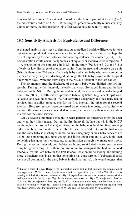
19.6 Sensitivity Analysis for Equivalence and Difference 343
bias would need to be Γ > 2.4, and to mask a reduction in pain of at least τ ≤−2,
the bias would need to be Γ > 3. If the surgical procedure actually reduces pain by
2 units or more, the bias masking this effect would have to be fairly large.
19.6 Sensitivity Analysis for Equivalence and Difference
A planned analysis may seek to demonstrate a predicted positive difference for one
outcome and predicted near equivalence for another, that is, an alternative hypoth-
esis of superiority for one outcome and near equivalence for another [2, 34]. The
demonstration would occur if a hypothesis of equality or inequivalence is rejected.10
A prediction of this sort arose in §12.3. In the study [30, 33] in §12.3 and §18.2
of early or late discharge of premature babies from the neonatal intensive care unit
(NICU), there were 701 pairs of an early baby and a late baby who were similar on
the day the early baby was discharged, although the late baby stayed in the hospital
a few more days. Were the extra days in the NICU of benefit to the late babies?
The six months after the discharge of the early baby were divided into two in-
tervals. During the first interval, the early baby was discharged home and the late
baby was in the NICU. During the second interval, both babies had been discharged
home. In [30, 33], health services provided to healthy babies (e.g., check-ups) were
set aside, and two outcomes in [30, 33] converted emergency and sick-baby health
services into a dollar amount, one for the first interval, the other for the second
interval. Because services were converted by schedule into costs, two babies who
received the same services were coded as having the same costs; there is no variation
in costs for the same service.
Let us devote a moment’s thought to what patterns of outcomes might be seen
and what they might mean. During the first interval, the late baby is in the NICU
receiving hospital (or sick-baby) services, but the baby may be doing fine, growing
older, chubbier, more mature, better able to face the world. During the first inter-
val, the early baby is discharged home, so any emergency or sick-baby services are
a sign that something has gone wrong, and if the dollar amount is very high, then
something has gone very wrong, say a readmission through the emergency room.
During the second interval, both babies are home, so sick-baby costs mean some-
thing has gone wrong. It is, therefore, important to distinguish the first and second
intervals: for the late baby in the first interval, cost could be money and nothing
more; elsewhere, cost is a sign that something has gone wrong. If substantial costs
were at all common for the early babies in the first interval, this would suggest that
10 This is a form of Roger Berger’s [5] intersection-union test, in that one tests the disjunction oftwo hypotheses, H1 ∨H2, in an effort to demonstrate a conjunction, (∼ H1)∧ (∼ H2). Here, H1 isequality or inferiority for one outcome and H2 is inequivalence for another outcome, so superiorityand equivalence is (∼ H1)∧ (∼ H2). In an intersection-union test, H1 ∨H2 is rejected at level αif H1 and H2 are rejected at level α; see [5, 20]. Intersection-union tests may be done in order,possibly rejecting H1 when H2 is not rejected, and a sensitivity analysis may be constructed fromsensitivity analyses for the separate tests of H1 and H2; see the appendix to this chapter.
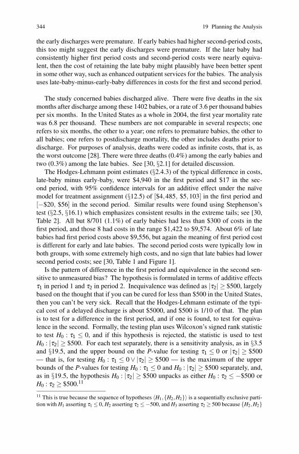
344 19 Planning the Analysis
the early discharges were premature. If early babies had higher second-period costs,
this too might suggest the early discharges were premature. If the later baby had
consistently higher first period costs and second-period costs were nearly equiva-
lent, then the cost of retaining the late baby might plausibly have been better spent
in some other way, such as enhanced outpatient services for the babies. The analysis
uses late-baby-minus-early-baby differences in costs for the first and second period.
The study concerned babies discharged alive. There were five deaths in the six
months after discharge among these 1402 babies, or a rate of 3.6 per thousand babies
per six months. In the United States as a whole in 2004, the first year mortality rate
was 6.8 per thousand. These numbers are not comparable in several respects; one
refers to six months, the other to a year; one refers to premature babies, the other to
all babies; one refers to postdischarge mortality, the other includes deaths prior to
discharge. For purposes of analysis, deaths were coded as infinite costs, that is, as
the worst outcome [28]. There were three deaths (0.4%) among the early babies and
two (0.3%) among the late babies. See [30, §2.1] for detailed discussion.
The Hodges-Lehmann point estimates (§2.4.3) of the typical difference in costs,
late-baby minus early-baby, were $4,940 in the first period and $17 in the sec-
ond period, with 95% confidence intervals for an additive effect under the naıve
model for treatment assignment (§12.5) of [$4,485, $5,103] in the first period and
[−$20, $56] in the second period. Similar results were found using Stephenson’s
test (§2.5, §16.1) which emphasizes consistent results in the extreme tails; see [30,
Table 2]. All but 8/701 (1.1%) of early babies had less than $300 of costs in the
first period, and those 8 had costs in the range $1,422 to $9,574. About 6% of late
babies had first period costs above $9,556, but again the meaning of first period cost
is different for early and late babies. The second period costs were typically low in
both groups, with some extremely high costs, and no sign that late babies had lower
second period costs; see [30, Table 1 and Figure 1].
Is the pattern of difference in the first period and equivalence in the second sen-
sitive to unmeasured bias? The hypothesis is formulated in terms of additive effects
τ1 in period 1 and τ2 in period 2. Inequivalence was defined as |τ2| ≥ $500, largely
based on the thought that if you can be cured for less than $500 in the United States,
then you can’t be very sick. Recall that the Hodges-Lehmann estimate of the typi-
cal cost of a delayed discharge is about $5000, and $500 is 1/10 of that. The plan
is to test for a difference in the first period, and if one is found, to test for equiva-
lence in the second. Formally, the testing plan uses Wilcoxon’s signed rank statistic
to test H0 : τ1 ≤ 0, and if this hypothesis is rejected, the statistic is used to test
H0 : |τ2| ≥ $500. For each test separately, there is a sensitivity analysis, as in §3.5
and §19.5, and the upper bound on the P-value for testing τ1 ≤ 0 or |τ2| ≥ $500
— that is, for testing H0 : τ1 ≤ 0∨ |τ2| ≥ $500 — is the maximum of the upper
bounds of the P-values for testing H0 : τ1 ≤ 0 and H0 : |τ2| ≥ $500 separately, and,
as in §19.5, the hypothesis H0 : |τ2| ≥ $500 unpacks as either H0 : τ2 ≤ −$500 or
H0 : τ2 ≥ $500.11
11 This is true because the sequence of hypotheses 〈H1,{H2,H2}〉 is a sequentially exclusive parti-tion with H1 asserting τ1 ≤ 0, H2 asserting τ2 ≤−500, and H3 asserting τ2 ≥ 500 because {H2,H2}

19.8 Further Reading 345
Table 19.3 Sensitivity analysis for difference in first period costs (τ1) and equivalence of secondperiod costs (τ2).
Γ H0 : τ1 ≤ 0 H0 : τ2 ≤−$500 H0 : τ2 ≥ $500 H0 : τ1 ≤ 0∨|τ2| ≥ $500
1 0.00001 0.00001 0.00001 0.000012 0.00001 0.00001 0.0020 0.0020
2.25 0.00001 0.00001 0.049 0.0492.5 0.00001 0.00042 0.28 0.283 0.00001 0.056 0.90 0.90
Table 19.3 is the sensitivity analysis [30, Table 3]. Because H0 : τ1 ≤ 0 is rejected
at the 0.05 level for each Γ in Table 19.3, the test plan continues and tests both
H0 : τ2 ≤−$500 and H0 : τ2 ≥ $500. For Γ ≤ 2.25, all three hypotheses are rejected
at the 0.05 level, so H0 : τ1 ≤ 0∨ |τ2| ≥ $500 is rejected; that is, late discharge
raised first period costs, but did not much affect second period costs. At Γ = 2.5,
it is plausible that late discharge increased second period costs by $500, but not
plausible it reduced them by $500. At Γ = 3, either an increase or a decrease of
$500 is plausible. It appears that late discharge raised first period costs, without a
compensating reduction in second period costs, and a small bias from nonrandom
treatment assignment could not have created this appearance.
19.7 Summary
To disambiguate an association between treatment and response, Fisher advised
“make your theories elaborate;” see §19.2 and [9, 26]. How should one plan the
analysis of an observational study to evaluate the predictions of an elaborate the-
ory? The plan should enlarge what can be said, not diminish it, yet control the
frequency of false inferences. This is done by giving priority in the analysis to the
evaluation of certain predictions, placing other predictions in a secondary role. The
plan should distinguish predictions of a difference from predictions of near equiv-
alence. This is implemented with appropriate use of equivalence tests and similar
methods. The plan should permit a sensitivity analysis, because in an observational
study it is never possible to be certain that adjustments for observed covariates have
eliminated bias from covariates that were not measured.
19.8 Further Reading
Fisher’s striking phrase “make your theories elaborate” has often been noted [9, 10,
11, 26].
is exclusive. In fact, the three hypotheses may be tested in order, so H1 may be rejected when H2
and H3 are not. See the appendix to the chapter for specifics.

346 19 Planning the Analysis
There is a large literature about planning the analysis of clinical trials, and it
provides some useful guidance for observational studies, where some of the issues
are the same and others are quite different. In particular, the confirmation, or par-
tial confirmation, of an elaborate theory plays no role in a randomized experiment,
where treatment assignment is known to be randomized.
The paper by Gary Koch and Stuart Gansky [17] is a gentle introduction to the
clinical trials literature, whereas the review paper by Roger Berger and Jason Hsu
[6] is a somewhat more technical discussion emphasizing tests of equivalence; see
also the fine papers by Peter Bauer and colleagues [1, 2, 3]. The clinical trials litera-
ture quickly becomes technical and terse, so the serious reader will want to become
acquainted with some of the early papers that shaped what came later, particularly
the papers on ‘closed testing’ by Ruth Marcus, Eric Peritz, and K.R. Gabriel [22],
the intersection-union principle of Roger Berger [5], the device introduced by Jul-
liet Popper Shaffer [32], and the false discovery rate of Yoav Benjamini and Yosef
Hochberg [4]. Erich Lehmann’s early paper [20] illuminates several issues and
is of continuing interest. Two potentially important ideas that have received less
attention are found in papers by Jason Hsu and Roger Berger [15] and Gerhard
Hommel and Siegfried Kropf [14, §3]. Specifically, in [15], a multiple test proce-
dure concludes with a confidence statement about a parameter, while in [14, §3] an
ordered testing procedure continues past a few acceptances with the aid of a mild
application of the Bonferroni inequality.
Less has been written about planning the analysis of an observational study. Is-
sues in the current chapter are discussed in greater detail in [29, 30].
19.9 Appendix: Testing Hypotheses in Order
This chapter has considered several plans for testing one of Fisher’s ‘elaborate the-
ories’ in a sequence of steps. These steps permit partial or total confirmation of the
‘elaborate theory.’ The investigator may select the first step in this sequence on the
basis of importance, priority, conjecture, or whim. The first step in the sequence is
an ordinary test done at level α as it might have been done without a plan for analy-
sis, so in this rather specific sense, the subsequent steps cost the investigator nothing
because the conclusion of the first step is the same. In brief, ambition in testing an
‘elaborate theory’ is not penalized; at worst, the result is the partial confirmation
that would have been obtained anyway in the single first test.
In addition, these plans permitted a sensitivity analysis to be performed using the
upper bounds on the P-values for the component tests; one applies the steps to the
upper bounds. In other words, if you know how to do a sensitivity analysis for each
step, then you know how to do a sensitivity analysis for the entire plan.
This appendix states and proves a result from [29], which then permits the state-
ment of another result from [30]. The first result concerns conventional testing of
a plan, while the second result concerns sensitivity analysis of the testing of a plan.
Although the first result is tailored for use with an elaborate theory in an observa-

19.9 Appendix: Testing Hypotheses in Order 347
tional study, it has many analogues and precedents from the literature on multiple
testing [2, 14, 15, 17, 22, 32], equivalence testing [2, 6, 16, 31, 37], and multiparam-
eter testing [5, 18, 20] in experiments. The second result takes more space to prove
[30], so the proof is not reproduced here, but some discussion of it here is needed.
What is a sequentially exclusive partition of a sequence of hypotheses?
We have a collection of hypotheses, Ht for t ∈ T , where T is a set of indices (or
names) for the hypotheses. The set T is totally ordered (like a dictionary or tele-
phone directory), and we write t ≺ t ′ if t is before t ′ in T . To say that T is totally
ordered is to say that it is always clear who is before whom: that is, if t ∈ T and
t ′ ∈ T with t �= t ′ then either t ≺ t ′ or t ′ ≺ t (and never both t ≺ t ′ and t ′ ≺ t). The
order ≺ will partially determine which hypotheses are tested first, although other
considerations will enter as well. Using numerical inequality, <, in place of ≺, five
possible sets T are: T = {1,2, . . . ,k}, T = {1,2, . . .}, T = {. . . , −1, 0, 1, 2, . . .},
T = [0, ∞), and the positive rational numbers T ={a/b : a,b ∈ {1,2, . . .}}. Other
important totally ordered sets use the lexical order on a product of sets, as in the dic-
tionary or telephone directory, where names are organized by first letter, then within
first letter by second letter, and so on. The lexical order on T = {1,2, . . . ,k}×[0, ∞)says that infinitely many hypotheses (1,a) ∈ T with a ∈ [0, ∞) come before (2,0).The lexical order on T = [0, ∞)×{1,2, . . . ,k} is very different: the k hypotheses
(0,a) ∈ T come before all the rest. In §19.3, there were several orders that com-
bined discrete and continuous aspects, testing one or two hypotheses, then building
an interval estimate, or testing several hypotheses for infinitely many values of a
parameter.
One assumption is made about the hypotheses, Ht for t ∈ T , namely the ‘struc-
ture assumption.’ In practical terms, it is an innocuous assumption, but interestingly
it seems to be needed nonetheless. A person disinclined to attend to innocuous as-
sumptions might skip this paragraph. (While walking down a city street, a person
disinclined to attend to innocuous assumptions might fall through a manhole whose
cover is missing.) The structure assumption says: either all hypotheses Ht for t ∈Tare false or else there is a first true hypothesis. Stated precisely, either Ht is false for
all t ∈T or else there exists a t ′ ∈T such that Ht ′ is true and Ht is false for all t ≺ t ′.It takes a moment’s thought to realize that the structure assumption is indeed an as-
sumption: it might be false. For instance, let T ={a/b : a,b ∈ {1,2, . . .}} be the
positive rational numbers ordered by inequality, <. Let Ht be the ‘hypothesis’ that
the circumference of a circle is less than or equal to t times its diameter. Then Ht is
false for t < π and is true for t > π , but there is not a first rational number t > π , so
the structure assumption is false in this case. In this case, the structure assumption
would be true if the positive rational numbers, T ={a/b : a,b ∈ {1,2, . . .}}, were
replaced by the positive real numbers, T =(0,∞). The structure assumption seems
to be a reminder that statistical inference needs the real numbers, and should avoid
topological games involving things like the rational numbers; however, as far as I
can see, the structure assumption is innocuous in practice because it is not an as-

348 19 Planning the Analysis
sumption about the world itself. Without further mention, the structure assumption
is assumed to be true.
We are headed for a definition of a sequentially exclusive partition of hypotheses,
a term that has been used informally at several points in this chapter. First we need
to define an interval in T and then a partition of T into disjoint intervals.
It is natural to speak of an interval in T . A nonempty subset I ⊆ T is an
interval if, for any t, t ′, t ′′ ∈ T with t ≺ t ′ ≺ t ′′, it follows that t, t ′′ ∈ I implies
t ′ ∈I . For example, in T = {1,2, . . . ,20}, the sets I = {2} and I = {17,18,19}are intervals, but {2,4,6} is not an interval. In T = {1,2, . . . ,k}× [0, ∞) with the
lexical order, the set {2}× [7, ∞)⋃{3}× [0, 1] is an interval.
Disjoint intervals are ordered by their contents. If I1 ⊆ T and I2 ⊆ T are
disjoint intervals, so I1 ∩I2 = /0, then write I1 ≺ I2 if t ≺ t ′ for all t ∈ I1 and
t ′ ∈ I2. For instance, in T = {1,2, . . . ,20}, we have {2,3} ≺ {6,7,8}. Write
t ≺ I if {t} ≺ I and I ≺ t if I ≺ {t}. For instance, in T = {1,2, . . . ,20}, we
have 2 ≺ {6,7,8}.
A partition of T into disjoint intervals is a representation of T as the union of
disjoint intervals Iλ , indexed by a set Λ , that is, T =⋃
λ∈Λ Iλ with Iλ ∩Iλ ′ = /0
for λ ,λ ′ ∈ Λ with λ �= λ ′. In T = {1,2, . . . ,20}, with Λ = {a,b,c}, one partition
of T into disjoint intervals is T =⋃
λ∈Λ Iλ where Ia = {1,2, . . . ,9}, Ib = {10},
Ic = {11,12, . . . ,20}. Because the intervals, Iλ , λ ∈ Λ , are disjoint, they are
ordered; so write λ ≺ λ ′ if Iλ ≺ Iλ ′ , and for t ∈ T , write t ≺ λ if t ≺ Iλ or
λ ≺ t if Iλ ≺ t. For instance, in the partition of T = {1,2, . . . ,20} just mentioned,
Ia ≺ Ic and 7 ≺ Ic.
A set S ⊆ T of hypotheses is exclusive if at most one of the hypotheses Ht ,
t ∈ S , is true. For instance, if θ is a real parameter, then the set of hypotheses
{Ht : t ∈ (−∞,∞)} would be exclusive if Ht were Ht : θ = t, but the same set would
not be exclusive if the Ht were Ht : θ ≤ t; in the first case, distinct hypotheses
contradict each other but in the second case they do not. The words ‘at most one’
are important: the set of hypotheses {Ht : t ∈ (12, 17)} with Ht : θ = t is exclusive
even if there is no reason to think θ is between 12 and 17.
Now, we can define a sequentially exclusive partition of hypotheses. A partition
of T into disjoint intervals, T =⋃
λ∈Λ Iλ , is a sequentially exclusive partition
if each interval Iλ , λ ∈ Λ , would be exclusive if all hypotheses in earlier inter-
vals were false; that is, at most one hypothesis Ht , t ∈ Iλ , is true whenever all
hypotheses, Ht ′ , t ′ ≺ Iλ , are false. For instance, with T = {1,2,3}, the partition
T = {1}∪{2,3} is a sequentially exclusive partition if at most one of H2 and H3 is
true whenever H1 is false; see §19.3 for several examples. Notice that {2,3} need
not be exclusive if H1 is true.
A sequentially exclusive partition always exists, namely the partition T =⋃t∈T {t}. This is so because a set containing a single hypothesis is always ex-
clusive; it contains at most one true hypothesis.

19.9 Appendix: Testing Hypotheses in Order 349
Testing hypotheses in order
In the following testing plan, T =⋃
λ∈Λ Iλ is a sequentially exclusive parti-
tion, and for each hypothesis, Ht , t ∈ T , there is a valid P-value, pt , such that
Pr(pt ≤ α) ≤ α for all α ∈ [0,1] if Ht is true. Fix an α , conventionally α = 0.05.
Testing plan. If ps ≤ α for all s ∈ Iλ for all λ ≺ ω , then reject all hypotheses
Ht , t ∈ Iω , with pt ≤ α .
This testing plan is, in fact, the general form of the plan used throughout this
chapter. For the partition T =⋃
t∈T {t}, the testing plan says to reject all hy-
potheses prior to the first acceptance and stop. In general, with T =⋃
λ∈Λ Iλ ,
the procedure stops with the first interval Iω that contains at least one hypothesis
t ′ ∈ Iω with pt ′ > α; however, all hypotheses t ∈ Iω are tested, and all of those
with pt ≤ α are rejected. Particular cases of Proposition 19.1 have been discussed
throughout this chapter.
Proposition 19.1. [29] If the testing plan is applied to a sequentially exclusive par-tition of hypotheses, Ht , t ∈ T =
⋃λ∈Λ Iλ , where Pr(pt ≤ α) ≤ α if Ht is true,
then the probability that the plan tests and rejects at least one true hypothesis is atmost α .
Proof. Let W be the event that the testing plan tests and rejects at least one true
hypothesis. If all hypotheses, Ht , t ∈ T , are false, then there is nothing to prove;
in particular, Pr(W ) = 0. Otherwise, let Hv be the first true hypothesis, let Rv be
the event that the testing plan tests and rejects Hv, and let Iω be the unique interval
that contains v. Then Ht is false for all t ≺Iω . This implies that Hv is the only true
hypothesis in Iω , because T =⋃
λ∈Λ Iλ is sequentially exclusive. It follows that
the plan tests and rejects at least one true hypothesis if and only if it tests and rejects
Hv, so W = Rv, and Pr(W ) = Pr(Rv) ≤ α .
Sensitivity analysis for testing in order
In §3.5, a sensitivity analysis was performed in which an upper bound, say Pt,max,
was found for the one-sided P-value when testing a single hypothesis, say Ht ; see
Table 3.2. This upper bound, Pt,max, was the largest P-value that could be produced
for a given magnitude Γ of deviation from random treatment assignment in (3.13).
That bound was sharp, in the sense that there was some set of treatment assignment
probabilities πi j satisfying (3.16)–(3.18) for which the bound Pt,max was the correct
P-value.
Suppose that we have a sequence of such bounds, Pt,max, for a sequence of hy-
potheses, Ht , t ∈ T , where T =⋃
λ∈Λ Iλ is a sequentially exclusive partition of
hypotheses. Suppose that the testing plan were applied using the bounds in place of
the unknown, actual P-values. What would happen? In fact, this was done several
times in this chapter.

350 19 Planning the Analysis
It is possible to show the following [30, Proposition 1]. First, if (3.13) is true for
a given value of Γ ≥ 1, the chance that the testing plan tests and rejects at least one
true hypothesis is at most α . Second, this bound is sharp: there are treatment as-
signment probabilities πi j satisfying (3.16)–(3.18) for which the testing plan would
terminate with acceptance of the same hypothesis, Hv, in the proof of Proposition
19.1. In other words, if the testing plan were used once for every set of treatment
assignment probabilities πi j satisfying (3.16)–(3.18), then a hypothesis Ht would be
rejected in all of these analyses if and only if it is rejected in the one analysis that
uses the individual bounds in place of the actual P-values.
The sharpness of the bound is actually somewhat surprising. The reason it is
surprising is that the treatment assignment probabilities πi j that produce Pt,max are
not generally the same as the πi j’s that produce Pt ′,max for t �= t ′, so there may be no
treatment assignment probabilities satisfying (3.16)–(3.18) that produce both Pt,max
and Pt ′,max. You can have Pt,max or you can have Pt ′,max, but there is no assurance
that you can have both Pt,max and Pt ′,max, even though the proposal is to plug them
both into the testing plan as if they could coexist. If the Bonferroni inequality is
used with Pt,max and Pt ′,max, then the result is conservative, not sharp [30, §4.5]: it
can happen that min(Pt,max, Pt ′,max
)> α/2, while the minimum of the two P-values
for testing Ht and Ht ′ is less than α/2 for all treatment assignment probabilities πi jsatisfying (3.16)–(3.18). Speaking informally, the bound is sharp for the testing plan
because the plan stops with a single P-value; see [30, Proposition 1] for a precise
statement.
The results in [29, 30] are general; they are not restricted to matched pairs.
References
1. Bauer P.: Multiple testing in clinical trials. Statist Med 10, 871–890 (1991)2. Bauer, P., Kieser, M.: A unifying approach for confidence intervals and testing of equivalence
and difference. Biometrika 83, 934–937 (1996)3. Bauer, P.: A note on multiple testing procedures in dose finding. Biometrics 53, 1125–1128
(1997)4. Benjamini, Y., Hochberg, Y.: Controlling the false discovery rate. J Roy Statist Soc B 57,
289–300 (1995)5. Berger, R.L.: Multiparameter hypothesis testing and acceptance sampling. Technometrics 24,
295–300 (1982)6. Berger, R.L., Hsu, J.C.: Bioequivalence trials, intersection-union tests and equivalence confi-
dence sets. Statist Sci 11, 283–319 (1996)7. Bilban, M., Jakopin, C.B.: Incidence of cytogenetic damage in lead-zinc mine workers ex-
posed to radon. Mutagenesis 20, 187–191 (2005)8. Bunker, J.P., Barnes, B.A., Mosteller, F.: Costs, Risks and Benefits of Surgery. Oxford: Oxford
University Press (1977)9. Cochran, W.G.: The planning of observational studies of human populations (with Discus-
sion). J Roy Statist Soc A 128, 234–265 (1965)10. Cox, D.R.: Causality: Some statistical aspects. J Roy Statist Soc A 155, 291–301 (1992)11. Gail, M.: Statistics in action. J Am Statist Assoc 91, 1–13 (1996)12. Heller, R., Rosenbaum, P.R., Small, D.: Split samples and design sensitivity in observational
studies. J Am Statist Assoc 104, to appear (2009)

References 351
13. Holm, S.: A simple sequentially rejective multiple test procedure. Scand J Statist 6, 65–70(1979)
14. Hommel, G., Kropf, S.: Tests for differentiation in gene expression using a data-driven orderor weights for hypotheses. Biomet J 47, 554–562 (2005)
15. Hsu, J.C., Berger, R.L.: Stepwise confidence intervals without multiplicity adjustment fordose-response and toxicity studies. J Am Statist Assoc 94, 468–475 (1999)
16. Hsu, J.C., Hwang, J.T.G., Liu, H-K., Ruberg, S.J.: Confidence intervals associated with testsfor bioequivalence. Biometrika 81, 103–114 (1994)
17. Koch, G.G., Gansky, S.A.: Statistical considerations for multiplicity in confirmatory protocols.Drug Inform J 30, 523–533 (1996)
18. Laska, E.M., Meisner, M.J.: Testing whether an identified treatment is best. Biometrics 45,1139–1151 (1989)
19. Lehmacher, W., Wassmer, G., Reitmeir, P.: Procedures for two-sample comparisons with mul-tiple endpoints controlling the experimentwise error rate. Biometrics 47, 511–521 (1991)
20. Lehmann, E.L.: Testing multiparameter hypotheses. Ann Math Statist 23, 541–552 (1952)21. Li, Y.F.P., Propert, K.J., Rosenbaum, P.R.: Balanced risk set matching. J Am Statist Assoc 96,
870–882 (2001)22. Marcus, R., Peritz, E., Gabriel, K.R.: On closed testing procedures with special reference to
ordered analysis of variance. Biometrika 63, 655–60 (1976)23. Masjedi, M.R., Heidary, A., Mohammadi, F., Velayati, A.A., and Dokouhaki, P.: Chromo-
somal aberrations and micronuclei in lymphocytes of patients before and after exposure toanti-tuberculosis drugs. Mutagenesis 15, 489–494 (2000)
24. McPherson, K., Bunker, J.P.: Costs, Risks and Benefits of Surgery: A milestone in the devel-opment of health services research. J Roy Soc Med 100, 387–390 (2007)
25. Propert, K.J., Schaeffer, A.J., Brensinger, C.M., Kusek, J.W., Nyberg, L.M., Landis, J.R.: Aprospective study of interstitial cystitis: Results of longitudinal followup of the interstitialcystitis data base cohort. J Urol 163, 1434–1439. (2000)
26. Rosenbaum, P.R.: From association to causation in observational studies. J Am Statist Assoc79, 41–48 (1984)
27. Rosenbaum, P.R.: Observational Studies (2nd ed). New York: Springer (2002)28. Rosenbaum, P.R.: Comment on a paper by Donald B. Rubin: The place of death in the quality
of life. Statist Sci 21, 313–316 (2006)29. Rosenbaum, P.R.: Testing hypotheses in order. Biometrika 95, 248–252 (2008)30. Rosenbaum, P.R., Silber, J.H.: Sensitivity analysis for equivalence and difference in an obser-
vational study of neonatal intensive care units. J Am Statist Assoc 104, 501–511 (2009)31. Schuirmann, D.L.: On hypothesis testing to determine if the mean of a normal distribution is
contained in a known interval. Biometrics 37, 617 (1981)32. Shaffer, J.P.: Modified sequentially rejective multiple test procedures. J Am Statist Assoc 81,
826–831 (1986)33. Silber, J.H., Lorch, S.L., Rosenbaum, P.R., Medoff-Cooper, B., Bakewell-Sachs, S., Millman,
A., Mi, L., Even-Shoshan, O., Escobar, G.E.: Additional maturity at discharge and subsequenthealth care costs. Health Serv Res 44, 444–463 (2009)
34. Tamhane, A., Logan, B.: A superiority-equivalence approach to one-sided tests on multipleendpoints in clinical trials. Biometrika 91, 715–727 (2004)
35. Tukey, J.W.: We need both exploratory and confirmatory. Am Statistician 34, 23–25 (1980)36. Tukey, J.W.: Sunset salvo. Am Statistician 40, 72–76 (1986)37. Westlake, W.J.: Response to Kirkwood. Biometrics 37, 591–593 (1981)38. Yoon, F.: New Methods for the Design and Analysis of Observational Studies. Doctoral The-
sis, Department of Statistics, University of Pennsylvania.

Summary: Key Elements of Design
In an observational study, competing theories should make conflicting predic-tions. Many studies dissipate before they begin from a simple lack of focus. The
study is intended to settle something, or at least take a step towards settling some-
thing, and for that, there needs to be something definite to settle and some prospect
of and means for settling it; see Chapter 4. Some pairs of theories rarely yield con-
flicting predictions, so one may search for unusual opportunities to contrast them;
see §5.1.
An observational study should be structured to resemble a simple experiment.A typical structure is the comparison of a treated and a control group that looked
comparable prior to treatment in terms of observed covariates. An experiment is an
unusual situation. In a carefully controlled experiment, one of the rarest of things
happens: the effects caused by treatments are seen with clarity. Each step away from
the experimental template is a step closer to the edge of an abyss; see §1.2 and §12.1.
Adjustments for observed covariates should be simple, transparent, and con-vincing. The major source of uncertainty about the conclusions of an observational
study comes from the possible failure to control for covariates that were not mea-
sured. This possibility is raised in virtually every observational study. If you think
this possibility will not be raised in evaluating your study, then you are kidding
yourself. There is little hope of addressing this major source of uncertainty if the
study becomes bogged down in unnecessarily complex, obscure, or unconvincing
adjustments for observed covariates. One simple, transparent, and convincing way
to adjust for observed covariates is to compare a treated and a control group with
similar distributions of the observed covariates. Such a control group may often be
constructed with the aid of multivariate matching; see Part II.
The most plausible alternatives to a treatment effect should be anticipated andaddressed. In an observational study, it is not possible to address every conceiv-
able alternative to a treatment effect. It is often possible to anticipate several plau-
sible objections to a claim that a comparison of matched treated and control groups
estimates the effects of the treatment. Such an objection claims that the comparison
353P.R. Rosenbaum, Design of Observational Studies, Springer Series in Statistics, DOI 10.1007/978-1-4419-1213-8, © Springer Science+Business Media, LLC 2010

354 Summary: Key Elements of Design
is ambiguous, that it could estimate a treatment effect or it could be distorted by
some specific form of bias. With a specific form of bias in mind, design elements
can often be added, such as two control groups or unaffected outcomes, that resolve
specific ambiguities; see §5.2.
The analysis should address possible biases from unmeasured covariates. Typ-
ically, the analysis should include a sensitivity analysis of one form or another; see
Chapter 3. A sensitivity analysis asks: how much bias from unmeasured covariates –
what magnitude of deviation from random assignment – would need to be present to
qualitatively alter the conclusions suggested by the naıve, straightforward compari-
son of matched treated and control groups? The degree of sensitivity to unmeasured
bias is a fact of the matter, something that is determined without ambiguity from the
data at hand. Whether or not biases of this magnitude are present remains a matter
of reasoned conjecture and responsible debate, but that debate is now informed and
constrained by the facts of the matter. A P-value does not rule out the possibility that
bad luck produced the observed results; rather, it objectively measures how much
bad luck would be required to produce the observed results. A sensitivity analysis
does not rule out the possibility that unmeasured bias produced the observed re-
sults; rather, it objectively measures how much unmeasured bias would be required
to produce the observed results.
To the extent possible, observational studies should be designed to be insensitiveto biases from unmeasured covariates. To do this, one must know what makes
some designs (or data generating processes) sensitive to unmeasured biases and
others insensitive. With this knowledge, when faced with a choice, an insensitive
design may be chosen. Many factors strongly affect design sensitivity; see Part III.
There should be a plan for a primary analysis. A randomized controlled trial
invariably has a protocol detailing a plan for a primary analysis. An observational
study also needs such a plan. With design elements intended to resolve otherwise
ambiguous comparisons, the study design anticipates one of a few patterns of re-
sults, what R.A. Fisher called an ‘elaborate theory’; see §19.2. The typical elaborate
theory predicts a difference here, near equivalence there, the absence of a trend here,
a discontinuity there. For instance, an elaborate theory might predict much higher re-
sponses in the treated group than in two control groups, with the two control groups
differing negligibly from each other. A planned primary analysis will attempt to ex-
amine, possibly confirm, the predictions of an elaborate theory; see Chapter 19. The
predictions of an elaborate theory are predictions only if they precede examination
of the outcomes; there is no value in an elaborate theory constructed after the fact to
accommodate a particular set of data. Therefore, the analysis of an elaborate theory
must be a planned analysis. Planning may be aided by sample splitting; see §18.1.
A plan for a primary analysis does not preclude unplanned exploratory analyses;
rather, it distinguishes planned and unplanned analyses.

Solutions to Common Problems
The matching problem is too large. If a matching problem is too large, divide it
into several smaller problems by exact matching for one or more important covari-
ates; see §9.3.
Treated and control groups are too far apart to match. Before trying to solve
this problem, make sure the problem is real. Compare boxplots of the propensity
scores for treated and control groups. If the boxplots cover much the same range,
but some covariates or the propensity score are poorly balanced, consider: (i) tight-
ening the caliper on the propensity score so that, for example, the penalty engages
at 10% of the standard deviation rather than 20% (see §8.4), (ii) use penalties to im-
prove balance on one or two stubborn covariates (see §9.2), or (iii) try full matching
(see §8.6). Otherwise, if the boxplots exhibit large regions with little or no overlap,
consider redefining the study population using a few key covariates (see §3.6). For
an example of redefining the study population, see [2].
Treated and control groups overlap, but at some values of x there are too fewcontrols even for 1-to-1 matching. Try full matching; see §8.6.
People are treated at different times. How do I match? Consider risk-set match-
ing; see Chapter 12.
I want to match for a variable with many categories, but there are not enoughpeople in the categories to permit a close match. Try matching with fine balance;
see Chapter 10.
I have two control groups. How do I match? There are several options. One ap-
proach is to form matched triples by matching one treated group twice, once to one
control group, then to the other. Another approach forms matched pairs in an ‘in-
complete block’ design. See Chapter 11. A different problem is to split one control
group to form two for a specific purpose; see the discussion of tapered matching in
§18.2.
My propensity score model does a poor job of predicting treatment assignment.Not a problem. In a large, completely randomized experiment, a propensity score
355

356 Solutions to Common Problems
model would have great difficulty predicting treatment assignments from covariates
precisely because treatment assignment is random and does not depend upon the
covariates. The propensity score is intended to fix a specific problem, namely im-
balances in observed covariates. If your study does not have that problem, then that
is just fine.
How do I judge whether my model for the propensity score is a good model?The propensity score has various uses, and the answer to this question depends upon
how the propensity score will be used. In this book, propensity scores are used for
matching. When used for matching, propensity scores are a means to an end, namely
matched pairs or sets that balance observed covariates. When you have matched
pairs or sets that balance observed covariates, the matching for observed covariates
is done, and attention shifts to potential bias from unmeasured covariates. In light
of this, judging the propensity score model when used in matching is essentially the
same task as judging whether the matching has balanced observed covariates; see
§9.1.
How do I select covariates to use in the propensity score? This question inverts
the means and the end. The proper question is: Which covariates do you wish to
balance by matching on the propensity score?
There is a covariate that strongly predicts treatment assignment Z but seemsunlikely to matter much for the response R. What should I do? Read about
‘seemingly innocuous confounding,’ analytical adjustments, and tapered matching
in §18.2.
There is a variable that is subsequent to treatment assignment and may havebeen affected by the treatment, so it is not a covariate, but I feel I should adjustfor it anyway. Although this is sometimes reasonable, think long and hard before
you do this. If you adjust for a concomitant variable that has been affected by the
treatment, you may introduce a bias that would not otherwise have been present; see
[5]. If in doubt, it may be best to leave such a variable unmatched, so that analyses
with and without analytical adjustments for it are possible; see §18.2. One alterna-
tive is to both match and not match for such a variable; see the discussion of tapered
matching in §18.2.
I have matched with a variable ratio of controls to treated subjects, and nowI want a boxplot. It is not difficult to do, but at the time I write this, current soft-
ware does not do it, so a few steps are needed. Essentially, you need to compute a
weighted empirical distribution function, compute the quantiles from it, and make a
boxplot using those quantiles. The R function ‘bxp’ will help: it will draw boxplots
from quantiles you give it. See Note 3 in Chapter 8. The resulting boxplots look like
ordinary boxplots, but they are weighted to reflect the variable numbers of controls.
Examples are found in [2].
Should I match with a fixed or a variable ratio of controls to treated subjects?The choice is discussed in §8.5. The previous solution, about the boxplot, illustrates
the biggest disadvantage of matching with variable controls; simple, straightforward

Solutions to Common Problems 357
tasks require special programming effort. Opposed to this, theory strongly suggests
that matching with variable controls is an efficient way to produce closer matches;
see [4].
People say that a specific unobserved covariate u is strongly related to the out-come, rC, but I doubt it. To show that a specific unobserved covariate u is not
strongly related to the outcome rC, find two control groups that differ markedly in
terms of the unobserved u, and show that outcomes do not greatly differ in these two
control groups. See §5.2.2 and §19.3.
People say that a specific unobserved covariate u is strongly related to treat-ment assignment Z, but I doubt it. To show that a specific unobserved covariate
u is not strongly related to treatment assignment, Z, find an outcome known to be
unaffected by the treatment that is highly correlated with u, and show that this un-
affected outcome has a similar distribution in treated (Z = 1) and control (Z = 0)
groups. See §5.2.4.
I would like to perform a sensitivity analysis, but I do not have matched pairs.It’s not difficult. See [6, Chapter 4]. A quick and easy approach for matching with
multiple controls uses the stratified Wilcoxon rank sum statistic and Table 1 in [1].
For matched sets with one to four controls (ni equal to two to five in that table),
and for Γ equal to one to four, the Table gives the calculations needed for one
matched set; these contributions are summed to produce the sensitivity analysis.
For any rank statistic, say the aligned rank statistic, the general calculations in [1,
§3] are easy to perform in R or with a spreadsheet. An alternative approach with
multiple controls uses an m-test [7]. Also, [7, §5] discusses sensitivity analysis with
covariance adjustment in matching with multiple controls.
I would like to perform a sensitivity analysis, but my outcomes are binary.Again, it is not difficult. See [6, Chapter 4]. That chapter also discusses outcomes
that are censored survival times.
How do I interpret the parameter Γ ? The parameter Γ is convenient in that it
is a single parameter that can refer to a wide variety of situations. The resulting
sensitivity analysis is one-dimensional: just one parameter varies. The sensitivity
bounds implicitly refer to an unobserved covariate u that is strongly related to the
response, rC, and that has a controlled relationship with the treatment, Z, the control
being provided by the value of Γ . Sometimes, that situation is not the one under
discussion, because a very strong relationship between u and rC isn’t plausible. It is
possible to reexpress the one-parameter analysis in terms of two parameters, where
one parameter controls the relationship between the unobserved covariate u and the
response rC and the other controls the relationship between u and the treatment, Z.
It is the same one-dimensional sensitivity analysis, with no new computations, but
now with a two-dimensional interpretation; see [8].
I am worried that my findings will be sensitive to small unmeasured biases.Review Chapters 14–17 to see what issues affect the sensitivity of conclusions to

358 Solutions to Common Problems
unmeasured biases. Consider sample splitting to guide design decisions that affect
design sensitivity; see §18.1 and [3].
I have doses of treatment, but I am not sure whether they are any good. Split
the sample and find out; see §18.1 and [3]. Similar advice applies to many other
design decisions.
The treatment that interests me is known to be assigned in a very biased fash-ion. Instead of studying the effect of that treatment, consider studying its differen-
tial effect compared with other treatments affected by the same biases; see §5.2.6.
This may help in some circumstances.
There have been several studies of the treatment that interests me, but none isconvincing. Is it possible to study the treatment again, this time removing one of
the several problems that made previous studies unconvincing? See §4.5.
The same problems inevitably occur whenever efforts are made to study thetreatment that interests me. Why is the treatment thought to work? What reasons
are given? Why is there doubt about the effects of the treatment? What reasons
are given? Can an empirical study shed light on whether these reasons are valid?
Perhaps the reasons can be supported or refuted, even though direct investigation of
the effects is difficult. See §4.6.
I am disappointed by my ‘null result.’ Do you possess evidence for the absence
of a large effect? That might be an important finding; see §19.5. Or do you lack
evidence about the magnitude of the effect? That is disappointing, but it is a common
occurrence, one that happens now and then to everyone.
References
1. Gastwirth, J.L., Krieger, A.M., Rosenbaum, P.R.: Asymptotic separability in sensitivity analy-sis. J Roy Statist Soc B 62, 545–555 (2000)
2. Haviland, A.M., Nagin, D.S., Rosenbaum, P.R.: Combining propensity score matching andgroup-based trajectory analysis in an observational study. Psychol Methods 12, 247–267 (2007)
3. Heller, R., Rosenbaum, P.R., Small, D.: Split samples and design sensitivity in observationalstudies. J Am Statist Assoc 104, to appear (2009)
4. Ming, K., Rosenbaum, P.R.: Substantial gains in bias reduction from matching with a variablenumber of controls. Biometrics 56, 118–124 (2000)
5. Rosenbaum, P.R.: The consequences of adjustment for a concomitant variable that has beenaffected by the treatment. J Roy Statist Soc A 147, 656–666 (1984)
6. Rosenbaum, P.R.: Observational Studies (2nd ed.). New York: Springer (2002)7. Rosenbaum, P.R.: Sensitivity analysis for m-estimates, tests, and confidence intervals in
matched observational studies. Biometrics 63, 456–464 (2007)8. Rosenbaum, P.R., Silber, J.H.: Amplification of sensitivity analysis in observational studies. J
Am Statist Assoc, to appear

Symbols
|A| If A is a finite set, |A| is the number of elements in A.
x Observed covariates for any one person. See §2.1.2.
x� Observed covariates for person �, � = 1, . . . ,L. The � subscript is used to
denote people before they are matched. The � subscript is used in the same
way with Z, R, rT , rC, and u. See §3.1.
xi j Observed covariates for person j, in pair i, i = 1,2, . . . , I, j = 1,2. The i jsubscripts are used to denote people after they are arranged into matched
pairs. The i j subscripts are used in the same way with Z, R, rT , rC, and u.
See §2.1.2.
Z Treatment indicator, Z = 1 if treated, Z = 0 if control. See §2.1.2.
Z Treatment indicators for the 2I subjects in the I matched pairs, Z =(Z11,Z12,Z21, . . . ,ZI2)T . See §2.1.2.
e(x) Propensity score, e(x) = Pr(Z = 1 | x). See §8.2.
(rT ,rC) For any one person, rT is the response the person would exhibit under
treatment, and rC is the response this same person would exhibit under
control. See §2.2.1.
(rT ,rC) Vectors rT = (rT 11,rT 12, . . . ,rT I2)T and rC = (rC11,rC12, . . . ,rCI2)T of po-
tential responses for all 2I subjects in I pairs. See §2.2.1.
R Observed response, that is, R = rT if Z = 1 and R = rC if Z = 0, so R =ZrT +(1−Z)rC. See §2.1.2.
R Observed responses for the 2I subjects in the I matched pairs, R =(R11,R12, . . . ,RI2)T . See §2.1.2.
sgn sgn(a) = 1 if a > 0 and sgn(a) = 0 otherwise. Not to be confused with its
sibling sign. See §2.3.3.
sign sign(a) = 1 if a > 0, sign(a) = 0 if a = 0, sign(a) = −1 if a < 0. Not to
be confused with its sibling sgn. See §2.9.
si si = 1 if |Yi| > 0 and si = 0 if |Yi| = 0. See §2.3.3.
u An unobserved covariate. See §2.1.2.
359

360 Symbols
u Unobserved covariates for the 2I subjects in the I matched pairs, u =(u11,u12, . . . ,uI2)T . See §2.1.2.
Yi Treated-minus-control difference in observed responses within pair i, that
is, Yi = (Zi1 −Zi2)(Ri1 −Ri2). See §2.1.2.
Y Treated-minus-control differences in observed responses for I pairs, Y =(Y1,Y2, . . . ,YI)T . See §2.1.2.
F The values of (rT , rC, x, u) for all subjects. Notice that these quantities do
not change when Z changes, whereas R does change when Z changes. In
this specific sense, F is fixed in Fisher’s theory of randomization infer-
ence. See §2.2.1. In simple experiments, the dose of treatment is the same
for every treated subject, and so doses are not explicitly mentioned when
F is first defined in §2.2.1. However, if there are doses di that vary by pair
i, as in §5.2.5, or that vary by individual, (dTi j,dCi j), as in §5.3, then these
doses are also part of F . In a strict sense, the doses are always present in
F , but when the doses are constant there is no need to mention them.
Z The set containing the 2I possible values of z = (z11,z12, . . . ,zI2)T of Z. So
z ∈ Z if zi j = 0 or zi j = 1 with zi1 + zi2 = 1. In conditional probabilities,
conditioning on Z means conditioning on the event Z ∈ Z . See §2.2.3.
di The dose at which the treatment is given in pair i. See the discussion of
dose-response in §5.2.5.
(dTi j,dCi j) For person j in pair i, dTi j is the dose of treatment this person would
accept if assigned to treatment, Zi j = 1, and dCi j is the dose of treatment
this person would accept if assigned to control, Zi j = 0. See the discussion
of instrumental variables in §5.3.
Di j For person j in pair i, Di j is the dose actually received, Di j = Zi jdTi j +(1−Zi j)dCi j. See the discussion of instrumental variables in §5.3.
Γ Sensitivity parameter in a sensitivity analysis. Two subjects with the same
observed covariates may differ in their odds of treatment by at most a
factor of Γ . The parameter Γ is a key element in the ‘second model’ for
an observational study in Chapter 3.
Pmin and Pmax Interval of possible P-values in a sensitivity analysis. See §3.5,
specifically Table 3.2.
Γ Design sensitivity. In the favorable situation, the power of a sensitivity
analysis tends to 1 as the sample size increases if Γ < Γ and the power
tends to 0 if Γ > Γ . See Chapter 14.

Acronyms
AAA ACE-inhibitor after anthracycline randomized trial. See §5.3.
AFDC Aid to Families with Dependent Children, a Federally funded public as-
sistance program in the United States
CI Confidence interval.
FARS Fatal Accident Reporting System. FARS records information about fatal
road accidents in the United States
FTE Full time equivalent employment.
GO Gynecologic oncologist.
HL Hodges-Lehmann point estimate.
IC Interstitial cystitis, a urologic disorder.
iid Independent and identically distributed. See §14.1.
IV Instrumental variable.
ICDB Interstitial Cystitis Data Base.
Medicare U.S. government program providing health care to people over the age
of 65.
MN Micronuclei, a common measure in genetic toxicology.
MO Medical oncologist.
NSAID Nonsteroidal anti-inflammatory drug.
NICU Neonatal intensive care unit.
NJ New Jersey, a state in the United States.
NSW National Supported Work Demonstration, a randomized experiment eval-
uating a program intended to aid the transition to employment.
PA Pennsylvania, a state in the United States.
PMA Postmenstrual age, a proxy for age from conception.
R A statistical software package. http://cran.r-project.org/. Ris distributed free.
SAS A statistical software package. http://www.sas.com/.
SEER Surveillance, Epidemiology and End Results Program of the U.S. National
Cancer Institute. http://seer.cancer.gov/.
sib-TDT Sibship transmission disequilibrium test.
stata A statistical software package. http://www.stata.com/.
361

362 Acronyms
TDT Transmission disequilibrium test.
TOST Two-one-sided tests procedure for equivalence testing.

Glossary of Statistical Terms
Bonferroni inequality If A and B are two events, then the probability of the
event ‘A or B’ is at most the sum of the probabilities of A and of B; that is,
Pr(A∪B) ≤ Pr(A)+Pr(B). The inequality applies also with more than two events.
The Bonferroni inequality is used in many different ways, but it shows up in this
book in connection with testing more than one hypothesis. If there are two hypothe-
ses, where A is the event of falsely rejecting the first hypothesis, and B is the event
of falsely rejecting the second hypothesis, then the chance of falsely rejecting at
least one hypothesis is at most Pr(A)+ Pr(B). In particular, if each test is done at
level 0.025, then the chance of at least one false rejection in two tests is at most
0.025 + 0.025 = 0.05. This use of the Bonferroni inequality is attractive because it
is simple and very general; however, there are methods that are only slightly more
complex and equally general but better; see Holm, S.: A simple sequentially rejec-
tive multiple test procedure, Scand J Statist 6, 65–70 (1979).
boxplot A boxplot is a graph that looks like a transistor. Figure 1.1 contains several
boxplots. The box contains half the observations. The box has a middle line at the
median and it ends at the upper and lower quartiles. One-quarter of the observations
are inside the box above the median, and one-quarter of the observations are inside
the box below the median. One-quarter of the observations are above the box, and
one-quarter of the observations are below the box. Extreme observations appear as
individual points. Boxplots were invented by John Tukey. See Cleveland, W.W.:
Elements of Graphing Data, Summit, NJ: Hobart Press, pp. 139–143.
censored If a patient was diagnosed two years ago and is alive today, then this
patient’s survival time from diagnosis is censored at two years. This means that
we know the patient’s total survival after diagnosis is at least two years, but we do
not know the actual survival time. Typically, some survival times are censored and
others are known or uncensored. Given a choice, you’d rather be censored.
close match A pair is closely matched for a covariate if the two individuals in the
pair have very similar values of that covariate. It is generally very difficult to obtain
363

364 Glossary of Statistical Terms
a close match on many covariates at the same time. See also ‘covariate balance’ for
a very different notion.
consistent estimate A consistent estimate is one that gets it right if the sample
size is large enough. An estimator θ is a consistent estimate of a parameter θ if
θ converges in probability to θ as the sample size increases. See ‘convergence in
probability’ in this glossary.
consistent test A consistent test is one that gets it right if the sample size is large
enough. A test of a null hypothesis H0 is consistent against an alternative hypothesis
HA if the power of the test tends to one as the sample size increases when HA is true.
convergence in distribution Convergence in distribution formalizes the notion that
a random variable, say ξI , almost has a certain distribution. Typically in this book, ξIis a statistic computed from a sample of size I — for instance, a standardized version
of Wilcoxon’s signed rank statistic, T — and the convergence occurs as the sample
size I increases. In this book, the approximating distribution is always the standard
Normal distribution, Φ(.) and, to be tangible, this glossary will define convergence
in distribution to the standard Normal distribution. Slightly more detail is needed to
define convergence in distribution in general. A sequence of random variables, ξI ,
I = 1,2, . . ., converges in distribution to the standard Normal distribution, Φ(.), if
limPr(ξI ≤ c) = Φ(c) for all c, the limit being taken as the sample size I increases.
convergence in probability Convergence in probability formalizes the notion that
a random variable, say ξI , is almost a certain constant. Typically in this book, ξI is a
statistic computed from a sample of size I — for instance, Wilcoxon’s signed rank
statistic, T , divided by I(I +1)/2 — and the convergence occurs as the sample size Iincreases. A sequence of random variables, ξI , I = 1,2, . . ., converges in probability
to the real number a if Pr(|ξI −a| > ε) tends to 0 as I increases for all ε > 0.
covariate A covariate is a variable measured prior to treatment assignment, and
hence prior to treatment. Because it is measured prior to treatment assignment and
prior to treatment, it cannot be affected by treatment. Therefore, a covariate exists
in a single version, say x, because an individual has the same value of a covariate
whether assigned to treatment or to control. In contrast, an outcome may be affected
by the treatment, so an outcome exists in two versions, one seen under treatment,
rT , the other seen under control, rC. See §2.1.2.
covariate balance If the distributions of covariates are similar in treated and con-
trol groups, then there is covariate balance. For instance, if age is one covariate,
then age is balanced if the distribution of ages for treated subjects is similar to the
distribution of ages for controls. Covariate balance is a property of the treated and
control groups taken as two whole groups, not a property of an individual matched
pair or set. See also the entry for ‘close match’ for a very different notion. Random-
ization tends to balance both observed and unobserved covariates. Matching on the
propensity score tends to balance observed covariates but not unobserved covariates.
Glossary of Statistical Terms 365
efficiency Speaking informally, a statistical procedure is efficient if it makes the
best possible use of the available sample size, producing the shortest confidence
intervals, the smallest standard errors, the most powerful test, and so on. One pro-
cedure, say A, is more efficient than another procedure, say B, if A can accomplish
with, say, 50 observations what B needs 52 observations to accomplish. Understand-
ably, efficiency is a major concern in randomized controlled clinical trials, in part
because each observation is expensive and time-consuming, and in part because
additional observations entail treating additional patients, perhaps with a treatment
that the trial itself will find to be an inferior treatment. Efficiency is not the central
concern in observational studies because a limited sample size is not the princi-
pal source of uncertainty. Bias of fixed size, not the standard error, is the principal
source of uncertainty in nonrandomized studies. Many observational studies would
not become more compelling if the sample size were increased. In addition, in some
observational studies, large samples are available from extant data.
exclusion restriction The exclusion restriction arises in the definition of an instru-
ment in §5.3. Randomized encouragement to accept a treatment is an instrument for
the treatment only if encouragement affects the outcome only to the extent that it
affects acceptance of the treatment; this is the exclusion restriction.
favorable situation In the favorable situation, an observational study is free of
bias from unmeasured covariates, but the investigator does not know this, and there
is actually a treatment effect, but the investigator does not know this either. The in-
vestigator sees that the treated-minus-control matched pair differences in outcomes,
Yi, tend to be positive, but does not know that they tend to be positive because of a
treatment effect, not because of some uncontrolled bias. It is in this favorable situ-
ation that the investigator would like to report that the treatment appears to have an
effect and that appearance is highly insensitive to unmeasured biases. See §14.2.
full matching In a full matching, a matched set may contain one treated subject
and one or more controls, or one control and one or more treated subjects. It is
the ‘optimal form’ of stratification in that it makes subjects in the same stratum as
similar as possible. See §8.6.
instrument, instrumental variable, IV An instrument (or instrumental variable or
IV) is a randomized nudge or encouragement to accept the treatment that affects the
outcome only to the extent that it affects acceptance of the treatment. See §5.3.
level α test A statistical test has level α if, in the worst case, it rejects a true hy-
pothesis with probability at most α , that is, if the supremum over true hypotheses
of the probability of rejection is less than or equal to α . Compare the level of a test
with the size α of a test as defined later in the glossary. In typical use, the level
of the test is a promise about the test’s performance and the size is a fact about its
performance, where the achieved fact may be better than the promised performance.
Suppose that a randomization test, such as Wilcoxon’s signed rank test, is applied in
a paired randomized experiment, as in Chapter 2, and the null hypothesis is rejected
if the P-value is less than or equal to 0.05. Then the test will have level α = 0.05.

366 Glossary of Statistical Terms
However, if |Z | is not divisible by 20, then the size of the test will be a little smaller
than 0.05. In this case, one is advertising false rejections of true hypotheses at a
5% rate, but the rate is a tad better, a bit lower, than 5%. See E.L. Lehmann’s book
Testing Statistical Hypotheses, New York: John Wiley (1959).
logit model, logistic regression If p is the probability of an event, then p/(1− p)is the odds of the event, and log(p/(1− p)) is the logit or log-odds. If you were to
build a linear model for p in terms of predictors, then the model might produce fitted
probabilities below 0 or above 1. If the logit is linear in predictors, the probabilities
stay between 0 and 1. Linear logit or logistic models assert that logits of probabilities
are linear in predictors. The models are typically fitted by the method of maximum
likelihood. In this book, logit models are used to estimate propensity scores, but
propensity scores can be estimated in other ways, and logit models have other uses.
Logit models have many attractive technical properties; see D. Cox and E. Snell,
Analysis of Binary Data, New York: Chapman and Hall/CRC (1989).
lowess Locally weighted scatterplot smoother. Lowess draws a curve through the
points of a scatter plot. Figure 7.2 displays a lowess smooth. The curve is estimated
locally, in the sense that, at a given value of x, the closest points (x,y) to x are given
the greatest weight. Lowess was invented by William Cleveland. See Cleveland,
W.W.: Elements of Graphing Data, Summit, NJ: Hobart Press, pp. 168–180.
marginal distribution The distribution of one random variable is its marginal dis-
tribution. The term marginal distribution is typically used when there are several
random variables in the current discussion and the speaker wishes to emphasize that
the distribution is for one random variable, ignoring the others. The situation is sim-
ilar to that of the fellow who was delighted to learn that he had been speaking prose
all his life.
Monte Carlo By tradition, algorithms that use random numbers are named for
cities where people gamble. For example, there is Monte Carlo integration and there
are Las Vegas algorithms. Monte Carlo integration means finding the value of an in-
tegral using random numbers. Typically, in statistical work, the integral is the expec-
tation of a random variable. In this case, the Monte Carlo algorithm samples many
independent copies of the random variable and takes their average. People some-
times use the terms Monte Carlo and simulation as if they meant the same thing, but
that is not correct. Monte Carlo evaluates integrals, whereas simulation may be used
for various purposes. Monte Carlo is a substitute for numerical integration, and as
such it should be carried through to be accurate to several significant figures, so the
value of the integral is known for practical purposes. When someone says that such
and such can be determined by Monte Carlo, the implication is that it may not be
worth the time to go into further mathematical details because a child could do it.
Perhaps a child with a network of supercomputers.
ostensibly comparable ‘Ostensibly comparable’ means comparable in terms of
measured covariates, x, leaving open the question of whether people who look com-
parable in terms of x are actually comparable in terms of unmeasured covariates u.

Glossary of Statistical Terms 367
To say that treated and control groups are ostensibly comparable after matching is
to say that matching has done its job, has controlled for x, without presuming that
this matching suffices for causal inference; it is to say that step one is complete and
step two is pending.
outcome An outcome is a variable measured after treatment. Because it is mea-
sured after treatment, it can be affected by treatment. Therefore, an outcome exists
in two versions, one seen under treatment, rT , the other seen under control, rC. In
contrast, a covariate measured prior to treatment assignment exists in a single ver-
sion, say x, because an individual has the same value of a covariate whether assigned
to treatment or to control. See §2.2.1.
power (of a test) The power of a test is the probability that the test will reject
the null hypothesis when the null hypothesis is false. You would like the power to
be high. If the test rejects when the P-value is less than 0.05, then the power of
the test is the chance that the P-value is less than 0.05 when the null hypothesis is
false. The power depends upon many things. In particular, the power depends upon
what is true. If the null hypothesis is false, then something else is true. For instance,
consider the power of a test of the null hypothesis that the treatment has no effect,
where the test rejects when the P-value is less than 0.05. If the actual treatment
effect is very small, the power may be only 0.06, but if the actual treatment effect is
very large, the power may be 0.99. In other words, there may be only a 6% chance of
rejecting the null hypothesis if the treatment effect is very small, but a 99% chance
of rejection if the effect is very large. (Remember, if you test a true null hypothesis
and reject when the P-value is less than 0.05, then you typically run a 5% chance of
rejecting the true null hypothesis; so, 6% power is no reason for pride.) The power
also depends upon the sample size. Typically, the power is larger when the sample
size is larger.
propensity score The propensity score is the conditional probability of assignment
to treatment given the observed covariates. See §3.3.
quantile-quantile plot, or qq-plot A plot of the quantiles of one distribution
against the quantiles of another. Figure 9.1 includes a quantile-quantile plot. For
instance, the lower quartile of one distribution is plotted against the lower quar-
tile of the other, and similarly for the medians, upper quartiles, and other quan-
tiles. Quantile-quantile plots, or qq-plots, were invented by Martin Wilk and Ram
Gnanadesikan. See Cleveland, W.W.: Elements of Graphing Data, Summit, NJ: Ho-
bart Press, pp. 143–149.
sensitivity analysis In an observational study, the naıve model says that people
who look comparable are comparable; that is, people who look the same in terms of
observed covariates do not differ in consequential ways in terms of covariates that
were not measured; see §3.3. A sensitivity analysis in an observational study asks
how the conclusions of the study might change if people who looked comparable
were actually somewhat different; see §3.4. More generally, a sensitivity analysis
asks how a conclusion that depends upon assumptions might change if those as-

368 Glossary of Statistical Terms
sumptions are relaxed. Performing several analyses of the same data set is not a
sensitivity analysis; see Note 11 of Chapter 3.
size α test A statistical test has size α if, in the worst case, it rejects a true hy-
pothesis with probability α , that is, if the supremum over true hypotheses of the
probability of rejection is equal to α . Compare this with a level α test. See E.L.
Lehmann’s book Testing Statistical Hypotheses, New York: John Wiley (1959).
unbiased estimate An unbiased estimate is one that is right on average. An es-
timator θ is an unbiased estimate of a parameter θ if the expectation of θ equals
θ .
unbiased test Speaking informally, a test is unbiased if it is more likely to reject
false hypotheses than to reject true hypotheses. An α level test is unbiased against
a set of alternative hypotheses if the power of the test against these alternatives is at
least α . See ‘level α test’ in this glossary.
uncensored See censored.

Some Books
Abstract The books listed here discuss aspects of causal inference in observational
studies or experiments.
References
1. Ashenfelter, O. (ed.): Labor Economics. New York: Worth (1999)2. Bickman, L. (ed.): Research Design. Thousand Oaks, CA: Sage (2000)3. Boruch, R.: Randomized Experiments for Planning and Evaluation. Thousand Oaks, CA: Sage
(1997)4. Breslow, N.E., Day, N.E.: Statistical Methods in Cancer Research: The Analysis of Case-
Control Studies. Lyon: IARC (1980)5. Campbell, D.T., Stanley, J.C.: Experimental and Quasi-Experimental Designs for Research.
Chicago: Rand McNally (1963)6. Campbell, D.T.: Methodology and Epistemology for Social Science: Selected Papers.
Chicago: University of Chicago Press (1988)7. Cox, D.R., Reid, N.: The Theory of the Design of Experiments. New York: Chapman and
Hall/CRC (2000)8. Cox, D.R., Wermuth, N.: Multivariate Dependencies: Models, Analysis and Interpretation.
New York: Chapman and Hall/CRC (1996)9. Diggle, P.J., Heagerty, P., Liang, K-Y., Zeger, S.L.: Analysis of Longitudinal Data (2nd ed).
New York: Oxford University Press (2002)10. Evans, A.S.: Causation and Disease: A Chronological Journey. New York: Plenum (1993)11. Evans, L.: Traffic Safety. Bloomfield Hills, MI: Science Serving Society (2004)12. Fisher, R.A.: Design of Experiments. Edinburgh: Oliver and Boyd (1935)13. Freedman, D.A.: Statistical Models. New York: Cambridge University Press (2005)14. Friedman, M. : Essays in Positive Economics. Chicago: University of Chicago Press (1953)15. Gelman, A., Hill, J.L.: Data Analysis Using Regression and Multilevel/Hierarchical Models.
New York: Cambridge (2007)16. Khoury, M.J., Little, J., Burke, W.: Human Genome Epidemiology. New York: Oxford Uni-
versity Press (2004)17. Koepsell, T.D., Weiss, N.S.: Epidemiologic Methods. New York: Oxford University Press
(2003)18. Lauritzen, S.L.: Graphical Models. New York: Oxford University Press (1996)19. Lilienfeld, A.M., Lilienfeld, D.E.: Foundations of Epidemiology. New York: Oxford Univer-
sity Press (1980)
369

370 Some Books
20. MacMahon, B., Trichopoulos, D.: Epidemiology. Boston: Little Brown (1996)21. Manski, C.F.: Identification Problems in the Social Sciences. Cambridge, MA: Harvard Uni-
versity Press (1995)22. Manski, C.F.: Identification for Prediction and Decision. Cambridge, MA: Harvard University
Press (2008)23. Morgan, S.L., Winship, C.: Counterfactuals and Causal Inference: Methods and Principles for
Social Science. New York: Cambridge University Press (2007)24. Nagin, D.S.: Group-Based Modeling of Development. Cambridge, MA: Harvard University
Press (2005)25. Pearl, J.: Causality. New York: Cambridge University Press (2000)26. Roberstson, L.S.: Injury Epidemiology. New York: Oxford University Press (1998)27. Rosenbaum, P.R.: Observational Studies (2nd ed). New York: Springer (2002)28. Rosenthal, R., Rosnow, R.L. (eds.): Artifact in Behavioral Research. New York: Academic
(1969)29. Rosnow, R.L., Rosenthal, R.: People Studying People: Artifacts and Ethics in Behavioral Re-
search. New York: W.H. Freeman (1997)30. Rossi, P.H., Freeman, H.E.: Evaluation. Newbury Park, CA: Sage (1993)31. Rothman, K.J., Greenland, S.: Modern Epidemiology. Philadelphia: Lippincott-Raven (1998)32. Rubin, D.B.: Matched Sampling for Causal Effects. New York: Cambridge University Press
(2006)33. Rutter, M.: Identifying the Environmental Causes of Disease: How Do We Decide What to
Believe and When to Take Action? London: Academy of Medical Sciences (2007)34. Shadish, W.R., Cook, T.D., Campbell, D.T.: Experimental and Quasi-Experimental Designs
for Generalized Causal Inference. Boston: Houghton-Mifflin (2002)35. Susser, E., Schwartz, S., Morabia, A., Bromet, E.J.: Psychiatric Epidemiology. New York:
Oxford University Press (2006)36. Susser, M.: Causal Thinking in the Health Sciences: Concepts and Strategies in Epidemiology.
New York: Oxford University Press (1973)37. Susser, M.: Epidemiology, Health and Society: Selected Papers. New York: Oxford Univer-
sity Press (1987)38. Tufte, E.: The Quantitative Analysis of Social Problems. Reading, MA: Addison-Wesley
(1970)39. van der Laan, M., Robins, J.: Unified Methods for Censored Longitudinal Data and Causality.
New York: Springer (2003)40. Willett, W.: Nutritional Epidemiology. New York: Oxford University Press (1998)41. Wooldridge, J.M.: Econometric Analysis of Cross Section and Panel Data. Cambridge, MA:
MIT Press (2002)

Suggested Readings for a Course
Abstract The articles listed here are suggested supplementary readings for a course
on the design of observational studies.
References
1. Angrist, J.D., Krueger, A.B.: Empirical strategies in labor economics. In: Ashenfelter, O.,Card, D. (eds.), Handbook of Labor Economics, Volume 3, pp. 1277–1366. New York: Else-vier (1999)
2. Bross, I.D.J.: Statistical criticism. Cancer 13, 394–400 (1961)3. Campbell, D.T.: Factors relevant to the validity of experiments in social settings. Psych Bull
54, 297–312 (1957)4. Cochran, W.G.: The planning of observational studies of human populations (with Discus-
sion). J Roy Statist Soc A 128, 234–265 (1965)5. Cornfield, J., Haenszel, W., Hammond, E., Lilienfeld, A., Shimkin, M., Wynder, E.: Smoking
and lung cancer: Recent evidence and a discussion of some questions. J Nat Cancer Instit 22,173–203 (1959)
6. Cox, D.R.: Causality: some statistical aspects. J Roy Statist Soc A 155, 291–301 (1992)7. Fisher, R.A.: Design of Experiments, Chapter 2. Edinburgh: Oliver and Boyd (1935)8. Frangakis, C.E., Rubin, D.B.: Principal stratification in causal inference. Biometrics 58, 21–
29 (2002)9. Freedman, D.A.: As others see us: A case study in path analysis. J Educ Statist 12, 101–128
(1987)10. Freedman, D.A.: On the so-called ‘Huber sandwich estimator’ and ‘robust standard errors’.
Am Statistician 60, 299–302 (2006)11. Friedman, M.: The Methodology of Positive Economics. In: Essays in Positive Economics.
Chicago: University of Chicago Press (1953)12. Gelman, A.: Multilevel (hierarchical) modelling: What it can and cannot do. Technometrics
48, 432–435 (2006)13. Greenhouse, S.W.: Jerome Cornfield’s contributions to epidemiology. Biometrics, Supple-
ment, 28, 33–45 (1982)14. Hansen, B.B.: Optmatch: Flexible, optimal matching for observational studies. R News 7,
18–24 (2007)15. Hill, A.B.: The environment and disease: Association or causation? Proc Roy Soc Med 58,
295–300 (1965)
371

372 Suggested Readings for a Course
16. Meyer, B.D.: Natural and quasi-experiments in economics. J Business Econ Statist 13, 151–161 (1995)
17. Neyman, J.: On the application of probability theory to agricultural experiments: Essay onprinciples, Section 9. In Polish, but reprinted in English with Discussion by T. Speed and D.B. Rubin in Statist Sci 5, 463–480 (1923, reprinted 1990)
18. Peto, R., Pike, M., Armitage, P., Breslow, N., Cox, D., Howard, S., Mantel, N., McPherson,K., Peto, J., Smith, P.: Design and analysis of randomised clinical trials requiring prolongedobservation of each patient, I. Brit J Cancer 34, 585–612 (1976)
19. Rosenzweig, M.R., Wolpin, K.I.: Natural ‘natural experiments’ in economics. J Econ Lit 38,827–874 (2000)
20. Rubin, D.B.: Estimating causal effects of treatments in randomized and nonrandomized stud-ies. J Educ Psychol 66, 688–701 (1974)
21. Rubin, D.B.: Direct and indirect causal effects via potential outcomes. Scand J Statist 31,161–170 (2004)
22. Shadish, W.R., Cook, T.D.: The renaissance of field experimentation in evaluating interven-tions. Annu Rev Psychol 60, 607–629 (2009)
23. Sobel, M.E.: An introduction to causal inference. Sociol Methods Res 24, 353–379 (1996)24. Vandenbroucke, J.P.: When are observational studies as credible as randomized trials? Lancet
363, 1728–1731 (2004)25. West, S.G., Duan, N., Pequegnat, W., Gaist, P., Des Jarlais, D.C., Holtgrave, D., Szapocznik, J.,
Fishbein, M., Rapkin, B., Clatts, M., Mullen, P.D.: Alternatives to the randomized controlledtrial. Am J Public Health 98, 1359–1366 (2008)

Index
Abadie, A., 69, 90, 141
Achinstein, P., 97, 110
ACM, 173
acronyms, 361
additive treatment effect, see treatment effect
Ahuja, R.K., 185
Ainslie, G., 105, 110
Aitkin, M., 248, 252
aligned rank statistic
generalization of Wilcoxon’s signed rankstatistic, 49
sensitivity analysis, 357
aligned response, 49Almond, D., 101, 110
almost exact matching, 190
in R, 252
Alonso, A., 7, 18, 19
analytic adjustments
Are they feasible?, 317
Anderson, I., 16, 18
Andrews, D.F., 35, 61
Angrist, J.D., 7, 18, 67, 90, 118, 121, 125,131, 133, 135, 137, 139, 141, 250, 252,308–310, 339, 371
Anthony, J.C., 130, 141
Armitage, P., 125, 143, 372
Armstrong, K.A., 153, 154, 161, 186, 195,197, 205, 220, 298, 321, 325
Ashenfelter, O., 282, 284, 369
assignment algorithm, 172
assignment problem, see assignment algorithm
Athens, L., 105, 110, 324
Athey, S., 69, 90
attributable effects, 49Avriel, M., 185, 194
Baker, R.M., 134, 141
Bakewell-Sachs, S., 186, 221, 228, 235, 318,325, 343–345, 351
balanced incomplete block design, 210, 212
Barnard, J., 141
Barnes, B.A., 341, 350
Battistin, E., 141
Bauer, P., 332, 335, 342, 343, 346, 347, 350
Beaumont, J.J., 94, 100, 112, 122, 145
Beck, C., 221
Becker, H.S., 323, 324
Behrman, J.R., 141
Benjamini, Y., 346, 350
Bennett, D.M., 61
Berger, R.L., 332, 335, 342, 343, 346, 347,350, 351
Bergstralh, E.J., 185
Berk, R.A., 115, 141
Bernanke, B.S., 123, 141
Bernardini, G., 98, 110
Bertrand, M., 69, 90
Bertsekas, D.P., 173, 183, 185, 238, 252
Besley, T., 18, 67, 90
bias
known direction, 123
test for, 118
Bickel, P., 35, 61
Bickman, L., 90, 369
Bilban, M., 116, 117, 141, 330, 331, 333, 334,336, 337, 350
biologic plausibility, see reasons for effects
biological gradient, see doses
Bitterman, M., 118
Bittner, E., 325
Black, S., 141
Blacker, D., 13, 19
Blauw, G.J., 101, 111
Blevins, D., 235
373

374 Index
Blokland, A.A.J., 234, 235
Boehnke, M., 12, 18
bold entry in index
meaning of, 17Bollobas, B., 16, 18
Bonferroni inequality, 330, 340, 363
versus split samples, 315
Boruch, R., 57, 61, 369
Bosk, C.L., 324, 325
Bound, J., 124, 134, 141
Bowers, J., 194
boxplot, 363
Braitman, L.E., 185
Braun, J., 185, 248, 252
Brensinger, C.M., 235, 351
Breslow, N., 125, 143, 369, 372
Brooks-Gunn, J., 91
Bross, I.D.J., 76, 90, 371
Brown, A., 101, 112
Brown, J.R., 97, 110
Bruckdorfer, K.R., 3, 19
Bunker, J.P., 341, 350, 351
Burke, W., 369
Cahuc, P., 102, 110, 213, 220
Cain, G.S., 317, 325
caliper
adjusting, 169, 355
for a time-dependent covariate, 230
how to set, 169, 174, 242, 355
in R, 242
using a penalty function, 174
caliper matching, see matching, caliper
Campbell, D.T., 18, 20, 56, 63, 90, 93, 115,116, 118, 119, 142, 145, 252, 253,369–371
Card, D., 102, 110, 140, 142, 213, 220, 250,252, 283, 284
Carpaneto, G., 185
Case reports from the Massachusetts GeneralHospital, 322
Case, A., 18, 67, 90
case-crossover study, 283
Ceballos, J.M., 125, 143
censored, 363
censored survival times
example, 157
Chamberlin, T.C., 97, 110
Chambers, J., 248, 252
characteristic function, 88
Chen, W., 93, 186, 325
Cheng, Y., 141
Choudhri, E.U., 123, 142
Cioran, E.M., 113, 142
Clark, B.J., 144
Clark, C.R., 104, 110
Clatts, M., 20, 145, 372
Cleveland, W.S., 158, 161, 194
Clinton, S.K., 108–110
close match, 363
Cnaan, A., 7, 19, 133–135, 139, 142, 144
Cochran, W.G., 4, 18, 61, 125, 142, 185, 194,210, 220, 317, 325, 329, 345, 350, 371
coherence, 69, 118–120, 299, 300, 339
and equivalence tests, 341
impact on design sensitivity, 299–303
coherent signed rank statistic, 120, 300, 308
Colditz, G.A., 143, 148, 149
Coleman, J., 317, 325
Coley, N., 110
comparability
checking, 5, 74, 154, 156, 160, 187, 225,230, 231, 244
conditional independence, | | , 71
confidence interval
for a multiplicative effect, 46
for a Tobit effect, 47
for an additive constant effect, 41
for attributable effects, 54, 55
Conover, W.J., 55, 61, 289, 293, 297, 298
consistent estimate, 364
consistent test, 364
constant treatment effect, see treatment effect
control by systematic variation, see systematicvariation
control construct, 121
control groups
tapered, 321
two, 69, 116–118, 218, 330–334, 339, 357
control outcome, 121
convergence
in distribution, 364
in probability, 364
Cook, T.D., 18, 20, 56, 57, 62, 63, 93, 115,142, 144, 253, 370, 372
Cook, W.J., 185, 194, 220
Copas, J.B., 90
Cornfield, J., 18, 76, 90, 371
Costa, M., 163, 164, 185, 198, 204
Couch, K.A., 22, 62
Coulibaly, D., 110
covariate, 5, 364
covariate balance, 154, 364
compared to balance produced byrandomization, 190
example, 156
in R, 244
in randomized experiments, 163

Index 375
standardized difference, 187
with time-dependent covariates, 225, 230
covariates
distinguished from outcomes, 26
missing values, 193, 240
time-dependent, 225, 228, 230
Cox, D.R., 28, 33, 57, 62, 125, 143, 147, 149,210, 233, 234, 315, 325, 345, 350, 369,371, 372
Cox, G.M., 210, 220
CRAN, 237
Cummings, P., 115, 143, 284, 285
Cunningham, W.H., 185, 194, 220
Curtis, D., 12, 18
D’Agostino, R.B., 90
Dalgaard, P., 248, 252
Daniel, S., 220, 321, 325
Darnell, R., 248, 252
Darwin, C., 95, 110
data sets, 250
Dawid’s notation for conditional independence,71
Dawid, A.P., 71, 90
Day, N.E., 369
de Leuuw, J., 115, 141
Dehejia, R.H., 22, 58, 62, 90
Dell’Amico, M., 173, 185
DeMets, D.L., 57, 62
Derigs, U., 220, 230, 234
Des Jarlais, D.C., 20, 145, 372
design sensitivity, 269, 294, 299, 354, 358
and dose-response, 303–308
and split samples, 315–317
and unit heterogeneity, 280
for coherence, 301
optimal, 302
with uncommon effects, 296
devices, 116, 299, 354
difference-in-differences, 11, 219
differential effect of two treatments, 129, 358
Diggle, P.J., 369
Diprete, T.A., 90
disambiguation, 116, 345
and elaborate theories, 329
planning analysis, 329
discontinuity design, 115
disparities, 220, 321
distance matrix, 168
in R, 242
time-dependent, 225, 230
distribution free statistic, 39
Dokouhaki, P., 351
Dorn, H.F., 4
dose-weighted signed rank statistic, 127, 303,308
doses
and design sensitivity, 303
Are they any good?, 358
dose-response, 124, 125, 127, 128, 299,303–308
fixed, 126
just two, as different as possible, 125
measured with error, 125, 307
potential, 133
Drake, C.M., 94, 100, 112, 122, 145
Dretske, F., 105, 110
drive for system, 108
diet and prostate cancer, 108
epidemiology of dementia, 109
health insurance, 109
Du, J.T., 141
Duan, N., 20, 145, 372
Duflo, E., 69, 90
Dynarski, S.M., 11, 19, 69, 90, 237, 252
e(x), 72
Ebrahim, S., 3, 19
Edmonds, J., 220
efficiency, 364
Eguchi, S., 90
Eichengreen, B., 123, 142
Eickhoff, I., 94, 274
elaborate theories, 329, 345
advocated by R.A. Fisher, 329
ambition not penalized, 346
and disambiguation, 329
and sensitivity analysis, 346
planning analyses to evaluate, 329, 330, 346
elaborate theory
coherence, 329, 339
equivalence and difference, 343
with two control groups, 329, 339
encouragement design, 131–133
equivalence test, 341, 358
Erasmus
Nota res mala optima, 318
Escobar, G.E., 186, 221, 228, 235, 318, 325,343–345, 351
Estroff, S.E., 324, 325
Evans, A.S., 369
Evans, L., 10, 19, 129, 142, 369
Even-Shoshan, O., 93, 153, 154, 161, 186,195, 197, 205, 221, 228, 235, 298, 318,325, 343–345, 351
Ewens, W.J., 12, 20
exact matching, 156
compared to fine balance, 203

376 Index
examples
AAA randomized trial, 132, 134, 135
advertising and prices, 104
Alzheimer disease, 12
Alzheimer disease and NSAIDs, 130
ambient light and auto accidents, 114
apolipoprotein E, 12
data sets, 250
diet and prostate cancer, 108
disability insurance, 124
DNA adducts from aluminum production,290
DNA strand breaks and welding, 79
DNA-protein cross-links, 163, 198
Dutch famine, 101
Furman v. Georgia, 114, 115
Galileo’s experiments, 96
gangs and violence, 231
gold standard, 123
growing up in a poor neighborhood, 114,115
gun buybacks, 105, 106
handguns, 100, 122, 124
heart transplant, 223
heroin or cocaine addiction, 103
interstitial cystitis, 224, 341
joint taxation, 114, 115
lead mining, 116, 330, 331
Maimonides’ rule, 7, 8, 67, 118–121, 125,133–137, 302, 308, 309
maturity at discharge from the NICU, 228,318–321, 343–345
minimum wage, 102, 213, 283
money for college, 10, 11, 237
motorcycle helmets, 283
National Supported Work Demonstration,22
National Supported Work Experiment, 287
nature’s natural experiment, 11
ovarian cancer, 153, 187, 197, 287
paint as a cause of genetic damage, 125, 303
permanent income hypothesis, 98
public versus private high schools, 317
road hazards, 283
seat belts, 9, 10, 129
sleep and auto accidents, 115
twins with differing education, 282
vitamins, 3
exclusion criteria, 6, 224
exclusion restriction, 132, 135, 139, 365
exclusive hypotheses, 334, 345, 348for equivalence tests, 335
in equivalence testing, 342
exiting the treatment group, 7
experimental economics, 107
external validity, see validity
F , 27factorial design, 128
fast Fourier transform, 88
Fatal Accident Reporting System (FARS), 10
favorable situation, 295, 365
defined, 266for coherence, 301
for unit heterogeneity, 277
Feldman, H.I., 91
Feller, W., 205
Fenech, M., 90, 142
Fermi, L., 98, 110
Feyerabend, P., 97, 109, 110
fine balance, 157, 197
compared to exact matching, 190, 203
compared to propensity scores, 197
exact, 198
how to do it, 199
not exact, but best possible, 201
with multiple controls, 200
Fishbein, M., 20, 145, 372
Fisher’s exact test, 164, 189
Fisher, R.A., 18, 19, 35, 57, 62, 329, 345, 346,369, 371
and Mill’s method of difference, 275, 281
randomization as the reasoned basis forinference, 33
sharp null hypothesis, 26
Flannagan, M.J., 114, 145
Fleiss, J.L., 185
Fleming, T.R., 157, 161
focused hypothesis, 120
Fodor, J., 95, 110
Foster, E.M., 90
Francis, B., 248, 252
Frangakis, C.E., 62, 90, 141, 143, 371
Franklin, A., 103, 110
Freedman, D.A., 57, 62, 369, 371
Freeman, H.E., 370
Friedman, L.M., 57, 62
Friedman, M., 98, 110, 123, 142, 369, 371
full matching, 179, 365
fullmatch, 178, 183, 238, 243
Furberg, C.D., 57, 62
Γ , 77Γ , 269Gabriel, K.R., 332, 333, 346, 347, 351
Gail, M., 107, 111, 223, 224, 233, 234, 345,350
Gaist, P., 20, 145, 372

Index 377
Galileo, 96–98, 110
Gangl, M., 90
Gansky, S.A., 332, 346, 347, 351
Garcia, G., 125, 143
Gardeazabal, J., 141
Garfinkel, H., 325
Gastwirth, J.L., 16, 19, 90, 94, 358
Gayer, T., 18, 19
Geertz, C., 323, 325
Gelman, A., 369, 371
generalized linear models, 240
generating function, 88
generic bias, 131
Ghosh, M., 293, 298
Gibbons, J., 52
Gibbons, R.D., 194, 195, 234
Gilbert, P.B., 93
Giovannucci, E., 108–111
Glazer, A., 104, 110
Goetghebeur, E., 142
Goldberger, A.S., 309, 310, 317, 325
Gonsebatt, M.E., 143
Greehouse, S.W., 371
Green, K.M., 184, 186
Greenland, S., 91, 283, 284, 370
Greenstone, M., 18, 19
Greevy, R., 7, 19, 62, 91, 133–135, 139, 142,221
Grodstein, F., 7, 18, 19
Gross, D.B., 91, 98, 99, 110
Gruber, J., 109, 110
Gu, X.S., 185
Haenszel, W., 18, 90, 371
Hahn, J., 90, 91, 115, 142
Halloran, M.E., 29, 62
Hamalainen, K., 58, 62
Hamermesh, D.S., 18, 19, 91, 142
Hammond, E., 18, 90, 284, 371
Hampel, F., 35, 61
Han, W.J., 91
Hansen, B.B., 91, 173, 178, 183–185, 194,200, 205, 237, 243, 248, 252, 371
Hargarten, S.W., 105, 111
Harre, R., 96, 110
Haviland, A.M., 86, 91, 183, 185, 231, 234,358
Heagerty, P., 369
Heckman, J., 19, 58, 62, 142
Heidary, A., 351
Heitjan, D.F., 92
Heller, R., 184, 272, 274, 284, 300–303, 309,310, 315–317, 324, 325, 340, 350, 358
Hernan, M.A., 7, 18, 19
heterogeneity
and design sensitivity, 280
and Mill’s method of difference, 275
and power of a sensitivity analysis, 280
and sensitivity of point estimates, 281
and sensitivity to unmeasured biases, 278
controlled versus uncontrolled, 276
different kinds, 276
examples of efforts to reduce heterogeneity,282
in a randomized experiment, 276
Hewer, A., 290, 298
Hill, A.B., 18, 19, 91, 116, 118, 119, 121, 122,124, 125, 142, 371
Hill, J.L., 91, 141, 369
Hinde, J., 248, 252
Hirano, K., 91
Ho, D.E., 91, 110, 142, 185, 248, 252
Hochberg, Y., 346, 350
Hodges, J.L., 43, 44, 46, 47, 49, 62, 274, 281,284
Hodges-Lehmann point estimate, 43of a multiplicative effect, 46
of a Tobit effect, 47
of an additive constant effect, 43
Hoeffding, W., 52, 62
Hoek, H.W., 101, 112
Hoffer, T., 317, 325
Holland, P.W., 19, 62, 131, 142, 144, 276, 285
Holley, R., 16, 19
Hollister, R., 62
Holm, S., 340, 351, 363
Holmes, A.P., 29, 62
Holtgrave, D., 20, 145, 372
Hommel, G., 332, 346, 347, 351
Hornik, R., 94, 209, 213, 220, 221
Hotz, V.J., 58, 62
Howard, S., 125, 143, 372
Howson, C., 103, 110
Hsu, J.C., 332, 335, 342, 346, 347, 350, 351
Hubbard, R.L., 103, 111
Huber, P., 35, 58, 61, 62
Huber-White correction, 371
Hudgens, M.G., 29, 62
Hughes, J.N., 234, 235
Hungarian method
for the assignment problem, 173
Hursting, S.D., 107, 112
Hwang, J.T.G., 335, 342, 347, 351
i, 23I, 23Imai, K., 91, 110, 142, 185, 194, 213, 220,
248, 252

378 Index
Imbens, G.W., 19, 69, 90, 91, 115, 131, 136,139, 141–143, 213, 220
in ’t Veld, B.A., 143
instrument, 7, 131, 365
strong, 134
weak, 134, 136
When are they useful?, 139
instrumental variable, 365
intention-to-treat analysis, 134
interference between units, 28
inference in the presence of, 29
internal validity, see validity
intersection-union test, 335, 343
IV, 365
j, 23Jacobsen, S.L., 185
Jacobsohn, L., 220
Jaeger, D.A., 134, 141
Jakopin, C.B., 116, 117, 141, 330, 331, 333,334, 336, 337, 350
Joffe, M.M., 91, 143, 148, 149, 213, 221
Johnson, B.A., 91
Joreskog, K.G., 309, 310
Jureckova, J., 35, 62
Kahn, H.S., 101, 111
Kalton, G., 220
Karmanov, V.G., 185, 195
Katan, M.B., 19
Keele, L.J., 87, 91
Kemper, P., 62
Kempthorne, O., 26, 57, 62
Khoury, M.J., 369
Kieser, M., 335, 342, 343, 347, 350
Kilgore, S., 317, 325
Kimmel, S.E., 91
King, G., 91, 185, 194, 248, 252
Klopfer, S.O., 184, 185, 252
known effects, 69, 121, 357
Koch, G., 332, 346, 347, 351
Kochin, L.A., 123, 142
Koepsell, T.D., 369
Kosanke, J.L., 185
Krieger, A.M., 16, 19, 90, 93, 94, 358
Kronmal, R.A., 91
Kropf, S., 332, 346, 347, 351
Krueger, A.B., 18, 90, 102, 110, 141, 213, 220,250, 252, 283, 284, 371
Kuhn, E.M., 105, 111
Kuhn, H.W., 173, 185
Kuhn, T., 97, 111
Kundo, D., 3, 19
Laird, N.M., 13, 19
LaLonde, R.J., 21, 22, 62, 250, 252
LaLumia, S., 115, 143
Lambe, M., 115, 143
Landis, J.R., 235, 351
Landrum, M.B., 92
Langefeld, C.D., 12, 18
Langen, V., 94, 274
Laska, E.M., 332, 347, 351
latent trajectory groups, 231
Lauritzen, S.L., 369
Lavy, V., 7, 18, 67, 90, 118, 121, 125, 133,135, 137, 139, 141, 250, 252, 308–310,339
Lawlor, D.A., 3, 19
Lee, M.J., 91
Lee, S.J., 91
Lehmacher, W., 340, 351
Lehmann alternative, 293
Lehmann, E.L., 43, 44, 46, 47, 49, 52, 57, 62,185, 274, 281, 284, 285, 289, 293, 297,298, 332, 343, 347, 351
Lemieux, T., 115, 143
Levin, B., 185
Li, F., 143
Li, G., 110
Li, H.G., 90
Li, Y.F.P., 221, 224, 232, 234, 341, 351
Liang, K-Y., 369
Lilienfeld, A., 18, 90, 369, 371
Lilienfeld, D.E., 369
Lin, D.Y., 91
Little, J., 369
Liu, H-K., 335, 342, 347, 351
Loeys, T., 142
Logan, B., 343, 351
Logan, R., 7, 18, 19
logistic, 366
logit, 167, 240, 366
ordinal, 212
Lorch, S.L., 93, 186, 221, 228, 235, 318, 325,343–345, 351
lowess, 158, 160, 366
Lu, B., 62, 91, 94, 140, 143, 209, 210, 213,220, 221, 230, 233, 234
Ludwig, J., 143
Lumey, L.H., 101, 111
m-estimate, 35, 58
m-test, 58
sensitivity analysis, 357
Maclure, M., 283, 285
MacMahon, B., 370
Magnanti, T.L., 185

Index 379
Mahalanobis distance, 170, 171
limitations of, 171
rank-based, 171
Mahalanobis, P.C., 185
Maindonald, J., 185, 248, 252
Make your theories elaborate, see elaboratetheories
Manduchi, E., 184
Manski, C.F., 91, 92, 103, 111, 143, 370
Manson, J.E., 7, 18, 19
Mantel, N., 125, 143, 372
Mantel-Haenszel test, 246
Marcus, R., 332, 333, 346, 347, 351
Marcus, S.M., 92, 194, 195, 234
marginal distribution, 366
Marguart, J.W., 115, 143
Maritz, J.S., 35, 58, 62
Mark, S.D., 92
Marolla, F., 101, 112
Masjedi, M.R., 351
matching
almost exact, 190
and seemingly innocuous confounding, 321
and thick description, 322
before randomization in experiments, 220
bias due to incomplete matching, 85
caliper, 168
efficiency, 184
exact, 156, 192, 355
fine balance, 197
fixed ratio, 175, 178
fixed versus variable ratio, 178
for the propensity score, 157
full, 179, 184
ideal, 66
in R, 237
nonbipartite, 207
on many covariates, 72
optimal, 172, 184
pair, 164
population before, 65
risk-set, 223, 233
tapered, 220, 321
to control an interaction, 156
variable controls, 175–178
boxplot for, 356
with doses of treatment, 209
with multiple controls, 175
with several groups, 210, 321
with time-dependent covariates, 225, 228,230
with two control groups, 210
without groups, 207
matching before randomization, 220
Maynard, R., 62
McCaffrey, D.F., 92
McCullagh, P., 252
McCullough, M.L., 109, 111
McGinnis, R.E., 12, 20
McKillip, J., 92, 122, 143
McNeil, B.J., 92
McPherson, K., 125, 143, 341, 351, 372
Medoff-Cooper, B., 186, 221, 228, 235, 318,325, 343–345, 351
Mehrotra, D.V., 93
Meisner, M.J., 332, 347, 351
method of difference, see Mill, J.S.
Meyer, B.D., 19, 92, 143, 372
Mi, L., 186, 221, 228, 235, 318, 325, 343–345,351
Michels, K.B., 7, 18, 19
micronuclei, 117
Mill, J.S., 97, 111, 147, 149, 285
method of difference, 275, 281
Miller, D.L., 143
Millman, A., 186, 221, 228, 235, 318, 325,343–345, 351
Milyo, J., 104, 111, 115, 143
Ming, K., 178, 183–185, 252, 358
missing data, 193
Mitra, N., 92
Mitrou, P.N., 111
modularity
as an aid to transparency, 148
Mohammadi, F., 351
Monte Carlo, 366
Morgan, S.L., 370
Morral, A.R., 92
Mosher, R.E., 93, 186, 325
Mosteller, F., 35, 341, 350
Mullainathan, S., 69, 90
Mullen, P.D., 20, 145, 372
multiple controls, 175
multiple operationalism, see coherence
naıve model
if naıve, why is it important?, 75
naıve model for treatment assignment, seetreatment assignment
Nagin, D.S., 86, 91, 92, 183, 185, 231, 234,235, 358, 370
natural experiment, 5, 67, 69, 75, 139
nature’s natural experiment, 11
Navarro-Lozano, S., 142
Nelder, J.A., 252
Neumark, D., 102, 111
Newey, W.K., 92
Neyman, J., 26, 57, 62

380 Index
Nichols, T.E., 29, 62
Nie, C.L., 105, 111
Nieuwbeerta, P., 234, 235
nonbipartite matching, 207
discarding some subjects, 211
in risk-set matching, 230
pairing an odd number of subjects, 211, 215
noncompliance, 7, 132, 134
Normand, S-L., 92, 194, 195, 234
Norvell, D.C., 284, 285
Nota res mala optima, 318
Nozick, R., 97, 111
null distribution, 31
O’Brien, M.E., 105, 111
O’Brien, P.C., 157, 161
opportunity, 113, 353
optimal matching, 172
optmatch, 173, 178, 183, 200, 238, 243
how to get it, 249
ordinal logit model, 212
Oreopoulos, P., 115, 143
Orlin, J.B., 185
Orwin, R., 220
ostensively comparable, 328, 366
outcome, 5, 367
outcomes
distinguished from covariates, 26
Pmax, 81
Pagano, M., 63, 88, 92
Paik, M.C., 185
Papadimitriou, C.H., 186, 221
Park, S.Y., 111
pattern matching, see coherence
Pearl, J., 370
Peirce, C.S., 104, 111
penalties
in R, 252
to implement almost exact matching, 191
to impose a design constraint, 214
to improve covariate balance, 192
penalty function, 214
in R, 251
to implement a caliper, 174
Pepper, J.V., 103, 106, 111, 112
Pequegnat, W., 20, 145, 372
Pericak-Vance, M., 12
Peritz, E., 332, 333, 346, 347, 351
Peto, J., 125, 143, 372
Peto, R., 125, 143, 148, 149, 372
Petrie, C.V., 106, 112
Phillips, D.H., 290, 298
π�, 65
Piantadosi, S., 57, 63
Piesse, A., 220
Pike, M., 125, 143, 372
Pinto, D., 125, 143
planned analysis, 327, 354
Platt, J., 97, 109, 111
plausible alternatives, 6, 354
Plott, C.R., 111
Polsky, D., 153, 154, 161, 186, 195, 197, 205,298
Polya, G., 103, 109, 111
Popper, K.R., 98, 109, 111, 147, 149
power, 367
in a randomized experiment, 258
of a sensitivity analysis, 265of a test, 257of Wilcoxon’s signed rank test, 261
suppositional collapse, 259–261
Pratt, J., 52
Prentice-Wilcoxon test for censored pairs, 157
primary analysis, 327, 354
primary endpoint, 327
probability generating function, 88
propensity score, 14, 157, 165–167, 367
and balancing observed covariates, 72, 166
and unobserved covariates, 73
definition, 72estimates work better, 74
estimation in R, 240
estimation of, 167
evaluating a model for, 356
logit model for, 167
poor predictions of treatment, 356
versus exact matching, 190
why randomization is better, 73
with missing covariate values, 193
with ordered doses of treatment, 212
with several groups, 212
with time-dependent covariates, 230, 233
propensity scores
compared to fine balance, 197
Propert, K.J., 221, 224, 232, 234, 235, 341,351
proportional hazards model, 230, 233
protocol, 7, 327
Psaty, B.M., 91
Pulleyblank, W.R., 185, 194, 220
quantile-quantile plot, 291, 367
quasi-experiment, 6, 69, 75
Quine, W.V.O., 108, 111
R, 237
books about, 248

Index 381
brief introduction, 248
convolve, 88
data.frame, 249
finding keywords, 248
help, 249
how to get optmatch, 249
how to get R, 248
Mahalanobis distance matrix, 250
NA, 249
R is free, really, 248
reading data into R, 249
using penalty functions, 251
R�, 65
Ri j , 23, 26(rTi j, rCi j
), 26
R Development Core Team, 186, 221, 252
R, 25(rT �,rC�), 65rC , 26rT , 26Rachlin, H., 105, 111
Randall, T.C., 153, 154, 161, 186, 195, 197,205, 298
randomization
and internal validity, 56
defined, 27
reasoned basis for inference in experiments,33
randomization inference
using Huber’s m-estimates, 58
using the mean, 31
using Wilcoxon’s signed rank statistic, 36
randomized experiment
example, 21
Rao, C.R., 301, 310
Rapaport-Kelz, R., 93, 186, 325
Rapkin, B., 20, 145, 372
Rauma, D., 115, 141
reasons for effects, 104, 358
example, 105, 107
importance of, 107
object for empirical investigation, 105
theoretical, 107, 213
versus direct evidence of effect, 107, 213
regression discontinuity design, seediscontinuity design
Reid, N., 57, 62, 210, 369
Reitmeir, P., 340, 351
replication, 104, 139, 358
example, 102, 103
goal of, 104
of biases, 101
restriction
as an aid to transparency, 148
Rettore, E., 141
Reynolds, K.D., 92, 119, 143
Ridder, G., 91
Ridgeway, G., 92
Ritov, Y., 92
Ritter, G., 235
Rivara, F.P., 124, 145
Robertson, L.S., 283, 285, 370
Robins, J.M., 7, 18, 19, 92, 93, 234, 235, 370
Robinson, J., 26, 57, 63
Rogers, W.H., 35, 61
Rohe, A., 220
Romano, P.S., 94
Romer, D., 111
Rosen, A.K., 69, 94
Rosenthal, R., 142, 370
Rosenzweig, M.R., 18, 20, 93, 144, 372
Rosnow, R.L., 142, 370
Ross, R.N., 153, 154, 161, 186, 195, 197, 205,298
Rossi, P.H., 370
Rothman, K.J., 125, 144, 370
Rotnitzky, A., 92, 93
Rouse, C., 282, 284
Roychoudhuri, R., 144
Ruberg, S.J., 335, 342, 347, 351
Rubin, D.B., 18, 20, 26, 62, 63, 71, 72, 90,92, 93, 131, 141–143, 145, 161, 165,166, 184, 186, 193–195, 205, 252, 253,370–372
Rutter, M., 18, 20, 93, 141, 144, 370
Ryle, G., 323, 325
si, 37
Sacerdote, B.I., 143
Sachs, J., 123, 142
Saenger, G., 101, 112
Salsburg, D.S., 55, 61, 63, 285, 288, 292, 297,298
Samuelson, P.A., 95, 111
SAS, 173, 200
Saunders, A.M., 12, 20
Savage, I.R., 16, 20
Scharfstein, D., 92
Schatzkin, A., 107, 111
Schmechel, D., 12, 20
Schoket, B., 290, 298
Schrijver, A., 185, 194, 220
Schuirmann, D.L., 335, 342, 347, 351
Schwartz, A.J., 123, 142
Schwartz, S., 153, 154, 161, 186, 195, 197,205, 298
seemingly innocuous confounding, 317–321
Sekhon, J.S., 20, 186

382 Index
Sen, P.K., 35, 62
Sennett, R., 114, 144
sensitivity analysis, 14, 70, 75, 76, 354, 367
and unit heterogeneity, 278
better than: association does not implycausation, 77
example, 79
for a confidence interval, 84
for a point estimate, 84
for an equivalence test, 341
for an instrument, 137, 139
for coherence, 340
for differential effects, 131
for superiority/equivalence test, 343
for testing in order, 349, 350
how to do it, 82
interpretation of Γ , 357
multiple controls, 357
power of, 265
with a binary outcome, 357
with a censored outcome, 357
with an m-test, 357
with covariance adjustment, 357
with time-dependent covariates, 233
sequentially exclusive partition, 347, 348exclusive hypotheses, 334
for coherence of two outcomes, 340
for equivalence tests, 335
for superiority/equivalence tests, 344
with two control groups, 333, 336, 338
setting up the comparisons, 14
sgn
with ties, 54
without ties, 36
Shadish, W.R., 18, 20, 56, 57, 62, 63, 93, 144,253, 370, 372
Shaffer, J.P., 33, 63, 333, 346, 347, 351
sharp null hypothesis of no effect
defined, 26
test of, 29
Shepherd, B.E., 93
Shestov, D.B., 101, 111
Shimkin, M., 18, 90, 371
sib-TDT, 12
Siddique, J., 194, 195, 234
signed rank statistic, 36
Silber, J.H., 7, 19, 62, 69, 91, 93, 94, 133–135,139, 142, 144, 153, 154, 156–161, 186,195, 197, 205, 220, 221, 228, 235,287–289, 298, 318–325, 342–345, 351,358
simplifying the conditions of observation, 148
Small, D., 58, 63, 93, 118, 137, 144, 145, 184,272, 274, 284, 285, 300–303, 308–310,315–317, 324–326, 340, 350, 358
Smith, G.D., 3, 19
Smith, H.L., 183, 186
Smith, J.A., 58, 63
Smith, P., 125, 143, 372
Smith, V.L., 111
Sobel, M.E., 29, 63, 145, 372
Sommer, A., 145
Sorensen, J.R., 115, 143
Souleles, N.S., 91, 98, 99, 110, 112
Sparen, P., 101, 111
specificity, see unaffected outcome
Spielman, R.S., 12, 20
split samples, 303, 315–317, 354
stability in the absence of treatment, 11
Staley, K.W., 97, 112
Steiglitz, K., 186, 221
Stein, Z., 101, 112
Stephenson, W.R., 49, 55, 63, 289, 293, 294,297, 298
Stigler, G.J., 213, 221
stochastically larger, 82, 292
Stolley, P.D., 93
Stone, M., 315, 326
Stone, R., 93
Strittmatter, W.J., 12, 20
strong instrument, 134
strongly ignorable treatment assignment, seetreatment assignment
structure assumption, 347
Stuart, E.A., 63, 91, 145, 184–186, 194, 195,234, 248, 252
study protocol, 7
Suissa, S., 224, 235
Sullivan, J.M., 114, 145
Summers, L.H., 141, 145
surrogate outcomes, see reasons for effects
surrogate units (e.g., laboratory animals), seereasons for effects
Susser, E., 101, 111, 112, 370
Susser, M., 18, 20, 101, 103, 112, 148, 149,317, 370
SUTVA, see interference between units
symbols, 359
systematic variation, 118, 276
Szapocznik, J., 20, 145, 372
Szulanski, G., 283, 285
T , 36Tamhane, A., 343, 351
Tan, Z., 145
tapered matching, 220, 321

Index 383
TDT, 12
Ten Have, T.R., 58, 63, 91, 194, 195, 234
test
equivalence, 334, 341, 358
intersection-union, 335, 343
level of, 365
power of, 257, 367
size of, 368
superiority/equivalence, 343
testing hypotheses in order, 349
thick description, 322, 323Thistlethwaite, D., 115, 145
Thomas, N., 93
Thomas, Y.F., 103, 111
ties, 38, 39, 54
time-dependent covariates, 230
distance matrix, 225, 230
example, 225, 228
propensity score, 230
unobserved, 233
Tobin, J., 47, 63
Tobit effect, see treatment effect
Todd, P., 58, 63, 115, 141, 142
Tollenaar, N., 235
Toniolo, P., 163, 164, 185, 198, 204
TOST, 335, 342
Toth, P., 173, 185
trajectory groups, 231
transmission disequilibrium test, 12
transparency, 147, 353
treatment assignment
and the propensity score, 72
naıve model, 70, 70, 71
strongly ignorable, 71
treatment effect
additive constant, 40, 41
differential, 129, 358
dilated, 297
direct evidence of, 106
general, 44
heterogeneous, 55, 308
hypothesis of no effect, 26
interference between units, 28
multiplicative, 46
proportional to dose, 135, 305
reason for, 106
superiority/equivalence, 343
Tobit, 47
uncommon but dramatic, 55
treatment effects
attributable, 49
Tremblay, R.E., 86, 91, 185, 231, 234, 235
Trichopoulos, D., 370
Tritchler, D., 63, 88, 92
Trochim, W.M.K., 94, 119, 145
Trudeau, M.E., 93, 186, 325
Tsiatis, A.A., 91
Tufte, E., 370
Tukey, J.W., 35, 61, 319, 326, 328, 351
two stage least squares, 134
two-one-sided test procedure, 335, 342
u�, 65
ui j , 25U-statistic, 52
u, 25unaffected outcome, 121
unbiased estimate, 368
unbiased test, 368
uncensored, 368
Uusitalo, R., 58, 62
Vagero, D., 101, 111
validity
internal versus external, 56
Van der Klaauw, W., 115, 142
van der Laan, M., 234, 235, 370
van der Pal-de Bruin, K.M., 101, 111
van Dyk, D.A., 213, 220
van Eeden, C., 127, 145, 310
Vandenbroucke, J., 3, 18, 20, 94, 141, 145,153, 161, 322, 326, 372
VanderWeele, T., 94
Velayati, A.A., 351
Vincze, I., 290, 298
Volpp, K.G., 69, 94
Vuori, J., 58, 62
Wahba, S., 22, 58, 62, 90
waiting list, 115
Waldfogel, J., 91, 104, 111, 115, 143
Wang, L.S., 94
Wassmer, G., 340, 351
weak instrument, 134, 136
Weed, D.L., 107, 112
Weiss, L., 63
Weiss, N., 94, 121, 122, 125, 145, 369
Welch, B.L., 26, 35, 56, 57, 63
Wellford, C.F., 106, 112
Werfel, U., 79, 94, 274
Wermink, H., 235
Wermuth, N., 369
West, S.G., 18, 20, 92, 119, 121, 143, 145, 234,235, 372
West, W., 234, 235
Westlake, W.J., 335, 342, 347, 351
Wilcox, M., 13, 19
Wilcoxon’s signed rank statistic, 36, 303

384 Index
Wilcoxon’s signed rank test, 158Wilcoxon, F., 35, 63, 298Wild, C.P., 309, 311Wilk, M.B., 26, 57, 63Willett, W., 370Willett, W.C., 7, 18, 19Williams, B., 108, 112Winship, C., 370Wintemute, G.J., 69, 94, 100, 105, 111, 112,
122, 124, 145Winter, S.G., 283, 285Withers, R.L., 105, 111Wolpin, K.I., 18, 20, 93, 144, 372Wooldridge, J.M., 19, 91, 250, 253, 370Wright, M.A., 94, 100, 112, 122, 124, 145Wright, P.G., 283, 285Wulfsohn, M., 235Wynder, E., 18, 90, 371
x�, 65xi j , 24
Xu, X., 221
Yi, 24Y, 25
Yoon, F., 332, 351
Yu, B.B., 94
Z�, 65
Zi j , 23Z, 25Z
as a set, 27
as an event, 27
Zanutto, E., 63, 94, 209, 213, 221
Zeger, S., 145, 369
Zellner, A., 112
Zhang, X., 93, 186, 325
Zhitkovich, A., 163, 164, 185, 198, 204
Zybert, P.A., 101, 111
Zylberberg, A., 102, 110, 213, 220