An object-oriented framework forapplication development and inte-gration in hydroinformatics

00k-. .

0.●NorwegiauUniversityofSaenceandTechnology

DepartmentofHydraulicandEnvironmentalEngineering

AN OBJECT-ORIENTED FRAMEWORK FORAPPLICATION DEVELOPMENT AND

INTEGRATION IN HYDROINFORMATICS

By

Knut Tore A1-fiedsen

A dissertationSubmitted to the faculty of Civil Engineering,

the Norwegian University of Science and Technology,in partial fulfiient of the requirements for the degree of

Doctor Engineer

Trondheim, Norway, March 1999

DISCLAIMER

Portions of this document may be illegiblein electronic image products. Images areproduced from the best available originaldocument.

..

SUMMARY

Computer-based simulation systems are commonly used as tools for planning andmanagement of water resources, The scope of such tools is growing out of thetraditional hydrologic/hydraulic modelling, and the need to integrate financial,ecological and other conditions has increased the complexity of the modellingsystems, The field of integrating the hydrology and hydraulics with the socio-technicalaspects is commonly referred to as hydroinformatics. This report describes an object-onented approach to build a platform for development and integration of modellingsystems to form hydroinfon-natics applications.

Object-oriented analysis, design and implementation methods have gained momentumover the past decade as the chosen tool in many application areas. The component-based development method offers advantages in the form of a more integrated and realworld true modelling process. Thus there is the opportunity to develop robust andreusable components and simplified maintenance and extendibility through abettermodularization of the software. In a networked future the object-oriented methods alsooffer advantages in building distributed systems. Object-orientation has many levelsof application in a hydroinformatics system, from handling parts like data storage oruser interfaces to being the method used for the complete development. Someexamples of using object-oriented methods in the development of hydroinformaticssystems are discussed in this report.

The development platform is built as an application framework with a special focus onextensibility and reuse of components. The framework consists of five sub parts:structural components describing the real world entities, computational elements forimplementation of process models and linkage to external modelling systems, datahandling classes, simulation control units, and a set of utility classes. Extensibility ismaintained either through the use of inheritance from abstract classes defining theinterface to a framework component or by developing classes after a predefinestructure that allows insertion into the main components of the fkunework. Thedeveloped framework can be used directly or it can be used as a foundation for furtherdevelopments.

The use of the framework is illustrated by its application to two development projects.After the large 1995 flood in the River Glomrna it was decided to start a project tostudy how human development in the catchment have affected the flood levels. Basedon the requirement specification made in a project called HYDRA, the framework wasselected as the integration platform in this project. Through the classes in theframework a model of the river system is built and a different process models areconnected, both as external and internal methods. These are then used to analysedifferent aspects of human encroachments, and an example showing how thehydropower system affects flood levels is described in MS thesis.

The second application example is the redesign of the physical habitat simulationsystem (HABITAT). This is an existing modelling system to quantify impacts of river

i

regulations on the available fish habitat. New developments in hydraulic modellingand biological assessment outdated the existing version and a new program wasrequired. The habitat modelling framework was built on top of the general framework.This was used to develop the new HABITAT and through the framework structure itis ensured that future developments would easily integrate into the habitat modellingsystem. The new version of the model contains several new options, such as links totwo- and three-dimensional hydraulics, use of spatial metrics for assessment of thephysical habitat, improved tools to study temporal habitat variation and a bioenergetichabitat model.

Research in information science provides new methodology and tools that are usefuladditions to the hydroinformatics system. Permanent storage of objects and data canbe a complicated process using the traditional database systems. New developments inobject-oriented databases may be a solution to this problem. The thesis discusses themerits of this approach and gives an example of the use of such a tool. Another areathat receives a lot of attention in information technology research is techniques fordistributed processing and data access. The thesis outlines the standards for distributedcomputing and shows an example using the HABITAT model and the world wide webas the distribution channel.

PREFACE

This thesis presents a general object-oriented application framework for buildinghydroinformatics systems. The thesis is submitted in partial Wfilment for the dr.ingdegree at the Norwegian University of Science and Technology (NTNU). Thedevelopment work has been carried out in the period from 1994 to 1998, in which Ihave been a doctoral student at the Department of Hydraulic and EnvironmentalEngineering. The work is financed partly by SINTEF Civil and EnvironmentalEngineering, Department of Water Resources through the strategic prograrnme“Rivers as a resource”, and partly by the Department of Hydraulic and EnvironmentalEngineering, NTNU.

Many people have contributed to this work. Special thanks go to my advisor Professor&mnd Killingtveit at the Department of Hydraulic and Environmental Engineeringfor his support and inspiration over these years. I wish to sincerely thank him formany ideas, comments and discussions during the period, and for taking care of allpractical details thereby creating a perfect work environment for me. My sincerethanks also go to Bj@n !Mher at SINTEF Civil and Environmental Engineering,Department of Water Resources for countless discussions on software design andimplementation, the access to his knowledge on the C++ language made my workmuch easier.

I am also grateful to Magne Wathne at SINTEF Civil and Environmental Engineering,Department of Water Resoumes for our collaboration on the flood model for L&gen,and to Daniele Montecchio who applied the software to flood modelling in Glommaduring his diploma thesis work. I also acknowledge the Norwegian Water and EnergyDirectorate and the Glommen and IAgen regulatory association which provided thedata needed for these studies.

I would also like to thank Atle Harby and the rest of the habitat modelling group atSINTEF Civil and Environmental Engineering, Department of Water Resources formany interesting discussions and for providing me with cases and data to develop andtest the habitat modelling tools. I wish to thank Wolf Marchand for testing an earlyversion of the HABITAT program during his diploma work. Special thanks go toPeter Borsanyi who applied the full version of the HABITAT program to his diplomawork and handled errors, strange results and a lack of documentation withoutcomplaining. I further thank Nils Reidar B@eOlsen for his help with setting up andrunning the SSIJM program.

I would like to express my sincere gratitude to Dr Terry Waddle and Dr ClairStalnaker and the rest of the team at USGS Midcontinent Ecological Science Center inFort Collins, Colorado who found time in their busy schedules to create a veryinteresting and inspiring visit for me.

Thanks to Tor Haakon Bakken at the Norwegian Institute for Water Research for ourcooperation on habitat modelling on the Internet and for providing me with innovativeideas for further developments in habitat modelling.

I acknowledge the assistance in editing the final version from Stewart Clark, Studentand Academic Division, NTNU and thank him for brushing up my English.

Finally I would like to thank my colleagues at the Department of Hydraulic andEnvironmental Engineering for creating a very friendly and inspiring working place.Special thanks to Trend Rinde (now at SINTEF Department of Water Resources) whoshares my interest in object-oriented development and to Leif Lia (now at Gr@nerEngineering) for enduring years in the same office as me and my computers.

TABLE OF CONTENTS

SUMMARY............................................................................................................................................................I

PREFACE............... ...... ....................... ........................ ....................................... ........ ...................................III

TABLEOF CONTENTS........ ........................................................ .....................................................................v

1INTRODUC’ITON.................................................................. .......... ... ............................................................11.1BACKGROUND...............................................................................................................................................1

1.1.1Thechallenge of managing water resources........................................................................................ 11.1.2 Development of modelling in water resources ..................................................................................... 11.1.3 Dejkition of terms and properties ....................................................................................................... 4

1.2 REQUREMENTSFORAMODELLINGSYSTEM..................................................................................................71.3 OBJECTIVESOFTHISWORK............................................................................................................................91.4PROP05EDSOLUTIONm REQUIREMENTSFORTHEDEWOP~~PUWOW ......................................... 101.5Smucm OFTHESIS................................................................................................................................11

2. OBJECT-ORIENTEDMETHODSINAPPLICATIONDESIGN....................................... .................... 13

2.1INTRODUcTTOiWTOOBJiXX-ORIENTED~~ODS ......................................................................................... 132.1.1Languages and inodelling issues ........................................................................................................ ]32.1.2 Classes and Objects ............................................................................................................................ 142.1.3 Inheritance, polymmphism and dynamic bitiing .............................................................................. 162.1.4 Inte#ace and implmemation ............................................................................................................. 162.1.5 Generic dames &&nctions ............................................................................................................ 172.1.6 &erloding ...................................................................................................+..................................- 172.I.7An example.......................................................................................................................................... 18

2.2OBJECT-ORIENTEDvs. FUNCTION-ORIENTEDsomwm DESIGN..............................................................202.3T= uSEOFOBJECT-ORIENTEDM3mODSINHYDROINFORMATTCS.... ..........................................................21

2.3.1Application areas.......................................................................................................<.+..............+...<+..212.3.2 Development of user interfaces .......................................................................................................... 222.3.3 Data ntanagemeti and stomge ........................................................................................................... 232.3.4 Modelling ........................................................................................................................................... 252.3.5 Distributed data systems..................................................................................................................... 302.3.6 Agent systems...................................................................................................................................... 312.3.7 The use of Geographical information Systew ................................................................................... 322.3.8 Integrating informatwn systems and modelling tools ........................................................................ 32

3. DESIGNINGTHEAPPLICATIONFRAMEWORK....................... ..................... ............ ..... ................ 333.1BASICSOFmmmwoms m PATTERNS....................................................................................................333.2 PROBUMDom m REQ~ ....................................................................................................34

3.2.1 Introduction to the method ................................................................................................................ 343.2.2 De$nition of problem domain............................................................................................................. 363.2.3 Requirements ...................................................................................................................................... 37

3.3 SYSTF34ANALYSIS.......................................................................................................................................423.3.1 General remarks about the qwtem analysis and design .................................................................... 423.3.2 Object identificti”on ........................................................................................................................... 423.3.3 External influences .............................................................................................................e............... 453.3.4 System behaviour

3.4 SYSTEMDESIGN................................................................................................................................45

........................................................................................................................................... 503.4.1 Classes and hierarchies3.4.2 Class interaction

...................................................................................................................... 50................................................................................................................................. 58

3.4.3 States and tramitiom ..................................................................................................................e....... 633.5 m~ATION ........................................................................................................................................643.6 TESTING..........................................S............................................................................................................65

4. FR4MEWOK COMPONliNTS.............. .... ................................. ... ...... .......... ................. .................... 674.1STRUCTURALCOMPONENTS....................................................................................................................... 67

v

4.2 COMPUTATIONALMETHODS........................................................................................................................4.3DATAcommms ......................................................................................................................................:4.4SIMULATIONCONTROLCOMPONENTS..........................................................................................................4.5uTILlmEs...................................................................................................................................................".E

5 FRAMEWORKUSE...................... .................................................................. .......................... ...................74

5.1 lNTRODU~ON............................................................................................................................................745.2BUILDINGAMODELOFAREAL-WORLDSYSTEM.........................................................................................74

5.2.1Model com~ctionprocedure ............................................................................................""""""""".".""745.2.2 Dejining components ..........................................................................................................................5.2.4 AaUingcomputational methods .......................................................................................................... ;5.2.5 Defkition of component linkage......................................................................................................... 78

5.2.3 Defining &ataJow between components............................................................................................ 78

5.3 EKTENDINGmmFRAMEWORKWTTHNEWSTRUCTORALCO~~NTS.......................................................78................................................................................................... 785.3.1Components with default behaviour

5.3.2 Components that alter dejiilt bekaviour ........................................................................................... 79

5.4 ADDINGcoMFuTAmoNALMETHODS.......................................................................................................... 805.4.1The ComputationalMethod inte~we. ................................................................................................. 805.4.2 De@ninga simple method. ............................................................................-......-...............""""""""""".815.4.3 Defining a complex method – using utility classes and class methods. ............................................. 825.4.4 Adding external applications as computational methods................................................................... 85

... .................................................................................................... 865.5 ~EVELOFINGDATASTORAGECLASSES.5.6 ADDINGAmmnwu’rMETHOD.................................................................................................................... 875.7 mAm0N5 ...............................................................................................................................................88

6.CASESTUDY1:THEHYDRARIVERSYSTEMMODEL................................................. ................... 90

6,1INTRODUCTION.............................................................!..............................................................................906.1.1Backgroundfor theproject .... .............................................................................................................6.1.2 Requirementfor the HYDRA river basin moo%?l................................................................................. E6.1.2 Theproposed solution ..................................................................................................."""."""""""""`""."93

6.2 DESCRIPTIONOFTHEGLOhmmm LAGENRIVERBASIN..........................................................................966.2.1 Catchment description ........................................................................................................................ 96

6.2.2 The hydropower system ...................................................................................................................... 97

6.3 COMPUTATIONALME’JMODS......................................................................................................""."""""""""."976.4T= tiGENMODEL...................................................................................................................................100

6.4.1Introduction ...................................................................................................................................... 100

6.4.2 System components ........................................................................................................................... 1016.4.3 Data .................................................................................................................................................. 104

6.4.4 Resultsfiom 1995j700d reconstruction ........................................................................................... 1056.4.5 Effects of regulations onJood levels.. .............................................................................................. 109

6.4.6 Discussion ......................................................................................................................................... 111

6.5 T= GLOw MODEL................................................................................................................................1126.5.1Background....................................................................................................................................... 112

6.5.2 Components ...................................................................................................................................... 113

6.5.3 Data .................................................................................................................................................. 116

6.5.4 Resultsfiom 1995flood simulations ................................................................................................ 1166.5.5 Conclusions atifirther work .. ........................................................................................................ 117

6.6 INTEGRAmONwmi EKTERNAL,TOOLS...................................................................................................... 118

7. CASESTUDYA REDESIGNOFTHEPHYSICALFISHHABITATSIMULATIONSYSTEM.....119

7.1INTRODUCTION..........................................................................................................................................1197.1.1An overview of physicaljish habitat modelling................................................................................ 119

7.1.2 Motivation for redesign of RSS-U4BIZAT....................................................................................... 125

7.1.3 Requirementsfor the new model ...................................................................................................... 126

7.1.4 Solution and strategy ........................................................................................................................ 127

7.2 ‘1%3HABITATMODELLINGFki+hmwow- HABITAT....................................................................... 1287.2.1Analysis and design issues................................................................................................................ 128

7.2.2 Features of the habitat mo&lltig@amework .................................................................................. ~~7.2.3 The i%4BITATprogram....................................................................................................................

7.3 NEWPOSSIBILITIESINHYDRALJUCMODELLING........................................................................................ 134

vi

7.3.1The status of two- and three-dimensional simulation systems in habitat modeling. ....................... 1347.3.2 IWwpossibilities in habitat assessment utilising new hydraulic data ............................................. 134

7.4 TOOLSTo UTILlzEmG=SPAM WOL~ON...................................................................................... 1397.4.1Spatial metrics: measures of spatial resolution and spatial interaction ......................................... 1397.4.2 Measures of spatial resolution and their application in habitat madelling..................................... 1407.4.3 Summary........................................................................................................................................... 145

7.5 BIOENERGETICMODELLINGOFDRETFEEDINGsuom ...................................................................... 1457.5.1A new strate~for modellingjish in rivers ...................................................................................... 1457.5.2 Structure of a bioenergetic model .................................................................................................... 1467.5.3 Foraging models............................................................................................................................... 1477.5.3 The components of the energetic equation ....................................................................................... 1497.5.4 Modelling Growth............................................................................................................................. 1517.5.5 Data needs ........................................................................................................................................ 1517.5.6 Model implement&ion ...................................................................................................................... 1527.5.7An example application .................................................................................................................... 154

7.6 CONCLUSIONSANDFUTUREWORKWITHTHEHABITATPROGRAMSYSTEM........................................... 156

8.FUTUREDEVELOPMENTPOSSIBILITIES.................... .................................. ................................... 159

8.1~ODUcmON..........................................................................................................................................1598.2OBJECT-ORIENTEDDATABASES................................................................................................................. 159

8.2.1 Using databases in combination with simulation models. ............................................................... 1598.2.2 Principles of object-oriented ti&ases ........................................................................................... 1618.2.3 An example 00DBMS interjaceforaframework component......................................................... 1628.2.4 Conclusions atifirther work .......................................................................................................... 166

8.3 DISTRIBUTEDOBJECT-ORIENTEDmmomEs ...................................................................................... 1688.3.1Distribution in hydroinfomtics ...................................................................................................... 1688.3.2 Object orientation in distribution: CORBAand COWActiveX ..................................................... 1698.3.3 Use ofji-amework components in a distributed envirometi .......................................................... 1718.3.4 Further work..................................................................................................................................... 174

9 CONCLUSIONSANDFURTHERWORK. ............................. ................................................................. 176

9.1 DEVELOPMENTANDAPPLICATIONOFTHE~0= ........................................................................... 1769.2THEOBJECT-OIUENTEDEn~m ........................................................................................................ 1769.3~= WOW.........................................................................................................................................178

REFERENCES........................................ .......... ................... ....................... ......... .......................................179

APPENDIX1:UMLAND00RAM NOTATION

APPENDIX2 STUDYSITES

APPENDIXY DERIVATIONOFMCAEQUATION

/

1 INTRODUCTION

1.1 Background

1.1.1 l%e challenge of managing water resources

Fresh water is indispensable for all life on earth. Water is also a finite resouree thathas a highly uneven distribution over the world. This fact combined with the strongincrease in demand for water provides numerous challenges for water managementaround the world, see for example Clarke (199 1) and Gleick (1993). The challenges inwater management vary a great deal, and range from coping with water scarcity thatthreatens life and development in whole countries to handling severe floods thatpotentially take live and destroy land and resourees for hundreds of millions in USD.In some parts of the world we have a combination, with flooding and drought indifferent seasons. To add to the problems of water scarcity, several of the areas wherethis problem is most imminent also have large shared watercourses (Miller et al. 1997)where water disputes may cause conflicts between neighboring countries (Smith andAMlawahy 1990).

Solutions to water management problems, if they exist at all, are on a social andpolitical level. Computer-based modelling systems play an increasingly important rolein providing the fundamental knowledge about water availability, transport anddistribution to support the management decisions. The systems are used both inplanning and management of the world’s water resources, often as part of multi-objective decision support systems that combine the engineering objectives witheconomic, environmental and social issues. The field of integrating multiple watermanagement objectives using information technology is often calledhydroinfonnatics, defined to be a soeio-technical application of “hydro knowledge”(like hydrology and hydraulics) and information technology. The “water engineering”complexity involved in this field is recognized among others by IAHR, devoting anentire section to the theme Water Management Coping with Scarcity and Abundancein the 1997 San Francisco Congress (English 1997).

1.1.2 Development of ntodelling in water resources

The ENIAC (Electronic Numerical Integrator And Calculator) finished in 1946, isconsidered to be the first computer. This is recognized as the start of the computer era,the first step in a development that still is accelerating today. The first commerciallyavailable system was the UNIVAC in 1951. Other milestones in the development ofcomputers are the release of the IBM 360 in 1964 and the JBM Personal Computer in1981. Computer-based tools have been used in the planning and analysis of waterresources nearly fi-om the beginning of the computer era. According to Cunge etal.(1980), Stoker and Isacsons model of the Missouri river published in 1953 was thefirst example of a computer-based flood routing application. This study was done inwhat is one of the most important areas of computer applications, studies of river

1

floods. During the 60s and early 70s there was a rapid development of simulationtools both in hydrology and hydraulics, The field known as computational hydraulicswas created as a foundation for building numerical hydraulic models (Abbott 1979),which resulted in the development of severaI codes and solutions for different rivers

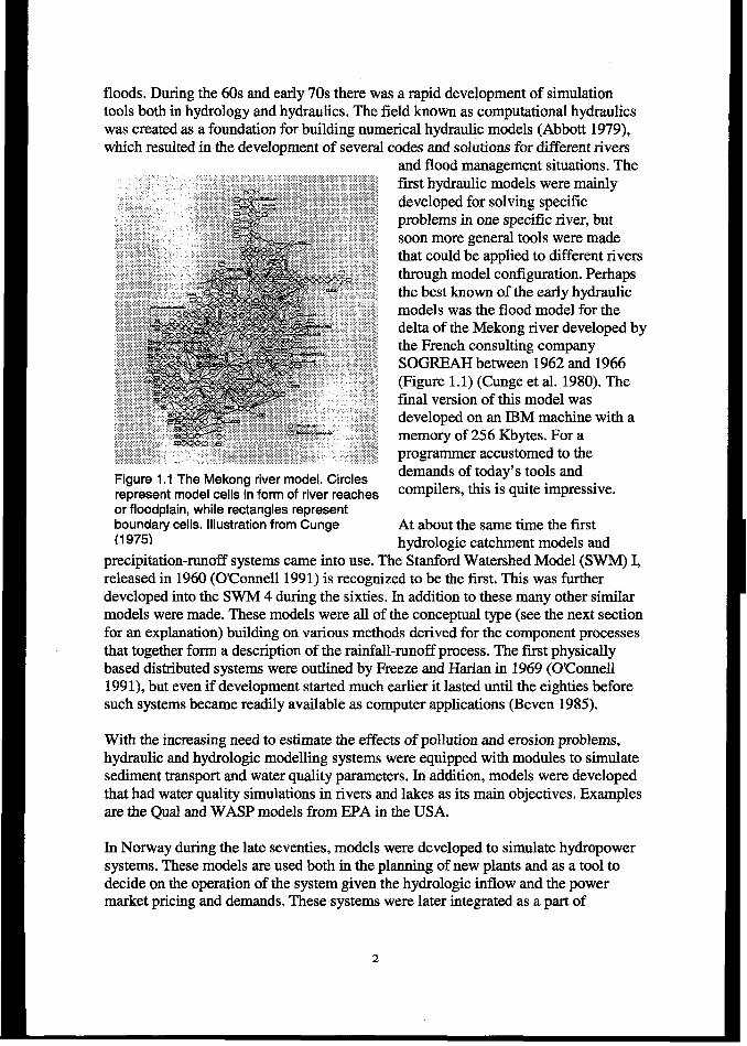
and flood management situations. Thefirst hydraulic models were mainlydeveloped for solving specificproblems in one specific river, butsoon more general tools were madethat could be applied to different riversthrough model configuration. Perhapsthe best known of the early hydraulicmodels was the flood model for thedelta of the Mekong river developed bythe French consulting companySOGREAH between 1962 and 1966(Figure 1.1) (Cunge et al. 1980). Thefinal version of this model wasdeveloped on an IBM machine with amemory of 256 Kbytes. For aprogrammer accustomed to the

Figure 1.1 The Mekong river model. Circlesdemands of today’s tools and

represent model cells in form of river reaches compilers, this is quite impressive.

or floodplain, while rectangles representboundary cells. Illustration from Cunge At about the same time the first(1975) hydrologic catchment models and

precipitation-runoff systems came into use. The Stanford Watershed Model (SWM) I,released in 1960 (O’Connell 1991) is recognized to be the first. This was furtherdeveloped into the SWM 4 during the sixties. In addition to these many other similarmodels were made. These models were all of the conceptual type (see the next sectionfor an explanation) building on various methods derived for the component processesthat together form a description of the rainfall-runoff process. The first physicallybased distributed systems were outlined by Freeze and Hahn in 1969 (OConnell199 1), but even if development started much earlier it lasted until the eighties beforesuch systems became readily available as computer applications (Beven 1985).

With the increasing need to estimate the effects of pollution and erosion problems,hydraulic and hydrologic modelling systems were equipped with modules to simulatesediment transport and water quality parameters. In addition, models were developedthat had water quality simulations in rivers and lakes as its main objectives, Examplesare the Qual and WASP models from EPA in the USA.

In Norway during the late seventies, models were developed to simulate hydropowersystems. These models are used both in the planning of new plants and as a tool todecide on the operation of the system given the hydrologic inflow and the powermarket pricing and demands. These systems were later integrated as a part of

2

environmental impact tools to model how environmental constraints on hydropoweroperation, most often minimum-flow release, which may affect the power production.

Through the 70s and 80s the increased availability of machines and tools combinedwith more demands on simulation objectives led to a steady development in this field.Especially the advent of the personal computer during the first part of the eighties ledto a increased user base and also to new demands on the up until then mainhme andmini machine-based simulation systems. The increased knowledge about interactionsbetween water and the environment and the need to model these interactions also putsincreasing demands on the modellings ystems. This led to the need to describe boththe hydrological and hydraulic processes and how these interact with each other, theecosystems and other components of the aquatic environment. The realization of theneed to not only consider the hydraulic and hydrologic aspects of modelling waterresources, but also the socio-tednical aspects led to the transition of computationalhydraulic into hydroinformatics. In his book Hydroinformatics, Abbott (1991)describes the development of the field through five generations:

‘l%ej%-stgeneration of the hydroinformatics system consisted of the use of computersto solve equations in a faster and more precise way than could be done manually.These systems were programs that incorporated the most used analytical methods.According to Abbott (1991) the first generation systems was implemented in a‘human-fiendly’ way. The human-friendly concept means that equations alreadyprepared for human use were directly implemented without any thoughts ofoptimizing them for computer use.

The second generation of the hydroinformatics system was based on using numericalmethods to solve the equations describing the physical system. Following the samenotion as for the first-generation system, these systems were developed in a ‘machine-friendly’ way. This approach utilized techniques made for taking advantage of thecomputer systems they were developed on. This involves development of numericalschemes, and transferring the equations into a form that is suitable for computer usebut not easily usable by humans. The second-generation systems were customised tothe problem they were going to solve, and specialized modelling groups that had theexpertise both to formulate, implement, calibrate and operate the program systemdeveloped them. The Mekong model mentioned earlier in this section is an example ofa second-generation system.

The use of “prefabricated” modelling tools emerged in order to simplify thedevelopment of large models and meet increased demands for such tools. These camein the form of function libraries that could be used to build the program. The Wrd-

gerzeratz’on hydroinformatics systems are based on the use of prefabricatedcomponents. This approach simplifies the implementation phase when a new system isconstructed. The third-generation systems lacks the “user-friendly” tools to guide theuser through setup and calibration, and therefore the operation of the third generationsystem still requires expert knowledge about the software itself. The advent of the

Personal Computer made the computer available to many new users. The increase inthe number of users led to the next generation of the hydroinformatics system.

l%e~orzrth-generation systems build on the second and third generations by providinguser-friendly tools for calibration and operation. The availability of machines withgraphical user interfaces provided the developers with a powerful tool to build bothsystems for data entry and data presentation in an easy and user-friendly way.Combined with built-in systems for guidance like providing defaults for variables andchecking user input for errors made the modellings ystems available to lots of newusers. Today there are almost an endless number of available systems on the marketfor hydraulic, hydrologic and other water-related purposes.

Still the fourth-generation systems provided the user with huge amounts of data thatneeded hydraulic expertise to translate and understand. Even with the advancedpresentation tools found in the previously mentioned system, it can be difficult tocomprehend the data. This problem is especially marked in cases where data should beprocessed and made available as input for a new program, for example an impactassessment module coupled to a hydraulic model.

Thefifih-generation systems extend the existing tools with a decision-makingcomponent. An expert system or knowledge-based system using artificial intelligence(AI) notation is a key component in the systems of this generation. This provides away to retrieve and present the information in a way that is relevant andunderstandable for the persons that are going to build their decisions on the simulationresults. Ongoing research in AI techniques like Neural Networking, GeneticAlgorithms, Data Mining and Agent systems provides important advances andpossibilities for development of hydroinformatics systems (Abbott et al. 1994;Karunanithi et al. 1994; Babovic 1996; Babovic 1998; Hall and Minns 1998). Anotherinteresting field is the research in Active Decision Support Systems (Carlson et al.1998) that could be employed in the field of water resource management as an“intelligent” information provider on top of the hydrologic and hydraulic simulationsystems. This can prove to be a very effective preprocessor to handle couplingbetween different program systems.

1.1.3 Definition of terms andprope~”es

There is no defined terminology that covers the subjects presented in this text. Asmuch as possible the terms and properties used in the descriptions follow the use inthe literature cited, but to avoid misunderstandings this section contains definitions ofthe most commonly used terminology.

The concept of a system is used in many situations in this thesis. Dooge defines asystem as being a structure, device, scheme or procedure that relates an input to anoutput in a given time frame (Overton and Meadows 1976). He defines the followingkey concepts:

4

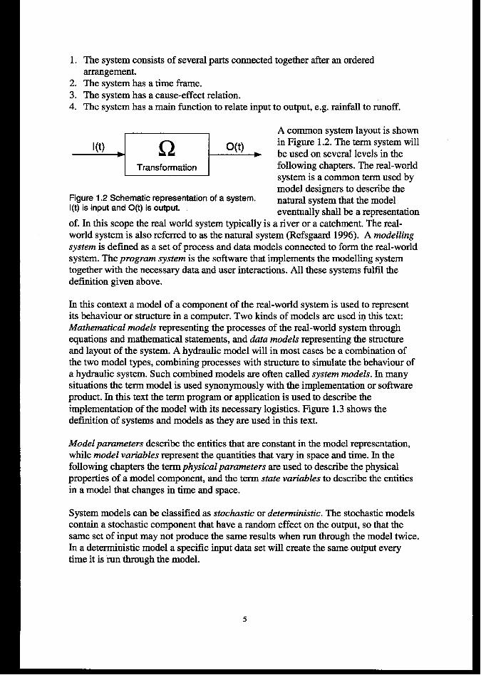
1. The system consists of several parts connected together after an orderedarrangement.

2. The system has a time frame.3. The system has a cause-effect relation.4. The system has a main function to relate input to output, e.g. rainfall to runoff.

--’L2GP!--2:::::following chapters. The real-world

model designers to describe theFigure 1.2 Schematic representation of a system.l(t) is input and O(t) is output.

natural system that the modeleventually shall be a representation

of. In this scope the real world system typically is a river or a catchment. The real-world system is also referred to as the naturals ystem (Refsgaard 1996). A modelling

system is defined as a set of process and data models connected to form the real-worldsystem. The program system is the software that implements the modelling systemtogether with the necessary data and user interactions. All these systems fulfil thedefinition given above.

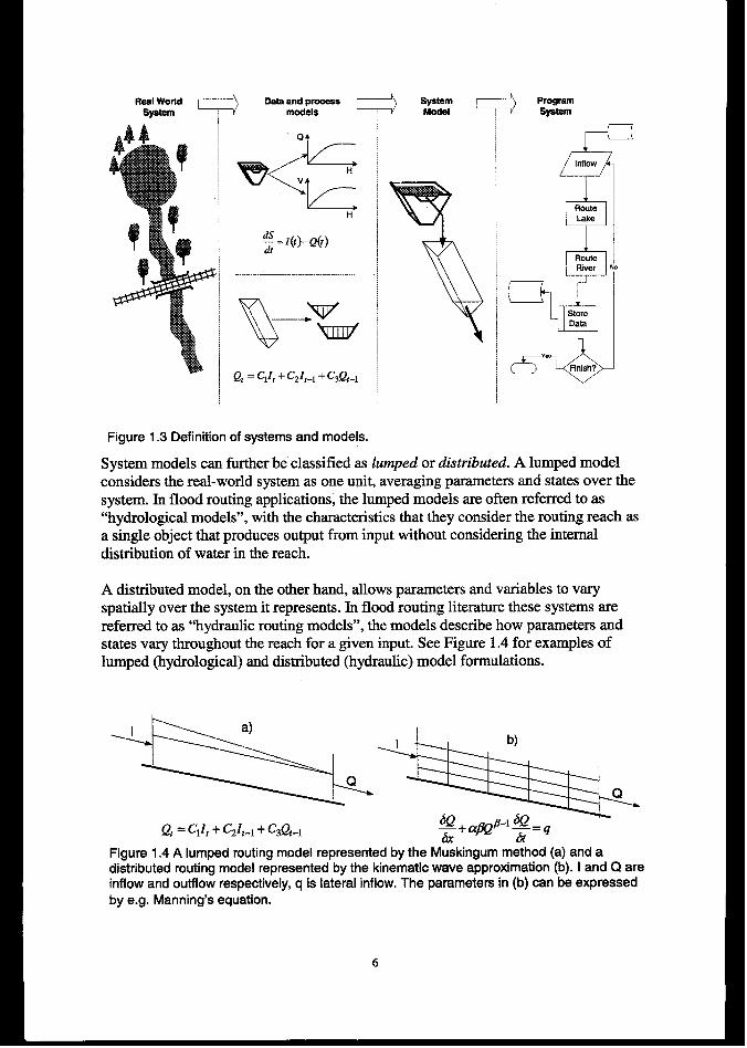
In this context a model of a component of the real-world system is used to representits behaviour or structure in a computer. Two kinds of models are used in this text:A4athematical models representing the processes of the real-world system throughequations and mathematical statements, and data models representing the structureand layout of thes ystem. A hydraulic model will in most cases be a combination ofthe two model types, combining processes with structure to simulate the behaviour ofa hydraulic system. Such combined models are often called system models. In manysituations the term model is used synonymously with the implementation or softwareproduct. In this text the term program or application is used to describe theimplementation of the model with its necessary logistics. Figure 1.3 shows thedefinition of systems and models as they are used in this text.

Model parameters describe the entities that are constant in the model representation,while model variables represent the quantities that vary in space and time. In thefollowing chapters the term physical parmneters are used to describe the physicalproperties of a model component, and the term state variables to describe the entitiesin a model that changes in time and space.

System models can be classified as stochastic or deterministic. The stochastic modelscontain a stochastic component that have a random effect on the output, so that thesame set of input may not produce the same results when run through the model twice.In a deterministic model a specific input data set will create the same output everytime it is run through the model.

5

m--, !.#--r-l ..- --- ---—- ~ . . . . ----4 .—...4

WLu ., ,“ p, w-.

models L

\

‘v“w

Q,= cI~, + c2ft-1 + c3~,-1

Figure 1.3 Definition of systems and models.

~

Inflow

QRouteLake

QRouteRiier

%

StoreData

System models can further be classified as lumped or distributed. A lumped modelconsiders the real-world system as one unit, averaging parameters and states over thesystem. In flood routing applications, the lumped models are often referred to as“hydrological models”, with the characteristics that they consider the routing reach asa single object that produces output from input without considering the internaldistribution of water in the reach.

A distributed model, on the other hand, allows parameters and variables to varyspatially over the system it represents. In flood routing literature theses ystems arereferred to as “hydraulic routing models”, the models describe how parameters andstates vary throughout the reach for a given input. See Figure 1.4 for examples oflumped (hydrological) and distributed (hydraulic) model formulations.

~ b)

Qt= W~ + W,.1 + C3Q,.I ~+a.fl-l~=qii

Figure 1.4 A lumped routing model represented by the Muskingum method (a) and adistributed routing model represented by the kinematic wave approximation (b). I and Q areinflow and outflow respectively, q is lateral inflow. The parameters in (b) can be expressedby e.g. Manning’s equation.

6

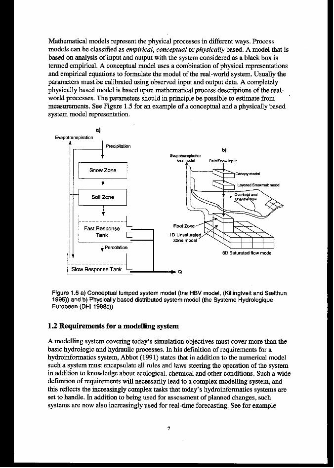
Mathematical models represent the physical processes in different ways. Processmodels can be classified as empirical, conceptual or physically based. A model that isbased on analysis of input and output with the system considered as a black box istermed empirical. A conceptual model uses a combination of physical representationsand empirical equations to formulate the model of the real-world system. Usually theparameters must be calibrated using observed input and output data. A completelyphysically based model is based upon mathematical process descriptions of the real-world processes. The parameters should in principle be possible to estimate frommeasurements. See Figure 1.5 for an example of a conceptual and a physically basedsystem model representation.

Evapc

a)mapiretion

+Precipitation

i~ b)

ht

-1 Soil Zone

I

I+,

1------------.,

I I

“-3s m&el Rainf%ow inout

Root

ID Unszone

3D Saturatedflowmodel

!----------------4 1I Slow ResponseTank ‘=.

Figure 1.5 a) Conceptual lumped system model (the HBV model, (KNingtveit and %elthun1995)) and b) Physically based distributed system model (the Systeme HydrologiqueEuropeen (DHI 1998c))

1.2 Requirements for a modelling system

A modelling system covering today’s simulation objectives must cover more than thebasic hydrologic and hydraulic processes. In his definition of requirements for ahydroinformatics system, Abbot (1991) states that in addition to the numerical modelsuch a system must encapsulate all rules and laws steering the operation of the systemin addition to knowledge about ecological, chemical and other conditions. Such a widedefinition of requirements will necessarily lead to a complex modelling system, andthis reflects the increasingly complex tasks that today’s hydroinforrnatics systems areset to handle. In addition to being used for assessment of planned changes, suchsystems are now also increasingly used for real-time forecasting. See for example

7

Refsgaard and Abbott (1996) for a discussion of the potential uses for distributedhydrological models in water resources management. Another example is therequirement specification for the Norwegian HYDRA flood model (Killingtveit et al.1998). In addition to the usual inflow calculation and flood routing, this modellingsystem should be able to integrate effects of urbanization, agriculture, forestry andoperation of complex hydropower system into the hydrologic and hydraulic floodsimulation system (Roald 1997). The number of potential application combined withthe range of processes a modern modelling system should be able to handle makes itnecessary to work through the requirement specification in great detail. Therequirements both ensure that the system will be able to perform all its functions andthat the models that build the system can be specified and implemented in a way thatmakes it possible to maintain and use them in the future.

An example of the need to integrate many simulation objectives is the Enmag(Killingtveit and Szelthun 1995) hydropower simulation programs covering hydrology,reservoir operation, water transport and hydropower production. The Hydropowersimulation part is governed by rules and restrictions often placed on the system byenvironmental issues. Restrictions on reservoir filling or minimum flows have to beconsidered in addition to economic restrictions defined by delivery contracts andpower pricing.

To handle some of the requirements outlined above, the application code willnecessarily become complex. In addition to the code solving equations and handlingthe data describing the system, one will need tools for data import and control, userinterface and possible links to databases and external applications. In many cases thecode that handles the actual numerical model is only a small part of the totalapplication code. This creates new requirements for the software development processitself, in order to avoid problems with future extensions, portability and maintenance.For a large commercial software system it is therefore needed to assess the softwareengineering problems with as much attention as the hydraulic or hydrologicalcomponents of the application.

A hydroinformatics system should provide a flexible way of representing the real-world system that can be adapted to both the simulation objective and the availableinformation about the real-world systems structure and operation. The importance ofthis flexibility is strongly linked to the complexity of the simulation since a largehydroinformatics system must be able to cope with a large number of interconnectedobjectives. It is also desirable to have the ability to use process descriptions ofdifferent complexity at different locations in the real-world system. This will reducesimulation time and reduce the need for detailed (and expensive) data collection inareas where the need for detailed simulations is not that important.

The hydroinformatics system should be flexible regarding inclusion of externallydeveloped applications in hydrology and hydraulics. Today there are many tested anddocumented commercial applications available, and being able to use one of thesesaves both development and testing time. It is also quite likely that “simulation

8

engines” without the logistics of a complete application will be available for futureapplication designers, either as installable plug-ins or as networked resources. Thiswill further enhance the development process.

Requirements, restrictions and other simulation control parameters must beencapsulated by the system. The encapsulation must be user defined and changeableto cover a number of possible types and combinations.

In order to cover the need to extend the simulation objectives to impact assessmentstudies, the hydroinformatics system should provide data exchange or integrationbetween the base hydrologic and hydraulic simulation systems and environmental andeconomic impact analysis tools.

For a large system, data handling is critical and efficient data storage and handling isneeded. For storage, it should be possible to integrate with a variety of databasesystems. The data handling facilities should provide data and interfaces for a possibleinclusion of decision support systems, and make it possible to export and present datain suitable systems, e.g. Geographical Information Systems.

In a similar fashion requirements can be set for the software development.

- Develop the tool based on reusable components and designs. This makes itpossible to develop an error-free and well-documented foundation for futureprojects. In today’s software development world this leads to the use of designpatternsl in the design phase and the use of application framework~ in theimplementation phase.

- Use and build on tested and supported commercizd libraries and applicationframeworks where this is possible. This reduces code size and simplifiesmaintenance.

- Reduce coupling between modules by a component-based development to easefuture extensions and simplify maintenance.

1.3 Objectives of this work

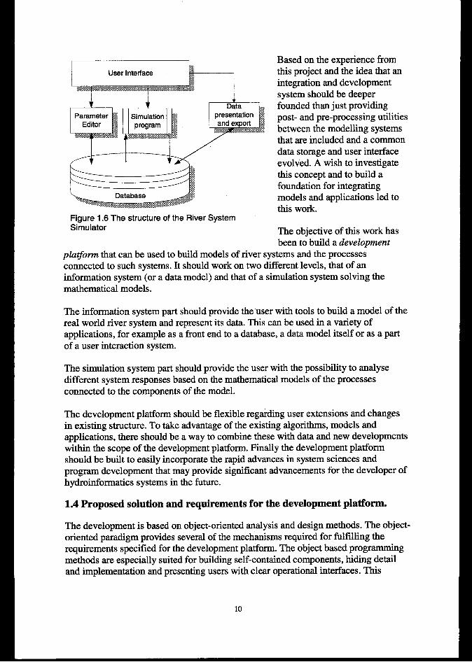
The work presented in this thesis stems from the development of the River SystemSimulator (RSS) (Killingtveit et al. 1995) where the author was involved in systemdesign and development. The RSS is an integration platform for a wide array ofexisting modelling systems. The project objective was to integrate the tools needed todo multi-purpose planning with an emphasis on hydropower development andanalysing environmental impacts of suchs ystems. The RSS integrated the models intoa common database and a common user interface. The actual applications were keptunchanged, they communicated with the database and the user interface thoughapplication specific data processors (Figure 1.6).

1Designpatternsprovidea solutionrecipeforspeciiicproblemsin thedesignofobject-orientedsoftware.2Anapplicationframeworkis a ma changeableandexpendablelibrmy.

9

1 User Intsrfaca I

I

.’:’”

Figure 1.6 The structure of the River SystemSimulator

Based on the experience fromthis project and the idea that anintegration and developmentsystem should be deeperfounded than just providingpost- and pre-processing utilitiesbetween the modelling systemsthat are included and a commondata storage and user interfaceevolved. A wish to investigatethis concept and to build afoundation for integratingmodels and applications led tothis work.

The obiective of this work hasbeen t; build a development

platjonn that can be used to build models of river systems and the processesconnected to such systems. It should work on two different levels, that of aninformation system (or a data model) and that of a simulation system solving themathematical models.

The information system part should provide the user with tools to build a model of thereal world river system and represent its data. This can be used in a variety ofapplications, for example as a front end to a database, a data model itself or as apartof a user interaction system.

The simulation system part should provide the user with the possibility to analysedifferent system responses based on the mathematical models of the processesconnected to the components of the model.

The development platform should be flexible regarding user extensions and changesin existing structure. To take advantage of the existing algorithms, models andapplications, there should be a way to combine these with data and new developmentswithin the scope of the development platform. Finally the development platformshould be built to easily incorporate the rapid advances in system sciences andprogram development that may provide significant advancements for the developer ofhydroinfonnatics systems in the fiture.

1.4 Proposed solution and requirements for the development platform.

The development is based on object-oriented analysis and design methods. The object-oriented paradigm provides several of the mechanisms required for fulfilling therequirements specified for the development platform. The object based programmingmethods are especially suited for building self-contained components, hiding detailand implementation and presenting users with clear operational interfaces. This

10

encapsulation of information into objects can in many cases be seen as a realization ofthe electronic knowledge encapsulator as defined by Abbott (1993). The use ofobjects requires a new way of thinking and a new method of structuring the problemwe are designing a solution to. During the development, the main emphasis has beenput on building an open system, a system where one can easily add newdevelopments, incorporate changes in modelling strategy and link differentapplications together. The developed system should fulfil the following requirements:

It should be possible to build a model of the real-world system by pickingcomponents that describe the real-world entities. Each component should be ableto store data representing both the physical parameters and states of thecomponent. The amount and type of data in each component should not be fwed.It should be possible to specify the processes we want to model for eachcomponent and insert them when they are needed. Each component should be ableto use a different number of process models of varying types.User interaction for example in the form of data insertion and result inspectionshould be separated from components and processes to avoid bindings to specificformats and systems and to simplify porting and maintenance.Coupling between components should beat a minimum to create reusable entitiesthat can be used in many applications without having the need to customise thecode every time it is used. Required interaction between modules should be clearlydefined.It should be possible to add new modules to the system and get them to behave likethe existing modules.The system should be open to integration with existing tools.

The development platform has been implemented in the C++ language. The reason forthis is mainly the author’s prior knowledge of the system, the excellent availability oftools and third party toolkits and the potential for inclusion of components written inother languages into C++ programs.

The work was carried out in two steps. First the development platform (the termframework will be used to describe the development platform hereafter) was designedand implemented, then it was applied to two cases concerning applicationdevelopment in water resource planning. During the application phase iterations weremade with the framework to correct errors and increase the flexibility in use.

The remainder of this report describes the framework design and its application to theHYDRA flood model development and the design of the new toolkit for physical fishhabitat modelling.

1.5 Structure of thesis

Chapter 2 gives a brief introduction to object-oriented concepts and the key points anddifferences between the object-oriented approach and the traditional functionalapproach. The chapter also gives an overview of potential applications of object-

11

oriented methods in the field of hydroinformatics, illustrated by examples of existingwork in this field.

The next three chapters present the development and use of the framework. Chapter 3presents the analysis and design of the framework and its components. This chapterdescribes how the requirements specified above are built into the system analysis andhow they are fulfilled through the design and implementation of the fkunework. Thechapter is based on a five-step object-oriented analysis and design methodology that isalso briefly introduced in this chapter. In the following Chapter 4, the componentclasses in the framework are presented together with their relations and interactions ona user level. Chapter 5 has several examples of how the framework can be used toconstruct modelling systems. This chapter also describes the process of including newcomponents, including the procedure for linking applications that are developedexternally.

The next two chapters present applications of the framework. The 1995 flood in theGlomma river system in Norway showed the need to build a tool for studying floodimpacts and the factors that may impact flood volumes and flood peaks, Chapter 6describes how the application framework was used to integrate the components of theHYDRA flood modelling study. River regulations for hydropower, irrigation orsimilar causes changes in the physical conditions in the river which again may createproblems for species using the river as a living area (tibitat), Fish is one of thespecies that may be adversely impacted by these encroachments, and the need toinvestigate how fish habitat is changing with changing physical conditions lead to thedevelopment of several models for quantifying these impacts. New tools for assessingimpacts on fish habitat are currently under development, and the framework has beenused in the development of this system. Chapter 7 gives an overview of the HabitatModelling Framework that is based on the framework, and there-design of theNorwegian HABITAT program system. The new version of HABITAT uses newhabitat assessment methods in combination with two- and three-dimensional hydraulicmodels to provide abetter foundation for quantifying effects from changes in instreamflow conditions on fish.

Chapter 8 gives a short introduction to possible future integration of new computingmethodologies into the framework. Developments in areas like database technologyand distribution of data and simulation tools may in the future provide usefultechniques for developing modelling systems in water resource management.

12

2. OBJECT-ORIENTED METHODS IN APPLICATION DESIGN

2.1 Introduction to object-oriented methods.

2.1.1 Languages and modelling issues

Over the last deeade the use of object-otiented techniques in analysis and design ofsoftware systems has become more and more common. Even if the concept of objectprogr amming has existed since the late sixties when the SIMULA language wasintroduced (Nygaard and Dahl 1978), it is mainly in the last decade that this techniquehas gained momentum. Much of the credit for this is due to the C++ language thatbrought object-oriented concepts into the widely used C language (Stroustrup 1994).Specialists on object-oriented theory debate if the success of CW as an object-onented language is a good thing, but it has definitely provided a lot of softwaredevelopers with a foundation of good tools and effective analysis and design methods.Especially the development of user interfaces through object-oriented tools hasbrought this technique into use among a lot of developers. It is also very likely thatobject-oriented methods will gain even more momentum in the future as aconsequence of the introduction of the Java language and the increasing popularity ofbuilding World Wide Web based applications. The increased focus on componentbased programming in the Microsoft Windows environment also build on object-oriented ideas, even when the components are used from procedural languages.

It is advisable to have a clearly defined development strategy in order to build a pieceof software. A common software development method follows these steps (e.g.(Somerville 1989)):

1) Domain analysis (Analysis phase).2) Model design (Design phase).3) Implementation of the design.4) Testing and verification.

In a function-oriented approach, the representation of the real-world system is definedthrough data and functions operating on the data. A problem with this approach is thetransition from the analysis phase (1) to the design phase (2) and vice versa. If welook at a river system, we may define lakes and rivers with their corresponding dataflow in the analysis phase. In the design phase these must be transformed (mapped)into functions and data in the form of flow charts and structure diagrams. The realworld entities are thereby transformed into completely different software entities. In aproject of some size there is no easy mapping between these phases, making tracingchanges or editing the analysis and design during development difficult. The object-oriented strategy is better since one is working with the entities of the real-world bothin the analysis and the design phase. A lake object found in the analysis phase willstill be a lake in the design, and it is possible to keep the notion of real world entitiesin both phases. Using this approach switching between the analysis and design phases

13

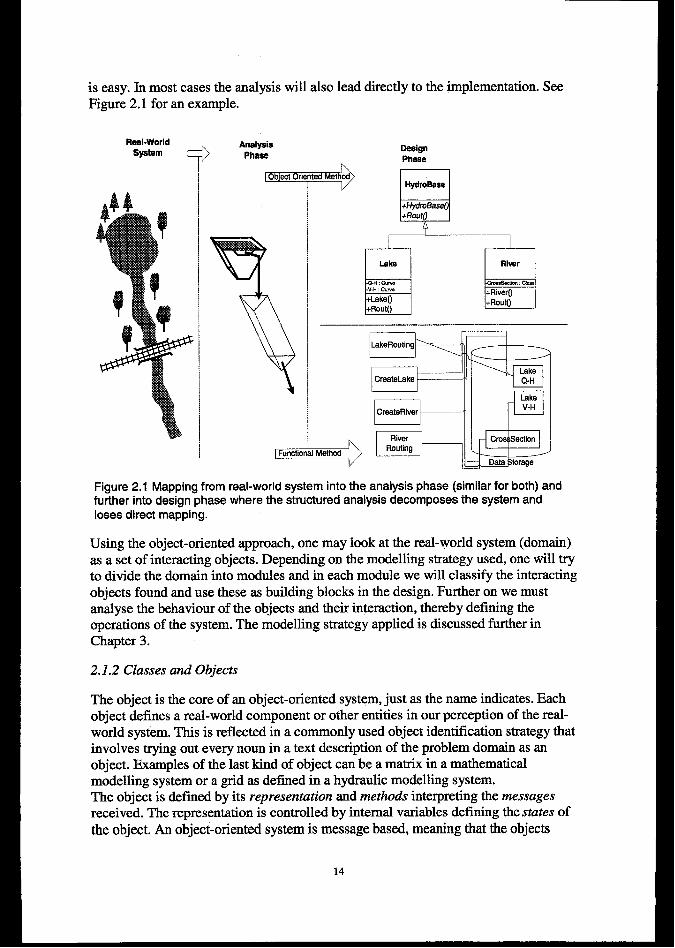
is easy. In most cases the analysis will also lead directly to the implementation. SeeFigure 2.1 for an example.

Reel-World+’)

AnalysisSyetem Pheee

I CEiIE!E

Deeign

Phese

+HytlroSsse(+Routfj

?

lake River

.Q.H : Cum

.V.H : cum—0” : *

+Lakeo+RiverO

+Routo+Routo

LakeRouting

CreateLske

1

CreeteRiier

J

Figure 2.1 Mapping from real-world system into the analysis phase (similar for both) andfurther into design phase where the structured analysis decomposes the system andloses direct mapping.

Using the objeet-onented approach, one may look at the real-world system (domain)as a set of interacting objects. Depending on the modelling strategy used, one will tryto divide the domain into modules and in each module we will classify the interactingobjects found and use these as building blocks in the design. Further on we mustanalyse the behaviour of the objects and their interaction, thereby defining theoperations of the system. The modelling strategy applied is discussed further inChapter 3.

2.1.2 Classes and Objects

The object is the core of an object-oriented system, just as the name indicates. Eachobject defines a real-world component or other entities in our perception of the real-world system. This is reflected in a commonly used object identification strategy thatinvolves trying out every noun in a text description of the problem domain as anobject. Examples of the last kind of object can be a matrix in a mathematicalmodelling system or a grid as defined in a hydraulic modelling system.The object is defined by its representation and methods interpreting the messagesreceived. The representation is controlled by internal variables defining the states ofthe object. An object-oriented system is message based, meaning that the objects

14

interact bypassing messages to each other. The methods that receive and translate themessages are implemented as functions in the object.

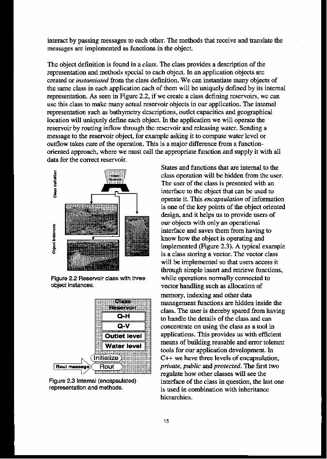
The object definition is found in a class. The class provides a description of therepresentation and methods special to each object. In an application objects arecreated or instann”ated from the class definition. We can instantiate many objects ofthe same class in each application each of them will be uniquely defined by its internalrepresentation. As seen in Figure 2.2, if we create a class defining reservoirs, we canuse this class to make many actual reservoir objects in our application. The internalrepresentation such as bathymetry descriptions, outlet capacities and geographicallocation will uniquely define each object. In the application we will operate thereservoir by routing inflow through the reservoir and releasing water. Sending amessage to the reservoir object, for example asking it to compute water level oroutflow takes care of the operation. This is a major difference from a function-oriented approach, where we must call the appropriate function and supply it with alldata for the correct reservoir.

Figure 2.2 Reservoir class with threeobject instances.

Figure 2.3 Internal (encapsulated)representation and methods.

States and functions that are internal to theclass operation will be hidden horn the user.The user of the class is presented with aninterface to the object that can be used tooperate it. This encapsulation of informationis one of the key points of the object orienteddesign, and it helps us to provide users ofour objects with only an operationalinterface and saves them from having toknow how the object is operating andimplemented (Figure 2.3). A typical exampleis a class storing a vector. The vector classwill be implemented so that users access itthrough simple insert and retrieve functions,while operations normally connected tovector handling such as allocation of

memory, indexing and other datamanagement functions are hidden inside theclass. The user is thereby spared from havingto handle the details of the class and canconcentrate on using the class as a tool inapplications. This provides us with efficientmeans of building reusable and error toleranttools for our application development. InC++ we have three levels of encapsulation,private, public and protected. The first two

regulate how other classes will see theinterface of the class in question, the last oneis used in combination with inheritancehierarchies.

15

2.1.3 Inheritance, polymorphism and dynamic binding

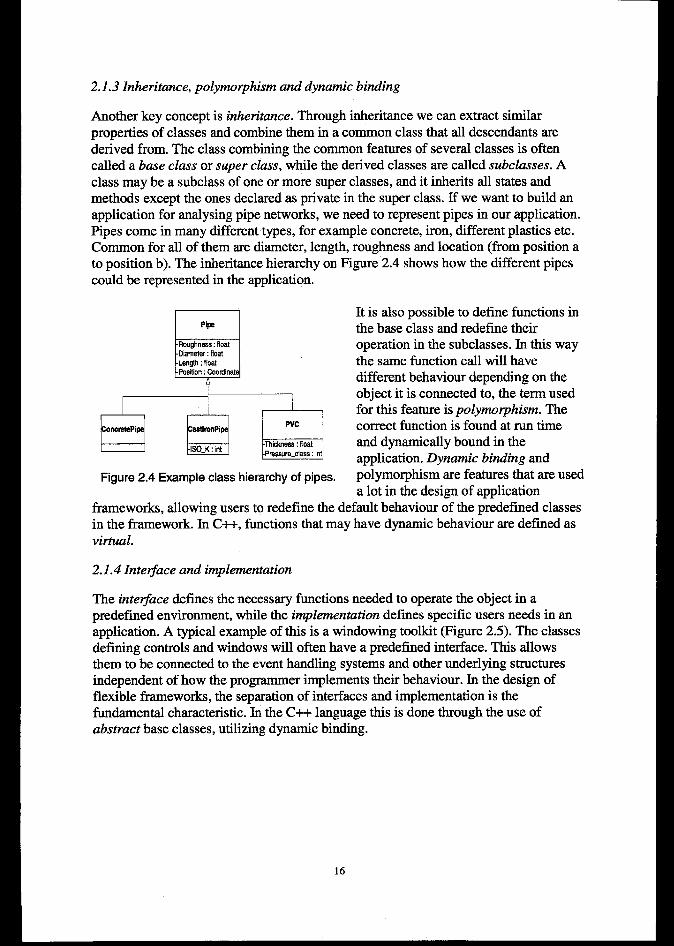
Another key concept is inheritance. Through inheritance we can extract similarproperties of classes and combine them in a common class that all descendants arederived from. The class combining the common features of several classes is oftencalled a base class or super ckzss, while the derived classes are called subclasses. Aclass may be a subclass of one or more super classes, and it inherits all states andmethods except the ones declared as private in the super class. If we want to build anapplication for analysing pipe networks, we need to represent pipes in our application.Pipes come in many different types, for example concrete, iron, different plastics etc.Common for all of them are diameter, length, roughness and location (from position ato position b). The inheritance hierarchy on Figure 2.4 shows how the different pipescould be represented in the application.

r==l

~

Roughness:floatDiameter:floatLength:fbatPOskbn: Coordinate

Figure 2.4 Example class hierarchy of pipes.

It is also possible to define functions inthe base class and redefine theiroperation in the subclasses. In this waythe same function call will havedifferent behaviour depending on theobject it is connected to, the term usedfor this feature is polymmphism. Thecorrect function is found at run timeand dynamically bound in theapplication. Dynamic binding andpolymorphism are features that are useda lot in the design of application

frameworks, allowing users to redefine the default behaviour of the predefine classesin the framework. In C++, functions that may have dynamic behaviour are defined asvirtual.

2.1.4 Inte~ace and implementation

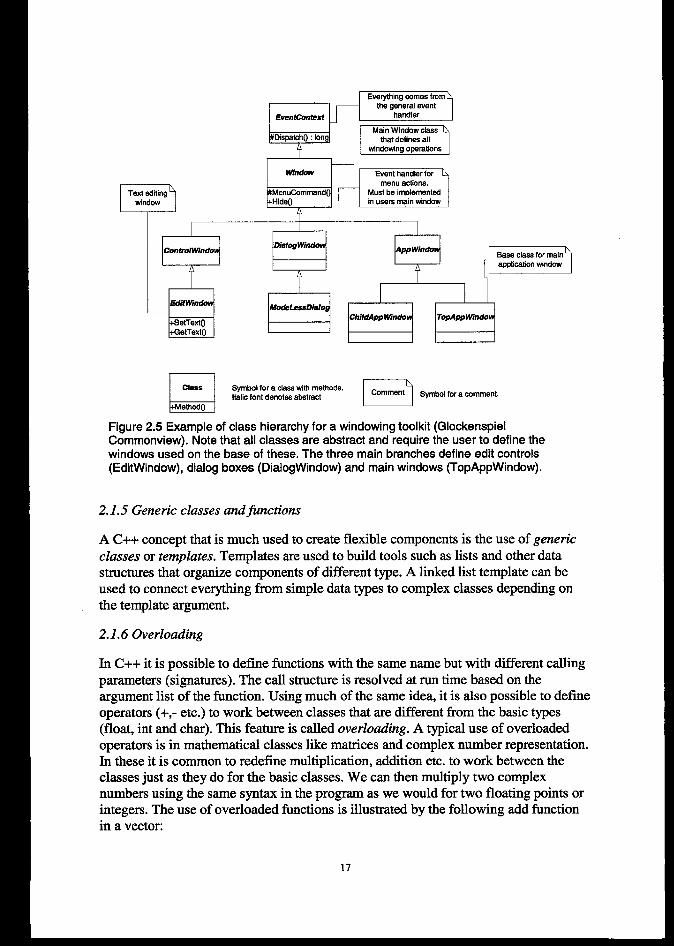
The inte~ace defines the necessary functions needed to operate the object in apredefine environment, while the implementation defines specific users needs in anapplication. A typical example of this is a windowing toolkit (Figure 2.5). The classesdefining controls and windows will often have a predefine interface. This allowsthem to be connected to the event handling systems and other underlying structuresindependent of how the programmer implements their behaviour. In the design offlexible frameworks, the separation of interfaces and implementation is thefundamental characteristic. In the C++ language this is done through the use ofabstract base classes, utilizing dynamic binding.

16

m

PCOnfdwnda

wEcWWn

etTexfOetTextl)

Everything cornea fmmthe general evant

EveWMfaxf handier

#Dispatch(J: long

4 -

menu actiinsMust be implementalin uaera main window

III

I I I

——

MClaaa Symbol fora c!aas with methods.Italic font denotes abstract

m

OOmment Symbol for a comment,

ethod(i

Figure 2.5 Example of class hierarchy for a windowing toolkit (GlockenspielCommonview). Note that all classes are abstract and require the user to define thewindows used on the base of these. The three main branches define edit controls(EditWindow), dialog boxes (DialogWindow) and main windows (TopAppWindow).

2.1.5 Generic classes atifinctions

A C++ concept that is much used to create flexible components is the use of genericclasses or templates. Templates are used to build tools such as lists and other datastructures that organize components of different type. A linked list template can beused to connect everything from simple data types to complex classes depending onthe template argument.

2.1.6 Overloading

In C++ it is possible to define functions with the same name but with different callingparameters (signatures). The call stmcture is resolved at run time based on theargument list of the function. Using much of the same idea, it is also possible to defineoperators (+,- etc.) to work between classes that are different from the basic types(float, int and char). This feature is called overloading. A typical use of overloadedoperators is in mathematical classes like matrices and complex number representation.In these it is common to redefine multiplication, addition etc. to work between theclasses just as they do for the basic classes. We can then multiply two complexnumbers using the same syntax in the program as we would for two floating points orintegers. The use of overloaded functions is illustrated by the following add functionin a vectoc

Void add(float number); Illldd a number to the end of the vector.Void add(float number, int index); //Add a number at position defined by index

Which function to call would be resolved by the program at runtime dependent on ifwe call it with only a float or with a float and an integer. For an interesting discussionon overloading operators and the cost of using itin computational intenseapplications, see (Arge et al. 1997).

2.1. 7An example

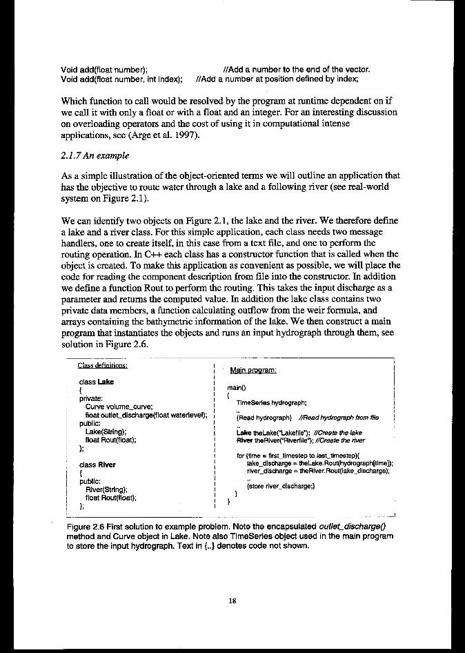
As a simple illustration of the object-oriented terms we will outline an application thathas the objective to route water through a lake and a following river (see real-worldsystem on Figure 2. 1).

We can identify two objects on Figure 2.1, the lake and the river. We therefore definea lake and a river class. For this simple application, each class needs two messagehandlers, one to create itself, in this case from a text file, and one to perform therouting operation. In C++ each class has a constructor function that is called when theobject is created. To make this application as convenient as possible, we will place thecode for reading the component description fkom file into the constructor. In additionwe define a function Rout to perform the routing. This takes the input discharge as aparameter and returns the computed value. In addition the lake class contains twoprivate data members, a function calculating outflow from the weir formula, andarrays containing the bathymetric information of the lake. We then construct a mainprogram that instantiates the objects and runs an input hydrography through them, seesolution in Figure 2.6.

Classdefinitions:

class Lake{private:

Curvevolume_cume;float outlet_diacharge(float waterievel);

publicLake(String);float Rout(float);

);

class River{public:

Rtver(String);float Rout(float);

};

Main cmxrram:

maino{

TimeSeries hydrography;

[Read hydrography} /YReadhydrograph fmm file

bke theLaka~Lakefile”); //Create the lakeRiver the!%ver(Wiverfile”);//Create the river

for (time = first_timeatepto laa_timeatap){lake_discharge= theLake.Rout(hydrograph[time]);~river_diseharga= theRiver.Rout(lake_dseharge); ~

{storeriver_dischargej} I

1 11

Figure 2.6 First solution to example problem. Note the encapsulated outle~dischargeomethod and Curve object in Lake. Note also TlmeSeries object used in the main programto store the input hydrography.Text in {..} denotes code not shown.

18

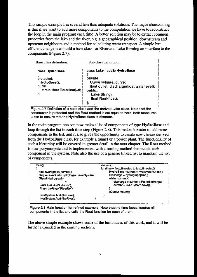
This simple example has several less than adequate solutions. The major shortcomingis that if we want to add more components to the computation we have to reconstructthe loop in the main program each time. A better solution maybe to extract commonproperties from the lake and the river, e.g. a geographical position, downstream andupst.nxun neighbors and a method for calculating water transport. A simple butefficient change is to build a base class for River and Lake forming an interface to thecomponents (Figure 2.7):

Base class definition: Sub class definition:

class HydroBaae I class Lake : public HydroBaae

I { ~{

protected: I private:HydroBaseo; I Curve volume_curve;

public: float outlet_discharge(float waterlevel);virtual float Rout(float)=O; ~ public:

!}; I Lake(String);

float Rout(float);

/ };

Figure 2.7 Definition of a base class and the derived Lake class. Note that theconstructor is protected and the Rout method is set equal to zero, both measurestaken to ensure that the HydroBase class is abstract.

In the main program one can now make a list of components of type HydroBase andloop through the list in each time step (Figure 2.8). This makes it easier to add morecomponents to the list, and it also gives the opportunity to create new classes derivedfrom the HydroBase class, for example a tunnel or a power plant. The functionality ofsuch a hierarchy will be covered in greater detail in the next chapter. The Rout methodis now polymorphic and is implemented with a routing method that match eachcomponent in the system. Note also the use of a generic linked list to maintain the listof components.

maino Main contd. 1

{ for (time = firet_timestepto last_timeetep){float hydrogrsph[number]; HydroBaee *current= riversystem.tlrsto; ~

I SingleLinkedListcHydroBase> riversystsm; D&harga = hydrograph[time]; ~{Read Hydrography} while (current){

,t; discharge = current->Rout(diacharge); ~

Lake thaLeke(’’Lskefile”); current = rivarSyetam.Nexto;River theRiver(”Riierfile”); } I

{Output resuits};I riverSyetem.Add (thel-aka} 1 1I riverSyetam.Add (thaRiver); } I,

Figure 2.8 Main function for refined example. Note that the time loops iterates ailcomponents in the list and calls the Rout function for each of them.

The above simple example shows some of the basic ideas of this work, and it will befurther expanded in the coming sections.

2.2 Object-Oriented vs. Function-Oriented software design.

Object-oriented development is different from traditional structural design, and tomake the most out of the object-oriented methods it is necessary to take advantage ofthe powerful features of the methodology. For an in-dept discussion of objects versusstructural design methods, see for example Douglas (1998). The increased consistencybetween phases in the development strategy in the object-oriented methodology is onedifference between the two approaches, this has been covered in Section 2.1.1.

One important goal for this work is the ability to give a more preeise abstraction of thereal world domain. This is perhaps the largest difference between traditional designmethods and object-oriented modelling. In an objeet oriented system the separation ofdata that is neeessary in a structural design can be completely avoided since data andfunctions are joined together in the class. This gives good cohesion between the dataand the operations, which is also a close representation of how the real world operates.The use of objects keeps the analysis and design phase closer to the real world andprevents implementation details from entering the work too early. By designing withobjects it is easier to maintain less coupling between modules which makes the designeasier to maintain and expand.

Handling changes is important in any software development process. Large changes orextension will in many cases be very time consuming and costly for the project. Anobject-oriented system is in many ways designed to easily accommodate changes tothe structure since there is a clear separation between the interface to an objeet and theobject implementation. The internal structure of the object can be changed while theuse of the object in the program is kept unchanged. This feature also gives us theopportunity to use different objects in a program without changing their operatingenvironment, of course assuming that the interfaces are the same. This can be used forexample to implement reading from different sources in a program without having tochange the program itself when anew reading method is to be incorporated. Theobjeet-oriented system also has powerful features to handle this through inheritanceand programming with interfaees3.

Error handling, reliability and critical safety handling are more easily built into classesthan into a structural design. Typical examples are dimension checks in vector classeswhere it is possibly to build in automatic checks for out-of-bound access and we canalso equip such classes with automatic “cleanup” systems that prevent memoryleakage.

Encapsulation lets the designer of the object hide details and data from the userthereby making the typical error-prone operations safer to handle. The encapsulationlets us provide the user with objects that have a clearly defined interface and no needto manipulate low level functionality. In a vector class for example, chores like

3Programming gwithinterfacesis thecoreofanyframeworkdesi~ andextensiveresearehhasbeendonetocreateefficientdesignsandtoolsforthistypeofdevelopment.Fora severalgoodexamples,seestructurepatternsin 0an33naet al.(1995)

20

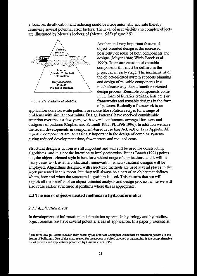
allocation, de-allocation and indexing could be made automatic and safe therebyremoving several potential error factors. The level of user visibility in complex objectsare illustrated by Meyer’s iceberg of (Meyer 1988) (figure 2.9).

A Another and very important feature of

Visible object-oriented design is the increasedpossibility of reuse of both components anddesigns (Meyer 1988; Wirfs-Brock et al.1990). To ensure creation of reusablecomponents this must be defined in theproject at an early stage. The mechanisms ofthe object-oriented system supports planningand design of reusable components in amuch clearer way than a function orienteddesign process. Reusable components comein the form of libraries (strings, lists etc.) or

Fiaure 2.9 Visibility of obiects. frameworks and reusable designs in the formof patterns. Basically a framework is an

application skeleton while patterns are more like solution recipes for a range ofproblems with similar constraints. Design Pattems4 have received considerableattention over the last few years, with several conferences arranged for users anddesigners of patterns (Coplien and Schmidt 1995; PLoP96 1996). In addition we havethe recent developments in component-based reuse like ActiveX or Java Applets. Allreusable components are increasingly important in the design of complex systemsgiving reduced development time, fewer errors and reduced costs.

Structural design is of course still important and will still be used for constructingalgorithms, and it is not the intention to imply otherwise. But as Booth (1994) pointsout, the object-oriented style is best for a widest range of applications, and it will inmany cases work as an architectural framework in which structural designs will beemployed. Algorithms designed with structured methods are used several places in thework presented in this report, but they will always be a part of an object that defineswhere, how and when the strucmred algorithm is used. This ensures that we willexploit all the benefits of an object-oriented analysis and design process, while we willalso reuse earlier structured algorithms where this is appropriate.

23 The use of object-oriented methods in hydroinformatics

2.3.1 Application areas

In development of information and simulation systems in hydrology and hydraulics,object orientations have several potential areas of application. k a paper presented at

4ThetermDesignPatternis takenfromworkbythearchitectChristopherAlexanderonstructuralpatternsin thedesignofbuildings.Oneofthemainreasonforitssuccessinobject-orientedprogrammingis thecomprehensivelistofpatternsandapplicationspresentedby Gammaet al.(1995)

21

the 1994 Hydroinformatics conference, Solornatine (1994) presented three areas ofapplication of object-orientation in hydroinformatics systems.

. Design and implementation of user interfaces

. Data management – data handling and storage

. Modelling

In addition, Solomatine also includes AI application as a field where object-orientedmethods could and have been applied. This is an important area of application,especially when we take the new developments in ecological modelling using agentbased systems (Babovic 1996) into consideration. Object-based methods are ideallysuited for building the agents and the link to the environment surrounding them.

Each of these areas presents several levels of object-oriented application, coveringeverything from a combination of object-oriented tools with traditional approaches todesigns based on pure object-oriented methods. To the three applications ofSolomatine three more areas that will have increasing importance in the future shouldbe included:

Development of distributed systems.Integration of simulation and information systems such as integration of WorldWide Web in simulation environments,Integration and development of Geographical Information Systems.

The following sections will investigate the possibilities of using object-orientation inthese categories and look at some of the current applications in each of these areas.

2.3.2 Development of user interfaces

Frameworks for designing and building user interfaces is perhaps one of the largestfields of application of objects today. Microsoft provides the Microsoft FoundationClasses (MFC) framework (Microsoft 1998) as a powerful toolkit for developingapplications on their Windows systems. Combined with the “wizards” in theirdevelopment environment, building an interface on the Windows platform hasevolved from the coding of hundreds of lines of native API commands to efficientprototyping and code generation in a high level language. Similar tools also exist onother platforms like UNIX and 0S/2. Using an object-oriented view on the elementsthat constructs windowing systems, toolkits that are portable between differentplatforms has been developed. Typically such a system provides the users with classesfor defining windows and their look and feel. The classes and their interfaces are keptunchanged between platforms making it possible to move code without any changes.The internal representation of the classes is on the other hand implemented on top ofthe underlying API of the windowing system. Typically such systems rely on the useof inheritance to create components for the users application, the framework onlyprovides an abstract interface to the windowing components. Figure 2.5 shows thehierarchy of the now defunct Comrnonview framework. This toolkit provided

22

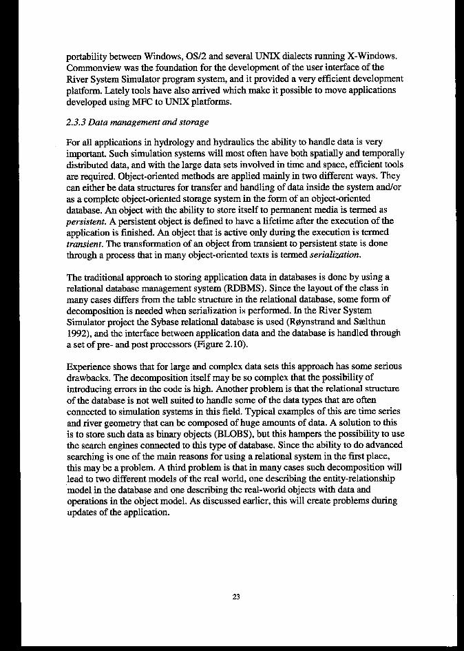
portability between Windows, 0S/2 and several UNIX dialects running X-Windows.Comrnonview was the foundation for the development of the user interface of theRiver System Simulator program system, and it provided a very efficient developmentplatform. Lately tools have also arrived which make it possible to move applicationsdeveloped using MFC to UNIX platforms.

2.3.3 Data management and storage

For all applications in hydrology and hydraulics the ability to handle data is veryimportant. Such simulation systems will most often have both spatially and temporallydistributed data, and with the large data sets involved in time and space, efficient toolsare required. Object-oriented methods are applied mainly in two different ways. Theycan either be data structures for transfer and handling of data inside the system and/oras a complete object-oriented storage system in the form of an object-orienteddatabase. An object with the ability to store itself to permanent media is termed aspersistent. A persistent object is defined to have a lifetime after the execution of theapplication is finished. An object that is active only during the execution is termedtransient. The transformation of an object from transient to persistent state is donethrough a process that in many object-oriented texts is termed serialization.

The traditional approach to storing application data in databases is done by using arelational database managements ystem (RDBMS). Since the layout of the class inmany cases differs from the table structure in the relational database, some form ofdecomposition is needed when serialization is performed. In the River SystemSimulator project the Sybase relational database is used (R@nstrand and Szelthun1992), and the interface between application data and the database is handled througha set of pre- and post processors (Figure 2. 10).

Experience shows that for large and complex data sets this approach has some seriousdrawbacks. The decomposition itself may be so complex that the possibility ofintroducing errors in the code is high. Another problem is that the relational structureof the database is not well suited to handle some of the data types that are oftenconnected to simulation systems in this field. Typical examples of this are time seriesand river geometry that can be composed of huge amounts of data. A solution to thisis to store such data as binary objects (BLOBS), but this hampers the possibility to usethe search engines connected to this type of database. Since the ability to do advancedsearching is one of the main reasons for using a relational system in the first place,this may be a problem. A third problem is that in many cases such decomposition willlead to two different models of the real world, one describing the entity-relationshipmodel in the database and one describing the real-world objects with data andoperations in the object model. As discussed earlier, this will create problems duringupdates of the application.

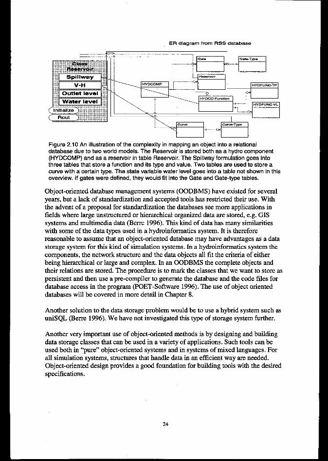
ER diagram from RSS database

Figure 2.10 An illustration of the complexity in mapping an object into a relationaldatabase due to two world models. The Reservoir is stored both as a hydro component(HYDCOMP) and as a resewoir in table Resewoir. The Spillway formulation goes intothree tables that store a function and its type and value. Two tables are used to store acurve with a certain type. The atate variable water level goes into a table not shown in thisoverview. if gates were defined, they would fit into the Gate and Gate-type tables.

Object-oriented database management systems (OODBMS) have existed for severalyears, but a lack of standardization and accepted tools has restricted their use. Withthe advent of a proposal for standardization the databases see more applications infields where large unstructured or hierarchical organized data are stored, e.g. GISsystems and multimedia data (Berre 1996). This kind of data has many similaritieswith some of the data types used in a hydroinformatics system. It is thereforereasonable to assume that an object-oriented database may have advantages as a datastorage system for this kind of simulations ystems. In a hydroinformatics system thecomponents, the network structure and the data objects all fit the criteria of eitherbeing hierarchical or large and complex. In an 00DBMS the complete objects andtheir relations are stored. The procedure is to mark the classes that we want to store aspersistent and then use a pre-compiler to generate the database and the code files fordatabase access in the program (POET-Software 1996). The use of object orienteddatabases will be covered in more detail in Chapter 8.

Another solution to the data storage problem would be to use a hybrid system such asuniSQL (Berre 1996). We have not investigated this type of storage system iirther.

Another very important use of object-oriented methods is by designing and buildingdata storage classes that can be used in a variety of applications. Such tools can beused both in “pure” object-oriented systems and in systems of mixed languages. Forall simulation systems, structures that handle data in an efficient way are needed.Object-oriented design provides a good foundation for building tools with the desiredspecifications.

24

To build cohesives and self-contained modules that require little progr arnrning effortto be used as building blocks in program development. This secures low couplingbbetween modules, which is a desirable asset in development and important in thedesign of reusable components.

Through the definition of a clear interface to the class we can limit erroneous use ofthe code in the application. This also helps the user of the tool to trace and locatesoftware problems. By encapsulating all data members and internal operations the userof the tool will not have to deal with operations such as allocation, de-allocation orlimit checking. This removes a major source of errors in the application code.Through the use of iterator classes or similar traversal operations data access can alsobe greatly simplified.

A well-defined data storage system is also an asset for developing systems where datasources are distributed and linked through some sort of networked object control (seeSection 2.3.5)

An example of such a system is a time series library developed at SINTEF (Sa%her1996). This provides the user with a tool to organize and retrieve data from regularand event-based series, the toolkit provides an extendible structure for storage andretrieval of series from variety of storage media and functionality for time seriesanalysis. The tool has operations for the serialization of time series to fdes anddatabases. The time series toolkit is built into the framework and will be covered indetail later. In addition there exist several commercial toolkits that have datamanagement capabilities, the Tools.h++ framework (RogueWave 1996) is used in thisdevelopment. This tool covers a variety of template-based storage classes like linkedlists, vectors and arrays. It also has routines for handling strings and date/time types. Itdoes also provides support for serialization and also distribution in a separateframework.

2.3.4 Modelling

In model design and implementation there are several potential uses of object-orientation from a complete object-based model to the use of such methods inparticular areas of the development. In the two previous sections we have discussedtwo potential areas, user interfaces and data storage. One area where the availability ofobject-oriented tools is increasing is in the field of numerical mathematics. Matrixpackages based on well-known tools such as LAPACK have been available for a longtime, e.g. (RogueWave 1998). Object-oriented techniques are also increasingly used inthe implementation of numerical simulation systems (Ross et al. 1992). Lately wehave seen some complete tools for handling systems of differential equations. Anexample of this is the Diffpack system (Langtangen 1994). By applying and extendingclasses from the Diffpack system, users can build efficient simulation systems for a

5Highcohesionindicatesa highfunctionalrelationbetweentheelementsinthesoftwarecomponen~cCouplingmeasurestheintereormectionbetweensoftwarecomponents.A systemwithlowcouplingis builtofindependentandself-containedcomponents.

25

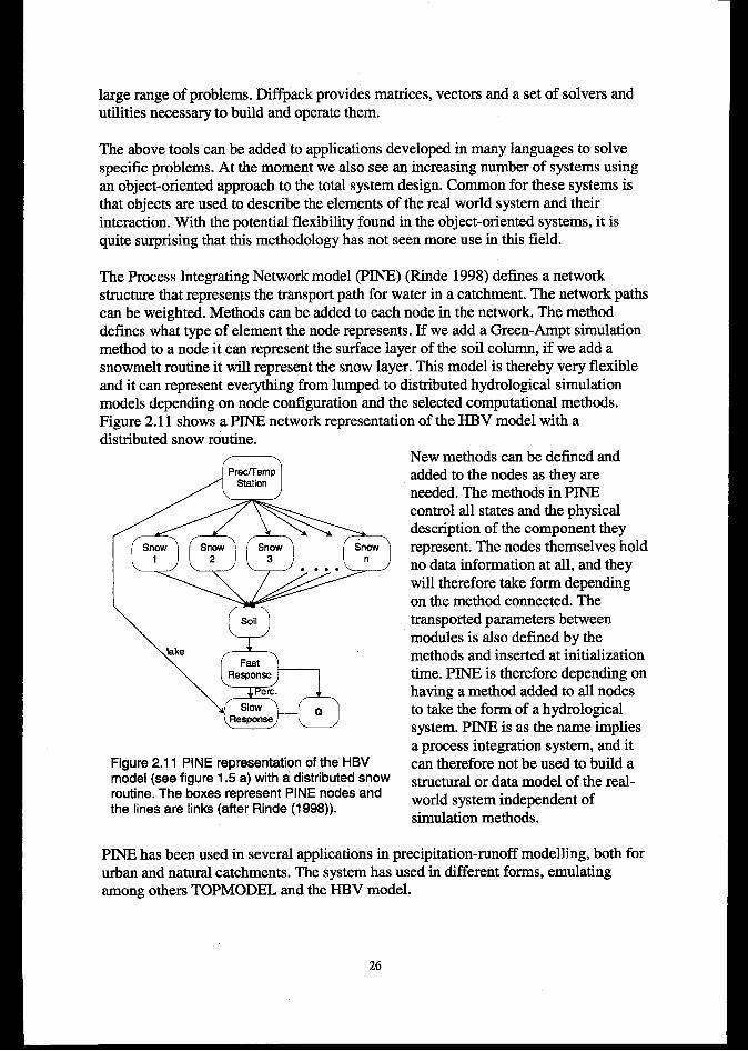
large range of problems. 13iffpack provides matrices, vectors and a set of solvers andutilities necessary to build and operate them.

The above tools can be added to applications developed in many languages to solvespecific problems. At the moment we also see an increasing number of systems usingan object-oriented approach to the total system design. Common for these systems isthat objects are used to describe the elements of the real world system and theirinteraction. With the potential flexibility found in the object-oriented systems, it isquite surprising that this methodology has not seen more use in this field.

The Process Integrating Network model (PINE) (Rinde 1998) defines a networkstructure that represents the transport path for water in a catchment. The network pathscan be weighted. Methods can be added to each node in the network. The methoddefines what type of element the node represents. If we add a Green-Ampt simulationmethod to a node it can represent the surface layer of the soil column, if we add asnowmelt routine it will represent the snow layer. This model is thereby very flexibleand it can represent everything horn lumped to distributed hydrological simulationmodels depending on node configuration and the selected computational methods.Figure 2.11 shows a PINE network representation of the HBV model with adistributed snow routine.

A Prec/Temp

Station

(*1 2 3’ n

● ***

Soil

\

Figure 2.11 PINE representation of the HBVmodel (see figure 1.5 a) with a distributed snowroutine. The boxes represent PINE nodes andthe lines are links (after Rinde (1998)).

New methods can be defined andadded to the nodes as they areneeded. The methods in PINEcontrol all states and the physicaldescription of the component theyrepresent. The nodes themselves holdno data information at all, and theywill therefore take form dependingon the method connected. Thetransported parameters betweenmodules is also defined by themethods and inserted at initializationtime. PINE is therefore depending onhaving a method added to all nodesto take the form of a hydrologicalsystem. PINE is as the name impliesa process integration system, and itcan therefore not be used to build astructural or data model of the real-world system independent ofsimulation methods.

PINE has been used in several applications in precipitation-runoff modelling, both forurban and natural catchments. The system has used in different forms, emulatingamong others TOPMODEL and the HBV model.

26

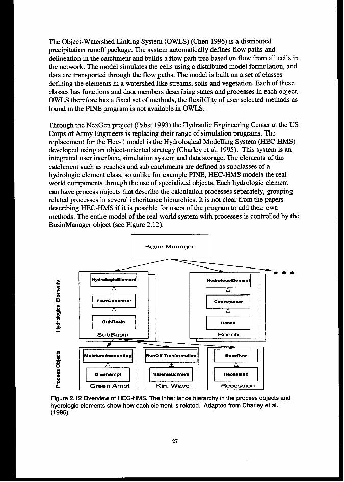
The Object-Watershed Linking System (OWLS) (Chen 1996) is a distributedprecipitation runoff package. The system automatically defines flow paths anddelineation in the catchrnent and builds a flow path tree based on flow from all cells inthe network. The model simulates the cells using a distributed model formulation, anddata are transported through the flow paths. The model is built on a set of classesdefining the elements in a watershed like streams, soils and vegetation. Each of theseclasses has functions and data members describing states and processes in each object.OWLS therefore has a fixed set of methods, the flexibility of user selected methods asfound in the PINE program is not available in OWLS.

Through the NexGen project (Pabst 1993) the Hydraulic Engineering Center at the USCorps of Army Engineers is replacing their range of simulation programs. Thereplacement for the Hec- 1 model is the Hydrological Modelling System (HEC-HMS)developed using an object-oriented strategy (Charley et al. 1995). This system is anintegrated user interface, simulation system and data storage. The elements of thecatchrnent such as reaches and sub catchments are defined as subclasses of ahydrologic element class, so unlike for example PINE, HEC-HMS models the real-world components through the use of specialized objects. Each hydrologic elementcan have process objects that describe the calculation processes separately, groupingrelated processes in several inheritance hierarchies. It is not clear from the papersdescribing HEC-HMS if it is possible for users of the program to add their ownmethods. The entire model of the real world system with processes is controlled by theBasinManager object (see Figure 2. 12).

Basin Manager

lHydrologlcElememtl I I

I “OwGe’’e’-OrI I I

L I

SubBasin IIzHydrologcElwnemt

convayxln-

ReachI

—*-m

Figure 2.12 Overview of HEC-HMS. The inheritance hierarchy in the process objects andhydrologic elements show how each element is related. Adapted from Charley et al.(1995)

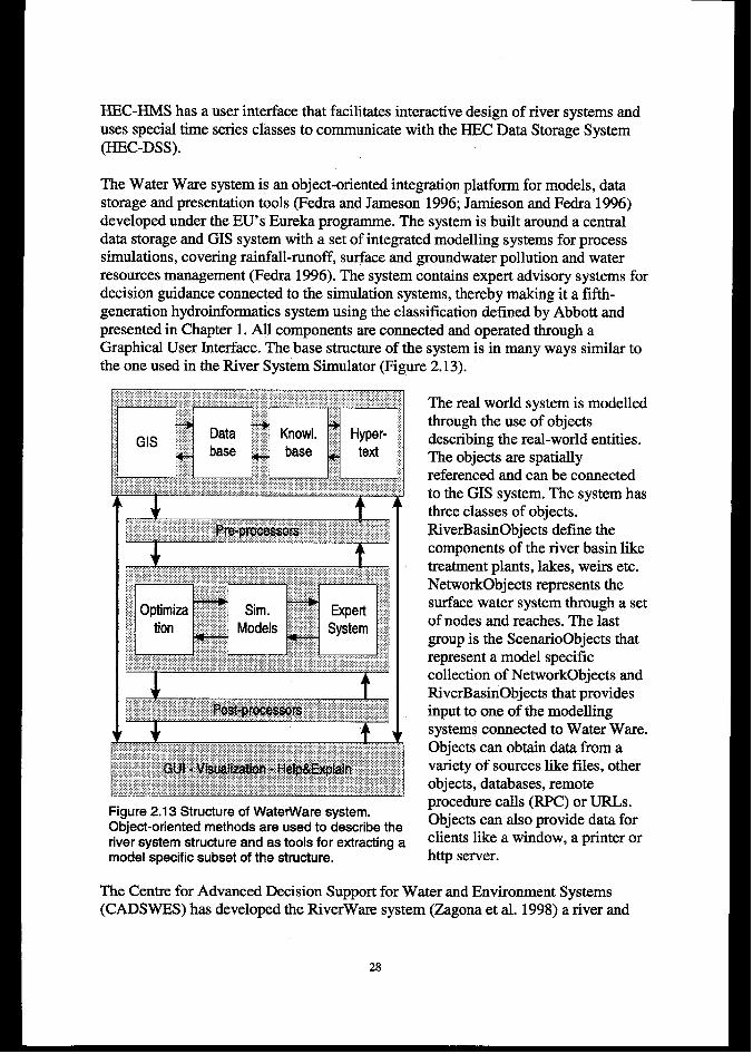
HEC-HMS has a user interface that facilitates interactive design of river systems anduses special time series classes to communicate with the HEC Data Storage System(HEC-DSS).

The Water Ware system is an object-oriented integration platform for models, datastorage and presentation tools (Fedra and Jameson 1996; Jamieson and Fedra 1996)developed under the EU’S Eureka programrne. The system is built around a centraldata storage and GIS system with a set of integrated modelling systems for processsimulations, covering rainfall-runoff, surface and groundwater pollution and waterresources management (Fedra 1996). The system contains expert advisory systems fordecision guidance connected to the simulation systems, thereby making it a fifth-generation hydroinformatics system using the classification defined by Abbott andpresented in Chapter 1. All components are connected and operated through aGraphical User Jnterface. The base structure of the system is in many ways similar tothe one used in the River System Simulator (Figure 2.13).

Figure 2.13 Structure of WaterWare system.Object-oriented methods are used to describe theriver system structure and as tools for extracting amodel specific subset of the structure.

The real world system is modelledthrough the use of objectsdescribing the real-world entities.The objects are spatiallyreferenced and can be connectedto the GIS system. The system hasthree classes of objects.RiverBasinObjects define thecomponents of the river basin liketreatment plants, lakes, weirs etc.NetworkObjects represents thesurface water system through a setof nodes and reaches. The lastgroup is the ScenarioObjects thatrepresent a model specificcollection of NetworkObjects andRiverBasinObjects that providesinput to one of the modellingsystems connected to Water Ware.Objects can obtain data from avariety of sources like files, otherobjects, databases, remoteprocedure caJls (RPC) or URLs.Objects can also provide data forclients like a window, a printer orhttp server.

The Centre for Advanced Decision Support for Water and Environment Systems(CADSWES) has developed the RiverWare system (Zagona et al. 1998) a river and

2s

reservoir modelling system. The system is built around a set of objects representingthe real-world components. Each of the objects has a set of slots and engineeringmethods. The slots of each object are the variables and parameters that define thatobject. The system has three types of slots, time series, table and scalar. The store timeseries, tabular data and single values respectively. The engineering methods representprocess models connected to each object. Each object usually has several options thatthe user can choose from.

RiverWare has a set of run controllers that steer the simulation. The user can choosehorn pure simulation, rule-based simulation, optimization and water accounting. Inthe pure simulation controller each object waits until it has its required data forexecuting the dispatch methods, it then fills unknown slots and transfers data toneighboring objects through links. This controller requires an exact specification ofthe object slots to run. If there is not enough exact information to solve the system, arule based simulation controller can be used. The rule-based controller uses a set ofrules to define the missing slots based on the state of the system. The optimizingcontroller uses linear prog ramming to optimise the system based on prioritized goaldefined by the user and the water accounting controller operates accounting of waterin a water-rights based system (Shane et al. 1995; Zagona et al. 1998).

RiverWare is built around a modelling environment that contains several datamanagement and graphical tools. Spreadsheet based slot editing is used to enter datainto objects. Thes ystem structure is defined through a river system editor (Reitsma etal. 1994).

Whittaker et al. (1991) presents an object-oriented approach to model the hydrologicalprocesses using hydrological response units (HRUS) as objects. The system is createdas a network of HRU objects. The simulation is done using an environment thatallows different processes to be updated or invoked at different time intervals.Vanecek et al. (1994) presents an object-oriented approach for building a simulationsystem for water hammer analysis. The user interface of the system lets tie user buildthe pipe system born a “palette” of objects and input the parameters to each pipe. Theauthors emphazise the use of inheritance to easily define the new components of thesystem and how this principle can be used to reduce code copying found intraditionally designed systems. Solomatine (1996) presents both a general case forusing object-oriented methods in hydraulic simulation systems and he presents thewater distribution system HIS, an experimental system for hydraulic modelling of pipesystems. The systems are built by combining objects like pipes, pumps and valves.Two versions of HIS, LinHIS and the full networked NetHIS are presented. Bente(1994) describes a software concept for building hydrological simulation modelsbased on a system to link process objects with data collectors (these combine outputfrom one or more processes and send them to the next process) and input and outputproviders. The core of the system is the process object that defines both the structureand the operation of the components in the hydrological system. The process objectcan hold a single process or combination of several processes. The Danish HydraulicInstitute is also using an object-oriented design strategy for the common platform for

29

the next version of their software systems, Mike Zero (DHI 1998). The rationale forthis effort is to provide easier data handling and coupling of models. DHI also expectlower development and maintenance costs in future projects, which definitely is animportant asset with a good object-oriented design.

Except for the DHI Mike Zero project and to some degree the WaterWare system,none of the above systems seem to be concerned with integration or coupling withexisting tools. With the current availability of high quality simulation tools it isnecessary to take some form of communication with these into consideration. Thecurrent use of integrated graphical user interfaces is very neat for the user of theprograms, but they do create problems for a seamless integration of applications. Inthis case the old command line, batch driven system was better. It is thereforeimportant to consider if such coupling is necessary and if a seamless integration ispossible, or if one has to resort to ascii file communication between programs. In thisrespect the Mike Zero system is very interesting with their use of OLE/COMstructures which will make efficient integration possible in the future. The use of thiskind of technique will be covered in the next section and in Chapter 8.

2.3.5 Distributed data systems

A large simulation system will often operate in a world with distributed actors. Inmany cases both program users and data providers will be located at different sites.The procedure that is used most today is based on collecting all data in a centralmachine and operating everything from there. Experience shows that this does notalways work as smoothly as one could expect. Another trend in software developmenttoday is to include more and more functionality into a single application, therebyincreasing both the size and complexity of the application. Larsen and Gavranovich(1994) seek a way to distribute and store objects over networks to promote easier dataexchange between users and to prevent existing system from evolving into“dinosaurs”, huge integrated systems with very high demands on the user and onhardware resources. The authors outline a computer system were for example users ofa decision framework can expand this with objects covering the needed simulationobjective. These objects, or Portable Knowledge Encapsulators7(PKE), contain bothdata and functions making them self contained networked building blocks in thesystem. This would require a common framework for developing a PKE to ensure thatthey will fit into the operational system run by the user.

Distributed technology and networked objects are one of the largest growing areas incomputer science today, and very much effort is spent on research and development.In the object-oriented research community, this work resulted in a proposedarchitecture for distributed objects. This proposal from the Object Management Group(OMG) resulted in the CORBA (Common Object Request Broker Architecture) asystem that contains the necessary tools to design and implement distributed softwaresystems based on networked objects. Using CORBA, objects can be defined to

7ThenamePortableKnowledgeEncapsulatorbuildsupontheElectronicKnowledgeEncapsulatorasdefiiedby Abbott(1993).

30

communicate over an “object bus” controlled by the object request broker (ORB). Forthe communication the implementation language is not important, the only thing thecommunicating objects need to know about each other is defined through a genericinterface definition language (IDL). Microsoft has (as usual) developed its ownstandard with their DCOM (Distributed Common Object Model). Companiesproducing software bridges that connect the two systems have already solved theproblem of integrating the two systems. The structure and use of such tools will becovered in some more detail in Chapter 8. Another interesting application ofdistributed systems is in the development of multi-databases, systems where severalphysically distributed object-oriented databases are joined into single transparentlogical structure (Stein 1994). Distributed databases are also increasingly important inthe design of data warehouses. A data warehouse will provide the means to integrateheterogeneous databases and to retrieve information from huge volumes of dataefficiently (Misseyer et al. 1998). Data Mining (Babovic 1998; Chung et al. 1998) is atypical technique used in the query of such database systems.

The distributed tools as outlined above have to the author’s knowledge not yet beenused in applications in hydroinformatics. One exception to this is the paper byVelickov (1998), which explores the possibilities using Microsoft ActiveXtechnology. This is probably changing, since the ability to distribute knowledge onseveral sites is an important part of the Engine 2000 project (Abbott 1997). In thispaper the author states (p. 861):

“It [Engine 2000] is to be distributed over a potentially large number of sites aroundthe globe and all such sites will be electronically connected for transferring data andsuitably encapsulated knowledge between sites. ”

A distributed object-oriented system like CORBA is designed to be the core of theimplementation of such systems. The development of systems like Engine 2000together with the increasing interest in web technology makes it therefore probablethat distributed systems will bean important part of future developments inhydroinformatics.

2.3.6 Agent systems

The concept of an intelligent agent is transferred to hydroinformatics from ArtificialIntelligence research. An agent is a self-contained software component that has aspecific set of properties. One definition of agent properties follows the notion ofweak and strong agency (Woolridge and Jennings 1995):

An agent should be autonomous, meaning that it should be able to operate withoutinteraction by having control over actions and internal state.It should be able to interact with other agents, a social ability.It should be reactive by responding to events in the surrounding environment.It should be pro-active by not only acting on events in the environment but also bytaking the initiative to perform tasks.

A notion of strong agency is used when the agent is given some sort of a “mentalcapability” such as knowledge, beliefs and intentions. Building systems based on

31

interacting agents is often termed agent-oriented programming (AOP) (Shobharn1993). This is closely related to object-oriented progr amrning (OOP), and objectmethods can often be the most efficient way of implementing the agents and theenvironments they operate in, the AOP is mostly an extension to the 00P where someobjects have specific properties. One area of hydroinforrnatics where agent basedprogr amming has been applied and shows promise is in the construction of ecologicalsimulation systems (Abbott et al. 1994; Babovic 1996; Campos and Hill 1997). Bydefining the actors in the ecological system as agents and letting them operate in anenvironment defined by the hydraulic simulation system powerful impact analysistools can be made. Software agents can also be distributed over the network, typicalexamples here are data search and retrieval tools,

2.3.7 The use of Geographical lnformution Systems

Geographical Information Systems (GIS) is commonly used in hydroinformatics astools for data preparation and visualization. Object-oriented methods can be used tointegrate GIS with modelling tools (Fedra and Jarneson 1996; Rinde 1996). For anargument in favour of building object-oriented modelling environments instead of lowlevel integration of environmental simulation systems and GIS see Raper andLivingston (1995). Current research into distributed GIS is based on object-orienteddesign methods and object-oriented distribution technologies as outlined in Section2.4.5 (DISGIS 1998).

2.3.8 Integrating information systems and modelling tools

One of the purposes of a hydroinformatics system is to integrate knowledge about awide variety of subjects, combine these and present results on many different userlevels. Information systems based on the underlying simulation systems must handle alarge and often very complex amount of data. The emerging technologies connected toInternet provides a powerful platform for distribution of information and buildinginformation systems connected to the underlying simulation tools (Abbott and Jonoski1998; Bakken et al. 1998). The use of Internet also invites to collaboration throughdialogue in a way that has never been possible in earlier systems. The simulationsystems can be integrated in different ways, the most seamless integration can beachieved by using the JAVA language and other component-based systems incombination with distribution technologies. Using this methodology Java-basedinterfaces could be made that corresponds with distributed simulation “objects”through the use of a system like COM/DCOM or CORBA. This will be covered insome more detail in Chapter 8.

32

3. DESIGNING THE APPLICATION FRAMEWORK

3.1 Basics of frameworks and patterns

Reuse of components is one on the main attractions of an object-oriented designstrategy. The major tool for acquiring reuse is the use of object-oriented frameworksand patterns. This provides reuse on a higher level than ordinary copy and paste ofcode, and will also provide the user with the opportunity to extend the reusablecomponents. Reenskaug (1996) describes an object-oriented framework “as a set ofbase classes that together describe a generally usejid object structure”. Manyframeworks in existence contain more than just base classes, but this part of theframework is the most important since it provides interfaces to the frameworkcomponents and lets the user insert his own constructs into the predefinecollaboration structure. Reenskaug (1996) continues to define patterns andframeworks:

“Patterns and frameworks are reusable components that describe solutions to generalproblems. The difference is on an abstraction level: the pattern describes how thereader can solve a problem, while the framework provides a concrete solution”

The framework is in practise a program skeleton in a specified domain, while thedesign pattern provide a solution recipe for a specific problem. A framework willoften utilize several patterns as building blocks during development. To build aflexible fiarnework several goals must be fulfilled, According to Booth (1994), aframework should provide a set of domain independent structures and algorithms that

cover the need of most applications in the domain. In addition it must be:

●

●

●

●

●

●

Complete. It should provide a family of classes united by a shared interface.Through different representations developers can select the ones that are mostappropriate to the application.Adaptable, All platform specific aspects must be isolated so that substitutions canbe made. Developers must have control over storage management and processsynchronization.Efficient. Components must be easily assembled (compile time efficiency), imposeminimal memory and run-time overhead (execution efficiency), and they must bereliable and usable (efficient in developer time)Saie. Abstractions must be type safe. Controlled handling of error situations mustbe done through exceptions.Simple. A clear and consistent organization makes it easy to select and applyappropriate classes.Extensible. Developers must be able to extend the framework with new classes andat the same time m~ntain the framework integrity.

If these requirements are met, the user will have a powerful tool for developingapplications. As opposed to a normal library, the framework supports redefinition of

33

functionality through the use of virtual functions and the addition of functionalitythrough programming with interfaces and the use of inheritance. Berre (1996) givesthe three goals for designing a framework

. To be able to build applications from predefine components.

. To use a small number of components many times.● To make it possible to develop applications with as little code writing as possible,

Compared to structured progr amming a ffamework can be compared to a library, butwith a defined collaboration structure and a potential for user extensions. The softwaresystem outlined in Chapter 1 will be implemented as a framework based on the abovespecifications, and applications will be built through the use of this framework. Theframework will have classes that cover all the aspects of designing a hydroinformaticssystem. Booth (1994) recommends a design based on class categories inside theframework, grouping all related classes into a category instead of using a flat design.This methodology will be adopted in the design, and the framework will be dividedinto several groups of related components. The following sections outline the analysisand the design phase that lead to the proposed toolkit. The next chapter gives anoverview of the component groups of the framework, their relation and functionalityin more detail. The use of the framework will be shown in Chapter 5.

3.2 Problem Domain and Requirements

3.2.1 Introduction to the method

The method used for the analysis and design phase is outlined in Figure 3.1 andnotation and details are defined in Appendix 1. Basically this is a five-step methodthat is based on a definition of a problem domain, which in our case will be adefinition of a “two part” system consisting of the real-world system and themodelling applications that we want to develop.

■

m

The first step of the phase defies functional and non-functional requirements thatroughly specify the behaviour and operation of thes ystem. The functionalrequirements are outlined using Use Cases, originally developed by Jacobson(1992).

According to Booth (1996):

“Object-oriented analysis is a method of analysis that examines requirementsfiomthe perspective of the classes and objects found in the vocabulary of the problemdomain. ”

The analysis step identifies potential objects through the use of Class-Response-Collaboration (CRC) cards (Beck and Cunningham 1989) based on the use ofsubject extraction from the domain description. This step also describes the systemresponses and interactions between objects to external stimuli.

34

■

■

■

,. .,_,@ :.;

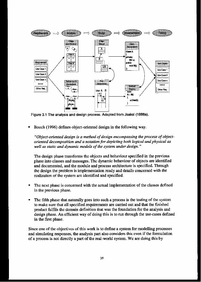
User A B,*.:;

\ E . ~ , < yw

Figure 3.1 The analysis and design process. Adapted from Jaaksi (1998a).

Booth (1996) defines object-oriented design in the following way.

“Object-oriented design is a method of design encompassing the process of object-oriented decomposition and a notation for depicting both logical and physical aswell as static and dynumic models of the system under design. ”

The design phase transforms the objects and behaviour specified in the previousphase into classes and messages. The dynamic behaviour of objects are identifiedand documented, and the module and process architecture is specified. Throughthe design the problem is implementation ready and details concerned with therealization of the system are identified and specified.

The next phase is concerned with the actual implementation of the classes definedin the previous phase.

The fifth phase that naturally goes into such a process is the testing of the systemto make sure that all specified requirements are carried out and that the finishedproduct fulfils the domain definition that was the foundation for the analysis anddesign phase. An efficient way of doing this is to run through the use-cases definedin the first phase.

Since one of the objectives of this work is to define a system for modelling processesand simulating responses, the analysis part also considers this even if the formulationof a process is not directly a part of the real-world system. We are doing this by

treating the process model itself as a kind of real-world system and model the objectsbased on this “abstract” real world.

To visualize the process of analysis and design we will use the Unified ModellingLanguage (uML) (Fowler and Scott 1997) for class and interaction diagrams. UML isa combined method built on Booth, OMT and the Objectory (Use Cases) methods. Inthe system analysis the Object-Oriented Role Analysis and Modelling (OORAM)(Reenskaug et al. 1996) will used. In the near fiture this method will follow many ofthe other object-oriented techniques and become integrated in UML, but here theoriginal notation is used in the diagrams. Also note that in the class diagrams thecomplete set of methods and attributes is not shown. This has several reasons. Sincethe code generation capacity in the analysis and design tool is not used, the classes arenot made in complete detail but the tool is merely used for outlining the major featuresof the design. It is also believed that a reduction in the number of details in the classdiagrams also adds clarity to the design. The third reason is purely practical, withoutthe proper code generation and reverse engineering facilities, updating diagrams forevery little detail in the implementation proves too cumbersome for practicalapplication. Therefore the diagrams are somewhat reduced in detail. When methodsare necessary for understanding the design, they are of course fully included.

3.2.2 Dej?nition of problem domuin

In Chapter 1 the requirements for the system was specified. These can be summarizedinto the following points:

A free selection of river system components and the possibility to connect themand structure them to forma representation of the real-world river system. Newcomponents can be added when needed.The data describing the component should not be fixed. The amount and type ofdata should be user defined.Since the simulation system may cover a range of objectives (such as floods, waterquality, hydropower production etc.) the processes must be separated from eachcomponent and added at runtime. The number of processes in each componentshould not be fixed. Processes can communicate through updates of states in theriver system components. A validation must be performed when the process isadded to confirm that the necessary data is available to properly execute theprocess. The structure should be open to the user’s own developments.All user interactions must be separate from the data, river system components andmethods to avoid bindings to specific formats and operating environments.

From the desired functionality specified above, the problem domain can roughly bedescribed as follows:

The framework will provide tools for building a model of a real-world river systemwith its structural components, descriptive data and logical connections. It must alsobe possible for the user of the system to build new components and data structures andadd these to the system. This description of the river system must be completely

36

independent from any simulation tools that might be added. It must be possible to adddifferent types of computational tools to the components depending on the objectivesof the simulation. The computational tools will depend on the data available in thecomponents, and they will update the states of the model components through thecomputations. When a system is defined, it must be possible to configure thesimulation to suit the needs of the user. This includes time steps in simulation,sequence of execution and result output during simulation.

This description covers the use of the system as a tool for building a variety ofsimulation models. It is important to put a strong emphasis on the desire to design asystem that is independent of the simulation methods used. All the following chapterswill divide between the system model that describes the rivers ystem and themathematical models thatdescribe processes in components of the river system. Thisdivision will allow us to use the system model components in applications that haveno simulation objective, such as database front ends, in the design of user interfacesand in future applications of object oriented databases. Some of the potential uses ofthe framework outside the development of simulation models will be covered later.

3.2.3 Requirements

The following requirements for the framework have been formulated based on theview of the problem domain. It is convenient to divide the functional requirementsinto three levels:

1. Requirements for the system model (structural components and transport).2. Requirements for the simulation system (interface to mathematical models).3. Requirements for the operation of the system.

In addition there will of course be requirements coupled to the applications built uponthis framework. These have to be covered in the specification of the actualapplication. The case study in Chapter 7 shows an example of this process. Inaddition, a set of non-functional requirements cover structural and usage demandsconnected to the system. The requirements are mostly based on a set of use-caseformulations that cover the operation of the system. The use-case formulations alsoprovide us with the opportunity to directly use them as test cases to see if theimplemented system fulfils the requirements (see Figure 3.1). Please note that theactor in the use-cases can be both the user of the system requesting something andinternal control units triggering responses from the system. The Use-Cases used todescribe the requirements is presented in Table 3.1 to Table 3.4. A table form (Jaaksi1998b) is used to present the Use-Case layout.

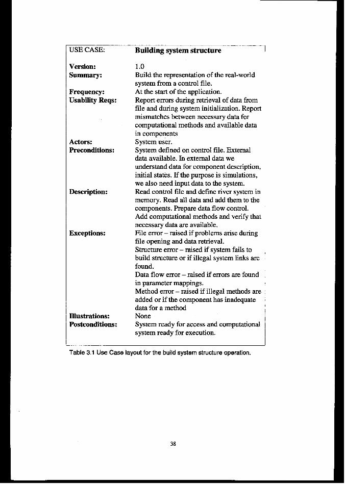
USE CASE:

Version:summary:

Frequency:Usability Reqs:

Actors:Preconditions:

Description:

Exceptions:

Illustrations:Postconditions:

Building system structure

1.0Build the representation of the real-worldsystem from a control file.At the start of the application.Report errors during retrieval of data fromfile and during system initialization. Reportmismatches between necessary data forcomputational methods and available datain componentsSystem user.System defined on control file. Externaldata available. In external data weunderstand data for component description,initial states. If the purpose is simulations,we also need input data to the system.Read control file and define river system inmemory. Read all data and add them to thecomponents. Prepare data flow control.Add computational methods and verify thatnecessary data are available.File error – raised if problems arise duringfile opening and data retrieval.Structure error – raised if system fails tobuild structure or if illegal system links arefound.Data flow error – raised if errors are foundin parameter mappings.Method error – raised if illegal methods areadded or if the component has inadequatedata for a methodNoneSystem ready for access and computationalsystem ready for execution.

Table 3.1 Use Case layout for the build system structure operation.

38

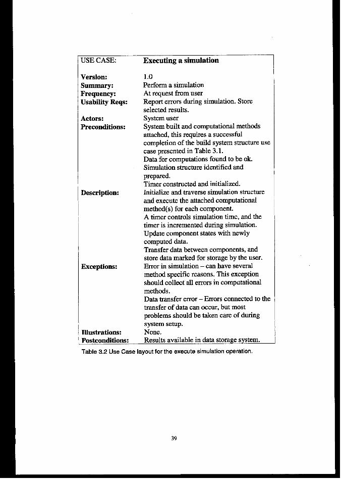
USE CASE:

Version:summary:Frequency:Usability Reqs:

Actors:Preconditions:

Description:

Exceptions:

Illustrations:

Executing a simulation

1.0Perform a simulationAt request from userReport errors during simulation. Storeselected results.System userSystem built and computational methodsattached, this requires a successfulcompletion of the build system structure usecase presented in Table 3.1.Data for computations found to be ok.Simulation structure identified andprepared.Timer constructed and initialized.Initialize and traverse simulation stractureand execute the attached computationalmethod(s) for each component.A timer controls simulation time, and thetimer is incremented during simulation.Update component states with newlycomputed data.Transfer data between components, andstore data marked for storage by the user.Error in simulation – can have severalmethod specific reasons. This exceptionshould collect all errors in computationalmethods.Data transfer error – Errors connected to thetransfer of data can occur, but mostproblems should be taken care of duringsystem setup.None.

Posteonditions: Results available in data storage system.

Table 3.2 Use Case layout for the execute simulation operation.

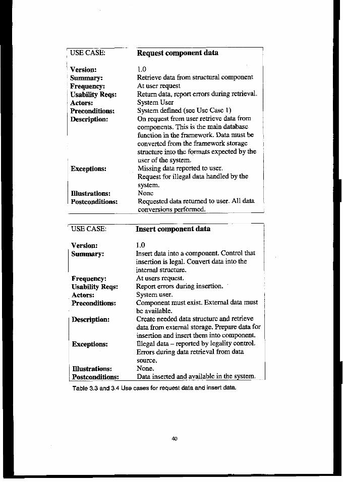
USE CASE Request component data

Version:s~:Frequency:Usability Reqs:Actors:Preconditions:Description:

Exceptions:

Illustrations:Posteonditions:

1.0Retrieve data from structural componentAt user requestReturn data, report errors during retrieval.System UserSystem defined (see Use Case 1)On request from user retrieve data fkomcomponents. This is the main databasefunction in the framework. Data must beconverted from the framework storagestructure into the formats expected by tieuser of the system.Missing data reported to user.Request for illegal data handled by thesystem.NoneRequested data returned to user. All dataconversions performed.

USE CASE Insert component data

Version: 1.0summary: Insert data into a component. Control that

insertion is legal. Convert data into theinternal structure.

Frequency: At users request.Usability Reqs: Report errors during insertion.Actors: System user.Preconditions: Component must exist. External data must

be available.Description: Create needed data structure and retrieve

data born external storage. Prepare data forinsertion and insert them into component.

Exceptions: Illegal data – reported by legality control.Errors during data retrieval from datasource.

Illustrations: None.Postconditions: Data inserted and available in the system.

Table 3.3 and 3.4 Use cases for request data and insert data.

Based on the Use-Case formulations we can summarize the requirements in thefollowing points:

Retirements for svstem model (real-world modellim svstem)

The system model must have a strongly modular structure allowing for a closerepresentation of the real-world system. The modules should define the real worldcomponents with their data and operations. The user of the system should be able toaccess them through a simple interface without any detail knowledge of the internalstructure of the components. The structure should also easily facilitate additions ofnew structural components.

The structural components should allow for inclusion of new data and calculationmethods without a change in the internal structure. The component should have aflexible configuration regarding data and methods used, so that they only store what isnecessary for the application. With the possibility of flexible configuration, meansmust be taken to avoid the insertion of illegal data or methods into the component(e.g. to prevent insertion of cross sections into a power plant module).

Rectuirements for simulation svstem

To achieve the separation into a system model and a separate process model, theprocess modelling tools (hereafter called computational methods) must be separatedfrom the structural components. We can then build a simulation system by firstdefining the structural system, then adding the appropriate methods to eachcomponent. The computational methods can be both tools developed in scope of theframework or they can be externally developed applications interfaced into thesystem. The ability to use already developed models ensures a connection to the largebase of existing software. Common to both approaches will be that they retrieve theirdata from a common underlying model of the river system. If the user tries to add amethod that requires more data than what is available, an error will occur. Thisapproach ensures that various methods can be used in different components, therebyallowing the user to select methods that suit the available data, the type of calculationneeded and the wanted detail in simulation.

Requirements for svstem control

The control of the system is defined in two phases, the system definition phase and thesystem execution phase. In the definition phase the real-world system model is built,data is imported and computational methods are added. In the system execution phasethe structure is traversed and computational methods are executed. The simulationcontrol system should be completely separated horn the structural and computationalpart of the framework. The system control will vary depending on the type ofsimulation that is carried out, therefore it must be user configurable to provide thisflexibility. In a later stage the simulation control system will be the interaction point

between user interfaces or databases and the stmctural and computational part of theframework.

Non-functional requirements

All data import and export routines should be separated from the components in themodel, this applies for both structural and data storage components. The main purposeof this is to avoid changing the internal structure of the components if a new storagesystem is to be used. This also ensures that the components are transparent to thestorage system used in the model.

In a similar fashion all user interactions should be done outside of the frameworkcomponents themselves to ensure independence from a specific GUIs ystem.

3.3 System analysis

3.3.1 General remarks about the system analysis and design.

There are two main objectives with the system analysis. First the objects in thedomain and their relationship are identified. The process used in this work involves agradual refinement of the problem domain with object identification in eachrefinement step. To document the objects CRC cards will be used, as mentioned. Itwas decided not to introduce class relationship diagrams at this stage, mainly toprevent details from entering the process too soon. The next step is to look at thedynamic behaviour of the system. This is done through the definition of system rolesand by looking at their interaction. This technique prevents message passing detailfrom entering the process at this stage. One of the major objectives has been to try toleave everything that reminds of function calls, typed variables, function signaturesetc. out of the analysis. Another advantage of role modelling is that it gives a differentabstraction level from the usual message analysis, thereby it is an effective tool fordiscovering aspects of the system that is not seen if one is only working with classes.

There will of course be overlapping work between the design and analysis part sincethis system is developed in an incremental fashion. The fact that some components aredesigned when other parts of the system are in the analysis phase will have an effecton the analysis. In our opinion this is an asset to the development since the processfrom requirement ~ analysis ~ design should not be a one-way road but a linkedprocess where discoveries in one of the phases could lead to re-engineering of parts ofan earlier phase.

3.3.2 Object identification

The rough domain description in Section 3.2.2 enables potential objects to be foundby assuming that subjects and objects in the sentences are possible program objects.This combined with general knowledge of the system forms the foundation of theobject identification. Based on this the following objects are found:

42

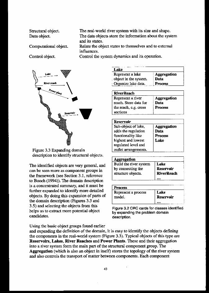
Structural object. The real-world river system with its size and shape.Data object. The data objects store the information about the system

and its states.Computational object. Relate the object states to themselves and to external

influences.Control object. Control the system dynamics and its operation.

Y River reach.\

LakeRepresent a lake Aggregationobject in the system. DataOrganize lake data. Process

Figure 3.3 Expanding domaindescription to identify structural objects.

The identified objects are very general, andcan be seen more as component groups inthe framework (see Section 3.1, referenceto Booth (1994)). The domain descriptionis a concentrated summary, and it must befin-ther expanded to identify more detailedobjects. By doing this expansion of parts ofthe domain description (Figures 3.3 and3.5) and selecting the objects from thishelps us to extract more potential objectcandidates.

RiverReach

ReservoirSub-object of lake,adds the regulationfunctionality likehighest and lowestregulated level andoutlet arrangements.

Aggregation

:

AggregationDataProcessLake

Figure 3.2 CRC cards for classes identifiedby expanding the problem domaindescription.

Using the basic object groups found earlierand expanding the definition of the domain, it is easy to identify the objects definingthe components in the real-world system (Figure 3.3). Typical objects of this type areReservoirs, Lakea, River Reaches and Power Plants. These and their aggregationinto a river system form the main part of the structural component group. TheAggregation (which is also an object in itself) stores the topology of the river systemand also controls the transport of matter between components. Each component

43

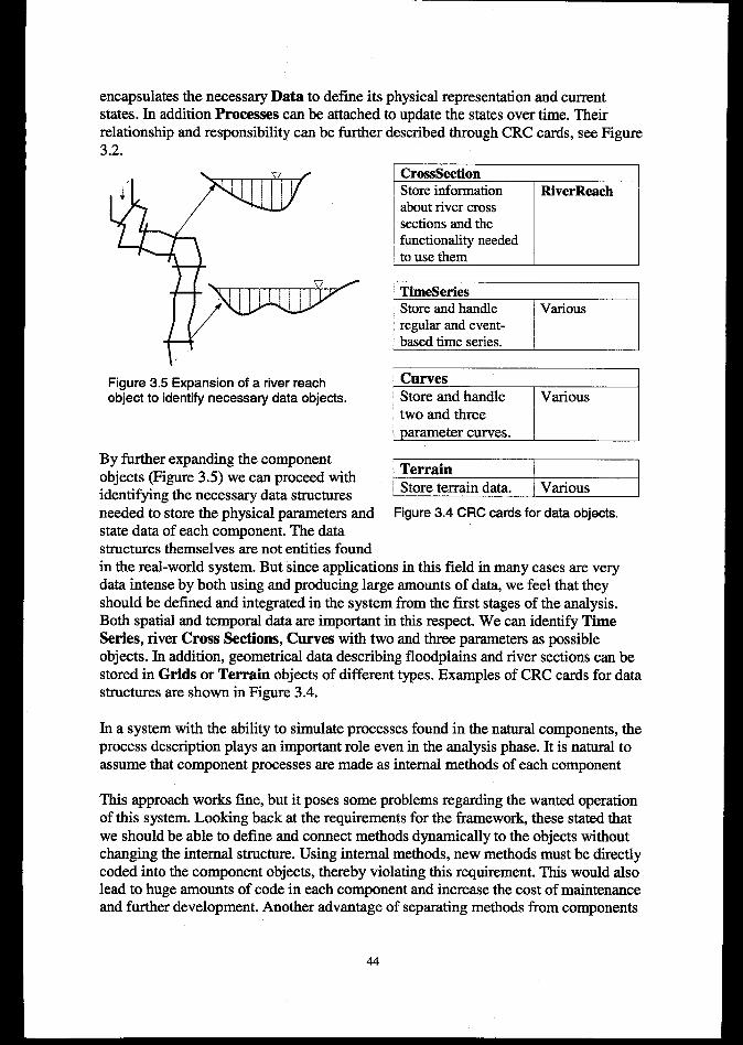
encapsulates the necessary Data to define its physical representation and currentstates. In addition Processes can be attached to update the states overtime. Theirrelationship and responsibility can be further described through CRC cards, see Figure3.2.

T-Figure 3.5 Expansion of a river reachobject to identify necessary data objects.

By further expanding the componentobjects (Figure 3.5) we can proceed withidentifying the necessary data structuresneeded to store the physical parameters andstate data of each component. The datastructures themselves are not entities found

CrossSectionStore informationabout river crosssections and thefunctionality neededto use them aRiverReach

CurvesStore and handle ~various

/ two and three I Iparameter curves.

TerrainStore terrain data. / various

Figure 3.4 CRC cards for data objects.

in the real-world system. But since applications in this field in many cases are verydata intense by both using and producing large amounts of data, we feel that theyshould be defined and integrated in thes ystem from the first stages of the analysis.Both spatial and temporal data are important in this respect. We can identify TimeSeries, river Cross Sections, Curves with two and three parameters as possibleobjects. In addition, geometrical data describing floodplains and river sections can bestored in Grids or Terrain objects of different types. Examples of CRC cards for datastructures are shown in Figure 3.4.

In a system with the ability to simulate processes found in the natural components, theprocess description plays an important role even in the analysis phase. It is natural toassume that component processes are made as internal methods of each component

This approach works fine, but it poses some problems regarding the wanted operationof this system. Looking back at the requirements for the framework, these stated thatwe should be able to define and connect methods dynamically to the objects withoutchanging the internal structure. Using internal methods, new methods must be directlycoded into the component objects, thereby violating this requirement. This would alsolead to huge amounts of code in each component and increase the cost of maintenanceand tier development. Another advantage of separating methods from components

44

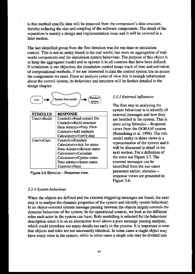
is that method specific data will be removed from the component’s data structure,thereby reducing the size and coupling of the software components. The detail of theseparation is mainly a design and implementation issue and it will be covered in alater section.

The last identified group from the first iteration was the run time or simulationcontrol. This is not an entity found in the real world, but more an aggregation of real-world components and the simulation system behaviour. The purpose of this object isto keep the aggregated model and to operate it in all contexts that have been defined.If simulation is our objective, the simulation control keeps track of time and activationof computational methods, if we are interested in data the control system lets us accessthe components we need. From an analysis point of view this is enough informationabout the control system, its behaviour and stmcture will be further detailed in thedesign chapter.

G-)+F===J+R53.3.3 External influences

.- —-~ “---

STIMULUSUsen=>Build

Use->Ca.lc.

RESPONSEControb->Read control fdeControl>>Build structureData Admin>X%ep. FlowControl>>Add methodsCalculatom>Verify dataControl>>SimulateCalculatom>Ask for statesData Adrnio>Return statesCalculato-XhlculateCalcuIato-XJpdate statesData adrnin>Xnsert statesControb>Next

Figure 3.6 Stimulus - Response view.

3.3.4 System behaviour

The first step in analysing thesystem behaviour is to identify allexternal messages and how theyare handled in the system. This isdone using Stimulus – Responseviews from the 00RAMs ystem(Reenskaug et al. 1996). The rolemodel entity in these views is arepresentation of the system and itwill be discussed in detail in thenext section. For a definition ofthe roles see Figure 3.7. Theexternal messages can beidentified from the use-casespresented earlier, stimulus –response views are presented inFigure 3.6:

When the objects are defined and the external triggering messages are found, the nextstep is to analyse the dynamic properties of the system and identify system behaviour.In an object-oriented system message passing between the objects largely controls thedynamic behaviour of the system. In the operational context, we look at the differentroles each actor in the system can have. Role modelling is selected for the behaviourdescription since it is on an abstraction level above a pure message passing analysis,which could introduce too many details too early in the process. It is important to notethat objects and roles are not necessarily identical. In some cases a single object mayhave many roles in the system, while in other cases a single role maybe divided into

45

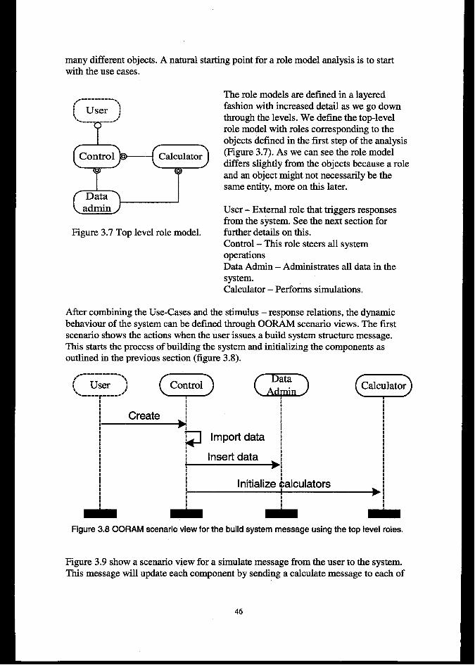
many different objects. A natural starting point for a role model analysis is to startwith the use cases.

Figure 3.7 Top level role model.

The role models are defmed in a layeredfashion with increased detail as we go downthrough the levels. We define the top-levelrole model with roles corresponding to theobjects defined in the first step of the analysis(Figure 3.7). As we can see the role modeldiffers slightly from the objects because a roleand an object might not necessarily be thesame entity, more on this later.

User – Extermd role that triggers responsesfrom the system, See the next section forfurther details on this.Control – This role steers all systemoperationsData Admin – Administrates all data in thesystem.Calculator – Performs simulations.

After combining the Use-Cases and the stimulus – response relations, the dynamicbehaviour of the system can be defined through 00RAM scenario views. The firstscenario shows the actions when the user issues a build system structure message.This starts the process of building the system and initializing the components asoutlined in the previous section (figure 3.8).

::UZJ= m -:11

It

1t

1

1I

1 Create ~: 1

1 11 i 11 : I1 4 I1 11

7I Import data ~

1II 1 :1 1 1 II I &1 I 11 I I1 I1 I1 I 1 11 1 t1 1 I1 I Initialize Calculators

11 1 1I 1

[ ,

A A A

Figure 3.8 OORAM scenario view for the build system message using the top level roles.

Figure 3.9 show a scenario view for a simulate message from the user to the system.This message will update each component by sending a calculate message to each of

46

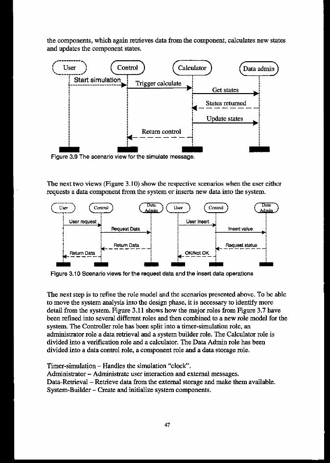
the components, which again retrieves data from the component, calculates new statesand updates the component states.

(::;--) (=) (i) FF@I

I Start simulation : I>: Trigger talc~---------------------

/ 1:11

:

11

1:

III

I 1 E 1

1 Ii I

1

: :I

!

* * - *Figure 3.9 The scenario view for the simulate message,

The next two views (Figure 3.10) show the respective scenarios when the user eitherrequests a data component from the system or inserts new data into the system.

Figure 3.10 Scenario viewa for the request data and the insert data operations

The next step is to refine the role model and the scenarios presented above. To be ableto move the system analysis into the design phase, it is necessary to identify moredetail from the system. Figure 3.11 shows how the major roles from Figure 3.7 havebeen refined into several different roles and then combined to a new role model for thesystem. The Controller role has been split into a timer-simulation role, anadministrator role a data retrieval and a system builder role. The Calculator role isdivided into a verification role and a calculator. The Data Admin role has beendivided into a data control role, a component role and a data storage role.

Timer-simulation – Handles the simulation “clock”.Administrator – Administrate user interaction and external messages.Data-Retrieval – Retrieve data ffom the external storage and make them available.System-Builder – Create and initialize system components.

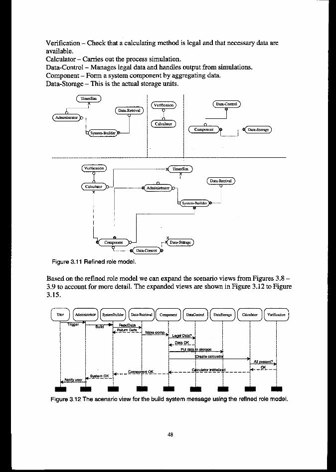
Verification – Check that a calculating method is legal and that necessary data areavailable.Calculator – Carries out the process simulation.Data-Control – Manages legal data and handles output from simulations.Component – Forma system component by aggregating data.Data-Storage – This is the actual storage units.

w zVerificadcm

Calculator

YData-Conaol

A

TData-Reaxiv.d

w-Figure 3.11 Refined role model.

Based on the refined role model we can expand the scenario views from Figures 3.8 –3.9 to account for more detail. The expanded views are shown in Figure 3.12 to Figure3.15.

Figure 3.12 The scenario view for the build system message using the refined role model.

48

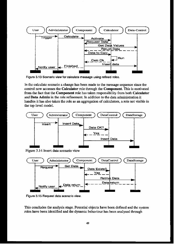
:---=---- -xTrigger ; Calculate JActivate !

fieq uest Datami-

Get Dat& Valuesw

~D=ta—to—:::yp=’=- — — — +

bRun

Calc Okb—————:

Figure 3.13 Scenario view for calculate message using refined roles.

In the calculate scenario a change has been made to the message sequence since thecontrol now accesses the Calculator role through the Component. This is motivatedfrom the fact that the Component role has taken responsibility from both Calculatorand Data Admin in the role refinement. In addition to the data administration ithandles it has also taken the role as an aggregation of calculators, a role not visible inthe top-level model.

,.:.

---;~> q.-----

i-----i~~~fi---- ,* ,, ‘

* ,

* ~–~e=––~, ,,, t Inseq Data,* *

Am - A Am

Figure 3.14 Insert data scenario view

‘==:- - =E- --,.

~---------------->iRequest Get Data ~* Data Exists

Data ~returnb

~Data return :~— ———~— ——— —’~~Notify user —————;------ --------- ~

- A -

Figure 3.15 Request data scenario view.

This concludes the analysis stage. Potential objects have been defined and the systemroles have been identified and the dynamic behaviour has been analysed through

49

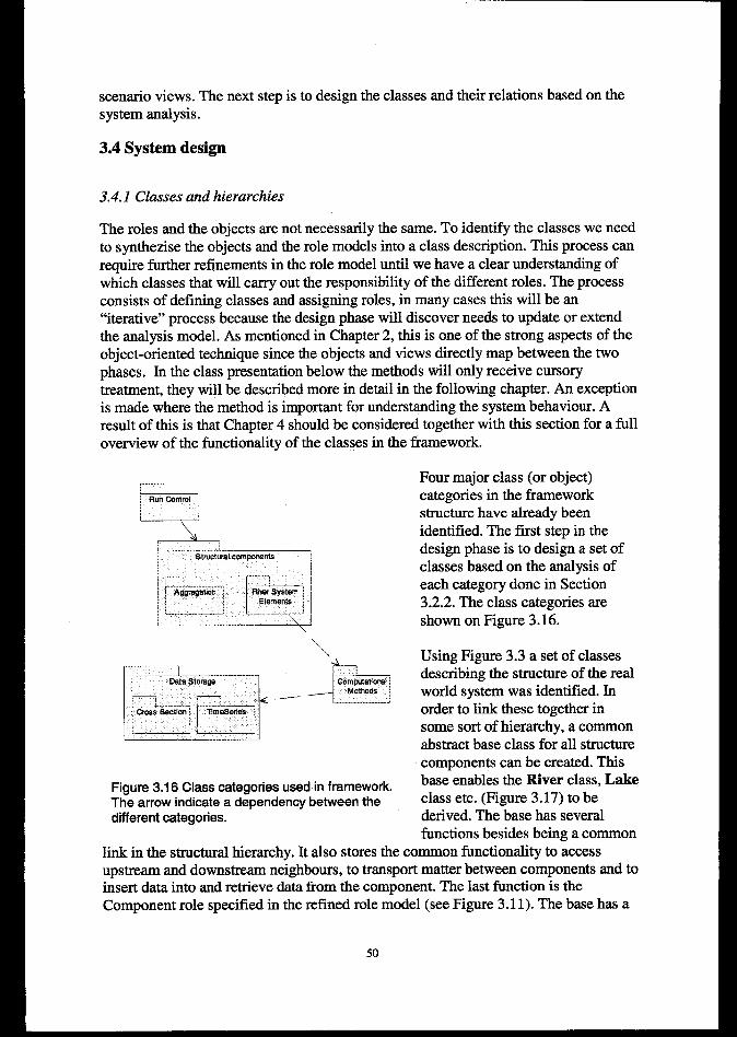
scenario views. The next step is to design the classes and their relations based on thesystem analysis.

3.4 System design

3.4.1 Classes and hierarchies

The roles and the objects are not necessarily the same. To identify the classes we needto synthezise the objects and the role models into a class description. This process canrequire further refinements in the role model until we have a clear understanding ofwhich classes that will carry out the responsibility of the different roles. The processconsists of defining classes and assigning roles, in many cases this will be an“iterative” process because the design phase will discover needs to update or extendthe analysis model. As mentioned in Chapter 2, this is one of the strong aspects of theobject-oriented technique since the objects and views directly map between the twophases. In the class presentation below the methods will only receive cursorytreatment, they will be described more in detail in the following chapter. An exceptionis made where the method is important for understanding the system behaviour. Aresult of this is that Chapter 4 should be considered together with this section for a fulloverview of the functionality of the classes in the framework.

--1

Lzl;Rum Control

\

Figure 3.16 Class categories used in framework,The arrow indicate a dependency between thedifferent categories.

Four major class (or object)categories in the frameworkstructure have already beenidentified. The first step in thedesign phase is to design a set ofclasses based on the analysis ofeach category done in Section3.2.2. The class categories areshown on Figure 3.16.

Using Figure 3.3 a set of classesdescribing the structure of the realworld system was identified. Inorder to link these together insome sort of hierarchy, a commonabstract base class for all structurecomponents can be created. Thisbase enables the River class, Lakeclass etc. (Figure 3.17) to bederived. The base has severalfunctions besides being a common

link in the structural hierarchy. It also stores the common functionality to accessupstream and downstream neighbors, to transport matter between components and toinsert data into and retrieve data from the component. The last function is theComponent role specified in the refined role model (see Figure 3. 11). The base has a

50

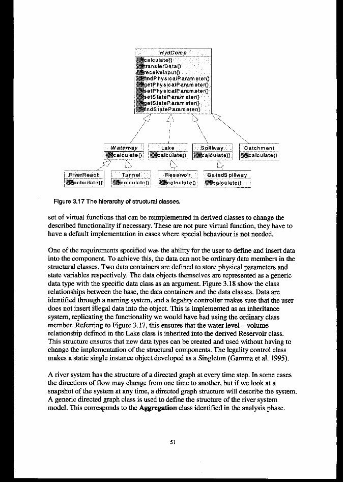
HydComp

#&calculateomransferDataoaeceivelnputomndPhysicalParam etero##getPhysicalParam etero&f#setPhysicalParameterojj#setStateParam etero###getStateParam eteromtndStateParametero

. . .-"-"-"-;~:"""-"""""""""""-":Y7-""""""""`"-"-""`T:""""

“\/“ I “

‘\\\

\\

y~mm~ Waterway :

i.Ea!cY!.a!.e(?... &@alc”lateo ] &#kalculateo““””””””’””’”””-”-”--””-~;-”-’

e:+ “--”’es-e”x’i’”--”“-’auedspi’’y-’y-””$j&jcalculateo~ =alculateo ~ =alculateo

Figure 3.17 The hierarchy of structural classes.

set of virtual functions that can be reimplemented in derived classes to change thedescribed functionality if necessary. These are not pure virtual function, they have tohave a default implementation in cases where special behaviour is not needed.

One of the requirements specified was the ability for the user to define and insert datainto the component. To achieve this, the data can not be ordinary data members in thestructural classes. Two data containers are defined to store physical parameters andstate variables respectively. The data objects themselves are represented as a genericdata type with the specific data class as an argument. Figure 3.18 show the classrelationships between the base, the data containers and the data classes. Data areidentified through a namings ysterrL and a legality controller makes sure that the userdoes not insert illegal data into the object. This is implemented as an inheritancesystem, replicating the functionality we would have had using the ordinary classmember. Referring to Figure 3.17, this ensures that the water level – volumerelationship defined in the Lake class is inherited into the derived Reservoir class.This structure ensures that new data types can be created and used without having tochange the implementation of the structural components. The legality control classmakes a static single instance object developed as a Singleton (Gamma et al. 1995).

A river system has the structure of a directed graph at every time step. In some casesthe directions of flow may change from one time to another, but if we look at asnapshot of the system at any time, a directed graph structure will describe the system.A generic directed graph class is used to define the structure of the river systemmodel. This corresponds to the Aggregation class identified in the analysis phase.

51

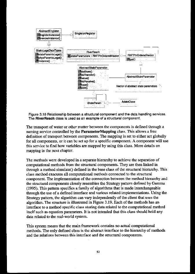
! AbatrectSinglelcm~

~~?zk$~-”-”m,?,,/,!,

wJ-"-"-'""'"""""""""-"""""""-""""-"-"""""""-""""""`"-"I:-"```"_ Jl%K)

Riu?rReach: -—————J—

i —7~tatepararnatwa: RWIPttOtdwedVectorC-- mO~g~&_

: . ..... ................. ..... ...................... .. .... ........ . . .I.....-!E!!?!IE!?.....–..- ......I

eL.-.-.-.-.-.-——.-....-..——.

: AbatractStatePerwneterMgdo’stereo-Trar#ero

L.

‘-W() ___.i AbstractStatePararneter

#&icReceiwO /YPS:

. .VectorofabstractJate patietem” ~...

,,—.. —=

L :-.,-’-”-””-”””; ~~~~~‘ ‘-------

StatePerem ‘C- — AdataClaes

Figure 3.18 Relationship between a structural component and the data handling services.The RiverReach class is used as an example of a structural component.

The transport of water or other matter between the components is defined through anaming service controlled by the ParameterMapping class. This allows a freedefinition of transport between components. The mapping is set to either act globallyfor all components, or it can be setup for a specific component. A component will usethis service to find how variables are mapped by using this class. More details onmapping in the next chapter.

The methods were developed in a separate hierarchy to achieve the separation ofcomputational methods from the structural components. They are then linked inthrough a method simulateo defined in the base class of the structural hierarchy. Thisclass method executes all computational methods connected to the structuralcomponent. The implementation of the connection between the method hierarchy andthe structural components closely resembles the Strategy pattern defined by Gamma(1995). This pattern specifies a family of algorithms that is made interchangeablethrough the use of a defined interface and various related implementations. Using theStrategy pattern, the algorithm can vary independently of the client that uses thealgorithm. The structure is illustrated in Figure 3.19. Each of the methods has aninterface to a method specific class storing data related to the computational methoditself such as equation parameters. It is not intended that this class should hold anydata related to the real-world system.

This system means that the main framework contains no actual computationalmethods. The only defined class is the abstract interface to the hierarchy of methodsand the relations between this interface and the structural components.

52

\

/ ‘\

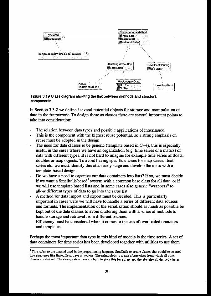
~ituir.~ ‘L......... .. ..._ . .._. _—-.-.-

[

~ M uskinggumData

implementation~~K : float~=: float

&

Figure 3.19 Class diagram showing the link between methods and structuralcomponents.

In Section 3.3.2 we defined several potential objects for storage and manipulation ofdata in the framework. To design these as classes there are several important points totake into consideration:

The relation between data types and possible applications of inheritance.This is the component with the highest reuse potential, so a strong emphasis onreuse must be adopted in the design.The need for data classes to be generic (template based in C++), this is especiallyuseful in the cases where we have an organization (e.g. time series or a matrix) ofdata with different types. It is not hard to imagine for example time series of floats,doubles or map objects. To avoid having specific classes for map series, floatseries ete. we must identify this at an early stage and develop the class with atemplate-based design.Do we have a need to organize our data containers into lists? If so, we must decideif we want a Smalltalk-based8 system with a common base class for all data, or ifwe will use template based lists and in some cases also generic “wrappers” toallow different types of data to go into the same list.A method for data import and export must be decided. This is particularlyimportant in cases were we will have to handle a series of different data sourcesand formats. The implementation of the serialization should as much as possible bekept out of the data classes to avoid cluttering them with a series of methods tohandle storage and retrieval from different sources.Efficiency must be considered when it comes to the use of overloaded operatorsand templates.

Perhaps the most important data type in this kind of models is the time series. A set ofdata containers for time series has been developed together with utilities to use them

8Thisrefersto themethodusedin theprogramminglanguageSmalltalktocreateclassesthatcouldbeinsertedintostructureslikelinkedlista,treesorvectors.Theprincipleis tocreatea baseclassfromwhichallotherclassesarederived.Thestoragestructuresaxeboiltto storethisbaseclassandtherebyrdsoallderivedclasses.

53

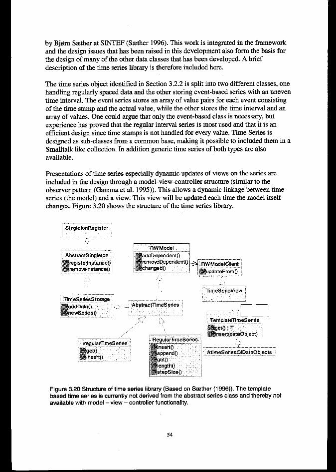
by Bj@n Sa%her at SIN’TEF (SaXher 1996). This work is integrated in the frameworkand the design issues that has been raised in this development also form the basis forthe design of many of the other data classes that has been developed. A briefdescription of the time series library is therefore included here.

The time series object identified in Section 3.2.2 is split into two different classes, onehandling regularly spaced data and the other storing event-based series with an uneventime interval. The event series stores an array of value pairs for each event consistingof the time stamp and the actual value, while the other stores the time interval and anarray of values. One could argue that only the event-based class is necessary, butexperience has proved that the regular interval series is most used and that it is anefficient design since time stamps is not handled for every value. Time Series isdesigned as sub-classes from a common base, making it possible to included them in aSmalltalk like collection. In addition generic time series of both types are alsoavailable.

Presentations of time series especially dynamic updates of views on the series areincluded in the design through a model-view-controller structure (similar to theobserver pattern (Gamma et al. 1995)). This allows a dynamic linkage between timeseries (the model) and a view. This view will be updated each time the model itselfchanges. Figure 3.20 shows the structure of the time series library.

(J

&Mremovelnstancao.......................... . . . . .,,

RWModel !... .. .................. ...... . ............ .. . .mddDependento j

L

#&mow?Dependento i#$&hangedo

,, ----,,,,-.....

TlmeSerieView !

Figure 3.20 Structure of time series library (Based on Sather (1996)). The templatebased time series is currently not derived from the abstract series class and thereby notavailable with model - view – controller functionality.

54

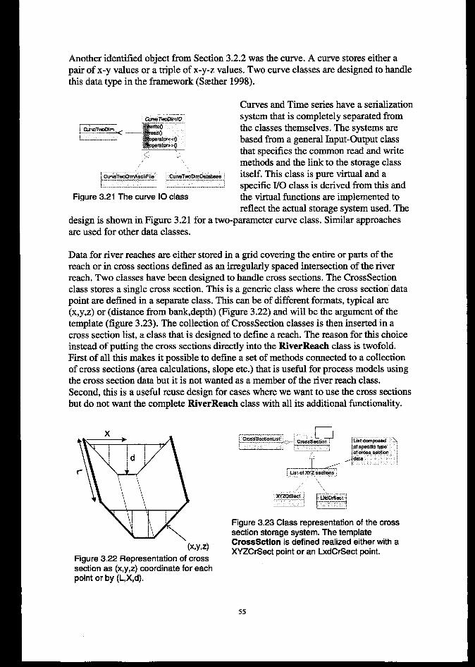
Another identified object from Section 3.2.2 was the curve. A curve stores either apair of x-y values or a triple of x-y-z values. Two curve classes are designed to handlethis data type in the framework (S=ther 1998).

Curves and Time series have a serialization

CIJfvaTw#%lfo system that is completely separated from~CXrwTwoDim ‘m@

< -+&e-adothe classes themselves. The systems are

i............ . . ........... &2pemt0r.x(l

,&@eratO*>obased from a general Input-Output class

~. . . that specifies the common read and write/. ,,<methods and the link to the storage class\

hRiTi&&ciEL Cui&T&JimDat&si itself. This class is pure virtual and a... . ...................... . . . . .. . . . . . . .1. specific I/O class is derived horn this and

Figure 3.21 The curve 10 class the virtual functions are implemented toreflect the actual storage system used. The

design is shown in Figure 3.21 for a two-parameter curve class. Similar approachesare used for other data classes.

Data for river reaches are either stored in a grid covering the entire or parts of thereach or in cross sections defined as an irregularly spaced intersection of the riverreach. Two classes have been designed to handle cross sections. The CrossSectionclass stores a single cross section. This is a generic class where the cross section datapoint are defined in a separate class. This can be of different formats, typical are(x,y,z) or (distance from bank,depth) (Figure 3.22) and will be the argument of thetemplate (figure 3.23). The collection of CrossSection classes is then inserted in across section list, a class that is designed to define a reach. The reason for this choiceinstead of putting the cross sections directly into the RiverReach class is twofold.First of all this makes it possible to define a set of methods connected to a collectionof cross sections (area calculations, slope etc.) that is usefi.d for process models usingthe cross section data but it is not wanted as a member of the river reach class.Second, this is a useful reuse design for cases where we want to use the cross sectionsbut do not want the complete RiverReach class with all its additional functionality.

(X,y,z)

Figure 3.22 Representation of crosssection as (x,Y,z) coordinate for eachpoint or by (L,X,d).

Figure 3.23 Class representation of the crosssection storage system. The templateCrossSction is defined realized either with aXYZCrSect point or an LxdCrSect point.

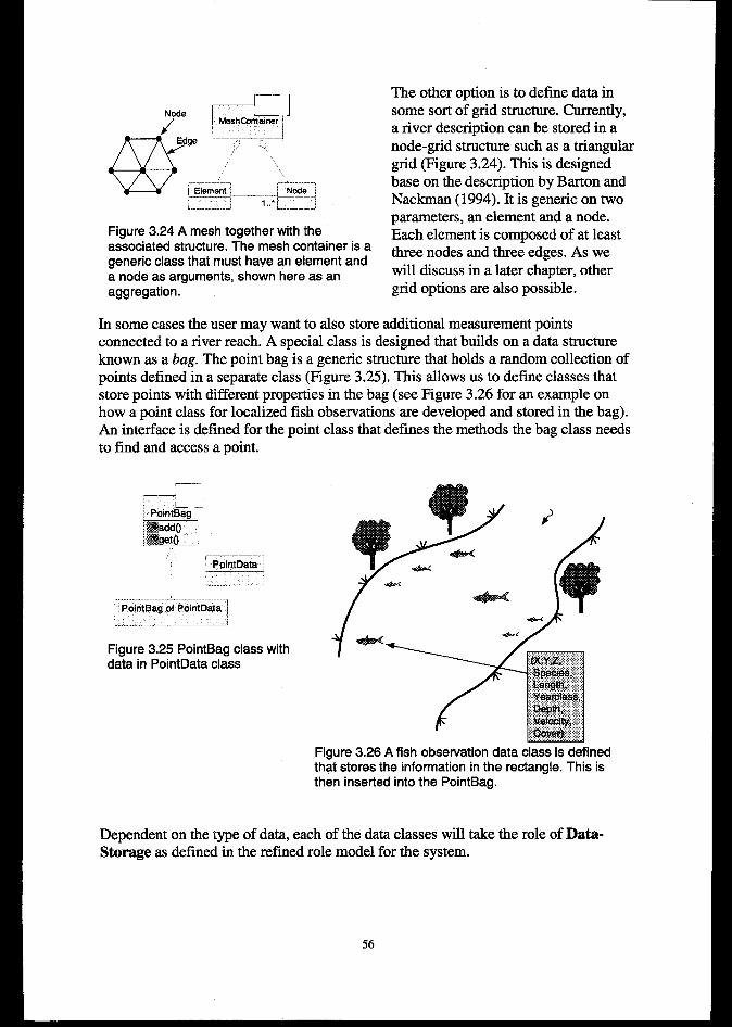
Figure 3.24 A mesh together with theassociated structure. The mesh container is ageneric class that must have an element anda node as arguments, shown here as anaggregation.

The other option is to define data insome sort of grid structure. Currently,a river description can be stored in anode-grid structure such as a triangulargrid (Figure 3.24). This is designedbase on the description by Barton andNackman (1994). It is generic on twoparameters, an element and a node.Each element is composed of at leastthree nodes and three edges. As wewill discuss in a later chapter, othergrid options are also possible.

In some cases the user may want to also store additional measurement pointsconnected to a river reach. A special class is designed that builds on a data structureknown as a bag. The point bag is a generic structure that holds a random collection ofpoints defined in a separate class (Figure 3.25), This allows us to define classes thatstore points with different properties in the bag (see Figure 3.26 for an example onhow a point class for localized fish observations are developed and stored in the bag).An interface is defined for the point class that defines the methods the bag class needsto find and access a point.

Figure 3.25 PointBag class withdata in PointData class

Figure 3.26 A fish observation data class is definedthat stores the infomnation in the rectangle. This isthen inserted into the PointBag.

Dependent on the type of data, each of the data classes will take the role of Data-Storage as defined in the refined role model for the system.

56

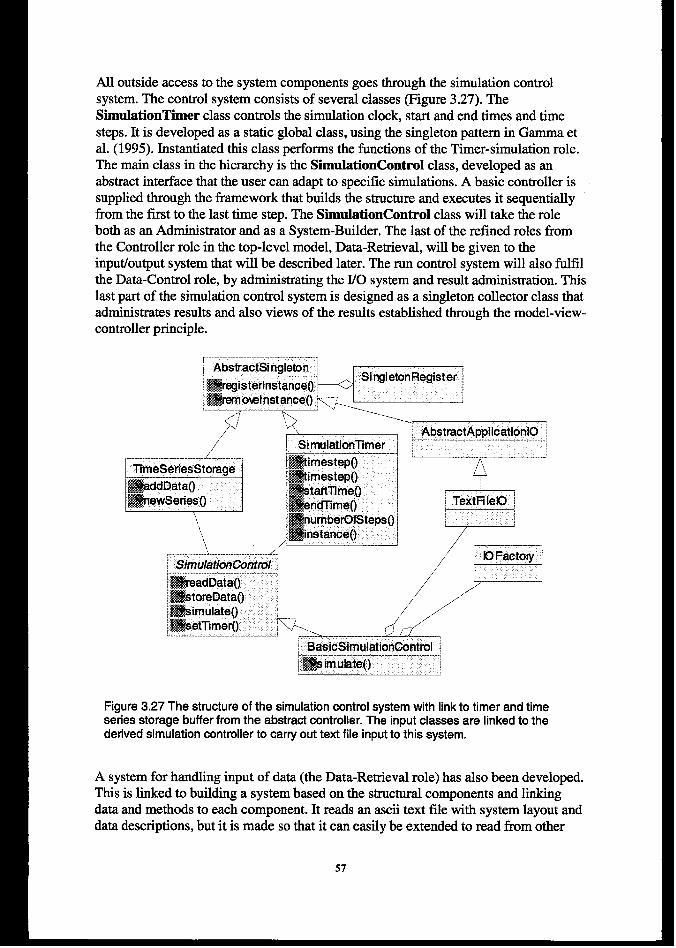
All outside access to the system components goes through the simulation controlsystem. The control system consists of several classes (Figure 3.27). TheSimulationTimer class controls the simulation clock, start and end times and timesteps. It is developed as a static global class, using the singleton pattern in Gamma etal. (1995). Instantiated this class performs the functions of the Timer-simulation role.The main class in the hierarchy is the SimulationControl class, developed as anabstract interface that the user can adapt to specific simulations. A basic controller issupplied through the framework that builds the structure and executes it sequentiallyfrom the first to the last time step. The SimulationControl class will take the roleboth as an Administrator and as a System-Builder, The last of the refined roles fromthe Controller role in the top-level model, Data-Retrieval, will be given to theinput/output system that will be described later. The run control system will also fulfilthe Data-Control role, by administrating the I/O system and result administration. Thislast part of the simulation control system is designed as a singleton collector class thatadministrates results and also views of the results established through the model-view-controller principle.

AbstractApplication10 I.-- ...--.—.-..——-------------~

/’ ;.—...—.—--.—

e

TimeSeriesStorageimimestepo /i\~mimestepo ~

Q

-dDatao,#&newSerieso

i-tartlimeo ~ ~

1wenfimeo ~ ~ TextRle10 1

!,, [f#numberOfStepso ~,,,, lmnstance~ i

... . ..... .. .. ...!'! ................ ..... .. .. ......J.r

p’/’ i ‘F=tov ‘

~=toreDataO,/’ ‘,//

‘.E;::;8 ....-.......-......k~==. /;>’”I Ba~i~Sim”lation~ntm~l..........................................................................<Imimubteo

Figure 3.27 The structure of the simulation control system with link to timer and timeseries storage buffer from the abstract controller. The input classes are linked to thederived simulation controller to carry out text file input to this system.

A system for handling input of data (the Data-Retrieval role) has also been developed.This is linked to building a system based on the structural components and linkingdata and methods to each component. It reads an ascii text file with system layout anddata descriptions, but it is made so that it can easily be extended to read from other

57

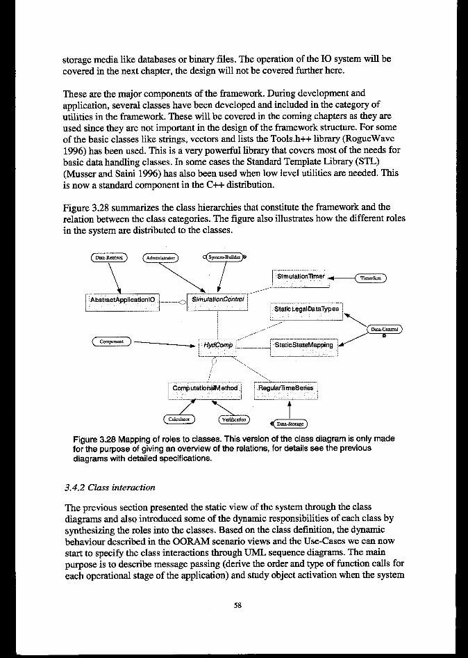
storage media like databases or binary files. The operation of the IO system will becovered in the next chapter, the design will not be covered further here.

These are the major components of the framework. During development andapplication, several classes have been developed and included in the category ofutilities in the framework. These will be covered in the coming chapters as they areused since they are not important in the design of the framework structure. For someof the basic classes like strings, vectors and lists the Tools.h++ library (RogueWave1996) has been used. This is a very powerful library that covers most of the needs forbasic data handling classes. In some cases the Standard Template Library (STL)(Musser and Saini 1996) has also been used when low level utilities are needed. Thisis now a standard component in the C++ distribution.

Figure 3.28 summarizes the class hierarchies that constitute the framework and therelation between the class categories. The figure also illustrates how the different rolesin the system are distributed to the classes.

,T‘=&:~,...F=AbstmctApplication10 . . .

~ StaticLegalOateTypee\

,/-,/-,

/“”’

~>-................................. .. ........ .. ........~ ~ ....... ...i................r.<.

iWZfCOMP L____________ StaticStateMapping.-... Tr_—. y., i —.

V “>. -.\.,

Figure 3.28 Mapping of roles to classes. This version of the class diagram is only madefor the purpose of giving an overview of the relations, for details see the previousdiagrams with detailed specifications.

3.4.2 Class interaction

The previous section presented the static view of the system through the classdiagrams and also introduced some of the dynamic responsibilities of each class bysynthesizing the roles into the classes. Based on the class definition, the dynamicbehaviour described in the 00RAM scenario views and the Use-Cases we can nowstart to specify the class interactions through UML sequence diagrams. The mainpurpose is to describe message passing (derive the order and type of function calls foreach operational stage of the application) and study object activation when the system

58

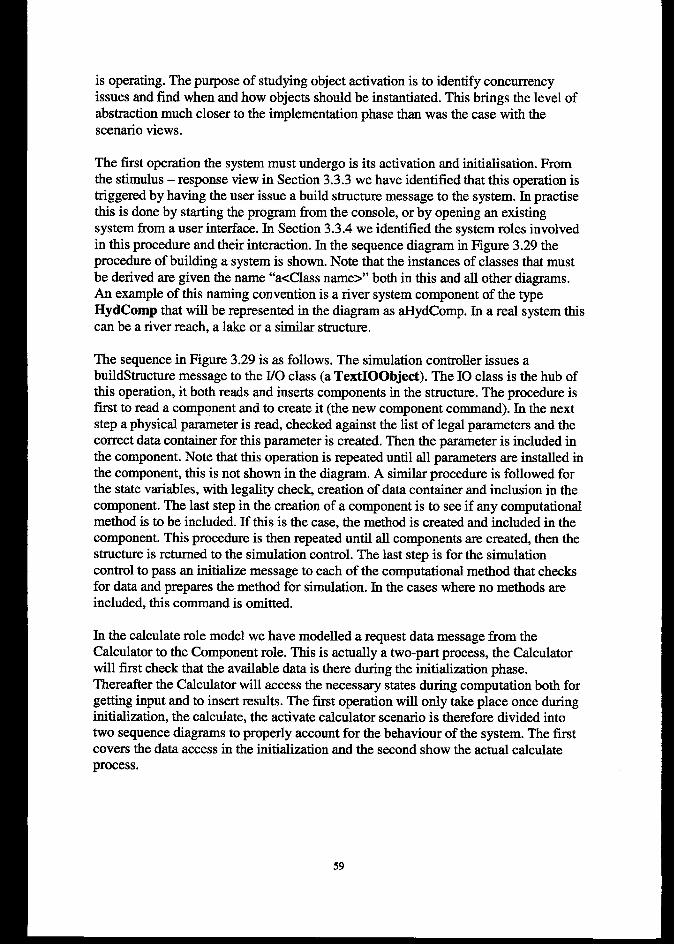
is operating. The purpose of studying object activation is to identify concurrencyissues and find when and how objects should be instantiated. This brings the level ofabstraction much closer to the implementation phase than was the case with thescenario views.

The first operation the system must undergo is its activation and initialisation. Fromthe stimulus – response view in Section 3.3.3 we have identified that this operation istriggered by having the user issue a build structure message to the system. In practisethis is done by starting the program from the console, or by opening an existingsystem from a user interface. In Section 3.3.4 we identified the system roles involvedin this procedure and their interaction. In the sequence diagram in Figure 3.29 theprocedure of building a system is shown. Note that the instances of classes that mustbe derived are given the name “a<Class name>” both in this and all other diagrams.An example of this naming convention is a river system component of the typeHydComp that will be represented in the diagram as aHydComp. In a real system thiscan be a river reach, a lake or a similar structure.

The sequence in Figure 3.29 is as follows. The simulation controller issues abuildStructure message to the I/O class (a TextIOObject). The IO class is the hub ofthis operation, it both reads and inserts components in the structure. The procedure isfirst to read a component and to create it (the new component command). In the nextstep a physical parameter is read, checked against the list of legal parameters and thecorrect data container for this parameter is created. Then the parameter is included inthe component. Note that this operation is repeated until all parameters are installed inthe component, this is not shown in the diagram. A similar procedure is followed forthe state variables, with legality check, creation of data container and inclusion in thecomponent. The last step in the creation of a component is to see if any computationalmethod is to be included. If this is the case, the method is created and included in thecomponent. This procedure is then repeated until all components are created, then thestructure is returned to the simulation control. The last step is for the simulationcontrol to pass an initialize message to each of the computational method that checksfor data and prepares the method for simulation. In the cases where no methods areincluded, this command is omitted.

In the calculate role model we have modelled a request data message from theCalculator to the Component role. This is actually a two-part process, the Calculatorwill first check that the available data is there during the initialization phase.Thereafter the Calculator will access the necessary states during computation both forgetting input and to insert results. The first operation will only take place once duringinitialization, the calculate, the activate calculator scenario is therefore divided intotwo sequence diagrams to properly account for the behaviour of the system. The firstcovers the data access in the initialization and the second show the actual calculateprocess.

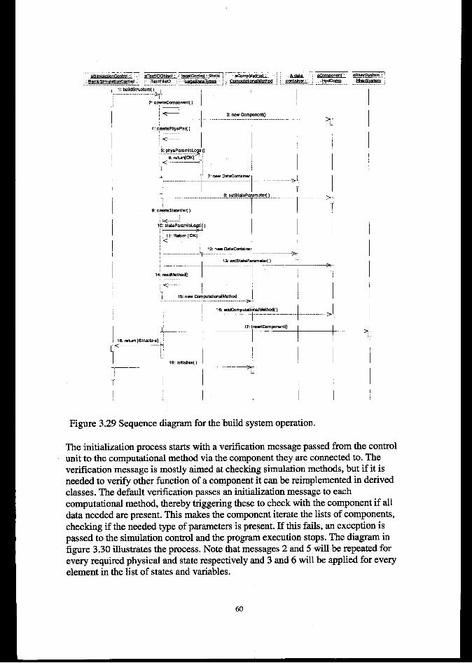
@Q!iw.- ntrd: ! :aTmtCCMect< h?d~.1 : static i ~ aCxmnMnthod COmmnant_ *-W

5k$5n@tb.w ml ‘I!@E!w ataTvces ~ c~vli#JoY?Y?w . ...i ‘“= ‘ ..; !:..!M?W ‘ !..!!!EWK:.

i< - I1,0 statePwamlsLqFJ\ )

11: Wm[OK] –~ <

Il.mt..[stmc.re]~~ “’”’””-”F”” 1T

~< .............-. . ......

I i ,9,”WI,**() I I

I I I

Figure 3.29 Sequence diagram for the build system operation.

The initialization process starts with a verification message passed from the controlunit to the computational method via the component they are connected to. Theverification message is mostly airned at checking simulation methods, but if it isneeded to verify other function of a component it can be reimplemented in derivedclasses. The default verification passes an initialization message to eachcomputational method, thereby triggering these to check with the component if alldata needed are present. This makes the component iterate the lists of components,checking if the needed type of parameters is present. If this fails, an exception ispassed to the simulation control and the program execution stops. The diagram infigure 3.30 illustrates the process. Note that messages 2 and 5 will be repeated forevery required physical and state respectively and 3 and 6 will be applied for everyelement in the list of states and variables.

60

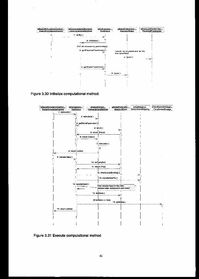
mii”eiho: ““”””c=”””””””;; s ,, i “t’;o !

. ..r..In..”.nt :

Ab raet s a

3: getPhyslcel Pemmetefl’) I— —+

[check Nst o; pemmters for theone specltie~)

r II ‘1 l_ti. 4: type()

J

5: @StateParmneter( ) r,.. >-

‘TI..........?.J?!?!.?.......J

i~.Ii

Figure 3.30 Initialize computational method,

jamsicSimulat cnCcot ml:: ~~nwon~ -:? aComDMsth@L ; z+SttZ~ B~iCS\m u&&

eParamfier: : stat 8MUYJM. , ~: l.~ essnesstomoe :~n,m, : YYsEQm9: ComoutWona!Method : Abstracts MS StatlcStateMaDDina, TineSenesStomue

1: Calculato( )..1,...................... ......_..........+

J 1‘, 2: calculate( )

,~- 1

~3: getStateParsm stem j.+ -------------H 4 wlue( )

,-----------------------------.--.-.--.= --- ---------- ----+

./k..-.-.-.--- .-::~!"rnt~~":!..- . ...-. .....---.--.-TI 8: mtum [Value]

m~--

7; Cakulato( )A ................ 1

1<-- ... .. . !’!?”+”!:’... ;“~

9 tlsnsfsri)sta( )..

IL

:1...............................!.0dJ’”’f@1 I-----~------------------->11: return [Yes] >

1<I

12 ohsckLooalBinding( );-= ------------------->

~“~14 receiwlnpm( )

!—.-.-z ‘Call receiw input In the next k.

,4 — dwmstmsm annponsnt and insert

> 115: doStore( )

,.. . ..- ....->1.

[f doStore =. trim] T10: addData( )

"""""""-"""l""-"`"""" "`""""""""`"`"`""`""""""`""`""`"""""""""""""-"-"""""""-"""""I

>1.,,

17 return c.xtml T~“:. I ‘1

I ‘T

I I I I I I

Figure 3.31 Execute computational method

61

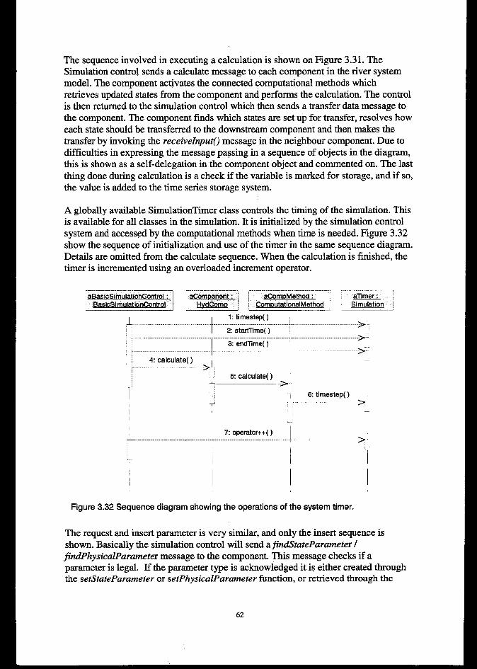
The sequence involved in executing a calculation is shown on Figure 3.31. TheSimulation control sends a calculate message to each component in the river systemmodel. The component activates the connected computational methods whichretrieves updated states from the component and performs the calculation. The controlis then returned to the simulation control which then sends a transfer data message tothe component. The component finds which states are set up for transfer, resolves howeach state should be transferred to the downstream component and then makes thetransfer by invoking the receivelnputo message in the neighbour component. Due todifficulties in expressing the message passing in a sequence of objects in the diagram,this is shown as a self-delegation in the component object and commented on. The lastthing done during calculation is a check if the variable is marked for storage, and if so,the value is added to the time series storage system.

A globally available SimulationTimer class controls the timing of the simulation. Thisis available for all classes in the simulation. It is initialized by the simulation controlsystem and accessed by the computational methods when time is needed. Figure 3.32show the sequence of initialization and use of the timer in the same sequence diagram.Details are omitted from the calculate sequence. When the calculation is finished, thetimer is incremented using an overloaded increment operator.

~ ‘“ae:~’-l [-c’fE~$=d ““””””””~-n ~~aBasicSimulationControl :

7-

1,.-.~.

“1

1 I

I

6: timestep( ) I---> ‘

---4

IFigure 3.32 Sequence diagram showing the operations of the system timer.

The request and insert parameter is very similar, and only the insert sequence isshown. Basically the simulation control will send a@r.uNateParanzeter /j%zdPhysicalParameter message to the component. This message checks if aparameter is legal. If the parameter type is acknowledged it is either created throughthe setStateParameter or setPhysicalParameter function, or retrieved through the

62

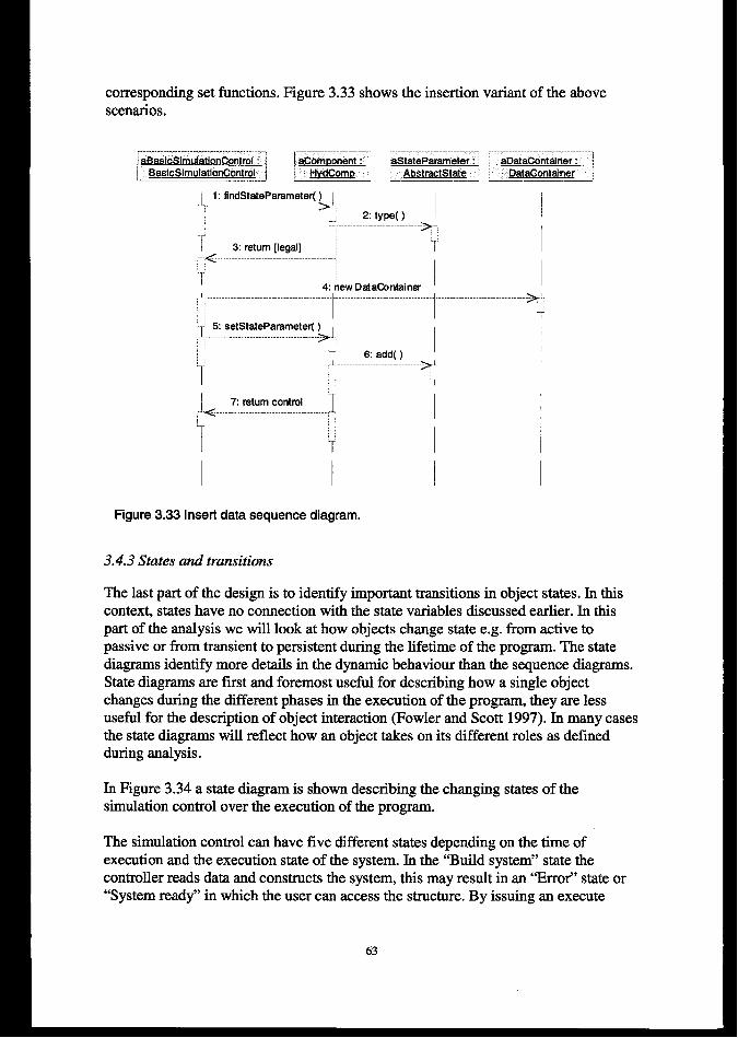
corresponding set functions.scenarios.

,...I@3astcSimulationContml: \~ BasicSimulationConttoi ~

Figure 3.33 shows the insertion variant of the above

:’-=-- ---

T,.1.

T I1 I

Figure 3.33 Insert data sequence diagram.

3.4.3 States and transitions

I

The last part of the design is to identify important transitions in object states. In thiscontext, states have no connection with the state variables discussed earlier. In thispart of the analysis we will look at how objects change state e.g. from active topassive or from transient to persistent during the lifetime of the program. The statediagrams identify more details in the dynamic behaviour than the sequence diagrams.State diagrams are first and foremost useful for describing how a single objectchanges during the different phases in the execution of the program, they are lessusefid for the description of object interaction (Fowler and Scott 1997). In many casesthe state diagrams will reflect how an object takes on its different roles as definedduring analysis.

In Figure 3.34a state diagram is shown describing the changing states of thesimulation control over the execution of the program,

The simulation control can have five different states depending on the time ofexecution and the execution state of the system. In the “Builds ystem” state thecontroller reads data and constructs the system, this may result in an “Errof’ state or“System ready” in which the user can access the structure. By issuing an execute

63

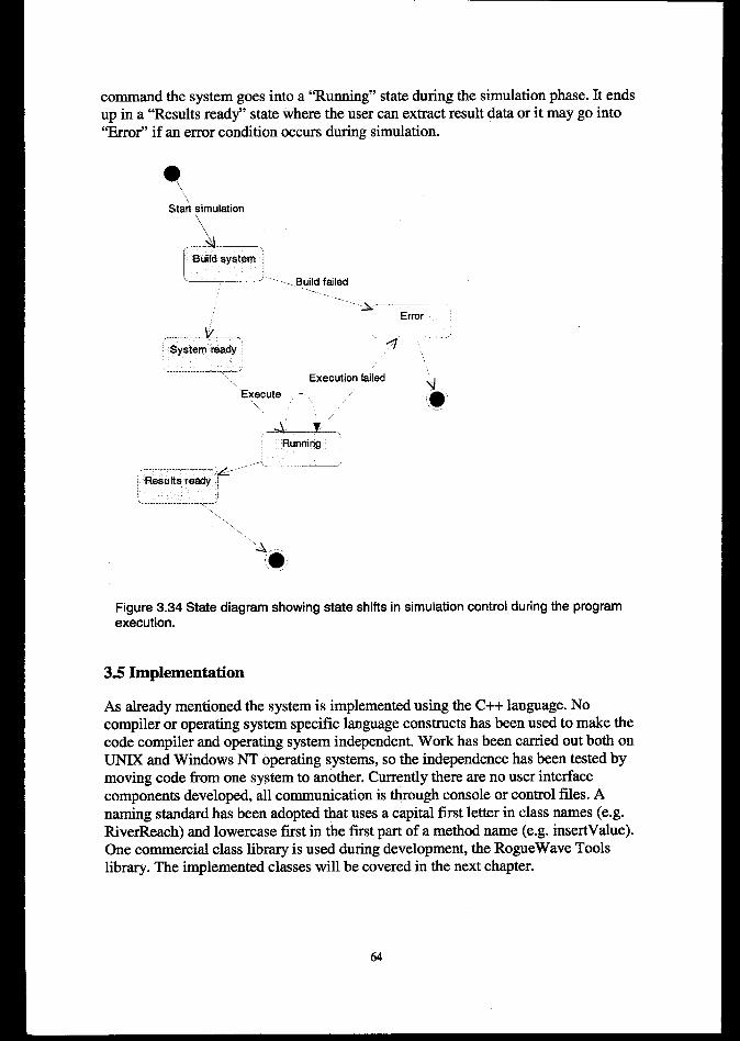
command the system goes into a “Running” state during the simulation phase. It endsup in a “Results ready” state where the user can extract result data or it may go into“Error” if an error condition occurs during simulation.

‘,

Sta~ simulation‘\\

‘&

‘ BuiId systemI“ ‘-- . . . . Build failed

.-..-. --...~,.-Error

. .,.

Figure 3.34 State diagram showing state shifts in simulation control during the programexecution.

3.5 Implementation

As already mentioned the system is implemented using the C++ language. Nocompiler or operating system specific language constructs has been used to make thecode compiler and operatings ystem independent. Work has been carried out both onUNIX and Windows NT operating systems, so the independence has been tested bymoving code from one system to another. Currently there are no user interfacecomponents developed, all communication is through console or control files. Anaming standard has been adopted that uses a capital first letter in class names (e.g.RiverReach) and lowerease first in the first part of a method name (e.g. insertValue).One commercial class library is used during development, the RogueWave Toolslibrary. The implemented classes will be covered in the next chapter.

64

3.6 Testing

A simple way to test the system is to take each of the Use Cases and execute them inthe system. A simple test case has been built based on a real world system consisting alake and a river reach similar to the example used in Chapter 2 (see Figure 2.1). Acatchment object is connected to the lake to provide input. A level pool routing is usedin the lake and a Muskingum algorithm is used in the river reach. Output from thetesting of system build and system execution is shown in Figure 3.37 and Figure 3.38respectively. For details on setting up and using the system, see Chapter 5. Realapplications of the system, and thereby thorough testing will be reported in Chapters 6and 7.

====================BUILD STRUCTURE============================---------------> Catchment LOCALMethods: TSFeeder---------------> Lake: LAKEPHYSICAL:STATE: Q_IN:: 1 * O * 1Q_CALC:: 1 * 1 * OWATER_LEVEL: 1 * O ● OMETHOD: ModPuts---------------> RiverReach: RIVERPHYSICALSTATE:Methods: Muskingum,---------------> Build:Inserting, U=LOCAL,O D=LAKE,lInserting, U=LAKE,l D=RIVER,2---------------> Time:0510119500:00:0005101195 00:00:008640041===================Topological search in progress!===================--> LOCAL--> LAKE--> RIVER

==================VERlFlCATlON===================Verification of LOCAL:Verification of LAKE:

DownstreanERSS_RIVER_REACHDownstream connections is not a spillwayRetrive data local to object

Verification of RIVERInit M: (cl,c2,c3,csum) (0.903382,0.951691,-0.855072,1)==> FINISHED VERIFICATION

Figure 3.35 Output dump from build system structure and system verification duringexecution of the test ease. The three main steps: build system, find execution orderand verify are marked in bold text.

..........-

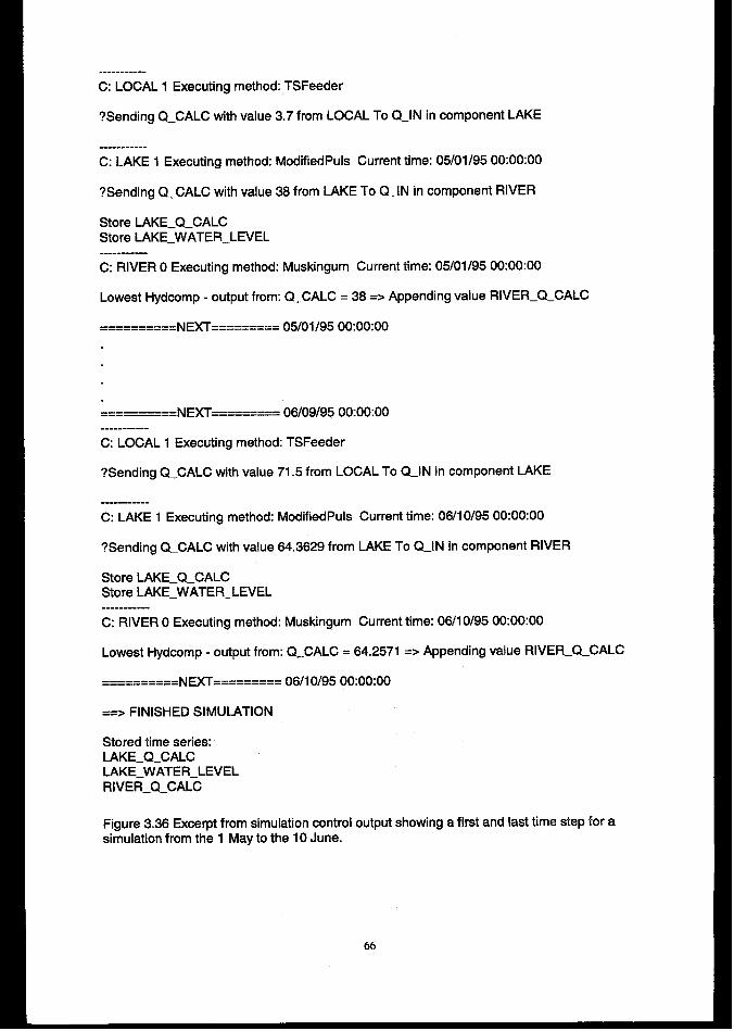
C: LOCAL 1 Executing method: TSFeeder

?Sending Q_CALC with value 3.7 from LOCAL To Q_lN in component LAKE

...--------C: LAKE 1 Executing method: ModifiedPuls Current time: 05/01/95 00:00:00

?Sending Q_CALC with value 38 from LAKE To Q_lN in component RIVER

Store LAKE_Q_CALCStore LAKE_WATER_LEVEL.. . . . . . . . . .

C: RIVER O Executing method: Muskingum Current time: 05/01/95 00:00:00

Lowest Hydcomp - output from: Q_CALC = 38 => Appending vaiue RlvEFLQ_cALc

==========NEXT========= 05/01/95 00:00:00

==========NEXT========= 06/09/95 00:00:00

C: LOCAL 1 Executing method: TSFeeder

?Sending Q_CALC with value 71.5 from LOCAL To Q_lN in component LAKE

...........C: LAKE 1 Executing method: ModifiedPuls Current time: 06/10/95 00:00:00

?Sending Q_CALC with value 64.3629 from LAKE To Q_lN in component RIVER

Store LAKE_Q_CALCStore LAKE_WATER_LEVEL-----------

C: RIVER O Executing method: Muskingum Current time: 06/10/95 00:00:00

Lowest Hydcomp - output from: Q_CALC = 64.2571 => Appending value RlvEFLQ_cALc

==========NEXT=-======== 06/1 0/95 00:00:00

==> FINISHED SIMULATION

Stored time series:LAKE_Q_CALCLAKE_WATER_LEVELRIVER_Q_CALC

Figure 3.36 Excerpt from simulation control output showing a first and last time step for asimulation from the 1 May to the 10 June.

66

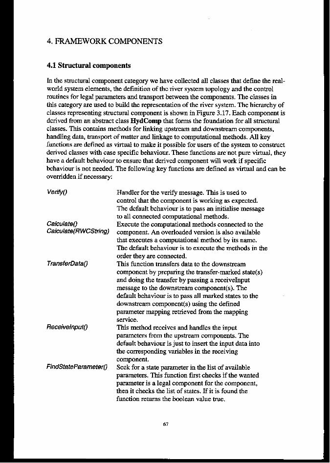
4. FRAMEWORK COMPONENTS

4.1 Structural components

In the structuralcomponent category we have collected all classes that define the real-world system elements, the definition of the river system topology and the controlroutines for legal parameters and transport between the components. The classes inthis category are used to build the representation of the river system. The hierarchy ofclasses representing structural component is shown in Figure 3.17. Each component isderived from an abstract class HydComp that forms the foundation for all structuralclasses. This contains methods for linking upstream and downstream components,handling data, transport of matter and linkage to computational methods. All keyfunctions are defined as virtual to make it possible for users of the system to constructderived classes with case specific behaviour. These functions are not pure virtual, theyhave a default behaviour to ensure that derived component will work if specificbehaviour is not needed. The following key functions are defined as virtual and can beoverridden if necessary

Verifyo

Ca/culateoCa/culate(RWCString)

TransferDatao

Receivelnputo

FindStateParametero

Handler for the verify message. This is used tocontrol that the component is working as expected.The default behaviour is to pass an initialise messageto all connected computational methods.Execute the computational methods connected to thecomponent. An overloaded version is also availablethat executes a computational method by its name.The default behaviour is to execute the methods in theorder they are connected.This function transfers data to the downstreamcomponent by preparing the transfer-marked state(s)and doing the transfer bypassing a receiveInputmessage to the downstream component(s). Thedefault behaviour is to pass all marked states to thedownstream component(s) using the definedparameter mapping retrieved from the mappingservice.This method receives and handles the inputparameters from the upstream components. Thedefault behaviour is just to insert the input data intothe corresponding variables in the receivingcomponent.Seek for a state parameter in the list of availableparameters. ‘I’M;function first checks if the wantedparameter is a legal component for the component,then it checks the list of states. If it is found thefunction returns the boolean value true.

67

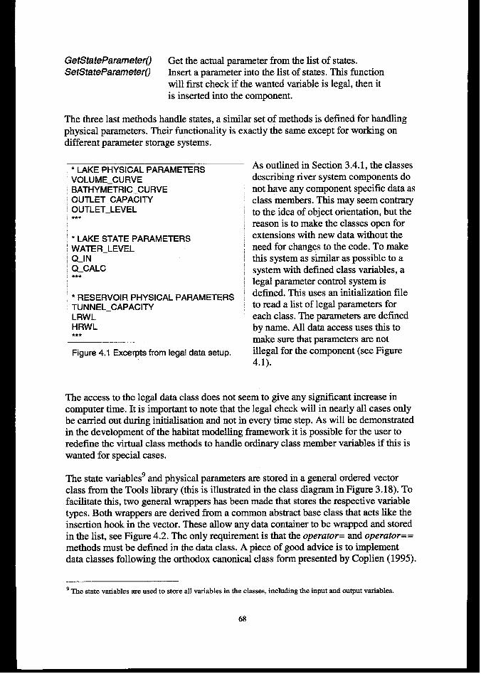
GetStateParametero Get the actual parameter from the list of states.SetStateParametero Insert a parameter into the list of states. This function

will first check if the wanted variable is legal, then itis inserted into the component.

The three last methods handle states, a similar set of methods is defined for handlingphysical parameters. Their functionality is exactly the same except for working ondifferent parameter storage systems.

● LAKE PHYSICAL PARAMETERSVOLUME.CURVEBATHYMETRIC.CURVEOUTLET.CAPACITYOUTLET_LEVEL***

* LAKE STATE PARAMETERSWATER_LEVELQ_lNQ_CALC***

* RESERVOIR PHYSICAL PARAMETERSTUNNEL.CAPACITYLRWLHRWL● **

Figure 4.1 Excerpte from legal data eetup.

As outlined in Section 3.4.1, the classesdescribing river system components donot have any component specific data asclass members. This may seem contraryto the idea of object orientation, but thereason is to make the classes open forextensions with new data without theneed for changes to the code. To makethis system as similar as possible to asystem with defined class variables, alegal parameter control system isdefined. This uses an initialization fileto read a list of legal parameters foreach class. The parameters are definedby name. All data access uses this tomake sure that parameters are notillegal for the component (see Figure4.1).

The access to the legal data class does not seem to give any significant increase incomputer time, It is important to note that the legal check will in nearly all cases onlybe carried out during initialisation and not in every time step. As will be demonstratedin the development of the habitat modelling framework it is possible for the user toredefine the virtual class methods to handle ordinary class member variables if this iswanted for special cases.

The state variables and physical parameters are stored in a general ordered vectorclass from the Tools library (this is illustrated in the class diagram in Figure 3.18). Tofacilitate this, two general wrappers has been made that stores the respective variabletypes. Both wrappers are derived from a common abstract base class that acts like theinsertion hook in the vector. These allow any data container to be wrapped and storedin the list, see Figure 4.2. The only requirement is that the operator= and operator==methods must be defined in the data class. A piece of good advice is to implementdata classes following the orthodox canonical class form presented by Coplien (1995).

9Thestatevariablesareusedto storeallvariablesintheclasses,includingtbeinputandoutputvtiables.

68

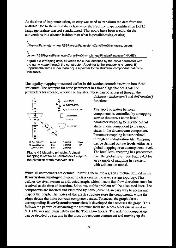
At the time of implementation, casting was used to transform the data from theabstract base to the actual data class since the Runtime Type Identification (RTL)language feature was not standardized. This could have been used to do theconvections in a cleaner fashion than what is possible using casting.

,~a)~pPhyeicalParameter= new RSSPhysieelParametercCurveTwoDim> (name, curve);

b)cuwe=(RSSPh~i~lPammetercCuweTwoDim>*)obj->getPhysimlParameter(''NAMF);

Figure 4.2 Wrapping data. a) wraps the curve identified by the cwve parameter withthe name name through the constructor. A pointer to the wrapper is returned. B)unpacks the same curve, here obj is a pointer to the structural component that ownsthis curve,

The legality mapping presented earlier in this section controls insertion into thesestructures. The wrapper for state parameters has three flags that designate theparameters for storage, receiver or transfer. These can be accessed through the

o $ Q_sNPuT

RI~ Q_mVs3’TED

~ Q_cALcuLATEsJ

G=z

RSH RiverReachr—,1 TunnelL:

0

‘Q.., n“-”=

R2

“’”<

QCALCIJLATED Global QINPUT GlobalQCALCULATED Res Q_lNPUT R2

Q_DiVERTED Res QJNPUT T1

Figure 4.3 Mapping principle. A globalmapping is set for all parameters except forthe diversion at the reservoir RES.

doStoreo, doReceiveo and doTransferofunctions.

Transport of matter betweencomponents is controlled by a mappingservice that uses a name basedparameter mapping to link the outputstates in one component to the inputstates in the downstream component.Parameter mapping is user definedthrough an initialization file. Mappingcan be defined on two levels, either as aglobal mapping or at a component level.The local level mapping has precedenceover the global level. See Figure 4.3 foran example of mapping in a systemwith a diversion tunnel.

When all components arc defined, inserting them into a graph structure defined in theRiverSystemTopology<T> generic class creates the river system topology. Thisdefines the river system as a directed graph, which means that flow directions must beresolved at the time of insertion. Solutions to this problem will be discussed later. Thecomponents are inserted and identified by name, creating an easy way to access andinspect the graph. The nodes of the graph structure store the components, while theedges define the links between component states. To access the graph class acorresponding RiverSystemIterator class is developed that accesses the graph. Thisfollows the pattern of separating the structure from the access functions as used inSTL (Musser and Saini 1996) and the Tools.h++ library. The order of computationcan be deeided by starting in the most downstream component and moving up the

69

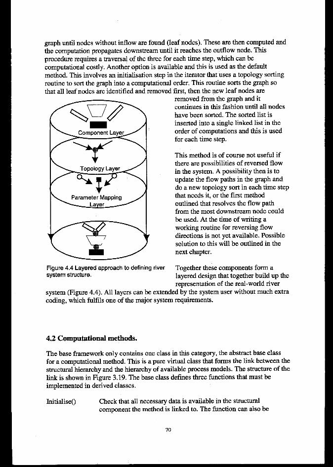
graph until nodes without inflow are found (leaf nodes). These are then computed andthe computation propagates downstream until it reaches the outflow node. Thisprocedure requires a traversal of the three for each time step, which can becomputational costly. Another option is available and this is used as the defaultmethod. This involves an initialisation step in the iterator that uses a topology sortingroutine to sort the graph into a computational order. This routine sorts the graph sothat all leaf nodes are identified and removed first, then the new leaf nodes are

+

Parameter Mapping

Layer

Figure 4.4 Layered approach to defining riversystem structure.

removed from the graph and itcontinues in this fashion until all nodeshave been sorted. The sorted list isinserted into a single linked list in theorder of computations and this is usedfor each time step.

This method is of course not useful ifthere are possibilities of reversed flowin the system. A possibility then is toupdate the flow paths in the graph anddo a new topology sort in each time stepthat needs it, or the frost methodoutlined that resolves the flow pathfrom the most downstream node couldbe used. At the time of writing aworking routine for reversing flowdirections is not yet available. Possiblesolution to this will be outlined in thenext chapter.

Together these components form alayered design that together build up therepresentation of the real-world river

system (Figure 4.4). All layers can be extended by the system user without much extracoding, which fulfils one of the majors ystem requirements.

4.2 Computational methods.

The base framework only contains one class in this category, the abstract base classfor a computational method. This is a pure virtual class that forms the link between thestructural hierarchy and the hierarchy of available process models. The structure of thelink is shown in Figure 3.19. The base class defines three functions that must beimplemented in derived classes.

Initialiseo Check that all necessary data is available in the structuralcomponent the method is linked to. The function can also be

70

used to initialize internal parameters in the computationalmethod itself. The method is default invoked from the verifymethod in the HydComp class.

calculate Perform the simulation. This must read the current stateinformation, calculate the new states and update them.

SetLocalDatao Add method specific data classes to the method. This can beused to insert data like equation parameters, convergencecriteria etc., data that does not belong in the componentsthemselves.

In addition, a setDatao method is defined but normally not used. The purpose of thismethod is to provide the method with data in cases where the computational method isused outside the framework. This ensures a reuse possibility of the methods in otherdomains than applications developed through the framework.

When it is used in framework-based applications the function of the computationalmethod is to read the current states from the component, calculate new values andthen update the states before control is transferred back to the component.

This way of structuring the connection between process simulation method andclasses representing river system elements may seem to break the normal notion of anobject-oriented design since one might expect the computational methods to beordinary class members. An approach where all methods are class members does notfulfil the requirements to the system, it is therefore necessary to structure the classesas described to achieve the wanted fimctionality in the system. An approach that couldhave been used is the one HEC has adopted in their HMS model, where processmethods are included in the class for all identified processes but where theimplementation of each are separated in a similar way to our approach. This approachidentifies the defied processes by real names, e.g. evaporation and percolationmethods in a catchment. Problems can arise if completely new processes are added, inwhich they must be made and put into the existing methods. We feel that it would bemore confusing having an evaporation method calculate snow melt than just using ageneric calculate method for all simulations. It is possible to use the version of themethod that takes a process name as an argument if more clarity is needed. Using thisfeature we could call the above described catchment processes on the formcalculate(’’Evaporation”) and calculate(’’Percolation”). Based on the flexibility inmethod connection and the above call structure we therefore feel that the selectedapproach is the simplest and most efficient to handle.

4.3 Data containers

The available data containers were covered in the design phase in Section 3.4.1. Sincedata containers are included in the components by the use of wrappers, there are nomore design constraints on them than the above-mentioned need for the operator=and operator== methods. The system therefore offers a large degree of flexibility forthe users to employ their specialized data containers. The number of data classes is

71

continuously growing as the tools are used. The list below describes the classesavailable in the base framework. In Chapter 5 more data classes will be introduced.Most classes are developed as C++ templates or have template equivalents to i%rtherincrease the usability of the classes.

Regular and irregulartime series

Template time series

Two and three parametercurve.Cross sections

A node grid

Point bag

Time-distance grid.

Stores evenly spaced or event-based time series. Linkedviews and transformations. For more information seeSzether (1996).Generic time series classes that can store a time series ofany data object. This can be used to store for exampletime stamped maps ffom e.g. a simulation of floodingover a floodplain.Stores a curve defined by an (x,y) pair or an (x,y,z) triplerespectively.Comprised of three classes, a single cross section isdefied in the generic cross section class that must beinstantiated with a cross section point class as anargument. Each cross section is then inserted into a crosssection list. Both the list and the cross section class haveseveral methods to calculate cross section data likewetted perimeter, distances, hydraulic radius etc.The node grid stores a terrain or bathymetry descriptionas a set of point connected by edges. This structure issimilar to the grid structures used in finite element basedequation solvers. The data storage class is based on ideasfrom Barton and Nackman (1994).This bag stores a random collection of points in an area(defined by the component it is linked to). It is generic,so the user can define the actual point structure. The bagallows duplicate points.For one-dimensional simulations and for storage of timeand space defined data a t-x grid is also defined. This isa generic class that will take a node configuration as thetemplate argument. The node configuration can forexample be the (depth, discharge) pair used in one-dimensional hydraulic simulations.

For simulations, a time series collector is defined to receive and store data valuesduring simulation. This is a global, static object that can be accessed from every otherclass in the framework. This class also controls the model-view-controllerfunctionality of the data objects, and it has possibilities to store data on file.

4.4 Simulation control components

A simulation control system has been developed to control the system and executesimulations. It is developed as abase class with several virtual functions that let users

72

develop their own controllers based on this. The simulation control is meant to be theonly link from the simulation system to user interaction and data storages ystems. Thisis the solution to one important requirement to prevent code for data storage and userinteraction into the components of the fhmework. The base class defines thefollowing methods, the virtual methods underlined.

BuildStructureo

Verif@ructureo

simulateo

SetStartTime(..)StartTimero

Create computational elements and construct the river systemstructure. The controller aggregates a RiverSystemTopologyclass that is used to store the structure. The defaultimplementation reads an ordinary text file that defines thestructure.Verify the structure, check parameter mappings and if allmethods have the necessary data available. The function can beimplemented in derived classes if more verification is needed.Perform simulation. In the default implementation executes allconnected methods in all components sequentially.Define the simulation start time, end time and time step.Start simulation clock. This instantiates the global timecontroller and makes it available for all other objects. Thesimulation clock is set to the start time, but it is actually startedfrom the simulate method.

All methods have a default implementation in a basic simulation control in the classBasicSimulationControl. This uses the basic input/output system to read the systemdescription from a control file and a simulation is then executed sequentially. Thiscontroller does not implement any interactive control of the system. If this is needed, anew controller must be derived.

4.5 utilities

As described in the previous chapter and in the first sections of this one, the systemhas a set of “singleton” objects, static global object available in only one instance.This poses a small problem, deletion of the singleton objects maybe difficult dodefine since they are shared between several objects (S~ther, personalcommunication). To overcome this, a register class stores all singleton objects andmakes sure that they are deleted before the program ends. We thereby avoid memoryleaks. The register class is not seen by the user of the system, it is handled internally.

A file-based input output system is also defined. The system uses the structure definedin Section 3.4.1 and it implements a branch of text file based I/O structures connectedto all parts of the system.

5 FRAMEWORK USE

5.1 Introduction

The framework has two main functions. It will define the building blocks for making amodel of a river system, and it is the foundation for defining new methods andintegrating external tools into the simulation system. The purpose of this chapter is tointroduce the use of the framework. The chapter starts with a description of how todefine structural components and insert data and methods. Then the components arelinked together to forma system representation. The second part of the chapter showshow the different parts of the system can be extended with the user’s owndevelopments.

5.2 Building a model of a real-world system

5.2.1 Model construction procedure.

One of the purposes of the framework is to provide the tools to build a model of thereal-world river system. This system can then be equipped with computationalmethods to take the form of a simulation system, or it can be used purely for datahandling purposes. The system construction involves a four-step procedure:

1. The first step identifies and defines the system “objects”. The identification ofsystem objects is controlled by the objective of the model construction and by thephysical conditions in the real-world system we are modelling. The firstcontrolling factor is dependent on the objective of our model construction. If weare going to look at the hydropower system, in most cases it will not be necessaryto model the unregulated areas of the system in detail. Similarly if the purpose is tolook at flood routing, we may omit a detailed representation of hydropower plantsin the model. The second controlling factor considers the physical properties of thesystem. Some physical entities are quite simple to find, like lakes, hydropowerplants and tunnels. The division of river reaches is also controlled by physicalfactors, like junctions with tributaries and reaches between lakes. In a system thatshould be used for simulations it may also be important to look at hydraulic controlin reach divides. When components are selected, data must be prepared andinserted into the component. The two typical factors that may control the amountand type of data inserted are the need to document the component for future use(this may lead to the insertion of pictures and maps) and the data needs in thesimulation methods connected to the component.

2. If simulation is the objective of the model construction we must add the requiredcomputational methods to each component. When the methods are added, we usethe term computational element to describe a component with data and methodsconnected.

74

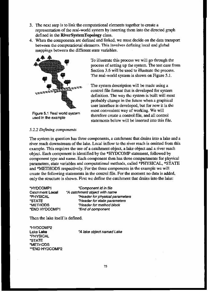
3.

4.

The next step is to link the computational elements together to create arepresentation of the real-worlds ystem by inserting them into the directed graphdefined in the RiverSystemTopology class.When the components are defined and linked, we must decide on the data transportbetween the c~mputational elements. This involves defining local and global -mappings between the different state variables.

To illustrate this process we will go through theprocess of setting up the system. The test case fromSection 3.6 will be used to illustrate the process.The real-world system is shown on F@we 5.1.

The system description will be made using acontrol file format that is developed for systemdefinition. The way the system is built will mostprobably change in the fiture when a graphicaluser interface is developed, but for now it is the

Figure 5.1 Real world systemmost convenient way of working. We will

used in the exampletherefore create a control file, and all controlstatements below will be inserted into this file.

5.2.2 Dejining components

The system in question has three components, a catchment that drains into a lake and ariver reach downstream of the lake. Local inflow to the river reach is omitted from thisexample. This requires the use of a catchment object, a lake object and a river reachobject. Each component is identified by the *HYDCOMP statement, followed bycomponent type and name. Each component then has three compartments for physicalparameters, state variables and computational methods, called *PHYSICAL, *STATEand *METHODS respectively. For the three components in the example we willcreate the following statements in the control file. For the moment no data is added,only the structure is shown. First we define the catchment that drains into the lake:

●HYDCOMPl “Component id in fileCatchment Local *A catchment object with name●PHYSICAL *Header for physical parameters*STATE ●Header for state parameters●METHODS *Header for method block*END HYDCOMP1 ●End of component

Then the lake itself is defined.

*HYDCOMP2Lake Lake *A lake object named Lake*PHYSiCAL*STATE*METHODS●*END HYDCOMP2

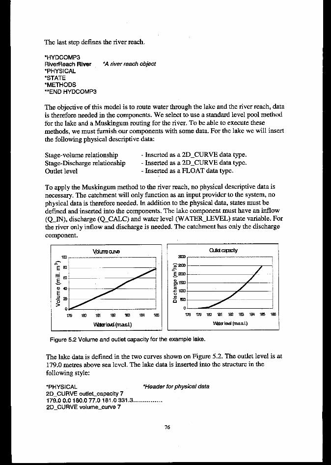
The last step defines the river reach.

*HYDCOMP3RiverReach Rhrer *A river reach object●PHYSICAL*STATE*METHODS**END HYDCOMP3

The objective of this model is to route water through the lake and the river reach, datais therefore needed in the components. We select to use a standard level pool methodfor the lake and a Muskingum routing for the river. To be able to execute thesemethods, we must furnish our components with some data. For the lake we will insertthe following physical descriptive data

Stage-volume relationship - Inserted as a 2D.CURVE data type.Stage-Discharge relationship - Inserted as a 2D.CURVE data type.Outlet level - Inserted as a FLOAT data type.

To apply the Muskingum method to the river reach, no physical descriptive data isnecessary. The catchrnent will only function as an input provider to the system, nophysical data is therefore needed. In addition to the physical data, states must bedefined and inserted into the components. The lake component must have an inflow(Q_IN), discharge (Q_CALC) and water level (WATER_LEVEL) state variable. Forthe river only inflow and discharge is needed. The catchment has only the dischargecomponent.

I lm, ,

m lel lsl I@ 1S3 1S4 1s

W&w (maal.)

Qikioqxitym

m17918J lslwls31841S5 1S3

VW& lad (mad)

Figure 5.2 Volume and outlet capacity for the example lake.

The lake data is defined in the two curves shown on Figure 5.2. The outlet level is at179.0 metres above sea level. The lake data is inserted into the structure in thefollowing style:

●PHYSICAL *Header for physical data2D_CURVE outlet_capacity 7179.00.0180.077.0181 .0331 .3 .. . . . . . . . . . . . . .2D_CURVE volume_cuwe 7

76

179,00.0180.012200000.0 181,024400000,0 ... . . . . . .FLOAT OUTLET_LEVEL 179.0*STATE *Header for state dataFLOAT Q_lN 0.0001FLOAT Q_CALC 0.0010FLOAT WATER_LEVEL 0.0100

The four values connected to each state parameter area default value, a storage flag (ifthis is equal to 1, the state is stored at each time step) and a transfer flag that indicatesif the value should be transferred to the downstream component. The last flag is areceive flag that indicates if this state is updated with values from the upstreamcomponent. This file defines the structural system and it prepares the first part of theparameter mapping service. The next step is to add the computational methods.

5.2.4 Adding computational methods

In this section we assume that a number of computational methods have been derivedfrom the base class and that the necessary functionality has been implemented. Wewill use two methods directly for simulation purposes, and in addition we will use athird method that feeds input data into the system from a time series. The first methodwe add is the level pool routing method for the lake object. This requires no methodspecific data, and is included through the following statements:

*METHODS ‘Method headerMethod: LevelPoolMethod ●Method name

The Muskingum routing method has two method specific parameters, the K and Xcalibration constants. They are included in the method specification, and willeventually be included in the method through the local data object. The statements are:

*METHODSMethod: MuskingumRouting0.25 *Method parameter (X)3.5 ‘Method parameter (K)

The last method we add is the data input routine in the catchrnent object. This is calledTSFeeder, and it takes a time series name and a scaling parameter as local inputi

●METHODSMethod: TSFeederinput_series.dat1.0

When combined with the structural definition from the previous section, the methoddefinition forms the complete definition of the computational elements in themodelling system. The next step is to define the river system topology throughspecifying the linkage between components.

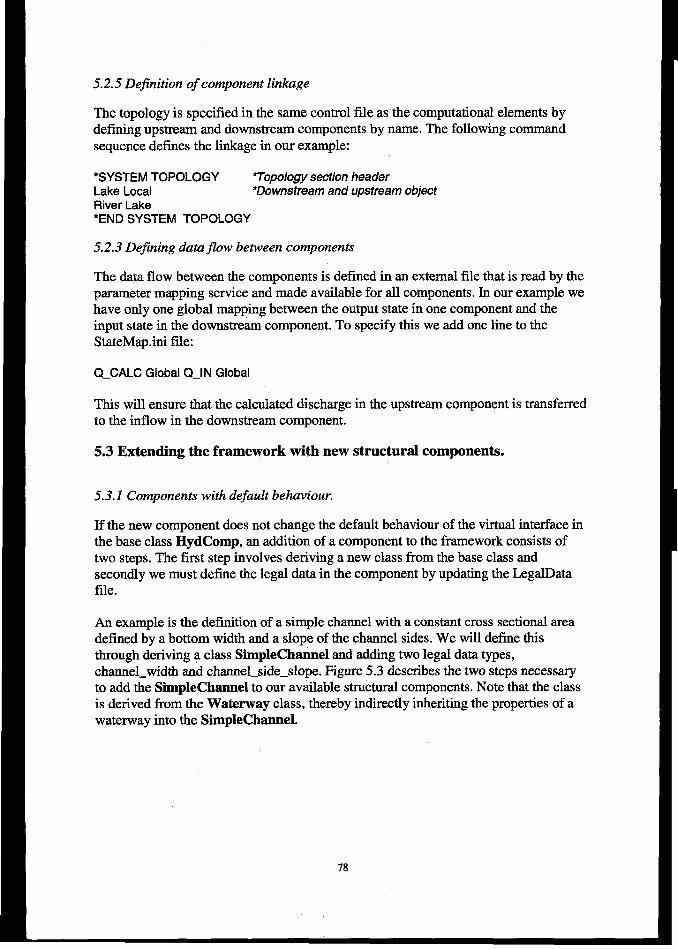
5.2.5 Definition of component linkage

The topology is specified in the same control file as the computational elements bydefining upstream and downstream components by name. The following commandsequence defines the linkage in our example:

*SYSTEM TOPOLOGY Topology section headerLake Local *Downstream and upstream objectRiver Lake*END SYSTEM TOPOLOGY

5.2.3 Defining datajlow between components

The data flow between the components is defined in an external file that is read by theparameter mapping service and made available for all components. In our example wehave only one global mapping between the output state in one component and theinput state in the downstream component. To specify this we add one line to theStateMap.ini file:

Q_CALC Global Q_lN Global

This will ensure that the calculated discharge in the upstream component is transferredto the inflow in the downstream component.

5.3 Extending the framework with new structural components.

5.3.1 Components with default behaviour.

If the new component does not change the default behaviour of the virtual interface inthe base class HydComp, an addition of a component to the framework consists oftwo steps. The first step involves deriving anew class from the base class andsecondly we must define the legal data in the component by updating the LegalDatafile.

An example is the definition of a simple channel with a constant cross sectional areadefined by a bottom width and a slope of the channel sides. We will define thisthrough deriving a class SimpleChannel and adding two legal data types,channel.width and channel_side_slope. Figure 5.3 describes the two steps necessaryto add the SimpleChannel to our available structural components. Note that the classis derived from the Waterway class, thereby indirectly inheriting the properties of awaterway into the SimpleChannel.

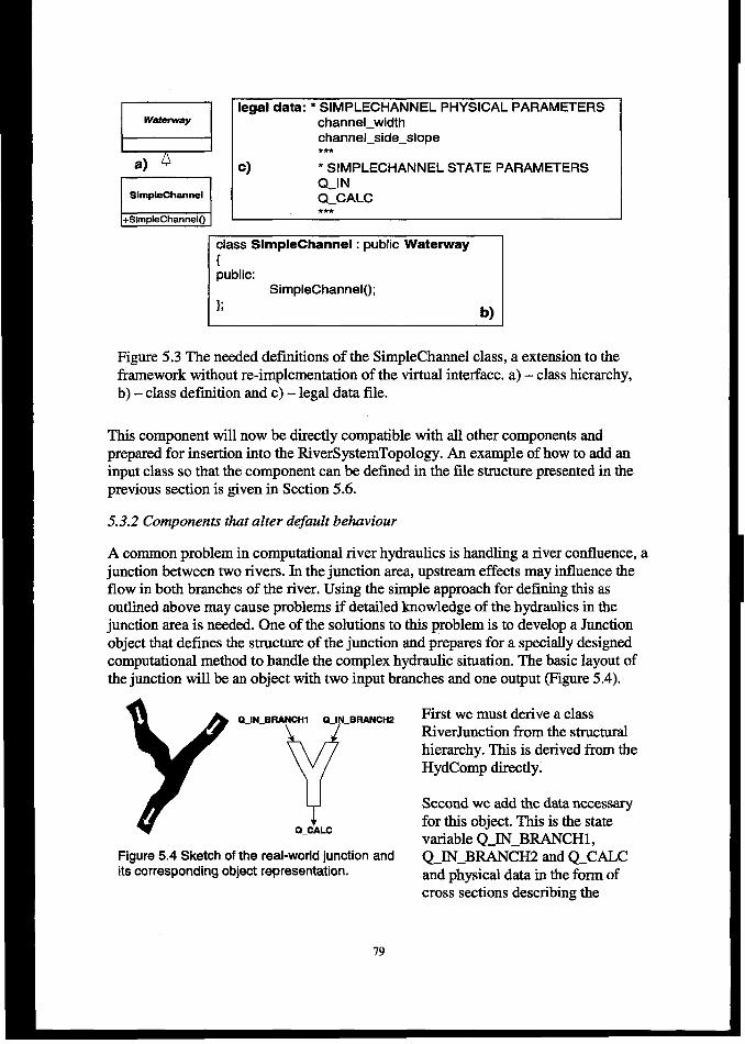
F?legal data: * SIMPLECHANNEL PHYSICAL PARAMETERS

Wafenvay channel_widthchannel_side_slope***

a) c) * SIMPLECHANNEL STATE PARAMETERSQ_l N

SimpleChannel Q_CALC

class SimpleChannel: public Waterway{public:

SimpleChannelo;

}; b)

Figure 5.3 The needed definitions of the SimpleChannel class, a extension to theframework without re-implementation of the virtual interface. a) – class hierarchy,b) - class definition and c) – legal data file.

This component will now be directly compatible with all other components andprepared for insertion into the RiverSystemTopology. An example of how to add aninput class so that the component can be defined in the file structure presented in theprevious section is given in Section 5.6.

5.3.2 Components that alter default behaviour

A common problem in computational river hydraulics is handling a river confluence, ajunction between two rivers. In the junction area, upstream effects may influence theflow in both branches of the river. Using the simple approach for defining this asoutlined above may cause problems if detailed knowledge of the hydratilcs in thejunction area is needed. One of the solutions to this problem is to develop a Junctionobject that defines the structure of the junction and prepares for a specially designedcomputational method to handle the complex hydraulic situation. The basic layout ofthe junction will bean object with two input branches and one output (Figure 5.4).

yniQ.IN.BRANCH1 Q_l _BRANCH2 First we must derive a classRiverJunction from the structuralhierarchy. This is derived from theHydComp directly.

1Second we add the data necessaryfor this object. This is the state

Q_CALCvariable C)_lN_BRANCHl,

Figure 5.4 Sketch of the real-world junction and Q_IN_BRANCH2 and Q_CALCits corresponding object representation. and physical data in the form of

cross sections describing the

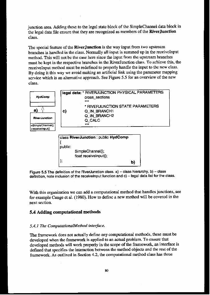
junction area. Adding these to the legal state block of the SimpleChannel data block inthe legal data file ensure that they are recognized as members of the RiverJunctionclass.

The special feature of the RiverJnuetion is the way input from two upstreambranches is handled in the class. Normally all input is summed up in the receiveIuputmethod. This will not be the case here since the input from the upstream branchesmust be kept in the respective branches in the RiverJunction class. To achieve this, thereceiveInput method must be redefined to properly handle the input to the new class.By doing h this way we avoid making an artificial link using the parameter mappingservice which is an alternative approach. See Figure 5.5 for an overview of the newclass.

F=lI

#lI RiverJunction !

legal data: * RIVERJUNCTION PHYSICAL PARAMETERScross_sections***

‘ RIVERJUNCTION STATE PARAMETERSc) Q_lN_BRANCHl

Q_lN_BRANcH2Q.CALC***

class RiverJunction : public HydComp

{public:

SimpleChannelo;float receivelnputo;

I}; b) IFigure 5.5 The definition of the RiverJunction class. a) - class hierarchy, b) - classdefinition, note inclusion of the receivelnput function and c) – legal data list for the class.

With this organization we can add a computational method that handles junctions, seefor example Cunge et al. (1980). How to define anew method will be covered in thenext section.

5.4 Adding computational methods

5.4.1 The ComputationalMethod inte~ace.

The framework does not actually define any computational methods, these must bedeveloped when the framework is applied to an actual problem. To ensure thatdeveloped methods will work properly in the scope of the framework, an interface isdefined that specifies the interaction between the method objects and the rest of theframework. As outlined in Section 4.2, the computational method class has three

80

virtual functions that defines this interface: calculate, initialiseo and setLocalDatao.When anew method is derived these must be implemented.

5.4.2 Defining a simple method.

This section describes the steps taken when a rather simple method is to beimplemented. The following features are covered:

– Derivation of the new class based on ComputatioualMethod.– Implementation of a method specific data block.– Implementation of the virtual fimctions, including the process algorithm.

A commonly used hydrologic routing method is based on solving the continuityequation:

(5.1) ~= Z(t)-o(t)

Where V is storage volume, I is inflow and O is discharge out of the volume.This exercise will implement this equation for reservoir routing based on areformulation given by Chow et al. (1988). This reformulation sets dV = A(h)dh andO(t) is replaced by a discharge function O(h) where h is the water depth in the reach.The reformulated equation (Equation 5.2) is then solved directly using a fourth orderRunge-Kutta procedure.

(5~, ~= z(t)-o(h)

dt A(h)

Necessary data is stage-area relationship, the stage-discharge function and the outletlevel of the reservoir. Based on the discussion in the previous section we also requirethe presence of three state variables, input, output and water level.The first step is to derive anew class RKReservoirRouting from theComputationalMethod base class. Then we must reimplement the three virtualfunctions. First we will look at the initialize method. The purpose of this is to ensurethat all data are available and link the data to the computational method. The control isdone by using the findStateParametero and the data is linked using thegetStateParametero. Figure 5.6 shows a part of the implementation of this function.

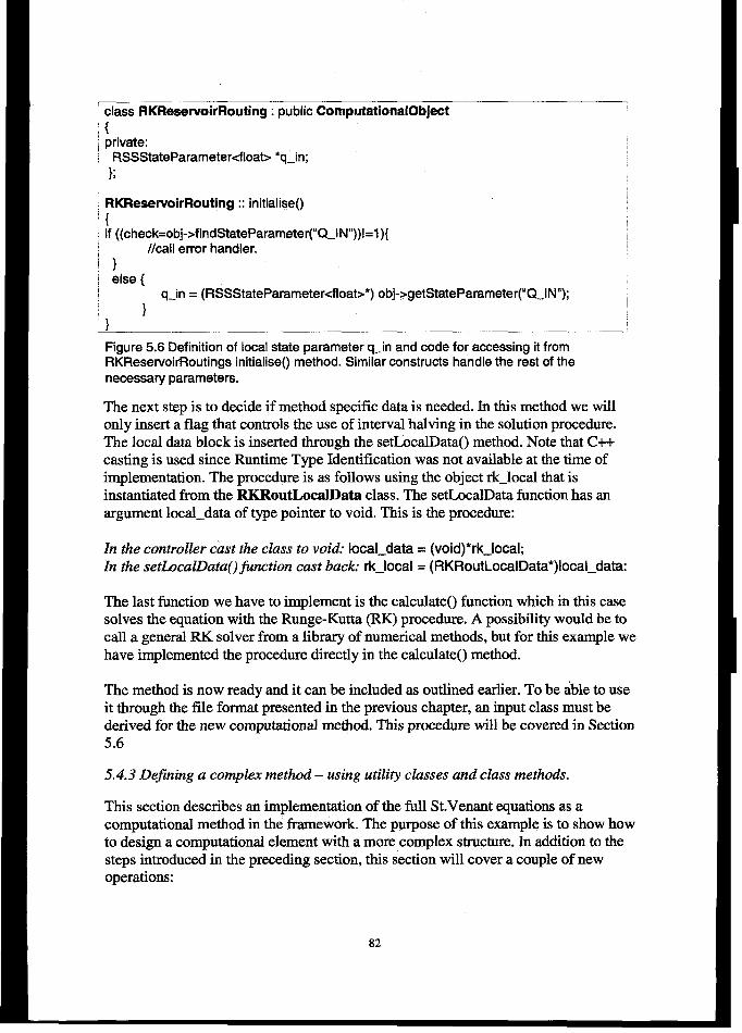
~class RKReservoirRouting: public ComputationalObject

1{~private:

RSSStateParameter<float> ‘q_in;

}; I

RKResenroirRouting :: initialiseo

{if ((check= obj->findStateParameter( ’’Q_lN’’))!=l ){

//call error handler,

}else {

q-in = (RSSStateparameter<float>*) Obj->getstatePararneter(’’Q-lN”);}

}

Figure 5.6 Definition of local state parameter q_in and code for accessing it fromRKReservoirRoutings initialiseo method. Similar constructs handle the rest of thenecessary parameters.

The next step is to decide if method specific data is needed. In this method we willonly insert a flag that controls the use of interval halving in the solution procedure.The local data block is inserted through the setLocalDatao method. Note that C++casting is used since Runtime Type Identification was not available at the time ofimplementation. The procedure is as follows using the object rk_local that isinstantiated from the RKRoutLoealData class. The set.bcall)ata function has anargument local_data of type pointer to void. This is the procedure:

In the controller cast the class to void: iocal_data = (void)*rk_local;

Zn the setl.ocallkztaofinction cast back: rk_local = (RKRoutLocalData*) local_data:

The last function we have to implement is the calculate function which in this casesolves the equation with the Runge-Kutta (RK) procedure. A possibility would be tocall a general RK solver from a library of numerical methods, but for this example wehave implemented the procedure directly in the calculate method.

The method is now ready and it can be included as outlined earlier. To be able to useit through the file format presented in the previous chapter, an input class must bederived for the new computational method. This procedure will be covered in Section5.6

5.4.3 Dejining a complex method – using utili~ classes and class methods.

This section describes an implementation of the full St.Venant equations as acomputational method in the framework. The purpose of this example is to show howto design a computational element with a more complex structure. In addition to thesteps introduced in the preceding section, this section will cover a couple of newoperations:

– Adding new class methods to the new class derived from ComputationalMethod.

– The use of utility classes.

This is a simple implementation of a dynamic routing method that has a limitedapplication to real-world problems, but it does show how the base class can beinherited and extended to accommodate more complex computational tools.

Unsteady flow in an open channel can be described one-dimensionally by theequations originally derived by Barre de St.Venant in the late 19ti century. Using thefull equations, upstream disturbances and steep waves can be described correctly. Thecontinuity equation is shown in Equation 5.3 and the momentum equation in Equation5.4. The equations are usually solved using a finite difference numerical scheme(Cunge et al., 1980).

(53) aQ+B~=o& at

[)i3Q il Q’(5.4) —+— — +gA~+gASf =0

& JxA1

Here the two dependent variables are the discharge (Q) and the water level (Z). Theother variables are t – time, x – distance, A – cross section area, Sf – friction slope, g –acceleration due to gravity and B - channel top width. There area large number ofschemes for solving this equation (see Cunge et al. (1980), Fred (1985)). Thefollowing solution is based on a four-point numerical scheme (Figure 5.7).

nAx

-..-..-.---.--..-.-.-..-;.:- ‘---: ~:1.n+’) ~f _ @&;;’ -f;+’)+ (I-e)(-f;l -f;)

z– AX

Ataf (j;+’- f;)+(f:;’-f:,)x= 2At

A w(j+7 ,n) T

Figure 5.2 Definition of four point scheme together with approximation used forderivatives. n direction is the time line, j direction is the space direction.

The equations are then solved using a double sweep method (Hromadka et al. 1985).

The implementation requires a cross section at each computational point. Theboundary conditions required are discharge at the upstream end and a stage-dischargerelationship at the downstream end. The implementation requires a manning numberfor each cross section, but it does not consider active and passive flow areas withdifferent roughness. The implementation has not been prepared for critical flow

83

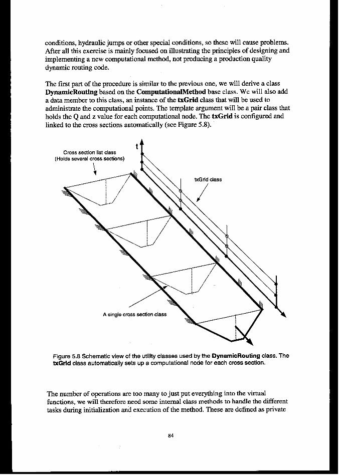
conditions, hydraulic jumps or other special conditions, so these will cause problems.After all this exercise is mainly focused on illustrating the principles of designing andimplementing a new computational method, not producing a production qualitydynamic routing code.

The first part of the procedure is similar to the previous one, we will derive a classDynamicRouting based on the ComputationalMethod base class. We will also adda data member to this class, an instance of the txGrid class that will be used toadministrate tie computational points. The template argument will be a pair class thatholds the Q and z value for each computational node. The txGrid is configured andlinked to the cross sections automatically (see Figure 5.8).

tCross section list class

(Holds several cross sections)L

Figure 5.8 Schematic view of the utility classes used by the DynamicRouting class.txGrid class automatically sets up a computational node for each cross setilon.

The

The number of operations are too many to just put everything into the virtualfunctions, we will therefore need some internal class methods to handle the differenttasks during initialization and execution of the method. These are defined as private

84

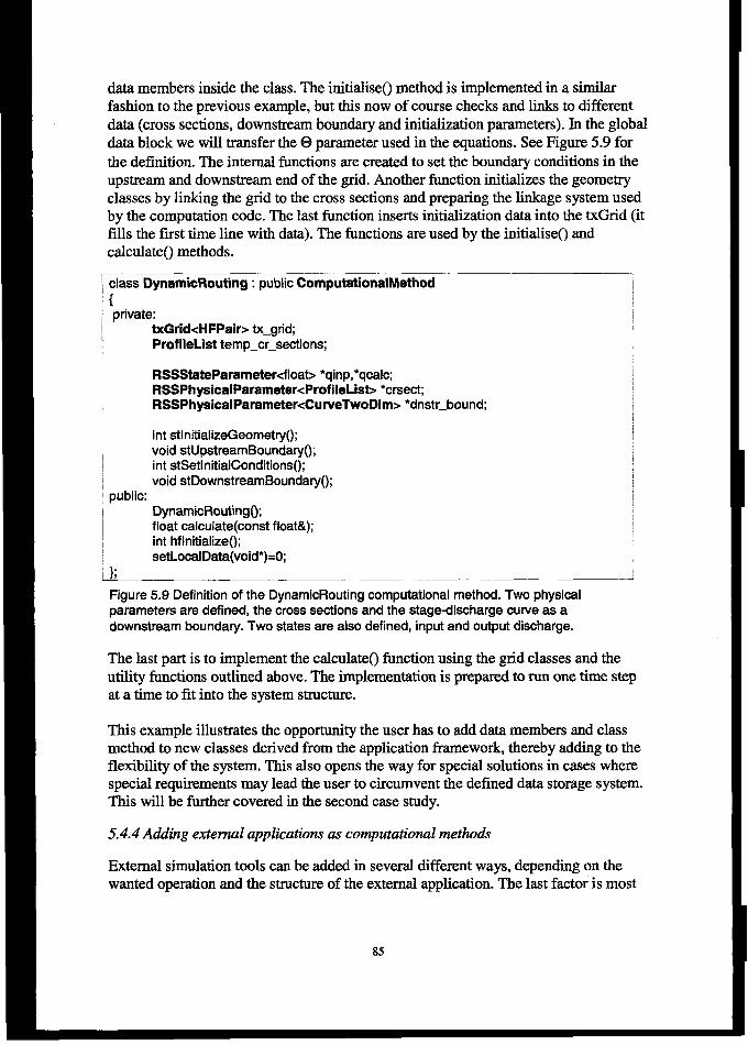
data members inside the class. The initialiseo method is implemented in a similarfashion to the previous example, but this now of course checks and links to differentdata (cross sections, downstream boundary and initialization parameters). In the globaldata block we will transfer the@ parameter used in the equations. See Figure 5.9 forthe definition. The internal functions are created to set the boundary conditions in theupstream and downstream end of the grid. Another function initializes the geometryclasses by linking the grid to the cross sections and preparing the linkage system usedby the computation code. The last function inserts initialization data into the txGnd (itfills the first time line with data). The functions are used by the initialiseo andcalculate methods.

j class DynamicRouting: public ComputationalMethod

;{~ private:

txGridcHFPair> tx_grid;I ProfileList temp_cr_setilons;I

RSSStateParametercfloat> ‘qinp,”qcal~RSSPhysicalParameter< ProfiieLisb ‘crsectRSSPhyeicalParameter<CurvaTwoDim> *dnstr_bound;

int stinitializeGeometryo;void stUpstreamBounda~();

I int stSetlnitialConditionso;void stDownstreamBoundaryo;

~public:DynamicRoutingo;

I float calculate(const float&);! int hflnitializeo;)

setLocalData(void*)=O;

!}

Figure 5.9 Definition of the DynamicRouting computational method. Two physicalparameters are defined, the cross sections and the stage-discharge curve as adownstream boundary. Two states are also defined, input and output discharge.

The last part is to implement the crdculateo function using the grid classes and theutility functions outlined above. The implementation is prepared to run onetime stepat a time to fit into the system structure.

This example illustrates the opportunity the user has to add data members and classmethod to new classes derived from the application ih-nework, thereby adding to theflexibility of the system. This also opens the way for special solutions in cases wherespecial requirements may lead the user to circumvent the defined data storage system.This will be fhrther covered in the second case study.

5.4.4 Adding external applications as computational methods

External simulation tools can be added in several different ways, depending on thewanted operation and the structure of the external application. The last factor is most

often the decisive one, not many existing simulation systems are made with efficientinterface for communication with other systems.

1.

2.

3.

4.

5,

Code level inclusion – needs the source of external application and much work.This is a common practise with public domain software elements.Batch level inclusion with time control. Executes the model for each time step byrebuilding the control parameters for the external tool.Batch inclusion – Long simulations. Needs modifications to the control system forhandling different time steps in various sections of the system. Pre- and post-processing tools are required to prepare input for external application and retrievedata horn the external application and put them back into the controlling system.External execution and result inclusion. This is more inconvenient and it violatesthe structure of the program. It may sometimes be necessary due to the layout ofthe external applications (especially when the application has an integratedgraphical user interface).Process communication inclusion. Typical solutions may be COM/OLE onWindows-based platforms or CORBA-based systems that are available on severaldifferent platforms.

5.5 Developing data storage classes

The user of the system is offered great freedom in development and inclusion ofclasses for data handling and storage. The only requirements are that properassignment operators (The copy constructor and the operator=) and the equalityoperator (operator==) are included. This is necessary to handle insertion in theparameter lists. It is recommended that the development follows the orthodoxcanonical class form presented as defined by Coplien (1992). Figure 5.10 illustratesthe interface to a data class by showing parts of the definition of the PointBag class.

~template <class T>~PointBag;{~public:

PointBagcT>(); /!ConstructorI PointBagcT>(const PointBagcT>&); flCopy-constructorI -PointBa!xT>(l lDestructor

PointBag~ ope=tor=(const PointBag<T>&); //operator =

int operator== (const PointBagcT>&); //Equality operator 1

\ void addElement ~); //Add new elementI T getElement (float,float); //Get an element based on (x,y) 1

/ };

Figure 5.10 Definition of PointBag class with orthodox canonical interface and operator==to ensure compatibility with framework data handling classes. Note that most of the actualfunctionality is omitted from the example.

86

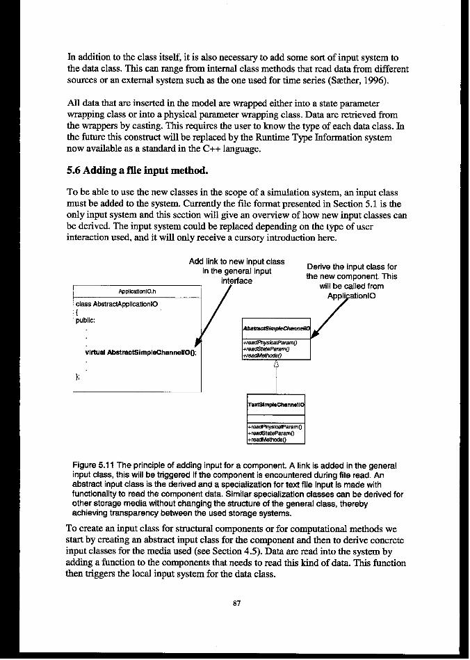
Iu addition to the class itself, it is also necessary to add some sort of input system tothe data class. This can range from internal class methods that read data from differentsources or an external system such as the one used for time series (S~ther, 1996).

All data that are inserted in the model are wrapped either into a state parameterwrapping class or into a physical parameter wrapping class. Data are retrieved fromthe wrappers by casting. This requires the user to know the type of each data class. Inthe future this construct will be replaced by the Runtime Type Information systemnow available as a standard in the C++ language.

5.6 Adding a file input method.

To be able to use the new classes in the scope of a simulation system, an input classmust be added to the system. Currently the file format presented in Section 5.1 is theonly input system and this section will give an overview of how new input classes canbe derived. The input system could be replaced depending on the type of userinteraction used, and it will only receive a cursory introduction here.

Add link to new input classin the general input

Derive the input class for

interfacethe new component. This

AppWalionlO,hwill be called from

Appli ation10claasAbatraotApplioation10[public:

* ~+

AbebncSimpMWenneU

+reedPhysicalParem~

&ual AbatractSimpleChanneliO();+reedSteteParemo+readMemcd50

Q

I mexlSimpleChannel10

Figure 5.11 The principle of adding input for a component. A link is added in the generalinput class, this will be triggered if the component is encountered during file read. Anabstract input class is the derived and a specialization for text file input is made withfunctionality to read the component data. Similar specialization classes can be derived forother storage media without changing the structure of the general class, therebyachieving transparency between the used storage systems.

To create an input class for structural components or for computational methods westart by creating an abstract input class for the component and then to derive concreteinput classes for the media used (see Section 4.5). Data are read into the system byadding a function to the components that needs to read this kind of data. This functionthen triggers the local input system for the data class.

87

The next step in the process of adding input for a component is to add a pointer to theabstract input class to the main input control class AbstractApplicationIO. Thecontroller then uses a specialization of this class as an interface to data. We must nowimplement the corresponding component input class. See figure 5.11 for an exampleon how to add input functionality for the SimpleChannel class.

5.7 Limitations

The handling of data flow in the system may impose some limitations on simulations,especially in handling complex hydraulic flow situations. This is particularly aproblem in cases where the simulation objective is detailed flow simulation where wehave reversed flow and upstream effect over object boundaries. In such cases specialprecautions must be taken.

The river system topology is created as a directed graph, thereby the flow directionsmust be defined before traversal and computation starts. In some situations we mayhave reversed flow direction within the simulation timeframe, and special solutionsmust be employed. Two potential solutions exist.

— Build a special object that contains the entire problem area and then build acomputational method to handle the reversed flow. The computational methodcould in this case be an external program. This solution will be further discussed inthe first case study.

— Employ a routine that checks for reversed flow between each time step and if thesituation occurs turn the flow direction between the involved components. If areversed flow situation is found, the simulation order must be changed before thenext time step can be executed.

The second problem that we encounter in flood routing, is the case where an effectfrom a downstream component impacts its upstream neighbors. Several possiblesolutions could be developed to handle this problem.

— Move connection point downstream or upstream to a place with hydraulic control,thereby moving the problem area inside the component. If tributaries or otherinflow motivated the location of the connection point, these could be handledthrough the parameter mapping system.

— Use and external computational engine directly without any object representationinside the framework based model.

— Build a special object to handle this, an example is the RiverJunction presented asan example earlier in this chapter. This could also be connected to an externalcomputational engine.

— Handle this through the simulation controller by developing a special routine thatbalances flow between components and iterates two or more components ifnecessary.

88

– Build the control into the computational method, in other words, a computationalmethod that handles branches. This will require the computational methods toaccess downstream neighbors directly and cooperate with downstream methods.This would also require the methods to do the parameter mapping. None of thisposes any problems in the framework structure. Such a solution requires changesin the simulation control to allow the solution of the critical area before theprocedure moves downstream. It will also require a specialized method that canoperate over the component boundaries. This can be done using the txGridpresented earlier. Another possible solution would be to use the object-orientedone-dimensional solver presented by Kutija (1998) or a similarly structuredprocedure. Using this the component boundary could be represented by the Vertexobjects and the component itself would contain an edge object that represents thegrid of computational nodes, much like the txGrid class. The major difference isthat the system outlined by Kutija has the equation solvers integrated into thenetwork representations.

89

6. CASE STUDY 1: THE HYDRA RIVER SYSTEM MODEL

6.1 Introduction

6.1.1 Background for the project

At the end of May and beginning of June 1995, Norway experienced its largest floodin this century. The total damage is estimated to about NOK 1800 million (about USD260 million with the exchange rate at the time of writing). A delayed spring, an abovenormal snow pack and a combination of high precipitation and air temperature duringthe event caused the flood. After the flood a research programme was initiated toinvestigate the effects of human encroachments on flood levels and provide tools forfuture decision making in flood situations. The Glomma basin in the southeastern partof Norway was selected as a study area for this project since it was most severelyinfluenced by the 1995 flood (figure 6.1). The issues included in the study were thefollowing:

The effects of regulation reservoirs on flood levels and how these can be used asflood management tools.The study of embankments and flood protection works and their effect on floodlevels.An assessment of changed land use from agricultural and forestry activities onfloods. The effect of different land uses on inflow to the river system will bemodelled using the PINE system (Rinde 1998).The effects of increased urbanization. This will lead to a set of calibrated SINBADmodels (Killingtveit et al. 1994) for a selection of urban areas in the river basin.A detailed model of the floodplain in a selected area of the river system both tostudy past floods and to provide an operational system for future use. This work isdone using MIKE 11 hydraulic modelling system from the Danish HydraulicInstitute (DHI 1998). The area selected is located in the southern Hedmark andAkershus counties, which is the most densely populated area and therefore subjectto the highest damage risk during a flood.Studies of environmental effects of floods, focusing on water quality, sedimentsand the effects on benthic invertebrates and fish.Development of cost functions for different types of infrastructure to better assessfinancial aspects of encroachments that may impact the flood levels.An evaluation of the currently used forecasting tools and a study of uncertainty inhydrological forecasts.

The results of the above studies and the simulation tools should then be integrated intoa modelling system that can be applied both to analyse previous

90

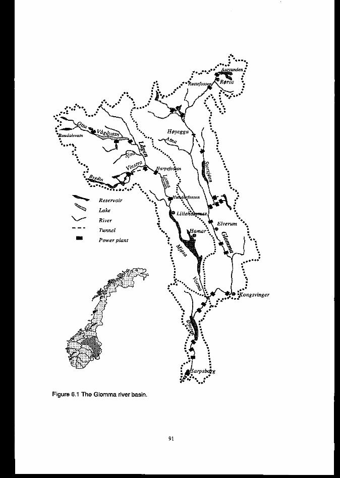
---Tunnel

D Power ~lant

Figure 6.1 The Glomma river basin,

3 -.+~ m ‘** Elverum ●“*-.

‘: ‘ii

91

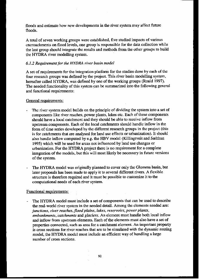
floods and estimate how new developments in the river system may affect futurefloods.

A total of seven working groups were established, five studied impacts of variousencroachments on flood levels, one group is responsible for the data collection whilethe last group should integrate the results and methods from the other groups to buildthe HYDRA river modelling system.

6.1.2 Requirement for the HYDRA river basin model

A set of requirements for the integration platform for the studies done by each of thefour research groups was defined by the project. This river basin modelling system,hereafter called HYDRA, was defined by one of the working groups (Roald 1997).The needed functionality of this system can be summarized into the following generaland fictional requirements:

General requirements:

The river system model builds on the principle of dividing the system into a set ofcomponents like river reaches, power plants, lakes etc. Each of these componentsshould have a local catchrnent and they should be able to receive inflow hornupstream components. Each of the local catchments should handle inflow in theform of time series developed by the different research groups in the project (thisis for catchments that are analysed for land use effects or urbanization). It shouldalso handle inflow computed by e.g. the HBV model (Killingtveit and SaMmn1995) which will be used for areas not influenced by land use changes orurbanization. For the HYDRA project there is no requirement for a completeintegration of the models, but this will most likely be necessary in future versionsof the system.

The HYDRA model was originally planned to cover only the Glornma basin, butlater proposals has been made to apply it to several different rivers. A flexiblestructure is therefore required and it must be possible to customize it to thecomputational needs of each river system.

Functional recmirements:

The HYDRA model must include a set of components that can be used to describethe real-world river system in the needed detail. Among the elements needed are:junctions, n“ver reaches, floodplains, lakes, reservoirs, power plants,embankments, catchments and glaciers. An element must handle both local inflowand inflow from upstream elements. Each of the elements must also have a set ofproperties connected, such as area for a catchment element. An important propertyis cross sections for river reaches that are to be simulated with the dynamic routingmodel, the HYDRA model must include an efficient way of handling a largenumber of cross sections.

92

The model must have a lake routing algorithm that can be used to simulate theoutflow horn reservoirs and lakes in the system.A dynamic routing model that can be used in areas with concentrated populationand in areas with a potential for severe flooding must be included in the model.This model should handle backwater effects and reversed flow. It must also modelthe floodplain and the effect of off channel storage of water.For areas where dynamic routing is not necessary or possible the system mustinclude simpler hydrologic routing methods.The system must be able to handle the operation of hydropower reservoirs.The proposed simulations will generate much data, there is therefore a need toorganize data into a hierarchy of alternatives which each clearly defines the linkbetween input used and results produced.Input data to the system will be in the form of time series, raster data, crosssections, polygons and curves. The necessary tools to read and handle these datamust be present in the system.The system should be able to read and write a set of standardized export andimport formats for data.

6.1.2 The proposed solution

Based on the requirement specification it was decided to use the framework presentedin Chapters 3,4 and 5 to build the HYDRA model. The framework already meetsmost of the requirements outlined by Roald (1997), and the flexibility in the systemmakes it possible to add the missing components. One key point will be theintegration of third party applications. By using the method hierarchy it is possible todo this in four different ways (for a detailed discussion on external model integrationsee chapter 5):

- A complete integration as a computational method where the code is available forthe program that is to be included. This is the case for the PINE model that will beused for catchment simulations.

- Through a wrapper where source code is not available but when it is possible torun the program within the framework. The application must then support batchprocessing.

- By exporting data to the external program and importing the results back into theprogram. This is necessary in the cases were the third party application does notlend itself to execution within the framework, this is the case with applications thatrun inside a user interface. This is a possible solution when the MIKEl 1 model isintegrated.

- By using process communication. This is the most seamless integration method,and it will be investigated as a way of including the latest version of MIKEl 1. Thisprogram supports automation through the MIKE Zero development plan asmentioned in Section 2.3.4.

The proposed solution would then be to build a representation of the entire basin usingthe components of the application fitunework. The external hydrological models willbe integrated as computational methods in the catchment objects since they are all

93

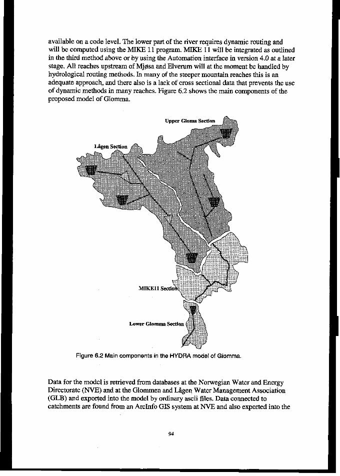
available on a code level. The lower part of the river requires dynamic routing andwill be computed using the MIKE 11 program. MIKE 11 will be integrated as outlinedin the third method above or by using the Automation interface in version 4.0 at a laterstage. All reaches upstream of Mj@a and Elverum will at the moment be handled byhydrological routing methods. In many of the steeper mountain reaches this is anadequate approach, and there also is a lack of cross sectional data that prevents the useof dynamic methods in many reaches. Figure 6.2 shows the main components of theproposed model of Glomma.

Figure 6.2 Main components in the HYDRA model of Glomma.

Data for the model is retrieved from databases at the Norwegian Water and EnergyDirectorate (NVE) and at the Glommen and Liigen Water Management Association(GLB) and exported into the model by ordinary ascii files. Data connected tocatchments are found from an ArcInfo GIS system at NVE and also exported into the

94

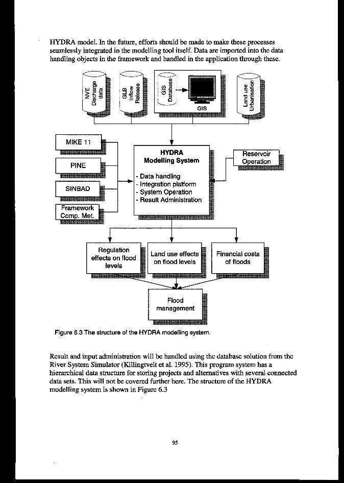
HYDRA model. In the future, efforts should be made to make these processessearnlessly integrated in the modelling tool itself. Data are imported into the datahandling objects in the framework and handled in the application through these.

1

I 1

3:............

a)

2concJ#

n ‘“’ ‘

GE

+

HYDRAModelling System

Data handlingIntegration platformSystem OperationResult Administration

F

+ + 4

Floodmanagement

1L E

Figure 6.3 The structure of the HYDRA modelling system.

Result and input administration will be handled using the database solution from theRiver System Simulator (Killingtveit et al. 1995). This program system has ahierarchical data structure for storing projects and alternatives with several connecteddata sets. This will not be covered further here. The structure of the HYDR4modelling system is shown in Figure 6.3

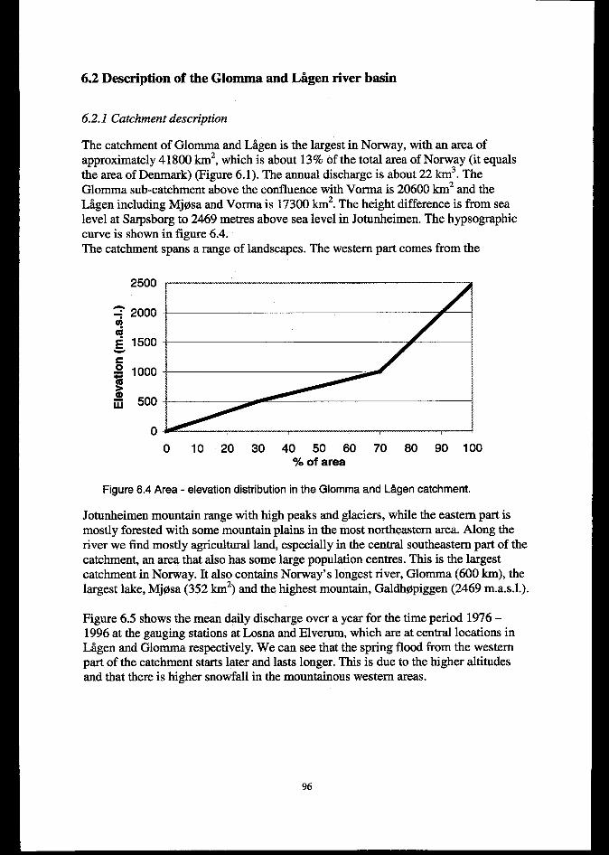
6.2 Description of the Glomrna and Li!igen river baein

6.2.1 Catchment description

The catehrnent of Glornma and L5gen is the largest in Norway, with an area ofapproximately 41800 km2, which is about 13~0 of the total area of Norway (it equalsthe area of Denmark) (Figure 6. 1). The annual discharge is about 22 krn3. TheGlomma sub-catchrnent above the confluence with Vorrna is 20600 km2 and theLfigen including Mj@a and Vorrna is 17300 km2. The height difference is from sealevel at Sarpsborg to 2469 metres above sea level in Jotunheimen. The hypsographiccurve is shown in figure 6.4.The catchment spans a range of landscapes. The western pint comes from the

2500

0

0 10 20 30 40 50 60 70 80 90 100‘/0of area

Figure 6.4 Area - elevation distribution in the Glomma and Li4gen catchment.

Jotunheimen mountain range with high peaks and glaciers, while the eastern part ismostly forested with some mountain plains in the most northeastern area. Along theriver we find mostly agricultural land, espeeiall y in the central southeastern part of thecatchment, an area that also has some large population centres. This is the largestcatehment in Norway. It also contains Norway’s longest river, Glomrna (600 km), thelargest lake, Mj@sa (352 km2) and the highest mountain, Galdh@piggen (2469 m.a.s.l.).

Figure 6.5 shows the mean daily discharge over a year for the time period 1976 –1996 at the gauging stations at Losna and Elvemm, which are at central locations inLilgen and Glomma respectively. We can see that the spring flood from the westernpart of the catchrnent starts later and lasts longer. This is due to the higher altitudesand that there is higher snowfall in the mountainous western areas.

96

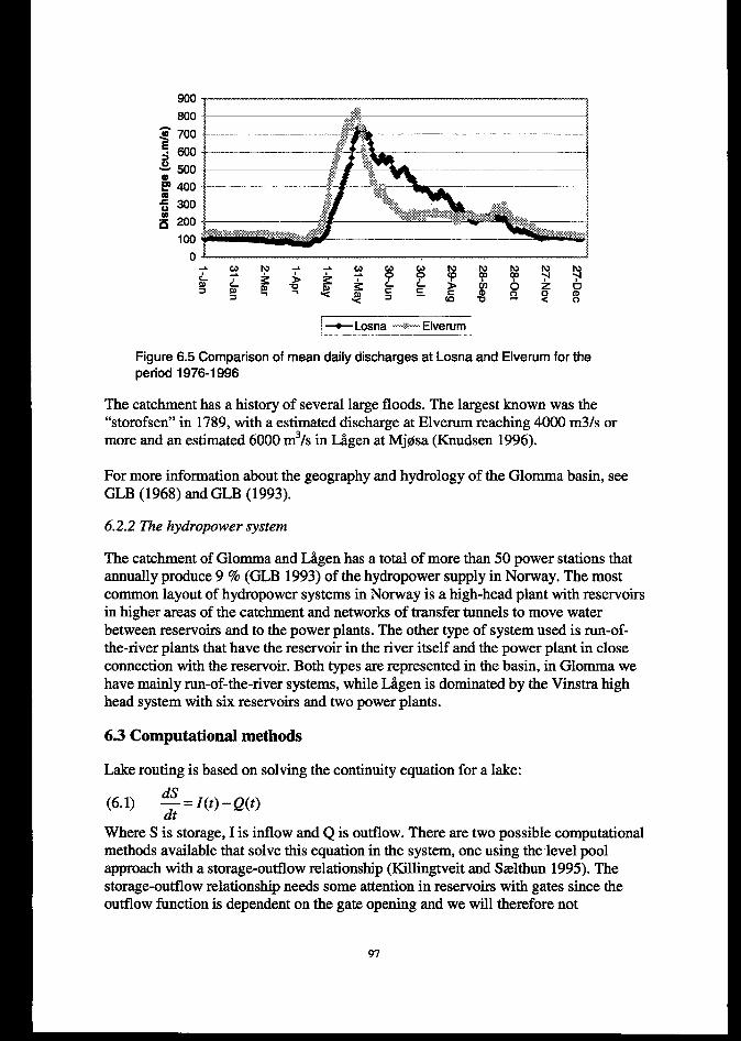
Figure 6.5 Comparison of mean daily discharges at Losna and Elverum for theperiod 1976-1996

The catchment has a history of several large floods. The largest known was the“storofsen” in 1789, with a estimated discharge at Elverum reaching 4000 m3/s ormore and an estimated 6000 m3/s in L&gen at Mj@sa (Knudsen 1996).

For more information about the geography and hydrology of the Glomma basin, seeGLB (1968) and GLB (1993).

6.2.2 The hydropower system

The catehrnent of Glornma and L&gen has a total of more than 50 power stations thatannually produce 970 (GLB 1993) of the hydropower supply in Norway. The mostcommon layout of hydropower systems in Norway is a high-head plant with reservoirsin higher areas of the catchment and networks of transfer tunnels to move waterbetween reservoirs and to the power plants. The other type of system used is run-of-the-river plants that have the reservoir in the river itself and the power plant in closeconnection with the reservoir. Both types are represented in the basin, in Glornma wehave mainly run-of-the-river systems, while L&gen is dominated by the Vinstra highhead system with six reservoirs and two power plants.

6,3 Computational methods

Lake routing is based on solving the continuity equation for a lake:

(6.1) ~= Z(t) – Q(t)dt

Where S is storage, I is inflow and Q is outflow. There are two possible computationalmethods available that solve this equation in the system, one using the level poolapproach with a storage-outflow relationship (Killingtveit and Szelthun 1995). Thestorage-outflow relationship needs some attention in reservoirs with gates since theoutflow function is dependent on the gate opening and we will therefore not

97

necessarily have a unique storage relationship function in this case. Another option wehave available is to use a reformulated equation solved by the Runge-Kutta procedureas outlined in Section 5.4.2. The last method has the advantage that it is not dependenton the storage outflow function, this makes it easier to incorporate releases of wateroutside the ovefflow arrangements into the method.

River routing is done using variations of the Muskingum equation:

(6.2) Q(t +1)= C1.Z(t+1) + C,.z(t)+ C, .Q(t)

Where

(6.3) Cl= ‘t ‘2= ,C2=At+ 2KX

,C3 =2K(l– X)–At

2K(l– X)+At 2K(l– X)+At 2K(l– X)+At

Q is discharge from the routing reach, I is inflow to the routing reach, K and X are theMuskingum equation constants and t is time. This (original) version of the methodassumes no lateral inflow to the reach. In the Glomma case lateral inflow is important,we therefore need to incorporate this into the equation. One option would be to addlocal inflow to the inflow horn the upstream component, but this has not been used inthis study. It was decided to include two extensions to the Muskingum method thattakes the lateral inflow into account. The first one is presented by O’Donnel (1985)which uses the standard routing equation, and add an o!parameter that gives lateralinflow proportional to the inflow from upstream reaches. This leads to the followingMuskingum coefficients:

(6.4) c, =(l+aAt – 2KX

,C2 =(l+aAt -I-2KX ,C =2K(l– X)–At

‘2K(l– X)+At ‘2K(l– X)+At 3 2K(l– X)+At

The a parameter is found during calibration. In the implemented method it was

possible to specify a variation of et with time. The disadvantage of this method is thatit is not possible to use the method for analysis if the inflow from the upstream objectschanges, e.g. because changes in reservoir operation. Since the lateral inflow isdependent on inflow to the component, such a change will alter the lateral inflow,which in most situations would not be the case. Another option is to use an extendedMuskingum equation described by Fread (1985). This adds a fourth part to the originalMuskingum equation:

(6.5) Q(t+l)= C1. Z(t+l)+C2. Z(t)+ C,” Q(t)+C,

The Cg is the lateral inflow parameter and it is defined as:

(6.6)c = (q, + q,)~*~

4 2K(l– X)+At

98

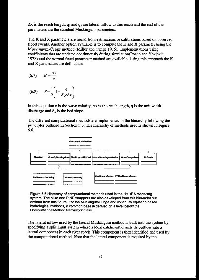
Axis the reach length, ql and qz are lateral inflow to this reach and the rest of theparameters are the standard Muskingum parameters.

The K and X parameters are found from estimations or calibrations based on observedflood events. Another option available is to compute the K and X parameter using theMuskingum-Cunge method (Miller and Cunge 1975). Implementations usingcoefficients that are updated continuously during simulation(Ponce and Yevjevic1978) and the normal fixed parameter method are available. Using this approach the Kand X parameters are defined as:

(6.7) K =2c

[)(6.8) x=: I--&0 )

In this equation c is the wave celerity, Ax is the reach length, q is the unit widthdischarge and SOis the bed slope.

The different computational methods are implemented in the hierarchy following theprinciples outlined in Section 5.3. The hierarchy of methods used is shown in Figure6.6.

pmwmtbn81Awtq

A

B “t”LQGI B.&MuskingumMethod LatemlMuskingumM6thod AfuskCun

RKRewtvoirRouting LwaiPoolRoutingMuskingumCunge MuskingumCunge

Figure 6.6 Hierarchy of computational methods used in the HYDRA modellingsystem. The Mike and PINE wrappers are also developed from this hierarchy butomitted from this figure. For the MuskingumCunge and continuity equation basedhydrological methods, a common base is derived on a level below theComputationalMethod framework class.

The lateral inflow used by the lateral Muskingum method is built into the system byspecifying a split input system where a local catchment directs its outflow into alateral component in each river reach. This component is then identified and used bythe computational method. Note that the lateral component is required by the

99

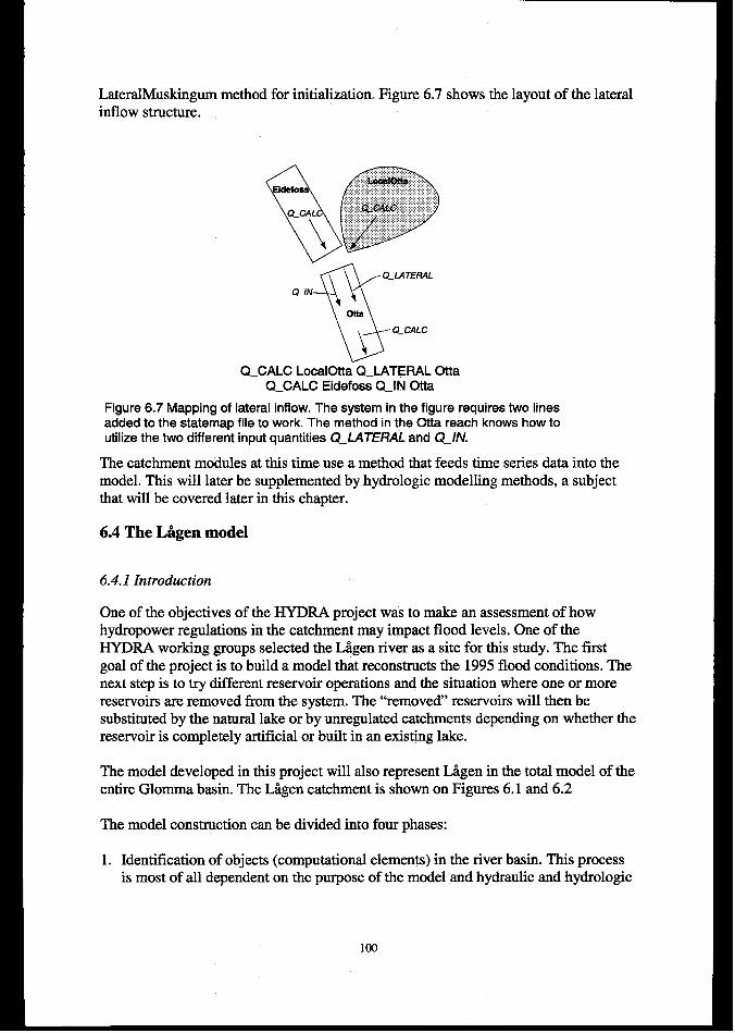
LateralMuskingum method for initialization. Figure 6.7 shows the layout of the lateralinflow structure.

%

. Q_ L4TERAL

Q.IN

\ \-%-”-aLcw

Q.CALC LocaK3tta Q_LATERAL OttaQ_CALC Eidefoss Q_lN Otta

Figure 6.7 Mapping of lateral inflow. The system in the figure requires two linesadded to the statemap file to work. The method in the Otta reach knows how toutilize the two different input quantities Q_ LATEFIAL and Q_//V.

The catchment modules at this time use a method that feeds time series data into themodel. This till later be supplemented by hydrologic modelling methods, a subjectthat will be covered later in this chapter.

6.4 The L&en model

6.4.1 Introduction

One of the objectives of the HYDRA project was to make an assessment of howhydropower regulations in the catchment may impact flood levels. One of theHYDRA working groups selected the L&gen river as a site for this study. The firstgoal of the project is to build a model that reconstructs the 1995 flood conditions. Thenext step is to try different reservoir operations and the situation where one or morereservoirs are removed ilom the system. The “removed” reservoirs will then besubstituted by the natural lake or by unregulated catchments depending on whether thereservoir is completely artificial or built in an existing lake.

The model developed in this project will also represent Liigen in the total model of theentire Glomma basin. The Liigen catchment is shown on Figures 6.1 and 6.2

The model construction can be divided into four phases:

1. Identification of objects (computational elements) in the river basin. This processis most of all dependent on the purpose of the model and hydraulic and hydrologic

100

considerations, The purpose of this model is to carry out flood simulations, thiswill therefore bean important factor in object identification.

2. Collection of data for all objects. The data needs are dependent on computationalmethods that are to be applied, in many cases the available data will limit the useof specific methods. These cases demand a simpler method or firther datacollection. In addition other data that the user wants to include for informationpurpose must be collected. This step also involves data processing to put them intoformats that the model can understand. Hopefully it will be possible to automatethis process in future applications.

3. Selection and/or implementation of computational methods for each object.4. Methods and data must be added to the structural object to form a computational

element. This must then be inserted into the topology structure.

6.4.2 System components

Liigen has one major tributary in the Otta, and some significant smaller ones like Sjoaand Gausa, The Vinstra is also a significant tributary to the main river, and is heavilyinfluenced by the Vinstra hydropower regulation. The main purpose of the modelconstruction in this project is to represent the major hydropower reservoirs and thereaches downstream of them, at the moment there is no need to build a detailed modelof parts of the Lilgen basin that is not influenced by regulations. The unregulatedtributaries to Lfigen are therefore treated as catchrnents with no further subdivision.This approach is used for the tributaries Sjoa, Gausa, Mesna and Moksa and the areaof the main river upstream of Sel.

The reservoirs and lakes in the system area natural starting point when the objects areselected. In the IAgen case there are three natural lakes in the river reach, Ottavatn,Viig&vatn and Losna. In the model we have combined Ottavatn and J%gi$ivatninto onecomponent. This is done because they are comected in nature and because the outletcapacity curve was only available for Vilgiivatn. Ten reservoirs have been identified inthe Liigen model, the six reservoirs in the Vinstra system and four in tributaries toOtta. In addition to these, Mj@a will be included in the final model. See Table 6.1 fora list of reservoirs and lakes in the system.

The lakes and reservoirs control the selection of river reaches and similarly thejunctions where tributaries reach the main branch of the river defines a division point.As far as it has been possible the division points between river reaches have beenselected in sections with hydraulic control. See Table 6.2 for a list of selected riverreaches.

A total of six power plants have been included in the L&gen model. Currently nothingis computed in the power plant objects since the power production is not a studyobjective in this phase. They have still been included for possible future use. In thecases of the hydropower plants, the outlet from the power plant object is connecteddirectly to its downstream component without the use of a tunnel reach. See Table 6.3for a list of power plants.

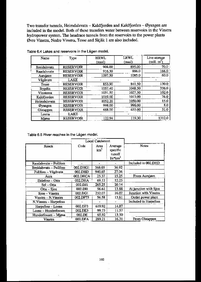
Two transfer tunnels, Heimdalsvatn – Kaldfjorden and Kaldfjorden – Oyangen areincluded in the model. Both of these transfers water between reservoirs in the Vinstrahydropower system. The headrace tunnels horn the reservoirs to the power plants@vre Vinstra, Nedre Vinstra, Tesse and Skj5k 1 are also included.

Table 6.4 Lakes and reservoirs in the L&gen model.

HRWL LRWL Live storage

Breidalsvatn RESERVOIR 908.00 895.00 70.0RESERVOIR 916.30 886.0 166.0

ESERVOIR 1097.50 1085.0 60.0

II Tesse RESEK

I Vinsteren R

1Heimdalsvatn RESERVOIR@yangen \ Rl

II Losna LfUcERESERVOIR .amn“ I ,.n Qn I 1312.0lZU.Y+ I llY..XJ I

Table 6.5 River reaches in the L&gen model.

Local Catchment

Reach Code Area Average Noteskm2 specific

runoff1/5*~2

Raudalsvatn– Pollfoss Includedin 002.DHDBreidalsvatn- Pollfoss 002.DHG1 568.05 36.92

Pollfoss– Viigivatn 002.DHD 940.65 27.06Aura 002.DHCA 25.37 15.25 From Aursj$en

Eidefoss– Otta 002.DHA 69.12 12.25Sel – Otta 002.DJ1 265.25 20.14

Otta – Sjoa 002.DH 56.61 13.88 Atjunction with SjoaSjoa– Vinstra 002.DG1 232.07 16.07 JunctionwithVinstra

Vinstra– N.Vinstra 002.DF73 56.58 13.81 OutletpowerplantN.Vinstra– Harpefoss Includedin Harpefoss

Harpefess – Losna 002.DF3 619.92 14.87Losna– Hunderfossen 002.DE3 99.73 11.57Hunderfossen– Mj@a 002.DE 65.92 13.10

002.DFA 289.21 16.31

102

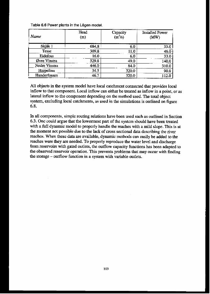
Table 6.6 Power plants in the LAgen model.

Head Capacity Installed PowerName (m) (m’/s) m)

SC@ 1 684.8 6.0 33.0Tesse 309.8 11.0 46.0

Eidefoss 16.0 6.0 33.0Ovre Vinstra 329.8 49.0 140.0

Nedre Vinstra 446,0 84.0 310.0Harpefoss 34.5 320.0 90.0

Hunderfossen 46.7 320.0 l19n

All objects in the system model have local catchment connected that provides localinflow to that component. Local inflow can either be treated as inflow in a point, or aslateral inflow to the component depending on the method used. The total objectsystem, excluding local catchments, as used in the simulations is outlined on figure6.8.

In all components, simple routing relations have been used such as outlined in Section6.3. One could argue that the lowermost part of the system should have been treatedwith a full dynamic model to properly handle the reaches with a mild slope, This is atthe moment not possible due to the lack of cross sectional data describing the riverreaches. When these data are available, dynamic methods can easily be added to thereaches were they are needed. To properly reproduce the water level and dischargefrom reservoirs with gated outlets, the outflow capacity fimctions has been adapted tothe observed reservoir operation. This prevents problems that may occur with findingthe storage – outflow function in a system with variable outlets.

103

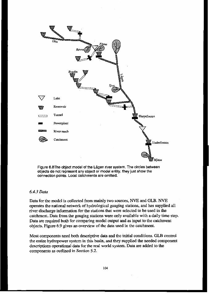
~ Lake.

w Resemoir

~“-......., Tunnel,. .........

m Powerpknt

- River reach

*

‘$,. Catchrnent

i

Huderfossen

., .,Y.:,,..

kfj@a

Figure 6.8The object model of the Lilgen river system. The circles betweenobjects do not represent any objeet or model entity, they just show theconnection points. Local catchments are omitted.

6.4.3 Data

Data for the model is collected from mainly two sources, NVE and GLB. NVEoperates the national network of hydrological gauging stations, and has supplied allriver discharge information for the stations that were selected to be used in thecatchment. Data from the gauging stations were only available with a daily time step.Data are required both for comparing model output and as input to the catehmentobjects. Figure 6.9 gives an overview of the data used in the catehment.

Most components need both descriptive data and the initial conditions. GLB controlthe entire hydropower system in this basin, and they supplied the needed componentdescriptions operational data for the real world system. Data are added to thecomponents as outlined in Section 5.2.

104

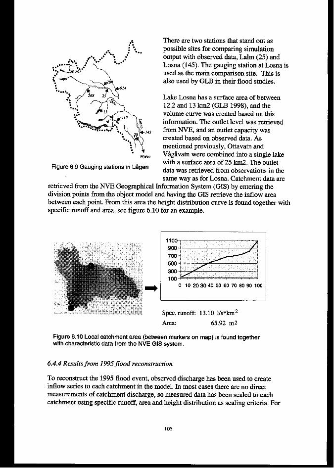
.s: “**

,**.a● : ● . .#*** ●*” : ●:”

.4.*** ●** . ●., ..* , h,. ,*

x..+●*,*●.*●* 291

●

ss.

h

%; ,4.*...,*

,:

#268 25

● .

;,)@oQ

\

s.“.●:%. .,:%** *.:’”, fi

●*a

h

:.* ‘?’45●...b.

Mj@a

Figure 6.9 Gauging stations in L&gen

There are two stations that stand out aspossible sites for comparing simulationoutput with observed data, Lalm (25) andLosna (145). The gauging station at Losna isused as the main comparison site. This isalso used by GLB in their flood studies.

Lake Losna has a surface area of between12.2 and 13 km2 (GLB 1998), and thevolume curve was created based on thisinformation. The outlet level was retrievedfrom NVE, and an outlet capacity wascreated based on observed data. Asmentioned previously, Ottavatn andViig&vatn were combined into a single lakewith a surface area of 25 km2. The outletdata was retrieved from observations in thesame way as for Losna. Catchment data are

retrieved from the NVE Geographical Information System (GIS) by entering thedivision points horn the object model and having the GIS retrieve the inflow areabetween each point. From this area the height distribution curve is found together withspecific runoff and area, see figure 6.10 for an example.

1 0 102030405060708090100

Spec. runoff 13.10 l/s*km2

Area 65.92 mz

Figure 6.10 Local catchment area (between markers on map) is found togetherwith characteristic data from the NVE GIS system.

6.4.4 Resultsfiom 1995@ood reconstruction

To reconstruct the 1995 flood event, observed discharge has been used to createinflow series to each catchment in the model. In most cases there are no directmeasurements of catchment discharge, so measured data has been scaled to eachcatchment using specific runoff, area and height distribution as scaling criteria. For

105

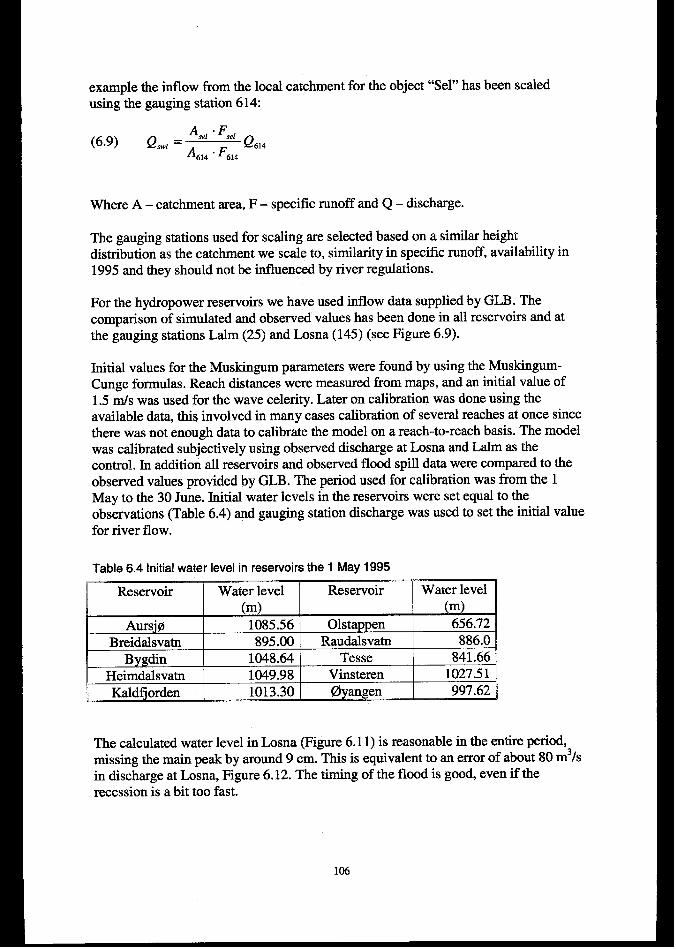
example the inflow from the local catchment for the object “Sel” has been scaledusing the gauging station 614:

(6.9) Qswi= $’: ~ Q,,,614 614

Where A – catchment area, F – specific runoff and Q – discharge.

The gauging stations used for scaling are selected based on a similar heightdistribution as the catchrnent we scale to, similarity in specific runoff, availability in1995 and they should not be influenced by river regulations.

For the hydropower reservoirs we have used inflow data supplied by GLB. Thecomparison of simulated and observed values has been done in all reservoirs and atthe gauging stations La.lm (25) and Losna (145) (see Figure 6.9).

Initial values for the Muskingum parameters were found by using the Muskingum-Cunge formulas. Reach distances were measured from maps, and an initial value of1.5 mh was used for the wave celerity. Later on calibration was done using theavailable data, this involved in many cases calibration of several reaches at once sincethere was not enough data to calibrate the model on a reach-to-reach basis. The modelwas calibrated subjectively using observed discharge at Losna and Lalm as thecontrol. In addition all reservoirs and observed flood spill data were compared to theobserved values provided by GLB. The period used for calibration was from the 1May to the 30 June. Initial water levels in the reservoirs were set equal to theobservations (Table 6.4) and gauging station discharge was used to set the initial valuefor river flow.

Table 6.4 Initial water level in resewoirs the 1 May 1995

Reservoir Water level Reservoir Water level(m) (m)

Aursj@ 1085.56 Olstappen 656.72Breidalsvatn 895.00 Raudalsvatn 886.0 ,

Bygdin 1048.64 Tesse 841.66Heimdrdsvatn 1049.98 Vinsteren 1027.51

J~Kaldf’orden 1013.30 @anen 997.62,

The calculated water level in Losna (Figure 6.11) is reasonable in the entire period,missing the main peak by around 9 cm. This is equivalent to an error of about 80 m3/sin discharge at Losna, Figure 6.12. The timing of the flood is good, even if therecession is a bit too fast.

1(J6

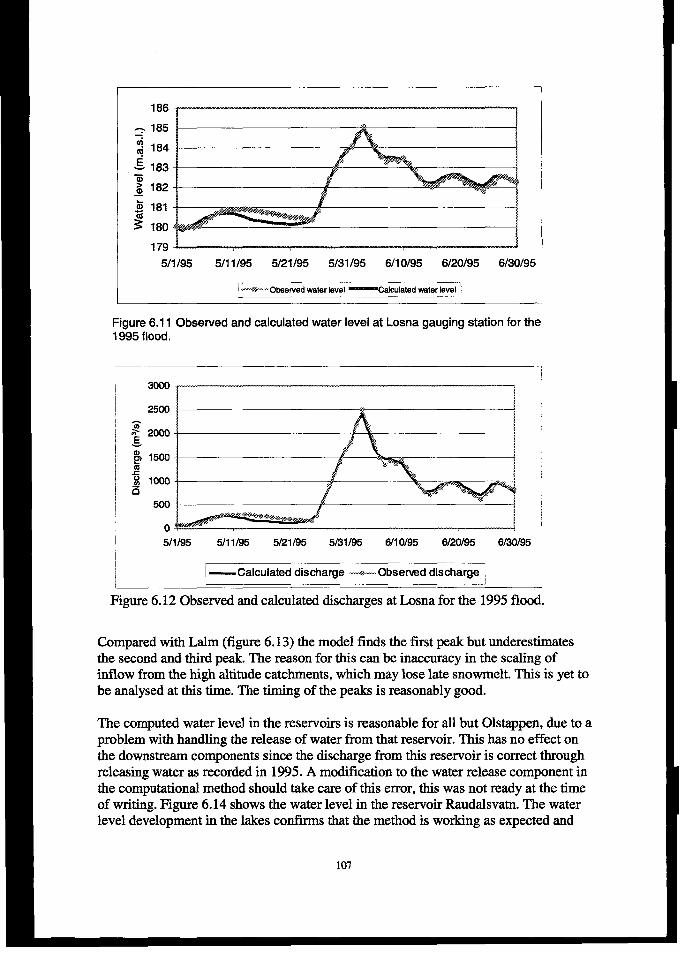
L

184

183

182

181 I

180

179 J- A

5/1/95 5111/95 5/21195 5131/95 6/10/95 6/20195 6130/95

--+-- Obsewed water level ‘Calculated weter level !

Figure 6.11 Observed and calculated water level at Losna gauging station for the1995 flood.

3000

2500

2000

1500

1000

500

0

511195 5/1 lM 5/21195 5/31/95 6110195 6120195 6f301e5

I—Calculated discharge ---+@-Observeddischarge ~

Figure 6.12 Observed and calculated discharges at Losna for the 1995 flood.

Compared with Lalm (figure 6. 13) the model finds the first peak but underestimatesthe seeond and third peak. The reason for this can be inaccuracy in the scaling ofinflow from the high altitude catchments, which may lose late snowmelt. This is yet tobe analysed at this time. The timing of the peaks is reasonably good.

The computed water level in the reservoirs is reasonable ford but Olstappen, due to aproblem with handling the release of water from that reservoir. This has no effect onthe downstream components since the discharge from this reservoir is correct throughreleasing water as reeorded in 1995. A modiilcation to the water release component inthe computational method should take care of this error, this was not ready at the timeof writing. Figure 6.14 shows the water level in the reservoir Raudalsvatn. The waterlevel development in the lakes confirms that the method is working as expected and

107

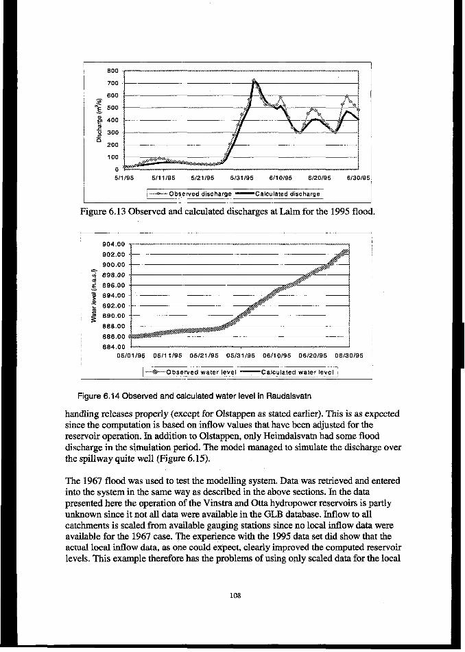
800

700

600?)“; 500

% 400gQ 300.2n 200

100

0~ 5/1/95 5/1 1/95 5/21 195 5131195 6/1 0/95 6/20/95 6/30/9!

I ~--++--ob~~rv~ddischarge‘Calculated discharge

Figure 6.13 Observed and calculated discharges at Lalm for the 1995 flood.

904.00902.00900.00898.00898.00894.00892.00890.00886.00886.00884.00 I !

05/01/95 05/11/95 05/21/95 05/31/95 06/10/95 06/20/95 06/30/95

l-%@---Obaerved water level ‘Calculated water level ;

Figure 6.14 Observed and calculated water level in Raudalsvatn

handling releases properly (except for Olstappen as stated earlier). This is as expectedsince the computation is based on inflow values that have been adjusted for thereservoir operation. In addition to Olstappen, only Heimdalsvatn had some flooddischarge in the simulation period. The model managed to simulate the discharge overthe spillway quite well (Figure 6.15).

The 1967 flood was used to test the modelling system. Data was retrieved and enteredinto the system in the same way as described in the above sections. In the datapresented here the operation of the Vinstra and Otta hydropower reservoirs is partlyunknown since it not all data were available in the GLB database. Inflow to allcatchments is scaled ffom available gauging stations since no local inflow data wereavailable for the 1967 case. The experience with the 1995 data set did show that theactual local inflow data, as one could expect, clearly improved the computed reservoirlevels. This example therefore has the problems of using only scaled data for the local

108

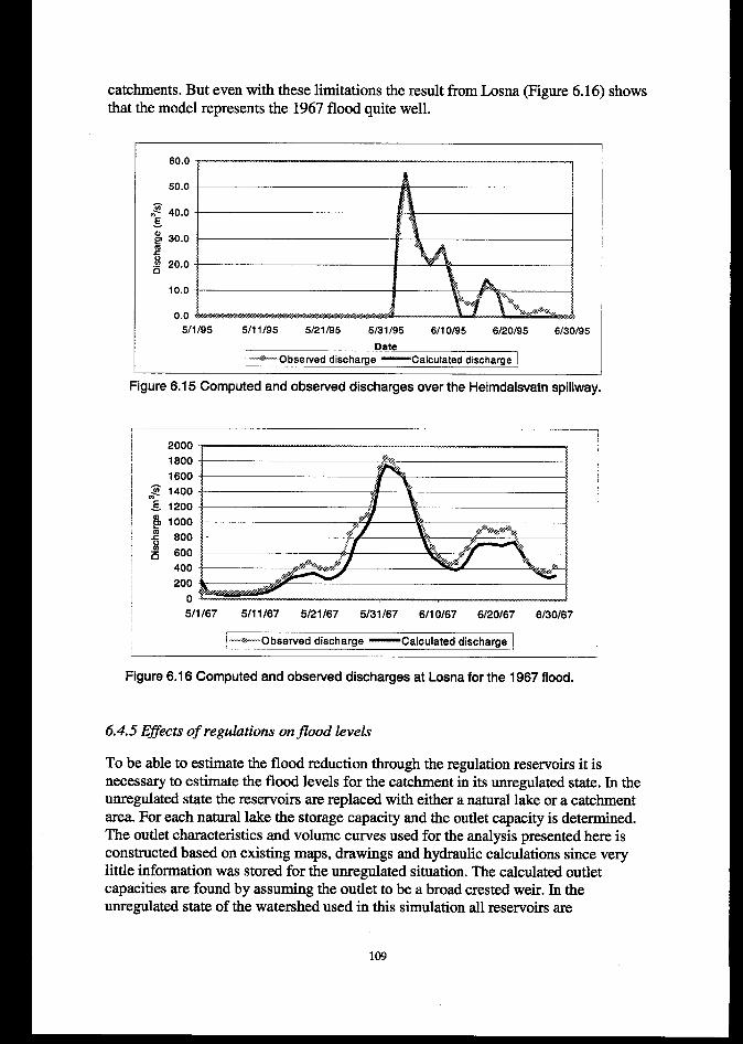
catchments. But even with these limitations the result from Losna (Figure 6.16) showsthat the model represents the 1967 flood quite well.

.-

50.0

.~ 40.0-g& 30.0J I{.Q 20.0 In

10.0

0.05/1/95 5/11/95 5/21/95 5131t95 6/10195 6120195 6130195

DateII--++-.obsewed discharge ‘Calculated discharge ~

I Figure 6.15 Computed and observed discharges over the Heimdalsvatn spillway.

2000 I1800

# 1400

8) 1000z5 800

~ 600400

200

0511167 5111167 5/21/67 5131167 6110167 6120167 6130167

f.—-+--Observed discharge ‘Calculated discharge I

Figure 6.16 Computed and observed discharges at Losna for the 1967 flood.

6.4.5 E#ects of regukztions on~ood levels

To be able to estimate the flood reduction through the regulation reservoirs it isnecessary to estimate the flood levels for the catchment in its unregulated state. In theunregulated state the reservoirs are replaced with either a natural lake or a catchmentarea. For each natural lake the storage capacity and the outlet capacity is determined.The outlet characteristics and volume curves used for the analysis presented here isconstructed based on existing maps, drawings and hydraulic calculations since verylittle information was stored for the unregulated situation. The calculated outletcapacities are found by assuming the outlet to be a broad crested weir. In theunregulated state of the watershed used in this simulation all reservoirs are

109

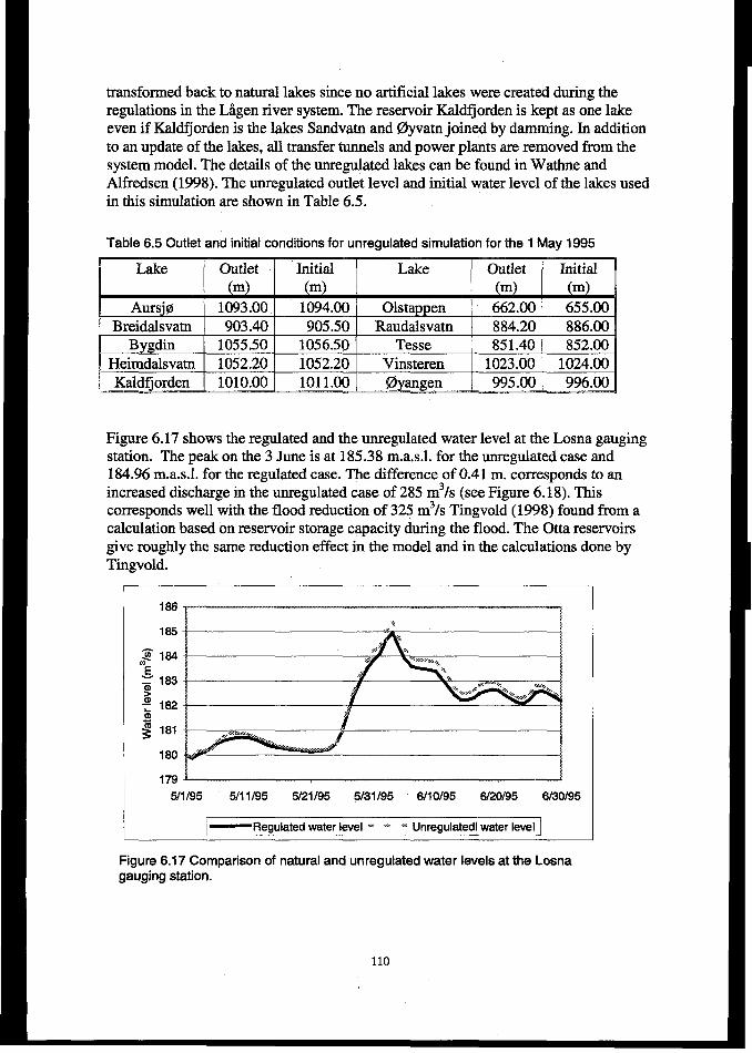
transformed back to natural lakes since no artificial lakes were created during theregulations in the Liigen river system. The reservoir Ka.Mi-jorden is kept as one lakeeven if Kaldfjorden is the lakes Sandvatn and @vatn joined by damming. In additionto an update of the lakes, all transfer tunnels and power plants are removed from thesystem model. The details of the unregulated lakes can be found in Wathne andAlfredsen (1998). The unregulated outlet level and initial water level of the lakes usedin this simulation are shown in Table 6.5.

Table 6.5 Outlet and initial conditions for unregulated simulation for the 1 May 1995

~ Lake Outlet Initial Lake Outlet Initial(m) (m) (m) (m)

Aursj@ 1093.00 1094.00 Olstappen 662.00 655.00Breidalsvatn 903.40 905.50 Raudalsvatn 884.20 886.00

Bygdin 1055.50 1056.50 Tesse 851.40 852.00Heimdalsvatn 1052.20 1052.20 Vinsteren 1023.00 1024.00Kald- 1010.00 1011.00 @yangen 995.00 996.00

Figure 6.17 shows the regulated and the unregulated water level at the Losna gaugingstation. The peak on the 3 June is at 185.38 m.a.s.l. for the unregulated case and184.96 m.a.s.l. for the regulated case. The difference of 0.41 m. corresponds to anincreased discharge in the unregulated case of 285 m3/s (see Figure 6.18). Thiscorresponds well with the flood reduction of 325 m3/s Tingvold (1998) found from acalculation based on reservoir storage capacity during the flood. The Otta reservoirsgive roughly the same reduction effect in the model and in the calctiations done byTingvold.

I186

i165

z

164

183

162

1794 f

5tlle5 5111/95 5/21195 5J31195 6HO195 6120195 6130195I

I‘Regulated water level “ * w Unregulated water level

Figure 6.17 Comparison of natural and unregulated water levels at the Losnagauging station.

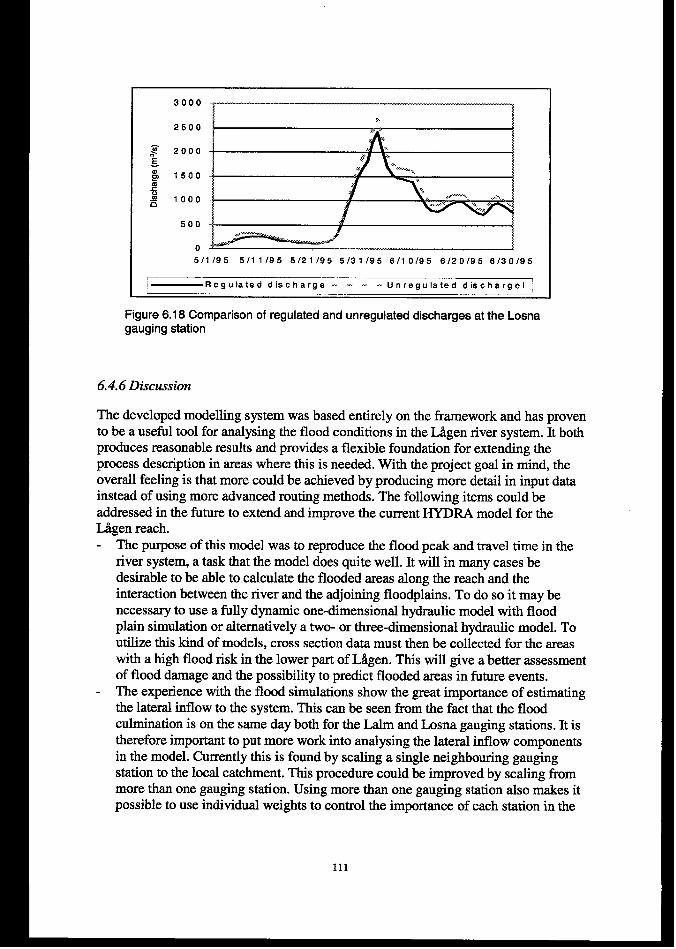
I &

2500

“? 2000gw *

1500P6;.-n 1000

500

0511195 51fl 195 5121195 5t31t95 6110195 6120195 6130195

:—Regulated die charge - - - -Unregulated dia chargelJ

Figure 6.18 Comparison of regulated and unregulated discharges at the Losnagauging station

6.4.6 Discussion

The developed modelling system was based entirely on the framework and has provento be a useful tool for analysing the flood conditions in the Liigen river system. It bothproduces reasonable results and provides a flexible foundation for extending theprocess description in areas where this is needed. With the projeet goal in mind, theoverall feeling is that more could be achieved by producing more detail in input datainstead of using more advanced routing methods. The following items could beaddressed in the future to extend and improve the current HYDRA model for theIAgen reaeh.- The purpose of this model was to reproduce the flood peak and travel time in the

river system, a task that the model does quite well. It will in many cases bedesirable to be able to calculate the flooded areas along the reach and theinteraction between the river and the adjoining floodplains. To do so it may benecessary to use a fully dynamic one-dimensional hydraulic model with floodplain simulation or alternatively a two- or three-dimensional hydraulic model. Toutilize this kind of models, cross section data must then be collected for the areaswith a high flood risk in the lower part of LAgen. This will give abetter assessmentof flood damage and the possibility to predict flooded areas in future events.

- The experience with the flood simulations show the great importance of estimatingthe lateral inflow to the system. This can be seen ffom the fact that the floodculmination is on the same day both for the Lalm and Losna gauging stations. It istherefore important to put more work into analysing the lateral inflow componentsin the model. Currently this is found by scaling a single neighboring gaugingstation to the local catehment. This procedure could be improved by scaling frommore than one gauging station. Using more than one gauging station also makes itpossible to use individual weights to control the importance of eaeh station in the

total result. Another option would be to use a hydrologic model to compute thelateral inflow component.

- To properly describe the outlet capacity for a gated reservoir it is now necessary tomanipulate the outlet capacity curve. The consequence of this is that manualchanges to the curves are needed to handle different reservoir operations. It isnecessary to enhance the reservoir operation part of the routing routine used in themodel, especially if future operative use of the model is planned. This works betterfor the version that uses the Runge Kutta solver, but this routine is not stable for adaily time step so an internal down-scaling of the time step is necessary. Inaddition it is important to be aware of the fact that the hydrological routing routinerequires a horizontal water surface in the reservoir when changes in outlet capacityare done during a simulation.

- Inflow from the highest regions in the catchrnent seems to need a further studysince this may be a possible solution to the problems encountered with the latepeaks in the Otta valley (see figure 6. 11). This problem might also be solved whenthe hydrological models for these areas are available.

- An assessment of the accuracy of the gauging stations is necessary since this is acritical parameter in estimating the goodness of the model. Especially the veryhigh flow conditions where the rating curve is extrapolated outside the calibratedrange should be investigated further.

Currently the system has been applied to the 1995 situation and a test has been doneusing the available data for the 1967 flood. A complete data set for the 1997 flood willbe available soon and this will be used to further assess the reliability of the modellingsystem. This work was not completed at the time of writing.

The uncertainties in the unregulated simulations are harder to assess in a properfashion. As mentioned in the previous section, the available archives contain littleinformation about the natural outlets and their capacities, neither do we haveinformation about the actual storage volume in the umegulated lakes. The constructedoutlet capacity curves are therefore very important for the results. Another problemwith the unregulated case is to properly assess the starting level of the reservoirs. Thiscan be handled by starting the simulation at a low water or by assessing it from nearbygauging stations.

6.5 The Glomma model

6.5.1 Background

The initial work with the main river in the Glomma (Figure 6.1) basin was done as apart of a diploma thesis at the Department of Hydraulic and EnvironmentalEngineering at NTNU (Montecchio 1998). The objective of the study was to build themodel and calibrate it to the 1995 flood. In addition floods from 1967 and 1966 wereused to test the model. This chapter presents an overview of the modelling process andthe results obtained.

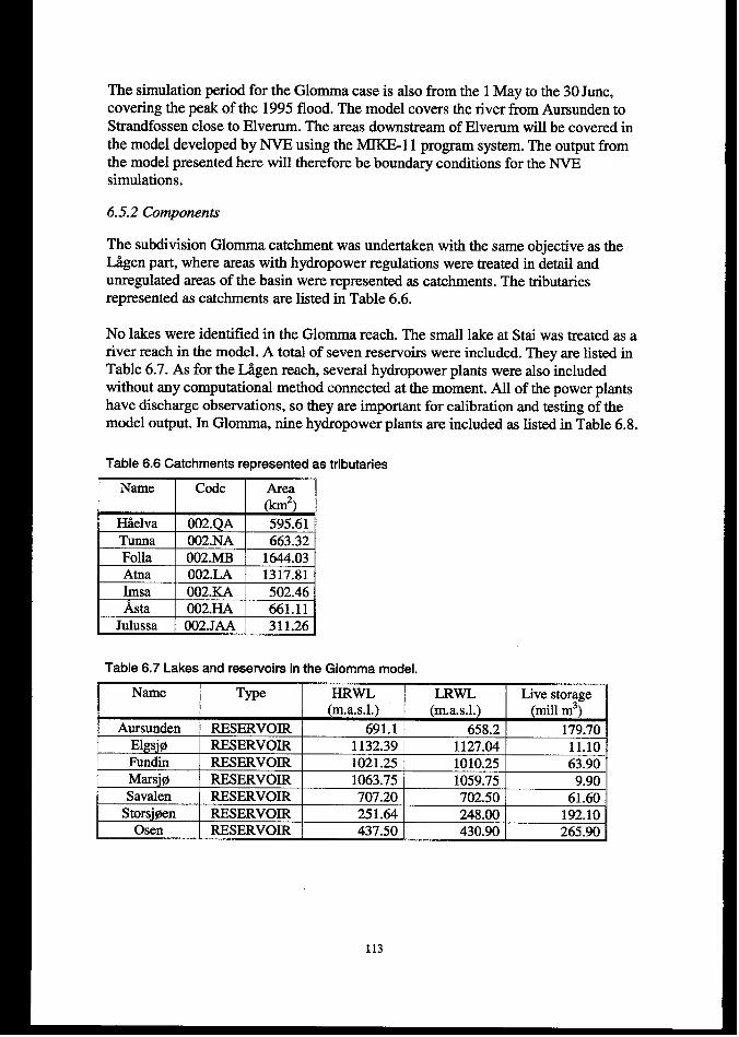
The simulation period for the Glornma case is also from the 1May to the 30 June,covering the peak of the 1995 flood. The model covers the river from Aursunden toStrandfossen close to Elvemm. The areas downstream of Elverum will be covered inthe model developed by NVE using the MIKE-11 program system. The output fromthe model presented here will therefore be boundary conditions for the NVEsimulations.

6.5.2 Components

The subdivision Glomrna catchment was undertaken with the same objective as theL&gen part, where areas with hydropower regulations were treated in detail andunregulated areas of the basin were represented as catchments. The tributariesrepresented as catchments are listed in Table 6.6.

No lakes were identified in the Glomma reach. The small lake at Stai was treated as ariver reach in the model. A total of seven reservoirs were included. They are listed inTable 6.7. As for the Liigen reach, several hydropower plants were also includedwithout any computational method connected at the moment. All of the power plantshave discharge observations, so they are important for calibration and testing of themodel output. In Glomma, nine hydropower plants are included as listed in Table 6.8,

Table 6.6 Catchments represented as tributaries

Name Code Area

I-Iiielva 002.QA 595.61Tunna 002.NA 663.32Folla 002.MB 1644.03Atria 002.LA 1317.81Imsa 002.KA 502.46ASta 002.HA 661.11

Julussa 002.JAA 311.26

Table 6.7 Lakes and reservoirs in the Glomma model.

Aursunden RESERVOIRElgsj@ RESERVOIR 1132.39 1127.04 11.10Fundin RESERVOIR 1021.25 1010.25 63.90Marsj@ RESERVOIR 1063.75 1059.75 9.90Savalen RESERVOIR 707.20 702.50 61.60

Storsj@en RESERVOIR 251.64 248.00 192.10Osen RESERVOTR 43750 430.90 265.90

113

Table 6.8 Power plants in the Glomma model.

Name Head Capacity7

Installed Power(m) (m3/s) (Mw)

Kuri%foss 47.77 25.50 10.00

R@tefossen 8.80 59.00 4.60

Einunna 124.73 10.00 9.60 ,

Savalen 231.03 32.00 57.00

Rendalen 210.40 55.00 92.00

Osa 198.60 52.00 90.00

Kvernfallet 18.00 7.00 0.90

Osfallet 41.80 17.00 5.50

L#pet 19.30 150.00 24.30

Strandfossen 13.50 235.00 22.50

The last part of the model is the water transport components, in Glornma this is acombination of tunnels and river reaches. The selected reaches are shown in Table 6.7,and the total system model for Glomma in Figure 6.20. As was the case in Liigen,every object has a local catchment producing a lateral inflow component.

Table 6.9 River reaches and turme/s in the Glomma model.

Local Catchrnent 7 –rReach Code Area Average Notes

m2 specificrunoff

lf5*km2

Aursunden- H&elva 002.R 194.18 13.91 To confluenceH&elvaH?ielva- R@efossen 002.Q122 94.62 12.12

;4.74 14.48 To confluenceTmmaTynset– SavalenKR 002.N3 169.77 11.08 Outletfrompower stationSavalenKRV– Folla 002.N 195.95 10.57“

K32.M7 536.10 14.37 TransferRendalen

II R@tefossen- Tynset 002.P 115

Folla – H@yegga oH@yegga – Rendalen -

H@yegga– Atria 002.M 49LI I Transfertnnnel II

[ Rena - Strandfossen 002.H71 I 30

4.37 14.97

Atria - Stai 002.L 565.27 14.42 AddsImsa at StaiStai - Rena 002.J 604.89 20.25

2.63 14.17Rendalen– Storsj@en 002.JES 175.23 14.30

Storsj@en– Osa 002.JC3 171.87 14.48Osen– Kvernfallet 002.JBA5 103.23 15.76

lwerp.D02.MBB3 211.54 13.62 ‘1omtalcepowerplant

Einzuana - Savalen I - EimmnaP.S. to Savalen

Osen – Osa Tunnelto OsapoEimmnna 1(

-. I —

At H@yegga, water is transferred from the main river to the Rena tributary and to theStorsj@en reservoir. This water is then utilized in several power plants before Renaagain joins Glornma. GLB has recorded the amount of water transfemed during the

114

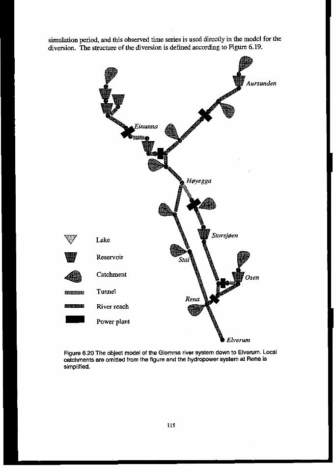
simulation period, and this observed time series is used direetly in the model for thediversion. The structure of the diversion is defined according to Figure 6.19.

v,..:..+.&

.:.t..

rsunden

Lake\

_ AJ#Uf OJ~C~t

Reservoir *

\\ ~

Stai if!

Catchment

Tunnel tJ“

River reach

Power plant

‘\

Osen

Venu

~ Elverum

Figure 6.20 The objeet model of the Glomma river system down to Elverum. Localcatchments are omitted from the figure and the hydropower system at Rena issimplified.

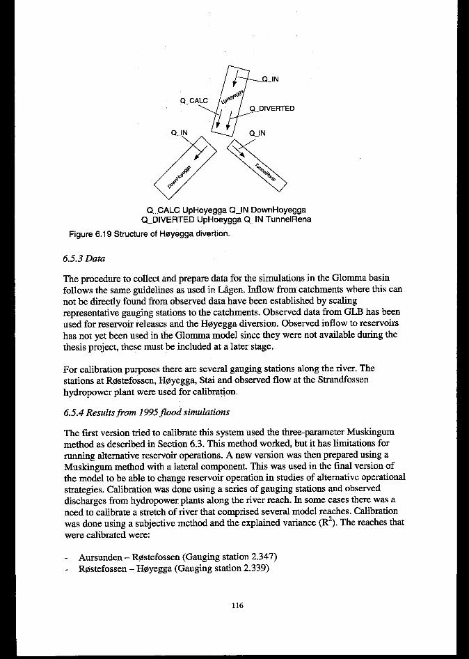
/7/-_.Q_lN

Q.CALC@a@

~9*‘-..,

//

Q DIVERTED/–

Q_lN~\\,

L “

,4%?%

%%

Q_CALC UpHoyegga Q_lN DownHoyeggaQ_DIVERTED UpHoeygga Q_lN TunnelRena

Figure 6.19 Structure of HOyegga divettion.

6.5.3 Data

The procedure to collect and prepare data for the simulations in the Glomma basinfollows the same guidelines as used in Lfigen. Inflow from catchments where this cannot be directly found from observed data have been established by scalingrepresentative gauging stations to the catchments. Observed data from GLB has beenused for reservoir releases and the H@yegga diversion. Observed inflow to reservoirshas not yet been used in the Glomma model since they were not available during thethesis project, these must be included at a later stage.

For calibration purposes there are several gauging stations along the river. Thestations at RfM.efossen, H@yegga, Stai and observed flow at the Strandfossenhydropower plant were used for calibration.

6.5.4 Results@om 1995 flood simulations

The first version tried to calibrate this system used the three-parameter Muskingummethod as described in Section 6.3. This method worked, but it has limitations forrunning alternative reservoir operations. A new version was then prepared using aMuskingum method with a lateral component. This was used in the final version ofthe model to be able to change reservoir operation in studies of alternative operationalstrategies. Calibration was done using a series of gauging stations and observeddischarges from hydropower plants along the river reach. In some cases there was aneed to calibrate a stretch of river that comprised several model reaches. Calibrationwas done using a subjective method and the explained variance (R2). The reaches thatwere calibrated were:

Aursunden – R@tefossen (Gauging station 2.347)R@tefossen - H@yegga (Gauging station 2.339)

116

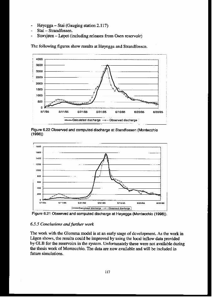
- H@yegga- Stai(Gauging station 2.117)- Stai – Strandfossen.- Storsj@en – Lj3pet (including releases from Osen reservoir)

The following figures show results at H@yegga and Strandfossen.

2500

2000 1

1500

1000

500

0511 /95 5111 /95 5121195 5131195 6/1 0/95 6/20/95 6/30/95

—calculated discharge -+-- Observed discharge

Figure 6.22 Observed and computed discharge at Standfossen (Montecchio(1998))

1800

*600

1400

1200

1000

800

600

400

200

0

5/1 /95 5/1 1/95 5/21/95 5/31 i95 6/1 0/s5 6120195 6/S0/95

i—Calculated discharge --e-- 0beerveddischarge

Figure 6.21 Observed and computed discharge at Hayegga (Montecchio (1998)).

6.5.5 Conclusions and firther work

The work with the Glomma model is at an early stage of development. As the work inL5gen shows, the results could be improved by using the local inflow data providedby GLB for the reservoirs in the system. Unfortunately these were not available duringthe thesis work of Montecchio. The data are now available and will be included infiture simulations.

117

6.6 Integration with external tools

The PINE system (Rinde 1998) will be integrated on a code level to simulate inflowhorn several catchments with varying land use. PINE is used by the framework as asingle object with an interface that provides access to the functionality in theapplication. A PINE specific computational method will be created that prepare dataand handles results from PINE and executes computations through this interface. Theflexible structure of PINE will be used to represent both the HBV and the SINBADprograms if this is necessary.

The MIKE11 progmun will be integrated through a wrapper that utilizes theAutomation interface in the MIKE Time Series editor to prepare the upstreamhydrography for the MIKE simulation. This will also retrieve the hydrogmph from thedownstream end as input to the last part of the HYDRA model (see figure 6.2). Afloodplain object will be made to hold the data used by MIKE to ensure that the reachfits into the general layout of the HYDRA model.

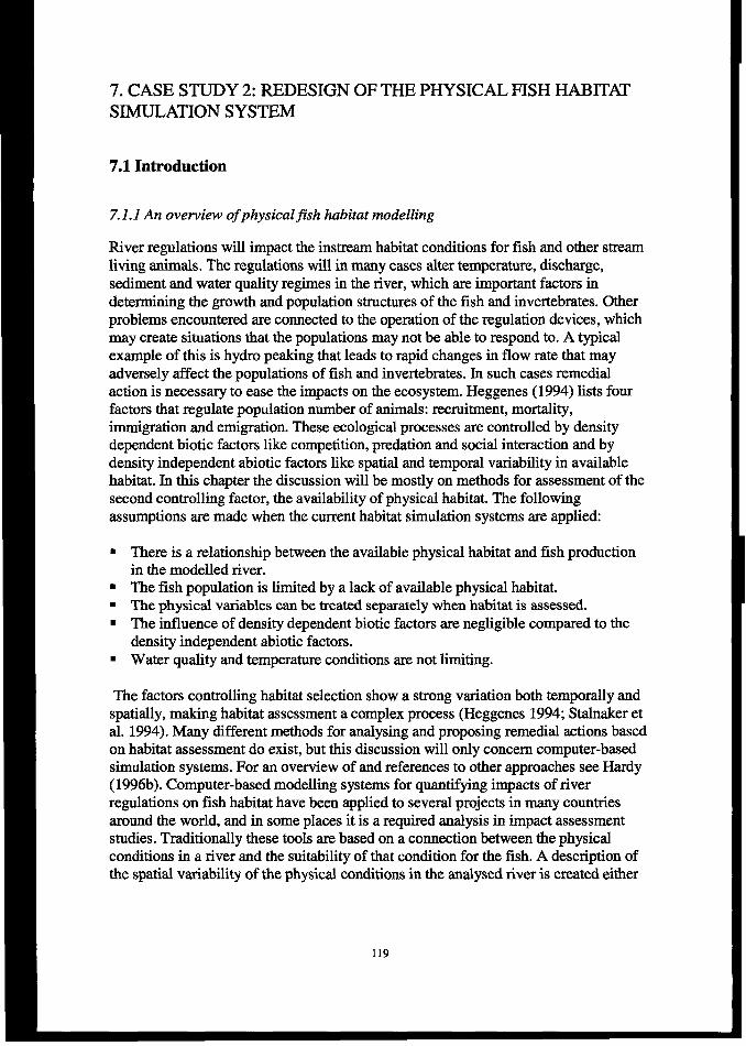
7. CASE STUDY 2: REDESIGN OF THE PHYSICAL FISH HABITATSIMULATION SYSTEM

7.1 Introduction

7.1.1 An overview ofphysicalfish habitat modelling

River regulations will impact the instream habitat conditions for fish and other streamliving animals. The regulations will in many cases alter temperature, discharge,sediment and water quality regimes in the river, which are important factors indetermining the growth and population stmctures of the fish and invertebrates. Otherproblems encountered are connected to the operation of the regulation devices, whichmay create situations that the populations may not be able to respond to. Atypicalexample of this is hydro peaking that leads to rapid changes in flow rate that mayadversely affect the populations of fish and invertebrates. In such cases remedialaction is necessary to ease the impacts on the ecosystem. Heggenes (1994) lists fourfactors that regulate population number of animals: recruitment, mortality,immigration and emigration. These ecological processes are controlled by densitydependent biotic factors like competition, predation and social interaction and bydensity independent abiotic factors like spatial and temporal variability in availablehabitat. In this chapter the discussion will be mostly on methods for assessment of thesecond controlling factor, the availability of physical habitat. The followingassumptions are made when the current habitat simulation systems are applied:

■ There is a relationship between the available physical habitat and fish productionin the modelled river.

‘ The fish population is limited by a lack of available physical habitat.“ The physical variables can be treated separately when habitat is assessed.■ The influence of density dependent biotic factors are negligible compared to the

density independent abiotic factors.‘ Water quality and temperature conditions are not limiting.

The factors controlling habitat selection show a strong variation both temporally andspatially, making habitat assessment a complex process (Heggenes 1994; Stalnaker etal. 1994). Many different methods for amdysing and proposing remedial actions basedon habitat assessment do exist, but this discussion will only concern computer-basedsimulation systems. For an overview of and references to other approaches see Hardy(1996b). Computer-based modelling systems for quantifying impacts of riverregulations on fish habitat have been applied to several projects in many countriesaround the world, and in some places it is a required analysis in impact assessmentstudies. Traditionally these tools are based on a convection between the physicalconditions in a river and the suitability of that condition for the fish. A description ofthe spatial variability of the physical conditions in the analysed river is created either

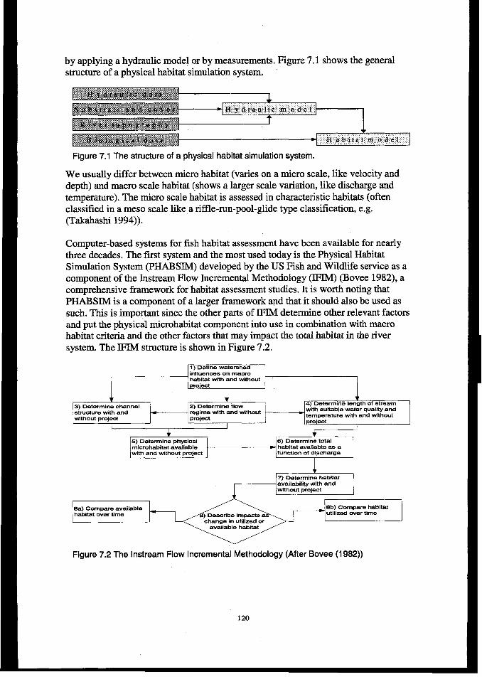
by applying a hydraulic model or by measurements. Figure 7.1 shows the generalstructure of a physical habitat simulation system.

Figure 7.1 The structure of a physical habitat simulation system.

We usually differ between microhabitat (varies on a micro scale, like velocity anddepth) and macro scale habitat (shows a larger scale variation, like discharge andtemperature). The micro scale habitat is assessed in characteristic habitats (oftenclassified in a meso scale like a riffle-run-pool-glide type classification, e.g.(Takahashi 1994)).

Computer-based systems for fish habitat assessment have been available for nearlythree decades. The first system and the most used today is the Physical HabitatSimulation System (PHABSIM) developed by the US Fish and Wildlife service as acomponent of the Instream Flow Incremental Methodology (IFIM) (Bovee 1982), acomprehensive framework for habitat assessment studies. It is worth noting thatPHABSIM is a component of a larger framework and that it should also be used assuch. This is important since the other parts of IFIM determine other relevant factorsand put the physical microhabitat component into use in combination with macrohabitat criteria and the other factors that may impact the total habitat in the riversystem. The IFIM structure is shown in Figure 7.2.

1) Define watershed

influences on macrohabitat with and withoutproject

43) Determine channel 2) Determine flow 4) Determine length of stream

structure with and regime with and without with suitable water qualify and

without project project temperature with and withoutproject

I I I+ t

5) Determine physical 6) Determine totalmicrohabitat available habitat available as awith and without project function of discharge

+7) Determine habitatavailabilii with andwithout project

8a) Compare available Sb) Compare habitathaMtat over time ) Describe impacts as utilized over time

change in utilized or

Figure 7.2 The Instream Flow Incremental Methodology (AfterBovee(1982))

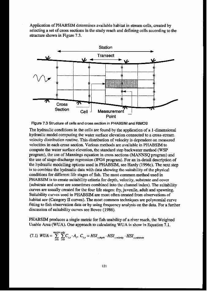
Application of PHABSIM determines available habitat in stream cells, created byselecting a set of cross sections in the study reach and defining cells according to thestructure shown in Figure 7.3.

Station4 b

uTransect

4 W*

4? J$ #$ @8+-—------ —---—--f—-—--——-

%4 ;~

_—.—_.+..—— ----.—.--..— 4 4$ 4$.--... -——

$k %1

.——_--— ________ .. —--. —-.I 4

$8 ----—---- .--. —,.._—j ______

SectionCell - Measurement

Point -

Figure 7.3 Structure of cells and cross section in PHABSIM and RIMOS

The hydraulic conditions in the cells are found by the application of a l-dimensionalhydraulic model computing the water surface elevation connected to a cross-streamvelocity distribution routine. This distribution of velocity is dependent on measuredvelocities in each cross section. Various methods are available in PHABSIM tocompute the water surface elevation, the standard step backwater method (WSPprogram), the use of Mannings equation in cross sections (MANNSQ program) andthe use of stage-discharge regression (IFG4 program). For an in-detail description ofthe hydraulic modelling options used in PHABSIM, see Hardy (1996c). The next stepis to combine the hydraulic data with data showing the suitability of the physicalconditions for different life stages of fish. The most common method used inPHABSIM is to create suitability criteria for depth, velocity, substrate and cover(substrate and cover are sometimes combined into the channel index). The suitabilitycurves are usually created for the four life stages: fry, juvenile, adult and spawning.Suitability curves used in PHABSIM are most often created from observations ofhabitat use (Category II curves). The most common techniques are polynomial curvefitting to fish observation data or by using frequency analysis on the data. For a furtherdiscussion of suitability curves see Bovee (1986).

PHABSIM produces a single metric for fish usability of a river reach, the WeightedUsable Area (WUA). One approach to calculating WUA is show in Equation 7.1.

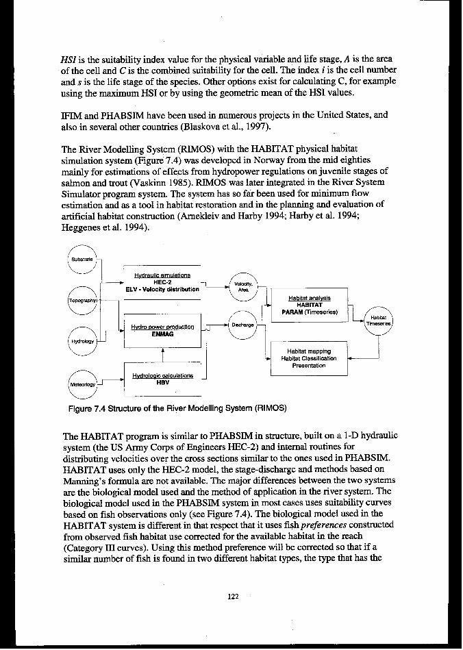
2%S1is the suitability index value for the physical variable and life stage, A is the area

of the cell and C is the combined suitability for the cell. The index i is the cell numberands is the life stage of the species. Other options exist for calculating C, for exampleusing the maximum HSI or by using the geometric mean of the HSI values.

IFIM and PHABSINf have been used in numerous projects in the United States, andalso in several other countries (Blaskova et al., 1997).

The River Modelling System (RIMOS) with the HABITAT physical habitatsimulation system (Figure 7.4) was developed in Norway from the mid eightiesmainly for estimations of effects from hydropower regulations on juvenile stages ofsalmon and trout (Vaskinn 1985). RIMOS was later integrated in the River SystemSimulator program system. The system has so far been used for minimum flowestimation and as a tool in habitat restoration and in the planning and evaluation ofartificial habitat construction (Arnekleiv and Harby 1994; Harby et al. 1994;Heggenes et al. 1994).

oSubstrate

oTo~raphy

o

Hydrolc&#

1 Habitat analveis

HABITATPARAM ~meaeriea)

1

Hvdro Dower vrodustion

‘= ‘F===”H drolo ic oalculationa

P“””A v ““” r ~

I

I I

Figure 7.4 Structure of the River Modelling System (RIMOS)

The HABITAT program is similar to PHABSIM in structure, built on a 1-D hydraulicsystem (the US Army Corps of Engineers HEC-2) and internal routines fordistributing velocities over the cross sections similar to the ones used in PHABSIM.HABITAT uses only the HEC-2 model, the stage-discharge and methods based onManning’s formula are not available. The major differences between the two systemsare the biological model used and the method of application in the river system. Thebiological model used in the PHABSIM system in most cases uses suitability curvesbased on fish observations only (see Figure 7.4). The biological model used in theHABITAT system is different in that respect that it uses fish pre~erences constructedfrom observed fish habitat use corrected for the available habitat in the reach(Category III curves). Using this method preference will be corrected so that if asimilar number of fish is found in two different habitat types, the type that has the

122

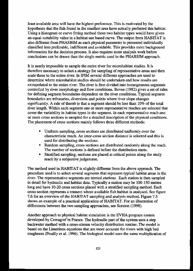
least available area will have the highest preference. This is motivated by thehypothesis that the fish found in the smallest area have actually preferred this habitat.Using a histogram or curve fitting method these two habitat types would have givenan equal suitability value in a habitat use based curve. The output from HABITAT isalso different from PHASBIM as each physical parameter is presented individuallyclassified into preferable, indifferent and avoidable. This provides more backgroundinformation for the decision process. It also requires more analysis work beforeconclusions can be drawn than the single metric used in the PHABSIM approach.

It is nearly impossible to sample the entire river for microhabitat studies. It istherefore necessary to select a strategy for sampling of representative areas and thenscale these to the entire river. In IFIM several different approaches are used todetermine where microhabitat studies should be undertaken and how results areextrapolated to the entire river. The river is first divided into homogeneous segmentscontrolled by river morphology and flow conditions. Bovee (1982) gives a set of rulesfor defining segment boundaries dependent on the river conditions. Typical segmentboundaries are tributaries, diversions and points where river slope changessignificantly. A rule of thumb is that a segment should be less than 10% of the totalriver length. Within each segment one or more representative reaches are selected thatcover the variability in habitat types in the segment. In each representative reach oneor more cross sections is sampled for a detailed description of the physical conditions.The placement of cross sections mainly follows three different methods:

‘ Uniform sampling, cross sections are distributed uniformly over thecharacteristic reach. An inter-cross section distance is selected and this isused for distributing the sections.

■ Random sampling, cross sections are distributed randomly along the reach.The number of sections is defined before the distribution starts.

I Stratified sampling, sections are placed at critical points along the studyreach by a subjective judgement.

The method used in HABITAT is slightly different from the above approach. Theprocedure used is to select several segments that represent typical habitat areas in theriver. The representative segments are termed stutions. Each station is then sampledin detail for hydraulic and habitat data. Typically a station maybe 100-150 metreslong and have 10-20 cross sections placed with a stratified sampling method. Eachcross section represents a transect where available fish habitat is analysed. See figure7.6 for an overview of the HABITAT sampling and analysis method. Figure 7.5shows an example of a practical application of HABITAT. For an illustration ofdifferences between the two sampling approaches, see Scruton (1998).

Another approach to physical habitat simulation is the EVHA program systemdeveloped by Cemagref in France. The hydraulic part of the system uses a stepbackwater method with a cross-stream velocity distribution routine. The model isbased on the Limerinos equations that are more accurate for rivers with high bedroughness (Pouilly et al. 1996). The biological model uses the same multiplication of

123

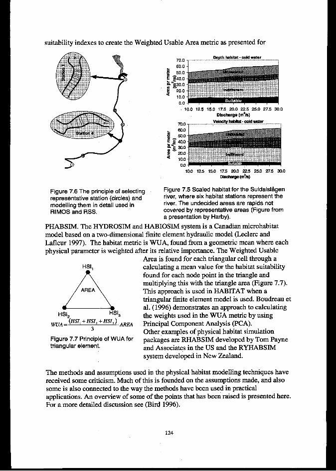
suitability indexes to create the Weighted Usable Area metric as presented for

r-”

10.0 12.5 15.0 17.5 20.0 22.5 25.0 27.5 30.0

Discharge (m*/e)

70.0 ~- ......v-rn..*=-.rn.~.= ...........

10.0 12.5 15.0 17.5 20.0 22.5 25.0 27.5 W.oD- (m’k)

Figure 7.6 The principle of selecting Figure 7.5 Scaled habitat for the Suldaisl~gen

representative station (circles) and river, where six habitat stations represent the

modelling them in detail used in river. The undecided areas are rapids not

RIMOS and RSS. covered by representative areas (Figure froma presentation by Harby).

PHABSIM. The HYDROSIM and HABIOSIM system is a Canadian microhabitatmodel based on a two-dimensional finite element hydraulic model (Leclerc andLafleur 1997). The habitat metric is WUA, found from a geometric mean where eachphysical parameter is weighted after its relative importance. The Weighted Usable

Area is found for each triangular cell through aHSI1

A

calculating a mean value for the habitat suitabilityfound for each node point in the triangle andmultiplying this with the triangle area (Figure 7.7).

AREA This approach is used in HABITAT when atriangular finite element model is used. Boudreau etal. (1996) demonstrates an approach to calculating

HSIZ HS13~~= (HSZ,+HSI, +HSI,),_

the weights used in the WUA metric by usingPrincipal Component Analysis (PCA).

3 Other examples of physical habitat simulationFigure 7.7’ Principle of WUA fortriangular element.

packages are RHABSIM developed by Tom Payneand Associates in the US and the RYHABSIMsystem developed in New Zealand.

The methods and assumptions used in the physical habitat modelling techniques havereceived some criticism. Much of this is founded on the assumptions made, and alsosome is also connected to the way the methods have been used in practicalapplications. An overview of some of the points that has been raised is presented here.For a more detailed discussion see (Bird 1996).

124.

All of the above methods build on the assumption that the lack of available habitat islimiting the population of fish in the river reach. In many cases this is not true sincethe density dependent biotic factors presented earlier will control the population. Inthese cases the prediction of stock sizes based on physical habitat modelling will fail,and this is one of the reason that such studies have a wide variation in results. It isimportant to note that even if the link to fish population size fails, the methods willstill predict changes in habitat with discharge and periods with a critical lack ofavailable habitat.

An assumption made when suitabilities or preferences are created is that the fish selectthe controlling variables independently. In the river, depth and velocity are connectedand vary with discharge, and it has been shown that the assumption of independence issometimes violated (Mathur et al. 1985). Problems are also encountered when thevariables are aggregated into habitat suitability indexes, since the aggregation is notbased on biological assumptions (Heggenes 1994). This is the main reason for theseparate analysis of variables in the HABITAT system. Since habitat use of fish canbe size structured (Heggenes 1994), the relative importance of the variables will alsovary through the life stages of the fish. Research has been done in the area to find therelative importance of variables e.g. by using multivariate statistical analysis(Boudreau et al. 1996) and by creation of multivariate suitability functions. Anotherimportant area is the scale of the variables. While the analysis considers meanconditions in a water volume, the selection criteria maybe on micro-scale variations.This warrants the study of spatial variation of parameters and higher resolution in thedescription of the physical domain.

Another theme for much discussion has been the transferability of habitat suitability orpreference curves (Bird 1996). IFIM provides statistical methods for transferabilitytesting (USGS-MESC 1998). In the HAIHTAT system a requirement is thatpreferences must be created from local data. Preferences must also be seasondependent since the habitat selection mechanism in the fish may vary both accordingto dayhight and summer/winter (Heggenes and Saltveit 199& LeDrew et al. 1996).Based the temporal variation in suitability it is also important to analyse temporalvariation in available habitat. Temporal variations in habitat have been identified asimportant, and the lack of such analyses in the early days was pointed out. In recentyears model developers have addressed this subject to a degree (Stalnaker et al. 199%Capra et al. 1995). Still the link between the time series of habitat and responses onthe individual, community and population level is lacking (Hardy 1996b).

7.1.2 Motivation for redesign of RSS-HABZTAT

The increased use of habitat modelling techniques in a variety of situations combinedwith continued research and development in both hydraulic and biological modellingmotivated the redesign of the HABITAT program. The development in hydraulic andbiological modelling does take place both to try to strengthen the weak sides of theexisting methodology and to introduce new modelling aspects into thes ystem. Overthe few last years the existing system did undergo several changes to accommodatenew analysis methods and the increasing need for flexibility in species and parameters

125

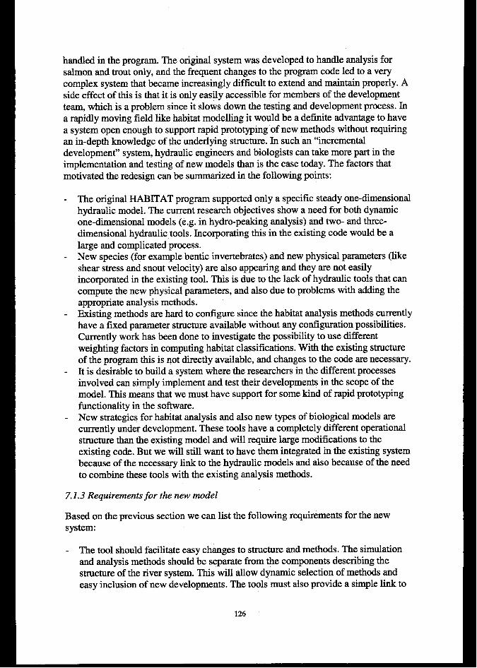
handled in the program. The original system was developed to handle analysis forsalmon and trout only, and the flequent changes to the program code led to a verycomplex system that became increasingly difficult to extend and maintain properly. Aside effect of this is that it is only easily accessible for members of the developmentteam, which is a problem since it slows down the testing and development process. Ina rapidly moving field like habitat modelling it would be a definite advantage to havea system open enough to support rapid prototyping of new methods without requiringan in-depth knowledge of the underlying structure. In such an “incrementaldevelopment” system, hydraulic engineers and biologists can take more part in theimplementation and testing of new models than is the case today. The factors thatmotivated the redesign can be summarized in the following points:

The original HABITAT program supported only a specific steady one-dimensionalhydraulic model. The current research objectives show a need for both dynamicone-dimensional models (e.g. in hydro-peaking analysis) and two- and three-dimensional hydraulic tools. Incorporating this in the existing code would be alarge and complicated process.New species (for example bentic invertebrates) and new physical parameters (likeshear stress and snout velocity) are also appearing and they are not easilyincorporated in the existing tool. This is due to the lack of hydraulic tools that cancompute the new physical parameters, and also due to problems with adding theappropriate analysis methods.Existing methods are hard to configure since the habitat analysis methods currentlyhave a fixed parameter structure available without any configuration possibilities.Currently work has been done to investigate the possibility to use differentweighting factors in computing habitat classifications. With the existing structureof the program this is not directly available, and changes to the code are necessary.It is desirable to build a system where the researchers in the different processesinvolved can simply implement and test their developments in the scope of themodel. This means that we must have support for some kind of rapid prototypingfunctionality in the software.New strategies for habitat analysis and also new types of biological models arecurrently under development. These tools have a completely different operationalstructure than the existing model and will require large modifications to theexisting code. But we will still want to have them integrated in the existing systembecause of the necessary link to the hydraulic models and also because of the needto combine these tools with the existing analysis methods.

7.1.3 Requirements for the new model

Based on the previous section we can list the following requirements for the newsystem.

The tool should facilitate easy changes to structure and methods. The simulationand analysis methods should be separate from the components describing thestructure of the river system. This will allow dynamic selection of methods andeasy inclusion of new developments. The tools must also provide a simple link to

126

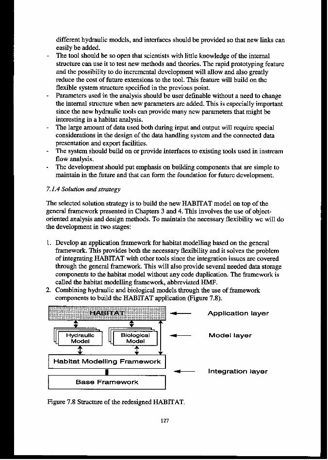
different hydraulic models, and interfaces should be provided so that new links caneasily be added.

- The tool should be so open that scientists with little knowledge of the intemdstructure can use it to test new methods and theories. The rapid prototyping featureand the possibility to do incremental development will allow and also greatlyreduce the cost of future extensions to the tool. This feature will build on theflexible system structure specified in the previous point.

- Parameters used in the analysis should be user definable without a need to changethe internal structure when new parameters are added. This is especially importantsince the new hydraulic tools can provide many new parameters that might beinteresting in a habitat analysis.

- The large amount of data used both during input and output will require specialconsiderations in the design of the data handling system and the connected datapresentation and export facilities.

- The system should build on or provide interfaces to existing tools used in instreamflow analysis.

- The development should put emphasis on building components that are simple tomaintain in the future and that can form the foundation for future development.

7.1.4 Solution and strategy

The selected solution strategy is to build the new HA131TAT model on top of thegeneral ihmework presented in Chapters 3 and 4. This involves the use of object-oriented analysis and design methods. To maintain the necessary flexibility we will dothe development in two stages:

1.

2.

Develop an application framework for habitat modelling based on the generalframework. This provides both the necessary flexibility and it solves the problemof integrating HABITAT with other tools since the integration issues are coveredthrough the general i%mnework. This will also provide several needed data storagecomponents to the habitat model without any code duplication. The framework iscalled the habitat modelling framework, abbreviated HMF.Combining hydraulic and biological models through the use of frameworkcomponen-m to build the HABfiAT application (Figure 7.8).

I Habitat Modelling Framework It !

I Integration layer

Base Framework

Figure 7.8 Structure of the redesigned HABITAT.

127

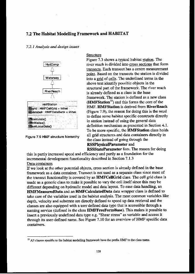
7.2 The Habitat Modelling Framework and HABITAT

7.2.1 Analysis and design issues

$##ealculateO,&~iseO,:H:~LocalDatao

Figure 7.9 HMF etrueture hierarchy

structureFigure 7.3 shows atypical habitat station. Theriver reach is divided into cross sections that formtransects, Each transect has a centre measurement~. Based on the transects the station is dividedinto a gr&l of ~. The underlined terms in theabove text identify possible objects in thestructural part of the framework. The river reaehis already defined as a class in the baseframework. The station is defined as a new class(HMFStationlO) and this forms the core of theHMF. HMFStation is derived from RiverReaeh(Figure 7.9), the reason for doing this is the needto define some habitat specific constructs directlyin station instead of using the general datadefinition mechanism as presented in Section 4.1.To be more specific, the HMFStation class holdsall grid structures and data containers directly inthe class instead of going through theRSSPhysiealPar~eter and -RSSStatePararneter lists. The reason for doing

this is partly increased speed and efficiency and partly as a foundation for theincremental development functionality described in Section 7.1.3Data containersIf we look at the other potential objects, cross section is already defined in the baseframework as a data container. Transect is not used as a separate class since most ofthe transect functionality is covered by an HMFCellGrid class. The cell grid class ismade as a generic class to make it possible to vary the cell itself since this maybedifferent depending on hydraulic model and data layout. To ease data handling, anHMFMeasuredData and an HMFCalcuIatedData data wrapper class is defined totake care of the variables used in the habitat analysis. The most common variables likedepth, velocity and substrate are directly defined to speed up data retrieval and theclasses are also equipped with a user defined data type that is accessible through anaming service (defined in the class HMFFreeFormBase). This makes it possible toinsert a previously undefined data type e.g. “Shear stress” as variable and aeeess itthrough its user-defined name. See Figure 7.10 for an overview of HMF specific datacontainers.

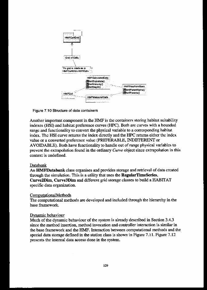
I 1-~ HMFCellGtid,

?

1-----------------I! Grid of CeMS ![.......... .. .. ..............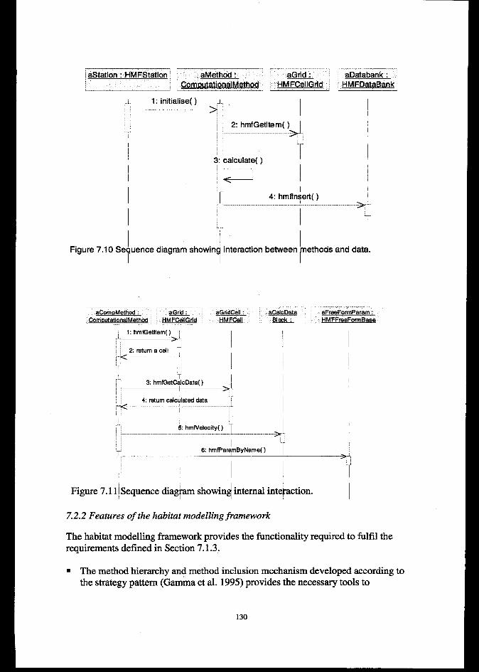

\\

--..; HMFFmeFormBase

&$JmffaG-N&%o.-fi,*mfPammsl)

Figure 7.10 Structure of data containers

Another important component in the HMF is the containers storing habitat suitabilityindexes (HSI) and habitat preference curves (lWC). Both are curves with a boundedrange and fimctionality to convert the physical variable to a corresponding habitatindex. The HSI curve returns the index directly and the HPC returns either the indexvalue or a converted preference value (PREFEIUBLE, INDIFFERENT orAVOIDABLE). Both have functionality to handle out of range physical variables toprevent the extrapolation found in the ordinary Curve object since extrapolation in thiscontext is undefined.

DatabankAn HMFDatabank class organises and provides storage and retrieval of data createdthrough the simulation. This is a utility that uses the RegularTimeSeries,Curve2Dim, Curve3Dim and different grid storage classes to build a HABITATspecific data organization.

ComuutationalMethodsThe computational methods are developed and included through the hierarchy in thebase framework.

Dvnamic behaviourMuch of the dynamic behavionr of the system is already described in Section 3.4.3since the method insertion, method invocation and controller interaction is similar inthe base framework and the HMF. Interaction between computational methods and thespecial data storage defined in the station class is shown in Figure 7.11. Figure 7.12presents the internal data access done in the system.

E! aMethi)d : aGrid “, , Comm.ttationalMethod HM=Grid

,1. 1:initiaiise( ) ,.~..>’ I

2: hmfGetltem( ) I

aDatabank :; HMFData6ank

>’T.

Figure 7,10 Se uence diagram showin interaction between ethods and dat .Y 1 r 1

1 1 1i.)

“[

1 4 1Figure 7.11 Sequence diag am showin internal inte action.

7.2.2 Features of the habitat modellingfiamework

The habitat modelling framework provides the functionality required to fulfil therequirements defined in Section 7.1.3.

“ The method hierarchy and method inclusion mechanism developed according tothe strategy pattern (Gamma et al. 1995) provides the necessary tools to

130

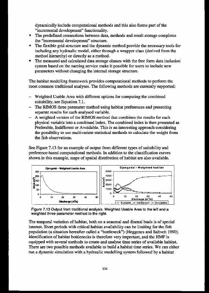
dynamically include computational methods and this also forms part of the“incremental development” functionality.

■ The predefine connections between data, methods and result storage completesthe “incremental development” structure.

= The flexible grid structure and the dynamic method provide the necessary tools forincluding any hydraulic model, either through a wrapper class (derived from themethod hierarchy) or directly as a method.

‘ The measured and calculated data storage classes with the free form data inclusionsystem based on the naming service make it possible for users to include newparameters without changing the internal storage structure.

The habitat modelling framework provides computational methods to perform themost common traditional analyses. The following methods are currently supported:

—

—

—

Weighted Usable Area with different options for computing the combinedsuitability, see Equation 7.1.The RIMOS three parameter method using habitat preferences and presentingseparate results for each analysed variable.A weighted version of the RIMOS method that combines the results for eachphysic-d variable into a combined index. The combined index is then presented asPreferable, Indifferent or Avoidable. This is an interesting approach consideringthe possibility to use mukivariate statistical methods to calculate the weight fromthe fish observations.

See Figure 7.13 for an example of output from different types of suitability andpreference-based computational methods. In addition to the classification curvesshown in this example, maps of spatial distribution of habitat are also available.

I =Q,GJengedel - Weighted Ueek4eAree

I

I Diacha~ (m%)

G}engedel - Weighted ha bitet

5000 ~

$;=

o 10 20 30 40 50Discharge (m%)

--- Suitable ~ Indifferent -Avoidabla

Figure 7.13 Output from traditional analysis. Weighted Usable Area to the left and aweighted three-parameter method to the right.

The temporal variation of habitat, both on a seasonal and diurnal basis is of specialinterest. Short periods with critical habitat availability can be limiting for the fishpopulation (a situation hereafter called a “bottleneck”) (Heggenes and Saltveit 1990).Identification of habitat bottlenecks is therefore very important, and the HMF isequipped with several methods to create and analyse time series of available habitat.There are two possible methods available to build a habitat time series. We can eitherrun a dynamic simulation with a hydraulic modelling system followed by a habitat

131

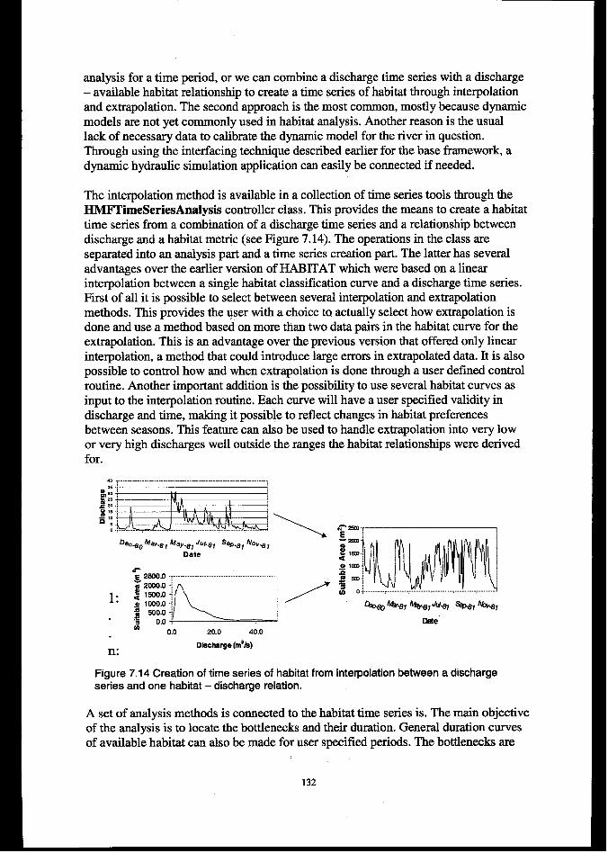
analysis for a time period, or we can combine a discharge time series with a discharge– available habitat relationship to create a time series of habitat through interpolationand extrapolation. The second approach is the most common, mostly because dynamicmodels are not yet commonly used in habitat analysis. Another reason is the usuallack of necessary data to calibrate the dynamic model for the river in question.Through using the interfacing technique described earlier for the base framework, adynamic hydraulic simulation application can easily be connected if needed.

The interpolation method is available in a collection of time series tools through theHMFTimeSeriesAnalysis controller class. This provides the means to create a habitattime series from a combination of a discharge time series and a relationship betweendischarge and a habitat metric (see Figure 7. 14). The operations in the class areseparated into an analysis part and a time series creation part. The latter has severaladvantages over the earlier version of HABITAT which were based on a linearinterpolation between a single habitat classification curve and a discharge time series.First of all it is possible to select between several interpolation and extrapolationmethods. This provides the user with a choice to actually select how extrapolation isdone and use a method based on more than two data pairs in the habitat curve for theextrapolation. This is an advantage over the previous version that offered only linearinterpolation, a method that could introduce large errors in extrapolated data. It is alsopossible to control how and when extrapolation is done through a user defined controlroutine. Another important addition is the possibility to use several habitat curves asinput to the interpolation routine. Each curve will have a user specified validity indischarge and time, making it possible to reflect changes in habitat preferencesbetween seasons. This feature can also be used to handle extrapolation into very lowor very high discharges well outside the ranges the habitat relationships were derivedfor.

40 . . . . . . . . . . . . . . . . .

$51 1

g s,& 25

= 2.0,$

-* ,,n,

o

1:

n:Oiicharge (m’k)

C%.@J%*, *,JU* %0.8,J&i/,

Ome

Figure 7.14 Creation of time series of habitat from interpolation between a dischargeseries and one habitat – discharge relation.

A set of analysis methods is connected to the habitat time series is. The main objectiveof the analysis is to locate the bottlenecks and their duration. General duration curvesof available habitat can also be made for user specified periods. The bottlenecks are

132

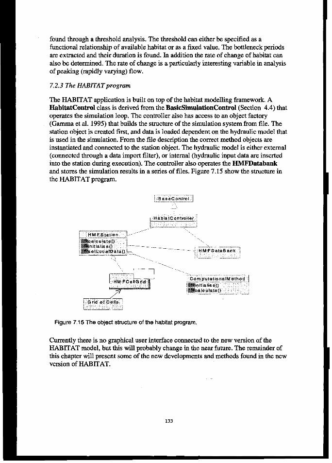
found through a threshold analysis. The threshold can either be specified as afunctional relationship of available habitat or as a fixed value. The bottleneck periodsare extracted and their duration is found. In addition the rate of change of habitat canalso be determined. The rate of change is a particularly interesting variable in analysisof peaking (rapidly varying) flow.

7.2.3 The H4BITATprograrn

The HABITAT application is built on top of the habitat modelling framework. AHabitatControl class is derived from the BasicSimulationControl (Section 4.4) thatoperates the simulation loop. The controller also has access to an object factory(Gamma et al. 1995) that builds the structure of the simulation system from file. Thestation object is created first, and data is loaded dependent on the hydraulic model thatis used in the simulation. From the file description the correct method objects areinstantiated and connected to the station object. The hydraulic model is either external(connected through a data import filter), or internal (hydraulic input data are insertedinto the station during execution). The controller also operates the HMFDatabankand stores the simulation results in a series of files. Figure 7.15 show the structure inthe HABITAT program.

‘\ \

\ . .....

Figure 7.15 The object structure of the habitat program.

Currently there is no graphical user interface connected to the new version of theHABITAT model, but this will probably change in the near future. The remainder ofthis chapter will present some of the new developments and methods found in the newversion of HABITAT.

133

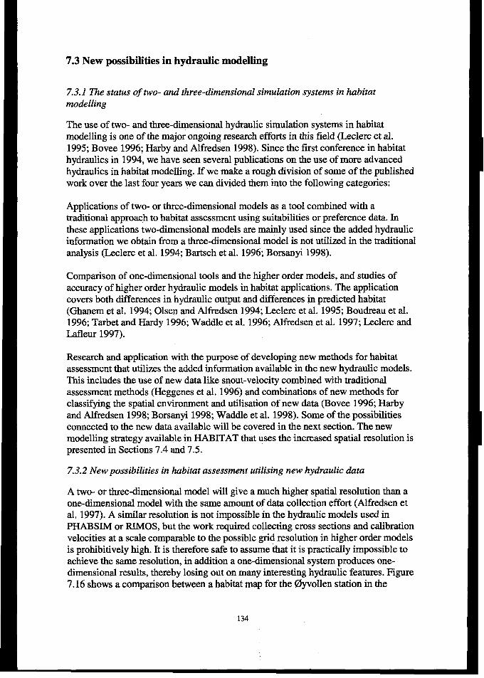
7.3 New possibilities in hydraulic modelling

7.3.1 The status of two- and three-dimensional simulation systems in hubitatmodelling

The use of two- and three-dimensional hydraulic simulation systems in habitatmodelling is one of the major ongoing research efforts in this field (Leelerc et al.1995; Bovee 1996; Harby and Alfredsen 1998). Since the fust conference in habitathydraulics in 1994, we have seen several publications on the use of more advancedhydraulics in habitat modelling. If we make a rough division of some of the publishedwork over the last four years we can divided them into the following categories:

Applications of two-or three-dimensional models as a tool combined with atraditional approach to habitat assessment using suitabilities or preference data. Inthese applications two-dimensional models are mainly used since the added hydraulicinformation we obtain from a three-dimensional model is not utilized in the traditionalanalysis (Leclerc et al. 1994; Bartsch et al. 1996; Borsanyi 1998).

Comparison of one-dimensional tools and the higher order models, and studies ofaccuracy of higher order hydraulic models in habitat applications. The applicationcovers both differences in hydraulic output and differences in predicted habitat(Ghanem et al. 1994; Olsen and Alfredsen 1994; Leclerc et al. 1995; Boudreau et al.1996; Tarbet and Hardy 1996; Waddle et al. 1996; Alfredsen et al. 1997; Leclere andLafleur 1997).

Researeh and application with the purpose of developing new methods for habitatassessment that utilizes the added information available in the new hydraulic models.This includes the use of new data like snout-velocity combined with traditionalassessment methods (Heggenes et al. 1996) and combinations of new methods forclassifying the spatial environment and utilisation of new data (Bovee 1996; Harbyand Alfredsen 1998; Borsanyi 1998; Waddle et al. 1998). Some of the possibilitiesconnected to the new data available will be covered in the next seetion. The newmodelling strategy available in HABITAT that uses the increased spatial resolution ispresented in Sections 7,4 and 7.5.

7.3.2 New possibilities in habitat assessment utilising new hydraulic duta

A two-or three-dimensional model will give a much higher spatial resolution than aone-dimensional model with the same amount of data collection effort (Alfredsen etal, 1997). A similar resolution is not impossible in the hydraulic models used inPHABSIM or RIMOS, but the work required collecting cross sections and calibrationvelocities at a scale comparable to the possible grid resolution in higher order modelsis prohibitively high. It is therefore safe to assume that it is practically impossible toachieve the same resolution, in addition a one-dimensional system produces one-dimensional results, thereby losing out on many interesting hydraulic features. Figure7.16 shows a comparison between a habitat map for the @vollen station in the

134

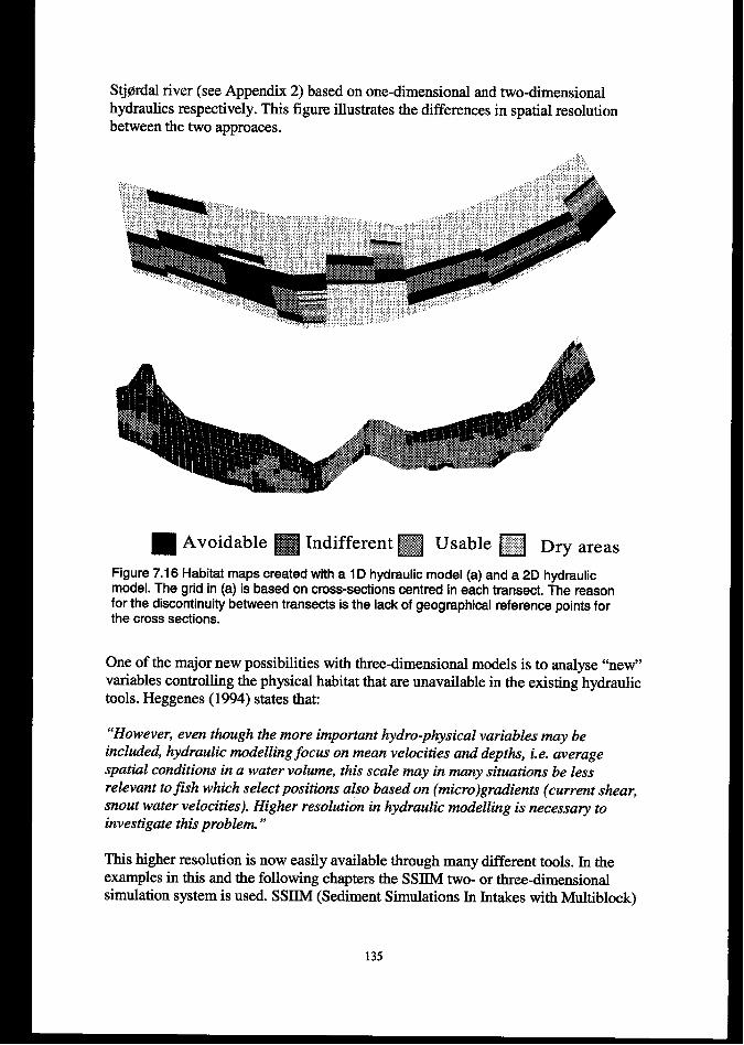
Stj@rdal river (see Appendix 2) based on one-dimensional and two-dimensionalhydraulics respectively. This figure illustrates the differences in spatial resolutionbetween the two approaces.

■ Avoidable ❑ Indifferent ❑ Usable ❑ Dry areas

Figure 7.16 Habitat maps created with a 1D hydraulic model (a) and a 2D hydraulicmodel. The grid in (a) is based on cross-sections centred in each transect, The reasonfor the discontinuity between transects is the lack of geographical reference points forthe cross sections.

One of the major new possibilities with three-dimensional models is to analyse “new”variables controlling the physical habitat that are unavailable in the existing hydraulictools. Heggenes (1994) states that

“However, even though the more important hydro-physical variables maybeincluded, hydraulic modelling focus on mean velocities and depths, i.e. averagespatial conditions in a water volume, this scale may in many situan”ons be lessrelevant to fish which select positions also based on (micro)gradients (current shear,snout water velocities). Higher resolution in hydraulic modelling is necessary toinvestigate this problem, ”

This higher resolution is now easily available through many different tools. In theexamples in this and the following chapters the SWIM two- or three-dimensionalsimulation system is used. SSIIM (Sediment Simulations In Jntakes with Multiblock)

135

solves the Navier Stokes equations using a k-~ turbulence model and a finite volumediscretisation (Olsen and Stokseth 1995; Olsen 1996). SWIM uses a non-orthogonalstructured grid, with the possibility to block out one or more regions within the grid.SSIIM runs in either steady or dynamic mode, thereby permitting simulations of risingand falling discharges. SSllM can also be configurated to run either in three-dimensional mode, or as a depth-averaged two-dimensional model making it a flexibletool for habitat hydraulic analysis. For further information about data collection andgrid creation for the simulations done in various rivers, see Appendix 2. The fullversion of SSIIM is at the moment of writing only available for the IBM 0S/2operating system. It is included HABITAT through a method that reads SHIM outputfiles and builds the station grid horn these.

The snout water velocity (also called focal point velocity) is the velocity component atthe snout level of the fish. A method is developed in HABITAT to extract the focalpoint velocity from a three-dimensional velocity field based on a user-specified levelof the fish above the bottom. This velocity is then classified into a habitat type using asnout velocity preference. Figure 7.17 shows a snout velocity habitat map horn theOvre-Ommedal station in the Gjengedal river (see Appendix 2).

Figure 7.17 An example of utilising 3D hydraulic data: A map of snout velocity habitat.

In the traditional approach it is assumed that fish may select the hysicrd parametersindividually. In many situation the position choice is controlled by combination ofparameters. An example of a combined flow structure that may attract fish is theexistence of an eddy (recirculation) in combination with a fast current (Freeman andGrossman 1993). Fish may in this case be attracted to food gathering in therecirculating current. Such flow structures were until the emergence of higher orderhydraulic simulation tools impossible to assess through numerical flow modellingused in habitat hydraulics. With the availability of such models came the possibility toidentify such structures, figure 7.18 shows a recirculating zone in the Trekantenstation in Nidelva. At this site, this effect will only appear in conditions of low flow.

136

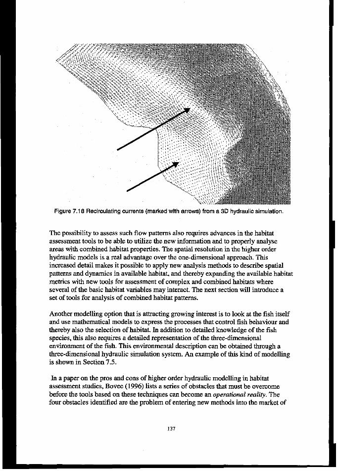
Figure 7.18 Recirculating currents (marked with arrows) from a 3D hydraulic simulation,

The possibility to assess such flow patterns also requires advances in the habitatassessment tools to be able to utilize the new information and to properly analyseareas with combined habitat properties. The spatial resolution in the higher orderhydraulic models is a real advantage over the one-dimensional approach. Thisincreased detail makes it possible to apply new analysis methods to describe spatialpatterns and dynamics in available habitat, and thereby expanding the available habitatmetrics with new tools for assessment of complex and combined habitats whereseveral of the basic habitat variables may interaet. The next section will introduce aset of tools for analysis of combined habitat patterns.

Another modelling option that is attracting growing interest is to look at the fish itselfand use mathematical models to express the processes that control fish behaviour andthereby also the selection of habitat. In addition to detailed knowledge of the fishspeeies, this also requires a detailed representation of the three-dimensionalenvironment of the fish. This environmental description can be obtained through athree-dimensional hydraulic simulation system. An example of this kind of modellingis shown in Seetion 7.5.

In a paper on the pros and cons of higher order hydraulic modelling in habitatassessment studies, Bovee (1996) lists a series of obstacles that must be overcomebefore the tools based on these techniques can beeome an operational reali~. Thefour obstacles identified are the problem of entering new methods into the market of

decision makers and project planners, the problem with the lack of validation, trainingand usability of the software and creating enthusiasm for the new methods among theusers.

The first obstacle is to sell what is now interesting research to the plannem andmanagers that are the potential users of the new tools, without overselling its potentialand possibilities. This requires us to provide clear examples of the practicalapplicability of the new tools and their use in setting flow regimes and operationalrules for regulatory organisations. This also puts special requirements on the supportfor the new product and its user friendliness.

Lack of proper validation and biological testing is one of the major areas of criticismof the existing PHABSIM technique. Effort should be undertaken both to providevalidation data for the new hydraulic tools and especially for its biologicalsignificance. Since the knowledge at the moment is much better regarding hydraulicsthan multi-dimensional habitat mapping, it is required that effort is put intodeveloping and understanding the new habitat assessment methods.

The complexity in applying the tools can be reduced by developing software thatintegrates the hydraulics and habitat tools in a user-friendly way. The work presentedin this chapter is a contribution to overcoming this obstacle. In this there is also theneed to clearly define field-sampling procedures and continue the work to providetools and methods for easy data collection and preparation.

Providing good solutions to the three first obstacles is the safest way to provideenthusiasm for the product and the methodology, and make users rely on the methodand apply them to their problems.

Given that Bovee’s obstacles can be overcome, the future possibilities in higher orderhydraulic modelling seem very good. A large research effort is put into developmentand testing of such models in many fields, the recent Hydroinformatics conferencehad a large number of presentations on advanced hydraulic modelling. Looking at the–94 and –96 conferences one can see that this is an area with a large research effort.This shows some of the potential that exists in this technique. Many developments canbenefit biologically based analysis directly, such as the ability to operate inunstructured and nested grids (Olsen 1998), a feature that is currently underdevelopment in SWIM. A nested grid will allow us to generate a coarse grid for theriver reach in question, and then place detailed sub grids at locations of specialinterest. One of the analyses this technique will support is the detailed investigation ofspecial structures in a river reach, for example the man-made habitat improvementworks that are frequently used in river restoration projects.

Some researchers involved in the development of methods for habitat assessment havemade the point that the developments in hydraulic modelling go too fast compared tothe development of corresponding biological models, and that the priorities shouldsomewhat be reversed (Bovee 1996; Hardy 1996a). This is of course a very valid

138

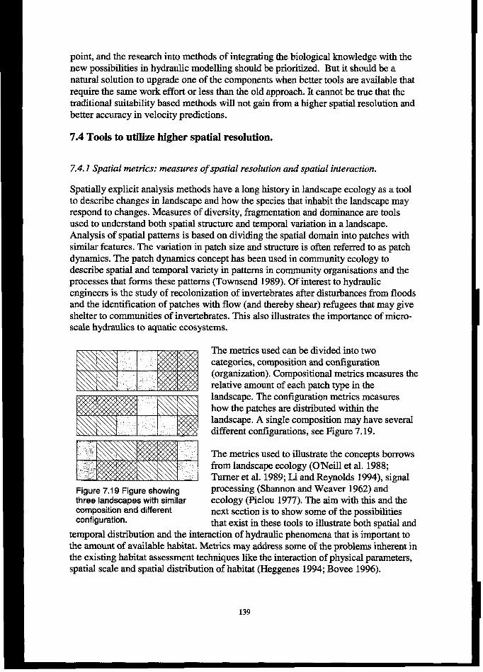
point, and the research into methods of integrating the biological knowledge with thenew possibilities in hydraulic modelling should be prioritized. But it should be anatural solution to upgrade one of the components when better tools are available thatrequire the same work effort or less than the old approach. It cannot be true that thetraditional suitability based methods will not gain from a higher spatial resolution andbetter accuracy in velocity predictions.

7.4 Tools to utilize higher spatial resolution.

7.4.1 Spatial metrics: measures of spatial resolution and spatial interaction.

Spatially explicit analysis methods have a long history in landscape ecology as a toolto describe changes in landscape and how the species that inhabit the landscape mayrespond to changes. Measures of diversity, fragmentation and dominance are toolsused to understand both spatial structure and temporal variation in a landscape.Analysis of spatial patterns is based on dividing the spatial domain into patches withsimilar features. The variation in patch size and structure is often referred to as patchdynamics. The patch dynamics concept has been used in community ecology todescribe spatial and temporal variety in patterns in community organisations and theprocesses that forms these patterns (Townsend 1989). Of interest to hydraulicengineers is the study of recolonization of invertebrates after disturbances from floodsand the identification of patches with flow (and thereby shear) refhgees that may giveshelter to communities of invertebrates. This also illustrates the importance of micro-scale hydraulics to aquatic ecosystems.

Figure 7.19 Figure showingthree landscapes with similarcomposition and differentconfiguration.

The metrics used can be divided into twocategories, composition and configuration(organization). Compositional metrics measures therelative amount of each patch type in thelandscape. The configuration metrics measureshow the patches are distributed within thelandscape. A single composition may have severaldifferent configurations, see Figure 7.19.

The metrics used to illustrate the concepts borrowsfrom landscape ecology (0’Neill et al, 1988;Turner et al. 1989; Li and Reynolds 1994), signalprocessing (Shannon and Weaver 1962) andecology (Pielou 1977). The aim with this and thenext section is to show some of the possibilitiesthat exist in these tools to illustrate both spatial and

temporal distribution and the interaction of hydraulic phenomena that is important tothe amount of available habitat. Metrics may address some of the problems inherent inthe existing habitat assessment techniques like the interaction of physical parameters,spatial scale and spatial distribution of habitat (Heggenes 1994; Bovee 1996).

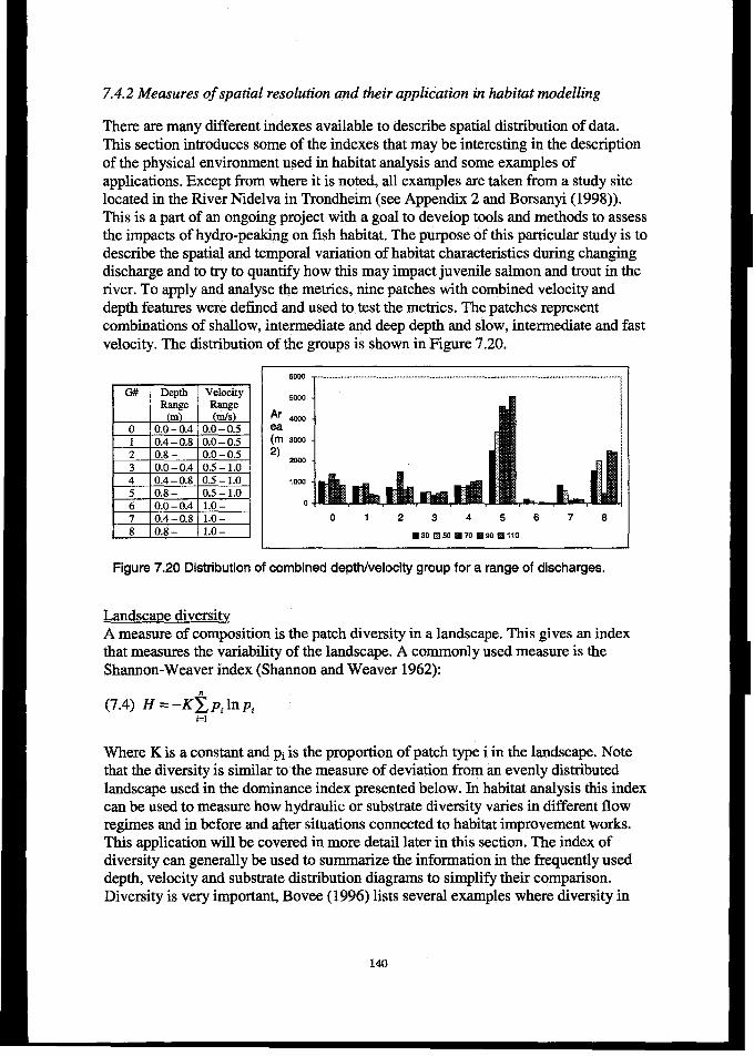
7.4.2 Measures of spatial resolution and their application in habitat rnodelling

There are many different indexes available to describe spatial distribution of data.This section introduces some of the indexes that maybe interesting in the descriptionof the physical environment used in habitat analysis and some examples ofapplications. Except horn where it is noted, all examples are taken from a study sitelocated in the River Nidelva in Trondheim (see Appendix 2 and Borsanyi (1998)).

This is a part of an ongoing project with a goal to develop tools and methods to assessthe impacts of hydro-peaking on fish habitat. The purpose of this particular study is todescribe the spatial and temporal variation of habitat characteristics during changingdischarge and to try to quantify how this may impact juvenile salmon and trout in theriver. To apply and analyse the metrics, nine patches with combined velocity anddepth features were defined and used to test the metrics. The patches representcombinations of shallow, intermediate and deep depth and slow, intermediate and fastvelocity. The distribution of the groups is shown in Figure 7.20.

EG# Depth velocity

Range RangeIII/s

o 0.0:0.4 0.0–0.51 0.4–0.s 0.0-0.52 0.8– 0.0–0.53 0.0-0.4 0.5- 1.04 0.4–0.8 0.5– 1.05 0.8- 0.5- 1.06 0.0- 0.4 1.0–7 0.4–0.8 1.0–8 0.8- 1.0-

0 1 2345678

■ 301350 m70B90sllo

Figure 7.20 Distribution of combined depth/velocity group for a range of discharges.

Landscaue diversityA measure of composition is the patch diversity in a landscape. This gives an indexthat measures the variability of the landscape. A commonly used measure is theShannon-Weaver index (Shannon and Weaver 1962):

(7.4) H = -K~pi in p,iel

Where K is a constant and pi is the proportion of patch type i in the landscape. Notethat the diversity is similar to the measure of deviation from an evenly distributedlandscape used in the dominance index presented below. In habitat analysis this indexcan be used to measure how hydraulic or substrate diversity varies in different flowregimes and in before and after situations connected to habitat improvement works.This application will be covered in more detail later in this section. The index ofdiversity can generally be used to summarize the information in the frequently useddepth, velocity and substrate distribution diagrams to simplify their comparison.Diversity is very importan~ Bovee (1996) lists several examples where diversity in

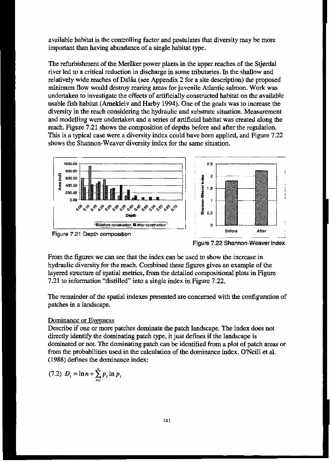
available habitat is the controlling factor and postulates that diversity maybe moreimportant than having abundance of a single habitat type.

The refurbishment of the Mer&lcerpower plants in the upper reaches of the Stj@dalriver led to a critical reduction in discharge in some tributaries. In the shallow andrelatively wide reaches of Dal% (see Appendix 2 for a site description) the proposedminimum flow would destroy rearing areas for juvenile Atlantic salmon. Work wasundertaken to investigate the effects of artificially constructed habitat on the availableusable fish habitat (Arnekleiv and Harby 1994). One of the goals was to increase thediversity in the reach considering the hydraulic and substrate situation. Measurementand modelling were undertaken and a series of artificial habitat was created along thereach. Figure 7.21 shows the composition of depths before and after the regulation.This is a typical case were a diversity index could have been applied, and Figure 7.22shows the Shannon-Weaver diversity index for the same situation.

800.KI

600,00

400SM

200.00

O.lxl

inee.fore constnxtkm BAfter constwdm \

Figure 7.21 Depth compositionBefore After I

Figure 7.22 Shannon-Weaver index

From the figures we can see that the index can be used to show the increase inhydraulic diversity for the reach. Combined these figures gives an example of thelayered structure of spatial metrics, from the detailed compositional plots in Figure7.21 to information “distilled” into a single index in Figure 7.22.

The remainder of the spatial indexes presented are concerned with the configuration ofpatches in a landscape.

Dominance or EvennessDescribe if one or more patches dominate the patch landscape. The index does notdirectly identify the dominating patch type, it just defines if the landscape isdominated or not. The dominating patch can be identified horn a plot of patch areas orfrom the probabilities used in the calculation of the dominance index. O’Neill et al.(1988) defines the dominance index:

(7.2) ~1 =kn+~~ihlpiis]

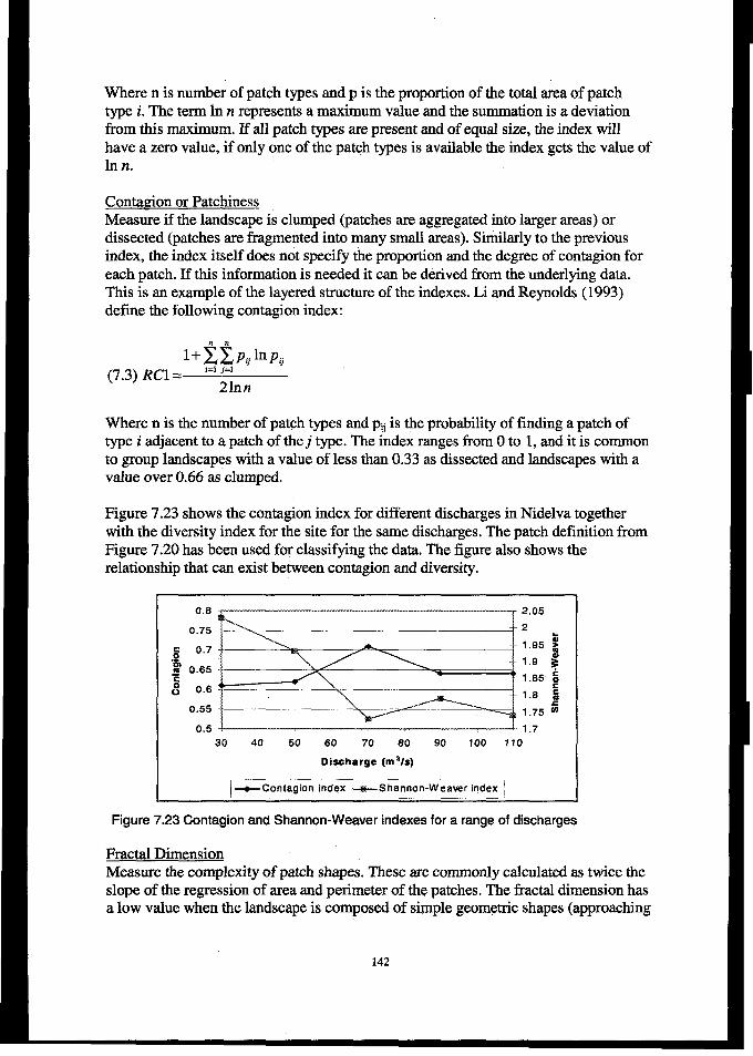
Where n is number of patch types and p is the proportion of the total area of patchtype i. The term In n represents a maximum value and the summation is a deviationfrom this maximum. If all patch types are present and of equal size, the index willhave a zero value, if only one of the patch types is available the index gets the value ofinn.

Cent.wion or PatchinessMeasure if the landscape is clumped (patches are aggregated into larger areas) ordissected (patches are fragmented into many small areas). Similarly to the previousindex, the index itself does not specify the proportion and the degree of contagion foreach patch. If this information is needed it can be derived flom the underlying data.This is an example of the layered structure of the indexes. Li and Reynolds (1993)define the following contagion index:

l+~~pijlnpti

(7.3) Z?cl = ‘“ :hn

Where n is the number of patch types and ~j is the probability of finding a patch oftype i adjacent to a patch of thej type. The index ranges from Oto 1, and it is commonto group landscapes with a value of less than 0.33 as dissected and landscapes with avalue over 0.66 as clumped.

Figure 7.23 shows the contagion index for different discharges in Nidelva togetherwith the diversity index for the site for the same discharges. The patch definition fromFigure 7.20 has been used for classifying the data. The figure also shows therelationship that can exist between contagion and diversity.

0.5 I I 1.730 40 50 60 70 80 90 100 110

Diecharge (m*/s)

~+-Contagion indax -w--Shannon-Weaver index i

Figure 7.23 Contagion and Shannon-Weaver indexes for a range of discharges

Fractal DimensionMeasure the complexity of patch shapes. These are commonly calculated as twice theslope of the regression of area and perimeter of the patches. The fractal dimension hasa low value when the landscape is composed of simple geometric shapes (approaching

142

1.0). If the landscape is composed of many complex shapes the fractal dimension willbe large.

Edge effectsSee how edges may affect neighboring patchesand how the edges themselves may formimportant habitat (Malcolm 1994). In habitatanalysis an example of this is a feeding stationfor a fish (Figure 7.24) where the combination

Figure 7.24 A sketch of a feeding between an adjacent resting and feeding areastation (Illustration from Swisher forms the important habitat. The edge effectand Richards (1976)) metric tries to compute how far from the

intersection between the habitats the edge isimportant, thereby creating anew patch defined by the edge. A simpler approach isusing an interface measure to identify the edge effect.

Interface between ~atchesThe interface metric is a simpler way of assessing variation in important edge habitat.The metric measures the length of interfaces between each patch type. Figure 7.25shows edge length between the patches defined in Figure 7.20 for a discharge of 30m3/s and 110 m31srespectively. As a hypothetical example we define the areas ofpatch 2 as resting habitat and patches 4 to 6 are feeding areas. In this case we have atotal of 164 metres of edge that creates a feeding habitat at the low discharge, whilethis is reduced to 80 metres on the high discharge.

_——”T—-----”..

Figure 7.25 Length of edges between patches at 30 m3/s (left) and 110 m3/s (right).

Nearest nei~hbour ProbabilitiesDirectionality in habitat can be important in many aspects, such as in studies ofstranding and pool trapping and h-identification of escape channels in shallow waterhabitat. Directionality can be identified by calculating matrixes with probabilities offirst order adjacency describing the probability of finding two patches of a specifiedtype adjacent to each other. By calculating this in both the cross current and streamwise directions we may assess directionality in the habitat. The probabilities will also

143

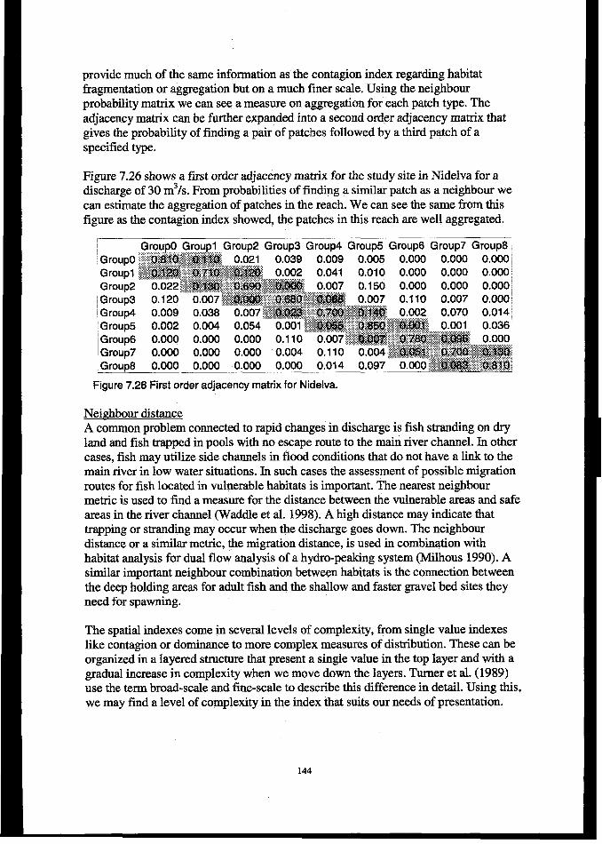
provide much of the same information as the contagion index regarding habitatfragmentation or aggregation but on a much finer scale. Using the neighbourprobability matrix we can see a measure on aggregation for each patch type. Theadjacency matrix can be further expanded into a second order adjacency matrix thatgives the probability of finding a pair of patches followed by a third patch of aspecified type.

Figure 7.26 shows a first order adjacency matrix for the study site in Nidelva for adischarge of 30 m3h. From probabilities of finding a similar patch as a neighbour wecan estimate the aggregation of patches in the reach. We can see the same from thisfigure as the contagion index showed, the patches in this reach are well aggregated.

GroupO Groupl Group2 Group3 Group4 Group5 Group6 Group7 Group8.>, . . ,?,Fm+y ,,~GroupO ~$;Q3%@%2m~ 0“02]., 0.039 0.009 0.005 0.000 0.000 0.000 ~$;:,,G*. . :.:.,?.. ~. ,,<..* i.Growl ~}%a~jj;~.fiq~$%m 0.002 0.041 0.010 0.000 0.000 o.000;

I.,.<.,++,,...:;.0.022 *##gg&! ;;nm~m:+ ,0.007 0.150 0.000 0.000 0.000 ;

~::!: o.120 0.007 g$mj ‘ :*:*ogfi.:_ 0.007 0.110 0.007 0.000;!Group4 0.009 0.038 0.007’##i3#%i :~.~~gw~$;% 0.002 0.070 0.014,IGroup5 w ‘%-“ “+’’’’:J-“=$:‘ ‘ ‘-’ w0.002 0.004 0.054 0.001 $gm,~:~oiam$$-; 0.001 0.036‘Group6 0.000 0.000 0.000 0.110 0.007~#~m ~:~,~?s~~~%~, ,0.000Group7 0.000 0>000 0.000 0.004 0s110 0.004 kmi: : g’ii~g%m.. , . ,,.* :<,; .:,~>,.,,..+>:x$+. . >..;Group8 0.000 0.000 0.000 0.000 0.014 0.097 0.000 j$,m;:~~@$nj

Figure 7.26 First order adjacency matrix for Nidelva.

Nei~bour distanceA common problem connected to rapid changes in discharge is fish stranding on dryland and fish trapped in pools with no escape route to the main river channel. In othercases, fish may utilize side channels in flood conditions that do not have a link to themain river in low water situations. In such cases the assessment of possible migrationroutes for fish located in vulnerable habitats is important. The nearest neighbourmetric is used to find a measure for the distance between the vulnerable areas and safeareas in the river channel (Waddle et al. 1998). A high distance may indicate thattrapping or stranding may occur when the discharge goes down. The neighbourdistance or a similar metric, the migration distance, is used in combination withhabitat analysis for dual flow analysis of a hydro-peaking system (Milhous 1990). Asimilar important neighbour combination between habitats is the connection betweenthe deep holding areas for adult fish and the shallow and faster gravel bed sites theyneed for spawning.

The spatial indexes come in several levels of complexity, from single value indexeslike contagion or dominance to more complex measures of distribution. These can beorganized in a layered structure that present a single value in the top layer and with agradual increase in complexity when we move down the layers. Turner et al. (1989)use the term broad-scale and fine-scale to describe this difference in detail. Using this,we may find a level of complexity in the index that suits our needs of presentation.

7.4.3 summary

Spatial metrics is an interesting way of integrating detailed hydraulic knowledge of ariver reach with knowledge about biological responses to hydraulic features. There isa lot of literature describing position selection and behaviour in fishes linked toenvironmental features. Even so, work is required to find ways to explicitly link thisbiological knowledge with the available metrics describing the hydraulic variability.The above examples show some of the possibilities of advancing the traditionalapproach of habitat assessment with new tools that consider interaction andcombination of the physical variables, but more work is needed to test the biologicalsignificance of the above examples. Another interesting approach that deserves moreattention is to link biological indexes with temporal and spatial hydraulic variations(Bowen et al. 1998). It is fair to assume that this field will continue its rapiddevelopment, since the use of spatial metrics is a way to solve some of the problemsand criticisms regarding the PHABSIM methodology in the field of habitat diversityand interaction of hydro-physical variables.

7.5 Bioenergetic modelling of drift feeding sahnonids.

7..S.1 A new strategy for modellingfish in rivers

Bioenergetic modelling has been studied for many years with objectives to predict fishgrowth and predator consumption in fisheries sciences (Ney 1993). The bioenergeticapproach is an interesting way of studying fish development since it has the potentialto model the fish based on a combination of many controlling factors combined in asound theoretical foundation. Ney (1993) defines bioenergetic modelling in thefollowing way

“l%e term bioenergetics refers to the ways in which animals dispose of energy theyacquire. Bioenergetic models are essentially mass-balance equations in which theenergy in consumed food is pa~”tioned into its various fates – growth, metabolismand waste products. ”

Ney refers this to Winberg who formulated and published the first detailed energybudget equation in 1956 (According to Elliott (1976b) this work was based on thepioneering efforts of Ivlev). Most applications so far model bioenergetics as a iimctionof temperature and prey availability. For example, Kitchen (1983) shows applicationsof an energetic model for growth and predation calculations. In the same paper there isa discussion on parameter sensitivity and on the simplifications that are necessary toconstruct this kind of model.

Over the last few years, the assumptions that salmonids are drift feeders (Bachman1984) and that they will try to maximize the energy gain in their environment byselecting appropriate habitats has led to research on using the bioenergetic models instudies on river fish. These models incorporate the effects from water velocity onforaging, and they also include water velocities in the calculation of metabolic costs.

145

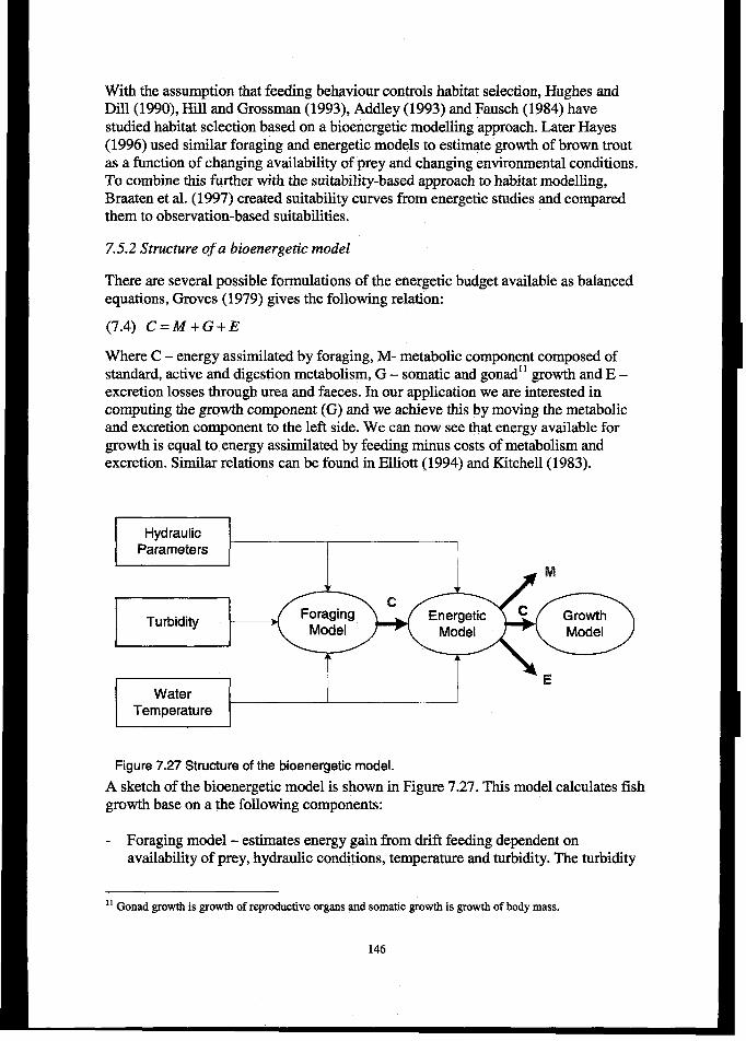
With the assumption that feeding behaviour controls habitat selection, Hughes andDill (1990), Hill and Grossman (1993), Addley (1993) and Fausch (1984) havestudied habitat selection based on a bioenergetic modelling approach. Later Hayes(1996) used similar foraging and energetic models to estimate growth of brown troutas a function of changing availability of prey and changing environmental conditions.To combine this further with the suitability-based approach to habitat modelling,Braaten et al. (1997) created suitability curves from energetic studies and comparedthem to observation-based suitabilities.

7.5.2 Structure of a bioenergetic model

There are several possible formulations of the energetic budget available as balancedequations, Groves (1979) gives the following relation:

(7.4) C=ikf+G+E

Where C – energy assimilated by foraging, M- metabolic component composed ofstandard, active and digestion metabolism, G – somatic and gonadl 1growth and E –excretion losses through urea and faeces. In our application we are interested incomputing the growth component (G) and we achieve this by moving the metabolicand excretion component to the left side. We can now see that energy available forgrowth is equal to energy assimilated by feeding minus costs of metabolism andexcretion. Similar relations can be found in Elliott (1994) and Kitchen (1983).

HydraulicParameters

Turbidity

WaterTemperature

Figure 7.27 Structure of the bioenergetic model.

A sketch of the bioenergetic model is shown in Figure 7.27. This model calculates fishgrowth base on a the following components:

- Foraging model - estimates energy gain from drift feeding dependent onavailability of prey, hydraulic conditions, temperature and turbidity. The turbidity

11Gonadgrowthis ~owtb ofreproductiveorgansandsomaticgrowthis growthofbodymass.

146

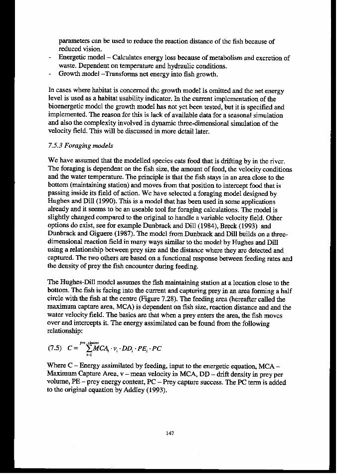
parameters can be used to reduce the reaction distance of the fish because ofreduced vision.

- Energetic model – Calculates energy loss because of metabolism and excretion ofwaste. Dependent on temperature and hydraulic conditions.

- Growth model –Transforms net energy into fish growth.

In cases where habitat is concerned the growth model is omitted and the net energylevel is used as a habitat usability indicator. In the current implementation of thebioenergetic model the growth model has not yet been tested, but it is specified andimplemented. The reason for this is lack of available data for a seasonal simulationand also the complexity involved in dynamic three-dimensional simulation of thevelocity field. This will be discussed in more detail later.

7.5.3 Foraging models

We have assumed that the modelled species eats food that is drifting by in the river.The foraging is dependent on the fish size, the amount of food, the velocity conditionsand the water temperature. The principle is that the fish stays in an area close to thebottom (maintaining station) and moves from that position to intercept food that ispassing inside its field of action. We have selected a foraging model designed byHughes and Dill (1990). This is a model that has been used in some applicationsalready and it seems to be an useable tool for foraging calculations. The model isslightly changed compared to the original to handle a variable velocity field. Otheroptions do exist, see for example Dunbrack and Dill (1984), Breck (1993) andDunbrack and Giguere (1987). The model from Dunbrack and Dill builds on a three-dimensional reaction field in many ways similar to the model by Hughes and Dillusing a relationship between prey size and the distance where they are detected andcaptured. The two others are based on a functional response between feeding rates andthe density of prey the fish encounter during feeding,

The Hughes-Dill model assumes the fish maintaining station at a location close to thebottom. The fish is facing into the current and capturing prey in an area forming a hrdfcircle with the fish at the centre (Figure 7.28). The feeding area (hereafter called themaximum capture area, MCA) is dependent on fish size, reaction distance and and thewater velocity field. The basics are that when a prey enters the area, the fish movesover and intercepts it. The energy assimilated can be found from the followingrelationship:

pre.ckasses

(7.5) C= ~MC~ ‘Vi .DD, .PEi -PCizl

Where C – Energy assimilated by feeding, input to the energetic equation, MCA –Maximum Capture Area, v – mean velocity in MCA, DD – drift density in prey pervolume, PE - prey energy content, PC - Prey capture success. The PC term is addedto the original equation by Addley (1993).

147

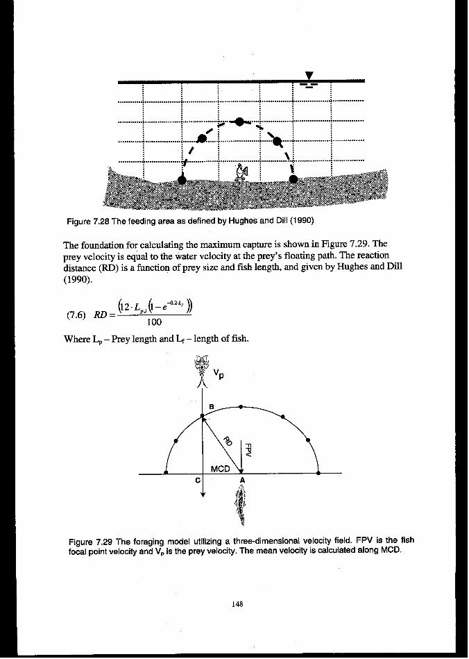
............................a.t....................................................~.................................:

............}.................*................i....> +.~ .............- ....................=............:

: S’:...........%.................y.... \’*: :............................... ......................................#:/\~ ~............ .................a..............~...................i..............4.................................

Figure 7.28 The feeding area as defined by Hughes and Dill (1990)

The foundation for calculating the maximum capture is shown in Figure 7.29. Theprey velocity is equal to the water velocity at the prey’s floating path. The reactiondistance (RD) is a function of prey size and fish length, and given by Hughes and Dill(1990).

(7.6, m=(lz~pi$;e+’z””))Where ~ – Prey length and L – length of fish.

Figure 7.29 The foraging model utilizing a three-dimensional velocity field, FPV is the fishfocal point velocity and VP is the prey velocity. ‘The mean velocity is calculated along MCD.

148

The travel time for the prey item along line BC is defined as (terms defined in Figure7,29). BC is expressed through the known distance RD and the distance we are afterMCD by using Phytagoras.

(7.7) TP = JRD2 –MCD2

V*

The fish travel time along the MCD is expressed using the velocity component of thefish along the MCD.

‘7”8) “==

The v~~ is the mean velocity over the travel distance of the fish to the interceptionpoint. To find a formulation for the unknown MCD we assume that the interceptionhappens when TF = TP. By solving this equation for MCD we get the followingexpression:

‘79)MCD=F2$R3This is simikr to the formula used by Hayes (1993) but an error is corrected in thedenominator. This is a difficult formula to solve since vman is dependent on MCD, aniterative procedure is therefore needed to solve the equation. By setting Vp= V~~, wecan easily derive the original equation presented by Hughes and Dill (1990). A moredetailed description is presented in Appendix 3. The MCD is then calculated for theentire circle. The total maximum capture area (MCA) is found by integrating the halfcircle defined by the set of MCDS.

7.5.3 The components of the energetic equation

The energetic equation (Equation 7.4) is reformulated to express energy for growth asa function of intake and losses with the terms for losses expanded to account for theneeded detail:

(7.10) G= C-RS-Ra-R~-P~-~

Where R,- Standard metabolism, R, – Active metabolism, & – Digestion, Pf –Losses through faeces, P, – Loss through urine. The standard metabolism contains thecosts of keeping up the bodily fimctions while the active metabolism contains thecosts of movement.

Much research effort has gone into the study of the processes of the energeticequation. A detailed study is done by Olsen and Balchen (1992) who presentcomprehensive mathematical models for the energetic exchange in a fish. Theapproach employed here is based on a simpler equation system using empirical

149

relations derived from laboratory and field studies. It is important to stress that thismodel is not based on a fixed set of equations, it is a simple task to reconfigure thedifferent parts of the energetic equations if needed. Much of the work that is availableis done for trout, some work has also been done on Pacific and Atlantic salmon. It isimportant to be aware of the possible problems with “species borrowing” when theequations are selected. A similar problem is the fact that some of the equations arederived for one life stage of the fish, and it is not trivial to transfer that to other lifestages. These problems will be discussed further in Section 7.6.

The standard and active metabolism components when the fish is maintaining stationis defined as an allometric equation by Elliott (1994) for brown trout:

(7.1 1) X = aWb’ . eb’~

Where a, bl and bz are constants within temperature ranges, W – fish weight, T–temperature and X is either standard or active metabolism. To account for the velocitythe fish encounter during foraging, an equation proposed by Stewart (Addley 1993) isused. This extends Equation 7.11 by a term that takes the water velocity into account.

Where c and d are constants and v is the water velocity. Stewart used the followingvalues for the constants a = 1.4905, b@.784, b2 = 0.068, c = 0.0259 and d = 0.0005.To assess the cost of maintaining station we use a velocity equal to the focal pointvelocity, while the velocity is set equal to the maximum burst speed for the capturetime period. Hayes (1996) presents a different set of parameters for this equationbased on a combination of data from Stewart and Elliott. Other possibilities also exist,Hughes and Kelly (1996) formulated a model for the energy losses in a swirnmin g fishbased on changes in swimming speed and direction. This work was done to solveproblems in connection with using only the focal point velocity and a straight line ofattack to assess energy losses in foraging. Hughes and Dill (1990) also present aswimming cost equation based on empirical data for sockeye salmon (a Pacific sahnonspecies, Oncorhynchus nerka) derived by Brett and Glass. Other models do exist anddevelopments in measurement and underwater video techniques will most likelyfiuther evolve the field of estimating the energy spent on swimming. The loss throughdigestion is set equal to a fraction of the energy consumption. Hayes (1996) used avalue of 15%, while Addley (1993) used 14%.

Losses through faeces and urine are found as proportions of the energy intake. Elliott(1976c) describes these proportions as a function of temperature, actual energy intakeand maximum energy intake. Addley (1993) applied these equations to find that avalue of 2890 of C accounted for losses through urine and faeces.

It is very important to evaluate the constraints of the equations before applying themodel, and to have a clear understanding of the limitations we have and theextrapolations we might make in the application of the equations. The equation will be

150

dependent on species and life stage in addition to being influenced by the laboratoryand field conditions in which they were derived. This is perhaps the main motivationfor building the model with a flexible structure. The tool is thereby a good platformfor experimenting and developing new energetic relations.

7.5.4 Modelling Growth

In our application of the model so far we have only used the two previous stages. Ifthe model should be used to predict fish growth, we need to extend it with a modelthat transforms net energy into an increase in growth. While the habitat assessmentsbased on available net energy are static (time independent), the growth model isdynamic and must be run over a period of time. The first we need to do then is toseparate into foraging and resting periods since the fish will not be able to feedcontinuously during the time period it has available for foraging. This will also bedifferentiate between costs of foraging and costs of maintaining station. Generallyforaging takes place during daylight and in pmticular periods over the year (thegrowth season) (Hayes 1996), so it is also necessary to take this into consideration. Todiffer between foraging and resting there are at lest two possible approaches. The mostcomplicated one requires accounting for satiation and gastric evacuation (Elliott 1972;Elliott 1975; Olsen and Balchen 1992). Basically we will find the time it takes for thefish to be fed and then let is rest until the stomach is empty. Another less complicatedapproach would be to use the relationship presented by Hayes (1993) that sums up theforaging time based on the earlier defined interception time (TF). The period spentresting is then the remainder of the available time. The growth season is defined bythe user using a similar approach to the one used in the temperature based growthmodel BIORIV in the River System Simulator (Killingtveit et al. 1995). The daylighthours needed to define the possible foraging time during the growth season can becalculated or given by the user.

Available net energy is converted to growth using energy densities as described byElliott (Elliott 1976a). The method computes an energy density for the fish usingEquation 7.13.

(7.13) Y=aehx.W6, X=L or X=?

Where Y – energy density, a, bl, bz – constants, W – wet weight and L is fish length.X is either the fish length or the condition factor expressed as the relationship betweenweight and length. Growth is computed from this value based on the net energyccdculated from the energetic equation. For fish species that reproduce during thesimulation period, it is necessary to account for a loss in body weight and an energydeficit after the reproduction.

7.5.5 Data needs

The model needs the following data as input

A hydraulic description of the study site with a three-dimensional velocity field.From this field the prey velocity, focal point velocity and the mean velocity alongthe prey interception path of the fish is found.Water temperature for the simulation period. For growth modelling this must bedaily values, while we have used mean temperatures for habitat modelling.Temperature can either be based on measurements or temperature models could beused to simulate the temperature in the reach.Data for the fish such as length and constants in the equations used in the energeticcalculations.A description of size and density of invertebrate drift in the modelled reach. Wehave not been able to locate models that can simulate growth and drift ofinvertebrates, so this must be based on observed data. The drift is divided intoseveral size classes with a density expressed as number of invertebrates/cubicmeter.

The most important parameter is the invertebrate drift that requires field sampling to

collect the necessary data. Drift is the collective term that encompasses severalreasons for invertebrates to leave the substrate and enter the water column(McCafferey 1981; Brittain and Eikeland 1988):

Behavioral drift – drift caused by activity (like being caught by the current whileforaging) or by actively seeking into the water column (also called active drift, forexample to escape from predators). The behavioral drifts often follow specificpatterns, a fact that is important for the modelling step.Catastrophic drift – drift caused by mainly by floods that creates a majordisturbance in the bottom substrate and thereby releasing invertebrates into thewater column. Drought, very warm water and pesticides may also causecatastrophic drift.Distribution drift – looked upon as a method of dispersal of invertebrates in youngstages soon after hatching.Background drift - a low number constant drifi.

Drifts may be composed of most life stages of the invertebrate. Drift also shows astrong temporal variation both diurnally and seasonally. In northern climates drift islow during winter and high in summer. Over the day, drift is highest just after sunsetwith a smaller peak just before sunrise (McCafferey 1981). This is importantinformation for setting up the model and for deciding on the detail needed in the timeresolution to achieve the objective of the simulation. For detailed studies with a timestep less than one day, drift should also be distributed over the day. The current modelneeds a sensitivity analysis on the importance of representing the drift data for us to beable to decide on the level of detail needed in chift sampling.

7.5.6 Model implementation

The bioenergetic model is implemented as a computational method in the HabitatModelling Framework hierarchy to be able to take full advantage of the links to theSWIM hydraulic model and the data storage classes available in this framework. To be

152

able to properly handle a future simulation system where different fish species mayinteract, it is necessary to consider this when the fish “object” is designed. This shouldbe constmcted to encapsulate all information regarding its states and processes andupdate itself based on the information it extracts from the environment through its“sensory” process. In addition, it is important to make all processes easily changeablesince we will have to change the process description based on the species we arestudying and the desired detail in the process formulations. Typically, we may employdifferent foraging models for individual species that have differing feeding strategies,and we will also change the component processes in the energetic equation dependingon available data, the detail needed in the specification and the functional relationship.To design this system we use a strategy based on the theory of “software agents”. Thiswill strengthen the individual style of the fish objects and simplify structuring ofsoftware that replicates an entity of the real world with an observe – interpret – acttype of functionality. The use of interacting agents in the simulation of environmentalsystems is described by Abbott et al. (1994) and Carnpos and Hill (1997). The object-oriented approach outlined in this chapter provides a very good mechanism forconstructing such a system.

The interface part of the agent structure consists of a sensor object that collectsinformation from the environment and an effecter object that acts on the environment.The internal structure has an interpreter that translates the information collected and aset of states that are continuously updated during the lifetime of the agent based on theinterpretation of collected information and the success of the agent’s interaction withthe environment. An intelligent agent has knowledge about how to respond to theinformation it gathers, and this knowledge is updated and expanded during its lifetime.Such an agent will also have some intentions or plans on how to respond toinformation and what goals it will try to reach. Figure 7.30 shows the structure of thefish agent, adapted from Kendall et al. (1997).

According to Babovic (1996) an agent must frdfil the following criteria

- Successjid – An agent is successful when it has the capability to perform its tasks.- Capable – An agent is capable if it has the effecters that can make it achieve its

gods.- Perceptive – The agent can process the environmental information through its

knowledge base.- Reactive – It is able to produce a fast response to the environmental input.

Reflexive – It responds to all stimulus it receive.

If we define success for the agent to be able to grow and reproduce successfully, therest of the criteria defines vital properties of a real-world species that has to survive ina natural environment.

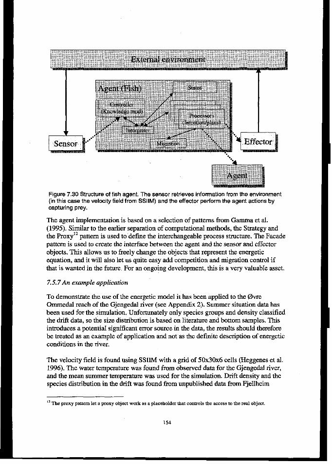
Figure 7.30 Structure of fish agent. The sensor retrieves information from the environment(in this case the velocity field from SSIIM) and the effeetor perform the agent actions bycapturing prey,

The agent implementation is based on a selection of patterns from Gamma et al.(1995). Similar to the earlier separation of computational methods, the Strategy andthe Proxy12 pattern is used to define the interchangeable process structure. The Facadepattern is used to create the interface between the agent and the sensor and effecterobjeets. This allows us to freely change the objects that represent the energeticequation, and it will also let us quite easy add competition and migration control ifthat is wanted in the future. For an ongoing development, this is a very valuable asset.

7.5.7 An example application

To demonstrate the use of the energetic model it has been applied to the OvreOmmedal reaeh of the Gjengedal river (see Appendix 2). Summer situation data hasbeen used for the simulation. Unfortunately only species groups and density classifiedthe drift data, so the size distribution is based on literature and bottom samples. Thisintroduces a potential significant error source in the data, the results should thereforebe treated as an example of application and not as the definite description of energeticconditions in the river.

The veloeity field is found using SWIM with a grid of 50x30x6 cells (Heggenes et al.1996). The water temperature was found from observed data for the Gjengedal river,and the mean summer temperature was used for the simulation. Drift density and thespecies distribution in the drift was found fkom unpublished data from Fjellheim

12Tbe proxy pattern let a proxy object work as a placehokler that contiols the access to the real object.

154

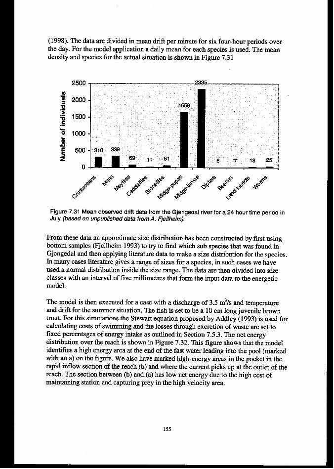
(1998). The data are divided in mean drift per minute for six four-hour periods overthe day. For the model application a daily mean for each species is used. The meandensity and species for the actual situation is shown in Figure 7.31

2500

0

9=

1658

310 339

6 7 18 25

Figure 7.31 Mean observed drift data from the Gjengedai river for a 24 hour time period inJuly (based on unpublished data from A. Fjellheim).

From these data an approximate size distribution has been constructed by first usingbottom samples (Fjellheim 1993) to try to find which sub species that was found inGjengedal and then applying literature data to make a size distribution for the species.In many cases literature gives a range of sizes for a species, in such cases we haveused a normal distribution inside the size range. The data are then divided into sizeclasses with an interval of five millimetres that form the input data to the energeticmodel.

The model is then executed for a case with a discharge of 3.5 m3/s and temperatureand drift for the summer situation. The fish is set to be a 10 cm long juvenile browntrout. For this simulations the Stewart equation proposed by Addley ( 1993) is used forcalculating costs of swimming and the losses through excretion of waste are set tofixed percentages of energy intake as outlined in Section 7.5.3. The net energydistribution over the reach is shown in Figure 7.32. This figure shows that the modelidentifies a high energy area at the end of the fast water leading into the pool (markedwith an a) on the figure. We also have marked high-energy areas in the pocket in therapid inflow section of the reach (b) and where the current picks up at the outlet of thereach. The section between (b) and (a) has low net energy due to the high cost ofmaintaining station and capturing prey in the high velocity area.

155

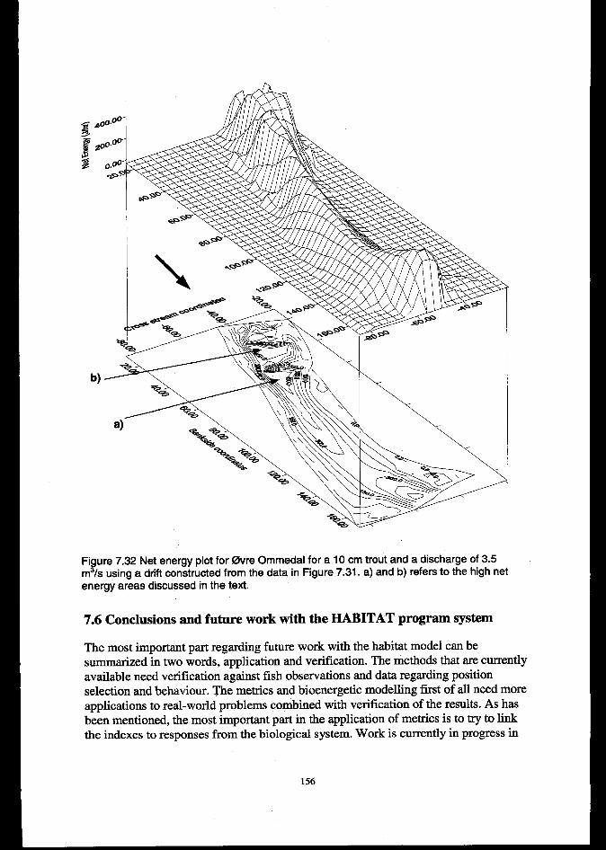
Fi ure 7.32 Net energy plot for Ovre Ommedal for a 10 cm trout and a discharge of 3.5?m /s using a drift constructed from the data in Figure 7.31. a) and b) refera to the high net

energy areas discussed in the text.

7.6 Conclusions and future work with the HABITAT program system

The most important part regarding future work with the habitat model can besummarized in two words, application and verification. The methods that are currentlyavailable need verification against fish observations and data regarding positionselection and behaviour. The metrics and bioenergetic modelling first of all need moreapplications to real-world problems combined with verification of the results. As hasbeen mentioned, the most important part in the application of metrics is to try to linkthe indexes to responses from the biological system. Work is currently in progress in

156

this field in several of the research organisations working with fish habitat assessmentso one may expect that results and recommendations will be available in the nearfuture. We can also see increasing interest in using bioenergetic models for driftfeeding river fish. Ney (1993) identifies several deficiencies in the current approach tobioenergetic modelling that need more work to improve the models for practicalapplications. His four categories are:

1. Unknown costs of activity.2. Extrapolation of allometric functions – covers problems with extending allometric

functions developed for one life stage to other life stages.3. Unjustified species borrowing – it is a common practize when data for the

modelled species is missing to use relations developed for other species.4. Inadequate estimation of external variables.

Since the publication of the paper of Ney, we have seen several articles addressingthese categories and one could expect that more will be published in the coming years.Still more research is needed to cover the interesting species and their life stages.Even if there are apparent weaknesses in the current bioenergetic models, thisapproach to modelling fish in rivers should be investigated further, since it is the onlymodelling approach that combines the effects of fish physiology with the impacts ofchanges in environmental conditions.

A complete set of input data is currently being collected for the Trekanten reach inNidelva, and the model presented in this chapter will be applied to these data in thenear iiture. Based on the results of this application the model will be furtherdeveloped and hopefidly weaknesses can be identified to provide input to furtherresearch in bioenergetic modelling. This data set will also allow us to finalize and testthe growth component of the model. For the first test of this diurnal and seasonal driftrates will be combined with hydraulic data. To avoid the problems of using acompletely dynamic hydraulic model, a range of hydraulic simulations will be used asinput. Using this the used daily discharge will be the simulated discharge closest to theactual discharge (e.g. if the discharge is 45 m3/s we will use the simulated data for 50m3/s and so on). This will give an indication of the complexity and problem areas ingrowth modelling.

The HABITAT modelling system currently is operated from control files similar tothe one used for the base fia.mework. A graphical user interface could improve thetool a great deal. Not so much in setting up the model and running the program whichis efficiently handled through the control files, but more as an interface to the methodsthemselves and as a tool for development of new methods. This will make it possiblefor researchers in biology and hydraulics to use the tool ckctly in prototyping andtesting of new biological models or the inclusion of new hydraulic data. Thusfacilitating the development and testing of new tools without involving computerprogrammers in early stages of the work. The interface to such a system will requireboth a traditional data setup procedure, code generation capabilities and automaticlinks to the underlying compilation and linking system. At the time of writing,

157

prototypes of code generation tools have been developed that create the skeletons ofnew methods with the necessary links to other framework classes. The availability ofsuch method “wizards” combined with the flexibility of an application frameworkprovides the user with a very powerful working environment for development,prototyping and testing of new models for habitat assessment.

8. FUTURE DEVELOPMENT POSSIBILITIES

8.1 Introduction

The purpose of this chapter is to outline two of the important new directions ininformation technology, and how these could be used to add functionality in ahydroinformatics system. At the moment of writing, the chapter cannot present anycomplete working applications, but it will rather present some examples of use basedon the software presented in the previous sections. This chapter will coverdevelopments in techniques for distributed computing and the use of object-orienteddatabases as storage systems in a hydroinformatics system that is built with an object-oriented strategy.

8.2 Object-oriented databases

8.2.1 Using databases in combination with simulation models.

Modem simulation systems in hydroinformatics both use and produce a vast amountof data during operation. In addition comes modem and sophisticated automatic datacollection systems that often retrieve sets of environmental measurements many timesa day. Such data collections are also a base for the growing interest in data miningtechniques applied to water-related problems. In all these applications it is necessaryboth to organize the data and to store them in an efficient way. For such applications adatabase system is often usefal because of the inherent data security (access and datasafety), query options and easy data sharing between applications. The possibilitiesare hierarchical systems, relational systems or object-oriented database systems. Thetwo latter will be discussed here.

Section 2.3.3 outlined the possibilities of using a combination of an object-orientedreal world model for the application and an entity-relation model for the associateddatabase. We have already mentioned the difficulties of representing large andunstructured data in a relational database without having to use the Binary LargeObjects (BLOBS) that some of the database management systems are equipped withtoday. This provides a problem in a hydroinfonnatics application since data like timeseries, terrain data and river cross section often are large and have a structure that donot fit into the relational concept. An alternative to the relational system that hasbecome more interesting in recent years is the object-oriented database managementsystems. Figure 8.1 outlines the differences between using a relational system and anobject-oriented system as data storage for an application developed using object-oriented techniques.

159

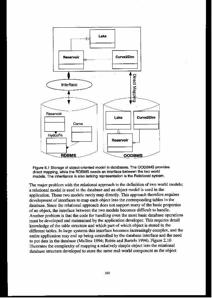
I

Reservoir Curve2Dimo

1 I I I

+

Interface

I

+>

I Reservoir

B Curve

HydcoFn

\D /

B .-..-,-”’....

RDBMS

Lx=Lake Curve2Dlm

F=lJI I

“---.JooDBM~

Fiaure 8.1 Storaae of obiect-oriented model in databases. The OODBMS providesdi~eet mapping, ~ile the RDBMS needs an interface between the two worldmodels. The inheritance is also lacking representation is the Relational system.

The major problem with the relational approach is the definition of two world models;a relational model is used in the database and an object model is used in theapplication. These two models rarely map directly. This approach therefore requiresdevelopment of interfaces to map each object into the corresponding tables in thedatabase. Since the relational approach does not support many of the basic propertiesof an object, the interface between the two models becomes difficult to handle.Another problem is that the code for handling even the most basic database operationsmust be developed and maintained by the application developer. This requires detailknowledge of the table structure and which part of which object is stored in thedifferent tables. In large systems this interface becomes increasingly complex, and theentire application may end up being controlled by the database interface and the needto put data in the database (Mullins 1994; Robie and Bartels 1994). Figure 2.10illustrates the complexity of mapping a relatively simple object into the relationaldatabase structure developed to store the same real-world component as the object

160

represents. A particular problem is that the tables in the relational database are two-dimensional while objects in most cases do not exhibit this two-dimensional style.

The problem with linkage of databases and object-oriented applications isacknowledged by many organizations, and research is going onto try to find bothmodelling methods and implementation tools to address the mapping between objectsand the relational table structure (Salo et al. 1998). Some work has also beenundertaken to build databases that combine object storage with relational approaches,

8.2.2 Principles of object-oriented databases

A possible solution is to use an object-oriented database system in combination withapplications based on object-oriented progr amming methods. Earlier these systemshad some difficulties regarding standardization on database schemas and querylanguages. A consortium from several of the large software companies, the ObjectDatabase Management Group (ODMG), then agreed on and created a standardisationdocument that defines the necessary components in an object-oriented databasesystem (Cattell 1993).

– An object model that defines how objects are to be treated inside the database.This included object referencing, object destruction, object updating and objectstorage.

– The ODL (Object Definition Language). This is a specification language that isused to define the interfaces of the object that should be stored in the database.Some database systems provide an automatic tool that generates the database fromthe class definitions used in the application program.

– The OQL (Object Query Language). This is somewhat similar to the SQLlanguage used in a relational database (using SELECT-FROM-WHERE typequeries). OQL lets the user query the objects in the database accessing bothmember variables and methods in the WHERE clauses.

– Language bindings to C++ and Smalltalk in the 1993 document. The POETdatabase also has a JAVA interface.

– The 1993 standard also compares the ODMG data model with the data modeldefined by OMG used in the CORBA distributed systems. The standard alsodescribes the integration between CORBA and 00DBMS systems.

When we design the classes for the application using the Unified Modelling Languagesupport for persistence is available. Classes that we intend to store in the database canbe marked as persistent already in the design phase. We can thereby integrate thedesign of the database components with the design of the application objects. Thiseliminates the need for separate real world models for application and database andsaves code, development time and project cost. This also greatly reduces maintenancesince there is less code to maintain and no need for manually keeping different modelsconsistent.

161

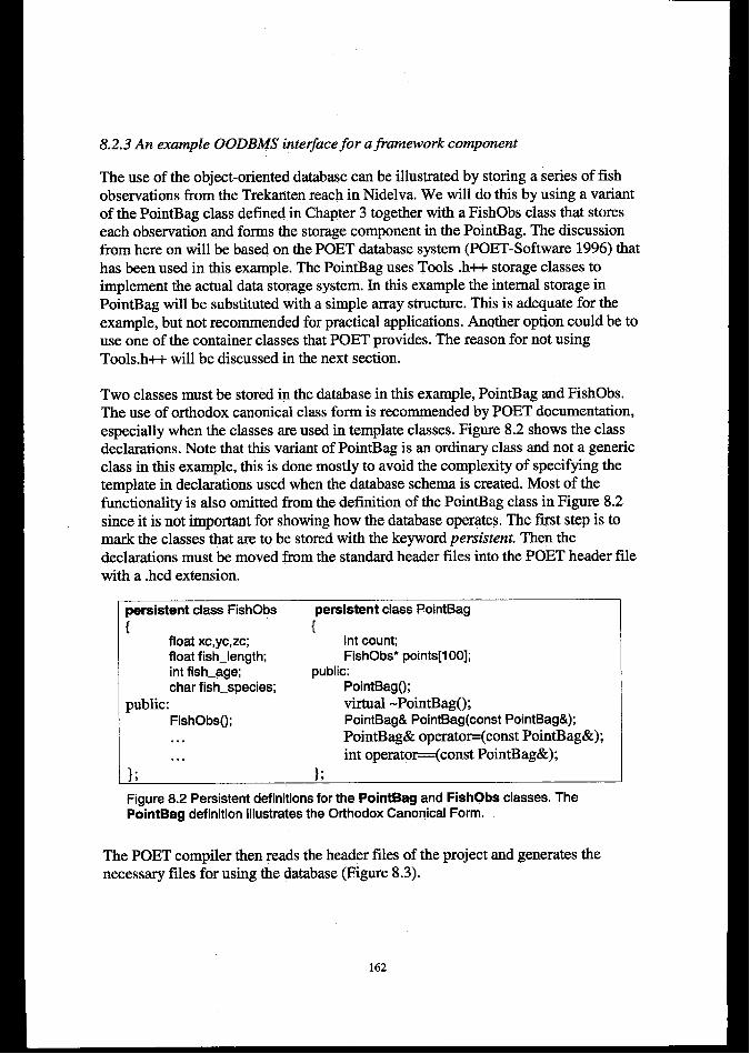
8.2.3 An exumple OODBMS interface for afiamework component

The use of the objeet-oriented database can be illustrated by storing a series of fishobservations from the Trekanten reach in Nidelva. We will do this by using a variantof the PointBag class defined in Chapter 3 together with a FishObs class that storeseach observation and forms the storage component in the PointBag. The discussionfrom here on will be based on the POET database system (POET-Software 1996) thathas been used in this example. The PointBag uses Tools h++ storage classes toimplement the actual data storage system. In this example the internal storage inPointBag will be substituted with a simple array structure. This is adequate for theexample, but not recommended for practical applications. Another option could be touse one of the container classes that POET provides. The reason for not usingTools.h++ will be discussed in the next section.

Two classes must be stored in the database in this example, PointBag and FishObs.The use of orthodox canonical class form is recommended by POET documentation,especially when the classes are used in template classes. Figure 8.2 shows the classdeclarations. Note that this variant of PointBag is an ordinary class and not a genericclass in this example, this is done mostly to avoid the complexity of specifying thetemplate in declarations used when the database schema is created. Most of thefimctionality is also omitted from the definition of the PointBag class in Figure 8.2since it is not important for showing how the database operates. The tirst step is tomark the classes that are to be stored with the keyword persistent. Then thedeclarations must be moved from the standard header files into the POET header filewith a .hcd extension.

persistent class FishObs persistent class PointBag

{ {float xc,yc,zc; int countfloat fish_length; FishObs* points[l 00];int fish_age; public:char fish_species; PointBago;

public: virtual -PointBago;FishObso; PointBag& PointBag(const PointBag&);

. . . PointBag& operator=(const PointBag&);int operator==(const PointBag&);

}; ““” };

Figure 8.2 Persistent definitions for the PointBag and FishObs classes. ThePointBag definition illustrates the Orthodox Canonical Form.

The POET compiler then reads the header tiles of the project and generates theneeessary files for using the database (Figure 8.3).

162

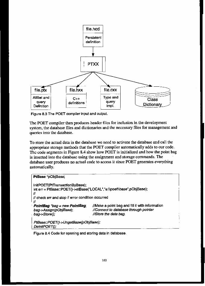
HPersistentdefinition

I i 1 I

& F

file.ptx file.hxx file.cxx

AllSet and c++ Type andClass

query definitions queryDefinition impl. <Dictionary >

Figure 8.3 The POET compiler input and output.

The POET compiler then produces header files for inclusion in the developmentsystem, the database files and dictionaries and the necessary files for management andqueries into the database.

To store the actual data in the database we need to activate the database and call theappropriate storage methods that the POET compiler automatically adds to our code.The code segments in Figure 8.4 show how POET is initialized and how the point bagis inserted into the database using the assignment and storage comman ds. The

database user produces no actual code to access it since POET generates everythingautomatically.

PtBase *pObjBase;

lnitPOET(PtTransaetionByBase);int err= PtB*e::POET()->etB*e( ''LOCAL'', ''e:\@oefi\base'', pObjBase);II

I// check err and stop if error condition occurredIIPointBag *bag= new PointBag //Make a point bag and fill it with informationbag->Assign(pObjBase); z7Conneet to database through pointerba&Storeo; /!Store the data bag.

PtBase::POET()-AJngetBase(pObjBase);DeinitPOET();

Figure 8.4 Code for opening and storing data in database.

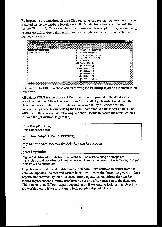
By inspecting the data through the POET tools, we can see that the PointBag objectsis stored inside the database together with the 5 fish observations we read into thesystem (figure 8.5). We can see from this figure that the complete array we are usingto store each fish observation is allocated in the database, which is an inefficientmethod of storage.

Figure 8.5 The POET database control showing the PointBag object as it is stored in thedatabase

All data in POET is stored in an AllSet. Each class imprinted in the database isassociated with an AllSet that controls and stores all objects instantiated from theclass. To retrieve data from the database we also employ functions that areautomatically added to our code by the POET compiler. We must first associate anAllSet with the class we are retrieving and then use this to access the actual objectsthrough the get method, (figure 8.6).

PointBag pPointBag;PointBagAllSet pbse~

err = pbset.Get(pPointBag, O, PtSTART);//

//Zfno error code occurred the PointBag can be accessed/’/’pbset.Unget(pb);

Figure 8.6 Retrieval of data from the database. The AllSet storing pointbags areinstantiated and the actual pointbag is restored from that. An example of retrieving multipleobjeets will be shown later.

Objects can be edited and updated in the database. If we retrieve an object from thedatabase, updates it values and write it back it will overwrite the existing version sinceobjects are identified by their instance. During operations on objects they can belocked to prevent concurrency problems by passing a lock message to the database.This can be set at different depths depending on if we want to lock just the object weare working on or if we also want to lock possible dependent objects.

164

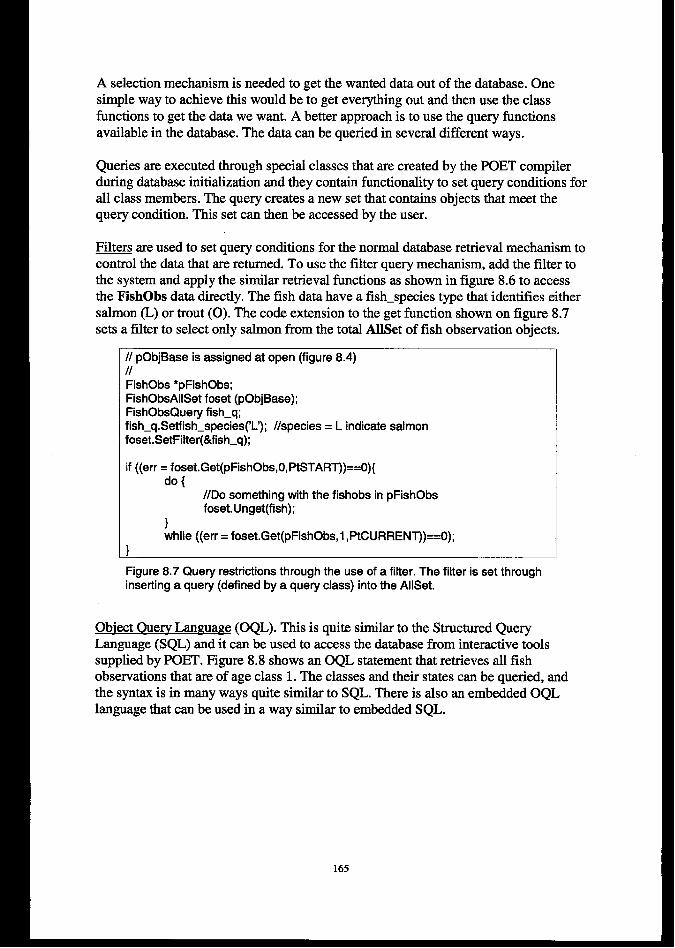
A selection mechanism is needed to get the wanted data out of the database. Onesimple way to achieve this would be to get everything out and then use the classfunctions to get the data we want. A better approach is to use the query fimctionsavailable in the database. The data can be queried in several different ways.

Queries are executed through special classes that are created by the POET compilerduring database initialization and they contain functionality to set query conditions forall class members. The query creates a new set that contains objects that meet thequery condition. This set can then be accessed by the user.

Filters are used to set query conditions for the normal database retrieval mechanism tocontrol the data that are returned. To use the filter query mechanism, add the filter tothe system and apply the similar retrieval functions as shown in figure 8.6 to accessthe FishObs data directly. The fish data have a fish_species type that identifies eithersalmon (L) or trout (0). The code extension to the get function shown on figure 8.7sets a filter to select only salmon from the total AllSet of fish observation objects.

// pObjBase is assigned at open (figure 8.4)IIFishObs *pFishObs;FishObsAllSet foset (pObjBase);FishObsQuety fish_q;fish_q.Setfish_species(’L’); //species = L indicate salmonfoset.SetFilter(&fish_q);

if ((err= foset.Get(pFishObs, O,PtSTART))==O){do{

//Do something with the fishobs in pFishObsfoset.Unget(fish);

}while ((err = foset.Get(pFishObs,l ,PtCURRENT))==O);

}

Figure 8.7 Query restrictions through the use of a filter. The filter is set throughinserting a query (defined by a query class) into the AllSet.

Obiect Ouem Lanwa~e (OQL). This is quite similar to the Structured QueryLanguage (SQL) and it can be used to access the database from interactive toolssupplied by POET. Figure 8.8 shows an OQL statement that retrieves all fishobservations that are of age class 1. The classes and their states can be queried, andthe syntax is in many ways quite similar to SQL. There is also an embedded OQLlanguage that can be used in a way similar to embedded SQL.

165

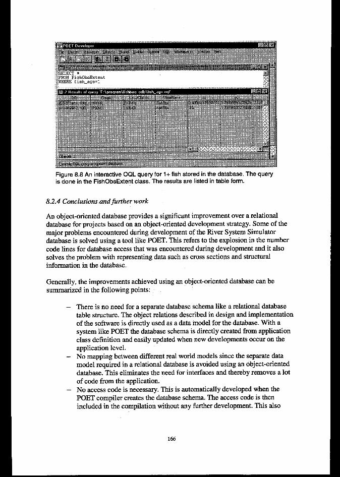
Figure 8.8 An interactive OQL query for 1+ fish stored in the database. The queryis~one in the FishObsExtent class.-The results are listed in table form.

8.2.4 Conclusions and~rther work

An object-oriented database provides a significant improvement over a relationaldatabase for projects based on an object-oriented development strategy. Some of themajor problems encountered during development of the River System Simulatordatabase is solved using a tool like POET. This refers to the explosion in the numbercode lines for database access that was encountered during development and it alsosolves the problem with representing data such as cross sections and structuralinformation in the database.

Generally, the improvements achieved using an object-oriented database can besummarized in the following points:

—

—

—

There is no need for a separate database schema like a relational databasetable structure. The object relations described in design and implementationof the software is directly used as a data model for the database. With asystem like POET the database schema is directly created from applicationclass definition and easily updated when new developments occur on theapplication level.No mapping between different real world models since the separate datamodel required in a relational database is avoided using an object-orienteddatabase. This eliminates the need for interfaces and thereby removes a lotof code from the application.No access code is necessary. This is automatically developed when thePOET compiler creates the database schema. The access code is thenincluded in the compilation without any further development. This also

166

reduces the amount of application code and thereby the cost of maintainingthe system.

– It helps in the separation between database access code and applicationcode that reduces coupling between modules.

One traditional negative side with the object databases has been the lack ofstandardization and the lack of commercially available software. With the advent ofthe standard in 1993 and the growing number of applications built on the standard thisis changing and we already have several standardized systems available.

Another drawback is the lack of a broadly used interface like SQL that makes itpossible to integrate databases into spreadsheets and word processors. This isparticularly important on the Microsoft operating system platforms where suchintegration possibilities are commonly used. To solve this, at least POET supplies anODBC (Open Database Connectivity) driver to allow integration of the POETdatabase into applications supporting ODBC. This solves the mapping from an object-oriented data model into the relational based ODBC. Another option on a Microsoftplatform would be to develop an ActiveX database interface that can be used in manydifferent applications and interfaced to several languages.

One of the design requirements for the framework was to properly describe the real-world river system through classes. This makes it relatively easy to build a databasemodel of the system based on the framework components, which is an indication thatthe requirement is fulfilled. This also illustrates the usability of the design aside frombuilding a simulation system, and it shows the flexibility in having a design based ona real world object model over a more simulation only oriented system.

To employ POET as storage system for the framework components would with fewexceptions be straightforward. The classes that need persistent storage must be markedpersistent and stored in the database, this includes handling of template classes usedfor data storage. The only real hurdle is handling the classes based on the Tools.h++library. The simplest would be to substitute the Tools.h++ classes with the collectionssupplied with POET. Another option that will be available is to use STL collectionclasses since POET will support these in the near future. A third option is to use theTools.h++ headers to create persistent storage for the tools classes that needs to bepersistent. The second option might be the best solution since we then will be usingstandardized tools for all storage.

8.3 Distributed object-oriented technologies

8.3.1 Distribution in hydroinfomatics

In research on information technology the development of distributed13 solutions isvery important and one of the major research areas today. This may also provide oneof the major advancements in the development and application of hydroinformaticssystems in the future. The Engine 2000 projeet, in which distribution of processes anddata seem to play an important role, has already been mentioned in Section 2,4.6. Anexample of using Internet (WWW) based distribution is given in Velickov et al.(1998).

We thus have the opportunity to distribute applications and data on different serversaround the globe. Instead of getting the tools installed locally they can be accessed atspecialized servers. In the same way data can be retrieved from (and provided to forthat matter) distributed objects. If we look at the applied hydroinformatics system,there are many possible uses of distributed techniques.

— The perhaps most imminent is an automatic data collection feature wheresimulation systems can be setup to retrieve the necessary data from sources insidethe organization that collects and maintains the data. An example is the HYDRAsystem presented in Chapter 6, which today relies on manual data retrieval fromseveral sources. This could be a two-way operation in the way that the core systemalso sent results back to interested organizations or make them available onnetworked sites such as the World Wide Web.

— A similar use is the distributed access to data sources utilized in data mining andautomatic data extraction services. This is a use that is quite common in manyother areas. Another related area is the development of search agents that are usedto retrieve data from remote data sources. These agents do often have fimctionalityto automatically adapt to user needs, an example is world wide web seareh robots.

— The natural communication in an object-oriented system is through passingmessages and objeets. Larsen and Gavranovich (1996) outlined a distributedsystem based on portable knowledge encapsulators (PI@, portable entities thatcontains both data and the methods to operate on the data. This would require aapplication framework used by all organization that develop PKE to ensureinteroperability between the components. In many ways this would be astandardization of portable hydroinformatics components.

— Building fkrther on the idea presented by Larsen and Gavranovich one couldimagine a distributed toolbox where the user prepares his system as an objector acollection of objects and ship this to a computational engine somewhere in thenetwork. The computational engine would know how to interact with the objects

13Distribution in this context refers to the distribution of computational tools and data sources on different

machines connected through a network. It has neither a relation to distributed modelling (modelling with a

spatial distribution of parameters) nor does it refer to the distribution of a single computational intense prccess

on multiple processors.

168

and how to simulate the system they represent. After simulation, the updatedobjects are returned to the user. This would eliminate the need for distributingsoftware to many organizations and it will allow smaller users without the need orthe funds to have expensive software permanently available to buy into adistributed solution. The distributed system would always be updated and this alsoreduces the need for handling and distributing different software versions. Thedistributed processing tools are often referred to as software agents, meaning aself-contained piece of software that communicates with other agents through astandardized interface.

– With the distribution of software follows the need for supplying manuals anddocumentation for the operation of the software and on the theory behind theprocess models simulated. Maintaining, printing and distributing documentation isoften an expensive and time-consuming process. The advent of the world-wide-web and the hypertext language provides the possibility to maintain only one copyof the manuals and make this available to the users through a standard webbrowser (Bakken et al. (1998)). This solution provides the same functionality as atraditional help system. As described in (lhkken et al. 1998) the use of WorldWide Web lends itself very well for user interaction, such as discussion groups,mailing lists or dynamic frequently asked question lists. Similarly it is an ideal toolfor distribution of software updates and new modules that can be added to theusers software systems.

8.3.2 Object orientation in dism”bution: CORBA and COM/ActiveX

Two major technologies exist for building distributed object-oriented systems, theObject Management Group (OMG) CORBA (Common Object Request BrokerArchitecture) and the Microsoft Distributed Component Object Model (DCOM). Inaddition new systems based on world wide web (WWW) technologies are alsoemerging, like techniques based on the JAVA progr arnming language, Microsoft’sActiveX component based technology and also CGI-based methods.

The OMG CORBA architecture contains four main elements (figure 8.9):

– The Object Request Broker (ORB). This is the object bus that transfers objectsbetween the distributed users. The ORB provides transparent message passingbetween objects over the network or locally. The requests are independent ofprogr amming language and object location. Objects act as clients or serversdepending on the circumstances, there is no fixed clientiserwer structure.

– The CORBA services, a system level framework that provides low level serviceslike concurrency, security, timing and Naming services.

– CORBA facilities define a high level frameworks that are used directly byapplication objects, and they provide services like help, user interaction, objectlinking and compound documents.

– Application objects are developed for a specific program and they will use theother CORBA facilities to build a distributed system. The interface to distributed

169

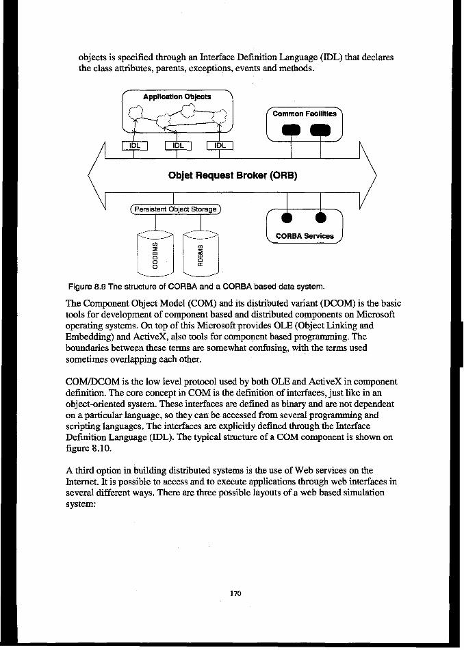
objects is specified through an Interface Definition Language (IDL) that declaresthe class attributes, parents, exceptions, events and methods.

( ApplicationObjeets ~

\1 I m

/ I 1 \

( Objet Request 13roker (ORB))

Persistent Object Storage

[ CORBA services J

Figure 8.9 The structure of CORBA and a CORBA based data system.

The Component Object Model (COM) and its distributed variant (DCOM) is the basictools for development of component based and distributed components on Microsoftoperating systems. On top of this Microsoft provides OLE (Object Linking andEmbedding) and ActiveX, also tools for component based progr amrning. Theboundaries between these terms are somewhat confusing, with the terms usedsometimes overlapping each other.

COM/DCOM is the low level protocol used by both OLE and ActiveX in componentdefinition. The core concept in COM is the definition of interfaces, just like in anobject-oriented system. These interfaces are defined as binary and are not dependenton a particular language, so they can be accessed from several programmingg andscripting languages. The interfaces are explicitly defined through the InterfaceDefinition Language (IDL). The typical structure of a COM component is shown onfigure 8.10.

A third option in building distributed systems is the use of Web services on theInternet. It is possible to access and to execute applications through web interfaces inseveral different ways. There are three possible layouts of a web based simulationsystem:

170

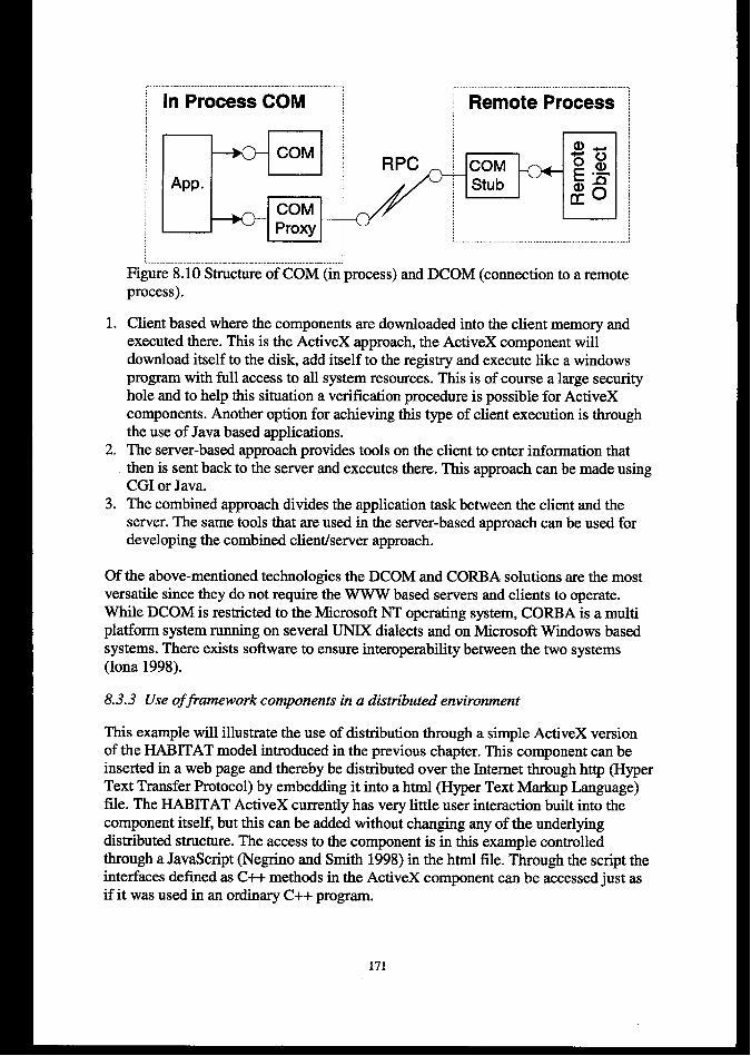
1.

2.

3.

‘ In Process COM

I.,

Remote Process

... ..... .. ..... ........... .. . .. ... ..... .. ..

...................................................................Figure 8.10 Structure of COM (in process) and DCOM (connection to a remoteprocess).

Client based where the components are downloaded into the client memory andexecuted there. This is the ActiveX approach, the ActiveX component willdownload itself to the disk add itself to the registry and execute like a windowsprogram with full access to all system resources. This is of course a large securityhole and to help this situation a verification procedure is possible for ActiveXcomponents. Another option for achieving this type of client execution is throughthe use of Java based applications.The server-based approach provides tools on the client to enter information thatthen is sent back to the server and executes there. This approach can be made usingCGI or Java.The combined approach divides the application task between the client and theserver. The sam: ~ools that are used ~ “tie server-based approach can be used fordeveloping the combined client/server approach.

Of the above-mentioned technologies the DCOM and COR.BA solutions are the mostversatile since they do not require the WWW based servers and clients to operate.While DCOM is restricted to the Microsoft NT operating system, CORBA is a multiplatform system running on several UNIX dialects and on Microsoft Windows basedsystems. There exists software to ensure interoperability between the twos ystems(Ions 1998).

8.3.3 Use offramework components in a disti”buted environment

This example will illustrate the use of distribution through a simple ActiveX versionof the HABITAT model introduced in the previous chapter. This component can beinserted in a web page and thereby be distributed over the Internet through http (HyperText Transfer Protocol) by embedding it into a htrnl (Hyper Text Markup Language)file. The HABITAT ActiveX currently has very little user interaction built into thecomponent itself, but this can be added without changing any of the underlyingdistributed structure. The access to the component is in this example controlledthrough a JavaScript (Negrino and Smith 1998) in the htn-d file. Through the script theinterfaces defined as C++ methods in the ActiveX component can be accessed just asif it was used in an ordinary C++ program.

The proper definition of ActiveX is difficult to find in the literature, the termsActiveX, OLE and COM are often used interchangeably about the same componentsin different papers or books. The ActiveX control is the name Microsoft now uses forwhat was earlier known as a VBX control or OLE control, the name change camewhen the control got defined Internet behaviour. For a fiuther discussion on thehistory of the COM/OLE/ActiveX system see (Platt 1998) or Chappel (1996).

The ActiveX control is an in-process COM server that exposes a set of methods,events and properties to the user. It must at least expose the IUnknown interfacesimilar to other COM-based components. In addition it must implement factories,registration and a series of other COM features depending on how it is intended tooperate. Like other COM components the interfaces are defined through the IDL(Interface Definition Language). COM has a binary interface standard that makes thecomponents readable by many applications and languages that support COM-basedcomponents.

Developing the ActiveX control is easiest using the control wizard included in theMicrosoft Developer Studio. This sets up all underlying COM details and creates thecode for registration and activation code, thereby shielding the developer from havingto access the low level detai114and supports reuse since much of the code is identicalfrom one component to another. The wizard creates a complete component ready foruse. The developer’s task is to add the properties, events and methods that are neededfor the component to operate as wanted.—

—

—

The properties can be set as through property pages that are available for the usersthat works with the component. Typical property pages include e.g. initial values,colours or fonts. Property pages are made for the situations were the component isused as apart in a software development. They are only accessible from thecomponent insertion tools found in a software development environment likeDevelopers Studio.Events that need special attention can be defined and event handlers added. Thedefined event handlers can be accessed and implemented by the user of thecomponent. These are also available from html code, see the example later in thissection.The methods control the operation of the component. They are added to theinterface defined, and users of the component can use these to access componentdata or to trigger operations inside the component.

The Habitat ActiveX component (OnLineHab is the name used in the remainder ofthis section) has no property pages since it is not yet intended as a component insoftware development. The OnLineHab defines an event handler for the double clickevent that is used to access the component data. The component define four methodsin its interface:

14T& is a great asset to the developer, Platt(1998) states that “the in-place activation code alone makes strong

men weep”. This is all now hidden imide the framework classes.

172

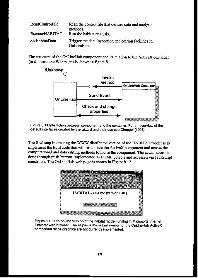
ReadControlFile Read the control file that defines data and analysismethods.

ExecuteHABITAT Run the habitat analysis.

SetHabitatData Trigger the data inspection and editing facilities inOnLineHab.

The structure of the OnLineHab component and its relation to the ActiveX container(in this case the Web page) is shown in figure 8.11.

lUnknownn

Invoke

Send EventOnLineHab >

Check and change

properties

Figure 8.11 Interaction between component and the container. For an overview of thedefault interfaces created by the wizard and their use seeChappel(1998),

The final step in creating the WWW distributed version of the HABITAT model is toimplement the html code that will instantiate the ActiveX component and access thecomputational and data editing methods found in the component. The actual access isdone through push buttons implemented as HTML objects and accessed via JavaScriptconstructs. The OnLineHab web page is shown in Figure 8.12.

Iw

HABITAT - OnLine (version 0.01) %~j;zI0

Figure 8.12 The on-line version of the habitat model running in Microsoft InternetExplorer web browser. The ellipse is the actual symbol for the OnLineHab ActiveXcomponent since graphics are not currently implemented.

173

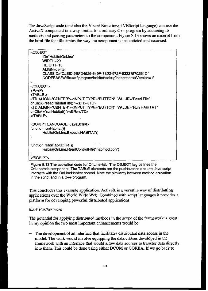
The JavaScript code (and also the Visual Basic based VBScript language) can use theActiveX component in a way similar to a ordinary C++ program by accessing itsmethods and passing parameters to the component. Figure 8.13 shows an excerpt fromthe html file that illustrates the way the component is instantiated and accessed.

<OBJECTlD=’’HabitatOnLine”WIDTH=20HEIGHT=IOALIGN=centerCLASSID=’’CLSID:9BFD4926-849F-I 1D2-972F-932315702B1 D“CODEBASE=''file://e:@ rogram\habitat\debug\habiWt.ocx#Version=l “

>c/OBJECT><P><P><TABLE >cTD ALIGN= ’’CENTER’’> <INPUT TYPE= ’’BUTTON” VALUE= ’’Read File”onClick=’’readHabitatFileo’’><BR>TD>D>cTD ALIGN.’’CENTEFV>< INPUT TYPE.’’BUTTON” VALUE= ’’Run HABITAT”onClick=’’runHabitato’’><BRdTD>D>c/TABLE>

<SCRIPT LANGUAGE.JavaScripbfunction runHabitato{

HabitatOnLine.ExecuteHABITAT()

}

function readHabitatFileo{HabitatOnLine.ReadControlFile(’’habmod.con”)

}cfSCRIPT>

Figure 8,13 The activation code for OnLineHab. The OBJECT tag defines theOnLlneHab component. The TABLE elements are the pushbuttons and the Java scriptinteracts with the OnLineHabitat control. Note the similarity between method activationin the script and in a C++ program.

This concludes this example application. ActiveX is a versatile way of distributing.-applications over the World Wide Web. Combined with script languages it provid-es aplatform for developing powerful distributed applications.

8,3.4 Further work

The potential for applying distributed methods in the scope of the framework is great.In my opinion the two most important enhancements would be:

– The development of an interface that facilitates distributed data access in themodel. The work would involve equipping the data classes developed in thefhrneworlc with an interface that would allow data sources to transfer data directlyinto them. This could be done using either DCOM or CORBA. If we go back to

Figure 6.3, the arrows that show the data transfer from external data sources wouldbe substituted by a direct link developed using one of the distribution protocols.

– A further development of the distributed interface following the path outlined inthe previous section. This would involve extending the ActiveX component withmore interaction and presentation facilities. Another option would be to developthe actual interface using JAVA and have only the computational part in theActiveX component. This approach would build fiuther on the approach used inthe example above. Compared to a pure ActiveX solution, this would conservespace and thereby download time. This could then be integrated with theinteractive help and documentation pages presented by Bakken et al. (1998) toprovide a complete WWW based habitat simulation system.

Work with Portable Knowledge Encapsulators (Larsen and Gavranovich 1996) andcompletely distributed systems seems to be further ahead since a common frameworkor at least a common interface must be agreed upon by the parties that work togetheron this development if the application potential is to be fully exploited. On Microsoft-based platforms the use of DCOM and COM will automatically become an integralpart of any hydroinformatics system since these are an important part in mostapplication development libraries provided with the system.

175

9 CONCLUSIONS AND FURTHER WORK

9.1 Development and application of the framework

The objective of this study was to develop an object-oriented framework fordevelopment and integration of programs in a variety of hydroinformaticsapplications. The development of the framework itself is outlined, and twoapplications are shown. The applications use the framework on different levels. InChapter 6 the components are used directly in the HYDRA flood modelling system,and in Chapter 7 the framework is used as a foundation for the development of thehabitat modelling framework (HMF). The HMF is later used in the development of theHABITAT program system. As has been reported, the testing has been done by theauthor and through three masters-level theses works covering both the HYDRA andthe HABITAT modelling systems.

To conclude on the development of the framework the six requirements specified inSection 1.4 can be compared with the developed software.

The model of the real world system can be built by selecting components from theHydcomp hierarchy as has been shown in Chapter 6 and in Montecchio (1998).The linkage and data transport between components is controlled by separateobjects and can be changed entirely outside the component itself. Data in differentforms ranging from single values to objects can be added to the structuralcomponents without changing the component.

Process models are specified in a separate hierarchy and linked at runtime, asshown in Chapters 6 and 7.

User interaction is separated from the framework components and processes. Theuser has one interaction point to the system, the simulation controller. This hasbeen configured both to interact with the console and file-based systems andthrough simple graphical-based user interfaces. As has been shown in Chapter 8,the controller can also operate with a web interface.

Coupling is at a minimum. Experience with the framework itself and with usingsome of the components in separate development projects show that the requiredlevel of reusability is met.

The system can be quite easily be updated with new modules through derivingthem from the inheritance hierarchies for components and processes or bydeveloping them following the guidelines given in Chapter 5 for data classes.

The link to external programs has been tested both for the HYDRA modellingsystem and for the HABITAT program.

9.2 The Object-Oriented Experience

Object oriented analysis and design methods have been used throughout this project,for the system identification (analysis phase), for the software design phase and for the

176

implementation. Object oriented methods give a large degree of flexibility in thestructuring of the software system and specially during restructuring and extensions toexisting software. The maintainability and extendibility of the software systemspresented in Chapters 6 and 7 are greatly enhanced through the object-orientedstructure of the programs. The price to pay to achieve this is the need to adhere to thedesign strategy even in cases where the usual solution would be a quick “hack” to thecode itself. This would necessarily lead to a required update to the “formal” designdocuments for all changes to the code, a process that is quite different the oneemployed in earlier projects. The importance of this is amplified in projects involvinga development team, since any violation of the strict analysis – design –implementation procedure may lead to incompatibility between the design and theimplementation making it (nearly) impossible for the project team to work on acommon code base. In my experience this shift of problem solving method is themajor threshold in the object-oriented learning curve, understanding the language andimplementation details provided few problems.

From this work three areas stand out as the major benefits of using the object-orientedmethodology

The development led to smaller self-contained components (classes) that could bebuilt and tested in a small environment. This reduces the coupling between thecomponents and it makes error correction simpler. This feature also reduces thenumber of errors in the complete code since each component is clearly set out andeasy to understand. Each class and its responsibility and collaboration is alsodocumented though the analysis and design phase, providing increased understandingof the functionality and operation of that particular class.

The development was centred on creating components that could be reused indifferent development projects. Classes from the framework have been used both indevelopment in the scope of the framework and some of the classes have also beenused in other projects. Experience with reuse is very good, the main attraction isreduced development time and less errors.

The last point is the much simplified maintenance and increased possibility ofextensions that are built into the software through the framework design. This was oneof the major reasons for the redesign of the HABITAT program systems, andexperiences with the new version of HAEITAT is so far very promising.

Together these three points sum up the major feature of this worlq a collection ofsmall, error free and reusable components that together can be used to build a varietyof software systems. Utilizing the easy extendable design new developments can beadded when needed. This is also a starting point for the development of componentware that seems to be the way software development is heading at the moment.

177

9.3 Further work

Chapter 8 outlined the developments that could extend the framework with state of theart information tools to provide the user with distribution possibilities and high qualitystorage facilities. The possibilities in distributed access to data and simulation toolsshould be investigated further. In addition, there are smaller changes that should beaddressed to enhance both the framework itself and the environment it operates in.

The weak point with the existing configuration is the flexibility in the input-outputsystem. At the moment this duplicates some code for each new class added, and thisshould be changed in the future.

A graphical user interface should also be included to provide more flexibility to thesystem. The interface should operate on two levels. The first level lets the user buildthe system model and add data through an interactive editor. The second and mostimportant level of the interface will be an interactive system builder with wizards toadd new processes, new components and new data objects. The wizards will ensurethat all connections are set up and that the new classes follow the requirements set bythe system. This interface will need to access the compiler to build the software.

178

REFERENCES

Abbott, M., V. Babovic, L. K. Amidsen, J. Baretta and J. D@ge (1994). Modellingecosystems with intelligent agents. In Verwey, A, Minns A.W., Babovic, V.,Maksimovic, C. (eds), Hydroinfonrzatics 94. A.A: Balkema, pp. 179-186.

Abbott, M. B. (1979). Computational hydraulics: elements of the theory officesuq6aceflows, Pittman.

Abbott, M. B. (1991). Hydroinformatics. Information technology and the aquaticenvironment. Avebu~ Technical.

Abbott, M. B. (1993). “The Electronic Encapsulation of Knowledge in Hydraulics,Hydrology and Water Resources.” Advances in Water Resources 16:21-39.

Abbott, M. B. (1997). Engine 2000: Researches Into the Next Generation ofComputational Hydraulic Modelling. In Wang, S.S.Y and Carstens, T. (eds),Environmental and Coastal Hydraulics: Protecting the Aquatic Habitat, Volume 2.The 27th Congress of L4HR: Water for a Changing Global Community, ASCEPublications, pp. 859-864.

Abbott, M. B. and A. Jonoski (1998). Promoting collaborative decision-makingthrough electronic networking. Hydroinforrnatics 98, Copenhagen, Denmark. pp.91 1-917. A.A.Balkema.

Addley, R. C. (1993). A Mechanistic Approach to Modeling Habitat Needs of Drift-Feeding Salmonids. Masters Thesis. Civil and Environmental Engineering. Logan,Utha State University: 141.

Alfredsen, K, A. Harby, T. H. Bakken and W. Marchand (1997). Application andcomparison of computer models for quantifying impacts of river regulations on fishhabitat. In Broth, E., Lysne, D.K., Flatab@, N., Helland-Hansen, E. (eds), Hydropower97, A.A.Balkema, pp. 3-9.

Arge, E., A. M. Bruaset and H. P. Langtangen (1997). Object-Oriented Numerics.Numerical Methods and Software Tools in Industrial Mathematics. M. DaMen and A.Tveito, pp 7-27. Birkhauser.

Arnekleiv, J. V. and A. Harby (1994). Biotope Improvement Analysis in the RiverDal% with the River System Simulator. Proceedingsfiom 1st InternationalSymposium on Habitat Hydraulics. Trondheirn SINTEF-NHL, pp. 513-529.

Babovic, V. (1996). Emergence, Evolution, Intelligence; Hydroinfonnatics. A.A.Balkema.

179

Babovic, V. (1998a). Data Mining. Class notes from tutorial at Hydroinformatics98.Copenhagen, Denmark.

Babovic, V. (1998b). A data mining approach to time series modelling andforecasting. In Babovic, V. and Larsen, L.C. (eds), Hydroinformatics 98, A.A.Balkema, pp. 847-857.

Bachman, R. (1984). “Foraging Behaviour of Free Ranging Wild and Hatchery BrownTrout in a Stream.” Transactions of the American Fisheries Society 113(1): 1-32.

Bakken, T. H., K. Alfredsen and W. Marchand (1998). Interactive training anddocumentation of habitat modelling using the Iiternet. In Babovic, V. and Larsen,L.C. (eds), Hydroinformatics 98, A.A.Balkema, pp. 919-926.

Blaskova, S. C.Stalnaker. O. Novicky (Editors) (1997). Hydroecological modelling -method, practice and legislation. Praha, Czech republic, T.G.Masaryk Water ResearchInstitute.

Barton, J. J. and L. R. Nackman (1994). Scientific and Engineering C++, AddisonWesley.

Bartsch, N., C. P. Gubala and T. B. Hardy (1996). Determining Habitat Criteria for theEndangered Fountain Darter Through Aquatic Mapping and Hydrologic Modelling. InM.Leclerc, Y.Cote, S.Valentin, H.Capra, Y.Boudreault.(eds), EcoHydraulics 2000(vol B), Quebec City: INRS-Eau pp. 251-262.

Beck, K. and W. Cunningham (1989). “A Laboratory for Teaching Object-OrientedThinking.” SIGPLANZVotices 24(10).

Bente, S. (1994). HydroNet: Ein objekt-orientiertes Softwarekonzept fiirhydrologische Simulationssysteme. Department of Hydraulic and EnvironmentalEngineering, Norwegian Institute of Technology.

Berre, A. J. (1996). Lecture notes in object-oriented development. Department ofComputer and Information Science, Norwegian University of Science andTechnology.

Beven, K (1985). Distributed Modelling. H-@rolo~ical Forecasting. M. G. Andersonand T. P. Burt, John Wiley 405-435.

Bird, D. J. (1996). Problems with the use of IFIM for salmonids and guidelines forfuture UK studies. In M.Leclerc, Y.Cote, S.Valentin, H.Capra, Y.Boudreault. (eds),EcoHydraulics 2000, Quebec City INRS-Eau, pp. 408-418.

Booth, G. (1994). “Designing an Application Framework.” Dr.Dobbs .lournai 19(2):24-30.

180

Booth, G. (1996). Object Oriented Anulysis and Design with Applications,Benjamin/Cummings publishing Company.

Boudreau, P., G. Bourgeois, M. Leclerc, A. Boudreault and L. Belzile (1996). Two-dimensional habitat model validation based on spatial fish distribution: Application tojuvenile Atlantic Salmon of Moisie river (Quebec, Canada). In M.Leelerc, Y.Cote,S.Valentin, H.Capra, Y.Boudreault. (eds), EcoHydrauJics 2000 (vol B), Quebec City~S-Eau, pp. 365-380.

Bovee, K. (1986). Development and evaluation of habitat suitability criteria for use inthe Instream Flow Incremental Methodology. Fort Collins, Colorado, US Fish andWildlife Service.

Bovee, K. (1996). Perspectives on Two-Dimensional River Habitat Models: thePHABSIM Experience. In M.Leclerc, Y.Cote, S.Valentin, H.Capra, Y.Boudreault.(eds), EcoHydrazdics 2000 (vol B), Quebec City: INRS-Eau, pp. 149-162.

Bovee, K. D. (1982). A guide to stream habitat analysis using the instream flowincremental methodology. Fort Collins, Colorado, National Biological Service.

Bowen, Z., M. C. Freeman and D. L. Watson (1998). Zndex oflliotic ZrztegrityAppliedto a Flow-regulated River. Annual Conference Southeast Association Fish andWildlife Agencies. @tp://www.mesc.nbs.gov/pubs/online/ifim-chron/ind_biotic_integ.htrnl)

Braaten, P. J., P. D. Dey and T. C. Annear (1997). “Development and Evaluation ofBioenergetic-Based Habitat Suitability Criteria for Trout.” ReguZuted Rivers 13:345-356.

Breck, J. E. (1993). “Foraging Theory and Piscivorous Fish: Are Forage Fish Just BigZooplankton.” Transactions of the American Fisheries Society 122:902-911.

Bnttain, J. E. and T. J. Eikeland (1988). “Invertebrate Drift - A review.”Hydrobiologia 166:77-93.

Campos, A. M. C. and D. R. C. Hill (1997). Web-based simulation of agentbehaviors. http://www.isima. ft/scs/wbms/d4/Websim.html#Behaviour.

Capra, H., P. Breil and Y. Souchon (1995). “A new tool to interpret magnitude andduration of fish habitat variations.” Regulated Rivers: Research and Management 10:281-289.

Carlson, C., T. Jelassi and P. Walden (1998). Intelligent Systems and Active DSS. InDolk, D. (cd), V014 Modeling Technologies and Intelligent Systems Track. 31”

Hawaii International Conference on System Sciences. IEEE Computer Society, pp. 4-8.

Cattell, R. G. G., Ed. (1993).The Object Database Standard: ODMG-93. MorganKaufman, San Mateo California.

Charley, W., A. Pabst and J. Peters (1995), “The Hydrologic Modeling System (HEC-HMS): Design and development issues.” Journal of Computing in Civil Engineering:131-138.

Chen, H. (1996). Object Watershed Link Simulation (OWLS). PhD thesis. OregonState University. U.S.A.

Chow, V. T., D. R. Maidment and L. W. Mays (1988). Applied Hydrology, McGraw-Hill.

Chung, H. M., P. Gray and M. Mannino (1998). introduction to Data Mining andKnowledge Discove~. In. E1-Rewini, H. (cd), V017: Software Technology Track. 3 ls’Hawaii International Conference on System Science. IEEE Computer Society, pp.244-247.

Clarke, R. (1991). Water: The International Crisis. London, Earthscan Publications.

Coplien, J. O. (1992). Advanced C+ + programming styles and idioms, AddisonWesley.

Coplien, J. O. and D. C, Schmidt, Eds. (1995). Pattern Languages of ProgramDesign, Addison Wesley.

Cunge, J. A., F. Holly and A. Verwey (1980). Practical Aspects of ComputationalRiver Hydraulics, Pittman.

DHI (1998a). MIKE - Zero- the common platform for all DHI software.http://www.dhi.dkfso ftware/mikezerohnikezero.htm.

DHI (1998b). MIKEl 10verview. http://www.dhi.dkhnikel Mndex.htrn.

DHI (1998c). MIKE SHE Overview.http://www.dhi.dk/software/mikeshe/mikeshe.htm

DISGIS (1998). DISGIS Project Summary (www.statkart.no/disgis/summary.html).

Douglas, B. P. (1998). Real-time UML: developing eflcient objects for embeddedsystems, Addison Wesley.

182

Dunbrac~ R. L. and L. M. Dill (1984). “Three-Dimensional Prey Reaction Field ofthe Juvenile Coho Salmon (Oncorhynchus kisutch).” Canadian Journal of Fisheriesand Aquatic Sciences 41:1176-1182.

Dunbrack, R. L. and L. A. Giguere (1987). “Adaptive Responses to AcceleratingCosts of Movement: A bioenergetic basis for the type-J.11functional response.” TheAmerican Naturalist 130(1): 147-160.

Elliott, J. M. (1972). “Rates of gastric evacuation in brown trout sahno trutta.”Freshwater Biology 2:1-18.

Elliott, J. M. (1975). “Weight of food and time required to satiate brown trout salmotrutta L.” Freshwater Biology 5:51-64.

Elliott, J. M. (1976a). “Body composition of Brown Trout(Salmo trutta) in relation totemperature and ration size.” Journal of Animal Ecology 45:273-289.

Elliott, J. M. (1976b). “The energetic of feeding, metabolism and growth of browntrout(Salmo trutta L.) in relation to body weight, water temperature and ration size.”Journal of Animal Ecology 45:923-948.

Elliott, J. M. (1976c). “Energy losses in the waste products of Brown Trout.” Journalof Animal Ecology 45:561-580.

Elliott, J. M. (1994). Quantitative Ecology and the Brown Trout. Oxford, OxfordUniversity press.

English, M., Editor (1997). Managing Water: Coping with Scarcity and Abundance.Proceedings from the 27th Congress of the IAHR. San Francisco, ASCE.

Fausch, K. (1984). “Profitable stream positions for salmonids: relating specific growthrate to net energy gain.” Canadian Journal of Zoology 62:441-451.

Fedra, K. (1996). “The Water Ware’ decision-support system for river-basin planning.2. Planning Capability.” Journal of Hydrology 177:177-198.

Fedra, K. and D. G. Jameson (1996). An object-oriented approach to modelintegration: a river basin information system example. In Nachtnebel, H.P. (cd)HydroGIS 96. IAHS Publication, pp. 669-676.

Fjellheb A. (1993). Fysisk Beskrivende Vassdragsmodell i Gjengeckdsvassdraget.Forelgbig datasamling Evertebrater. ~ver Modelling System applied to theGjengedal river. Preliminary data collection Invertebrates. In Norwegian]. Departmentof Zoology, University of Bergen.

Fjellheim, A. (1998). Personal communication on drift data for @vre Ommedal.

183

Fowler, M. and K. Scott (1997). Uh4L.Distilled, Addison Wesley.

Fread, D. L. (1985). Channel routing. ~. M. G. Anderson andT. P. Burt, John Wiley 437-503.

Freeman, M. C. and G. D. Grossman (1993). “Effects of habitat availability of streamcyprinid.” Environmental Biology of Fishes 37:121-130.

Gamma, E., R. Helm, R. Johnson and J. Vlissides (1995). Design Patterns - Elementsof Reusable Object Oriented Software, Addison Wesley.

Ghanem, A., P. Steffler, F. Hicks and C. Katopodis (1994). Two-dimensional finiteelement flow modeling of fish habitat. Proceedingsfiom the 1st InternationalSymposium on Habitat Hydraulics. Trondheirn SINTEF-NHL, pp. 84-98.

GLB (1968). Glommens og Ldgens Brukseierforening. Bind ZZ[Zn Norwegian].

GLB (1993). Glommen og L.&gensBrukseierforening. Bind ZZZ1968-1993 [InNorwegian], GLB.

GLB (1998). Volume curve for Losna and ViigAvatn. Personal communication.

Gleick, P. H., Ed. (1993). Water In Crisis A Guide to the Worldh Fresh WaterResources. Oxford, Oxford University Press.

Groves, T. D. D. and J. R. Brett (1979). Physiological energetic. Fish PhYsiolo~v(VO1VIII Bioenemetics and Growth). W. S. Hoar, D. J. Randall and J. R. Brett,Academic Press. VIII: 280-353.

Hall, M. J. and A. W. Minns (1998). Regional Flood Frequency Analysis UsingArtificial Neural networks. In Babovic, V. and Larsen, L.C. (eds), Hydroinfomzatics98 (volume 2). A A Balkema, pp. 759-765..

Harby, A. and K. Alfredsen (1998). Application of new modelling tools for spatialphysical habitat assessment. INTECOL-98, Florence, Italy. (To be published)

Harby, A., ~. Killingtveit and G. Doorman (1994). Simulations of EnvironmentalImpacts and Hydropower Production at a Refurbished Hydropower System inNorway. Proceedingsfiom Uprating and Refurbishing Hydropowerplants, Nice,France.

Hardy, T. (1996a). Personal communication on the use of 3D hydraulic modelling inhabitat assessment. Course on habitat modelling Vienna 1996.

184

Hardy, T. B. (1996b). The future of Habitat Modeling. In M.Leclerc, Y.Cote,S.Valentin, H.Capra, Y.Boudreauk. (eds), EcoHydraulics 2000 (vol B), Quebec CitylNRS-Eau, pp. 447-463.

Hardy, T. (1996c). A compilation of lecture notes in habitat hydraulics. Universitet forBodenkultur, Vienna.

Hayes, J. W. (1996). Bioenergetics Model for Drift-Feeding Brown Trout. InM.Leclerc, Y.Cote, S.Valentin, H.Capra, Y.Boudreault. (eds), Ecdiydnzulics 2000(VOIB), Quebec City INRS-Eau, pp. 465-476.

Heggenes, J. (1994). Physical Habitat Selection and Behaviour by BrownTrout(Salmo trutta) and Young Atlantic Salmon(Salmo salar) in Spatially andTemporally Heterogeneous Streams: Implications for Hydraulic Modelling.Proceedings of the 1st International Symposium on Habitat Hydraulics., TrondheirrxSINTEF-NHL, pp. 12-31.

Heggenes, J., A. Harby and T. Bult (1996). Microposition choice in stream livingAtlantic salmon (salmo salar) parr and brown trout (salmo trutta): Habitat hydraulic 3-dimensional model and test. In M.Leclerc, Y.Cote, S.Valentin, H.Capra,Y.Boudreault. (eds), EcoHydraulics 2000 (vol B), Quebec City lNRS-Eau, pp. 353-361.

Heggenes, J. and S. J. Saltveit (1990). “Seasonal and spatial microhabitat andsegregation in young Atlantic salmon, Salmo Salar L., and Brown Trout, Salmo truttaL., in a Norwegian river.” Journal of Fish Biology 36:707-720.

Heggenes, J., S. J. Saltveit, K A. Vaskinn and O. Lingaas (1994). Predicting FishHabitat Use Responses to Changes in Waterflow Regime: Modelling CriticalMinimum Flows for Atlantic Salmon and Brown trout in a Heterogeneous Stream.Proceedings from the 1st International Symposium on Habitat Hydraulics,Trondheirn SINTEF-NHL, pp. 124-143.

Hill, J. and G, D. Grossman (1993). “An energetic Model of Microhabitat Use forRainbow Trout and Rosyside Date.” Ecology 74(3): 687-698.

Hromadka, T. V., T. J. Durbin and J. J. DeVries (1985). Computer methods in waterresources, Lighthouse Publications.

Hughes, N. F. and L. M. Dill (1990). “Position Choice by Drift -Feeding Salmonids;Model and Test for Arctic Grayling (Thymallus arcticus) in Subarctic MountainStreams, Interior Alaska.” Can. Journal Fish. Aquat. Sci. 47:2039-2048.

Hughes, N. F. and L. H. Kelly (1996). “A hydrodynamic model for estimating theenergetic cost of swimming maneuvers from a description of their geometry anddynamics.” Canadian Journal of Aquatic Science 53:2484-2493.

185

Iona ( 1998). IONA Information. WWW.kma.ie.

Jaaksi, A. (1998a). “A Method for Your First Object-Oriented Program.” Journal ofObject-Oriented Programming 10(8): 17-25.

Jaaksi, A. (1998b). “Our Cases with use cases.” .Joumal of Object OrientedProgramming 10(9): 58-65.

Jacobson, 1., M. Christenson, P. Jonsson and G. Overgaard (1992). Object-OrientedSo@are Engineering, ACM Press Addison Wesley Publishing Company.

Jamieson, D. G. and K. Fedra (1996). “The Water Ware’ decision-support system forriver-basin planning. 1. Conceptual Design.” Journal ofllydrology 177:163-175.

Karunanithi,N,,W. J. Grenney, D. Whitley and K. Bovee (1994).“Neural Networksfor River Flow Prediction.” Journal of Computing in Civil Engineering 8(2): 201-220.

Kendall, E. A., M. T. Malkoun and C. Jiang (1997). “Multiagent system design basedon object-oriented patterns.” Journal of Object Oriented Programming 10(3): 41-46.

Killingtveit, ~, K. Alfiwdsen and T. Rinde (1998) Andzropogenic Znj%ence onfZoodregimes in Norway - Model Development Strategy in the HYDRA project. SecondInternational RIBAMOD workshop, Wallingford, UK.

Killingtveh, ~., K. Alfredsen and T. H. Bakken (1995). The River System Simulator.User’s manual. Trondheim, Norway, Norwegiag Hydrotechnical Laboratory.

Killingtveit, ~., T. Rinde, E. Markhus, T. Boslzgm, T. Furuberg, S. Siegrov and J.Milina (1994). Application of a semi-distributed urban hydrology model. InProceedings@om Nordic Hydrological Conference 1994. Nordic HydrologicalCommittee (NHK).

Killingtveit, ~. and N. R. SaMmn (1995). Hydrology. Hydropower DevelopmentSeries, Vol. 7. Norwegian Institute of Technology, Trondheim, Norway

Kitchen, J. F. (1983). Energetic. In Fish Biomechanics. Edited by P. W. Webb and D.Weihs, Praeger. 1:313-338.

Knudsen, K (1996). 1995 -Flommen i Glomma sett i historisk perspective. (The 1995flood in Glomma seen in a historical perspective) [In Norwegian]. In Sigurdsson, O.,einarsson, K. and Adalsteinsson, H. (eds) Nordic Hydrological Conference 1996 volII. Nordic Hydrologic Programrne, pp. 476-485.

186

Kutija, V. (1998). Use of Object Oriented Programminggin modelling of flow in openchannel networks. In Babovic, V. and Larsen, L.C. (eds), Hydroin..onmztics 98 VOI2.AA Balkema, pp. 633-640.

Langtangen, H. P. (1994). Basic concepts in Diffpack. Diffpack report series. SINTEFand the University of Oslo.

Larsen, L. C. and N. Gavranovic (1994). “Hydroinformatics: further steps into objectorientation.” Journal of Hydraulic Research 32(Special issue): 195-202,

Leclerc, M., J. A. Bechara, P. Boudreau and L. Belzile (1994). A numerical methodfor modeling the dynamics of the spawning habitat of landlocked salmon. Proceedingsfrom the Ist International Symposium on Habitat Hydraulics. Trondheirn SINTEF-NHL, pp. 170-184.

Leclerc, M., A. Boudreault, J. A. Bechara and G. Corfa (1995). “Two-DimensionalHydrodynamic Modeling: A Neglected Tool in the Instream Flow IncrementalMethodology.” Transactions of the American Fisheries Socie~ 124(5): 645-662.

Leclerc, M. and J. Lafleur (1997). The Fish Habitat ModelZing with Two-DimensionalHydraulic Tools: a Worthwile Approach for Settt”ngMinimum Flow Requirements?Instrearn&Environmental Flow Symposium, Houston, Texas, USA.

LeDrew, L. J., D.A. Scruton, R. S. McKinley and G. Power (1996). A comparison ofhabitat suitability indices developed from daytime versus nighttime observations forAtlantic salmon in a regukated Newfoundland stream. In M.Leclerc, Y.Cote,S.Valentin, H.Capra, Y.Boudreault. (eds), EcoHydrauZics 2000 (vol B), Quebec CityINRS-Eau, pp.33-44.

Li, H. and J. Reynolds (1993). “A new contagion index to quantify spatial patterns oflandscapes.” Lundscape Ecology 8:155-162.

Li, H. and J. F. Reynolds (1994). “A Simulation Experiment to Quanti@ SpatialHeterogeneity in Categorical Maps.” Ecology 75(8): 2446-2455.

Malcolm, J. R. (1994). “Edge effects in central Amazonian forest fragments.” Ecology75(8): 2438-2445.

Mathur, D., W. H. Bason, E. J. Purdy and C. A. Silver (1985). “A Critique of theInstream Flow Incremental Methodology.” Canadian Journal of Fisheries andAquutic Sciences 42:825-831.

McCafferey, W. P. (1981). Aquatic Entomology. The Fisherman’s and EcologistIllustrated Guide to Insects and i’%eirRelatives. Jones and Bartlett Publishers.

Meyer, B. (1988). Object Oriented So&are Construction, Prentice Hall.

187

Microsoft (1998). Microsofi Foundation Classes - online documentation. MicrosoftCorporation.

Milhous, R. T. (1990). The Physical Habitat versus Streamflow Relationships for theSalmon River, Oswego County, New York. US Fish and Wildlife Service. NationalEcology Research Center, Fort Collins, CO.

Miller, B., V. Alavian, G. Matthews and L. L. Cole (1997). International RiverBasins: Forging a Consensus. The 27th IAHR Congress: Water for a ChangingGlobal Society, San Francisco, USA, Vol. 1, pp. 917-922. ASCE Publications.

Miller, W. A. and J. A. Cunge (1975). Simplified Equations for Unsteady Flow.Unsteady Flow in men Channels. K. Mahmood and V. Yevjevich. Water ResourcePublications. 1:183-257.

Misseyer, M. P., E. R. K. Spoor and H. J. Scholten (1998). The TASTE-model and theEPM-system: Conceptual designs for exploitation and explorationof aggregatedemission inventory information in environmental monitoring. In E1-Rewini, H. (cd),V017: Software Technology Track. Proceedings from Hawaii International Conferenceon System Science. IEEE Computer Society, pp.428-441.

Montecchio, D. (1998). Development of a flood simulation model for upper Glomma.Department of Hwlraulic and Environmental Em%neering. Trondheim, Norway,Norwegian University of Science and Technology 76.

Mullins, C. S. (1994). “The Great Debate.” BYTE(April): 85,162-167.

Musser, D. R. and A. Saini (1996). The STL tutorial and reference guide. C++programming with the Standard Template Libraiy., Addison Wesley.

Negrino, T. and D. Smith (1998). Java Script for the World Wide Web, Peachpit Press.

Ney,J. J. (1993).“Bioenergetics modeling today growing pains on the cutting edge.”Transactions of the American Fisheries Society X22: 736-748.

Nygaard, K. and O.-J. Dahl (1978). l%e development of the SIMULA languages.Norwegian Computing Centre, Oslo.

OConnell, P. E. (1991). A Historical Perspective. In: Recent Advances in theModeling of Hwlrolo2ic Svstems. Editors: D. S. Bowles and P. E. O’Connell, KluwerAcademic: 3-30.

ODonnel, T. (1985). “A direct three-parameter Muskingum procedure incorporatinglateral inflow.” Hydrological Sciences Journal 30(4): 479-497.

188

Olsen, N. R. B. (1996). SSIIM user’s manual Vension 1.4. Department of Hydraulicand Environmental Engineering, Norwegian University of Science and Technology,Trondheim.

Olsen, N. R. B. (1998). Unstructured and nested grids for 3D CFD modelling inhydraulic engineering. In babovic, V. and Larsen, L.C. (eds) Hydroir@wrnatics 98(Vol 1). A A Balkema, pp. 199-204.

Olsen, N. R. B. and K. Alfredsen (1994). A three-dimensional numerical model forcalculation of hydraulic conditions for fish habitat. Proceedingsfiom the 1stIntemationul Symposium on Habitat Hydraulics. Trondheim: SINTEF-NHL, pp. 113-123.

Olsen, N. R. B. and S. Stokseth (1995). “Three-dimensional modelling of water flowin a river with large bed roughness.” L4HR Journal of Hydraulic Research 33(4): 571-581.

Olsen, O. A. and J. G. Balchen (1992). “Structured Modelling of Fish Physiology.”Mathematical Biosciences 112:81-113.

O’Neill, R. V., J. R. Krummel, R. H. Gardner, G. Sugihara, B. Jackson, D. L.DeAngelis, B. T. Milne, M. G. Turner, B. Zygmunt, S. W. Christensen, V. H. Daleand R. L. Graham (1988). “Indices of landscape pattern.” Landscape Ecology 1(3):153-162.

Overton, D. andM. Meadows (1976).Stormwater Modeling. New York, AcademicPress.

Pabst, A. (1993). Next Generation HEC Catchment Modeling. Proceedings fromEngineering Hydrology, San Francisco, California. ASCE-Publications.

Borsanyi, P. (1998). Physical Habitat Modeling in Nidelva, Norway. Dept. ofHydraulic and Environmental Engineering. Trondheim, Norwegian University ofScience and Technology 88.

Pielou, E. C. (1977). Mathematical Ecology, John Wiley.

Platt, D. (1998). The Essence of COM with ActiveX, Prentice Hall.

PLoP96 (1996). Pattern Languages of Program Design.http://www.cs.wustl.edu/-schmidt/PLoP-96/program.html.

POET-Software (1996). A POET Progr amming Tutorial.

Ponce, V. M. and V. Yevjevic (1978). “Muskingum-Cunge method with variableparameters.” Journal of the Hydraulics Division 104(12): 1663-1667.

1s9

Raper, J. and D. Livingstone (1995). “Development of a geomorphological spatialmodel using object-oriented design.” Znt. J. Geographical Information Systems 9(4):359-383.

Reenskaug, T., P. Weld and O. A. Lene ( 1996). Working with ObjectsThe OOram So~are Engineering Method. Greenwich, Manning.

Refsgaard, J. C. (1996). Terminology, Modelling Protocol and Classification ofHydrological Model Codes. Distributed Hydrological Modelling. M. B. Abbott and J.C. Refsgaard. Dordrecht, Kluwer Academic. 1:17-41.

Refsgaard, J. C. and M. B. Abbott (1996). The Role of Distributed HydrologicalModelling in Water Resources Management. Distributed Hvdrolo~ical Modelling. M.B. Abbott and J. C. Refsgard, Kluwer Academic. 1:1-17.

Reitsma, R. F., A.M. Sautins and S. C. Wehrend (1994). “Construction Kit for VisualProgramming of River-Basin Models.” Journal of Computing in Civil Engineering8(3): 378-384.

Rinde, T. (1996). PINE - a hydrological model with flexible model structure. InSigurdsson, O, Einarsson, K and Adalsteinsscm, H. (eds) Nordic HydrologicalConference 1996 vol 1. Nordic Association for Hydrology, pp. 235-247.

Rinde, T. (1998). A flexible hydrological modelling system using an object orientedmethodology. Dr.Ing Thesis. Department of Hydraulic and EnvironmentalEngineering. Norwegian University of Science and Technology, Trondheim.

Roald, L. A. (1997). Requirement specification for the HYDRA river system model (InNorwegian). Norwegian Water and Energy Administration, Oslo, Norway.

Robie, J. and D. Bartels (1994). White Paper. A comparison between Relational andObject Oriented databases for object oriented application development., POETSoftware Corporation.

RogueWave (1996). Tools. h++ Class Reference, Rogue Wave Software.

RogueWave (1998). Rouge Wave Software. http://www.roguewave. coml.

Ross, L. R., T. J. Wagner and G. F. Luger (1992). “Object Oriented Progr arnming forScientific Codesl Thoughts and Concepts.” Journal of Computing in CivilEngineering 6(4): 480-496.

R@mstrand, J. and N. R. SaMmn (1992). ER-model for the Modular Interactive RiverSystem Simulator (MIRSS). Norwegian Electric Power Research Institute,Trondheim, Norway.

190

SaXher, B. (1996). An object-oriented toolkit for time series handling. In Muller, A.(cd), Hydroinfonnatics ’96. A.A. Balkema, pp. 273-278.

Szether, B. (1998).Personal communication.

Sale, T., J. Hill and K. Williams (1998). “Scalable Object-Persistence Frameworks.”Journal of Object Oriented Programming 11(7): 18-25.

Scruton, D. A., J. Heggenes, S. Valentin, A. Harby and T. H. Bakken (1998). “Fieldsampling design and spatial scale in habitat-hydraulic modelling: comparison of threemodels.” Fisheries Management and Ecology 5:225-240.

Shane, R. M., E. A. Zagona, D. McIntosh and T. J. Fulp (1995). Modeling Frameworkfor Optimizing Basin Hydropower. WATERPOWER ’95.

Shannon, C. and W. Weaver (1962). The Mathematical Theory of Communication,University of Illinois Press.

Shobham, Y. (1993). “Agent-oriented Programming.” Artificial Intelligence 60:51-92.

Smith,S.E. andH. M. A1-Rawahy (1990).“The Blue Nile: Potential for Conflict andAlternatives for Meeting Future.” Water International 15:217-222.

Solomatine, D. (1994). Objeet orientation in hydroinformatics. In Verwey, A., Minns,A.W., Babovic, V. and Maksimovic, C. (eds), Hydroinformatics 94. A A Balkema, pp.261-266.

Solomatine, D. P. (1996). “Object orientation in Hydraulic Modeling Architectures,”Journal of Computing in Civil Engineering 10(2): 125-135.

Somerville, I. (1989). So~are Engineering, Addison Wesley.

Stalnaker, C. B., K. D. Bovee and T. J. Waddle (1994). The importance of temporalaspects of habitat hydraulics in fish populations. Proceedingsfiom the IstInternational Symposium on Habitat Hydraulics. Trondheim: SINTEF-NHL, pp 1-11.

Stein, R. M. (1994). State of the Art Object Databases. ~: 75-84.

Stroustrup, B. (1994). i%e Design and evolution of C++, Addison Wesley.

Takahashi, G. (1994). Basis for a Classification of Riffle-Pool Components and itsApplication. Proceedingsfiom the 1st International Symposium of HabitatHydraulics. Trondheim: SINTEF-NHL, pp. 294-305.

Tarbet, K. and T. B. Hardy (1996). Evaluation of one-dimensional and two-dimensional hydraulic modeling in a natural river and implications in instrearn flowassessment methods. In M.Leclerc, Y.Cote, S.Valentin, H.Capra, Y.Boudreauh. (eds),Ecoklydnzulic.s 2000 (vol B), Quebec City INRS-Eau, pp.395-406.

Tingvold, J. K. (1998). Effekten av vassdragsreuleringene i Glomma og IAgen paflomrnen i 1995. [The effect of the hydropower regulation on the 1995 flood inGlornma and Lilgen] (In Norwegian) Glomrnens og Liigens Brukseierforening.

Townsend, C. (1989). “The Patch Dynamics Concept of a Stream CommunityEcology.” Journal of the North American Benthological Society 8(l): 36-50.

Turner, M. G., R. Costanza and F. H. Sklar (1989). “Methods to Evaluate thePerformance of Spatial Simulation Models.” Ecological Modelling 48:1-18.

USGS-MESC (1998). Course material for PHABSIM.

Vanecek, S., A. Verwey and M. B. Abbott (1994). HYPRESS: An exercise in object-orientation for water hammer and water distribution simulation in pipe networks. InVerwey, A., Minns, A.W., Babovic, V. and Maksimovic, C. (eds),Hydroinformatics94. A A Balkema, pp. 267-272.

Vaskinn, K. A. (1985). Fysisk Beskrivende Vassdragsmodell [In Norwegian].Trondheim, Norway, Norwegian Hydrotecimical Laboratory.

Velickov, S., R. K. Price and D. P. Solomatine (1998). Using Internet forhydroinformatics - practical examples of client/server modelling. In Babovic, V. andLarsen, L.C. (eds), Hydroinformatics 98. A A Balkema, pp. 965-972.

Waddle, T., P. Steffler, A. Ghanem, C. Katopodis and A. Locke (1996). Comparisonof one and two-dimensional hydrodynamic models for a small habitat stream. InM.Leclerc, Y.Cote, S.Valentin, H.Capra, Y.Boudreault. (eds), EcoHydraulics 2000.Quebec City INRS-Eau, (extra paper).

Waddle, T. J., K. Bovee and Z. Bowen (1998). Two-dimenswnal Habitat Modelling inthe Yellowstone/Upper Missouri River System. USGS-Midcontinent EcologicalScience Center, Ft.Collins, CO,USA.

Wathne, M. and K. Alfredsen (1998). Effekten av regulering pii flomdempning iGudbrandsdals15gen.(The effect of regulation on flood reduction in Gudbrandsdalsliigen) [In Norwegian].Trondheim, SINTEF Civil and Environmental Engineering, Department of WaterResources.

192

Whittaker, A. D., M. L. Wolfe, R. Godbole and G. J. v. Alem (1991). “Object-Oriented Modeling of Hydrologic Processes.” A I Applications in Natural ResourceManagement 5(4): 49-58.

Wirfs-Brock, R., B. Wilkerson and L. Wiener (1990). Designing Object OrientedSo~are. Englewood Cliffs, Prentice hall.

Woolridge, M. and N. R. Jennings (1995). “Intelligent Agents: theory and practice.”The Knowledge Engineering Review 10(2): 115-152.

Zagona, E. A., T. J. Fulp, H. M. Goranflo and R. M. Shane (1998). RiverWare: Ageneral River and Reservoir Modeling Environment.http://cadsweb.colorado.edu/riverware/RiverW~_paperLAS.html, CADSWES.

193

APPENDIX 1: UMLAND 00RAM NOTATION

This appendix gives and overview of the Unified Modelling Language (uML) and the00RAM notation used in the thesis to describe the object-oriented analysis anddesign process. The UML is a very comprehensive notation, therefore only thenotation used are presented.

uB

-Properties: void

+methodo

The rectangular box represent a class or an object in theUML style diagrams. Each class has a name (Bin this case),a compartment for describing class properties (attributes) inform of member variables and a compartment for classmethods.

B

-Properties : void

+methodo

EB

A

A solid line arrow is used to indicate inheritance (often termedgeneralisation in UML texts). The arrow points from thesubclass to its superclass. In this case class A inherits class B.

Attributes can be added to the inheritance relation to specify itsvisibility.

Aggregation is denoted by a solid line with a diamond shapedmarker on the side of the class that aggregates another class. In theexample, the class B aggregates the class A.

class A{

B*pB; //Pointer inclusion of BB b; 17Value based inclusion of B

};

In this aggregation the class A can exist even after class B isdestroyed.

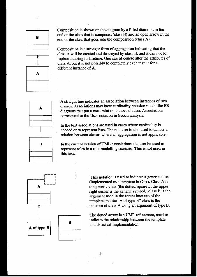
ElB

Composition is shown on the diagram by a filled diamond in theend of the class that is composed (class B) and an open arrow in theend of the class that goes into the composition (class A).

Composition is a stronger form of aggregation indicating that theclass A will be created and destroyed by class B, and it can not bereplaced during its lifetime. One can of course alter-the attributes ofclass A, but it is not possibly to completely exchange it for adifferent instance of A.

A straight line indicates an association between instances of twoclasses. Associations may have cardinality notation much like ERdiagrams that put a constraint on the association. Associationscorrespond to the Uses notation in Booth analysis.

In the text associations are used in cases where cardinality isneeded or to represent lists. The notation is also used to denote arelation between classes where an aggregation is not applicable.

In the current version of UML associations also can be used torepresent roles in a role-modelling scenario. This is not used inthis text.

,———.‘This notation is used to indicate a generic class(implemented as a template in C++). Class A isthe generic class (the dotted square in the upperright corner is the generic symbol), class B is theargument used in the actual instance of thetemplate and the “A of type B“ class is theinstance of class A using an argument of type B.

The dotted arrow is a UML refinement, used toindicate the relationship between the templateand its actual implementation.

2

=

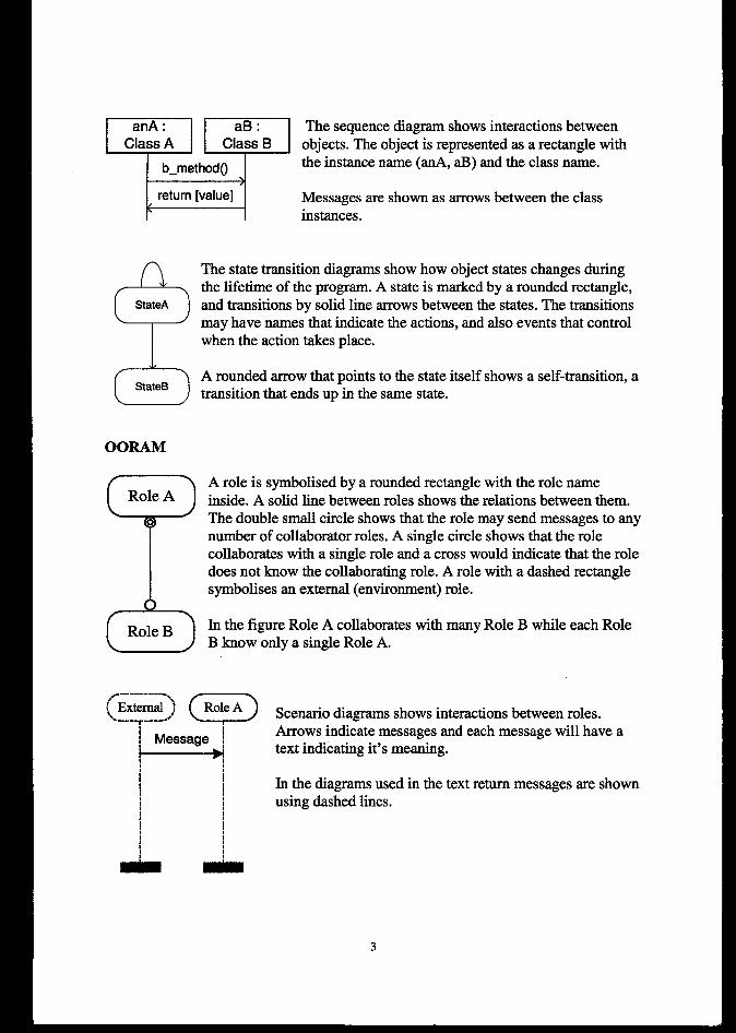
awl: aB:

Class A Class B

b_methodo

return [value]

The sequence diagram shows interactions betweenobjects. The object is represented as a rectangle withthe instance name (anA, aB) and the class name.

Messages are shown as arrows between the classinstances.

‘?StateA

CDStateB

OORAM

z

Role A

o

Role B

The state transition diagrams show how object states changes duringthe lifetime of the program. A state is marked by a rounded rectangle,and transitions by solid line arrows between the states. The transitionsmay have names that indicate the actions, and also events that controlwhen the action takes place.

A rounded arrow that points to the state itself shows a self-transition, atransition that ends up in the same state.

A role is symbolised by a rounded rectangle with the role nameinside. A solid line between roles shows the relations between them.The double small circle shows that the role may send messages to anynumber of collaborator roles. A single circle shows that the rolecollaborates with a single role and a cross would indicate that the roledoes not know the collaborating role. A role with a dashed rectanglesymbolises an external (environment) role.

In the figure Role A collaborates with many Role B while each RoleB know only a single Role A.

I,t1

,

1

Scenario diagrams shows interactions between roles.Arrows indicate messages and each message will have atext indicating it’s meaning.

In the diagrams used in the text return messages are shownusing dashed lines.

# i, 1

1 8

AAt

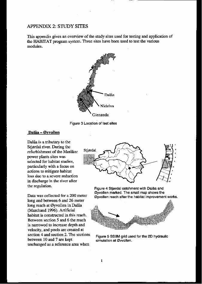
APPENDIX 2: STUDY SITES

This appendix gives an overview of the study sites used for testing and application ofthe HABITAT program system. Three sites have been used to test the variousmodules.

Figure 3 Location of test sites

Dal% - Ovvollen

Daliia is a tributary to theStj9rdal river. During therefurbishment of the Meriikerpower plants sites wasselected for habitat studies,particularly with a focus on~ctions to kdigate habitatloss due to a severe reductionin discharge in the river afterthe regulation.

Data was collected for a 200 meterlong and between 6 and 26 meterlong reach at @yvollen in Dal%(Marchand 1996). Artificialhabitat is constructed in this reach.Between section 5 and 6 the reachis narrowed to increase depth andvelocity, and pools are created at

Figure 4 Stjardal catchment with Dak%aandOyvollen marked. The small map shows theOyvollen reach after the habitat improvement works

section- 4 and ~ection 2. The sectionsbetween 10 and 7 are kept

Figure 5 SSIIM grid used for the 2D hydraulicsimulation at Owollen.

unchanged as a reference area when

1

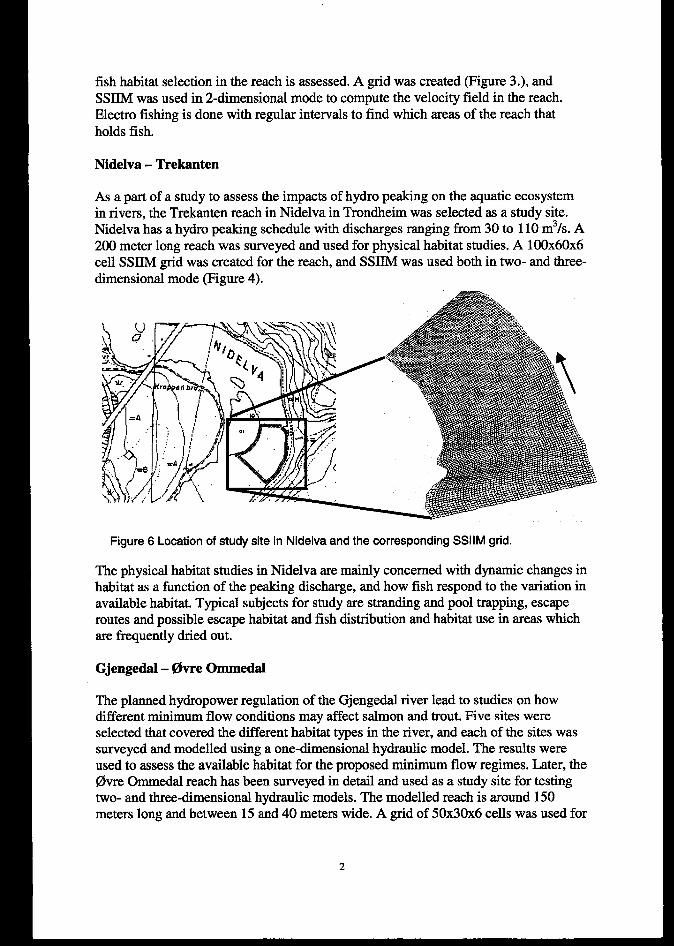
fish habitat selection in the reach is assessed. A grid was created (Figure 3.), andSSIIM was used in 2-dimensional mode to compute the velocity field in the reach.Electro fishing is done with regular intervals to find which areas of the reach thatholds fish.

Nidelva - Trekanten

As a part of a study to assess the impacts of hydro peaking on the aquatic ecosystemin rivers, the Trekanten reach in Nidelva in Trondheim was selected as a study site.Nidelva has a hydro peaking schedule with discharges ranging from 30 to 110 m3/s. A200 meter long reach was surveyed and used for physical habitat studies. A 100x6OX6cell SWIM grid was created for the reach, and SSIIM was used both in two- and three-dimensional mode (Figure 4).

Figure 6 Location of study site in Nidelva and the corresponding SSIIM grid.

The physical habitat studies in Nidelva are mainly concerned with dynamic changes inhabitat as a function of the peaking discharge, and how fish respond to the variation inavailable habitat. Typical subjects for study are stranding and pool trapping, escaperoutes and possible escape habitat and fish distribution and habitat use in areas whichare frequently dried out.

Gjengedal - Ovre Ommedal

The planned hydropower regulation of the Gjengedal river lead to studies on howdifferent minimum flow conditions may affect salmon and trout. Five sites wereselected that covered the different habitat types in the river, and each of the sites wassurveyed and modelled using a one-dimensional hydraulic model. The results wereused to assess the available habitat for the proposed minimum flow regimes. Later, the@vre Ommedal reach has been surveyed in detail and used as a study site for testingtwo- and three-dimensional hydraulic models. The modelled reach is around 150meters long and between 15 and 40 meters wide. A grid of 50x30x6 cells was used for

2

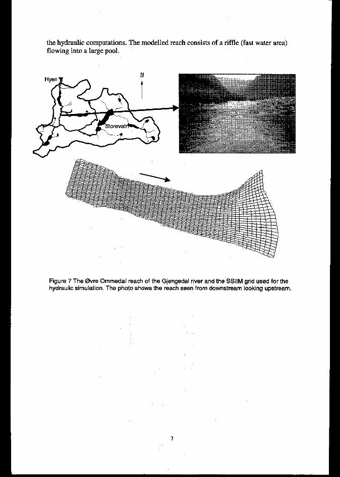
the hydraulic computations. The modelled reach consists of a riffle (fast water area)flowing into a large pool.

Figure 7 The ~re Ommedal reach of the Gjengedal river and the SSIIM grid used for thehydraulic simulation. The photo shows the reach seen from downstream looking upstream.

3

APPENDIX 3: DERIVA~ON OF MCA EQUATION

The figure shows the fish maintaining station. A prey is drifting with velocity VPalongthe line BC. The velocity at the fish holding position is FPV (Focal Point Velocity),RD is the reaction distance of the fish and the mean current velocity (vm~)the fish hasdo endure during attack is calculated along AC. The line AC is called the MinimumCapture Distance (MCD).

The prey travel time is found by assuming it equal to the travel distance divided by theprey velocity. The travel distance BC is expressed through the known RD and thewanted MCD by using Phytagoras:

(1)~P= iRD2 –MCD2

Vp

The time the fish needs to intercept the prey is the travel time along MCD alsoexpressed as travel distance/ velocity. The velocity of the fish during capture is acomponent expressed by the maximum swimming speed in a capture situation and themean water velocity the fish must overcome to reach the prey. The equation thenbecomes:

(2)

‘F=*

The interception of the prey happens when TF = ‘ITthe power of two yields the following expression:

Raising the resulting equation to

1

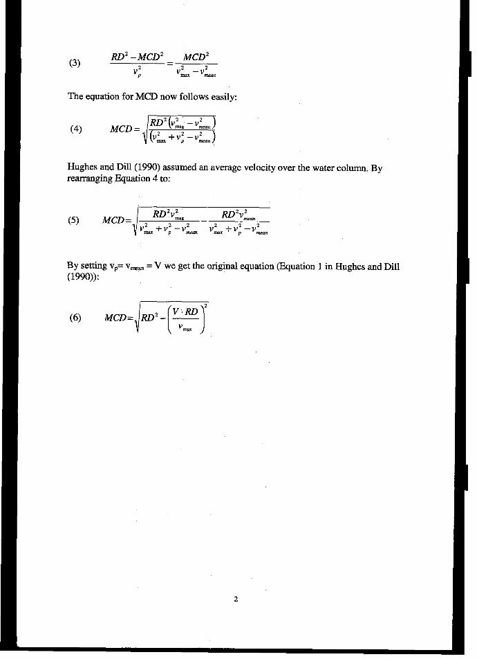
(3)RD2 –MCD2 . MCD2

v: v; – VL

The equation for MCD now follows easily:

(4)““=m

Hughes and Dill (1990) assumed an average velocity over the water column. Byrearranging Equation 4 to:

(5) ‘cD=ETz=7TiBy setting VP=vw.n = V we get the original equation (Equation 1 in Hughes and Dill(1990)):