AN INVESTIGATION OF THE APPLICATIONS AND LIMITATIONS OF UTILISING GLOBAL NAVIGATIONAL SATELLITE SYSTEMS (GNSS)

APPLICATIONS IN THE SOUTH AFRICAN NATIONAL DEFENCE

Submitted in partial fulfilment of the requirements for the degree

Master of Science

in the

Department of Geography, Geoinformatics and Meteorology

Faculty of Natural and Agricultural Science of the

University of Pretoria

South Africa

Frankie van Niekerk

Student Number: 27469299

Supervised by:

Professor W.L. Combrinck

February 2011

©© UUnniivveerrssiittyy ooff PPrreettoorriiaa

ii

Table of Contents

Chapter 1 : Introduction 1-1

Background Information ........................................................................................................................................ 1-1

Assumptions/Exclusions ....................................................................................................................................... 1-3

Research Question ............................................................................................................................................... 1-3

Aim and Objectives ............................................................................................................................................... 1-4

Significance of this Study ...................................................................................................................................... 1-4

Brief Chapter Overview ......................................................................................................................................... 1-4

Chapter 2 : Conceptual Framework and Methods 2-1

Background ........................................................................................................................................................... 2-1

Receivers, Software and Data .............................................................................................................................. 2-3

Chapter 3 : Common Frame of Reference 3-1

Reference Systems ............................................................................................................................................... 3-1

Positional Accuracy Standards ........................................................................................................................... 3-18

Chapter 4 : GPS Fundamentals 4-1

Introduction ........................................................................................................................................................... 4-1

Operational Aspects .............................................................................................................................................. 4-1

GPS Measurement: Errors and Biases ............................................................................................................... 4-14

GPS Measurement Augmentation ...................................................................................................................... 4-23

Chapter 5 : GPS in the Field – Applications 5-1

Introduction ........................................................................................................................................................... 5-1

Measurements with Geodetic Type GPS Receivers ............................................................................................ 5-3

Measurements with Navigational type GPS Receivers ...................................................................................... 5-23

Increasing Baselines for Differential GPS Measurements .................................................................................. 5-28

Precise Point Positioning Techniques ................................................................................................................ 5-32

Field Measurements with Navigational GPS Receivers ..................................................................................... 5-34

Satellite Based Augmentation System Tested ................................................................................................... 5-50

Concluding Remarks ........................................................................................................................................... 5-51

Selective Denial or Intentional Jamming............................................................................................................. 5-51

Unintentional Jamming ....................................................................................................................................... 5-54

Chapter 6 : Summary of Conclusions 6-1

Appendix A: References 1

iii

Appendix B: Datums used in Africa 1

Appendix C: Military Data Standards used in the SANDF 1

Multinational Geospatial Co-production ProgramME Standard ............................................................................... 1

ICAO D9881 Standard ............................................................................................................................................. 3

S-57 Data Standard ................................................................................................................................................. 7

Appendix D: GPS Field Manual 1

iv

Table of Figures

Figure 3-1: Maclear's Meridian Arc 3-2

Figure 3-2: WGS 84 Ellipsoid Values 3-3

Figure 3- 3: Ellipsoidal Coordinate System 3-4

Figure 3- 4: Geocentric Cartesian Coordinate System 3-5

Figure 3-5: ECEF Reference System 3-6

Figure 3-6: WGS84 Reference Stations 3-8

Figure 3-7: Selection of the best Ellipsoid 3-9

Figure 3-8: HRAO Velocities: 1996 to 2010 3-11

Figure 3-9: Orthometric Height (H) = h - N 3-13

Figure 3-10: IGS Reference Stations - Africa 3-14

Figure 3-11: UTM Zones of Africa 3-16

Figure 3-12: MGRS Blocks - South Africa 3-17

Figure 3-13: Accuracy and Precision 3-19

Figure 4-1: Generic Layout of a GPS Satellite's Subsystems 4-3

Figure 4-2: GPS Ground Control Stations 4-4

Figure 4-3: Generic Layout of a GPS Receiver 4-6

Figure 4-4: GPS Signal Structure 4-7

Figure 4-5: Synchronisation of Satellite and GPS Receiver Signals to Measure Time and Range 4-9

Figure 4-6: Satellite and Receiver Clock Offsets Calculated to Measure Time and Range 4-9

Figure 4-7: Ranging from four Satellites 4-11

Figure 4-8: Measuring Time and Range with Carrier Signals 4-13

Figure 4-9: Satellite Geometry - Dilution of Precision 4-16

Figure 4-10: Sunspot Activity since 1995 4-17

Figure 5-1: Location of GPS Station Positions in Local Network. 5-2

Figure 5-2: Distances between Stations (Global View - WGS 84, UTM Projection, Z35S 5-2

Figure 5-3: Distances between Stations (Focused View - WGS 84, UTM Projection, Z35S) 5-3

Figure 5-4: Station 1 - 2010_03_03 (1H) 5-4

Figure 5-5: Station 2 - 2010_03_03 (1H) 5-5

Figure 5-6: Station 3 - 2010_03_03 (1H) 5-5

Figure 5-7: Station 4 - 2010_03_03 (1H) 5-6

v

Figure 5-8: Station 5 - 2010_03_03 5-6

Figure 5-9: Satellites and PDOP Values 5-7

Figure 5-10: Electron Content: 100 km to 2 000 km 5-8

Figure 5-11: Electron Density: 09:00 - 23:00 5-9

Figure 5-12: Correlation between Electron Density and GPS Precision 5-10

Figure 5-13: Global Ionosphere Model 5-11

Figure 5-14: Station 1 - 2010_03_03 (2H) 5-12

Figure 5-15: Station 2 - 2010_03_03 (2H) 5-12

Figure 5-16: Station 4 - 2010_03_03 (H3) 5-13

Figure 5-17: Station 5 - 2010_03_03 (3H) 5-13

Figure 5-18: Station 1 - 2010_03_10 (1H) 5-14

Figure 5-19: Station 1 - 2010_03_10 (2H) 5-14

Figure 5-20: Station 1 - 2010_03_10 (3H) 5-15

Figure 5-21: Consecutive Measurements 5-15

Figure 5-22: Station3 - ProXH - 2010_03_24 5-19

Figure 5-23: Station 3 - ProXH - 2010_03_25 5-19

Figure 5-24: Station 3 - ProXH - 2010_03_26 5-20

Figure 5-25: Station 3 – ProXH - 2010_03_27 5-20

Figure 5-26: Station 3 - ProXH - 2010_03_24 (20 min intervals) 5-21

Figure 5-27: Station 3 - Consecutive Measurements - 2010_03_23 5-22

Figure 5-28: Station 3: Garmin GPSMap 60CSx - 2010_03_08 5-24

Figure 5-29: Station 3 - Garmin GPSMap 60CSx - 2010_03_09 5-25

Figure 5-30: Station 3: Garmin eTrex - 2010_03_12 5-25

Figure 5-31: Station 3 – Garmin eTrex - 2010_03_16 5-26

Figure 5-32: Geometry of Station 4 (Zwartkop) 5-35

Figure 5-33: Geometry of Station 5 (Schanskop) 5-36

Figure 5-34: Trimble ProXH Track - Valhalla 5-37

Figure 5-35: Trimble ProXH Track Valhalla (South) 5-37

Figure 5-36: Trimble ProXH Track Valhalla (North) 5-38

Figure 5-37: Garmin GPSMap 60CSx Track (in Pouch) - South 5-39

Figure 5-38: Garmin GPSMap 60CSx (in Pouch) - North 5-39

Figure 5-39: Garmin eTrex 1 (in Hand) South 5-40

vi

Figure 5-40: Garmin eTrex 1 (in Hand) – North 5-40

Figure 5-41: Garmin eTrex (in Pouch) - South 5-41

Figure 5-42: Garmin eTrex 2 (in Pouch) - North 5-42

Figure 5-43: Trimble ProXH Track though Pretoria 5-43

Figure 5-44: ProXH Tracks - Intersection 5-44

Figure 5-45: ProXH Tracks - Highway 5-45

Figure 5-46: Garmin GPSMap 60CSx - Intersection 5-45

Figure 5-47: Garmin GPSMap 60CSx - Highway 5-46

Figure 5-48: Garmin GPSMap 60CSx Track - Fountains Valley Traffic Circle/Interchange 5-47

Figure 5-49: Garmin GPSMap 60CSx Track - Traffic Circle 5-47

Figure 5-50: ProXH and eTrex Tracks - Inner City (Sunnyside, Pretoria) 5-48

Figure 5-51: ProXH and eTrex Tracks - Tree Cover (Brooklyn – Pretoria) 5-49

Figure 5-52: Garmin eTrek Tracks with EGNOS Activated 5-50

Figure 5-53: Photo of Jammer Setup 5-52

Figure 5-54: Viewshed of GPS Jamming Tests 5-52

vii

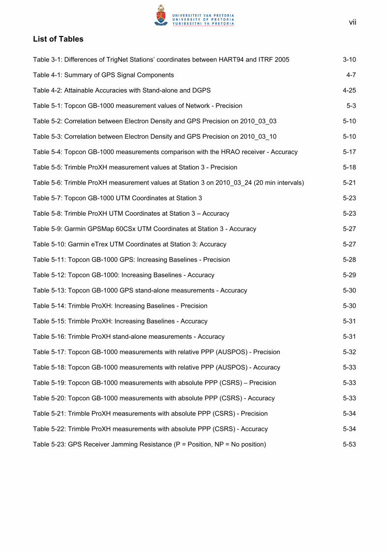
List of Tables

Table 3-1: Differences of TrigNet Stations’ coordinates between HART94 and ITRF 2005 3-10

Table 4-1: Summary of GPS Signal Components 4-7

Table 4-2: Attainable Accuracies with Stand-alone and DGPS 4-25

Table 5-1: Topcon GB-1000 measurement values of Network - Precision 5-3

Table 5-2: Correlation between Electron Density and GPS Precision on 2010_03_03 5-10

Table 5-3: Correlation between Electron Density and GPS Precision on 2010_03_10 5-10

Table 5-4: Topcon GB-1000 measurements comparison with the HRAO receiver - Accuracy 5-17

Table 5-5: Trimble ProXH measurement values at Station 3 - Precision 5-18

Table 5-6: Trimble ProXH measurement values at Station 3 on 2010_03_24 (20 min intervals) 5-21

Table 5-7: Topcon GB-1000 UTM Coordinates at Station 3 5-23

Table 5-8: Trimble ProXH UTM Coordinates at Station 3 – Accuracy 5-23

Table 5-9: Garmin GPSMap 60CSx UTM Coordinates at Station 3 - Accuracy 5-27

Table 5-10: Garmin eTrex UTM Coordinates at Station 3: Accuracy 5-27

Table 5-11: Topcon GB-1000 GPS: Increasing Baselines - Precision 5-28

Table 5-12: Topcon GB-1000: Increasing Baselines - Accuracy 5-29

Table 5-13: Topcon GB-1000 GPS stand-alone measurements - Accuracy 5-30

Table 5-14: Trimble ProXH: Increasing Baselines - Precision 5-30

Table 5-15: Trimble ProXH: Increasing Baselines - Accuracy 5-31

Table 5-16: Trimble ProXH stand-alone measurements - Accuracy 5-31

Table 5-17: Topcon GB-1000 measurements with relative PPP (AUSPOS) - Precision 5-32

Table 5-18: Topcon GB-1000 measurements with relative PPP (AUSPOS) - Accuracy 5-33

Table 5-19: Topcon GB-1000 measurements with absolute PPP (CSRS) – Precision 5-33

Table 5-20: Topcon GB-1000 measurements with absolute PPP (CSRS) - Accuracy 5-33

Table 5-21: Trimble ProXH measurements with absolute PPP (CSRS) - Precision 5-34

Table 5-22: Trimble ProXH measurements with absolute PPP (CSRS) - Accuracy 5-34

Table 5-23: GPS Receiver Jamming Resistance (P = Position, NP = No position) 5-53

viii

ACRONYMS

AFREF: African Reference Frame

AUSPOS: Australian Positioning Service

C/A-code: Coarse Acquisition Code

CDNGI: Chief Directorate National Geospatial Information, formally CDSM

CDSM: Chief Directorate Surveys and Mapping, now CDNGI

CEP: Circular Error Probability

CORS: Continuously Operating GPS Reference Stations

CSRS: Canadian Spatial Reference System

DGPS: Differential GPS

DOP: Dilution of Precision

DSSS: Direct Sequence Spread Spectrum

ECEF: Earth-centred Earth-fixed

ECI: Earth-centred Inertial

EGM 96 Earth Gravitational Model 1996

EGM 2008: Earth Gravitational Model 2008

EGNOS: European Geostationary Navigation Overlay System

GALILEO: European Union’s GNSS

GBAS: Ground Based Augmentation Systems

GCP: Ground Control Point

GIS: Geographical Information System

GLONASS: The Russian GNSS

GNSS: Global Navigational Satellite Systems

GPRS: General Packet Radio Service

GPS: Global Positioning System

GRS80: Geodetic Reference System 1980

HART94: Hartebeesthoek Datum 1994

HartROA: Hartebeesthoek Radio Astronomy Observatory near Pretoria, South Africa

HDOP: Horizontal Dilution of Precision

ix

HRAO: IGS reference station at HartRAO

ICAO: International Civil Aviation Organisation

IGS: International GNSS Service

IHO: International Hydrographical Office

ITRF: International Terrestrial Reference Frame

JPL: Jet Propulsion Laboratory of NASA

LLR: Lunar Laser Ranging

MGCP: Multinational Geospatial Co-production Programme

MGRS: Military Grid Reference System

MSL: Mean Sea Level

NASA: National Aeronautics and Space Administration of the USA

NAVSTAR: Navigation System with Timing and Ranging

NGA: National Geospatial-intelligence Agency

NTRIP: Network Transport of RTCM via Internet Protocol

P-code: Precise Code

PDOP: Positional Dilution of Precision

PPP: Precise Point Positioning

PPS: Precise Positioning Service

PRN: Pseudorandom Noise

RINEX: Receiver Independent Exchange Format

RTCM: Radio Technical Commission for Maritime Services

SAC: Satellite Application Centre

SANDF: South African National Defence Force

SBAS: Satellite Based Augmentation System

SLR: Satellite Laser Ranging

SPS: Standard Positioning Service

SUTH IGS reference station at Sutherland, South Africa

SVN: Space Vehicle Number

TDOP: Time Dilution of Precision

x

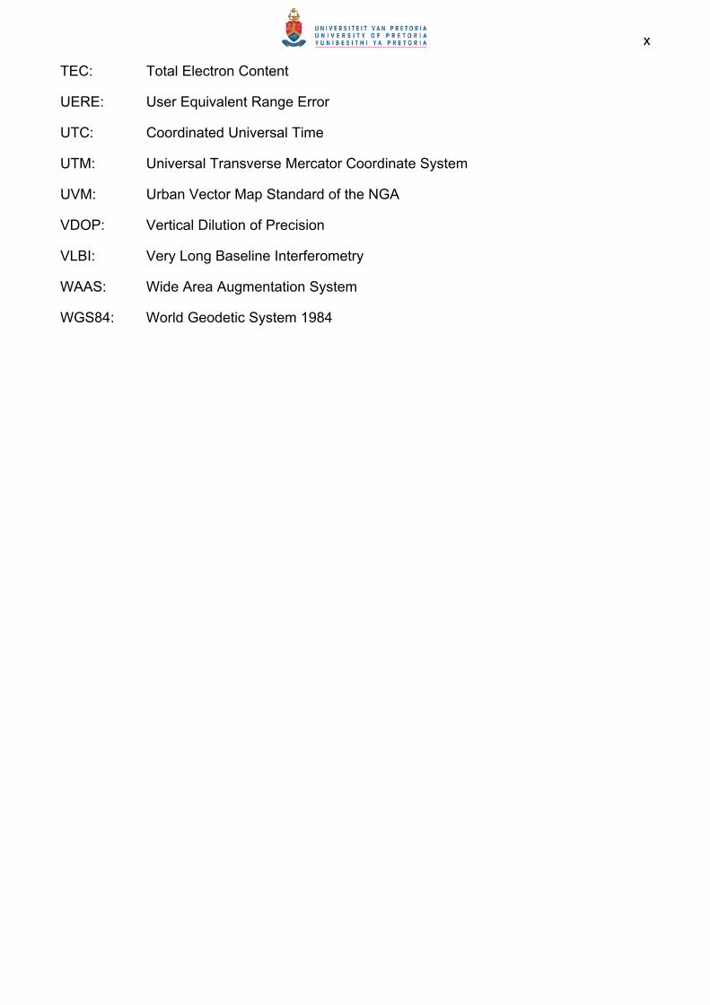
TEC: Total Electron Content

UERE: User Equivalent Range Error

UTC: Coordinated Universal Time

UTM: Universal Transverse Mercator Coordinate System

UVM: Urban Vector Map Standard of the NGA

VDOP: Vertical Dilution of Precision

VLBI: Very Long Baseline Interferometry

WAAS: Wide Area Augmentation System

WGS84: World Geodetic System 1984

xi

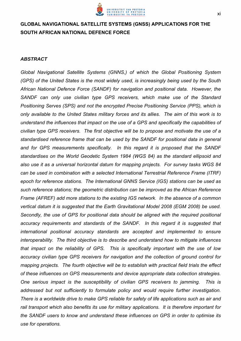
GLOBAL NAVIGATIONAL SATELLITE SYSTEMS (GNSS) APPLICATIONS FOR THE

SOUTH AFRICAN NATIONAL DEFENCE FORCE

ABSTRACT

Global Navigational Satellite Systems (GNNS,) of which the Global Positioning System

(GPS) of the United States is the most widely used, is increasingly being used by the South

African National Defence Force (SANDF) for navigation and positional data. However, the

SANDF can only use civilian type GPS receivers, which make use of the Standard

Positioning Serves (SPS) and not the encrypted Precise Positioning Service (PPS), which is

only available to the United States military forces and its allies. The aim of this work is to

understand the influences that impact on the use of a GPS and specifically the capabilities of

civilian type GPS receivers. The first objective will be to propose and motivate the use of a

standardised reference frame that can be used by the SANDF for positional data in general

and for GPS measurements specifically. In this regard it is proposed that the SANDF

standardises on the World Geodetic System 1984 (WGS 84) as the standard ellipsoid and

also use it as a universal horizontal datum for mapping projects. For survey tasks WGS 84

can be used in combination with a selected International Terrestrial Reference Frame (ITRF)

epoch for reference stations. The International GNNS Service (IGS) stations can be used as

such reference stations; the geometric distribution can be improved as the African Reference

Frame (AFREF) add more stations to the existing IGS network. In the absence of a common

vertical datum it is suggested that the Earth Gravitational Model 2008 (EGM 2008) be used.

Secondly, the use of GPS for positional data should be aligned with the required positional

accuracy requirements and standards of the SANDF. In this regard it is suggested that

international positional accuracy standards are accepted and implemented to ensure

interoperability. The third objective is to describe and understand how to mitigate influences

that impact on the reliability of GPS. This is specifically important with the use of low

accuracy civilian type GPS receivers for navigation and the collection of ground control for

mapping projects. The fourth objective will be to establish with practical field trials the effect

of these influences on GPS measurements and device appropriate data collection strategies.

One serious impact is the susceptibility of civilian GPS receivers to jamming. This is

addressed but not sufficiently to formulate policy and would require further investigation.

There is a worldwide drive to make GPS reliable for safety of life applications such as air and

rail transport which also benefits its use for military applications. It is therefore important for

the SANDF users to know and understand these influences on GPS in order to optimise its

use for operations.

xii

Acknowledgments

I would like to express my gratitude to the following individuals and institutions whose

support made this research possible:

Professor Ludwig Combrinck, the Associate Director of HartRAO who aided me throughout

this research. His practical and innovative approach is commendable.

The Director Geospatial Information, Brigadier General Pieter Thirion who created the

opportunity and environment to conduct the research.

The young people of Directorate Geospatial Information for assisting in obtaining GNSS

measurements over extended periods.

The Training Staff of SA Army Combat Training Centre at Lohatla.

Special Forces Headquarters’ Staff.

The Commander and Staff of the Mobile Deployment Wing and the Reutech personnel for

assisting with jamming tests with RADAR.

Dr Adriaan Combrink of CK Surveying for giving advice and assistance on various aspects of

this research.

Mr Fritz van der Merwe of the Geography Department of the University of Pretoria for giving

advice on statistical analysis.

Mr Richard Wonnacott of the Chief Directorate National Geospatial Information for giving

advice on content and reference systems.

CHAPTER 1: INTRODUCTION

BACKGROUND INFORMATION

1. The South African National Defence Force (SANDF) requires positional data for

various applications, including situational awareness, navigation and surveying. Positional

data are also required for the accurate delivery of munitions, logistics supply, delivery of

medical health services, administrative and construction activities. Two broad approaches

are used to provide positional data that relate to the chicken and egg situation, for instance,

maps and charts are used for positional data but positional data are required to create maps

and charts. Firstly, the more traditional approach is to use hard copy maps and charts that

are updated manually from various sources, such as reconnaissance reports. Secondly, an

approach is used which involves the use of a digital map by means of a Geographical

Information System (GIS) to which deployed sensors report automatically via connected

communication systems to update the digital map. A variation on this approach is to use an

operator to update the digital map manually.

2. Almost all digital map data are created from satellite imagery and aerial photography.

In order to extract features that meet the required positional accuracy, these images need to

be geometrically rectified based on accurate positional data. The SANDF is deployed on the

African continent in places such as the Democratic Republic of the Congo (DRC) and Sudan,

where the collection of positional data is difficult and risky. It should also be noted that a

general lack of reference points and minimal infrastructure in rural areas poses significant

challenges for acquiring positional data. Built-up areas and densely populated areas pose

different challenges. Thus, different approaches need to be developed to collect positional

data in rural and urban areas.

3. With the advent of Global Navigation Satellite Systems (GNSS), of which the Global

Positioning System (GPS) of the United States Air Force is the most widely used, a new

opportunity for acquiring positional data is available. Other satellite navigational systems,

which include the Russian GNSS (GLONASS) and the proposed European GALILEO system

can and will render positional data. However, as early as the 1980s the South African

Defence Force started to use Navigation System with Timing and Ranging (NAVSTAR) GPS

to acquire positional data to confirm positions in the field. The GPS receiver was never used

as the only source of positional data, but merely to confirm positions that were derived from

conventional navigational techniques.

4. The GPS is a space based navigational system. At least twenty-four satellites orbiting

the earth at a mean distance of 26 600 km in space are transmitting radio signals that

1-2

propagate through the atmosphere at the approximate speed of light. These signals are

used by a GPS receiver to determine a position on Earth by converting the known positions

of the satellites to a single position on earth. This is made possible by using the known

speed of these signals from each satellite multiplied by the time it took to reach the receiver.

The intersection of these signal vectors allows the receiver to determine a position on a

reference ellipsoid that is a close representation of the earth’s shape. Software conversion

packages are used to convert this position on the ellipsoid to a three dimensional position on

Earth that may have an error in the range from 10 m to sub-centimetre. This is a hugely

oversimplified version of reality, but may suffice to create an understanding of the basic

concepts involved. Aspects of how GPS functions and the influences on accurate

measurements will be discussed in more detail in Chapter 3.

5. The GPS satellite signal structure is of paramount importance for positioning. Each

satellite is transmitting two signals, namely the L1 at 1 575.42 MHz and L2 at 1 227.6 MHz,

also referred to as the carrier signals. Two other signals that are used for determining range

are modulated on these carrier signals. On L1 a Coarse Acquisition code (C/A-code) and a

Precise code (P-code) are modulated whereas on L2 only the P-code is modulated. The

GPS navigation message containing information about the status of satellite orbits and

clocks is also modulated on both carrier signals. Most civilian navigational type GPS

receivers use only the C/A-code to determine position. More expensive survey type

receivers are also able to use the carrier signals to determine position. However, the

encrypted P-code code is only available to the United States military forces and its allies.

Two additional satellite signals, the L2C and the L5, are planned for the modernisation and

improvement of GPS and will most probably be available from 2013. The signal structure

and its implications for positioning will be discussed in Chapter 4.

6. The accuracy of the measurement with a GPS receiver is dependent on various

environmental factors, satellite deficiencies and quality of the receiver. Environmental

aspects include refraction of the GPS satellite signal travelling through the atmosphere,

reflection of signals from surfaces close to the receiver that creates bogus signals and

objects obscuring the signal from reaching the receiver. Satellite deficiencies include orbit

and clock errors as well as sub-optimal positioning of the satellites in the sky at the time of

measurement, for instance being clustered in one segment or too low on the horizon. The

quality of the receiver relates to the number of satellites that can be tracked, the quality of the

receiver clock and the capability to receive and process positions from both code and carrier

signals. All these aspects and ways to mitigate accuracy limiting factors will be discussed in

more detail in Chapter 4.

1-3

7. One way of improving the accuracy of GPS measurements is to use a known

position as a reference point. By deploying a GPS receiver at this known point or base

station of which the position has been measured accurately before, any deviation in the

measurements caused by environmental influences or satellite deficiencies can be measured

relative to the known point. These deviations can then be used to correct any measurement

taken with another GPS receiver in the vicinity of the base station. This concept is known as

the differential correction of GPS measurements and can be conducted on the fly or

afterwards during post-processing. This concept will be discussed in more detail in Chapter

4 as it plays an important role in taking accurate measurements for mapping and surveying

purposes.

8. The SANDF is making use of civilian type receivers for positional data. Directorate

Geospatial Information, the SA Army Engineer Formation, the SA Navy Hydrographer and

Directorate Aviation Safety all use GPS receivers that are capable of using both carrier and

code signals for mapping and surveying. Naval vessels and aircraft use embedded GPS

receivers and integrate their measurements with other onboard inertial navigational systems

to render an integrated positional solution. The rest of the SANDF, including infantry soldiers

and peace observers, uses navigation type receivers that utilise the C/A-code for determining

position. It can be assumed that a large number of SANDF members also use privately

owned GPS receivers in this category.

ASSUMPTIONS/EXCLUSIONS

9. This study focuses on the use of civilian type GPS receivers and its application in the

SANDF. Munitions guidance and GPS solutions as applied to weapon systems will not be

discussed. Neither will survey applications be discussed, although the principles outlined in

this study may be of great value to both weapon system developers and military surveyors.

10. Other GNSS solutions such as the Russian GLONASS and the European planned

GALILEO system will not be discussed.

RESEARCH QUESTION

11. There is a requirement to identify suitable approaches to using civilian GNSS to

acquire accurate positional data for diverse applications in the SANDF. The limits and

capabilities of GNSS as applied in the SANDF need to be identified and evaluated to ensure

correct use. Currently there is no official policy or guidelines on the use of GNSS in the

SANDF.

1-4

AIM AND OBJECTIVES

12. The aim of this study is to discuss the different positional data requirements in the

SANDF and create a theoretical and tested approach for collection of these data using

GNSS. This will be done by

a. discussing a proposed common frame of reference for positional data that

can be used by the SANDF;

b. discussing an attainable positional accuracy standard for use in the SANDF;

c. discussing the functioning of GPS in general, including GPS errors and its

effect on measurements;

d. completing an empirical study of how to overcome some of these errors and

to create a repeatable and reliable approach for GPS use in the field; and

e. presenting a field manual that can be used by the SANDF for GPS data

collection.

SIGNIFICANCE OF THIS STUDY

13. This study will establish a firm base for policy guidelines for using civilian type GPS

receivers under different circumstances, including restrictive influences. The SANDF will

most probably remain dependent on civilian type GPS receivers and will therefore need to

develop knowledge and skills to use this type of receiver.

BRIEF CHAPTER OVERVIEW

14. After an appropriate introduction (Chapter 1) and (Chapter 2) sketching a conceptual

framework, this study will establish a theoretical approach for a common frame of reference

for positional data on the African continent in Chapter 3. Aspects such as different

coordinate systems, ellipsoids, horizontal and vertical datums are discussed. This is

followed by a discussion of positional accuracy requirements with proposed accuracy

standards to be adopted in the SANDF.

15. Chapter 4 contains a discussion of the theoretical aspects of GPS and the capabilities

and limitations of the different types of receivers. It includes the environmental effects,

satellite health and receiver quality that impact on the accuracy and reliability of

measurements. This chapter also includes selective denial or jamming of GPS signals and

concludes with augmentation techniques to improve the accuracy of measurements. The

1-5

focus remains on applications on the African continent and concludes the bulk of the

literature study.

16. Chapter 5 encapsulates testing of the theoretical approach established in the

preceding chapters through the introduction of measurements taken with different types of

receivers under different conditions. An approach for using the different types of receivers in

the field is developed. Conclusions of this study are summarised in Chapter 6.

17. Appendix D provides a practical hands-on field manual for GPS users in the SANDF.

CHAPTER 2: CONCEPTUAL FRAMEWORK AND METHODS

BACKGROUND

1. Establishing a Departure Point. This study would like to establish a theoretical and

tested approach for the collection of positional data for use in the SANDF by making use of

civilian type GPS receivers. Although the focus will be on the collection of positional data,

the requirements for navigation by means of GPS are equally important and will be

addressed by implication. The departure point for positional data is a common reference

frame. A theoretical approach will be followed to discuss trends globally and on the African

continent to establish an approach for such a common reference frame. The objective is to

suggest an approach that can be used by the SANDF. This will be followed by a discussion

of the theoretical requirements for positional data by the various services in the SANDF. In

the absence of existing policy, applicable international policy guidelines will be suggested as

the way to be followed. Some of these international trends are followed in practice, but are

not taken up in SANDF policy.

2. Discussing GPS Fundamentals. The objective will be to explain the basic functions of

GPS to provide a theoretical framework that can be used to understand the capabilities of

different GPS receivers, including its limitations. Causes of less than optimal measurements

and the augmentation of GPS measurements for the improvement of accuracy will be

discussed as an integral part of collecting positional data and navigation. This approach will

build on the previous discussion by explaining how the common reference frame is used by

GPS to provide positional data and lay the foundation for the discussion of practical field

measurements.

3. Field Measurements. The theoretical approach of the previous sections will be

verified by the analysis of field data. The approach will be to determine a reference network

that can be used to test the precision and accuracy of other receivers. The following process

will be followed:

a. Reference Network with Geodetic Receivers. A reference network with

geodetic type GPS receivers will be established that could be used to

evaluate and calibrate other receivers. The precision, accuracy and

repeatability of measurements with these receivers in the network will be

analyzed and discussed. This will require measurements longer than eight

hours throughout the network to render sufficient data for this analysis. To

ensure that measurements are not influenced by controllable systematic

errors, the following precautionary steps are implemented. The positions of

2-2

the stations in the network are to be selected to ensure that the influence

of the ionosphere would be the same throughout the network. This requires

baselines shorter than 15 km according to Combrinck (personal

communication, 2010). Stations will be selected which are stable where

foreseen or predictable movements of the receiver antennas will not occur.

It should also be both accessible and out of reach of the general public to

prevent tampering with the receivers or the antennas while measurements

are taken. Station positions in the network will be selected to prevent

multipathing and/or shadowing. The influences that impact on the accuracy

of measurements as well as the augmentation of GPS measurements

discussed in the theoretical discussions will be analysed in practice,

including exploring the extension of baselines to a distance that would be

more suitable for stand-alone GPS receivers instead. The challenge of

insufficient base stations on the Continent and the inherent risks involved in

setting up own base stations highlight the importance of this analysis.

b. Mapping GPS Receivers. The next process will be to establish the precision

and accuracy levels attainable with typical mapping GPS receivers that are

used in the SANDF. These receivers are used for mapping projects and are

used for the collection of ground control data. These receivers will be

deployed at the same stations as the reference network to evaluate the

levels of precision and accuracy attainable with mapping receivers. These

mapping receivers will also be used for the evaluation of extended baselines.

c. Navigational Receiver. Typical navigational receivers that are used in the

SANDF will be used to establish attainable precision and accuracy levels at

the same network stations. Although navigational receivers are not the

primary instruments for collecting ground control data, the number of these

receivers in the field and the high costs associated with deploying mapping

receivers impel the use of navigational receivers for this purpose. It is

therefore important to understand the levels of precision and accuracy

attainable with these receivers.

d. Collection of Positional Data. Positional data are collected by means of GPS

receivers in the field. This takes place by means of handheld GPS receivers

used on patrols on foot and vehicles or imbedded GPS receivers on board

vehicles or craft. Whatever the application, the precision and accuracy of

2-3

data collected by these means need to be established to provide useful

and reliable positional data.

4. Reliability. The reliability of the GPS receivers for navigation and collection of data is

of paramount importance in the military. It is therefore important to explore and understand

accuracy, precision and reliability of different civilian type GPS receivers. Susceptibility of

these GPS receivers to jamming will also be discussed and tested in field trials. However, it

will not be possible to explore the topic sufficiently to provide thorough policy guidelines. The

possible tactics applied in the jamming and prevention of jamming of GPS receivers may be

sensitive. The objective therefore will only be to demonstrate the vulnerability of civilian type

GPS receivers to jamming.

RECEIVERS, SOFTWARE AND DATA

5. Geodetic Type GPS Receivers. Topcon GB-1000 receivers and associated antennas

provided by Professor W.L. Combrinck of the Hartebeesthoek Radio Astronomy Observatory

(HartRAO) will be used as geodetic receivers. These 40 channel receivers are capable of

collecting data from both the GPS and GLONASS satellites, although only GPS data will be

processed. These receivers can collect positional data with the C/A-code, L1 and L2 satellite

signals.1

6. Mapping Type GPS Receivers. Trimble ProXH receivers and associated Zephyr

antennas provided by the SANDF will be used as mapping receivers. These 12 channel

receivers are capable of collecting positional data with the C/A-code, L1 and L2 carrier

signals2.

7. Navigational Receivers. Garmin GPSMap 60CSx and eTrex Legind HCx receivers

with internal antennas provided by the SANDF will be used as navigational type receivers3.

Data will be collected with 30 second intervals (static) and one second intervals (mobile),

exported with the propriety Garmin software into .gpx format. These .gpx exported files can

be imported into Microsoft Office Excel 2003 where it can be analysed.

8. Reference Data. Precise ephemeris data, which includes accurate satellite clock and

orbit data will be accessed from the International GNSS Service (IGS) website and will be

used throughout this study where measurements are post-processed differentially. These

1 More technical detail of these receivers can be accessed at http://www.topconpositioning.com.

2 More technical detail of these receivers can be accessed at http://www.trimble.com.

3 Technical detail about these receivers can be accessed at http://www.garmin.co.za.

2-4

data are only available approximately two weeks after measurement. Epoch data (station

coordinates) will be accessed from the International Terrestrial Reference Frame (ITRF)

website. The IGS station at Hartebeesthoek (HRAO) will be used as base stations for post-

processing, while the Australian Positioning Service (AUSPOS) and the Canadian Spatial

Reference System (CSRS) will be used for Precise Point Positioning (PPP). The TrigNet

stations of Chief Director National Geospatial Information (CDNGI) will also be used for

assessing increasing baselines. WGS84 will be used as the reference ellipsoid and

EGM2008 as geoid model. Base stations will be fixed to the published ITRF 2005,

2008_01_09 epoch values to create a single reference epoch for all differential processing.

Ellipsoidal height values will be used throughout this study.

9. Data Analysis.

a. Survey and Mapping Receivers. Static measurements with survey and

mapping receivers used in this study will be collected during periods

extending over eight hours. Data will be collected at 30 second intervals,

exported in Receiver Independent Exchange Format (RINEX) format and

post-processed with Topcon Tools Version 7.3. using precise ephemeris

data, base stations and station coordinates as indicated in paragraph 8.

The Topcon Tools software will be used to export processed data in

ellipsoidal coordinates, including the precision of these measurements in

metre values. A special software package TEQC4 will be used to decimate

measurements into shorter time periods to establish the repeatability of

sessions. Take note that after processing with the Topcon Tools software,

which includes adjustments, the standard deviations on the measurements

values throughout the 5 station network will be the same for all stations. The

accuracy of measurements will be determined by comparing it with

measurements with a receiver with a known higher accuracy capability. For

accuracy comparisons measurement values will be converted to Universal

Transverse Mercator Projection (UTM) plane coordinates in metre values

which is a typical military map projection that can be used across the African

continent. Height values will be in ellipsoidal values. A software package

XForm version 4.3 and 4.4 acquired from Professor C.L. Merry will be used

for these conversions.

4 Teqc can be downloaded from http://facility.unavco.org/software/teqc

2-5

b. Navigational Receivers. Static measurements with navigational type

receivers will be exported in .gpx format to Microsoft Excel. The precision of

measurements will be determined by calculating averages and standard

deviations over the complete collection period as well as in one hour

segments. The accuracy of measurements with these receivers will be

conducted similar to survey and mapping receivers.

c. Mobile Measurements. Mobile measurements will be collected by means of

practical field trials with navigational and mapping GPS receivers that are

used in the SANDF, this will be conducted to establish attainable levels of

accuracy and to provide advice on how to improve measurements with these

types of receivers. To provide sufficient data for reliable analysis, these trials

will be conducted over and over and with different operators. Most of these

trials will exceed thirty incidences to provide for a reliable statistical analysis.

Data for the analysis of mobile solutions will be collected at one second

intervals. Points and tracks collected with survey and mapping receivers will

be used to indicate the accuracy of tracks collected with navigational

receivers. Measurements with mapping receives in the mobile role will be

processed with the Timble Pathfinder Office version 4.10 software. The

TrigNet station of CDNGI in Silverton will be used as a base station for this

processing. Background images will be used to create a visual orientation of

these mobile measurements.

10. Background Data. Results of the analysis of GPS receiver capabilities will be

presented in table and line graph formats. However, where navigational and mapping GPS

receivers are used in the field the results will be displayed in a GIS product. ArcGIS

Version 9.3.1 provided by the SANDF will be used for these analyses and background data

for these products were provided as follows:

a. High Resolution Aerial Photography. The Satellite Application Centre (SAC)

of the CSIR at Hartebeesthoek supplied the 10 cm resolution photography of

the Tshwane Metropolitan Area. Date (probably 2007) and the sensor is

unknown.

b. High Resolution Satellite Imagery. In addition, SAC also supplied the 5 m

Spot (2009) imagery of the General Piet Joubert Training Area.

2-6

c. High Resolution Digital Elevation Model (DEM). The 20 m resolution

DEM that will be used to conduct the analysis of the jamming of GPS signals

was supplied by CDNGI.

d. Google Earth Imagery. Google Earth imagery will be used to demonstrate

the effect of EGNOS on measurements with a navigational GPS receiver.

CHAPTER 3: COMMON FRAME OF REFERENCE

REFERENCE SYSTEMS

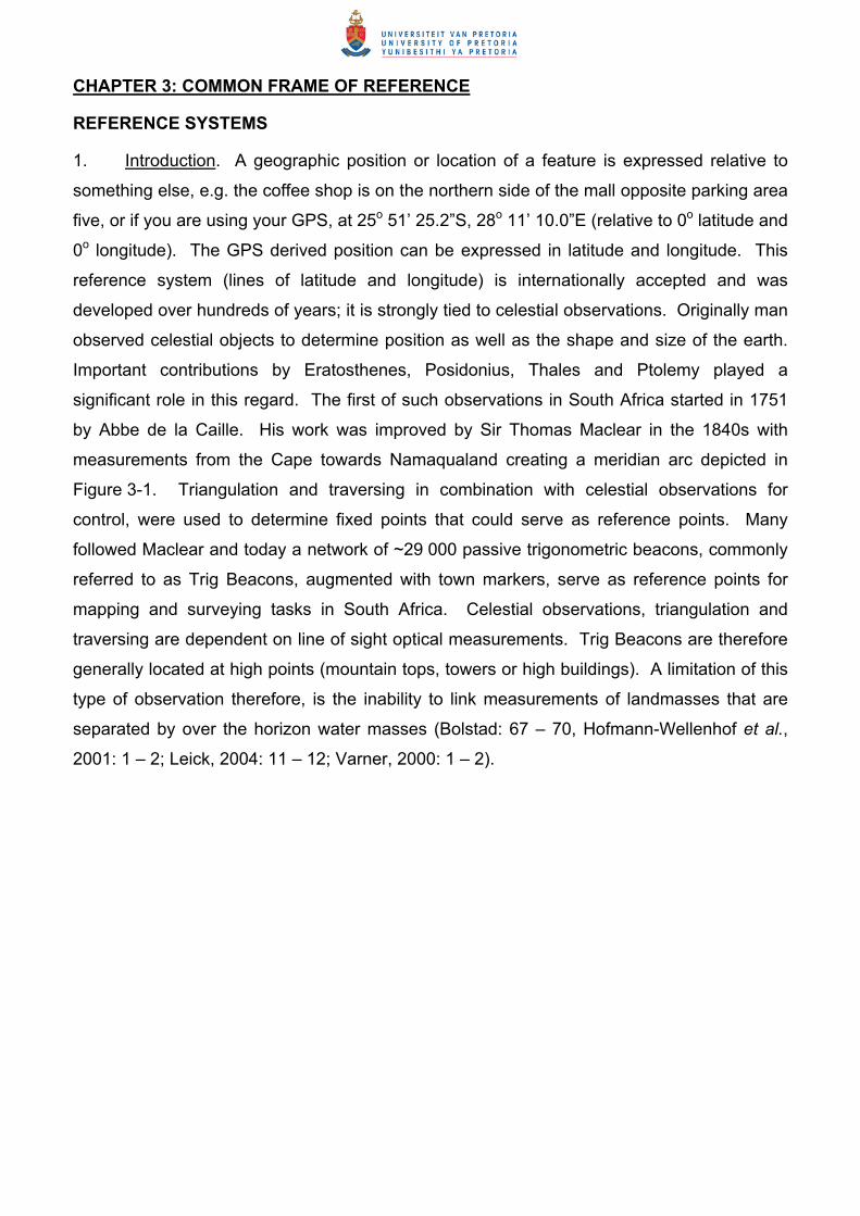
1. Introduction. A geographic position or location of a feature is expressed relative to

something else, e.g. the coffee shop is on the northern side of the mall opposite parking area

five, or if you are using your GPS, at 25o 51’ 25.2”S, 28o 11’ 10.0”E (relative to 0o latitude and

0o longitude). The GPS derived position can be expressed in latitude and longitude. This

reference system (lines of latitude and longitude) is internationally accepted and was

developed over hundreds of years; it is strongly tied to celestial observations. Originally man

observed celestial objects to determine position as well as the shape and size of the earth.

Important contributions by Eratosthenes, Posidonius, Thales and Ptolemy played a

significant role in this regard. The first of such observations in South Africa started in 1751

by Abbe de la Caille. His work was improved by Sir Thomas Maclear in the 1840s with

measurements from the Cape towards Namaqualand creating a meridian arc depicted in

Figure 3-1. Triangulation and traversing in combination with celestial observations for

control, were used to determine fixed points that could serve as reference points. Many

followed Maclear and today a network of ~29 000 passive trigonometric beacons, commonly

referred to as Trig Beacons, augmented with town markers, serve as reference points for

mapping and surveying tasks in South Africa. Celestial observations, triangulation and

traversing are dependent on line of sight optical measurements. Trig Beacons are therefore

generally located at high points (mountain tops, towers or high buildings). A limitation of this

type of observation therefore, is the inability to link measurements of landmasses that are

separated by over the horizon water masses (Bolstad: 67 – 70, Hofmann-Wellenhof et al.,

2001: 1 – 2; Leick, 2004: 11 – 12; Varner, 2000: 1 – 2).

3-2

Figure 3-1: Maclear's Meridian Arc1

2. The Shape and Size of the Earth – The Geoid. The irregular surface of the earth

inhibits coordinate computations. A surface close to mean sea level referred to as the geoid

can be used as an approximation of the shape of the earth. This surface is everywhere

perpendicular to the direction and force of gravity that is influenced by the density of the

earth’s crust. This three-dimensional equipotential surface is determined by means of gravity

observations and represents a surface with equal or constant gravitation value or potential. It

changes slowly over wavelengths of tens of kilometres and globally deviates approximately

one metre from measured mean sea level. Global measurements to determine the geoid

were not possible until recently. The National Geospatial Intelligence Agency (NGA) of the

United States used satellite observations to compute a global geoid model. The first widely

used global geoid model, Earth Gravitational Model 1996 (EGM96), has been replaced with a

more detailed and accurate model (EGM2008) that was released in April 2008. Knowledge

of the geoid is also important for height measurements for mapping projects that will be

discussed further in paragraph 6 under Vertical Datums (Iliffe & Lott, 2008: 8).

1 Source: Chief Director: National Geospatial Information accessed during April 2009 at http://w3sli.wcape.gov.za

3-3

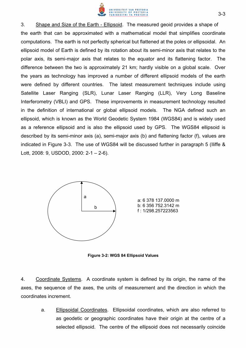
3. Shape and Size of the Earth - Ellipsoid. The measured geoid provides a shape of

the earth that can be approximated with a mathematical model that simplifies coordinate

computations. The earth is not perfectly spherical but flattened at the poles or ellipsoidal. An

ellipsoid model of Earth is defined by its rotation about its semi-minor axis that relates to the

polar axis, its semi-major axis that relates to the equator and its flattening factor. The

difference between the two is approximately 21 km; hardly visible on a global scale. Over

the years as technology has improved a number of different ellipsoid models of the earth

were defined by different countries. The latest measurement techniques include using

Satellite Laser Ranging (SLR), Lunar Laser Ranging (LLR), Very Long Baseline

Interferometry (VBLI) and GPS. These improvements in measurement technology resulted

in the definition of international or global ellipsoid models. The NGA defined such an

ellipsoid, which is known as the World Geodetic System 1984 (WGS84) and is widely used

as a reference ellipsoid and is also the ellipsoid used by GPS. The WGS84 ellipsoid is

described by its semi-minor axis (a), semi-major axis (b) and flattening factor (f), values are

indicated in Figure 3-3. The use of WGS84 will be discussed further in paragraph 5 (Iliffe &

Lott, 2008: 9, USDOD, 2000: 2-1 – 2-6).

Figure 3-2: WGS 84 Ellipsoid Values

4. Coordinate Systems. A coordinate system is defined by its origin, the name of the

axes, the sequence of the axes, the units of measurement and the direction in which the

coordinates increment.

a. Ellipsoidal Coordinates. Ellipsoidal coordinates, which are also referred to

as geodetic or geographic coordinates have their origin at the centre of a

selected ellipsoid. The centre of the ellipsoid does not necessarily coincide

a

b

a: 6 378 137.0000 m b: 6 356 752.3142 m f : 1/298.257223563

3-4

with the centre of mass of the earth. The poles are defined by the

rotational axis of the ellipsoid and the equator is the circle that bisects it in a

northern and southern hemisphere, while the prime meridian is selected.

The coordinates are defined as latitude ( ), longitude ( ) and height (h) in

this sequence. Ellipsoidal coordinates can be two-dimensional (latitude and

longitude) or three-dimensional (latitude, longitude and ellipsoidal height).

Latitude is the angle formed by the ellipsoidal normal north (+) or south (-)

from the equatorial plane. Longitude is the angle east (+) and west (-) from

the prime meridian. Latitude and longitude are expressed in degrees or

hours, where one hour equals 15 degrees, and height in metres above the

surface of the ellipsoid. The equator is designated 0º. All other circles that

run parallel to the equator are termed latitudes and their values are

designated by their magnitude of direction of the ellipsoidal normal to a

maximum value of 90º towards the poles. Lines of constant longitude are

termed meridians or longitudes. In 1884 it was generally agreed that the

longitude running through the Royal Greenwich Observatory in England will

be designated 0º and is known as the Greenwich or Prime Meridian.

Longitudes west of Greenwich are negative, while eastern longitudes are

positive to the magnitude of its direction with the maximum value of 180º.

Selecting and realising a geodetic datum constitutes ellipsoidal coordinates

as a coordinate system which is the basis for mapping projects and will be

discussed further under Horizontal Datum. Computations in ellipsoidal

coordinates are complex (Iliffe & Lott, 2008: 8 – 14, Bolstad, 2006: 75 – 77).

Figure 3- 3: Ellipsoidal Coordinate System

Pole

Equator h

Pole

3-5

b. Geocentric Cartesian Coordinates. Geocentric Cartesian coordinates

have their origin at the centre of a selected ellipsoid which is aligned with the

centre of mass of the earth. It is three dimensional with the axes denoted as

x, y and z. Units of measurement are normally metres but for space

applications kilometres can be used. The z-axis is aligned with the polar axis

of the ellipsoid, while the x-axis is in the equatorial plane and points to the

prime meridian. The y-axis completes a right handed coordinate system.

Cartesian coordinates can be converted to ellipsoidal coordinates and vica

versa. (Iliffe & Lott, 2008: 8 – 15, Hofmann-Wellenhof et al., 2001: 279 -

282).

Figure 3- 4: Geocentric Cartesian Coordinate System

c. Earth-Centred Inertial (ECI) Coordinate System. The Cartesian coordinate

system is also used to provide coordinates of celestial bodies which are

referred to as its ephemeris. To determine the ephemeris of celestial objects

relative to an imaginary celestial sphere an ECI coordinate system is used.

The origin of this system is the centre of mass of the earth or geo-centre.

The xy-plane of the ECI coordinate system coincides with the earth’s

equatorial plane, with the x-axis permanently fixed in the direction of the

vernal equinox. The z-axis is orthogonal to the xy-plane, and coincides with

the earth’s rotational vector in the direction of the North Pole. The +y-axis

forms the right-handed coordinate system. However, various forces,

including gravitational forces of the sun and moon cause irregularities in the

earth’s movement relative towards the celestial sphere. This movement,

also known as precession and notation, causes the ECI coordinate system to

be near-inertial. To overcome this, the axis is defined at a particular moment

X

Y

Z

Prime Meridian

Equator

3-6

in time or epoch. Such an epoch was defined on 1 January 2000 at

12:00 Coordinated Universal Time (UTC) denoted as J2000 according to the

Julian calendar. It should be noted that the fixing of the ECI coordinate

system is based on celestial observations of over 500 quasars and galactic

nuclei. Although these celestial radio sources move through space at

different velocities, the distances to these bodies are so large that they can

be considered as fixed points in space. The ECI coordinate system is used

to determine GPS satellite positions and orbits (Hofmann-Wellenhof et al.,

2001: 25 – 28; Leick, 2004: 11 – 28; Kaplan & Hegarty, 2006: 27 – 28).

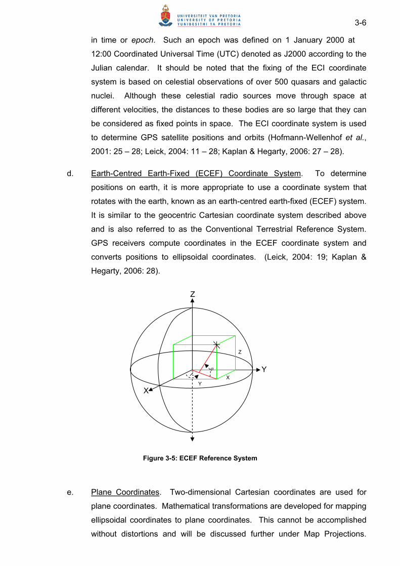
d. Earth-Centred Earth-Fixed (ECEF) Coordinate System. To determine

positions on earth, it is more appropriate to use a coordinate system that

rotates with the earth, known as an earth-centred earth-fixed (ECEF) system.

It is similar to the geocentric Cartesian coordinate system described above

and is also referred to as the Conventional Terrestrial Reference System.

GPS receivers compute coordinates in the ECEF coordinate system and

converts positions to ellipsoidal coordinates. (Leick, 2004: 19; Kaplan &

Hegarty, 2006: 28).

Figure 3-5: ECEF Reference System

e. Plane Coordinates. Two-dimensional Cartesian coordinates are used for

plane coordinates. Mathematical transformations are developed for mapping

ellipsoidal coordinates to plane coordinates. This cannot be accomplished

without distortions and will be discussed further under Map Projections.

X

Y

Z

Y X

Z

3-7

Suffice to indicate that there are a number of plane coordinate systems

that denote axes such as X and Y, y and x or eastings (E) and northings (N).

Measurement value is in metre such as in the UTM projection (Iliffe & Lott,

2008: 16, Merry, 2006: 9 – 11).

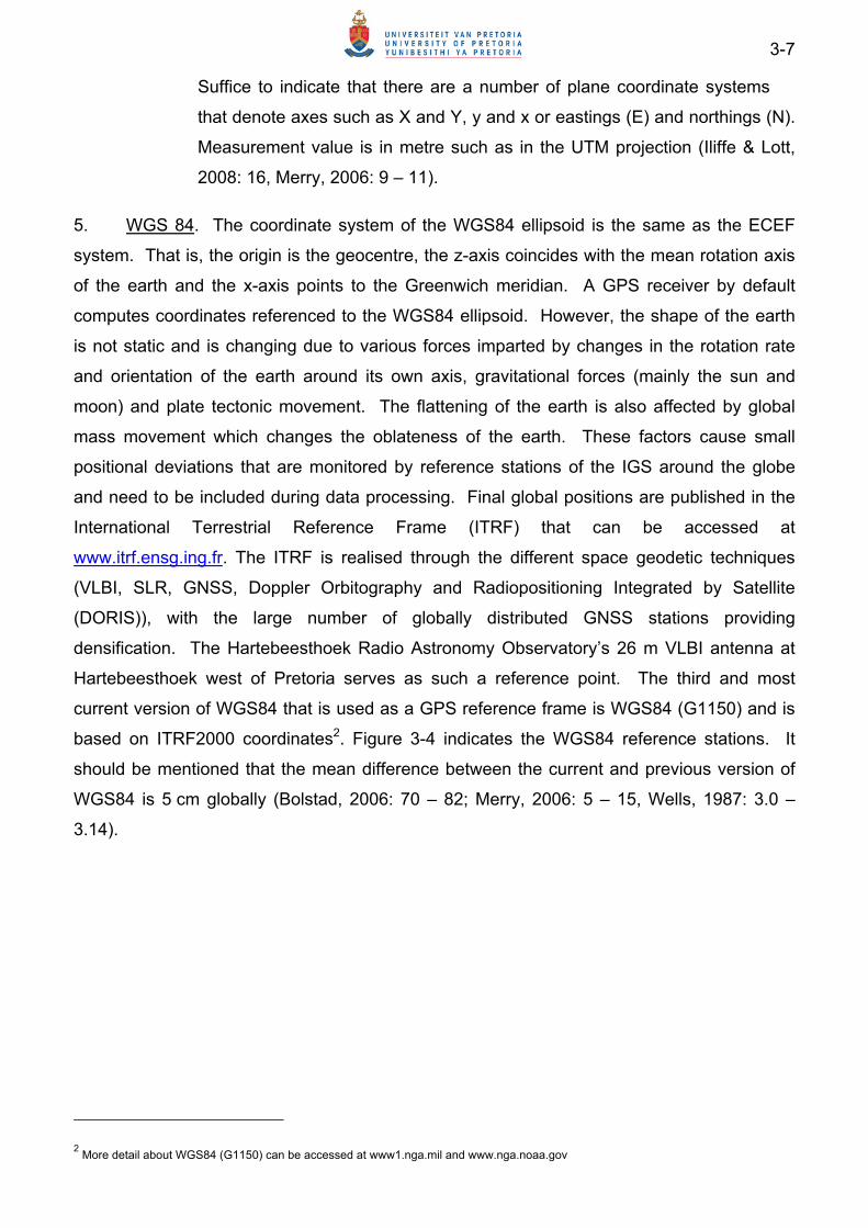
5. WGS 84. The coordinate system of the WGS84 ellipsoid is the same as the ECEF

system. That is, the origin is the geocentre, the z-axis coincides with the mean rotation axis

of the earth and the x-axis points to the Greenwich meridian. A GPS receiver by default

computes coordinates referenced to the WGS84 ellipsoid. However, the shape of the earth

is not static and is changing due to various forces imparted by changes in the rotation rate

and orientation of the earth around its own axis, gravitational forces (mainly the sun and

moon) and plate tectonic movement. The flattening of the earth is also affected by global

mass movement which changes the oblateness of the earth. These factors cause small

positional deviations that are monitored by reference stations of the IGS around the globe

and need to be included during data processing. Final global positions are published in the

International Terrestrial Reference Frame (ITRF) that can be accessed at

www.itrf.ensg.ing.fr. The ITRF is realised through the different space geodetic techniques

(VLBI, SLR, GNSS, Doppler Orbitography and Radiopositioning Integrated by Satellite

(DORIS)), with the large number of globally distributed GNSS stations providing

densification. The Hartebeesthoek Radio Astronomy Observatory’s 26 m VLBI antenna at

Hartebeesthoek west of Pretoria serves as such a reference point. The third and most

current version of WGS84 that is used as a GPS reference frame is WGS84 (G1150) and is

based on ITRF2000 coordinates2. Figure 3-4 indicates the WGS84 reference stations. It

should be mentioned that the mean difference between the current and previous version of

WGS84 is 5 cm globally (Bolstad, 2006: 70 – 82; Merry, 2006: 5 – 15, Wells, 1987: 3.0 –

3.14).

2 More detail about WGS84 (G1150) can be accessed at www1.nga.mil and www.nga.noaa.gov

3-8

Figure 3-6: WGS84 Reference Stations3

6. Horizontal Datum. WGS84 (G1150) is a best-fit ellipsoid globally. However, because

of variations in the shape of the earth, local ellipsoids are used that have a better fit to the

shape of the earth for that geographical location. A number of countries are using these

best-fit ellipsoids. Determining a horizontal datum involves selecting an ellipsoid that fits the

geoid the best for that location and determining the initial point where the ellipsoid coincides

with the geoid. The rotational axis of the ellipsoid is aligned with the rotational axis of the

earth. Selecting a local best-fit ellipsoid implies that the centre of the ellipsoid does not

necessarily coincides with the centre of mass of the earth. The demarcation of the initial

point to define the horizontal datum for that country is depicted in Figure 3-5 by means of the

blue and red circles respectively.

3 Source: www1.nga.mil, accessed October 2010

3-9

Figure 3-7: Selection of the best Ellipsoid4

In South Africa the Cape Datum was initially used and was based on the Clark 1880

ellipsoid. The values for the Clark 1880 ellipsoid are:

a: 6 378 294.1454 m

b: 6 356 514.9667 m

f: 1/293.5

The initial point is demarcated as the Trig Beacon at Buffelsfontein just west of Port

Elizabeth. This is significant because some older maps in use in the RSA are still based on

the Cape Datum. However, on 1 January 1999 South Africa started to use the

Hartebeesthoek Datum 1994 (HART94). This datum was based on ITRF91 (epoch 1994.0)

and WGS84 was used as the reference ellipsoid. The coordinates of the initial point were

based on VLBI measurements at the radio astronomy telescope (antenna) at

Hartebeesthoek. The coordinates of the initial point (intersection of the perpendicular

projection of the declination axis onto the polar axis of the 26 m radio telescope) of HART94

were extrapolated to the existing network of passive Trigonometric Beacons, commonly

referred to as Trig Beacons. This constituted a datum shift that caused the plane

coordinates of these Trig Beacons to change by approximately 300 metres. These values of

the Trig Beacons are fixed and will most probably remain unchanged for purposes of

consistency. Plate tectonic motion will cause all GPS measurements based on WGS84 to

vary slightly from these values. Coordinates published by CDNGI of its active TrigNet

stations were converted to UTM values. (The TrigNet will be discussed in Chapter 4,

4 Source: www.csr.utexas.edu/grace, accessed during September 2010.

3-10

Measurement Augmentation.) The difference in metres between coordinate values of

some of these stations in the HART94 and ITRF 2005 (epoch 2008_01_09) are as follows:

Table 3-1: Differences of TrigNet Stations’ coordinates between HART94 and ITRF 20055

TrigNet Station ∆E (m) ∆N (m) Springbok 0.234 0.298 Beaufort Wes 0.122 0.427 Cape Town 0.224 0.424 Sutherland 0.142 0.415 Aliwal North 0.054 0.397 De Aar 0.123 0.385 Grahamstown 0.061 0.495 Port Elizabeth 0.103 0.548 Pretoria 0.207 0.355 Durban 0.219 0.367 Thohoyandou 0.120 0.421

Plate tectonic movement measured at the HRAO station generally correlates with the values

of Table 3-1. See Figure 3-6 for detail of the HRAO station velocities. Movement in both the

latitude and longitude is positive which causes movement in a north-easterly direction of

approximately 2 cm per annum.

5 Source: www.Trignet.co.za accessed during November 2010.

3-11

Figure 3-8: HRAO Velocities: 1996 to 20106

These differences are insignificantly small and it should have no impact on navigation or

mapping projects in the SANDF. (Bolstad, 2006: 82; Merry, 2006: 14 – 17)

7. Other Regional Horizontal Datums. Botswana, Lesotho and Swaziland use the

original Cape Datum based on the Clark 1880 ellipsoid and is included in the network of

observations that constitutes the Cape Datum. Zimbabwe uses an adjusted Cape Datum,

while Namibia’s datum is based on the Bessel ellipsoid with the initial point at Schwarzek,

6 Source: http://sideshow.jpl.nasa.gov/mbh/series.html accessed in January 2011

3-12

east of Windhoek. Mozambique uses the Clark 1866 ellipsoid and used three different

initial points that constitute three different datums. The datum of Angola is also based on the

Clark 1866 ellipsoid. The Arc Datum which is used in some parts of Southern- and East

Africa is based on the Clark 1880 ellipsoid. It consists of a single chain of triangulations

along the 30th meridian starting from Buffelsfontein stretching up to the Uganda-Sudan

border. It differs from the Cape Datum as it consists of a single chain of observations, while

the Cape Datum is a network of observations. Coordinates of the Arc Datum were calculated

twice, in 1950 and in 1960 resulting in two versions, Arc 1950 and Arc 1960. Some Southern

African countries may have started to use the WGS 84 ellipsoid. See Appendix B for a NGA

list of datums used in Africa. Datums used in the region are highlighted in yellow. Observe

that South Africa is indicated as using the Cape Datum. Thus, there may be more errors on

the list (Merry, 2006: 16 - 17).

8. Vertical Datums. Whereas the horizontal datum is used to define the latitude and

longitude coordinates of a network of reference points, the heights of these points are

defined differently. Traditionally heights are defined above mean sea level (MSL) and are

established by measurements with tidal meters. However, until recently it was not possible

to determine this type of height for all places on earth with a reasonable level of accuracy.

Gravitational forces of the earth cause mean sea levels to vary over the surface of the earth.

The average ocean surface level at Iceland is more than 150 m higher than the average

ocean surface at north eastern Jamaica. As indicated in paragraph 2, the geoid is a close

representation of mean sea level and can be used for height measurements. Test

measurements in some places in South Africa rendered accuracies of 15 cm for EGM2008.

Accuracies elsewhere on the African continent are unknown. A limitation of the model is that

although satellite technology was used to determine the equipotential surface or geoid, the

model is dependent on measurements on the earth’s surface to improve and confirm its

accuracy. Gravitational measurements on the African continent is lacking for large areas.

However, using any other vertical references, such as a locally derived MSL, values may

provide more problems than solutions. Challenges are the absence of tide gauges, errors in

tide measurements and the systematic rise of MSL. Heights along the South Africa -

Zimbabwe border differ with 2.5 m because heights in Zimbabwe were determined from MSL

at Beira. Currently, CDNGI is confirming the vertical coordinates of Trig Beacons that has

resulted in a project to augment EGM2008 with GPS measurements that provide a South

African Geoid Model 20107. With extensive validation it was found that this model can

7 More detail as well as the geoid model can be downloaded from www.trignet.co.za at Raw Data Download, Station Information, SA Geoid.

3-13

render vertical accuracies of 7 cm. According to Merry (2003) a similar process was

followed in the UK, USA and Australia and will have to be developed for mapping projects on

the African continent (Bolstad, 2006: 72 – 75; Merry, 2003: 12 – 14; Merry, 2008: 23,

Chandler and Merry 2010: 29 - 33; Iliffe & Lott, 2008: 30 – 35; personal communication

R Wonnacott of CDNGI during the first quarter of 2009).

9. Ellipsoidal, Geoidal and Orthometric Heights. From the previous discussions one can

deduce that a number of height measurements are possible from these reference surfaces

as indicated in Figure 3-7. The first is the ellipsoidal height (h) which defines the height

above the ellipsoid. A GPS receiver, by default, measures heights above the ellipsoid

(WGS84). Geoidal height (N) is the difference between the ellipsoid and the geoid or the

geoidal undulation and varies globally between + 85 m and -150 m. However, the height that

is generally used in mapping projects is orthometric height (H) or height above MSL. This

height is to a large extent similar to the height above the geoid. Advanced GPS software can

convert ellipsoidal height measurements to orthometric or MSL measurements using Earth

Gravitational Model 2008 (EGM 2008) (Bolstad, 2006: 73; Iliffe & Lot, 2008: 32; Kaplan &

Hegarty, 2006: 32 – 34; Merry, 2006: 13).

Figure 3-9: Orthometric Height (H) = h - N

10. African Geodetic Reference Frame (AFREF). This reference frame is an initiative of

some African countries and the international community to establish a common geodetic

reference frame for Africa. This reference frame will be realised by a network of

Continuously Operating GPS Reference Stations (CORS) operated by national mapping

agencies and other institutions within the framework of the IGS. The solution will be linked to

a particular epoch of the ITRF. The objective is to establish a network of reference points

that can replace old datums and serve as a continental horizontal and vertical datum. It is

planned that CORS stations will not be further than 1 000 km apart and will provide a trans-

border reference. This network of reference stations can then be densified to serve specific

national requirements. Progress with this initiative is limited and lacks regional and

hH

N

Ellipsoid

Geoid

Terrain

3-14

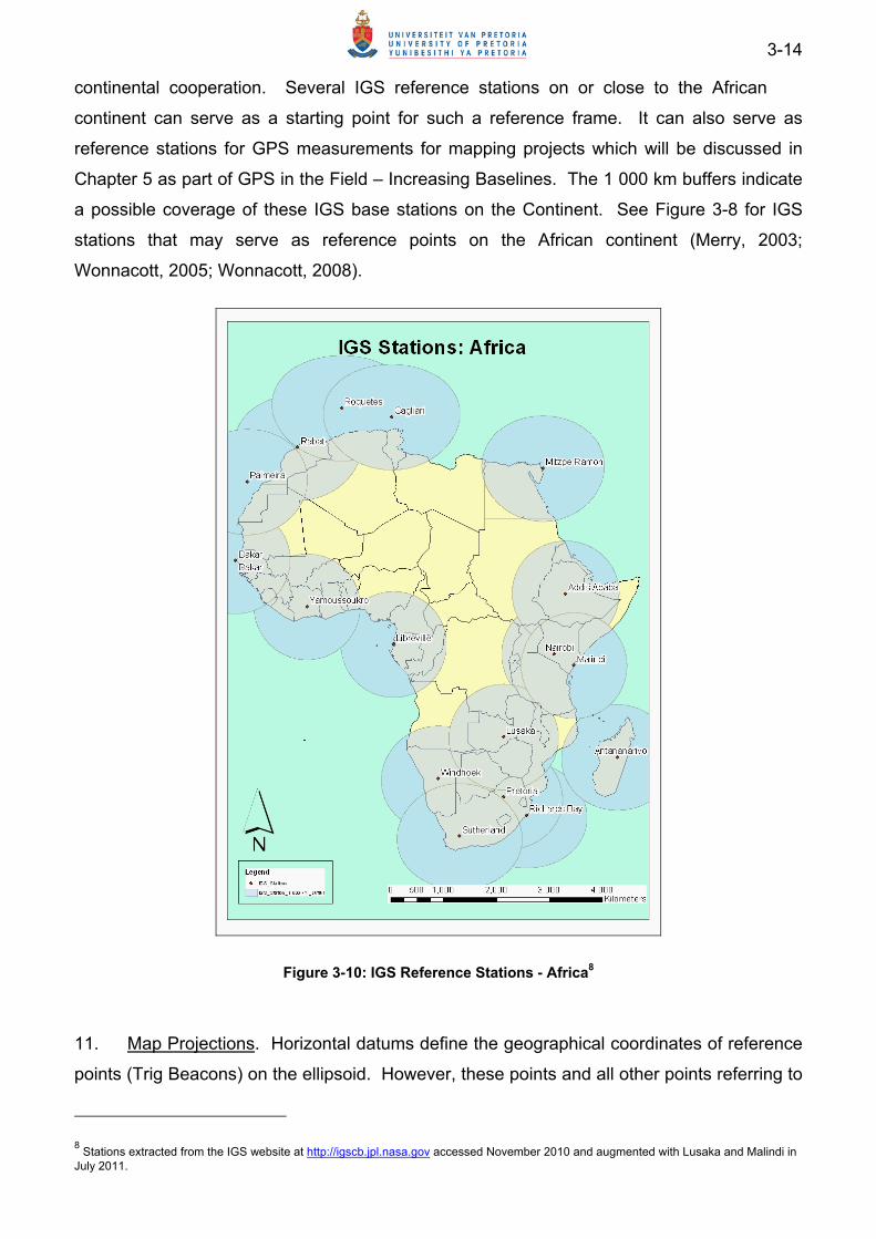
continental cooperation. Several IGS reference stations on or close to the African

continent can serve as a starting point for such a reference frame. It can also serve as

reference stations for GPS measurements for mapping projects which will be discussed in

Chapter 5 as part of GPS in the Field – Increasing Baselines. The 1 000 km buffers indicate

a possible coverage of these IGS base stations on the Continent. See Figure 3-8 for IGS

stations that may serve as reference points on the African continent (Merry, 2003;

Wonnacott, 2005; Wonnacott, 2008).

Figure 3-10: IGS Reference Stations - Africa8

11. Map Projections. Horizontal datums define the geographical coordinates of reference

points (Trig Beacons) on the ellipsoid. However, these points and all other points referring to

8 Stations extracted from the IGS website at http://igscb.jpl.nasa.gov accessed November 2010 and augmented with Lusaka and Malindi in

July 2011.

3-15

them need to be represented on a flat surface such as a map to be useful for positional

data in for example a command and control system. Map projections are the systematic

rendering of positions from the curved surface of the ellipsoid to a flat surface. This cannot

be accomplished without distortions in shape, area, distance or direction. Projections are

classified in terms of the particular properties they were designed to preserve and no

projection can solve more than two distortions. Projections are based on a developable

surface like a cylinder, cone or plane with a projection centre defined as orthographic (at

infinity), stereographic (at the antipode) or gnomonic (at ellipsoid centre). Map projections

can also be a mathematical method to project points from the ellipsoid onto a flat surface

(Bolstad, 2006: 88 – 94; Iliffe & Lot, 2008: 42 - 44).

12. Military Map Projections. In the military, conformal projections, such as the Mercator

projection, are used. The Mercator projection is a cylindrical projection where the cylinder is

tangent along the Equator. Along the Equator there will be no distortion. Each parallel is as

long as the Equator and distortion is therefore towards the poles. In the Transverse Mercator

projection the cylinder is rotated 90º and tangent with a chosen meridian, called the central

meridian. Along the central meridian distances will be true and distances within 3º from the

central meridian will be fairly accurate. Thus, by selecting a new central meridian for

projection at every 6º and merging these projections, a fairly accurate global projection can

be created, also referred to as the Universal Transverse Mercator Projection (UTM), which is

used in the SANDF. A scale factor of 0.9996 is applied across the projection zone. The

projection zones are limited to between 84º north and 80º south. The projection zones of the

UTM are numbered from 1 to 60 in an easterly direction with zone one starting at the 180º

West (International Datum Line). Thus, the central meridian for Zone 1 is 177º west and for

Zone 2 it is 171º west and so on. South Africa lies between zones 33 and 36. Where

operations are conducted within the borders of South Africa the maps of CDNGI are used.

These maps are based on the Gauss Conform projection that is a variant of the Transverse

Mercator projection that uses 2º zones centred on an uneven longitude starting at the 0º

meridian, for example 19º, 21º, 23º, etc. Both the orientation and the labels of the axes are

reversed to render a positive y value directed west and a positive x value is directed south.

The Mercator projection is used for maritime charts, while the Polar Stereographic projection

is used for the areas north of 84º north and south of 80º south (CDSM, 2010; Iliffe & Lot,

2008: 40 – 62; USDMA Technical Manual, 1996: 2-5 – 2-14).

13. Universal Transverse Mercator Grid System (UTM). The UTM was developed by the

NGA for the military as a universal metre coordinate system. In the UTM the globe is divided

in 60 zones, each 6º wide and is limited to an area between 84º North and 80º South that

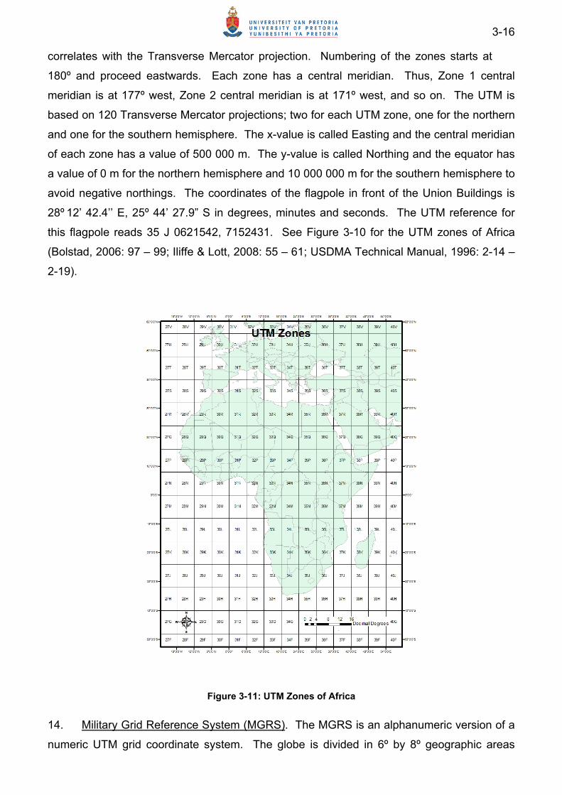
3-16

correlates with the Transverse Mercator projection. Numbering of the zones starts at

180º and proceed eastwards. Each zone has a central meridian. Thus, Zone 1 central

meridian is at 177º west, Zone 2 central meridian is at 171º west, and so on. The UTM is

based on 120 Transverse Mercator projections; two for each UTM zone, one for the northern

and one for the southern hemisphere. The x-value is called Easting and the central meridian

of each zone has a value of 500 000 m. The y-value is called Northing and the equator has

a value of 0 m for the northern hemisphere and 10 000 000 m for the southern hemisphere to

avoid negative northings. The coordinates of the flagpole in front of the Union Buildings is

28º 12’ 42.4’’ E, 25º 44’ 27.9” S in degrees, minutes and seconds. The UTM reference for

this flagpole reads 35 J 0621542, 7152431. See Figure 3-10 for the UTM zones of Africa

(Bolstad, 2006: 97 – 99; Iliffe & Lott, 2008: 55 – 61; USDMA Technical Manual, 1996: 2-14 –

2-19).

Figure 3-11: UTM Zones of Africa

14. Military Grid Reference System (MGRS). The MGRS is an alphanumeric version of a

numeric UTM grid coordinate system. The globe is divided in 6º by 8º geographic areas

3-17

called a grid zone with a unique alphanumeric identifier. Grid zones are subdivided into

100 km squares with each having a letter identifier. See Figure 3-11 for a presentation of the

MGRS Block of South Africa. To provide positional data the full MGRS reference need not

be used and can be adjusted according to accuracy requirements. The first part provides the

easting component and the second part provides the northing component of the position.

The MGRS values for the same flagpole are:

35J PM in a 100 km square

35J PM 25 in a 10 km square

35J PM 2152 in a 1 km square

35J PM 215524 in a 100 m square

35 J PM 21545243 in a 10 m square

35 J PM 2154252431 in a 1 m square

Figure 3-12: MGRS Blocks - South Africa

Both GPS receiver and Geographical Information System (GIS) packages can be used to

convert coordinates from degrees, minutes and seconds to UTM and MGRS values and the

3-18

other way around. Thus, the GPS receiver can be set to take coordinate measurements

in any of these formats9 (Bolstad, 2006: 97 – 98, USDMA, 1996: 3-1 – 3-5).

15. Concluding Remarks. With these few introductory remarks about reference systems it

is proposed that the SANDF standardise on using WGS84 (G1150) ellipsoid and that it

should also serve as the horizontal datum for positional data, including mapping projects on

the African continent. IGS reference stations can serve as reference points to assist in the

implementation of this approach. For operations on South African soil, map data from

CDNGI referenced to the HART94 datum will be used. The difference between the two is

small and should not pose any risk to operations. However, using older maps based on the

Cape Datum could have a shift of coordinate values of 300 m. It is further proposed that in

the absence of any tangible vertical datum for orthometric heights, EGM 2008 (or as

updated) is used and that these values are used for reporting heights in mapping projects on

the continent. The use of different coordinate systems such as decimal degrees, degrees-

minutes-seconds, UTM or MGRS should not be a problem. It only poses a challenge when

they are mixed in an operation where for instance the Air Force uses latitudes and

longitudes, while the Army is using MGRS. However, in close air support operations this is

addressed sufficiently in working procedures. The same approach as with horizontal data

should be applied in reporting heights. Normally heights are reported in metres above MSL

in mapping projects. However, the Air Force uses height measurements in feet. The user of

a GPS receiver in operations should therefore understand how to select the correct datum

(WGS84), the correct coordinate system applicable for the operation and the correct

measurement values, i.e. metres or feet. Officers in command of operations should ensure

that the use of the correct datum and measurement values are spelled out clearly in

operational orders.

POSITIONAL ACCURACY STANDARDS

16. Introduction. Paper maps and charts or digital map-data displays are used for

positional data in the SANDF. Navigating on foot or in vehicles in open terrain during

daytime may require positional accuracies in the range of 10 m to 50 m or even worse.

However, navigation during night-time in closed terrain may change this considerably,

especially if navigation should take place through minefields via cleared lanes, which will

require higher accuracies. Flying an aircraft at 35 000 ft from airport to airport will require

relative low accuracies, while landing that aircraft in low visibility conditions may require

positional data with a much higher accuracy. Similarly, navigation at sea may require 50 m

9 UTM zones and the MGRS blocks can be downloaded in shape file format from http://earth_info.nga.mil.

3-19

to 500 m horizontal positional accuracies depending on the application. Different

products and applications require different positional data accuracies.

17. Accuracy, Precision and Error Theory. The terms accuracy and precision are often

used interchangeably. However, there is an important difference between them. Precision is

the closeness of values obtained from replicate measurements. Accuracy is the closeness of

the average estimated value obtained compared to the true value. In mapping and GIS

projects one would strive to have high accuracy with a high level of precision as

demonstrated in Figure 3-12.

Figure 3-13: Accuracy and Precision

Notwithstanding the precision of the measuring receiver or method, the true value is an

unattainable goal. Understanding measuring errors will assist in determining a level of

certainty about the true value. Errors can be categorised in three classes; systematic,

random and blunders.

a. Blunders or Outliers. Blunders are incorrect measurements, such as

changing the x and y coordinates around, reading the coordinate values

incorrectly or receiver failures. Outliers differ considerably from the parent

population and are easily detected. Automated data transfer processes

between receivers and processing packages strive to minimise blunders.

However, they do occur from time to time and need to be explained and

eradicated. Blunders can be detected by averaging measurements and any

measurement larger than a pre-selected standard deviation from the mean is

rejected as not a valid part of the population – e.g. selecting three standard

deviations would result in the so called three sigma test.

Precision

Acc

ura

cy

Low High

Low

H

igh

3-20

b. Systematic Errors. Systematic errors are caused by small receiver

deviations or human limitations and are hard to detect with repeated

observations. They are constant and have the same sign causing a constant

bias. Often receivers that are not calibrated cause systematic errors.

Hardware and firmware problems in GPS receivers may cause systematic

errors. These errors can be detected by using different receivers with the

same or better precision characteristics to verify measurements. If the error

is known one can apply mathematical models to compensate for it.

c. Random Errors. Random errors are accidental or unknown influences on the

measurement that are beyond the control of the observer. They are

characterised by positive and negative errors occurring with equal frequency

and are normally small. Random errors are those errors that remain after

blunders and systematic errors are removed and are the cause that no true

value can be measured. However, they tend to display a normal frequency

distribution that enables the observer to predict that the random error will

probably not exceed a certain magnitude. Thus, it is possible to express a

measured value at a certain probable accuracy value and confidence level

(Allan, 2007: 59 – 76; USDMA, 1991: 1 - 7).

18. Accuracy and Scale. Accuracy should be placed in perspective when map data are

used. It should be remembered that one millimetre on a 250 k scale map or chart represents

250 m in reality. Producing and updating paper or digital maps and charts therefore require

a certain level of accuracy that needs to be adhered to in order to make them useful for

decision-making. Traditionally the Army has used the 50 k scale map as the tactical

operations map. The same map scale is used for close air support. In peace support

operations the Army is increasingly involved in urban operations that may require 10 k or

20 k scale maps. The 250 k scale maps are used for operational planning and control in the

Army, while it is also used for air support. The Air Force also use 500 k and 1 000 k scale

charts for navigation. The Navy uses 8 k to 15 k as harbour charts, while 20 k to 50 k is used

as approach charts and 150 k to 300 k is used for coastal and general navigation.

19. Accuracy Standards. The SANDF has no official positional accuracy standard. In

light of the large variations in positional accuracy requirements discussed above and the

absence of an official policy, it was accepted by Directorate Geospatial Information that

international standards should be followed in this regard. The following are proposed:

3-21

a. Topographic Maps and GIS Data. The Multinational Geospatial Co-

production Program (MGCP) which is an international military mapping

initiative proposes a 25 m circular error probability (CEP) at a 90%

confidence level as an accuracy standard for global mapping at 50 k and

100 k scales10. Twenty-eight defence forces worldwide are represented in

the MGCP, which includes some of the most significant role-players in the

field. It was therefore accepted that this proposed positional accuracy

standard should be adopted by the SANDF. This also creates a level of

interoperability when operations are conducted in cooperation with foreign

defence forces, as in peace support operations. For larger scale maps, such

as the 10 k and 20 k urban maps a higher accuracy level will be required.

The NGA prescribe a 12.5 m CEP at 90% confidence level in their Urban

Vector Map standard ((UVM) not available to the public). These accuracy

standards generally concur with the International Standards Organisations’

positional accuracy standard (ISO Standard 15046-13) and the Geospatial

Accuracy Standards of the Federal Geographic Data Committee of the

United States (FGDC, 1998).

b. Aeronautical Maps and Charts. The requirements of the International Civil

Aviation Organisation (ICAO) standards should be followed, as is applied to

aerodrome charts that require a horizontal accuracy of 2.5 m. See Appendix

C for more detail on this accuracy standard.

c. Hydrographical Charts. The SA Navy’s Hydrographical Office has to adhere

to the prescripts of the International Hydrographical Office (IHO) according to

international law. See Appendix C for more detail on this accuracy standard.

20. GPS as Navigational Aid. To attain these proposed accuracy standards accurate

source data are required. Currently the majority of landward mapping projects make use of

imagery as source data. Imagery needs to be orthorectified to render accurate positional

data and in most cases ground control is required for this process. Ground control is

currently obtained by means of GPS measurements. The Navy’s Hydrographical Office uses

depth soundings and other surveying techniques including GPS, to acquire source data for

navigational charts. Although maps and charts are still being used as primary sources for

positional data, GPS is gaining ground in a number of applications in the SANDF. The Army

10 The MGCP is a purely international military initiative and the standards are not available to the public.

3-22

plans to use GPS as a navigational tool for the infantry soldier. In the Air Force and the

Navy GPS is integrated with other onboard navigational instruments such as gyroscopes and

accelerators, to render an integrated positional solution via a Kalman filter. The continued

improvement of the accuracy and reliability of GPS makes it an attractive solution as a

primary source for positional data (Collinson, 2003: 314 – 322, Discussions with system

owners/users and specialists in the SANDF during April 2009).

21. Concluding Remarks. Without any official policy statement in the SANDF on

positional accuracy, it should be concluded that international military standards used by the

Multinational Geospatial Co-production Programme and the NGA should be used for general

topographic mapping projects on the African continent. It should be augmented in the

aeronautical and nautical environments by standards from the International Civil Aviation

Organisation and the International Hydrographical Office as applicable. Most GPS receivers

provide higher positional accuracies than can be presented on a map or chart. However,

care should be taken to understand the accuracy capabilities of a specific receiver used in

the field. This will be discussed in more detail.

CHAPTER 4: GPS FUNDAMENTALS

INTRODUCTION

1. In 1973 the Joint Programme Office of the Space and Missile Centre was

commissioned by the United States Department of Defence to establish an all-weather

space-based positioning system. The present Navigation System with Timing and Ranging

(NAVSTAR) Global Positioning System (GPS) is a result of this instruction. GPS is therefore

a navigation system designed and built for military use. However, over time the civilian

applications of GPS exceeded the military applications in the number of users by far. The

design and operations of the GPS consist of three main components, namely the space

segment, control segment and the user segment. Currently the GPS Wing of the United

States Air Force is managing and operating the space and control segments of the GPS.

The GPS signal and time play significant roles in positioning and will be discussed

separately. Aspects that influence the accuracy of GPS measurements will receive special

attention, including selective denial or jamming. The planned modernisation of GPS will be

mentioned with possible implications for the SANDF.

OPERATIONAL ASPECTS

2. Space Segment

a. At least twenty-four NAVSTAR satellites orbit the earth in six earth-centred

orbital planes with four satellites in each plane. The orbits are nearly circular

at a 55º inclination relative to the equatorial plane. Satellites are evenly

spaced in the orbital plane. The orbital radius is approximately 26 600 km

from the earth’s centre. Satellites travel at an approximate speed of 3.9 km/s

and orbit the earth every 12 h sidereal time, which correlates with 11 h and

58 min solar time and causes satellites to appear four minutes earlier every

day. This placement of satellites ensures that there are at least six satellites

above the horizon at any moment and at any place on earth (Hofmann-

Wellenhof et al., 2001: 14 – 13; Leick, 2004: 72 – 73; Kaplan & Hegarty,

2006: 69).

b. There are different ways GPS satellites can be identified. One way is to

identify each orbit with a letter A, B, C, etc. and each satellite in the orbit with

a number 1, 2, 3 and 4. A satellite can then be referred to as D2. Another

system is to refer to a satellite’s space vehicle number (SVN) assigned by

the NAVSTAR programme. A third way is to use the pseudorandom noise

(PRN) code of the satellite that is used by the GPS receiver to identify the

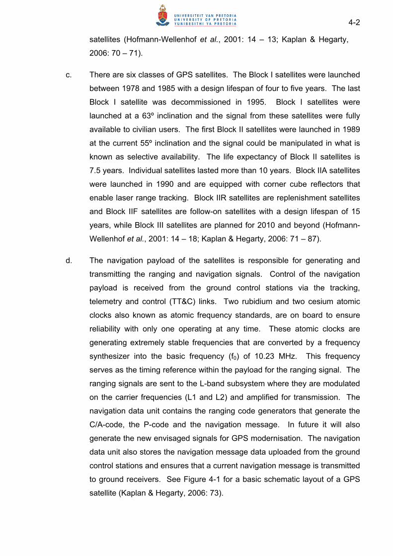
4-2

satellites (Hofmann-Wellenhof et al., 2001: 14 – 13; Kaplan & Hegarty,

2006: 70 – 71).

c. There are six classes of GPS satellites. The Block I satellites were launched

between 1978 and 1985 with a design lifespan of four to five years. The last

Block I satellite was decommissioned in 1995. Block I satellites were

launched at a 63º inclination and the signal from these satellites were fully

available to civilian users. The first Block II satellites were launched in 1989

at the current 55º inclination and the signal could be manipulated in what is

known as selective availability. The life expectancy of Block II satellites is

7.5 years. Individual satellites lasted more than 10 years. Block IIA satellites

were launched in 1990 and are equipped with corner cube reflectors that

enable laser range tracking. Block IIR satellites are replenishment satellites

and Block IIF satellites are follow-on satellites with a design lifespan of 15

years, while Block III satellites are planned for 2010 and beyond (Hofmann-

Wellenhof et al., 2001: 14 – 18; Kaplan & Hegarty, 2006: 71 – 87).

d. The navigation payload of the satellites is responsible for generating and

transmitting the ranging and navigation signals. Control of the navigation

payload is received from the ground control stations via the tracking,

telemetry and control (TT&C) links. Two rubidium and two cesium atomic

clocks also known as atomic frequency standards, are on board to ensure

reliability with only one operating at any time. These atomic clocks are

generating extremely stable frequencies that are converted by a frequency

synthesizer into the basic frequency (f0) of 10.23 MHz. This frequency

serves as the timing reference within the payload for the ranging signal. The

ranging signals are sent to the L-band subsystem where they are modulated

on the carrier frequencies (L1 and L2) and amplified for transmission. The

navigation data unit contains the ranging code generators that generate the

C/A-code, the P-code and the navigation message. In future it will also

generate the new envisaged signals for GPS modernisation. The navigation

data unit also stores the navigation message data uploaded from the ground

control stations and ensures that a current navigation message is transmitted

to ground receivers. See Figure 4-1 for a basic schematic layout of a GPS

satellite (Kaplan & Hegarty, 2006: 73).

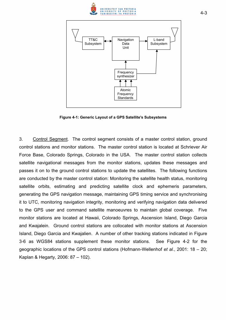
4-3

Figure 4-1: Generic Layout of a GPS Satellite's Subsystems

3. Control Segment. The control segment consists of a master control station, ground

control stations and monitor stations. The master control station is located at Schriever Air

Force Base, Colorado Springs, Colorado in the USA. The master control station collects

satellite navigational messages from the monitor stations, updates these messages and

passes it on to the ground control stations to update the satellites. The following functions

are conducted by the master control station: Monitoring the satellite health status, monitoring

satellite orbits, estimating and predicting satellite clock and ephemeris parameters,

generating the GPS navigation message, maintaining GPS timing service and synchronising

it to UTC, monitoring navigation integrity, monitoring and verifying navigation data delivered

to the GPS user and command satellite manoeuvres to maintain global coverage. Five

monitor stations are located at Hawaii, Colorado Springs, Ascension Island, Diego Garcia

and Kwajalein. Ground control stations are collocated with monitor stations at Ascension

Island, Diego Garcia and Kwajalien. A number of other tracking stations indicated in Figure

3-6 as WGS84 stations supplement these monitor stations. See Figure 4-2 for the

geographic locations of the GPS control stations (Hofmann-Wellenhof et al., 2001: 18 – 20;

Kaplan & Hegarty, 2006: 87 – 102).

Navigation Data Unit

Frequencysynthesizer

Atomic FrequencyStandards

L-band Subsystem

TT&C Subsystem

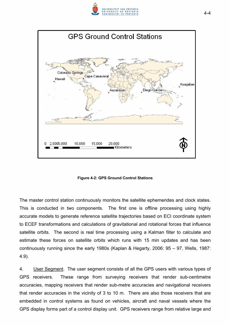
4-4

Figure 4-2: GPS Ground Control Stations

The master control station continuously monitors the satellite ephemerides and clock states.

This is conducted in two components. The first one is offline processing using highly

accurate models to generate reference satellite trajectories based on ECI coordinate system

to ECEF transformations and calculations of gravitational and rotational forces that influence

satellite orbits. The second is real time processing using a Kalman filter to calculate and

estimate these forces on satellite orbits which runs with 15 min updates and has been

continuously running since the early 1980s (Kaplan & Hegarty, 2006: 95 – 97, Wells, 1987:

4.9).

4. User Segment. The user segment consists of all the GPS users with various types of

GPS receivers. These range from surveying receivers that render sub-centimetre

accuracies, mapping receivers that render sub-metre accuracies and navigational receivers

that render accuracies in the vicinity of 3 to 10 m. There are also those receivers that are

embedded in control systems as found on vehicles, aircraft and naval vessels where the

GPS display forms part of a control display unit. GPS receivers range from relative large and

4-5

heavy receivers with external antennas to lightweight handhelds and are even found in

cellular phones and other small devices. GPS receivers can also be classified in terms of

their signal acquisition and processing capabilities. The following broad categories can be

established:

a. Receivers that track only the C/A-code on the L1 carrier signal. Most

navigational and recreational receivers are in this category.

b. Receivers that track the A/C- and P-codes on the L1 carrier signal and the P-

code on L2. These are military receivers that have the encryption keys to

use the P-code on L1 and L2 and are only available to the United States

military forces and its allies. When the P-code is encrypted with the W-code

it is denoted as the P(Y)-code.

c. Receivers that can track the C/A-code on the L1 carrier signal as well as the

L1 and the L2 carrier signals, which are known as carrier-phase

measurements. These are receivers that are used for mapping and

surveying solutions. Some of these receivers can also track the P(Y)-code

without decryption (Kaplan & Hegarty, 2006: 106).

5. Generic Receiver Layout. Different receivers have different processing capabilities.

However, a generic receiver will have multiple channels, normally 8 to 12, to allocate a

channel to each satellite that is tracked. The antenna receives the satellite signal that is

filtered and forwarded to a down-converter to be converted to an intermediate frequency.

Consequently the intermediate frequency is sampled and converted by an analogue-digital

converter. The sampled digital signal is forwarded to a digital signal processor that contains

the number of channels for the specific receiver. Each channel contains the code and carrier

tracking loops to perform code and carrier processing and demodulates the navigation

message. Depending on the type of receiver, each channel may compute up to three

different satellite-to-receiver measurements, namely pseudo-ranges, delta pseudo-ranges

and integrated Doppler. The computed range or phase measurements with the demodulated

navigation message are forwarded to the GPS processor that integrates with the

control/display unit. See Figure 4-3 for a basic generic layout of a GPS receiver (Hofmann-

Wellenhof et al., 2001: 79; Kaplan & Hegarty, 2006: 107– 108; Wells, 1987: 4.17).

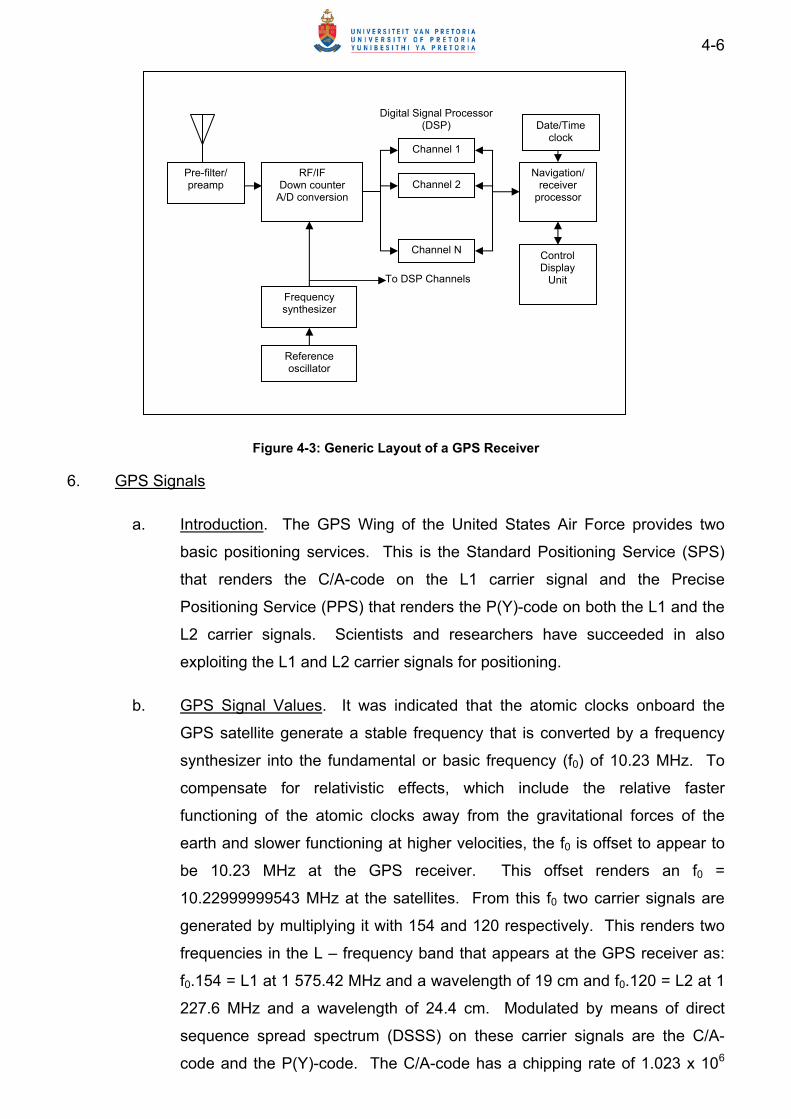
4-6

Figure 4-3: Generic Layout of a GPS Receiver

6. GPS Signals

a. Introduction. The GPS Wing of the United States Air Force provides two

basic positioning services. This is the Standard Positioning Service (SPS)

that renders the C/A-code on the L1 carrier signal and the Precise

Positioning Service (PPS) that renders the P(Y)-code on both the L1 and the

L2 carrier signals. Scientists and researchers have succeeded in also

exploiting the L1 and L2 carrier signals for positioning.

b. GPS Signal Values. It was indicated that the atomic clocks onboard the

GPS satellite generate a stable frequency that is converted by a frequency

synthesizer into the fundamental or basic frequency (f0) of 10.23 MHz. To

compensate for relativistic effects, which include the relative faster

functioning of the atomic clocks away from the gravitational forces of the

earth and slower functioning at higher velocities, the f0 is offset to appear to

be 10.23 MHz at the GPS receiver. This offset renders an f0 =

10.22999999543 MHz at the satellites. From this f0 two carrier signals are

generated by multiplying it with 154 and 120 respectively. This renders two

frequencies in the L – frequency band that appears at the GPS receiver as:

f0.154 = L1 at 1 575.42 MHz and a wavelength of 19 cm and f0.120 = L2 at 1

227.6 MHz and a wavelength of 24.4 cm. Modulated by means of direct

sequence spread spectrum (DSSS) on these carrier signals are the C/A-

code and the P(Y)-code. The C/A-code has a chipping rate of 1.023 x 106

Pre-filter/ preamp

RF/IF Down counter

A/D conversion

Frequency synthesizer

Reference oscillator

Channel 1

Channel 2

Channel N

Date/Time clock

Navigation/ receiver

processor

Control Display

Unit

Digital Signal Processor (DSP)

To DSP Channels

4-7

chips/s = 1.023 MHz and a chip length of 293 m. The P(Y)-code has a

chipping rate of 10.23 x 106 chips/s = 10.23 MHz and chip length of 29.3 m.

These codes are also known as the pseudorandom noise (PRN) codes or

ranging signals. See Table 4-1 for a tabular summary of GPS satellite signal

properties and Figure 4-4 for a geometric presentation of these signals

(Hofmann-Wellenhof et al., 2001: 71 – 76; Leick, 2004: 75 – 78; Kaplan &

Hegarty, 2006: 113 – 127; Merry, 2006: 29 – 30; Ashby, 2002).

Table 4-1: Summary of GPS Signal Components

S/N Component Factor Frequency: MHz Wavelength

1 Fundamental frequency f0 10.23

2 Carrier L1 F0 154 1 575.42 19.0 cm

3 Carrier L2 F0 120 1 227.60 24.4 cm

4 C/A-code F0/10 1.023

5 P(Y)-code f0 10.23

6 Navigation message F0/204 600 50.10-6

Figure 4-4: GPS Signal Structure

c. GPS Navigation Message. The C/A- and P(Y)-codes are both modulated

with a 50 bps navigation message that contains all the information to

Carrier Signal

Navigation Code

C/A-Code

P-Code

4-8

compute the precise location of every visible GPS satellite and the time of

transmission of the ranging signals. It is transmitted in five 300 bit sub-

frames with each having ten 30 bit words. Each sub-frame contains vital

information for positioning that include satellite accuracy and health, clock

correction terms, satellite ephemeris data, ionosphere and universal time

data and GPS almanac data (Hofmann-Wellenhof et al., 2001: 76 – 77;

Kaplan & Hegarty, 2006: 142 – 144; 6: 31).

d. PRN Code Structure. The DSSS modulation technique renders a digital

signalling scheme in which the carrier signal is either transmitted unchanged

or with a 180º phase shift over successive intervals depending on the code

structure of digital 0s or 1s. This renders a predictable signal pattern that

can be replicated by the GPS receiver.

e. C/A-code. Each satellite broadcasts a unique C/A-code at a 1 ms period that

repeats constantly. The GPS receiver is capable of generating a replica of

the received C/A-code. The receiver passes the replica C/A-code through

the tracking loop until it matches the received C/A-code from the satellite. If

the clocks of the satellite and the GPS receiver were perfectly synchronised,

the time it takes to shift the replica C/A-code to synchronise with the satellite

code would have been the correct propagation time for the signal. However,

the GPS receiver clock will have a bias error from system time. Even the

highly accurate atomic clocks of the satellite have an offset from system

time. Thus, when the geometric satellite-to-receiver range is augmented with

the two time offsets and multiplied by the velocity (c) of the signal, it renders

a pseudo-range. How to overcome this uncertainty will be explained later.

See Figures 4-5 and 4-6 for sketches explaining the synchronisation of

satellite and GPS receiver signals (Hofmann-Wellenhof et al., 2001: 81 – 82;

Kaplan & Hegarty, 2006: 50 – 54; Merry, 2006: 29 – 30).

4-9

Figure 4-5: Synchronisation of Satellite and GPS Receiver Signals to Measure Time and Range

Figure 4-6: Satellite and Receiver Clock Offsets Calculated to Measure Time and Range

Where:

sT = System time at which the signal left the satellite

uT = System time at which the signal reached the receiver

t = Offset of the satellite clock from system time

ut = Offset of receiver clock from system time

sT t = Satellite clock reading at the time the signal left the satellite

u uT t = Receiver clock reading at the time the signal reached the receiver

Time

t

ut

sT sT t uT u uT t

t

Pseudo-range time equivalent

Satellite generated code

Code received from satellite

Receiver generated code

Receiver-generated replica code shifted

Code generated at t1 arrive at ∆t seconds

t t∆t

Geometric range time equivalent

4-10

Geometric range r u sc T T c t 4.1

Pseudo-range u u sc T t T t

u s uc T T c t t

ur c t t 4.2

f. P(Y)-code. The P(Y)-code is broken into 38 seven-day portions each

assigned to a different satellite which then only broadcasts that portion of the

code. The P(Y) does not repeat for 266 days. Each portion is assigned a

PRN number that allows the GPS receiver to identify it. The encrypted P(Y)-

code requires decryption keys to use it for positioning. This is only available

to the United States military and its allies (Kaplan & Hegarty, 2006: 50;

Merry, 2006: 30).

7. Signal Propagation. The GPS signals travel at the approximate speed of light which is

299 792 458 m/s. The different GPS signals travel as a group at slightly different velocities

which are differently refracted when travelling through the ionosphere. However, as

indicated earlier, the navigation message has embedded correction data for this refraction

(Kaplan & Hegarty, 2006: 309).

8. Code Pseudo-ranging. Knowing that the satellites are in orbits 26 600 km from the

earth centre, and knowing that each satellite is broadcasting omni-directional signals (as

seen by the receiver, but in fact directional from the satellite with an antenna gain of 13dBi)

which travel at the velocity of light, one can create a solution to determine position. With a

single satellite the receiver could be at any place on the arc of the pseudo-range explained

above. With two satellites two pseudo-range intersections are created, one close to the

earth’s surface and another far away into space. With a third satellite a pseudo-range

intersection is created that is a close approximation of the receiver position. To determine

the true position one has to start with the previous equation (4.2) for pseudo-range,

r c tu t . However, we know that the satellite clocks are synchronised to Co-

ordinated Universal Time (UTC) and that clock corrections are broadcasted as part the

navigation message. Although there is still a satellite clock error to be corrected, it is

marginally small and can be ignored for this argument. Thus, equation 4.2 can be rewritten

for this argument to ur c t . To solve this equation simultaneous pseudo-range

4-11

measurements to four satellites are made to solve the four uncertainties, xu, yu, xu and

c.tu resulting in a system of equations as shown in Figure 4-7:

Figure 4-7: Ranging from four Satellites

1 = 2 2 2

1 1 1( ) ( ) ( ) .u u u ux x y y z z c t

2 = 2 2 2

2 2 2( ) ( ) ( ) .u u u ux x y y z z c t

3 = 2 2 2

3 3 3( ) ( ) ( ) .u u u ux x y y z z c t

4 = 2 2 2

4 4 4( ) ( ) ( ) .u u u ux x y y z z c t 4.3

Where x 1- 4, y 1- 4 and z 1- 4 represent the three-dimensional positions of the satellites 1 – 4.

When the four satellites are observed simultaneously, the four uncertainties can be resolved,

which will render a position with a resolution of approximately 1% of the signal chip length.

For measurements with the C/A-code this could be in the vicinity of 3 m. However, a number

of external influences (which will be discussed) will impact on this measurement (Hofmann-

Wellenhof et al., 2001: 87 – 88; Leick, 2004: 170 – 174; Kaplan & Hegarty, 2006: 54; Merry,

2006: 24 – 32).

9. Carrier-Phase Ranging

a. Measuring Carrier-Phase. As indicated, GPS was designed to use coded

pseudo-range measurements. For surveying this approach results in

accuracies that are too low. Researchers and scientists found a way to use

12 3

4

4-12

the carrier signals with much shorter wavelengths (L1 = 19 cm and L2 =

24.4 cm) to provide sub-centimetre accuracies. Switching on a GPS receiver

at any given epoch ( 0t ) the instantaneous fractional phase ( 0 ) of the carrier

signal is measured by means of the Doppler frequency offset and is derived

from the carrier-phase tracking loop of the receiver. For each following

epoch ( 1t ) the value of the previous epoch ( 0t ) plus the advance in phase

( 1 ) during the current epoch is measured by the receiver. See Figure 4-8

for a geometrical interpretation of the phase ranging. The number of full

signal cycles between the satellite and the receiver is unknown and hence

the integer cycle ambiguity (N) which needs to be treated as an unknown.

However, when tracking is continued without loss of lock on the satellite, the

N remains the same. Again the range represents the distance between the

satellite at epoch sT and uT at the receiver. The phase of the carrier can be

measured to better than 0.01 cycles which corresponds to millimetre

accuracies (Hofmann-Wellenhof et al., 2001: 89 – 90; Kaplan & Hegarty,

2006: 399 – 401; Merry, 2006: 53 – 55; Wells, 19987: 3.5 & 4.15).

4-13

Figure 4-8: Measuring Time and Range with Carrier Signals

b. Solving Cycle Ambiguity. A variety of techniques are used to solve cycle

ambiguity, such as using the pseudo-range measurement to approximate the

extent of the ambiguity, augmenting it with wide-lane and narrow-lane

measurements. Wide-lane is a technique using both carrier frequencies (L1

and L2) for tracking a satellite and subtracting the frequencies from each

other in order to render a wavelength of approximately 86 cm that is

significantly smaller to work with to solve the cycle ambiguity.

fwl = 1 575.42 – 1 227.6 = 347.82 MHz

wl = 86.25 cm 4.4ג

Research to improve the capacity of solving cycle ambiguity is continuing. It

is estimated that the addition of the L5 signal at 1 176.45 MHz will allow the

construction of an extra wide-lane metric which will enable a very rapid

ambiguity resolution. It is estimated that L5 will only be available in 2015.

However, when the cycle ambiguity is solved, it remains fixed in the solution

as long as the GPS receiver maintains lock on the satellite signal. When lock

N N N N

Ø1

Ø2

Ø3

t0

t1

t2

t3

4-14

is lost, called cycle slip, the cycle ambiguity needs to be resolved again.

Any object that may obstruct the line of sight between the receiver and the

satellite may cause a cycle slip (Kaplan & Hegarty, 2006: 401 – 418; School

of Surveying & Spatial Information Systems, 2010: Chapter 3).

10. Concluding Remarks. Different entities in the SANDF use different types of GPS

receivers as indicated earlier. Users should understand the capabilities of the specific

receiver and ensure that receivers procured are indeed capable of delivering the required

capabilities. However, the next section will discuss GPS measurement errors that will

highlight the capabilities and limitations of the different receivers further.

GPS MEASUREMENT: ERRORS AND BIASES

11. Introduction. A number of factors influence the accuracy of GPS measurements.

These can be categorised as those related to the satellite, such as clock and orbit errors and

satellite geometry, those related to the propagation of the GPS signal through the

atmosphere, sun activity and drag, and those related to the GPS receiver, including thermal

noise and clock drift. Some errors are related to obstructions at the point of measuring, for

instance multipathing. To put measurement errors in perspective, it should be remembered

that a delay of one millisecond translates to a 300 km pseudo-range error. For this reason

significant measures are taken to prevent them.

Satellite Clock Error. Satellite clocks that are used to generate the fundamental signal are

very stable as discussed earlier. These clocks are digitally synchronised because of inherent

offsets and linear drift over time. The master control centre monitors these clocks and

updates them with clock correction parameters that are rebroadcasted by the satellites as

part of the navigation message. Because these correction parameters are computed to

predict actual satellite clock errors, some residual errors remain. This may cause range

measurement errors in the order of 0.3 m to 4 m depending on the type of satellite and the

age of the correction parameters. The range errors will therefore be the smallest just after

the correction parameters were uploaded. At 24 h later the clock drift could cause

measurement errors of up to 4 m. Several other factors remain that may cause the clock to

be in error, including the inability of the master control centre to perfectly determine the clock

offset, the limited number of data bits in the navigation message to fully communicate the

predicted clock error and orbit ephemeris and the delay between the clock error estimate

upload and the time the satellite broadcasts the navigation message. Clock corrections are

available from GPS monitor networks such as the IGS that can be used to improve the

accuracy of measurements. Another assured way of minimising the effect of satellite clock

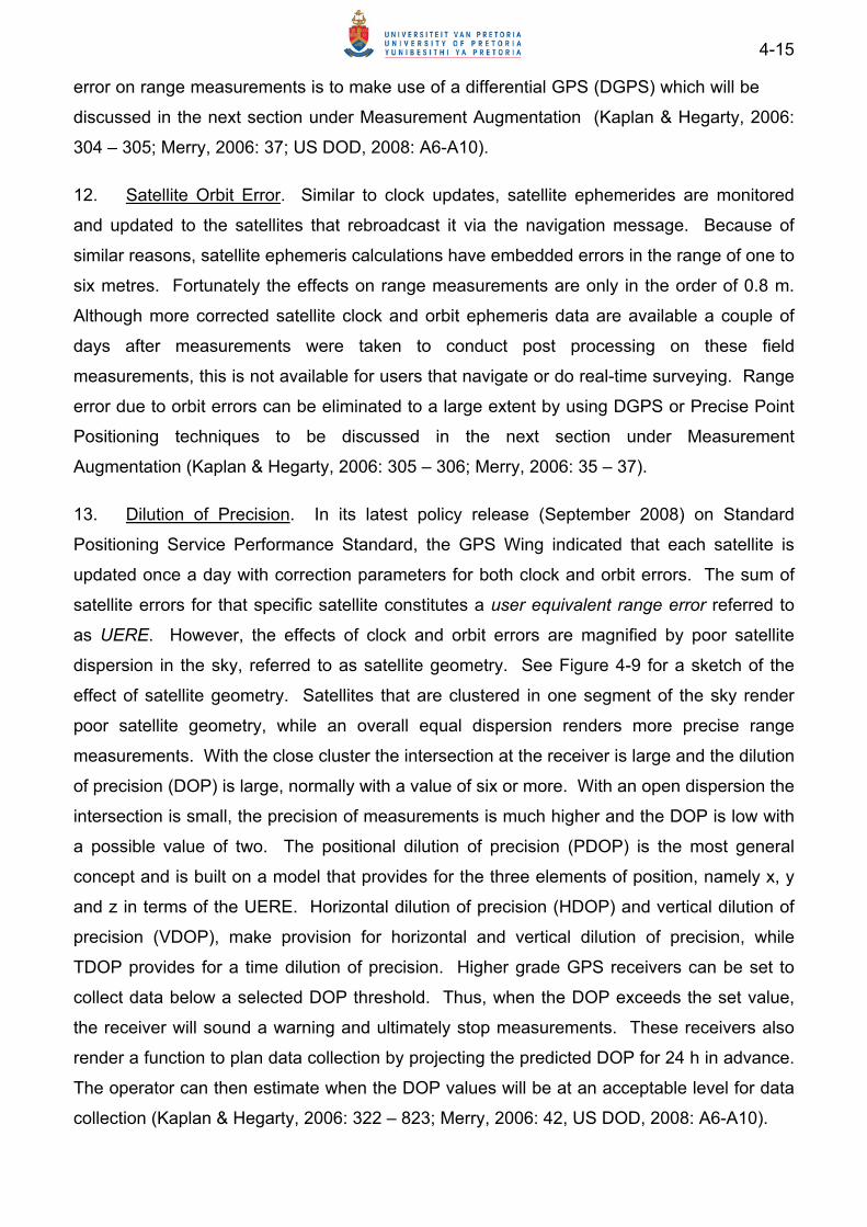
4-15

error on range measurements is to make use of a differential GPS (DGPS) which will be

discussed in the next section under Measurement Augmentation (Kaplan & Hegarty, 2006:

304 – 305; Merry, 2006: 37; US DOD, 2008: A6-A10).

12. Satellite Orbit Error. Similar to clock updates, satellite ephemerides are monitored

and updated to the satellites that rebroadcast it via the navigation message. Because of

similar reasons, satellite ephemeris calculations have embedded errors in the range of one to

six metres. Fortunately the effects on range measurements are only in the order of 0.8 m.

Although more corrected satellite clock and orbit ephemeris data are available a couple of

days after measurements were taken to conduct post processing on these field

measurements, this is not available for users that navigate or do real-time surveying. Range

error due to orbit errors can be eliminated to a large extent by using DGPS or Precise Point

Positioning techniques to be discussed in the next section under Measurement

Augmentation (Kaplan & Hegarty, 2006: 305 – 306; Merry, 2006: 35 – 37).

13. Dilution of Precision. In its latest policy release (September 2008) on Standard

Positioning Service Performance Standard, the GPS Wing indicated that each satellite is

updated once a day with correction parameters for both clock and orbit errors. The sum of

satellite errors for that specific satellite constitutes a user equivalent range error referred to

as UERE. However, the effects of clock and orbit errors are magnified by poor satellite

dispersion in the sky, referred to as satellite geometry. See Figure 4-9 for a sketch of the

effect of satellite geometry. Satellites that are clustered in one segment of the sky render

poor satellite geometry, while an overall equal dispersion renders more precise range

measurements. With the close cluster the intersection at the receiver is large and the dilution

of precision (DOP) is large, normally with a value of six or more. With an open dispersion the

intersection is small, the precision of measurements is much higher and the DOP is low with

a possible value of two. The positional dilution of precision (PDOP) is the most general

concept and is built on a model that provides for the three elements of position, namely x, y

and z in terms of the UERE. Horizontal dilution of precision (HDOP) and vertical dilution of

precision (VDOP), make provision for horizontal and vertical dilution of precision, while

TDOP provides for a time dilution of precision. Higher grade GPS receivers can be set to

collect data below a selected DOP threshold. Thus, when the DOP exceeds the set value,

the receiver will sound a warning and ultimately stop measurements. These receivers also

render a function to plan data collection by projecting the predicted DOP for 24 h in advance.

The operator can then estimate when the DOP values will be at an acceptable level for data

collection (Kaplan & Hegarty, 2006: 322 – 823; Merry, 2006: 42, US DOD, 2008: A6-A10).

4-16

Figure 4-9: Satellite Geometry - Dilution of Precision

14. Ionosphere

a. Introduction. The propagation speed of a wave can be expressed in terms of

the level of refraction of the medium it travels through. In a dispersive

medium such as the ionosphere, the propagation velocity of carrier signals

differs from the velocity of the signals carrying the signal information. Thus,

signals travel together in a group, but at slightly different velocities.

b. Influence of the Sun. The ionosphere is the dispersive medium located

between 70 km and a 1 000 km above the earth’s surface. The sun’s

ultraviolet rays ionise the gas molecules of the ionosphere, resulting in the

release of free electrons. These free electrons influence the propagation of

electromagnetic waves (GPS satellite signals). This ionospheric effect is

proportional to the total electron content (TEC), calculated from a cross-

section of a vertical 1 m2 column along the path of the signal. The TEC

fluctuates as a function of solar radiation, latitude, season and local time.

Values of TEC are dependent on solar radiation which reaches its peak at

midday and is at its lowest at midnight and early morning. These TEC

values are also a function of sunspot activity which has a 10 to 11 year cycle.

A number of sources predicted the lowest turning point for the current cycle

(24) to be during 2005. However, as can be seen from Figure 4-10, the

lowest turning point of cycle 24 was 2009 with the next predicted high during

2014. The ionospheric effect is higher for signals from satellites that are low

on the horizon and lower for satellites at zenith. It is therefore important to

eliminate measurements from satellites that are low on the horizon by setting

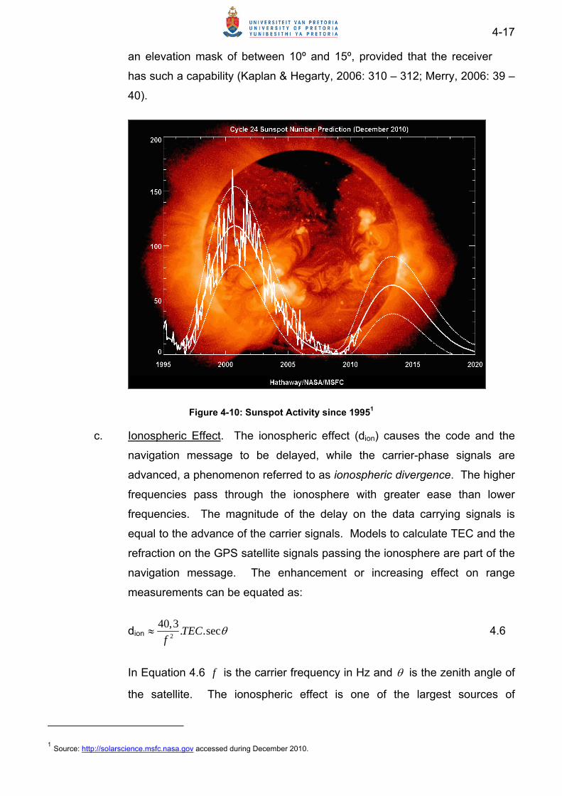
4-17

an elevation mask of between 10º and 15º, provided that the receiver

has such a capability (Kaplan & Hegarty, 2006: 310 – 312; Merry, 2006: 39 –

40).

Figure 4-10: Sunspot Activity since 19951

c. Ionospheric Effect. The ionospheric effect (dion) causes the code and the

navigation message to be delayed, while the carrier-phase signals are

advanced, a phenomenon referred to as ionospheric divergence. The higher

frequencies pass through the ionosphere with greater ease than lower

frequencies. The magnitude of the delay on the data carrying signals is

equal to the advance of the carrier signals. Models to calculate TEC and the

refraction on the GPS satellite signals passing the ionosphere are part of the

navigation message. The enhancement or increasing effect on range

measurements can be equated as:

dion 2

40,3. .secTEC

f 4.6

In Equation 4.6 f is the carrier frequency in Hz and is the zenith angle of

the satellite. The ionospheric effect is one of the largest sources of

1 Source: http://solarscience.msfc.nasa.gov accessed during December 2010.

4-18

measurement errors in a single frequency GPS receiver. However,

because the delay is frequency dependent, it is possible to eliminate its

effect almost completely by making range measurements with dual

frequency receivers. The dual frequency receiver can measure the time

difference between the propagation delays of the two frequencies. The

delay factor can then be used to correct the GPS measurements in

processing software. Unfortunately the P(Y)-code is not available to civilian

users. The new envisaged civilian signal L2C will enhance civilian GPS

receivers to neutralise the ionospheric effect. Currently civilian GPS

receivers that can use carrier-phase measurements on L1 and L2 are

required for this technique. With DGPS this effect can also be eliminated to

a large extent (Hofmann-Wellenhof et al., 2001: 99 – 106; Leick, 2004: 211 –

215; Kaplan & Hegarty, 2006: 310 – 312, Merry, 2006: 39).

15. Troposphere. The troposphere (dtrop) is the lower part of the atmosphere (40 km

above the earth) that is non-dispersive for electromagnetic frequencies up to 15 GHz. In the

troposphere carrier-phase frequencies and the data carrying frequencies are equally

delayed. This delay is dependent on the local temperature, pressure and humidity. The dry

component of the troposphere that extends to about 40 km above the earth, accounts for

almost 90% of the delay and can be predicted fairly accurately. The wet component extends

to about 10 km above the earth and is more unpredictable. Various models are used to

calculate the dry, wet and combined delaying effects of the troposphere on the GPS signals.

Variable models are used for measurements with signals from satellites at zenith, called

zenith delay, satellites low on the horizon called vertical delay and satellites at an arbitrary

elevation called slant delay. Signal delay is larger for signals from satellites on the horizon

relative to those at the zenith. A model to calculate dtrop can be equated as:

dtrop3 21255

2,27.10 0,05 tan secP eT

4.7

In Equation 4.7 P represents the atmospheric pressure, T is temperature in Kelvin, e is the

water vapour pressure and the zenith angle of the GPS satellite. The range error at sea

level can vary from about 2.4 m for measurements from satellites at zenith to 25 m for

satellites at an elevation of 5º above the horizon. It is therefore important to reject

measurements from satellites below a cut-off elevation. An elevation mask of between 10º

and 15º is proposed. Tropospheric delay can also be eliminated to a large extent by using

4-19

DGPS techniques (Hofmann-Wellenhof et al., 2001: 106 – 118; Kaplan & Hegarty, 2006:

314 – 319; Merry, 2006: 37 – 38).

16. GPS Signal Availability and Integrity

a. GPS satellites are placed in such a fashion that at least six satellites are

available at any place on earth at any time. However, this does not mean

that the placement of these satellites in the sky is such that it will deliver the

required PDOP at the required mask level for a required level of accuracy.

This unavailability may only last for a relative short time periods. Kaplan and

Hegarty tested and argued that with 24 satellites available and a mask level

of 7.5º and a PDOP threshold of 6.0 the GPS constellation provided a

99,98% availability. The maximum unavailability measured was only 10 min

at latitudes beyond 60º N and 60º S. In an estimate where two satellites

were removed from the constellation, coverage was 99,903% with

unavailability up to 25 min. However, with three satellites removed from the

constellation availability drops to 99.197% with unavailability up to 65 min. In

this scenario parts of Southern and Northern Africa will be affected (Kaplan &

Hegarty, 2006: 334 – 345).

b. Selective availability (SA) is something that remains in the mind of GPS

users. According to US military specifications the master control centre

should be able to adjust the fundamental frequency and therefore also the

code signals and the transmitted time. This may cause a horizontal range

error in the vicinity of 100 m and was intended to deny adversaries the use of

GPS in conflict. Selective availability was used during the Gulf War in 1991

but deactivated soon because more American troops used civilian receivers

than military ones and the GPS proved to be very useful for navigation in the

desert. It was officially deactivated on 2 May 2000 and will most probably not

be used again. Reasons for this are that SA can be neutralised with DGPS

and many life support systems including ambulances, shipping, aircraft and

large transport fleets navigate by GPS. Enabling SA may cause havoc. The

ability to apply selective denial or jamming has also improved lately and

allowed adversaries to manipulate or deny the use of GPS signals in the

theatre of operations. This will be discussed in more detail in paragraph 19

(Hofmann-Wellenhof et al., 2001: 15 – 20).

4-20

c. Although integrity anomalies will be rare, it is possible. It is for instance

not possible for the monitor stations to monitor all 24 satellites 24 h every

day. Thus, if any integrity issue occurs, it may take up to a few minutes for

the control centres to restore the situation and that may be too long for an

aviation solution. The clock failure that occurred on one of the GPS satellites

on 28 July 2001 can be cited as an incident of integrity failure (Kaplan &

Hegarty, 2006: 345 – 360).

17. Receiver Errors

a. Tracking Loops. Measurement errors are induced by receiver tracking loops

and may be one of the major sources of error measurements in stand-alone

GPS receivers.

b. Clock Errors. A receiver clock is normally a low accuracy quartz crystal

oscillator which re-initialises every time the receiver is switched on. However,

this is solved at every measurement epoch by using the received navigation

message for pseudo-range measurements and by double differencing for

carrier-phase measurements.

c. Antenna Phase Centre. A GPS antenna has a physical and electrical phase

centre. The physical centre can be measured. The electrical phase centre is

the point where the broadcasted GPS signal is received. Thus, this is the

actual point of measurement and it may deviate from the physical centre with

one to two centimetres. In navigational receivers this will have no relevant

effect, but for survey purposes it should be addressed. Using the same type

of antennas and orienting them in the same direction on the baseline may

minimise this effect. The antennas can also be calibrated, using a well

surveyed point (Hofmann-Wellenhof et al., 2001: 124 – 125, Kaplan &

Hegarty, 2006: 104 – 106, Merry, 2006: 42).

18. Signal Reflection and Shadowing. The reflection of GPS signals from nearby

surfaces, such as high-rise buildings or passing vehicles, causes the receiver to make

erroneous measurements, resulting from multipathing. On an aircraft the tail and wings may

cause multipathing. The reflected signal normally arrives at the receiver later than the direct

signal. When the delay is large, the receiver will be able to reject the reflected signals.

However, when the reflecting surface is close to the receiver antenna, the arrival time of the

reflected signals will arrive fractions of nanoseconds later at the receiver antenna; it will be

4-21

difficult for the receiver to discern between direct and reflected signals. Signals from

satellites low on the horizon tend to render more multipath measurements than satellites at

zenith. The two opposing requirements of using signals from low orbiting satellites to render

lower PDOPs and possible multipath measurements from the same low orbiting satellites

need to be balanced by setting appropriate mask levels for the prevailing circumstances.

The size of the multipath errors in tracking different satellites may be different and is difficult

to model due to the wide variety of circumstances that may cause multipathing. Shadowing

is when GPS signals are obstructed by objects, for instance foliage. Under thick tree cover

the shadowing effect may be so severe that a GPS receiver can only track reflected signals.

Multipathing and shadowing can not be corrected by DGPS as with other errors and biases.

Both the reference station and the rover station in a differential solution may record different

multipath measurements, which may cause larger errors than normal. Thus, both these

effects pose a serious challenge for making accurate measurements. An assured way to

prevent multipathing and shadowing is to avoid reflecting surfaces and obstructions, such as

foliage. In aircraft and vehicle mountings it may require reconstruction to remove reflective

surfaces or the use of absorbent materials. Antenna design, such as a choke ring design

and a built-in base plate that can prevent measurements with reflected signals can help to

prevent multipathing measurements. Another approach is to make measurements over a

longer time period. Satellite positions change over time and the multipathing effect will also

change, allowing averaging and therefore minimising of the multipath effect. Measurements

between 10 to 30 min may suffice for this purpose (Hofmann-Wellenhof et al., 2001: 125 –

131, Kaplan & Hegarty, 2006: 279 – 295, Merry, 2006: 41).

19. Selective Denial. Selective denial or jamming is a military concept and has to do with

interference applied to the reception of GPS satellite signals to deny an adversary the use of

GPS signals for positioning, navigation or timing. Two approaches can be followed. Use a

stronger signal in the same frequency band to disrupt the broadcasted GPS satellite signals

in a limited area of operations at the receiver. The other approach, also known as spoofing,

is to broadcast similar signals as the GPS satellites that can take over the adversary’s

receivers and gradually lead them astray. A limitation of both approaches is that the signals

come from mainly one direction and is dependent on line of sight. Dispersion of transmission

is also possible to some extent. Military receivers use null-steering antenna techniques to

make them jamming resistant. The exclusive use of the P(Y)-code for military receivers is

another approach to minimise chances of being jammed. The GPS signal level at the

receiver is in the vicinity of -130 dBm or -158.5 dBW. This is a relatively low level signal and

can therefore be jammed easily. Civilian receivers that use C/A-code and carrier signals are

not designed to withstand the application of jamming techniques. Jamming devices can be

4-22

bought on the open market and an Internet search will render numerous results2. There

is also the possibility of unintentional disruption of GPS satellite signals. Examples of typical

radiolocation services which could cause interference include air traffic control radars and

electronic aids for air navigation. These services transmit on frequency bands close to the

L2 frequency and the intended L5 frequency. It is inevitable that some of the out-of-band

energy from these signals in adjacent bands or energy resulting from the malfunctioning of

these transmitters will interfere with the reception of GPS receivers. There is even evidence

that television transmissions have disrupted GPS receiver functioning. GPS jammers can be

bought on the market for private use. Because the SANDF is using civilian type GPS

receivers, jamming is a very relevant challenge. This will be addressed in more detail in

Chapter 5 where the results of GPS jamming tests are discussed (Kaplan & Hegarty 2006:

243 – 248; US DOD, 2008: 7; Frossel & Olsen 2003; Richardson, 2003; Whitman, 2002;

Lekkerkerk 2008: 83 - 84).

20. GPS Modernisation. In January 1999 the United States government announced the

modernisation of GPS. Modernisation will include the addition of two new signals, L2C and

L5. The L2C signal will be available on the L2 frequency and is intended for non-safety of life

applications. The L5 signal at 1 176.45 MHz resides in the aeronautical radio navigation

band and is intended for the safety of life applications. The combination of the L1 and L5

signal will enhance aviation significantly. These signals will provide SPS users with more

accurate and quicker measurement capabilities. The additional signals will also improve

GPS robustness to interference. If one signal is experiencing interference, the receiver can

switch to another signal. It is envisaged that L2C will be available on the Block IIR satellites,

while L5 will be available on the Block IIF satellites. It is further envisaged that the Block III

satellites will be launched in 2013. The current worldwide economic situation may postpone

this programme. However, it is planned that upgrades will allow civilian users to acquire sub-

metre accuracies and provide higher signal power to meet military anti-jamming

requirements (Kaplan & Hegarty, 2006: 145 – 150).

21. Concluding Remarks. The SANDF uses exclusively civilian type GPS receivers.

More advanced receivers can be configured to mitigate certain errors in the measurements

by selecting satellites above a certain elevation, low signal to noise ratios and DOP levels,

while others can merely use factory settings. GPS modernisation will enable higher

accuracies with navigational type receivers that will be within the accuracy requirements for

2 http://www.tayx.co.uk/gmt10-gps-l1-l2-l5-jammer.html accessed in February 2009 is an example of a website that markets commercial

jammers.

4-23

mapping purposes. Other augmentation techniques that can further improve GPS

measurements will be discussed in the next section. However, it is relatively easy to jam any

civilian type GPS receiver and it poses a serious challenge for using GPS receivers as

navigational receivers in operations. It is beyond the scope of this study to address this

issue satisfactorily and requires additional research.

GPS MEASUREMENT AUGMENTATION

22. Introduction. Error measurements and biases caused by satellite and receiver

deficiencies and propagation media discussed above can be corrected by making use of two

broad augmentation techniques, namely DGPS and external sensors. DGPS in principle

utilises a GPS receiver located at a reference point with a known position to collect data that

is thereafter used to correct measurements of the roving GPS receiver. As the position of

the reference station is known, the extent of the errors measured are known and therefore

the “known error” for each epoch can be used to correct the measurements of the roving

receiver for each corresponding epoch. External sensors are used to collect satellite health

and propagation media data continuously in order to correct measurements taken with the

roving receiver. Two approaches can be followed to correct the measurements of the roving

receiver. Live data links, including radios or the Internet between the reference station (or

external sensor) and the roving receiver can be used to correct measurements on-the-fly.

The other approach is to collect data separately at both the reference station and the roving

receiver on a storage medium, such as a hard drive and conduct post-processing. These

approaches are termed kinematic and static solutions respectively.

23. DGPS. Two approaches can be followed, namely absolute and relative DGPS. With

absolute DGPS the coordinates of the reference or base station should be known to the

highest possible or required accuracy level in the same ECEF coordinate system that is

required for the roving GPS receiver. The deviations of measurements taken at the

reference station during the time of measurement can then be used to correct the

measurements taken with the roving receiver. With relative DGPS the coordinates of the

reference station may not be known that accurately, for instance in the case of DGPS

application to land on an aircraft carrier. A differential correction can be applied to both

pseudo-range and carrier-phase measurements. Pseudo-range measurements may render

solutions of sub-metre accuracies, while carrier-phase measurements may render sub-

centimetre accuracies. In order to conduct differential corrections, both the reference station

and the roving receiver should observe the same satellites simultaneously and

measurements should be taken over the same time period in order to ensure that common

errors are experienced. This places some constraints on the distance between the reference

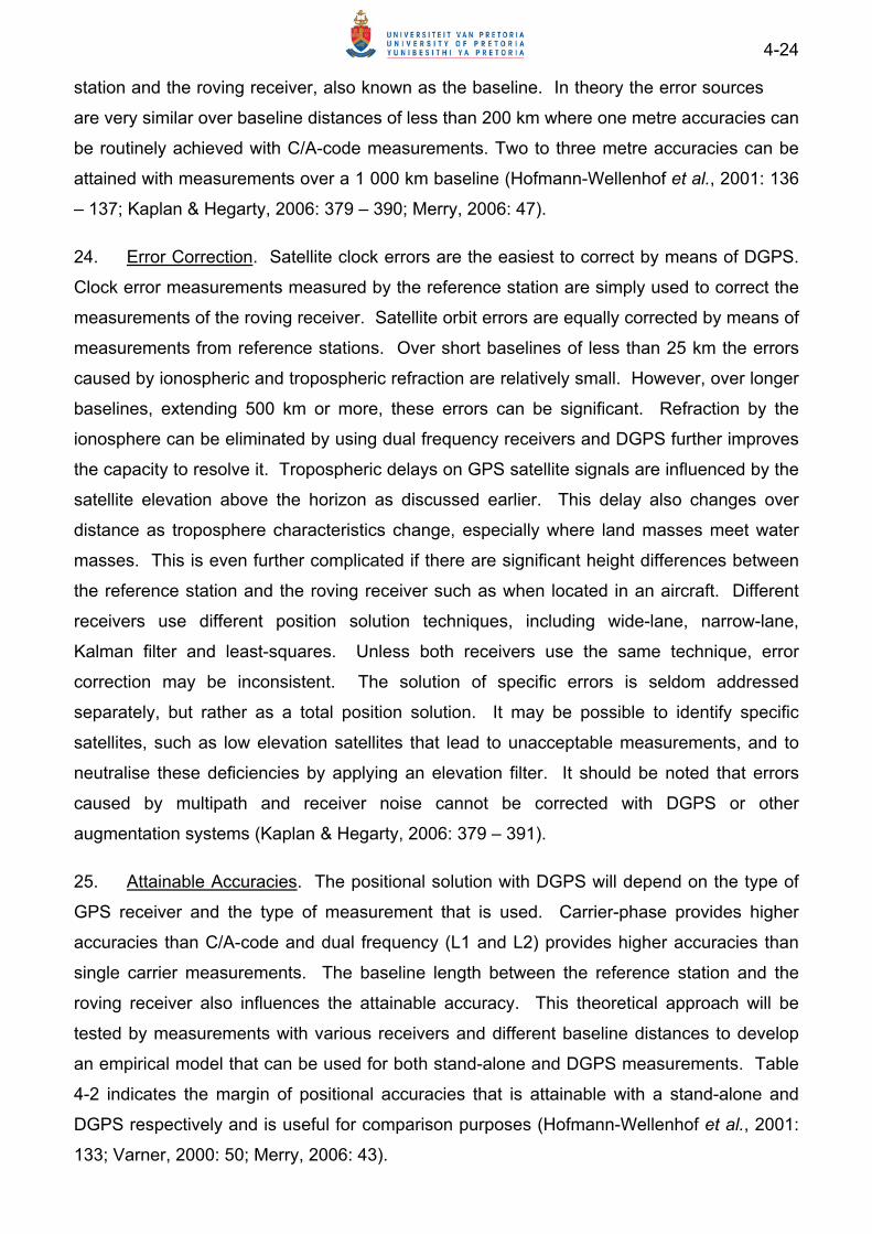
4-24

station and the roving receiver, also known as the baseline. In theory the error sources

are very similar over baseline distances of less than 200 km where one metre accuracies can

be routinely achieved with C/A-code measurements. Two to three metre accuracies can be

attained with measurements over a 1 000 km baseline (Hofmann-Wellenhof et al., 2001: 136

– 137; Kaplan & Hegarty, 2006: 379 – 390; Merry, 2006: 47).

24. Error Correction. Satellite clock errors are the easiest to correct by means of DGPS.

Clock error measurements measured by the reference station are simply used to correct the

measurements of the roving receiver. Satellite orbit errors are equally corrected by means of

measurements from reference stations. Over short baselines of less than 25 km the errors

caused by ionospheric and tropospheric refraction are relatively small. However, over longer

baselines, extending 500 km or more, these errors can be significant. Refraction by the

ionosphere can be eliminated by using dual frequency receivers and DGPS further improves

the capacity to resolve it. Tropospheric delays on GPS satellite signals are influenced by the

satellite elevation above the horizon as discussed earlier. This delay also changes over

distance as troposphere characteristics change, especially where land masses meet water

masses. This is even further complicated if there are significant height differences between

the reference station and the roving receiver such as when located in an aircraft. Different

receivers use different position solution techniques, including wide-lane, narrow-lane,

Kalman filter and least-squares. Unless both receivers use the same technique, error

correction may be inconsistent. The solution of specific errors is seldom addressed

separately, but rather as a total position solution. It may be possible to identify specific

satellites, such as low elevation satellites that lead to unacceptable measurements, and to

neutralise these deficiencies by applying an elevation filter. It should be noted that errors

caused by multipath and receiver noise cannot be corrected with DGPS or other

augmentation systems (Kaplan & Hegarty, 2006: 379 – 391).

25. Attainable Accuracies. The positional solution with DGPS will depend on the type of

GPS receiver and the type of measurement that is used. Carrier-phase provides higher

accuracies than C/A-code and dual frequency (L1 and L2) provides higher accuracies than

single carrier measurements. The baseline length between the reference station and the

roving receiver also influences the attainable accuracy. This theoretical approach will be

tested by measurements with various receivers and different baseline distances to develop

an empirical model that can be used for both stand-alone and DGPS measurements. Table

4-2 indicates the margin of positional accuracies that is attainable with a stand-alone and

DGPS respectively and is useful for comparison purposes (Hofmann-Wellenhof et al., 2001:

133; Varner, 2000: 50; Merry, 2006: 43).

4-25

Table 4-2: Attainable Accuracies with Stand-alone and DGPS

S/N Error Source Stand-alone GPS DGPS3

1 Satellite clock < 3 m Eliminated

2 Satellite orbit < 3 m 0.0 m

3 Tropospheric refraction < 1 m 0.0 m

4 Ionospheric refraction 5 – 10 m 0.0 m

26. Ground Based Augmentation Systems (GBAS). A variation of DGPS is the installation

of a network of permanent “base stations” that can be used for differential correction, using

both post-processing and on-the-fly correction. These augmentation systems can be very

small, such as those used at an airport for landing assistance. Larger systems are for

instance, networks that are used in a high activity area e.g. Gauteng, and national systems

such as the TrigNet system of CDNGI which provide coverage of South Africa. These

systems include a master station that integrates the measurements from the different

stations to provide network solutions. When the stations are dispersed as in the CDNGI

system, smaller networks are established within the larger system to render an area specific

solution, for instance for Cape Town, Gauteng and Durban. Various methods are used to

communicate the corrected measurements to the rover stations, including radio links or the

Internet (using cellular phones or other GPRS technologies) making use of Network

Transport of the Radio Technical Commission for Maritime Services (RTCM) via Internet

Protocol (NTRIP). Two approaches can be followed with a network DGPS. Firstly, one can

use an individual reference station in the network, normally the closest, to provide differential

corrected data to the rover receiver in real-time or using post-processing. The rover receiver

will always communicate via the control station to the reference station that implies a

fractional delay. The second method is to use a number of reference stations in which case

the master station or the rover receiver has to apply statistical weighting to the values from

the different reference stations, based on the distance from each station (Hofmann-

3 The quality of the receiver as well as the length of the baseline between the base and the roving receivers has an impact on the accuracy of measurements. This will be demonstrated with measurements values in Chapter Five.

4-26

Wellenhof et al., 2001: 137 – 138, Kaplan & Hegarty, 2006: 446 – 449, Merry, 2006: 47

– 50, 22).

27. Satellite Based Augmentation System (SBAS). A geostationary satellite can be used

to retransmit the differential corrections over a wider area. Two such systems are the wide

area augmentation system (WAAS) of the United States Federal Aviation Authority and the

European Geostationary Navigation Overlay System (EGNOS). They use multiple reference

stations (25 and 30 respectively) and also use multiple geostationary satellites rendering

large footprints. The entire United States and Canada are covered by WAAS, while EGNOS

provides complete coverage of Europe and Northern Africa. The aim of WAAS and EGNOS

is to improve measurements with stand-alone GPSs taking C/A-code measurements,

resulting in accuracies of less than 3 m. These services are not available in Southern Africa

and verification of measurements will thus not be possible. However, SBAS enabled

receivers can be used in Northern Africa to exploit the EGNOS signals. It is also foreseen

that the EGNOS signals may be deployed to cover South Africa and by implication also the

rest of Africa. Negotiations in this regard are still ongoing. There are also commercially

available SBAS services in Africa and South Africa, such as OMNISTAR. Utilisation of these

services involves purchasing a receiver with a decoder and subscribing to the service. The

service includes range correcting data and quality assurance in that the service provider can

use its reference stations to monitor the accuracy of the service. Accuracies of sub-metre

level are possible (Kaplan & Hegarty, 2006: 432 – 446; Merry, 2006: 50; Mireault, 2008;

Personal communication, E. Avenant, CSIR (SAC), 2009 ).

28. Precise Point Positioning (PPP). Precise Point Positioning is a technique developed

by the Jet Propulsion Laboratory (JPL) of NASA in the 1990s. Post-processing is not

conducted with measurements from a reference station, but the precise satellite clock and

orbit data provided by an external network, such as the IGS are used. The provided clock

and orbit predictions are used to conduct differential corrections with special software.

Because no reference station is used, the datum is hidden in the satellite coordinates. A

variation of this approach is to take measurements and convert them to receiver independent

exchange format (RINEX) and then to send it to a service provider such as AUSPOS,

SCOUT, Auto Gipsy or CSRS-PPP to conduct the corrections on your behalf. The data

correction is carried out in two ways:

a. Relative Positioning. Data from nearby stations are used with precise

ephemeris data to conduct differencing. The positions of the known

4-27

reference stations are treated as fixed at the epoch of observation

resulting in relative accuracies of one to two centimetres.4

b. Absolute Positioning. The precise ephemeris and clock corrections of the

satellites are used. The satellites’ positions are treated as fixed, leading to

two to five centimetre accuracies5.

One challenge is that the precise clock and orbit data are only available approximately two

weeks after the measurement. A rapid solution which can provide sub-decimetre accuracies

is available 90 min after measurement. Precise point positioning should be exploited as a

solution to render accurate measurements in areas where very few reference stations are

available or where reference stations cannot be placed (Kaplan & Hegarty, 2006: 449 – 454;

Merry, 2006: 74 – 75; Gao & Chen, 2004; Ovstedal et al., 2006; Mireault et al., 2008, King et

al.).

29. Concluding Remarks. Differential GPS can be used to improve GPS measurements

significantly and is used primarily in the mapping environment of the SANDF. Other possible

applications of DGPS are military surveying, demarcation of obstacles such as minefields,

target acquisition by special forces, the artillery and approaching of airfield in low visibility

conditions. In this case base or reference stations can be deployed at temporary airfields in

operations that could assist precision landings in low visibility conditions. This type of

implementation of DGPS would require radio assisted transmissions to facilitate receiving

correctional data from a base station and needs to be investigated by system owners as

required. Some mapping entities in the SANDF are or were using SBAS. Commercial SBAS

can be replaced by using (no subscription fees) the TrigNet system for post-processing or

real-time correction of field measurements. The possible deployment of the EGNOS signal

to Southern Africa should significantly improve the usability of navigational type GPS

receivers for mapping. Acquiring DGPS measurements elsewhere on the African continent

may require the deployment of additional base stations. Maximum baselines for these

measurements need to be investigated. Precise Point Positioning should also be

investigated as an alternative to correct field measurements taken beyond reasonable

baseline lengths. To collect sufficient ground control data for large mapping projects may be

a daunting task. This may require using data from navigational GPS measurements, this

4 The Australian Positioning Service can be accessed at http://www.ga.gov.au/geodesy/sgc/wwwgps/ .

5 The Canadian Spatial Reference System – Precise Point Positioning can be accessed at http://ess.nrcan.gc.ca/2002_2006/gnd/csrs_e.php.

4-28

being the only available alternative in some remote areas. The risk is that the accuracy

of these measurements is unknown. Therefore, attainable accuracies with navigational GPS

receivers and how to improve the accuracy need to be investigated. The earmarked

modernisation, especially the L2C code, may improve the accuracy of navigational GPS

receivers to the required level for mapping purposes. However, this will only be practical in

the future, as some time will elapse before a large number of GPS receivers that utilise the

new codes will be in the hands of travellers and adventurers who are the basis of this data

source.

CHAPTER 5: GPS IN THE FIELD – APPLICATIONS

INTRODUCTION

1. In order to confirm the attainable levels of precision and accuracy with different types

of GPS receivers a small network consisting of five points were laid out in the vicinity of Air

Force Base Waterkloof (AFBWK). These points were selected specifically to minimise

multipath and shadowing of GPS satellite signals. A further consideration was to select

stable points which would not be influenced significantly by weather and temperature

changes. The accessibility of these points for future use as calibration points was also

considered. For this purpose all points were placed on permanent building structures within

protected areas. Two points were located at Trig Beacons at Schanskop and Zwartkop.

Point No 2 at the reservoir at Radcliffe is close to a high-rise water tank that may cause

some multipath. The points were established by fixing self-centring-plates, provided by

HartRAO, with an adhesive onto the selected buildings. For the Trig Beacons 30 cm

antenna poles, provided by OPTRON Geomatics, were used.

2. The positions of the measuring points presented on an aerial photograph background

acquired by the SAC of the CSIR are displayed in Figure 5-1. Figure 5-2 and 5-3 indicate

distances of the network.

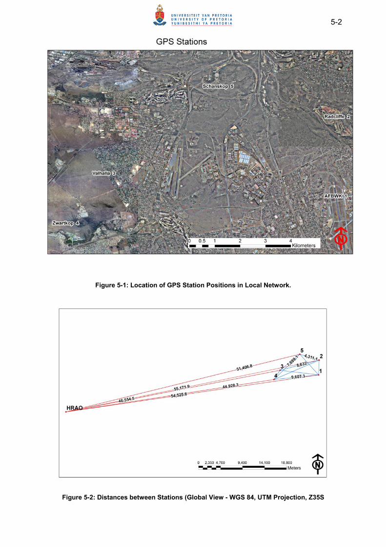
5-2

Figure 5-1: Location of GPS Station Positions in Local Network.

Figure 5-2: Distances between Stations (Global View - WGS 84, UTM Projection, Z35S

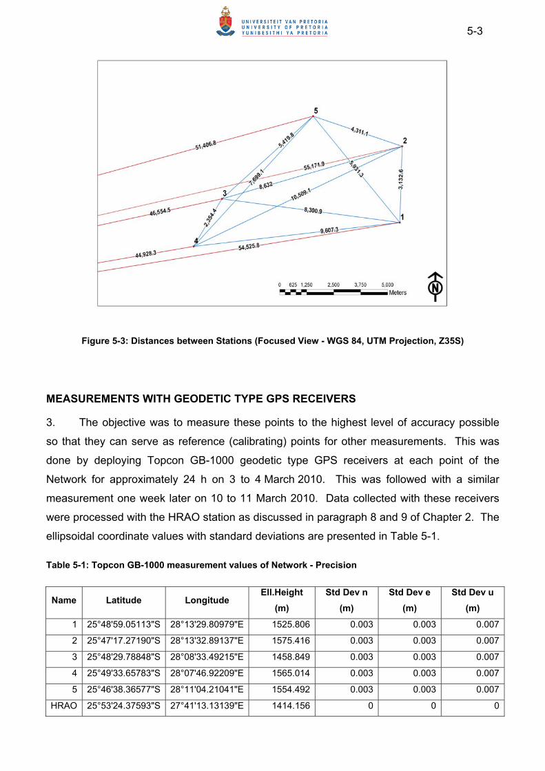
5-3

Figure 5-3: Distances between Stations (Focused View - WGS 84, UTM Projection, Z35S)

MEASUREMENTS WITH GEODETIC TYPE GPS RECEIVERS

3. The objective was to measure these points to the highest level of accuracy possible

so that they can serve as reference (calibrating) points for other measurements. This was

done by deploying Topcon GB-1000 geodetic type GPS receivers at each point of the

Network for approximately 24 h on 3 to 4 March 2010. This was followed with a similar

measurement one week later on 10 to 11 March 2010. Data collected with these receivers

were processed with the HRAO station as discussed in paragraph 8 and 9 of Chapter 2. The

ellipsoidal coordinate values with standard deviations are presented in Table 5-1.

Table 5-1: Topcon GB-1000 measurement values of Network - Precision

Name Latitude Longitude Ell.Height

(m)

Std Dev n

(m)

Std Dev e

(m)

Std Dev u

(m)

1 25°48'59.05113"S 28°13'29.80979"E 1525.806 0.003 0.003 0.007

2 25°47'17.27190"S 28°13'32.89137"E 1575.416 0.003 0.003 0.007

3 25°48'29.78848"S 28°08'33.49215"E 1458.849 0.003 0.003 0.007

4 25°49'33.65783"S 28°07'46.92209"E 1565.014 0.003 0.003 0.007

5 25°46'38.36577"S 28°11'04.21041"E 1554.492 0.003 0.003 0.007

HRAO 25°53'24.37593"S 27°41'13.13139"E 1414.156 0 0 0

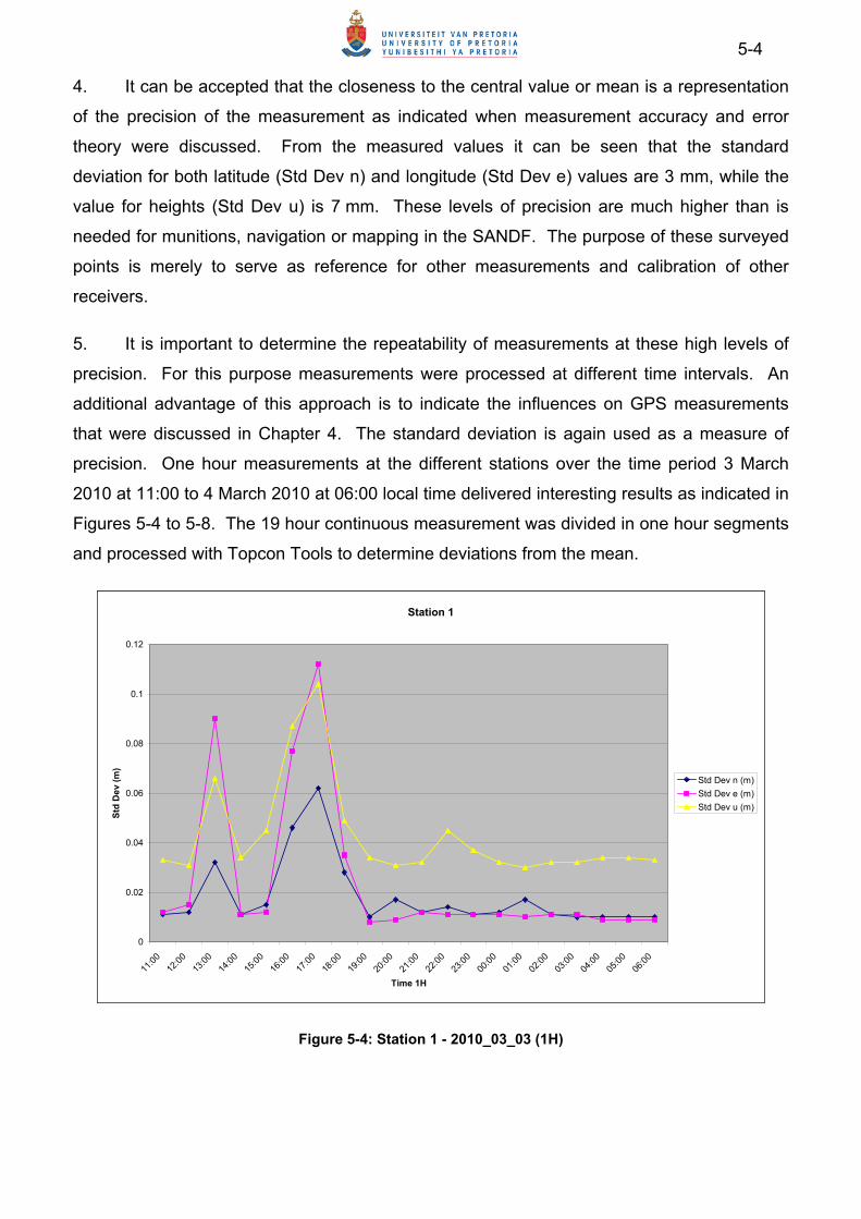
5-4

4. It can be accepted that the closeness to the central value or mean is a representation

of the precision of the measurement as indicated when measurement accuracy and error

theory were discussed. From the measured values it can be seen that the standard

deviation for both latitude (Std Dev n) and longitude (Std Dev e) values are 3 mm, while the

value for heights (Std Dev u) is 7 mm. These levels of precision are much higher than is

needed for munitions, navigation or mapping in the SANDF. The purpose of these surveyed

points is merely to serve as reference for other measurements and calibration of other

receivers.

5. It is important to determine the repeatability of measurements at these high levels of

precision. For this purpose measurements were processed at different time intervals. An

additional advantage of this approach is to indicate the influences on GPS measurements

that were discussed in Chapter 4. The standard deviation is again used as a measure of

precision. One hour measurements at the different stations over the time period 3 March

2010 at 11:00 to 4 March 2010 at 06:00 local time delivered interesting results as indicated in

Figures 5-4 to 5-8. The 19 hour continuous measurement was divided in one hour segments

and processed with Topcon Tools to determine deviations from the mean.

Station 1

0

0.02

0.04

0.06

0.08

0.1

0.12

11:0

012

:00

13:0

014

:00

15:0

016

:00

17:0

018

:00

19:0

020

:00

21:0

022

:00

23:0

000

:00

01:0

002

:00

03:0

004

:00

05:0

006

:00

Time 1H

Std

Dev

(m

)

Std Dev n (m)

Std Dev e (m)

Std Dev u (m)

Figure 5-4: Station 1 - 2010_03_03 (1H)

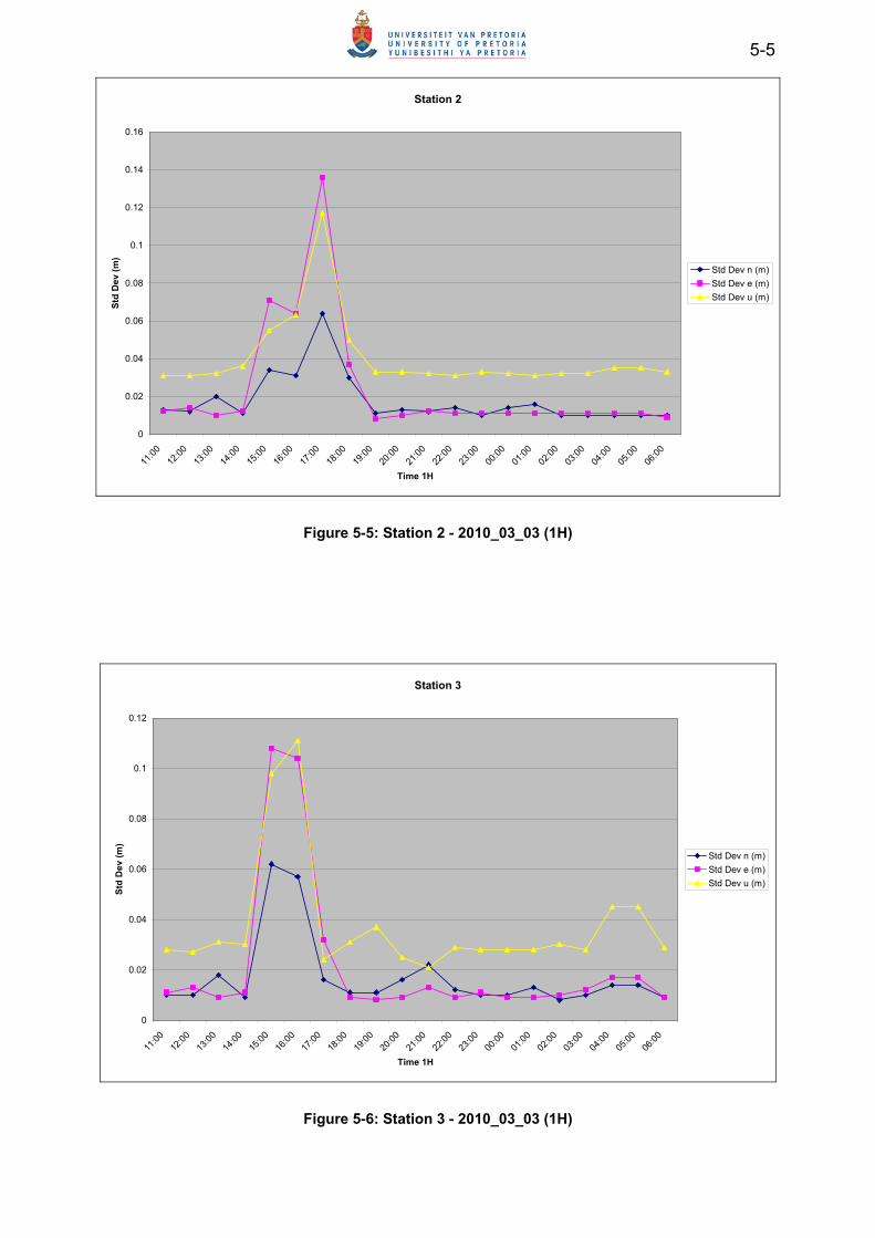
5-5

Station 2

0

0.02

0.04

0.06

0.08

0.1

0.12

0.14

0.16

11:0

012

:00

13:0

014

:00

15:0

016

:00

17:0

018

:00

19:0

020

:00

21:0

022

:00

23:0

000

:00

01:0

002

:00

03:0

004

:00

05:0

006

:00

Time 1H

Std

Dev

(m

)

Std Dev n (m)

Std Dev e (m)

Std Dev u (m)

Figure 5-5: Station 2 - 2010_03_03 (1H)

Station 3

0

0.02

0.04

0.06

0.08

0.1

0.12

11:0

012

:00

13:0

014

:00

15:0

016

:00

17:0

018

:00

19:0

020

:00

21:0

022

:00

23:0

000

:00

01:0

002

:00

03:0

004

:00

05:0

006

:00

Time 1H

Std

Dev

(m

)

Std Dev n (m)

Std Dev e (m)

Std Dev u (m)

Figure 5-6: Station 3 - 2010_03_03 (1H)

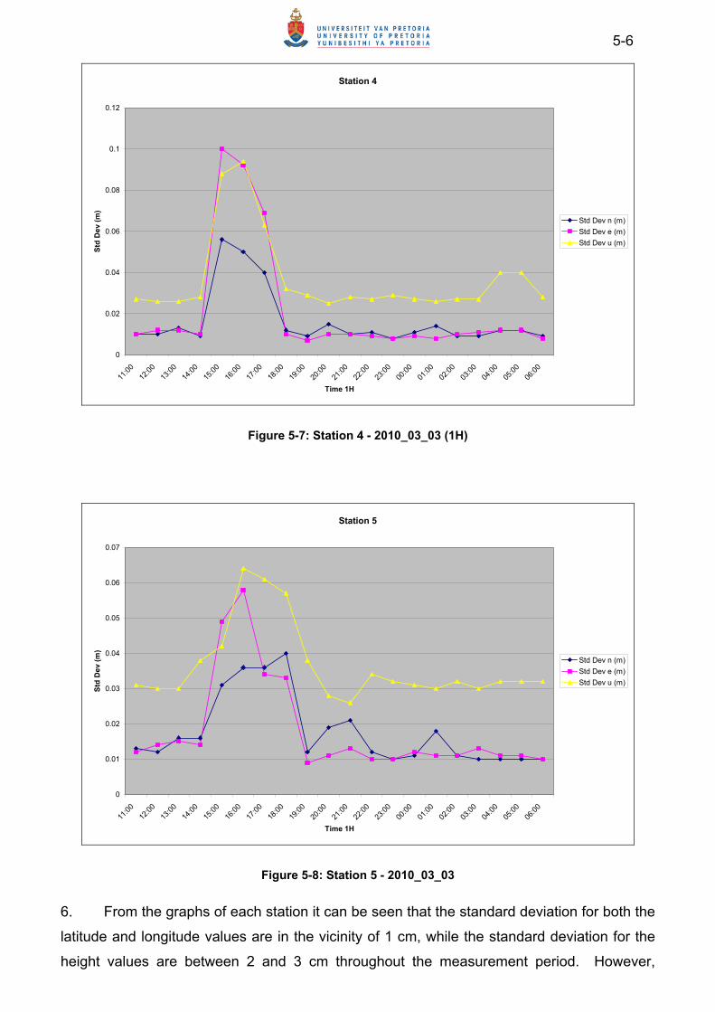
5-6

Station 4

0

0.02

0.04

0.06

0.08

0.1

0.12

11:0

012

:00

13:0

014

:00

15:0

016

:00

17:0

018

:00

19:0

020

:00

21:0

022

:00

23:0

000

:00

01:0

002

:00

03:0

004

:00

05:0

006

:00

Time 1H

Std

Dev

(m

)

Std Dev n (m)

Std Dev e (m)

Std Dev u (m)

Figure 5-7: Station 4 - 2010_03_03 (1H)

Station 5

0

0.01

0.02

0.03

0.04

0.05

0.06

0.07

11:0

012

:00

13:0

014

:00

15:0

016

:00

17:0

018

:00

19:0

020

:00

21:0

022

:00

23:0

000

:00

01:0

002

:00

03:0

004

:00

05:0

006

:00

Time 1H

Std

Dev

(m

)

Std Dev n (m)

Std Dev e (m)

Std Dev u (m)

Figure 5-8: Station 5 - 2010_03_03

6. From the graphs of each station it can be seen that the standard deviation for both the

latitude and longitude values are in the vicinity of 1 cm, while the standard deviation for the

height values are between 2 and 3 cm throughout the measurement period. However,

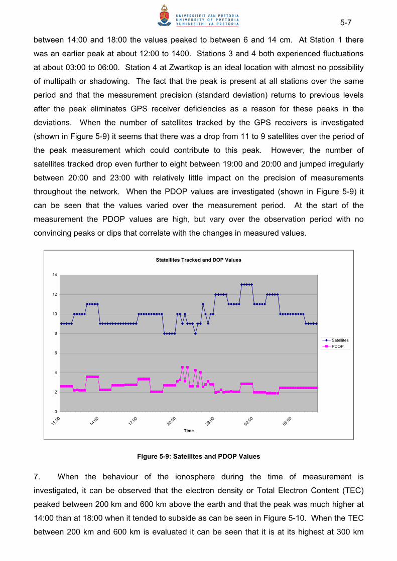
5-7

between 14:00 and 18:00 the values peaked to between 6 and 14 cm. At Station 1 there

was an earlier peak at about 12:00 to 1400. Stations 3 and 4 both experienced fluctuations

at about 03:00 to 06:00. Station 4 at Zwartkop is an ideal location with almost no possibility

of multipath or shadowing. The fact that the peak is present at all stations over the same

period and that the measurement precision (standard deviation) returns to previous levels

after the peak eliminates GPS receiver deficiencies as a reason for these peaks in the

deviations. When the number of satellites tracked by the GPS receivers is investigated

(shown in Figure 5-9) it seems that there was a drop from 11 to 9 satellites over the period of

the peak measurement which could contribute to this peak. However, the number of

satellites tracked drop even further to eight between 19:00 and 20:00 and jumped irregularly

between 20:00 and 23:00 with relatively little impact on the precision of measurements

throughout the network. When the PDOP values are investigated (shown in Figure 5-9) it

can be seen that the values varied over the measurement period. At the start of the

measurement the PDOP values are high, but vary over the observation period with no

convincing peaks or dips that correlate with the changes in measured values.

Statellites Tracked and DOP Values

0

2

4

6

8

10

12

14

11:0

014

:00

17:0

020

:00

23:0

002

:00

05:0

0

Time

Satellites

PDOP

Figure 5-9: Satellites and PDOP Values

7. When the behaviour of the ionosphere during the time of measurement is

investigated, it can be observed that the electron density or Total Electron Content (TEC)

peaked between 200 km and 600 km above the earth and that the peak was much higher at

14:00 than at 18:00 when it tended to subside as can be seen in Figure 5-10. When the TEC

between 200 km and 600 km is evaluated it can be seen that it is at its highest at 300 km

5-8

above the earth where after it subsides. At 250 km the peak marginally shifts to the right and

peaks between 11:00 and 17:00 as indicated in Figure 5-11. It can be deduced that the

combination of the peak in the TEC of the ionosphere, the drop in the number of satellites

tracked and the equivalent rise in PDOP values contributed to the sharp peak in the standard

deviations observed over the whole network between at 12:00 and 18:00 on 3 March 2010.

These influences on the precision of measurement also align with the discussion on GPS

measurement errors and biases discussed in Chapter 4

Figure 5-10: Electron Content: 100 km to 2 000 km

Electron Density: 2010_03_03

0

1E+11

2E+11

3E+11

4E+11

5E+11

6E+11

7E+11

8E+11

100 200 300 400 500 600 700 800 900 1000 1100 1200 1300 1400 1500 1600 1700 1800 1900 2000 Height (km)

Ne 14:00

15:00

16:00

17:00

18:00

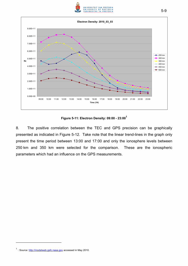
5-9

Figure 5-11: Electron Density: 09:00 - 23:001

8. The positive correlation between the TEC and GPS precision can be graphically

presented as indicated in Figure 5-12. Take note that the linear trend-lines in the graph only

present the time period between 13:00 and 17:00 and only the ionosphere levels between

250 km and 350 km were selected for the comparison. These are the ionospheric

parameters which had an influence on the GPS measurements.

1 : Source: http://modelweb.gsfc.nasa.gov accessed in May 2010.

Electron Density: 2010_03_03

0.00E+00

1.00E+11

2.00E+11

3.00E+11

4.00E+11

5.00E+11

6.00E+11

7.00E+11

8.00E+11

9.00E+11

09:00 10:00 11:00 12:00 13:00 14:00 15:00 16:00 17:00 18:00 19:00 20:00 21:00 22:00 23:00 Time (1H)

Ne

250 km

300 km

350 km

400 km

450 km

500 km

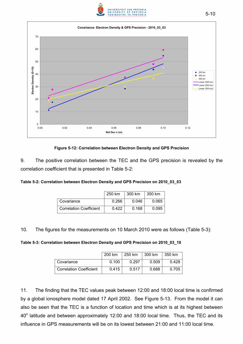
5-10

Covariance: Electron Density & GPS Precision - 2010_03_03

0

10

20

30

40

50

60

70

0.00 0.02 0.04 0.06 0.08 0.10 0.12

Std Dev n (m)

Ele

cto

n D

ensi

ty (

E+

10)

250 km

300 km

350 km

Linear (300 km)

Linear (250 km)

Linear (350 km)

Figure 5-12: Correlation between Electron Density and GPS Precision

9. The positive correlation between the TEC and the GPS precision is revealed by the

correlation coefficient that is presented in Table 5-2:

Table 5-2: Correlation between Electron Density and GPS Precision on 2010_03_03

250 km 300 km 350 km

Covariance 0.266 0.046 0.065

Correlation Coefficient 0.422 0.168 0.095

10. The figures for the measurements on 10 March 2010 were as follows (Table 5-3):

Table 5-3: Correlation between Electron Density and GPS Precision on 2010_03_10

200 km 250 km 300 km 350 km

Covariance 0.100 0.297 0.509 0.428

Correlation Coefficient 0.415 0.517 0.688 0.705

11. The finding that the TEC values peak between 12:00 and 18:00 local time is confirmed

by a global ionosphere model dated 17 April 2002. See Figure 5-13. From the model it can

also be seen that the TEC is a function of location and time which is at its highest between

40o latitude and between approximately 12:00 and 18:00 local time. Thus, the TEC and its

influence in GPS measurements will be on its lowest between 21:00 and 11:00 local time.

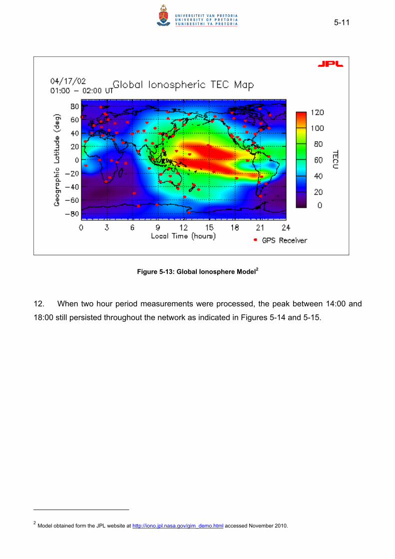
5-11

Figure 5-13: Global Ionosphere Model2

12. When two hour period measurements were processed, the peak between 14:00 and

18:00 still persisted throughout the network as indicated in Figures 5-14 and 5-15.

2 Model obtained form the JPL website at http://iono.jpl.nasa.gov/gim_demo.html accessed November 2010.

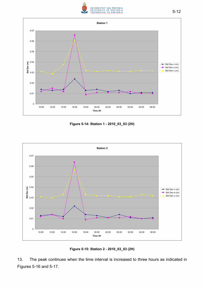
5-12

Station 1

0

0.01

0.02

0.03

0.04

0.05

0.06

0.07

10:00 12:00 14:00 16:00 18:00 20:00 22:00 00:00 02:00 04:00 06:00

Time 2H

Std

Dev

(m

)

Std Dev n (m)

Std Dev e (m)

Std Dev u (m)

Figure 5-14: Station 1 - 2010_03_03 (2H)

Station 2

0

0.01

0.02

0.03

0.04

0.05

0.06

0.07

10:00 12:00 14:00 16:00 18:00 20:00 22:00 00:00 02:00 04:00 06:00

Time 2H

Std

Dev

(m

)

Std Dev n (m)

Std Dev e (m)

Std Dev u (m)

Figure 5-15: Station 2 - 2010_03_03 (2H)

13. The peak continues when the time interval is increased to three hours as indicated in

Figures 5-16 and 5-17.

5-13

Station 4

0

0.01

0.02

0.03

0.04

0.05

0.06

12:00 15:00 18:00 21:00 00:00 03:00

Time 3H

Std

Dev

(m

)

Std Dev n (m)

Std Dev e (m)

Std Dev u (m)

Figure 5-16: Station 4 - 2010_03_03 (H3)

Station 5

0

0.005

0.01

0.015

0.02

0.025

0.03

0.035

0.04

0.045

12:00 15:00 18:00 21:00 00:00 03:00

Time 3H

Std

Dev

(m

)

Std Dev n (m)

Std Dev e (m)

Std Dev u (m)

Figure 5-17: Station 5 - 2010_03_03 (3H)

14. A similar trend was experienced with the measurements on 10 to 11 Mar 10 as

indicated in Figures 5-18, 5-19 and 5-20.

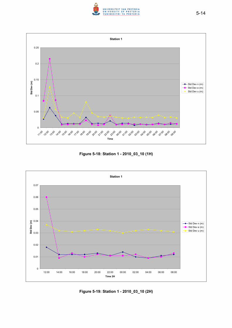
5-14

Station 1

0

0.05

0.1

0.15

0.2

0.25

11:0

012

:00

13:0

014

:00

15:0

016

:00

17:0

018

:00

19:0

020

:00

21:0

022

:00

23:0

000

:00

01:0

002

:00

03:0

004

:00

05:0

006

:00

07:0

008

:00

09:0

0

Time

Std

Dev

(m

)

Std Dev n (m)

Std Dev e (m)

Std Dev u (m)

Figure 5-18: Station 1 - 2010_03_10 (1H)

Station 1

0

0.01

0.02

0.03

0.04

0.05

0.06

0.07

12:00 14:00 16:00 18:00 20:00 22:00 00:00 02:00 04:00 06:00 08:00

Time 2H

Std

Dev

(m

)

Std Dev n (m)

Std Dev e (m)

Std Dev u (m)

Figure 5-19: Station 1 - 2010_03_10 (2H)

5-15

Station 1

0

0.005

0.01

0.015

0.02

0.025

0.03

0.035

0.04

12:00 15:00 18:00 21:00 00:00 03:00

Time 3H

Std

Dev

(m

)

Std Dev n (m)

Std Dev e (m)

Std Dev u (m)

Figure 5-20: Station 1 - 2010_03_10 (3H)

Consecutive Measurements

0

0.05

0.1

0.15

0.2

0.25

1H 2H 3H 4H 5H 6H 12H

Time Duration of Measurement

Std

Dev

(m

)

Std Dev n (m)

Std Dev e (m)

Std Dev u (m)

Figure 5-21: Consecutive Measurements

15. With an increase in the measurement intervals, the precision increased and the peak

disappeared. Precision increased as the measurement period increased with consecutive

measurements as is indicated in Figure 5-21. Measurements started from 12:00, initially with

5-16

a one hour measurement increasing hourly to a 6 h measurement and ultimately to a 12 h

measurement. With a three hour measurement the precision of the latitude and longitude

values drops to approximately 11 mm and the height values to 32 mm. The level of precision

does not increase significantly with a further increase in the measurement period and is

almost the same at the 12 h measurement. When the observation period is increased to

24 h the precision of the latitude value drops to 3 mm, the longitude to 4 mm and the height

to 9 mm. With a 48 h measurement the latitude and longitude values are both 3 mm and the

height value 7 mm as indicated in Table 5-1.

16. The accuracy of the measurements with the Topcon GB-1000 can only be determined

by comparing it with measurements with another receiver with a higher and known accuracy.

For this reason measurements were taken by means of an antenna splitter from the same

antenna of the HRAO ITRF station at HartRAO, effectively creating a zero-baseline test.

Thus, HRAO was taken as a reference measurement. The HRAO receiver is an Ashtech

UZ-12 supplied by JPL and conforms to the highest accuracy standards. It uses an Ashtech

701945E_M choke ring antenna.3 All external influences that could cause the GPS receivers

to take inaccurate measurements needed to be eliminated. These aspects were addressed

as follows:

a. Satellite Clock and Orbit Errors. The precise clock and orbit correction data

were downloaded from the IGS website and measurements were processed

with this data to eliminate their effects.

b. Ionospheric and Tropospheric Effect. The fact that the same antenna was

used by both receivers ensured that the effect of both the ionosphere and

the troposphere were exactly the same for both receivers.

c. Satellite Availability. The same antenna was used over the same time

period. Thus, the same satellites were used by both receivers and therefore

GDOP values are the same.

d. Multipathing and Shadowing. The HRAO station is placed according to IGS

specifications that require the site to be free of any multipathing or

shadowing.

3 More specifications about the HRAO setup can be acquired at http://igscb.jpl.nasa.gov/igscb/station/log/ hrao_20090212.log.

5-17

e. Receiver Clock Errors and Receiver Noise. These are the only factors that

could cause the two receivers to measure differently. The HRAO receiver

uses a hydrogen maser that is extremely stable and is accurate to

approximately one second per one million years. The HRAO station has

been providing IGS data for more than 14 years and has been included in

the ITRF solution. It can therefore be used with confidence as a reference.

17. The measurements obtained over the period 14 to 22 September 2010 with the

Topcon GB-1000 at HartRAO (the same receiver that was used at Station 3), were

processed with WGS84 as the reference ellipsoid and heights are in ellipsoidal values.

Results were processed with the Topcon Tools software. For this purpose the HRAO station

was fixed at the ITRF 2005 (2008/01/09) epoch values to ensure values were comparable

with the rest of this study. The results were exported in ellipsoidal coordinate values.

However, only the deviations of the TopconGB-100 from the HRAO receiver for the nine

days measurement period are contained in Table 5-4 in metre values, including precision,

PDOP values and RMS.

Table 5-4: Topcon GB-1000 measurements comparison with the HRAO receiver - Accuracy

Date ∆ N (m) ∆ E (m) ∆ h (m)

2010_09_14 0 0 0

2010_09_15 0 0 0.001

2010_09_16 0 0 0.001

2010_09_17 0 0 0

2010_09_18 0 0 0.001

2010_09_19 0 0 0.001

2010_09_20 0 0 0.001

2010_09_21 0 0 0.001

2010_09_22 0 0 0.001

18. From these values it can be seen that the two receivers for all practical purposes

measured the same values. The deviations of the Topcon GB-1000 from the HRAO receiver

are in the vicinity of 1 mm and can be attributed to receiver noise. Measurements with the

Topcon GB-1000 receiver can therefore be considered as accurate to an indiscernible level

for the purposes of this study.

5-18

MEASUREMENTS WITH MAPPING TYPE GPS RECEIVERS

19. The same procedure as with the Topcon GB-1000 was followed when measurements

were obtained with a mapping type GPS, the Trimble ProXH fitted with a Zephyr antenna, at

Station 3. To make comparable measurements, datasets were differentially corrected similar

to the Topcon GB- 1000. The measurements were taken to simulate operational conditions.

For this reason the ProXH was used only with the onboard battery pack that renders

approximately an eight hour measurement period. Measurements were therefore repeated

to ascertain the repeatability of the attainable accuracies and precision levels.

20. Results of these measurements at Station 3 were downloaded from the GPS receiver

and processed with the Topcon Tools software are contained in Table 5-5.

Table 5-5: Trimble ProXH measurement values at Station 3 - Precision

Name Latitude Longitude Ell.Height

(m)

Std Dev n

(m)

Std Dev e

(m)

Std Dev u

(m)

2010_03_23 25°48'29.78874"S 28°08'33.49214"E 1458.783 0.014 0.01 0.029

2010_03_24 25°48'29.78885"S 28°08'33.49243"E 1458.799 0.012 0.01 0.029

2010_03_25 25°48'29.78891"S 28°08'33.49187"E 1458.784 0.014 0.013 0.026

2010_03_26 25°48'29.78871"S 28°08'33.49222"E 1458.781 0.014 0.013 0.025

2010_03_27 25°48'29.78843"S 28°08'33.49258"E 1458.808 0.014 0.012 0.026

21. The first obvious result evident from Table 5-5 is that the precision of measurements

for the longitude and latitude values are in the vicinity of 10 mm to 14 mm, while the height

values are 25 mm to 29 mm. However, when the hourly measurements are evaluated

certain trends can be seen as depicted in Figures 5-22 to 5-25.

5-19

ProXH: 2010/03/24

0

0.02

0.04

0.06

0.08

0.1

0.12

0.14

0.16

0.18

16:00 17:00 18:00 19:00 20:00 21:00 22:00 23:00

Time

Sta

d D

ev (

m)

Std Dev n (m)

Std Dev e (m)

Std Dev u (m)

Figure 5-22: Station3 - ProXH - 2010_03_24

ProXH: 2010/03/25

0

0.02

0.04

0.06

0.08

0.1

0.12

0.14

16:00 17:00 18:00 19:00 20:00 21:00 22:00 23:00

Time

Sta

d D

ev (

m)

Std Dev n (m)

Std Dev e (m)

Std Dev u (m)

Figure 5-23: Station 3 - ProXH - 2010_03_25

5-20

ProXH: 2010/03/26

0

0.02

0.04

0.06

0.08

0.1

0.12

16:00 17:00 18:00 19:00 20:00 21:00 22:00 23:00

Time

Std

De

v (

m)

Std Dev n (m)

Std Dev e (m)

Std Dev u (m)

Figure 5-24: Station 3 - ProXH - 2010_03_26

ProXH: 2010/03/27

0

0.02

0.04

0.06

0.08

0.1

0.12

0.14

0.16

16:00 17:00 18:00 19:00 20:00 21:00 22:00 23:00

Time

Std

Dev

(m

)

Std Dev n (m)

Std Dev e (m)

Std Dev u (m)

Figure 5-25: Station 3 – ProXH - 2010_03_27

22. At the start of the measurement at 16:00 the precision of measurements of the latitude

and longitude values are in the vicinity of 60 mm to 140 mm and drops to 20 mm at about

5-21

17:00. The reason for this can be attributed to the ionospheric effect at the time of the day

as previously discussed.

23. The steep rise in the values at the end of the measurement is repeated at three

consecutive days. To understand this rise, the measurements were processed in 20 min

intervals and compared with variables of the rest of the measurement. The results are

presented in Figure 5-26 and Table 5-6. From these values it can be seen that the steep rise

from 23:00 correlates with a drop in the number of satellites observed and a corresponding

rise of the DOP values.

ProXH 2010_03_24

0

0.02

0.04

0.06

0.08

0.1

0.12

0.14

0.16

0.18

0.2

22:20 22:40 23:00 23:20 23:40

Time (20 min)

Std

Dev

(m

)

Std Dev n (m)

Std Dev e (m)

Std Dev u (m)

Figure 5-26: Station 3 - ProXH - 2010_03_24 (20 min intervals)

Table 5-6: Trimble ProXH measurement values at Station 3 on 2010_03_24 (20 min intervals)

Start Time

Std Dev n

(m)

Std Dev e

(m)

Std Dev u

(m)

GPS

Satellites PDOP HDOP VDOP

22:20 0.011 0.009 0.029 10 2.107 0.851 1.928

22:40 0.01 0.009 0.029 9 2.344 0.975 2.132

23:00 0.013 0.01 0.027 8 2.28 1.065 2.016

23:20 0.097 0.072 0.18 8 2.631 1.438 2.203

23:40 0.086 0.114 0.189 7 4.523 2.321 3.882

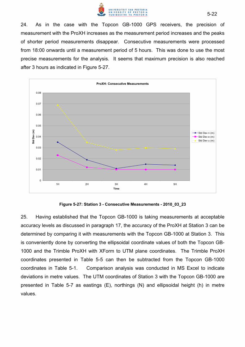
5-22

24. As in the case with the Topcon GB-1000 GPS receivers, the precision of

measurement with the ProXH increases as the measurement period increases and the peaks

of shorter period measurements disappear. Consecutive measurements were processed

from 18:00 onwards until a measurement period of 5 hours. This was done to use the most

precise measurements for the analysis. It seems that maximum precision is also reached

after 3 hours as indicated in Figure 5-27.

ProXH: Consecutive Measurements

0

0.01

0.02

0.03

0.04

0.05

0.06

0.07

0.08

1H 2H 3H 4H 5H

Time

Std

De

v (

m)

Std Dev n (m)

Std Dev e (m)

Std Dev u (m)

Figure 5-27: Station 3 - Consecutive Measurements - 2010_03_23

25. Having established that the Topcon GB-1000 is taking measurements at acceptable

accuracy levels as discussed in paragraph 17, the accuracy of the ProXH at Station 3 can be

determined by comparing it with measurements with the Topcon GB-1000 at Station 3. This

is conveniently done by converting the ellipsoidal coordinate values of both the Topcon GB-

1000 and the Trimble ProXH with XForm to UTM plane coordinates. The Trimble ProXH

coordinates presented in Table 5-5 can then be subtracted from the Topcon GB-1000

coordinates in Table 5-1. Comparison analysis was conducted in MS Excel to indicate

deviations in metre values. The UTM coordinates of Station 3 with the Topcon GB-1000 are

presented in Table 5-7 as eastings (E), northings (N) and ellipsoidal height (h) in metre

values.

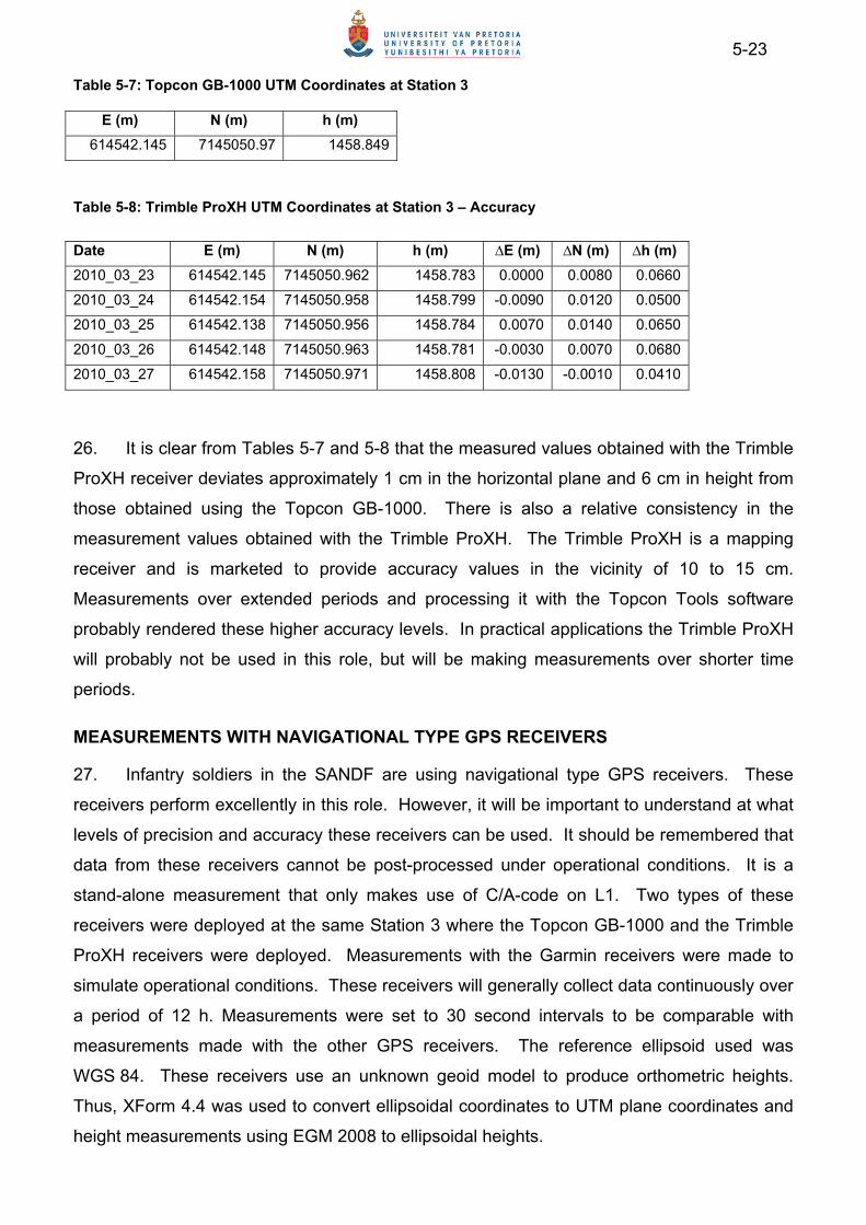
5-23

Table 5-7: Topcon GB-1000 UTM Coordinates at Station 3

E (m) N (m) h (m)

614542.145 7145050.97 1458.849

Table 5-8: Trimble ProXH UTM Coordinates at Station 3 – Accuracy

Date E (m) N (m) h (m) ∆E (m) ∆N (m) ∆h (m)

2010_03_23 614542.145 7145050.962 1458.783 0.0000 0.0080 0.0660

2010_03_24 614542.154 7145050.958 1458.799 -0.0090 0.0120 0.0500

2010_03_25 614542.138 7145050.956 1458.784 0.0070 0.0140 0.0650

2010_03_26 614542.148 7145050.963 1458.781 -0.0030 0.0070 0.0680

2010_03_27 614542.158 7145050.971 1458.808 -0.0130 -0.0010 0.0410

26. It is clear from Tables 5-7 and 5-8 that the measured values obtained with the Trimble

ProXH receiver deviates approximately 1 cm in the horizontal plane and 6 cm in height from

those obtained using the Topcon GB-1000. There is also a relative consistency in the

measurement values obtained with the Trimble ProXH. The Trimble ProXH is a mapping

receiver and is marketed to provide accuracy values in the vicinity of 10 to 15 cm.

Measurements over extended periods and processing it with the Topcon Tools software

probably rendered these higher accuracy levels. In practical applications the Trimble ProXH

will probably not be used in this role, but will be making measurements over shorter time

periods.

MEASUREMENTS WITH NAVIGATIONAL TYPE GPS RECEIVERS

27. Infantry soldiers in the SANDF are using navigational type GPS receivers. These

receivers perform excellently in this role. However, it will be important to understand at what

levels of precision and accuracy these receivers can be used. It should be remembered that

data from these receivers cannot be post-processed under operational conditions. It is a

stand-alone measurement that only makes use of C/A-code on L1. Two types of these

receivers were deployed at the same Station 3 where the Topcon GB-1000 and the Trimble

ProXH receivers were deployed. Measurements with the Garmin receivers were made to

simulate operational conditions. These receivers will generally collect data continuously over

a period of 12 h. Measurements were set to 30 second intervals to be comparable with

measurements made with the other GPS receivers. The reference ellipsoid used was

WGS 84. These receivers use an unknown geoid model to produce orthometric heights.

Thus, XForm 4.4 was used to convert ellipsoidal coordinates to UTM plane coordinates and

height measurements using EGM 2008 to ellipsoidal heights.

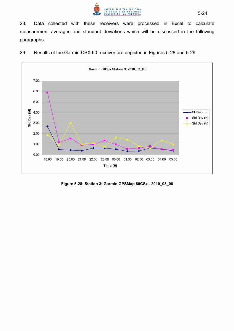
5-24

28. Data collected with these receivers were processed in Excel to calculate

measurement averages and standard deviations which will be discussed in the following

paragraphs.

29. Results of the Garmin CSX 60 receiver are depicted in Figures 5-28 and 5-29:

Garmin 60CSx Station 3: 2010_03_08

0.00

1.00

2.00

3.00

4.00

5.00

6.00

7.00

18:00 19:00 20:00 21:00 22:00 23:00 00:00 01:00 02:00 03:00 04:00 05:00

Time (H)

Std

Dev

(M

)

St Dev (E)

Std Dev (N)

Std Dev (h)

Figure 5-28: Station 3: Garmin GPSMap 60CSx - 2010_03_08

5-25

Garmin 60CSx Station 3: 2010_03_09

0.00

0.50

1.00

1.50

2.00

2.50

3.00

18:00 19:00 20:00 21:00 22:00 23:00 00:00 01:00 02:00 03:00 04:00 05:00

Time (H)

Std

Dev

(m

)

Std Dev (E)

Std Dev (N)

Std Dev (h)

Figure 5-29: Station 3 - Garmin GPSMap 60CSx - 2010_03_09

30. The results of the Garmin eTrex are presented in Figures 5-30 and 5-31:

Garmin eTrex Station 3: 2010_03_12

0.00

0.20

0.40

0.60

0.80

1.00

1.20

1.40

1.60

1.80

2.00

18:00 19:00 20:00 21:00 22:00 23:00 00:00 01:00 02:00 03:00 04:00 05:00

Time (H)

Std

Dev

(m

)

Std Dev (E)

Std Dev (N)

Std Dev (h)

Figure 5-30: Station 3: Garmin eTrex - 2010_03_12

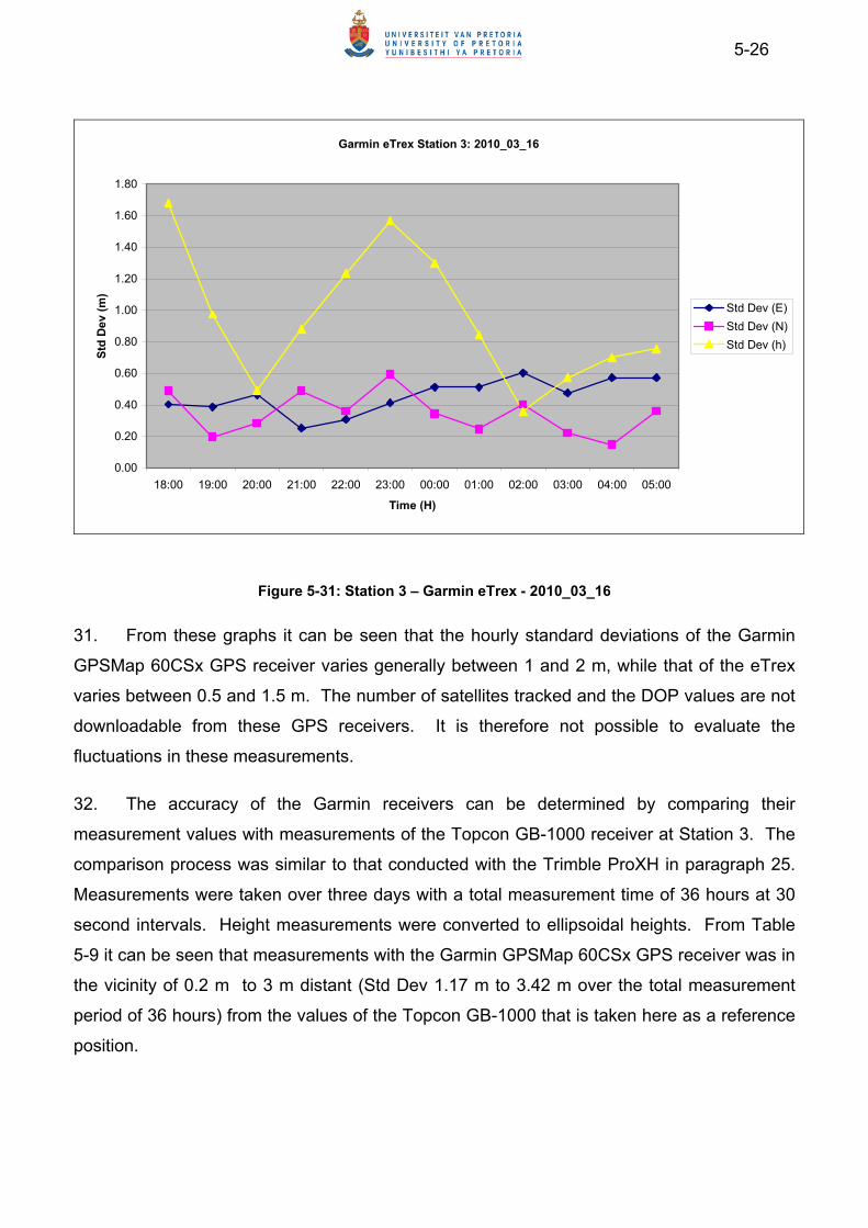
5-26

Garmin eTrex Station 3: 2010_03_16

0.00

0.20

0.40

0.60

0.80

1.00

1.20

1.40

1.60

1.80

18:00 19:00 20:00 21:00 22:00 23:00 00:00 01:00 02:00 03:00 04:00 05:00

Time (H)

Std

Dev

(m

)

Std Dev (E)

Std Dev (N)

Std Dev (h)

Figure 5-31: Station 3 – Garmin eTrex - 2010_03_16

31. From these graphs it can be seen that the hourly standard deviations of the Garmin

GPSMap 60CSx GPS receiver varies generally between 1 and 2 m, while that of the eTrex

varies between 0.5 and 1.5 m. The number of satellites tracked and the DOP values are not

downloadable from these GPS receivers. It is therefore not possible to evaluate the

fluctuations in these measurements.

32. The accuracy of the Garmin receivers can be determined by comparing their

measurement values with measurements of the Topcon GB-1000 receiver at Station 3. The

comparison process was similar to that conducted with the Trimble ProXH in paragraph 25.

Measurements were taken over three days with a total measurement time of 36 hours at 30

second intervals. Height measurements were converted to ellipsoidal heights. From Table

5-9 it can be seen that measurements with the Garmin GPSMap 60CSx GPS receiver was in

the vicinity of 0.2 m to 3 m distant (Std Dev 1.17 m to 3.42 m over the total measurement

period of 36 hours) from the values of the Topcon GB-1000 that is taken here as a reference

position.

5-27

Table 5-9: Garmin GPSMap 60CSx UTM Coordinates at Station 3 - Accuracy

GPS Receiver E (m) N (m) h (m)

Topcon GB-1000 614542.145 7145050.970 1458.849

Garmin 60CSx 614542.357 7145051.013 1461.930

Std Dev (m) of 60CSx 1.17 1.61 3.42

∆ (m) -0.21 -0.04 -3.08

33. The accuracy values of measurements taken the Garmin eTrex receiver over three

days compared with the Topcon GB-1000 are as indicated in Table 5-10:

Table 5-10: Garmin eTrex UTM Coordinates at Station 3: Accuracy

GPS Receiver E (m) N (m) H (m)

Topcon GB-1000 614542.145 7145050.970 1458.849

Garmin eTrex 614541.423 7145050.817 1459.277

Std Dev (m) eTrex 0.93 0.98 2.85

∆ (m) 0.72 0.15 -0.43

34. Garmin receivers will normally not be used for measurements over such extended

periods. These are navigational type receivers and measurements taken under different

circumstances may render different results. It must also be indicated that measurements

were taken from 19:00 to 05:00 the next day when the influence of ionosphere was on its

lowest. Measurements with the GPSMap 60CSx reveal the effect of the ionosphere at the

start of measurement. Although the eTrex appear to be the more precise and accurate

receiver in this analysis, the GPS MAP 60CSx is a more advanced receiver and delivers

more accurate data in other tests in this study. The inability to evaluate the number of

satellites tracked and DOP values precluded the use of these to improve the analysis.

35. This confirms that the Garmin receivers used in this study may be used with

confidence for navigation and the collection of ground control for mapping projects at 50 k

scale and smaller that requires a CEP of 25 m. See also the positional standard

requirements discussed in Appendix C. Various efforts have been made to improve the

precision and the accuracy of measurements with Garmin receivers. Two can be mentioned;

the one by Schweiger and Gläser and the other by the E. Ralini of the Osaka City University.

However, these solutions require that the receiver is connected to a computer during the time

of the measurements. This will be a difficult solution to be implemented during operations

and mapping receivers can then rather be used. Officials at Garmin South Africa were

approached during March 2010 to establish if there is a way to access other observables

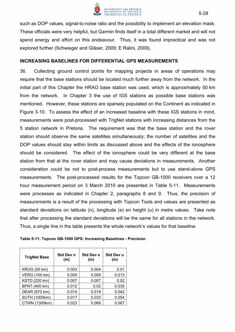
5-28

such as DOP values, signal-to-noise ratio and the possibility to implement an elevation mask.

These officials were very helpful, but Garmin finds itself in a total different market and will not

spend energy and effort on this endeavour. Thus, it was found impractical and was not

explored further (Schwieger and Gläser, 2009; E Ralini, 2009).

INCREASING BASELINES FOR DIFFERENTIAL GPS MEASUREMENTS

36. Collecting ground control points for mapping projects in areas of operations may

require that the base stations should be located much further away from the network. In the

initial part of this Chapter the HRAO base station was used, which is approximately 50 km

from the network. In Chapter 3 the use of IGS stations as possible base stations was

mentioned. However, these stations are sparsely populated on the Continent as indicated in

Figure 3-10. To assess the effect of an increased baseline with these IGS stations in mind,

measurements were post-processed with TrigNet stations with increasing distances from the

5 station network in Pretoria. The requirement was that the base station and the rover

station should observe the same satellites simultaneously; the number of satellites and the

DOP values should stay within limits as discussed above and the effects of the ionosphere

should be considered. The effect of the ionosphere could be very different at the base

station from that at the rover station and may cause deviations in measurements. Another

consideration could be not to post-process measurements but to use stand-alone GPS

measurements. The post-processed results for the Topcon GB-1000 receivers over a 12

hour measurement period on 3 March 2010 are presented in Table 5-11. Measurements

were processes as indicated in Chapter 2, paragraphs 8 and 9. Thus, the precision of

measurements is a result of the processing with Topcon Tools and values are presented as

standard deviations on latitude (n), longitude (e) en height (u) in metre values. Take note

that after processing the standard deviations will be the same for all stations in the network.

Thus, a single line in the table presents the whole network’s values for that baseline.

Table 5-11: Topcon GB-1000 GPS: Increasing Baselines - Precision

TrigNet Base Std Dev n

(m) Std Dev e

(m) Std Dev u

(m)

KRUG (50 km) 0.003 0.004 0.01

VERG (100 km) 0.005 0.005 0.013

KSTD (220 km) 0.007 0.007 0.02

BFNT (400 km) 0.012 0.02 0.035

DEAR (670 km) 0.014 0.019 0.042

SUTH (1000km) 0.017 0.033 0.054

CTWN (1300km) 0.023 0.069 0.067

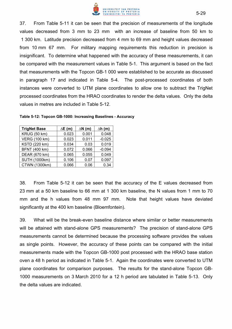
5-29

37. From Table 5-11 it can be seen that the precision of measurements of the longitude

values decreased from 3 mm to 23 mm with an increase of baseline from 50 km to

1 300 km. Latitude precision decreased from 4 mm to 69 mm and height values decreased

from 10 mm 67 mm. For military mapping requirements this reduction in precision is

insignificant. To determine what happened with the accuracy of these measurements, it can

be compared with the measurement values in Table 5-1. This argument is based on the fact

that measurements with the Topcon GB-1 000 were established to be accurate as discussed

in paragraph 17 and indicated in Table 5-4. The post-processed coordinates of both

instances were converted to UTM plane coordinates to allow one to subtract the TrigNet

processed coordinates from the HRAO coordinates to render the delta values. Only the delta

values in metres are included in Table 5-12.

Table 5-12: Topcon GB-1000: Increasing Baselines - Accuracy

TrigNet Base ∆E (m) ∆N (m) ∆h (m) KRUG (50 km) 0.023 0.001 0.048VERG (100 km) 0.023 0.011 -0.025KSTD (220 km) 0.034 0.03 0.019BFNT (400 km) 0.072 0.066 -0.094DEAR (670 km) 0.065 0.055 0.049SUTH (1000km) 0.106 0.07 0.097CTWN (1300km) 0.066 0.06 0.34

38. From Table 5-12 it can be seen that the accuracy of the E values decreased from

23 mm at a 50 km baseline to 66 mm at 1 300 km baseline, the N values from 1 mm to 70

mm and the h values from 48 mm 97 mm. Note that height values have deviated

significantly at the 400 km baseline (Bloemfontein).

39. What will be the break-even baseline distance where similar or better measurements

will be attained with stand-alone GPS measurements? The precision of stand-alone GPS

measurements cannot be determined because the processing software provides the values

as single points. However, the accuracy of these points can be compared with the initial

measurements made with the Topcon GB-1000 post processed with the HRAO base station

oven a 48 h period as indicated in Table 5-1. Again the coordinates were converted to UTM

plane coordinates for comparison purposes. The results for the stand-alone Topcon GB-

1000 measurements on 3 March 2010 for a 12 h period are tabulated in Table 5-13. Only

the delta values are indicated.

5-30

Table 5-13: Topcon GB-1000 GPS stand-alone measurements - Accuracy

Station Name ∆E (m) ∆N (m) ∆h (m)

1 -0.108 -0.153 0.038

2 -0.109 -0.128 -0.163

3 -0.127 0.026 -0.533

4 -0.08 0.016 -0.172

5 -0.112 0.086 -0.2

40. Comparing results of Table 4-12 with results of Table 5-13 it can be seen that

accuracy of the post-processed values over increasing baselines from 50 km to 1 300 km is

generally better than using stand-alone GPS measurements. Similar results were obtained

with the measurements on 10 Mar 10. Thus, the break-off point using increased baselines is

probably much further than the 1 300 km. The add-on uncertainty of using unchecked

(stand-alone) field measurement increases the need to process field measurements over

extended baselines. This also indicates that using a survey type GPS such as the Topcon

GB-1000 with base station data to conduct differential post-processing could render

coverage for mapping projects on the Continent as indicated with the 1 000 km buffers in

Figure 3-10. Using geodetic type receivers such as IGS stations and scientific processing

software will deliver sub-centimetre results over global baselines. However, this will not be a

typical military application.

41. Measurements with a mapping type GPS receiver such as the Trimble ProXH located

at Station 3 over an 8 hour measurement period were processed with increasing baselines.

Measurements were repeated for four consecutive days from 23 to 26 March 2010. The data

of 25 March 2010 are presented in Table 5-14. Similar results were obtained with

measurements during the other days.

Table 5-14: Trimble ProXH: Increasing Baselines - Precision

TrigNet Base Std Dev n

(m) Std Dev e

(m) Std Dev u

(m)

KRUG (50 km) 0.012 0.01 0.03VERG (100 km) 0.017 0.014 0.039KSTD (220 km) 0.027 0.025 0.076BFTN (400 km) 0.047 0.03 0.078DEAR (670 km) 0.063 0.037 0.1SUTH (1000 km) 0.079 0.05 0.119CTWN (1300 km) 0.087 0.049 0.139

5-31

42. From Table 5-14 it can be seen that the precision of latitude values of measurements

with the Trimble ProXH decreased from 12 mm at a 50 km baseline to 87 mm with a

1 300 km baseline. Longitude precision values decreased from 10 mm to 49 mm and height

values from 30 mm to 139 mm. These values are within the limits that are required for

military positional standards.

Table 5-15: Trimble ProXH: Increasing Baselines - Accuracy

TrigNet Base ∆E (m) ∆N (m) ∆h (m)

KRUG (50 km) 0.002 -0.018 0.12

VERG (100 km) -0.002 -0.03 0.174

KSTD (220 km) -0.04 -0.053 0.095

BFTN (400 km) 0.17 0.241 0.327

DEAR (670 km) 0.187 0.238 0.746

SUTH (1000 km) 0.214 0.29 1.083

CTWN (1300 km) 0.395 0.317 1.389

43. Accuracy of measurements with the Trimble ProXH receiver on 25 March 2010 with

increasing baselines can also be compared with the measurements with the Topcon GB-

1000 in Table 5-1. From Table 5-15 it can be seen that the accuracy of the E values reduced

from 2 mm to 395 mm, the N values from 18 mm to 317 mm and the h values from 120 mm

to 1.3 m. These values are still within the limits of military positional standards. However,

the same question can be asked in this regard; will it be better to post-process over this long

baseline or rather use stand-alone GPS measurements? The accuracy values of the ProXH

(not deferentially corrected) are presented in Table 5-16.

Table 5-16: Trimble ProXH stand-alone measurements - Accuracy

Date ∆E (m) ∆N (m) ∆h (m)

2010_03_23 -0.628 1.522 -1.781

2010_03_24 -0.166 0.992 -1.753

2010_03_25 -0.293 0.860 -1.508

2010_03_26 -0.411 0.839 -1.762

44. From Tables 5-15 and 5-16 it can be seen that the post-processed values with

baselines exceeding approximately 670 km are marginally better than stand-alone values.

Thus, stand-alone or post-processed strategies with mapping type GPS receivers utilising

baselines between 600 km and 1 000 km can be used with almost the same results.

However, it will be better to use shorter baselines in the vicinity of 500 km with mapping type

receivers to provide data with higher accuracies.

5-32

45. Setting up an own base station can be risky and probably not worth the value of the

mapping project. However, there could be a better approach, for instance using Precise

Point Positioning (to be discussed in the next section). In closing, it should be realised that

the measurements of both these GPS receivers were taken over relatively long observation

periods; 12 and 8 h respectively. Collecting positional data in operational conditions may

require measurements with a mobile platform (kinematic measurements) that may cause

lower precision and accuracy levels. Due to positional uncertainties when a mobile platform

such as a vehicle is used, the comparison of precision and accuracy will not be valid.

However, when measurements are planned, all aspects that may impact on the accuracy

and precision including the availability of satellites, DOP values and the effect of the

ionosphere, especially with extended baselines, should be considered as was illustrated with

these few examples.

PRECISE POINT POSITIONING TECHNIQUES

46. Relative PPP measurements are obtained when the values of other IGS stations close

to the point are taken for post-processing and are very similar to the differential processing

technique discussed in the previous section. The Australian Positioning Service (AUSPOS)

provides a relative PPP service using the GRS80 ellipsoid4 and IGS stations close to the

station in question as discussed in Chapter 4 paragraph 28. The values of the network on

3 March 2010 were submitted for processing. The precision of the measurements processed

by AUSPOS is provided in Cartesian coordinate values as indicated in Table 5-17.

Table 5-17: Topcon GB-1000 measurements with relative PPP (AUSPOS) - Precision

Name X (m) Y (m) Z (m) ∆x (m) ∆y (m) ∆z (m)

1 5063301 2717757 -2761431 0.0045 0.003 0.003

2 5064501 2718499 -2758632 0.0045 0.003 0.003

3 5067493 2710637 -2760591 0.0045 0.003 0.003

4 5067434 2709134 -2762407 0.0045 0.003 0.003

5 5066902 2715085 -2757544 0.0065 0.005 0.003

47. The accuracy of these measurements can be calculated by comparing them to the

Topcon GB-1000 measurements post-processed with the HRAO base station. The

comparison of the accuracy of the values from the AUSPOS service is as indicated in Table

5-18 in UTM plane coordinate values followed by the deltas:

4 The GRS80 ellipsoid is practically the same as WGS84. However, the flattening factor (f-1 = 298.257 222 101) differs from WGS84. See H. MORITZ (1979): Report of Special Study Group No 539 of I.A.G., Fundamental Geodetic Constants, presented at XVII General Assembly og I.U.G.G., Canberra. Accessed during July 2011 at www.gfy.ku.dk/.

5-33

Table 5-18: Topcon GB-1000 measurements with relative PPP (AUSPOS) - Accuracy

Name E (m) N (m) H (m) ∆E ∆N ∆h

1 622785.685 7144076.481 1525.959 -0.056 -0.035 -0.153

2 622900.658 7147206.994 1575.545 -0.054 -0.038 -0.129

3 614542.199 7145051.006 1458.951 -0.054 -0.036 -0.102

4 613228.444 7143097.26 1565.15 -0.044 -0.04 -0.136

5 618770.228 7148441.853 1554.606 -0.054 -0.037 -0.114

48. From Table 5-18 it can be seen that the AUSPOS values are significantly worse than

post-processing with the HRAO base station. However, where the user does not have

access to an IGS base station, this service can render excellent results and can be

considered as a solution for mapping projects.

49. The other service is the absolute PPP solution. In this technique no specific base

station is used but the clock and ephemeris correction data from a number of base stations

operated by this service are used to correct the in situ GPS measurements. The Canadian

Spatial Reference System (CSRS) is such a service that uses the ITRF (2005) stations and

thus by implication WGS84 as reference ellipsoid. The values of measurements taken on

3 March 2010 using the 5 station network locations occupied with the Topcon GB-1000,

processed by the CSRP-PPP are presented in Table 5-19.

Table 5-19: Topcon GB-1000 measurements with absolute PPP (CSRS) – Precision

Station Latitude Longitude Height Std Dev n (m) Std Dev e (m) Std Dev u (m)

1 -25 48 59.0502 -25 48 59.0502 1525.834 0.002 0.005 0.011

2 -25 47 17.2708 28 13 32.8929 1575.443 0.002 0.005 0.011

3 -25 48 29.7873 28 08 33.4937 1458.852 0.002 0.005 0.011

4 -25 49 33.6567 28 07 46.9233 1565.044 0.002 0.005 0.011

5 -25 46 38.3646 28 11 04.2118 1554.526 0.003 0.007 0.014

Table 5-20: Topcon GB-1000 measurements with absolute PPP (CSRS) - Accuracy

Name E (m) N (m) H (m) ∆E (m) ∆N (m) ∆h (m)

1 622785.68 7144076.475 1525.834 -0.051 -0.029 -0.028

2 622900.647 7147206.99 1575.443 -0.043 -0.034 -0.027

3 614542.189 7145051.006 1458.852 -0.044 -0.036 -0.003

4 613228.434 7143097.256 1565.044 -0.034 -0.036 -0.03

5 618770.214 7148441.852 1554.526 -0.04 -0.036 -0.034

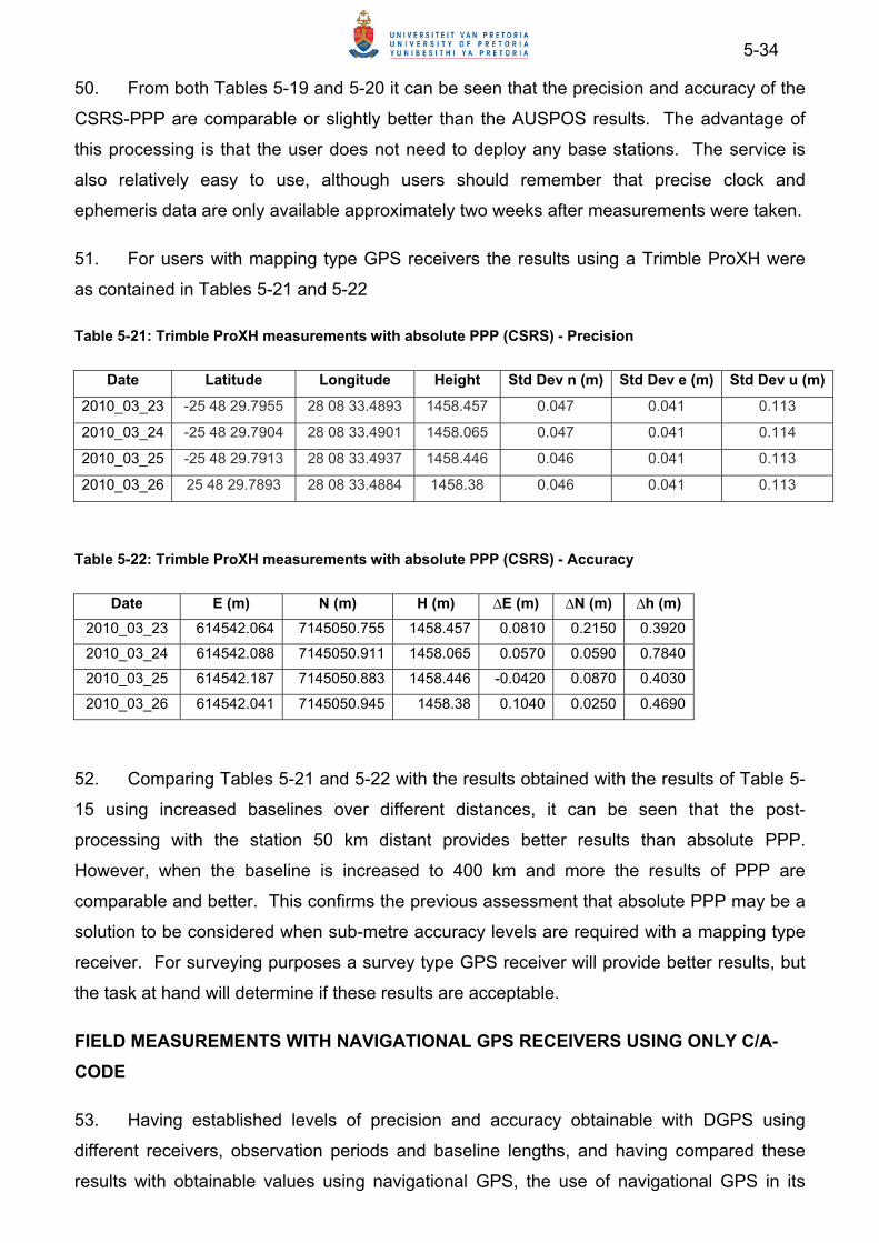
5-34

50. From both Tables 5-19 and 5-20 it can be seen that the precision and accuracy of the

CSRS-PPP are comparable or slightly better than the AUSPOS results. The advantage of

this processing is that the user does not need to deploy any base stations. The service is

also relatively easy to use, although users should remember that precise clock and

ephemeris data are only available approximately two weeks after measurements were taken.

51. For users with mapping type GPS receivers the results using a Trimble ProXH were

as contained in Tables 5-21 and 5-22

Table 5-21: Trimble ProXH measurements with absolute PPP (CSRS) - Precision

Date Latitude Longitude Height Std Dev n (m) Std Dev e (m) Std Dev u (m)

2010_03_23 -25 48 29.7955 28 08 33.4893 1458.457 0.047 0.041 0.113

2010_03_24 -25 48 29.7904 28 08 33.4901 1458.065 0.047 0.041 0.114

2010_03_25 -25 48 29.7913 28 08 33.4937 1458.446 0.046 0.041 0.113

2010_03_26 25 48 29.7893 28 08 33.4884 1458.38 0.046 0.041 0.113

Table 5-22: Trimble ProXH measurements with absolute PPP (CSRS) - Accuracy

Date E (m) N (m) H (m) ∆E (m) ∆N (m) ∆h (m)

2010_03_23 614542.064 7145050.755 1458.457 0.0810 0.2150 0.3920

2010_03_24 614542.088 7145050.911 1458.065 0.0570 0.0590 0.7840

2010_03_25 614542.187 7145050.883 1458.446 -0.0420 0.0870 0.4030

2010_03_26 614542.041 7145050.945 1458.38 0.1040 0.0250 0.4690

52. Comparing Tables 5-21 and 5-22 with the results obtained with the results of Table 5-

15 using increased baselines over different distances, it can be seen that the post-

processing with the station 50 km distant provides better results than absolute PPP.

However, when the baseline is increased to 400 km and more the results of PPP are

comparable and better. This confirms the previous assessment that absolute PPP may be a

solution to be considered when sub-metre accuracy levels are required with a mapping type

receiver. For surveying purposes a survey type GPS receiver will provide better results, but

the task at hand will determine if these results are acceptable.

FIELD MEASUREMENTS WITH NAVIGATIONAL GPS RECEIVERS USING ONLY C/A-

CODE

53. Having established levels of precision and accuracy obtainable with DGPS using

different receivers, observation periods and baseline lengths, and having compared these

results with obtainable values using navigational GPS, the use of navigational GPS in its

5-35

primary role should be investigated. Navigational type GPS receivers are used widely in the

SANDF for different solutions, ranging from weapon platforms to handhelds by infantrymen.

The objective here will be to determine how accurately these receivers can be used for

positional data. Data were collected over extended periods. Only a few examples will be

presented to highlight certain trends, otherwise the analysis will be too extensive without

providing additional arguments.

54. These receivers will primarily be used in a mobile role. It is therefore not possible to

compare measurements with a specific predestined point. However, the geometry of these

measurements can be compared to referenced aerial photography provided by SAC. The

Trig Beacons of CDNGI at Stations 4 and 5 can be used as fixed points for this analysis.

When the positions of Stations 4 and 5 measured with the Topcon GB 100 receivers are

exported to ArcGIS the values of these stations can be compared to their physical location

on the aerial photography. See Figures 5-33 and 5-34 for these positions.

Figure 5-32: Geometry of Station 4 (Zwartkop)

5-36

Figure 5-33: Geometry of Station 5 (Schanskop)

55. Both positions of these stations exported from the Topcon GB-1000 to ArcGIS appear

to be almost exactly at the beacons. At closer inspection the measured position values seem

to be offset approximately 35 cm north, north-east relative to the beacons. A number of

reasons can be presented to explain this offset. The first and obvious is that the values of

the trigonometric beacons are in the HART 94 (ITRF 91) reference frame and the GPS

measurements are in WGS 84 (ITRF 2005) reference frame. Generally, features referenced

to these beacons are used to geometrically rectify these high resolution images (10 cm

resolution). This offset generally agrees with continental drift that can be observed in the

velocity values of the ITRF HRAO base station as demonstrated in Figure 3-6 in Chapter 3.

Another observable effect is the off-nadir photography as clearly can be seen in these

images. The northern sides of the beacons and walls at Schanskop and Zwartkop can be

seen, which indicates that the camera was tilted to the south when these images were taken.

Any height different from the focal plane will therefore have an offset. A third possibility is

that the offset at the two beacons is a compromise to find a general fit to all the reference

points used in the registration process of these images.

56. The first observation consisted of walking while carrying a mapping and navigational

GPS receiver. Measurements were taken while en route in the suburb of Valhalla which is

located between Stations 4 and 5. Care was taken to minimise multipathing and shadowing,

while measurements were generally taken at times when the ionospheric effect was low.

Measurements with the mapping GPS that will serve as a benchmark track were post-

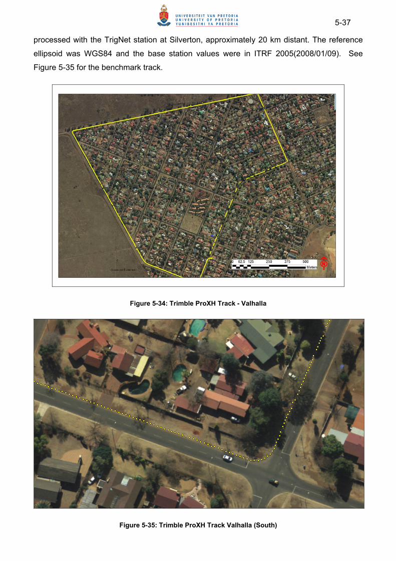
5-37

processed with the TrigNet station at Silverton, approximately 20 km distant. The reference

ellipsoid was WGS84 and the base station values were in ITRF 2005(2008/01/09). See

Figure 5-35 for the benchmark track.

Figure 5-34: Trimble ProXH Track - Valhalla

Figure 5-35: Trimble ProXH Track Valhalla (South)

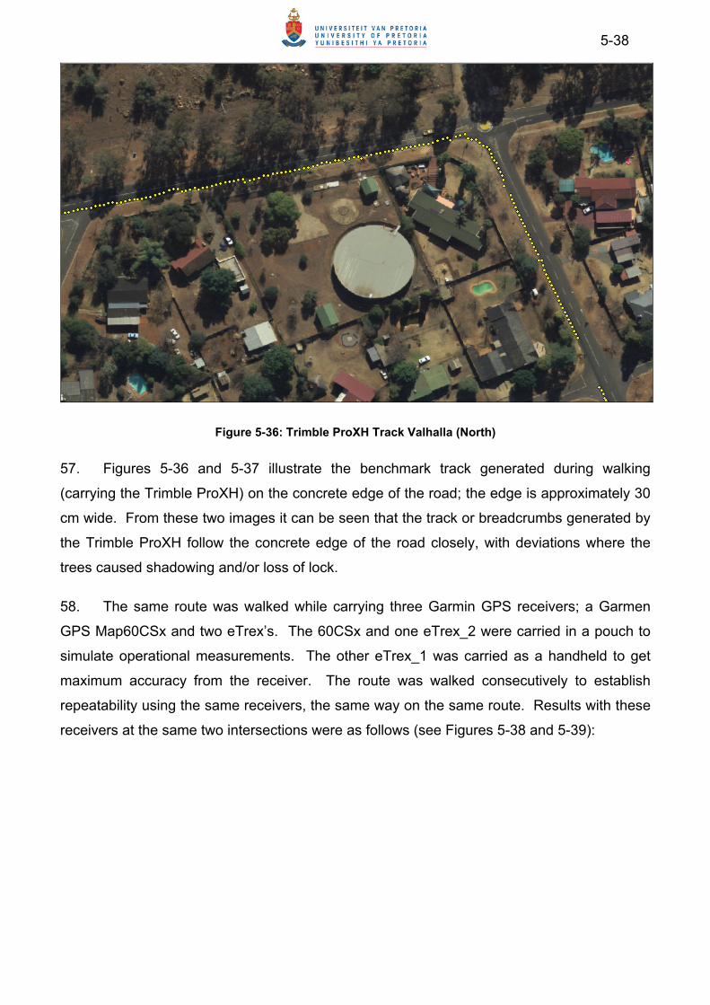
5-38

Figure 5-36: Trimble ProXH Track Valhalla (North)

57. Figures 5-36 and 5-37 illustrate the benchmark track generated during walking

(carrying the Trimble ProXH) on the concrete edge of the road; the edge is approximately 30

cm wide. From these two images it can be seen that the track or breadcrumbs generated by

the Trimble ProXH follow the concrete edge of the road closely, with deviations where the

trees caused shadowing and/or loss of lock.

58. The same route was walked while carrying three Garmin GPS receivers; a Garmen

GPS Map60CSx and two eTrex’s. The 60CSx and one eTrex_2 were carried in a pouch to

simulate operational measurements. The other eTrex_1 was carried as a handheld to get

maximum accuracy from the receiver. The route was walked consecutively to establish

repeatability using the same receivers, the same way on the same route. Results with these

receivers at the same two intersections were as follows (see Figures 5-38 and 5-39):

5-39

Figure 5-37: Garmin GPSMap 60CSx Track (in Pouch) - South

Figure 5-38: Garmin GPSMap 60CSx (in Pouch) - North

59. The Garmin GPSMap 60CSx’s tracks are generally 5 meters from the concrete edge

of the road. At some instances the 60CSx is as accurate as the ProXH, while from time to

time it deviates further than 5 m. It should be kept in mind that the 60CSx is a navigational

receiver and that it performs excellently in this role. It should also be kept in mind that at a

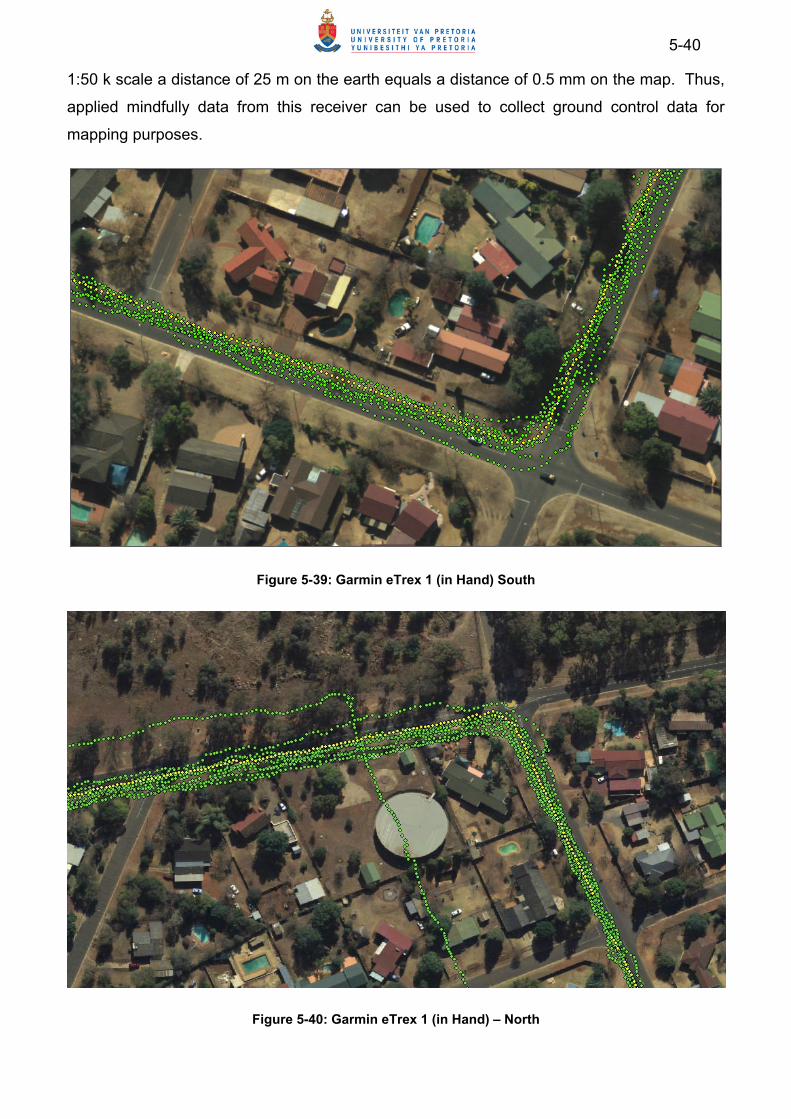
5-40

1:50 k scale a distance of 25 m on the earth equals a distance of 0.5 mm on the map. Thus,

applied mindfully data from this receiver can be used to collect ground control data for

mapping purposes.

Figure 5-39: Garmin eTrex 1 (in Hand) South

Figure 5-40: Garmin eTrex 1 (in Hand) – North

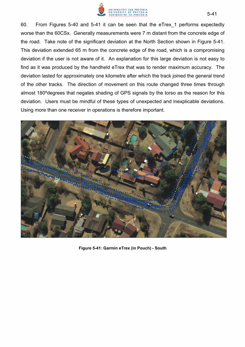
5-41

60. From Figures 5-40 and 5-41 it can be seen that the eTrex_1 performs expectedly

worse than the 60CSx. Generally measurements were 7 m distant from the concrete edge of

the road. Take note of the significant deviation at the North Section shown in Figure 5-41.

This deviation extended 65 m from the concrete edge of the road, which is a compromising

deviation if the user is not aware of it. An explanation for this large deviation is not easy to

find as it was produced by the handheld eTrex that was to render maximum accuracy. The

deviation lasted for approximately one kilometre after which the track joined the general trend

of the other tracks. The direction of movement on this route changed three times through

almost 180ºdegrees that negates shading of GPS signals by the torso as the reason for this

deviation. Users must be mindful of these types of unexpected and inexplicable deviations.

Using more than one receiver in operations is therefore important.

Figure 5-41: Garmin eTrex (in Pouch) - South

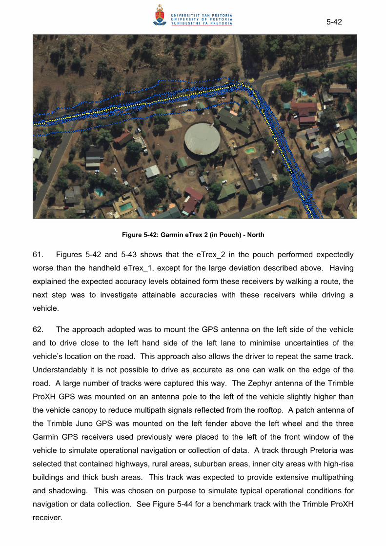
5-42

Figure 5-42: Garmin eTrex 2 (in Pouch) - North

61. Figures 5-42 and 5-43 shows that the eTrex_2 in the pouch performed expectedly

worse than the handheld eTrex_1, except for the large deviation described above. Having

explained the expected accuracy levels obtained form these receivers by walking a route, the

next step was to investigate attainable accuracies with these receivers while driving a

vehicle.

62. The approach adopted was to mount the GPS antenna on the left side of the vehicle

and to drive close to the left hand side of the left lane to minimise uncertainties of the

vehicle’s location on the road. This approach also allows the driver to repeat the same track.

Understandably it is not possible to drive as accurate as one can walk on the edge of the

road. A large number of tracks were captured this way. The Zephyr antenna of the Trimble

ProXH GPS was mounted on an antenna pole to the left of the vehicle slightly higher than

the vehicle canopy to reduce multipath signals reflected from the rooftop. A patch antenna of

the Trimble Juno GPS was mounted on the left fender above the left wheel and the three

Garmin GPS receivers used previously were placed to the left of the front window of the

vehicle to simulate operational navigation or collection of data. A track through Pretoria was

selected that contained highways, rural areas, suburban areas, inner city areas with high-rise

buildings and thick bush areas. This track was expected to provide extensive multipathing

and shadowing. This was chosen on purpose to simulate typical operational conditions for

navigation or data collection. See Figure 5-44 for a benchmark track with the Trimble ProXH

receiver.

5-43

Figure 5-43: Trimble ProXH Track though Pretoria

63. The track of the Trimble Pro XH is again used as a benchmark for the navigational

type of GPS receivers. In this case specific prominent road features were used as

identifiable ground control points. These features include the yellow line (on the left) on

“highways”, intersections, small traffic circles, large traffic circles, street blocks; driving on

both sides of a road augmented the data capturing To gather maximum reference points the

capturing intervals were set to 1 s intervals. Navigational GPS receivers were configured not

to lock on to road features so as to obtain unbiased tracks. Data of the ProXH was post

processed with the TrigNet base station at Silverton (approximately 20 km distant). Base

station values were in ITRF 2005 (2008/01/09).

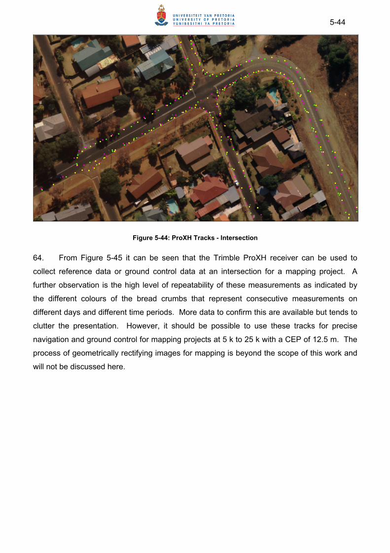
5-44

Figure 5-44: ProXH Tracks - Intersection

64. From Figure 5-45 it can be seen that the Trimble ProXH receiver can be used to

collect reference data or ground control data at an intersection for a mapping project. A

further observation is the high level of repeatability of these measurements as indicated by

the different colours of the bread crumbs that represent consecutive measurements on

different days and different time periods. More data to confirm this are available but tends to

clutter the presentation. However, it should be possible to use these tracks for precise

navigation and ground control for mapping projects at 5 k to 25 k with a CEP of 12.5 m. The

process of geometrically rectifying images for mapping is beyond the scope of this work and

will not be discussed here.

5-45

Figure 5-45: ProXH Tracks - Highway

65. From Figure 5-46 it can be seen that the speed along a straight stretch has almost no

effect on the accuracy on collected data and that it will be possible to use it for rectifying an

image. How will the navigational GPS receivers perform in this regard? First the Garmin

GPSMap 60CSx will be used for the intersection shown here in Figure 5-47:

Figure 5-46: Garmin GPSMap 60CSx - Intersection

5-46

66. From the image in Figure 5-46 it can be seen that the breadcrumbs of the Garmin

GPSMap 60CSx creates uncertainty. The implication is that because the breadcrumbs

generally deviate approximately 5 m from the “true” track, the intersection is too small to

create a clear picture. From the performances of the Garmin eTrex receivers in the previous

analysis it should be concluded that the general deviation of approximately 7 m will increase

the level of uncertainty at this intersection. Thus, larger features need to be selected.

Figure 5-47: Garmin GPSMap 60CSx - Highway

67. From Figure 5-48 is can be seen that on the highway similar trends were evident as

were found while walking and carrying the Garmin GPSMap 60CSx receiver. Sometimes

accuracy equalled that of theTrimble ProXH and occasionally it deviated up to 5 m from the

“true” track.

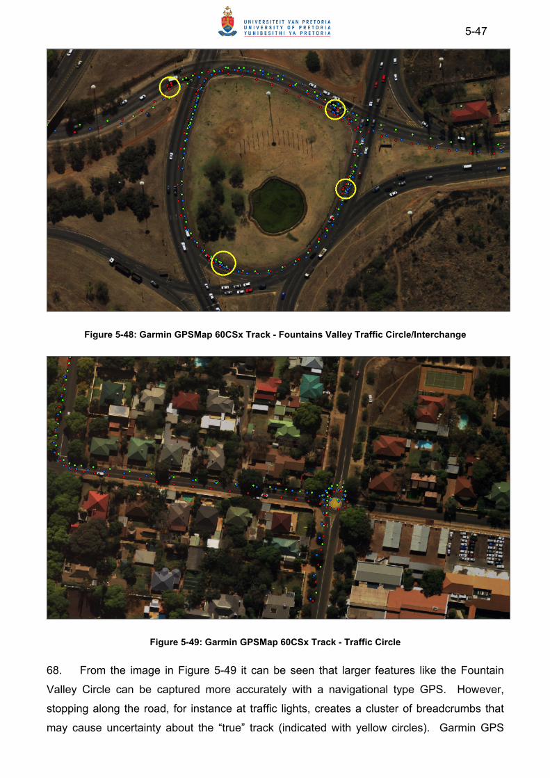
5-47

Figure 5-48: Garmin GPSMap 60CSx Track - Fountains Valley Traffic Circle/Interchange

Figure 5-49: Garmin GPSMap 60CSx Track - Traffic Circle

68. From the image in Figure 5-49 it can be seen that larger features like the Fountain

Valley Circle can be captured more accurately with a navigational type GPS. However,

stopping along the road, for instance at traffic lights, creates a cluster of breadcrumbs that

may cause uncertainty about the “true” track (indicated with yellow circles). Garmin GPS

5-48

receivers use a filter to predict direction of movement. This function produced excellent

results for navigation. However, when direction is changed quickly it tends to carry on along

the predicted track. This delayed effect on the breadcrumbs can be seen in the image with

the small traffic circle in Figure 5-50. It is this same effect that created some problems

collecting tracks at the intersection above depicted in Figure 5-47. One needs to be mindful

of this effect when navigating and/or collecting data for mapping projects.

Figure 5-50: ProXH and eTrex Tracks - Inner City (Sunnyside, Pretoria)

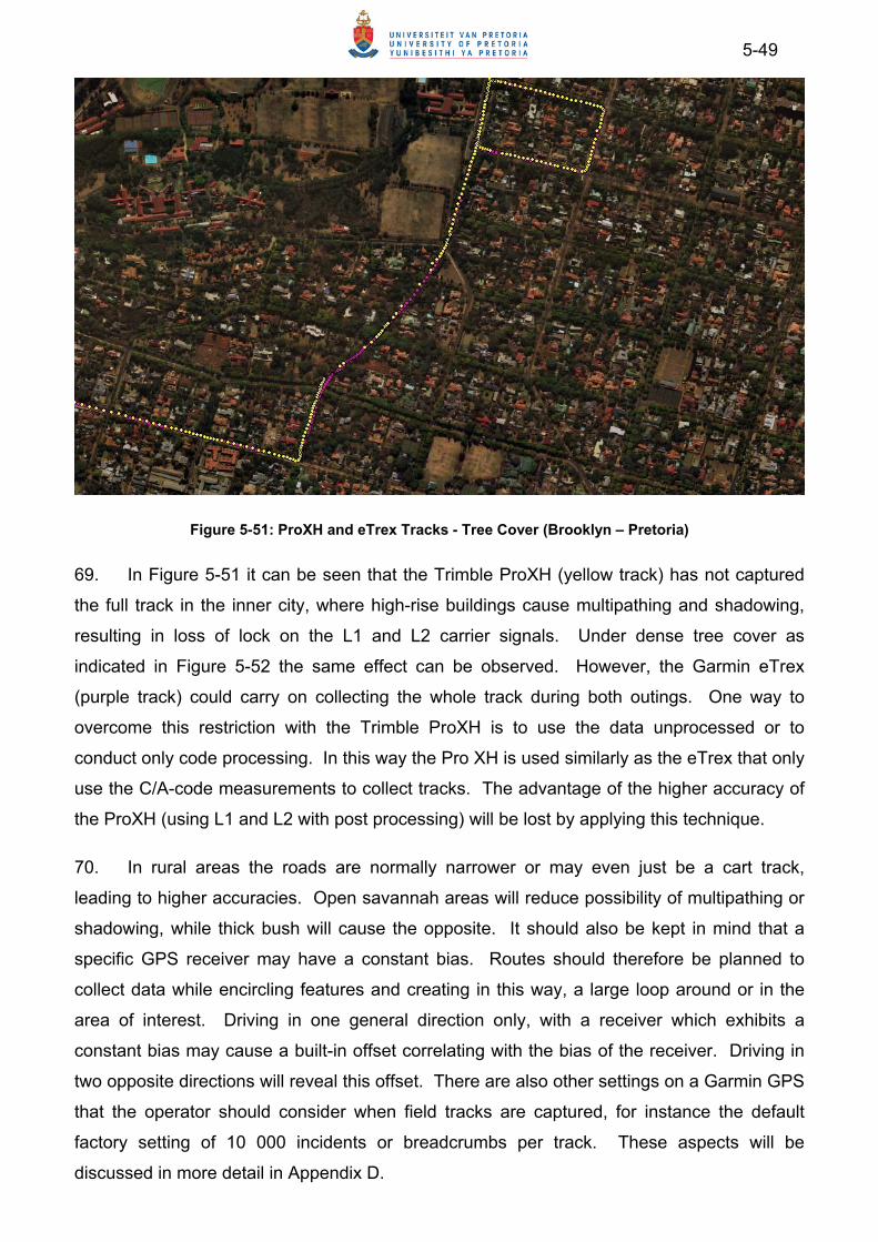
5-49

Figure 5-51: ProXH and eTrex Tracks - Tree Cover (Brooklyn – Pretoria)

69. In Figure 5-51 it can be seen that the Trimble ProXH (yellow track) has not captured

the full track in the inner city, where high-rise buildings cause multipathing and shadowing,

resulting in loss of lock on the L1 and L2 carrier signals. Under dense tree cover as

indicated in Figure 5-52 the same effect can be observed. However, the Garmin eTrex

(purple track) could carry on collecting the whole track during both outings. One way to

overcome this restriction with the Trimble ProXH is to use the data unprocessed or to

conduct only code processing. In this way the Pro XH is used similarly as the eTrex that only

use the C/A-code measurements to collect tracks. The advantage of the higher accuracy of

the ProXH (using L1 and L2 with post processing) will be lost by applying this technique.

70. In rural areas the roads are normally narrower or may even just be a cart track,

leading to higher accuracies. Open savannah areas will reduce possibility of multipathing or

shadowing, while thick bush will cause the opposite. It should also be kept in mind that a

specific GPS receiver may have a constant bias. Routes should therefore be planned to

collect data while encircling features and creating in this way, a large loop around or in the

area of interest. Driving in one general direction only, with a receiver which exhibits a

constant bias may cause a built-in offset correlating with the bias of the receiver. Driving in

two opposite directions will reveal this offset. There are also other settings on a Garmin GPS

that the operator should consider when field tracks are captured, for instance the default

factory setting of 10 000 incidents or breadcrumbs per track. These aspects will be

discussed in more detail in Appendix D.

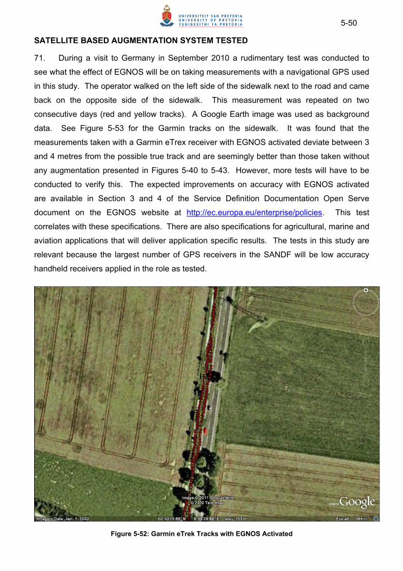
5-50

SATELLITE BASED AUGMENTATION SYSTEM TESTED

71. During a visit to Germany in September 2010 a rudimentary test was conducted to

see what the effect of EGNOS will be on taking measurements with a navigational GPS used

in this study. The operator walked on the left side of the sidewalk next to the road and came

back on the opposite side of the sidewalk. This measurement was repeated on two

consecutive days (red and yellow tracks). A Google Earth image was used as background

data. See Figure 5-53 for the Garmin tracks on the sidewalk. It was found that the

measurements taken with a Garmin eTrex receiver with EGNOS activated deviate between 3

and 4 metres from the possible true track and are seemingly better than those taken without

any augmentation presented in Figures 5-40 to 5-43. However, more tests will have to be

conducted to verify this. The expected improvements on accuracy with EGNOS activated

are available in Section 3 and 4 of the Service Definition Documentation Open Serve

document on the EGNOS website at http://ec.europa.eu/enterprise/policies. This test

correlates with these specifications. There are also specifications for agricultural, marine and

aviation applications that will deliver application specific results. The tests in this study are

relevant because the largest number of GPS receivers in the SANDF will be low accuracy

handheld receivers applied in the role as tested.

Figure 5-52: Garmin eTrek Tracks with EGNOS Activated

5-51

CONCLUDING REMARKS

72. From the analyses it can be concluded that navigational type GPS receivers can be

used for collecting ground control in the horizontal plane for mapping projects at scales of

50 k and smaller. The operator should be mindful of the fact that accuracies are much lower

than mapping type GPS receivers. To overcome this, the project should be planned to

collect features that are generally bigger than 25 m in diameter and are scattered evenly

throughout the area of interest. The vehicle should be driven at a constant slow speed when

direction is changed regularly. The operator should plan to collect where it will not be

necessary to stop too frequently as this causes tracks with uncertainty. On straight stretches

speed has no direct impact on the accuracy of the receiver. Narrower roads can be captured

with higher accuracies. Capturing tracks on wide double and triple lane highways can be

problematic. The yellow edge mark of the road is not always visible from aerial photography

or satellite imagery, but in most cases the edge of the road can be seen. The effects of the

ionosphere, multipathing and shadowing should be considered. It will be wise to use more

than one receiver for the same track to ensure a backup and to counter unexpected

deviations as indicated earlier. The availability of EGNOS will improve the accuracy of

navigational GPS receivers. The principles explained here are equally applicable to purely

navigational tasks.

SELECTIVE DENIAL OR INTENTIONAL JAMMING

73. The susceptibility of civilian type GPS receivers to jamming were tested by means of a

rudimentary setup of a Rhode and Schwarz SML-B3 signal generator connected to an omni-

directional choke ring GPS antenna. The signal generator can generate signals in the

spectrum 9 kHz to 3.3 GHz with an output level of −140 dBm to +19 dBm. The signal

generator, GPS antenna and Topcon GB-1000 GPS receiver were supplied by HartRAO.

The antenna was tilted in the horizontal plane to project the jamming signal in a specific

direction to control some of the signal emissions for measuring purposes. See Figure 5-54

below. The signal generator was set to generate a frequency modulation (FM) signal on the

L1 band at 1 575.42 MHz. The signal output strength was tested between -3 dBm and 17

dBm.

5-52

Figure 5-53: Photo of Jammer Setup

74. The tests were conducted at the General Piet Joubert Training Area north of Pretoria.

Broken terrain with savannah vegetation was selected to simulate operational conditions and

to indicate the effect of terrain on jamming. To depict the effect of terrain a viewshed from

the jammers perspective was created with data supplied by SAC and CDNGI. The green

shaded areas in Figure 5-55 are those that were in direct line of sight and are therefore

“visible” to the jammer.

Figure 5-54: Viewshed of GPS Jamming Tests

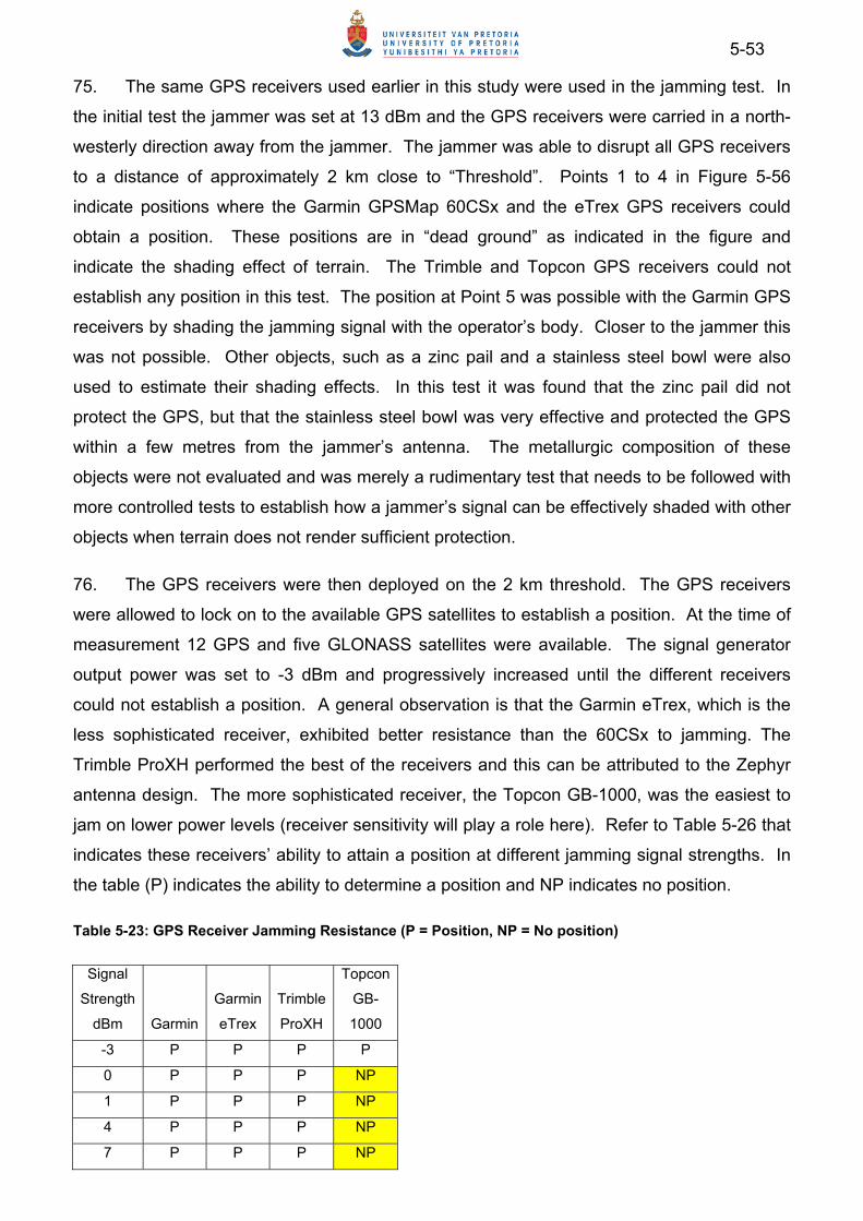
5-53

75. The same GPS receivers used earlier in this study were used in the jamming test. In

the initial test the jammer was set at 13 dBm and the GPS receivers were carried in a north-

westerly direction away from the jammer. The jammer was able to disrupt all GPS receivers

to a distance of approximately 2 km close to “Threshold”. Points 1 to 4 in Figure 5-56

indicate positions where the Garmin GPSMap 60CSx and the eTrex GPS receivers could

obtain a position. These positions are in “dead ground” as indicated in the figure and

indicate the shading effect of terrain. The Trimble and Topcon GPS receivers could not

establish any position in this test. The position at Point 5 was possible with the Garmin GPS

receivers by shading the jamming signal with the operator’s body. Closer to the jammer this

was not possible. Other objects, such as a zinc pail and a stainless steel bowl were also

used to estimate their shading effects. In this test it was found that the zinc pail did not

protect the GPS, but that the stainless steel bowl was very effective and protected the GPS

within a few metres from the jammer’s antenna. The metallurgic composition of these

objects were not evaluated and was merely a rudimentary test that needs to be followed with

more controlled tests to establish how a jammer’s signal can be effectively shaded with other

objects when terrain does not render sufficient protection.

76. The GPS receivers were then deployed on the 2 km threshold. The GPS receivers

were allowed to lock on to the available GPS satellites to establish a position. At the time of

measurement 12 GPS and five GLONASS satellites were available. The signal generator

output power was set to -3 dBm and progressively increased until the different receivers

could not establish a position. A general observation is that the Garmin eTrex, which is the

less sophisticated receiver, exhibited better resistance than the 60CSx to jamming. The

Trimble ProXH performed the best of the receivers and this can be attributed to the Zephyr

antenna design. The more sophisticated receiver, the Topcon GB-1000, was the easiest to

jam on lower power levels (receiver sensitivity will play a role here). Refer to Table 5-26 that

indicates these receivers’ ability to attain a position at different jamming signal strengths. In

the table (P) indicates the ability to determine a position and NP indicates no position.

Table 5-23: GPS Receiver Jamming Resistance (P = Position, NP = No position)

Signal

Strength

dBm Garmin

Garmin

eTrex

Trimble

ProXH

Topcon

GB-

1000

-3 P P P P

0 P P P NP

1 P P P NP

4 P P P NP

7 P P P NP

5-54

9 P P P NP

10 NP P P NP

12 NP P P NP

13 NP NP P NP

15 NP NP P NP

17 NP NP NP NP

77. These tests were conducted to indicate how easy it is to jam civilian type GPS

receivers. Using more appropriate equipment, such as directional antennas and higher

signal outputs could render more significant results. Jamming is dependent on line of sight

and terrain can shade the GPS receiver. However, to deploy a number of aerial jammers

could not be too difficult, in which case the shading effect of terrain can be neutralised.

Thus, the possibility to jam or spoof civilian type GPS receivers and protective

measurements needs to be investigated further.

UNINTENTIONAL JAMMING

78. The unintentional jamming of GPS receivers by RADARS used in the SANDF that use

the L-band was tested5. Tests with two of these RADARS, the ESR 220 or Kameelperd and

Tactical Mobile Radar were conducted. It was found that none of these RADARS influenced

the GPS receivers to the extent that they could not establish a position. The signal-to-noise

ratio that indicates the strength of the GPS satellite signal at the receiver was not influenced

visibly. It was only with measurements next to the Kameelperd that some influences could

be observed, but it was not sufficient to prevent the receivers of establishing position. It can

therefore be deducted that these RADARS will not influence or jam GPS receivers during

operations

5 More can be read about these RADARS at the Reutech website at http://www.rrs.co.za/products accessed during December 2010.

CHAPTER 6: SUMMARY OF CONCLUSIONS

79. Reference Systems. Using GPS for positional data in the SANDF requires that

universal standards be established for reference systems that can be used throughout for

setting up receivers for navigation and for collecting data. These same reference standards

should also be applied in the mapping projects of the SANDF to ensure compatibility across

systems. It is realised that existing systems may have legacy or different reference frames

embedded. In these cases the geospatial officers attached to operations should assist

operational commanders to understand the impact on operations and publish guidelines in

operational orders. However, in this study it was proposed that WGS84 is used for the

reference ellipsoid and the current published values of the ITRF be taken as the realisation of

this datum throughout the African continent. It is therefore of paramount importance that the

applicable ITRF epoch is understood and used correctly for a specific task. IGS stations can

be used as base stations for differential corrections. Height measurements with GPS

receivers could be in ellipsoidal (WGS84) values, while heights on maps and charts will be in

orthometric values. The conversion of ellipsoidal heights to orthometric heights can be

conducted with geoid models such as EGM 2008 and will be the responsibility of the

geospatial officer attached to the operation. In mapping projects this will be conducted by

the responsible cartographer. On South African soil the HART94 datum will be used and

height above mean sea level as published on the CDNGI maps.

80. Accuracy Standards. Positional accuracy standards should be applied for each

specific environment as required. For topographic mapping projects in the SANDF the

positional accuracy standards of the Multinational Co-production Programme for 50 k to

100 k products and the NGA’s UVM standard for 10 k to 25 k products will be used, while the

S57 and ICAO standards will be applied in the maritime and aeronautical environments

respectively.

81. GPS Theory. The SANDF is dependent on civilian type GPS receivers and will most

probably not be able to use the military type GPS receivers that make use of the encrypted

P(Y)-code. Three broad categories namely navigational, mapping and survey or geodetic

GPS receivers are used and were discussed. Navigational receivers produce stand-alone

solutions that make use of the C/A-code modulated on the L1 carrier signal and can attain

accuracies of up to 3 m. Mapping and surveying receivers make use of the C/A-code as well

as the L1 and L2 carrier signals and are capable of attaining sub-metre accuracies.

Differential GPS, PPP and SBAS are augmentation techniques to improve accuracy and

efficiency. Absolute PPP should be considered as a proposed solution for mapping projects

where IGS or AFREF reference stations are lacking. There is great expectation for the

6-2

possible expanding of the EGNOS footprint to include the rest of Africa which will improve

the attainable accuracies with C/A-code measurements. Details of this plan are not yet

available. The proposed GPS modernisation to include two new signals, namely the L2C

and L5 signals, will improve accuracy and presumably also improve resistance to

interference or jamming.

82. Attainable Accuracies. Measurements were conducted to indicate attainable

accuracies. A number of aspects that influence these accuracies were demonstrated and

users should be mindful of these aspects. Different receivers and systems can render

different accuracies and again the user should be aware of these capabilities. It was

established that after three hours both the geodetic and the mapping receivers reached

optimal accuracy levels. It was also established that augmentation of GPS measurements

such as differential post-processing and PPP can eliminate most influences that cause less

than optimal measurements. The influence of multipathing and shadowing by features such

as high-rise buildings in urban areas and foliage were demonstrated. These influences

should be prevented when navigational GPS receivers are used. The influence of the

ionosphere is significant on measurements between about 12:00 and 20:00 local time.

Measurements should therefore rather be taken during the early morning or at night.

Another measure to minimise the effect of the ionosphere is to set elevation masks of 10º or

15º as was discussed under GPS Fundamentals (Effect of the Sun). It was established that

civilian type navigational GPS receivers can be used with confidence for navigation and

mapping projects at 50 k scale and smaller. For larger scale mapping projects mapping type

GPS receivers should rather be used. Sufficient preparation and planning are required to

ensure that the correct approach for the task is selected. This was discussed at length under

Field Measurements with Navigational GPS Receivers in Chapter 5 and is summarised

under Concluding Remarks in paragraph 5-75. More detail about this is included in Appendix

D. It was indicated that a GPS receiver can fail unexpectedly and backup measures should

be put in place.

83. Jamming. It was demonstrated that civilian type GPS receivers can easily be

disrupted. This is a serious vulnerability that needs further investigation and special

measures need to be developed to ensure survival on the battlefield. This is highlighted

further when it is considered that the SANDF plans to conduct decisive actions by means of

night operations when navigation is significantly more difficult. It is suggested that this topic

be investigated further in a separate study.

Appendix A to GNSS in the SANDF

APPENDIX A: REFERENCES

1. Allan, A.L. 2007. Principles of Geospatial Surveying. Whittles Publishing, Dunbeath

Scotland.

2. Ashby, N. 2002. Relativity and the Global Positioning System. Physics Today, May.

Access at htpp://www.ift.unesp.br during April 2009.

3. Bolstad, P. 2006. GIS Fundamentals, 2nd Edition 2006. Eider Press, White Bear Lake,

Minnesota.

4. Chief Director Surveys and Mapping, 2010. Datums and Coordinate Systems.

Pamphlet accessible at http://www.ngi.gov.za/index.php/Geodesy-GPS/datums-and-

coordinate-systems.html updated during November 2010.

5. Collinson, R.P. 2003. Introduction to Avionics Systems, 2nd Edition. Kluwer Academic

Publishers, Dordrecht, The Netherlands.

6. Forssell, B. and Olsen T.B. 2003. Jamming GPS: Susceptibility of some civil GPS

receivers. GPS World.14.1 (Jan).

7. Gao, Y. and Chen, K. 2004. Performance Analysis of Precise Point Positioning Using

Real-Time Orbit and Clock Products. Journal of Global Positioning Systems (2004) Vol. 3,

No. 1-2: 95-100. Accessed at http://www.gmat.unsw.edu.au/wang/jgps during April 2009.

8. Hofmann-Wellenhof, B., Lichtenegger, H. and Collins, J. 2001. GPS Theory and

Practice, 5th Revised Edition. Springer Wein, New York.

9. Illife, J. and Lott, R. 2008. Datums and Map Projetctions. 2nd Edition. Whittles

Publishing, Dunbeath, Caithness, Scotland.

10. Kaplan, E.D. and Hegarty, C.J. 2006. Understanding GPS Principles and Applications,

2nd Edition. Artech House, 685 Canton Street, Norwood.

11. King, M., Edwards, S. and Clarke, P. Precise Point Positioning: Breaking the

Monopoly of Relative GPS Processing. Accessed at ftp://stella.ncl.ac.uk during April 2009.

12. Leick, A. 2004. GPS Satellite Surveying. 3rd Edition. John Wily and Sons. Canada.

A - 2

13. Lekkerkerk, H. 2008. GPS Handbook for Professional GPS Users, C Media

Productions.

14. Leslie, M.W. 2008. The Measure of Time. Inside GNSS, July/August.

15. Merry C. L. 2003. The African Geoid Project and its Relevance to the Unification of

African Vertical Reference Frames. Paper presented at the 2nd FIG Regional Conference

Marrakech, Morocco, December 2-5.

16. Merry, C.L. 2006. Introduction to the Global Positioning System, 4th Edition. Technical

notes for use by the University of Cape Town.

17. Merry, C.L. 2007. Augmentation Systems for GPS. PositionIT, May/June.

18. Merry, C.L. 2008. GPS and the Geoid. PositionIT. July/August.

19. Chandler, G. and Merry, C.L. 2010. South African Geoid 2010: SAGEOID 10. Poisition

IT, June.

20. Mireault, Y., Tetreault, P., Lahaye, F., Heroux, P. and Kouba, 2008. Precise Point

Positioning: A new, timely service from Natural Resources Canada J. GPS World 19.9

(Sept).

21. Ovstedal, O., Kjorsvik, N.S. and Gjevestad, J.G.O. 2006. Surveying using GPS

Precise Point Positioning. Accessed at http://www.fig.net/pub/fig2006/papers/ during April

2009.

22. Realini, E. 2009. goGPS – a navigation software to enhance the accuracy of low cost

GPS receivers. Presentation at the Free and Open Software Conference of 2009 accessed

at http://download.osgeo.org/osgeo/foss4g/2009 during April 2010.

23. Richardson, D. 2003. GPS Proves Jam Resistant. Armada International No 3 of 2003.

24. School of Surveying & Spatial Information Systems at the University of New South

Wales, Australia. Updated May 2010. Principles and Practice of GPS Surveying. Accessed at

www.gmat.unsw.edu.au/snap/gps/ gps_survey during April 2009.

25. Schwieger, V. and Gläser, A. 2009. Possibilities of Low Cost GPS Technology for

Precise Geodetic Applications. Accessed at www.fig.net/pub/fig.2009 during April 2010.

A - 3

26. United States Defence Mapping Agency’s Technical Manual 8400.1, 1991. Error

Theory as Applied to Mapping, Charting and Geodesy.

27. USA Federal Geographic Data Committee’s Geospatial Positioning Accuracy

Standards. 1998. FGDC-STD-007-1-1998 accessed at http://fgdc.er.usgs.gov/fgdc.html

during April 2009.

28. USA Defence Mapping Agency’s Technical Manual 8358.1, 1996, Datums, Ellipsoids,

Grids and Grid Reference Systems.

29. USA National Mapping Agency’s Technical Report 8350. 2000. Department of

Defence World Geodetic System. 3rd Edition.

30. USA Department of Defence. 2008. Global Position System Standard Positioning

Service Performance Standard, 4th Edition.

31. Varner, C.C. 2000. UCGE Report Number 20129. DGPS Carrier Phase Network and

Partial Derivative Algorithms. University of Calgary, Alberta, Canada.

32. Wells. D. 1987. Guide to GPS Positioning. 2nd Edition. Fredericton, New Brunswick,

Canada.

33. Whitman. 2002., Keeping our bearings. U.S. News & World Report. Vol. 133, Issue

15.

34. Wonnacott, R. 2005. AFREF: Background and Progress towards a Unified Reference

Frame for Africa. Paper presented at the FIG Working Week at Cairo, Egypt 16 – 21 April

2005. Accessed at http://www.fig.net/pub/montley_articles/june_2005 during October 2010.

35. Wonnacott, R. 2008. The African Reference Frame Project and South Africa’s TrigNet

System. Paper presented at the International Committee on GNSS, Pasadena, California on

9 December 2008. Accessed at http://www.oosa.unviena.org/pdf/icg during October 2010.

Appendix B to GNSS for the SANDF

APPENDIX B: DATUMS USED IN AFRICA

Local Geodetic Datums Reference Ellipsoids and Parameter

Differences

No. of Satellite Stations Used

Transformation Parameters

Name Code Name DA(M) Df x 104 Cycle No.

Pub Date

DX(m) DY(m) DZ(m)

NORTH SAHARA 1959

Algeria

NSD Clarke 1880 -112.145 -0.54750714 3 0 1993 -186 +/-25

-93 +/-25

310 +/-25

VOIROL 1960

Algeria

VOR Clarke 1880 -112.145 -0.54750714 2 0 1993 -123 +/-25

-206 +/-25

219 +/-25

VOIROL 1874

Algeria/Tunisia

VOI Clarke 1880 -112.145 -0.54750714 0 1997 -73 -247 227

ADINDAN

Burkina Faso

ADI-E Clarke 1880 -112.145 -0.54750714 1 0 1991 -118 +/-25

-14 +/-25

218 +/-25

ARC 1950

Botswana

ARF-A Clarke 1880 -112.145 -0.54750714 9 0 1991 -138 +/-3

-105 +/- 5

-289 +/-3

ARC 1950

Burundi

ARF-H Clarke 1880 -112.145 -0.54750714 3 0 1991 -153 +/-20

- 5 +/-20

-292 +/-20

ADINDAN

Cameroon ADI-F Clarke 1880 -112.145 -0.54750714 1 0 1991

-134 +/-25 -2

+/-25

210 +/-25

MINNA

Cameroon

MIN-A Clarke 1880 -112.145 -0.54750714 2 0 1991 - 81 +/-25

- 84 +/-25

115 +/-25

POINTE NOIRE 1948

Congo

PTN Clarke 1880 -112.145 -0.54750714 1 0 1991 -148 +/-25

51 +/-25

-291 +/-25

AYABELLE LIGHTHOUSE

Djibouti

PHA Clarke 1880 -112.145 -0.54750714 1 0 1991 - 79 +/-25

-129 +/-25

145 +/-25

EUROPEAN 1950

Egypt

EUR-FInternational 1924

-251 -0.14192702 14 0 1991 -130 +/-6

- 117 +/-8-151 +/-8

OLD EGYPTIAN 1907

Egypt

OEG Helmert 1906 -63 0.00480795 14 0 1987 -130 +/-3

+110 +/-6

-13 +/-8

MASSAWA

Eritrea (Ethiopia)

MAS Bessel 1841 739.845 0.10037483 1 0 1987 639 +/-25

405 +/-25

60 +/-25

ADINDAN

Ethiopia

ADI-A Clarke 1880 -112.145 -0.54750714 8 0 1991 -165 +/-3

-11 +/-3

206 +/-3

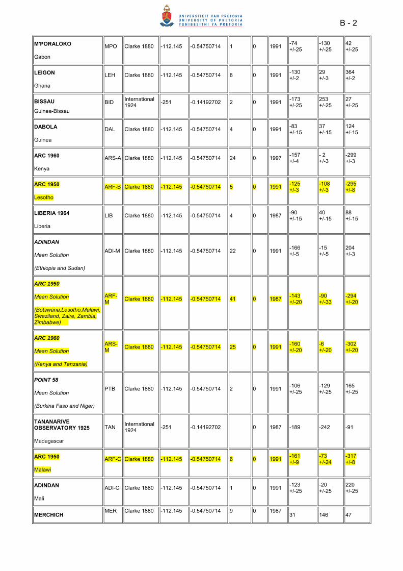
B - 2

M'PORALOKO

Gabon

MPO Clarke 1880 -112.145 -0.54750714 1 0 1991 -74 +/-25

-130 +/-25

42 +/-25

LEIGON

Ghana

LEH Clarke 1880 -112.145 -0.54750714 8 0 1991 -130 +/-2

29 +/-3

364 +/-2

BISSAU

Guinea-Bissau

BID International 1924

-251 -0.14192702 2 0 1991 -173 +/-25

253 +/-25

27 +/-25

DABOLA

Guinea

DAL Clarke 1880 -112.145 -0.54750714 4 0 1991 -83 +/-15

37 +/-15

124 +/-15

ARC 1960

Kenya

ARS-A Clarke 1880 -112.145 -0.54750714 24 0 1997 -157 +/-4

- 2 +/-3

-299 +/-3

ARC 1950

Lesotho

ARF-B Clarke 1880 -112.145 -0.54750714 5 0 1991 -125 +/-3

-108 +/-3

-295 +/-8

LIBERIA 1964

Liberia

LIB Clarke 1880 -112.145 -0.54750714 4 0 1987 -90 +/-15

40 +/-15

88 +/-15

ADINDAN

Mean Solution

(Ethiopia and Sudan)

ADI-M Clarke 1880 -112.145 -0.54750714 22 0 1991 -166 +/-5

-15 +/-5

204 +/-3

ARC 1950

Mean Solution

(Botswana,Lesotho,Malawi, Swaziland, Zaire, Zambia, Zimbabwe)

ARF-M

Clarke 1880 -112.145 -0.54750714 41 0 1987 -143 +/-20

-90 +/-33

-294 +/-20

ARC 1960

Mean Solution

(Kenya and Tanzania)

ARS-M

Clarke 1880 -112.145 -0.54750714 25 0 1991 -160 +/-20

-6 +/-20

-302 +/-20

POINT 58

Mean Solution

(Burkina Faso and Niger)

PTB Clarke 1880 -112.145 -0.54750714 2 0 1991 -106 +/-25

-129 +/-25

165 +/-25

TANANARIVE OBSERVATORY 1925

Madagascar

TAN International 1924

-251 -0.14192702 0 1987 -189 -242 -91

ARC 1950

Malawi

ARF-C Clarke 1880 -112.145 -0.54750714 6 0 1991 -161 +/-9

-73 +/-24

-317 +/-8

ADINDAN

Mali

ADI-C Clarke 1880 -112.145 -0.54750714 1 0 1991 -123 +/-25

-20 +/-25

220 +/-25

MERCHICH MER Clarke 1880 -112.145 -0.54750714 9 0 1987

31 146 47

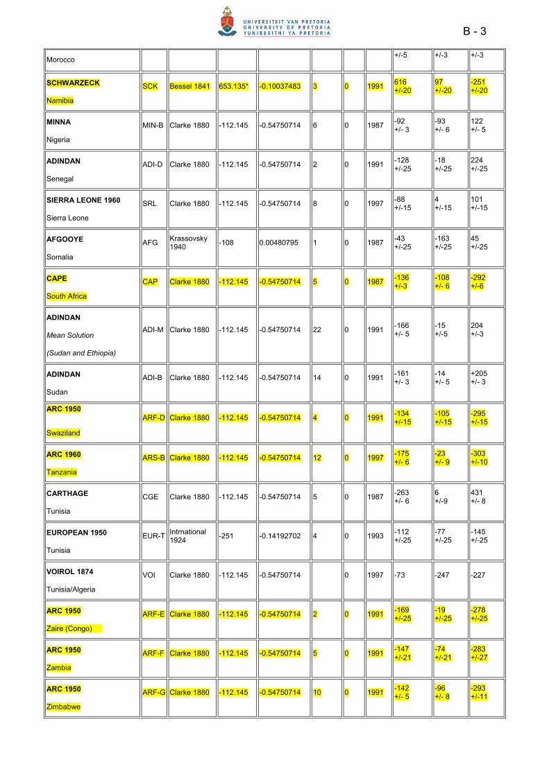
B - 3

Morocco +/-5 +/-3 +/-3

SCHWARZECK

Namibia

SCK Bessel 1841 653.135* -0.10037483 3 0 1991 616 +/-20

97 +/-20

-251 +/-20

MINNA

Nigeria

MIN-B Clarke 1880 -112.145 -0.54750714 6 0 1987 -92 +/- 3

-93 +/- 6

122 +/- 5

ADINDAN

Senegal

ADI-D Clarke 1880 -112.145 -0.54750714 2 0 1991 -128 +/-25

-18 +/-25

224 +/-25

SIERRA LEONE 1960

Sierra Leone

SRL Clarke 1880 -112.145 -0.54750714 8 0 1997 -88 +/-15

4 +/-15

101 +/-15

AFGOOYE

Somalia

AFG Krassovsky 1940

-108 0.00480795 1 0 1987 -43 +/-25

-163 +/-25

45 +/-25

CAPE

South Africa

CAP Clarke 1880 -112.145 -0.54750714 5 0 1987 -136 +/-3

-108 +/- 6

-292 +/-6

ADINDAN

Mean Solution

(Sudan and Ethiopia)

ADI-M Clarke 1880 -112.145 -0.54750714 22 0 1991 -166 +/- 5

-15 +/-5

204 +/-3

ADINDAN

Sudan

ADI-B Clarke 1880 -112.145 -0.54750714 14 0 1991 -161 +/- 3

-14 +/- 5

+205 +/- 3

ARC 1950

Swaziland

ARF-D Clarke 1880 -112.145 -0.54750714 4 0 1991 -134 +/-15

-105 +/-15

-295 +/-15

ARC 1960

Tanzania

ARS-B Clarke 1880 -112.145 -0.54750714 12 0 1997 -175 +/- 6

-23 +/- 9

-303 +/-10

CARTHAGE

Tunisia

CGE Clarke 1880 -112.145 -0.54750714 5 0 1987 -263 +/- 6

6 +/-9

431 +/- 8

EUROPEAN 1950

Tunisia

EUR-TIntrnational 1924

-251 -0.14192702 4 0 1993 -112 +/-25

-77 +/-25

-145 +/-25

VOIROL 1874

Tunisia/Algeria

VOI Clarke 1880 -112.145 -0.54750714 0 1997 -73 -247 -227

ARC 1950

Zaire (Congo)

ARF-E Clarke 1880 -112.145 -0.54750714 2 0 1991 -169 +/-25

-19 +/-25

-278 +/-25

ARC 1950

Zambia

ARF-F Clarke 1880 -112.145 -0.54750714 5 0 1991 -147 +/-21

-74 +/-21

-283 +/-27

ARC 1950

Zimbabwe

ARF-G Clarke 1880 -112.145 -0.54750714 10 0 1991 -142 +/- 5

-96 +/- 8

-293 +/-11

B - 4

Source: http://earth-info.nga.mil/GandG/coordsys/onlinedatum/CountryAfricaTable.html accessed July 2009.

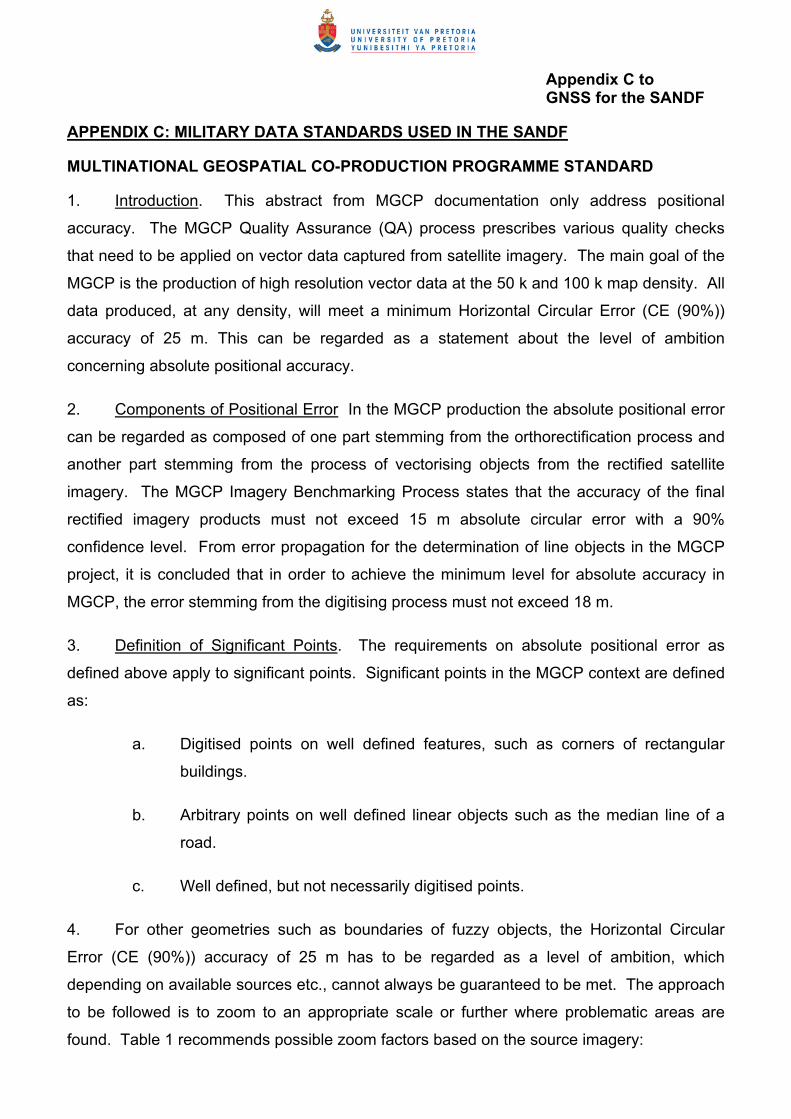
Appendix C to GNSS for the SANDF

APPENDIX C: MILITARY DATA STANDARDS USED IN THE SANDF

MULTINATIONAL GEOSPATIAL CO-PRODUCTION PROGRAMME STANDARD

1. Introduction. This abstract from MGCP documentation only address positional

accuracy. The MGCP Quality Assurance (QA) process prescribes various quality checks

that need to be applied on vector data captured from satellite imagery. The main goal of the

MGCP is the production of high resolution vector data at the 50 k and 100 k map density. All

data produced, at any density, will meet a minimum Horizontal Circular Error (CE (90%))

accuracy of 25 m. This can be regarded as a statement about the level of ambition

concerning absolute positional accuracy.

2. Components of Positional Error In the MGCP production the absolute positional error

can be regarded as composed of one part stemming from the orthorectification process and

another part stemming from the process of vectorising objects from the rectified satellite

imagery. The MGCP Imagery Benchmarking Process states that the accuracy of the final

rectified imagery products must not exceed 15 m absolute circular error with a 90%

confidence level. From error propagation for the determination of line objects in the MGCP

project, it is concluded that in order to achieve the minimum level for absolute accuracy in

MGCP, the error stemming from the digitising process must not exceed 18 m.

3. Definition of Significant Points. The requirements on absolute positional error as

defined above apply to significant points. Significant points in the MGCP context are defined

as:

a. Digitised points on well defined features, such as corners of rectangular

buildings.

b. Arbitrary points on well defined linear objects such as the median line of a

road.

c. Well defined, but not necessarily digitised points.

4. For other geometries such as boundaries of fuzzy objects, the Horizontal Circular

Error (CE (90%)) accuracy of 25 m has to be regarded as a level of ambition, which

depending on available sources etc., cannot always be guaranteed to be met. The approach

to be followed is to zoom to an appropriate scale or further where problematic areas are

found. Table 1 recommends possible zoom factors based on the source imagery:

C - 2

Table 1: Zoom Factor for Imagery Source Type

QA Scale

Quickbird Ikonos Spot Radar

(GeoSAR X- and P-

band)

Overview Scale 1:10,000 1:10,000 1:40,000 1:20,000

Check Scale 1:5,000 1:5,000 1:25,000 1:10,000

Zoom In Scale 1:3,000/

1:1,500

1:2,500/

1:1,000

1:10,000/

1:5,000

1:5,000

5. Visual Positional Accuracy Check

a. For each 10 km x 10 km section, get a general overview and select ideally 20

arbitrary but well defined points/features. Measure and record the distance

between the vector point/feature and compare it to its corresponding position

on the imagery.

b. Are features captured in their exact position relative to the imagery – or does

the line, point or area geometry not match the feature, e.g. is the point

captured right at the centre of a point feature?

c. Are well defined features correctly captured relative to adjacent features, e.g.

all buildings are placed on the correct side of a road?

d. Is the generalisation of features in accordance with the Extraction Guide?

e. Any measurement that is greater than 18 m and any other discrepancies

found, must be pointed out in a QA Report.

The implication of this QA standard is that the imagery used for vector data capturing should

have been correctly orthorectified to enable accurate capturing and this requires ground

control points collected by means of a GPS.

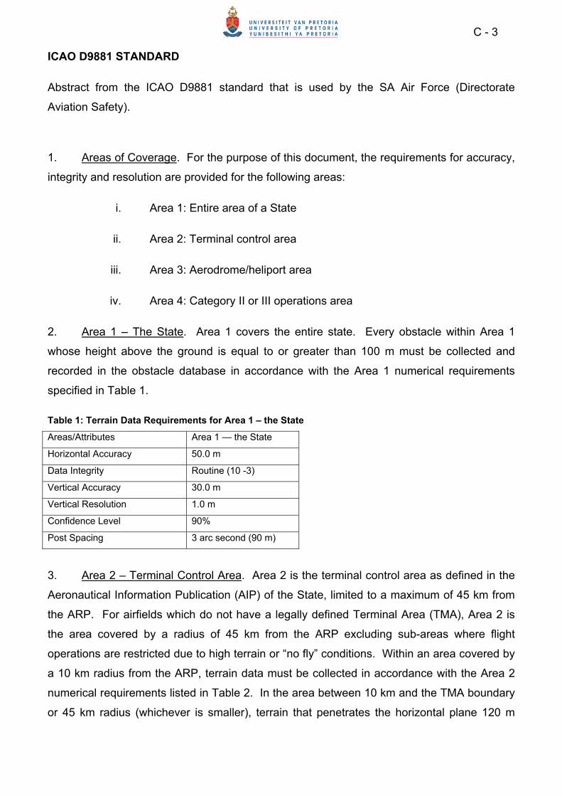
C - 3

ICAO D9881 STANDARD

Abstract from the ICAO D9881 standard that is used by the SA Air Force (Directorate

Aviation Safety).

1. Areas of Coverage. For the purpose of this document, the requirements for accuracy,

integrity and resolution are provided for the following areas:

i. Area 1: Entire area of a State

ii. Area 2: Terminal control area

iii. Area 3: Aerodrome/heliport area

iv. Area 4: Category II or III operations area

2. Area 1 – The State. Area 1 covers the entire state. Every obstacle within Area 1

whose height above the ground is equal to or greater than 100 m must be collected and

recorded in the obstacle database in accordance with the Area 1 numerical requirements

specified in Table 1.

Table 1: Terrain Data Requirements for Area 1 – the State

Areas/Attributes Area 1 — the State

Horizontal Accuracy 50.0 m

Data Integrity Routine (10 -3)

Vertical Accuracy 30.0 m

Vertical Resolution 1.0 m

Confidence Level 90%

Post Spacing 3 arc second (90 m)

3. Area 2 – Terminal Control Area. Area 2 is the terminal control area as defined in the

Aeronautical Information Publication (AIP) of the State, limited to a maximum of 45 km from

the ARP. For airfields which do not have a legally defined Terminal Area (TMA), Area 2 is

the area covered by a radius of 45 km from the ARP excluding sub-areas where flight

operations are restricted due to high terrain or “no fly” conditions. Within an area covered by

a 10 km radius from the ARP, terrain data must be collected in accordance with the Area 2

numerical requirements listed in Table 2. In the area between 10 km and the TMA boundary

or 45 km radius (whichever is smaller), terrain that penetrates the horizontal plane 120 m

C - 4

above the lowest runway elevation must be collected and recorded in accordance with the

Area 2 numerical requirements listed in Table 2. In the area between 10 km and the TMA

boundary or 45 km radius (whichever is smaller), terrain that does not penetrate the

horizontal plane 120 m above the lowest runway elevation must be collected and recorded in

accordance with the Area 1 numerical requirements listed in Table 2. In those portions of

Area 2 where the flight operations are prohibited due to very high terrain or other regulations,

terrain must only be collected and recorded in accordance with the Area 1 numerical

requirements listed in Table 2. See Figure 1 for a graphical presentation.

Table 2: Terrain Data Requirements for Area 2

Areas/Attributes Area 2 — Terminal Airspace

Horizontal Accuracy 5.0 m

Data Integrity Essential (10 -5)

Vertical Accuracy 3.0 m

Vertical Resolution 0.1 m

Confidence Level 90%

Post Spacing 1.0 arc second (30 m)

Figure 1: Areas 1 and 2 for Terrain

4. Area 3 — Aerodrome/Heliport Area. When surveying vertical objects, the horizontal

spatial extent to be surveyed must include the aerodrome surface movement area plus a

buffer of 50 m or the minimum separation distances specified in Doc 9157, whichever is

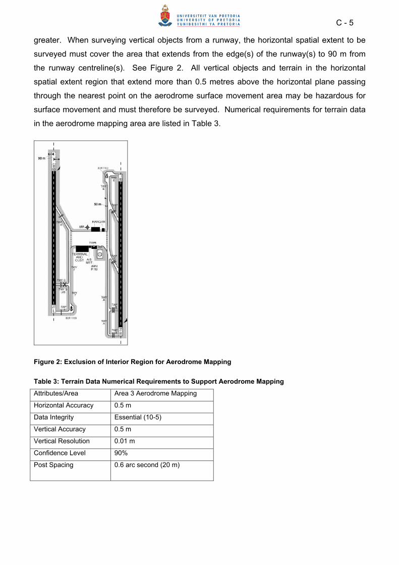
C - 5

greater. When surveying vertical objects from a runway, the horizontal spatial extent to be

surveyed must cover the area that extends from the edge(s) of the runway(s) to 90 m from

the runway centreline(s). See Figure 2. All vertical objects and terrain in the horizontal

spatial extent region that extend more than 0.5 metres above the horizontal plane passing

through the nearest point on the aerodrome surface movement area may be hazardous for

surface movement and must therefore be surveyed. Numerical requirements for terrain data

in the aerodrome mapping area are listed in Table 3.

Figure 2: Exclusion of Interior Region for Aerodrome Mapping

Table 3: Terrain Data Numerical Requirements to Support Aerodrome Mapping

Attributes/Area Area 3 Aerodrome Mapping

Horizontal Accuracy 0.5 m

Data Integrity Essential (10-5)

Vertical Accuracy 0.5 m

Vertical Resolution 0.01 m

Confidence Level 90%

Post Spacing 0.6 arc second (20 m)

C - 6

5. Area 4 — CAT II and III Operation Area. Area 4 is defined as the Radar Altimeter

Area for CAT II/III Precision Approach procedures. The area extends from the runway

threshold to 900 m (3000 ft) from the threshold. It is 120 m (400 ft) wide and centred on an

extension of the runway centreline. See Figure 3. At those airports where runways are

equipped for CAT II or III operations, terrain data requirements for Area 4, provided in Table

4, must apply.

Table 4: Terrain Data Requirements for Area 4

Areas Attributes Area 4 — CAT II/III Operation Area

Horizontal Accuracy 2.5 m

Data Integrity Essential (10-5)

Vertical Accuracy 1.0 m

Vertical Resolution 0.1 m

Confidence Level 90%

Terrain Publication Timeliness

As required

Post Spacing 0.3 arc second (9 m)

Figure 3: Terrain Data Collection Surface — Area 4

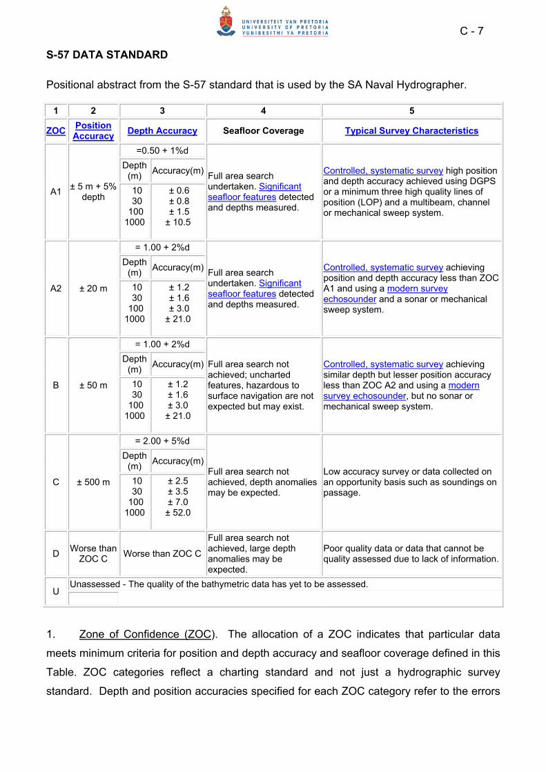
C - 7

S-57 DATA STANDARD

Positional abstract from the S-57 standard that is used by the SA Naval Hydrographer.

1 2 3 4 5

ZOC Position Accuracy

Depth Accuracy Seafloor Coverage Typical Survey Characteristics

A1 ± 5 m + 5%

depth

=0.50 + 1%d

Full area search undertaken. Significant seafloor features detected and depths measured.

Controlled, systematic survey high position and depth accuracy achieved using DGPS or a minimum three high quality lines of position (LOP) and a multibeam, channel or mechanical sweep system.

Depth (m)

Accuracy(m)

10 30 100 1000

± 0.6 ± 0.8 ± 1.5 ± 10.5

A2 ± 20 m

= 1.00 + 2%d

Full area search undertaken. Significant seafloor features detected and depths measured.

Controlled, systematic survey achieving position and depth accuracy less than ZOC A1 and using a modern survey echosounder and a sonar or mechanical sweep system.

Depth (m)

Accuracy(m)

10 30 100 1000

± 1.2 ± 1.6 ± 3.0 ± 21.0

B ± 50 m

= 1.00 + 2%d

Full area search not achieved; uncharted features, hazardous to surface navigation are not expected but may exist.

Controlled, systematic survey achieving similar depth but lesser position accuracy less than ZOC A2 and using a modern survey echosounder, but no sonar or mechanical sweep system.

Depth (m)

Accuracy(m)

10 30 100 1000

± 1.2 ± 1.6 ± 3.0 ± 21.0

C ± 500 m

= 2.00 + 5%d

Full area search not achieved, depth anomalies may be expected.

Low accuracy survey or data collected on an opportunity basis such as soundings on passage.

Depth (m)

Accuracy(m)

10 30 100 1000

± 2.5 ± 3.5 ± 7.0 ± 52.0

D Worse than

ZOC C Worse than ZOC C

Full area search not achieved, large depth anomalies may be expected.

Poor quality data or data that cannot be quality assessed due to lack of information.

U Unassessed - The quality of the bathymetric data has yet to be assessed.

1. Zone of Confidence (ZOC). The allocation of a ZOC indicates that particular data

meets minimum criteria for position and depth accuracy and seafloor coverage defined in this

Table. ZOC categories reflect a charting standard and not just a hydrographic survey

standard. Depth and position accuracies specified for each ZOC category refer to the errors

C - 8

of the final depicted soundings and include not only survey errors, but also other errors

introduced in the chart production process. Data may be further qualified by Object Class

"Quality of Data" (M_QUAL) sub-attributes as follows:

a. Positional Accuracy (POSACC) and Sounding Accuracy (SOUACC) may be

used to indicate that a higher position or depth accuracy has been achieved

than defined in this Table (e.g. a survey where full seafloor coverage was not

achieved could not be classified higher that ZOC B; however, if the position

accuracy was, for instance, ± 15 m, the sub-attribute POSACC could be

used to indicate this).

b. Swept areas where the clearance depth is accurately known but the actual

seabed depth is not accurately known may be accorded a "higher" ZOC (i.e.

A1 or A2) providing positional and depth accuracies of the swept depth

meets the criteria in this Table. In this instance, Depth Range Value 1

(DRVAL1) may be used to specify the swept depth. The position accuracy

criteria apply to the boundaries of swept areas.

2. Position Accuracy. Position Accuracy of depicted soundings at 95% CI (2.45 sigma)

with respect to the given datum. It is the cumulative error and includes survey,

transformation and digitizing errors etc. Position accuracy need not be rigorously computed

for ZOCs B, C and D, but may be estimated based on type of equipment, calibration regime

and historical accuracy.

Appendix D to GNSS for the SANDF

APPENDIX D: GPS FIELD MANUAL

1. This section will elaborate on the preparations that need to be made before collection

of positional data with a GPS receiver will commence. First and foremost the task at hand

needs to be understood for it will determine the type of planning and equipment that is

needed.

2. Plan the Task. The following salient points may assist in the planning of the data

collection excursion.

a. Determine where the task will be conducted. Will it be in an own controlled

environment or should access permission be obtained, such as in national

parks or privately owned land/area? Determine the correct authorities and

procedures.

b. Use maps and imagery to plan access and routes. Determine the extent of

the target area and the proposed features, such as ground control points

(GCPs) that need to be collected. Allocate sufficient time to travel as well as

to collect the data. Remember travelling time in the field is significantly

slower.

c. Plan safety aspects, especially on military training areas and shooting

ranges, for instance:

i. Areas to be avoided or no-go areas.

ii. Safety clothes when working in dangerous areas, e.g. special head gear

when working on construction sites or clothes for extreme climates.

iii. Security rope when on ladders, rooftops, etc.

iv. Special vehicle licences when needed.

d. Determine the need for a base station.

i. Determine if there is a fixed or known point that is available that has

been surveyed before. Are the coordinates known and reliable? Are the

datum and projection of the coordinates known? Is there an ITRF or

other base station in the vicinity?

D - 2

ii. Determine if a new point needs to be established. The following may be

of importance:

(1) Plan to avoid multipath. Thus, avoid high-rise buildings and/or

reflective surfaces close to the point. Ensure antennas are fitted

with base plates to prevent reflection from low elevations.

(2) Ensure that it is situated on stable ground. Avoid areas that are

known to be unstable, such as areas with varying underground

water levels or close to disturbed areas where large excavations

took place.

(3) Determine how accessible it is and if it can be visited any time

without restriction?

(4) Is it safe to put up the base station at the selected point?

iii. Plan the monitoring of data collection at the base station during the

excursion to ensure it is operating continuously and properly.

iv. Plan the quality control to ensure base data are accurate/usable.

v. When base data are radio transmitted from the base station to the roving

receiver, this needs to be planned and tested beforehand.

vi. Plan the excursion to be conducted under favourable conditions. The

following aspects may be considered:

(1) The ionosphere effect on measurements as discussed earlier.

Early mornings or late nights will generally provide better results.

After midday until 18:00 should be avoided. At lower latitudes this

may shift to a later timeslot.

(2) The forecast of satellite availability and associated DOP values.

Some GPS software allows for this and can be used to plan the

excursion accordingly.

(3) Avoid reflective surfaces and shadowing as discussed.

D - 3

3. Prepare Equipment. After the task has been planned the equipment needs to be

prepared and tested. The following needs to be confirmed.

a. Ensure GPS receivers are in working condition.

b. Ensure that the settings such as the datum, measurement units, elevation

mask, locking interval, etc. are set correctly on all GPS receivers.

c. Charge batteries and ensure that chargers and or solar panels with fittings

are tested and packed. Ensure correct wall-plug fittings for chargers and

other equipment. Ensure enough batteries of the correct type are packed for

the task.

d. Make sure enough space is available on receivers’ internal memory and data

cards. A good principle is not to erase all data from receivers or format data

cards. You do not know when old data on the receiver or data card is

needed again by somebody else. Create only sufficient space for the task at

hand by erasing some of the oldest data.

e. Pack measuring tapes to determine antenna heights in the field.

f. Check and pack GPS poles, tripods and carrying bags. A 30 cm antenna

pole to be used at Trig Beacons in the RSA can be handy.

g. Test and pack power and antenna cables.

h. If a computer is used as a data logger the necessary GPS software must be

loaded and tested. Ensure USB – serial port conversion cables and software

is loaded and working. Ensure chargers and or solar panels with correct

fittings are tested and packed.

i. GPS receivers and computers need to be protected against the elements

when extended field measurements are taken. The protective cases of

expensive equipment may suffice and where these are not available a cooler

box may be handy.

j. The following prove to come in handy during field measurements:

i. A coil of strong rope, tie-downs and bungee-cords to fix antenna poles to

other structures on rooftops and other places.

D - 4

ii. A multi-tool such as a Leatherman®.

iii. A couple of locks and chains to lock up base or static stations when

these cannot be guarded. Sometimes you can access a relatively safe

place, such as a rooftop, a fenced in tennis court or a swimming pool to

establish a base station, but often there is no means to lock a gate.

Beware of multipathing, which can result when locating a GPS antenna

too close to a fence.

k. Ensure and test that base or reference data provider’s websites are

accessible and available. It may require registering and acquiring passwords

or even subscription.

l. Ensure that the data dictionary is downloaded to the GPS receivers when

attribute data of features need to be captured with the positional data.

Ensure that the terminology of the data dictionary is understood by every

operator.

m. Ensure that other equipment, such as laser range finders are operational and

measurement data formats are properly integrated with the GPS software.

n. Ensure that other software that may be needed, such as GeoRover for

integrating digital photos with GPS tracks are loaded and functional.

o. Synchronise time settings on data loggers, computers and digital cameras

that will be used.

4. Garmin Receiver Settings. Garmin receivers are navigational instruments and special

care should be taken when these receivers are used for collecting ground control data for

mapping projects. The following settings are important.

a. Ensure the correct datum is selected. On the Main Menu select Setup and

under Setup select Units.

b. On the Main Menu select Tracks and set Track Log to “On”, on the Track Log

Setup menu “Wrap When Full” should be switched off (unselected) and on

the Data Card Setup the “Log Track To Data Card” should be activated

(selected). Garmin receivers are factory set to lock only 10 000 incidents per

track. Thus, when “Wrap When Full” is selected and the 10 000 limit is

D - 5

reached the receiver will capture the additional incidents over the beginning

of the track and that part will be lost. Thus, by switching off “Wrap When

Full”, the receiver will warn the operator that the track is full. The operator

can save the track to the data card and the “Track Log” can be cleared for

work to continue.

c. On the Main Menu select Tracks. On the Tracks Setup menu the “Record

Method” and “Interval” should be set to a preferred time interval and not on

“Auto”. If set on “Auto” some of the incidents or bread crumbs will be

weeded out when the track is saved to save space on the micro SD card. A

full track of 10 0000 incidents without additional annotation will be in the

vicinity of 1 to 1,5 MB that approximates 2 h and 46 min of capturing at one

second intervals. Some of the Garmin receivers that are used in the SANDF

are equipped with a 2 GB micro SD cards of which 1 GB is allocated to the

background maps. Thus, approximately 800 full tracks can be stored on the

remaining 1 GB space on the micro SD card. Bigger micro SD cards are

also available and background maps are helpful, but not essential for

capturing mapping data.

d. On the Main Menu select Setup and Map. On the Map Setup – General the

“Lock On Road” should be switched off. If this function is switched on the

track will lock to the centreline of the road of the background map and the

readings may be incorrect depending on the accuracy of the background

map. If the GPS tracks are intended to verify the accuracy of available data,

this will be futile. “Lock On Road” should therefore be switched off.

5. Conduct Field Measurements. All planning and preparatory steps were taken to

conduct the measurements. Stay with the original collection plan, but be ready to adjust the

plan on the spot if necessary. However, the client agreed to the collection plan and expects

results accordingly. Remember also that an equal dispersion of GCP over the area remains

a prerequisite for the effective rectification of an image. A detailed field record or log of the

collection excursion is of paramount importance. The following should be included:

a. Names of the operators involved and name of the team leader.

b. Date, time and place of collection.

D - 6

c. Description of the feature or GCP. Attribute data should be logged according

to the data dictionary.

d. A sketch and or photos of the feature.

e. The type and serial numbers of the GPS receiver and antenna used for

collecting the data.

f. Name given to the feature on the GPS receiver, for instance Point 1, 2, 3,. A,

B, C or description according to data dictionary.

g. Name of base station/s used.

6. Confirm GPS settings, e.g. minimum PDOP values, elevation masks, logging interval,

etc. Monitor GPS receivers from time to time to visually check the logging values. Be

mindful not to mask satellite signals during setup or checking of receivers.

7. Quality Control. Quality control can be conducted in the field. The following should be

considered.

a. Confirm readings of a specific receiver by taking readings at a known or

surveyed point.

b. Take the first measurement of the day at the last point of the previous day.

c. Download GPS data and assess published precision and PDOP values.

d. Geometrically assess downloaded GPS data by visualising it in a GIS

programme. Outliers and multipath measurements can be easier spotted.

e. Conduct spot-checks on the collected data to determine precision and

accuracy.

8. Download Data, Quality Control and Publish. Data can be downloaded from GPS

receivers in the field and e-mailed back to the office or stored on removable media. It is wise

to make backups of all data when it is downloaded in the field. The cost of additional

removable media is insignificant in comparison with the cost of a new collection excursion. A

strong antivirus programme should be in place to protect data on computers and removable

media. When data are downloaded at the office, backups can be made on the respective

servers. An alternative is to write data to CDs or DVDs for long term storage. When data

D - 7

are secured it needs to be post-processed, quality checked and published in the formats that

were agreed on with the client.