JOURNAL OF GEOPHYSICAL RESEARCH, VOL. 91, NO. B5, PAGES 4909-4919, APRIL 10, 1986

An Inversion for Slip Distribution and Fault Shape from Geodetic Observations of the 1983, Borah Peak, Idaho, Earthquake

STEVEN N. WARD AND SERGIO E. BARRIENTOS

O. F. th'chter Labo•ory, Earth $ciene• Board, University of California Santa Orua

This paper develops an inversion technique for static surface displacements associated with shallow faulting and applies the method to geodetic observations of the Borah Peak, Idaho, earth- quake (Ms=7.3) of October 28, 1983. This technique improves upon classical, uniform slip planar (USP) models by admitting earthquake faults which are curved and contain variable slip. By summing elemental point sources, employing a gradient strategy with positivity constraints, and combining both geodetic and surface scarp height data, we can now resolve fault orientation, di- mension, shape, and slip distribution. Large formal misfits to the geodetic data and disagreements in observed surface scarp locations found with the best USP fault are eliminated in variable slip planar (VSP) models. The best VSP fault reaches to 18 km depth in the southeast but only to 3 km depth in the northwest. Surface slip and slip at depth are poorly correlated in the VSP model. In fact, toward the southeast, slip at depth extends 13 km beyond the terminus of the fault's surface expression. Three or four knots of concentrated slip are found in VSP models. These knots are 3-6 km in dimension and may represent the breaking of asperities. To test for listric-like behavior of the Borah Peak fault, we considered all possible variable slip listric (VSL) faults of parabolic shape. The best VSL model has a slight downward curvature; however, it does not fit the data significantly better than VSP models. The geodetic measurements do not support significant listric curvature at depths shallower than 20 km. Our techniques permit the calculation of sensitivity kernels for surface displacement. These functions explicitly reveal fault locations where a certain geodetic measurement is most sensitive. For faults like Borah Peak, a surface measurement at point r samples slip to a depth roughly equal to the distance from r to the fault trace. Consequently, near fault bench marks and surface scarp height measurements are very weak constraints on slip at depth. We feel that variable slip fault models will allow significant new interpretations to be drawn from the geodetic data pool concerning the physics of earthquakes and their potential hazard.

1. INTRODUCTION tions. By representing the dislocation surface as a super- position of point sources, we can compute the coseismic de-

The 1983 Borah Peak (Ms - 7.3) earthquake was the formation of virtually an unlimited variety of earthquake largest earthquake to occur in the Basin and Range province faults. This progress in the forward calculation is accompa- of the western United States since the 1957 Hebgen Lake, nied by progress in the corresponding inverse problem. Sur- Montana, event. To our fortune, geodetic leveling surveys of face geodetic data can now be used to invert for fault shape 1933 and 1948 passed virtually on top of the 1983 faulting. A and moment release patterns. Relative to previous methods resurvey of these lines in 1984 provided the best record yet which could only recover the best uniform slip planar fault, available of coseismic deformation associated with a large our technique allows significant new interpretations to be extentional earthquake in the province. These data allow drawn from the geodetic data pool. us to address some important questions related to the char- acteristics of Basin and Range normal faults: (1) Is slip on 2. DATA the rupture surface uniform? (2) Do variations in surface scarp heights reflect variations in slip at depth? (3) Does• Three leveling surveys of the Borah Peak, Idaho, region the rupture surface flatten with depth as suggested in listric conducted by the National Geodetic Survey in 1933, 1948, fault models? and 1984 enable the static elevation changes associated with

In modeling coseismic deformation, few workers have con- the earthquake of October 28, 1983, to be calculated. The sidered the possibilities of non-uniform slip over curved rup- northeastern elevations (points 1-23 in Figure 1) were mea- ture surfaces. Typical analyses assume a rectangular fault sured in August 1948 with a second-order, single-run lev- on which the dislocation vector is everywhere constant [Stein eling. The southwestern portion of the 70-km-long route and Lisoswski, 1983; Mansinha and Staylie, 1971; Savage was carried out in 1933 using first-order, double-run stan- and Hastie, 1966, 1969;Chinnery, 1961]. The restrictions dards which permitted comparatively smaller errors. The of uniform slip and planar rectangular faults, however, are only common points of the two routes are bench marks 22 probably unrealistic. In our work we have made substan- and 23. In spite of the disparity of standards required for tim improvement in the theory by removing these resttic- both levelings, the 1.58 mm discrepancy between the 1938

and 1948 measurements of the elevation difference between

these two stations is actually smaller than the expected ran- dom error for a first-order survey. The July 1984 leveling, Copyright 1986 by the American Geophysical Union. which reoccupied the 1933 and 1948 stations, was conducted

Paper number 5B5671 to first-order, single-run standards over the central portion 0148-0227/86/005B-5671505.00 of the survey, but was double-run over 15 km at the ends

49O9

4910 WARD AND BARRIENTOS: FAULT SLIP FROM GEODETIC OBSERVATIONS

2O

Borah Peak [ i I

++

+

•+

++ Epicenter lO km

[ I I 11 4 ̧ 5o ' 4-o '

where

or

M.•sin20 + • I2(r, b,) (1)

3•r •

,(,) =

where Mii(i,j = 1,3) are the components of the moment tensor, R = ][r-ro[[ is the distance between r and to, r = V'R •- h•, and 8 = tan-'[•. (r-ro)/i. (r-ro)] [0omer, 1982]. With the z coordinate positive downward, t and /• are orthonormal unit vectors parallel to the surface of the half-space. For a double couple, the trace and the determinant of the moment tensor M vanish. If the largest eigenvalue of M equals 1, then mo represents the scalar mo- ment of the source. The components of M are assumed fault

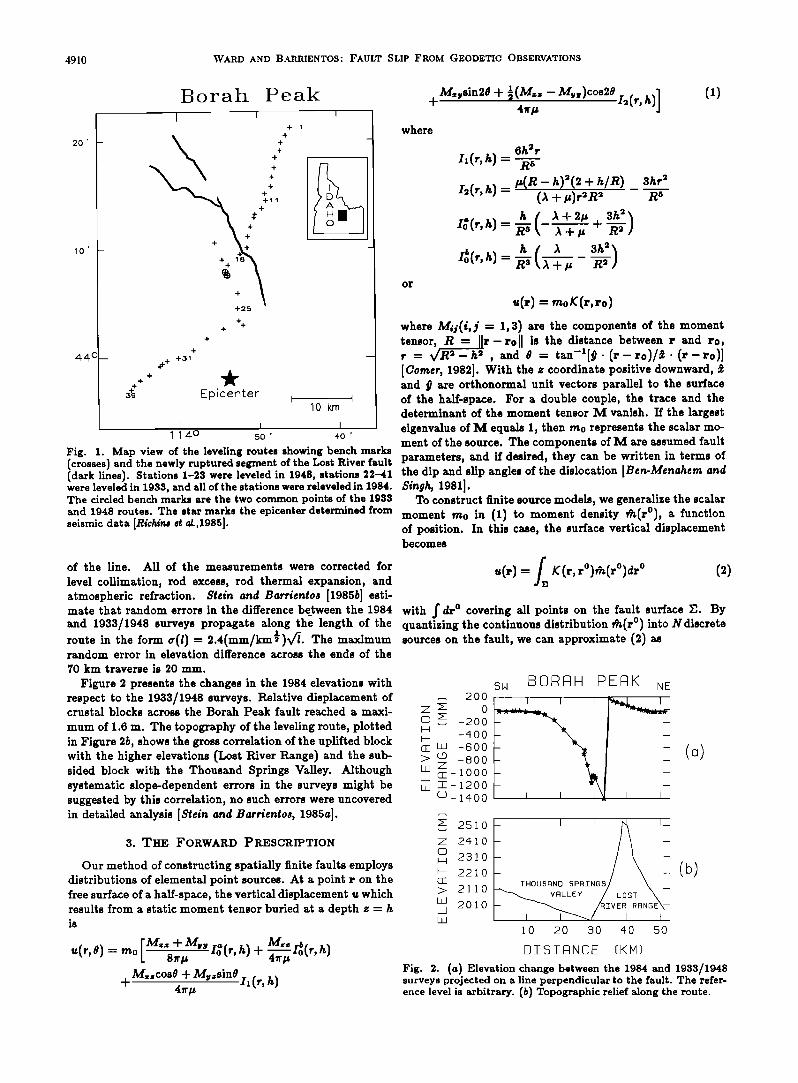
Fig. 1. Map view of the leveling routes showing bench marks (crosses) and the newly ruptured segment of the Lost River fault parameters, and if desired, they can be written in terms of (dark lines). Stations 1-23 were leveled in 1948, stations 22-41 the dip and slip angles of the dislocation [Ben-Menahera and were leveled in 1933, and all of the stations were releveled in 1984. $ingh• 1981]. The circled bench marks are the two common points of the 1933 To construct finite source models, we generalize the scalar and 1948 routes. The star marks the epicenter determined from moment mo in (1) to moment density •(rø), a function seismic data [Rich,ns et a/.,1985]. of position. In this case, the surface vertical displacement

becomes

of the line. All of the measurements were corrected for u(r) =/•, K(r,rø)•(rø)dr ø (2) level collimation, rod excess, rod thermal expansion, and atmospheric refraction. Stein and Barriento• [198515] esti- mate that random errors in the difference be_tween the 1984 with f dr ø covering all points on the fault surface •. By and 1933/1948 surveys propagate along the length of the quantizing the continuous distribution •(r ø) into Ndiscrete route in the form •(1) = 2.4(mm/km«)V•. The maximum sources on the fault, we can approximate (2) as random error in elevation difference across the ends of the 70 km traverse is 20 mm.

Figure 2 presents the changes in the 1984 elevations with respect to the 1933/1948 surveys. Relative displacement of crustal blocks across the Borah Peak fault reached a maxi-

mum of 1.6 m. The topography of the leveling route, plotted in Figure 215, shows the gross correlation of the uplifted block with the higher elevations (Lost River Range) and the sub- sided block with the Thousand Springs Valley. Although systematic slope-dependent errors in the surveys might be suggested by this correlation, no such errors were uncovered in detailed analysis [Stein and Barrientos, 1985a].

3. THE FORWARD PRESCRIPTION

Our method of constructing spatially finite faults employs distributions of elemental point sources. At a point r on the free surface of a half-space, the vertical displacement u which results from a static moment tensor buried at a depth z = h is

+ -%, (,.,

+ M..cosO + M•.sinO I•(r, h) 4/r/z

200

0 -200 -•00 -600 -800

-lOOO -1200 -1•oo

2510

2•10

2310 2210

2110

2010

SN

I I I

8088H PERK HE

i i

(o)

THOUSAND SPRZNGS/

I I -"--Jr I I

10 20 30 •0 50

BISTFINCE (KH)

Fig. 2. (a) Elevation change between the 1984 and 1933/1948 surveys projected on a line perpendicular to the fault. The refer- ence level is arbitrary. (b) Topographic relief along the route.

WARD AND BARRIENTOS' FAULT SLIP FROM GEODETIC OBSERVATIONS 4911

or

or

H

iv

,,(,,) = j--1

u = K m

With uniformly distributed bench marks, I, = (n- 1)A/, L = {N- 1)AI, and

H

• Zn--1 • N

In case here, •m,x = 0.02 m , N = 39, and the expected random error in the data is 0.0078 m •. The summed square

(3) error in the best USP model amounted to 0.0261 m •. Thus either •m,•, for the survey is underestimated by a factor of

if the surface displacement u(r) is considered to consist of 1.8 or the USP model is in some way unsatisfactory. Because M observations u(ri) at ri. it is unlikely that Stein and Barrientos' [1985b] estimate of

4. THE CLASSICAL APPROACH:

UNIFORM SLIP PLANAR (USP) FAULTS

To simulate a planar fault with both length and width, a rectangular grid of point sources can be constructed. In this classical model, the fault strike is parallel to the surface scarp {N152øE), and the distribution of moment is constant. The inversion consists of varying the fault parameters within a prescribed range and recovering the two free parameters m0 and u0 (the displacement reference level relative to mon- ument 1) by minimizing the misfit in the vertical static dis- placement along the leveling line. Apart from m0 and u0, five fault parameters enter into the search: fault width (di- mension downdip), fault length (dimension along strike), dip angle, slip angle, and the southeast end point of the fault.

The superposition of 900 point sources and the inversion

the survey errors are understated to this degree, we are lead to suspect the USP model.

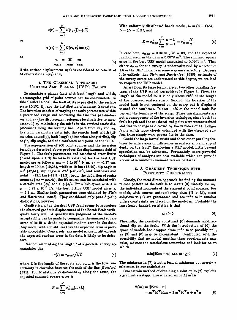
Apart from its large formal error, two other puzzling fea- tures of the USP model are evident in Figure 3. First, the length of the model fault is only about 60% of the length of the observed surface scarp. Second, the location of the model fault is not centered on the scarp but is displaced toward the southeast. In fact, 15% of the model fault lies beyond the terminus of the scarp. These misalignments are not a consequence of the inversion technique, since both the fault length and the southeast end point were unconstrained and free to change as directed by the variance of fit. Longer faults which more closely coincided with the observed sur- face trace simply were poorer fits to the data.

Could the large formal misfit and these other puzzling fea- tures be indications of differences in surface slip and slip at depth on the fault? Employing a USP model, little beyond

technique described above produce the displacement field of speculation can be advanced. Fortunately, more powerful Figure 3. The fault parameters and associated error limits techniques of analysis are now available which can provide (based upon a 10% increase in variance) for the best USP a view of nonuniform moment release patterns. model are as follows: m0 = 2.6x10 • N m, u0 =-0.37 cm,

length = 19 km (19,23), width = 19 km (18,20), dip angle = 5. A GRADIENT TECHNIQUE WITH 49 ø (47,51), slip angle =-75 ø (-70,-90), and southeast end POSITIVITY CONSTRAINTS point = -13.1 km (-12.9,-13.3). From the definition of scalar moment (mi = I•siAi), the ith source can be associated with Clearly, the most direct approach for finding the moment a certain area (Ai) and slip (si). For a half-space with I = release pattern of the fault is to invert (3) directly for rni, /• = 3.23 x 10 •ø Pa, the best fitting USP model gives sl the individual moments of the elemental point sources. For = 2.2 m. Similar fault parameters were obtained by Stein models.with sources outnumbering data (N > M), exact and Barrientos [1985b]. They considered only pure dip-slip soluti0hs to (3) are guaranteed and are infinite in number dislocations, however. ' u•{iess constraints are placed on the model m. Probably the

Qualitatively, the classical USP fault seems to reproduce least heavy handed restriction is that the observed geodetic displacement of the Borah Peak earth- quake fairly welE A quantitative judgment of the model's rni •_ 0 (6) acceptability can be made by comparing the summed square error of its fit with t•he expected random error in the data. Physically, the positivity constraint (6) demands unidirec- Any model with a misfit less than the expected error is prob- tional slip on the fault. With the introduction of (6) the ably acceptable. Conversely, any model whose misfit exceeds space of models has dropped from infinite to possibly null, the expected random'error in the data is likely to be defec- as (3) and (6) may be inconsistent. Confronted with the rive. ' -'•. possibility that no model meeting these requirements may

Random error along the length I of a geodetic survey ac- exist, we ease the restrictions somewhat and look for an m cumulates like which

o'(1) = •m.xV•-/L (4) minll Km - ,•11 and rrti Z 0 (7)

where L is the length of the route and •rm,,, is the total un- The minimum in (7) is not a formal minimum but merely a certainty in elevation between the ends of the line [Bornford, minimum to our satisfaction. 1971]. For N stations at distances I, along the route, the One certain method of obtaining a solution to (7) exploits expected summed square error is a gradient strategy. The squared error E(m) is

• = Z 2 E(m) = I IKm-,•11 ,=• = mTKTKm- 2mTKTu + 11T11 (8)

4912 WARD AND BARRIENTOS' FAULT SLIP FROM GEODETIC OBSERVATIONS

2.62E+19

1 52.0

49.0

-75.0

SQERR=O,0261

[] OBSERVATIONS

+ THEORY

55 KM

Fig. 3. (Left) Contour map of vertical surface deformation at 0.1-m intervals for the best fitting USP source. Dashed contours map depressions. Stippled area is the surface projection of the fault. (Right) Cross section of observed and theoretical vertical displacement. The numbers next to the lower focal hemisphere are the scalar moment and strike, dip, and slip angles of the fault. Although the model appears to reproduce the data, the summed square error of the fit (0.0261 m 2) far exceeds the expected random error in the survey (0.0078 m2). Also note the poor degree of overlap between the observed surface scarp and the model fault.

and schemes based on programs found in the above mentioned

-VE(m)- IlI•T(u- I•m) (9) works, but no successful models could be generated until modification (10) was adapted. (3) Any nonnegative slip

Positive or negative signs of the ith element of (9) indicate model is a valid starting model. (4) The size and shape of the that total error could be reduced by increasing or decreasing fault need not be specified. If at any stage in the inversion the moment of the ith source. For some model m ø, a stably the current fault model needs to contract to better fit the improved model m x is data, sources near its edges will be reduced in moment and

eventually shut off when mi reaches zero. Conversely, if the m x -- m ø + Amsgn{-VE(mø)• (10) fault dimension need to increase to better fit the data, zeroed

sources will turn on. This is a remarkable attribute as the

where the scalar Am is taken to be small enough such that operator need no longer force fault shape on the inversion. (5) Surface scarp heights As øbs can be simultaneously fit by

E(m•) < E(m ø) (11) including the term

In practice, if (11) is not satisfied then Am is reduced. To e(Z•s- As øbs) (12) satisfy (6), negative perturbations in m ø are permitted only

o • is set equal to zero. if m; - Am > 0. If not, then m; within the brackets on the right side of (10). Elements of Although seemingly ill posed, the iterative method above vector As contain the equivalent slip for those m which lie

has several special advantages: (1) No matrix inversion is closest to the surface along strike and are zero otherwise. required. (2) A degree of smoothness is implied in (10) as The constant e determines the responsiveness of the new all sources are increased or decreased in moment equally solution m x to surface scarp data relative to the geodetic without regard to the magnitude of-VE(m). Equation data. (10), in fact, is the key to the success of this program and it is The principal disadvantages of the gradient method are the point at which our method deviates from other gradient the same as any inversion with nonlinear constraints: The techniques such as those found in Lawson and Hanson [1974] convergence characteristics, error estimates, and physical ac- or Menke [1984]. In those techniques, the unknown with the ceptability of the end model must be judged after the fact. largest value Of -VE(m) is removed from a slack variable set and transferred to an active set which attempts to satisfy 6. VARIABLE SLIP PLANAR (VS P) FAULTS the constraints and fit the data in the least squares sense. These and other approachs which alter model parameters To contrast the results of section 4, we recover the best based on the magnitude of the local error gradient may reach planar fault with variable slip. In this process, with the fault low levels quickly, but they can become unstable in many strike coinciding with that of the surface trace, uo fixed at applications. We made several attempts to construct inverse -0.15 cm, and the fault width, length, and southeast end

WARD AND BARRIENTOS' FAULT SLIP FROM GEODETIC OBSERVATIONS 4913

,3,5 KM

2.75E+19

I 52.0

49.0

-75.0

$QERR=O.0015

[] OBSERVATIONS

+ THEORY

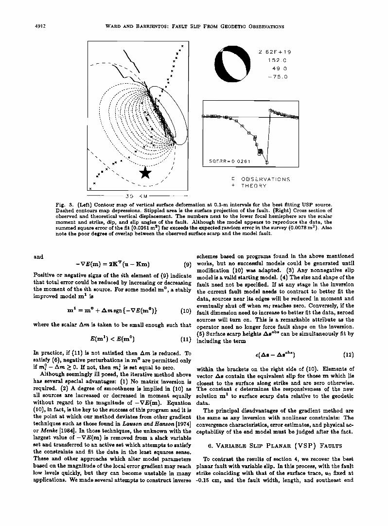
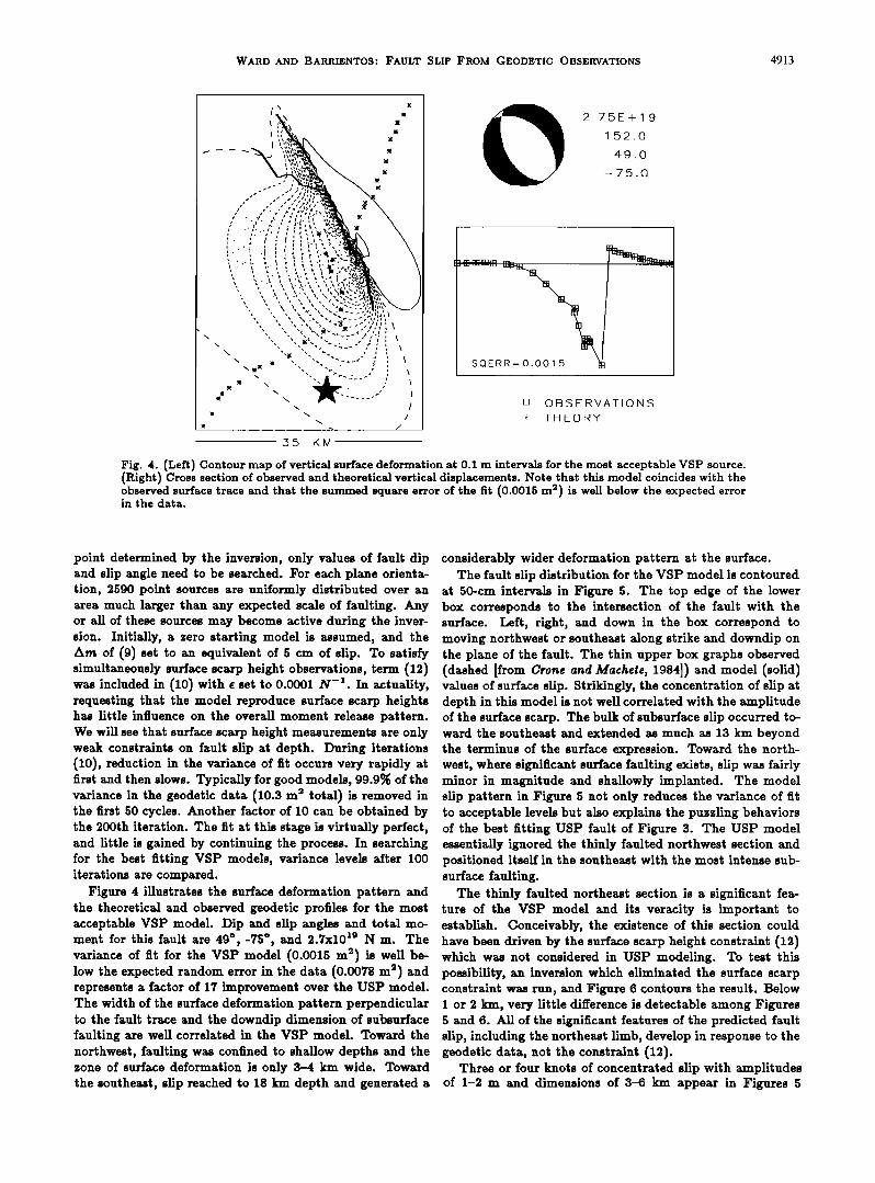
Fig. 4. (Left) Contour map of vertical surface deformation at 0.1 m intervals for the most acceptable VSP source. (Right) Cross section of observed and theoretical vertical displacements. Note that this model coincides with the observed surface trace and that the summed square error of the fit (0.0015 m 2) is well below the expected error in the data.

point determined by the inversion, only values of fault dip and slip angle need to be searched. For each plane orienta- tion, 2590 point sources are uniformly distributed over an area much larger than any expected scale of faulting. Any or all of these sources may become active during the inver- sion. Initially, a zero starting model is assumed, and the Am of (9) set to an equivalent of 5 cm of slip. To satisfy simultaneously surface scarp height observations, term (12) was included in (10) with • set to 0.0001/V -•. In actuality, requesting that the model reproduce surface scarp heights has little influence on the overall moment release pattern. We will see that surface scarp height measurements are only weak constraints on fault slip at depth. During iterations (10), reduction in the variance of fit occurs very rapidly at first and then slows. Typically for good models, 99.9% of the variance in the geodetic data (10.3 m 2 total) is removed in the first 50 cycles. Another factor of 10 can be obtained by the 200th iteration. The fit at this stage is virtually perfect, and little is gained by continuing the process. In searching for the best fitting VSP models, variance levels after 100 iterations are compared.

Figure 4 illustrates the surface deformation pattern and the theoretical and observed geodetic profiles for the most acceptable VSP model. Dip and slip angles and total mo- ment for this fault are 49 ø, -75 ø, and 2.7x10 •9 N m. The variance of fit for the VSP model (0.0015 m •) is well be- low the expected random error in the data (0.0078 m •) and represents a factor of 17 improvement over the USP model. The width of the surface deformation pattern perpendicular to the fault trace and the downdip dimension of subsurface faulting are well correlated in the VSP model. Toward the northwest, faulting was confined to shallow depths and the zone of surface deformation is only 3-4 km wide. Toward the southeast, slip reached to 18 km depth and generated a

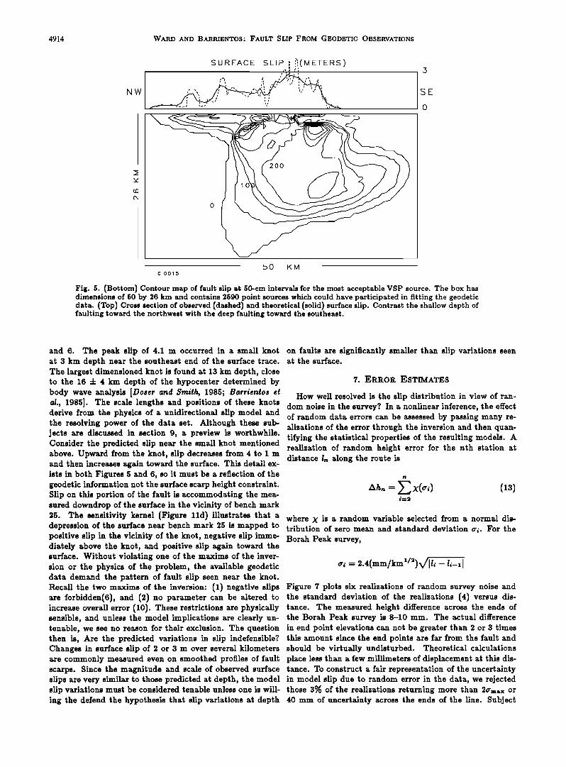
considerably wider deformation pattern at the surface. The fault slip distribution for the VSP model is contoured

at 50-cm intervals in Figure 5. The top edge of the lower box corresponds to the intersection of the fault with the surface. Left, right, and down in the box correspond to moving northwest or southeast along strike and downdip on the plane of the fault. The thin upper box graphs observed (dashed [from Crone and Machete, 1984]) and model (solid) values of surface slip. Strikingly, the concentration of slip at depth in this model is not well correlated with the amplitude of the surface scarp. The bulk of subsurface slip occurred to- ward the southeast and extended as much as 13 km beyond the terminus of the surface expression. Toward the north- west, where significant surface faulting exists, slip was fairly minor in magnitude and shallowly implanted. The model slip pattern in Figure 5 not only reduces the variance of fit to acceptable levels but also explains the puzzling behaviors of the best fitting USP fault of Figure 3. The USP model essentially ignored the thinly faulted northwest section and positioned itself in the southeast with the most intense sub- surface faulting.

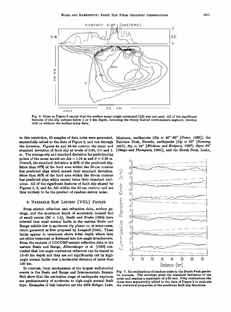
The thinly faulted northeast section is a significant fea- ture of the VSP model and its veracity is important to establish. Conceivably, the existence of this section could have been driven by the surface scarp height constraint (12) which was not considered in USP modeling. To test this possibility, an inversion which eliminated the surface scarp constraint was run, and Figure 6 contours the result. Below 1 or 2 km, very little difference is detectable among Figures 5 and 6. All of the significant features of the predicted fault slip, •.ncluding the northeast limb, develop in response to the geodetic data, not the constraint (12).

Three or four knots of concentrated slip with amplitudes of 1-2 m and dimensions of 3-6 km appear in Figures 5

4914 WARD AND BARRIENTOS: FAULT SLIP FROM GEODETIC OBSERVATIONS

NW

SURFACE SLIP •, !!(METERS)

0.0015

50 KM

SE

Fig. 5. (Bottom) Contour map of fault slip at 50-cm intervals for the most acceptable VSP source. The box has dimensions of 50 by 26 krn and contains 2590 point sources which could have participated in fitting the geodetic

(Top) or theoretical (olid) aip. Cotrt or faulting toward the northwest with the deep faulting toward the southeast.

and 6. The peak slip of 4.1 m occurred in a small knot at 3 km depth near the southeast end of the surface trace. The largest dimensioned knot is found at 13 km depth, close to the 16 + 4 km depth of the hypocenter determined by body wave analysis [Doser and Smith, 1985; Barrientos et al., 1985]. The scale lengths and positions of these knots derive from the physics of a unidirectional slip model and the resolving power of the data set. Although these sub- jects are discussed in section 9, a preview is worthwhile. Consider the predicted slip near the small knot mentioned above. Upward from the knot, slip decreases from 4 to I m and then increases again toward the surface. This detail ex- ists in both Figures 5 and 6, so it must be a reflection of the geodetic information not the surface scarp height constraint. Slip on this portion of the fault is accommodating the mea- sured downdrop of the surface in the vicinity of bench mark 25. The sensitivity kernel (Figure 11d) illustrates that a depression of the surface near bench mark 25 is mapped to positive slip in the vicinity of the knot, negative slip imme- diately above the knot, and positive slip again toward the surface. Without violating one of the maxims of the inver- sion or the physics of the problem, the available geodetic data demand the pattern of fault slip seen near the knot. Recall the two maxims of the inversion: (1) negative slips are forbidden(6), and (2) no parameter can be altered to increase overall error (10). These restrictions are physically sensible, and unless the model implications are clearly un- tenable, we see no reason for their exclusion. The question then is, Are the predicted variations in slip indefensible? Changes in surface slip of 2 or 3 m over several kilometers are commonly measured even on smoothed profiles of fault scarps. Since the magnitude and scale of observed surface slips are very similar to those predicted at depth, the model slip variations must be considered tenable unless one is will- ing the defend the hypothesis that slip variations at depth

on faults are significantly smaller than slip variations seen at the surface.

7. ERROR ESTIMATES

How well resolved is the slip distribution in view of ran- dom noise in the survey? In a nonlinear inference, the effect of random data errors can be assessed by passing many re- alizations of the error through the inversion and then quan- tifying the statistical properties of the resulting models. A realization of random height error for the nth station at distance I, along the route is

where X is a random variable selected from a normal dis- tribution of zero mean and standard deviation cri. For the

Borah Peak survey,

•, = 2.4(mm/km•/2)•/ll, - •'-,I

Figure 7 plots six realizations of random survey noise and the standard deviation of the realizations (4) versus dis- tance. The measured height difference across the ends of the Borah Peak survey is 8-10 mm. The actual difference in end point elevations can not be greater than 2 or 3 times this amount since the end points are far from the fault and should be virtually undisturbed. Theoretical calculations place less than a few millimeters of displacement at this dis- tance. To construct a fair representation of the uncertainty in model slip due to random error in the data, we rejected those 3% of the realizations returning more than 2crm•:, or 40 mm of uncertainty across the ends of the line. Subject

WARD AND BARRIENTOS' FAULT SLIP FROM GEODETIC OBSERVATIONS 4915

NW

SURFACE SLAP •I i!(METERS )

SE

2

50 KM 0.0013

Fig. 6. Same as Figure 5 except that the surface scarp height constraint (12) was not used. All of the significant features of the slip pattern below 1 or 2 km depth, including the thinly faulted northwestern segment, develop with or without the surface scarp data.

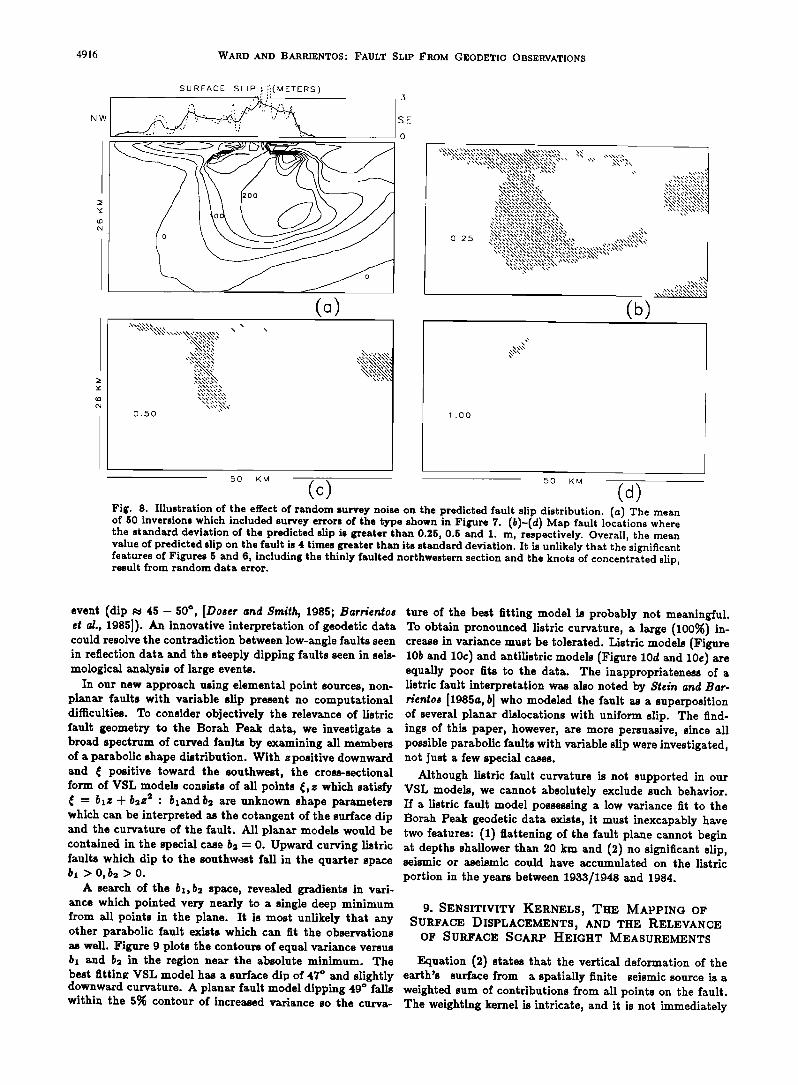
to this restriction, 50 samples of data noise were generated, Montana, earthquake (dip • 45ø-60 ø [Doser, 1985]), the sequentially added to the data of Figure 2, and run through Fairview Peak, Nevada, earthquake (dip • 62 ø [Ror•,ey, the inversion. Figures 8• and 8b-Sd contour the mean and 1957]; dip • 54 ø [W'i½lce• a,d Hodgso,, 1967]; dip• 62 ø standard deviation of fault slip at levels of 0.25, 0.5 and 1. [O/caya a,d TAor•]•so,, 1985]), and the Borah Peak, Idaho, m. The average slip and standard deviation for participating points of the mean model are A• -- 1.04 m and • -- 0.26 m. Overall, the standard deviation is 25% of the predicted slip. More than 975{ of the fault area within the 50-cm contour

has predicted slips which exceed their standard deviation. More than 85% of the fault area within the 50-cm contour has predicted slips which exceed twice their standard devi- ation. All of the significant features of fault slip shared by Figures 5, 6, and 8•, fall within the 50-cm contour and are thus unlikely to be the product of random survey noise.

8. VARIABLE SLIP LISTRIC (VSL) FAULTS

From seismic reflection and refraction data, surface ge- ology, and the maximum depth of accurately located loci of small events (/bf < 5.5), Sr•itA a-• BruA, [1984] have inferred that most normal faults in the eastern Basin and

Range exhibit low to moderate dip planar or, in some cases, listtic geometry as first proposed by Lo,gweII [1945]. These faults appear to terminate above 8-km depth where they are either truncated or flattened into low-angle detachments. From the analysis of COCORP seismic reflection data in the eastern Basin and Range, Allr•en•l•nger e• •l. [1983] con- cluded that low-angle continuous reflectors can be traced to 12-20 km depth and they are not significantly cut by high- angle normal faults over a horizontal distance of more than 120 km.

In contrast, focal mechanisms of the largest well-studied

-3

0

-3

3

0

-3

3

0

-3

3

0

-3

0 10 20 30 40 50 60 70

Disfence (km) events in the Basin and Range and Intermountain Seismic Fig. 7. Six realizations of random noise in the Borah Peak geode- Belt show that the nucleation stage of earthquake ruptures tic traverse. The envelope plots the standard deviation of the noise and reaches a maximum of +20 mm. Fifty realizations like are predominantly of moderate to high-angle normal fault these were sequentially added to the data of Figure 2 to evaluate type. Examples of this behavior are the 1959 Hebgen Lake, the statistical properties of the predicted fault slip functions.

4916 WARD AND BARRIENTOS- FAULT SLIP FROM GEODETIC OBSERVATIONS

NW

SURFACE SLIP il :'!(METERS)

SE

5\X'O.X\'X','.X\,,'O.\\'.,.'•R.\\'X,•',.'•:x,,X'X 0 xx e.x x.4e.xx ( ,x.xxx. e.x.•.k.b.•3 x . e., O,x x'x,,NWx.',x.x\x..•x'.•X.x,U ,x.\ ON

\.x',,.x..X,\ x' ,x.x ,x'\x x,

x,,x x x,N, ,,,x,< x, a>,,x-, \N,.,,.,\ \ x:.,Nx

\ ,,' ,x N 'x',' ,x. \ x,N• ,x N.,,' ,'.x,x x' ,x -x, x,'x• ,x \ x' xx-x N x' x' ,NN x,' ,xLx N x• -x x\ -x\ x' ,' ,x, \ x,'.x X• x' ,xNg x' ,x N x' ,' , x\x,, o. 2 5 x"xx-x'x',xXx"x, \x'0N•x',x.'xxx ',x x' xx•'¾ x,<, x, ,-,xx, x.x,,\xx,,,,,x\x,,xx>,Nx,,. x\-x- x.,x N\.h,,x,\x,•, x,

x',,.xxx'xx.•Nx,,,,x,\x,,xN. ,'x.\ ,x.,xxXx, x,\ ß ,'xx,

x-o,x,.\ x, o ,x \ x,, ,x,x N ,x

\x'xxxXx ' \'x' ,x

1 .00

x x-.xx, i ,,,x x • x,.,.\,,,,x,,x \•x,,x x,\,x,,x,\x,,• 'x',X NNx',x N

.',. \ x, ,, ,x, \ x. ,, ,x ,xl

,x\x,•, .\\\',, 3 N 'xx.x,N x

Fig. 8. Illustration of the effect of random survey noise on the predicted fault slip distribution. (a) The mean of 50 inversions which included survey errors of the type shown in Figure 7. (b)-(d) Map fault locations where the standard deviation of the predicted slip is greater than 0.25, 0.5 and 1. m, respectively. Overall, the mean value of predicted slip on the fault is 4 times greater than its standard deviation. It is unlikely that the significant features of Figures 5 and 6, including the thinly faulted northwestern section and the knots of concentrated slip, result from random data error.

event (dip • 45- $0 ø, [Doser and Smith, 1985; Barrientos et al., 1985]). An innovative interpretation of geodetic data could resolve the contradiction between low-angle faults seen in reflection data and the steeply dipping faults seen in seis- mological analysis of large events.

In our new approach using elemental point sources, non- planar faults with variable slip present no computational difficulties. To consider objectively the relevance of listtic fault geometry to the Borah Peak data, we investigate a broad spectrum of curved faults by examining all members of a parabolic shape distribution. With z positive downward and • positive toward the southwest, the cross-sectional form of VSL models consists of all points •, z which satisfy • -- bxz + b2z • : •xand•2 are unknown shape parameters which can be interpreted as the cotangent of the surface dip and the curvature of the fault. All planar models would be contained in the special case • -- 0. Upward curving listric faults which dip to the southwest fall in the quarter space • >0, b• >0.

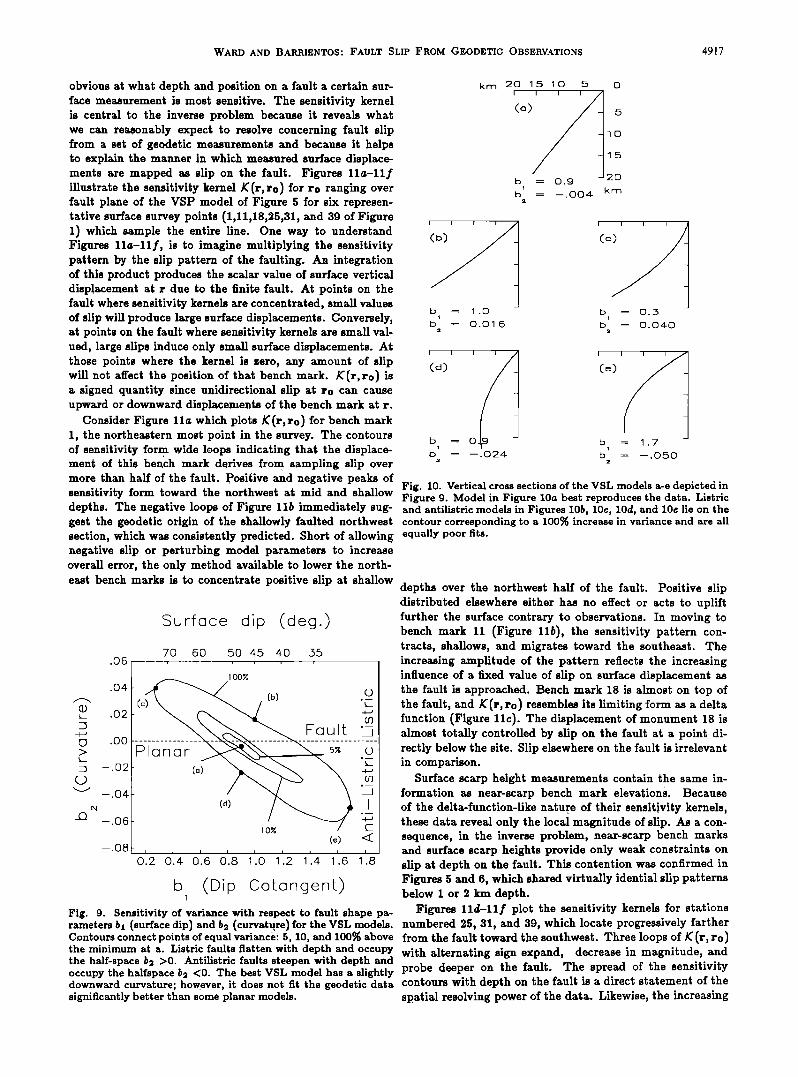
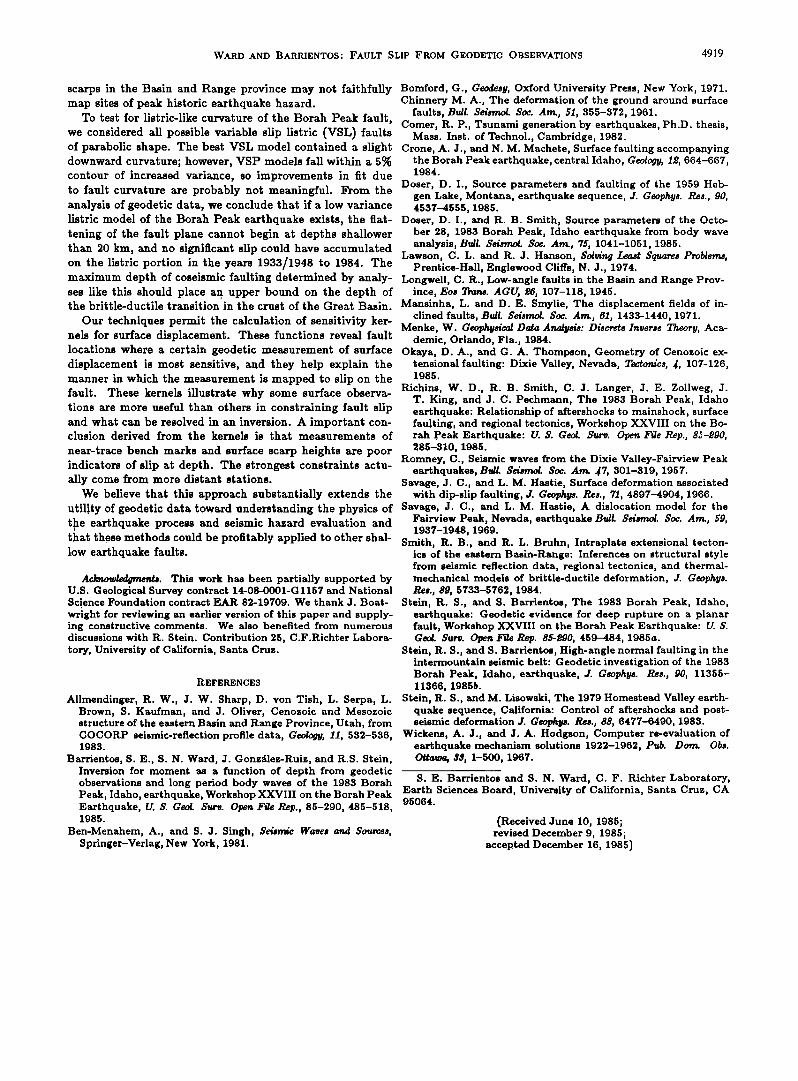
A search of the •,5• space, revealed gradients in vari- ance which pointed very nearly to a single deep minimum from all points in the plane. It is most unlikely that any other parabolic fault exists which can fit the observations as well. Figure 9 plots the contours of equal variance versus • and • in the region near the absolute minimum. The best fitting: VSL model has a surface dip of 47 ø and slightly downward curvature. A planar fault model dipping 49 ø falls within the 5% contour of increased variance so the curva-

ture of the best fitting model is probably not meaningful. To obtain pronounced listtic curvature, a large (100%) in- crease in variance must be tolerated. Listtic models (Figure 10b and 10½) and antilistric models (Figure 10d and 10e) are equally poor fits to the data. The inappropriateness of a listtic fault interpretation was also noted by Stein and Bar- rientos [1985a, b] who modeled the fault as a superposition of several planar dislocations with uniform slip. The find- ings of this paper, however, are more persuasive, since all possible parabolic faults with variable slip were investigated, not just a few special cases.

Although listric fault curvature is not supported in our VSL models, we cannot absolutely exclude such behavior. If a listric fault model possessing a low variance fit to the Borah Peak geodetic data exists, it must inexcapably have two features: (1) flattening of the fault plane cannot begin at depths shallower than 20 km and (2) no significant slip, seismic or aseismic could have accumulated on the listric

portion in the years between 1933/1948 and 1984.

9. SENSITIVITY KERNELS, THE MAPPING OF SURFACE DISPLACEMENTS, AND THE RELEVANCE

OF SURFACE SCARP HEIGHT MEASUREMENTS

Equation (2) states that the vertical deformation of the earth's surface from a spatially finite seismic source is a weighted sum of contributions from all points on the fault. The weighting kernel is intricate, and it is not immediately

WARD AND BARRIENTOS' FAULT SLIP FROM GEODETIC OBSERVATIONS 4917

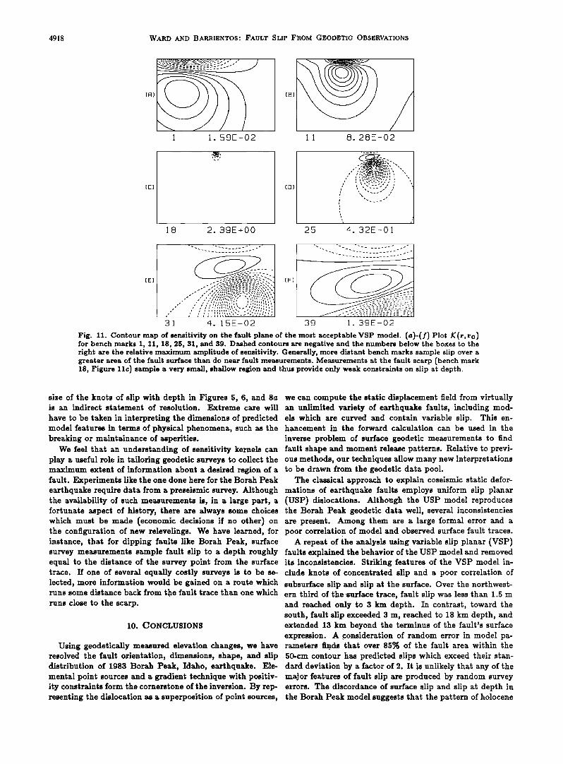
obvious at what depth and position on a fault a certain sur- face measurement is most sensitive. The sensitivity kernel is central to the inverse problem because it reveals what we can reasonably expect to resolve concerning fault slip from a set of geodetic measurements and because it helps to explain the manner in which measured surface displace- ments are mapped as slip on the fault. Figures 11a-llf illustrate the sensitivity kernel K(r, ro) for ro ranging over fault plane of the VSP model of Figure 5 for six represen- tative surface survey points (1,11,18,25,31, and 39 of Figure 1) which sample the entire line. One way to understand Figures 11a-llf, is to imagine multiplying the sensitivity pattern by the slip pattern of the faulting. An integration of this product produces the scalar value of surface vertical displacement at r due to the finite fault. At points on the fault where sensitivity kernels are concentrated, small values of slip will produce large surface displacements. Conversely, at points on the fault where sensitivity kernels are small val- ued, large slips induce only small surface displacements. At those points where the kernel is zero, any amount of slip will not affect the position of that bench mark. K(r, ro) is a signed quantity since unidirectional slip at ro can cause upward or downward displacements of the bench mark at r.

Consider Figure 11a which plots ]((r, ro) for bench mark 1, the northertern most point in the survey. The contours of sensitivity form wide loops indicating that the displace- ment of this bench mark derives from sampling slip over more than half of the fault. Positive and negative peaks of sensitivity form toward the northwest at mid and shallow depths. The negative loops of Figure 11b immediately sug- gest the geodetic origin of the shallowly faulted northwest section, which was consistently predicted. Short of allowing negative slip or perturbing model parameters to increase overall error, the only method available to lower the north- east bench marks is to concentrate positive slip at shallow

Surface dip (deg.)

70 60 50 45 4-0 55 .05 ......

.O4

--.O2

--.04

-.08

i t i 0 I O.2 0.4 0.6 .8

b (Dip 1

(•) <( i i i i i

1.0 1.2 1.4 1.6 1.8

Cotangent)

km 20 15 10 5 0 I

(ø) 5

lO

b -- O.9 20 • km

b = --.004

b = I .0 b = 0.• 1

b -- 0.01 6 b : 0.040 2 2

i

(d)

b

i i i

o. b = 1.7 1

--.024 b = --.050

Fig. 10 Vertical cross sections of the VSL models a-e depicted in Figure •. Model in Figure 10a best reproduces the data. Listtic and antilistric models in Figures 10b, 10½, 10d, and 10e lie on the contour corresponding to a 100% increase in variance and are all equally poor fits.

depths over the northwest half of the fault. Positive slip distributed elsewhere either has no effect or acts to uplift further the surface contrary to observations. In moving to bench mark 11 (Figure 11b), the sensitivity pattern con- tracts, shallows, and migrates toward the southeast. The increasing amplitude of the pattern reflects the increasing influence of a fixed value of slip on surface displacement as the fault is approached. Bench mark 18 is almost on top of the fault, and X (r, re) resembles its limiting form as a delta function (Figure 11½). The displacement of monument 18 is almost totally controlled by slip on the fault at a point di- rectly below the site. Slip elsewhere on the fault is irrelevant in comparison.

Surface scarp height measurements contain the same in- formation as near-scarp bench mark elevations. Because of the delta-function-like nature of their sensitivity kernels, these data reveal only the local magnitude of slip. As a con- sequence, in the inverse problem, near-scarp bench marks and surface scarp heights provide only weak constraints on slip at depth on the fault. This contention was confirmed in Figures 5 and 6, which shared virtually idential slip patterns below 1 or 2 km depth.

Fig. 9. Sensitivity of variance with respect to fault shape pa- Figures 11d-llf plot the sensitivity kernels for stations rameters bl (surface dip) and b2 (curvatu. re)for the VSL models. numbered 25, 31, and 39, which locate progressively farther Contours connect points of equal variance: 5, 10, and 100% above from the fault toward the southwest. Three loops of K (r, ro) the minimum at a. Listric faults fiatten with depth and occupy with alternating sign expand, decrease in magnitude, and the half-space b2 >0. Antilistric faults steepen with depth and occupy the halfspace ba <0. The best VSL model has a slightly probe deeper on the fault. The spread of the sensitivity downward curvature; however, it does not fit the geodetic data contours with depth on the fault is a direct statement of the significantly better than some planar models. spatial resolving power of the data. Likewise, the increasing

4918 WARD AND BARRIENTOS' FAULT SLIP FROM GEODETIC OBSERVATIONS

1 1. 59E-02 ]1 8. 28E-02

{c)

18 2,, 39E+00 25 qo 32E-0 ]

[E] [F]

31 4. 15E-02 39 1. 39E-02

Fig. 11. Contour map of sensitivity on the fault plane of the most acceptable VSP model. (a)-(f) Plot •((r, ro) for bench marks 1, 11, 18, 25, 31, and 39. Dashed contours are negative and the numbers below the boxes to the right are the relative maximum amplitude of sensitivity. Generally, more distant bench marks sample slip over a greater area of the fault surface than do near fault measurements. Measurements at the fault scarp (bench mark 18, Figure 11½) sample a very small, shallow region and thus provide only weak constraints on slip at depth.

size of the knots of slip with depth in Figures 5, 6, and 8a we can compute the static displacement field from virtually is an indirect statement of resolution. Extreme care will an unlimited variety of earthquake faults, including mod- have to be taken in interpreting the dimensions of predicted els which are curved and contain variable slip. This en- model features in terms of physical phenomena, such as the hancement in the forward calculation can be used in the breaking or maintainance of asperities. inverse problem of surface geodetic measurements to find

We feel that an understanding of sensitivity kernels can fault shape and moment release patterns. Relative to previ- play a useful role in tailoring geodetic surveys to collect the ous methods, our techniques allow many new interpretations maximum extent of information about a desired region of a fault. Experiments like the one done here for the Borah Peak earthquake require data from a preseismic survey. Although the availability of such measurements is, in a large part, a fortunate aspect of history, there are always some choices which must be made (economic decisions if no other) on the configuration of new relevelings. We have learned, for instance, that for dipping faults like Borah Peak, surface survey measurements sample fault slip to a depth roughly equal to the distance of the survey point from the surface trace. If one of several equally costly surveys is to be se- lected, more information would be gained on a route which runs some distance back from the fault trace than one which runs close to the scarp.

10. CONCLUSIONS

Using geodetically measured elevation changes, we have resolved the fault orientation, dimensions, shape, and slip distribution of 1983 Borah Peak, Idaho, earthquake. Ele- mental point sources and a gradient technique with positiv- ity constraints form the cornerstone of the inversion. By rep- resenting the dislocation as a superposition of point sources,

to be drawn from the geodetic data pool. The classical approach to explain coseismic static defor-

mations of earthquake faults employs uniform slip planar (USP) dislocations. Although the USP model reproduces the Borah Peak geodetic data well, several inconsistencies are present. Among them are a large formal error and a poor correlation of model and observed surface fault traces.

A repeat of the analysis using variable slip planar (VSP) faults explained the behavior of the USP model and removed its inconsistencies. Striking features of the VSP model in- clude knots of concentrated slip and a poor correlation of

subsurface slip and slip at the surface. Over the northwest- ern third of t•he surface trace, fault slip was less than 1.5 m and reached only to 3 km depth. In contrast, toward the south, fault slip exceeded 3 m, reached to 18 km depth, and extended 13 km beyond the terminus of the fault's surface expression. A consideration of random error in model pa- rameters finds that over 85% of the fault area within the

50,m contour has predicted slips which exceed their stan- dard deviation by a factor of 2. It is unlikely that any of the major features of fault slip are produced by random survey errors. The discordance of surface slip and slip at depth in the Borah Peak model suggests that the pattern of holocene

WARD AND BARRIENTOS: FAULT SLIP FROM GEODETIC OBSERVATIONS 4919

scarps in the Basin and Range province may not faithfully Bornford, G., Geodesy, Oxford University Press, New York, 1971. map sites of peak historic earthquake hazard.

To test for listric-like curvature of the Borah Peak fault, we considered all possible variable slip listric (VSL) faults of parabolic shape. The best VSL model contained a slight downward curvature; however, VSP models fall within a 5% contour of increased variance, so improvements in fit due to fault curvature are probably not meaningful. From the analysis of geodetic data, we conclude that if a low variance listric model of the Borah Peak earthquake exists, the flat- tening of the fault plane cannot begin at depths shallower than 20 km, and no significant slip could have accumulated on the listric portion in the years 1933•1948 to 1984. The maximum depth of coseismic faulting determined by analy- ses like this should place an upper bound on the depth of the brittle-ductile transition in the crust of the Great Basin.

Our techniques permit the calculation of sensitivity ker- nels for surface displacement. These functions reveal fault locations where a certain geodetic measurement of surface displacement is most sensitive, and they help explain the manner in which the measurement is mapped to slip on the fault. These kernels illustrate why some surface observa- tions are more useful than others in constraining fault slip and what can be resolved in an inversion. A important con- clusion derived from the kernels is that measurements of

near-trace bench marks and surface scarp heights are poor indicators of slip at depth. The strongest constraints actu- ally come from more distant stations.

We believe that this approach substantially extends the

Chinnery M. A., The deformation of the ground around surface faults, Bull. $eismol. $oc. Arr•, 51, 355-372, 1961.

Comer, R. P., Tsunami generation by earthquakes, Ph.D. thesis, Mass. Inst. of Technol., Cambridge, 1982.

Crone, A. J., and N.M. Machete, Surface faulting accompanying the Borah Peak earthquake, central Idaho, Geology, 12, 664-667, 1984.

Doser, D. I., Source parameters and faulting of the 1959 Heb- gen Lake, Montana, earthquake sequence, J. Geophys. Res., 90, 4537-4555, 1985.

Doser, D. I., and R. B. Smith, Source parameters of the Octo- ber 28, 1983 Borah Peak, Idaho earthquake from body wave analysis, Bull. $eismol. $oc. Arr•, 75, 1041-1051, 1985.

Lawson, C. L. and R. J. Hanson, Solving Least Squares Problems, Prentice-Hall, Englewood Cliffs, N.J., 1974.

Longwell, C. R., Low-angle faults in the Basin and Range Prov- ince, Eos •ns. AGU, 26, 107-118, 1945.

Mansinha, L. and D. E. Staylie, The displacement fields of in- clined faults, Bull. $•ismol. $oc. Am., 61, 1433-1440, 1971.

Menke, W. Geophysical Data Analysis: Discrete Inverse Theory, Aca- demic, Orlando, Fla., 1984.

Okaya, D. A., and G. A. Thompson, Geometry of Cenozoic ex- tensional faulting: Dixie Valley, Nevada, Tectonics, g, 107-126, 1985.

Richins, W. D., R. B. Smith, C. J. Langer, J. E. Zollweg, J. T. King, and J. C. Pechmann, The 1983 Borah Peak, Idaho earthquake: Relationship of aftershocks to mainshock, surface faulting, and regional tectonics, Workshop XXVIII on the Bo- rah peak Earthquake: U. $. Gez•. $urv. Open File Rep., $2-290, 285-310, 1985.

Romney, C., Seismic waves from the Dixie Valley-Fairview Peak earthquakes, Bu/l. $e/smo/. $oc. A•r• g7, 301-319, 1957.

Savage, J. C., and L. M. Hastie, Surface deformation associated with dip-slip faulting, J. G•ophys. Res., 71, 4897-4904, 1966.

utility of geodetic data toward understanding the physics of Savage, J. C., and L. M. Hastie, A dislocation model for the the earthquake process and seismic hazard evaluation and Fairview Peak, Nevada, earthquake Bull. $eismo!. $oc. Am., 59,

• 1937-1948, 1969. that these methods could be profitably applied to other shal- Smith, R. B., and R. L. Bruhn, Intraplate extensional tecton- low earthquake faults. ics of the eastern Basin-Range: Inferences on structural style

Acknowlm•7m•nts. This work has been partially supported by U.S. Geological Survey contract 14-08-0001-Gl157 and National Science Foundation contract EAR 82-19709. We thank J. Boat-

wright for reviewing an earlier version of this paper and supply- ing constructive comments. We also benefited from numerous discussions with R. Stein. Contribution 25, C.F.Richter Labora- tory, University of California, Santa Cruz.

REFERENCES

Allmendinger, R. W., J. W. Sharp, D. yon Tish, L. Serpa, L. Brown, S. Kaufman, and J. Oliver, Cenozoic and Mesozoic structure of the eastern Basin and Range Province, Utah, from COCORP seismic-reflection profile data, Geology, 11, 532-536, 1983.

Barrientos, S. E., S. N. Ward, J. Gonz•lez-Ruiz, and R.S. Stein, Inversion for moment as a function of depth from geodetic observations and long period body waves of the 1983 Borah Peak, Idaho, earthquake, Workshop XXVIII on the Borah Peak Earthquake, U. $. Gez•. $ur•. Open F•e Rep., 85-290, 485-518, 1985.

Ben-Menahem, A., and S. J. Singh, $e/sm/½ Waves and Sources, Springer-Verlag, New York, 1981.

from seismic reflection data, regional tectonics, and thermal- mechanical models of brittle-ductile deformation, J. Geophys. Res., $9, 5733-5762, 1984.

Stein, R. S., and S. Barrientos, The 1983 Borah Peak, Idaho, earthquake: Geodetic evidence for deep rupture on a planar fault, Workshop XXVIII on the Borah Peak Earthquake: U. $. Gez•. $ur•. Open Fae Rep. $$-290, 459-484, 1985a.

Stein, R. S., and S. Barrientos, High-angle normal faulting in the intermountain seismic belt: Geodetic investigation of the 1983 Borah Peak, Idaho, earthquake, J. Geophys. Res., 90, 11355- 11366, 1985b.

Stein, R. S., and M. Lisowski, The 1979 Homestead Valley earth- quake sequence, California: Control of aftershocks and post- seismic deformation J. Geophys. Res., $$, 6477-6490, 1983.

Wickens, A. J., and J. A. Hodgson, Computer re-evaluation of earthquake mechanism solutions 1922-1962, Pub. DoM Ohs. Ot•aw• 33, 1-500, 1967.

S. E. Barrientos and S. N. Ward, C. F. Richter Laboratory, Earth Sciences Board, University of California, Santa Cruz, CA 95064.

(Received June 10, 1985; revised December 9, 1985;

accepted December 16, 1985)