Introduction to Money Market Funds - Goldman Sachs Asset ...
Upload
khangminh22Category
view
0download
0

An Introduction to the Mathematics of Money

David Lovelock Marilou Mendel A. Larry Wright
An Introduction to theMathematics of Money
Saving and Investing

David Lovelock Marilou MendelDepartment of Mathematics Department of MathematicsUniversity of Arizona University of ArizonaTucson, AZ 85721 Tucson, AZ 85721USA [email protected] [email protected]
A. Larry WrightDepartment of Mathematics University of ArizonaTucson, AZ [email protected]
Mathematics Subject Classification (2000): 91B82
Library of Congress Control Number: 2006931194
ISBN-10: 0-387-34432-2ISBN-13: 978-0387-34432-4
Printed on acid-free paper.
© 2007 Springer Science+Business Media, LLCAll rights reserved. This work may not be translated or copied in whole or in part without the writtenpermission of the publisher (Springer Science+Business Media, LLC, 233 Spring Street, New York,NY 10013, USA), except for brief excerpts in connection with reviews or scholarly analysis. Use in connection with any form of information storage and retrieval, electronic adaptation, computer software,or by similar or dissimilar methodology now known or hereafter developed is forbidden.The use in this publication of trade names, trademarks, service marks, and similar terms, even if theyare not identified as such, is not to be taken as an expression of opinion as to whether or not they aresubject to proprietary rights.
9 8 7 6 5 4 3 2 1
springer.com

Preface
Introduction
Some people distinguish between savings and investments, where savings aremonies placed in relatively risk-free accounts with modest rewards, and whereinvestments involve more risk and the potential for greater rewards. In thisbook we do not distinguish between these ideas. We treat them both underthe umbrella of investing.
In general, income falls into two categories: earned income—which isthe income derived from your everyday job—and unearned income—whichis income derived from investing. You attend college to strengthen yourprospects for earned income, so why do you need to worry about unearnedincome, namely, investment income?
There are many reasons to invest and to learn about investing. Perhapsthe primary one is to take charge of your own financial future. You needmoney for short-term goals (such as living expenses, emergencies) and forlong-term goals (such as buying a car, buying a house, educating children,paying catastrophic medical bills, funding retirement).
Investing involves borrowing and lending, and buying and selling.
• borrowing and lending. When you put money into a bank savingsaccount, you are lending your money and the bank is borrowing it. You canlend money to a bank, a business, a government, or a person. In exchangefor this, the borrower promises to pay you interest and to return your initialinvestment at a future date. Why would the borrower do this? Because theborrower anticipates using this money in a way that earns more than theinterest promised to you. Examples of borrowing and lending are savingsaccounts, certificates of deposits, money-market accounts, and bonds.
• buying and selling. When you buy something for investment purposes,you are buying an asset from a seller. You expect that this asset willgenerate a profit or will increase in value, part of which will be returnedto you. Examples of this are owning real estate or stocks in companies.

vi Preface
There are two ways that you can make (lose) money buying stocks: stock-price appreciation (depreciation)—which depends on the expectations andopinions of the public—and dividends paid to you by the company—whichdepend on the company sharing its profits with you, a shareholder.
When investing, there are three things that can impact your profit—taxes,inflation, and risk. The first, taxes, should concern everyone. The second, infla-tion, should concern you if you make a profit. The third, risk, should concernyou before you make an investment because risk influences the profitability ofthe investment. Generally, if you expect a high return on your money, thenyou should also expect a high risk. In the same way, low risks are usually asso-ciated with low returns. The larger the risk the greater the chance of actuallylosing money. There are various types of risk: inflation, market, currency fluc-tuations, political, interest-rate, liquidity, economic, default, business, etc.
Objectives and Background
We wrote this book with two objectives in mind:
• To use investing as a vehicle to introduce you, the student, to ideas, tech-niques, and applications that you might not encounter in your other math-ematics courses. These include proofs by induction, recurrence relations,inequalities (in particular, the Arithmetic-Geometric Mean inequality andthe Cauchy-Schwarz inequality), and elements of probability and statistics.
• To introduce you, the student, to elements of investing that are of life-longpractical use. If you have not yet done so, then as you advance through life,you are forced to deal with such things as credit cards, student loans, car-loans, savings accounts, certificates of deposit, money-market accounts,mortgage payments, buying and selling bonds, and buying and sellingstocks.
This book targets students at the sophomore/junior level, without assum-ing a background or any experience in investing. We assume knowledge ofa two-semester calculus course as well as some mathematical sophistication.Specifically we use inequalities, log, exp, differentiation, the Mean Value The-orem, integration, Newton’s method, limits of sequences, geometric series, thebinomial expansion, and Taylor series.
There are problems at the end of each chapter. Some of these problemsrequire that you have access to a spreadsheet program and that you know howto use it. A simple scientific or financial calculator (with functions such as log,exp, and the ability to calculate yx) is all that is required for the remainderof the problems that involve arithmetical calculations. Some problems requireyou to obtain data from the World Wide Web (WWW), so access to theWWW, and familiarity with a browser, is a prerequisite.1
1 The web page www.mathematics-of-money.com is dedicated to this book.

Preface vii
Comments
The following numbering system is used throughout the book: Example 2.3refers to the third example in Chapter 2, Theorem 4.1 refers to the firsttheorem in Chapter 4, Figure 4.2 refers to the second figure in Chapter 4,Table 1.3 refers to the third table in Chapter 1, and Problem 1.5 refers to thefifth problem in Chapter 1.
The symbol � indicates the end of an example, and the symbol � indicatesthe end of a proof.
Many of the theorems in the book are given names (for example, TheCompound Interest Theorem). This is done for ease of navigation for thestudent.
The problems are divided into two groups: “Walking”, which involve rou-tine, straight-forward calculations, and “Running”, which are more challeng-ing problems.
There are two appendices. Appendix A covers mathematical induction,recurrence relations, and inequalities. This material should be introduced atthe beginning of the course. Appendix B covers elements of probability andstatistics. It is not needed until the latter part of the course and can beintroduced as needed. Many students may have seen this material in previousclasses.
Unless indicated otherwise, all numerical results are rounded to three dec-imal places, and all dollar amounts are rounded to cents. Because of thisconvention, when the same calculation is performed in two different ways, theanswers may differ slightly.
In most, but not all, cases in this book the interest rate is assumed to bepositive. It is interesting to note that there are instances when the interestrate is negative. See, for example, [21]. A good reference on investments is [4].A more advanced treatment is [18].
The information contained in this book is not intended to be construed asinvestment, legal, or accounting advice.
The Family
In order to try to personalize the investment examples and problems in thisbook, we have introduced a fictional family, the Kendricks. Helen (48) andHugh (50) Kendrick, are husband and wife. They have three children, twinsWendy (25) and Tom (25), and Amanda (20), a college freshman. Jana Carmel(35) is one of Hugh’s coworkers.

viii Preface
Acknowledgments
This book originated from classes taught in the Department of Mathematicsat The University of Arizona, and in the Industrial Engineering and Opera-tions Research Department at Columbia University. Several students providedvaluable comments and corrected errors in the original notes. In particular,we thank Tom Wilkening and Michael Urbancic.
We also thank Wayne Hacker, David Lomen, and Doug Ulmer of the De-partment of Mathematics at The University of Arizona, who reviewed largeportions of the manuscript and corrected several errors.
A guest lecture series, where professionals from both inside and outsideacademia are invited to discuss their specialities, is an integral part of theclass and introduces the students to real-world applications of the mathemat-ics of money. We thank the following guest lecturers: Dennis Bartlett, SueBurroughs, Steve Kou, Steve Przewlocki, and Lauren Wright.
Special thanks go to Murray Teitelbaum and some of the many people atthe New York Stock Exchange who are involved with the Teachers WorkshopProgram.
We thank the many other people who have assisted in the preparation ofthe manuscript: Pat Brockett, Han Gao, Joe Harwood, Pavan Korada, RobertMaier, Charles Newman, Keith Schlottman, Michael Sobel, and AramianWasielak.
We also thank the reviewers of the manuscript for their invaluable sugges-tions.
Finally, we thank our contacts at Springer—Achi Dosanjh, Yana Mermel,and Frank Ganz, for their indispensable support and advice.
Tucson, Arizona, David LovelockJuly, 2006 Marilou Mendel
A. Larry Wright

Contents
Preface . . . . . . . . . . . . . . . . . . . . . . . . . . . . . . . . . . . . . . . . . . . . . . . . . . . . . . . . v
1 Simple Interest . . . . . . . . . . . . . . . . . . . . . . . . . . . . . . . . . . . . . . . . . . . . 11.1 The Simple Interest Theorem . . . . . . . . . . . . . . . . . . . . . . . . . . . . 11.2 Ambiguities When Interest Period is Measured in Days . . . . . 81.3 Problems . . . . . . . . . . . . . . . . . . . . . . . . . . . . . . . . . . . . . . . . . . . . . . 10
2 Compound Interest . . . . . . . . . . . . . . . . . . . . . . . . . . . . . . . . . . . . . . . . 132.1 The Compound Interest Theorem . . . . . . . . . . . . . . . . . . . . . . . . 132.2 Time Diagrams and Cash Flows . . . . . . . . . . . . . . . . . . . . . . . . . . 232.3 Internal Rate of Return . . . . . . . . . . . . . . . . . . . . . . . . . . . . . . . . . 262.4 The Rule of 72 . . . . . . . . . . . . . . . . . . . . . . . . . . . . . . . . . . . . . . . . . 362.5 Problems . . . . . . . . . . . . . . . . . . . . . . . . . . . . . . . . . . . . . . . . . . . . . . 37
3 Inflation and Taxes . . . . . . . . . . . . . . . . . . . . . . . . . . . . . . . . . . . . . . . . 453.1 Inflation. . . . . . . . . . . . . . . . . . . . . . . . . . . . . . . . . . . . . . . . . . . . . . . 453.2 Consumer Price Index (CPI) . . . . . . . . . . . . . . . . . . . . . . . . . . . . . 483.3 Personal Taxes . . . . . . . . . . . . . . . . . . . . . . . . . . . . . . . . . . . . . . . . . 503.4 Problems . . . . . . . . . . . . . . . . . . . . . . . . . . . . . . . . . . . . . . . . . . . . . . 51
4 Annuities . . . . . . . . . . . . . . . . . . . . . . . . . . . . . . . . . . . . . . . . . . . . . . . . . . 554.1 An Ordinary Annuity . . . . . . . . . . . . . . . . . . . . . . . . . . . . . . . . . . . 554.2 An Annuity Due . . . . . . . . . . . . . . . . . . . . . . . . . . . . . . . . . . . . . . . 664.3 Perpetuities . . . . . . . . . . . . . . . . . . . . . . . . . . . . . . . . . . . . . . . . . . . 704.4 Problems . . . . . . . . . . . . . . . . . . . . . . . . . . . . . . . . . . . . . . . . . . . . . . 71
5 Loans and Risks . . . . . . . . . . . . . . . . . . . . . . . . . . . . . . . . . . . . . . . . . . . 755.1 Problems . . . . . . . . . . . . . . . . . . . . . . . . . . . . . . . . . . . . . . . . . . . . . . 79

x Contents
6 Amortization . . . . . . . . . . . . . . . . . . . . . . . . . . . . . . . . . . . . . . . . . . . . . . 836.1 Amortization Tables . . . . . . . . . . . . . . . . . . . . . . . . . . . . . . . . . . . . 836.2 Periodic Payments . . . . . . . . . . . . . . . . . . . . . . . . . . . . . . . . . . . . . . 886.3 Linear Interpolation . . . . . . . . . . . . . . . . . . . . . . . . . . . . . . . . . . . . 946.4 Problems . . . . . . . . . . . . . . . . . . . . . . . . . . . . . . . . . . . . . . . . . . . . . . 97
7 Credit Cards . . . . . . . . . . . . . . . . . . . . . . . . . . . . . . . . . . . . . . . . . . . . . . 1017.1 Credit Card Payments . . . . . . . . . . . . . . . . . . . . . . . . . . . . . . . . . . 1017.2 Credit Card Numbers . . . . . . . . . . . . . . . . . . . . . . . . . . . . . . . . . . . 1087.3 Problems . . . . . . . . . . . . . . . . . . . . . . . . . . . . . . . . . . . . . . . . . . . . . . 110
8 Bonds . . . . . . . . . . . . . . . . . . . . . . . . . . . . . . . . . . . . . . . . . . . . . . . . . . . . . 1138.1 Noncallable Bonds . . . . . . . . . . . . . . . . . . . . . . . . . . . . . . . . . . . . . . 1148.2 Duration . . . . . . . . . . . . . . . . . . . . . . . . . . . . . . . . . . . . . . . . . . . . . . 1268.3 Modified Duration . . . . . . . . . . . . . . . . . . . . . . . . . . . . . . . . . . . . . . 1298.4 Convexity . . . . . . . . . . . . . . . . . . . . . . . . . . . . . . . . . . . . . . . . . . . . . 1378.5 Treasury Bills . . . . . . . . . . . . . . . . . . . . . . . . . . . . . . . . . . . . . . . . . . 1398.6 Portfolio of Bonds . . . . . . . . . . . . . . . . . . . . . . . . . . . . . . . . . . . . . . 1418.7 Problems . . . . . . . . . . . . . . . . . . . . . . . . . . . . . . . . . . . . . . . . . . . . . . 144
9 Stocks and Stock Markets . . . . . . . . . . . . . . . . . . . . . . . . . . . . . . . . . 1499.1 Buying and Selling Stock . . . . . . . . . . . . . . . . . . . . . . . . . . . . . . . . 1519.2 Reading The Wall Street Journal Stock Tables . . . . . . . . . . . . . 1609.3 Problems . . . . . . . . . . . . . . . . . . . . . . . . . . . . . . . . . . . . . . . . . . . . . . 161
10 Stock Market Indexes, Pricing, and Risk . . . . . . . . . . . . . . . . . . 16510.1 Stock Market Indexes . . . . . . . . . . . . . . . . . . . . . . . . . . . . . . . . . . . 16510.2 Rates of Return for Stocks and Stock Indexes . . . . . . . . . . . . . . 17210.3 Pricing and Risk . . . . . . . . . . . . . . . . . . . . . . . . . . . . . . . . . . . . . . . 17510.4 Portfolio of Stocks . . . . . . . . . . . . . . . . . . . . . . . . . . . . . . . . . . . . . . 18610.5 Problems . . . . . . . . . . . . . . . . . . . . . . . . . . . . . . . . . . . . . . . . . . . . . . 188
11 Options . . . . . . . . . . . . . . . . . . . . . . . . . . . . . . . . . . . . . . . . . . . . . . . . . . . . 19111.1 Put and Call Options . . . . . . . . . . . . . . . . . . . . . . . . . . . . . . . . . . . 19211.2 Adjusting for Stock Splits and Dividends . . . . . . . . . . . . . . . . . . 19611.3 Option Strategies . . . . . . . . . . . . . . . . . . . . . . . . . . . . . . . . . . . . . . . 19811.4 Put-Call Parity Theorem . . . . . . . . . . . . . . . . . . . . . . . . . . . . . . . . 20811.5 Hedging with Options . . . . . . . . . . . . . . . . . . . . . . . . . . . . . . . . . . . 21111.6 Modeling Stock Market Prices . . . . . . . . . . . . . . . . . . . . . . . . . . . 21511.7 Pricing of Options . . . . . . . . . . . . . . . . . . . . . . . . . . . . . . . . . . . . . . 22011.8 The Black-Scholes Option Pricing Model . . . . . . . . . . . . . . . . . . 22511.9 Problems . . . . . . . . . . . . . . . . . . . . . . . . . . . . . . . . . . . . . . . . . . . . . . 238

Contents xi
A Appendix: Induction, Recurrence Relations, Inequalities . . . 245A.1 Mathematical Induction . . . . . . . . . . . . . . . . . . . . . . . . . . . . . . . . . 245A.2 Recurrence Relations . . . . . . . . . . . . . . . . . . . . . . . . . . . . . . . . . . . 247A.3 Inequalities . . . . . . . . . . . . . . . . . . . . . . . . . . . . . . . . . . . . . . . . . . . . 249A.4 Problems . . . . . . . . . . . . . . . . . . . . . . . . . . . . . . . . . . . . . . . . . . . . . . 252
B Appendix: Statistics . . . . . . . . . . . . . . . . . . . . . . . . . . . . . . . . . . . . . . . 255B.1 Set Theory . . . . . . . . . . . . . . . . . . . . . . . . . . . . . . . . . . . . . . . . . . . . 255B.2 Probability . . . . . . . . . . . . . . . . . . . . . . . . . . . . . . . . . . . . . . . . . . . . 256B.3 Random Variables . . . . . . . . . . . . . . . . . . . . . . . . . . . . . . . . . . . . . . 256B.4 Moments . . . . . . . . . . . . . . . . . . . . . . . . . . . . . . . . . . . . . . . . . . . . . . 271B.5 Joint Distribution of Random Variables . . . . . . . . . . . . . . . . . . . 275B.6 Linear Regression . . . . . . . . . . . . . . . . . . . . . . . . . . . . . . . . . . . . . . 277B.7 Estimates of Parameters of Random Variables . . . . . . . . . . . . . 280B.8 Problems . . . . . . . . . . . . . . . . . . . . . . . . . . . . . . . . . . . . . . . . . . . . . . 281
Answers . . . . . . . . . . . . . . . . . . . . . . . . . . . . . . . . . . . . . . . . . . . . . . . . . . . . . . . 283
References . . . . . . . . . . . . . . . . . . . . . . . . . . . . . . . . . . . . . . . . . . . . . . . . . . . . . 287
Index . . . . . . . . . . . . . . . . . . . . . . . . . . . . . . . . . . . . . . . . . . . . . . . . . . . . . . . . . . 289
1
Simple Interest
Would you prefer to have $100 now or $100 a year from now? Even though theamounts are the same, most people would prefer to have $100 now because ofthe interest it can earn. Thus, whenever we talk of money we must state notonly the amount, but also the time. This concept—that money today is worthmore than the same amount of money in the future—is called the time valueof money. The present value of an amount is its worth today, while thefuture value is its worth at a later time. These topics are discussed hereand in Chap. 2. Another reason that most people would prefer to have $100now is that its purchasing power in the future may be less than at presentdue to inflation, which is discussed in Chap. 3.
When money earns interest it can do so in various ways—for example, sim-ple interest, compounded annually, compounded semi-annually, compoundedquarterly, compounded monthly, compounded daily, and compounded contin-uously. When referring to an interest rate, it is important to know which ofthese methods is being used.1
In this chapter we concentrate on simple interest. Compound interest isthe subject of Chap. 2. A thorough familiarity with these two chapters iscritical for an understanding of the rest of this book.
1.1 The Simple Interest Theorem
We invest $1,000 at 10% interest per year for 5 years. After one year we earn10% of $1,000, namely, $100. We withdraw that interest and put it under amattress, leaving the original $1,000 to earn interest in the second year. It tooearns $100, which we also put under the mattress, so after two years we havethe original $1,000 and $200 under the mattress. We continue doing this for5 years, and so after five years we have the original $1,000 and $500 under
1 A reference on interest rates with a historical summary dating back to about 400B.C. is [15].

2 1 Simple Interest
the mattress, for a total of $1,500. Table 1.1 shows the details. (Check thecalculations in this table using a calculator or a spreadsheet program, and fillin the missing entries.)
Table 1.1. Simple Interest
Year’s Beginning Year’s EndYear Principal Interest Amount
1 $1,000.00 $100.00 $1,100.002 $1,000.00 $100.00 $1,200.0034 $1,000.00 $100.00 $1,400.005 $1,000.00 $100.00 $1,500.00
We now derive the general formula for this process. First, the total amountwe have at any time is the future value of $1,000 at that time. Thus, $1,500is the future value of $1,000 after 5 years. Second, the annual interest rateis called the nominal rate, the quoted rate, or the stated rate. Ratherthan restricting ourselves to annual calculations, we let n measure the totalnumber of interest periods, of which we assume that there are m per year.(For example, if interest is calculated four times a year, that is, every threemonths, for five years, then m = 4 and n = 4 × 5 = 20.) So we let2
P0 be the initial principal (present value, lump sum) invested,n be the total number of interest periods,Pn be the future value of P0 at the end of the nth interest period,m be the number of interest periods per year,
i(m) be the nominal rate (annual interest rate), expressed as a decimal,i be the interest rate per interest period.
The interest rate per interest period is
i =i(m)
m.
For example, if the nominal rate is 12% calculated four times a year, thenm = 4 and i(4) = 0.12, so i = 0.12/4 = 0.03, the interest rate per quarter.
Using this notation we rewrite Table 1.1 symbolically in spreadsheet for-mat3 as Table 1.2, which is explained as follows.2 Throughout this chapter these symbols are used for this purpose. It is assumed
that the units of currency are dollars, that m and n are positive integers, andthat i(m) ≥ 0. Similar comments apply to subsequent chapters, as appropriate.
3 We use this spreadsheet format throughout. It is always advisable to check calcu-lations in more than one way—the spreadsheet is an excellent tool for this. Thelast entry on the Year 1 row, namely, P0 + iP0 = P1, means that P0 + iP0 is thevalue of that entry, and we call it P1.

1.1 The Simple Interest Theorem 3
Table 1.2. Simple Interest—Spreadsheet Format
Period’s Beginning Period’s EndPeriod Principal Interest Amount
1 P0 iP0 P0 + iP0 = P1
2 P0 iP0 P1 + iP0 = P2
3 P0 iP0 P2 + iP0 = P3
4 P0 iP0 P3 + iP0 = P4
5 P0 iP0 P4 + iP0 = P5
At the end of the first interest period (n = 1) we receive iP0 in interest,so the future value of P0 after one period is
P1 = P0 + iP0 = P0 (1 + i) .
At the end of the second interest period (n = 2) we again receive iP0 ininterest, so the future value after two periods is
P2 = P1 + iP0 = P0 (1 + i) + iP0 = P0 (1 + 2i) .
At the end of the third interest period (n = 3) we again receive iP0 ininterest, so the future value after three periods is
P3 = P2 + iP0 = P0 (1 + 2i) + iP0 = P0 (1 + 3i) .
This suggests the following theorem.
Theorem 1.1. The Simple Interest Theorem.If we start with principal P0, and invest it for n interest periods at a nominalrate of i(m) (expressed as a decimal) calculated m times a year using simpleinterest, then Pn, the future value of P0 at the end of n interest periods, is
Pn = P0 (1 + ni) , (1.1)
where i = i(m)/m.
Proof. We can prove this theorem in at least two different ways: either usingmathematical induction (see p. 245) or using recurrence relations (see p. 247).
We first prove it using mathematical induction. We know that (1.1) is truefor n = 1. We assume that it is true for n = k, that is,
Pk = P0(1 + ki),
and we must show that it is true for n = k + 1.Now Pk+1, the amount of money at the end of period k + 1, is the sum of
Pk, the amount of money at the beginning of this period, and iP0, the interestearned during that period, that is,

4 1 Simple Interest
Pk+1 = Pk + iP0,
soPk+1 = P0(1 + ki) + iP0 = P0(1 + (k + 1)i),
which shows that (1.1) is true for n = k + 1. This concludes the proof bymathematical induction.
We now prove (1.1) using recurrence relations. We know that
Pk+1 = Pk + iP0,
so if we sum this from k = 0 to k = n − 1, then we have
n−1∑k=0
Pk+1 =n−1∑k=0
Pk +n−1∑k=0
iP0.
By canceling the common terms on both sides of this equation, we find that
Pn = P0 +n−1∑k=0
iP0 = P0(1 + ni).
This concludes the proof using recurrence relations. ��
Comments About the Simple Interest Theorem
• We notice that Pn = P0(1 + ni) is a function of the three variables P0, n,and i. We see that it is directly proportional4 to P0 and linear in each of theother two variables. Thus, a plot of the future value versus any one of thesethree variables, holding the other two fixed, is a line. An example of thisis seen in Fig. 1.1, which shows the future value of $1 as a function of n inyears for 5% (the lower curve) and 10% (the upper curve) nominal interestrates i(1). You might ask why we selected P0 = 1. We did this because Pn
is directly proportional to P0, so knowing the value of Pn when P0 = 1allows us to compute Pn for any other P0, simply by multiplying by P0.This is an important point, which recurs in later chapters.
• The quantity Pn −P0 is the principal appreciation. Notice that, in the caseof simple interest, Pn −P0 = P0ni, that is, Pn −P0 is directly proportionalto P0, n, and i, so doubling any of them doubles the principal appreciation.This is seen in Fig. 1.1. For example, if we look at n = 20, then we seethat the vertical distance from the future value at 10% ($3) to the presentvalue ($1) is twice the distance from the future value at 5% ($2) to thepresent value ($1).
4 A function f(x) is directly proportional to x if f(x) = ax, where a is a constant.“Directly proportional” is a special case of “linear”.

1.1 The Simple Interest Theorem 5
Years
0 5 10 15 20 25
Fu
ture
Val
ue
of
$1
0
1
2
3
4
5%
10%
Fig. 1.1. Future Value of $1 at 5% and 10% simple interest
• The quantity (Pn − P0)/P0 is called the rate of return. Notice that inthe case of simple interest we have (Pn − P0)/P0 = ni, so doubling eithern, the number of interest periods, or i, the interest rate per period, doublesthe rate of return.
• The quantity (Pn − P0)/(nP0) is the rate of return per period. No-tice that in the case of simple interest we have (Pn − P0)/(nP0) = i, sothe simple interest rate per interest period is the rate of return per period.
• Equation (1.1) is valid for n ≥ 0. What happens if n < 0? In other words,if we accumulate P0 over the past n years at a simple interest rate of iper year, then what amount, which we call P−n, did we start with n yearsago? From (1.1) we have
P0 = P−n(1 + ni),
soP−n = P0
11 + ni
, (1.2)
which is not (1.1) with n replaced by −n. Thus, (1.1) is valid only forn ≥ 0.
Financial DigressionA common form of investing is through a certificate of deposit (CD).CDs are issued by financial institutions. The institution pays a fixed interestrate on the lender’s initial investment for a specified term. Typical termsare 6 months, and 1, 2, or 5 years. Usually the longer the term, the higherthe rate because long-term investments are usually riskier than short-term

6 1 Simple Interest
investments.5 The lender cannot withdraw the initial investment before theend of the term without penalty (see Problem 1.4 on p. 10), but the lender canwithdraw the interest as it is credited to the lender’s account, if desired. Oftena minimum amount is required to open a CD. Some CDs are insured up to amaximum amount by the Federal Deposit Insurance Corporation (FDIC) andso are relatively risk-free. Others are uninsured, and should the institutionfail, the lender could lose money. Such CDs usually pay higher rates thanFDIC-insured CDs.
Certificate of DepositTypical Term 6 to 60 monthsPayment Frequency At maturity for short-term; monthly for long-termPenalty Early withdrawalIssuer Commercial Banks, Savings & Loans, Credit UnionsRisks Inflation, Interest Rate, Reinvestment, LiquidityMarketable SomeRestrictions Minimum Investment
Example 1.1. Tom Kendrick invests $1,000 in a CD at 10% a year for fiveyears. He withdraws the interest at the end of each year. What amount doeshe have at the end of five years assuming that he does not spend or invest theinterest?
Solution. This is a simple interest example because the interest is withdrawnat the end of each year. Here the principal is $1,000 (so P0 = 1000), thenumber of periods per year is 1 (so m = 1), the interest rate is 10% (soi(1) = 0.1, and i = i(1)/m = 0.1), and the number of years is 5 (so n = 5).Thus, the final amount is P5 = 1000(1 + 5(0.1)) = $1,500, which agrees withthe step-by-step calculation on p. 2. �Example 1.2. Helen Kendrick invests $1,000 in a CD that doubles her moneyin five years. To what annual interest rate does this correspond assuming thatshe withdraws the interest each year?
Solution. Here the principal is $1,000 (so P0 = 1000), the number of periodsper year is 1 (so m = 1), the number of years is 5 (so n = 5), and the finalamount is $2,000 (so P5 = 2000). From (1.1) we have
2000 = 1000(1 + 5i),
so i = 0.2 and i(1) = mi = 0.2, which is 20%.We could also solve this using (1.2) with P0 = 2000, P−5 = 1000, and
n = 5, so that
1000 = 20001
1 + 5i,
which again yields i(1) = mi = 0.2. �5 Examples of such risks are an institution defaulting on payment or an investor
being locked in to a lower interest rate. Risks are discussed in greater detail inChaps. 5 and 10.

1.1 The Simple Interest Theorem 7
Financial DigressionThere are several investment vehicles available at banks and savings and loansin addition to CDs. The most common ones are savings accounts, checkingaccounts, and money market accounts.
Savings accounts pay a stated annual interest rate. In many cases, theinterest is computed based on the daily balance. Checking accounts mayor may not pay interest. Both savings and checking accounts are “liquid”,that is, the holder of the account may withdraw money at any time with-out penalty. Savings and checking accounts are frequently insured up to amaximum amount by the federal government.
The funds in a money market account are invested in vehicles suchas short-term municipal bonds, Treasury bills,6 and forms of short-term cor-porate debt. Money market accounts tend to pay a higher rate than savingsaccounts, checking accounts, or CDs. Money market accounts are not liquidin the sense that the number of withdrawals per month is limited.
The rates offered at different institutions for CDs, savings and checkingaccounts, and money market accounts are found in the financial sections oflarge city papers as well as financial newspapers such as the Investor’s Busi-ness Daily and The Wall Street Journal.
Savings AccountTypical Term NonePayment Frequency MonthlyPenalty NoneIssuer Commercial Banks, Savings & Loans, Credit UnionsRisks ReinvestmentMarketable NoRestrictions None
Example 1.3. Helen Kendrick has a savings account that pays interest at anominal rate of 5%. Interest is calculated 365 times per year on the minimumdaily balance and credited to the account at the end of the month. Helenhas an opening balance of $1,000 at the beginning of April. On April 11 shedeposits $200, and on April 21 she withdraws $300. How much interest doesshe earn in April?
Solution. Here i(m) = 0.05 and m = 365, so i = 0.05/365. From April 1 tothe end of April 11 Helen has $1,000 in the bank, so the interest earned is1000 (1 + 11(0.05/365)) − 1000 = $1.51.7 However, she does not receive this$1.51 until the month’s end. From April 12 to the end of April 20 Helen has$1,200 in the bank, so the interest earned is 1200 (1 + 9(0.05/365)) − 1200 =$1.48. However, she does not receive this $1.48 until the month’s end. From
6 We discuss Treasury bills in Section 8.5.7 Note that interest is computed on the minimum daily balance. On April 11 the
minimum balance is $1,000.

8 1 Simple Interest
April 21 to the end of April 30 Helen has $900 in the bank, so the interestearned is 900 (1 + 10(0.05/365)) − 900 = $1.23. At this stage Helen receives$1.51 + $1.48 + $1.23 = $4.22 in total interest.8 �
1.2 Ambiguities When Interest Period is Measured inDays
From a mathematical point of view, there is no ambiguity in calculating n, thetotal number of interest periods, and m, the number of interest periods peryear. However, in practice, these quantities are ambiguous when the interestperiod is measured in days.
Number of Days Between Two DatesThere are different conventions used to calculate the total number of days
between two dates. The most common are based either on the actual numberof days between the dates or on a 30 day month.
The actual or exact number of days between two dates is calculatedby counting the number of days between the given dates, excluding either thefirst or last day. Thus, the actual number of days between January 31 andFebruary 5 is 5. Table 1.3 on p. 9 numbers the days of a year and is usefulwhen computing the actual number of days.
Example 1.4. How many actual days are there between May 4, 2005 and Oc-tober 3, 2005?
Solution. From Table 1.3, May 4 is day number 124 and October 3 is daynumber 276. So the actual number of days between them is 276 − 124 = 152days. �
In the case of a leap year, there are two conventions: either February 29 isignored, or it is included, in which case all numbers in Table 1.3 after February28 are increased by one. In the actual method, February 29 is included.
The second convention, the 30-day month method, assumes that allmonths have 30 days. Here the number of days from the date m1/d1/y1 tothe date m2/d2/y2, where mi is the number of the month, di the day, and yi
the year of the date (i = 1, 2), is given by the formula9
Number of days = 360 (y2 − y1) + 30 (m2 − m1) + (d2 − d1) . (1.3)
8 Because financial transactions are rounded to the nearest penny, all calculationsare subject to roundoff error. It makes a difference whether the rounding is donebefore or after a calculation. For example, rounding 1.3698 + 1.6438 + 1.2328 =4.2464 after adding gives 4.25; rounding before gives 1.37 + 1.64 + 1.23 = 4.24.
9 Even this formula is not universally accepted. Sometimes additional conventionsare adopted if either d1 = 31 or d2 = 31. (See Problem 1.9 on p. 11.)

1.2 Ambiguities When Interest Period is Measured in Days 9
Table 1.3. Numbered Days of the Year
Day Jan Feb Mar Apr May Jun Jul Aug Sep Oct Nov Dec1 1 32 60 91 121 152 182 213 244 274 305 3352 2 33 61 92 122 153 183 214 245 275 306 3363 3 34 62 93 123 154 184 215 246 276 307 3374 4 35 63 94 124 155 185 216 247 277 308 3385 5 36 64 95 125 156 186 217 248 278 309 3396 6 37 65 96 126 157 187 218 249 279 310 3407 7 38 66 97 127 158 188 219 250 280 311 3418 8 39 67 98 128 159 189 220 251 281 312 3429 9 40 68 99 129 160 190 221 252 282 313 343
10 10 41 69 100 130 161 191 222 253 283 314 34411 11 42 70 101 131 162 192 223 254 284 315 34512 12 43 71 102 132 163 193 224 255 285 316 34613 13 44 72 103 133 164 194 225 256 286 317 34714 14 45 73 104 134 165 195 226 257 287 318 34815 15 46 74 105 135 166 196 227 258 288 319 34916 16 47 75 106 136 167 197 228 259 289 320 35017 17 48 76 107 137 168 198 229 260 290 321 35118 18 49 77 108 138 169 199 230 261 291 322 35219 19 50 78 109 139 170 200 231 262 292 323 35320 20 51 79 110 140 171 201 232 263 293 324 35421 21 52 80 111 141 172 202 233 264 294 325 35522 22 53 81 112 142 173 203 234 265 295 326 35623 23 54 82 113 143 174 204 235 266 296 327 35724 24 55 83 114 144 175 205 236 267 297 328 35825 25 56 84 115 145 176 206 237 268 298 329 35926 26 57 85 116 146 177 207 238 269 299 330 36027 27 58 86 117 147 178 208 239 270 300 331 36128 28 59 87 118 148 179 209 240 271 301 332 36229 29 88 119 149 180 210 241 272 302 333 36330 30 89 120 150 181 211 242 273 303 334 36431 31 90 151 212 243 304 365
Example 1.5. How many days are there between May 4, 2005 and October 3,2005 using the 30-day month convention?
Solution. Here m1 = 5, d1 = 4, y1 = 2005, m2 = 10, d2 = 3, and y2 = 2005,so (1.3) gives 360 (2005 − 2005) + 30 (10 − 5) + (3 − 4) = 149 days. �
Number of Days in a YearThere are also different conventions used to determine the number of days
in the year. The two most common are the actual method (where the numberof days is either 365 or 366) and the 30-day month method (where the numberof days is computed from 12 × 30 = 360.)
When the actual method is used to calculate the number of days betweentwo dates and the actual method is used to compute the number of days

10 1 Simple Interest
in a year, this is denoted by “actual/actual”. Interest calculated using thisconvention is called exact interest.
When the 30-day month method is used to calculate the number of daysbetween two dates and the 30-day month method is used to compute thenumber of days in a year, this is denoted by “30/360”. Interest calculatedusing this convention is called ordinary interest.
When the actual method is used to calculate the number of days betweentwo dates and the 30-day month method is used to compute the number ofdays in a year, this is denoted by “actual/360”. Interest calculated using thisconvention is said to be computed by the Banker’s Rule.
1.3 Problems
Walking
1.1. Tom Kendrick invests $1,000 at a nominal rate of i(1), and he withdrawsthe interest at the end of each year. At the end of the fourth year he hasearned $300 in total interest. What nominal interest rate does he earn?
1.2. Tom Kendrick invests $1,000 at a nominal rate of i(2), and he withdrawsthe interest at the end of each six months. At the end of the fourth year hehas earned $300 in total interest. What nominal interest rate does he earn?Would you expect it to be higher or lower than the answer to Problem 1.1?
1.3. Hugh Kendrick has a savings account that pays interest at a nominal rateof 3%. Interest is calculated 365 times a year on the minimum daily balanceand credited to the account at the end of the month. Hugh has an openingbalance of $1,500 at the beginning of March. On March 13 he withdraws $500,and on March 27 he deposits $750. How much interest does he earn in March?
1.4. A certificate of deposit usually carries a penalty for early withdrawal:“The penalty is 90 days loss of interest, whether earned or not.” Under whatcircumstances is it possible to lose money on a CD?
1.5. What is the actual number of days between October 4, 2004 and May 4,2005?
1.6. What is the number of days between October 4, 2004 and May 4, 2005using the 30-day month convention?
1.7. Explain why (1.3), namely 360 (y2 − y1)+30 (m2 − m1)+(d2 − d1), givesthe correct number of days between dates using the 30-day month convention.
1.8. Explain why the 30/360 method for calculating interest is unambiguousin a leap year.

1.3 Problems 11
1.9. A convention that is sometimes used to compute the number of days be-tween two dates is based on 30-day month formula (1.3), namely 360 (y2 − y1)+30 (m2 − m1) + (d2 − d1), but d1 and d2 are calculated from
di ={
di if 1 ≤ di ≤ 30,30 if di = 31,
for i = 1, 2. This is sometimes referred to as the 30(E) method. Find twodates where the number of days between them differs using the 30-day monthmethod and the 30(E) method.
Running
1.10. Show that simple interest calculated using exact interest is never greaterthan simple interest calculated using the Banker’s Rule. Does a similar rela-tionship hold between ordinary interest and the Banker’s Rule? Explain.
Questions for Review
• What is meant by the expression “the time value of money”?• What is the difference between the present value and the future value of
money?• How do you calculate simple interest?• What is a proof by induction?• What is a recurrence relation?• Why is there ambiguity in counting the number of days between two dates?• How do you count the number of days between two dates?• What are the major differences between a CD, a savings account, a check-
ing account, and a money market account?• What is the rate of return on an investment?• What does the Simple Interest Theorem say?

2
Compound Interest
The difference between simple interest and compound interest—the subject ofthis chapter—is that compound interest generates interest on interest, whereassimple interest does not.
2.1 The Compound Interest Theorem
We invest $1,000 at 10% per annum (per year), compounded annually for5 years. After one year we earn 10% of $1,000 in interest, that is, $100.We combine that interest with the original amount, giving a new amount of$1,000 + $100 = $1,100. At the end of the second year this new amount earns10% interest, that is, $110, giving a new amount of $1,100 + $110 = $1,210.If we continue doing this for 5 years, then at the end of the fifth year we have$1,610.51.1 Table 2.1 shows the details. (Check the calculations in this tableusing a calculator or a spreadsheet program, and fill in the missing entries.)
Table 2.1. Compound Interest
Year’s Beginning Year’s EndYear Principal Interest Amount
1 $1,000.00 $100.00 $1,100.002 $1,100.00 $110.00 $1,210.0034 $1,331.00 $133.10 $1,464.105 $1,464.10 $146.41 $1,610.51
1 Compare this with $1,000 invested for five years at 10% using simple interest. SeeExample 1.1 on p. 6.

14 2 Compound Interest
We now derive the general formula for this process. As with simple interest,we let n measure the total number of interest periods, of which we assumethat there are m per year. The total amount we have at the end of n interestperiods is called the future value (or accumulated principal), and the annualinterest rate is called the nominal rate. So we let2
P0 be the initial principal (present value, lump sum) invested,n be the total number of interest periods,Pn be the future value of P0 (accumulated principal) at the end
of the nth interest period,m be the number of interest periods per year,
i(m) be the nominal rate (annual interest rate), expressed as a decimal,i be the interest rate per interest period.
The interest rate per interest period is i = i(m)/m.We want to find a formula for the future value Pn, and we do this by looking
at n = 1, n = 2, and so on, hoping to see a pattern. Using this notation werewrite Table 2.1 symbolically in spreadsheet format as Table 2.2, which isexplained as follows.
Table 2.2. Compound Interest—Spreadsheet Format
Period’s Beginning Period’s EndPeriod Principal Interest Amount
1 P0 iP0 P0 + iP0 = P1
2 P1 iP1 P1 + iP1 = P2
3 P2 iP2 P2 + iP2 = P3
4 P3 iP3 P3 + iP3 = P4
5 P4 iP4 P4 + iP4 = P5
At the end of the first interest period (n = 1) we receive iP0 in interest,so the future value of P0 after one interest period is
P1 = P0 + iP0 = P0(1 + i).
At the end of the second interest period (n = 2) we receive iP1 in interest,so the future value of P0 after two interest periods is
P2 = P1 + iP1 = P1(1 + i) = P0(1 + i)2.
At the end of the third interest period (n = 3) we receive iP2 in interest,so the future value of P0 after three interest periods is
P3 = P2 + iP2 = P2(1 + i) = P0(1 + i)3.
2 See footnote 2 on p. 2.

2.1 The Compound Interest Theorem 15
This suggests the following theorem.
Theorem 2.1. The Compound Interest Theorem.If we start with principal P0, and invest it for n interest periods at a nominalrate of i(m) (expressed as a decimal) compounded m times a year, then Pn,the future value of P0 at the end of n interest periods, is
Pn = P0(1 + i)n, (2.1)
where i = i(m)/m.
Proof. We can prove this theorem either by mathematical induction or byrecurrence relations.
We first prove it using mathematical induction. We already know that(2.1) is true for n = 1. We assume that it is true for n = k, that is,
Pk = P0(1 + i)k,
and we must show that it is true for n = k + 1.Now,
Pk+1 = Pk + iPk,
soPk+1 = Pk(1 + i) = P0(1 + i)k+1,
which shows that (2.1) is true for n = k + 1. This concludes the proof bymathematical induction.
We now prove (2.1) using recurrence relations. We know that
Pk+1 = Pk + iPk = (1 + i)Pk,
so if we multiply this by 1/(1 + i)k+1, then we can write it as
1(1 + i)k+1 Pk+1 =
1(1 + i)k
Pk.
Summing this from k = 0 to k = n − 1 gives
n−1∑k=0
1(1 + i)k+1 Pk+1 =
n−1∑k=0
1(1 + i)k
Pk,
or by canceling the common terms on both sides of this equation,
1(1 + i)n
Pn = P0,
which is (2.1). This concludes the proof using recurrence relations. ��

16 2 Compound Interest
Comments About the Compound Interest Theorem
• We see that Pn = P0(1 + i)n is a function of the three variables P0, n,and i. It is linear in P0, but nonlinear in i and n. Thus, a plot of the futurevalue versus either i or n, holding P0 fixed, is not a line.
• Table 2.3 shows the future value of $1 compounded annually (so m = 1)for different interest rates i and different numbers of years.
Table 2.3. Future Value of $1
YearsInterest Rate 5 10 15 20 25 30
3% 1.159 1.344 1.558 1.806 2.094 2.4274% 1.217 1.480 1.801 2.191 2.666 3.2435% 1.276 1.629 2.079 2.653 3.386 4.3226% 1.338 1.791 2.397 3.207 4.292 5.7447% 1.403 1.967 2.759 3.870 5.427 7.6128% 1.469 2.159 3.172 4.661 6.849 10.0639% 1.539 2.367 3.643 5.604 8.623 13.26810% 1.611 2.594 4.177 6.728 10.835 17.44911% 1.685 2.839 4.785 8.062 13.586 22.89212% 1.762 3.106 5.474 9.646 17.000 29.96013% 1.842 3.395 6.254 11.523 21.231 39.11514% 1.925 3.707 7.138 13.744 26.462 50.95015% 2.011 4.046 8.137 16.367 32.919 66.212
• We can use Table 2.3 to show the dependence of Pn on i. This is seen inFig. 2.1, which shows the future value of $1 as a function of i for 10 years(the lower curve) and 20 years (the upper curve) with annual compound-ing. Both curves appear to be increasing and concave up. In Problem 2.26on p. 40 you are asked to prove this.
• We can use Table 2.3 to show the dependence of Pn on n. This is seenin Fig. 2.2, which shows the future value of $1 as a function of n for 5%interest (the lower curve) and 10% interest (the upper curve) compoundedannually. Both curves appear to be increasing and concave up. In Prob-lem 2.27 on p. 40 you are asked to prove this.
• Due to the linear relationship between Pn−P0 and P0, the principal appre-ciation, Pn −P0 = P0 ((1 + i)n − 1), doubles if P0 doubles. What happens,however, when i or n doubles?◦ First, we discuss what happens to the principal appreciation if we dou-
ble the interest rate, i. If we look at n = 25 in Fig. 2.2, then we seethat the vertical distance from the future value at 10% (about $10.80)

2.1 The Compound Interest Theorem 17
Interest Rate
2% 3% 4% 5% 6% 7% 8% 9% 10% 11% 12%
Futu
reV
alue
of$1
0
2
4
6
8
10
10 years20 years
Fig. 2.1. Future Value of $1 for 10 and 20 years with annual compounding
Years
0 5 10 15 20 25
Fu
ture
Val
ue
of
$1
0
2
4
6
8
10
12
10%5%
Fig. 2.2. Future Value of $1 at 5% and 10% interest compounded annually
to the present value ($1) is more than twice the distance from thefuture value at 5% (about $3.40) to the present value ($1). This sug-gests that doubling the interest rate more than doubles the principalappreciation. In Problem 2.28 on p. 40 you are asked to prove this.
◦ Second, we discuss what happens to the principal appreciation if wedouble the number of periods n. If we look at the 10% curve in Fig. 2.2,then we see that the vertical distance from the future value at n = 20(about $6.70) to the present value ($1) is more than twice the distancefrom the future value at n = 10 (about $2.60) to the present value ($1).This suggests that doubling the number of periods more than doublesthe principal appreciation. In Problem 2.29 you are asked to prove this.

18 2 Compound Interest
• Equation (2.1) is valid for n ≥ 0. What happens if n < 0? In other words, ifwe accumulate P0 over the past n interest periods at a compound interestrate of i per interest period, what amount, which we call P−n, did we startwith n interest periods ago? From (2.1) we must have
P0 = P−n(1 + i)n,
soP−n = P0
1(1 + i)n
= P0(1 + i)−n,
which is (2.1) with n replaced by −n. Thus, (2.1) is valid for n =0,±1,±2, . . ..
• When we calculate the value of an amount of money at a future time—thatis, when we calculate the future value from the present value—we talk ofcompounding. When we calculate the value of an amount of money ata previous time—that is, when we calculate the present value from thefuture value—we talk of discounting.For example, if we invest $1,000 at 6% compounded annually for two years,then this $1,000 grows to 1000 (1 + 0.06)2 = $1,123.60. This is compound-ing, and we say the future value of $1,000 is $1,123.60, while (1 + 0.06)2
is the compounding factor. On the other hand, if we ask the question,“How much must we invest at 6% per annum compounded once a yearif we want $1,123.60 in our account in two years?” then the answer is1123.60 (1 + 0.06)−2 = $1,000.00. This is discounting, and we refer to the$1,000 as the discounted value of $1,123.60, while (1 + 0.06)−2 is thediscount factor.
Example 2.1. Wendy Kendrick, Tom’s twin sister, invests $1,000 in a CD at10% a year for five years, but when the interest is credited at the end of eachyear, she leaves it in her account. What amount does she have at the end offive years?
Solution. This is a compound interest example because the interest is notwithdrawn, but earns interest. Here the principal is $1,000 (so P0 = 1000),the compounding is once per year (so m = 1), the interest is 10% (so i(1) = 0.1and i = i(1)/1 = 0.1), and the number of interest periods is 5 (so n = 5). Thus,the final amount is P5 = 1000(1 + 0.1)5 = $1,610.51. This is $110.51 morethan her brother made using simple interest in Example 1.1 on p. 6. �Example 2.2. Under the conditions of Example 2.1, find the future value ifinterest is compounded
(a) Semi-annually, that is, 2 times a year.(b) Quarterly, that is, 4 times a year.(c) Monthly, that is, 12 times a year.(d) Daily, that is, 365 times a year.

2.1 The Compound Interest Theorem 19
Solution.
(a) In this case i(2) = 0.10 and m = 2, so the semi-annual interest rate i isi(2)/2 = 0.10/2. This is compounded 2× 5 times, so the future value of P0after 5 years is
P10 = P0
(1 +
i(2)
2
)2×5
= 1000(
1 +0.102
)10
= $1,628.89.
(b) In this case i(4) = 0.10 and m = 4, so the quarterly interest rate i isi(4)/4 = 0.10/4. This is compounded 4× 5 times, so the future value of P0after 5 years is
P20 = P0
(1 +
i(4)
4
)4×5
= 1000(
1 +0.104
)20
= $1,638.62.
(c) In this case i(12) = 0.10 and m = 12, so the monthly interest rate i isi(12)/12 = 0.10/12. This is compounded 12 × 5 times, so the future valueof P0 after 5 years is
P60 = P0
(1 +
i(12)
12
)12×5
= 1000(
1 +0.1012
)60
= $1,645.31.
(d) In this case i(365) = 0.10 and m = 365, so the daily interest rate i isi(365)/365 = 0.10/365. This is compounded 365 × 5 times, so the futurevalue of P0 after 5 years is
P1825 = P0
(1 +
i(365)
365
)365×5
= 1000(
1 +0.10365
)1825
= $1,648.61.
�
This leads to the following result.If P0 is compounded m times a year at a nominal interest rate of i(m),then the future value of P0 after N years is
PmN = P0
(1 +
i(m)
m
)mN
. (2.2)
If we compound continuously, by which we mean that the number ofinterest periods per year grows without bound, that is, m → ∞, while thenominal rate i(m) is the same for all m, then, because limm→∞ (1 + x/m)m =ex for all x,3 the future value of P0, denoted by P∞, after N years at a nominal
3 See Problem 2.31.

20 2 Compound Interest
rate of i(∞) isP∞ = P0ei(∞)N .
So in Example 2.1 on p. 18, if $1,000 is compounded continuously at 10% for5 years, then we have P∞ = 1000e0.1×5 = $1,648.72.
If we tabulate these previous results with i(m) = 0.1, then we have
m Future Value1 $1,610.512 $1,628.894 $1,638.62
12 $1,645.31365 $1,648.61∞ $1,648.72
From this table, and from our intuition, it appears that if the nominal ratei(m) is the same for all m, then the more frequently the compounding, thegreater the future value. We justify this as follows.
Theorem 2.2. If i(m) is positive and independent of m, m ≥ 1, then thesequence
{(1 + i(m)
m
)m}is increasing, that is,
(1 +
i(m−1)
m − 1
)m−1
<
(1 +
i(m)
m
)m
,
and is bounded above by ei(m), and limm→∞
(1 + i(m)
m
)m
= ei(m).
Proof. To prove this we use the Arithmetic-Geometric Mean Inequality (seeAppendix A.3 on p. 249), namely, if a1, a2, . . . , am are non-negative and notall zero, then
(a1a2 · · · am)1/m ≤ a1 + a2 + · · · + am
m,
with equality if and only if a1 = a2 = · · · = am.If we select a1 = 1, a2 = a3 = · · · = am = 1 + i(m−1)/(m − 1), then we
get4 (1(
1 +i(m−1)
m − 1
)m−1)1/m
<1 + (m − 1)
(1 + i(m−1)
m−1
)m
,
or ((1 +
i(m−1)
m − 1
)m−1)1/m
<m + i(m−1)
m= 1 +
i(m−1)
m.
4 Equality cannot occur because a1 �= a2.

2.1 The Compound Interest Theorem 21
But i(m−1) = i(m) (why?), so(1 +
i(m−1)
m − 1
)m−1
<
(1 +
i(m)
m
)m
.
Thus, the sequence{(
1 + i(m)
m
)m}is increasing.
Because limm→∞(1 + i(m)/m
)m= ei(m)
, the sequence is bounded aboveby ei(m)
. ��
In Problem 2.42 on p. 42, you are asked to prove a more general resultthan Theorem 2.2.
In order to compare investments with a constant rate of return but withdifferent frequencies of compounding, it is common to calculate the AnnualEffective Rate (EFF) for each investment.5
Definition 2.1. The annual effective rate (EFF), ieff, is the annualrate of return i(1) that is equivalent to the nominal rate i(m) (compounded mtimes a year), or the nominal rate i(∞) (compounded continuously).6
If the investment is compounded m times a year, then this means that
P0(1 + ieff) = P0
(1 +
i(m)
m
)m
,
so
ieff =(
1 +i(m)
m
)m
− 1 = (1 + i)m − 1. (2.3)
If the investment is compounded continuously, then this means that
P0(1 + ieff) = P0ei(∞),
soieff = ei(∞) − 1. (2.4)
Example 2.3. Washington Federal Savings offers a CD with a nominal rate of4.88% compounded 365 times a year. What is the EFF?
5 In Sect. 2.3, we discuss how to compare investments that are not annual. Thiscomparison requires introducing the Internal Rate of Return of an investment.
6 The annual effective rate is sometimes called the Annual Percentage Rate (APR)when one is referring to debts. On financial calculators, the Annual Effective Rateis often calculated using the EFF button.

22 2 Compound Interest
Solution. From (2.3), with i(365) = 0.0488 and m = 365, we have
ieff =(
1 +0.0488365
)365
− 1 = 0.05.
So ieff = 5%. �Example 2.4. Wendy Kendrick has the choice between two CDs, both of whichmature in one year. One offers a nominal rate of 8% compounded semi-annually, and the other 7.85% compounded 365 times a year. Which is thebetter deal?
Solution. With i(2) = 0.08, we have i = 0.08/2, so
ieff =(
1 +0.082
)2
− 1 = 0.0816.
With i(365) = 0.0785, we have i = 0.0785/365, so
ieff =(
1 +0.0785365
)365
− 1 = 0.0817.
The second CD is the better deal.An alternative way of answering this question is to compute the future
value of each CD assuming an initial investment of P0. The future value of P0in the first case is P0 (1 + 0.08/2)2 = 1.0816P0, while in the second case it isP0 (1 + 0.0785/365)365 = 1.0817P0. �Example 2.5. Henry Kendrick’s business can buy a piece of equipment for$200,000 now, or for $70,000 now, $70,000 in one year, and $70,000 in twoyears. Which option is better if money can be invested at a nominal rate of6% compounded monthly?
Solution. We can solve this in two different ways, which shed light on theconcept of present value.
Solution 1.The present value of the three cash flows is
70000 + 70000(
1 +0.0612
)−12
+ 70000(
1 +0.0612
)−24
= $198,036.37.
Thus, the present value is less than $200,000 so he would save $200,000 −$198,036.37, that is, $1,963.63, which has a future value of 1963.63(1 +0.06/12)24 = $2,213.32. Thus, the installment plan is better.

2.2 Time Diagrams and Cash Flows 23
Solution 2.In order to consider these two options, Henry’s business must have
$200,000 available. So under the installment plan, he first pays $70,000, leaving$130,000. He invests this at 6% for one year, giving $138,018.12. He then pays$70,000, leaving $68,018.12. This is invested for one year, giving $72,213.33.After paying $70,000 he is left with $2,213.33, which has a present value of$1,963.63.
If we let P = 200000, M = 70000, and i = 0.06/12, then we can see theequivalence of these two approaches because
P − M − M(1 + i)−12 − M(1 + i)−24
=((
(P − M) (1 + i)12 − M)
(1 + i)12 − M)
(1 + i)−24.
�
2.2 Time Diagrams and Cash Flows
A useful device, called a time diagram, allows us to visualize the cashflow—the flow of cash in and out of an investment.
• First, a horizontal line is drawn, which represents time increasing from thepresent (denoted by 0) as we move from left to right.
• Second, we draw short vertical lines that start on the horizontal line. Thosethat go up represent cash coming in (a positive cash flow, or receipts),while those that go down represent cash going out (a negative cash flow,or disbursement). Thus, the vertical lines represent the cash flow.
For example, suppose that we invest $1,000 at 6% compounded annuallyfor two years. At the end of two years this $1,000 grows to the future value1000(1 + 0.06)2 = $1,123.60. The cash flows are represented as follows:
Years 0 1 2Cash Flow −$1,000.00 $0.00 +$1,123.60 .
At year zero we invested $1,000 (so the cash went out, and hence theminus sign), and at year two we received $1,123.60 (so the cash came in, andhence the plus sign, which we normally omit). We represent this with the timediagram shown in Fig. 2.3.
In general, the cash flows for compounding are
Time 0 1 · · · n − 1 nCash Flow −P 0 · · · 0 P (1 + i)n ,

24 2 Compound Interest
0 1
$1,000
$1,123.60
2
Fig. 2.3. Time diagram
0
P
P (1 + i)n
n
Fig. 2.4. Time diagram for compounding
and are represented by Fig. 2.4.The cash flows for discounting are
Time 0 1 · · · n − 1 nCash Flow −P (1 + i)−n 0 · · · 0 P
,
and are represented by Fig. 2.5.
0
P (1 + i)−n
P
n
Fig. 2.5. Time diagram for discounting
If we consider Fig. 2.6, then we see that it represents the following cash
0
P
F
1
F
2
· · ·F
n − 1
F + P
n
Fig. 2.6. Mystery time diagram
flows: initially an amount P is invested, and at unit time intervals an amountF is received regularly, and finally, after n time intervals, an amount F + Pis received, that is,
Time 0 1 2 · · · n − 1 nCash Flow −P F F · · · F F + P
.
2.2 Time Diagrams and Cash Flows 25
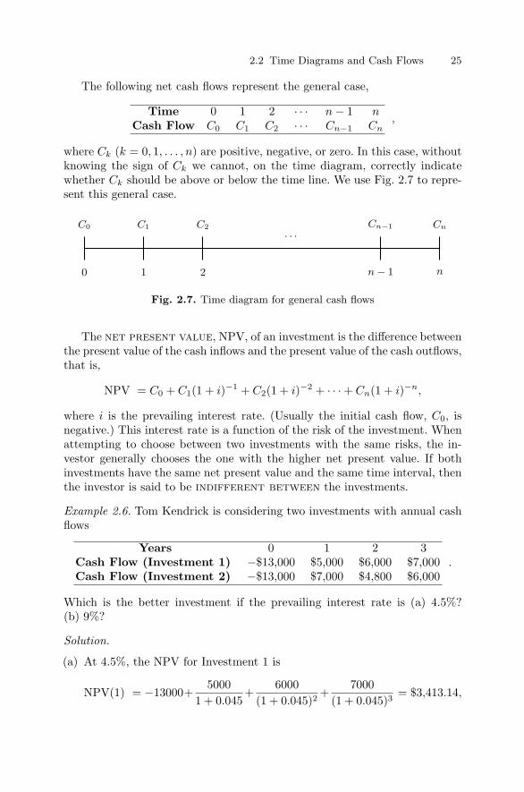
The following net cash flows represent the general case,
Time 0 1 2 · · · n − 1 nCash Flow C0 C1 C2 · · · Cn−1 Cn
,
where Ck (k = 0, 1, . . . , n) are positive, negative, or zero. In this case, withoutknowing the sign of Ck we cannot, on the time diagram, correctly indicatewhether Ck should be above or below the time line. We use Fig. 2.7 to repre-sent this general case.
C0
0
C1
1
C2
2
· · ·Cn−1
n − 1
Cn
n
Fig. 2.7. Time diagram for general cash flows
The net present value, NPV, of an investment is the difference betweenthe present value of the cash inflows and the present value of the cash outflows,that is,
NPV = C0 + C1(1 + i)−1 + C2(1 + i)−2 + · · · + Cn(1 + i)−n,
where i is the prevailing interest rate. (Usually the initial cash flow, C0, isnegative.) This interest rate is a function of the risk of the investment. Whenattempting to choose between two investments with the same risks, the in-vestor generally chooses the one with the higher net present value. If bothinvestments have the same net present value and the same time interval, thenthe investor is said to be indifferent between the investments.
Example 2.6. Tom Kendrick is considering two investments with annual cashflows
Years 0 1 2 3Cash Flow (Investment 1) −$13,000 $5,000 $6,000 $7,000Cash Flow (Investment 2) −$13,000 $7,000 $4,800 $6,000
.
Which is the better investment if the prevailing interest rate is (a) 4.5%?(b) 9%?
Solution.
(a) At 4.5%, the NPV for Investment 1 is
NPV(1) = −13000+5000
1 + 0.045+
6000(1 + 0.045)2
+7000
(1 + 0.045)3= $3,413.14,

26 2 Compound Interest
and for Investment 2,
NPV(2) = −13000+7000
1 + 0.045+
4800(1 + 0.045)2
+6000
(1 + 0.045)3= $3,351.85.
Thus, at 4.5%, Investment 1 is the better choice.(b) At 9%, the NPV for Investment 1 is
NPV(1) = −13000 +5000
1 + 0.09+
6000(1 + 0.09)2
+7000
(1 + 0.09)3= $2,042.52,
and for Investment 2,
NPV(2) = −13000 +7000
1 + 0.09+
4800(1 + 0.09)2
+6000
(1 + 0.09)3= $2,095.18.
Thus, at 9%, Investment 2 is the better choice.
�In this example we see that increasing the prevailing interest rate causes
the NPV of a cash flow to drop. This is generally true if C0 < 0 andC1, C2, . . . , Cn are non-negative, but not all zero.
2.3 Internal Rate of Return
If we invest $1,000 at 6% per annum, and then a year later invest $2,000 at5% per annum, what is the future value of the entire investment after a totalof two years? This is represented by the following cash flows,
Years 0 1 2Cash Flow −$1,000.00 −$2,000.00 ? ,
or by Fig. 2.8.
0
$1,000 $2,000
1?
2
Fig. 2.8. Time diagram
The $1,000 has a future value of 1000 (1 + 0.06)2 = $1,123.60 after 2 years,while the $2,000 has a future value of 2000 (1 + 0.05) = $2,100 after 1 year,so the future value of the entire investment is
1000 (1 + 0.06)2 + 2000 (1 + 0.05) = 1123.60 + 2, 100 = $3,223.60.

2.3 Internal Rate of Return 27
0
$1,000
1$1,123.60
2+
0
$2,000
1$2,100
2=
0
$1,000 $2,000
1$3,223.60
2
Fig. 2.9. Decomposition of time diagram
Figure 2.9 shows how to decompose Fig. 2.8.
Because the interest rates changed during the investment period, a naturalquestion to ask is, “What rate have we really been earning over the twoyears?” (We cannot use the annual effective rate ieff because that applies onlyto investments that earn a constant rate of return.) One way to answer thisquestion is to say that we made $223.60 on an investment of $3,000 over twoyears, so we made $223.60/$3,000 = 0.0745 over two years, which is a rate of0.03725 per year.
However, there are two things wrong with this. First, by dividing 0.0745by 2 we have computed a simple interest rate. Second, we have not taken intoaccount that the $2,000 and the $1,000 are deposited at different times.
We can correct the first problem by finding the annual interest rate irequired to discount $3,223.60 to $3,000, that is, find i > 0 for which
3000 = 3223.60 (1 + i)−2,
so
i = ±√
3223.603000
− 1 = 0.0366 or − 2.0366.
Because i must be positive, we find that i = 0.0366. (Why is this way ofcomputing the interest rate lower than 0.03725, the interest rate we obtainedthe previous way?)
However, this technique does not take into account the second problem,namely, that the $2,000 was deposited at a different time from the $1,000.We can solve this problem by finding the annual interest rate r requiredto discount $3,223.60 to $1,000 plus the discounted value of $2,000, namely2000(1 + r)−1. Thus, we must find r for which
1000 + 2000(1 + r)−1 = 3223.60(1 + r)−2.
This means we must solve the quadratic equation
1000(1 + r)2 + 2000(1 + r) − 3223.60 = 0,
that is,(1 + r)2 + 2(1 + r) − 3.2236 = 0,

28 2 Compound Interest
for 1 + r, giving
1 + r =12
(−2 ±
√22 + 4 × 3.22360
)= 1.055 or − 3.055,
so r = 0.055 or −4.055. However, r must be positive, so r = 0.055. Theannual interest rate computed in this way is called the internal rate ofreturn (IRR), and takes into account both compounding and the time valueof money.
Definition 2.2. The internal rate of return (IRR), iirr, for an invest-ment is the interest rate that is equal to the annually compounded rate earnedon a savings account with the same cash flows.
Example 2.7. Hugh Kendrick, the father of Wendy and Tom, invests $10,000in a CD that yields 5% compounded 365 days a year. At the end of the yearhe moves the proceeds to a new CD that yields 6% compounded 4 times ayear. How much interest does he have when the second CD matures? Whatis the IRR, iirr, for this investment?
Solution. At the end of the first year he has 10000 (1 + 0.05/365)365, which isthe amount he invests as the principal in the second CD. This leads to(
10000(
1 +0.05365
)365)(
1 +0.064
)4
= $11,157.77,
so he earned $1,157.77 in interest.To find the IRR, we want to find the rate iirr for which
10000(1 + iirr)2 = 10000(
1 +0.05365
)365 (1 +
0.064
)4
,
so
iirr = ±√(
1 +0.05365
)365 (1 +
0.064
)4
− 1 = 0.0563 or − 2.0563.
Thus, the IRR is about 5.6%. �Example 2.8. Find the IRR, iirr, that is equivalent to a simple interest invest-ment rate of 20% a year for 5 years.
Solution. Over 5 years under simple interest with P0 = 1, i = 0.20, and n = 5,(1.1) gives
P5 = (1 + (5 × 0.2)) = 2.
Now, (1 + iirr)5 = 2 means that iirr = 21/5 − 1 = 0.149.
Thus, a rate of 14.9%, compounded annually, doubles an investment in 5years. �

2.3 Internal Rate of Return 29
Financial DigressionAn index fund is a fund whose collection of assets is designed to mirrorthe performance of a particular broad-based stock market index.7 Usuallyindex funds are managed so that decisions are automated and transactions areinfrequent. There is usually a minimum opening balance, unless the investorinvests a regular amount each month. Investors are usually discouraged fromfrequent buying and selling, and they may be penalized for this. The first indexfund for individual investors was created by The Vanguard Group in 1976.
Example 2.9. At the beginning of every month for 12 months, Hugh Kendrickbuys $100 worth of shares in an index fund. At the end of the twelfth monthhis shares are worth $1,500. What is the internal rate of return, iirr, of hisinvestment?
Solution. Hugh’s investment is represented by Fig. 2.10.
0
$100 $100
1
$100
2 · · ·
$100
11$1,500
12
Fig. 2.10. Internal rate of return
The present value of his investment at an annual interest rate of iirr is
100 + 100(1 + iirr)−1/12 + 100(1 + iirr)−2/12 + · · · + 100(1 + iirr)−11/12
= 1500(1 + iirr)−12/12,
or
100(1 + iirr)12/12 + 100(1 + iirr)11/12 + · · · + 100(1 + iirr)1/12 = 1500.
The first equation is obtained by discounting to the present value, the secondby compounding to the future value at the end of the twelfth month. Noticewe assume that 1 + iirr > 0.
If in the second equation we let 1 + i = (1 + iirr)1/12, so 1 + i > 0, then wefind that
100(1 + i)12 + 100(1 + i)11 + 100(1 + i)10 + · · · + 100(1 + i) = 1500. (2.5)
We rewrite the equation as((1 + i)11 + (1 + i)10 + · · · + 1
)(1 + i) = 15,
7 We discuss stock market indexes in Chap. 10.

30 2 Compound Interest
and then use the geometric series8
1 + x + x2 + · · · + xn−1 = (xn − 1)/(x − 1), valid for x = 1 and n ≥ 1,
with x = 1 + i and n = 12, to find that i satisfies
(1 + i)12 − 1i
(1 + i) − 15 = 0. (2.6)
In general we are unable to solve the equation for i analytically, but it canbe solved numerically—for example, by the bisection method or by Newton’sMethod (see Problem 2.20 on p. 39)—or graphically, by graphing the left-handside of (2.6) and estimating where it crosses the horizontal axis (see Fig. 2.11),giving i = 0.0339. Here 1 + i = 1.0339 > 0 and from 1 + i = (1 + iirr)1/12
we find that iirr = (1 + i)12 − 1 = 0.492. Thus, the internal rate of return is49.2%. �
i
0.030 0.032 0.034 0.036 0.038 0.040
f(i)
0.0
0.5
1.0
Fig. 2.11. The function f(i) = (1+i)12−1i
(1 + i) − 15
In the previous example we have overlooked a very important point—howdo we know that 1 + i = 1.0339 is the only solution of (2.6)? We don’t, and itisn’t, because 1 + i = −1.318 is another solution. But this solution does notsatisfy 1 + i > 0, so we reject it. So how do we know that 1.0339 is the onlyacceptable solution?8 See Problems 2.34 and 2.35.

2.3 Internal Rate of Return 31
In fact, if we rewrite (2.5) in the form
100(1 + i)12 + 100(1 + i)11 + 100(1 + i)10 + · · · + 100(1 + i) − 1500 = 0, (2.7)
then we see that this is a polynomial equation of degree 12 in (1+i). In general,polynomials of degree n have n roots (some of which may be complex); thus,we might expect (2.7) to have 12 solutions! In fact, it has only one real solutionthat satisfies 1 + i > 0, which we show shortly.
To show this, we turn to the general case, where we have the following netcash flows:
Period 0 1 2 · · · n − 1 nCash Flow C0 C1 C2 · · · Cn−1 Cn
,
where Ck (k = 0, 1, . . . , n) are positive, negative, or zero. We let m be thenumber of periods per year, while n is the total number of periods. Figure 2.12represents this general case.
C0
0
C1
1
C2
2
· · ·Cn−1
n − 1
Cn
n
Fig. 2.12. General time diagram
The IRR, iirr, for this series of cash flows is the solution of the equation9
C0 + C1(1 + iirr)−1/m + C2(1 + iirr)−2/m + · · · + Cn(1 + iirr)−n/m = 0,
which can be written in the form
C0(1 + iirr)n/m + C1(1 + iirr)(n−1)/m + C2(1 + iirr)(n−2)/m + · · · + Cn = 0.
If we let 1+ i = (1+ iirr)1/m, where 1+ i > 0, then this last equation becomes
C0(1 + i)n + C1(1 + i)n−1 + C2(1 + i)n−2 + · · · + Cn = 0.
This is a polynomial equation of degree n in 1 + i, and therefore has exactlyn solutions, including complex ones.9 Notice that the IRR for an investment is the annual rate that makes the net
present value equal to zero. So the IRR is the rate that makes the present valueof the expected future cash flows equal to the initial cost of the investment. TheIRR is useful for comparing investments with different costs or with cash flowsthat differ in terms of amount or frequency of payment, and for determining howa potential investment compares with the investor’s requirements.

32 2 Compound Interest
From 1 + i = (1 + iirr)1/m we find that
iirr = (1 + i)m − 1,
which relates the internal rate of return, iirr, to the periodic internal rate ofreturn, i. Notice that if m = 1, then iirr = i, and that if i > 0, then iirr > 0.If we use the binomial approximation
(1 + i)m = 1 + mi + · · · ,
then we find thatiirr ≈ mi,
which is sometimes used in place of iirr = (1 + i)m − 1.For the case n = 1 (so there are two cash flows), this equation reduces to
C0(1 + i) + C1 = 0,
which has the solutioni =
−C1 − C0
C0.
If we let P0 = −C0 < 0 and P1 = C1 > 0, which corresponds to a savingsaccount that is opened with a balance of P0 and accumulates to P1 after oneperiod, then
i =P1 − P0
P0.
This is the rate of return defined on p. 5 for these cash flows. Thus, if thereis one cash inflow and one cash outflow, then the periodic internalrate of return and the rate of return of the investment are identical.
For the case n = 2 this equation reduces to
C0i2 + (2C0 + C1) i + (C0 + C1 + C2) = 0,
which could have no real solutions, one real solution repeated, or two distinctreal solutions. Only in the second and third cases does i exist and is possiblyunique. In fact, it is possible to construct perfectly reasonable cash flows forwhich the IRR does not exist, or does exist, but is not unique.
Example 2.10. Find the IRR for
Years 0 1 2Cash Flow −$1,000 $2,000 −$1,500 .
This corresponds to giving someone $1,000 now and $1,500 after two years,in exchange for $2,000 after one year.

2.3 Internal Rate of Return 33
Solution. Here iirr must satisfy
−1000(1 + iirr)2 + 2000(1 + iirr) − 1500 = 0,
which reduces to2i2irr + 1 = 0,
which has no real solutions. Thus, this transaction has no IRR. �Example 2.11. Find the IRR for
Years 0 1 2Cash Flow −$1,000 $2,150 −$1,155 .
This corresponds to giving someone $1,000 now and $1,155 after two years,in exchange for $2,150 after one year.
Solution. Here iirr must satisfy
−1000(1 + iirr)2 + 2150(1 + iirr) − 1155 = 0,
which, when solved for 1 + iirr, reduces to
1 + iirr = 1.05 or 1.1.
Thus, iirr = 0.05 or iirr = 0.10, and iirr is not unique. �
We can give partial answers to the uniqueness question as follows.
Theorem 2.3. The IRR Uniqueness Theorem I.If there exists an integer p for which C0, C1, . . . , Cp are of the same sign orzero (but not all zero) and for which Cp+1, Cp+2, . . . , Cn are all of the oppositesign or zero (but not all zero), then
C0 + C1(1 + i)−1 + C2(1 + i)−2 + · · · + Cn(1 + i)−n = 0
has at most one positive solution 1 + i.
Proof. By thinking of
C0(1 + i)n + C1(1 + i)n−1 + C2(1 + i)n−2 + · · · + Cn = 0
as a polynomial equation in 1 + i, and using Descartes’ Rule of Signs,10 thereis exactly one change of sign, so there is at most one positive root of thepolynomial. ��10 Descartes’ Rule of Signs states that the maximum number of positive solutions
of the polynomial equation anxn + an−1xn−1 + · · · + a1x + a0 = 0 is the number
of sign changes that occur when one looks at the coefficients an, an−1, . . . , a1, a0
in order (excluding the coefficients that are zero).

34 2 Compound Interest
Comments About the IRR Uniqueness Theorem I
• This theorem guarantees that there is at most one positive solution, 1 + i.However, that does not guarantee that i is positive.
• Returning to (2.7) we see that it has one change of sign, so it has atmost one positive solution—the one we found numerically. Each of thetwo examples for which the IRR either did not exist (Example 2.10 onp. 32) or was not unique (Example 2.11 on p. 33) had two sign changes.
There is another theorem that is sometimes useful (see [16]).
Theorem 2.4. The IRR Uniqueness Theorem II.If there exists an i for which
(a) 1 + i > 0,(b)
∑pk=0 Ck(1 + i)p−k > 0 for all integers p satisfying 0 ≤ p ≤ n − 1 (that is,
the future value of all the cash flows up to period p are positive), and(c)
∑nk=0 Ck(1 + i)n−k = 0,
then i is unique.
Proof. Assume that there is a second solution j of (c), that is,
n∑k=0
Ck(1 + j)n−k = 0,
satisfying (a) and (b). Without loss of generality, we may assume that j > i.
We first prove, by induction on p, that
p∑k=0
Ck(1 + j)p−k >
p∑k=0
Ck(1 + i)p−k
for p = 1 to n. For p = 1 this becomes
C0(1 + j) + C1 > C0(1 + i) + C1,
which is true because from condition (b) with p = 0, we have C0 > 0.
We assume that∑h
k=0 Ck(1 + j)h−k >∑h
k=0 Ck(1 + i)h−k, and we mustshow that
h+1∑k=0
Ck(1 + j)h+1−k >
h+1∑k=0
Ck(1 + i)h+1−k.

2.3 Internal Rate of Return 35
Now,
h+1∑k=0
Ck(1 + j)h+1−k =h∑
k=0
Ck(1 + j)h+1−k + Ch+1
=h∑
k=0
Ck(1 + j)h−k(1 + j) + Ch+1
>
h∑k=0
Ck(1 + i)h−k(1 + j) + Ch+1
>
h∑k=0
Ck(1 + i)h−k(1 + i) + Ch+1
=h+1∑k=0
Ck(1 + i)h+1−k,
which proves the inequality by induction. (Where did we use condition (a)?Condition (b)?)
Thus,n∑
k=0
Ck(1 + j)n−k >
n∑k=0
Ck(1 + i)n−k = 0.
But by (c),n∑
k=0
Ck(1 + j)n−k = 0,
which is a contradiction. (Why were we allowed to assume that j > i?) ��
Comments About the IRR Uniqueness Theorem II
• Condition (b) requires that C0 > 0. Condition (c) requires that Cn =−∑n−1
k=0 Ck(1 + i)n−k = −(1 + i)∑n−1
k=0 Ck(1 + i)n−1−k, which is nega-tive by conditions (a) and (b). Thus, Cn < 0. However, the remainingC1, . . . , Cn−1 have no sign restrictions, other than satisfying (b).
• This theorem guarantees that a typical savings account has a unique IRR,in the following sense. If the savings account is opened with a positivebalance C0 > 0, and despite withdrawals and deposits, the interest rate, i,is unchanged and the account is never overdrawn, so
∑pk=0 Ck(1+i)p−k > 0
for 0 ≤ p ≤ n − 1, then there is an IRR, namely i, and it is unique. (Herethe quantity Cn is the value of the account, and we are viewing everythingthrough the eyes of the savings institution.)
• This theorem is also valid if the inequality in condition (b) is replaced with∑pk=0 Ck(1 + i)p−k < 0. (See Problem 2.44 on p. 43.)

36 2 Compound Interest
2.4 The Rule of 72
The Rule of 72 is a rule of thumb sometimes used by investors. It states: tocalculate the time it takes to double an investment, divide 72 by the annualinterest rate expressed as a percentage. For example, if the interest rate is14%, then, according to the Rule of 72, it takes 72/14 = 5.14 years to doublean investment.
The justification for this rule is based on the following. If interest is com-pounded continuously at a nominal rate of i(∞), then the future value at timen is
P (n) = P0ei(∞)n.
The question we want answered is, at what time n + T is P (n + T ) = 2P (n)?The condition P (n + T ) = 2P (n) requires that
P0ei(∞)(n+T ) = 2P0ei(∞)n,
orei(∞)T = 2,
so thatT =
ln 2i(∞) =
0.693i(∞) .
Thus, if i(∞) is expressed as a percentage, then the time T needed to doubleour money is approximately 69.3/i(∞). (Notice that this does not depend onthe initial investment nor does it depend on when we start.) Thus, the Ruleof 72 should really be called the Rule of 69.3, and it applies only if interest iscompounded continuously.
However, investments are frequently compound annually, not continuously.So what rule of thumb applies in this case? The answer is, there is no simplerule of thumb like “dividing a particular number by the interest rate”. In thiscase
Pn = P0 (1 + i)n,
so we want to find the N for which
PN = 2P0,
or(1 + i)N = 2.
Solving for N gives
N =ln 2
ln (1 + i). (2.8)
So the rule of thumb is, divide 0.693 by the natural logarithm of (1 + i). Notexactly a handy rule of thumb!

2.5 Problems 37
2.5 Problems
Walking
2.1. Use a spreadsheet to confirm the entries in Table 2.3 on p. 16.
2.2. Tom Kendrick invests $1,000 at a nominal rate of i(1), leaving the interestat the end of each year to compound. At the end of the fourth year he earned$300 in total interest. Determine i(1). Compare your answer to the one youfound for Problem 1.1 on p. 10. Which one do you expect to be higher?Explain.
2.3. We invest $1,000 in an account earning 6% per year for 3 years. What isthe net present value of our investment if the nominal interest rate is 5%?
2.4. At what nominal interest rate, compounded daily, will money double in7 years? What is the IRR for this investment?
2.5. How long will it take for an investment of $1,000 to increase to $1,500 ata nominal interest rate of 7% compounded semi-annually? What is the IRRfor this investment?
2.6. Tom lends a friend $1,000 on the condition that in 10 years, the friendrepays $4,000. What is the IRR for this investment?
2.7. Wendy decides to save for her retirement starting on her 25th birthday.She puts $1,000 a year in an investment that earns 10% a year compoundedannually. She does this for 20 years (she is then 45, and has invested $20,000)and then stops adding more money. She then leaves the money invested at10% annually until she is 65, when she retires. Tom, Wendy’s twin brother,does not save for his retirement until his 45th birthday, and then he startsinvesting a fixed amount each year at 10% per annum for 20 years (at whichtime both Tom and Wendy are 65). How much does Tom have to invest peryear to have the same amount of money as Wendy when she retires?
2.8. Tom buys a stock for $50 and a year later it is worth $100, so the returnon Tom’s investment for that year is 100%. A year later the stock is worth$50, so the return on Tom’s investment for the second year is −50%. Tomclaims that the average return on his investment per year over the two yearperiod is (100 + (−50)) /2 = 25%. Comment on this claim.
2.9. What is the IRR that corresponds to a simple interest investment rateof 20% over 5 years? Over 4 years? Over 10 years?
2.10. Hugh’s wife, Helen Kendrick, buys shares in Cisco for $68. Two monthslater they are worth $104. What is Helen’s IRR?

38 2 Compound Interest
2.11. Hugh estimates that he needs $1,000,000 when he retires in 15 years.How much must he have in his current retirement account, which earns $8% ayear compounded annually, to reach his goal assuming that he adds no moreto his current account?
2.12. An initial amount of $10,000 is invested for 2 years at successive annualinterest rates of 10% and 9% compounded annually. Do you think the futurevalue of this investment is different from the future value of $10,000 investedfor 2 years at successive annual interest rates of 9% and 10% compoundedannually? Justify your answer.
2.13. If the EFF of an investment is 8%, then what is the nominal interestrate, if interest is compounded monthly?
2.14. The National Association of Investors Corporation (NAIC) encouragesits members to use a special form (the Stock Selection Guide) to analyzestocks. Part of the form requires the user to convert the projected annual rateof return on an investment over five years from simple to compound interest.The following table is used for this purpose—for example, according to thistable five years of simple interest at an annual rate of 10.00% is equivalentto 5 years of compound interest at an annual rate of 8.45%. Confirm that thistable is accurate. Is the compound interest row a concave up or a concavedown function of the simple interest row?
Simple (%) 10.00 15.00 20.00 25.00 30.00 35.00 40.00Compound (%) 8.45 11.84 14.87 17.61 20.11 22.42 24.57
2.15. Some banks used to make the promise: “Deposit by the 10th of themonth and earn interest from the 1st. Withdraw your money at any time.”Two banks, A and B, both compound interest daily at the nominal rate i(360),while only Bank B makes this promise. You deposit an amount in Bank Afrom the 1st to the 10th of the month, then transfer all your money from BankA to Bank B on the 10th, and finally transfer all your money from Bank Bback to Bank A at the end of the month. You do this every month for a year.Assuming that each month has 30 days, what is the EFF? What is the IRR?
2.16. Use (2.8) on p. 36 to construct a table with the following headings,
Annual Interest Rate Number of Years Rule Of
for annual interest rates running from 1% to 30% in increments of 1%. The“Number of Years” column is the number of years it takes for the investmentto double at the corresponding annual interest rate. The “Rule Of” column iscalculated by multiplying the interest rate (as a percentage) by the numberof years, as was the case in the Rule of 72. For what interest rates is there aRule of 72?

2.5 Problems 39
2.17. Use (2.8) on p. 36 to construct a table with the following headings,
Number of Years Annual Interest Rate Rule Of
for numbers of years running from 1 to 15 in increments of 1. The “AnnualInterest Rate” column is the interest rate (as a percentage) required for theinvestment to double in the number of years. The “Rule Of” column is cal-culated by multiplying the interest rate (as a percentage) by the number ofyears, as was the case in the Rule of 72. For what years is there a Rule of 72?
2.18. Construct a time diagram that represents the cash flows
Years 0 1 2Cash Flow $1,000 −$500 −$600 .
What is the IRR? Give an explanation of these cash flows in terms of everydayexperiences, starting with “If I borrow . . ..”
2.19. Assuming that P > 0, construct a time diagram that represents thecash flows
Years 0 1 2 3 4 5Cash Flow −P $0 $0 $1,000 $2,000 $3,000 .
Find P assuming a 10% nominal interest compounded annually. Give an ex-planation of these cash flows in terms of everyday experiences, starting with“To be able to withdraw . . ..”
2.20. Rewrite (2.6) on p. 30 in the form
(1 + i)13 − 16(1 + i) + 15 = 0.
(a) Find three solutions of this equation by graphing the function f(x) =x13 − 16x + 15.
(b) Find three solutions of this equation using the bisection method.(c) Find three solutions of this equation using Newton’s Method.(d) Show that one solution of this equation is i = 0. Explain why i = 0 is not
a solution of (2.5) on p. 29.
2.21. What are the interest rates compounded (a) monthly, (b) semi-annually,and (c) annually that yield the same return as an investment earning 6%interest compounded continuously?

40 2 Compound Interest
2.22. Consider four different loans for $50,000:
(a) A 10-year loan at 7.5% a year.(b) A 10-year loan at 10% a year.(c) A 15-year loan at 7.5% a year.(d) A 15-year loan at 10% a year.
The monthly payments on the four loans are $593.51, $463.51, $660.76, and$537.71, although not necessarily in that order. The monthly payment for the10-year loan at 7.5% a year is $593.51. Without using a calculator, match themonthly payments with the loans.
2.23. Find the IRR of a three-year investment of $10,000 that returns thefollowing amounts at the end of each of the three years. What do you conclude?
(a) $400, $500, $10,600.(b) $500, $600, $10,400.(c) $600, $400, $10,500.(d) $600, $500, $10,400.
2.24. Hugh Kendrick is considering three different investments:
(a) One paying 7% compounded quarterly.(b) One paying 7.1% compounded annually.(c) One paying 6.9% compounded continuously.
Which has the highest IRR?
2.25. Tom Kendrick is considering two investments with cash flows
Years 0 1 2 3Cash Flow −$13,000 $5,000 $6,000 $7,000 .
What is the IRR? Give an explanation of these cash flows in terms of everydayexperiences, starting with “If I borrow . . ..”
Running
2.26. Show that P0(1 + x)n is an increasing, concave up function of x. (Seep. 16.)
2.27. Show that P0(1 + i)x is an increasing, concave up function of x. (Seep. 16.)
2.28. Show, by induction, that for n > 1 and i > 0,
(1 + 2i)n − 1 > 2 ((1 + i)n − 1) .
Use this to show that if i, the interest rate per period, is doubled, then theprice appreciation from compounding is more than doubled if n > 1. Whathappens if n = 1? (See p. 17.)

2.5 Problems 41
2.29. Show that for n > 0 and i > 0,
(1 + i)2n − 1 > 2 ((1 + i)n − 1) ,
by rewriting the inequality as a quadratic in (1 + i)n. Use this to show thatif n, the number of periods, is doubled, then the principal appreciation fromcompounding is more than doubled. (See p. 17.)
2.30. We used Fig. 2.2 on p. 17 to suggest that doubling the interest ratemore than doubles the principal appreciation, and that doubling the numberof periods more than doubles the principal appreciation. Explain how thosesuggestions could also be made from Fig. 2.1 on p. 17.
2.31. Show thatlim
m→∞
(1 +
x
m
)m
= ex.
2.32. Look at (2.2) on p. 19. Based on the fact that mN = Nm, do you thinkthat PmN = PNm? If so, prove it. If not, provide a counter-example.
2.33. Show that the EFF of a nominal rate i(m) compounded m times a yearis always greater than i(m) for m > 1.
2.34. Use induction to sum the geometric series∑n
k=1 xk−1, that is, provethat
n∑k=1
xk−1 =xn − 1x − 1
,
where x = 1, for n = 1, 2, . . . by induction. (See p. 30.)
2.35. Sum the geometric series∑n
k=1 xk−1, where x = 1, using the followingidea. Let Sn =
∑nk=1 xk−1. Show that xSn − Sn = xn − 1. Solve this for Sn.
(See p. 30.)
2.36. The geometric mean of the non-negative numbers a1, a2, . . . , an is
(a1a2 · · · an)1/n.
Prove that the IRR of n successive annual investments with rates i1, i2, . . . , incompounded m1, m2, . . . , mn times a year, respectively, is one less than thegeometric mean of(
1 +i1m1
)m1
,
(1 +
i2m2
)m2
, . . . ,
(1 +
i1mn
)mn
.
2.37. Show that the IRR that corresponds to a nominal rate i(m) compoundedm times a year does not depend on the number of years it is invested.
2.38. Show that the IRR that corresponds to a simple interest investmentrate of i depends on the number of years it is invested.

42 2 Compound Interest
2.39. Show that for a sequence of cash flows over one year, the IRR is thesame as the EFF.
2.40. Show that the future value at the end of the first year when invested ata simple annual interest rate of i is the same as the future value at the endof the first year when invested at a compound annual interest rate of i. Showthat the future value at the end of the nth year (n ≥ 2) when invested at asimple annual interest rate of i is always less than the future value at the endof the nth year when invested at a compound annual interest rate of i.
2.41. An initial amount P0 is compounded annually for n years at successiveannual interest rates of i1, i2, · · · , in. Show that11
Pn = P0
n∏j=1
(1 + ij) .
What has this result to do with Problem 2.12 on p. 38?
2.42. The purpose of this problem is to show that the function (1 + i/t)t isan increasing function of t if i > 0.
(a) Consider the function
g(x) =x
x + 1− ln(1 + x)
for x > 0. Show that g′(x) < 0. Explain why this leads to g(0) > g(x),that is, if x > 0, then
x
x + 1− ln(1 + x) < 0.
(b) Now consider the function
f(x) = (1 + x)1/x
for x > 0. By considering f ′(x) and the inequality from part (a), showthat f(x) is a decreasing function of x.
(c) By putting x = i/t in part (b), show that (1 + i/t)t is an increasingfunction of t. (Where did you need i > 0?)
(d) Explain how part (c) generalizes Theorem 2.2 on p. 20.
11 The product symbol,∏n
j=1 aj , is defined by
n∏j=1
aj = a1a2 · · · an.

2.5 Problems 43
2.43. Is it possible for the cash flows
Time 0 1 2Cash Flow C0 C1 C2
to have no IRR if the sequence C0, C1, C2 has exactly one sign change?
2.44. Prove that the IRR Uniqueness Theorem II on p. 34 is also true if theinequality in condition (b) is replaced with
∑pk=0 Ck(1 + i)p−k < 0.
2.45. Give an example of constants C0, C1, . . . , Cn such that there is a uniquei that satisfies condition (c) of the IRR Uniqueness Theorem II on p. 34, butnot conditions (a) and (b).
2.46. If the rate of change of P (t) with respect to t is proportional to theinitial amount P0 = P (0), that is, if dP/dt = kP0 where k is a positiveconstant, then show that P is growing at a simple interest rate of k.
2.47. If the rate of change of P (t) with respect to t is proportional to theamount P (t) present at time t, that is, if dP/dt = kP , where k is a positiveconstant, then show that P is growing at an interest rate of k, compoundedcontinuously.
2.48. If the rate of change of P (t) with respect to t is proportional to thesquare of the amount P (t) present at time t, that is, if dP/dt = kP 2, where kis a positive constant, then show that the graph of P has a vertical asymptote.What is the practical significance of this asymptote?
2.49. What compound annual interest rate of i gives the Rule of 72 exactly?
Questions for Review
• How do you calculate compound interest?• What does compounded continuously mean?• What is discounting?• What is the difference between the annual effective rate and the internal
rate of return?• What is a time diagram?• What is the NPV?• Why are the IRR Uniqueness Theorems important?• What is the Rule of 72?• What is a proof by induction?• What is a recurrence relation?

3
Inflation and Taxes
In this chapter we discuss two topics that usually reduce the annual effectiverate (EFF) of an investment—inflation and taxes. The impact of these twoitems on any profits should not be ignored.
3.1 Inflation
Inflation changes the purchasing power of money and so behaves like interestbut in reverse. For example, if inflation in one year is 10%, then $100 worth ofgoods at the beginning of the year typically costs $110 at the end. Thus, we areonly able to purchase 100/110 of the goods at the end of the year comparedto the beginning. Thus, if the annual inflation rate is iinf (expressed as adecimal), then P0 at the beginning of a year purchases P0/(1 + iinf) at theend.
Imagine that we keep our money P0 under the mattress and that theinflation rate, iinf , is constant. After n years, the purchasing power of ourmoney is reduced to
Pn = P0
(1
1 + iinf
)n
.
Another way of saying this is that Pn future dollars are worth P0 in today’sdollars.
Theorem 3.1. The Purchasing Power Theorem.If the annual inflation rate is iinf , then the purchasing power of P0 after nyears is reduced to
Pn = P0
(1
1 + iinf
)n
. (3.1)

46 3 Inflation and Taxes
Comments About the Purchasing Power Theorem
• Table 3.1 shows the impact of inflation on the buying power of $1,000 overtime, in five-year intervals, for various annual inflation rates.
Table 3.1. Impact of Inflation on Buying Power of $1,000
YearsInflation Rate 5 10 15 20 25 30
3% 862.61 744.09 641.86 553.68 477.61 411.994% 821.93 675.56 555.26 456.39 375.12 308.325% 783.53 613.91 481.02 376.89 295.30 231.386% 747.26 558.39 417.27 311.80 233.00 174.117% 712.99 508.35 362.45 258.42 184.25 131.378% 680.58 463.19 315.24 214.55 146.02 99.389% 649.93 422.41 274.54 178.43 115.97 75.37
• Figure 3.1 shows the purchasing power of $1,000 as a function of the in-flation rate for 10 years (the upper curve) and 20 years (the lower curve).
Inflation Rate
0% 2% 4% 6% 8% 10% 12%
Pu
rch
asin
gP
ow
er
0
200
400
600
800
1000
10 years
20 years
Fig. 3.1. Purchasing power of $1,000 as a function of inflation rate for 10 and 20years
• Figure 3.2 shows the purchasing power of $1,000 as a function of years for3% (the upper curve) and 6% (the lower curve).
• Notice, from Figure 3.2, that at a modest 3% inflation rate our purchasingpower decreases by 50% in about 23 years. Some parents start saving for

3.1 Inflation 47
their children’s college education shortly after the child’s birth. If inflationrates are between 3% and 5% during that time, then they need to savemore than twice as much as the current estimate since increases in thecost of education typically outpace inflation.
• We notice that Pn is directly proportional to P0 but is a nonlinear functionof iinf and n. Figures 3.1 and 3.2 suggest that the graphs of Pn as afunction of i, and Pn as a function of n are both decreasing and concaveup.1 Problems 3.9 and 3.10 on p. 52 ask you to prove these conjectures.
• If iinf > 0, then {Pn} is a decreasing sequence for which limn→∞ Pn = 0.Thus, during times of inflation, our money buys less and less as time goesby.
• If iinf < 0—this is usually called deflation—then {Pn} is an increasingsequence for which limn→∞ Pn = ∞. Thus, during times of deflation, ourmoney buys more and more as time goes by.
Years
0 5 10 15 20 25
Pu
rch
asin
gP
ow
er
0
200
400
600
800
1000
3%
6%
Fig. 3.2. Purchasing power of $1,000 as a function of years for 3% and 6% inflationrates
Example 3.1. Today Amanda Kendrick pays $7 for a movie ticket. In 20 years,how much does she pay in today’s dollars if inflation runs at 5%?
Solution. We want to find P0 in today’s dollars if P20 = 7. From Pn = P0(1 +iinf)−n, we have P0 = 7(1 + 0.05)20 = 18.57. Thus, we estimate that a movieticket costs $18.57 in 20 years due to inflation. �
1 Concave up functions are special cases of convex functions, and are widely usedin financial circles. (See Problem 3.13 on p. 52.)

48 3 Inflation and Taxes
Now imagine that we keep our money P0 in an interest bearing accountat an annual effective rate of ieff. If the inflation rate iinf is a constant, thenafter n years, the purchasing power of our money is
Pn = P0(1 + ieff)n
(1
1 + iinf
)n
= P0
(1 + ieff1 + iinf
)n
. (3.2)
• If iinf > ieff, then {Pn} is a decreasing sequence for which limn→∞ Pn = 0.Thus, as time goes by, our money buys less and less.
• If iinf = ieff, then {Pn} is a constant sequence. As time goes by, our moneybuys the same amount even though we are earning interest.
• If iinf < ieff, then {Pn} is an increasing sequence for which limn→∞ Pn =∞. Thus, as time goes by, our money buys more and more.
We introduce the real rate of interest, ireal, which is the annual rateat which P0 grows to Pn when interest is compounded annually at ieff adjustedfor inflation. Thus,
Pn = P0(1 + ireal)n.
So from (3.2), we have
1 + ireal =1 + ieff1 + iinf
.
This can be rewritten as
ireal =1 + ieff1 + iinf
− 1 =ieff − iinf
1 + iinf.
Thus, we have the following theorem.
Theorem 3.2. The Inflation Theorem.If the annual inflation rate is iinf , then the real rate of interest, ireal, thatcorresponds to an annual effective rate of ieff, is
ireal =ieff − iinf
1 + iinf. (3.3)
Solving (3.3) for ieff gives
ieff = iinf + ireal + iinf ireal.
3.2 Consumer Price Index (CPI)
The Consumer Price Index (CPI) is a measure of the average price over timeof a fixed market basket of goods and services bought by consumers for day-to-day living. The CPI for the United States is the broadest, most comprehensiveindex and is often quoted as the source for the “rate of inflation”.2
2 Some people feel that the CPI is an upper limit for the rate of inflation.

3.2 Consumer Price Index (CPI) 49
Table 3.2 shows the average annual CPI, and how it has changed from1913 to 2005, with the CPI of 100 occurring in mid-1983.3
Table 3.2. Average Annual CPI
Year Index % Year Index % Year Index %1913 9.9 1944 17.6 1.7 1975 53.8 9.11914 10.0 1.0 1945 18.0 2.3 1976 56.9 5.81915 10.1 1.0 1946 19.5 8.3 1977 60.6 6.51916 10.9 7.9 1947 22.3 14.4 1978 65.2 7.61917 12.8 17.4 1948 24.1 8.1 1979 72.6 11.31918 15.1 18.0 1949 23.8 −1.2 1980 82.4 13.51919 17.3 14.6 1950 24.1 1.3 1981 90.9 10.31920 20.0 15.6 1951 26.0 7.9 1982 96.5 6.21921 17.9 −10.5 1952 26.5 1.9 1983 99.6 3.21922 16.8 −6.1 1953 26.7 0.8 1984 103.9 4.31923 17.1 1.8 1954 26.9 0.7 1985 107.6 3.61924 17.1 0.0 1955 26.8 −0.4 1986 109.6 1.91925 17.5 2.3 1956 27.2 1.5 1987 113.6 3.61926 17.7 1.1 1957 28.1 3.3 1988 118.3 4.11927 17.4 −1.7 1958 28.9 2.8 1989 124.0 4.81928 17.1 −1.7 1959 29.1 0.7 1990 130.7 5.41929 17.1 0.0 1960 29.6 1.7 1991 136.2 4.21930 16.7 −2.3 1961 29.9 1.0 1992 140.3 3.01931 15.2 −9.0 1962 30.2 1.0 1993 144.5 3.01932 13.7 −9.9 1963 30.6 1.3 1994 148.2 2.61933 13.0 −5.1 1964 31.0 1.3 1995 152.4 2.81934 13.4 3.1 1965 31.5 1.6 1996 156.9 3.01935 13.7 2.2 1966 32.4 2.9 1997 160.5 2.31936 13.9 1.5 1967 33.4 3.1 1998 163.0 1.61937 14.4 3.6 1968 34.8 4.2 1999 166.6 2.21938 14.1 −2.1 1969 36.7 5.5 2000 172.2 3.41939 13.9 −1.4 1970 38.8 5.7 2001 177.1 2.81940 14.0 0.7 1971 40.5 4.4 2002 179.9 1.61941 14.7 5.0 1972 41.8 3.2 2003 184.0 2.31942 16.3 10.9 1973 44.4 6.2 2004 188.9 2.71943 17.3 6.1 1974 49.3 11.0 2005 195.3 3.4
The % column represents the percentage change in the index from one yearto the next. For example, the percentage change of 3.4 in 2005 is calculatedfrom
Index in 2005 − Index in 2004Index in 2004
=195.3 − 188.9
188.9= 0.0339,
which is 3.4% to one decimal place.
3 ftp://ftp.bls.gov/pub/special.requests/CPI/cpiai.txt, accessed March 17, 2006.

50 3 Inflation and Taxes
From the table, we see that in 1970 the index was 38.8, and by 2005 ithad grown to 195.3. This suggests that goods that cost $38.80 in 1970 cost$195.30 in 2005. Thus, after 35 years an amount P0 has its purchasing powerreduced to P35 = (38.8/195.3)P0, and so the inflation rate, iinf , for those 35years must satisfy
38.8195.3
P0 = P0
(1
1 + iinf
)35
,
that is,
iinf =(
195.338.8
)1/35
− 1 = 0.047.
So inflation has been about 5% per year over those 35 years.
3.3 Personal Taxes
If we keep our money P0 in an interest bearing account at an annual effectiverate of ieff, then after one year we have P0(1 + ieff). Thus, our pre-tax profitthat year is ieffP0. This profit incurs taxes, and if t is our tax rate (expressedas a decimal), then we pay ieffP0t in taxes.4 Thus, the actual after-tax amountwe have available to re-invest the second year is
P1 = P0(1 + ieff) − ieffP0t = P0(1 + ieff − iefft).
One year later this has grown to P1(1 + ieff), pre-tax, and so after taxeswe have
P2 = P1(1 + ieff) − ieffP1t = P1(1 + ieff − iefft).
Continuing in this way, we find that
Pk+1 = Pk(1 + ieff) − ieffPkt = Pk(1 + ieff − iefft).
This is the same recurrence relation that we found in the proof of Theorem2.1 on p. 15, which has solution
Pn = P0(1 + ieff − iefft)n.
Thus, we have the following theorem.
4 In the United States, as of July 2006, the tax rates on earned income depend onmarital status and taxable income. The rates are: 15%, 25%, 28%, and 35%. Thetax rates on unearned income (such as investments) are different from those onearned income (such as salary).

3.4 Problems 51
Theorem 3.3. The Tax Theorem.If the annual effective rate is ieff and the annual tax rate, t, is constant, thenthe after-tax future value of P0 after n years is
Pn = P0(1 + ieff − iefft)n. (3.4)
We now introduce the after-tax rate of interest, itax, which is theafter-tax annual rate at which P0 grows to Pn when compounded annually atthat rate. Thus,
Pn = P0(1 + itax)n,
and so from (3.4), we have
1 + itax = 1 + ieff − iefft.
This can be rewritten as
itax = ieff − iefft = ieff(1 − t). (3.5)
3.4 Problems
Walking
3.1. Confirm that the entries in Table 3.1 on p. 46 are correct.
3.2. In what years did the United States experience deflation?
3.3. What is the rate of inflation for the period 1980–2005? The period 1990–2005? The period 2000–2005?
3.4. In 1974, Helen Kendrick received 10% interest compounded annually onher savings account. Should she be pleased? What was the real rate of interest?
3.5. On average, the cost of a college textbook is about $75. How much doesit cost 25 years from now (in today’s dollars)—when the children of currentfreshmen are themselves freshmen—if inflation runs at 5%?
3.6. In January 1970, Hugh Kendrick bought a new Toyota Corolla for $2,000.In January 2000, he bought one for $14,000. What annual rate of inflation doesthis correspond to?
3.7. Some investments are tax-exempt. The following table shows that, for aperson in the 15% taxable income bracket, an annual effective rate of 2.35%on a taxable investment is equivalent to an annual effective rate of 2% on atax-exempt investment. Complete this table.

52 3 Inflation and Taxes
Tax RateTax Exempt Return 15% 25% 28% 35%
2% 2.35% 2.67% 2.78% 3.08%3%4%5%6%7%8%9%10%
Running
3.8. A rule of thumb used to estimate the real interest rate is ireal ≈ ieff − iinf .Show that this estimate is always too high during times of inflation and toolow during times of deflation.
3.9. Show that
f(x) = P0
(1
1 + iinf
)x
is a decreasing, concave up function of x for iinf > 0. (See p. 47.)
3.10. Show that
g(x) = P0
(1
1 + x
)n
is a decreasing, concave up function of x. (See p. 47.)
3.11. Some people think, incorrectly, that the inflation equation is not (3.2)on p. 48, but is given by P0(1 − iinf)n. Show that these people predict a valuethat is always lower than the correct one when −1 < iinf < 1.
3.12. If P0 is placed in an interest bearing account at an annual effective rateof ieff, if the annual inflation rate is iinf , and if the annual tax rate is t, thenwhat is the after-tax after-inflation rate of interest?
3.13. A function f(x) on an interval I is said to be convex on I if for everyp ∈ (0, 1) and every x, y ∈ I, the function f(x) satisfies5
f (px + (1 − p)y) ≤ pf(x) + (1 − p)f(y).
(a) Show that the function f(x) = x is convex.(b) Show that the function f(x) = |x| is convex.(c) Show that the function f(x) = x2 is convex.
5 The notation a ∈ I, means that a is an element or member of I. If I is notspecified it is assumed to be (−∞, ∞).

3.4 Problems 53
3.14. Give an example of a function that is not convex.
3.15. Consider the function
f(x) ={
x if x ≤ 1,2 − x if x > 1.
Show that f(x) is convex on −∞ < x ≤ 1 and convex on 1 < x < ∞ but notconvex on −∞ < x < ∞.
3.16. If f(x) is convex on an interval I, if pi ≥ 0 (i = 1, 2, . . . , n) wherep1 + p2 + · · · pn = 1, and if x1, x2, · · · , xn ∈ I, then show that
f
(n∑
i=1
pixi
)≤
n∑i=1
pif(xi).
[Hint: Use induction.]
3.17. Suppose that f(x) is defined on the interval I. If x1 < x2 < x3 are inI and f(x1) < f(x2) and f(x3) < f(x2), then show that f(x) is not convexon I.
Questions for Review
• What is inflation?• What is deflation?• What is meant by the expression “the purchasing power of money”? How
is it calculated?• What is the real rate of interest?• What is the Consumer Price Index?• What is the after-tax rate of interest?

4
Annuities
An annuity is a constant amount of money paid at regular intervals, calledperiods. When the payments are made at the end of the period, the annuityis called an ordinary annuity. When payments are made at the beginningof the period, the annuity is called an annuity due.
Annuities occur in a variety of different settings. For example, someonewho is saving for retirement by investing a constant amount of money at theend of every month in an account that pays a fixed interest rate is creatingan ordinary annuity. Someone who wins the lottery and who has selected theannuity payout option is paid a constant amount of money immediately andevery year thereafter for a fixed number of years—an annuity due.
It is important that annuities be thoroughly understood—they are funda-mental to the remaining chapters.
4.1 An Ordinary Annuity
We invest $1,000 at the end of each year at 10% annual interest for 5 years.At the end of the first year we earn no interest because we have just deposited$1,000. At the end of the second year we earn 10% of $1,000, namely, $100, andwe deposit $1,000, totaling $2,100. At the end of the third year we earn 10%of $2,100, namely, $210, and we deposit $1,000, totaling $3,310. We continuedoing this for 5 years. Table 4.1 shows the details. (Check the calculations inthis table using a calculator or a spreadsheet program, and fill in the missingentries.)
We now derive the general formula for this process. We let
P be the amount invested at the end of every period,n be the total number of periods,Pn be the future value of the annuity at the end of the nth period,m be the number of periods per year,
i(m) be the nominal rate (annual interest rate), expressed as a decimal,i be the interest rate per interest period.

56 4 Annuities
Table 4.1. Ordinary Annuity
Year’s Beginning Year’s EndYear Principal Interest Investment Amount
1 $0.00 $0.00 $1,000.00 $1,000.002 $1,000.00 $100.00 $1,000.00 $2,100.003 $2,100.00 $210.00 $1,000.00 $3,310.0045 $4,641.00 $464.10 $1,000.00 $6,105.10
The interest rate per period is i = i(m)/m.We want to find a formula for the future value Pn, and we do this by looking
at n = 1, n = 2, and so on, hoping to see a pattern. Using this notation, werewrite Table 4.1 symbolically in spreadsheet format as Table 4.2, which isexplained as follows.
Table 4.2. Ordinary Annuity—Spreadsheet Format
Period’s Beginning Period’s EndPeriod Principal Interest Investment Amount
1 0 0 P 0 + 0 + P = P1
2 P1 iP1 P P1 + iP1 + P = P2
3 P2 iP2 P P2 + iP2 + P = P3
4 P3 iP3 P P3 + iP3 + P = P4
5 P4 iP4 P P4 + iP4 + P = P5
At the end of period 1 we have made 1 payment, and our future value is
P1 = P.
At the end of period 2 we have made 2 payments, and our future value is
P2 = P1(1 + i) + P = P (1 + i) + P.
At the end of period 3 we have made 3 payments, and our future value is
P3 = P2(1 + i) + P = P (1 + i)2 + P (1 + i) + P.
At the end of period 4 we have made 4 payments, and our future value is
P4 = P3(1 + i) + P = P (1 + i)3 + P (1 + i)2 + P (1 + i) + P.
This suggests that at the end of period n we have made n payments, andour future value is
Pn = P (1 + i)n−1 + P (1 + i)n−2 + · · · + P (1 + i) + P.

4.1 An Ordinary Annuity 57
Using the geometric series
1 + x + · · · + xn−1 =xn − 1x − 1
, x = 1,
we can rewrite this conjecture in closed form1
Pn = P((1 + i)n−1 + (1 + i)n−2 + · · · + (1 + i) + 1
)= P
(1 + i)n − 1i
.
This suggests the following theorem.
Theorem 4.1. The Future Value of an Ordinary Annuity Theorem.If we invest P at the end of every period for n periods (where there are mperiods per year) at a nominal rate of i(m) (expressed as a decimal), then Pn,the future value of the annuity after n periods, is
Pn = P
n∑k=1
(1 + i)k−1 = P(1 + i)n − 1
i, (4.1)
where i = i(m)/m.
Proof. We can prove this conjecture in at least two different ways: either usingmathematical induction or using recurrence relations.
We first prove it using mathematical induction. We already know that(4.1) is true for n = 1. We assume that it is true for n = k, that is,
Pk = P(1 + i)k − 1
i.
and we must show that it is true for n = k + 1. Now,
Pk+1 = Pk(1 + i) + P,
so
Pk+1 = P(1 + i)k − 1
i(1 + i) + P = P
(1 + i)k+1 − 1i
,
which shows that (4.1) is true for n = k + 1. This concludes the proof bymathematical induction.
We now prove it using recurrence relations. We know that P1 = P andthat for k > 0,
Pk+1 = Pk(1 + i) + P,
so if we multiply this by 1/(1 + i)k+1, then we can write it as
1 Loosely speaking, an expression is in “closed form” if it does not contain termssuch as “· · · ”.

58 4 Annuities
Pk+11
(1 + i)k+1 = Pk1
(1 + i)k+ P
1
(1 + i)k+1 .
Summing this from k = 1 to k = n − 1 (where n > 1) gives
n−1∑k=1
Pk+11
(1 + i)k+1 =n−1∑k=1
Pk1
(1 + i)k+ P
n−1∑k=1
1
(1 + i)k+1 ,
or by canceling the common terms on both sides of this equation,
Pn1
(1 + i)n = P1
1 + i+ P
n−1∑k=1
1
(1 + i)k+1 ,
that is,
Pn = P
n−1∑k=0
(1 + i)n
(1 + i)k+1 .
However,n−1∑k=0
(1 + i)n
(1 + i)k+1 = 1 + (1 + i) + · · · + (1 + i)n−1,
which is a geometric series that can be written in the form
n−1∑k=0
(1 + i)n
(1 + i)k+1 =(1 + i)n − 1
i.
Thus,
Pn = P(1 + i)n − 1
i,
which is (4.1). This concludes the proof using recurrence relations. ��
Comments About the Future Value of an Ordinary Annuity Theo-rem
• The general situation is represented by Fig. 4.1.
0
P
1
P
2 · · ·
P
n − 1Pn
P
Fig. 4.1. Time diagram of an ordinary annuity

4.1 An Ordinary Annuity 59
• Notice that (4.1), namely,
Pn = P (1 + i)n−1 + P (1 + i)n−2 + · · · + P (1 + i) + P,
is consistent with Fig. 4.1 because the future value of the first payment P(after n periods) is P (1 + i)n−1, the future value of the second paymentP (after n periods) is P (1 + i)n−2, and so on.
• Table 4.3 shows the future value of an ordinary annuity of $1 for differentannually-compounded interest rates and different numbers of years.
Table 4.3. Future Value of an Ordinary Annual Annuity of $1
YearsInterest Rate 5 10 15 20 25 30
3% 5.309 11.464 18.599 26.870 36.459 47.5754% 5.416 12.006 20.024 29.778 41.646 56.0855% 5.526 12.578 21.579 33.066 47.727 66.4396% 5.637 13.181 23.276 36.786 54.865 79.0587% 5.751 13.816 25.129 40.995 63.249 94.4618% 5.867 14.487 27.152 45.762 73.106 113.2839% 5.985 15.193 29.361 51.160 84.701 136.30810% 6.105 15.937 31.772 57.275 98.347 164.49411% 6.228 16.722 34.405 64.203 114.413 199.02112% 6.353 17.549 37.280 72.052 133.334 241.33313% 6.480 18.420 40.417 80.947 155.620 293.19914% 6.610 19.337 43.842 91.025 181.871 356.78715% 6.742 20.304 47.580 102.444 212.793 434.745
• We notice that Pn is a function of the three variables P , n, and i. It isdirectly proportional to P—which is why we selected P = 1 in Table 4.3—but nonlinear in i and n.
• The dependence of Pn on i is seen in Fig. 4.2, which shows the futurevalue of an ordinary annuity of $1 as a function of i for 10 years (the lowercurve) and 20 years (the upper curve) with annual compounding. Noticethat both curves appear to be increasing and concave up. In Problem 4.18on p. 73 you are asked to prove this.
• The dependence of Pn on n is seen in Fig. 4.3, which shows the future valueof an ordinary annuity of $1 as a function of n for 5% interest (the lowercurve) and 10% interest (the upper curve) compounded annually. Noticethat both curves appear to be increasing and concave up. In Problem 4.19on p. 73 you are asked to prove this.
Example 4.1. Helen and Hugh Kendrick decide to give Amanda, their 20-yearold daughter, an extended birthday gift. They deposit $2,000 in her name on

60 4 Annuities
Interest Rate
2% 3% 4% 5% 6% 7% 8% 9% 10% 11% 12%
Fu
ture
Val
ue
of
$1A
nn
uit
y
0
10
20
30
40
50
60
70
80
10 years20 years
Fig. 4.2. Future Value of $1 annuity for 10 and 20 years with annual compounding
Years
0 5 10 15 20
Fu
ture
Val
ue
of
$1A
nn
uit
y
0
10
20
30
40
50
60
5%10%
Fig. 4.3. Future Value of $1 annuity at 5% and 10% interest compounded annually
her next five birthdays at a nominal rate of 8% compounded annually, andthen they stop the annual deposits. Amanda leaves the accumulated amountinvested at 8%. How much does Amanda have when she turns 65?
Solution. In this case Helen and Hugh make five deposits, so n = 5, andat the end of the fifth year Amanda has
P5 = 2000(1 + 0.08)5 − 1
0.08= $11,733.20.
This is now invested for 40 years at 8%, giving
11733.20 (1 + 0.08)40 = $254,898.16. �

4.1 An Ordinary Annuity 61
Example 4.2. If, under the circumstances of Example 4.1, a rival institutionoffered the Kendricks a 10% interest rate (instead of 8%), then how muchdoes Amanda have when she turns 65?
Solution. At the end of the fifth year she has
P5 = 2000(1 + 0.10)5 − 1
0.10= $12,210.20.
This is now invested for 40 years at 10%, giving
12210.20 (1 + 0.10)40 = $552,624.56.
�
Notice that a relatively small change in interest rates, in this case from8% to 10%, can make a huge difference in the value of the investment aftera number of years, in this case a difference of about $300,000 on an initialinvestment of $10,000.
Example 4.3. Tom Kendrick is repaying a student loan with a nominal interestof 5% at $100 a month. He misses three successive payments but makes thefourth. He then pays an additional lump sum2 to make up for the three missedpayments. How much is the lump sum? How much extra interest does he payas a result of his late payments?
Solution. Tom’s scheduled cash flows are represented by Fig. 4.4, where P4 isthe total value of the four payments.
0
$100
1
$100
2
$100
3P4
$100
Fig. 4.4. Time diagram of Tom’s scheduled cash flows
We recognize this as an ordinary annuity with P = $100, n = 4, andi = 0.05/12, so
P4 = 100
(1 + 0.05
12
)4 − 10.0512
= $402.51.
Thus, the lump sum is P4 − 100 = $302.51. The $302.51 − $300.00 = $2.51 isthe extra interest for the late payments. An alternative way to think of thisproblem is represented by Fig. 4.5, where L is the lump sum owed due to themissed payments.2 In practice, there might be an additional charge for missing the payments.

62 4 Annuities
0
$100
1
$100
2
$100
3L
Fig. 4.5. Time diagram of Tom’s debt
The future value of the first missed payment is 100 (1 + 0.05/12)3, of thesecond missed payment is 100 (1 + 0.05/12)2, and of the final missed paymentis 100 (1 + 0.05/12). Thus,
L = 100(
1 +0.0512
)3
+ 100(
1 +0.0512
)2
+ 100(
1 +0.0512
)= $302.51.
�The present value of Pn is P0, where Pn = P0 (1 + i)n, so the present value
of an ordinary annuity is
P0 = Pn(1 + i)−n = P(1 + i)n − 1
i(1 + i)−n = P
1 − (1 + i)−n
i.
We thus have the following theorem.
Theorem 4.2. The Present Value of an Ordinary Annuity Theorem.If we invest P at the end of every period for n periods (where there are mperiods per year) at a nominal rate of i(m) (expressed as a decimal), then P0,the present value of the annuity, is
P0 =Pn
(1 + i)n = P
n∑k=1
1
(1 + i)n+1−k= P
1 − (1 + i)−n
i, (4.2)
where i = i(m)/m.
Comments About the Present Value of an Ordinary Annuity The-orem
• Notice that (4.2), namely,
P0 = P
n∑k=1
1
(1 + i)n+1−k=
P
1 + i+
P
(1 + i)2+ · · · +
P
(1 + i)n ,
is represented by Fig. 4.6.This is interpreted as receiving an initial loan of P0 and repaying P over npayment periods—called amortizing a loan. Given any positive P , i, andn (where n is an integer), we use (4.2) to compute P0. In other words, wecan answer questions like, “If I can afford to pay P a month for n months,

4.1 An Ordinary Annuity 63
P
1
P
2 · · ·
P
n − 1P0
n
P
Fig. 4.6. Time diagram of a simple loan
then how much can I borrow at a monthly interest rate of i?” However, ingeneral and for a very subtle reason, we cannot answer the question, “If Iwant to borrow P0 at a monthly interest rate of i and can afford to payP a month, then how long does it take to repay the loan?” To answer thisquestion, we have to solve (4.2), namely,
P0 = P1 − (1 + i)−n
i,
for n, obtaining
n =ln
(P
P−iP0
)ln (1 + i)
.
However, in general the left-hand side is an integer, whereas the right-handside is not. We return to this type of problem in Chap. 6.
Example 4.4. The Kendricks are thinking of buying a new house by amortizinga loan. They can afford to pay $700 a month for 30 years. If the current interestrate is 8%, then how much can they borrow?
Solution. From (4.2), with P = 700, m = 12, i = 0.08/12, and n = 30 × 12 =360, we find that
P0 = 7001 − (
1 + 0.0812
)−360
0.0812
= $95,398.45.
Thus, they can borrow about $95,000. �
A sinking fund is an account, earning a nominal interest rate of i(m),into which a constant amount of money P is deposited regularly m times ayear (often monthly) with a view to accumulating a targeted amount F on aspecified date n periods in the future. If the deposits are made at the end ofeach period, including the final period, then the time diagram is Fig. 4.7.
This is just an ordinary annuity, so from (4.1), we have
F = P(1 + i)n − 1
i, (4.3)

64 4 Annuities
0
P
1
P
2 · · ·
P
n − 1F
P
Fig. 4.7. Time diagram of a sinking fund
where i = i(m)/m. Usually the question with a sinking fund is, “How muchmust we deposit every period to have a targeted final figure at a specifiedtime?” In other words, find P in terms of F , n, and i. Thus, from (4.3),
P = Fi
(1 + i)n − 1. (4.4)
Example 4.5. Hugh Kendrick expects to replace his car in 5 years. He estimatesthat he needs $20,000. How much per month must he put into a sinking fundat a nominal rate of 6% compounded monthly to replace his car?
Solution. Here F = 20000, n = 5 × 12 = 60, and i = 0.06/12 = 0.005, so
P = 200000.005
(1.005)60 − 1= 286.656,
namely, $286.66 a month. �
We can do two back-of-the-envelope, order-of-magnitude calculations tosee whether $286.66 a month is in the right ballpark.
• First, intuition suggests that the total deposited is less than the fi-nal amount because most deposits earn interest. The total deposited is$286.66 × 60 = $17,199.60, which is less than $20,000. This intuitive cal-culation suggests that for n > 1,
nP < F.
But is our intuition correct?For nP < F to be true we need, from (4.3),
n <(1 + i)n − 1
i,
or(1 + i)n − 1 − ni > 0.
We prove this by induction on n > 1. With n = 2, the left-hand side ofthis inequality becomes (1 + i)2 − 1 − 2i = i2 > 0, so it is true for n = 2.We assume that it is true for n = k, that is,
(1 + i)k − 1 − ki > 0,

4.1 An Ordinary Annuity 65
and consider the left-hand side with n = k + 1, namely, (1 + i)k+1 − 1 −(k + 1)i. Now,
(1 + i)k+1 − 1 − (k + 1)i = (1 + i)k(1 + i) − 1 − (k + 1)i> (1 + ki)(1 + i) − 1 − (k + 1)i= ki2,
which is positive. Thus, our intuition is correct.
• Second, intuition suggests that the total deposited is greater than thepresent value of the final amount because each new deposit only earnsinterest from the time it is made to the time of the final deposit, whereasthe present value of the final amount is computed assuming that theinvestment earns interest immediately. The present value of $20,000 is$20,000(1 + 0.005)−60 = $14,827.44, which is less than $286.66 × 60 =$17,199.60. This intuitive calculation suggests that for n > 0,
F (1 + i)−n < nP.
But is our intuition correct? For this to be true we need, from (4.3),
(1 + i)n − 1i
(1 + i)−n < n,
or(1 + i)n(1 − ni) < 1.
This is clearly true if 1 − ni ≤ 0, so we prove this by induction on n > 0assuming that 1 − ni > 0, that is, n < 1/i.
With n = 1, the left-hand side of this inequality becomes (1 + i)(1 − i) =1− i2 < 1, so it is true for n = 1. We assume that it is true for n = k, thatis,
(1 + i)k(1 − ki) < 1,
and consider the left-hand side with n = k + 1, namely, (1 + i)k+1 (1−(k + 1)i).
Now,(1 + i)k+1(1 − (k + 1)i) = (1 + i)k(1 + i)(1 − ki − i)
< 11−ki (1 + i)(1 − ki − i)
= 1 + i − i(1+i)1−ki
= 1 − i2(1+k)1−ki
< 1.
Thus, our intuition is correct again. (Where did we use the fact that n <1/i?)

66 4 Annuities
Thus, we can always check the numerical value of P using the followingresult.
Theorem 4.3. For a sinking fund, the periodic payment P given by (4.4),
P = Fi
(1 + i)n − 1,
must satisfy the inequality
F
n(1 + i)−n
< P <F
n,
for n > 1.
Example 4.6. Jana Carmel, a coworker of Hugh Kendrick, is 35 years old andwants to have $1 million when she retires at age 65. If she earns 10% interestcompounded annually on her savings, then how much must she save per yearassuming no inflation? Assuming inflation at 5% per year?
Solution. Here F = 106, n = 65 − 35 = 30, and i = 0.1/1 = 0.1, so we knowthat 106/30× (1.1)−30
< P < 106/30, that is, $1,910.29 < P < $33,333.33. Infact,
P = 106 0.1(1.1)30 − 1
= $6,079.25.
Thus, Jana must save $6,079.25 a year for 30 years to become a before-inflationmillionaire.
If inflation runs at 5% per year, then by the Purchasing Power Theoremon p. 45, the purchasing power of 106 dollars 30 years from now is F =106 (1 + 0.05)30, so
P = 106 (1 + 0.05)300.1
(1.1)30 − 1= $26,274.16.
Thus, Jana should save $26,274.16 a year for 30 years to become an after-inflation millionaire. The moral of the story is: inflation matters. �
4.2 An Annuity Due
Now let us assume that we invest $1,000 at the beginning of each year at10% annual interest for 5 years. At the end of the first year we earn 10% of$1,000, namely, $100, totaling $1,100. At the beginning of the second yearwe deposit an additional $1,000, totaling $2,100, so at end of the second yearwe earn 10% of $2,100, namely, $210, totaling $2,310. We continue doing thisfor 5 years. Table 4.4 shows the details. (Check the calculations in this tableusing a calculator or a spreadsheet program, and fill in the missing entries.)

4.2 An Annuity Due 67
Table 4.4. Annuity Due
Year’s Beginning Year’s EndYear Investment Principal Interest Amount
1 $1,000.00 $1,000.00 $100.00 $1,100.002 $1,000.00 $2,100.00 $210.00 $2,310.003 $1,000.00 $3,310.00 $331.00 $3,641.0045 $1,000.00 $6,105.10 $610.51 $6,715.61
We now derive the general formula for this process. We let
P be the amount invested at the beginning of every period,n be the total number of periods,Pn be the future value of the annuity at the end of the nth period,m be the number of periods per year,
i(m) be the nominal rate (annual interest rate), expressed as a decimal,i be the interest rate per interest period.
The interest rate per period is i = i(m)/m.The general situation is represented by Fig. 4.8.
P
0
P
1
P
2 · · ·
P
n − 1Pn
Fig. 4.8. Time diagram of an annuity due
We want to find a formula for the future value Pn, and we do this by lookingat n = 1, n = 2, and so on, hoping to see a pattern. Using this notation, werewrite Table 4.4 symbolically in spreadsheet format as Table 4.5, which isexplained as follows.
Table 4.5. Annuities Due—Spreadsheet Format
Period’s Beginning Period’s EndPeriod Investment Principal Interest Amount
1 P P iP P + iP = P1
2 P P + P1 i (P + P1) P + P1 + i (P + P1) = P2
3 P P + P2 i (P + P2) P + P2 + i (P + P2) = P3
4 P P + P3 i (P + P3) P + P3 + i (P + P3) = P4
5 P P + P4 i (P + P4) P + P4 + i (P + P4) = P5

68 4 Annuities
If we make only 1 payment, then at the end of period 1 our future value is
P1 = P (1 + i) .
If we make 2 payments, then at the end of period 2 our future value is
P2 = (P + P1) (1 + i) = P (1 + i) + P (1 + i)2 .
If we make 3 payments, then at the end of period 3 our future value is
P3 = (P + P2) (1 + i) = P (1 + i) + P (1 + i)2 + P (1 + i)3 .
If we make 4 payments, then at the end of period 4 our future value is
P4 = (P + P3) (1 + i) = P (1 + i) + P (1 + i)2 + P (1 + i)3 + P (1 + i)4 .
This suggests that if we make n payments, then at the end of period n ourfuture value is
Pn = P (1 + i) + P (1 + i)2 + · · · + P (1 + i)n−1 + P (1 + i)n,
which we write in the form
Pn = P(1 + (1 + i) + (1 + i)2 + · · · + (1 + i)n−2 + (1 + i)n−1
)(1 + i) .
Using the geometric series for x = 1,
1 + x + · · · + xn−1 =xn − 1x − 1
,
we rewrite this conjecture in closed form
Pn = P(1 + i)n − 1
i(1 + i) .
Thus, we have the following theorem.
Theorem 4.4. The Future Value of an Annuity Due Theorem.If we invest P at the beginning of every period for n periods (where there arem periods per year) at a nominal rate of i(m) (expressed as a decimal), thenPn, the future value of the annuity after n periods, is
Pn = P(1 + i)n − 1
i(1 + i) , (4.5)
where i = i(m)/m.
The proof of this theorem is developed in Problem 4.21 on p. 73.

4.2 An Annuity Due 69
Comments About the Future Value of an Annuity Due Theorem
• The future value of an annuity due is always greater than the future valueof an ordinary annuity with the same P , n, m, and i because it is (1 + i)times the future value of an ordinary annuity.
• The future value of an annuity due is always increasing and concave up asa function of i because it is (1 + i) times the future value of an increasingand concave up ordinary annuity. (See Problem 4.23 on p. 73.)
Example 4.7. Repeat Example 4.1 on p. 59 for the case when all payments aremade one year earlier.
Solution. At the end of the fifth year Amanda has
P5 = 2000(1 + 0.08)5 − 1
0.08(1 + 0.08) = $12,671.86.
This is now invested for 40 years at 8%, giving
12671.86 (1 + 0.08)40 = $275,290.09,
a difference of over $20,000 from the result of Example 4.1. �Example 4.8. Repeat Example 4.2 on p. 61 for the case when all payments aremade one year earlier.
Solution. At the end of the fifth year Amanda has
P5 = 2000(1 + 0.10)5 − 1
0.10(1 + 0.10) = $13,431.22.
This is now invested for 40 years at 10%, giving
13431.22 (1 + 0.10)40 = $607,887.02,
a difference of over $55,000 from the result of Example 4.2. �
The present value of Pn is P0, where Pn = P0(1 + i)n. From this we mayderive the following theorem.
Theorem 4.5. The Present Value of an Annuity Due Theorem.If we invest P at the beginning of every period for n periods (where there arem periods per year) at a nominal rate of i(m) (expressed as a decimal), thenP0, the present value of the annuity, is
P0 =Pn
(1 + i)n = P1 − (1 + i)−n
i(1 + i) , (4.6)
where i = i(m)/m.

70 4 Annuities
In Problem 4.22 on p. 73 you are asked to prove this theorem.
Example 4.9. Jana Carmel wins the Arizona Lottery. She receives $207,850immediately and at the end of each of the following 19 years for a total of 20payments.
(a) The State of Arizona buys an annuity to cover this. If the nominal interestrate is 7.06%, then how much does the state pay for this annuity?
(b) If Jana pays 28% in taxes, then what is her after-taxes yearly payout?(c) If Jana pays 28% in taxes and inflation averages 5% a year, then what is
her final payment worth, after taxes, in today’s dollars?
Solution.
(a) Because Jana received the first payment immediately, this is an annuitydue where P = 207850, m = 1, i(1) = 0.0706, and n = 20, so the presentvalue (which is what the state pays) is
P0 = 2078501 − (1 + 0.0706)−20
0.0706(1 + 0.0706) = $2,346,471.02.
(b) After taxes, $207,850 becomes 207850 × (1 − 0.28) = $149,652.(c) After taxes and after 19 years inflation (remember, her final payment
is made at the end of the 19th year) this is worth 149652 (1/1.05)19 =$59,222.38 in today’s dollars, which is less than one third of the originalyearly payout.
�
4.3 Perpetuities
In case you think that your intuition is infallible—so it is really not worthproving anything—consider the following situation.
Example 4.10. Which would you prefer to receive: $10,000 at the end of everyyear forever or $200,000 now if both are invested at 5% compounded annually?
Solution. The way to compare these two choices is to calculate the presentvalue, P0, of the first choice and compare that to $200,000. The present valueis
P0 = 10000(1 + 0.05)−1 + 10000(1 + 0.05)−2 + · · · + 10000(1 + 0.05)−n + · · · .
This can be written as
P0 = 10000(1 + 0.05)−1 (1 + (1 + 0.05)−1 + · · · + (1 + 0.05)−n+1 + · · · ) ,

4.4 Problems 71
or
P0 = 10000(1 + 0.05)−1∞∑
n=0
(1
1 + 0.05
)n
.
The series is the infinite geometric series,∑∞
n=0 xn, which converges to1/(1 − x) if |x| < 1. In our case x = 1/1.05, so
P0 = 10000(1.05)−1 11 − 1
1.05
=100000.05
= $200,000.
Thus, you should have no preference between the two propositions. To somethis is counter-intuitive because they think that $10,000 a year forever is thebetter choice. It isn’t. In fact, if instead of receiving $10,000 a year forever,you only receive $10,000 a year for a finite number of years, no matter howmany, the $200,000 now is the better deal. �
An annuity that goes on forever is called a perpetuity. The present value,P0, of a perpetuity of payments in the amount of P per payment period atinterest i per payment period, is given by
P0 = P (1 + i)−1 + P (1 + i)−2 + · · · + P (1 + i)−n + · · · ,
that is,
P0 = P (1 + i)−1∞∑
n=0
(1
1 + i
)n
= P (1 + i)−1 11 − 1
1+i
=P
i.
We thus have the following result.
Theorem 4.6. The present value, P0, of a perpetuity of payments in theamount of P per payment period at interest i per payment period, is
P0 =P
i.
4.4 Problems
Walking
4.1. Use a spreadsheet program to confirm the entries in Table 4.3 on p. 59.
4.2. Use Table 4.2 on p. 56 as a template to construct a spreadsheet thatsolves Examples 4.1 on p. 59 and 4.2 on p. 61.
4.3. The following is a quotation from The Arizona Daily Star (February 27,2000): “If a person saved $50 a month for 20 years and earned 8% a yearover the entire period, that person would end up with $29,451.02.” Is thisstatement true?

72 4 Annuities
4.4. The Department of Mathematics at the University of Arizona wants toset up a fund to assist graduate students with travel expenses to conferences.The department estimates that it needs to withdraw $1,000 from the fund atthe end of each year, forever. If the fund earns 7% interest per annum, thenhow much money needs to be placed in the fund at the beginning?
4.5. Repeat Problem 4.4 taking into account inflation at 3% a year.
4.6. The cost of a four-year college education at a public university is expectedto be $7,000 a year in 18 years. How much money should be invested now at7% so that the balance of the account after 18 years covers the cost of a collegeeducation?
4.7. A person deposits $50 at the end of every month for the next 10 yearsin an account earning 9% compounded monthly. What is the balance of theaccount at the end of the 10 years?
4.8. Repeat Problem 4.7 under the assumption that the deposits are made atthe beginning of each month rather than at the end of each month.
4.9. A college education is expected to cost $20,000 per year in 18 years. Howmuch money should be deposited at the end of each year for 18 years in anaccount earning 10% compounded monthly so that the balance of the accountafter 18 years covers the cost of a college education?
4.10. Repeat Problem 4.9 under the assumption that the deposits are madeat the beginning of each year rather than at the end of each year.
4.11. In five years, a person plans to buy a car that is currently valued at$16,000. The expected inflation rate is 3% per year. How much money shouldthat person invest at the end of each month for 60 months in an accountearning 9% compounded monthly so that the balance of the account at theend of the five years covers the cost of the car?
4.12. The cost of a college education is currently $15,000 per year. The ex-pected annual inflation rate over the next five years is 3%. How much moneyshould be deposited at the end of each year for five years in an account earning10% compounded quarterly so that the balance of the account after five yearscovers the cost of a college education?
4.13. A person pays $100,000 for an investment that promises to pay $15,000per year at the end of each year for 10 years. What is the rate of return onthe investment?
4.14. Repeat Problem 4.13 under the assumption that the payments are madeat the beginning of each year rather than at the end of each year.
4.15. A person pays $50,000 for an investment that promises to pay a fixedamount of money at the end of each year for 15 years. If the rate of return is8%, then what is the amount of the annual payments?

4.4 Problems 73
4.16. Repeat Problem 4.15 under the assumption that the payments are madeat the beginning of each year rather than at the end of each year.
4.17. An investment promises to pay $50 per year in perpetuity. If the in-vestor’s tax rate is 30% and if the investor can deposit the payments into anaccount earning 10% compounded monthly, then what is the present value ofthe perpetuity?
Running
4.18. Show that
f(x) = P0(1 + x)n − 1
x
is an increasing, concave up function of x. What is limx→0+ f(x)? (See p. 59.)
4.19. Show that
g(x) = P0(1 + i)x − 1
i
is an increasing, concave up function of x. What is limi→0+ g(x)? (See p. 59.)
4.20. Prove Theorem 4.3 on p. 66 by induction.
4.21. Prove (4.5) on p. 68.
4.22. Prove (4.6) on p. 69.
4.23. Show that for x > 0, if f(x) is positive, increasing, and concave up,then so is g(x) = (1 + x)f(x). (See p. 69.)
4.24. It is claimed that an annuity due can be thought of as one initial pay-ment and n − 1 ordinary annuity payments. Is this true?
Questions for Review
• What is an annuity?• What is the difference between an ordinary annuity and an annuity due?• How do you calculate the future value of an ordinary annuity? An annuity
due?• How do you calculate the present value of an ordinary annuity? An annuity
due?• What is a sinking fund?• What is a perpetuity?

5
Loans and Risks
Many students obtain student loans. These loans may be issued by in-dividuals, businesses (as part of an employee’s benefit program), or by thegovernment. A common type of student loan is a Stafford loan, which is guar-anteed by the federal government. Typical conditions for a Stafford loan arethat the repayment period of the loan is at most 10 years, the minimummonthly payment is $50, and there is no prepayment penalty (this last condi-tion is important because many real estate loans, for example, charge a veryhigh penalty for paying off the loan early). These loans are currently at a fixedrate, and there is a late fee for late payments. An important feature of theseloans is that the student does not begin to repay the loan until 6 months aftercompleting the academic program or leaving school.
Home loans are available through banks, savings and loans, and mort-gage brokers. Home loans can be at a fixed or adjustable rate.
• Fixed rate loans are usually given for terms of 15 or 30 years. Usually, theinterest rate for a 30-year loan is higher than that for a 15-year loan. Inthis case the borrower pays an added premium (a higher interest rate) forthe privilege of paying off the loan over a longer period of time.
• An adjustable rate loan offers a fixed rate for an initial period of time(typically 1 to 5 years). At the end of this initial period the rate maybe adjusted, usually in relation to some government index, such as theTreasury bill rate. Generally, the initial rate for an adjustable rate loanis lower than the comparable rate for a fixed rate loan. The borrower isgiven this consideration to compensate for the uncertainty of future rates.At the end of the initial period, periodic reviews of the loan are made, andthe rate is adjusted according to the index being used. Usually there is a“cap”—a maximum amount that the rate may be increased at any time.
Home loans often carry a prepayment penalty. If homeowners wish to payoff their loans early in order to refinance at a lower rate, then a prepaymentpenalty may make this a bad decision. A prepayment penalty may be as muchas six months interest on 80% of the remaining balance.

76 5 Loans and Risks
Business loans are available from many banks, individuals, and local,state, or federal government agencies. In many cases the seller of a businessmay “carry back” a loan to the buyer. In these cases there may be greatflexibility in the structure of the loan. For example, a common practice is todefer payment of the principal and interest until the new owner has been inbusiness for a fixed period of time. This is an example of a concession by theowner. In other cases there may be a “balloon” payment. In these cases thebuyer makes periodic payments until a fixed date, at which time the remainderof the principal is due. This is an example of a concession by the buyer.
Borrowers often have many choices when deciding how to finance pur-chases. The choices vary with respect to the term of the loan, the interest ratecharged for the loan, whether or not payments include principal, and whetheror not the loan is secured. For example, business loans tend to have higherrates than home loans, real estate loans for non-owner-occupied propertiesgenerally have higher interest rates than for owner-occupied properties, andfixed rate loans generally have higher initial interest rates than adjustable rateloans. The differences in choices are associated with differences in the associ-ated risks. In this and other financial contexts, the term risk is synonymouswith uncertainty.
One source of risk is interest rate risk. The more quickly a loan is repaid,the lower the impact of unexpected increases in interest rates on the lender.Therefore, short-term loans and loans that include principal repayments areless risky than long-term loans and loans that do not include principal repay-ments.
Another source of risk is default risk. Default risk is the risk that a borrowerfails to make interest or principal payments when promised. Again, the morequickly a loan is repaid, the less risky the loan for the lender; if a borrowerdefaults on a loan, then the amount of the outstanding principal is lower forshort-term loans that include principal repayments. Also, secured loans areless risky than unsecured loans. If a borrower fails to repay a loan that issecured by collateral, then the lender can take possession of the collateral.However, this is not the case with unsecured loans. These differences in riskresult in differences in the rates charged for the various loans; higher rates arecharged for riskier loans.
However, even loans with the same interest rate don’t necessarily have thesame total interest. We now look at four different ways of repaying a loan, allbased on the fact that we borrow the same amount at the same interest rate.
Loan 1: Consider an annuity in which we pay $1,000 at the end of each yearfor 5 years. Current interest rates are 8%. We know from (4.2) on p. 62 thatwe can borrow
P0 = P1 − (1 + i)−n
i= 1000
1 − (1 + 0.08)−5
0.08= $3,992.71.

5 Loans and Risks 77
Table 5.1 shows the details of this loan repayment.
Table 5.1. Amortization
Year’s Start Year’s EndYear Remaining Interest Payment Interest Principal Remaining
Principal Owed Paid Paid Principal1 $3,992.71 $319.42 $1,000.00 $319.42 $680.58 $3,312.132 $3,312.13 $264.97 $1,000.00 $264.97 $735.03 $2,577.103 $2,577.10 $206.17 $1,000.00 $206.17 $793.83 $1,783.274 $1,783.27 $142.66 $1,000.00 $142.66 $857.34 $925.935 $925.93 $74.07 $1,000.00 $74.07 $925.93 $0.00
The total interest paid is $1,007.29. This is typical of an amortization,which was discussed in Section 4.1 and is discussed fully in Chap. 6. Anamortized loan is one for which constant principal and interest payments aremade at regular intervals until the loan is repaid.
The IRR, iA, for these transactions satisfies
3992.71 − 10001 + iA
− 1000(1 + iA)2
− 1000(1 + iA)3
− 1000(1 + iA)4
− 1000(1 + iA)5
= 0,
or3992.71x5 − 1000x4 − 1000x3 − 1000x2 − 1000x − 1000 = 0.
where x = 1 + iA. This polynomial in x has only one change of sign and sohas at most one positive solution, namely, x = 1 + iA = 1.08, so iA = 0.08.
The remaining three loans are also for $3,992.71 at 8%, but the methodof repayment differs in each case.
Loan 2: Another institution offers to lend us the same $3,992.71 at 8% overfive years, but we are only required to pay the interest at the end of each yearand the original principal at the end of the fifth year. Table 5.2 shows thedetails of the loan repayment.
Table 5.2. Bond
Year’s Start Year’s EndYear Remaining Interest Payment Interest Principal Remaining
Principal Owed Paid Paid Principal1 $3,992.71 $319.42 $319.42 $319.42 $0.00 $3,992.712 $3,992.71 $319.42 $319.42 $319.42 $0.00 $3,992.713 $3,992.71 $319.42 $319.42 $319.42 $0.00 $3,992.714 $3,992.71 $319.42 $319.42 $319.42 $0.00 $3,992.715 $3,992.71 $319.42 $4,312.13 $319.42 $3,992.71 $0.00

78 5 Loans and Risks
The total interest paid is $1,597.08. This is typical of bonds, which arediscussed in Chap. 8. A bond is a loan that an investor makes to a govern-mental agency or corporation for which the borrower pays the lender a fixedamount at regular intervals until the last payment, at which time the principalis repaid.
The IRR, iB , for these transactions satisfies
3992.71 − 319.421 + iB
− 319.42(1 + iB)2
− 319.42(1 + iB)3
− 319.42(1 + iB)4
− 4312.13(1 + iB)5
= 0.
This polynomial in 1+ iB has only one change of sign and so has at most onepositive solution, namely, 1 + iB = 1.08, so iB = 0.08.
Loan 3: Another institution offers to lend us the same $3,992.71 at 8% overfive years, but we are only required to pay the principal and interest at theend of the fifth year. Table 5.3 shows the details of this loan repayment.
Table 5.3. Zero Coupon Bond
Year’s Start Year’s EndYear Remaining Interest Payment Interest Principal Remaining
Principal Owed Paid Paid Principal1 $3,992.71 $319.42 $0.00 $0.00 $0.00 $4,312.132 $4,312.13 $344.97 $0.00 $0.00 $0.00 $4,657.103 $4,657.10 $372.57 $0.00 $0.00 $0.00 $5,029.674 $5,029.67 $402.37 $0.00 $0.00 $0.00 $5,432.045 $5,432.04 $434.56 $5,866.60 $1,873.89 $3,992.71 $0.00
Note that for example, the remaining principal at the start of year 3($4,657.10) includes the remaining principal at the start of year 2 ($4,312.13)plus the interest accrued during that year ($344.97). The interest for year 3 iscalculated from the remaining principal at the start of that year ($4,657.10).Thus, interest is computed upon interest.
The total interest paid is $1,873.89. This is typical of zero coupon bonds,which are discussed in Chap. 8. A zero coupon bond is a bond for which thereare no regular payments. Thus, the only payment made is a lump sum paymentat the end of the loan period.
The IRR, iZ , for these transactions satisfies
3992.71 − 5866.60(1 + iZ)5
= 0,
or
iZ =(
5866.603992.71
)1/5
− 1 = 0.08.

5.1 Problems 79
Loan 4: Another institution offers to lend us the same $3,992.71 at 8%, butwe are only required to pay $500 a year until the debt is repaid, and no interestis charged the first year. Table 5.4 shows the details of this loan repayment.
Table 5.4. Credit Card
Year’s Start Year’s EndYear Remaining Interest Payment Interest Principal Remaining
Principal Owed Paid Paid Principal1 $3,992.71 $0.00 $500.00 $0.00 $500.00 $3,492.712 $3,492.71 $279.42 $500.00 $279.42 $220.58 $3,272.133 $3,272.13 $261.77 $500.00 $261.77 $238.23 $3,033.904 $3,033.90 $242.71 $500.00 $242.71 $257.29 $2,776.615 $2,776.61 $222.13 $500.00 $222.13 $277.87 $2,498.746 $2,498.74 $199.90 $500.00 $199.90 $300.10 $2,198.647 $2,198.64 $175.89 $500.00 $175.89 $324.11 $1,874.538 $1,874.53 $149.96 $500.00 $149.96 $350.04 $1,524.499 $1,524.49 $121.96 $500.00 $121.96 $378.04 $1,146.4510 $1,146.45 $91.72 $500.00 $91.72 $408.28 $738.1611 $738.16 $59.05 $500.00 $59.05 $440.95 $297.2212 $297.22 $23.78 $321.00 $23.78 $297.22 $0.00
The total interest paid is $1828.29, and it takes 12 years to pay off thedebt. This is typical of a credit card. Credit cards are discussed in Chap. 7. Acredit card is issued by a financial institution and regular payments are madeon the outstanding balance of the loan. The minimum payment is the greaterof a fixed rate times the outstanding balance and a fixed dollar amount.
The IRR, iC , for these transactions satisfies
3992.71 − 500 −10∑
k=1
500
(1 + iC)k− 321
(1 + iC)11= 0.
This has only one change of sign and so has at most one positive solution,namely, 1 + iC = 1.08, so iC = 0.08.
5.1 Problems
Walking
5.1. Helen Kendrick wishes to borrow $50,000 when the interest rate is 7.5%.She is only willing to pay the interest at the end of each year and the originalprincipal at the end of the fourth year. Construct the payment schedule forthis loan.

80 5 Loans and Risks
5.2. Hugh Kendrick has a 30-year home loan for $100,000 at 7%. After 15years, he wishes to pay off the loan in order to refinance at a lower rate. Theloan has a prepayment penalty of six months interest on 80% of the remainingbalance of the loan.
(a) How much is the remaining balance on Hugh’s loan?(b) If Hugh can refinance with a 15-year loan at 6% with no other costs, then
should he do it?(c) If Hugh can refinance the loan over 15 years with no other costs, then
what interest rate would make it worthwhile?
5.3. Helen Kendrick wishes to borrow money when the interest rate is 8.5%,and she is willing to pay $5,000 at the end of each year for four years.
(a) How much money can she borrow?(b) Create a table similar to Table 5.1 on p. 77 for this loan.
5.4. Helen Kendrick wishes to borrow $50,000 when the interest rate is 7.5%.She needs cash and is only willing to pay interest and principal at the end ofthe fourth year. Construct the payment schedule for this loan.
5.5. Helen Kendrick wishes to borrow $50,000 when the interest rate is 7.5%.She is only willing to pay $3,000 interest for the first three years and then payoff the loan at the end of the fourth year. Construct the payment schedule forthis loan.
5.6. Consider two four-year loans—one for $50,000 and one for $100,000—both at 7.5%. Treating these loans as amortization loans, is the monthly pay-ment of the second loan twice the monthly payment of the first loan? Is theamount of interest paid during any given month for the second loan twice theinterest paid during the same month for the first loan?
Running
5.7. The following is a partially completed table similar to Table 5.1 on p. 77for an amortized loan.
Year’s Start Year’s EndYear Remaining Int. Payment Int. Princ. Remaining
Principal Owed Paid Paid Principal1 $10,000.00 $2,820.12234 $0.00
(a) What is the interest rate?(b) Complete the table.

5.1 Problems 81
5.8. Under what circumstances is an adjustable rate loan preferable to a fixedrate loan?
5.9. Compare the four different ways of repaying a loan discussed in thischapter. Noting that they all have an IRR of 8%, are there situations whereone of these loans may be better than the others?
5.10. Hugh Kendrick wishes to borrow $10,000. He must choose between twofixed rate five-year loans: one at 7% with no prepayment penalty, and oneat 6.75% with a 1% prepayment penalty. Under what circumstances is thesecond loan preferable to the first loan?
5.11. Referring to Problem 5.10, how much is Hugh’s final payment if hechooses the loan with the prepayment penalty and pays off the loan immedi-ately after his third payment? Will he have paid more or less in total than hewould had he taken the other loan?
Questions for Review
• How does risk impact the interest rate charged to a borrower?• What are some of the risks associated with loans?
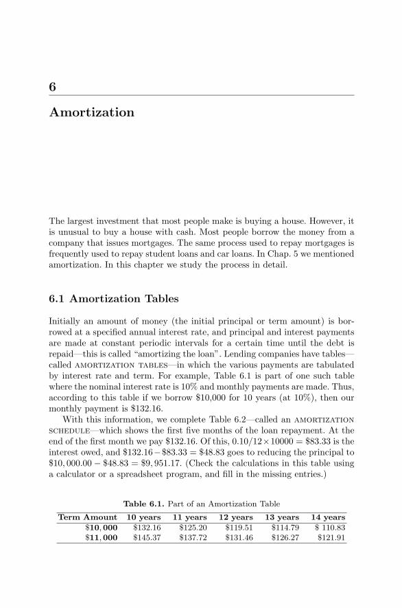
6
Amortization
The largest investment that most people make is buying a house. However, itis unusual to buy a house with cash. Most people borrow the money from acompany that issues mortgages. The same process used to repay mortgages isfrequently used to repay student loans and car loans. In Chap. 5 we mentionedamortization. In this chapter we study the process in detail.
6.1 Amortization Tables
Initially an amount of money (the initial principal or term amount) is bor-rowed at a specified annual interest rate, and principal and interest paymentsare made at constant periodic intervals for a certain time until the debt isrepaid—this is called “amortizing the loan”. Lending companies have tables—called amortization tables—in which the various payments are tabulatedby interest rate and term. For example, Table 6.1 is part of one such tablewhere the nominal interest rate is 10% and monthly payments are made. Thus,according to this table if we borrow $10,000 for 10 years (at 10%), then ourmonthly payment is $132.16.
With this information, we complete Table 6.2—called an amortizationschedule—which shows the first five months of the loan repayment. At theend of the first month we pay $132.16. Of this, 0.10/12×10000 = $83.33 is theinterest owed, and $132.16−$83.33 = $48.83 goes to reducing the principal to$10, 000.00 − $48.83 = $9, 951.17. (Check the calculations in this table usinga calculator or a spreadsheet program, and fill in the missing entries.)
Table 6.1. Part of an Amortization Table
Term Amount 10 years 11 years 12 years 13 years 14 years$10,000 $132.16 $125.20 $119.51 $114.79 $ 110.83$11,000 $145.37 $137.72 $131.46 $126.27 $121.91

84 6 Amortization
Table 6.2. Amortization Schedule
Month Monthly Interest Principal OutstandingPayment Paid Repaid Principal
0 $0.00 $0.00 $0.00 $10,000.001 $132.16 $83.33 $48.83 $9,951.172 $132.16 $82.93 $49.23 $9,901.943 $132.16 $82.52 $49.64 $9,852.3045 $132.16 $81.69 $50.47 $9,751.77
Notice that Table 6.2 depends critically on knowing Table 6.1. But how dowe know Table 6.1, and more importantly, how do we know that it is accurate?
In this section we show how these loan payments are computed. We let
P0 be the initial principal (term amount) that has to be repaid,Pn be the outstanding principal (principal remaining to be paid)
at the end of the nth payment period,M be the periodic payment,N be the total number of payment periods,m be the number of periodic payments per year,
i(m) be the annual interest rate, expressed as a decimal, andi be the periodic interest rate,
so i = i(m)/m.Figure 6.1 shows a time diagram for this.
P0
0
M
1
M
2 · · ·
M
N − 1 N
M
Fig. 6.1. Time diagram of a mortgage
Using this notation, we rewrite Table 6.2 symbolically in spreadsheet for-mat as Table 6.3, which is explained as follows.
At the end of the first payment period (n = 1) we make our periodicpayment of M , but the interest owed is iP0, so the outstanding principal is
P1 = P0 − M + iP0 = P0(1 + i) − M.
At the end of the second payment period (n = 2) the interest owed is iP1,so the outstanding principal is
P2 = P1 − M + iP1 = P1(1 + i) − M = (P0(1 + i) − M) (1 + i) − M,

6.1 Amortization Tables 85
Table 6.3. Amortization Schedule—Spreadsheet Format
Period Periodic Interest Principal OutstandingPayment Paid Repaid Principal
0 P0
1 M iP0 M − iP0 P0 − (M − iP0) = P1
2 M iP1 M − iP1 P1 − (M − iP1) = P2
3 M iP2 M − iP2 P2 − (M − iP2) = P3
4 M iP3 M − iP3 P3 − (M − iP3) = P4
5 M iP4 M − iP4 P4 − (M − iP4) = P5
which reduces toP2 = P0(1 + i)2 − M(1 + (1 + i)).
At the end of the third payment period (n = 3) the interest owed is iP2,so the outstanding principal is
P3 = P2 − M + iP2,
which reduces to
P3 = P0(1 + i)3 − M(1 + (1 + i) + (1 + i)2
).
This suggests that Pn, the outstanding principal at the end of the nth
payment period, is
Pn = P0(1 + i)n − M(1 + (1 + i) + · · · + (1 + i)n−1
).
We rewrite this conjecture, using the fact that for
1 + x + · · · + xn−1 =xn − 1x − 1
for x = 1,
in the form1
Pn = P0(1 + i)n − M(1 + i)n − 1
i, (6.1)
or
Pn =(
P0 − M
i
)(1 + i)n +
M
i.
1 Equation (6.1) can be interpreted as the future value of the principal, P0(1+ i)n,less the future value of the annuity payments, M((1 + i)n−)/i.

86 6 Amortization
Thus, we have the following theorem.
Theorem 6.1. The Amortization Theorem.If P0 is the initial principal borrowed at a nominal interest rate of i(m) and ifperiodic payments of M are made m times a year, then Pn, the outstandingprincipal after n payment periods, is
Pn =(
P0 − M
i
)(1 + i)n +
M
i, (6.2)
where i = i(m)/m.
Proof. We can prove this conjecture either by mathematical induction or byrecurrence relations. We prove it using recurrence relations and leave the proofby induction for Problem 6.12 on p. 98.
We know thatPk+1 = Pk (1 + i) − M,
so if we multiply this by 1/(1 + i)k+1, then we can write it as
Pk+11
(1 + i)k+1 = Pk1
(1 + i)k− M
1
(1 + i)k+1 .
Summing this from k = 0 to k = n − 1 gives
n−1∑k=0
Pk+11
(1 + i)k+1 =n−1∑k=0
Pk1
(1 + i)k− M
n−1∑k=0
1
(1 + i)k+1 ,
or by canceling the common terms on both sides of this equation,
Pn1
(1 + i)n = P0 − M
n−1∑k=0
1
(1 + i)k+1 ,
that is,
Pn = P0(1 + i)n − M (1 + i)nn−1∑k=0
1
(1 + i)k+1 .
However,
(1 + i)nn−1∑k=0
1
(1 + i)k+1 = 1 + (1 + i) + · · · + (1 + i)n−1 =(1 + i)n − 1
i.
Thus,
Pn = P0(1 + i)n − M(1 + i)n − 1
i,
which is (6.2). This concludes the proof using recurrence relations. ��

6.1 Amortization Tables 87
Because
Pn =(
P0 − M
i
)(1 + i)n +
M
i
and because {(1 + i)n} is an increasing sequence, that is, (1 + i)n< (1 + i)n+1,
we see that Pn < Pn+1 if P0 − M/i > 0 and that Pn > Pn+1 if P0 − M/i < 0.We thus have the following intuitively obvious result.
Theorem 6.2. Let Pn be given by (6.2).
(a) If M > iP0, then Pn > Pn+1, that is, if the periodic payment exceeds theinitial periodic interest owed, then the outstanding principal decreases.
(b) If M = iP0, then Pn = Pn+1, that is, if the periodic payment exactlyequals the initial periodic interest owed, then the outstanding principal isconstant.
(c) If M < iP0, then Pn < Pn+1, that is, if the periodic payment is less thanthe initial periodic interest owed, then the outstanding principal increasesand is never paid off.
From now on we concentrate on the case M > iP0, which also implies thatM > iPn (why?), and we rewrite (6.2) in the form
Pn =M
i−
(M
i− P0
)(1 + i)n
.
In this form we see that mathematically limn→∞ Pn = −∞. In view of thisfact and that {Pn} is a decreasing sequence for which P0 > 0, there must bean integer N for which PN−1 > 0 and PN ≤ 0. This N represents the numberof payment periods required to repay the loan. Thus, N must satisfy
M
i−
(M
i− P0
)(1 + i)N−1
> 0
andM
i−
(M
i− P0
)(1 + i)N ≤ 0,
so (M
i− P0
)(1 + i)N−1
<M
i≤
(M
i− P0
)(1 + i)N
.
This can be rewritten in the form
M
M − iP0≤ (1 + i)N
<M
M − iP0(1 + i) , (6.3)

88 6 Amortization
so that N must satisfy
ln(
MM−iP0
)ln (1 + i)
≤ N <ln
((M
M−iP0
)(1 + i)
)ln (1 + i)
.
A natural question to ask is whether more than one integer N can satisfy(6.3). Intuitively we expect not, and this is seen by rewriting the last inequalityas
ln(
MM−iP0
)ln (1 + i)
≤ N <ln
(M
M−iP0
)ln (1 + i)
+ 1. (6.4)
6.2 Periodic Payments
If we finish repaying the loan exactly at the end of the N th payment period,then we have PN = 0 and we can then calculate the periodic payment M . In(6.2) we set n = N and PN = 0 and solve for M , finding
M =iP0 (1 + i)N
(1 + i)N − 1,
so the periodic payments are
M =iP0
1 − (1 + i)−N.
Theorem 6.3. The Periodic Payment Theorem.If P0 is the initial principal borrowed at a nominal interest rate of i(m) for Npayment periods, then M , the payment that is made m times a year, is
M =iP0
1 − (1 + i)−N, (6.5)
where i = i(m)/m.
Comments About the Periodic Payment Theorem
• We notice that M is a function of the three variables P0, i, and N . Thequantity M is directly proportional to P0. Table 6.4 and Fig. 6.2 show Mas a function of i. Notice that all the curves appear to be increasing andconcave up. In Problem 6.15 on p. 99 you are asked to prove this. Table 6.5and Fig. 6.3 show M as a function of N . Notice that all the curves appearto be decreasing and concave up. In Problem 6.16 on p. 100 you are askedto prove this.

6.2 Periodic Payments 89
Table 6.4. Monthly payments as a function of the annual interest rate for 5-, 15-,and 30-year loans in the amount of $10,000
Interest Rate 5 years 15 years 30 years1% $170.94 $59.85 $32.162% $175.28 $64.35 $36.963% $179.69 $69.06 $42.164% $184.17 $73.97 $47.745% $188.71 $79.08 $53.686% $193.33 $84.39 $59.967% $198.01 $89.88 $66.538% $202.76 $95.57 $73.389% $207.58 $101.43 $80.4610% $212.47 $107.46 $87.7611% $217.42 $113.66 $95.2312% $222.44 $120.02 $102.86
Interest Rate
0% 2% 4% 6% 8% 10% 12%
Mo
nth
lyP
aym
ents
$0
$50
$100
$150
$200
$250
5 years15 years30 years
Fig. 6.2. Monthly payments as a function of the annual interest rate for 5-, 15-,and 30-year loans in the amount of $10,000
Table 6.5. Monthly payments as a function of the length of a $10,000 loan forannual interest rates of 4%, 8%, and 12%
Length of Loan 4% 8% 12%5 $184.17 $202.76 $222.4410 $101.25 $121.33 $143.4715 $73.97 $95.57 $120.0220 $60.60 $83.64 $110.1125 $52.78 $77.18 $105.3230 $47.74 $73.38 $102.8635 $44.28 $71.03 $101.5540 $41.79 $69.53 $100.8545 $39.96 $68.56 $100.47

90 6 Amortization
Years
5 10 15 20 25 30 35 40 45
Mo
nth
lyP
aym
ents
$0
$50
$100
$150
$200
$250
4%8%
12%
Fig. 6.3. Monthly payments as a function of the length of a $10,000 loan for annualinterest rates of 4%, 8%, and 12%
• Because the periodic payment is typically rounded up to the nearest cent,PN is usually negative, not zero. Therefore, the final payment, F , maynot be exactly M . Figure 6.4 shows a time diagram for this. Now, F isgiven by
F = PN−1(1 + i) =((
P0 − M
i
)(1 + i)N−1 +
M
i
)(1 + i) .
Thus, the final payment2 is
F =(
P0 − M
i
)(1 + i)N + M
1 + i
i. (6.6)
Intuitively we expect 0 < F ≤ M (why?), but is it? From (6.3) and (6.6)and the fact that M > iP0, we have 0 < F ≤ M.
Example 6.1. Amanda Kendrick takes out a student loan for $10,000 at anannual interest rate of 10% to be repaid monthly over 10 years. How muchare her monthly payments? What is the final payment?
2 In practice, the final payment may differ slightly from the amount given by F . Thiscould occur if the lender rounds all calculations to two decimal places at everystage. In this case an accumulative round-off error in Pn may come into effect.For example, if $130,000 is borrowed at 8.5% for 180 months and M = $1,280.16,then F = $1,280.68, whereas if all calculations are rounded to two decimal places,then the final payment is $1,280.62. (See Problems 6.4 and 6.5 on p. 98.)

6.2 Periodic Payments 91
P0
0
M
1
M
2 · · ·
M
N − 1 N
F
Fig. 6.4. Time diagram of a mortgage
Solution. Here P0 = 10,000, i = 0.10 (10%), m = 12, and N = 120 (10years), so (6.5) gives
M =0.1012 10000
1 − (1 + 0.10
12
)−120 = 132.151.
The amortization table on p. 83 gives $132.16. It is common practice to roundthe payments up (why?), so these two numbers agree if we do that. Henceforth,we follow this practice of rounding all amortization payments up.3
The final payment is
F =(
10000 − 132.160.1012
)(1 +
0.1012
)120
+ 132.16(
1 + 0.1012
0.1012
)= $130.26.
The payments total 119 × $132.16 + $130.26 = $15,857.30. Thus, Amandapays $5,857.30 interest on a $10,000 loan over 10 years at 10%. �Example 6.2. Amanda wants to borrow the same $10,000 at the same annualinterest rate of 10%, but she wants to extend her payments over 30 years.How much is her monthly payment?
Solution. Here P0 = 10, 000, i = 0.10 (10%), m = 12, and N = 360 (30 years),so (6.5) gives
M =0.1012 10000
1 − (1 + 0.10
12
)−360 = $87.757.
Amortization tables give $87.76.The final payment is
F =(
10000 − 87.760.1012
)(1 +
0.1012
)360
+ 87.76(
1 + 0.1012
0.1012
)= $81.33.
The payments total 359 × $87.76 + $81.34 = $31,587.18. Thus, Amandapays $21,587.18 interest on a $10,000 loan over 30 years at 10%. �3 This is the practice of lending agencies such as the Government National Mortgage
Association (GNMA, known as “Ginnie Mae”), the Federal National MortgageAssociation (FNMA, known as “Fannie Mae”), and the Federal Home Loan Mort-gage Corporation (FHLMC, known as “Freddie Mac”). However, this practice isnot universal; see the previous footnote.
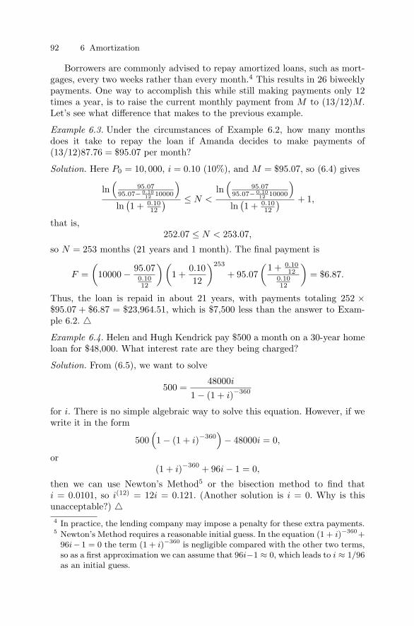
92 6 Amortization
Borrowers are commonly advised to repay amortized loans, such as mort-gages, every two weeks rather than every month.4 This results in 26 biweeklypayments. One way to accomplish this while still making payments only 12times a year, is to raise the current monthly payment from M to (13/12)M.Let’s see what difference that makes to the previous example.
Example 6.3. Under the circumstances of Example 6.2, how many monthsdoes it take to repay the loan if Amanda decides to make payments of(13/12)87.76 = $95.07 per month?
Solution. Here P0 = 10, 000, i = 0.10 (10%), and M = $95.07, so (6.4) gives
ln(
95.0795.07− 0.10
12 10000
)ln
(1 + 0.10
12
) ≤ N <ln
(95.07
95.07− 0.1012 10000
)ln
(1 + 0.10
12
) + 1,
that is,252.07 ≤ N < 253.07,
so N = 253 months (21 years and 1 month). The final payment is
F =(
10000 − 95.070.1012
)(1 +
0.1012
)253
+ 95.07(
1 + 0.1012
0.1012
)= $6.87.
Thus, the loan is repaid in about 21 years, with payments totaling 252 ×$95.07 + $6.87 = $23,964.51, which is $7,500 less than the answer to Exam-ple 6.2. �Example 6.4. Helen and Hugh Kendrick pay $500 a month on a 30-year homeloan for $48,000. What interest rate are they being charged?
Solution. From (6.5), we want to solve
500 =48000i
1 − (1 + i)−360
for i. There is no simple algebraic way to solve this equation. However, if wewrite it in the form
500(1 − (1 + i)−360
)− 48000i = 0,
or(1 + i)−360 + 96i − 1 = 0,
then we can use Newton’s Method5 or the bisection method to find thati = 0.0101, so i(12) = 12i = 0.121. (Another solution is i = 0. Why is thisunacceptable?) �4 In practice, the lending company may impose a penalty for these extra payments.5 Newton’s Method requires a reasonable initial guess. In the equation (1 + i)−360+
96i− 1 = 0 the term (1 + i)−360 is negligible compared with the other two terms,so as a first approximation we can assume that 96i−1 ≈ 0, which leads to i ≈ 1/96as an initial guess.

6.2 Periodic Payments 93
Example 6.5. Helen is in the market for a new car. She sees an advertisementthat offers either a $1,500 discount for paying cash or 0.9% nominal intereston a 60-month amortized loan. Which is the better deal if savings accountsare currently earning 5% per year?
Solution. For Helen to consider the first option, she must have enough cash tobuy the car outright. If she chooses the second option, then she could investher money in a savings account.
We look at this problem in a general setting and calculate how much Helenwould have in her savings account if she does not buy the car outright. LetP0 be the cost of the car, let i be the monthly interest rate on the savingsaccount, and let j the monthly interest on the car loan. Let P be the monthlycar payment of which there are N , so from (6.5)
P =jP0
1 − (1 + j)−N.
At the end of the first month she receives iP0 interest and pays P , so P1,the amount in the savings account at the end of the first month, would be
P1 = P0 + iP0 − P = (1 + i)P0 − P.
At the end of the second month she receives iP1 interest and pays P , so
P2 = P1 + iP1 − P = (1 + i)P1 − P = ((1 + i)P0 − P ) (1 + i) − P,
orP2 = (1 + i)2P0 − P ((1 + i) + 1) .
Thus, the amount in the savings account at the end of the nth month wouldbe
Pn = (1 + i)nP0 − P((1 + i)n−1 + (1 + i)n−2 + · · · + 1
)= (1 + i)nP0 − (1 + i)n − 1
iP,
or
Pn = (1 + i)nP0 − (1 + i)n − 1i
jP0
1 − (1 + j)−N
= (1 + i)n
(1 − j
i
1 − (1 + i)−n
1 − (1 + j)−N
)P0.
For PN , the amount in the savings account when the car is paid off, to beequivalent to C(1 + i)N , the future value of a discount of C dollars, we musthave PN = C(1 + i)N , so
P0 =C(
1 − ji
1−(1+i)−N
1−(1+j)−N
) .

94 6 Amortization
For i = 0.05/12, j = 0.009/12, N = 60, and C = 1500, we have
P0 =1500(
1 − 0.0090.05
1−(1+ 0.0512 )−60
1−(1+ 0.00912 )−60
) = 15548.89.
So if the car costs less than $15,548.89, then Helen should pay cash; otherwiseshe should choose the loan. �
6.3 Linear Interpolation
There are a number of financial tables available that tabulate, in numericalform, some of the formulas we have derived so far. For example, reference [9]contains tables of future values, present values, compound interest compar-isons, and amortization tables. Inevitably, the tables cannot contain all pos-sible cases.
What do we do if we are forced to use tables, but the information thatwe require is not contained in the tables? We approximate. For example, Ta-ble 2.3 on p. 16 shows the future value of $1 compounded annually for differentinterest rates i and different numbers of years. Part of that is reproduced hereas Table 6.6.
Table 6.6. Future Value of $1
YearsInterest Rate 5 15
3% $1.159 $1.5585% $1.276 $2.079
If all we have is this table and we need the future value of $1 for 5 yearsat 4%, which is halfway between 3% and 5%, then we estimate halfway be-tween 1.159 and 1.276, that is, (1.159 + 1.276)/2 = 1.2175. The exact number,computed from (2.1) on p. 15, is
Pn = P0(1 + i)n = (1 + 0.04)5 = 1.2166 . . . ,
so the estimate of 1.2175 is reasonable.On the other hand if we need the future value of $1 at 3% for 10 years,
which is halfway between 5 years and 15 years, then we estimate halfway be-tween 1.159 and 1.558, that is, (1.159 + 1.558)/2 = 1.3585. The exact numberis
Pn = P0(1 + i)n = (1 + 0.03)10 = 1.3439 . . . ,
so the estimate of 1.3585 is reasonable.

6.3 Linear Interpolation 95
This estimation technique is called linear interpolation and can beexplained in the following way. Given two points (a, f(a)) and (b, f(b)) and anumber l such that a < l < b, how do we estimate f(l)? Without any otherinformation, we join the two given points with a line, y = g(x), and thenapproximate f(l) with g(l). We derive a general formula for g(l) as follows.
The line y = g(x) that joins the points (a, f(a)) and (b, f(b)) passesthrough (a, f(a)) and has slope (f(b) − f(a))/(b − a); therefore its equationis given by
g(x) − f(a) =f(b) − f(a)
b − a(x − a).
With x = l, where a < l < b, we have
g(l) =f(b) − f(a)
b − a(l − a) + f(a),
which can be rewritten in the form
g(l) =b − l
b − af(a) +
l − a
b − af(b). (6.7)
This can be interpreted geometrically if we realize that (b − l)/(b − a) isthe ratio of the distance from l to b to the distance from a to b and that(l − a)/(b − a) is the corresponding ratio from a to l. In the event that l ismidway between a and b, that is, l = (a + b)/2, we find that
g
(a + b
2
)=
12f(a) +
12f(b),
the formula we used at the start of this section.
Example 6.6. Use Table 6.6 to estimate the future value of $1 at 3.5% for 15years. Compare this to the exact number obtained from (2.1) on p. 15.
Solution. Here a = 3, b = 5, and l = 3.5, so
g(3.5) =1.52
f(3) +0.52
f(5) =341.558 +
142.079 = 1.68825.
The exact number is
Pn = P0(1 + i)n = (1 + 0.035)15 = 1.6753 . . . .
�Again 1.68825 is a reasonable estimate of the exact number 1.6753 . . ..
However, from this calculation, we cannot tell how good the estimate is oreven whether the estimate is too large or too small. But we notice that allthree estimates that we have made are larger than the exact number. Is thatan accident? If we look at Fig. 2.1 on p. 17, then we are reminded that thefuture value is a concave up function of the interest rate. Thus, if we try to

96 6 Amortization
estimate a value between two points by joining those two points with a line,then our estimate is too large. A similar observation is true when we thinkof the future value as a function of the total number of interest periods (seeFig. 2.2 on p. 17).
That f(l) < g(l) in this case is made precise by the following theorem.
Theorem 6.4. Let f(x) be a twice differentiable function on the closed inter-val [a, b] with the property that f ′′(x) > 0 for all x in the open interval (a, b).Then for any point l in the open interval (a, b), we have
f(l) <b − l
b − af(a) +
l − a
b − af(b). (6.8)
Proof. By the Mean Value Theorem6 applied to f(x) in the closed interval[a, l], there must exist a c in (a, l) for which
f ′(c) =f(l) − f(a)
l − a.
Similarly, there must exist a d in (l, b) for which
f ′(d) =f(b) − f(l)
b − l.
Because f ′′(x) > 0, it follows that f ′(x) is an increasing function. Also,a < c < l < d < b, so f ′(c) < f ′(d), that is,
f(l) − f(a)l − a
<f(b) − f(l)
b − l.
Solving this inequality for f(l) shows that
f(l) <b − l
b − af(a) +
l − a
b − af(b).
Comments
• The equation of the line y = g(x) that joins the points (a, f(a)) and(b, f(b)) is
g(x) =b − x
b − af(a) +
x − a
b − af(b),
which is the right-hand side of (6.8) when x = l. Thus, the right-hand sideof (6.8) is the height of the line at x = l, whereas the left-hand side, f(l),is the height of the function f(x) at x = l. Thus, this theorem proves theintuitively obvious fact that if a positive function is concave up, then theline between the end-points is always higher than the function.
6 Let f be a continuous function on the closed interval [a, b] with a derivative atevery x in the open interval (a, b). Then there is at least one number c in theopen interval (a, b) such that f ′(c) = (f(b) − f(a))/(b − a).

6.4 Problems 97
• If we are given the value of the function f(x) at the two points a andb—so we are given the two points (a, f(a)) and (b, f(b))—and are askedto estimate the value of f(x) at the point x = l between a and b, thena standard way to do this is by linear interpolation, that is, join the twopoints with a line y = g(x) and use the estimate g(l) for f(l). The theoremtells us that in the case of a positive, concave up function, the estimateg(l) is always too large. In the same way, an estimate obtained by linearinterpolation for a positive, concave down function is always too small.
• The inequality (6.8) can be rewritten in the form
f (λa + (1 − λ)b) < λf(a) + (1 − λ)f(b) (6.9)
for all λ satisfying 0 < λ < 1. (See Problem 6.17.)
6.4 Problems
Walking
6.1. Use a spreadsheet program to reproduce the following amortization tablefor 10% interest.
Term Amount 10 years 11 years 12 years 13 years 14 years$10,000 132.16 125.20 119.51 114.79 110.83$11,000 145.37 137.72 131.46 126.27 121.91
6.2. An amortization schedule is a table with the following (or equivalent)headings.
Month Monthly Interest Principal OutstandingPayment Paid Repaid Principal
Complete the following partial amortization schedule.
Month Monthly Interest Principal OutstandingPayment Paid Repaid Principal
1 $188.12 $55.42 $132.70 $9,367.302345
6.3. You buy a house by borrowing $100,000 at 8% over 30 years. Show thefirst two and last two lines of the amortization schedule. Is the final paymentthe same as the monthly payment?

98 6 Amortization
6.4. Use a spreadsheet program to construct an amortization schedule for a15-year loan for $130,000 at 8.5% with monthly payments of $1,280.16. Whatis the final payment? Does it agree with (6.6) on p. 90? Why does the finalpayment exceed the monthly payment? What monthly payment guaranteesthat the final payment is less than the monthly payment?
6.5. Repeat Problem 6.4, but now round the entries in the Interest Paid col-umn to 2 decimal places. What is the final payment? Does it agree with (6.6)on p. 90?
6.6. A person pays $200.04 a month on a 15-year loan for $30,000. Whatinterest rate is being charged?
6.7. In [10], a 30-year loan for $75,000 at 10% is discussed. On page 51 itis claimed that paying $25 a month more than the regular monthly amountreduces the term of the mortgage by 12 years and 3 months, while saving$34,162 in interest costs. Is this claim valid?
6.8. Use linear interpolation to estimate the monthly loan payment on $45,000at 10% for 30 years given that the monthly loan payment on $100,000 at 10%for 30 years is $877.58. Is your estimate exact, too large, or too small?
6.9. Use linear interpolation to complete the following amortization table.Indicate which of your entries are exact, too large, or too small
(a) Without calculating exact values.(b) By calculating exact values.
Term Amount 10 years 11 years 12 years 13 years 14 years$1,000
$10,000 $132.16 $110.83$11,000
Given that m=12, that is, payments are made monthly, what is the annualinterest rate?
Running
6.10. Intuitively you might expect that if you double the amount of moneythat you borrow (at the same rate over the same number of years), then youhave to double your monthly payments. Prove that this is true.
6.11. Intuitively you might expect that if you double the monthly payments,then your loan is repaid in half the time. Is this true?
6.12. Prove (6.2) on p. 86 by induction.
6.13. Show that if we finish repaying a loan exactly at the end of the N th
period, so that PN = 0, then (6.2) can be written in the form
Pn =M
i
(1 − (1 + i)n−N
).

6.4 Problems 99
6.14. Consider the following eight loans, with initial principals (amounts bor-rowed) of $10,000 and $20,000, maturities of 10 and 25 years, and interestrates of 10% and 7.5%.
Amount Borrowed Maturity Interest Rate Monthly Payment$10,000 10 10.0%$10,000 10 7.5%$10,000 25 10.0%$10,000 25 7.5%$20,000 10 10.0%$20,000 10 7.5%$20,000 25 10.0% $181.75$20,000 25 7.5%
The monthly payment for the $20,000 loan with a maturity of 25 years andan interest rate of 10% is $181.75. The remaining monthly payments are
$73.90, $90.88, $118.71, $132.16, $147.80, $237.41, and $264.31,
although not necessarily in this order. Without using a calculator, completethe table.
6.15. Show that by substituting i = x − 1 and N = n + 1 into (6.5) on p. 88,we have
M
P0=
i
1 − (1 + i)−N=
(x − 1)xn+1
xn+1 − 1=
xn+1∑nk=0 xk
.
(a) Show that
d
dx
(M
P0
)=
1(∑n
k=0 xk)2
n∑k=0
(n + 1 − k)xn+k.
Explain how this shows that M is an increasing function of i if i > 0.(b) Show that
d2
dx2
(M
P0
)=
1(∑n
k=0 xk)3
n∑k=0
n∑h=0
(n + 1 − k)(n + k − 2h)xn+k+h−1.
(c) Show thatn∑
k=0
n∑h=0
akhxn+k+h−1 =2n∑
j=0
bjxn+j−1,
where bj =∑j
k=0 akj−k if 0 ≤ j ≤ n and bj =∑2n−j
k=0 an−kj+k−n ifn ≤ j ≤ 2n.

100 6 Amortization
(d) Use parts (b) and (c) to show that bj = (j + 1)(n + 1)(n − j) if 0 ≤ j ≤ nand bj = 0 if n ≤ j ≤ 2n.
(e) Explain how parts (b), (c), and (d) show that M is a concave up functionof i if i > 0.
6.16. Show that by substituting N = x and 1 + i = a into (6.5) on p. 88, wehave
M
iP0=
11 − a−x
= 1 +1
ax − 1.
(a) Show thatd
dx
(M
iP0
)= − ax ln a
(ax − 1)2.
Explain how this shows that M is a decreasing function of the positiveinteger N .
(b) Show thatd2
dx2
(M
iP0
)=
(ln a)2(a2x + ax)(ax − 1)3
.
Explain how this shows that M is a concave up function of i if i > 0.
6.17. By introducing λ = (b − l)/(b − a), show that 1 − λ = (l − a)/(b − a)and that l = λa + (1 − λ) b. Now show that (6.9) is a consequence of (6.8).
6.18. Show that for a concave down function f(x) if we estimate the value off(x) at a point x with a < x < b using linear interpolation, then the estimateis too small.
Questions for Review
• What is amortization?• What is an amortization table?• What is an amortization schedule?• How do you calculate the principal remaining to be paid after n periods?• What is the impact on the outstanding principal if M > iP0? If M = iP0?
If M < iP0?• How do you calculate the number of months required to repay the loan?• How do you calculate the periodic payment on a loan?• How do you calculate the final payment on a loan?• What does the Amortization Theorem say?• What is linear interpolation?• What is the Mean Value Theorem?• How do you use linear interpolation to estimate the value of a function at
a point c in (a, b)?• Why are the estimates of the future value of $1 obtained by linear inter-
polation always too high?

7
Credit Cards
A credit card account is an unsecured revolving line of credit issued by afinancial institution to an entity.1 Credit cards are often used for purchasesof goods and services when payment by cash is not convenient or permissi-ble. Examples of such transactions include on-line or telephone purchases ofgoods and services, business expenditures, reservations for hotel rooms, andcar rentals.
The loan is unsecured, so there is no collateral that the bank can seize ifthe borrower defaults on the loan. The loan is also revolving, which means thatthe borrower can continue to borrow against the line of credit as long as thereare available funds. These aspects cause credit cards to be riskier from thefinancial institution’s perspective than mortgages, car loans, and other securedinstallment loans. Therefore, the interest rates charged on credit cards tendto be higher than those charged on secured loans. In return for the borrowedfunds, the borrower promises to pay each month either a fixed amount or apercentage of the outstanding balance, whichever is higher. In general, creditcard disclosures contain a statement similar to “the minimum payment willbe $p or r% of the balance remaining to be paid, whichever is higher”.
In this chapter we show how credit card payments are computed.
7.1 Credit Card Payments
We charge $1,000 to a credit card with an annual interest rate of 15% forwhich the minimum monthly payment is $10 or 2% of the balance remainingto be paid, whichever is higher. We do not charge anything more to the cardand decide to make only the minimum payment each month.
1 An unsecured loan is a loan that is not backed by collateral, a mortgage, orother lien. A line of credit is an agreement between a lender and a borrowerestablishing a maximum balance that the lender permits the borrower to carry.

102 7 Credit Cards
When the first month’s bill arrives we pay the higher of $10 and $1,000 ×0.02 = $20, namely, $20. The outstanding balance when next month’s billarrives is $1,000 − $20 = $980. We pay the higher of $10 and $980 × 0.02 =$19.60, namely, $19.60. However, the outstanding balance is $980, so we owe$980×0.15/12 = $12.25 in interest. Thus, the outstanding balance in the thirdmonth is $980−$19.60+$12.25 = $972.65. With this information, we completeTable 7.1, which shows the first five payments. (Check the calculations in thistable using a calculator or a spreadsheet program, and fill in the missingentries.)
Table 7.1. Credit Card Schedule
Month Monthly Interest RemainingPayment Accrued Principal
0 $0.00 $0.00 $1,000.001 $20.00 $0.00 $980.002 $19.60 $12.25 $972.653 $19.45 $12.16 $965.3645 $19.16 $11.98 $950.94
Based on this, we let
P0 be the initial principal (initial balance) that has to be repaid,Pn be the principal remaining to be paid (outstanding balance) at the
end of the nth month,i(12) be the fixed annual interest rate, expressed as a decimal,
i be the monthly interest rate,(i = i(12)/12
),
p be the minimum monthly payment, andr be the minimum monthly balance repayment rate, expressed as
a decimal.
Using this notation we rewrite Table 7.1 symbolically in spreadsheet formatas Table 7.2, which is explained as follows.
Table 7.2. Credit Card Schedule—Spreadsheet Format
Month Monthly Interest RemainingPayment Accrued Principal
0 0 0 P0
1 rP0 0 P0 − rP0 = P1
2 rP1 iP1 P1 − rP1 + iP1 = P2
3 rP2 iP2 P2 − rP2 + iP2 = P3
4 rP3 iP3 P3 − rP3 + iP3 = P4
5 rP4 iP4 P4 − rP4 + iP4 = P5

7.1 Credit Card Payments 103
We concentrate on the case where we charge P0 to this credit card andthen charge nothing else but elect to pay the minimum each month. Also,initially we assume that rP0 > p. (See Problem 7.8 on p. 111 for the case inwhich rP0 ≤ p.)
At the end of the first month (n = 1) we make our monthly payment ofrP0 (assuming that rP0 > p), and because there is no interest, the principalremaining to be paid is
P1 = P0 − rP0 = P0(1 − r).
At the end of the second month (n = 2) we make our monthly payment ofrP1 (assuming that rP1 > p), but the interest that we owe on the outstandingbalance P1 is iP1, so the principal remaining to be paid is
P2 = P1 − rP1 + iP1 = P1(1 − r + i) = P0(1 − r + i)(1 − r).
At the end of the third month (n = 3) the interest that we owe is iP2, sothe principal remaining to be paid is
P3 = P2 − rP2 + iP2,
which reduces toP3 = P0(1 − r + i)2(1 − r).
This suggests that Pn, the principal remaining to be paid at the end ofthe nth month, is
Pn = P0(1 − r + i)n−1(1 − r). (7.1)
We make three observations about this formula.
1. If i > r, then Pn+1 > Pn and limn→∞ Pn = ∞, that is, {Pn} is an in-creasing sequence that is unbounded. In other words, the amount owedincreases each month. Not only does it increase, it increases at an expo-nential rate.
2. If i = r, then Pn = P0(1 − r) for all n, so the amount owed remainsconstant.
3. If i < r, then Pn+1 < Pn, Pn > 0, and limn→∞ Pn = 0, that is, it takesan infinite time to repay the loan. We note that rPn+1 < rPn, so ourpayments always decrease. However, we see that the amount going to payoff the debt, namely (r − i)Pn, is also decreasing. Finally, the proportioni of our payment going to interest every month is constant.
However, credit cards have a statement to the effect that the minimummonthly payment is either p or r% of the balance remaining to be paid,whichever is higher. Thus, in the third case there is a month N1 when, forthe last time, our proposed monthly payment (rPN1−1) is greater than p, thatis, rPN1−1 > p. Because N1 is the last month in which this occurs, the next

104 7 Credit Cards
monthly payment (rPN1) cannot be greater than p, that is, rPN1 ≤ p. Thus,the integer N1 must satisfy
rPN1 ≤ p < rPN1−1,
orP0 (1 − r + i)N1−1 (1 − r) ≤ p
r< P0 (1 − r + i)N1−2 (1 − r) .
Because ln (1 − r + i) < 0, we have
N1 − 2 <ln
(p
P0r(1−r)
)ln (1 − r + i)
≤ N1 − 1,
or N1, the month when we switch from decreasing payments to the constantpayment of p, is determined from
1 +ln
(p
P0r(1−r)
)ln (1 − r + i)
≤ N1 < 2 +ln
(p
P0r(1−r)
)ln (1 − r + i)
. (7.2)
Because we have assumed that rP1 > p, we have p/(P0r (1 − r)) < 1, whichrequires that ln (p/(P0r (1 − r))) < 0 (why?), so that
ln(
pP0r(1−r)
)ln (1 − r + i)
> 0.
Thus, (7.2) has an integer solution N1 ≥ 2. (See Problems 7.9 and 7.8 onp. 111 for the case in which rP1 ≤ p.)
In this case
PN1+1 = PN1 − p + iPN1 = PN1(1 + i) − p.
However, because i < r, we then have
PN1+1 = PN1(1 + i) − p ≤ (1 + i)p
r− p =
p
r(1 + i − r) <
p
r,
so PN1+1 < p/r. Thus, once the constant payment starts it remains in effect,giving
PN1+2 = PN1+1 − p + iPN1+1 = PN1+1(1 + i) − p,
which can be written as
PN1+2 = (PN1(1 + i) − p)(1 + i) − p = PN1(1 + i)2 − p(1 + (1 + i)).
Similarly,
PN1+3 = PN1+2 − p + iPN1+2 = PN1(1 + i)3 − p(1 + (1 + i) + (1 + i)2).

7.1 Credit Card Payments 105
Thus, we expect, once PN1 ≤ p/r, that
PN1+n = PN1(1 + i)n − p(1 + (1 + i) + · · · + (1 + i)n−1
),
or, using the fact that for x = 1,
1 + x + · · · + xn−1 =xn − 1x − 1
,
we have
PN1+n = PN1(1 + i)n − p(1 + i)n − 1
i. (7.3)
Except for notation, this is exactly the same equation as (6.1) on p. 85and is proved in the same way, leading to a result similar to (6.4). We thushave the following results.
Theorem 7.1. The Credit Card Theorem.Assume that rP0 > p and rP1 > p.
(a) If i > r, thenPn = P0 (1 − r + i)n−1 (1 − r)
and Pn+1 > Pn, so the amount owed increases each month.(b) If i = r, then
Pn = P0 (1 − r)
and Pn+1 = Pn, so the amount owed remains constant each month.(c) If i < r, then we have
Pn ={
P0 (1 − r + i)n−1 (1 − r) for 1 ≤ n ≤ N1,(PN1 − p
i
)(1 + i)n−N1 + p
i for N1 < n,
where the month N1 is determined by (7.2). In this case the amount chargedis paid off in N1 + N2 months, where
ln(
pp−iPN1
)ln (1 + i)
≤ N2 <ln
(p
p−iPN1
)ln (1 + i)
+ 1. (7.4)
Comments About the Credit Card Theorem
• If part (c) of the theorem applies, then the total amount paid is approxi-mately2 (see Problem 7.13 on p. 111)
rP0
⎛⎝1 +(1 − r)
(1 − (1 − r + i)N1−1
)r − i
⎞⎠ + N2p. (7.5)
2 This formula assumes that the final payment is exactly p. However, as with amor-tization, the final payment may be smaller than p.

106 7 Credit Cards
• The Credit Card Theorem is also valid if the borrower decides to pay alarger p, the minimum monthly payment, and a larger r, the minimummonthly balance repayment rate, than the credit card company requires.
Example 7.1. Tom charges $1,000 on a credit card with an annual interestrate of 15% and for which the minimum payment is $10 or 2% of the balanceremaining to be paid, whichever is higher. If Tom charges no more on thiscard but makes the minimum payment each month, then how long does ittake for him to repay the debt, and approximately how much does he pay intotal?
Solution. Here P0 = 1, 000, i(12) = 0.15 (15%), r = 0.02 (2%), and p = 10.First, we see that rP0 = 20 is greater than p and that rP1 = P0r (1 − r) =$19.60 is greater than p, so the Credit Card Theorem applies. Second, we seethat i = 0.15/12 = 0.0125 is less than 0.02, so part (c) of that theorem applies.
We find N1 from (7.2),
1 +ln
(10
1000×0.02(1−0.02)
)ln
(1 − 0.02 + 0.15
12
) ≤ N1 < 2 +ln
(10
1000×0.02(1−0.02)
)ln
(1 − 0.02 + 0.15
12
) .
Now,ln
(10
1000×0.02(1−0.02)
)ln
(1 − 0.02 + 0.15
12
) = 89.389,
so90.389 ≤ N1 < 91.389,
giving N1 = 91. It takes 91 months (7 years 7 months) to switch from de-creasing minimum payments to constant ones.
We find N2 from (7.4),
ln(
1010− 0.15
12 P91
)ln
(1 + 0.15
12
) ≤ N2 <ln
(10
10− 0.1512 P91
)ln
(1 + 0.15
12
) + 1,
where from (7.1),
P91 = 1000(
1 − 0.02 +0.1512
)91−1
(1 − 0.02) = 497.71,
soln
(10
10− 0.1512 P91
)ln
(1 + 0.15
12
) = 78.34.
Thus,78.34 ≤ N2 < 79.34,
so N2 = 79. Thus, N1 + N2 = 91 + 79 = 170, so it takes 170 months (14 yearsand 2 months) to repay the loan.

7.1 Credit Card Payments 107
The total amount paid is given approximately3 by (7.5), namely,
0.02(1000)
⎛⎝1 +(1 − 0.02)
(1 − (1 − 0.02 + 0.0125)90
)0.02 − 0.0125
⎞⎠+79(10) = 2096.119.
So on the $1,000 loan, Tom pays about $2,096.12. �We now repeat Example 7.1, to see what happens if Tom decides to pay
more than the minimum each month.
Example 7.2. Tom charges $1,000 on a credit card with an annual interestrate of 15% and for which the minimum payment is $10 or 2% of the balanceremaining to be paid, whichever is higher. If Tom charges no more on thiscard but pays twice the minimum payment each month, then how long doesit take Tom to repay the debt and approximately how much does he pay intotal?
Solution. Here P0 = 1000, i(12) = 0.15 (15%), r = 0.04 (twice 2%), andp = 20 (twice 10). First, we see that rP0 = 40 is greater than p, and thatrP1 = P0r (1 − r) = $38.40 is greater than p, so the Credit Card Theoremapplies. Second, we see that i = 0.15/12 = 0.0125 is less than 0.04, so part (c)of that theorem applies.
We find N1 from (7.2),
1 +ln
(20
1000×0.04(1−0.04)
)ln
(1 − 0.04 + 0.15
12
) ≤ N1 < 2 +ln
(20
1000×0.04(1−0.04)
)ln
(1 − 0.04 + 0.15
12
) .
Now,ln
(20
1000×0.04(1−0.04)
)ln
(1 − 0.04 + 0.15
12
) = 23.39,
so24.39 ≤ N1 < 25.39,
giving N1 = 25. It takes 25 months (2 years 1 month) to switch from decreasingminimum payments to constant ones.
We find N2 from (7.4),
ln(
2020− 0.15
12 P25
)ln
(1 + 0.15
12
) ≤ N2 <ln
(20
20− 0.1512 P25
)ln
(1 + 0.15
12
) + 1,
3 In fact, the final payment is not $10, but P169 = $3.40. (See Problem 7.1 onp. 110.)

108 7 Credit Cards
where from (7.1),
P25 = 1000(
1 − 0.04 +0.1512
)25−1
(1 − 0.04) = 491.61,
soln
(20
20− 0.1512 P25
)ln
(1 + 0.15
12
) = 29.55.
Thus,29.55 ≤ N2 < 30.55,
so N2 = 30. Thus, N1 + N2 = 25 + 30 = 55, so it takes 55 months (4 yearsand 7 months) to repay the loan.
The total amount paid is given approximately by (7.5), namely,
0.04(1000)
⎛⎝1 +(1 − 0.04)
(1 − (1 − 0.04 + 0.0125)24
)0.04 − 0.0125
⎞⎠+30(20) = 1321.293.
So on the $1,000 loan Tom pays about $1,321.29.Thus, by doubling the payments, the time to repay the loan drops from
14 years and 2 months to 4 years and 7 months and the amount paid dropsfrom $2,096.12 to $1,321.29. �
7.2 Credit Card Numbers
The digits on a credit card are not chosen randomly, and many of the popularones (VISA, Mastercard, American Express, Diners Club, Discover) follow asimilar pattern. The total number of digits (usually between 13 and 16) isspecified by the company. The initial digits determine the type of card, thenext digits the issuing financial institution, and the remaining digits (exceptfor the final one) identifies the customer. The final digit is a checksum. It iscomputed from the previous digits in such a way so as to reduce the risk ofincorrectly entering a digit, transposing adjacent digits, or simply entering aninvalid card number.
The technique that is used to compute the checksum is called the Luhnalgorithm or the Mod 10 Method.4 To demonstrate the algorithm, considerthe credit card number 9876543219876543, so that 3 is the checksum. We con-centrate on the other 15 digits. Starting from the right-hand side we multiplyevery other digit by 2 and leave the remaining digits unchanged, giving
9 8 7 6 5 4 3 2 1 9 8 7 6 5 4×2 ×2 ×2 ×2 ×2 ×2 ×2 ×218 8 14 6 10 4 6 2 2 9 16 7 12 5 8
.
4 Canadian Social Insurance Numbers, which are nine digits long, also use the Luhnalgorithm to check the last digit.

7.2 Credit Card Numbers 109
Now, we add the resulting digits, treating each digit separately, so that 18is treated as 1 + 8. Thus,
(1 + 8)+8+(1 + 4)+6+(1 + 0)+4+6+2+2+9+(1 + 6)+7+(1 + 2)+5+8 = 82.
We now add the checksum, 3, to this total to find 85. If the new total isdivisible by 10, then the credit card number has passed the validation test.5
This number fails, whereas 9876543219876548 passes.In order to analyze whether this algorithm detects the incorrect entry of
a digit or the transposition of adjacent digits, we look at what each of thenumbers from 0 to 9 transform into as a result of the “multiply by two andadd the digits” rule.
Initial Digit ×2 Final Digitd 2d f(d)0 0 01 2 22 4 43 6 64 8 85 10 16 12 37 14 58 16 79 18 9
Imagine that we inadvertently change one digit in an otherwise valid creditcard number. If it is the check digit that is changed, then the new number isno longer valid because the sum of the remaining digits requires the correctcheck digit to pass the test. If it is one of the undoubled digits that is changed,then the new sum differs from the old one by a number less than 10, so it doesnot give the correct check digit. The same is true if one of the doubled digitsis changed.
Imagine that we inadvertently transpose adjacent digits in an otherwisevalid credit card number. There are 100 possible combinations of two digits,from 00 through 99, of which ten (00, 11, 22, . . ., 99) won’t cause any problemsif the digits are transposed. If d1 and d2 are adjacent digits in the credit cardnumber (d1 = d2), then their contribution to the checksum is either f(d1)+d2or f(d2) + d1, and if transposed they are either f(d2) + d1 or f(d1) + d2. Ifthese two sums are the same or their difference is a multiple of 10, then thechecksum does not distinguish between their transposition. This suggests thatwe should look at (f(d1) + d2) − (f(d2) + d1) = (f(d1) − d1) − (f(d2) − d2).In other words, we should consider f(d) − d.
5 Of course, this does not check whether the credit card is valid.

110 7 Credit Cards
d f(d) f(d) − d0 0 01 2 12 4 23 6 34 8 45 1 −46 3 −37 5 −28 7 −19 9 0
One question that we can ask is, “Are there two different d’s, called d1and d2, for which (f(d1) − d1) − (f(d2) − d2) = 0?” Looking at the precedingtable, we can answer “Yes, 0 and 9.” Thus, if the adjacent digits are 0 and9 and they are interchanged, then the checksum does not pick up this error.Another question we can ask is, “Are there two different d’s, called d1 and d2,for which (f(d1) − d1) − (f(d2) − d2) = 0 but is divisible by 10?” Looking atthe preceding table, we can answer “No.” Thus, the Luhn algorithm detectsthe transposition of adjacent digits if they are not 09 or 90.
7.3 Problems
Walking
7.1. Show that the final payment in Example 7.1 on p. 106 is P169 and thatit is $3.40.
7.2. We charge $2,100 on a credit card with an annual interest rate of 18% andfor which the minimum payment is $10 or 2.5% of the balance remaining tobe paid, whichever is higher. How long will it take to repay the debt assumingthat the minimum payment is always made, and how much will we have paidin total? If we borrow the same $2,100 at the same annual interest rate of18% but repay it as an amortized loan with a monthly payment of $55, howlong will it take to repay the debt, and how much will we have paid in total?
7.3. Using Table 7.2 on p. 102 as a template, construct a spreadsheet thatreproduces the calculations in Example 7.1 on p. 106 and in Problem 7.2.
7.4. Use (7.5) on p. 105 and the Credit Card Theorem on p. 105 to constructa spreadsheet that calculates N1, N2, and the (approximate) total amountrepaid after the user inputs P0, i(12), p, and r. Use the format in the followingtable.

7.3 Problems 111
Amount owed = P0 = $1,000.00Annual interest rate = i(12) = 15%
Minimum monthly payment = p = $10.00Minimum monthly balance repayment rate = r = 2%
i < r? YesrP0 > p? YesrP1 > p? Yes
N1 91PN1 $491.71N2 79
Months to repay = N1 + N2 170Total repaid = $2,096.12
7.5. Apply the Luhn algorithm to 9876543219876453. Is the checksum a validone? If not, then what should the final digit be?
7.6. If 9876543219076545 has a valid checksum using the Luhn Algorithm,will 9876543210976545?
7.7. Apply the Luhn algorithm to 0000000000000000. Is the checksum a validone?
Running
7.8. State and prove a result similar to the Credit Card Theorem on p. 105if initially rP0 ≤ p.
7.9. State and prove a result similar to the Credit Card Theorem on p. 105if initially rP0 > p but rP1 ≤ p.
7.10. Determine what happens if instead of a single charge of P0 to a creditcard, we charge P0 every month but still elect to pay the minimum eachmonth.
7.11. Determine what happens if in addition to paying the minimum amounteach month, we add a fixed dollar amount $M .
7.12. Sometimes a credit card company lets a borrower skip a monthly pay-ment (but not the interest). How does this affect the total interest paid?
7.13. Assuming that the final payment is exactly p, prove (7.5) on p. 105.
7.14. Sometimes in the Luhn algorithm, the “multiply by two and add thedigits” rule, is replaced by “multiply by two and, if the resulting number isgreater than 9, subtract 9” rule. Are these rules the same? Verify.
7.15. Sometimes in the Luhn algorithm, the “multiply by two and add thedigits” rule, is replaced by “multiply by two, divide the resulting number by9, and keep the remainder” rule. Are these rules the same? Verify.

112 7 Credit Cards
Questions for Review
• How do you find the total amount paid when i < r?• What does the Credit Card Theorem say?• What is the Luhn algorithm?• What is the purpose of the Luhn algorithm?• How does the Luhn algorithm work?• What is a checksum?• How is the outstanding balance on a credit card computed?• How are the payments on the outstanding balance on a credit card com-
puted?• How does the remaining balance on a credit card change when i > r?
When i = r? When i < r?• How do you find the month in which you switch from decreasing payments
to constant payments?• How do you find the number of months in which the minimum monthly
payment, p, is made?

8
Bonds
Bonds are loans that an investor makes either to a government agency (USTreasury bonds or notes1 or Municipal bonds) or to a corporation (Corporatebonds). The borrower promises to pay the lender interest at regular intervals(usually every six months) and to repay the principal at the end of the loan.In investor’s language the previous sentence reads, “The borrower promisesto pay the lender the coupons on the coupon payment dates and to paythe face value of the bond at the redemption date.”
Government Bonds and NotesTypical Term 2 years, 3 years, 5 years, 10 years, 30 yearsPayment Frequency Semi-annuallyPenalty NoneIssuer Federal GovernmentRisks Inflation, Interest Rate, Reinvestment, MaturityMarketable YesRestrictions Minimum Investment
Corporate BondsTypical Term 10 to 30 yearsPayment Frequency Semi-annuallyPenalty NoneIssuer CorporationsRisks Inflation, Market, Interest Rate, Liquidity,
Default, Business, Reinvestment, MaturityMarketable YesRestrictions Minimum Investment
1 US Treasury bonds are obligations of the United States government with a ma-turity of more than 10 years. US Treasury notes are obligations of the UnitedStates government with a maturity of between 1 and 10 years.

114 8 Bonds
There are various types of bonds, but one which is not redeemable be-fore the scheduled redemption date is called noncallable. In this book weconcentrate on noncallable bonds.
8.1 Noncallable Bonds
The value of a noncallable bond varies with time. When a bond is first is-sued, the interest rate is determined by the competitive interest rates of otherbonds available at that time. This determines the initial value of the bond—the primary market value. Later this bond may be offered for resale. Thenits resale value—the secondary market value—is determined by the com-petitive interest rates available at that time, as well as the proportion of thecoupon period that has elapsed by the record date.2
For example, suppose that an investor purchases a 20-year bond for $1,000when the interest rate is 7%. Later the competitive interest rate falls to 6.5%,and the investor decides to sell the bond. Clearly the investor expects morethan $1,000 for the bond because bonds with coupon rates of 6.5% are sellingfor $1,000. However, if the interest rate rises to 7.5%, then no one will pay$1,000 for the investor’s bond because it is worth less than $1,000. But whatis a fair price for these bonds? In other words, how do we value a bond thatis for sale? This section is devoted to answering that question.
When a bond is sold its value is reported as a percent of its face value;for example, the price of a $1,000 bond may be reported as 98, which meansthat the market value of the bond is 98/100 × $1, 000 = $980. A price of 100means that the value of the bond is its face value.
Let
F be the face value (par value, redemption value) of the bond,P be the price of the bond (percentage of the face value),n be the total number of coupon payment periods,m be the number of coupon payments per year,
r(m) be the annual coupon rate (nominal yield), expressed as a decimal,r be the coupon rate per coupon payment period,
expressed as a decimal,y(m) be the annual yield to maturity (investor’s rate of return),
expressed as a decimal, andy be the yield to maturity per coupon payment period,
expressed as a decimal.
2 The Record Date is the date on which a purchaser of a bond becomes the legalowner.

8.1 Noncallable Bonds 115
Notice that P is expressed as a percentage, whereas r and y are expressed asdecimals,3 and that y = y(m)/m and r = r(m)/m. The cost of the bond is(P/100)F , and the coupon payment is rF .
Initially we assume that the price, P , is to be determined immediatelyfollowing a coupon payment, so the next coupon payment is due exactly onepayment period in the future and there are n coupon payment periods re-maining. Later we take into account what happens to the price if the bond issold between coupon payment periods.
The future value of the first coupon payment, rF , on the maturity dateis rF (1 + y)n−1. The future value of the second coupon payment, rF , on thematurity date is rF (1+ y)n−2. The future value of the final coupon payment,rF , on the maturity date is rF . The future value of the face value, F , is F .The future value of the cost of the bond, (P/100)F , on the maturity date is(P/100)F (1+ y)n. This is represented by the time diagram shown in Fig. 8.1.
P100F
rF
1
rF
2
· · ·rF
n − 1
rF + F
n
Fig. 8.1. Time diagram of a typical bond
Thus,
P
100F (1 + y)n = rF
((1 + y)n−1 + (1 + y)n−2 + · · · + (1 + y) + 1
)+ F,
or
P
100(1 + y)n = r
((1 + y)n−1 + (1 + y)n−2 + · · · + (1 + y) + 1
)+ 1. (8.1)
This equation can be rewritten in various ways. If we multiply by 100/(1 + y)n,then we have
P = 100r
(1
1 + y+
1(1 + y)2
+ · · · +1
(1 + y)n
)+
100(1 + y)n , (8.2)
or
P = 100r
n∑k=1
(1 + y)−k + 100 (1 + y)−n, (8.3)
3 Sometimes, instead of being measured in decimal or percentage, rates and yieldsare measured in basis points. A basis point is 0.01%, that is, 0.0001. Basispoints are frequently used by dealers dealing with billions of dollars of bonds,and a change of one basis point on one billion dollars is $100,000.

116 8 Bonds
which can be interpreted as “the price is the present value of the expectedfuture cash flows”. By rewriting (8.2) in the form
P =100r
1 + y
(1 +
11 + y
+ · · · +1
(1 + y)n−1
)+
100(1 + y)n
and recognizing the expression in parentheses as a geometric series, we find,after a little algebra, that for y = 0,
P = 100
(r1 − (1 + y)−n
y+ (1 + y)−n
), (8.4)
or
P = 100
((r − y)
1 − (1 + y)−n
y+ 1
). (8.5)
Theorem 8.1. The Bond Theorem.The price, P , of a noncallable bond immediately following a coupon paymentis given by any of the four equivalent equations (8.1), (8.2), (8.4), and (8.5).
If r = 0, that is, there are no coupons paid, then the bond is called a zerocoupon bond. Thus, from (8.4) we have the following result.
Theorem 8.2. The Zero Coupon Bond Theorem.The price, P , of a zero coupon bond is given by
P = 100(1 + y)−n.
Comments About the Bond Theorem
• There are three different annual yields used in connection with bonds: thenominal yield r(m) = rm, the current yield 100rm/P , and the yieldto maturity y(m) = ym. The yield to maturity is frequently referred tojust as the yield. The nominal yield or stated yield, is of little practicalsignificance. The yield to maturity is the annual rate of return that aninvestor should receive if the bond is held to maturity. The current yieldmeasures that part of the yield to maturity that is due to coupon payments.
• From (8.5), written in the form
P − 100 = 100(r − y)1 − (1 + y)−n
y,
we see that P = 100 is equivalent to y = r. If P = 100, then the bondis said to be purchased at par. In this case y = r = 100r/P. Thus, whena bond is purchased at par, the nominal yield, the current yield, and theyield to maturity are equivalent.

8.1 Noncallable Bonds 117
• From (8.5), written in the form
P − 100 = 100(r − y)1 − (1 + y)−n
y,
and realizing that (1 + y)n > 1, so that 1 − (1 + y)−n > 0, we see thatthe sign of P − 100 is the same as the sign of r − y. If P > 100 (which isequivalent to r > y), then the bond is said to be purchased at a premium.If P < 100 (which is equivalent to r < y), then the bond is said to bepurchased at a discount.
• From (8.5), written in the form
y − 100r
P= (y − r)
100P
(1 + y)−n,
we see that the sign of y − r is the same as the sign of y − 100r/P .Thus, if a bond is purchased at a premium (so P > 100 and r > y),then y − 100r/P < 0, so ym < 100rm/P < rm, that is, the yield tomaturity is less than the current yield, which is less than the nominalyield. However, if a bond is purchased at a discount (so P < 100 andr < y), then y − 100r/P > 0, so ym > 100rm/P > rm, that is, the yieldto maturity is greater than the current yield, which is greater than thenominal yield.
• The relationship between the yield to maturity, ym, and the maturity,4
n/m, for bonds with similar degrees of default risk is represented graph-ically by a yield curve. During economic expansion, yield curves are gen-erally upward sloping, that is, the yields on long-term bonds are higherthan the yields on short-term bonds. However, at economic peaks, yieldcurves often become inverted, that is, the yields on long-term bonds arelower than the yields on short-term bonds.
Example 8.1. What are the semi-annual coupon payments and the price of a9% noncallable bond with 20 years to maturity and a face value of $1,000 ifthe yield to maturity is 12%? What are the nominal and current yields forthis bond? Is the bond selling at par, at a premium, or at a discount?
Solution. Here the coupons are paid twice a year (m = 2), so there are 40payments (n = 40). We also have F = 1000 and r(2) = 0.09, so r = 0.045 andthe semi-annual coupon payments, rF , are 0.045 × 1, 000 = $45. The yield tomaturity is y(2) = 0.12, so y = 0.06. From (8.5) we find that
P = 100
((0.045 − 0.06)
1 − (1 + 0.06)−40
0.06+ 1
)= 77.43.
Thus, the bond should sell for 77.43% of its face value, that is, for 77.43/100×1000 = $774.30.4 We use the terms “maturity” and “years to maturity” interchangeably.

118 8 Bonds
The nominal yield is rm = 0.045 × 2 = 0.09, and the current yield is100rm/P = 100 × 0.045 × 2/77.43 ≈ 0.116. The bond is selling at a discountbecause P < 100. �Example 8.2. What are the semi-annual coupon payments and the price of a12% noncallable bond with 2 years to maturity and a face value of $1,000 ifthe yield to maturity is 9%?
Solution. Here the coupons are paid twice a year (m = 2), so there are 4payments (n = 4). We also have F = 1000 and r(2) = 0.12, so r = 0.06 andthe semi-annual coupon payments, rF , are 0.06 × 1, 000 = $60. The yield tomaturity is y(2) = 0.09, so y = 0.045. From (8.5) we find that
P = 100
((0.06 − 0.045)
1 − (1 + 0.045)−4
0.045+ 1
)= 105.381.
Thus, the bond should sell for about 105.381% of its face value, that is, for105.381/100 × 1000 = $1,053.81. �
There is another way of looking at this last example, which sheds a dif-ferent light on bonds. Imagine that we buy this bond for $1,053.81 when theyield is 9% and the coupon rate is 12%. We can think of this as lendingsomeone $1053.81 at 9% per annum. Then after six months we receive a $60payment, of which $1053.81 × 0.09/2 = $47.42 is interest, and the remainder,$60 − $47.42 = $12.58, is used to reduce the principal. This is deducted from$1053.81, giving $1,041.23, which represents the outstanding principal (thevalue of the bond) with only three payments left. In this way we can con-struct the bond amortization schedule shown in Table 8.1. Notice that,at the fourth and final payment, the value of the bond is $1,000—its facevalue.
Table 8.1. Bond Amortization Schedule
Period Payment Interest Principal Repaid Value0 $1,053.811 $60.00 $47.42 $12.58 $1,041.232 $60.00 $46.86 $13.14 $1,028.093 $60.00 $46.26 $13.74 $1,014.354 $60.00 $45.65 $14.35 $1,000.00
Table 8.2 shows the general situation symbolically in spreadsheet format,where Pi is the value of the bond at period i.
Notice that this schedule does not use (8.4). In fact, it can be used to givean alternative derivation of (8.4), as follows. It is not difficult to see that
P2 = (1 + y) P1 − rF = (1 + y) ((1 + y) P0 − rF ) − rF
= (1 + y)2 P0 − rF (1 + (1 + y)) ,

8.1 Noncallable Bonds 119
Table 8.2. Bond Amortization Schedule—Spreadsheet Format
Period Payment Interest Principal Repaid Value0 P
100F = P0
1 rF yP0 rF − yP0 (1 + y) P0 − rF = P1
2 rF yP1 rF − yP1 (1 + y) P1 − rF = P2
......
......
...n − 1 rF yPn−2 rF − yPn−2 (1 + y) Pn−2 − rF = Pn−1
n rF yPn−1 rF − yPn−1 (1 + y) Pn−1 − rF = Pn
and
P3 = (1 + y) P2 − rF = (1 + y)3 P0 − rF(1 + (1 + y) + (1 + y)2
),
and finally
Pn = (1 + y) Pn−1 − rF = (1 + y)nP0 − rF
(1 + (1 + y) + · · · + (1 + y)n−1
),
or
Pn = (1 + y)nP0 − rF
(1 + y)n − 1y
.
However, P0 = P100F and Pn = F (why?), so
F = (1 + y)n P
100F − rF
(1 + y)n − 1y
,
or
(1 + y)n P
100=
(r(1 + y)n − 1
y+ 1
),
from which (8.4) follows.
From (8.4) we can construct Table 8.3 which gives the prices of differentnoncallable bonds,5 with coupon rates of 5% and 10%, with 5 and 20 yearsto maturity, and for yields from 4% to 12%. Notice that the price of 100.00(that is, the price of the bond that exactly equals the face value) occurs whenthe yield equals the coupon rate, in agreement with one of the comments wemade following the Bond Theorem.
Let’s look at this table in detail and make a number of observations.
• First, if we look at the second and fourth columns, then we see that fora fixed yield, the price of a 5-year bond with a coupon rate of 10% islarger than the price of a 5-year bond with a coupon rate of 5%. We seethat the same phenomenon is true for the 20-year bonds if we comparethe third and fifth columns. This leads us to suspect that, in general, the
5 Unless stated otherwise, all coupons are paid semi-annually, so m = 2.

120 8 Bonds
Table 8.3. The Prices of Different Noncallable Bonds
Yield 5%/5 years 5%/20 years 10%/5 years 10%/20 years4% 104.491 113.678 126.948 182.0665% 100.000 100.000 121.880 162.7576% 95.735 88.443 117.060 146.2307% 91.683 78.645 112.475 132.0338% 87.834 70.311 108.111 119.7939% 84.175 63.197 103.956 109.20110% 80.696 57.102 100.000 100.00011% 77.387 51.862 96.231 91.97712% 74.240 47.338 92.640 84.954
price increases with the coupon rate, something that is intuitively obvious(if the coupon rate increases, then so does the value of the coupon so thebond is worth more). Thus, we conjecture that P is an increasing functionof r, and we prove this shortly.
• Second, if we look at the second and third columns, then we see thatfor a fixed coupon rate, the price of a 5-year bond is smaller than theprice of a 20-year bond if the coupon rate is larger than the yield, but islarger if the coupon rate is smaller than the yield. We see that the samephenomenon is true for the 10% bonds if we compare the fourth and fifthcolumns. This leads us to suspect that, in general, the price increases withmaturity if the coupon rate is larger than the yield and decreases withmaturity if the coupon rate is smaller than the yield. (This is intuitivelyobvious because if the coupon rate is higher than the yield, the investoris receiving more than required over a longer time, and therefore, shouldexpect to pay more. A similar argument holds when the coupon rate isless than the yield.) Thus, we conjecture that P is an increasing functionof n if r > y and is a decreasing function of n if r < y. We prove thisconjecture shortly.
• Third, looking at the second column, we see that the price decreases as theyield increases. We see the same phenomenon in the third, fourth and fifthcolumns. This leads us to suspect that, in general, the price and the yieldmove in opposite directions, something that is also intuitively obvious (ifthe current interest rates rise, then the prudent investor does not investin a bond that has a lower interest rate unless the price is right, namely,lower). Thus, we conjecture that P is a decreasing function of y. We provethis conjecture shortly as well.
We now look at these three conjectures, by noting that, from the BondTheorem on p. 116, the price P is a function of the three independent variables,r, n, and y (or equivalently, y(m) because y(m) = my). We look at these threedependencies in turn.
First, if we think of P as a function of r (with n and y fixed), then wesee from (8.4) that P is linear in r. Because (1 + y)n
> 1, the coefficient

8.1 Noncallable Bonds 121
of r, namely (1 − (1 + y)−n)/y, is always positive. Thus, P is an increasingfunction of r, that is, as the coupon rate increases so does the price, exactlyas expected. Notice also that as n increases, the slope becomes larger, andlimn→∞ P = 100r/y.
Plotting P versus r gives a line with positive slope—see Fig. 8.2. From(8.5) we see that if r = y, then P = 100, so this line passes through the point(y, 100) . This tells us that when the coupon rate and the yield coincide, thebond should sell for 100% of the face value, namely the face value. We alsonote that if r = 0, then P = 100 (1 + y)−n, so the line must also pass throughthe point
(0, 100 (1 + y)−n
). This is the price of a zero coupon bond. Thus,
the line joins the points (y, 100) and(0, 100 (1 + y)−n
).
Coupon Rate
0% 2% 4% 6% 8% 10% 12%
Pri
ce
0
50
100
150
200
1 year5 years
10 years
30 years
Fig. 8.2. Price as a function of coupon rate for 1, 5, 10, and 30 years with 6% yield
Second, if we think of P as a function of n (with r and y fixed), thenwe see from (8.5) that P is linear in −100 (r − y) (1 + y)−n. The sequence{
− (1 + y)−n}
is increasing, so P is an increasing function of n if r > y anda decreasing function of n if r < y. This is what we expected. We also noticethat limn→∞ P = 100r/y. This is seen in Fig. 8.3.
Third, we now think of P as a function of y (with r and n fixed). If wedifferentiate (8.2) with respect to y, then we find that6
dP
dy= −100r
n∑k=1
k (1 + y)−k−1 − 100n (1 + y)−n−1,
6 Strictly speaking, because P is a function of three independent variables, weshould use the notation ∂P/∂y, rather than dP/dy.

122 8 Bonds
Maturity
0 10 20 30 40 50 60
Pri
ce
0
20
40
60
80
100
120
140
160
180
2%6%
10%
Fig. 8.3. Price as a function of maturity (with m = 1) for a bond yielding 6% withcoupons of 2%, 6%, and 10%
which is negative, so P is a decreasing function of y and therefore a decreasingfunction of y(m). Thus, as the yield rises the price falls, and as the yieldfalls, the price rises, leading to the following commonly quoted property ofnoncallable bonds.
Theorem 8.3. The Price-Yield Theorem.The price and yield of a noncallable bond move in opposite directions.
If we evaluate the second derivative of (8.2) with respect to y, then we findthat
d2P
dy2 = 100r
n∑k=1
k (k + 1) (1 + y)−k−2 + 100n (n + 1) (1 + y)−n−2,
which is positive, so the graph of P versus y is concave up. Thus, P (y) is adecreasing, concave up function of y and therefore of y(m) as is demonstratedin Fig. 8.4.
If we think of P as a function of y, and if we are given a value for P , thenhow do we know that y exists, that is, how do we know that there is alwaysa solution to (8.1)? We know that P is a continuous decreasing function of yfor y ≥ 0. Furthermore
limy→∞ P = 0,
and from (8.2)lim
y→0+P = 100nr + 100.
So for there to be a solution, P must satisfy the inequality 0 < P < 100nr +100.

8.1 Noncallable Bonds 123
Yield
4% 6% 8% 10% 12%
Pri
ce
50
60
70
80
90
100
110
120
130
Fig. 8.4. Price versus yield for a 6% bond with a 20-year maturity
Theorem 8.4. The Yield Existence Theorem.If P satisfies
0 < P < 100nr + 100,
then (8.1) has a solution y for given P , r, and n.
Comments About the Yield Existence Theorem
• By rewriting (8.1) we see that the equation has one change of sign, so theIRR Uniqueness Theorem I on p. 33 applies. Thus, that theorem guaran-tees that there is no more than one solution for which 1 + y > 0.
• In general, for n > 4, there is no algebraic way to solve (8.1) for y.• It is instructive to solve (8.1) exactly for n = 2 to see where the restriction
0 < P < 200r + 100 comes into play. In this case we try to solve thequadratic
P
100(1 + y)2 = r ((1 + y) + 1) + 1,
that is,P (1 + y)2 − 100r (1 + y) − 100 (1 + r) = 0,
orPy2 + y (2P − 100r) + (P − 100 − 200r) = 0
for y. This has solutions
y =− (2P − 100r) ±
√(2P − 100r)2 − 4P (P − 100 − 200r)
2P.

124 8 Bonds
If P ≥ 200r + 100, then
(2P − 100r)2 − 4P (P − 100 − 200r) ≤ (2P − 100r)2 ,
so both solutions are non-positive. If 0 < P < 200r + 100, then
(2P − 100r)2 − 4P (P − 100 − 200r) > (2P − 100r)2 ,
giving one positive and one negative solution.• Although (8.5) cannot in general be solved analytically for y, it can be
solved numerically, for example, by Newton’s method, if we can find areasonable initial guess for y. We now construct two such guesses.Equation (8.5) can be written in the form
y = r − (P − 100) y
100(1 − (1 + y)−n
) .
Our objective is to simplify the right-hand side’s dependence on y usingvarious approximations. If we use the approximation
(1 + y)−n ≈ 1 − ny +n (n + 1)
2y2,
valid for y near 0, so that
1 − (1 + y)−n ≈ n
(y − (n + 1)
2y2
),
then we havey ≈ r − P − 100
100n(1 − (n+1)
2 y) .
If we use the approximation
1
1 − (n+1)2 y
≈ 1 +(n + 1)
2y,
then we have
y ≈ r − P − 100100n
(1 +
(n + 1)2
y
).
Solving this for y gives
y ≈ 100nr + 100 − P
P n+12 + 100n−1
2
, (8.6)
which is used as an approximation for y. If n is large, then this leads to
y ≈100−P
n + 100rP+100
2
, (8.7)

8.1 Noncallable Bonds 125
which can be interpreted as follows:
y ≈ Average price change per period + couponAverage of price and face value
.
Either of (8.6) or (8.7) could be used as the initial guess in Newton’sMethod to find y.
Example 8.3. What is the yield to maturity of a 9% noncallable bond with 20years to maturity and a face value of $1,000 if the price is 77.43?
Solution. We want to solve (8.5), namely,
P = 100 (r − y)1 − (1 + y)−n
y+ 100,
for y given P = 77.43, r = 0.09/2 = 0.045, and n = 40, that is,
77.43 = 100 (0.045 − y)1 − (1 + y)−40
y+ 100.
The two approximations, (8.6) and (8.7), are
y ≈ 100nr + 100 − P
P n+12 + 100n−1
2
=100 × 40 × 0.045 + 100 − 77.43
77.43 × 412 + 100 × 39
2
= 0.0573,
and
y ≈100−P
n + 100rP+100
2
=100−77.43
40 + 100 × 0.04577.43+100
2
= 0.0571,
either of which can be used as an initial value in Newton’s Method to findthat y = 0.06, so the yield y(m) is approximately 12%. �
Accrued InterestWe have calculated the price of a bond on a coupon date. Now, we look at
the case when the bond is sold part way through the coupon period—which iswhat often happens in practice. We view this through the eyes of the buyer, sothe next coupon is the buyer’s first coupon, and there are n coupon paymentperiods remaining. We let w, where 0 < w < 1, be the proportion of the firstcoupon payment period remaining when the bond value is calculated. Thereare two issues to be addressed.
1. The first coupon is owned partly by the seller (for 1 − w of a couponpayment period) and partly by the buyer (for w of a coupon paymentperiod).
2. The buyer is going to receive all of the first coupon, so the seller shouldreceive that part of the coupon in proportion to the time that it wastechnically owned by the seller, namely (1 − w) rF , called the accruedcoupon.

126 8 Bonds
0P
100F
1 − wrF
1
rF
2
· · ·rF
n − 1
rF + F
n
Fig. 8.5. Time diagram
We treat these two issues in turn, using Figure 8.5, which shows the timediagram for this cash flow.
Using the time 1 − w as the present time, we find that
P
100F = rF
(1
(1 + y)w +1
(1 + y)1+w + · · · +1
(1 + y)n−1+w
)+
F
(1 + y)n−1+w .
This can be written as follows:
P
100=
r
(1 + y)w
[1 +
(1
1 + y
)+ · · · +
(1
1 + y
)n−1]
+1
(1 + y)n−1+w
=r
(1 + y)w
(1
1+y
)n
− 1(1
1+y
)− 1
+1
(1 + y)n−1+w ,
that is,
P =100r
(1 + y)w
(1 + y − (1 + y)1−n
y
)+
100(1 + y)n−1+w ,
or
P = 100
((r − y)
1 − (1 + y)−n
y+ 1
)(1 + y)1−w
.
The price that should be paid for the bond is P plus the accrued coupon(1 − w) rF .
8.2 Duration
Sometimes we need to compare two different bonds, but because the price P isa function of three variables, namely r, y, and n, this is difficult. However, wecan compare two bonds from the point of view of risk. In order to introducethis method, we consider the following question. Which bond do you expectto be riskier—a 10-year zero coupon bond or a 10-year noncallable bond, ifboth have a 7% yield? Most people regard the second bond as carrying lessrisk than the first, because if the issuers both default, then the second bondhas paid some coupons, whereas the first has not.

8.2 Duration 127
To quantify this idea, consider placing n weights, a1, a2, . . . , an, equaldistances, s, apart on a weightless beam. We want to find the distance d atwhich the beam balances. (See Fig. 8.6.)
0
a1
s
a2
2s
ak
ks
d
· · ·ak+1
(k + 1)s
· · ·an
ns
Fig. 8.6. Balancing weights
Assuming that d falls between ks and (k + 1) s, we require that the con-tributions of the weights to the left of d to balance those on the right, thatis,
(d − s) a1 + · · · + (d − ks) ak = ((k + 1) s − d) ak+1 + · · · + (ns − d) an.
Solving this for d gives
d =sa1 + 2sa2 + · · · + nsan
a1 + a2 + · · · + an= s
∑nk=1 kak∑nk=1 ak
,
the weighted average of a1, a2, . . . , an. In Problem 8.15 you are asked to showthat d always lies between s and ns.
We apply this idea to bonds, by considering the future values of thecoupons, which are paid m times a year. (See Fig. 8.7.)
0
rF (1 + y)n−1
1m
rF (1 + y)n−2
2m
d
· · ·rF (1 + y)
n−1m
rF + F
nm
Fig. 8.7. The weighted average of a typical bond
In this case s = 1/m, ak = rF (1 + y)n−k for k = 1, . . . , n − 1, andan = rF + F , so7
d =1m
∑n−1k=1 krF (1 + y)n−k + n(rF + F )∑n−1
k=1 rF (1 + y)n−k + rF + F,
7 The same formula results if we consider the present value of the coupons, ratherthan the future value.

128 8 Bonds
which can be rewritten as
d =1m
r∑n
k=1 k(1 + y)n−k + n
r∑n
k=1(1 + y)n−k + 1. (8.8)
In this context d is called the duration or Macaulay duration, andit has the dimension of time. It is the weighted average time that it takes toreceive all of the cash flows. Thus, for bonds with the same yield, the smallerthe duration, the lower the risk.
Example 8.4. If the yield to maturity is 6%, then what is the duration of
(a) A 9% noncallable bond with 20 years to maturity?(b) A 7% noncallable bond with 15 years to maturity?
Which bond is less risky?
Solution.
(a) Here m = 2, r = 0.09/2 = 0.045, y = 0.06/2 = 0.03, and n = 40, sofrom (8.8) we have
d =12
0.045∑40
k=1 k(1 + 0.03)40−k + 40
0.045∑40
k=1(1 + 0.03)40−k + 1= 10.983 years.
(b) Here m = 2, r = 0.07/2 = 0.035, y = 0.06/2 = 0.03, and n = 30, sofrom (8.8) we have
d =12
0.035∑30
k=1 k(1 + 0.03)30−k + 30
0.035∑30
k=1(1 + 0.03)30−k + 1= 9.787 years.
The second bond is less risky. �The concept of duration can be extended to any sequence of cash flows
as follows. If Ck is the cash flow at period k, paid m times a year, where0 ≤ k ≤ n, (see Fig. 8.8) then the duration, d, of these cash flows when theinterest rate per period is y is the time weighted average of the future valuesof these cash flows, that is,
d =∑n
k=0kmCk(1 + y)n−k∑n
k=0 Ck(1 + y)n−k=
∑nk=0 kCk(1 + y)n−k
m∑n
k=0 Ck(1 + y)n−k.
This is equivalent to the time weighted average of the present values of thesecash flows,
d =∑n
k=0 kCk(1 + y)−k
m∑n
k=0 Ck(1 + y)−k. (8.9)

8.3 Modified Duration 129
C0
0
C1
1m
C2
2m
· · ·Cn−1
n−1m
Cn
nm
Fig. 8.8. General time diagram
8.3 Modified Duration
We can also compare two bonds by looking at the sensitivity of the prices toa change in yield, that is, if the yield y(m) changes by an amount ∆y(m), thenwe can compare how the percent price changes are affected. Thus, we want tocalculate the percent price change,8
P(y(m) + ∆y(m)
) − P(y(m)
)P
(y(m)
) ,
for each bond. For bonds with the same yield, the larger the magnitude ofthis number, the greater the risk.
Example 8.5. Which is riskier under a 1% increase in yield, a 9% noncallablebond with 20 years to maturity or a 7% noncallable bond with 15 years tomaturity if the yield to maturity in each case is 6%?
Solution. In this case y(m) = 0.06 and ∆y(m) = 0.01, so
P (0.06 + 0.01) − P (0.06)P (0.06)
=P (0.07)P (0.06)
− 1.
For the first bond (with m = 2, r = 0.09/2 = 0.045, and n = 40) we have,from (8.4),
P(y(m)
)= 100
⎛⎜⎝0.0451 −
(1 + y(m)
2
)−40
y(m)
2
+(
1 +y(m)
2
)−40⎞⎟⎠ ,
soP (0.06) = 134.672,
andP (0.07) = 121.355.
Thus, for the first bond
P (0.07)P (0.06)
− 1 = −0.0989,
8 Although this is called the percent price change, it is not a percent, it is a decimal.

130 8 Bonds
so a 1% increase in the yield gives approximately a 9.9% decrease in thepercent price change. (Were you surprised by the minus sign?)
For the second bond (with m = 2, r = 0.07/2 = 0.035, and n = 30) wehave, in the same way,
P (0.06) = 109.8,
andP (0.07) = 100,
givingP (0.07)P (0.06)
− 1 = −0.0893,
so a 1% increase in the yield gives approximately an 8.9% decrease in thepercent price change. (Were you surprised that P (0.07) = 100?)
Thus, the first bond is riskier than the second. �We now derive a formula that gives us an approximate measure of the
percent price change of a bond. From local linearity, we have
P(y(m) + ∆y(m)
)− P
(y(m)
)≈ ∆y(m) dP
dy(m)
for small ∆y(m), which we can write as
P(y(m) + ∆y(m)
) − P(y(m)
)P
(y(m)
) ≈ ∆y(m) P′ (y(m)
)P
(y(m)
) .
In this form we see that the percent price change of P(y(m)
)to changes in
y(m) is approximately linear in the change, ∆y(m) and linear in the quantityP ′(y(m))/P
(y(m)
). Because P
(y(m)
)> 0 and P ′ (y(m)
)< 0, we see that
the sign of the percent price change is the opposite of the sign of the changein y(m).
It is common to define the modified duration by
v = −P ′ (y(m))
P(y(m)
) . (8.10)
The minus sign is introduced to ensure that v is positive. Modified durationhas the dimension of time. (Why?)
With this definition, we have
P(y(m) + ∆y(m)
) − P(y(m)
)P
(y(m)
) ≈ −∆y(m)v. (8.11)
Thus, the percent price change of P(y(m)
)to changes in y(m) is proportional
to the modified duration v, once ∆y(m) is selected.

8.3 Modified Duration 131
From (8.11) if ∆y(m) = 0.01, then we have
v ≈ −100
(P
(y(m) + 0.01
) − P(y(m)
)P
(y(m)
) ).
We can interpret this as follows: for every 1% increase (or decrease) in theyield, the percent decrease (or increase) in the price is approximately v, themodified duration. For example, the price of a bond with a modified durationof 10.00 decreases by approximately 10% for every 1% increase in the yield.
We derive an equation for v as follows. From (8.4), namely
P(y(m)
)= 100
(r1 − (1 + y)−n
y+ (1 + y)−n
)
where y = y(m)/m, and because
dP
dy(m) =dP
dy
dy
dy(m) =dP
dy
1m
,
we have
dP
dy(m) = 1001m
(rn (1 + y)−n−1
y − 1 + (1 + y)−n
y2 − n (1 + y)−n−1
).
Thus,
v = − 1m
r n(1+y)−n−1y−1+(1+y)−n
y2 − n (1 + y)−n−1
r 1−(1+y)−n
y + (1 + y)−n. (8.12)
If we multiply the numerator and denominator by y2 (1 + y)n+1, then we findthat
v = − 1ym
r(ny − (1 + y)n+1 + (1 + y)
)− ny2
r((1 + y)n+1 − (1 + y)
)+ y (1 + y)
,
or
v = − 1ym
r(1 + y + ny − (1 + y)n+1
)− ny2
(1 + y) [r {(1 + y)n − 1} + y]. (8.13)
Example 8.6. If the yield to maturity is 6%, then what is the modified durationand the percent price change of
(a) A 9% noncallable bond with 20 years to maturity?(b) A 7% noncallable bond with 15 years to maturity?

132 8 Bonds
Solution.
(a) Here m = 2, r = 0.09/2 = 0.045, y = 0.06/2 = 0.03, and n = 40, so from(8.13), we have
v = − 10.03 × 2
0.045(1 + 0.03 + 40 × 0.03 − (1 + 0.03)40+1
)− 40 × 0.032
(1 + 0.03)(0.045
((1 + 0.03)40 − 1
)+ 0.03
)= 10.663.
From (8.11)
P(0.06 + ∆y(m)
) − P (0.06)P (0.06)
≈ −10.663∆y(m).
Thus, a 1% increase in the yield gives about a 10.663% decrease in thepercent price change compared to the value of 9.89% found in Example 8.5.
(b) Here m = 2, r = 0.07/2 = 0.035, y = 0.06/2 = 0.03, and n = 30, so
v = − 10.03 × 2
0.035(1 + 0.03 + 30 × 0.03 − (1 + 0.03)30+1
)− 30 × 0.032
(1 + 0.03)(0.035
((1 + 0.03)30 − 1
)+ 0.03
)= 9.502.
From (8.11)
P(0.06 + ∆y(m)
) − P (0.06)P (0.06)
≈ −9.502∆y(m).
Thus, a 1% increase in the yield gives about a 9.502% decrease in thepercent price change compared to the value of 8.93% found in Example 8.5.
�From (8.2), namely,
P = 100r
n∑k=1
(1 + y)−k + 100 (1 + y)−n,
we derive another equation for v that is occasionally useful. If we let
pk ={
r (1 + y)−k for 1 ≤ k ≤ n − 1,
(r + 1) (1 + y)−n for k = n,(8.14)
then
P = 100n∑
k=1
pk.

8.3 Modified Duration 133
Notice that pk is the present value of the kth cash flow. From (8.14) we have
dpk
dy= −kpk (1 + y)−1 for 1 ≤ k ≤ n, (8.15)
so
v = −dP
dy(m)
P= − 1
m
dPdy
P,
giving
v =1m
11 + y
∑nk=1 kpk∑nk=1 pk
, (8.16)
or
v =1m
11 + y
r∑n
k=1 k (1 + y)−k + n (1 + y)−n
r∑n
k=1 (1 + y)−k + (1 + y)−n. (8.17)
Equations (8.12), (8.13), and (8.17) show that the modified duration is afunction of r, y, and n. We investigate each of these dependencies in turn.
We use (8.13) to construct Table 8.4 and Fig. 8.9 for the modified durationsof different noncallable bonds with a 9% yield for different coupon rates andmaturities.
Table 8.4. The Modified Durations of Different Noncallable Bonds with 9% Yield
Coupon Rate 10 years 20 years 30 years 50 years3% 7.894 11.744 12.614 11.8576% 7.030 9.988 10.952 11.2009% 6.504 9.201 10.319 10.97512% 6.150 8.755 9.985 10.862
We notice that for a fixed maturity, the modified duration decreases as thecoupon rate increases. We prove this as follows. If we differentiate (8.17) withrespect to r and simplify, then we find that
dv
dr= − 1
m
11 + y
∑nk=1 (n − k) (1 + y)−k−n(
r∑n
k=1 (1 + y)−k + (1 + y)−n)2 .
Because this is negative we have proved that modified duration is a de-creasing function of the coupon rate. The higher the coupon rate, thefaster the investment is repaid, so the lower the modified duration.
We use (8.13) to construct Table 8.5 and Fig. 8.10 for the modified dura-tions of different noncallable bonds with a 9% coupon rate for different yieldsand maturities.

134 8 Bonds
Coupon Rate
3% 6% 9% 12%
Mod
ified
Dur
atio
n
6
7
8
9
10
11
12
13
10 year20 year
30 year
50 year
Fig. 8.9. The modified durations of different noncallable bonds with 9% yield
Table 8.5. The Modified Durations of Different Noncallable Bonds with 9% CouponRate
Yield 10 years 20 years 30 years 50 years3% 7.342 12.200 15.988 21.6616% 6.925 10.663 12.921 15.2229% 6.504 9.201 10.319 10.97512% 6.083 7.879 8.283 8.347
Yield
3% 6% 9% 12%
Mod
ified
Dur
atio
n
6
8
10
12
14
16
18
20
22
10 year20 year
30 year
50 year
Fig. 8.10. The modified durations of different noncallable bonds with 9% couponrate

8.3 Modified Duration 135
We notice that for a fixed maturity, the modified duration decreases asthe yield increases. We prove this as follows. If we differentiate (8.16) withrespect to y and simplify, then we find that
mdv
dy= −
(∑nk=1 k2pk
)(∑n
k=1 pk) − (∑n
k=1 kpk)2
(1 + y)2 (∑n
k=1 pk)2− (
∑nk=1 kpk)
(1 + y)2 (∑n
k=1 pk).
The second term is negative, so we need concentrate only on the numeratorof the first term. If we consider the Cauchy-Schwarz inequality (see p. 250),namely (
n∑k=1
akbk
)2
≤(
n∑k=1
a2k
)(n∑
k=1
b2k
),
with ak = k√
pk and bk =√
pk, then we find that(n∑
k=1
kpk
)2
≤(
n∑k=1
k2pk
)(n∑
k=1
pk
).
Thus, dv/dy is negative, so modified duration is a decreasing functionof the yield. The higher the yield, the faster the investment is repaid, so thelower the modified duration.
If we plot the modified duration, v, as a function of the maturity (from 5to 30 years) for a 9% yield and coupon rates of 3%, 6%, 9% and 12%, thenwe have Fig. 8.11.
Maturity
5 10 15 20 25 30
Mod
ified
Dur
atio
n
0
2
4
6
8
10
12
14
3%
6%9%
12%
Fig. 8.11. The modified duration as a function of maturity for 9% yield and couponrates of 3%, 6%, 9% and 12%
This suggests that v is an increasing, concave down function of n. However,if we extend the maturity to 100 years, then we have Fig. 8.12.

136 8 Bonds
Maturity
0 20 40 60 80 100
Mod
ified
Dur
atio
n
0
2
4
6
8
10
12
14
3%
6%9%
12%
Fig. 8.12. The modified duration as a function of maturity for 9% yield and couponsof 3%, 6%, 9% and 12%
This clearly shows that v is neither an increasing nor a concave downfunction of maturity.9 However, it does suggest that there is a horizontalasymptote. So what happens to the modified duration if n → ∞? From (8.12)because
limn→∞ (1 + y)−n = 0
andlim
n→∞ n (1 + y)−n = 0,
we havelim
n→∞ v =1
ym=
1y(m) .
This is consistent with Fig. 8.12, where y(m) = 0.09, so limn→∞ v = 1/0.09 =11.111. This asymptote is independent of the coupon rate.
Modified duration is closely related to duration. From (8.17) we have
v =1m
11 + y
r∑n
k=1 k (1 + y)−k + n (1 + y)−n
r∑n
k=1 (1 + y)−k + (1 + y)−n,
which we rewrite as
v =1
1 + y
1m
r∑n
k=1 k (1 + y)n−k + n
r∑n
k=1 (1 + y)n−k + 1.
9 Based on Fig. 8.12 it appears that v is an increasing, concave down function ofn if y ≤ r, while v has a single maximum if y > r. You are asked to prove thisconjecture for the case y = r (see Problem 8.17). The result for y �= r has onlyrecently been proved (see [22]).

8.4 Convexity 137
From (8.8) we find that
v =d
1 + y, (8.18)
so
d = − 1ym
r(1 + y + ny − (1 + y)n+1
)− ny2
[r {(1 + y)n − 1} + y]. (8.19)
Because d = (1 + y)v, we use the fact that v decreases with r to statethat the duration is a decreasing function of the coupon rate. This isintuitively obvious because if the coupon rate increases, then the owner of thebond receives more per coupon period, thereby shortening the duration.
However, from d = (1 + y) v and the fact that v decreases with y, we cannotconclude that d decreases with y. (Why?) Nevertheless, in Problem 8.18 youare asked to show that duration is a decreasing function of yield. Becauseduration is the weighted average time that it takes to receive the cash flows,the higher the yield the faster the return of money, hence the shorter theduration.
From d = (1 + y)v and
limn→∞ v =
1y(m) ,
we have
limn→∞ d =
1 + y
y(m) =1 + y(m)
m
y(m) .
8.4 Convexity
On p. 130 we saw that for bonds with the same yield, the larger the magnitudeof
P(y(m) + ∆y(m)
) − P(y(m)
)P
(y(m)
) ,
the greater the risk. Using local linearity, that is, the first two terms of aTaylor expansion,
P(y(m) + ∆y(m)
)− P
(y(m)
)≈ ∆y(m)P ′
(y(m)
),
we showed in (8.11) that
P(y(m) + ∆y(m)
) − P(y(m)
)P
(y(m)
) ≈ −∆y(m)v,

138 8 Bonds
where the modified duration, v, is
v = −P ′ (y(m))
P(y(m)
) .
Generally, if ∆y(m) > 0, then because of the minus sign in the definition of v,the larger the modified duration the riskier the bond.
What do we do if two bonds have the same yield and the same modifiedduration? We include the next term of the Taylor expansion,
P(y(m) + ∆y(m)
)− P
(y(m)
)≈ ∆y(m)P ′
(y(m)
)+
12
(∆y(m)
)2P ′′
(y(m)
),
soP
(y(m) + ∆y(m)
) − P(y(m)
)P
(y(m)
) ≈ −∆y(m)v +12
(∆y(m)
)2C,
where
C =P ′′ (y(m)
)P
(y(m)
) .
The quantity C is called the convexity of the bond. So if ∆y(m) > 0 forbonds with the same yield and the same modified duration, then the largerthe convexity the riskier the bond.
From (8.3) we can show that the convexity is given by
C =r∑n
k=1 k(k + 1) (1 + y)−k + n(n + 1) (1 + y)−n
(1 + y)2(r∑n
k=1 (1 + y)−k + (1 + y)−n) . (8.20)
(See Problem 8.21.)
It is important to realize that the terms “convexity”, “second derivative”,and “curvature” are not interchangeable. In fact, neither convexity nor thesecond derivative of a function measure how much a function “bends”. Thecurvature κ of P
(y(m)
), namely
κ =P ′′ (y(m)
)(1 +
(P ′ (y(m)
))2)3/2 ,
does that. (See Problems 8.22–8.24.)

8.5 Treasury Bills 139
8.5 Treasury Bills
United States Treasury bills (T-bills) are short term obligations with initialmaturities of 4 weeks, 13 weeks, or 26 weeks.10 They differ from traditionalbonds in that they do not pay coupons. They are purchased at less than facevalue and are redeemed at face value. Thus, a T-bill is discounted from itsface value. The profit is the difference between the face value and the purchaseprice.
Treasury BillsTypical Term 4 weeks, 13 weeks, 26 weeksPayment Frequency At maturityPenalty NoneIssuer Federal GovernmentRisks Inflation, Interest Rate, Reinvestment, MaturityMarketable YesRestrictions Minimum Investment of $1,000
Table 8.6 shows a sample of Treasury bill quotations from The Wall StreetJournal of September 1, 2000.
Table 8.6. Treasury Bill Quotations
Daysto Ask
Maturity Mat. Bid Asked Chg. Yld.Sep 07 2000 6 6.03 5.95 −0.07 6.04Oct 26 2000 55 6.12 6.08 +0.01 6.22Jan 04 2001 125 6.07 6.05 +0.01 6.27
The figures in the Bid and Asked columns are discount yields (expressedas percentages) and are calculated using the discount yield method, whichassumes that a year consists of 360 days (that is, twelve 30-day months). If Fis the face value of the T-bill, if P is either the purchase price from a dealer(asked price) or the selling price to a dealer (bid price), and if n is the numberof days to maturity, then the discount yield, yd, is
yd =F − P
F
360n
=(F − P ) /F
n/360.
Thus, the discount yield is the annualized ratio of the profit to the face valueof the T-bill, based on a 360-day year. Solving for P gives the price
P = F(1 − n
360yd
).
10 This is the situation as of July 1, 2006. Until February 2001, there was also a 52week T-bill.

140 8 Bonds
Example 8.7. Use Table 8.6 to find the asked price for a $10,000 T-bill thatmatures on October 26, 2000.
Solution. Here F = 10000, while from Table 8.6 we have n = 55 and yd =0.0608, so
P = 10000(
1 − 55360
0.0608)
= $9,907.11.
�
The figures under the Ask Yld. column are investment yields11 (ex-pressed as percentages) and are calculated using the investment yieldmethod. If F is the face value of the T-bill, if P is the purchase price from adealer (asked price), and if n is the actual number of days to maturity, thenthe investment yield, yi, is12
yi =F − P
P
365n
.
Thus, the investment yield is the annualized ratio of the profit to the price ofthe T-bill, based on a 365-day year. Solving for P gives the price
P =F
1 + n365yi
.
The relationship between yd and yi is
yi =365yd
360 − nyd.
Example 8.8. Use the values of yd and n from Table 8.6 to confirm the invest-ment yield (ask yield) for the T-bill that matures on October 26, 2000.
Solution. From Table 8.6 we have yd = 0.0608 and n = 55, so
yi =365 × 0.0608
360 − 55 × 0.0608= 0.0622,
in agreement with Table 8.6. �
From Table 8.6 we see that yd < yi. Is this true in general?
11 The investment yield is also called the bond equivalent yield, the coupon equiva-lent yield, the interest yield, and the effective yield.
12 The reason that the investment yield is calculated using the asked price (as op-posed to the bid price) is that the investor buying the bond is interested in theyield, whereas the investor selling the bond is not.

8.6 Portfolio of Bonds 141
Theorem 8.5. The T-bill TheoremIf P < F , then yd < yi.
Proof. Here
yd =F − P
F
360n
=F − P
P
P
F
365n
360365
=(
P
F
360365
)yi.
If P < F , then (P/F )(360/365) < 1, so yd < yi. ��
8.6 Portfolio of Bonds
It is prudent to diversify investments over several assets. Instead of a singlebond, a prudent investor holds a portfolio consisting of several bonds. Thus,we are interested in obtaining a measure of the sensitivity of the value of aportfolio to changes in interest rates. As with a single bond, an appropriatemeasure of sensitivity for a portfolio is duration.
We assume that the portfolio consists of J bonds, each with maturitynj/m, price Pj , and duration dj , where 1 ≤ j ≤ J . For each bond the yieldper period is y and the number of coupons payments per year is m.
There are two equivalent methods to compute the duration of a portfolio.In the first method, the duration of the portfolio is the weighted average
duration of the bonds that comprise the portfolio, where the weights are theratios of the market values (prices) of the bonds to the total market value ofthe portfolio. Thus, if Ckj is the cash flow13 at period k for bond j, then theduration D of the portfolio is
D =J∑
j=1
(Pj∑J
h=1 Ph
)dj =
∑Jj=1 Pjdj∑Jh=1 Ph
,
where
Pj =nj∑
k=0
Ckj(1 + y)−k
and
dj =∑nj
k=0 kCkj (1 + y)−k
m∑nj
k=0 Ckj (1 + y)−k.
13 For a bond, the cash flow is the coupon payment, which is determined by the facevalue and the coupon rate.

142 8 Bonds
For example, consider a portfolio consisting of two bonds—Bond 1 (a$10,000 face value, 5% coupon rate, 2-year bond) and Bond 2 (a $20,000face value, 8% coupon rate, 3-year bond). If the yield is currently 7%, thenfrom (8.4), the market value of Bond 1 is
P1 = 10000
(0.025
1 − (1 + 0.035)−4
0.035+ (1 + 0.035)−4
)= $9,632.69,
and the market value of Bond 2 is
P2 = 20000
(0.04
1 − (1 + 0.035)−6
0.035+ (1 + 0.035)−6
)= $20,532.86.
Thus, the market value of the portfolio is
P1 + P2 = $9,632.69 + $20,532.86 = $30,165.55.
From (8.19), the duration of Bond 1 is
d1 = − 10.035 × 2
0.025(1 + 0.035 + 4 × 0.035 − (1 + 0.035)4+1
)− 4 × 0.0352
0.025((1 + 0.035)4 − 1
)+ 0.035
= 1.926,
and the duration of Bond 2 is
d2 = − 10.035 × 2
0.04(1 + 0.035 + 6 × 0.035 − (1 + 0.035)6+1
)− 6 × 0.0352
0.04((1 + 0.035)6 − 1
)+ 0.035
= 2.730.
Thus, the duration of the portfolio is
D =P1d1 + P2d2
P1 + P2=
9632.69 × 1.926 + 20532.86 × 2.73030165.55
= 2.473.
In the second method for computing the duration of a portfolio, the cashflows of the bonds that make-up the portfolio are combined and the formulafor the computation of duration is applied to this single stream of cash flowsaccording to (8.9). Thus, the duration of the portfolio is∑n
k=0 k (1 + y)−k ∑Jj=1 Ckj
m∑n
k=0 (1 + y)−k ∑Jh=1 Ckh
,
where n is the maximum of n1, n2, . . . , nJ , and Ckj = 0 if k > nj . In theprevious example, the cash flows from Bond 1 are (check these)

8.6 Portfolio of Bonds 143
Period 1 2 3 4Cash Flow $250 $250 $250 $10,250 ,
and those from Bond 2 are (check these)
Period 1 2 3 4 5 6Cash Flow $800 $800 $800 $800 $800 $20,800 ,
giving the time diagram shown in Fig. 8.13.
0
$250$800
1
$250$800
2
$250$800
3
$10,250$800
4
$800
5
$20,800
6
Fig. 8.13. Cash flows of a portfolio
Combining these cash flows gives
Period 1 2 3 4 5 6Cash Flow $1,050 $1,050 $1,050 $11,050 $800 $20,800 .
In order to substitute this into∑nk=0 k (1 + y)−k ∑J
j=1 Ckj
m∑n
k=0 (1 + y)−k ∑Jh=1 Ckh
,
we construct the following table.
k∑J
j=1 Ckj (1 + y)−k ∑Jj=1 Ckj k (1 + y)−k ∑J
j=1 Ckj
1 $1,050.00 $1,014.49 $1,014.492 $1,050.00 $980.19 $1,960.373 $1,050.00 $947.04 $2,841.124 $11,050.00 $9,629.44 $38,517.755 $800.00 $673.58 $3,367.896 $20,800.00 $16,920.81 $101,524.88
Total $30,165.55 $149,226.50
From this we find that∑nk=0 k (1 + y)−k ∑J
j=1 Ckj
m∑n
k=0 (1 + y)−k ∑Jh=1 Ckh
=149226.50
2 × 30165.55= 2.473,
in agreement with the first method.

144 8 Bonds
That the two methods are equivalent is seen from the following.
D =
∑Jj=1 Pjdj∑Jh=1 Ph
=
∑Jj=1
(∑nk=0 Ckj (1 + y)−k
) ∑nk=0 kCkj(1+y)−k
∑nk=0 Ckj(1+y)−k
m∑J
h=1∑n
k=0 Ckh (1 + y)−k
=
∑Jj=1
∑nk=0 kCkj (1 + y)−k
m∑J
h=1∑n
k=0 Ckh (1 + y)−k
=
∑nk=0 k (1 + y)−k ∑J
j=1 Ckj
m∑n
k=0 (1 + y)−k ∑Jh=1 Ckh
.
8.7 Problems
Walking
8.1. Construct a bond amortization schedule, similar to that shown in Ta-ble 8.1 on p. 118, for a 9% noncallable bond with 2 years to maturity and aface value of $1,000 if the yield to maturity is 12% and the coupons are paidsemi-annually.
8.2. How can you tell from Table 8.4 on p. 133 that modified duration is notan increasing function of maturity?
8.3. How can you tell from Fig. 8.9 on p. 134 that modified duration is notan increasing function of maturity?
8.4. Show that limn→∞ y(m) = 100rm/P , the current yield. Under what cir-cumstances is the current yield of a bond a good approximation for the yieldto maturity?
8.5. Confirm that the yields yi in the Ask Yld. column in Table 8.6 on p. 139are accurate.
8.6. Prove the T-bill Theorem on p. 141 using
yi =365yd
360 − nyd.
8.7. Use Table 8.6 on p. 139 to find the annual effective rate (EFF) for theT-bill that matures on October 26, 2000.
8.8. By looking at two successive editions of The Wall Street Journal , decidewhat the figures in the Chg. column in Table 8.6 on p. 139 represent.

8.7 Problems 145
8.9. On March 1, 2000 Hugh Kendrick invests $2,000 in Bond 1 and $2,000 inBond 2. On the same day Tom Kendrick invests $2,000 in Bond 3 and $8,000in Bond 4. At the end of six months Bond 1 is worth $2,050, Bond 2 is worth$2,100, Bond 3 is worth $2,040, and Bond 4 is worth $8,360. Confirm thatHugh has a higher (internal) rate of return on each of his bonds than Tom,but Tom has a higher (internal) rate of return on his total portfolio.14
8.10. Tom invests $2,000 in a bond, and at the end of one year its value is$2,100. How much must he invest in a second bond that yields 10% over thesame period to have a total internal rate of return of 8% on this portfolio?
8.11. If Tom invests $2,000 in a bond with an annual rate of return of 4.5%and $4,000 in a second bond with the same maturity, then what rate of returnis needed on the second bond to have a total internal rate of return of 8% onthis portfolio?
8.12. Wendy and Amanda Kendrick purchase bonds on the same day. Bothbonds have a yield of 6% and a face value of $10,000.
(a) If Wendy’s bond is a 9% bond with 15 years to maturity, then how muchdoes she pay for it?
(b) If Amanda’s bond has 10 years to maturity and she pays $11,487.75 forit, then what is the coupon rate?
8.13. Referring to Problem 8.12, find the duration and modified duration forboth bonds.
8.14. Referring to Problems 8.12 and 8.13, find the duration and modified du-ration for the single portfolio consisting of both Wendy’s bond and Amanda’sbond.
Running
8.15. Prove that if a1, a2, · · · , an are positive, then
n∑k=1
ak ≤n∑
k=1
kak ≤ n
n∑k=1
ak.
Use this to show that if
d = s
∑nk=1 kak∑nk=1 ak
,
then s ≤ d ≤ ns. (See p. 127.)
8.16. Show that the duration can never exceed the maturity, that is, d ≤ n/m.
14 This is an example of Simpson’s paradox, which states that if a/b > c/d ande/f > g/h, then it need not follow that (a + e)/(b + f) > (c + g)/(d + h).

146 8 Bonds
8.17. Show that if a bond is selling at par, that is, r = y, then the modifiedduration, v, is an increasing, concave down function of maturity, n/m. (Seep. 136.)
8.18. If pk are given by (8.14), then show that
md =∑n
k=1 kpk∑nk=1 pk
.
Differentiate this with respect to y and use the Cauchy-Schwarz inequality toshow that duration is a decreasing function of yield. (See p. 137.)
8.19. Show that for a zero coupon bond, we have d = (1/m)n, which is a lineof slope 1 if duration is plotted as a function of maturity. Conversely, showthat if d = (1/m)n, then r = 0 or n = 1, a zero coupon bond.
8.20. Suppose that the price of an investment is∑n
k=1 C/(1 + y)k, the cashflow C > 0 is paid over n time periods, and the yield is y > 0. Thus, the totalof the cash flows is nC. Compare this to a second investment in a zero couponbond with yield y and face value nC, which is paid at time T .
(a) Show that the price of the second investment is nC/(1 + y)T .(b) Show that, in order to have the prices of the two investments equal, we
need
(1 + y)−T =n∑
k=1
(1 + y)−k
n.
(c) Prove that if T satisfies the equation in part (b), then T ≤ (n + 1)/2.(d) Express T in terms of y and n.(e) Show that, with n fixed, T is a decreasing function of y.(f) Show that, with n fixed, lim
y→0+T = (n + 1)/2.
8.21. Show, from (8.3) on p. 115, that the convexity, C, of a bond is given by
C =r∑n
k=1 k(k + 1) (1 + y)−k + n(n + 1) (1 + y)−n
(1 + y)2(r∑n
k=1 (1 + y)−k + (1 + y)−n) .
(See (8.20) on p. 138.)
8.22. If P (y) = y2, then evaluate
(a) P ′′(y).(b) P ′′(y)/P (y).
(c) P ′′(y)/(1 + (P ′(y))2
)3/2.
Does the graph of the parabola P (y) = y2 have a constant “bend” for ally? Which of your answers to parts (a), (b), and (c) is constant? Is that areasonable measure of the “bend” of the function? (See p. 138.)

8.7 Problems 147
8.23. If P (y) = ey, then evaluate
(a) P ′′(y).(b) P ′′(y)/P (y).
(c) P ′′(y)/(1 + (P ′(y))2
)3/2.
Does the graph of the exponential function P (y) = ey have a constant “bend”for all y? Which of your answers to parts (a), (b), and (c) is constant? Is thata reasonable measure of the “bend” of the function? (See p. 138.)
8.24. If P (y) =√
1 − y2, then evaluate
(a) P ′′(y).(b) P ′′(y)/P (y).
(c) P ′′(y)/(1 + (P ′(y))2
)3/2.
Does the graph of the semi-circle P (y) =√
1 − y2 have a constant “bend” forall y? Which of your answers to parts (a), (b), and (c) is constant? Is that areasonable measure of the “bend” of the function? (See p. 138.)
Questions for Review
• What is the difference between a callable and a noncallable bond?• What is the yield to maturity? The current yield?• How do you calculate the price of a bond immediately following a coupon
payment?• What is a zero coupon bond?• What does it mean to say that a bond is purchased at a premium? At a
discount?• How is the price of a bond related to r? To n? To y?• What is duration?• How do you compute the duration of a bond?• How is duration related to r? To y?• How do you compute the duration of a portfolio?• What is modified duration?• How do you compute the modified duration of a bond?• How is modified duration related to r? To y?• What do the Bond and Zero Coupon Bond Theorems say?• What is the Price-Yield Theorem?• What is the Yield Existence Theorem?• What is a T-bill?• How are the discount and investment yields for a T-bill computed?• What does the T-bill Theorem say?

9
Stocks and Stock Markets
Stock represents ownership of a corporation. The stockholders, or sharehold-ers, are the holders of the stock. There are different types of stock, but in thisbook we study common stock.1
A corporation in need of funds may issue stock to private investors. Theinvestors purchase shares of stock in the company. These investors assume alarge amount of risk in return for the possibility of growth of the companyand a corresponding increase in the value of the shares. If the company issuccessful, then it may decide to “go public” and offer shares of stock to thegeneral public. This is accomplished through an initial public offering. If inthe future the company wants to raise additional funds, then it may havea secondary public offering. It is important to realize that the corporationreceives its money when the shares are issued. Any trading after that pointtakes place between the shareholders and the persons wishing to purchase thestock, and does not directly represent a profit or loss to the company.
Investors who purchase stock may receive dividends periodically (usuallyquarterly). Thus, the investor may profit in two ways: through an increasein the value of the stock and through the receipt of dividends. There can besubstantial risk for the shareholders, but historically stocks have been a verygood investment for individuals who hold stocks for long periods of time.
Corporations sometimes use stock splits to create more shares of the stockat a lower price per share. For example, if a company declares a two-for-onestock split, then each shareholder receives two new shares for each old shareof the stock. The price of each new share is initially one-half the price of anold share. Companies may do this to attract new buyers since the new priceis less than the old price. Less frequently, a company may declare a reverse
1 Owners of common stock have voting rights and are entitled to the earnings ofthe company after all obligations are paid.

150 9 Stocks and Stock Markets
stock split. For example, it may declare a two-for-one reverse split. In thiscase one new share is issued for every two old shares. A company may do thisto attract institutional investors, who may have a minimum price requirementper share.
The first stock market in the United States originated in Philadelphiain 1790. It eventually became known as the Philadelphia Stock Exchange.The New York Stock Exchange (NYSE), initiated in 1792, is the largest stockexchange in the world. As many as one billion shares are traded during asingle day on the NYSE. Trading on this exchange occurs auction style. Thebuyers and sellers have the option of sending bids and offers to the exchangeand accepting the bids and offers from others at the exchange. Stock is soldto the highest bidder and bought at the lowest offer. The NASDAQ (NationalAssociation of Securities Dealers Automatic Quotation System) is anothermajor United States stock exchange. As with the NYSE, over one billionshares have been traded on this exchange during some trading days. Thisexchange differs in operation from the NYSE in that orders are placed andtrades are made electronically.
There are several types of risk involved in the purchase and sale of stock.Among these are economic risk, interest rate sensitivity, the possibility of com-pany failure, company management problems, competition from other com-panies, and governmental rulings that may negatively affect the company.In order to study some of these risks, we break companies into three dif-ferent groups, depending on the capitalization—the total value of issuedshares2—of the company.3
Common StockIssuer CorporationRisks Default, Exchange Rate, Interest Rate,
Market Price, Volatility, Political
The largest companies are called big caps or large caps. In general, thesecompanies have a very high capitalization (over $10 billion). These are largecompanies with an established track record. There is usually little possibilityof company failure. Stock prices are usually relatively high, and thus theremay not be a high growth potential. Many of these companies pay regulardividends.
Mid-cap companies have a capitalization of around $1.5 billion to $10billion. These companies usually have a higher growth potential than big capcompanies.
Small-cap companies have a capitalization of less than $1.5 billion. Thesecompanies have the highest growth potential but also have a correspondinghigher chance of company failure.2 The total value of issued shares is the product of the share price and the number
of shares issued. Shares that have been issued to investors are frequently called“outstanding shares”.
3 The capitalization cut-off values between these groups are approximate.

9.1 Buying and Selling Stock 151
9.1 Buying and Selling Stock
In order to buy or sell stock in the United States, the investor uses an in-vestment firm registered with the appropriate governmental agencies—theSecurities and Exchange Commission (SEC) and the National Association ofSecurities Dealers (NASD). The person actually making the transactions forthe firm is called a broker.4
The fee or commission charged for the transaction is an important con-sideration. Fees are highest for a full-service broker, who can also provideinvestment advice. Investors placing trades through the Internet usually paylower commissions. It is important to note that a commission is charged forboth buying and selling stock.
There are different ways to buy and sell stock. The most common way is topay the full price in cash. For example, if Helen Kendrick buys 500 shares of astock when the price is $20 a share, then she pays $10,000 to her investmentfirm plus the commission for the purchase. If the stock increases in price to$30 per share, then she sells the stock through her investment firm, receiving$15,000 less commission for the sale. So Helen makes a profit of $5,000 lessany commissions.
Suppose that Helen and Hugh Kendrick both buy the same stock on aregular monthly basis using different methods. Helen buys 10 shares everymonth, while Hugh buys $100 worth of the same shares, regardless of thenumber that can be purchased for that amount. The method of investing usedby Hugh is called dollar cost averaging. We discuss these two methodsin more detail.
Let S(t) be the stock price at time t. If we buy the same number of shares,N , at times t = 1 and t = 2, then we pay NS(1) + NS(2) for a total of 2Nshares, so the average price per share is
NS(1) + NS(2)2N
=S(1) + S(2)
2=
12
2∑t=1
S(t).
If we buy the same number of shares at times t = 1, . . . , n, then the averageprice per share is
1n
n∑t=1
S(t).
If we use dollar cost averaging and spend D dollars to buy shares at timest = 1 and t = 2, then we pay 2D for a total of D/S(1) + D/S(2) shares, sothe average price per share is
2DD
S(1) + DS(2)
=2
1S(1) + 1
S(2)
=2∑2
t=11
S(t))
.
4 We use the terms “the firm” and “the broker” interchangeably.

152 9 Stocks and Stock Markets
If we spend D dollars to buy shares at times t = 1, . . . , n, then the averageprice per share is
n∑nt=1
1S(t)
.
The question we want to answer is, “Which method gives the lower averageprice per share?”
First, we concentrate on n = 2. If we look at the difference between theaverage prices per share, then we see that
S(1) + S(2)2
− 21
S(1) + 1S(2)
=S(1) + S(2)
2− 2S(1)S(2)
S(1) + S(2)
=(S(1) + S(2))2 − 4S(1)S(S)
2(S(1) + S(2))
=(S(1) − S(2))2
2(S(1) + S(2)).
This difference is positive unless S(1) = S(2), in which case it is zero. Thus,unless S(1) = S(2), dollar cost averaging gives the lower average share priceif n = 2. If S(1) = S(2), then both methods give the same average price pershare.
This can be generalized to n time intervals by considering the sign of thequantity
1n
n∑t=1
S(t) − n∑nt=1
1S(t)
=1
n∑n
t=11(t)
((n∑
t=1
S(t)
)(n∑
t=1
1S(t)
)− n2
).
Now, the Cauchy-Schwarz inequality (see Appendix A.3 on p. 249) states that(n∑
t=1
atbt
)2
≤(
n∑t=1
a2t
)(n∑
t=1
b2t
),
with equality if and only if either at = λbt (t = 1, 2, . . . , n) for some constantλ, or bt = 0 (t = 1, 2, . . . , n). With at =
√S(t) and bt = 1/
√S(t), we see that
n2 ≤(
n∑t=1
S(t)
)(n∑
t=1
1S(t)
),
with equality if and only if√
S(t) = λ/√
S(t), that is, S(1)) = S(2) = · · · =S(n) = λ. Thus, unless S(1) = S(2) = · · · = S(n), then dollar cost averaginggives the lower average price per share. If S(1) = S(2) = · · · = S(n), thenboth methods give the same average price per share.

9.1 Buying and Selling Stock 153
This leads to the following theorem.
Theorem 9.1. The Dollar Cost Averaging Theorem.If we are buying shares of stock, then dollar cost averaging gives a loweraverage price per share than buying a fixed number of shares on a regularbasis. If we are selling shares, then selling a fixed number of shares on aregular basis gives a higher average price per share than dollar cost averaging.
Another way to buy stock is buying on margin, which allows investors toleverage their purchases. An investor who wishes to buy stock on margin mustset up a margin account with a broker. The investor may then purchase stockin this account using money borrowed from the broker. However, the investoris required to deposit a down payment on the purchase of the stock. Therequired minimum down payment, the margin equity, is 50% of the purchaseprice of the stock.5 This is called the margin requirement. The equity inthe margin account is the difference between the current market value of theshares and the money owed to the broker for the purchase of the stock, thedebit balance. As the market value of the shares fluctuates then so willthe equity in the margin account. Although the margin requirement appliesonly to the initial purchase of the stock, the investor is required to maintainsufficient equity in the margin account at all times. The required minimumequity, the required (maintenance) equity, is a specified proportion, themaintenance level, of the current market value of the shares. This is calledthe maintenance requirement.
We illustrate this with the following example. An investor opens a marginaccount with a deposit of $5,000 and borrows $5,000 from the broker, so thedebit balance is $5,000. The investor uses the $10,000 to buy 500 shares ofstock at $20 a share. At this point the investor has a total of $10,000−$5,000 =$5,000 in equity. In this example, the maintenance requirement is 25% of themarket value of the shares in the account. This means that the equity in theaccount must be at least 25% of the market value of the shares. The requiredequity is 0.25 × $10,000 = $2,500, which is smaller than the equity of $5,000,so the investor satisfies the maintenance requirement.
This is expressed symbolically in Table 9.1, where m is the maintenancelevel (expressed as a decimal).
Table 9.1. Buying on Margin
Price Number Market Debit Equity Required MarginShares Value Balance Equity Equity
S N V = NS D E = V − D mV 0.5V$20 500.00 $10,000.00 $5,000.00 $5,000.00 $2,500.00 $5,000.00
5 The rate of 50% is the rate in effect in the United States as of July, 2006.

154 9 Stocks and Stock Markets
We consider three scenarios.
1. The price of the stock rises to $30 per share.(a) If the investor sells all of the shares, then the investor makes a profit of
500 × ($30 − $20) = $5,000 less any commissions and interest chargedfor the loan.
(b) If the investor sells no shares, then because the market value of theshares is now V = NS = 500 × $30 = $15,000, but the debit balanceis still D = $5, 000, the equity is now E = V −D = $15,000− 5,000 =$10,000. The required equity is mV = 0.25× $15,000 = $3,750, so themaintenance requirement is satisfied. The margin equity is 0.5V =0.5 × $15,000 = $7,500. Thus, there is excess equity in the marginaccount of $10,000 − $7,500 = $2,500.This excess equity can be used to borrow an additional $2,500/0.5 =$5,000 to purchase $5,000/$30 = 166.67 additional shares. The mar-ket value of the shares is now V = 666.67 × $30 = $20,000, and theinvestor has a debit balance of D = $5,000 + $5,000 = $10,000.6 Theequity is E = V − D = $20,000 − $10,000 = $10,000, the requiredequity is 0.25V = 0.25 × $20,000 = $5,000, and the margin equity is0.5V = 0.5 × $20,000 = $10,000. As long as the stock price rises, theinvestor can buy additional shares by borrowing from the broker with-out investing more money. This is an example of leveraging money.Table 9.2 follows this example as the stock price increases from $20 to$50 a share assuming that the excess equity is always used to purchaseadditional shares on margin.
Table 9.2. The Effect of a Price Increase When Stock is Purchased on Margin
Price Number Market Debit Equity Required MarginShares Value Balance Equity Equity
$20 500.00 $10,000.00 $5,000.00 $5,000.00 $2,500.00 $5,000.00$30 500.00 $15,000.00 $5,000.00 $10,000.00 $3,750.00 $7,500.00$30 666.67 $20,000.00 $10,000.00 $10,000.00 $5,000.00 $10,000.00$40 666.67 $26,666.67 $10,000.00 $16,666.67 $6,666.67 $13,333.33$40 833.33 $33,333.33 $16,666.67 $16,666.67 $8,333.33 $16,666.67$50 833.33 $41,666.67 $16,666.67 $25,000.00 $10,416.67 $20,833.33$50 1000.00 $50,000.00 $25,000.00 $25,000.00 $12,500.00 $25,000.00
At this stage the investor owns 1,000 shares with a market value of$50,000, and the equity is $25,000. The value of the investor’s positionin the stock has quintupled! It is important to note that the investorpays commissions on each purchase and pays interest on the loans.
6 Note that at this point the broker loaned the investor another $5,000 for thepurchase of additional shares, bringing the debit balance to $10,000.

9.1 Buying and Selling Stock 155
2. The price of the stock falls to $15 per share. At this point the requiredequity is mV = mNS = 0.25 × 500 × $15 = $1,875, and the equity isE = V −D = 500×$15−$5,000 = $2,500, so the maintenance requirementis satisfied. These calculations are summarized in Table 9.3.
Table 9.3. The Effect of a Price Decrease When Stock is Purchased on Margin
Price Number Market Debit Equity Required MarginShares Value Balance Equity Equity
$20 500.00 $10,000.00 $5,000.00 $5,000.00 $2,500.00 $5,000.00$15 500.00 $7,500.00 $5,000.00 $2,500.00 $1,875.00 $3,750.00
3. The price of the stock falls to $10 per share. At this point the re-quired equity is mV = 0.25 × 500 × $10 = $1,250, and the equity isE = V − D = 500 × $10 − $5,000 = $0. The value of the shares equalsthe amount owed for the purchase of the stock! Thus, the maintenance re-quirement is not met, and the investor receives a maintenance call fromthe broker because the investor owes $1,250. To meet the maintenancerequirement the investor is required to deposit $1,250 into the marginaccount, increasing the equity in the account so that the maintenancerequirement is met.7 If the price continues to fall, then the investor isrequired to deposit additional money to meet the maintenance require-ment. It should be noted that the investor’s potential loss is limited tothe original price of the shares plus commissions plus interest on the loan.Table 9.4 follows this example as the stock price decreases from $20 to $5a share.
Table 9.4. The Effect of a Price Decrease When Stock is Purchased on Margin
Price Number Market Debit Equity Required MarginShares Value Balance Equity Equity
$20 500.00 $10,000.00 $5,000.00 $5,000.00 $2,500.00 $5,000.00$15 500.00 $7,500.00 $5,000.00 $2,500.00 $1,875.00 $3,750.00$10 500.00 $5,000.00 $5,000.00 $0.00 $1,250.00 $2,500.00$10 500.00 $5,000.00 $3,750.00 $1,250.00 $1,250.00 $2,500.00$5 500.00 $2,500.00 $3,750.00 −$1,250.00 $625.00 $1,250.00$5 500.00 $2,500.00 $1,875.00 $625.00 $625.00 $1,250.00
At this point the investor has paid a total of $3,125 in maintenance fees8
to meet the maintenance requirement. This is in addition to the initial7 The investor could also sell some shares.8 When the price falls to $10 a share, the investor pays $1,250. When it falls to
$5 a share the equity is −$1,250, and the required equity is $625, so the investorpays $625 + $1,250 = $1,875, for a total of $1,250 + $1,875 = $3,125.

156 9 Stocks and Stock Markets
deposit of $5,000. If the stock price continues to fall, then the investor isrequired to deposit more money, but the total amount of the maintenancefees can never exceed $5,000, the original debit balance.
Notice from Table 9.4 that somewhere between a share price of $15 anda share price of $10, there must be a price, S, at which the required equityequals the equity, below which a maintenance call is issued. In this case thatwill occur when
0.25 × 500S = 500S − 5000,
which gives S = $13.33.
A natural question to ask is, “To what level can the stock price fall beforea maintenance call is issued?” This is answered in the following theorem.
Theorem 9.2. The Long Sale Maintenance Level Theorem.If a stock is purchased on margin, if the original market value of the sharespurchased is Vo, if the original equity is Eo, and if the maintenance level ism, then the minimum market value, V ∗, for which the equity, E, is equal toor greater than the required equity (and so does not generate a maintenancecall) is
V ∗ =1
1 − m(Vo − Eo).
Proof. We notice that D = Vo − Eo is the debit balance, the money owed tothe broker for the purchase of the stock. However, if V is the current marketvalue of the shares and E is the current equity, then V − E is also the moneyowed to the broker for the purchase of the stock (why?), so
V − E = Vo − Eo.
At the minimum market value V ∗ we have E∗ = mV ∗, so
V ∗ − mV ∗ = Vo − Eo,
that is,
V ∗ =Vo − Eo
1 − m.
We now show that (Vo − Eo)/(1 − m) is the minimum market value.If V < (Vo − Eo)/(1 − m), then the current market value is less than
1/(1 − m) times the money owed to the broker for the purchase of the stock.This means that V < (V − E)/(1 − m), which gives E < mV , a maintenancecall. ��Example 9.1. To avoid a maintenance call, what is the minimum level to whichthe market value of the stock can fall in a margin account containing 500 sharesif the original market value is $10,000, if the original equity is $5,000, and ifthe maintenance level is 0.25? At what price per share does this occur?

9.1 Buying and Selling Stock 157
Solution. Here Vo = 10000, Eo = 5000, and m = 0.25, so the minimum marketvalue of the stock is 1/0.75 × ($10,000 − $5,000) = $6,666.67. The requiredequity is 0.25 × $6,666.67 = $1,666.67, and the equity is $6,666.67 − $5,000 =$1,666.67. At this level the price per share of the stock is $6,666.67/500 =$13.33, in agreement with our previous result. �
If an investor believes that a stock is going to decrease in value, then theinvestor may borrow shares from the broker, and then sell the stock. This iscalled Short Selling. If the stock decreases in value, then the investor maypurchase an equivalent number of shares at the lower price, and use thoseshares to repay the loan.
The following example illustrates this. An investor wishes to short sell 100shares of stock, which is currently selling at $50 per share. The market valueof the stock is 100 × $50 = $5,000. The margin requirement is 50% of themarket value of the stock, so the investor deposits 0.50 × $5,000 = $2,500 ina margin account, and the broker loans the investor 100 shares. The investorthen sells the stock for $50 per share, and receives 100 × $50 = $5, 000 (lesscommissions). So the investor has a credit balance of $2,500+$5,000 = $7, 500(the sum of the proceeds from the sale plus the initial deposit).
Because the investor must return the loaned shares to the broker, if thereis an increase in price, then the investor loses money on the stock, and theinvestment firm incurs a risk. Therefore, there is a maintenance requirementfor short sales. We assume that the maintenance requirement is 30%, whichin this example is 0.3 × $5,000 = $1,500. This means that the equity in theaccount must be at least 30% of the value of the shares at all times. The equityis the difference between the credit balance and the current market value ofthe stock, so in this example the equity is $7,500 − $5,000 = $2,500, and themaintenance requirement is satisfied.
This is shown symbolically in Table 9.5, where m is the maintenance level(expressed as a decimal).
Table 9.5. Selling Stock Short
Credit Price Number of Market Equity RequiredBalance Per Share Shares Value Equity
C S N V = NS E = C − V mV$7,500 $50 100 $5,000 $2,500 $1,500
We consider two cases.
1. The price of the stock falls to $40 per share.(a) If the investor buys the stock at $40 per share, and returns the shares
to the firm, then the investor makes a profit of 100 × ($50 − $40) =$1,000, less commissions on the sale and purchase of the shares andany interest due to the broker on the loan of the shares.

158 9 Stocks and Stock Markets
(b) If the investor does not buy the stock at this time, then because themarket value of the stock is $40×100 = $4,000, the required equity is30% of $4,000, that is, 0.3 × $4,000 = $1,200. The equity is $7,500 −$4, 000 = $3, 500. So if the price falls, then the equity is greater thanthe required equity, and the maintenance requirement is satisfied. Thisis summarized in Table 9.6. In fact any equity in excess of 50% ofthe current price can be used for further short selling. In this case0.50×$4,000 = $2,000, so there is $1,500 in excess equity. The investorcould use this to borrow and sell $1,500/0.50 = $3,000 worth of stock.
Table 9.6. The Effect of a Price Decrease When a Stock is Sold Short
Credit Price Number of Market Equity RequiredBalance Per Share Shares Value Equity
$7,500 $50 100 $5,000 $2,500 $1,500$7,500 $40 100 $4,000 $3,500 $1,200
2. The price of stock rises to $60 per share. In this case, the required equity is0.30 × $6,000 = $1,800, and the equity is $7,500 − $6,000 = $1,500, so theinvestor pays an extra $300 ($1, 800 − $1, 500) to satisfy the maintenancerequirement. If the stock price rises rapidly, then the investor can lose anunlimited amount of money, whereas the investor’s profit is limited to theproceeds of the sale less any costs (commissions and interest on the loan ofthe shares). This makes short selling extremely risky. Table 9.7 illustratesthis. Notice that the maintenance fee paid when the price of the stockrises is the difference between the required equity and the equity beforethe fee is deposited.
Table 9.7. The Effect of a Price Increase When a Stock is Sold Short
Credit Price Number of Market Equity RequiredBalance Per Share Shares Value Equity
$7,500 $50 100 $5,000 $2,500 $1,500$7,500 $60 100 $6,000 $1,500 $1,800$7,800 $60 100 $6,000 $1,800 $1,800$7,800 $70 100 $7,000 $800 $2,100$9,100 $70 100 $7,000 $2,100 $2,100$9,100 $80 100 $8,000 $1,100 $2,400
$10,400 $80 100 $8,000 $2,400 $2,400$10,400 $90 100 $9,000 $1,400 $2,700$11,700 $90 100 $9,000 $2,700 $2,700$11,700 $100 100 $10,000 $1,700 $3,000$13,000 $100 100 $10,000 $3,000 $3,000

9.1 Buying and Selling Stock 159
In this example, the investor originally deposits $2,500 in the margin ac-count to short sell the stock. When the price reaches $100 per share, theinvestor has paid an additional $5,500 in maintenance fees.9 With shortselling there is no upper limit to the amount of money one can lose! Inthis example, once the price of the stock reaches $60 per share, for every$1,000 increase in the market value of the stock the investor must depositan additional $1,300 to satisfy the maintenance requirement.
Notice from Table 9.7 that somewhere between a share price of $50 anda share price of $60, there must be a price, S, at which the required equityequals the equity, above which a maintenance call is issued. In this case thatwill occur when
7500 − 100S = 0.3 × 100S,
which gives S = $57.69.A natural question to ask is, “To what level can the stock price rise before
a maintenance call is generated?” This question is answered in the followingtheorem.
Theorem 9.3. The Short Sale Maintenance Level Theorem.If an investor short sells a stock and has an initial credit balance of Co, and ifthe maintenance level is m, then the maximum level, V ∗, to which the marketvalue of the stock can rise and not generate a maintenance call, is
V ∗ =1
1 + mCo.
Proof. If a stock is purchased on margin, if the original market value of theshares purchased is Vo, and if the original equity is Eo, then Co = Vo + Eo.If V is the current market value of the shares, and if E is the current equity,then we have
Co = V + E,
as long as the equity has remained at least as large as the required equity.(Why?) At the maximum level V ∗ we have E∗ = mV ∗ and Co = V ∗ + E∗,which must be solved for V ∗, giving
V ∗ =Co
1 + m,
orV ∗ =
Vo + Eo
1 + m.
9 When the price of this stock reaches $100 per share there have been five increasesin price, each one generating a maintenance fee. The total of these additionalmaintenance fees is ($1,800 − $1,500) + ($2,100 − $800) + ($2,400 − $1,100) +($2,700 − $1,400) + ($3,000 − $1,700) = $5,500.

160 9 Stocks and Stock Markets
To show that (Vo + Eo)/(1 + m) is the maximum level, suppose that
V >Vo + Eo
1 + m.
Then the equity is
Co − V = (Vo + Eo) − V
< (Vo + Eo) − Vo + Eo
1 + m
=m
1 + m(Vo + Eo) .
But the required equity is
mV >m
1 + m(Vo + Eo) ,
so E = Co − V < mV , a maintenance call. ��Example 9.2. To avoid a maintenance call, what is the maximum level to whichthe market value of a stock can rise in a margin account containing 100 sharesand an initial credit balance of $7,500 if the maintenance level is 0.3? At whatprice per share does this occur?
Solution. Here Co = 7500 and m = 0.3, so the maximum market value
V ∗ =1013
Co =1013
$7,500 = $5,769.23.
The required equity is 0.3× $5,769.23 = $1,730.77, and the equity is $7,500−$5,769.23 = $1,730.77. At this level the price per share is $5,769.23/100 =$57.69, in agreement with our previous result. �
9.2 Reading The Wall Street Journal Stock Tables
Section C (Money and Investing) of The Wall Street Journal (WSJ) con-tains tables for the New York Stock Exchange and the NASDAQ. There areexplanatory notes for both.
The following stock table is taken from The Wall Street Journal of Wednes-day, October 11, 2000. The latest trading day, mentioned below, is Tuesday,October 10, and the previous trading day is Monday, October 9.
52 Weeks Yld Vol Net
Hi Lo Stock Sym Div % P/E 100s Hi Lo Close Chg
4958
2638
McDonalds MCD .22 .7 21 19448 3038
2994
2994 - 0
13

9.3 Problems 161
We now explain each of these entries, one by one.
• 52 Weeks Hi: $49.58 is the highest price of the stock during the preceding52 weeks including the current week, excluding the latest trading day.
• 52 Weeks Lo: $26.38 is the lowest price of the stock during the preceding52 weeks including the current week, excluding the latest trading day.
• Stock: McDonalds is the company name.• Sym: MCD is the company ticker symbol. Usually, companies with ticker
symbols of three or fewer letters are traded on the NYSE, and those withfour or more on the NASDAQ.
• Div: $0.22 is the latest annual cash dividend.• Yld %: 0.7% is the dividend expressed as a percentage of the closing price
(Close), namely (0.22/29.94) × 100 = 0.7348, which is 0.7 rounded to onedecimal place.
• P/E: 21 is the price to earnings ratio, which is obtained by dividing theclosing price (Close) by the total earnings per share over the previous fourquarters. Thus, the earnings per share is $29.94/21 = $1.4257. There arevarious ways of interpreting a P/E ratio of 21. One way is: If the priceper share stays constant, then it takes 21 years for the total earnings pershare to equal the current price per share. A second way is: It costs thestockholder $21 for every $1 the company earns.
• Vol 100s: Approximately 1,944,800 McDonalds’ shares were traded (dailyand unofficial).
• Hi: $30.38 is the stock’s highest price on the latest trading day.• Lo: $29.94 is the stock’s lowest price on the latest trading day.• Close: $29.94 is the stock’s closing (that is, last) price on the latest trading
day.• Net Chg: −$0.13 is the change in the closing price of the stock on the
latest trading day from the closing price on the previous trading day. Thus,the closing price on the previous trading day is $30.07.
9.3 Problems
Walking
9.1. Use the Internet to find the ticker symbols and closing prices on April10, 2006 for the following stocks: AT&T, International Paper, and Verizon.
9.2. Use the Internet to find the following information for Microsoft.
(a) What was the first day that Microsoft’s stock was traded publicly?(b) What is the highest price for Microsoft from the date in (a) to the present?
(Note that there were several stock splits during this time. What does“highest price” mean in this context?)

162 9 Stocks and Stock Markets
9.3. Helen Kendrick buys 10 shares of stock once a month for 4 months. HughKendrick buys $100 worth of the same stock each month at the same time asHelen. Who should have the lower cost per share if the price per share changesover the 4 month period? Verify this if the stock prices are $20, $21, $22, and$23 over the 4 months.
9.4. When is it better to sell a fixed number of shares on a regular basis ratherthan using dollar cost averaging if one is selling stock?
9.5. Helen Kendrick buys 100 shares on margin. If the margin requirementis 50%, if the maintenance requirement is 25%, and if the stock is selling for$30 a share, then at what price would she receive a maintenance call? Createa table similar to Table 9.4 on p. 155 with stock prices of $30, $25, $20, $15,and $10.
9.6. Referring to Problem 9.5, Hugh Kendrick, believing that the stock pricewill fall, short sells 100 shares. If the maintenance requirement for short salesis 30%, then at what price would Hugh receive a maintenance call? Create atable similar to Table 9.7 on p. 158 with share prices of $30, $35, $40, $45,and $50.
9.7. Turn to Section C in the latest edition of The Wall Street Journal , andfind the listing for AT&T. What is the closing price? What is the closingprice on the previous trading day? Estimate the earnings per share. How isthe earnings calculated? How many shares were traded?
9.8. On which exchange (the NYSE or the NASDAQ) is the stock with tickersymbol CSCO listed? Find the listing in the latest edition of The Wall StreetJournal . Explain each of the symbols and numbers listed for this stock.
9.9. Let S(t) be the price of XY Z at time t in months. Assume that S(1) = 10,S(2) = 15, S(3) = 18, S(4) = 20, and S(5) = 24. Wendy and Tom Kendrickeach purchase 100 shares of the same stock at time t = 1. Show that Tomhas a greater profit at time t = 5 if he purchases 100 shares at each time,t = 1, 2, . . . , 5, than Wendy, who uses dollar cost averaging each month. Doesthis contradict what was discussed concerning dollar cost averaging? Explain.
9.10. Hugh Kendrick short sells 100 shares of stock on margin. If the marginrequirement is 50%, if the maintenance requirement for short sales is 30%,and if the stock is sold for $60 a share, then how many additional shares canHugh short sell if the price falls to $55 a share? Create an appropriate tablewith share prices of $60, $55, $50, $45, and $40.

9.3 Problems 163
Questions for Review
• What is a stock split?• What is dollar cost averaging?• How do you buy on margin? What are the risks?• What is short selling? What are the risks?• What is the Long Sale Maintenance Level Theorem?• What is the Short Sale Maintenance Level Theorem?

10
Stock Market Indexes, Pricing, and Risk
Stock market indexes are used to compute an “average” price for groups ofstocks. A stock market index attempts to mirror the performance of the groupof stocks it represents through the use of one number, the index. Indexes mayrepresent the performance of all stocks in an exchange or a smaller group ofstocks, such as an industrial or technological sector of the market. In addition,there are foreign and international indexes.
10.1 Stock Market Indexes
In this section we discuss how Dow Jones, Standard and Poor’s, NASDAQ,and Value Line calculate their indexes. These indexes depend on stock price,number of shares issued, stock splits, and dividends. However, these are notindependent. For example, if a $50 stock with 100 shares issued splits two-for-one, then after the split there are 200 shares, each worth $25. If a $50 stockpays 10% stock dividend (worth $5 a share), then after the dividend the stockis worth $50/1.1 = $45.45.
Dow Jones Industrial Average
The oldest and most quoted stock market index is the Dow Jones IndustrialAverage (DJIA) instituted in 1884. Charles Dow created the index and madeit public on May 26, 1896. The DJIA originally contained 12 stocks, but stockswere added and deleted until the present number, 30, first appeared in 1928.1
The original Dow Jones Average was simply an equal-weighted average ofthe prices of the stocks that make up the average. However, because of stock
1 There are also Dow Jones indexes for 20 transportation stocks and for 15 utilitystocks. These indexes appear in Section C of each issue of The Wall Street Journal ,unless the NYSE was closed on the previous weekday.
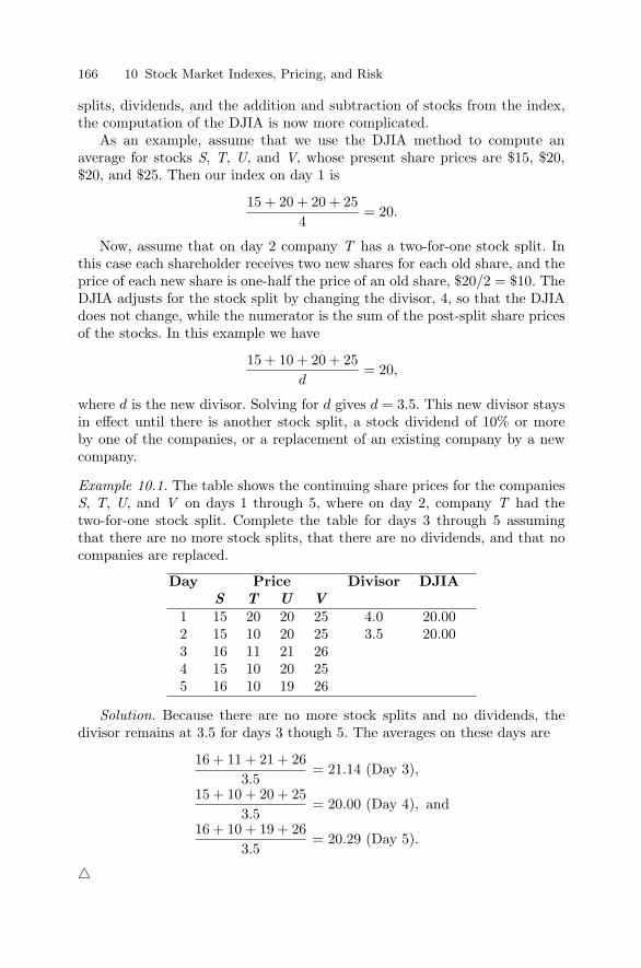
166 10 Stock Market Indexes, Pricing, and Risk
splits, dividends, and the addition and subtraction of stocks from the index,the computation of the DJIA is now more complicated.
As an example, assume that we use the DJIA method to compute anaverage for stocks S, T, U, and V, whose present share prices are $15, $20,$20, and $25. Then our index on day 1 is
15 + 20 + 20 + 254
= 20.
Now, assume that on day 2 company T has a two-for-one stock split. Inthis case each shareholder receives two new shares for each old share, and theprice of each new share is one-half the price of an old share, $20/2 = $10. TheDJIA adjusts for the stock split by changing the divisor, 4, so that the DJIAdoes not change, while the numerator is the sum of the post-split share pricesof the stocks. In this example we have
15 + 10 + 20 + 25d
= 20,
where d is the new divisor. Solving for d gives d = 3.5. This new divisor staysin effect until there is another stock split, a stock dividend of 10% or moreby one of the companies, or a replacement of an existing company by a newcompany.
Example 10.1. The table shows the continuing share prices for the companiesS, T, U, and V on days 1 through 5, where on day 2, company T had thetwo-for-one stock split. Complete the table for days 3 through 5 assumingthat there are no more stock splits, that there are no dividends, and that nocompanies are replaced.
Day Price Divisor DJIAS T U V
1 15 20 20 25 4.0 20.002 15 10 20 25 3.5 20.003 16 11 21 264 15 10 20 255 16 10 19 26
Solution. Because there are no more stock splits and no dividends, thedivisor remains at 3.5 for days 3 though 5. The averages on these days are
16 + 11 + 21 + 263.5
= 21.14 (Day 3),
15 + 10 + 20 + 253.5
= 20.00 (Day 4), and
16 + 10 + 19 + 263.5
= 20.29 (Day 5).
�

10.1 Stock Market Indexes 167
We now discuss the effect of stock splits and dividends on the DJIA andwhy they may lead to a downward bias (a value smaller than expected) in theDJIA. Suppose that after the stock split (so the divisor is 3.5) company T ’sstock price increases by 10%, from $10 to $11. Then the new average is
15 + 11 + 20 + 253.5
= 20.29.
On the other hand, if company U ’s share price increases by 10%, from $20 to$22, while the other share prices do not change, then the new average is
15 + 10 + 22 + 253.5
= 20.57.
This suggests that the impact of a stock that splits is less than that of a stockthat does not split in computing the average. You are asked to verify this inProblem 10.9.
Now, consider the effect of not adjusting for stock dividends of less than10%. Suppose that the prices of our four stocks are $15, $10, $20, and $25, andthat d = 3.5; the share prices and divisor immediately following the stock splitof company T. If company U issues a stock dividend of 5% ($1 per share),then the resulting stock price is $20/1.05 = $19.05, which artificially lowersthe average. (Note that the divisor does not change in this case.)
Standard and Poor’s 500 Index
Standard and Poor’s Corporation publishes several stock indexes that usea different approach than the DJIA. The most followed of these indexes isthe Standard and Poor’s 500 (S&P 500). There are two essential differencesbetween the S&P 500 and the DJIA. The first is that the S&P 500 includes500 companies rather than 30, which may better reflect the overall market.The second is that the indexes are computed differently. Because all the S&Pindexes are calculated in the same manner, we restrict our discussion to theS&P 500.
The S&P 500 weights all stocks in the index in proportion to the sum oftheir market capitalizations. The formula is
S&P 500 (t) = 10∑500
i=1 Si(t)Ni(t)∑500i=1 Si(1)Ni(1)
.
Here Si(1) is the price per share of the ith stock on the original date. For theS&P 500 this is the average of the ith stock’s prices for the years 1941–1943.The quantity Si(t) is the price per share of the ith stock at time t, and Ni(t)is the number of shares issued of the ith stock at time t.
Returning to Example 10.1, if we calculate this average at day 1 assumingthat 100 shares are issued for each company, then we have

168 10 Stock Market Indexes, Pricing, and Risk
4∑i=1
Si(1)Ni(1) = 15(100) + 20(100) + 20(100) + 25(100) = 8000
as the divisor. On day 1 this is also the numerator, so the original index is
S&P 500 (1) = 10(8000/8000) = 10.
On day 2, after the stock split we have
4∑i=1
Si(2)Ni(2) = 15(100) + 10(200) + 20(100) + 25(100) = 8000,
so that the stock split does not change the divisor. The index following thestock split is
S&P 500 (2) = 10(8000/8000) = 10.
With this index all stock splits and stock dividends are accounted for in thenumerator. The denominator changes if new stocks are introduced in the in-dex, replacing other stocks. In this case the numerator uses the total marketcapitalization of the 500 stocks after the replacement, and the denominator isadjusted so that the new average is the same as the old average.
Example 10.2. The table shows the continuing share prices for the companiesS, T, U, and V on days 1 through 5, where on day 2, company T had thetwo-for-one stock split. Complete the table for days 3 through 5, assumingthat there are no more stock splits and no dividends.
Day Price S&P 500S T U V
1 15 20 20 25 10.002 15 10 20 25 10.003 16 11 21 264 15 10 20 255 16 10 19 26
Solution. Because there are no more stock splits and no dividends, thereare 100 shares issued for companies S, U, and V, and 200 for company T. Theindexes on these days are
10(
16(100) + 11(200) + 21(100) + 26(100)8000
)= 10.63 (Day 3),
10(
15(100) + 10(200) + 20(100) + 25(100)8000
)= 10.00 (Day 4), and
10(
16(100) + 10(200) + 19(100) + 26(100)8000
)= 10.13 (Day 5).
�

10.1 Stock Market Indexes 169
NASDAQ Composite Index
Another closely watched index is the NASDAQ Composite Index. It was cre-ated in 1971 and currently includes over 2000 stocks. It is computed in thesame manner as the S&P 500.
The following table lists the year-end closing values of the DJIA, S&P 500,and NASDAQ Composite Index from 1980 through 2005.
DJIA S&P 500 NASDAQ DJIA S&P 500 NASDAQ1980 963.99 135.76 202.34 1993 3754.09 466.45 776.801981 875.00 121.57 195.84 1994 3834.44 459.27 751.961982 1046.54 140.64 232.41 1995 5117.12 615.93 1052.131983 1258.64 164.93 278.60 1996 6448.27 740.74 1291.031984 1211.57 167.24 247.10 1997 7908.25 970.43 1570.351985 1546.67 211.28 324.90 1998 9181.43 1229.23 2192.691986 1895.95 242.17 348.80 1999 11497.12 1469.25 4069.311987 1938.83 247.08 330.50 2000 10787.99 1320.28 2470.521988 2168.57 277.72 381.40 2001 10021.57 1148.08 1950.401989 2753.20 353.40 454.80 2002 8341.63 879.82 1335.511990 2633.66 330.22 373.80 2003 10453.92 1111.92 2003.371991 3168.83 417.09 586.34 2004 10783.01 1211.92 2175.441992 3301.11 435.71 676.95 2005 10717.50 1248.29 2205.32
The IRR, iirr, for the DJIA over these 26 years is
iirr =(
10717.50963.99
)1/25
− 1 = 10.114%.
In the same way, the IRR’s for the S&P 500 and the NASDAQ CompositeIndex are 9.280% and 10.026%, respectively. This is consistent with the fre-quently heard statement that in the long run the stock market gains about10% a year.
Value Line Index
Value Line published two indexes: the Value Line Geometric Average, startedin 1961, and the Value Line Arithmetic Average, started in 1988. Both indexesuse all the (over 1600) stocks covered by The Value Line Investment Survey.These stocks include big cap, mid-cap, and small-cap companies, and theyare all treated equally. In both indexes stock splits and stock dividends areconsidered by making the appropriate adjustment to the stock’s price.
The Value Line Geometric Average uses a geometric-average of the ratioof stock prices. The base (original) index is 100. There are four steps to thisprocedure.

170 10 Stock Market Indexes, Pricing, and Risk
1. The closing price of each of the n stocks in The Value Line InvestmentSurvey is expressed as a ratio of the preceding day’s price, adjusted forstock splits.
2. These ratios are multiplied together.3. The nth root of this product is calculated, where n is the total number of
stocks. This gives the geometric daily ratio.4. The geometric daily ratio is multiplied by the prior day’s index value.
We illustrate this method using stocks S, T, U, and V for a 5-day periodwith a base index of 100 where T had a two-for-one stock split at the end ofday 2.
Day Stock PriceS T U V
1 15 20 20 252 15 10 20 253 16 11 21 264 15 10 20 255 16 10 19 26
On day 2 the relative price of stock T is
Price on day 2Adjusted price on day 1
=$10$10
= 1,
because the adjusted price at day 1 is $20/2 = $10, reflecting the two-for-onestock split. All the other relative stock prices are equal to 1. Steps 2 and 3yield the geometric relative price (1 × 1 × 1 × 1)1/4 = 1, and Step 4 yields100 × 1 = 100, reflecting the fact that the prices remained the same afteradjusting for the stock split of company T.
For day 3, combining Steps 1 through 4, we find that the index is(1615
· 1110
· 2120
· 2625
)1/4
× 100 = 106.392.
In Problem 10.5 you are asked to compute this index for day 5. You mightsuspect that if all the stock prices rise, then the value of the index increases.Other interesting questions are, “What happens to the index if on some daythe stock prices have returned to their original levels? What happens to theindex if at some day all stocks have doubled in price?” You are asked toconsider these questions in Problems 10.6, 10.7, and 10.8.
We write a formula for this index as follows. On day t let Si(t) be theclosing price of stock i, where 1 ≤ i ≤ n, so the previous day’s closing priceis Si(t − 1). If V LG(t) is the index at the end of day t, so the previous day’sindex is V LG(t − 1), then
V LG(t) = V LG(t − 1)(
S1(t)S1(t − 1)
S2(t)S2(t − 1)
· · · Sn(t)Sn(t − 1)
)1/n
. (10.1)

10.1 Stock Market Indexes 171
The Value Line Arithmetic Average uses an equal-weighted average of theratio of stock prices. There are three steps to this procedure.
1. The closing price of each of the n stocks in The Value Line InvestmentSurvey is expressed as a ratio of the preceding day’s price, adjusted forstock splits. This is the same calculation as the Value Line GeometricAverage
2. These ratios are added together and divided by n, giving the arithmeticdaily ratio.
3. The arithmetic daily ratio is multiplied by the prior day’s index value.
With the same notation used in defining V LG(t), the Value Line Arith-metic Average, V LA(t), on day t is
V LA(t) = V LA(t − 1)S1(t)
S1(t−1) + S2(t)S2(t−1) + · · · + Sn(t)
Sn(t−1)
n. (10.2)
These two Value Line Indexes are related by the following theorem.2
Theorem 10.1. The Value Line Theorem.The maximum daily ratio attainable by the Value Line Geometric Average isequal to the daily ratio of the Value Line Arithmetic Average. Equality canonly occur when every stock in the average has the same percentage pricechange on a given day.
Proof. On day t, the Geometric Average daily ratio is V LG(t)/V LG(t − 1),while the Arithmetic Average daily ratio is V LA(t)/V LA(t − 1). Thus, wemust show that V LG(t)/V LG(t − 1) ≤ V LA(t)/V LA(t − 1).
From (10.1), we have
V LG(t)V LG(t − 1)
=(
S1(t)S1(t − 1)
S2(t)S2(t − 1)
· · · Sn(t)Sn(t − 1)
)1/n
,
while, from (10.2), we have
V LA(t)V LA(t − 1)
=S1(t)
S1(t−1) + S2(t)S2(t−1) + · · · + Sn(t)
Sn(t−1)
n,
so we must show that(S1(t)
S1(t − 1)S2(t)
S2(t − 1)· · · Sn(t)
Sn(t − 1)
)1/n
≤S1(t)
S1(t−1) + S2(t)S2(t−1) + · · · + Sn(t)
Sn(t−1)
n.
2 Quoted, with minor modifications, from the Value Line article “Comparing theValue Line Averages” at http://www.valueline.com/news/vlv050311.html, ac-cessed on May 23, 2006.
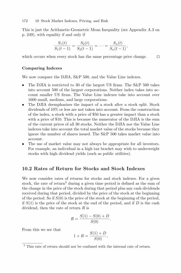
172 10 Stock Market Indexes, Pricing, and Risk
This is just the Arithmetic-Geometric Mean Inequality (see Appendix A.3 onp. 249), with equality if and only if
S1(t)S1(t − 1)
=S2(t)
S2(t − 1)= · · · =
Sn(t)Sn(t − 1)
,
which occurs when every stock has the same percentage price change. ��
Comparing Indexes
We now compare the DJIA, S&P 500, and the Value Line indexes.
• The DJIA is restricted to 30 of the largest US firms. The S&P 500 takesinto account 500 of the largest corporations. Neither index takes into ac-count smaller US firms. The Value Line indexes take into account over1600 small, medium, and large corporations.
• The DJIA deemphasizes the impact of a stock after a stock split. Stockdividends of 10% or less are not taken into account. From the constructionof the index, a stock with a price of $50 has a greater impact than a stockwith a price of $10. This is because the numerator of the DJIA is the sumof the current prices of all 30 stocks. Neither the DJIA nor the Value Lineindexes take into account the total market value of the stocks because theyignore the number of shares issued. The S&P 500 takes market value intoaccount.
• The use of market value may not always be appropriate for all investors.For example, an individual in a high tax bracket may wish to underweightstocks with high dividend yields (such as public utilities).
10.2 Rates of Return for Stocks and Stock Indexes
We now consider rates of returns for stocks and stock indexes. For a givenstock, the rate of return3 during a given time period is defined as the sum ofthe change in the price of the stock during that period plus any cash dividendsreceived during that period, divided by the price of the stock at the beginningof the period. So if S(0) is the price of the stock at the beginning of the period,if S(1) is the price of the stock at the end of the period, and if D is the cashdividend, then the rate of return R is
R =S(1) − S(0) + D
S(0).
From this we see that
1 + R =S(1) + D
S(0),
3 This rate of return should not be confused with the internal rate of return.

10.2 Rates of Return for Stocks and Stock Indexes 173
which is positive because S(0) > 0, S(1) > 0, and D ≥ 0. This property willbe used later.
Example 10.3. A stock is trading at $50 a share on 12/31/2004. The followingis a list of the stock prices and the dividends paid from 1/1/2005 through12/31/2005 on the last day of each quarter. What are the rates of return foreach of the quarters?
Date 3/31/2005 6/30/2005 9/30/2005 12/31/2005Price $52.00 $54.00 $53.00 $56.00
Dividend $0.50 $0.50 $0.50 $0.50
Solution. The rates of return for the four quarters are
(52.00 − 50.00) + 0.5050.00
= 0.05 = 5%,
(54.00 − 52.00) + 0.5052.00
= 0.0481 = 4.81%,
(53.00 − 54.00) + 0.5054.00
= −0.0093 = −0.93%,
and(56.00 − 53.00) + 0.50
53.00= 0.066 = 6.6%.
�If R1, R2, R3, and R4 are the quarterly rates of return (expressed as
decimals), then how can we quantify the average quarterly rate of return, R?This depends on whether we use simple or compound interest.
If we use simple interest, then the year-end value of a $1 investment is1 + R1 + R2 + R3 + R4, and we want this to be equal to 1 + 4R, so
1 + 4R = 1 + R1 + R2 + R3 + R4.
Solving this for R, gives the arithmetic average quarterly return,4
RA =R1 + R2 + R3 + R4
4.
If we use compound interest, then the year-end value of a $1 investmentis (1 + R1)(1 + R2)(1 + R3)(1 + R4), and we want this to equal (1 + R)4, so
(1 + R)4 = (1 + R1)(1 + R2)(1 + R3)(1 + R4).
Solving this for R, gives the geometric average quarterly return,5
4 Strictly speaking this should be called a rate of return, but for the sake of brevity,in this section we use the shorter expression return.
5 Note that, although the Arithmetic Average Quarterly Return of R1, R2, R3, R4
is their arithmetic mean, the Geometric Average Quarterly Return of R1, R2, R3,R4 is not their geometric mean.

174 10 Stock Market Indexes, Pricing, and Risk
RG = ((1 + R1)(1 + R2)(1 + R3)(1 + R4))1/4 − 1.
We have already shown that each of the terms in parentheses is positive, soRG is always defined.
Example 10.4. For the stock in Example 10.3, calculate the arithmetic andgeometric average quarterly returns.
Solution. The arithmetic average quarterly return is
0.05 + 0.0481 + (−0.0093) + 0.0664
= 0.0387 = 3.87%,
while the geometric average quarterly return is
((1.05)(1.0481)(0.9907)(1.066))1/4 − 1 = 0.0383 = 3.83%.
�Note that the geometric average quarterly return is less than the arithmetic
average quarterly return. This is generally true, as can be seen in the followingtheorem.
Theorem 10.2. The Average Quarterly Return Theorem.
RG ≤ RA.
Proof. Using the Arithmetic-Geometric Mean Inequality (see Appendix A.3on p. 249), which states that if a1, a2, . . . , an are non-negative and not all zero,then
(a1a2 · · · an)1/n ≤ a1 + a2 + · · · + an
n,
with equality if and only if a1 = a2 = · · · = an. With n = 4 and ai = 1+Ri > 0for i = 1, . . . , 4, this inequality becomes
((1 + R1)(1 + R2) · · · (1 + R4))1/4 ≤ (1 + R1) + (1 + R2) + · · · + (1 + R4)
4,
with equality if and only if R1 = R2 = R3 = R4. This shows that the geometricaverage quarterly return is less than the arithmetic average quarterly returnunless the quarterly returns are equal, in which case the averages are thesame. ��
There are several things to note about these definitions of return.
• It is assumed that dividends are paid on the last day of each quarter. Ifthis is not the case, then the calculation is done daily.
• It is assumed that dividends are not reinvested in the stock.• We cannot calculate this form of return if we do not know the amounts
and timing of the dividend payments. For example, we cannot calculatethe return on the S&P 500 from a listing of the year-end values of thatindex.

10.3 Pricing and Risk 175
10.3 Pricing and Risk
As defined in the previous section, the return on an investment in commonstock consists of two components: cash dividends and the rise or fall of thestock price, capital gains or losses. The price that an investor is willing topay for a share of common stock is based upon the investor’s expectationsregarding dividends and the future price of the stock.
Let S(0) be the current price per share of the stock, Dt be the expecteddividend at time t in quarters, T be the length of the holding period in quar-ters, and k be the quarterly required rate of return (expressed as a decimal).
Initially, we assume that dividends are paid quarterly and that the priceof the stock is to be determined immediately following a dividend payment.We also ignore certain aspects of the trading mechanism.
Theoretically, the length of the holding period could be infinite. Commonstocks do not mature, unlike bonds. As long as the company continues toexist, then so does the stock. The investor expects to receive dividends in theamount of D1 at the end of the first quarter, D2 at the end of the secondquarter, and so on. In return, the investor is willing to pay S(0) for the stocktoday. These cash flows are represented by the diagram in Fig. 10.1.
S(0)
D1
1
D2
2
· · ·DT
T
· · ·
Fig. 10.1. Time diagram of a typical stock held forever
The price that the investor is willing to pay for the stock today is givenby the present value of the expected future dividends discounted at the ap-propriate required rate of return.6 Assuming that the appropriate requiredrate of return per quarter is k, the general formula for the price of the stocktoday is
S(0) =D1
(1 + k)1+
D2
(1 + k)2+ · · · ,
or
S(0) =∞∑
t=1
Dt
(1 + k)t. (10.3)
In practice, however, the length of the holding period is not infinite. Theinvestor expects to receive dividends in the amount of D1 at the end of thefirst quarter, D2 at the end of the second quarter, and so on. In addition, the6 We discuss the required rate of return on p. 177 and the relationship between the
required rate of return and the expected rate of return on p. 184.

176 10 Stock Market Indexes, Pricing, and Risk
investor expects to be able to sell the stock for a price of S(T ) at the end ofT quarters. In return, the investor is willing to pay S(0) for the stock today.These cash flows are represented by the diagram in Fig. 10.2.
S(0)
D1
1
D2
2
· · ·DT−1
T − 1
DT + S(T )
T
Fig. 10.2. Time diagram of a typical stock
Again, the price that the investor is willing to pay for the stock today isgiven by the present value of the expected future cash flows discounted at theappropriate required rate of return. Therefore, an alternative formula for theprice of the stock today is given by
S(0) =D1
(1 + k)1+
D2
(1 + k)2+ · · · +
DT−1
(1 + k)T−1 +DT + S(T )(1 + k)T
,
or
S(0) =T∑
t=1
Dt
(1 + k)t+
S(T )(1 + k)T
. (10.4)
Thus, we have the following theorem.
Theorem 10.3. The Common Stock Theorem.If the price S(0) of a share of common stock is given by (10.3), then the pricemay be written as (10.4).
The converse of this theorem is not necessarily true (see Problem 10.13).
Example 10.5. Helen Kendrick expects to receive dividends in the amount of$1.50 at the end of each of the next four quarters and $1.75 at the end of eachof the following four quarters. Furthermore, she expects to be able to sell thestock for $94.50 at the end of the second year. If the required rate of returnper quarter is 0.025, then what price should she pay for the stock?
Solution. Here T = 8, D1 = D2 = D3 = D4 = 1.5, D5 = D6 = D7 = D8 =1.75, k = 0.025, and S(T ) = 94.5. Substituting these into (10.4) gives
S(0) =4∑
t=1
1.5(1.025)t
+8∑
t=5
1.75(1.025)t
+94.5
(1.025)8= 89.168,
so Helen should pay $89.17 for the stock. �Dividends tend to be relatively stable over the short term; however, there is
usually variability in a perpetual stream of dividends. This creates difficulties

10.3 Pricing and Risk 177
in applying the general pricing formula. However, it is often assumed that thedividends paid by a company to its shareholders will grow indefinitely at afixed rate. If we let g be the quarterly rate of dividend growth (expressed asa decimal), then
D1 = D0(1 + g),
D2 = D1(1 + g) = D0(1 + g)2,
and so on.According to the general pricing formula (10.3),
S(0) =∞∑
t=1
D0 (1 + g)t
(1 + k)t. (10.5)
This leads to the following theorem.
Theorem 10.4. The Constant Growth Theorem.If the dividend grows according to Dn = D0(1 + g)n and if k > g, then
S(0) = D01 + g
k − g.
Proof. We can rewrite (10.5) as
S(0) =∞∑
t=1
D0
(1 + g
1 + k
)t
= D0
(1 + g
1 + k
) ∞∑t=0
(1 + g
1 + k
)t
,
which is a geometric series. Because k > g, we have (1 + g) / (1 + k) < 1,which means that the series converges. Thus,
S(0) = D0
(1 + g
1 + k
)1
1 − 1+g1+k
= D01 + g
k − g.
��Example 10.6. A company just paid a dividend of $2.25, and future dividendsare expected to increase at a rate of 1% per quarter. If the quarterly rate ofreturn on the company’s stock is 2%, then what price should the investor payfor the stock?
Solution. Here D0 = 2.25, g = 0.01, and k = 0.02, so k > g and thus
S(0) = D01 + g
k − g= 2.25
1.010.01
= 227.25.
The investor should pay $227.25. �When discussing how to price a stock, we talk about using an appropriate
risk-adjusted rate to discount the dividends that are expected to be paid onthe stock in the future. This is the required rate of return mentioned on p. 175.

178 10 Stock Market Indexes, Pricing, and Risk
However, two crucial questions remain unanswered at this point. How do wemeasure the risk of a stock? How do we use that measure of risk to computethe appropriate discount rate? These questions are now addressed.
The risk of a stock is associated with uncertainty about the returns on thestock. If the return is certain, then there is no risk. As the uncertainty of thereturns increases, then so does risk. Risk can be estimated using any one of anumber of measures. These include the range, the mean absolute deviation, theprobability of a negative return, the semivariance, and the standard deviationof the returns on the stock.
We assume that the returns, Rs, on a stock have S possible values, so 1 ≤s ≤ S, and that the probability of Rs is Ps. If R is the random variable thatgives the return on the stock, then the possible values of R are R1, R2, . . . , RS ,and the expected return on the stock is E(R) =
∑Ss=1 PsRs.
The range is the difference between the largest and smallest returns. Ifthe largest return is maxs∈S Rs and the smallest return is mins∈S Rs, thenthe range is
maxs∈S
Rs − mins∈S
Rs.
This is simple to compute; however, it does not consider returns between theextremes and it does not consider the likelihoods of the possible returns.
The mean absolute deviation is the expected absolute difference be-tween the return on the stock and its expected return, E(R), and is givenby
MAD =S∑
s=1
Ps|Rs − E(R)|.
This may be a reasonable measure, but it is statistically difficult to use.The probability of a negative return is the sum of the probabilities of
all negative returns and is given by7
S∑s=1
Ps1Rs< 0.
The weakness of this measure is that it does not consider all aspects of risk.For example, neither non-negative returns nor the magnitudes of negativereturns are considered.
Semivariance is a statistical measure of the variability of returns belowthe expected return and is given by
S∑s=1
Ps(Rs − E(R))21Rs<E(R).
7 If X is a random variable, and (X ⊂ A) is an event, then the indicator variable1X⊂A is defined by
1X⊂A ={
1 if X ⊂ A,0 if X � A.

10.3 Pricing and Risk 179
As with the probability of a negative return, the semivariance does not con-sider the uncertainty of returns greater than the expected return.
The standard deviation of R is one of the most commonly used measuresof risk. It is a measure of the dispersion both above and below the expectedreturn and is given by
σ =
√√√√ S∑s=1
Ps(Rs − E(R))2 .
The quantity σ2 is the variance of R.
Example 10.7. Suppose that an investment has three possible annual rates ofreturn: a return of 0.10 with probability 0.50, a return of 0.15 with probability0.30, and a return of −0.05 (a loss of 5%) with probability 0.20. Thus, if welet R be the annual rate of return, then P (R = 0.10) = 0.50, P (R = 0.15) =0.30, and P (R = −0.05) = 0.20. What is the range, expected return, MAD,probability of a negative return, semivariance, and standard deviation?
Solution. The range is 0.15 − (−0.05) = 0.20.The expected return is E(R) = 0.5(0.10)+0.3(0.15)+0.2(−0.05) = 0.085.The MAD is 0.5|0.10−0.085|+0.3|0.15−0.085|+0.2|−0.05−0.085| = 0.054.The probability of a negative return is 0.2.The semivariance is 0.2(−0.05 − 0.085)2 = 0.0036.The standard deviation is
σ =√
0.5(0.10 − 0.085)2 + 0.3(0.15 − 0.085)2 + 0.2(−0.05 − 0.085)2
= 0.0709.
�
These measures of risk consider two types of risk—systematic risk andunsystematic risk. Systematic risk is risk that is common to all risky stocks.Unsystematic risk is unique to each company. We discuss each of these inturn.
Systematic risk includes the impact of inflation, uncertainties about long-run aggregate economic growth, changes in investors’ attitudes toward risk,and changes in interest rates.
• Inflation affects stock prices through corporate profits. If inflation resultsin higher borrowing rates, then expected future corporate profits are likelyto decrease. On the other hand, if inflation results in higher prices, thenexpected future corporate profits are likely to increase. The effect is similarfor all stocks.

180 10 Stock Market Indexes, Pricing, and Risk
• Uncertainties about long-run aggregate economic growth also affect stockprices through corporate profits. Corporate profits of all firms are depen-dent upon the long-run health and growth of the aggregate economy. Fac-tors that affect aggregate output include population growth, labor produc-tivity, political uncertainty, tax policy, technology, etc.
• Changes in investors’ attitudes toward risk have a more direct affect onstock prices. If the average investor suddenly becomes more risk-averse,then the required rate of return increases. To provide this larger return,stock prices have to fall. The opposite occurs if the average investor sud-denly becomes less risk-averse. Again, the effect is similar for all stocks.
• Interest rate changes also affect the prices of all stocks. Increases in interestrates result in increases in interest expense and decreases in corporateprofits. Changes in interest rates also affect investors’ attitudes towardrisk that in turn affect stock prices.
Systematic risk cannot be eliminated through diversification. For this reasonit is often referred to as market or nondiversifiable risk.
Unsystematic risk is unique to each company. This type of risk includeslawsuits, strikes, competition, and changes in consumer base.
• If one company sues another for breach of contract, then the market valueof the winning company increases, and the market value of the losingcompany decreases. An appropriate position in both stocks eliminates theneed for any concern about the outcome of the lawsuit.
• If a company suffers a labor strike, then that company’s profit decreases.However, if the lost sales are picked up by a competitor, then that com-pany’s profit increases. An appropriate position in both stocks eliminatesthe need for any concern about the outcome of the strike.
• If one company has a patent on a major product line that may be coun-teracted through research and development at another company, then theprofits of the company with the patent are likely to decrease with the lossof its effective patent position, and the profits of the competitor are likelyto increase. Once again, an appropriate position in both stocks eliminatesthe need for any concern.
• If the companies in one region lose customers to companies in anotherregion as a result of migration, then the profits of companies in the firstregion decrease, and the profits of companies in the second region increase.Yet again, an appropriate position in the stocks of companies in bothregions eliminates the need for any concern.
Unsystematic risk can be eliminated by investing in a well diversified portfolio.Losses in one stock are offset by gains in another stock. For this reason,unsystematic risk is often referred to as diversifiable risk.

10.3 Pricing and Risk 181
Because unsystematic risk can be eliminated through proper diversifica-tion, investors are not rewarded or compensated for that type of risk; investorsare only rewarded for systematic risk. In order to determine how much of astock’s return is not diversifiable, we need a measure of the relationship of thereturns on that stock with the returns on other stocks.
The correlation coefficient is a commonly used statistical measure of therelationship between two random variables. We assume that the returns onstocks i and j, namely, Ris and Rjs, have S possible values, so 1 ≤ s ≤ S, thatthe probabilities of Ris and Rjs are the same, Ps, that the expected returnson stocks i and j are E(Ri) and E(Rj) respectively, and that the standarddeviation of the return on stocks i and j are σi and σj respectively. Then thecorrelation coefficient between the returns on stock i and the returns on stockj is given by
ρij =
S∑s=1
Ps(Ris − E(Ri))(Rjs − E(Rj))
σiσj.
Example 10.8. In addition to the information given for the annual rate ofreturn R of the investment in Example 10.7, suppose that there is a secondinvestment for which the annual rate of return U is correlated with R asfollows: P (R = 0.10, U = 0.15) = 0.50, P (R = 0.15, U = 0.20) = 0.30,and P (R = −0.05, U = −0.10) = 0.20. Find ρRU , the correlation coefficientbetween R and U .
Solution. The expected return on the second stock is E(U) = 0.5(0.15) +0.3(0.20) + 0.2(−0.10) = 0.115, and the standard deviation is
σ =√
0.5(0.15 − 0.115)2 + 0.3(0.20 − 0.115)2 + 0.2(−0.10 − 0.115)2
= 0.1097.
Therefore, the correlation coefficient is
ρRU =1
0.0709(0.1097)[0.5(0.10 − 0.085)(0.15 − 0.115)
+ 0.3(0.15 − 0.085)(0.20 − 0.115)+ 0.2(−0.05 − 0.085)(−0.10 − 0.115)]
= 0.993. �
If the correlation coefficient between the returns on two stocks is −1, then riskcan be eliminated through proper diversification. If the correlation coefficientbetween the returns on two stocks is 1, then risk cannot be eliminated throughdiversification.
However, it is not sufficient to consider the relationship between just twostocks; we must consider the relationships among all stocks. Then one appro-priate measure of the risk of a stock is the amount of nondiversifiable risk

182 10 Stock Market Indexes, Pricing, and Risk
that the stock contributes to that of the market portfolio. For stocks issuedby domestic companies, an index such as the S&P 500 or the NYSE Compos-ite Index8 is used as a proxy for the market portfolio. This measure of riskis given by σiρiM , where σi is the standard deviation of the returns on thestock, and ρiM is the correlation coefficient between the returns on the stockand the returns on the market.
A more commonly used measure of the risk of a stock is the amountof nondiversifiable risk inherent in the stock relative to that of the marketportfolio. This measure of the relative risk of a stock is known as the stock’sbeta and is given by βi = (σi/σM )ρiM , where σi is the standard deviation ofthe returns on the stock, σM is the standard deviation of the returns on themarket, and ρiM is the correlation coefficient between the returns on the stockand the returns on the market. For example, if RM represents the returns onthe S&P 500, then ρiM is the correlation coefficient between RM and thereturns on the given stock.
The ratio of σi to σM measures how volatile the stock is in relation to thevolatility of the reference portfolio, and the correlation coefficient determineshow much of that relative volatility should be counted. If the stock is perfectlycorrelated with the market, then all of the relative volatility counts. If thecorrelation is zero, then none of the relative volatility counts.
In practice, investors do not know σi, σM , or ρiM . Therefore, these pa-rameters must be estimated. What is needed are ex ante9 estimates of σi, σM ,and ρiM .
However, the use of ex ante values requires that all possible future returnsand the corresponding probabilities be identified—an extremely difficult, ifnot impossible, task. Thus, ex post10 or historical estimates of σi, σM , andρiM are often used as estimates of the ex ante values of σi, σM , and ρiM
respectively.A regression line is a line that describes the relationship between an ex-
planatory variable and a response variable. The characteristic line for a stockis the best-fit regression line that describes the relationship between the re-turns on the stock and the returns on the market. The slope of this line isgiven by bi = (si/sM )riM , where si and sM are estimates of σi and σM re-spectively, and riM is an estimate of ρiM (see Appendix B.7 on p. 280). Thus,bi is the estimate of βi. In other words, the estimate of a stock’s β is obtainedby regressing the stock’s historical returns against the returns on the market.
Although this sounds simple, there are several questions that remain.Should βi be estimated over a time period that consists of the past month, thepast year, the past five years, the past 20 years? Should βi be estimated us-ing daily, weekly, monthly, quarterly, or annual returns? Which index should
8 The NYSE Composite Index includes all common stocks traded on the NYSE. De-tails of its calculation can be found at www.nyse.com/pdfs/methodology nya.pdf.
9 Ex ante means before the fact.10 Ex post means after the fact.

10.3 Pricing and Risk 183
be used as a proxy for the market portfolio? Unfortunately these questionsremain unanswered. Therefore, it is important to emphasize the fact that bi
is only an estimate of βi and that the value of that estimate is determinedby the particular data that was used in the regression. In other words, theuse of different data may result in a different estimate. However, in spite ofthe difficulties associated with estimating βi, it is accepted as an appropriatemeasure of risk.
Example 10.9. Closing prices and weekly returns for Amazon.com and theS&P 500 from December 1999 to June 2000 are given in following table.11
Use a spreadsheet to estimate Amazon.com’s β.
Amazon.com S&P 500Week of Close Return Close Return26-Jun-00 36.3125 0.071956 1454.60 0.00910219-Jun-00 33.8750 −0.263587 1441.48 −0.01569212-Jun-00 46.0000 −0.118563 1464.46 0.0051555-Jun-00 52.1875 −0.098272 1456.95 −0.013748
29-May-00 57.8750 0.244624 1477.26 0.07201622-May-00 46.5000 −0.116390 1378.02 −0.02056215-May-00 52.6250 −0.020930 1406.95 −0.0098608-May-00 53.7500 −0.081197 1420.96 −0.0081461-May-00 58.5000 0.060023 1432.63 −0.01363224-Apr-00 55.1875 0.053699 1452.43 0.01247117-Apr-00 52.3750 0.117333 1434.54 0.05748410-Apr-00 46.8750 −0.306198 1356.56 −0.1053783-Apr-00 67.5625 0.008396 1516.35 0.011858
27-Mar-00 67.0000 −0.078246 1498.58 −0.01890720-Mar-00 72.6875 0.121504 1527.46 0.04301213-Mar-00 64.8125 −0.030841 1464.47 0.0497476-Mar-00 66.8750 0.070000 1395.07 −0.01000628-Feb-00 62.5000 −0.095841 1409.17 0.05685621-Feb-00 69.1250 0.067568 1333.36 −0.00945714-Feb-00 64.7500 −0.150123 1346.09 −0.0295797-Feb-00 76.1875 −0.030231 1387.12 −0.026152
31-Jan-00 78.5625 0.273556 1424.37 0.04720824-Jan-00 61.6875 −0.006042 1360.16 −0.05633617-Jan-00 62.0625 −0.034047 1441.36 −0.01623710-Jan-00 64.2500 −0.076370 1465.15 0.0164283-Jan-00 69.5625 −0.086207 1441.47 −0.018908
27-Dec-99 76.1250 −0.154167 1469.25 0.00748120-Dec-99 90.0000 1458.34
11 Data obtained from http://finance.yahoo.com/.

184 10 Stock Market Indexes, Pricing, and Risk
Solution. Microsoft� Excel was used to regress the returns for Amazon.comon the returns for the S&P 500. The slope of the regression line is 2.214659.Therefore, an estimate of Amazon.com’s β is 2.21. �
The price of a stock is determined by discounting all expected future div-idends at the appropriate required rate of return. A model known as theCapital Asset Pricing Model (CAPM) specifies the equilibrium relationshipbetween expected returns and risk for stocks. Equilibrium is defined to be astate in which the expected rates of return are equal to the required ratesof return. According to this model, investors should be compensated for thetime value of money and for nondiversifiable risk.
The line that relates the expected return on a portfolio, E(R), where Ris the random variable that gives the return on the portfolio, to the standarddeviation of the returns on the portfolio, σ, is called the Capital Market Line.The equation of this line in the (σ,E(R)) plane is given by
E(R) = Rrf +E(RM ) − Rrf
σMσ,
where Rrf is the risk-free rate of return,12 E(RM ) is the expected return onthe market, and σM is the standard deviation of the returns on the market.The Capital Market Line is the efficient boundary for portfolios, so, under theassumption that the market portfolio is efficient, all portfolios, as plotted inthe (σ,E(R)) plane, must lie on or below this line
Now, we show how the expected rate of return on an individual assetrelates to its individual risk.
Consider a portfolio consisting of a proportion w invested in asset i and aproportion 1−w invested in the market portfolio. The expected rate of returnon this portfolio is
E(Ri,w) = wE(Ri) + (1 − w)E(RM ),
where Ri,w is the random variable that gives the return on the portfolio andRi is the random variable that gives the return on asset i.13 This portfoliohas standard deviation14
σi,w =√
w2σ2i + 2w(1 − w)σiM + (1 − w)2σ2
M ,
12 The risk-free rate of return is usually the rate of return on a United States Trea-sury bill.
13 Thus, Ri,0 = RM and Ri,1 = Ri. Do not confuse the Ri used here, which is thereturn on asset i, with the Rs used on p. 178, which is one of the possible valuesof R, the return on a stock.
14 Thus, σi,0 = σM and σi,1 = σi.

10.3 Pricing and Risk 185
where σi is the standard deviation of Ri, σM is the standard deviation of RM ,and σiM is the covariance of Ri and RM .
As we vary w, we obtain different points (σi,w, E(Ri,w)) in the (σ,E(R))plane. When w = 0 we are fully invested in the market, so Ri,0 = RM andσi,0 = σM , and we intersect the Capital Market Line at (σM , E(RM )).
By the definition of the Capital Market Line, points (σi,w, E(Ri,w)) cannever cross this line. Hence the curve (σi,w, E(Ri,w)), −∞ < w < ∞, istangent to the Capital Market Line at (σM , E(RM )). Thus, the slope of thiscurve at (σM , E(RM )) must be equal to the slope of the Capital Market Lineat (σ0, E(R0)).
The slope of the Capital Market Line is
Slope =E(RM ) − Rrf
σM,
while the slope of our curve at w is
dE(Ri,w)dσi,w
=dE(Ri,w)
dwdσi,w
dw
=E(Ri) − E(RM )
(wσ2i + (1 − 2w)σiM − (1 − w)σ2
M )/σi,w.
Thus, when w = 0 we must have
E(RM ) − Rrf
σM=
E(Ri) − E(RM )(σiM − σ2
M )/σM.
If we rearrange the terms, then we have
E(Ri) = Rrf + βi(E(RM ) − Rrf ), (10.6)
whereβi =
σi
σMρiM .
We interpret (10.6) as follows. The expected return (which is the sameas the required rate of return in equilibrium) is equal to the risk-free rateof return plus a risk premium. The risk premium is proportional to βi andthe market risk premium, the difference between the expected return on themarket and the risk-free rate.
Example 10.10. Suppose that the risk-free rate is Rrf = 0.06, the expectedreturn on the market is E(RM ) = 0.15, and beta is βi = 1.2. What is theexpected rate of return?
Solution. From (10.6), the expected rate of return is E(Ri) = 0.06+1.2(0.15−0.06) = 0.168. �

186 10 Stock Market Indexes, Pricing, and Risk
10.4 Portfolio of Stocks
As with bonds, prudent investors invest in portfolios of stocks rather than inindividual stocks. The primary advantage of this strategy is risk reduction, atopic discussed in the previous section. In particular, we saw that investorsare not compensated for diversifiable risk. A portfolio of stocks consists ofinvestments in several underlying stocks. Therefore, the value of the portfoliois a function of the values of the underlying stocks, and the risk of the portfoliois a function of the risks of the underlying stocks.
The value of a portfolio is simply the sum of the values of the underlyingstocks. If the number of different stocks in a portfolio is given by n, thecurrent price of stock i is given by Si, and the number of shares of stock i inthe portfolio is given by Ni, then the value of the portfolio is given by
Value of portfolio =n∑
i=1
NiSi.
Example 10.11. An investor owns 150 shares of stock X and 200 shares ofstock Y . If the current prices of stocks X and Y are $50 and $35 respectively,then what is the value of the portfolio?
Solution. The value of the portfolio is 150($50) + 200($35) = $14,500. �As with individual stocks, one of the most commonly used measures of
the volatility of the returns on a portfolio of stocks is the standard deviation.Similarly, a commonly used measure of the risk of a portfolio of stocks is β.
The variance of a portfolio is not the weighted average of the variancesof the underlying stocks. Nor is the standard deviation of the returns on aportfolio the weighted average of the standard deviations of the returns onthe underlying stocks. Recall that the returns on a stock are often correlatedwith the returns on other stocks. These correlations must be considered in thecomputation of the standard deviation.
The fraction of the portfolio that is invested in stock i is given by
wi =NiSi
n∑j=1
NjSj
.
If P is the random variable that gives the return on the portfolio, if σi andσj are the standard deviations of the returns on stocks i and j respectively,and if ρij is the correlation coefficient between the returns on stock i and thereturns on stock j, then the standard deviation of the returns on the portfoliois given by
σP =
√√√√ n∑i=1
w2i σ2
i + 2n−1∑i=1
n∑j=i+1
wiwjσiσjρij .

10.4 Portfolio of Stocks 187
Example 10.12. A portfolio consists of three stocks: Stock 1, Stock 2, andStock 3. The following table shows the fraction of the portfolio that is investedin each stock and the standard deviation of the returns on each stock.
Stock Fraction of Portfolio σ1 0.25 0.052 0.40 0.073 0.35 0.02
The correlation coefficient between the returns on Stock 1 and the returns onStock 2 is −0.80, the correlation coefficient between the returns on Stock 1and the returns on Stock 3 is −0.40, and the correlation coefficient betweenthe returns on Stock 2 and the returns on Stock 3 is 0.10. What is the standarddeviation of the returns on the portfolio?
Solution. We find that
σP = [(0.25)2(0.05)2 + (0.40)2(0.07)2 + (0.35)2(0.02)2
+ 2(0.25)(0.40)(0.05)(0.07)(−0.80)+ 2(0.25)(0.35)(0.05)(0.02)(−0.40) + 2(0.40)(0.35)(0.07)(0.02)(0.10)]1/2
= 0.02.
�
There are two equivalent ways to compute the beta of a portfolio of stocks.
1. If the standard deviation of the returns on the portfolio is σP , if the stan-dard deviation of the returns on the market is σM , and if the correlationcoefficient between the returns on the portfolio and the returns on themarket is ρpM , then the beta of the portfolio is
βP =σP
σMρPM .
2. The beta of a portfolio of stocks is also the weighted average of the betasof the stocks that comprise the portfolio. If the number of stocks in theportfolio is n, if the beta of stock i is βi, and if the weight of stock i is wi,then the beta of the portfolio is
βP =n∑
i=1
wiβi.
That these are equivalent is seen by showing15 they are both equal to σPM/σ2M
as follows:βP =
σP
σMρPM =
σP
σM
σPM
σP σM=
σPM
σ2M
,
15 Recall that the covariance of X and Y satisfies σXY = ρXY σXσY .

188 10 Stock Market Indexes, Pricing, and Risk
while
βP =n∑
i=1
wiβi =n∑
i=1
wiσi
σMρiM =
n∑i=1
wiσiM
σ2M
=σPM
σ2M
.
Example 10.13. A portfolio consists of 25% of a stock with a beta of 1.10, 30%of a stock with a beta of 0.95 and 45% of a stock with a beta of 1.30. Whatis the beta of the portfolio?
Solution. The beta of the portfolio is 0.25(1.10) + 0.30(0.95) + 0.45(1.30) =1.145. �
10.5 Problems
Walking
10.1. The following table contains data on three stocks: S, T , and U .
12/31/98 3/31/99 6/30/99 9/30/99 12/31/99Price S 25 27 28 28 28
T 30 32 33 35 33U 40 42 43 45 43
Shares S 100 200 200 200 200Issued T 500 500 500 500 500
U 300 450 450 550 550
(a) Use the DJIA approach to calculate a price index for the three stocks foreach period.
(b) Calculate a price index modeled after the S&P 500.(c) Calculate the arithmetic and geometric average quarterly returns for each
series of returns.
10.2. The following are the yearly returns on a portfolio for the years 1995to 1998,
1995 1996 1997 199822.55% −13.66% −18.23% 9.34%
and the dividend and portfolio values (in millions of dollars) in 1999.
12/31/98 3/31/99 6/30/99 9/30/99 12/31/99Dividends 0 4 4 4 2
Value 200 195 200 200 210
(a) Calculate the rate of return on the portfolio for each quarter in 1999.(b) If the annual return for the portfolio for 1999 is given by (210−200)/200 =
0.05 = 5%, then calculate the arithmetic average return and the geometricaverage return for the five year interval. Explain why these are different.

10.5 Problems 189
10.3. The list of stocks that make up the DJIA changed on April 8, 2004.The stocks that were removed from the list along with their closing prices onApril 7, 2004 are: AT&T ($19.52), International Paper ($42.40), and East-man Kodak ($25.49). The stocks that were added to the list along with theirclosing prices on April 7, 2004 are: AIG ($76.25), Pfizer ($35.67), and Verizon($37.31). The DJIA closed at 10,480.15 on April 7, 2004, and the divisor was0.13500289. What was the new divisor on April 8, 2004?
10.4. On September 18, 1995, International Paper, a DJIA component com-pany, had a 2-for-1 stock split. The DJIA closed at 4797.57 on September 17,1995, and International Paper closed at $85.625. The divisor on that date was0.3549192. What was the divisor on September 18, 1995?
10.5. Compute the Value Line Geometric Index on day 5 for the stock priceson p. 170.
10.6. What happens to the Value Line Geometric Index if all the stocks in-crease in price?
10.7. Verify that the Value Line Geometric Index is 100 if all the stock pricesare at their original prices.
10.8. What happens to the Value Line Geometric Index if all the stocks doublein price?
Running
10.9. If xi > 0 for i = 1, 2, . . . , n then for n ≥ 2, their arithmetic mean isx = (1/n)
∑ni=1 xi.
(a) For what value of d is
1d
(x1 + · · · + xj−1 +
12xj + xj+1 + · · · + xn
)= x?
(b) Let a, b, and d1 be positive, and let d2 be such that
a + b
d1=
a + 12b
d2.
(i) Write d2 in terms of a, b, and d1.(ii) Show that 1
2d1 < d2 < d1.(c) How do the results from parts (a) and (b) relate to the computation of
the DJIA?
10.10. Let Sn, Tn, Un, and Vn be the prices of stocks S, T , U , and V onday n for the stocks on p. 170. What relationship must they satisfy so thatthe Value Line Geometric Index on day n is 200? 50?

190 10 Stock Market Indexes, Pricing, and Risk
10.11. From (10.1) on p. 170, show that, for any day m, where m < t,
V LG(t) = V LG(m)(
S1(t)S1(m)
S2(t)S2(m)
· · · Sn(t)Sn(m)
)1/n
.
10.12. Compute the percent increase in the DJIA, S&P 500, and NASDAQComposite Index from 1980 through 2005.
10.13. Give an example of prices, S(0), S(1), . . ., dividends, D1, D2, . . ., andrequired rate of return, k, for a stock that satisfies (10.4) on p. 176 butnot (10.3).
10.14. Verify the calculation in Example 10.7 on p. 179.
10.15. Verify the calculation in Example 10.8 on p. 181.
10.16. Verify that β = 2.21 for the Amazon.com and S&P 500 data in Ex-ample 10.9 on p. 183.
Questions for Review
• What is the DJIA? How is it computed?• How does a stock split affect the DJIA?• What is the Standard & Poor’s 500? How is it computed?• What is the NASDAQ Composite Index? How is it computed?• What is the Value Line Geometric Average? How is it computed?• What is the Value Line Arithmetic Average? How is it computed?• What is the Value Line Theorem?• What is the Average Quarterly Return Theorem?• What is the Common Stock Theorem?• What is the Constant Growth Theorem?• What are some of the measures of the risk of a stock? How are they
computed?• What is the difference between systematic and unsystematic risk?• What is beta? How is the beta of a stock computed? How is the beta of a
portfolio computed?• What is the CAPM?

11
Options
American options are contracts that give buyers the right, but not the obli-gation, to buy or sell a specified product at a specified price on or before aspecified date. Options have been written for numerous products such as gold,wheat, tulip bulbs, foreign exchange, movie scripts, and stocks.1 For exam-ple, an owner of gold might sell an option that gives the buyer the right topurchase the gold anytime in the next 30 days at a specified price. The buyerdoes not have to exercise that right; but if the buyer does, then the sellermust sell the gold. An interesting recent example involving airline tickets canbe found in [12].
Amanda Kendrick goes to a store where MP3 players are on sale for $100.However, they are sold out, and all the rain checks have been taken. Someoneoffers to sell her a rain check for $10, which she buys. The rain check expiresin one month. In the language of options, Amanda has bought an option (therain check) that has an expiration date of a month from now and an exerciseprice of $100 at a premium of $10.
Consider the following possibilities.
• The store restocks the MP3 players pricing them at $90. The option isout of the money because the exercise price is higher than the currentprice. Amanda need not exercise her option because she could buy theMP3 player from the store for $90.
• The store restocks the MP3 players pricing them at $150. The option isin the money because the exercise price is lower than the current price.Amanda could exercise her option by buying a $150 item for $100.
• Amanda is given an MP3 player, so she offers her option for sale. If theoption is out of the money on the expiration date, then it has no value. If itis in the money, then the premium is positive and increases as the price ofthe MP3 player increases, but can be no larger than the difference betweenthe price of the MP3 player and the exercise price on the expiration date.
1 An advanced treatment of options and other securities is given in [14]. An ele-mentary and entertaining discussion of options is given in [24].

192 11 Options
The purchase price of an option is the premium. An option is in themoney if exercising the option yields a profit, excluding the premium. It isout of the money if exercising the option is unprofitable. If the price of theasset is equal to the exercise price, then the option is at the money.
In this chapter we deal with stock options, which give the holder the rightto buy or sell a stock for a specified price during a specified time period. Thus,the buyer of an option has the right, but not the obligation, to buy or sellthe stock. The seller (writer) of an option must sell or buy the stock oncethe option is exercised. For an investor who holds a stock and wants to beprotected against large price drops, options can guarantee a minimum price.For an aggressive investor, options can provide a great deal of leverage, thatis, a small change in the price of a stock can be accompanied by a large changein the value of the options. There are option strategies that can yield a largeprofit for large moves in the price of a stock in either direction.
11.1 Put and Call Options
An American option gives its holder the right to buy or sell an asset for aspecified price, called the exercise or strike price, on or before a specifieddate, called the expiration date. A European option gives the same right,except the option may only be exercised on the expiration date.2 The termsAmerican and European refer to the type of option, not the geographicalregion where the options are bought or sold. A call option gives the rightto buy the asset at a specified price. A put option gives the right to sell theasset at a specified price.
Table 11.1 shows some options information from The Wall Street Journalof August 22, 2000. The first column gives the name and current price of theunderlying stock. We see that IBM traded at $121.44 at the end of the previoustrading day. In the second column the exercise or strike prices are listed inincreasing order. For IBM the exercise prices are $110, $115, $120, $125, $130,and $135. The third column lists the expiration months. For options that arelisted on an exchange, the last day to trade or to exercise the options is thethird Friday of the expiration month, unless the market is closed on that day.The fourth column gives the number of trades during the previous trading dayfor calls at that exercise price and expiration month. The fifth column givesthe last transaction price for that call option. The final two columns give thevolumes and last prices for the put options.
2 There are several other types of options. For example, a Bermudian option canbe exercised on specific dates before expiration. An Asian option calculates theexercise price as the average price of the asset over the life of the option.

11.1 Put and Call Options 193
Table 11.1. Option Information in August
— Call — — Put —Options Strike Exp. Vol. Last Vol. Last
IBM 110 Oct 14 14.88 673 2.56121.44 115 Sep 174 8 636 1.56121.44 115 Oct 18 11 595 4.13121.44 115 Jan 11 16.50 546 7.13121.44 120 Sep 570 5.13 865 3.13121.44 125 Sep 1991 2.75 122 5.75121.44 125 Oct 484 6 . . . . . .121.44 130 Sep 1136 1.13 . . . . . .121.44 130 Oct 984 4.13 30 11.75121.44 135 Sep 688 0.38 5 13.50121.44 135 Oct 608 2.69 . . . . . .
The first line shows that the holder of that call option can buy a share ofIBM at the exercise price of $110 anytime until the third Friday of October.This is called an IBM October 110 call option, which sold at $14.88 a share.Alternatively, the holder of that put option can sell a share of IBM for $110in the same time frame. This is called an IBM October 110 put option, whichsold at $2.56 a share.
Option transactions take place in terms of contracts for 100 shares. Forexample, if the holder of an IBM September 120 call option exercises theoption, then the holder buys 100 shares of IBM at $120 a share, for a totalof $12,000 (excluding commissions). Corresponding to this trade is anothertrade involving a writer (seller) of an IBM September 120 call option. Thelast price of an IBM September 120 call option is $5.13.
Notice that the last price for an IBM October 110 call option is greaterthan that of an IBM October 115 call option and that the last price of anOctober 110 put option is less than that of an October 115 put option. Also,the last price for an IBM September 115 call option is less than that of anIBM October 115 call option. We explain why these properties hold as follows.
• The holder of an IBM October 110 call option has the right to buy thestock at $110 a share, whereas the holder of an October 115 call optionwould pay $115 a share. This makes the IBM October 110 call option morevaluable than an October 115 call option, and thus it has a higher price.
• The IBM September 115 and October 115 call options both give the rightto purchase IBM stock at $115 a share, but because the IBM October 115call option expires later than the IBM September 115 call option, thereis greater opportunity for the price of IBM stock to reach a level higherthan $115 during the life of the October option. Thus, the October optionis more valuable, and it should have a higher price.

194 11 Options
If the option is out of the money, then it costs less than if it were in themoney. For a call option, if the stock price is less than the exercise price, thenthe option is out of the money. If the stock price is much less than the exerciseprice, then there is a very good chance that the option will expire worthless,especially if the expiration date is near. In this case, the price of the optionwill be low. If we look at the IBM September 135 call option, then we see thatthe last price of the option was 0.38, which makes sense, since the option hasabout one month left before expiration and is “deep” out of the money.
If the option is in the money, then the value of the option will be high. Infact, if the option is deep in the money, then a change of $1 in the price ofthe stock is typically matched by a change of approximately $1 in the price ofthe option. Note also that the closer to the expiration date of the call option,the lower the price of the option.
We quantify this by deriving a formula that gives the prices of call andput options at expiration as a function of the price of the stock by provingthe following theorem.
Theorem 11.1. The Prices of Call and Put Options Theorem.3
Suppose that T is the time of expiration, that X is the exercise price, andthat, at time T , the quantity S(T ) is the price of the stock, while C(T ) andP (T ) are the prices per share of the call and put options, respectively. Then
C(T ) ={
0 if S(T ) ≤ X,S(T ) − X if S(T ) > X,
(11.1)
and
P (T ) ={
0 if S(T ) ≥ X,X − S(T ) if S(T ) < X.
(11.2)
Proof. We prove (11.1), which is illustrated in Fig. 11.1, and leave the proofof (11.2) to you (see Problem 11.1).
Because an investor would not buy a call option if the option were out ofthe money, that is, S(T ) ≤ X, we have C(T ) = 0 if S(T ) ≤ X, which is thefirst part of (11.1).
Now, assume that just before expiration the price of the call option is equalto C(T ), and the price of the underlying stock is equal to S(T ).
There are only three possibilities: C(T ) < S(T ) − X, C(T ) > S(T ) − X,or C(T ) = S(T ) − X. We now show that the first two are not possible, whichleaves the third, which is the second part of (11.1).
If C(T ) < S(T )−X, then an investor could buy the call option, exercise itfor X, obtaining the stock, and then sell the stock for S(T ), making a profitof S(T ) − C(T ) − X. Such a situation could not exist for any length of time.
3 This theorem makes several assumptions. For example, it assumes that there areno transaction costs, and that the call option, the put option, and the stock canbe purchased at the given prices.

11.1 Put and Call Options 195
If C(T ) > S(T ) − X, then C(T ) + X > S(T ), so the cost of buying thecall and exercising it, C(T ) + X, is greater than the price of the stock. Thus,an investor who wanted the stock would never buy the call option.
Thus, C(T ) = S(T ) − X if S(T ) > X. ��
S(T)
C(T
)
X0
C(T) = S(T) -X
Fig. 11.1. Call-stock price relationship at expiration
There are several factors that affect the premium including the price ofthe underlying stock, the time to expiration, and the volatility of the returnson the stock.4 The time to expiration is especially important. If the optionis in the money, then the intrinsic value of the option is defined as thedifference between the price of the stock and the exercise price. If the optionis out of the money, then the intrinsic value is zero. The time value is thedifference between the premium and the intrinsic value. Thus, the premiumis equal to the sum of the option’s intrinsic value and time value.
For example, if the price of the stock is $35 per share, if the exercise pricefor a corresponding call option is $30, and if the call premium is $7, then theintrinsic value is $35 − $30 = $5, and the time value is $7 − $5 = $2.
Once an investor has established an option position, there are three pos-sible alternatives.
1. Liquidate the position. The writer (seller) of an option may repurchasethe option in the marketplace. The buyer of an option may sell the con-tract. In both cases, these transactions are offsetting transactions, and the
4 One measure of the volatility of a stock is the variance of the continuously com-pounded rate of return of the stock.

196 11 Options
investor’s option position is terminated. This is the only way in which theholder of a European option may dispose of this asset prior to expiration.
2. Hold the position. If the option expires out of the money, then the writerof the option will realize the premium as a gain (less any commissions).
3. Exercise the option. For example, the buyer of a call option buys the stockat the exercise price. The writer of the option sells the stock at the exerciseprice.
Suppose that a company’s stock is trading at S(t) per share, that the priceof a corresponding call option is C(t), that the price of the corresponding putoption is P (t) at time t, 0 ≤ t ≤ T , and that the exercise price is X. Becausein practice investors do not sell assets for negative amounts, we assume thatS(t) ≥ 0, X ≥ 0, C(t) ≥ 0, and P (t) ≥ 0. We now show that the followingrelations hold:
C(t) ≥ S(t) − X, (11.3)
P (t) ≥ X − S(t). (11.4)
The proofs of (11.3) and (11.4) rely on the concept of arbitrage, whichwe now define. Arbitrage is a no risk, no net investment strategy that, withpositive probability, generates a profit. In other words, arbitrage is the invest-ment counterpart of a “free lunch”. In practice arbitrage situations cannotexist for an extended period of time (why?), so henceforth we assume thatarbitrage cannot happen.
We prove (11.3). The proof of (11.4) is left to you (see Problem 11.2).Clearly, if S(t) ≤ X, then (11.3) holds because in this case S(t) − X ≤ 0,and we must have C(t) ≥ 0. Now, we consider the remaining case, namelyS(t) > X. We give a proof by contradiction, that is, we assume that C(t) <S(t) − X and show that this leads to an arbitrage situation, which cannotoccur. If S(t) > X and C(t) < S(t) − X, then an investor could purchasethe call option for C(t), exercise it for X, obtaining the stock, and then sellthe stock for S(t). The investor’s profit is then S(t) − C(t) − X > 0 becauseC(t) + X < S(t). Assuming that the transactions can be made (essentiallysimultaneously) and that there are no transaction costs, the investor has arisk-free, no net cost opportunity, that is, arbitrage, which cannot occur.
11.2 Adjusting for Stock Splits and Dividends
In general, option contracts are adjusted for stock splits or dividends paid ofmore than 10% and are not adjusted for dividends paid of less than 10%.We describe general rules for these adjustments. However, an adjustmentcommittee, as described in the By-Laws and Rules5 of the Options ClearingCorporation, is ultimately responsible for deciding whether an adjustment isappropriate.5 These can be found at http://www.optionsclearing.com, accessed July 1, 2006.

11.2 Adjusting for Stock Splits and Dividends 197
We first consider even stock splits. Suppose that the stock splits 2 for 1.The owner of an August 50 call option contract now owns two August 25 calloption contracts. Each contract is for 100 shares, as before. In the case of evensplits, the exercise price is divided by the split factor (2 in this case), and thenumber of contracts is multiplied by the split factor. In the case of an oddsplit, say 5 for 2, the situation is different. Suppose that the stock splits 5for 2. Then the owner of an August 50 stock call now owns one August 20stock call, but the contract is for 250 shares. In the case of an odd split, thenumber of contracts does not change, but the number of shares per contractis multiplied by the split factor (5/2 in this example), and the exercise priceis divided by the split factor.
Adjustments are also made for stock dividends of more than 10%. Theadjustments are made on the ex-dividend date.6 Suppose that a stock declaresa 25% stock dividend. Then the holder of an August 50 call option contractnow owns one August 40 call option contract for 125 shares. In the case ofstock dividends of more than 10%, the exercise price is divided by 1 + d,where d is the percent of the dividend (expressed as a decimal). The numberof shares per contract is multiplied by 1 + d.
Notice that in all cases, the total aggregate price (the number of con-tracts times the exercise price per contract times the number of shares percontract) does not change. For example, in the previous example the totalaggregate price is 1 × 40 × 125 = $5,000, the same as the original price of1 × 50 × 100 = $5,000. Table 11.2 summarizes the different possibilities.
Table 11.2. Effects of Stock Splits and Dividends on Option Prices
Strike Number of Number ofPrice Contracts Shares/Contract
Even split (2 for 1) 25 2 100Odd split (5 for 2) 20 1 250Dividend > 10% 40 1 125Dividend ≤ 10% 50 1 100 (no change)
6 When a company declares a dividend, it sets a date by which a stock buyer mustbe on the company’s books as a shareholder in order to receive the dividend. Afterthis date is set the stock exchanges set the ex-dividend date, which is usually twobusiness days before the record date. If a buyer purchases a stock on its ex-dividend date or later, the buyer does not receive the next dividend payment; theseller does. If a buyer purchases the stock before the ex-dividend date, the buyerreceives the dividend.

198 11 Options
11.3 Option Strategies
We now consider some common option strategies. Of particular emphasis arethe regions of profit and loss, the break-even points, and the maximum profitand loss. In the following, we assume that there are no transaction costs andthat the specified prices can be realized.
11.3.1 Buying Calls
Suppose that the price of the stock at time t is S(t), the price of the call isC(t), and the exercise price is X, where 0 ≤ t < T . If X > S(t), then theoption is out of the money, and the option should not be exercised, so weconsider the case X ≤ S(t). From 11.3, we have C(t) ≥ S(t) − X, so theholder of the call option makes C(t) by selling the option, thereby liquidatingthe position. If the holder of the option exercises it and then immediately sellsthe stock, then the holder earns S(t)−X ≤ C(t). Therefore, it is never in theinterest of the holder to exercise a call option prior to expiration.
We now look at what happens at expiration. Suppose that Tom Kendrickis bullish7 on the stock of HIGH Corp. The stock is currently at $48 a share,and the September 50 call option is at $2 a share. Because X = 50, the optionis out of the money. Tom buys one September 50 call option, so his cost, C, is$2 per share. If he sells the contract at or before expiration, then he makes aprofit if and only if the current option price is greater than $2. If he waits untilexpiration, then the price of the contract per share, C(T ), is given by (11.1),which in this case is
C(T ) ={
0 if S(T ) ≤ 50,S(T ) − 50 if S(T ) > 50.
Tom’s profit or loss per share is C(T )−C. He makes a profit if C(T ) > C,that is, if S(T )− 50 > 2 or S(T ) > $52. He makes a loss if C(T ) < C, that is,if S(T ) < $52. His total profit is 100(C(T )−C), which, if negative, representsa loss. His potential profit is unlimited because at expiration each $1 increasein the price of the stock is matched by a corresponding $1 increase in theprice of the option. His potential loss is limited to his initial investment of$200 ($2 × 100 shares). Thus, we have Fig. 11.2, which shows his total profitor loss on 100 shares.
From (11.1) we have
C(T ) ={
0 if S(T ) ≤ X,S(T ) − X if S(T ) > X.
7 Someone is bullish on a stock if that person believes that the stock will increasein price. Someone is bearish if that person believes that the stock will decreasein price.

11.3 Option Strategies 199
Price of Stock48 49 50 51 52 53
-200
-100
0
100P
rofit
Loss
Fig. 11.2. Tom Kendrick’s total profit at expiration
If C is the price paid for the call option per share, then the profit per share,C(T ) − C, is
Profit per share ={ −C if S(T ) ≤ X,
S(T ) − X − C if S(T ) > X,
so the profit-loss diagram for buying calls is of the form shown in Fig. 11.3.
Price of Stock
Pro
fit
Lo
ss
X X + C
-C
0
Fig. 11.3. Profit per share at expiration when buying calls

200 11 Options
Notice that Figs. 11.2 and 11.3 are not the same. The first shows the totalprofit. The second shows the profit per share. However, their shapes are thesame.
11.3.2 Buying Puts
Helen Kendrick is bearish on the stock of GOLO Corp. The stock is tradingat $78 a share, and the May 80 puts are selling at $5. (The intrinsic value is$2 because the put is in the money by $2, and the time value is $3.) Helenpurchases 10 May 80 puts on GOLO, for a total cost of 10×$5×100 = $5,000.If P is the price paid for the put option per share, then we have P = 5.
At expiration, Helen may close out her position by selling the put. Theprice of the put per share at expiration is given by (11.2), which in this caseis
P (T ) ={
0 if S(T ) ≥ 80,80 − S(T ) if S(T ) < 80.
Helen’s profit or loss per share is P (T )−P . She makes a profit if P (T ) > P ,that is, if 80 − S(T ) > 5 or S(T ) < $75. She makes a loss if P (T ) < P , thatis, if S(T ) > $75. Her total profit is 10 × 100(P (T ) − P ), which, if negative,represents a loss. Her maximum profit occurs at a stock price of zero. (This isactually possible as one of the authors discovered.) At this point the put canbe sold for $80, and Helen’s total profit is 10 × $80 × 100 − $5,000 = $75,000.As with Tom, Helen’s maximum loss is her original investment, in this case$5,000. Notice that Helen paid only $5,000 to establish her position, but herprofit per $1 decrease in share price is $1 × 10 × 100 = $1,000 because shebought 10 option contracts. In Problem 11.3 you are asked to draw the profit-loss diagram for Helen.
From (11.2) we have
P (T ) ={
0 if S(T ) ≥ X,X − S(T ) if S(T ) < X.
If P is the price paid for the put option per share, then the profit per share,P (T ) − P , is
Profit per share ={ −P if S(T ) ≥ X,
X − S(T ) − P if S(T ) < X.
The profit-loss per share diagram for buying puts is shown in Fig. 11.4. Whatis the value of the vertical intercept in this figure? Identify this on the figure.What does this mean in realistic terms?

11.3 Option Strategies 201
Price of Stock
Pro
fit
Lo
ss X - P
-P
X0
Fig. 11.4. Profit per share at expiration when buying puts
11.3.3 Writing Calls
A person who is bearish on the stock of a company may write calls on thestock. The writer of the call is obliged to sell the stock at the exercise price ifthe call is exercised. There are two different situations, depending on whetherthe writer of the call owns the stock or not. We consider the more riskysituation first.
Writing Uncovered CallsUncovered calls are calls in which the writer of the call does not own the
underlying stock. This is considered one of the most risky option strategiesbecause the uncovered call writer has unlimited loss potential. The writer ofan uncovered call is subject to a margin requirement.
The stock of DROP Corp. is currently trading at $63 a share. A September60 call ($3 in the money) is selling for $6. Hugh Kendrick writes 10 September60 calls on DROP. His premium for the transaction is 10× $6× 100 = $6,000.He does not own the stock, so the calls are uncovered. Hugh keeps the entirepremium if DROP closes at or below the exercise price of $60 at expiration.He loses $1 × 10 × 100 = $1,000 times (S(T ) − 60) if the price of the stockis above $60 at expiration but keeps the premium of $6,000. Thus, his break-even point is $66. If S(T ) > 66, then he has a net loss of $1,000(S(T ) − 66).Thus, Hugh has unlimited loss potential. Figure 11.5 shows Hugh’s profit orloss at expiration.
If DROP increases in price, then Hugh may receive a maintenance call.He can liquidate his position at any time by buying 10 September 60 calls onDROP.

202 11 Options
Price of Stock
58 60 62 64 66 68 70 72
-6000
-4000
-2000
0
2000
4000
6000P
rofi
tL
oss
Fig. 11.5. Hugh Kendrick’s position at expiration for writing uncovered calls
In general, we have
Profit per share ={
C if S(T ) ≤ X,X − S(T ) + C if S(T ) > X,
where C is the price per share received for the call, and X is the exercise priceper share. Fig. 11.6 shows the profit-loss per share diagram for this case.
Price of Stock
Pro
fit
Lo
ss
X X + C
C
0
Fig. 11.6. Per share uncovered call writing position at expiration

11.3 Option Strategies 203
Writing Covered CallsCovered calls differ from uncovered calls in that the writer of covered calls
owns the appropriate number of shares of the underlying stock. Referring tothe last example, if Hugh had bought 1,000 shares of DROP at $62 a shareprior to writing the calls, then he could supply the shares if the option wereexercised.
We now consider Hugh’s initial position if he wrote covered calls on DROPand had previously purchased 1,000 shares at $62 a share. He paid $62,000 forthe stock and received $6,000 for the call options. Therefore, the net cost ofestablishing the position is $56,000. This situation is more complicated thanthe uncovered call case. Note that Hugh keeps the $6,000 premium if DROPcloses at or below $60 at expiration. However, if it closes at $56 a share atexpiration, then he loses $1,000(62 − 56) = $6,000 due to the decrease in thevalue of his purchased shares, making a zero net profit. If the stock closesbelow $56, then he has a net loss. His maximum profit occurs if DROP closesat or above $60 at expiration. At that point his profit is $6,000 for the calloption and −$2,000 for the cost of the shares purchased, for a net profit of$4,000. Hugh’s profit-loss diagram is shown in Fig. 11.7.
Price of Stock
20 40 60
-60000
-50000
-40000
-30000
-20000
-10000
0
10000
Pro
fit
Lo
ss
Fig. 11.7. Hugh Kendrick’s covered call writing position at expiration
In general, for the writer of a covered call, we have
Profit per share ={
S(T ) − S(0) + C if S(T ) ≤ X,X + C − S(0) if S(T ) > X,

204 11 Options
where S(0) is the price paid for the stock, C is the price per share receivedfor the call, and X is the exercise price per share. You are asked to prove thisin Problem 11.5 and to draw the corresponding profit-loss diagram.
11.3.4 Writing Puts
A person who is bullish on a stock may write puts on the stock. The writer of aput is obligated to buy the stock at the exercise price if the option is exercised.As with the writing of calls, there are two different cases when writing puts.
Writing Uncovered PutsIn this case, the writer of the put does not have cash on deposit equal
to the exercise price times the number of shares written and is not short thestock.8 The writer of an uncovered put is subject to a margin requirement.
Tom Kendrick is bullish on the stock of RISE Corp. Tom writes 10 Septem-ber 50 puts on RISE at $2 per share. His premium for the transaction is10 × $2 × 100 = $2,000. Tom does not have cash on deposit equal to the totalexercise price (10 × $50 × 100 = $50,000) and is not short the stock, so this isan uncovered put, and he is subject to a margin requirement.
If the stock of RISE closes at a price greater than $50 at expiration, thenthe puts are not exercised, and Tom keeps the premium of $2,000. If the stockcloses below $50 a share, then the puts should be exercised, and in that case,he loses 10× $1× 100 = $1,000 for each dollar below $50. Thus, Tom’s break-even point is $48, and his maximum loss occurs if RISE expires worthless, inwhich case Tom loses 10 × $50 × 100 = $50,000 due to the obligated purchaseof the stock but keeps the $2,000 premium, for a net loss of $48,000. Fig. 11.8shows the profit-loss diagram.
In general, for an uncovered put we have
Profit per share ={
P − X + S(T ) if S(T ) ≤ X,P if S(T ) > X,
where P is the price per share received for the put, and X is the exercise priceper share. Fig. 11.9 shows the profit-loss per share diagram for the put writer.You are asked to prove this in Problem 11.6.
Writing Covered PutsA put is considered covered if the writer of the put is either short the
stock or has cash on deposit equal to the total exercise price. This case ismore complicated than the case with uncovered puts, and we shall see that inthis case there is no limit to the potential loss if the writer is short the stock.
Using the last example, suppose that Tom Kendrick is short 1,000 shares ofRISE, having borrowed the 1,000 shares from his investment firm and selling
8 The expression “short the stock” means “having a short position in the stock”.

11.3 Option Strategies 205
Price of Stock
10 20 30 40 50 60
-50000
-40000
-30000
-20000
-10000
0
10000P
rofi
tL
oss
Fig. 11.8. Tom Kendrick’s uncovered put writing position at expiration
Price of Stock
Pro
fit
Lo
ss
X - P X
P - X
P
0
Fig. 11.9. Uncovered put per share writing position at expiration
them for $52 a share. In this case, Tom has $52,000 on deposit,9 and thus hehas a covered position. The exercise price is $50, and Tom writes 10 September50 puts on RISE for $2 a share.
In this case, Tom loses 10 × $1 × 100 = $1,000 for each dollar above $52at which the stock closes because he is short the stock. Tom’s break-evenpoint is $54. At this point Tom has to pay 10 × $54 × 100 = $54,000 to cover
9 This does not include any margin paid to the broker.

206 11 Options
his short position, offsetting the $52,000 + $2,000 = $54,000 that he receivedfrom the short sale and writing of the put. If the stock closes above $54 ashare, then Tom loses money, and he has unlimited potential losses. Note thatthe put is not exercised if the stock closes above $50 a share at expiration.Tom’s maximum profit occurs if the stock closes at or below $50 a share atexpiration. If the stock closes below $50 at expiration, then the put should beexercised, and Tom pays 10 × $50 × 100 = $50,000 for the obligated purchaseof the stock. These shares can cover his short position. He makes a profit of10×($52,000−$50,000) = $2,000 from the sale and purchase of the stock, andhe keeps the $2,000 from the sale of the put, for a profit of $4,000. Fig. 11.10shows the profit-loss diagram.
Price of Stock
48 50 52 54 56 58 60
-6000
-4000
-2000
0
2000
4000
Pro
fit
Lo
ss
Fig. 11.10. Tom Kendrick’s covered put writing position at expiration
In general,
Profit per share ={
S(0) + P − X if S(T ) ≤ X,S(0) + P − S(T ) if S(T ) > X,
where S(0) is the price per share received for the short sale, P is the priceper share received for the put, and X is the exercise price per share, and weassume that S(0) + P > X. The profit-loss per share diagram for the writingof covered puts, where the writer is short the stock, is shown in Fig. 11.11.You are asked to prove this in Problem 11.7. What is the value of the verticalintercept in this figure? Identify this on the figure. What does this mean inrealistic terms?
The maximum profit occurs when the price of the stock at expiration isless than or equal to X. The break-even point occurs when the stock price isS(0) + P , and there are unlimited potential losses.

11.3 Option Strategies 207
Price of Stock
Pro
fitLo
ss
X S(0) + P
0
Fig. 11.11. Covered put per share writing position at expiration
11.3.5 Straddles
A straddle is the purchase of a call and a put or the sale of a call and a put ona stock, with the exercise price and expiration date being the same for bothoptions. The buyer of a straddle expects a large change in the price of thestock but is unsure of the direction of the change. If there is a large increasein the price of the stock, then the buyer of the straddle may profit from thecall option, whereas if there is a large decrease in the price of the stock, thenthe buyer may profit from the put option. Conversely, the writer of a straddleexpects little or no change in the price of the stock and may profit from thepremiums received from the sale of the options. We study the case where theinvestor buys a straddle. The case of the writer of a straddle is left as anexercise (see Problem 11.8).
Suppose that Helen Kendrick believes that the stock of MOVE Corp. isdue for a large change in price but is unsure as to the direction of the change.MOVE is currently selling at $40 a share. The June 40 call options on MOVEare selling at $3 a share, and the June 40 put options are selling at $2 a share.Helen buys 10 June 40 calls and 10 June 40 puts on MOVE, paying a total of(10 × $3 × 100) + (10 × $2 × 100) = $5,000. If MOVE is below $40 a share atexpiration, then Helen profits from the put position. If MOVE is above $40a share at expiration, then she profits from the call position. The profit-lossdiagram for Helen’s position is shown in Fig. 11.12.
Helen breaks even if MOVE closes at $45 or at $35 at expiration. She losesif the price is between $35 and $45 at expiration. Her maximum loss occursif MOVE closes at the exercise price of $40 a share at expiration, in whichcase she loses the entire premium of $5,000. Her potential profit from the call

208 11 Options
Price of Stock
20 40 60
-5000
0
5000
10000
15000
20000
25000
30000
35000P
rofi
tL
oss
Fig. 11.12. Helen Kendrick’s straddle position at expiration
option is unlimited, whereas the maximum profit from the put option occursif the stock expires worthless, in which case the put option yields a profit of$40,000, and her total profit is $40,000 − $5,000 = $35,000.
In general,
Profit per share ={
X − S(T ) − C − P if S(T ) ≤ X,S(T ) − X − C − P if S(T ) > X,
where C is the price paid per share for the call option, P is the price paid pershare for the put option, and X is the exercise price per share. The profit-lossper share diagram for the buyer of a straddle is shown in Fig. 11.13. You areasked to prove this in Problem 11.9. What is the value of the vertical interceptin this figure? What is the minimum value? Identify these on the figure. Whatdo these mean in realistic terms? Does the function have a maximum value?
There are many other option strategies. The ones that we have discussedare very common.
11.4 Put-Call Parity Theorem
Consider a call option with price C, and a put option with price P , whereboth are European options written on the same stock. (A European optionmay not be exercised prior to expiration.) Both options have the same exerciseprice X and expiration date T . At time t = 0 we form two portfolios. The firstconsists of the call option and a risk-free zero-coupon bond, with a face valueof X, maturing at time T . The second portfolio consists of the stock and theput option.

11.4 Put-Call Parity Theorem 209
Price of Stock
Pro
fitLo
ss
X - C - P X X + C + P
0
Fig. 11.13. Straddle position at expiration
The following table compares the values of the two portfolios at time T ,where S(T ) is the price of the stock at time T .
S(T ) ≤ X S(T ) > XPortfolio 1: Value of call option 0 S(T ) − X
Value of bond X XTotal value X S(T )
Portfolio 2: Value of stock S(T ) S(T )Value of put option X − S(T ) 0Total value X S(T )
It follows that, regardless of the stock price at time T , the values of the twoportfolios are the same at time T . Therefore, by our no arbitrage assumption,the initial costs of creating the two portfolios should be the same.
The cost of creating the first portfolio is C + Xe−i(∞)T , where i(∞) is thecontinuously compounded risk-free rate of return. The cost of creating thesecond portfolio is S(0) + P , where S(0) is the price of the stock at time 0.This yields the following theorem.
Theorem 11.2. The Put-Call Parity Theorem.Suppose that C is the price of a call option, that P is the price of a put option(where both are European options written on the same stock), that both optionshave the same exercise price X and expiration date T, that S(0) is the priceof the stock at time 0, and that the stock pays no dividends. Then
C + Xe−i(∞)T = S(0) + P,
where i(∞) is the continuously compounded risk-free rate of return.

210 11 Options
We can view this theorem in the following way. Suppose that C +Xe−i(∞)T < S(0) + P . Then the value of the second portfolio is greater thanthe value of the first portfolio. This presents the following arbitrage opportu-nity to an investor: Purchase the call for C, purchase the bond for Xe−i(∞)T ,short the stock, and sell the put for P . The total cost of establishing thisposition is C + Xe−i(∞)T − S(0) − P < 0, that is, the investor has made aninitial net profit. Recalling that we are dealing with European options andthat the call and put options cannot be exercised prior to expiration, then wehave the following possible positions at time T .
S(T ) ≥ X S(T ) < XValue of call option S(T ) − X 0Value of bond X XValue of stock (short) −S(T ) −S(T )Value of put (short) 0 −(X − S(T ))
0 0
Thus, the value of the portfolio at time T is 0, regardless of the price ofthe stock, S(T ). Since there is an initial net profit in setting up the portfolio,there is a risk-free, guaranteed profit. We assume that this arbitrage situationcannot exist.
Similarly, if C + Xe−i(∞)T > S(0) + P , then an investor can short the callfor C, short the bond for Xe−i(∞)T , purchase the stock for S(0) and purchasethe put for P . In Problem 11.10 you are asked to verify that this leads to anarbitrage opportunity.
The following example illustrates the use of the Put-Call Parity Theorem.
Example 11.1. HOT1 is currently selling at $95 per share, pays no dividends,and has call and put options expiring at time T = 0.5 (six months) with thesame exercise price of $100. The call costs $5 and the put costs $8, and thecontinuously compounded risk-free rate of return is 10%.10 Calculate the costsof creating Portfolios 1 and 2 discussed on p. 209.
Solution.Portfolio 1.
C + Xe−i(∞)T = 5 + 100e−0.10×0.5 = 5 + 95.12 = 100.12.
Portfolio 2.S(0) + P = 95 + 8 = 103.
Thus, the cost of creating the first portfolio is less than the cost of creatingthe second portfolio. We take advantage of this arbitrage situation by “buying”the first portfolio and “selling” the second portfolio. That is, we purchase the
10 Note that the put is in the money and thus has a higher premium than the call.

11.5 Hedging with Options 211
call for $5, we purchase the bond for $95.12, we short the stock for $95, andwe sell the put for $8. This represents a net profit of $2.88. (Note that whenwe short a stock, we must pay any dividends to the lender of the stock. Thisis one of the reasons that we assumed that the stock pays no dividends.) Attime T (six months) we have the following values for the portfolios.
S(T ) ≤ X S(T ) > XValue of call option 0 S(T ) − 100Value of bond 100 100Value of stock (short) −S(T ) −S(T )Value of put (short) −100 + S(T ) 0Total 0 0
We have achieved the desired result. We make a net profit of $2.88 increating the position, and the value of the portfolio at time T is 0, independentof the price of the stock, S(T ). �
Let us review some of the assumptions made. We assumed that we couldpurchase a risk-free bond with a face value of X that matures at time T .Since the bond is risk-free, this excludes such investments as corporate bonds,municipal bonds, and callable bonds. We also assumed that the portfolio couldbe created at the stated values. For example, the stock, the bond, and thecall and put options could be purchased (or sold short) at the given prices,in effect simultaneously. This is a liquidity assumption. We assumed thatthe options were European, so they cannot be exercised prior to expiration.We previously pointed out that, at least in principle, American call optionsare never exercised prior to expiration, but there are cases where it makessense to exercise put options. The following (extreme) case illustrates thispoint: Suppose that a put is bought on a company that files for bankruptcy,after which the stock price is zero. Then it is obvious that the put should beexercised, since the price of the stock can go no lower. A similar argumentholds if the price of the stock falls to a low non-zero price.
11.5 Hedging with Options
Hedging involves offsetting the risk of a given investment or portfolio by in-vesting in a different asset. For example, an investment in a particular stockmay be accompanied by the purchase of a put option.
Example 11.2. Wendy Kendrick purchases 100 shares of DROP at $30 a share.She is worried that the stock may decrease in price and wants to limit herpotential loss. She purchases one put option on DROP with an exercise priceof $25. What happens if the price of DROP falls below $25?
Solution. If the stock price falls below $25, then Wendy can exercise the putoption and limit her loss due to the decrease in stock price to 100 × ($30 −

212 11 Options
$25) = $500. This is an example of a protective put. Note that she pays$30 a share for the stock, pays for the put option, and pays commissions foreach transaction. �
Now, consider the following example: At the beginning of the year, GOUPtrades at $50 a share and it can move to either $25 or $100 per share by theend of the year. (Assume that these are the only possibilities.) Suppose thatthe continuously compounded risk-free rate of return is 5% and that a calloption for GOUP has an exercise price of $75. At expiration the call price is$25 if the price of the stock is $100 and $0 if the price of the stock is $25.This is illustrated in the following table.
S(T ) ≤ X S(T ) > XS(T ) 25 100C(T ) 0 25
We illustrate hedging in the following way. We wish to create a portfolioby purchasing ∆ shares of the stock and borrowing the present value of Bdollars discounted at 5% compounded continuously. This portfolio is to havethe same value as another portfolio consisting of one call option. In order toowe B at the end of the year, we must borrow Be−i(∞)
. In order to create thedesired portfolio, the following equation must be satisfied
∆S(T ) − B = C(T ),
where S(T ) is the price of the stock at the end of the year and C(T ) is theprice of the call on the expiration date. This leads to the system of equations
25∆ − B = 0, and100∆ − B = 25.
Solving for ∆ and B gives ∆ = 1/3 and B = 25/3. Thus, we purchase 1/3share of GOUP at $50 a share and borrow (25/3)e−0.05 = $7.93. (Note thatwe have assumed that we can buy fractional shares of the stock.) At the endof the year we have the following values for the portfolios.
S(T ) ≤ X S(T ) > XPortfolio 1: One call option 0 25
Total 0 25
Portfolio 2: 1/3 share of GOUP 8.33 33.33Loan Repay −8.33 −8.33Total 0 25
Thus, we have replicated the first portfolio with 1/3 share of GOUP and aloan of $7.93 at 5% compounded continuously. What does this tell us? Usingthe usual arbitrage arguments, the costs of creating the two portfolios must

11.5 Hedging with Options 213
be the same. The cost of 1/3 share of GOUP is 1/3 × $50 = $16.67. The costof the loan is −$7.93. Thus, the total cost to set up this portfolio is $8.74.Because Portfolio 1 consists of one call option, the price of a call option onGOUP should be $8.74.
We now generalize the hedging method. We have a stock whose currentprice is S(0), with a call expiring at time T > 0 with exercise price X. Thecontinuously compounded risk-free rate of return is i(∞). The stock can eitherincrease in price to SU or decrease in price to SD at expiration, and weassume that these are the only two possibilities. We wish to create a portfolioconsisting of ∆ stock shares and cash in a risk-free investment with a futurevalue of B. Then the value of our hedged portfolio agrees with the value ofthe call option, regardless of the price of the stock at time T , if the followingtwo equations are satisfied:
∆SU − B = CU ,
∆SD − B = CD,
where SU and SD are the possible values of the stock at expiration, andCU and CD are the corresponding prices of the call options. Solving theseequations for ∆ and B, we find that
∆ =CU − CD
SU − SD,
the slope of the line passing through the points (SD, CD) and (SU , CU ), andthat
B =CUSD − CDSU
SU − SD.
In our example, we have SD = 25, SU = 100, CD = 0, and CU = 25.
We now consider a slightly different problem: that of hedging with a port-folio constructed by purchasing ∆ shares of the stock and selling one calloption. We make the same assumptions and use the same notation as before.We call the quantity
CU − CD
SU − SD
the hedge ratio.
We have the following theorem.
Theorem 11.3. The Hedge Ratio Theorem.The hedge ratio is the ratio of stock held for every one call option sold so thatthe value of the portfolio is unaffected by the price of the stock.

214 11 Options
Proof. For the proof of the theorem, we simply show that the value of theportfolio is the same for the two values SU and SD. When the price of thestock is SU , then the value of the portfolio is
∆SU − CU =CU − CD
SU − SDSU − CU
=CUSD − CDSU
SU − SD.
When the price of the stock is SD, then the value of the portfolio is
CU − CD
SU − SDSD − CD =
CUSD − CDSU
SU − SD.
This completes the proof of the theorem. ��An important feature of the Hedge Ratio Theorem is that the result is
independent of the probabilities that the stock increases in price from S(0) toSU or decreases in price from S(0) to SD.
We note that in the previous example we had SU = 100, SD = 25, CU = 25,and CD = 0, so for that example,
∆ =25 − 0
100 − 25=
13,
that is, we should hold 1/3 share of stock for every call option sold.Referring to this example, suppose that the call option is overpriced, say
C = 10 instead of 8.74. Then we have S(0) = 50, SU = 100, SD = 25,CU = 25, CD = 0, and i(∞) = 0.05.
We can use arbitrage to make a profit as follows: write three call options at10, purchase one share at 50, and borrow $20 at 5% compounded continuously.Our initial cash flow is 30 − 50 + 20 = 0, so there is no cost of financing theportfolio. Let us see what happens at expiration:
S(T ) = 25 S(T ) = 100Write three options 0.00 −75.00Purchase one share 25.00 100.00Borrow $20 at 5% compounded continuously −21.03 −21.03
3.97 3.97
We have a riskless investment. The initial investment was zero, and wehave a profit of $3.97, independent of the price of the stock at expiration.Note that to get the desired profit, we simply used the hedge ratio of 1/3(one-third share of stock for every call option sold) and borrowed enoughmoney at the risk-free interest rate to have no initial cost.

11.6 Modeling Stock Market Prices 215
11.6 Modeling Stock Market Prices
In his doctoral thesis [2] written in 1900, Bachelier laid the groundwork forthe study of stock market pricing. A discussion of different approaches is givenin [6]. Much of the material in this and the next section follows argumentsdeveloped in [23].
We now discuss the pricing of options. Because the price of an optiondepends, in large part, on the price of the underlying stock, we first discussthe pricing of stocks, which in turn depends on how stock market prices aremodeled.
Suppose that we follow the price of a stock over time. Let S(t), 0 ≤ t < ∞,denote the price of the stock at time t.
One model of these prices is the Brownian motion model. With thismodel we assume that if 0 ≤ t0 < t1 < · · · < tn−1 < tn, n ≥ 1, thenS(ti+1) − S(ti), i = 0, 1, . . . , n − 1, has a normal distribution with meanµ(ti+1 − ti) and variance σ2(ti+1 − ti) and that the random variables S(t1) −S(t0), . . . , S(tn) − S(tn−1) are independent. We assume that S(t0) is known.
Thus, the change in the price of the stock has a normal distribution, withthe mean and variance of the price change linear in the length of the interval.The price change is independent of the previous prices. One of the drawbacksof this model is that the change S(ti+1) − S(ti) does not depend on the priceS(ti) at time ti, i = 0, 1, . . . , n − 1. Thus, for example, the probabilities thata stock with price S(tn) = $2.00 at time tn and that a different stock withprice S(tn) = $100.00 at time tn both increase in price by $1.00 in the nexttime period are the same.
A modified version of this model considers the price ratios S(ti+1)/S(ti),rather than differences. This is the Geometric Brownian Motion Model.For this model it is assumed that the ratios S(t1)/S(t0), . . . , S(tn)/S(tn−1) areindependent and that the random variable ln(S(ti+1)/S(ti)) is a normal ran-dom variable with mean µ(ti+1−ti) and variance σ2(ti+1−ti), i = 0, . . . , n−1.Note that, with this model, S(ti+1)/S(ti) has a lognormal distribution, andif two stocks have this distribution with the same parameter σ2, then thelikelihood that each stock increases in price by the same percent is the samefor each stock.
The binomial model of stock prices is a discrete model. We assume thata stock trades during a fixed time interval [0, T ], and we divide the intervalinto n equally spaced subintervals[
0,T
n
],
(T
n,2T
n
], . . . ,
((n − 1) T
n, T
].
We define t0 = 0, t1 = T/n, . . . , tn = T . This is called the n-step model.

216 11 Options
The model is the following: If the stock price is S(ti) at time ti, then weassume that it may increase to price SU (ti+1) with probability P (ti) at timeti+1 or decrease to price SD(ti+1) with probability 1−P (ti).11 We also assumethat the price changes S(t1) − S(t0), S(t2) − S(t1), . . . , S(tn) − S(tn−1) areindependent. Then at each time ti+1 the stock price may be at either SU (ti+1)or SD(ti+1), and these values depend only on the past price S(ti) and theprobability P (ti). Our model (a recombining tree) contains the assumptionthat the value of a stock after a decrease followed by an increase is the sameas that of the stock after an increase followed by a decrease.
We begin with a simple model that is used in practice. This is a stan-dard binomial tree, in which it is assumed that P (ti) and the ratiosSU (ti+1)/S(ti) and SD(ti+1)/S(ti) are constant for i = 0, . . . , n − 1. Theseconstants are denoted by p, u, and d, respectively, and u and d are called theup and down ratios.
Example 11.3. Confirm that Table 11.3 is the standard binomial tree for n = 4,u = 1.02, d = 0.98, and S(t0) = 100. All values have been rounded off to thenearest 0.01.
Table 11.3. Standard Binomial Tree for Example 11.3
t0 t1 t2 t3 t4
108.24�
106.12� �
104.04 104.00� � �
102.00 101.96� � � �
Price 100.00 99.96 99.92� � � �
98.00 97.96� � �
96.04 96.00� �
94.12�
92.24
11 The probabilities P (ti) and 1 − P (ti) are called transition probabilities.

11.6 Modeling Stock Market Prices 217
Solution. This tree can be constructed in the following way: The nodes inthe first column are obtained from 100 × 1.02 = 102, and 100 × 0.98 = 98.The node in the third column with a price of 99.96 represents the price of thestock after two time periods with either an increase followed by a decrease or adecrease followed by an increase. Thus, 100×1.02×0.98 = 100×0.98×1.02 =99.96. (Note that, contrary to intuition, the price is not 100, the initial price.)At time t2 the stock can have three possible prices: 96.04, 99.96, or 104.04,corresponding to two decreases in a row, one increase and one decrease (ineither order), or two increases in a row. �
Because the probabilities are p and 1 − p at each step, and we have abinomial model, P (S(t1) = 102.00) = p is the probability that there is anincrease in price from time t0 to time t1, and P (S(t1) = 98.00) = 1 − p is theprobability of a decrease. We can calculate the other probabilities in the samemanner. For example, P (S(t2) = 96.04) = (1 − p)2, and P (S(t2) = 99.96) =p(1 − p) + (1 − p)p = 2p(1 − p). What is P (S(t2) = 104.04)?
We have not yet specified the value of p. We first consider a one-step model.Because S(t1) is a random variable, we can compute its expected value, whichis pSU (t1)+ (1− p)SD(t1). Here SU (t1) is the price following an increase, andSD(t1) is the price following a decrease.
Now, we wish to determine the p that will yield a given (continuouslycompounded) rate of return. We let i(∞) be the required rate of return peryear. Then, because the initial price was S(t0), we want the expected valueof S(t1) to be S(t0)ei(∞)δt, where δt = t1 − t0. Thus, we need pSU (t1) + (1 −p)SD(t1) = S(t0)ei(∞)δt.
Solving for p gives
p =S(t0)ei(∞)δt − SD(t1)
SU (t1) − SD(t1).
For the standard tree, P (ti) = p, SU (ti+1)/S(ti) = u, and SD(ti+1)/ S(ti) = dfor all i. Thus, we have
p =ei(∞)δt − d
u − d. (11.5)
In this case we need pu+(1−p)d = ei(∞)δt. This leads to the following result.
Theorem 11.4. For an n-step standard binomial tree with initial price S(t0),transition probabilities p and 1 − p, and up and down ratios u and d, re-spectively, suppose that the expected value of S(t1) is S(t0)ei(∞)δt, whereδt = t1−t0. Then the expected value of S(ti) is S(t0)ei(∞)iδt, for i = 0, 1, . . . , n.Thus, the expected value of the stock price is equal to the return on an invest-ment of S(t0) with a continuously compounded rate of return of i(∞) per year.
Proof. We note that after k increases and i − k decreases in the stock price,the resulting price is ukdi−kS(t0), for k = 0, . . . , i. But this can occur in
(ik
)different ways, each with probability pk(1 − p)i−k.
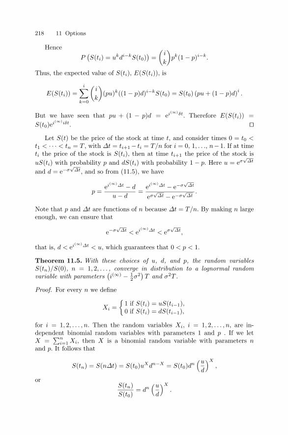
218 11 Options
Hence
P(S(ti) = ukdi−kS(t0)
)=
(i
k
)pk(1 − p)i−k.
Thus, the expected value of S(ti), E(S(ti)), is
E(S(ti)) =i∑
k=0
(i
k
)(pu)k((1 − p)d)i−kS(t0) = S(t0) (pu + (1 − p)d)i
.
But we have seen that pu + (1 − p)d = ei(∞)δt. Therefore E(S(ti)) =S(t0)ei(∞)iδt. ��
Let S(t) be the price of the stock at time t, and consider times 0 = t0 <t1 < · · · < tn = T , with ∆t = ti+1 − ti = T/n for i = 0, 1, . . ., n−1. If at timeti the price of the stock is S(ti), then at time ti+1 the price of the stock isuS(ti) with probability p and dS(ti) with probability 1 − p. Here u = eσ
√∆t
and d = e−σ√
∆t, and so from (11.5), we have
p =ei(∞)∆t − d
u − d=
ei(∞)∆t − e−σ√
∆t
eσ√
∆t − e−σ√
∆t.
Note that p and ∆t are functions of n because ∆t = T/n. By making n largeenough, we can ensure that
e−σ√
∆t < ei(∞)∆t < eσ√
∆t,
that is, d < ei(∞)∆t < u, which guarantees that 0 < p < 1.
Theorem 11.5. With these choices of u, d, and p, the random variablesS(tn)/S(0), n = 1, 2, . . . , converge in distribution to a lognormal randomvariable with parameters
(i(∞) − 1
2σ2)T and σ2T .
Proof. For every n we define
Xi ={
1 if S(ti) = uS(ti−1),0 if S(ti) = dS(ti−1),
for i = 1, 2, . . . , n. Then the random variables Xi, i = 1, 2, . . . , n, are in-dependent binomial random variables with parameters 1 and p . If we letX =
∑ni=1 Xi, then X is a binomial random variable with parameters n
and p. It follows that
S(tn) = S(n∆t) = S(t0)uXdn−X = S(t0)dn(u
d
)X
,
orS(tn)S(t0)
= dn(u
d
)X
.

11.6 Modeling Stock Market Prices 219
Thus,
ln(
S(tn)S(t0)
)= n ln d + X ln
(u
d
).
But,ln d = ln
(e−σ
√∆t
)= −σ
√∆t,
and
ln(u
d
)= ln
(eσ
√∆t
e−σ√
∆t
)= 2σ
√∆t,
so
ln(
S(tn)S(t0)
)= −nσ
√∆t + 2Xσ
√∆t.
We rewrite this as
ln(
S(tn)S(t0)
)= (2p − 1) nσ
√∆t + 2 (X − np) σ
√∆t
= (2p − 1) nσ√
∆t +(X − np)√np (1 − p)
2√
np (1 − p)σ√
∆t.
Now,
p =ei(∞)∆t − d
u − d
=ei(∞)∆t − e−σ
√∆t
eσ√
∆t − e−σ√
∆t
=σ√
∆t + i(∞)∆t − 12σ2∆t
2σ√
∆t+ terms of order ∆t
=12
+i(∞) − 1
2σ2
2σ
√∆t + terms of order ∆t,
so
(2p − 1) nσ√
∆t =
(i(∞) − 1
2σ2
σ
√∆t + terms of order ∆t
)σT√∆t
,
giving
limn→∞ (2p − 1) nσ
√∆t =
(i(∞) − 1
2σ2
)T.
Also, we have
limn→∞ 2
√np (1 − p)σ
√∆t = lim
n→∞ 2√
p (1 − p)σ√
T
= σ√
T .

220 11 Options
From the Binomial Convergence Theorem on p. 273 of Appendix B.4, it followsthat
Zn =(X − np)√np (1 − p)
d−→ Z,
the standard normal random variable. It follows immediately that
ln(
S(tn)S(t0)
)d−→
(i(∞) − 1
2σ2
)T + σ
√TZ,
a normal random variable with mean(i(∞) − 1
2σ2)T and variance σ2T . ��
11.7 Pricing of Options
We now discuss option pricing using binomial trees. We consider a standardbinomial tree with initial stock price S(t0) and initial call option price C (t0).At time t1 the stock price is SU (t1) or SD(t1) with SD(t1) < SU (t1). Theseare the only two possibilities. For a one-step tree, we have CU (t1) and CD(t1)as the call option prices at time t1. We construct a portfolio consisting of ∆shares of the stock and cash in a risk-free investment with a future value of B,which costs ∆S (t0) + Be−i(∞)δt , where i(∞) is the continuously compoundedrisk-free rate of return and δt = t1 − t0.
At time t1 the value of our portfolio is ∆SU (t1) + B if the stock price isSU (t1) and ∆SD(t1) + B if the stock price is SD(t1).
Suppose that we want the value of the portfolio to match the option pricein both cases, that is,
∆SU (t1) + B = CU (t1),∆SD(t1) + B = CD(t1).
Solving for ∆ and B gives
∆ =CU (t1) − CD(t1)SU (t1) − SD(t1)
,
and
B = CU (t1) − CU (t1) − CD(t1)SU (t1) − SD(t1)
SU (t1) =CD(t1)SU (t1) − CU (t1)SD(t1)
SU (t1) − SD(t1).
Because the value of our portfolio at time t1 agrees with the value of thecall option at time t1, we need C(t0) = ∆S(t0) + Be−i(∞)δt . Thus,
C(t0) =CU (t1) − CD(t1)SU (t1) − SD(t1)
S(t0) +(
CD(t1)SU (t1) − CU (t1)SD(t1)SU (t1) − SD(t1)
)e−i(∞)δt .

11.7 Pricing of Options 221
So to hedge we buy (CU (t1) − CD(t1))/(SU (t1) − SD(t1)) shares of thestock and purchase a risk-free investment with face value B.
In this case, it can be shown that
C(t0)ei(∞)δt = pCU (t1) + (1 − p)CD(t1),
with
p =S(t0)ei(∞)δt − SD(t1)
SU (t1) − SD(t1).
Thus, if
0 <S(t0)ei(∞)δt − SD(t1)
SU (t1) − SD(t1)< 1,
then the quantity C(t0)ei(∞)δt can be thought of as the expected value of thecall option price at time t1. Note that this is equivalent to d < ei(∞)δt < u inthe case of a standard binomial tree.
We may also write this as
C(t0) = [pCU (t1) + (1 − p)CD(t1)] e−i(∞)δt , (11.6)
which can be thought of as the expected value of the call option price at timet1, discounted to time t0.
Note that if SD(t1) < SU (t1) and
1δt
ln(
SD(t1)S(t0)
)< i(∞) <
1δt
ln(
SU (t1)S(t0)
),
then 0 < p < 1 holds, that is,
0 <S(t0)ei(∞)δt − SD(t1)
SU (t1) − SD(t1)< 1.
If we do not have a standard binomial tree, that is, the up and down ratiosu and d are not constant, then the transition probabilities may differ.
We now generalize the one-step model to any number of steps. Let ussuppose that we have an n-step standard binomial tree, starting at time t0,with tn being the expiration time of the corresponding call option. Supposethat we also know the stock price at each node of the tree and that we knowthe exercise price of the corresponding call option. We may then calculate thefair price of the call option, as given by (11.6), at every node of the tree.
Consider the tree given previously in Table 11.3 on p. 216, which we re-produce here.

222 11 Options
t0 t1 t2 t3 t4
108.24�
106.12� �
104.04 104.00� � �
102.00 101.96� � � �
Stock Price 100.00 99.96 99.92� � � �
98.00 97.96� � �
96.04 96.00� �
94.12�
92.24t0 t1 t2 t3 t4
8.24�
?� �
? 4.00� � �
? ?� � � �
Call Price ? ? 0.00� � � �
? ?� � �
? 0.00� �
?�
0.00
Note that the call prices at time t4 (expiration) are determined uniquelyby the corresponding stock prices at that time. That is, the call prices at timet4 are S(t4) − 100 if S(t4) > 100 and 0 if S(t4) ≤ 100.
Assuming an exercise price of 100, we use “backward induction” to fill inthe missing values. Consider the call prices at time t3 with i(∞) = 0.05 andδt = 1/12. We need

11.7 Pricing of Options 223
C(t3) = [pCU (t4) + (1 − p)CD(t4)] e−i(∞)δt ,
where e−i(∞)δt = e−1/240. Also,
p =e1/240S(t3) − SD(t4)
SU (t4) − SD(t4).
We next note that because we have a standard binomial tree, this value ofp is the same throughout the tree. In this case, p = 0.6044.
At time t3 we have the following for the top branch: CU (t4) = 8.24 andCD(t4) = 4.00. Hence
C(t3) = [pCU (t4) + (1 − p)CD(t4)] e−i(∞)δt
= [0.6044(8.24) + 0.3956(4.00)] e−1/240
= 6.54.
Similarly, for the second branch from the top, SU (t4) = 104.00, SD(t4) =99.92, CU (t4) = 4.00, and CD(t4) = 0.00. This leads to C(t3) = 2.41. Thebottom two branches have C(t3) = 0. Similarly, at time t2, for the top branchwe have SU (t3) = 106.12, SD(t3) = 101.96, CU (t2) = 6.54, and CD(t2) = 2.41.This yields C(t2) = 4.88.
Completing the calculations yields the following tree:
t0 t1 t2 t3 t4
8.24�
6.54� �
4.88 4.00� � �
3.51 2.41� � � �
2.46 1.45 0.00� � � �
0.87 0.00� � �
0.00 0.00� �
0.00�
0.00
Notice that the call prices satisfy the relationship C(ti) + X ≥ S(ti) (callprice plus exercise price is greater than or equal to the stock price) at eachtime ti. If this were not the case (that is, C(ti)+X < S(ti)), then an investor

224 11 Options
could purchase the call, exercise it, and then sell the stock, for a profit ofS(ti) − (C(ti) + X) > 0, a guaranteed profit.
Notice also that several of the call prices are zero. For example, if the stockdecreases in price in each of the first two time periods, giving a price of $96.04,then the highest possible price at expiration (time t4) is $99.92, which is lessthan the exercise price.
A binomial tree that is not a standard binomial tree is called a flexibletree. Given the stock price at each node and the exercise price, we may stillcalculate the fair price of an option12 if we know the continuously compoundedrisk-free rate of return.
Consider the following example for the stock of company WILD:
t0 t1 t2 t3
115.00�
111.13� �
102.90 101.32� � �
95.00 95.05� � �
92.35 92.13� �
88.95�
85.25
This is a three-step tree. We assume that the continuously compoundedrisk-free rate of return is 4% and that the exercise price is $100. As before,δt = 1/12, so the option expires in three months.
We use the formulas
C(ti) = [pCU (ti+1) + (1 − p)CD(ti+1)] e−i(∞)δt
and
p =S(ti)ei(∞)δt − SD(ti+1)SU (ti+1) − SD(ti+1)
.
We calculate e−i(∞)δt = e−0.04/12 and ei(∞)δt = e0.04/12. At time t3 thevalues of the call options, from top to bottom, are 15.00, 1.32, 0.00, and0.00 because the call option has price equal to the larger of S(t3) − X and0 at expiration. For times t0, t1, t2, and t3 we must recalculate p at each
12 The fair price of an option is the price at which no arbitrage opportunities exist.

11.8 The Black-Scholes Option Pricing Model 225
branch. For example, at time t2 for the upper branch we have S(t2) = 111.13,SU (t3) = 115.00, and SD(t3) = 101.32. Then
p =e0.04/12(111.13) − 101.32
115.00 − 101.32= 0.7442,
andC(t2) = [0.7442(15.00) + 0.2558(1.32)]e−0.04/12 = 11.46.
In Problem 11.26 on p. 241 you are asked to compute the call option pricesfor this tree.
11.8 The Black-Scholes Option Pricing Model
In Theorem 11.5 on p. 218 we investigated a particular binomial model ofstock prices, which in the limit converges to a Geometric Brownian MotionModel, where at each time t the ratio S(t)/S(0) is a lognormal random vari-able with parameters
(i(∞) − 1
2σ2)T and σ2T . In this section we derive the
Black-Scholes formula, which gives the fair (arbitrage-free) price, C(0), of aEuropean call option on a stock using this Geometric Brownian Motion Model.
We point out that, by definition, the natural logarithm of a lognormal ran-dom variable is a normal random variable. However, if this normal randomvariable has expected value µ and variance σ2, then the lognormal randomvariable has expected value eµ+σ2/2. These considerations lead to the lognor-mal random variable
(with parameters
(i(∞) − 1
2σ2)T and σ2T
)as the ap-
propriate one to use. We can show that, under these conditions, S(t) hasa lognormal distribution with E(S(t)) = ei(∞)tS(0). (See Problems 11.29and 11.30.) We now find the fair call option price for a stock, the price ofwhich has this distribution.
In the following the stock price S(t) and the volatility σ > 0 are as inTheorem 11.5 on p. 218. The exercise price is X, the time to expiration is Tin years, and the continuously compounded risk-free rate of return is i(∞).
Derivation of the Black-Scholes Formula
Recall from (11.1) on p. 194, that at time T the price of the stock, S(T ),the price of the call option, C(T ), and the exercise price, X are related by
C(T ) ={
0 if S(T ) ≤ X,S(T ) − X if S(T ) > X,
so13
C(T ) = [S(T ) − X]+ .
13 The function [x]+ is defined to be x if x > 0, and 0 if x ≤ 0.

226 11 Options
In order to find the fair price of the option, C(0), at time14 t = 0 we discountthe expected value of the call option on the expiration date, E(C(T )), usingthe continuously compounded risk-free rate of return, so
C(0) = e−i(∞)T E(C(T )) = e−i(∞)T E([S(T ) − X]+
).
Now,
S(T ) = S(0)S(T )S(0)
= S(0)eln(S(T )/S(0)) = S(0)eW ,
where W = ln(S(T )/S(0)), and thus W is a normal random variable withmean
(i(∞) − 1
2σ2)T , variance σ2T , and density function
f(w) =1√
2πσ2Te− 1
2 (w−(i(∞)− 12 σ2)T)2
/(σ2T ),
for −∞ < w < ∞.Thus, we have
C(0) = e−i(∞)T E([S(T ) − X]+
)= e−i(∞)T E
([S(0)eW − X
]+),
so all that remains is to calculate E([
S(0)eW − X]+)
, which we do now.
We have
E([
S(0)eW − X]+)
=1√
2πσ2T
∫ ∞
−∞
[S(0)eW − X
]+e− 1
2 (w−(i(∞)− 12 σ2)T)2
/(σ2T ) dw.
However, S(0)eW − X ≥ 0 if and only if W ≥ ln (X/(S(0))), so we have
E([
S(0)eW − X]+)
=1√
2πσ2T
∫ ∞
ln(X/S(0))(S(0)ew − X) e− 1
2 (w−(i(∞)− 12 σ2)T)2
/(σ2T ) dw.
This integral is the difference between two integrals, I1 and I2, that is,
E([
S(0)eW − X]+)
= I1 − I2,
where
14 We may always assume that t = 0 (the present time is 0) because it is only thetime remaining until expiration, T , that matters (in addition to S(0), X, i(∞),and σ2) in calculating the fair price of an option.

11.8 The Black-Scholes Option Pricing Model 227
I1 =1√
2πσ2T
∫ ∞
ln(X/S(0))S(0)ewe− 1
2 (w−(i(∞)− 12 σ2)T)2
/(σ2T ) dw
=S(0)√2πσ2T
∫ ∞
ln(X/S(0))ew− 1
2 (w−(i(∞)− 12 σ2)T)2
/(σ2T ) dw,
and15
I2 =1√
2πσ2T
∫ ∞
ln(X/S(0))Xe− 1
2 (w−(i(∞)− 12 σ2)T)2
/(σ2T ) dw,
which we evaluate in turn.
In order to evaluate I1 we set
u =w − (
i(∞) + 12σ2
)T
σ√
T,
so that
w − 12
(w − (
i(∞) − 12σ2
)T)2
σ2T
= −12
−2σ2Tw +(w2 − 2
(i(∞) − 1
2σ2)Tw +
(i(∞) − 1
2σ2)2
T 2)
σ2T
= −12
(w2 − 2
(i(∞) + 1
2σ2)Tw +
(i(∞) + 1
2σ2)2
T 2)
− 2i(∞)σ2T 2
σ2T
= −12u2 + i(∞)T,
givingew− 1
2 (w−(i(∞)− 12 σ2)T)2
/(σ2T ) = e− 12 u2
ei(∞)T .
Substituting this into I1, we find that
I1 = S(0)ei(∞)T 1√2π
∫ ∞
−δ
e− 12 u2
du
= S(0)ei(∞)T (1 − Φ (−δ)) ,
where δ and Φ(x) are given by
δ =
(i(∞) + 1
2σ2)T − ln (X/S(0))
σ√
T,
15 Note that I2 is equal to the exercise price, X, times the probability that theoption is in the money at time T .

228 11 Options
andΦ(x) =
1√2π
∫ x
−∞e−t2/2 dt.
However (see Problem 11.32),
Φ(δ) = 1 − Φ(−δ),
soI1 = S(0)ei(∞)T Φ (δ) .
We now turn to I2. Substituting
v =w − (
i(∞) − 12σ2
)T
σ√
T
into I2 we have
I2 =X√2π
∫ ∞
−δ+σ√
T
e− 12 v2
dv
= X(1 − Φ
(−δ + σ
√T))
= XΦ(δ − σ
√T)
.
Finally, we find that
E([
S(0)eW − X]+)
= ei(∞)T S(0)Φ (δ) − XΦ(δ − σ
√T)
,
which, when substituted into
C(0) = e−i(∞)T E([
S(0)eW − X]+)
,
leads to the famous Black-Scholes formula:
C(0) = S(0)Φ (δ) − Xe−i(∞)T Φ(δ − σ
√T)
, (11.7)
where δ and Φ(x) are given by
δ =
(i(∞) + 1
2σ2)T − ln (X/S(0))
σ√
T, (11.8)
andΦ(x) =
1√2π
∫ x
−∞e−t2/2 dt. (11.9)

11.8 The Black-Scholes Option Pricing Model 229
Significance of the Black-Scholes Formula
The Black-Scholes formula (11.7) gives the price of a European call optionassuming that the price of a stock follows a Geometric Brownian Motion. Thetheory leading to this result is given in [3] and is still of great importance. In1997, Myron Scholes and Robert Merton shared the Nobel prize in Economicsfor its development.16
The Black-Scholes formula (11.7) is a major result for several reasons. Itis one of the results that ushered in the modern theory of finance, which isbased in large part on mathematical reasoning. There are five quantities inthe Black-Scholes pricing formula, of which four are observable, so there isonly one quantity, σ, that needs to be estimated.
Black-Scholes Assumptions
This derivation of the Black-Scholes formula (11.7) depends implicitly on thefollowing two assumptions.
1. The price of the stock follows a Geometric Brownian Motion.As a result of this assumption we have the following consequences.• The continuously compounded risk-free rate of return, i(∞), is con-
stant. The risk-free rate is used to discount the expected value of thecall option on the expiration date. The risk-free rate also appears in theparameter
(i(∞) − 1
2σ2)T of the Geometric Brownian Motion Model,
so if it is not constant, then the assumption that the price of the stockfollows a Geometric Brownian Motion is violated.
• The volatility, σ, is constant. If this constant volatility assumption isnot made, then changes in the value of the option may occur even ifthe stock price is unchanged. This would be a violation of the model.
• The stock price follows a continuous path over time. Otherwise therewould be jumps in the price of the stock, which violates this model.
• There are no dividends during the life of the stock. Dividends are oftenassociated with jumps in the price of the stock. Such jumps violate theassumption that the price of the stock follows a Geometric BrownianMotion.17
• At time t the ratio S(t)/S(0) has a lognormal distribution.2. There are no arbitrage opportunities.
These assumptions are generally not satisfied in the real world. For ex-ample, jumps, occasionally large, in the stock price do occur. However, thesignificance of this result, which provides a mathematical framework for optionpricing, should not be underestimated.16 Fischer Black was deceased when the Nobel Prize was awarded. Robert Merton,
in [19], had developed a similar theory on options during the same time period.17 However, depending on the type of dividend, alternative models are available.

230 11 Options
Comments on the Black-Scholes Formula
• The Black-Scholes formula (11.7) allows us to find an exact solution forthe fair price of the call option, which is one of the surprising propertiesof this model.
• The Black-Scholes formula (11.7) consists of two parts, S(0)Φ(δ) andXe−i(∞)T Φ
(δ − σ
√T). In Problem 11.35 you are asked to show that
Φ(δ) =∂C(0)∂S(0)
.
In Problem 11.36 you are asked to show that Φ(δ − σ
√T)
is the proba-bility that the option is in the money at expiration, that is, S(T ) > X.Thus, the Black-Scholes formula can be interpreted as: C(0) is equal tothe present stock price S(0) times the rate of change of C(0) with respectto S(0) plus the present value of a cash flow equal to X if the option is inthe money at expiration (S(T ) > X) and equal to 0 otherwise.
• The only unobservable quantity, σ, is often estimated from historical data.Another method uses what is called implied volatility. If we know S(0),C(0), X, T , and i(∞), then we can estimate σ from the Black-Scholes for-mula (11.7) because it is the only missing quantity. This requires numericalmethods because there is no analytic solution of (11.7) for σ in terms ofthe remaining quantities.
• Using the Put-Call Parity Theorem on p. 209, we can derive the Black-Scholes price for a European put option, namely
P (0) = −S(0)Φ(−δ) + e−i(∞)T Φ(−δ + σ
√T)
.
(See Problem 11.33.)• Formulas exist for European options on stocks with dividends, and for
some American call options. At the present time there is no known analyticformula for the value of an American put.
• We have only introduced you to the subject of Black-Scholes. There areexcellent books and articles—such as [5] and [7]—which treat this subjectin greater depth.
• To use the Black-Scholes formula (11.7) we must estimate
Φ(x) =1√2π
∫ x
−∞e−t2/2 dt,
for different values of x. Immediately following these comments, we digressto show various ways of doing this. If this is not new to you, please proceedto Example 11.4 on p. 235.

11.8 The Black-Scholes Option Pricing Model 231
Digression on Calculating Φ(x)
To apply the Black-Scholes formula (11.7) we must be able to estimate
Φ(x) =1√2π
∫ x
−∞e−t2/2 dt,
for different values of x. In this section we discuss four different ways of doingthis, depending on the resources available. This is done in the context ofestimating Φ(0.1584), Φ(−0.1245), and 98Φ(0.1584) − 100e−0.025Φ(−0.1245),which are used in Example 11.4.
1. TablesHere we use a look-up table, such as Table B.1 on p. 268 (which has valuesfrom 0.00 to 2.99, in steps of 0.01, to 4 decimal places) or Table 26.1 onp. 966 of [1] (which has values from 0.00 to 2.00, in steps of 0.02, to 15decimal places).The advantage of this method is that all we have to do is to turn to eitherTable B.1 or Table 26.1 in [1] and look up the value of Φ(0.1584). Thedisadvantage is that 0.1584 is not one of the entries in either table. Sowhat do we do? We round 0.1584 to the nearest entry in the table. Wenow perform the calculations using both tables and denote these estimatesby ΦT1(x) and ΦT2(x).(a) The nearest entry in Table B.1 to 0.1584 is 0.16, so we estimate that
ΦT1(0.1584) ≈ Φ(0.16) = 0.5636.
There is a further disadvantage when we try to estimate Φ(−0.1245)because negative values are not in this table (nor in Table 26.1 of [1]).In this case we need to use the identity (see Problem 11.32)
Φ(−x) = 1 − Φ(x),
so thatΦ(−0.1245) = 1 − Φ(0.1245).
Again 0.1245 is not one of the entries in Table B.1, so we round 0.1245to the nearest entry in this table, which is 0.12, and estimate that
ΦT1(0.1245) ≈ Φ(0.12) = 0.5478,
soΦT1(−0.1245) ≈ 1 − 0.5478 = 0.4522.
Thus,98Φ(0.1584) − 100e−0.025Φ(−0.1245) ≈ 11.1293.

232 11 Options
(b) The nearest entry in Table 26.1 of [1] to 0.1584 is 0.16, so we estimatethat
ΦT2(0.1584) ≈ Φ(0.16) = 0.563559462891433.
To estimate Φ(−0.1245) we again use the identity
Φ(−0.1245) = 1 − Φ(0.1245).
Once more 0.1245 is not one of the entries in Table 26.1, so we round0.1245 to the nearest entry on this table, which is 0.12, and estimatethat
ΦT2(0.1245) ≈ Φ(0.12) = 0.547758426020584,
so
ΦT2(−0.1245) ≈ 1 − 0.547758426020584 = 0.452241573979416.
Thus,
98Φ(0.1584) − 100e−0.025Φ(−0.1245) ≈ 11.121258390018500.
2. Linear InterpolationHere we use one of the tables mentioned in the first part, together with lin-ear interpolation described by (6.7) on p. 95. We now perform the calcula-tions using both tables and denote these estimates by ΦLI1(x) and ΦLI2(x).(a) From Table B.1, we see that the nearest entries on either side of 0.1584
are 0.15 and 0.16, with Φ(0.15) = 0.5596 and Φ(0.16) = 0.5636. Us-ing (6.7) with l = 0.1584, a = 0.15, and b = 0.16, gives
ΦLI1(0.1584) =0.16 − 0.15840.16 − 0.15
Φ(0.15) +0.1584 − 0.150.16 − 0.15
Φ(0.16)
= 0.16(0.5596) + 0.84(0.5636)= 0.56296.
In the same way
ΦLI1(−0.1245) = 1 − ΦLI1(0.1245)
= 1 −(
0.13 − 0.12450.13 − 0.12
Φ(0.12) +0.1245 − 0.120.13 − 0.12
Φ(0.13))
= 1 − 0.55(0.5478) − 0.45(0.5517)= 0.450445.
Thus,98Φ(0.1584) − 100e−0.025Φ(−0.1245) ≈ 11.2377.

11.8 The Black-Scholes Option Pricing Model 233
(b) From Table 26.1 of [1], we see that the nearest entries on either sideof 0.1584 are 0.14 nd 0.16, with Φ(0.14) = 0.555670004805907 andΦ(0.16) = 0.563559462891433. Using (6.7) with l = 0.1584, a = 0.14,and b = 0.16, gives
ΦLI2(0.1584) =0.16 − 0.15840.16 − 0.14
Φ(0.15) +0.1584 − 0.140.16 − 0.14
Φ(0.16)
= 0.08(0.555670004805907) + 0.92(0.563559462891433)= 0.562928306244591.
In the same way
ΦLI2(−0.1245) = 1 − ΦLI2(0.1245)
= 1 −(
0.14 − 0.12450.14 − 0.12
Φ(0.12) +0.1245 − 0.120.14 − 0.12
Φ(0.14))
= 1 − 0.775(0.547758426020584)− 0.225(0.555670004805907)
= 0.450461468752718.
Thus,
98Φ(0.1584) − 100e−0.025Φ(−0.1245) ≈ 11.233020465833200.
Because Φ(x) is positive for all x and concave down for x > 0 (seeProblem 11.32), we can use the comments following Theorem 6.4on p. 96 to conclude that ΦLI2(0.1584) is an underestimate forΦLI2(0.1584), that is,
ΦLI2(0.1584) = 0.562928306244591 < Φ(0.1584).
Also, because Φ(x) is concave up for x < 0, the value of ΦLI2(−0.1245)is an overestimate for Φ(−0.1245), that is,
ΦLI2(−0.1245) = 0.450461468752718 > Φ(−0.1245).
Finally, because
ΦLI2(0.1584) < Φ(0.1584) and − ΦLI2(−0.1245) < −Φ(−0.1245),
we see that
98ΦLI2(0.1584) − 100e−0.025ΦLI2(−0.1245)< 98Φ(0.1584) − 100e−0.025Φ(−0.1245),
so 11.233020465833200 is an underestimate, that is,
11.233020465833200 < 98Φ(0.1584) − 100e−0.025Φ(−0.1245).

234 11 Options
3. Numerical ApproximationsHere we use a numerical approximation. There are various formulas usedto approximate the value of Φ(x) (see p. 932 of [1]). We present two, whichwe denote by ΦNA1(x) and ΦNA2(x).(a) The first approximation is
ΦNA1(x) = 1 − e−x2/2√
2π
(a1t + a2t
2 + a3t3) ,
wheret =
11 + px
,
with p = 0.33267, a1 = 0.4361836, a2 = −0.1201676, and a3 =0.9372980. This approximation has an error of less than 1.0 × 10⁻⁵.Using this numerical approximation we find that
ΦNA1(0.1584) = 0.5629382,
ΦNA1(−0.1245) = 0.4503966,
98Φ(0.1584) − 100e−0.025Φ(−0.1245) ≈ 11.2403182.
(b) The second approximation is
ΦNA2(x) = 1 − e−x2/2√
2π
(b1t + b2t
2 + b3t3 + b4t
4 + b5t5) ,
wheret =
11 + px
,
with p = 0.2316419, b1 = 0.319381530, b2 = −0.356563782, b3 =1.781477937, b4 = −1.821255978, and b5 = 1.330274429. This approx-imation has an error of less than 7.5 × 10⁻⁸,Using this numerical approximation we find that
ΦNA2(0.1584) = 0.56292921,
ΦNA2(−0.1245) = 0.45045863,
98ΦNA2(0.1584) − 100e−0.025ΦNA2(−0.1245) = 11.23338582.
4. ExactHere we use an “Exact” result using either a spreadsheet or a sophisticatedscientific or financial calculator. We denote this value by ΦE(x).In Microsoft� Excel, the command NORMSDIST (x) calculates Φ(x).Using this we find that
ΦE(0.1584) = 0.56292920,
ΦE(−0.1245) = 0.45045966,
98Φ(0.1584) − 100e−0.025Φ(−0.1245) ≈ 11.23328500.

11.8 The Black-Scholes Option Pricing Model 235
Notice that, as expected when compared to the linear interpolation esti-mates,
ΦLI2(0.1584) < ΦE(0.1584),
ΦLI2(−0.1245) > ΦE(−0.1245),
and
98ΦLI2(0.1584) − 100e−0.025ΦLI2(−0.1245)< 98ΦE(0.1584) − 100e−0.025ΦE(−0.1245).
Table 11.4 compares these approximations, rounded to 4 decimal places.Now that we can estimate Φ(x) we can use the Black-Scholes formula (11.7).
Table 11.4. Comparison of Different Estimates for Φ(x)
Φ(0.1584) Φ(−0.1245) 98Φ(0.1584) − 100e−0.025Φ(−0.1245)T1 0.5636 0.4522 11.1293T2 0.5636 0.4522 11.1213LI1 0.5630 0.4504 11.2377LI2 0.5629 0.4505 11.2330NA1 0.5629 0.4504 11.2403NA2 0.5629 0.4505 11.2334E 0.5629 0.4505 11.2333
Example 11.4. If the current price of the stock is $98, if the exercise price fora European call option on this stock is $100, if the time to expiration is 0.5(one-half year), if the continuously compounded risk-free annual rate of returnis 5%, and if the volatility is 0.4, then use the Black-Scholes formula (11.7) tofind a fair price for the option.
Solution. Here S(0) = 98, X = 100, T = 0.5, i(∞) = 0.05, and σ = 0.4.From (11.8) we have
δ =
(0.05 + 1
2 (0.16))0.50 − ln (100/98)
0.40√
0.50≈ 0.1584,
andδ − σ
√T ≈ −0.1245,
soC(0) = 98Φ(0.1584) − 100e−0.025Φ(−0.1245).
These are exactly the values we’ve used to estimate Φ in Table 11.4. Thus,the values we find for Φ(0.1584) and Φ(−0.1245), which determine the valueof C(0), depend on which of the estimates in Table 11.4 we use.
If we use Table B.1, then we find that C(0) ≈ 11.13, so the option shouldcost approximately $11.13, whereas if we use the “exact” calculation, then wefind that C(0) ≈ 11.23, so the option should cost approximately $11.23. �
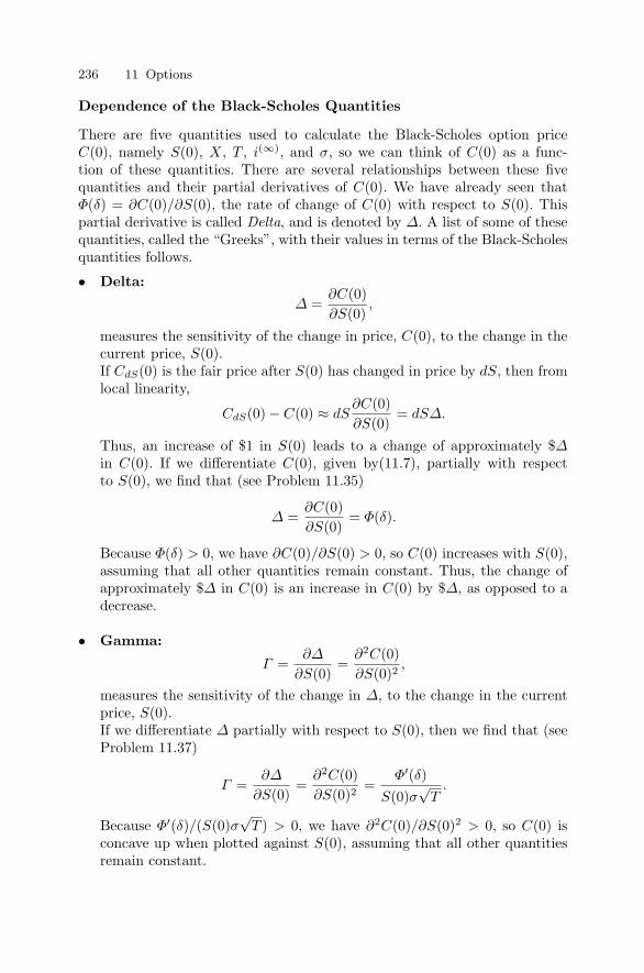
236 11 Options
Dependence of the Black-Scholes Quantities
There are five quantities used to calculate the Black-Scholes option priceC(0), namely S(0), X, T , i(∞), and σ, so we can think of C(0) as a func-tion of these quantities. There are several relationships between these fivequantities and their partial derivatives of C(0). We have already seen thatΦ(δ) = ∂C(0)/∂S(0), the rate of change of C(0) with respect to S(0). Thispartial derivative is called Delta, and is denoted by ∆. A list of some of thesequantities, called the “Greeks”, with their values in terms of the Black-Scholesquantities follows.
• Delta:
∆ =∂C(0)∂S(0)
,
measures the sensitivity of the change in price, C(0), to the change in thecurrent price, S(0).If CdS(0) is the fair price after S(0) has changed in price by dS, then fromlocal linearity,
CdS(0) − C(0) ≈ dS∂C(0)∂S(0)
= dS∆.
Thus, an increase of $1 in S(0) leads to a change of approximately $∆in C(0). If we differentiate C(0), given by(11.7), partially with respectto S(0), we find that (see Problem 11.35)
∆ =∂C(0)∂S(0)
= Φ(δ).
Because Φ(δ) > 0, we have ∂C(0)/∂S(0) > 0, so C(0) increases with S(0),assuming that all other quantities remain constant. Thus, the change ofapproximately $∆ in C(0) is an increase in C(0) by $∆, as opposed to adecrease.
• Gamma:
Γ =∂∆
∂S(0)=
∂2C(0)∂S(0)2
,
measures the sensitivity of the change in ∆, to the change in the currentprice, S(0).If we differentiate ∆ partially with respect to S(0), then we find that (seeProblem 11.37)
Γ =∂∆
∂S(0)=
∂2C(0)∂S(0)2
=Φ′(δ)
S(0)σ√
T.
Because Φ′(δ)/(S(0)σ√
T ) > 0, we have ∂2C(0)/∂S(0)2 > 0, so C(0) isconcave up when plotted against S(0), assuming that all other quantitiesremain constant.

11.8 The Black-Scholes Option Pricing Model 237
• Theta:
Θ =∂C(0)
∂T,
measures the sensitivity of the change in price, C(0), to the change in thetime until the expiration date, T , of the option.18
If we differentiate C(0), given by(11.7), partially with respect to T , thenwe find that (see Problem 11.38)
Θ =∂C(0)
∂T=
S(0)σ2√
TΦ′(δ) + i(∞)Xe−i(∞)T Φ(δ − σ
√T ).
Because the right-hand side is positive, we have ∂C(0)/∂T > 0, so C(0)increases with T , assuming that all other quantities remain constant. Thus,a decrease of one day in T , the time until expiration, leads to a decreaseof approximately $Θ/365 in C(0).
• rho:
ρ =∂C(0)∂i(∞) ,
measures the sensitivity of the change in price, C(0), to the change in thecontinuously compounded risk-free rate of return, i(∞).If we differentiate C(0), given by(11.7), partially with respect to i(∞), thenwe find that (see Problem 11.39)
ρ =∂C(0)∂i(∞) = XT e−i(∞)T Φ(δ − σ
√T ).
Because the right-hand side is positive, we have ∂C(0)/∂i(∞) > 0, so C(0)increases with i(∞), assuming that all other quantities remain constant.Thus, an increase of 0.01 in i(∞) leads to an increase of approximately$0.01ρ in C(0).
• Vega:19
V =∂C(0)
∂σ,
measures the sensitivity of the change in price, C(0), to the change in thevolatility of the stock, σ.If we differentiate C(0), given by(11.7), partially with respect to σ, thenwe find that (see Problem 11.40)
V =∂C(0)
∂σ= S(0)
√TΦ′(δ).
18 Theta is sometimes defined by Θ = −∂C(0)/∂T .19 This partial derivative is not named after a Greek letter, but after the brightest
star in the constellation Lyra.

238 11 Options
Because the right-hand side is positive, we have ∂C(0)/∂σ > 0, so C(0)increases with σ, assuming that all other quantities remain constant. Thus,an increase of 1 in σ leads to an increase of approximately $V in C(0).
From these equations we obtain the following condition on some of theGreeks:
−Θ +12σ2S2(0)Γ + i(∞)S(0)∆ − i(∞)C(0) = 0.
(See Problem 11.47.) If we replace the Greeks with their partial derivatives,then we obtain the partial differential equation
−∂F
∂T+
12σ2S2(0)
∂2F
∂S(0)2+ i(∞)S(0)
∂F
∂S(0)− i(∞)F = 0, (11.10)
the solution, F , of which gives the fair price of a call option,20 F = C(0), orput option,21 F = P (0), in terms of the stock price S(0), the exercise price X,the time to expiration T , the continuously compounded rate of return i(∞),and the volatility σ > 0.
You may have wondered why ∂C(0)/∂X is not among the Greeks. It isbecause the quantity X is constant during the life of an option. It is specifiedin the contract when written. Therefore, the sensitivity of C(0) to changesin X is of no practical significance to buyers and sellers of options. However,it can still be evaluated mathematically, and you are asked to do this inProblem 11.41. As a consequence of this, we see that C(0) is a decreasingfunction of X. Explain why this is not unexpected.
11.9 Problems
Walking
11.1. Verify that P (T ) ={
0 if S(T ) ≥ X,X − S(T ) if S(T ) < X.
11.2. Prove (11.4) on p. 196.20 Subject to the boundary condition
F (T ) ={
0 if S(T ) ≤ X,S(T ) − X if S(T ) > X.
21 Subject to the boundary condition
F (T ) ={
0 if S (T ) ≥ X,X − S (T ) if S (T ) < X.

11.9 Problems 239
11.3. Draw the profit-loss diagram for Helen’s purchase of puts described onp. 200.
11.4. Prove the profit per share formula for writing uncovered calls on p. 202.Confirm that Fig. 11.6 is correct.
11.5. Prove the profit per share formula for writing covered calls on p. 203,and draw the corresponding profit-loss diagram.
11.6. Prove the profit per share formula for writing uncovered puts on p. 204.Confirm that Fig. 11.9 is correct.
11.7. Prove the profit per share formula for writing covered puts on p. 206.Confirm that Fig. 11.11 is correct.
11.8. Referring to the stock MOVE on p. 207, create a profit-loss diagram fora writer of a straddle for MOVE.
11.9. Prove the profit per share formula for writing straddles on p. 208. Con-firm that Fig. 11.13 is correct.
11.10. Verify that if C + Xe−i(∞)T > S(0) + P , then the position discussedon p. 210 creates an arbitrage opportunity.
11.11. BIG1 is currently trading at $100 per share. A put on BIG1 costs$7, the exercise price is $105, the time until expiration is 6 months, and thecontinuously compounded risk-free rate of return is 4%. What should the priceof a call option be to satisfy the put-call parity relationship?
11.12. Let X = $100, C = $8, P = $2, S(0) = $105, i(∞) = 0.05, and T = 1(one year). Does the Put-Call Parity relationship hold? If not, describe anarbitrage portfolio that would generate a guaranteed positive profit. What isthe amount of the profit?
11.13. Describe the arbitrage portfolio that one can create if
C + Xe−i(∞)T > S(0) + P.
11.14. There is a more general put-call parity relationship for European op-tions in the case of dividends. The condition is
C + PV (X) + PV (dividends) = S(0) + P.
Here PV stands for the present value. Assume that only one dividend paymentis made, for D dollars, at expiration. Derive the appropriate relationship inthis case.

240 11 Options
11.15. The Put-Call Parity Theorem on p. 209 holds for European options,where the option can only be exercised at expiration. Are there any caseswhere a violation of the put-call parity relationship gives an arbitrage op-portunity for American options? [Hint: Recall that American call options arenever exercised early, whereas American put options may be exercised in cer-tain cases.]
11.16. Referring to the example on p. 212 with GOUP stock, and assumingthe same conditions, suppose that we have a put option on GOUP with thesame exercise price ($75) and expiration time (one year) as the call option.Create a portfolio consisting of ∆∗ shares of GOUP stock and B dollars ofcash, discounted to the present time, which has the same payoff as a portfolioconsisting of one put option.
11.17. Prove that
∆ =CU − CD
SU − SD, and B =
CUSD − CDSU
SU − SD.
(See p. 213.)
11.18. Verify that the hedge ratio for a call option can never be negative.What is the value of ∆ when both SD < X and SU < X? What conclusionsdo you infer from this answer?
11.19. Verify the values for the binomial tree in Example 11.3 on p. 216.
11.20. This problem is based on Example 11.3 on p. 216. Assume that p = 0.6.If the stock decreases in price for the first two months, so that its price aftertwo months is $96.04, then what is the expected price at expiration? [Hint:The possible prices at expiration are $99.92, $96.00, and $92.24. Calculate theprobabilities of attaining these prices and consider the appropriate randomvariable.]
11.21. Prove that
p =S(t0)ei(∞)δt − SD(t1)
SU (t1) − SD(t1),
for the standard binomial tree.
11.22. Consider an n-step standard binomial tree with initial stock priceS (t0) = $200. Suppose that the expected value of the stock price after onemonth is E(S (t1)) = $201.
(a) What is the expected value of the stock price after six months?(b) What is the expected value of the stock price after one year?(c) What is the continuously compounded rate of return?(d) What is the annually compounded rate of return?(e) What is the semi-annually compounded rate of return?

11.9 Problems 241
Running
11.23. For the standard binomial tree, let p = 0.5, 0 < d ≤ u, with u = 1/d(so that ud = 1) and an initial stock price of S(t0).
(a) What is the expected value of S(t1), E(S(t1))?(b) What is the smallest possible value of E(S(t1))?
11.24. Consider the standard binomial tree for the limiting case with d = 0.
(a) What is the value of E(S(tn)), n ≥ 1?(b) What are the possible values of limn→∞ E(S(tn))?(c) Under what conditions is limn→∞ E(S(tn)) = 0?
11.25. Verify the call option prices for the tree on p. 222.
11.26. Calculate the call option prices for the tree discussed on p. 224.
11.27. In Problem A.4 on p. 252 you are asked to prove that for any two realnumbers x and y, and n a positive integer,
(x + y)n =n∑
k=0
(n
k
)xkyn−k.
How does this result relate to the binomial distribution?
11.28. Consider the following three-step binomial tree for the stock of com-pany SLOW. Assume that the exercise price is $200 and that the continuouslycompounded rate of return is 8%. Create the corresponding tree for the calloption. What can you say about the values of p?
208.50�
202.40� �
201.00 201.20� � �
200.00 200.50� � �
199.00 198.53� �
197.32�
195.00
11.29. Let X be a lognormal random variable with Y = lnX having a normaldistribution with mean µ and variance σ2. Show that E(X) = eµ+σ2/2 and
σ2X = e2µ+2σ2 − e2µ+σ2
.
(See p. 225.)

242 11 Options
11.30. Show that S(t) has a lognormal distribution, with E(S(t)) = ei(∞)tS(0).(See p. 225.)
11.31. What should the Black–Scholes option price be in (11.7) on p. 228, ifwe let T = 0 but do not change the other values? Verify this by taking thelimit as T approaches 0 of δ (with the other values fixed) in the three casesX < S(0), X = S(0), and X > S(0). (Note that Φ (∞) = 1, Φ (−∞) = 0.)
11.32. Show thatΦ(x) =
1√2π
∫ x
−∞e−t2/2 dt,
is defined for all x and has the following properties:
(a) Φ(x) > 0.(b) Φ(−x) = 1 − Φ(x).(c) Φ(x) is an increasing function.(d) Φ(x) is concave down for x > 0, and concave up for x < 0.
11.33. Prove
P (0) = −S(0)Φ(−δ) + e−i(∞)T Φ(−δ + σ
√T)
.
(See p. 230.)
11.34. If
δ =
(i(∞) + 1
2σ2)T − ln (X/S(0))
σ√
T,
(see (11.8) on p. 228), then show that
S(0)Φ′(δ) − Xe−i(∞)T Φ′(δ − σ√
T ) = 0.
[Hint: Start with ln(Φ′(δ)/Φ′(δ − σ
√T )
).]
11.35. Show that
Φ(δ) =∂C(0)∂S(0)
.
(See p. 230.) [Hint: Use Problem 11.34.]
11.36. Show that Φ(δ − σ
√T)
is equal to the probability that the option isin the money at expiration, that is, S(T ) > X. (See p. 230.)
11.37. Show that∂2C(0)∂S(0)2
=Φ′(δ)
S(0)σ√
T.
(See p. 236.)

11.9 Problems 243
11.38. Show that
∂C(0)∂T
=S(0)σ2√
TΦ′(δ) + i(∞)Xe−i(∞)T Φ(δ − σ
√T ).
(See p. 237.)
11.39. Show that
∂C(0)∂i(∞) = XT e−i(∞)T Φ(δ − σ
√T ).
(See p. 237.)
11.40. Show that∂C(0)
∂σ= S(0)
√TΦ′(δ).
(See p. 237.)
11.41. Show that∂C(0)∂X
= −e−i(∞)T Φ(δ − σ√
T ).
(See p. 238.)
11.42. Suppose, in Example 11.4 on p 235, that we change S(0) from $98 to$102 but do not change the other four values. Calculate the new Black-Scholesoption price. Does this agree with your intuition? Verify this by calculatingthe Greek ∆ for this example.
11.43. Change X from $100 to $99 in (11.7) on p. 228 and proceed as inProblem 11.42 using the appropriate Greek.
11.44. Change i(∞) from 0.05 to 0.10 in (11.7) on p. 228. Calculate the newBlack–Scholes option price. Does this agree with your intuition? Verify thisby calculating ρ for this example.
11.45. Change T from 0.50 to 0.25 in (11.7) on p. 228 and proceed as inProblem 11.44 using the appropriate Greek.
11.46. Change σ from 0.4 to 0.5 in (11.7) on p. 228 and proceed as in Prob-lem 11.44 using the appropriate Greek. (Intuition may not work in this case.)
11.47. Show that
−Θ +12σ2S2(0)Γ + i(∞)S(0)∆ − i(∞)C(0) = 0,
and that
−∂C(0)∂T
+12σ2S2(0)
∂2C(0)∂S(0)2
+ i(∞)S(0)∂C(0)∂S(0)
− i(∞)C(0) = 0.
(See p. 238.)

244 11 Options
11.48. Show that the Black-Scholes formula
C(0) = S(0)Φ (δ) − Xe−i(∞)T Φ(δ − σ
√T)
,
where
δ =
(i(∞) + 1
2σ2)T − ln (X/S(0))
σ√
T,
where 0 is always the current time (fixed) and T is the time remaining toexpiration (variable), can be written in the form
C(t) = S(t)Φ (δ∗) − Xe−i(∞)(T ∗−t)Φ(δ∗ − σ
√T ∗ − t
),
where
δ∗ =
(i(∞) + 1
2σ2)(T ∗ − t) − ln (X/S(t))σ√
T ∗ − t,
where t is the current time (variable) and T ∗ is the expiration date (fixed).
11.49. Show, under the conditions of Problem 11.48, that the Black-Scholespartial differential equation (11.10) is
∂F
∂t+
12σ2S2(t)
∂2F
∂S(t)2+ i(∞)S(t)
∂F
∂S(t)− i(∞)F = 0.
Questions for Review
• What is a call option?• What is a put option?• How do the price of the stock and time to expiration affect the price of a
call (put) option?• What is a covered call?• What is a covered put?• What does the Put-Call Parity Theorem say?• What does the Hedge Ratio Theorem say?• What is a binomial tree?• Explain arbitrage.• What does the Black-Scholes Theorem say? What conditions are assumed?• What are the Greeks and what do they measure?

A
Appendix: Induction, Recurrence Relations,Inequalities
A.1 Mathematical Induction
Mathematical induction is a technique used to prove a proposition that in-volves an integer variable. Frequently the proposition is an identity or aninequality involving an integer n such as
1 + 2 + 4 + · · · + 2n−1 = 2n − 1 for n = 1, 2, . . . ,
orn2 > 2n + 1 for n = 3, 4, . . . .
In both cases, we have a proposition, P (n), that must be proved for n ≥ n0.The technique of mathematical induction requires two steps.
1. Prove that P (n) is true for the first value of n, namely, n = n0. This isthe basic step.
2. Assume that P (k) is true and prove that, as a consequence of this, P (k+1)is true. This is the inductive step.
If both of these steps are proved, then P (n) is true for n ≥ n0 by thefollowing reasoning. From the basic step we know that P (n0) is true. Now,from the inductive step with k = n0 we know that P (n0) being true requiresthat P (n0 + 1) is true. We use this and the inductive step again to show thatP (n0 + 2) is true, and so on.
Example A.1. Show by induction that
1 + 2 + 4 + · · · + 2n−1 = 2n − 1 for n = 1, 2, . . . .
Solution. Here n0 = 1 and the proposition P (n) is 1+2+4+· · ·+2n−1 = 2n−1.Basic Step: We must show that P (n0), that is, P (1) is true. The statementP (1) is the proposition that 1 = 21 − 1, which is clearly true.

246 A Appendix: Induction, Recurrence Relations, Inequalities
Inductive Step: We must show that P (k + 1) is true as a consequence ofP (k) being true, that is, we must show that
1 + 2 + 4 + · · · + 2k = 2k+1 − 1
is a consequence of
1 + 2 + 4 + · · · + 2k−1 = 2k − 1.
Now,
1 + 2 + 4 + · · · + 2k = 1 + 2 + 4 + · · · + 2k−1 + 2k
= (1 + 2 + 4 + · · · + 2k−1) + 2k
= (2k − 1) + 2k
= 2k+1 − 1.
By mathematical induction, the equality is valid for all integers n ≥ 1. �Example A.2. Show by induction that
n2 > 2n + 1 for n = 3, 4, . . . .
Solution. Here n0 = 3 and the proposition P (n) is n2 > 2n + 1.Basic Step: We must show that P (n0), that is, P (3) is true. The statementP (3) is the proposition that 32 > 2 × 3 + 1, that is, 9 > 7, which is clearlytrue.Inductive Step: We must show that P (k + 1) is true as a consequence ofP (k) being true, that is, we must show that
(k + 1)2 > 2(k + 1) + 1
is a consequence ofk2 > 2k + 1.
Now,
(k + 1)2 = k2 + 2k + 1> (2k + 1) + 2k + 1= 2k + (2k + 2)> 2k + 3= 2(k + 1) + 1.
By mathematical induction, the inequality is valid for all integers n ≥ 3.�
The process of mathematical induction is frequently compared to an in-finite line of dominoes that has the property that if the nth domino falls sodoes the next one. This is the inductive step, and no dominoes fall until oneof them, the nth
0 , falls. This is the basic step. If the nth0 domino falls, then so
do all the dominos for which n ≥ n0.

A.2 Recurrence Relations 247
A.2 Recurrence Relations
Definition A.1. A recurrence relation among P0, P1, P2, . . ., is anequation of the type
Pn+m = f(Pn, Pn+1, . . . , Pn+m−1),
so Pn+m is determined by its previous m terms.
Comments About Recurrence Relations
• Recurrence relations are also called finite difference equations.• The positive integer m is the order of the recurrence relation. For exam-
ple, the recurrence relation
Pn+2 =(n + 1)Pn
(n + 3), n = 0, 1, 2, . . . ,
is a second order recurrence relation.• There is no general way to solve recurrence relations. However, a first order
recurrence relation can be solved if it can be rewritten in the form
Qn = Qn−1, n = 1, 2, . . . .
In this form we sum both sides from 1 to N , giving
N∑n=1
Qn =N∑
n=1
Qn−1.
Canceling the common terms on both sides gives
QN = Q0,
so the recurrence relation Qn = Qn−1 has solution Qn = Q0.(An alternative way to show this from Qn = Qn−1 is to realize that thisimplies that Q1 = Q0, that Q2 = Q1, and so on, so that
Qn = Qn−1 = Qn−2 = · · · = Q2 = Q1 = Q0,
and so the solution is Qn = Q0.)
Example A.3. Solve the following recurrence relations (n = 1, 2, . . .).
(a) Pn = −Pn−1(b)Pn = aPn−1, where a is constant(c) nPn = Pn−1(d)Pn = (n + 1)Pn−1(e) Pn = Pn−1 + a, where a = 0 is constant(f) Pn = Pn−1 + ban, where a = 0, b = 0 are constants

248 A Appendix: Induction, Recurrence Relations, Inequalities
Solution.
(a) The recurrence relationPn = −Pn−1
can be rewritten in the form (−1)nPn = (−1)n−1Pn−1, that is, Qn = Qn−1with Qn = (−1)nPn. This has the solution Qn = Q0, that is, (−1)nPn =(−1)0P0, so Pn = (−1)nP0.
(b) The recurrence relationPn = aPn−1
can be rewritten in the form Pn/an = Pn−1/an−1, that is, Qn = Qn−1 withQn = Pn/an. This has the solution Qn = Q0, that is, Pn/an = P0/a0, soPn = anP0.
(c) The recurrence relationnPn = Pn−1
can be rewritten in the form n!Pn = (n − 1)!Pn−1, that is, Qn = Qn−1with Qn = n!Pn. This has the solution Qn = Q0, that is, n!Pn = 0!P0, soPn = P0/n!.
(d) The recurrence relation
Pn = (n + 1)Pn−1
can be rewritten in the form Pn/(n + 1)! = Pn−1/n!, that is, Qn = Qn−1with Qn = Pn/(n + 1)!. This has the solution Qn = Q0, that is, Pn/(n +1)! = P0/1!, so Pn = (n + 1)!P0.
(e) The recurrence relationPn = Pn−1 + a
can be rewritten in the form Pn −a = Pn−1 or Pn −na = Pn−1 − (n−1)a,that is, Qn = Qn−1 with Qn = Pn − na. This has the solution Qn = Q0,that is, Pn − na = P0 − 0a, so Pn = na + P0.
(f) The recurrence relationPn = Pn−1 + ban
can be rewritten in the form Pn − ban = Pn−1, or
Pn − ban − b
n−1∑i=0
ai = Pn−1 − b
n−1∑i=0
ai,
or
Pn − b
n∑i=0
ai = Pn−1 − b
n−1∑i=0
ai,
that is, Qn = Qn−1 with Qn = Pn − b∑n
i=0 ai. This has the solutionQn = Q0, that is, Pn − b
∑ni=0 ai = P0 − b, so Pn = b
∑ni=0 ai + P0 − b =
b∑n
i=1 ai + P0.
�

A.3 Inequalities 249
A.3 Inequalities
Theorem A.1. Arithmetic-Geometric Mean Inequality.If a1, a2, . . . , an are non-negative and not all zero, then
(a1a2 · · · an)1/n ≤ a1 + a2 + · · · + an
n,
with equality if and only if a1 = a2 = · · · = an.
Proof. The proof of the Arithmetic-Geometric Mean Inequality proceeds intwo stages. First, we prove it by induction for n = 2m, namely,
(a1a2 · · · a2m)1/2m ≤ a1 + a2 + · · · + a2m
2m
and then we fill in the missing n’s.With m = 1 we want to show that
(a1a2)1/2 ≤ a1 + a2
2.
However, from (a1 − a2)2 ≥ 0, we have a2
1 +a22 ≥ 2a1a2, which is the required
inequality. Equality occurs if and only if a1 = a2.We assume that this is valid for m and show that it is true for m+1, that
is, we want to show that
(a1a2 · · · a2m+1)1/2m+1 ≤ a1 + a2 + · · · + a2m+1
2m+1 ,
with equality if and only if a1 = a2 = · · · = a2m+1 .Now,
(a1a2 · · · a2m+1)1/2m+1
=[(a1a2 · · · a2m)1/2m
(a2m+1a2m+2 · · · a2m+1)1/2m]1/2
.
But, [(a1a2 · · · a2m)1/2m
(a2m+1a2m+2 · · · a2m+1)1/2m]1/2
≤[(
a1+a2+···+a2m
2m
) (a2m+1+a2m+2+···+a2m+1
2m
)]1/2,
with equality if and only if a1 = a2 = · · · = a2m and a2m+1 = a2m+2 = · · · =a2m+1. Now, [(
a1+a2+···+a2m
2m
) (a2m+1+a2m+2+···+a2m+1
2m
)]1/2
≤ 12
[(a1+a2+···+a2m
2m
)+
(a2m+1+a2m+2+···+a2m+1
2m
)],
with equality if and only if a1+a2+· · ·+a2m = a2m+1+a2m+2+· · ·+a2m+1 . Thisis the desired inequality, with equality if and only if a1 = a2 = · · · = a2m+1.

250 A Appendix: Induction, Recurrence Relations, Inequalities
Now, consider the case when n = 2m. Then choose an+1 = an+2 = · · · =a2m = A, where
A =a1 + a2 + · · · + an
n.
Thus,(a1a2 · · · anA2m−n
)1/2m
≤ a1 + a2 + · · · + an + (2m − n) A
2m= A,
ora1a2 · · · anA2m−n ≤ A2m
,
that is,a1a2 · · · an ≤ An.
Equality occurs if and only if a1 = a2 = · · · = an.This completes the proof. ��
Theorem A.2. (1 +
r
n − 1
)n−1
<(1 +
r
n
)n
.
Proof. To prove this we use the Arithmetic-Geometric Mean Inequality witha1 = 1 , a2 = a3 = · · · = an = 1 + r/(n − 1), which gives[
1(
1 +r
n − 1
)n−1]1/n
≤1 + (n − 1)
(1 + r
n−1
)n
,
or [(1 +
r
n − 1
)n−1]1/n
≤ n + r
n= 1 +
r
n.
��Theorem A.3. Cauchy-Schwarz Inequality.(
n∑i=1
aibi
)2
≤(
n∑i=1
a2i
)(n∑
i=1
b2i
),
with equality if and only if either ai = λbi for some constant λ or bi = 0 forall i.
Proof. The Cauchy-Schwarz inequality is obviously true if b1 = b2 = · · · =bn = 0, so we concentrate on the case when not all bi are zero, in which case∑n
j=1 b2j = 0. Consider, with
λ =
∑nj=1 ajbj∑nj=1 b2
j
,

A.3 Inequalities 251
the quantity
0 ≤n∑
i=1
(ai − λbi)2 =
n∑i=1
a2i − 2λ
n∑i=1
aibi + λ2n∑
i=1
b2i .
Clearly the equality holds if and only if ai = λbi for all i. Otherwise we have
0 <
n∑i=1
a2i − 2
∑nj=1 ajbj∑nj=1 b2
j
n∑i=1
aibi +
(∑nj=1 ajbj∑nj=1 b2
j
)2 n∑i=1
b2i ,
which can be written as
0 <
n∑i=1
a2i −
(∑nj=1 ajbj
)2
∑nj=1 b2
j
.
This is the Cauchy-Schwarz inequality. ��
Theorem A.4. Holder’s Inequality.For p > 1 and q such that 1/p + 1/q = 1,∣∣∣∣∣
n∑i=1
uivi
∣∣∣∣∣ ≤(
n∑i=1
|ui|p)1/p (
n∑i=1
|vi|q)1/q
.
Proof. We assume, without loss of generality, that at least one value of ui andat least one value of vi is non-zero. We may also assume that ui ≥ 0 and thatvi ≥ 0 for all i. (Why?) Let p > 0 and define q so that 1/p+1/q = 1. For fixedy > 0, consider the function f(x) = xy − xp/p. We have f ′(x) = y − xp−1, sof ′(x) = 0 if and only if x = y1/(p−1). For this value of x,
f(x) = y1/(p−1)+1 − yp/(p−1)
p= yp/(p−1)
(1 − 1
p
)=
yq
q.
Thus, for all x ≥ 0, xy ≤ xp/p + yq/q. Now, let
xi =ui
(∑n
i=1 |ui|p)1/p
andyi =
vi
(∑n
i=1 |vi|q)1/q,
so that
uivi ≤(
1p
|ui|p∑ni=1 |ui|p +
1q
|vi|q∑ni=1 |vi|q
)(n∑
i=1
|ui|p)1/p (
n∑i=1
|vi|q)1/q
.

252 A Appendix: Induction, Recurrence Relations, Inequalities
Summing from i = 1, 2, . . . , n gives
n∑i=1
uivi ≤(
1p
+1q
)(n∑
i=1
|ui|p)1/p (
n∑i=1
|vi|q)1/q
=
(n∑
i=1
|ui|p)1/p (
n∑i=1
|vi|q)1/q
.
Holder’s Inequality follows. ��Note that the main statement in the Cauchy-Schwarz Inequality is a special
case of Holder’s Inequality with p = q = 2.
A.4 Problems
A.1. Prove thatn∑
k=1
k =12n (n + 1)
for n = 1, 2, . . . by induction.
A.2. Prove thatn∑
k=1
k2 =16n (n + 1) (2n + 1)
for n = 1, 2, . . . by induction.
A.3. Prove thatn∑
k=1
k3 =14n2 (n + 1)2
for n = 1, 2, . . . by induction.
A.4. Consider1 (n
k
)=
n!k! (n − k)!
.
(a) Prove that (n
k − 1
)+
(n
k
)=
(n + 1
k
).
(b) Use part (a) and induction to prove the binomial expansion
(a + b)n =n∑
k=0
(n
k
)akbn−k.
1 Remember that 0! = 1 and that n! = n (n − 1) (n − 2) · · · 3(2)(1) for n > 0.

A.4 Problems 253
A.5. Use induction to prove the triangle inequality∣∣∣∣∣n∑
k=1
xk
∣∣∣∣∣ ≤n∑
k=1
|xk| .
A.6. Prove that the number of subsets2 of a set with n elements is 2n.
A.7. Show that f(n) = n2 + n + 41 is prime for n = 0, n = 1, n = 2, n = 4,and n = 5. Try this for a few more values of n, say up to n = 10. Do youthink this means that f(n) is prime for all n? If so, prove it. If not, supplya counterexample, that is, find an n for which f(n) is the product of twopositive integers, neither of which is 1.
2 Remember that the empty set is a subset of every set.

B
Appendix: Statistics
A basic knowledge of probability and statistics is necessary for understandingmuch of the material in Chaps. 10 and 11. Two useful references are [13]and [20].
B.1 Set Theory
Consider an experiment (such as the tossing of a coin) that may result in afixed (possibly infinite) number of outcomes. The set of all outcomes is calledthe sample space of the experiment. An event is a subset of the sample space.Events are said to be mutually exclusive (or disjoint) if they have no elementsin common.
For any two events A and B we have the following definitions:
1. The union of A and B, A ∪ B, is the set of all elements that belong to Aor to B (or both A and B).
2. The intersection of A and B, A ∩ B, is the set of all elements that belongto both A and B.
3. The complement of A, Ac, is the set of all elements that do not belong toA.
4. The empty set, ∅, is the set consisting of no elements.5. A is a subset of B, written A ⊂ B, if every element of A is also an element
of B.6. A = B if A ⊂ B and B ⊂ A.
We extend 1 and 2 as follows:
1′ If A1, A2, . . . , An are events, then A1 ∪A2 ∪· · ·∪An is the event consistingof all elements that are in at least one of the events A1, A2, . . . , An.
2′ If A1, A2, . . . , An are events, then A1 ∩A2 ∩· · ·∩An is the event consistingof all elements that belong to each of the sets A1, A2, . . . , An.
1′ and 2′ extend in the obvious way for a countably infinite number ofevents A1, A2, . . ..

256 B Appendix: Statistics
B.2 Probability
A probability measure is a real-valued function P (·) defined on a set of eventssuch that
1. 0 ≤ P (A) ≤ 1 for any event A.2. P (A1 ∪ A2 ∪ · · · ) = P (A1) + P (A2) + · · · if A1, A2, . . . are mutually
exclusive events.3. P (S) = 1, where S is the sample space.
Note that from 2 we have P (∅) = 2P (∅), implying that P (∅) = 0.Because A∪Ac = S and A and Ac are mutually exclusive, we have P (A)+
P (Ac) = P (S), so P (Ac) = 1 − P (A) for any event A.For two events A and B, with P (B) > 0, we define the conditional prob-
ability of A given B by P (A|B) = P (A ∩ B)/P (B).Consider the following example: Suppose that P (A ∩ B) = 0.10, P (A) =
0.40, and P (B) = 0.30. We have P (A|B) = P (A ∩ B)/P (B) = 0.10/0.30 =0.33 and P (B|A) = P (A ∩ B)/P (A) = 0.25.
We say that A and B are independent events if P (A ∩ B) = P (A)P (B).If A and B are independent and P (B) > 0, then we have P (A|B) =P (A ∩ B)/P (B) = (P (A)P (B))/P (B) = P (A), so A and B are independentif P (A|B) = P (A).
We extend the definition of independence as follows: Events A1, A2, . . . , An
are said to be independent if for l = 2, . . . , n, and distinct indices i1, i2, . . . , il ⊂{1, . . . , n}, P (Ai1 ∩ Ai2 ∩ · · · ∩ Ail
) = P (Ai1)P (Ai2) · · ·P (Ail).
Consider the following example: Let P (A1∩A2∩A3) = 0.125, P (A1∩A2) =P (A1 ∩ A3) = P (A2 ∩ A3) = 0.25, and P (A1) = P (A2) = P (A3) = 0.50. It iseasy to demonstrate that A1, A2, and A3 are independent events.
The definition of independence extends in the obvious way for a countablyinfinite number of events A1, A2, . . . .
B.3 Random Variables
A random variable is a real-valued function defined on the sample space. Theprobability distribution of the random variable is determined by its distribu-tion function. The distribution function of a random variable X isgiven by
F (x) = P (X ≤ x),
defined for any real number x.
Example B.1. Consider the stock of LMN Corp, where X is the hourly dollarchange in the stock price. Assume that the probability distribution of X isas follows: P (X = −0.50) = 0.15, P (X = −0.25) = 0.20, P (X = 0) = 0.20,P (X = 0.25) = 0.20, and P (X = 0.50) = 0.25. Find the probabilities of anhourly increase and an hourly decrease in the stock price.

B.3 Random Variables 257
Solution. The event (X > 0) is the event that there is an hourly increasein the stock price. Note that P (X > 0) = P (X = 0.25) + P (X = 0.50) =0.20 + 0.25 = 0.45. This is the probability of an hourly increase in the stockprice. Also, P (X < 0) = P (X = −0.50)+P (X = −0.25) = 0.15+0.20 = 0.35.This is the probability of an hourly decrease in the stock price. Thus, the stockprice is more likely to increase than to decrease. �
B.3.1 Discrete Random Variables
We say that a random variable is a discrete random variable if the set ofall possible values of the random variable is countable. The random variableX in Example B.1 is a discrete random variable. For any discrete randomvariable X the probability function of X, f(x), is defined for all real numbersx by f(x) = P (X = x). Note that f(x) is a probability function if and only iff(x) ≥ 0 for all x and ∑
all x
f(x) = 1.
Example B.2. Find the probability function of the random variable X in Ex-ample B.1.
Solution. The probability function is given by f(−0.50) = 0.15, f(−0.25) =0.20, f(0) = 0.20, f(0.25) = 0.20, f(0.50) = 0.25, and f(x) = 0.00 otherwise.�
We may be interested in the average hourly price change of LMN Corp.This leads to the following definition: For a discrete random variable X withpossible values x1, x2, . . ., we define the mean or expected value of X by
µ = E(X) =∑all x
xf(x),
if the sum is defined. Note that µ is a weighted average of the possible valuesof X, where the weights f(x) sum to one.
For LMN Corp. we have
µ = E(X)= −0.50 × 0.15 − 0.25 × 0.20 + 0.0 × 0.20 + 0.25 × 0.20 + 0.50 × 0.25= 0.05,
which is 5 cents. Note that this is not the unweighted or equally weightedaverage of the possible values of X, which is −0.50−0.25+0.0+0.25+0.50 =0.0.

258 B Appendix: Statistics
Example B.3. Let Y be the random variable that gives the hourly dollar pricechange in the stock of company OPQ. This random variable has the followingprobability distribution.
y f(y)−0.5 0.20
0.0 0.500.5 0.30
Find the expected value of Y .
Solution.The expected value is E(Y ) = −0.50×0.20+0×0.50+0.50×0.30 =0.05, which is 5 cents. �
Notice that the mean hourly dollar price change is the same for companiesLMN and OPQ. However, the probability distributions of the two randomvariables are quite different. For example, P (Y = −0.50) = 0.20 > P (X =−0.50) = 0.15, and P (Y = 0.50) = 0.30 > P (X = 0.50) = 0.25. Thus, it ismore probable that Y takes on the extreme values −0.50 and 0.50.
To account for the variability in the possible values of a random variablewe have the following definitions:
If X is a discrete random variable with finite mean E(X), then we definethe variance of X by
σ2 = E((X − µ)2
)=
∑all x
(x − µ)2f(x).
Note that σ2 may be infinite and that σ2 = 0 if and only if f(µ) = 1. Thestandard deviation of X is σ =
√σ2. Note that
σ2 =∑all x
(x − µ)2f(x)
=∑all x
(x2 − 2µx + µ2) f(x)
=∑all x
x2f(x) − 2µ∑all x
xf(x) + µ2∑all x
f(x)
=∑all x
x2f(x) − 2µ2 + µ2
=∑all x
x2f(x) − µ2.
For LMN Corp. we have
σ2 = (−0.50 − 0.05)2 × 0.15 + (−0.25 − 0.05)2 × 0.20+(0.00 − 0.05)2 × 0.20 + (0.25 − 0.05)2 × 0.20 + (0.50 − 0.05)2 × 0.25
= 0.1225.

B.3 Random Variables 259
We may also compute σ2 as follows:
σ2 =∑all x
x2f(x) − µ2
= (−0.50)2 × 0.15 + (−0.25)2 × 0.20 + (0)2 × 0.20 + (0.25)2 × 0.20+ (0.50)2 × 0.25 − (0.05)2
= 0.1225.
It is left as an exercise to show that the variance of the random variable Y isalso equal to 0.1225. This shows that two discrete random variables may havethe same means and variances, but different probability distributions.
B.3.2 Independence of Random Variables
If X1, X2, . . . , Xn are random variables defined on the same sample space,then we say that they are independent if
P (X1 ≤ x1, X2 ≤ x2, . . . , Xn ≤ xn)= P (X1 ≤ x1)P (X2 ≤ x2) · · ·P (Xn ≤ xn)
for any real numbers x1, x2, . . . , xn. An infinite collection of random variablesis said to be independent if every finite collection of the random variables isindependent.
It can be shown that if X1, X2, . . . , Xn are independent random variablesand A1, A2, . . . , An are subsets of real numbers such that the events (X1 ⊂A1), (X2 ⊂ A2), . . . , (Xn ⊂ An) are defined, then
P (X1 ⊂ A1, X2 ⊂ A2, . . . , Xn ⊂ An)= P (X1 ⊂ A1)P (X2 ⊂ A2) · · ·P (Xn ⊂ An).
Furthermore, if f1, f2, . . . , fn are functions such that f1(X1), f2(X2), . . . ,fn(Xn) are random variables, then f1(X1), f2(X2), . . . , fn(Xn) are indepen-dent random variables.
Also if X1, X2, . . . , Xn are independent random variables and E (| Xi |n)is finite for i = 1, 2, . . . , n, then
E (X1X2 · · ·Xn) = E(X1)E(X2) · · ·E(Xn).
Now, consider the following experiment as exemplified by the repeatedtossing of a (possibly biased) coin:
1. The number, n, of trials is fixed in advance.2. Each trial results in either a success or a failure.3. The probability of success is p, with 0 ≤ p ≤ 1, on each trial.4. The trials are independent.

260 B Appendix: Statistics
We define the random variables X1, X2, . . . , Xn by Xi = 1 if the ith trialis a success, and Xi = 0 if the ith trial is a failure. We see that X1, X2, . . . , Xn
are independent.Let X =
∑ni=1 Xi. Then X is the number of successes in the n trials.
A random variable satisfying conditions 1 through 4 is a binomial ran-dom variable. Note that the probability distribution of X is completelydetermined by the parameters n and p. We now determine the probabilitydistribution and mean and variance of X.
Theorem B.1. If X is a binomial random variable with parameters n and p,then we have
(a) f(x) = P (X = x) =(nx
)px(1 − p)n−x, x = 0, . . . , n.
(b) µ = E(X) = np.(c) σ2 = E
((X − µ)2
)= np(1 − p).
Proof.
(a) We prove part (a) using induction on k, the number of trials. Now, (a)is true for k = 1 because in this case f(0) = P (X = 0) = 1 − p andf(1) = P (X = 1) = p. Now assume that (a) holds for k = 1, . . . , n − 1.We need to show that (a) holds for k = n. In this case, f(x) = P (X =x) = P (x successes in the first n − 1 trials and a failure on the nth
trial) + P (x − 1 successes in the first n − 1 trials and a success on the nth
trial) for x = 0, . . . , n. (Note that the second probability is zero if x = 0.)Using independence,
f(x) = P (X = x)
=(
n − 1x
)px (1 − p)(n−1)−x (1 − p) +
(n − 1x − 1
)px−1 (1 − p)(n−1)−(x−1)
p
=[(
n − 1x
)+
(n − 1x − 1
)]px (1 − p)n−x
.
We know, from Problem A.4 on p. 252, that(n − 1
x
)+
(n − 1x − 1
)=
(n
x
),
so
f(x) = P (X = x) =(
n
x
)px (1 − p)n−x
.
This proves part (a).

B.3 Random Variables 261
(b) We prove part (b) using algebraic manipulation. The mean of X is givenby
µ = E(X) =∑all x
xf(x)
=n∑
x=0
x
(n
x
)px (1 − p)n−x
=n∑
x=0
xn!
x! (n − x)!px (1 − p)n−x
=n∑
x=1
xn!
x! (n − x)!px (1 − p)n−x
= np
n∑x=1
(n − 1)!(x − 1)! (n − x)!
px−1 (1 − p)n−x.
Let y = x − 1. Then
E(X) = np
n−1∑y=0
(n − 1
y
)py (1 − p)(n−1)−y
= np.
Here we used the fact that(
n − 1y
)py (1 − p)(n−1)−y is the probability
that a binomial random variable with parameters n − 1 and p is equal tothe value y, y = 0, 1, . . . , n − 1.
(c) The proof of part (c) is left to you (see Problem B.2). ��Consider the following three binomial distributions. In each case the num-
ber of trials, n, is equal to four, but the probability p goes from 0.1, to 0.5, to0.9.
f(x)x p = 0.1 p = 0.5 p = 0.90 0.6561 0.0625 0.00011 0.2916 0.2500 0.00362 0.0486 0.3750 0.04863 0.0036 0.2500 0.29164 0.0001 0.0625 0.6561
We note that the graphs for p = 0.1 (Fig. B.1) and p = 0.9 (Fig. B.2) aremirror images and that the graph for p = 0.5 (Fig. B.3) is symmetric aboutits mean µ = np = 4 × 0.50 = 2.0. Can you see this from the table?

262 B Appendix: Statistics
X
0 1 2 3 4
f(X
)
0.0
0.5
1.0
Fig. B.1. Binomial distribution with n = 4 and p = 0.1
X
0 1 2 3 4
f(X
)
0.0
0.5
1.0
Fig. B.2. Binomial distribution with n = 4 and p = 0.9
B.3.3 Duration and Random Variables
In Chap. 8 we introduce the concept of duration as a time-weighted averageof the future values of cash flows. Using the notation of that chapter, let C(k)be the cash flow at period k, paid m times a year, where 0 ≤ k ≤ n, and lety be the interest rate per period. We assume that C(k) ≥ 0 for all k.

B.3 Random Variables 263
X
0 1 2 3 4
f(X
)
0.0
0.5
1.0
Fig. B.3. Binomial distribution with n = 4 and p = 0.5
Then we define duration as
d =∑n
k=0kmC (k) (1 + y)−k∑n
k=0 C (k) (1 + y)−k.
We now define a random variable X with expectation E(X) = d.Let f(k), 0 ≤ k ≤ n, be defined by
f(k) =C (k) (1 + y)−k∑n
k=0 C (k) (1 + y)−k.
Then 0 ≤ f(k) ≤ 1, 0 ≤ k ≤ n, and∑n
k=0 f(k) = 1, so the f(k)’s maybe thought of as probabilities. Now, let X be a random variable satisfyingP (X = k/m) = f(k), k = 0, . . . , n. By construction E(X) = d.
Consider two different series of cash flows:
C(0), . . . , C(n) and D(0), . . . , D(n).
Suppose that C(k) ≥ 0 and D(k) ≥ 0, k = 0, . . . , n, that∑n
k=0 C(k) =∑nk=0 D(k), that the cash flows are paid m times a year, that the interest rate
per period y is the same for both sets of cash flows, and that the durations ofthe two sets of cash flows are the same.
What makes an investor favor one series of cash flows over the other?Viewing the cash flows in terms of random variables, we derive a measure ofthe “variability” of the cash flows, which may help in deciding which series ofcash flows is preferable.

264 B Appendix: Statistics
Consider the series of cash flows C(0), . . . , C(n), and let X be the randomvariable with distribution given by P (X = k/m) = f(k), k = 0, . . . , n. Thenwe may write
σ2 = E((X − E(X))2)= E((X − d)2)
=n∑
k=0
(k
m
)2
f(k) − d2,
where we used the fact that E(X) = d.
The following example illustrates the use of this idea. Suppose that wehave two series of cash flows:
(C(0), . . . , C(4)) = (10, 10, 10, 10, 10),
and(D(0), . . . , D(4)) = (23.7809, 0, 0, 0, 26.2191).
Also assume that y = 0.05 and m = 2 in both cases. Note that∑4
k=0 C(k) =∑4k=0 D(k) = 50. Let X1 and X2 be the random variables associated with the
two series of cash flows. For the first series of cash flows,
f(k) = P (X1 = k/m)= P (X1 = k/2)
=(1.05)−k∑4
k=0 (1.05)−k.
Then f(0) = 0.2200, f(1) = 0.2095, f(2) = 0.1995, f(3) = 0.1900, f(4) =0.1810, and E(X1) is
d1 =∑n
k=0kmC (k) (1 + y)−k∑n
k=0 C (k) (1 + y)−k= 0.9513.
For the second series of cash flows we have
g(k) = P (X2 = (k/2)) =
⎧⎨⎩0.5244, if k = 0,
0, if k = 1, 2, 3,0.4756 if k = 4,
and d2 = 0.9513.Thus, both series of cash flows yield the same total cash flow, 50, and have
the same duration, 0.9513. Now, we compare the variances of X1 and X2.We have σ2
X1=
∑4k=0(k/2)2f(k) − d2
1 = 0.4985. A similar calculation givesσ2
X2= 0.9975.

B.3 Random Variables 265
Thus, the variance of X2 is approximately twice that of X1. This reflectsthe fact that there are only two positive cash flows (23.7809 and 26.2191)for the second series of cash flows, one at either end, while the first seriesis a constant series of cash flows (10 each period). An investor who wants aconstant series of cash flows may prefer the first series, whereas an investorwho wants a large cash flow immediately and is willing to delay the remainingpayments may prefer the second series.
B.3.4 Continuous Random Variables
Random variables measuring quantities such as height in centimeters, weightin pounds, and length in meters are not discrete random variables becausethe number of possible values is not countable. In these cases we have thefollowing definition:
A random variable X is a continuous random variable if its distri-bution function, F (x), is differentiable for all x. Because continuous randomvariables can take an uncountable number of values, probability calculationscannot be done by summing probabilities. Instead, these variables are char-acterized by their density functions, and probabilities are calculated usingintegration. The density function of a continuous random variable is definedfor all real numbers x by
f(x) =d
dxF (x).
Note that f(x) is a density function if and only if f(x) ≥ 0 for all x and∫ ∞
−∞f(x) dx = 1.
It follows that1
F (x) = P (X ≤ x) =∫ x
−∞f(t) dt.
Consider the following example: Let X have a uniform distribution on theinterval [0, 1]. That is, F (x) = P (X ≤ x) = 0 if x < 0, F (x) = x if 0 ≤ x ≤ 1,and F (x) = 1 if x > 1. It is easy to see that in this case we may set f(x) = 0if x ≤ 0, f(x) = 1 if 0 < x < 1, and f(x) = 0 if x ≥ 1.2
We define the mean of a continuous random variable X with density func-tion f(x) by
µ = E(X) =∫ ∞
−∞xf(x) dx,
if the integral exists. If E(X) exists, then we define the variance of X by
σ2 = E((X − µ)2) =∫ ∞
−∞(x − µ)2 f(x) dx.
1 Because∫ x
xf(t) dt = 0, we have P (X < x) = P (X ≤ x).
2 It does not matter how f (x) is defined at x = 0 or x = 1.

266 B Appendix: Statistics
The standard deviation is σ =√
σ2. The variance σ2 may be infinite, but inmost practical cases 0 < σ2 < ∞.
The most important continuous random variable is the normal randomvariable, which is characterized by its mean µ and variance σ2. It plays abasic role in modeling the rates of returns on investments. It is defined asfollows:
A random variable X has a normal distribution with parameters µ and σ2
ifF (x) = P (X ≤ x) =
1√2πσ2
∫ x
−∞e−(t−µ)2/(2σ2) dt,
where −∞ < µ < ∞ and 0 < σ2 < ∞. Thus, the density function of a normalrandom variable with parameters µ and σ2 is given by
f(x) =1√
2πσ2e−(x−µ)2/(2σ2),
where −∞ < x < ∞.
Theorem B.2. The following properties hold for a normal random variable:
(a) f(x) is a density function.(b) The expected value of X is E(X) = µ.(c) The variance of X is σ2 = E
((X − µ)2
).
Proof.
(a) The proof of part (a) requires multivariate calculus and is omitted.(b) Using the substitution w = x − µ, we have
E (X)
=1√
2πσ2
∫ ∞
−∞xe−(x−µ)2/(2σ2) dx
=1√
2πσ2
∫ ∞
−∞(x − µ + µ) e−(x−µ)2/(2σ2) dx
=1√
2πσ2
(∫ ∞
−∞(x − µ) e−(x−µ)2/(2σ2) dx +
∫ ∞
−∞µe−(x−µ)2/(2σ2) dx
)=
1√2πσ2
∫ ∞
−∞we−w2/(2σ2) dw +
µ√2πσ2
∫ ∞
−∞e−(x−µ)2/(2σ2) dx.
Both integrals exist, and by symmetry, the value of the first integral is 0.Because f(x) is a density function the value of the second integral is µ.
(c) The proof of part (c) is left as an exercise.��

B.3 Random Variables 267
Figure B.4 shows the density functions of normal random variables withcommon mean µ = 100 and variances σ2 = 0.5, 1.0, and 2.0. Note that thecurves are all symmetric across the mean µ = 100 and that they becomeflatter as σ2 becomes larger.
x
98 99 100 101 102
f(x)
0.0
0.2
0.4
0.6 σ2 = 0.5
σ2 = 1.0
σ2 = 2.0
Fig. B.4. Density functions with mean µ = 100 and variances σ2 = 0.5, 1.0, and2.0
One interesting and useful property of the normal distribution is the factthat it is invariant under linear transformations.
Theorem B.3. If X has a normal distribution with mean µ and variance σ2,and if a and b are any two real numbers, then the random variable Y = aX +bhas a normal distribution with mean aµ + b and variance a2σ2.
Proof. In the following we assume, without loss of generality, that a > 0. Lety be any real number. Then
P (Y ≤ y) = P (aX + b ≤ y)= P (X ≤ (y − b)/a)
=1√
2πσ2
∫ (y−b)/a
−∞e−(x−µ)2/(2σ2) dx.
Using the substitution t = ax + b we have
P (Y ≤ y) =1√
2πa2σ2
∫ y
−∞e−(t−(aµ+b))2/(2a2σ2) dt,
which is the distribution function of a normal random variable with meanaµ + b and variance a2σ2 evaluated at y. This completes the proof of thetheorem. ��

268 B Appendix: Statistics
Table B.1 gives values of the standard normal distribution function F (z),where Z is the standard normal random variable—the normal random variablewith mean µ = 0 and variance σ2 = 1. The function F (z0) is denoted by Φ(z0),so
Φ(z0) = P (Z ≤ z0) =1√2π
∫ z0
−∞e−t2/2 dt.
Table B.1. Standard Normal Cumulative Probability in Left-Hand Tail
Second Decimal Place of z0
z0 0.00 0.01 0.02 0.03 0.04 0.05 0.06 0.07 0.08 0.090.0 0.5000 0.5040 0.5080 0.5120 0.5160 0.5199 0.5239 0.5279 0.5319 0.53590.1 0.5398 0.5438 0.5478 0.5517 0.5557 0.5596 0.5636 0.5675 0.5714 0.57530.2 0.5793 0.5832 0.5871 0.5910 0.5948 0.5987 0.6026 0.6064 0.6103 0.61410.3 0.6179 0.6217 0.6255 0.6293 0.6331 0.6368 0.6406 0.6443 0.6480 0.65170.4 0.6554 0.6591 0.6628 0.6664 0.6700 0.6736 0.6772 0.6808 0.6844 0.68790.5 0.6915 0.6950 0.6985 0.7019 0.7054 0.7088 0.7123 0.7157 0.7190 0.72240.6 0.7257 0.7291 0.7324 0.7357 0.7389 0.7422 0.7454 0.7486 0.7517 0.75490.7 0.7580 0.7611 0.7642 0.7673 0.7704 0.7734 0.7764 0.7794 0.7823 0.78520.8 0.7881 0.7910 0.7939 0.7967 0.7995 0.8023 0.8051 0.8078 0.8106 0.81330.9 0.8159 0.8186 0.8212 0.8238 0.8264 0.8289 0.8315 0.8340 0.8365 0.83891.0 0.8413 0.8438 0.8461 0.8485 0.8508 0.8531 0.8554 0.8577 0.8599 0.86211.1 0.8643 0.8665 0.8686 0.8708 0.8729 0.8749 0.8770 0.8790 0.8810 0.88301.2 0.8849 0.8869 0.8888 0.8907 0.8925 0.8944 0.8962 0.8980 0.8997 0.90151.3 0.9032 0.9049 0.9066 0.9082 0.9099 0.9115 0.9131 0.9147 0.9162 0.91771.4 0.9192 0.9207 0.9222 0.9236 0.9251 0.9265 0.9279 0.9292 0.9306 0.93191.5 0.9332 0.9345 0.9357 0.9370 0.9382 0.9394 0.9406 0.9418 0.9429 0.94411.6 0.9452 0.9463 0.9474 0.9484 0.9495 0.9505 0.9515 0.9525 0.9535 0.95451.7 0.9554 0.9564 0.9573 0.9582 0.9591 0.9599 0.9608 0.9616 0.9625 0.96331.8 0.9641 0.9649 0.9656 0.9664 0.9671 0.9678 0.9686 0.9693 0.9699 0.97061.9 0.9713 0.9719 0.9726 0.9732 0.9738 0.9744 0.9750 0.9756 0.9761 0.97672.0 0.9772 0.9778 0.9783 0.9788 0.9793 0.9798 0.9803 0.9808 0.9812 0.98172.1 0.9821 0.9826 0.9830 0.9834 0.9838 0.9842 0.9846 0.9850 0.9854 0.98572.2 0.9861 0.9864 0.9868 0.9871 0.9875 0.9878 0.9881 0.9884 0.9887 0.98902.3 0.9893 0.9896 0.9898 0.9901 0.9904 0.9906 0.9909 0.9911 0.9913 0.99162.4 0.9918 0.9920 0.9922 0.9925 0.9927 0.9929 0.9931 0.9932 0.9934 0.99362.5 0.9938 0.9940 0.9941 0.9943 0.9945 0.9946 0.9948 0.9949 0.9951 0.99522.6 0.9953 0.9955 0.9956 0.9957 0.9959 0.9960 0.9961 0.9962 0.9963 0.99642.7 0.9965 0.9966 0.9967 0.9968 0.9969 0.9970 0.9971 0.9972 0.9973 0.99742.8 0.9974 0.9975 0.9976 0.9977 0.9977 0.9978 0.9979 0.9979 0.9980 0.99812.9 0.9981 0.9982 0.9982 0.9983 0.9984 0.9984 0.9985 0.9985 0.9986 0.9986
The following example illustrates the use of this table.
Example B.4. Suppose that the daily price change X of an investment is nor-mally distributed with mean µ = 0.05 and variance σ2 = 0.01. For a givenday, what is the probability that the price change is

B.3 Random Variables 269
(a) Less than 0.05?(b) Greater than −0.05?(c) Greater than 0.15?(d) Between −0.05 and 0.15?
Solution. In the following we let Z = aX + b, where a = 1/0.10 and b =−0.05/0.10. It is easy to see that Z has the standard normal distribution.In some of these calculations we make use of the fact that the distributionfunction of Z is symmetric about 0, that is, P (Z ≥ z) = P (Z ≤ −z) for anyreal number z.
(a) We have
P (X < 0.05) = P ((X − 0.05)/0.10 < (0.05 − 0.05)/0.10)= P (Z < 0)= 0.5000.
(b) We have
P (X > −0.05) = P ((X − 0.05)/0.10 > (−0.05 − 0.05)/0.10)= P (Z > −1)= P (Z ≤ 1)= 0.8413.
(c) We have
P (X > 0.15) = P (Z > (0.15 − 0.05)/0.10)= P (Z > 1)= 1 − P (Z ≤ 1)= 0.1587.
(d) We have
P (−0.05 < X < 0.15) = P (−1 < Z < 1)= P (Z < 1) − P (Z ≤ −1)= 0.8413 − 0.1587= 0.6826.
�If Xi, i = 1, 2, . . . , n, are independent normal random variables, and if Xi
has mean µi and variance σ2i for each i, then it can be shown that
∑ni=1 Xi
has a normal distribution with mean∑n
i=1 µi and variance∑n
i=1 σ2i .

270 B Appendix: Statistics
We have the following theorem, which we state without proof.3
Theorem B.4. The Central Limit Theorem.If X1, X2, . . . are independent random variables that have a common distri-bution function with mean µ, −∞ < µ < ∞, and variance σ2, 0 < σ2 < ∞,then, for any real number z,
limn→∞ P
( 1n
∑ni=1 Xi − µ
σ/√
n≤ z
)= Φ(z),
where Φ (z) = P (Z ≤ z), the distribution function of the standard normalrandom variable Z, evaluated at z.
We write this as
Zn =1n
∑ni=1 Xi − µ
σ/√
n
converges in distribution to the standard normal distribution4 and denotethis by Zn
d−→ Z. Notice that the restrictions placed on the random variablesX1, X2, . . . are that they are independent, have the same distribution, andhave a finite and non-zero variance.5
Example B.5. Suppose that we toss a fair coin a large number of times. Wedefine the random variables X1, X2, . . . by Xi = 1 if the ith toss is a headand Xi = 0 if the ith toss is a tail. Each random variable Xi has a binomialdistribution with parameters n = 1 and p = 0.50. If we assume that the tossesare independent and that the coin is tossed n times, then X =
∑ni=1 Xi has
a binomial distribution with mean 0.5n and variance n × 0.5 × 0.5 = 0.25n.Answer the following questions:
(a) If the coin is tossed 100 times, then what is P (X = 50)?(b) If the coin is tossed 100 times, then what is P (X ≥ 60)?(c) If the coin is tossed 100 times, then what is P (40 ≤ X ≤ 60)?
Solution. We can approximate these probabilities using the Central LimitTheorem. We use the fact that with n = 100 and p = 0.50, the randomvariable X has a binomial distribution with mean µ = E(X) = np = 50 andvariance σ2 = np(1 − p) = 100 × 0.50 × 0.50 = 25. Thus, (
∑100i=1 Xi − 50)/5
has an approximate standard normal distribution. Note that because X is adiscrete random variable and Z is a continuous random variable, events suchas (X = 50) need to be rewritten as (49.5 < X < 50.5) in order to make useof the Central Limit Theorem.
3 A proof of the Central Limit Theorem can be found in [17].4 Let X1, X2, . . . and Y be random variables with distribution functions Φ1, Φ2, . . .
and ψ, respectively. We say that Xn converges in distribution to Y , written Xnd−→
Y , if Φn(x) → ψ(x) at each continuity point of ψ.5 If a random variable has a finite variance, then it also has a finite mean.

B.4 Moments 271
(a) We have
P (X = 50) = P (49.5 < X < 50.5)= P ((49.5 − 50)/5 < (X − 50)/5 < (50.5 − 50)/5)≈ P (−0.1 < Z < 0.1)= P (Z ≤ 0.1) − P (Z ≤ −0.1)= 0.5398 − 0.4602= 0.0796.
(b) We have
P (X ≥ 60) = P (X ≥ 59.5)= P ((X − 50)/5 ≥ (59.5 − 50)/5)≈ P (Z ≥ 1.90)= 1 − P (Z ≤ 1.90)= 1 − 0.9713= 0.0287.
(c) We have
P (40 ≤ X ≤ 60) = P (39.5 ≤ X ≤ 60.5)= P ((39.5 − 50)/5 ≤ (X − 50)/5 ≤ (60.5 − 50)/5)≈ P (−2.10 ≤ Z ≤ 2.10)= P (Z ≤ 2.10) − P (Z ≤ −2.10)= 0.9821 − 0.0179= 0.9642.
�Another important continuous random variable is the lognormal ran-
dom variable. A random variable X is said to be lognormal if Y = lnX hasa normal distribution. Note that X can only take positive values. Lognormaldistributions are often used to model rates of returns on investments. Supposethat Y = lnX has a normal distribution with mean µ and variance σ2. Notethat f(x) = 0 for x ≤ 0 and that f(x) > 0 for x > 0. It is left as an exerciseto derive the density function.
B.4 Moments
Although the Central Limit Theorem works very well in many cases, there areinstances where one or more of its assumptions are not met. The conditionson the mean and variance (−∞ < µ < ∞, 0 < σ2 < ∞) are usually satisfied

272 B Appendix: Statistics
in real-world cases, but the other conditions may not be satisfied. For exam-ple, suppose that for each n, Xi depends on n. Another example is the casewhere X1, X2, . . . , Xn are not independent random variables. In both casesthe Central Limit Theorem is not applicable, but it may still be possible thatZn = (X1+· · ·+Xn−nµ)/(σ
√n) converges in distribution to Z, the standard
normal random variable.To explore these cases further we introduce the concept of moment gen-
erating functions. Let X be a random variable and t a real number. Themoment generating function of the random variable X is defined byMX(t) = E(etX) for all t for which the expectation exists. Note that MX(0)exists for any random variable, but there are random variables for whichMX(t) does not exist for t = 0.
Consider the following two cases.Case 1. Let X be a binomial random variable with n = 1 and probability
of success p. Then
MX(t) = E(etX) = pet×1 + (1 − p)et×0 = pet + (1 − p).
Case 2. Let X have a normal distribution with mean µ and variance σ2.Then
MX(t) = E(etX)
=1√
2πσ2
∫ ∞
−∞etxe−(x−µ)2/(2σ2) dx
=1√
2πσ2
∫ ∞
−∞etx−(x−µ)2/(2σ2) dx.
We have
tx − (x − µ)2
2σ2 =1
2σ2
(2σ2tx − (x − µ)2
)=
12σ2
(− (
x − (σ2t + µ
))2+ σ4t2 + 2µσ2t
).
SoMX(t) = eµt+σ2t2/2 1√
2πσ2
∫ ∞
−∞e−(x−(σ2t+µ))2
/(2σ2) dx.
We introduce
v =x − (
σ2t + µ)
σ,
to obtain
MX(t) = eµt+σ2t2/2 1√2π
∫ ∞
−∞e−v2/2 dv
= eµt+σ2t2/2.

B.4 Moments 273
In the important case where X = Z, the standard normal random variable,we have MX(t) = et2/2.
The following theorem, which we state without proof,6 is often useful inderiving limiting distributions of random variables in cases where the CentralLimit Theorem is not applicable.
Theorem B.5. Moment Generating Function Convergence Theorem.Let Z1, Z2, . . . be random variables such that MZn(t) exists for every real num-ber t and all n ≥ 1. Then if MZn(t) converges to MT (t) for every real numbert, where T is a random variable, then P (Zn ≤ x) converges to P (T ≤ x) forevery real number x. Thus, if the moment generating functions converge, thenthe distribution functions converge and Zn
d−→ T .
Using the Moment Generating Function Convergence Theorem we mayprove the following useful result.
Theorem B.6. Binomial Convergence Theorem.For every n, let Sn = X1 + X2 + · · · + Xn, where X1, X2, . . . , Xn are in-dependent with P (Xi = 1) = pn and P (Xi = 0) = 1 − pn for i =1, 2, . . . , n. This has a binomial distribution with parameters n and pn. IfZn = (Sn − npn)/
√npn(1 − pn) and if pn converges to p as n approaches ∞,
with 0 < p < 1, then Znd−→ Z.
Proof. We use the Moment Generating Function Convergence Theorem.We have P (Xi = 1) = pn and P (Xi = 0) = 1 − pn for i = 1, 2, . . . , n. It is
important to note that for each n the Xi’s may depend on n.Then
MZn(t) = E(etZn)
= E(et(Sn−npn)/
√npn(1−pn)
)= E
(et(X1+X2+···+Xn−npn)/
√npn(1−pn)
)= E
(et(X1−pn)/
√npn(1−pn)
)· · ·E
(et(Xn−pn)/
√npn(1−pn)
)=
(E
(et(X1−pn)/
√npn(1−pn)
))n
,
where we used the facts that the Xi’s are independent and identically dis-tributed for each n ≥ 1.
It remains to show that
limn→∞ MZn(t) = MZ(t) = et2/2
for all t.6 A proof of the Moment Generating Function Convergence Theorem can be found
in [8].

274 B Appendix: Statistics
Expanding et(X1−pn)/√
npn(1−pn) in a Taylor series about t = 0, we seethat
et(X1−pn)/√
npn(1−pn) = 1 +t (X1 − pn)√npn (1 − pn)
+t2 (X1 − pn)2
2!npn (1 − pn)+ · · · .
Now, E(X1 − pn) = 0 and E(X1 − pn)2 = σ2X1
= pn (1 − pn), so
E
(1 +
t (X1 − pn)√npn (1 − pn)
+t2 (X1 − pn)2
2npn (1 − pn)
)= 1 +
t2
2n
for every n. Thus, we have
MZn(t) =(
1 +t2
2n(1 + rn)
)n
,
where
rn = 2∞∑
k=3
tk−2n1−k/2
k!E
⎛⎝(X1 − pn√pn (1 − pn)
)k⎞⎠ .
Now, ∣∣∣∣∣ X1 − pn√pn (1 − pn)
∣∣∣∣∣ =
⎧⎨⎩√
1−pn
pnif X1 = 1,√
pn
1−pnif X1 = 0.
Thus, for large enough n, ∣∣∣∣∣ X1 − pn√pn (1 − pn)
∣∣∣∣∣ ≤ cM,
where c is any number greater than 1, and
M = max(√
1 − p
p,
√p
1 − p
),
so ∣∣∣∣∣∣ tk−2n1−k/2
k!E
⎛⎝(X1 − pn√pn (1 − pn)
)k⎞⎠∣∣∣∣∣∣ ≤ tk−2n1−k/2
k!(cM)k
= tk−2n1−k/2 (cM)k
k!.
From this we see that rn approaches 0 as n approaches infinity. Thus, itfollows (see Problem B.20 on p. 282) that
limn→∞ MZn(t) = MZ(t) = et2/2.
This proves thatZn
d−→ Z,
by the Moment Generating Function Convergence Theorem. ��

B.5 Joint Distribution of Random Variables 275
B.5 Joint Distribution of Random Variables
Suppose that X and Y are two discrete random variables defined on the samesample space. Then we may determine the joint distribution of X and Yfrom their joint probability function as follows: For all real numbers x and y,define f(x, y) = P (X = x, Y = y). Consider the following joint probabilitydistribution of the random variables X and Y .
X\Y −1 0 10 1/12 1/8 1/241 1/6 1/4 1/122 1/12 1/8 1/24
Thus, for example, f(1, 0) = P (X = 1, Y = 0) = 1/4 and f(0, 1) = P (X =0, Y = 1) = 1/24. Note that we may calculate the probability function of Xas follows:
P (X = 0) = f(0,−1) + f(0, 0) + f(0, 1) =14,
P (X = 1) = f(1,−1) + f(1, 0) + f(1, 1) =12,
and, similarly,
P (X = 2) =14.
From these we may calculate E(X) = 1 and σ2X = 0.5.
Using this procedure, we may calculate the probability function of Y , andthus the parameters E(Y ) and σ2
Y . We may also find the probability functionof the random variable XY , which is given by P (XY = −2) = 1/12, P (XY =−1) = 1/6, P (XY = 0) = 5/8, P (XY = 1) = 1/12, and P (XY = 2) = 1/24.From these we may calculate E(XY ) and σ2
XY . You should do this.If we plot these data, then we have Fig. B.5. There does not appear to be
a strong linear relationship between X and Y .On the other hand, consider the following joint probability distribution of
the random variable S and T .
S\T −1 0 10 1/6 1/8 1/241 1/12 1/8 1/122 1/24 1/12 1/4
If we plot these data, then we have Fig. B.6.In this case there appears to be a positive linear relationship between S
and T . For example, f(0,−1) = P (S = 0, T = −1) = 1/6, whereas f(0, 1) =P (S = 0, T = 1) = 1/24. Also, f(2, 1) = 1/4, and f(2,−1) = 1/24. Largervalues of S are more likely to occur with larger values of T , and smaller valuesof S are more likely to occur with smaller values of T .

276 B Appendix: Statistics
0 0.5 1 1.5 2-1
-0.5
0
0.5
1
X
Y
Fig. B.5. Joint probability function of X and Y
0 0.5 1 1.5 2-1
-0.5
0
0.5
1
S
T
Fig. B.6. Joint probability function of S and T
A measure of linearity is given by the covariance, which is defined forrandom variables X and Y by
σXY = E ((X − E(X))(Y − E(Y ))) = E(XY ) − E(X)E(Y ).
For the random variables X and Y given at the beginning of this section,σXY = 0, whereas for the random variables S and T , σST = 0.3299. However,

B.6 Linear Regression 277
this measure of linearity is dependent on the units of measurement. For ex-ample, it is easy to show that σ(2S)T = 2σST = 0.6597. A unitless measure oflinearity is the correlation coefficient, which is defined for random variablesX and Y by
ρXY =σXY√σ2
Xσ2Y
.
Using this measure, ρXY = 0 and ρST = 0.4831. By Holder’s Inequality, wehave −1 ≤ ρXY ≤ 1. We have ρXY = 1 if and only if Y = a + bX withb > 0, and we have ρXY = −1 if and only if Y = c + dX with d < 0. (SeeProblem B.17.)
B.6 Linear Regression
Consider the following data collected on the relationship between family sizeand annual family income.
Number of Children Annual Family Incomein Family, X (Thousands of Dollars), Y
1 552 473 454 435 406 38
If we plot these data, then we have Fig. B.7.We wish to fit a line—called a regression line—to these data that
describes the relationship between X and Y . How to “best” fit the line isthe subject of this section. Consider the general case where we have n pairsof points: (x1, y1), (x2, y2), . . . , (xn, yn). One possible criterion for fitting aline to the data is to choose a line y = a + bx, which minimizes the sumof the absolute values of the errors. That is, we seek a line that minimizes∑n
i=1 |yi − (a + bxi)|. In some cases this is a reasonable criterion, but it hasseveral deficiencies.
For example, consider the following data set, plotted in Fig. B.8.
x y1 12 23 24 1
Now, consider three possible lines: L1: y = 1.0 (a = 1, b = 0), L2: y = 1.5(a = 1.5, b = 0), and L3: y = 2.0 (a = 2, b = 0). It is easy to see that all threelines yield the same sum of absolute values of errors, namely 2. Thus, there is

278 B Appendix: Statistics
Fig. B.7. Annual family income versus number of children in family
Fig. B.8. The data set
no way to choose between the three lines using this criterion. In general, theremay be more than one line that minimizes the sum of the absolute valuesof the errors. Also, this method of choosing the “best fit” line is usually notamenable to statistical analysis.

B.6 Linear Regression 279
The most common method of fitting lines to bivariate data sets uses the“least-squares” criterion. With this criterion we choose the line y = a + bxthat minimizes the sum of the squares of the errors,
∑ni=1 (yi − (a + bxi))
2.This method is preferred because it yields a unique line and leads to usefulapplied and theoretical statistical applications. We now derive the equationsfor a and b that give the least-squares regression line.
We are given n pairs of points: (x1, y1), (x2, y2), . . . , (xn, yn), and we areto find the line y = a + bx that minimizes
∑ni=1 (yi − (a + bxi))
2. We derivethe equations for a and b using calculus. We first differentiate the expres-sion
∑ni=1 (yi − (a + bxi))
2 with respect to a and set the derivative equal tozero. Then differentiate the (original) expression with respect to b and set thederivative equal to zero. This leads to two linear equations in a and b, whichwe solve for the desired values.
First, differentiating with respect to a, we have
−2n∑
i=1
(yi − (a + bxi)) = 0,
son∑
i=1
yi = na + b
n∑i=1
xi.
Second, differentiating with respect to b, we have
−2n∑
i=1
xi (yi − (a + bxi)) = 0,
son∑
i=1
xiyi = a
n∑i=1
xi + b
n∑i=1
x2i .
If we set x =∑n
i=1 xi/n and y =∑n
i=1 yi/n and solve for a and b, then wehave
a = y − bx,
and
b =∑n
i=1 (xi − x) (yi − y)∑ni=1 (xi − x)2
The least squares regression line is y = a + bx.Referring back to the data set plotted in Fig. B.8, it is easy to see that
L2: y = 1.5 is the least-squares regression line. The calculation of the least-squares regression line for family size versus annual family income is left asan exercise. For that example, should b be less than, equal to, or greater thanzero? From Fig. B.7, estimate the value of a.

280 B Appendix: Statistics
B.7 Estimates of Parameters of Random Variables
Let X and Y be random variables, with means E(X) and E(Y ), variances σ2X
and σ2Y , covariance σXY , and correlation coefficient ρXY . In real-world appli-
cations these parameters are usually unknown, and they must be estimatedfrom random samples.
Example B.6. Consider the following sample of verbal test scores and highschool grade point averages for first-year students at a university. Use thissample to estimate the following parameters: E(X), E(Y ), σ2
Y , σ2X , σXY ,
and ρXY .
Verbal Test Score, X High School GPA, Y35 2.7350 2.9362 3.2558 3.3075 3.49
Solution. In general, we have a bivariate random sample (x1, y1), (x2, y2), . . . , (xn, yn)from the population of all pairs (X, Y ).
1. The estimate of E(X) is x =∑n
i=1 xi/n, the sample mean. In this ex-ample, x = 56, the arithmetic average of x1, x2, . . . , x5. The estimate ofE(Y ) is y = 3.14.

B.8 Problems 281
2. The estimate of σ2X is s2
X =∑n
i=1 (xi − x)2/(n − 1), the sample variance.In this example, the estimate of σ2
X is s2X = 219.50, and the estimate of
σ2Y is s2
Y = 0.0931.3. The estimate of σXY is sXY =
∑ni=1 (xi − x) (yi − y)/(n − 1). In this
example, the estimate of σXY is sXY = 4.375.4. The estimate of ρXY is rXY = sXY /
√s2
Xs2Y , the sample correlation co-
efficient. In this example, the estimate of ρXY is rXY = 0.9678 . Theestimator, r, satisfies the same restriction as the population correlationcoefficient, ρ, namely −1 ≤ r ≤ 1. Note that rXY = 0.9678 is very closeto 1, indicating that there is a strong positive linear relationship betweenX and Y . This should be obvious by looking at the figure.
�
B.8 Problems
B.1. If X is a random variable and (X ⊂ A) is an event, then the indicatorvariable 1(X⊂A) is defined to be 1 if X ⊂ A, and 0 if X � A.
(a) Show that E(1(X⊂A)) = P (X ⊂ A).(b) If A1, A2, . . . , An are disjoint, then what is E(1(X⊂A1) + 1(X⊂A2) + · · · +
1(X⊂An))?(c) If X1 and X2 are independent random variables and x1, x2 are real num-
bers, then what is E(1(X1<x1)1(X2<x2))?
B.2. Verify that the variance of a binomial random variable is np(1 − p).
B.3. Verify the values of f(k) and g(k) on p. 264.
B.4. Verify that d1 = d2 = 0.9513 on p. 264.
B.5. Let λ > 0 and
f(x) ={
cλx
x! , if x = 0, 1, . . . ,0 otherwise.
(a) For what constant c is f(x) a probability function?(b) What is E(X)?(c) What is σ2?
B.6. Let X be any random variable, with moment-generating function MX(t).What is the value of MX(0)?
B.7. Verify the calculations for σXY and σST on p. 276.
B.8. Prove that∑n
i=1 (xi − x) = 0.

282 B Appendix: Statistics
B.9. Prove that∑n
i=1(xi − x)2 =∑n
i=1 x2i − (
∑ni=1 xi)
2/n.
B.10. Compute the correlation coefficient between the DJIA and NASDAQindexes from 1980 through 2005.
B.11. In deriving the coefficients a and b for the least-squares regression line,we differentiated
∑ni=1 (yi − (a + bxi))
2 with respect to a and with respectto b and set the derivatives equal to zero to obtain the desired intercept andslope for the line. Is this enough to guarantee that these values minimize thesum of the squared errors? If not, complete the proof.
B.12. Suppose that (x1, y1), (x2, y2), . . . , (xn, yn) are given, and we wish tominimize
∑ni=1
(yi − (
c + dxi + ex2i
))2. That is, we wish to find the quadraticfunction y = c+dx+ex2 that minimizes the sum of the squared errors. Usingcalculus, derive the proper values of the constants c, d, and e.
B.13. Verify the values of the sample statistics on p. 280.
B.14. Let X have a normal distribution with density function
1√2πσ2
e−(x−µ)2/(2σ2).
Show that σ2 = E((X − µ)2
). [Hint: Use integration by parts.]
B.15. Let X have a lognormal distribution, with Y = lnX having a normaldistribution with mean µ and variance σ2. Derive the density function of X.
B.16. Prove that∑n
i=1 x2i ≥ (
∑ni=1 xi)
2/n using the Cauchy-Schwarz Inequal-
ity.
B.17. Prove that −1 ≤ rXY ≤ 1 using Holder’s Inequality.
B.18. Calculate the sample mean and sample variance for the DJIA data from1980 through 2005.
B.19. For any real number x, define [x]+ by
[x]+ ={
x if x > 0,0 if x ≤ 0.
(a) When is [ax]+ = ax?(b) Is [x]+ + [y]+ = [x + y]+? Prove this or give a counter-example. If it is
false, under what conditions is it true?
B.20. For n ≥ 1, let r(n) be a function of n converging to 0 as n approachesinfinity. Show that (1 + (x + r (n))/n)n converges to ex as n approaches in-finity for any x. [Hint: Use the fact that (1 + (y/n))n converges to ey forany y.]

Answers
1.1 0.075 = 7.5%
1.2 0.075 = 7.5%; same
1.3 $3.29
1.4 Withdrawal made before 90 days
1.5 212 days
1.6 210 days
1.9 Oct. 4, 1998 and Oct. 31, 1998
1.10 No
2.2 0.0678 = 6.78%; simple interest
2.3 $28.84
2.4 0.099 = 9.9%; 0.1041 = 10.41%
2.5 5.893 years; 0.071225 = 7.1%
2.6 0.1487 = 14.87%
2.7 $6727.50
2.8 IRR = 0
2.9 0.1487, 0.1583, 0.1161
2.10 11.798 = 1179.8%
2.11 $315,241.71
2.12 Same
2.13 0.0772 = 7.72%
2.14 Concave down
2.16 7%, 8%, 9%, after rounding
2.17 8, 9, 10, 11 years
2.18 0.0639 = 6.39%
2.19 $3,980.11
2.20 x = −1.32, 1, 1.034
2.21
(a) 0.06015(b) 0.0609(c) 0.0618
2.22
(a) $593.51(b) $660.76(c) $463.51(d) $537.71

284 Answers
2.23
(a) 0.0497(b) 0.05016(c) 0.05017(d) 0.0503
2.24
(a) 0.0719(b) 0.071(c) 0.0714
(a) is highest
2.25 0.1712 = 17.12%
2.43 No
2.45 n = 1, C(0) = −1, C(1) = −1
2.49 0.0785 = 7.85%
3.2 1921, 1922, 1927, 1928, 1930,1931, 1932, 1933, 1938, 1939, 1949,1955
3.3 0.03512, 0.027137, 0.02550
3.4 No; −0.009
3.5 $253.98
3.6 0.0670 = 6.7%
3.12 (ieff(1 − t) − iinf)/(1 + iinf)
3.14 f(x) = x if x ≤ 1,f(x) = 2 − x if x > 1
4.3 Yes, if compounded monthly
4.4 $14,285.71
4.5 $25,750.00
4.6 $7,506.13
4.7 $9,675.71
4.8 $9,748.28
4.9 $1,450.53
4.10 $1,313.04
4.11 $245.92
4.12 $10,222.58
4.13 0.0814 = 8.14%.
4.14 0.104 = 10.4%
4.15 $5,841.18
4.16 $5,408.78
4.17 $334.25
4.24 Yes
5.3 (a) $16,377.98
5.6 Yes; Yes (except for rounding)
5.7 (a) 0.05 = 5%
6.6 0.025 = 2.5%
6.7 No
6.8 $394.91, exact
6.9 13.22, 12.68, 12.15, 11.62, 11.08132.16, 126.83, 121.50, 116.16, 110.83145.38, 139.51, 133.64, 127.78, 121.910.10 = 10%estimates too large for years 11, 12,13
6.11 No, paid off in less than half thetime
6.14 $132.16, $118.71, $90.88, $73.90,$264.31, $237.41, $181.75, $147.80
7.2 226 months (18 yr 10 months),$4,786.66; 58 months (4 yr 10 months),$3,141.25
7.5 No, 6
7.6 Yes
7.7 Yes
7.11 Less total interest paid
7.12 Increases
7.14 Yes
7.15 Yes, unless the digit is 9

Answers 285
8.9 Hugh: Bond 1: 0.0506,Bond 2: 0.1025, Port.: 0.0764Tom: Bond 3: 0.0404, Bond 4: 0.09203,Port.: 0.0816.
8.10 $3,000.00
8.11 0.0975 = 9.75%
8.12
(a) $12,940.07(b) 0.08 = 8%
8.13 Wendy: 9.313 years, 9.042 yearsAmanda: 7.286 years, 7.074 years
8.14 8.360 years, 8.117 years
8.22
(a) 2(b) 2/y2
(c) 2/(1 + 4y2)3/2
No; (a); no
8.23
(a) ey
(b) 1(c) ey/(1 + e2y)3/2
No; (b); no
8.24
(a) −1/(1 − y2)3/2
(b) −1/(1 − y2)2
(c) −1
Yes; (c); yes
9.1 AT&T: T $26.03International Paper: IP $34.00Verizon: VZ $33.48
9.2 (a) March 13, 1986
9.3 Hugh
9.5 Below $20 a share
9.6 $34.62 per share
9.9 Profit: Tom $3300,Wendy $2533.33Wendy greater profit per share.Tom greater total profit.
9.10 27.273 shares
10.1
(a) 31.67, 33.67, 34.67, 36.00, 34.67(b) 10, 13.66, 14.05, 16.22, 15.51(c) DJIA: Arith. 0.02357,
Geom. 0.02289;S&P 500: Arith. 0.1263,Geom. 0.1159
10.2
(a) −0.005, 0.046, 0.02, 0.06(b) Arith. 0.01; Geom. −0.00134;
Arithmetic-Geometric Mean Inequal-ity
10.3 0.1409
10.4 0.3460
10.5 101.3203
10.6 Increases
10.8 Doubles
10.10 200: product relative prices: 1650: product relative prices: 1/16
10.12 DJIA: 1011.79%,S&P 500: 819.48%,NASDAQ: 989.91%
10.13 S(t) = 2t + 1, Dt = 1, k = 1
11.11 $4.08
11.12 No. Buy call option for $8,buy zero-coupon bond with face valueof $100 for e−0.05100 = $95.12, shortstock for $105, short put for $2. Profit$3.88
11.14 S(t0)+P = C+(X+D)e−i(∞)T
11.16 ∆∗ = −2/3, B = 200/3

286 Answers
11.20 96.8096
11.22
(a) 206.076(b) 212.336(c) 0.0599(d) 0.0617(e) 0.06076
11.23
(a) (u + 1/u)S(t0)/2(b) S(t0)
11.24
(a) (pu)nS(t0)(b) 0, S(t0), ∞(c) pu < 1
11.26 15, 1.32, 0, 0, 11.46, 0.46,0, 6.048, 0.281, 1.896
11.28 Some p > 1
11.42 13.59
11.43 11.68
11.44 12.36
11.45 7.46
11.46 13.95
A.7 No; f(41) = 41 · 43
B.1
(b) P [X ⊂ A1] + · · · + P [X ⊂ An](c) P [X1 < x1]P [X2 < x2]
B.5
(a) c = e−λ
(b) λ(c) λ
B.6 1
B.10 0.9371
B.18 Mean = 5138.804,variance = 14862318.404
B.19
(a) ax ≥ 0(b) Counter example: x = 1, y = −1.
True when x ≥ 0 and y ≥ 0, orwhen x ≤ 0 and y ≤ 0.

References
1. Abramowitz, M., Stegun, I.A.: Handbook of Mathematical Functions withFormulas, Graphs and Mathematical Functions, Dover, New York (1972)
2. Bachelier, L.: Theorie de la Speculation. Annales Scientifiques de l’EcoleNormale Superieure, 17, 21–86 (1900)
3. Black, F., Scholes, M.S.: The Pricing of Options and Corporate Liabili-ties. Journal of Political Economy, 81, 637–654 (1973)
4. Bodie, Z., Kane A., Marcus, A.J.: Investments, 6th Edition. McGraw-Hill/Irwin, Boston (2005)
5. Chriss, N.A.: Black-Scholes and Beyond: Option Pricing Models.McGraw-Hill, New York (1997)
6. Cootner, P.: The Random Character of Stock Market Prices. M.I.T. Press,Cambridge, Mass (1964)
7. Cox, J.C., Ross, S.A., Rubinstein, M.: Option Pricing: A Simplified Ap-proach. Journal of Financial Economics, 7, 229–263 (1979)
8. Curtiss, J.H.: A Note on the Theory of Moment Generating Functions,Ann. Math. Stat., 13, 430–433 (1942)
9. de Heer, R.: The Realty Bluebook Financial Tables. Dearborn FinancialPublishing, Inc., Chicago (1995)
10. Eisenson, M.: The Banker’s Secret. Villard Books, New York (1990)11. Fabozzi, F.J., Mann S.V.: The Handbook of Fixed Income Securities, 7th
Edition. McGraw-Hill, New York (2005)12. Guillermo, G., Kou, S., Phillips, R.: Revenue Management of Callable
Products, Preprint. (2004)13. Hogg, R.V., McKean, J.W., Craig, A.T.: Introduction to Mathematical
Statistics, 6th Edition. Prentice Hall, Upper Saddle River, New Jersey(2005)
14. Hull, J.C.: Options, Futures and Other Derivatives, 6th Edition. PrenticeHall, Upper Saddle River, New Jersey (2006)
15. James, J., Webber, N.: Interest Rate Modelling. John Wiley and Sons,New York (2000)
16. Kellison, S.G.: The Theory of Interest, 2nd Edition. McGraw-Hill/Irwin,Homewood, Illinois (1991)
17. Lindeberg, J.W.: Eine neue Herleitung des Exponentialgesetzes in derWahrscheinlichkeitsrechnung, Math. Z., 15, 211–225 (1922)

288 References
18. Luenberger, D.G.: Investment Science. Oxford University Press, NewYork (1997)
19. Merton, R.C.: Theory of Rational Option Pricing, Bell Journal of Eco-nomic and Management Science, 4, 141–183 (Spring 1973)
20. Mood, A.M., Graybill, F.A., Boes, D.C.: Introduction to the Theory ofStatistics, 3rd Edition. McGraw-Hill, New York (1973)
21. Ostrom, D.: Japanese Interest Rates Enter Negative Territory. JapaneseEconomics Institute Weekly Review, 43, 4–5 (1998)
22. Rodriguez, R.J.: Bond Duration, Maturity, And Concavity: A CloserSecond Look. To be presented at the FMA Annual Meeting, SaltLake City, Utah, in October 2006, as reported on the web pagehttp://www.fma.org/SLC/Papers/DurationConcavity0106FMA.pdf.
23. Ross, S.M.: An Elementary Introduction to Mathematical Finance: Op-tions and Other Topics, 2nd Edition. Cambridge University Press, NewYork (2002)
24. Thorp, E.O., Kassouf, S.M.: Beat the Market, A Scientific Stock MarketSystem. Random House, New York (1967)

Index
30-day month method, 8–1130/360 method, 10
Accrued interest, 125Actual number of days, 8Adjustable rate loan, 75After-tax rate of interest, 51AIG, 189Amazon.com, 183American Express, 108American option, 192Amortization, 77, 80, 83–86
schedule, 83, 97table, 83, 100Theorem, 86
Amortization schedule, 83, 97Amortization table, 83, 100Amortization Theorem, 86Annual effective rate, 21, 22, 48Annual yield to maturity, 114Annuity, 55–70
due, 55, 66–70ordinary, 55
Annuity due, 55, 66–70Arithmetic average quarterly return,
173Arithmetic-Geometric Mean Inequality,
20, 249, 250Asian option, 192Ask yield, 140Asked price, 139, 140Asymptote, 136AT&T, 189
Average Quarterly Return Theorem,174
Banker’s Rule, 10Basis points, 115Bearish, 198, 200Bermudian option, 192Beta, 182–185Bid price, 139, 140Big caps, 150Binomial Convergence Theorem, 220,
273Binomial random variable, 218, 260, 272Binomial tree, 216, 217, 220, 221, 223,
224Bisection method, 30Black-Scholes formula, 228, 230Black-Scholes Option Pricing Model,
225Bond, 77, 78, 113–121, 208–211
amortization schedule, 118noncallable, 114–117Theorem, 116
Bond amortization schedule, 118Bond Theorem, 116Broker, 151Brownian Motion Model, 215Bullish, 198Business loan, 76
Call option, 192–196, 209, 224Capital Asset Pricing Model, 184Capital Market Line, 184Capitalization, 150
290 Index
CAPM, see Capital Asset PricingModel
Cash dividend, 161Cash flow, 23–26Cauchy-Schwarz Inequality, 152, 249CD, 5, 6Central Limit Theorem, 270Certificate of deposit, 5, 6, 18Checking account, 7, 11Checksum, 108, 109Commission, 151, 157Common Stock Theorem, 176Complement, 255Compound continuously, 19Compound interest, 1, 13–25Compound Interest Theorem, 15Compounding, 18Compounding factor, 18Concave
down, 135, 136up, 16, 47, 59, 69, 122
Concave down, 135, 136Concave up, 16, 47, 59, 69, 122Conditional probability, 256Constant Growth Theorem, 177Consumer Price Index, 48, 49Continuous random variable, 265, 266Convergence in distribution, 218, 270Convex, 47, 52, 53Convexity, 137, 138Correlation coefficient, 181, 277Coupon, 78, 113–118, 125, 126, 133, 137Coupon rate, 114, 134Coupon rate per coupon payment
period, 114Covariance, 276Covered call, 203Covered put, 206CPI, see Consumer Price IndexCredit card, 79, 101–110Credit Card Theorem, 105–107Current yield, 116–118
Deflation, 47Density function, 265, 266Descartes’ Rule of Signs, 33Diners Club, 108Discount, 117, 118, 139, 147, 177, 178Discount factor, 18
Discount yield, 139Discount yield method, 139Discounted value, 18Discounting, 18Discover, 108Discrete random variable, 257Disjoint, 255Divisor, 166–168Dollar cost averaging, 151–153Dow Jones Industrial Average, 165Down ratio, 216Duration, 126, 128, 146, 147, 262–264
E(R), see Expected returnEastman Kodak, 189EFF, see Annual effective rateEmpty set, 253, 255Equity, 153–155, 157, 158European option, 192Exact interest, 10Exact number of days, 8Exchange rate, 150Exercise price, 192, 194–198Expected return, 178Expected value, 257, 266Expiration date, 192Explanatory variable, 182
Face value, 113–115, 117–119, 121, 125,139, 140, 142, 144, 211, 221
Fair price, 224Fannie Mae, see Federal National
Mortgage AssociationFDIC, see Federal Deposit Insurance
CorporationFederal Deposit Insurance Corporation,
6Federal Home Loan Mortgage Corpora-
tion, 91Federal National Mortgage Association,
91FHLMC, see Federal Home Loan
Mortgage CorporationFinal payment, 70, 90, 105, 111, 115,
118Finite difference equation, 247Fixed rate loan, 75, 81Flexible tree, 224

Index 291
FNMA, see Federal National MortgageAssociation
Freddie Mac, see Federal Home LoanMortgage Corporation
Future value, 1–5, 14–19, 55–57, 67–69,115
Future Value of an Annuity DueTheorem, 68, 69
Future Value of an Ordinary AnnuityTheorem, 57, 58
Geometric average quarterly return, 173Geometric Brownian Motion, 229Geometric Brownian Motion Model,
215, 225Ginnie Mae, 91GNMA, see Government National
Mortgage AssociationGovernment National Mortgage
Association, 91Greeks, 236–238
Holder’s Inequality, 251Hedge ratio, 213, 214, 240Hedge Ratio Theorem, 213, 244Hedging, 211, 213
In the money, 194, 195In the money premium, 192Independence, 256, 259, 260Independent random variables, 259,
270, 272, 281Index fund, 29Indicator variable, 178, 281Indifferent between, 25Induction, see Mathematical inductionInequality
Arithmetic-Geometric MeanInequality, 20, 249
Cauchy-Schwarz Inequality, 250Holder’s Inequality, 251Triangle inequality, 253
Inflation, 6, 45–48, 50, 113, 139, 179Inflation Theorem, 48Initial public offering, 149Interest
accrued, 125compound, 1, 13–25exact, 10
rate, 2, 5–7, 14, 16, 17, 28, 35, 55, 56,59, 61, 63, 67, 84, 86, 88, 89, 94,101, 113, 139, 150
simple, 1–10, 27Interest rate, 2, 5–7, 14, 16, 17, 28, 35,
55, 56, 59, 61, 63, 67, 84, 86, 88,89, 94, 101, 113, 139, 150
Internal rate of return, 21, 26–36, 78International Paper, 161, 189Intersection, 255Intrinsic value, 195Investment yield, 140Investment yield method, 140Investor’s Business Daily, 7Investor’s rate of return, 114IRR, see Internal rate of returnIRR Uniqueness Theorem I, 33, 34IRR Uniqueness Theorem II, 34, 35
Joint distribution of random variables,275
Large caps, 150Latest trading day, 160, 161Least-squares criterion, 279Least-squares regression line, 279Linear interpolation, 94–97Linear regression, 277Lognormal distribution, 271Long Sale Maintenance Level Theorem,
156Luhn algorithm, 108
Macaulay duration, see DurationMAD, see Mean absolute deviationMaintenance call, 155Maintenance requirement, 153, 155,
157–159Margin, 153–157Margin account, 153Market risk premium, 185Market value, 114, 141, 159Mastercard, 108Mathematical induction, 3, 4, 15, 34,
57, 86, 245–246, 249, 260Maturity, 6, 113, 116–118, 139Mean, 215, 220, 226, 249, 250, 257, 258,
260, 261, 265–272Mean absolute deviation, 178, 179

292 Index
Mean Value Theorem, 96Merton, Robert C., 229Mid-cap, 150Mod 10 Method, 108Modified duration, 129–137Moment generating function, 272–274Moment Generating Function Conver-
gence Theorem, 273, 274Moments, 271Money market account, 7Mutually exclusive, 255
NAIC, see National Association ofInvestors Corporation
NASD, see National Association ofSecurities Dealers
NASDAQ Composite Index, 169National Association of Investors
Corporation, 38National Association of Securities
Dealers, 151National Association of Securities
Dealers Automatic QuotationSystem, 150, 169
Net present value, 25New York Stock Exchange, 150Newton’s Method, 30Nobel prize, 229Nominal rate, 2, 3, 14, 15, 20, 21, 55,
57, 62, 67–69Nominal yield, 116–118Noncallable bond, 114–117Nondiversifiable risk, see Systematic
riskNonsystematic risk, 180Normal random variable, 215, 220, 226,
266, 272
Option, 191American, 192Asian, 192Bermudian, 192Call, 192–196, 209, 224European, 192Put, 192–196
Ordinary annuity, 55Ordinary interest, 10Out of the money, 192, 194, 196
P/E, see Price to earnings ratio
Par value, 114Percent price change, 130–132Periodic Payment Theorem, 88Perpetuity, 71Pfizer, 189Philadelphia Stock Exchange, 150Portfolio, 141–143, 186–188, 208–214,
220Portfolio of bonds, 141Portfolio of stocks, 186, 187Premium, 117, 192–196Present value, 1–4, 14, 62, 116Present Value of an Annuity Due
Theorem, 69Present Value of an Ordinary Annuity
Theorem, 62Price appreciation, 40Price to earnings ratio, 160, 161Price-Yield Theorem, 122, 147Prices of Call and Put Options
Theorem, 194Primary market value, 114Principal, 2, 3, 76–79, 83–88, 102, 103,
118, 119Probability, 256Probability function, 257Probability measure, 256Profit-loss diagram, 208Protective put, 212Purchasing Power Theorem, 45, 46Put option, 192–196, 207–208Put-Call Parity Theorem, 208–210
Quoted interest rate, 2
Random variable, 217, 218, 225,256–277
binomial, 218, 260, 272continuous, 265, 266discrete, 257normal, 215, 220, 226, 266, 272
Rate of return, 5, 27, 116, 172, 175–177,184, 185, 209, 217
Rate of return per period, 5Real rate of interest, 48Recombining tree, 216Recurrence relations, 3, 4, 15, 57, 86,
247Redemption date, 114

Index 293
Regression line, 182, 184, 279Required equity, 153, 154Required rate of return, 175–177, 180,
184, 217Response variable, 182Return, 37–39, 63, 101, 137, 145, 149,
172–176, 178–181, 183, 188, 217Reverse stock split, 150Risk, 175–185Risk-free rate of return, 184, 209, 213Rule of 69.3, 36Rule of 72, 36
S&P 500, see Standard and Poor’s 500Sample mean, 280, 282Sample variance, 281, 282Savings account, 7, 35Scholes, Myron, 229SEC, see Securities and Exchange
CommissionSecondary market value, 114Securities and Exchange Commission,
151Seller of an option, 192Semivariance, 178, 179Set theory, 255Settlement date, 114Share, 149–161Short Sale Maintenance Level Theorem,
159Short selling, 157, 159, 163Simple interest, 1–10, 27Simple Interest Theorem, 3, 4Simpson’s paradox, 145Sinking fund, 63, 64, 66, 73Small-cap, 150Spreadsheet, 2, 3, 14, 55, 56, 66, 67,
83–85, 102, 118, 119Stafford loan, 75Standard and Poor’s 500, 167Standard binomial tree, 216, 217, 221,
223, 224, 240, 241Standard deviation, 179, 181, 182, 186,
187, 258, 266Standard normal distribution, 268, 270Stated rate, 2Stock, 149–161Stock market index, 165Stock Selection Guide, 38
Stock split, 149, 166–168, 170, 172Straddle, 207–209Strike, 180, 192, 193, 197Student loan, 75, 90Systematic risk, 179–182, 184
T-bill Theorem, 141T-bills, 139Tax Theorem, 51Theorem
Amortization Theorem, 86Average Quarterly Return Theorem,
174Binomial Convergence Theorem, 273Bond Theorem, 116Central Limit Theorem, 270Common Stock Theorem, 176Compound Interest Theorem, 15, 16Constant Growth Theorem, 177Credit Card Theorem, 105Dollar Cost Averaging Theorem, 153Future Value of an Annuity Due
Theorem, 68, 69Future Value of an Ordinary Annuity
Theorem, 57, 58Hedge Ratio Theorem, 213Inflation Theorem, 48IRR Uniqueness Theorem I, 33, 34IRR Uniqueness Theorem II, 34, 35Long Sale Maintenance Level
Theorem, 156Moment Generating Function
Convergence Theorem, 273Periodic Payment Theorem, 88Present Value of an Annuity Due
Theorem, 69Present Value of an Ordinary Annuity
Theorem, 62Price-Yield Theorem, 122Prices of Call and Put Options
Theorem, 194Purchasing Power Theorem, 45Put-Call Parity Theorem, 209Short Sale Maintenance Level
Theorem, 159Simple Interest Theorem, 3, 4T-bill Theorem, 141Tax Theorem, 51Value Line Theorem, 171

294 Index
Yield Existence Theorem, 123Zero Coupon Bond Theorem, 116
Ticker symbol, 161Time diagram, 23–27, 31, 39, 43, 58,
61–64, 67, 84, 91, 115, 126, 129,143, 175, 176
Time value, 195, 200Time value of money, 1, 28Today’s dollars, 45, 47, 70Total aggregate price, 197Treasury bills, 7, 139Triangle Inequality, 253Two-for-one stock split, 149
Uncovered call, 201–203Uncovered put, 204, 205Unsystematic risk, 179–181Up ratio, 216
Value Line Index, 169Value Line Theorem, 171Variance, 179, 258–260, 265–267Verizon, 189VISA, 108
Wall Street Journal, 7, 139, 144, 160Writer of an option, 192Writing calls, 201Writing puts, 204WSJ, see Wall Street Journal
Yield, 117–123current, 116–118Existence Theorem, 123investment, 140nominal, 116–118to maturity, 116, 117to maturity per coupon payment
period, 114Yield curve, 117Yield Existence Theorem, 123Yield to maturity, 116, 117Yield to maturity per coupon payment
period, 114
Zero coupon bond, 116, 121Zero Coupon Bond Theorem, 116
Copyright © 2022 FDOKUMEN