An Introduction to Reservoir Simulation Using MATLAB - SINTEF
222
Knut-Andreas Lie An Introduction to Reservoir Simulation Using MATLAB User Guide for the Matlab Reservoir Simulation Toolbox (MRST) May 27, 2014 SINTEF ICT, Departement of Applied Mathematics Oslo, Norway
-
Upload
khangminh22 -
Category
Documents
-
view
2 -
download
0
Transcript of An Introduction to Reservoir Simulation Using MATLAB - SINTEF
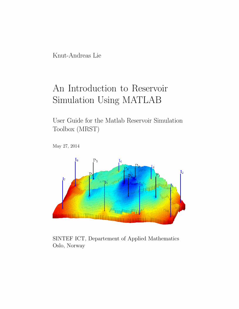
Knut-Andreas Lie
An Introduction to ReservoirSimulation Using MATLAB
User Guide for the Matlab Reservoir Simulation
Toolbox (MRST)
May 27, 2014
SINTEF ICT, Departement of Applied MathematicsOslo, Norway

Preface
There are many good books that describe mathematical models for flow inporous media and present numerical methods that can be used to discretizeand solve the corresponding systems of partial differential equations. However,neither of these books describe how to do this in practice. Some may presentalgorithms and data structures, but most leave it up to you to figure out allthe nitty-gritty details you need to get your implementation up and running.Likewise, you may read papers that present models or computational methodsthat may be exactly what you need for your work. After the first enthusiasm,however, you very often end up quite disappointed–or at least, I do–when Irealize that the authors have not presented all the details of their model, orthat it will probably take me months to get my own implementation working.
In this book, I try to be a bit different and give a reasonably self-containedintroduction to the simulation of flow and transport in porous media thatalso discusses how to implement the models and algorithms in a robust andefficient manner. In the presentation, I have tried to let the discussion ofmodels and numerical methods go hand in hand with numerical examplesthat come fully equipped with codes and data, so that you can rerun andreproduce the results by yourself and use them as a starting point for yourown research and experiments. All examples in the book are based on theMatlab Reservoir Simulation Toolbox (MRST), which has been developedby my group and published online as free open-source code under the GNUGeneral Public License since 2009.
The book can alternatively be seen as a comprehensive user-guide toMRST. Over the years, MRST has become surprisingly popular (the latest re-leases have more than a thousand unique downloads each) and has expandedrapidly with new features. Unfortunately, the manuscript has not been able tokeep pace. The current version is up-to-date with respect to the latest devel-opment in data structures and syntax, but only includes material on single-phase flow. However, more material is being added almost every day, and themanuscript will hopefully be expanded to cover multiphase flow and variousworkflow tools and special-purpose solvers in the not too distant future.

VI Preface
I hereby grant you permission to use the manuscript and the accompa-nying example scripts for your own educational purpose, but please do notreuse or redistribute this material as a whole, or in parts, without explicitpermission. Moreover, notice that the current manuscript is a snapshot ofwork in progress and is far from complete. The text may contain a numberof misprints and errors, and I would be grateful if you help to improve themanuscript by sending me an email. Suggestions for other improvement arealso most welcome.
Oslo, Knut-Andreas LieMay 27, 2014 [email protected]
Contents
1 Introduction . . . . . . . . . . . . . . . . . . . . . . . . . . . . . . . . . . . . . . . . . . . . . . . 11.1 Reservoir Simulation . . . . . . . . . . . . . . . . . . . . . . . . . . . . . . . . . . . . . 21.2 About This Book . . . . . . . . . . . . . . . . . . . . . . . . . . . . . . . . . . . . . . . . 41.3 The First Encounter with MRST . . . . . . . . . . . . . . . . . . . . . . . . . . 51.4 More about MRST . . . . . . . . . . . . . . . . . . . . . . . . . . . . . . . . . . . . . . 61.5 About examples and standard datasets . . . . . . . . . . . . . . . . . . . . . 9
Part I Geological Models and Grids
2 Modelling Reservoir Rocks . . . . . . . . . . . . . . . . . . . . . . . . . . . . . . . . 152.1 Formation of a Sedimentary Reservoir . . . . . . . . . . . . . . . . . . . . . . 152.2 Multiscale Modelling of Permeable Rocks . . . . . . . . . . . . . . . . . . . 17
2.2.1 Macroscopic Models . . . . . . . . . . . . . . . . . . . . . . . . . . . . . . . 192.2.2 Representative Elementary Volumes . . . . . . . . . . . . . . . . . 202.2.3 Microscopic Models: The Pore Scale . . . . . . . . . . . . . . . . . 212.2.4 Mesoscopic Models . . . . . . . . . . . . . . . . . . . . . . . . . . . . . . . . 23
2.3 Modelling of Rock Properties . . . . . . . . . . . . . . . . . . . . . . . . . . . . . 242.3.1 Porosity . . . . . . . . . . . . . . . . . . . . . . . . . . . . . . . . . . . . . . . . . . 252.3.2 Permeability . . . . . . . . . . . . . . . . . . . . . . . . . . . . . . . . . . . . . . 262.3.3 Other parameters . . . . . . . . . . . . . . . . . . . . . . . . . . . . . . . . . 28
2.4 Rock Modelling in MRST . . . . . . . . . . . . . . . . . . . . . . . . . . . . . . . . 292.4.1 Homogeneous Models . . . . . . . . . . . . . . . . . . . . . . . . . . . . . . 292.4.2 Random and Lognormal Models . . . . . . . . . . . . . . . . . . . . . 302.4.3 10th SPE Comparative Solution Project: Model 2 . . . . . . 312.4.4 The Johansen Formation . . . . . . . . . . . . . . . . . . . . . . . . . . . 342.4.5 The SAIGUP Model . . . . . . . . . . . . . . . . . . . . . . . . . . . . . . . 36
3 Grids in Subsurface Modeling . . . . . . . . . . . . . . . . . . . . . . . . . . . . . 433.1 Structured Grids . . . . . . . . . . . . . . . . . . . . . . . . . . . . . . . . . . . . . . . . 453.2 Unstructured Grids . . . . . . . . . . . . . . . . . . . . . . . . . . . . . . . . . . . . . . 49
VIII Contents
3.2.1 Delaunay Tessellation . . . . . . . . . . . . . . . . . . . . . . . . . . . . . . 503.2.2 Voronoi Diagrams . . . . . . . . . . . . . . . . . . . . . . . . . . . . . . . . . 53
3.3 Stratigraphic Grids . . . . . . . . . . . . . . . . . . . . . . . . . . . . . . . . . . . . . . 553.3.1 Corner-Point Grids . . . . . . . . . . . . . . . . . . . . . . . . . . . . . . . . 563.3.2 Layered 2.5D PEBI Grids . . . . . . . . . . . . . . . . . . . . . . . . . . 66
3.4 Grid Structure in MRST . . . . . . . . . . . . . . . . . . . . . . . . . . . . . . . . . 70
4 Grid Coarsening . . . . . . . . . . . . . . . . . . . . . . . . . . . . . . . . . . . . . . . . . . . 874.1 Partition Vectors . . . . . . . . . . . . . . . . . . . . . . . . . . . . . . . . . . . . . . . . 88
4.1.1 Uniform Partitions . . . . . . . . . . . . . . . . . . . . . . . . . . . . . . . . 884.1.2 Connected Partitions . . . . . . . . . . . . . . . . . . . . . . . . . . . . . . 894.1.3 Composite Partitions . . . . . . . . . . . . . . . . . . . . . . . . . . . . . . 90
4.2 Coarse Grid Representation in MRST . . . . . . . . . . . . . . . . . . . . . . 934.2.1 Subdivision of Coarse Faces . . . . . . . . . . . . . . . . . . . . . . . . . 94
4.3 Coarsening of Realistic Reservoir Models . . . . . . . . . . . . . . . . . . . 974.3.1 The Johansen Aquifer . . . . . . . . . . . . . . . . . . . . . . . . . . . . . . 974.3.2 The Shallow-Marine SAIGUP Model . . . . . . . . . . . . . . . . . 100
4.4 General Advice and Simple Guidelines . . . . . . . . . . . . . . . . . . . . . 104
Part II Single-Phase Flow
5 Mathematical Models and Basic Discretizations . . . . . . . . . . . 1095.1 Fundamental concept: Darcy’s law . . . . . . . . . . . . . . . . . . . . . . . . . 1095.2 General flow equations for single-phase flow . . . . . . . . . . . . . . . . . 1115.3 Auxiliary conditions and equations . . . . . . . . . . . . . . . . . . . . . . . . 115
5.3.1 Boundary and initial conditions . . . . . . . . . . . . . . . . . . . . . 1165.3.2 Models for injection and production wells . . . . . . . . . . . . . 1175.3.3 Field lines and time-of-flight . . . . . . . . . . . . . . . . . . . . . . . . 1195.3.4 Tracers and volume partitions . . . . . . . . . . . . . . . . . . . . . . . 120
5.4 Basic finite-volume discretizations . . . . . . . . . . . . . . . . . . . . . . . . . 1215.4.1 A two-point flux-approximation (TPFA) method . . . . . . 1225.4.2 Abstract formulation: discrete div and grad operators . 1265.4.3 Discretizing the time-of-flight and tracer equations . . . . 128
6 Incompressible Solvers in MRST . . . . . . . . . . . . . . . . . . . . . . . . . . 1316.1 Basic data structures . . . . . . . . . . . . . . . . . . . . . . . . . . . . . . . . . . . . 131
6.1.1 Fluid properties . . . . . . . . . . . . . . . . . . . . . . . . . . . . . . . . . . . 1316.1.2 Reservoir states . . . . . . . . . . . . . . . . . . . . . . . . . . . . . . . . . . . 1326.1.3 Fluid sources . . . . . . . . . . . . . . . . . . . . . . . . . . . . . . . . . . . . . 1336.1.4 Boundary conditions . . . . . . . . . . . . . . . . . . . . . . . . . . . . . . . 1346.1.5 Wells . . . . . . . . . . . . . . . . . . . . . . . . . . . . . . . . . . . . . . . . . . . . 135
6.2 Incompressible two-point pressure solver . . . . . . . . . . . . . . . . . . . . 1376.3 Upwind solver for time-of-flight and tracer . . . . . . . . . . . . . . . . . . 1406.4 Simulation examples . . . . . . . . . . . . . . . . . . . . . . . . . . . . . . . . . . . . . 143
Contents IX
6.4.1 Quarter-five spot . . . . . . . . . . . . . . . . . . . . . . . . . . . . . . . . . . 1436.4.2 Boundary conditions . . . . . . . . . . . . . . . . . . . . . . . . . . . . . . . 1476.4.3 Structured versus unstructured stencils . . . . . . . . . . . . . . . 1516.4.4 Using Peaceman well models . . . . . . . . . . . . . . . . . . . . . . . . 156
7 Single-Phase Solvers Based on Automatic Differentiation . . 1617.1 Implicit discretization . . . . . . . . . . . . . . . . . . . . . . . . . . . . . . . . . . . . 1617.2 Automatic differentiation . . . . . . . . . . . . . . . . . . . . . . . . . . . . . . . . . 1637.3 Automatic differentiation in MRST . . . . . . . . . . . . . . . . . . . . . . . . 1647.4 An implicit single-phase solver . . . . . . . . . . . . . . . . . . . . . . . . . . . . 168
7.4.1 Model setup and initial state . . . . . . . . . . . . . . . . . . . . . . . . 1687.4.2 Discrete operators and equations . . . . . . . . . . . . . . . . . . . . 1707.4.3 Well model . . . . . . . . . . . . . . . . . . . . . . . . . . . . . . . . . . . . . . . 1717.4.4 The simulation loop . . . . . . . . . . . . . . . . . . . . . . . . . . . . . . . 172
7.5 Rapid prototyping . . . . . . . . . . . . . . . . . . . . . . . . . . . . . . . . . . . . . . . 1757.5.1 Pressure-dependent viscosity . . . . . . . . . . . . . . . . . . . . . . . . 1757.5.2 Non-Newtonian fluid . . . . . . . . . . . . . . . . . . . . . . . . . . . . . . . 178
8 Consistent Discretizations on Polyhedral Grids . . . . . . . . . . . . 1858.1 The Mixed Finite-Element Method . . . . . . . . . . . . . . . . . . . . . . . . 188
8.1.1 Continuous Formulation . . . . . . . . . . . . . . . . . . . . . . . . . . . . 1888.1.2 Discrete Formulation . . . . . . . . . . . . . . . . . . . . . . . . . . . . . . 1908.1.3 Hybrid formulation . . . . . . . . . . . . . . . . . . . . . . . . . . . . . . . . 193
8.2 Consistent Methods on Mixed Hybrid Form . . . . . . . . . . . . . . . . . 1958.3 The Mimetic Method . . . . . . . . . . . . . . . . . . . . . . . . . . . . . . . . . . . . 198
8.3.1 General Family of Inner Products . . . . . . . . . . . . . . . . . . . 1998.3.2 General Parametric Family . . . . . . . . . . . . . . . . . . . . . . . . . 2028.3.3 Two-Point Type Methods . . . . . . . . . . . . . . . . . . . . . . . . . . 2028.3.4 Raviart–Thomas Type Inner Product . . . . . . . . . . . . . . . . 2048.3.5 Default Inner Product in MRST. . . . . . . . . . . . . . . . . . . . . 2068.3.6 Local-Flux Mimetic Method . . . . . . . . . . . . . . . . . . . . . . . . 206
References . . . . . . . . . . . . . . . . . . . . . . . . . . . . . . . . . . . . . . . . . . . . . . . . . . . . . 209

1
Introduction
Modelling of flow processes in the subsurface is important for many applica-tions. In fact, subsurface flow phenomena cover some of the most importanttechnological challenges of our time. The road toward sustainable use andmanagement of the earth’s groundwater reserves necessarily involves mod-elling of groundwater hydrological systems. In particular, modelling is usedto acquire general knowledge of groundwater basins, quantify limits of sus-tainable use, monitor transport of pollutants in the subsurface, and appraiseschemes for groundwater remediation.
A perhaps equally important problem is how to reduce emission of green-house gases, such as CO2, into the atmosphere. Carbon sequestration inporous media has been suggested as a possible means. The primary concernrelated to storage of CO2 in subsurface rock formations is how fast the storedCO2 will escape back to the atmosphere. Repositories do not need to storeCO2 forever, just long enough to allow the natural carbon cycle to reduce theatmospheric CO2 to near pre-industrial level. Nevertheless, making a quali-fied estimate of the leakage rates from potential CO2 storage facilities is anontrivial task, and demands interdisciplinary research and software based onstate-of-the art numerical methods for modelling subsurface flow. Other ques-tions of concern is whether the stored CO2 will leak into fresh-water aquifersor migrate to habitated or different legislative areas
The third challenge is petroleum production. The civilized world will (mostlikely) continue to depend on the utilization of petroleum resources both asan energy carrier and as a raw material for consumer products the next 30–40 years. Given the decline in conventional petroleum production and thereduced rate of new major discoveries, optimal utilization of current fieldsand discoveries is of utter importance to meet the demands for petroleumand lessen the pressure on exploration in vulnerable areas like in the arcticregions. Likewise, there is a strong need to understand how unconventionalpetroleum resources can be produced in an economic way that minimizes theharm to the environment.
2 1 Introduction
Reliable computer modeling of subsurface flow is much needed to overcomethese three challenges, but is also needed to exploit deep geothermal energy,ensure safe storage of nuclear waster, improve remediation technologies toremove contaminants from the subsurface, etc. Indeed, the need for tools thathelp us understand flow processes in the subsurface is probably greater thanever, and increasing. More than fifty years of prior research in this area has ledto some degree of agreement in terms of how subsurface flow processes can bemodelled adequately with numerical simulation technology. Most of our priorresearch in this area has targeted reservoir simulation, i.e., modelling flowin oil and gas reservoirs, and hence we will mainly focus on this applicationin this book. However, the general modelling framework, and the numericalmethods that are discussed, apply also to modelling other types of flow inconsolidated and saturated porous media.
Techniques developed for the study of subsurface flow are also applicableto other natural and man-made porous media such as soils, biological tissuesand plants, filters, fuel cells, concrete, textiles, polymer composites, etc. Aparticular interesting example is in-tissue drug delivery, where the challengeis to minimize the volume swept by the injected fluid. This is the completeopposite of the challenge in petroleum production, in which one seeks to max-imize the volumetric sweep of the injected fluid to push as much petroleumout as possible.
1.1 Reservoir Simulation
Reservoir simulation is the means by which we use a numerical model of thepetrophysical characteristics of a hydrocarbon reservoir to analyze and predictfluid behavior in the reservoir over time. Simulation of petroleum reservoirsstarted in the mid 1950’s and has become an important tool for qualitativeand quantitative prediction of the flow of fluid phases. Reservoir simulation isa complement to field observations, pilot field and laboratory tests, well test-ing and analytical models and is used to estimate production characteristics,calibrate reservoir parameters, visualize reservoir flow patterns, etc. The mainpurpose of simulation is to provide an information database that can help theoil companies to position and manage wells and well trajectories to maximizethe oil and gas recovery. Generally, the value of simulation studies dependson what kind of extra monetary or other profit they will lead to, e.g., by in-creasing the recovery from a given reservoir. However, even though reservoirsimulation can be an invaluable tool to enhance oil-recovery, the demand forsimulation studies depends on many factors. For instance, petroleum fieldsvary in size from small pockets of hydrocarbon that may be buried just afew meters beneath the surface of the earth and can easily be produced, tohuge reservoirs stretching out several square kilometres beneath remote andstormy seas, for which extensive simulation studies are inevitable to avoidmaking incorrect, costly decisions.
1.1 Reservoir Simulation 3
To describe the subsurface flow processes mathematically, two types ofmodels are needed. First, one needs a mathematical model that describes howfluids flow in a porous medium. These models are typically given as a set ofpartial differential equations describing the mass-conservation of fluid phases,accompanied by a suitable set of constitutive relations. Second, one needs ageological model that describes the given porous rock formation (the reser-voir). The geological model is realized as a grid populated with petrophysicalproperties that are used as input to the flow model, and together they makeup the reservoir simulation model.
Unfortunately, obtaining an accurate prediction of reservoir flow scenariosis a difficult task. One of the reasons is that we can never get a completeand accurate characterization of the rock parameters that influence the flowpattern. And even if we did, we would not be able to run simulations that ex-ploit all available information, since this would require a tremendous amountof computer resources that exceed by far the capabilities of modern multi-processor computers. On the other hand, we do not need, nor do we seek asimultaneous description of the flow scenario on all scales down to the porescale. For reservoir management it is usually sufficient to describe the generaltrends in the reservoir flow pattern.
In the early days of the computer, reservoir simulation models were builtfrom two-dimensional slices with 102–103 Cartesian grid cells representing thewhole reservoir. In contrast, contemporary reservoir characterization methodscan model the porous rock formations by the means of grid-blocks down to themeter scale. This gives three-dimensional models consisting of multi-millioncells. Stratigraphic grid models, based on extrusion of 2D areal grids to formvolumetric descriptions, have been popular for many years and are the currentindustry standard. However, more complex methods based on unstructuredgrids are gaining in popularity.
Despite an astonishing increase in computer power, and intensive researchon computation techniques, commercial reservoir simulators can seldom runsimulations directly on geological grid models. Instead, coarse grid modelswith grid-blocks that are typically ten to hundred times larger are built usingsome kind of upscaling of the geophysical parameters. How one should performthis upscaling is not trivial. In fact, upscaling has been, and probably still is,one of the most active research areas in the oil industry. This effort reflectsthat it is a general opinion that, with the ever increasing size and complexity ofthe geological reservoir models, one cannot generally expect to run simulationsdirectly on geological models in the foreseeable future.
Along with the development of better computers, new and more robustupscaling techniques, and more detailed reservoir characterizations, there hasalso been an equally significant development in the area of numerical methods.State-of-the-art simulators employ numerical methods that can take advan-tage of multiple processors, distributed memory workstations, adaptive gridrefinement strategies, and iterative techniques with linear complexity. For thesimulation, there exists a wide variety of different numerical schemes that all
4 1 Introduction
have their pros and cons. With all these techniques available we see a trendwhere methods are being tuned to a special set of applications, as opposedto traditional methods that were developed for a large class of differentialequations.
1.2 About This Book
The book is intended to serve several purposes. First, we wish to give a self-contained introduction to the basic theory of flow in porous media and thenumerical methods used to solve the underlying differential equations. In doingso, we will present both the basic model equations and physical parameters,classical numerical methods that are the current industry standard, as wellas more recent methods that are still being researched by academia. Thepresentation of computational methods and modeling concepts is accompaniedby illustrative examples ranging from idealized and highly simplified examplesto real-life cases.
All visual and numerical examples presented in this book have been createdusing the MATLAB Reservoir Simulation Toolbox (MRST). This open-sourcetoolboxes contains a comprehensive set of routines and data structures forreading, representing, processing, and visualizing structured and unstructuredgrids, with particular emphasis on the corner-point format used within thepetroleum industry. The core part of the toolbox contains basic flow andtransport solvers that can be used to simulate incompressible, single- andtwo-phase flow on general unstructured grids. Solvers for more complex flowphysics as well as special-purpose computational tools for various workflowscan be found in a large set of add-on modules. The second purpose of thebook is therefore to give a presentation of the various functionality in MRST.By providing data and sufficient detail in all examples, we hope that theinterested reader will be able to repeat and modify our examples on his/herown computer. We hope that this material can give other researchers, orstudents about to embark on a Master or a PhD project, a head start.
MRST was originally developed to support our research on consistent dis-cretization and multiscale solvers on unstructured, polyhedral grids, but hasover the years developed into an efficient platform for rapid prototyping andefficient testing of new mathematical models and simulation methods. A par-ticular aim of MRST is to accelerate the process of moving from simplifiedand conceptual testing to validation of realistic setups. The book is thereforefocused on questions that are relevant to the petroleum industry. However,to benefit readers that interested in developing more generic computationalmethodologies, we also try to teach a few general principles and methods thatare useful for developing flexible and efficient MATLAB solvers for other ap-plications of porous media flow or on unstructured polyhedral grids in general.In particular, we seek to provide sufficient implementation details so that theinterested reader can use MRST as a starting point for his/her own develop-
1.3 The First Encounter with MRST 5
ment. Being an open-source software, it is our hope that readers of this bookcan contribute to extend MRST in new directions.
Over the last few years, key parts of MRST have become relatively matureand well tested. This has enabled a stable release policy with two releases peryear, typically in April and October. Throughout the releases, the basic func-tionality like grid structures has remained largely unchanged, except for occa-sional and inevitable bugfixes, and the primary focus has been on expandingfunctionality by maturing and releasing in-house prototype modules. However,MRST is mainly developed and maintained as an efficient prototyping toolto support contract research carried out by SINTEF for the energy-resourceindustry and public research agencies. Fundamental changes will thereforeoccur from time to time, e.g., like when automatic differentiation was intro-duced in 2012. In writing this, we (regretfully) acknowledge the fact thatspecific code details (and examples) in books that describe evolving softwaretend to become somewhat outdated. To countermand this, we intend to keepan up-to-date version of all examples in the book on the MRST webpage:
http://www.sintef.no/Projectweb/MRST/
These examples are designed using cell-mode scripts, which can be seen as atype of “MATLAB workbook” that allowes you break the scripts down intosmaller pieces that can be run individually to perform a specific subtask suchas creating a parts of a model or making an illustrative plot. In our opinion, thebest way to understand the examples is to go through the script, evaluatingone cell at at time. Alternatively, you can set a breakpoint on the first line,and step through the script in debug mode. Some of the scripts contain moretext and are designed to make easily published documents. If you are notfamiliar with cell-mode scripts, or debug mode, we strongly urge you to learnthese useful features in MATLAB as soon as possible.
You are now ready to start digging into the material. However, beforedoing so, we present an example that will give you a first taste of flow inporous media and the MATLAB Reservoir Simulation Toolbox.
1.3 The First Encounter with MRST
The purpose of the example is to show the basic steps for setting up, solving,and visualizing a simple flow problem. To this end, we will compute a knownanalytical solution: the linear pressure solution describing hydrostatic equilib-rium for an incompressible, single-phase fluid. The basic model in subsurfaceflow consists of an equation expressing conservation of mass and a constitu-tive relation called Darcy’s law that relates the volumetric flow rate to thegradient of flow potential
∇ · ~v = 0, ~v = −− K
µ
[∇p+ ρg∇z
], (1.1)
6 1 Introduction
where the unknowns are the pressure p and the flow velocity ~v. By eliminating~v, we can reduce (1.1) to the elliptic Poisson equation. In (1.1), the rock ischaracterized by the permeability K that gives the rock’s ability to transmitfluid. Here, K is set to 100 milli-darcies (mD). The fluid has a density ρ of1000 kg/m3 and viscosity µ equal 1 cP, g is the gravity constant, and z is thedepth. More details on these flow equations, the rock and fluid parameters,the computational method, and its MATLAB implementation will be giventhroughout the book.
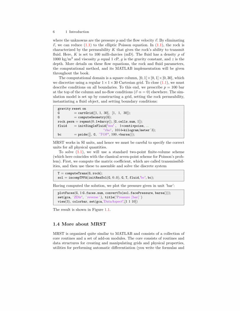
The computational domain is a square column, [0, 1]× [0, 1]× [0, 30], whichwe discretize using a regular 1×1×30 Cartesian grid. To close (1.1), we mustdescribe conditions on all boundaries. To this end, we prescribe p = 100 barat the top of the column and no-flow conditions (~v ·n = 0) elsewhere. The sim-ulation model is set up by constructing a grid, setting the rock permeability,instantiating a fluid object, and setting boundary conditions:
gravity reset on
G = cartGrid([1, 1, 30], [1, 1, 30]);G = computeGeometry(G);rock.perm = repmat(0.1*darcy(), [G.cells.num, 1]);fluid = initSingleFluid('mu' , 1*centi*poise, ...
'rho' , 1014*kilogram/meterˆ3);bc = pside([], G, 'TOP', 100.*barsa());
MRST works in SI units, and hence we must be careful to specify the correctunits for all physical quantities.
To solve (1.1), we will use a standard two-point finite-volume scheme(which here coincides with the classical seven-point scheme for Poisson’s prob-lem). First, we compute the matrix coefficient, which are called transmissibil-ities, and then use these to assemble and solve the discrete system
T = computeTrans(G, rock);sol = incompTPFA(initResSol(G, 0.0), G, T, fluid,'bc', bc);
Having computed the solution, we plot the pressure given in unit ’bar’:
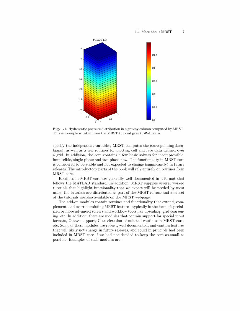
plotFaces(G, 1:G.faces.num, convertTo(sol.facePressure, barsa()));set(gca, 'ZDir', ' reverse ' ), title('Pressure [bar] ' )view(3), colorbar, set(gca,'DataAspect',[1 1 10])
The result is shown in Figure 1.1.
1.4 More about MRST
MRST is organized quite similar to MATLAB and consists of a collection ofcore routines and a set of add-on modules. The core consists of routines anddata structures for creating and manipulating grids and physical properties,utilities for performing automatic differentiation (you write the formulas and
1.4 More about MRST 7
0
0.5
1
0
0.5
1
0
5
10
15
20
25
30
Pressure [bar]
100
100.5
101
101.5
102
102.5
Fig. 1.1. Hydrostatic pressure distribution in a gravity column computed by MRST.This is example is taken from the MRST tutorial gravityColumn.m
specify the independent variables, MRST computes the corresponding Jaco-bians), as well as a few routines for plotting cell and face data defined overa grid. In addition, the core contains a few basic solvers for incompressible,immiscible, single-phase and two-phase flow. The functionality in MRST coreis considered to be stable and not expected to change (significantly) in futurereleases. The introductory parts of the book will rely entirely on routines fromMRST core.
Routines in MRST core are generally well documented in a format thatfollows the MATLAB standard. In addition, MRST supplies several workedtutorials that highlight functionality that we expect will be needed by mostusers; the tutorials are distributed as part of the MRST release and a subsetof the tutorials are also available on the MRST webpage.
The add-on modules contain routines and functionality that extend, com-plement, and override existing MRST features, typically in the form of special-ized or more advanced solvers and workflow tools like upscaling, grid coarsen-ing, etc. In addition, there are modules that contain support for special inputformats, Octave support, C-acceleration of selected routines in MRST core,etc. Some of these modules are robust, well-documented, and contain featuresthat will likely not change in future releases, and could in principle had beenincluded in MRST core if we had not decided to keep the core as small aspossible. Examples of such modules are:
8 1 Introduction
consistent discretizations on general polyhedral grids: mimetic and MPFA-Omethods;
a small module for downloading and setting up flow models based on theSPE10 data set [19], which are commonly used benchmarks encounteredin a multitude of papers;
upscaling, including methods for flow-based single-phase upscaling as wellas steady-state methods for two-phase upscaling;
extended data structures for representing coarse grids as well as routinesfor partitioning logically Cartesian grids;
agglomeration based grid coarsening: methods for defining coarse gridsthat adapt to geological features, flow patterns, etc;
multiscale mixed finite-element methods for incompressible flow on strati-graphic and unstructured grids;
multiscale finite-volume methods for incompressible flow on structuredgrids;
the simplified deck reader, which contains support for processing simula-tion decks in the ECLIPSE format, including input reading, conversion toSI units, and construction MRST objects for grids, fluids, rock properties,and wells;
C-acceleration of grid processing and basic solvers for incompressible flow.
Other modules and workflow tools, on the other hand, are constantly changingto support ongoing research:
fully-implicit solvers based on automatic differentiation: rapid prototypingof flow models of industry-standard complexity;
gui-based tools for interactive visualization of geological models and sim-ulation results;
flow diagnostics: simple, controlled numerical experiments that are runto probe a reservoir model and establish connections and basic volumeestimates to compare, rank, and cluster models, or used as simplified flowproxies
a numerical CO2 that offers a chain of simulation tools of increasing com-plexity: geometrical methods for identifying structural traps, percolationtype methods for identifying potential spill paths, and vertical-equilibriummethods that can efficiently simulate structural, residual, and solubilitytrapping in a thousand-year perspective;
multiscale finite-volume methods for simulation of ’full physics’ on strati-graphic and unstructured grids;
production optimization based on adjoint methods.
All these modules are publicly available from the MRST webpage. In addi-tion, there are several third-party modules that are available courtesy of theirdevelopers, as well as in-house prototype modules and workflow examples thatare available upon request:
1.5 About examples and standard datasets 9
two-point and multipoint solvers for discrete fracture-matrix systems, in-cluding multiscale methods, developed by researchers at the University ofBergen;
an ensemble Kalman filter module developed by researchers at TNO, in-cluding EnKF and EnRML schemes, localization, inflation, asynchronousdata, production and seismic data, updating of conventional and structuralparameters;
polymer flooding based on a Todd–Longstaff model with adsorption anddead pore space, permeability reduction, shear thinning, near-well (radial)and standard grids;
geochemistry with conventional and structural parameters and withoutchemical equilibrium and coupling with fluid flow.
Discussing all these modules in detail is beyond the scope of the book. Instead,we encourge the interested reader to download and explore the modules onhis/her own. Finally, the MRST webpage features several user-supplied casesand code examples that are not discussed in this book.
1.5 About examples and standard datasets
The examples play an important role in this book. Most examples have beenequipped with codes the reader can rerun to reproduce the results discussedin the example. Likewise, many of the figures include a small box with theMATLAB and MRST commands necessary to create the plots. To the extentpossible, we have tried to make the examples self-contained, but in some casewe have for brevity omitted details that either have been discussed elsewhereor should be part of the reader’s MATLAB basic repertoire.
MRST provides several routines that can be used to create examples interms of grids and petrophysical data. The grid-factory routines are mostlydeterministic and should enable the reader to create the exact same grids thatare discussed in the book. The routines for generating petrophysical data, onthe other hand, rely on random numbers, which means that the reader canonly expect to reproduce plots and numbers that are qualitatively similarwhenever these are used.
In addition, the book will use a few standard datasets that all can bedownloaded freely from the internet. Herein, we use the convention that thesedatasets are stored in sub-directories of the following standard MRST path:
fullfile(ROOTDIR, 'examples', 'data')
We recommend that the reader adheres to this convention. In the following,we will briefly introduce the datasets and describe how to obtain them.
The SPE10 dataset
Model 2 of the 10th SPE Comparative Solution Project [19] was originallyposed as a benchmark for upscaling methods. The 3-D geological model con-
10 1 Introduction
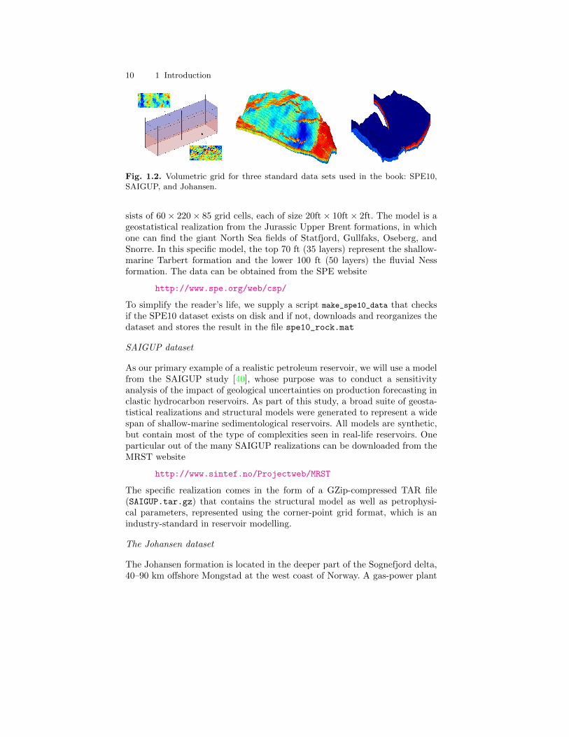
Fig. 1.2. Volumetric grid for three standard data sets used in the book: SPE10,SAIGUP, and Johansen.
sists of 60× 220× 85 grid cells, each of size 20ft× 10ft× 2ft. The model is ageostatistical realization from the Jurassic Upper Brent formations, in whichone can find the giant North Sea fields of Statfjord, Gullfaks, Oseberg, andSnorre. In this specific model, the top 70 ft (35 layers) represent the shallow-marine Tarbert formation and the lower 100 ft (50 layers) the fluvial Nessformation. The data can be obtained from the SPE website
http://www.spe.org/web/csp/
To simplify the reader’s life, we supply a script make_spe10_data that checksif the SPE10 dataset exists on disk and if not, downloads and reorganizes thedataset and stores the result in the file spe10_rock.mat
SAIGUP dataset
As our primary example of a realistic petroleum reservoir, we will use a modelfrom the SAIGUP study [40], whose purpose was to conduct a sensitivityanalysis of the impact of geological uncertainties on production forecasting inclastic hydrocarbon reservoirs. As part of this study, a broad suite of geosta-tistical realizations and structural models were generated to represent a widespan of shallow-marine sedimentological reservoirs. All models are synthetic,but contain most of the type of complexities seen in real-life reservoirs. Oneparticular out of the many SAIGUP realizations can be downloaded from theMRST website
http://www.sintef.no/Projectweb/MRST
The specific realization comes in the form of a GZip-compressed TAR file(SAIGUP.tar.gz) that contains the structural model as well as petrophysi-cal parameters, represented using the corner-point grid format, which is anindustry-standard in reservoir modelling.
The Johansen dataset
The Johansen formation is located in the deeper part of the Sognefjord delta,40–90 km offshore Mongstad at the west coast of Norway. A gas-power plant
1.5 About examples and standard datasets 11
with carbon capture and storage is planned at Mongstad and the water-bearing Johansen formation is a possible candidate for storing the capturedCO2. The Johansen formation is part of the Dunlin group, and is interpretedas a large sandstone delta 2200–3100 meters below sea level that is limitedabove by the Dunlin shale and below by the Amundsen shale. The averagethickness of the formation is roughly 100 m and the lateral extensions are upto 100 km in the north-south direction and 60 km in the east-west direction.With average porosities of approximately 25 percent, this implies that thetheoretical storage capacity of the Johansen formation is more than one giga-tons of CO2 [28]. The Troll field, one of the largest gas field in the North Sea,is located some 500 meters above the north-western parts of the Johansenformation. Through a collaboration between the Norwegian Petroleum Direc-torate and researchers in the MatMoRA project, a set of geological modelshave been created and made available from the MatMoRA webpage:
http://www.sintef.no/Projectweb/MatMorA/Downloads/Johansen/
Altogether, there are five models: one full-field model (149 × 189 × 16 grid),three homogeneous sector models (100× 100× n for n = 11, 16, 21), and oneheterogeneous sector model (100× 100× 11).


Part I
Geological Models and Grids

2
Modelling Reservoir Rocks
Aquifers and natural petroleum reservoirs consist of a subsurface body ofsedimentary rock having sufficient porosity and permeability to store andtransmit fluids. In this chapter, we will given an overview of how such rocksare modelled to become part of a simulation model. We start by describingvery briefly how sedimentary rocks are formed and then move on to describehow they are modelled. Finally, we discuss how rock properties are representedin MRST and show several examples of rock models with varying complexity,ranging from a homogeneous shoe-box rock body, via the widely used SPE 10model, to two realistic models (one synthetic and one real-life).
2.1 Formation of a Sedimentary Reservoir
Sedimentary rocks are created by a process called sedimentation, in which min-eral particles are broken off from a solid material by weathering and erosion ina source area and transported e.g., by water, to a place where they settle andaccumulate to form what is called a sediment. Sediments may also contain or-ganic particles that originate from the remains of plants, living creatures, andsmall organisms living in water, and may be deposited by other geophysicalprocesses like wind, mass movement, and glaciers.
Sedimentary rocks have a layered structure with different mixtures of rocktypes with varying grain size, mineral types, and clay content. Over millions ofyears, layers of sediments built up in lakes, rivers, sand deltas, lagoons, choralreefs, and other shallow-marine waters; a few centimetres every hundred yearsformed sedimentary beds (or strata) that may extend many kilometres in thelateral directions. A bed denotes the smallest unit of rock that is distinguish-able from an adjacent rock layer unit above or below it, and can be seen asbands of different color or texture in hillsides, cliffs, river banks, road cuts,etc. Each band represents a specific sedimentary environment, or mode ofdeposition, and can be from a few centimeters to several meters thick, of-ten varying in the lateral direction. A sedimentary rock is characterized by
16 2 Modelling Reservoir Rocks
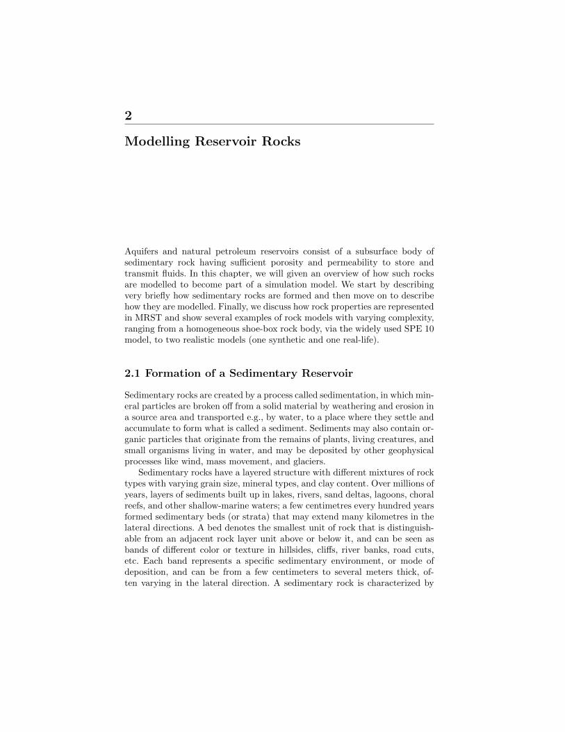
Fig. 2.1. Outcrops of sedimentary rocks from Svalbard, Norway. The length scaleis a few hundred meters.
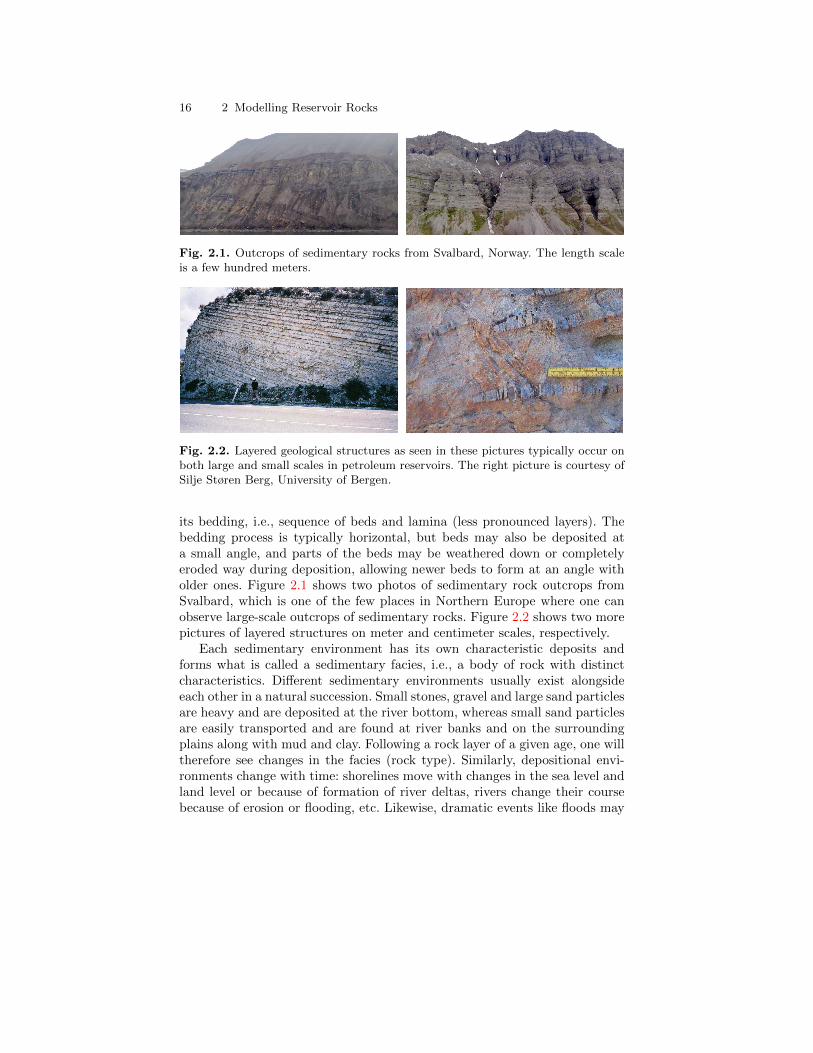
Fig. 2.2. Layered geological structures as seen in these pictures typically occur onboth large and small scales in petroleum reservoirs. The right picture is courtesy ofSilje Støren Berg, University of Bergen.
its bedding, i.e., sequence of beds and lamina (less pronounced layers). Thebedding process is typically horizontal, but beds may also be deposited ata small angle, and parts of the beds may be weathered down or completelyeroded way during deposition, allowing newer beds to form at an angle witholder ones. Figure 2.1 shows two photos of sedimentary rock outcrops fromSvalbard, which is one of the few places in Northern Europe where one canobserve large-scale outcrops of sedimentary rocks. Figure 2.2 shows two morepictures of layered structures on meter and centimeter scales, respectively.
Each sedimentary environment has its own characteristic deposits andforms what is called a sedimentary facies, i.e., a body of rock with distinctcharacteristics. Different sedimentary environments usually exist alongsideeach other in a natural succession. Small stones, gravel and large sand particlesare heavy and are deposited at the river bottom, whereas small sand particlesare easily transported and are found at river banks and on the surroundingplains along with mud and clay. Following a rock layer of a given age, one willtherefore see changes in the facies (rock type). Similarly, depositional envi-ronments change with time: shorelines move with changes in the sea level andland level or because of formation of river deltas, rivers change their coursebecause of erosion or flooding, etc. Likewise, dramatic events like floods may
2.2 Multiscale Modelling of Permeable Rocks 17
create abrupt changes. At a given position, the accumulated sequence of bedswill therefore contain different facies.
As time passes by, more and more sediments accumulate and the stack ofbeds piles up to hundreds of meters. Simultaneously, severe geological activitytakes place: Cracking of continental plates and volcanic activity changed whatis to become our reservoir from being a relatively smooth, layered sedimen-tary basin into a complex structure where previously continuous layers werecut, shifted, or twisted in various directions, introducing fractures and faults.Fractures are cracks or breakage in the rock, across which there has been nomovement; faults are fractures across which the layers in the rock have beendisplaced.
Over time, the depositional rock bodies got buried deeper and deeper, andthe pressure and temperature increased because of the overburden. The de-posits not only consisted of sand grains, mud, and small rock particles but alsocontained remains of plankton, algae, and other organisms living in the waterthat had died and fallen down to the bottom. As the organic material wascompressed and ’cooked’, it eventually turned into crude oil and natural gas.The lightest hydrocarbons (methane, ethane, etc.) usually escaped quickly,whilst the heavier oils moved slowly towards the surface. At certain sites,the migrating hydrocarbons were trapped in structural or stratigraphic traps.Structural traps (domes, folds, and anticlines) are created as geological ac-tivity deforms the layers containing hydrocarbon, near salt domes created byburied salt deposits that rise unevenly, or by sealing faults forming a closure.Stratigraphic traps form because of changes in facies (e.g., in clay content)within the bed itself or when the bed is sealed by an impermeable bed. Thesequantities of trapped hydrocarbons form todays oil and gas reservoirs. In theNorth Sea (which the authors are most familiar with), reservoirs are typicallyfound 1 000–3 000 meters below the sea bed.
2.2 Multiscale Modelling of Permeable Rocks
All sedimentary rocks consist of a solid matrix with an interconnected void.The void pore space allows the rocks to store and transmit fluids. The ability tostore fluids is determined by the volume fraction of pores (the rock porosity),and the ability to transmit fluids (the rock permeability) is given by theinterconnection of the pores.
Rock formations found in natural petroleum reservoirs are typically het-erogeneous at all length scales, from the micrometre scale of pore channelsbetween the solid particles making up the rock to the kilometre scale of afull reservoir formation. On the scale of individual grains, there can be largevariation in grain sizes, giving a broad distribution of void volumes and inter-connections. Moving up a scale, laminae may exhibit large contrasts on themm-cm scale in the ability to store and transmit fluids because of alternatinglayers of coarse and fine-grained material. Laminae are stacked to form beds,
18 2 Modelling Reservoir Rocks
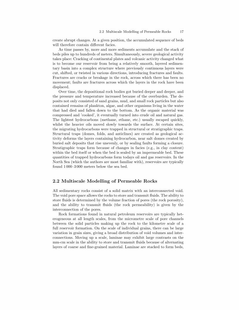
Fig. 2.3. Illustration of the hierarchy of flow models used in subsurface modeling.The length scales are the vertical sizes of typical elements in the models.
which are the smallest stratigraphic units. The thickness of beds varies frommillimetres to tens of meters, and different beds are separated by thin layerswith significantly lower permeability. Beds are, in turn, grouped and stackedinto parasequences or sequences (parallel layers that have undergone similargeologic history). Parasequences represent the deposition of marine sediments,during periods of high sea level, and tend to be somewhere in the range from1–100 meters thick and have a horizontal extent of several kilometres.
The trends and heterogeneity of parasequences depend on the deposi-tional environment. For instance, whereas shallow-marine deposits may leadto rather smoothly varying permeability distributions with correlation lengthsin the order 10–100 meters, fluvial reservoirs may contain intertwined patternsof sand bodies on a background with high clay content, see Figure 2.8. Thereservoir geology can also consist of other structures like for instance shalelayers (impermeable clays), which are the most abundant sedimentary rocks.Fractures and faults, on the other hand, are created by stresses in the rockand may extend from a few centimeters to tens or hundreds of meters. Faultsmay have a significantly higher or lower ability to transmit fluids than thesurrounding rocks, depending upon whether the void space has been filledwith clay material.
All these different length scales can have a profound impact on fluid flow.However, it is generally not possible to account for all pertinent scales thatimpact the flow in a single model. Instead, one has to create a hierarchy ofmodels for studying phenomena occurring at reduced spans of scales. This is il-lustrated in Figure 2.3. Microscopic models represent the void spaces betweenindividual grains and are used to provide porosity, permeability, electrical andelastic properties of rocks from core samples and drill cuttings. Mesoscopicmodels are used to upscale these basic rock properties from the mm/cm-scaleof internal laminations, through the lithofacies scale (∼ 50 cm), to the macro-
2.2 Multiscale Modelling of Permeable Rocks 19
scopic facies association scale (∼ 100 m) of geological models. In this book,we will primarily focus on another scale, simulation models, which representthe last scale in the model hierarchy. Simulation models are obtained by up-scaling geological models and are either introduced out of necessity becausegeological models contain more details than a flow simulator can cope with,or out of convenience to provide faster calculation of flow responses.
2.2.1 Macroscopic Models
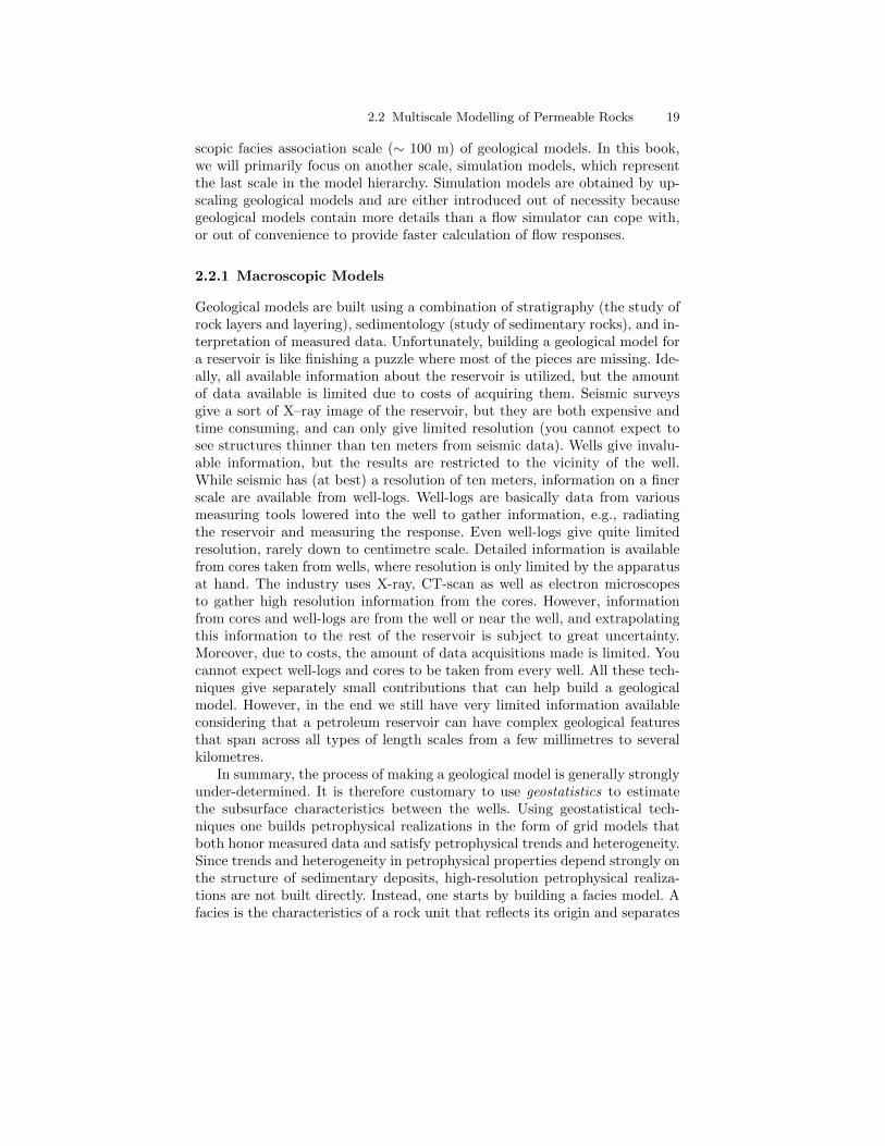
Geological models are built using a combination of stratigraphy (the study ofrock layers and layering), sedimentology (study of sedimentary rocks), and in-terpretation of measured data. Unfortunately, building a geological model fora reservoir is like finishing a puzzle where most of the pieces are missing. Ide-ally, all available information about the reservoir is utilized, but the amountof data available is limited due to costs of acquiring them. Seismic surveysgive a sort of X–ray image of the reservoir, but they are both expensive andtime consuming, and can only give limited resolution (you cannot expect tosee structures thinner than ten meters from seismic data). Wells give invalu-able information, but the results are restricted to the vicinity of the well.While seismic has (at best) a resolution of ten meters, information on a finerscale are available from well-logs. Well-logs are basically data from variousmeasuring tools lowered into the well to gather information, e.g., radiatingthe reservoir and measuring the response. Even well-logs give quite limitedresolution, rarely down to centimetre scale. Detailed information is availablefrom cores taken from wells, where resolution is only limited by the apparatusat hand. The industry uses X-ray, CT-scan as well as electron microscopesto gather high resolution information from the cores. However, informationfrom cores and well-logs are from the well or near the well, and extrapolatingthis information to the rest of the reservoir is subject to great uncertainty.Moreover, due to costs, the amount of data acquisitions made is limited. Youcannot expect well-logs and cores to be taken from every well. All these tech-niques give separately small contributions that can help build a geologicalmodel. However, in the end we still have very limited information availableconsidering that a petroleum reservoir can have complex geological featuresthat span across all types of length scales from a few millimetres to severalkilometres.
In summary, the process of making a geological model is generally stronglyunder-determined. It is therefore customary to use geostatistics to estimatethe subsurface characteristics between the wells. Using geostatistical tech-niques one builds petrophysical realizations in the form of grid models thatboth honor measured data and satisfy petrophysical trends and heterogeneity.Since trends and heterogeneity in petrophysical properties depend strongly onthe structure of sedimentary deposits, high-resolution petrophysical realiza-tions are not built directly. Instead, one starts by building a facies model. Afacies is the characteristics of a rock unit that reflects its origin and separates
20 2 Modelling Reservoir Rocks
it from surrounding rock units. By supplying knowledge of the depositionalenvironment (fluvial, shallow marine, deep marine, etc) and conditioning toobserved data, one can determine the geometry of the facies and how theyare mixed. In the second step, the facies are populated with petrophysicaldata and stochastic simulation techniques are used to simulate multiple re-alizations of the geological model in terms of high-resolution grid models forpetrophysical properties. Each grid model has a plausible heterogeneity andcan contain from a hundred thousand to a hundred million cells. The col-lection of all realizations gives a measure of the uncertainty involved in themodelling. Hence, if the sample of realizations (and the upscaling procedurethat converts the geological models into simulation models) is unbiased, thenit is possible to supply predicted production characteristics, such as the cu-mulative oil production, obtained from simulation studies with a measure ofuncertainty.
This cursory overview of different models is all that is needed for what fol-lows in the next few chapters, and the reader can therefore skip to Section 2.3which discusses macroscopic modelling of reservoir rocks. The remains of thissection will discuss microscopic and mesoscopic modelling in some more detail.First, however, we will briefly discuss the concept of representative elementaryvolumes, which underlies the continuum models used to describe subsurfaceflow and transport.
2.2.2 Representative Elementary Volumes
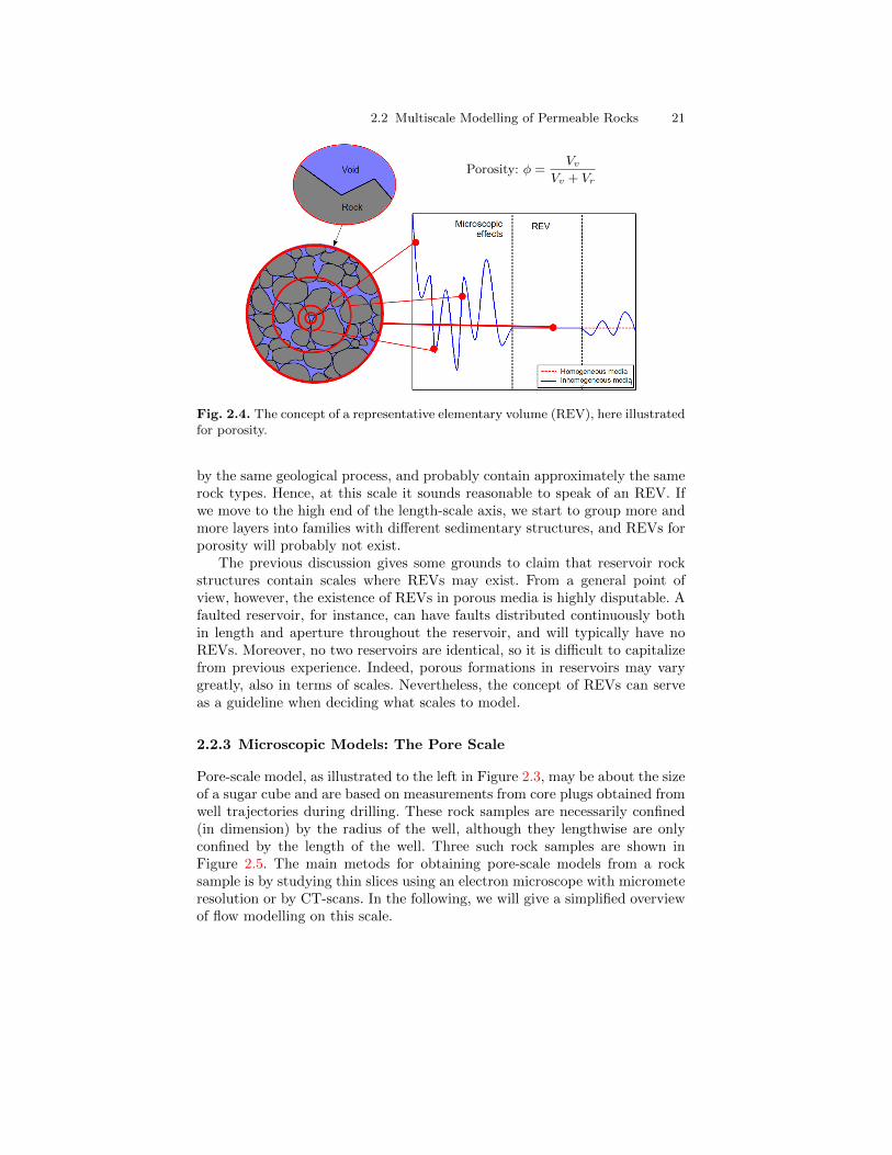
Choosing appropriate modelling scales is often done by intuition and expe-rience, and it is hard to give very general guidelines. An important conceptin choosing model scales is the notion of representative elementary volumes(REVs), which is the smallest volume over which a measurement can be madeand be representative of the whole. This concept is based on the idea thatpetrophysical flow properties are constant on some intervals of scale, see Fig-ure 2.4. Representative elementary volumes, if they exist, mark transitionsbetween scales of heterogeneity, and present natural length scales for mod-elling.
To identify a range of length scales where REVs exist, e.g., for porosity,we move along the length-scale axis from the micrometer-scale of pores to-ward the kilometre-scale of the reservoir. At the pore scale, the porosity is arapidly oscillating function equal to zero (in solid rock) or one (in the pores).Hence, obviously no REVs can exist at this scale. At the next characteristiclength scale, the core scale level, we find laminae deposits. Because the lami-nae consist of alternating layers of coarse and fine grained material, we cannotexpect to find a common porosity value for the different rock structures. Mov-ing further along the length-scale axis, we may find long thin layers, perhapsextending throughout the entire horizontal length of the reservoirs. Each ofthese individual layers may be nearly homogeneous because they are created
2.2 Multiscale Modelling of Permeable Rocks 21
Porosity: φ =Vv
Vv + Vr
Fig. 2.4. The concept of a representative elementary volume (REV), here illustratedfor porosity.
by the same geological process, and probably contain approximately the samerock types. Hence, at this scale it sounds reasonable to speak of an REV. Ifwe move to the high end of the length-scale axis, we start to group more andmore layers into families with different sedimentary structures, and REVs forporosity will probably not exist.
The previous discussion gives some grounds to claim that reservoir rockstructures contain scales where REVs may exist. From a general point ofview, however, the existence of REVs in porous media is highly disputable. Afaulted reservoir, for instance, can have faults distributed continuously bothin length and aperture throughout the reservoir, and will typically have noREVs. Moreover, no two reservoirs are identical, so it is difficult to capitalizefrom previous experience. Indeed, porous formations in reservoirs may varygreatly, also in terms of scales. Nevertheless, the concept of REVs can serveas a guideline when deciding what scales to model.
2.2.3 Microscopic Models: The Pore Scale
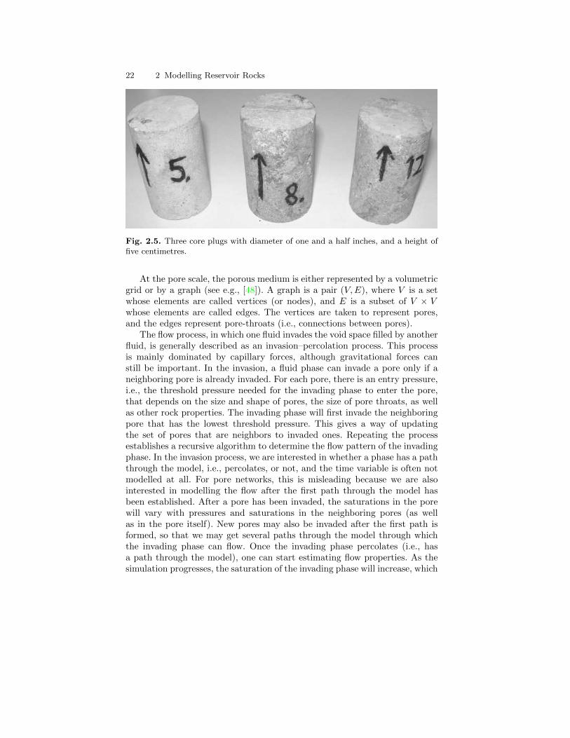
Pore-scale model, as illustrated to the left in Figure 2.3, may be about the sizeof a sugar cube and are based on measurements from core plugs obtained fromwell trajectories during drilling. These rock samples are necessarily confined(in dimension) by the radius of the well, although they lengthwise are onlyconfined by the length of the well. Three such rock samples are shown inFigure 2.5. The main metods for obtaining pore-scale models from a rocksample is by studying thin slices using an electron microscope with micrometeresolution or by CT-scans. In the following, we will give a simplified overviewof flow modelling on this scale.
22 2 Modelling Reservoir Rocks
Fig. 2.5. Three core plugs with diameter of one and a half inches, and a height offive centimetres.
At the pore scale, the porous medium is either represented by a volumetricgrid or by a graph (see e.g., [48]). A graph is a pair (V,E), where V is a setwhose elements are called vertices (or nodes), and E is a subset of V × Vwhose elements are called edges. The vertices are taken to represent pores,and the edges represent pore-throats (i.e., connections between pores).
The flow process, in which one fluid invades the void space filled by anotherfluid, is generally described as an invasion–percolation process. This processis mainly dominated by capillary forces, although gravitational forces canstill be important. In the invasion, a fluid phase can invade a pore only if aneighboring pore is already invaded. For each pore, there is an entry pressure,i.e., the threshold pressure needed for the invading phase to enter the pore,that depends on the size and shape of pores, the size of pore throats, as wellas other rock properties. The invading phase will first invade the neighboringpore that has the lowest threshold pressure. This gives a way of updatingthe set of pores that are neighbors to invaded ones. Repeating the processestablishes a recursive algorithm to determine the flow pattern of the invadingphase. In the invasion process, we are interested in whether a phase has a paththrough the model, i.e., percolates, or not, and the time variable is often notmodelled at all. For pore networks, this is misleading because we are alsointerested in modelling the flow after the first path through the model hasbeen established. After a pore has been invaded, the saturations in the porewill vary with pressures and saturations in the neighboring pores (as wellas in the pore itself). New pores may also be invaded after the first path isformed, so that we may get several paths through the model through whichthe invading phase can flow. Once the invading phase percolates (i.e., hasa path through the model), one can start estimating flow properties. As thesimulation progresses, the saturation of the invading phase will increase, which
2.2 Multiscale Modelling of Permeable Rocks 23
can be used to estimate flow properties at different saturation compositionsin the model.
In reality, the process is more complicated that explained above because ofwettability. When two immiscible fluids (such as oil and water) contact a solidsurface (such as the rock), one of them tends to spread on the surface morethan the other. The fluid in a porous medium that preferentially contacts therock is called the wetting fluid. Note that wettability conditions are usuallychanging throughout a reservoir. The flow process where the invading fluidis non-wetting is called drainage and is typically modelled with invasion–percolation. The flow process where the wetting fluid displaces the non-wettingfluid is called imbibition, and is more complex, involving effects termed filmflow and snap-off.
Another approach to multiphase modelling is through the use of the latticeBoltzmann method that represents the fluids as a set of particles that prop-agate and collide according to a set of rules defined for interactions betweenparticles of the same fluid phase, between particles of different fluid phases,and between the fluids and the walls of the void space. A further presentationof pore-scale modelling is beyond the scope here, but the interested reader isencouraged to consult, e.g., [48] and references therein.
From an analytical point of view, pore-scale modelling is very importantas it represents flow at the fundamental scale (or more loosely, where the flowreally takes place), and hence provides the proper framework for understand-ing the fundamentals of porous media flow. From a practical point of view,pore-scale modelling has a huge potential. Modelling flow at all other scalescan be seen as averaging of flow at the pore scale, and properties describingthe flow at larger scales are usually a mixture of pore-scale properties. Atlarger scales, the complexity of flow modelling is often overwhelming, withlarge uncertainties in determining flow parameters. Hence being able to singleout and estimate the various factors determining flow parameters is invalu-able, and pore-scale models can be instrumental in this respect. However, toextrapolate properties from the pore scale to an entire reservoir is very chal-lenging, even if the entire pore space of the reservoir was known (of course, inreal life you will not be anywhere close to knowing the entire pore space of areservoir).
2.2.4 Mesoscopic Models
Models based on flow experiments on core plugs is by far the most commonmesoscopic models. The fundamental equations describing flow are continu-ity of fluid phases and Darcy’s law, which basically states that flow rate isproportional to pressure drop. The purpose of core-plug experiments is to de-termine capillary pressure curves and the proportionality constant in Darcy’slaw that measures the ability to transmit fluids, see (1.1) in Section 1.3. Tothis end, the sides of the core are insulated and flow is driven through the
24 2 Modelling Reservoir Rocks
core. By measuring the flow rate versus pressure drop, one can estimate theproportionality constant for both single-phase or multi-phase flows.
In conventional reservoir modelling, the effective properties from core-scaleflow experiments are extrapolated to the macroscopic geological model, or di-rectly to the simulation model. Cores should therefore ideally be representativefor the heterogeneous structures that one may find in a typical grid block inthe geological model. However, flow experiments are usually performed on rel-atively homogeneous cores that rarely exceed one meter in length. Cores cantherefore seldom be classified as representative elementary volumes. For in-stance, cores may contain a shale barrier that blocks flow inside the core, butdoes not extend much outside the well-bore region, and the core was slightlywider, there would be a passage past the shale barrier. Flow at the core scaleis also more influenced by capillary forces than flow on a reservoir scale.
As a supplement to core-flooding experiments, it has in recent years be-come popular to build 3D grid models to represent small-scale geological de-tails like the bedding structure and lithology (composition and texture). Oneexample of such a model is shown in Figure 2.3. Effective flow properties forthe 3D model can now be estimated in the same way as for core plugs byreplacing the flow experiment by flow simulations using rock properties thatare e.g., based on the input from microscopic models. This way, one can incor-porate fine-scale geological details from lamina into the macroscopic reservoirmodels.
This discussion shows that the problem of extrapolating information fromcores to build a geological model is largely under-determined. Supplementarypieces of information are also needed, and the process of gathering geologicaldata from other sources is described next.
2.3 Modelling of Rock Properties
How to describe the flow through a porous rock structure is largely a questionof the scale of interest, as we saw in the previous section. The size of the rockbodies forming a typical petroleum reservoir will be from ten to hundred me-ters in the vertical direction and several hundred meters or a few kilometersin the lateral direction. On this modelling scale, it is clearly impossible todescribe the storage and transport in individual pores and pore channels asdiscussed in Section 2.2.3 or the through individual lamina as in Section 2.2.4.To obtain a description of the reservoir geology, one builds models that at-tempt to reproduce the true geological heterogeneity in the reservoir rockat the macroscopic scale by introducing macroscopic petrophysical proper-ties that are based on a continuum hypothesis and volume averaging overa sufficiently large representative elementary volume (REV), as discussed inSection 2.2.2. These petrophysical properties are engineering quantities thatare used as input to flow simulators and are not geological or geophysicalproperties of the underlying media.
2.3 Modelling of Rock Properties 25
A geological model is a conceptual, three-dimensional representation ofa reservoir, whose main purpose is therefore to provide the distribution ofpetrophysical parameters, besides giving location and geometry of the reser-voir. The rock body itself is modelled in terms of a volumetric grid, in whichthe layered structure of sedimentary beds and the geometry of faults and large-scale fractures in the reservoir are represented by the geometry and topologyof the grid cells. The size of a cell in a typical geological grid-model is in therange of 0.1–1 meters in the vertical direction and 10–50 meters in the hori-zontal direction. The petrophysical properties of the rock are represented asconstant values inside each grid cell (porosity and permeability) or as valuesattached to cell faces (fault multipliers, fracture apertures, etc). In the fol-lowing, we will describe the main rock properties in more detail. More detailsabout the grid modelling will follow in Chapter 3.
2.3.1 Porosity
The porosity φ of a porous medium is defined as the fraction of the bulkvolume that is occupied by void space, which means that 0 ≤ φ < 1. Likewise,1−φ is the fraction occupied by solid material (rock matrix). The void spacegenerally consists of two parts, the interconnected pore space that is availableto fluid flow, and disconnected pores (dead-ends) that is unavailable to flow.Only the first part is interesting for flow simulation, and it is therefore commonto introduce the so-called “effective porosity” that measures the fraction ofconnected void space to bulk volume.
For a completely rigid medium, porosity is a static, dimensionless quantitythat can be measured in the absence of flow. Porosity is mainly determinedby the pore and grain-size distribution. Rocks with nonuniform grain sizetypically have smaller porosity than rocks with a uniform grain size, becausesmaller grains tend to fill pores formed by larger grains. Similarly, for a bed ofsolid spheres of uniform diameter, the porosity depends on the packing, vary-ing between 0.2595 for a rhombohedral packing to 0.4764 for cubic packing.For most naturally-occuring rocks, φ is in the range 0.1–0.4, although valuesoutside this range may be observed on occasion. Sandstone porosity is usuallydetermined by the sedimentological process by which the rock was deposited,whereas for carbonate porosity is mainly a result of changes taking place afterdeposition.
For non-rigid rocks, the porosity is usually modelled as a pressure-dependentparameter. That is, one says that the rock is compressible, having a rock com-pressibility defined by:
cr =1
φ
dφ
dp=d ln(φ)
dp, (2.1)
where p is the overall reservoir pressure. Compressibility can be significantin some cases, e.g., as evidenced by the subsidence observed in the Ekofiskarea in the North Sea. For a rock with constant compressibility, (2.1) can beintegrated to give
26 2 Modelling Reservoir Rocks
φ(p) = φ0ecr(p−p0), (2.2)
and for simplified models, it is common to use a linearization so that:
φ = φ0
[1 + cr(p− p0)
]. (2.3)
Because the dimension of the pores is very small compared to any interestingscale for reservoir simulation, one normally assumes that porosity is a piece-wise continuous spatial function. However, ongoing research aims to under-stand better the relation between flow models on pore scale and on reservoirscale.
2.3.2 Permeability
The permeability is the basic flow property of a porous medium and measuresits ability to transmit a single fluid when the void space is completely filledwith this fluid. This means that permeability, unlike porosity, is a parameterthat cannot be defined apart from fluid flow. The precise definition of the(absolute, specific, or intrinsic) permeability K is as the proportionality factorbetween the flow rate and an applied pressure or potential gradient ∇Φ,
~u = −Kµ∇Φ. (2.4)
This relationship is called Darcy’s law after the french hydrologist HenryDarcy, who first observed it in 1856 while studying flow of water through bedsof sand [21]. In (2.4), µ is the fluid viscosity and ~u is the superficial velocity,i.e., the flow rate divided by the cross-sectional area perpendicular to the flow,which should not be confused with the interstitial velocity ~v = φ−1~u, i.e., therate at which an actual fluid particle moves through the medium. We willcome back to a more detailed discussion of Darcy’s law in Section 5.2.
The SI-unit for permeability is m2, which reflects the fact that permeabil-ity is determined by the geometry of the medium. However, it is more commonto use the unit ’darcy’ (D). The precise definition of 1D (≈ 0.987 · 10−12 m2)involves transmission of a 1cp fluid through a homogeneous rock at a speedof 1cm/s due to a pressure gradient of 1atm/cm. Translated to reservoir con-ditions, 1D is a relatively high permeability and it is therefore customary tospecify permeabilities in milli-darcies (mD). Rock formations like sandstonestend to have many large or well-connected pores and therefore transmit flu-ids readily. They are therefore described as permeable. Other formations, likeshales, may have smaller, fewer or less interconnected pores and are hencedescribed as impermeable. Conventional reservoirs typically have permeabili-ties ranging from 0.1 mD to 20 D for liquid flow and down to 10 mD for gasflow. In recent years, however, there has been an increasing interest in uncon-ventional resources, that is, gas and oil locked in extraordinarily impermeableand hard rocks, with permeability values ranging from 0.1 mD and down to 1
2.3 Modelling of Rock Properties 27
µD or lower. Compared with conventional resources, the potential volumes oftight gas, shale gas, shale oil are enormous, but cannot be easily produced ateconomic rates unless stimulated, e.g., using a pressurized fluid to fracture therock (hydraulic fracturing). In this book, our main focus will be on simulationof conventional resources.
In general, the permeability is a tensor, which means that the permeabilityin the different directions depends on the permeability in the other directions.The tensor is represented by a matrix in which the diagonal terms representdirect flow, i.e., flow in one direction caused by a pressure drop in the samedirection. The off-diagonal terms represent cross-flow, i.e., flow caused by pres-sure drop in directions perpendicular to the flow. A full tensor is needed tomodel local flow in directions at an angle to the coordinate axes. For example,in a layered system the dominant direction of flow will generally be along thelayers but if the layers form an angle to the coordinate axes, then a pres-sure drop in one coordinate direction will produce flow at an angle to thisdirection. This type of flow can be modelled correctly only with a permeabil-ity tensor with nonzero off-diagonal terms. However, by a change of basis, Kmay sometimes be diagonalized, and because of the reservoir structure, hori-zontal and vertical permeability suffices for several models. We say that themedium is isotropic (as opposed to anisotropic) if K can be represented asa scalar function, e.g., if the horizontal permeability is equal to the verticalpermeability.
The permeability is obviously a function of porosity. Assuming a laminarflow (low Reynolds numbers) in a set of capillary tubes, one can derive theCarman–Kozeny relation,
K =1
8τA2v
φ3
(1− φ)2, (2.5)
which relates permeability to porosity φ, but also shows that the permeabilitydepends on local rock texture described by tortuosity τ and specific surfacearea Av. The tortuosity is defined as the squared ratio of the mean arc-chordlength of flow paths, i.e., the ratio between the length of a flow path and thedistance between its ends. The specific surface area is an intrinsic and char-acteristic property of any porous medium that measures the internal surfaceof the medium per unit volume. Clay minerals, for instance, have large spe-cific surface areas and hence low permeability. The quantities τ and Av canbe calculated for simple geometries, e.g., for engineered beds of particles andfibers, but are seldom measured for reservoir rocks. Moreover, the relation-ship in (2.5) is highly idealized and only gives satisfactory results for mediathat consist of grains that are approximately spherical and have a narrowsize distribution. For consolidated media and cases where rock particles arefar from spherical and have a broad size-distribution, the simple Carman–Kozeny equation does not apply. Instead, permeability is typically obtainedthrough macroscopic flow measurements.
28 2 Modelling Reservoir Rocks
Permeability is generally heterogeneous in space because of different sort-ing of particles, degree of cementation (filling of clay), and transitions betweendifferent rock formations. Indeed, the permeability may vary rapidly over sev-eral orders of magnitude, local variations in the range 1 mD to 10 D are notunusual in a typical field. The heterogeneous structure of a porous rock for-mation is a result of the deposition and geological history and will thereforevary strongly from one formation to another, as we will see in a few of theexamples in Section 2.4.
Production of fluids may also change the permeability. When temperatureand pressure is changed, microfractures may open and significantly changethe permeability. Furthermore, since the definition of permeability involves acertain fluid, different fluids will experience different permeability in the samerock sample. Such rock-fluid interactions are discussed in Chapter ??.
2.3.3 Other parameters
Not all rocks in a reservoir zone are reservoir rocks. To account for the factthat some portion of a cell may consist of impermeable shale, it is commonto introduce the so-called “net-to-gross” (N/G) property, which is a numberin the range 0 to 1 that represents the fraction of reservoir rock in the cell.To get the effective porosity of a given cell, one must multiply the porosityand N/G value of the cell. (The N/G values also act as multipliers for lateraltransmissibilities, which we will come back to later in the book). A zero valuemeans that the corresponding cell only contains shale (either because theporosity, the N/G value, or both are zero), and such cells are by conventiontypically not included in the active model. Inactive cells can alternatively bespecified using a dedicated field (called ’actnum’ in industry-standard inputformats).
Faults can either act as conduits for fluid flow in subsurface reservoirs orcreate flow barriers and introduce compartmentalization that severely affectsfluid distribution and/or reduces recovery. On a reservoir scale, faults are gen-erally volumetric objects that can be described in terms of displacement andpetrophysical alteration of the surrounding host rock. However, lack of geo-logical resolution in simulation models means that fault zones are commonlymodelled as surfaces that explicitly approximate the faults’ geometrical prop-erties. To model the hydraulic properties of faults, it is common to introduceso-called multipliers that alter the ability to transmit fluid between two neigh-boring cells. Multipliers are also used to model other types of subscale featuresthat affect communication between grid blocks, e.g., thin mud layers result-ing from flooding even which may partially cover the sand bodies and reducevertical communication. It is also common to (ab)use multipliers to increaseor decrease the flow in certain parts of the model to calibrate the simulatedreservoir responses to historic data (production curves from wells, etc). Moredetails about multipliers will be given later in the book.
2.4 Rock Modelling in MRST 29
2.4 Rock Modelling in MRST
All flow and transport solvers in MRST assume that the rock parametersare represented as fields in a structure. Our naming convention is that thisstructure is called rock, but this is not a requirement. The fields for porosityand permeability, however, must be called poro and perm, respectively. Theporosity field rock.poro is a vector with one value for each active cell inthe corresponding grid model. The permeability field rock.perm can eithercontain a single column for an isotropic permeability, two or three columnsfor a diagonal permeability (in two and three spatial dimensions, respectively,or six columns for a symmetric, full tensor permeability. In the latter case,cell number i has the permeability tensor
Ki =
[K1(i) K2(i)K2(i) K3(i)
], Ki =
K1(i) K2(i) K3(i)K2(i) K4(i) K5(i)K3(i) K5(i) K6(i)
,where Kj(i) is the entry in column j and row i of rock.perm. Full-tensor, non-symmetric permeabilities are currently not supported in MRST. In additionto porosity and permeability, MRST supports a field called ntg that representsthe net-to-gross ratio and consists of either a scalar or a single column withone value per active cell.
In the rest of the section, we present a few examples that demonstrate howto generate and specify permeability and porosity values. In addition, we willbriefly discuss a few models with industry-standard complexity. Through thediscussion, you will also be exposed to a lot of the visualization capabilitiesof MRST. Complete scripts necessary to reproduce the results and the figurespresented can be found in various scripts in the rock subdirectory of thesoftware module that accompanies the book.
2.4.1 Homogeneous Models
Homogeneous models are very simple to specify, as is illustrated by a simpleexample. We consider a square 10× 10 grid model with a uniform porosity of0.2 and isotropic permeability equal 200 mD:
G = cartGrid([10 10]);rock.poro = repmat( 0.2, [G.cells.num,1]);rock.perm = repmat( 200*milli*darcy, [G.cells.num,1]);
Because MRST works in SI units, it is important to convert from the fieldunits ’darcy’ to the SI unit ’meters2’. Here, we did this by multiplying withmilli and darcy, which are two functions that return the corresponding con-version factors. Alternatively, we could have used the conversion functionconvertFrom(200, milli*darcy). Homogeneous, anisotropic permeability can bespecified in the same way:
rock.perm = repmat( [100 100 10].*milli*darcy, [G.cells.num,1]);
30 2 Modelling Reservoir Rocks
2.4.2 Random and Lognormal Models
Given the difficulty of measuring rock properties, it is common to use geo-statistical methods to make realizations of porosity and permeability. MRSTcontains two very simplified methods for generating geostatistical realizations.For more realistic geostatistics, the reader should use GSLIB [24] or a com-mercial geomodelling software.
In our first example, we will generate the porosity φ as a Gaussian field.To get a crude approximation to the permeability-porosity relationship, weassume that our medium is made up of uniform spherical grains of diame-ter dp = 10µm, for which the specific surface area is Av = 6/dp. Using theCarman–Kozeny relation (2.5), we can then calculate the isotropic permeabil-ity K from
K =1
72τ
φ3d2p
(1− φ)2,
where we further assume that τ = 0.81. As a simple approximation to a Gaus-sian field, we generate a field of independent normally distributed variablesand convolve it with a Gaussian kernel.
G = cartGrid([50 20]);p = gaussianField(G.cartDims, [0.2 0.4], [11 3], 2.5);K = p.ˆ3.*(1e−5)ˆ2./(0.81*72*(1−p).ˆ2);rock.poro = p(:);rock.perm = K(:);
The resulting porosity field is shown in the left plot of Figure 2.6. The rightplot shows the permeability obtained for a 3D realization generated in thesame way.
In the second example, we use the same methodology as above to generatelayered realizations, for which the permeability in each geological layer isindependent of the other layers and lognormally distributed. Each layer canbe represented by several grid cells in the vertical direction. Rather thanusing a simple Cartesian grid, we will generate a stratigraphic grid with wavygeological faces and a single fault. Such grids will be described in more detailin Chapter 3.
G = processGRDECL(simpleGrdecl([50 30 10], 0.12));K = logNormLayers(G.cartDims, [100 400 50 350], ...
' indices ' , [1 2 5 7 11]);
Here we have specified four geological layers with mean values of 100 mD,400 mD, 50 mD, and 350 mD from top to bottom (stratigraphic grids arenumbered from the top and downward). The layers are represented with one,three, two, and four grid cells, respectively, in the vertical direction. Theresulting permeability is shown in Figure 2.7.
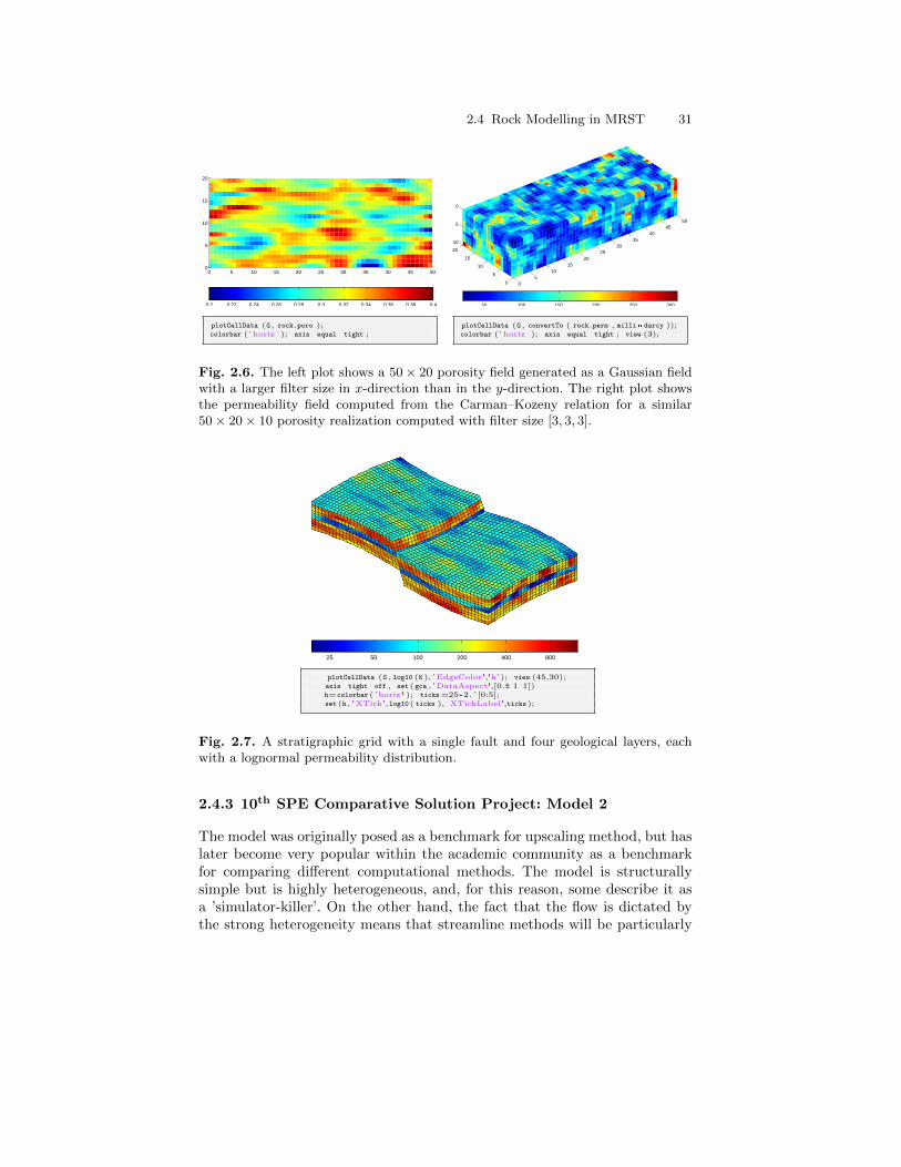
2.4 Rock Modelling in MRST 31
0 5 10 15 20 25 30 35 40 45 500
5
10
15
20
0.2 0.22 0.24 0.26 0.28 0.3 0.32 0.34 0.36 0.38 0.4
plotCellData (G , rock.poro );colorbar ( 'horiz ' ); axis equal tight ;
05
1015
2025
3035
4045
50
0
5
10
15
20
0
5
10
50 100 150 200 250 300
plotCellData (G , convertTo ( rock.perm , milli* darcy ));colorbar ( 'horiz ' ); axis equal tight ; view (3);
Fig. 2.6. The left plot shows a 50× 20 porosity field generated as a Gaussian fieldwith a larger filter size in x-direction than in the y-direction. The right plot showsthe permeability field computed from the Carman–Kozeny relation for a similar50× 20× 10 porosity realization computed with filter size [3, 3, 3].
25 50 100 200 400 800
plotCellData (G , log10 (K ), 'EdgeColor','k'); view (45,30);axis tight off , set(gca , 'DataAspect',[0.5 1 1])h=colorbar( 'horiz ' ); ticks=25*2.ˆ[0:5];set(h , 'XTick',log10 ( ticks ), 'XTickLabel',ticks);
Fig. 2.7. A stratigraphic grid with a single fault and four geological layers, eachwith a lognormal permeability distribution.
2.4.3 10th SPE Comparative Solution Project: Model 2
The model was originally posed as a benchmark for upscaling method, but haslater become very popular within the academic community as a benchmarkfor comparing different computational methods. The model is structurallysimple but is highly heterogeneous, and, for this reason, some describe it asa ’simulator-killer’. On the other hand, the fact that the flow is dictated bythe strong heterogeneity means that streamline methods will be particularly
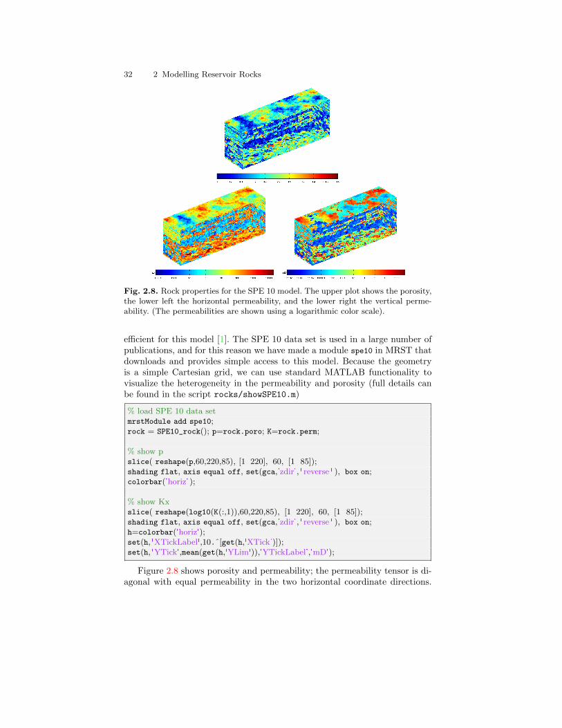
32 2 Modelling Reservoir Rocks
Fig. 2.8. Rock properties for the SPE 10 model. The upper plot shows the porosity,the lower left the horizontal permeability, and the lower right the vertical perme-ability. (The permeabilities are shown using a logarithmic color scale).
efficient for this model [1]. The SPE 10 data set is used in a large number ofpublications, and for this reason we have made a module spe10 in MRST thatdownloads and provides simple access to this model. Because the geometryis a simple Cartesian grid, we can use standard MATLAB functionality tovisualize the heterogeneity in the permeability and porosity (full details canbe found in the script rocks/showSPE10.m)
% load SPE 10 data setmrstModule add spe10;rock = SPE10_rock(); p=rock.poro; K=rock.perm;
% show pslice( reshape(p,60,220,85), [1 220], 60, [1 85]);shading flat, axis equal off, set(gca,'zdir', ' reverse ' ), box on;colorbar('horiz' );
% show Kxslice( reshape(log10(K(:,1)),60,220,85), [1 220], 60, [1 85]);shading flat, axis equal off, set(gca,'zdir', ' reverse ' ), box on;h=colorbar('horiz');set(h,'XTickLabel',10.ˆ[get(h,'XTick')]);set(h,'YTick',mean(get(h,'YLim')),'YTickLabel','mD');
Figure 2.8 shows porosity and permeability; the permeability tensor is di-agonal with equal permeability in the two horizontal coordinate directions.
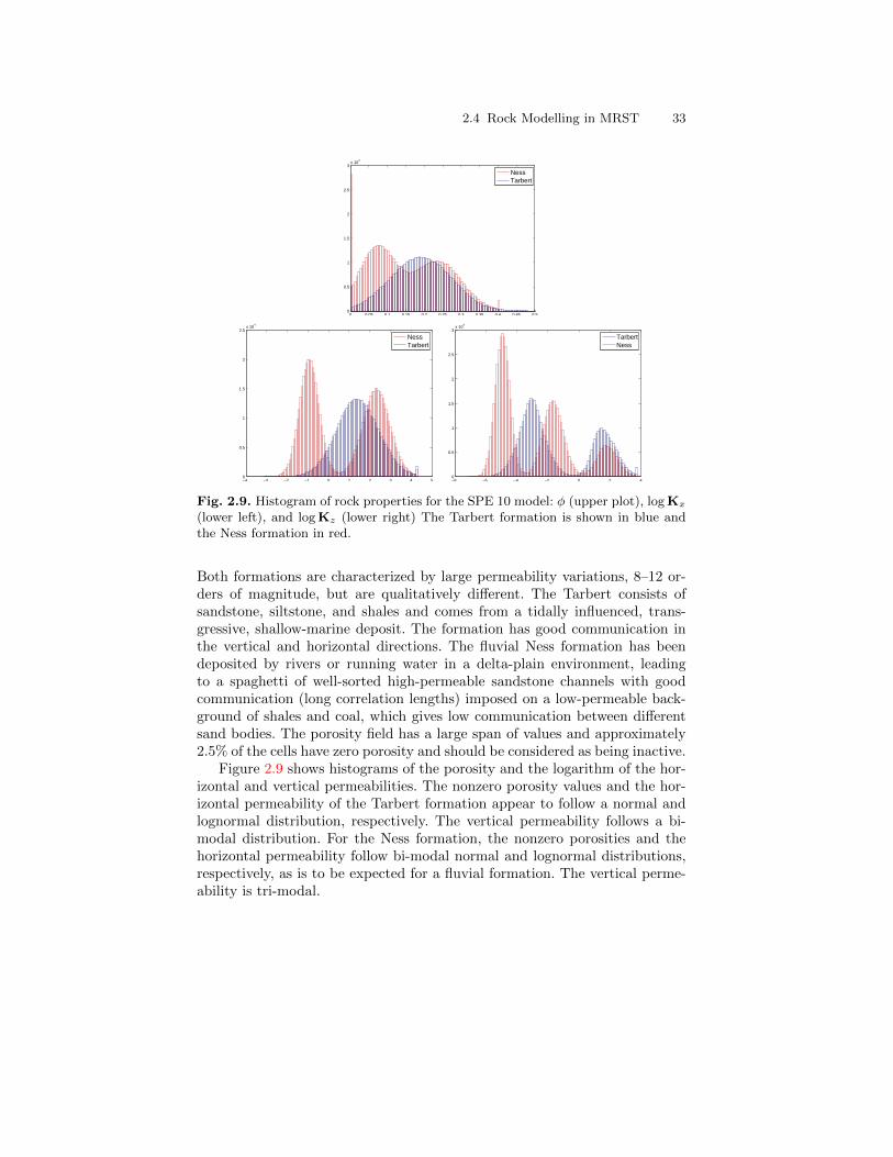
2.4 Rock Modelling in MRST 33
0 0.05 0.1 0.15 0.2 0.25 0.3 0.35 0.4 0.45 0.50
0.5
1
1.5
2
2.5
3x 10
4
NessTarbert
−4 −3 −2 −1 0 1 2 3 4 50
0.5
1
1.5
2
2.5x 10
4
NessTarbert
−8 −6 −4 −2 0 2 40
0.5
1
1.5
2
2.5
3x 10
4
TarbertNess
Fig. 2.9. Histogram of rock properties for the SPE 10 model: φ (upper plot), logKx
(lower left), and logKz (lower right) The Tarbert formation is shown in blue andthe Ness formation in red.
Both formations are characterized by large permeability variations, 8–12 or-ders of magnitude, but are qualitatively different. The Tarbert consists ofsandstone, siltstone, and shales and comes from a tidally influenced, trans-gressive, shallow-marine deposit. The formation has good communication inthe vertical and horizontal directions. The fluvial Ness formation has beendeposited by rivers or running water in a delta-plain environment, leadingto a spaghetti of well-sorted high-permeable sandstone channels with goodcommunication (long correlation lengths) imposed on a low-permeable back-ground of shales and coal, which gives low communication between differentsand bodies. The porosity field has a large span of values and approximately2.5% of the cells have zero porosity and should be considered as being inactive.
Figure 2.9 shows histograms of the porosity and the logarithm of the hor-izontal and vertical permeabilities. The nonzero porosity values and the hor-izontal permeability of the Tarbert formation appear to follow a normal andlognormal distribution, respectively. The vertical permeability follows a bi-modal distribution. For the Ness formation, the nonzero porosities and thehorizontal permeability follow bi-modal normal and lognormal distributions,respectively, as is to be expected for a fluvial formation. The vertical perme-ability is tri-modal.
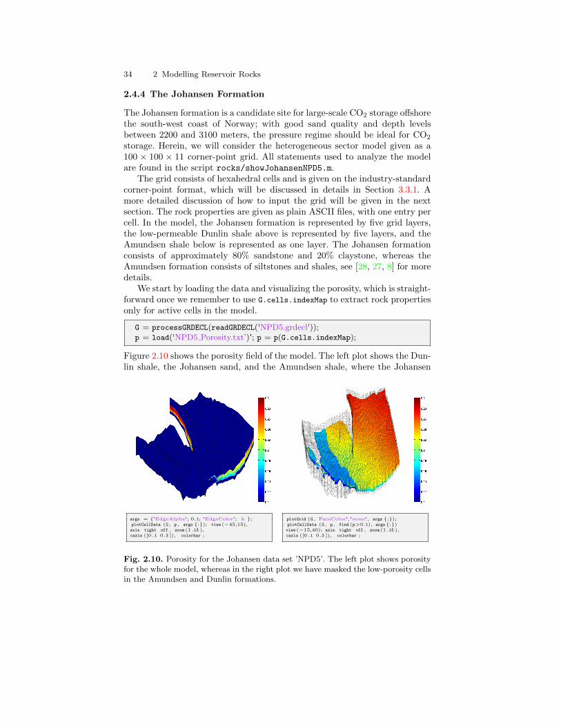
34 2 Modelling Reservoir Rocks
2.4.4 The Johansen Formation
The Johansen formation is a candidate site for large-scale CO2 storage offshorethe south-west coast of Norway; with good sand quality and depth levelsbetween 2200 and 3100 meters, the pressure regime should be ideal for CO2
storage. Herein, we will consider the heterogeneous sector model given as a100 × 100 × 11 corner-point grid. All statements used to analyze the modelare found in the script rocks/showJohansenNPD5.m.
The grid consists of hexahedral cells and is given on the industry-standardcorner-point format, which will be discussed in details in Section 3.3.1. Amore detailed discussion of how to input the grid will be given in the nextsection. The rock properties are given as plain ASCII files, with one entry percell. In the model, the Johansen formation is represented by five grid layers,the low-permeable Dunlin shale above is represented by five layers, and theAmundsen shale below is represented as one layer. The Johansen formationconsists of approximately 80% sandstone and 20% claystone, whereas theAmundsen formation consists of siltstones and shales, see [28, 27, 8] for moredetails.
We start by loading the data and visualizing the porosity, which is straight-forward once we remember to use G.cells.indexMap to extract rock propertiesonly for active cells in the model.
G = processGRDECL(readGRDECL('NPD5.grdecl'));p = load('NPD5 Porosity.txt')'; p = p(G.cells.indexMap);
Figure 2.10 shows the porosity field of the model. The left plot shows the Dun-lin shale, the Johansen sand, and the Amundsen shale, where the Johansen
args = 'EdgeAlpha'; 0.1; 'EdgeColor'; 'k';plotCellData (G , p , args :); view(−45,15),axis tight off , zoom (1.15 ),caxis ([0 .1 0.3 ]), colorbar ;
plotGrid (G , 'FaceColor','none', args :);plotCellData (G , p , find (p>0.1), args:)view(−15,40); axis tight off , zoom (1.15 ),caxis ([0 .1 0.3 ]), colorbar ;
Fig. 2.10. Porosity for the Johansen data set ’NPD5’. The left plot shows porosityfor the whole model, whereas in the right plot we have masked the low-porosity cellsin the Amundsen and Dunlin formations.
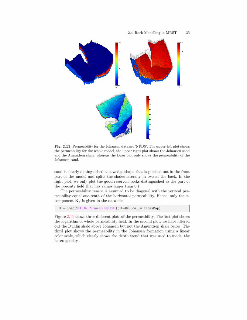
2.4 Rock Modelling in MRST 35
Fig. 2.11. Permeability for the Johansen data set ’NPD5’. The upper-left plot showsthe permeability for the whole model, the upper-right plot shows the Johansen sandand the Amundsen shale, whereas the lower plot only shows the permeability of theJohansen sand.
sand is clearly distinguished as a wedge shape that is pinched out in the frontpart of the model and splits the shales laterally in two at the back. In theright plot, we only plot the good reservoir rocks distinguished as the part ofthe porosity field that has values larger than 0.1.
The permeability tensor is assumed to be diagonal with the vertical per-meability equal one-tenth of the horizontal permeability. Hence, only the x-component Kx is given in the data file
K = load('NPD5 Permeability.txt')'; K=K(G.cells.indexMap);
Figure 2.11 shows three different plots of the permeability. The first plot showsthe logarithm of whole permeability field. In the second plot, we have filteredout the Dunlin shale above Johansen but not the Amundsen shale below. Thethird plot shows the permeability in the Johansen formation using a linearcolor scale, which clearly shows the depth trend that was used to model theheterogeneity.

36 2 Modelling Reservoir Rocks
2.4.5 The SAIGUP Model
Most commercial simulators use a combination of an ’input language’ and aset of data files to describe and set up a simulation model of a reservoir. How-ever, although the principles for the input description has much in common,the detail syntax is obviously unique to each simulator. Herein, we will mainlyfocus on the ECLIPSE input format, which has emerged as an industry stan-dard for describing static and dynamic properties of a reservoir system, fromthe reservoir rock, via production and injection wells and up to connected top-side facilities. ECLIPSE input decks use keywords to signify and separate thedifferent data elements that comprise a full model. These keywords define adetailed language that can be used to specify how the data elements should beput together, and modify each other, to form a full spatio-temporal model ofa reservoir. In the most general form, an ECLIPSE input file consists of eightsets of keywords are organized into eight sections that must come in a pre-scribed order. However, some of the sections are optional and may not alwaysbe present. The order of the keywords within each section is arbitrary, exceptin the section that defines wells and gives operating schedule, etc. Altogether,the ECLIPSE format consists of thousands of keywords, and describing themall is far beyond the scope of this presentation.
In the following, we will instead briefly outline some of the most commonkeywords that are used in the GRID section that describes the reservoir geom-etry and petrophysical properties. The purpose is to provide you with a basicunderstanding of the required input for simulations of real-life reservoir mod-els. Our focus is mainly on the ingredients of a model and not on the specificsyntax. For brevity, we will therefore not go through all Matlab and MRSTstatements used to visualize the different data elements. All details necessaryto reproduce the results can be found in the script rocks/showSAIGUP.m.
As an example of a realistic representation of a shallow-marine reservoir,we will use a simulation model taken from the SAIGUP study [40]. TheSAIGUP models mainly focus on shoreface reservoirs in which the deposi-tion of sediments is caused by variation in sea level, so that facies are formingbelts in a systematic pattern (river deposits create curved facies belts, wavedeposits create parallel belts, etc). Sediments are in general deposited whenthe sea level is increasing. No sediments are deposited during decreasing sealevels; instead, the receding sea may affect the appearing shoreline and causethe creation of a barrier.
Assuming that the archive file SAIGUP.tar.gz that contains the modelrealization has been downloaded as described in Section 1.5, we used MAT-LAB’s untar function to extract the data set and place it in a standardizedpath relative to the root directory of MRST:
untar('SAIGUP.tar.gz', fullfile(ROOTDIR, 'examples', 'data', 'SAIGUP'))
This will create a new directory that contains seventeen data files that com-prise the structural model, various petrophysical parameters, etc:
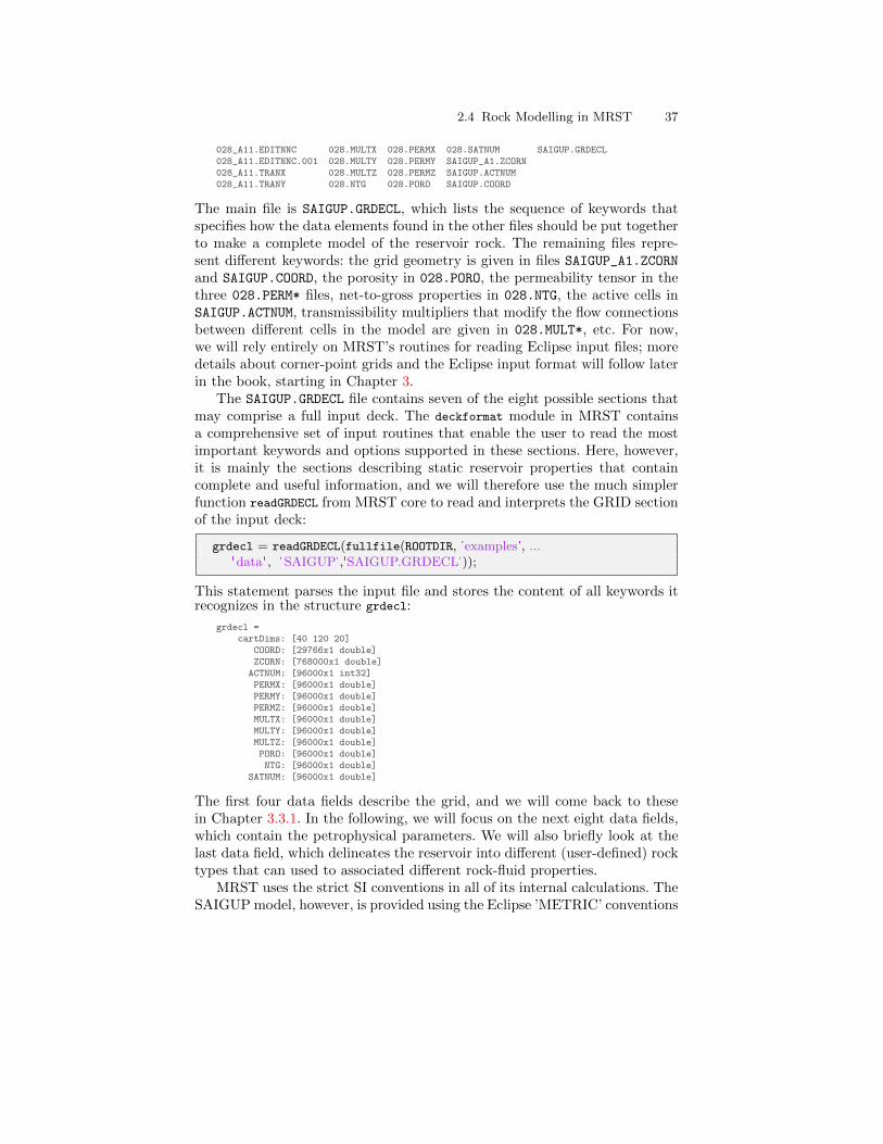
2.4 Rock Modelling in MRST 37
028_A11.EDITNNC 028.MULTX 028.PERMX 028.SATNUM SAIGUP.GRDECL028_A11.EDITNNC.001 028.MULTY 028.PERMY SAIGUP_A1.ZCORN028_A11.TRANX 028.MULTZ 028.PERMZ SAIGUP.ACTNUM028_A11.TRANY 028.NTG 028.PORO SAIGUP.COORD
The main file is SAIGUP.GRDECL, which lists the sequence of keywords thatspecifies how the data elements found in the other files should be put togetherto make a complete model of the reservoir rock. The remaining files repre-sent different keywords: the grid geometry is given in files SAIGUP_A1.ZCORN
and SAIGUP.COORD, the porosity in 028.PORO, the permeability tensor in thethree 028.PERM* files, net-to-gross properties in 028.NTG, the active cells inSAIGUP.ACTNUM, transmissibility multipliers that modify the flow connectionsbetween different cells in the model are given in 028.MULT*, etc. For now,we will rely entirely on MRST’s routines for reading Eclipse input files; moredetails about corner-point grids and the Eclipse input format will follow laterin the book, starting in Chapter 3.
The SAIGUP.GRDECL file contains seven of the eight possible sections thatmay comprise a full input deck. The deckformat module in MRST containsa comprehensive set of input routines that enable the user to read the mostimportant keywords and options supported in these sections. Here, however,it is mainly the sections describing static reservoir properties that containcomplete and useful information, and we will therefore use the much simplerfunction readGRDECL from MRST core to read and interprets the GRID sectionof the input deck:
grdecl = readGRDECL(fullfile(ROOTDIR, 'examples', ...'data' , 'SAIGUP','SAIGUP.GRDECL'));
This statement parses the input file and stores the content of all keywords itrecognizes in the structure grdecl:
grdecl =cartDims: [40 120 20]
COORD: [29766x1 double]ZCORN: [768000x1 double]
ACTNUM: [96000x1 int32]PERMX: [96000x1 double]PERMY: [96000x1 double]PERMZ: [96000x1 double]MULTX: [96000x1 double]MULTY: [96000x1 double]MULTZ: [96000x1 double]PORO: [96000x1 double]NTG: [96000x1 double]
SATNUM: [96000x1 double]
The first four data fields describe the grid, and we will come back to thesein Chapter 3.3.1. In the following, we will focus on the next eight data fields,which contain the petrophysical parameters. We will also briefly look at thelast data field, which delineates the reservoir into different (user-defined) rocktypes that can used to associated different rock-fluid properties.
MRST uses the strict SI conventions in all of its internal calculations. TheSAIGUP model, however, is provided using the Eclipse ’METRIC’ conventions
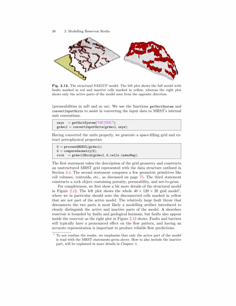
38 2 Modelling Reservoir Rocks
Fig. 2.12. The structural SAIGUP model. The left plot shows the full model withfaults marked in red and inactive cells marked in yellow, whereas the right plotshows only the active parts of the model seen from the opposite direction.
(permeabilities in mD and so on). We use the functions getUnitSystem andconvertInputUnits to assist in converting the input data to MRST’s internalunit conventions.
usys = getUnitSystem('METRIC');grdecl = convertInputUnits(grdecl, usys);
Having converted the units properly, we generate a space-filling grid and ex-tract petrophysical properties
G = processGRDECL(grdecl);G = computeGeometry(G);rock = grdecl2Rock(grdecl, G.cells.indexMap);
The first statement takes the description of the grid geometry and constructsan unstructured MRST grid represented with the data structure outlined inSection 3.4. The second statement computes a few geometric primitives likecell volumes, centroids, etc., as discussed on page 75. The third statementconstructs a rock object containing porosity, permeability, and net-to-gross.
For completeness, we first show a bit more details of the structural modelin Figure 2.12. The left plot shows the whole 40 × 120 × 20 grid model1,where we in particular should note the disconnected cells marked in yellowthat are not part of the active model. The relatively large fault throw thatdisconnects the two parts is most likely a modelling artifact introduced toclearly distinguish the active and inactive parts of the model. A shorefacereservoir is bounded by faults and geological horizons, but faults also appearinside the reservoir as the right plot in Figure 2.12 shows. Faults and barrierswill typically have a pronounced effect on the flow pattern, and having anaccurate representation is important to produce reliable flow predictions.
1 To not confuse the reader, we emphasize that only the active part of the modelis read with the MRST statements given above. How to also include the inactivepart, will be explained in more details in Chapter 3.
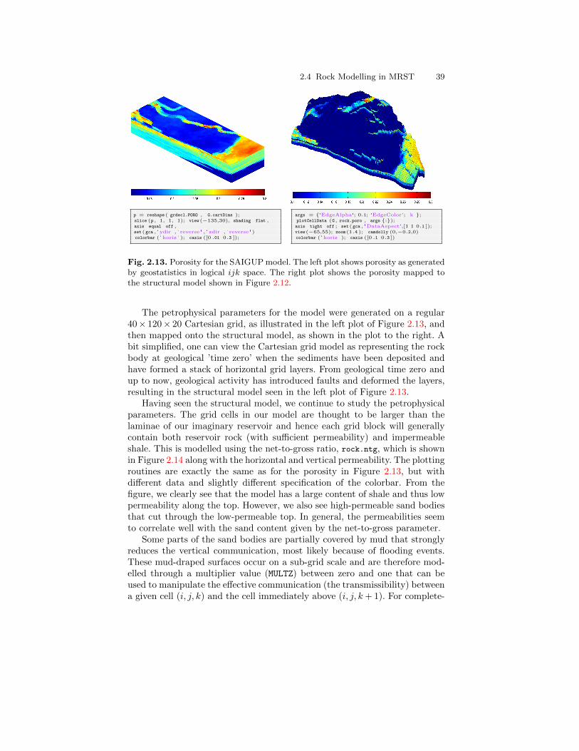
2.4 Rock Modelling in MRST 39
p = reshape ( grdecl.PORO , G.cartDims );slice (p , 1, 1, 1); view(−135,30), shading flat ,axis equal off ,set(gca , 'ydir ' , ' reverse ' , 'zdir ' , ' reverse ')colorbar ( 'horiz ' ); caxis ([0 .01 0.3 ]);
args = 'EdgeAlpha'; 0.1; 'EdgeColor'; 'k';plotCellData (G , rock.poro , args :);axis tight off ; set(gca , 'DataAspect',[1 1 0.1 ]);view(−65,55); zoom(1.4 ); camdolly (0,−0.2,0)colorbar ( 'horiz ' ); caxis ([0 .1 0.3 ])
Fig. 2.13. Porosity for the SAIGUP model. The left plot shows porosity as generatedby geostatistics in logical ijk space. The right plot shows the porosity mapped tothe structural model shown in Figure 2.12.
The petrophysical parameters for the model were generated on a regular40× 120× 20 Cartesian grid, as illustrated in the left plot of Figure 2.13, andthen mapped onto the structural model, as shown in the plot to the right. Abit simplified, one can view the Cartesian grid model as representing the rockbody at geological ’time zero’ when the sediments have been deposited andhave formed a stack of horizontal grid layers. From geological time zero andup to now, geological activity has introduced faults and deformed the layers,resulting in the structural model seen in the left plot of Figure 2.13.
Having seen the structural model, we continue to study the petrophysicalparameters. The grid cells in our model are thought to be larger than thelaminae of our imaginary reservoir and hence each grid block will generallycontain both reservoir rock (with sufficient permeability) and impermeableshale. This is modelled using the net-to-gross ratio, rock.ntg, which is shownin Figure 2.14 along with the horizontal and vertical permeability. The plottingroutines are exactly the same as for the porosity in Figure 2.13, but withdifferent data and slightly different specification of the colorbar. From thefigure, we clearly see that the model has a large content of shale and thus lowpermeability along the top. However, we also see high-permeable sand bodiesthat cut through the low-permeable top. In general, the permeabilities seemto correlate well with the sand content given by the net-to-gross parameter.
Some parts of the sand bodies are partially covered by mud that stronglyreduces the vertical communication, most likely because of flooding events.These mud-draped surfaces occur on a sub-grid scale and are therefore mod-elled through a multiplier value (MULTZ) between zero and one that can beused to manipulate the effective communication (the transmissibility) betweena given cell (i, j, k) and the cell immediately above (i, j, k+ 1). For complete-
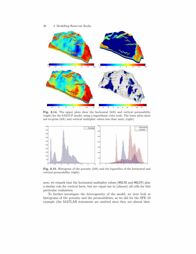
40 2 Modelling Reservoir Rocks
Fig. 2.14. The upper plots show the horizontal (left) and vertical permeability(right) for the SAIGUP model, using a logarithmic color scale. The lower plots shownet-to-gross (left) and vertical multiplier values less than unity (right).
0 0.05 0.1 0.15 0.2 0.25 0.3 0.350
500
1000
1500
2000
2500
3000
3500
4000
4500
5000
Porosity
−4 −3 −2 −1 0 1 2 3 40
500
1000
1500
2000
2500
3000
3500
HorizontalVertical
Fig. 2.15. Histogram of the porosity (left) and the logarithm of the horizontal andvertical permeability (right).
ness, we remark that the horizontal multiplier values (MULTX and MULTY) playa similar role for vertical faces, but are equal one in (almost) all cells for thisparticular realization.
To further investigate the heterogeneity of the model, we next look athistograms of the porosity and the permeabilities, as we did for the SPE 10example (the MATLAB statements are omitted since they are almost iden-
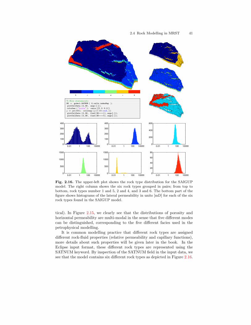
2.4 Rock Modelling in MRST 41
% Key statementsSN = grdecl.SATNUM ( G.cells.indexMap );plotCellData (G , SN , args :);colorbar ( 'horiz ' ); caxis ([0 .5 6.5 ])j = jet(60); colormap (j (1:10:end,:))plotCellData (G , SN , find (SN==1), args:);plotCellData (G , SN , find (SN==5), args:);
0.01 1 100 100000
100
200
300
400
0.01 1 100 100000
100
200
300
400
0.01 1 100 100000
200
400
600
0.01 1 100 100000
500
1000
1500
0.01 1 100 100000
500
1000
1500
0.01 1 100 100000
20
40
60
80
Fig. 2.16. The upper-left plot shows the rock type distribution for the SAIGUPmodel. The right column shows the six rock types grouped in pairs; from top tobottom, rock types number 1 and 5, 2 and 4, and 3 and 6. The bottom part of thefigure shows histograms of the lateral permeability in units [mD] for each of the sixrock types found in the SAIGUP model.
tical). In Figure 2.15, we clearly see that the distributions of porosity andhorizontal permeability are multi-modal in the sense that five different modescan be distinguished, corresponding to the five different facies used in thepetrophysical modelling.
It is common modelling practice that different rock types are assigneddifferent rock-fluid properties (relative permeability and capillary functions),more details about such properties will be given later in the book. In theEclipse input format, these different rock types are represented using theSATNUM keyword. By inspection of the SATNUM field in the input data, wesee that the model contains six different rock types as depicted in Figure 2.16.
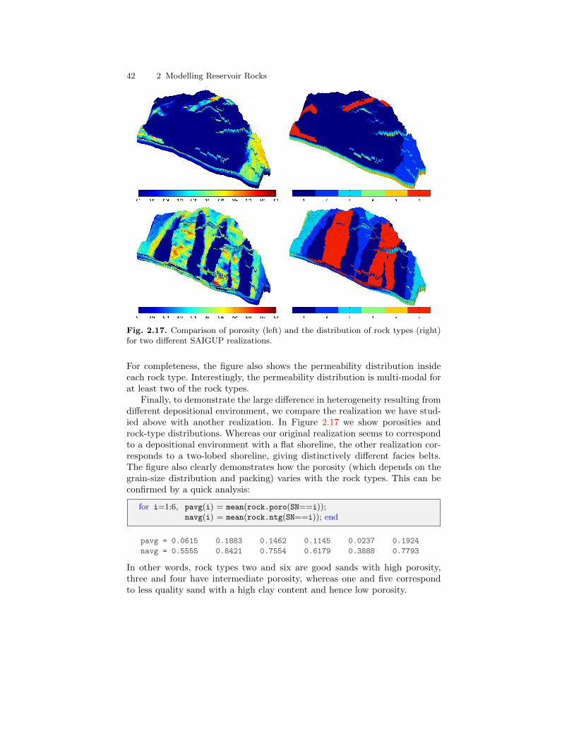
42 2 Modelling Reservoir Rocks
Fig. 2.17. Comparison of porosity (left) and the distribution of rock types (right)for two different SAIGUP realizations.
For completeness, the figure also shows the permeability distribution insideeach rock type. Interestingly, the permeability distribution is multi-modal forat least two of the rock types.
Finally, to demonstrate the large difference in heterogeneity resulting fromdifferent depositional environment, we compare the realization we have stud-ied above with another realization. In Figure 2.17 we show porosities androck-type distributions. Whereas our original realization seems to correspondto a depositional environment with a flat shoreline, the other realization cor-responds to a two-lobed shoreline, giving distinctively different facies belts.The figure also clearly demonstrates how the porosity (which depends on thegrain-size distribution and packing) varies with the rock types. This can beconfirmed by a quick analysis:
for i=1:6, pavg(i) = mean(rock.poro(SN==i));navg(i) = mean(rock.ntg(SN==i)); end
pavg = 0.0615 0.1883 0.1462 0.1145 0.0237 0.1924
navg = 0.5555 0.8421 0.7554 0.6179 0.3888 0.7793
In other words, rock types two and six are good sands with high porosity,three and four have intermediate porosity, whereas one and five correspondto less quality sand with a high clay content and hence low porosity.
3
Grids in Subsurface Modeling
The basic geological description of a petroleum reservoir or an aquifer systemwill typically consist of two sets of surfaces. Geological horizons are lateralsurfaces that describe the bedding planes that delimit the rock strata, whereasfaults are vertical or inclined surfaces along which the strata may have beendisplaced by geological processes. In this chapter, we will discuss how to turnthe basic geological description into a discrete model that can be used toformulate various computational methods, e.g., for solving the equations thatdescribe fluid flow.
A grid is a tessellation of a planar or volumetric object by a set of contigu-ous simple shapes referred to as cells. Grids can be described and distinguishedby their geometry, reflected by the shape of the cells that form the grid, andtheir topology that tells how the individual cells are connected. In 2D, a cell isin general a closed polygon for which the geometry is defined by a set of ver-tices and a set of edges that connect pairs of vertices and define the interfacebetween two neighboring cells. In 3D, a cell is a closed polyhedron for whichthe geometry is defined by a set of vertices, a set of edges that connect pairs ofvertices, and a set of faces (surfaces delimited by a subset of the edges) thatdefine the interface between two different cells, see Figure 3.1. Herein, we willassume that all cells in a grid are non-overlapping, so that each point in theplanar/volumetric object represented by the grid is either inside a single cell,lies on an interface or edge, or is a vertex. Two cells that share a commonface are said to be connected. Likewise, one can also define connections basedon edges and vertices. The topology of a grid is defined by the total set ofconnections, which is sometimes also called the connectivity of the grid.
When implementing grids in modeling software, one always has the choicebetween generality and efficiency. To represent an arbitrary grid, it is necessaryto explicitly store the geometry of each cell in terms of vertices, edges, andfaces, as well as storing the connectivity among cells, faces, edges, and vertices.However, as we will see later, huge simplifications can be made for particularclasses of grids by exploiting regularity in the geometry and structures inthe topology. Consider, for instance, a planar grid consisting of rectangular
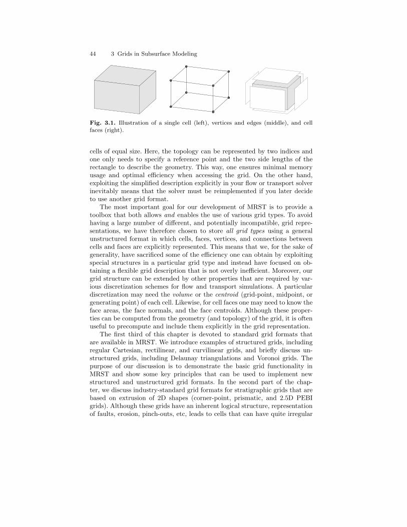
44 3 Grids in Subsurface Modeling
Fig. 3.1. Illustration of a single cell (left), vertices and edges (middle), and cellfaces (right).
cells of equal size. Here, the topology can be represented by two indices andone only needs to specify a reference point and the two side lengths of therectangle to describe the geometry. This way, one ensures minimal memoryusage and optimal efficiency when accessing the grid. On the other hand,exploiting the simplified description explicitly in your flow or transport solverinevitably means that the solver must be reimplemented if you later decideto use another grid format.
The most important goal for our development of MRST is to provide atoolbox that both allows and enables the use of various grid types. To avoidhaving a large number of different, and potentially incompatible, grid repre-sentations, we have therefore chosen to store all grid types using a generalunstructured format in which cells, faces, vertices, and connections betweencells and faces are explicitly represented. This means that we, for the sake ofgenerality, have sacrificed some of the efficiency one can obtain by exploitingspecial structures in a particular grid type and instead have focused on ob-taining a flexible grid description that is not overly inefficient. Moreover, ourgrid structure can be extended by other properties that are required by var-ious discretization schemes for flow and transport simulations. A particulardiscretization may need the volume or the centroid (grid-point, midpoint, orgenerating point) of each cell. Likewise, for cell faces one may need to know theface areas, the face normals, and the face centroids. Although these proper-ties can be computed from the geometry (and topology) of the grid, it is oftenuseful to precompute and include them explicitly in the grid representation.
The first third of this chapter is devoted to standard grid formats thatare available in MRST. We introduce examples of structured grids, includingregular Cartesian, rectilinear, and curvilinear grids, and briefly discuss un-structured grids, including Delaunay triangulations and Voronoi grids. Thepurpose of our discussion is to demonstrate the basic grid functionality inMRST and show some key principles that can be used to implement newstructured and unstructured grid formats. In the second part of the chap-ter, we discuss industry-standard grid formats for stratigraphic grids that arebased on extrusion of 2D shapes (corner-point, prismatic, and 2.5D PEBIgrids). Although these grids have an inherent logical structure, representationof faults, erosion, pinch-outs, etc, leads to cells that can have quite irregular
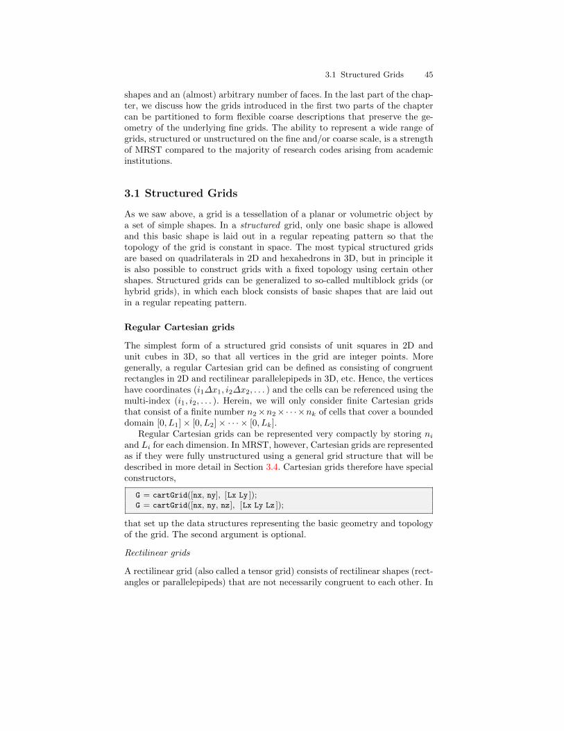
3.1 Structured Grids 45
shapes and an (almost) arbitrary number of faces. In the last part of the chap-ter, we discuss how the grids introduced in the first two parts of the chaptercan be partitioned to form flexible coarse descriptions that preserve the ge-ometry of the underlying fine grids. The ability to represent a wide range ofgrids, structured or unstructured on the fine and/or coarse scale, is a strengthof MRST compared to the majority of research codes arising from academicinstitutions.
3.1 Structured Grids
As we saw above, a grid is a tessellation of a planar or volumetric object bya set of simple shapes. In a structured grid, only one basic shape is allowedand this basic shape is laid out in a regular repeating pattern so that thetopology of the grid is constant in space. The most typical structured gridsare based on quadrilaterals in 2D and hexahedrons in 3D, but in principle itis also possible to construct grids with a fixed topology using certain othershapes. Structured grids can be generalized to so-called multiblock grids (orhybrid grids), in which each block consists of basic shapes that are laid outin a regular repeating pattern.
Regular Cartesian grids
The simplest form of a structured grid consists of unit squares in 2D andunit cubes in 3D, so that all vertices in the grid are integer points. Moregenerally, a regular Cartesian grid can be defined as consisting of congruentrectangles in 2D and rectilinear parallelepipeds in 3D, etc. Hence, the verticeshave coordinates (i1∆x1, i2∆x2, . . . ) and the cells can be referenced using themulti-index (i1, i2, . . . ). Herein, we will only consider finite Cartesian gridsthat consist of a finite number n2×n2×· · ·×nk of cells that cover a boundeddomain [0, L1]× [0, L2]× · · · × [0, Lk].
Regular Cartesian grids can be represented very compactly by storing niand Li for each dimension. In MRST, however, Cartesian grids are representedas if they were fully unstructured using a general grid structure that will bedescribed in more detail in Section 3.4. Cartesian grids therefore have specialconstructors,
G = cartGrid([nx, ny], [Lx Ly ]);G = cartGrid([nx, ny, nz], [Lx Ly Lz ]);
that set up the data structures representing the basic geometry and topologyof the grid. The second argument is optional.
Rectilinear grids
A rectilinear grid (also called a tensor grid) consists of rectilinear shapes (rect-angles or parallelepipeds) that are not necessarily congruent to each other. In
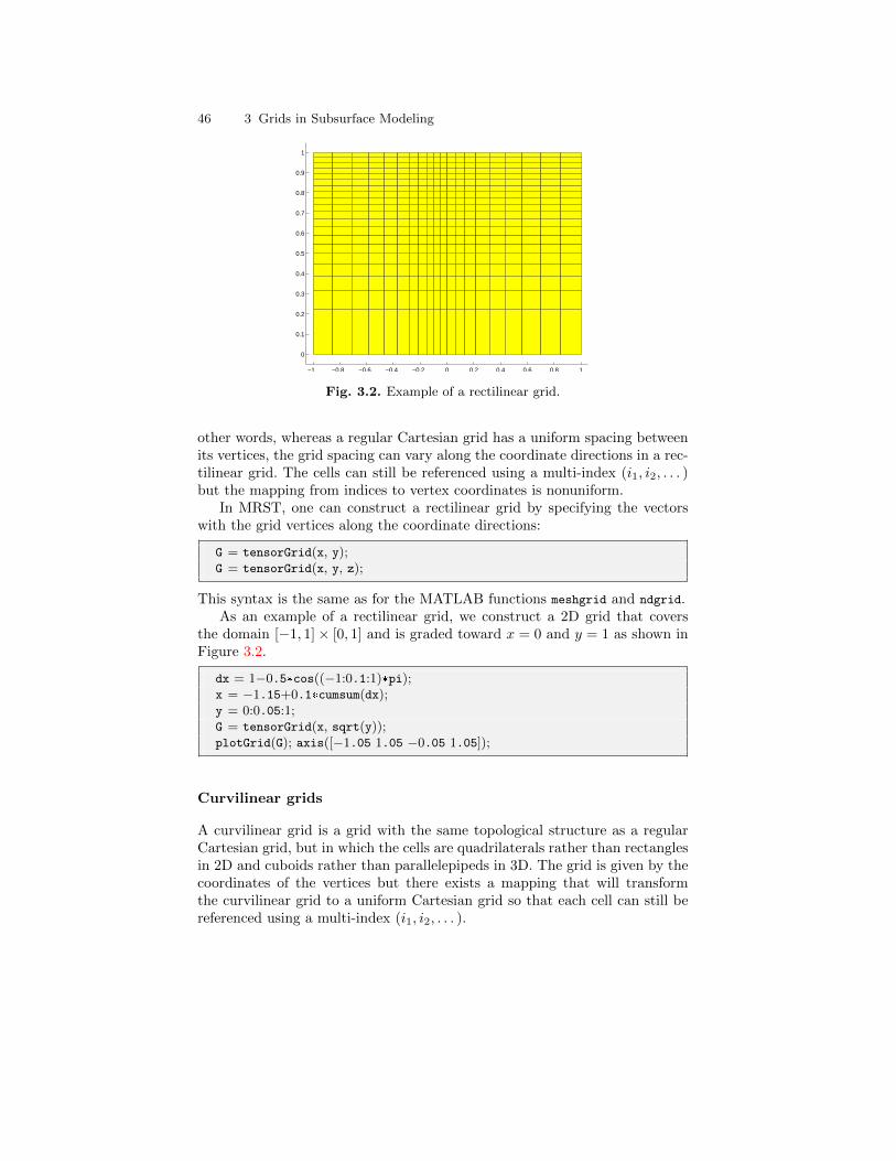
46 3 Grids in Subsurface Modeling
−1 −0.8 −0.6 −0.4 −0.2 0 0.2 0.4 0.6 0.8 1
0
0.1
0.2
0.3
0.4
0.5
0.6
0.7
0.8
0.9
1
Fig. 3.2. Example of a rectilinear grid.
other words, whereas a regular Cartesian grid has a uniform spacing betweenits vertices, the grid spacing can vary along the coordinate directions in a rec-tilinear grid. The cells can still be referenced using a multi-index (i1, i2, . . . )but the mapping from indices to vertex coordinates is nonuniform.
In MRST, one can construct a rectilinear grid by specifying the vectorswith the grid vertices along the coordinate directions:
G = tensorGrid(x, y);G = tensorGrid(x, y, z);
This syntax is the same as for the MATLAB functions meshgrid and ndgrid.As an example of a rectilinear grid, we construct a 2D grid that covers
the domain [−1, 1]× [0, 1] and is graded toward x = 0 and y = 1 as shown inFigure 3.2.
dx = 1−0.5*cos((−1:0.1:1)*pi);x = −1.15+0.1*cumsum(dx);y = 0:0.05:1;G = tensorGrid(x, sqrt(y));plotGrid(G); axis([−1.05 1.05 −0.05 1.05]);
Curvilinear grids
A curvilinear grid is a grid with the same topological structure as a regularCartesian grid, but in which the cells are quadrilaterals rather than rectanglesin 2D and cuboids rather than parallelepipeds in 3D. The grid is given by thecoordinates of the vertices but there exists a mapping that will transformthe curvilinear grid to a uniform Cartesian grid so that each cell can still bereferenced using a multi-index (i1, i2, . . . ).
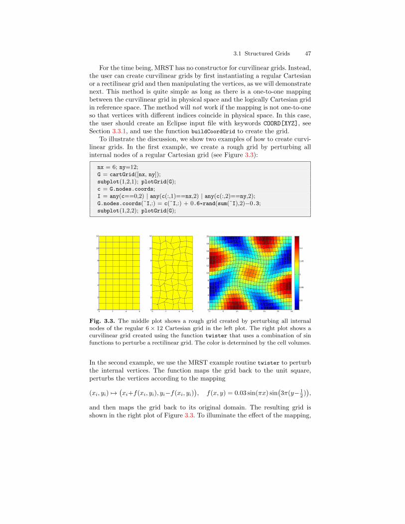
3.1 Structured Grids 47
For the time being, MRST has no constructor for curvilinear grids. Instead,the user can create curvilinear grids by first instantiating a regular Cartesianor a rectilinear grid and then manipulating the vertices, as we will demonstratenext. This method is quite simple as long as there is a one-to-one mappingbetween the curvilinear grid in physical space and the logically Cartesian gridin reference space. The method will not work if the mapping is not one-to-oneso that vertices with different indices coincide in physical space. In this case,the user should create an Eclipse input file with keywords COORD[XYZ], seeSection 3.3.1, and use the function buildCoordGrid to create the grid.
To illustrate the discussion, we show two examples of how to create curvi-linear grids. In the first example, we create a rough grid by perturbing allinternal nodes of a regular Cartesian grid (see Figure 3.3):
nx = 6; ny=12;G = cartGrid([nx, ny]);subplot(1,2,1); plotGrid(G);c = G.nodes.coords;I = any(c==0,2) | any(c(:,1)==nx,2) | any(c(:,2)==ny,2);G.nodes.coords(˜I,:) = c(˜I,:) + 0.6*rand(sum(˜I),2)−0.3;subplot(1,2,2); plotGrid(G);
0 2 4 60
2
4
6
8
10
12
0 2 4 60
2
4
6
8
10
12
0 5 10 15 20 25 300
2
4
6
8
10
12
14
16
18
20
0.9
0.95
1
1.05
1.1
Fig. 3.3. The middle plot shows a rough grid created by perturbing all internalnodes of the regular 6 × 12 Cartesian grid in the left plot. The right plot shows acurvilinear grid created using the function twister that uses a combination of sinfunctions to perturbe a rectilinear grid. The color is determined by the cell volumes.
In the second example, we use the MRST example routine twister to perturbthe internal vertices. The function maps the grid back to the unit square,perturbs the vertices according to the mapping
(xi, yi) 7→(xi+f(xi, yi), yi−f(xi, yi)
), f(x, y) = 0.03 sin(πx) sin
(3π(y− 1
2 )),
and then maps the grid back to its original domain. The resulting grid isshown in the right plot of Figure 3.3. To illuminate the effect of the mapping,
48 3 Grids in Subsurface Modeling
we have colored the cells according to their volume, which has been computedusing the function computeGeometry, which we will come back to below.
G = cartGrid([30, 20]);G.nodes.coords = twister(G.nodes.coords);G = computeGeometry(G);plotCellData(G, G.cells.volumes, 'EdgeColor', 'k'), colorbar
Fictitious domains
One obvious drawback with Cartesian and rectilinear grids, as defined above,is that they can only represent rectangular domains in 2D and cubic domainsin 3D. Curvilinear grids, on the other hand, can represent more general shapesby introducing an appropriate mapping, and can be used in combination withrectangular/cubic grids in multiblock grids for efficient representation of re-alistic reservoir geometries. However, finding a mapping that conforms to agiven boundary is often difficult, in particular for complex geologies, and us-ing a mapping in the interior of the domain will inadvertently lead to cellswith rough geometries that deviate far from being rectilinear. Such cells mayin turn introduce problems if the grid is to be used in a subsequent numericaldiscretization, as we will see later.
As an alternative, complex geometries can be easily modelled using struc-tured grids by a so-called fictitious domain method. In this method, the com-plex domain is embedded into a larger ”fictitious” domain of simple shape (arectangle or cube) using, e.g., a boolean indicator value in each cell to tellwhether the cell is part of the domain or not. The observant reader will noticethat we already have encountered the use of this technique for the SAIGUPdataset (Figure 2.12) and the Johansen dataset in Chapter 2. In some cases,one can also adapt the structured grid by moving the nearest vertices to thedomain boundary.
MRST has support for fictitious domain methods through the functionremoveCells, which we will demonstrate in the next example, where we createa regular Cartesian grid that fills the volume of an ellipsoid:
x = linspace(−2,2,21);G = tensorGrid(x,x,x);subplot(1,2,1); plotGrid(G);view(3); axis equal
subplot(1,2,2); plotGrid(G,'FaceColor','none');G = computeGeometry(G);c = G.cells.centroids;r = c(:,1).ˆ2 + 0.25*c(:,2).ˆ2+0.25*c(:,3).ˆ2;G = removeCells(G, r>1);plotGrid(G); view(−70,70); axis equal;
Worth observing here is the use of computeGeometry to compute cell cen-troids which are not part of the basic geometry representation in MRST.
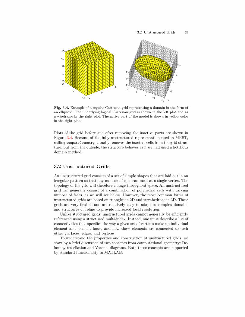
3.2 Unstructured Grids 49
−2
0
2
−2
0
2
−2
−1
0
1
2
−2
−1
0
1
2
−2−1
01
2
−2
0
2
Fig. 3.4. Example of a regular Cartesian grid representing a domain in the form ofan ellipsoid. The underlying logical Cartesian grid is shown in the left plot and asa wireframe in the right plot. The active part of the model is shown in yellow colorin the right plot.
Plots of the grid before and after removing the inactive parts are shown inFigure 3.4. Because of the fully unstructured representation used in MRST,calling computeGeometry actually removes the inactive cells from the grid struc-ture, but from the outside, the structure behaves as if we had used a fictitiousdomain method.
3.2 Unstructured Grids
An unstructured grid consists of a set of simple shapes that are laid out in anirregular pattern so that any number of cells can meet at a single vertex. Thetopology of the grid will therefore change throughout space. An unstructuredgrid can generally consist of a combination of polyhedral cells with varyingnumber of faces, as we will see below. However, the most common forms ofunstructured grids are based on triangles in 2D and tetrahedrons in 3D. Thesegrids are very flexible and are relatively easy to adapt to complex domainsand structures or refine to provide increased local resolution.
Unlike structured grids, unstructured grids cannot generally be efficientlyreferenced using a structured multi-index. Instead, one must describe a list ofconnectivities that specifies the way a given set of vertices make up individualelement and element faces, and how these elements are connected to eachother via faces, edges, and vertices.
To understand the properties and construction of unstructured grids, westart by a brief discussion of two concepts from computational geometry: De-launay tessellation and Voronoi diagrams. Both these concepts are supportedby standard functionality in MATLAB.
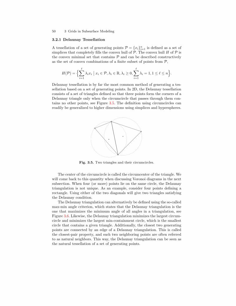
50 3 Grids in Subsurface Modeling
3.2.1 Delaunay Tessellation
A tessellation of a set of generating points P = xini=1 is defined as a set ofsimplices that completely fills the convex hull of P. The convex hull H of P isthe convex minimal set that contains P and can be described constructivelyas the set of convex combinations of a finite subset of points from P,
H(P) =∑i=1
λixi∣∣ xi ∈ P, λi ∈ R, λi ≥ 0,
∑i=1
λi = 1, 1 ≤ ` ≤ n.
Delaunay tessellation is by far the most common method of generating a tes-sellation based on a set of generating points. In 2D, the Delaunay tessellationconsists of a set of triangles defined so that three points form the corners of aDelaunay triangle only when the circumcircle that passes through them con-tains no other points, see Figure 3.5. The definition using circumcircles canreadily be generalized to higher dimensions using simplices and hyperspheres.
Fig. 3.5. Two triangles and their circumcircles.
The center of the circumcircle is called the circumcenter of the triangle. Wewill come back to this quantity when discussing Voronoi diagrams in the nextsubsection. When four (or more) points lie on the same circle, the Delaunaytriangulation is not unique. As an example, consider four points defining arectangle. Using either of the two diagonals will give two triangles satisfyingthe Delaunay condition.
The Delaunay triangulation can alternatively be defined using the so-calledmax-min angle criterion, which states that the Delaunay triangulation is theone that maximizes the minimum angle of all angles in a triangulation, seeFigure 3.6. Likewise, the Delaunay triangulation minimizes the largest circum-circle and minimizes the largest min-containment circle, which is the smallestcircle that contains a given triangle. Additionally, the closest two generatingpoints are connected by an edge of a Delaunay triangulation. This is calledthe closest-pair property, and such two neighboring points are often referredto as natural neighbors. This way, the Delaunay triangulation can be seen asthe natural tessellation of a set of generating points.
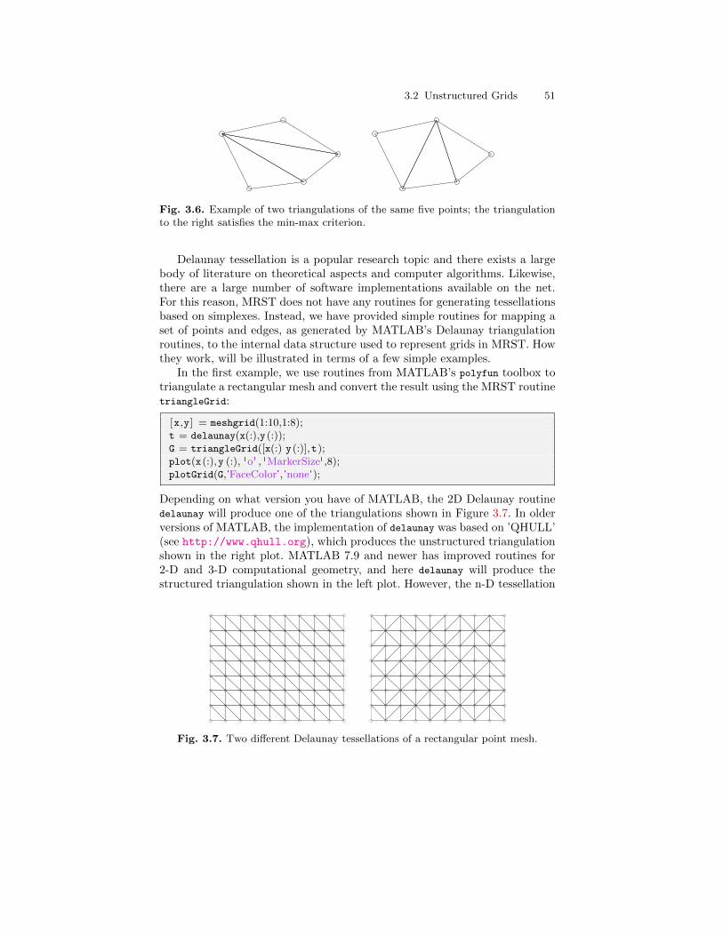
3.2 Unstructured Grids 51
Fig. 3.6. Example of two triangulations of the same five points; the triangulationto the right satisfies the min-max criterion.
Delaunay tessellation is a popular research topic and there exists a largebody of literature on theoretical aspects and computer algorithms. Likewise,there are a large number of software implementations available on the net.For this reason, MRST does not have any routines for generating tessellationsbased on simplexes. Instead, we have provided simple routines for mapping aset of points and edges, as generated by MATLAB’s Delaunay triangulationroutines, to the internal data structure used to represent grids in MRST. Howthey work, will be illustrated in terms of a few simple examples.
In the first example, we use routines from MATLAB’s polyfun toolbox totriangulate a rectangular mesh and convert the result using the MRST routinetriangleGrid:
[x,y] = meshgrid(1:10,1:8);t = delaunay(x(:),y (:));G = triangleGrid([x(:) y(:)],t);plot(x(:),y (:), 'o' , 'MarkerSize',8);plotGrid(G,'FaceColor','none');
Depending on what version you have of MATLAB, the 2D Delaunay routinedelaunay will produce one of the triangulations shown in Figure 3.7. In olderversions of MATLAB, the implementation of delaunay was based on ’QHULL’(see http://www.qhull.org), which produces the unstructured triangulationshown in the right plot. MATLAB 7.9 and newer has improved routines for2-D and 3-D computational geometry, and here delaunay will produce thestructured triangulation shown in the left plot. However, the n-D tessellation
Fig. 3.7. Two different Delaunay tessellations of a rectangular point mesh.
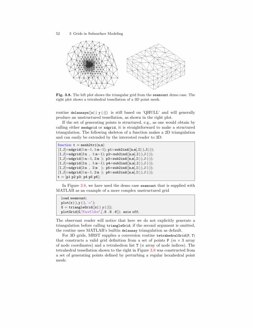
52 3 Grids in Subsurface Modeling
Fig. 3.8. The left plot shows the triangular grid from the seamount demo case. Theright plot shows a tetrahedral tessellation of a 3D point mesh.
routine delaunayn([x(:) y (:)]) is still based on ’QHULL’ and will generallyproduce an unstructured tessellation, as shown in the right plot.
If the set of generating points is structured, e.g., as one would obtain bycalling either meshgrid or ndgrid, it is straightforward to make a structuredtriangulation. The following skeleton of a function makes a 2D triangulationand can easily be extended by the interested reader to 3D:
function t = mesh2tri(n,m)[I,J]=ndgrid(1:n−1, 1:m−1); p1=sub2ind([n,m],I(:),J(:));[I,J]=ndgrid(2:n , 1:m−1); p2=sub2ind([n,m],I(:),J (:));[I,J]=ndgrid(1:n−1, 2:m ); p3=sub2ind([n,m],I(:),J (:));[I,J]=ndgrid(2:n , 1:m−1); p4=sub2ind([n,m],I(:),J (:));[I,J]=ndgrid(2:n , 2:m ); p5=sub2ind([n,m],I(:),J (:));[I,J]=ndgrid(1:n−1, 2:m ); p6=sub2ind([n,m],I(:),J (:));t = [p1 p2 p3; p4 p5 p6 ];
In Figure 3.8, we have used the demo case seamount that is supplied withMATLAB as an example of a more complex unstructured grid
load seamount;plot(x(:),y (:), 'o' );G = triangleGrid([x(:) y (:)]);plotGrid(G,'FaceColor',[.8 .8 .8 ]); axis off;
The observant reader will notice that here we do not explicitly generate atriangulation before calling triangleGrid; if the second argument is omitted,the routine uses MATLAB’s builtin delaunay triangulation as default.
For 3D grids, MRST supplies a conversion routine tetrahedralGrid(P, T)
that constructs a valid grid definition from a set of points P (m × 3 arrayof node coordinates) and a tetrahedron list T (n array of node indices). Thetetrahedral tessellation shown to the right in Figure 3.8 was constructed froma set of generating points defined by perturbing a regular hexahedral pointmesh:
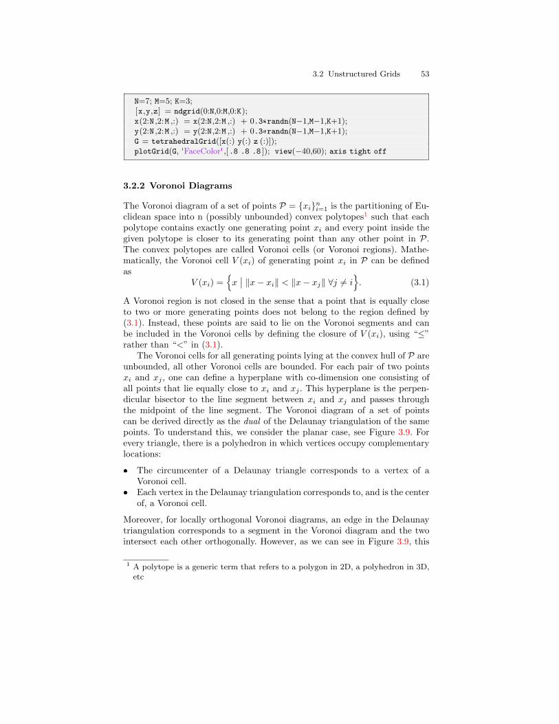
3.2 Unstructured Grids 53
N=7; M=5; K=3;[x,y,z] = ndgrid(0:N,0:M,0:K);x(2:N ,2:M ,:) = x(2:N,2:M ,:) + 0.3*randn(N−1,M−1,K+1);y(2:N ,2:M ,:) = y(2:N,2:M ,:) + 0.3*randn(N−1,M−1,K+1);G = tetrahedralGrid([x(:) y(:) z (:)]);plotGrid(G, 'FaceColor' ,[.8 .8 .8 ]); view(−40,60); axis tight off
3.2.2 Voronoi Diagrams
The Voronoi diagram of a set of points P = xini=1 is the partitioning of Eu-clidean space into n (possibly unbounded) convex polytopes1 such that eachpolytope contains exactly one generating point xi and every point inside thegiven polytope is closer to its generating point than any other point in P.The convex polytopes are called Voronoi cells (or Voronoi regions). Mathe-matically, the Voronoi cell V (xi) of generating point xi in P can be definedas
V (xi) =x∣∣ ‖x− xi‖ < ‖x− xj‖ ∀j 6= i
. (3.1)
A Voronoi region is not closed in the sense that a point that is equally closeto two or more generating points does not belong to the region defined by(3.1). Instead, these points are said to lie on the Voronoi segments and canbe included in the Voronoi cells by defining the closure of V (xi), using “≤”rather than “<” in (3.1).
The Voronoi cells for all generating points lying at the convex hull of P areunbounded, all other Voronoi cells are bounded. For each pair of two pointsxi and xj , one can define a hyperplane with co-dimension one consisting ofall points that lie equally close to xi and xj . This hyperplane is the perpen-dicular bisector to the line segment between xi and xj and passes throughthe midpoint of the line segment. The Voronoi diagram of a set of pointscan be derived directly as the dual of the Delaunay triangulation of the samepoints. To understand this, we consider the planar case, see Figure 3.9. Forevery triangle, there is a polyhedron in which vertices occupy complementarylocations:
The circumcenter of a Delaunay triangle corresponds to a vertex of aVoronoi cell.
Each vertex in the Delaunay triangulation corresponds to, and is the centerof, a Voronoi cell.
Moreover, for locally orthogonal Voronoi diagrams, an edge in the Delaunaytriangulation corresponds to a segment in the Voronoi diagram and the twointersect each other orthogonally. However, as we can see in Figure 3.9, this
1 A polytope is a generic term that refers to a polygon in 2D, a polyhedron in 3D,etc
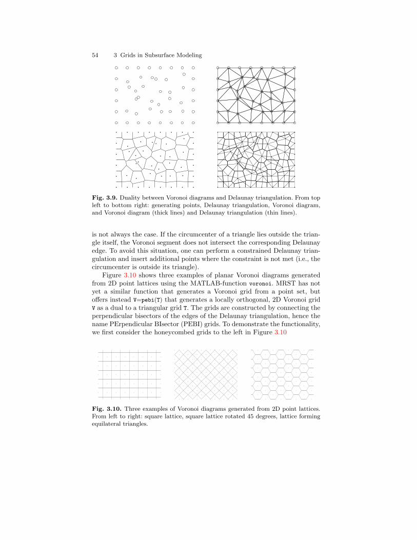
54 3 Grids in Subsurface Modeling
Fig. 3.9. Duality between Voronoi diagrams and Delaunay triangulation. From topleft to bottom right: generating points, Delaunay triangulation, Voronoi diagram,and Voronoi diagram (thick lines) and Delaunay triangulation (thin lines).
is not always the case. If the circumcenter of a triangle lies outside the trian-gle itself, the Voronoi segment does not intersect the corresponding Delaunayedge. To avoid this situation, one can perform a constrained Delaunay trian-gulation and insert additional points where the constraint is not met (i.e., thecircumcenter is outside its triangle).
Figure 3.10 shows three examples of planar Voronoi diagrams generatedfrom 2D point lattices using the MATLAB-function voronoi. MRST has notyet a similar function that generates a Voronoi grid from a point set, butoffers instead V=pebi(T) that generates a locally orthogonal, 2D Voronoi gridV as a dual to a triangular grid T. The grids are constructed by connecting theperpendicular bisectors of the edges of the Delaunay triangulation, hence thename PErpendicular BIsector (PEBI) grids. To demonstrate the functionality,we first consider the honeycombed grids to the left in Figure 3.10
Fig. 3.10. Three examples of Voronoi diagrams generated from 2D point lattices.From left to right: square lattice, square lattice rotated 45 degrees, lattice formingequilateral triangles.
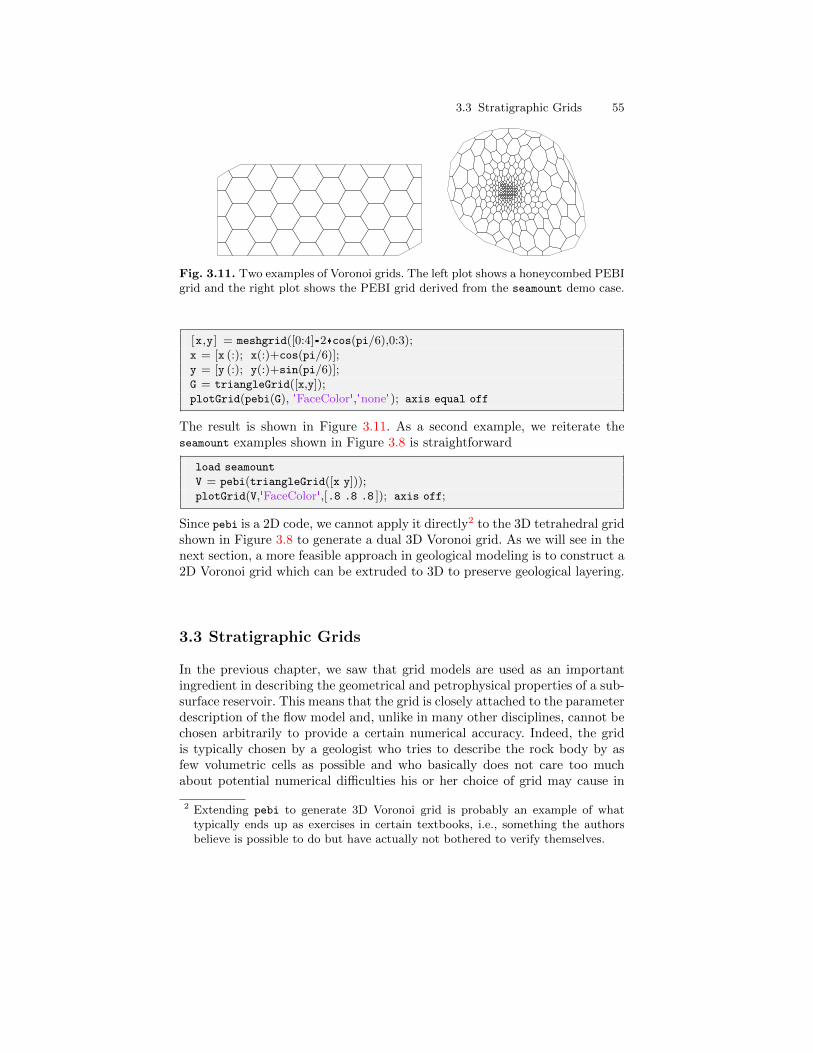
3.3 Stratigraphic Grids 55
Fig. 3.11. Two examples of Voronoi grids. The left plot shows a honeycombed PEBIgrid and the right plot shows the PEBI grid derived from the seamount demo case.
[x,y] = meshgrid([0:4]*2*cos(pi/6),0:3);x = [x (:); x(:)+cos(pi/6)];y = [y (:); y(:)+sin(pi/6)];G = triangleGrid([x,y]);plotGrid(pebi(G), 'FaceColor','none'); axis equal off
The result is shown in Figure 3.11. As a second example, we reiterate theseamount examples shown in Figure 3.8 is straightforward
load seamount
V = pebi(triangleGrid([x y]));plotGrid(V,'FaceColor',[.8 .8 .8 ]); axis off;
Since pebi is a 2D code, we cannot apply it directly2 to the 3D tetrahedral gridshown in Figure 3.8 to generate a dual 3D Voronoi grid. As we will see in thenext section, a more feasible approach in geological modeling is to construct a2D Voronoi grid which can be extruded to 3D to preserve geological layering.
3.3 Stratigraphic Grids
In the previous chapter, we saw that grid models are used as an importantingredient in describing the geometrical and petrophysical properties of a sub-surface reservoir. This means that the grid is closely attached to the parameterdescription of the flow model and, unlike in many other disciplines, cannot bechosen arbitrarily to provide a certain numerical accuracy. Indeed, the gridis typically chosen by a geologist who tries to describe the rock body by asfew volumetric cells as possible and who basically does not care too muchabout potential numerical difficulties his or her choice of grid may cause in
2 Extending pebi to generate 3D Voronoi grid is probably an example of whattypically ends up as exercises in certain textbooks, i.e., something the authorsbelieve is possible to do but have actually not bothered to verify themselves.
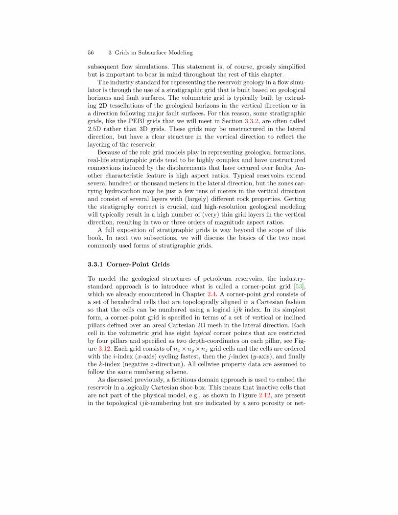
56 3 Grids in Subsurface Modeling
subsequent flow simulations. This statement is, of course, grossly simplifiedbut is important to bear in mind throughout the rest of this chapter.
The industry standard for representing the reservoir geology in a flow simu-lator is through the use of a stratigraphic grid that is built based on geologicalhorizons and fault surfaces. The volumetric grid is typically built by extrud-ing 2D tessellations of the geological horizons in the vertical direction or ina direction following major fault surfaces. For this reason, some stratigraphicgrids, like the PEBI grids that we will meet in Section 3.3.2, are often called2.5D rather than 3D grids. These grids may be unstructured in the lateraldirection, but have a clear structure in the vertical direction to reflect thelayering of the reservoir.
Because of the role grid models play in representing geological formations,real-life stratigraphic grids tend to be highly complex and have unstructuredconnections induced by the displacements that have occured over faults. An-other characteristic feature is high aspect ratios. Typical reservoirs extendseveral hundred or thousand meters in the lateral direction, but the zones car-rying hydrocarbon may be just a few tens of meters in the vertical directionand consist of several layers with (largely) different rock properties. Gettingthe stratigraphy correct is crucial, and high-resolution geological modelingwill typically result in a high number of (very) thin grid layers in the verticaldirection, resulting in two or three orders of magnitude aspect ratios.
A full exposition of stratigraphic grids is way beyond the scope of thisbook. In next two subsections, we will discuss the basics of the two mostcommonly used forms of stratigraphic grids.
3.3.1 Corner-Point Grids
To model the geological structures of petroleum reservoirs, the industry-standard approach is to introduce what is called a corner-point grid [53],which we already encountered in Chapter 2.4. A corner-point grid consists ofa set of hexahedral cells that are topologically aligned in a Cartesian fashionso that the cells can be numbered using a logical ijk index. In its simplestform, a corner-point grid is specified in terms of a set of vertical or inclinedpillars defined over an areal Cartesian 2D mesh in the lateral direction. Eachcell in the volumetric grid has eight logical corner points that are restrictedby four pillars and specified as two depth-coordinates on each pillar, see Fig-ure 3.12. Each grid consists of nx×ny×nz grid cells and the cells are orderedwith the i-index (x-axis) cycling fastest, then the j-index (y-axis), and finallythe k-index (negative z-direction). All cellwise property data are assumed tofollow the same numbering scheme.
As discussed previously, a fictitious domain approach is used to embed thereservoir in a logically Cartesian shoe-box. This means that inactive cells thatare not part of the physical model, e.g., as shown in Figure 2.12, are presentin the topological ijk-numbering but are indicated by a zero porosity or net-
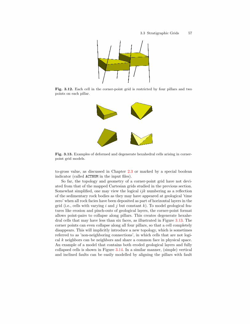
3.3 Stratigraphic Grids 57
Fig. 3.12. Each cell in the corner-point grid is restricted by four pillars and twopoints on each pillar.
Fig. 3.13. Examples of deformed and degenerate hexahedral cells arising in corner-point grid models.
to-gross value, as discussed in Chapter 2.3 or marked by a special booleanindicator (called ACTNUM in the input files).
So far, the topology and geometry of a corner-point grid have not devi-ated from that of the mapped Cartesian grids studied in the previous section.Somewhat simplified, one may view the logical ijk numbering as a reflectionof the sedimentary rock bodies as they may have appeared at geological ’timezero’ when all rock facies have been deposited as part of horizontal layers in thegrid (i.e., cells with varying i and j but constant k). To model geological fea-tures like erosion and pinch-outs of geological layers, the corner-point formatallows point-pairs to collapse along pillars. This creates degenerate hexahe-dral cells that may have less than six faces, as illustrated in Figure 3.13. Thecorner points can even collapse along all four pillars, so that a cell completelydisappears. This will implicitly introduce a new topology, which is sometimesreferred to as ’non-neighboring connections’, in which cells that are not logi-cal k neighbors can be neighbors and share a common face in physical space.An example of a model that contains both eroded geological layers and fullycollapsed cells is shown in Figure 3.14. In a similar manner, (simple) verticaland inclined faults can be easily modelled by aligning the pillars with fault
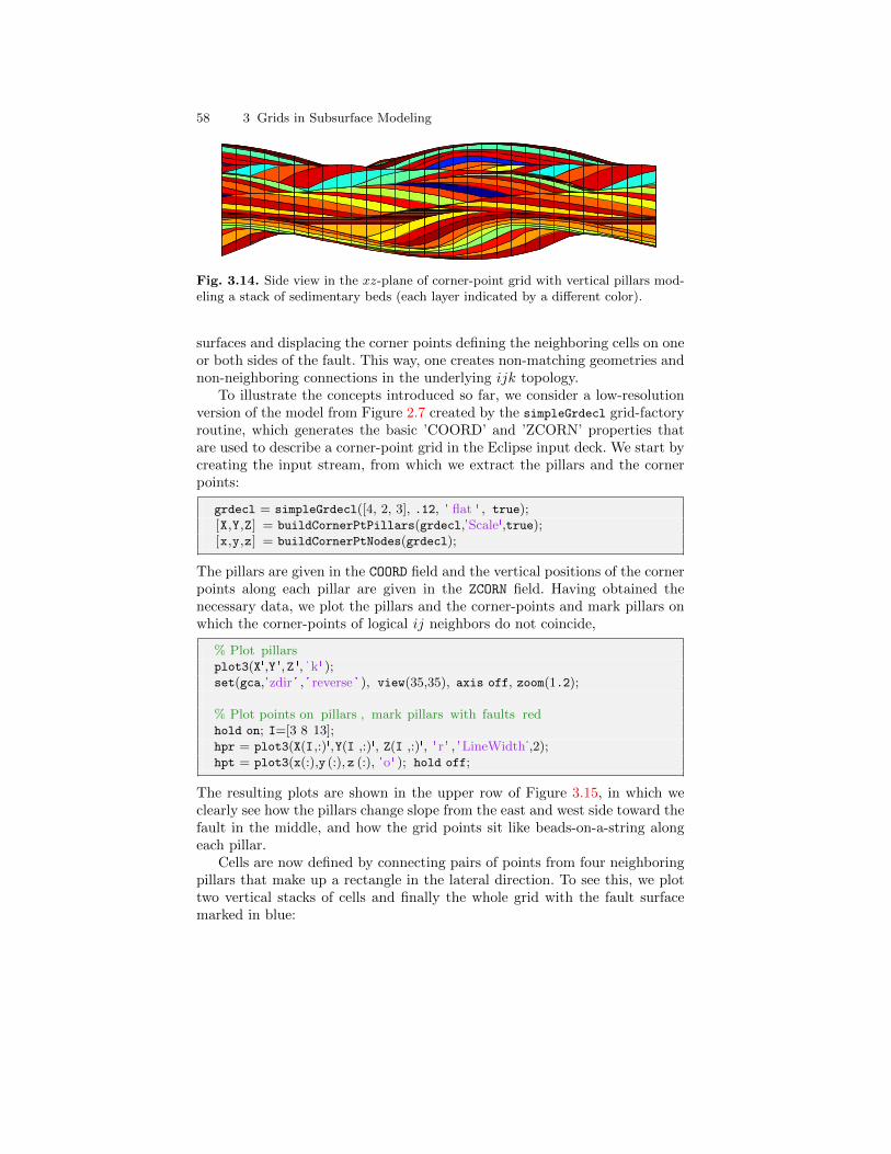
58 3 Grids in Subsurface Modeling
Fig. 3.14. Side view in the xz-plane of corner-point grid with vertical pillars mod-eling a stack of sedimentary beds (each layer indicated by a different color).
surfaces and displacing the corner points defining the neighboring cells on oneor both sides of the fault. This way, one creates non-matching geometries andnon-neighboring connections in the underlying ijk topology.
To illustrate the concepts introduced so far, we consider a low-resolutionversion of the model from Figure 2.7 created by the simpleGrdecl grid-factoryroutine, which generates the basic ’COORD’ and ’ZCORN’ properties thatare used to describe a corner-point grid in the Eclipse input deck. We start bycreating the input stream, from which we extract the pillars and the cornerpoints:
grdecl = simpleGrdecl([4, 2, 3], .12, ' flat ' , true);[X,Y,Z] = buildCornerPtPillars(grdecl,'Scale',true);[x,y,z] = buildCornerPtNodes(grdecl);
The pillars are given in the COORD field and the vertical positions of the cornerpoints along each pillar are given in the ZCORN field. Having obtained thenecessary data, we plot the pillars and the corner-points and mark pillars onwhich the corner-points of logical ij neighbors do not coincide,
% Plot pillarsplot3(X',Y ',Z ', 'k' );set(gca,'zdir ' , ' reverse ' ), view(35,35), axis off, zoom(1.2);
% Plot points on pillars , mark pillars with faults redhold on; I=[3 8 13];hpr = plot3(X(I ,:)',Y(I ,:)', Z(I ,:)', 'r ' , 'LineWidth',2);hpt = plot3(x(:),y (:),z (:), 'o' ); hold off;
The resulting plots are shown in the upper row of Figure 3.15, in which weclearly see how the pillars change slope from the east and west side toward thefault in the middle, and how the grid points sit like beads-on-a-string alongeach pillar.
Cells are now defined by connecting pairs of points from four neighboringpillars that make up a rectangle in the lateral direction. To see this, we plottwo vertical stacks of cells and finally the whole grid with the fault surfacemarked in blue:
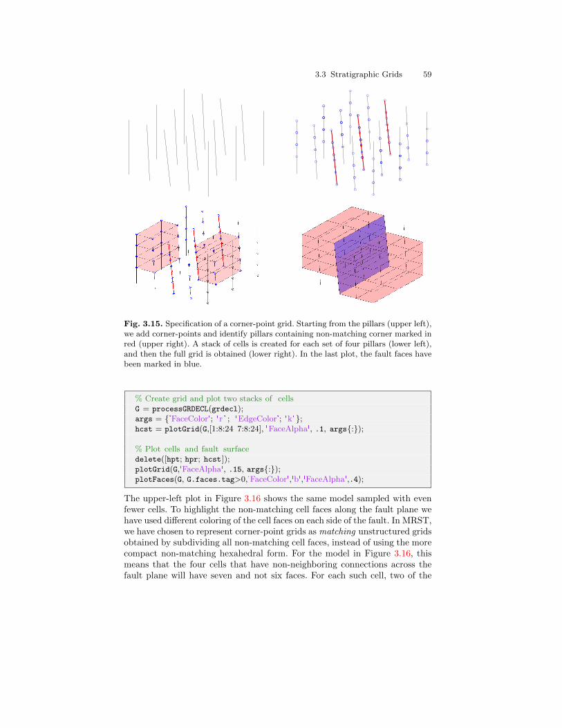
3.3 Stratigraphic Grids 59
Fig. 3.15. Specification of a corner-point grid. Starting from the pillars (upper left),we add corner-points and identify pillars containing non-matching corner marked inred (upper right). A stack of cells is created for each set of four pillars (lower left),and then the full grid is obtained (lower right). In the last plot, the fault faces havebeen marked in blue.
% Create grid and plot two stacks of cellsG = processGRDECL(grdecl);args = 'FaceColor'; 'r ' ; 'EdgeColor'; 'k';hcst = plotGrid(G,[1:8:24 7:8:24], 'FaceAlpha', .1, args:);
% Plot cells and fault surfacedelete([hpt; hpr; hcst]);plotGrid(G,'FaceAlpha', .15, args:);plotFaces(G, G.faces.tag>0,'FaceColor','b','FaceAlpha',.4);
The upper-left plot in Figure 3.16 shows the same model sampled with evenfewer cells. To highlight the non-matching cell faces along the fault plane wehave used different coloring of the cell faces on each side of the fault. In MRST,we have chosen to represent corner-point grids as matching unstructured gridsobtained by subdividing all non-matching cell faces, instead of using the morecompact non-matching hexahedral form. For the model in Figure 3.16, thismeans that the four cells that have non-neighboring connections across thefault plane will have seven and not six faces. For each such cell, two of the
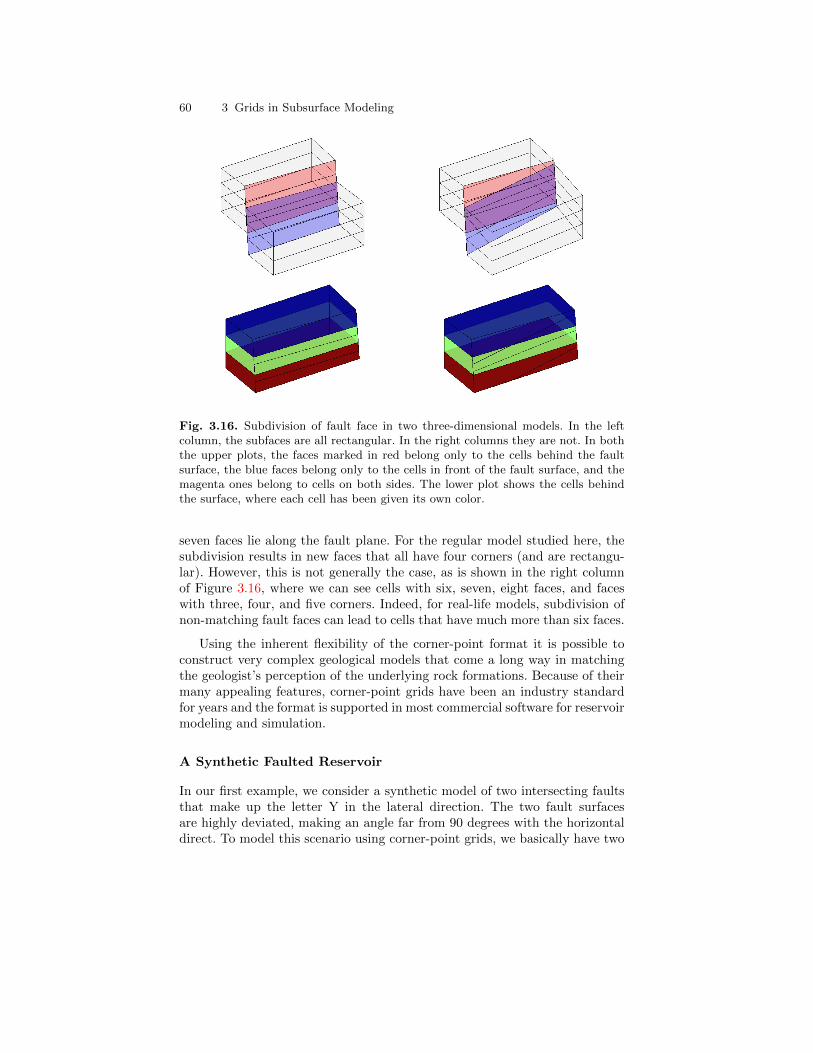
60 3 Grids in Subsurface Modeling
Fig. 3.16. Subdivision of fault face in two three-dimensional models. In the leftcolumn, the subfaces are all rectangular. In the right columns they are not. In boththe upper plots, the faces marked in red belong only to the cells behind the faultsurface, the blue faces belong only to the cells in front of the fault surface, and themagenta ones belong to cells on both sides. The lower plot shows the cells behindthe surface, where each cell has been given its own color.
seven faces lie along the fault plane. For the regular model studied here, thesubdivision results in new faces that all have four corners (and are rectangu-lar). However, this is not generally the case, as is shown in the right columnof Figure 3.16, where we can see cells with six, seven, eight faces, and faceswith three, four, and five corners. Indeed, for real-life models, subdivision ofnon-matching fault faces can lead to cells that have much more than six faces.
Using the inherent flexibility of the corner-point format it is possible toconstruct very complex geological models that come a long way in matchingthe geologist’s perception of the underlying rock formations. Because of theirmany appealing features, corner-point grids have been an industry standardfor years and the format is supported in most commercial software for reservoirmodeling and simulation.
A Synthetic Faulted Reservoir
In our first example, we consider a synthetic model of two intersecting faultsthat make up the letter Y in the lateral direction. The two fault surfacesare highly deviated, making an angle far from 90 degrees with the horizontaldirect. To model this scenario using corner-point grids, we basically have two
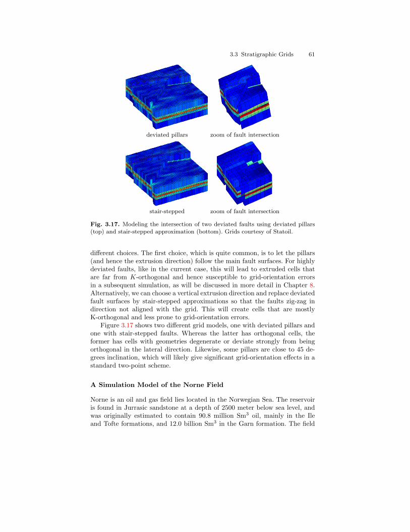
3.3 Stratigraphic Grids 61
deviated pillars zoom of fault intersection
stair-stepped zoom of fault intersection
Fig. 3.17. Modeling the intersection of two deviated faults using deviated pillars(top) and stair-stepped approximation (bottom). Grids courtesy of Statoil.
different choices. The first choice, which is quite common, is to let the pillars(and hence the extrusion direction) follow the main fault surfaces. For highlydeviated faults, like in the current case, this will lead to extruded cells thatare far from K-orthogonal and hence susceptible to grid-orientation errorsin a subsequent simulation, as will be discussed in more detail in Chapter 8.Alternatively, we can choose a vertical extrusion direction and replace deviatedfault surfaces by stair-stepped approximations so that the faults zig-zag indirection not aligned with the grid. This will create cells that are mostlyK-orthogonal and less prone to grid-orientation errors.
Figure 3.17 shows two different grid models, one with deviated pillars andone with stair-stepped faults. Whereas the latter has orthogonal cells, theformer has cells with geometries degenerate or deviate strongly from beingorthogonal in the lateral direction. Likewise, some pillars are close to 45 de-grees inclination, which will likely give significant grid-orientation effects in astandard two-point scheme.
A Simulation Model of the Norne Field
Norne is an oil and gas field lies located in the Norwegian Sea. The reservoiris found in Jurrasic sandstone at a depth of 2500 meter below sea level, andwas originally estimated to contain 90.8 million Sm3 oil, mainly in the Ileand Tofte formations, and 12.0 billion Sm3 in the Garn formation. The field
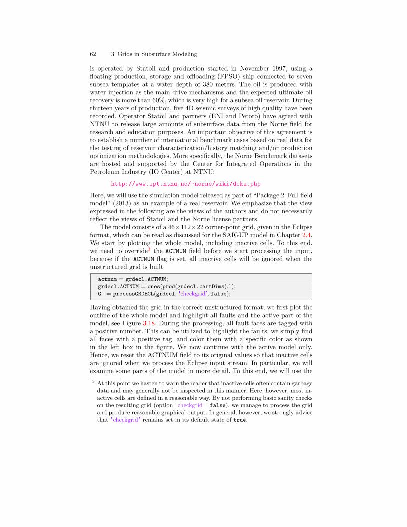
62 3 Grids in Subsurface Modeling
is operated by Statoil and production started in November 1997, using afloating production, storage and offloading (FPSO) ship connected to sevensubsea templates at a water depth of 380 meters. The oil is produced withwater injection as the main drive mechanisms and the expected ultimate oilrecovery is more than 60%, which is very high for a subsea oil reservoir. Duringthirteen years of production, five 4D seismic surveys of high quality have beenrecorded. Operator Statoil and partners (ENI and Petoro) have agreed withNTNU to release large amounts of subsurface data from the Norne field forresearch and education purposes. An important objective of this agreement isto establish a number of international benchmark cases based on real data forthe testing of reservoir characterization/history matching and/or productionoptimization methodologies. More specifically, the Norne Benchmark datasetsare hosted and supported by the Center for Integrated Operations in thePetroleum Industry (IO Center) at NTNU:
http://www.ipt.ntnu.no/~norne/wiki/doku.php
Here, we will use the simulation model released as part of “Package 2: Full fieldmodel” (2013) as an example of a real reservoir. We emphasize that the viewexpressed in the following are the views of the authors and do not necessarilyreflect the views of Statoil and the Norne license partners.
The model consists of a 46×112×22 corner-point grid, given in the Eclipseformat, which can be read as discussed for the SAIGUP model in Chapter 2.4.We start by plotting the whole model, including inactive cells. To this end,we need to override3 the ACTNUM field before we start processing the input,because if the ACTNUM flag is set, all inactive cells will be ignored when theunstructured grid is built
actnum = grdecl.ACTNUM;grdecl.ACTNUM = ones(prod(grdecl.cartDims),1);G = processGRDECL(grdecl, 'checkgrid', false);
Having obtained the grid in the correct unstructured format, we first plot theoutline of the whole model and highlight all faults and the active part of themodel, see Figure 3.18. During the processing, all fault faces are tagged witha positive number. This can be utilized to highlight the faults: we simply findall faces with a positive tag, and color them with a specific color as shownin the left box in the figure. We now continue with the active model only.Hence, we reset the ACTNUM field to its original values so that inactive cellsare ignored when we process the Eclipse input stream. In particular, we willexamine some parts of the model in more detail. To this end, we will use the
3 At this point we hasten to warn the reader that inactive cells often contain garbagedata and may generally not be inspected in this manner. Here, however, most in-active cells are defined in a reasonable way. By not performing basic sanity checkson the resulting grid (option 'checkgrid'=false), we manage to process the gridand produce reasonable graphical output. In general, however, we strongly advicethat 'checkgrid' remains set in its default state of true.
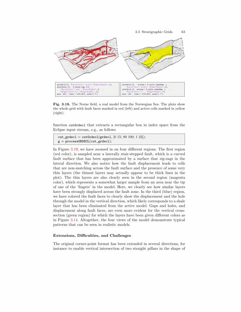
3.3 Stratigraphic Grids 63
plotGrid (G , 'FaceColor','none', 'EdgeAlpha',.1);plotFaces (G , G.faces.tag >0, ...
'FaceColor','red' , 'FaceAlpha',.2, ...'EdgeColor','r' , 'EdgeAlpha',.1);
axis off ; view(−155,80); zoom(1.7 );
plotGrid (G , ˜ actnum ( G.cells.indexMap ), ...'FaceColor','none', 'EdgeAlpha',.1);
plotGrid (G , actnum ( G.cells.indexMap ), ...'FaceColor','y' , 'EdgeAlpha',.1);
axis off ; view(−155,80); zoom(1.7 );
Fig. 3.18. The Norne field, a real model from the Norwegian Sea. The plots showthe whole grid with fault faces marked in red (left) and active cells marked in yellow(right).
function cutGrdecl that extracts a rectangular box in index space from theEclipse input stream, e.g., as follows
cut_grdecl = cutGrdecl(grdecl, [6 15; 80 100; 1 22]);g = processGRDECL(cut_grdecl);
In Figure 3.19, we have zoomed in on four different regions. The first region(red color), is sampled near a laterally stair-stepped fault, which is a curvedfault surface that has been approximated by a surface that zig-zags in thelateral direction. We also notice how the fault displacement leads to cellsthat are non-matching across the fault surface and the presence of some verythin layers (the thinest layers may actually appear to be thick lines in theplot). The thin layers are also clearly seen in the second region (magentacolor), which represents a somewhat larger sample from an area near the tipof one of the ’fingers’ in the model. Here, we clearly see how similar layershave been strongly displaced across the fault zone. In the third (blue) region,we have colored the fault faces to clearly show the displacement and the holethrough the model in the vertical direction, which likely corresponds to a shalelayer that has been eliminated from the active model. Gaps and holes, anddisplacement along fault faces, are even more evident for the vertical cross-section (green region) for which the layers have been given different colors asin Figure 3.14. Altogether, the four views of the model demonstrate typicalpatterns that can be seen in realistic models.
Extensions, Difficulties, and Challenges
The original corner-point format has been extended in several directions, forinstance to enable vertical intersection of two straight pillars in the shape of
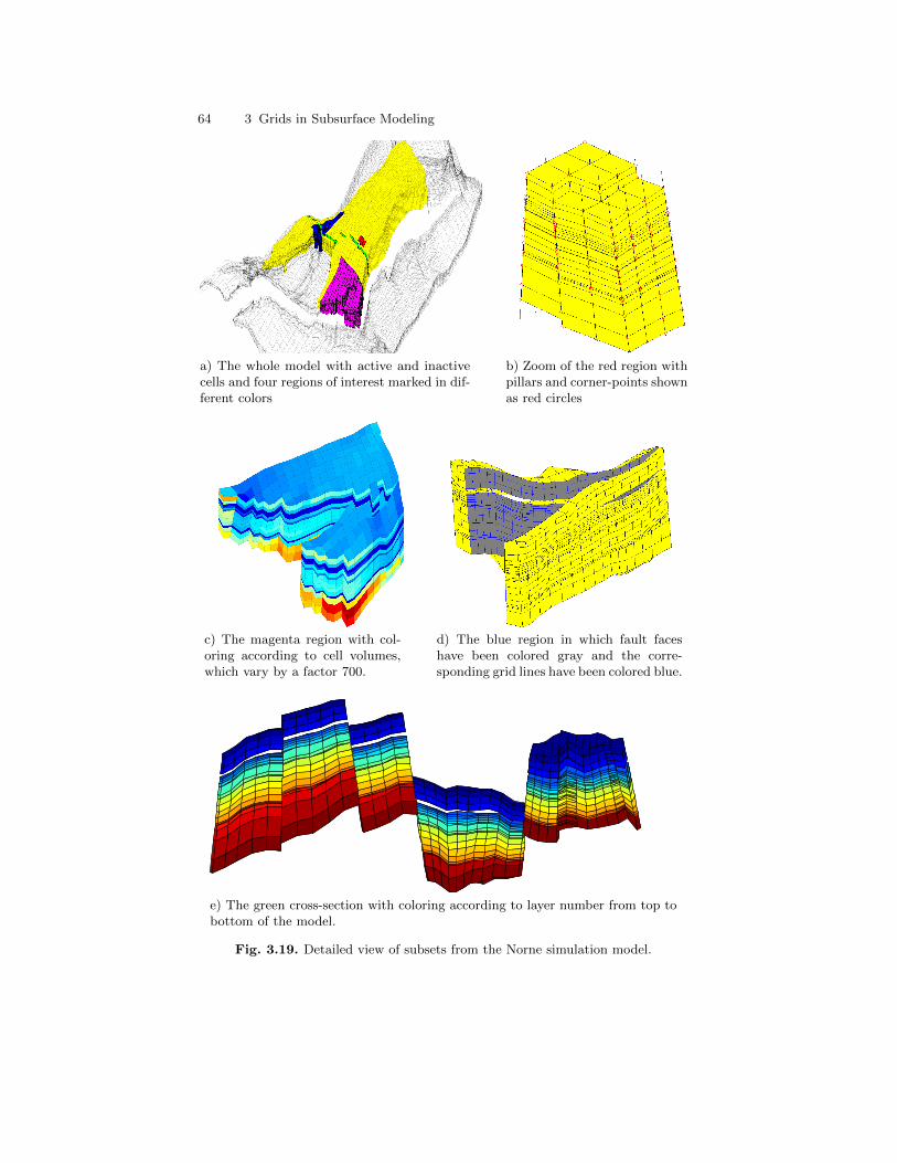
64 3 Grids in Subsurface Modeling
a) The whole model with active and inactivecells and four regions of interest marked in dif-ferent colors
b) Zoom of the red region withpillars and corner-points shownas red circles
c) The magenta region with col-oring according to cell volumes,which vary by a factor 700.
d) The blue region in which fault faceshave been colored gray and the corre-sponding grid lines have been colored blue.
e) The green cross-section with coloring according to layer number from top tobottom of the model.
Fig. 3.19. Detailed view of subsets from the Norne simulation model.
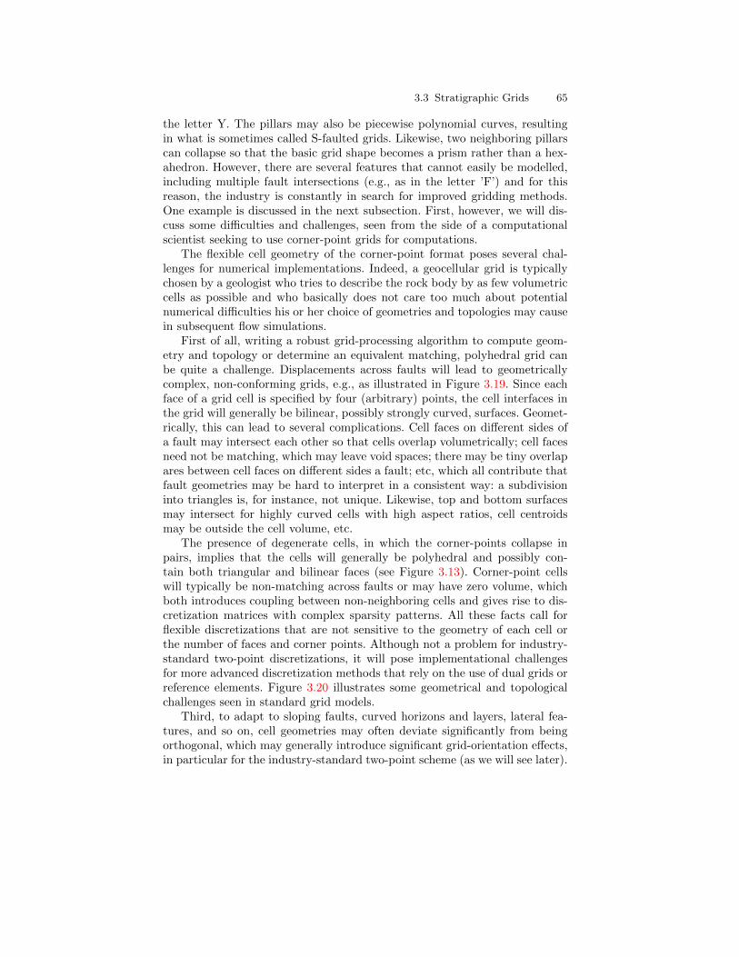
3.3 Stratigraphic Grids 65
the letter Y. The pillars may also be piecewise polynomial curves, resultingin what is sometimes called S-faulted grids. Likewise, two neighboring pillarscan collapse so that the basic grid shape becomes a prism rather than a hex-ahedron. However, there are several features that cannot easily be modelled,including multiple fault intersections (e.g., as in the letter ’F’) and for thisreason, the industry is constantly in search for improved gridding methods.One example is discussed in the next subsection. First, however, we will dis-cuss some difficulties and challenges, seen from the side of a computationalscientist seeking to use corner-point grids for computations.
The flexible cell geometry of the corner-point format poses several chal-lenges for numerical implementations. Indeed, a geocellular grid is typicallychosen by a geologist who tries to describe the rock body by as few volumetriccells as possible and who basically does not care too much about potentialnumerical difficulties his or her choice of geometries and topologies may causein subsequent flow simulations.
First of all, writing a robust grid-processing algorithm to compute geom-etry and topology or determine an equivalent matching, polyhedral grid canbe quite a challenge. Displacements across faults will lead to geometricallycomplex, non-conforming grids, e.g., as illustrated in Figure 3.19. Since eachface of a grid cell is specified by four (arbitrary) points, the cell interfaces inthe grid will generally be bilinear, possibly strongly curved, surfaces. Geomet-rically, this can lead to several complications. Cell faces on different sides ofa fault may intersect each other so that cells overlap volumetrically; cell facesneed not be matching, which may leave void spaces; there may be tiny overlapares between cell faces on different sides a fault; etc, which all contribute thatfault geometries may be hard to interpret in a consistent way: a subdivisioninto triangles is, for instance, not unique. Likewise, top and bottom surfacesmay intersect for highly curved cells with high aspect ratios, cell centroidsmay be outside the cell volume, etc.
The presence of degenerate cells, in which the corner-points collapse inpairs, implies that the cells will generally be polyhedral and possibly con-tain both triangular and bilinear faces (see Figure 3.13). Corner-point cellswill typically be non-matching across faults or may have zero volume, whichboth introduces coupling between non-neighboring cells and gives rise to dis-cretization matrices with complex sparsity patterns. All these facts call forflexible discretizations that are not sensitive to the geometry of each cell orthe number of faces and corner points. Although not a problem for industry-standard two-point discretizations, it will pose implementational challengesfor more advanced discretization methods that rely on the use of dual grids orreference elements. Figure 3.20 illustrates some geometrical and topologicalchallenges seen in standard grid models.
Third, to adapt to sloping faults, curved horizons and layers, lateral fea-tures, and so on, cell geometries may often deviate significantly from beingorthogonal, which may generally introduce significant grid-orientation effects,in particular for the industry-standard two-point scheme (as we will see later).
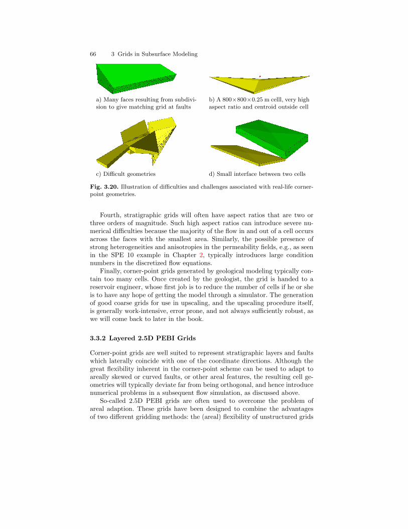
66 3 Grids in Subsurface Modeling
a) Many faces resulting from subdivi-sion to give matching grid at faults
b) A 800×800×0.25 m celll, very highaspect ratio and centroid outside cell
c) Difficult geometries d) Small interface between two cells
Fig. 3.20. Illustration of difficulties and challenges associated with real-life corner-point geometries.
Fourth, stratigraphic grids will often have aspect ratios that are two orthree orders of magnitude. Such high aspect ratios can introduce severe nu-merical difficulties because the majority of the flow in and out of a cell occursacross the faces with the smallest area. Similarly, the possible presence ofstrong heterogeneities and anisotropies in the permeability fields, e.g., as seenin the SPE 10 example in Chapter 2, typically introduces large conditionnumbers in the discretized flow equations.
Finally, corner-point grids generated by geological modeling typically con-tain too many cells. Once created by the geologist, the grid is handed to areservoir engineer, whose first job is to reduce the number of cells if he or sheis to have any hope of getting the model through a simulator. The generationof good coarse grids for use in upscaling, and the upscaling procedure itself,is generally work-intensive, error prone, and not always sufficiently robust, aswe will come back to later in the book.
3.3.2 Layered 2.5D PEBI Grids
Corner-point grids are well suited to represent stratigraphic layers and faultswhich laterally coincide with one of the coordinate directions. Although thegreat flexibility inherent in the corner-point scheme can be used to adapt toareally skewed or curved faults, or other areal features, the resulting cell ge-ometries will typically deviate far from being orthogonal, and hence introducenumerical problems in a subsequent flow simulation, as discussed above.
So-called 2.5D PEBI grids are often used to overcome the problem ofareal adaption. These grids have been designed to combine the advantagesof two different gridding methods: the (areal) flexibility of unstructured grids
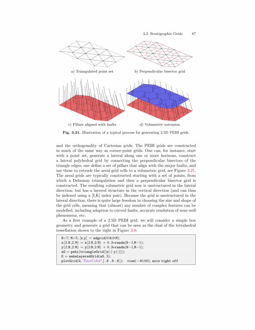
3.3 Stratigraphic Grids 67
a) Triangulated point set b) Perpendicular bisector grid
c) Pillars aligned with faults d) Volumetric extrusion
Fig. 3.21. Illustration of a typical process for generating 2.5D PEBI grids.
and the orthogonality of Cartesian grids. The PEBI grids are constructedin much of the same way as corner-point grids. One can, for instance, startwith a point set, generate a lateral along one or more horizons, constructa lateral polyhedral grid by connecting the perpendicular bisectors of thetriangle edges, one define a set of pillars that align with the major faults, anduse these to extrude the areal grid cells to a volumetric grid, see Figure 3.21.The areal grids are typically constructed starting with a set of points, fromwhich a Delaunay triangulation and then a perpendicular bisector grid isconstructed. The resulting volumetric grid now is unstructured in the lateraldirection, but has a layered structure in the vertical direction (and can thusbe indexed using a [I,K] index pair). Because the grid is unstructured in thelateral direction, there is quite large freedom in choosing the size and shape ofthe grid cells, meaning that (almost) any number of complex features can bemodelled, including adaption to curved faults, accurate resolution of near-wellphenomena, etc.
As a first example of a 2.5D PEBI grid, we will consider a simple boxgeometry and generate a grid that can be seen as the dual of the tetrahedraltessellation shown to the right in Figure 3.8:
N=7; M=5; [x,y] = ndgrid(0:N,0:M);x(2:N ,2:M) = x(2:N,2:M) + 0.3*randn(N−1,M−1);y(2:N ,2:M) = y(2:N,2:M) + 0.3*randn(N−1,M−1);aG = pebi(triangleGrid([x(:) y(:)]));G = makeLayeredGrid(aG, 3);plotGrid(G, 'FaceColor' ,[.8 .8 .8 ]); view(−40,60); axis tight off
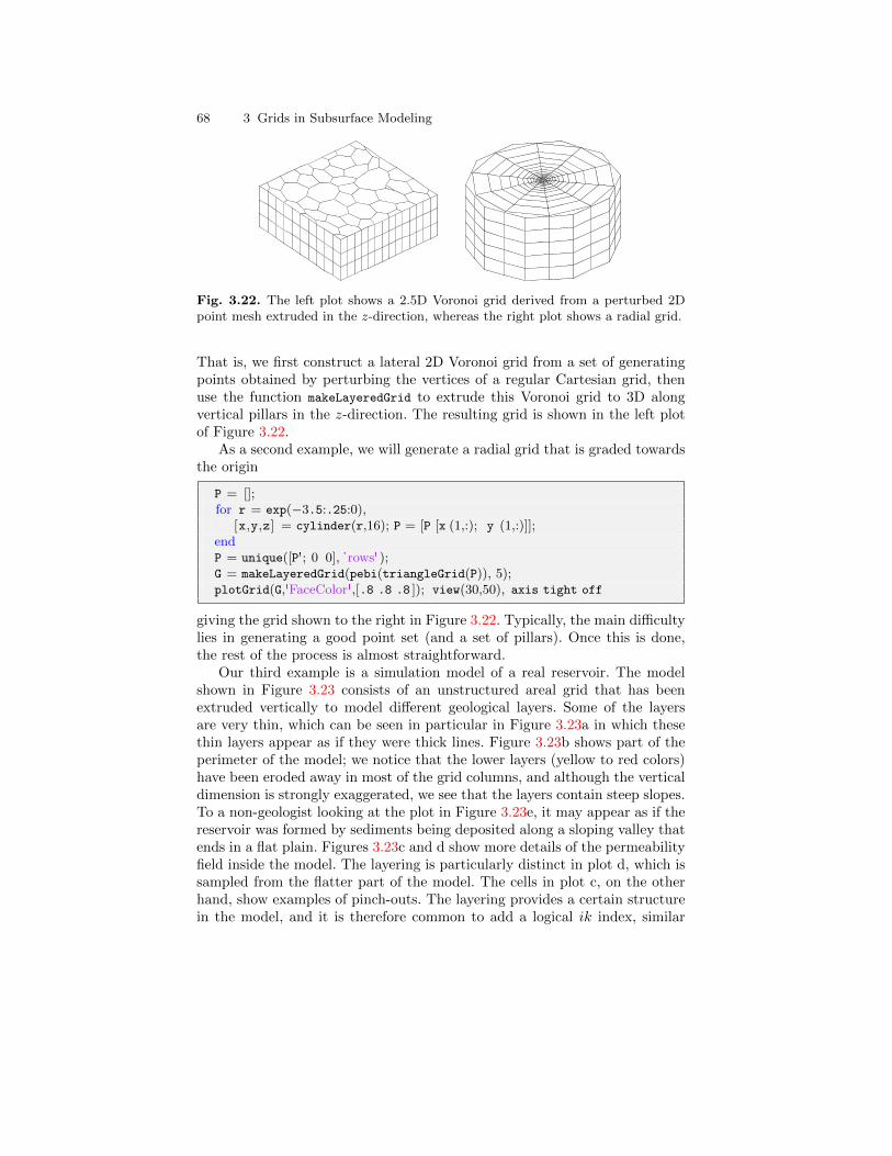
68 3 Grids in Subsurface Modeling
Fig. 3.22. The left plot shows a 2.5D Voronoi grid derived from a perturbed 2Dpoint mesh extruded in the z-direction, whereas the right plot shows a radial grid.
That is, we first construct a lateral 2D Voronoi grid from a set of generatingpoints obtained by perturbing the vertices of a regular Cartesian grid, thenuse the function makeLayeredGrid to extrude this Voronoi grid to 3D alongvertical pillars in the z-direction. The resulting grid is shown in the left plotof Figure 3.22.
As a second example, we will generate a radial grid that is graded towardsthe origin
P = [];for r = exp(−3.5:.25:0),
[x,y,z] = cylinder(r,16); P = [P [x (1,:); y (1,:)]];endP = unique([P'; 0 0], 'rows');G = makeLayeredGrid(pebi(triangleGrid(P)), 5);plotGrid(G,'FaceColor',[.8 .8 .8 ]); view(30,50), axis tight off
giving the grid shown to the right in Figure 3.22. Typically, the main difficultylies in generating a good point set (and a set of pillars). Once this is done,the rest of the process is almost straightforward.
Our third example is a simulation model of a real reservoir. The modelshown in Figure 3.23 consists of an unstructured areal grid that has beenextruded vertically to model different geological layers. Some of the layersare very thin, which can be seen in particular in Figure 3.23a in which thesethin layers appear as if they were thick lines. Figure 3.23b shows part of theperimeter of the model; we notice that the lower layers (yellow to red colors)have been eroded away in most of the grid columns, and although the verticaldimension is strongly exaggerated, we see that the layers contain steep slopes.To a non-geologist looking at the plot in Figure 3.23e, it may appear as if thereservoir was formed by sediments being deposited along a sloping valley thatends in a flat plain. Figures 3.23c and d show more details of the permeabilityfield inside the model. The layering is particularly distinct in plot d, which issampled from the flatter part of the model. The cells in plot c, on the otherhand, show examples of pinch-outs. The layering provides a certain structurein the model, and it is therefore common to add a logical ik index, similar
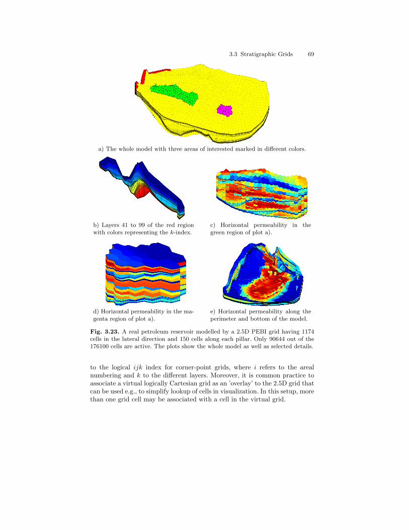
3.3 Stratigraphic Grids 69
a) The whole model with three areas of interested marked in different colors.
b) Layers 41 to 99 of the red regionwith colors representing the k-index.
c) Horizontal permeability in thegreen region of plot a).
d) Horizontal permeability in the ma-genta region of plot a).
e) Horizontal permeability along theperimeter and bottom of the model.
Fig. 3.23. A real petroleum reservoir modelled by a 2.5D PEBI grid having 1174cells in the lateral direction and 150 cells along each pillar. Only 90644 out of the176100 cells are active. The plots show the whole model as well as selected details.
to the logical ijk index for corner-point grids, where i refers to the arealnumbering and k to the different layers. Moreover, it is common practice toassociate a virtual logically Cartesian grid as an ’overlay’ to the 2.5D grid thatcan be used e.g., to simplify lookup of cells in visualization. In this setup, morethan one grid cell may be associated with a cell in the virtual grid.
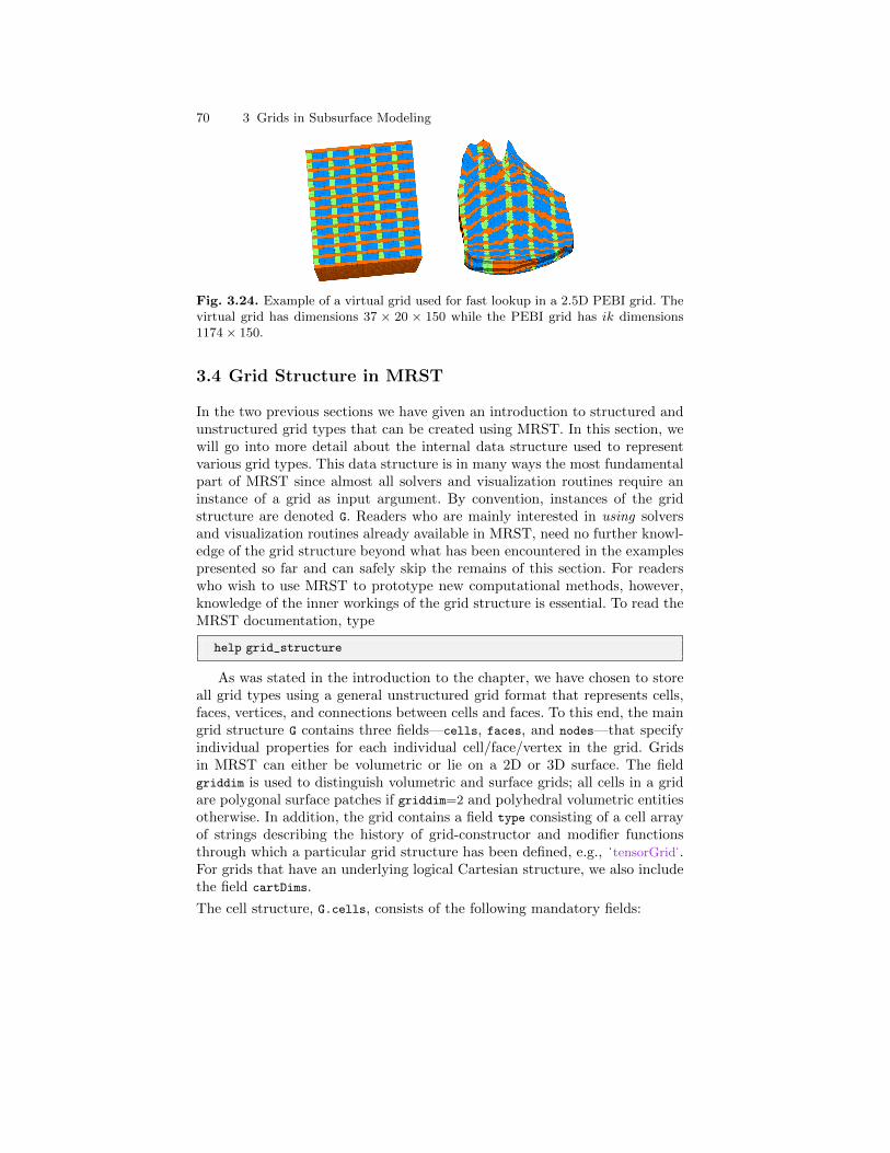
70 3 Grids in Subsurface Modeling
Fig. 3.24. Example of a virtual grid used for fast lookup in a 2.5D PEBI grid. Thevirtual grid has dimensions 37 × 20 × 150 while the PEBI grid has ik dimensions1174× 150.
3.4 Grid Structure in MRST
In the two previous sections we have given an introduction to structured andunstructured grid types that can be created using MRST. In this section, wewill go into more detail about the internal data structure used to representvarious grid types. This data structure is in many ways the most fundamentalpart of MRST since almost all solvers and visualization routines require aninstance of a grid as input argument. By convention, instances of the gridstructure are denoted G. Readers who are mainly interested in using solversand visualization routines already available in MRST, need no further knowl-edge of the grid structure beyond what has been encountered in the examplespresented so far and can safely skip the remains of this section. For readerswho wish to use MRST to prototype new computational methods, however,knowledge of the inner workings of the grid structure is essential. To read theMRST documentation, type
help grid_structure
As was stated in the introduction to the chapter, we have chosen to storeall grid types using a general unstructured grid format that represents cells,faces, vertices, and connections between cells and faces. To this end, the maingrid structure G contains three fields—cells, faces, and nodes—that specifyindividual properties for each individual cell/face/vertex in the grid. Gridsin MRST can either be volumetric or lie on a 2D or 3D surface. The fieldgriddim is used to distinguish volumetric and surface grids; all cells in a gridare polygonal surface patches if griddim=2 and polyhedral volumetric entitiesotherwise. In addition, the grid contains a field type consisting of a cell arrayof strings describing the history of grid-constructor and modifier functionsthrough which a particular grid structure has been defined, e.g., 'tensorGrid'.For grids that have an underlying logical Cartesian structure, we also includethe field cartDims.
The cell structure, G.cells, consists of the following mandatory fields:
3.4 Grid Structure in MRST 71
– num: the number nc of cells in the global grid.– facePos: an indirection map of size [num+1,1] into the faces array. Specifi-
cally, the face information of cell i is found in the submatrixfaces(facePos(i) : facePos(i+1)−1, :)
The number of faces of each cell may be computed using the state-ment diff(facePos) and the total number of faces is given as nf =facePos(end)−1.
– faces: an nf × 3 array that gives the global faces connected to a givencell. Specifically, if faces(i,1)==j, then global face number faces(i,2) isconnected to global cell number j. The last component, faces(i,3), isoptional and can for certain types of grids contain a tag used to distinguishface directions: East, West, South, North, Bottom, Top.The first column of face is redundant: it consists of each cell index j re-peated facePos(j+1)−facePos(j) times and can therefore be reconstructedby decompressing a run-length encoding with the cell indices 1:num as en-coded vector and the number of faces per cell as repetition vector. Hence,to conserve memory, only the last two columns of face are stored, whilethe first column can be reconstructed using the statement:
rldecode(1:G.cells.num, diff(G.cells.facePos), 2) .'
This construction is used a lot throughout MRST and has therefore beenimplemented as a utility function inside mrst−core/utils/gridtools
f2cn = gridCellNo(G);
– indexMap: an optional nc×1 array that maps internal cell indices to externalcell indices. For models with no inactive cells, indexMap equals 1 : nc. Forcases with inactive cells, indexMap contains the indices of the active cellssorted in ascending order. An example of such a grid is the ellipsoid inFigure 3.4 that was created using a fictitious domain method. For logicallyCartesian grids, a map of cell numbers to logical indices can be constructedusing the following statements in 2D:
[ij1:2] = ind2sub(dims, G.cells.indexMap(:));ij = [ij:];
and likewise in 3D:
[ijk1:3] = ind2sub(dims, G.cells.indexMap(:));ijk = [ijk:];
In the latter case, ijk(i:) is the global (I, J,K) index of cell i.
In addition, the cell structure can contain the following optional fields thattypically will be added by a call to computeGeometry:
– volumes: an nc × 1 array of cell volumes– centroids: an nc × d array of cell centroids in IRd
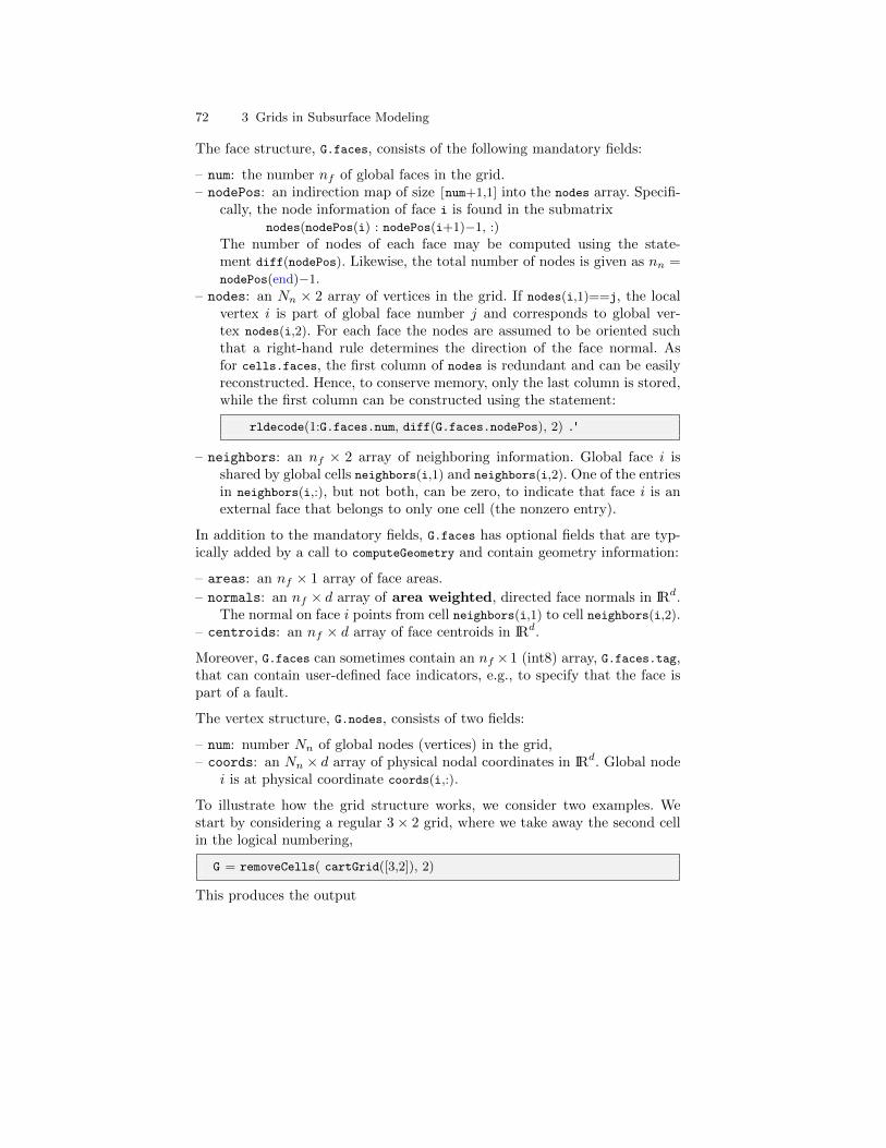
72 3 Grids in Subsurface Modeling
The face structure, G.faces, consists of the following mandatory fields:
– num: the number nf of global faces in the grid.– nodePos: an indirection map of size [num+1,1] into the nodes array. Specifi-
cally, the node information of face i is found in the submatrixnodes(nodePos(i) : nodePos(i+1)−1, :)
The number of nodes of each face may be computed using the state-ment diff(nodePos). Likewise, the total number of nodes is given as nn =nodePos(end)−1.
– nodes: an Nn × 2 array of vertices in the grid. If nodes(i,1)==j, the localvertex i is part of global face number j and corresponds to global ver-tex nodes(i,2). For each face the nodes are assumed to be oriented suchthat a right-hand rule determines the direction of the face normal. Asfor cells.faces, the first column of nodes is redundant and can be easilyreconstructed. Hence, to conserve memory, only the last column is stored,while the first column can be constructed using the statement:
rldecode(1:G.faces.num, diff(G.faces.nodePos), 2) .'
– neighbors: an nf × 2 array of neighboring information. Global face i isshared by global cells neighbors(i,1) and neighbors(i,2). One of the entriesin neighbors(i,:), but not both, can be zero, to indicate that face i is anexternal face that belongs to only one cell (the nonzero entry).
In addition to the mandatory fields, G.faces has optional fields that are typ-ically added by a call to computeGeometry and contain geometry information:
– areas: an nf × 1 array of face areas.
– normals: an nf × d array of area weighted, directed face normals in IRd.The normal on face i points from cell neighbors(i,1) to cell neighbors(i,2).
– centroids: an nf × d array of face centroids in IRd.
Moreover, G.faces can sometimes contain an nf ×1 (int8) array, G.faces.tag,that can contain user-defined face indicators, e.g., to specify that the face ispart of a fault.
The vertex structure, G.nodes, consists of two fields:
– num: number Nn of global nodes (vertices) in the grid,– coords: an Nn × d array of physical nodal coordinates in IRd. Global node
i is at physical coordinate coords(i,:).
To illustrate how the grid structure works, we consider two examples. Westart by considering a regular 3× 2 grid, where we take away the second cellin the logical numbering,
G = removeCells( cartGrid([3,2]), 2)
This produces the output
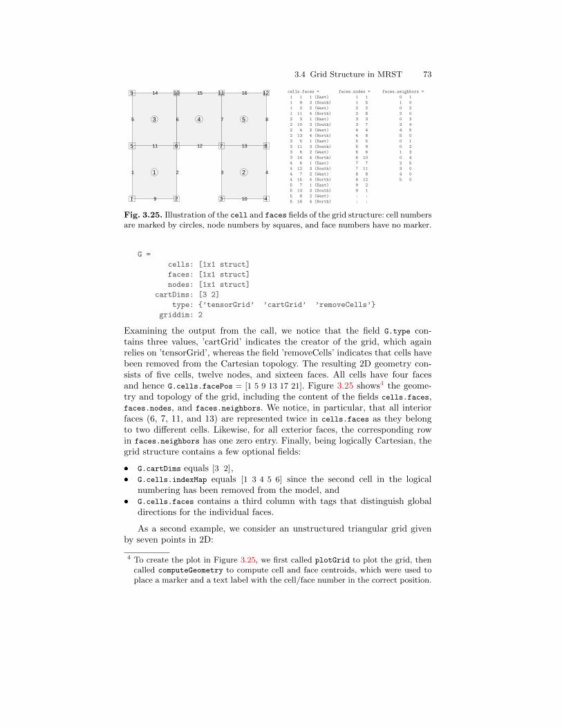
3.4 Grid Structure in MRST 73
1 2
3 4 5
1 2 3 4
5 6 7 8
9 10
11 12 13
14 15 16
1 2 3 4
5 6 7 8
9 10 11 12 cells.faces = faces.nodes = faces.neighbors =
1 1 1 (East) 1 1 0 1
1 9 3 (South) 1 5 1 0
1 2 2 (West) 2 2 0 2
1 11 4 (North) 2 6 2 0
2 3 1 (East) 3 3 0 3
2 10 3 (South) 3 7 3 4
2 4 2 (West) 4 4 4 5
2 13 4 (North) 4 8 5 0
3 5 1 (East) 5 5 0 1
3 11 3 (South) 5 9 0 2
3 6 2 (West) 6 6 1 3
3 14 4 (North) 6 10 0 4
4 6 1 (East) 7 7 2 5
4 12 3 (South) 7 11 3 0
4 7 2 (West) 8 8 4 0
4 15 4 (North) 8 12 5 0
5 7 1 (East) 9 2
5 13 3 (South) 9 1
5 8 2 (West) : :
5 16 4 (North) : :
Fig. 3.25. Illustration of the cell and faces fields of the grid structure: cell numbersare marked by circles, node numbers by squares, and face numbers have no marker.
G =
cells: [1x1 struct]
faces: [1x1 struct]
nodes: [1x1 struct]
cartDims: [3 2]
type: ’tensorGrid’ ’cartGrid’ ’removeCells’
griddim: 2
Examining the output from the call, we notice that the field G.type con-tains three values, ’cartGrid’ indicates the creator of the grid, which againrelies on ’tensorGrid’, whereas the field ’removeCells’ indicates that cells havebeen removed from the Cartesian topology. The resulting 2D geometry con-sists of five cells, twelve nodes, and sixteen faces. All cells have four facesand hence G.cells.facePos = [1 5 9 13 17 21]. Figure 3.25 shows4 the geome-try and topology of the grid, including the content of the fields cells.faces,faces.nodes, and faces.neighbors. We notice, in particular, that all interiorfaces (6, 7, 11, and 13) are represented twice in cells.faces as they belongto two different cells. Likewise, for all exterior faces, the corresponding rowin faces.neighbors has one zero entry. Finally, being logically Cartesian, thegrid structure contains a few optional fields:
G.cartDims equals [3 2], G.cells.indexMap equals [1 3 4 5 6] since the second cell in the logical
numbering has been removed from the model, and G.cells.faces contains a third column with tags that distinguish global
directions for the individual faces.
As a second example, we consider an unstructured triangular grid givenby seven points in 2D:
4 To create the plot in Figure 3.25, we first called plotGrid to plot the grid, thencalled computeGeometry to compute cell and face centroids, which were used toplace a marker and a text label with the cell/face number in the correct position.
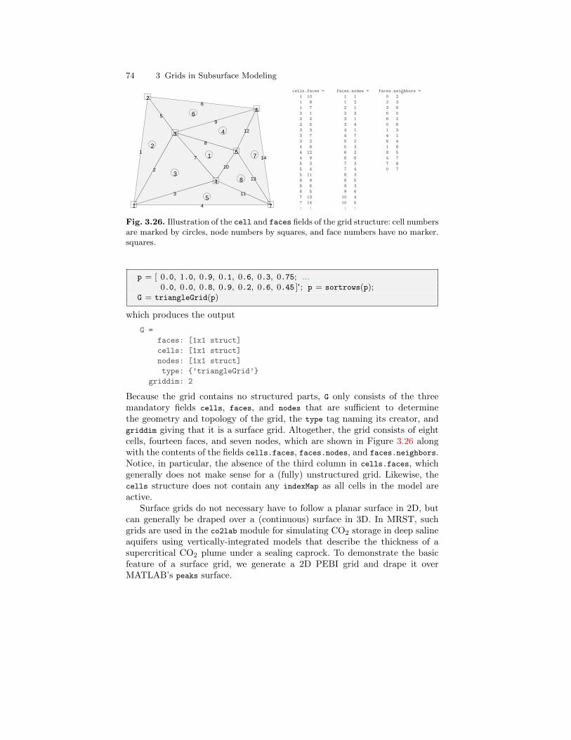
74 3 Grids in Subsurface Modeling
1
2
3
4
5
6
7
8
1
2
3
4
5
6
7
8
9
10
11
12
13
14
1
2
3
4
5
6
7
cells.faces = faces.nodes = faces.neighbors =
1 10 1 1 0 2
1 8 1 2 2 3
1 7 2 1 3 5
2 1 2 3 5 0
2 2 3 1 6 2
2 5 3 4 0 6
3 3 4 1 1 3
3 7 4 7 4 1
3 2 5 2 6 4
4 8 5 3 1 8
4 12 6 2 8 5
4 9 6 6 4 7
5 3 7 3 7 8
5 4 7 4 0 7
5 11 8 3
6 9 8 5
6 6 9 3
6 5 9 6
7 13 10 4
7 14 10 5
: : : :
Fig. 3.26. Illustration of the cell and faces fields of the grid structure: cell numbersare marked by circles, node numbers by squares, and face numbers have no marker.squares.
p = [ 0.0, 1.0, 0.9, 0.1, 0.6, 0.3, 0.75; ...0.0, 0.0, 0.8, 0.9, 0.2, 0.6, 0.45 ]'; p = sortrows(p);
G = triangleGrid(p)
which produces the output
G =
faces: [1x1 struct]
cells: [1x1 struct]
nodes: [1x1 struct]
type: ’triangleGrid’
griddim: 2
Because the grid contains no structured parts, G only consists of the threemandatory fields cells, faces, and nodes that are sufficient to determinethe geometry and topology of the grid, the type tag naming its creator, andgriddim giving that it is a surface grid. Altogether, the grid consists of eightcells, fourteen faces, and seven nodes, which are shown in Figure 3.26 alongwith the contents of the fields cells.faces, faces.nodes, and faces.neighbors.Notice, in particular, the absence of the third column in cells.faces, whichgenerally does not make sense for a (fully) unstructured grid. Likewise, thecells structure does not contain any indexMap as all cells in the model areactive.
Surface grids do not necessary have to follow a planar surface in 2D, butcan generally be draped over a (continuous) surface in 3D. In MRST, suchgrids are used in the co2lab module for simulating CO2 storage in deep salineaquifers using vertically-integrated models that describe the thickness of asupercritical CO2 plume under a sealing caprock. To demonstrate the basicfeature of a surface grid, we generate a 2D PEBI grid and drape it overMATLAB’s peaks surface.
3.4 Grid Structure in MRST 75
Fig. 3.27. Example of a surface grid: 2D PEBI grid draped over the peaks surface.
[x,y] = meshgrid([0:6]*2*cos(pi/6),0:7);x = [x (:); x(:)+cos(pi/6)]; x=(x − mean(x(:)))/2;y = [y (:); y(:)+sin(pi/6)]; y=(y − mean(y(:)))/2;G = pebi(triangleGrid([x(:),y(:)]));G.nodes.coords(:,3) = −peaks(G.nodes.coords(:,1),G.nodes.coords(:,2));
The resulting grid is shown in Figure 3.27. At the time of writing, the resultinggrid is not a proper grid in the sense that although computeGeometry givessensible results, the grid may not work properly with any of the flow andtransport solvers supplied with MRST.
Computing geometry information
All grid factory routines in MRST generate the basic geometry and topol-ogy of a grid, that is, how nodes are connected to make up faces, how facesare connected to form cells, and how cells are connected over common faces.Whereas this information is sufficient for many purposes, more geometricalinformation may be required in many cases. As explained above, such informa-tion is provided by the routine computeGeometry, which computes cell centroidsand volumes and face areas, centroids, and normals. Whereas computing thisinformation is straightforward for simplexes and Cartesian grids, it is not sofor general polyhedral grids that may contain curved polygonal faces. In thefollowing we will therefore go through how it is done in MRST.
For each cell, the basic grid structure provides us with a list of vertices,a list of cell faces, etc, as shown in the upper-left plots of Figures 3.28 and3.29. The routine starts by computing face quantities (areas, centroids, andnormals). To utilize MATLAB efficiently, the computations are programmedusing vectorization so that each derived quantity is computed for all points,all faces, and all cells in one go. To keep the current presentation as simpleas possible, we will herein only give formulas for a single face and a singlecell. Let us consider a single face given by the points ~p(i1), . . . , ~p(im) and letα = (α1, . . . , αm) denote a multi-index that describes how these points are
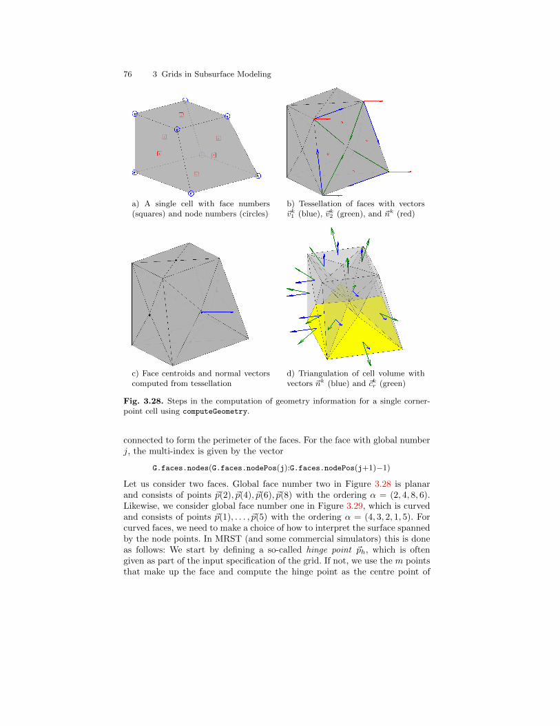
76 3 Grids in Subsurface Modeling
a) A single cell with face numbers(squares) and node numbers (circles)
b) Tessellation of faces with vectors~vk1 (blue), ~vk2 (green), and ~nk (red)
c) Face centroids and normal vectorscomputed from tessellation
d) Triangulation of cell volume withvectors ~nk (blue) and ~ckr (green)
Fig. 3.28. Steps in the computation of geometry information for a single corner-point cell using computeGeometry.
connected to form the perimeter of the faces. For the face with global numberj, the multi-index is given by the vector
G.faces.nodes(G.faces.nodePos(j):G.faces.nodePos(j+1)−1)
Let us consider two faces. Global face number two in Figure 3.28 is planarand consists of points ~p(2), ~p(4), ~p(6), ~p(8) with the ordering α = (2, 4, 8, 6).Likewise, we consider global face number one in Figure 3.29, which is curvedand consists of points ~p(1), . . . , ~p(5) with the ordering α = (4, 3, 2, 1, 5). Forcurved faces, we need to make a choice of how to interpret the surface spannedby the node points. In MRST (and some commercial simulators) this is doneas follows: We start by defining a so-called hinge point ~ph, which is oftengiven as part of the input specification of the grid. If not, we use the m pointsthat make up the face and compute the hinge point as the centre point of
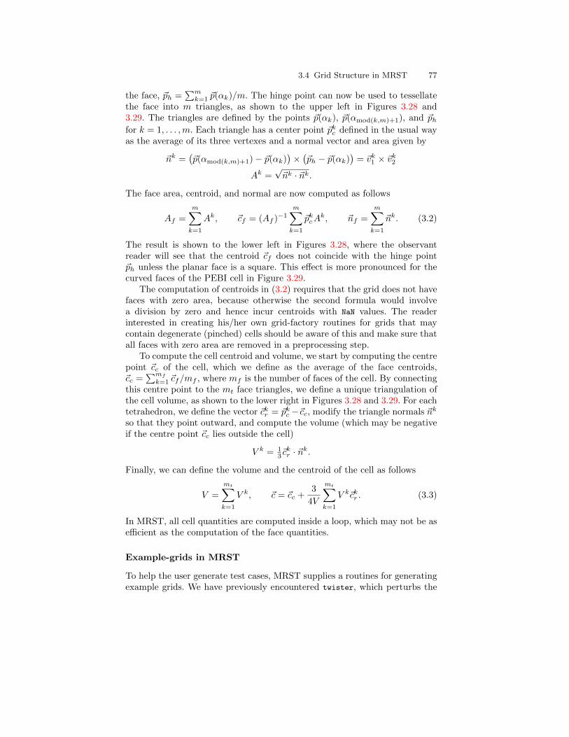
3.4 Grid Structure in MRST 77
the face, ~ph =∑mk=1 ~p(αk)/m. The hinge point can now be used to tessellate
the face into m triangles, as shown to the upper left in Figures 3.28 and3.29. The triangles are defined by the points ~p(αk), ~p(αmod(k,m)+1), and ~phfor k = 1, . . . ,m. Each triangle has a center point ~pkc defined in the usual wayas the average of its three vertexes and a normal vector and area given by
~nk =(~p(αmod(k,m)+1)− ~p(αk)
)×(~ph − ~p(αk)
)= ~vk1 × ~vk2
Ak =√~nk · ~nk.
The face area, centroid, and normal are now computed as follows
Af =
m∑k=1
Ak, ~cf = (Af )−1m∑k=1
~pkcAk, ~nf =
m∑k=1
~nk. (3.2)
The result is shown to the lower left in Figures 3.28, where the observantreader will see that the centroid ~cf does not coincide with the hinge point~ph unless the planar face is a square. This effect is more pronounced for thecurved faces of the PEBI cell in Figure 3.29.
The computation of centroids in (3.2) requires that the grid does not havefaces with zero area, because otherwise the second formula would involvea division by zero and hence incur centroids with NaN values. The readerinterested in creating his/her own grid-factory routines for grids that maycontain degenerate (pinched) cells should be aware of this and make sure thatall faces with zero area are removed in a preprocessing step.
To compute the cell centroid and volume, we start by computing the centrepoint ~cc of the cell, which we define as the average of the face centroids,~cc =
∑mf
k=1 ~cf/mf , where mf is the number of faces of the cell. By connectingthis centre point to the mt face triangles, we define a unique triangulation ofthe cell volume, as shown to the lower right in Figures 3.28 and 3.29. For eachtetrahedron, we define the vector ~ckr = ~pkc −~cc, modify the triangle normals ~nk
so that they point outward, and compute the volume (which may be negativeif the centre point ~cc lies outside the cell)
V k = 13~ckr · ~nk.
Finally, we can define the volume and the centroid of the cell as follows
V =
mt∑k=1
V k, ~c = ~cc +3
4V
mt∑k=1
V k~ckr . (3.3)
In MRST, all cell quantities are computed inside a loop, which may not be asefficient as the computation of the face quantities.
Example-grids in MRST
To help the user generate test cases, MRST supplies a routines for generatingexample grids. We have previously encountered twister, which perturbs the
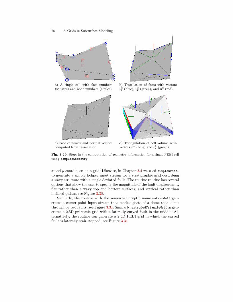
78 3 Grids in Subsurface Modeling
a) A single cell with face numbers(squares) and node numbers (circles)
b) Tessellation of faces with vectors~vk1 (blue), ~vk2 (green), and ~nk (red)
c) Face centroids and normal vectorscomputed from tessellation
d) Triangulation of cell volume withvectors ~nk (blue) and ~ckr (green)
Fig. 3.29. Steps in the computation of geometry information for a single PEBI cellusing computeGeometry.
x and y coordinates in a grid. Likewise, in Chapter 2.4 we used simpleGrdecl
to generate a simple Eclipse input stream for a stratigraphic grid describinga wavy structure with a single deviated fault. The routine routine has severaloptions that allow the user to specify the magnitude of the fault displacement,flat rather than a wavy top and bottom surfaces, and vertical rather thaninclined pillars, see Figure 3.30.
Similarly, the routine with the somewhat cryptic name makeModel3 gen-erates a corner-point input stream that models parts of a dome that is cutthrough by two faults, see Figure 3.31. Similarly, extrudedTriangleGrid.m gen-erates a 2.5D prismatic grid with a laterally curved fault in the middle. Al-ternatively, the routine can generate a 2.5D PEBI grid in which the curvedfault is laterally stair-stepped, see Figure 3.31.
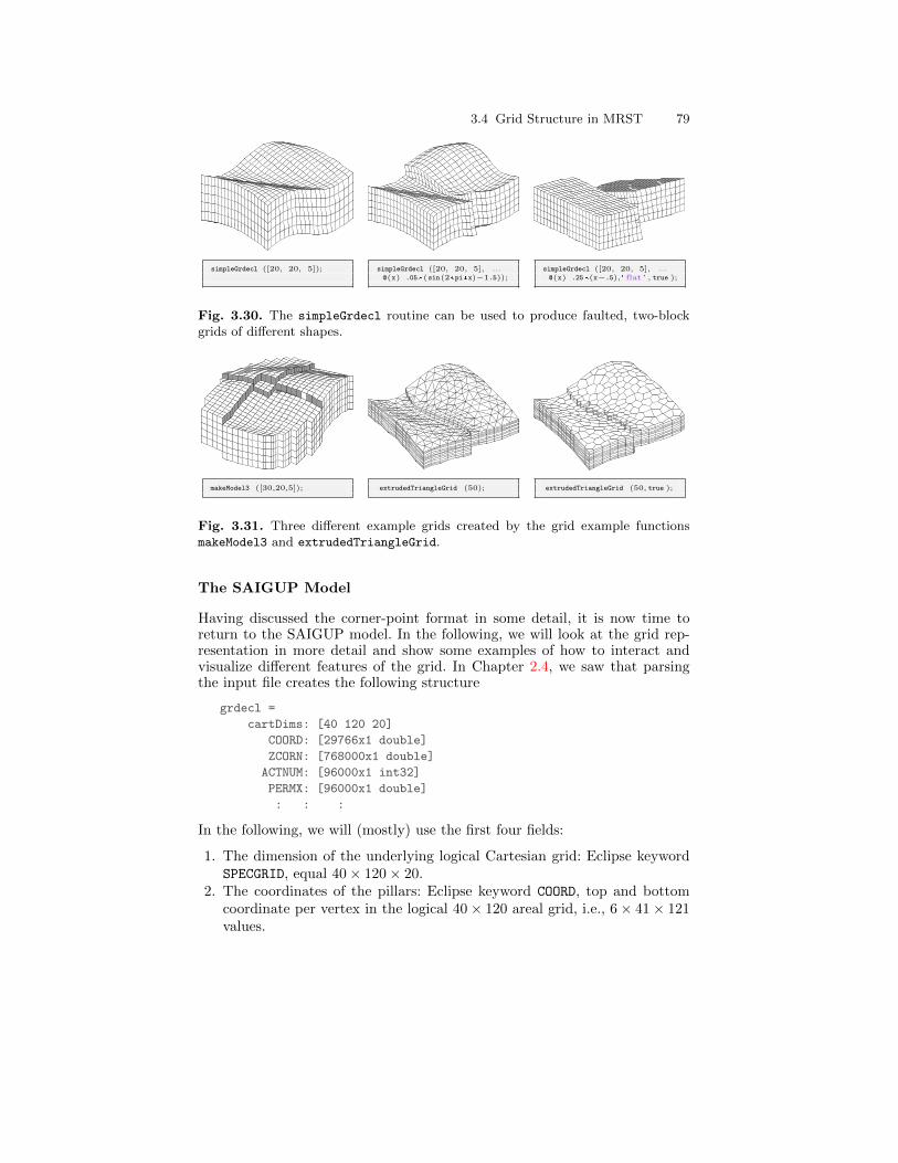
3.4 Grid Structure in MRST 79
simpleGrdecl ([20, 20, 5]); simpleGrdecl ([20, 20, 5], ...@(x) .05*(sin(2*pi*x)−1.5));
simpleGrdecl ([20, 20, 5], ...@(x) .25*(x−.5),' flat ' , true );
Fig. 3.30. The simpleGrdecl routine can be used to produce faulted, two-blockgrids of different shapes.
makeModel3 ([30,20,5]); extrudedTriangleGrid (50); extrudedTriangleGrid (50, true );
Fig. 3.31. Three different example grids created by the grid example functionsmakeModel3 and extrudedTriangleGrid.
The SAIGUP Model
Having discussed the corner-point format in some detail, it is now time toreturn to the SAIGUP model. In the following, we will look at the grid rep-resentation in more detail and show some examples of how to interact andvisualize different features of the grid. In Chapter 2.4, we saw that parsingthe input file creates the following structure
grdecl =
cartDims: [40 120 20]
COORD: [29766x1 double]
ZCORN: [768000x1 double]
ACTNUM: [96000x1 int32]
PERMX: [96000x1 double]
: : :
In the following, we will (mostly) use the first four fields:
1. The dimension of the underlying logical Cartesian grid: Eclipse keywordSPECGRID, equal 40× 120× 20.
2. The coordinates of the pillars: Eclipse keyword COORD, top and bottomcoordinate per vertex in the logical 40× 120 areal grid, i.e., 6× 41× 121values.
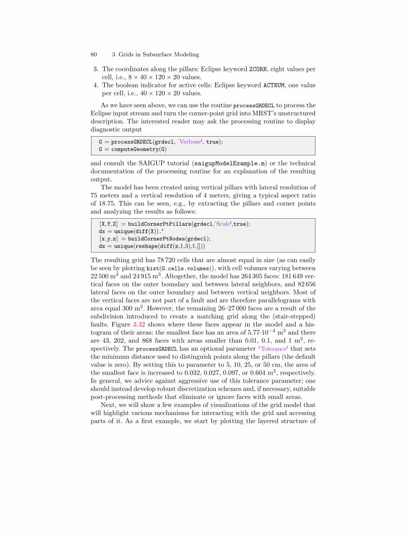
80 3 Grids in Subsurface Modeling
3. The coordinates along the pillars: Eclipse keyword ZCORN, eight values percell, i.e., 8× 40× 120× 20 values.
4. The boolean indicator for active cells: Eclipse keyword ACTNUM, one valueper cell, i.e., 40× 120× 20 values.
As we have seen above, we can use the routine processGRDECL to process theEclipse input stream and turn the corner-point grid into MRST’s unstructureddescription. The interested reader may ask the processing routine to displaydiagnostic output
G = processGRDECL(grdecl, 'Verbose', true);G = computeGeometry(G)
and consult the SAIGUP tutorial (saigupModelExample.m) or the technicaldocumentation of the processing routine for an explanation of the resultingoutput.
The model has been created using vertical pillars with lateral resolution of75 meters and a vertical resolution of 4 meters, giving a typical aspect ratioof 18.75. This can be seen, e.g., by extracting the pillars and corner pointsand analyzing the results as follows:
[X,Y,Z] = buildCornerPtPillars(grdecl,'Scale',true);dx = unique(diff(X)).'[x,y,z] = buildCornerPtNodes(grdecl);dz = unique(reshape(diff(z,1,3),1,[]))
The resulting grid has 78 720 cells that are almost equal in size (as can easilybe seen by plotting hist(G.cells.volumes)), with cell volumes varying between22 500 m3 and 24 915 m3. Altogether, the model has 264 305 faces: 181 649 ver-tical faces on the outer boundary and between lateral neighbors, and 82 656lateral faces on the outer boundary and between vertical neighbors. Most ofthe vertical faces are not part of a fault and are therefore parallelograms witharea equal 300 m2. However, the remaining 26–27 000 faces are a result of thesubdivision introduced to create a matching grid along the (stair-stepped)faults. Figure 3.32 shows where these faces appear in the model and a his-togram of their areas: the smallest face has an area of 5.77·10−4 m2 and thereare 43, 202, and 868 faces with areas smaller than 0.01, 0.1, and 1 m2, re-spectively. The processGRDECL has an optional parameter 'Tolerance' that setsthe minimum distance used to distinguish points along the pillars (the defaultvalue is zero). By setting this to parameter to 5, 10, 25, or 50 cm, the area ofthe smallest face is increased to 0.032, 0.027, 0.097, or 0.604 m2, respectively.In general, we advice against aggressive use of this tolerance parameter; oneshould instead develop robust discretization schemes and, if necessary, suitablepost-processing methods that eliminate or ignore faces with small areas.
Next, we will show a few examples of visualizations of the grid model thatwill highlight various mechanisms for interacting with the grid and accessingparts of it. As a first example, we start by plotting the layered structure of
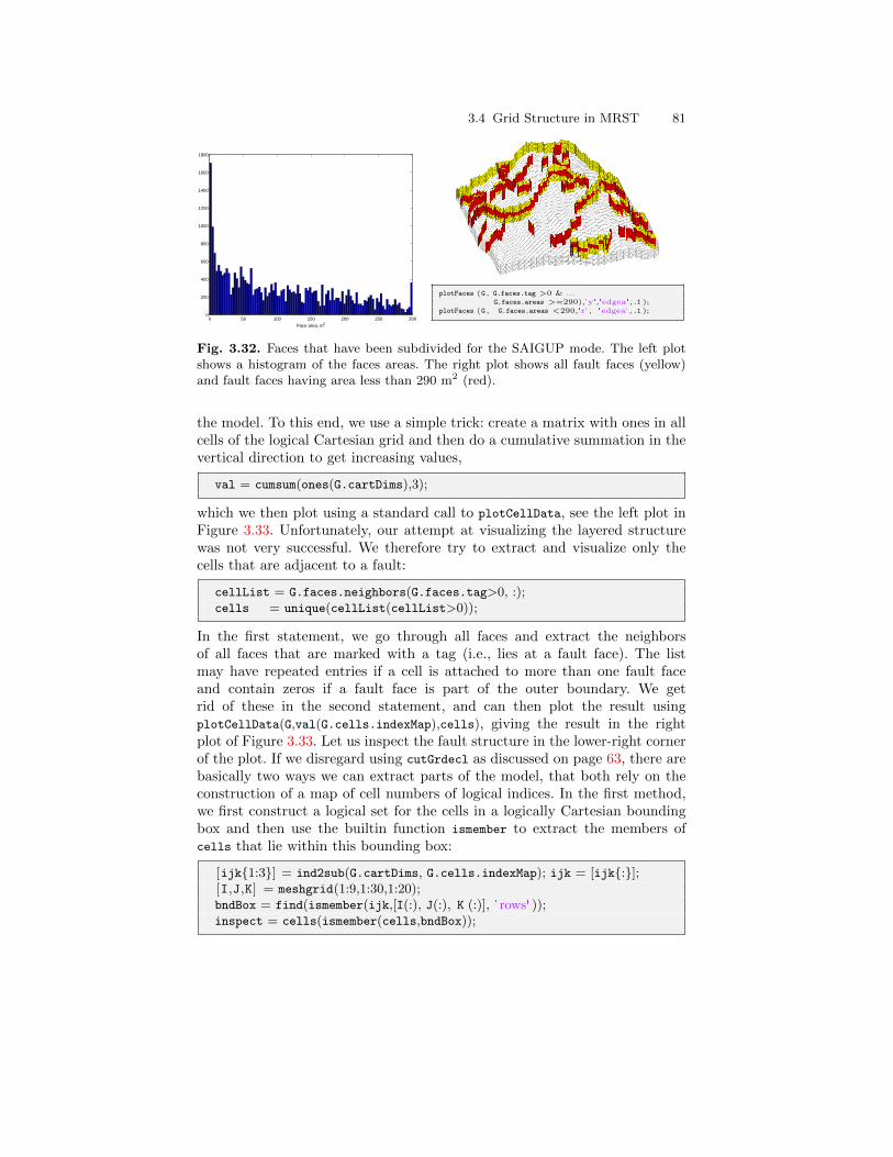
3.4 Grid Structure in MRST 81
0 50 100 150 200 250 3000
200
400
600
800
1000
1200
1400
1600
1800
Face area, m2
plotFaces (G , G.faces.tag >0 & ...G.faces.areas >=290),'y','edgea',.1 );
plotFaces (G , G.faces.areas <290,'r', 'edgea',.1 );
Fig. 3.32. Faces that have been subdivided for the SAIGUP mode. The left plotshows a histogram of the faces areas. The right plot shows all fault faces (yellow)and fault faces having area less than 290 m2 (red).
the model. To this end, we use a simple trick: create a matrix with ones in allcells of the logical Cartesian grid and then do a cumulative summation in thevertical direction to get increasing values,
val = cumsum(ones(G.cartDims),3);
which we then plot using a standard call to plotCellData, see the left plot inFigure 3.33. Unfortunately, our attempt at visualizing the layered structurewas not very successful. We therefore try to extract and visualize only thecells that are adjacent to a fault:
cellList = G.faces.neighbors(G.faces.tag>0, :);cells = unique(cellList(cellList>0));
In the first statement, we go through all faces and extract the neighborsof all faces that are marked with a tag (i.e., lies at a fault face). The listmay have repeated entries if a cell is attached to more than one fault faceand contain zeros if a fault face is part of the outer boundary. We getrid of these in the second statement, and can then plot the result usingplotCellData(G,val(G.cells.indexMap),cells), giving the result in the rightplot of Figure 3.33. Let us inspect the fault structure in the lower-right cornerof the plot. If we disregard using cutGrdecl as discussed on page 63, there arebasically two ways we can extract parts of the model, that both rely on theconstruction of a map of cell numbers of logical indices. In the first method,we first construct a logical set for the cells in a logically Cartesian boundingbox and then use the builtin function ismember to extract the members ofcells that lie within this bounding box:
[ijk1:3] = ind2sub(G.cartDims, G.cells.indexMap); ijk = [ijk:];[I,J,K] = meshgrid(1:9,1:30,1:20);bndBox = find(ismember(ijk,[I(:), J(:), K (:)], 'rows' ));inspect = cells(ismember(cells,bndBox));
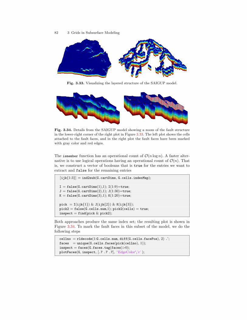
82 3 Grids in Subsurface Modeling
Fig. 3.33. Visualizing the layered structure of the SAIGUP model.
Fig. 3.34. Details from the SAIGUP model showing a zoom of the fault structurein the lower-right corner of the right plot in Figure 3.33. The left plot shows the cellsattached to the fault faces, and in the right plot the fault faces have been markedwith gray color and red edges.
The ismember function has an operational count of O(n log n). A faster alter-native is to use logical operations having an operational count of O(n). Thatis, we construct a vector of booleans that is true for the entries we want toextract and false for the remaining entries
[ijk1:3] = ind2sub(G.cartDims, G.cells.indexMap);
I = false(G.cartDims(1),1); I(1:9)=true;J = false(G.cartDims(2),1); J(1:30)=true;K = false(G.cartDims(3),1); K(1:20)=true;
pick = I(ijk1) & J(ijk2) & K(ijk3);pick2 = false(G.cells.num,1); pick2(cells) = true;inspect = find(pick & pick2);
Both approaches produce the same index set; the resulting plot is shown inFigure 3.34. To mark the fault faces in this subset of the model, we do thefollowing steps
cellno = rldecode(1:G.cells.num, diff(G.cells.facePos), 2) .';faces = unique(G.cells.faces(pick(cellno), 1));inspect = faces(G.faces.tag(faces)>0);plotFaces(G, inspect, [.7 .7 .7], 'EdgeColor','r ' );
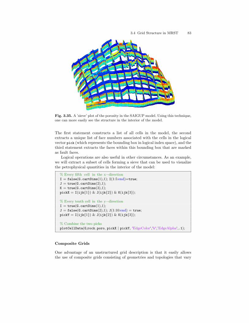
3.4 Grid Structure in MRST 83
Fig. 3.35. A ’sieve’ plot of the porosity in the SAIGUP model. Using this technique,one can more easily see the structure in the interior of the model.
The first statement constructs a list of all cells in the model, the secondextracts a unique list of face numbers associated with the cells in the logicalvector pick (which represents the bounding box in logical index space), and thethird statement extracts the faces within this bounding box that are markedas fault faces.
Logical operations are also useful in other circumstances. As an example,we will extract a subset of cells forming a sieve that can be used to visualizethe petrophysical quantities in the interior of the model:
% Every fifth cell in the x−directionI = false(G.cartDims(1),1); I(1:5:end)=true;J = true(G.cartDims(2),1);K = true(G.cartDims(3),1);pickX = I(ijk1) & J(ijk2) & K(ijk3);
% Every tenth cell in the y−directionI = true(G.cartDims(1),1);J = false(G.cartDims(2),1); J(1:10:end) = true;pickY = I(ijk1) & J(ijk2) & K(ijk3);
% Combine the two picksplotCellData(G,rock.poro, pickX | pickY, 'EdgeColor','k','EdgeAlpha',.1);
Composite Grids
One advantage of an unstructured grid description is that it easily allowsthe use of composite grids consisting of geometries and topologies that vary
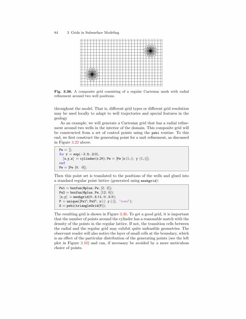
84 3 Grids in Subsurface Modeling
Fig. 3.36. A composite grid consisting of a regular Cartesian mesh with radialrefinement around two well positions.
throughout the model. That is, different grid types or different grid resolutionmay be used locally to adapt to well trajectories and special features in thegeology
As an example, we will generate a Cartesian grid that has a radial refine-ment around two wells in the interior of the domain. This composite grid willbe constructed from a set of control points using the pebi routine. To thisend, we first construct the generating point for a unit refinement, as discussedin Figure 3.22 above.
Pw = [];for r = exp(−3.5:.2:0),
[x,y,z] = cylinder(r,28); Pw = [Pw [x (1,:); y (1,:)]];endPw = [Pw [0; 0]];
Then this point set is translated to the positions of the wells and glued intoa standard regular point lattice (generated using meshgrid):
Pw1 = bsxfun(@plus, Pw, [2; 2]);Pw2 = bsxfun(@plus, Pw, [12; 6]);[x,y] = meshgrid(0:.5:14, 0:.5:8);P = unique([Pw1'; Pw2'; x (:) y (:)], 'rows');G = pebi(triangleGrid(P));
The resulting grid is shown in Figure 3.36. To get a good grid, it is importantthat the number of points around the cylinder has a reasonable match with thedensity of the points in the regular lattice. If not, the transition cells betweenthe radial and the regular grid may exhibit quite unfeasible geometries. Theobservant reader will also notice the layer of small cells at the boundary, whichis an effect of the particular distribution of the generating points (see the leftplot in Figure 3.10) and can, if necessary be avoided by a more meticulouschoice of points.
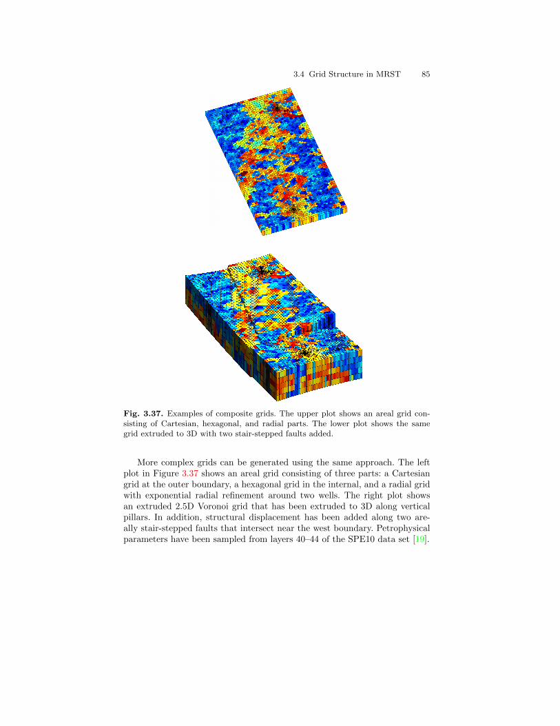
3.4 Grid Structure in MRST 85
Fig. 3.37. Examples of composite grids. The upper plot shows an areal grid con-sisting of Cartesian, hexagonal, and radial parts. The lower plot shows the samegrid extruded to 3D with two stair-stepped faults added.
More complex grids can be generated using the same approach. The leftplot in Figure 3.37 shows an areal grid consisting of three parts: a Cartesiangrid at the outer boundary, a hexagonal grid in the internal, and a radial gridwith exponential radial refinement around two wells. The right plot showsan extruded 2.5D Voronoi grid that has been extruded to 3D along verticalpillars. In addition, structural displacement has been added along two are-ally stair-stepped faults that intersect near the west boundary. Petrophysicalparameters have been sampled from layers 40–44 of the SPE10 data set [19].

4
Grid Coarsening
Over the last decades, methods for mapping and characterizing subsurfacerock formations have improved tremendously. This, together with a dramaticincrease in computational power, has enabled the industry to build increas-ingly detailed and complex models to account for heterogeneous structures ondifferent spatial scales. Using the gridding techniques outlined above, one cantoday easily build complex geological models consisting of multiple millioncells that account for most of the features seen in typical reservoirs. In fact,it is generally possible to identify many more geological layers and fine-scaleheterogeneity features than it is practical to include in flow simulations.
Through parallelization and use of high-performance computers it is pos-sible to simulate fluid flow on grid models with multimillion cells, at least inprinciple. In many practical engineering workflows, however, such large-scalecomputations many not be feasible. The user may not have access to parallelhardware or software, or he/she may want to spend the available computa-tional power on running a large number of model realizations instead of afew highly resolved ones. To obtain simulation models that are computation-ally tractable within a given computational budget, it is therefore commonto develop reduced models through some kind of upscaling (homogenization)procedure that removes spatial detail from the geological description. Typi-cally, a coarser model is developed by identifying regions consisting of severalcells and then replacing each region by a single, coarse cell with homogeneousproperties that represent the heterogeneity inside the region in some averagedsense. Upscaling, and alternative multiscale approaches, will be discussed laterin the book.
Coarse grids required for upscaling can obviously be generated as dis-cussed earlier in this chapter, using a coarser spatial resolution. However, thisapproach has two obvious disadvantages: First of all, if the original grid hasa complex geometry, it will generally not be possible to preserve the exactgeometry of the fine grid for an arbitrary coarse resolution. Second, there willgenerally not be a one-to-one mapping between cells in the fine and coarsegrids. Herein, we have therefore chosen a different approach. In MRST, a
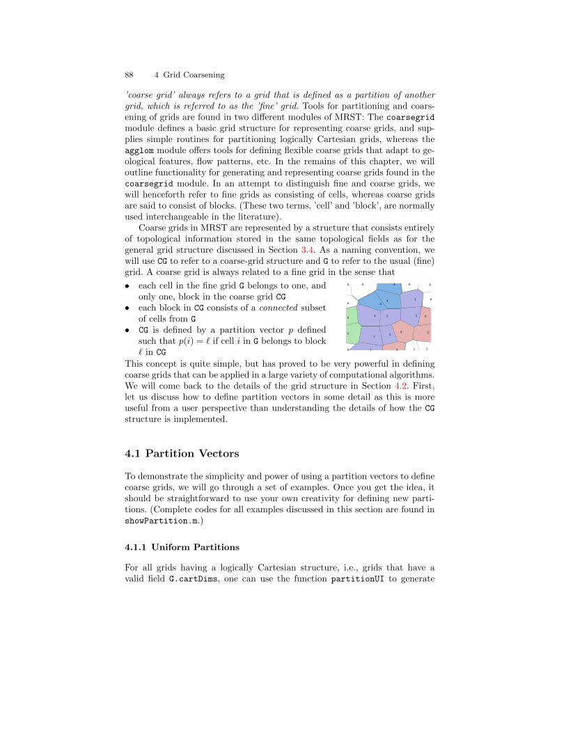
88 4 Grid Coarsening
’coarse grid’ always refers to a grid that is defined as a partition of anothergrid, which is referred to as the ’fine’ grid. Tools for partitioning and coars-ening of grids are found in two different modules of MRST: The coarsegrid
module defines a basic grid structure for representing coarse grids, and sup-plies simple routines for partitioning logically Cartesian grids, whereas theagglom module offers tools for defining flexible coarse grids that adapt to ge-ological features, flow patterns, etc. In the remains of this chapter, we willoutline functionality for generating and representing coarse grids found in thecoarsegrid module. In an attempt to distinguish fine and coarse grids, wewill henceforth refer to fine grids as consisting of cells, whereas coarse gridsare said to consist of blocks. (These two terms, ’cell’ and ’block’, are normallyused interchangeable in the literature).
Coarse grids in MRST are represented by a structure that consists entirelyof topological information stored in the same topological fields as for thegeneral grid structure discussed in Section 3.4. As a naming convention, wewill use CG to refer to a coarse-grid structure and G to refer to the usual (fine)grid. A coarse grid is always related to a fine grid in the sense that
each cell in the fine grid G belongs to one, andonly one, block in the coarse grid CG
each block in CG consists of a connected subsetof cells from G
CG is defined by a partition vector p definedsuch that p(i) = ` if cell i in G belongs to block` in CG 5
2
2
6
6
1
1
1
4
6
3
1
1
4
4
7
3
1
1
8
7
3
3
8
8
This concept is quite simple, but has proved to be very powerful in definingcoarse grids that can be applied in a large variety of computational algorithms.We will come back to the details of the grid structure in Section 4.2. First,let us discuss how to define partition vectors in some detail as this is moreuseful from a user perspective than understanding the details of how the CG
structure is implemented.
4.1 Partition Vectors
To demonstrate the simplicity and power of using a partition vectors to definecoarse grids, we will go through a set of examples. Once you get the idea, itshould be straightforward to use your own creativity for defining new parti-tions. (Complete codes for all examples discussed in this section are found inshowPartition.m.)
4.1.1 Uniform Partitions
For all grids having a logically Cartesian structure, i.e., grids that have avalid field G.cartDims, one can use the function partitionUI to generate
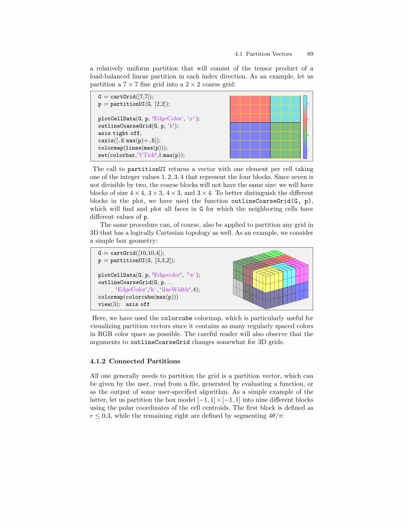
4.1 Partition Vectors 89
a relatively uniform partition that will consist of the tensor product of aload-balanced linear partition in each index direction. As an example, let uspartition a 7× 7 fine grid into a 2× 2 coarse grid:
G = cartGrid([7,7]);p = partitionUI(G, [2,2]);
plotCellData(G, p, 'EdgeColor', 'y' );outlineCoarseGrid(G, p, 'k');axis tight off,caxis([.5 max(p)+.5]);colormap(lines(max(p)));set(colorbar,'YTick',1:max(p));
1
2
3
4
The call to partitionUI returns a vector with one element per cell takingone of the integer values 1, 2, 3, 4 that represent the four blocks. Since seven isnot divisible by two, the coarse blocks will not have the same size: we will haveblocks of size 4× 4, 3× 3, 4× 3, and 3× 4. To better distinguish the differentblocks in the plot, we have used the function outlineCoarseGrid(G, p),which will find and plot all faces in G for which the neighboring cells havedifferent values of p.
The same procedure can, of course, also be applied to partition any grid in3D that has a logically Cartesian topology as well. As an example, we considera simple box geometry:
G = cartGrid([10,10,4]);p = partitionUI(G, [3,3,2]);
plotCellData(G, p, 'Edgecolor', 'w');outlineCoarseGrid(G, p, ...
'EdgeColor','k' , ' lineWidth' ,4);colormap(colorcube(max(p)))view(3); axis off
Here, we have used the colorcube colormap, which is particularly useful forvisualizing partition vectors since it contains as many regularly spaced colorsin RGB color space as possible. The careful reader will also observe that thearguments to outlineCoarseGrid changes somewhat for 3D grids.
4.1.2 Connected Partitions
All one generally needs to partition the grid is a partition vector, which canbe given by the user, read from a file, generated by evaluating a function, oras the output of some user-specified algorithm. As a simple example of thelatter, let us partition the box model [−1, 1]× [−1, 1] into nine different blocksusing the polar coordinates of the cell centroids. The first block is defined asr ≤ 0.3, while the remaining eight are defined by segmenting 4θ/π:
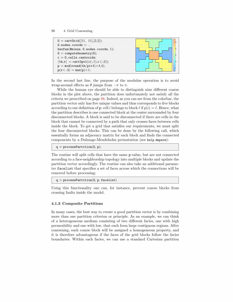
90 4 Grid Coarsening
G = cartGrid([11, 11],[2,2]);G.nodes.coords = ...bsxfun(@minus, G.nodes.coords, 1);G = computeGeometry(G);c = G.cells.centroids;[th,r] = cart2pol(c(:,1),c (:,2));p = mod(round(th/pi*4)+4,4);p(r<.3) = max(p)+1;
1
2
3
4
5
In the second last line, the purpose of the modulus operation is to avoidwrap-around effects as θ jumps from −π to π.
While the human eye should be able to distinguish nine different coarseblocks in the plot above, the partition does unfortunately not satisfy all thecriteria we prescribed on page 88. Indeed, as you can see from the colorbar, thepartition vector only has five unique values and thus corresponds to five blocksaccording to our definition of p: cell i belongs to block ` if p(i) = `. Hence, whatthe partition describes is one connected block at the center surrounded by fourdisconnected blocks. A block is said to be disconnected if there are cells in theblock that cannot be connected by a path that only crosses faces between cellsinside the block. To get a grid that satisfies our requirements, we must splitthe four disconnected blocks. This can be done by the following call, whichessentially forms an adjacency matrix for each block and finds the connectedcomponents by a Dulmage-Mendelsohn permutation (see help dmperm):
q = processPartition(G, p);
The routine will split cells that have the same p-value, but are not connectedaccording to a face-neighborship topology into multiple blocks and update thepartition vector accordingly. The routine can also take an additional parame-ter facelist that specifies a set of faces across which the connections will beremoved before processing:
q = processPartition(G, p, facelist)
Using this functionality one can, for instance, prevent coarse blocks fromcrossing faults inside the model.
4.1.3 Composite Partitions
In many cases, the best way to create a good partition vector is by combiningmore than one partition criterion or principle. As an example, we can thinkof a heterogeneous medium consisting of two different facies, one with highpermeability and one with low, that each form large contiguous regions. Aftercoarsening, each coarse block will be assigned a homogeneous property, andit is therefore advantageous if the faces of the grid blocks follow the faciesboundaries. Within each facies, we can use a standard Cartesian partition
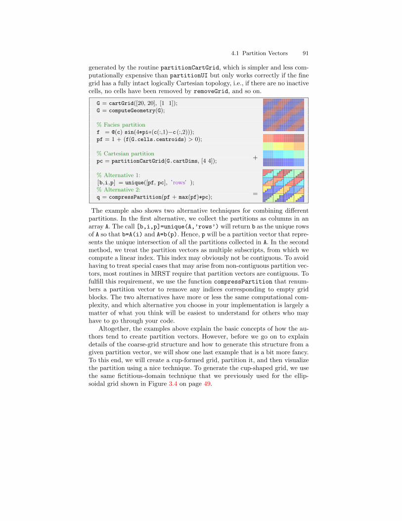
4.1 Partition Vectors 91
generated by the routine partitionCartGrid, which is simpler and less com-putationally expensive than partitionUI but only works correctly if the finegrid has a fully intact logically Cartesian topology, i.e., if there are no inactivecells, no cells have been removed by removeGrid, and so on.
G = cartGrid([20, 20], [1 1]);G = computeGeometry(G);
% Facies partitionf = @(c) sin(4*pi*(c(:,1)−c (:,2)));pf = 1 + (f(G.cells.centroids) > 0);
% Cartesian partitionpc = partitionCartGrid(G.cartDims, [4 4]);
% Alternative 1:[b,i,p] = unique([pf, pc], 'rows' );% Alternative 2:q = compressPartition(pf + max(pf)*pc);
+
=
The example also shows two alternative techniques for combining differentpartitions. In the first alternative, we collect the partitions as columns in anarray A. The call [b,i,p]=unique(A,’rows’) will return b as the unique rowsof A so that b=A(i) and A=b(p). Hence, p will be a partition vector that repre-sents the unique intersection of all the partitions collected in A. In the secondmethod, we treat the partition vectors as multiple subscripts, from which wecompute a linear index. This index may obviously not be contiguous. To avoidhaving to treat special cases that may arise from non-contiguous partition vec-tors, most routines in MRST require that partition vectors are contiguous. Tofulfill this requirement, we use the function compressPartition that renum-bers a partition vector to remove any indices corresponding to empty gridblocks. The two alternatives have more or less the same computational com-plexity, and which alternative you choose in your implementation is largely amatter of what you think will be easiest to understand for others who mayhave to go through your code.
Altogether, the examples above explain the basic concepts of how the au-thors tend to create partition vectors. However, before we go on to explaindetails of the coarse-grid structure and how to generate this structure from agiven partition vector, we will show one last example that is a bit more fancy.To this end, we will create a cup-formed grid, partition it, and then visualizethe partition using a nice technique. To generate the cup-shaped grid, we usethe same fictitious-domain technique that we previously used for the ellip-soidal grid shown in Figure 3.4 on page 49.
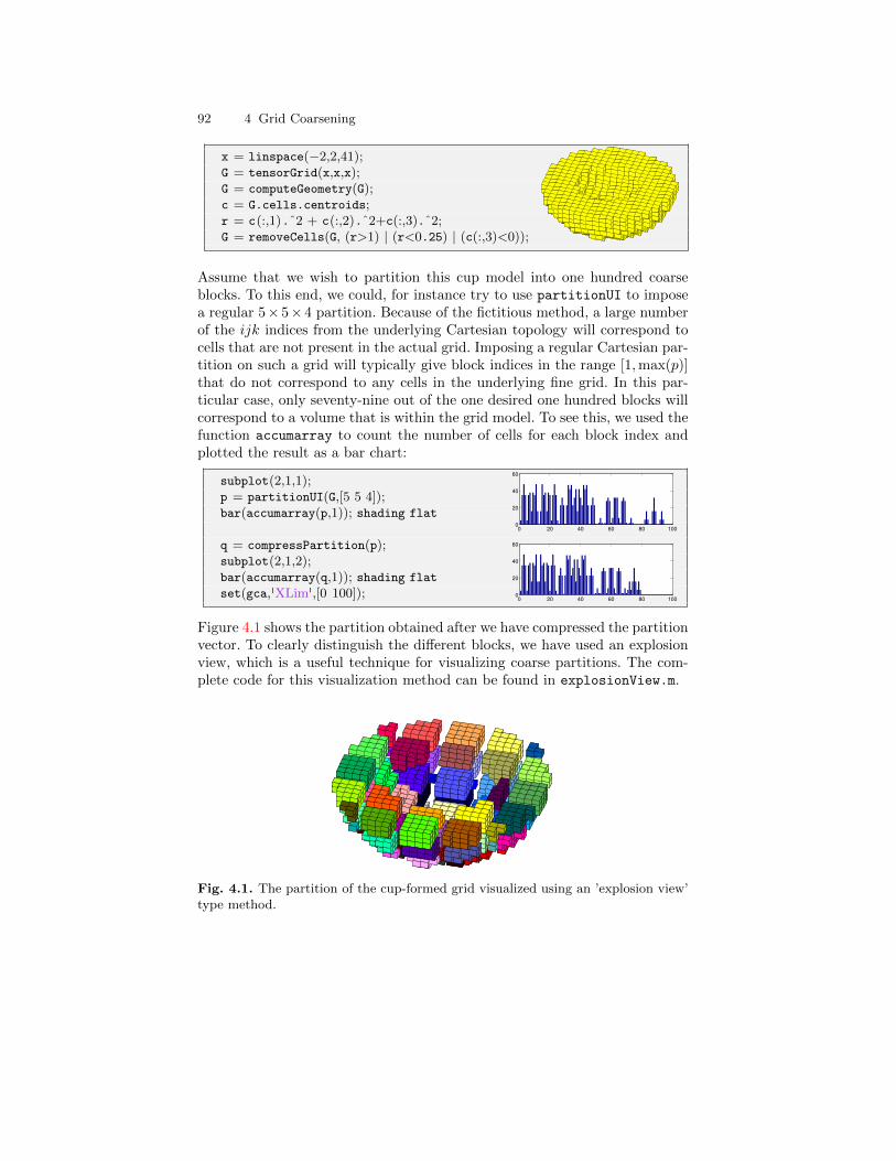
92 4 Grid Coarsening
x = linspace(−2,2,41);G = tensorGrid(x,x,x);G = computeGeometry(G);c = G.cells.centroids;r = c(:,1).ˆ2 + c(:,2).ˆ2+c(:,3).ˆ2;G = removeCells(G, (r>1) | (r<0.25) | (c(:,3)<0));
Assume that we wish to partition this cup model into one hundred coarseblocks. To this end, we could, for instance try to use partitionUI to imposea regular 5× 5× 4 partition. Because of the fictitious method, a large numberof the ijk indices from the underlying Cartesian topology will correspond tocells that are not present in the actual grid. Imposing a regular Cartesian par-tition on such a grid will typically give block indices in the range [1,max(p)]that do not correspond to any cells in the underlying fine grid. In this par-ticular case, only seventy-nine out of the one desired one hundred blocks willcorrespond to a volume that is within the grid model. To see this, we used thefunction accumarray to count the number of cells for each block index andplotted the result as a bar chart:
subplot(2,1,1);p = partitionUI(G,[5 5 4]);bar(accumarray(p,1)); shading flat
q = compressPartition(p);subplot(2,1,2);bar(accumarray(q,1)); shading flat
set(gca,'XLim',[0 100]);
0 20 40 60 80 1000
20
40
60
0 20 40 60 80 1000
20
40
60
Figure 4.1 shows the partition obtained after we have compressed the partitionvector. To clearly distinguish the different blocks, we have used an explosionview, which is a useful technique for visualizing coarse partitions. The com-plete code for this visualization method can be found in explosionView.m.
Fig. 4.1. The partition of the cup-formed grid visualized using an ’explosion view’type method.
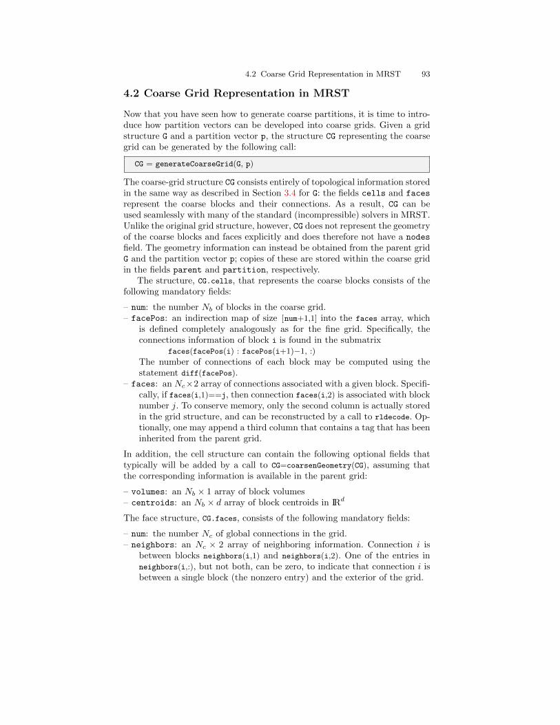
4.2 Coarse Grid Representation in MRST 93
4.2 Coarse Grid Representation in MRST
Now that you have seen how to generate coarse partitions, it is time to intro-duce how partition vectors can be developed into coarse grids. Given a gridstructure G and a partition vector p, the structure CG representing the coarsegrid can be generated by the following call:
CG = generateCoarseGrid(G, p)
The coarse-grid structure CG consists entirely of topological information storedin the same way as described in Section 3.4 for G: the fields cells and faces
represent the coarse blocks and their connections. As a result, CG can beused seamlessly with many of the standard (incompressible) solvers in MRST.Unlike the original grid structure, however, CG does not represent the geometryof the coarse blocks and faces explicitly and does therefore not have a nodes
field. The geometry information can instead be obtained from the parent gridG and the partition vector p; copies of these are stored within the coarse gridin the fields parent and partition, respectively.
The structure, CG.cells, that represents the coarse blocks consists of thefollowing mandatory fields:
– num: the number Nb of blocks in the coarse grid.– facePos: an indirection map of size [num+1,1] into the faces array, which
is defined completely analogously as for the fine grid. Specifically, theconnections information of block i is found in the submatrix
faces(facePos(i) : facePos(i+1)−1, :)
The number of connections of each block may be computed using thestatement diff(facePos).
– faces: an Nc×2 array of connections associated with a given block. Specifi-cally, if faces(i,1)==j, then connection faces(i,2) is associated with blocknumber j. To conserve memory, only the second column is actually storedin the grid structure, and can be reconstructed by a call to rldecode. Op-tionally, one may append a third column that contains a tag that has beeninherited from the parent grid.
In addition, the cell structure can contain the following optional fields thattypically will be added by a call to CG=coarsenGeometry(CG), assuming thatthe corresponding information is available in the parent grid:
– volumes: an Nb × 1 array of block volumes– centroids: an Nb × d array of block centroids in IRd
The face structure, CG.faces, consists of the following mandatory fields:
– num: the number Nc of global connections in the grid.– neighbors: an Nc × 2 array of neighboring information. Connection i is
between blocks neighbors(i,1) and neighbors(i,2). One of the entries inneighbors(i,:), but not both, can be zero, to indicate that connection i isbetween a single block (the nonzero entry) and the exterior of the grid.
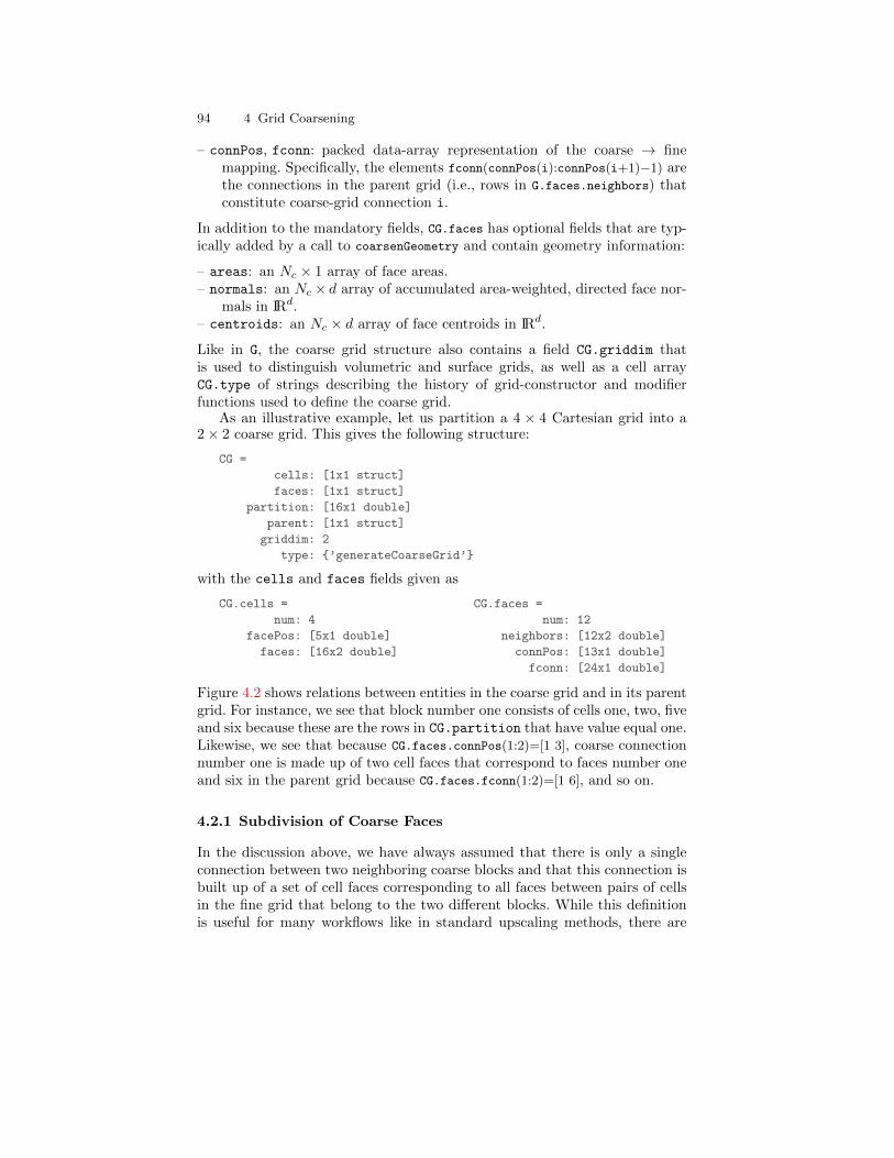
94 4 Grid Coarsening
– connPos, fconn: packed data-array representation of the coarse → finemapping. Specifically, the elements fconn(connPos(i):connPos(i+1)−1) arethe connections in the parent grid (i.e., rows in G.faces.neighbors) thatconstitute coarse-grid connection i.
In addition to the mandatory fields, CG.faces has optional fields that are typ-ically added by a call to coarsenGeometry and contain geometry information:
– areas: an Nc × 1 array of face areas.– normals: an Nc × d array of accumulated area-weighted, directed face nor-
mals in IRd.– centroids: an Nc × d array of face centroids in IRd.
Like in G, the coarse grid structure also contains a field CG.griddim thatis used to distinguish volumetric and surface grids, as well as a cell arrayCG.type of strings describing the history of grid-constructor and modifierfunctions used to define the coarse grid.
As an illustrative example, let us partition a 4 × 4 Cartesian grid into a2× 2 coarse grid. This gives the following structure:
CG =
cells: [1x1 struct]
faces: [1x1 struct]
partition: [16x1 double]
parent: [1x1 struct]
griddim: 2
type: ’generateCoarseGrid’
with the cells and faces fields given as
CG.cells = CG.faces =
num: 4 num: 12
facePos: [5x1 double] neighbors: [12x2 double]
faces: [16x2 double] connPos: [13x1 double]
fconn: [24x1 double]
Figure 4.2 shows relations between entities in the coarse grid and in its parentgrid. For instance, we see that block number one consists of cells one, two, fiveand six because these are the rows in CG.partition that have value equal one.Likewise, we see that because CG.faces.connPos(1:2)=[1 3], coarse connectionnumber one is made up of two cell faces that correspond to faces number oneand six in the parent grid because CG.faces.fconn(1:2)=[1 6], and so on.
4.2.1 Subdivision of Coarse Faces
In the discussion above, we have always assumed that there is only a singleconnection between two neighboring coarse blocks and that this connection isbuilt up of a set of cell faces corresponding to all faces between pairs of cellsin the fine grid that belong to the two different blocks. While this definitionis useful for many workflows like in standard upscaling methods, there are
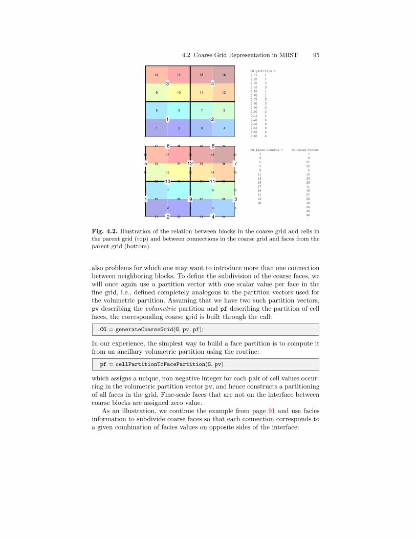
4.2 Coarse Grid Representation in MRST 95
1 2 3 4
5 6 7 8
9 10 11 12
13 14 15 16
1 2
3 4
CG.partition =
( 1) 1
( 2) 1
( 3) 2
( 4) 2
( 5) 1
( 6) 1
( 7) 2
( 8) 2
( 9) 3
(10) 3
(11) 4
(12) 4
(13) 3
(14) 3
(15) 4
(16) 4
1 2 3 4 5
6 7 8 9 10
11 12 13 14 15
16 17 18 19 20
21 22 23 24
25 26 27 28
29 30 31 32
33 34 35 36
37 38 39 40
1
2
3
4
5
6
7
8
9
10 11
12
CG.faces.connPos = CG.faces.fconn=
1 1
3 6
5 21
7 22
9 5
11 10
13 23
15 24
17 11
19 16
21 37
23 38
25 15
20
39
40
:
Fig. 4.2. Illustration of the relation between blocks in the coarse grid and cells inthe parent grid (top) and between connections in the coarse grid and faces from theparent grid (bottom).
also problems for which one may want to introduce more than one connectionbetween neighboring blocks. To define the subdivision of the coarse faces, wewill once again use a partition vector with one scalar value per face in thefine grid, i.e., defined completely analogous to the partition vectors used forthe volumetric partition. Assuming that we have two such partition vectors,pv describing the volumetric partition and pf describing the partition of cellfaces, the corresponding coarse grid is built through the call:
CG = generateCoarseGrid(G, pv, pf);
In our experience, the simplest way to build a face partition is to compute itfrom an ancillary volumetric partition using the routine:
pf = cellPartitionToFacePartition(G, pv)
which assigns a unique, non-negative integer for each pair of cell values occur-ring in the volumetric partition vector pv, and hence constructs a partitioningof all faces in the grid. Fine-scale faces that are not on the interface betweencoarse blocks are assigned zero value.
As an illustration, we continue the example from page 91 and use faciesinformation to subdivide coarse faces so that each connection corresponds toa given combination of facies values on opposite sides of the interface:
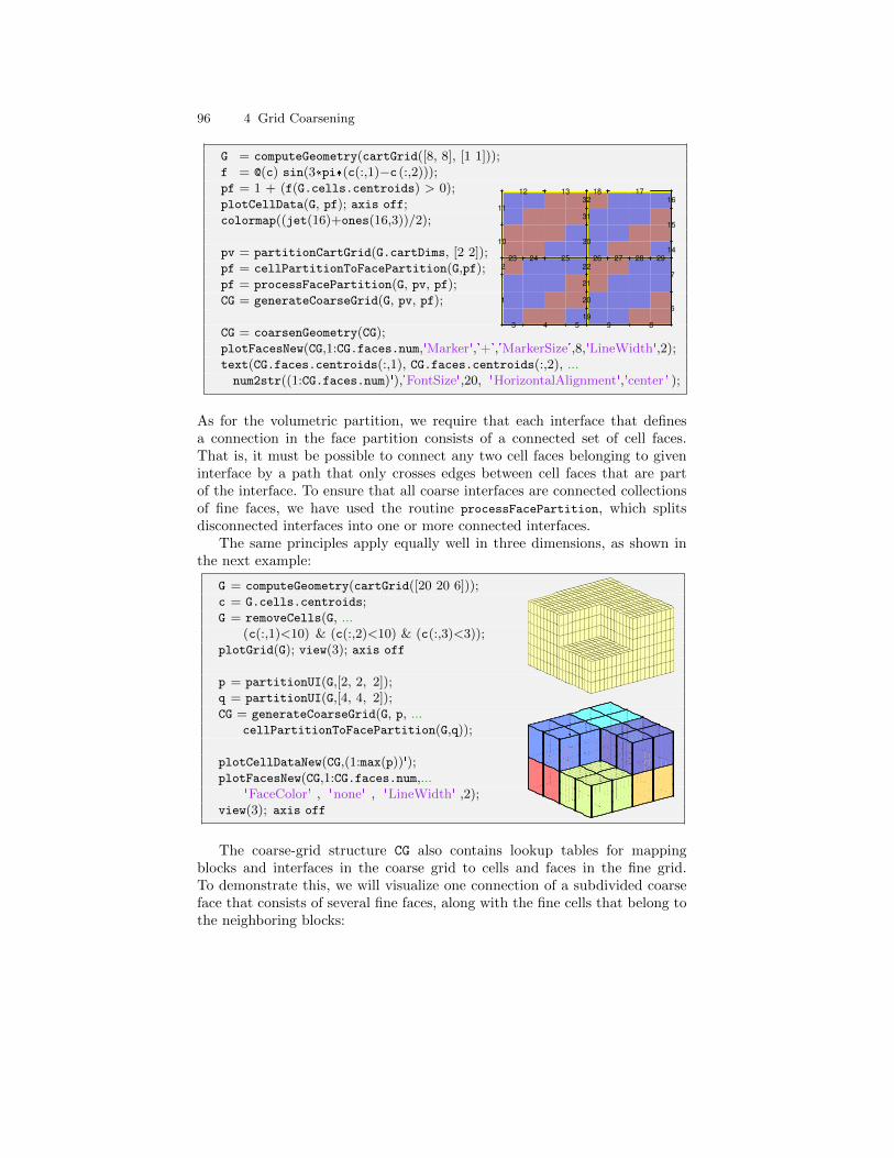
96 4 Grid Coarsening
G = computeGeometry(cartGrid([8, 8], [1 1]));f = @(c) sin(3*pi*(c(:,1)−c (:,2)));pf = 1 + (f(G.cells.centroids) > 0);plotCellData(G, pf); axis off;colormap((jet(16)+ones(16,3))/2);
pv = partitionCartGrid(G.cartDims, [2 2]);pf = cellPartitionToFacePartition(G,pf);pf = processFacePartition(G, pv, pf);CG = generateCoarseGrid(G, pv, pf);
CG = coarsenGeometry(CG);plotFacesNew(CG,1:CG.faces.num,'Marker','+','MarkerSize',8,'LineWidth',2);text(CG.faces.centroids(:,1), CG.faces.centroids(:,2), ...num2str((1:CG.faces.num)'),'FontSize',20, 'HorizontalAlignment','center ' );
1
2
3 4 5
6
7
8 9
10
11
12 13
14
15
16
1718
19
20
21
22
23 24 25 26 27 28 29
30
31
32
As for the volumetric partition, we require that each interface that definesa connection in the face partition consists of a connected set of cell faces.That is, it must be possible to connect any two cell faces belonging to giveninterface by a path that only crosses edges between cell faces that are partof the interface. To ensure that all coarse interfaces are connected collectionsof fine faces, we have used the routine processFacePartition, which splitsdisconnected interfaces into one or more connected interfaces.
The same principles apply equally well in three dimensions, as shown inthe next example:
G = computeGeometry(cartGrid([20 20 6]));c = G.cells.centroids;G = removeCells(G, ...
(c(:,1)<10) & (c(:,2)<10) & (c(:,3)<3));plotGrid(G); view(3); axis off
p = partitionUI(G,[2, 2, 2]);q = partitionUI(G,[4, 4, 2]);CG = generateCoarseGrid(G, p, ...
cellPartitionToFacePartition(G,q));
plotCellDataNew(CG,(1:max(p))');plotFacesNew(CG,1:CG.faces.num,...
'FaceColor' , 'none' , 'LineWidth' ,2);view(3); axis off
The coarse-grid structure CG also contains lookup tables for mappingblocks and interfaces in the coarse grid to cells and faces in the fine grid.To demonstrate this, we will visualize one connection of a subdivided coarseface that consists of several fine faces, along with the fine cells that belong tothe neighboring blocks:
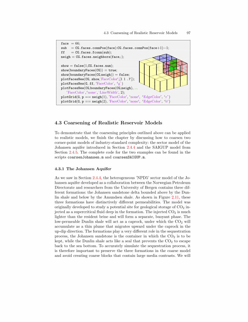
4.3 Coarsening of Realistic Reservoir Models 97
face = 66;sub = CG.faces.connPos(face):CG.faces.connPos(face+1)−1;ff = CG.faces.fconn(sub);neigh = CG.faces.neighbors(face,:);
show = false(1,CG.faces.num);show(boundaryFaces(CG)) = true;show(boundaryFaces(CG,neigh)) = false;plotFacesNew(CG, show,'FaceColor',[1 1 .7 ]);plotFacesNew(G, ff, 'FaceColor', 'g')plotFacesNew(CG,boundaryFaces(CG,neigh), ...
'FaceColor', 'none', 'LineWidth', 2);plotGrid(G, p == neigh(1), 'FaceColor', 'none', 'EdgeColor', 'r ' )plotGrid(G, p == neigh(2), 'FaceColor', 'none', 'EdgeColor', 'b')
4.3 Coarsening of Realistic Reservoir Models
To demonstrate that the coarsening principles outlined above can be appliedto realistic models, we finish the chapter by discussing how to coarsen twocorner-point models of industry-standard complexity: the sector model of theJohansen aquifer introduced in Section 2.4.4 and the SAIGUP model fromSection 2.4.5. The complete code for the two examples can be found in thescripts coarsenJohansen.m and coarsenSAIGUP.m.
4.3.1 The Johansen Aquifer
As we saw in Section 2.4.4, the heterogeneous ’NPD5’ sector model of the Jo-hansen aquifer developed as a collaboration between the Norwegian PetroleumDirectorate and researchers from the University of Bergen contains three dif-ferent formations: the Johansen sandstone delta bounded above by the Dun-lin shale and below by the Amundsen shale. As shown in Figure 2.11, thesethree formations have distinctively different permeabilities. The model wasoriginally developed to study a potential site for geological storage of CO2 in-jected as a supercritical fluid deep in the formation. The injected CO2 is muchlighter than the resident brine and will form a separate, buoyant phase. Thelow-permeable Dunlin shale will act as a caprock, under which the CO2 willaccumulate as a thin plume that migrates upward under the caprock in theup-dip direction. The formations play a very different role in the sequestrationprocess, the Johansen sandstone is the container in which the CO2 is to bekept, while the Dunlin shale acts like a seal that prevents the CO2 to escapeback to the sea bottom. To accurately simulate the sequestration process, itis therefore important to preserve the three formations in the coarse modeland avoid creating coarse blocks that contain large media contrasts. We will
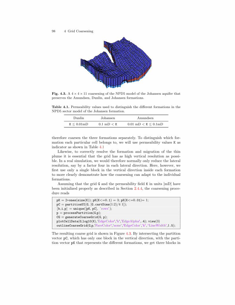
98 4 Grid Coarsening
Fig. 4.3. A 4× 4× 11 coarsening of the NPD5 model of the Johansen aquifer thatpreserves the Amundsen, Dunlin, and Johansen formations.
Table 4.1. Permeability values used to distinguish the different formations in theNPD5 sector model of the Johansen formation.
Dunlin Johansen Amundsen
K ≤ 0.01mD 0.1 mD < K 0.01 mD < K ≤ 0.1mD
therefore coarsen the three formations separately. To distinguish which for-mation each particular cell belongs to, we will use permeability values K asindicator as shown in Table 4.1
Likewise, to correctly resolve the formation and migration of the thinplume it is essential that the grid has as high vertical resolution as possi-ble. In a real simulation, we would therefore normally only reduce the lateralresolution, say by a factor four in each lateral direction. Here, however, wefirst use only a single block in the vertical direction inside each formationto more clearly demonstrate how the coarsening can adapt to the individualformations.
Assuming that the grid G and the permeability field K in units [mD] havebeen initialized properly as described in Section 2.4.4, the coarsening proce-dure reads
pK = 2*ones(size(K)); pK(K<=0.1) = 3; pK(K<=0.01)= 1;pC = partitionUI(G, [G.cartDims(1:2)/4 1]);[b,i,p] = unique([pK, pC], 'rows');p = processPartition(G,p);CG = generateCoarseGrid(G, p);plotCellData(G,log10(K),'EdgeColor','k','EdgeAlpha',.4); view(3)outlineCoarseGrid(G,p,'FaceColor','none','EdgeColor','k', 'LineWidth',1.5);
The resulting coarse grid is shown in Figure 4.3. By intersecting the partitionvector pC, which has only one block in the vertical direction, with the parti-tion vector pK that represents the different formations, we get three blocks in
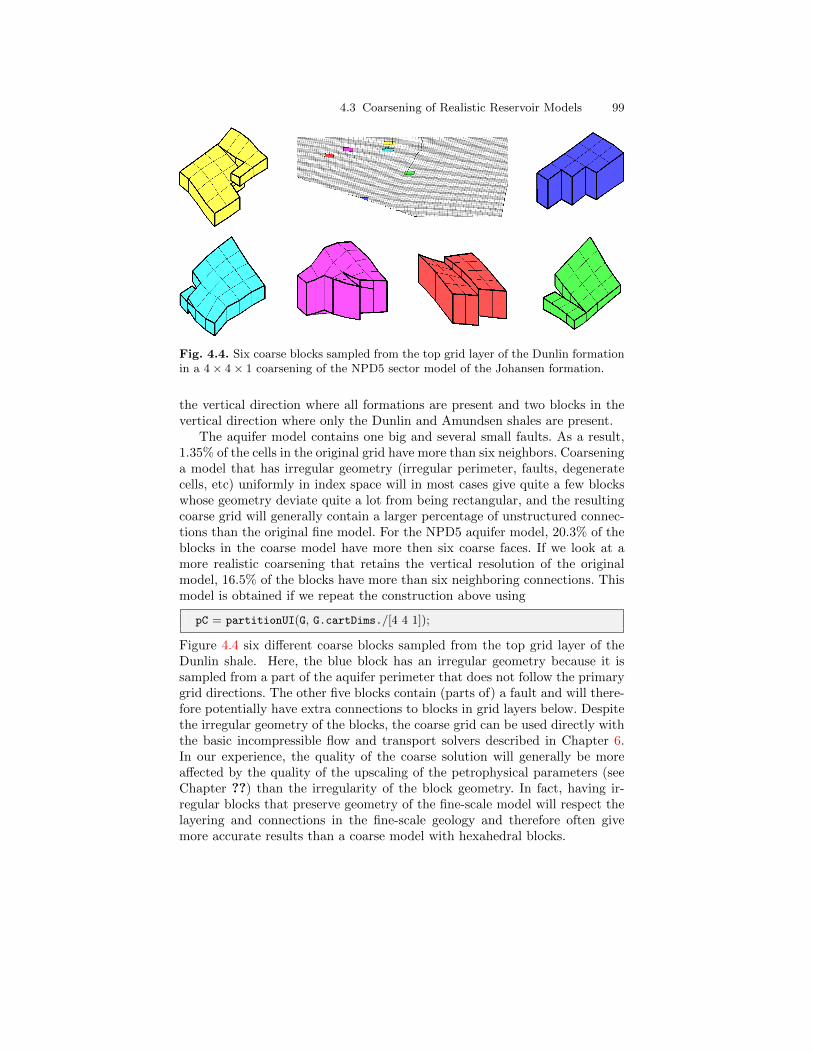
4.3 Coarsening of Realistic Reservoir Models 99
Fig. 4.4. Six coarse blocks sampled from the top grid layer of the Dunlin formationin a 4× 4× 1 coarsening of the NPD5 sector model of the Johansen formation.
the vertical direction where all formations are present and two blocks in thevertical direction where only the Dunlin and Amundsen shales are present.
The aquifer model contains one big and several small faults. As a result,1.35% of the cells in the original grid have more than six neighbors. Coarseninga model that has irregular geometry (irregular perimeter, faults, degeneratecells, etc) uniformly in index space will in most cases give quite a few blockswhose geometry deviate quite a lot from being rectangular, and the resultingcoarse grid will generally contain a larger percentage of unstructured connec-tions than the original fine model. For the NPD5 aquifer model, 20.3% of theblocks in the coarse model have more then six coarse faces. If we look at amore realistic coarsening that retains the vertical resolution of the originalmodel, 16.5% of the blocks have more than six neighboring connections. Thismodel is obtained if we repeat the construction above using
pC = partitionUI(G, G.cartDims./[4 4 1]);
Figure 4.4 six different coarse blocks sampled from the top grid layer of theDunlin shale. Here, the blue block has an irregular geometry because it issampled from a part of the aquifer perimeter that does not follow the primarygrid directions. The other five blocks contain (parts of) a fault and will there-fore potentially have extra connections to blocks in grid layers below. Despitethe irregular geometry of the blocks, the coarse grid can be used directly withthe basic incompressible flow and transport solvers described in Chapter 6.In our experience, the quality of the coarse solution will generally be moreaffected by the quality of the upscaling of the petrophysical parameters (seeChapter ??) than the irregularity of the block geometry. In fact, having ir-regular blocks that preserve geometry of the fine-scale model will respect thelayering and connections in the fine-scale geology and therefore often givemore accurate results than a coarse model with hexahedral blocks.
100 4 Grid Coarsening
4.3.2 The Shallow-Marine SAIGUP Model
As our next example, we will revisit the SAIGUP model discussed on page 79.As shown in Figure 2.16 in Section 2.4.5, the model has six user-defined rocktypes (also known as saturation regions) that can be used to specify differentrock-fluid behavior. Depending upon the purpose of the reduced model, onemay want to preserve these rock types using the same type of technique asdescribed in the previous example. This has the advantage that if each coarseblock is made up of one rock type only, one would not have to upscale therock-fluid properties. On the other hand, this will typically lead to coarsegrids with (highly) irregular block geometries and large variations in blockvolumes. To illustrate this point, we start by partitioning the grid uniformlyinto 6× 12× 3 coarse blocks in index space:
p = partitionUI(G,[6 12 3]);
This will introduce a partition of all cells in the logical 40 × 120 × 20 grid,including cells that are inactive. To get a contiguous partition vector, weremove blocks that contain no active cells, and then renumber the vector,which reduces the total number of blocks from 216 to 201. Some of the blocksmay contain disconnected cells because of faults and other nonconformities,and we therefore need to postprocess the grid in physical space and split eachdisconnected block into a new set of connected sub-blocks:
p = compressPartition(p);p = processPartition(G,p);
The result is a partition with 243 blocks, in which each coarse block consistsof a set of connected cells in the fine grid. Figure 4.5 shows the individualcoarse blocks using the explosion-view technique introduced above. Whereasall cells in the original model are almost exactly the same size, there is almosttwo orders difference between the volumes of the smallest and largest blocksin the coarsened model. In particular, the irregular boundary near the crestof the model will introduce small blocks that consist of only a single fine cellin the lateral direction. Large variations in block volumes will adversely affectany flow solver that is later run on the model and to get a more even sizedistribution for the coarse blocks, we will therefore remove these small blocksby merging them with the neighbor that has the smallest block volume. This isdone repeatedly until the volumes of all blocks are above the lower threshold.
The merging algorithm is quite simple: we compute the block volumes,select the block with the smallest volume, and then merge this block with oneof its neighbors. Then we update the partition vector by relabling all cells inthe block with the new block number, compress the partition vector to get ridof empty entries, regenerate a coarse grid, recompute block volumes, pick theblock with the smallest volume in the new grid, and so on. In each iteration,we plot the selected block and its neighbors:
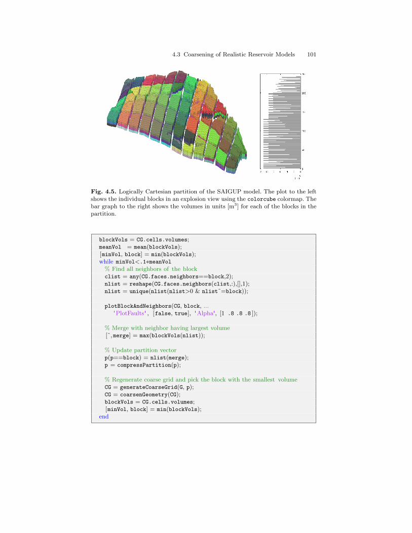
4.3 Coarsening of Realistic Reservoir Models 101
Fig. 4.5. Logically Cartesian partition of the SAIGUP model. The plot to the leftshows the individual blocks in an explosion view using the colorcube colormap. Thebar graph to the right shows the volumes in units [m3] for each of the blocks in thepartition.
blockVols = CG.cells.volumes;meanVol = mean(blockVols);[minVol, block] = min(blockVols);while minVol<.1*meanVol
% Find all neighbors of the blockclist = any(CG.faces.neighbors==block,2);nlist = reshape(CG.faces.neighbors(clist,:),[],1);nlist = unique(nlist(nlist>0 & nlist˜=block));
plotBlockAndNeighbors(CG, block, ...'PlotFaults' , [false, true], 'Alpha', [1 .8 .8 .8 ]);
% Merge with neighbor having largest volume[˜,merge] = max(blockVols(nlist));
% Update partition vectorp(p==block) = nlist(merge);p = compressPartition(p);
% Regenerate coarse grid and pick the block with the smallest volumeCG = generateCoarseGrid(G, p);CG = coarsenGeometry(CG);blockVols = CG.cells.volumes;[minVol, block] = min(blockVols);
end
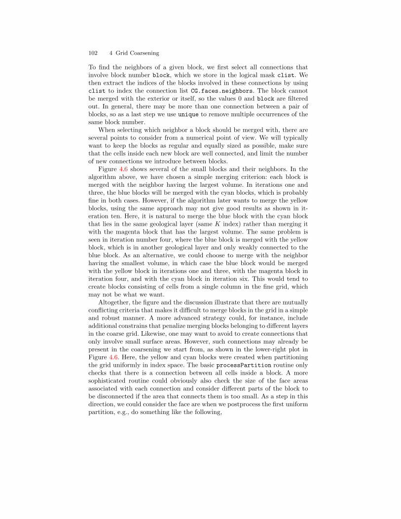
102 4 Grid Coarsening
To find the neighbors of a given block, we first select all connections thatinvolve block number block, which we store in the logical mask clist. Wethen extract the indices of the blocks involved in these connections by usingclist to index the connection list CG.faces.neighbors. The block cannotbe merged with the exterior or itself, so the values 0 and block are filteredout. In general, there may be more than one connection between a pair ofblocks, so as a last step we use unique to remove multiple occurrences of thesame block number.
When selecting which neighbor a block should be merged with, there areseveral points to consider from a numerical point of view. We will typicallywant to keep the blocks as regular and equally sized as possible, make surethat the cells inside each new block are well connected, and limit the numberof new connections we introduce between blocks.
Figure 4.6 shows several of the small blocks and their neighbors. In thealgorithm above, we have chosen a simple merging criterion: each block ismerged with the neighbor having the largest volume. In iterations one andthree, the blue blocks will be merged with the cyan blocks, which is probablyfine in both cases. However, if the algorithm later wants to merge the yellowblocks, using the same approach may not give good results as shown in it-eration ten. Here, it is natural to merge the blue block with the cyan blockthat lies in the same geological layer (same K index) rather than merging itwith the magenta block that has the largest volume. The same problem isseen in iteration number four, where the blue block is merged with the yellowblock, which is in another geological layer and only weakly connected to theblue block. As an alternative, we could choose to merge with the neighborhaving the smallest volume, in which case the blue block would be mergedwith the yellow block in iterations one and three, with the magenta block initeration four, and with the cyan block in iteration six. This would tend tocreate blocks consisting of cells from a single column in the fine grid, whichmay not be what we want.
Altogether, the figure and the discussion illustrate that there are mutuallyconflicting criteria that makes it difficult to merge blocks in the grid in a simpleand robust manner. A more advanced strategy could, for instance, includeadditional constrains that penalize merging blocks belonging to different layersin the coarse grid. Likewise, one may want to avoid to create connections thatonly involve small surface areas. However, such connections may already bepresent in the coarsening we start from, as shown in the lower-right plot inFigure 4.6. Here, the yellow and cyan blocks were created when partitioningthe grid uniformly in index space. The basic processPartition routine onlychecks that there is a connection between all cells inside a block. A moresophisticated routine could obviously also check the size of the face areasassociated with each connection and consider different parts of the block tobe disconnected if the area that connects them is too small. As a step in thisdirection, we could consider the face are when we postprocess the first uniformpartition, e.g., do something like the following,
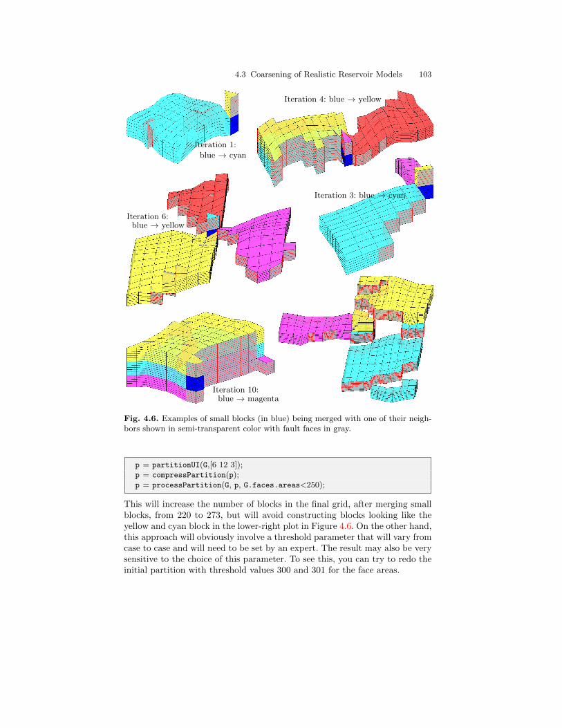
4.3 Coarsening of Realistic Reservoir Models 103
Iteration 1:
blue → cyan
Iteration 4: blue → yellow
Iteration 6:blue → yellow
Iteration 3: blue → cyan
Iteration 10:blue → magenta
Fig. 4.6. Examples of small blocks (in blue) being merged with one of their neigh-bors shown in semi-transparent color with fault faces in gray.
p = partitionUI(G,[6 12 3]);p = compressPartition(p);p = processPartition(G, p, G.faces.areas<250);
This will increase the number of blocks in the final grid, after merging smallblocks, from 220 to 273, but will avoid constructing blocks looking like theyellow and cyan block in the lower-right plot in Figure 4.6. On the other hand,this approach will obviously involve a threshold parameter that will vary fromcase to case and will need to be set by an expert. The result may also be verysensitive to the choice of this parameter. To see this, you can try to redo theinitial partition with threshold values 300 and 301 for the face areas.
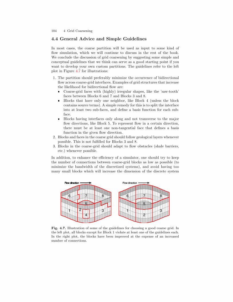
104 4 Grid Coarsening
4.4 General Advice and Simple Guidelines
In most cases, the coarse partition will be used as input to some kind offlow simulation, which we will continue to discuss in the rest of the book.We conclude the discussion of grid coarsening by suggesting some simple andconceptual guidelines that we think can serve as a good starting point if youwant to develop your own custom partitions. The guidelines refer to the leftplot in Figure 4.7 for illustrations:
1. The partition should preferably minimize the occurrence of bidirectionalflow across coarse-grid interfaces. Examples of grid structures that increasethe likelihood for bidirectional flow are: Coarse-grid faces with (highly) irregular shapes, like the ’saw-tooth’
faces between Blocks 6 and 7 and Blocks 3 and 8. Blocks that have only one neighbor, like Block 4 (unless the block
contains source terms). A simple remedy for this is to split the interfaceinto at least two sub-faces, and define a basis function for each sub-face.
Blocks having interfaces only along and not transverse to the majorflow directions, like Block 5. To represent flow in a certain direction,there must be at least one non-tangential face that defines a basisfunction in the given flow direction.
2. Blocks and faces in the coarse grid should follow geological layers wheneverpossible. This is not fulfilled for Blocks 3 and 8.
3. Blocks in the coarse-grid should adapt to flow obstacles (shale barriers,etc.) whenever possible.
In addition, to enhance the efficiency of a simulator, one should try to keepthe number of connections between coarse-grid blocks as low as possible (tominimize the bandwidth of the discretized systems), and avoid having toomany small blocks which will increase the dimension of the discrete system
1 2 34
5
6 7 8
Flow direction Flow direction Flow direction Flow direction Flow direction Flow direction
1 32
5
6 7 8
Flow direction Flow direction
Fig. 4.7. Illustration of some of the guidelines for choosing a good coarse grid. Inthe left plot, all blocks except for Block 1 violate at least one of the guidelines each.In the right plot, the blocks have been improved at the expense of an increasednumber of connections.
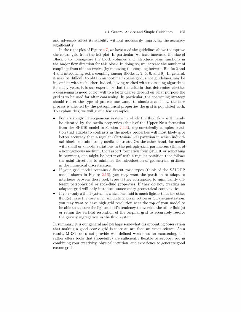
4.4 General Advice and Simple Guidelines 105
and adversely affect its stability without necessarily improving the accuracysignificantly.
In the right plot of Figure 4.7, we have used the guidelines above to improvethe coarse grid from the left plot. In particular, we have increased the size ofBlock 5 to homogenise the block volumes and introduce basis functions inthe major flow direction for this block. In doing so, we increase the number ofcouplings from nine to twelve (by removing the coupling between Blocks 2 and4 and introducing extra coupling among Blocks 1, 3, 5, 6, and 8). In general,it may be difficult to obtain an ’optimal’ coarse grid, since guidelines may bein conflict with each other. Indeed, having worked with coarsening algorithmsfor many years, it is our experience that the criteria that determine whethera coarsening is good or not will to a large degree depend on what purpose thegrid is to be used for after coarsening. In particular, the coarsening strategyshould reflect the type of process one wants to simulate and how the flowprocess is affected by the petrophysical properties the grid is populated with.To explain this, we will give a few examples:
For a strongly heterogeneous system in which the fluid flow will mainlybe dictated by the media properties (think of the Upper Ness formationfrom the SPE10 model in Section 2.4.3), a geometrically complex parti-tion that adapts to contrasts in the media properties will most likely givebetter accuracy than a regular (Cartesian-like) partition in which individ-ual blocks contain strong media contrasts. On the other hand, for mediawith small or smooth variations in the petrophysical parameters (think ofa homogeneous medium, the Tarbert formation from SPE10, or somethingin between), one might be better off with a regular partition that followsthe axial directions to minimize the introduction of geometrical artifactsin the numerical discretization.
If your grid model contains different rock types (think of the SAIGUPmodel shown in Figure 2.16), you may want the partition to adapt tointerfaces between these rock types if they correspond to significantly dif-ferent petrophysical or rock-fluid properties. If they do not, creating anadapted grid will only introduce unnecessary geometrical complexities.
If you study a fluid system in which one fluid is much lighter than the otherfluid(s), as is the case when simulating gas injection or CO2 sequestration,you may want to have high grid resolution near the top of your model tobe able to capture the lighter fluid’s tendency to override the other fluid(s)or retain the vertical resolution of the original grid to accurately resolvethe gravity segregation in the fluid system.
In summary, it is our general and perhaps somewhat disappointing observationthat making a good coarse grid is more an art than an exact science. As aresult, MRST does not provide well-defined workflows for coarsening, butrather offers tools that (hopefully) are sufficiently flexible to support you incombining your creativity, physical intuition, and experience to generate goodcoarse grids.


Part II
Single-Phase Flow

5
Mathematical Models and Basic Discretizations
If you have read the chapters of the book in chronological order, you havealready encountered the equations modeling flow of a single, incompressiblefluid through a porous media twice: first in Section 1.3 where we showed howto use MRST to compute vertical equilibrium inside a gravity column, andthen in Section 2.3.2, in which we discussed the concept of rock permeabil-ity. In this section, we will review the mathematical modeling of single-phaseflow in more detail, introduce basic numerical methods for solving the result-ing equations, and discuss how these are implemented in MRST and can becombined with the tools introduced in Chapters 2 and 3 to develop efficientsimulators for single-phase incompressible flow. Solvers for compressible flowwill be discussed in more detail in Chapter 7.
5.1 Fundamental concept: Darcy’s law
Mathematical modeling of single-phase flow in porous media started with thework of Henry Darcy, a french hydraulic engineer, who in the middle of the19th century was engaged by to enlarge and modernize the waterworks of thecity of Dijon. To understand the physics of flow through the sand filters thatwere used to clean the water supply, Darcy designed a vertical experimentaltank filled with sand, in which water was injected at the top and allowed toflow out at the bottom of the tank; Figure 5.1 shows a conceptual illustration.Once the sand pack is filled with water, and the inflow and outflow ratesare equal, the hydraulic head at the inlet and at the outlet can be measuredusing mercury-filled manometers. The hydraulic head is given as, h = E/mg =z+p/ρg, relative to a fixed datum. As water flows through the porous medium,it will experience a loss of energy. In a series of experiments, Darcy measuredthe water volumetric flow rate out of the tank and compared this rate withthe loss of hydrostatic head from top to bottom of the column. From theexperiments, he established that for the same sand pack, the discharge (flowrate) Q [m3/s] is proportional to the cross-sectional area A [m2], proportional
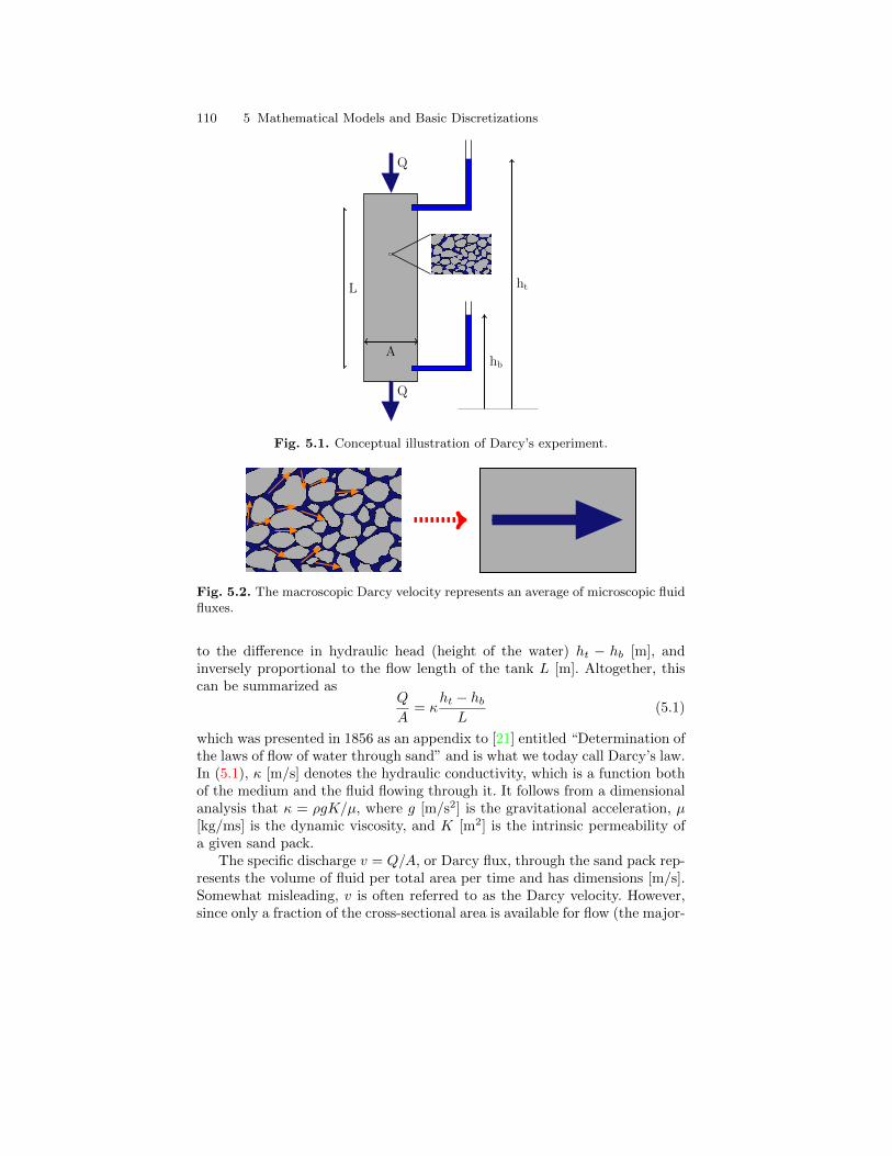
110 5 Mathematical Models and Basic Discretizations
Q
Q
A
L
hb
ht
Fig. 5.1. Conceptual illustration of Darcy’s experiment.
Fig. 5.2. The macroscopic Darcy velocity represents an average of microscopic fluidfluxes.
to the difference in hydraulic head (height of the water) ht − hb [m], andinversely proportional to the flow length of the tank L [m]. Altogether, thiscan be summarized as
Q
A= κ
ht − hbL
(5.1)
which was presented in 1856 as an appendix to [21] entitled “Determination ofthe laws of flow of water through sand” and is what we today call Darcy’s law.In (5.1), κ [m/s] denotes the hydraulic conductivity, which is a function bothof the medium and the fluid flowing through it. It follows from a dimensionalanalysis that κ = ρgK/µ, where g [m/s2] is the gravitational acceleration, µ[kg/ms] is the dynamic viscosity, and K [m2] is the intrinsic permeability ofa given sand pack.
The specific discharge v = Q/A, or Darcy flux, through the sand pack rep-resents the volume of fluid per total area per time and has dimensions [m/s].Somewhat misleading, v is often referred to as the Darcy velocity. However,since only a fraction of the cross-sectional area is available for flow (the major-
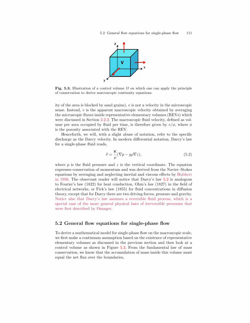
5.2 General flow equations for single-phase flow 111
Fig. 5.3. Illustration of a control volume Ω on which one can apply the principleof conservation to derive macroscopic continuity equations.
ity of the area is blocked by sand grains), v is not a velocity in the microscopicsense. Instead, v is the apparent macroscopic velocity obtained by averagingthe microscopic fluxes inside representative elementary volumes (REVs) whichwere discussed in Section 2.2.2. The macroscopic fluid velocity, defined as vol-ume per area occupied by fluid per time, is therefore given by v/φ, where φis the porosity associated with the REV.
Henceforth, we will, with a slight abuse of notation, refer to the specificdischarge as the Darcy velocity. In modern differential notation, Darcy’s lawfor a single-phase fluid reads,
~v =K
µ(∇p− gρ∇z), (5.2)
where p is the fluid pressure and z is the vertical coordinate. The equationexpresses conservation of momentum and was derived from the Navier–Stokesequations by averaging and neglecting inertial and viscous effects by Hubbertin 1956. The observant reader will notice that Darcy’s law 5.2 is analogousto Fourier’s law (1822) for heat conduction, Ohm’s law (1827) in the field ofelectrical networks, or Fick’s law (1855) for fluid concentrations in diffusiontheory, except that for Darcy there are two driving forces, pressure and gravity.Notice also that Darcy’s law assumes a reversible fluid process, which is aspecial case of the more general physical laws of irreversible processes thatwere first described by Onsager.
5.2 General flow equations for single-phase flow
To derive a mathematical model for single-phase flow on the macroscopic scale,we first make a continuum assumption based on the existence of representativeelementary volumes as discussed in the previous section and then look at acontrol volume as shown in Figure 5.3. From the fundamental law of massconservation, we know that the accumulation of mass inside this volume mustequal the net flux over the boundaries,
112 5 Mathematical Models and Basic Discretizations
∂
∂t
∫Ω
φρ d~x+
∫∂Ω
ρ~v · ~n ds =
∫Ω
q d~x, (5.3)
where ρ is the density of the fluid, φ is the rock porosity, ~v is the macroscopicDarcy velocity, ~n denotes the normal at the boundary ∂Ω of the computa-tional domain Ω, and q denotes fluid sources and sinks, i.e., outflow and inflowof fluids per volume at certain locations. Applying Gauss’ theorem, this con-servation law can be written on the alternative integral form∫
Ω
[ ∂∂tφρ+∇ · (ρ~v)
]d~x =
∫Ω
q d~x. (5.4)
This equation is valid for any volume Ω, and in particular volumes that areinfinitesimally small, and hence it follows that the macroscopic behavior ofthe single-phase fluid must satisfy the continuity equation
∂(φρ)
∂t+∇ · (ρ~v) = q. (5.5)
Equation (5.5) contains more unknowns than equations and to derive a closedmathematical model, we need to introduce what is commonly referred to asconstitutive equations that give the relationship between different states ofthe system (pressure, volume, temperature, etc) at given physical conditions.Darcy’s law, discussed in the previous section, is an example of a constitutiverelation that has been derived to provide a phenomenological relationship be-tween the macroscale ~v and the fluid pressure p. In Section 2.3.1 we introducedthe rock compressibility cr = d ln(φ)/dp, which describes the relationship be-tween the porosity φ and the pressure p. In a similar way, we can introducethe fluid compressibility to relate the density ρ to the fluid pressure p.
A change in density will generally cause a change in both the pressure pand the temperature T . The usual way of describing these changes in ther-modynamics is to consider the change of volume V for a fixed number ofparticles,
dV
V=
1
V
(∂V
∂p
)T
dp+1
V
(∂V
∂T
)p
dT, (5.6)
where the subscripts T and p indicate that the change takes place underconstant temperature and pressure, respectively. Since ρV is constant for afixed number of particles, dρV = ρdV , and (5.6) can written in the equivalentform
dρ
ρ=
1
ρ
(∂ρ
∂p
)T
dp+1
ρ
(∂ρ
∂T
)p
dT = cfdp+ αfdT, (5.7)
where the cf denotes the isothermal compressibility and αf denotes the ther-mal expansion coefficient. In many subsurface systems, the density changesslowly so that heat conduction keeps the temperature constant, in which case(5.7) simplifies to
cf =1
ρ
dρ
dp=d ln(ρ)
dp. (5.8)
5.2 General flow equations for single-phase flow 113
The factor cf , which we henceforth will refer to as the fluid compressibility,is non-negative and will generally depend on both pressure and temperature,i.e., cf = cf (p, T ).
Introducing Darcy’s law and fluid and rock compressibilities in (5.5), weobtain the following parabolic equation for the fluid pressure
ctφρ∂p
∂t−∇ ·
[ρKµ
(∇p− gρ∇z)]
= q, (5.9)
where ct = cr + cf denotes the total compressibility. Notice that this equationis generally nonlinear since both ρ and ct may depend on p. In the following,we will look briefly at several special cases in which the governing single-phase equation becomes a linear equation for the primary unknown; moreextensive discussions can be found in standard textbooks like [50, Chap. 1],[18, Chap. 2]. For completeness, we will also briefly review the concept of anequation-of-state.
Incompressible flow
In the special case of an incompressible rock and fluid (that is, ρ and φ areindependent of p so that ct = 0), (5.9) simplifies to an elliptic equation withvariable coefficients,
∇ ·[ρKµ∇(p− gρz)
]= q. (5.10)
If we introduce the fluid potential, Φ = p − gρz, (5.10) can be recognized asthe (generalized) Poisson’s equation ∇ · K∇Φ = q or as the Laplace equation∇ · K∇Φ = 0 if there are no volumetric fluid sources or sinks. In the nextsection, we will discuss in detail how to discretize the second-order spatialLaplace operator L = ∇ · K∇, which is a key technological component thatwill enter almost any software for simulation of flow in porous rock formations.
Constant compressibility
If the fluid compressibility is constant and independent of pressure, (5.8) canbe integrated from a known density ρ0 at a pressure datum p0 to give thefollowing equation,
ρ(p) = ρ0ecf (p−p0) (5.11)
which applies well to most liquids that do not contain large quantities ofdissolved gas. To develop the differential equation, we first assume that theporosity and the fluid viscosity do not depend on pressure. Going back to thedefinition of fluid compressibility (5.8), it also follows from this equation that∇p = (cfρ)−1∇ρ, which we can use to eliminate ∇p from Darcy’s law (5.2).Inserting the result into (5.5) gives us the following continuity equation
∂ρ
∂t− 1
µφcf∇ ·(K∇ρ− cgρ2K∇z
)= q, (5.12)
114 5 Mathematical Models and Basic Discretizations
which in the absence of gravity forces and source terms is a linear equationfor the fluid density that is similar to the classical heat equation with variablecoefficients,
∂ρ
∂t=
1
µφcf∇ ·(K∇ρ
). (5.13)
Slightly compressible flow
In the case that the fluid compressibility is small, it is sufficient to use a linearrelationship
ρ = ρ0
[1 + cf (p− p0)
]. (5.14)
We further assume that φ is a function of ~x only and that µ is constant. Forsimplicity, we also assume that g and q are both zero. Then, we can simplify(5.9) as follows:
(cfφρ)∂p
∂t=cfρ
µ∇p · K∇p+
ρ
µ∇ · (K∇p)
If cf is sufficiently small, in the sense that cf∇p · K∇p ∇ · (K∇p), we canneglect the first term on the right-hand side to derive a linear equation similarto (5.13) for the fluid pressure
∂p
∂t=
1
µφcf∇ ·(K∇p
). (5.15)
Ideal gas
If the fluid is a gas, compressibility can be derived from the gas law, whichfor an ideal gas can be written in two alternative forms,
pV = nRT, ρ = p(γ − 1)e. (5.16)
In the first form, T is temperature, V is volume, R is the gas constant (8.314J K−1mol−1), and n = m/M is the amount of substance of the gas in moles,where m is the mass and M is the molecular weight. In the second form, γis the adiabatic constant, i.e., ratio of specific heats at constant pressure andconstant volume, and e is the specific internal energy (internal energy per unitmass). In either case, it follows from (5.8) that cf = 1/p.
If the fluid is a gas, we can neglect gravity, and once again we assume thatφ is a function of ~x only. Inserting (5.16) into (5.9) gives
∂(ρφ)
∂t= φ(γ − 1)e
∂p
∂t=
1
µ∇ ·(ρK∇p
)=
(γ − 1)e
µ∇ ·(pK∇p
)from which it follows that
φµ∂p
∂t= ∇ ·
(pK∇p
)⇔ φµ
p
∂p2
∂t= ∇ ·
(K∇p2
). (5.17)
5.3 Auxiliary conditions and equations 115
Equation of state
Equations (5.11), (5.14), and (5.16) are all examples of what is commonlyreferred to as equations of state, which provide constitutive relationships be-tween mass, pressures, temperature, and volumes at thermodynamic equilib-rium. Another popular form of these equations are the so-called cubic equa-tions of state, which can be written as cubic functions of the molar volumeVm = V/n = M/ρ involving constants that depend on the pressure pc, thetemperature Tc, and the molar volume Vc at the critical point, i.e., the point at
which ( ∂p∂V )T = ( ∂2p
∂V 2 )T ≡ 0. A few particular examples include the Redlich–Kwong–Soave equation of state
p =RT
Vm − b− aα√
T Vm(Vm + b),
a =0.427R2T 2
c
pc, b =
0.08664RTcpc
α =[1 +
(0.48508 + 1.55171ω − 0.15613ω2
)(1−
√T/Tc)
]2(5.18)
and the Peng–Robinson equation of state,
p =RT
Vm − b− aα
V 2m + 2bVm − b2)
,
a =0.4527235R2T 2
c
pc, b =
0.077796RTcpc
α =[1 +
(0.37464 + 1.54226ω − 0.26992ω2
)(1−
√T/Tc)
]2(5.19)
In both equations, ω denotes the acentric factor of the species, which is ameasure of the centricity (deviation from spherical form) of the molecules inthe fluid. The Peng–Robinson model is much better at predicting the densitiesof liquids than the Redlich–Kwong–Soave model, which was developed to fitpressure data of hydrocarbon vapor phases. If we introduce
A =aαp
(RT )2, B =
bp
RT, Z =
pV
RT,
the Redlich–Kwong–Soave equation (5.18) and the Peng–Robinson equation(5.19) can be written in alternative polynomial forms,
0 = Z3 − Z2 + Z(A−B −B2)−AB, (5.20)
0 = Z3 − (1−B)Z2 + (A− 2B − 3B2)Z − (AB −B2 −B3), (5.21)
which explain the why they are called cubic equations of state.
5.3 Auxiliary conditions and equations
The governing equations for single-phase flow discussed above are all parabolicequations, except for the incompressible case in which the governing equation
116 5 Mathematical Models and Basic Discretizations
is elliptic. For the solution to be well-posed1 inside a finite domain for any ofthe equations, one needs to supply boundary conditions that determine thebehavior on the external boundary. For the parabolic equations describingunsteady flow, one also needs to impose an initial condition that determinesthe initial state of the fluid system. In this section, we will discuss theseconditions in more detail. We will also discuss models for representing flow inand out of the reservoir rock through wellbores. Because this flow typicallytakes place on a length scale that is much smaller than the length scales ofthe global flow inside the reservoir, it is customary to model it using specialanalytical models. Finally, we also discuss a set of auxiliary equations fordescribing the movement of fluid elements and/or neutral particles that followthe single-phase flow without affecting it.
5.3.1 Boundary and initial conditions
In reservoir simulation one is often interested in describing closed flow systemsthat have no fluid flow across its external boundaries. This is a natural assump-tion when studying full reservoirs that have trapped and contained petroleumfluids for million of years. Mathematically, no-flow conditions across externalboundaries are modeled by specifying homogeneous Neumann conditions,
~v · ~n = 0 for ~x ∈ ∂Ω. (5.22)
With no-flow boundary conditions, any pressure solution of (5.10) is imma-terial and only defined up to an additive constant, unless a datum value isprescribed at some internal point or along the boundary.
It is also common that parts of the reservoir may be in communicationwith a larger aquifer system that provide external pressure support, whichcan be modeled in terms of a Dirichlet condition of the form
p(~x) = pa(~x, t) for ~x ∈ Γa ⊂ ∂Ω. (5.23)
The function pa can, for instance, be given as a hydrostatic condition. Alter-natively, parts of the boundary may have a certain prescribed influx, whichcan be modeled in terms of an inhomogeneous Neumann condition,
~v · ~n = ua(~x, t) for ~x ∈ Γa ⊂ ∂Ω. (5.24)
Combinations of these conditions are used when studying parts of a reservoir(e.g., a sector models). There are also cases, e.g., when describing ground-water systems or CO2 sequestration in saline aquifers, where (parts of) theboundaries are open or the system contains a background flow. More infor-mation of how to set boundary conditions will be given in Section 6.1.4. In
1 A solution is well-posed if it exists, is unique, and depends continuously on theinitial and boundary conditions.
5.3 Auxiliary conditions and equations 117
the compressible case in (5.9), we also need to specify an initial pressure dis-tribution. Typically, this pressure distribution will be hydrostatic, as in thegravity column we discussed briefly in Section 1.3, and hence be given by theordinary differential equation,
dp
dz= ρg, p(z0) = p0. (5.25)
5.3.2 Models for injection and production wells
In a typical reservoir simulator, the inflow and outflow in wells occur on asubgrid scale. Therefore, special models have to be developed to model thisparticular flow. Normally, fluids are injected in a grid block at either con-stant surface rate or at constant bottom-hole pressure, which is sometimesalso called wellbore flowing pressure. Similarly, fluids are produced at con-stant bottom-hole pressure or constant surface liquid rate. The expressioninflow performance relation (IPR) denotes the relation between the bottom-hole pressure and the surface flow rate.
The simplest and most widely used inflow-performance relation is the lin-ear law
qo = J(pR − pbh), (5.26)
which states that the flow rate is directly proportional to the pressure draw-down in the well; that is, flow rate is proportional to the difference betweenthe average reservoir pressure pR in the grid cell and the bottom-hole pressurepbh in the well. The constant of proportionality J is called the productivityindex (PI) for production wells or the well injectivity index (WI) for injectorsand accounts for all rock and fluid properties, as well as geometric factorsthat affect the flow. In MRST, we do not distinguish between productivityand injectivity indices, and henceforth we will only use the shorthand ’WI’.
The basic linear relation (5.26) can be derived from Darcy’s law. Consider avertical well that drains a rock with uniform permeability K. As an equationof state, we introduce the formation volume factor B defined as the ratiobetween the volume of the fluid at reservoir conditions and the volume ofthe fluid at surface conditions. (For incompressible flow, B ≡ 1). The wellpenetrates the rock completely a height h and is open in the radial direction.We assume a pseudo-steady, radial flow that can be described by Darcy’s law
v =qB
2πrh=K
µ
dp
dr.
We now integrate this equation from the wellbore and to the drainage bound-ary r = re where the pressure is constant
2πKh
∫ pe
pbh
1
qµBdp =
∫ re
rw
1
rdr.
118 5 Mathematical Models and Basic Discretizations
Here, B and µ are pressure-dependent quantities; B decreases with pressureand µ increases. The composite effect is that (µB)−1 decreases (almost) lin-early with pressure. We can therefore approximate µB by (µB)avg evaluatedat the average pressure pavg = (pbh + pe)/2. For convenience, we drop thesubscript in the following. This gives us the pressure as a function of radialdistance
pe = pbh +qµB
2πKhln(re/rw). (5.27)
To close the system, we need to know the location of the drainage boundaryr = re where the pressure is constant. This is often hard to know, and it iscustomary to relate q to the volumetric average pressure instead. For pseudo-steady flow the volumetric average pressure occurs at r = 0.472re. Hence,
q =2πKh
µB(ln(re/rw)− 0.75
)(pR − pbh). (5.28)
The above relation (5.28) was developed for an ideal well under several simpli-fied assumptions: homogeneous and isotropic formation of constant thickness,clean wellbore, etc. In practice, a well will rarely produce under these idealconditions. Typically the permeability is altered close to the wellbore underdrilling and completion, the well will only be partially completed, and so on.The actual pressure performance will therefore deviate from (5.28). To modelthis, it is customary to include a skin factor S to account for extra pressureloss due to alterations in the inflow zone. The resulting equation is
q =2πKh
µB(ln(re/rw)− 0.75 + S
)(pR − pbh). (5.29)
Often the constant −0.75 is included in the skin factor S, and for stimulatedwells the skin factor could be negative. Sometimes h is modified to ch, wherec is the completion factor, i.e., a dimensionless number between zero and onedescribing the fraction of the wellbore open to flow.
To use the radial model in conjunction with a reservoir model, the volumet-ric average pressure in the radial model must be related to the computed cellaverage pressure. This was first done by Peaceman [51]. Assuming isotropicpermeabilities, square grid blocks, single phase flow and a well at a center ofan interior block, Peaceman showed that the equivalent radius is
re ≈ 0.2√∆x∆y.
This basic model has later been extended to cover a lot of other cases, e.g., off-center wells, multiple wells, non-square grids, anisotropic permeability, hor-izontal wells; see for instance [9, 29, 5]. For anisotropic permeabilities–andhorizontal wells–the equivalent radius is defined as [49]
re = 0.28
(√Ky/Kx∆x
2 +√Kx/Ky∆y
2)1/2
(Ky/Kx
)1/4+(Kx/Ky
)1/4 , (5.30)
5.3 Auxiliary conditions and equations 119
and the permeability is replaced by an effective permeability
Ke =√KxKy. (5.31)
If we include gravity forces in the well and assume hydrostatic equilibrium,the well model thus reads
qi =2πhcKe
ln(re/rw) + S
1
µiBi
(pR − pbh − ρi(z − zbh)g
), (5.32)
where Ke is given by (5.31) and re is given by (5.30). For deviated wells, hdenotes the length of the grid block in the major direction of the wellbore andnot the length of the wellbore.
5.3.3 Field lines and time-of-flight
Equation (5.10) together with a set of suitable and compatible boundary con-ditions is all that one needs to describe the flow of an incompressible fluidinside an incompressible rock. In the remains of this section, we will discussa few simple concepts and auxiliary equations that have proven useful to vi-sualize, analyze, and understand flow fields.
A simple way to visualize a flow field is to use field lines resulting from thevector field: streamlines, streaklines, and pathlines. In steady flow, the threeare identical. However, if the flow is not steady, i.e., when ~v changes withtime, they differ. Streamlines are associated with an instant snapshot of theflow field and consists of a family of curves that are everywhere tangential to~v and show the direction a fluid element will travel at this specific point intime. That is, if ~x(r) is a parametric representation of a single streamline atthis instance t in time, then
d~x
dr× ~v(~x, t) = 0, or equivalently,
d~x
dr=
~v(t)
|~v(t)|. (5.33)
In other words, streamlines are calculated instantaneously throughout thefluid from an instantaneous snapshot of the flow field. Because two streamlinesfrom the same instance in time cannot cross, there cannot be flow across it,and if we align a coordinate along a bundle of streamlines, the flow throughthem will be one-dimensional.
Pathlines are the trajectories that individual fluid elements will follow overa certain period. In each moment of time, the path a fluid particle takes will bedetermined by the streamlines associated with the streamlines at this instancein time. If ~y(t) represents a single path line starting at ~y0 at time t0, then
d~y
dt= ~v(~y, t), ~y(t0) = ~y0. (5.34)
A streakline is the line traced out by all fluid particles that have passedthrough a prescribed point throughout a certain period of time. (Think of dye
120 5 Mathematical Models and Basic Discretizations
injected into the fluid at a specific point). If we ~z(t, s) denote a parametrizationof a streakline and ~z0 the specific point through which all fluid particles havepassed, then
d~z
dt= ~v(~z, t), ~z(s) = ~z0. (5.35)
Like streamlines, two streaklines cannot intersect each other.In summary: streamline patterns change over time, but are easy to generate
mathematically. Pathlines and streaklines are recordings of the passage of timeand are obtained through experiments.
Within reservoir simulation streamlines are far more used that pathlinesand streaklines. Moreover, rather than using the arc length r to parametrizestreamlines, it is common to introduce an alternative parametrization calledtime-of-flight, which takes into account the reduced volume available for flow,i.e., the porosity φ. Time-of-flight is defined by the following integral
τ(r) =
∫ r
0
φ(~x(s))
|~v(~x(s))|ds, (5.36)
where τ expresses the time it takes a fluid particle to travel a distance ralong a streamline (in the interstitial velocity field ~v/φ). Alternatively, by thefundamental theorem of calculus and the directional derivative,
dτ
dr=
φ
|~v|=
~v
|~v|· ∇τ,
from which it follows that τ can be expressed by the following differentialequation [22, 23]
~v · ∇τ = φ. (5.37)
In lack of a better name, we will refer to this as the time-of-flight equation.
5.3.4 Tracers and volume partitions
Somewhat simplified, tracers can be considered as neutral particles that pas-sively flow with the fluid without altering its flow properties. The concentra-tion of a tracer is given by a continuity equation on the same form as (5.5),
∂(φC)
∂t+∇ ·
(~vC)
= qC . (5.38)
Communication patterns within a reservoir can be determined by simulatingthe evolution of artificial, neutral tracers. A simple flow diagnostics is to setthe tracer concentration equal to one in a particular fluid source or at a certainpart of the inflow boundary, and compute the concentration approached atsteady-state conditions,
∇ ·(~vC)
= qC , C|inflow = 1. (5.39)
5.4 Basic finite-volume discretizations 121
The resulting tracer distribution gives the portion of the total fluid volumecoming from a certain fluid source, or parts of the inflow boundary, thateventually will reach each point in the reservoir. Likewise, by reversing thesign of the flow field and assigning unit tracers to a particular fluid sink orparts of the outflow, one can compute the portion of the fluid arriving at asource or outflow boundary that can be attributed to a certain point in thereservoir. By repeating this process for all parts of the inflow, one can easilyobtain a partition of the instantaneous flow field.
A more dynamic view can be obtained by utilizing the fact that streamlinesand time-of-flight can be used to define an alternative curvilinear and flow-based coordinate system in three dimensions. To this end, we introduce thebi-streamfunctions ψ and χ [10], for which ~v = ∇ψ × ∇χ. In the streamlinecoordinates (τ, ψ, χ), the gradient operator is expressed as
∇(τ,ψ,χ) = (∇τ)∂
∂τ+ (∇ψ)
∂
∂ψ+ (∇χ)
∂
∂χ. (5.40)
Moreover, a streamline Ψ is defined by the intersection of a constant valuefor ψ and a constant value for χ. Because ~v is orthogonal to ∇ψ and ∇χ, itfollows from (5.37) that
~v · ∇(τ,ψ,χ) = (~v · ∇τ)∂
∂τ= φ
∂
∂τ. (5.41)
Therefore, the coordinate transformation (x, y, z) → (τ, ψ, χ) will reduce thethree-dimensional transport equation (5.38) to a family of one-dimensionaltransport equations along each streamline [22, 35], which for incompressibleflow reads
∂C
∂t+∂C
∂τ= 0. (5.42)
In other words, there is no exchange of the quantity C between streamlinesand each streamline can be viewed as an isolated flow system. Assuming aprescribed concentration history C0(t) at the inflow, gives a time-dependentboundary-value problem for the concentration at the outflow (5.42). Here, theresponse is given as [22],
C(t) = C0(t− τ), (5.43)
which is easily verified by inserting the expression into (5.42) and the fact thatthe solution is unique [33]. For the special case of continuous and constantinjection, the solution is particularly simple
C(t) =
0, t < τ,
C0, t > τ.
5.4 Basic finite-volume discretizations
Research on numerical solution of the Laplace/Poisson equation has a longtradition, and there exist a large number of different finite-difference and
122 5 Mathematical Models and Basic Discretizations
finite-volume methods, as well as finite-element methods based on standardGalerkin, mixed, or discontinuous Galerkin formulations, which all have theirmerits. In Chapter 8, we will discuss consistent discretizations of Poisson-typeequations in more detail. We introduce a general framework for formulatingsuch method on general polyhedral grids and present several recent methodsthat are specially suited for irregular grids with strongly discontinuous coef-ficients, which are typically seen in realistic reservoir simulation models. Inparticular, we will discuss multipoint flux-approximation (MPFA) methodsand mimetic finite-difference (MFD) methods, which are both available inadd-on modules that are part of the standard MRST releases. As a startingpoint, however, we will in rest of this section present the simplest exampleof a finite-volume discretization, the two-point flux-approximation (TPFA)scheme, which is used extensively throughout industry and also is the defaultdiscretization method in MRST. We will give a detailed derivation of themethod and point out its advantages and shortcomings. For completeness,we also briefly outline how to discretize the time-of-flight and the stationarytracer equations.
5.4.1 A two-point flux-approximation (TPFA) method
To keep technical details at a minimum, we will in the following without lossof generality consider the simplified single-phase flow equation
∇ · ~v = q, ~v = −K∇p, in Ω ⊂ Rd. (5.44)
In classical finite-difference methods, partial differential equations are approx-imated by replacing the derivatives with appropriate divided differences be-tween point-values on a discrete set of points in the domain. Finite-volumemethods, on the other hand, have a more physical motivation and are de-rived from conservation of (physical) quantities over cell volumes. Thus, ina finite-volume method the unknown functions are represented in terms ofaverage values over a set of finite-volumes, over which the integrated PDEmodel is required to hold in an averaged sense. Although finite-difference andfinite-volume methods have fundamentally different interpretation and deriva-tion, the names are used interchangeably in the scientific literature. The mainreason for this is probably that for certain low-order methods, the discreteequations derived for the cell-centered values in a mass-conservative finite-difference method are identical to the discrete equations for the cell averagesin the corresponding finite-volume method. Herein, we will stick to this con-vention and not make a strict distinction between the two types of methods
To develop a finite-volume discretization for (5.44), we start by rewritingthe equation in integral form (see (5.3)) using a single cell Ωi in the discretegrid as control volume ∫
∂Ωi
~v · ~n ds =
∫Ωi
q d~x (5.45)
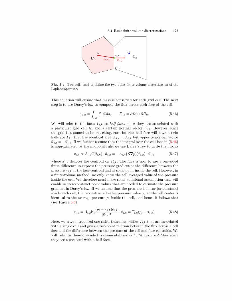
5.4 Basic finite-volume discretizations 123
pi
Ωi
Γi,k
pk
Ωk~ni,k
~ci,k
πi,k
Fig. 5.4. Two cells used to define the two-point finite-volume discretization of theLaplace operator.
This equation will ensure that mass is conserved for each grid cell. The nextstep is to use Darcy’s law to compute the flux across each face of the cell,
vi,k =
∫Γik
~v · ~n ds, Γi,k = ∂Ωi ∩ ∂Ωk. (5.46)
We will refer to the faces Γi,k as half-faces since they are associated witha particular grid cell Ωi and a certain normal vector ~ni,k. However, sincethe grid is assumed to be matching, each interior half face will have a twinhalf-face Γk,i that has identical area Ak,i = Ai,k but opposite normal vector~nk,i = −~ni,k. If we further assume that the integral over the cell face in (5.46)is approximated by the midpoint rule, we use Darcy’s law to write the flux as
vi,k ≈ Ai,k~v(~xi,k) · ~ni,k = −Ai,k(K∇p)(~xi,k) · ~ni,k, (5.47)
where ~xi,k denotes the centroid on Γi,k. The idea is now to use a one-sidedfinite difference to express the pressure gradient as the difference between thepressure πi,k at the face centroid and at some point inside the cell. However, ina finite-volume method, we only know the cell averaged value of the pressureinside the cell. We therefore must make some additional assumption that willenable us to reconstruct point values that are needed to estimate the pressuregradient in Darcy’s law. If we assume that the pressure is linear (or constant)inside each cell, the reconstructed value pressure value πi at the cell center isidentical to the average pressure pi inside the cell, and hence it follows that(see Figure 5.4)
vi,k = Ai,kKi(pi − πi,k)~ci,k|~ci,k|2
· ~ni,k = Ti,k(pi − πi,k). (5.48)
Here, we have introduced one-sided transmissibilities Ti,k that are associatedwith a single cell and gives a two-point relation between the flux across a cellface and the difference between the pressure at the cell and face centroids. Wewill refer to these one-sided transmissibilities as half-transmissibilities sincethey are associated with a half face.
124 5 Mathematical Models and Basic Discretizations
To derive the final discretization, we impose continuity of fluxes across allfaces, vi,k = −vk,i = vik and continuity of face pressures πi,k = πk,i = πik.This gives us two equations,
T−1i,k vik = pi − πik, −T−1
k,i vik = pk − πik.
By eliminating the interface pressure πik, we end up with the following two-point flux-approximation (TPFA) scheme,
vik =[T−1i,k + T−1
k,i
]−1(pi − pk) = Tik(pi − pk). (5.49)
where is the Tik the transmissibility associated with the connection betweenthe two cells. As the name suggests, the TPFA scheme uses two ’points’,the cell averages pi and pk, to approximate the flux across the interface Γikbetween the cells Ωi and Ωk. In the derivation above, the cell fluxes wereparametrized in terms of the index of the neighboring cell. Extending thederivation to also include fluxes on exterior faces is trivial since we eitherknow the flux explicitly for Neumann boundary conditions (5.22) or (5.24),or know the interface pressure for Dirichlet boundary conditions (5.23).
By inserting the expression for vik into (5.45), we see that the TPFAscheme for (5.44), in compact form, seeks a set of cell averages that satisfythe following system of equations∑
k
Tik(pi − pk) = qi, ∀Ωi ⊂ Ω (5.50)
This system is clearly symmetric, and a solution is, as for the continuousproblem, defined up to an arbitrary constant. The system is made positivedefinite, and symmetry is preserved by specifying the pressure in a singlepoint. In MRST, we have chosen to set p1 = 0 by adding a positive constantto the first diagonal of the matrix A = [aij ], where:
aij =
∑k Tik if j = i,
−Tij if j 6= i,
The matrix A is sparse and will have a banded structure for structured grids(tridiagonal for 1D grids and penta- and heptadiagonal for logically Cartesiangrids in 2D and 3D, respectively). The TPFA scheme is monotone, robust,and relatively simple to implement, and is currently the industry standardwith reservoir simulation.
Example 5.1. To tie the links with standard finite-difference methods onCartesian grids, we will derive the two-point discretization for a 2D Cartesiangrid with isotropic permeability. Consider the flux in the x-direction betweentwo cells i and k as illustrated in Figure 5.5. As above, we impose mass con-servation inside each cell. For cell i this reads:
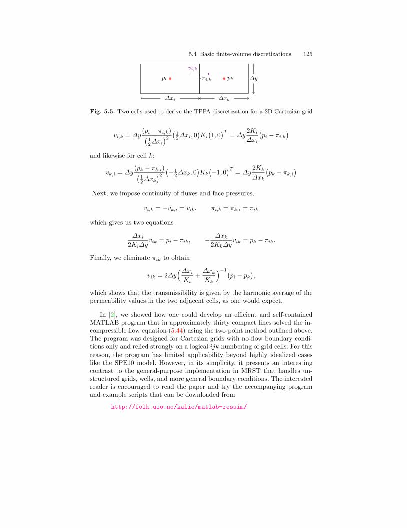
5.4 Basic finite-volume discretizations 125
vi,k
∆xi ∆xk
∆ypi pkπi,k
Fig. 5.5. Two cells used to derive the TPFA discretization for a 2D Cartesian grid
vi,k = ∆y(pi − πi,k)(
12∆xi
)2 ( 12∆xi, 0
)Ki
(1, 0)T
= ∆y2Ki
∆xi
(pi − πi,k
)and likewise for cell k:
vk,i = ∆y(pk − πk,i)(
12∆xk
)2 (− 12∆xk, 0
)Kk
(−1, 0
)T= ∆y
2Kk
∆xk
(pk − πk,i
)Next, we impose continuity of fluxes and face pressures,
vi,k = −vk,i = vik, πi,k = πk,i = πik
which gives us two equations
∆xi2Ki∆y
vik = pi − πik, − ∆xk2Kk∆y
vik = pk − πik.
Finally, we eliminate πik to obtain
vik = 2∆y(∆xiKi
+∆xkKk
)−1(pi − pk
),
which shows that the transmissibility is given by the harmonic average of thepermeability values in the two adjacent cells, as one would expect.
In [2], we showed how one could develop an efficient and self-containedMATLAB program that in approximately thirty compact lines solved the in-compressible flow equation (5.44) using the two-point method outlined above.The program was designed for Cartesian grids with no-flow boundary condi-tions only and relied strongly on a logical ijk numbering of grid cells. For thisreason, the program has limited applicability beyond highly idealized caseslike the SPE10 model. However, in its simplicity, it presents an interestingcontrast to the general-purpose implementation in MRST that handles un-structured grids, wells, and more general boundary conditions. The interestedreader is encouraged to read the paper and try the accompanying programand example scripts that can be downloaded from
http://folk.uio.no/kalie/matlab-ressim/
126 5 Mathematical Models and Basic Discretizations
5.4.2 Abstract formulation: discrete div and grad operators
While the double-index notation vi,k and vik used in the previous section issimple and easy to comprehend when working with a single interface betweentwo neighboring cells, it becomes more involved when we want to introducethe same type of discretizations for more complex equations than the Poissonequation for incompressible flow. To prepare for discussions that will followlater in the book, we will in the following introduce a more abstract way ofwriting the two-point finite-volume discretization introduced in the previoussection. The idea is to introduce discrete operators for the divergence andgradient operators that mimic their continuous counterparts, which will en-able us to write the discretized version of the Poisson equation (5.44) in thesame form as its continuous counterpart. To this end, we start by a quickrecap of the definition of unstructured grids. As discussed in detail in Sec-tion 3.4, the grid structure in MRST, consists of three objects: The cells,the faces, and the nodes. Each cell corresponds to a set of faces, and eachface to a set of edges, which again are determined by the nodes. Each ob-ject has given geometrical properties (volume, areas, centroids). As before,let us denote by nc and nf , the number of cells and faces, respectively. Todefine the topology of the grid, we will mainly use two different mappings.The first mapping is given by N : 1, . . . , nc → 0, 1nf and maps a cellto the set of faces that constitute this cell. In a grid structure G, this is rep-resented as the G.cells.faces array, where the first column that gives thecell numbers is not stored since it is redundant and instead must be com-puted by a call f2cn = gridCellNo(G);. The second mapping consists in factof two mappings that, for a given face, give the corresponding neighboringcells, N1, N2 : 1, . . . , nf → 1, . . . , nc. In a grid structure G, N1 is given byG.faces.neighbors(:,1) and N2 by G.faces.neighbors(:,2).
Let us now construct the discrete versions of the divergence and gradientoperators, which we denote div and grad. The mapping div is a linear map-ping from faces to cells. We consider a discrete flux v ∈ Rnf . For a face f , theorientation of the flux v[f ] is from N1(f) to N2(f). Hence, the total amountof matter leaving the cell c is given by
div(v)[c] =∑
f∈N(c)
v[f ] 1c=N1(f) −∑
f∈N(c)
v[f ] 1c=N2(f). (5.51)
The grad mapping maps Rnc to Rnf and it is defined as
grad(p)[f ] = p[N2(f)]− p[N1(f)], (5.52)
for any p ∈ Rnc . In the continuous case, the gradient operator is the adjointof the divergence operator (up to a sign), as we have∫
Ω
p∇ · ~v d~x+
∫Ω
~v · ∇p d~x = 0, (5.53)
5.4 Basic finite-volume discretizations 127
for vanishing boundary conditions. Let us prove that this property holds alsoin the discrete case. To simplify the notations, we set Sc = 1, . . . , nc andSf = 1, . . . , nf. For any v ∈ Rnf and p ∈ Rnc , we have
∑c∈Sc
div(v)[c]p[c] =∑c∈Sc
p[c]
( ∑f∈N(c)
v[f ] 1c=N1(f) −∑
f∈N(c)
v[f ] 1c=N2(f)
)
=∑c∈Sc
∑f∈Sf
v[f ]p[c] 1c=N1(f) 1f∈N(c)
−∑c∈Sc
∑f∈Sf
v[f ]p[c] 1c=N2(f) 1f∈N(c) (5.54)
We can switch the order in the sums above and obtain∑c∈Sc
∑f∈Sf
v[f ]p[c] 1c=N1(f) 1f∈N(c) =∑f∈Sf
∑c∈Sc
v[f ]p[c] 1c=N1(f) 1f∈N(c).
For a given face f , we have that 1c=N1(f)1f∈N(c) is nonzero if and only ifc = N1(f) and therefore∑
f∈Sf
∑c∈Sc
1c=N1(f)1f∈N(c)v[f ]p[c] =∑f∈Sf
v[f ]p[N1(f)].
In the same way, we have∑c∈Sc
∑f∈Sf
v[f ]p[c] 1c=N2(f) 1f∈N(c) =∑f∈Sf
v[f ]p[N2(f)]
so that (5.54) yields∑c∈Sc
div(v)[c]p[c] +∑f∈Sf
grad(p)[f ]v[f ] = 0. (5.55)
Until now, the boundary conditions have been ignored. They are included byintroducing one more cell number c = 0 to denote the exterior. Then we canconsider external faces and extend the mappings N1 and N2 to Sc ∪ 0 sothat, if a given face f satisfies N1(f) = 0 or N2(f) = 0 then it is external.Note that the grad operator only defines values on internal faces. Now takingexternal faces into account, we obtain∑
c∈Sc
div(v)[c]p[c] +∑f∈Sf
grad(p)[f ]v[f ]
=∑
f∈Sf\Sf
(p[N1(f)] 1N2(f)=0 − p[N2(f)] 1N1(f)=0
)v[f ], (5.56)
128 5 Mathematical Models and Basic Discretizations
where Sf denotes the set of internal and external faces. The identity (5.56) isthe discrete counterpart to∫
Ω
p∇ · ~v d~x+
∫Ω
~v · ∇p d~x =
∫∂Ω
p~v · ~n ds. (5.57)
Going back to (5.44), we see that the vector v ∈ Rnf is a discrete approxima-tion of the flux on faces. Given f ∈ Sf , we have
v[f ] ≈∫Γf
~v(x) · ~nf ds,
where ~nf is the normal to the face f , where the orientation is given by thegrid. The relation between the discrete pressure p ∈ Rnc and the discrete fluxis given by the two-point flux approximation discussed in the previous section,
v[f ] = −T [f ] grad(p)[f ] ≈ −∫Γf
K(x)∇p · ~nf ds, (5.58)
where T [f ] denotes the transmissibility of the face f , as defined in (5.49).Hence, the discretization of (5.44) is
div(v) = q (5.59a)
v = −T grad(p). (5.59b)
where the multiplication in (5.59b) holds element-wise.
5.4.3 Discretizing the time-of-flight and tracer equations
The transport equations (5.37) and (5.39) can be written on the common form
∇ ·(u~v)
= h(~x, u), (5.60)
where u = τ and h = φ + τ∇ · ~v for time-of-flight, and u = C and h = 0 forthe stationary tracer distribution. To discretize the steady transport equation(5.60), we integrate it over a single grid cell Ωi and use Gauss’ divergencetheorem to obtain ∫
∂Ωi
u~v · ~n ds =
∫Ωi
h(~x, u(~x)
)d~x.
In Section 5.4.1 we discussed how to discretize the flux over an interface Γikbetween two cells Ωi and Ωk for the case that u ≡ 1. To be consistent with thenotation used above, we will call this flux vik. If we can define an appropriatevalue uik at the interface Γik, we can write the flux across the interface as∫
Γik
u~v · ~n ds = uikvik. (5.61)
5.4 Basic finite-volume discretizations 129
The obvious idea of setting uik = 12 (ui + uk) gives a centered scheme that is
unfortunately notoriously unstable. By inspecting the direction informationis propagating in the transport equation, we can instead use the so-calledupwind value
uik =
ui, if vij ≥ 0,
uk, otherwise.(5.62)
This can be thought of as adding extra numerical dispersion which will sta-bilize the resulting scheme so that it does not introduce spurious oscillations.
For completeness, let us also write this discretization using the abstractnotation defined in the previous section. If we discretize u by a vector u ∈ Rnc
and h by a vector function h(u) ∈ Rnc , the transport equation (5.60) can bewritten in the discrete form
div(uv) = h(u). (5.63)
We also substitute the expression for v from (5.59b) and use (5.62) to defineu at each face f . Then, we define, for each face f ∈ Sf ,
(uv)[f ] = uf [f ]T [f ] grad(p)[f ], (5.64)
where
uf [f ] =
u[N1(f)]), if grad(p)[f ] > 0,
u[N2(f)]), otherwise.(5.65)
Time-of-flight and tracer distributions can of course also be computedbased on tracing streamlines by solving the ordinary differential equations(5.33). The most commonly used method for tracing streamlines on hexahe-dral grids is a semi-analytical tracing algorithm introduced by Pollock [52],which uses analytical expressions of the streamline paths inside each cell basedon the assumption that the velocity field is piecewise linear locally. AlthoughPollock’s method is only correct for regular grids, it is often used also for highlyskewed and irregular grids. Other approaches for tracing on unstructured gridsand the associated accuracy are discussed in [20, 54, 34, 42, 32, 41, 37]. On un-structured polygonal grids, tracing of streamlines becomes significantly moreinvolved. Because the general philosophy of MRST is that solvers should workindependent of grid type, so that the user can seamlessly switch from struc-tured to fully unstructured, polygonal grids, we prefer to use finite-volumemethods rather than streamline tracing to compute time-of-flight and tracerdistributions.

6
Incompressible Solvers in MRST
To form a full simulation model based upon the equations and discretiza-tions introduced in the previous chapter, one generally needs the followingcomponents:
A grid object, usually called G, describing the geometry of the reservoir. An object, usually called rock, that describes the petrophysical parameters
of the reservoir. A fluid object describing fluid and rock-fluid properties. Objects to represent boundary conditions, source terms, and wells that
may drive the flow in the reservoir. A state object holding the reservoir states (primary unknowns and derived
quantities) like pressure, fluxes, face pressures, etc.
The implementation of grids and petrophysical properties in MRST was de-scribed in Chapters 3 and 2. In this chapter, we will present data structuresand basic constructors used to represent fluid properties, reservoir states, anddriving forces. Once these are in place, we move on to outline and discusshow the discretizations introduced in Section 5.4 have been implemented inmrst-core to provide a set of basic flow solvers for (single-phase) incomprssi-ble flow. Then at the end, we will go through a few examples and give allcode lines that are necessary for full simulation setups with various drivingmechanisms.
6.1 Basic data structures
In this section we will outline the basic data structures that are needed to setup a single-phase simulation model.
6.1.1 Fluid properties
The only fluid properties we need in the basic single-phase flow equation arethe viscosity and the fluid density for incompressible models and the fluid
132 6 Incompressible Solvers in MRST
compressibility for compressible models. For more complex single-phase andmultiphase models, there are other fluid and rock-fluid properties that willbe needed by flow and transport solvers. To simplify the communication offluid properties, MRST uses so-called fluid object that contain basic fluidproperties as well as a few function handles that can be used to evaluate rock-fluid properties that are relevant for multiphase flow. This basic structure canbe expanded further to represent more advanced fluid models.
The following shows how to initialize a simple fluid object that only re-quires viscosity and density as input
fluid = initSingleFluid('mu' , 1*centi*poise, ...'rho' , 1014*kilogram/meterˆ3);
After initialization, the fluid object will contain pointers to functions that canbe used to evaluate petrophysical properties of the fluid:
fluid =
properties: @(varargin)properties(opt,varargin:)
saturation: @(x,varargin)x.s
relperm: @(s,varargin)relperm(s,opt,varargin:)
Only the first function is relevant for single-phase flow, and returns the vis-cosity when called with a single output argument and the viscosity and thedensity when called with two output arguments. The other two functions canbe considered as dummy functions that can be used to ensure that the single-phase fluid object is compatible with solvers written for more advanced fluidmodels. The saturation function accepts a reservoir state as argument (seeSection 6.1.2) and returns the corresponding saturation (volume fraction ofthe fluid phase) which will either be empty or set to unity, depending uponhow the reservoir state has been initialized. The relperm function accepts afluid saturation as argument and returns the relative permeability, i.e., thereduction in permeability due to the presence of other fluid phases, which isalways identical to one for a single-phase model.
6.1.2 Reservoir states
To hold the dynamic state of the reservoir, MRST uses a special date structure.We will in the following refer to realizations of this structure as state objects.In its basic form, the structure contains three elements: a vector pressure
with one pressure per cell in the model, a vector flux with one flux per gridface in the model, and a vector s with one saturation value for each cell, whichshould either be empty or be an identity vector since we only have a singlefluid. The state object is typically initialized by a call to the following function
state = initResSol(G, p0, s0);
where p0 is the initial pressure and s0 is an optional parameter that gives theinitial saturation (which should be identical to one for single-phase models).
6.1 Basic data structures 133
Notice that this initialization does not initialize the fluid pressure to be athydrostatic equilibrium. If such a condition is needed, it must be enforcedexplicitly by the user. In the case that the reservoir has wells, one should usethe alternative function:
state = initState(G, W, p0, s0);
This will give a state object with an additional field wellSol, which is avector with length equal the number of wells. Each element in the vector isa structure that has two fields wellSol.pressure and wellSol.flux. Thesetwo fields are vectors of length equal the number of completions in the welland contain the bottom-hole pressure and flux for each completion.
6.1.3 Fluid sources
The simplest way to describe flow into or flow out from interior points of thereservoir is to use volumetric source terms. These source terms can be addedusing the following function:
src = addSource(src, cells, rates);src = addSource(src, cells, rates, 'sat', sat);
Here, the input values are:
– src: structure from a prior call to addSource which will be updated on out-put or an empty array (src==[]) in which case a new structure is created.The structure contains the following fields:
– cell: cells for which explicit sources are provided– rate: rates for these explicit sources– value: pressure or flux value for the given condition– sat: fluid composition of injected fluids in cells with rate>0
– cells: indices to the cells in the grid model in which this source term shouldbe applied.
– rates: vector of volumetric flow rates, one scalar value for each cell incells. Note that these values are interpreted as flux rates (typically inunits of [m3/day] rather than as flux density rates (which must be inte-grated over the cell volumes to obtain flux rates).
– sat: optional parameter that specifies the composition of the fluid injectedfrom this source. An n × m array of fluid compositions with n beingthe number of elements in cells and m is the number of fluid phases.For m = 3, the columns are interpreted as: 1=’aqua’, 2=’liquid’, and3=’vapor’. This field is for the benfit of multiphase transport solvers, andis ignored for all sinks (at which fluids flow out of the reservoir). Thedefault value is sat = [], which corresponds to single-phase flow. As aspecial case, if size(sat,1)==1, then the saturation value will be repeatedfor all cells specified by cells.
134 6 Incompressible Solvers in MRST
For convenience, values and sat may contain a single value; this value is thenused for all faces specified in the call.
There can only be a single net source term per cell in the grid. Moreover, forincompressible flow with no-flow boundary conditions, the source terms mustsum to zero if the model is to be well posed, or alternatively sum to the fluxacross the boundary. If not, we would either inject more fluids than we extract,or vice versa, and hence implicitly violate the assumption of incompressbilitity.
6.1.4 Boundary conditions
As discussed in Section 5.3.1, all outer faces in a grid model are assumed tobe no-flow boundaries in MRST unless other conditions are specified explic-itly. The basic mechanism for specifying Dirichlet and Neumann boundaryconditions is to use the function:
bc = addBC(bc, faces, type, values);bc = addBC(bc, faces, type, values, 'sat' , sat);
Here, the input values are:
– bc: structure from a prior call to addBC which will be updated on outputor an empty array (bc==[]) in which case a new structure is created. Thestructure contains the following fields:
– face: external faces for which explicit conditions are set– type: cell array of strings denoting type of condition– value: pressure or flux value for the given condition– sat: fluid composition of fluids passing through inflow faces, not
used for single-phase models
– faces: array of external faces at which this boundary condition is applied.– type: type of boundary condition. Supported values are ’pressure’ and
’flux’, or cell array of such strings.– values: vector of boundary conditions, one scalar value for each face in
faces. Interpreted as a pressure value in units of [Pa] when type equals’pressure’ and as a flux value in units of [m3/s] when type is ’flux’. If thelatter case, the positive values in values are interpreted as injection fluxesinto the reservoir, while negative values signify extraction fluxs, i.e., fluxesout of the reservoir.
– sat: optional parameter that specifies the composition of the fluid injectedacross inflow faces. Similar setup as for explained for source terms inSection 6.1.3.
There can only be a single boundary condition per face in the grid. Solversassume boundary conditions are given on the boundary; conditions in the in-terior of the domain yield unpredictable results. Moreover, for incompressibleflow and only Neumann conditions, the boundary fluxes must sum to zeroif the model is to be well posed. If not, we would either inject more fluids
6.1 Basic data structures 135
than we extract, or vice versa, and hence implicitly violate the assumption ofincompressbilitity.
For convenience, MRST also offers two additional routines that can beused to set Dirichlet and Neumann conditions at all outer faces in a certaindirection for grids having a logical IJK numbering:
bc = pside(bc, G, side, p);bc = fluxside(bc, G, side, flux)
The side argument is a string that much match one out of the following sixalias groups:
1: ’West’, ’XMin’, ’Left’2: ’East’, ’XMax’, ’Right’3: ’South’, ’YMin’, ’Back’4: ’North’, ’YMax’, ’Front’5: ’Upper’, ’ZMin’, ’Top’6: ’Lower’, ’ZMax’, ’Bottom’
These groups correspond to the cardinal directions mentioned as the firstalternative in each group. The user should also be aware of an important dif-ference in how fluxes are specified in addBC and fluxside. Specifying a scalarvalue in addBC means that this value will be copied to all faces the boundarycondition is applied to, whereas a scalar value in fluxside sets the cummula-tive flux for all faces that make up the global side to be equal the specifiedvalue.
6.1.5 Wells
Wells are similar to source terms in the sense that they describe injection orextraction of fluids from the reservoir, but differ in the sense that they notonly provide a volumetric flux rate, but also contain a model that couples thisflux rate to the difference between the average reservoir in the grid cell andthe pressure inside the wellbore. As discussed in Section 5.3.2, this relationcan be written for each perforation as
vp =WI
µ(pi − pf ) (6.1)
where WI is the well index, pi is the pressure in the perforated grid cell, andpf is the flowing pressure in the wellbore. The latter can be found from thepressure at the top of hte well and the density of the fluid in each perforation.For single-phase, incompressible this pf = pwh + ρ∆zf , where pwh is thepressure at the well head and ∆zf is the vertical distance from this point andto the perforation.
In MRST, the structure used to represent wells, which by convention istypically called W, consists of the following fields:
136 6 Incompressible Solvers in MRST
– cells: an array index to cells perforated by this well– type: string describing which variable is controlled (i.e., assumed to be
fixed), either ’bhp or ’rate’– val: the target value of the well control (pressure value for type=’bhp’ or
the rate for type=’rate’.– r: the wellbore radius (double).– dir: a char describing the direction of the perforation, one of the cardinal
directions ’x’, ’y’ or ’z’– WI: the well index: either the productivity index or the well injectivity index
depending on whether the well is producing or injecting.– dZ: the height differences from the well head, which is defined as the ’high-
est’ contact (i.e., the contact with the minimum z-value counted amongstall cells perforated by this well)
– name: string giving the name of the well– compi: fluid composition, only used for injectors– refDepth: reference depth of control mode– sign: define if the well is intended to be producer or injector
Well structures are created by a call to the function
W = addWell(W, G, rock, cellInx);W = addWell(W, G, rock, cellInx, 'pn', pv, ... );
Here, cellInx is a vector of indices to the cells perforated by the well, and’pn’/pv denote one or more ’key’/value pairs that can be used to specifyoptional parameters that influence the well model:
– type: string specifying well control, ’bhp’ (default) means that the well iscontrolled by bottom-hole pressure, whereas ’rate’ means that the well israte controlled.
– val: target for well control. Interpretation of this values depends upon type.For ’bhp’ the value is assumed to be in unit Pascal, and for ’rate’ the valueis given in unit [m3/sec]. Default value is 0.
– radius: wellbore radius in meters. Either a single, scalar value that appliesto all perforations, or a vector of radii, with one value for each perforation.The default radius is 0.1 m.
– dir: well direction. A single CHAR applies to all perforations, while aCHAR array defines the direction of the corresponding perforation.
– innerProduct: used for consistent discretizations discussed in Chapter 8– WI: well index. Vector of length equal the number of perforations in the
well. The default value is -1 in all perforations, whence the well index willbe computed from available data (cell geometry, petrophysical data, etc)in grid cells containing well completions
– Kh: permeability times thickness. Vector of length equal the number of per-forations in the well. The default value is -1 in all perforations, whencethe thickness will be computed from the geometry of each perforated cell.
6.2 Incompressible two-point pressure solver 137
– skin: skin factor for computing effective well bore radius. Scalar value orvector with one value per perforation. Default value: 0.0 (no skin effect).
– Comp i: fluid composition for injection wells. Vector of saturations. Defaultvalue: Comp_i = [1, 0, 0] (water injection)
– Sign: well type: production (sign=−1) or injection (sign=1). Default value:[] (no type specified)
– name: string giving the name of the well. Default value is ’Wn’ where n isthe number of this well, i.e., n=numel(W)+1
For convenience, MRST also provides the function
W = verticalWell(W, G, rock, I, J, K)W = verticalWell(W, G, rock, I, K)
that can be used to specify vertical wells in models described by Cartesiangrids or grids that have some kind of extruded structure. Here,
– I,J: gives the horizontal location of the well heel. In the first mode, bothI and J are given and then signify logically Cartesian indices so that I isthe index along the first logical direction while J is the index along thesecond logical direction. This mode is only supported in grids which havean underlying Cartesian (logical) structure such as purely Cartesian gridsor corner-point grids.In the second mode, only I is described and gives the cell index of thetopmost cell in the column through which the vertical well will be com-pleted. This mode is supported for logically Cartesian grids containing athree-component field G.cartDims or for otherwise layered grids whichcontain the fields G.numLayers and G.layerSize.
– K: a vector of layers in which this well should be completed. If isemmpty(K)
is true, then the well is assumed to be completed in all layers in this gridcolumn and the vector is replaced by 1:num_layers.
6.2 Incompressible two-point pressure solver
In MRST, the two-point flux-approximation scheme introduced in Section 5.4.1is implemented as two different routines:
hT = computeTrans(G,rock)
computes the half-face transmissibilities and does not depend on the fluidmodel, the reservoir state, or the driving mechanisms, whereas
state = incompTPFA(state, G, hT, fluid, 'mech1', obj1, ...)
takes the complete model description as input and assembles and solvesthe two-point system. Here, mech arguments the drive mechanism (’src’,
138 6 Incompressible Solvers in MRST
’bc’, and/or ’wells’) using correctly defined objects obj, as discussed in Sec-tions 6.1.3–6.1.5. Notice that computeTrans may fail to compute sensible trans-missibilities of the permeability field in rock is not given in SI units. Likewise,incompTPFA may produce strange results if the inflow and outflow specifiedby the boundary conditions, source terms, and wells does not sum to zero andhence violates the assumption of incompressibility. However, if fixed pressureis specified in wells or on parts of the outer boundary, there will be an outflowor inflow that will balance the net rate that is specified elsewhere. In the re-mains of this section, we will discuss more details of the incompressible solverand demonstrate how simple it is to implement the TPFA method on generalpolyhedral grid by going through the essential code lines needed to computehalf-transmissibilities and solve and assemble the global system. The impa-tient reader can jump directly to Section 6.4, in which we go through severalexamples that demonstrate the use of the incompressible solver for single-phase flow.
To focus on the discretization and keep the discussion simple, we will notlook at the full implementation of the two-point solver in mrst-core. Instead,we will discuss excerpts from two simplified functions, simpleComputeTrans andsimpleIncompTPFA, that are located in the 1phase directory of the mrst-book
module and together form a simplified single-phase solver that has beencreated for pedagogical purposes. The standard computeTrans function canbe used for different representations of petrophysical parameters and in-cludes functionality to modify the discretization by overriding the definitionof cell and face centers and/or including multipliers that modify the valuesof the half-transmissibilities, see e.g., Sections 2.3.3 and 2.4.5. Likewise, theincompTPFA solver is implemented for a general, incompressible flow model withmultiple fluid phases with flow driven by a general combination of boundaryconditions, fluid sources, and well models.
Assuming that we have a standard grid G that contains cell and face cen-troids, e.g., as computed by computeGeometry as discussed in Section 3.4, theessential code lines of simpleComputeTrans are as follows: First, we define thevectors ~ci,k from cell centroids to face centroids. To this end, we first need todetermine the map from faces to cell number so that the correct cell centroidis subtracted from each face centroid.
hf2cn = gridCellNo(G);C = G.faces.centroids(G.cells.faces(:,1),:) − G.cells.centroids(hf2cn,:);
The face normals in MRST are assumed to have length equal to the corre-sponding face areas, and hence correspond to Ai,k~ni,k in (5.48). To get thecorrect sign, we look at the neighboring information that describes which cellsshare the face: if the current cell number is in the first column, the face normalhas a positive sign. If not, it gets a negative sign:
sgn = 2*(hf2cn == G.faces.neighbors(G.cells.faces(:,1), 1)) − 1;N = bsxfun(@times, sgn, G.faces.normals(G.cells.faces(:,1),:));
6.2 Incompressible two-point pressure solver 139
The permeability tensor may be stored in different formats, as discussed inSection 2.4, and we therefore use an utility function to extract it:
[K, i, j] = permTensor(rock, G.griddim);
Finally, we compute the half transmissibilities, CTKN/CTC. To limit mem-ory use, this is done in a for-loop (which are rarely used in MRST):
hT = zeros(size(hf2cn));for k=1:size(i,2),
hT = hT + C(:,i(k)) .* K(hf2cn, k) .* N (:, j(k ));endhT = hT./ sum(C.*C,2);
The actual code has a few additional lines the perform various safeguards andconsistency checks.
Once the half transmissibilities have been computed, they can be passedto the simpleIncompTPFA solver. The first thing this solver needs to do is adjustthe half transmissibilities to account for fluid viscosity, since they were derivedfor a fluid with unit viscosity:
mob = 1./fluid.properties(state);hT = hT .* mob(hf2cn);
Then we loop through all faces and compute the face transmissibility as theharmonic average of the half-transmissibilities
T = 1 ./ accumarray(G.cells.faces(:,1), 1 ./ hT, [G.faces.num, 1]);
Here, we have used the MATLAB function accumarray which constructs an ar-ray by accumulation. A call to a = accumarray(subs,val) will use the subscriptsin subs to create an array a based on the values val. Each element in val has acorresponding row in subs. The function collects all elements that correspondto identical subscripts in subs and stores the sum of those values in the ele-ment of a corresponding to the subscript. In our case, G.cells.faces(:,1) givesthe global face number for each half face, and hence the call to accumarray
will sum the transmissibilities of the half-faces that correspond to a givenglobal face and store the result in the correct place in a vector of G.faces.numelements. The function accumarray is a very powerful function that is used alot in MRST in place of nested for-loops. In fact, we will use this function toloop over all the cells in the grid and collect and sum the transmissibilities ofthe faces of each cell to define the diagonal of the TPFA matrix:
nc = G.cells.num;i = all(G.faces.neighbors ˜= 0, 2);d = accumarray(reshape(G.faces.neighbors(i,:), [], 1), ...
repmat(T(i), [2,1]), [nc, 1]);
140 6 Incompressible Solvers in MRST
Now that we have computed both the diagonal and the off-diagonal elementof A, the discretization matrix itself can be constructed by a straightforwardcall to MATLAB’s sparse function:
I = [G.faces.neighbors(i,1); G.faces.neighbors(i,2); (1:nc)'];J = [G.faces.neighbors(i,2); G.faces.neighbors(i,1); (1:nc)'];V = [−T(i); −T(i); d ]; clear d;A = sparse(double(I), double(J), V, nc, nc);
Finally, we check if Dirichlet boundary conditions are imposed on the system,and if not we modify the first element of the system matrix to (somewhatarbitrarily) fix the pressure in the first cell to zero, before we solve the systemto compute the pressure:
A(1) = 2*A(1);p = mldivide(A, rhs);
As linear solver we have used MATLAB’s default solver mldivide, which fora sparse system boils down to calling a direct solver from UMFPACK that isbased on a unsymmetric, sparse, multifrontal LU factorization add citation.While this solver is efficient for small to medium-sized systems, larger systemsare more efficiently solved using more problem-specific solvers. To provideflexibility, the linear solver can be passed as a function-pointer argument toboth incompTPFA and simpleIncompTPFA.
Once the pressures have been computed, we can compute pressure valuesat the face centroids using the half-face transmissibilities
fp = accumarray(G.cells.faces(:,1), p(hf2cn).*hT, [G.faces.num,1])./ ...accumarray(G.cells.faces(:,1), hT, [G.faces.num,1]);
and likewise construct the fluxes across the interior faces
ni = G.faces.neighbors(i,:);flux = −accumarray(find(i), T(i).*(p(ni(:,2))−p(ni(:,1))), [nf, 1]);
In the code excerpts given above, we did not account for gravity forces andboundary conditions, which both will complicate the code beyond the scopeof the current presentation. The interested reader should consult the actualcode to work out these details.
6.3 Upwind solver for time-of-flight and tracer
In mrst-core the upwind, finite-volume discretization introduced in Sec-tion 5.4.3 is implemented in the function
tof = computeTimeOfFlight(state, G, rock, mech1, obj1, ...)
6.3 Upwind solver for time-of-flight and tracer 141
whose main purpose is to solve the time-of-flight equation. The mech argu-ments specify the drive mechanism (’src’, ’bc’, and/or ’wells’) specified interms of specific objects obj, as discussed in Sections 6.1.3 to 6.1.5. Tracerpartitions can also be computed if the user specifies extra input parameters.In the following, we will go through the main parts of how this discretizationis implemented.
We start by identifying all volumetric sources of inflow and outflow, andcollect the results in a vector q of source terms having one value per cell
q = sparse(src.cell, 1, src.rate, G.cells.num, 1);
We also need to compute the accumulated inflow and outflow from boundaryfluxes for each cell. This will be done in three steps. First, we create an emptyvector ff with one entry per global face, find all faces that have Neumannconditions, and insert the corresponding value in the correct row
ff = zeros(G.faces.num, 1);isNeu = strcmp('flux', bc.type);ff(bc.face(isNeu)) = bc.value(isNeu);
For faces having Dirichlet boundary conditions, the flux is not specified andmust be extracted from the solution computed by the pressure solver, i.e.,from the state object that holds the reservoir state. We also need to set thecorrect sign so that fluxes into a cell are positive and fluxes out of a cell arenegative. To this end, we use the fact that the normal vector of face i pointsfrom cell G.faces.neighbors(i,1) to G.faces.neighbors(i,2). In other words,the sign of the flux across an outer face is correct if neighbors(i,1)==0, but ifneighbors(i,2)==0 we need to reverse the sign
isDir = strcmp('pressure', bc.type);i = bc.face(isDir);if ˜isempty(i)
ff(i) = state.flux(i) .* (2*(G.faces.neighbors(i,1)==0) − 1);end
The last step is to sum all the fluxes across outer faces and collect the resultin a vector qb that has one value per cell
is_outer = ˜all(double(G.faces.neighbors) > 0, 2);qb = sparse(sum(G.faces.neighbors(is_outer,:), 2), 1, ...
ff(is_outer), G.cells.num, 1);
Here, G.faces.neighbors(is_outer,:), 2) gives the index of the cell that is at-tached to each outer face (since the entry in one of the columns must be zerofor an outer face).
Once the contributions to inflow and outflow are collected, we buildan upwind flux matrix A defined such that Aji = max(vij , 0) and Aij =−min(vij , 0), where vij is the flux computed by the TPFA scheme discussedin the previous section.
142 6 Incompressible Solvers in MRST
i = ˜any(G.faces.neighbors==0, 2);n = double(G.faces.neighbors(i,:));nc = G.cells.num;A = sparse(n(:,2), n (:,1), max(state.flux(i), 0), nc, nc) ...
+ sparse(n(:,1), n (:,2), −min(state.flux(i), 0), nc, nc);
Then the diagonal of the discretization matrix is obtained by summing rowsin the upwind flux matrix. This will give the correct diagonal in all cell exceptfor those with a positive fluid source. In these cells, we can as a reasonableapproximation set the average time-of-flight to be equal half the time it takesto fill the cell, which means that the diagonal entry should be equal twice thefluid rate inside the cell:
A = −A + spdiags(sum(A,2)+2*max(q+qb,0), 0, nc, nc);
Finally, we subtract the divergence of the velocity minus any source termsfrom the diagonal of A to account for compressibility effects.
div = accumarray(gridCellNo(G), faceFlux2cellFlux(G, state.flux));A = A − spdiags(div−q, 0, nc, nc);
We have now established the complete discretization matrix, and time-of-flightcan be computed by a simple matrix inversion
tof = A \ poreVolume(G,rock);
If there are no gravity forces and the flux has been computed by a monotonescheme, one can show that the discretization matrix A can be permuted toa lower-triangular form [45, 44]. In the general case, the permuted matrixwill be block triangular with irreducible diagonal blocks. Such systems can beinverted very efficiently using a permuted backsubstitution algorithm as longas the irreducible diagonal blocks are small. In our experience, MATLAB isquite good at detecting such structures and using the simple backslash (\)operator is therefore efficient, even for quite large models.
In addition to time-of-flight, we can compute stationary tracers as dis-cussed in Section 5.3.4. This is done by passing an optional parameter,
tof = computeTimeOfFlight(state, G, rock, ..., 'tracer ', tr)
where tr is a cell-array of vectors that each give the indexes of the cells thatwill be assigned a unique color. For incompressible flow, the discretizationmatrix of the tracer equation is the same as that for time-of-flight, and all weneed to do is to assemble the right-hand side
numTrRHS = numel(tr);TrRHS = zeros(nc,numTrRHS);for i=1:numTrRHS,
TrRHS(tri,i) = 2*qp(tri);end
6.4 Simulation examples 143
Since we have doubled the rate in any cells with a positive source when con-structing the matrix A, we need to also double the rate on the right-handside.
Now we can solve the combined time-of-flight, tracer problem as a linearsystem with multiple right-hand side,
T = A \ [poreVolume(G,rock) TrRHS];
which means that we essentially get the tracer for free as long as the numberof tracers does not exceed MATLAB’s limit for the number of right-handcolumns that can be handled in one solve.
6.4 Simulation examples
You have now been introduced to all the functionality from mrst-core thatis necessary to solve a single-phase flow problem. In following, we will discussseveral examples, in which we demonstrate step-by-step, how to set up flowmodel, solve them, and visualize and analyze the resulting flow fields. Com-plete codes can be found in the 1phase directory of the mrst-book module.
6.4.1 Quarter-five spot
As our first example, we show how to solve (5.44) with no-flow boundary con-ditions and two source terms at diagonally opposite corners of a 2D Cartesiangrid covering a 500 × 500 m2 area. This setup mimics a quarter five-spotwell pattern, which is a standard test in reservoir simulation. The full code isavailable in the script quarterFiveSpot.m.
We use a nx×ny grid with homogeneous petrophysical data, permeabilityof 100 mD and porosity of 0.2:
[nx,ny] = deal(32);G = cartGrid([nx,ny ],[500,500]);G = computeGeometry(G);rock.perm = ones(G.cells.num, 1)*100*milli*darcy;rock.poro = ones(G.cells.num, 1)*.2;
As we saw above, all we need to know to develop the spatial discretization isthe reservoir geometry and the petrophysical properties. This means that wecan compute the half transmissibilities without knowing any details about thefluid properties and the boundary conditions and/or sources/sinks that willdrive the global flow:
hT = simpleComputeTrans(G, rock);
The result of this computation is a vector with one value per local face of eachcell in the grid, i.e., a vector with G.cells.faces entries.
144 6 Incompressible Solvers in MRST
The reservoir is horizontal and gravity forces are therefore not active. Wecreate a fluid with properties that are typical for water:
gravity reset off
fluid = initSingleFluid('mu' , 1*centi*poise, ...'rho' , 1014*kilogram/meterˆ3);
To drive the flow, we will use a fluid source at the south-west corner and afluid sink at the north-east corner of the model. The time scale of the problemis defined by the strength of the source term. In our case, we set the sourceterms such that a unit time corresponds to the injection of one pore volume offluids. All flow solvers in MRST automatically assume no-flow conditions onall outer (and inner) boundaries if no other conditions are specified explicitly.
pv = sum(poreVolume(G,rock));src = addSource([], 1, pv);src = addSource(src, G.cells.num, −pv);display(src)
The data structure used to represent the fluid sources contains three elements:a vector src.cell of cell numbers, a vector src.rate with the fluid rate (pos-itive for inflow into the reservoir and negative for outflow from the reservoir),and a vector src.sat with the fluid saturation (which has no meaning hereand is hence set to be empty)
src =
cell: [2x1 double]
rate: [2x1 double]
sat: []
To simplify communication among different flow and transport solvers, allunknowns (reservoir states) are collected in a structure. Strictly speaking,this structure need not be initialized for an incompressible model in whichnone of the fluid properties depend on the reservoir states. However, to avoidtreatment of special cases, MRST requires that the structure is initialized andpassed as argument to the pressure solver. We therefore initialize it with adummy pressure value of zero and a unit fluid saturation since we only havea single fluid
state = initResSol(G, 0.0, 1.0);display(state)
state =
pressure: [1024x1 double]
flux: [2112x1 double]
s: [1024x1 double]
This completes the setup of the model. To solve for the pressure, we simplypass the reservoir state, grid model, half transmissibilities, fluid model, and
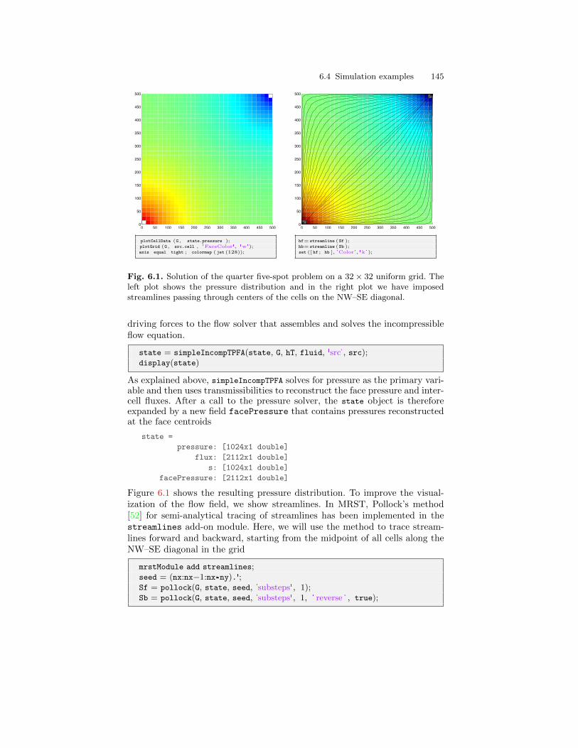
6.4 Simulation examples 145
0 50 100 150 200 250 300 350 400 450 5000
50
100
150
200
250
300
350
400
450
500
plotCellData (G , state.pressure );plotGrid (G , src.cell , 'FaceColor', 'w');axis equal tight ; colormap (jet (128));
0 50 100 150 200 250 300 350 400 450 5000
50
100
150
200
250
300
350
400
450
500
hf= streamline (Sf );hb= streamline (Sb );set ([ hf ; hb ], 'Color', 'k' );
Fig. 6.1. Solution of the quarter five-spot problem on a 32× 32 uniform grid. Theleft plot shows the pressure distribution and in the right plot we have imposedstreamlines passing through centers of the cells on the NW–SE diagonal.
driving forces to the flow solver that assembles and solves the incompressibleflow equation.
state = simpleIncompTPFA(state, G, hT, fluid, 'src', src);display(state)
As explained above, simpleIncompTPFA solves for pressure as the primary vari-able and then uses transmissibilities to reconstruct the face pressure and inter-cell fluxes. After a call to the pressure solver, the state object is thereforeexpanded by a new field facePressure that contains pressures reconstructedat the face centroids
state =
pressure: [1024x1 double]
flux: [2112x1 double]
s: [1024x1 double]
facePressure: [2112x1 double]
Figure 6.1 shows the resulting pressure distribution. To improve the visual-ization of the flow field, we show streamlines. In MRST, Pollock’s method[52] for semi-analytical tracing of streamlines has been implemented in thestreamlines add-on module. Here, we will use the method to trace stream-lines forward and backward, starting from the midpoint of all cells along theNW–SE diagonal in the grid
mrstModule add streamlines;seed = (nx:nx−1:nx*ny).';Sf = pollock(G, state, seed, 'substeps', 1);Sb = pollock(G, state, seed, 'substeps', 1, ' reverse ' , true);
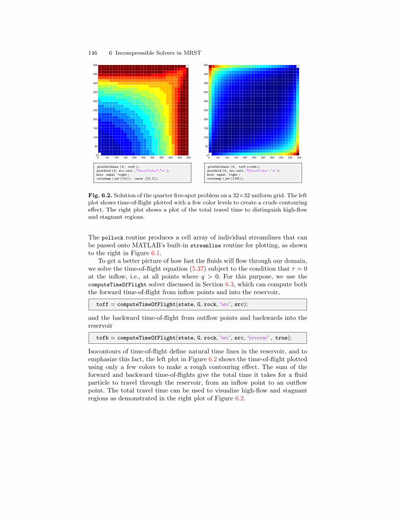
146 6 Incompressible Solvers in MRST
0 50 100 150 200 250 300 350 400 450 5000
50
100
150
200
250
300
350
400
450
500
plotCellData (G , toff );plotGrid (G , src.cell , 'FaceColor','w');axis equal tight ;colormap (jet (16)); caxis ([0,1]);
0 50 100 150 200 250 300 350 400 450 5000
50
100
150
200
250
300
350
400
450
500
plotCellData (G , toff+tofb);plotGrid (G , src.cell , 'FaceColor','w');axis equal tight ;colormap (jet (128));
Fig. 6.2. Solution of the quarter five-spot problem on a 32×32 uniform grid. The leftplot shows time-of-flight plotted with a few color levels to create a crude contouringeffect. The right plot shows a plot of the total travel time to distinguish high-flowand stagnant regions.
The pollock routine produces a cell array of individual streamlines that canbe passed onto MATLAB’s built-in streamline routine for plotting, as shownto the right in Figure 6.1.
To get a better picture of how fast the fluids will flow through our domain,we solve the time-of-flight equation (5.37) subject to the condition that τ = 0at the inflow, i.e., at all points where q > 0. For this purpose, we use thecomputeTimeOfFlight solver discussed in Section 6.3, which can compute boththe forward time-of-flight from inflow points and into the reservoir,
toff = computeTimeOfFlight(state, G, rock, 'src', src);
and the backward time-of-flight from outflow points and backwards into thereservoir
tofb = computeTimeOfFlight(state, G, rock, 'src', src, 'reverse ' , true);
Isocontours of time-of-flight define natural time lines in the reservoir, and toemphasize this fact, the left plot in Figure 6.2 shows the time-of-flight plottedusing only a few colors to make a rough contouring effect. The sum of theforward and backward time-of-flights give the total time it takes for a fluidparticle to travel through the reservoir, from an inflow point to an outflowpoint. The total travel time can be used to visualize high-flow and stagnantregions as demonstrated in the right plot of Figure 6.2.
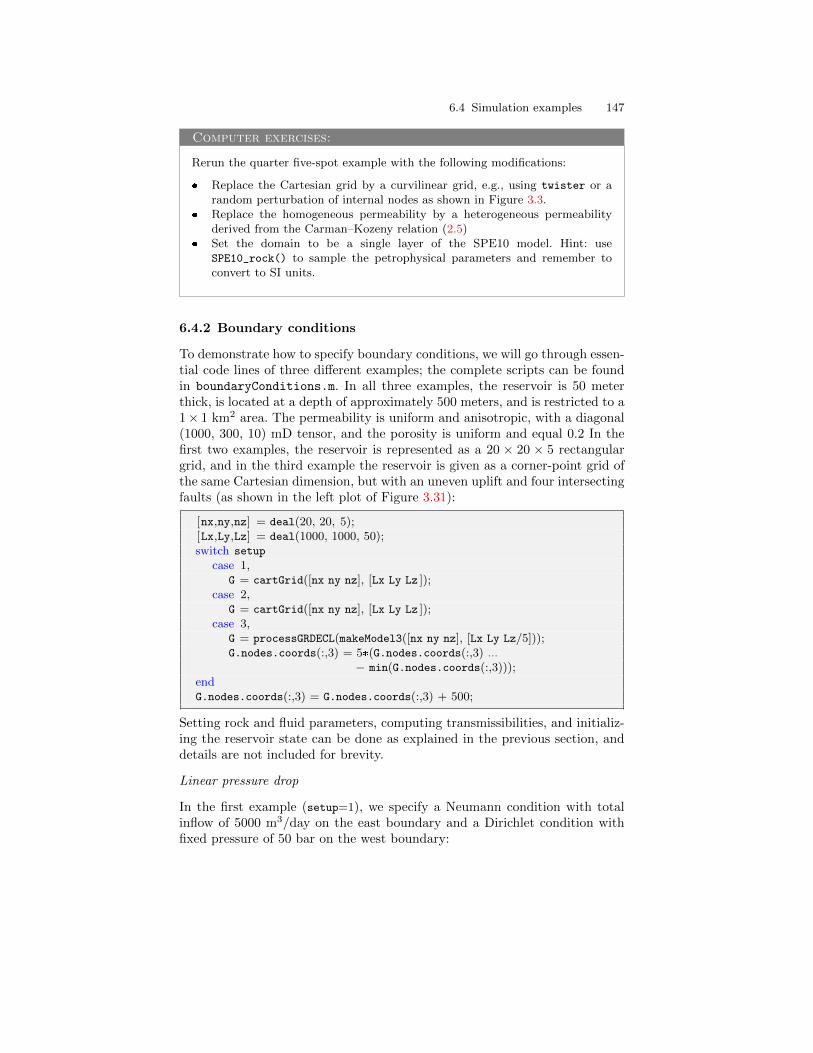
6.4 Simulation examples 147
Computer exercises:
Rerun the quarter five-spot example with the following modifications:
Replace the Cartesian grid by a curvilinear grid, e.g., using twister or arandom perturbation of internal nodes as shown in Figure 3.3.
Replace the homogeneous permeability by a heterogeneous permeabilityderived from the Carman–Kozeny relation (2.5)
Set the domain to be a single layer of the SPE10 model. Hint: useSPE10_rock() to sample the petrophysical parameters and remember toconvert to SI units.
6.4.2 Boundary conditions
To demonstrate how to specify boundary conditions, we will go through essen-tial code lines of three different examples; the complete scripts can be foundin boundaryConditions.m. In all three examples, the reservoir is 50 meterthick, is located at a depth of approximately 500 meters, and is restricted to a1× 1 km2 area. The permeability is uniform and anisotropic, with a diagonal(1000, 300, 10) mD tensor, and the porosity is uniform and equal 0.2 In thefirst two examples, the reservoir is represented as a 20 × 20 × 5 rectangulargrid, and in the third example the reservoir is given as a corner-point grid ofthe same Cartesian dimension, but with an uneven uplift and four intersectingfaults (as shown in the left plot of Figure 3.31):
[nx,ny,nz] = deal(20, 20, 5);[Lx,Ly,Lz] = deal(1000, 1000, 50);switch setup
case 1,G = cartGrid([nx ny nz], [Lx Ly Lz ]);
case 2,G = cartGrid([nx ny nz], [Lx Ly Lz ]);
case 3,G = processGRDECL(makeModel3([nx ny nz], [Lx Ly Lz/5]));G.nodes.coords(:,3) = 5*(G.nodes.coords(:,3) ...
− min(G.nodes.coords(:,3)));endG.nodes.coords(:,3) = G.nodes.coords(:,3) + 500;
Setting rock and fluid parameters, computing transmissibilities, and initializ-ing the reservoir state can be done as explained in the previous section, anddetails are not included for brevity.
Linear pressure drop
In the first example (setup=1), we specify a Neumann condition with totalinflow of 5000 m3/day on the east boundary and a Dirichlet condition withfixed pressure of 50 bar on the west boundary:
148 6 Incompressible Solvers in MRST
0
200
400
600
800
1000
0
200
400
600
800
1000
500
510
520
530
540
550
0
200
400
600
800
1000
0
200
400
600
800
1000
500
510
520
530
540
550
xy
De
pth
[bar]
51
52
53
54
55
56
57
58
59
60
61
Fig. 6.3. First example of a flow driven by boundary conditions. In the left plot,faces with Neumann conditions are marked in blue and faces with Dirichlet condi-tions are marked in red. The right plot shows the resulting pressure distribution.
bc = fluxside(bc, G, 'EAST', 5e3*meterˆ3/day);bc = pside (bc, G, 'WEST', 50*barsa);
This completes the definition of the model, and we can pass the resultingobjects to the simpleIncompTFPA solver to compute the pressure distributionshown to the right in Figure 6.3. In the absence of gravity, these boundaryconditions will result in a linear pressure drop from east to west inside thereservoir.
Hydrostatic boundary conditions
In the next example, we will use the same model, except that we now includethe effects of gravity and assume hydrostatic equilibrium at the outer verticalboundaries of the model. First, we initialize the reservoir state according tohydrostatic equilibrium, which is straightforward to compute if we for sim-plicity assume that the overburden pressure is caused by a column of fluidswith the exact same density as in the reservoir:
state = initResSol(G, G.cells.centroids(:,3)*rho*norm(gravity), 1.0);
There are at least two different ways to specify hydrostatic boundary condi-tions. The simplest approach is to use the function psideh, i.e.,
bc = psideh([], G, 'EAST', fluid);bc = psideh(bc, G, 'WEST', fluid);bc = psideh(bc, G, 'SOUTH', fluid);bc = psideh(bc, G, 'NORTH', fluid);
Alternatively, we can do it manually ourselves. To this end, we need to extractthe reservoir perimeter defined as all exterior faces are vertical, i.e., whosenormal vector have no z-component,
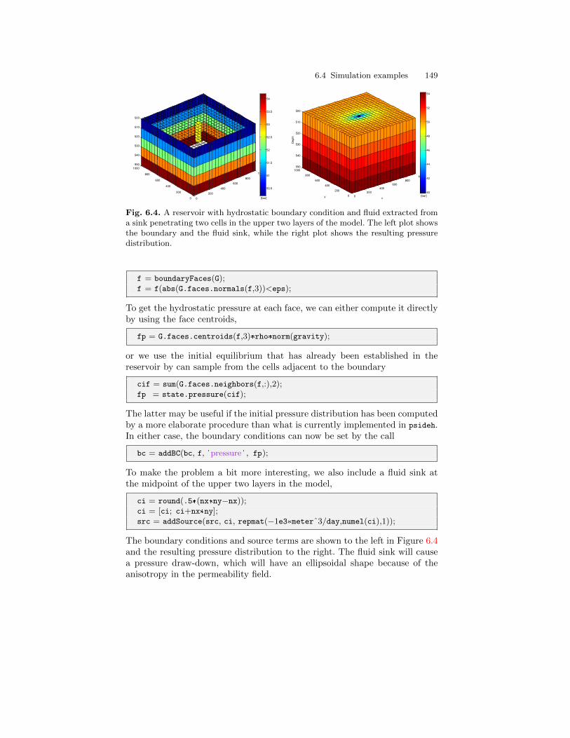
6.4 Simulation examples 149
0
200
400
600
800
1000
0
200
400
600
800
1000
500
510
520
530
540
550
[bar]
50.5
51
51.5
52
52.5
53
53.5
54
0
200
400
600
800
1000
0
200
400
600
800
1000
500
510
520
530
540
550
xy
De
pth
[bar]40
42
44
46
48
50
52
54
Fig. 6.4. A reservoir with hydrostatic boundary condition and fluid extracted froma sink penetrating two cells in the upper two layers of the model. The left plot showsthe boundary and the fluid sink, while the right plot shows the resulting pressuredistribution.
f = boundaryFaces(G);f = f(abs(G.faces.normals(f,3))<eps);
To get the hydrostatic pressure at each face, we can either compute it directlyby using the face centroids,
fp = G.faces.centroids(f,3)*rho*norm(gravity);
or we use the initial equilibrium that has already been established in thereservoir by can sample from the cells adjacent to the boundary
cif = sum(G.faces.neighbors(f,:),2);fp = state.pressure(cif);
The latter may be useful if the initial pressure distribution has been computedby a more elaborate procedure than what is currently implemented in psideh.In either case, the boundary conditions can now be set by the call
bc = addBC(bc, f, 'pressure ' , fp);
To make the problem a bit more interesting, we also include a fluid sink atthe midpoint of the upper two layers in the model,
ci = round(.5*(nx*ny−nx));ci = [ci; ci+nx*ny];src = addSource(src, ci, repmat(−1e3*meterˆ3/day,numel(ci),1));
The boundary conditions and source terms are shown to the left in Figure 6.4and the resulting pressure distribution to the right. The fluid sink will causea pressure draw-down, which will have an ellipsoidal shape because of theanisotropy in the permeability field.
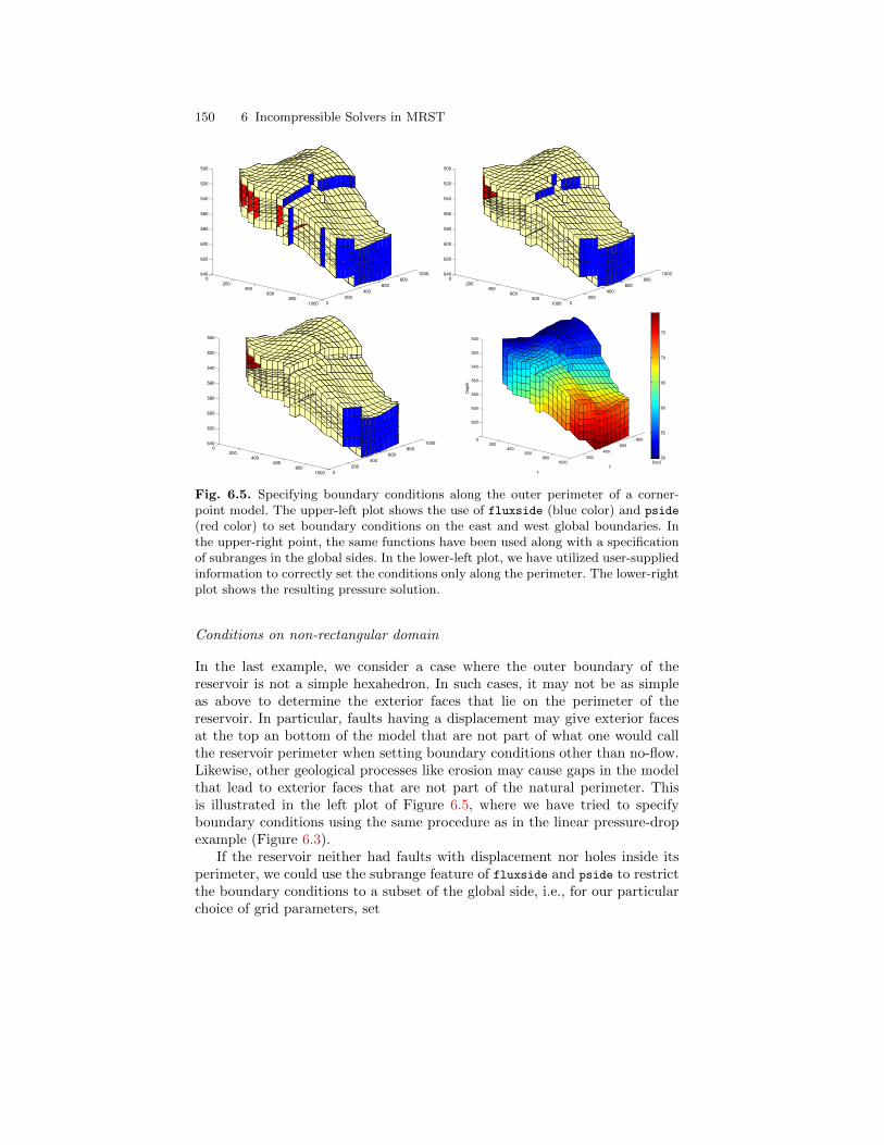
150 6 Incompressible Solvers in MRST
0
200
400
600
800
1000 0
200
400
600
800
1000
500
520
540
560
580
600
620
640
0
200
400
600
800
1000 0
200
400
600
800
1000
500
520
540
560
580
600
620
640
0
200
400
600
800
1000 0
200
400
600
800
1000
500
520
540
560
580
600
620
6400
200400
600800
1000200
400
600
800
500
520
540
560
580
600
620
y
x
Depth
[bar]50
55
60
65
70
75
Fig. 6.5. Specifying boundary conditions along the outer perimeter of a corner-point model. The upper-left plot shows the use of fluxside (blue color) and pside
(red color) to set boundary conditions on the east and west global boundaries. Inthe upper-right point, the same functions have been used along with a specificationof subranges in the global sides. In the lower-left plot, we have utilized user-suppliedinformation to correctly set the conditions only along the perimeter. The lower-rightplot shows the resulting pressure solution.
Conditions on non-rectangular domain
In the last example, we consider a case where the outer boundary of thereservoir is not a simple hexahedron. In such cases, it may not be as simpleas above to determine the exterior faces that lie on the perimeter of thereservoir. In particular, faults having a displacement may give exterior facesat the top an bottom of the model that are not part of what one would callthe reservoir perimeter when setting boundary conditions other than no-flow.Likewise, other geological processes like erosion may cause gaps in the modelthat lead to exterior faces that are not part of the natural perimeter. Thisis illustrated in the left plot of Figure 6.5, where we have tried to specifyboundary conditions using the same procedure as in the linear pressure-dropexample (Figure 6.3).
If the reservoir neither had faults with displacement nor holes inside itsperimeter, we could use the subrange feature of fluxside and pside to restrictthe boundary conditions to a subset of the global side, i.e., for our particularchoice of grid parameters, set
6.4 Simulation examples 151
bc = fluxside([], G, 'EAST', 5e3*meterˆ3/day, 4:15, 1:5);bc = pside (bc, G, 'WEST', 50*barsa, 7:17, []);
Unfortunately, this will not work properly in the current case, as shown inthe middle plot of Figure 6.5. The problem is that fluxside and pside definetheir ’east’ sides to consist of all faces that only belong to one cell and arecategorized to be on the east side of this cell.
To find the faces that are on the perimeter, we need to use expert knowl-edge. In our case, this amounts to utilizing the fact that the perimeter isdefined as those faces that lie on the bounding box of the model. For theNeumann condition we therefore get
x = G.faces.centroids(f,1);[xm,xM] = deal(min(x), max(x));ff = f(x>xM−1e−5);bc = addBC(bc, ff, 'flux ' , (5e3*meterˆ3/day) ...
* G.faces.areas(ff)/ sum(G.faces.areas(ff)));
Notice how the total flux has been distributed to individual faces accordingto the face area. The Dirichlet condition can be specified in a similar manner.
Computer exercises:
1. Consider a 2D box with a sink at the midpoint and inflow across the perime-ter specified either in terms of a constant pressure or a constant flux. Arethere differences in the two solutions, and if so, can you explain why? Hint:use time-of-flight, total travel time, and/or streamlines to investigate theflow pattern.
2. Apply the production setup from Figure 6.4, with hydrostatic boundaryconditions and fluids extracted from two cells at the midpoint of the model,to the model depicted in Figure 6.5.
6.4.3 Structured versus unstructured stencils
We have so far only discussed grids that have an underlying structured cellnumbering. The two-point schemes can also be applied to fully unstructuredand polyhedral grids. To demonstrate this, we use the triangular grid gener-ated from the seamount data set that is supplied with MATLAB, see Fig-ure 3.8, scaled to cover a 1 × 1 km2 area. Based on this grid, we define anon-rectangular reservoir. The reservoir is assumed to be homogeneous withan isotropic permeability of 100 mD and the resident fluid has the same prop-erties as in the previous examples. A constant pressure of 50 bar is set atthe outer perimeter and fluid is drained from a well located at (450, 500) ata constant rate of one pore volume over fifty years. (All details are found inthe script stencilComparison.m).
152 6 Incompressible Solvers in MRST
We start by generating the triangular grid, which will subsequently beused to define the extent of the reservoir:
load seamount
T = triangleGrid([x(:) y(:)], delaunay(x,y));[Tmin,Tmax] = deal(min(T.nodes.coords), max(T.nodes.coords));T.nodes.coords = bsxfun(@times, ...
bsxfun(@minus, T.nodes.coords, Tmin), 1000./(Tmax − Tmin));T = computeGeometry(T);
Next, we generate two Cartesian grids that cover the same domain, one withapproximately the same number of cells as the triangular grid and a 10× 10refinement of this grid that will give us a reference solution,
G = computeGeometry(cartGrid([25 25], [1000 1000]));inside = isPointInsideGrid(T, G.cells.centroids);G = removeCells(G, ˜inside);
The function isPointInsideGrid implements a simple algorithm for findingwhether one or more points lie inside the circumference of a grid. First, allboundary faces are extracted and then the corresponding nodes are sorted sothat they form a closed polygon. Then, MATLAB’s built-in function inpolygon
can be used to check whether the points are inside this polygon or no.To construct a radial grid centered around the point at which we will
extract fluids, we start by using the same code as on page 68 to generate aset of points inside [−1, 1]× [−1, 1] that are graded radially towards the origin(see e.g., Figure 3.22),
P = [];for r = exp([−3.5:.2:0, 0, .1 ]),
[x,y] = cylinder(r,25); P = [P [x (1,:); y (1,:)]];endP = unique([P'; 0 0], 'rows');
The points are scaled and translated so that their origin is moved to the point(450,500), from which fluid will be extracted:
[Pmin,Pmax] = deal(min(P), max(P));P = bsxfun(@minus, bsxfun(@times, ...
bsxfun(@minus, P, Pmin), 1200./(Pmax−Pmin)), [150 100]);
Then, we remove all points outside of the triangular grid, before the point setis passed to two grid-factory routines to first generate a triangular and thena Voronoi grid:
inside = isPointInsideGrid(T, P);V = computeGeometry( pebi( triangleGrid(P(inside,:)) ));
Once the grids have been constructed, the setup of the remaining part ofthe model will be the same in all cases. To avoid unnecessary replication of
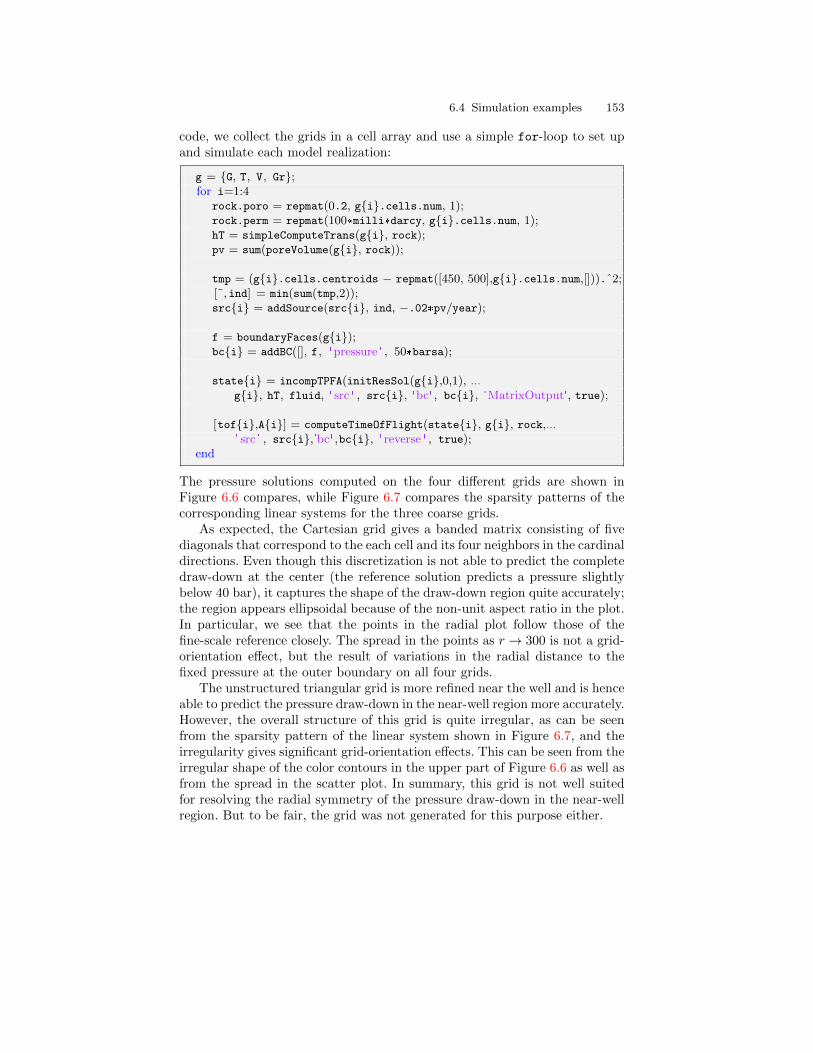
6.4 Simulation examples 153
code, we collect the grids in a cell array and use a simple for-loop to set upand simulate each model realization:
g = G, T, V, Gr;for i=1:4
rock.poro = repmat(0.2, gi.cells.num, 1);rock.perm = repmat(100*milli*darcy, gi.cells.num, 1);hT = simpleComputeTrans(gi, rock);pv = sum(poreVolume(gi, rock));
tmp = (gi.cells.centroids − repmat([450, 500],gi.cells.num,[])).ˆ2;[˜,ind] = min(sum(tmp,2));srci = addSource(srci, ind, −.02*pv/year);
f = boundaryFaces(gi);bci = addBC([], f, 'pressure ' , 50*barsa);
statei = incompTPFA(initResSol(gi,0,1), ...gi, hT, fluid, ' src ' , srci, 'bc' , bci, 'MatrixOutput', true);
[tofi,Ai] = computeTimeOfFlight(statei, gi, rock,...' src ' , srci,'bc' ,bci, ' reverse ' , true);
end
The pressure solutions computed on the four different grids are shown inFigure 6.6 compares, while Figure 6.7 compares the sparsity patterns of thecorresponding linear systems for the three coarse grids.
As expected, the Cartesian grid gives a banded matrix consisting of fivediagonals that correspond to the each cell and its four neighbors in the cardinaldirections. Even though this discretization is not able to predict the completedraw-down at the center (the reference solution predicts a pressure slightlybelow 40 bar), it captures the shape of the draw-down region quite accurately;the region appears ellipsoidal because of the non-unit aspect ratio in the plot.In particular, we see that the points in the radial plot follow those of thefine-scale reference closely. The spread in the points as r → 300 is not a grid-orientation effect, but the result of variations in the radial distance to thefixed pressure at the outer boundary on all four grids.
The unstructured triangular grid is more refined near the well and is henceable to predict the pressure draw-down in the near-well region more accurately.However, the overall structure of this grid is quite irregular, as can be seenfrom the sparsity pattern of the linear system shown in Figure 6.7, and theirregularity gives significant grid-orientation effects. This can be seen from theirregular shape of the color contours in the upper part of Figure 6.6 as well asfrom the spread in the scatter plot. In summary, this grid is not well suitedfor resolving the radial symmetry of the pressure draw-down in the near-wellregion. But to be fair, the grid was not generated for this purpose either.
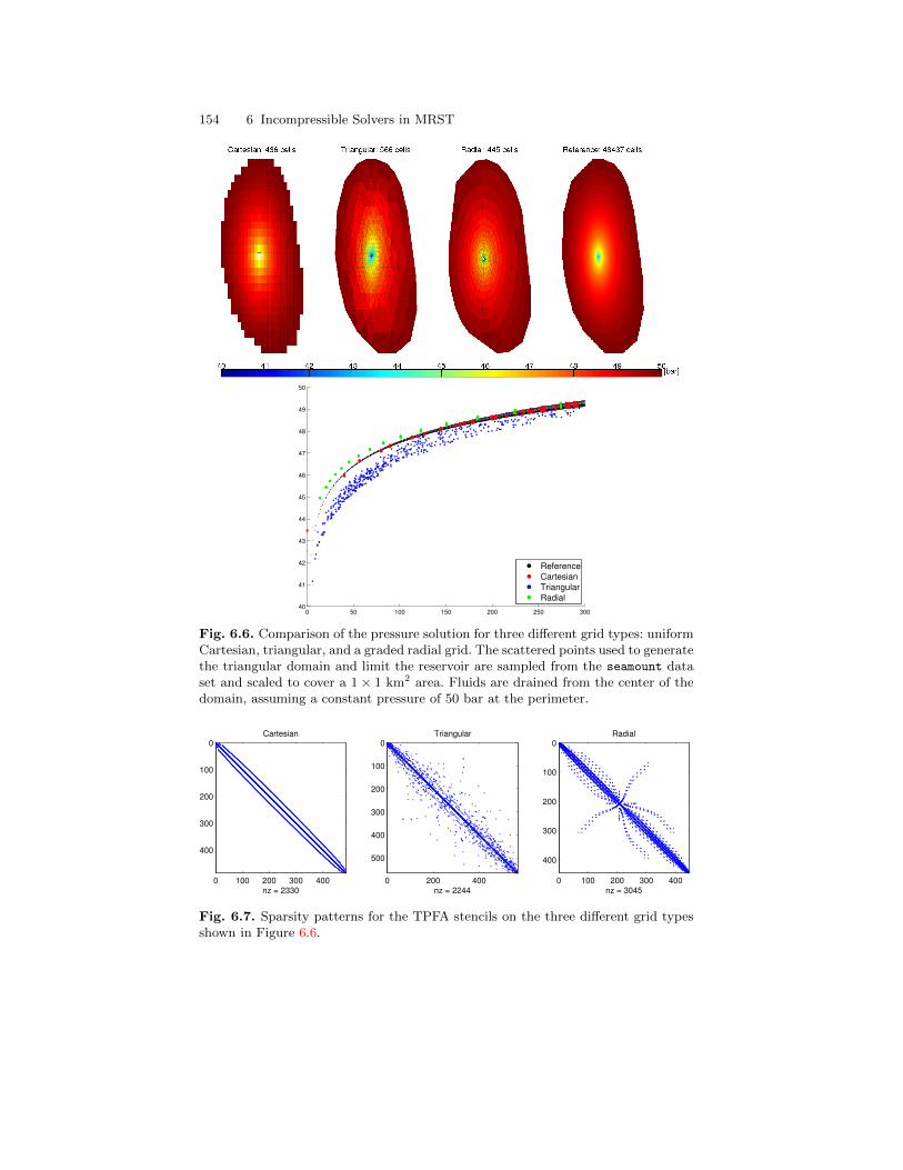
154 6 Incompressible Solvers in MRST
0 50 100 150 200 250 30040
41
42
43
44
45
46
47
48
49
50
Reference
Cartesian
Triangular
Radial
Fig. 6.6. Comparison of the pressure solution for three different grid types: uniformCartesian, triangular, and a graded radial grid. The scattered points used to generatethe triangular domain and limit the reservoir are sampled from the seamount dataset and scaled to cover a 1× 1 km2 area. Fluids are drained from the center of thedomain, assuming a constant pressure of 50 bar at the perimeter.
0 100 200 300 400
0
100
200
300
400
nz = 2330
Cartesian
0 200 400
0
100
200
300
400
500
nz = 2244
Triangular
0 100 200 300 400
0
100
200
300
400
nz = 3045
Radial
Fig. 6.7. Sparsity patterns for the TPFA stencils on the three different grid typesshown in Figure 6.6.
6.4 Simulation examples 155
Except for close to the well and close to the exterior boundary, the topologyof the radial grid is structured in the sense that each cell has four neighbors,two in the radial direction and two in the angular direction, and the cells areregular trapezoids. This should, in principle, give a banded sparsity patternprovided that the cells are ordered starting at the natural center point andmoving outward, one ring at the time. To verify this claim, you can executethe following code:
[˜,q]=sort(state3.pressure);spy(state3.A(q,q));
However, as a result of how the grid was generated, by first triangulating andthen forming the dual, the cells are numbered from west to east, which explainswhy the sparsity pattern is so far from being a simple banded structure. Whilethis may potentially affect the efficiency of a linear solver, it has no impacton the accuracy of the numerical approximation, which is good because ofthe grading towards the well and the symmetry inherent in the grid. Slightdifferences in the radial profile compared with the Cartesian grid(s) can mainlybe attributed to the fact that the source term and the fixed pressure conditionsare not located at the exact same positions in the simulations.
In Figure 6.8, we also show the sparsity pattern of the linear system usedto compute the reverse time-of-flight from the well and back into the reservoir.Using the default cell ordering, the sparsity pattern of each upwind matrixwill appear as a less dense version of the pattern for the corresponding TPFAmatrix. However, whereas the TPFA matrices represent an elliptic equationin which information propagates in both directions across cell interfaces, theupwind matrices are based on one-way connections arising from fluxes betweenpairs of cells that are connected in the TPFA discretization. To reveal thetrue nature of the system, we can permute the system by either sorting thecell pressures in ascending order (potential ordering) or using the functiondmperm to compute a Dulmage–Mendelsohn decomposition. As pointed out inSection 6.3, the result is a lower triangular matrix, from which it is simple tosee that the unidirectional propagation of information one would expect for ahyperbolic equations having only positive characteristics.
Computer exercises:
1. Compare the sparsity patterns resulting from the potential ordering anduse of dmperm for both the upwind and the TPFA matrices.
2. Investigate the flow patterns in more details using forward time-of-flight,travel time, and/or streamlines.
3. Replace the boundary conditions by a constant influx, or set pressure valuessampled from a radially symmetric pressure solution in an infinite domain.
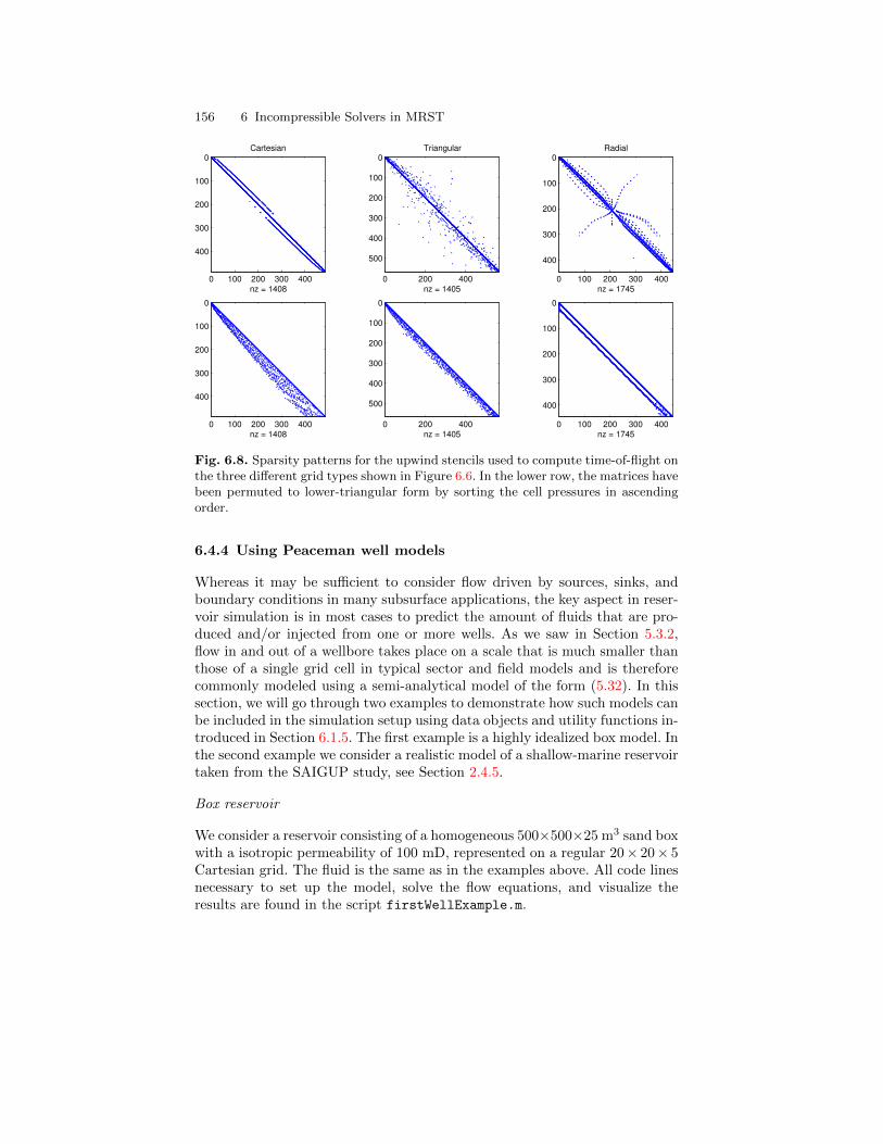
156 6 Incompressible Solvers in MRST
0 100 200 300 400
0
100
200
300
400
nz = 1408
Cartesian
0 100 200 300 400
0
100
200
300
400
nz = 1408
0 200 400
0
100
200
300
400
500
nz = 1405
Triangular
0 200 400
0
100
200
300
400
500
nz = 1405
0 100 200 300 400
0
100
200
300
400
nz = 1745
Radial
0 100 200 300 400
0
100
200
300
400
nz = 1745
Fig. 6.8. Sparsity patterns for the upwind stencils used to compute time-of-flight onthe three different grid types shown in Figure 6.6. In the lower row, the matrices havebeen permuted to lower-triangular form by sorting the cell pressures in ascendingorder.
6.4.4 Using Peaceman well models
Whereas it may be sufficient to consider flow driven by sources, sinks, andboundary conditions in many subsurface applications, the key aspect in reser-voir simulation is in most cases to predict the amount of fluids that are pro-duced and/or injected from one or more wells. As we saw in Section 5.3.2,flow in and out of a wellbore takes place on a scale that is much smaller thanthose of a single grid cell in typical sector and field models and is thereforecommonly modeled using a semi-analytical model of the form (5.32). In thissection, we will go through two examples to demonstrate how such models canbe included in the simulation setup using data objects and utility functions in-troduced in Section 6.1.5. The first example is a highly idealized box model. Inthe second example we consider a realistic model of a shallow-marine reservoirtaken from the SAIGUP study, see Section 2.4.5.
Box reservoir
We consider a reservoir consisting of a homogeneous 500×500×25 m3 sand boxwith a isotropic permeability of 100 mD, represented on a regular 20× 20× 5Cartesian grid. The fluid is the same as in the examples above. All code linesnecessary to set up the model, solve the flow equations, and visualize theresults are found in the script firstWellExample.m.
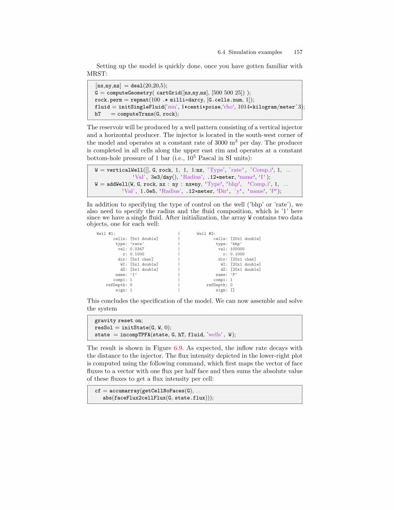
6.4 Simulation examples 157
Setting up the model is quickly done, once you have gotten familiar withMRST:
[nx,ny,nz] = deal(20,20,5);G = computeGeometry( cartGrid([nx,ny,nz], [500 500 25]) );rock.perm = repmat(100 .* milli*darcy, [G.cells.num, 1]);fluid = initSingleFluid('mu', 1*centi*poise,'rho', 1014*kilogram/meterˆ3);hT = computeTrans(G, rock);
The reservoir will be produced by a well pattern consisting of a vertical injectorand a horizontal producer. The injector is located in the south-west corner ofthe model and operates at a constant rate of 3000 m3 per day. The produceris completed in all cells along the upper east rim and operates at a constantbottom-hole pressure of 1 bar (i.e., 105 Pascal in SI units):
W = verticalWell([], G, rock, 1, 1, 1:nz, 'Type', ' rate ' , 'Comp i', 1, ...'Val' , 3e3/day(), 'Radius', .12*meter, 'name', 'I ' );
W = addWell(W, G, rock, nx : ny : nx*ny, 'Type', 'bhp', 'Comp i', 1, ...'Val' , 1.0e5, 'Radius', .12*meter, 'Dir' , 'y' , 'name', 'P');
In addition to specifying the type of control on the well (’bhp’ or ’rate’), wealso need to specify the radius and the fluid composition, which is ’1’ heresince we have a single fluid. After initialization, the array W contains two dataobjects, one for each well:
Well #1: | Well #2:cells: [5x1 double] | cells: [20x1 double]type: ’rate’ | type: ’bhp’val: 0.0347 | val: 100000
r: 0.1000 | r: 0.1000dir: [5x1 char] | dir: [20x1 char]WI: [5x1 double] | WI: [20x1 double]dZ: [5x1 double] | dZ: [20x1 double]
name: ’I’ | name: ’P’compi: 1 | compi: 1
refDepth: 0 | refDepth: 0sign: 1 | sign: []
This concludes the specification of the model. We can now assemble and solvethe system
gravity reset on;resSol = initState(G, W, 0);state = incompTPFA(state, G, hT, fluid, 'wells' , W);
The result is shown in Figure 6.9. As expected, the inflow rate decays withthe distance to the injector. The flux intensity depicted in the lower-right plotis computed using the following command, which first maps the vector of facefluxes to a vector with one flux per half face and then sums the absolute valueof these fluxes to get a flux intensity per cell:
cf = accumarray(getCellNoFaces(G), ...abs(faceFlux2cellFlux(G, state.flux)));
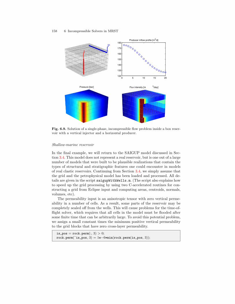
158 6 Incompressible Solvers in MRST
P
I
0 5 10 15 20120
130
140
150
160
170
180Producer inflow profile [m
3/d]
Pressure [bar] Flux intensity [m3/day]
Fig. 6.9. Solution of a single-phase, incompressible flow problem inside a box reser-voir with a vertical injector and a horizontal producer.
Shallow-marine reservoir
In the final example, we will return to the SAIGUP model discussed in Sec-tion 3.4. This model does not represent a real reservoir, but is one out of a largenumber of models that were built to be plausible realizations that contain thetypes of structural and stratigraphic features one could encounter in modelsof real clastic reservoirs. Continuing from Section 3.4, we simply assume thatthe grid and the petrophysical model has been loaded and processed. All de-tails are given in the script saigupWithWells.m. (The script also explains howto speed up the grid processing by using two C-accelerated routines for con-structing a grid from Eclipse input and computing areas, centroids, normals,volumes, etc).
The permeability input is an anisotropic tensor with zero vertical perme-ability in a number of cells. As a result, some parts of the reservoir may becompletely sealed off from the wells. This will cause problems for the time-of-flight solver, which requires that all cells in the model must be flooded aftersome finite time that can be arbitrarily large. To avoid this potential problem,we assign a small constant times the minimum positive vertical permeabilityto the grid blocks that have zero cross-layer permeability.
is_pos = rock.perm(:, 3) > 0;rock.perm(˜is_pos, 3) = 1e−6*min(rock.perm(is_pos, 3));
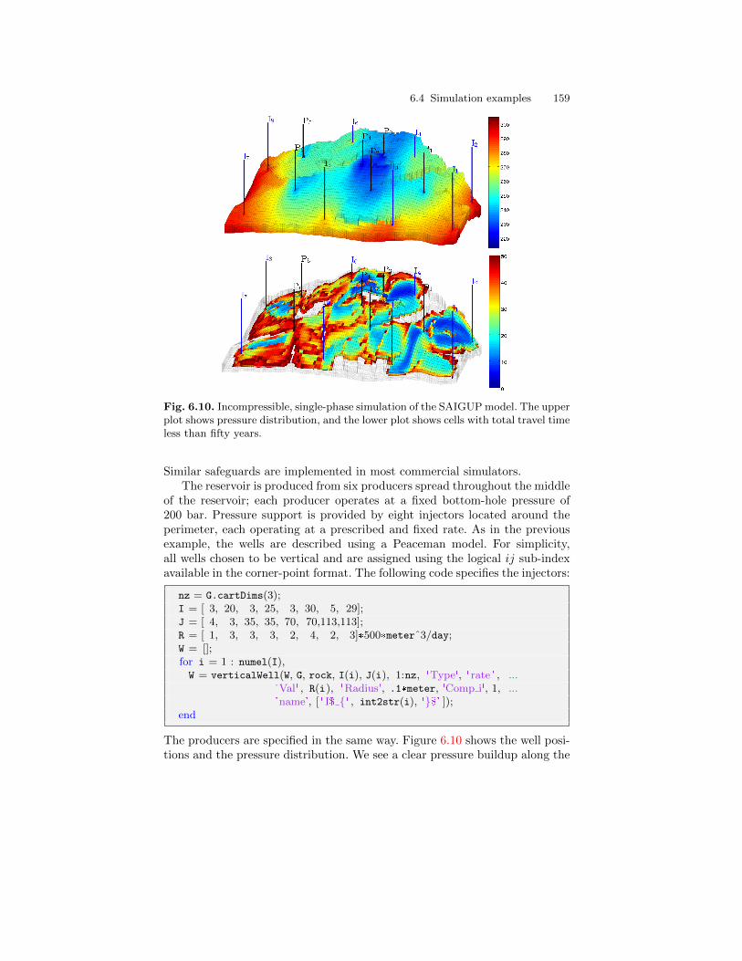
6.4 Simulation examples 159
Fig. 6.10. Incompressible, single-phase simulation of the SAIGUP model. The upperplot shows pressure distribution, and the lower plot shows cells with total travel timeless than fifty years.
Similar safeguards are implemented in most commercial simulators.The reservoir is produced from six producers spread throughout the middle
of the reservoir; each producer operates at a fixed bottom-hole pressure of200 bar. Pressure support is provided by eight injectors located around theperimeter, each operating at a prescribed and fixed rate. As in the previousexample, the wells are described using a Peaceman model. For simplicity,all wells chosen to be vertical and are assigned using the logical ij sub-indexavailable in the corner-point format. The following code specifies the injectors:
nz = G.cartDims(3);I = [ 3, 20, 3, 25, 3, 30, 5, 29];J = [ 4, 3, 35, 35, 70, 70,113,113];R = [ 1, 3, 3, 3, 2, 4, 2, 3]*500*meterˆ3/day;W = [];for i = 1 : numel(I),W = verticalWell(W, G, rock, I(i), J(i), 1:nz, 'Type', ' rate ' , ...
'Val' , R(i), 'Radius', .1*meter, 'Comp i', 1, ...'name', [ ' I$ ' , int2str(i), '$' ]);
end
The producers are specified in the same way. Figure 6.10 shows the well posi-tions and the pressure distribution. We see a clear pressure buildup along the
160 6 Incompressible Solvers in MRST
east, south, and west rim of the model. Similarly, there is a pressure draw-down in the middle of the model around producers P2, P3, and P4. The totalinjection rate is set so that one pore volume will be injected in a little lessthan forty years.
Although this is a single-phase simulation, let us for a while think of oursetup in terms of injection and production of different fluids (since the fluidshave identical properties, we can think of a ’blue’ fluid being injected into a’black’ fluid). In an ideal situation, one would wish that the ’blue’ fluid wouldsweep the whole reservoir before it breaks through to the production wells, asthis would maximize the displacement of the ’black’ fluid. Even in the simplequarter five-spot examples in Section 6.4.1 (see Figure 6.2), we saw that thiswas not the case, and one cannot expect that this will happen here, either. Thelower plot in Figure 6.10 shows all cells in which the total travel time (sumof forward and backward time-of-flight) is less than fifty years. By lookingat such a plot, on can get a quite a good idea of regions in which there isvery limited communication between the injectors and producers (i.e., areaswithout colors). If this was a multiphase flow problem, these areas wouldtypically contain bypassed oil and be candidates for infill drilling or othermechanisms that would improve the volumetric sweep.
Computer exercises:
1. Change the parameter 'Dir' from 'y' to 'z ' in the box example and rerunthe case. Can you explain why you get a different result?
2. Switch the injector in the box example to be controlled by a bottom-holepressure of 200 bar. Where would you place the injector to maximize pro-duction rate if you can only complete it in five cells?
3. Consider the SAIGUP model: can you improve the well placement and/orthe distribution of fluid rates. Hint: is it possible to utilize time-of-flightinformation?
7
Single-Phase Solvers Based on AutomaticDifferentiation
In the previous chapter, we outlined and explained details of the functionalityMRST offers for simulation of incompressible, single-phase problems. Later inthe book we will come back to how these methods and tools can be extendedto time-dependent multiphase problems based on various operator-splittingformulations in which flow and transport are computed in different substeps.Operator splitting is one of the main approaches used for simulating flowin porous media. The other approach, which is the predominantly used inindustry, is based on so-called fully-implicit discretizations in which flow andtransport are solved as a coupled system. This approach is very robust andparticularly useful for compressible problems with small time constants orstrong coupling between different types of flow mechanisms.
In this chapter, we will discuss fully-implicit discretizations of compress-ible, single-phase problems. In doing so, we will also introduce you to auto-matic differentiation (AD), which will enable you to numerically evaluatethe derivative of a function specified by a computer program directly withoutfirst having to derive a set of underlying analytical expressions. The com-bination of this concept with the highly vectorized and interactive scriptinglanguage of Matlab and MRST’s flexible grid structure is in our opinion themain reason why MRST has proved to be a particularly efficient tool for rapidprototyping of new models and computational methods. To substantiate thisclaim, we will in the following demonstrate how the discrete differential opera-tors introduced in Section 5.4.2, and similar discrete averaging operators, canbe used as powerful abstractions that will enable you to keep the physics at theforefront in your code and rapidly explore alternative methods for discretizingand linearizing nonlinear flow equations.
7.1 Implicit discretization
As our basic model, we will in the following mainly be concerned with thesingle-phase continuity equation
162 7 Single-Phase Solvers Based on Automatic Differentiation
∂
∂t(φρ) +∇ · (ρ~v) = q, ~v = −K
µ(∇p− gρ∇z) . (7.1)
The primary unknown is usually the fluid pressure p and additional equationsare supplied to provide relations between p and the other quantities in theequation, e.g., by specifying φ = φ(p), an equation-of-state ρ = ρ(p) for thefluid, and so on; see the discussion in Section 5.2.
Using the discrete operators introduced in Section 5.4.2, the basic implicitdiscretization of (7.1) reads
(φρ)n+1 − (φρ)n
∆tn+ div(ρv)n+1 = qn+1, (7.2a)
vn+1 = − K
µn+1
[grad(pn+1)− gρn+1grad(z)
]. (7.2b)
Here, φ ∈ Rnc denotes the vector porosity values per cell, v the vector offluxes per face, and so on, and the superscript refers to discrete times atwhich one wishes to compute the unknown reservoir states and ∆t denotesthe time between two consecutive points in time.
In many cases of practical interest it is possible to simplify (7.2). Forinstance, if the fluid is only slightly compressible, several terms can be ne-glected so that the nonlinear equation reduces to an equation that is linear inthe unknown pn+1,
pn+1 − pn
∆tn− 1
ctφµdiv(K grad(pn+1)
)= qn. (7.3)
However, this is not always possible and for generality, we will in the followingassume that φ and ρ depend nonlinearly on p so that (7.2) gives rise to a(highly) nonlinear system of equations that needs to be solved in each timestep. For non-Newtonian fluids, the viscosity will also depend on the velocity,which will add further nonlinearity to the system and generally make it harderto solve. A simple example is a power law of the form µ(|~v|) = µ0|~v|α−1, whereα is a parameter that is determined experimentally.
In the following, we will mainly work with discretized equations writtenin residual form. As an example, the residual form of (7.3) reads
pn+1 − ∆tn
ctφµdiv(K grad(pn+1)
)− pn −∆tnqn = 0.
After spatial discretization, we can write the resulting system of nonlinearequations in the short vector-form as
F (xn+1;xn) = 0, (7.4)
where xn+1 is the vector of unknown state variables at the next time step andthe vector of current states xn can be seen as a parameter.
7.2 Automatic differentiation 163
7.2 Automatic differentiation
Nonlinear systems of discrete equations arising from the discretization of (par-tial) differential equations are typically solved by Newton’s method. In mostcases, this means that the main computational cost of solving a nonlinearPDE lies in solving the linear systems involved in each Newton iteration. Fora discretized equation on vector form, F (x) = 0, the (i + 1)-th iterationapproximation xi+1 is obtained from
∂F (xi)
∂xiδxi+1 = −F (xi), xi+1 ← xi + δxi+1. (7.5)
Here, J(xi) = ∂F (xi)/∂xi is the Jacobian matrix, while we refer to δxi+1 asthe Newton update at iteration step number i + 1. The Newton process willunder certain smoothness and differentiability requirements exhibit quadraticconvergence. This is, however, crucially dependent on a sufficiently accurateJacobian matrix. Typically, obtaining the Jacobian matrix can be broken downto differentiation of elementary operations and functions. Nevertheless, if Frepresents a set of complex equations, analytical derivation and subsequentcoding of the Jacobian can be very time-consuming and prone to errors anddebugging. On the other hand, computing Jacobians is a good candidate forautomation since it follows a set of fixed rules and should therefore in principlebe straightforward in principle.
Automatic differentiation is a technique that exploits the fact that anycomputer code, regardless of complexity, can be broken down to a limited setof arithmetic operations (+, −, ∗, /, etc), and, in our case, more or less elemen-tary MATLAB functions (exp, sin, power, interp, etc). In automatic differen-tiation (AD) the key idea is to keep track of quantities and their derivativessimultaneously; every time an operation is applied to a quantity, the corre-sponding differential operation is applied to its derivative. Consider a scalarprimary variable x and a function f = f(x). Their AD-representations wouldthen be the pairs 〈x, 1〉 and 〈f, fx〉, where fx is the derivative of f w.r.t. x (and1 is the derivative of x w.r.t. x). Accordingly, the action of the elementaryoperations and functions must be defined for such pairs, e.g.,
〈f, fx〉+ 〈g, gx〉 = 〈f + g, fx + gx〉 ,〈f, fx〉 ∗ 〈g, gx〉 = 〈fg, fgx + fxg〉 ,
〈f, fx〉 / 〈g, gx〉 =
⟨f
g,fxg − fgx
g2
⟩exp(〈f, fx〉) = 〈exp(f), exp(f)fx〉 ,sin(〈f, fx〉) = 〈sin(f), cos(f)fx〉 .
In addition to this, one needs to use the chain rule to accumulate derivatives;that is, if f(x) = g(h(x)), then fx(x) = dg
dhhx(x). This more or less summarizesthe key idea behind automatic differentiation, the remaining (and difficult
164 7 Single-Phase Solvers Based on Automatic Differentiation
part) is how to implement the idea as efficient computer code that has a lowuser-threshold and minimal computational overhead.
As the above example illustrates, it is straightforward to write down allelementary rules needed to differentiate a program or piece of code. To beuseful, however, it is important that these rules are not implemented asstandard functions, in which case you would need to write something likemyPlus(a, myTimes(b,c)) when you want to evaluate a+ bc. An elegant solutionto this is the use of classes and operator overloading. When MATLAB en-counters an expression a+b, the meaning of ”+” is dependent on the natureof a and b. In other words, there may be multiple functions plus defined, andthe one to choose is determined from which classes a and b belongs to. Anice introduction to how this is can be implemented in MATLAB is given byNeidinger [46].
7.3 Automatic differentiation in MRST
There are many automatic differentiation libraries for MATLAB, e.g., ADi-Mat [57, 12], ADMAT [17, 59], MAD [58, 56, 31], or from MATLAB Central[30, 43]. The AD class in MRST uses operator overloading as suggested in[46] and uses a relatively simple forward accumulation, but differs from otherlibraries in a subtle, but important way. Instead of working with a singleJacobian of the full discrete system as one matrix, MRST uses a list of ma-trices that represent the derivatives with respect to different variables, whichwill constitute sub-blocks in the Jacobian of the full system. The reason forthis choice is two-fold: computational performance and user utility. In typicalsimulation, and particularly for complex model, the mathematical model willconsist of several equations (continuum equations, Darcy’s law, equations ofstate, other constitutive relationships, control equations for wells, etc) thathave different characteristics and play different roles in the overall equationsystem. Although we are using fully implicit discretizations in which one seeksto solve for all state variables simultaneously, we may still want to manipulateparts of the full equation system that e.g., represents specific sub-equations.This is not practical if the Jacobian of the system is represented as a singlematrix; manipulating subsets of large sparse matrices is of currently not veryefficient in MATLAB, and keeping track of the necessary index sets may alsobe quite cumbersome from a user’s point-of-view. Accordingly, our currentchoice is to let the MRST AD-class represent the derivatives of different pri-mary variable (e.g., pressure, saturations, bottom-hole-pressures, . . . ) as a listof matrices.
In the rest of the section, we will instead go through two simple examplesthat demonstrate how the AD class works, before we move on to demon-strate how automatic differentiation can be used to set up simulations in a(surprisingly) few number of code lines.
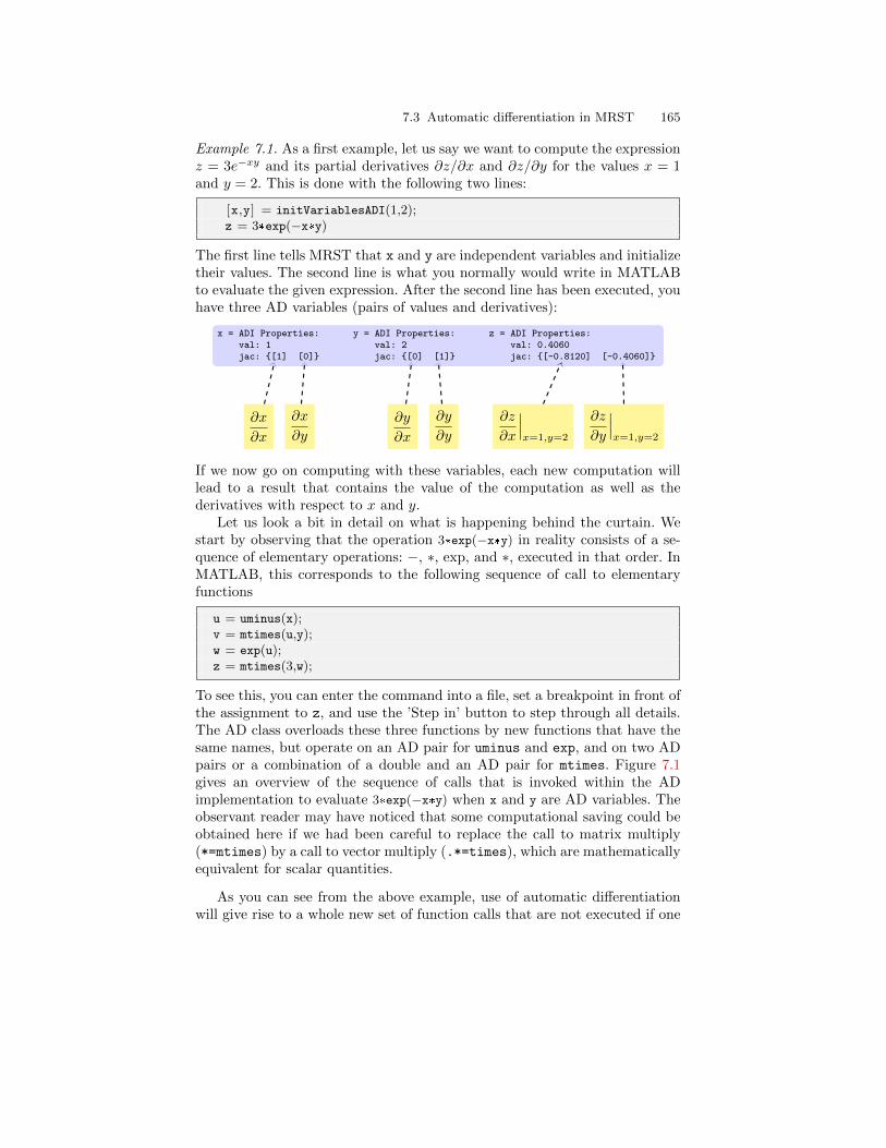
7.3 Automatic differentiation in MRST 165
Example 7.1. As a first example, let us say we want to compute the expressionz = 3e−xy and its partial derivatives ∂z/∂x and ∂z/∂y for the values x = 1and y = 2. This is done with the following two lines:
[x,y] = initVariablesADI(1,2);z = 3*exp(−x*y)
The first line tells MRST that x and y are independent variables and initializetheir values. The second line is what you normally would write in MATLABto evaluate the given expression. After the second line has been executed, youhave three AD variables (pairs of values and derivatives):
x = ADI Properties:val: 1jac: [1] [0]
y = ADI Properties:val: 2jac: [0] [1]
z = ADI Properties:val: 0.4060jac: [-0.8120] [-0.4060]
∂x
∂x
∂x
∂y
∂y
∂x
∂y
∂y
∂z
∂x
∣∣∣x=1,y=2
∂z
∂y
∣∣∣x=1,y=2
If we now go on computing with these variables, each new computation willlead to a result that contains the value of the computation as well as thederivatives with respect to x and y.
Let us look a bit in detail on what is happening behind the curtain. Westart by observing that the operation 3*exp(−x*y) in reality consists of a se-quence of elementary operations: −, ∗, exp, and ∗, executed in that order. InMATLAB, this corresponds to the following sequence of call to elementaryfunctions
u = uminus(x);v = mtimes(u,y);w = exp(u);z = mtimes(3,w);
To see this, you can enter the command into a file, set a breakpoint in front ofthe assignment to z, and use the ’Step in’ button to step through all details.The AD class overloads these three functions by new functions that have thesame names, but operate on an AD pair for uminus and exp, and on two ADpairs or a combination of a double and an AD pair for mtimes. Figure 7.1gives an overview of the sequence of calls that is invoked within the ADimplementation to evaluate 3*exp(−x*y) when x and y are AD variables. Theobservant reader may have noticed that some computational saving could beobtained here if we had been careful to replace the call to matrix multiply(*=mtimes) by a call to vector multiply (.*=times), which are mathematicallyequivalent for scalar quantities.
As you can see from the above example, use of automatic differentiationwill give rise to a whole new set of function calls that are not executed if one
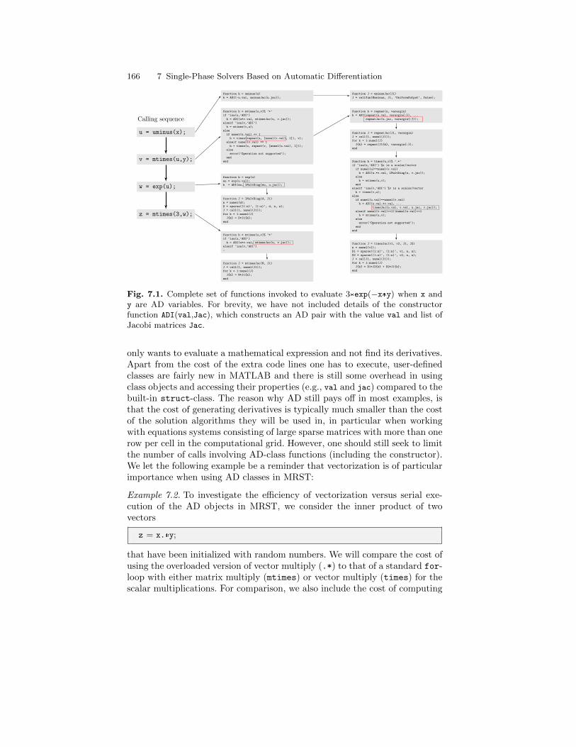
166 7 Single-Phase Solvers Based on Automatic Differentiation
u = uminus(x);
v = mtimes(u,y);
w = exp(u);
z = mtimes(3,w);
Calling sequence
function h = uminus(u)
h = ADI(-u.val, uminusJac(u.jac));
function J = uminusJac(J1)
J = cellfun(@uminus, J1, ’UniformOutput’, false);
function h = mtimes(u,v)% ’*’
if ~isa(u,’ADI’)
h = ADI(u*v.val, mtimesJac(u, v.jac));
elseif ~isa(v,’ADI’)
h = mtimes(v,u);
else
if numel(u.val) == 1
h = times(repmat(u, [numel(v.val), 1]), v);
elseif numel(v.val) == 1
h = times(u, repmat(v, [numel(u.val), 1]));
else
error(’Operation not supported’);
end
end
function h = repmat(u, varargin)
h = ADI(repmat(u.val, varargin:), ...
repmatJac(u.jac, varargin:));
function J = repmatJac(J1, varargin)
J = cell(1, numel(J1));
for k = 1:numel(J)
Jk = repmat(J1k, varargin:);
end
function h = times(u,v)% ’.*’
if ~isa(u,’ADI’) %u is a scalar/vector
if numel(u)==numel(v.val)
h = ADI(u.*v.val, lMultDiag(u, v.jac));
else
h = mtimes(u,v);
end
elseif ~isa(v,’ADI’) %v is a scalar/vector
h = times(v,u);
else
if numel(u.val)==numel(v.val)
h = ADI(u.val.*v.val, ...
timesJac(u.val, v.val, u.jac, v.jac));
elseif numel(v.val)==1||numel(u.val)==1
h = mtimes(u,v);
else
error(’Operation not supported’);
end
end
function J = timesJac(v1, v2, J1, J2)
n = numel(v1);
D1 = sparse((1:n)’, (1:n)’, v1, n, n);
D2 = sparse((1:n)’, (1:n)’, v2, n, n);
J = cell(1, numel(J1));
for k = 1:numel(J)
Jk = D1*J2k + D2*J1k;
end
function h = exp(u)
eu = exp(u.val);
h = ADI(eu, lMultDiag(eu, u.jac));
function J = lMultDiag(d, J1)
n = numel(d);
D = sparse((1:n)’, (1:n)’, d, n, n);
J = cell(1, numel(J1));
for k = 1:numel(J)
Jk = D*J1k;
end
function h = mtimes(u,v)% ’*’
if ~isa(u,’ADI’)
h = ADI(u*v.val, mtimesJac(u, v.jac));
elseif ~isa(v,’ADI’)
:
function J = mtimesJac(M, J1)
J = cell(1, numel(J1));
for k = 1:numel(J)
Jk = M*J1k;
end
Fig. 7.1. Complete set of functions invoked to evaluate 3*exp(−x*y) when x andy are AD variables. For brevity, we have not included details of the constructorfunction ADI(val,Jac), which constructs an AD pair with the value val and list ofJacobi matrices Jac.
only wants to evaluate a mathematical expression and not find its derivatives.Apart from the cost of the extra code lines one has to execute, user-definedclasses are fairly new in MATLAB and there is still some overhead in usingclass objects and accessing their properties (e.g., val and jac) compared to thebuilt-in struct-class. The reason why AD still pays off in most examples, isthat the cost of generating derivatives is typically much smaller than the costof the solution algorithms they will be used in, in particular when workingwith equations systems consisting of large sparse matrices with more than onerow per cell in the computational grid. However, one should still seek to limitthe number of calls involving AD-class functions (including the constructor).We let the following example be a reminder that vectorization is of particularimportance when using AD classes in MRST:
Example 7.2. To investigate the efficiency of vectorization versus serial exe-cution of the AD objects in MRST, we consider the inner product of twovectors
z = x.*y;
that have been initialized with random numbers. We will compare the cost ofusing the overloaded version of vector multiply (.*) to that of a standard for-loop with either matrix multiply (mtimes) or vector multiply (times) for thescalar multiplications. For comparison, we also include the cost of computing
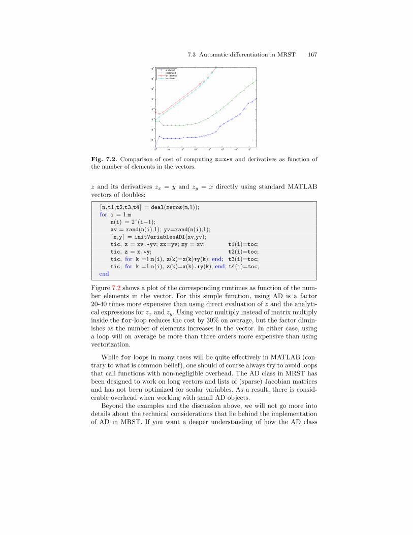
7.3 Automatic differentiation in MRST 167
100
101
102
103
104
105
106
107
10−5
10−4
10−3
10−2
10−1
100
101
102
analytical
vectorized
for+mtimes
for+times
Fig. 7.2. Comparison of cost of computing z=x*v and derivatives as function ofthe number of elements in the vectors.
z and its derivatives zx = y and zy = x directly using standard MATLABvectors of doubles:
[n,t1,t2,t3,t4] = deal(zeros(m,1));for i = 1:m
n(i) = 2ˆ(i−1);xv = rand(n(i),1); yv=rand(n(i),1);[x,y] = initVariablesADI(xv,yv);tic, z = xv.*yv; zx=yv; zy = xv; t1(i)=toc;tic, z = x.*y; t2(i)=toc;tic, for k =1:n(i), z(k)=x(k)*y(k); end; t3(i)=toc;tic, for k =1:n(i), z(k)=x(k).*y(k); end; t4(i)=toc;
end
Figure 7.2 shows a plot of the corresponding runtimes as function of the num-ber elements in the vector. For this simple function, using AD is a factor20-40 times more expensive than using direct evaluation of z and the analyti-cal expressions for zx and zy. Using vector multiply instead of matrix multiplyinside the for-loop reduces the cost by 30% on average, but the factor dimin-ishes as the number of elements increases in the vector. In either case, usinga loop will on average be more than three orders more expensive than usingvectorization.
While for-loops in many cases will be quite effectively in MATLAB (con-trary to what is common belief), one should of course always try to avoid loopsthat call functions with non-negligible overhead. The AD class in MRST hasbeen designed to work on long vectors and lists of (sparse) Jacobian matricesand has not been optimized for scalar variables. As a result, there is consid-erable overhead when working with small AD objects.
Beyond the examples and the discussion above, we will not go more intodetails about the technical considerations that lie behind the implementationof AD in MRST. If you want a deeper understanding of how the AD class
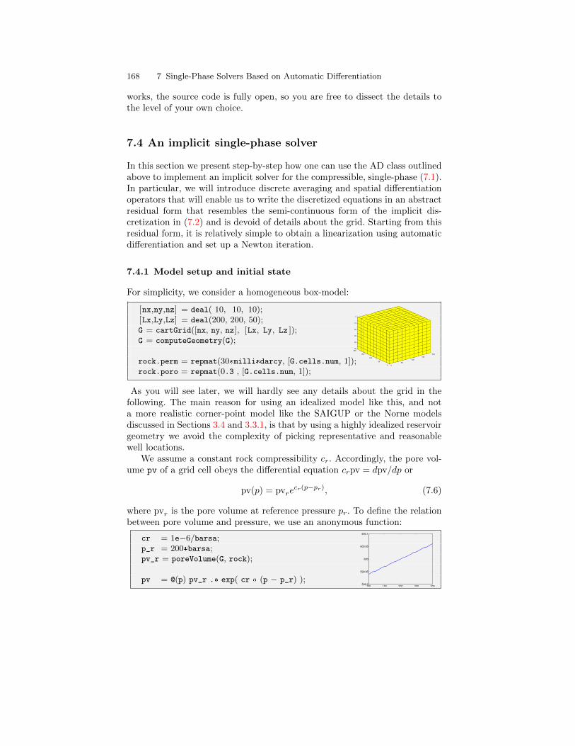
168 7 Single-Phase Solvers Based on Automatic Differentiation
works, the source code is fully open, so you are free to dissect the details tothe level of your own choice.
7.4 An implicit single-phase solver
In this section we present step-by-step how one can use the AD class outlinedabove to implement an implicit solver for the compressible, single-phase (7.1).In particular, we will introduce discrete averaging and spatial differentiationoperators that will enable us to write the discretized equations in an abstractresidual form that resembles the semi-continuous form of the implicit dis-cretization in (7.2) and is devoid of details about the grid. Starting from thisresidual form, it is relatively simple to obtain a linearization using automaticdifferentiation and set up a Newton iteration.
7.4.1 Model setup and initial state
For simplicity, we consider a homogeneous box-model:
[nx,ny,nz] = deal( 10, 10, 10);[Lx,Ly,Lz] = deal(200, 200, 50);G = cartGrid([nx, ny, nz], [Lx, Ly, Lz ]);G = computeGeometry(G);
rock.perm = repmat(30*milli*darcy, [G.cells.num, 1]);rock.poro = repmat(0.3 , [G.cells.num, 1]);
0
50
100
150
200
0
50
100
150
200
0
10
20
30
40
50
As you will see later, we will hardly see any details about the grid in thefollowing. The main reason for using an idealized model like this, and nota more realistic corner-point model like the SAIGUP or the Norne modelsdiscussed in Sections 3.4 and 3.3.1, is that by using a highly idealized reservoirgeometry we avoid the complexity of picking representative and reasonablewell locations.
We assume a constant rock compressibility cr. Accordingly, the pore vol-ume pv of a grid cell obeys the differential equation crpv = dpv/dp or
pv(p) = pvrecr(p−pr), (7.6)
where pvr is the pore volume at reference pressure pr. To define the relationbetween pore volume and pressure, we use an anonymous function:
cr = 1e−6/barsa;p_r = 200*barsa;pv_r = poreVolume(G, rock);
pv = @(p) pv_r .* exp( cr * (p − p_r) );100 150 200 250 300
599.9
599.95
600
600.05
600.1
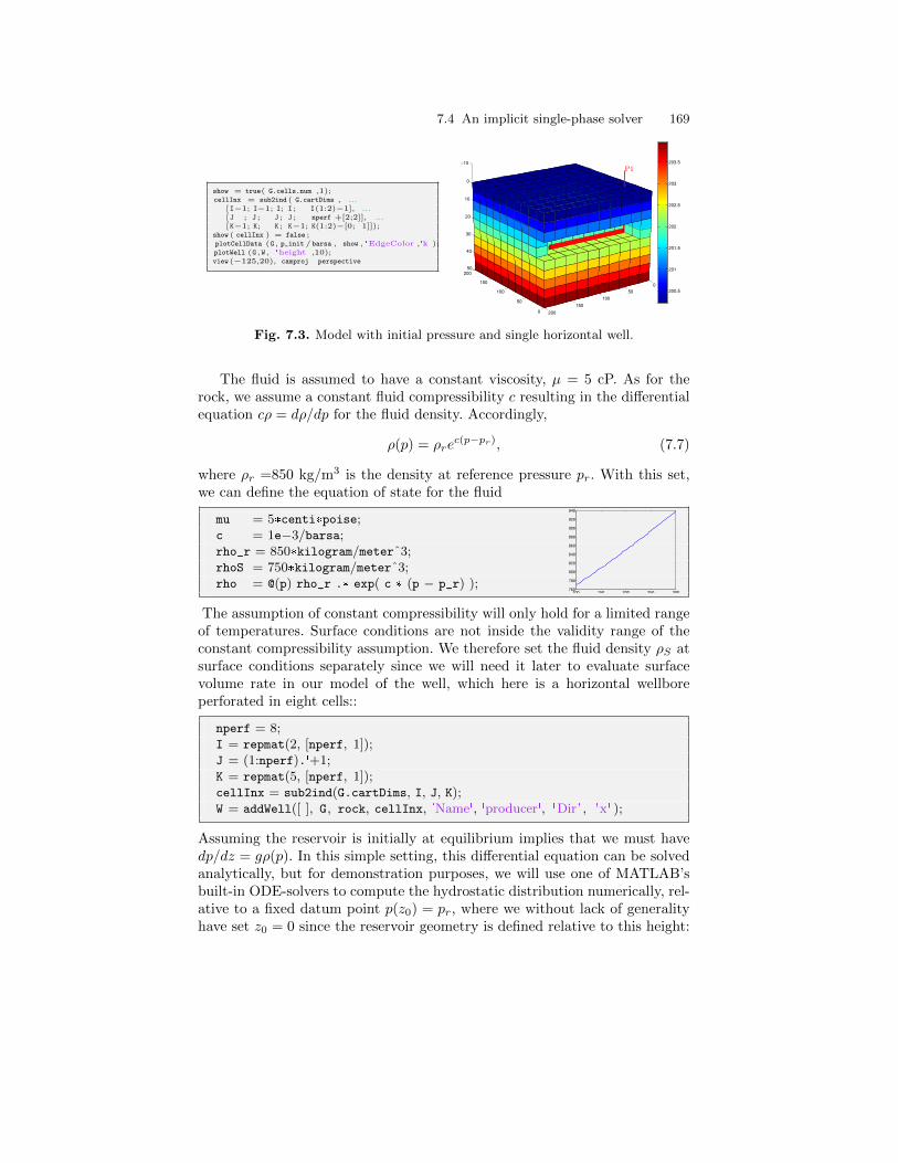
7.4 An implicit single-phase solver 169
show = true( G.cells.num ,1);cellInx = sub2ind ( G.cartDims , ...
[I−1; I−1; I; I ; I(1:2)−1], ...[J ; J ; J ; J ; nperf +[2;2]], ...[K−1; K; K ; K−1; K(1:2)−[0; 1]]);
show ( cellInx ) = false ;plotCellData (G , p_init / barsa , show , 'EdgeColor','k');plotWell (G ,W , 'height' ,10);view(−125,20), camproj perspective
0
50
100
150
200
0
50
100
150
200
−10
0
10
20
30
40
50
P1
200.5
201
201.5
202
202.5
203
203.5
Fig. 7.3. Model with initial pressure and single horizontal well.
The fluid is assumed to have a constant viscosity, µ = 5 cP. As for therock, we assume a constant fluid compressibility c resulting in the differentialequation cρ = dρ/dp for the fluid density. Accordingly,
ρ(p) = ρrec(p−pr), (7.7)
where ρr =850 kg/m3 is the density at reference pressure pr. With this set,we can define the equation of state for the fluid
mu = 5*centi*poise;c = 1e−3/barsa;rho_r = 850*kilogram/meterˆ3;rhoS = 750*kilogram/meterˆ3;rho = @(p) rho_r .* exp( c * (p − p_r) );
100 150 200 250 300760
780
800
820
840
860
880
900
920
940
The assumption of constant compressibility will only hold for a limited rangeof temperatures. Surface conditions are not inside the validity range of theconstant compressibility assumption. We therefore set the fluid density ρS atsurface conditions separately since we will need it later to evaluate surfacevolume rate in our model of the well, which here is a horizontal wellboreperforated in eight cells::
nperf = 8;I = repmat(2, [nperf, 1]);J = (1:nperf).'+1;K = repmat(5, [nperf, 1]);cellInx = sub2ind(G.cartDims, I, J, K);W = addWell([ ], G, rock, cellInx, 'Name', 'producer', 'Dir' , 'x' );
Assuming the reservoir is initially at equilibrium implies that we must havedp/dz = gρ(p). In this simple setting, this differential equation can be solvedanalytically, but for demonstration purposes, we will use one of MATLAB’sbuilt-in ODE-solvers to compute the hydrostatic distribution numerically, rel-ative to a fixed datum point p(z0) = pr, where we without lack of generalityhave set z0 = 0 since the reservoir geometry is defined relative to this height:

170 7 Single-Phase Solvers Based on Automatic Differentiation
gravity reset on, g = norm(gravity);[z_0, z_max] = deal(0, max(G.cells.centroids(:,3)));equil = ode23(@(z,p) g .* rho(p), [z_0, z_max], p_r);p_init = reshape(deval(equil, G.cells.centroids(:,3)), [], 1);
This finishes the model setup, and at this stage we plot the reservoir with welland initial pressure (see Figure 7.3)
7.4.2 Discrete operators and equations
We are now ready to discretize the model. Assuming no-flow boundary con-ditions (except at the well), we restrict the equations to the interior faces ofthe grid. To derive the spatial discretization, we will use the MRST-functioncomputeTrans, which we have seen in Section 6.2 computes the half transmissi-bilities associated with the two-point flux approximation (TPFA). This meansthat we need to take the harmonic average to obtain the face-transmissibilities,i.e., for neighboring cells i and j, Tij = (T−1
i,j + T−1j,i )−1 as in (5.49).
N = double(G.faces.neighbors);intInx = all(N ˜= 0, 2);N = N(intInx, :); % Interior neighborshT = computeTrans(G, rock); % Half−transmissibilitiescf = G.cells.faces(:,1);nf = G.faces.num;T = 1 ./ accumarray(cf, 1 ./ hT, [nf, 1]); % Harmonic averageT = T(intInx); % Restricted to interior
The final ingredients for the discretization are discrete functions for the diver-gence and gradient differential operators. As seen in Section 5.4.2, the discreteversion of the divergence operator is a linear mapping from the set of faces tothe set of cells, and for a flux field, it sums the outward fluxes for each cell.The discrete gradient operator maps from the set of cells to the set of faces,and for a pressure-field, it computes the pressure increase between neighbor-ing cells of each face.In MATLAB notation with N defined as above, it followsthat grad(x) = x(N(:, 2))− x(N(:, 1)) = Cx, where the matrix C is definedin the code below. As a linear mapping, the discrete div-function is simplythe negative transpose of grad; this follows from the discrete version of theGauss-Green theorem, (5.55). Bellow, we will in addition define an average-mapping which for each face takes the average value of the neighboring cells
n = size(N,1);C = sparse([(1:n)'; (1:n )'], N, ...
ones(n,1)*[−1 1], n, G.cells.num);grad = @(x) C*x;div = @(x) −C'*x;avg = @(x) 0.5 * (x(N (:,1)) + x(N (:,2)));
∂∂x
∂∂y
∂∂z
7.4 An implicit single-phase solver 171
Having defined the necessary discrete operators, we are in a position to usethe basic implicit discretization from (7.2). We start with Darcy’s law (7.2b),which for each face f can be written
~v[f ] = −T [f ]
µ
(grad(p)− g ρa[f ] grad(z)
), (7.8)
where the density at the interface is evaluated using arithmetic average:
ρa[f ] = 12
(ρ[N1(f)] + ρ[N2(f)]
)(7.9)
Similarly, we can write the continuity equation for each cell c as
1
∆t
((φ(p)[c]ρ(p)[c]
)n+1 −(φ(p)[c]ρ(p)[c]
)n)+ div(ρav)[c] = 0. (7.10)
In MRST, the two residual equations (7.8) and (7.10) are implemented asanonymous functions of pressure:
gradz = grad(G.cells.centroids(:,3));v = @(p) −(T/mu).*( grad(p) − g*avg(rho(p)).*gradz );
presEq = @(p,p0,dt) (1/dt)*(pv(p).*rho(p) − pv(p0).*rho(p0)) ...+ div( avg(rho(p)).*v(p) );
In the code above, p0 is the pressure field at the previous time step (i.e.,pn−1), while p is the pressure at the current time step (pn). Having definedthe discrete expression for Darcy-fluxes, we can check that this is in agreementwith our initial pressure field, i.e., we compute norm(v(p_init))*day. The resultis 1.5 × 10⁻⁶ m3/day, which should convince us that the initial state of thereservoir is sufficiently close to equilibrium.
7.4.3 Well model
To include source-terms in the pressure equation arising from the produc-tion well, we need to define an expression for flow rate in each cell that thewell is connected to the reservoir (which we will refer to as well connections).Assuming instantaneous flow in the well, we only need to consider hydro-static pressure drop, which we include for completeness even though the wellis horizontal in this particular case. Approximating the fluid density in thewell as constant (computed at bottom-hole pressure), the pressure pc[w] inconnection w of well Nw(w) is given by
pc[w] = pbh[Nw(w)] + g∆z[w] ρ(pbh[Nw(w)]), (7.11)
where ∆z[w] is the vertical distance from bottom-hole to the connection. Torelate the pressure at the well connection to the average pressure inside thegrid cell, we will use the standard Peaceman model introduced in Section 5.3.2.Using the well-indices provided in W, the mass flow-rate at connection c is given
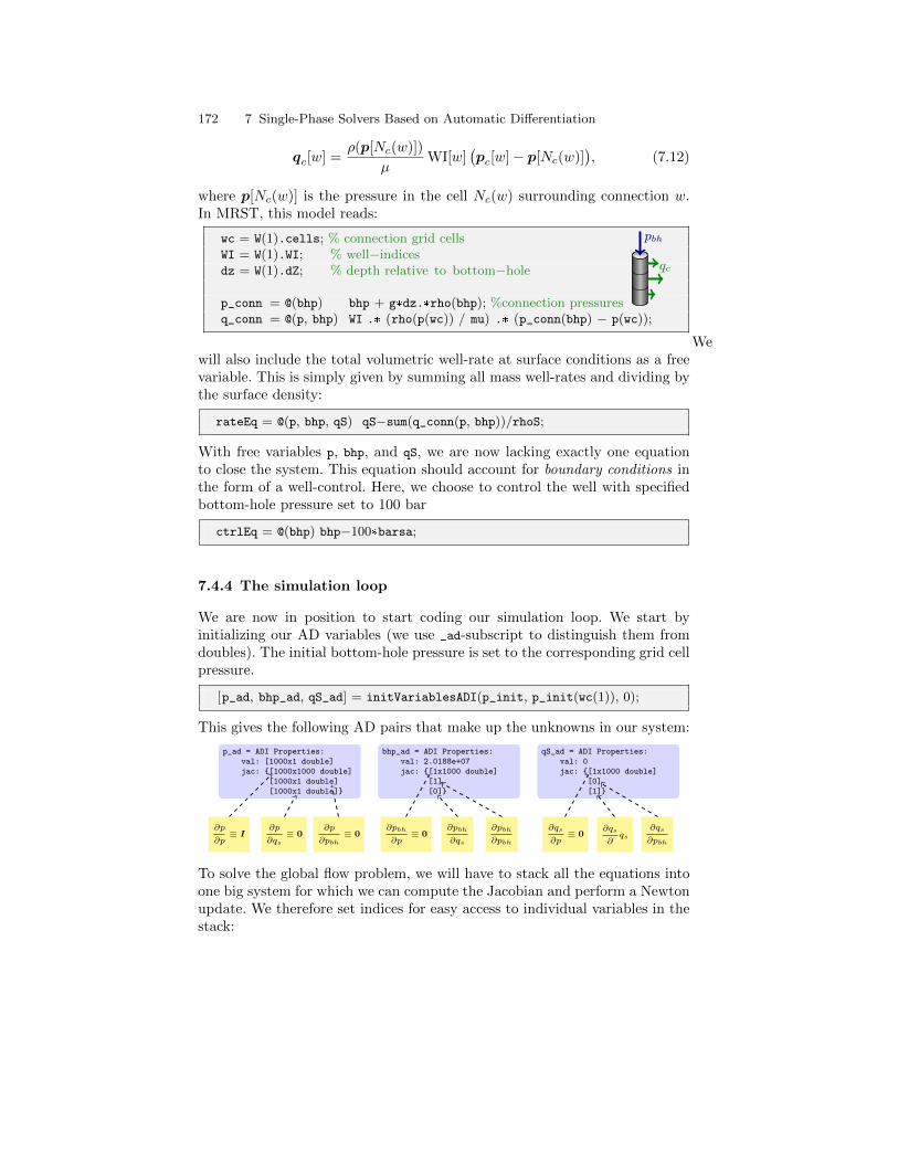
172 7 Single-Phase Solvers Based on Automatic Differentiation
qc[w] =ρ(p[Nc(w)])
µWI[w]
(pc[w]− p[Nc(w)]
), (7.12)
where p[Nc(w)] is the pressure in the cell Nc(w) surrounding connection w.In MRST, this model reads:
wc = W(1).cells; % connection grid cellsWI = W(1).WI; % well−indicesdz = W(1).dZ; % depth relative to bottom−hole
p_conn = @(bhp) bhp + g*dz.*rho(bhp); %connection pressuresq_conn = @(p, bhp) WI .* (rho(p(wc)) / mu) .* (p_conn(bhp) − p(wc));
pbh
qc
Wewill also include the total volumetric well-rate at surface conditions as a freevariable. This is simply given by summing all mass well-rates and dividing bythe surface density:
rateEq = @(p, bhp, qS) qS−sum(q_conn(p, bhp))/rhoS;
With free variables p, bhp, and qS, we are now lacking exactly one equationto close the system. This equation should account for boundary conditions inthe form of a well-control. Here, we choose to control the well with specifiedbottom-hole pressure set to 100 bar
ctrlEq = @(bhp) bhp−100*barsa;
7.4.4 The simulation loop
We are now in position to start coding our simulation loop. We start byinitializing our AD variables (we use _ad-subscript to distinguish them fromdoubles). The initial bottom-hole pressure is set to the corresponding grid cellpressure.
[p_ad, bhp_ad, qS_ad] = initVariablesADI(p_init, p_init(wc(1)), 0);
This gives the following AD pairs that make up the unknowns in our system:
p_ad = ADI Properties:val: [1000x1 double]jac: [1000x1000 double]
[1000x1 double][1000x1 double]
∂p
∂p≡ I
∂p
∂qs≡ 0
∂p
∂pbh≡ 0
bhp_ad = ADI Properties:val: 2.0188e+07jac: [1x1000 double]
[1][0]
∂pbh
∂p≡ 0
∂pbh
∂qs
∂pbh
∂pbh
qS_ad = ADI Properties:val: 0jac: [1x1000 double]
[0][1]
∂qs
∂p≡ 0
∂qs
∂qs
∂qs
∂pbh
To solve the global flow problem, we will have to stack all the equations intoone big system for which we can compute the Jacobian and perform a Newtonupdate. We therefore set indices for easy access to individual variables in thestack:
7.4 An implicit single-phase solver 173
[p_ad, bhp_ad, qS_ad] = initVariablesADI(p_init, p_init(wc(1)), 0);nc = G.cells.num;[pIx, bhpIx, qSIx] = deal(1:nc, nc+1, nc+2);
Next, we set parameters that will control the time steps in the simulation andthe iterations in the Newton solver:
numSteps = 52; % number of time−stepstotTime = 365*day; % total simulation timedt = totTime / numSteps; % constant time steptol = 1e−5; % Newton tolerancemaxits = 10; % max number of Newton its
We will store simulation results from all time steps in a structure sol, whichwe allocate before the main loop for efficiency and initialize so that the firstentry is the initial state of the reservoir:
sol = repmat(struct('time', [ ], 'pressure ' , [ ], 'bhp', [ ], ...'qS', []), [numSteps + 1, 1]);
sol(1) = struct('time', 0, 'pressure ' , double(p_ad), ...'bhp', double(bhp_ad), 'qS', double(qS_ad));
We now have all we need to set up the time-stepping algorithm, which willconsist of an outer and an inner loop. The outer loop updates the time step,advances the solution forward one step in time, and stores the result in thesol structure. This procedure is repeated until we reach the desired final time:
t = 0; step = 0;while t < totTime,
t = t + dt; step = step + 1;fprintf('\nTime step %d: Time %.2f −> %.2f days\n', ...
step, convertTo(t − dt, day), convertTo(t, day));% Newton loopresNorm = 1e99;p0 = double(p_ad); % Previous step pressurenit = 0;while (resNorm > tol) && (nit <= maxits)
: % Newton update:resNorm = norm(res);nit = nit + 1;fprintf(' Iteration %3d: Res = %.4e\n', nit, resNorm);
endif nit > maxits, error('Newton solves did not converge')else % store solution
sol(step+1) = struct('time', t, 'pressure ' , double(p_ad), ...'bhp', double(bhp_ad), 'qS', double(qS_ad));
endend
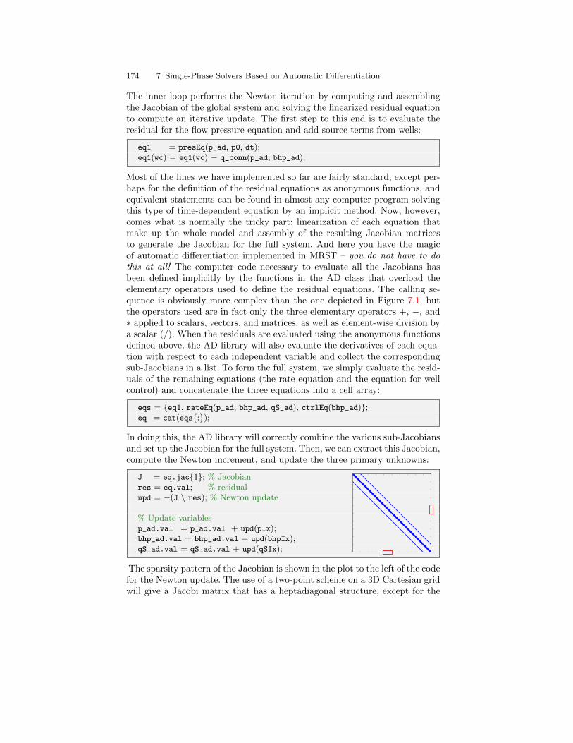
174 7 Single-Phase Solvers Based on Automatic Differentiation
The inner loop performs the Newton iteration by computing and assemblingthe Jacobian of the global system and solving the linearized residual equationto compute an iterative update. The first step to this end is to evaluate theresidual for the flow pressure equation and add source terms from wells:
eq1 = presEq(p_ad, p0, dt);eq1(wc) = eq1(wc) − q_conn(p_ad, bhp_ad);
Most of the lines we have implemented so far are fairly standard, except per-haps for the definition of the residual equations as anonymous functions, andequivalent statements can be found in almost any computer program solvingthis type of time-dependent equation by an implicit method. Now, however,comes what is normally the tricky part: linearization of each equation thatmake up the whole model and assembly of the resulting Jacobian matricesto generate the Jacobian for the full system. And here you have the magicof automatic differentiation implemented in MRST – you do not have to dothis at all! The computer code necessary to evaluate all the Jacobians hasbeen defined implicitly by the functions in the AD class that overload theelementary operators used to define the residual equations. The calling se-quence is obviously more complex than the one depicted in Figure 7.1, butthe operators used are in fact only the three elementary operators +, −, and∗ applied to scalars, vectors, and matrices, as well as element-wise division bya scalar (/). When the residuals are evaluated using the anonymous functionsdefined above, the AD library will also evaluate the derivatives of each equa-tion with respect to each independent variable and collect the correspondingsub-Jacobians in a list. To form the full system, we simply evaluate the resid-uals of the remaining equations (the rate equation and the equation for wellcontrol) and concatenate the three equations into a cell array:
eqs = eq1, rateEq(p_ad, bhp_ad, qS_ad), ctrlEq(bhp_ad);eq = cat(eqs:);
In doing this, the AD library will correctly combine the various sub-Jacobiansand set up the Jacobian for the full system. Then, we can extract this Jacobian,compute the Newton increment, and update the three primary unknowns:
J = eq.jac1; % Jacobianres = eq.val; % residualupd = −(J \ res); % Newton update
% Update variablesp_ad.val = p_ad.val + upd(pIx);bhp_ad.val = bhp_ad.val + upd(bhpIx);qS_ad.val = qS_ad.val + upd(qSIx);
The sparsity pattern of the Jacobian is shown in the plot to the left of the codefor the Newton update. The use of a two-point scheme on a 3D Cartesian gridwill give a Jacobi matrix that has a heptadiagonal structure, except for the
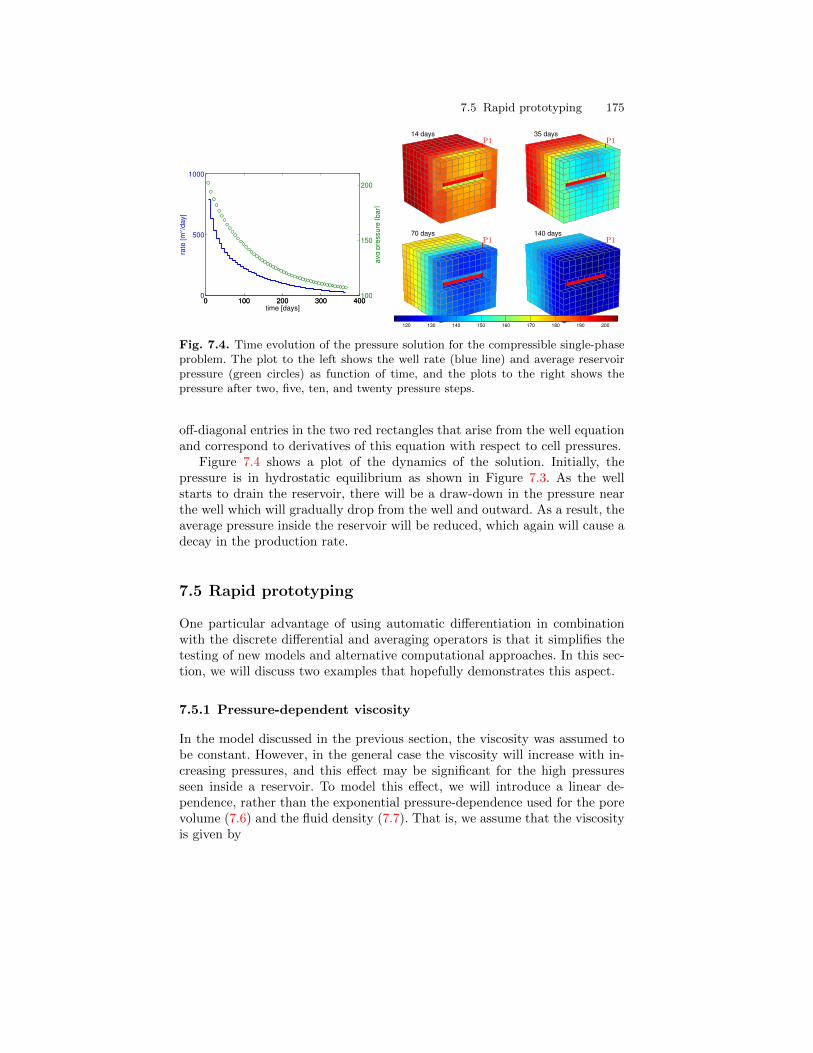
7.5 Rapid prototyping 175
0 100 200 300 4000
500
1000
time [days]
rate
[m
3/d
ay]
0 100 200 300 400100
150
200
avg p
ressure
[bar]
P1
14 daysP1
35 days
P1
70 days
P1
140 days
120 130 140 150 160 170 180 190 200
Fig. 7.4. Time evolution of the pressure solution for the compressible single-phaseproblem. The plot to the left shows the well rate (blue line) and average reservoirpressure (green circles) as function of time, and the plots to the right shows thepressure after two, five, ten, and twenty pressure steps.
off-diagonal entries in the two red rectangles that arise from the well equationand correspond to derivatives of this equation with respect to cell pressures.
Figure 7.4 shows a plot of the dynamics of the solution. Initially, thepressure is in hydrostatic equilibrium as shown in Figure 7.3. As the wellstarts to drain the reservoir, there will be a draw-down in the pressure nearthe well which will gradually drop from the well and outward. As a result, theaverage pressure inside the reservoir will be reduced, which again will cause adecay in the production rate.
7.5 Rapid prototyping
One particular advantage of using automatic differentiation in combinationwith the discrete differential and averaging operators is that it simplifies thetesting of new models and alternative computational approaches. In this sec-tion, we will discuss two examples that hopefully demonstrates this aspect.
7.5.1 Pressure-dependent viscosity
In the model discussed in the previous section, the viscosity was assumed tobe constant. However, in the general case the viscosity will increase with in-creasing pressures, and this effect may be significant for the high pressuresseen inside a reservoir. To model this effect, we will introduce a linear de-pendence, rather than the exponential pressure-dependence used for the porevolume (7.6) and the fluid density (7.7). That is, we assume that the viscosityis given by
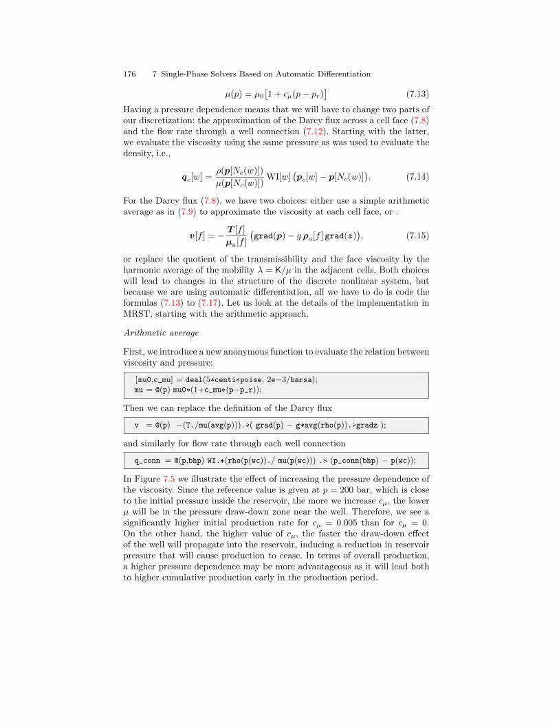
176 7 Single-Phase Solvers Based on Automatic Differentiation
µ(p) = µ0
[1 + cµ(p− pr)
](7.13)
Having a pressure dependence means that we will have to change two parts ofour discretization: the approximation of the Darcy flux across a cell face (7.8)and the flow rate through a well connection (7.12). Starting with the latter,we evaluate the viscosity using the same pressure as was used to evaluate thedensity, i.e.,
qc[w] =ρ(p[Nc(w)])
µ(p[Nc(w)])WI[w]
(pc[w]− p[Nc(w)]
). (7.14)
For the Darcy flux (7.8), we have two choices: either use a simple arithmeticaverage as in (7.9) to approximate the viscosity at each cell face, or .
v[f ] = − T [f ]
µa[f ]
(grad(p)− g ρa[f ] grad(z)
), (7.15)
or replace the quotient of the transmissibility and the face viscosity by theharmonic average of the mobility λ = K/µ in the adjacent cells. Both choiceswill lead to changes in the structure of the discrete nonlinear system, butbecause we are using automatic differentiation, all we have to do is code theformulas (7.13) to (7.17). Let us look at the details of the implementation inMRST, starting with the arithmetic approach.
Arithmetic average
First, we introduce a new anonymous function to evaluate the relation betweenviscosity and pressure:
[mu0,c_mu] = deal(5*centi*poise, 2e−3/barsa);mu = @(p) mu0*(1+c_mu*(p−p_r));
Then we can replace the definition of the Darcy flux
v = @(p) −(T./mu(avg(p))).*( grad(p) − g*avg(rho(p)).*gradz );
and similarly for flow rate through each well connection
q_conn = @(p,bhp) WI.*(rho(p(wc))./ mu(p(wc))) .* (p_conn(bhp) − p(wc));
In Figure 7.5 we illustrate the effect of increasing the pressure dependence ofthe viscosity. Since the reference value is given at p = 200 bar, which is closeto the initial pressure inside the reservoir, the more we increase cµ, the lowerµ will be in the pressure draw-down zone near the well. Therefore, we see asignificantly higher initial production rate for cµ = 0.005 than for cµ = 0.On the other hand, the higher value of cµ, the faster the draw-down effectof the well will propagate into the reservoir, inducing a reduction in reservoirpressure that will cause production to cease. In terms of overall production,a higher pressure dependence may be more advantageous as it will lead bothto higher cumulative production early in the production period.
7.5 Rapid prototyping 177
100 120 140 160 180 2002.5
3
3.5
4
4.5
5
5.5
pressure [bar]
vis
cosity [cP
]
cµ=0
cµ=0.002
cµ=0.005
0 50 100 150 200 250 300 350 400100
120
140
160
180
200
220
time [days]
avg p
ressure
[bar]
cµ=0
cµ=0.002
cµ=0.005
0 50 100 150 200 250 300 350 4000
200
400
600
800
1000
1200
time [days]
rate
[m
3/d
ay]
cµ=0
cµ=0.002
cµ=0.005
0 50 100 150 200 250 300 350 4000
1000
2000
3000
4000
5000
6000
7000
8000
9000
10000
time [days]
cu
mm
ula
tive
pro
du
ctio
n [
m3]
cµ=0
cµ=0.002
cµ=0.005
Fig. 7.5. The effect of increasing the degree of pressure-dependence for the viscosity.
Face mobility: harmonic average
A more correct approximation is to write Darcy’s law based on mobility in-stead of using the quotient of the transmissibility and an averaged viscosity:
v[f ] = −Λ[f ](grad(p)− g ρa[f ] grad(z)
). (7.16)
The face mobility Λ[f ] can be defined in the same way as the transmissibilityis defined in terms of the half transmissibilities using harmonic averages. Thatis, if T [f, c] denotes the half transmissibility associated with face f and cellc, the face mobility Λ[f ] for face f can be written as
Λ[f ] =( µ[N1(f)]
T [f,N1(f)]+
µ[N2(f)]
T [f,N2(f)]
)−1
. (7.17)
In MRST, the corresponding code reads:
hf2cn = getCellNoFaces(G);nhf = numel(hf2cn);hf2f = sparse(double(G.cells.faces(:,1)),(1:nhf)',1);hf2if = hf2f(intInx,:);hlam = @(mu,p) 1./(hf2if*(mu(p(hf2cn))./hT));
v = @(p) −hlam(mu,p).*( grad(p) − g*avg(rho(p)).*gradz );
178 7 Single-Phase Solvers Based on Automatic Differentiation
Here, hf2cn represents the maps N1 and N2 that enables us to sample theviscosity value in the correct cell for each half-face transmissibility, whereashf2if represents a map from half faces (i.e., faces seen from a single cell) toglobal faces (which are shared by two cells). The map has a unit value in rowi and column j if half face j belongs to global face i. Hence, premultiplying avector of half-face quantities by hf2if amounts to summing the contributionsfrom cells N1(f) and N2(f) for each global face f .
For a homogeneous model, using the harmonic average should produce sim-ulation results that are identical (to machine precision) to those produced byusing arithmetic average. With heterogeneous permeability, there will be smalldifferences in the well rates and averaged pressures for the specific parame-ters considered herein. For sub-samples of the SPE 10 data set, we typicallyobserve maximum relative differences in well rates of the order 10−3.
7.5.2 Non-Newtonian fluid
Viscosity is the material property that measures a fluid’s resistance to flow,i.e., the resistance to a change in shape, or to the movement of neighboringportions of the fluid relative to each other. The more viscous a fluid is, the lesseasily it will flow. In Newtonian fluids, the shear stress (the force applied perarea tangential to the force), at any point is proportional to the strain rate (thesymmetric part of the velocity gradient) at that point and the viscosity is theconstant of proportionality. For non-Newtonian fluids, the relationship is nolonger linear. The most common nonlinear behavior is shear thinning, in whichthe viscosity of the system decreases as the shear rate is increased. An exampleis paint, which should flow easily when leaving the brush, but stay on thesurface and not drip once it has been applied. The second type of nonlinearityis shear thickening, in which the viscosity increases with increasing shear rate.A common example is the mixture of cornstarch and water. If you searchYouTube for “cornstarch pool” you can view several spectacular videos ofpools filled with this mixture. When stress is applied to the liquid, it exhibitsproperties like a solid and you may be able to run across its surface. However,if you go too slow, it will behave more like a liquid and you will fall in.
Solutions of large polymeric molecules are another example of shear-thinning liquids. In enhanced oil recovery, polymer solutions may be injectedinto reservoirs to improve unfavorable mobility ratios between oil and waterand improve the sweep efficiency of the injected fluid. At low flow rates, thepolymer molecule chains will tumble around randomly and present large re-sistance to flow. When the flow velocity increases, the viscosity will decreaseas the molecules will gradually align themselves in the direction of increasingshear rate. A model of the rheology is given by
µ = µ∞ + (µ0 − µ∞)
(1 +
(Kc
µ0
) 2n−1
γ2
)n−12
, (7.18)
7.5 Rapid prototyping 179
where µ0 represents the Newtonian viscosity at zero shear rate, µ∞ representsthe Newtonian viscosity at infinite shear rate, Kc represents the consistencyindex, and n represents the power-law exponent (n < 1). The shear rate γ ina porous medium can be approximated by
γapp = 6
(3n+ 1
4n
) nn−1 |~v|√
Kφ. (7.19)
Combining (7.18) and (7.19), we can write our model for the viscosity as
µ = µ0
(1 + Kc
|~v|2
Kφ
)n−12
, Kc = 36
(Kc
µ0
) 2n−1
(3n+ 1
4n
) 2nn−1
, (7.20)
where we for simplicity have assumed that µ∞ = 0. In the following, we willshow how easy it is to extend the simulator developed in the previous sectionsto model this non-Newtonian fluid behavior (see nonNewtonianCell.m). Tosimulate injection, we increase the bottom-hole pressure to 300 bar. Our rhe-ology model has parameters:
mu0 = 100*centi*poise;nmu = 0.3;Kc = .1;Kbc = (Kc/mu0)ˆ(2/(nmu−1))*36*((3*nmu+1)/(4*nmu))ˆ(2*nmu/(nmu−1));
In principle, we could continue to solve the system using the same primaryunknowns as before. However, it has proved convenient to write (7.20) in theform µ = η µ0 and introduce η as an additional unknown. In each Newtonstep, we start by solving the equation for the shear factor η exactly for thegiven pressure distribution. This is done by initializing an AD variable for η,but not for p in etaEq so that this residual now only has one unknown, η.This will take out the implicit nature of Darcy’s law and hence reduce thenonlinearity and simplify the solution of the global system.
while (resNorm > tol) && (nit < maxits)
% Newton loop for eta (shear multiplier)[resNorm2,nit2] = deal(1e99, 0);eta_ad2 = initVariablesADI(eta_ad.val);while (resNorm2 > tol) && (nit2 <= maxits)eeq = etaEq(p_ad.val, eta_ad2);res = eeq.val;eta_ad2.val = eta_ad2.val − (eeq.jac1 \ res);resNorm2 = norm(res);nit2 = nit2+1;
endeta_ad.val = eta_ad2.val;
180 7 Single-Phase Solvers Based on Automatic Differentiation
Once the shear factor has been computed for the values in the previous iterate,we can use the same approach as earlier to compute a Newton update for thefull system. (Here, etaEq is treated as a system with two unknowns, p and η.)
eq1 = presEq(p_ad, p0, eta_ad, dt);eq1(wc) = eq1(wc) − q_conn(p_ad, eta_ad, bhp_ad);eqs = eq1, etaEq(p_ad, eta_ad), ...rateEq(p_ad, eta_ad, bhp_ad, qS_ad), ctrlEq(bhp_ad);
eq = cat(eqs:);upd = −(eq.jac1 \ eq.val); % Newton update
To finish the solver, we will of course need to define the flow equations andthe extra equation for the shear multiplier. The main question to this end is:how should we compute |~v|? One solution could be to define |~v| on each faceas the flux divided by the face area. In other words, use a code like
phiK = avg(rock.perm.*rock.poro)./G.faces.areas(intInx).ˆ2;v = @(p, eta) −(T./(mu0*eta)).*( grad(p) − g*avg(rho(p)).*gradz );etaEq = @(p, eta) eta − (1 + Kbc*v(p,eta).ˆ2./phiK).ˆ((nmu−1)/2);
Although simple, this approach has three potential issues: First, it does nottell us how to compute the shear factor for the well perforations. Second, itdisregards contributions from any tangential components of the velocity field.Third, the number of unknowns in the linear system will increase by almosta factor six since we now will have one extra unknown per internal face. Thefirst issue is easy to fix: to get a representative value in the well cells, wesimply average the η values from the cells’ faces. If we now recall how the dis-crete divergence operator was defined, we realize that this operation is almostimplemeted for us already: if div(x)=-C’*x computes the discrete divergencein each cell of the field x defined at the faces, then cavg(x)=1/6*abs(C)’*x
will compute the average of x for each cell. In other words, our well equationbecomes:
wavg = @(eta) 1/6*abs(C(:,W.cells))'*eta;q_conn = @(p, eta, bhp) ...WI .* (rho(p(wc)) ./ (mu0*wavg(eta))) .* (p_conn(bhp) − p(wc));
The second issue would have to be investigated in more detail and this is notwithin the scope of this book. The third issue is simply a disadvantage.
To get a method that consumes less memory, we can compute one η valueper cell. Using the following formula, we can compute an approximate velocity~vi at the center of cell i
~vi =∑
j∈N(i)
vijVi
(~cij − ~ci
), (7.21)
where N(i) is the map from cell i to its neighboring cells, vij is the fluxbetween cell i and cell j, ~cij is the centroid of the corresponding face, and ~ci
7.5 Rapid prototyping 181
is the centroid of cell i. For a Cartesian grid, this formula simplifies so that anapproximate velocity can be obtained as the sum of the absolute value of theflux divided by the face area over all faces that make up a cell. Using a similartrick as we used to compute η in well cells above, our implementation followstrivially. We first define the averaging operator to compute cell velocity
aC = bsxfun(@rdivide, 0.5*abs(C), G.faces.areas(intInx))';cavg = @(x) aC*x;
In doing so, we also rename our old averaging operator avg as favg to avoidconfusion and make it more clear that this operator maps from cell values toface values. Then we can define the needed equations:
phiK = rock.perm.*rock.poro;gradz = grad(G.cells.centroids(:,3));v = @(p, eta)−(T./(mu0*favg(eta))).*( grad(p) − g*favg(rho(p)).*gradz );
etaEq = @(p, eta)eta − ( 1 + Kbc* cavg(v(p,eta)).ˆ2 ./phiK ).ˆ((nmu−1)/2);
presEq= @(p, p0, eta, dt) ...(1/dt)*(pv(p).*rho(p) − pv(p0).*rho(p0)) + div(favg(rho(p)).*v(p, eta));
With this approach the well equation becomes particularly simple since all weneed to do is to sample the η value from the correct cell:
q_conn = @(p, eta, bhp) ...WI .* (rho(p(wc)) ./ (mu0*eta(wc))) .* (p_conn(bhp) − p(wc));
A potential drawback of this second approach is that it may introduce nu-merical smearing, but this will, on the other hand, most likely increase therobustness of the resulting scheme.
In Figure 7.6 we compare the predicted flow rates and average reservoirpressure for two different fluid models: one that assumes that the fluid is astandard Newtonian fluid (i.e., η ≡ 1) and one that models shear thinning,which has been computed by both methods discussed above. With shear thin-ning, the higher pressure in the injection well will cause a decrease in theviscosity which will lead to significantly higher injection rates than for theNewtonian fluid and hence a higher average reservoir pressure. Perhaps moreinteresting is the large discrepancy in the rates and pressures predicted by theface-based and the cell-based simulation algorithms. If we in the face-basedmethod disregard the shear multiplier q_conn, the predicted rate and pressurebuild-up is smaller than what is predicted by the cell-based method and closerto the Newtonian fluid case. We take this as evidence that the differences be-tween the cell and the face-base methods to a large extent can be explainedby differences in the discretized well models and their ability to capture theformation and propagation of the strong initial transient. To further back thisup, we have included results from a simulation with ten times as many timesteps in Figure 7.7, which also includes plots of the evolution of min(η) as a
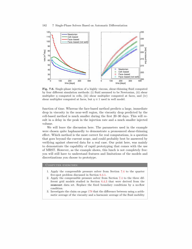
182 7 Single-Phase Solvers Based on Automatic Differentiation
0 100 200 300 40020
30
40
50
60
70
80
90
100
110
120
time [days]
rate
[m
3/d
ay]
Newtonian
Cell−based
Face−based
Face−based (not well)
0 100 200 300 400200
205
210
215
220
225
230
235
time [days]
avg
pre
ssu
re [
ba
r]
Newtonian
Cell−based
Face−based
Face−based (not well)
Fig. 7.6. Single-phase injection of a highly viscous, shear-thinning fluid computedby four different simulation methods: (i) fluid assumed to be Newtonian, (ii) shearmultiplier η computed in cells, (iii) shear multiplier computed at faces, and (iv)shear multiplier computed at faces, but η ≡ 1 used in well model.
function of time. Whereas the face-based method predicts a large, immediatedrop in viscosity in the near-well region, the viscosity drop predicted by thecell-based method is much smaller during the first 20–30 days. This will re-sult in a delay in the peak in the injection rate and a much smaller injectedvolume.
We will leave the discussion here. The parameters used in the examplewere chosen quite haphazardly to demonstrate a pronounced shear-thinningeffect. Which method is the most correct for real computations, is a questionthat goes beyond the current scope, and could probably best be answered byverifying against observed data for a real case. Our point here, was mainlyto demonstrate the capability of rapid prototyping that comes with the useof MRST. However, as the example shows, this lunch is not completely free:you will still have to understand features and limitations of the models anddiscretizations you choose to prototype.
Computer exercises:
1. Apply the compressible pressure solver from Section 7.4 to the quarterfive-spot problem discussed in Section 6.4.1.
2. Apply the compressible pressure solver from Section 7.4 to the three dif-ferent grid models studied in Section 6.4.3 that were derived from theseamount data set. Replace the fixed boundary conditions by a no-flowcondition.
3. Investigate the claim on page 178 that the difference between using a arith-metic average of the viscosity and a harmonic average of the fluid mobility
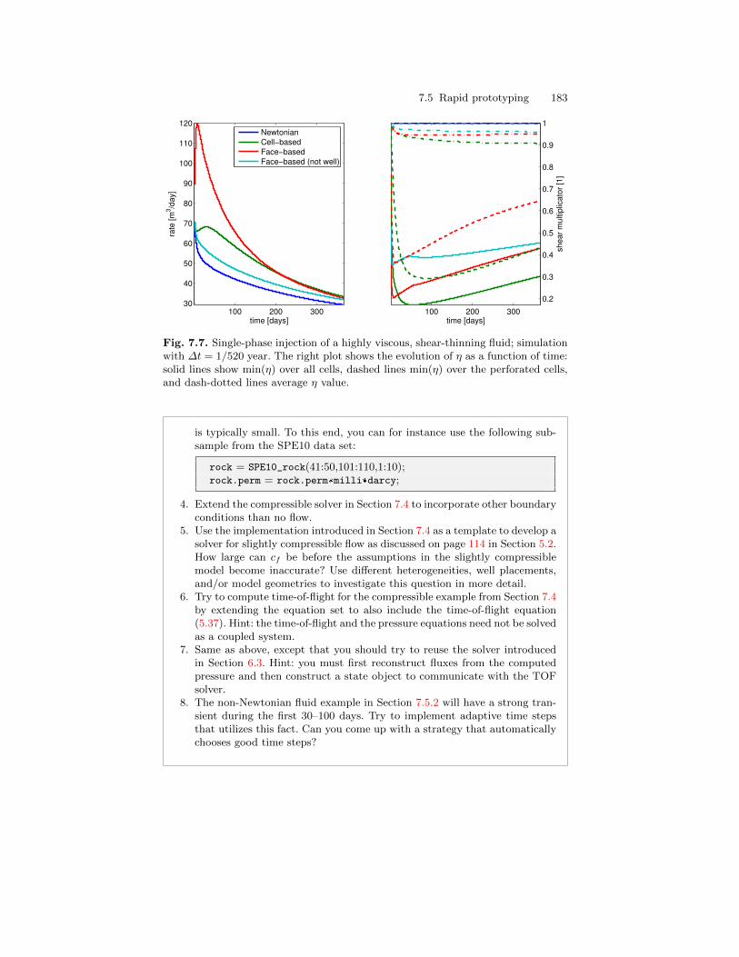
7.5 Rapid prototyping 183
100 200 30030
40
50
60
70
80
90
100
110
120
time [days]
rate
[m
3/d
ay]
Newtonian
Cell−based
Face−based
Face−based (not well)
100 200 300
0.2
0.3
0.4
0.5
0.6
0.7
0.8
0.9
1
time [days]
sh
ea
r m
ultip
lica
tor
[1]
Fig. 7.7. Single-phase injection of a highly viscous, shear-thinning fluid; simulationwith ∆t = 1/520 year. The right plot shows the evolution of η as a function of time:solid lines show min(η) over all cells, dashed lines min(η) over the perforated cells,and dash-dotted lines average η value.
is typically small. To this end, you can for instance use the following sub-sample from the SPE10 data set:
rock = SPE10_rock(41:50,101:110,1:10);rock.perm = rock.perm*milli*darcy;
4. Extend the compressible solver in Section 7.4 to incorporate other boundaryconditions than no flow.
5. Use the implementation introduced in Section 7.4 as a template to develop asolver for slightly compressible flow as discussed on page 114 in Section 5.2.How large can cf be before the assumptions in the slightly compressiblemodel become inaccurate? Use different heterogeneities, well placements,and/or model geometries to investigate this question in more detail.
6. Try to compute time-of-flight for the compressible example from Section 7.4by extending the equation set to also include the time-of-flight equation(5.37). Hint: the time-of-flight and the pressure equations need not be solvedas a coupled system.
7. Same as above, except that you should try to reuse the solver introducedin Section 6.3. Hint: you must first reconstruct fluxes from the computedpressure and then construct a state object to communicate with the TOFsolver.
8. The non-Newtonian fluid example in Section 7.5.2 will have a strong tran-sient during the first 30–100 days. Try to implement adaptive time stepsthat utilizes this fact. Can you come up with a strategy that automaticallychooses good time steps?

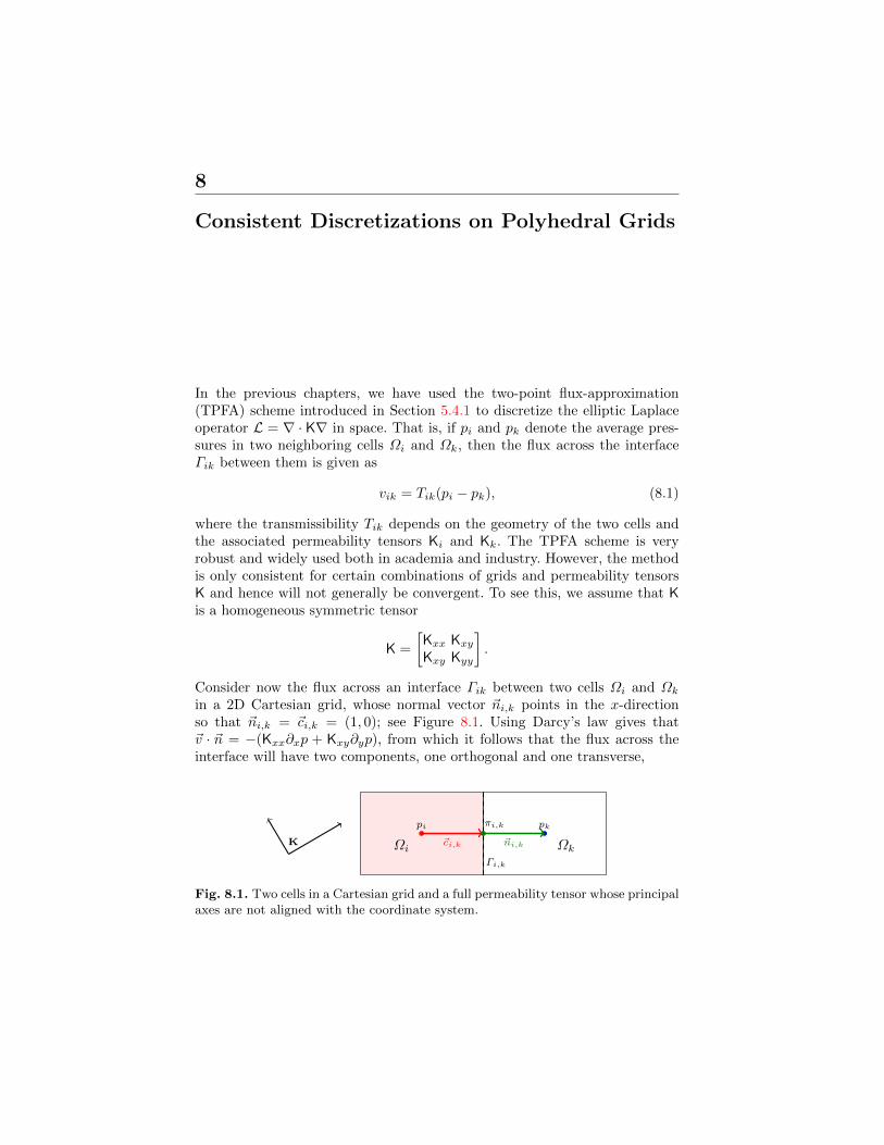
8
Consistent Discretizations on Polyhedral Grids
In the previous chapters, we have used the two-point flux-approximation(TPFA) scheme introduced in Section 5.4.1 to discretize the elliptic Laplaceoperator L = ∇ · K∇ in space. That is, if pi and pk denote the average pres-sures in two neighboring cells Ωi and Ωk, then the flux across the interfaceΓik between them is given as
vik = Tik(pi − pk), (8.1)
where the transmissibility Tik depends on the geometry of the two cells andthe associated permeability tensors Ki and Kk. The TPFA scheme is veryrobust and widely used both in academia and industry. However, the methodis only consistent for certain combinations of grids and permeability tensorsK and hence will not generally be convergent. To see this, we assume that Kis a homogeneous symmetric tensor
K =
[Kxx KxyKxy Kyy
].
Consider now the flux across an interface Γik between two cells Ωi and Ωkin a 2D Cartesian grid, whose normal vector ~ni,k points in the x-directionso that ~ni,k = ~ci,k = (1, 0); see Figure 8.1. Using Darcy’s law gives that~v · ~n = −(Kxx∂xp + Kxy∂yp), from which it follows that the flux across theinterface will have two components, one orthogonal and one transverse,
pi
ΩiΓi,k
pk
Ωk~ni,k~ci,k
πi,k
K
Fig. 8.1. Two cells in a Cartesian grid and a full permeability tensor whose principalaxes are not aligned with the coordinate system.
186 8 Consistent Discretizations on Polyhedral Grids
vik = −∫Γik
K∇p · ~n ds = −∫Γik
(Kxx ∂xp+ Kxy ∂yp
)ds
that correspond to the x-derivative and the y-derivative of the pressure, re-spectively. In the two-point approximation (8.1), the only points we can useto approximate these flux contributions are the pressures pi and pk, but sincethese two pressures are associated with the same y-value, their difference canonly be used to estimate ∂xp and not ∂yp. This means that the TPFA methodcannot account for the transverse flux contribution Kxy∂yp and will hencegenerally not be consistent. The only exception is if Kxy ≡ 0 in all cells inthe grid, in which case there are no fluxes in the transverse direction. To linkthe above derivation to the geometry of the cells, we can use the one-sideddefinition of fluxes (5.48) of the two-point scheme, two write
vi,k ≈ Ti,k(pi − πi,k) =Ai,k|~ci,k|2
K~ci,k · ~ni,k(pi − πi,k).
More generally, we have that the TPFA scheme is only convergent for K-orthogonal grids. An example of a K-orthogonal grid is a grid in which all cellsare parallelepipeds in 3D or parallelograms in 2D and satisfy the condition
~ni,j · K~ni,k = 0, ∀j 6= k, (8.2)
where ~ni,j and ~ni,k denote normal vectors to faces of cell number i.What about grids that are not parallelepipeds or parallelograms? For sim-
plicity, we only consider the 2D case. Let ~c = (c1, c2) denote the vector fromthe center of cell Ωi to the centroid of face Γik, see Figure 5.4. If we let~c⊥ = (c2,−c1) denote a vector that is orthogonal to ~c, then any constantpressure gradient inside Ωi can be written as ∇p = p1~c+ p2~c⊥, where p1 canbe determined from pi and πi,k and p2 is some unknown constant. Insertedinto the definition of the face flux, this gives
vi,k = −∫Γik
(p1K~c · ~n+ p2K~c⊥ · ~n
)ds.
For the two-point scheme to be correct, the second term in the integrand mustbe zero. Setting ~n = (n1, n2), we have that
0 = K~c⊥ · ~n = (K1c2,−K2c1) · (n1, n2) = (K1n1c2 −K2n2c1) = (K~n)× ~c.
In other words, a sufficient condition for a polygonal grid to be K-orthogonalis that (K~ni,k) ‖ ~ci,k for all cells in the grid, in which case the transverse fluxcontributions are all zero and hence need not be estimated. Consequently, theTPFA method will be consistent.
The lack of consistency in the TPFA scheme for grids that are not K-orthogonal may lead to significant grid-orientation effects, i.e., artifacts orerrors in the solution that will appear in varying degree depending upon the
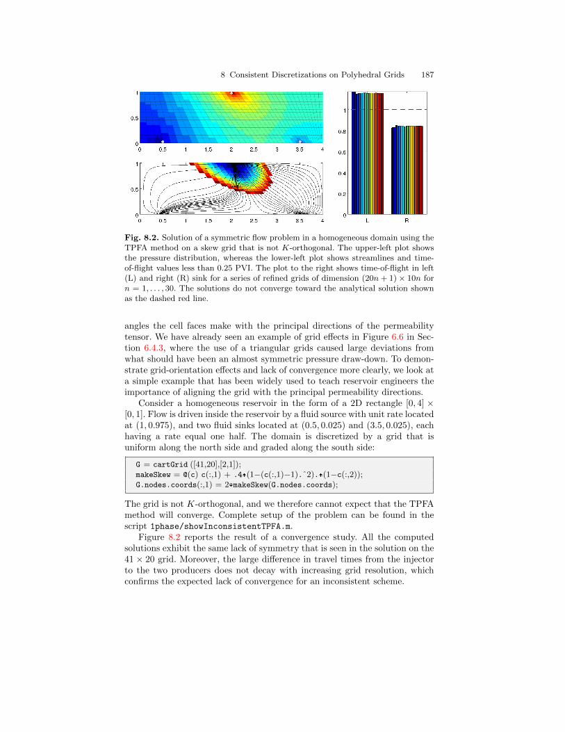
8 Consistent Discretizations on Polyhedral Grids 187
Fig. 8.2. Solution of a symmetric flow problem in a homogeneous domain using theTPFA method on a skew grid that is not K-orthogonal. The upper-left plot showsthe pressure distribution, whereas the lower-left plot shows streamlines and time-of-flight values less than 0.25 PVI. The plot to the right shows time-of-flight in left(L) and right (R) sink for a series of refined grids of dimension (20n+ 1)× 10n forn = 1, . . . , 30. The solutions do not converge toward the analytical solution shownas the dashed red line.
angles the cell faces make with the principal directions of the permeabilitytensor. We have already seen an example of grid effects in Figure 6.6 in Sec-tion 6.4.3, where the use of a triangular grids caused large deviations fromwhat should have been an almost symmetric pressure draw-down. To demon-strate grid-orientation effects and lack of convergence more clearly, we look ata simple example that has been widely used to teach reservoir engineers theimportance of aligning the grid with the principal permeability directions.
Consider a homogeneous reservoir in the form of a 2D rectangle [0, 4] ×[0, 1]. Flow is driven inside the reservoir by a fluid source with unit rate locatedat (1, 0.975), and two fluid sinks located at (0.5, 0.025) and (3.5, 0.025), eachhaving a rate equal one half. The domain is discretized by a grid that isuniform along the north side and graded along the south side:
G = cartGrid ([41,20],[2,1]);makeSkew = @(c) c(:,1) + .4*(1−(c(:,1)−1).ˆ2).*(1−c(:,2));G.nodes.coords(:,1) = 2*makeSkew(G.nodes.coords);
The grid is not K-orthogonal, and we therefore cannot expect that the TPFAmethod will converge. Complete setup of the problem can be found in thescript 1phase/showInconsistentTPFA.m.
Figure 8.2 reports the result of a convergence study. All the computedsolutions exhibit the same lack of symmetry that is seen in the solution on the41 × 20 grid. Moreover, the large difference in travel times from the injectorto the two producers does not decay with increasing grid resolution, whichconfirms the expected lack of convergence for an inconsistent scheme.
188 8 Consistent Discretizations on Polyhedral Grids
8.1 The Mixed Finite-Element Method
There are several ways to formulate consistent discretization methods. In thissection, we will introduce a method, the mixed finite-element method [15],which is based on a formulation that is quite different from the one we haveseen so far for the inconsistent two-point method. The first new idea is thatinstead of forming a second-order elliptic pressure equation, we will form a sys-tem of equations consisting of two first-order equations: the mass-conservationequation and Darcy’s law. This means that unlike for the TPFA method, inwhich discrete fluxes are computed by post-processing the pressure solution,the mixed method solves for pressure and fluxes simultaneously. The secondnew idea is to look for solutions that satisfy the flow equations in a weaksense; that is, look for solutions that fulfill the equation when multiplied witha suitable test function and integrated in space. The third new idea is to ex-press the unknown solution as a linear combination of a set of basis functionsthat take the form of piecewise polynomials with localized support.
The mixed finite-element method is not implemented directly in MRST,but the key ideas of this method will be instrumental in the development of ageneral class of finite-volume discretizations that will be outlined in Section 8.2and discussed in more details in the remaining sections of the chapter. As aprecursor to this discussion, we will in the following present the mixed finite-element method in some detail.
8.1.1 Continuous Formulation
We start by restating the continuous flow equation in full detail:
∇ · ~v = q, ~v = −K∇p, ~x ∈ Ω ⊂ Rd (8.3)
with boundary conditions ~v × ~n for ~x ∈ ∂Ω. For compatibility, we requirethat
∫Ωq d~x = 0. Since this is a pure Neumann boundary-value problem,
the pressure p is only defined up to an arbitrary constant, and as an extraconstraint, we require that
∫Ωp d~x = 0.
In the mixed method, we will look for solutions that lie in an abstractfunction space. To this end, we need two spaces: L2(Ω) is the space of squareintegrable functions, and Hdiv
0 is a so-called Sobolev space defined as
Hdiv0 (Ω) = ~v ∈ L2(Ω)d : ∇ · ~v ∈ L2(Ω) and ~v · ~n on ∂Ω, (8.4)
i.e., the set of square-integrable, vector-valued functions that have compactsupport in Ω and whose divergence is also square integrable. The mixed for-mulation of (8.3) now reads: find a pair (p,~v) that lies in L2(Ω) × Hdiv
0 (Ω)and satisfies∫
Ω
~u · K−1~v d~x−∫Ω
p∇ · ~u d~x = 0, ∀~u ∈ Hdiv0 (Ω),∫
Ω
w∇ · ~v d~x =
∫Ω
qw d~x, ∀w ∈ L2(Ω).
(8.5)
8.1 The Mixed Finite-Element Method 189
The first equation follows by multiplying Darcy’s law by K−1 applying thedivergence theorem to the term involving the pressure gradient. (Recall that~u is zero on ∂Ω by definition so that the term
∫∂Ω
p~u · ~n ds = 0).Equation (8.5) can be written on a more compact form if we introduce the
following three inner products
b(·, ·) : Hdiv0 ×Hdiv
0 → R, b(~u,~v) =
∫Ω
~u · K−1~v d~x
c(·, ·) : Hdiv0 × L2 → R, c(~u, p) =
∫Ω
p∇ · ~u d~x
(·, ·) : L2 × L2 → R, (q, w) =
∫Ω
qw d~x,
(8.6)
and write
b(~u,~v)− c(~u, p) = 0
c(~v, w) = (q, w)(8.7)
The mixed formulation (8.7) can alternatively be derived by minimizing theenergy functional
I(~v) =1
2
∫Ω
~v · K−1~v d~x,
over all functions ~v ∈ Hdiv0 (Ω) that are mass conservative, i.e., subject to the
constraint∇ · ~v = q.
The common strategy for solving such mimization problems is to introduce aLagrangian functional, which in our case reads
L(~v, p) =
∫Ω
(12~v · K
−1~v − p(∇ · ~v − q
))d~x =
1
2b(~v,~v)− c(~v, p) + (p, q),
where p is the so-called the Lagrangian multiplier. At a minimum of L, wemust have that ∂L/∂~v = 0. Looking at an increment ~u of ~v, we have therequirement that
0 =∂L
∂~v~u = lim
ε→0
1
ε
[L(~v + ε~u, p)− L(~v, p)
]= b(~u,~v)− c(~u, p)
must be zero for all u ∈ Hdiv0 (Ω). Similarly, we can show that
0 =∂L
∂pw = lim
ε→0
1
ε
[L(~v, p+ εw)− L(~v, p)
]= −c(~v, w) + (q, w)
must be zero for all w ∈ L2(Ω). To show that the solution ~v is a minimal point,we consider a perturbation ~v + ~u that satisfies the constraints, i.e., ~u ∈ Hdiv
0
and ∇ · ~u = 0. For the energy functional we have that
190 8 Consistent Discretizations on Polyhedral Grids
I(~v + ~u) =1
2
∫Ω
(~v + ~u) · K−1(~v + ~u) d~x = I(~v) + I(~u) + b(~u,~v)
= I(~v) + I(~u) + c(~u, p) = I(~v) + I(~u) > I(~v),
which proves that ~v is indeed a minimum of I. One can also prove that thesolution (p,~v) is a saddle-point of the Lagrange functional, i.e., that L(~v, w) ≤L(~v, p) ≤ L(~u, p) for all ~u 6= ~v and w 6= p. The right inequality can be shownas follows
L(~v + ~u, p) = 12b(~v + ~u,~v + ~u)− c(~v + ~u, p) + (q, p)
= L(~v, p) + I(~u) + b(~u,~v)− c(~u, p) = L(~v, p) + I(~u) > L(~v, p).
The left inequality follows in a similar manner.
8.1.2 Discrete Formulation
To discretize the mixed formulation, (8.5), we introduce a grid Ωh = ∪Ωi andreplace L2(Ω) and Hdiv
0 (Ω) by finite-dimensional subspaces U and V definedover the grid. Likewise, we rewrite the inner products (8.6) as sums of integralslocalized to cells
b(·, ·)h : V × V → R, b(~u,~v)h =∑i
∫Ωi
~u · K−1~v d~x
c(·, ·)h : V × U → R, c(~u, p)h =∑i
∫Ωi
p∇ · ~u d~x
(·, ·)h : U × U → R, (q, w)h =∑i
∫Ωi
qw d~x,
(8.8)
To obtain a practical numerical method, the spaces U and V are typicallydefined as piecewise polynomial functions that are nonzero on a small col-lection of grid cells. For instance, in the Raviart–Thomas method [55, 15] oflowest order for triangular, tetrahedral or regular parallelepiped grids, L2(Ω)is replaced by
U = p ∈ L2(∪Ωi) : p|Ωi is constant ∀Ωi ⊂ Ω = spanχi,
where χi is the characteristic function of grid cell Ωi,
χi =
1, ~x ∈ Ωi0, otherwise.
Likewise, Hdiv0 (Ω) is replaced by a space V consisting of functions ~v ∈
Hdiv0 (∪Ωi) that have linear components on each grid cell Ωi ∈ Ω, has normal
components ~v · ~nik that are constant on each cell interface Γik and contin-uous across these interfaces. These requirements are satisfied by functions
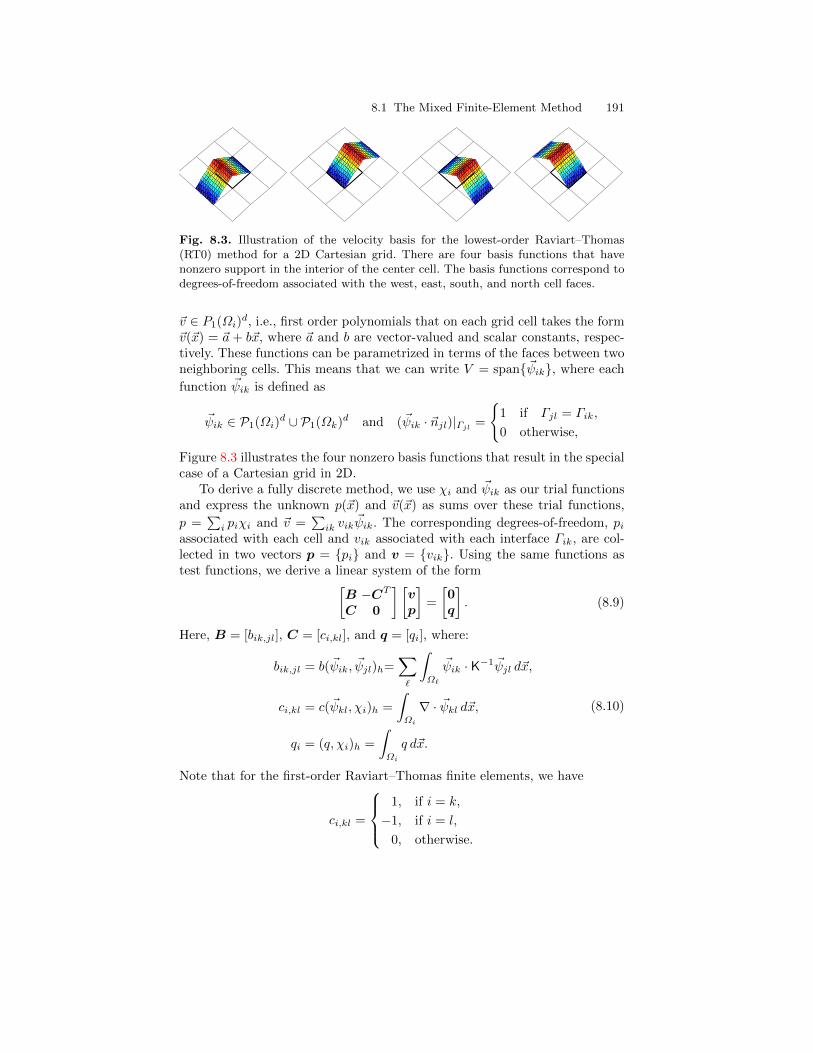
8.1 The Mixed Finite-Element Method 191
Fig. 8.3. Illustration of the velocity basis for the lowest-order Raviart–Thomas(RT0) method for a 2D Cartesian grid. There are four basis functions that havenonzero support in the interior of the center cell. The basis functions correspond todegrees-of-freedom associated with the west, east, south, and north cell faces.
~v ∈ P1(Ωi)d, i.e., first order polynomials that on each grid cell takes the form
~v(~x) = ~a + b~x, where ~a and b are vector-valued and scalar constants, respec-tively. These functions can be parametrized in terms of the faces between twoneighboring cells. This means that we can write V = span~ψik, where each
function ~ψik is defined as
~ψik ∈ P1(Ωi)d ∪ P1(Ωk)d and (~ψik · ~njl)|Γjl
=
1 if Γjl = Γik,
0 otherwise,
Figure 8.3 illustrates the four nonzero basis functions that result in the specialcase of a Cartesian grid in 2D.
To derive a fully discrete method, we use χi and ~ψik as our trial functionsand express the unknown p(~x) and ~v(~x) as sums over these trial functions,
p =∑i piχi and ~v =
∑ik vik
~ψik. The corresponding degrees-of-freedom, piassociated with each cell and vik associated with each interface Γik, are col-lected in two vectors p = pi and v = vik. Using the same functions astest functions, we derive a linear system of the form[
B −CT
C 0
] [vp
]=
[0q
]. (8.9)
Here, B = [bik,jl], C = [ci,kl], and q = [qi], where:
bik,jl = b(~ψik, ~ψjl)h=∑`
∫Ω`
~ψik · K−1 ~ψjl d~x,
ci,kl = c(~ψkl, χi)h =
∫Ωi
∇ · ~ψkl d~x,
qi = (q, χi)h =
∫Ωi
q d~x.
(8.10)
Note that for the first-order Raviart–Thomas finite elements, we have
ci,kl =
1, if i = k,
−1, if i = l,
0, otherwise.
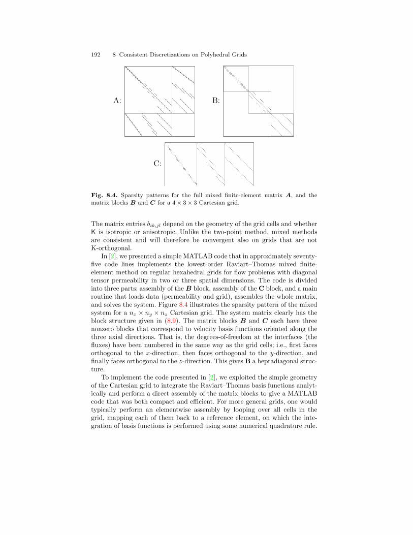
192 8 Consistent Discretizations on Polyhedral Grids
A: B:
C:
Fig. 8.4. Sparsity patterns for the full mixed finite-element matrix A, and thematrix blocks B and C for a 4× 3× 3 Cartesian grid.
The matrix entries bik,jl depend on the geometry of the grid cells and whetherK is isotropic or anisotropic. Unlike the two-point method, mixed methodsare consistent and will therefore be convergent also on grids that are notK-orthogonal.
In [2], we presented a simple MATLAB code that in approximately seventy-five code lines implements the lowest-order Raviart–Thomas mixed finite-element method on regular hexahedral grids for flow problems with diagonaltensor permeability in two or three spatial dimensions. The code is dividedinto three parts: assembly of theB block, assembly of the C block, and a mainroutine that loads data (permeability and grid), assembles the whole matrix,and solves the system. Figure 8.4 illustrates the sparsity pattern of the mixedsystem for a nx × ny × nz Cartesian grid. The system matrix clearly has theblock structure given in (8.9). The matrix blocks B and C each have threenonzero blocks that correspond to velocity basis functions oriented along thethree axial directions. That is, the degrees-of-freedom at the interfaces (thefluxes) have been numbered in the same way as the grid cells; i.e., first facesorthogonal to the x-direction, then faces orthogonal to the y-direction, andfinally faces orthogonal to the z-direction. This gives B a heptadiagonal struc-ture.
To implement the code presented in [2], we exploited the simple geometryof the Cartesian grid to integrate the Raviart–Thomas basis functions analyt-ically and perform a direct assembly of the matrix blocks to give a MATLABcode that was both compact and efficient. For more general grids, one wouldtypically perform an elementwise assembly by looping over all cells in thegrid, mapping each of them back to a reference element, on which the inte-gration of basis functions is performed using some numerical quadrature rule.
8.1 The Mixed Finite-Element Method 193
In our experience, this procedure becomes cumbersome to implement for gen-eral stratigraphic grids and would typically require the use of several differentreference elements. Because MRST is designed to work on general polyhedralgrids in 3D, the software does not supply any direct implementation of mixedfinite-element methods. Instead, the closest we get to a mixed method is afinite-volume method in which the half-transmissibilities are equivalent to thediscrete inner products for the lowest-order Raviart–Thomas (RT0) methodon rectangular cuboids. More details will be explained in Section 8.3.4. In therest of this section, we will introduce an alternative formulation of the mixedmethod that gives a smaller linear system that is better conditioned.
8.1.3 Hybrid formulation
In the same way as we proved that the solution of the mixed problem isa saddle point, one can show that the linear system in (8.9) is indefinite.Indefinite systems are harder to solve and generally require special linearsolvers. In the following, we therefore introduce an alternative formulation ofthe mixed method that, when discretized, will give a positive-definite discretesystem and thereby simplify the computation of a discrete solution. Later inthe chapter, this so-called hybrid formulation will form the basis for a generalfamily of finite-volume discretizations on polygonal and polyhedral grids.
In a hybrid formulation, the need to solve a saddle-point problem is avoidedby lifting the constraint that the normal velocity must be continuous acrosscell faces and instead integrate (8.3) to get a weak form that contains jumpterms at the cell interfaces. Continuity of the normal velocity component isthen reintroduced by adding an extra set of equations, in which the pres-sure π at the cell interfaces plays the role of Lagrange multipliers. (Recallhow Lagrange multipliers were used to impose mass conservation as a con-straint in the minimization procedure used to derive the mixed formulation inSection 8.1.1). Introducing Lagrange multipliers does not change ~v or p, butenables the recovery of pressure values at cell faces, in addition to introduc-ing a change in the structure of the weak equations. Mathematically, mixedhybrid formulation reads: find (~v, p, π) ∈ Hdiv
0 (Ωh)× L2(Ωh)×H 12 (Γh) such
that ∑i
∫Ωi
(~u · K−1~v − p∇ · ~u
)d~x+
∑ik
∫Γik
π ~u · ~n ds = 0,
∑i
∫Ωi
w∇ · ~v d~x =
∫Ωh
qw d~x,
∑ik
∫Γik
µ~v · ~n ds = 0
(8.11)
for all test functions ~u ∈ Hdiv0 (Ωh), w ∈ L2(Ωh), and µ ∈ H
12 (Γh). Here,
Γh = ∪Γik = ∪∂Ωh \∂Ω denotes all the interior faces of the grid and H12 (Γh)
194 8 Consistent Discretizations on Polyhedral Grids
is the space spanned by the traces1 of functions in H1(Ωh), i.e., the space ofsquare integrable functions whose derivatives are also square integrable. Asfor the mixed formulation, we can introduce inner products to write the weakequations (8.11) in a more compact form,
b(~u,~v)− c(~u, p) + d(~u, π) = 0
c(~v, w) = (q, w)
d(~v, µ) = 0,
(8.12)
where the inner products b(·, ·), c(·, ·), and (·, ·) are defined as in (8.6), andd(·, ·) is a new inner product defined over the interior faces,
d(·, ·)h : Hdiv0 (Ωh)×H 1
2 (Γh)→ R, d(~v, π) =∑ik
∫Γik
π ~v · ~n ds. (8.13)
To derive a fully discrete problem, we proceed in the exact same way as forthe mixed problem by first replacing the function spaces L2, Hdiv
0 , and H12 by
finite-dimensional subspaces V and U that are spanned by piecewise polyno-mial basis functions with local support as discussed above. In the lowest-orderapproximation, the finite-dimensional space Π consists of functions that areconstant on each face,
Π = spanµik, µik(~x) =
1, if ~x ∈ Γik,0, otherwise.
(8.14)
Using these basis functions as test and trial functions, one can derive a discretelinear system of the form, B C D
CT 0 0
DT 0 0
v−pπ
=
0q0
, (8.15)
where the vectors v, p, and π collect the degrees-of-freedom associated withfluxes across the cell interfaces, face pressures, and cell pressures, respectively,the matrix blocks B and C are defined as in (8.10), and D has two non-zeroentries per column (one entry for each side of the cell interfaces).
The linear system (8.15) is an example of a sparse, symmetric, indefinitesystem (i.e., a system A whose quadratic form xTAx takes both positive andnegative values). Several methods for solving such systems can be found inthe literature, but these are generally not as efficient as solving a symmetric,positive-definite system. We will therefore use a so-called Schur-complementmethod to reduce the mixed hybrid system to a positive-definite system. TheSchur-complement method basically consists of using a block-wise Gaussian
1 If you are not familiar with the notion of a trace operator, think of it as the valuesof a function along the boundary of the domain this function is defined on.
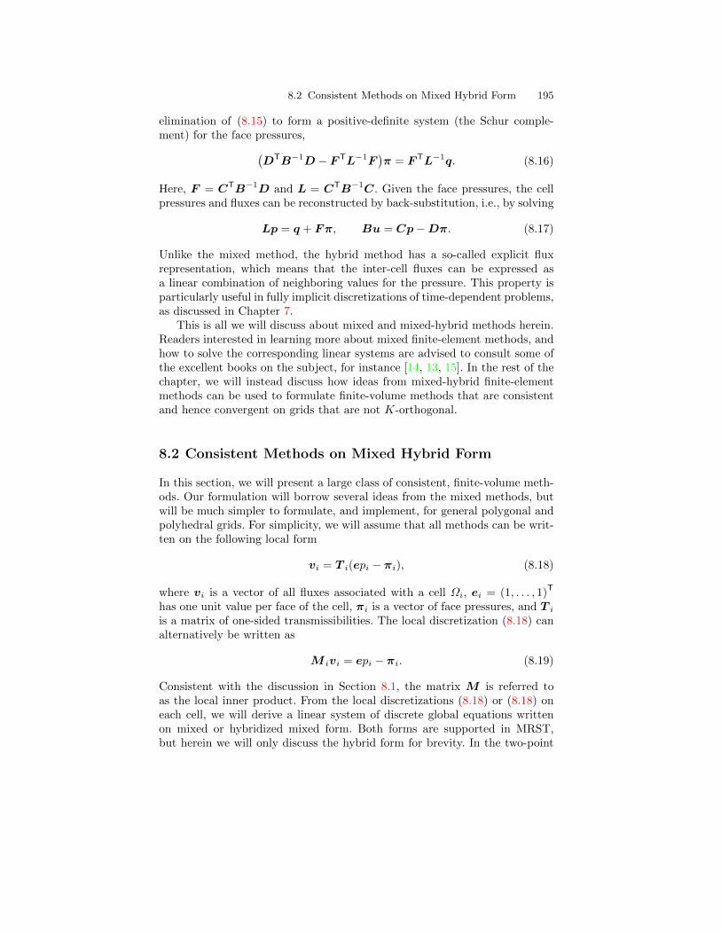
8.2 Consistent Methods on Mixed Hybrid Form 195
elimination of (8.15) to form a positive-definite system (the Schur comple-ment) for the face pressures,(
DTB−1D − F TL−1F)π = F TL−1q. (8.16)
Here, F = CTB−1D and L = CTB−1C. Given the face pressures, the cellpressures and fluxes can be reconstructed by back-substitution, i.e., by solving
Lp = q + Fπ, Bu = Cp−Dπ. (8.17)
Unlike the mixed method, the hybrid method has a so-called explicit fluxrepresentation, which means that the inter-cell fluxes can be expressed asa linear combination of neighboring values for the pressure. This property isparticularly useful in fully implicit discretizations of time-dependent problems,as discussed in Chapter 7.
This is all we will discuss about mixed and mixed-hybrid methods herein.Readers interested in learning more about mixed finite-element methods, andhow to solve the corresponding linear systems are advised to consult some ofthe excellent books on the subject, for instance [14, 13, 15]. In the rest of thechapter, we will instead discuss how ideas from mixed-hybrid finite-elementmethods can be used to formulate finite-volume methods that are consistentand hence convergent on grids that are not K-orthogonal.
8.2 Consistent Methods on Mixed Hybrid Form
In this section, we will present a large class of consistent, finite-volume meth-ods. Our formulation will borrow several ideas from the mixed methods, butwill be much simpler to formulate, and implement, for general polygonal andpolyhedral grids. For simplicity, we will assume that all methods can be writ-ten on the following local form
vi = T i(epi − πi), (8.18)
where vi is a vector of all fluxes associated with a cell Ωi, ei = (1, . . . , 1)T
has one unit value per face of the cell, πi is a vector of face pressures, and T iis a matrix of one-sided transmissibilities. The local discretization (8.18) canalternatively be written as
M ivi = epi − πi. (8.19)
Consistent with the discussion in Section 8.1, the matrix M is referred toas the local inner product. From the local discretizations (8.18) or (8.18) oneach cell, we will derive a linear system of discrete global equations writtenon mixed or hybridized mixed form. Both forms are supported in MRST,but herein we will only discuss the hybrid form for brevity. In the two-point
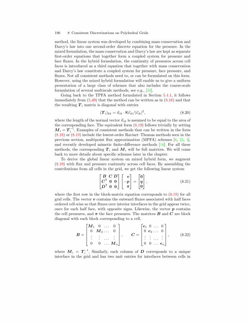
196 8 Consistent Discretizations on Polyhedral Grids
method, the linear system was developed by combining mass conservation andDarcy’s law into one second-order discrete equation for the pressure. In themixed formulation, the mass conservation and Darcy’s law are kept as separatefirst-order equations that together form a coupled system for pressure andface fluxes. In the hybrid formulation, the continuity of pressures across cellfaces is introduced as a third equation that together with mass conservationand Darcy’s law constitute a coupled system for pressure, face pressure, andfluxes. Not all consistent methods need to, or can be formulated on this form.However, using the mixed hybrid formulation will enable us to give a uniformpresentation of a large class of schemes that also includes the coarse-scaleformulation of several multiscale methods, see e.g., [26].
Going back to the TPFA method formulated in Section 5.4.1, it followsimmediately from (5.49) that the method can be written as in (8.18) and thatthe resulting T i matrix is diagonal with entries
(T i)kk = ~nik · K~cik/|~cik|2, (8.20)
where the length of the normal vector ~nik is assumed to be equal to the area ofthe corresponding face. The equivalent form (8.19) follows trivially by settingM i = T−1
i . Examples of consistent methods that can be written in the form(8.18) or (8.19) include the lowest-order Raviart–Thomas methods seen in theprevious section, multipoint flux approximation (MPFA) schemes [6, 25, 4],and recently developed mimetic finite-difference methods [16]. For all thesemethods, the corresponding T i and M i will be full matrices. We will comeback to more details about specific schemes later in the chapter.
To derive the global linear system on mixed hybrid form, we augment(8.19) with flux and pressure continuity across cell faces. By assembling thecontributions from all cells in the grid, we get the following linear system B C D
CT 0 0
DT 0 0
v−pπ
=
0q0
, (8.21)
where the first row in the block-matrix equation corresponds to (8.19) for allgrid cells. The vector v contains the outward fluxes associated with half facesordered cell-wise so that fluxes over interior interfaces in the grid appear twice,once for each half face, with opposite signs. Likewise, the vector p containsthe cell pressures, and π the face pressures. The matrices B and C are blockdiagonal with each block corresponding to a cell,
B =
M1 0 . . . 0
0 M2 . . . 0...
... . . ....
0 0 . . . Mn
, C =
e1 0 . . . 00 e2 . . . 0...
... . . ....
0 0 . . . en
, (8.22)
where M i = T−1i . Similarly, each column of D corresponds to a unique
interface in the grid and has two unit entries for interfaces between cells in
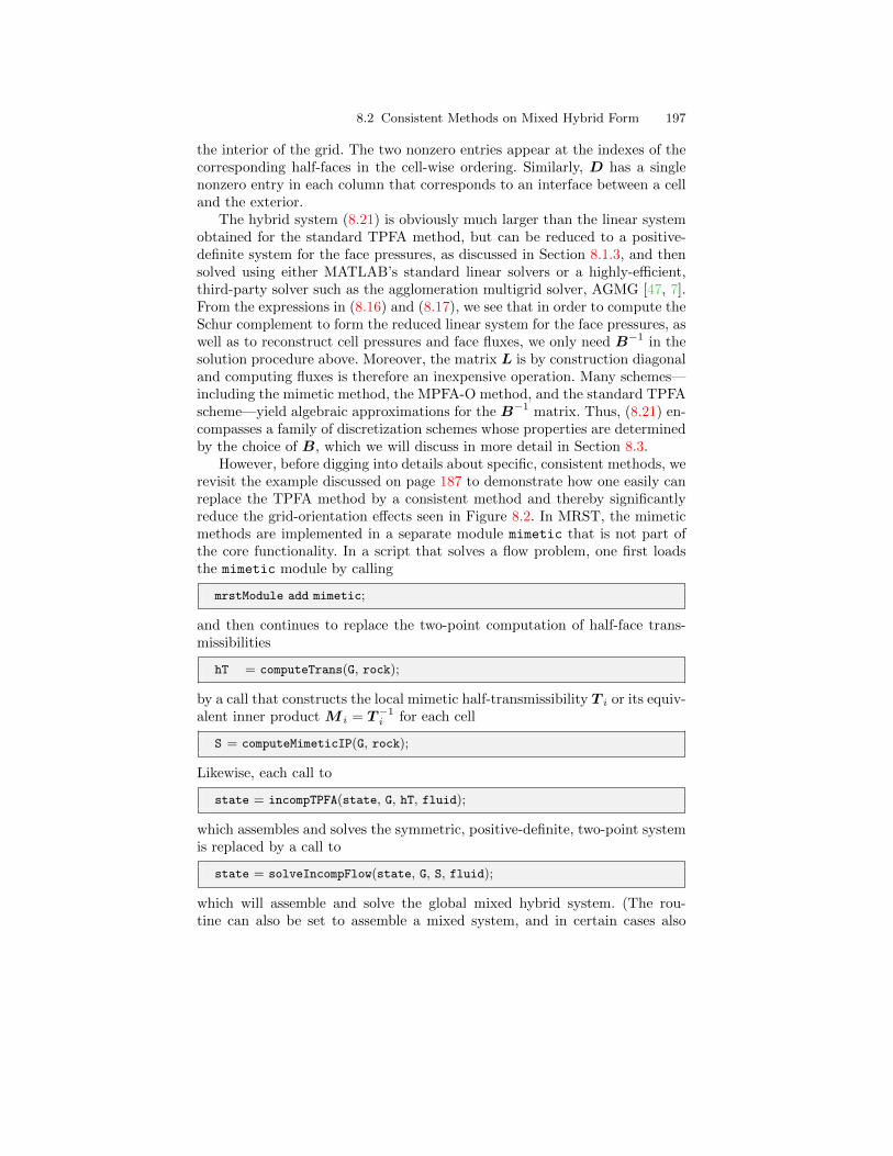
8.2 Consistent Methods on Mixed Hybrid Form 197
the interior of the grid. The two nonzero entries appear at the indexes of thecorresponding half-faces in the cell-wise ordering. Similarly, D has a singlenonzero entry in each column that corresponds to an interface between a celland the exterior.
The hybrid system (8.21) is obviously much larger than the linear systemobtained for the standard TPFA method, but can be reduced to a positive-definite system for the face pressures, as discussed in Section 8.1.3, and thensolved using either MATLAB’s standard linear solvers or a highly-efficient,third-party solver such as the agglomeration multigrid solver, AGMG [47, 7].From the expressions in (8.16) and (8.17), we see that in order to compute theSchur complement to form the reduced linear system for the face pressures, aswell as to reconstruct cell pressures and face fluxes, we only need B−1 in thesolution procedure above. Moreover, the matrix L is by construction diagonaland computing fluxes is therefore an inexpensive operation. Many schemes—including the mimetic method, the MPFA-O method, and the standard TPFAscheme—yield algebraic approximations for the B−1 matrix. Thus, (8.21) en-compasses a family of discretization schemes whose properties are determinedby the choice of B, which we will discuss in more detail in Section 8.3.
However, before digging into details about specific, consistent methods, werevisit the example discussed on page 187 to demonstrate how one easily canreplace the TPFA method by a consistent method and thereby significantlyreduce the grid-orientation effects seen in Figure 8.2. In MRST, the mimeticmethods are implemented in a separate module mimetic that is not part ofthe core functionality. In a script that solves a flow problem, one first loadsthe mimetic module by calling
mrstModule add mimetic;
and then continues to replace the two-point computation of half-face trans-missibilities
hT = computeTrans(G, rock);
by a call that constructs the local mimetic half-transmissibility T i or its equiv-alent inner product M i = T−1
i for each cell
S = computeMimeticIP(G, rock);
Likewise, each call to
state = incompTPFA(state, G, hT, fluid);
which assembles and solves the symmetric, positive-definite, two-point systemis replaced by a call to
state = solveIncompFlow(state, G, S, fluid);
which will assemble and solve the global mixed hybrid system. (The rou-tine can also be set to assemble a mixed system, and in certain cases also
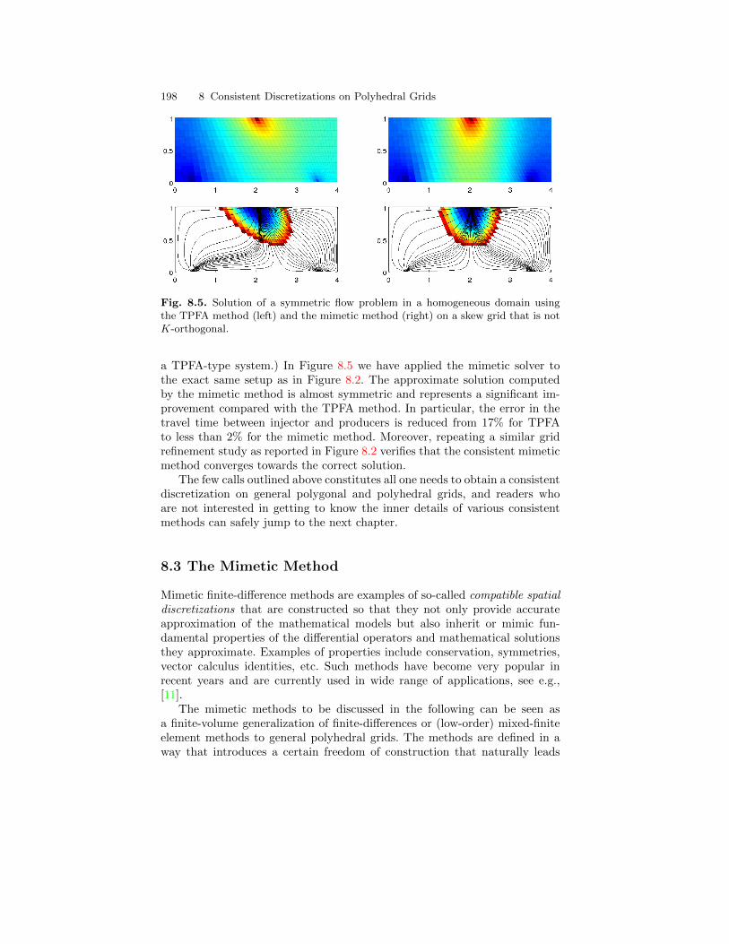
198 8 Consistent Discretizations on Polyhedral Grids
Fig. 8.5. Solution of a symmetric flow problem in a homogeneous domain usingthe TPFA method (left) and the mimetic method (right) on a skew grid that is notK-orthogonal.
a TPFA-type system.) In Figure 8.5 we have applied the mimetic solver tothe exact same setup as in Figure 8.2. The approximate solution computedby the mimetic method is almost symmetric and represents a significant im-provement compared with the TPFA method. In particular, the error in thetravel time between injector and producers is reduced from 17% for TPFAto less than 2% for the mimetic method. Moreover, repeating a similar gridrefinement study as reported in Figure 8.2 verifies that the consistent mimeticmethod converges towards the correct solution.
The few calls outlined above constitutes all one needs to obtain a consistentdiscretization on general polygonal and polyhedral grids, and readers whoare not interested in getting to know the inner details of various consistentmethods can safely jump to the next chapter.
8.3 The Mimetic Method
Mimetic finite-difference methods are examples of so-called compatible spatialdiscretizations that are constructed so that they not only provide accurateapproximation of the mathematical models but also inherit or mimic fun-damental properties of the differential operators and mathematical solutionsthey approximate. Examples of properties include conservation, symmetries,vector calculus identities, etc. Such methods have become very popular inrecent years and are currently used in wide range of applications, see e.g.,[11].
The mimetic methods to be discussed in the following can be seen asa finite-volume generalization of finite-differences or (low-order) mixed-finiteelement methods to general polyhedral grids. The methods are defined in away that introduces a certain freedom of construction that naturally leads
8.3 The Mimetic Method 199
to a family of methods. By carefully picking the parameters that are neededto fully specify a method, one can construct mimetic methods that coincidewith other known methods, or reduce to these methods (e.g., the two-pointmethod, the RT0 mixed finite-element method, or the MPFA-O multipointmethod) on certain types of grids.
The mimetic methods discussed herein, can all be written on the equivalentforms (8.18) or (8.19) and are constructed so that they are exact for linearpressure fields and give a symmetric positive-definite matrix M . In addition,the methods use discrete pressures and fluxes associated with cell and facecentroids, respectively, and consequently resemble finite-difference methods.
A linear pressure field can be written in the form p = ~x·~a+b for a constantvector ~a and scalar b, giving a Darcy velocity equal ~v = −K~a. Let ~nik denotethe area-weighted normal vector to Γik and ~cik be the vector pointing fromthe centroid of cell Ωi to the centroid of face Γik, as seen in Figure 5.4. UsingDarcy’s law and the notion of a one-sided transmissibility T ik (which willgenerally not be the same as the two-point transmissibility), the flux andpressure drop can be related as follows,
vik = −~nikK~a = Tik(pi − πik) = −Tik~cik · ~a. (8.23)
To get this relations in the one of the local forms (8.18) and (8.19) we collectall vectors ~cik and ~nik defined for a specific cell Ωi as rows in two matrices Ci
and N i. Because the relation (8.23) is required to hold for all linear pressuredrops, i.e., for an arbitrary vector ~a, we see that the matrices M i and T imust satisfy the following consistency conditions
MNK = C, NK = TC, (8.24)
where we for simplicity have dropped the subscript i that identifies the cellnumber. These general equations give us (quite) large freedom in how tospecify a specific discretization method: any method in which the local innerproduct M i, or equivalently the local transmissibility matrix T i, is positivedefinite and satisfies (8.24) will be a consistent, first-order accurate discretiza-tion. In the rest of the section, we will discuss various choices of valid innerproducts M i or reverse inner products T i.
8.3.1 General Family of Inner Products
The original article [16] that first introduced the mimetic methods consideredherein, discussed inner products for discrete velocities. However, as we haveseen in previous chapters, it is more common in the simulation of flow inporous media to consider inter-cell fluxes as the primary unknowns. We willtherefore henceforth consider inner products of fluxes rather than velocities.The relation between the two is trivial: an inner product of velocities becomesan inner product for fluxes by pre- and post-multiplying by the inverse of thearea of the corresponding cell faces. In other words, if A is a diagonal matrix
200 8 Consistent Discretizations on Polyhedral Grids
with element Ajj equal the are of the j-th face, then the flux inner productMflux is related to the velocity inner product Mvel through
Mflux = A−1MvelA−1. (8.25)
To simplify the derivation of valid solutions, we start by stating the fol-lowing geometrical property which relates C and N as follows (for a proof,see [16]):
CTN = V = diag(|Ωi|). (8.26)
Next, we multiply the left matrix equation in (8.24) by K−1CTN
C (K−1CTN) = (MNK) (K−1CTN) = MNCTN = MNV ,
from which it follows that there is a family of valid solution that has the form
M =1
|Ωi|CK−1CT +M2, (8.27)
where M2 is a matrix defined such that M2N = 0, i.e., any matrix whoserows lie in the left nullspace of NT. Moreover, to make a sensible methodwe must require that M is symmetric positive definite. In other words, anysymmetric and positive definite inner product that fulfills these requirementscan be represented in two alternative compact forms,
M =1
|Ωi|CK−1CT +Q⊥NSMQ
⊥N
T
=1
|Ωi|CK−1CT + P⊥NSMP
⊥N ,
(8.28)
where SM denotes any symmetric, positive definite matrix,Q⊥N is an orthonor-mal basis for the left null space of NT, and P⊥N is the null-space projectionI−QNQN
T in which QN is a basis for the spaces spanned by the columns ofN . Similarly, we can derive a closed expression for the inverse inner productT by multiplying the right matrix equation in (8.24) by V −1 from the leftand by V from the right and using the identity (8.26),
TC = V −1 (NK)V = V −1 (NK) (CTN)T
= V −1 (NKNT)C
By the same argument as for M , mutatis mutandis, we obtain the followingfamily of inverse inner products,
T =1
|Ωi|NKNT +Q⊥CSTQ
⊥C
T
=1
|Ωi|NKNT + P⊥CSTP
⊥C ,
(8.29)
where Q⊥C is an orthonormal basis for the left nullspace of CT and P⊥C =I −QCQC
T is the corresponding nullspace projection.
8.3 The Mimetic Method 201
The matrices M and T in (8.28) and (8.29) are evidently symmetric, sowe only need to prove that they are positive definite. We start by writing theinner product as M = M1 +M2, and observe that each of these matrices arepositive semi-definite and our result follows if we can prove that this impliesthat M is positive definite. Let z be an arbitrary nonzero vector which wesplit uniquely as z = Nx+ y, where x lies in the column space of N and ylies in the left nullspace of NT. If y is zero, we have
zTMz = xTNTM1Nx
= |Ωi|−1xT (NTC)K−1 (CTN)x = |Ωi|xTK−1x > 0
because K−1 is a positive definite matrix. If y is nonzero, we have
zTMz = zTM1z + yTM2y > 0
because zTM1z ≥ 0 and yTM2y > 0. An analogous argument holds for thematrix T , and hence we have proved that (8.28) and (8.29) give a well-definedfamily of consistent discretizations.
So far, we have not put any restrictions on the matrices SM and ST thatwill determine the specific methods, except for requiring that they should bepositive definite. In addition, they these matrices should mimic the scalingproperties of the continuous equation, which is invariant under affine trans-formations of space and permeability,
~x 7→ σ~x and K 7→ σTKσ, (8.30)
To motivate how we should choose the matrices SM and ST to mimic thesescaling properties, we will look at a simple 1D example:
Example 8.1. Consider the a grid cell x ∈ [−1, 1], for which N = C = [1,−1]T
and Q⊥N = Q⊥C = 1√2[1, 1]
T. Hence
M =1
2
[1−1
]1
K[1,−1] +
1
2
[11
]SM [1, 1],
T =1
2
[1−1
]K [1,−1] +
1
2
[11
]S [1, 1].
(8.31)
The structure of the inner product should be invariant under scaling of K andthus we can write the inner product as a one-parameter family of the form
M =1
2K
([1 −1−1 1
]+
2
t
[1 11 1
]),
T =K
2
([1 −1−1 1
]+t
2
[1 11 1
]).
(8.32)
Having established a plausible way of scaling the inner products, we are nowin a position to go through various specific choices that are implemented in themimetic module of MRST and look at correspondence between these methodsand the standard two-point method, the lowest-order RT0 mixed method, andthe MPFA-O method. Our discussion follows [38].
202 8 Consistent Discretizations on Polyhedral Grids
8.3.2 General Parametric Family
Motivated by the example above, we propose to choose the matrix ST as thediagonal of the first matrix term in (8.29) so that these two terms scale simi-larly under transformations of the type (8.30). Using this definition of ST andthat M should be equal to T−1 suggests the following general family of innerproducts that only differ in the constant in front of the second (regularization)matrix term:
M =1
|Ωi|CK−1CT +
|Ωi|tP⊥N diag(NKNT)−1P⊥N ,
T =1
|Ωi|
[NKNT + tP⊥C diag(NKNT)P⊥C
].
(8.33)
In MRST, this family of inner products is called ’ip qfamily’ and the parametert is supplied in a separate option:
S = computeMimeticIP(G, rock, 'InnerProduct', 'ip qfamily', 'qparam', t);
As we will see below, mimetic inner products that reduce to the standardTPFA method or the RT0 mixed finite-element method on simple grids aremembers of this family.
8.3.3 Two-Point Type Methods
A requirement of the two-point method is that the transmissibility matrixT (and hence also the matrix M of the inner product) should be diagonal.
Looking at (8.24), we see that this is only possible if the vectors K ~Nik and~cik are parallel, which is the exact same condition for K-orthogonality thatwe argued was sufficient to guarantee consistency of the method on page 8.An explicit expression for the diagonal entries of the two-point method onK-orthogonal grids has already been given in (8.20). Strictly speaking, thisrelation does not always yield a positive value for the two-point transmissi-bility on any grid. For instance, for corner-point grids it is normal to definethe face centroids as the arithmetic mean of the associated corner-point nodesand the cell centroids as the arithmetic mean of the centroids top and bottomcell faces, which for most grids will guarantee a positive transmissibility.
The extension of the two-point to non-orthogonal grids is not unique. Here,we will present a mimetic method that coincides with the two-point methodsin this method’s region of validity, while at the same time giving a validmimetic inner product and hence a consistent discretization for all types ofgrids and permeability tensors. One advantage of this method, compared withmultipoint flux-approximation methods, is that the implementation is simplerfor general unstructured grids.
The most instructive way to introduce the general method is to look at asimple example that will motivate the general construction.
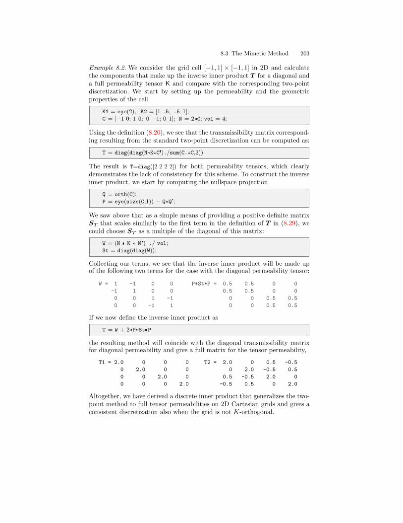
8.3 The Mimetic Method 203
Example 8.2. We consider the grid cell [−1, 1] × [−1, 1] in 2D and calculatethe components that make up the inverse inner product T for a diagonal anda full permeability tensor K and compare with the corresponding two-pointdiscretization. We start by setting up the permeability and the geometricproperties of the cell
K1 = eye(2); K2 = [1 .5; .5 1];C = [−1 0; 1 0; 0 −1; 0 1]; N = 2*C; vol = 4;
Using the definition (8.20), we see that the transmissibility matrix correspond-ing resulting from the standard two-point discretization can be computed as:
T = diag(diag(N*K*C')./sum(C.*C,2))
The result is T=diag([2 2 2 2]) for both permeability tensors, which clearlydemonstrates the lack of consistency for this scheme. To construct the inverseinner product, we start by computing the nullspace projection
Q = orth(C);P = eye(size(C,1)) − Q*Q';
We saw above that as a simple means of providing a positive definite matrixST that scales similarly to the first term in the definition of T in (8.29), wecould choose ST as a multiple of the diagonal of this matrix:
W = (N * K * N ') ./ vol;St = diag(diag(W));
Collecting our terms, we see that the inverse inner product will be made upof the following two terms for the case with the diagonal permeability tensor:
W = 1 -1 0 0 P*St*P = 0.5 0.5 0 0
-1 1 0 0 0.5 0.5 0 0
0 0 1 -1 0 0 0.5 0.5
0 0 -1 1 0 0 0.5 0.5
If we now define the inverse inner product as
T = W + 2*P*St*P
the resulting method will coincide with the diagonal transmissibility matrixfor diagonal permeability and give a full matrix for the tensor permeability,
T1 = 2.0 0 0 0 T2 = 2.0 0 0.5 -0.5
0 2.0 0 0 0 2.0 -0.5 0.5
0 0 2.0 0 0.5 -0.5 2.0 0
0 0 0 2.0 -0.5 0.5 0 2.0
Altogether, we have derived a discrete inner product that generalizes the two-point method to full tensor permeabilities on 2D Cartesian grids and gives aconsistent discretization also when the grid is not K-orthogonal.
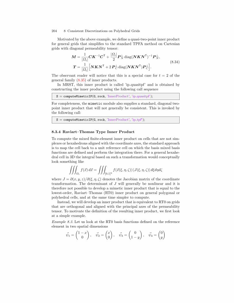
204 8 Consistent Discretizations on Polyhedral Grids
Motivated by the above example, we define a quasi-two-point inner productfor general grids that simplifies to the standard TPFA method on Cartesiangrids with diagonal permeability tensor:
M =1
|Ωi|CK−1CT +
|Ωi|2P⊥N diag(NKNT)−1P⊥N ,
T =1
|Ωi|
[NKNT + 2P⊥C diag(NKNT)P⊥C
].
(8.34)
The observant reader will notice that this is a special case for t = 2 of thegeneral family (8.35) of inner products.
In MRST, this inner product is called ’ip quasitpf’ and is obtained byconstructing the inner product using the following call sequence
S = computeMimeticIP(G, rock, 'InnerProduct', 'ip quasitpf');
For completeness, the mimetic module also supplies a standard, diagonal two-point inner product that will not generally be consistent. This is invoked bythe following call:
S = computeMimeticIP(G, rock, 'InnerProduct', 'ip tpf');
8.3.4 Raviart–Thomas Type Inner Product
To compute the mixed finite-element inner product on cells that are not sim-plexes or hexahedrons aligned with the coordinate axes, the standard approachis to map the cell back to a unit reference cell on which the basis mixed basisfunctions are defined and perform the integration there. For a general hexahe-dral cell in 3D the integral based on such a transformation would conceptuallylook something like∫∫∫
Ωi
f(~x) d~x =
∫∫∫[0,1]3
f(~x(ξ, η, ζ)) |J(ξ, η, ζ)| dξdηdζ
where J = ∂(x, y, z)/∂(ξ, η, ζ) denotes the Jacobian matrix of the coordinatetransformation. The determinant of J will generally be nonlinear and it istherefore not possible to develop a mimetic inner product that is equal to thelowest-order, Raviart–Thomas (RT0) inner product on general polygonal orpolyhedral cells, and at the same time simpler to compute.
Instead, we will develop an inner product that is equivalent to RT0 on gridsthat are orthogonal and aligned with the principal axes of the permeabilitytensor. To motivate the definition of the resulting inner product, we first lookat a simple example.
Example 8.3. Let us look at the RT0 basis functions defined on the referenceelement in two spatial dimensions
~ψ1 =
(1− x
0
), ~ψ2 =
(x0
), ~ψ3 =
(0
1− y
), ~ψ4 =
(0y
)
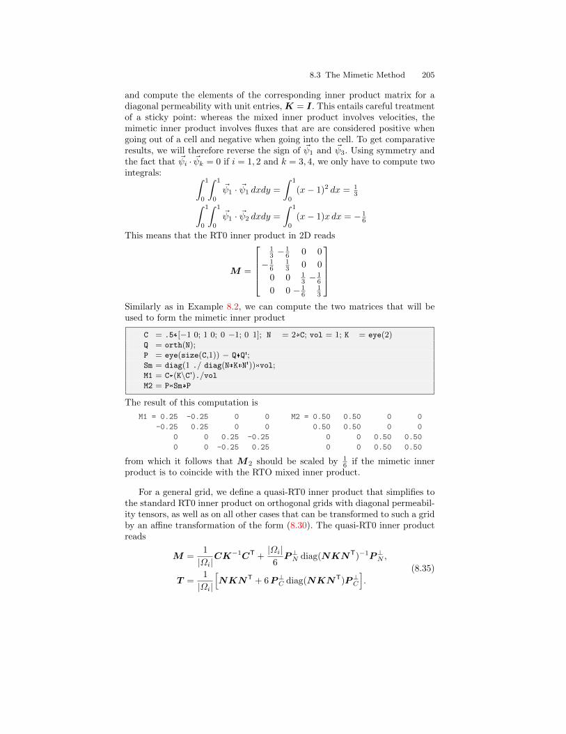
8.3 The Mimetic Method 205
and compute the elements of the corresponding inner product matrix for adiagonal permeability with unit entries, K = I. This entails careful treatmentof a sticky point: whereas the mixed inner product involves velocities, themimetic inner product involves fluxes that are are considered positive whengoing out of a cell and negative when going into the cell. To get comparativeresults, we will therefore reverse the sign of ~ψ1 and ~ψ3. Using symmetry andthe fact that ~ψi · ~ψk = 0 if i = 1, 2 and k = 3, 4, we only have to compute twointegrals: ∫ 1
0
∫ 1
0
~ψ1 · ~ψ1 dxdy =
∫ 1
0
(x− 1)2 dx = 13∫ 1
0
∫ 1
0
~ψ1 · ~ψ2 dxdy =
∫ 1
0
(x− 1)x dx = − 16
This means that the RT0 inner product in 2D reads
M =
13 −
16 0 0
− 16
13 0 0
0 0 13 −
16
0 0 − 16
13
Similarly as in Example 8.2, we can compute the two matrices that will beused to form the mimetic inner product
C = .5*[−1 0; 1 0; 0 −1; 0 1]; N = 2*C; vol = 1; K = eye(2)Q = orth(N);P = eye(size(C,1)) − Q*Q';Sm = diag(1 ./ diag(N*K*N'))*vol;M1 = C*(K\C')./volM2 = P*Sm*P
The result of this computation is
M1 = 0.25 -0.25 0 0 M2 = 0.50 0.50 0 0
-0.25 0.25 0 0 0.50 0.50 0 0
0 0 0.25 -0.25 0 0 0.50 0.50
0 0 -0.25 0.25 0 0 0.50 0.50
from which it follows that M2 should be scaled by 16 if the mimetic inner
product is to coincide with the RTO mixed inner product.
For a general grid, we define a quasi-RT0 inner product that simplifies tothe standard RT0 inner product on orthogonal grids with diagonal permeabil-ity tensors, as well as on all other cases that can be transformed to such a gridby an affine transformation of the form (8.30). The quasi-RT0 inner productreads
M =1
|Ωi|CK−1CT +
|Ωi|6P⊥N diag(NKNT)−1P⊥N ,
T =1
|Ωi|
[NKNT + 6P⊥C diag(NKNT)P⊥C
].
(8.35)
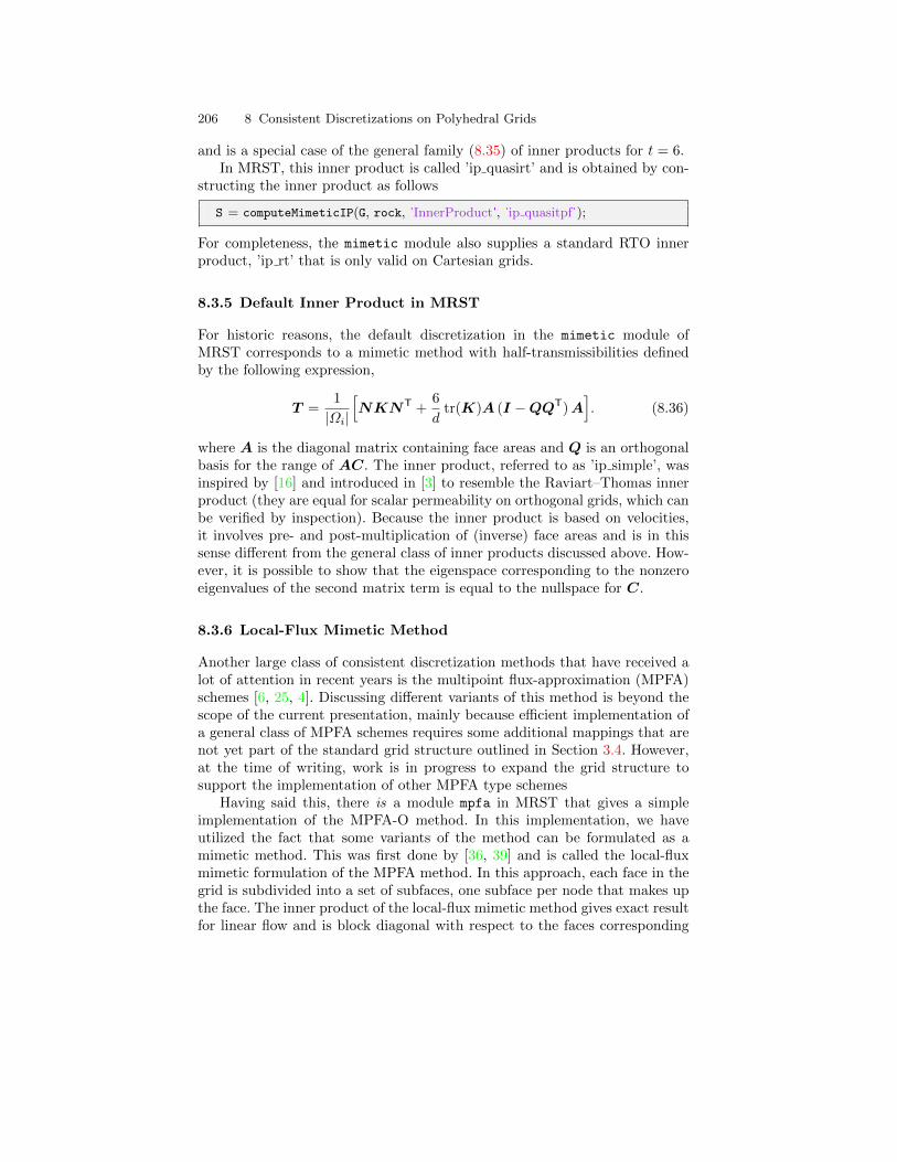
206 8 Consistent Discretizations on Polyhedral Grids
and is a special case of the general family (8.35) of inner products for t = 6.In MRST, this inner product is called ’ip quasirt’ and is obtained by con-
structing the inner product as follows
S = computeMimeticIP(G, rock, 'InnerProduct', 'ip quasitpf');
For completeness, the mimetic module also supplies a standard RTO innerproduct, ’ip rt’ that is only valid on Cartesian grids.
8.3.5 Default Inner Product in MRST
For historic reasons, the default discretization in the mimetic module ofMRST corresponds to a mimetic method with half-transmissibilities definedby the following expression,
T =1
|Ωi|
[NKNT +
6
dtr(K)A (I −QQT)A
]. (8.36)
where A is the diagonal matrix containing face areas and Q is an orthogonalbasis for the range of AC. The inner product, referred to as ’ip simple’, wasinspired by [16] and introduced in [3] to resemble the Raviart–Thomas innerproduct (they are equal for scalar permeability on orthogonal grids, which canbe verified by inspection). Because the inner product is based on velocities,it involves pre- and post-multiplication of (inverse) face areas and is in thissense different from the general class of inner products discussed above. How-ever, it is possible to show that the eigenspace corresponding to the nonzeroeigenvalues of the second matrix term is equal to the nullspace for C.
8.3.6 Local-Flux Mimetic Method
Another large class of consistent discretization methods that have received alot of attention in recent years is the multipoint flux-approximation (MPFA)schemes [6, 25, 4]. Discussing different variants of this method is beyond thescope of the current presentation, mainly because efficient implementation ofa general class of MPFA schemes requires some additional mappings that arenot yet part of the standard grid structure outlined in Section 3.4. However,at the time of writing, work is in progress to expand the grid structure tosupport the implementation of other MPFA type schemes
Having said this, there is a module mpfa in MRST that gives a simpleimplementation of the MPFA-O method. In this implementation, we haveutilized the fact that some variants of the method can be formulated as amimetic method. This was first done by [36, 39] and is called the local-fluxmimetic formulation of the MPFA method. In this approach, each face in thegrid is subdivided into a set of subfaces, one subface per node that makes upthe face. The inner product of the local-flux mimetic method gives exact resultfor linear flow and is block diagonal with respect to the faces corresponding

8.3 The Mimetic Method 207
to each node of the cell, but it is not symmetric. The block-diagonal propertymakes it possible to reduce the system into a cell-centered discretisation forthe cell pressures. This naturally leads to a method for calculating the MPFAtransmissibilities. The crucial point is to have the corner geometry in thegrid structure and handle the problems with corners which do not have threeunique half faces associated.
The local-flux mimetic implementation of the MPFA-O method can beused with a calling sequence that is similar to the TPFA and the mimeticmethods:
mrstModule add mpfa;hT = computeMultiPointTrans(G, rock);state = incompMPFA(state, G, hT, fluid)
However, the implementation is based on a combination of MATLAB and C,which is used to invert small systems, and may not work out of the box on allcomputers.

References
[1] J. E. Aarnes, V. Kippe, and K.-A. Lie. Mixed multiscale fi-nite elements and streamline methods for reservoir simulationof large geomodels. Adv. Water Resour., 28(3):257–271, 2005.doi:10.1016/j.advwatres.2004.10.007.
[2] J. E. Aarnes, T. Gimse, and K.-A. Lie. An introduction to the numer-ics of flow in porous media using Matlab. In G. Hasle, K.-A. Lie, andE. Quak, editors, Geometrical Modeling, Numerical Simulation and Op-timisation: Industrial Mathematics at SINTEF, pages 265–306. SpringerVerlag, Berling Heidelberg New York, 2007.
[3] J. E. Aarnes, S. Krogstad, and K.-A. Lie. Multiscale mixed/mimeticmethods on corner-point grids. Comput. Geosci., 12(3):297–315, 2008.ISSN 1420-0597. doi:10.1007/s10596-007-9072-8.
[4] I. Aavatsmark. An introduction to multipoint flux approxima-tions for quadrilateral grids. Comput. Geosci., 6:405–432, 2002.doi:10.1023/A:1021291114475.
[5] I. Aavatsmark and R. Klausen. Well index in reservoir simulation forslanted and slightly curved wells in 3d grids. SPE J., 8(01):41–48, 2003.
[6] I. Aavatsmark, T. Barkve, Ø. Bøe, and T. Mannseth. Discretization onnon-orthogonal, curvilinear grids for multi-phase flow. Proc. of the 4thEuropean Conf. on the Mathematics of Oil Recovery, 1994.
[7] AGMG. Iterative solution with AGgregation-based algebraic MultiGrid,2012. http://homepages.ulb.ac.be/∼ynotay/AGMG/.
[8] I. Akervoll and P. Bergmo. A study of Johansen formation located off-shore Mongstad as a candidate for permanent CO2 storage. In EuropeanConference on CCS Research, Development and Demonstration. 10–11February 2009, Oslo, Norway, 2009.
[9] J. Alvestad, K. Holing, K. Christoffersen, O. Stava, et al. Interactivemodelling of multiphase inflow performance of horizontal and highly de-viated wells. In European Petroleum Computer Conference. Society ofPetroleum Engineers, 1994.

210 References
[10] J. Bear. Dynamics of Fluids in Porous Media. Dover, 1988. ISBN 0-486-45355-3.
[11] L. Beirao da Veiga, K. Lipnikov, and G. Manzini. The Mimetic FiniteDifference Method for Elliptic Problems, volume 11 of MS&A – Model-ing, Simulation and Applications. Springer, 2014. doi:10.1007/978-3-319-02663-3.
[12] C. H. Bischof, H. M. Bucker, B. Lang, A. Rasch, and A. Vehreschild.Combining source transformation and operator overloading techniquesto compute derivatives for MATLAB programs. In Proceedings of theSecond IEEE International Workshop on Source Code Analysis and Ma-nipulation (SCAM 2002), pages 65–72, Los Alamitos, CA, USA, 2002.IEEE Computer Society. doi:10.1109/SCAM.2002.1134106.
[13] D. Braess. Finite elements: Theory fast solvers and applications in solidmechanics. Cambridge University Press, Cambridge, 1997.
[14] S. C. Brenner and L. R. Scott. The mathematical theory of finite elementmethods, volume 15 of Texts in Applied Mathematics. Springer–Verlag,New York, 1994.
[15] F. Brezzi and M. Fortin. Mixed and Hybrid Finite Element Methods,volume 15 of Springer Series in Computational Mathematics. Springer-Verlag, New York, 1991. ISBN 0-387-97582-9.
[16] F. Brezzi, K. Lipnikov, and V. Simoncini. A family of mimetic finite differ-ence methods on polygonial and polyhedral meshes. Math. Models Meth-ods Appl. Sci., 15:1533–1553, 2005. doi:10.1142/S0218202505000832.
[17] Cayuga Research. Admat. URL http://www.cayugaresearch.com/
admat.html. [Online; accessed 15-04-2014].[18] Z. Chen, G. Huan, and Y. Ma. Computational methods for multiphase
flows in porous media, volume 2 of Computational Science and Engi-neering. Society of Industrial and Applied Mathematics (SIAM), 2006.doi:10.1137/1.9780898718942.
[19] M. A. Christie and M. J. Blunt. Tenth SPE comparative solution project:A comparison of upscaling techniques. SPE Reservoir Eval. Eng., 4:308–317, 2001. doi:10.2118/72469-PA. Url: http://www.spe.org/csp/.
[20] C. Cordes and W. Kinzelbach. Continous groundwater velocity fields andpath lines in linear, bilinear, and trilinear finite elements. Water Resour.Res., 28(11):2903–2911, 1992.
[21] H. P. G. Darcy. Les Fontaines Publiques de la Ville de Dijon. Dalmont,Paris, 1856.
[22] A. Datta-Gupta and M. King. A semianalytic approach to tracer flowmodeling in heterogeneous permeable media. Adv. Water Resour., 18:9–24, 1995.
[23] A. Datta-Gupta and M. J. King. Streamline Simulation: Theory andPractice, volume 11 of SPE Textbook Series. Society of Petroleum Engi-neers, 2007.
[24] C. V. Deutsch and A. G. Journel. GSLIB: Geostatistical software libraryand user’s guide. Oxford University Press, New York, 2nd edition, 1998.
References 211
[25] M. G. Edwards and C. F. Rogers. A flux continuous scheme for thefull tensor pressure equation. Proc. of the 4th European Conf. on theMathematics of Oil Recovery, 1994.
[26] Y. Efendiev and T. Y. Hou. Multiscale Finite Element Methods, volume 4of Surveys and Tutorials in the Applied Mathematical Sciences. SpringerVerlag, New York, 2009.
[27] G. Eigestad, H. Dahle, B. Hellevang, W. Johansen, K.-A. Lie, F. Riis, andE. Øian. Geological and fluid data for modelling CO2 injection in theJohansen formation, 2008. URL http://www.sintef.no/Projectweb/
MatMorA/Downloads/Johansen.[28] G. Eigestad, H. Dahle, B. Hellevang, F. Riis, W. Johansen, and E. Øian.
Geological modeling and simulation of CO2 injection in the Johansenformation. Comput. Geosci., 13(4):435–450, 2009. doi:10.1007/s10596-009-9153-y.
[29] R. E. Ewing, R. D. Lazarov, S. L. Lyons, D. V. Papavassiliou,J. Pasciak, and G. Qin. Numerical well model for non-Darcy flowthrough isotropic porous media. Comput. Geosci., 3(3-4):185–204, 1999.doi:10.1023/A:1011543412675.
[30] M. Fink. Automatic differentiation for Matlab. MATLAB Central, 2007.URL http://www.mathworks.com/matlabcentral/fileexchange/
15235-automatic-differentiation-for-matlab. [Online; accessed15-04-2014].
[31] S. A. Forth. An efficient overloaded implementation of forward modeautomatic differentiation in MATLAB. ACM Trans. Math. Software, 32(2):195–222, 2006.
[32] H. Hægland, H. K. Dahle, K.-A. Lie, and G. Eigestad. Adaptive stream-line tracing for streamline simulation on irregular grids. In P. Binning,P. Engesgaard, H. Dahle, G. Pinder, and W. Gray, editors, Proceed-ings of the XVI International Conference on Computational Methodsin Water Resources, Copenhagen, Denmark, 18–22 June 2006. URLhttp://proceedings.cmwr-xvi.org/.
[33] H. Holden and N. Risebro. Front Tracking for Hyperbolic ConservationLaws, volume 152 of Applied Mathematical Sciences. Springer, New York,2002.
[34] E. Jimenez, K. Sabir, A. Datta-Gupta, and M. King. Spatial error andconvergence in streamline simulation. SPE J., 10(3):221–232, June 2007.
[35] M. King and A. Datta-Gupta. Streamline simulation: A current perspec-tive. In Situ, 22(1):91–140, 1998.
[36] R. A. Klausen and A. F. Stephansen. Mimetic MPFA. In Proc. 11thEuropean Conference on the Mathematics of Oil Recovery, 8-11 Sept.,Bergen, Norway, number A12. EAGE, 2008.
[37] R. A. Klausen, A. F. Rasmussen, and A. Stephansen. Velocity inter-polation and streamline tracing on irregular geometries. ComputationalGeosciences, 16:261–276, 2012. doi:10.1007/s10596-011-9256-0.
212 References
[38] K.-A. Lie, S. Krogstad, I. S. Ligaarden, J. R. Natvig, H. Nilsen, andB. Skaflestad. Open-source MATLAB implementation of consistentdiscretisations on complex grids. Comput. Geosci., 16:297–322, 2012.doi:10.1007/s10596-011-9244-4.
[39] K. Lipnikov, M. Shashkov, and I. Yotov. Local flux mimetic finite differ-ence methods. Numer. Math., 112(1):115–152, 2009. doi:10.1007/s00211-008-0203-5.
[40] T. Manzocchi et al. Sensitivity of the impact of geological uncertaintyon production from faulted and unfaulted shallow-marine oil reservoirs:objectives and methods. Petrol. Geosci., 14(1):3–15, 2008.
[41] S. Matringe and M. Gerritsen. On accurate tracing of streamlines. InSPE Annual Technical Conference and Exhibition, Houston, Texas, USA,26-29 September 2004. SPE 89920.
[42] S. Matringe, R. Juanes, and H. Tchelepi. Streamline tracing on generaltriangular or quadrilateral grids. SPE J., 12(2):217–233, June 2007.
[43] W. McIlhagga. Automatic differentiation with Mat-lab objects. MATLAB Central, mar 2010. URLhttp://www.mathworks.com/matlabcentral/fileexchange/
26807-automatic-differentiation-with-matlab-objects. [On-line; accessed 15-04-2014].
[44] J. R. Natvig and K.-A. Lie. Fast computation of multiphase flow inporous media by implicit discontinuous Galerkin schemes with optimalordering of elements. J. Comput. Phys., 227(24):10108–10124, 2008.doi:10.1016/j.jcp.2008.08.024.
[45] J. R. Natvig, K.-A. Lie, B. Eikemo, and I. Berre. An efficient discontinu-ous Galerkin method for advective transport in porous media. Adv. WaterResour., 30(12):2424–2438, 2007. doi:10.1016/j.advwatres.2007.05.015.
[46] R. Neidinger. Introduction to automatic differentiation and MAT-LAB object-oriented programming. SIAM Review, 52(3):545–563, 2010.doi:10.1137/080743627.
[47] Y. Notay. An aggregation-based algebraic multigrid method. Electron.Trans. Numer. Anal., 37:123–140, 2010.
[48] P.-E. Øren, S. Bakke, and O. J. Arntzen. Extending predictive capabili-ties to network models. SPE J., 3(4):324–336, 1998.
[49] D. W. Peaceman. Interpretation of well-block pressures in numericalreservoir simulation with nonsquare grid blocks and anisotropic perme-ability. Soc. Petrol. Eng. J., 23(3):531–543, 1983. doi:10.2118/10528-PA.SPE 10528-PA.
[50] D. W. Peaceman. Fundamentals of Numerical Reservoir Simulation. El-sevier Science Inc., New York, NY, USA, 1991. ISBN 0444415785.
[51] D. W. Peaceman et al. Interpretation of well-block pressures in numericalreservoir simulation. Soc. Petrol. Eng. J., 18(3):183—194, 1978.
[52] D. Pollock. Semi-analytical computation of path lines for finite-differencemodels. Ground Water, 26(6):743–750, 1988.
References 213
[53] D. K. Ponting. Corner point geometry in reservoir simulation. In P. King,editor, Proceedings of the 1st European Conference on Mathematics ofOil Recovery, Cambridge, 1989, pages 45–65, Oxford, July 25–27 1989.Clarendon Press.
[54] M. Prevost, M. Edwards, and M. Blunt. Streamline tracing on curvilinearstructured and unstructured grids. SPE J., 7(2):139–148, June 2002.
[55] P. A. Raviart and J. M. Thomas. A mixed finite element method forsecond order elliptic equations. In I. Galligani and E. Magenes, edi-tors, Mathematical Aspects of Finite Element Methods, pages 292–315.Springer–Verlag, Berlin – Heidelberg – New York, 1977.
[56] L. F. Shampine, R. Ketzscher, and S. A. Forth. Using AD to solve BVPsin MATLAB. ACM Trans. Math. Software, 31(1):79–94, 2005.
[57] Technische Universitat Darmstadt. Automatic Differentiation for Mat-lab (ADiMat). URL http://www.adimat.de/. [Online; accessed 15-04-2014].
[58] Tomlab Optimization Inc. Matlab Automatic Differentiation (MAD).URL http://matlabad.com/. [Online; accessed 15-04-2014].
[59] A. Verma. ADMAT: Automatic differentiation in MATLAB using ob-ject oriented methods. In SIAM Interdiscplinary Workshop on ObjectOriented Methods for Interoperability, pages 174–183, 1999.