
IEAGHG TechnicalReview - SINTEF
320
IEA GREENHOUSE GAS R&D PROGRAMME IEAGHG Technical Review 2017-TR8 August 2017 Understanding the Cost of Retrofitting CO 2 capture in an Integrated Oil Refinery
-
Upload
khangminh22 -
Category
Documents
-
view
1 -
download
0
Transcript of IEAGHG TechnicalReview - SINTEF

IEA GREENHOUSE GAS R&D PROGRAMME
IEAGHG Technical Review2017-TR8
August 2017
Understanding the Cost of Retrofitting CO2 capture in an Integrated Oil Refinery

DISCLAIMERThis report was prepared as an account of the work sponsored by IEAGHG, CLIMIT, Concawe and SINTEF. The views and opinions of the authors expressed herein do not necessarily reflect those of the IEAGHG, its members, the International Energy Agency, the organisations listed below, nor any employee or persons acting on behalf of any of them. In addition, none of these make any warranty, express or implied, assumes any liability or responsibility for the accuracy, completeness or usefulness of any information, apparatus, product of process disclosed or represents that its use would not infringe privately owned rights, including any parties intellectual property rights. Reference herein to any commercial product, process, service or trade name, trade mark or manufacturer does not necessarily constitute or imply any endorsement, recommendation or any favouring of such products.
COPYRIGHT
Copyright © IEA Environmental Projects Ltd. (IEAGHG) 2017.
All rights reserved.
ACKNOWLEDGEMENTS AND CITATIONS
This report describes research sponsored by IEAGHG and was edited by:
• John Gale, IEAGHG
To ensure the quality and technical integrity of the research undertaken by IEAGHG each study is managed by an appointed IEAGHG manager.
The IEAGHG manager for this report was: • John Gale, IEAGHG
The expert reviewers for this report were:
• Lily Gray and Damien Valdenaire, on behalf of CONCAWE Members
The report should be cited in literature as follows:
‘IEAGHG, “Understanding the Cost of Retrofitting CO2 capture in an Integrated Oil Refinery” 2017/TR8, August 2017.’
Files associated with this report can be found at www.sintef.no/recap• An excel sheet for calculation of the costs of CO2 capture in integrated oil refineries• Appendix A and B for the section “Performance analysis of CO2 capture options”• Calculations of the crude processing costs for the refinery base cases
Further information or copies of the report can be obtained by contacting IEAGHG at:
IEAGHG, Pure Offices, Cheltenham Office ParkHatherley Lane, Cheltenham,GLOS., GL51 6SH, UKTel: +44 (0)1242 802911E-mail: [email protected]: www.ieaghg.org
International Energy Agency The International Energy Agency (IEA) was established in 1974 within the framework of the Organisation for Economic Co-operation and Development (OECD) to implement an international energy programme. The IEA fosters co-operation amongst its 29 member countries and the European Commission, and with the other countries, in order to increase energy security by improved efficiency of energy use, development of alternative energy sources and research, development and demonstration on matters of energy supply and use. This is achieved through a series of collaborative activities, organised under 39 Technology Collaboration Programmes. These agreements cover more than 200 individual items of research, development and demonstration. IEAGHG is one of these Technology Collaboration Programmes.
vsdv
Background
In the past years, IEA Greenhouse Gas R&D Programme (IEAGHG) has undertaken a series of projects
evaluating the performance and cost of deploying CO2 capture technologies in energy intensive
industries such as the cement, iron and steel, hydrogen, pulp and paper, and others.
In line with these activities, IEAGHG initiated this project in collaboration with CONCAWE1,
GASSNOVA and SINTEF Energy Research, to evaluate the performance and cost of retrofitting CO2
capture in an integrated oil refinery.
The global-refining sector contributes around 4% of the total anthropogenic CO2 emissions. CO2 capture
and storage (CCS) has been recognised as one of the technologies that could be deployed to achieve
deep reduction of greenhouse gas emissions in this and other industry sectors.
To enable the deployment of CCS in the oil-refining sector, it is essential to have a good understanding
of the direct impact on the financial performance and market impact, resulti9ng from the retrofitting
CO2 capture technology.
In several OECD countries (especially in Europe), it is expected that no new refineries will be built in
the coming decades. Furthermore, most of these refineries are at least 20 years old. Therefore, this study
aims to evaluate and understand the cost of retrofitting CO2 capture technologies to an existing integrated
oil refinery.
The project was supported under the Norwegian CLIMIT programme, with contributions from IEAGHG
and CONCAWE. It was managed by SINTEF Energy Research. The project consortium selected Amec
Foster Wheeler as the engineering contractor to work with SINTEF Energy Research in performing the
basic engineering and cost estimation for the reference cases.
Scope of work
The main purpose of the study was to evaluate the cost of retrofitting CO2 capture in a range of refinery
types typical of those found in Europe. These included bo0th simple and high complexity refineries
covering typical European refinery capacities from 100,000 to 350,000 bbl/d.
Specifically, the study aimed to:
1. Formulate a reference document providing the different design basis and key assumptions to be
used as the basis for the study.
2. Define 4 different oil refineries as Base Cases. This covers the following:
a. Simple Hydroskimming2 refinery with a nominal capacity of 100,000 bbl/d.
b. Medium complex refinery with nominal capacity of 220,000 bbl/d.
c. Highly complex refinery with a nominal capacity of 220,000 bbl/d.
d. Highly complex refinery with a nominal capacity of 350,000 bbl/d.
3. Define a list of emission sources for each reference case and agree on CO2 capture priorities.
4. Investigate the techno-economics performance of the integrated oil refinery (covering simple to
complex refineries, with 100,000 to 350,000 bbl/d capacity) capturing CO2 emissions from
various sources using post-combustion CO2 capture technology based on standard MEA solvent.
5. Analyse pre-combustion capture (capture from the SMR syngas) options for refinery retrofit.
This was achieved by using results from the IEAGHG report 2017/02 "Techno-Economic
1 CONCAWE is a trade association for the European refining industry it carries out research on environmental
issues relevant to the oil industry. 2 Hydroskimming is one of the simplest types of refinery used in the petroleum industry. A Hydroskimming
refinery is defined as a refinery equipped with atmospheric distillation, naphtha reforming and necessary treating processes.

Evaluation of SMR based standalone (merchant) plant with CCS". The focus will be to estimate
the important relative cost between pre- and post combustion capture for SMRs.
6. Perform a literature study on the performance and cost of CO2 capture from refineries with
oxyfuel combustion. The literature study will cover but not be limited to the work done by the
CO2 Capture Project (CCP), and will attempt to relate the findings to the highly complex
refinery case.
7. Develop a constructability study for retrofitting CO2 capture in a complex oil refinery. The study
will produce high-level guidelines on plant layout, space requirement, safety, pipeline network
modification, access route for equipment, modular construction vs. stick-built fabrication, and
others.
Refinery Base Cases
Four refinery base cases were defined to represent typical crude mix and product slate of similar
capacity European oil refineries:
Base Case 1 (BC1) is a simple hydro skimming refinery.
Base Case 2 (BC2) is a medium complexity refinery that is a retrofit of Base Case 1.
Similarly, Base Case 3 (BC3) is a complex refinery that is a retrofit of Base Case 2.
Base Case 4 (BC4) is a large complex oil refinery.
As the complexity of the refinery increases from Base Case 1 to 4, the yield of naphtha and gasoil
fraction increases as the heavy cuts are converted into lighter and more valuable products in the more
complex refineries.
The performance of the refinery base cases, in terms of mass and energy balances, and CO2 emissions,
are the basis for comparison of the effectiveness and cost of oil refineries with CO2 capture.
The market conditions in the last decade have pushed the refineries to upgrade their configuration to
process heavier crudes, cheaper than the lighter ones, and to re-process heavy distillate products to
obtain more valuable fractions. These energy intensive units, however, demand a greater amount of fuel
and, in turn, increase the amount of CO2 emitted.
The four identified base cases are good starting points for evaluating the effects of retrofitting CO2
capture facilities in existing refineries, different per size and complexity.
Figure 1: Fuel demand and CO2 emissions in the 4 base case refineries
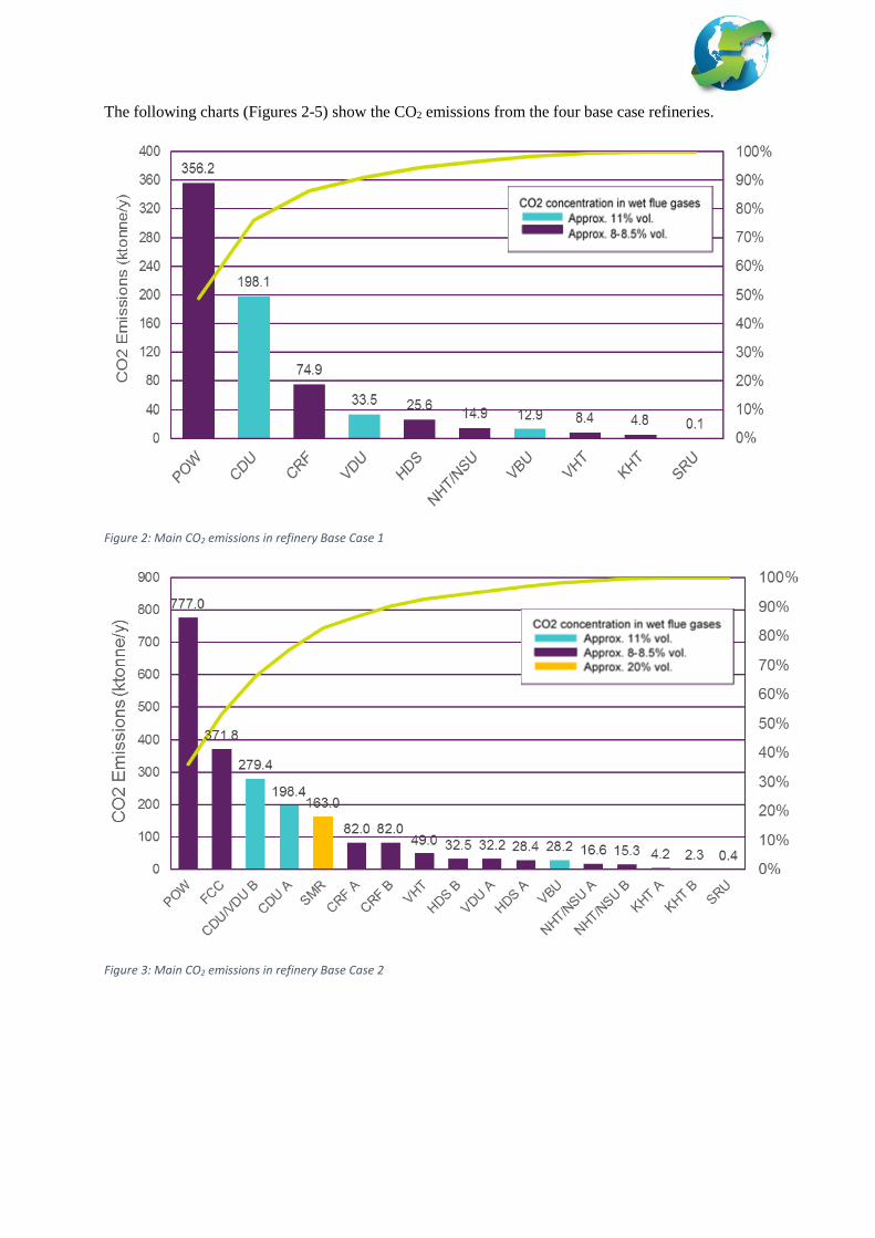
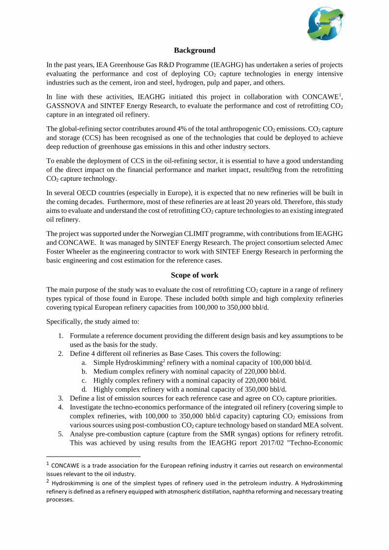
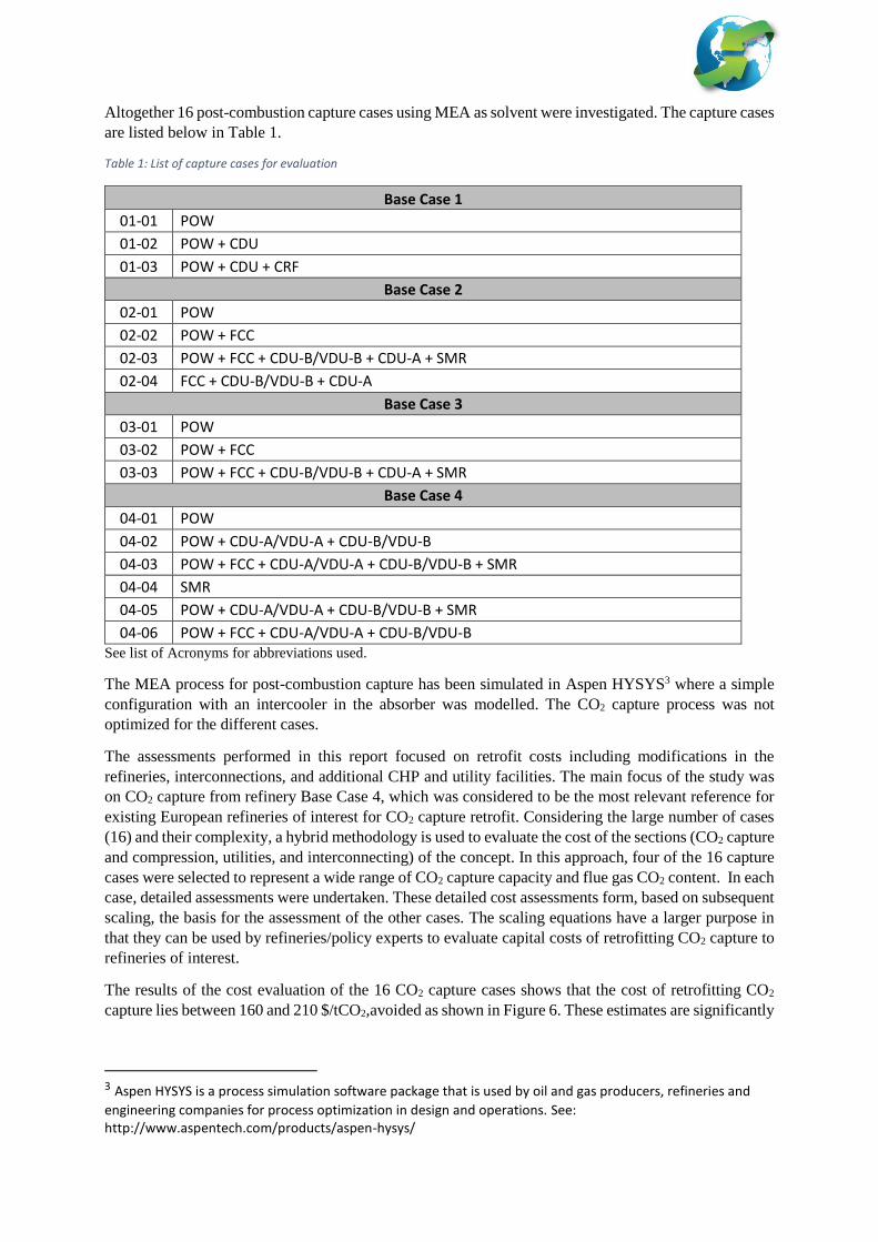
The following charts (Figures 2-5) show the CO2 emissions from the four base case refineries.
Figure 2: Main CO2 emissions in refinery Base Case 1
Figure 3: Main CO2 emissions in refinery Base Case 2
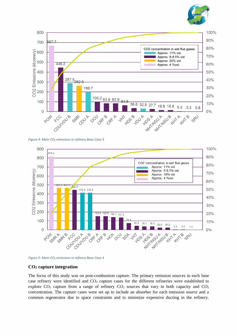
Figure 4: Main CO2 emissions in refinery Base Case 3
Figure 5: Main CO2 emissions in refinery Base Case 4
CO2 capture integration
The focus of this study was on post-combustion capture. The primary emission sources in each base
case refinery were identified and CO2 capture cases for the different refineries were established to
explore CO2 capture from a range of refinery CO2 sources that vary in both capacity and CO2
concentration. The capture cases were set up to include an absorber for each emission source and a
common regenerator due to space constraints and to minimize expensive ducting in the refinery.
Altogether 16 post-combustion capture cases using MEA as solvent were investigated. The capture cases
are listed below in Table 1.
Table 1: List of capture cases for evaluation
Base Case 1
01-01 POW
01-02 POW + CDU
01-03 POW + CDU + CRF
Base Case 2
02-01 POW
02-02 POW + FCC
02-03 POW + FCC + CDU-B/VDU-B + CDU-A + SMR
02-04 FCC + CDU-B/VDU-B + CDU-A
Base Case 3
03-01 POW
03-02 POW + FCC
03-03 POW + FCC + CDU-B/VDU-B + CDU-A + SMR
Base Case 4
04-01 POW
04-02 POW + CDU-A/VDU-A + CDU-B/VDU-B
04-03 POW + FCC + CDU-A/VDU-A + CDU-B/VDU-B + SMR
04-04 SMR
04-05 POW + CDU-A/VDU-A + CDU-B/VDU-B + SMR
04-06 POW + FCC + CDU-A/VDU-A + CDU-B/VDU-B See list of Acronyms for abbreviations used.
The MEA process for post-combustion capture has been simulated in Aspen HYSYS3 where a simple
configuration with an intercooler in the absorber was modelled. The CO2 capture process was not
optimized for the different cases.
The assessments performed in this report focused on retrofit costs including modifications in the
refineries, interconnections, and additional CHP and utility facilities. The main focus of the study was
on CO2 capture from refinery Base Case 4, which was considered to be the most relevant reference for
existing European refineries of interest for CO2 capture retrofit. Considering the large number of cases
(16) and their complexity, a hybrid methodology is used to evaluate the cost of the sections (CO2 capture
and compression, utilities, and interconnecting) of the concept. In this approach, four of the 16 capture
cases were selected to represent a wide range of CO2 capture capacity and flue gas CO2 content. In each
case, detailed assessments were undertaken. These detailed cost assessments form, based on subsequent
scaling, the basis for the assessment of the other cases. The scaling equations have a larger purpose in
that they can be used by refineries/policy experts to evaluate capital costs of retrofitting CO2 capture to
refineries of interest.
The results of the cost evaluation of the 16 CO2 capture cases shows that the cost of retrofitting CO2
capture lies between 160 and 210 $/tCO2,avoided as shown in Figure 6. These estimates are significantly
3 Aspen HYSYS is a process simulation software package that is used by oil and gas producers, refineries and
engineering companies for process optimization in design and operations. See: http://www.aspentech.com/products/aspen-hysys/
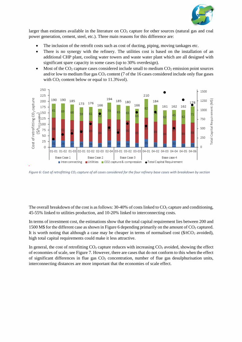
larger than estimates available in the literature on CO2 capture for other sources (natural gas and coal
power generation, cement, steel, etc.). Three main reasons for this difference are:
The inclusion of the retrofit costs such as cost of ducting, piping, moving tankages etc.
There is no synergy with the refinery. The utilities cost is based on the installation of an
additional CHP plant, cooling water towers and waste water plant which are all designed with
significant spare capacity in some cases (up to 30% overdesign).
Most of the CO2 capture cases considered include small to medium CO2 emission point sources
and/or low to medium flue gas CO2 content (7 of the 16 cases considered include only flue gases
with CO2 content below or equal to 11.3%vol).
Figure 6: Cost of retrofitting CO2 capture of all cases considered for the four refinery base cases with breakdown by section
The overall breakdown of the cost is as follows: 30-40% of costs linked to CO2 capture and conditioning,
45-55% linked to utilities production, and 10-20% linked to interconnecting costs.
In terms of investment cost, the estimations show that the total capital requirement lies between 200 and
1500 M$ for the different case as shown in Figure 6 depending primarily on the amount of CO2 captured.
It is worth noting that although a case may be cheaper in terms of normalised cost ($/tCO2 avoided),
high total capital requirements could make it less attractive.
In general, the cost of retrofitting CO2 capture reduces with increasing CO2 avoided, showing the effect
of economies of scale, see Figure 7. However, there are cases that do not conform to this when the effect
of significant differences in flue gas CO2 concentration, number of flue gas desulphurisation units,
interconnecting distances are more important that the economies of scale effect.
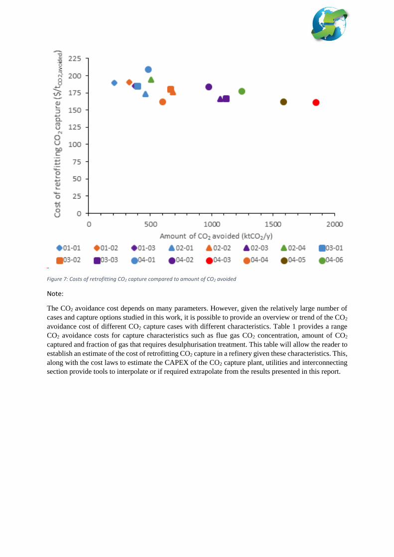
Figure 7: Costs of retrofitting CO2 capture compared to amount of CO2 avoided
Note:
The CO2 avoidance cost depends on many parameters. However, given the relatively large number of
cases and capture options studied in this work, it is possible to provide an overview or trend of the CO2
avoidance cost of different CO2 capture cases with different characteristics. Table 1 provides a range
CO2 avoidance costs for capture characteristics such as flue gas CO2 concentration, amount of CO2
captured and fraction of gas that requires desulphurisation treatment. This table will allow the reader to
establish an estimate of the cost of retrofitting CO2 capture in a refinery given these characteristics. This,
along with the cost laws to estimate the CAPEX of the CO2 capture plant, utilities and interconnecting
section provide tools to interpolate or if required extrapolate from the results presented in this report.
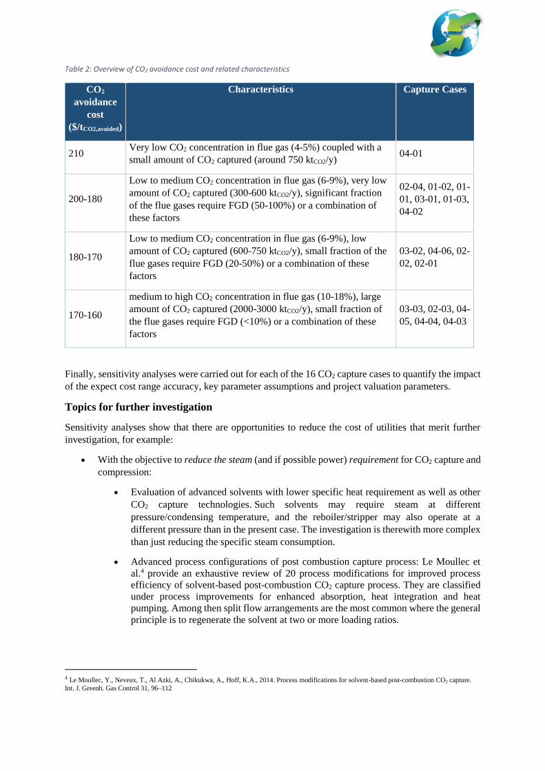
Table 2: Overview of CO2 avoidance cost and related characteristics
CO2
avoidance
cost
($/tCO2,avoided)
Characteristics Capture Cases
210 Very low CO2 concentration in flue gas (4-5%) coupled with a
small amount of CO2 captured (around 750 ktCO2/y) 04-01
200-180
Low to medium CO2 concentration in flue gas (6-9%), very low
amount of CO2 captured (300-600 ktCO2/y), significant fraction
of the flue gases require FGD (50-100%) or a combination of
these factors
02-04, 01-02, 01-
01, 03-01, 01-03,
04-02
180-170
Low to medium CO2 concentration in flue gas (6-9%), low
amount of CO2 captured (600-750 ktCO2/y), small fraction of the
flue gases require FGD (20-50%) or a combination of these
factors
03-02, 04-06, 02-
02, 02-01
170-160
medium to high CO2 concentration in flue gas (10-18%), large
amount of CO2 captured (2000-3000 ktCO2/y), small fraction of
the flue gases require FGD (<10%) or a combination of these
factors
03-03, 02-03, 04-
05, 04-04, 04-03
Finally, sensitivity analyses were carried out for each of the 16 CO2 capture cases to quantify the impact
of the expect cost range accuracy, key parameter assumptions and project valuation parameters.
Topics for further investigation
Sensitivity analyses show that there are opportunities to reduce the cost of utilities that merit further
investigation, for example:
With the objective to reduce the steam (and if possible power) requirement for CO2 capture and
compression:
Evaluation of advanced solvents with lower specific heat requirement as well as other
CO2 capture technologies. Such solvents may require steam at different
pressure/condensing temperature, and the reboiler/stripper may also operate at a
different pressure than in the present case. The investigation is therewith more complex
than just reducing the specific steam consumption.
Advanced process configurations of post combustion capture process: Le Moullec et
al.4 provide an exhaustive review of 20 process modifications for improved process
efficiency of solvent-based post-combustion CO2 capture process. They are classified
under process improvements for enhanced absorption, heat integration and heat
pumping. Among then split flow arrangements are the most common where the general
principle is to regenerate the solvent at two or more loading ratios.
4 Le Moullec, Y., Neveux, T., Al Azki, A., Chikukwa, A., Hoff, K.A., 2014. Process modifications for solvent-based post-combustion CO2 capture.
Int. J. Greenh. Gas Control 31, 96–112
Use of readily available waste heat within the refinery plant as well as (when relevant) from
nearby industries in combination with purchase of the necessary power for CO2 capture and
compression from the grid, preferably from renewable power or large efficient thermal power
plants with CO2 capture.
Lower utilities investment cost through reduced design margins: The design of CHP plant has
been performed considering significant overdesign in some cases (up to 30%). In practice, this
over-design of the additional CHP, included to provide the steam and power required for CO2
capture, might be reduced.
Operation at full load of existing CHP plants in a refinery. This would mean to accept temporary
shut-down of CO2 capture when there is a CHP plant failure since refinery production has
priority.
ACRONYMS
CHP Combined heat and power plant
CDU Crude distillation unit
CRF Catalytic reformer
DCU Delayed coker unit
FCC Fluid catalytic cracker
FGD Flue gas desulphurisation unit
HCK Hydro cracker
HDS Diesel hydro-desulphurisation unit
KHT Kerosene hydrotreater
NHT Napthha hydrotreater
NSU Naphtha splitter unit
POW Power/CHP plant
SDA Solvent deasphalting unit
SMR Steam methane reformer
SRU Sulphur recovery unit
VBU Visbreaker unit
VDU Vacuum distillation unit
VHT Vacuum gasoil hydrotreater
ReCAP Project
Evaluation the Cost of
Retrofitting CO2 Capture in
an Integrated Oil Refiners
Description of Reference Plants
ReCAP Project Evaluating the Cost of Retrofitting
CO2 Capture in an Integrated Oil Refinery
Description of Reference Plants
Doc No.: BD0839A-PR-0000-RE-001
F01 16/09/2016 Including comments L.Boschetti C.Gilardi M.Castellano
C00 13/11/2015 First Issue L.Boschetti C.Gilardi M.Castellano
REV. ISSUE DATE DESCRIPTION PREPARED BY CHECKED BY APPROVED BY
Revision F01 16/09/2016 amecfw.com Page i
Table of contents
Page
Background of the Project 5
Executive Summary 6
1. Introduction 10
List of Base Cases 10
1.1.1 Base Case 1: Simple Hydro-skimming Refinery 10
1.1.2 Base Case 2: Medium Conversion Refinery 12
1.1.3 Base Case 3: High Conversion Refinery 13
1.1.4 Base Case 4: High Conversion Refinery 15
2. Methodology 17
Refinery balances 17
Refinery layouts 17
3. Design Basis 19
Crudes 19
Product Specifications 20
Market Constraints 20
3.3.1 Gasoline 20
3.3.2 Jet fuel 20
3.3.3 Gasoils 20
3.3.4 Bitumen 20
Raw Material and Product Prices 21
Utility Conditions 21
On-stream Factor 21
Imported Vacuum Gasoil 21
Refinery Fuel Oil 21
Refinery Fuel Gas 21
Bio-additives 22
Revision F01 16/09/2016 amecfw.com Page ii
4. General data and assumptions 23
Primary Distillation Units 23
Specific Hydrogen Consumptions 27
Sulphur Recovery 28
Utility Consumptions 28
Power Plant 30
Rate and composition of Flue gases from Fired Heaters 31
Syngas and Flue Gas from Steam Methane Reformer 35
Flue Gas from Fluid Catalytic Cracking (FCC) unit 38
Flue Gas from Gas Turbine (GT) and Heat Recovery Steam Generators (HRSG) 39
5. Base Case 1 40
Refinery Balances 40
Refinery Layout 51
Main Utility Networks 53
Configuration of Power Plant 59
6. Base Case 2 61
Refinery Balances 61
Refinery Layout 74
Main Utility Networks 76
Configuration of Power Plant 82
7. Base Case 3 84
Refinery Balances 85
Refinery Layout 96
Main Utility Networks 98
Configuration of Power Plant 104
8. Base Case 4 106
Refinery Balances 106
Refinery Layout 118
Main Utility Networks 120
Configuration of Power Plant 126
Revision F01 16/09/2016 amecfw.com Page iii
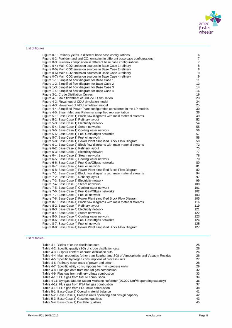
List of figures
Figure 0-1: Refinery yields in different base case configurations 6Figure 0-2: Fuel demand and CO2 emission in different base case configurations 7Figure 0-3: Fuel mix composition in different base case configurations 7Figure 0-4) Main CO2 emission sources in Base Case 1 refinery 8Figure 0-5) Main CO2 emission sources in Base Case 2 refinery 8Figure 0-6) Main CO2 emission sources in Base Case 3 refinery 9Figure 0-7) Main CO2 emission sources in Base Case 4 refinery 9Figure 1-1: Simplified flow diagram for Base Case 1 11Figure 1-2: Simplified flow diagram for Base Case 2 13Figure 1-3: Simplified flow diagram for Base Case 3 14Figure 1-4: Simplified flow diagram for Base Case 4 16Figure 3-1: Crude Distillation Curves 19Figure 4-1: Main flowsheet of CDU/VDU simulation 23Figure 4-2: Flowsheet of CDU simulation model 24Figure 4-3: Flowsheet of VDU simulation model 25Figure 4-4: Simplified Power Plant configuration considered in the LP models 30Figure 4-5: Steam Methane Reformer simplified representation 36Figure 5-1: Base Case 1) Block flow diagrams with main material streams 49Figure 5-2: Base Case 1) Refinery layout 52Figure 5-3: Base Case 1) Electricity network 54Figure 5-4: Base Case 1) Steam networks 55Figure 5-5: Base Case 1) Cooling water network 56Figure 5-6: Base Case 1) Fuel Gas/Offgas networks 57Figure 5-7: Base Case 1) Fuel oil network 58Figure 5-8: Base Case 1) Power Plant simplified Block Flow Diagram 59Figure 6-1: Base Case 2) Block flow diagrams with main material streams 72Figure 6-2: Base Case 2) Refinery layout 75Figure 6-3: Base Case 2) Electricity network 77Figure 6-4: Base Case 2) Steam networks 78Figure 6-5: Base Case 2) Cooling water network 79Figure 6-6: Base Case 2) Fuel Gas/Offgas networks 80Figure 6-7: Base Case 2) Fuel oil network 81Figure 6-8: Base Case 2) Power Plant simplified Block Flow Diagram 82Figure 7-1: Base Case 3) Block flow diagrams with main material streams 94Figure 7-2: Base Case 3) Refinery layout 97Figure 7-3: Base Case 3) Electricity network 99Figure 7-4: Base Case 3) Steam networks 100Figure 7-5: Base Case 3) Cooling water network 101Figure 7-6: Base Case 3) Fuel Gas/Offgas networks 102Figure 7-7: Base Case 3) Fuel oil network 103Figure 7-8: Base Case 3) Power Plant simplified Block Flow Diagram 105Figure 8-1: Base Case 4) Block flow diagrams with main material streams 116Figure 8-2: Base Case 4) Refinery layout 119Figure 8-3: Base Case 4) Electricity network 121Figure 8-4: Base Case 4) Steam networks 122Figure 8-5: Base Case 4) Cooling water network 123Figure 8-6: Base Case 4) Fuel Gas/Offgas networks 124Figure 8-7: Base Case 4) Fuel oil network 125Figure 8-8: Base Case 4) Power Plant simplified Block Flow Diagram 127
List of tables
Table 4-1: Yields of crude distillation cuts 25Table 4-2: Specific gravity (SG) of crude distillation cuts 26Table 4-3: Sulphur content of crude distillation cuts 26Table 4-4: Main properties (other than Sulphur and SG) of Atmospheric and Vacuum Residue 26Table 4-5: Specific hydrogen consumptions of process units 27Table 4-6: Refinery base loads of power and steam 28Table 4-7: Specific utility consumptions for main process units 29Table 4-8: Flue gas data from natural gas combustion 32Table 4-9: Flue gas from refinery offgas combustion 33Table 4-10: Flue gas from fuel oil combustion 34Table 4-11: Syngas data for Steam Methane Reformer (20,000 Nm3/h operating capacity) 35Table 4-12: Flue gas from PSA tail gas combustion 37Table 4-13: Flue gas from FCC coke combustion 38Table 5-1: Base Case 1) Overall material balance 41Table 5-2: Base Case 1) Process units operating and design capacity 42Table 5-3: Base Case 1) Gasoline qualities 43Table 5-4: Base Case 1) Distillate qualities 45

Revision F01 16/09/2016 amecfw.com Page iv
Table 5-5: Base Case 1) Fuel oil and bitumen qualities 47 Table 5-6: Base Case 1) Main utility balance, fuel mix composition, CO2 emissions 48 Table 5-7: Base Case 1) CO2 emissions per unit 50 Table 6-1: Base Case 2) Overall material balance 63 Table 6-2: Base Case 2) Process units operating and design capacity 64 Table 6-3: Base Case 2) Gasoline qualities 65 Table 6-4: Base Case 2) Distillate qualities 67 Table 6-5: Base Case 2) Fuel oil and bitumen qualities 69 Table 6-6: Base Case 2) Main utility balance, fuel mix composition, CO2 emissions 71 Table 6-7: Base Case 2) CO2 emissions per unit 73 Table 7-1: Base Case 3) Overall material balance 86 Table 7-2: Base Case 3) Process units operating and design capacity 87 Table 7-3: Base Case 3) Gasoline qualities 88 Table 7-4: Base Case 3) Distillate qualities 90 Table 7-5: Base Case 3) Fuel oil and bitumen qualities 92 Table 7-6: Base Case 3) Main utility balance, fuel mix composition, CO2 emissions 93 Table 7-7: Base Case 3) CO2 emissions per unit 95 Table 8-1: Base Case 4) Overall material balance 108 Table 8-2: Base Case 4) Process units operating and design capacity 109 Table 8-3: Base Case 4) Gasoline qualities 110 Table 8-4: Base Case 4) Distillate qualities 112 Table 8-5: Base Case 4) Fuel oil and bitumen qualities 114 Table 8-6: Base Case 4) Main utility balance, fuel mix composition, CO2 emissions 115 Table 8-7: Base Case 4) CO2 emissions per unit 117
Revision F01 16/09/2016 amecfw.com Page 5
Background of the Project
In the past years, IEA Greenhouse Gas R&D Programme (IEAGHG) has undertaken a series of projects
evaluating the performance and cost of deploying CO2 capture technologies in energy intensive industries
such as the cement, iron and steel, hydrogen, pulp and paper, and others.
In line with these activities, IEAGHG has initiated this project in collaboration with CONCAWE, GASSNOVA
and SINTEF Energy Research, to evaluate the performance and cost of retrofitting CO2 capture in an
integrated oil refinery.
The project consortium has selected Amec Foster Wheeler as the engineering contractor to work with
SINTEF in performing the basic engineering and cost estimation for the reference cases.
The main purpose of this study is to evaluate the cost of retrofitting CO2 capture in simple to high complexity
refineries covering typical European refinery capacities from 100,000 to 350,000 bbl/d. Specifically, the study
will aim to:
► Formulate a reference document providing the different design basis and key assumptions to be used
in the study.
► Define 4 different oil refineries as Base Cases. This covers the following:
► Simple refinery with a nominal capacity of 100,000 bbl/d.
► Medium to highly complex refineries with nominal capacity of 220,000 bbl/d.
► Highly complex refinery with a nominal capacity of 350,000 bbl/d.
► Define a list of emission sources for each reference case and agreed on CO2 capture priorities.
► Investigate the techno-economics performance of the integrated oil refinery (covering simple to complex
refineries, with 100,000 to 350,000 bbl/d capacity) capturing CO2 emissions:
► from various sources using post-combustion CO2 capture technology based on standard MEA
solvent.
► from hydrogen production facilities using pre-combustion CO2 capture technology.
► using oxyfuel combustion technology applied the Fluid Catalytic Cracker.
► Develop a case study evaluating the constructability of retrofitting CO2 capture in a complex oil refinery
providing key information on the following (but not limited to): plant layout, space requirement, safety,
pipeline network modification, access route for equipment, modular construction vs. stick-built
fabrication, and others.
This project will deliver “REFERENCE Documents” providing detailed information about the mass and
energy balances, carbon balance, techno-economic assumptions, data evaluation and CO2 avoidance cost,
that could be adapted and used for future economic assessment of CCS deployment in the oil refining
industry.
Revision F01 16/09/2016 amecfw.com Page 6
Executive Summary
Scope of the present report is to provide a description of the four different oil refineries identified as Base
Cases:
► Base Case 1) Simple refinery with a nominal capacity of 100,000 bbl/d.
► Base Case 2 and 3) Medium to highly complex refineries with nominal capacity of 220,000 bbl/d.
► Base Case 4) Highly complex refinery with a nominal capacity of 350,000 bbl/d.
The performance, in terms of mass and energy balances, and CO2 emissions of the REFERENCE Plants
(Base Cases) is the basis for comparison of the effectiveness and cost of the Oil Refinery with CO2 capture.
In particular, the following figures show the performance, in terms of specific energy consumptions and CO2
emissions, of the four Base Case Refineries:
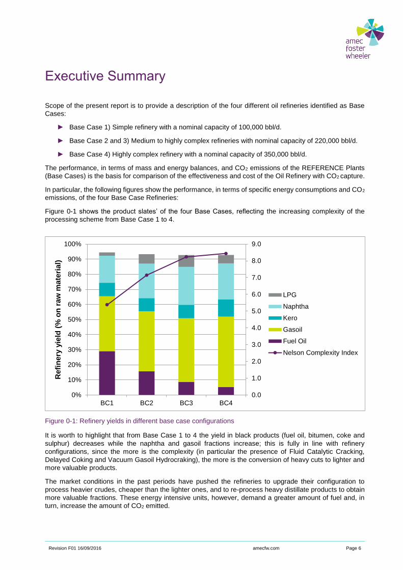
Figure 0-1 shows the product slates’ of the four Base Cases, reflecting the increasing complexity of the
processing scheme from Base Case 1 to 4.
Figure 0-1: Refinery yields in different base case configurations
It is worth to highlight that from Base Case 1 to 4 the yield in black products (fuel oil, bitumen, coke and
sulphur) decreases while the naphtha and gasoil fractions increase; this is fully in line with refinery
configurations, since the more is the complexity (in particular the presence of Fluid Catalytic Cracking,
Delayed Coking and Vacuum Gasoil Hydrocraking), the more is the conversion of heavy cuts to lighter and
more valuable products.
The market conditions in the past periods have pushed the refineries to upgrade their configuration to
process heavier crudes, cheaper than the lighter ones, and to re-process heavy distillate products to obtain
more valuable fractions. These energy intensive units, however, demand a greater amount of fuel and, in
turn, increase the amount of CO2 emitted.
0.0
1.0
2.0
3.0
4.0
5.0
6.0
7.0
8.0
9.0
0%
10%
20%
30%
40%
50%
60%
70%
80%
90%
100%
BC1 BC2 BC3 BC4
Re
fin
ery
yie
ld (
% o
n r
aw
ma
teri
al)
LPG
Naphtha
Kero
Gasoil
Fuel Oil
Nelson Complexity Index

Revision F01 16/09/2016 amecfw.com Page 7
Figure 0-2 includes a comparison of specific fuel consumptions and CO2 emission of the four cases, while
Figure 0-3 reports the different fuel mix compositions.
It can be noted that the fuel demand in Base Case 4 is indeed more than 50% bigger than the consumption
in Base Case 1, and this trend can be identified in CO2 emission too.
Figure 0-2: Fuel demand and CO2 emission in different base case configurations
Figure 0-3: Fuel mix composition in different base case configurations
As a conclusion, the four identified base cases can be regarded as a good starting point for evaluating the
effects of retrofitting CO2 capture facilities in existing refineries, different per size and complexity.
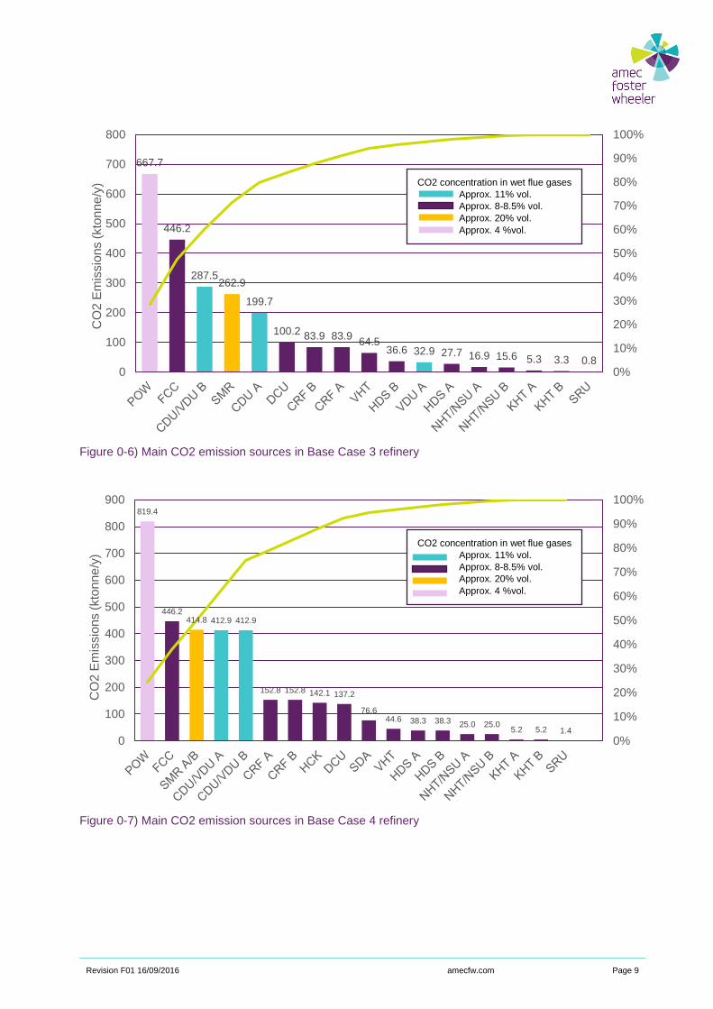
The following charts summarize the main CO2 emission sources of the four base case refineries.
0
50
100
150
200
250
5.0%
5.5%
6.0%
6.5%
7.0%
7.5%
8.0%
BC1 BC2 BC3 BC4
CO
2 e
mis
sio
n (
kg
CO
2/t
on
cru
de
oil
)
Fu
el &
Lo
ss (
% o
n r
aw
ma
teri
al)
Fuel & Loss
CO2 refinery
CO2 refinery + power plant
0%
10%
20%
30%
40%
50%
60%
70%
80%
90%
100%
BC1 BC2 BC3 BC4
Natural Gas
Refinery Fuel Gas
Low Sulphur Fuel Oil
FCC Coke

Revision F01 16/09/2016 amecfw.com Page 8
Figure 0-4) Main CO2 emission sources in Base Case 1 refinery
Figure 0-5) Main CO2 emission sources in Base Case 2 refinery
356.2
198.1
74.9
33.5 25.614.9 12.9 8.4 4.8 0.1
0%
10%
20%
30%
40%
50%
60%
70%
80%
90%
100%
0
40
80
120
160
200
240
280
320
360
400
CO
2 E
mis
sio
ns (
kto
nn
e/y
)
777.0
371.8
279.4
198.4163.0
82.0 82.049.0 32.5 32.2 28.4 28.2 16.6 15.3 4.2 2.3 0.4
0%
10%
20%
30%
40%
50%
60%
70%
80%
90%
100%
0
100
200
300
400
500
600
700
800
900
CO
2 E
mis
sio
ns (
kto
nn
e/y
)
CO2 concentration in wet flue gases
Approx. 11% vol.
Approx. 8-8.5% vol.
CO2 concentration in wet flue gases
Approx. 11% vol.
Approx. 8-8.5% vol.
Approx. 20% vol.
Revision F01 16/09/2016 amecfw.com Page 9
Figure 0-6) Main CO2 emission sources in Base Case 3 refinery
Figure 0-7) Main CO2 emission sources in Base Case 4 refinery
667.7
446.2
287.5262.9
199.7
100.2 83.9 83.964.5
36.6 32.9 27.7 16.9 15.6 5.3 3.3 0.80%
10%
20%
30%
40%
50%
60%
70%
80%
90%
100%
0
100
200
300
400
500
600
700
800
CO
2 E
mis
sio
ns (
kto
nne/y
)
819.4
446.2414.8 412.9 412.9
152.8 152.8 142.1 137.2
76.644.6 38.3 38.3 25.0 25.0
5.2 5.2 1.4
0%
10%
20%
30%
40%
50%
60%
70%
80%
90%
100%
0
100
200
300
400
500
600
700
800
900
CO
2 E
mis
sio
ns (
kto
nn
e/y
)
CO2 concentration in wet flue gases
Approx. 11% vol.
Approx. 8-8.5% vol.
Approx. 20% vol.
Approx. 4 %vol.
CO2 concentration in wet flue gases
Approx. 11% vol.
Approx. 8-8.5% vol.
Approx. 20% vol.
Approx. 4 %vol.
Revision F01 16/09/2016 amecfw.com Page 10
1. Introduction
The performance, in terms of mass and energy balances, and CO2 emissions of the REFERENCE Plants
(Base Cases) are the basis for comparison of the effectiveness and cost of the Oil Refinery with CO2 capture.
Scope of the present report is to provide a description of the four different oil refineries identified as Base
Cases, including the following main information:
► Refinery Block Flow Diagram showing the major processes of the refinery, including the overall mass
balance,
► Overall plant layout,
► Refinery fuel balance,
► Hydrogen balance,
► Breakdown of the utilities consumptions (water, electricity and steam) for each major process,
► Summary of CO2 emissions/concentrations from individual processes.
List of Base Cases
Four Base Cases have been considered which differ in terms of capacity and complexity, so providing a
representative sample of most of the existing refineries in Europe.
All the assumptions made to build the base cases have been shared among the members of the consortium
in order to reflect as much as possible the typical range of configurations, units’ capacities, product slates,
energy efficiencies, etc. of European refineries.
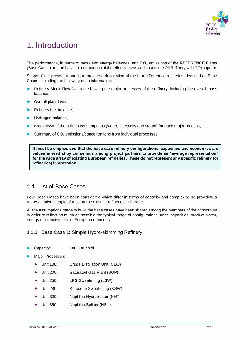
1.1.1 Base Case 1: Simple Hydro-skimming Refinery
► Capacity: 100,000 bbl/d
► Major Processes:
► Unit 100: Crude Distillation Unit (CDU)
► Unit 200: Saturated Gas Plant (SGP)
► Unit 250: LPG Sweetening (LSW)
► Unit 280: Kerosene Sweetening (KSW)
► Unit 300: Naphtha Hydrotreater (NHT)
► Unit 350: Naphtha Splitter (NSU)
It must be emphasised that the base case refinery configurations, capacities and economics are
values arrived at by consensus among project partners to provide an "average representation"
for the wide array of existing European refineries. These do not represent any specific refinery (or
refineries) in operation.
Revision F01 16/09/2016 amecfw.com Page 11
► Unit 400: Isomerization Unit (ISO)
► Unit 500: Catalytic Reformer (CRF)
► Unit 550: Reformate Splitter (RSU)
► Unit 600: Kerosene Hydrotreater (KHT)
► Unit 700: Diesel Hydro-desulphurisation Unit (HDS)
► Unit 1100: Vacuum Distillation Unit (VDU)
► Unit 1500: Visbreaker Unit (VBU)
► Unit 2000: Amine Regeneration Unit (ARU)
► Unit 2100: Sour Water Stripper Unit (SWS)
► Unit 2200: Sulphur Recovery Unit (SRU)
► Unit 2300: Waste Water Treatment (WWT)
► Unit 2500: Power Plant (Electricity and Steam Production)
► Unit 3000: Utilities
► Unit 4000: Off-sites Unit
Figure 1-1: Simplified flow diagram for Base Case 1
BITUMEN
C
D
UKHTHDS
JET FUEL
DIESEL
MOGAS
FUEL OIL
NSU
ISO
CRF
ADDITIVES
NHT
HYDROGEN
DESULPHURIZED HEAVY GASOIL
V
D
U VHTHEATING / MARINE
DIESEL
100,000BPSD
VISBROKEN RESIDUE
VACUUM RESIDUE
VBU
VACUUM GASOIL
HEAVY GASOIL
LIGHT GASOIL
KEROSENE
NAPHTHA
VACUUMGASOIL
VACUUMRESIDUE
Revision F01 16/09/2016 amecfw.com Page 12
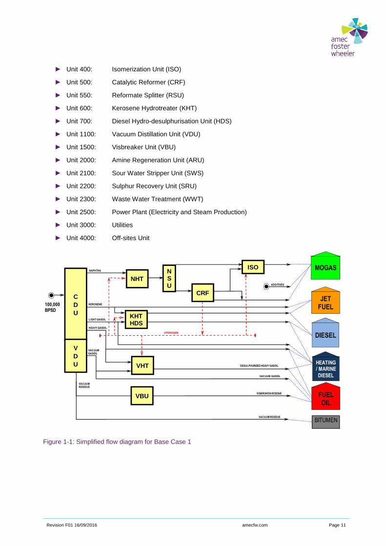
1.1.2 Base Case 2: Medium Conversion Refinery
► Capacity: 220,000 bbl/d
► Major Processes:
► Unit 100: Crude Distillation Unit (CDU)
► Unit 200: Saturated Gas Plant (SGP)
► Unit 250: LPG Sweetening (LSW)
► Unit 280: Kerosene Sweetening (KSW)
► Unit 300: Naphtha Hydrotreater (NHT)
► Unit 350: Naphtha Splitter (NSU)
► Unit 400: Isomerization Unit (ISO)
► Unit 500: Catalytic Reformer (CRF)
► Unit 550: Reformate Splitter (RSU)
► Unit 600: Kerosene Hydrotreater (KHT)
► Unit 700: Diesel Hydro-desulphurisation Unit (HDS)
► Unit 800: Vacuum Gasoil Hydrotreater (VHT)
► Unit 1000: Fluid Catalytic Cracker (FCC)
► Unit 1050: FCC Gasoline Post-Treatment Unit (PTU)
► Unit 1100: Vacuum Distillation Unit (VDU)
► Unit 1200: Steam Methane Reformer (SMR)
► Unit 1500: Visbreaker Unit (VBU)
► Unit 2000: Amine Regeneration Unit (ARU)
► Unit 2100: Sour Water Stripper Unit (SWS)
► Unit 2200: Sulphur Recovery Unit (SRU)
► Unit 2300: Waste Water Treatment (WWT)
► Unit 2500: Power Plant (POW)
► Unit 3000: Utilities
► Unit 4000: Off-sites

Revision F01 16/09/2016 amecfw.com Page 13
Figure 1-2: Simplified flow diagram for Base Case 2
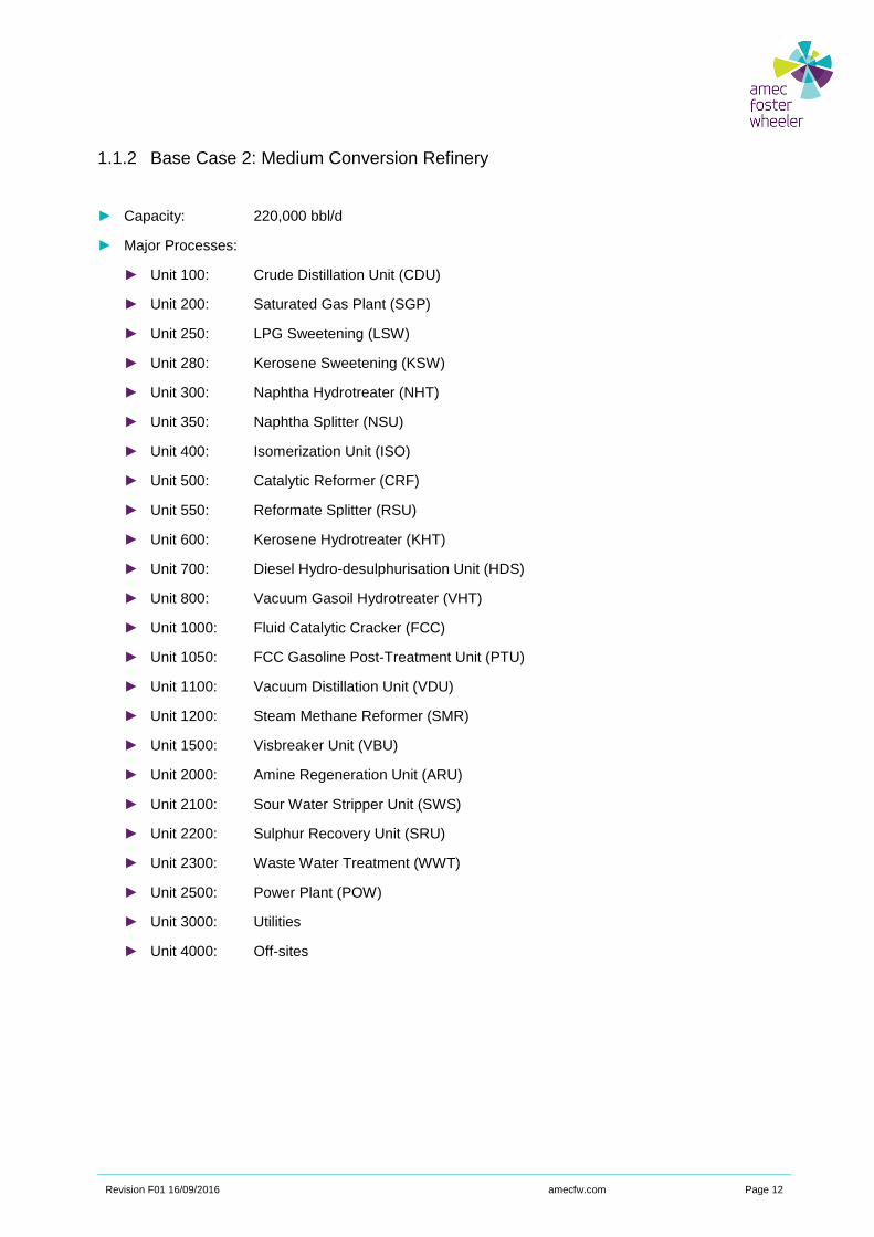
1.1.3 Base Case 3: High Conversion Refinery
► Capacity: 220,000 bbl/d
► Major Processes:
► Unit 100: Crude Distillation Unit (CDU)
► Unit 200: Saturated Gas Plant (SGP)
► Unit 250: LPG Sweetening (LSW)
► Unit 280: Kerosene Sweetening (KSW)
► Unit 300: Naphtha Hydrotreater (NHT)
► Unit 350: Naphtha Splitter (NSU)
► Unit 400: Isomerization Unit (ISO)
► Unit 500: Catalytic Reformer (CRF)
► Unit 550: Reformate Splitter (RSU)
► Unit 600: Kerosene Hydrotreater (KHT)
► Unit 700: Diesel Hydro-desulphurisation Unit (HDS)
► Unit 800: Vacuum Gasoil Hydrotreater (VHT)
BITUMEN
C
D
U KHTHDS
JET FUEL
DIESEL
MOGAS
FUEL OIL
NSU
ISO
CRF
ADDITIVES
NHT
HYDROGEN
V
D
U VHT
HEATING / MARINE
DIESEL
220,000BPSD
VISBROKEN RESIDUE
VACUUM RESIDUE
VBU
HEAVY GASOIL
LIGHT GASOIL
KEROSENE
NAPHTHA
VACUUMGASOIL
VACUUMRESIDUE
FCC
PTU
CLARIFIED OIL
HEAVY CRACKED NAPHTHA
LIGHT CYCLE OIL
LIGHT CRACKED NAPHTHA
SMR
ISOMERATE
REFORMATE
Revision F01 16/09/2016 amecfw.com Page 14
► Unit 1000: Fluid Catalytic Cracker (FCC)
► Unit 1050: FCC Gasoline Post-Treatment Unit (PTU)
► Unit 1100: Vacuum Distillation Unit (VDU)
► Unit 1200: Steam Methane Reformer (SMR)
► Unit 1400: Delayed Coker Unit (DCU)
► Unit 2000: Amine Regeneration Unit (ARU)
► Unit 2100: Sour Water Stripper Unit (SWS)
► Unit 2200: Sulphur Recovery Unit (SRU)
► Unit 2300: Waste Water Treatment (WWT)
► Unit 2500: Power Plant (POW)
► Unit 3000: Utilities
► Unit 4000: Off-sites
Figure 1-3: Simplified flow diagram for Base Case 3
BITUMEN
C
D
U KHTHDS
JET FUEL
DIESEL
MOGAS
FUEL OIL
NSU
ISO
CRF
ADDITIVES
NHT
HYDROGEN
V
D
U VHT
HEATING / MARINE
DIESEL
220,000BPSD
VACUUM RESIDUE
DCU
HEAVY GASOIL
LIGHT GASOIL
KEROSENE
NAPHTHA
VACUUMGASOIL
VACUUMRESIDUE
FCC
PTU
CLARIFIED OIL
HEAVY CRACKED NAPHTHA
LIGHT CYCLE OIL
LIGHT CRACKED NAPHTHA
PETCOKE
SMR
ISOMERATE
REFORMATE
Revision F01 16/09/2016 amecfw.com Page 15
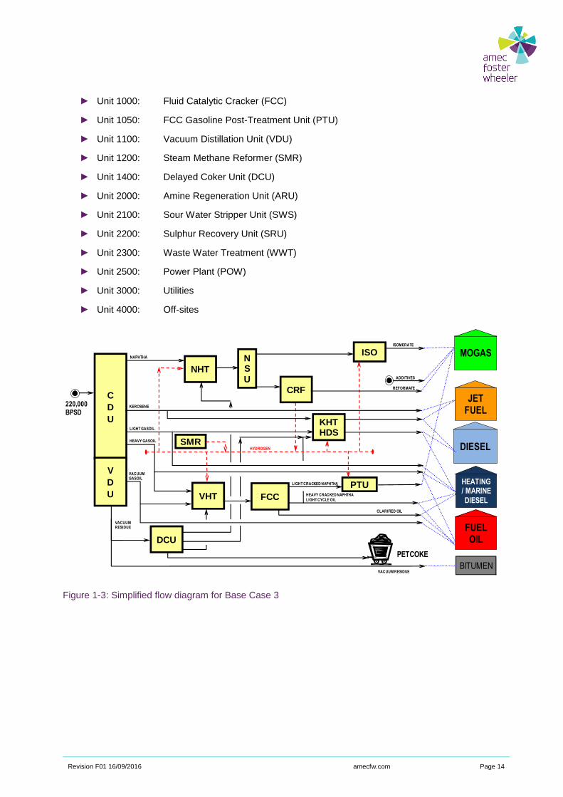
1.1.4 Base Case 4: High Conversion Refinery
► Capacity: 350,000 bbl/d
► Major Processes:
► Unit 100: Crude Distillation Unit (CDU)
► Unit 200: Saturated Gas Plant (SGP)
► Unit 250: LPG Sweetening (LSW)
► Unit 280: Kerosene Sweetening (KSW)
► Unit 300: Naphtha Hydrotreater (NHT)
► Unit 350: Naphtha Splitter (NSU)
► Unit 400: Isomerization Unit (ISO)
► Unit 500: Catalytic Reformer (CRF)
► Unit 550: Reformate Splitter (RSU)
► Unit 600: Kerosene Hydrotreater (KHT)
► Unit 700: Gasoil Hydro-desulphurisation Unit (HDS)
► Unit 800: Vacuum Gasoil Hydrotreater (VHT)
► Unit 900: Hydrocracker Unit (HCK)
► Unit 1000: Fluid Catalytic Cracker (FCC)
► Unit 1050: FCC Gasoline Post-Treatment Unit (PTU)
► Unit 1100: Vacuum Distillation Unit (VDU)
► Unit 1200: Steam Methane Reformer (SMR)
► Unit 1300: Solvent Deasphalting Unit (SDA)
► Unit 1400: Delayed Coker Unit (DCU)
► Unit 2000: Amine Regeneration Unit (ARU)
► Unit 2100: Sour Water Stripper Unit (SWS)
► Unit 2200: Sulphur Recovery Unit (SRU)
► Unit 2300: Waste Water Treatment (WWT)
► Unit 2500: Power Plant (POW)
► Unit 3000: Utilities
► Unit 4000: Off-sites
Revision F01 16/09/2016 amecfw.com Page 16
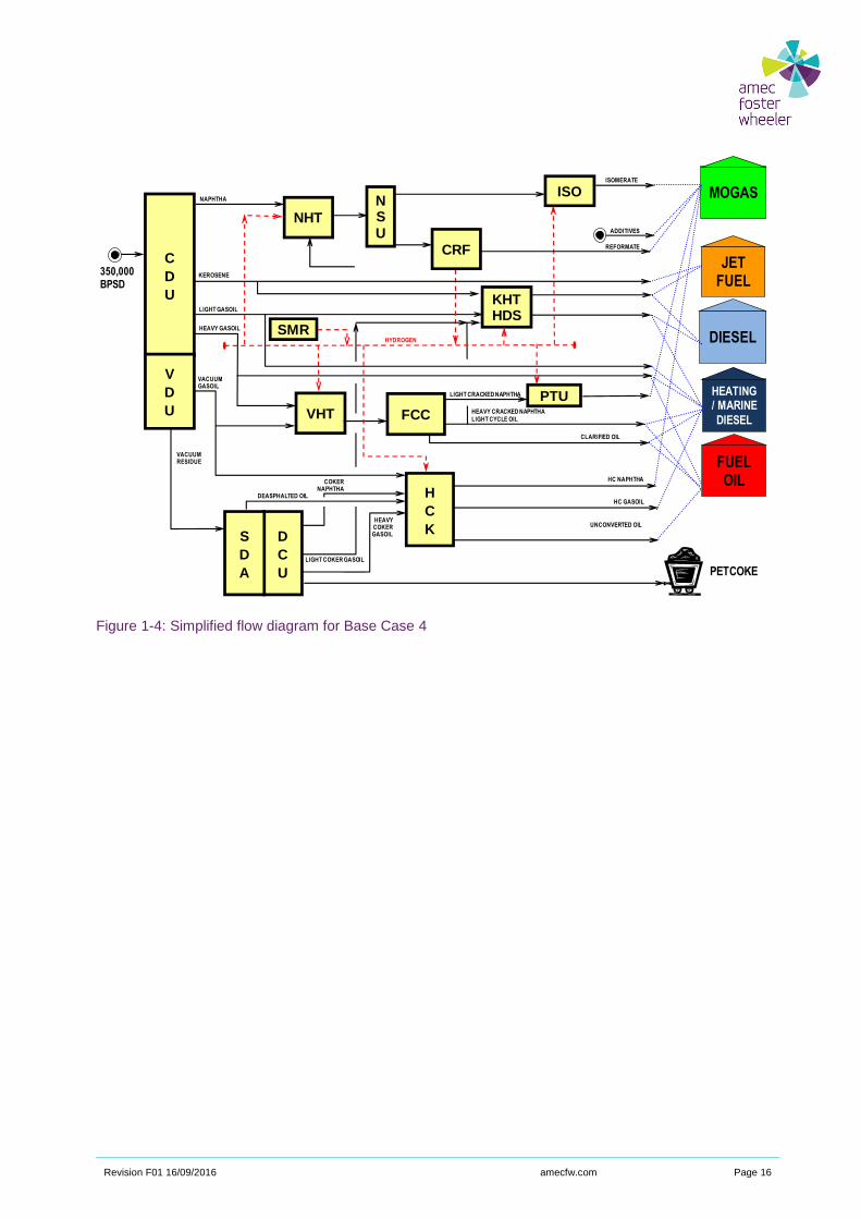
Figure 1-4: Simplified flow diagram for Base Case 4
C
D
U KHTHDS
JET FUEL
DIESEL
MOGAS
FUEL OIL
NSU
ISO
CRF
ADDITIVES
NHT
HYDROGEN
V
D
U VHT
HEATING / MARINE
DIESEL
350,000BPSD
HEAVY GASOIL
LIGHT GASOIL
KEROSENE
NAPHTHA
VACUUMGASOIL
VACUUMRESIDUE
FCC
PTU
CLARIFIED OIL
HEAVY CRACKED NAPHTHA
LIGHT CYCLE OIL
LIGHT CRACKED NAPHTHA
PETCOKE
SMR
ISOMERATE
REFORMATE
D
C
U
HEAVYCOKERGASOIL
H
C
K
COKERNAPHTHA
UNCONVERTED OIL
HC NAPHTHA
HC GASOIL
LIGHT COKER GASOIL
S
D
A
DEASPHALTED OIL
Revision F01 16/09/2016 amecfw.com Page 17
2. Methodology
Refinery balances
A linear programming model has been built for each one of the four Base Cases, in order to produce
consistent and realistic refinery balances.
Linear programming (LP) is an optimisation technique widely used in petroleum refineries.
LP models of refineries are used for capital investment decisions, the evaluation of term contracts for crude
oil, spot crude oil purchases, production planning and scheduling, and supply chain optimisation.
Haverly Systems GRTMPS software (v. 5.0) has been used to build the refinery LP models.
For each process unit, typical yields’ structure, products’ qualities and specific utility consumptions have
been input, based on Amec Foster Wheeler in-house database.
In particular, as far as the primary distillation units are concerned (i.e. Crude Atmospheric and Vacuum
Units), some process simulation models have been run in order to evaluate the distillates’ yields and main
qualities.
The model has been run based on:
► a consistent set of crude, natural gas and products’ prices,
► a typical (average) crude diet,
► typical (average) units’ sizes and utilization factors,
► European products’ specifications,
► typical products’ slates, reflecting the average proportions among gasoline markets (i.e. EU/US Export),
middle distillates grades (jet fuel/automotive diesel/marine diesel/heating oil) and fuel oil/bitumen
productions.
Moreover, in the LP model, an internal production of power and steam to satisfy the refinery needs has been
considered.
In the following sections, more details are provided to describe the main input data and constraints of the
linear programming models.
Reference is also made to the Reference Document – Technical Basis, including most of the basic
assumptions made to develop the refinery balances.
Refinery layouts
The refinery layouts for the four Base Cases have been developed based on the processing schemes and
units’ capacities defined as a result of the modelling optimisation.
The layouts have been conceived starting from real examples (real sites) in Amec Foster Wheeler in-house
database, to reflect as a much as possible the typical arrangement of European refineries. The intent of
presenting typical layouts for the Base Cases is to create a reasonable background for evaluating, in a
second phase of this Study, the impact of retrofitting CO2 capture facilities in an existing site with the relevant
constraints (e.g. the limitations in the available plot area, the need for long interconnecting ducts between
the existing and the new plants, etc.)

Revision F01 16/09/2016 amecfw.com Page 18
The following notes apply to the Base Case layouts:
► Process units’ block is normally located in a central area of the plot;
► Utility block is located in a lateral position with respect of process units;
► Storage tank areas are all around the units’ block. Different tank sizes are shown for crude, finished
products, intermediate products; ► Main pipe-racks connecting the various process units and utility blocks are shown; ► Jetties and truck loading facilities for sending/receiving products are shown;
► Flare and Waste Water Treatment facilities, which are very demanding in terms of plot area, are shown;
► The main gaseous emission points (e.g. fired heaters stacks) are shown.
Revision F01 16/09/2016 amecfw.com Page 19
3. Design Basis
Crudes
In order to develop the refinery balances, the following crudes have been considered:
► Ekofisk (Norway), 42.4° API, Sulphur content 0.17% wt.
► Bonny Light (Nigeria), 35.0° API, Sulphur content 0.13% wt.
► Arabian Light (Saudi Arabia), 33.9° API, Sulphur content 1.77% wt.
► Urals Medium (Russia), 32.0° API, Sulphur content 1.46% wt.
► Arabian Heavy (Saudi Arabia), 28.1° API, Sulphur content 2.85% wt.
► Maya (Mexico), 21.7°API, Sulphur content 3.18% wt.
The crude basket has been selected as representative of different supply regions, products’ yields and
qualities, and it is deemed to reflect with a fair representation the “average” operation of the four European
refineries identified as Base Cases.
As far as Maya crude is concerned, it has been considered to be processed only in mixture with Arabian
Light, in the proportion 50/50% wt. This to consider the fact that the typical crude distillation units in Europe
were not originally designed for extra-heavy crudes and can accommodate them only in blended mode.
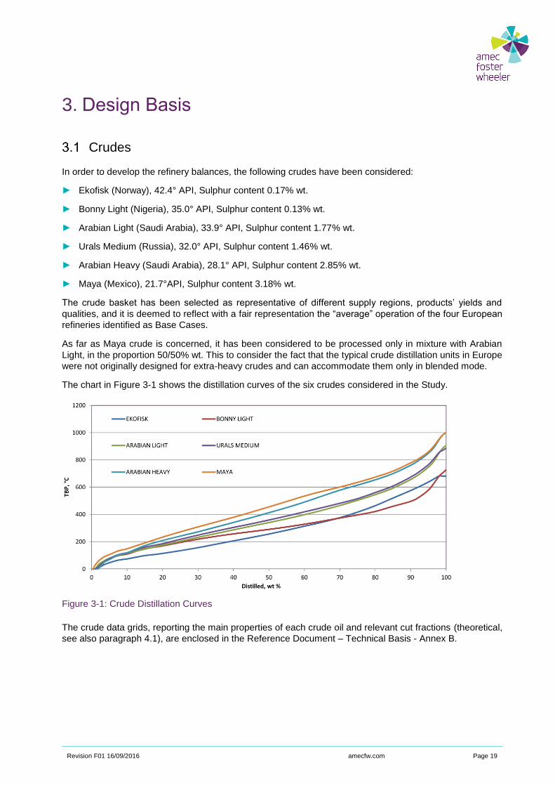
The chart in Figure 3-1 shows the distillation curves of the six crudes considered in the Study.
Figure 3-1: Crude Distillation Curves
The crude data grids, reporting the main properties of each crude oil and relevant cut fractions (theoretical,
see also paragraph 4.1), are enclosed in the Reference Document – Technical Basis - Annex B.
Revision F01 16/09/2016 amecfw.com Page 20
As far as the proportions among the different crudes are considered, the following have been forced into the
LP models to produce the optimised refinery balances:
► Maya Blend: 4% minimum.
► Arabian Heavy: 3% minimum (*)
► Arabian Light: 10% minimum.
► Urals: 30% minimum.
► Bonny Light: 30% maximum (*).
► Ekofisk: no limit. Balancing crude.
(*) Arabian Heavy increased to 10% minimum and Bonny Light decreased to 23% maximum in Base Case 3 and Base Case 4.
Product Specifications
The refinery product specifications considered in this Study are reported in the Reference Document –
Technical Basis - Annex C.
No seasonal variations are considered.
Market Constraints
Products’ market constraints have been input in the LP model in order to “drive” the model solution to reflect
the typical products’ slates of the European refineries.
3.3.1 Gasoline
Gasoline Export to US is 30 to 40% wt. of the total gasoline production. The rest of gasoline production is
sold in Europe.
3.3.2 Jet fuel
Sales of Jet Fuel represent approx. 10% wt. of the total crude intake for Base Case 1 to Base Case 3.
Jet Fuel production is increased to 13% wt. of total crude intake for Base Case 4.
3.3.3 Gasoils
Automotive Diesel is minimum 75% wt. of the total gasoil production.
Marine Diesel is maximum 10% wt. of the total gasoil production.
3.3.4 Bitumen
Bitumen sold in Base Case 1, 2 and 3 is approx. 2.5% wt. of the total crude intake.
Bitumen is not produced in Base Case 4, since in such a deep conversion refinery it is considered to
maximise the distillates’ production.
Revision F01 16/09/2016 amecfw.com Page 21
Raw Material and Product Prices
The sets of prices considered in the LP models have been agreed among the members of the Consortium.
They have been provided to Amec Foster Wheeler only for the purpose of calculations and they do not
represent prices for any specific refinery.
Utility Conditions
In the LP models, the utility conditions have been considered as per Reference Document – Technical Basis
- Paragraph 7.4.
On-stream Factor
350 operating days per year have been considered to develop the overall material balances of the four Base
Case refineries, reflecting as an average:
► 1 week shutdown per year for unplanned shutdowns/catalyst replacements/minor repairs, plus
► 4 weeks general planned turnaround every 4 years for maintenance/major repairs.
Imported Vacuum Gasoil
Vacuum Gasoil is imported in some Base Cases in order to saturate the capacity of the heavy gasoil
conversion units (e.g. Fluid Catalytic Cracking). The quality of imported Vacuum Gasoil is assumed equal to
the quality of Heavy Vacuum Gasoil (nominal TBP cut range 420÷530°C) obtained by distillation of the Urals
crude.
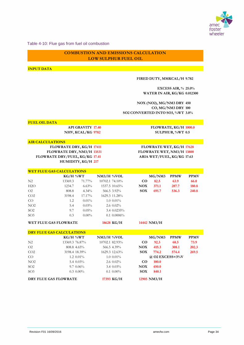
Refinery Fuel Oil
Low Sulphur Fuel Oil with 0.5% wt. Sulphur content is burnt in some of the refinery heaters.
Reference is made to Reference Document – Technical Basis - Paragraph 5.1 for the main properties of
Low Sulphur Fuel Oil.
The heaters in the following process units have been considered 100% fuel oil fired:
► Unit 100: Crude Distillation Unit (CDU)
► Unit 1100: Vacuum Distillation Unit (VDU)
► Unit 1500: Visbreaker Unit (VBU) (*)
(*) VBU is present only in Base Case 1 and Base Case 2.
Refinery Fuel Gas
With the exception of the fired heaters burning fuel oil listed in the previous paragraph 3.8, the other refinery
heaters and the Power Plant are 100% gas fired.
The off-gases produced in the various process units, after removal of H2S in amine absorbers (to achieve a
residual H2S content of 50 ppm vol. max.), are collected into a Refinery Fuel Gas system to constitute the
primary fuel of the refinery. Imported natural gas is mixed with refinery off-gases to saturate the fuel demand.
Revision F01 16/09/2016 amecfw.com Page 22
Reference is made to Reference Document – Technical Basis - Paragraph 4.2 and 5.2, respectively for the
quality of natural gas and refinery off-gases (average) used for combustion calculations.
Bio-additives
Bio-ethanol is an additive to European Gasoline, while Bio-diesel is an additive to Automotive Gas Oil
(Diesel).
To produce the typical refinery balances, the quantity of bio-additives in each finished product has been
set/limited to the values reflecting the average European qualities:
► bio-ethanol blended into European Gasoline has been limited to 5% vol. max (despite the “official”
specification is limiting the bio-ethanol content to 10% vol. max.);
► bio-diesel has been fixed in the range 6÷7% vol. on Diesel.
Revision F01 16/09/2016 amecfw.com Page 23
4. General data and assumptions
This chapter includes the sets of data and assumptions, common to all the Base Cases, used to build the
refinery LP models.
The methodology normally used for refinery configuration studies has been adopted, trying however to:
► remove all the site-specific constraints coming from Amec Foster Wheeler past projects;
► obtain generic but realistic balances, with the level of accuracy needed for the purposes of ReCAP
Project.
The valuable input from the members of the Consortium, has been used to optimise the refinery LP model
calibration.
For the purpose of this study the capacity of the majority of the units has been adjusted to provide a utilisation
rate over 90%. Exceptions to this are the sulphur recovery units and the steam reformers.
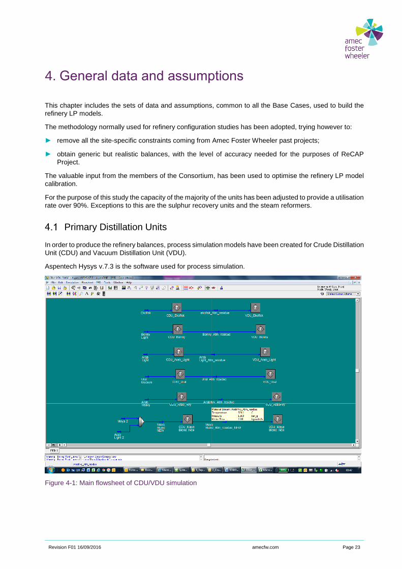
Primary Distillation Units
In order to produce the refinery balances, process simulation models have been created for Crude Distillation
Unit (CDU) and Vacuum Distillation Unit (VDU).
Aspentech Hysys v.7.3 is the software used for process simulation.
Figure 4-1: Main flowsheet of CDU/VDU simulation
Revision F01 16/09/2016 amecfw.com Page 24
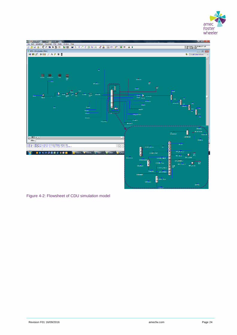
Figure 4-2: Flowsheet of CDU simulation model
Revision F01 16/09/2016 amecfw.com Page 25
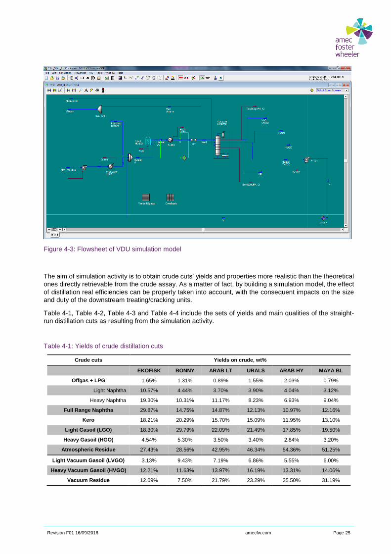
Figure 4-3: Flowsheet of VDU simulation model
The aim of simulation activity is to obtain crude cuts’ yields and properties more realistic than the theoretical
ones directly retrievable from the crude assay. As a matter of fact, by building a simulation model, the effect
of distillation real efficiencies can be properly taken into account, with the consequent impacts on the size
and duty of the downstream treating/cracking units.
Table 4-1, Table 4-2, Table 4-3 and Table 4-4 include the sets of yields and main qualities of the straight-
run distillation cuts as resulting from the simulation activity.
Table 4-1: Yields of crude distillation cuts
Crude cuts Yields on crude, wt%
EKOFISK BONNY ARAB LT URALS ARAB HY MAYA BL
Offgas + LPG 1.65% 1.31% 0.89% 1.55% 2.03% 0.79%
Light Naphtha 10.57% 4.44% 3.70% 3.90% 4.04% 3.12%
Heavy Naphtha 19.30% 10.31% 11.17% 8.23% 6.93% 9.04%
Full Range Naphtha 29.87% 14.75% 14.87% 12.13% 10.97% 12.16%
Kero 18.21% 20.29% 15.70% 15.09% 11.95% 13.10%
Light Gasoil (LGO) 18.30% 29.79% 22.09% 21.49% 17.85% 19.50%
Heavy Gasoil (HGO) 4.54% 5.30% 3.50% 3.40% 2.84% 3.20%
Atmospheric Residue 27.43% 28.56% 42.95% 46.34% 54.36% 51.25%
Light Vacuum Gasoil (LVGO) 3.13% 9.43% 7.19% 6.86% 5.55% 6.00%
Heavy Vacuum Gasoil (HVGO) 12.21% 11.63% 13.97% 16.19% 13.31% 14.06%
Vacuum Residue 12.09% 7.50% 21.79% 23.29% 35.50% 31.19%
Revision F01 16/09/2016 amecfw.com Page 26
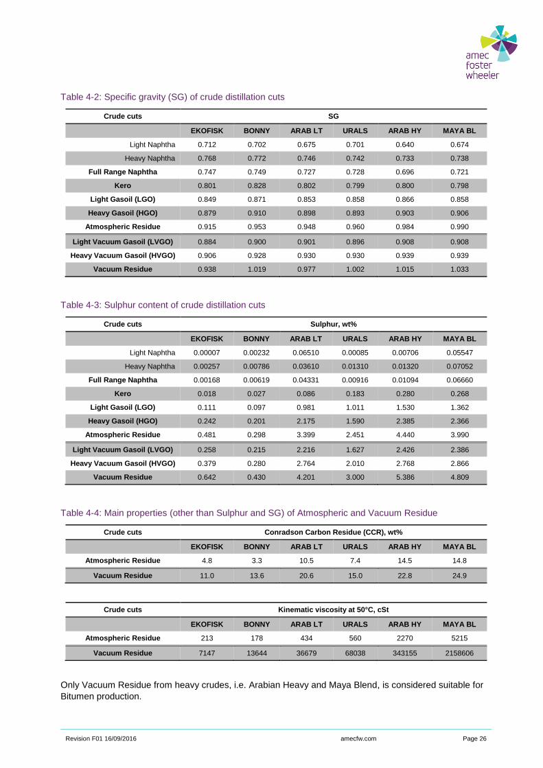
Table 4-2: Specific gravity (SG) of crude distillation cuts
Crude cuts SG
EKOFISK BONNY ARAB LT URALS ARAB HY MAYA BL
Light Naphtha 0.712 0.702 0.675 0.701 0.640 0.674
Heavy Naphtha 0.768 0.772 0.746 0.742 0.733 0.738
Full Range Naphtha 0.747 0.749 0.727 0.728 0.696 0.721
Kero 0.801 0.828 0.802 0.799 0.800 0.798
Light Gasoil (LGO) 0.849 0.871 0.853 0.858 0.866 0.858
Heavy Gasoil (HGO) 0.879 0.910 0.898 0.893 0.903 0.906
Atmospheric Residue 0.915 0.953 0.948 0.960 0.984 0.990
Light Vacuum Gasoil (LVGO) 0.884 0.900 0.901 0.896 0.908 0.908
Heavy Vacuum Gasoil (HVGO) 0.906 0.928 0.930 0.930 0.939 0.939
Vacuum Residue 0.938 1.019 0.977 1.002 1.015 1.033
Table 4-3: Sulphur content of crude distillation cuts
Crude cuts Sulphur, wt%
EKOFISK BONNY ARAB LT URALS ARAB HY MAYA BL
Light Naphtha 0.00007 0.00232 0.06510 0.00085 0.00706 0.05547
Heavy Naphtha 0.00257 0.00786 0.03610 0.01310 0.01320 0.07052
Full Range Naphtha 0.00168 0.00619 0.04331 0.00916 0.01094 0.06660
Kero 0.018 0.027 0.086 0.183 0.280 0.268
Light Gasoil (LGO) 0.111 0.097 0.981 1.011 1.530 1.362
Heavy Gasoil (HGO) 0.242 0.201 2.175 1.590 2.385 2.366
Atmospheric Residue 0.481 0.298 3.399 2.451 4.440 3.990
Light Vacuum Gasoil (LVGO) 0.258 0.215 2.216 1.627 2.426 2.386
Heavy Vacuum Gasoil (HVGO) 0.379 0.280 2.764 2.010 2.768 2.866
Vacuum Residue 0.642 0.430 4.201 3.000 5.386 4.809
Table 4-4: Main properties (other than Sulphur and SG) of Atmospheric and Vacuum Residue
Crude cuts Conradson Carbon Residue (CCR), wt%
EKOFISK BONNY ARAB LT URALS ARAB HY MAYA BL
Atmospheric Residue 4.8 3.3 10.5 7.4 14.5 14.8
Vacuum Residue 11.0 13.6 20.6 15.0 22.8 24.9
Crude cuts Kinematic viscosity at 50°C, cSt
EKOFISK BONNY ARAB LT URALS ARAB HY MAYA BL
Atmospheric Residue 213 178 434 560 2270 5215
Vacuum Residue 7147 13644 36679 68038 343155 2158606
Only Vacuum Residue from heavy crudes, i.e. Arabian Heavy and Maya Blend, is considered suitable for
Bitumen production.

Revision F01 16/09/2016 amecfw.com Page 27
Specific Hydrogen Consumptions
Hydrogen balances have been developed by considering the units’ specific hydrogen demands reported in
Table 4-5.
The following notes apply:
► Specific consumptions are dependent on feed quality;
► Specific consumptions include chemical consumptions, solution losses and mechanical losses.
The hydrogen balances are reported in the block flow diagrams developed for each Base Case (reference
is made to Figure 5-1, Figure 6-1, Figure 7-1 and Figure 8-1).
Table 4-5: Specific hydrogen consumptions of process units
Unit Feed H2 consumption
(wt% on feed)
0300 NHT Naphtha Hydrotreater Straight-run Naphtha 0.12
VB Naphtha/Coker Naphtha 0.15
0400 ISO Isomerization Hydrotreated Light Naphtha 0.085
0600A KHT Kero HDS Straight-run Kerosene 0.2
0700A HDS Gasoil HDS Straight-run Light Gasoil 0.7
VB Gasoil 0.8
Light Coker Gasoil 0.8
Light Cycle Oil 0.8
Heavy Cracked Naphtha 0.25
0800 VHT Vacuum Gasoil Hydrotreater Straight-run Heavy Gasoil 1.2
Light Vacuum Gasoil 1.2
Heavy Vacuum Gasoil 1.5
Heavy Coker Gasoil 1.5
Deasphalted OIl 1.57
0900 HCK Vacuum Gasoil Hydrocracker Straight-run Heavy Gasoil 2.0
Light Vacuum Gasoil 2.0
Heavy Vacuum Gasoil 2.9
Heavy Coker Gasoil 4.0
Revision F01 16/09/2016 amecfw.com Page 28
Sulphur Recovery
The H2S produced in the desulphurization units will be recovered by means of Amine Washing and
Regeneration Unit (Unit 2000 – ARU) and Sour Water Stripper (Unit 2100 – SWS). The acid gases recovered
from the top of Amine Regenerator and the Sour gases from the top of the SWS column are then sent to
Sulphur Recovery Unit (Unit 2200 – SRU). An overall sulphur recovery of 99.5% has been considered,
assuming that a Tail Gas Treatment section is installed downstream the SRU Claus section.
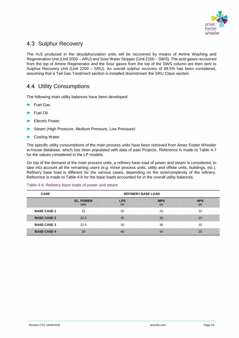
Utility Consumptions
The following main utility balances have been developed:
► Fuel Gas
► Fuel Oil
► Electric Power
► Steam (High Pressure, Medium Pressure, Low Pressure)
► Cooling Water
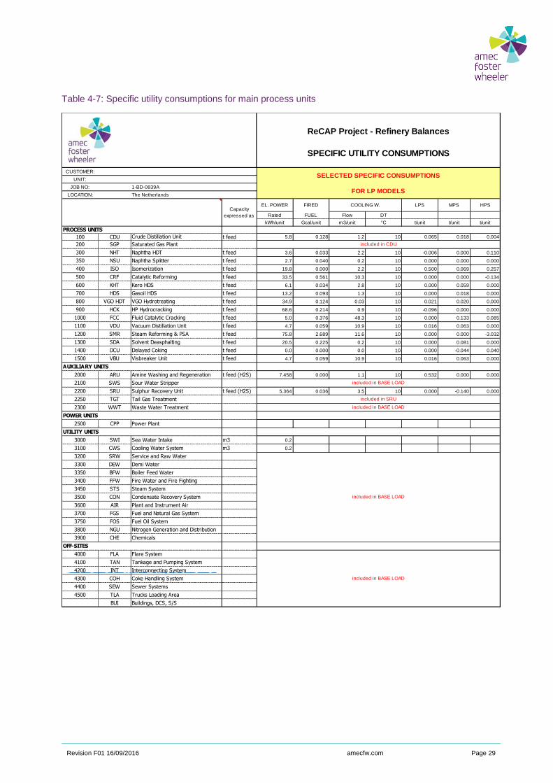
The specific utility consumptions of the main process units have been retrieved from Amec Foster Wheeler
in-house database, which has been populated with data of past Projects. Reference is made to Table 4-7
for the values considered in the LP models.
On top of the demand of the main process units, a refinery base load of power and steam is considered, to
take into account all the remaining users (e.g. minor process units, utility and offsite units, buildings, etc.).
Refinery base load is different for the various cases, depending on the size/complexity of the refinery.
Reference is made to Table 4-6 for the base loads accounted for in the overall utility balances.
Table 4-6: Refinery base loads of power and steam
CASE REFINERY BASE LOAD
EL. POWER MW
LPS t/h
MPS t/h
HPS t/h
BASE CASE 1 15 20 20 10
BASE CASE 2 22.5 30 30 15
BASE CASE 3 22.5 30 30 15
BASE CASE 4 30 40 40 20
Revision F01 16/09/2016 amecfw.com Page 29
Table 4-7: Specific utility consumptions for main process units
ReCAP Project - Refinery Balances
SPECIFIC UTILITY CONSUMPTIONS
CUSTOMER:
UNIT:
JOB NO: 1-BD-0839A
LOCATION: The Netherlands
EL. POWER FIRED COOLING W. LPS MPS HPS
Rated FUEL Flow DT
kWh/unit Gcal/unit m3/unit °C t/unit t/unit t/unit
100 CDU t feed 5.8 0.128 1.2 10 0.065 0.018 0.004
200 SGP
300 NHT t feed 3.6 0.033 2.2 10 -0.006 0.000 0.110
350 NSU t feed 2.7 0.040 0.2 10 0.000 0.000 0.000
400 ISO t feed 19.8 0.000 2.2 10 0.500 0.069 0.257
500 CRF t feed 33.5 0.561 10.3 10 0.000 0.000 -0.134
600 KHT t feed 6.1 0.034 2.8 10 0.000 0.059 0.000
700 HDS t feed 13.2 0.093 1.3 10 0.000 0.018 0.000
800 VGO HDT t feed 34.9 0.124 0.03 10 0.021 0.020 0.000
900 HCK t feed 68.6 0.214 0.9 10 -0.096 0.000 0.000
1000 FCC t feed 5.0 0.376 48.3 10 0.000 0.133 0.085
1100 VDU t feed 4.7 0.059 10.9 10 0.016 0.063 0.000
1200 SMR t feed 75.8 2.689 11.6 10 0.000 0.000 -3.032
1300 SDA t feed 20.5 0.225 0.2 10 0.000 0.081 0.000
1400 DCU t feed 0.0 0.000 0.0 10 0.000 -0.044 0.040
1500 VBU t feed 4.7 0.059 10.9 10 0.016 0.063 0.000
2000 ARU t feed (H2S) 7.458 0.000 1.1 10 0.532 0.000 0.000
2100 SWS
2200 SRU t feed (H2S) 5.364 0.036 3.5 10 0.000 -0.140 0.000
2250 TGT
2300 WWT
2500 CPP
3000 SWI m3 0.2
3100 CWS m3 0.2
3200 SRW
3300 DEW
3350 BFW
3400 FFW
3450 STS
3500 CON
3600 AIR
3700 FGS
3750 FOS
3800 NGU
3900 CHE
4000 FLA
4100 TAN
4200 INT
4300 COH
4400 SEW
4500 TLA
BUI
included in SRU
included in BASE LOAD
included in BASE LOAD
included in BASE LOAD
Interconnecting System
Coke Handling System
Cooling Water System
included in BASE LOAD
included in CDU
Flare System
Tankage and Pumping System
Buildings, DCS, S/S
Sea Water Intake
Power Plant
Trucks Loading Area
Chemicals
OFF-SITES
SELECTED SPECIFIC CONSUMPTIONS
FOR LP MODELS
Sewer Systems
Delayed Coking
Condensate Recovery System
Plant and Instrument Air
Fuel and Natural Gas System
Fuel Oil System
Nitrogen Generation and Distribution
Steam System
Service and Raw Water
Demi Water
Boiler Feed Water
Fire Water and Fire Fighting
UTILITY UNITS
Amine Washing and Regeneration
Sour Water Stripper
Sulphur Recovery Unit
Tail Gas Treatment
Waste Water Treatment
POWER UNITS
Solvent Deasphalting
Visbreaker Unit
AUXILIARY UNITS
Kero HDS
Gasoil HDS
VGO Hydrotreating
HP Hydrocracking
Fluid Catalytic Cracking
Vacuum Distillation Unit
Catalytic Reforming
PROCESS UNITS
Crude Distillation Unit
Saturated Gas Plant
Naphtha Splitter
Steam Reforming & PSA
Capacity
expressed as
Naphtha HDT
Isomerization
Revision F01 16/09/2016 amecfw.com Page 30
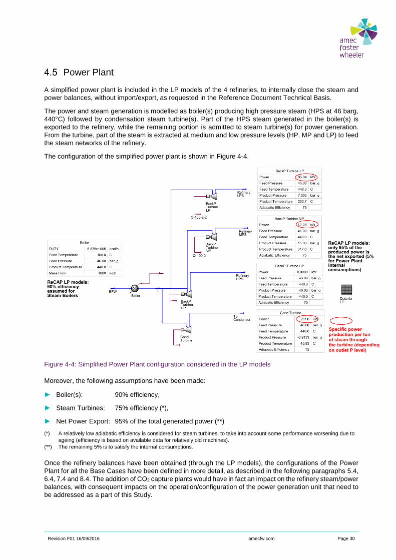
Power Plant
A simplified power plant is included in the LP models of the 4 refineries, to internally close the steam and
power balances, without import/export, as requested in the Reference Document Technical Basis.
The power and steam generation is modelled as boiler(s) producing high pressure steam (HPS at 46 barg,
440°C) followed by condensation steam turbine(s). Part of the HPS steam generated in the boiler(s) is
exported to the refinery, while the remaining portion is admitted to steam turbine(s) for power generation.
From the turbine, part of the steam is extracted at medium and low pressure levels (HP, MP and LP) to feed
the steam networks of the refinery.
The configuration of the simplified power plant is shown in Figure 4-4.
Figure 4-4: Simplified Power Plant configuration considered in the LP models
Moreover, the following assumptions have been made:
► Boiler(s): 90% efficiency,
► Steam Turbines: 75% efficiency (*),
► Net Power Export: 95% of the total generated power (**)
(*) A relatively low adiabatic efficiency is considered for steam turbines, to take into account some performance worsening due to
ageing (efficiency is based on available data for relatively old machines).
(**) The remaining 5% is to satisfy the internal consumptions.
Once the refinery balances have been obtained (through the LP models), the configurations of the Power
Plant for all the Base Cases have been defined in more detail, as described in the following paragraphs 5.4,
6.4, 7.4 and 8.4. The addition of CO2 capture plants would have in fact an impact on the refinery steam/power
balances, with consequent impacts on the operation/configuration of the power generation unit that need to
be addressed as a part of this Study.

Revision F01 16/09/2016 amecfw.com Page 31
In particular, for Base Case 3 and Base Case 4, the Power Plant configuration includes gas turbine(s) in
addition to the steam boilers/turbines. Therefore, the LP models relevant to these two cases have been
updated to implement the configuration with gas turbine in parallel to steam turbine, in order to calculate
more precisely the fuel demand (and consequently the emissions’ data) of the Power Plant. Reference is
made to paragraphs 7.4 and 8.4 for more details.
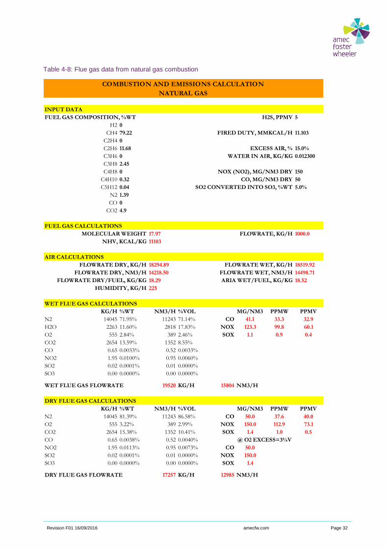
Rate and composition of Flue gases from Fired Heaters
The composition of flue gases from the various fired heaters of the refinery has been calculated depending
on the fuel type.
They are reported in the following Table 4-8, Table 4-9 and Table 4-10 respectively for natural gas, sweet
refinery offgas and fuel oil.
In all the tables, the combustion of 1 ton of fuel is considered.
It has to be remarked that, in all the refinery balances, the internally produced offgas is not sufficient to
satisfy the gaseous fuel demand of the Plant. Therefore, natural gas is imported as a supplementary fuel.
The offgas and the natural gas are assumed to be mixed in a centralized refinery fuel gas system and then
distributed to all the users of gaseous fuel.
The relative weight of natural gas versus the offgas is dependent on the refinery configuration and it is
therefore different in the four Base Cases.
The flowrates of the offgas and natural gas used as refinery fuel are reported in the section “FUEL MIX
COMPOSITION” in Table 5-6 (Base Case 1), Table 5-6 (Base Case 2), Table 7-6 (Base Case 3), Table 8-6
(Base Case 4).
For each Base Case, the composition of flue gas from refinery heaters could be calculated as a linear
combination of the flue gases generated by the combustion of 1 ton of natural gas (Table 4-8) and by the
combustion of 1 ton of sweet refinery offgas (Table 4-9). The flue gas rate from each source could be then
calculated from the refinery fuel gas rates reported in Table 5-7, Table 6-7, Table 7-7 and Table 8-7,
respectively for Base Case 1 to 4.
In the same tables, the typical temperature levels of flue gases to the stacks are reported for each source.
Temperatures are depending on the process service, the presence of heat recovery coils in the convective
section (e.g. for steam generation and/or superheating), the presence of air preheating facilities (APH).
In particular, the presence of APH systems is considered typical for heaters designed for a fired duty higher
than 20 MMkcal/h (because the payback period for the APH is relatively lower than for small heaters), so
resulting in a lower temperature level for the relevant flue gases.
Revision F01 16/09/2016 amecfw.com Page 32
Table 4-8: Flue gas data from natural gas combustion
COMBUSTION AND EMISSIONS CALCULATION
NATURAL GAS
INPUT DATA
FUEL GAS COMPOSITION, %WT H2S, PPMV 5
H2 0
CH4 79.22 FIRED DUTY, MMKCAL/H 11.103
C2H4 0
C2H6 11.68 EXCESS AIR, % 15.0%
C3H6 0 WATER IN AIR, KG/KG 0.012300
C3H8 2.45
C4H8 0 NOX (NO2), MG/NM3 DRY 150
C4H10 0.32 CO, MG/NM3 DRY 50
C5H12 0.04 SO2 CONVERTED INTO SO3, %WT 5.0%
N2 1.39
CO 0
CO2 4.9
FUEL GAS CALCULATIONS
MOLECULAR WEIGHT 17.97 FLOWRATE, KG/H 1000.0
NHV, KCAL/KG 11103
AIR CALCULATIONS
FLOWRATE DRY, KG/H 18294.89 FLOWRATE WET, KG/H 18519.92
FLOWRATE DRY, NM3/H 14218.50 FLOWRATE WET, NM3/H 14498.71
FLOWRATE DRY/FUEL, KG/KG 18.29 ARIA WET/FUEL, KG/KG 18.52
HUMIDITY, KG/H 225
WET FLUE GAS CALCULATIONS
KG/H %WT NM3/H %VOL MG/NM3 PPMW PPMV
N2 14045 71.95% 11243 71.14% CO 41.1 33.3 32.9
H2O 2263 11.60% 2818 17.83% NOX 123.3 99.8 60.1
O2 555 2.84% 389 2.46% SOX 1.1 0.9 0.4
CO2 2654 13.59% 1352 8.55%
CO 0.65 0.0033% 0.52 0.0033%
NO2 1.95 0.0100% 0.95 0.0060%
SO2 0.02 0.0001% 0.01 0.0000%
SO3 0.00 0.0000% 0.00 0.0000%
WET FLUE GAS FLOWRATE 19520 KG/H 15804 NM3/H
DRY FLUE GAS CALCULATIONS
KG/H %WT NM3/H %VOL MG/NM3 PPMW PPMV
N2 14045 81.39% 11243 86.58% CO 50.0 37.6 40.0
O2 555 3.22% 389 2.99% NOX 150.0 112.9 73.1
CO2 2654 15.38% 1352 10.41% SOX 1.4 1.0 0.5
CO 0.65 0.0038% 0.52 0.0040% @ O2 EXCESS=3%V
NO2 1.95 0.0113% 0.95 0.0073% CO 50.0
SO2 0.02 0.0001% 0.01 0.0000% NOX 150.0
SO3 0.00 0.0000% 0.00 0.0000% SOX 1.4
DRY FLUE GAS FLOWRATE 17257 KG/H 12985 NM3/H

Revision F01 16/09/2016 amecfw.com Page 33
Table 4-9: Flue gas from refinery offgas combustion
COMBUSTION AND EMISSIONS CALCULATION
SWEET REFINERY OFFGAS (AVERAGE COMPOSITION)
INPUT DATA
FUEL GAS COMPOSITION, %WT H2S, PPMV 50
H2 8
CH4 12 FIRED DUTY, MMKCAL/H 12.579
C2H4 0
C2H6 18 EXCESS AIR, % 15.0%
C3H6 0 WATER IN AIR, KG/KG 0.0123
C3H8 24
C4H8 0 NOX (NO2), MG/NM3 DRY 150
C4H10 38 CO, MG/NM3 DRY 50
C5H12 0 SO2 CONVERTED INTO SO3, %WT 5.0%
N2 0
CO 0
CO2 0
FUEL GAS CALCULATIONS
MOLECULAR WEIGHT 15.27 FLOWRATE, KG/H 1000.0
NHV, KCAL/KG 12579
AIR CALCULATIONS
FLOWRATE DRY, KG/H 19875.88 FLOWRATE WET, KG/H 20120.36
FLOWRATE DRY, NM3/H 15447.23 FLOWRATE WET, NM3/H 15751.65
FLOWRATE DRY/FUEL, KG/KG 19.88 ARIA WET/FUEL, KG/KG 20.12
HUMIDITY, KG/H 244
WET FLUE GAS CALCULATIONS
KG/H %WT NM3/H %VOL MG/NM3 PPMW PPMV
N2 15244 72.18% 12203 71.02% CO 40.8 33.2 32.7
H2O 2541 12.03% 3164 18.41% NOX 122.4 99.6 59.6
O2 603 2.86% 422 2.46% SOX 12.3 10.0 4.3
CO2 2730 12.92% 1391 8.09%
CO 0.70 0.0033% 0.56 0.0033%
NO2 2.10 0.0100% 1.02 0.0060%
SO2 0.20 0.0010% 0.07 0.0004%
SO3 0.01 0.0000% 0.00 0.0000%
WET FLUE GAS FLOWRATE 21120 KG/H 17181 NM3/H
DRY FLUE GAS CALCULATIONS
KG/H %WT NM3/H %VOL MG/NM3 PPMW PPMV
N2 15244 82.05% 12203 87.05% CO 50.0 37.7 40.0
O2 603 3.25% 422 3.01% NOX 150.0 113.2 73.1
CO2 2730 14.69% 1391 9.92% SOX 15.1 11.4 5.2
CO 0.70 0.0038% 0.56 0.0040% @ O2 EXCESS=3%V
NO2 2.10 0.0113% 1.02 0.0073% CO 50.0
SO2 0.20 0.0011% 0.07 0.0005% NOX 150.1
SO3 0.01 0.0001% 0.00 0.0000% SOX 15.1
DRY FLUE GAS FLOWRATE 18580 KG/H 14017 NM3/H
Revision F01 16/09/2016 amecfw.com Page 34
Table 4-10: Flue gas from fuel oil combustion
COMBUSTION AND EMISSIONS CALCULATION
LOW SULPHUR FUEL OIL
INPUT DATA
FIRED DUTY, MMKCAL/H 9.782
EXCESS AIR, % 25.0%
WATER IN AIR, KG/KG 0.012300
NOX (NO2), MG/NM3 DRY 450
CO, MG/NM3 DRY 100
SO2 CONVERTED INTO SO3, %WT 3.0%
FUEL OIL DATA
API GRAVITY 17.40 FLOWRATE, KG/H 1000.0
NHV, KCAL/KG 9782 SULPHUR, %WT 0.5
AIR CALCULATIONS
FLOWRATE DRY, KG/H 17411 FLOWRATE WET, KG/H 17628
FLOWRATE DRY, NM3/H 13531 FLOWRATE WET, NM3/H 13800
FLOWRATE DRY/FUEL, KG/KG 17.41 ARIA WET/FUEL, KG/KG 17.63
HUMIDITY, KG/H 217
WET FLUE GAS CALCULATIONS
KG/H %WT NM3/H %VOL MG/NM3 PPMW PPMV
N2 13369.3 71.77% 10702.1 74.10% CO 82.5 63.9 66.0
H2O 1234.7 6.63% 1537.5 10.65% NOX 371.1 287.7 180.8
O2 808.8 4.34% 566.5 3.92% SOX 691.7 536.3 240.8
CO2 3198.4 17.17% 1629.3 11.28%
CO 1.2 0.01% 1.0 0.01%
NO2 5.4 0.03% 2.6 0.02%
SO2 9.7 0.05% 3.4 0.0235%
SO3 0.3 0.00% 0.1 0.0006%
WET FLUE GAS FLOWRATE 18628 KG/H 14442 NM3/H
DRY FLUE GAS CALCULATIONS
KG/H %WT NM3/H %VOL MG/NM3 PPMW PPMV
N2 13369.3 76.87% 10702.1 82.93% CO 92.3 68.5 73.9
O2 808.8 4.65% 566.5 4.39% NOX 415.3 308.1 202.3
CO2 3198.4 18.39% 1629.3 12.63% SOX 774.2 574.4 269.5
CO 1.2 0.01% 1.0 0.01% @ O2 EXCESS=3%V
NO2 5.4 0.03% 2.6 0.02% CO 100.0
SO2 9.7 0.06% 3.4 0.03% NOX 450.0
SO3 0.3 0.00% 0.1 0.00% SOX 840.1
DRY FLUE GAS FLOWRATE 17393 KG/H 12905 NM3/H
Revision F01 16/09/2016 amecfw.com Page 35
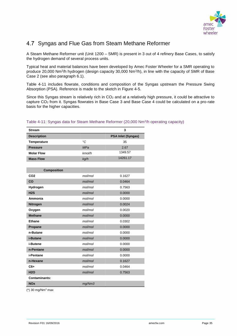
Syngas and Flue Gas from Steam Methane Reformer
A Steam Methane Reformer unit (Unit 1200 – SMR) is present in 3 out of 4 refinery Base Cases, to satisfy
the hydrogen demand of several process units.
Typical heat and material balances have been developed by Amec Foster Wheeler for a SMR operating to
produce 20,000 Nm3/h hydrogen (design capacity 30,000 Nm3/h), in line with the capacity of SMR of Base
Case 2 (see also paragraph 6.1).
Table 4-11 includes flowrate, conditions and composition of the Syngas upstream the Pressure Swing
Absorption (PSA). Reference is made to the sketch in Figure 4-5.
Since this Syngas stream is relatively rich in CO2 and at a relatively high pressure, it could be attractive to
capture CO2 from it. Syngas flowrates in Base Case 3 and Base Case 4 could be calculated on a pro-rate
basis for the higher capacities.
Table 4-11: Syngas data for Steam Methane Reformer (20,000 Nm3/h operating capacity)
Stream 3
Description PSA Inlet (Syngas)
Temperature °C 35
Pressure MPa 2.67
Molar Flow kmol/h 1349.57
Mass Flow kg/h 14261.17
Composition
CO2 mol/mol 0.1627
CO mol/mol 0.0464
Hydrogen mol/mol 0.7563
H2S mol/mol 0.0000
Ammonia mol/mol 0.0000
Nitrogen mol/mol 0.0024
Oxygen mol/mol 0.0020
Methane mol/mol 0.0000
Ethane mol/mol 0.0302
Propane mol/mol 0.0000
n-Butane mol/mol 0.0000
i-Butane mol/mol 0.0000
i-Butene mol/mol 0.0000
n-Pentane mol/mol 0.0000
i-Pentane mol/mol 0.0000
n-Hexane mol/mol 0.1627
C6+ mol/mol 0.0464
H2O mol/mol 0.7563
Contaminants:
NOx mg/Nm3
(*) 30 mg/Nm3 max
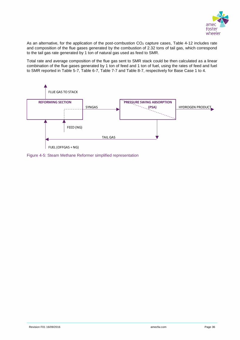
Revision F01 16/09/2016 amecfw.com Page 36
As an alternative, for the application of the post-combustion CO2 capture cases, Table 4-12 includes rate
and composition of the flue gases generated by the combustion of 2.32 tons of tail gas, which correspond
to the tail gas rate generated by 1 ton of natural gas used as feed to SMR.
Total rate and average composition of the flue gas sent to SMR stack could be then calculated as a linear
combination of the flue gases generated by 1 ton of feed and 1 ton of fuel, using the rates of feed and fuel
to SMR reported in Table 5-7, Table 6-7, Table 7-7 and Table 8-7, respectively for Base Case 1 to 4.
Figure 4-5: Steam Methane Reformer simplified representation
FLUE GAS TO STACK
REFORMING SECTION PRESSURE SWING ABSORPTION
SYNGAS (PSA) HYDROGEN PRODUCT
FEED (NG)
TAIL GAS
FUEL (OFFGAS + NG)
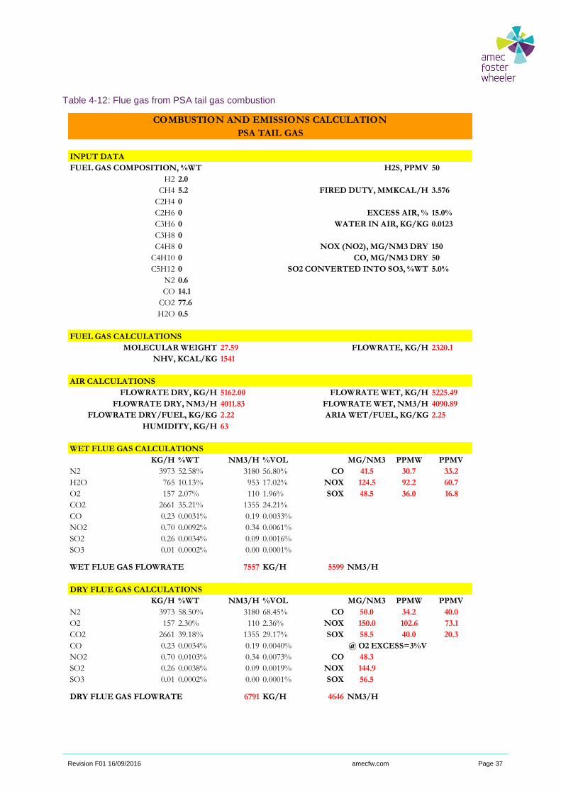
Revision F01 16/09/2016 amecfw.com Page 37
Table 4-12: Flue gas from PSA tail gas combustion
COMBUSTION AND EMISSIONS CALCULATION
PSA TAIL GAS
INPUT DATA
FUEL GAS COMPOSITION, %WT H2S, PPMV 50
H2 2.0
CH4 5.2 FIRED DUTY, MMKCAL/H 3.576
C2H4 0
C2H6 0 EXCESS AIR, % 15.0%
C3H6 0 WATER IN AIR, KG/KG 0.0123
C3H8 0
C4H8 0 NOX (NO2), MG/NM3 DRY 150
C4H10 0 CO, MG/NM3 DRY 50
C5H12 0 SO2 CONVERTED INTO SO3, %WT 5.0%
N2 0.6
CO 14.1
CO2 77.6
H2O 0.5
FUEL GAS CALCULATIONS
MOLECULAR WEIGHT 27.59 FLOWRATE, KG/H 2320.1
NHV, KCAL/KG 1541
AIR CALCULATIONS
FLOWRATE DRY, KG/H 5162.00 FLOWRATE WET, KG/H 5225.49
FLOWRATE DRY, NM3/H 4011.83 FLOWRATE WET, NM3/H 4090.89
FLOWRATE DRY/FUEL, KG/KG 2.22 ARIA WET/FUEL, KG/KG 2.25
HUMIDITY, KG/H 63
WET FLUE GAS CALCULATIONS
KG/H %WT NM3/H %VOL MG/NM3 PPMW PPMV
N2 3973 52.58% 3180 56.80% CO 41.5 30.7 33.2
H2O 765 10.13% 953 17.02% NOX 124.5 92.2 60.7
O2 157 2.07% 110 1.96% SOX 48.5 36.0 16.8
CO2 2661 35.21% 1355 24.21%
CO 0.23 0.0031% 0.19 0.0033%
NO2 0.70 0.0092% 0.34 0.0061%
SO2 0.26 0.0034% 0.09 0.0016%
SO3 0.01 0.0002% 0.00 0.0001%
WET FLUE GAS FLOWRATE 7557 KG/H 5599 NM3/H
DRY FLUE GAS CALCULATIONS
KG/H %WT NM3/H %VOL MG/NM3 PPMW PPMV
N2 3973 58.50% 3180 68.45% CO 50.0 34.2 40.0
O2 157 2.30% 110 2.36% NOX 150.0 102.6 73.1
CO2 2661 39.18% 1355 29.17% SOX 58.5 40.0 20.3
CO 0.23 0.0034% 0.19 0.0040% @ O2 EXCESS=3%V
NO2 0.70 0.0103% 0.34 0.0073% CO 48.3
SO2 0.26 0.0038% 0.09 0.0019% NOX 144.9
SO3 0.01 0.0002% 0.00 0.0001% SOX 56.5
DRY FLUE GAS FLOWRATE 6791 KG/H 4646 NM3/H
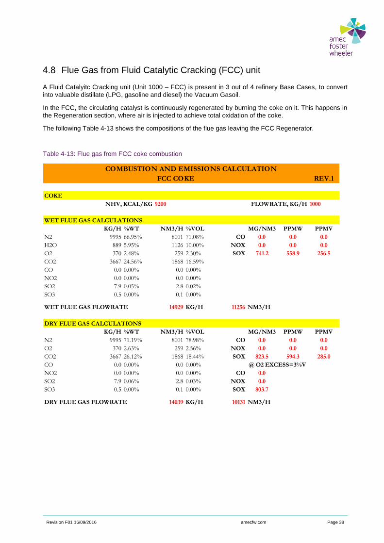
Revision F01 16/09/2016 amecfw.com Page 38
Flue Gas from Fluid Catalytic Cracking (FCC) unit
A Fluid Catalyitc Cracking unit (Unit 1000 – FCC) is present in 3 out of 4 refinery Base Cases, to convert
into valuable distillate (LPG, gasoline and diesel) the Vacuum Gasoil.
In the FCC, the circulating catalyst is continuously regenerated by burning the coke on it. This happens in
the Regeneration section, where air is injected to achieve total oxidation of the coke.
The following Table 4-13 shows the compositions of the flue gas leaving the FCC Regenerator.
Table 4-13: Flue gas from FCC coke combustion
COMBUSTION AND EMISSIONS CALCULATION
FCC COKE REV.1
COKE
NHV, KCAL/KG 9200 FLOWRATE, KG/H 1000
WET FLUE GAS CALCULATIONS
KG/H %WT NM3/H %VOL MG/NM3 PPMW PPMV
N2 9995 66.95% 8001 71.08% CO 0.0 0.0 0.0
H2O 889 5.95% 1126 10.00% NOX 0.0 0.0 0.0
O2 370 2.48% 259 2.30% SOX 741.2 558.9 256.5
CO2 3667 24.56% 1868 16.59%
CO 0.0 0.00% 0.0 0.00%
NO2 0.0 0.00% 0.0 0.00%
SO2 7.9 0.05% 2.8 0.02%
SO3 0.5 0.00% 0.1 0.00%
WET FLUE GAS FLOWRATE 14929 KG/H 11256 NM3/H
DRY FLUE GAS CALCULATIONS
KG/H %WT NM3/H %VOL MG/NM3 PPMW PPMV
N2 9995 71.19% 8001 78.98% CO 0.0 0.0 0.0
O2 370 2.63% 259 2.56% NOX 0.0 0.0 0.0
CO2 3667 26.12% 1868 18.44% SOX 823.5 594.3 285.0
CO 0.0 0.00% 0.0 0.00% @ O2 EXCESS=3%V
NO2 0.0 0.00% 0.0 0.00% CO 0.0
SO2 7.9 0.06% 2.8 0.03% NOX 0.0
SO3 0.5 0.00% 0.1 0.00% SOX 803.7
DRY FLUE GAS FLOWRATE 14039 KG/H 10131 NM3/H

Revision F01 16/09/2016 amecfw.com Page 39
Flue Gas from Gas Turbine (GT) and Heat Recovery Steam Generators (HRSG)
As described in the following paragraphs 7.4 and 8.4, the Power Plant in Base Case 3 and Base Case 4
includes Gas Turbine(s) and relevant Het Recovery Steam Generator(s).
The specific rate (per ton of natural gas fed to the gas turbine) and composition of flue gases from the
GT+HRSG is reported in the following tables. SOx concentration in the flue gas is not reported, being it far
below 5 ppm wt.
from GT From HRSG
%vol MW %wt %vol MW %wt
kg/kmol kg/kmol
CH4 0% 16 0% CH4 0% 16 0%
C2H6 0% 30 0% C2H6 0% 30 0%
C3H8 0% 44 0% C3H8 0% 44 0%
C4H10 0% 58 0% C4H10 0% 58 0%
C5H12 0% 72 0% C5H12 0% 72 0%
CO2 3.20% 44 5.00% CO2 4.87% 44 7.55%
N2 76.40% 28 74.94% N2 75.10% 28 74.22%
SO2 0% 32 0% SO2 0% 32 0%
O2 13.40% 32 15.00% O2 9.78% 32 11.04%
H2 0% 2 0% H2 0% 2 0%
H2O 6.10% 18 3.84% H2O 9.40% 18 5.98%
Ar 0.90% 40 1.22% Ar 0.86% 40 1.21%
Total 1 28.6 100% Total 1 28.3 100%
Spec flue gas flowrate [t/t NG to GT] 53.0 t/t NG to GT
Revision F01 16/09/2016 amecfw.com Page 40
5. Base Case 1
Hydro-skimming Refinery - 100,000 BPSD Crude Capacity
The Hydro-skimming refinery is essentially composed of primary distillation units (Atmospheric and
Vacuum), a gasoline block (Naphtha Hydrotreater, Splitter, Isomerization and Catalytic Reformer) for the
production of on-spec gasolines, a Kerosene Sweetening unit for jet fuel production and middle-distillates
Hydro-desulphurization units for the production of automotive diesel, marine diesel and heating oil. The
residue from Vacuum distillation unit is partially sold as bitumen and partially sent to Visbreaking Unit, for
partial conversion into distillates and viscosity reduction of the residue to comply with fuel oils’ specifications.
The Hydrogen Rich Gas from the Heavy Naphtha Catalytic Reformer is compressed, sent to a Pressure
Swing Absorber (PSA) module to increase the hydrogen concentration, and finally used for the
desulphurization of products. No Steam Methane Reformer is included in the process scheme.
Crude Atmospheric Distillation and Vacuum Distillation are not thermally integrated, since they are
considered being built in different phases (i.e. Vacuum Distillation, Vacuum Gasoil Hydrotreater and
Visbreaking added in a second phase).
Sea Water is used for condensation and cooling purposes. No cooling towers are installed.
Refinery Balances
The balances developed for Base Case 1 are reported in the following tables and figures:
► Table 5-1: Base Case 1) Overall material balance
► Table 5-2: Base Case 1) Process units operating and design capacity
► Table 5-3: Base Case 1) Gasoline qualities
► Table 5-4: Base Case 1) Distillate qualities
► Table 5-5: Base Case 1) Fuel oil and bitumen qualities
► Table 5-6: Base Case 1) Main utility balance, fuel mix composition, CO2 emissions
► Figure 5-1: Base Case 1) Block flow diagrams with main material streams
► Table 5-7: Base Case 1) CO2 emissions per unit
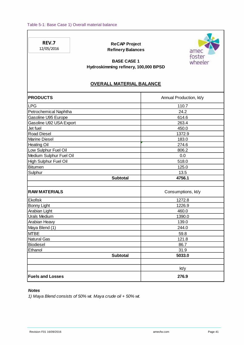
Revision F01 16/09/2016 amecfw.com Page 41
Table 5-1: Base Case 1) Overall material balance
ReCAP Project
Refinery Balances
BASE CASE 1
Hydroskimming refinery, 100,000 BPSD
PRODUCTS
LPG
Petrochemical Naphtha
Gasoline U95 Europe
Gasoline U92 USA Export
Jet fuel
Road Diesel
Marine Diesel
Heating Oil
Low Sulphur Fuel Oil
Medium Sulphur Fuel Oil
High Sulphur Fuel Oil
Bitumen
Sulphur
Subtotal
RAW MATERIALS
Ekofisk
Bonny Light
Arabian Light
Urals Medium
Arabian Heavy
Maya Blend (1)
MTBE
Natural Gas
Biodiesel
Ethanol
Subtotal
Fuels and Losses
Notes
1) Maya Blend consists of 50% wt. Maya crude oil + 50% wt. Arabian Light Crude Oil
276.9
121.8
86.7
31.9
5033.0
kt/y
460.0
1390.0
139.0
244.0
59.8
4756.1
Consumptions, kt/y
1272.8
1226.9
OVERALL MATERIAL BALANCE
Annual Production, kt/y
110.7
24.2
614.6
263.4
450.0
1372.9
183.0
274.6
806.2
0.0
518.0
125.0
13.5
REV.712/05/2016
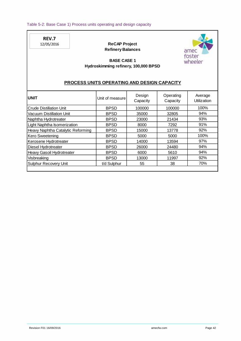
Revision F01 16/09/2016 amecfw.com Page 42
Table 5-2: Base Case 1) Process units operating and design capacity
ReCAP Project
Refinery Balances
BASE CASE 1
Hydroskimming refinery, 100,000 BPSD
UNIT Unit of measureDesign
Capacity
Operating
Capacity
Average
Utilization
Crude Distillation Unit BPSD 100000 100000 100%
Vacuum Distillation Unit BPSD 35000 32805 94%
Naphtha Hydrotreater BPSD 23000 21434 93%
Light Naphtha Isomerization BPSD 8000 7292 91%
Heavy Naphtha Catalytic Reforming BPSD 15000 13778 92%
Kero Sweetening BPSD 5000 5000 100%
Kerosene Hydrotreater BPSD 14000 13594 97%
Diesel Hydrotreater BPSD 26000 24480 94%
Heavy Gasoil Hydrotreater BPSD 6000 5610 94%
Visbreaking BPSD 13000 11997 92%
Sulphur Recovery Unit t/d Sulphur 55 38 70%
PROCESS UNITS OPERATING AND DESIGN CAPACITY
REV.712/05/2016
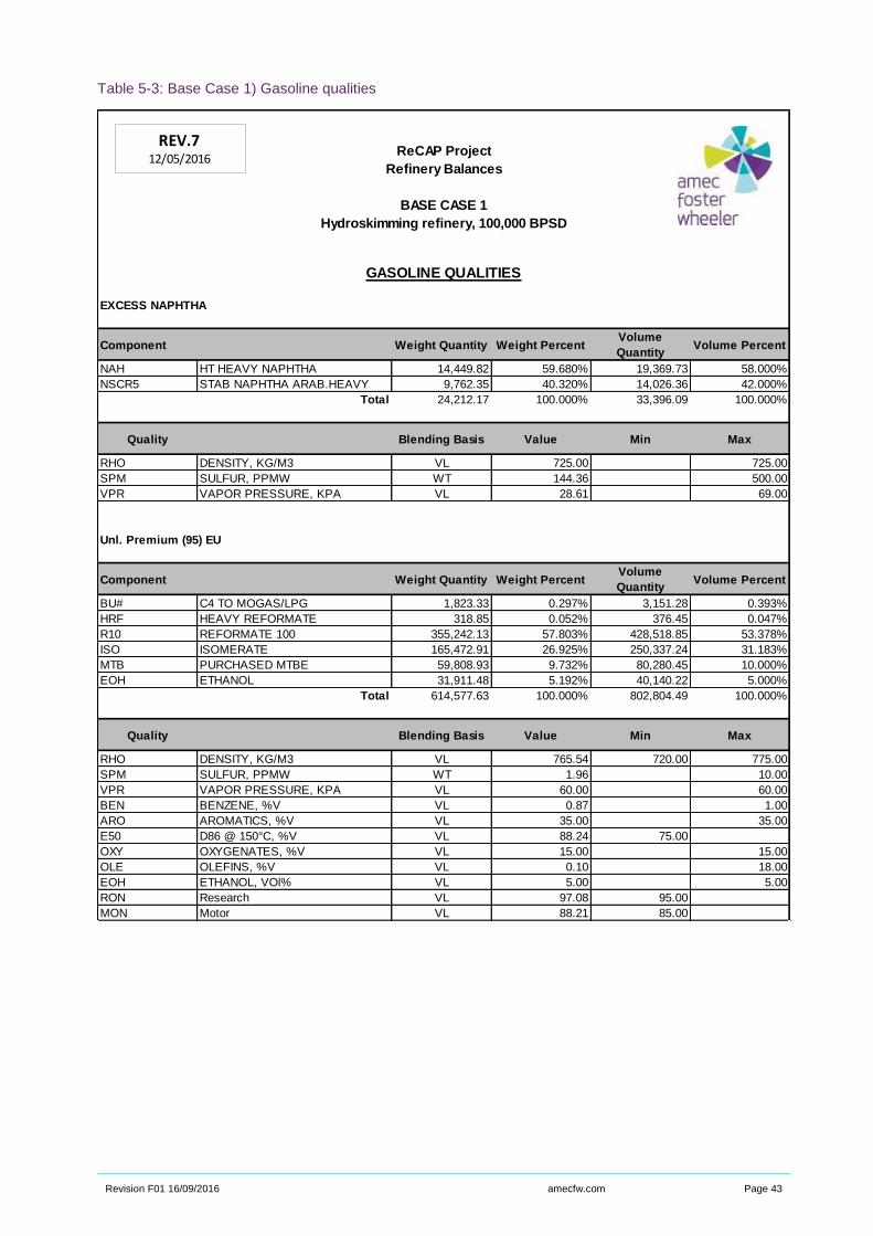
Revision F01 16/09/2016 amecfw.com Page 43
Table 5-3: Base Case 1) Gasoline qualities
ReCAP Project
Refinery Balances
BASE CASE 1
Hydroskimming refinery, 100,000 BPSD
GASOLINE QUALITIES
EXCESS NAPHTHA
Component Weight Quantity Weight PercentVolume
QuantityVolume Percent
NAH HT HEAVY NAPHTHA 14,449.82 59.680% 19,369.73 58.000%
NSCR5 STAB NAPHTHA ARAB.HEAVY 9,762.35 40.320% 14,026.36 42.000%
Total 24,212.17 100.000% 33,396.09 100.000%
Quality Blending Basis Value Min Max
RHO DENSITY, KG/M3 VL 725.00 725.00
SPM SULFUR, PPMW WT 144.36 500.00
VPR VAPOR PRESSURE, KPA VL 28.61 69.00
Unl. Premium (95) EU
Component Weight Quantity Weight PercentVolume
QuantityVolume Percent
BU# C4 TO MOGAS/LPG 1,823.33 0.297% 3,151.28 0.393%
HRF HEAVY REFORMATE 318.85 0.052% 376.45 0.047%
R10 REFORMATE 100 355,242.13 57.803% 428,518.85 53.378%
ISO ISOMERATE 165,472.91 26.925% 250,337.24 31.183%
MTB PURCHASED MTBE 59,808.93 9.732% 80,280.45 10.000%
EOH ETHANOL 31,911.48 5.192% 40,140.22 5.000%
Total 614,577.63 100.000% 802,804.49 100.000%
Quality Blending Basis Value Min Max
RHO DENSITY, KG/M3 VL 765.54 720.00 775.00
SPM SULFUR, PPMW WT 1.96 10.00
VPR VAPOR PRESSURE, KPA VL 60.00 60.00
BEN BENZENE, %V VL 0.87 1.00
ARO AROMATICS, %V VL 35.00 35.00
E50 D86 @ 150°C, %V VL 88.24 75.00
OXY OXYGENATES, %V VL 15.00 15.00
OLE OLEFINS, %V VL 0.10 18.00
EOH ETHANOL, VOl% VL 5.00 5.00
RON Research VL 97.08 95.00
MON Motor VL 88.21 85.00
REV.712/05/2016
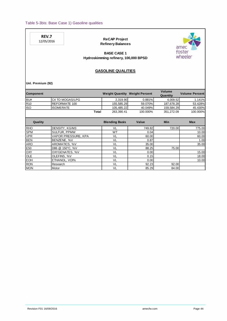
Revision F01 16/09/2016 amecfw.com Page 44
Table 5-3bis: Base Case 1) Gasoline qualities
ReCAP Project
Refinery Balances
BASE CASE 1
Hydroskimming refinery, 100,000 BPSD
GASOLINE QUALITIES
Unl. Premium (92)
Component Weight Quantity Weight PercentVolume
QuantityVolume Percent
BU# C4 TO MOGAS/LPG 2,319.90 0.881% 4,009.52 1.141%
R10 REFORMATE 100 155,585.29 59.070% 187,678.28 53.428%
ISO ISOMERATE 105,485.22 40.049% 159,584.29 45.430%
Total 263,390.41 100.000% 351,272.09 100.000%
Quality Blending Basis Value Min Max
RHO DENSITY, KG/M3 VL 749.82 720.00 775.00
SPM SULFUR, PPMW WT 0.04 10.00
VPR VAPOR PRESSURE, KPA VL 60.00 60.00
BEN BENZENE, %V VL 0.87 1.00
ARO AROMATICS, %V VL 35.00 35.00
E50 D86 @ 150°C, %V VL 88.25 75.00
OXY OXYGENATES, %V VL 0.00 15.00
OLE OLEFINS, %V VL 0.15 18.00
EOH ETHANOL, VOl% VL 0.00 10.00
RON Research VL 92.23 92.00
MON Motor VL 85.29 84.00
REV.712/05/2016
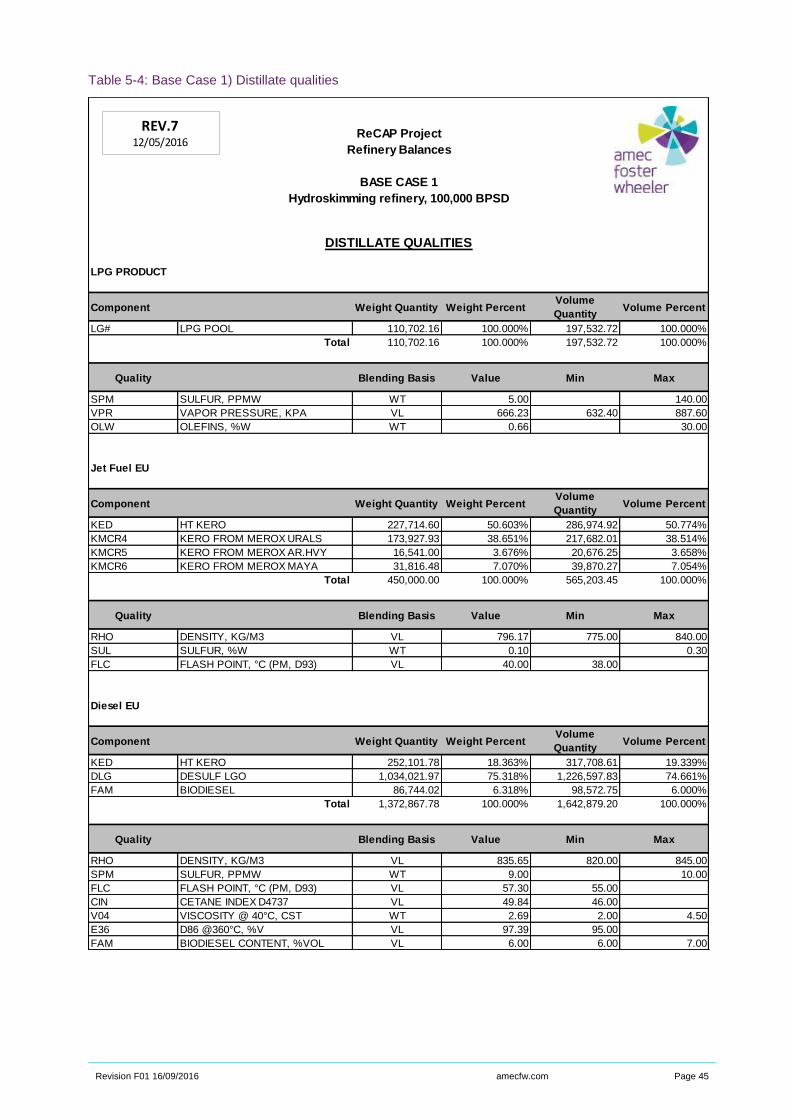
Revision F01 16/09/2016 amecfw.com Page 45
Table 5-4: Base Case 1) Distillate qualities
ReCAP Project
Refinery Balances
BASE CASE 1
Hydroskimming refinery, 100,000 BPSD
DISTILLATE QUALITIES
LPG PRODUCT
Component Weight Quantity Weight PercentVolume
QuantityVolume Percent
LG# LPG POOL 110,702.16 100.000% 197,532.72 100.000%
Total 110,702.16 100.000% 197,532.72 100.000%
Quality Blending Basis Value Min Max
SPM SULFUR, PPMW WT 5.00 140.00
VPR VAPOR PRESSURE, KPA VL 666.23 632.40 887.60
OLW OLEFINS, %W WT 0.66 30.00
Jet Fuel EU
Component Weight Quantity Weight PercentVolume
QuantityVolume Percent
KED HT KERO 227,714.60 50.603% 286,974.92 50.774%
KMCR4 KERO FROM MEROX URALS 173,927.93 38.651% 217,682.01 38.514%
KMCR5 KERO FROM MEROX AR.HVY 16,541.00 3.676% 20,676.25 3.658%
KMCR6 KERO FROM MEROX MAYA 31,816.48 7.070% 39,870.27 7.054%
Total 450,000.00 100.000% 565,203.45 100.000%
Quality Blending Basis Value Min Max
RHO DENSITY, KG/M3 VL 796.17 775.00 840.00
SUL SULFUR, %W WT 0.10 0.30
FLC FLASH POINT, °C (PM, D93) VL 40.00 38.00
Diesel EU
Component Weight Quantity Weight PercentVolume
QuantityVolume Percent
KED HT KERO 252,101.78 18.363% 317,708.61 19.339%
DLG DESULF LGO 1,034,021.97 75.318% 1,226,597.83 74.661%
FAM BIODIESEL 86,744.02 6.318% 98,572.75 6.000%
Total 1,372,867.78 100.000% 1,642,879.20 100.000%
Quality Blending Basis Value Min Max
RHO DENSITY, KG/M3 VL 835.65 820.00 845.00
SPM SULFUR, PPMW WT 9.00 10.00
FLC FLASH POINT, °C (PM, D93) VL 57.30 55.00
CIN CETANE INDEX D4737 VL 49.84 46.00
V04 VISCOSITY @ 40°C, CST WT 2.69 2.00 4.50
E36 D86 @360°C, %V VL 97.39 95.00
FAM BIODIESEL CONTENT, %VOL VL 6.00 6.00 7.00
REV.712/05/2016
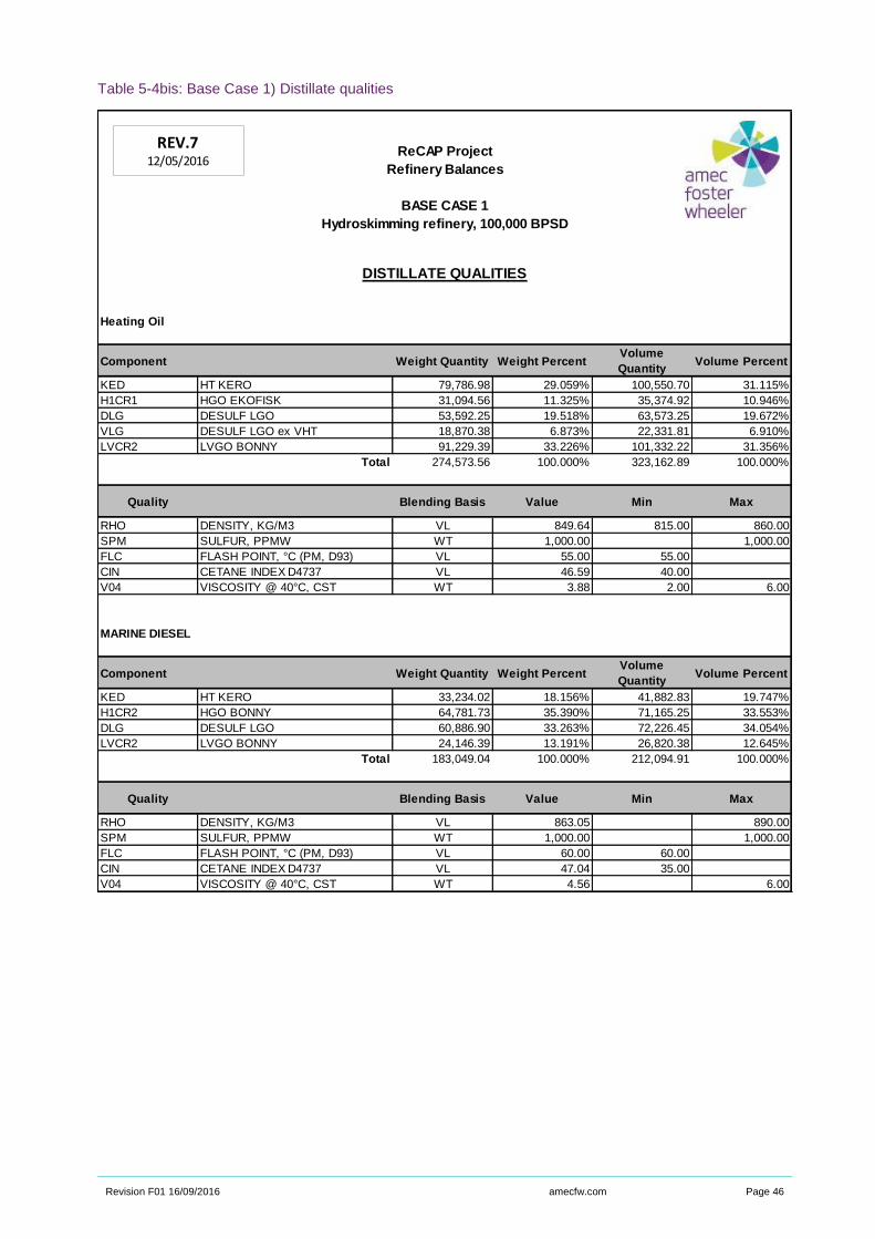
Revision F01 16/09/2016 amecfw.com Page 46
Table 5-4bis: Base Case 1) Distillate qualities
ReCAP Project
Refinery Balances
BASE CASE 1
Hydroskimming refinery, 100,000 BPSD
DISTILLATE QUALITIES
Heating Oil
Component Weight Quantity Weight PercentVolume
QuantityVolume Percent
KED HT KERO 79,786.98 29.059% 100,550.70 31.115%
H1CR1 HGO EKOFISK 31,094.56 11.325% 35,374.92 10.946%
DLG DESULF LGO 53,592.25 19.518% 63,573.25 19.672%
VLG DESULF LGO ex VHT 18,870.38 6.873% 22,331.81 6.910%
LVCR2 LVGO BONNY 91,229.39 33.226% 101,332.22 31.356%
Total 274,573.56 100.000% 323,162.89 100.000%
Quality Blending Basis Value Min Max
RHO DENSITY, KG/M3 VL 849.64 815.00 860.00
SPM SULFUR, PPMW WT 1,000.00 1,000.00
FLC FLASH POINT, °C (PM, D93) VL 55.00 55.00
CIN CETANE INDEX D4737 VL 46.59 40.00
V04 VISCOSITY @ 40°C, CST WT 3.88 2.00 6.00
MARINE DIESEL
Component Weight Quantity Weight PercentVolume
QuantityVolume Percent
KED HT KERO 33,234.02 18.156% 41,882.83 19.747%
H1CR2 HGO BONNY 64,781.73 35.390% 71,165.25 33.553%
DLG DESULF LGO 60,886.90 33.263% 72,226.45 34.054%
LVCR2 LVGO BONNY 24,146.39 13.191% 26,820.38 12.645%
Total 183,049.04 100.000% 212,094.91 100.000%
Quality Blending Basis Value Min Max
RHO DENSITY, KG/M3 VL 863.05 890.00
SPM SULFUR, PPMW WT 1,000.00 1,000.00
FLC FLASH POINT, °C (PM, D93) VL 60.00 60.00
CIN CETANE INDEX D4737 VL 47.04 35.00
V04 VISCOSITY @ 40°C, CST WT 4.56 6.00
REV.712/05/2016
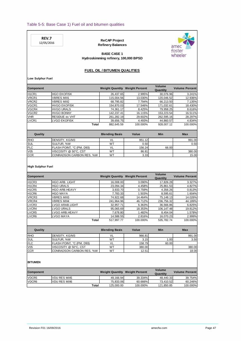
Revision F01 16/09/2016 amecfw.com Page 47
Table 5-5: Base Case 1) Fuel oil and bitumen qualities
ReCAP Project
Refinery Balances
BASE CASE 1
Hydroskimming refinery, 100,000 BPSD
FUEL OIL / BITUMEN QUALITIES
Low Sulphur Fuel
Component Weight Quantity Weight PercentVolume
QuantityVolume Percent
H1CR1 HGO EKOFISK 26,437.65 2.995% 30,076.96 3.241%
VRCR1 VBRES MIX1 115,004.56 13.030% 120,046.52 12.936%
VRCR2 VBRES MIX2 68,795.82 7.794% 66,213.50 7.135%
VGCR1 HVGO EKOFISK 154,870.03 17.546% 171,032.61 18.430%
VGCR4 HVGO URALS 74,361.17 8.425% 79,958.25 8.616%
VGCR2 HVGO BONNY 142,237.41 16.115% 153,223.54 16.511%
VHR RESIDUE ex VHT 261,282.19 29.602% 262,595.16 28.297%
LVCR1 LVGO EKOFISK 39,656.75 4.493% 44,860.57 4.834%
Total 882,645.59 100.000% 928,007.12 100.000%
Quality Blending Basis Value Min Max
RHO DENSITY, KG/M3 VL 951.12 991.00
SUL SULFUR, %W WT 0.50 0.50
FLC FLASH POINT, °C (PM, D93) VL 156.24 66.00
V05 VISCOSITY @ 50°C, CST WT 86.81 380.00
CCR CONRADSON CARBON RES, %W WT 3.33 15.00
High Sulphur Fuel
Component Weight Quantity Weight PercentVolume
QuantityVolume Percent
H1CR3 HGO ARB. LIGHT 16,008.00 3.090% 17,826.28 3.327%
H1CR4 HGO URALS 23,094.34 4.458% 25,861.53 4.827%
H1CR5 HGO ARB.HEAVY 3,933.70 0.759% 4,356.26 0.813%
H1CR6 HGO MAYA 7,783.33 1.503% 8,595.61 1.604%
VRCR3 VBRES MIX3 74,922.68 14.464% 75,148.13 14.026%
VRCR4 VBRES MIX4 241,964.96 46.712% 236,756.32 44.189%
LVCR3 LVGO ARAB.LIGHT 32,957.71 6.363% 36,566.86 6.825%
LVCR4 LVGO URALS 95,065.69 18.353% 106,147.48 19.812%
LVCR5 LVGO ARB.HEAVY 7,678.80 1.482% 8,454.04 1.578%
LVCR6 LVGO MAYA 14,588.55 2.816% 16,070.23 2.999%
Total 517,997.77 100.000% 535,782.74 100.000%
Quality Blending Basis Value Min Max
RHO DENSITY, KG/M3 VL 966.81 991.00
SUL SULFUR, %W WT 3.15 1.00 3.50
FLC FLASH POINT, °C (PM, D93) VL 158.79 60.00
V05 VISCOSITY @ 50°C, CST WT 380.00 380.00
CCR CONRADSON CARBON RES, %W WT 12.51 18.00
BITUMEN
Component Weight Quantity Weight PercentVolume
QuantityVolume Percent
VDCR5 VDU RES MIX5 49,166.94 39.334% 48,440.33 39.754%
VDCR6 VDU RES MIX6 75,833.06 60.666% 73,410.52 60.246%
Total 125,000.00 100.000% 121,850.85 100.000%
REV.712/05/2016
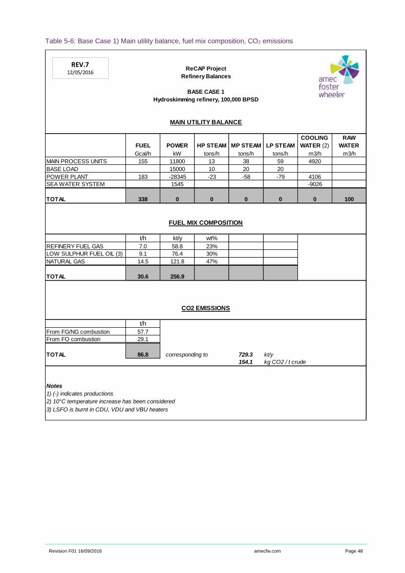
Revision F01 16/09/2016 amecfw.com Page 48
Table 5-6: Base Case 1) Main utility balance, fuel mix composition, CO2 emissions
ReCAP Project
Refinery Balances
BASE CASE 1
Hydroskimming refinery, 100,000 BPSD
FUEL POWER HP STEAM MP STEAM LP STEAM
COOLING
WATER (2)
RAW
WATER
Gcal/h kW tons/h tons/h tons/h m3/h m3/h
MAIN PROCESS UNITS 155 11800 13 38 59 4920
BASE LOAD 15000 10 20 20
POWER PLANT 183 -28345 -23 -58 -79 4106
SEA WATER SYSTEM 1545 -9026
TOTAL 338 0 0 0 0 0 100
t/h kt/y wt%
REFINERY FUEL GAS 7.0 58.8 23%
LOW SULPHUR FUEL OIL (3) 9.1 76.4 30%
NATURAL GAS 14.5 121.8 47%
TOTAL 30.6 256.9
t/h
From FG/NG combustion 57.7
From FO combustion 29.1
TOTAL 86.8 corresponding to 729.3 kt/y
154.1 kg CO2 / t crude
Notes
1) (-) indicates productions
2) 10°C temperature increase has been considered
3) LSFO is burnt in CDU, VDU and VBU heaters
MAIN UTILITY BALANCE
FUEL MIX COMPOSITION
CO2 EMISSIONS
REV.712/05/2016
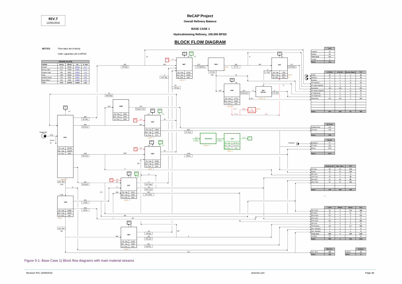
Revision F01 16/09/2016 amecfw.com Page 49
Figure 5-1: Base Case 1) Block flow diagrams with main material streams
ReCAP Project
Overall Refinery Balance
BASE CASE 1
Hydroskimming Refinery, 100,000 BPSD
BLOCK FLOW DIAGRAM
NOTES: Flow rates are in kton/y LPG
Propane 25
Units' capacities are in BPSD Butane 85
10 10 0.3 0 16 Total prod. 111
1.1 To fuel 0
CRUDE SLATE Sales 111
CRUDE kton/y BPSD SG S, %wt 855 845 873 284 284 271
Ekofisk 1273 28025 0.8162 0.17 check
Bonny Light 1227 25695 0.8581 0.13 0 0
Arabian Light 460 9663 0.8555 1.79 Op. Cap. 21434 Op. Cap. 7292 U 95-EU U 92-US Excess Naph. TOT
Urals 1390 28835 0.8663 1.46 4 Des. Cap. 23000 589 14 Des. Cap. 8000 check MTBE 60 0 0 60
Arabian Heavy 139 2835 0.8811 2.85 Ut. Fact. 93% Ut. Fact. 91% 0 Ethanol 32 0 0 32
Maya Blend 244 4946 0.8865 2.45 check 0 Butanes 2 2 0 4
Total 4733 100000 0.8505 0.89 46 SR Naphtha 0 0 10 10
33 0 0 HT Light Naphtha 0 0 0 0
Isomerate 165 105 0 271
575 511 0 0 HT Heavy Naphtha 0 0 14 14
44 LT Reformate 0 0 0 0
HV Reformate 0 0 0 0
Op. Cap. 13778 511 check 0 Reformate 355 156 0 511
Des. Cap. 15000
Ut. Fact. 92%
222 222 check 0
17.4 15.0 check
67 0 Sales 615 263 24 902
Op. Cap. 5000 2.1 0.3 17.4 2.4
855 Des. Cap. 5000
Ut. Fact. 100% 1.2 20
836 614 Jet Fuel
Treated Kero 222
Op. Cap. 13594 593 HT Kero 228
Crude Oil Des. Cap. 14000
4733 Ut. Fact. 97% Sales 450
check 0 14.4 13.5
losses Diesel
19 Op. Cap. 38 t/d S Biodiesel Biodiesel 87
16 7.3 check 0 Des. Cap. 55 t/d S HT Kero 252
Op. Cap. 100000 8.4 Ut. Fact. 70% Diesel 1034
Des. Cap. 100000 24 check 0
Ut. Fact. 100% 1067 1067 1149 Sales 1373
Op. Cap. 24480
120 Des. Cap. 26000
Ut. Fact. 94% Heating Oil Mar. Dies. TOT
0 check 0 HT Kero 80 33 113
Diesel 54 61 114
0 SR LGO 0 0 0
4 6.5 VHT LGO 19 0 19
check 0 4.3 SR HGO 31 65 96
197 24 4 SR LVGO 91 24 115
1736
0 0 19
Sales 275 183 458
173 266 Op. Cap. 5610 261
1736 Des. Cap. 6000
Ut. Fact. 94% #REF!
305 check 0
638 LSFO MSFO HSFO TOT
Op. Cap. 32805 SR LVGO 40 0 150 190
Des. Cap. 35000 SR HGO 26 0 51 77
Ut. Fact. 94% 305 SR HVGO 371 0 0 371
check 0 371 VHT LGO 0 0 0 0
VHT HGO 261 0 0 261
VB LGO 0 0 0 0
13 VB Residue 184 0 317 501
Atm. Residue 0 0 0 0
793 33 120 Vac. Residue 0 0 0 0
Total prod. 883 0 518 1401
668 120 0 To RFO 76 - - 76
Sales 806 0 518 1324
Op. Cap. 11997
Des. Cap. 13000 501
Ut. Fact. 92%
check 0 Bitumen Sulphur
125 Vac. Res. 125 Sulphur 13
Sales 125 Sales 13
CDU
Atm. Res
SR HGO
Wild Nap
SR LGO
SR Kero
HT Kero
SR Nap
NSU
HT Naphtha
LT Ref
KHT
ISO
HDS
H2
to units
H2
NHT
RefSplitter
Diesel
H2
CRF
H2
Vac. Res
VDU
VHT
VHT HGO
H2
VHT Nap
VHT LGO
HVGO
C4-
C4-
C4-
C4-
C4-
C4-
C4-
H2S
H2S
H2S
ARU/SWS SRU S
H2S H2S
VHT Nap
SR Nap
VBU
HT HN
HT LN
Reformate HV Ref
Isomerate
C4-
VB Nap
VB LGO
VB Res.
VB Nap
LVGO
H2S
KME
Treated Kero
REV.712/05/2016
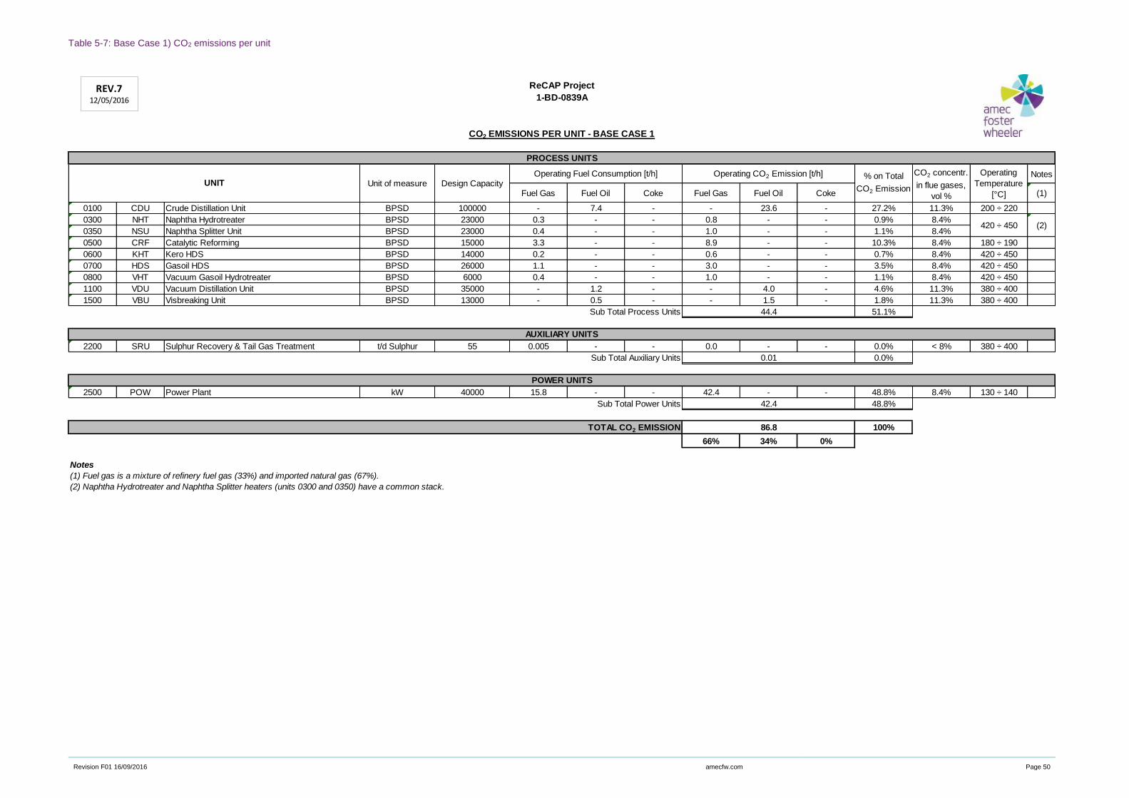
Revision F01 16/09/2016 amecfw.com Page 50
Table 5-7: Base Case 1) CO2 emissions per unit
Notes
Fuel Gas Fuel Oil Coke Fuel Gas Fuel Oil Coke (1)
0100 CDU Crude Distillation Unit BPSD 100000 - 7.4 - - 23.6 - 27.2% 11.3% 200 ÷ 220
0300 NHT Naphtha Hydrotreater BPSD 23000 0.3 - - 0.8 - - 0.9% 8.4%
0350 NSU Naphtha Splitter Unit BPSD 23000 0.4 - - 1.0 - - 1.1% 8.4%
0500 CRF Catalytic Reforming BPSD 15000 3.3 - - 8.9 - - 10.3% 8.4% 180 ÷ 190
0600 KHT Kero HDS BPSD 14000 0.2 - - 0.6 - - 0.7% 8.4% 420 ÷ 450
0700 HDS Gasoil HDS BPSD 26000 1.1 - - 3.0 - - 3.5% 8.4% 420 ÷ 450
0800 VHT Vacuum Gasoil Hydrotreater BPSD 6000 0.4 - - 1.0 - - 1.1% 8.4% 420 ÷ 450
1100 VDU Vacuum Distillation Unit BPSD 35000 - 1.2 - - 4.0 - 4.6% 11.3% 380 ÷ 400
1500 VBU Visbreaking Unit BPSD 13000 - 0.5 - - 1.5 - 1.8% 11.3% 380 ÷ 400
Sub Total Process Units 51.1%
2200 SRU Sulphur Recovery & Tail Gas Treatment t/d Sulphur 55 0.005 - - 0.0 - - 0.0% < 8% 380 ÷ 400
Sub Total Auxiliary Units 0.0%
2500 POW Power Plant kW 40000 15.8 - - 42.4 - - 48.8% 8.4% 130 ÷ 140
Sub Total Power Units 48.8%
100%
66% 34% 0%
Notes
(1) Fuel gas is a mixture of refinery fuel gas (33%) and imported natural gas (67%).
(2) Naphtha Hydrotreater and Naphtha Splitter heaters (units 0300 and 0350) have a common stack.
Operating Fuel Consumption [t/h] Operating CO2 Emission [t/h] % on Total
CO2 Emission
Operating
Temperature
[°C]
420 ÷ 450
CO2 concentr.
in flue gases,
vol %
TOTAL CO2 EMISSION 86.8
0.01
ReCAP Project
1-BD-0839A
42.4
CO2 EMISSIONS PER UNIT - BASE CASE 1
POWER UNITS
PROCESS UNITS
UNIT Unit of measure Design Capacity
(2)
44.4
AUXILIARY UNITS
REV.712/05/2016

Revision F01 16/09/2016 amecfw.com Page 51
Refinery Layout
The layout of the hydro-skimming refinery has been developed in analogy with some real plants of similar
size and complexity.
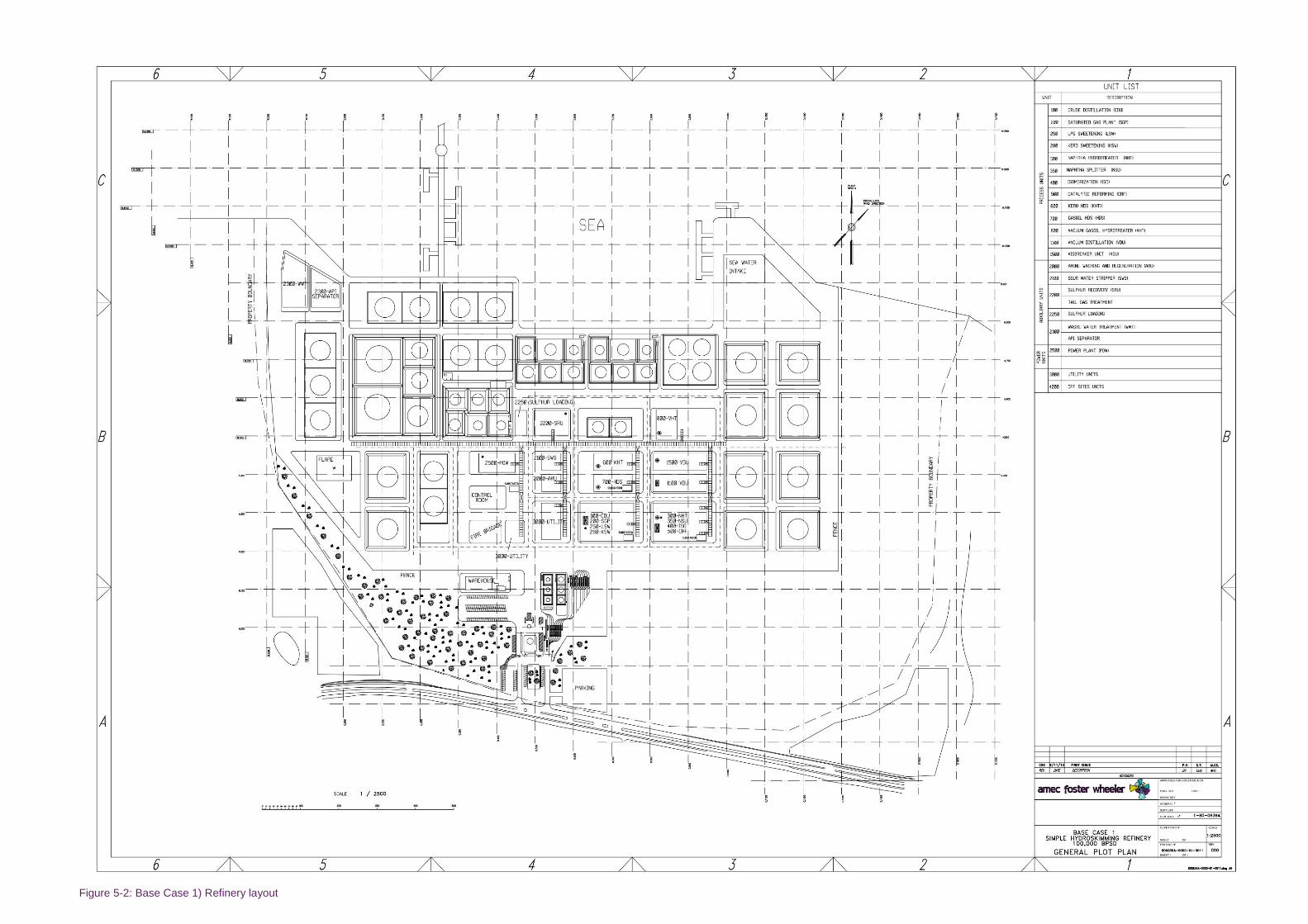
Figure 5-2: Base Case 1) Refinery layout
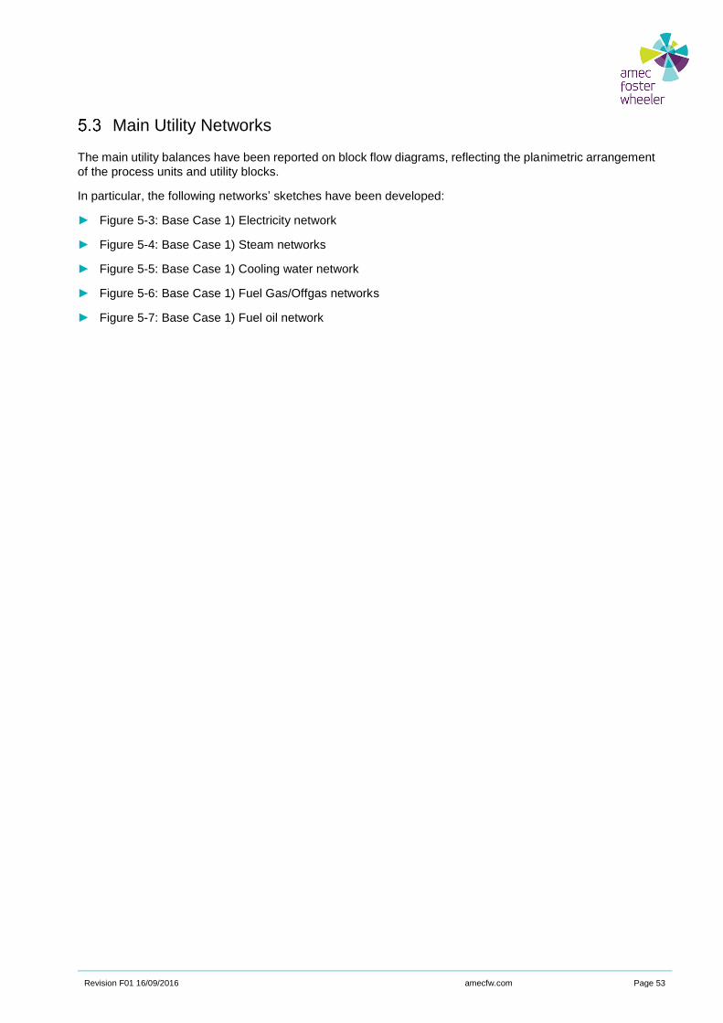
Revision F01 16/09/2016 amecfw.com Page 53
Main Utility Networks
The main utility balances have been reported on block flow diagrams, reflecting the planimetric arrangement
of the process units and utility blocks.
In particular, the following networks’ sketches have been developed:
► Figure 5-3: Base Case 1) Electricity network
► Figure 5-4: Base Case 1) Steam networks
► Figure 5-5: Base Case 1) Cooling water network
► Figure 5-6: Base Case 1) Fuel Gas/Offgas networks
► Figure 5-7: Base Case 1) Fuel oil network
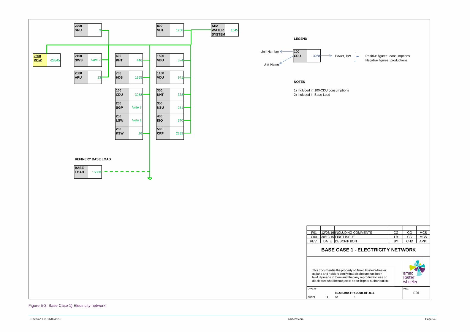
Revision F01 16/09/2016 amecfw.com Page 54
Figure 5-3: Base Case 1) Electricity network
2200 800 SEA
SRU 9 VHT 1206 WATER 1545
SYSTEM
LEGEND
Unit Number 100
2500 2100 600 1500 CDU 3268 Power, kW Positive figures: consumptions
POW -28345 SWS KHT 446 VBU 374 Negative figures: productions
Unit Name
2000 700 1100
ARU 13 HDS 1865 VDU 971
NOTES
100 300 1) Included in 100-CDU consumptions
CDU 3268 NHT 378 2) Included in Base Load
200 350
SGP NSU 281
250 400
LSW ISO 670
280 500
KSW 26 CRF 2293
REFINERY BASE LOAD
BASE
LOAD 15000
F01 12/05/16 INCLUDING COMMENTS CG CG MCS
C00 30/10/15 FIRST ISSUE LB CG MCS
REV. DATE DESCRIPTION BY CHD APP:
DWG. N° REV.
F01SHEET 1 OF 1
Note 2
Note 1
Note 1
BASE CASE 1 - ELECTRICITY NETWORK
BD0839A-PR-0000-BF-011
This document is the property of Amec Foster Wheeler Italiana and holders certify that disclosure has been lawfully made to them and that any reproduction use or disclosure shall be subject to specific prior authorisation.
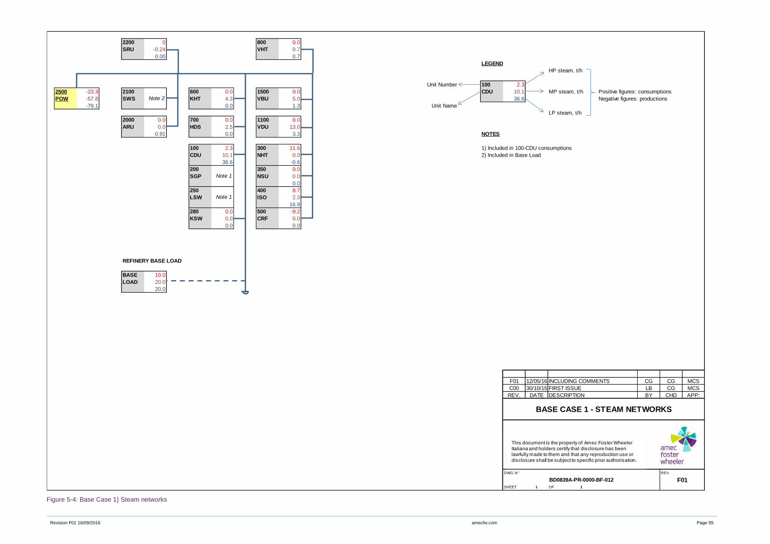
Revision F01 16/09/2016 amecfw.com Page 55
Figure 5-4: Base Case 1) Steam networks
2200 0 800 0.0
SRU -0.24 VHT 0.7
0.00 0.7
LEGEND
HP steam, t/h
Unit Number 100 2.3
2500 -23.3 2100 600 0.0 1500 0.0 CDU 10.1 MP steam, t/h Positive figures: consumptions
POW -57.8 SWS KHT 4.3 VBU 5.0 36.6 Negative figures: productions
-79.1 0.0 1.3 Unit Name
LP steam, t/h
2000 0.0 700 0.0 1100 0.0
ARU 0.0 HDS 2.5 VDU 13.0
0.91 0.0 3.3 NOTES
100 2.3 300 11.6 1) Included in 100-CDU consumptions
CDU 10.1 NHT 0.0 2) Included in Base Load
36.6 -0.6
200 350 0.0
SGP NSU 0.0
0.0
250 400 8.7
LSW ISO 2.3
16.9
280 0.0 500 -9.2
KSW 0.0 CRF 0.0
0.0 0.0
REFINERY BASE LOAD
BASE 10.0
LOAD 20.0
20.0
F01 12/05/16 INCLUDING COMMENTS CG CG MCS
C00 30/10/15 FIRST ISSUE LB CG MCS
REV. DATE DESCRIPTION BY CHD APP:
DWG. N° REV.
F01SHEET 1 OF 1
Note 2
Note 1
Note 1
BASE CASE 1 - STEAM NETWORKS
BD0839A-PR-0000-BF-012
This document is the property of Amec Foster Wheeler Italiana and holders certify that disclosure has been lawfully made to them and that any reproduction use or disclosure shall be subject to specific prior authorisation.
Revision F01 16/09/2016 amecfw.com Page 56
Figure 5-5: Base Case 1) Cooling water network
2200 800 SEA
SRU 6 VHT 1 WATER -9026
SYSTEM
LEGEND
Unit Number 100
2500 2100 600 1500 CDU 676 Cooling water, m3/h Positive figures: consumptions
POW 4106 SWS KHT 205 VBU 556 Negative figures: productions
Unit Name
2000 700 1100
ARU 2 HDS 184 VDU 2252
NOTES
100 300 1) Included in 100-CDU consumptions
CDU 676 NHT 231
200 350
SGP NSU 21
250 400
LSW ISO 74
280 500
KSW 0 CRF 712
F01 12/05/16 INCLUDING COMMENTS CG CG MCS
C00 30/10/15 FIRST ISSUE LB CG MCS
REV. DATE DESCRIPTION BY CHD APP:
DWG. N° REV.
F01SHEET 1 OF 1
BD0839A-PR-0000-BF-013
Note 1
Note 1
BASE CASE 1 - COOLING WATER NETWORK
This document is the property of Amec Foster Wheeler Italiana and holders certify that disclosure has been lawfully made to them and that any reproduction use or disclosure shall be subject to specific prior authorisation.

Revision F01 16/09/2016 amecfw.com Page 57
Figure 5-6: Base Case 1) Fuel Gas/Offgas networks
2200 0.005 800 0.4
SRU VHT
-0.4
LEGEND
Sweet fuel gas, t/h
Unit Number 100 0.0
2500 15.8 2100 0.0 600 0.2 1500 0.0 CDU Positive figures: consumptions
POW SWS KHT VBU -1.9 Negative figures: productions
-0.1 -0.4 Unit Name
Sour fuel gas, t/h
2000 -7.0 700 1.1 1100 0.0
ARU HDS VDU
7.0 -0.6 NOTES
100 0.0 300 0.3 1) Included in 100-CDU consumptions/productions
CDU NHT
FUEL -21.5 -1.9 -0.4
GAS 200 350 0.4
SYSTEM SGP NSU
NATURAL GAS IMPORT 250 400 0.0
-14.5 LSW ISO
-0.5
280 0.0 500 3.3
KSW CRF
-2.8
F01 12/05/16 INCLUDING COMMENTS CG CG MCS
C00 30/10/15 FIRST ISSUE LB CG MCS
REV. DATE DESCRIPTION BY CHD APP:
DWG. N° REV.
F01SHEET 1 OF 1
BD0839A-PR-0000-BF-014
Note 1
Note 1
BASE CASE 1 - FUEL GAS / OFFGAS NETWORKS
This document is the property of Amec Foster Wheeler Italiana and holders certify that disclosure has been lawfully made to them and that any reproduction use or disclosure shall be subject to specific prior authorisation.
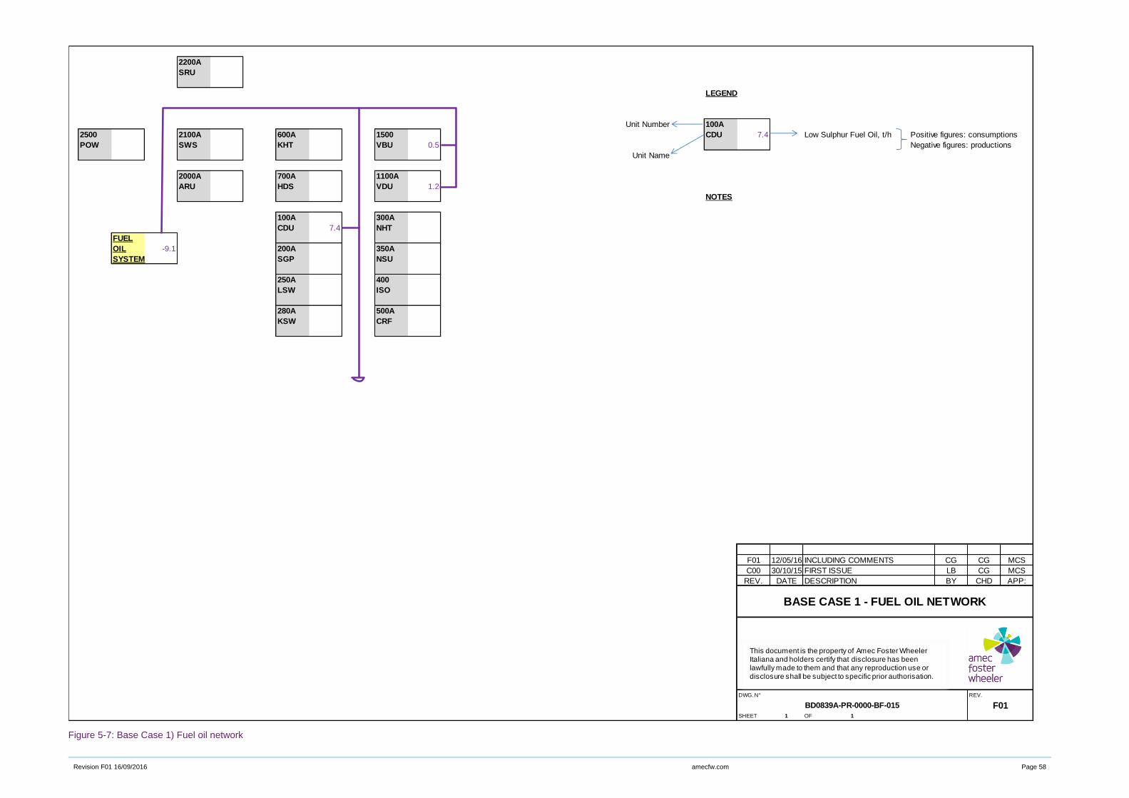
Revision F01 16/09/2016 amecfw.com Page 58
Figure 5-7: Base Case 1) Fuel oil network
2200A
SRU
LEGEND
Unit Number 100A
2500 2100A 600A 1500 CDU 7.4 Low Sulphur Fuel Oil, t/h Positive figures: consumptions
POW SWS KHT VBU 0.5 Negative figures: productions
Unit Name
2000A 700A 1100A
ARU HDS VDU 1.2
NOTES
100A 300A
CDU 7.4 NHT
FUEL
OIL -9.1 200A 350A
SYSTEM SGP NSU
250A 400
LSW ISO
280A 500A
KSW CRF
F01 12/05/16 INCLUDING COMMENTS CG CG MCS
C00 30/10/15 FIRST ISSUE LB CG MCS
REV. DATE DESCRIPTION BY CHD APP:
DWG. N° REV.
F01SHEET 1 OF 1
BASE CASE 1 - FUEL OIL NETWORK
BD0839A-PR-0000-BF-015
This document is the property of Amec Foster Wheeler Italiana and holders certify that disclosure has been lawfully made to them and that any reproduction use or disclosure shall be subject to specific prior authorisation.
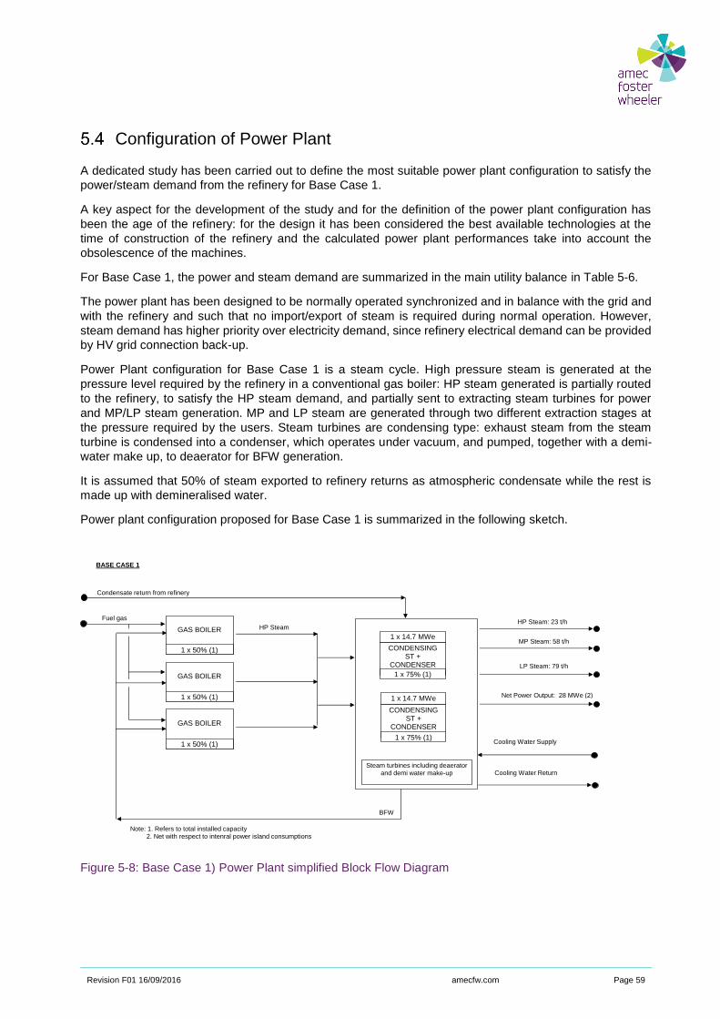
Revision F01 16/09/2016 amecfw.com Page 59
Configuration of Power Plant
A dedicated study has been carried out to define the most suitable power plant configuration to satisfy the
power/steam demand from the refinery for Base Case 1.
A key aspect for the development of the study and for the definition of the power plant configuration has
been the age of the refinery: for the design it has been considered the best available technologies at the
time of construction of the refinery and the calculated power plant performances take into account the
obsolescence of the machines.
For Base Case 1, the power and steam demand are summarized in the main utility balance in Table 5-6.
The power plant has been designed to be normally operated synchronized and in balance with the grid and
with the refinery and such that no import/export of steam is required during normal operation. However,
steam demand has higher priority over electricity demand, since refinery electrical demand can be provided
by HV grid connection back-up.
Power Plant configuration for Base Case 1 is a steam cycle. High pressure steam is generated at the
pressure level required by the refinery in a conventional gas boiler: HP steam generated is partially routed
to the refinery, to satisfy the HP steam demand, and partially sent to extracting steam turbines for power
and MP/LP steam generation. MP and LP steam are generated through two different extraction stages at
the pressure required by the users. Steam turbines are condensing type: exhaust steam from the steam
turbine is condensed into a condenser, which operates under vacuum, and pumped, together with a demi-
water make up, to deaerator for BFW generation.
It is assumed that 50% of steam exported to refinery returns as atmospheric condensate while the rest is
made up with demineralised water.
Power plant configuration proposed for Base Case 1 is summarized in the following sketch.
Figure 5-8: Base Case 1) Power Plant simplified Block Flow Diagram
GAS BOILER
CONDENSINGST +
CONDENSER
1 x 50% (1)
1 x 75% (1)
1 x 14.7 MWe
GAS BOILER
1 x 50% (1)
GAS BOILER
1 x 50% (1)
CONDENSINGST +
CONDENSER
1 x 75% (1)
1 x 14.7 MWe
Steam turbines including deaerator and demi water make-up
BFW
HP Steam
Fuel gas
Note: 1. Refers to total installed capacity2. Net with respect to intenral power island consumptions
Condensate return from refinery
HP Steam: 23 t/h
MP Steam: 58 t/h
LP Steam: 79 t/h
Net Power Output: 28 MWe (2)
Cooling Water Supply
Cooling Water Return
BASE CASE 1
Revision F01 16/09/2016 amecfw.com Page 60
Major equipment number and sizes are summarized hereinafter:
► 3 x 115 t/h Gas Boilers, normally operated at 69% of their design load (corresponding to 79.3 t/h each)
► 2 x 20 MWe Condensing Steam Turbines, normally operated at 74% of their design load (corresponding
to 14.7 MWe each)
The system has been conceived to have such an installed spare capacity both for power and steam
generation to handle possible oscillations in power/steam demand from refinery users and to avoid refinery
shutdown in case one equipment (boiler or turbine) trips.
In case one of the steam turbines trips, however, only 68% of the total power demand is guaranteed: in this
scenario, a load shedding is necessary unless there is the possibility to import the remaining electrical
demand from the HV grid.
Total installed spare capacity is summarized hereinafter:
► Gas Boilers (Steam) +45%
► Steam Turbines (Electric Energy) +37%
Revision F01 16/09/2016 amecfw.com Page 61
6. Base Case 2
Medium Conversion Refinery - 220,000 BPSD Crude Capacity
The Medium Conversion Refinery, with respect of the Hydro-skimming Refinery described at paragraph 5,
includes additional process units for the conversion of the Vacuum Gasoil (VGO) into more valuable
distillates (essentially gasoline and automotive diesel).
In Europe, the most wide-spread VGO conversion unit is the Fluid Catalytic Cracking (FCC) and so this unit
is included in Base Case 2.
Upstream of the FCC, a Vacuum Gasoil Hydrotreating (VHT) unit is present to decrease the sulphur content
of FCC feedstock, in order to respect SOx limits at FCC stack.
The hydrogen from the Heavy Naphtha Catalytic Reformer is not enough to cover the overall hydrogen
demand of the refinery. Therefore, a Steam Methane Reformer (SMR) is also foreseen to close the hydrogen
balance.
The FCC products are sent to finishing units to comply with the 10 ppm wt. sulphur specification for the
automotive fuels.
The overall configuration of Base Case 2 is considered as a step-up evolution of Base Case 1, both in terms
of capacity and complexity increase. In other words, it is considered that, in a simple hydro-skimming refinery
(as the one depicted as Base Case 1), a second crude distillation train (Atmospheric and Vacuum Distillation
Units) and FCC block (VHT+FCC+SMR) are built in a second phase. The consequent capacity increase of
the gasoline block and the hydrotreating units is considered achieved by adding a second train in parallel to
the original one.
The above assumption reflects the typical “life” of the European refineries, which have gradually expanded
starting from an original nucleus. This results in the following main effects:
► Several units of the same type are running in parallel, resulting in a relatively good flexibility of the
processing scheme (e.g. different feedstocks could be fed to each train) but also, on the other hand, in
some inefficiencies (e.g. higher maintenance costs, lower energy efficiencies, etc.).
► Also the Power Plant in Base Case 2 is considered as an expansion of the facilities foreseen in Base
Case 1, reflecting the “modular” expansion of the original refinery into a bigger, more complex and more
demanding site.
► The increased demand of cooling water –with respect of cooling water consumption in Base Case 1- is
considered to be satisfied by a closed loop circuit with cooling towers, working in parallel to the original
open circuit of sea cooling water. As a matter of fact, for the upgrading of the refinery, it is assumed that
more stringent environmental regulations have been met.
► Finally, also the layout of the Base Case 2 refinery reflects two main areas of units’ allocation: beside
the original nucleus of the older units (unit numbers identified with suffix –A), a second block of units is
present and clearly identifiable (unit numbers identified with suffix –B). The FCC block is included in this
newer portion of the refinery.
Refinery Balances
The balances developed for Base Case 2 are reported in the following tables and figures:
► Table 6-1: Base Case 2) Overall material balance
► Table 6-2: Base Case 2) Process units operating and design capacity

Revision F01 16/09/2016 amecfw.com Page 62
► Table 6-3: Base Case 2) Gasoline qualities
► Table 6-4: Base Case 2) Distillate qualities
► Table 6-5: Base Case 2) Fuel oil and bitumen qualities
► Table 6-6: Base Case 2) Main utility balance, fuel mix composition, CO2 emissions
► Figure 6-1: Base Case 2) Block flow diagrams with main material streams
► Table 6-7: Base Case 2) CO2 emissions per unit
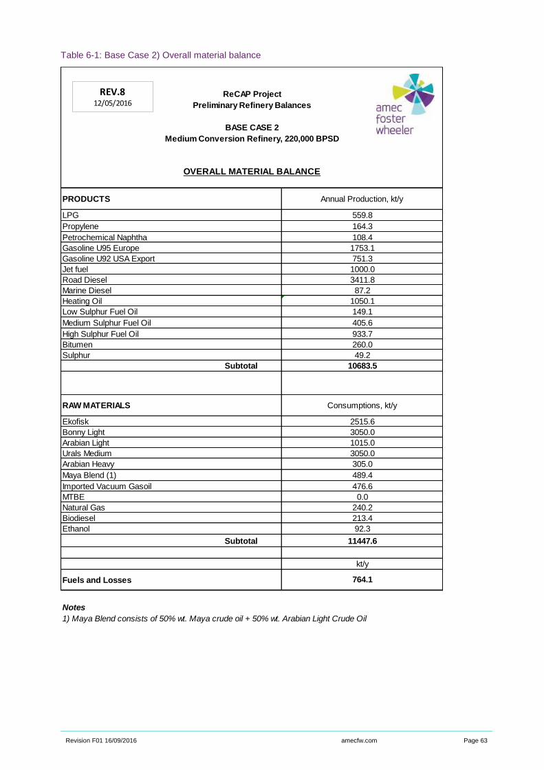
Revision F01 16/09/2016 amecfw.com Page 63
Table 6-1: Base Case 2) Overall material balance
ReCAP Project
Preliminary Refinery Balances
BASE CASE 2
Medium Conversion Refinery, 220,000 BPSD
PRODUCTS
LPG
Propylene
Petrochemical Naphtha
Gasoline U95 Europe
Gasoline U92 USA Export
Jet fuel
Road Diesel
Marine Diesel
Heating Oil
Low Sulphur Fuel Oil
Medium Sulphur Fuel Oil
High Sulphur Fuel Oil
Bitumen
Sulphur
Subtotal
RAW MATERIALS
Ekofisk
Bonny Light
Arabian Light
Urals Medium
Arabian Heavy
Maya Blend (1)
Imported Vacuum Gasoil
MTBE
Natural Gas
Biodiesel
Ethanol
Subtotal
Fuels and Losses
Notes
1) Maya Blend consists of 50% wt. Maya crude oil + 50% wt. Arabian Light Crude Oil
OVERALL MATERIAL BALANCE
Annual Production, kt/y
559.8
164.3
108.4
1753.1
751.3
1000.0
3411.8
87.2
1050.1
149.1
405.6
933.7
260.0
49.2
10683.5
Consumptions, kt/y
2515.6
3050.0
1015.0
3050.0
305.0
489.4
11447.6
kt/y
764.1
476.6
0.0
240.2
213.4
92.3
REV.812/05/2016
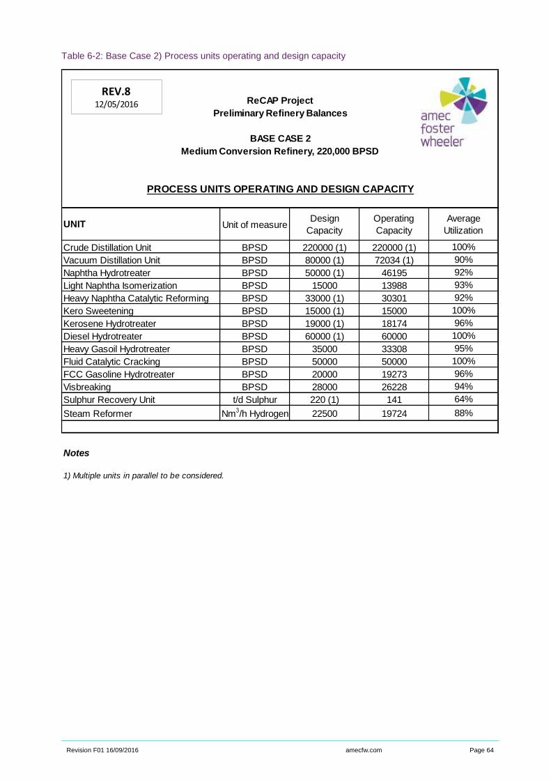
Revision F01 16/09/2016 amecfw.com Page 64
Table 6-2: Base Case 2) Process units operating and design capacity
ReCAP Project
Preliminary Refinery Balances
BASE CASE 2
Medium Conversion Refinery, 220,000 BPSD
UNIT Unit of measureDesign
Capacity
Operating
Capacity
Average
Utilization
Crude Distillation Unit BPSD 220000 (1) 220000 (1) 100%
Vacuum Distillation Unit BPSD 80000 (1) 72034 (1) 90%
Naphtha Hydrotreater BPSD 50000 (1) 46195 92%
Light Naphtha Isomerization BPSD 15000 13988 93%
Heavy Naphtha Catalytic Reforming BPSD 33000 (1) 30301 92%
Kero Sweetening BPSD 15000 (1) 15000 100%
Kerosene Hydrotreater BPSD 19000 (1) 18174 96%
Diesel Hydrotreater BPSD 60000 (1) 60000 100%
Heavy Gasoil Hydrotreater BPSD 35000 33308 95%
Fluid Catalytic Cracking BPSD 50000 50000 100%
FCC Gasoline Hydrotreater BPSD 20000 19273 96%
Visbreaking BPSD 28000 26228 94%
Sulphur Recovery Unit t/d Sulphur 220 (1) 141 64%
Steam Reformer Nm3/h Hydrogen 22500 19724 88%
Notes
1) Multiple units in parallel to be considered.
PROCESS UNITS OPERATING AND DESIGN CAPACITY
REV.812/05/2016

Revision F01 16/09/2016 amecfw.com Page 65
Table 6-3: Base Case 2) Gasoline qualities
ReCAP Project
Preliminary Refinery Balances
BASE CASE 2
Medium Conversion Refinery, 220,000 BPSD
GASOLINE QUALITIES
EXCESS NAPHTHA
Component Weight Quantity Weight PercentVolume
QuantityVolume Percent
NAH HT HEAVY NAPHTHA 8,782.63 8.103% 11,772.96 7.611%
NAL HT LIGHT NAPHTHA 64,337.19 59.358% 92,305.86 59.676%
LCN FCC LIGHT NAPHTHA treated 1,963.13 1.811% 2,745.64 1.775%
NSCR5 STAB NAPHTHA ARAB.HEAVY 33,306.00 30.728% 47,853.45 30.937%
Total 108,388.95 100.000% 154,677.91 100.000%
Quality Blending Basis Value Min Max
RHO DENSITY, KG/M3 VL 700.74 725.00
SPM SULFUR, PPMW WT 62.24 500.00
VPR VAPOR PRESSURE, KPA VL 69.00 69.00
Unl. Premium (95) EU
Component Weight Quantity Weight PercentVolume
QuantityVolume Percent
BU# C4 TO MOGAS/LPG 12,656.60 0.722% 21,700.02 0.934%
R10 REFORMATE 100 785,262.42 44.794% 947,240.55 40.772%
ISO ISOMERATE 275,236.94 15.700% 416,394.76 17.923%
LCN FCC LIGHT NAPHTHA treated 587,550.95 33.516% 821,749.57 35.371%
EOH ETHANOL 92,349.08 5.268% 116,162.36 5.000%
Total 1,753,055.99 100.000% 2,323,247.27 100.000%
Quality Blending Basis Value Min Max
RHO DENSITY, KG/M3 VL 754.57 720.00 775.00
SPM SULFUR, PPMW WT 3.39 10.00
VPR VAPOR PRESSURE, KPA VL 60.00 60.00
BEN BENZENE, %V VL 0.71 1.00
ARO AROMATICS, %V VL 32.01 35.00
E50 D86 @ 150°C, %V VL 91.03 75.00
OXY OXYGENATES, %V VL 5.00 15.00
OLE OLEFINS, %V VL 14.53 18.00
EOH ETHANOL, VOl% VL 5.00 5.00
RON Research VL 95.00 95.00
MON Motor VL 85.00 85.00
REV.812/05/2016
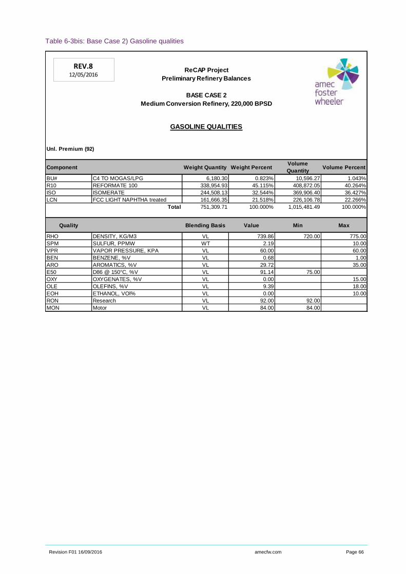
Revision F01 16/09/2016 amecfw.com Page 66
Table 6-3bis: Base Case 2) Gasoline qualities
ReCAP Project
Preliminary Refinery Balances
BASE CASE 2
Medium Conversion Refinery, 220,000 BPSD
GASOLINE QUALITIES
Unl. Premium (92)
Component Weight Quantity Weight PercentVolume
QuantityVolume Percent
BU# C4 TO MOGAS/LPG 6,180.30 0.823% 10,596.27 1.043%
R10 REFORMATE 100 338,954.93 45.115% 408,872.05 40.264%
ISO ISOMERATE 244,508.13 32.544% 369,906.40 36.427%
LCN FCC LIGHT NAPHTHA treated 161,666.35 21.518% 226,106.78 22.266%
Total 751,309.71 100.000% 1,015,481.49 100.000%
Quality Blending Basis Value Min Max
RHO DENSITY, KG/M3 VL 739.86 720.00 775.00
SPM SULFUR, PPMW WT 2.19 10.00
VPR VAPOR PRESSURE, KPA VL 60.00 60.00
BEN BENZENE, %V VL 0.68 1.00
ARO AROMATICS, %V VL 29.72 35.00
E50 D86 @ 150°C, %V VL 91.14 75.00
OXY OXYGENATES, %V VL 0.00 15.00
OLE OLEFINS, %V VL 9.39 18.00
EOH ETHANOL, VOl% VL 0.00 10.00
RON Research VL 92.00 92.00
MON Motor VL 84.00 84.00
REV.812/05/2016

Revision F01 16/09/2016 amecfw.com Page 67
Table 6-4: Base Case 2) Distillate qualities
ReCAP Project
Preliminary Refinery Balances
BASE CASE 2
Medium Conversion Refinery, 220,000 BPSD
DISTILLATE QUALITIES
LPG PRODUCT
Component Weight Quantity Weight PercentVolume
QuantityVolume Percent
LG# LPG POOL 559,790.66 100.000% 984,736.23 100.000%
Total 559,790.66 100.000% 984,736.23 100.000%
Quality Blending Basis Value Min Max
SPM SULFUR, PPMW WT 5.00 140.00
VPR VAPOR PRESSURE, KPA VL 622.89 887.60
OLW OLEFINS, %W WT 0.78 30.00
Jet Fuel EU
Component Weight Quantity Weight PercentVolume
QuantityVolume Percent
KED HT KERO 332,718.22 33.272% 419,304.62 33.438%
KMCR3 KERO FROM MEROX AR.LIGHT 108,750.20 10.875% 135,598.75 10.813%
KMCR4 KERO FROM MEROX URALS 458,415.00 45.842% 573,735.92 45.753%
KMCR5 KERO FROM MEROX AR.HVY 36,295.00 3.630% 45,368.75 3.618%
KMCR6 KERO FROM MEROX MAYA 63,821.58 6.382% 79,976.92 6.378%
Total 1,000,000.00 100.000% 1,253,984.97 100.000%
Quality Blending Basis Value Min Max
RHO DENSITY, KG/M3 VL 797.46 775.00 840.00
SUL SULFUR, %W WT 0.12 0.30
FLC FLASH POINT, °C (PM, D93) VL 40.00 38.00
Diesel EU
Component Weight Quantity Weight PercentVolume
QuantityVolume Percent
LCO LIGHT CYCLE OIL treated 193,322.80 5.666% 203,497.69 5.035%
HCN FCC HEAVY NAPHTHA 375,590.21 11.009% 441,870.84 10.933%
KED HT KERO 469,302.16 13.755% 591,433.10 14.633%
DLG DESULF LGO 2,160,135.16 63.314% 2,562,437.92 63.399%
FAM BIODIESEL 213,404.09 6.255% 242,504.65 6.000%
Total 3,411,754.44 100.000% 4,041,744.19 100.000%
Quality Blending Basis Value Min Max
RHO DENSITY, KG/M3 VL 844.13 820.00 845.00
SPM SULFUR, PPMW WT 9.10 10.00
FLC FLASH POINT, °C (PM, D93) VL 55.00 55.00
CIN CETANE INDEX D4737 VL 48.16 46.00
V04 VISCOSITY @ 40°C, CST WT 2.45 2.00 4.50
E36 D86 @360°C, %V VL 97.53 95.00
FAM BIODIESEL CONTENT, %VOL VL 6.00 6.00 7.00
REV.812/05/2016
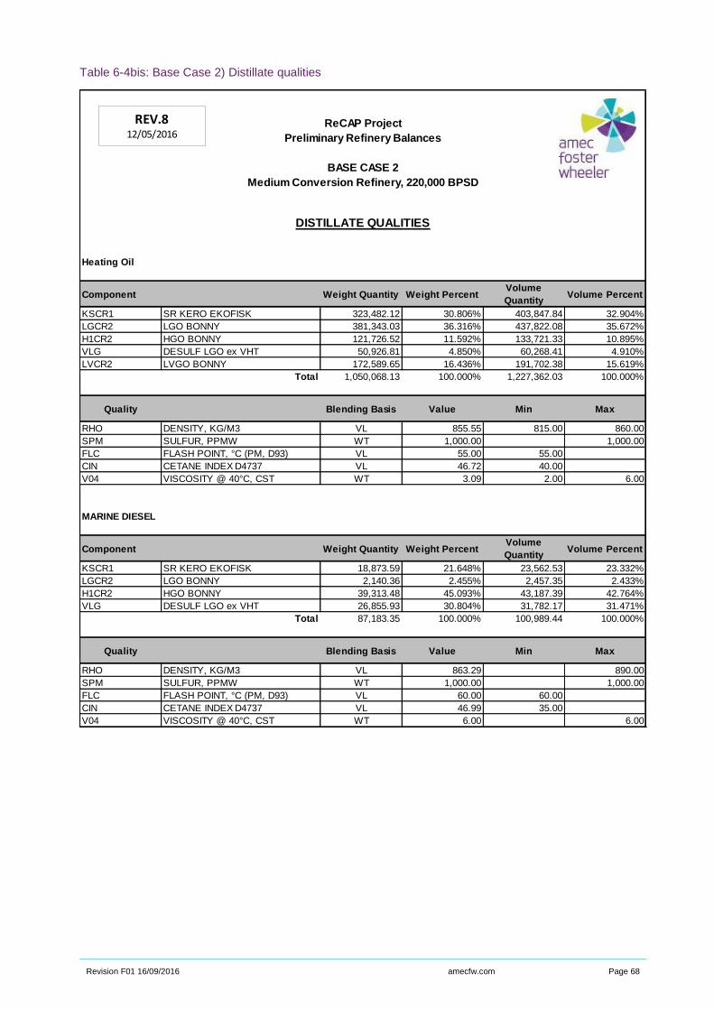
Revision F01 16/09/2016 amecfw.com Page 68
Table 6-4bis: Base Case 2) Distillate qualities
ReCAP Project
Preliminary Refinery Balances
BASE CASE 2
Medium Conversion Refinery, 220,000 BPSD
DISTILLATE QUALITIES
Heating Oil
Component Weight Quantity Weight PercentVolume
QuantityVolume Percent
KSCR1 SR KERO EKOFISK 323,482.12 30.806% 403,847.84 32.904%
LGCR2 LGO BONNY 381,343.03 36.316% 437,822.08 35.672%
H1CR2 HGO BONNY 121,726.52 11.592% 133,721.33 10.895%
VLG DESULF LGO ex VHT 50,926.81 4.850% 60,268.41 4.910%
LVCR2 LVGO BONNY 172,589.65 16.436% 191,702.38 15.619%
Total 1,050,068.13 100.000% 1,227,362.03 100.000%
Quality Blending Basis Value Min Max
RHO DENSITY, KG/M3 VL 855.55 815.00 860.00
SPM SULFUR, PPMW WT 1,000.00 1,000.00
FLC FLASH POINT, °C (PM, D93) VL 55.00 55.00
CIN CETANE INDEX D4737 VL 46.72 40.00
V04 VISCOSITY @ 40°C, CST WT 3.09 2.00 6.00
MARINE DIESEL
Component Weight Quantity Weight PercentVolume
QuantityVolume Percent
KSCR1 SR KERO EKOFISK 18,873.59 21.648% 23,562.53 23.332%
LGCR2 LGO BONNY 2,140.36 2.455% 2,457.35 2.433%
H1CR2 HGO BONNY 39,313.48 45.093% 43,187.39 42.764%
VLG DESULF LGO ex VHT 26,855.93 30.804% 31,782.17 31.471%
Total 87,183.35 100.000% 100,989.44 100.000%
Quality Blending Basis Value Min Max
RHO DENSITY, KG/M3 VL 863.29 890.00
SPM SULFUR, PPMW WT 1,000.00 1,000.00
FLC FLASH POINT, °C (PM, D93) VL 60.00 60.00
CIN CETANE INDEX D4737 VL 46.99 35.00
V04 VISCOSITY @ 40°C, CST WT 6.00 6.00
REV.812/05/2016

Revision F01 16/09/2016 amecfw.com Page 69
Table 6-5: Base Case 2) Fuel oil and bitumen qualities
ReCAP Project
Preliminary Refinery Balances
BASE CASE 2
Medium Conversion Refinery, 220,000 BPSD
FUEL OIL / BITUMEN QUALITIES
Low Sulphur Fuel
Component Weight Quantity Weight PercentVolume
QuantityVolume Percent
SLU FCC SLURRY OIL 25,340.95 7.986% 24,366.30 7.610%
lco LIGHT CYCLE OIL untreated 22,066.39 6.954% 23,227.78 7.255%
LCO LIGHT CYCLE OIL treated 15,040.81 4.740% 15,832.43 4.945%
VRCR1 VBRES MIX1 50,540.30 15.928% 52,756.05 16.477%
VRCR2 VBRES MIX2 171,018.58 53.898% 164,599.21 51.408%
VLG DESULF LGO ex VHT 33,292.38 10.492% 39,399.26 12.305%
Total 317,299.41 100.000% 320,181.04 100.000%
Quality Blending Basis Value Min Max
RHO DENSITY, KG/M3 VL 991.00 991.00
SUL SULFUR, %W WT 0.50 0.50
FLC FLASH POINT, °C (PM, D93) VL 129.30 66.00
V05 VISCOSITY @ 50°C, CST WT 380.00 380.00
CCR CONRADSON CARBON RES, %W WT 11.36 15.00
Medium Sulphur Fuel
Component Weight Quantity Weight PercentVolume
QuantityVolume Percent
SLU FCC SLURRY OIL 167,462.02 41.287% 161,021.18 39.501%
lco LIGHT CYCLE OIL untreated 27,663.62 6.820% 29,119.60 7.143%
VRCR1 VBRES MIX1 176,752.37 43.578% 184,501.43 45.261%
VRCR4 VBRES MIX4 33,725.32 8.315% 32,999.33 8.095%
Total 405,603.33 100.000% 407,641.54 100.000%
Quality Blending Basis Value Min Max
RHO DENSITY, KG/M3 VL 995.00 995.00
SUL SULFUR, %W WT 1.00 1.00
FLC FLASH POINT, °C (PM, D93) VL 156.64 66.00
V05 VISCOSITY @ 50°C, CST WT 380.00 380.00
CCR CONRADSON CARBON RES, %W WT 7.58 17.00
REV.812/05/2016
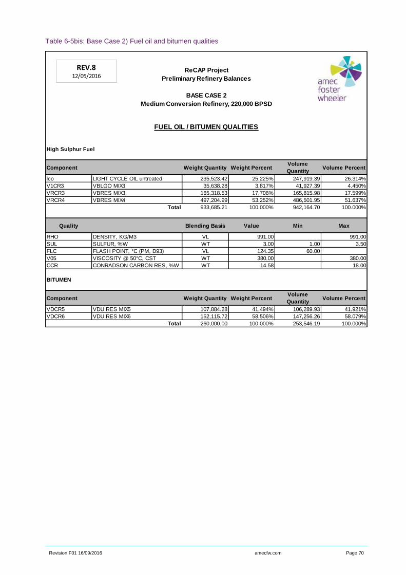
Revision F01 16/09/2016 amecfw.com Page 70
Table 6-5bis: Base Case 2) Fuel oil and bitumen qualities
ReCAP Project
Preliminary Refinery Balances
BASE CASE 2
Medium Conversion Refinery, 220,000 BPSD
FUEL OIL / BITUMEN QUALITIES
High Sulphur Fuel
Component Weight Quantity Weight PercentVolume
QuantityVolume Percent
lco LIGHT CYCLE OIL untreated 235,523.42 25.225% 247,919.39 26.314%
V1CR3 VBLGO MIX3 35,638.28 3.817% 41,927.39 4.450%
VRCR3 VBRES MIX3 165,318.53 17.706% 165,815.98 17.599%
VRCR4 VBRES MIX4 497,204.99 53.252% 486,501.95 51.637%
Total 933,685.21 100.000% 942,164.70 100.000%
Quality Blending Basis Value Min Max
RHO DENSITY, KG/M3 VL 991.00 991.00
SUL SULFUR, %W WT 3.00 1.00 3.50
FLC FLASH POINT, °C (PM, D93) VL 124.35 60.00
V05 VISCOSITY @ 50°C, CST WT 380.00 380.00
CCR CONRADSON CARBON RES, %W WT 14.58 18.00
BITUMEN
Component Weight Quantity Weight PercentVolume
QuantityVolume Percent
VDCR5 VDU RES MIX5 107,884.28 41.494% 106,289.93 41.921%
VDCR6 VDU RES MIX6 152,115.72 58.506% 147,256.26 58.079%
Total 260,000.00 100.000% 253,546.19 100.000%
REV.812/05/2016
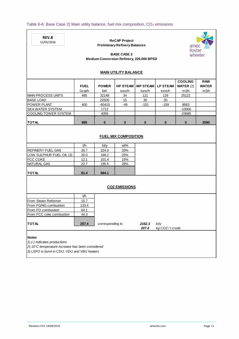
Revision F01 16/09/2016 amecfw.com Page 71
Table 6-6: Base Case 2) Main utility balance, fuel mix composition, CO2 emissions
ReCAP Project
Preliminary Refinery Balances
BASE CASE 2
Medium Conversion Refinery, 220,000 BPSD
FUEL POWER HP STEAM MP STEAM LP STEAM
COOLING
WATER (2)
RAW
WATER
Gcal/h kW tons/h tons/h tons/h m3/h m3/h
MAIN PROCESS UNITS 485 32148 34 121 129 25122
BASE LOAD 22500 15 30 30
POWER PLANT 400 -60415 -49 -151 -159 8563
SEA WATER SYSTEM 1712 -10000
COOLING TOWER SYSTEM 4055 -23685
TOTAL 885 0 0 0 0 0 2590
t/h kt/y wt%
REFINERY FUEL GAS 26.7 224.0 33%
LOW SULPHUR FUEL OIL (3) 20.0 168.2 25%
FCC COKE 12.1 101.4 15%
NATURAL GAS 22.7 190.5 28%
TOTAL 81.4 684.1
t/h
From Steam Reformer 15.7
From FG/NG combustion 133.4
From FO combustion 64.1
From FCC coke combustion 44.3
TOTAL 257.4 corresponding to 2162.3 kt/y
207.4 kg CO2 / t crude
Notes
1) (-) indicates productions
2) 10°C temperature increase has been considered
3) LSFO is burnt in CDU, VDU and VBU heaters
MAIN UTILITY BALANCE
FUEL MIX COMPOSITION
CO2 EMISSIONS
REV.812/05/2016
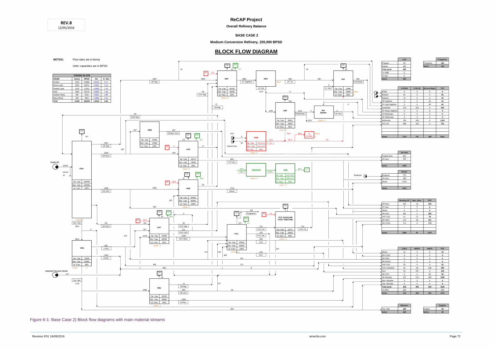
Revision F01 16/09/2016 amecfw.com Page 72
Figure 6-1: Base Case 2) Block flow diagrams with main material streams
ReCAP Project
Overall Refinery Balance
BASE CASE 2
Medium Conversion Refinery, 220,000 BPSD
BLOCK FLOW DIAGRAM
NOTES: Flow rates are in kton/y LPG Propylene
Propane 94 Propylene 164
Units' capacities are in BPSD Butane 465 Sales 164
33 22 0.7 64 30 Total prod. 560
2.3 To SMR 0
CRUDE SLATE To fuel 0
CRUDE kton/y BPSD SG S, %wt 1837 1804 1883 609 545 520 Sales 560
Ekofisk 2516 55388 0.8162 0.17 check
Bonny Light 3050 63875 0.8581 0.13 0 0
Arabian Light 1015 21321 0.8555 1.79 Op. Cap. 46195 Op. Cap. 13988 U 95-EU U 92-US Excess Naph. TOT
Urals 3050 63270 0.8663 1.46 26 Des. Cap. 50000 1273 9 Des. Cap. 15000 check MTBE 0 0 0 0
Arabian Heavy 305 6221 0.8811 2.85 Ut. Fact. 92% Ut. Fact. 93% 0 Ethanol 92 0 0 92
Maya Blend 489 9922 0.8865 2.45 check 0 Butanes 13 6 0 19
Total 10425 220000 0.8516 0.88 102 SR Naphtha 0 0 33 33
73 0 0 HT Light Naphtha 0 0 64 64
Isomerate 275 245 0 520
1265 1124 0 0 HT Heavy Naphtha 0 0 9 9
80 LT Reformate 0 0 0 0
HV Reformate 0 0 0 0
Op. Cap. 30301 1124 check 0 Reformate 785 339 0 1124
Des. Cap. 33000 FCC LN 588 162 2 751
Ut. Fact. 92%
667 667 check 0
LPG 38.3 48.6 check
147 0 0 Sales 1753 751 108 2613
Op. Cap. 15000 3.0 0.3 14.9 53.2 4.6
1837 Des. Cap. 15000 50 Op. Cap. 19724 Nm3/h
Ut. Fact. 100% 1.7 27 Natural Gas Des. Cap. 22500 Nm3/h
342 Ut. Fact. 88%
1840 830 check 0 Jet Fuel
Treated Kero 667
Op. Cap. 18174 802 HT Kero 333
Crude Oil Des. Cap. 19000
10425 Ut. Fact. 96% Sales 1000
check 0 52.6 49.2
losses Diesel
42 Op. Cap. 141 t/d S Biodiesel Biodiesel 213
37 15.9 check 0 Des. Cap. 220 t/d S HT Kero 469
Op. Cap. 220000 18.6 Ut. Fact. 64% Diesel 2729
Des. Cap. 220000 54 check 0
Ut. Fact. 100% 2388 2005 2744 Sales 3412
Op. Cap. 60000
827 Des. Cap. 60000 Heating Oil Mar. Dies. TOT
Ut. Fact. 100% SR Kero 323 19 342
383 check 0 HT Kero 0 0 0
164 2 Diesel 0 0 0
0 1.9 SR LGO 381 2 383
24 34.5 VHT LGO 51 27 78
check 0 24.2 SR HGO 122 39 161
437 163 26 572 1.3 SR LVGO 173 0 173
3814 751 751
0 327 111 Op. Cap. 19273
376 Des. Cap. 20000 Sales 1050 87 1137
275 1219 Op. Cap. 33308 1538 Ut. Fact. 96%
3814 Des. Cap. 35000 509 check 0
Ut. Fact. 95% Op. Cap. 50000 #REF!
693 check 0 Des. Cap. 50000
Ut. Fact. 100% 224 LSFO MSFO HSFO TOT
114 193 check 0 193 Diesel 15 0 0 15
1402 660 SR LVGO 0 0 0 0
Op. Cap. 72034 161 SR HGO 0 0 0 0
Des. Cap. 80000 SR HVGO 0 0 0 0
Ut. Fact. 90% 365 173 VHT LGO 33 0 0 33
check 0 660 0 LCO untreated 22 28 236 285
Imported Vacuum Gasoil SLU 25 167 0 193
477 VB LGO 0 0 36 36
29 VB Residue 222 210 663 1095
Atm. Residue 0 0 0 0
1719 73 227 Vac. Residue 0 0 0 0
Total prod. 302 406 934 1642
1459 263 36 To RFO 168 - - 168
Sales 134 406 934 1473
Op. Cap. 26228
Des. Cap. 28000 1095
Ut. Fact. 94%
check 0 Bitumen Sulphur
260 Vac. Res. 260 Sulphur 49
Sales 260 Sales 49
CDU
Atm. Res
SR HGO
Wild Nap
SR LGO
SR Kero
HT Kero
SR Nap
NSU
HT Naphtha
LT Ref
KHT
ISO
HDS
H2
to units
H2
NHT
RefSplitter
Diesel
H2
CRF
H2
Vac. Res
VDU
VHT
VHT HGO
H2
VHT Nap
VHT LGO
HVGO
SMR
C4-
C4-
C4-
C4-
C4-
C4-
C4-
H2S
H2S
H2S
ARU/SWS SRU S
H2S H2S
FCC
SLU
LCO
FCC HN
FCC LN
VHT Nap
SR Nap
VBU
HT HN
HT LN
Reformate HV Ref
Isomerate
C4-
VB Nap
VB LGO
VB Res.
VB Nap
C4-
H2S
Propylene
FCC GASOLINEPOST TREATING
C4-
LVGO
H2
FCC LN
H2S
H2
KME
Treated Kero
REV.812/05/2016
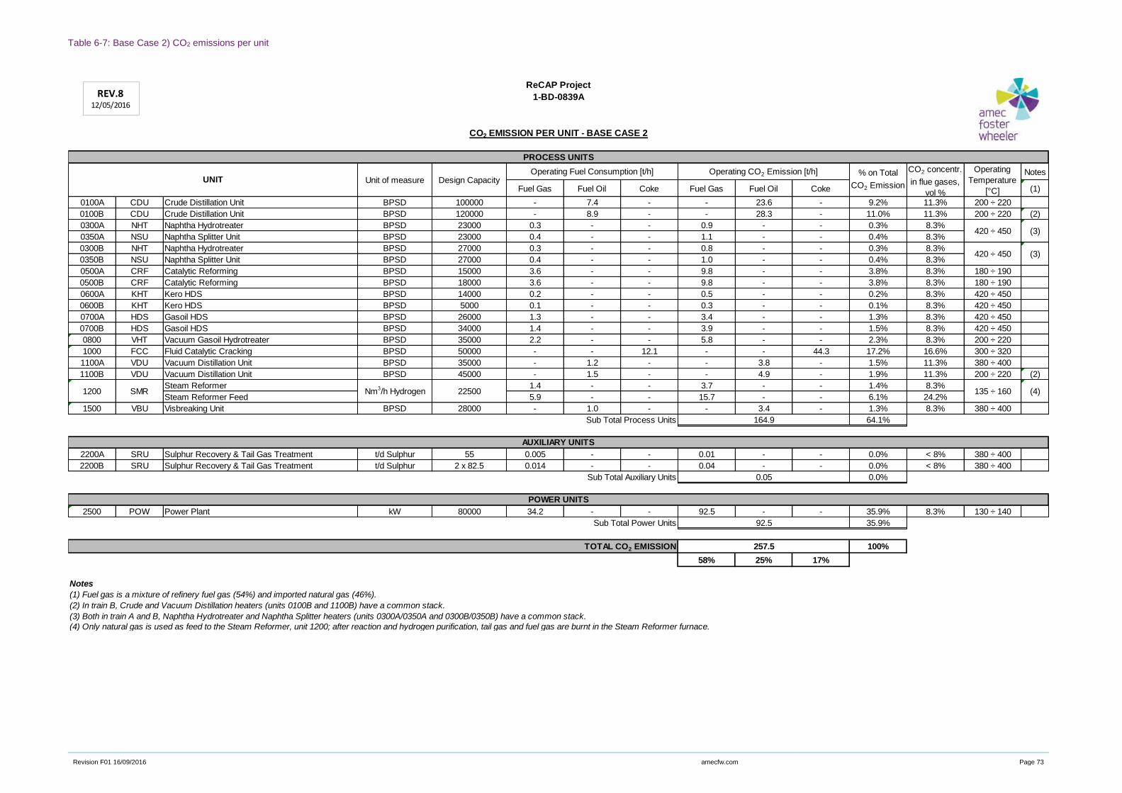
Revision F01 16/09/2016 amecfw.com Page 73
Table 6-7: Base Case 2) CO2 emissions per unit
Notes
Fuel Gas Fuel Oil Coke Fuel Gas Fuel Oil Coke (1)
0100A CDU Crude Distillation Unit BPSD 100000 - 7.4 - - 23.6 - 9.2% 11.3% 200 ÷ 220
0100B CDU Crude Distillation Unit BPSD 120000 - 8.9 - - 28.3 - 11.0% 11.3% 200 ÷ 220 (2)
0300A NHT Naphtha Hydrotreater BPSD 23000 0.3 - - 0.9 - - 0.3% 8.3%
0350A NSU Naphtha Splitter Unit BPSD 23000 0.4 - - 1.1 - - 0.4% 8.3%
0300B NHT Naphtha Hydrotreater BPSD 27000 0.3 - - 0.8 - - 0.3% 8.3%
0350B NSU Naphtha Splitter Unit BPSD 27000 0.4 - - 1.0 - - 0.4% 8.3%
0500A CRF Catalytic Reforming BPSD 15000 3.6 - - 9.8 - - 3.8% 8.3% 180 ÷ 190
0500B CRF Catalytic Reforming BPSD 18000 3.6 - - 9.8 - - 3.8% 8.3% 180 ÷ 190
0600A KHT Kero HDS BPSD 14000 0.2 - - 0.5 - - 0.2% 8.3% 420 ÷ 450
0600B KHT Kero HDS BPSD 5000 0.1 - - 0.3 - - 0.1% 8.3% 420 ÷ 450
0700A HDS Gasoil HDS BPSD 26000 1.3 - - 3.4 - - 1.3% 8.3% 420 ÷ 450
0700B HDS Gasoil HDS BPSD 34000 1.4 - - 3.9 - - 1.5% 8.3% 420 ÷ 450
0800 VHT Vacuum Gasoil Hydrotreater BPSD 35000 2.2 - - 5.8 - - 2.3% 8.3% 200 ÷ 220
1000 FCC Fluid Catalytic Cracking BPSD 50000 - - 12.1 - - 44.3 17.2% 16.6% 300 ÷ 320
1100A VDU Vacuum Distillation Unit BPSD 35000 - 1.2 - - 3.8 - 1.5% 11.3% 380 ÷ 400
1100B VDU Vacuum Distillation Unit BPSD 45000 - 1.5 - - 4.9 - 1.9% 11.3% 200 ÷ 220 (2)
Steam Reformer 1.4 - - 3.7 - - 1.4% 8.3%
Steam Reformer Feed 5.9 - - 15.7 - - 6.1% 24.2%
1500 VBU Visbreaking Unit BPSD 28000 - 1.0 - - 3.4 - 1.3% 8.3% 380 ÷ 400
Sub Total Process Units 64.1%
2200A SRU Sulphur Recovery & Tail Gas Treatment t/d Sulphur 55 0.005 - - 0.01 - - 0.0% < 8% 380 ÷ 400
2200B SRU Sulphur Recovery & Tail Gas Treatment t/d Sulphur 2 x 82.5 0.014 - - 0.04 - - 0.0% < 8% 380 ÷ 400
Sub Total Auxiliary Units 0.0%
2500 POW Power Plant kW 80000 34.2 - - 92.5 - - 35.9% 8.3% 130 ÷ 140
Sub Total Power Units 35.9%
100%
58% 25% 17%
Notes
(1) Fuel gas is a mixture of refinery fuel gas (54%) and imported natural gas (46%).
(2) In train B, Crude and Vacuum Distillation heaters (units 0100B and 1100B) have a common stack.
(3) Both in train A and B, Naphtha Hydrotreater and Naphtha Splitter heaters (units 0300A/0350A and 0300B/0350B) have a common stack.
(4) Only natural gas is used as feed to the Steam Reformer, unit 1200; after reaction and hydrogen purification, tail gas and fuel gas are burnt in the Steam Reformer furnace.
CO2 EMISSION PER UNIT - BASE CASE 2
Nm3/h Hydrogen 22500 135 ÷ 160 (4)
PROCESS UNITS
UNIT Unit of measure Design CapacityOperating Fuel Consumption [t/h] Operating CO2 Emission [t/h] % on Total
CO2 Emission
Operating
Temperature
[°C]
CO2 concentr.
in flue gases,
vol %
1-BD-0839A
ReCAP Project
92.5
TOTAL CO2 EMISSION 257.5
164.9
AUXILIARY UNITS
0.05
POWER UNITS
420 ÷ 450 (3)
420 ÷ 450 (3)
1200 SMR
REV.812/05/2016

Revision F01 16/09/2016 amecfw.com Page 74
Refinery Layout
The layout of the medium conversion refinery has been developed starting from the plot plan of Base Case
1, essentially by adding a second block of process units beside the original nucleus of the refinery.
As already mentioned, this approach reflects the assumption of a refinery expanded, over its life, both in
terms of capacity and complexity.
Also some auxiliary, utility and offsite systems, like for example the Waste Water Treatment (WWT) and the
Flare, have been duplicated in the final configuration of the site.
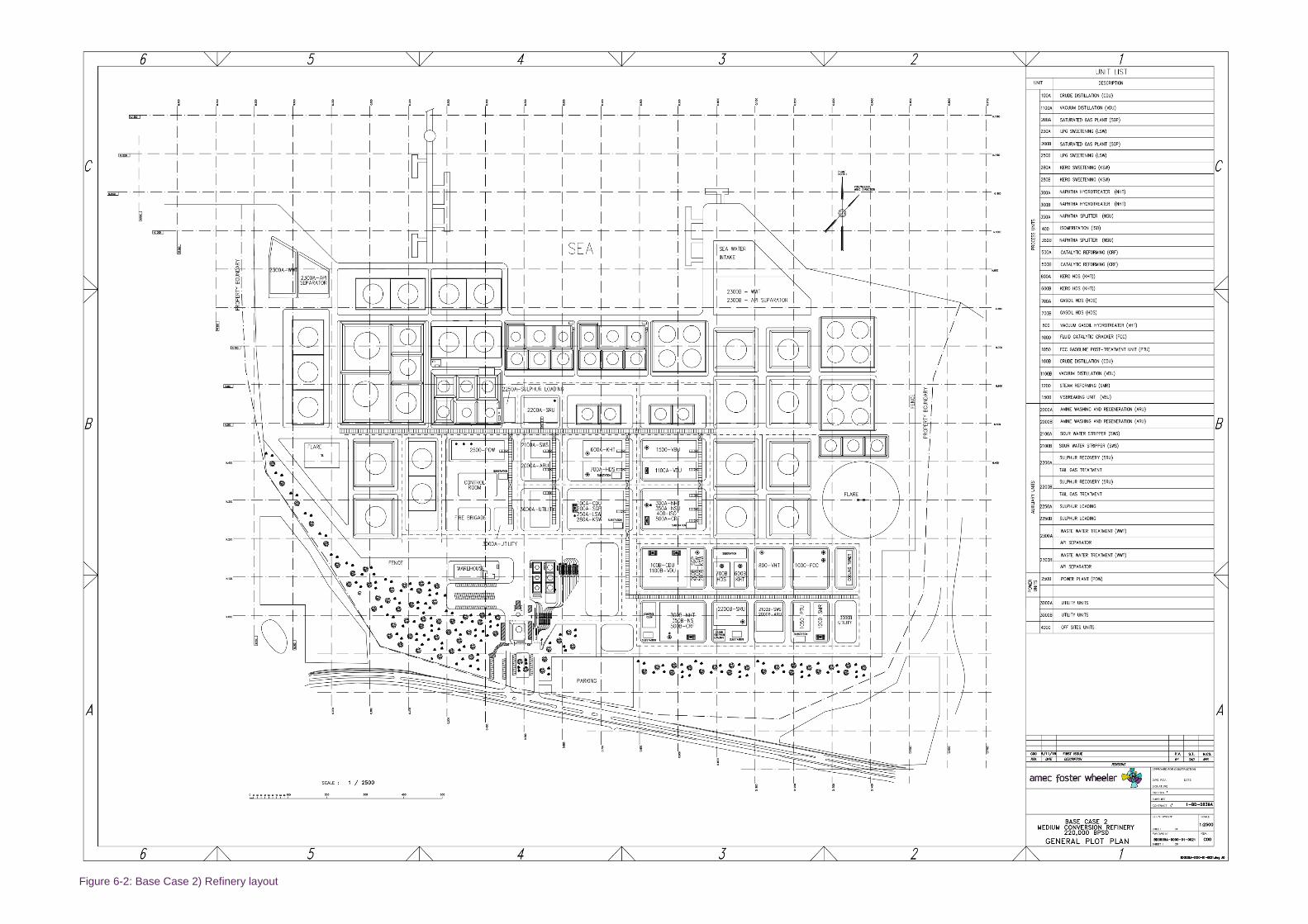
Figure 6-2: Base Case 2) Refinery layout

Revision F01 16/09/2016 amecfw.com Page 76
Main Utility Networks
The main utility balances have been reported on block flow diagrams, reflecting the planimetric arrangement
of the process units and utility blocks.
In particular, the following networks’ sketches have been developed:
► Figure 6-3: Base Case 2) Electricity network
► Figure 6-4: Base Case 2) Steam networks
► Figure 6-5: Base Case 2) Cooling water network
► Figure 6-6: Base Case 2) Fuel Gas/Offgas networks
► Figure 6-7: Base Case 2) Fuel oil network
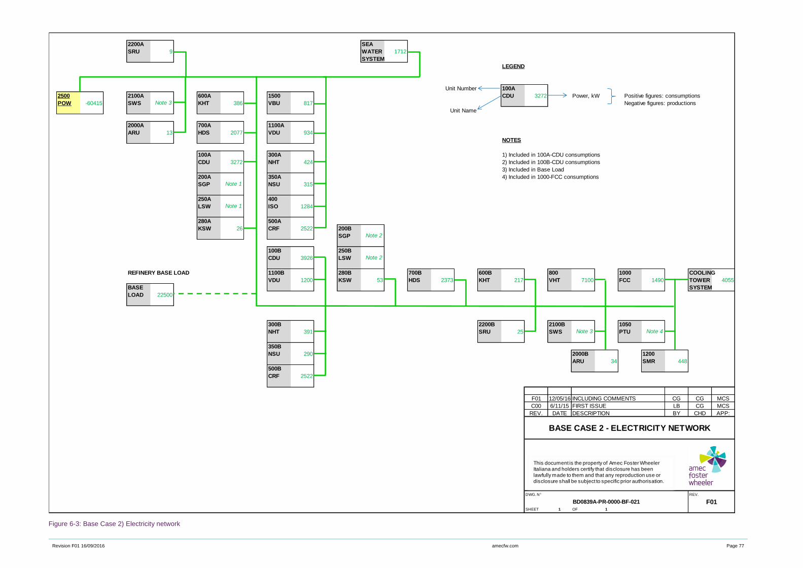
Revision F01 16/09/2016 amecfw.com Page 77
Figure 6-3: Base Case 2) Electricity network
2200A SEA
SRU 9 WATER 1712
SYSTEM
LEGEND
Unit Number 100A
2500 2100A 600A 1500 CDU 3272 Power, kW Positive figures: consumptions
POW -60415 SWS KHT 386 VBU 817 Negative figures: productions
Unit Name
2000A 700A 1100A
ARU 13 HDS 2077 VDU 934
NOTES
100A 300A 1) Included in 100A-CDU consumptions
CDU 3272 NHT 424 2) Included in 100B-CDU consumptions
3) Included in Base Load
200A 350A 4) Included in 1000-FCC consumptions
SGP NSU 315
250A 400
LSW ISO 1284
280A 500A
KSW 26 CRF 2522 200B
SGP
100B 250B
CDU 3926 LSW
REFINERY BASE LOAD 1100B 280B 700B 600B 800 1000 COOLING
VDU 1200 KSW 53 HDS 2373 KHT 217 VHT 7100 FCC 1490 TOWER 4055
BASE SYSTEM
LOAD 22500
300B 2200B 2100B 1050
NHT 391 SRU 25 SWS PTU
350B
NSU 290 2000B 1200
ARU 34 SMR 448
500B
CRF 2522
F01 12/05/16 INCLUDING COMMENTS CG CG MCS
C00 6/11/15 FIRST ISSUE LB CG MCS
REV. DATE DESCRIPTION BY CHD APP:
DWG. N° REV.
F01SHEET 1 OF 1
Note 4
BASE CASE 2 - ELECTRICITY NETWORK
BD0839A-PR-0000-BF-021
Note 3
Note 1
Note 1
Note 2
Note 2
Note 3
This document is the property of Amec Foster Wheeler Italiana and holders certify that disclosure has been lawfully made to them and that any reproduction use or disclosure shall be subject to specific prior authorisation.
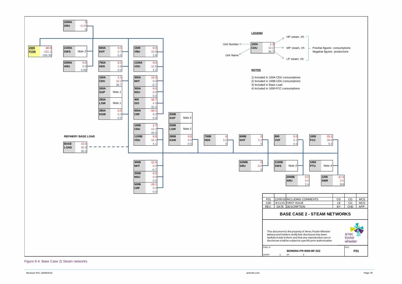
Revision F01 16/09/2016 amecfw.com Page 78
Figure 6-4: Base Case 2) Steam networks
2200A 0
SRU -0.24
0
LEGEND
HP steam, t/h
Unit Number 100A 2.3
2500 -48.8 2100A 600A 0.0 1500 0.0 CDU 10.2 MP steam, t/h Positive figures: consumptions
POW -151.1 SWS KHT 3.7 VBU 10.9 36.7 Negative figures: productions
-159.39 0.0 2.8 Unit Name
LP steam, t/h
2000A 0.0 700A 0.0 1100A 0.0
ARU 0.0 HDS 2.8 VDU 12.5
0.89 0.0 3.2 NOTES
100A 2.3 300A 13.0 1) Included in 100A-CDU consumptions
CDU 10.2 NHT 0.0 2) Included in 100B-CDU consumptions
36.7 -0.7 3) Included in Base Load
200A 350A 0.0 4) Included in 1000-FCC consumptions
SGP NSU 0.0
0.0
250A 400 16.7
LSW ISO 4.5
32.4
280A 0.0 500A -10.1
KSW 0.0 CRF 0.0 200B
0.0 0.0 SGP
100B 2.7 250B
CDU 12.2 LSW
44.0
REFINERY BASE LOAD 1100B 0.0 280B 0.0 700B 0 600B 0 800 0.0 1000 25.3
VDU 16.1 KSW 0.0 HDS 3.2 KHT 2.1 VHT 4.1 FCC 39.6
BASE 15.0 4.1 0.0 0 0 4.3 0.0
LOAD 30.0
30.0
300B 12.0 2200B 0 2100B 1050
NHT 0.0 SRU -0.6 SWS PTU
-0.7 0
350B 0.0
NSU 0.0 2000B 0.0 1200 -17.9
0.0 ARU 0.0 SMR 0.0
500B -10.1 2.4 0.0
CRF 0.0
0.0
F01 12/05/16 INCLUDING COMMENTS CG CG MCS
C00 6/11/15 FIRST ISSUE LB CG MCS
REV. DATE DESCRIPTION BY CHD APP:
DWG. N° REV.
F01SHEET 1 OF 1
Note 4
BASE CASE 2 - STEAM NETWORKS
BD0839A-PR-0000-BF-022
Note 3
Note 1
Note 1
Note 2
Note 2
Note 3
This document is the property of Amec Foster Wheeler Italiana and holders certify that disclosure has been lawfully made to them and that any reproduction use or disclosure shall be subject to specific prior authorisation.
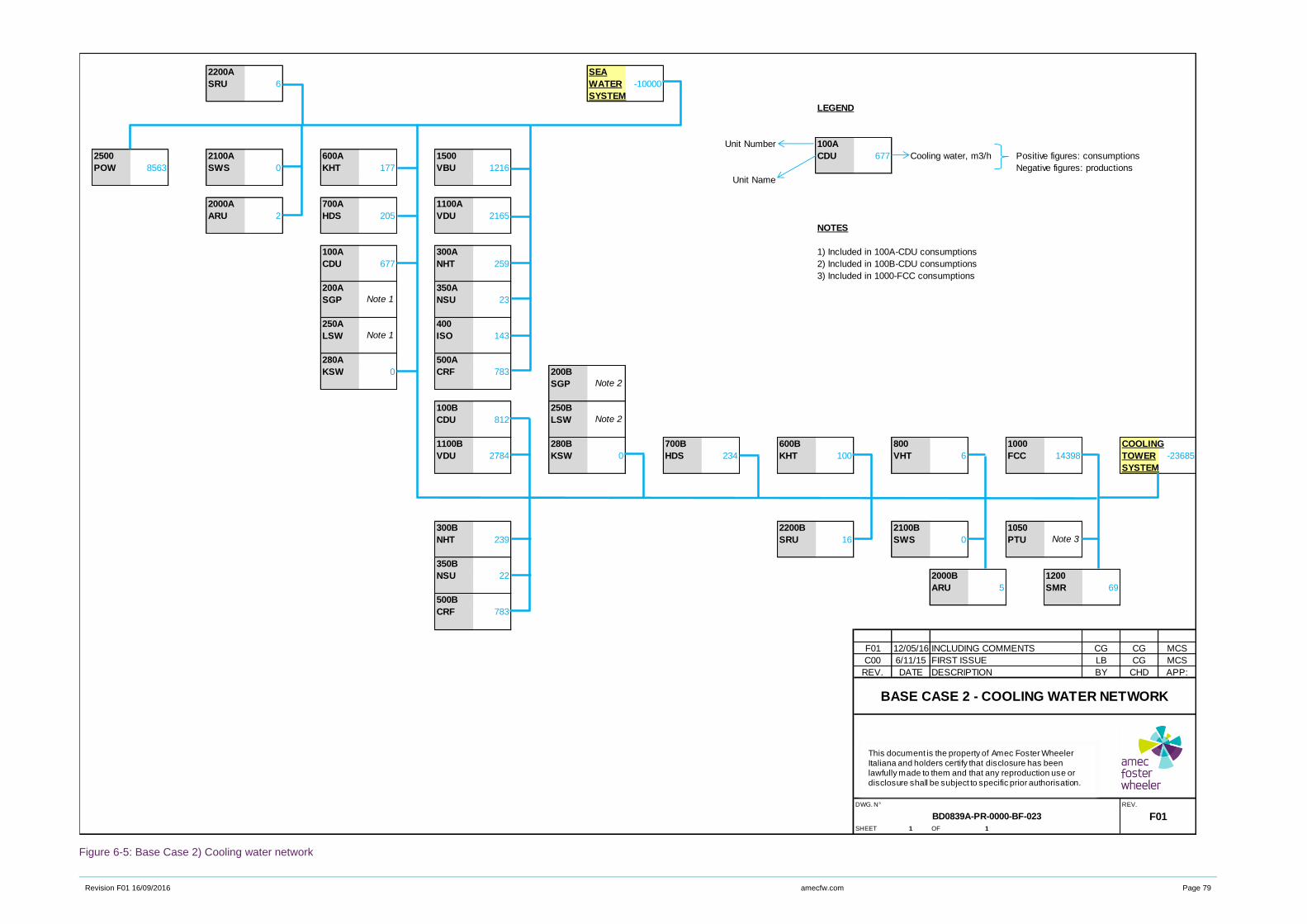
Revision F01 16/09/2016 amecfw.com Page 79
Figure 6-5: Base Case 2) Cooling water network
2200A SEA
SRU 6 WATER -10000
SYSTEM
LEGEND
Unit Number 100A
2500 2100A 600A 1500 CDU 677 Cooling water, m3/h Positive figures: consumptions
POW 8563 SWS 0 KHT 177 VBU 1216 Negative figures: productions
Unit Name
2000A 700A 1100A
ARU 2 HDS 205 VDU 2165
NOTES
100A 300A 1) Included in 100A-CDU consumptions
CDU 677 NHT 259 2) Included in 100B-CDU consumptions
3) Included in 1000-FCC consumptions
200A 350A
SGP NSU 23
250A 400
LSW ISO 143
280A 500A
KSW 0 CRF 783 200B
SGP
100B 250B
CDU 812 LSW
1100B 280B 700B 600B 800 1000 COOLING
VDU 2784 KSW 0 HDS 234 KHT 100 VHT 6 FCC 14398 TOWER -23685
SYSTEM
300B 2200B 2100B 1050
NHT 239 SRU 16 SWS 0 PTU
350B
NSU 22 2000B 1200
ARU 5 SMR 69
500B
CRF 783
F01 12/05/16 INCLUDING COMMENTS CG CG MCS
C00 6/11/15 FIRST ISSUE LB CG MCS
REV. DATE DESCRIPTION BY CHD APP:
DWG. N° REV.
F01SHEET 1 OF 1
BD0839A-PR-0000-BF-023
Note 1
Note 1
Note 2
Note 2
Note 3
BASE CASE 2 - COOLING WATER NETWORK
This document is the property of Amec Foster Wheeler Italiana and holders certify that disclosure has been lawfully made to them and that any reproduction use or disclosure shall be subject to specific prior authorisation.
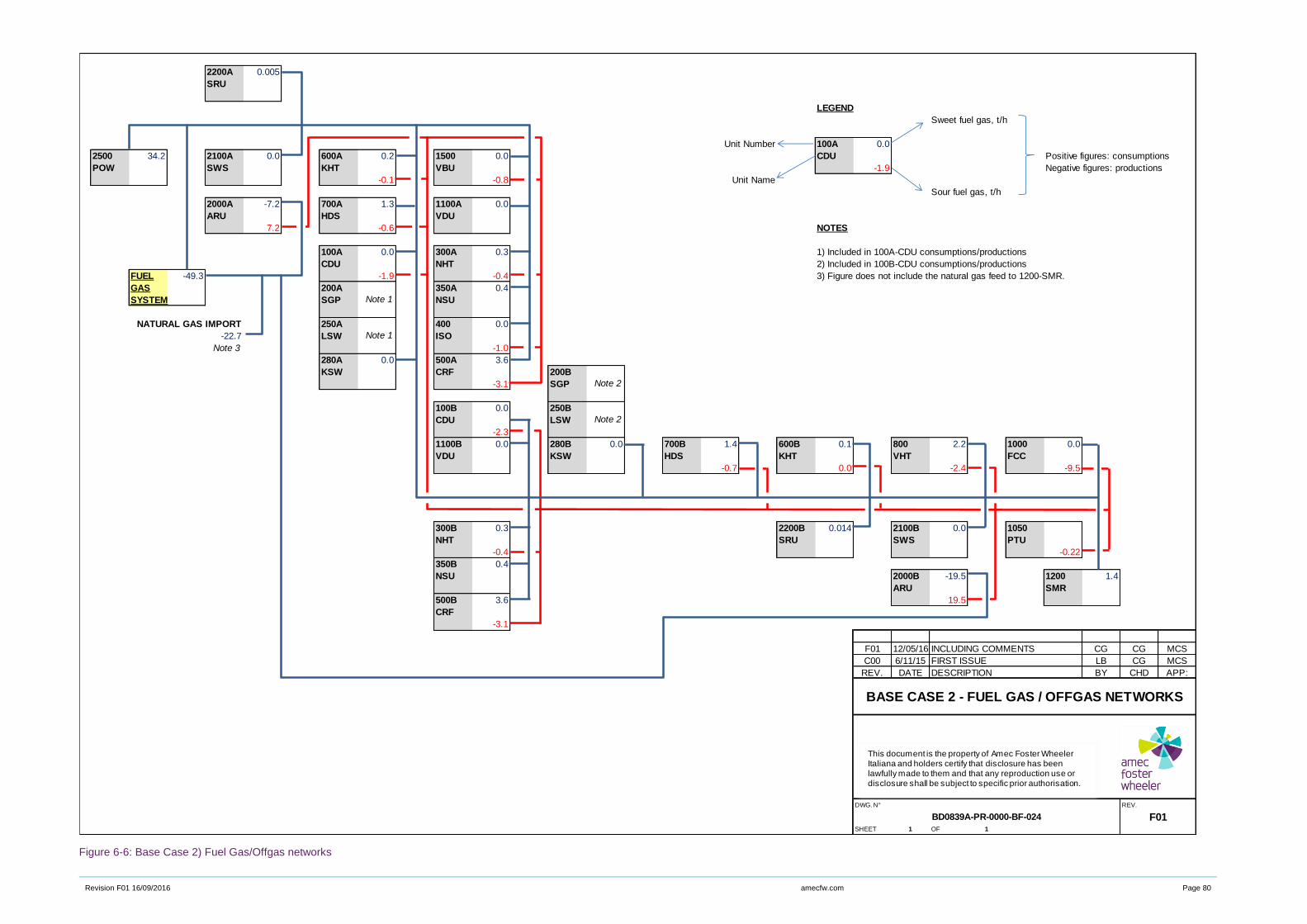
Revision F01 16/09/2016 amecfw.com Page 80
Figure 6-6: Base Case 2) Fuel Gas/Offgas networks
2200A 0.005
SRU
LEGEND
Sweet fuel gas, t/h
Unit Number 100A 0.0
2500 34.2 2100A 0.0 600A 0.2 1500 0.0 CDU Positive figures: consumptions
POW SWS KHT VBU -1.9 Negative figures: productions
-0.1 -0.8 Unit Name
Sour fuel gas, t/h
2000A -7.2 700A 1.3 1100A 0.0
ARU HDS VDU
7.2 -0.6 NOTES
100A 0.0 300A 0.3 1) Included in 100A-CDU consumptions/productions
CDU NHT 2) Included in 100B-CDU consumptions/productions
FUEL -49.3 -1.9 -0.4 3) Figure does not include the natural gas feed to 1200-SMR.
GAS 200A 350A 0.4
SYSTEM SGP NSU
NATURAL GAS IMPORT 250A 400 0.0
-22.7 LSW ISO
Note 3 -1.0
280A 0.0 500A 3.6
KSW CRF 200B
-3.1 SGP
100B 0.0 250B
CDU LSW
-2.3
1100B 0.0 280B 0.0 700B 1.4 600B 0.1 800 2.2 1000 0.0
VDU KSW HDS KHT VHT FCC
-0.7 0.0 -2.4 -9.5
300B 0.3 2200B 0.014 2100B 0.0 1050
NHT SRU SWS PTU
-0.4 -0.22
350B 0.4
NSU 2000B -19.5 1200 1.4
ARU SMR
500B 3.6 19.5
CRF
-3.1
F01 12/05/16 INCLUDING COMMENTS CG CG MCS
C00 6/11/15 FIRST ISSUE LB CG MCS
REV. DATE DESCRIPTION BY CHD APP:
DWG. N° REV.
F01SHEET 1 OF 1
BD0839A-PR-0000-BF-024
Note 1
Note 1
Note 2
Note 2
BASE CASE 2 - FUEL GAS / OFFGAS NETWORKS
This document is the property of Amec Foster Wheeler Italiana and holders certify that disclosure has been lawfully made to them and that any reproduction use or disclosure shall be subject to specific prior authorisation.
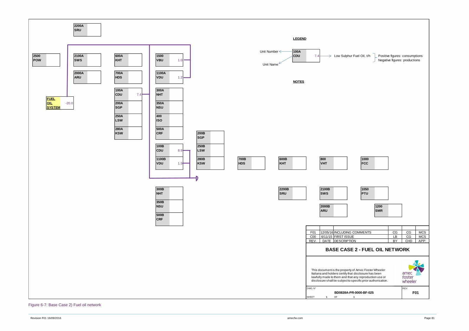
Revision F01 16/09/2016 amecfw.com Page 81
Figure 6-7: Base Case 2) Fuel oil network
2200A
SRU
LEGEND
Unit Number 100A
2500 2100A 600A 1500 CDU 7.4 Low Sulphur Fuel Oil, t/h Positive figures: consumptions
POW SWS KHT VBU 1.0 Negative figures: productions
Unit Name
2000A 700A 1100A
ARU HDS VDU 1.2
NOTES
100A 300A
CDU 7.4 NHT
FUEL
OIL -20.0 200A 350A
SYSTEM SGP NSU
250A 400
LSW ISO
280A 500A
KSW CRF 200B
SGP
100B 250B
CDU 8.9 LSW
1100B 280B 700B 600B 800 1000
VDU 1.5 KSW HDS KHT VHT FCC
300B 2200B 2100B 1050
NHT SRU SWS PTU
350B
NSU 2000B 1200
ARU SMR
500B
CRF
F01 12/05/16 INCLUDING COMMENTS CG CG MCS
C00 6/11/15 FIRST ISSUE LB CG MCS
REV. DATE DESCRIPTION BY CHD APP:
DWG. N° REV.
F01SHEET 1 OF 1
BASE CASE 2 - FUEL OIL NETWORK
BD0839A-PR-0000-BF-025
This document is the property of Amec Foster Wheeler Italiana and holders certify that disclosure has been lawfully made to them and that any reproduction use or disclosure shall be subject to specific prior authorisation.
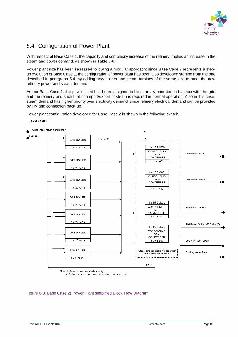
Revision F01 16/09/2016 amecfw.com Page 82
Configuration of Power Plant
With respect of Base Case 1, the capacity and complexity increase of the refinery implies an increase in the
steam and power demand, as shown in Table 6-6.
Power plant size has been increased following a modular approach: since Base Case 2 represents a step-
up evolution of Base Case 1, the configuration of power plant has been also developed starting from the one
described in paragraph 5.4, by adding new boilers and steam turbines of the same size to meet the new
refinery power and steam demand.
As per Base Case 1, the power plant has been designed to be normally operated in balance with the grid
and the refinery and such that no import/export of steam is required in normal operation. Also in this case,
steam demand has higher priority over electricity demand, since refinery electrical demand can be provided
by HV grid connection back-up.
Power plant configuration developed for Base Case 2 is shown in the following sketch.
Figure 6-8: Base Case 2) Power Plant simplified Block Flow Diagram
Revision F01 16/09/2016 amecfw.com Page 83
Base Case 2 power plant major equipment number and size are summarized hereinafter:
► 7 x 115 t/h Gas Boilers normally operated at 65% of their design load (corresponding to 74.7 t/h each)
► 4 x 20 MWe Condensing Steam Turbines normally operated at 79.6% of their design load
(corresponding to 15.9 MWe each)
Power plant configuration has been conceived to have such an installed spare capacity both for power and
steam generation to handle possible oscillations in power/steam from the users and to avoid refinery
shutdown in case of equipment (boiler or steam turbine) trip.
In case one steam turbine trips, 95% of the total power demand is guaranteed by the remaining three steam
turbines in operation: only a small import from the grid or load shedding is required in this scenario in order
not to compromise the refinery normal operation.
Total installed spare capacity is summarized hereinafter:
► Gas Boilers (Steam) +54%
► Steam Turbines (Electric Energy) +26%
Revision F01 16/09/2016 amecfw.com Page 84
7. Base Case 3
High Conversion Refinery - 220,000 BPSD Crude Capacity
The High Conversion Refinery, with respect of the Hydro-skimming Refinery described at paragraph 4.8,
includes additional process units for the conversion of the Vacuum Gasoil (VGO) and of the Vacuum Residue
into more valuable distillates (essentially gasoline and automotive diesel).
In Europe, the most wide-spread VGO conversion unit is the Fluid Catalytic Cracking (FCC) and so this unit
is included in Base Case 3 (as in Base Case 2).
Upstream of the FCC, a Vacuum Gasoil Hydrotreating (VHT) unit is present to decrease the sulphur content
of FCC feedstock, in order to respect SOx limits at FCC stack.
For Vacuum Residue conversion, a Coker Unit is considered. It is considered to sell the fuel grade coke
produced.
The FCC and Coker distillates are sent to finishing units to comply with the 10 ppm wt. sulphur specification
for the automotive fuels.
The hydrogen from the Heavy Naphtha Catalytic Reformer is not enough to cover the overall hydrogen
demand of the refinery. Therefore, a Steam Methane Reformer (SMR) is foreseen to close the hydrogen
balance.
The overall configuration of Base Case 3 is considered as a step-up evolution of Base Case 1, both in terms
of capacity and complexity increase. In other words, it is considered that, in a simple hydro-skimming refinery
(as the one depicted as Base Case 1), a second crude distillation train (Atmospheric and Vacuum Distillation
Units), FCC block (VHT+FCC+SMR) and DCU are built in a second phase. The consequent capacity
increase of the gasoline block and the hydrotreating units is considered achieved by adding a second train
in parallel to the original one.
The above assumption reflects the typical “life” of the European refineries, which have gradually expanded
starting from an original nucleus. This results in the following main effects:
► Several units of the same type are running in parallel, resulting in a relatively good flexibility of the
processing scheme (e.g. different feedstocks could be fed to each train) but also, on the other hand, in
some inefficiencies (e.g. higher maintenance costs, lower energy efficiencies, etc.).
► Also the Power Plant in Base Case 3 is considered as an expansion of the facilities foreseen in Base
Case 1, reflecting the “modular” expansion of the original refinery into a bigger, more complex and more
demanding site.
► The increased demand of cooling water –with respect of cooling water consumption in Base Case 1- is
considered to be satisfied by a closed loop circuit with cooling towers, working in parallel to the original
open circuit of sea cooling water. As a matter of fact, for the upgrading of the refinery, it is assumed that
more stringent environmental regulations have been met.
► Finally, also the layout of the Base Case 3 refinery reflects two main areas of units’ allocation: beside
the original nucleus of the older units (unit numbers identified with suffix –A), a second block of units is
present and clearly identifiable (unit numbers identified with suffix –B). The FCC block and DCU are
included in this newer portion of the refinery.
Revision F01 16/09/2016 amecfw.com Page 85
Refinery Balances
The balances developed for Base Case 3 are reported in the following tables and figures:
► Table 7-1: Base Case 3) Overall material balance
► Table 7-2: Base Case 3) Process units operating and design capacity
► Table 7-3: Base Case 3) Gasoline qualities
► Table 7-4: Base Case 3) Distillate qualities
► Table 7-5: Base Case 3) Fuel oil and bitumen qualities
► Table 7-6: Base Case 3) Main utility balance, fuel mix composition, CO2 emissions
► Figure 7-1: Base Case 3) Block flow diagrams with main material streams
► Table 7-7: Base Case 3) CO2 emissions per unit

Revision F01 16/09/2016 amecfw.com Page 86
Table 7-1: Base Case 3) Overall material balance
ReCAP Project
Preliminary Refinery Balances
BASE CASE 3
High Conversion Refinery, 220,000 BPSD
PRODUCTS
LPG
Propylene
Petrochemical Naphtha
Gasoline U95 Europe
Gasoline U92 USA Export
Jet fuel
Road Diesel
Marine Diesel
Heating Oil
Low Sulphur Fuel Oil
Medium Sulphur Fuel Oil
High Sulphur Fuel Oil
Bitumen
Coke Fuel Grade
Sulphur
Subtotal
RAW MATERIALS
Ekofisk
Bonny Light
Arabian Light
Urals Medium
Arabian Heavy
Maya Blend (1)
Imported Vacuum Gasoil
MTBE
Natural Gas
Biodiesel
Ethanol
Subtotal
Fuels and Losses
Notes
1) Maya Blend consists of 50% wt. Maya crude oil + 50% wt. Arabian Light Crude Oil
96.1
11195.1
kt/y
814.4
406.0
206.7
0.0
176.1
221.4
1648.8
2350.0
1015.0
4060.0
1015.0
522.6
89.3
10380.7
Consumptions, kt/y
708.6
209.8
0.0
0.0
150.0
1824.8
782.1
1000.0
3542.8
472.4
OVERALL MATERIAL BALANCE
Annual Production, kt/y
680.6
197.1
200.6
REV.712/05/2016

Revision F01 16/09/2016 amecfw.com Page 87
Table 7-2: Base Case 3) Process units operating and design capacity
ReCAP Project
Preliminary Refinery Balances
BASE CASE 3
High Conversion Refinery, 220,000 BPSD
UNIT Unit of measureDesign
Capacity
Operating
Capacity
Average
Utilization
Crude Distillation Unit BPSD 220000 (1) 220000 (1) 100%
Vacuum Distillation Unit BPSD 86000 (1) 78604 (1) 91%
Naphtha Hydrotreater BPSD 50000 (1) 48797 98%
Light Naphtha Isomerization BPSD 15000 13774 92%
Heavy Naphtha Catalytic Reforming BPSD 33000 (1) 31589 96%
Kero Sweetening BPSD 15000 (1) 15000 100%
Kerosene Hydrotreater BPSD 26000 (1) 24673 95%
Diesel Hydrotreater BPSD 65000 (1) 65000 100%
Heavy Gasoil Hydrotreater BPSD 50000 45154 90%
Fluid Catalytic Cracking BPSD 60000 60000 100%
FCC Gasoline Hydrotreater BPSD 24000 23128 96%
Delayed Coker BPSD 35000 33807 97%
Sulphur Recovery Unit t/d Sulphur 450 (1) 255 57%
Steam Reformer Nm3/h Hydrogen 35000 31922 91%
Notes
1) Multiple units in parallel to be considered.
PROCESS UNITS OPERATING AND DESIGN CAPACITY
REV.712/05/2016
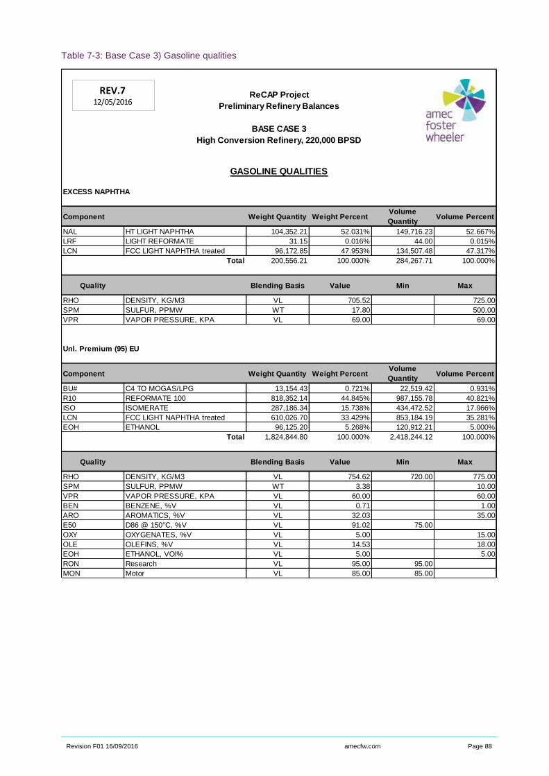
Revision F01 16/09/2016 amecfw.com Page 88
Table 7-3: Base Case 3) Gasoline qualities
ReCAP Project
Preliminary Refinery Balances
BASE CASE 3
High Conversion Refinery, 220,000 BPSD
GASOLINE QUALITIES
EXCESS NAPHTHA
Component Weight Quantity Weight PercentVolume
QuantityVolume Percent
NAL HT LIGHT NAPHTHA 104,352.21 52.031% 149,716.23 52.667%
LRF LIGHT REFORMATE 31.15 0.016% 44.00 0.015%
LCN FCC LIGHT NAPHTHA treated 96,172.85 47.953% 134,507.48 47.317%
Total 200,556.21 100.000% 284,267.71 100.000%
Quality Blending Basis Value Min Max
RHO DENSITY, KG/M3 VL 705.52 725.00
SPM SULFUR, PPMW WT 17.80 500.00
VPR VAPOR PRESSURE, KPA VL 69.00 69.00
Unl. Premium (95) EU
Component Weight Quantity Weight PercentVolume
QuantityVolume Percent
BU# C4 TO MOGAS/LPG 13,154.43 0.721% 22,519.42 0.931%
R10 REFORMATE 100 818,352.14 44.845% 987,155.78 40.821%
ISO ISOMERATE 287,186.34 15.738% 434,472.52 17.966%
LCN FCC LIGHT NAPHTHA treated 610,026.70 33.429% 853,184.19 35.281%
EOH ETHANOL 96,125.20 5.268% 120,912.21 5.000%
Total 1,824,844.80 100.000% 2,418,244.12 100.000%
Quality Blending Basis Value Min Max
RHO DENSITY, KG/M3 VL 754.62 720.00 775.00
SPM SULFUR, PPMW WT 3.38 10.00
VPR VAPOR PRESSURE, KPA VL 60.00 60.00
BEN BENZENE, %V VL 0.71 1.00
ARO AROMATICS, %V VL 32.03 35.00
E50 D86 @ 150°C, %V VL 91.02 75.00
OXY OXYGENATES, %V VL 5.00 15.00
OLE OLEFINS, %V VL 14.53 18.00
EOH ETHANOL, VOl% VL 5.00 5.00
RON Research VL 95.00 95.00
MON Motor VL 85.00 85.00
REV.712/05/2016
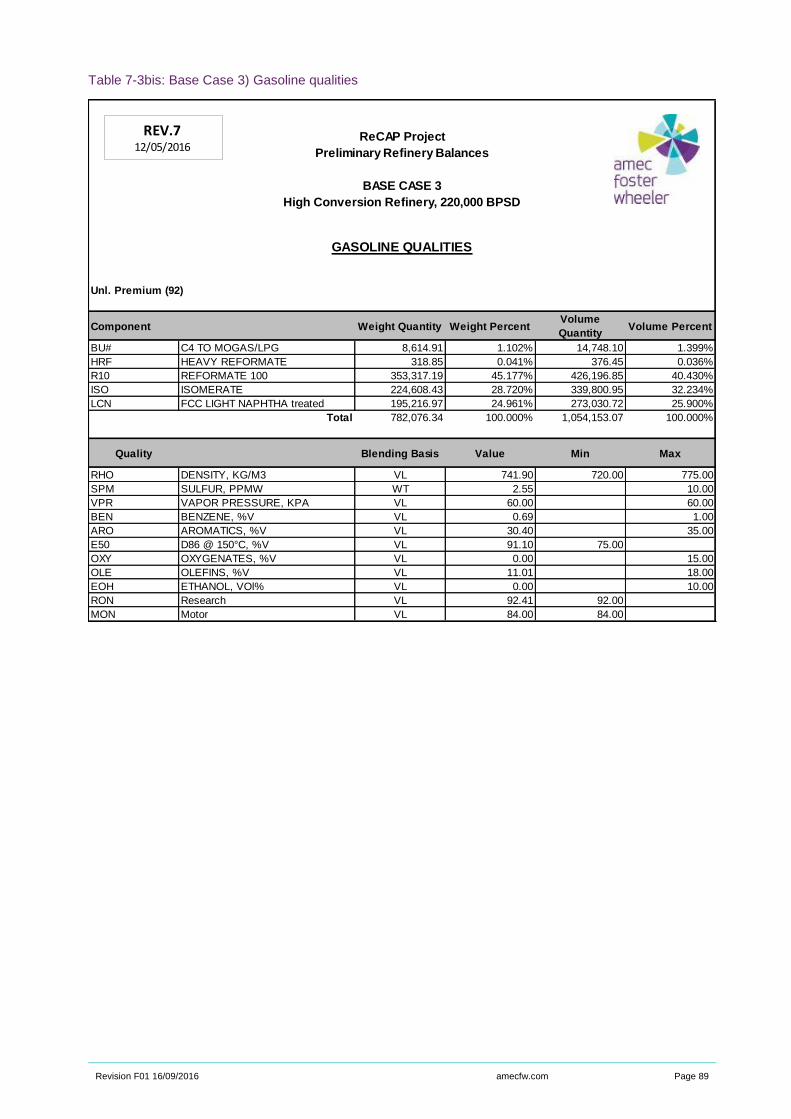
Revision F01 16/09/2016 amecfw.com Page 89
Table 7-3bis: Base Case 3) Gasoline qualities
ReCAP Project
Preliminary Refinery Balances
BASE CASE 3
High Conversion Refinery, 220,000 BPSD
GASOLINE QUALITIES
Unl. Premium (92)
Component Weight Quantity Weight PercentVolume
QuantityVolume Percent
BU# C4 TO MOGAS/LPG 8,614.91 1.102% 14,748.10 1.399%
HRF HEAVY REFORMATE 318.85 0.041% 376.45 0.036%
R10 REFORMATE 100 353,317.19 45.177% 426,196.85 40.430%
ISO ISOMERATE 224,608.43 28.720% 339,800.95 32.234%
LCN FCC LIGHT NAPHTHA treated 195,216.97 24.961% 273,030.72 25.900%
Total 782,076.34 100.000% 1,054,153.07 100.000%
Quality Blending Basis Value Min Max
RHO DENSITY, KG/M3 VL 741.90 720.00 775.00
SPM SULFUR, PPMW WT 2.55 10.00
VPR VAPOR PRESSURE, KPA VL 60.00 60.00
BEN BENZENE, %V VL 0.69 1.00
ARO AROMATICS, %V VL 30.40 35.00
E50 D86 @ 150°C, %V VL 91.10 75.00
OXY OXYGENATES, %V VL 0.00 15.00
OLE OLEFINS, %V VL 11.01 18.00
EOH ETHANOL, VOl% VL 0.00 10.00
RON Research VL 92.41 92.00
MON Motor VL 84.00 84.00
REV.712/05/2016
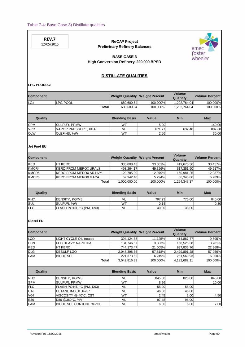
Revision F01 16/09/2016 amecfw.com Page 90
Table 7-4: Base Case 3) Distillate qualities
ReCAP Project
Preliminary Refinery Balances
BASE CASE 3
High Conversion Refinery, 220,000 BPSD
DISTILLATE QUALITIES
LPG PRODUCT
Component Weight Quantity Weight PercentVolume
QuantityVolume Percent
LG# LPG POOL 680,600.64 100.000% 1,202,764.04 100.000%
Total 680,600.64 100.000% 1,202,764.04 100.000%
Quality Blending Basis Value Min Max
SPM SULFUR, PPMW WT 5.00 140.00
VPR VAPOR PRESSURE, KPA VL 671.77 632.40 887.60
OLW OLEFINS, %W WT 2.56 30.00
Jet Fuel EU
Component Weight Quantity Weight PercentVolume
QuantityVolume Percent
KED HT KERO 333,008.43 33.301% 419,670.36 33.457%
KMCR4 KERO FROM MEROX URALS 493,264.17 49.326% 617,351.90 49.217%
KMCR5 KERO FROM MEROX AR.HVY 120,785.00 12.079% 150,981.25 12.037%
KMCR6 KERO FROM MEROX MAYA 52,942.40 5.294% 66,343.86 5.289%
Total 1,000,000.00 100.000% 1,254,347.37 100.000%
Quality Blending Basis Value Min Max
RHO DENSITY, KG/M3 VL 797.23 775.00 840.00
SUL SULFUR, %W WT 0.14 0.30
FLC FLASH POINT, °C (PM, D93) VL 40.00 38.00
Diesel EU
Component Weight Quantity Weight PercentVolume
QuantityVolume Percent
LCO LIGHT CYCLE OIL treated 394,124.38 11.125% 414,867.77 9.895%
HCN FCC HEAVY NAPHTHA 134,746.57 3.803% 158,525.38 3.781%
KED HT KERO 744,173.47 21.005% 937,836.76 22.368%
DLG DESULF LGO 2,048,398.35 57.818% 2,429,891.28 57.956%
FAM BIODIESEL 221,373.62 6.249% 251,560.93 6.000%
Total 3,542,816.39 100.000% 4,192,682.11 100.000%
Quality Blending Basis Value Min Max
RHO DENSITY, KG/M3 VL 845.00 820.00 845.00
SPM SULFUR, PPMW WT 8.96 10.00
FLC FLASH POINT, °C (PM, D93) VL 55.00 55.00
CIN CETANE INDEX D4737 VL 46.86 46.00
V04 VISCOSITY @ 40°C, CST WT 2.45 2.00 4.50
E36 D86 @360°C, %V VL 97.48 95.00
FAM BIODIESEL CONTENT, %VOL VL 6.00 6.00 7.00
REV.712/05/2016
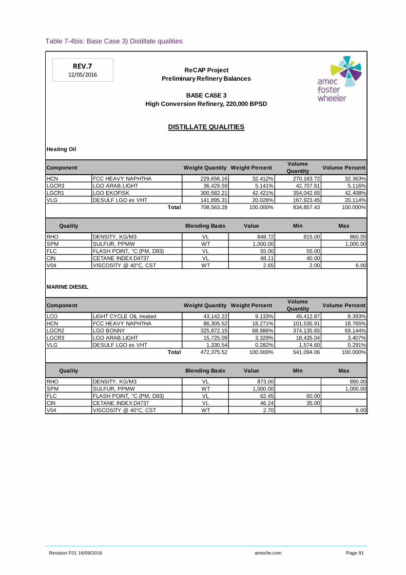
Revision F01 16/09/2016 amecfw.com Page 91
Table 7-4bis: Base Case 3) Distillate qualities
ReCAP Project
Preliminary Refinery Balances
BASE CASE 3
High Conversion Refinery, 220,000 BPSD
DISTILLATE QUALITIES
Heating Oil
Component Weight Quantity Weight PercentVolume
QuantityVolume Percent
HCN FCC HEAVY NAPHTHA 229,656.16 32.412% 270,183.72 32.363%
LGCR3 LGO ARAB.LIGHT 36,429.59 5.141% 42,707.61 5.116%
LGCR1 LGO EKOFISK 300,582.21 42.421% 354,042.65 42.408%
VLG DESULF LGO ex VHT 141,895.31 20.026% 167,923.45 20.114%
Total 708,563.28 100.000% 834,857.43 100.000%
Quality Blending Basis Value Min Max
RHO DENSITY, KG/M3 VL 848.72 815.00 860.00
SPM SULFUR, PPMW WT 1,000.00 1,000.00
FLC FLASH POINT, °C (PM, D93) VL 55.00 55.00
CIN CETANE INDEX D4737 VL 48.11 40.00
V04 VISCOSITY @ 40°C, CST WT 2.65 2.00 6.00
MARINE DIESEL
Component Weight Quantity Weight PercentVolume
QuantityVolume Percent
LCO LIGHT CYCLE OIL treated 43,142.22 9.133% 45,412.87 8.393%
HCN FCC HEAVY NAPHTHA 86,305.52 18.271% 101,535.91 18.765%
LGCR2 LGO BONNY 325,872.15 68.986% 374,135.65 69.144%
LGCR3 LGO ARAB.LIGHT 15,725.09 3.329% 18,435.04 3.407%
VLG DESULF LGO ex VHT 1,330.54 0.282% 1,574.60 0.291%
Total 472,375.52 100.000% 541,094.06 100.000%
Quality Blending Basis Value Min Max
RHO DENSITY, KG/M3 VL 873.00 890.00
SPM SULFUR, PPMW WT 1,000.00 1,000.00
FLC FLASH POINT, °C (PM, D93) VL 62.45 60.00
CIN CETANE INDEX D4737 VL 46.24 35.00
V04 VISCOSITY @ 40°C, CST WT 2.70 6.00
REV.712/05/2016

Revision F01 16/09/2016 amecfw.com Page 92
Table 7-5: Base Case 3) Fuel oil and bitumen qualities
ReCAP Project
Preliminary Refinery Balances
BASE CASE 3
High Conversion Refinery, 220,000 BPSD
FUEL OIL / BITUMEN QUALITIES
Low Sulphur Fuel
Component Weight Quantity Weight PercentVolume
QuantityVolume Percent
SLU FCC SLURRY OIL 231,363.57 62.137% 243,540.60 62.137%
lco LIGHT CYCLE OIL untreated 140,981.25 37.863% 148,401.31 37.863%
Total 372,344.82 100.000% 391,941.92 100.000%
Quality Blending Basis Value Min Max
RHO DENSITY, KG/M3 VL 950.00 991.00
SUL SULFUR, %W WT 0.36 0.50
FLC FLASH POINT, °C (PM, D93) VL 119.54 66.00
V05 VISCOSITY @ 50°C, CST WT 17.10 380.00
CCR CONRADSON CARBON RES, %W WT 0.00 15.00
BITUMEN
Component Weight Quantity Weight PercentVolume
QuantityVolume Percent
VDCR5 VDU RES MIX5 23,814.30 15.876% 23,462.36 16.112%
VDCR6 VDU RES MIX6 126,185.70 84.124% 122,154.60 83.888%
Total 150,000.00 100.000% 145,616.96 100.000%
REV.712/05/2016
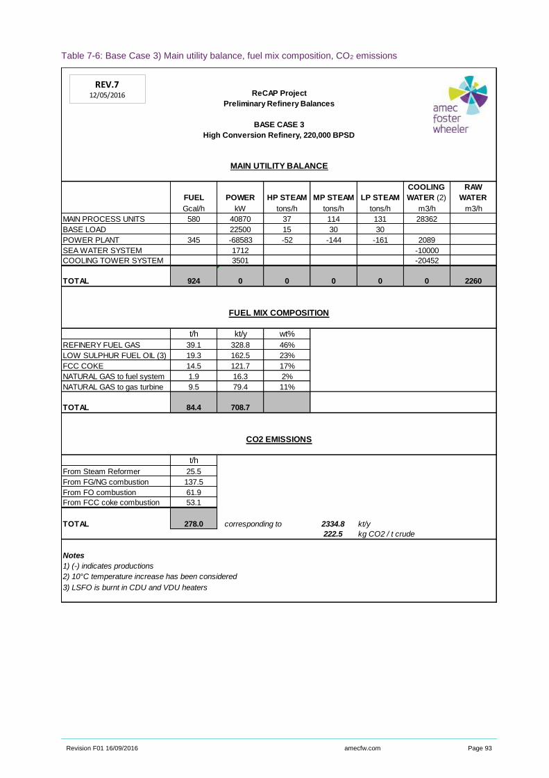
Revision F01 16/09/2016 amecfw.com Page 93
Table 7-6: Base Case 3) Main utility balance, fuel mix composition, CO2 emissions
ReCAP Project
Preliminary Refinery Balances
BASE CASE 3
High Conversion Refinery, 220,000 BPSD
FUEL POWER HP STEAM MP STEAM LP STEAM
COOLING
WATER (2)
RAW
WATER
Gcal/h kW tons/h tons/h tons/h m3/h m3/h
MAIN PROCESS UNITS 580 40870 37 114 131 28362
BASE LOAD 22500 15 30 30
POWER PLANT 345 -68583 -52 -144 -161 2089
SEA WATER SYSTEM 1712 -10000
COOLING TOWER SYSTEM 3501 -20452
TOTAL 924 0 0 0 0 0 2260
t/h kt/y wt%
REFINERY FUEL GAS 39.1 328.8 46%
LOW SULPHUR FUEL OIL (3) 19.3 162.5 23%
FCC COKE 14.5 121.7 17%
NATURAL GAS to fuel system 1.9 16.3 2%
NATURAL GAS to gas turbine 9.5 79.4 11%
TOTAL 84.4 708.7
t/h
From Steam Reformer 25.5
From FG/NG combustion 137.5
From FO combustion 61.9
From FCC coke combustion 53.1
TOTAL 278.0 corresponding to 2334.8 kt/y
222.5 kg CO2 / t crude
Notes
1) (-) indicates productions
2) 10°C temperature increase has been considered
3) LSFO is burnt in CDU and VDU heaters
MAIN UTILITY BALANCE
FUEL MIX COMPOSITION
CO2 EMISSIONS
REV.712/05/2016
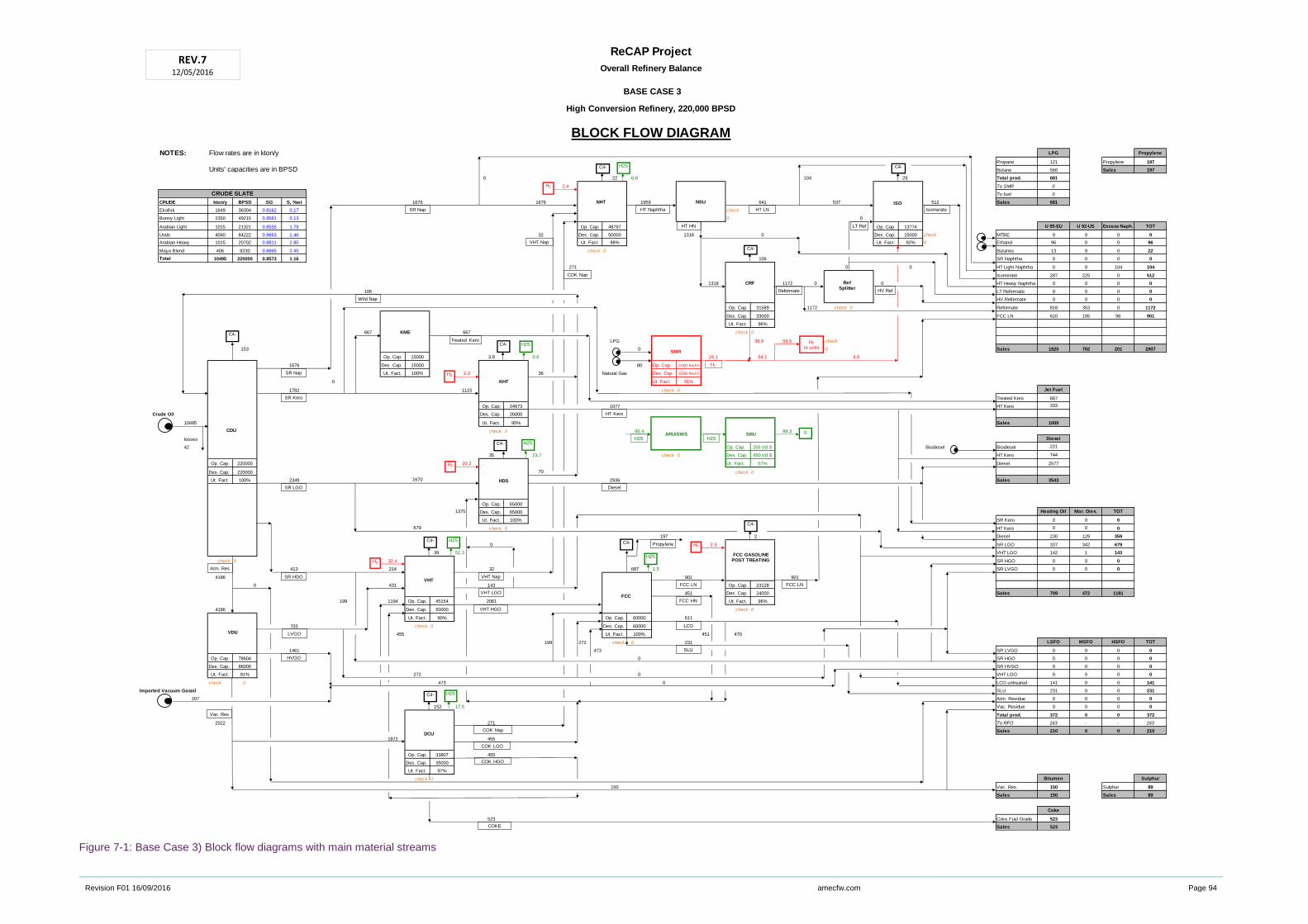
Revision F01 16/09/2016 amecfw.com Page 94
Figure 7-1: Base Case 3) Block flow diagrams with main material streams
ReCAP Project
Overall Refinery Balance
BASE CASE 3
High Conversion Refinery, 220,000 BPSD
BLOCK FLOW DIAGRAM
NOTES: Flow rates are in kton/y LPG Propylene
Propane 121 Propylene 197
Units' capacities are in BPSD Butane 560 Sales 197
0 22 0.8 104 29 Total prod. 681
2.4 To SMR 0
CRUDE SLATE To fuel 0
CRUDE kton/y BPSD SG S, %wt 1676 1676 1959 641 537 512 Sales 681
Ekofisk 1649 36304 0.8162 0.17 check
Bonny Light 2350 49215 0.8581 0.13 0 0
Arabian Light 1015 21321 0.8555 1.79 Op. Cap. 48797 Op. Cap. 13774 U 95-EU U 92-US Excess Naph. TOT
Urals 4060 84222 0.8663 1.46 32 Des. Cap. 50000 1318 0 Des. Cap. 15000 check MTBE 0 0 0 0
Arabian Heavy 1015 20702 0.8811 2.85 Ut. Fact. 98% Ut. Fact. 92% 0 Ethanol 96 0 0 96
Maya Blend 406 8230 0.8865 2.45 check 0 Butanes 13 9 0 22
Total 10495 220000 0.8573 1.16 106 SR Naphtha 0 0 0 0
271 0 0 HT Light Naphtha 0 0 104 104
Isomerate 287 225 0 512
1318 1172 0 0 HT Heavy Naphtha 0 0 0 0
106 LT Reformate 0 0 0 0
HV Reformate 0 0 0 0
Op. Cap. 31589 1172 check 0 Reformate 818 353 0 1172
Des. Cap. 33000 FCC LN 610 195 96 901
Ut. Fact. 96%
667 667 check 0
LPG 39.9 59.5 check
153 0 0 Sales 1825 782 201 2807
Op. Cap. 15000 3.8 0.6 24.1 64.1 4.6
1676 Des. Cap. 15000 80 Op. Cap. 31922 Nm3/h
Ut. Fact. 100% 2.2 36 Natural Gas Des. Cap. 35000 Nm3/h
0 Ut. Fact. 91%
1782 1115 check 0 Jet Fuel
Treated Kero 667
Op. Cap. 24673 1077 HT Kero 333
Crude Oil Des. Cap. 26000
10495 Ut. Fact. 95% Sales 1000
check 0 95.4 89.3
losses Diesel
42 Op. Cap. 255 t/d S Biodiesel Biodiesel 221
35 23.7 check 0 Des. Cap. 450 t/d S HT Kero 744
Op. Cap. 220000 20.2 Ut. Fact. 57% Diesel 2577
Des. Cap. 220000 70 check 0
Ut. Fact. 100% 2349 1670 2936 Sales 3543
Op. Cap. 65000
1375 Des. Cap. 65000 Heating Oil Mar. Dies. TOT
Ut. Fact. 100% SR Kero 0 0 0
679 check 0 HT Kero 0 0 0
197 2 Diesel 230 129 359
0 2.3 SR LGO 337 342 679
39 51.3 VHT LGO 142 1 143
check 0 32.4 SR HGO 0 0 0
413 214 32 687 1.5 SR LVGO 0 0 0
4186 901 901
0 431 143 Op. Cap. 23128
451 Des. Cap. 24000 Sales 709 472 1181
199 1194 Op. Cap. 45154 2061 Ut. Fact. 96%
4186 Des. Cap. 50000 check 0
Ut. Fact. 90% Op. Cap. 60000 611 #REF!
703 check 0 Des. Cap. 60000
455 Ut. Fact. 100% 451 470
199 272 check 0 231 LSFO MSFO HSFO TOT
1461 473 SR LVGO 0 0 0 0
Op. Cap. 78604 0 SR HGO 0 0 0 0
Des. Cap. 86000 SR HVGO 0 0 0 0
Ut. Fact. 91% 272 0 VHT LGO 0 0 0 0
check 0 473 0 LCO untreated 141 0 0 141
Imported Vacuum Gasoil SLU 231 0 0 231
207 Atm. Residue 0 0 0 0
152 17.5 Vac. Residue 0 0 0 0
Total prod. 372 0 0 372
2022 271 To RFO 163 - - 163
Sales 210 0 0 210
1872 455
Op. Cap. 33807 455
Des. Cap. 35000
Ut. Fact. 97%
check 0 Bitumen Sulphur
150 Vac. Res. 150 Sulphur 89
Sales 150 Sales 89
Coke
523 Coke Fuel Grade 523
Sales 523
CDU
Atm. Res
SR HGO
Wild Nap
SR LGO
SR Kero
HT Kero
SR Nap
NSU
HT Naphtha
LT Ref
KHT
ISO
HDS
H2
to units
H2
NHT
RefSplitter
Diesel
H2
CRF
H2
Vac. Res
VDU
VHT
VHT HGO
H2
VHT Nap
VHT LGO
HVGO
SMR
C4-
C4-
C4-
C4-
C4-
C4-
C4-
H2S
H2S
H2S
ARU/SWS SRU S
H2S H2S
FCC
SLU
LCO
FCC HN
FCC LN
VHT Nap
SR Nap
DCU
HT HN
HT LN
Reformate HV Ref
Isomerate
C4-
COK Nap
COK LGO
COK Nap
C4-
H2S
Propylene
FCC GASOLINEPOST TREATING
C4-
LVGO
H2
FCC LN
H2S
H2
KME
Treated Kero
REV.712/05/2016
H2S
COK HGO
COKE
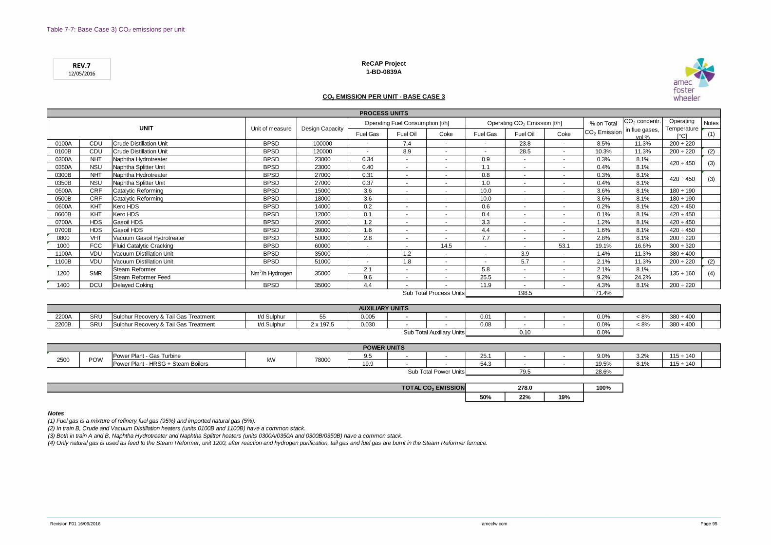
Revision F01 16/09/2016 amecfw.com Page 95
Table 7-7: Base Case 3) CO2 emissions per unit
Notes
Fuel Gas Fuel Oil Coke Fuel Gas Fuel Oil Coke (1)
0100A CDU Crude Distillation Unit BPSD 100000 - 7.4 - - 23.8 - 8.5% 11.3% 200 ÷ 220
0100B CDU Crude Distillation Unit BPSD 120000 - 8.9 - - 28.5 - 10.3% 11.3% 200 ÷ 220 (2)
0300A NHT Naphtha Hydrotreater BPSD 23000 0.34 - - 0.9 - - 0.3% 8.1%
0350A NSU Naphtha Splitter Unit BPSD 23000 0.40 - - 1.1 - - 0.4% 8.1%
0300B NHT Naphtha Hydrotreater BPSD 27000 0.31 - - 0.8 - - 0.3% 8.1%
0350B NSU Naphtha Splitter Unit BPSD 27000 0.37 - - 1.0 - - 0.4% 8.1%
0500A CRF Catalytic Reforming BPSD 15000 3.6 - - 10.0 - - 3.6% 8.1% 180 ÷ 190
0500B CRF Catalytic Reforming BPSD 18000 3.6 - - 10.0 - - 3.6% 8.1% 180 ÷ 190
0600A KHT Kero HDS BPSD 14000 0.2 - - 0.6 - - 0.2% 8.1% 420 ÷ 450
0600B KHT Kero HDS BPSD 12000 0.1 - - 0.4 - - 0.1% 8.1% 420 ÷ 450
0700A HDS Gasoil HDS BPSD 26000 1.2 - - 3.3 - - 1.2% 8.1% 420 ÷ 450
0700B HDS Gasoil HDS BPSD 39000 1.6 - - 4.4 - - 1.6% 8.1% 420 ÷ 450
0800 VHT Vacuum Gasoil Hydrotreater BPSD 50000 2.8 - - 7.7 - - 2.8% 8.1% 200 ÷ 220
1000 FCC Fluid Catalytic Cracking BPSD 60000 - - 14.5 - - 53.1 19.1% 16.6% 300 ÷ 320
1100A VDU Vacuum Distillation Unit BPSD 35000 - 1.2 - - 3.9 - 1.4% 11.3% 380 ÷ 400
1100B VDU Vacuum Distillation Unit BPSD 51000 - 1.8 - - 5.7 - 2.1% 11.3% 200 ÷ 220 (2)
Steam Reformer 2.1 - - 5.8 - - 2.1% 8.1%
Steam Reformer Feed 9.6 - - 25.5 - - 9.2% 24.2%
1400 DCU Delayed Coking BPSD 35000 4.4 - - 11.9 - - 4.3% 8.1% 200 ÷ 220
Sub Total Process Units 71.4%
2200A SRU Sulphur Recovery & Tail Gas Treatment t/d Sulphur 55 0.005 - - 0.01 - - 0.0% < 8% 380 ÷ 400
2200B SRU Sulphur Recovery & Tail Gas Treatment t/d Sulphur 2 x 197.5 0.030 - - 0.08 - - 0.0% < 8% 380 ÷ 400
Sub Total Auxiliary Units 0.0%
Power Plant - Gas Turbine 9.5 - - 25.1 - - 9.0% 3.2% 115 ÷ 140
Power Plant - HRSG + Steam Boilers 19.9 - - 54.3 - - 19.5% 8.1% 115 ÷ 140
Sub Total Power Units 28.6%
100%
50% 22% 19%
Notes
(1) Fuel gas is a mixture of refinery fuel gas (95%) and imported natural gas (5%).
(2) In train B, Crude and Vacuum Distillation heaters (units 0100B and 1100B) have a common stack.
(3) Both in train A and B, Naphtha Hydrotreater and Naphtha Splitter heaters (units 0300A/0350A and 0300B/0350B) have a common stack.
(4) Only natural gas is used as feed to the Steam Reformer, unit 1200; after reaction and hydrogen purification, tail gas and fuel gas are burnt in the Steam Reformer furnace.
(3)
CO2 concentr.
in flue gases,
vol %
1200
TOTAL CO2 EMISSION 278.0
420 ÷ 450
420 ÷ 450
79.5
2500 POW kW 78000
198.5
AUXILIARY UNITS
0.10
POWER UNITS
(3)
ReCAP Project
Nm3/h Hydrogen 35000 135 ÷ 160 (4)
PROCESS UNITS
UNIT Unit of measure Design CapacityOperating Fuel Consumption [t/h] Operating CO2 Emission [t/h] % on Total
CO2 Emission
1-BD-0839A
CO2 EMISSION PER UNIT - BASE CASE 3
SMR
Operating
Temperature
[°C]
REV.712/05/2016

Revision F01 16/09/2016 amecfw.com Page 96
Refinery Layout
The layout of the Base Case 3 refinery has been developed starting from the plot plan of Base Case 1,
essentially by adding a second block of process units beside the original nucleus of the refinery.
As already mentioned, this approach reflects the assumption of a refinery expanded, over its life, both in
terms of capacity and complexity.
Also some auxiliary, utility and offsite systems, like for example the Waste Water Treatment (WWT) and the
Flare, have been duplicated in the final configuration of the site.
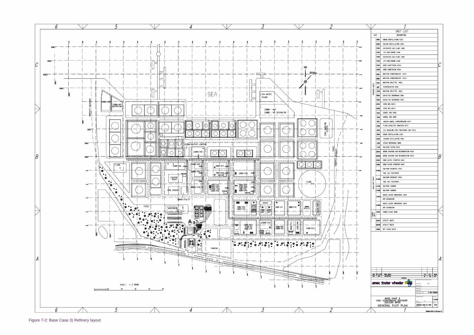
Figure 7-2: Base Case 3) Refinery layout

Revision F01 16/09/2016 amecfw.com Page 98
Main Utility Networks
The main utility balances have been reported on block flow diagrams, reflecting the planimetric arrangement
of the process units and utility blocks.
In particular, the following networks’ sketches have been developed:
► Figure 7-3: Base Case 3) Electricity network
► Figure 7-4: Base Case 3) Steam networks
► Figure 7-5: Base Case 3) Cooling water network
► Figure 7-6: Base Case 3) Fuel Gas/Offgas networks
► Figure 7-7: Base Case 3) Fuel oil network
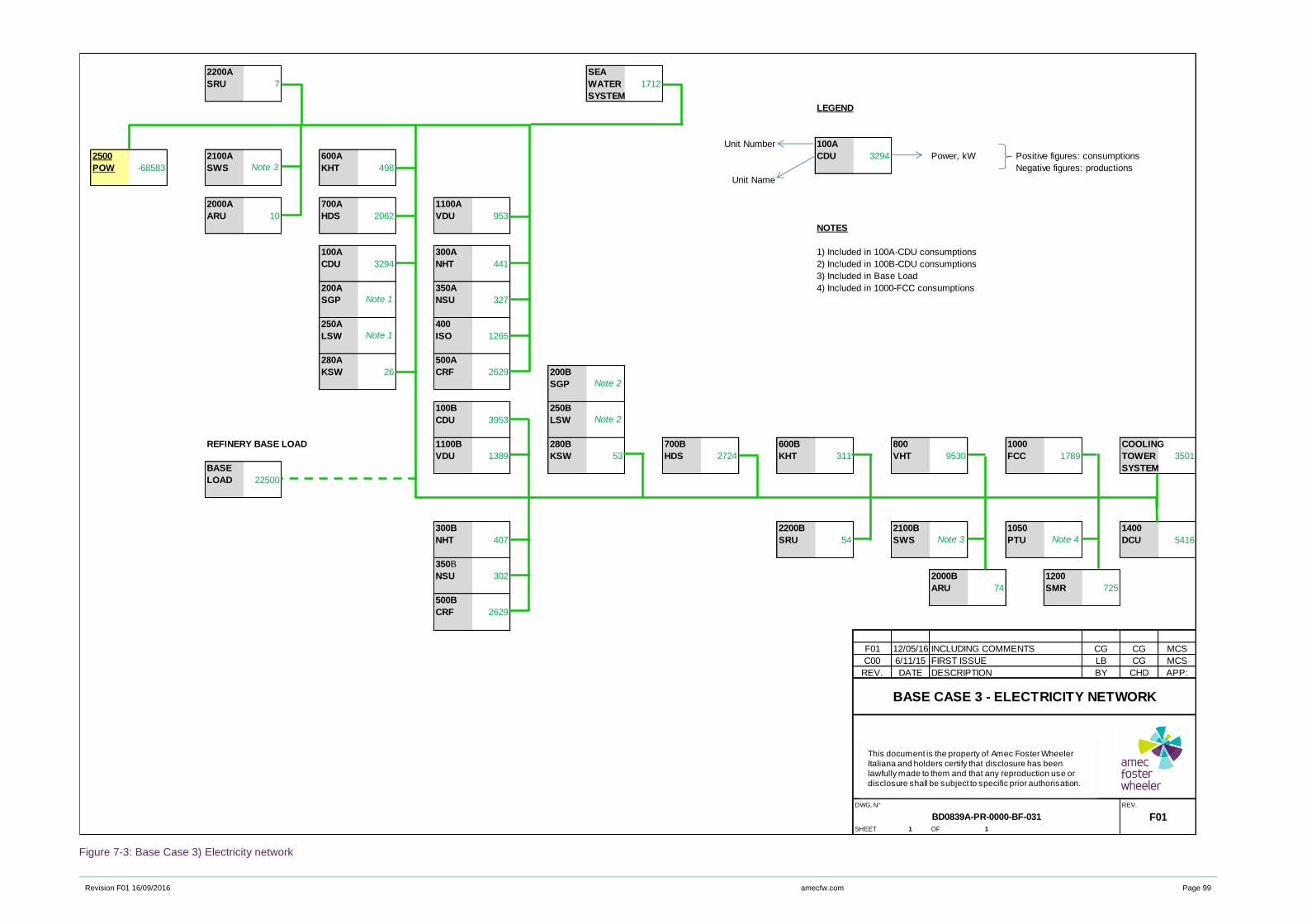
Revision F01 16/09/2016 amecfw.com Page 99
Figure 7-3: Base Case 3) Electricity network
2200A SEA
SRU 7 WATER 1712
SYSTEM
LEGEND
Unit Number 100A
2500 2100A 600A CDU 3294 Power, kW Positive figures: consumptions
POW -68583 SWS KHT 498 Negative figures: productions
Unit Name
2000A 700A 1100A
ARU 10 HDS 2062 VDU 953
NOTES
100A 300A 1) Included in 100A-CDU consumptions
CDU 3294 NHT 441 2) Included in 100B-CDU consumptions
3) Included in Base Load
200A 350A 4) Included in 1000-FCC consumptions
SGP NSU 327
250A 400
LSW ISO 1265
280A 500A
KSW 26 CRF 2629 200B
SGP
100B 250B
CDU 3953 LSW
REFINERY BASE LOAD 1100B 280B 700B 600B 800 1000 COOLING
VDU 1389 KSW 53 HDS 2724 KHT 311 VHT 9530 FCC 1789 TOWER 3501
BASE SYSTEM
LOAD 22500
300B 2200B 2100B 1050 1400
NHT 407 SRU 54 SWS PTU DCU 5416
350B
NSU 302 2000B 1200
ARU 74 SMR 725
500B
CRF 2629
F01 12/05/16 INCLUDING COMMENTS CG CG MCS
C00 6/11/15 FIRST ISSUE LB CG MCS
REV. DATE DESCRIPTION BY CHD APP:
DWG. N° REV.
F01SHEET 1 OF 1
Note 4
BASE CASE 3 - ELECTRICITY NETWORK
BD0839A-PR-0000-BF-031
Note 3
Note 1
Note 1
Note 2
Note 2
Note 3
This document is the property of Amec Foster Wheeler Italiana and holders certify that disclosure has been lawfully made to them and that any reproduction use or disclosure shall be subject to specific prior authorisation.

Revision F01 16/09/2016 amecfw.com Page 100
Figure 7-4: Base Case 3) Steam networks
2200A 0
SRU -0.19
0
LEGEND
HP steam, t/h
Unit Number 100A 2.3
2500 -51.6 2100A 600A 0.0 CDU 10.2 MP steam, t/h Positive figures: consumptions
POW -144.29 SWS KHT 4.8 36.9 Negative figures: productions
-161.48 0.0 Unit Name
LP steam, t/h
2000A 0.0 700A 0.0 1100A 0.0
ARU 0.0 HDS 2.8 VDU 12.8
0.74 0.0 3.2 NOTES
100A 2.3 300A 13.5 1) Included in 100A-CDU consumptions
CDU 10.2 NHT 0.0 2) Included in 100B-CDU consumptions
36.9 -0.7 3) Included in Base Load
200A 350A 0.0 4) Included in 1000-FCC consumptions
SGP NSU 0.0
0.0
250A 400 16.4
LSW ISO 4.4
31.9
280A 0.0 500A -10.5
KSW 0.0 CRF 0.0 200B
0.0 0.0 SGP
100B 2.7 250B
CDU 12.3 LSW
44.3
REFINERY BASE LOAD 1100B 0.0 280B 0.0 700B 0 600B 0 800 0.0 1000 30.4
VDU 18.6 KSW 0.0 HDS 3.7 KHT 3.0 VHT 5.5 FCC 47.6
BASE 15.0 4.7 0.0 0 0 5.7 0.0
LOAD 30.0
30.0
300B 12.4 2200B 0 2100B 1050 1400 8.9
NHT 0.0 SRU -1.4 SWS PTU DCU -9.8
-0.7 0 0.0
350B 0.0
NSU 0.0 2000B 0.0 1200 -29.0
0.0 ARU 0.0 SMR 0.0
500B -10.5 5.3 0.0
CRF 0.0
0.0
F01 12/05/16 INCLUDING COMMENTS CG CG MCS
C00 6/11/15 FIRST ISSUE LB CG MCS
REV. DATE DESCRIPTION BY CHD APP:
DWG. N° REV.
F01SHEET 1 OF 1
Note 4
BASE CASE 3 - STEAM NETWORKS
BD0839A-PR-0000-BF-032
Note 3
Note 1
Note 1
Note 2
Note 2
Note 3
This document is the property of Amec Foster Wheeler Italiana and holders certify that disclosure has been lawfully made to them and that any reproduction use or disclosure shall be subject to specific prior authorisation.

Revision F01 16/09/2016 amecfw.com Page 101
Figure 7-5: Base Case 3) Cooling water network
2200A SEA
SRU 5 WATER -10000
SYSTEM
LEGEND
Unit Number 100A
2500 2100A 600A CDU 681 Cooling water, m3/h Positive figures: consumptions
POW 2089 SWS 0 KHT 229 Negative figures: productions
Unit Name
2000A 700A 1100A
ARU 1 HDS 203 VDU 2211
NOTES
100A 300A 1) Included in 100A-CDU consumptions
CDU 681 NHT 270 2) Included in 100B-CDU consumptions
3) Included in 1000-FCC consumptions
200A 350A
SGP NSU 24
250A 400
LSW ISO 141
280A 500A
KSW 0 CRF 816 200B
SGP
100B 250B
CDU 818 LSW
1100B 280B 700B 600B 800 1000 COOLING
VDU 3221 KSW 0 HDS 268 KHT 143 VHT 8 FCC 17277 TOWER -20452
SYSTEM
300B 2200B 2100B 1050 1400
NHT 249 SRU 35 SWS 0 PTU DCU 802
350B
NSU 22 2000B 1200
ARU 11 SMR 111
500B
CRF 816
F01 12/05/16 INCLUDING COMMENTS CG CG MCS
C00 6/11/15 FIRST ISSUE LB CG MCS
REV. DATE DESCRIPTION BY CHD APP:
DWG. N° REV.
F01SHEET 1 OF 1
BD0839A-PR-0000-BF-033
Note 1
Note 1
Note 2
Note 2
Note 3
BASE CASE 3 - COOLING WATER NETWORK
This document is the property of Amec Foster Wheeler Italiana and holders certify that disclosure has been lawfully made to them and that any reproduction use or disclosure shall be subject to specific prior authorisation.
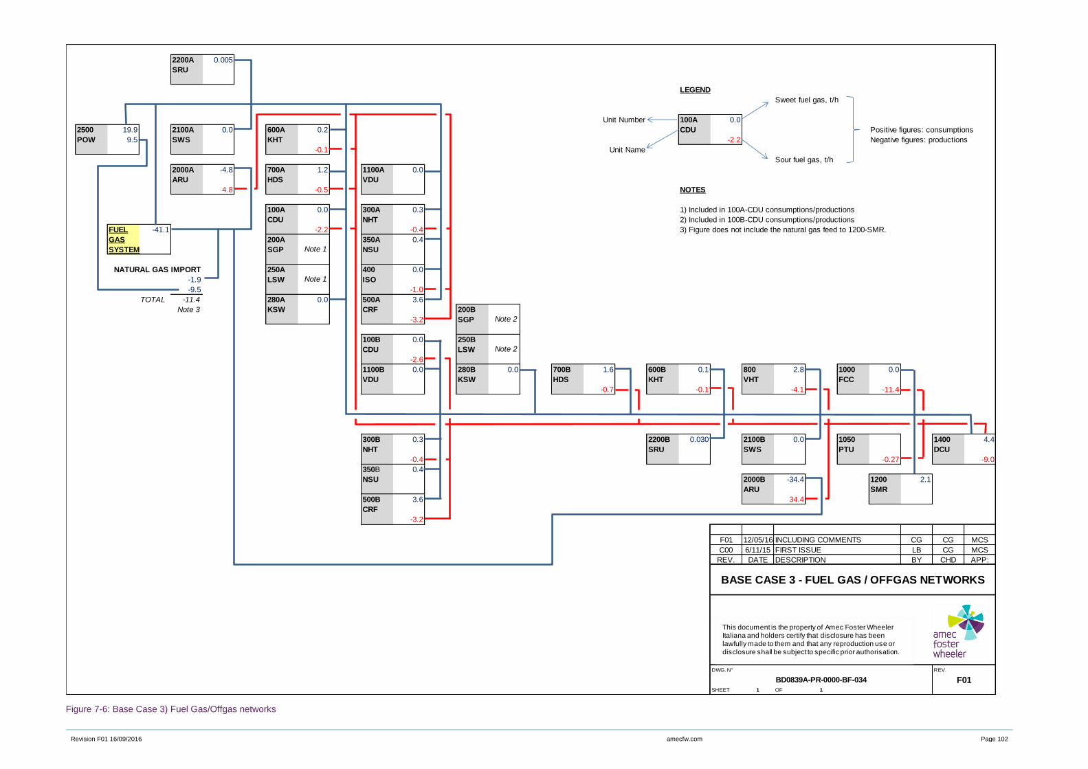
Revision F01 16/09/2016 amecfw.com Page 102
Figure 7-6: Base Case 3) Fuel Gas/Offgas networks
2200A 0.005
SRU
LEGEND
Sweet fuel gas, t/h
Unit Number 100A 0.0
2500 19.9 2100A 0.0 600A 0.2 CDU Positive figures: consumptions
POW 9.5 SWS KHT -2.2 Negative figures: productions
-0.1 Unit Name
Sour fuel gas, t/h
2000A -4.8 700A 1.2 1100A 0.0
ARU HDS VDU
4.8 -0.5 NOTES
100A 0.0 300A 0.3 1) Included in 100A-CDU consumptions/productions
CDU NHT 2) Included in 100B-CDU consumptions/productions
FUEL -41.1 -2.2 -0.4 3) Figure does not include the natural gas feed to 1200-SMR.
GAS 200A 350A 0.4
SYSTEM SGP NSU
NATURAL GAS IMPORT 250A 400 0.0
-1.9 LSW ISO
-9.5 -1.0
TOTAL -11.4 280A 0.0 500A 3.6
Note 3 KSW CRF 200B
-3.2 SGP
100B 0.0 250B
CDU LSW
-2.6
1100B 0.0 280B 0.0 700B 1.6 600B 0.1 800 2.8 1000 0.0
VDU KSW HDS KHT VHT FCC
-0.7 -0.1 -4.1 -11.4
300B 0.3 2200B 0.030 2100B 0.0 1050 1400 4.4
NHT SRU SWS PTU DCU
-0.4 -0.27 -9.0
350B 0.4
NSU 2000B -34.4 1200 2.1
ARU SMR
500B 3.6 34.4
CRF
-3.2
F01 12/05/16 INCLUDING COMMENTS CG CG MCS
C00 6/11/15 FIRST ISSUE LB CG MCS
REV. DATE DESCRIPTION BY CHD APP:
DWG. N° REV.
F01SHEET 1 OF 1
BD0839A-PR-0000-BF-034
Note 1
Note 1
Note 2
Note 2
BASE CASE 3 - FUEL GAS / OFFGAS NETWORKS
This document is the property of Amec Foster Wheeler Italiana and holders certify that disclosure has been lawfully made to them and that any reproduction use or disclosure shall be subject to specific prior authorisation.
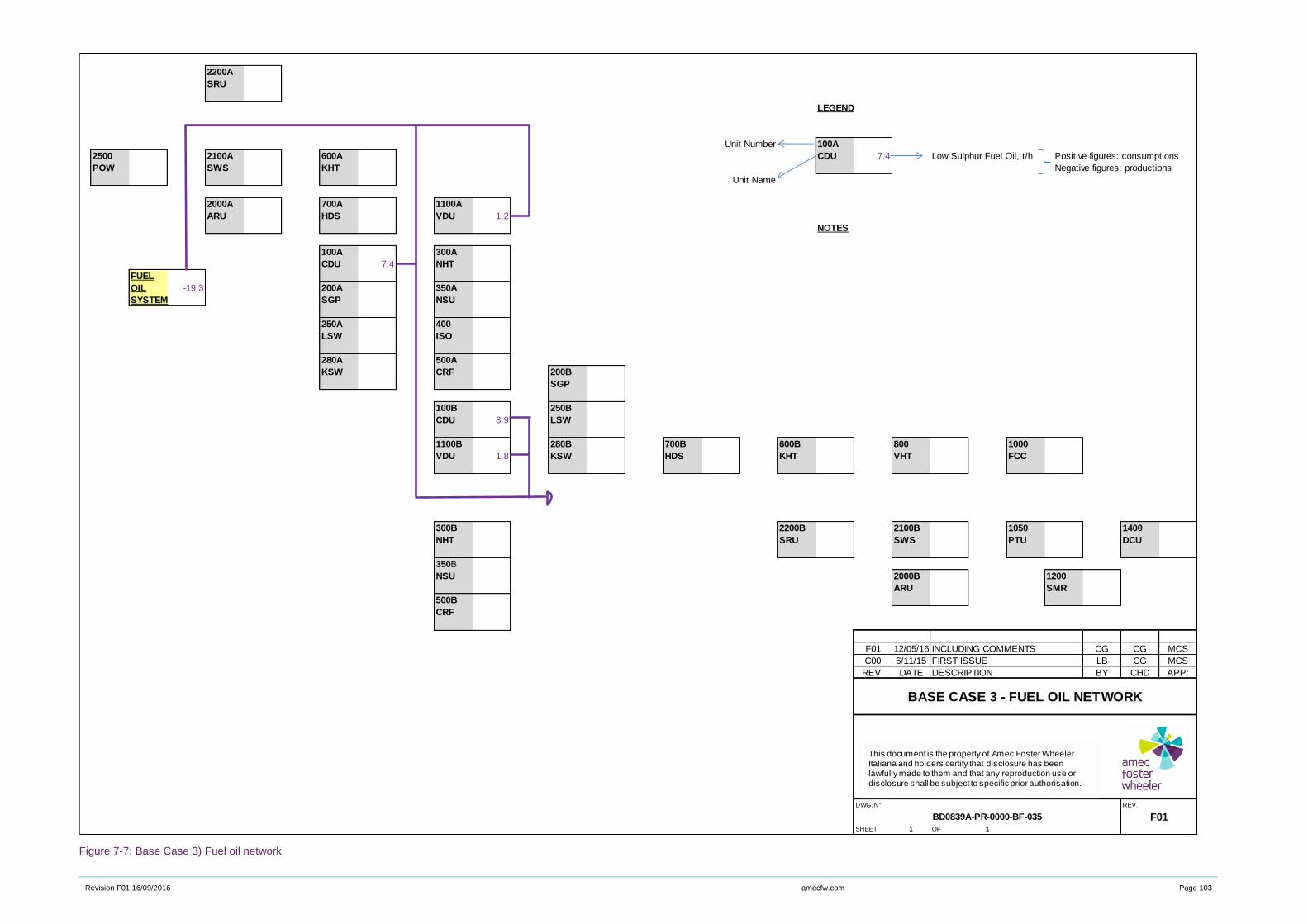
Revision F01 16/09/2016 amecfw.com Page 103
Figure 7-7: Base Case 3) Fuel oil network
2200A
SRU
LEGEND
Unit Number 100A
2500 2100A 600A CDU 7.4 Low Sulphur Fuel Oil, t/h Positive figures: consumptions
POW SWS KHT Negative figures: productions
Unit Name
2000A 700A 1100A
ARU HDS VDU 1.2
NOTES
100A 300A
CDU 7.4 NHT
FUEL
OIL -19.3 200A 350A
SYSTEM SGP NSU
250A 400
LSW ISO
280A 500A
KSW CRF 200B
SGP
100B 250B
CDU 8.9 LSW
1100B 280B 700B 600B 800 1000
VDU 1.8 KSW HDS KHT VHT FCC
300B 2200B 2100B 1050 1400
NHT SRU SWS PTU DCU
350B
NSU 2000B 1200
ARU SMR
500B
CRF
F01 12/05/16 INCLUDING COMMENTS CG CG MCS
C00 6/11/15 FIRST ISSUE LB CG MCS
REV. DATE DESCRIPTION BY CHD APP:
DWG. N° REV.
F01SHEET 1 OF 1
BASE CASE 3 - FUEL OIL NETWORK
BD0839A-PR-0000-BF-035
This document is the property of Amec Foster Wheeler Italiana and holders certify that disclosure has been lawfully made to them and that any reproduction use or disclosure shall be subject to specific prior authorisation.

Revision F01 16/09/2016 amecfw.com Page 104
Configuration of Power Plant
As already mentioned, Base Case 3 is considered a step-up evolution of Base Case 1: therefore, the power
plant configuration nucleus of Base Case 1 (3 x 115 t/h Gas Boiler and 2 x 20 MW Steam Turbines) is kept
also in Base Case 3.
In terms of power and steam demand, Base Case 3 differs from Base Case 2 only for the higher power
requirement while the steam demand is nearly the same.
For Base Case 3 design, steam and power requirements are summarized in Table 7-6.
In addition to the Base Case 1 configuration (3 boilers and 2 Steam Turbine) power plant configuration for
Base Case 3 is based on the addition of a Gas Turbine and an associated Heat Recovery Steam Generator
(HRSG), equipped with supplementary firing.
Part of the power is produced by the Gas Turbine 38.3 MW frame, whose exhaust pass through a heat
recovery steam generator generating superheated high pressure steam at the conditions required from the
refinery. Natural gas only is fed to the Gas Turbine, while refinery fuel gas is fed to HRSG.
The post firing installed in the HRSG is operated at the 84% of its nominal load in order to meet the total
steam requirement. In case of need, post firing load can be raised to 100% and the steam generation
increased accordingly. As a matter of fact, in order to meet the HP/MP/LP steam and power requirements,
it is necessary to produce an additional amount of steam with respect to what generated in the gas boilers,
kept in operation as per Base Case 1.
Therefore, the HP steam generated from the HRSG is mixed with steam generated by boilers and then
partially routed to the refinery users and partially sent to the Steam Turbines for power and MP/LP Steam
generation. MP and LP Steam are produced through two different extraction stages at the pressure required
by the users. Desuperheaters are installed both on MP and LP steam lines to bring the steam temperatures
down to the values required by the refinery at power plant battery limits. Steam turbines are condensing
type: exhaust steam from the steam turbines is condensed in a cooling water condenser, which operates
under vacuum, and pumped, together with a demi water make up, to deaerators for BFW generation.
Also in Base Case 3 the power plant has been designed to be normally operated in balance with the grid
and the refinery and such that no import/export of steam is required in normal operation. Also in this case,
steam demand has higher priority over electricity demand, since refinery electrical demand can be provided
by HV grid connection back-up.
A simplified scheme of power plant configuration in Base Case 3 is shown in Figure 7-8.
Base Case 3 power plant major equipment number and sizes are summarized hereinafter:
► 1 x 38.3 MWe Gas Turbine normally operating at 100% of the design load and 84% post fired plus 1 x
HRSG producing 148.3 t/h HP Steam;
► 3 x 115 t/h normally operating at 66% of their design load (corresponding to 75.3 t/h HP Steam)
► 2 x 20 MWe Condensing Steam Turbines normally operating at 85% of their design load (corresponding
to 17 MWe each)
Either in case a steam turbine or the gas turbine trips, it is necessary to import electrical power from the
national grid or, as an alternative, to put in place a load shedding plan.
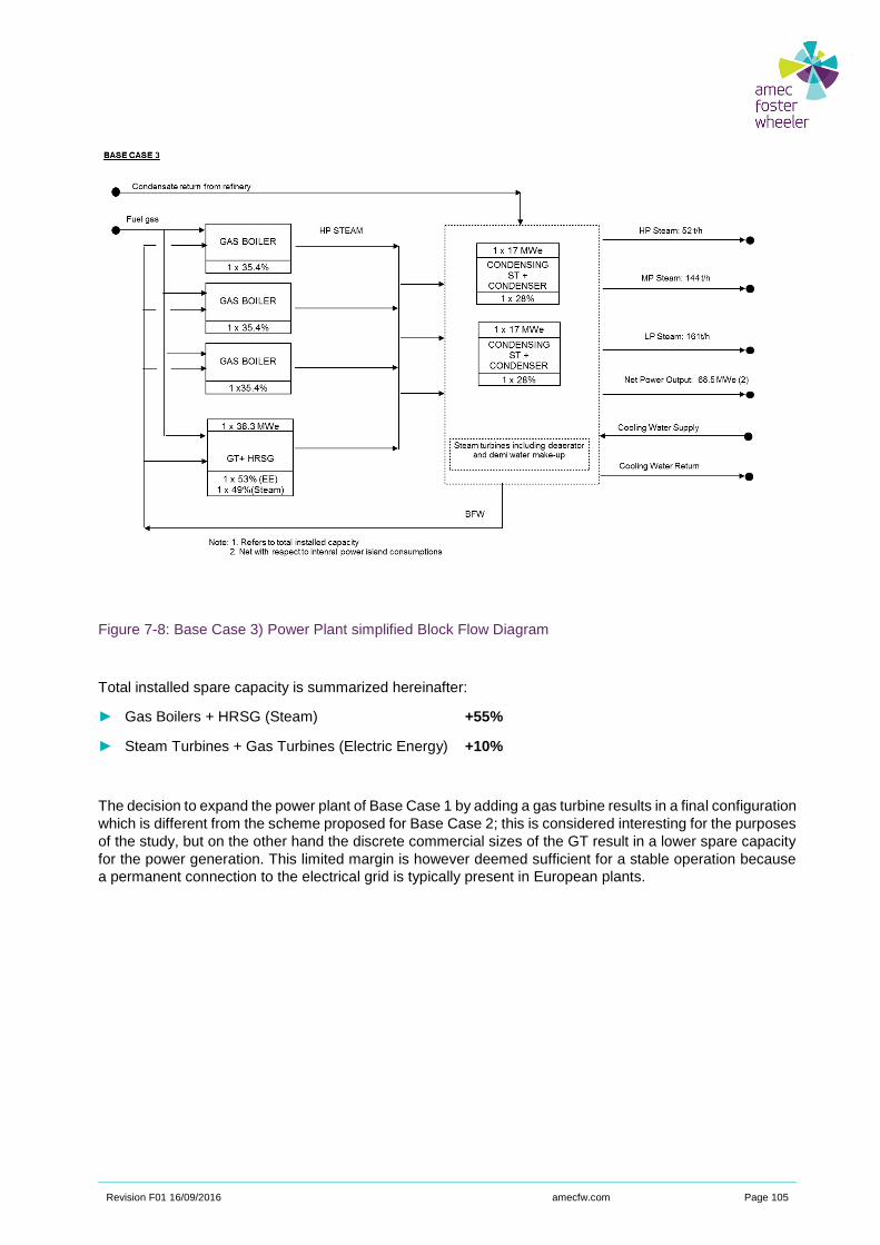
Revision F01 16/09/2016 amecfw.com Page 105
Figure 7-8: Base Case 3) Power Plant simplified Block Flow Diagram
Total installed spare capacity is summarized hereinafter:
► Gas Boilers + HRSG (Steam) +55%
► Steam Turbines + Gas Turbines (Electric Energy) +10%
The decision to expand the power plant of Base Case 1 by adding a gas turbine results in a final configuration
which is different from the scheme proposed for Base Case 2; this is considered interesting for the purposes
of the study, but on the other hand the discrete commercial sizes of the GT result in a lower spare capacity
for the power generation. This limited margin is however deemed sufficient for a stable operation because
a permanent connection to the electrical grid is typically present in European plants.
Revision F01 16/09/2016 amecfw.com Page 106
8. Base Case 4
High Conversion Refinery - 350,000 BPSD Crude Capacity
The High Conversion Refinery consists of two parallel crude distillation trains (Crude Atmospheric and
Vacuum Distillation Units), followed by gasoline blocks for octane improvement, kerosene sweetening units,
hydrotreating units for the middle-distillates.
Two different types of Vacuum Gasoil (VGO) conversion units are also included: i.e. the Fluid Catalytic
Cracking (FCC) and the High Pressure Hydrocracking (HCK). These two units have the same design
capacity of 60,000 BPSD each.
Upstream of the FCC, a Vacuum Gasoil Hydrotreating (VHT) unit is present to decrease the sulphur content
of FCC feedstock, in order to respect SOx limits at FCC stack.
For Vacuum Residue conversion, a Solvent Deasphalting Unit (SDA) followed by a Coker Unit (DCU) are
considered. Solvent Deasphalting allows recovering from the Vacuum Residue the paraffinic material (DAO),
which can be then fed to the VGO cracking units (essentially to HCK) for being converted into more valuable
distillates.
The pitch from SDA is then sent to DCU. It is considered to sell the fuel grade coke produced in DCU.
The FCC and Coker distillates are sent to finishing units to comply with the 10 ppm wt. sulphur specification
for the automotive fuels.
Two parallel Steam Methane Reformer (SMR) trains are foreseen to satisfy the hydrogen demand of this
complex refinery.
Base Case 4 is conceived as representative of top-class refineries, which have achieved their final
configuration and capacity in a more straight-forward way with respect of Base Case 2 and 3.
This results in a more organic layout, design with parallel symmetrical trains for process and utility units and
a more efficient power plant.
Refinery Balances
The balances developed for Base Case 4 are reported in the following tables and figures:
► Table 8-1: Base Case 4) Overall material balance
► Table 8-2: Base Case 4) Process units operating and design capacity
► Table 8-3: Base Case 4) Gasoline qualities

Revision F01 16/09/2016 amecfw.com Page 107
► Table 8-4: Base Case 4) Distillate qualities
► Table 8-5: Base Case 4) Fuel oil and bitumen qualities
► Figure 8-1: Base Case 4) Block flow diagrams with main material streams
► Table 8-6: Base Case 4) Main utility balance, fuel mix composition, CO2 emissions
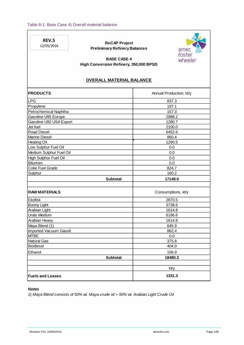
Revision F01 16/09/2016 amecfw.com Page 108
Table 8-1: Base Case 4) Overall material balance
ReCAP Project
Preliminary Refinery Balances
BASE CASE 4
High Conversion Refinery, 350,000 BPSD
PRODUCTS
LPG
Propylene
Petrochemical Naphtha
Gasoline U95 Europe
Gasoline U92 USA Export
Jet fuel
Road Diesel
Marine Diesel
Heating Oil
Low Sulphur Fuel Oil
Medium Sulphur Fuel Oil
High Sulphur Fuel Oil
Bitumen
Coke Fuel Grade
Sulphur
Subtotal
RAW MATERIALS
Ekofisk
Bonny Light
Arabian Light
Urals Medium
Arabian Heavy
Maya Blend (1)
Imported Vacuum Gasoil
MTBE
Natural Gas
Biodiesel
Ethanol
Subtotal
Fuels and Losses
Notes
1) Maya Blend consists of 50% wt. Maya crude oil + 50% wt. Arabian Light Crude Oil
1290.5
0.0
0.0
0.0
0.0
2988.2
1280.7
2100.0
6452.6
860.4
OVERALL MATERIAL BALANCE
Annual Production, kt/y
837.3
197.1
157.3
645.9
862.4
824.7
160.2
Consumptions, kt/y
2870.5
3738.6
17149.0
1614.8
6196.6
1614.8
18480.3
kt/y
1331.3
0.0
375.8
404.0
156.9
REV.512/05/2016
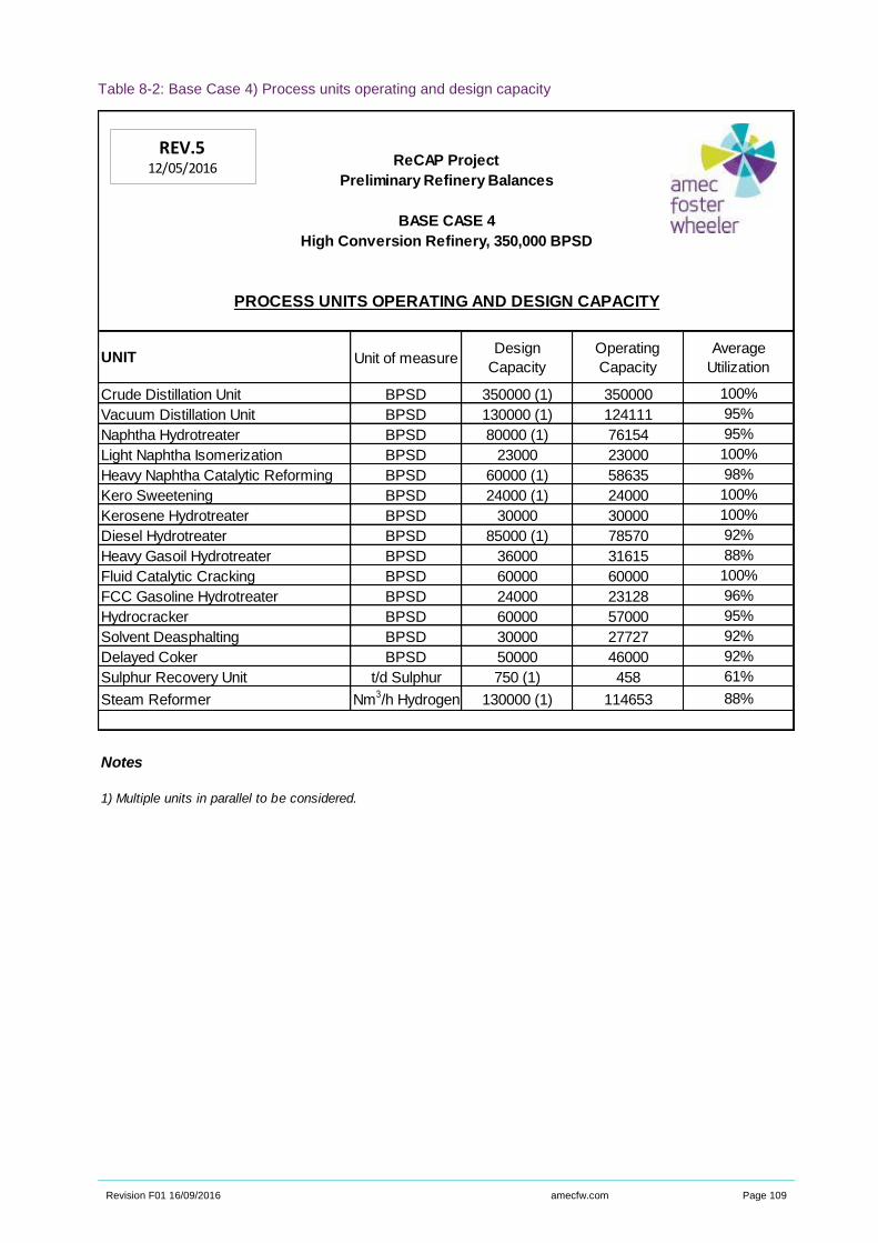
Revision F01 16/09/2016 amecfw.com Page 109
Table 8-2: Base Case 4) Process units operating and design capacity
ReCAP Project
Preliminary Refinery Balances
BASE CASE 4
High Conversion Refinery, 350,000 BPSD
UNIT Unit of measureDesign
Capacity
Operating
Capacity
Average
Utilization
Crude Distillation Unit BPSD 350000 (1) 350000 100%
Vacuum Distillation Unit BPSD 130000 (1) 124111 95%
Naphtha Hydrotreater BPSD 80000 (1) 76154 95%
Light Naphtha Isomerization BPSD 23000 23000 100%
Heavy Naphtha Catalytic Reforming BPSD 60000 (1) 58635 98%
Kero Sweetening BPSD 24000 (1) 24000 100%
Kerosene Hydrotreater BPSD 30000 30000 100%
Diesel Hydrotreater BPSD 85000 (1) 78570 92%
Heavy Gasoil Hydrotreater BPSD 36000 31615 88%
Fluid Catalytic Cracking BPSD 60000 60000 100%
FCC Gasoline Hydrotreater BPSD 24000 23128 96%
Hydrocracker BPSD 60000 57000 95%
Solvent Deasphalting BPSD 30000 27727 92%
Delayed Coker BPSD 50000 46000 92%
Sulphur Recovery Unit t/d Sulphur 750 (1) 458 61%
Steam Reformer Nm3/h Hydrogen 130000 (1) 114653 88%
Notes
1) Multiple units in parallel to be considered.
PROCESS UNITS OPERATING AND DESIGN CAPACITY
REV.512/05/2016
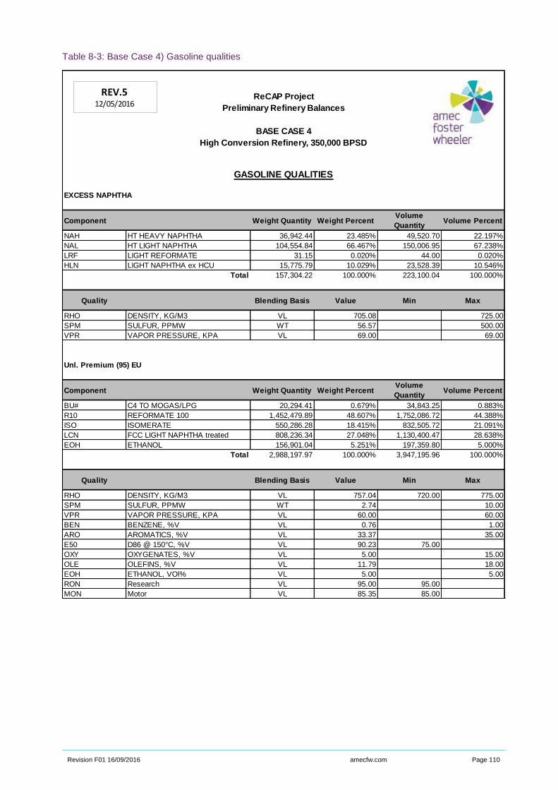
Revision F01 16/09/2016 amecfw.com Page 110
Table 8-3: Base Case 4) Gasoline qualities
ReCAP Project
Preliminary Refinery Balances
BASE CASE 4
High Conversion Refinery, 350,000 BPSD
GASOLINE QUALITIES
EXCESS NAPHTHA
Component Weight Quantity Weight PercentVolume
QuantityVolume Percent
NAH HT HEAVY NAPHTHA 36,942.44 23.485% 49,520.70 22.197%
NAL HT LIGHT NAPHTHA 104,554.84 66.467% 150,006.95 67.238%
LRF LIGHT REFORMATE 31.15 0.020% 44.00 0.020%
HLN LIGHT NAPHTHA ex HCU 15,775.79 10.029% 23,528.39 10.546%
Total 157,304.22 100.000% 223,100.04 100.000%
Quality Blending Basis Value Min Max
RHO DENSITY, KG/M3 VL 705.08 725.00
SPM SULFUR, PPMW WT 56.57 500.00
VPR VAPOR PRESSURE, KPA VL 69.00 69.00
Unl. Premium (95) EU
Component Weight Quantity Weight PercentVolume
QuantityVolume Percent
BU# C4 TO MOGAS/LPG 20,294.41 0.679% 34,843.25 0.883%
R10 REFORMATE 100 1,452,479.89 48.607% 1,752,086.72 44.388%
ISO ISOMERATE 550,286.28 18.415% 832,505.72 21.091%
LCN FCC LIGHT NAPHTHA treated 808,236.34 27.048% 1,130,400.47 28.638%
EOH ETHANOL 156,901.04 5.251% 197,359.80 5.000%
Total 2,988,197.97 100.000% 3,947,195.96 100.000%
Quality Blending Basis Value Min Max
RHO DENSITY, KG/M3 VL 757.04 720.00 775.00
SPM SULFUR, PPMW WT 2.74 10.00
VPR VAPOR PRESSURE, KPA VL 60.00 60.00
BEN BENZENE, %V VL 0.76 1.00
ARO AROMATICS, %V VL 33.37 35.00
E50 D86 @ 150°C, %V VL 90.23 75.00
OXY OXYGENATES, %V VL 5.00 15.00
OLE OLEFINS, %V VL 11.79 18.00
EOH ETHANOL, VOl% VL 5.00 5.00
RON Research VL 95.00 95.00
MON Motor VL 85.35 85.00
REV.512/05/2016
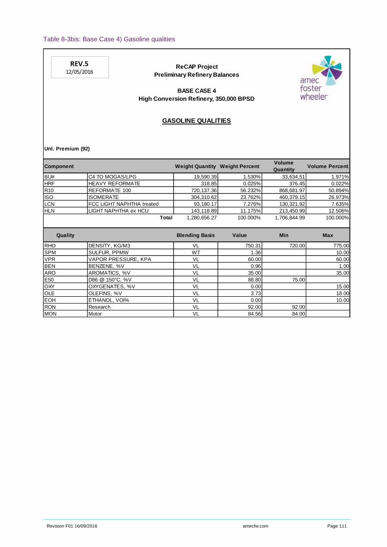
Revision F01 16/09/2016 amecfw.com Page 111
Table 8-3bis: Base Case 4) Gasoline qualities
ReCAP Project
Preliminary Refinery Balances
BASE CASE 4
High Conversion Refinery, 350,000 BPSD
GASOLINE QUALITIES
Unl. Premium (92)
Component Weight Quantity Weight PercentVolume
QuantityVolume Percent
BU# C4 TO MOGAS/LPG 19,590.39 1.530% 33,634.51 1.971%
HRF HEAVY REFORMATE 318.85 0.025% 376.45 0.022%
R10 REFORMATE 100 720,137.36 56.232% 868,681.97 50.894%
ISO ISOMERATE 304,310.62 23.762% 460,379.15 26.973%
LCN FCC LIGHT NAPHTHA treated 93,180.17 7.276% 130,321.92 7.635%
HLN LIGHT NAPHTHA ex HCU 143,118.89 11.175% 213,450.99 12.506%
Total 1,280,656.27 100.000% 1,706,844.99 100.000%
Quality Blending Basis Value Min Max
RHO DENSITY, KG/M3 VL 750.31 720.00 775.00
SPM SULFUR, PPMW WT 1.36 10.00
VPR VAPOR PRESSURE, KPA VL 60.00 60.00
BEN BENZENE, %V VL 0.96 1.00
ARO AROMATICS, %V VL 35.00 35.00
E50 D86 @ 150°C, %V VL 88.80 75.00
OXY OXYGENATES, %V VL 0.00 15.00
OLE OLEFINS, %V VL 3.73 18.00
EOH ETHANOL, VOl% VL 0.00 10.00
RON Research VL 92.00 92.00
MON Motor VL 84.56 84.00
REV.512/05/2016
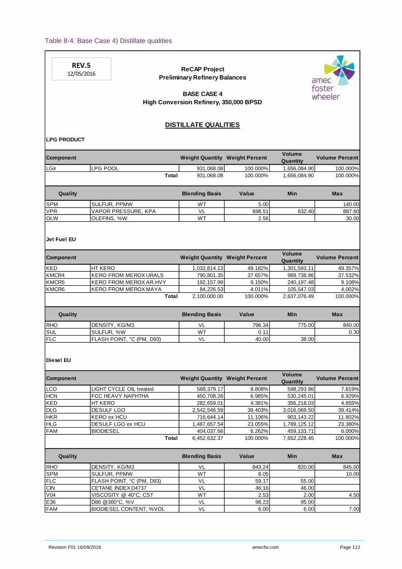
Revision F01 16/09/2016 amecfw.com Page 112
Table 8-4: Base Case 4) Distillate qualities
ReCAP Project
Preliminary Refinery Balances
BASE CASE 4
High Conversion Refinery, 350,000 BPSD
DISTILLATE QUALITIES
LPG PRODUCT
Component Weight Quantity Weight PercentVolume
QuantityVolume Percent
LG# LPG POOL 931,068.08 100.000% 1,656,084.90 100.000%
Total 931,068.08 100.000% 1,656,084.90 100.000%
Quality Blending Basis Value Min Max
SPM SULFUR, PPMW WT 5.00 140.00
VPR VAPOR PRESSURE, KPA VL 698.51 632.40 887.60
OLW OLEFINS, %W WT 2.56 30.00
Jet Fuel EU
Component Weight Quantity Weight PercentVolume
QuantityVolume Percent
KED HT KERO 1,032,814.13 49.182% 1,301,593.11 49.357%
KMCR4 KERO FROM MEROX URALS 790,801.35 37.657% 989,738.86 37.532%
KMCR5 KERO FROM MEROX AR.HVY 192,157.99 9.150% 240,197.48 9.108%
KMCR6 KERO FROM MEROX MAYA 84,226.53 4.011% 105,547.03 4.002%
Total 2,100,000.00 100.000% 2,637,076.49 100.000%
Quality Blending Basis Value Min Max
RHO DENSITY, KG/M3 VL 796.34 775.00 840.00
SUL SULFUR, %W WT 0.11 0.30
FLC FLASH POINT, °C (PM, D93) VL 40.00 38.00
Diesel EU
Component Weight Quantity Weight PercentVolume
QuantityVolume Percent
LCO LIGHT CYCLE OIL treated 568,379.17 8.808% 598,293.86 7.819%
HCN FCC HEAVY NAPHTHA 450,708.26 6.985% 530,245.01 6.929%
KED HT KERO 282,659.01 4.381% 356,218.03 4.655%
DLG DESULF LGO 2,542,546.59 39.403% 3,016,069.50 39.414%
HKR KERO ex HCU 716,644.14 11.106% 903,143.22 11.802%
HLG DESULF LGO ex HCU 1,487,657.54 23.055% 1,789,125.12 23.380%
FAM BIODIESEL 404,037.66 6.262% 459,133.71 6.000%
Total 6,452,632.37 100.000% 7,652,228.45 100.000%
Quality Blending Basis Value Min Max
RHO DENSITY, KG/M3 VL 843.24 820.00 845.00
SPM SULFUR, PPMW WT 8.05 10.00
FLC FLASH POINT, °C (PM, D93) VL 59.17 55.00
CIN CETANE INDEX D4737 VL 46.16 46.00
V04 VISCOSITY @ 40°C, CST WT 2.53 2.00 4.50
E36 D86 @360°C, %V VL 98.23 95.00
FAM BIODIESEL CONTENT, %VOL VL 6.00 6.00 7.00
REV.512/05/2016
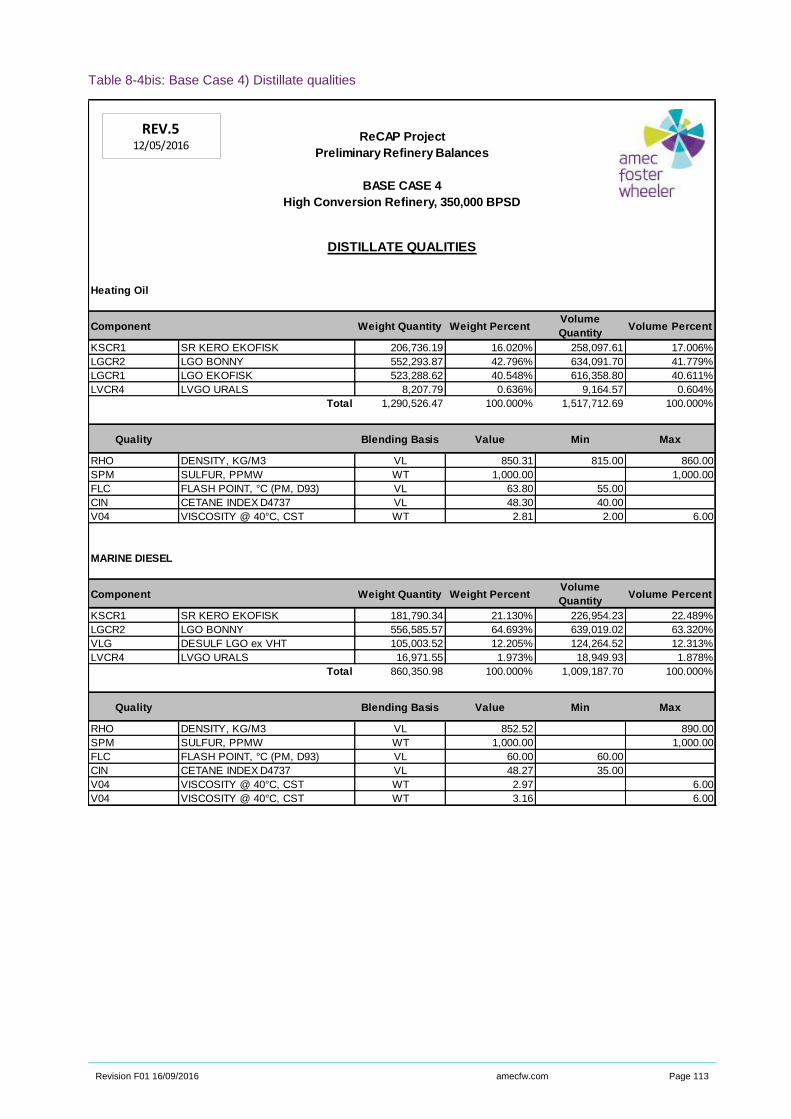
Revision F01 16/09/2016 amecfw.com Page 113
Table 8-4bis: Base Case 4) Distillate qualities
ReCAP Project
Preliminary Refinery Balances
BASE CASE 4
High Conversion Refinery, 350,000 BPSD
DISTILLATE QUALITIES
Heating Oil
Component Weight Quantity Weight PercentVolume
QuantityVolume Percent
KSCR1 SR KERO EKOFISK 206,736.19 16.020% 258,097.61 17.006%
LGCR2 LGO BONNY 552,293.87 42.796% 634,091.70 41.779%
LGCR1 LGO EKOFISK 523,288.62 40.548% 616,358.80 40.611%
LVCR4 LVGO URALS 8,207.79 0.636% 9,164.57 0.604%
Total 1,290,526.47 100.000% 1,517,712.69 100.000%
Quality Blending Basis Value Min Max
RHO DENSITY, KG/M3 VL 850.31 815.00 860.00
SPM SULFUR, PPMW WT 1,000.00 1,000.00
FLC FLASH POINT, °C (PM, D93) VL 63.80 55.00
CIN CETANE INDEX D4737 VL 48.30 40.00
V04 VISCOSITY @ 40°C, CST WT 2.81 2.00 6.00
MARINE DIESEL
Component Weight Quantity Weight PercentVolume
QuantityVolume Percent
KSCR1 SR KERO EKOFISK 181,790.34 21.130% 226,954.23 22.489%
LGCR2 LGO BONNY 556,585.57 64.693% 639,019.02 63.320%
VLG DESULF LGO ex VHT 105,003.52 12.205% 124,264.52 12.313%
LVCR4 LVGO URALS 16,971.55 1.973% 18,949.93 1.878%
Total 860,350.98 100.000% 1,009,187.70 100.000%
Quality Blending Basis Value Min Max
RHO DENSITY, KG/M3 VL 852.52 890.00
SPM SULFUR, PPMW WT 1,000.00 1,000.00
FLC FLASH POINT, °C (PM, D93) VL 60.00 60.00
CIN CETANE INDEX D4737 VL 48.27 35.00
V04 VISCOSITY @ 40°C, CST WT 2.97 6.00
V04 VISCOSITY @ 40°C, CST WT 3.16 6.00
REV.512/05/2016

Revision F01 16/09/2016 amecfw.com Page 114
Table 8-5: Base Case 4) Fuel oil and bitumen qualities
ReCAP Project
Preliminary Refinery Balances
BASE CASE 4
High Conversion Refinery, 350,000 BPSD
FUEL OIL / BITUMEN QUALITIES
Low Sulphur Fuel
Component Weight Quantity Weight PercentVolume
QuantityVolume Percent
SLU FCC SLURRY OIL 231,363.57 89.661% 243,540.60 89.721%
HHR RESIDUE ex HCU 6,809.62 2.639% 8,073.05 2.974%
VDCR4 VDU RES MIX4 19,868.83 7.700% 19,829.17 7.305%
Total 258,042.02 100.000% 271,442.83 100.000%
Quality Blending Basis Value Min Max
RHO DENSITY, KG/M3 VL 950.63 991.00
SUL SULFUR, %W WT 0.50 0.50
FLC FLASH POINT, °C (PM, D93) VL 197.68 66.00
V05 VISCOSITY @ 50°C, CST WT 131.16 380.00
CCR CONRADSON CARBON RES, %W WT 1.16 15.00
REV.512/05/2016

Revision F01 16/09/2016 amecfw.com Page 115
Table 8-6: Base Case 4) Main utility balance, fuel mix composition, CO2 emissions
ReCAP Project
Preliminary Refinery Balances
BASE CASE 4
High Conversion Refinery, 350,000 BPSD
FUEL POWER HP STEAM MP STEAM LP STEAM
COOLING
WATER (2)
RAW
WATER
Gcal/h kW tons/h tons/h tons/h m3/h m3/h
MAIN PROCESS UNITS 975 83180 -20 160 174 35364
BASE LOAD 30000 20 40 40
POWER PLANT 419 -119235 0 -200 -214
SEA WATER SYSTEM 1712 -10000
COOLING TOWER SYSTEM 4342 -25364
TOTAL 1393 0 0 0 0 0 2900
t/h kt/y wt%
REFINERY FUEL GAS 57.2 480.1 46%
LOW SULPHUR FUEL OIL (3) 30.7 258.0 25%
FCC COKE 14.5 121.7 12%
NATURAL GAS to fuel system 0.1 1.1 0%
NATURAL GAS to gas turbine 22.9 192.2 18%
TOTAL 125.4 1053.1
t/h
From Steam Reformer 29.7
From FG/NG combustion 217.7
From FO combustion 98.3
From FCC coke combustion 53.1
TOTAL 398.8 corresponding to 3349.5 kt/y
200.8 kg CO2 / t crude
Notes
1) (-) indicates productions
2) 10°C temperature increase has been considered
3) LSFO is burnt in CDU and VDU heaters
MAIN UTILITY BALANCE
FUEL MIX COMPOSITION
CO2 EMISSIONS
REV.512/05/2016
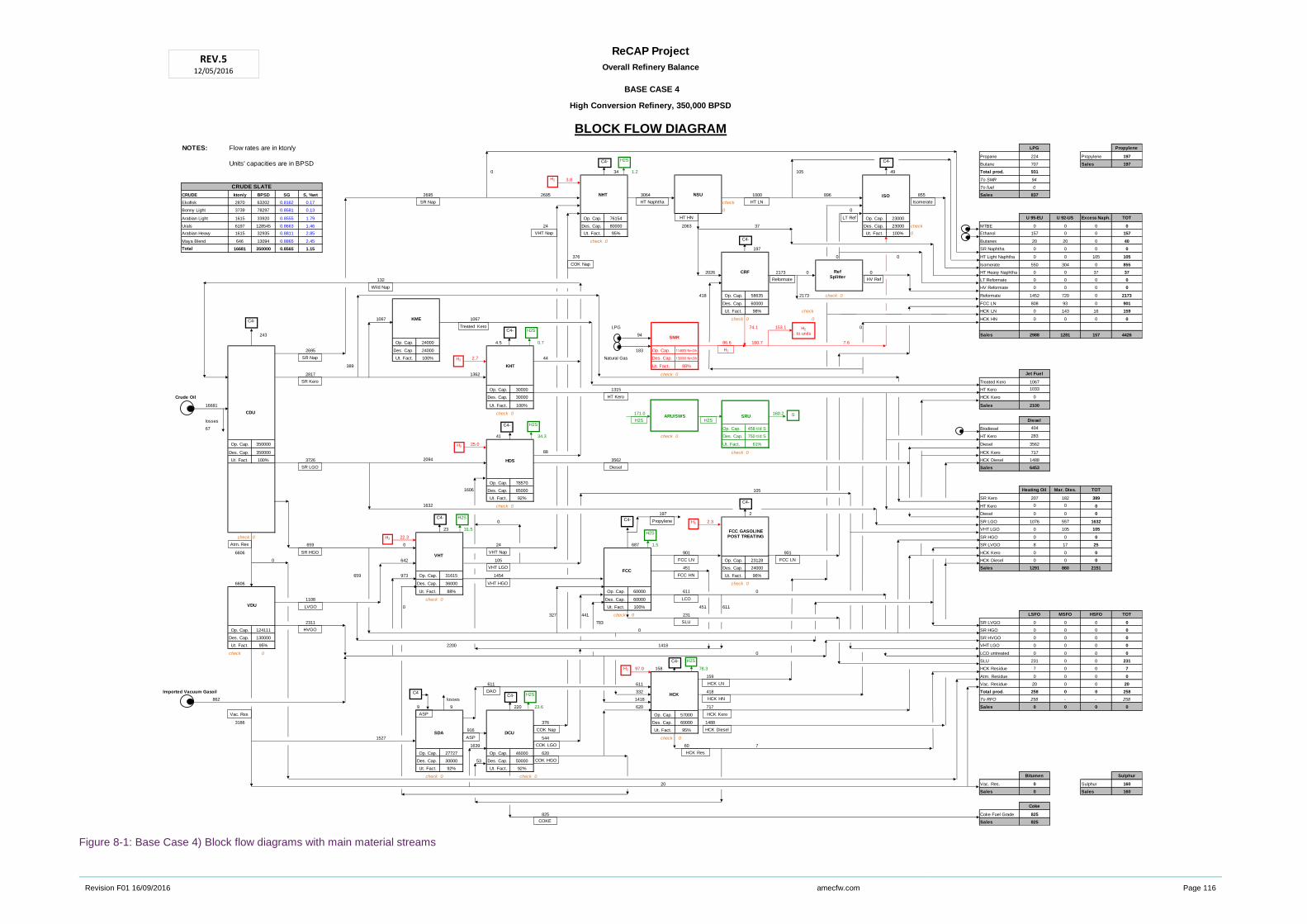
Revision F01 16/09/2016 amecfw.com Page 116
Figure 8-1: Base Case 4) Block flow diagrams with main material streams
ReCAP Project
Overall Refinery Balance
BASE CASE 4
High Conversion Refinery, 350,000 BPSD
BLOCK FLOW DIAGRAM
NOTES: Flow rates are in kton/y LPG Propylene
Propane 224 Propylene 197
Units' capacities are in BPSD Butane 707 Sales 197
0 34 1.2 105 49 Total prod. 931
3.8 To SMR 94
CRUDE SLATE To fuel 0
CRUDE kton/y BPSD SG S, %wt 2695 2695 3064 1000 896 855 Sales 837
Ekofisk 2870 63202 0.8162 0.17 check
Bonny Light 3739 78297 0.8581 0.13 0 0
Arabian Light 1615 33920 0.8555 1.79 Op. Cap. 76154 Op. Cap. 23000 U 95-EU U 92-US Excess Naph. TOT
Urals 6197 128545 0.8663 1.46 24 Des. Cap. 80000 2063 37 Des. Cap. 23000 check MTBE 0 0 0 0
Arabian Heavy 1615 32935 0.8811 2.85 Ut. Fact. 95% Ut. Fact. 100% 0 Ethanol 157 0 0 157
Maya Blend 646 13094 0.8865 2.45 check 0 Butanes 20 20 0 40
Total 16681 350000 0.8565 1.15 197 SR Naphtha 0 0 0 0
376 0 0 HT Light Naphtha 0 0 105 105
Isomerate 550 304 0 855
2026 2173 0 0 HT Heavy Naphtha 0 0 37 37
132 LT Reformate 0 0 0 0
HV Reformate 0 0 0 0
418 Op. Cap. 58635 2173 check 0 Reformate 1452 720 0 2173
Des. Cap. 60000 FCC LN 808 93 0 901
Ut. Fact. 98% check HCK LN 0 143 16 159
1067 1067 check 0 0 HCK HN 0 0 0 0
LPG 74.1 153.1 0
243 94 Sales 2988 1281 157 4426
Op. Cap. 24000 4.5 0.7 86.6 160.7 7.6
2695 Des. Cap. 24000 183 Op. Cap. 114653 Nm3/h
Ut. Fact. 100% 2.7 44 Natural Gas Des. Cap. 130000 Nm3/h
389 Ut. Fact. 88%
2817 1362 check 0 Jet Fuel
Treated Kero 1067
Op. Cap. 30000 1315 HT Kero 1033
Crude Oil Des. Cap. 30000 HCK Kero 0
16681 Ut. Fact. 100% Sales 2100
check 0 171.0 160.2
losses Diesel
67 Op. Cap. 458 t/d S Biodiesel 404
41 34.3 check 0 Des. Cap. 750 t/d S HT Kero 283
Op. Cap. 350000 25.0 Ut. Fact. 61% Diesel 3562
Des. Cap. 350000 88 check 0 HCK Kero 717
Ut. Fact. 100% 3726 2094 3562 HCK Diesel 1488
Sales 6453
Op. Cap. 78570
1606 Des. Cap. 85000 105 Heating Oil Mar. Dies. TOT
Ut. Fact. 92% SR Kero 207 182 389
1632 check 0 HT Kero 0 0 0
197 2 Diesel 0 0 0
0 2.3 SR LGO 1076 557 1632
23 31.5 VHT LGO 0 105 105
check 0 22.3 SR HGO 0 0 0
659 0 24 687 1.5 SR LVGO 8 17 25
6606 901 901 HCK Kero 0 0 0
0 642 105 Op. Cap. 23128 HCK Diesel 0 0 0
451 Des. Cap. 24000 Sales 1291 860 2151
659 973 Op. Cap. 31615 1454 Ut. Fact. 96%
6606 Des. Cap. 36000 check 0
Ut. Fact. 88% Op. Cap. 60000 611 0 #REF!
1108 check 0 Des. Cap. 60000
0 Ut. Fact. 100% 451 611
327 441 check 0 231 LSFO MSFO HSFO TOT
2311 783 SR LVGO 0 0 0 0
Op. Cap. 124111 0 SR HGO 0 0 0 0
Des. Cap. 130000 SR HVGO 0 0 0 0
Ut. Fact. 95% 2200 1418 VHT LGO 0 0 0 0
check 0 0 LCO untreated 0 0 0 0
SLU 231 0 0 231
97.0 158 78.3 HCK Residue 7 0 0 7
159 Atm. Residue 0 0 0 0
611 611 Vac. Residue 20 0 0 20
Imported Vacuum Gasoil 332 418 Total prod. 258 0 0 258
862 losses 1418 To RFO 258 - - 258
9 9 220 23.6 620 717 Sales 0 0 0 0
Op. Cap. 57000
3186 376 Des. Cap. 60000 1488
916 Ut. Fact. 95%
1527 544 check 0
1639 60 7
Op. Cap. 27727 Op. Cap. 46000 620
Des. Cap. 30000 53 Des. Cap. 50000
Ut. Fact. 92% Ut. Fact. 92%
check 0 check 0 Bitumen Sulphur
20 Vac. Res. 0 Sulphur 160
Sales 0 Sales 160
Coke
825 Coke Fuel Grade 825
Sales 825
CDU
Atm. Res
SR HGO
Wild Nap
SR LGO
SR Kero
HT Kero
SR Nap
NSU
HT Naphtha
LT Ref
KHT
ISO
HDS
H2
to units
H2
NHT
RefSplitter
Diesel
H2
CRF
H2
Vac. Res
VDU
VHT
VHT HGO
H2
VHT Nap
VHT LGO
HVGO
SMR
C4-
C4-
C4-
C4-
C4-
C4-
C4-
H2S
H2S
H2S
ARU/SWS SRU S
H2S H2S
FCC
SLU
LCO
FCC HN
FCC LN
VHT Nap
SR Nap
DCU
HT HN
HT LN
Reformate HV Ref
Isomerate
C4-
COK Nap
COK LGO
COK Nap
C4-
H2S
Propylene
FCC GASOLINEPOST TREATING
C4-
LVGO
H2
FCC LN
H2S
H2
KME
Treated Kero
REV.512/05/2016
H2S
COK HGO
COKE
SDA
HCKDAO
ASP
H2
C4
H2SC4-
HCK Res
HCK Diesel
HCK Kero
HCK HN
HCK LN
ASP
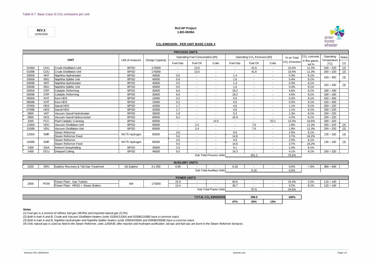
Revision F01 16/09/2016 amecfw.com Page 117
Table 8-7: Base Case 4) CO2 emissions per unit
Notes
Fuel Gas Fuel Oil Coke Fuel Gas Fuel Oil Coke (1)
0100A CDU Crude Distillation Unit BPSD 175000 - 13.0 - - 41.6 - 10.4% 11.3% 200 ÷ 220 (2)
0100B CDU Crude Distillation Unit BPSD 175000 - 13.0 - - 41.6 - 10.4% 11.3% 200 ÷ 220 (2)
0300A NHT Naphtha Hydrotreater BPSD 40000 0.5 - - 1.4 - - 0.3% 8.1%
0350A NSU Naphtha Splitter Unit BPSD 40000 0.6 - - 1.6 - - 0.4% 8.1%
0300B NHT Naphtha Hydrotreater BPSD 40000 0.5 - - 1.4 - - 0.3% 8.1%
0350B NSU Naphtha Splitter Unit BPSD 40000 0.6 - - 1.6 - - 0.4% 8.1%
0500A CRF Catalytic Reforming BPSD 30000 6.6 - - 18.2 - - 4.6% 8.1% 180 ÷ 190
0500B CRF Catalytic Reforming BPSD 30000 6.6 - - 18.2 - - 4.6% 8.1% 180 ÷ 190
0600A KHT Kero HDS BPSD 15000 0.2 - - 0.6 - - 0.2% 8.1% 420 ÷ 450
0600B KHT Kero HDS BPSD 15000 0.2 - - 0.6 - - 0.2% 8.1% 420 ÷ 450
0700A HDS Gasoil HDS BPSD 42500 1.7 - - 4.6 - - 1.1% 8.1% 200 ÷ 220
0700B HDS Gasoil HDS BPSD 42500 1.7 - - 4.6 - - 1.1% 8.1% 200 ÷ 220
0800 VHT Vacuum Gasoil Hydrotreater BPSD 36000 1.9 - - 5.3 - - 1.3% 8.1% 200 ÷ 220
0900 HCK Vacuum Gasoil Hydrocracker BPSD 60000 6.2 - - 16.9 - - 4.2% 8.1% 200 ÷ 220
1000 FCC Fluid Catalytic Cracking BPSD 60000 - - 14.5 - - 53.1 13.3% 16.6% 300 ÷ 320
1100A VDU Vacuum Distillation Unit BPSD 65000 - 2.4 - - 7.6 - 1.9% 11.3% 200 ÷ 220 (2)
1100B VDU Vacuum Distillation Unit BPSD 65000 - 2.4 - - 7.6 - 1.9% 11.3% 200 ÷ 220 (2)
Steam Reformer 3.6 - - 9.9 - - 2.5% 8.1%
Steam Reformer Feed 5.6 - - 14.8 - - 3.7% 24.2%
Steam Reformer 3.6 - - 9.9 - - 2.5% 8.1%
Steam Reformer Feed 5.6 - - 14.8 - - 3.7% 24.2%
1300 SDA Solvent Deasphalting BPSD 35000 3.3 - - 9.1 - - 2.3% 8.1%
1400 DCU Delayed Coking BPSD 46000 6.0 - - 16.3 - - 4.1% 8.1% 200 ÷ 220
Sub Total Process Units 75.5%
2200 SRU Sulphur Recovery & Tail Gas Treatment t/d Sulphur 3 x 250 0.06 - - 0.16 - - 0.0% < 8% 380 ÷ 400
Sub Total Auxiliary Units 0.0%
Power Plant - Gas Turbine 22.9 - - 60.8 - - 15.3% 3.2% 115 ÷ 140
Power Plant - HRSG + Steam Boilers 13.4 - - 36.7 - - 9.2% 8.1% 115 ÷ 140
Sub Total Power Units 24.5%
100%
47% 25% 13%
Notes
(1) Fuel gas is a mixture of refinery fuel gas (99.8%) and imported natural gas (0.2%).
(2) Both in train A and B, Crude and Vacuum Distillation heaters (units 0100A/1100A and 0100B/1100B) have a common stack.
(3) Both in train A and B, Naphtha Hydrotreater and Naphtha Splitter heaters (units 0300A/0350A and 0300B/0350B) have a common stack.
(4) Only natural gas is used as feed to the Steam Reformer, units 1200A/B; after reaction and hydrogen purification, tail gas and fuel gas are burnt in the Steam Reformer furnaces.
1-BD-0839A
ReCAP Project
PROCESS UNITS
UNIT Unit of measure Design CapacityOperating Fuel Consumption [t/h] Operating CO2 Emission [t/h] % on Total
CO2 Emission
Operating
Temperature
[°C]
CO2 EMISSION - PER UNIT BASE CASE 4
CO2 concentr.
in flue gases,
vol %
1200A SMR Nm3/h Hydrogen 85000 135 ÷ 160
(4)
420 ÷ 450 (3)
420 ÷ 450 (3)
(4)
1200B SMR Nm3/h Hydrogen 85000 135 ÷ 160
97.6
TOTAL CO2 EMISSION 398.9
301.2
AUXILIARY UNITS
0.16
POWER UNITS
2500 POW kW 175000
REV.512/05/2016

Revision F01 16/09/2016 amecfw.com Page 118
Refinery Layout
The layout of the Base Case 4 refinery is enclosed in Figure 8-2.
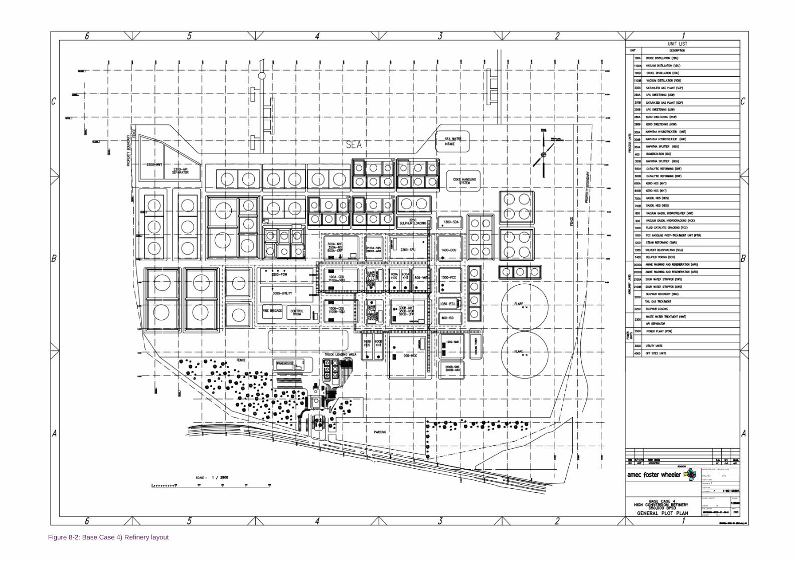
Figure 8-2: Base Case 4) Refinery layout

Revision F01 16/09/2016 amecfw.com Page 120
Main Utility Networks
The main utility balances have been reported on block flow diagrams, reflecting the planimetric arrangement
of the process units and utility blocks.
In particular, the following networks’ sketches have been developed:
► Figure 8-3: Base Case 4) Electricity network
► Figure 8-4: Base Case 4) Steam networks
► Figure 8-5: Base Case 4) Cooling water network
► Figure 8-6: Base Case 4) Fuel Gas/Offgas networks
► Figure 8-7: Base Case 4) Fuel oil network
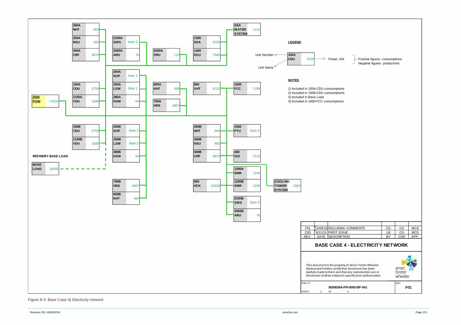
Revision F01 16/09/2016 amecfw.com Page 121
Figure 8-3: Base Case 4) Electricity network
300A SEA
NHT 663 WATER 1712
SYSTEM
350A 2100A 1300
NSU 492 SWS SDA 3728 LEGEND
500A 2000A 2200A 1400
CRF 4874 ARU 76 SRU 110 DCU 7545 Unit Number 100A
CDU 5759 Power, kW Positive figures: consumptions
Negative figures: productions
Unit Name
200A
SGP
NOTES
100A 250A 600A 800 1000
CDU 5759 LSW KHT 494 VHT 6712 FCC 1789 1) Included in 100A-CDU consumptions
2) Included in 100B-CDU consumptions
2500 1100A 280A 3) Included in Base Load
POW -119235 VDU 1848 KSW 64 700A 4) Included in 1000-FCC consumptions
HDS 2907
100B 200B 300B 1050
CDU 5759 SGP NHT 663 PTU
1100B 250B 350B
VDU 1848 LSW NSU 492
280B 500B 400
REFINERY BASE LOAD KSW 64 CRF 4874 ISO 2112
BASE
LOAD 30000 1200A
SMR 1246
700B 900 1200B COOLING
HDS 2907 HCK 24339 SMR 1246 TOWER 4342
SYSTEM
600B
KHT 494 2100B
SWS
2000B
ARU 76
F01 12/05/16 INCLUDING COMMENTS CG CG MCS
C00 6/11/15 FIRST ISSUE LB CG MCS
REV. DATE DESCRIPTION BY CHD APP:
DWG. N° REV.
F01SHEET 1 OF 1
Note 3
BASE CASE 4 - ELECTRICITY NETWORK
BD0839A-PR-0000-BF-041
Note 3
Note 1
Note 1
Note 2 Note 4
Note 2
This document is the property of Amec Foster Wheeler Italiana and holders certify that disclosure has been lawfully made to them and that any reproduction use or disclosure shall be subject to specific prior authorisation.
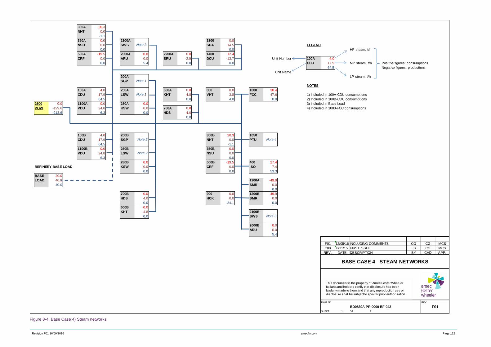
Revision F01 16/09/2016 amecfw.com Page 122
Figure 8-4: Base Case 4) Steam networks
300A 20.3
NHT 0.0
-1.1
350A 0.0 2100A 1300 0.0
NSU 0.0 SWS SDA 14.5 LEGEND
0.0 0.0 HP steam, t/h
500A -19.5 2000A 0.0 2200A 0.0 1400 12.4
CRF 0.0 ARU 0.0 SRU -2.9 DCU -13.7 Unit Number 100A 4.0
0.0 5.4 0.0 0.0 CDU 17.9 MP steam, t/h Positive figures: consumptions
64.5 Negative figures: productions
Unit Name
200A LP steam, t/h
SGP
NOTES
100A 4.0 250A 600A 0.0 800 0.0 1000 30.4
CDU 17.9 LSW KHT 4.8 VHT 3.8 FCC 47.6 1) Included in 100A-CDU consumptions
64.5 0.0 4.0 0.0 2) Included in 100B-CDU consumptions
2500 0.0 1100A 0.0 280A 0.0 3) Included in Base Load
POW -199.6 VDU 24.8 KSW 0.0 700A 0.0 4) Included in 1000-FCC consumptions
-213.6 6.3 0.0 HDS 4.0
0.0
100B 4.0 200B 300B 20.3 1050
CDU 17.9 SGP NHT 0.0 PTU
64.5 -1.1
1100B 0.0 250B 350B 0.0
VDU 24.8 LSW NSU 0.0
6.3 0.0
280B 0.0 500B -19.5 400 27.4
REFINERY BASE LOAD KSW 0.0 CRF 0.0 ISO 7.4
0.0 0.0 53.3
BASE 20.0
LOAD 40.0 1200A -49.9
40.0 SMR 0.0
0.0
700B 0.0 900 0.0 1200B -49.9
HDS 4.0 HCK 0.0 SMR 0.0
0.0 -34.1 0.0
600B 0.0
KHT 4.8 2100B
0.0 SWS
2000B 0.0
ARU 0.0
5.4
F01 12/05/16 INCLUDING COMMENTS CG CG MCS
C00 6/11/15 FIRST ISSUE LB CG MCS
REV. DATE DESCRIPTION BY CHD APP:
DWG. N° REV.
F01SHEET 1 OF 1
Note 3
BASE CASE 4 - STEAM NETWORKS
BD0839A-PR-0000-BF-042
Note 3
Note 1
Note 1
Note 2 Note 4
Note 2
This document is the property of Amec Foster Wheeler Italiana and holders certify that disclosure has been lawfully made to them and that any reproduction use or disclosure shall be subject to specific prior authorisation.
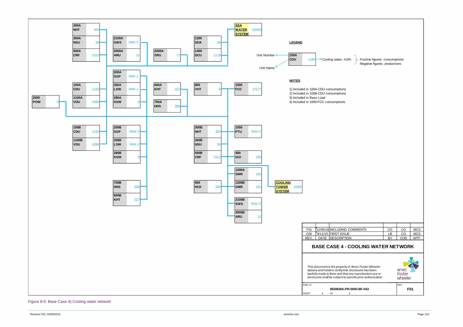
Revision F01 16/09/2016 amecfw.com Page 123
Figure 8-5: Base Case 4) Cooling water network
300A SEA
NHT 405 WATER -10000
SYSTEM
350A 2100A 1300
NSU 36 SWS SDA 36 LEGEND
500A 2000A 2200A 1400
CRF 1513 ARU 11 SRU 71 DCU 1118 Unit Number 100A
CDU 1192 Cooling water, m3/h Positive figures: consumptions
Negative figures: productions
Unit Name
200A
SGP
NOTES
100A 250A 600A 800 1000
CDU 1192 LSW KHT 227 VHT 6 FCC 17277 1) Included in 100A-CDU consumptions
2) Included in 100B-CDU consumptions
2500 1100A 280A 3) Included in Base Load
POW 0 VDU 4286 KSW 0 700A 4) Included in 1000-FCC consumptions
HDS 286
100B 200B 300B 1050
CDU 1192 SGP NHT 405 PTU
1100B 250B 350B
VDU 4286 LSW NSU 36
280B 500B 400
KSW 0 CRF 1513 ISO 235
1200A
SMR 191
700B 900 1200B COOLING
HDS 286 HCK 326 SMR 191 TOWER -25364
SYSTEM
600B
KHT 227 2100B
SWS
2000B
ARU 11
F01 12/05/16 INCLUDING COMMENTS CG CG MCS
C00 6/11/15 FIRST ISSUE LB CG MCS
REV. DATE DESCRIPTION BY CHD APP:
DWG. N° REV.
F01SHEET 1 OF 1
Note 3
BASE CASE 4 - COOLING WATER NETWORK
BD0839A-PR-0000-BF-043
Note 3
Note 1
Note 1
Note 2 Note 4
Note 2
This document is the property of Amec Foster Wheeler Italiana and holders certify that disclosure has been lawfully made to them and that any reproduction use or disclosure shall be subject to specific prior authorisation.
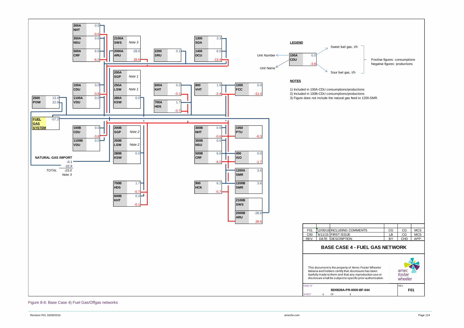
Revision F01 16/09/2016 amecfw.com Page 124
Figure 8-6: Base Case 4) Fuel Gas/Offgas networks
300A 0.5
NHT
-0.6
350A 0.6 2100A 1300 3.3
NSU SWS SDA LEGEND
Sweet fuel gas, t/h
500A 6.6 2000A -28.6 2200 0.1 1400 6.0
CRF ARU SRU DCU Unit Number 100A 0.0
-6.0 28.6 -13.4 CDU Positive figures: consumptions
-3.8 Negative figures: productions
Unit Name
200A Sour fuel gas, t/h
SGP
NOTES
100A 0.0 250A 600A 0.2 800 1.9 1000 0.0
CDU LSW KHT VHT FCC 1) Included in 100A-CDU consumptions/productions
-3.8 -0.1 -2.4 -11.4 2) Included in 100B-CDU consumptions/productions
2500 13.4 1100A 0.0 280A 0.0 3) Figure does not include the natural gas feed to 1200-SMR.
POW 22.9 VDU KSW 700A 1.7
HDS
-0.7
FUEL -57.3
GAS
SYSTEM 100B 0.0 200B 300B 0.5 1050
CDU SGP NHT PTU
-3.8 -0.6 -0.3
1100B 0.0 250B 350B 0.6
VDU LSW NSU
280B 0.0 500B 6.6 400 0.0
NATURAL GAS IMPORT KSW CRF ISO
-0.1 -6.0 -1.7
-22.9
TOTAL -23.0 1200A 3.6
Note 3 SMR
700B 1.7 900 6.2 1200B 3.6
HDS HCK SMR
-0.7 -5.7
600B 0.2
KHT 2100B
-0.1 SWS
2000B -28.6
ARU
28.6
F01 12/05/16 INCLUDING COMMENTS CG CG MCS
C00 6/11/15 FIRST ISSUE LB CG MCS
REV. DATE DESCRIPTION BY CHD APP:
DWG. N° REV.
F01SHEET 1 OF 1
BD0839A-PR-0000-BF-044
Note 3
Note 1
Note 1
Note 2
Note 2
BASE CASE 4 - FUEL GAS NETWORK
This document is the property of Amec Foster Wheeler Italiana and holders certify that disclosure has been lawfully made to them and that any reproduction use or disclosure shall be subject to specific prior authorisation.

Revision F01 16/09/2016 amecfw.com Page 125
Figure 8-7: Base Case 4) Fuel oil network
300A
NHT 0
350A 2100A 1300
NSU 0 SWS SDA 0 LEGEND
500A 2000A 2200 1400
CRF 0 ARU 0 SRU 0 DCU 0 Unit Number 100A
CDU 13.0 Low Sulphur Fuel Oil, t/h Positive figures: consumptions
Negative figures: productions
Unit Name
200A
SGP
NOTES
100A 250A 600A 800 1000
CDU 13.0 LSW KHT 0 VHT 0 FCC 0
2500 1100A 280A
POW VDU 2.4 KSW 0 700A
HDS 0
FUEL
OIL -30.7
SYSTEM 100B 200B 300B 1050
CDU 13.0 SGP NHT 0 PTU
1100B 250B 350B
VDU 2.4 LSW NSU 0
280B 500B 400
KSW 0 CRF 0 ISO 0
1200A
SMR 0
700B 900 1200B
HDS 0 HCK 0 SMR 0
600B
KHT 0 2100B
SWS
2000B
ARU 0
F01 12/05/16 INCLUDING COMMENTS CG CG MCS
C00 6/11/15 FIRST ISSUE LB CG MCS
REV. DATE DESCRIPTION BY CHD APP:
DWG. N° REV.
F01SHEET 1 OF 1
Note 3
BASE CASE 4 - FUEL OIL NETWORK
BD0839A-PR-0000-BF-045
Note 3
Note 1
Note 1
Note 2 Note 4
Note 2
This document is the property of Amec Foster Wheeler Italiana and holders certify that disclosure has been lawfully made to them and that any reproduction use or disclosure shall be subject to specific prior authorisation.
Revision F01 16/09/2016 amecfw.com Page 126
Configuration of Power Plant
Base Case 4, representing a high capacity, high conversion refinery, is not considered as an evolution of a
different scheme.
Following the same approach, also it has been defined an optimized power plant configuration, disregarding
any constraints represented by existing equipment to be re-used, considering also the present best available
technologies.
Power and steam demand shown in Table 8-6 have been taken as a basis.
The power plant has been designed to be normally operated synchronized and in balance with the grid and
with the refinery and such that no import/export of steam is required during normal operation. However,
steam demand has higher priority over electricity demand, since refinery electrical demand can be provided
by HV grid connection back-up.
Power plant configuration for Base Case 4 is a combined cycle. The configuration of the gas cycle foresees
three Gas Turbines 45 MWe frame (ISO conditions) operating at 69% load. Exhaust gases from the gas
turbine are post fired to enhance the HP steam production in the Heat Recovery Steam Generators (HRSG).
HP Steam leaves the HRSGs at the condition required by the refinery units. Natural gas only is fed to the
Gas Turbines, while refinery fuel gas is fed to HRSG.
HP Steam produced by the HRSGs is routed to the Steam Turbines for power and MP/LP Steam generation.
For Base Case 4, an auxiliary boiler normally operating at the minimum load has been foreseen to ensure
that the steam supply to the refinery is not compromised when a gas turbine (and the corresponding HRSG)
trips or is in maintenance. Steam generated by the Auxiliary boiler goes directly to the common HP header
before being sent to the steam turbines.
In Base Case 4, Steam turbines are backpressure type. MP Steam is generated through a medium pressure
extraction and desuperheated to the temperature required by the users. Exhaust steam from the steam
turbine is almost completely sent to the battery limits as LP steam export to the refinery users, except the
amount needed from the deaerator for BFW generation.
There is no cooling water consumption, since there is no steam condenser.
Power plant configuration considered for Base Case 4 is shown in Figure 8-8.
Base Case 4 power plant major equipment number and size are summarized hereinafter:
► 3 x 45 MWe GTs normally operating at 69% of their design load (corresponding to 31 MWe) plus
3xHRSGs normally producing 122.8 t/h HP Steam;
► 2 x 20 MWe Steam Turbines normally operating at 85% of their design load (corresponding to 17 MWe
each)
► 1 x 130 t/h Auxiliary boiler normally operated at 30% of the design load (corresponding to 39 t/h),
assumed to be its minimum stable load.
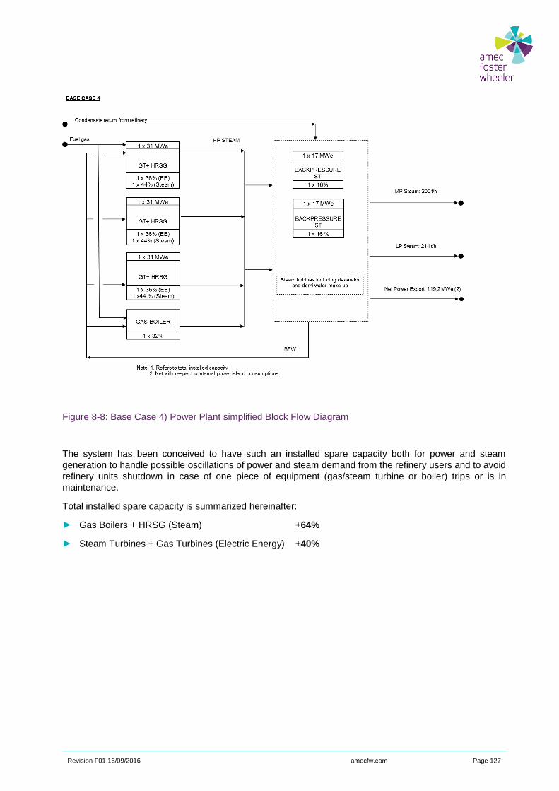
Revision F01 16/09/2016 amecfw.com Page 127
Figure 8-8: Base Case 4) Power Plant simplified Block Flow Diagram
The system has been conceived to have such an installed spare capacity both for power and steam
generation to handle possible oscillations of power and steam demand from the refinery users and to avoid
refinery units shutdown in case of one piece of equipment (gas/steam turbine or boiler) trips or is in
maintenance.
Total installed spare capacity is summarized hereinafter:
► Gas Boilers + HRSG (Steam) +64%
► Steam Turbines + Gas Turbines (Electric Energy) +40%
ReCAP Project
Understanding the Cost of
Retrofitting CO2 Capture in
an Integrated Oil
Refinery
Performance analysis of CO2 capture
options
SINTEF Energy Research
Gas Technology 2017‐06‐20
2017:00220‐ Unrestricted
Report
Understanding the Cost of Retrofitting CO2 capture in an Integrated Oil Refinery
Performance analysis of CO2 capture options
Authors Rahul Anantharaman, Kristin Jordal, Chao Fu, Per Eilif Wahl, Elisabeth Vågenes

2 of 45
SINTEF Energi AS SINTEF Energy Research
Address: Postboks 4761 Sluppen NO‐7465 Trondheim NORWAY Switchboard: +47 73597200 Telefax: +47 73597250
[email protected] www.sintef.no/energi Enterprise /VAT No: NO 939 350 675 MVA
REPORT NO.
2017:00220
ISBN
CLASSIFICATION
Unrestricted
CLASSIFICATION THIS PAGE
Unrestricted
PROJECT NO. 502000822
REPORT NO. 2017:00220
VERSION Final 3 of 45
Document history
VERSION DATE VERSION DESCRIPTION
1 2017‐04‐28 First version with results for all post‐combustion capture cases. CO2 avoided missing.
2 2017‐04‐28 Second version: Modified according to input from Concawe to V1. Added CO2 avoided for Base Case 4 and report summary.
3 (final) 2017‐06‐20 Final version incorporating comments from CONCAWE, IEAGHG. Updated the report to include Base Cases 1‐3.

PROJECT NO. 502000822
REPORT NO. 2017:00220
VERSION Final 4 of 45
Table of contents
Summary .................................................................................................................................................. 6
1 Introduction ................................................................................................................................... 13
1.1 Assumptions ................................................................................................................................. 13
1.2 Capture case selection rationale .................................................................................................. 13
1.3 Results generation and processing .............................................................................................. 13
2 Post‐combustion CO2 capture process using MEA ........................................................................... 15
3 Flue gas desulfurization .................................................................................................................. 17
4 Base Case 1 .................................................................................................................................... 18
4.1 Capture case descriptions ............................................................................................................ 18
4.2 Results .......................................................................................................................................... 19
4.2.1 Specific utilities consumption .......................................................................................... 19
4.2.2 Steam consumption ......................................................................................................... 19
4.2.3 Makeup water consumption ........................................................................................... 20
4.2.4 Cooling water requirement ............................................................................................. 21
4.2.5 Electric power consumption ............................................................................................ 22
4.2.6 CO2 avoided ..................................................................................................................... 22
5 Base Case 2 .................................................................................................................................... 24
5.1 Capture case descriptions ............................................................................................................ 24
5.2 Results .......................................................................................................................................... 25
5.2.1 Specific utilities consumption .......................................................................................... 25
5.2.2 Steam consumption ......................................................................................................... 25
5.2.3 Makeup water consumption ........................................................................................... 26
5.2.4 Cooing water requirement .............................................................................................. 27
5.2.5 Electric power consumption ............................................................................................ 27
5.2.6 CO2 avoided ..................................................................................................................... 28
6 Base Case 3 .................................................................................................................................... 29
6.1 Capture case descriptions ............................................................................................................ 29
6.2 Results .......................................................................................................................................... 30
6.2.1 Specific utilities consumption .......................................................................................... 30
6.2.2 Steam consumption ......................................................................................................... 30
6.2.3 Makeup water consumption ........................................................................................... 31
PROJECT NO. 502000822
REPORT NO. 2017:00220
VERSION Final 5 of 45
6.2.4 Cooing water requirement .............................................................................................. 32
6.2.5 Electric power consumption ............................................................................................ 32
6.2.6 CO2 avoided ..................................................................................................................... 33
7 Base Case 4 .................................................................................................................................... 34
7.1 Capture case descriptions ............................................................................................................ 34
7.2 Results .......................................................................................................................................... 35
7.2.1 Specific utilities consumption .......................................................................................... 35
7.2.2 Steam consumption ......................................................................................................... 36
7.2.3 Makeup water consumption ........................................................................................... 37
7.2.4 Cooing water requirement .............................................................................................. 37
7.2.5 Electric power consumption ............................................................................................ 38
7.2.6 CO2 avoided ..................................................................................................................... 39
8 CO2 capture from SMRs in refineries ............................................................................................... 40
9 Literature review of Oxy‐combustion capture from FCCs in refineries ............................................. 43
A CO2 capture process summary, stream data and PFDs .................................................................... 45
B CO2 capture integration and utilities ............................................................................................... 45
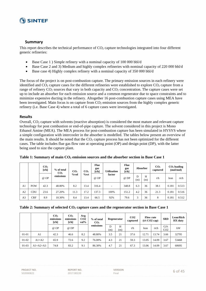
PROJECT NO. 502000822
REPORT NO. 2017:00220
VERSION Final 6 of 45
Summary
This report describes the technical performance of CO2 capture technologies integrated into four different generic refineries:
Base Case 1 ) Simple refinery with a nominal capacity of 100 000 bbl/d Base Case 2 and 3) Medium and highly complex refineries with nominal capacity of 220 000 bbl/d Base case 4) Highly complex refinery with a nominal capacity of 350 000 bbl/d
The focus of the project is on post-combustion capture. The primary emission sources in each refinery were identified and CO2 capture cases for the different refineries were established to explore CO2 capture from a range of refinery CO2 sources that vary in both capacity and CO2 concentration. The capture cases were set up to include an absorber for each emission source and a common regenerator due to space constraints and to minimize expensive ducting in the refinery. Altogether 16 post-combustion capture cases using MEA have been investigated. Main focus is on capture from CO2 emission sources from the highly complex generic refinery (i.e. Base Case 4) where a total of 6 capture cases were investigated. Results Overall, CO2 capture with solvents (reactive absorption) is considered the most mature and relevant capture technology for post combustion or end-of-pipe capture. The solvent considered in this project is Mono Ethanol Amine (MEA). The MEA process for post-combustion capture has been simulated in HYSYS where a simple configuration with intercooler in the absorber is modelled. The tables below present an overview of the main results. It should be noted that the CO2 capture process has not been optimized for the different cases. The table includes flue gas flow rate at operating point (OP) and design point (DP), with the latter being used to size the capture plant. Table 1: Summary of main CO2 emission sources and the absorber section in Base Case 1
CO2 [t/h] % of total
CO2 emissions
CO2 %vol
CO2 %wt
Flue gas [t/h] Utilization
factor
Flue gas [t/h]
Absorber CO2
captured CO2 loading
(mol/mol)
@ OP @ OP @ DP D
(m) H
(m) t/h lean rich
A1 POW 42.3 48.80% 8.2 13.4 316.4 - 348.8 6.3 36 38.1 0.181 0.513
A2 CDU 23.6 27.20% 11.3 17.2 137.3 100% 151.2 4.2 36 21.3 0.181 0.516
A3 CRF 8.9 10.30% 8.4 13.4 66.5 92% 79.6 3 36 8 0.181 0.512
Table 2: Summary of selected CO2 capture cases and the regenerator section in Base Case 1
CO2 emissions
[t/h]
CO2 emissions
[t/h]
Avg CO2 vol%
% of total CO2
emissions
Regenerator CO2
captured Flow rate
(t/t CO2 cap) SRD
Lean/Rich HX duty
@ OP @ DP D (m)
H (m)
t/h lean rich GJ/t CO2
kW
01-01 A1 42.3 46.6 8.2 48.80% 3.5 21 37.6 12.71 13.74 3.66 32795
01-02 A1+A2 65.9 72.6 9.2 76.00% 4.3 21 59.3 13.05 14.09 3.67 53468
01-03 A1+A2+A3 74.8 83.2 9.1 86.30% 4.7 21 67.3 13.06 14.09 3.67 60695
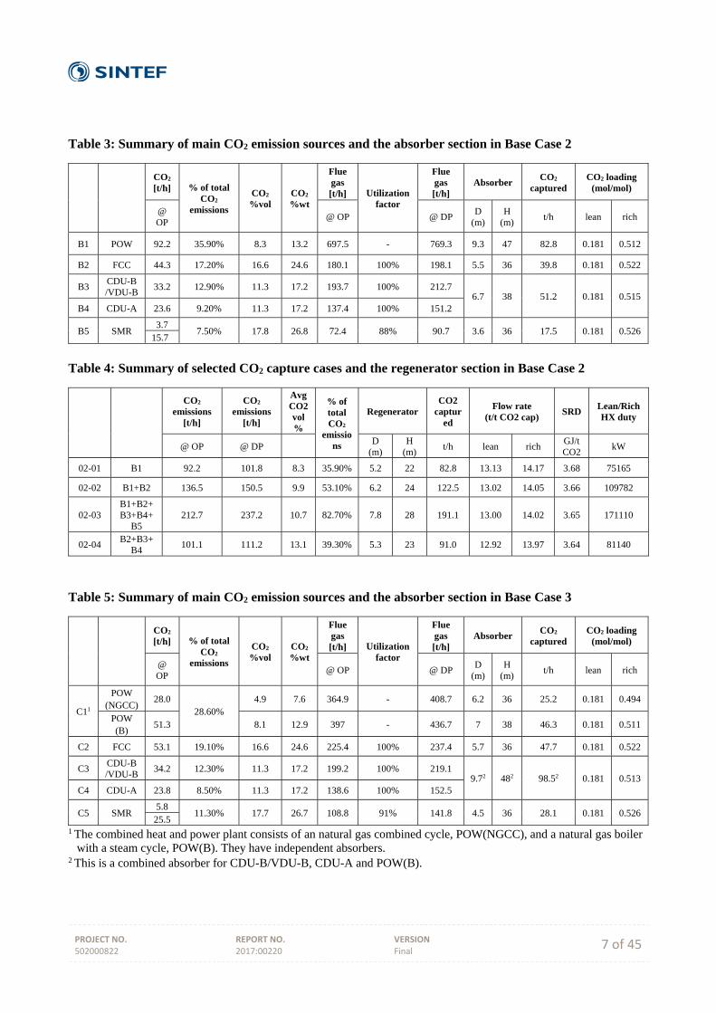
PROJECT NO. 502000822
REPORT NO. 2017:00220
VERSION Final 7 of 45
Table 3: Summary of main CO2 emission sources and the absorber section in Base Case 2
CO2 [t/h] % of total
CO2 emissions
CO2 %vol
CO2 %wt
Flue gas [t/h] Utilization
factor
Flue gas [t/h]
Absorber CO2
captured CO2 loading
(mol/mol)
@ OP
@ OP @ DP D
(m) H
(m) t/h lean rich
B1 POW 92.2 35.90% 8.3 13.2 697.5 - 769.3 9.3 47 82.8 0.181 0.512
B2 FCC 44.3 17.20% 16.6 24.6 180.1 100% 198.1 5.5 36 39.8 0.181 0.522
B3 CDU-B /VDU-B
33.2 12.90% 11.3 17.2 193.7 100% 212.7 6.7 38 51.2 0.181 0.515
B4 CDU-A 23.6 9.20% 11.3 17.2 137.4 100% 151.2
B5 SMR 3.7
7.50% 17.8 26.8 72.4 88% 90.7 3.6 36 17.5 0.181 0.526 15.7
Table 4: Summary of selected CO2 capture cases and the regenerator section in Base Case 2
CO2 emissions
[t/h]
CO2 emissions
[t/h]
Avg CO2 vol%
% of total CO2
emissions
Regenerator CO2
captured
Flow rate (t/t CO2 cap)
SRD Lean/Rich HX duty
@ OP @ DP D (m)
H (m)
t/h lean rich GJ/t CO2
kW
02-01 B1 92.2 101.8 8.3 35.90% 5.2 22 82.8 13.13 14.17 3.68 75165
02-02 B1+B2 136.5 150.5 9.9 53.10% 6.2 24 122.5 13.02 14.05 3.66 109782
02-03 B1+B2+B3+B4+
B5 212.7 237.2 10.7 82.70% 7.8 28 191.1 13.00 14.02 3.65 171110
02-04 B2+B3+
B4 101.1 111.2 13.1 39.30% 5.3 23 91.0 12.92 13.97 3.64 81140
Table 5: Summary of main CO2 emission sources and the absorber section in Base Case 3
CO2 [t/h] % of total
CO2 emissions
CO2 %vol
CO2 %wt
Flue gas [t/h] Utilization
factor
Flue gas [t/h]
Absorber CO2
captured CO2 loading
(mol/mol)
@ OP
@ OP @ DP D
(m) H
(m) t/h lean rich
C11
POW (NGCC)
28.0 28.60%
4.9 7.6 364.9 - 408.7 6.2 36 25.2 0.181 0.494
POW (B)
51.3 8.1 12.9 397 - 436.7 7 38 46.3 0.181 0.511
C2 FCC 53.1 19.10% 16.6 24.6 225.4 100% 237.4 5.7 36 47.7 0.181 0.522
C3 CDU-B /VDU-B
34.2 12.30% 11.3 17.2 199.2 100% 219.1 9.72 482 98.52 0.181 0.513
C4 CDU-A 23.8 8.50% 11.3 17.2 138.6 100% 152.5
C5 SMR 5.8
11.30% 17.7 26.7 108.8 91% 141.8 4.5 36 28.1 0.181 0.526 25.5
1 The combined heat and power plant consists of an natural gas combined cycle, POW(NGCC), and a natural gas boiler with a steam cycle, POW(B). They have independent absorbers.
2 This is a combined absorber for CDU-B/VDU-B, CDU-A and POW(B).
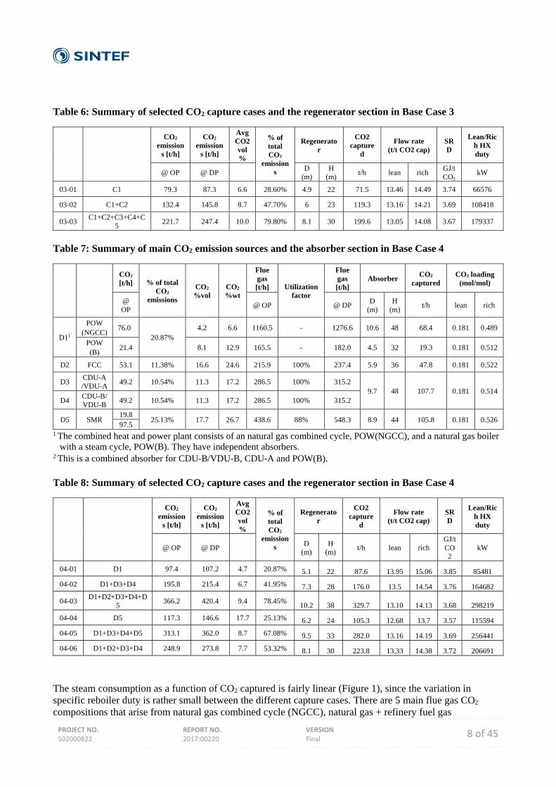
PROJECT NO. 502000822
REPORT NO. 2017:00220
VERSION Final 8 of 45
Table 6: Summary of selected CO2 capture cases and the regenerator section in Base Case 3
CO2 emission
s [t/h]
CO2 emission
s [t/h]
Avg CO2 vol%
% of total CO2
emissions
Regenerator
CO2 capture
d
Flow rate (t/t CO2 cap)
SRD
Lean/Rich HX duty
@ OP @ DP D (m)
H (m)
t/h lean rich GJ/t CO2
kW
03-01 C1 79.3 87.3 6.6 28.60% 4.9 22 71.5 13.46 14.49 3.74 66576
03-02 C1+C2 132.4 145.8 8.7 47.70% 6 23 119.3 13.16 14.21 3.69 108418
03-03 C1+C2+C3+C4+C
5 221.7 247.4 10.0 79.80% 8.1 30 199.6 13.05 14.08 3.67 179337
Table 7: Summary of main CO2 emission sources and the absorber section in Base Case 4
CO2 [t/h] % of total
CO2 emissions
CO2 %vol
CO2 %wt
Flue gas [t/h] Utilization
factor
Flue gas [t/h]
Absorber CO2
captured CO2 loading
(mol/mol)
@ OP
@ OP @ DP D
(m) H
(m) t/h lean rich
D11
POW (NGCC)
76.0 20.87%
4.2 6.6 1160.5 - 1276.6 10.6 48 68.4 0.181 0.489
POW (B)
21.4 8.1 12.9 165.5 - 182.0 4.5 32 19.3 0.181 0.512
D2 FCC 53.1 11.38% 16.6 24.6 215.9 100% 237.4 5.9 36 47.8 0.181 0.522
D3 CDU-A /VDU-A
49.2 10.54% 11.3 17.2 286.5 100% 315.2 9.7 48 107.7 0.181 0.514
D4 CDU-B/ VDU-B
49.2 10.54% 11.3 17.2 286.5 100% 315.2
D5 SMR 19.8
25.13% 17.7 26.7 438.6 88% 548.3 8.9 44 105.8 0.181 0.526 97.5
1 The combined heat and power plant consists of an natural gas combined cycle, POW(NGCC), and a natural gas boiler with a steam cycle, POW(B). They have independent absorbers.
2 This is a combined absorber for CDU-B/VDU-B, CDU-A and POW(B). Table 8: Summary of selected CO2 capture cases and the regenerator section in Base Case 4
CO2 emission
s [t/h]
CO2 emission
s [t/h]
Avg CO2 vol%
% of total CO2
emissions
Regenerator
CO2 capture
d
Flow rate (t/t CO2 cap)
SRD
Lean/Rich HX duty
@ OP @ DP D (m)
H (m)
t/h lean rich GJ/t CO2
kW
04-01 D1 97.4 107.2 4.7 20.87% 5.1 22 87.6 13.95 15.06 3.85 85481
04-02 D1+D3+D4 195.8 215.4 6.7 41.95% 7.3 28 176.0 13.5 14.54 3.76 164682
04-03 D1+D2+D3+D4+D
5 366.2 420.4 9.4 78.45%
10.2 38 329.7 13.10 14.13 3.68 298219
04-04 D5 117.3 146.6 17.7 25.13% 6.2 24 105.3 12.68 13.7 3.57 115594
04-05 D1+D3+D4+D5 313.1 362.0 8.7 67.08% 9.5 33 282.0 13.16 14.19 3.69 256441
04-06 D1+D2+D3+D4 248.9 273.8 7.7 53.32% 8.1 30 223.8 13.33 14.38 3.72 206691
The steam consumption as a function of CO2 captured is fairly linear (Figure 1), since the variation in specific reboiler duty is rather small between the different capture cases. There are 5 main flue gas CO2 compositions that arise from natural gas combined cycle (NGCC), natural gas + refinery fuel gas

PROJECT NO. 502000822
REPORT NO. 2017:00220
VERSION Final 9 of 45
combustion, fuel oil combustion, fluid catalytic cracker (FCC) catalyst regeneration and steam methane reformer (SMR) furnace exhaust. Of these, the NGCC flue gas and SMR exhaust are the outliers with the NGCC having a CO2 concentration of around 4vol% while the SMR furnace exhaust has a CO2 concentration of around 18%. The specific reboiler duty (SRD) of the NGCC unit is higher than that of the SMR exhaust. However, as most of the cases have absorbers with a combination of flue gas compositions, the effect of this variation is diluted. The highest SRD is 3.85 GJ/t CO2 captured for Case 04-01 (NGCC) and the lowest is 3.57 for Case 04-04 (SMR). Most of the other cases have SRDs in between 3.64-3.69 GJ/t CO2 captured.
Figure 1. Reboiler steam consumption dependency on captured CO2 for all investigated capture cases.
As expected, the power consumption for CO2 compression as function of captured CO2 is linear (Figure 2)
Figure 2. Compressor power dependency on captured CO2 captured for all investigated capture cases.
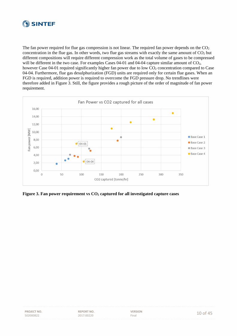
PROJECT NO. 502000822
REPORT NO. 2017:00220
VERSION Final 10 of 45
The fan power required for flue gas compression is not linear. The required fan power depends on the CO2 concentration in the flue gas. In other words, two flue gas streams with exactly the same amount of CO2 but different compositions will require different compression work as the total volume of gases to be compressed will be different in the two case. For examples Cases 04-01 and 04-04 capture similar amount of CO2, however Case 04-01 required significantly higher fan power due to low CO2 concentration compared to Case 04-04. Furthermore, flue gas desulphurization (FGD) units are required only for certain flue gases. When an FGD is required, addition power is required to overcome the FGD pressure drop. No trendlines were therefore added in Figure 3. Still, the figure provides a rough picture of the order of magnitude of fan power requirement.
Figure 3. Fan power requirement vs CO2 captured for all investigated capture cases

PROJECT NO. 502000822
REPORT NO. 2017:00220
VERSION Final 11 of 45
Figure 4. Pump power vs CO2 captured for all investigated capture cases
The pump power requirement also depends on CO2 concentration in the flue gas (Figure 4). Additionally, the CO2 loading also has an effect on the pump power requirement. Compared to the fan power consumption, the pump power appears to show a small deviation from a linear relationship due to its smaller magnitude. For a quick, rough, back-of-the-envelope estimation, the pump power can be assumed to be linear. All the absorbers in this work are designed to capture 90% of the CO2 from the stacks. However, the net CO2 avoided is significantly lower than the CO2 capture rate of 90%. This is due to CO2 emissions from the natural-gas fired CHP plant required for providing additional steam and power. The net CO2 avoided is around 60% only.
Suggestions for future work on post‐combustion capture from integrated oil refineries The results in this report are used as the technology basis for estimating the cost of retrofitting post-combustion CO2 capture to refineries, as presented in the subsequent report Cost estimation and economic evaluation of CO2 capture options for refineries. The study does not pretend to cover all possible technical aspects of refinery post-combustion capture. Items that merit further attention are
Investigating and quantifying the (expected reduced) energy consumption when applying a more modern solvent than MEA. Such solvents may require steam at different pressure/condensing temperature, and the reboiler/stripper may also operate at a different pressure than in the present case. The investigation is therewith more complex than just reducing the specific steam consumption.
PROJECT NO. 502000822
REPORT NO. 2017:00220
VERSION Final 12 of 45
Advanced process configurations of post combustion capture process: Le Moullec et al.1 provide an exhaustive review of 20 process modifications for improved process efficiency of solvent-based post-combtion CO2 capture process. They are classified under process improvements for enhanced absorption, heat integration and heat pumping. Among then split flow arrangements are the most common where the general principle is to regenerate the solvent at two or more loading ratios.
CO2 capture from refineries integrated in industrial clusters. It is clear from the present report that generating the steam and power required for CO2 capture and compression with a stand-alone natural-gas fired CHP plant significantly reduces the CO2 avoided – although 90% of the CO2 is captured from the investigated emission points, the net CO2 avoided is only around 60%. Refineries located in industrial clusters with excess heat available should therefore be of interest to investigate from a CO2 capture perspective – if the necessary steam can be provided with little or no additional fuel consumption this would be beneficial from a CO2 emissions perspective. Power supply would then ideally come from a highly efficient thermal plant with CCS, or even from renewable energy.
CO2 capture from H2 production and Fluid Catalytic Cracker (FCC) As mentioned earlier, the focus of this report is on post-combustion capture from refinery emission sources. However, CO2 capture from syngas stream in an SMR and oxy-combustion capture from fluid catalytic cracking are receiving significant attention for CO2 capture from refineries. A brief study is provided of CO2 capture from a refinery SMR based on the IEAGHG report Techno-Economic Evaluation of Deploying CCS in Standalone (Merchant) SMR Based Hydrogen Plant using Natural Gas as Feedstock/Fuel, report No 2017-02. This case is investigated in this report on CO2 capture from the SMR in Base Case 4 ("Case 04-04" in Chapter 7). Also, a literature review is provided in this report on oxy-combustion capture from Fluid Catalytic Crackers (FCC) in refineries, mainly relating to research undertaken by the CCP (CO2 capture project)2.
1 Le Moullec, Y., Neveux, T., Al Azki, A., Chikukwa, A., Hoff, K.A., 2014. Process modifications for solvent-based
post-combustion CO2 capture. Int. J. Greenh. Gas Control 31, 96–112.
2 http://www.co2captureproject.org/

PROJECT NO. 502000822
REPORT NO. 2017:00220
VERSION Final 13 of 45
1 Introduction
The aim of this study is to describe and analyse the technical performance of CO2 capture from refineries. Four generic refinery Base Cases were developed and described by Amec FW in the document Performance Analysis – Refinery Reference Plants:
Base Case 1) Simple refinery with a nominal capacity of 100 000 bbl/d Base Case 2 and 3) Medium to highly complex refineries with nominal capacity of 220 000 bbl/d Base case 4) Highly complex refinery with a nominal capacity of 350 000 bbl/d
All post combustion CO2 capture studies in this document are related to one of these cases. Main focus is on CO2 capture from refinery Base Case 4, which is seen as the most relevant reference for existing European refineries of interest for retrofit of CO2 capture. The aim is that the work presented in this report together with Performance Analysis – Refinery Reference Plants should be a useful basis the European refinery industry to estimate the energy and utilities requirements for CO2 capture from their own refineries. Overall, CO2 capture with solvents (reactive absorption) is considered the most mature and relevant capture technology for post combustion or end-of-pipe capture. The solvent considered in this project is Mono Ethanol Amine (MEA). MEA is used in this study primarily as it is considered as "standard" with well-known thermodynamics. It has also been used in many other IEAGHG CO2 capture studies. Solvents are also considered mature technology for CO2 capture from shifted syngas associated with Steam Methane Reformer (SMR) for hydrogen production. This option has not been investigated in detail in the present work. Instead, results are retrieved from the recently published IEAGHG report "Techno-Economic Evaluation of Standalone H2 Plant (Merchant)", and related to the results for CO2 capture from the SMR in Base Case 4 (Case 04-04). Finally, to cover oxy-combustion capture from refineries, a review on work done on oxyfuel capture for refineries in the CCP project is presented in chapter 9.
1.1 Assumptions
A basic assumption for this study of CO2 capture from refineries is that the refinery production does not change, i.e. amount of crude fed to the refineries as well as the products and product quantities are unchanged. To provide the additional steam required for MEA regeneration and additional power required by the CO2 capture unit and associated units, it is assumed that an additional natural gas-fired CHP plant is constructed on the refinery site. CO2 capture from this CHP plant has not been included in the study. CO2 capture can of course be added to such a CHP plant also, but this would require a scale-up of the plant to produce additional steam for this additional CO2 capture.
1.2 Capture case selection rationale
For the emission sources from the four refinery Base Cases, a range of CO2 capture cases were defined, focusing on the largest point sources among the refinery stacks. The rationale for selecting the cases was to have one case with a rather low capture rate (while ignoring really small, and hence impractical, emission sources), one with medium capture rate and one with high capture rate. After selecting the first 12 cases, one additional capture case was selected for Base Case 2 (case 02-04) and three additional capture cases were selected for Base Case 4 (cases 04-04, 04-05 and 04-06). The rationale for these selections is provided in sections 5.1 and 7.1.
1.3 Results generation and processing
The 16 CO2 capture cases were simulated in Aspen HYSYS v9. The input data are defined in the report Common Framework – technical. Changes in this input (e.g. ambient conditions or cooling water temperature) would of course have an impact on the results.

PROJECT NO. 502000822
REPORT NO. 2017:00220
VERSION Final 14 of 45
After simulating the CO2 capture cases, Excel-based results files with the main results and stream data were generated. The main simulation results can be found in appendix A, where also process flow diagrams (PFDs) for each capture case are included. Key results (consumption of steam and power, cooling and makeup water requirement) are displayed graphically for all capture cases. The process simulation results were used by Amec Foster Wheeler to establish the refinery balances, which can be found in appendix B. The CO2 emissions from the CHP plants were used to calculate the net CO2 emissions for each capture case. Process simulations of the capture cases were done at the operating point, i.e. matching the operating points of the refinery Base Cases, as listed in the report Performance analysis – Refinery reference plants. Also, the refinery balances were established for the operating point.
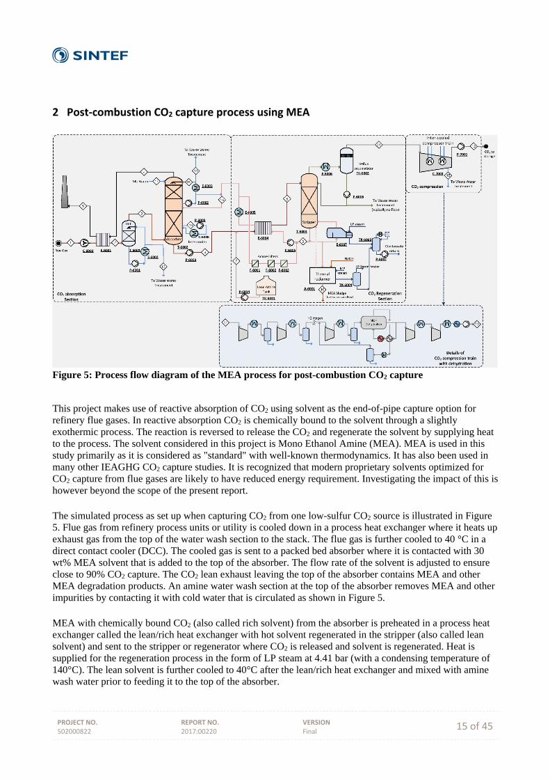
PROJECT NO. 502000822
REPORT NO. 2017:00220
VERSION Final 15 of 45
2 Post‐combustion CO2 capture process using MEA
Figure 5: Process flow diagram of the MEA process for post-combustion CO2 capture
This project makes use of reactive absorption of CO2 using solvent as the end-of-pipe capture option for refinery flue gases. In reactive absorption CO2 is chemically bound to the solvent through a slightly exothermic process. The reaction is reversed to release the CO2 and regenerate the solvent by supplying heat to the process. The solvent considered in this project is Mono Ethanol Amine (MEA). MEA is used in this study primarily as it is considered as "standard" with well-known thermodynamics. It has also been used in many other IEAGHG CO2 capture studies. It is recognized that modern proprietary solvents optimized for CO2 capture from flue gases are likely to have reduced energy requirement. Investigating the impact of this is however beyond the scope of the present report. The simulated process as set up when capturing CO2 from one low-sulfur CO2 source is illustrated in Figure 5. Flue gas from refinery process units or utility is cooled down in a process heat exchanger where it heats up exhaust gas from the top of the water wash section to the stack. The flue gas is further cooled to 40 °C in a direct contact cooler (DCC). The cooled gas is sent to a packed bed absorber where it is contacted with 30 wt% MEA solvent that is added to the top of the absorber. The flow rate of the solvent is adjusted to ensure close to 90% CO2 capture. The CO2 lean exhaust leaving the top of the absorber contains MEA and other MEA degradation products. An amine water wash section at the top of the absorber removes MEA and other impurities by contacting it with cold water that is circulated as shown in Figure 5. MEA with chemically bound CO2 (also called rich solvent) from the absorber is preheated in a process heat exchanger called the lean/rich heat exchanger with hot solvent regenerated in the stripper (also called lean solvent) and sent to the stripper or regenerator where CO2 is released and solvent is regenerated. Heat is supplied for the regeneration process in the form of LP steam at 4.41 bar (with a condensing temperature of 140°C). The lean solvent is further cooled to 40°C after the lean/rich heat exchanger and mixed with amine wash water prior to feeding it to the top of the absorber.

PROJECT NO. 502000822
REPORT NO. 2017:00220
VERSION Final 16 of 45
The CO2 released from the top of the regenerator contains mainly water and nitrogen as impurities. This is sent to a seven stage inter-cooled compression process to compress the CO2 product stream to 85 bar. The water is flashed out after the first five intercooling stages and then sent to a molecular sieve dehydration process to achieve the 10 ppm water specification in the CO2 product stream. 10% of the dry CO2 stream from the dehydration process is used as a purge gas in the regeneration stage of the dehydration process, and then recycled back to the prior stage for recompression. After compression to 85 bar the CO2 product is cooled with cooling water and a chiller (using propane as refrigerant) in series to reach 25°C and then pumped to 110 bars. The use of a chiller is not necessarily required, but this is a process design choice that was made for the present study. MEA degrades in the presence of O2, SOx and NOx in addition to thermal degradation. A portion of the lean amine is sent to the thermal reclaimer to remove the degraded MEA by forming heat stable salts with sodium hydroxide (NaOH). Heat is supplied to the thermal reclaimer as MP steam. As mentioned earlier, the reaction is slightly exothermic that causes the temperature to increase along the height of the absorber column from the bottom to the top. While MEA absorption kinetics are favoured by high temperatures, the absorption capacity deteriorates. An intercooler is thus included in the process close to the bottom to cool the solvent to 40°C and boost absorption and reduce the specific energy for solvent regeneration, commonly referred to as Specific Reboiler Duty (SRD). The placement of this intercooler has not been optimised as part of this work. Another option to decrease the SRD is to increase the temperature at the top of the absorber to improve kinetics. Thus pre-cooled amine wash water is mixed with the cooled lean amine to achieve a temperature of around 50°C rather than 40°C for the lean amine feed to the absorber. It should be noted that the absorption profile is top heavy, i.e., most of the absorption of CO2 in the MEA takes places at the top of the column. In cases where CO2 is captured from more than one stack, one absorber per stack is typically used in the simulations, while there is one common stripper for the refinery. It is common refinery practice to pipe rich solvents to one common stripper. The simulations for the different cases were performed in Aspen HYSYS v9.
PROJECT NO. 502000822
REPORT NO. 2017:00220
VERSION Final 17 of 45
3 Flue gas desulfurization
The flue gases from the CDU/VDU and FCC have a sulfur content of 240.8 and 256.5 ppmv respectively. This would cause excessive amine degradation, and the sulfur content of the flue gas must be reduced prior to CO2 capture. A SOx content of 10 ppmv is known as an economical limitation for MEA CO2 capture processes. Flue Gas Desulfurization (FGD) units should thus be installed for sulfur removal prior to the CO2 capture process. In the wet scrubbing process applied here, the reagent is reacted with SOx in a wet scrubber where the flue gas passes through. The reagent in wet scrubbers can be limestone (CaCO3), lime (CaO), magnesium enhanced lime (MgO and CaO) and sodium carbonate (Na2CO3). Limestone based wet FGD technology, which can achieve very high sulfur removal rates, has the largest number of industrial installations. The technology has been selected in this project. Limestone (CaCO3) and SO2 are converted into gypsum (CaSO4·2H2O) with presence of water and oxygen. The overall reaction is shown in the following equation.
3 2 2 2 4 2 2CaCO +SO +2H O+0.5O CaSO 2H O+CO
The mass balance of the FGD unit, such as the removal rate of SO2, the consumption of limestone and O2 as well as the production of gypsum, is mainly determined using the above reaction. The flue gas at the outlet of the wet scrubber is saturated with water. The flue gas is cooled mainly due to the evaporation of water vapor. The water content in the flue gas thus increases. Fresh water make-up is necessary to balance the water lost into the flue gas, the effluent as well as the water in gypsum. The impurities in the effluent is referred to the IEAGHG report (2010/05). The main energy consumption of the FGD unit is the additional electric power that is consumed to drive an additional induced draft fan to overcome the pressure drops in the unit, the oxidization air blower, the agitators and the pumps. The wet FGD units are included for the CO2 capture cases where the SOx content in the flue gas exceeds 10 ppmv, as can be seen from the process flow diagrams as well as the stream data for the cases.

PROJECT NO. 502000822
REPORT NO. 2017:00220
VERSION Final 18 of 45
4 Base Case 1
It should be noted that all results provided for CO2 capture from this and the other Base Cases in this report are for the refinery operating point, as determined in the report Performance analysis – Refinery reference plants. Sizing and costing in the subsequent report Cost estimation and economic evaluation of CO2 capture options is done for the design point.
4.1 Capture case descriptions
The three largest emission sources in the refinery Base Case 1, the power plant (A1), the crude distillation unit (A2) and the catalytic reformer (A3), were selected as candidates for CO2 capture (refer to Table 9). The emissions from the power plant (A1) are from natural gas and refinery fuel gas combustion in gas boilers. The emissions from the crude distillation unit (A2) come from fuel oil combustion in the fired heater related to the process while that of the catalytic reformer unit (A3) comes from natural gas and refinery fuel gas combustion in the fired heater related to the process. Table 9. Emission sources selected for capture in refinery Base Case 1.
CO2 [t/h] @
operating point
% of total CO2
emissionsCO2 %vol CO2 %wt
Flue gas [t/h]
@ operating point
A1 POW1 42.3 48.8% 8.2 13.4 317.1
A2 CDU 23.6 27.2% 11.3 17.2 137.4
A3 CRF 8.9 10.3% 8.4 13.4 66.6 1Reference should be made to section 1.1.1 in report Performance analysis – Refinery reference plants for explanation of abbreviations POW, CDU, CRF. Based on the emission sources in Table 9, three post-combustion capture cases were defined for refinery Base Case 1 that capture an incrementally larger share of the refinery CO2 emissions. The three capture cases selected are shown in Table 10. Table 10. The three selected capture cases for refinery Base Case 1. Refer to Table 9 for definition of emission sources A1-A3.
CO2 emissions
[t/h] @ operating point
% of total CO2 emissions
Avg CO2 vol%
01‐01 A1 42.3 48.8% 8.2
01‐02 A1+A2 65.9 76.0% 9.2
01‐03 A1+A2+A3 74.8 86.3% 9.1
The refinery Base Case 1 without CO2 capture is self-sustained with power. To cover the additional power consumption caused by the CO2 capture and compression, an additional natural gas-fired CHP plant is included (see appendix B). CO2 is not captured from this CHP plant in the present study.
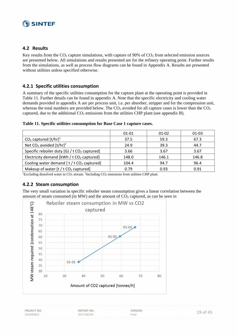
PROJECT NO. 502000822
REPORT NO. 2017:00220
VERSION Final 19 of 45
4.2 Results
Key results from the CO2 capture simulations, with capture of 90% of CO2 from selected emission sources are presented below. All simulations and results presented are for the refinery operating point. Further results from the simulations, as well as process flow diagrams can be found in Appendix A. Results are presented without utilities unless specified otherwise.
4.2.1 Specific utilities consumption
A summary of the specific utilities consumption for the capture plant at the operating point is provided in Table 11. Further details can be found in appendix A. Note that the specific electricity and cooling water demands provided in appendix A are per process unit, i.e. per absorber, stripper and for the compression unit, whereas the total numbers are provided below. The CO2 avoided for all capture cases is lower than the CO2 captured, due to the additional CO2 emissions from the utilities CHP plant (see appendix B). Table 11. Specific utilities consumption for Base Case 1 capture cases.
01‐01 01‐02 01‐03 CO2 captured [t/hr]1 37.5 59.3 67.3
Net CO2 avoided [t/hr]2 24.9 39.3 44.7
Specific reboiler duty [GJ / t CO2 captured] 3.66 3.67 3.67
Electricity demand [kWh / t CO2 captured] 148.0 146.1 146.8
Cooling water demand [ t / t CO2 captured] 104.4 94.7 96.4
Makeup of water [t / t CO2 captured] 0.79 0.93 0.91 1Excluding dissolved water in CO2 stream. 2Including CO2 emissions from utilities CHP plant.
4.2.2 Steam consumption
The very small variation in specific reboiler steam consumption gives a linear correlation between the amount of steam consumed (in MW) and the amount of CO2 captured, as can be seen in

PROJECT NO. 502000822
REPORT NO. 2017:00220
VERSION Final 20 of 45
Figure 6. It should be recalled that the heat released from condensing steam varies4 with varying condensation temperature and pressure, results are valid for steam condensing at 147.7°C with the corresponding heat of condensation being 2121.37 kJ/kg steam (a temperature approach of 20°C was selected in the CO2 capture process simulations).
Figure 6. Amount of CO2 captured as function of the amount of condensing steam for Base Case 1 capture cases.
4.2.3 Makeup water consumption
The total makeup water consumption for each case can be seen in Figure 7.
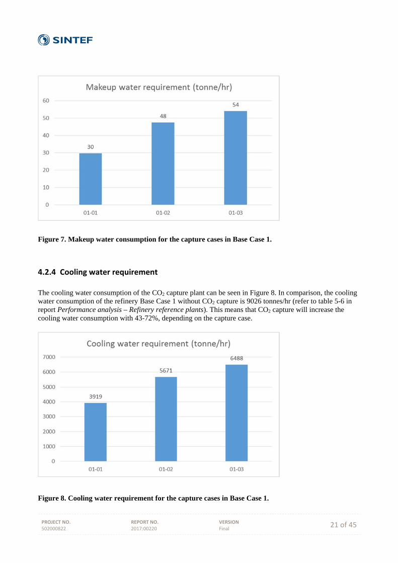
PROJECT NO. 502000822
REPORT NO. 2017:00220
VERSION Final 21 of 45
Figure 7. Makeup water consumption for the capture cases in Base Case 1.
4.2.4 Cooling water requirement
The cooling water consumption of the CO2 capture plant can be seen in Figure 8. In comparison, the cooling water consumption of the refinery Base Case 1 without CO2 capture is 9026 tonnes/hr (refer to table 5-6 in report Performance analysis – Refinery reference plants). This means that CO2 capture will increase the cooling water consumption with 43-72%, depending on the capture case.
Figure 8. Cooling water requirement for the capture cases in Base Case 1.

PROJECT NO. 502000822
REPORT NO. 2017:00220
VERSION Final 22 of 45
4.2.5 Electric power consumption
The electric power consumption caused by the CO2 capture can be seen in Figure 9. As can be seen, the main power consumers are CO2 compression and flue gas fans, whereas the power consumption for the CO2 pump and chiller is of smaller significance. In comparison, the power consumption for the refinery Base Case 1 without CO2 capture is 28 MW (refer to table 5-6 in report Performance analysis – Refinery reference plants). This means that the power consumption increases with 20-35% depending on the capture case.
Figure 9. Electric power consumption for the capture cases in Base Case 1.
4.2.6 CO2 avoided
As mentioned above, it has been assumed in this report that an additional natural gas-fired CHP plant is constructed on the refinery site to respond to increased steam and power requirements. CO2 capture from this CHP plant has not been included in the study. Hence, although the CO2 capture from the stacks in the investigated cases is 90%, the net CO2 avoided from these emission sources is lower. This is illustrated in Figure 10.
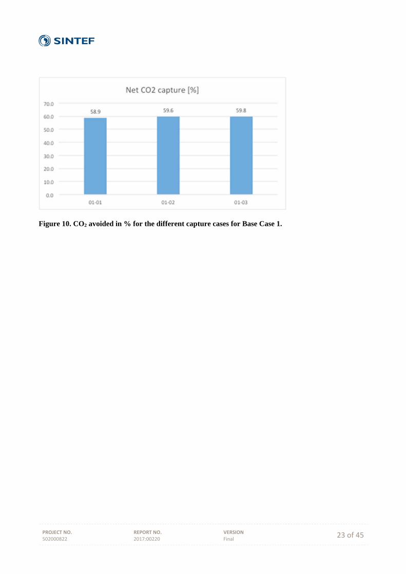
PROJECT NO. 502000822
REPORT NO. 2017:00220
VERSION Final 23 of 45
Figure 10. CO2 avoided in % for the different capture cases for Base Case 1.
PROJECT NO. 502000822
REPORT NO. 2017:00220
VERSION Final 24 of 45
5 Base Case 2
It should be noted that all results provided for CO2 capture from this and the other Base Cases in this report are for the refinery operating point, as determined in the report Performance analysis – Refinery reference plants. Sizing and costing in the subsequent report Cost estimation and economic evaluation of CO2 capture options is done for the design point.
5.1 Capture case descriptions
The five largest emission sources in the refinery Base Case 2, the power plant (B1), the fluid catalytic cracking unit (B2), the crude and vacuum distillation units train B (B3), the crude distillation unit train A (B4) and the steam methane reformer (B5), were selected as candidates for CO2 capture (refer to Table 12). The emissions from the power plant (B1) are from natural gas and refinery fuel gas combustion in gas boilers. The emissions from the fluid catalytic cracking unit (B2) come from burning coke desposited on the catalysts in the cracking process and regeneration of the deactivated catalyst. The emissions from the crude and vacuum distillation units train B and the crude distillation unit train A (B3 and B4) come from fuel oil combustion in the fired heater related to the process. The steam methane reformer (B5) converts natural gas to syngas that mainly contains hydrogen and carbon dioxide. The syngas stream contains 15.7 t/h of CO2 as shown in Table 12 with a concentration of 24.2 vol% (35.2 wt%). H2 is separated from CO2 in a PSA and the resulting tail gas that mainly contains CO2, some H2 and unreacted methane are sent to the furnace as supplementary fuel. Refinery fuel gas is used as the primary fuel in the furnace to provide heat to the endothermic reforming reaction. The combustion of refinery fuel gas results in 3.7 t/h of CO2. Thus the total CO2 emitted in the furnace exhaust is the sum of these two sources with a concentration of 17.7 vol% (26.7 wt%). Table 12. Emission sources selected for capture in refinery Base Case 2.
CO2 [t/h] @
operating point
% of total CO2
emissionsCO2 %vol CO2 %wt
Flue gas [t/h]
@ operating point
B1 POW1 92.2 35.9% 8.3 13.2 697.5
B2 FCC 44.3 17.2% 16.6 24.6 180.1
B3 CDU‐B/VDU‐B 33.2 12.9% 11.3 17.2 193.7
B4 CDU‐A 23.6 9.2% 11.3 17.2 137.4
B5 SMR 3.7
7.5% 17.7 26.4 72.4 15.7
1Reference should be made to section 1.1.2 in report Performance analysis – Refinery reference plants for explanation of abbreviations POW, FCC, CDU, VDU, SMR.
Based on the emission sources listed in Table 12, four CO2 capture cases were defined for Base Case 2. First, cases 02-01, 02-02 and 02-03 were selected according to the principle to have three cases of varying size. Thereafter case 02-04 was added. Approximately the same amount of CO2 is capture from cases 02-01 and 02-04, but the difference is that the flue gases in case 02-04 require desulfurization before CO2 capture while case 02-01 does not, and the difference in cost between these two options is interesting to investigate. The capture cases are described in Table 13.
PROJECT NO. 502000822
REPORT NO. 2017:00220
VERSION Final 25 of 45
Table 13. The four selected capture cases for refinery Base Case 2. Refer to Table 12Table 9 for definition of emission sources B1-B5.
CO2 emissions
[t/h] @ operating point
% of total CO2 emissions
Avg CO2 vol%
02‐01 B1 92.3 35.9% 8.3
02‐02 B1+B2 136.5 53.1% 9.9
02‐03 B1+B2+B3+B4+B5 212.7 82.7% 10.7
02‐04 B2+B3+B4 101.1 39.3% 13.1
The refinery Base Case 2 without CO2 capture is self-sustained with power. To cover the additional power consumption caused by the CO2 capture and compression, an additional natural gas-fired CHP plant is included (see appendix B). CO2 is not captured from this CHP plant in the present study.
5.2 Results
Key results from the CO2 capture simulations, with capture of 90% of CO2 from selected emission sources are presented below. All simulations and results presented are for the refinery operating point. Further results from the simulations, as well as process flow diagrams can be found in Appendix A. Results are presented without utilities unless specified otherwise. In the diagrams, the cases are presented in ascending order with respect to amount of CO2 captured, i.e. case 02-04 is presented between case 02-10 and case 02-02. Further results from the simulations can be found in Appendix A.
5.2.1 Specific utilities consumption
A summary of the specific utilities consumption for the capture plant at the operating point is provided in Table 14. Further details can be found in appendix A. Note that the specific electricity and cooling water demands provided in appendix A are per process unit, i.e. per absorber, stripper and for the compression unit, whereas the total numbers are provided below. The CO2 avoided for all capture cases is lower than the CO2 captured, due to the additional CO2 emissions from the utilities CHP plant (see appendix B). Table 14. Specific utilities consumption for Base Case 2 capture cases.
02‐01 02‐02 02‐03 02‐04
CO2 captured [t/hr]1 82.8 122.5 191.1 91.0
Net CO2 avoided [t/hr]2 54.9 81.4 127.2 60.6
Steam demand [GJ / t CO2 captured] 3.68 3.66 3.65 3.64
Electricity demand [kWh / t CO2 captured] 155.2 144.2 142.1 139.8
Cooling water demand [ t / t CO2 captured] 101.5 96.9 92.1 86.6
Makeup of water [t / t CO2 captured] 0.93 0.95 0.98 1.19 1Excluding dissolved water in CO2 stream. 2Including CO2 emissions from utilities CHP plant.
5.2.2 Steam consumption
The very small variation in specific reboiler steam consumption gives a linear correlation between the amount of steam consumed (in MW) and the amount of CO2 captured, as can be seen in

PROJECT NO. 502000822
REPORT NO. 2017:00220
VERSION Final 26 of 45
Figure 11. It should be recalled that the heat released from condensing steam varies with varying condensation temperature and pressure, i.e. is valid for steam condensing at 147.7°C with the corresponding heat of condensation being 2121.37 kJ/kg steam (a temperature approach of 20°C was selected in the CO2 capture process simulations).
Figure 11. Amount of CO2 captured as function of the amount of condensing steam for Base Case 2 capture cases.
5.2.3 Makeup water consumption
The makeup water consumption for each case can be seen in Figure 12.
Figure 12. Makeup water consumption for the capture cases in Base Case 2.
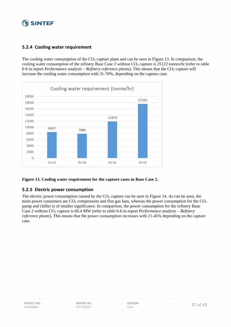
PROJECT NO. 502000822
REPORT NO. 2017:00220
VERSION Final 27 of 45
5.2.4 Cooling water requirement
The cooling water consumption of the CO2 capture plant and can be seen in Figure 13. In comparison, the cooling water consumption of the refinery Base Case 2 without CO2 capture is 25122 tonnes/hr (refer to table 6-6 in report Performance analysis – Refinery reference plants). This means that the CO2 capture will increase the cooling water consumption with 31-70%, depending on the capture case.
Figure 13. Cooling water requirement for the capture cases in Base Case 2.
5.2.5 Electric power consumption
The electric power consumption caused by the CO2 capture can be seen in Figure 14. As can be seen, the main power consumers are CO2 compression and flue gas fans, whereas the power consumption for the CO2 pump and chiller is of smaller significance. In comparison, the power consumption for the refinery Base Case 2 without CO2 capture is 60.4 MW (refer to table 6-6 in report Performance analysis – Refinery reference plants). This means that the power consumption increases with 21-45% depending on the capture case.
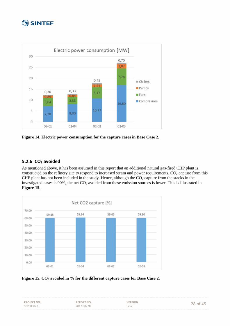
PROJECT NO. 502000822
REPORT NO. 2017:00220
VERSION Final 28 of 45
Figure 14. Electric power consumption for the capture cases in Base Case 2.
5.2.6 CO2 avoided
As mentioned above, it has been assumed in this report that an additional natural gas-fired CHP plant is constructed on the refinery site to respond to increased steam and power requirements. CO2 capture from this CHP plant has not been included in the study. Hence, although the CO2 capture from the stacks in the investigated cases is 90%, the net CO2 avoided from these emission sources is lower. This is illustrated in Figure 15.
Figure 15. CO2 avoided in % for the different capture cases for Base Case 2.
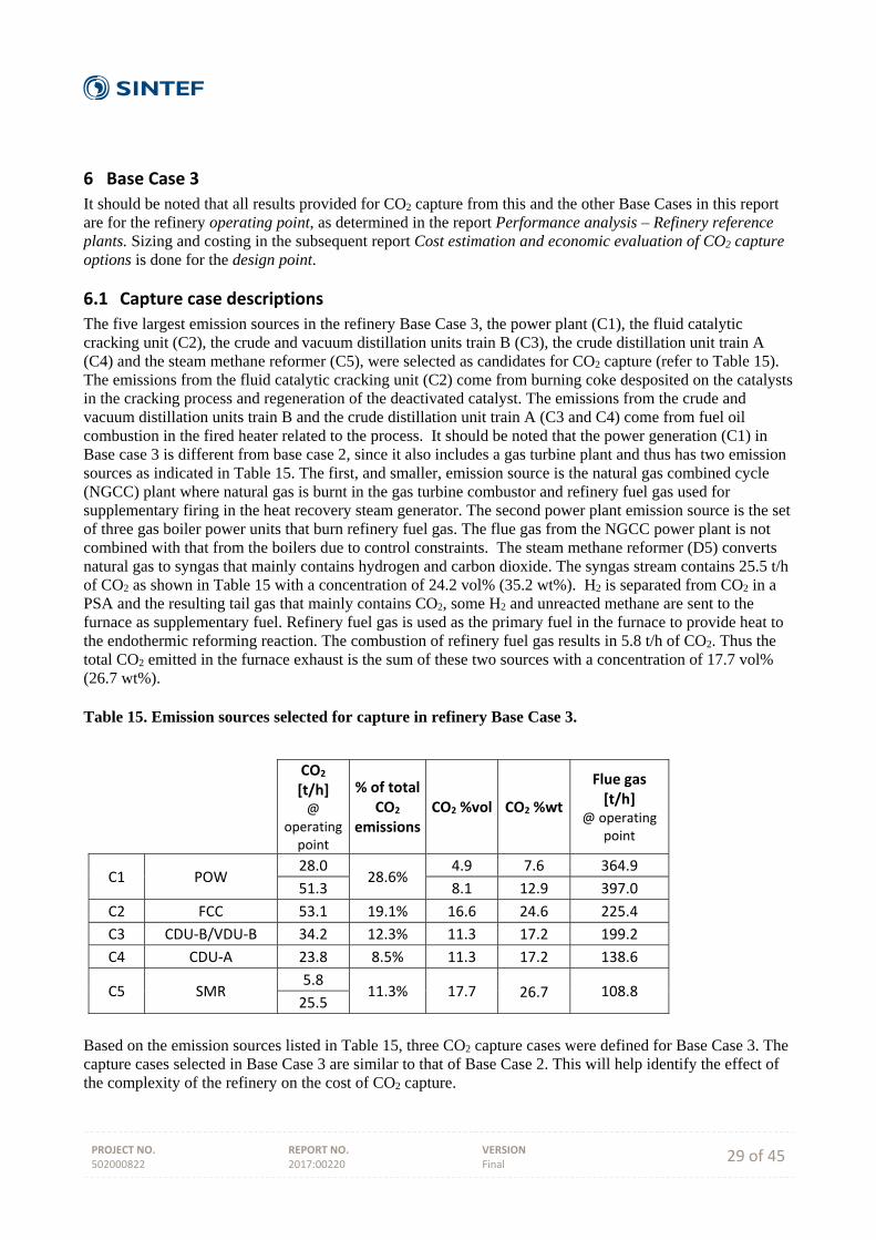
PROJECT NO. 502000822
REPORT NO. 2017:00220
VERSION Final 29 of 45
6 Base Case 3
It should be noted that all results provided for CO2 capture from this and the other Base Cases in this report are for the refinery operating point, as determined in the report Performance analysis – Refinery reference plants. Sizing and costing in the subsequent report Cost estimation and economic evaluation of CO2 capture options is done for the design point.
6.1 Capture case descriptions
The five largest emission sources in the refinery Base Case 3, the power plant (C1), the fluid catalytic cracking unit (C2), the crude and vacuum distillation units train B (C3), the crude distillation unit train A (C4) and the steam methane reformer (C5), were selected as candidates for CO2 capture (refer to Table 15). The emissions from the fluid catalytic cracking unit (C2) come from burning coke desposited on the catalysts in the cracking process and regeneration of the deactivated catalyst. The emissions from the crude and vacuum distillation units train B and the crude distillation unit train A (C3 and C4) come from fuel oil combustion in the fired heater related to the process. It should be noted that the power generation (C1) in Base case 3 is different from base case 2, since it also includes a gas turbine plant and thus has two emission sources as indicated in Table 15. The first, and smaller, emission source is the natural gas combined cycle (NGCC) plant where natural gas is burnt in the gas turbine combustor and refinery fuel gas used for supplementary firing in the heat recovery steam generator. The second power plant emission source is the set of three gas boiler power units that burn refinery fuel gas. The flue gas from the NGCC power plant is not combined with that from the boilers due to control constraints. The steam methane reformer (D5) converts natural gas to syngas that mainly contains hydrogen and carbon dioxide. The syngas stream contains 25.5 t/h of CO2 as shown in Table 15 with a concentration of 24.2 vol% (35.2 wt%). H2 is separated from CO2 in a PSA and the resulting tail gas that mainly contains CO2, some H2 and unreacted methane are sent to the furnace as supplementary fuel. Refinery fuel gas is used as the primary fuel in the furnace to provide heat to the endothermic reforming reaction. The combustion of refinery fuel gas results in 5.8 t/h of CO2. Thus the total CO2 emitted in the furnace exhaust is the sum of these two sources with a concentration of 17.7 vol% (26.7 wt%). Table 15. Emission sources selected for capture in refinery Base Case 3.
CO2 [t/h] @
operating point
% of total CO2
emissionsCO2 %vol CO2 %wt
Flue gas [t/h]
@ operating point
C1 POW 28.0
28.6% 4.9 7.6 364.9
51.3 8.1 12.9 397.0
C2 FCC 53.1 19.1% 16.6 24.6 225.4
C3 CDU‐B/VDU‐B 34.2 12.3% 11.3 17.2 199.2
C4 CDU‐A 23.8 8.5% 11.3 17.2 138.6
C5 SMR 5.8
11.3% 17.7 26.7 108.8 25.5
Based on the emission sources listed in Table 15, three CO2 capture cases were defined for Base Case 3. The capture cases selected in Base Case 3 are similar to that of Base Case 2. This will help identify the effect of the complexity of the refinery on the cost of CO2 capture.
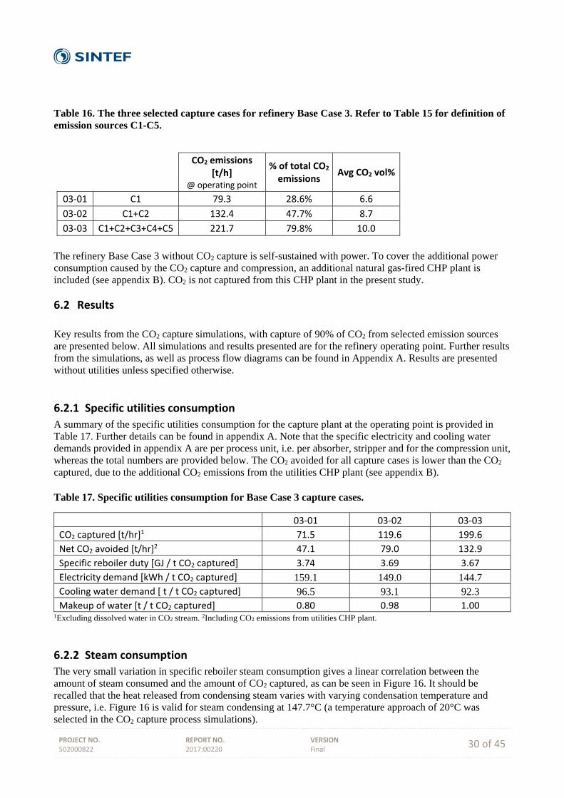
PROJECT NO. 502000822
REPORT NO. 2017:00220
VERSION Final 30 of 45
Table 16. The three selected capture cases for refinery Base Case 3. Refer to Table 15 for definition of emission sources C1-C5.
CO2 emissions
[t/h] @ operating point
% of total CO2 emissions
Avg CO2 vol%
03‐01 C1 79.3 28.6% 6.6
03‐02 C1+C2 132.4 47.7% 8.7
03‐03 C1+C2+C3+C4+C5 221.7 79.8% 10.0
The refinery Base Case 3 without CO2 capture is self-sustained with power. To cover the additional power consumption caused by the CO2 capture and compression, an additional natural gas-fired CHP plant is included (see appendix B). CO2 is not captured from this CHP plant in the present study.
6.2 Results
Key results from the CO2 capture simulations, with capture of 90% of CO2 from selected emission sources are presented below. All simulations and results presented are for the refinery operating point. Further results from the simulations, as well as process flow diagrams can be found in Appendix A. Results are presented without utilities unless specified otherwise.
6.2.1 Specific utilities consumption
A summary of the specific utilities consumption for the capture plant at the operating point is provided in Table 17. Further details can be found in appendix A. Note that the specific electricity and cooling water demands provided in appendix A are per process unit, i.e. per absorber, stripper and for the compression unit, whereas the total numbers are provided below. The CO2 avoided for all capture cases is lower than the CO2 captured, due to the additional CO2 emissions from the utilities CHP plant (see appendix B). Table 17. Specific utilities consumption for Base Case 3 capture cases.
03‐01 03‐02 03‐03 CO2 captured [t/hr]1 71.5 119.6 199.6
Net CO2 avoided [t/hr]2 47.1 79.0 132.9
Specific reboiler duty [GJ / t CO2 captured] 3.74 3.69 3.67
Electricity demand [kWh / t CO2 captured] 159.1 149.0 144.7 Cooling water demand [ t / t CO2 captured] 96.5 93.1 92.3 Makeup of water [t / t CO2 captured] 0.80 0.98 1.00
1Excluding dissolved water in CO2 stream. 2Including CO2 emissions from utilities CHP plant.
6.2.2 Steam consumption
The very small variation in specific reboiler steam consumption gives a linear correlation between the amount of steam consumed and the amount of CO2 captured, as can be seen in Figure 16. It should be recalled that the heat released from condensing steam varies with varying condensation temperature and pressure, i.e. Figure 16 is valid for steam condensing at 147.7°C (a temperature approach of 20°C was selected in the CO2 capture process simulations).
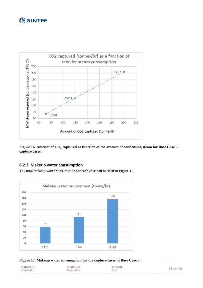
PROJECT NO. 502000822
REPORT NO. 2017:00220
VERSION Final 31 of 45
Figure 16. Amount of CO2 captured as function of the amount of condensing steam for Base Case 3 capture cases.
6.2.3 Makeup water consumption
The total makeup water consumption for each case can be seen in Figure 17.
Figure 17. Makeup water consumption for the capture cases in Base Case 3.
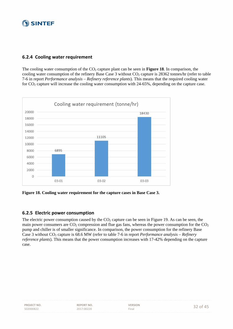
PROJECT NO. 502000822
REPORT NO. 2017:00220
VERSION Final 32 of 45
6.2.4 Cooling water requirement
The cooling water consumption of the CO2 capture plant can be seen in Figure 18. In comparison, the cooling water consumption of the refinery Base Case 3 without CO2 capture is 28362 tonnes/hr (refer to table 7-6 in report Performance analysis – Refinery reference plants). This means that the required cooling water for CO2 capture will increase the cooling water consumption with 24-65%, depending on the capture case.
Figure 18. Cooling water requirement for the capture cases in Base Case 3.
6.2.5 Electric power consumption
The electric power consumption caused by the CO2 capture can be seen in Figure 19. As can be seen, the main power consumers are CO2 compression and flue gas fans, whereas the power consumption for the CO2 pump and chiller is of smaller significance. In comparison, the power consumption for the refinery Base Case 3 without CO2 capture is 68.6 MW (refer to table 7-6 in report Performance analysis – Refinery reference plants). This means that the power consumption increases with 17-42% depending on the capture case.

PROJECT NO. 502000822
REPORT NO. 2017:00220
VERSION Final 33 of 45
Figure 19. Electric power consumption for the capture cases in Base Case 3.
6.2.6 CO2 avoided
As mentioned above, it has been assumed in this report that an additional natural gas-fired CHP plant is constructed on the refinery site to respond to increased steam and power requirements. CO2 capture from this CHP plant has not been included in the study. Hence, although the CO2 capture from the stacks in the investigated cases is 90%, the net CO2 avoided from these emission sources is lower. This is illustrated in Figure 20.
Figure 20. CO2 avoided in % for the different capture cases for Base Case 3.
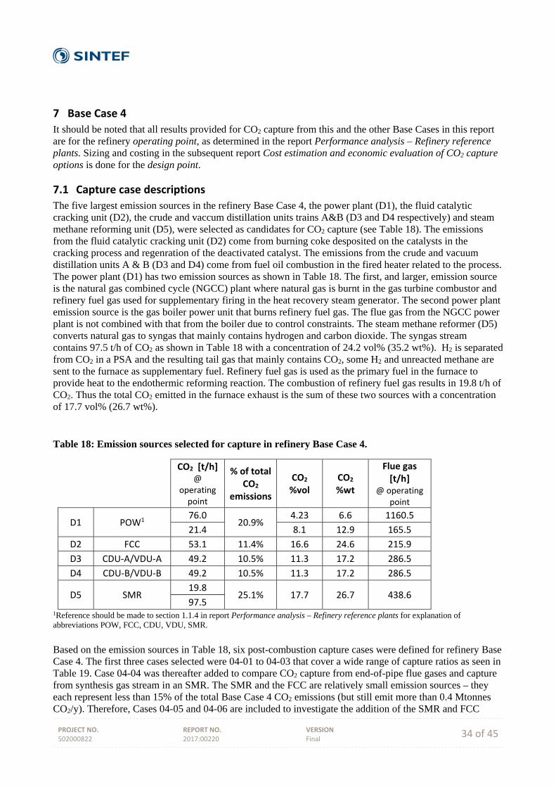
PROJECT NO. 502000822
REPORT NO. 2017:00220
VERSION Final 34 of 45
7 Base Case 4
It should be noted that all results provided for CO2 capture from this and the other Base Cases in this report are for the refinery operating point, as determined in the report Performance analysis – Refinery reference plants. Sizing and costing in the subsequent report Cost estimation and economic evaluation of CO2 capture options is done for the design point.
7.1 Capture case descriptions
The five largest emission sources in the refinery Base Case 4, the power plant (D1), the fluid catalytic cracking unit (D2), the crude and vaccum distillation units trains A&B (D3 and D4 respectively) and steam methane reforming unit (D5), were selected as candidates for CO2 capture (see Table 18). The emissions from the fluid catalytic cracking unit (D2) come from burning coke desposited on the catalysts in the cracking process and regenration of the deactivated catalyst. The emissions from the crude and vacuum distillation units A & B (D3 and D4) come from fuel oil combustion in the fired heater related to the process. The power plant (D1) has two emission sources as shown in Table 18. The first, and larger, emission source is the natural gas combined cycle (NGCC) plant where natural gas is burnt in the gas turbine combustor and refinery fuel gas used for supplementary firing in the heat recovery steam generator. The second power plant emission source is the gas boiler power unit that burns refinery fuel gas. The flue gas from the NGCC power plant is not combined with that from the boiler due to control constraints. The steam methane reformer (D5) converts natural gas to syngas that mainly contains hydrogen and carbon dioxide. The syngas stream contains 97.5 t/h of CO2 as shown in Table 18 with a concentration of 24.2 vol% (35.2 wt%). H2 is separated from CO2 in a PSA and the resulting tail gas that mainly contains CO2, some H2 and unreacted methane are sent to the furnace as supplementary fuel. Refinery fuel gas is used as the primary fuel in the furnace to provide heat to the endothermic reforming reaction. The combustion of refinery fuel gas results in 19.8 t/h of CO2. Thus the total CO2 emitted in the furnace exhaust is the sum of these two sources with a concentration of 17.7 vol% (26.7 wt%). Table 18: Emission sources selected for capture in refinery Base Case 4.
CO2 [t/h] @
operating point
% of total CO2
emissions
CO2 %vol
CO2 %wt
Flue gas [t/h]
@ operating point
D1 POW1 76.0
20.9% 4.23 6.6 1160.5
21.4 8.1 12.9 165.5
D2 FCC 53.1 11.4% 16.6 24.6 215.9
D3 CDU‐A/VDU‐A 49.2 10.5% 11.3 17.2 286.5
D4 CDU‐B/VDU‐B 49.2 10.5% 11.3 17.2 286.5
D5 SMR 19.8
25.1% 17.7 26.7 438.6 97.5
1Reference should be made to section 1.1.4 in report Performance analysis – Refinery reference plants for explanation of abbreviations POW, FCC, CDU, VDU, SMR. Based on the emission sources in Table 18, six post-combustion capture cases were defined for refinery Base Case 4. The first three cases selected were 04-01 to 04-03 that cover a wide range of capture ratios as seen in Table 19. Case 04-04 was thereafter added to compare CO2 capture from end-of-pipe flue gases and capture from synthesis gas stream in an SMR. The SMR and the FCC are relatively small emission sources – they each represent less than 15% of the total Base Case 4 CO2 emissions (but still emit more than 0.4 Mtonnes CO2/y). Therefore, Cases 04-05 and 04-06 are included to investigate the addition of the SMR and FCC
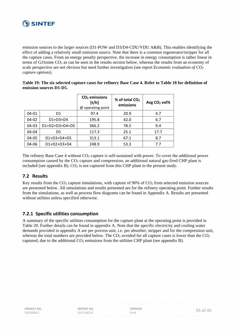
PROJECT NO. 502000822
REPORT NO. 2017:00220
VERSION Final 35 of 45
emission sources to the larger sources (D1-POW and D3/D4-CDU/VDU A&B). This enables identifying the effect of adding a relatively small emission source. Note that there is a common regenerator/stripper for all the capture cases. From an energy penalty perspective, the increase in energy consumption is rather linear in terms of GJ/tonne CO2 as can be seen in the results section below, whereas the results from an economy of scale perspective are not obvious but need further investigation (see report Economic evaluation of CO2 capture options). Table 19: The six selected capture cases for refinery Base Case 4. Refer to Table 18 for definition of emission sources D1-D5.
CO2 emissions
[t/h] @ operating point
% of total CO2 emissions
Avg CO2 vol%
04‐01 D1 97.4 20.9 4.7
04‐02 D1+D3+D4 195.8 42.0 6.7
04‐03 D1+D2+D3+D4+D5 366.2 78.5 9.4
04‐04 D5 117.3 25.1 17.7
04‐05 D1+D3+D4+D5 313.1 67.1 8.7
04‐06 D1+D2+D3+D4 248.9 53.3 7.7
The refinery Base Case 4 without CO2 capture is self-sustained with power. To cover the additional power consumption caused by the CO2 capture and compression, an additional natural gas-fired CHP plant is included (see appendix B). CO2 is not captured from this CHP plant in the present study.
7.2 Results
Key results from the CO2 capture simulations, with capture of 90% of CO2 from selected emission sources are presented below. All simulations and results presented are for the refinery operating point. Further results from the simulations, as well as process flow diagrams can be found in Appendix A. Results are presented without utilities unless specified otherwise.
7.2.1 Specific utilities consumption
A summary of the specific utilities consumption for the capture plant at the operating point is provided in Table 20. Further details can be found in appendix A. Note that the specific electricity and cooling water demands provided in appendix A are per process unit, i.e. per absorber, stripper and for the compression unit, whereas the total numbers are provided below. The CO2 avoided for all capture cases is lower than the CO2 captured, due to the additional CO2 emissions from the utilities CHP plant (see appendix B).
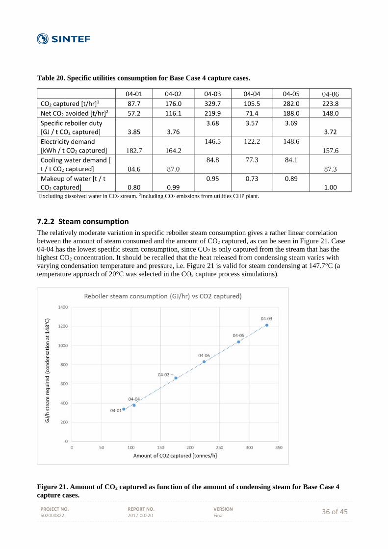
PROJECT NO. 502000822
REPORT NO. 2017:00220
VERSION Final 36 of 45
Table 20. Specific utilities consumption for Base Case 4 capture cases.
04‐01 04‐02 04‐03 04‐04 04‐05 04-06 CO2 captured [t/hr]1 87.7 176.0 329.7 105.5 282.0 223.8
Net CO2 avoided [t/hr]2 57.2 116.1 219.9 71.4 188.0 148.0
Specific reboiler duty [GJ / t CO2 captured] 3.85 3.76
3.68 3.57 3.69 3.72
Electricity demand [kWh / t CO2 captured] 182.7 164.2
146.5 122.2 148.6 157.6
Cooling water demand [ t / t CO2 captured] 84.6 87.0
84.8
77.3 84.1 87.3
Makeup of water [t / t CO2 captured] 0.80 0.99
0.95 0.73 0.89 1.00
1Excluding dissolved water in CO2 stream. 2Including CO2 emissions from utilities CHP plant.
7.2.2 Steam consumption
The relatively moderate variation in specific reboiler steam consumption gives a rather linear correlation between the amount of steam consumed and the amount of CO2 captured, as can be seen in Figure 21. Case 04-04 has the lowest specific steam consumption, since CO2 is only captured from the stream that has the highest CO2 concentration. It should be recalled that the heat released from condensing steam varies with varying condensation temperature and pressure, i.e. Figure 21 is valid for steam condensing at 147.7°C (a temperature approach of 20°C was selected in the CO2 capture process simulations).
Figure 21. Amount of CO2 captured as function of the amount of condensing steam for Base Case 4 capture cases.
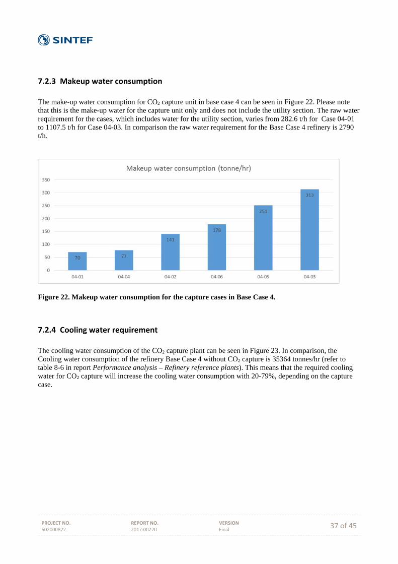
PROJECT NO. 502000822
REPORT NO. 2017:00220
VERSION Final 37 of 45
7.2.3 Makeup water consumption
The make-up water consumption for CO2 capture unit in base case 4 can be seen in Figure 22. Please note that this is the make-up water for the capture unit only and does not include the utility section. The raw water requirement for the cases, which includes water for the utility section, varies from 282.6 t/h for Case 04-01 to 1107.5 t/h for Case 04-03. In comparison the raw water requirement for the Base Case 4 refinery is 2790 t/h.
Figure 22. Makeup water consumption for the capture cases in Base Case 4.
7.2.4 Cooling water requirement
The cooling water consumption of the CO2 capture plant can be seen in Figure 23. In comparison, the Cooling water consumption of the refinery Base Case 4 without CO2 capture is 35364 tonnes/hr (refer to table 8-6 in report Performance analysis – Refinery reference plants). This means that the required cooling water for CO2 capture will increase the cooling water consumption with 20-79%, depending on the capture case.
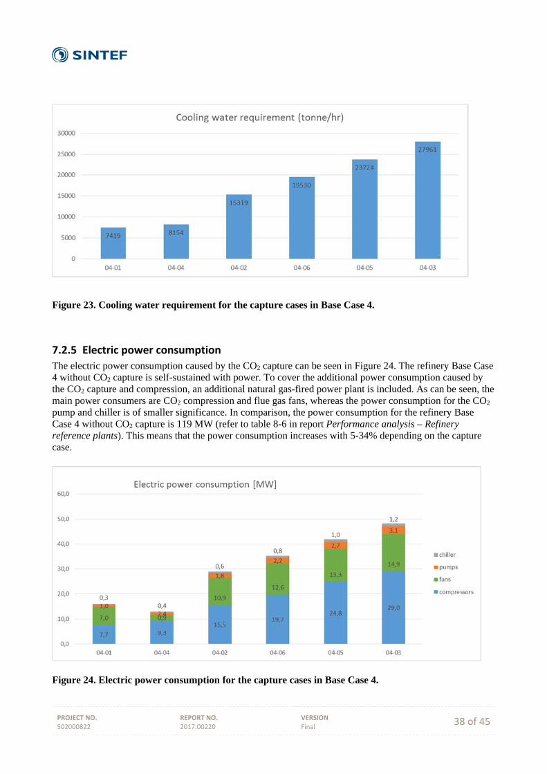
PROJECT NO. 502000822
REPORT NO. 2017:00220
VERSION Final 38 of 45
Figure 23. Cooling water requirement for the capture cases in Base Case 4.
7.2.5 Electric power consumption
The electric power consumption caused by the CO2 capture can be seen in Figure 24. The refinery Base Case 4 without CO2 capture is self-sustained with power. To cover the additional power consumption caused by the CO2 capture and compression, an additional natural gas-fired power plant is included. As can be seen, the main power consumers are CO2 compression and flue gas fans, whereas the power consumption for the CO2 pump and chiller is of smaller significance. In comparison, the power consumption for the refinery Base Case 4 without CO2 capture is 119 MW (refer to table 8-6 in report Performance analysis – Refinery reference plants). This means that the power consumption increases with 5-34% depending on the capture case.
Figure 24. Electric power consumption for the capture cases in Base Case 4.
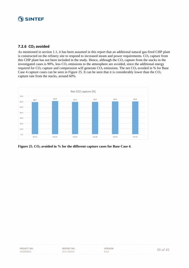
PROJECT NO. 502000822
REPORT NO. 2017:00220
VERSION Final 39 of 45
7.2.6 CO2 avoided
As mentioned in section 1.1, it has been assumed in this report that an additional natural gas-fired CHP plant is constructed on the refinery site to respond to increased steam and power requirements. CO2 capture from this CHP plant has not been included in the study. Hence, although the CO2 capture from the stacks in the investigated cases is 90%, less CO2 emissions to the atmosphere are avoided, since the additional energy required for CO2 capture and compression will generate CO2 emissions. The net CO2 avoided in % for Base Case 4 capture cases can be seen in Figure 25. It can be seen that it is considerably lower than the CO2 capture rate from the stacks, around 60%.
Figure 25. CO2 avoided in % for the different capture cases for Base Case 4.
PROJECT NO. 502000822
REPORT NO. 2017:00220
VERSION Final 40 of 45
8 CO2 capture from SMRs in refineries
IEAGHG has recently released a report3 that evaluates steam methane reformer (SMR) for hydrogen production with CCS through a techno-economic analysis. The study evaluates the design, performance and cost of a "greenfield" state-of-the-art SMR plant producing 100,000 Nm3/h of hydrogen using natural gas as feedstock and fuel. The work looked at different options for CO2 capture within the H2 plant with overall capture rate ranging between 50 and 90%. The different CO2 capture cases considered are:
Case 1A: SMR with CO2 capture from shifted syngas using MDEA Case 1B: SMR with burners firing H2 rich fuel and capture of CO2 from the shifted syngas using
MDEA Case 2A: SMR with CO2 capture from PSA tailgas using MDEA Case 2B: SMR with CO2 capture from PSA tail gas using cryogenic and membrane separation Case 03: SMR with capture of CO2 from the flue has using MEA.
The cases of specific interest to this report are Cases 1A and Case 03 as they are the most "mature" options for capturing CO2 from SMR process and have been demonstrated on industrial units. The performance parameters for these two cases compared with the base case SMR with no CO2 capture are provided in the table below. Table 21: Comparison of process performance of base case SMR with no CO2 capture and two capture options4
Base Case (no capture) Case 1A Case 3 Total energy input (as NG) [MWth]
394.77 407.68 433.72
Total energy in product (as H2) [MWth]
299.70 299.70 299.70
Net power exported to grid [MWe]
9.918 1.492 0.426
Specific NG consumption [MJ/Nm3 H2]
14.21 14.68 15.61
Specific CO2 emissions [kg/Nm3 H2]
0.8091 0.3704 0.0888
CO2 capture rate [%] - 55.7 90 CO2 avoided [%] - 54.2 89 SPECCA [MJ/kg CO2] - 2.44 2.90
Note that the SMR plant is a net exporter of power without CCS. The net power exported to the grid shown in Table 21 is from the hydrogen plant and not a separate combined heat and power plant. It is clear from Table 21 that Case 3 where CO2 is captured from flue gas at atmospheric conditions has a greater thermal energy input and lower net power output compared to Case 1A where CO2 is captured from shifted syngas prior to H2 purification in the PSA. However, Case 3 has a greater CO2 capture rate and CO2 avoided compared to Case 1A.
3 IEAGHG, Techno-Economic Evaluation of SMR Based Standalone (Merchant) Plant with CCS, 2017/02, February, 2017 4 All data from IEAGHG extracted from the above IEAGHG report except SPECCA
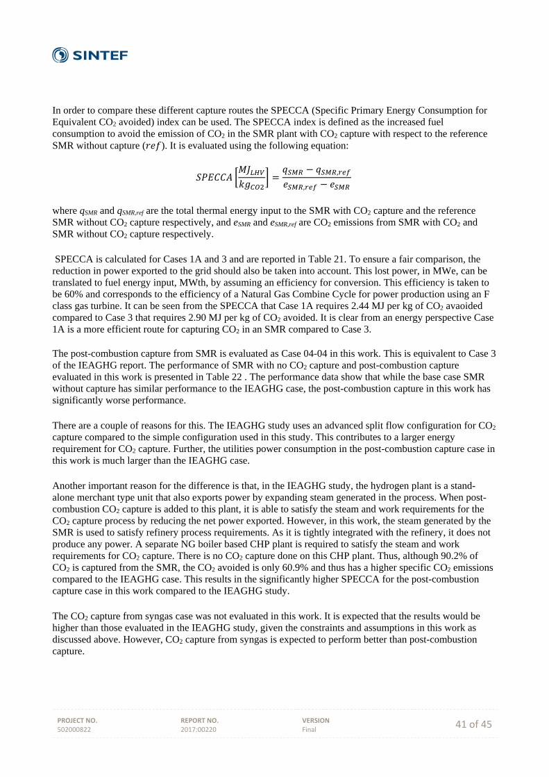
PROJECT NO. 502000822
REPORT NO. 2017:00220
VERSION Final 41 of 45
In order to compare these different capture routes the SPECCA (Specific Primary Energy Consumption for Equivalent CO2 avoided) index can be used. The SPECCA index is defined as the increased fuel consumption to avoid the emission of CO2 in the SMR plant with CO2 capture with respect to the reference SMR without capture ( ). It is evaluated using the following equation:
,
,
where qSMR and qSMR,ref are the total thermal energy input to the SMR with CO2 capture and the reference SMR without CO2 capture respectively, and eSMR and eSMR,ref are CO2 emissions from SMR with CO2 and SMR without CO2 capture respectively. SPECCA is calculated for Cases 1A and 3 and are reported in Table 21. To ensure a fair comparison, the reduction in power exported to the grid should also be taken into account. This lost power, in MWe, can be translated to fuel energy input, MWth, by assuming an efficiency for conversion. This efficiency is taken to be 60% and corresponds to the efficiency of a Natural Gas Combine Cycle for power production using an F class gas turbine. It can be seen from the SPECCA that Case 1A requires 2.44 MJ per kg of CO2 avaoided compared to Case 3 that requires 2.90 MJ per kg of CO2 avoided. It is clear from an energy perspective Case 1A is a more efficient route for capturing CO2 in an SMR compared to Case 3. The post-combustion capture from SMR is evaluated as Case 04-04 in this work. This is equivalent to Case 3 of the IEAGHG report. The performance of SMR with no CO2 capture and post-combustion capture evaluated in this work is presented in Table 22 . The performance data show that while the base case SMR without capture has similar performance to the IEAGHG case, the post-combustion capture in this work has significantly worse performance. There are a couple of reasons for this. The IEAGHG study uses an advanced split flow configuration for CO2 capture compared to the simple configuration used in this study. This contributes to a larger energy requirement for CO2 capture. Further, the utilities power consumption in the post-combustion capture case in this work is much larger than the IEAGHG case. Another important reason for the difference is that, in the IEAGHG study, the hydrogen plant is a stand-alone merchant type unit that also exports power by expanding steam generated in the process. When post-combustion CO2 capture is added to this plant, it is able to satisfy the steam and work requirements for the CO2 capture process by reducing the net power exported. However, in this work, the steam generated by the SMR is used to satisfy refinery process requirements. As it is tightly integrated with the refinery, it does not produce any power. A separate NG boiler based CHP plant is required to satisfy the steam and work requirements for CO2 capture. There is no CO2 capture done on this CHP plant. Thus, although 90.2% of CO2 is captured from the SMR, the CO2 avoided is only 60.9% and thus has a higher specific CO2 emissions compared to the IEAGHG case. This results in the significantly higher SPECCA for the post-combustion capture case in this work compared to the IEAGHG study. The CO2 capture from syngas case was not evaluated in this work. It is expected that the results would be higher than those evaluated in the IEAGHG study, given the constraints and assumptions in this work as discussed above. However, CO2 capture from syngas is expected to perform better than post-combustion capture.
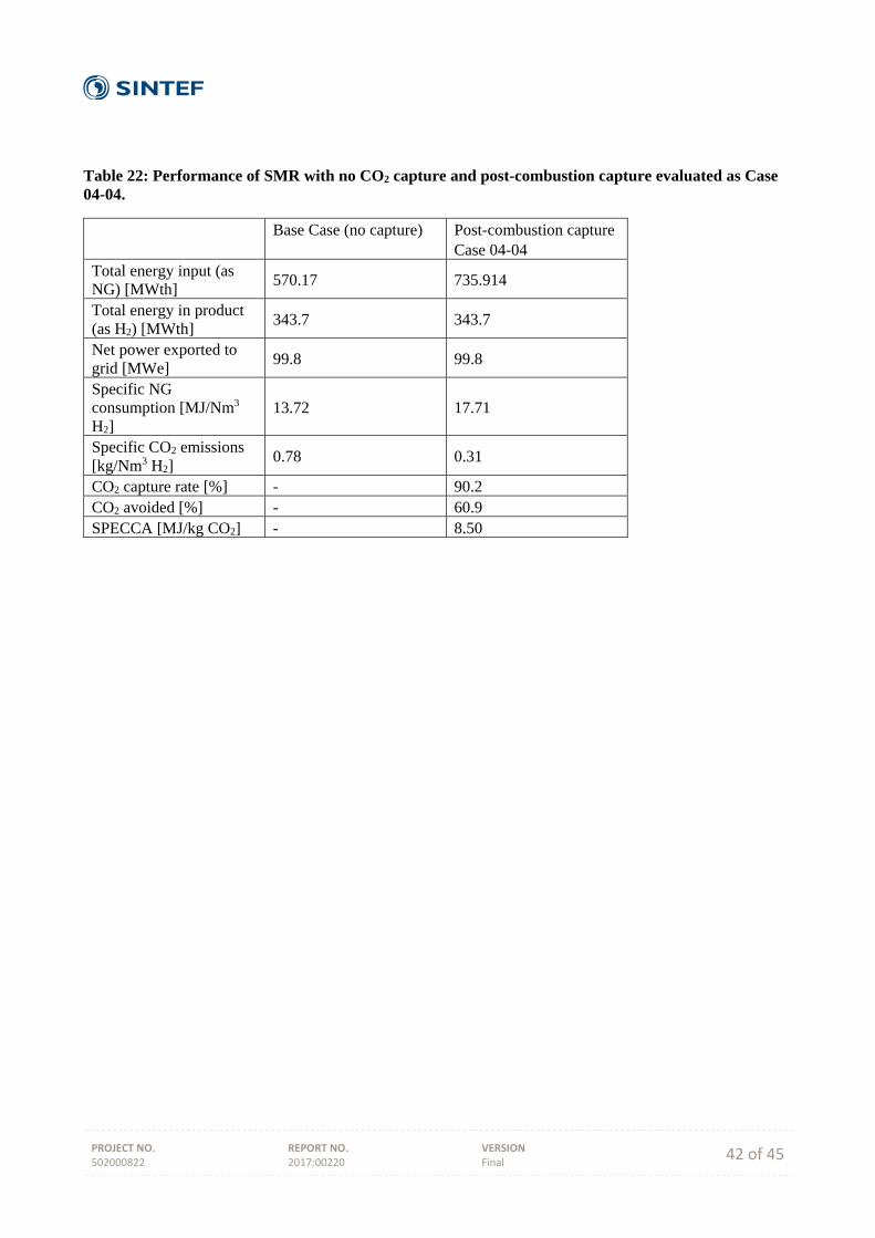
PROJECT NO. 502000822
REPORT NO. 2017:00220
VERSION Final 42 of 45
Table 22: Performance of SMR with no CO2 capture and post-combustion capture evaluated as Case 04-04.
Base Case (no capture) Post-combustion capture Case 04-04
Total energy input (as NG) [MWth]
570.17 735.914
Total energy in product (as H2) [MWth]
343.7 343.7
Net power exported to grid [MWe]
99.8 99.8
Specific NG consumption [MJ/Nm3 H2]
13.72 17.71
Specific CO2 emissions [kg/Nm3 H2]
0.78 0.31
CO2 capture rate [%] - 90.2 CO2 avoided [%] - 60.9 SPECCA [MJ/kg CO2] - 8.50
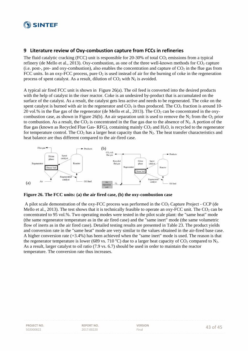
PROJECT NO. 502000822
REPORT NO. 2017:00220
VERSION Final 43 of 45
9 Literature review of Oxy‐combustion capture from FCCs in refineries
The fluid catalytic cracking (FCC) unit is responsible for 20-30% of total CO2 emissions from a typical refinery (de Mello et al., 2013). Oxy-combustion, as one of the three well-known methods for CO2 capture (i.e. post-, pre- and oxy-combustion), also enables the concentration and capture of CO2 in the flue gas from FCC units. In an oxy-FCC process, pure O2 is used instead of air for the burning of coke in the regeneration process of spent catalyst. As a result, dilution of CO2 with N2 is avoided. A typical air fired FCC unit is shown in Figure 26(a). The oil feed is converted into the desired products with the help of catalyst in the riser reactor. Coke is an undesired by-product that is accumulated on the surface of the catalyst. As a result, the catalyst gets less active and needs to be regenerated. The coke on the spent catalyst is burned with air in the regenerator and CO2 is thus produced. The CO2 fraction is around 10-20 vol.% in the flue gas of the regenerator (de Mello et al., 2013). The CO2 can be concentrated in the oxy-combustion case, as shown in Figure 26(b). An air separation unit is used to remove the N2 from the O2 prior to combustion. As a result, the CO2 is concentrated in the flue gas due to the absence of N2. A portion of the flue gas (known as Recycled Flue Gas- RFG), containing mainly CO2 and H2O, is recycled to the regenerator for temperature control. The CO2 has a larger heat capacity than the N2. The heat transfer characteristics and heat balance are thus different compared to the air-fired case.
(a)
(b)
Figure 26. The FCC units: (a) the air fired case, (b) the oxy-combustion case
A pilot scale demonstration of the oxy-FCC process was performed in the CO2 Capture Project - CCP (de Mello et al., 2013). The test shows that it is technically feasible to operate an oxy-FCC unit. The CO2 can be concentrated to 95 vol.%. Two operating modes were tested in the pilot scale plant: the "same heat" mode (the same regenerator temperature as in the air fired case) and the "same inert" mode (the same volumetric flow of inerts as in the air fired case). Detailed testing results are presented in Table 23. The product yields and conversion rate in the "same heat" mode are very similar to the values obtained in the air-fired base case. A higher conversion rate (+3.4%) has been achieved when the "same inert" mode is used. The reason is that the regenerator temperature is lower (689 vs. 710 oC) due to a larger heat capacity of CO2 compared to N2. As a result, larger catalyst to oil ratio (7.9 vs. 6.7) should be used in order to maintain the reactor temperature. The conversion rate thus increases.

PROJECT NO. 502000822
REPORT NO. 2017:00220
VERSION Final 44 of 45
Table 23. Main results from the pilot testing of the oxy-FCC processes (de Mello et al., 20135)
Testing mode Air-fired base case Oxy-fired same heat
Oxy-fired same inert
Reaction temperature, oC 540 540 540 Feed temperature, oC 350 349 348 Feed flow, kg/h 150 150 150 Catalyst to oil ratio (CTO) 6.7 6.8 7.9 Yields (mass basis), wt% (% change relative to air-fired case) Dry gas - -1.9 -1.6 LPG - 2.8 6.7 Gasoline - -0.8 2.4 Gasoline+LPG - 0.1 3.4 LCO+Bottoms - - - Coke - 0.8 9.0 Conversion - 1.0 4.9 Regenerator dense phase temperature, oC 710 709 689 Air/oxidant temperature, oC 249 249 251 Excess O2 in flue gas, mol% 2.7 2.6 2.5 %O2 in oxidant gas, mol% 21 28.9 23.8 Inert flow rate, m3/h 123 87 117 Flue gas composition, mol% (dry) CO2 14.2 94.3 94.8 O2 2.7 2.6 2.5 N2 83.1 3.1 2.5 CO 0.00 0.06 0.11
5 de Mello, L.F., Gobbo, R., Moure, G.T., Miracca, I., 2013. Oxy-combustion Technology Development for Fluid Catalytic Crackers (FCC) – Large Pilot Scale Demonstration. Energy Procedia 37, 7815–7824.
PROJECT NO. 502000822
REPORT NO. 2017:00220
VERSION Final 45 of 45
A CO2 capture process summary, stream data and PFDs
Separate document available at http://www.sintef.no/RECAP
B CO2 capture integration and utilities
Separate document available at http://www.sintef.no/RECAP

Technology for a better society www.sintef.no
ReCAP Project
Understanding the Cost of
Retrofitting CO2 Capture in
an Integrated Oil
Refinery
Cost estimation and economic
evaluation of CO2 capture options for
refineries
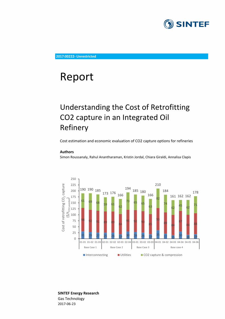
SINTEF Energy Research
Gas Technology 2017‐06‐23
2017:00222‐ Unrestricted
Report
Understanding the Cost of Retrofitting CO2 capture in an Integrated Oil Refinery
Cost estimation and economic evaluation of CO2 capture options for refineries
Authors Simon Roussanaly, Rahul Anantharaman, Kristin Jordal, Chiara Giraldi, Annalisa Clapis
31 29 27 25 26 19 30 28 26 1935 22 15
30 16 19
98 92 91 89 8984
91 92 9085
9389
8487
84 88
61 69 6859 61
62
73 65 6563
82
7462
4562
71
190 190 185173 176
166
194185 180
166
210
184
161 162 162178
0
25
50
75
100
125
150
175
200
225
250
01‐01 01‐02 01‐03 02‐01 02‐02 02‐03 02‐04 03‐01 03‐02 03‐03 04‐01 04‐02 04‐03 04‐04 04‐05 04‐06
Base Case 1 Base Case 2 Base Case 3 Base case 4
Cost of retrofitting CO2capture
($/t
CO2,avoided)
Interconnecting Utilities CO2 capture & compression

2 of 94
SINTEF Energi AS SINTEF Energy Research
Address: Postboks 4761 Sluppen NO‐7465 Trondheim NORWAY Switchboard: +47 73597200 Telefax: +47 73597250
[email protected] www.sintef.no/energi Enterprise /VAT No: NO 939 350 675 MVA
REPORT NO.
2017:00222
ISBN
978‐82‐14‐06683‐8
CLASSIFICATION
Unrestricted
CLASSIFICATION THIS PAGE
Unrestricted
PROJECT NO. 502000822
REPORT NO. 2017:00222
VERSION Final 3 of 94
Document history
VERSION DATE VERSION DESCRIPTION
1 2017‐05‐08 First draft with results only for Base Case 4
2 2017‐06‐23 Second draft with results for all four Base Cases
3 (final) 2017‐06‐23 Final version including comments received from partners and Appendixes B and C
PROJECT NO. 502000822
REPORT NO. 2017:00222
VERSION Final 4 of 94
Table of contents
Summary .................................................................................................................................................. 6
1 Introduction ..................................................................................................................................... 9
1.1 Cost evaluation methodology ...................................................................................................... 10
1.2 Sensitivity analyses ...................................................................................................................... 11
2 Results for post‐combustion capture from refineries ...................................................................... 13
2.1 Base Case 1 .................................................................................................................................. 13
2.2 Base Case 2 .................................................................................................................................. 15
2.3 Base Case 3 .................................................................................................................................. 18
2.4 Base Case 4 .................................................................................................................................. 21
2.5 Discussions and overall comparison ............................................................................................ 25
3 CO2 capture from SMR in refineries ................................................................................................ 29
A Detailed equipment list of selected cases ....................................................................................... 32
A.1 Base case 01‐03 ............................................................................................................................ 32
A.1.1 CO2 capture and compression ......................................................................................... 32
A.1.2 Utilities and interconnecting ........................................................................................... 33
A.2 Base case 02‐02 ............................................................................................................................ 38
A.2.1 CO2 capture and compression ......................................................................................... 38
A.2.2 Utilities and interconnecting ........................................................................................... 42
A.3 Base case 04‐03 ............................................................................................................................ 48
A.3.1 CO2 capture and compression ......................................................................................... 48
A.3.2 Utilities and interconnecting ........................................................................................... 55
A.4 Base case 04‐04 ............................................................................................................................ 61
A.4.1 CO2 capture and compression ......................................................................................... 61
A.4.2 Utilities and interconnecting ........................................................................................... 64
B Equipment cost functions developed .............................................................................................. 70
C Excel model for evaluation of retrofitting CO2 capture from refineries ............................................ 76
D Cost evaluation results for all the cases considered ........................................................................ 78
D.1 Base case 1 ................................................................................................................................... 78
D.1.1 Base case 01‐01 ............................................................................................................... 78
D.1.2 Base case 01‐02 ............................................................................................................... 79
D.1.3 Base case 01‐03 ............................................................................................................... 80
PROJECT NO. 502000822
REPORT NO. 2017:00222
VERSION Final 5 of 94
D.2 Base case 2 ................................................................................................................................... 81
D.2.1 Base case 02‐01 ............................................................................................................... 81
D.2.2 Base case 02‐02 ............................................................................................................... 82
D.2.3 Base case 02‐03 ............................................................................................................... 83
D.2.4 Base case 02‐04 ............................................................................................................... 84
D.3 Base case 3 ................................................................................................................................... 85
D.3.1 Base case 03‐01 ............................................................................................................... 85
D.3.2 Base case 03‐02 ............................................................................................................... 86
D.3.3 Base case 03‐03 ............................................................................................................... 87
D.4 Base case 4 ................................................................................................................................... 88
D.4.1 Base case 04‐01 ............................................................................................................... 88
D.4.2 Base case 04‐02 ............................................................................................................... 89
D.4.3 Base case 04‐03 ............................................................................................................... 90
D.4.4 Base case 04‐04 ............................................................................................................... 91
D.4.5 Base case 04‐05 ............................................................................................................... 92
D.4.6 Base case 04‐06 ............................................................................................................... 93

PROJECT NO. 502000822
REPORT NO. 2017:00222
VERSION Final 6 of 94
Summary
Report approach
This report describes and analyses the cost of retrofitting CO2 capture from refineries. The costs of retrofitting CO2 capture of 16 CO2 capture cases, developed and designed for four generic integrated oil refineries, are assessed and analysed considering Mono Ethanol Amine (MEA) based CO2 capture. Compared to other studies on CO2 capture, the assessments performed in this report focuses on retrofit costs including modifications in the refineries, interconnections, and additional CHP and utility facilities. The main focus is on CO2 capture from refinery Base Case 4, which is seen as the most relevant reference for existing European refineries of interest for CO2 capture retrofit. Considering the large number of cases (16) and their complexity, a hybrid methodology is used in order to evaluate the cost of the sections (CO2 capture and compression, utilities, and interconnecting) of the concept. In this approach, four of the 16 capture cases are selected to represent a wide range of CO2 capture capacity and flue gas CO2 content and assessed in detail, based on the cost methodology presented in Technical Design Basis and Economic Assumptions. These detailed cost assessments form, based on subsequent scaling, the basis for the assessment of the other cases. Finally, sensitivity analyses are carried out for each of the 16 CO2 capture cases in order to quantify the impact of the expect cost range accuracy, key parameter assumptions and project valuation parameters. A review of the IEAGHG technical report "Techno-Economic Evaluation of SMR based standalone (merchant) hydrogen plant with CCS" was performed and compared to capture Case 04-04 (a case with CO2 capture from the refinery SMR only). Insights on the effects of tight integration of the hydrogen plant with the refinery and additional CHP plant are provided.
Results The results of the cost evaluation of the 16 CO2 capture cases shows that the cost of retrofitting CO2 capture lies between 160 and 210 $/tCO2,avoided as shown in Figure 1. These estimates are significantly larger than estimates available in the literature on CO2 capture for other sources (natural gas and coal power generation, cement, steel, etc.). Three main reasons for this difference are:
The inclusion of the retrofit costs such as interconnection costs. The utilities cost is based on the installation of an additional CHP plant, cooling water towers and
waste water plant which are all designed with significant spare capacity in some cases (up to 30% overdesign).
Most of the CO2 capture cases considered include small to medium CO2 emission point sources and/or low to medium flue gas CO2 content (7 of the 16 cases considered include only flue gases with CO2 contents below or equal to 11.3%vol).
Although the cost distribution is specific to each case considered, the overall breakdown is as follows: 30-40% of costs linked to CO2 capture and conditioning, 45-55% linked to utilities production, and 10-20% linked to interconnecting costs. In terms of investment cost, the estimations show that the total capital requirement lies between 200 and 1500 M$ for the different case as shown in Figure 2. The main reasons for this wide range is mainly the differences in the amount of CO2 captured between the cases. It is worth noting that although a case may be cheaper in terms of normalised cost ($/tCO2,avoided), high total capital requirement could make it less attractive.
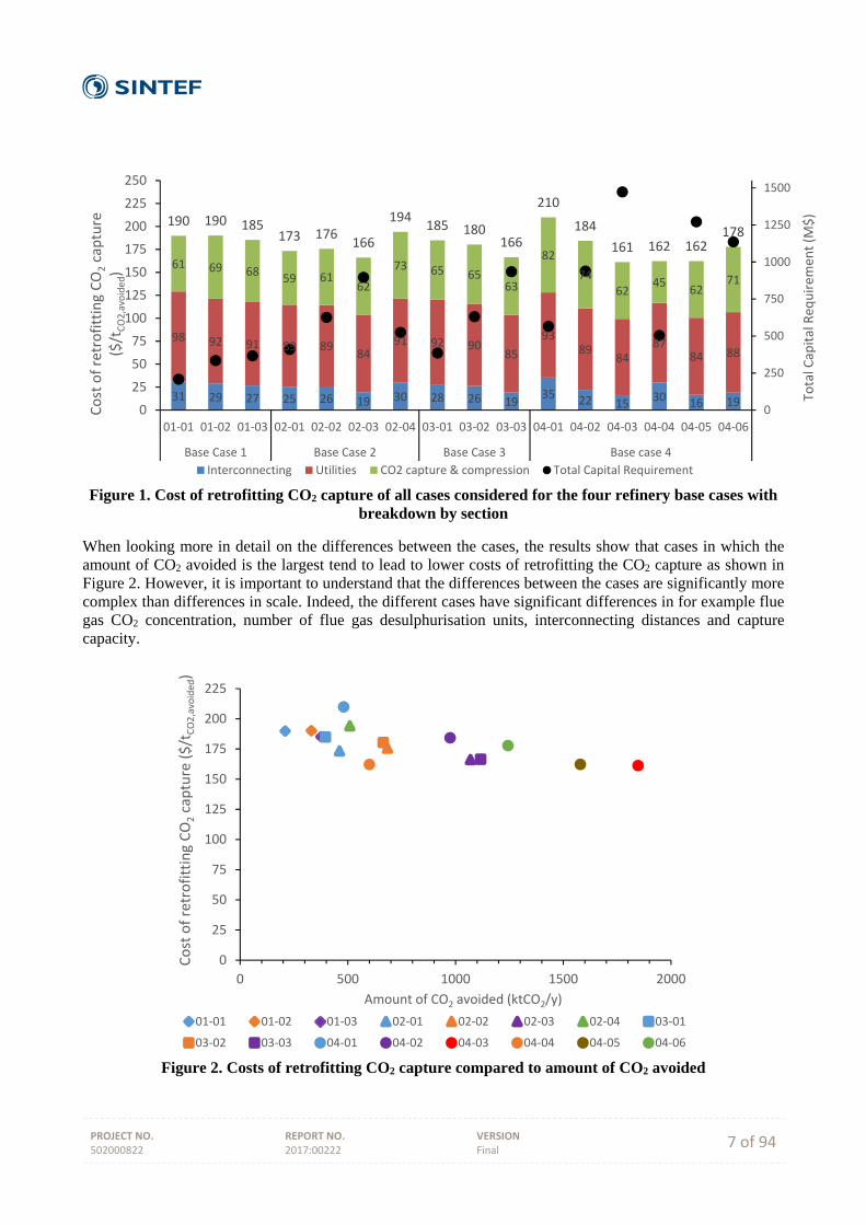
PROJECT NO. 502000822
REPORT NO. 2017:00222
VERSION Final 7 of 94
Figure 1. Cost of retrofitting CO2 capture of all cases considered for the four refinery base cases with
breakdown by section
When looking more in detail on the differences between the cases, the results show that cases in which the amount of CO2 avoided is the largest tend to lead to lower costs of retrofitting the CO2 capture as shown in Figure 2. However, it is important to understand that the differences between the cases are significantly more complex than differences in scale. Indeed, the different cases have significant differences in for example flue gas CO2 concentration, number of flue gas desulphurisation units, interconnecting distances and capture capacity.
Figure 2. Costs of retrofitting CO2 capture compared to amount of CO2 avoided
31 29 27 25 26 19 30 28 26 1935 22 15
30 16 19
98 92 91 89 8984
91 92 9085
9389
8487
84 88
61 69 6859 61
62
73 65 6563
82
7462
4562
71
190 190 185173 176
166
194185 180
166
210
184
161 162 162178
0
250
500
750
1000
1250
1500
0
25
50
75
100
125
150
175
200
225
250
01‐01 01‐02 01‐03 02‐01 02‐02 02‐03 02‐04 03‐01 03‐02 03‐03 04‐01 04‐02 04‐03 04‐04 04‐05 04‐06
Base Case 1 Base Case 2 Base Case 3 Base case 4
Total Capital Req
uirem
ent (M
$)
Cost of retrofitting CO2capture
($/t
CO2,avoided)
Interconnecting Utilities CO2 capture & compression Total Capital Requirement
0
25
50
75
100
125
150
175
200
225
0 500 1000 1500 2000
Cost of retrofitting CO2capture ($/t
CO2,avoided)
Amount of CO2 avoided (ktCO2/y)
01‐01 01‐02 01‐03 02‐01 02‐02 02‐03 02‐04 03‐01
03‐02 03‐03 04‐01 04‐02 04‐03 04‐04 04‐05 04‐06
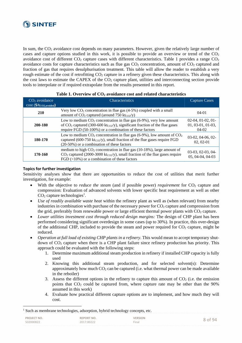
PROJECT NO. 502000822
REPORT NO. 2017:00222
VERSION Final 8 of 94
In sum, the CO2 avoidance cost depends on many parameters. However, given the relatively large number of cases and capture options studied in this work, it is possible to provide an overview or trend of the CO2 avoidance cost of different CO2 capture cases with different characteristics. Table 1 provides a range CO2 avoidance costs for capture characteristics such as flue gas CO2 concentration, amount of CO2 captured and fraction of gas that requires desulphurisation treatment. This table will allow the reader to establish a very rough estimate of the cost if retrofitting CO2 capture in a refinery given these characteristics. This along with the cost laws to estimate the CAPEX of the CO2 capture plant, utilities and interconnecting section provide tools to interpolate or if required extrapolate from the results presented in this report.
Table 1. Overview of CO2 avoidance cost and related characteristics CO2 avoidance
cost ($/tCO2,avoided) Characteristics Capture Cases
210 Very low CO2 concentration in flue gas (4-5%) coupled with a small amount of CO2 captured (around 750 ktCO2/y)
04-01
200-180 Low to medium CO2 concentration in flue gas (6-9%), very low amount of CO2 captured (300-600 ktCO2/y), significant fraction of the flue gases require FGD (50-100%) or a combination of these factors
02-04, 01-02, 01-01, 03-01, 01-03,
04-02
180-170 Low to medium CO2 concentration in flue gas (6-9%), low amount of CO2 captured (600-750 ktCO2/y), small fraction of the flue gases require FGD (20-50%) or a combination of these factors
03-02, 04-06, 02-02, 02-01
170-160 medium to high CO2 concentration in flue gas (10-18%), large amount of CO2 captured (2000-3000 ktCO2/y), small fraction of the flue gases require FGD (<10%) or a combination of these factors
03-03, 02-03, 04-05, 04-04, 04-03
Topics for further investigation Sensitivity analyses show that there are opportunities to reduce the cost of utilities that merit further investigation, for example:
With the objective to reduce the steam (and if possible power) requirement for CO2 capture and compression: Evaluation of advanced solvents with lower specific heat requirement as well as other CO2 capture technologies1.
Use of readily available waste heat within the refinery plant as well as (when relevant) from nearby industries in combination with purchase of the necessary power for CO2 capture and compression from the grid, preferably from renewable power or large efficient thermal power plants with CO2 capture.
Lower utilities investment cost through reduced design margins: The design of CHP plant has been performed considering significant overdesign in some cases (up to 30%). In practice, this over-design of the additional CHP, included to provide the steam and power required for CO2 capture, might be reduced.
Operation at full load of existing CHP plants in a refinery. This would mean to accept temporary shut-down of CO2 capture when there is a CHP plant failure since refinery production has priority. This approach could be evaluated with the following steps:
1. Determine maximum additional steam production in refinery if installed CHP capacity is fully used
2. Knowing this additional steam production, and for selected solvent(s): Determine approximately how much CO2 can be captured (i.e. what thermal power can be made available in the reboiler)
3. Assess the different options in the refinery to capture this amount of CO2 (i.e. the emission points that CO2 could be captured from, where capture rate may be other than the 90% assumed in this work)
4. Evaluate how practical different capture options are to implement, and how much they will cost.
1 Such as membrane technologies, adsorption, hybrid technology concepts, etc.
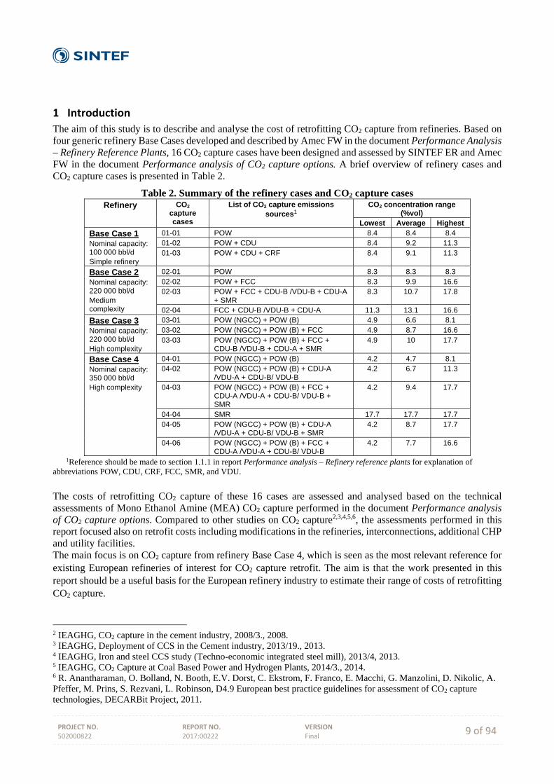
PROJECT NO. 502000822
REPORT NO. 2017:00222
VERSION Final 9 of 94
1 Introduction
The aim of this study is to describe and analyse the cost of retrofitting CO2 capture from refineries. Based on four generic refinery Base Cases developed and described by Amec FW in the document Performance Analysis – Refinery Reference Plants, 16 CO2 capture cases have been designed and assessed by SINTEF ER and Amec FW in the document Performance analysis of CO2 capture options. A brief overview of refinery cases and CO2 capture cases is presented in Table 2.
Table 2. Summary of the refinery cases and CO2 capture cases Refinery CO2
capture cases
List of CO2 capture emissions
sources1
CO2 concentration range (%vol)
Lowest Average Highest
Base Case 1 Nominal capacity: 100 000 bbl/d
Simple refinery
01-01 POW 8.4 8.4 8.4
01-02 POW + CDU 8.4 9.2 11.3
01-03 POW + CDU + CRF 8.4 9.1 11.3
Base Case 2 Nominal capacity: 220 000 bbl/d
Medium complexity
02-01 POW 8.3 8.3 8.3
02-02 POW + FCC 8.3 9.9 16.6
02-03 POW + FCC + CDU-B /VDU-B + CDU-A + SMR
8.3 10.7 17.8
02-04 FCC + CDU-B /VDU-B + CDU-A 11.3 13.1 16.6
Base Case 3
Nominal capacity: 220 000 bbl/d
High complexity
03-01 POW (NGCC) + POW (B) 4.9 6.6 8.1
03-02 POW (NGCC) + POW (B) + FCC 4.9 8.7 16.6
03-03 POW (NGCC) + POW (B) + FCC + CDU-B /VDU-B + CDU-A + SMR
4.9 10 17.7
Base Case 4 Nominal capacity: 350 000 bbl/d
High complexity
04-01 POW (NGCC) + POW (B) 4.2 4.7 8.1
04-02 POW (NGCC) + POW (B) + CDU-A /VDU-A + CDU-B/ VDU-B
4.2 6.7 11.3
04-03 POW (NGCC) + POW (B) + FCC + CDU-A /VDU-A + CDU-B/ VDU-B + SMR
4.2 9.4 17.7
04-04 SMR 17.7 17.7 17.7
04-05 POW (NGCC) + POW (B) + CDU-A /VDU-A + CDU-B/ VDU-B + SMR
4.2 8.7 17.7
04-06 POW (NGCC) + POW (B) + FCC + CDU-A /VDU-A + CDU-B/ VDU-B
4.2 7.7 16.6
1Reference should be made to section 1.1.1 in report Performance analysis – Refinery reference plants for explanation of abbreviations POW, CDU, CRF, FCC, SMR, and VDU. The costs of retrofitting CO2 capture of these 16 cases are assessed and analysed based on the technical assessments of Mono Ethanol Amine (MEA) CO2 capture performed in the document Performance analysis of CO2 capture options. Compared to other studies on CO2 capture2,3,4,5,6, the assessments performed in this report focused also on retrofit costs including modifications in the refineries, interconnections, additional CHP and utility facilities. The main focus is on CO2 capture from refinery Base Case 4, which is seen as the most relevant reference for existing European refineries of interest for CO2 capture retrofit. The aim is that the work presented in this report should be a useful basis for the European refinery industry to estimate their range of costs of retrofitting CO2 capture.
2 IEAGHG, CO2 capture in the cement industry, 2008/3., 2008. 3 IEAGHG, Deployment of CCS in the Cement industry, 2013/19., 2013. 4 IEAGHG, Iron and steel CCS study (Techno-economic integrated steel mill), 2013/4, 2013. 5 IEAGHG, CO2 Capture at Coal Based Power and Hydrogen Plants, 2014/3., 2014. 6 R. Anantharaman, O. Bolland, N. Booth, E.V. Dorst, C. Ekstrom, F. Franco, E. Macchi, G. Manzolini, D. Nikolic, A. Pfeffer, M. Prins, S. Rezvani, L. Robinson, D4.9 European best practice guidelines for assessment of CO2 capture technologies, DECARBit Project, 2011.
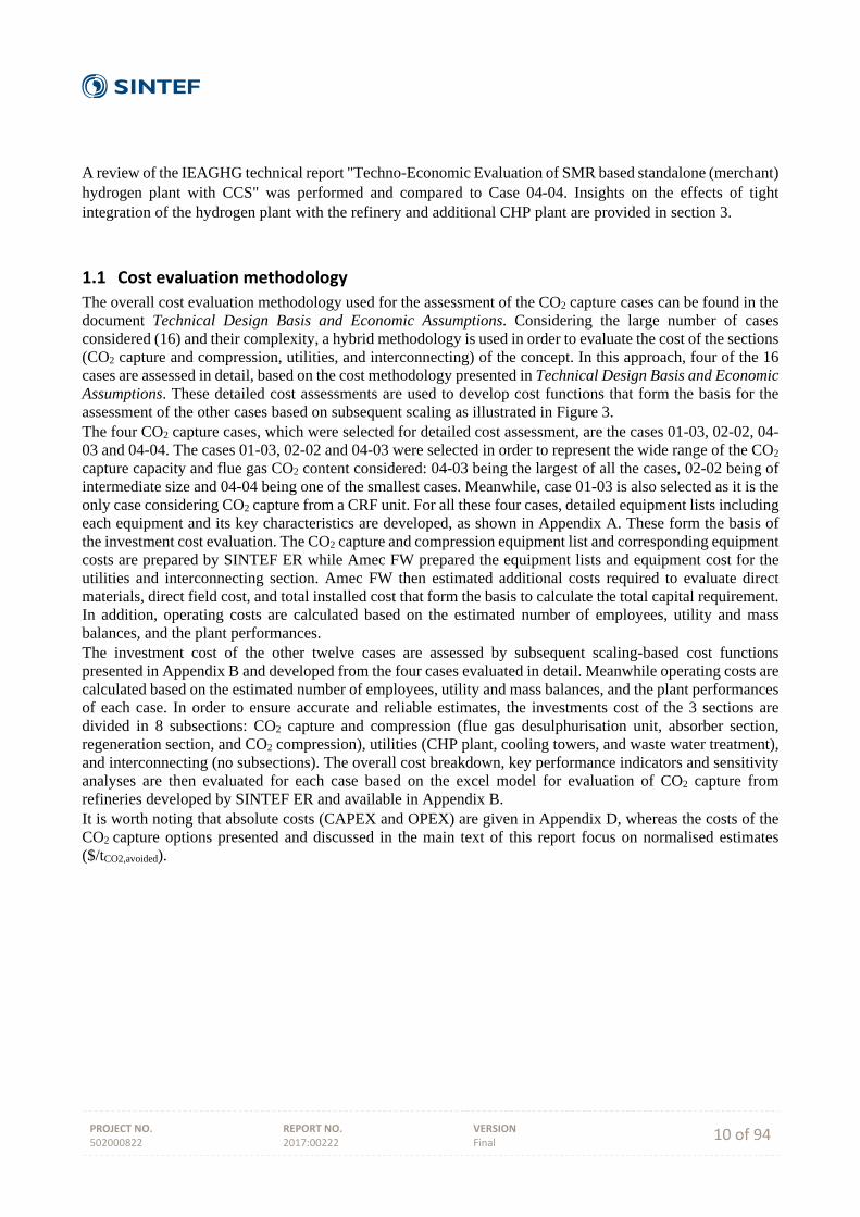
PROJECT NO. 502000822
REPORT NO. 2017:00222
VERSION Final 10 of 94
A review of the IEAGHG technical report "Techno-Economic Evaluation of SMR based standalone (merchant) hydrogen plant with CCS" was performed and compared to Case 04-04. Insights on the effects of tight integration of the hydrogen plant with the refinery and additional CHP plant are provided in section 3.
1.1 Cost evaluation methodology
The overall cost evaluation methodology used for the assessment of the CO2 capture cases can be found in the document Technical Design Basis and Economic Assumptions. Considering the large number of cases considered (16) and their complexity, a hybrid methodology is used in order to evaluate the cost of the sections (CO2 capture and compression, utilities, and interconnecting) of the concept. In this approach, four of the 16 cases are assessed in detail, based on the cost methodology presented in Technical Design Basis and Economic Assumptions. These detailed cost assessments are used to develop cost functions that form the basis for the assessment of the other cases based on subsequent scaling as illustrated in Figure 3. The four CO2 capture cases, which were selected for detailed cost assessment, are the cases 01-03, 02-02, 04-03 and 04-04. The cases 01-03, 02-02 and 04-03 were selected in order to represent the wide range of the CO2 capture capacity and flue gas CO2 content considered: 04-03 being the largest of all the cases, 02-02 being of intermediate size and 04-04 being one of the smallest cases. Meanwhile, case 01-03 is also selected as it is the only case considering CO2 capture from a CRF unit. For all these four cases, detailed equipment lists including each equipment and its key characteristics are developed, as shown in Appendix A. These form the basis of the investment cost evaluation. The CO2 capture and compression equipment list and corresponding equipment costs are prepared by SINTEF ER while Amec FW prepared the equipment lists and equipment cost for the utilities and interconnecting section. Amec FW then estimated additional costs required to evaluate direct materials, direct field cost, and total installed cost that form the basis to calculate the total capital requirement. In addition, operating costs are calculated based on the estimated number of employees, utility and mass balances, and the plant performances. The investment cost of the other twelve cases are assessed by subsequent scaling-based cost functions presented in Appendix B and developed from the four cases evaluated in detail. Meanwhile operating costs are calculated based on the estimated number of employees, utility and mass balances, and the plant performances of each case. In order to ensure accurate and reliable estimates, the investments cost of the 3 sections are divided in 8 subsections: CO2 capture and compression (flue gas desulphurisation unit, absorber section, regeneration section, and CO2 compression), utilities (CHP plant, cooling towers, and waste water treatment), and interconnecting (no subsections). The overall cost breakdown, key performance indicators and sensitivity analyses are then evaluated for each case based on the excel model for evaluation of CO2 capture from refineries developed by SINTEF ER and available in Appendix B. It is worth noting that absolute costs (CAPEX and OPEX) are given in Appendix D, whereas the costs of the CO2 capture options presented and discussed in the main text of this report focus on normalised estimates ($/tCO2,avoided).
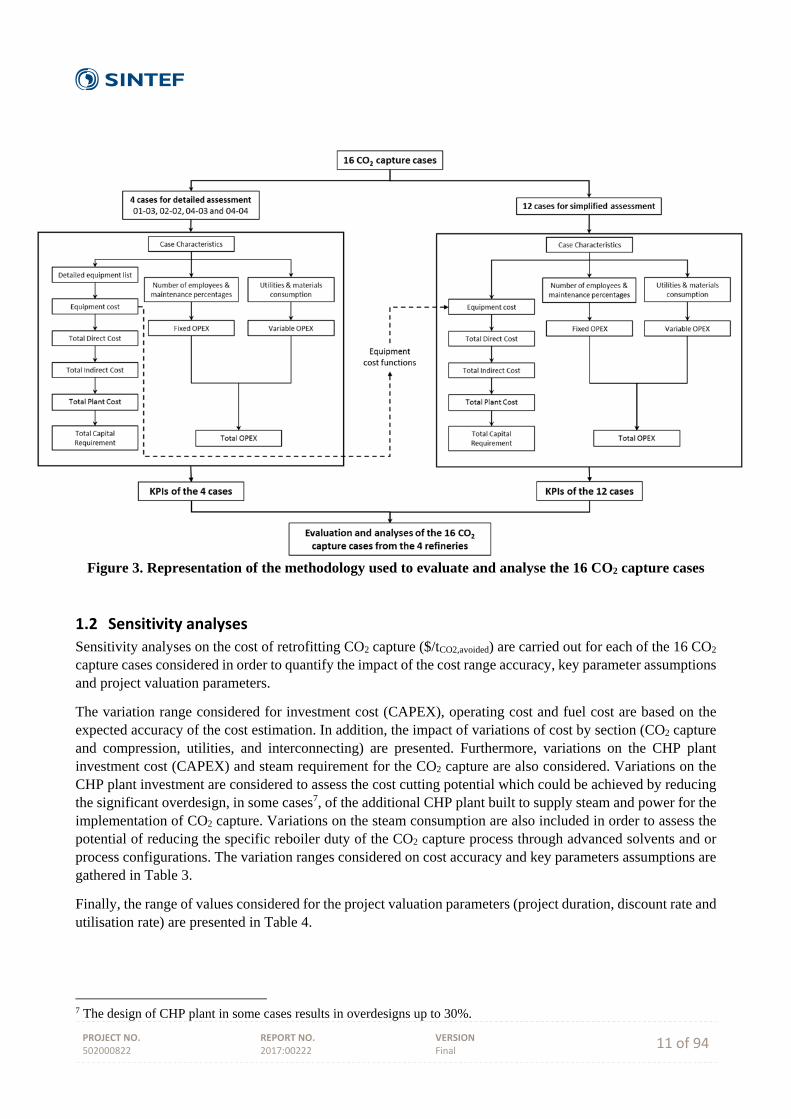
PROJECT NO. 502000822
REPORT NO. 2017:00222
VERSION Final 11 of 94
Figure 3. Representation of the methodology used to evaluate and analyse the 16 CO2 capture cases
1.2 Sensitivity analyses
Sensitivity analyses on the cost of retrofitting CO2 capture ($/tCO2,avoided) are carried out for each of the 16 CO2 capture cases considered in order to quantify the impact of the cost range accuracy, key parameter assumptions and project valuation parameters.
The variation range considered for investment cost (CAPEX), operating cost and fuel cost are based on the expected accuracy of the cost estimation. In addition, the impact of variations of cost by section (CO2 capture and compression, utilities, and interconnecting) are presented. Furthermore, variations on the CHP plant investment cost (CAPEX) and steam requirement for the CO2 capture are also considered. Variations on the CHP plant investment are considered to assess the cost cutting potential which could be achieved by reducing the significant overdesign, in some cases7, of the additional CHP plant built to supply steam and power for the implementation of CO2 capture. Variations on the steam consumption are also included in order to assess the potential of reducing the specific reboiler duty of the CO2 capture process through advanced solvents and or process configurations. The variation ranges considered on cost accuracy and key parameters assumptions are gathered in Table 3.
Finally, the range of values considered for the project valuation parameters (project duration, discount rate and utilisation rate) are presented in Table 4.
7 The design of CHP plant in some cases results in overdesigns up to 30%.
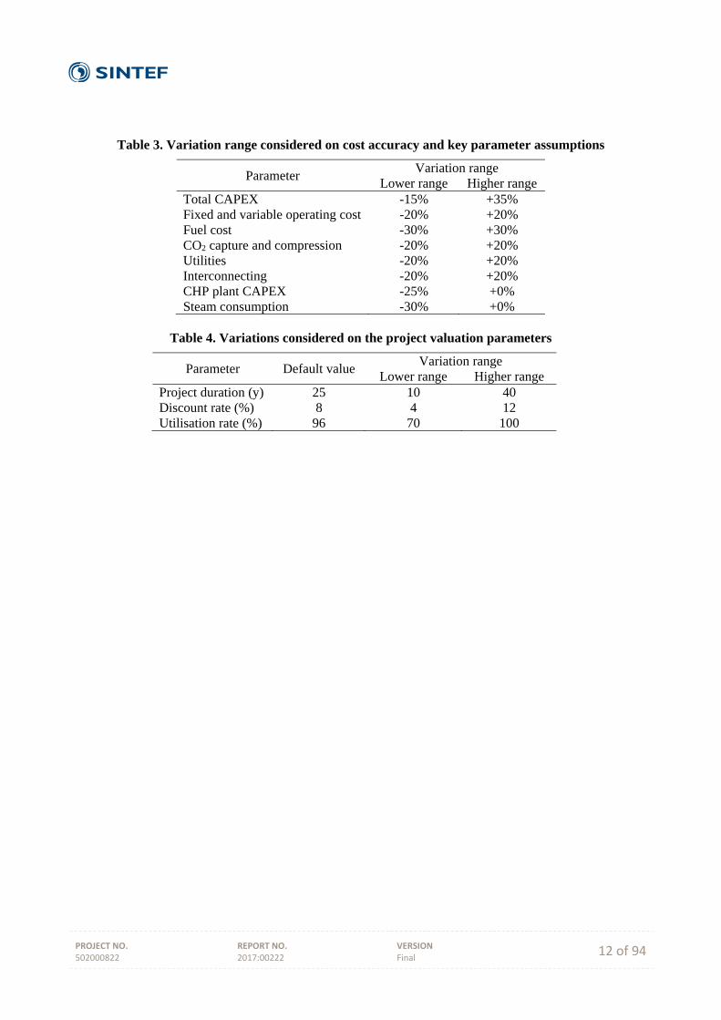
PROJECT NO. 502000822
REPORT NO. 2017:00222
VERSION Final 12 of 94
Table 3. Variation range considered on cost accuracy and key parameter assumptions
Parameter Variation range
Lower range Higher range Total CAPEX -15% +35% Fixed and variable operating cost -20% +20% Fuel cost -30% +30% CO2 capture and compression -20% +20% Utilities -20% +20% Interconnecting -20% +20% CHP plant CAPEX -25% +0% Steam consumption -30% +0%
Table 4. Variations considered on the project valuation parameters
Parameter Default value Variation range
Lower range Higher range Project duration (y) 25 10 40 Discount rate (%) 8 4 12 Utilisation rate (%) 96 70 100
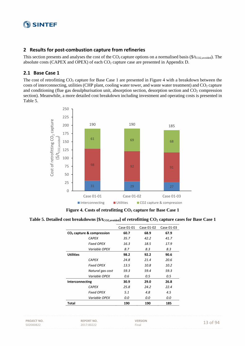
PROJECT NO. 502000822
REPORT NO. 2017:00222
VERSION Final 13 of 94
2 Results for post‐combustion capture from refineries
This section presents and analyses the cost of the CO2 capture options on a normalised basis ($/tCO2,avoided). The absolute costs (CAPEX and OPEX) of each CO2 capture case are presented in Appendix D.
2.1 Base Case 1
The cost of retrofitting CO2 capture for Base Case 1 are presented in Figure 4 with a breakdown between the costs of interconnecting, utilities (CHP plant, cooling water tower, and waste water treatment) and CO2 capture and conditioning (flue gas desulphurisation unit, absorption section, desorption section and CO2 compression section). Meanwhile, a more detailed cost breakdown including investment and operating costs is presented in Table 5.
Figure 4. Costs of retrofitting CO2 capture for Base Case 1
Table 5. Detailed cost breakdowns [$/tCO2,avoided] of retrofitting CO2 capture cases for Base Case 1
Case 01‐01 Case 01‐02 Case 01‐03
CO2 capture & compression 60.7 68.9 67.9
CAPEX 35.7 42.2 41.7
Fixed OPEX 16.3 18.5 17.9
Variable OPEX 8.7 8.3 8.3
Utilities 98.2 92.2 90.6
CAPEX 24.8 21.4 20.6
Fixed OPEX 13.5 10.8 10.2
Natural gas cost 59.3 59.4 59.3
Variable OPEX 0.6 0.5 0.5
Interconnecting 30.9 29.0 26.8
CAPEX 25.8 24.2 22.4
Fixed OPEX 5.1 4.8 4.5
Variable OPEX 0.0 0.0 0.0
Total 190 190 185
31 29 27
98 92 91
61 69 68
190 190 185
0
25
50
75
100
125
150
175
200
225
250
Case 01‐01 Case 01‐02 Case 01‐03
Cost of retrofitting CO2capture
($/t
CO2,avoided)
Interconnecting Utilities CO2 capture & compression
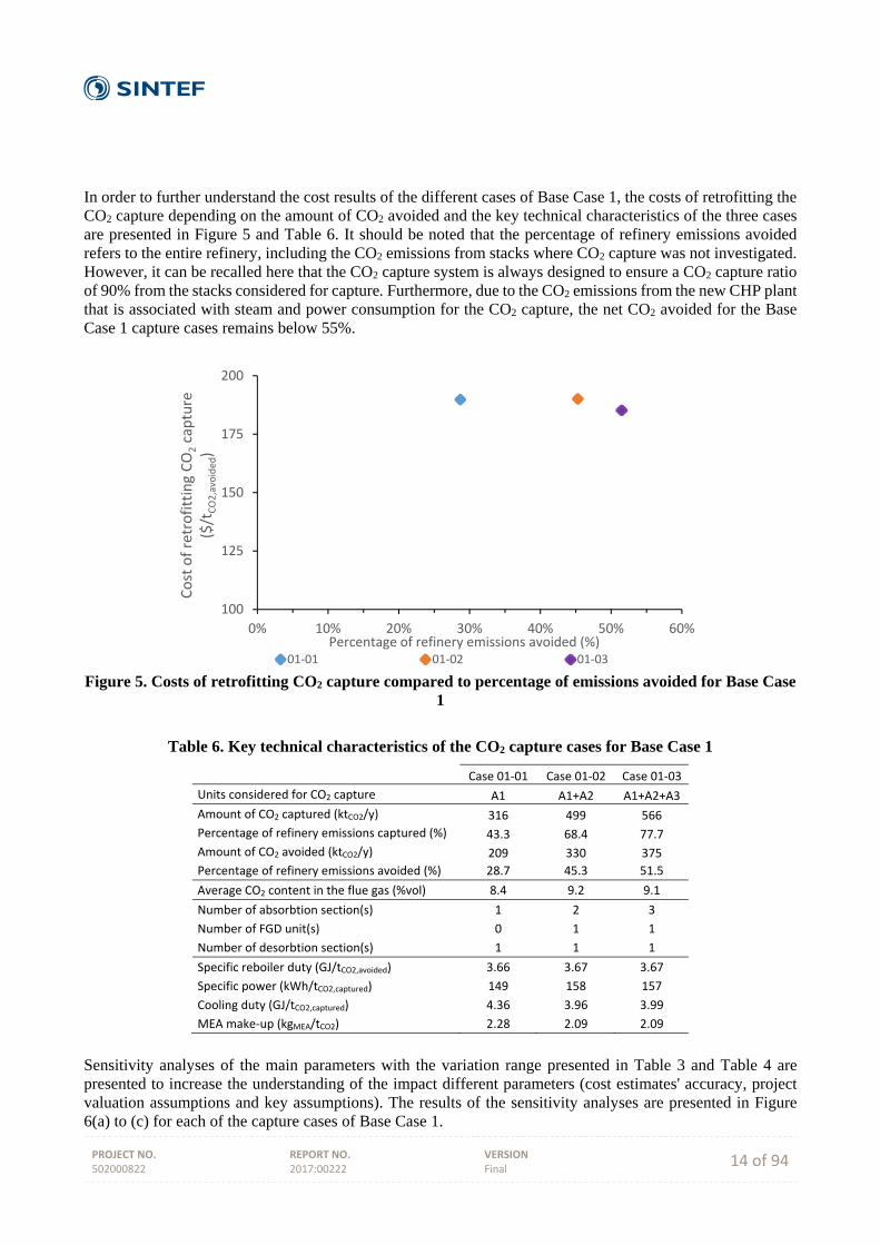
PROJECT NO. 502000822
REPORT NO. 2017:00222
VERSION Final 14 of 94
In order to further understand the cost results of the different cases of Base Case 1, the costs of retrofitting the CO2 capture depending on the amount of CO2 avoided and the key technical characteristics of the three cases are presented in Figure 5 and Table 6. It should be noted that the percentage of refinery emissions avoided refers to the entire refinery, including the CO2 emissions from stacks where CO2 capture was not investigated. However, it can be recalled here that the CO2 capture system is always designed to ensure a CO2 capture ratio of 90% from the stacks considered for capture. Furthermore, due to the CO2 emissions from the new CHP plant that is associated with steam and power consumption for the CO2 capture, the net CO2 avoided for the Base Case 1 capture cases remains below 55%.
Figure 5. Costs of retrofitting CO2 capture compared to percentage of emissions avoided for Base Case
1
Table 6. Key technical characteristics of the CO2 capture cases for Base Case 1
Case 01‐01 Case 01‐02 Case 01‐03
Units considered for CO2 capture A1 A1+A2 A1+A2+A3
Amount of CO2 captured (ktCO2/y) 316 499 566
Percentage of refinery emissions captured (%) 43.3 68.4 77.7
Amount of CO2 avoided (ktCO2/y) 209 330 375
Percentage of refinery emissions avoided (%) 28.7 45.3 51.5
Average CO2 content in the flue gas (%vol) 8.4 9.2 9.1
Number of absorbtion section(s) 1 2 3
Number of FGD unit(s) 0 1 1
Number of desorbtion section(s) 1 1 1
Specific reboiler duty (GJ/tCO2,avoided) 3.66 3.67 3.67
Specific power (kWh/tCO2,captured) 149 158 157
Cooling duty (GJ/tCO2,captured) 4.36 3.96 3.99
MEA make‐up (kgMEA/tCO2) 2.28 2.09 2.09
Sensitivity analyses of the main parameters with the variation range presented in Table 3 and Table 4 are presented to increase the understanding of the impact different parameters (cost estimates' accuracy, project valuation assumptions and key assumptions). The results of the sensitivity analyses are presented in Figure 6(a) to (c) for each of the capture cases of Base Case 1.
100
125
150
175
200
0% 10% 20% 30% 40% 50% 60%
Cost of retrofitting CO2capture
($/t
CO2,avoided)
Percentage of refinery emissions avoided (%)01‐01 01‐02 01‐03
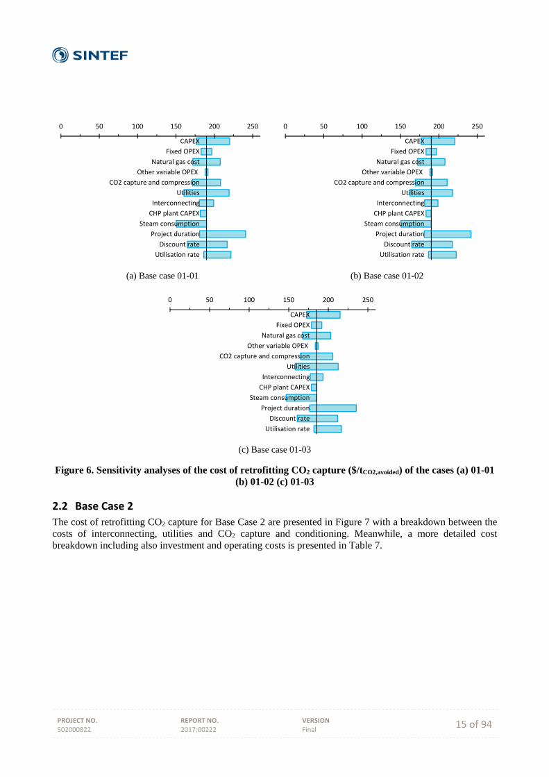
PROJECT NO. 502000822
REPORT NO. 2017:00222
VERSION Final 15 of 94
(a) Base case 01-01 (b) Base case 01-02
(c) Base case 01-03
Figure 6. Sensitivity analyses of the cost of retrofitting CO2 capture ($/tCO2,avoided) of the cases (a) 01-01 (b) 01-02 (c) 01-03
2.2 Base Case 2
The cost of retrofitting CO2 capture for Base Case 2 are presented in Figure 7 with a breakdown between the costs of interconnecting, utilities and CO2 capture and conditioning. Meanwhile, a more detailed cost breakdown including also investment and operating costs is presented in Table 7.
0 50 100 150 200 250
CAPEX
Fixed OPEX
Natural gas cost
Other variable OPEX
CO2 capture and compression
Utilities
Interconnecting
CHP plant CAPEX
Steam consumption
Project duration
Discount rate
Utilisation rate
0 50 100 150 200 250
CAPEX
Fixed OPEX
Natural gas cost
Other variable OPEX
CO2 capture and compression
Utilities
Interconnecting
CHP plant CAPEX
Steam consumption
Project duration
Discount rate
Utilisation rate
0 50 100 150 200 250
CAPEX
Fixed OPEX
Natural gas cost
Other variable OPEX
CO2 capture and compression
Utilities
Interconnecting
CHP plant CAPEX
Steam consumption
Project duration
Discount rate
Utilisation rate
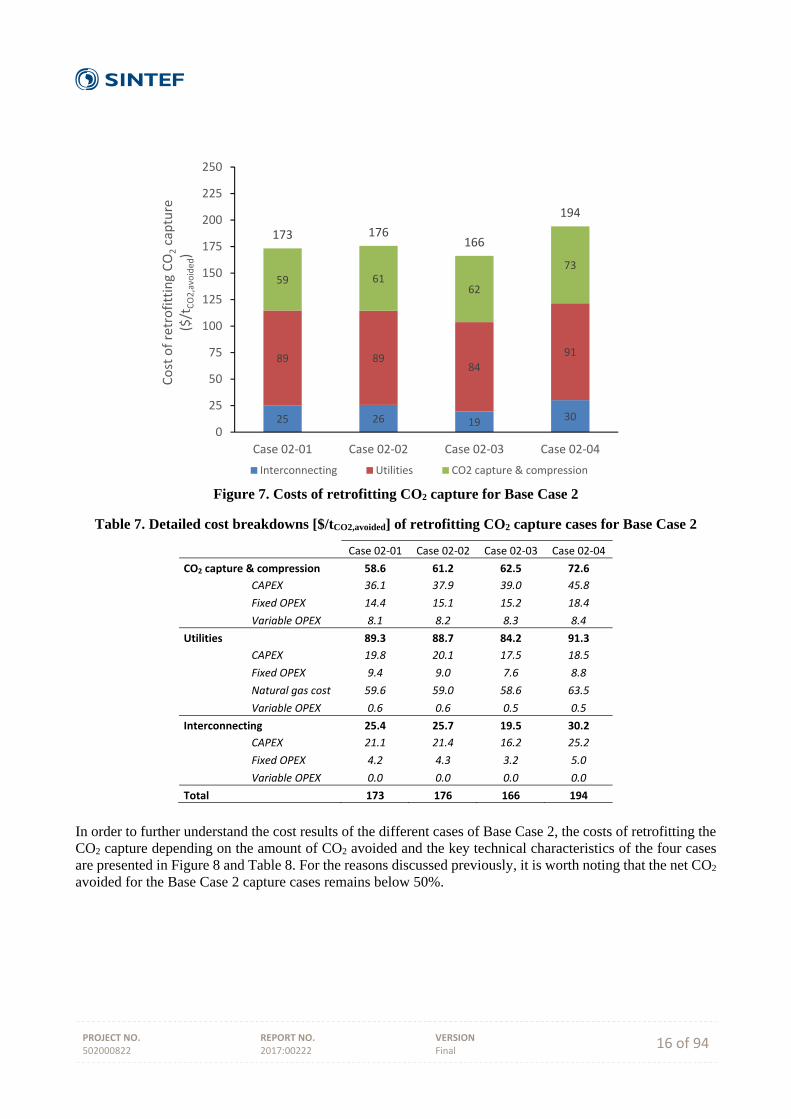
PROJECT NO. 502000822
REPORT NO. 2017:00222
VERSION Final 16 of 94
Figure 7. Costs of retrofitting CO2 capture for Base Case 2
Table 7. Detailed cost breakdowns [$/tCO2,avoided] of retrofitting CO2 capture cases for Base Case 2
Case 02‐01 Case 02‐02 Case 02‐03 Case 02‐04
CO2 capture & compression 58.6 61.2 62.5 72.6
CAPEX 36.1 37.9 39.0 45.8
Fixed OPEX 14.4 15.1 15.2 18.4
Variable OPEX 8.1 8.2 8.3 8.4
Utilities 89.3 88.7 84.2 91.3
CAPEX 19.8 20.1 17.5 18.5
Fixed OPEX 9.4 9.0 7.6 8.8
Natural gas cost 59.6 59.0 58.6 63.5
Variable OPEX 0.6 0.6 0.5 0.5
Interconnecting 25.4 25.7 19.5 30.2
CAPEX 21.1 21.4 16.2 25.2
Fixed OPEX 4.2 4.3 3.2 5.0
Variable OPEX 0.0 0.0 0.0 0.0
Total 173 176 166 194
In order to further understand the cost results of the different cases of Base Case 2, the costs of retrofitting the CO2 capture depending on the amount of CO2 avoided and the key technical characteristics of the four cases are presented in Figure 8 and Table 8. For the reasons discussed previously, it is worth noting that the net CO2 avoided for the Base Case 2 capture cases remains below 50%.
25 26 19 30
89 8984
91
59 6162
73
173 176166
194
0
25
50
75
100
125
150
175
200
225
250
Case 02‐01 Case 02‐02 Case 02‐03 Case 02‐04
Cost of retrofitting CO2capture
($/t
CO2,avoided)
Interconnecting Utilities CO2 capture & compression
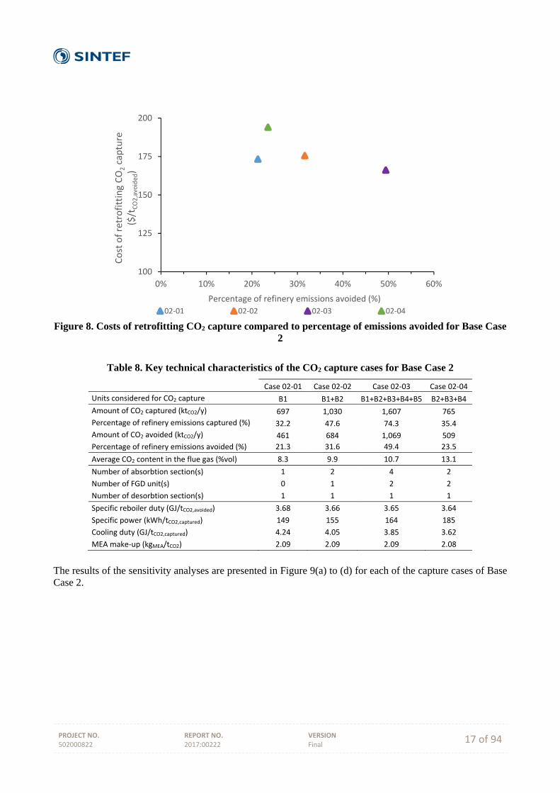
PROJECT NO. 502000822
REPORT NO. 2017:00222
VERSION Final 17 of 94
Figure 8. Costs of retrofitting CO2 capture compared to percentage of emissions avoided for Base Case
2
Table 8. Key technical characteristics of the CO2 capture cases for Base Case 2
Case 02‐01 Case 02‐02 Case 02‐03 Case 02‐04
Units considered for CO2 capture B1 B1+B2 B1+B2+B3+B4+B5 B2+B3+B4
Amount of CO2 captured (ktCO2/y) 697 1,030 1,607 765
Percentage of refinery emissions captured (%) 32.2 47.6 74.3 35.4
Amount of CO2 avoided (ktCO2/y) 461 684 1,069 509
Percentage of refinery emissions avoided (%) 21.3 31.6 49.4 23.5
Average CO2 content in the flue gas (%vol) 8.3 9.9 10.7 13.1
Number of absorbtion section(s) 1 2 4 2
Number of FGD unit(s) 0 1 2 2
Number of desorbtion section(s) 1 1 1 1
Specific reboiler duty (GJ/tCO2,avoided) 3.68 3.66 3.65 3.64
Specific power (kWh/tCO2,captured) 149 155 164 185
Cooling duty (GJ/tCO2,captured) 4.24 4.05 3.85 3.62
MEA make‐up (kgMEA/tCO2) 2.09 2.09 2.09 2.08
The results of the sensitivity analyses are presented in Figure 9(a) to (d) for each of the capture cases of Base Case 2.
100
125
150
175
200
0% 10% 20% 30% 40% 50% 60%
Cost of retrofitting CO2capture
($/t
CO2,avoided)
Percentage of refinery emissions avoided (%)
02‐01 02‐02 02‐03 02‐04
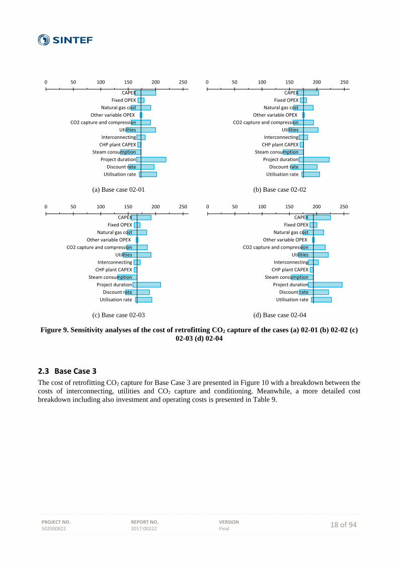
PROJECT NO. 502000822
REPORT NO. 2017:00222
VERSION Final 18 of 94
(a) Base case 02-01 (b) Base case 02-02
(c) Base case 02-03 (d) Base case 02-04
Figure 9. Sensitivity analyses of the cost of retrofitting CO2 capture of the cases (a) 02-01 (b) 02-02 (c) 02-03 (d) 02-04
2.3 Base Case 3
The cost of retrofitting CO2 capture for Base Case 3 are presented in Figure 10 with a breakdown between the costs of interconnecting, utilities and CO2 capture and conditioning. Meanwhile, a more detailed cost breakdown including also investment and operating costs is presented in Table 9.
0 50 100 150 200 250
CAPEX
Fixed OPEX
Natural gas cost
Other variable OPEX
CO2 capture and compression
Utilities
Interconnecting
CHP plant CAPEX
Steam consumption
Project duration
Discount rate
Utilisation rate
0 50 100 150 200 250
CAPEX
Fixed OPEX
Natural gas cost
Other variable OPEX
CO2 capture and compression
Utilities
Interconnecting
CHP plant CAPEX
Steam consumption
Project duration
Discount rate
Utilisation rate
0 50 100 150 200 250
CAPEX
Fixed OPEX
Natural gas cost
Other variable OPEX
CO2 capture and compression
Utilities
Interconnecting
CHP plant CAPEX
Steam consumption
Project duration
Discount rate
Utilisation rate
0 50 100 150 200 250
CAPEX
Fixed OPEX
Natural gas cost
Other variable OPEX
CO2 capture and compression
Utilities
Interconnecting
CHP plant CAPEX
Steam consumption
Project duration
Discount rate
Utilisation rate
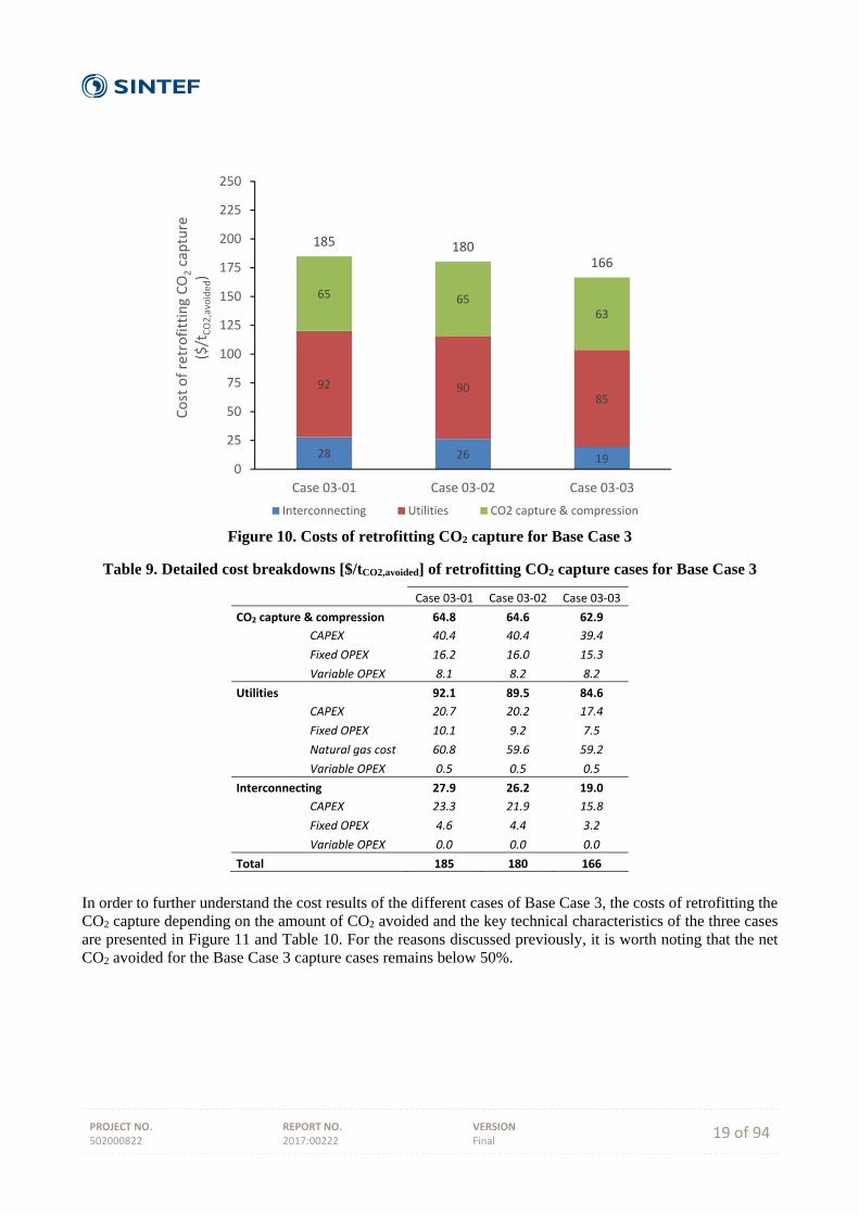
PROJECT NO. 502000822
REPORT NO. 2017:00222
VERSION Final 19 of 94
Figure 10. Costs of retrofitting CO2 capture for Base Case 3
Table 9. Detailed cost breakdowns [$/tCO2,avoided] of retrofitting CO2 capture cases for Base Case 3
Case 03‐01 Case 03‐02 Case 03‐03
CO2 capture & compression 64.8 64.6 62.9
CAPEX 40.4 40.4 39.4
Fixed OPEX 16.2 16.0 15.3
Variable OPEX 8.1 8.2 8.2
Utilities 92.1 89.5 84.6
CAPEX 20.7 20.2 17.4
Fixed OPEX 10.1 9.2 7.5
Natural gas cost 60.8 59.6 59.2
Variable OPEX 0.5 0.5 0.5
Interconnecting 27.9 26.2 19.0
CAPEX 23.3 21.9 15.8
Fixed OPEX 4.6 4.4 3.2
Variable OPEX 0.0 0.0 0.0
Total 185 180 166
In order to further understand the cost results of the different cases of Base Case 3, the costs of retrofitting the CO2 capture depending on the amount of CO2 avoided and the key technical characteristics of the three cases are presented in Figure 11 and Table 10. For the reasons discussed previously, it is worth noting that the net CO2 avoided for the Base Case 3 capture cases remains below 50%.
28 26 19
92 9085
65 6563
185 180166
0
25
50
75
100
125
150
175
200
225
250
Case 03‐01 Case 03‐02 Case 03‐03
Cost of retrofitting CO2capture
($/t
CO2,avoided)
Interconnecting Utilities CO2 capture & compression
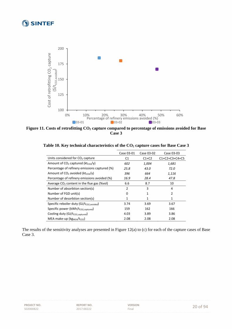
PROJECT NO. 502000822
REPORT NO. 2017:00222
VERSION Final 20 of 94
Figure 11. Costs of retrofitting CO2 capture compared to percentage of emissions avoided for Base
Case 3
Table 10. Key technical characteristics of the CO2 capture cases for Base Case 3
Case 03‐01 Case 03‐02 Case 03‐03
Units considered for CO2 capture C1 C1+C2 C1+C2+C3+C4+C5
Amount of CO2 captured (ktCO2/y) 602 1,004 1,681
Percentage of refinery emissions captured (%) 25.8 43.0 72.0
Amount of CO2 avoided (ktCO2/y) 396 664 1,116
Percentage of refinery emissions avoided (%) 16.9 28.4 47.8
Average CO2 content in the flue gas (%vol) 6.6 8.7 10
Number of absorbtion section(s) 2 3 4
Number of FGD unit(s) 0 1 2
Number of desorbtion section(s) 1 1 1
Specific reboiler duty (GJ/tCO2,avoided) 3.74 3.69 3.67
Specific power (kWh/tCO2,captured) 159 162 166
Cooling duty (GJ/tCO2,captured) 4.03 3.89 3.86
MEA make‐up (kgMEA/tCO2) 2.08 2.08 2.08
The results of the sensitivity analyses are presented in Figure 12(a) to (c) for each of the capture cases of Base Case 3.
100
125
150
175
200
0% 10% 20% 30% 40% 50% 60%
Cost of retrofitting CO2capture
($/t
CO2,avoided)
Percentage of refinery emissions avoided (%)03‐01 03‐02 03‐03
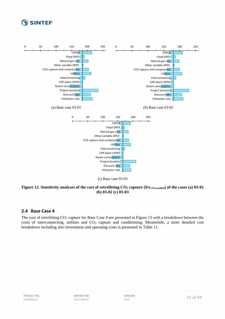
PROJECT NO. 502000822
REPORT NO. 2017:00222
VERSION Final 21 of 94
(a) Base case 03-01 (b) Base case 03-02
(c) Base case 03-03
Figure 12. Sensitivity analyses of the cost of retrofitting CO2 capture ($/tCO2,avoided) of the cases (a) 03-01 (b) 03-02 (c) 03-03
2.4 Base Case 4
The cost of retrofitting CO2 capture for Base Case 4 are presented in Figure 13 with a breakdown between the costs of interconnecting, utilities and CO2 capture and conditioning. Meanwhile, a more detailed cost breakdown including also investment and operating costs is presented in Table 11.
0 50 100 150 200 250
CAPEX
Fixed OPEX
Natural gas cost
Other variable OPEX
CO2 capture and compression
Utilities
Interconnecting
CHP plant CAPEX
Steam consumption
Project duration
Discount rate
Utilisation rate
0 50 100 150 200 250
CAPEX
Fixed OPEX
Natural gas cost
Other variable OPEX
CO2 capture and compression
Utilities
Interconnecting
CHP plant CAPEX
Steam consumption
Project duration
Discount rate
Utilisation rate
0 50 100 150 200 250
CAPEX
Fixed OPEX
Natural gas cost
Other variable OPEX
CO2 capture and compression
Utilities
Interconnecting
CHP plant CAPEX
Steam consumption
Project duration
Discount rate
Utilisation rate
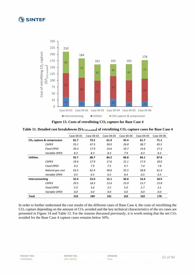
PROJECT NO. 502000822
REPORT NO. 2017:00222
VERSION Final 22 of 94
Figure 13. Costs of retrofitting CO2 capture for Base Case 4
Table 11. Detailed cost breakdowns [$/tCO2,avoided] of retrofitting CO2 capture cases for Base Case 4
Case 04‐01 Case 04‐02 Case 04‐03 Case 04‐04 Case 04‐05 Case 04‐06
CO2 capture & compression 81.7 73.5 61.9 45.4 61.7 71.1
CAPEX 53.1 47.3 39.0 26.8 38.7 45.5
Fixed OPEX 20.3 17.9 14.6 10.7 14.6 17.3
Variable OPEX 8.3 8.3 8.3 7.9 8.3 8.3
Utilities 92.7 88.7 84.2 86.8 84.1 87.8
CAPEX 19.4 17.9 17.6 21.1 17.4 18.0
Fixed OPEX 9.3 7.9 7.5 9.7 7.4 7.8
Natural gas cost 63.5 62.4 58.6 55.5 58.8 61.4
Variable OPEX 0.5 0.5 0.5 0.4 0.5 0.5
Interconnecting 35.4 22.0 15.1 30.0 16.4 18.9
CAPEX 29.5 18.3 12.6 25.0 13.7 15.8
Fixed OPEX 5.9 3.6 2.5 5.0 2.7 3.1
Variable OPEX 0.0 0.0 0.0 0.0 0.0 0.0
Total 210 184 161 162 162 178
In order to further understand the cost results of the different cases of Base Case 4, the costs of retrofitting the CO2 capture depending on the amount of CO2 avoided and the key technical characteristics of the six cases are presented in Figure 14 and Table 12. For the reasons discussed previously, it is worth noting that the net CO2 avoided for the Base Case 4 capture cases remains below 50%.
3522 15
3016 19
93
8984
87
84 88
82
74
6245
6271
210
184
161 162 162178
0
25
50
75
100
125
150
175
200
225
250
Case 04‐01 Case 04‐02 Case 04‐03 Case 04‐04 Case 04‐05 Case 04‐06
Cost of retrofitting CO2capture
($/t
CO2,avoided)
Interconnecting Utilities CO2 capture & compression

PROJECT NO. 502000822
REPORT NO. 2017:00222
VERSION Final 23 of 94
Figure 14. Costs of retrofitting CO2 capture compared to percentage of emissions avoided for Base
Case 4
Table 12. Key technical characteristics of the CO2 capture cases for Base Case 4
Case 04‐01 Case 04‐02 Case 04‐03 Case 04‐04 Case 04‐05 Case 04‐06
Units considered for CO2 capture D1 D1+D3+D4 D1+D2+D3+D4+D5
D5 D1+D3 +D4+D5
D1+D2 +D3+D4
Amount of CO2 captured (ktCO2/y) 740 1,485 2,777 886 2,376 1,886
Percentage of refinery emissions captured (%) 19.1 38.4 71.7 22.9 61.4 48.7
Amount of CO2 avoided (ktCO2/y) 481 975 1,847 600 1,579 1,243
Percentage of refinery emissions avoided (%) 12.4 25.2 47.7 15.5 40.8 32.1
Average CO2 content in the flue gas (%vol) 4.7 6.7 9.4 17.7 8.7 7.7
Number of absorbtion section(s) 2 2 4 1 3 3
Number of FGD unit(s) 0 1 2 0 1 2
Number of desorbtion section(s) 1 1 1 1 1 1
Specific reboiler duty (GJ/tCO2,avoided) 3.85 3.76 3.68 3.57 3.69 3.65
Specific power (kWh/tCO2,captured) 183 184 162 123 161 180
Cooling duty (GJ/tCO2,captured) 3.54 3.64 3.55 3.24 3.52 3.72
MEA make‐up (kgMEA/tCO2) 2.09 2.09 2.09 2.09 2.09 2.09
The results of the sensitivity analyses are presented in Figure 15(a) to (f) for each of the capture cases of Base Case 4.
100
125
150
175
200
225
0% 10% 20% 30% 40% 50% 60%
Cost of retrofitting CO2capture
($/t
CO2,avoided)
Percentage of refinery emissions avoided (%)
04‐01 04‐02 04‐03 04‐04 04‐05 04‐06
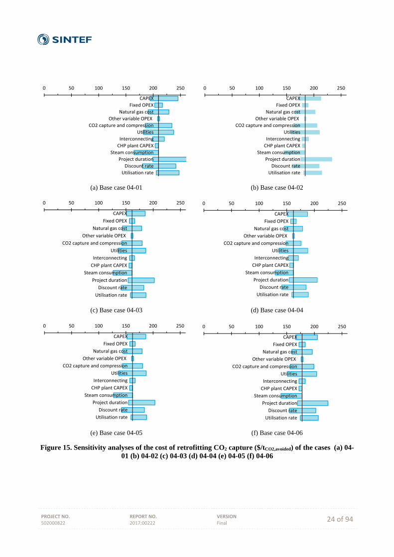
PROJECT NO. 502000822
REPORT NO. 2017:00222
VERSION Final 24 of 94
(a) Base case 04-01 (b) Base case 04-02
(c) Base case 04-03 (d) Base case 04-04
(e) Base case 04-05 (f) Base case 04-06
Figure 15. Sensitivity analyses of the cost of retrofitting CO2 capture ($/tCO2,avoided) of the cases (a) 04-01 (b) 04-02 (c) 04-03 (d) 04-04 (e) 04-05 (f) 04-06
0 50 100 150 200 250
CAPEX
Fixed OPEX
Natural gas cost
Other variable OPEX
CO2 capture and compression
Utilities
Interconnecting
CHP plant CAPEX
Steam consumption
Project duration
Discount rate
Utilisation rate
0 50 100 150 200 250
CAPEX
Fixed OPEX
Natural gas cost
Other variable OPEX
CO2 capture and compression
Utilities
Interconnecting
CHP plant CAPEX
Steam consumption
Project duration
Discount rate
Utilisation rate
0 50 100 150 200 250
CAPEX
Fixed OPEX
Natural gas cost
Other variable OPEX
CO2 capture and compression
Utilities
Interconnecting
CHP plant CAPEX
Steam consumption
Project duration
Discount rate
Utilisation rate
0 50 100 150 200 250
CAPEX
Fixed OPEX
Natural gas cost
Other variable OPEX
CO2 capture and compression
Utilities
Interconnecting
CHP plant CAPEX
Steam consumption
Project duration
Discount rate
Utilisation rate
0 50 100 150 200 250
CAPEX
Fixed OPEX
Natural gas cost
Other variable OPEX
CO2 capture and compression
Utilities
Interconnecting
CHP plant CAPEX
Steam consumption
Project duration
Discount rate
Utilisation rate
0 50 100 150 200 250
CAPEX
Fixed OPEX
Natural gas cost
Other variable OPEX
CO2 capture and compression
Utilities
Interconnecting
CHP plant CAPEX
Steam consumption
Project duration
Discount rate
Utilisation rate

PROJECT NO. 502000822
REPORT NO. 2017:00222
VERSION Final 25 of 94
2.5 Discussions and overall comparison
The evaluations show that the cost obtained for the 16 cases range between 160 and 210 $/tCO2,avoided , as shown in Figure 16, which is significantly larger than general CO2 capture and conditioning estimates available in the literature for other sources (natural gas and coal power generation, cement, steel, etc.)8,9,10,11,12. Several reasons can be used to explain this difference. First, the present study is aimed at including the retrofit costs, of such as interconnection costs. Furthermore, the utilities cost is based on the installation of an additional CHP plant, cooling water towers and waste water plant which are all designed with significant spare capacity in some cases (up to 30% overdesign). Finally, most of the CO2 capture cases considered include small to medium CO2 emission point sources with low to medium flue gas CO2 content (7 of the 16 cases considered only flue gases with a CO2 content below 11.3%vol). Although the cost distribution is specific to each case considered, the overall breakdown between the different sections is as follow. 30-40% of costs linked to CO2 capture and conditioning, 45-55% linked to utilities production, and 10-20% linked to interconnecting costs. When looking at the more detailed cost breakdowns, the results show that the main elements, which vary between the 16 cases, are the investment and thus fixed operation costs of the three sections and the operating costs linked to natural gas consumption. In term of investment, the estimations show that the total capital requirement lies between 200 and 1500 M$ for the different case as shown in Figure 16. The main reasons for this wide range is mainly the differences in amount of CO2 captured between the cases. It is worth noting that although a case may be cheaper in term of normalised cost ($/tCO2,avoided), high total capital requirement could make it less attractive.
Figure 16. Cost of retrofitting CO2 capture of all cases considered for the four refinery base cases by
section
Figure 17 seems to indicate that, apart from few cases, the capture cases with higher amount of CO2 avoided results in lower costs. However, it is important to understand that here the differences between the cases are significantly more complex than difference in scale. Indeed, as shown in the key characteristics of each cases,
8 IEAGHG, CO2 capture in the cement industry, 2008/3., 2008. 9 IEAGHG, Deployment of CCS in the Cement industry, 2013/19., 2013. 10 IEAGHG, Iron and steel CCS study (Techno-economic integrated steel mill), 2013/4, 2013. 11 IEAGHG, CO2 Capture at Coal Based Power and Hydrogen Plants, 2014/3., 2014. 12 R. Anantharaman, O. Bolland, N. Booth, E.V. Dorst, C. Ekstrom, F. Franco, E. Macchi, G. Manzolini, D. Nikolic, A. Pfeffer, M. Prins, S. Rezvani, L. Robinson, D4.9 European best practice guidelines for assessment of CO2 capture technologies, DECARBit Project, 2011.
31 29 27 25 26 19 30 28 26 1935 22 15 30 16 19
98 92 91 89 8984
91 92 9085
9389
8487
84 88
61 69 68 59 6162
73 65 6563
82
7462
4562
71
190 190 185173 176
166
194185 180
166
210
184
161 162 162178
0
250
500
750
1000
1250
1500
0
25
50
75
100
125
150
175
200
225
250
01‐01 01‐02 01‐03 02‐01 02‐02 02‐03 02‐04 03‐01 03‐02 03‐03 04‐01 04‐02 04‐03 04‐04 04‐05 04‐06
Base Case 1 Base Case 2 Base Case 3 Base case 4
Total Capital Req
uirem
ent (M
$)
Cost of retrofitting CO2capture
($/t
CO2,avoided)
Interconnecting Utilities CO2 capture & compression Total Capital Requirement
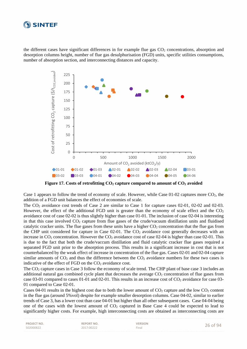
PROJECT NO. 502000822
REPORT NO. 2017:00222
VERSION Final 26 of 94
the different cases have significant differences in for example flue gas CO2 concentrations, absorption and desorption columns height, number of flue gas desulphurisation (FGD) units, specific utilities consumptions, number of absorption section, and interconnecting distances and capacity.
Figure 17. Costs of retrofitting CO2 capture compared to amount of CO2 avoided
Case 1 appears to follow the trend of economy of scale. However, while Case 01-02 captures more CO2, the addition of a FGD unit balances the effect of economies of scale. The CO2 avoidance cost trends of Case 2 are similar to Case 1 for capture cases 02-01, 02-02 and 02-03. However, the effect of the additional FGD unit is greater than the economy of scale effect and the CO2 avoidance cost of case 02-02 is thus slightly higher than case 01-01. The inclusion of case 02-04 is interesting in that this case involved CO2 capture from flue gases of the crude/vacuum distillation units and fluidised catalytic cracker units. The flue gases from these units have a higher CO2 concentration that the flue gas from the CHP unit considered for capture in Case 02-01. The CO2 avoidance cost generally decreases with an increase in CO2 concentration. However the CO2 avoidance cost of case 02-04 is higher than case 02-01. This is due to the fact that both the crude/vaccum distillation and fluid catalytic cracker flue gases required a separated FGD unit prior to the absorption process. This results in a significant increase in cost that is not counterbalanced by the weak effect of increase in concentration of the flue gas. Cases 02-01 and 02-04 capture similar amounts of CO2 and thus the difference between the CO2 avoidance numbers for these two cases is indicative of the effect of FGD on the CO2 avoidance cost. The CO2 capture cases in Case 3 follow the economy of scale trend. The CHP plant of base case 3 includes an additional natural gas combined cycle plant that decreases the average CO2 concentration of flue gases from case 03-01 compared to cases 01-01 and 02-01. This results in an increase cost of CO2 avoidance for case 03-01 compared to Case 02-01. Cases 04-01 results in the highest cost due to both the lower amount of CO2 capture and the low CO2 content in the flue gas (around 5%vol) despite for example smaller desorption columns. Case 04-02, similar to earlier trends of Case 3, has a lower cost than case 04-01 but higher than all other subsequent cases. Case 04-04 being one of the cases with the lowest amount of CO2 captured in Base Case 4 could be expected to lead to significantly higher costs. For example, high interconnecting costs are obtained as interconnecting costs are
0
25
50
75
100
125
150
175
200
225
0 500 1000 1500 2000
Cost of retrofitting CO2capture ($/t
CO2,avoided)
Amount of CO2 avoided (ktCO2/y)
01‐01 01‐02 01‐03 02‐01 02‐02 02‐03 02‐04 03‐01
03‐02 03‐03 04‐01 04‐02 04‐03 04‐04 04‐05 04‐06
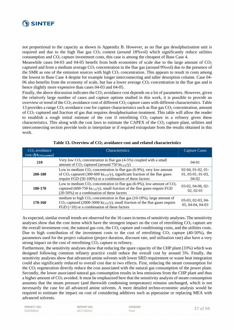
PROJECT NO. 502000822
REPORT NO. 2017:00222
VERSION Final 27 of 94
not proportional to the capacity as shown in Appendix B. However, as no flue gas desulphurisation unit is required and due to the high flue gas CO2 content (around 18%vol) which significantly reduce utilities consumption and CO2 capture investment costs, this case is among the cheapest of Base Case 4. Meanwhile cases 04-03 and 04-05 benefit from both economies of scale due to the large amount of CO2 captured and from a medium average CO2 concentration in the flue gas (around 9%vol) due to the presence of the SMR as one of the emission sources with high CO2 concentration. This appears to result in costs among the lowest in Base Case 4 despite for example longer interconnecting and taller desorption column. Case 04-06 also benefits from the economy of scale, but has a lower average CO2 concentration in the flue gas and is hence slightly more expensive than cases 04-03 and 04-05. Finally, the above discussion indicates the CO2 avoidance cost depends on a lot of parameters. However, given the relatively large number of cases and capture options studied in this work, it is possible to provide an overview or trend of the CO2 avoidance cost of different CO2 capture cases with different characteristics. Table 13 provides a range CO2 avoidance cost for capture characteristics such as flue gas CO2 concentration, amount of CO2 captured and fraction of gas that requires desulphurisation treatment. This table will allow the reader to establish a rough initial estimate of the cost if retrofitting CO2 capture in a refinery given these characteristics. This along with the cost laws to estimate the CAPEX of the CO2 capture plant, utilities and interconnecting section provide tools to interpolate or if required extrapolate from the results obtained in this work.
Table 13. Overview of CO2 avoidance cost and related characteristics
CO2 avoidance cost ($/tCO2,avoided)
Characteristics Capture Cases
210 Very low CO2 concentration in flue gas (4-5%) coupled with a small amount of CO2 captured (around 750 ktCO2/y)
04-01
200-180 Low to medium CO2 concentration in flue gas (6-9%), very low amount of CO2 captured (300-600 ktCO2/y), significant fraction of the flue gases require FGD (50-100%) or a combination of these factors
02-04, 01-02, 01-01, 03-01, 01-03,
04-02
180-170 Low to medium CO2 concentration in flue gas (6-9%), low amount of CO2 captured (600-750 ktCO2/y), small fraction of the flue gases require FGD (20-50%) or a combination of these factors
03-02, 04-06, 02-02, 02-01
170-160 medium to high CO2 concentration in flue gas (10-18%), large amount of CO2 captured (2000-3000 ktCO2/y), small fraction of the flue gases require FGD (<10) or a combination of these factors
03-03, 02-03, 04-05, 04-04, 04-03
As expected, similar overall trends are observed for the 16 cases in terms of sensitivity analyses. The sensitivity analyses show that the cost items which have the strongest impact on the cost of retrofitting CO2 capture are the overall investment cost, the natural gas cost, the CO2 capture and conditioning costs, and the utilities costs. Due to high contribution of the investment costs to the cost of retrofitting CO2 capture (40-50%), the parameters used for the project valuation (project duration, discount rate, and utilisation rate) also have a very strong impact on the cost of retrofitting CO2 capture to refinery. Furthermore, the sensitivity analyses show that reducing the spare capacity of the CHP plant (33%) which was designed following common refinery practice could reduce the overall cost by around 5%. Finally, the sensitivity analyses show that advanced amine solvents with lower SRD requirement or waste heat integration could also significantly reduced to overall cost due to two effects. First, reducing the steam consumption for the CO2 regeneration directly reduce the cost associated with the natural gas consumption of the power plant. Secondly, the lower associated natural gas consumption results in less emissions from the CHP plant and thus a higher amount of CO2 avoided. It must be emphasized here that the sensitivity analysis of steam consumption assumes that the steam pressure (and therewith condensing temperature) remains unchanged, which is not necessarily the case for all advanced amine solvents. A more detailed techno-economic analysis would be required to estimate the impact on cost of considering additives such as piperazine or replacing MEA with advanced solvents.
PROJECT NO. 502000822
REPORT NO. 2017:00222
VERSION Final 28 of 94
Sensitivity analyses show that there are opportunities to reduce the cost of utilities that merit further investigation, for example:
With the objective to reduce the steam (and if possible power) requirement for CO2 capture and compression: Evaluation of advanced solvents with lower specific heat requirement as well as other CO2 capture technologies13.
Use of readily available waste heat within the refinery plant as well as (when relevant) from nearby industries in combination with purchase of the necessary power for CO2 capture and compression from the grid, preferably from renewable power or large efficient thermal power plants with CO2 capture.
Lower utilities investment cost through reduced design margins: The design of CHP plant has been performed considering significant overdesign in some cases (up to 30%). In practice, this over-design of the additional CHP, included to provide the steam and power required for CO2 capture, might be reduced.
Operation at full load of existing CHP plants in a refinery. This would mean to accept temporary shut-down of CO2 capture when there is a CHP plant failure since refinery production has priority. This approach could be evaluated with the following steps:
5. Determine maximum additional steam production in refinery if installed CHP capacity is fully used
6. Knowing this additional steam production, and for selected solvent(s): Determine approximately how much CO2 can be captured (i.e. what thermal power can be made available in the reboiler)
7. Assess the different options in the refinery to capture this amount of CO2 (i.e. the emission points that CO2 could be captured from, where capture rate may be other than the 90% assumed in this work)
8. Evaluate how practical different capture options are to implement, and how much they will cost.
13 Such as membrane technologies, adsorption, hybrid technology concepts, etc.
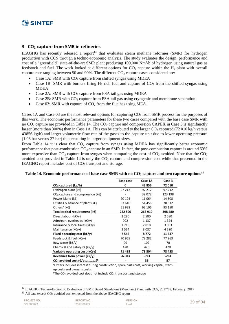
PROJECT NO. 502000822
REPORT NO. 2017:00222
VERSION Final 29 of 94
3 CO2 capture from SMR in refineries
IEAGHG has recently released a report14 that evaluates steam methane reformer (SMR) for hydrogen production with CCS through a techno-economic analysis. The study evaluates the design, performance and cost of a "greenfield" state-of-the-art SMR plant producing 100,000 Nm3/h of hydrogen using natural gas as feedstock and fuel. The work looked at different options for CO2 capture within the H2 plant with overall capture rate ranging between 50 and 90%. The different CO2 capture cases considered are:
Case 1A: SMR with CO2 capture from shifted syngas using MDEA Case 1B: SMR with burners firing H2 rich fuel and capture of CO2 from the shifted syngas using
MDEA Case 2A: SMR with CO2 capture from PSA tail gas using MDEA Case 2B: SMR with CO2 capture from PSA tail gas using cryogenic and membrane separation Case 03: SMR with capture of CO2 from the flue has using MEA.
Cases 1A and Case 03 are the most relevant options for capturing CO2 from SMR process for the purposes of this work. The economic performance parameters for these two cases compared with the base case SMR with no CO2 capture are provided in Table 14. The CO2 capture and compression CAPEX in Case 3 is signifanctly larger (more than 300%) than in Case 1A. This can be attributed to the larger CO2 captured (72 010 kg/h versus 43856 kg/h) and larger volumetric flow rate of the gases to the capture unit due to lower operating pressure (1.03 bar versus 27 bar) thus resulting in larger equipment sizes. From Table 14 it is clear that CO2 capture from syngas using MDEA has significantly better economic performance that post-combustion CO2 capture in an SMR. In fact, the post-combustion capture is around 60% more expensive than CO2 capture from syngas when comparing the cost of CO2 avoided. Note that the CO2 avoided cost provided in Table 14 is only the CO2 capture and compression cost while that presented in the IEAGHG report includes cost of CO2 transport and storage.
Table 14. Economic performance of base case SMR with no CO2 capture and two capture options15
Base case Case 1A Case 3
CO2 captured (kg/h) 0 43 856 72 010
Hydrogen plant (k€) 97 212 97 212 97 212
CO2 capture and compression (k€) ‐ 39 072 123 198
Power island (k€) 20 124 11 064 14 608
Utilities & balance of plant (k€) 53 616 54 456 70 312
Othersa (k€) 51 938 62 106 93 150
Total capital requirement (k€) 222 890 263 910 398 480
Direct labour (k€/y) 2 280 2 580 2 580
Adm/gen. overheads (k€/y) 992 1 137 1 324
Insurance & local taxes (k€/y) 1 710 2 018 3 053
Maintenance (k€/y) 2 564 3 037 4 580
Fixed operating cost (k€/y) 7 546 8 772 11 537
Feedstock & fuel (k€/y) 70 965 73 282 77 963
Raw water (k€/y) 99 102 70
Chemical and catalysts (k€/y) 420 420 420
Variable operating cost (k€/y) 71 485 73 804 78 453
Revenues from power (k€/y) ‐6 603 ‐993 ‐284
CO2 avoided cost (€/tCO2,avoided)b ‐ 36 57 aOthers includes interest during construction, spare parts cost, working capital, start‐up costs and owner's costs. bThe CO2 avoided cost does not include CO2 transport and storage
14 IEAGHG, Techno-Economic Evaluation of SMR Based Standalone (Merchant) Plant with CCS, 2017/02, February, 2017 15 All data except CO2 avoided cost extracted from the above IEAGHG report

PROJECT NO. 502000822
REPORT NO. 2017:00222
VERSION Final 30 of 94
Comparison of the results presented in the IEAGHG report with calculated values from this work could present insights on the effect of refinery integration. The economic data in the IEAGHG report is evaluated in Euros with Q42014 as the reporting period while in this work the economic data are reported in US Dollars with Q42015 as the reporting period. The IEAGHG economic performance data updated based on the CEPCI and a $/€ 2015 conversion rate of 1.11 is reported in Table 15.
Table 15. Economic performance of base case SMR with no CO2 capture and two capture options corrected for 2015Q4 and converted currency to US Dollars
Base case Case 1A Case 3
CO2 captured (kg/h) 0 43 856 72 010
Hydrogen plant (k€) 99 707 99 707 99 707
CO2 capture and compression (k€) ‐ 40 075 126 360
Power island (k€) 20 641 11 348 14 983
Utilities & balance of plant (k€) 54 992 55 854 72 117
Others (k€) 53 271 63 700 95 541
Total capital requirement (k€) 228 612 270 685 408 709
Direct labour (k€/y) 2 526 2 858 2 858
Adm/gen. overheads (k€/y) 1 099 1 260 1 466
Insurance & local taxes (k€/y) 1 753 2 070 3 132
Maintenance (k€/y) 2 630 3 115 4 697
Fixed operating cost (k€/y) 8 008 9 303 12 154
Feedstock & fuel (k€/y) 78 615 81 182 86 367
Raw water (k€/y) 111 113 78
Chemical and catalysts (k€/y) 468 468 468
Variable operating cost (k€/y) 79 195 81 763 86 913
Revenues from power (k€/y) ‐6 603 ‐993 ‐284
CO2 avoided cost (€/tCO2,avoided) ‐ 37.5 59.4
A summary of the economic data for Case 04-04, which is similar to Case 3 of the IEAGHG report is presented below in Table 16. The details of the economic data for Capture Case 04-04 are presented in Appendix D4.4.
Table 16. Economic performance of Capture Case 04-04
Case 04‐04
CO2 captured (kg/h) 105 485
CO2 capture and compression (k€) 147 062
Power island & utilities(k€) 115 564
Interconnecting (k€) 137 770
Others (k€) 103 268
Total capital requirement (k€) 503 664
Direct labour (k€/y) 1 600
Maintenance (k€/y) 9 942
Other (k€/y) 1 795
Fixed operating cost (k€/y) 13 337
Feedstock & fuel (k€/y) 33 322
Raw water (k€/y) 261
Chemical and catalysts (k€/y) 3 684
Waste disposal (k€/y) 1 058
Variable operating cost (k€/y) 38 325
CO2 avoided cost (€/tCO2,avoided) 151.4
The results show that the capital cost of the CO2 capture and compression plant are similar in this work and the IEAGHG report. Apart from that all other costs in this work are significantly higher. This is mainly because
PROJECT NO. 502000822
REPORT NO. 2017:00222
VERSION Final 31 of 94
the capture case in this work involves building a new CHP plant for supplying the steam and power required for the CO2 capture and compression plant while in the IEAGHG report, this is extracted from the stand-alone H2 plant. This shows not only in the CAPEX of the power plant and utilities, but also in the variable operating cost attributed to the fuel. Additionally, the capture case in this work also required building a cooling tower for providing cooling water and there is a significant CAPEX associated with the interconnecting. These are not required in the IEAGHG case. It is clear from the above discussion that the high cost of CO2 avoided in Capture Case 04-04 is primarily due to its tight integration with the refinery and additional costs for building and operating a CHP plant to provide steam and power for the CO2 capture and compression units. It is expected that CO2 capture from syngas relevant to this work will also be 50% less expensive than the post-combustion capture case following a similar pattern to that presented in the IEAGHG report. To summarize, CO2 capture from the syngas stream in refineries leads to lower CO2 avoidance cost compared to capture from the SMR furnace flue gas stream. However, only 55% of the SMR emissions are captured in the former compared to 90% capture in the latter. The choice of CO2 capture from syngas or furnace flue gas will thus depend on how much CO2 requires to be captured from the refinery. From the earlier discussion on post-combustion CO2 capture, it is clear that CO2 capture from SMR furnace flue gases result in one of the cheapest CO2 avoidance cost. Thus when large amounts of CO2 are required to be captured from refineries post-combustion CO2 capture from SMR furnace flue gas is the most relevant option.

PROJECT NO. 502000822
REPORT NO. 2017:00222
VERSION Final 32 of 94
A Detailed equipment list of selected cases
A.1 Base case 01‐03
A.1.1 CO2 capture and compression
Table 17. Equipment list for the CRF Absorber section for Base case 01-03
ITEM No.
DESCRIPTION TYPE SIZE DESIGN
PRESSURE DESIGN
TEMPERATURE MATERIAL REMARKS
ID H barg °C
Columns (mm) (mm)
T-6001 Direct Contact
Cooler Vertical 3 100 10 000 2,0 116 SS304L
Packed column
(Mellapak 250X)
T-6002 Absorber Vertical 3 000 36 000 1,9 99 SS304L
Packed column
(Mellapak 250X). Water wash section
included
ITEM No.
DESCRIPTION TYPE SIZE DESIGN
PRESSURE DESIGN
TEMPERATURE MATERIAL REMARKS
Duty Area barg °C
Heat
Exchangers (kW) (m2)
E-6001 Flue gas reheater
P&F 2 581 116 2,0 232 SS304L
E-6002 DCC cooler P&F 5 518 526 4,8 91 SS304L
E-6003 Amine wash
cooler P&F 220 7 4,8 92 SS304L
E-6008 Intercooler P&F 632 50 4,8 74 SS304L
ITEM No.
DESCRIPTION TYPE SIZE DESIGN
PRESSURE DESIGN
TEMPERATURE MATERIAL REMARKS
Flow Power barg °C
Fans and
Compressors (N m3/h) (kW)
C-6001 Exhaust fan 64 538 492 2,00 232 SS304L Pin/Poutrrrre
0.0/0.1
ITEM No.
DESCRIPTION TYPE SIZE DESIGN
PRESSURE DESIGN
TEMPERATURE MATERIAL REMARKS
Flow Power barg °C
Pumps (Actual m3/h)
(kW)
P-6001 DCC Circulating
pump Centrifugal 174 12 3,7 91 SS304L
Pin/Pout: 0.1/1.9
P-6002 Amine water wash pump
Centrifugal 17 1 3,5 92 SS304L Pin/Pout: 0.1/1.7
P-6003 Rich amine
pump Centrifugal 138 24 7,1 70 SS304L
Pin/Pout: 0.1/5.2
P-6009 Intercooler pump Centrifugal 135 7 3,4 74 SS304L Pin/Pout: 0.1/1.5
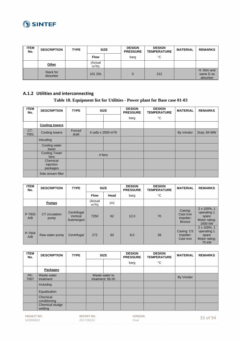
PROJECT NO. 502000822
REPORT NO. 2017:00222
VERSION Final 33 of 94
ITEM No.
DESCRIPTION TYPE SIZE DESIGN
PRESSURE DESIGN
TEMPERATURE MATERIAL REMARKS
Flow barg °C
Other (Actual m3/h)
Stack for Absorber
101 291 0 212 H: 50m and same D as absorber
A.1.2 Utilities and interconnecting
Table 18. Equipment list for Utilities - Power plant for Base case 01-03
ITEM No.
DESCRIPTION TYPE SIZE DESIGN
PRESSURE DESIGN
TEMPERATURE MATERIAL REMARKS
barg °C
Cooling towers
CT-7001
Cooling towers Forced draft
4 cells x 2500 m3/h By Vendor Duty: 84 MW
Inlcuding
Cooling water
basin
Cooling Tower
fans 4 fans
Chemical injection
packages
Side stream filter
ITEM No.
DESCRIPTION TYPE SIZE DESIGN
PRESSURE DESIGN
TEMPERATURE MATERIAL REMARKS
Flow Head barg °C
Pumps (Actual m3/h)
(m)
P-7003 A/B
CT circulation pump
Centrifugal Vertical
Submerged 7250 62 12.0 70
Casing: Cast Iron Impeller: Bronze
2 x 100%, 1 operating 1
spare Motor rating:
1600 kW
P-7004 A/B
Raw water pump Centrifugal 272 60 8.0 38 Casing: CS
Impeller: Cast Iron
2 x 100%, 1 operating 1
spare Motor rating:
75 kW
ITEM No.
DESCRIPTION TYPE SIZE DESIGN
PRESSURE DESIGN
TEMPERATURE MATERIAL REMARKS
barg °C
Packages
PK-7007
Waste water treatment
Waste water to
treatment: 56 t/h By Vendor
Including
Equalization
Chemical conditioning
Chemical sludge settling
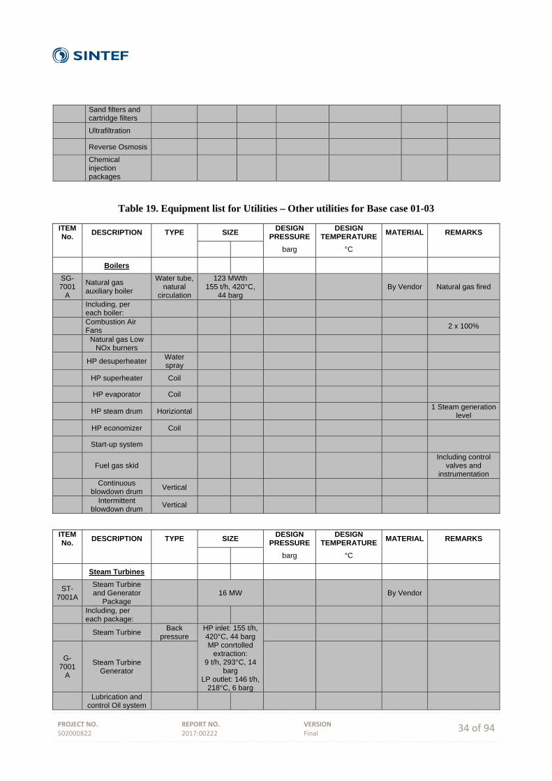
PROJECT NO. 502000822
REPORT NO. 2017:00222
VERSION Final 34 of 94
Sand filters and cartridge filters
Ultrafiltration
Reverse Osmosis
Chemical injection packages
Table 19. Equipment list for Utilities – Other utilities for Base case 01-03
ITEM No.
DESCRIPTION TYPE SIZE DESIGN
PRESSURE DESIGN
TEMPERATURE MATERIAL REMARKS
barg °C
Boilers
SG-7001
A
Natural gas auxiliary boiler
Water tube, natural
circulation
123 MWth 155 t/h, 420°C,
44 barg By Vendor Natural gas fired
Including, per each boiler:
Combustion Air Fans
2 x 100%
Natural gas Low
NOx burners
HP desuperheater Water spray
HP superheater Coil
HP evaporator Coil
HP steam drum Horiziontal 1 Steam generation
level
HP economizer Coil
Start-up system
Fuel gas skid Including control
valves and instrumentation
Continuous
blowdown drum Vertical
Intermittent
blowdown drum Vertical
ITEM No.
DESCRIPTION TYPE SIZE DESIGN
PRESSURE DESIGN
TEMPERATURE MATERIAL REMARKS
barg °C
Steam Turbines
ST-7001A
Steam Turbine and Generator
Package 16 MW By Vendor
Including, per each package:
Steam Turbine Back
pressure HP inlet: 155 t/h, 420°C, 44 bargMP conrtolled
extraction: 9 t/h, 293°C, 14
barg LP outlet: 146 t/h,
218°C, 6 barg
G-7001
A
Steam Turbine Generator
Lubrication and
control Oil system
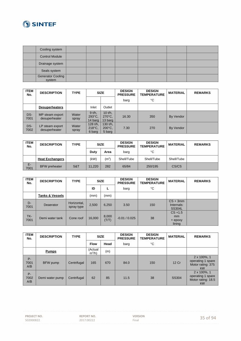
PROJECT NO. 502000822
REPORT NO. 2017:00222
VERSION Final 35 of 94
Cooling system
Control Module
Drainage system
Seals system
Generator Cooling
system
ITEM No.
DESCRIPTION TYPE SIZE DESIGN
PRESSURE DESIGN
TEMPERATURE MATERIAL REMARKS
barg °C
Desuperheaters Inlet Outlet
DS-7001
MP steam export desuperheater
Water spray
9 t/h, 293°C, 14 barg
10 t/h, 270°C, 13 barg
16.30 350 By Vendor
DS-7002
LP steam export desuperheater
Water spray
128 t/h, 218°C, 6 barg
130 t/h, 200°C, 5 barg
7.30 270 By Vendor
ITEM No.
DESCRIPTION TYPE SIZE DESIGN
PRESSURE DESIGN
TEMPERATURE MATERIAL REMARKS
Duty Area barg °C
Heat Exchangers (kW) (m2) Shell/Tube Shell/Tube Shell/Tube
E-7001
BFW preheater S&T 11,220 282 65/84 250/195 CS/CS
ITEM No.
DESCRIPTION TYPE SIZE DESIGN
PRESSURE DESIGN
TEMPERATURE MATERIAL REMARKS
ID L barg °C
Tanks & Vessels (mm) (mm)
D-7001
Deaerator Horizontal, spray type
2,500 6,250 3.50 150 CS + 3mm Internals: SS304L
TK-7001
Demi water tank Cone roof 16,000 8,000 (T/T)
-0.01 / 0.025 38
CS +1.5 mm
+ epoxy lining
ITEM No.
DESCRIPTION TYPE SIZE DESIGN
PRESSURE DESIGN
TEMPERATURE MATERIAL REMARKS
Flow Head barg °C
Pumps (Actual m3/h)
(m)
P-7001 A/B
BFW pump Centrifugal 165 670 84.0 150 12 Cr
2 x 100%, 1 operating 1 spare Motor rating: 375
kW
P-7002 A/B
Demi water pump Centrifugal 62 85 11.5 38 SS304
2 x 100%, 1 operating 1 spareMotor rating: 18.5
kW
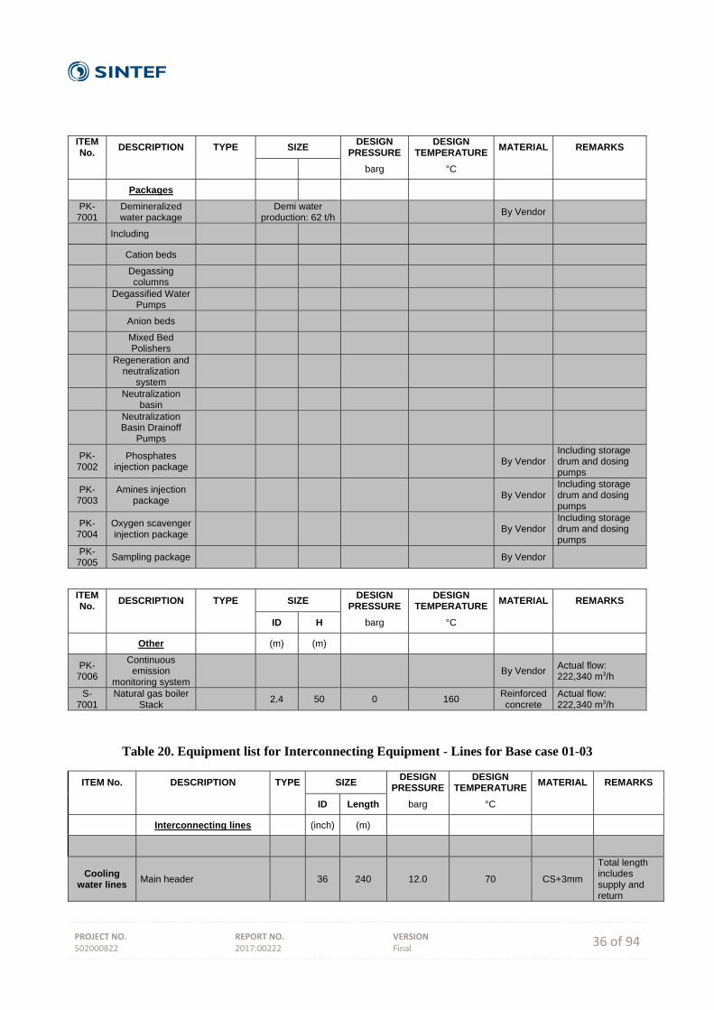
PROJECT NO. 502000822
REPORT NO. 2017:00222
VERSION Final 36 of 94
ITEM No.
DESCRIPTION TYPE SIZE DESIGN
PRESSURE DESIGN
TEMPERATURE MATERIAL REMARKS
barg °C
Packages
PK-7001
Demineralized water package
Demi water
production: 62 t/h By Vendor
Including
Cation beds
Degassing columns
Degassified Water
Pumps
Anion beds
Mixed Bed Polishers
Regeneration and
neutralization system
Neutralization
basin
Neutralization Basin Drainoff
Pumps
PK-7002
Phosphates injection package
By Vendor Including storage drum and dosing pumps
PK-7003
Amines injection package
By Vendor Including storage drum and dosing pumps
PK-7004
Oxygen scavenger injection package
By Vendor Including storage drum and dosing pumps
PK-7005
Sampling package By Vendor
ITEM No.
DESCRIPTION TYPE SIZE DESIGN
PRESSURE DESIGN
TEMPERATURE MATERIAL REMARKS
ID H barg °C
Other (m) (m)
PK-7006
Continuous emission
monitoring system By Vendor
Actual flow: 222,340 m3/h
S-7001
Natural gas boiler Stack
2.4 50 0 160 Reinforced concrete
Actual flow: 222,340 m3/h
Table 20. Equipment list for Interconnecting Equipment - Lines for Base case 01-03
ITEM No. DESCRIPTION TYPE SIZE DESIGN
PRESSUREDESIGN
TEMPERATURE MATERIAL REMARKS
ID Length barg °C
Interconnecting lines (inch) (m)
Cooling water lines
Main header 36 240 12.0 70 CS+3mm
Total length includes supply and return
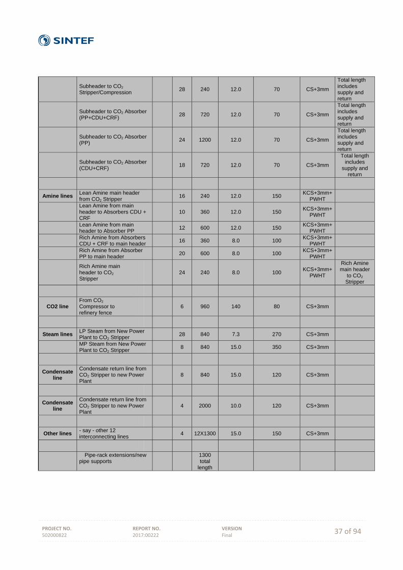
PROJECT NO. 502000822
REPORT NO. 2017:00222
VERSION Final 37 of 94
Subheader to CO2 Stripper/Compression
28 240 12.0 70 CS+3mm
Total length includes supply and return
Subheader to CO2 Absorber (PP+CDU+CRF)
28 720 12.0 70 CS+3mm
Total length includes supply and return
Subheader to CO2 Absorber (PP)
24 1200 12.0 70 CS+3mm
Total length includes supply and return
Subheader to CO2 Absorber (CDU+CRF)
18 720 12.0 70 CS+3mm
Total length includes
supply and return
Amine lines Lean Amine main header from CO2 Stripper
16 240 12.0 150 KCS+3mm+
PWHT
Lean Amine from main header to Absorbers CDU + CRF
10 360 12.0 150 KCS+3mm+
PWHT
Lean Amine from main header to Absorber PP
12 600 12.0 150 KCS+3mm+
PWHT
Rich Amine from Absorbers CDU + CRF to main header
16 360 8.0 100 KCS+3mm+
PWHT
Rich Amine from Absorber PP to main header
20 600 8.0 100 KCS+3mm+
PWHT
Rich Amine main header to CO2 Stripper
24 240 8.0 100 KCS+3mm+
PWHT
Rich Amine main header
to CO2 Stripper
CO2 line From CO2 Compressor to refinery fence
6 960 140 80 CS+3mm
Steam lines LP Steam from New Power Plant to CO2 Stripper
28 840 7.3 270 CS+3mm
MP Steam from New Power Plant to CO2 Stripper
8 840 15.0 350 CS+3mm
Condensate line
Condensate return line from CO2 Stripper to new Power Plant
8 840 15.0 120 CS+3mm
Condensate line
Condensate return line from CO2 Stripper to new Power Plant
4 2000 10.0 120 CS+3mm
Other lines - say - other 12 interconnecting lines
4 12X1300 15.0 150 CS+3mm
Pipe-rack extensions/new
pipe supports
1300 total
length
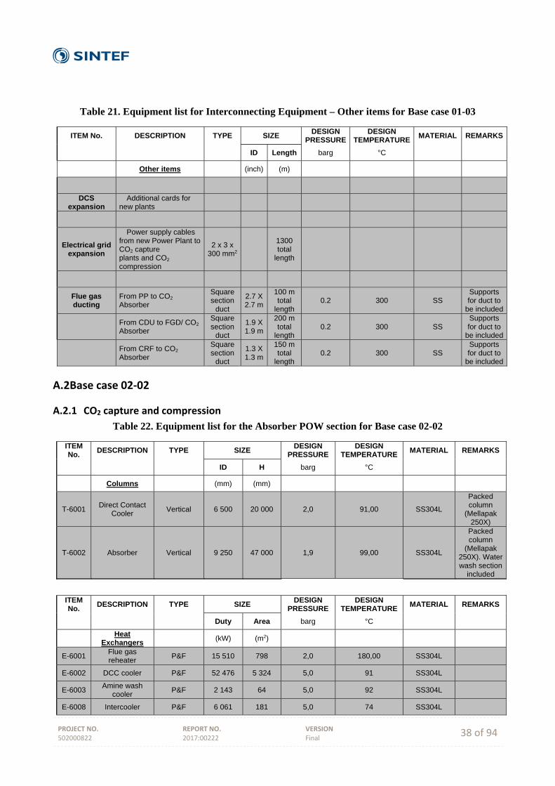
PROJECT NO. 502000822
REPORT NO. 2017:00222
VERSION Final 38 of 94
Table 21. Equipment list for Interconnecting Equipment – Other items for Base case 01-03
ITEM No. DESCRIPTION TYPE SIZE DESIGN
PRESSUREDESIGN
TEMPERATURE MATERIAL REMARKS
ID Length barg °C
Other items (inch) (m)
DCS expansion
Additional cards for new plants
Electrical grid expansion
Power supply cables from new Power Plant to CO2 capture plants and CO2 compression
2 x 3 x 300 mm2
1300 total
length
Flue gas ducting
From PP to CO2 Absorber
Square section
duct
2.7 X 2.7 m
100 m total
length 0.2 300 SS
Supports for duct to
be included
From CDU to FGD/ CO2 Absorber
Square section
duct
1.9 X 1.9 m
200 m total
length 0.2 300 SS
Supports for duct to
be included
From CRF to CO2 Absorber
Square section
duct
1.3 X 1.3 m
150 m total
length 0.2 300 SS
Supports for duct to
be included
A.2 Base case 02‐02
A.2.1 CO2 capture and compression
Table 22. Equipment list for the Absorber POW section for Base case 02-02
ITEM No.
DESCRIPTION TYPE SIZE DESIGN
PRESSURE DESIGN
TEMPERATURE MATERIAL REMARKS
ID H barg °C
Columns (mm) (mm)
T-6001 Direct Contact
Cooler Vertical 6 500 20 000 2,0 91,00 SS304L
Packed column
(Mellapak 250X)
T-6002 Absorber Vertical 9 250 47 000 1,9 99,00 SS304L
Packed column
(Mellapak 250X). Water wash section
included
ITEM No.
DESCRIPTION TYPE SIZE DESIGN
PRESSURE DESIGN
TEMPERATURE MATERIAL REMARKS
Duty Area barg °C
Heat
Exchangers (kW) (m2)
E-6001 Flue gas reheater
P&F 15 510 798 2,0 180,00 SS304L
E-6002 DCC cooler P&F 52 476 5 324 5,0 91 SS304L
E-6003 Amine wash
cooler P&F 2 143 64 5,0 92 SS304L
E-6008 Intercooler P&F 6 061 181 5,0 74 SS304L
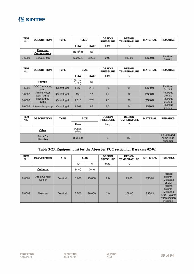
PROJECT NO. 502000822
REPORT NO. 2017:00222
VERSION Final 39 of 94
ITEM No.
DESCRIPTION TYPE SIZE DESIGN
PRESSURE DESIGN
TEMPERATURE MATERIAL REMARKS
Flow Power barg °C
Fans and
Compressors (N m3/h) (kW)
C-6001 Exhaust fan 622 531 4 224 2,00 180,00 SS304L Pin/Pout: 0.0/0.1
ITEM No.
DESCRIPTION TYPE SIZE DESIGN
PRESSURE DESIGN
TEMPERATURE MATERIAL REMARKS
Flow Power barg °C
Pumps (Actual m3/h)
(kW)
P-6001 DCC Circulating
pump Centrifugal 1 660 234 5,8 91 SS304L
Pin/Pout: 0.1/3.8
P-6002 Amine water wash pump
Centrifugal 158 17 4,7 92 SS304L Pin/Pout: 0.0/3.0
P-6003 Rich amine
pump Centrifugal 1 315 232 7,1 70 SS304L
Pin/Pout: 0.1/5.3
P-6009 Intercooler pump Centrifugal 1 303 62 3,3 74 SS304L Pin/Pout: 0.1/1.5
ITEM No.
DESCRIPTION TYPE SIZE DESIGN
PRESSURE DESIGN
TEMPERATURE MATERIAL REMARKS
Flow barg °C
Other (Actual m3/h)
Stack for Absorber
863 490 0 160 H: 50m and same D as absorber
Table 3-23. Equipment list for the Absorber FCC section for Base case 02-02
ITEM No.
DESCRIPTION TYPE SIZE DESIGN
PRESSURE DESIGN
TEMPERATURE MATERIAL REMARKS
ID H barg °C
Columns (mm) (mm)
T-6001 Direct Contact
Cooler Vertical 5 000 15 000 2,0 93,00 SS304L
Packed column
(Mellapak 250X)
T-6002 Absorber Vertical 5 500 36 000 1,9 108,00 SS304L
Packed column
(Mellapak 250X). Water wash section
included

PROJECT NO. 502000822
REPORT NO. 2017:00222
VERSION Final 40 of 94
ITEM No.
DESCRIPTION TYPE SIZE DESIGN
PRESSURE DESIGN
TEMPERATURE MATERIAL REMARKS
Duty Area barg °C
Heat
Exchangers (kW) (m2)
E-6001 Flue gas reheater
P&F 13 706 543 2,0 345,00 SS304L
E-6002 DCC cooler P&F 18 009 1 713 5,0 93 SS304L
E-6003 Amine wash
cooler P&F 1 343 34 5,0 100 SS304L
E-6008 Intercooler P&F 3 591 272 5,0 75 SS304L
ITEM No.
DESCRIPTION TYPE SIZE DESIGN
PRESSURE DESIGN
TEMPERATURE MATERIAL REMARKS
Flow Power barg °C
Fans and
Compressors (N m3/h) (kW)
C-6001 Exhaust fan 149 166 442 1,90 345,00 SS304L Pin/Pout: 0.0/0.1
C-6002 Fan after FGD 182 902 1 020 2,00 104,00 SS304L Pin/Pout: 0.0/0.1
ITEM No.
DESCRIPTION TYPE SIZE DESIGN
PRESSURE DESIGN
TEMPERATURE MATERIAL REMARKS
Flow Power barg °C
Pumps (Actual m3/h)
(kW)
P-6001 DCC Circulating
pump Centrifugal 523 46 4,3 93 SS304L
Pin/Pout: 0.1/2.5
P-6002 Amine water wash pump
Centrifugal 74 6 3,9 100 SS304L Pin/Pout: 0.0/2.0
P-6003 Rich amine
pump Centrifugal 616 108 7,1 71 SS304L
Pin/Pout: 0.1/5.3
P-6009 Intercooler pump Centrifugal 613 30 3,3 75 SS304L Pin/Pout: 0.1/1.5
ITEM No.
DESCRIPTION TYPE SIZE DESIGN
PRESSURE DESIGN
TEMPERATURE MATERIAL REMARKS
Flow barg °C
Other (Actual m3/h)
Flue Gas
Desulfurization Unit
320 000 1,9
Limestone based wet scrubbing
system
Stack for Absorber
341 942 0 304 H: 50m and same D as absorber
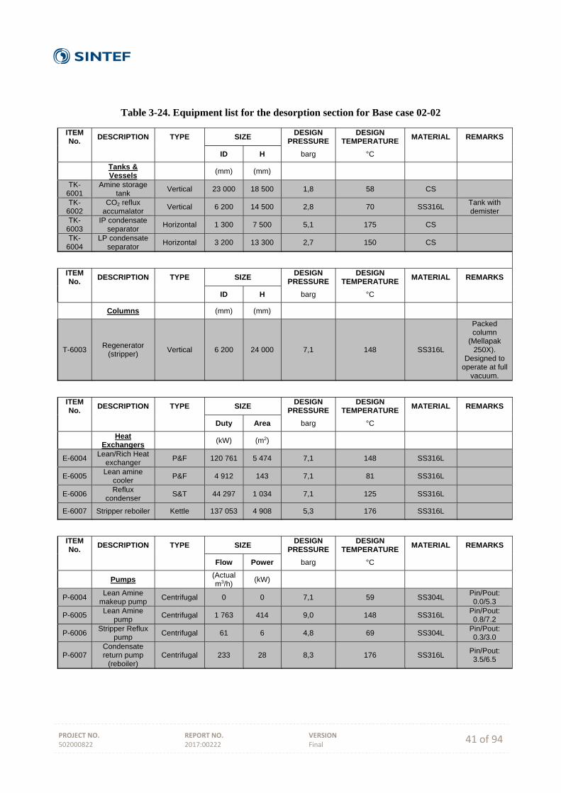
PROJECT NO. 502000822
REPORT NO. 2017:00222
VERSION Final 41 of 94
Table 3-24. Equipment list for the desorption section for Base case 02-02
ITEM No.
DESCRIPTION TYPE SIZE DESIGN
PRESSURE DESIGN
TEMPERATURE MATERIAL REMARKS
ID H barg °C
Tanks & Vessels
(mm) (mm)
TK-6001
Amine storage tank
Vertical 23 000 18 500 1,8 58 CS
TK-6002
CO2 reflux accumalator
Vertical 6 200 14 500 2,8 70 SS316L Tank with demister
TK-6003
IP condensate separator
Horizontal 1 300 7 500 5,1 175 CS
TK-6004
LP condensate separator
Horizontal 3 200 13 300 2,7 150 CS
ITEM No.
DESCRIPTION TYPE SIZE DESIGN
PRESSURE DESIGN
TEMPERATURE MATERIAL REMARKS
ID H barg °C
Columns (mm) (mm)
T-6003 Regenerator
(stripper) Vertical 6 200 24 000 7,1 148 SS316L
Packed column
(Mellapak 250X).
Designed to operate at full
vacuum.
ITEM No.
DESCRIPTION TYPE SIZE DESIGN
PRESSURE DESIGN
TEMPERATURE MATERIAL REMARKS
Duty Area barg °C
Heat
Exchangers (kW) (m2)
E-6004 Lean/Rich Heat
exchanger P&F 120 761 5 474 7,1 148 SS316L
E-6005 Lean amine
cooler P&F 4 912 143 7,1 81 SS316L
E-6006 Reflux
condenser S&T 44 297 1 034 7,1 125 SS316L
E-6007 Stripper reboiler Kettle 137 053 4 908 5,3 176 SS316L
ITEM No.
DESCRIPTION TYPE SIZE DESIGN
PRESSURE DESIGN
TEMPERATURE MATERIAL REMARKS
Flow Power barg °C
Pumps (Actual m3/h)
(kW)
P-6004 Lean Amine
makeup pump Centrifugal 0 0 7,1 59 SS304L
Pin/Pout: 0.0/5.3
P-6005 Lean Amine
pump Centrifugal 1 763 414 9,0 148 SS316L
Pin/Pout: 0.8/7.2
P-6006 Stripper Reflux
pump Centrifugal 61 6 4,8 69 SS304L
Pin/Pout: 0.3/3.0
P-6007 Condensate return pump
(reboiler) Centrifugal 233 28 8,3 176 SS316L
Pin/Pout: 3.5/6.5
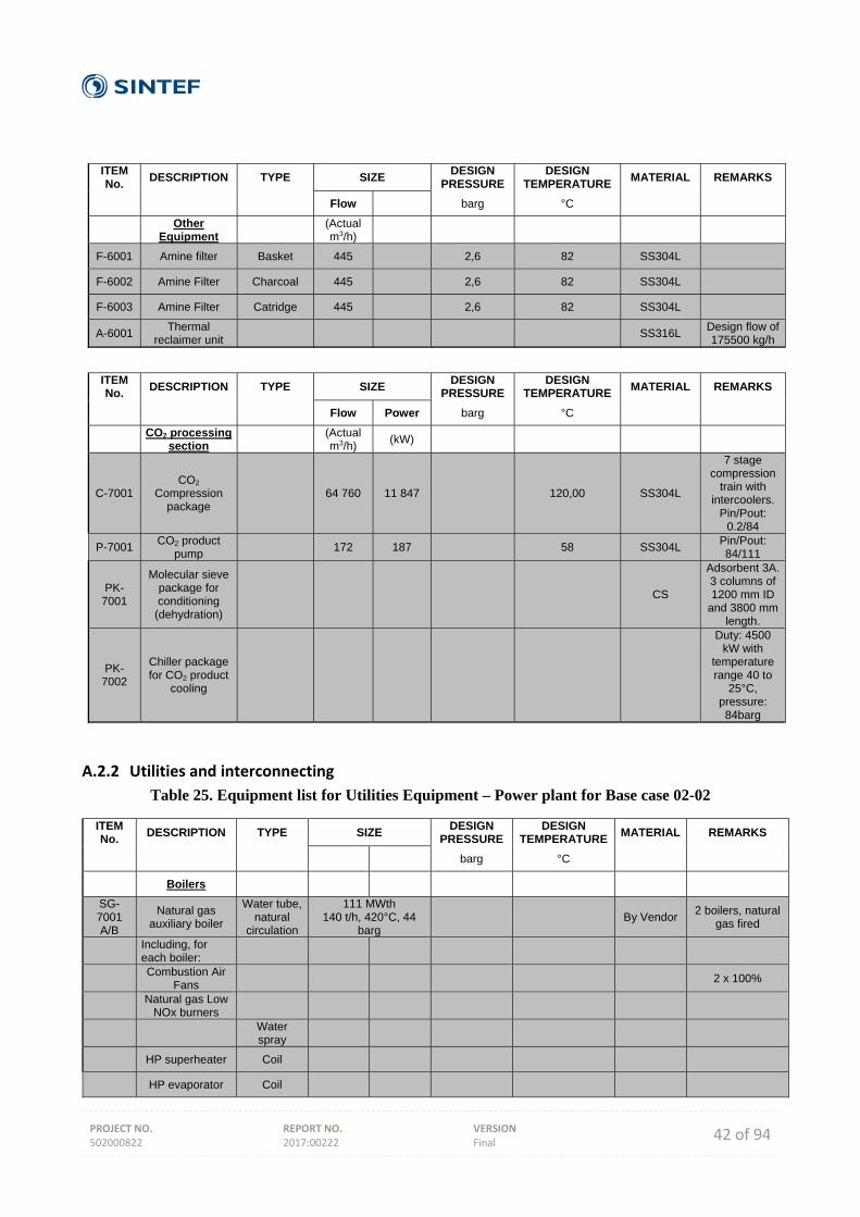
PROJECT NO. 502000822
REPORT NO. 2017:00222
VERSION Final 42 of 94
ITEM No.
DESCRIPTION TYPE SIZE DESIGN
PRESSURE DESIGN
TEMPERATURE MATERIAL REMARKS
Flow barg °C
Other
Equipment
(Actual m3/h)
F-6001 Amine filter Basket 445 2,6 82 SS304L
F-6002 Amine Filter Charcoal 445 2,6 82 SS304L
F-6003 Amine Filter Catridge 445 2,6 82 SS304L
A-6001 Thermal
reclaimer unit SS316L
Design flow of 175500 kg/h
ITEM No.
DESCRIPTION TYPE SIZE DESIGN
PRESSURE DESIGN
TEMPERATURE MATERIAL REMARKS
Flow Power barg °C
CO2 processing
section
(Actual m3/h)
(kW)
C-7001 CO2
Compression package
64 760 11 847 120,00 SS304L
7 stage compression
train with intercoolers.
Pin/Pout: 0.2/84
P-7001 CO2 product
pump 172 187 58 SS304L
Pin/Pout: 84/111
PK-7001
Molecular sieve package for conditioning
(dehydration)
CS
Adsorbent 3A. 3 columns of 1200 mm ID
and 3800 mm length.
PK-7002
Chiller package for CO2 product
cooling
Duty: 4500 kW with
temperature range 40 to
25°C, pressure: 84barg
A.2.2 Utilities and interconnecting
Table 25. Equipment list for Utilities Equipment – Power plant for Base case 02-02
ITEM No.
DESCRIPTION TYPE SIZE DESIGN
PRESSURE DESIGN
TEMPERATURE MATERIAL REMARKS
barg °C
Boilers
SG-7001 A/B
Natural gas auxiliary boiler
Water tube, natural
circulation
111 MWth 140 t/h, 420°C, 44
barg By Vendor
2 boilers, natural gas fired
Including, for each boiler:
Combustion Air
Fans 2 x 100%
Natural gas Low
NOx burners
Water spray
HP superheater Coil
HP evaporator Coil
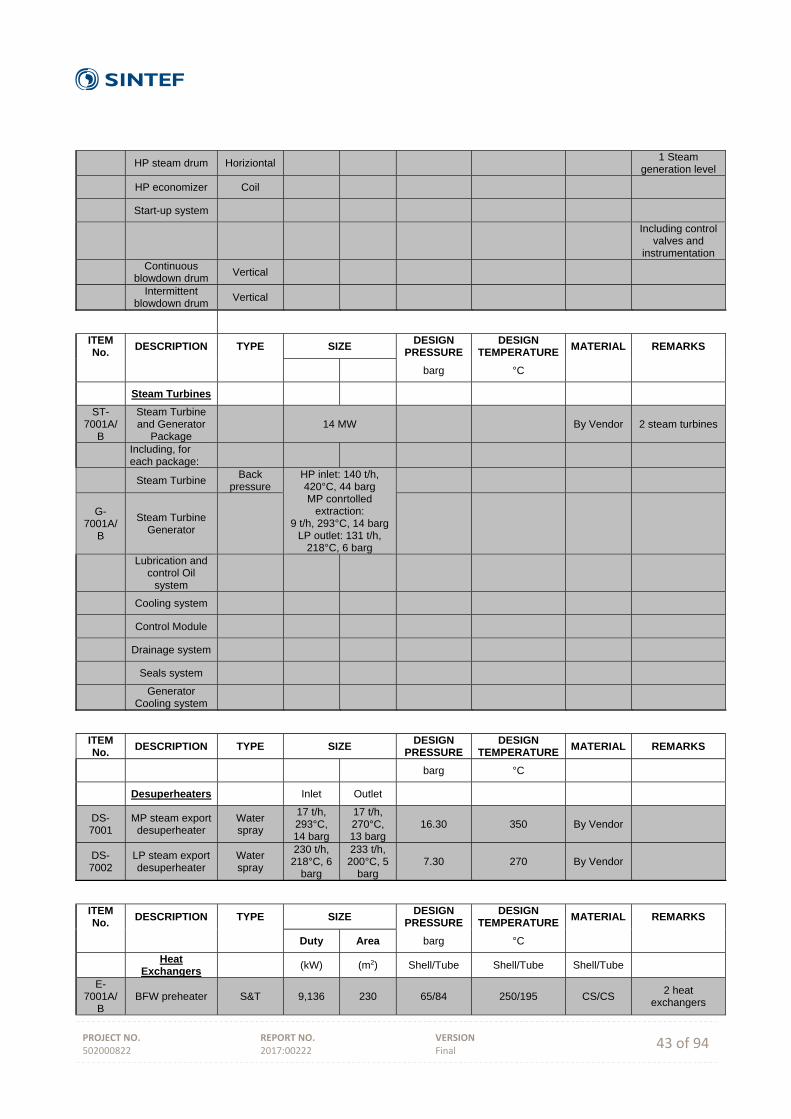
PROJECT NO. 502000822
REPORT NO. 2017:00222
VERSION Final 43 of 94
HP steam drum Horiziontal 1 Steam
generation level
HP economizer Coil
Start-up system
Including control
valves and instrumentation
Continuous
blowdown drum Vertical
Intermittent
blowdown drum Vertical
ITEM No.
DESCRIPTION TYPE SIZE DESIGN
PRESSURE DESIGN
TEMPERATURE MATERIAL REMARKS
barg °C
Steam Turbines
ST-7001A/
B
Steam Turbine and Generator
Package 14 MW By Vendor 2 steam turbines
Including, for each package:
Steam Turbine Back
pressure HP inlet: 140 t/h, 420°C, 44 barg MP conrtolled
extraction: 9 t/h, 293°C, 14 barg
LP outlet: 131 t/h, 218°C, 6 barg
G-7001A/
B
Steam Turbine Generator
Lubrication and
control Oil system
Cooling system
Control Module
Drainage system
Seals system
Generator
Cooling system
ITEM No.
DESCRIPTION TYPE SIZE DESIGN
PRESSURE DESIGN
TEMPERATURE MATERIAL REMARKS
barg °C
Desuperheaters Inlet Outlet
DS-7001
MP steam export desuperheater
Water spray
17 t/h, 293°C, 14 barg
17 t/h, 270°C, 13 barg
16.30 350 By Vendor
DS-7002
LP steam export desuperheater
Water spray
230 t/h, 218°C, 6
barg
233 t/h, 200°C, 5
barg 7.30 270 By Vendor
ITEM No.
DESCRIPTION TYPE SIZE DESIGN
PRESSURE DESIGN
TEMPERATURE MATERIAL REMARKS
Duty Area barg °C
Heat
Exchangers (kW) (m2) Shell/Tube Shell/Tube Shell/Tube
E-7001A/
B BFW preheater S&T 9,136 230 65/84 250/195 CS/CS
2 heat exchangers

PROJECT NO. 502000822
REPORT NO. 2017:00222
VERSION Final 44 of 94
ITEM No.
DESCRIPTION TYPE SIZE DESIGN
PRESSURE DESIGN
TEMPERATURE MATERIAL REMARKS
ID L barg °C
Tanks & Vessels
(mm) (mm)
D-7001 Deaerator Horizontal, spray type
3,000 7,500 3.50 150 CS + 3mm Internals: SS304L
TK-7001
Demi water tank Cone roof 20,000 9,000 (T/T)
-0.01 / 0.025 38
CS +1.5 mm
+ epoxy lining
ITEM No.
DESCRIPTION TYPE SIZE DESIGN
PRESSURE DESIGN
TEMPERATURE MATERIAL REMARKS
Flow Head barg °C
Pumps (Actual m3/h)
(m)
P-7001 A/B/C
BFW pump Centrifugal 148 670 84.0 150 12 Cr
3 x 100%, 2 operating 1 spare Motor rating: 335
kW
P-7002 A/B
Demi water pump
Centrifugal 109 95 12.5 38 SS304
2 x 100%, 1 operating 1 spareMotor rating: 37
kW
ITEM No.
DESCRIPTION TYPE SIZE DESIGN
PRESSURE DESIGN
TEMPERATURE MATERIAL REMARKS
barg °C
Packages
PK-7001
Demineralized water package
Demi water
production: 108 t/h By Vendor
Including
Cation beds
Degassing columns
Degassified
Water Pumps
Anion beds
Mixed Bed Polishers
Regeneration and
neutralization system
Neutralization
basin
Neutralization Basin Drainoff
Pumps
PK-7002
Phosphates injection package
By Vendor Including storage drum and dosing pumps
PK-7003
Amines injection package
By Vendor Including storage drum and dosing pumps
PK-7004
Oxygen scavenger
injection package By Vendor
Including storage drum and dosing pumps
PK-7005
Sampling package
By Vendor
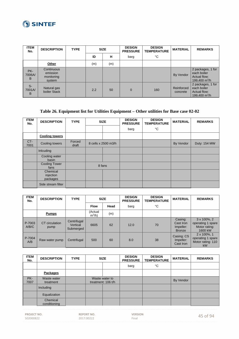
PROJECT NO. 502000822
REPORT NO. 2017:00222
VERSION Final 45 of 94
ITEM No.
DESCRIPTION TYPE SIZE DESIGN
PRESSURE DESIGN
TEMPERATURE MATERIAL REMARKS
ID H barg °C
Other (m) (m)
PK-7006A/
B
Continuous emission
monitoring system
By Vendor
2 packages, 1 for each boiler Actual flow: 199,400 m3/h
S-7001A/
B
Natural gas boiler Stack
2.2 50 0 160 Reinforced concrete
2 packages, 1 for each boiler Actual flow: 199,400 m3/h
Table 26. Equipment list for Utilities Equipment – Other utilities for Base case 02-02
ITEM No.
DESCRIPTION TYPE SIZE DESIGN
PRESSURE DESIGN
TEMPERATURE MATERIAL REMARKS
barg °C
Cooling towers
CT-7001
Cooling towers Forced
draft 8 cells x 2500 m3/h By Vendor Duty: 154 MW
Inlcuding
Cooling water
basin
Cooling Tower
fans 8 fans
Chemical injection
packages
Side stream filter
ITEM No.
DESCRIPTION TYPE SIZE DESIGN
PRESSURE DESIGN
TEMPERATURE MATERIAL REMARKS
Flow Head barg °C
Pumps (Actual m3/h)
(m)
P-7003 A/B/C
CT circulation pump
Centrifugal Vertical
Submerged 6605 62 12.0 70
Casing: Cast Iron Impeller: Bronze
3 x 100%, 2 operating 1 spare
Motor rating: 1600 kW
P-7004 A/B
Raw water pump Centrifugal 500 60 8.0 38 Casing: CS
Impeller: Cast Iron
2 x 100%, 1 operating 1 spareMotor rating: 110
kW
ITEM No.
DESCRIPTION TYPE SIZE DESIGN
PRESSURE DESIGN
TEMPERATURE MATERIAL REMARKS
barg °C
Packages
PK-7007
Waste water treatment
Waste water to
treatment: 106 t/h By Vendor
Including
Equalization
Chemical
conditioning
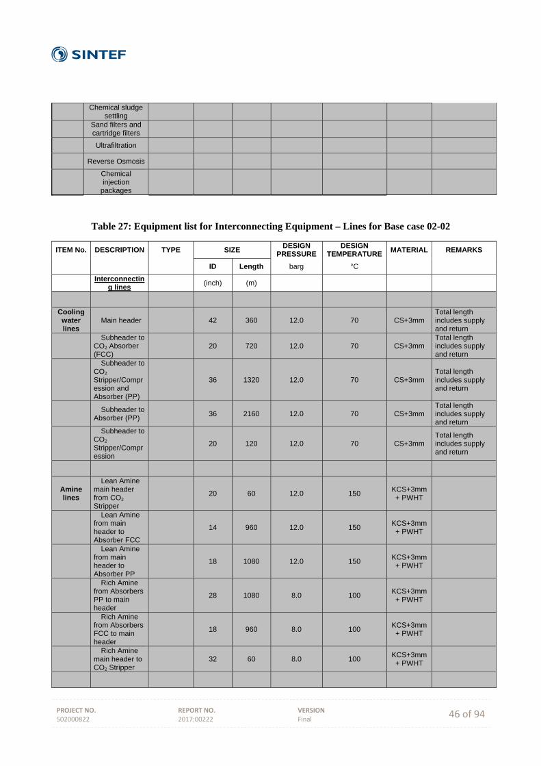
PROJECT NO. 502000822
REPORT NO. 2017:00222
VERSION Final 46 of 94
Chemical sludge
settling
Sand filters and cartridge filters
Ultrafiltration
Reverse Osmosis
Chemical injection
packages
Table 27: Equipment list for Interconnecting Equipment – Lines for Base case 02-02
ITEM No. DESCRIPTION TYPE SIZE DESIGN
PRESSURE DESIGN
TEMPERATURE MATERIAL REMARKS
ID Length barg °C
Interconnectin
g lines (inch) (m)
Cooling water lines
Main header 42 360 12.0 70 CS+3mm Total length includes supply and return
Subheader to
CO2 Absorber (FCC)
20 720 12.0 70 CS+3mm Total length includes supply and return
Subheader to CO2 Stripper/Compression and Absorber (PP)
36 1320 12.0 70 CS+3mm Total length includes supply and return
Subheader to
Absorber (PP) 36 2160 12.0 70 CS+3mm
Total length includes supply and return
Subheader to CO2 Stripper/Compression
20 120 12.0 70 CS+3mm Total length includes supply and return
Amine lines
Lean Amine main header from CO2 Stripper
20 60 12.0 150 KCS+3mm+ PWHT
Lean Amine from main header to Absorber FCC
14 960 12.0 150 KCS+3mm+ PWHT
Lean Amine from main header to Absorber PP
18 1080 12.0 150 KCS+3mm+ PWHT
Rich Amine from Absorbers PP to main header
28 1080 8.0 100 KCS+3mm+ PWHT
Rich Amine from Absorbers FCC to main header
18 960 8.0 100 KCS+3mm+ PWHT
Rich Amine
main header to CO2 Stripper
32 60 8.0 100 KCS+3mm+ PWHT
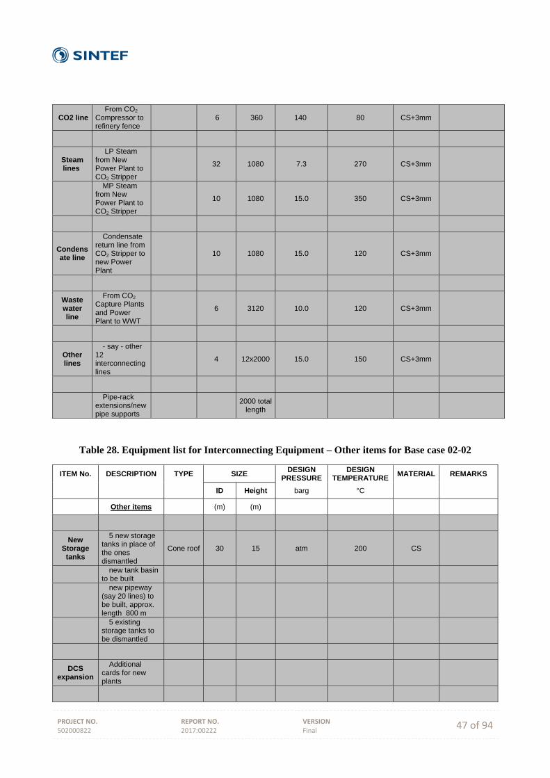
PROJECT NO. 502000822
REPORT NO. 2017:00222
VERSION Final 47 of 94
CO2 line From CO2
Compressor to refinery fence
6 360 140 80 CS+3mm
Steam lines
LP Steam from New Power Plant to CO2 Stripper
32 1080 7.3 270 CS+3mm
MP Steam from New Power Plant to CO2 Stripper
10 1080 15.0 350 CS+3mm
Condensate line
Condensate return line from CO2 Stripper to new Power Plant
10 1080 15.0 120 CS+3mm
Waste water line
From CO2 Capture Plants and Power Plant to WWT
6 3120 10.0 120 CS+3mm
Other lines
- say - other 12 interconnecting lines
4 12x2000 15.0 150 CS+3mm
Pipe-rack
extensions/new pipe supports
2000 total
length
Table 28. Equipment list for Interconnecting Equipment – Other items for Base case 02-02
ITEM No. DESCRIPTION TYPE SIZE DESIGN
PRESSURE DESIGN
TEMPERATURE MATERIAL REMARKS
ID Height barg °C
Other items (m) (m)
New Storage
tanks
5 new storage tanks in place of the ones dismantled
Cone roof 30 15 atm 200 CS
new tank basin
to be built
new pipeway (say 20 lines) to be built, approx. length 800 m
5 existing
storage tanks to be dismantled
DCS expansion
Additional cards for new plants
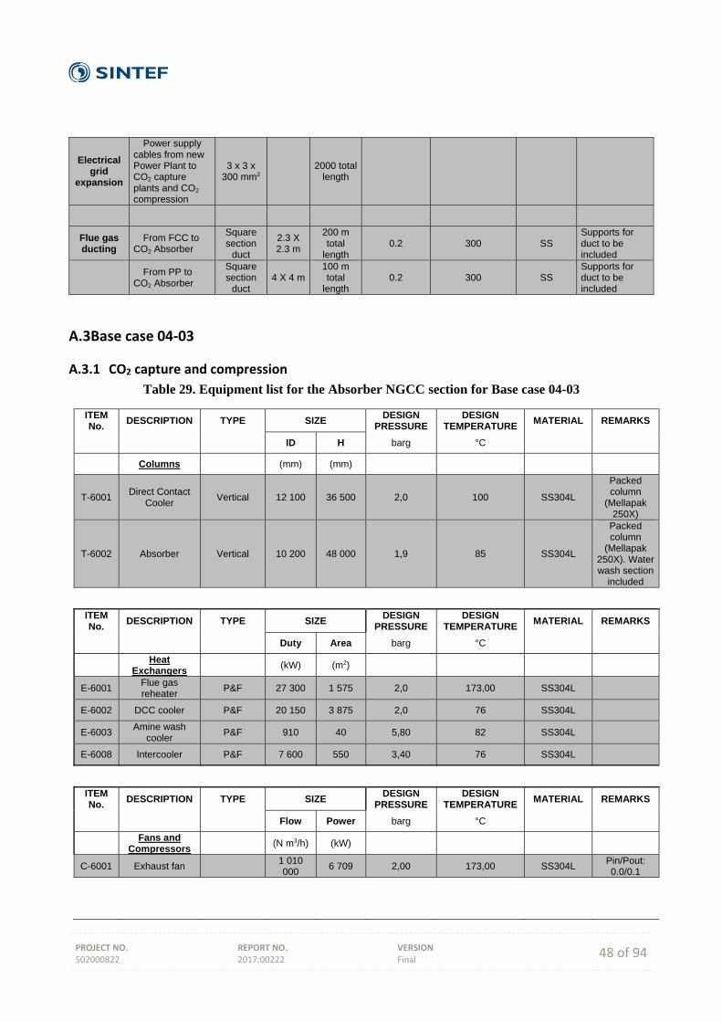
PROJECT NO. 502000822
REPORT NO. 2017:00222
VERSION Final 48 of 94
Electrical grid
expansion
Power supply cables from new Power Plant to CO2 capture plants and CO2 compression
3 x 3 x 300 mm2
2000 total
length
Flue gas ducting
From FCC to CO2 Absorber
Square section
duct
2.3 X 2.3 m
200 m total
length 0.2 300 SS
Supports for duct to be included
From PP to
CO2 Absorber
Square section
duct 4 X 4 m
100 m total
length 0.2 300 SS
Supports for duct to be included
A.3 Base case 04‐03
A.3.1 CO2 capture and compression
Table 29. Equipment list for the Absorber NGCC section for Base case 04-03
ITEM No.
DESCRIPTION TYPE SIZE DESIGN
PRESSURE DESIGN
TEMPERATURE MATERIAL REMARKS
ID H barg °C
Columns (mm) (mm)
T-6001 Direct Contact
Cooler Vertical 12 100 36 500 2,0 100 SS304L
Packed column
(Mellapak 250X)
T-6002 Absorber Vertical 10 200 48 000 1,9 85 SS304L
Packed column
(Mellapak 250X). Water wash section
included
ITEM No.
DESCRIPTION TYPE SIZE DESIGN
PRESSURE DESIGN
TEMPERATURE MATERIAL REMARKS
Duty Area barg °C
Heat
Exchangers (kW) (m2)
E-6001 Flue gas reheater
P&F 27 300 1 575 2,0 173,00 SS304L
E-6002 DCC cooler P&F 20 150 3 875 2,0 76 SS304L
E-6003 Amine wash
cooler P&F 910 40 5,80 82 SS304L
E-6008 Intercooler P&F 7 600 550 3,40 76 SS304L
ITEM No.
DESCRIPTION TYPE SIZE DESIGN
PRESSURE DESIGN
TEMPERATURE MATERIAL REMARKS
Flow Power barg °C
Fans and
Compressors (N m3/h) (kW)
C-6001 Exhaust fan 1 010 000
6 709 2,00 173,00 SS304L Pin/Pout: 0.0/0.1
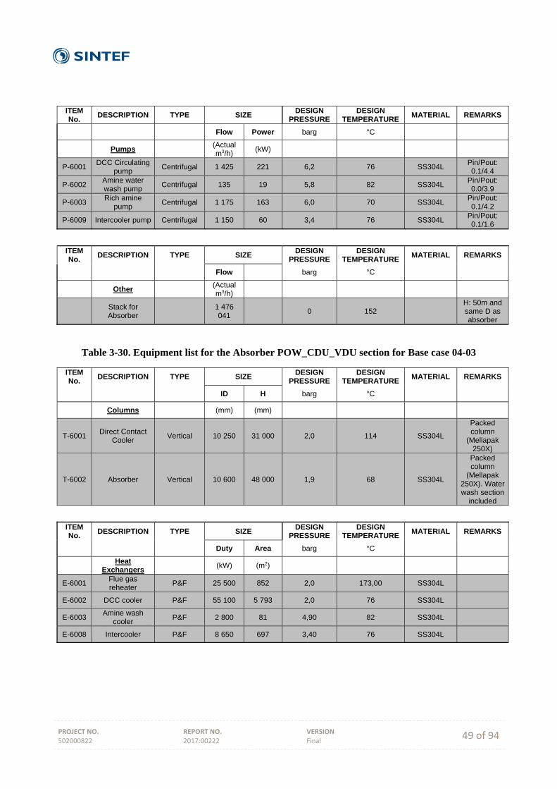
PROJECT NO. 502000822
REPORT NO. 2017:00222
VERSION Final 49 of 94
ITEM No.
DESCRIPTION TYPE SIZE DESIGN
PRESSURE DESIGN
TEMPERATURE MATERIAL REMARKS
Flow Power barg °C
Pumps (Actual m3/h)
(kW)
P-6001 DCC Circulating
pump Centrifugal 1 425 221 6,2 76 SS304L
Pin/Pout: 0.1/4.4
P-6002 Amine water wash pump
Centrifugal 135 19 5,8 82 SS304L Pin/Pout: 0.0/3.9
P-6003 Rich amine
pump Centrifugal 1 175 163 6,0 70 SS304L
Pin/Pout: 0.1/4.2
P-6009 Intercooler pump Centrifugal 1 150 60 3,4 76 SS304L Pin/Pout: 0.1/1.6
ITEM No.
DESCRIPTION TYPE SIZE DESIGN
PRESSURE DESIGN
TEMPERATURE MATERIAL REMARKS
Flow barg °C
Other (Actual m3/h)
Stack for Absorber
1 476 041
0 152 H: 50m and same D as absorber
Table 3-30. Equipment list for the Absorber POW_CDU_VDU section for Base case 04-03
ITEM No.
DESCRIPTION TYPE SIZE DESIGN
PRESSURE DESIGN
TEMPERATURE MATERIAL REMARKS
ID H barg °C
Columns (mm) (mm)
T-6001 Direct Contact
Cooler Vertical 10 250 31 000 2,0 114 SS304L
Packed column
(Mellapak 250X)
T-6002 Absorber Vertical 10 600 48 000 1,9 68 SS304L
Packed column
(Mellapak 250X). Water wash section
included
ITEM No.
DESCRIPTION TYPE SIZE DESIGN
PRESSURE DESIGN
TEMPERATURE MATERIAL REMARKS
Duty Area barg °C
Heat
Exchangers (kW) (m2)
E-6001 Flue gas reheater
P&F 25 500 852 2,0 173,00 SS304L
E-6002 DCC cooler P&F 55 100 5 793 2,0 76 SS304L
E-6003 Amine wash
cooler P&F 2 800 81 4,90 82 SS304L
E-6008 Intercooler P&F 8 650 697 3,40 76 SS304L
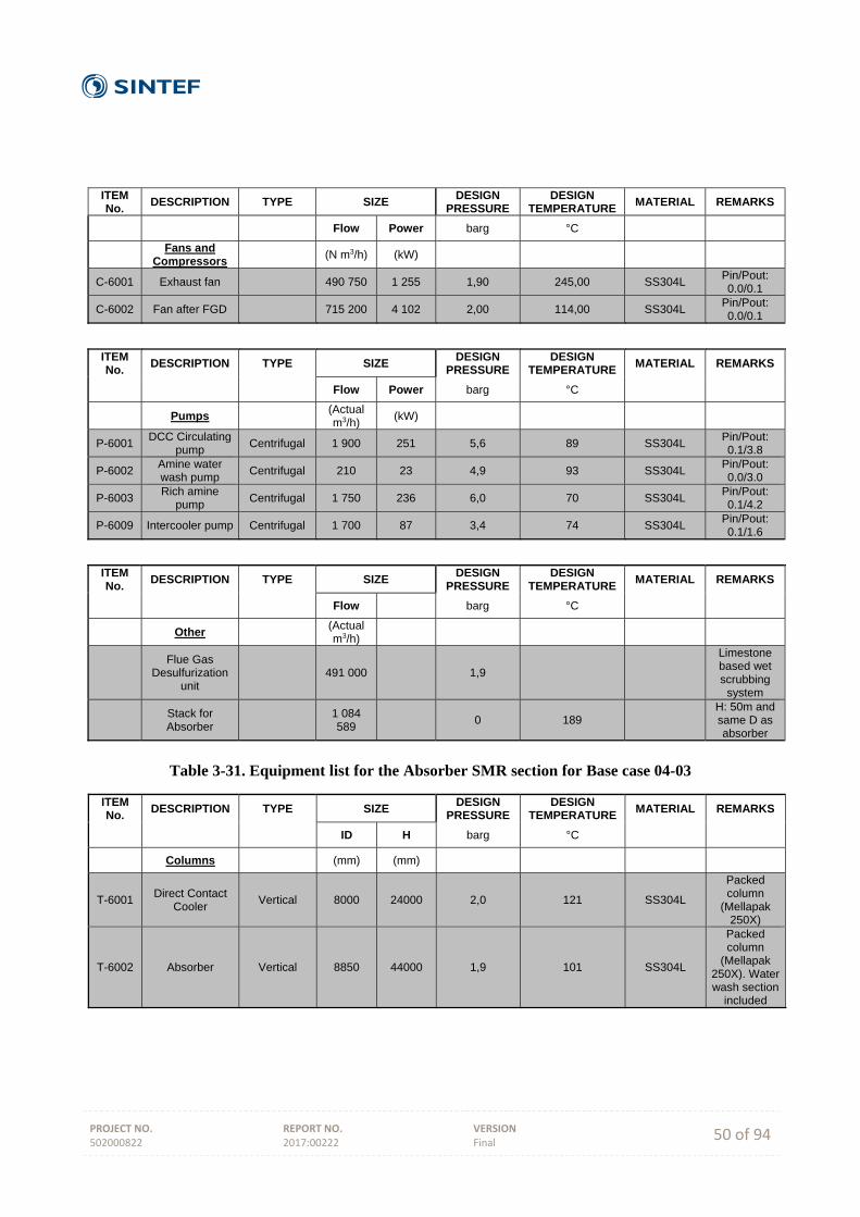
PROJECT NO. 502000822
REPORT NO. 2017:00222
VERSION Final 50 of 94
ITEM No.
DESCRIPTION TYPE SIZE DESIGN
PRESSURE DESIGN
TEMPERATURE MATERIAL REMARKS
Flow Power barg °C
Fans and
Compressors (N m3/h) (kW)
C-6001 Exhaust fan 490 750 1 255 1,90 245,00 SS304L Pin/Pout: 0.0/0.1
C-6002 Fan after FGD 715 200 4 102 2,00 114,00 SS304L Pin/Pout: 0.0/0.1
ITEM No.
DESCRIPTION TYPE SIZE DESIGN
PRESSURE DESIGN
TEMPERATURE MATERIAL REMARKS
Flow Power barg °C
Pumps (Actual m3/h)
(kW)
P-6001 DCC Circulating
pump Centrifugal 1 900 251 5,6 89 SS304L
Pin/Pout: 0.1/3.8
P-6002 Amine water wash pump
Centrifugal 210 23 4,9 93 SS304L Pin/Pout: 0.0/3.0
P-6003 Rich amine
pump Centrifugal 1 750 236 6,0 70 SS304L
Pin/Pout: 0.1/4.2
P-6009 Intercooler pump Centrifugal 1 700 87 3,4 74 SS304L Pin/Pout: 0.1/1.6
ITEM No.
DESCRIPTION TYPE SIZE DESIGN
PRESSURE DESIGN
TEMPERATURE MATERIAL REMARKS
Flow barg °C
Other (Actual m3/h)
Flue Gas
Desulfurization unit
491 000 1,9
Limestone based wet scrubbing
system
Stack for Absorber
1 084 589
0 189 H: 50m and same D as absorber
Table 3-31. Equipment list for the Absorber SMR section for Base case 04-03
ITEM No.
DESCRIPTION TYPE SIZE DESIGN
PRESSURE DESIGN
TEMPERATURE MATERIAL REMARKS
ID H barg °C
Columns (mm) (mm)
T-6001 Direct Contact
Cooler Vertical 8000 24000 2,0 121 SS304L
Packed column
(Mellapak 250X)
T-6002 Absorber Vertical 8850 44000 1,9 101 SS304L
Packed column
(Mellapak 250X). Water wash section
included
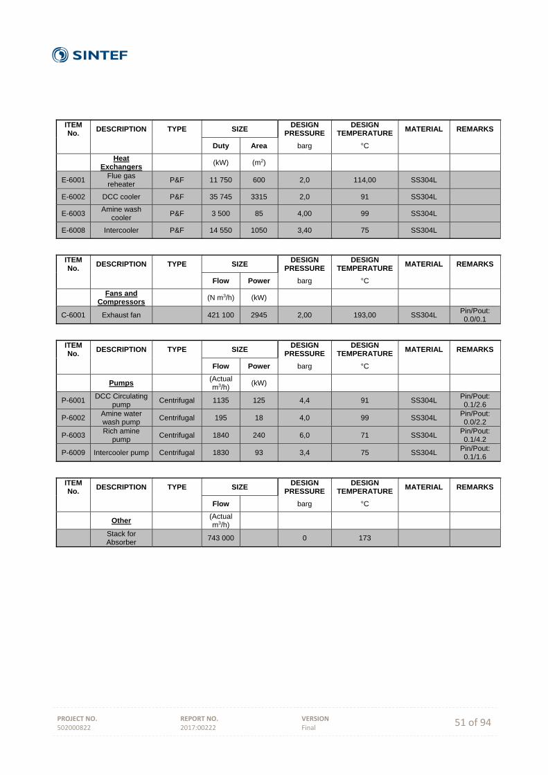
PROJECT NO. 502000822
REPORT NO. 2017:00222
VERSION Final 51 of 94
ITEM No.
DESCRIPTION TYPE SIZE DESIGN
PRESSURE DESIGN
TEMPERATURE MATERIAL REMARKS
Duty Area barg °C
Heat
Exchangers (kW) (m2)
E-6001 Flue gas reheater
P&F 11 750 600 2,0 114,00 SS304L
E-6002 DCC cooler P&F 35 745 3315 2,0 91 SS304L
E-6003 Amine wash
cooler P&F 3 500 85 4,00 99 SS304L
E-6008 Intercooler P&F 14 550 1050 3,40 75 SS304L
ITEM No.
DESCRIPTION TYPE SIZE DESIGN
PRESSURE DESIGN
TEMPERATURE MATERIAL REMARKS
Flow Power barg °C
Fans and
Compressors (N m3/h) (kW)
C-6001 Exhaust fan 421 100 2945 2,00 193,00 SS304L Pin/Pout: 0.0/0.1
ITEM No.
DESCRIPTION TYPE SIZE DESIGN
PRESSURE DESIGN
TEMPERATURE MATERIAL REMARKS
Flow Power barg °C
Pumps (Actual m3/h)
(kW)
P-6001 DCC Circulating
pump Centrifugal 1135 125 4,4 91 SS304L
Pin/Pout: 0.1/2.6
P-6002 Amine water wash pump
Centrifugal 195 18 4,0 99 SS304L Pin/Pout: 0.0/2.2
P-6003 Rich amine
pump Centrifugal 1840 240 6,0 71 SS304L
Pin/Pout: 0.1/4.2
P-6009 Intercooler pump Centrifugal 1830 93 3,4 75 SS304L Pin/Pout: 0.1/1.6
ITEM No.
DESCRIPTION TYPE SIZE DESIGN
PRESSURE DESIGN
TEMPERATURE MATERIAL REMARKS
Flow barg °C
Other (Actual m3/h)
Stack for Absorber
743 000 0 173
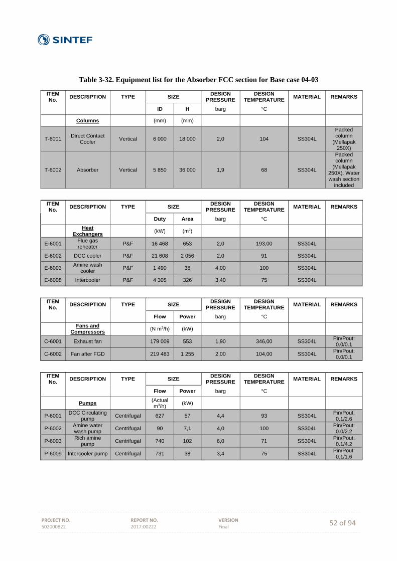
PROJECT NO. 502000822
REPORT NO. 2017:00222
VERSION Final 52 of 94
Table 3-32. Equipment list for the Absorber FCC section for Base case 04-03
ITEM No.
DESCRIPTION TYPE SIZE DESIGN
PRESSURE DESIGN
TEMPERATURE MATERIAL REMARKS
ID H barg °C
Columns (mm) (mm)
T-6001 Direct Contact
Cooler Vertical 6 000 18 000 2,0 104 SS304L
Packed column
(Mellapak 250X)
T-6002 Absorber Vertical 5 850 36 000 1,9 68 SS304L
Packed column
(Mellapak 250X). Water wash section
included
ITEM No.
DESCRIPTION TYPE SIZE DESIGN
PRESSURE DESIGN
TEMPERATURE MATERIAL REMARKS
Duty Area barg °C
Heat
Exchangers (kW) (m2)
E-6001 Flue gas reheater
P&F 16 468 653 2,0 193,00 SS304L
E-6002 DCC cooler P&F 21 608 2 056 2,0 91 SS304L
E-6003 Amine wash
cooler P&F 1 490 38 4,00 100 SS304L
E-6008 Intercooler P&F 4 305 326 3,40 75 SS304L
ITEM No.
DESCRIPTION TYPE SIZE DESIGN
PRESSURE DESIGN
TEMPERATURE MATERIAL REMARKS
Flow Power barg °C
Fans and
Compressors (N m3/h) (kW)
C-6001 Exhaust fan 179 009 553 1,90 346,00 SS304L Pin/Pout: 0.0/0.1
C-6002 Fan after FGD 219 483 1 255 2,00 104,00 SS304L Pin/Pout: 0.0/0.1
ITEM No.
DESCRIPTION TYPE SIZE DESIGN
PRESSURE DESIGN
TEMPERATURE MATERIAL REMARKS
Flow Power barg °C
Pumps (Actual m3/h)
(kW)
P-6001 DCC Circulating
pump Centrifugal 627 57 4,4 93 SS304L
Pin/Pout: 0.1/2.6
P-6002 Amine water wash pump
Centrifugal 90 7,1 4,0 100 SS304L Pin/Pout: 0.0/2.2
P-6003 Rich amine
pump Centrifugal 740 102 6,0 71 SS304L
Pin/Pout: 0.1/4.2
P-6009 Intercooler pump Centrifugal 731 38 3,4 75 SS304L Pin/Pout: 0.1/1.6
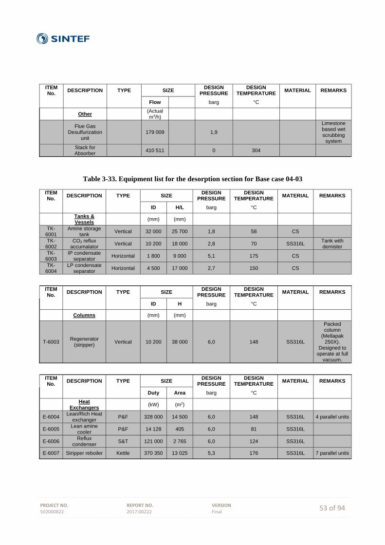
PROJECT NO. 502000822
REPORT NO. 2017:00222
VERSION Final 53 of 94
ITEM No.
DESCRIPTION TYPE SIZE DESIGN
PRESSURE DESIGN
TEMPERATURE MATERIAL REMARKS
Flow barg °C
Other (Actual m3/h)
Flue Gas
Desulfurization unit
179 009 1,9
Limestone based wet scrubbing
system
Stack for Absorber
410 511 0 304
Table 3-33. Equipment list for the desorption section for Base case 04-03
ITEM No.
DESCRIPTION TYPE SIZE DESIGN
PRESSURE DESIGN
TEMPERATURE MATERIAL REMARKS
ID H/L barg °C
Tanks & Vessels
(mm) (mm)
TK-6001
Amine storage tank
Vertical 32 000 25 700 1,8 58 CS
TK-6002
CO2 reflux accumalator
Vertical 10 200 18 000 2,8 70 SS316L Tank with demister
TK-6003
IP condensate separator
Horizontal 1 800 9 000 5,1 175 CS
TK-6004
LP condensate separator
Horizontal 4 500 17 000 2,7 150 CS
ITEM No.
DESCRIPTION TYPE SIZE DESIGN
PRESSURE DESIGN
TEMPERATURE MATERIAL REMARKS
ID H barg °C
Columns (mm) (mm)
T-6003 Regenerator
(stripper) Vertical 10 200 38 000 6,0 148 SS316L
Packed column
(Mellapak 250X).
Designed to operate at full
vacuum.
ITEM No.
DESCRIPTION TYPE SIZE DESIGN
PRESSURE DESIGN
TEMPERATURE MATERIAL REMARKS
Duty Area barg °C
Heat
Exchangers (kW) (m2)
E-6004 Lean/Rich Heat
exchanger P&F 328 000 14 500 6,0 148 SS316L 4 parallel units
E-6005 Lean amine
cooler P&F 14 128 405 6,0 81 SS316L
E-6006 Reflux
condenser S&T 121 000 2 765 6,0 124 SS316L
E-6007 Stripper reboiler Kettle 370 350 13 025 5,3 176 SS316L 7 parallel units
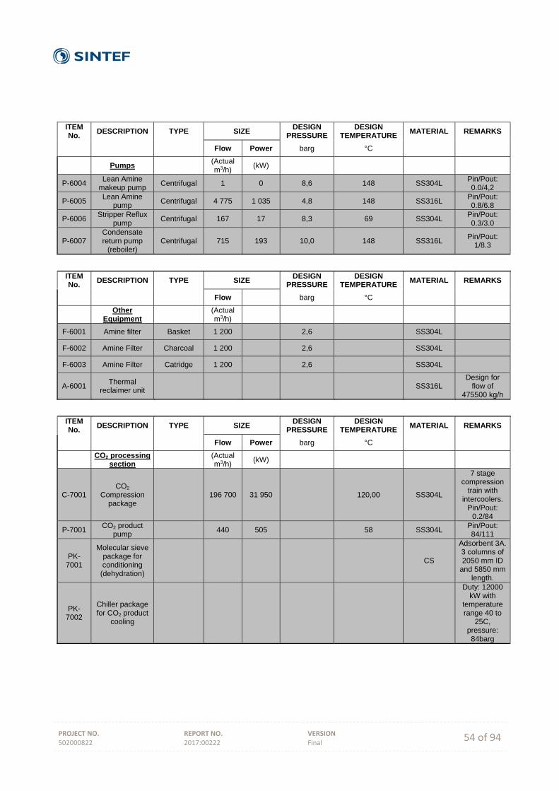
PROJECT NO. 502000822
REPORT NO. 2017:00222
VERSION Final 54 of 94
ITEM No.
DESCRIPTION TYPE SIZE DESIGN
PRESSURE DESIGN
TEMPERATURE MATERIAL REMARKS
Flow Power barg °C
Pumps (Actual m3/h)
(kW)
P-6004 Lean Amine
makeup pump Centrifugal 1 0 8,6 148 SS304L
Pin/Pout: 0.0/4,2
P-6005 Lean Amine
pump Centrifugal 4 775 1 035 4,8 148 SS316L
Pin/Pout: 0.8/6.8
P-6006 Stripper Reflux
pump Centrifugal 167 17 8,3 69 SS304L
Pin/Pout: 0.3/3.0
P-6007 Condensate return pump
(reboiler) Centrifugal 715 193 10,0 148 SS316L
Pin/Pout: 1/8.3
ITEM No.
DESCRIPTION TYPE SIZE DESIGN
PRESSURE DESIGN
TEMPERATURE MATERIAL REMARKS
Flow barg °C
Other
Equipment
(Actual m3/h)
F-6001 Amine filter Basket 1 200 2,6 SS304L
F-6002 Amine Filter Charcoal 1 200 2,6 SS304L
F-6003 Amine Filter Catridge 1 200 2,6 SS304L
A-6001 Thermal
reclaimer unit SS316L
Design for flow of
475500 kg/h
ITEM No.
DESCRIPTION TYPE SIZE DESIGN
PRESSURE DESIGN
TEMPERATURE MATERIAL REMARKS
Flow Power barg °C
CO2 processing
section
(Actual m3/h)
(kW)
C-7001 CO2
Compression package
196 700 31 950 120,00 SS304L
7 stage compression
train with intercoolers.
Pin/Pout: 0.2/84
P-7001 CO2 product
pump 440 505 58 SS304L
Pin/Pout: 84/111
PK-7001
Molecular sieve package for conditioning
(dehydration)
CS
Adsorbent 3A. 3 columns of 2050 mm ID
and 5850 mm length.
PK-7002
Chiller package for CO2 product
cooling
Duty: 12000 kW with
temperature range 40 to
25C, pressure: 84barg
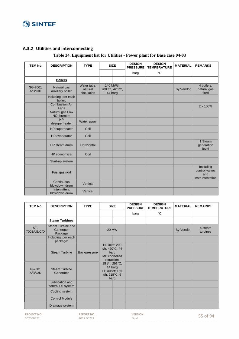
PROJECT NO. 502000822
REPORT NO. 2017:00222
VERSION Final 55 of 94
A.3.2 Utilities and interconnecting
Table 34. Equipment list for Utilities - Power plant for Base case 04-03
ITEM No. DESCRIPTION TYPE SIZE DESIGN
PRESSUREDESIGN
TEMPERATURE MATERIAL REMARKS
barg °C
Boilers
SG-7001 A/B/C/D
Natural gas auxiliary boiler
Water tube, natural
circulation
140 MWth 200 t/h, 420°C,
44 barg
By Vendor 4 boilers,
natural gas fired
Including, per each boiler:
Combustion Air Fans
2 x 100%
Natural gas Low NOx burners
HP desuperheater
Water spray
HP superheater Coil
HP evaporator Coil
HP steam drum Horiziontal 1 Steam
generation level
HP economizer Coil
Start-up system
Fuel gas skid
Including control valves
and instrumentation
Continuous blowdown drum
Vertical
Intermittent blowdown drum
Vertical
ITEM No. DESCRIPTION TYPE SIZE
DESIGN PRESSURE
DESIGN TEMPERATURE
MATERIAL REMARKS
barg °C
Steam Turbines
ST-7001A/B/C/D
Steam Turbine and Generator Package
20 MW By Vendor 4 steam turbines
Including, per each package:
Steam Turbine Backpressure
HP inlet: 200 t/h, 420°C, 44
barg MP conrtolled
extraction: 15 t/h, 293°C,
14 barg LP outlet: 185 t/h, 218°C, 6
barg
G-7001 A/B/C/D
Steam Turbine Generator
Lubrication and control Oil system
Cooling system
Control Module
Drainage system
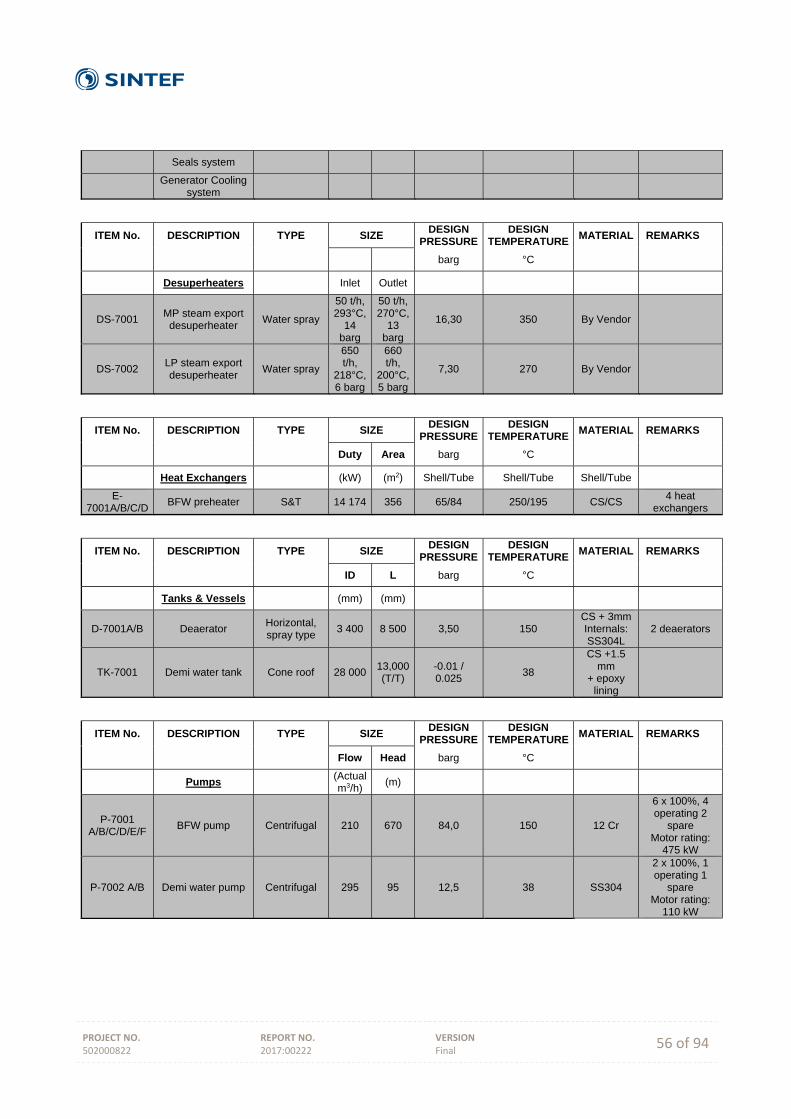
PROJECT NO. 502000822
REPORT NO. 2017:00222
VERSION Final 56 of 94
Seals system
Generator Cooling system
ITEM No. DESCRIPTION TYPE SIZE
DESIGN PRESSURE
DESIGN TEMPERATURE
MATERIAL REMARKS
barg °C
Desuperheaters Inlet Outlet
DS-7001 MP steam export
desuperheater Water spray
50 t/h, 293°C,
14 barg
50 t/h, 270°C,
13 barg
16,30 350 By Vendor
DS-7002 LP steam export desuperheater
Water spray
650 t/h,
218°C, 6 barg
660 t/h,
200°C, 5 barg
7,30 270 By Vendor
ITEM No. DESCRIPTION TYPE SIZE
DESIGN PRESSURE
DESIGN TEMPERATURE
MATERIAL REMARKS
Duty Area barg °C
Heat Exchangers (kW) (m2) Shell/Tube Shell/Tube Shell/Tube
E-7001A/B/C/D
BFW preheater S&T 14 174 356 65/84 250/195 CS/CS 4 heat
exchangers
ITEM No. DESCRIPTION TYPE SIZE
DESIGN PRESSURE
DESIGN TEMPERATURE
MATERIAL REMARKS
ID L barg °C
Tanks & Vessels (mm) (mm)
D-7001A/B Deaerator Horizontal, spray type
3 400 8 500 3,50 150 CS + 3mm Internals: SS304L
2 deaerators
TK-7001 Demi water tank Cone roof 28 00013,000 (T/T)
-0.01 / 0.025
38
CS +1.5 mm
+ epoxy lining
ITEM No. DESCRIPTION TYPE SIZE
DESIGN PRESSURE
DESIGN TEMPERATURE
MATERIAL REMARKS
Flow Head barg °C
Pumps (Actual m3/h)
(m)
P-7001 A/B/C/D/E/F
BFW pump Centrifugal 210 670 84,0 150 12 Cr
6 x 100%, 4 operating 2
spare Motor rating:
475 kW
P-7002 A/B Demi water pump Centrifugal 295 95 12,5 38 SS304
2 x 100%, 1 operating 1
spare Motor rating:
110 kW
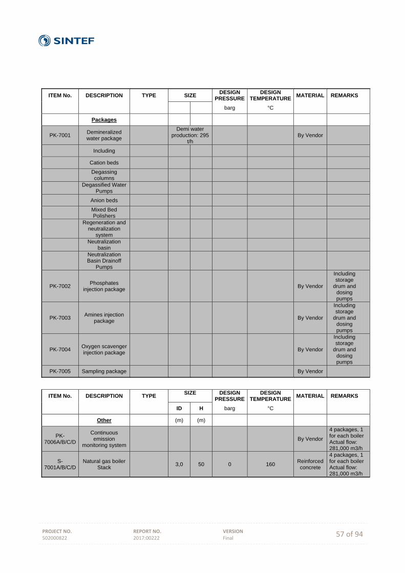
PROJECT NO. 502000822
REPORT NO. 2017:00222
VERSION Final 57 of 94
ITEM No. DESCRIPTION TYPE SIZE
DESIGN PRESSURE
DESIGN TEMPERATURE
MATERIAL REMARKS
barg °C
Packages
PK-7001 Demineralized water package
Demi water
production: 295 t/h
By Vendor
Including
Cation beds
Degassing columns
Degassified Water Pumps
Anion beds
Mixed Bed Polishers
Regeneration and
neutralization system
Neutralization basin
Neutralization Basin Drainoff
Pumps
PK-7002 Phosphates
injection package By Vendor
Including storage
drum and dosing pumps
PK-7003 Amines injection
package By Vendor
Including storage
drum and dosing pumps
PK-7004 Oxygen scavenger injection package
By Vendor
Including storage
drum and dosing pumps
PK-7005 Sampling package By Vendor
ITEM No. DESCRIPTION TYPE
SIZE
DESIGN PRESSURE
DESIGN TEMPERATURE
MATERIAL REMARKS
ID H barg °C
Other (m) (m)
PK-7006A/B/C/D
Continuous emission
monitoring system By Vendor
4 packages, 1 for each boilerActual flow: 281,000 m3/h
S-7001A/B/C/D
Natural gas boiler Stack
3,0 50 0 160 Reinforced concrete
4 packages, 1 for each boilerActual flow: 281,000 m3/h
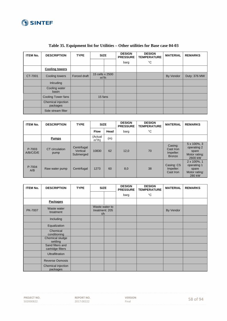
PROJECT NO. 502000822
REPORT NO. 2017:00222
VERSION Final 58 of 94
Table 35. Equipment list for Utilities – Other utilities for Base case 04-03
ITEM No. DESCRIPTION TYPE SIZE DESIGN
PRESSURE DESIGN
TEMPERATURE MATERIAL REMARKS
barg °C
Cooling towers
CT-7001 Cooling towers Forced draft 15 cells x 2500
m3/h By Vendor Duty: 376 MW
Inlcuding
Cooling water basin
Cooling Tower fans 15 fans
Chemical injection packages
Side stream filter
ITEM No. DESCRIPTION TYPE SIZE
DESIGN PRESSURE
DESIGN TEMPERATURE
MATERIAL REMARKS
Flow Head barg °C
Pumps (Actual m3/h)
(m)
P-7003 A/B/C/D/E
CT circulation pump
Centrifugal Vertical
Submerged 10830 62 12,0 70
Casing: Cast Iron Impeller: Bronze
5 x 100%, 3 operating 2
spare Motor rating:
2600 kW
P-7004 A/B
Raw water pump Centrifugal 1273 60 8,0 38 Casing: CS
Impeller: Cast Iron
2 x 100%, 1 operating 1
spare Motor rating:
280 kW
ITEM No. DESCRIPTION TYPE SIZE
DESIGN PRESSURE
DESIGN TEMPERATURE
MATERIAL REMARKS
barg °C
Packages
PK-7007 Waste water
treatment
Waste water to treatment: 205
t/h
By Vendor
Including
Equalization
Chemical conditioning
Chemical sludge settling
Sand filters and cartridge filters
Ultrafiltration
Reverse Osmosis
Chemical injection packages
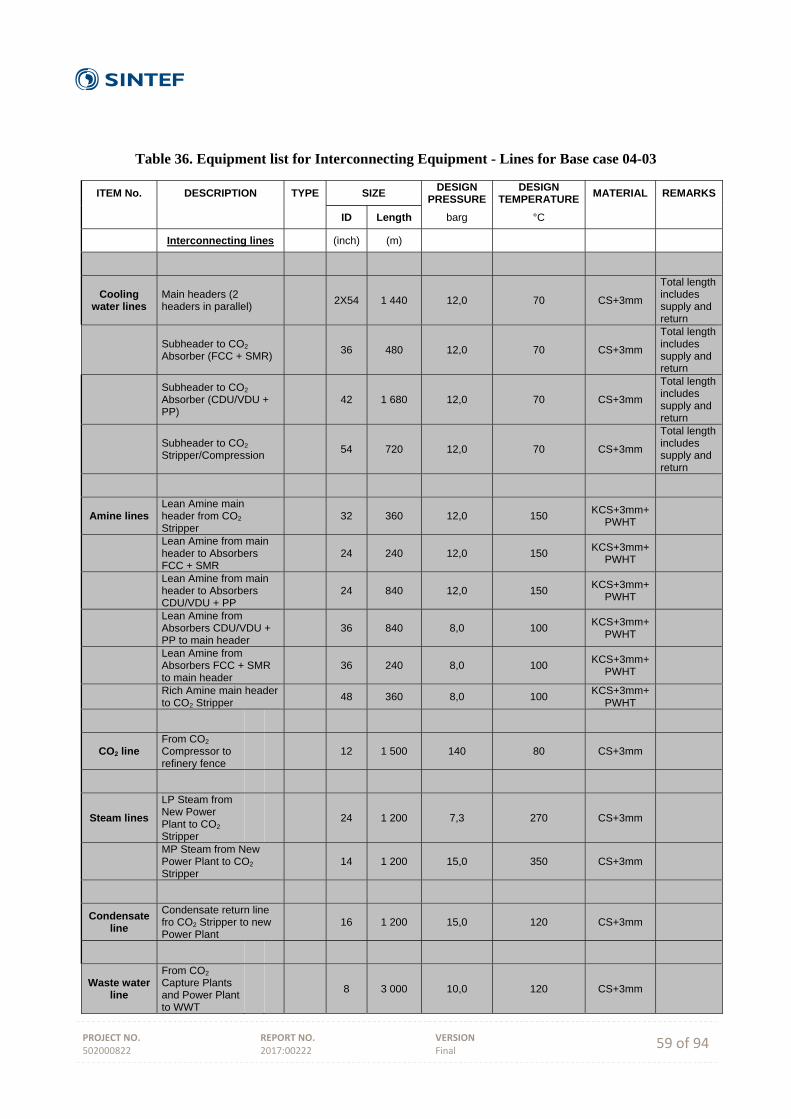
PROJECT NO. 502000822
REPORT NO. 2017:00222
VERSION Final 59 of 94
Table 36. Equipment list for Interconnecting Equipment - Lines for Base case 04-03
ITEM No. DESCRIPTION TYPE SIZE DESIGN
PRESSURE DESIGN
TEMPERATURE MATERIAL REMARKS
ID Length barg °C
Interconnecting lines (inch) (m)
Cooling water lines
Main headers (2 headers in parallel)
2X54 1 440 12,0 70 CS+3mm
Total length includes supply and return
Subheader to CO2 Absorber (FCC + SMR)
36 480 12,0 70 CS+3mm
Total length includes supply and return
Subheader to CO2 Absorber (CDU/VDU + PP)
42 1 680 12,0 70 CS+3mm
Total length includes supply and return
Subheader to CO2 Stripper/Compression
54 720 12,0 70 CS+3mm
Total length includes supply and return
Amine lines Lean Amine main header from CO2 Stripper
32 360 12,0 150 KCS+3mm+
PWHT
Lean Amine from main header to Absorbers FCC + SMR
24 240 12,0 150 KCS+3mm+
PWHT
Lean Amine from main header to Absorbers CDU/VDU + PP
24 840 12,0 150 KCS+3mm+
PWHT
Lean Amine from Absorbers CDU/VDU + PP to main header
36 840 8,0 100 KCS+3mm+
PWHT
Lean Amine from Absorbers FCC + SMR to main header
36 240 8,0 100 KCS+3mm+
PWHT
Rich Amine main header to CO2 Stripper
48 360 8,0 100 KCS+3mm+
PWHT
CO2 line From CO2 Compressor to refinery fence
12 1 500 140 80 CS+3mm
Steam lines
LP Steam from New Power Plant to CO2 Stripper
24 1 200 7,3 270 CS+3mm
MP Steam from New Power Plant to CO2 Stripper
14 1 200 15,0 350 CS+3mm
Condensate line
Condensate return line fro CO2 Stripper to new Power Plant
16 1 200 15,0 120 CS+3mm
Waste water line
From CO2 Capture Plants and Power Plant to WWT
8 3 000 10,0 120 CS+3mm
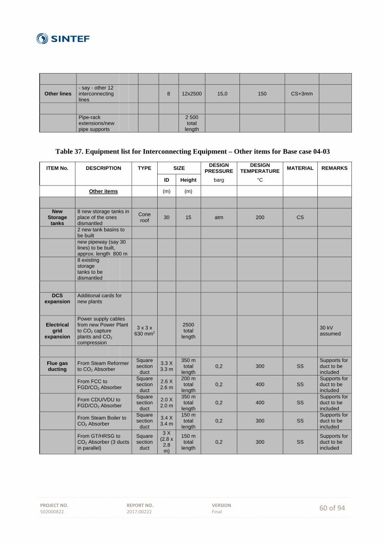
PROJECT NO. 502000822
REPORT NO. 2017:00222
VERSION Final 60 of 94
Other lines - say - other 12 interconnecting lines
8 12x2500 15,0 150 CS+3mm
Pipe-rack extensions/new pipe supports
2 500 total
length
Table 37. Equipment list for Interconnecting Equipment – Other items for Base case 04-03
ITEM No. DESCRIPTION TYPE SIZE DESIGN
PRESSURE DESIGN
TEMPERATURE MATERIAL REMARKS
ID Height barg °C
Other items (m) (m)
New Storage
tanks
8 new storage tanks in place of the ones dismantled
Cone roof
30 15 atm 200 CS
2 new tank basins to be built
new pipeway (say 30 lines) to be built, approx. length 800 m
8 existing storage tanks to be dismantled
DCS expansion
Additional cards for new plants
Electrical grid
expansion
Power supply cables from new Power Plant to CO2 capture plants and CO2 compression
3 x 3 x 630 mm2
2500 total
length
30 kV assumed
Flue gas ducting
From Steam Reformer to CO2 Absorber
Square section
duct
3.3 X 3.3 m
350 m total
length 0,2 300 SS
Supports for duct to be included
From FCC to FGD/CO2 Absorber
Square section
duct
2.6 X 2.6 m
200 m total
length 0,2 400 SS
Supports for duct to be included
From CDU/VDU to FGD/CO2 Absorber
Square section
duct
2.0 X 2.0 m
350 m total
length 0,2 400 SS
Supports for duct to be included
From Steam Boiler to CO2 Absorber
Square section
duct
3.4 X 3.4 m
150 m total
length 0,2 300 SS
Supports for duct to be included
From GT/HRSG to CO2 Absorber (3 ducts in parallel)
Square section
duct
3 X (2.8 x
2.8 m)
150 m total
length 0,2 300 SS
Supports for duct to be included
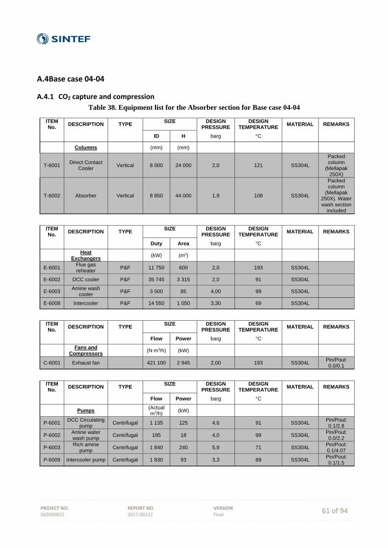
PROJECT NO. 502000822
REPORT NO. 2017:00222
VERSION Final 61 of 94
A.4 Base case 04‐04
A.4.1 CO2 capture and compression
Table 38. Equipment list for the Absorber section for Base case 04-04
ITEM No.
DESCRIPTION TYPE SIZE
DESIGN
PRESSURE DESIGN
TEMPERATURE MATERIAL REMARKS
ID H barg °C
Columns (mm) (mm)
T-6001 Direct Contact
Cooler Vertical 8 000 24 000 2,0 121 SS304L
Packed column
(Mellapak 250X)
T-6002 Absorber Vertical 8 850 44 000 1,9 108 SS304L
Packed column
(Mellapak 250X). Water wash section
included
ITEM No.
DESCRIPTION TYPE SIZE
DESIGN
PRESSURE DESIGN
TEMPERATURE MATERIAL REMARKS
Duty Area barg °C
Heat
Exchangers (kW) (m2)
E-6001 Flue gas reheater
P&F 11 750 600 2,0 193 SS304L
E-6002 DCC cooler P&F 35 745 3 315 2,0 91 SS304L
E-6003 Amine wash
cooler P&F 3 500 85 4,00 99 SS304L
E-6008 Intercooler P&F 14 550 1 050 3,30 69 SS304L
ITEM No.
DESCRIPTION TYPE SIZE
DESIGN
PRESSURE DESIGN
TEMPERATURE MATERIAL REMARKS
Flow Power barg °C
Fans and
Compressors (N m3/h) (kW)
C-6001 Exhaust fan 421 100 2 945 2,00 193 SS304L Pin/Pout: 0.0/0.1
ITEM No.
DESCRIPTION TYPE SIZE
DESIGN
PRESSURE DESIGN
TEMPERATURE MATERIAL REMARKS
Flow Power barg °C
Pumps (Actual m3/h)
(kW)
P-6001 DCC Circulating
pump Centrifugal 1 135 125 4,6 91 SS304L
Pin/Pout: 0.1/2.8
P-6002 Amine water wash pump
Centrifugal 195 18 4,0 99 SS304L Pin/Pout: 0.0/2.2
P-6003 Rich amine
pump Centrifugal 1 840 240 5,9 71 SS304L
Pin/Pout: 0.1/4.07
P-6009 Intercooler pump Centrifugal 1 830 93 3,3 69 SS304L Pin/Pout: 0.1/1.5
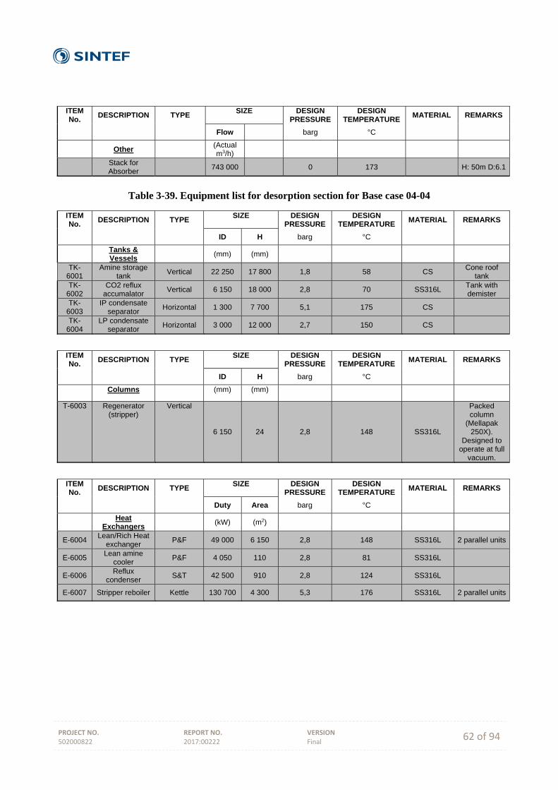
PROJECT NO. 502000822
REPORT NO. 2017:00222
VERSION Final 62 of 94
ITEM No.
DESCRIPTION TYPE SIZE
DESIGN
PRESSURE DESIGN
TEMPERATURE MATERIAL REMARKS
Flow barg °C
Other (Actual m3/h)
Stack for Absorber
743 000 0 173 H: 50m D:6.1
Table 3-39. Equipment list for desorption section for Base case 04-04
ITEM No.
DESCRIPTION TYPE SIZE
DESIGN
PRESSURE DESIGN
TEMPERATURE MATERIAL REMARKS
ID H barg °C
Tanks & Vessels
(mm) (mm)
TK-6001
Amine storage tank
Vertical 22 250 17 800 1,8 58 CS Cone roof
tank
TK-6002
CO2 reflux accumalator
Vertical 6 150 18 000 2,8 70 SS316L Tank with demister
TK-6003
IP condensate separator
Horizontal 1 300 7 700 5,1 175 CS
TK-6004
LP condensate separator
Horizontal 3 000 12 000 2,7 150 CS
ITEM No.
DESCRIPTION TYPE SIZE
DESIGN
PRESSURE DESIGN
TEMPERATURE MATERIAL REMARKS
ID H barg °C
Columns (mm) (mm)
T-6003 Regenerator (stripper)
Vertical
6 150 24 2,8 148 SS316L
Packed column
(Mellapak 250X).
Designed to operate at full
vacuum.
ITEM No.
DESCRIPTION TYPE SIZE
DESIGN
PRESSURE DESIGN
TEMPERATURE MATERIAL REMARKS
Duty Area barg °C
Heat
Exchangers (kW) (m2)
E-6004 Lean/Rich Heat
exchanger P&F 49 000 6 150 2,8 148 SS316L 2 parallel units
E-6005 Lean amine
cooler P&F 4 050 110 2,8 81 SS316L
E-6006 Reflux
condenser S&T 42 500 910 2,8 124 SS316L
E-6007 Stripper reboiler Kettle 130 700 4 300 5,3 176 SS316L 2 parallel units
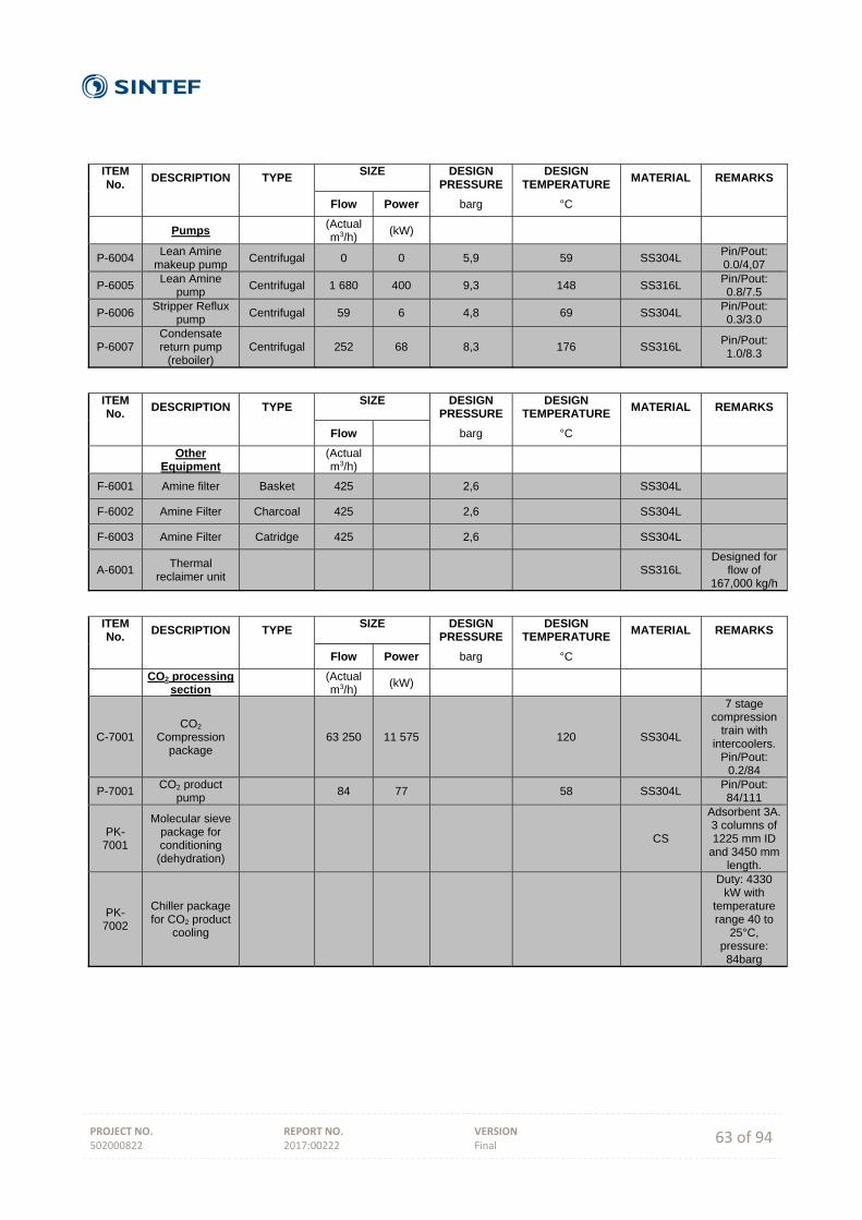
PROJECT NO. 502000822
REPORT NO. 2017:00222
VERSION Final 63 of 94
ITEM No.
DESCRIPTION TYPE SIZE
DESIGN
PRESSURE DESIGN
TEMPERATURE MATERIAL REMARKS
Flow Power barg °C
Pumps (Actual m3/h)
(kW)
P-6004 Lean Amine
makeup pump Centrifugal 0 0 5,9 59 SS304L
Pin/Pout: 0.0/4,07
P-6005 Lean Amine
pump Centrifugal 1 680 400 9,3 148 SS316L
Pin/Pout: 0.8/7.5
P-6006 Stripper Reflux
pump Centrifugal 59 6 4,8 69 SS304L
Pin/Pout: 0.3/3.0
P-6007 Condensate return pump
(reboiler) Centrifugal 252 68 8,3 176 SS316L
Pin/Pout: 1.0/8.3
ITEM No.
DESCRIPTION TYPE SIZE
DESIGN
PRESSURE DESIGN
TEMPERATURE MATERIAL REMARKS
Flow barg °C
Other
Equipment
(Actual m3/h)
F-6001 Amine filter Basket 425 2,6 SS304L
F-6002 Amine Filter Charcoal 425 2,6 SS304L
F-6003 Amine Filter Catridge 425 2,6 SS304L
A-6001 Thermal
reclaimer unit SS316L
Designed for flow of
167,000 kg/h
ITEM No.
DESCRIPTION TYPE SIZE
DESIGN
PRESSURE DESIGN
TEMPERATURE MATERIAL REMARKS
Flow Power barg °C
CO2 processing
section
(Actual m3/h)
(kW)
C-7001 CO2
Compression package
63 250 11 575 120 SS304L
7 stage compression
train with intercoolers.
Pin/Pout: 0.2/84
P-7001 CO2 product
pump 84 77 58 SS304L
Pin/Pout: 84/111
PK-7001
Molecular sieve package for conditioning
(dehydration)
CS
Adsorbent 3A. 3 columns of 1225 mm ID
and 3450 mm length.
PK-7002
Chiller package for CO2 product
cooling
Duty: 4330 kW with
temperature range 40 to
25°C, pressure: 84barg
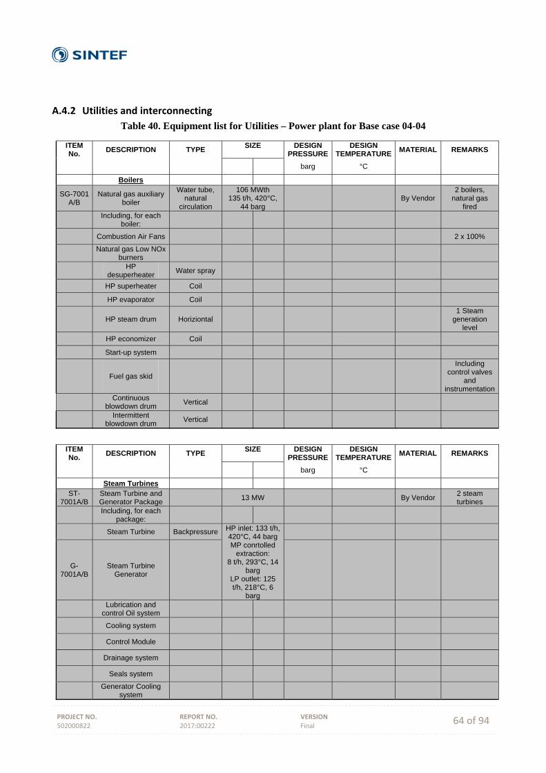
PROJECT NO. 502000822
REPORT NO. 2017:00222
VERSION Final 64 of 94
A.4.2 Utilities and interconnecting
Table 40. Equipment list for Utilities – Power plant for Base case 04-04
ITEM No.
DESCRIPTION TYPE SIZE
DESIGN
PRESSUREDESIGN
TEMPERATURE MATERIAL REMARKS
barg °C
Boilers
SG-7001 A/B
Natural gas auxiliary boiler
Water tube, natural
circulation
106 MWth 135 t/h, 420°C,
44 barg By Vendor
2 boilers, natural gas
fired
Including, for each
boiler:
Combustion Air Fans 2 x 100%
Natural gas Low NOx
burners
HP
desuperheater Water spray
HP superheater Coil
HP evaporator Coil
HP steam drum Horiziontal 1 Steam
generation level
HP economizer Coil
Start-up system
Fuel gas skid
Including control valves
and instrumentation
Continuous
blowdown drum Vertical
Intermittent
blowdown drum Vertical
ITEM No.
DESCRIPTION TYPE SIZE
DESIGN
PRESSUREDESIGN
TEMPERATURE MATERIAL REMARKS
barg °C
Steam Turbines
ST-7001A/B
Steam Turbine and Generator Package
13 MW By Vendor 2 steam turbines
Including, for each
package:
Steam Turbine Backpressure HP inlet: 133 t/h, 420°C, 44 bargMP conrtolled
extraction: 8 t/h, 293°C, 14
barg LP outlet: 125 t/h, 218°C, 6
barg
G-7001A/B
Steam Turbine Generator
Lubrication and
control Oil system
Cooling system
Control Module
Drainage system
Seals system
Generator Cooling
system
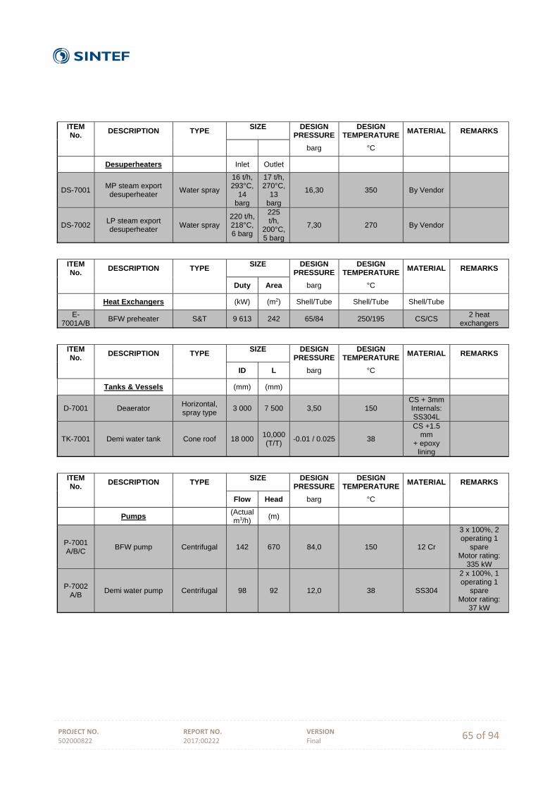
PROJECT NO. 502000822
REPORT NO. 2017:00222
VERSION Final 65 of 94
ITEM No.
DESCRIPTION TYPE SIZE
DESIGN
PRESSUREDESIGN
TEMPERATURE MATERIAL REMARKS
barg °C
Desuperheaters Inlet Outlet
DS-7001 MP steam export
desuperheater Water spray
16 t/h, 293°C,
14 barg
17 t/h, 270°C,
13 barg
16,30 350 By Vendor
DS-7002 LP steam export desuperheater
Water spray 220 t/h, 218°C, 6 barg
225 t/h,
200°C, 5 barg
7,30 270 By Vendor
ITEM No.
DESCRIPTION TYPE SIZE
DESIGN
PRESSUREDESIGN
TEMPERATURE MATERIAL REMARKS
Duty Area barg °C
Heat Exchangers (kW) (m2) Shell/Tube Shell/Tube Shell/Tube
E-7001A/B
BFW preheater S&T 9 613 242 65/84 250/195 CS/CS 2 heat
exchangers
ITEM No.
DESCRIPTION TYPE SIZE
DESIGN
PRESSUREDESIGN
TEMPERATURE MATERIAL REMARKS
ID L barg °C
Tanks & Vessels (mm) (mm)
D-7001 Deaerator Horizontal, spray type
3 000 7 500 3,50 150 CS + 3mm Internals: SS304L
TK-7001 Demi water tank Cone roof 18 000 10,000 (T/T)
-0.01 / 0.025 38
CS +1.5 mm
+ epoxy lining
ITEM No.
DESCRIPTION TYPE SIZE
DESIGN
PRESSUREDESIGN
TEMPERATURE MATERIAL REMARKS
Flow Head barg °C
Pumps (Actual m3/h)
(m)
P-7001 A/B/C
BFW pump Centrifugal 142 670 84,0 150 12 Cr
3 x 100%, 2 operating 1
spare Motor rating:
335 kW
P-7002 A/B
Demi water pump Centrifugal 98 92 12,0 38 SS304
2 x 100%, 1 operating 1
spare Motor rating:
37 kW

PROJECT NO. 502000822
REPORT NO. 2017:00222
VERSION Final 66 of 94
ITEM No.
DESCRIPTION TYPE SIZE
DESIGN
PRESSUREDESIGN
TEMPERATURE MATERIAL REMARKS
barg °C
Packages
PK-7001 Demineralized water
package
Demi water production: 98
t/h By Vendor
Including
Cation beds
Degassing columns
Degassified Water
Pumps
Anion beds
Mixed Bed Polishers
Regeneration and
neutralization system
Neutralization basin
Neutralization Basin
Drainoff Pumps
PK-7002 Phosphates injection
package By Vendor
Including storage drum and dosing
pumps
PK-7003 Amines injection
package By Vendor
Including storage drum and dosing
pumps
PK-7004 Oxygen scavenger injection package
By Vendor
Including storage drum and dosing
pumps
PK-7005 Sampling package By Vendor
ITEM No.
DESCRIPTION TYPE SIZE
DESIGN
PRESSUREDESIGN
TEMPERATURE MATERIAL REMARKS
ID H barg °C
Other (m) (m)
PK-7006A/B
Continuous emission monitoring system
By Vendor
2 packages, 1 for each boiler
Actual flow: 190,500 m3/h
S-7001A/B
Natural gas boiler Stack
2,2 50 0 160 Reinforced concrete
2 packages, 1 for each boiler
Actual flow: 190,500 m3/h
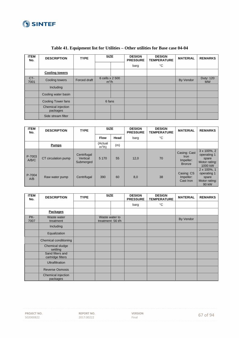
PROJECT NO. 502000822
REPORT NO. 2017:00222
VERSION Final 67 of 94
Table 41. Equipment list for Utilities – Other utilities for Base case 04-04
ITEM No.
DESCRIPTION TYPE SIZE
DESIGN
PRESSURE DESIGN
TEMPERATURE MATERIAL REMARKS
barg °C
Cooling towers
CT-7001
Cooling towers Forced draft 6 cells x 2 500
m3/h By Vendor
Duty: 120 MW
Including
Cooling water basin
Cooling Tower fans 6 fans
Chemical injection
packages
Side stream filter
ITEM No.
DESCRIPTION TYPE SIZE
DESIGN
PRESSURE DESIGN
TEMPERATURE MATERIAL REMARKS
Flow Head barg °C
Pumps (Actual m3/h)
(m)
P-7003 A/B/C
CT circulation pump Centrifugal
Vertical Submerged
5 170 55 12,0 70
Casing: Cast Iron
Impeller: Bronze
3 x 100%, 2 operating 1
spare Motor rating:
1000 kW
P-7004 A/B
Raw water pump Centrifugal 390 60 8,0 38 Casing: CS
Impeller: Cast Iron
2 x 100%, 1 operating 1
spare Motor rating:
90 kW
ITEM No.
DESCRIPTION TYPE SIZE
DESIGN
PRESSURE DESIGN
TEMPERATURE MATERIAL REMARKS
barg °C
Packages
PK-7007
Waste water treatment
Waste water to
treatment: 56 t/h By Vendor
Including
Equalization
Chemical conditioning
Chemical sludge
settling
Sand filters and cartridge filters
Ultrafiltration
Reverse Osmosis
Chemical injection
packages
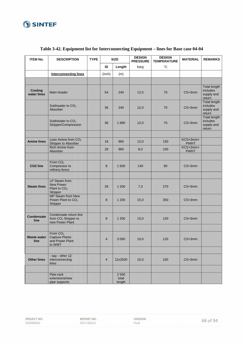
PROJECT NO. 502000822
REPORT NO. 2017:00222
VERSION Final 68 of 94
Table 3-42. Equipment list for Interconnecting Equipment – lines for Base case 04-04
ITEM No. DESCRIPTION TYPE SIZE DESIGN
PRESSURE DESIGN
TEMPERATURE MATERIAL REMARKS
ID Length barg °C
Interconnecting lines (inch) (m)
Cooling water lines
Main header 54 240 12,0 70 CS+3mm
Total length includes supply and return
Subheader to CO2 Absorber
36 240 12,0 70 CS+3mm
Total length includes supply and return
Subheader to CO2 Stripper/Compression
36 1 680 12,0 70 CS+3mm
Total length includes supply and return
Amine lines Lean Amine from CO2 Stripper to Absorber
18 960 12,0 150 KCS+3mm+
PWHT
Rich Amine from Absorber
28 960 8,0 100 KCS+3mm+
PWHT
CO2 line From CO2 Compressor to refinery fence
8 1 500 140 80 CS+3mm
Steam lines
LP Steam from New Power Plant to CO2 Stripper
28 1 200 7,3 270 CS+3mm
MP Steam from New Power Plant to CO2 Stripper
8 1 200 15,0 350 CS+3mm
Condensate line
Condensate return line from CO2 Stripper to new Power Plant
8 1 200 15,0 120 CS+3mm
Waste water line
From CO2 Capture Plants and Power Plant to WWT
4 3 000 10,0 120 CS+3mm
Other lines - say - other 12 interconnecting lines
4 12x2500 15,0 150 CS+3mm
Pipe-rack extensions/new pipe supports
2 500 total
length

PROJECT NO. 502000822
REPORT NO. 2017:00222
VERSION Final 69 of 94
Table 43. Equipment list for Interconnecting Equipment – Other items for Base case 04-04
ITEM No. DESCRIPTION TYPE SIZE DESIGN
PRESSURE DESIGN
TEMPERATURE MATERIAL REMARKS
ID Height barg °C
Other items (m) (m)
New Storage
tanks
5 new storage tanks in place of the ones dismantled
Cone roof
30 15 atm 200 CS
new tank basin to be built
new pipeway (say 20 lines) to be built, approx. length 800 m
5 existing storage tanks to be dismantled
DCS expansion
Additional cards for new plants
Electrical grid
expansion
Power supply cables from new Power Plant to CO2 capture plants and CO2 compression
3 x 3 x 300 mm2
2500 total
length
Flue gas ducting
From Steam Reformer to CO2 Absorber
Square section
duct
3.3 X 3.3 m
350 m total
length 0,2 300 SS
Supports for duct to be included
PROJECT NO. 502000822
REPORT NO. 2017:00222
VERSION Final 70 of 94
B Equipment cost functions developed
As previously explained, equipment cost functions for simplified assessment of some of the CO2 capture cases. These functions can be used in order to assess the 12 cases considered for simplified assessment as well as to help others to assess their own CO2 capture cases. These cost functions are based on the four cases assessed in details and experience on system characteristics important for equipment cost scaling. In order to ensure a good trade-off between level of detail and accuracy, cost functions are developed for the eight system subsections considered:
CO2 capture and compression o Flue gas desulphurisation unit o Absorber section o Regeneration section o CO2 compression
Utilities o CHP plant o Cooling towers o Waste water treatment
Interconnecting (no subsection)
Once the both the equipment and total plant cost for the reference cases 01-03, 02-02, 04-03 and 04-04 was
developed, the cost for all the other capture cases was calculated based on a factored estimating methodology,
which is described hereinafter.
With the capacity factored estimate methodology, the cost of the plant under evaluation is derived from the
known cost of a similar plant of known capacity (power cost law). Cost and capacity are related by means of a
non-linear equation, which can be expressed as:
Cost CapacityactualCapacityref
exp
Cost
In this function:
Costactual is the cost of the plant under evaluation Costref is the cost of the reference plant Capacityactual and Capacityref are the respective capacities of the plants exp is the exponent, which typically varies between 0.5 and 0.85, depending on plant type and
size. The exponent is usually lower than 1, when scale economies are given evidence in scaling up or down the reference cost, while it approaches the value of 1 for modularized systems.
The above described methodology was used to calculate the investment cost of the main plant units, including
the most significant capacity parameters of each process section.
B.1 CO2 capture and compression cost estimate
B.1.1 Absorption section estimate
For the four selected cases, the absorption section cost was estimated based on the developed equipment
lists:
Case 01-03: CRF absorber Case 02-02: Power Plant and FCC absorbers Case 04-03: NGCC, Boiler + CDU/VDU, SMR, FCC absorbers Case 04-04: SMR absorber
Using these equipment-based estimates as references, the absorption section costs for all the other cases
were estimated as a factored cost estimate. The absorption section cost calculations were performed
considering the cost of the absorber column separately from all the other section items:
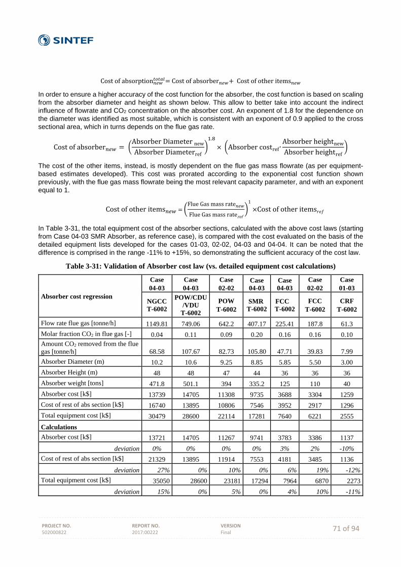
PROJECT NO. 502000822
REPORT NO. 2017:00222
VERSION Final 71 of 94
Costofabsorption Costofabsorber Costofotheritems
In order to ensure a higher accuracy of the cost function for the absorber, the cost function is based on scaling
from the absorber diameter and height as shown below. This allow to better take into account the indirect
influence of flowrate and CO2 concentration on the absorber cost. An exponent of 1.8 for the dependence on
the diameter was identified as most suitable, which is consistent with an exponent of 0.9 applied to the cross
sectional area, which in turns depends on the flue gas rate.
Costofabsorber AbsorberDiameternewAbsorberDiameterref
.
Absorbercostref∙AbsorberheightnewAbsorberheightref
The cost of the other items, instead, is mostly dependent on the flue gas mass flowrate (as per equipment-
based estimates developed). This cost was prorated according to the exponential cost function shown
previously, with the flue gas mass flowrate being the most relevant capacity parameter, and with an exponent
equal to 1.
Costofotheritems FlueGasmassrate
FlueGasmassrateref
1
Costofotheritems
In Table 3-31, the total equipment cost of the absorber sections, calculated with the above cost laws (starting
from Case 04-03 SMR Absorber, as reference case), is compared with the cost evaluated on the basis of the
detailed equipment lists developed for the cases 01-03, 02-02, 04-03 and 04-04. It can be noted that the
difference is comprised in the range -11% to +15%, so demonstrating the sufficient accuracy of the cost law.
Table 3-31: Validation of Absorber cost law (vs. detailed equipment cost calculations)
Absorber cost regression
Case 04-03
Case 04-03
Case 02-02
Case 04-03
Case 04-03
Case 02-02
Case 01-03
NGCC T-6002
POW/CDU/VDU
T-6002
POW T-6002
SMR T-6002
FCC T-6002
FCC T-6002
CRF T-6002
Flow rate flue gas [tonne/h] 1149.81 749.06 642.2 407.17 225.41 187.8 61.3
Molar fraction CO2 in flue gas [-] 0.04 0.11 0.09 0.20 0.16 0.16 0.10 Amount CO2 removed from the flue gas [tonne/h] 68.58 107.67 82.73 105.80 47.71 39.83 7.99
Absorber Diameter (m) 10.2 10.6 9.25 8.85 5.85 5.50 3.00
Absorber Height (m) 48 48 47 44 36 36 36
Absorber weight [tons] 471.8 501.1 394 335.2 125 110 40
Absorber cost [k$] 13739 14705 11308 9735 3688 3304 1259
Cost of rest of abs section [k$] 16740 13895 10806 7546 3952 2917 1296
Total equipment cost [k$] 30479 28600 22114 17281 7640 6221 2555
Calculations Absorber cost [k$] 13721 14705 11267 9741 3783 3386 1137
deviation 0% 0% 0% 0% 3% 2% -10%
Cost of rest of abs section [k$] 21329 13895 11914 7553 4181 3485 1136
deviation 27% 0% 10% 0% 6% 19% -12%
Total equipment cost [k$] 35050 28600 23181 17294 7964 6870 2273
deviation 15% 0% 5% 0% 4% 10% -11%
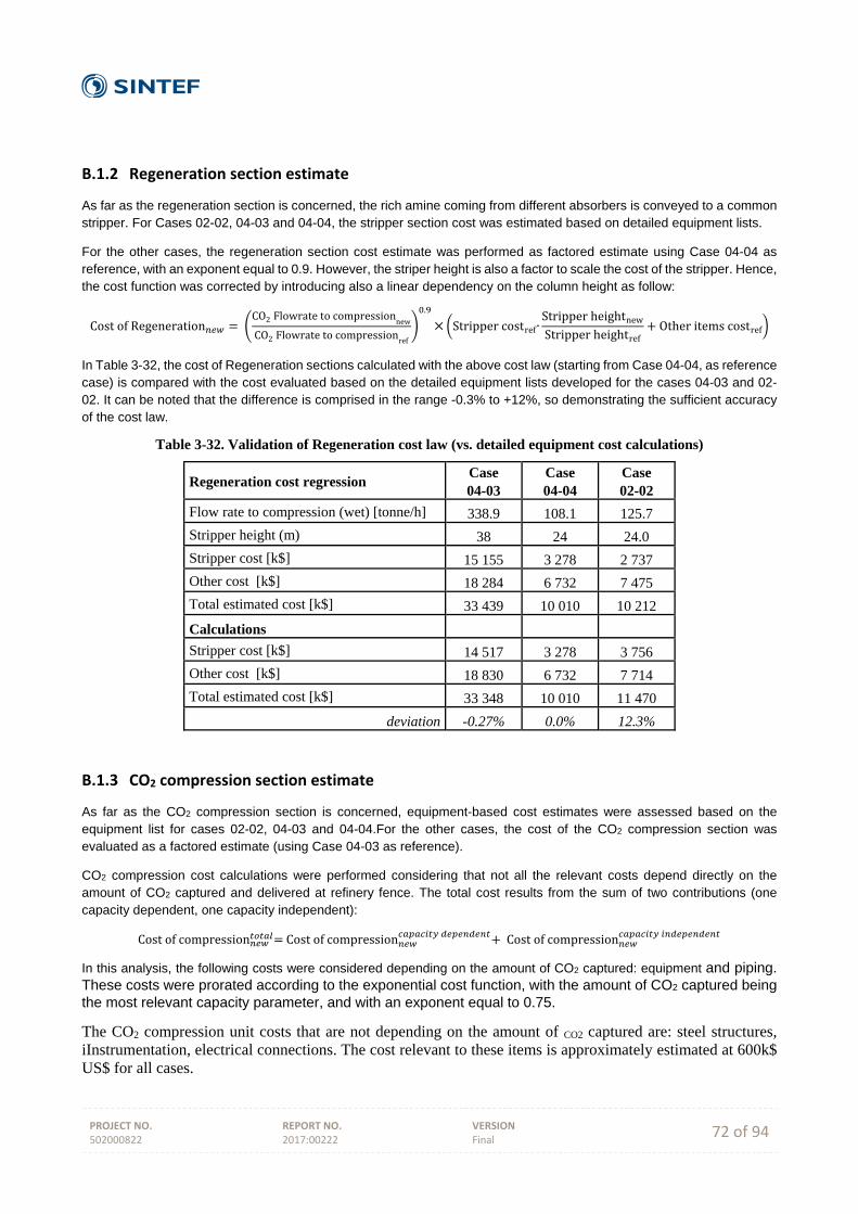
PROJECT NO. 502000822
REPORT NO. 2017:00222
VERSION Final 72 of 94
B.1.2 Regeneration section estimate
As far as the regeneration section is concerned, the rich amine coming from different absorbers is conveyed to a common
stripper. For Cases 02-02, 04-03 and 04-04, the stripper section cost was estimated based on detailed equipment lists.
For the other cases, the regeneration section cost estimate was performed as factored estimate using Case 04-04 as
reference, with an exponent equal to 0.9. However, the striper height is also a factor to scale the cost of the stripper. Hence,
the cost function was corrected by introducing also a linear dependency on the column height as follow:
CostofRegeneration CO2FlowratetocompressionnewCO2Flowratetocompressionref
.
Strippercostref∙StripperheightnewStripperheightref
Otheritemscostref
In Table 3-32, the cost of Regeneration sections calculated with the above cost law (starting from Case 04-04, as reference
case) is compared with the cost evaluated based on the detailed equipment lists developed for the cases 04-03 and 02-
02. It can be noted that the difference is comprised in the range -0.3% to +12%, so demonstrating the sufficient accuracy
of the cost law.
Table 3-32. Validation of Regeneration cost law (vs. detailed equipment cost calculations)
Regeneration cost regression Case 04-03
Case 04-04
Case 02-02
Flow rate to compression (wet) [tonne/h] 338.9 108.1 125.7
Stripper height (m) 38 24 24.0
Stripper cost [k$] 15 155 3 278 2 737
Other cost [k$] 18 284 6 732 7 475
Total estimated cost [k$] 33 439 10 010 10 212
Calculations Stripper cost [k$] 14 517 3 278 3 756
Other cost [k$] 18 830 6 732 7 714
Total estimated cost [k$] 33 348 10 010 11 470
deviation -0.27% 0.0% 12.3%
B.1.3 CO2 compression section estimate
As far as the CO2 compression section is concerned, equipment-based cost estimates were assessed based on the
equipment list for cases 02-02, 04-03 and 04-04.For the other cases, the cost of the CO2 compression section was
evaluated as a factored estimate (using Case 04-03 as reference).
CO2 compression cost calculations were performed considering that not all the relevant costs depend directly on the
amount of CO2 captured and delivered at refinery fence. The total cost results from the sum of two contributions (one
capacity dependent, one capacity independent):
Costofcompression Costofcompression Costofcompression
In this analysis, the following costs were considered depending on the amount of CO2 captured: equipment and piping.
These costs were prorated according to the exponential cost function, with the amount of CO2 captured being
the most relevant capacity parameter, and with an exponent equal to 0.75.
The CO2 compression unit costs that are not depending on the amount of CO2 captured are: steel structures, iInstrumentation, electrical connections. The cost relevant to these items is approximately estimated at 600k$ US$ for all cases.
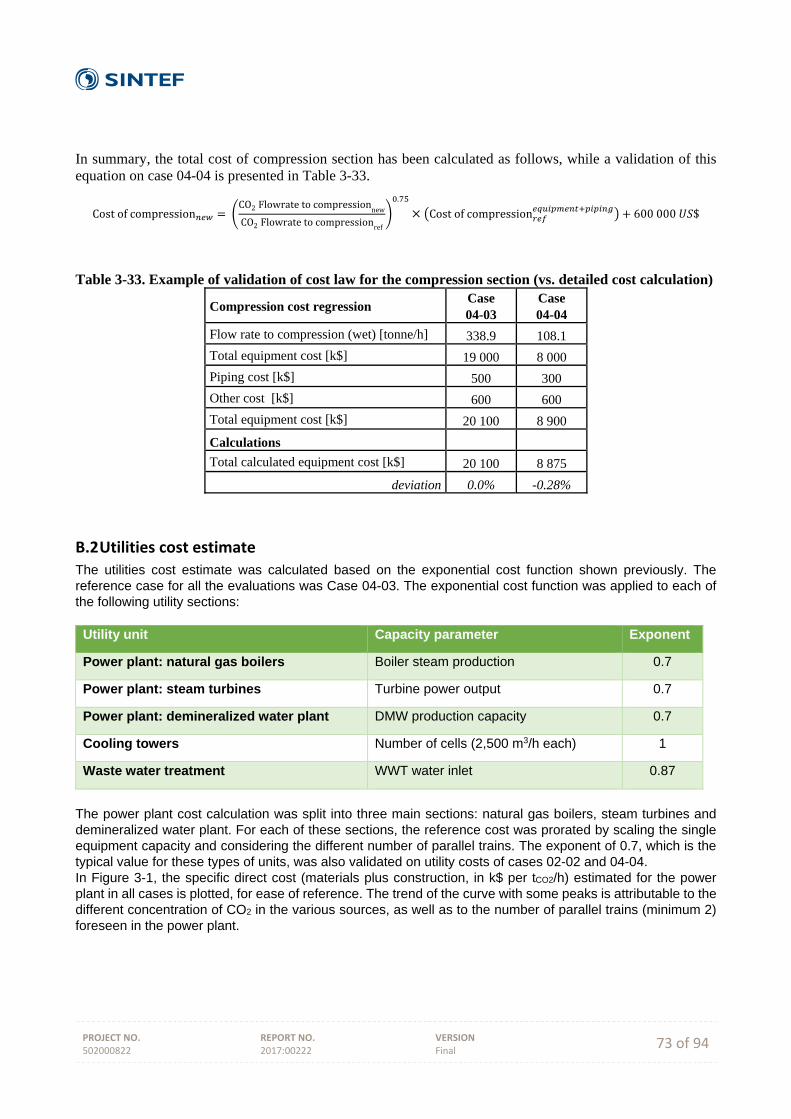
PROJECT NO. 502000822
REPORT NO. 2017:00222
VERSION Final 73 of 94
In summary, the total cost of compression section has been calculated as follows, while a validation of this equation on case 04-04 is presented in Table 3-33.
Costofcompression CO2FlowratetocompressionnewCO2Flowratetocompressionref
.
Costofcompression 600000 $
Table 3-33. Example of validation of cost law for the compression section (vs. detailed cost calculation)
Compression cost regression Case 04-03
Case 04-04
Flow rate to compression (wet) [tonne/h] 338.9 108.1
Total equipment cost [k$] 19 000 8 000
Piping cost [k$] 500 300
Other cost [k$] 600 600
Total equipment cost [k$] 20 100 8 900
Calculations
Total calculated equipment cost [k$] 20 100 8 875
deviation 0.0% -0.28%
B.2 Utilities cost estimate
The utilities cost estimate was calculated based on the exponential cost function shown previously. The
reference case for all the evaluations was Case 04-03. The exponential cost function was applied to each of
the following utility sections:
Utility unit Capacity parameter Exponent
Power plant: natural gas boilers Boiler steam production 0.7
Power plant: steam turbines Turbine power output 0.7
Power plant: demineralized water plant DMW production capacity 0.7
Cooling towers Number of cells (2,500 m3/h each) 1
Waste water treatment WWT water inlet 0.87
The power plant cost calculation was split into three main sections: natural gas boilers, steam turbines and
demineralized water plant. For each of these sections, the reference cost was prorated by scaling the single
equipment capacity and considering the different number of parallel trains. The exponent of 0.7, which is the
typical value for these types of units, was also validated on utility costs of cases 02-02 and 04-04.
In Figure 3-1, the specific direct cost (materials plus construction, in k$ per tCO2/h) estimated for the power
plant in all cases is plotted, for ease of reference. The trend of the curve with some peaks is attributable to the
different concentration of CO2 in the various sources, as well as to the number of parallel trains (minimum 2)
foreseen in the power plant.
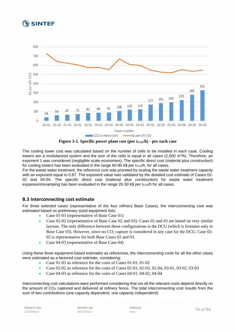
PROJECT NO. 502000822
REPORT NO. 2017:00222
VERSION Final 74 of 94
Figure 3-1. Specific power plant cost (per tCO2/h) - per each case
The cooling tower cost was calculated based on the number of cells to be installed in each case. Cooling
towers are a modularized system and the size of the cells is equal in all cases (2,500 m3/h). Therefore, an
exponent 1 was considered (negligible scale economies). The specific direct cost (material plus construction)
for cooling towers has been evaluated in the range 60-90 k$ per tCO2/h, for all cases.
For the waste water treatment, the reference cost was prorated by scaling the waste water treatment capacity
with an exponent equal to 0.87. The exponent value was validated by the detailed cost estimate of Cases 02-
02 and 04-04. The specific direct cost (material plus construction) for waste water treatment
expansion/revamping has been evaluated in the range 20-30 k$ per tCO2/h for all cases.
B.3 Interconnecting cost estimate For three selected cases (representative of the four refinery Base Cases), the interconnecting cost was
estimated based on preliminary sized equipment lists:
Case 01-03 (representative of Base Case 01) Case 02-02 (representative of Base Case 02 and 03): Cases 02 and 03 are based on very similar
layouts. The only difference between these configurations is the DCU (which is foreseen only in Base Case 03). However, since no CO2 capture is considered in any case for the DCU, Case 02-02 is representative for both Base Cases 02 and 03.
Case 04-03 (representative of Base Case 04) Using these three equipment-based estimates as references, the interconnecting costs for all the other cases
were estimated as a factored cost estimate, considering:
Case 01-03 as reference for the costs of Cases 01-01, 01-02 Case 02-02 as reference for the costs of Cases 02-01, 02-03, 02-04, 03-01, 03-02, 03-03 Case 04-03 as reference for the costs of Cases 04-01, 04-02, 04-04
Interconnecting cost calculations were performed considering that not all the relevant costs depend directly on
the amount of CO2 captured and delivered at refinery fence. The total interconnecting cost results from the
sum of two contributions (one capacity dependent, one capacity independent):

PROJECT NO. 502000822
REPORT NO. 2017:00222
VERSION Final 75 of 94
Costofinterconnecting Costofinterconnecting Costofinterconnecting
In this analysis, the following costs were considered to be dependent of the amount of CO2 captured: flue gas ducting, cooling water lines, amine lines, CO2 line to refinery fence, steam lines, condensate line, waste water line, DCS expansion, electrical grid expansion. These costs were prorated according to the exponential cost function previously presented, with the amount of CO2 captured being the most relevant capacity parameter, and with an exponent equal to 0.75.
Figure 3-2. Specific interconnecting cost (per tCO2/h) - capacity dependent portion - per each case
The interconnecting costs that do not depend on the amount of CO2 captured, but only on the refinery layout,
are: storage tanks relocation (calculated based on the number of relocated tanks) and pipe-rack
extensions/new pipe supports (calculated on the basis of the length of new pipe supports). A total direct cost
(materials + construction) of 2500 k$ has been estimated per each tank to be relocated, while a total direct
cost of new piperack has been estimated equal to approx. 1900 k$/100m.
It has to be noticed that the economic outcomes of the above described interconnecting cost methodology are strongly dependent on the specificity of each site. Therefore, it is recommended that a careful evaluation of site characteristics is performed when developing interconnecting cost estimates for other refiner
PROJECT NO. 502000822
REPORT NO. 2017:00222
VERSION Final 76 of 94
C Excel model for evaluating the cost of retrofitting CO2 capture from refineries
The following elements present and describe how to use the excel model developed by SINTEF Energy Research for evaluation of the cost of retrofitting CO2 capture from refineries and available at http://www.sintef.no/RECAP. Presentations: This spreadsheet aims at providing help for potential users to evaluate and understand the cost of retrofitting CO2 capture on a refinery. This spreadsheet is divided into five sheets:
Sheet "Presentation - instructions": which includes the presentation of the spreadsheet and instructions to perform an evaluation
Sheet "Input data": in which all data required (case, technical, cost, and sensitivity analyses) to evaluate the cost of retrofitting CO2 capture shall be filled in.
Sheet "Discount factor": in which the discount factors (used to evaluate the annualized CAPEX) are assessed for the base case and the sensitivity analyses (when varying project duration, discount rate and utilisation rate)
Sheet "Detailed cost results": which includes the detailed cost evaluation results of retrofitting CO2 capture (values)
Sheet "Summarised cost results": which includes the breakdown of the cost of retrofitting CO2 capture ($/tCO2,avoided) results - (values and graphical representation)
Sheet "Sensitivity analyses": which includes the results of the sensitivity analyses - (values and graphical representation)
Instructions: To evaluate a case with the present spreadsheet, the user needs to fill out, with the data corresponding to the case which needs to be evaluated, all the orange cells in the sheet "Input data":
1. Project valuation data (discount rate, reference year, number of years of operations, average annual utilisation rate)
2. CO2 captured and avoided streams (amount of CO2 captured, amount of CO2 emitted by the power plant)
3. Data for calculation of CAPEX (costs for each of the cost sections of the system, contingencies, data for evaluation of the Total Capital requirement, planned allocation of construction costs)
4. Data for calculation of the annual fixed OPEX (number of employees, average fully burdened salary, annual material maintenance percentages, overall maintenance cost percentage, other cost percentages)
5. Data for calculation of the annual variable OPEX (utilities consumptions and sludge disposal quantities and cost, material replacement and cost, share of natural gas consumption linked to steam production for CO2 stripping)
6. Data for valorisation of excess power if relevant (Choice to consider excess power valorisation, amount and economic value of excess power)
7. Variation ranges considered for sensitivity analyses Remark: It is strongly recommended that the user always checks carefully the units used. The user is free to use their own estimates, however help to evaluate CAPEX through cost functions can be found in Appendix B while help to evaluate utilities consumption and material replacement can be found in the document Performance analysis of CO2 capture options. Once these data are filled out, the results generated (presented above) can directly be found in the three sheets "Detailed cost results", "Summarised cost results", and "Sensitivity analyses".
PROJECT NO. 502000822
REPORT NO. 2017:00222
VERSION Final 77 of 94
To provide support for user based evaluations, the spreadsheets of the 16 CO2 capture cases evaluated in the ReCap project can be found at http://www.sintef.no/RECAP. It is worth noting that the cost of retrofitting CO2 capture is calculated based on the additional costs of implementing CO2 capture (including utilities generation and interconnecting) using the following equation:
CO2 avoided cost =Annualized CO2 capture CAPEX + Annual CO2 capture OPEX
Annual amount of CO2 avoided
Finally, note that, apart from the cells marked in orange, all the cells of the spreadsheet are locked for editing and may not be modified. Contact: For further question(s) on this spreadsheet, please contact Simon Roussanaly at SINTEF Energy Research at [email protected] with the following e-mail subject "Spreadsheet for evaluation of cost of retrofitting CO2 capture from refineries". Acknowledgement: This Spreadsheet was developed by SINTEF Energy Research in the ReCap project with funding from Gassnova (contract 232308), IEAGHG and Concawe. Disclaimer: SINTEF Energy Research has developed this spreadsheet for calculations of the costs presented in the report "Understanding the cost of retrofitting CO2 capture to integrated oil refineries" The spreadsheet is provided as is for enabling user-specific assessments of CO2 capture retrofit to integrated oil refineries. SINTEF assumes no responsibility for the results generated with this spreadsheet.
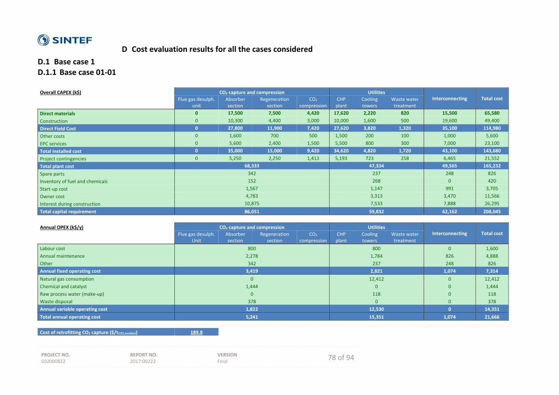
PROJECT NO. 502000822
REPORT NO. 2017:00222
VERSION Final 78 of 94
D Cost evaluation results for all the cases considered
D.1 Base case 1 D.1.1 Base case 01‐01
Overall CAPEX (k$) CO2 capture and compression Utilities
Interconnecting Total cost Flue gas desulph. unit
Absorber section
Regeneration section
CO2 compression
CHP plant
Cooling towers
Waste water treatment
Direct materials 0 17,500 7,500 4,420 17,620 2,220 820 15,500 65,580
Construction 0 10,300 4,400 3,000 10,000 1,600 500 19,600 49,400
Direct Field Cost 0 27,800 11,900 7,420 27,620 3,820 1,320 35,100 114,980
Other costs 0 1,600 700 500 1,500 200 100 1,000 5,600
EPC services 0 5,600 2,400 1,500 5,500 800 300 7,000 23,100
Total installed cost 0 35,000 15,000 9,420 34,620 4,820 1,720 43,100 143,680
Project contingencies 0 5,250 2,250 1,413 5,193 723 258 6,465 21,552
Total plant cost 68,333 47,334 49,565 165,232
Spare parts 342 237 248 826
Inventory of fuel and chemicals 152 268 0 420
Start‐up cost 1,567 1,147 991 3,705
Owner cost 4,783 3,313 3,470 11,566
Interest during construction 10,875 7,533 7,888 26,295
Total capital requirement 86,051 59,832 62,162 208,045
Annual OPEX (k$/y) CO2 capture and compression Utilities
Interconnecting Total cost Flue gas desulph. Unit
Absorber section
Regeneration section
CO2 compression
CHP plant
Cooling towers
Waste water treatment
Labour cost 800 800 0 1,600
Annual maintenance 2,278 1,784 826 4,888
Other 342 237 248 826
Annual fixed operating cost 3,419 2,821 1,074 7,314
Natural gas consumption 0 12,412 0 12,412
Chemical and catalyst 1,444 0 0 1,444
Raw process water (make‐up) 0 118 0 118
Waste disposal 378 0 0 378
Annual variable operating cost 1,822 12,530 0 14,351
Total annual operating cost 5,241 15,351 1,074 21,666
Cost of retrofitting CO2 capture ($/tCO2,avoided) 189.8
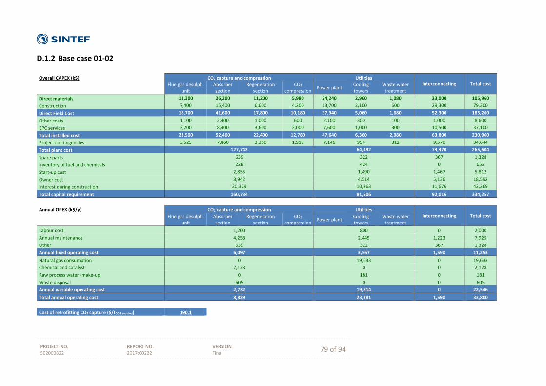
PROJECT NO. 502000822
REPORT NO. 2017:00222
VERSION Final 79 of 94
D.1.2 Base case 01‐02
Overall CAPEX (k$) CO2 capture and compression Utilities
Interconnecting Total cost Flue gas desulph. unit
Absorber section
Regeneration section
CO2 compression
Power plant Cooling towers
Waste water treatment
Direct materials 11,300 26,200 11,200 5,980 24,240 2,960 1,080 23,000 105,960
Construction 7,400 15,400 6,600 4,200 13,700 2,100 600 29,300 79,300
Direct Field Cost 18,700 41,600 17,800 10,180 37,940 5,060 1,680 52,300 185,260
Other costs 1,100 2,400 1,000 600 2,100 300 100 1,000 8,600
EPC services 3,700 8,400 3,600 2,000 7,600 1,000 300 10,500 37,100
Total installed cost 23,500 52,400 22,400 12,780 47,640 6,360 2,080 63,800 230,960
Project contingencies 3,525 7,860 3,360 1,917 7,146 954 312 9,570 34,644
Total plant cost 127,742 64,492 73,370 265,604
Spare parts 639 322 367 1,328
Inventory of fuel and chemicals 228 424 0 652
Start‐up cost 2,855 1,490 1,467 5,812
Owner cost 8,942 4,514 5,136 18,592
Interest during construction 20,329 10,263 11,676 42,269
Total capital requirement 160,734 81,506 92,016 334,257
Annual OPEX (k$/y) CO2 capture and compression Utilities
Interconnecting Total cost Flue gas desulph. unit
Absorber section
Regeneration section
CO2 compression
Power plant Cooling towers
Waste water treatment
Labour cost 1,200 800 0 2,000
Annual maintenance 4,258 2,445 1,223 7,925
Other 639 322 367 1,328
Annual fixed operating cost 6,097 3,567 1,590 11,253
Natural gas consumption 0 19,633 0 19,633
Chemical and catalyst 2,128 0 0 2,128
Raw process water (make‐up) 0 181 0 181
Waste disposal 605 0 0 605
Annual variable operating cost 2,732 19,814 0 22,546
Total annual operating cost 8,829 23,381 1,590 33,800
Cost of retrofitting CO2 capture ($/tCO2,avoided) 190.1
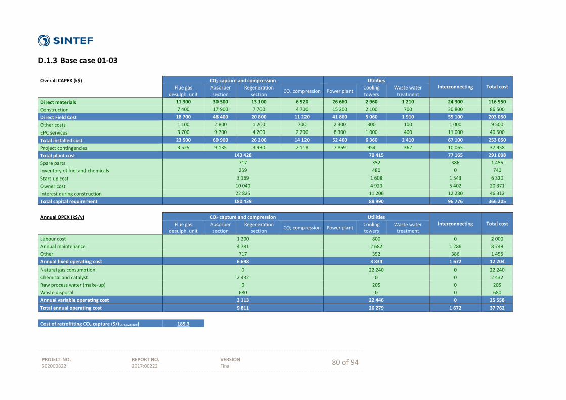
PROJECT NO. 502000822
REPORT NO. 2017:00222
VERSION Final 80 of 94
D.1.3 Base case 01‐03
Overall CAPEX (k$) CO2 capture and compression Utilities
Interconnecting Total cost Flue gas desulph. unit
Absorber section
Regeneration section
CO2 compression Power plant Cooling towers
Waste water treatment
Direct materials 11 300 30 500 13 100 6 520 26 660 2 960 1 210 24 300 116 550
Construction 7 400 17 900 7 700 4 700 15 200 2 100 700 30 800 86 500
Direct Field Cost 18 700 48 400 20 800 11 220 41 860 5 060 1 910 55 100 203 050
Other costs 1 100 2 800 1 200 700 2 300 300 100 1 000 9 500
EPC services 3 700 9 700 4 200 2 200 8 300 1 000 400 11 000 40 500
Total installed cost 23 500 60 900 26 200 14 120 52 460 6 360 2 410 67 100 253 050
Project contingencies 3 525 9 135 3 930 2 118 7 869 954 362 10 065 37 958
Total plant cost 143 428 70 415 77 165 291 008
Spare parts 717 352 386 1 455
Inventory of fuel and chemicals 259 480 0 740
Start‐up cost 3 169 1 608 1 543 6 320
Owner cost 10 040 4 929 5 402 20 371
Interest during construction 22 825 11 206 12 280 46 312
Total capital requirement 180 439 88 990 96 776 366 205
Annual OPEX (k$/y) CO2 capture and compression Utilities
Interconnecting Total cost Flue gas desulph. unit
Absorber section
Regeneration section
CO2 compression Power plant Cooling towers
Waste water treatment
Labour cost 1 200 800 0 2 000
Annual maintenance 4 781 2 682 1 286 8 749
Other 717 352 386 1 455
Annual fixed operating cost 6 698 3 834 1 672 12 204
Natural gas consumption 0 22 240 0 22 240
Chemical and catalyst 2 432 0 0 2 432
Raw process water (make‐up) 0 205 0 205
Waste disposal 680 0 0 680
Annual variable operating cost 3 113 22 446 0 25 558
Total annual operating cost 9 811 26 279 1 672 37 762
Cost of retrofitting CO2 capture ($/tCO2,avoided) 185,3
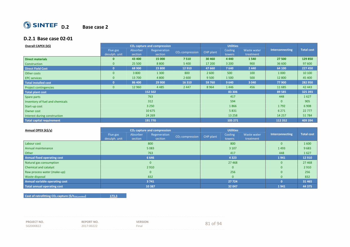
PROJECT NO. 502000822
REPORT NO. 2017:00222
VERSION Final 81 of 94
D.2 Base case 2
D.2.1 Base case 02‐01 Overall CAPEX (k$) CO2 capture and compression Utilities
Interconnecting Total cost Flue gas desulph. unit
Absorber section
Regeneration section
CO2 compression CHP plant Cooling towers
Waste water treatment
Direct materials 0 43 400 15 000 7 510 30 460 4 440 1 540 27 500 129 850
Construction 0 25 500 8 800 5 400 17 200 3 200 900 36 600 97 600
Direct Field Cost 0 68 900 23 800 12 910 47 660 7 640 2 440 64 100 227 450
Other costs 0 3 800 1 300 800 2 600 500 100 1 000 10 100
EPC services 0 13 700 4 800 2 600 9 500 1 500 500 12 800 45 400
Total installed cost 0 86 400 29 900 16 310 59 760 9 640 3 040 77 900 282 950
Project contingencies 0 12 960 4 485 2 447 8 964 1 446 456 11 685 42 443
Total plant cost 152 502 83 306 89 585 325 393
Spare parts 763 417 448 1 627
Inventory of fuel and chemicals 312 594 0 905
Start‐up cost 3 250 1 866 1 792 6 908
Owner cost 10 675 5 831 6 271 22 777
Interest during construction 24 269 13 258 14 257 51 784
Total capital requirement 191 770 105 271 112 352 409 394
Annual OPEX (k$/y) CO2 capture and compression Utilities
Interconnecting Total cost Flue gas desulph. unit
Absorber section
Regeneration section
CO2 compression CHP plant Cooling towers
Waste water treatment
Labour cost 800 800 0 1 600
Annual maintenance 5 083 3 107 1 493 9 683
Other 763 417 448 1 627
Annual fixed operating cost 6 646 4 323 1 941 12 910
Natural gas consumption 0 27 468 0 27 468
Chemical and catalyst 2 910 0 0 2 910
Raw process water (make‐up) 0 256 0 256
Waste disposal 832 0 0 832
Annual variable operating cost 3 741 27 724 0 31 465
Total annual operating cost 10 387 32 047 1 941 44 375
Cost of retrofitting CO2 capture ($/tCO2,avoided) 173,3

PROJECT NO. 502000822
REPORT NO. 2017:00222
VERSION Final 82 of 94
D.2.2 Base case 02‐02 Overall CAPEX (k$) CO2 capture and compression Utilities
Interconnecting Total cost Flue gas desulph. unit
Absorber section
Regeneration section
CO2 compression Power plant Cooling towers
Waste water treatment
Direct materials 13 600 56 200 22 400 9 870 46 860 5 920 2 110 41 200 198 160
Construction 8 900 33 000 13 200 7 300 26 600 4 300 1 200 54 700 149 200
Direct Field Cost 22 500 89 200 35 600 17 170 73 460 10 220 3 310 95 900 347 360
Other costs 1 400 4 900 2 000 1 100 3 900 600 200 2 000 16 100
EPC services 4 500 17 800 7 100 3 400 14 700 2 000 700 19 200 69 400
Total installed cost 28 400 111 900 44 700 21 670 92 060 12 820 4 210 117 100 432 860
Project contingencies 4 260 16 785 6 705 3 251 13 809 1 923 632 17 565 64 929
Total plant cost 237 671 125 454 134 665 497 789
Spare parts 1 188 627 673 2 489
Inventory of fuel and chemicals 466 873 0 1 339
Start‐up cost 5 053 2 709 2 693 10 456
Owner cost 16 637 8 782 9 427 34 845
Interest during construction 37 823 19 965 21 431 79 219
Total capital requirement 298 839 158 409 168 889 626 137
Annual OPEX (k$/y) CO2 capture and compression Utilities
Interconnecting Total cost Flue gas desulph. unit
Absorber section
Regeneration section
CO2 compression Power plant Cooling towers
Waste water treatment
Labour cost 1 200 800 0 2 000
Annual maintenance 7 922 4 738 2 244 14 904
Other 1 188 627 673 2 489
Annual fixed operating cost 10 311 6 165 2 918 19 393
Natural gas consumption 0 40 370 0 40 370
Chemical and catalyst 4 365 0 0 4 365
Raw process water (make‐up) 0 381 0 381
Waste disposal 1 229 0 0 1 229
Annual variable operating cost 5 594 40 751 0 46 345
Total annual operating cost 15 905 46 916 2 918 65 738
Cost of retrofitting CO2 capture ($/tCO2,avoided) 175,6
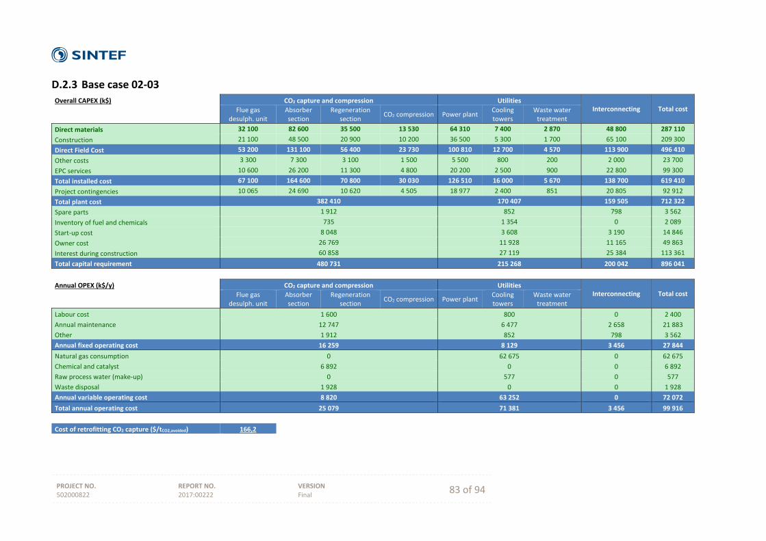
PROJECT NO. 502000822
REPORT NO. 2017:00222
VERSION Final 83 of 94
D.2.3 Base case 02‐03 Overall CAPEX (k$) CO2 capture and compression Utilities
Interconnecting Total cost Flue gas desulph. unit
Absorber section
Regeneration section
CO2 compression Power plant Cooling towers
Waste water treatment
Direct materials 32 100 82 600 35 500 13 530 64 310 7 400 2 870 48 800 287 110
Construction 21 100 48 500 20 900 10 200 36 500 5 300 1 700 65 100 209 300
Direct Field Cost 53 200 131 100 56 400 23 730 100 810 12 700 4 570 113 900 496 410
Other costs 3 300 7 300 3 100 1 500 5 500 800 200 2 000 23 700
EPC services 10 600 26 200 11 300 4 800 20 200 2 500 900 22 800 99 300
Total installed cost 67 100 164 600 70 800 30 030 126 510 16 000 5 670 138 700 619 410
Project contingencies 10 065 24 690 10 620 4 505 18 977 2 400 851 20 805 92 912
Total plant cost 382 410 170 407 159 505 712 322
Spare parts 1 912 852 798 3 562
Inventory of fuel and chemicals 735 1 354 0 2 089
Start‐up cost 8 048 3 608 3 190 14 846
Owner cost 26 769 11 928 11 165 49 863
Interest during construction 60 858 27 119 25 384 113 361
Total capital requirement 480 731 215 268 200 042 896 041
Annual OPEX (k$/y) CO2 capture and compression Utilities
Interconnecting Total cost Flue gas desulph. unit
Absorber section
Regeneration section
CO2 compression Power plant Cooling towers
Waste water treatment
Labour cost 1 600 800 0 2 400
Annual maintenance 12 747 6 477 2 658 21 883
Other 1 912 852 798 3 562
Annual fixed operating cost 16 259 8 129 3 456 27 844
Natural gas consumption 0 62 675 0 62 675
Chemical and catalyst 6 892 0 0 6 892
Raw process water (make‐up) 0 577 0 577
Waste disposal 1 928 0 0 1 928
Annual variable operating cost 8 820 63 252 0 72 072
Total annual operating cost 25 079 71 381 3 456 99 916
Cost of retrofitting CO2 capture ($/tCO2,avoided) 166,2
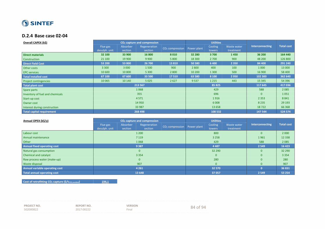
PROJECT NO. 502000822
REPORT NO. 2017:00222
VERSION Final 84 of 94
D.2.4 Base case 02‐04 Overall CAPEX (k$) CO2 capture and compression Utilities
Interconnecting Total cost Flue gas desulph. unit
Absorber section
Regeneration section
CO2 compression Power plant Cooling towers
Waste water treatment
Direct materials 32 100 33 900 16 800 8 010 32 280 3 700 1 450 36 200 164 440
Construction 21 100 19 900 9 900 5 800 18 300 2 700 900 48 200 126 800
Direct Field Cost 53 200 53 800 26 700 13 810 50 580 6 400 2 350 84 400 291 240
Other costs 3 300 3 000 1 500 900 2 800 400 100 1 000 13 000
EPC services 10 600 10 800 5 300 2 800 10 200 1 300 500 16 900 58 400
Total installed cost 67 100 67 600 33 500 17 510 63 580 8 100 2 950 102 300 362 640
Project contingencies 10 065 10 140 5 025 2 627 9 537 1 215 443 15 345 54 396
Total plant cost 213 567 85 825 117 645 417 036
Spare parts 1 068 429 588 2 085
Inventory of fuel and chemicals 355 696 0 1 051
Start‐up cost 4 571 1 916 2 353 8 841
Owner cost 14 950 6 008 8 235 29 193
Interest during construction 33 987 13 658 18 722 66 368
Total capital requirement 268 498 108 532 147 544 524 574
Annual OPEX (k$/y) CO2 capture and compression Utilities
Interconnecting Total cost Flue gas desulph. unit
Absorber section
Regeneration section
CO2 compression Power plant Cooling towers
Waste water treatment
Labour cost 1 200 800 0 2 000
Annual maintenance 7 119 3 258 1 961 12 338
Other 1 068 429 588 2 085
Annual fixed operating cost 9 387 4 487 2 549 16 423
Natural gas consumption 0 32 290 0 32 290
Chemical and catalyst 3 354 0 0 3 354
Raw process water (make‐up) 0 280 0 280
Waste disposal 907 0 0 907
Annual variable operating cost 4 261 32 570 0 36 831
Total annual operating cost 13 648 37 057 2 549 53 254
Cost of retrofitting CO2 capture ($/tCO2,avoided) 194,1

PROJECT NO. 502000822
REPORT NO. 2017:00222
VERSION Final 85 of 94
D.3 Base case 3
D.3.1 Base case 03‐01 Overall CAPEX (k$) CO2 capture and compression Utilities
Interconnecting Total cost Flue gas desulph. unit
Absorber section
Regeneration section
CO2 compression CHP plant Cooling towers
Waste water treatment
Direct materials 0 43 500 13 100 6 800 27 760 3 700 1 170 26 000 122 030
Construction 0 25 500 7 700 4 900 15 700 2 700 700 34 600 91 800
Direct Field Cost 0 69 000 20 800 11 700 43 460 6 400 1 870 60 600 213 830
Other costs 0 3 800 1 200 700 2 300 400 100 1 000 9 500
EPC services 0 13 800 4 200 2 300 8 700 1 300 400 12 100 42 800
Total installed cost 0 86 600 26 200 14 700 54 460 8 100 2 370 73 700 266 130
Project contingencies 0 12 990 3 930 2 205 8 169 1 215 356 11 055 39 920
Total plant cost 146 625 74 670 84 755 306 050
Spare parts 733 373 424 1 530
Inventory of fuel and chemicals 269 519 0 788
Start‐up cost 3 133 1 693 1 695 6 521
Owner cost 10 264 5 227 5 933 21 423
Interest during construction 23 334 11 883 13 488 48 705
Total capital requirement 184 357 94 365 106 295 385 018
Annual OPEX (k$/y) CO2 capture and compression Utilities
Interconnecting Total cost Flue gas desulph. unit
Absorbersection
Regeneration section
CO2 compression CHP plant Cooling towers
Waste water treatment
Labour cost 800 800 0 1 600
Annual maintenance 4 888 2 810 1 413 9 110
Other 733 373 424 1 530
Annual fixed operating cost 6 421 3 984 1 836 12 241
Natural gas consumption 0 24 073 0 24 073
Chemical and catalyst 2 506 0 0 2 506
Raw process water (make‐up) 0 212 0 212
Waste disposal 718 0 0 718
Annual variable operating cost 3 224 24 285 0 27 509
Total annual operating cost 9 645 28 268 1 836 39 749
Cost of retrofitting CO2 capture ($/tCO2,avoided) 184,9

PROJECT NO. 502000822
REPORT NO. 2017:00222
VERSION Final 86 of 94
D.3.2 Base case 03‐02 Overall CAPEX (k$) CO2 capture and compression Utilities
Interconnecting Total cost Flue gas desulph. unit
Absorber section
Regeneration section
CO2 compression Power plant Cooling towers
Waste water treatment
Direct materials 15 400 58 100 22 400 9 690 46 450 5 180 1 860 40 800 199 880
Construction 10 100 34 000 13 200 7 100 26 400 3 700 1 100 54 200 149 800
Direct Field Cost 25 500 92 100 35 600 16 790 72 850 8 880 2 960 95 000 349 680
Other costs 1 500 5 100 2 000 1 100 3 900 600 100 2 000 16 300
EPC services 5 100 18 500 7 100 3 400 14 700 1 800 600 19 000 70 200
Total installed cost 32 100 115 700 44 700 21 290 91 450 11 280 3 660 116 000 436 180
Project contingencies 4 815 17 355 6 705 3 194 13 718 1 692 549 17 400 65 427
Total plant cost 245 859 122 349 133 400 501 607
Spare parts 1 229 612 667 2 508
Inventory of fuel and chemicals 453 855 0 1 308
Start‐up cost 5 217 2 647 2 668 10 532
Owner cost 17 210 8 564 9 338 35 112
Interest during construction 39 127 19 471 21 230 79 827
Total capital requirement 309 095 154 498 167 303 630 895
Annual OPEX (k$/y) CO2 capture and compression Utilities
Interconnecting Total cost Flue gas desulph. unit
Absorber section
Regeneration section
CO2 compression Power plant Cooling towers
Waste water treatment
Labour cost 1 200 800 0 2 000
Annual maintenance 8 195 4 668 2 223 15 087
Other 1 229 612 667 2 508
Annual fixed operating cost 10 625 6 080 2 890 19 595
Natural gas consumption 0 39 591 0 39 591
Chemical and catalyst 4 249 0 0 4 249
Raw process water (make‐up) 0 363 0 363
Waste disposal 1 191 0 0 1 191
Annual variable operating cost 5 439 39 954 0 45 394
Total annual operating cost 16 064 46 034 2 890 64 989
Cost of retrofitting CO2 capture ($/tCO2,avoided) 180,3
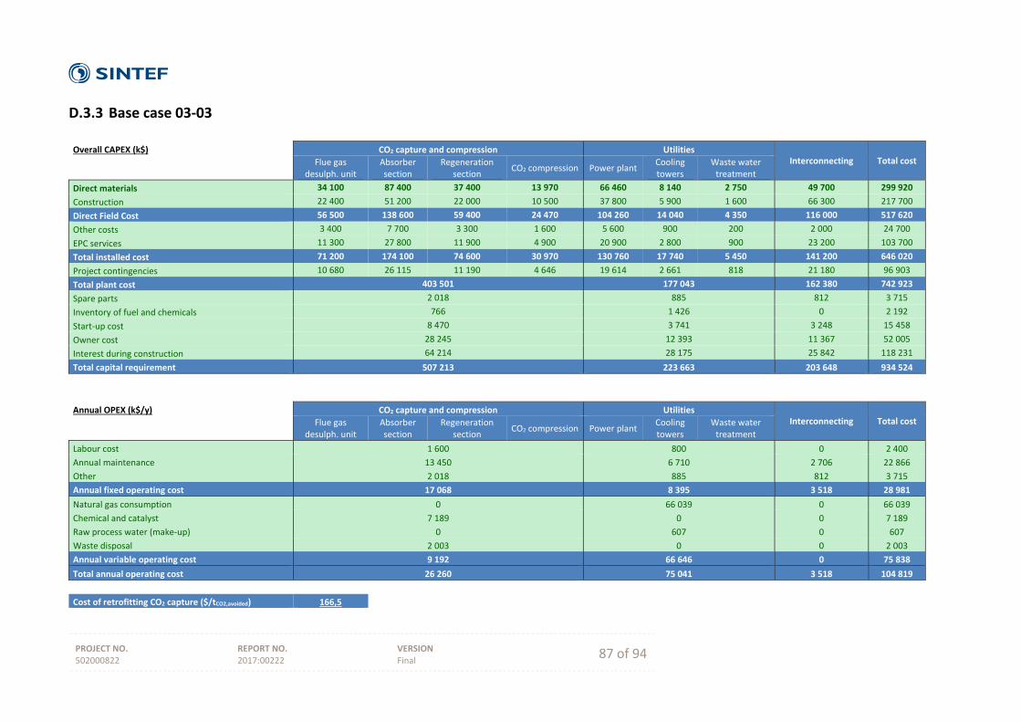
PROJECT NO. 502000822
REPORT NO. 2017:00222
VERSION Final 87 of 94
D.3.3 Base case 03‐03
Overall CAPEX (k$) CO2 capture and compression Utilities
Interconnecting Total cost Flue gas desulph. unit
Absorber section
Regeneration section
CO2 compression Power plant Cooling towers
Waste water treatment
Direct materials 34 100 87 400 37 400 13 970 66 460 8 140 2 750 49 700 299 920
Construction 22 400 51 200 22 000 10 500 37 800 5 900 1 600 66 300 217 700
Direct Field Cost 56 500 138 600 59 400 24 470 104 260 14 040 4 350 116 000 517 620
Other costs 3 400 7 700 3 300 1 600 5 600 900 200 2 000 24 700
EPC services 11 300 27 800 11 900 4 900 20 900 2 800 900 23 200 103 700
Total installed cost 71 200 174 100 74 600 30 970 130 760 17 740 5 450 141 200 646 020
Project contingencies 10 680 26 115 11 190 4 646 19 614 2 661 818 21 180 96 903
Total plant cost 403 501 177 043 162 380 742 923
Spare parts 2 018 885 812 3 715
Inventory of fuel and chemicals 766 1 426 0 2 192
Start‐up cost 8 470 3 741 3 248 15 458
Owner cost 28 245 12 393 11 367 52 005
Interest during construction 64 214 28 175 25 842 118 231
Total capital requirement 507 213 223 663 203 648 934 524
Annual OPEX (k$/y) CO2 capture and compression Utilities Interconnecting Total cost Flue gas
desulph. unit Absorber section
Regeneration section
CO2 compression Power plant Cooling towers
Waste water treatment
Labour cost 1 600 800 0 2 400
Annual maintenance 13 450 6 710 2 706 22 866
Other 2 018 885 812 3 715
Annual fixed operating cost 17 068 8 395 3 518 28 981
Natural gas consumption 0 66 039 0 66 039
Chemical and catalyst 7 189 0 0 7 189
Raw process water (make‐up) 0 607 0 607
Waste disposal 2 003 0 0 2 003
Annual variable operating cost 9 192 66 646 0 75 838
Total annual operating cost 26 260 75 041 3 518 104 819
Cost of retrofitting CO2 capture ($/tCO2,avoided) 166,5
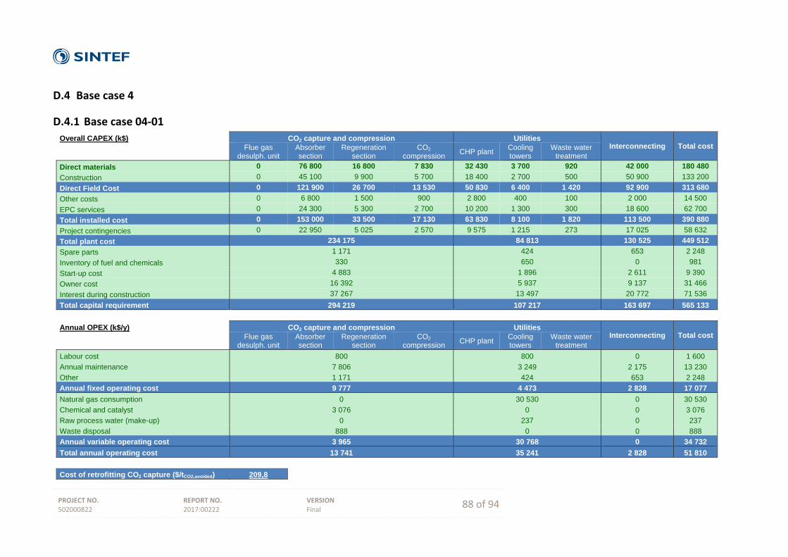
PROJECT NO. 502000822
REPORT NO. 2017:00222
VERSION Final 88 of 94
D.4 Base case 4
D.4.1 Base case 04‐01
Overall CAPEX (k$) CO2 capture and compression Utilities Interconnecting Total cost Flue gas
desulph. unit Absorber section
Regeneration section
CO2 compression
CHP plant Cooling towers
Waste water treatment
Direct materials 0 76 800 16 800 7 830 32 430 3 700 920 42 000 180 480
Construction 0 45 100 9 900 5 700 18 400 2 700 500 50 900 133 200
Direct Field Cost 0 121 900 26 700 13 530 50 830 6 400 1 420 92 900 313 680
Other costs 0 6 800 1 500 900 2 800 400 100 2 000 14 500
EPC services 0 24 300 5 300 2 700 10 200 1 300 300 18 600 62 700
Total installed cost 0 153 000 33 500 17 130 63 830 8 100 1 820 113 500 390 880
Project contingencies 0 22 950 5 025 2 570 9 575 1 215 273 17 025 58 632
Total plant cost 234 175 84 813 130 525 449 512
Spare parts 1 171 424 653 2 248
Inventory of fuel and chemicals 330 650 0 981
Start-up cost 4 883 1 896 2 611 9 390
Owner cost 16 392 5 937 9 137 31 466
Interest during construction 37 267 13 497 20 772 71 536
Total capital requirement 294 219 107 217 163 697 565 133
Annual OPEX (k$/y) CO2 capture and compression Utilities Interconnecting Total cost Flue gas
desulph. unit Absorber section
Regeneration section
CO2 compression
CHP plant Cooling towers
Waste water treatment
Labour cost 800 800 0 1 600
Annual maintenance 7 806 3 249 2 175 13 230
Other 1 171 424 653 2 248
Annual fixed operating cost 9 777 4 473 2 828 17 077
Natural gas consumption 0 30 530 0 30 530
Chemical and catalyst 3 076 0 0 3 076
Raw process water (make-up) 0 237 0 237
Waste disposal 888 0 0 888
Annual variable operating cost 3 965 30 768 0 34 732
Total annual operating cost 13 741 35 241 2 828 51 810
Cost of retrofitting CO2 capture ($/tCO2,avoided) 209,8
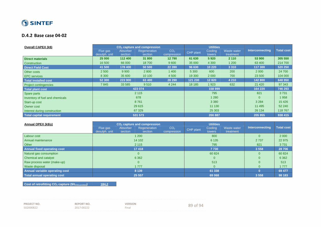
PROJECT NO. 502000822
REPORT NO. 2017:00222
VERSION Final 89 of 94
D.4.2 Base case 04‐02
Overall CAPEX (k$) CO2 capture and compression Utilities
Interconnecting Total cost Flue gas desulph. unit
Absorber section
Regeneration section
CO2 compression
CHP plant Cooling towers
Waste water treatment
Direct materials 25 000 112 400 31 800 12 790 61 630 5 920 2 110 53 900 305 550
Construction 16 500 66 000 18 700 9 600 35 000 4 300 1 200 63 400 214 700
Direct Field Cost 41 500 178 400 50 500 22 390 96 630 10 220 3 310 117 300 520 250
Other costs 2 500 9 900 2 800 1 400 5 300 600 200 2 000 24 700
EPC services 8 300 35 600 10 100 4 500 19 300 2 000 700 23 500 104 000
Total installed cost 52 300 223 900 63 400 28 290 121 230 12 820 4 210 142 800 648 950
Project contingencies 7 845 33 585 9 510 4 244 18 185 1 923 632 21 420 97 343
Total plant cost 423 074 158 999 164 220 746 293
Spare parts 2 115 795 821 3 731
Inventory of fuel and chemicals 678 1 280 0 1 958
Start-up cost 8 761 3 380 3 284 15 426
Owner cost 29 615 11 130 11 495 52 240
Interest during construction 67 329 25 303 26 134 118 767
Total capital requirement 531 573 200 887 205 955 938 415
Annual OPEX (k$/y) CO2 capture and compression Utilities
Interconnecting Total cost Flue gas desulph. unit
Absorber section
Regeneration section
CO2 compression
CHP plant Cooling towers
Waste water treatment
Labour cost 1 200 800 0 2 000
Annual maintenance 14 102 6 135 2 737 22 975
Other 2 115 795 821 3 731
Annual fixed operating cost 17 418 7 730 3 558 28 706
Natural gas consumption 0 60 824 0 60 824
Chemical and catalyst 6 362 0 0 6 362
Raw process water (make-up) 0 513 0 513
Waste disposal 1 777 0 0 1 777
Annual variable operating cost 8 139 61 338 0 69 477
Total annual operating cost 25 557 69 068 3 558 98 183
Cost of retrofitting CO2 capture ($/tCO2,avoided) 184,2
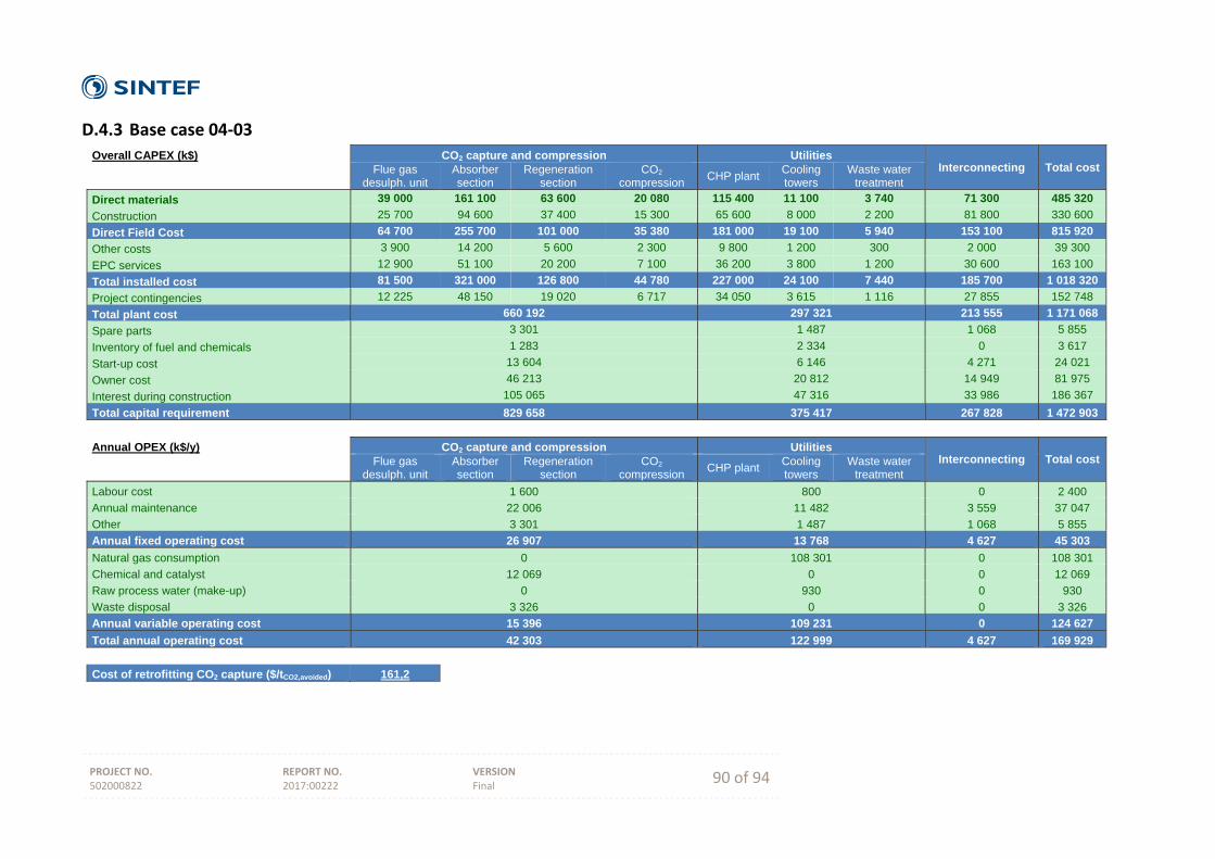
PROJECT NO. 502000822
REPORT NO. 2017:00222
VERSION Final 90 of 94
D.4.3 Base case 04‐03
Overall CAPEX (k$) CO2 capture and compression Utilities Interconnecting Total cost Flue gas
desulph. unit Absorber section
Regeneration section
CO2 compression
CHP plant Cooling towers
Waste water treatment
Direct materials 39 000 161 100 63 600 20 080 115 400 11 100 3 740 71 300 485 320
Construction 25 700 94 600 37 400 15 300 65 600 8 000 2 200 81 800 330 600
Direct Field Cost 64 700 255 700 101 000 35 380 181 000 19 100 5 940 153 100 815 920
Other costs 3 900 14 200 5 600 2 300 9 800 1 200 300 2 000 39 300
EPC services 12 900 51 100 20 200 7 100 36 200 3 800 1 200 30 600 163 100
Total installed cost 81 500 321 000 126 800 44 780 227 000 24 100 7 440 185 700 1 018 320
Project contingencies 12 225 48 150 19 020 6 717 34 050 3 615 1 116 27 855 152 748
Total plant cost 660 192 297 321 213 555 1 171 068
Spare parts 3 301 1 487 1 068 5 855
Inventory of fuel and chemicals 1 283 2 334 0 3 617
Start-up cost 13 604 6 146 4 271 24 021
Owner cost 46 213 20 812 14 949 81 975
Interest during construction 105 065 47 316 33 986 186 367
Total capital requirement 829 658 375 417 267 828 1 472 903
Annual OPEX (k$/y) CO2 capture and compression Utilities
Interconnecting Total cost Flue gas desulph. unit
Absorber section
Regeneration section
CO2 compression
CHP plant Cooling towers
Waste water treatment
Labour cost 1 600 800 0 2 400
Annual maintenance 22 006 11 482 3 559 37 047
Other 3 301 1 487 1 068 5 855
Annual fixed operating cost 26 907 13 768 4 627 45 303
Natural gas consumption 0 108 301 0 108 301
Chemical and catalyst 12 069 0 0 12 069
Raw process water (make-up) 0 930 0 930
Waste disposal 3 326 0 0 3 326
Annual variable operating cost 15 396 109 231 0 124 627
Total annual operating cost 42 303 122 999 4 627 169 929
Cost of retrofitting CO2 capture ($/tCO2,avoided) 161,2
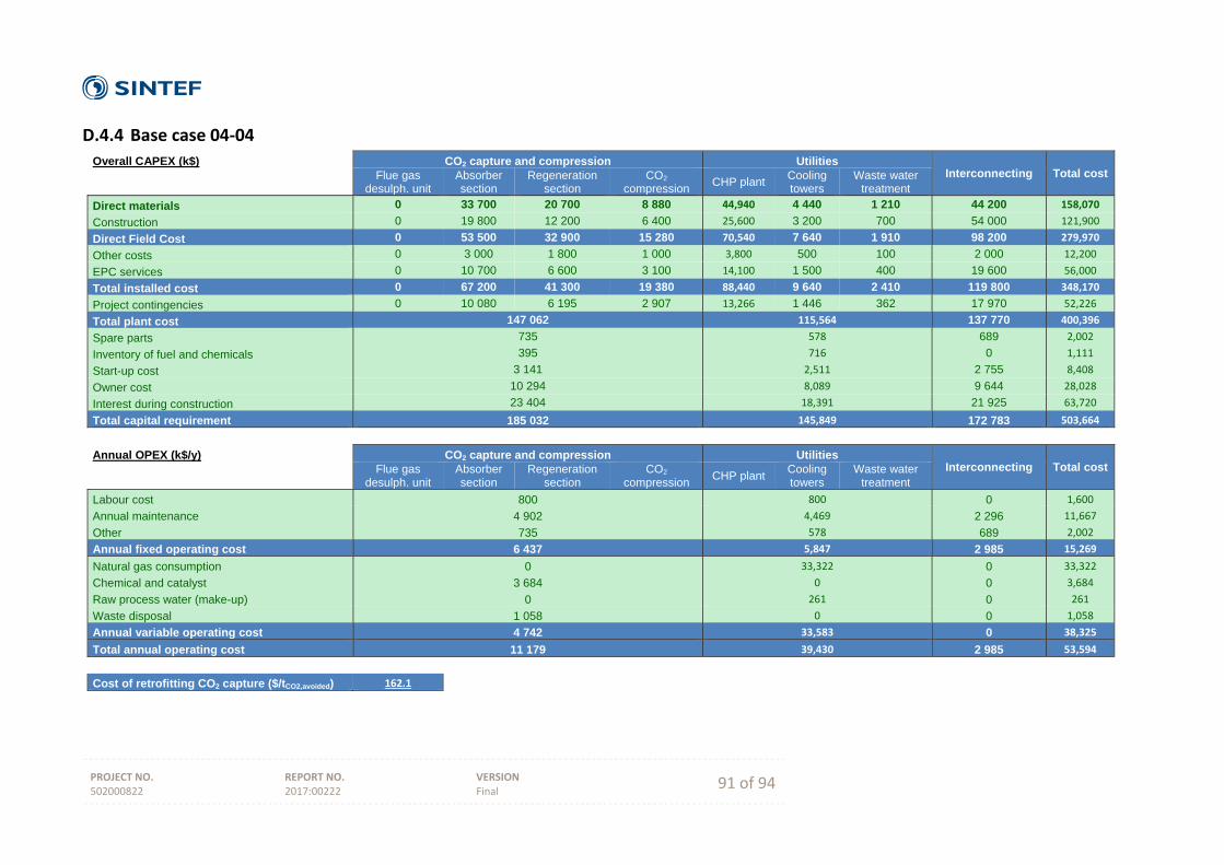
PROJECT NO. 502000822
REPORT NO. 2017:00222
VERSION Final 91 of 94
D.4.4 Base case 04‐04
Overall CAPEX (k$) CO2 capture and compression Utilities Interconnecting Total cost Flue gas
desulph. unit Absorber section
Regeneration section
CO2 compression
CHP plant Cooling towers
Waste water treatment
Direct materials 0 33 700 20 700 8 880 44,940 4 440 1 210 44 200 158,070
Construction 0 19 800 12 200 6 400 25,600 3 200 700 54 000 121,900
Direct Field Cost 0 53 500 32 900 15 280 70,540 7 640 1 910 98 200 279,970
Other costs 0 3 000 1 800 1 000 3,800 500 100 2 000 12,200
EPC services 0 10 700 6 600 3 100 14,100 1 500 400 19 600 56,000
Total installed cost 0 67 200 41 300 19 380 88,440 9 640 2 410 119 800 348,170
Project contingencies 0 10 080 6 195 2 907 13,266 1 446 362 17 970 52,226
Total plant cost 147 062 115,564 137 770 400,396
Spare parts 735 578 689 2,002
Inventory of fuel and chemicals 395 716 0 1,111
Start-up cost 3 141 2,511 2 755 8,408
Owner cost 10 294 8,089 9 644 28,028
Interest during construction 23 404 18,391 21 925 63,720
Total capital requirement 185 032 145,849 172 783 503,664
Annual OPEX (k$/y) CO2 capture and compression Utilities
Interconnecting Total cost Flue gas desulph. unit
Absorber section
Regeneration section
CO2 compression
CHP plant Cooling towers
Waste water treatment
Labour cost 800 800 0 1,600
Annual maintenance 4 902 4,469 2 296 11,667
Other 735 578 689 2,002
Annual fixed operating cost 6 437 5,847 2 985 15,269
Natural gas consumption 0 33,322 0 33,322
Chemical and catalyst 3 684 0 0 3,684
Raw process water (make-up) 0 261 0 261
Waste disposal 1 058 0 0 1,058
Annual variable operating cost 4 742 33,583 0 38,325
Total annual operating cost 11 179 39,430 2 985 53,594
Cost of retrofitting CO2 capture ($/tCO2,avoided) 162.1

PROJECT NO. 502000822
REPORT NO. 2017:00222
VERSION Final 92 of 94
D.4.5 Base case 04‐05
Overall CAPEX (k$) CO2 capture and compression Utilities Interconnecting Total cost Flue gas
desulph. unit Absorber section
Regeneration section
CO2 compression
CHP plant Cooling towers
Waste water treatment
Direct materials 25 000 146 100 52 400 17 930 96 480 10 360 3 110 66 200 417 580
Construction 16 500 85 800 30 800 13 600 54 900 7 500 1 800 76 400 287 300
Direct Field Cost 41 500 231 900 83 200 31 530 151 380 17 860 4 910 142 600 704 880
Other costs 2 500 12 900 4 600 2 000 8 200 1 100 200 2 000 33 500
EPC services 8 300 46 300 16 600 6 300 30 200 3 500 1 000 28 500 140 700
Total installed cost 52 300 291 100 104 400 39 830 189 780 22 460 6 110 173 100 879 080
Project contingencies 7 845 43 665 15 660 5 975 28 467 3 369 917 25 965 131 862
Total plant cost 560 775 251 103 199 065 1 010 942
Spare parts 2 804 1 256 995 5 055
Inventory of fuel and chemicals 1 096 1 998 0 3 095
Start-up cost 11 615 5 222 3 981 20 819
Owner cost 39 254 17 577 13 935 70 766
Interest during construction 89 243 39 961 31 680 160 884
Total capital requirement 704 787 317 117 249 656 1 271 560
Annual OPEX (k$/y) CO2 capture and compression Utilities
Interconnecting Total cost Flue gas desulph. unit
Absorber section
Regeneration section
CO2 compression
CHP plant Cooling towers
Waste water treatment
Labour cost 1 600 800 0 2 400
Annual maintenance 18 692 9 641 3 318 31 651
Other 2 804 1 256 995 5 055
Annual fixed operating cost 23 096 11 697 4 313 39 106
Natural gas consumption 0 92 804 0 92 804
Chemical and catalyst 10 320 0 0 10 320
Raw process water (make-up) 0 778 0 778
Waste disposal 2 835 0 0 2 835
Annual variable operating cost 13 155 93 582 0 106 737
Total annual operating cost 36 251 105 279 4 313 145 843
Cost of retrofitting CO2 capture ($/tCO2,avoided) 162,2
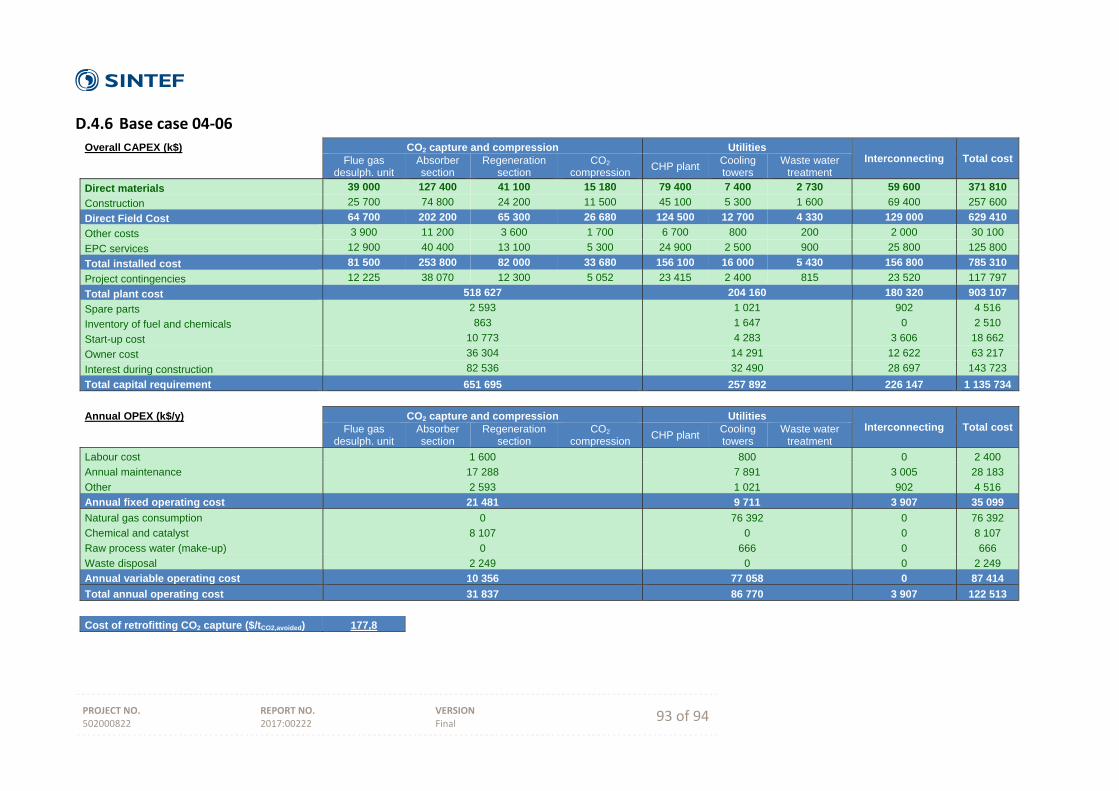
PROJECT NO. 502000822
REPORT NO. 2017:00222
VERSION Final 93 of 94
D.4.6 Base case 04‐06
Overall CAPEX (k$) CO2 capture and compression Utilities Interconnecting Total cost Flue gas
desulph. unit Absorber section
Regeneration section
CO2 compression
CHP plant Cooling towers
Waste water treatment
Direct materials 39 000 127 400 41 100 15 180 79 400 7 400 2 730 59 600 371 810
Construction 25 700 74 800 24 200 11 500 45 100 5 300 1 600 69 400 257 600
Direct Field Cost 64 700 202 200 65 300 26 680 124 500 12 700 4 330 129 000 629 410
Other costs 3 900 11 200 3 600 1 700 6 700 800 200 2 000 30 100
EPC services 12 900 40 400 13 100 5 300 24 900 2 500 900 25 800 125 800
Total installed cost 81 500 253 800 82 000 33 680 156 100 16 000 5 430 156 800 785 310
Project contingencies 12 225 38 070 12 300 5 052 23 415 2 400 815 23 520 117 797
Total plant cost 518 627 204 160 180 320 903 107
Spare parts 2 593 1 021 902 4 516
Inventory of fuel and chemicals 863 1 647 0 2 510
Start-up cost 10 773 4 283 3 606 18 662
Owner cost 36 304 14 291 12 622 63 217
Interest during construction 82 536 32 490 28 697 143 723
Total capital requirement 651 695 257 892 226 147 1 135 734
Annual OPEX (k$/y) CO2 capture and compression Utilities
Interconnecting Total cost Flue gas desulph. unit
Absorber section
Regeneration section
CO2 compression
CHP plant Cooling towers
Waste water treatment
Labour cost 1 600 800 0 2 400
Annual maintenance 17 288 7 891 3 005 28 183
Other 2 593 1 021 902 4 516
Annual fixed operating cost 21 481 9 711 3 907 35 099
Natural gas consumption 0 76 392 0 76 392
Chemical and catalyst 8 107 0 0 8 107
Raw process water (make-up) 0 666 0 666
Waste disposal 2 249 0 0 2 249
Annual variable operating cost 10 356 77 058 0 87 414
Total annual operating cost 31 837 86 770 3 907 122 513
Cost of retrofitting CO2 capture ($/tCO2,avoided) 177,8

PROJECT NO. 502000822
REPORT NO. 2017:00222
VERSION Final 94 of 94

Technology for a better society www.sintef.no

ReCAP Project
Evaluating the Cost of
Retrofitting CO2 Capture in
an Integrated Oil Refinery
Constructability Assessment
ReCAP Project Evaluating the Cost of Retrofitting CO2 Capture in an Integrated Oil Refinery
Constructability Assessment
Doc No.: BD0839A-PR-0000-RE-004
C00 30/05/2017 First Issue M.Mandelli/C.Gilardi - M.Mandelli
REV. ISSUE DATE DESCRIPTION PREPARED BY CHECKED BY APPROVED BY
Revision C00 30/05/2017 amecfw.com Page i
Table of contents
Page
Background of the Project 3
1. Introduction 4
Reference Case 4
2. Constructability - Introduction 9
Operating method 10
Areas of attention 10
3. Accessibility requirements 11
4. Modular vs stick-built approach 13
Road map decision process 14
5. Site preparation and enabling works 15
6. Main construction works 16
Main Equipment 16
Pre-Assembly 16
6.2.1 Structural Steel Sections/Modules 16
Piperacks 16
Piping 17
6.4.1 Tie-ins 17
7. Critical lifting activities 18
Critical items 19
Revision C00 30/05/2017 amecfw.com Page ii
8. Systems turnover 22
9. Site material management 23
10. Construction quality control 23
11. HSE management 24
12. Interface management 25
Work permits 25
Interface with Local Authorities 25
13. Site Security 26
14. Temporary Construction Facilities 27
Site offices 27
Warehouse and storage areas 28
14.2.1 Warehouse 28
14.2.2 Storage areas 28
Construction contractors areas 29
Temporary utilities 29
15. Waste management 31
Waste water management 31
Waste management 31
16. Conclusions 32
List of tables
Table 1-1: Summary of main CO2 emission sources in Base Case 4 5 Table 4-1: Modularized vs Stick built assessment criteria 13 Table 7-1: Critical Lifting Table 19
List of figures
Figure 1-1: Post-combustion case 04-03) Process flow diagram 6 Figure 1-2: Base Case 4) Refinery layout 7 Figure 1-3: Post-combustion case 04-03) Refinery layout with location of the new plants 8 Figure 3-1: Conceptual logistic assessment 12 Figure 7-1: Reactor installation with gantry crane (example) 19 Figure 7-2: Installation with hydraulic gantry crane (example) 21 Figure 14-1: Temporary Construction Facilities conceptual layout 30
Revision C00 30/05/2017 amecfw.com Page 3
Background of the Project
In the past years, IEA Greenhouse Gas R&D Programme (IEAGHG) has undertaken a series of projects evaluating the performance and cost of deploying CO2 capture technologies in energy intensive industries such as the cement, iron and steel, hydrogen, pulp and paper, and others.
In line with these activities, IEAGHG has initiated this project in collaboration with CONCAWE, GASSNOVA and SINTEF Energy Research, to evaluate the performance and cost of retrofitting CO2 capture in an integrated oil refinery.
The project consortium has selected Amec Foster Wheeler as the engineering contractor to work with SINTEF in performing the basic engineering and cost estimation for the reference cases.
The main purpose of this study is to evaluate the cost of retrofitting CO2 capture in simple to high complexity refineries covering typical European refinery capacities from 100,000 to 350,000 bbl/d. Specifically, the study will aim to:
► Formulate a reference document providing the different design basis and key assumptions to be used in the study.
► Define 4 different oil refineries as Base Cases. This covers the following:
► Simple refinery with a nominal capacity of 100,000 bbl/d.
► Medium to highly complex refineries with nominal capacity of 220,000 bbl/d.
► Highly complex refinery with a nominal capacity of 350,000 bbl/d.
► Define a list of emission sources for each reference case and agreed on CO2 capture priorities.
► Investigate the techno-economics performance of the integrated oil refinery (covering simple to complex refineries, with 100,000 to 350,000 bbl/d capacity) capturing CO2 emissions:
► From various sources using post-combustion CO2 capture technology based on standard MEA solvent.
► From hydrogen production facilities using pre-combustion CO2 capture technology.
► Using oxyfuel combustion technology applied the Fluid Catalytic Cracker.
► Perform a preliminary constructability assessment, analyzing the main areas of attention related to the execution phase of a case study that considers the implementation of retrofitting CO2 capture in a complex oil refinery.
This project will deliver “REFERENCE Documents” providing detailed information about the mass and energy balances, carbon balance, techno-economic assumptions, data evaluation and CO2 avoidance cost, that could be adapted and used for future economic assessment of CCS deployment in the oil refining industry.

Revision C00 30/05/2017 amecfw.com Page 4
1. Introduction
The Construction Industry Institute defines Constructability as “the optimum use of construction knowledge and experience in planning, design, procurement, and field operations to achieve overall project objectives.”
Specific studies demonstrate that, when methodically implemented, front-end constructability efforts are an investment that results in a substantial return. Documentation of constructability efforts showed that owners accrued an average reduction in total project cost and schedule of 4.3 percent and 7.5 percent, respectively. These savings represented a 10 to 1 return on the owner’s investment in the constructability effort.
Especially in a retrofitting Project, an accurate constructability study in parallel to the engineering activities is essential, since during the construction of the new units/portions, the refinery operation shall not be disrupted.
In particular, when looking at constructability issues in an existing site, the following main aspects are crucial:
► Access route for large or heavy equipment
► Location of temporary facilities
► Interference of the construction works with the routine operation/maintenance activities in the Refinery
► Safety
► Security
► Plant start-up considerations (impacting on the sequence of erection/completion of the new portions)
This report provides a high-level guidance in implementing projects of retrofitting CO2 capture facilities in a complex industrial site like an operating refinery.
Reference Case
Post-combustion capture case 04-03 has been selected as the reference case for the high-level constructability study.
This is the most complex case considered in the ReCAP Study, with CO2 captured from the 5 main emitters of Base Case 4 refinery (see summary in Table 1-1).
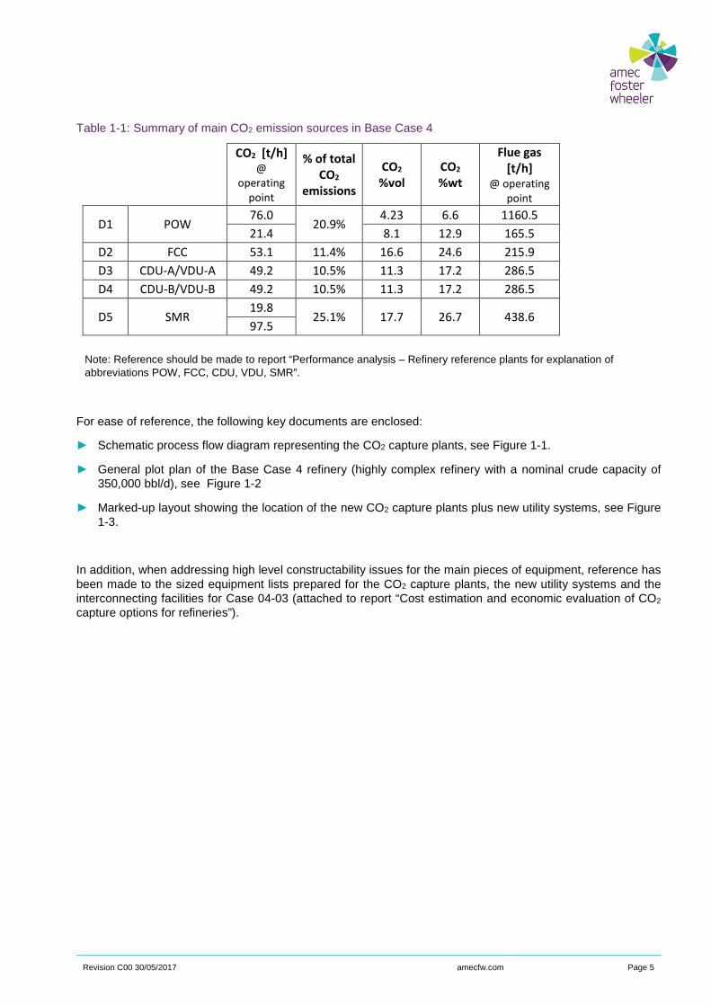
Revision C00 30/05/2017 amecfw.com Page 5
Table 1-1: Summary of main CO2 emission sources in Base Case 4
Note: Reference should be made to report “Performance analysis – Refinery reference plants for explanation of abbreviations POW, FCC, CDU, VDU, SMR”.
For ease of reference, the following key documents are enclosed:
► Schematic process flow diagram representing the CO2 capture plants, see Figure 1-1.
► General plot plan of the Base Case 4 refinery (highly complex refinery with a nominal crude capacity of 350,000 bbl/d), see Figure 1-2
► Marked-up layout showing the location of the new CO2 capture plants plus new utility systems, see Figure 1-3.
In addition, when addressing high level constructability issues for the main pieces of equipment, reference has been made to the sized equipment lists prepared for the CO2 capture plants, the new utility systems and the interconnecting facilities for Case 04-03 (attached to report “Cost estimation and economic evaluation of CO2 capture options for refineries”).
CO2 [t/h]
@
operating
point
% of total
CO2
emissions
CO2
%vol
CO2
%wt
Flue gas
[t/h]
@ operating
point
D1 POW 76.0
20.9% 4.23 6.6 1160.5
21.4 8.1 12.9 165.5
D2 FCC 53.1 11.4% 16.6 24.6 215.9
D3 CDU-A/VDU-A 49.2 10.5% 11.3 17.2 286.5
D4 CDU-B/VDU-B 49.2 10.5% 11.3 17.2 286.5
D5 SMR 19.8
25.1% 17.7 26.7 438.6 97.5
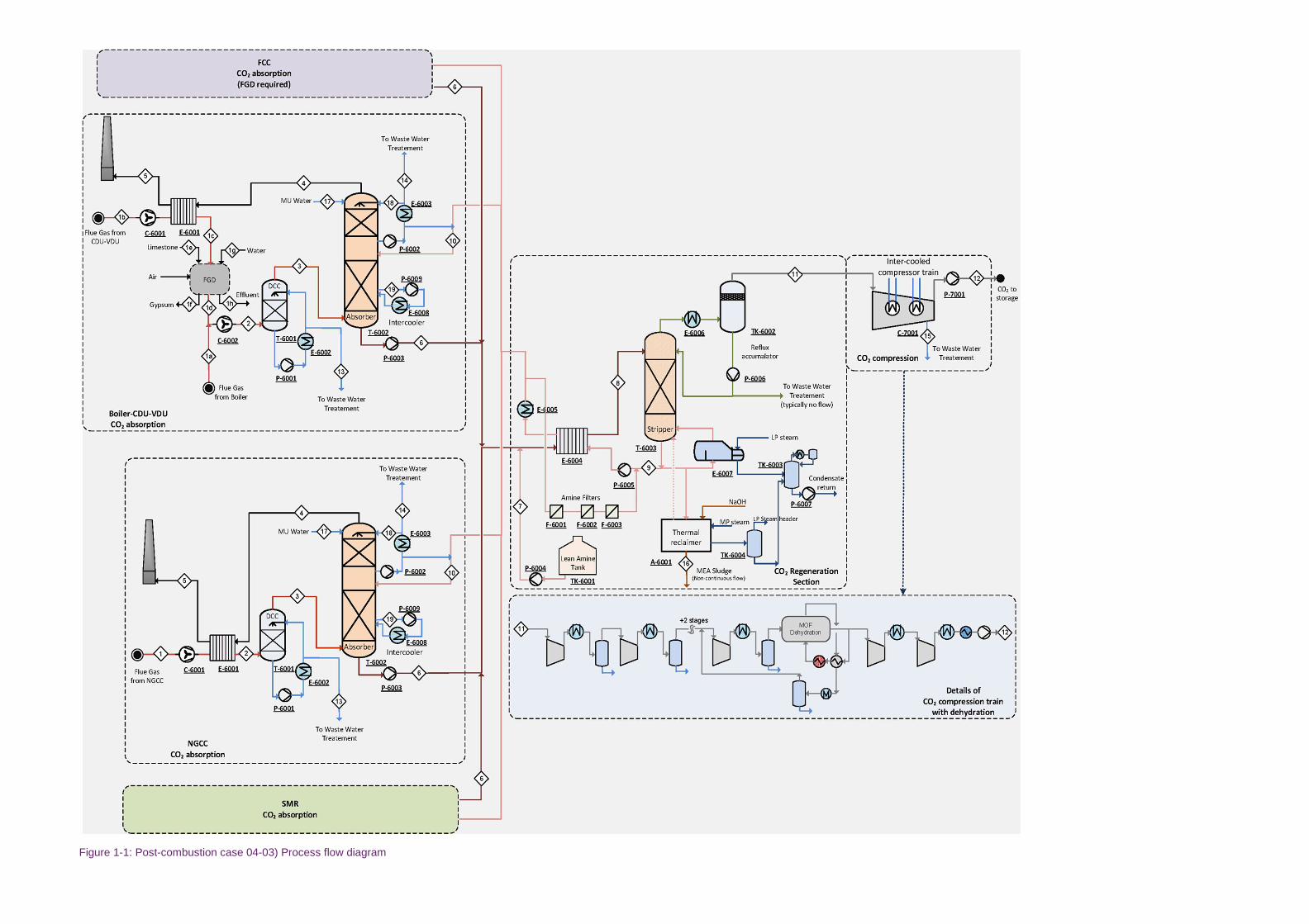
Figure 1-1: Post-combustion case 04-03) Process flow diagram
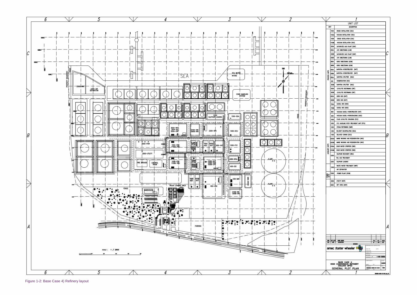
Figure 1-2: Base Case 4) Refinery layout
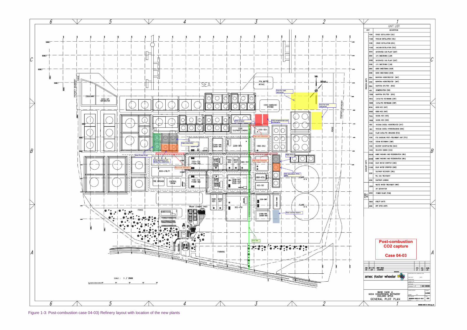
Figure 1-3: Post-combustion case 04-03) Refinery layout with location of the new plants
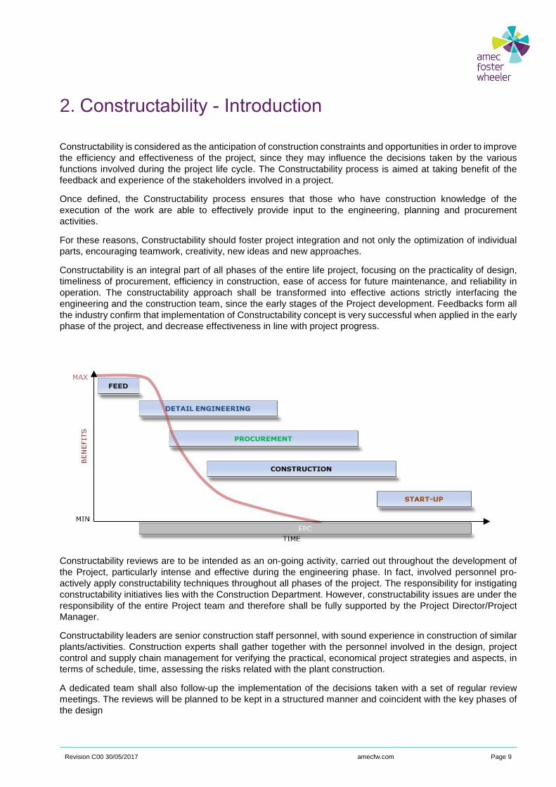
Revision C00 30/05/2017 amecfw.com Page 9
2. Constructability - Introduction
Constructability is considered as the anticipation of construction constraints and opportunities in order to improve the efficiency and effectiveness of the project, since they may influence the decisions taken by the various functions involved during the project life cycle. The Constructability process is aimed at taking benefit of the feedback and experience of the stakeholders involved in a project.
Once defined, the Constructability process ensures that those who have construction knowledge of the execution of the work are able to effectively provide input to the engineering, planning and procurement activities.
For these reasons, Constructability should foster project integration and not only the optimization of individual parts, encouraging teamwork, creativity, new ideas and new approaches.
Constructability is an integral part of all phases of the entire life project, focusing on the practicality of design, timeliness of procurement, efficiency in construction, ease of access for future maintenance, and reliability in operation. The constructability approach shall be transformed into effective actions strictly interfacing the engineering and the construction team, since the early stages of the Project development. Feedbacks form all the industry confirm that implementation of Constructability concept is very successful when applied in the early phase of the project, and decrease effectiveness in line with project progress.
Constructability reviews are to be intended as an on-going activity, carried out throughout the development of the Project, particularly intense and effective during the engineering phase. In fact, involved personnel pro-actively apply constructability techniques throughout all phases of the project. The responsibility for instigating constructability initiatives lies with the Construction Department. However, constructability issues are under the responsibility of the entire Project team and therefore shall be fully supported by the Project Director/Project Manager.
Constructability leaders are senior construction staff personnel, with sound experience in construction of similar plants/activities. Construction experts shall gather together with the personnel involved in the design, project control and supply chain management for verifying the practical, economical project strategies and aspects, in terms of schedule, time, assessing the risks related with the plant construction.
A dedicated team shall also follow-up the implementation of the decisions taken with a set of regular review meetings. The reviews will be planned to be kept in a structured manner and coincident with the key phases of the design
Revision C00 30/05/2017 amecfw.com Page 10
Operating method
The constructability engagement review process shall be conducted in a structured manner under the leadership of the facilitator and includes, but it is not limited to, the following phases:
► Preparation and issue of the Project Constructability Plan.
► Preparation and issue of the Constructability Checklist.
► Constructability Review meetings: Kick-off and follow-up sessions.
► Issue of the Constructability Action lists.
► Verification and implementation of the Constructability Action lists items and achievement of the established objectives.
► Preparation of the Constructability Report.
Areas of attention
Constructability analysis may focus on several topics; the assessment performed for the project identified the following areas of attention, on which the document has been focused:
► HSE management.
► Accessibility requirements for construction activities.
► Site preparation and enabling works.
► Sequential construction planning efforts.
► Critical lifting, access routes and planning area requirements for heavy lifts.
► Sewage and Waste Management.
► Temporary Construction Facilities.
Outcomes of the analysis done shall be considered as indicative, developed only at conceptual level, since a detailed study could be performed only on “real” sites, by considering all the relevant constraints (procedures, accesses, available areas, etc.).
The outcomes of the assessment performed are resumed in the following sections of the document.

Revision C00 30/05/2017 amecfw.com Page 11
3. Accessibility requirements
Logistic aspects play a crucial role while defining the project construction strategy. Existing space and dimensional limitations, and consequent implications on engineering and items dimensioning, may represent the rationale for leaning towards a modular approach or a stick built one.
The case study covers the implementation of the retrofitting CO2 capture inside an existing European refinery, that could made the logistic challenges even more complex. In fact the assessment of maximum size and weight of the transportable cargo shall take into consideration all the limitations posed by the surrounding environment.
In order to assure that logistic aspects are correctly taken into consideration, it is recommended, to engage a specialized contractor to perform a logistic study tailored on the specific cases, with the scope to investigate the following aspects:
► Define detailed transportation routes studies, providing suitable alternatives, remarking pro and cons of each alternatives.
► Verification of existing logistic facilities: jetty characteristics.
► Determine maximum transportable dimensions (size and weight) of equipment and modules.
► Definition of any temporary work that may be required to overcome the constraints given by existing operating facilities (e.g. pipe racks, etc.), up to a maximum reasonable extent.
With reference to the case study in subject, the proposed refinery presents two clear alternatives in terms of accessibility: via maritime transport from the seaside and via inland transportation from the existing road network.
Road transportation limits are imposed by the characteristics of the existing infrastructure, such as bridges, tunnels, etc. Obstacles and interferences shall be assessed not only from the origin of the cargos to the refinery but also inside the refinery boundaries. These limitations, in fact, could impose restrictions even to the items that could be shipped through sea transportation.
The proposed layout (reference is made to para. 1.1) has been studied and divided in two main areas of intervention:
► In a brown field area (i.e. construction activities foreseen in an area already occupied by existing facilities), requiring the relocation of some existing tanks: new power plant, CO2 absorber area and FGD for CDU/VDU).
► In a peripheral green field area (i.e. an area ideally free from existing facilities): CO2 compression and purification, stripper, new and relocated tanks.
Access to the two areas shall be studied independently, considering also the potential limitations imposed by the new installations. Result of the assessment would potentially suggest to adopt two different strategies for the two areas, ideally a more modularized driven approach for the green field area and a stick built one for the brown field one.
Appling ideally the proposed approach to the case study, it has been assumed that handling of oversized equipment could be handled though a dedicated existing offloading point: preliminary definition of these items can be found included in the assessment of the critical lift (section 7.1). After offload, the oversized cargos could be transported from that offloading point to the final location.
Differently, delivery of standardized cargo should be managed though road transport and initially delivered at the project warehouse (for warehouse and storage areas refer also to section 12).
Figure 3-1 shows the assumed routings of the two alternative logistic approaches..
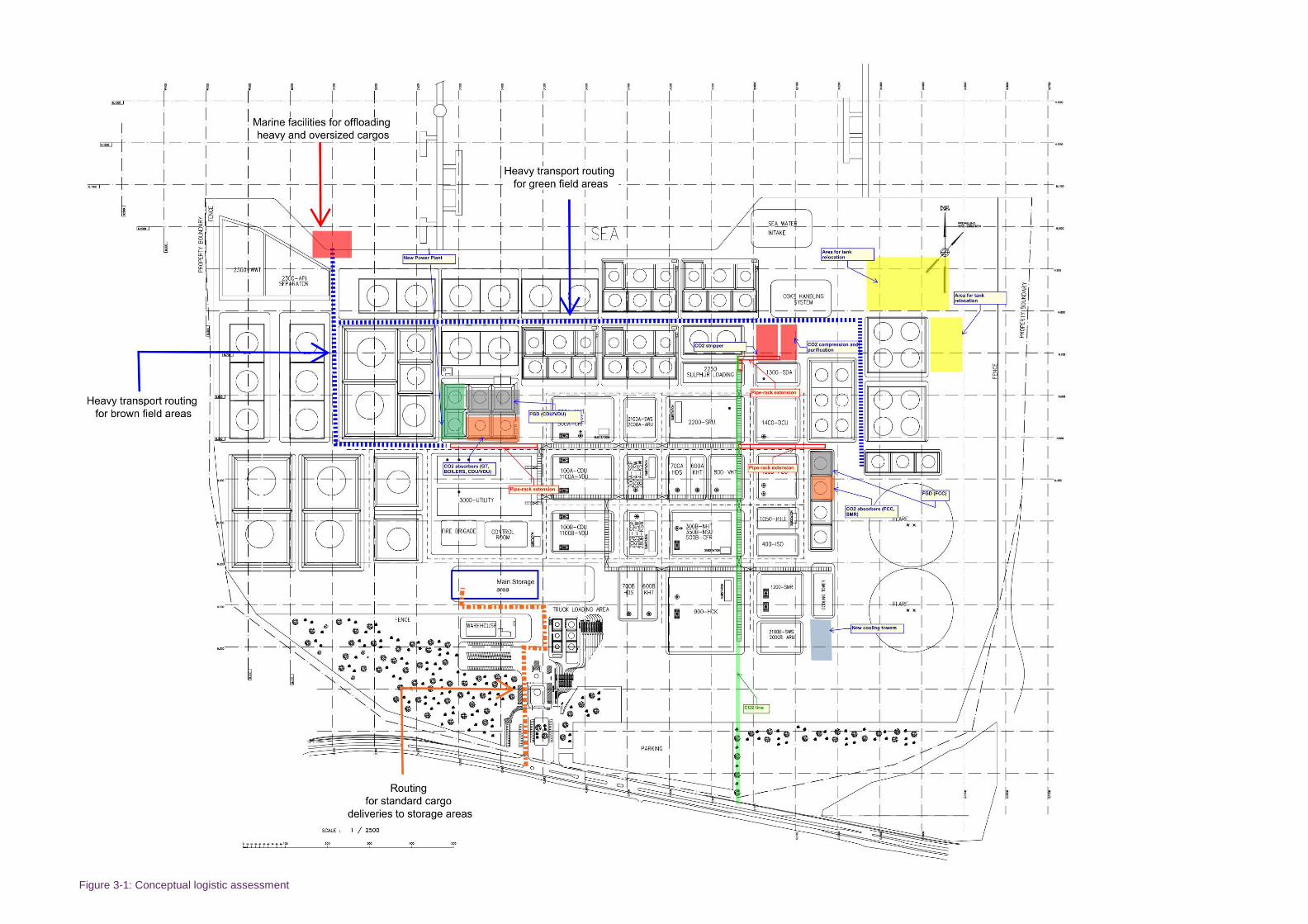
Figure 3-1: Conceptual logistic assessment

Revision C00 30/05/2017 amecfw.com Page 13
4. Modular vs stick-built approach
The construction activities approach is a key decision that shall be assessed during the very preliminary phases of the project. A structured assessment for the modularization-stick built decision could be performed following the Construction Industry Institute (CII) guidelines on the topic, considering either qualitative and semi-quantitative analysis.
A first level assessment shall be performed as a gate to access to a more detailed analysis. Basically, an evaluation relevant to main criteria may lead to take the orientation for construction approach. In this step it is required only to define if those preliminary criteria considered, are pro stick-built or pro modularization approach. The table below summaries all benefits for each type of design and construction approach. As shown on the table there are several factors that drive the decision and therefore the contribute of all project parties is required.
Table 4-1: Modularized vs Stick built assessment criteria
Key considerations for selecting an appropriate Construction
Execution Strategy Modularized Stick built
Schedule
Possibility to carry out parallel work, possibility to
resequencing site work activities. �
Relaxed schedule – traditional construction work,
proceeding in series, with seasonal disruption, is
acceptable.
�
Logistics
Challenges to access for material supply, high cost
of maintaining large workforce at site. �
Easy access, can deliver materials at any time:
cheap and easy to maintain large workforce at site �
Labour Lack of readily available local skilled labour. �
Abundant labor available locally. �
Weather
Extreme cold, high winds – high probability of
impact on site activities. �
Benign weather – low impact on site activities. �
Safety and
Environmental
Site conditions challenging to achieving safety and
environmental norms �
Easy site conditions, few challenges to achieving
HSE norms. �
Special/Authority
permit required
Yes – before site activities can begin – need to start
work offsite to compress overall schedule. �
No – work can go ahead on site at any time. �
Plant Suitability for
Modularization
Greenfield site, no SIMOPS complications.
Repetitive elements (e.g. 3 trains). �

Revision C00 30/05/2017 amecfw.com Page 14
Brownfield site, few repetitive items, difficulty in
coping with long lead equipment. �
Quality
Higher quality required – can be achieved in
“factory” conditions of specialized fabricators �
Site quality under the expected harsh conditions
will be good enough. �
Local content Local content decidable but not mandatory. �
Local content. �
A second level assessment instead shall consist in an evaluation that allow to get into the details of each criteria. A “Criteria weight” table shall be agreed in order to better determinate an accurate weight (in %) of each criteria and then all criteria shall be discussed inside the constructability team in order to give a score for each of them (e.g. from 1, totally pro-stick built, to 4, totally pro-Modularization, or 2.5 when it was considered as neutral.
Road map decision process
The decision-making process required in the development of a modularisation of a plant, aligned with typical project phases and typical cost estimate accuracies shall be summarized in six key steps:
► Step 1: key investigation / constraints.
► Step 2: module screening study
► Step 3: module quantification study
► Step 4: module proving study
► Step 5: module definition phase
► Step 6: module execution phase.
Even if it will be decided not to implement any pre-fabrication, it is advised to maximize the preassembly/pre-dressing of equipment at ground level, in order to reduce safety risks and having at the same time a positive impact on work efficiency.

Revision C00 30/05/2017 amecfw.com Page 15
5. Site preparation and enabling works
Enabling works are defined as the activities required to allow the start of the construction phase of the new installations.
A clear and careful definition of these works will enhance the possibility of a quick execution phase. With reference to the case study, the attention shall be principally paid to the following activities:
► Existing tanks relocation.
Definition of sequences of relocation activities, such as, tie-ins execution, tanks empting and dismantling activities shall be carefully defined with the involvement of the operation and production of the refinery.
► Soil remediation activities inside existing tanks area.
► Soil preparation and structural soil improvement inside existing tanks area and new project areas. Geotechnical, geological and environmental aspects shall not be underestimated, since the time impact is usually remarkable. It is recommended to organize a soil investigation campaign in a very early phase of the project.
► Preparation activities for civil works in brown field areas (e.g. erection of new piperack foundations, see also section 6.3). Trial excavation and definition of actual underground installations is a time consuming activity, but it is fundamental in order to prevent clashes and future delays due to unfeasible design solutions.
► Preparation activities for mechanical works in brown field area (e.g. tie-ins preparation, see also para. 6.4.1). In order to minimize the amount of activities that require a shut down of the operating installation, the activities that require connections with existing installation shall be duly planned in detail since the initial execution phase. The advance effort will be beneficial, since it should reduce to a minimum the existing installation shut down time required.
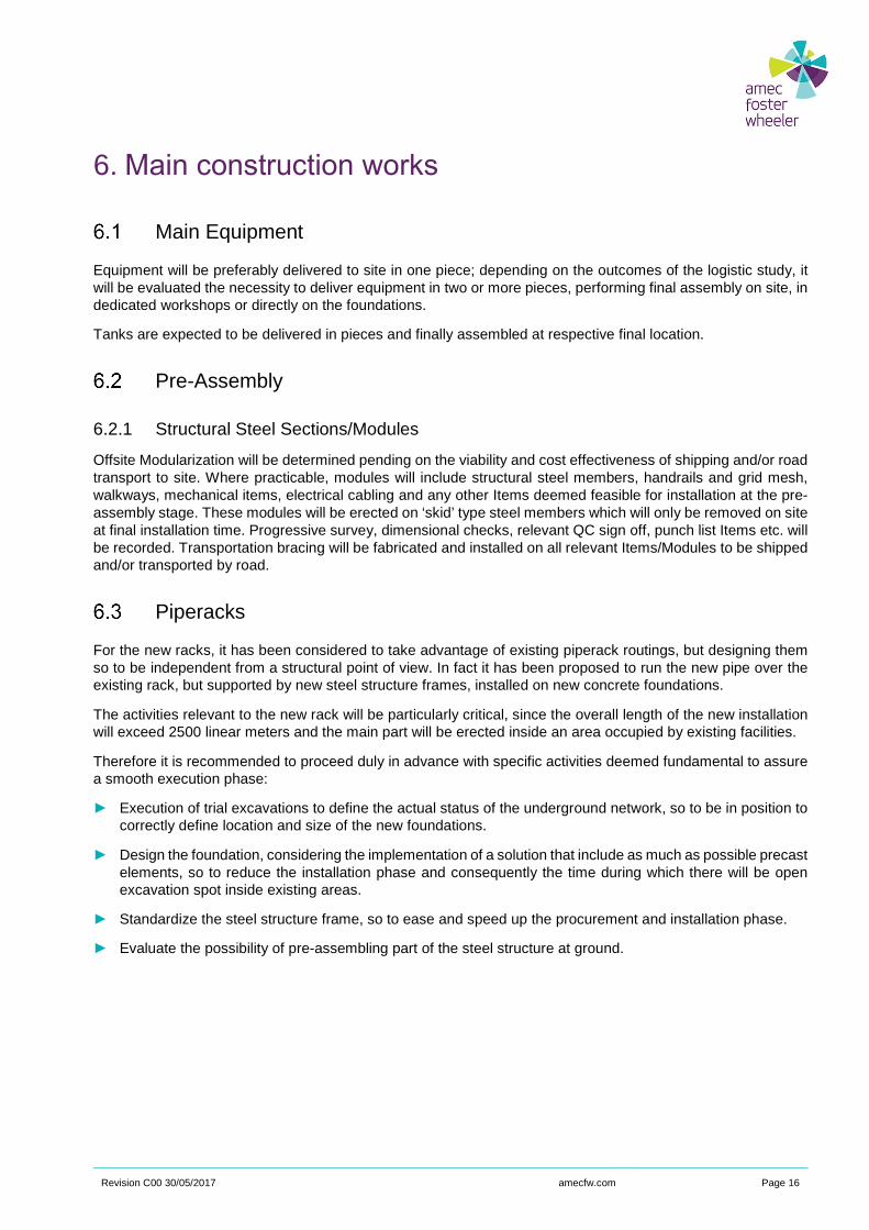
Revision C00 30/05/2017 amecfw.com Page 16
6. Main construction works
Main Equipment
Equipment will be preferably delivered to site in one piece; depending on the outcomes of the logistic study, it will be evaluated the necessity to deliver equipment in two or more pieces, performing final assembly on site, in dedicated workshops or directly on the foundations.
Tanks are expected to be delivered in pieces and finally assembled at respective final location.
Pre-Assembly
6.2.1 Structural Steel Sections/Modules
Offsite Modularization will be determined pending on the viability and cost effectiveness of shipping and/or road transport to site. Where practicable, modules will include structural steel members, handrails and grid mesh, walkways, mechanical items, electrical cabling and any other Items deemed feasible for installation at the pre-assembly stage. These modules will be erected on ‘skid’ type steel members which will only be removed on site at final installation time. Progressive survey, dimensional checks, relevant QC sign off, punch list Items etc. will be recorded. Transportation bracing will be fabricated and installed on all relevant Items/Modules to be shipped and/or transported by road.
Piperacks
For the new racks, it has been considered to take advantage of existing piperack routings, but designing them so to be independent from a structural point of view. In fact it has been proposed to run the new pipe over the existing rack, but supported by new steel structure frames, installed on new concrete foundations.
The activities relevant to the new rack will be particularly critical, since the overall length of the new installation will exceed 2500 linear meters and the main part will be erected inside an area occupied by existing facilities.
Therefore it is recommended to proceed duly in advance with specific activities deemed fundamental to assure a smooth execution phase:
► Execution of trial excavations to define the actual status of the underground network, so to be in position to correctly define location and size of the new foundations.
► Design the foundation, considering the implementation of a solution that include as much as possible precast elements, so to reduce the installation phase and consequently the time during which there will be open excavation spot inside existing areas.
► Standardize the steel structure frame, so to ease and speed up the procurement and installation phase.
► Evaluate the possibility of pre-assembling part of the steel structure at ground.
Revision C00 30/05/2017 amecfw.com Page 17
Piping
Piping and supports major fabrication activities are planned to be done at site, in dedicated workshops.
6.4.1 Tie-ins
Tie-ins represent the interface between the new and existing facilities. As such, they shall be installed in a logical sequence. Considerations for tie-in timing and design shall include:
► Ability to isolate the existing line at tie-in location.
► Construction access to the tie point for installation.
► Piping configuration from routing and stress point of view.
► Minimize overall count and maximizing the pre turn-around count.
► Minimizing / eliminating the need of any hot tap (*).
(*) Method of making a connection to existing piping or pressure vessels without the interrupting or emptying that section of pipe or vessel.
A project tie-in strategy should take into utmost considerations the safety aspects, but shall additionally include:
► Tie-in package content
► Tagging, walk-down, inspection and sign-off requirements
► Hot tap procedure.
► Air testing restrictions / procedure.
Generally, more tie-ins will be made during the turn-around (TA) than in pre-TA due to unavailability of existing lines and equipment; differently, in case a significant amount of re-commissioned, out-of-service equipment is available, higher percentages could be considered for pre-TA activities.
Further valid considerations, resulting from the long experience in turn around execution, are:
► Tie-ins are more effectively executed when they are walked down in the field during the design phase by the designer and the operator.
► Making tie-in packages is a significant, time-consuming activity. Plan allocation of resources based on tie-in count and the tie-in packages content requirements.
► Show tie in on an actualized plot plan (e.g. issued for construction).
In our case study, there will be a very limited integration between the new CO2 capture plants and the existing refinery units, especially when looking at the relevant utility systems. As a matter of fact, no capacity margins have been considered in the refinery utility systems to fulfil the demand of the new CO2 capture plants, but instead completely new – parallel- utility systems have been considered. As a result, the existing refinery block (with relevant utility units) and the new CO2 capture plants (with relevant new utility units) can be regarded as “independent”, interconnected only on the flue gas side. No many tie-ins will be therefore needed. However, in other Projects, a deeper integration of the CO2 capture plants with the refinery could be realised (e.g. to take advantage of some capacity margins in the existing utility systems). In that case an accurate tie-ins study is recommended not to jeopardise the normal operation of the Refinery when connecting the new CO2 capture facilities.

Revision C00 30/05/2017 amecfw.com Page 18
7. Critical lifting activities
As soon as a preliminary sizing/design of the main equipment is available, it is advised to execute a heavy lifting optimization study with the aim to minimize the number of heavy lifting equipment.
Mentioned study shall include lifting feasibility evaluations, items delivery timing and construction schedule considerations. The lifting plans, tailored to every single critical lift, shall specify cranes and lifting equipment to be provided, crane’s lifting locations and boom length to be used. The crane’s out-rigger loading and special ground preparation requirements should also be specified.
Dedicated lifting drawings and plans shall be produced for review and approval for all heavy lifts deemed critical, usually meaning lifts meeting one or more of the following criteria:
► The load is heavier than 45 t (50 ton).
► The load is less than 45 t (50 ton) but a complex lifting sequence is required.
► The lift involves a complex rigging arrangement or that requires specialty rigging.
► The load is heavier than 18 t (20 ton) and it is also greater than 80 percent of the manufacturer's rated capacity.
► The load is being lifted over or near an occupied building, operating equipment, or electrical power-lines.
► Two or more pieces of lifting equipment are required to work in unison: this includes using a tailing crane.
► Special lifting equipment (e.g. hydraulic gantries) or non-standard crane configurations, is used.
► The load represents more than 90 percent of the manufacturer's rated capacity at the working radius.
The lifting studies shall provide as a minimum:
► Definition of special equipment and rigging needs.
► Development of a rigging plan for each heavy lift.
► Definition of type, rating, and anticipated duration for all lifting equipment.
► Incorporation of heavy lift equipment needs and durations into the overall project construction schedule.
All heavy lift cranes shall be utilized in the permitted configuration, rated and tested by the crane manufacturer. All cranes capacities shall be within the published equipment charts capacities, in the configuration being utilized for the lift and in compliance with applicable local codes. Any propose lifting frames shall be supported by structural calculation in compliance with all applicable codes, industry practice and local regulations. Whenever possible, the equipment delivered to site will be offloaded and erected immediately onto their foundations, to avoid double handling.
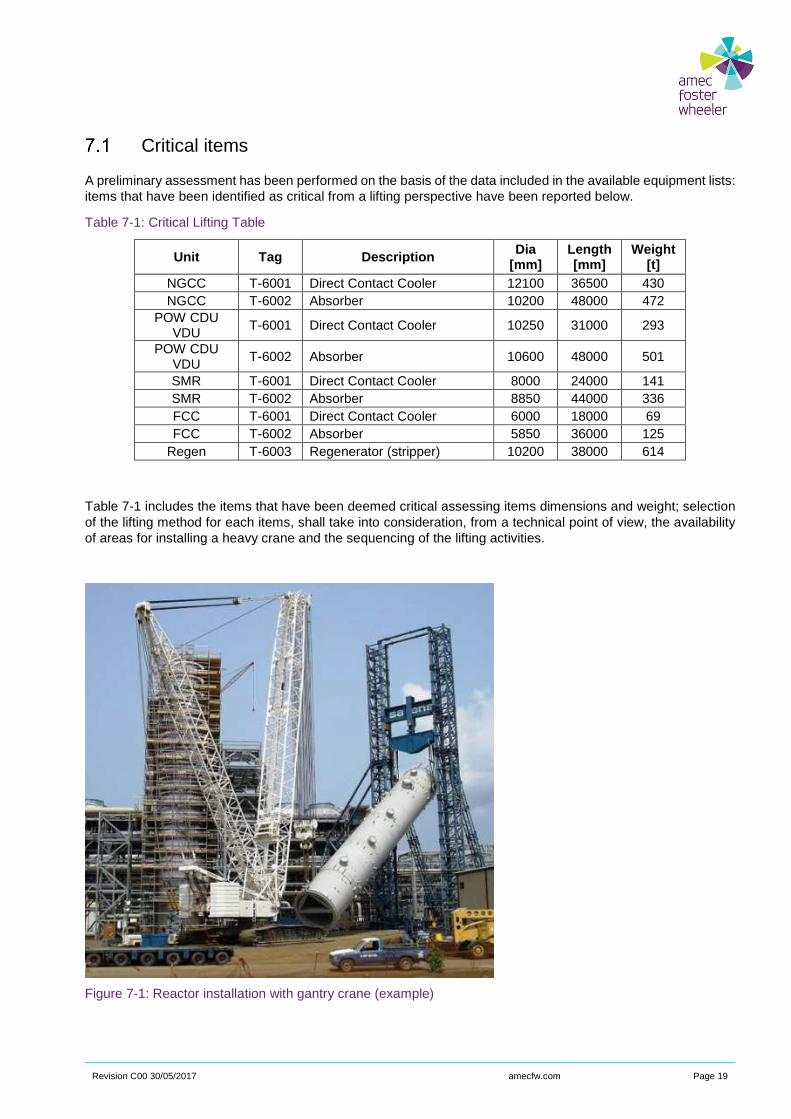
Revision C00 30/05/2017 amecfw.com Page 19
Critical items
A preliminary assessment has been performed on the basis of the data included in the available equipment lists: items that have been identified as critical from a lifting perspective have been reported below.
Table 7-1: Critical Lifting Table
Unit Tag Description Dia [mm]
Length [mm]
Weight [t]
NGCC T-6001 Direct Contact Cooler 12100 36500 430 NGCC T-6002 Absorber 10200 48000 472
POW CDU VDU
T-6001 Direct Contact Cooler 10250 31000 293
POW CDU VDU
T-6002 Absorber 10600 48000 501
SMR T-6001 Direct Contact Cooler 8000 24000 141 SMR T-6002 Absorber 8850 44000 336 FCC T-6001 Direct Contact Cooler 6000 18000 69 FCC T-6002 Absorber 5850 36000 125
Regen T-6003 Regenerator (stripper) 10200 38000 614
Table 7-1 includes the items that have been deemed critical assessing items dimensions and weight; selection of the lifting method for each items, shall take into consideration, from a technical point of view, the availability of areas for installing a heavy crane and the sequencing of the lifting activities.
Figure 7-1: Reactor installation with gantry crane (example)
Revision C00 30/05/2017 amecfw.com Page 20
Other packages that have evaluated as critical from an erection prospective are:
► Flue Gas Desulfurization unit.
► CO2 Compression package.
As of today it is not expected that these packages includes items with dimensions similar to the ones included in table 7-1, but the overall size of the packages and the technical complexity recommend to develop dedicated study to assess the installation sequence and optimize the duration of the construction activities.
It is recommended to execute during an early execution phase a heavy lifting optimization study with the aim of minimizing the number of heavy lifting equipment. Mentioned study shall include lifting feasibility evaluations, items delivery timing and construction schedule considerations. Considered installation methods may include the use of standard crawler and telescopic cranes or of other heavy lifting equipment, such gantry cranes, strand jacks, etc.
A gantry system is a side shift mechanism that allows to transverse the load giving the system the capacity to move the load in the 3 directions. It consist in 4 jacking units, supported on wheels or on rails, having one vertical lift cylinder and a vertical lift boom mounted on top; a lifting beam is installed on each two jacking units. According this scenario items shall be delivered on site, lifted by the gantry system, translated inside the shelter and afterwards laid on the foundations.
Installation method selection may have impacts on the design of surrounding structures. For example, in case of items to be installed inside sheltered structures, it is advised to do not link equipment installation to the erection of the structure, in order to avoid the risk of having the progress of the shelter blocked by any inconvenience related to a long delivery equipment.
On this basis, shelter/enclosures shall be designed in such a way to allow item installation with the structure almost completed or in an advanced status of progress.
In case of installation by crane, shelter roof shall be removable, considering a net opening over each item foundation of such dimensions to allow safe lifting operations. On the contrary, choosing a gantry system solution, roof can be completed, but shelter façade, shall present, on one side, in correspondence of each foundation, a net opening between the columns wider than the sum of the width of the concrete item pedestal and the installation device (i.e. width of a rail and a jack unit per side).
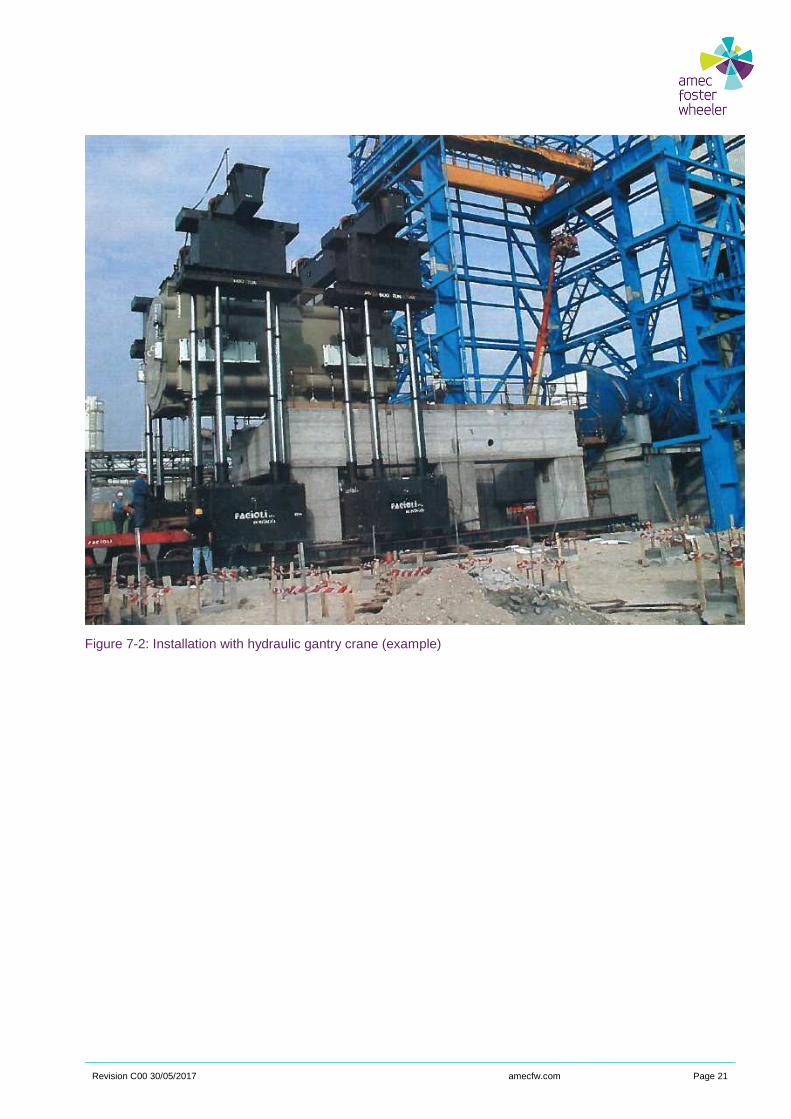
Revision C00 30/05/2017 amecfw.com Page 21
Figure 7-2: Installation with hydraulic gantry crane (example)
Revision C00 30/05/2017 amecfw.com Page 22
8. Systems turnover
To ensure that construction and pre-commissioning are performed in the sequence required for commissioning and start-up the following measures shall be taken and procedures followed:
► Required completion sequences of commissioning/start-up systems shall be identified in as “as early as possible” phase of the Project. Commissioning/start-up systems and required completion sequences should be defined during the P&ID development phase. Mark-up P&ID’s with commissioning system identification numbers to be provided.
► Hydro-test systems, loop tests and electrical continuity tests will be established in line with the commissioning systems.
► Dedicated system component lists shall be prepared identifying each hydro-test system, equipment tag, instrument loop and identification of MCC’s pertaining to a commissioning system. The lists shall be kept up-to-date for items completed.
► Pre-commissioning schedules shall be prepared in line with the commissioning system priority sequences.
► Installation activities shall be shifted from geographical oriented construction to system oriented construction at approx. 60-70% overall construction progress.
► Follow-up system progress and completion through periodical updates of the system component lists.
Dedicated Turnover and Commissioning procedures shall be prepared.

Revision C00 30/05/2017 amecfw.com Page 23
9. Site material management
A dedicated material management system has to be set up and afterwards implemented to control the flow of equipment and materials from material take off preparation through issue to construction contractors and final utilization.
The system shall register and monitor all materials to be delivered to the warehouse(s) and therefore issued to the construction contractors. At the same time the material management system shall offer an integrated handling of materials required for field changes, field purchased materials and production planning based on expected material availability and actual material availability.
10. Construction quality control
A dedicated quality control plan has to be developed in order to agree the quality control system to be adopted to duly monitor the execution of the construction activities.
The quality control plan shall be organized at discipline level and shall consider the specific tasks belonging to each phase.
Every construction contractor shall issue a specific quality control plan in accordance to the minimum Project requirements. Any test, inspection and check shall be carried out in due time before moving to other activities.
Level of test and inspections required for all works in field and relevant inspecting personnel involvement shall be summarized in dedicated tables.

Revision C00 30/05/2017 amecfw.com Page 24
11. HSE management
Considering the complexity of the project and the large numbers of people that shall be engaged during the field activities, HSE require a detailed approach shared and considered as top priority by everyone involved in the Project. To achieve HSE excellence an intensive training program shall be organized to train all the manpower and employees before starting the work at site.
► General training
The general HSE training will be conduct to all people before entering to site and will regards the following topics:
► Behaviour
Training will stress the behaviour that people shall maintain while working at field and in the office, about respect each other, ready to help the colleagues, not smoking unless in the denigrated area, housekeeping of the work areas including offices, work management, drink fluid to maintain the correct hydration.
► Golden Rules
To prevent occupational accidents:
► Clear explain the Basic Rules that everyone should know and apply;
► Risk identification and risk mitigation;
► String then prevention by incomes people to step in whenever they see something being done wrong;
► Stop work if the risk is not being properly managed.
The Golden Rules must be fully understood and obeyed by everyone.
Example of Golden Rules are: traffic, use of correct PPE, lifting operation, energized system, confined space, excavation work, work at high, management of change, simultaneous operation or co-activities.
► Permit to work
Basic understanding of the work permit process including the risk evaluation and mitigation.
► House Keeping
Basic explanation on how important is to maintain any work area tidies and clean to prevent accidents.
► Dedicate training for each trade
Training for each type of trade will be arranged with the aim to verify the real skill of the workers and to refresh their behaviour.
It will be important to ascertain the real capability and understanding of HSE rules of the foreman and supervisors and retrain them when their performance is not as for the required standard.
Revision C00 30/05/2017 amecfw.com Page 25
12. Interface management
A proper site interface management will reduce the risk of delay due to lack of permits and avoid any problems during the normal operation of the refinery. The interface management will follow up also the coordination with other contractors who can be present at Site during project activities construction period.
Usually the interface management is directly managed by a site technical manager, however in some cases (e.g. schedule analysis, request of work permits, etc.) he will be supported by his/her discipline co-operators (e.g. construction managers, planners).
The site technical manager shall organize regular meetings (on daily, weekly or monthly basis as per necessity) with the Owner responsible and operational management of the refinery to evaluate the schedule, organize the activities to be performed and request the necessary permits. In the above mentioned meeting shall be invited also the other Contractors present in the Terminal during the period of project scope of work.
Work permits
It is considered that all the activities inside the plant shall be done under work permits, managed directly by the Client. The type of Work Permit shall be different in relation to the area in which the activities shall be performed. For example, works in operation area should be managed by PTW released for task/working crew; differently, general work permit should be released for less risky activities in green field areas.
In order to regulate site activities and properly plan the duration of the works, a dedicated “Permit to Work (PTW)” procedure shall be developed and agreed with the refinery management in an early phase of the project.
Interface with Local Authorities
During the construction activities, some interfaces with the local authorities shall be faced; project strategy will define whether these interfaces will be managed directly by the refinery or delegated to a specific contractor. Typical activities that will require Local Authorities permission shall be:
► Dewatering;
► Erection of Temporary Site Facilities.
► Excavation and disposal of excavated soil.
► Certification of particular kind of scaffoldings.
► Waste disposal.

Revision C00 30/05/2017 amecfw.com Page 26
13. Site Security
Considered the project location and the fact that the intervention shall be executed inside an existing production facility, general plant security services are assumed to be already properly organized. Anyhow, a project dedicated security plan shall be developed in advance with respect to the execution phase, in order to define project related aspects and assess the management of interfaces with refinery activities. The project security plan shall cover, but not be limited to, the following topics:
► Security organization, responsibilities matrix and communications channels.
► Access and egress procedures to and from the area of operations, yards, offices and work areas including but not limited to, searches of people, luggage, vessels, vehicles, containers and equipment.
► Surveillance.
► Contingency plans and emergency response plans.
► Area of operations evacuation plan.
► Equipment requirements.
► Physical security measures (fencing, alarms, etc.).
► Security personnel requirements.
► Efficient and reliable communications equipment.
► Standard operating procedures.
► Transportation procedures of the personnel to and from area of operations, yards, work areas and offices.
► Reporting and investigation of security incidents.
Furthermore, project security plan shall delineate the roles and responsibilities of manager(s) and supervisors and require that their actions clearly demonstrate an understanding of their roles and responsibilities with regard to the security process.

Revision C00 30/05/2017 amecfw.com Page 27
14. Temporary Construction Facilities
The Temporary Construction Facilities (TCF) are intended as all the areas, the temporary buildings and structures, the temporary workshops and more generically all the temporary facilities required to support the construction activities and to sustain the execution of the planned works.
Correct, efficient and timely planning and execution of the TCF are important preplanning tasks that can either enhance or adversely affect construction productivity. A correct and efficient TCF can significantly reduce construction conflicts and improve project efficiency.
An overall conceptual layout of the TCF, including all the areas presented in the following subsections is shown in Figure 14-1.
Site offices
It is recommended to organize the site team in a unique building; in case free space should not be available inside permanent refinery facilities, a temporary site office shall be erected to accommodate the project site team.
The types and layouts of offices must be consistent with the level of organization envisaged. Preference must, however, be given to arrangements that allow for the expansion of spaces in the event of unforeseeable future circumstances.
Office space shall be fully equipped to support the functionality of the office; and shall be equipped with meeting rooms, it tools, document reproduction/file equipment, pc, fax machine, telecommunications, computers, toilets and washrooms. First-aid facilities shall be made available in the first aid room
Sufficient parking area will be arranged around the site office.
Furthermore, if a part of field engineering is done directly on site, a dedicated and suitably equipped space should be set aside for this. Special care should also be taken with the arrangement of controlled areas for the management and adequate space for the technical archive.
Office spaces must be made up of single rooms for the higher levels of management and of double, triple and multiple rooms for the rest of the organization and for secretarial and services staff as well open space. Spaces must be available for meeting rooms, conference room, document filing, changing rooms, kitchens and coffee bays men’s and women’s toilets, inclusive of showers.
All staff that require a computer (generally the majority) will be equipped with one, and a certain number of printers will be connected using the site LAN. Office equipment must include slide projectors, containers for files and drawings, white/blackboards and, lastly, infirmary equipment.
In any case, all localities must be equipped in such a way as to facilitate voice or data transmission services, both between themselves and with headquarters and the engineering offices (if engineering is not done centrally). These connections must be also provided for video conferences which are increasingly used on sites located at long distances from the main office.
Revision C00 30/05/2017 amecfw.com Page 28
Warehouse and storage areas
Part of the incoming materials must be protected while waiting to be installed. For this reason, roofed and indoor warehouses are prepared for those materials following the suppliers recommend. Other materials can simply be covered or left outdoors in fenced areas. Some materials (solvents, glues, paints, etc.) must be kept in well-aired environments and be separated from the rest of the materials, following the MDS specification.
The warehousing and delivery of materials is an extremely important activity for the success of the site. Alongside complete management of the process, the traceability and fabrication analysis for certain material (such as piping) based on inventories and pre-allocated stock should be stressed.
14.2.1 Warehouse
Site warehouses shall be composed by the following sections:
► Covered section for mechanical material to be assembled
Covered warehouse building will be installed at Site, the warehouse may be constructed using a traditional structure with walls made of corrugated metal, pre-fabricated modular wooden elements, brick, etc. Material control staff will be located in a dedicated office space.
Materials to be stored in this space are: gaskets, pipe fittings, flanges and valves, bolts, electrical item, instrument item, equipment, electronic components, switchgears, fuses, relays, instruments, control boards, analyzers, instrumentation fittings, pre- commissioning materials, spare parts, etc.
► Covered section for painting and chemicals
For the storage of dangerous materials (toxic, corrosive, flammable, etc.) an isolated building with air conditioning must be provided. In addition to the above, all the requirements included in the MSDS (Material Safety Data Sheet) of the materials shall be followed during the design of the warehouse. Proper safety signs shall be applied at the entrance of the warehouse.
► Shed section for insulation material
► Marshalling yard for quarantine materials
► Shed Section for materials which can be exposed to the weather, but in their packaging
14.2.2 Storage areas
Storage areas are required lo laydown the construction material and shall include:
► Fenced areas
The fenced area must be:
► Placed adjacent of the warehouse;
► Adequately lighting;
► Flat and compacted to allow the circulation of vehicles such as fork-lift trucks, cranes.
Materials to be stored in this area are: pipes, flanges, fittings, filters, columns internals, steel plates, steel section bars, concrete steel bars, cable coils, packages, etc.
► Unfenced areas
The unfenced area must be located as close as possible to the fenced area. For the storage of vessels, equipment, machinery, packages, steel structures, etc.
Revision C00 30/05/2017 amecfw.com Page 29
Construction contractors areas
Dedicated areas shall be assigned to Construction contractors for the installation of their Temporary Construction Facilities, that, depending on contractors’ core activities, may include:
► Site offices
► Piping Fabrication, sandblasting and painting workshops
► Contractors equipment and material storage facilities.
Considering the location of the project, it is expected that some of the construction contractors TCF and material production facilities (e.g. concrete batching plant) shall be available on the local market and hence shall not be temporarily erected for project scope only.
Temporary utilities
Temporary utilities are required to support the execution of the construction works, and typically include:
► Industrial water
► Demi water
► Potable water
► Electrical power
► Sewage system
► Data system
► Steam
► Compressed air
Utilities shall be either sourced from refinery networks (e.g. industrial water) or generated on purpose (e.g. power diesel generators in case of unavailability of enough power through the existing grid).
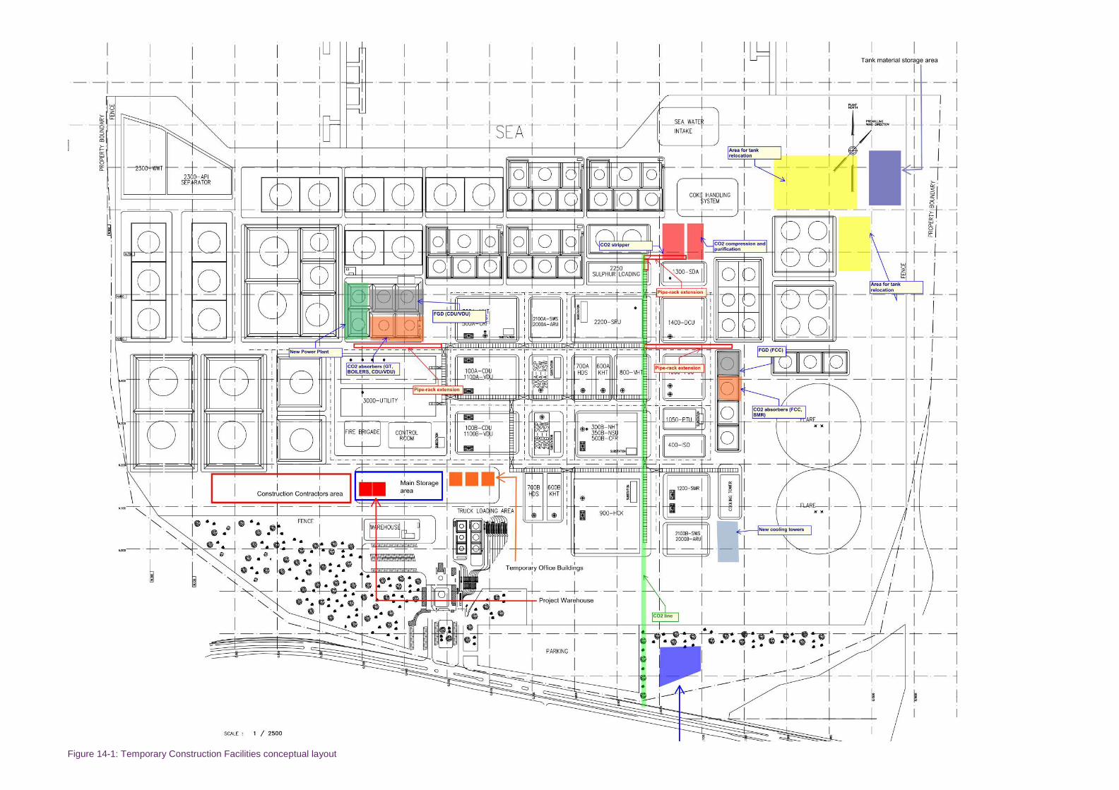
Figure 14-1: Temporary Construction Facilities conceptual layout
Revision C00 30/05/2017 amecfw.com Page 31
15. Waste management
Waste water management
All sewage water, including the one derived from construction activities, shall be treated before disposal. Treatment could be done through the existing refinery water treatment plant. Alternatively, a new dedicated waste water treatment plant should be erected or, in case a treatment plant is available not too far from the site, transfer of the sewage shall be organized by appropriate means, of course by entering into an agreement with the owner of the Waste Water Treatment Plant and with the support of the client.
For the disposal of hydrotest water it could be considered, in accordance with refinery and local regulation, the use of a temporary evaporation pond.
Disposal of waste water could also be through vacuum tankers to a local waste water treatment plant.
Waste management
Solid waste shall be segregated by type directly at site and collected in dedicated skip’s ready for collection and disposal in an approved dumping area for further process.
Construction contractors shall be responsible for managing and arranging disposal in an acceptable manner of the various types and categories of waste, which accrues throughout the execution of the Project.
All hauling and dumping operations shall be in accordance with refinery procedures and methods of disposing of waste and local regulation. Waste types shall include, but not be limited to, the following typologies:
► Chemicals and Oils:
This includes any Chemicals and Oils, which constitute a high degree of hazard to public health and the environment, such as hydrocarbons (Oils, Lubricants etc.), corrosive, reactive and toxic Chemicals. These must be handled and disposed of in an approved area for further process.
► Construction debris and material unsuitable for fill
These materials will be disposed of in the approved dump site; it includes material such as timber, steel, packaging material, concrete etc.
► Garbage Disposal
Biodegradable, chemically decomposable and inert waste will be dumped in an approved dump site. This material includes non-hazardous solid waste and sludge that are biologically or chemically decomposable in the natural environment such as paper, digestive sewage, garbage or waste that is not biologically or chemically active in the natural environment such as glass, most plastics and rubber products.

Revision C00 30/05/2017 amecfw.com Page 32
16. Conclusions
Retrofitting CO2 capture plants in an existing refinery requires an accurate constructability study to be carried out at the very beginning of the design phase, to identify as soon as possible all the critical aspects that could have an impact on the construction duration, strategy, cost.
The new CO2 capture plants have relatively few interfaces, in terms of process, with the rest of the facility, but they are very demanding in terms of plot area requirements and interconnections between the different portions of the plant (e.g. Absorber, Stripper, Compression/Purification, Utility systems). This implies an accurate planning of the works required for the areas’ preparation, as well as for the extension/revamping of main piperacks to connect all the portions.
Moreover, the size of the main columns (DCC, Absorber, Stripper) is large and requires dedicated studies for identifying the most suitable access/routing for the transportation and for defining a proper lifting strategy.
All the interfaces (physical, human, operational) between the new and the existing installations need to be taken into account.
In conclusion, for revamping even more than for grass-root projects, the constructability task is a very complex activity, driven by many key-factors like schedule, cost, impact on the existing facilities and routine operations, and, first of all, safety during all the phases of the project implementation.

IEA Greenhouse Gas R&D ProgrammePure Offices, Cheltenham Office Park, Hatherley Lane,Cheltenham, Glos. GL51 6SH, UK
Tel: +44 1242 802911 [email protected] www.ieaghg.org