An Introduction to Optimization Models and Methods

4An Introduction to OptimizationModels and Methods

Water resource systems are characterized bymultiple interdependent components that toge-ther produce multiple economic, environmental,ecological, and social impacts. As discussed inthe previous chapter, planners and managersworking toward improving the design and per-formance of these complex systems must identifyand evaluate alternative designs and operatingpolicies, comparing their predicted performancewith desired goals or objectives. Typically, thisidentification and evaluation process is accom-plished with the aid of optimization and simula-tion models. While optimization methods aredesigned to provide preferred values of systemdesign and operating policy variables—valuesthat will lead to the highest levels of systemperformance—they are often used to eliminatethe clearly inferior options. Using optimizationfor a preliminary screening followed by moredetailed and accurate simulation is the primaryway we have, short of actually building physicalmodels, of estimating effective system designsand operating policies. This chapter introducesand illustrates the art of optimization model de-velopment and use in analyzing water resourcessystems. The models and methods introduced inthis chapter are extended in subsequent chapters.

4.1 Introduction

This chapter introduces some optimizationmodeling approaches for identifying ways ofsatisfying specified goals or objectives. The

modeling approaches are illustrated by theirapplication to some relatively simple waterresources planning and management problems.The purpose here is to introduce and comparesome commonly used optimization methods andapproaches. This is not a text on the state of theart of optimization modeling. More realistic andmore complex problems usually require muchbigger and more complex models than thosedeveloped and discussed in this chapter, butthese bigger and more complex models are oftenbased on the principles and techniques intro-duced here.

The emphasis here is on the art of modeldevelopment—just how one goes about con-structing and solving optimization models thatwill provide information useful for addressingand perhaps even solving particular problems. Itis unlikely anyone will ever use any of thespecific models developed in this or other chap-ters simply because the specific examples used toillustrate the approach to model development andsolution will not be the ones they face. However,it is quite likely water resource managers andplanners will use these modeling approaches andsolution methods to analyze a variety of waterresource systems. The particular systems mod-eled and analyzed here, or any others that couldhave been used, can be the core of more complexmodels needed to analyze more complex prob-lems in practice.

Water resources planning and managementtoday is dominated by the use of optimizationand simulation models. Computer software is

© The Author(s) 2017D.P. Loucks and E. van Beek, Water Resource Systems Planning and Management,DOI 10.1007/978-3-319-44234-1_4

93

becoming increasingly available for solvingvarious types of optimization and simulationmodels. However, no software currently existsthat will build models of particular waterresource systems. What and what not to includeand assume in models requires judgment, expe-rience, and knowledge of the particular problemsbeing addressed, the system being modeled andthe decision-making environment—includingwhat aspects can be changed and what cannot.Understanding the contents of this and followingchapters and performing the suggested exercisesat the end of each chapter can only be a first steptoward gaining some judgment and experience inmodel development.

Before proceeding to a more detailed discus-sion of optimization, a review of some methodsof dealing with time streams of economicincomes or costs (engineering economics) maybe useful. Those familiar with this subject that istypically covered in applied engineering eco-nomics courses can skip this next section.

4.2 Comparing Time Streamsof Economic Benefits and Costs

All of us make decisions that involve futurebenefits and costs. The extent to which we valuefuture benefits or costs compared to presentbenefits or costs is reflected by what is called adiscount rate. While economic criteria are onlyone aspect of everything we consider whenmaking decisions, they are often among theimportant ones. Economic evaluation methodsinvolving discount rates can be used to considerand compare alternatives characterized by vari-ous benefits and costs that are expected to occurnow and in the future. This section offers a quickand basic review of the use of discount rates thatenable comparisons of alternative time series ofbenefits and costs. Many economic optimizationmodels incorporate discount rates in their eco-nomic objective functions.

Engineering economic methods typicallyfocus on the comparison of a discrete set of

mutually exclusive alternatives (only one ofwhich can be selected) each characterized by atime series of benefits and costs. Using variousmethods involving the discount rate, the timeseries of benefits and costs are converted to asingle net benefit that can be compared withother such net benefits in order to identify the onethat is best. The values of the decision variables(e.g., the design and operating policy variablevalues) are known for each discrete alternativebeing considered. For example, consider againthe tank design problem presented in the previ-ous chapter. Alternative tank designs could beidentified, and then each could be evaluated, onthe basis of cost and perhaps other criteria aswell. The best would be called the optimal one, atleast with respect to the objective criteria usedand the discrete alternatives being considered.

The optimization methods introduced in thefollowing sections of this chapter extend thoseengineering economics methods. Some methodsare discrete, some are continuous. Continuousoptimization methods, such as the model definedby Eqs. 3.1–3.3 in Sect. 3.2 of the previouschapter can identify the “best” tank designdirectly without having to identify and comparenumerous discrete, mutually exclusive alterna-tives. Just how such models can be solved will bediscussed later in this chapter. For now, considerthe comparison of alternative discrete plansp having different benefits and costs over time.

Let the net benefit generated at the end of timeperiod t by plan p be designated simply as Bp(t).Each plan is characterized by the time streamof net benefits it generates over its planningperiod Tp.

fBpð1Þ;Bpð2Þ;Bpð3Þ; . . .;BpðTpÞ ð4:1Þ

Clearly, if in any time period t the benefitsexceed the costs, then BpðtÞ[ 0; and if the costsexceed the benefits, BpðtÞ\0. This sectiondefines two ways of comparing different benefit,cost or net-benefit time streams produced bydifferent plans perhaps having different planningperiod durations Tp.

94 4 An Introduction to Optimization Models and Methods

http://dx.doi.org/10.1007/978-3-319-44234-1_3

http://dx.doi.org/10.1007/978-3-319-44234-1_3

4.2.1 Interest Rates

Fundamental to the conversion of a time series ofincomes and costs to an equivalent single value, sothat it can be compared to other equivalent singlevalues of other time series, is the concept of thetime value of money. From time to time, individ-uals, private corporations, and governments needto borrow money to do what they want to do. Theamount paid back to the lender has two compo-nents: (1) the amount borrowed and (2) an addi-tional amount called interest. The interest amountis the cost of borrowing money, of having themoney when it is loaned compared to when it ispaid back. In the private sector the interest rate, theadded fraction of the amount owed that equals theinterest, is often identified as the marginal rate ofreturn on capital. Those who have money, calledcapital, can either use it themselves or they canlend it to others, including banks, and receiveinterest. Assuming people with capital invest theirmoney where it yields the largest amount ofinterest, consistent with the risk they are willing totake, most investors should be receiving at least theprevailing interest rate as the return on their capital.

Any interest earned by an investor or paid bya debtor depends on the size of the loan, theduration of the loan, and the interest rate. Theinterest rate includes a number of considerations.One is the time value of money (a willingness topay something to obtain money now rather thanto obtain the same amount later). Another is therisk of losing capital (not getting the full amountof a loan or investment returned at some futuretime). A third is the risk of reduced purchasingcapability (the expected inflation over time). Thegreater the risks of losing capital or purchasingpower, the higher the interest rate compared tothe rate reflecting only the time value of moneyin a secure and inflation-free environment.

4.2.2 Equivalent Present Value

To compare projects or plans involving differenttime series of benefits and costs, it is often con-venient to express these time series as a singleequivalent value. One way to do this is to convert

each amount in the time series to what it is worthtoday, its present worth, that is, a single value atthe present time. This present worth will dependon the prevailing interest rate in each future timeperiod. Assuming a value V0 is invested at thebeginning of a time period, e.g., a year, in aproject or a savings account earning interest at arate r per period, then at the end of the period thevalue of that investment is (1 + r)V0.

If one invests an amount V0 at the beginningof period t = 1 and at the end of that periodimmediately reinvests the total amount (theoriginal investment plus interest earned), andcontinues to do this for n consecutive periods atthe same period interest rate r, the value, Vn, ofthat investment at the end of n periods would be

Vn ¼ V0 1þ rð Þn ð4:2Þ

This results from V1 ¼ V0= 1þ rð Þ at the end ofperiod 1,V2 ¼ V1=ð1þ rÞ ¼ V0ð1þ rÞ2 at the endof period 2, and so on until at the end of period n.

The initial amount V0 is said to be equivalentto Vn at the end of n periods. Thus the presentworth or present value, V0, of an amount ofmoney Vn at the end of period n is

V0 ¼ Vn= 1þ rð Þn ð4:3Þ

Equation 4.3 is the basic compound interestdiscounting relation needed to determine thepresent value at the beginning of period 1 (or endof period 0) of net benefits Vn that accrue at theend of n time periods.

The total present value of the net benefitsgenerated by plan p, denoted Vp

0 , is the sum ofthe values of the net benefits Vp(t) accrued at theend of each time period t times the discountfactor for that period t. Assuming the interest ordiscount rate r in the discount factor applies forthe duration of the planning period, i.e., fromt = 1 to t = Tp.

Vp0 ¼

Xt¼1;Tp

VpðtÞ= 1þ rð Þt ð4:4Þ

The present value of the net benefits achievedby two or more plans having the same economic

4.2 Comparing Time Streams of Economic Benefits and Costs 95

planning horizons Tp can be used as an economicbasis for plan selection. If the economic lives orplanning horizons of projects differ, then thepresent value of the plans may not be an appro-priate measure for comparison and plan selection.A valid comparison of alternative plans usingpresent values is possible if all plans have thesame planning horizon or if funds remaining atthe end of the shorter planning horizon areinvested for the remaining time up until the longerplanning horizon at the same interest rate r.

4.2.3 Equivalent Annual Value

If the lives of various plans differ, but the sameplans will be repeated on into the future, then oneneed to only compare the equivalent constantannual net benefits of each plan. Finding theaverage or equivalent annual amount Vp is donein two steps. First, one can compute the presentvalue, Vp

0 , of the time stream of net benefits,using Eq. 4.4. The equivalent constant annualbenefits, Vp, all discounted to the present mustequal the present value, Vp

0 .

Vp0 ¼

Xt¼1;Tp

Vp= 1þ rð Þt or

Vp ¼ Vp0=

Xt¼1;Tp

1= 1þ rð Þtð4:5Þ

Using a little algebra the average annualend-of-year benefits Vp of the project or plan p is

Vp ¼ Vp0 rð1þ rÞTp� �

= ð1þ rÞTp � 1� � ð4:6Þ

The capital recovery factor CRFn is theexpression rð1þ rÞTp� �

= ð1þ rÞTp � 1� �

in Eq. 4.6that converts a fixed payment or present value Vp

0

at the beginning of the first time period into anequivalent fixed periodic payment Vp at the endof each time period. If the interest rate per periodis r and there are n periods involved, then thecapital recovery factor is

CRFn ¼ rð1þ rÞn½ �= ð1þ rÞn � 1½ � ð4:7Þ

This factor is often used to compute theequivalent annual end-of-year cost of engineer-ing structures that have a fixed initial construc-tion cost C0 and annual end-of-year operation,maintenance, and repair (OMR) costs. Theequivalent uniform end-of-year total annual cost,TAC, equals the initial cost times the capitalrecovery factor plus the equivalent annualend-of-year uniform OMR costs.

TAC ¼ CRFn C0 þOMR ð4:8Þ

For private investments requiring borrowedcapital, interest rates are usually established, andhence fixed, at the time of borrowing. However,benefits may be affected by changing interestrates, which are not easily predicted. It is com-mon practice in benefit–cost analyses to assumeconstant interest rates over time, for lack of anybetter assumption.

Interest rates available to private investors orborrowers may not be the same rates that are usedfor analyzing public investment decisions. In aneconomic evaluation of public-sector invest-ments, the same relationships are used eventhough government agencies are not generallyfree to loan or borrow funds on private moneymarkets. In the case of public-sector investments,the interest rate to be used in an economic anal-ysis is a matter of public policy; it is the rate atwhich the government is willing to forego currentbenefits to its citizens in order to provide benefitsto those living in future time periods. It can beviewed as the government’s estimate of the timevalue of public monies or the marginal rate ofreturn to be achieved by public investments.

These definitions and concepts of engineeringeconomics are applicable to many of the prob-lems faced in water resources planning andmanagement. Each of the equations above isapplicable to discrete alternatives whose decisionvariables (investments over time) are known. Theequations are used to identify the best alternativefrom a set of mutually exclusive alternativeswhose decision variable values are known. Moredetailed discussions of the application of


engineering economics are contained in numer-ous texts on the subject. In the next section, weintroduce methods that can identify the bestalternative among those whose decision variablevalues are not known. For example, engineeringeconomic methods can identify, for example, themost cost-effective tank from among those whosedimension values have been previously selected.The optimization methods that follow can iden-tify directly the values of the dimensions of mostcost-effective tank.

4.3 Nonlinear Optimization Modelsand Solution Procedures

Constrained optimization involves finding thevalues of decision variables given specifiedrelationships that have to be satisfied. Con-strained optimization is also called mathematicalprogramming. Mathematical programming tech-niques include calculus-based Lagrange multi-pliers and various methods for solving linear andnonlinear models including dynamic program-ming, quadratic programming, fractional pro-gramming, and geometric programming, tomention a few. The applicability of each of these

as well as other constrained optimization proce-dures is highly dependent on the mathematicalstructure of the model that in turn is dependenton the system being analyzed. Individuals tend toconstruct models in a way that will allow them touse a particular optimization technique they thinkis best. Thus, it pays to be familiar with varioustypes of optimization methods since no onemethod is best for all optimization problems.Each has its strengths and limitations. Theremainder of this chapter introduces and illus-trates the application of some of the most com-mon constrained optimization techniques used inwater resources planning and management.

Consider a river from which diversions aremade to three water-consuming firms that belongto the same corporation, as illustrated in Fig. 4.1.Each firm makes a product. Water is needed inthe process of making that product, and is thecritical resource. The three firms can be denotedby the index j = 1, 2, and 3 and their water al-locations by xj. Assume the problem is to deter-mine the allocations xj of water to each of threefirms (j = 1, 2, 3) that maximize the total netbenefits,

Pj NBjðxjÞ, obtained from all three

firms. The total amount of water available isconstrained or limited to a quantity of Q.

Fig. 4.1 Three water-using firms obtain water from a river. The amounts xj allocated to each firm j will depend on theriver flow Q

4.2 Comparing Time Streams of Economic Benefits and Costs 97

Assume the net benefits, NBj(xj), derived fromwater xj allocated to each firm j, are defined by

NB1ðx1Þ ¼ 6x1 � x21 ð4:9Þ

NB2ðx2Þ ¼ 7x2 � 1:5x22 ð4:10Þ

NB3ðx3Þ ¼ 8x3 � 0:5x23 ð4:11Þ

These are concave functions exhibitingdecreasing marginal net benefits with increasingallocations. These functions look like hills, asillustrated in Fig. 4.2.

4.3.1 Solution Using Calculus

Calculus can be used to find the allocations thatmaximize each user’s net benefits, simply byfinding where the slope or derivative of the netbenefit function for each firm equals zero. Thederivative, dNB(x1)/dx1, of the net benefit func-tion for Firm 1 is (6 − 2x1) and hence the allo-cation to Firm 1 that maximizes its net benefitswould be 6/2 or 3. The corresponding allocationsfor Firms 2 and 3 are 2.33 and 8, respectively.The total amount of water desired by all firms isthe sum of each firm’s desired allocation, or13.33 flow units. However, suppose only 8 unitsof flow are available for all three firms and 2

units must remain in the river. Introducing thisconstraint renders the previous solution infeasi-ble. In this case we want to find the allocationsthat maximize the total net benefits obtained fromall firms subject to having only 6 flow unitsavailable for allocations. Using simple calculuswill not suffice.

4.3.2 Solution Using Hill Climbing

One approach for finding, at least approximately,the particular allocations that maximize the totalnet benefit derived from all firms in this exampleis an incremental steepest-hill-climbing method.This method divides the total available flowQ into increments and allocates each successiveincrement so as to get the maximum additionalnet benefit from that incremental amount ofwater. This procedure works in this examplebecause each of the net benefit functions is con-cave; in other words, the marginal benefitsdecrease as the allocation increases. This proce-dure is illustrated by the flow diagram in Fig. 4.3.

Table 4.1 lists the results of applying theprocedure shown in Fig. 4.3 to the problem when(a) only 8 and (b) only 20 flow units are avail-able. Here a minimum river flow of 2 is requiredand is to be satisfied, when possible, before anyallocations are made to the firms.

The hill-climbing method illustrated inFig. 4.3 and Table 4.1 assigns each incremental

Fig. 4.2 Concave net benefit functions for three water users, j, and their slopes at allocations xj


flow ΔQ to the use that yields the largest addi-tional (marginal) net benefit. An allocation isoptimal for any total flow Q when the marginalnet benefits from each nonzero allocation areequal, or as close to each other as possible giventhe size of the increment ΔQ. In this example,with a ΔQ of 1 and Qmax of 8, it just happens thatthe marginal net benefits associated with eachallocation are all equal (to 4). The smaller theΔQ, the more precise will be the optimal allo-cations in each iteration, as shown in the lowerportion of Table 4.1, where ΔQ approaches 0.

Based on the allocations derived for variousvalues of available water Q, as shown inTable 4.1, an allocation policy can be defined.For this problem, the allocation policy thatmaximizes total net benefits for any particularvalue of Q is shown in Fig. 4.4.

This hill-climbing approach leads to optimalallocations only if all of the net benefit functionswhose sum is being maximized are concave: thatis, the marginal net benefits decrease as theallocation increases. Otherwise, only a localoptimum solution can be guaranteed. This is true

using any calculus-based optimization procedureor algorithm.

4.3.3 Solution Using LagrangeMultipliers

4.3.3.1 ApproachAs an alternative to hill-climbing methods, con-sider a calculus-based method involvingLagrange multipliers. To illustrate this approach,a slightly more complex water-allocation exam-ple will be used. Assume that the benefit, Bj(xj),each water-using firm receives is determined, inpart, by the quantity of product it produces andthe price per unit of the product that is charged.As before, these products require water and wateris the limiting resource. The amount of productproduced, pj, by each firm j is dependent on theamount of water, xj, allocated to it.

Let the function Pj(xj) represent the maximumamount of product, pj, that can be produced byfirm j from an allocation of water xj. These arecalled production functions. They are typically

Fig. 4.3 Steepest hill-climbing approach for finding allocation of a flow Qmax to the three firms, while meetingminimum river flow requirements R

4.3 Nonlinear Optimization Models and Solution Procedures 99

Fig. 4.4 Water-allocationpolicy that maximizes totalnet benefits derived fromall three water-using firms

Table 4.1 Hill-climbing iterations for finding allocations that maximize total net benefit given a flow of Qmax and arequired (minimum) streamflow of R = 2


concave: as xj increases the slope, dPj(xj)/dxj, ofthe production function, Pj(xj), decreases. Forthis example, assume the production functionsfor the three water-using firms are

P1ðx1Þ ¼ 0:4ðx1Þ0:9 ð4:12Þ

P2ðx2Þ ¼ 0:5ðx2Þ0:8 ð4:13Þ

P3ðx3Þ ¼ 0:6ðx3Þ0:7 ð4:14Þ

Next consider the cost of production. Assumethe associated cost of production can be expres-sed by the following convex functions:

C1 ¼ 3ðP1ðx1ÞÞ1:3 ð4:15Þ

C2 ¼ 5ðP2ðx2ÞÞ1:2 ð4:16Þ

C3 ¼ 6ðP3ðx3ÞÞ1:15 ð4:17Þ

Each firm produces a unique patented product,and hence it can set and control the unit price ofits product. The lower the unit price, the greaterthe demand and thus the more each firm can sell.Each firm has determined the relationshipbetween the unit price and the amount that will

be demanded and sold. These are the demandfunctions for that product. These unit price ordemand functions are shown in Fig. 4.5, wherethe pj s are the amounts of each product pro-duced. The vertical axis of each graph is the unitprice. To simplify the problem we are assuminglinear demand functions, but this assumption isnot a necessary condition.

The optimization problem is to find the waterallocations, the production levels, and the unitprices that together maximize the total net benefitobtained from all three firms. The water alloca-tions plus the amount that must remain in theriver, R, cannot exceed the total amount of waterQ available.

Constructing and solving a model of thisproblem for various values of Q, the total amountof water available, will define the three allocationpolicies as functions of Q. These policies can bedisplayed as a graph, as in Fig. 4.4, showing thethree best allocations given any value of Q. Thisof course assumes the firms can adjust to varyingallocations. In reality this may not be the case(Chapter 9 examines this problem using morerealistic benefit functions that reflect the degreeto which firms can adapt to changing inputs overtime.)

The model:

Maximize Net benefit ð4:18Þ

Fig. 4.5 Unit prices that will guarantee the sale of the specified amounts of products pj produced in each of the threefirms (linear functions are assumed in this example for simplicity)


http://dx.doi.org/10.1007/978-3-319-44234-1_9

Subject toDefinitional constraints:

Net benefit ¼ Total return� Total cost

ð4:19Þ

Total return ¼ 12� p1ð Þp1 þ 20 � 1:5p2ð Þp2þ 28� 2:5p3ð Þp3

ð4:20Þ

Total cost ¼ 3ðp1Þ1:30 þ 5ðp2Þ1:20 þ 6ðp3Þ1:15ð4:21Þ

Production functions defining the relationshipbetween water allocations xj and production pj

p1 ¼ 0:4ðx1Þ0:9 ð4:22Þ

p2 ¼ 0:5ðx2Þ0:8 ð4:23Þ

p3 ¼ 0:6ðx3Þ0:7 ð4:24Þ

Water-allocation restriction

Rþ x1 þ x2 þ x3 ¼ Q ð4:25Þ

One can first solve this model for the values ofeach pj that maximize the total net benefits,assuming water is not a limiting constraint. This isequivalent to finding each individual firm’smaximum net benefits, assuming all the water thatis needed is available. Using calculus we canequate the derivatives of the total net benefitfunction with respect to each pj to 0 and solveeach of the resulting three independent equations:

Total Net benefit ¼ 12� p1ð Þp1 þ 20� 1:5p2ð Þp2½þ 28� 2:5p3ð Þp3� � 3 p1ð Þ1:30

h

þ 5ðp2Þ1:20 þ 6ðp3Þ1:15i

ð4:26Þ

Derivatives:

@ðNet benefit)=@p1 ¼ 0¼ 12� 2p1 � 1:3ð3Þp0:31

ð4:27Þ

@ðNet benefit)=@p2 ¼ 0¼ 20� 3p2 � 1:2ð5Þp0:22

ð4:28Þ

@ Net benefitð Þ=@p3 ¼ 0¼ 28� 5p3 � 1:15ð6Þp0:153

ð4:29Þ

The result (rounded off) is p1 = 3.2, p2 = 4.0,and p3 = 3.9 to be sold for unit prices of 8.77,13.96, and 18.23, respectively, for a maximumnet revenue of 155.75. This would require waterallocations x1 = 10.2, x2 = 13.6, and x3 = 14.5,totaling 38.3 flow units. Any amount of waterless than 38.3 will restrict the allocation to, andhence the product production at, one or more ofthe three firms.

If the total available amount of water is lessthan that desired, constraint Eq. 4.25 can bewritten as an equality, since all the water avail-able, less any that must remain in the river, R,will be allocated. If the available water suppliesare less than the desired 38.3 plus the requiredstreamflow R, then Eqs. 4.22–4.25 need to beadded. These can be rewritten as equalities sincethey will be binding. Equation 4.25 in this casecan always be an equality since any excess waterwill be allocated to the river, R.

To consider values of Q that are less than thedesired 38.3 units, constraints 4.22–4.25 can beincluded in the objective function, Eq. 4.26, oncethe right-hand side has been subtracted from theleft-hand side so that they equal 0. We set thisfunction equal to L.


L ¼ 12� p1ð Þp1 þ 20� 1:5p2ð Þp2 þ 28� 2:5p3ð Þp3½ �� 3ðp1Þ1:30 þ 5 p2ð Þ1:20 þ 6ðp3Þ1:15h i

� k1 p1 � 0:4ðx1Þ0:9h i

� k2 p2 � 0:5ðx2Þ0:8h i

� k3 p3 � 0:6ðx3Þ0:7h i

� k4 Rþ x1 þ x2 þ x3 � Q½ �ð4:30Þ

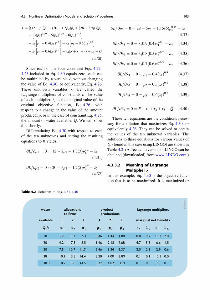
Since each of the four constraint Eqs. 4.22–4.25 included in Eq. 4.30 equals zero, each canbe multiplied by a variable λi without changingthe value of Eq. 4.30, or equivalently, Eq. 4.26.These unknown variables λi are called theLagrange multipliers of constraints i. The valueof each multiplier, λi, is the marginal value of theoriginal objective function, Eq. 4.26, withrespect to a change in the value of the amountproduced, p, or in the case of constraint Eq. 4.25,the amount of water available, Q. We will showthis shortly.

Differentiating Eq. 4.30 with respect to eachof the ten unknowns and setting the resultingequations to 0 yields:

@L=@p1 ¼ 0 ¼ 12� 2p1 � 1:3ð3Þp0:31 � k1ð4:31Þ

@L=@p2 ¼ 0 ¼ 20� 3p2 � 1:2ð5Þp0:22 � k2ð4:32Þ

@L=@p3 ¼ 0 ¼ 28� 5p3 � 1:15ð6Þp0:153 � k3

ð4:33Þ@L=@x1 ¼ 0 ¼ k10:9ð0:4Þx�0:1

1 � k4 ð4:34Þ

@L=@x2 ¼ 0 ¼ k20:8 0:5ð Þx�0:22 � k4 ð4:35Þ

@L=@x3 ¼ 0 ¼ k30:7ð0:6Þx�0:33 � k4 ð4:36Þ

@L=@k1 ¼ 0 ¼ p1 � 0:4ðx1Þ0:9 ð4:37Þ

@L=@k2 ¼ 0 ¼ p2 � 0:5ðx2Þ0:8 ð4:38Þ

@L=@k3 ¼ 0 ¼ p3 � 0:6ðx3Þ0:7 ð4:39Þ

@L=@k4 ¼ 0 ¼ Rþ x1 þ x2 þ x3 � Q ð4:40Þ

These ten equations are the conditions neces-sary for a solution that maximizes Eq. 4.30, orequivalently 4.26. They can be solved to obtainthe values of the ten unknown variables. Thesolutions to these equations for various values ofQ, (found in this case using LINGO) are shown inTable 4.2. (A free demo version of LINGO can beobtained (downloaded) from www.LINDO.com.)

4.3.3.2 Meaning of LagrangeMultiplier λ

In this example, Eq. 4.30 is the objective func-tion that is to be maximized. It is maximized or

Table 4.2 Solutions to Eqs. 4.31–4.40


http://www.LINDO.com

minimized by equating to zero each of its partialderivatives with respect to each unknown vari-able. Equation 4.30 consists of the original netbenefit function plus each constraint i multipliedby a weight or multiplier λi. This equation isexpressed in monetary units. The added con-straints are expressed in other units: either thequantity of product produced or the amount ofwater available. Thus the units of the weights ormultipliers λi associated with these constraintsare expressed in monetary units per constraintunits. In this example, the multipliers λ1, λ2, andλ3 represent the change in the total net benefitvalue of the objective function (Eq. 4.26) perunit change in the products p1, p2, and p3 pro-duced. The multiplier λ4 represents the change inthe total net benefit per unit change in the wateravailable for allocation, Q − R.

Note in Table 4.2 that as the quantity ofavailable water increases, the marginal net ben-efits decrease. This is reflected in the values ofeach of the multipliers, λi. In other words, the netrevenue derived from a quantity of product pro-duced at each of the three firms, and from thequantity of water available, is a concave functionof those quantities, as illustrated in Fig. 4.2.

To review the general Lagrange multiplierapproach and derive the definition of the multi-pliers, consider the general constrained opti-mization problem containing n decision variablesxj and m constraint equations i.

Maximize ðor minimize)FðXÞ ð4:41Þ

subject to constraints

giðXÞ ¼ bi i ¼ 1; 2; 3; . . .;m; ð4:42Þ

where X is the vector of all xj. The Lagrangefunction L(X, λ) is formed by combiningEq. 4.42, each equaling zero, with the objectivefunction of Eq. 4.41.

LðX; kÞ ¼ F Xð Þ �Xi

ki gi Xð Þ � bið Þ ð4:43Þ

Solutions of the equations ∂L/∂xj = 0 for alldecision variables xj and ∂L/∂λi = 0 for all con-straints gi are possible local optima.

There is no guarantee that a global optimumsolution will be found using calculus-basedmethods such as this one. Boundary conditionsneed to be checked. Furthermore, since there isno difference in the Lagrange multipliers proce-dure for finding a minimum or a maximumsolution, one needs to check whether in fact amaximum or minimum is being obtained. In thisexample, since each net benefit function is con-cave, a maximum will result.

The meaning of the values of the multipliers λiat the optimum solution can be derived bymanipulation of ∂L/∂λi = 0. Taking the partialderivative of the Lagrange function, Eq. 4.43,with respect to an unknown variable xj and set-ting it to zero results in

@L=@xj ¼ 0 ¼ @F=@xj �Xi

ki@ gi Xð Þð Þ=@xj

ð4:44Þ

Multiplying each term by ∂xj yields

@F ¼Xi

ki@ gi Xð Þð Þ ð4:45Þ

Dividing each term by ∂bk associated with aparticular constraint, say k, defines the meaningof λk.

@F=@bk ¼Xi

ki@ðgiðXÞÞ=@bk ¼ kk ð4:46Þ

Equation 4.46 follows from the fact that@ðgiðXÞÞ=@bk equals 0 for constraints i ≠ k andequals 1 for the constraint i = k. The latter is truesince bi = gi(X) and thus ∂(gi(X)) = ∂bi.

From Eq. 4.46, each multiplier λi is the mar-ginal change in the original objective function F(X) with respect to a change in the constant biassociated with the constraint i. For nonlinearproblems, it is the slope of the objective functionplotted against the value of bi.

Readers can work out a similar proof if a slackor surplus variable, Si, is included in inequalityconstraints to make them equations. For a less-than-or-equal constraint gi(X) ≤ bi a squaredslack variable S2i can be added to the left-handside to make it an equation giðXÞþ S2i ¼ bi. For a


greater-than-or-equal constraint gi(X) ≥ bi asquared surplus variable S2i can be subtractedfrom the left-hand side to make it an equationgiðXÞ � S2i ¼ bi. These slack or surplus variablesare squared to ensure they are nonnegative, andalso to make them appear in the differentialequations.

@L=@Si ¼ 0 ¼ �2Siki ¼ Siki ð4:47Þ

Equation 4.47 shows that either the slack orsurplus variable, S, or the multiplier, λ, willalways be zero. If the value of the slack or sur-plus variable S is nonzero, the constraint isredundant. The optimal solution will not beaffected by the constraint. Small changes in thevalues, b, of redundant constraints will notchange the optimal value of the objective func-tion F(X). Conversely, if the constraint is bind-ing, the value of the slack or surplus variableS will be zero. The multiplier λ can be nonzero ifthe value of the function F(X) is sensitive to theconstraint value b.

The solution of the set of partial differentialEquations Eqs. 4.47 often involves a trial-and-error process, equating to zero a λ or a S for eachinequality constraint and solving the remainingequations, if possible. This tedious procedure,along with the need to check boundary solutionswhen nonnegativity conditions are imposed,detracts from the utility of classical Lagrangemultiplier methods for solving all but relativelysimple water resources planning problems.

4.4 Dynamic Programming

The water-allocation problems in the previoussection assumed a net-benefit function for eachwater-using firm. In those examples, these func-tions were continuous and differentiable, a con-venient attribute if methods based on calculus(such as hill-climbing or Lagrange multipliers) areto be used to find the best solution. In manypractical situations, these functions may not be socontinuous, or so conveniently concave for max-imization or convex for minimization, makingcalculus-based methods for their solution difficult.

A possible solution method for constrainedoptimization problems containing continuousand/or discontinuous functions of any shape iscalled discrete dynamic programming. Eachdecision variable value can assume one of a setof discrete values. For continuous valued objec-tive functions, the solution derived from discretedynamic programming may therefore be only anapproximation of the best one. For all practicalpurposes this is not a significant limitation,especially if the intervals between the discretevalues of the decision variables are not too largeand if simulation modeling is used to refine thesolutions identified using dynamic programming.

Dynamic programming is an approach thatdivides the original optimization problem, with allof its variables, into a set of smaller optimizationproblems, each of which needs to be solved beforethe overall optimum solution to the originalproblem can be identified. The water supply allo-cation problem, for example, needs to be solvedfor a range of water supplies available to each firm.Once this is done the particular allocations thatmaximize the total net benefit can be determined.

4.4.1 Dynamic ProgrammingNetworks and RecursiveEquations

A network of nodes and links can represent eachdiscrete dynamic programming problem.Dynamic programming methods find the bestway to get to, or go from, any node in that net-work. The nodes represent possible discretestates of the system that can exist and the linksrepresent the decisions one could make to getfrom one state (node) to another. Figure 4.6illustrates a portion of such a network for thethree-firm allocation problem shown in Fig. 4.1.In this case the total amount of water available,Q − R, to all three firms is 10.

Thus, dynamic programming models involvestates, stages, and decisions. The relationshipsamong states, stages, and decisions are repre-sented by networks, such as that shown inFig. 4.6. The states of the system are the nodesand the values of the states are the numbers in the


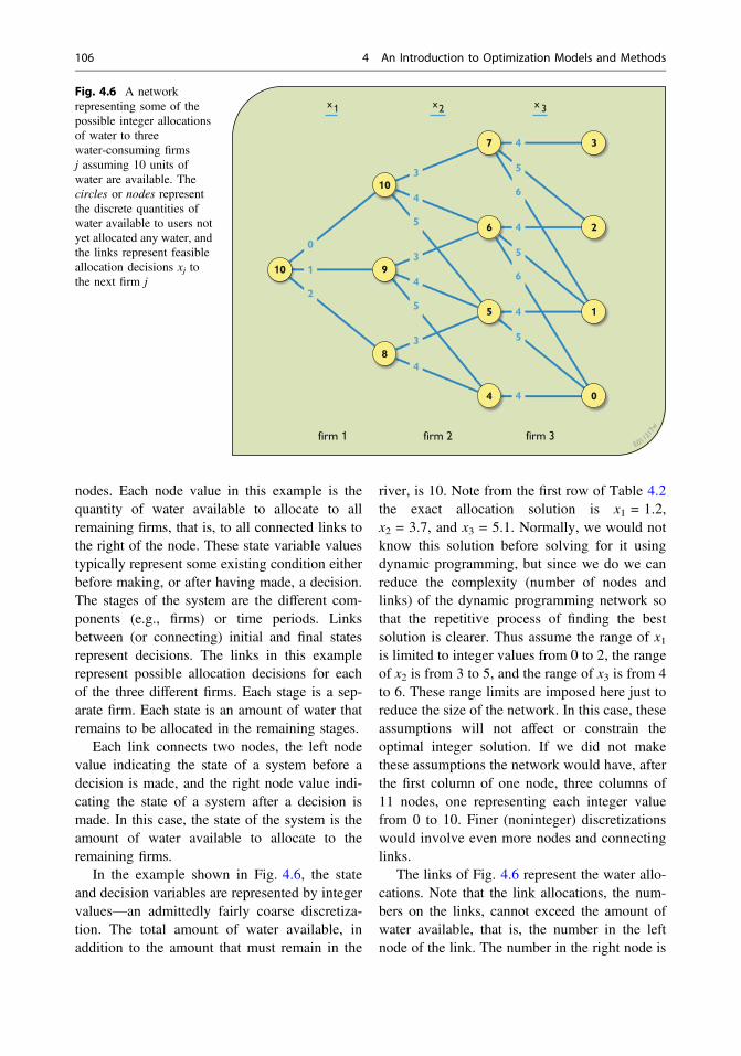
nodes. Each node value in this example is thequantity of water available to allocate to allremaining firms, that is, to all connected links tothe right of the node. These state variable valuestypically represent some existing condition eitherbefore making, or after having made, a decision.The stages of the system are the different com-ponents (e.g., firms) or time periods. Linksbetween (or connecting) initial and final statesrepresent decisions. The links in this examplerepresent possible allocation decisions for eachof the three different firms. Each stage is a sep-arate firm. Each state is an amount of water thatremains to be allocated in the remaining stages.

Each link connects two nodes, the left nodevalue indicating the state of a system before adecision is made, and the right node value indi-cating the state of a system after a decision ismade. In this case, the state of the system is theamount of water available to allocate to theremaining firms.

In the example shown in Fig. 4.6, the stateand decision variables are represented by integervalues—an admittedly fairly coarse discretiza-tion. The total amount of water available, inaddition to the amount that must remain in the

river, is 10. Note from the first row of Table 4.2the exact allocation solution is x1 = 1.2,x2 = 3.7, and x3 = 5.1. Normally, we would notknow this solution before solving for it usingdynamic programming, but since we do we canreduce the complexity (number of nodes andlinks) of the dynamic programming network sothat the repetitive process of finding the bestsolution is clearer. Thus assume the range of x1is limited to integer values from 0 to 2, the rangeof x2 is from 3 to 5, and the range of x3 is from 4to 6. These range limits are imposed here just toreduce the size of the network. In this case, theseassumptions will not affect or constrain theoptimal integer solution. If we did not makethese assumptions the network would have, afterthe first column of one node, three columns of11 nodes, one representing each integer valuefrom 0 to 10. Finer (noninteger) discretizationswould involve even more nodes and connectinglinks.

The links of Fig. 4.6 represent the water allo-cations. Note that the link allocations, the num-bers on the links, cannot exceed the amount ofwater available, that is, the number in the leftnode of the link. The number in the right node is

Fig. 4.6 A networkrepresenting some of thepossible integer allocationsof water to threewater-consuming firmsj assuming 10 units ofwater are available. Thecircles or nodes representthe discrete quantities ofwater available to users notyet allocated any water, andthe links represent feasibleallocation decisions xj tothe next firm j


the quantity of water remaining after an allocationhas been made. The value in the right node, stateSj+1, at the beginning of stage j + 1, is equal to thevalue in the left node, Sj, less the amount of water,xj, allocated to firm j as indicated on the link.Hence, beginning with a quantity of water S1 thatcan be allocated to all three firms, after allocatingx1 to Firm 1 what remains is S2:

S1 � x1 ¼ S2 ð4:48Þ

Allocating x2 to Firm 2, leaves S3.

S2 � x2 ¼ S3 ð4:49Þ

Finally, allocating x3 to Firm 3 leaves S4.

S3 � x3 ¼ S4 ð4:50Þ

Figure 4.6 shows the different values of eachof these states, Sj, and decision variables xjbeginning with a quantity S1 = Q − R = 10. Ourtask is to find the best path through the network,beginning at the leftmost node having a statevalue of 10. To do this we need to know the netbenefits we will get associated with all the links

(representing the allocation decisions we couldmake) at each node (state) for each firm (stage).

Figure 4.7 shows the same network as inFig. 4.6; however the numbers on the links rep-resent the net benefits obtained from the associ-ated water allocations. For the three firms j = 1,2, and 3, the net benefits, NBj(xj), associated withallocations xj are

NB1 x1ð Þ ¼ maximum 12� p1ð Þp1 � 3 p1ð Þ1:30

where p1 � 0:4ðx1Þ0:9ð4:51Þ

NB2 x2ð Þ ¼ maximum 20� 1:5p2ð Þp2 � 5 p2ð Þ1:20

where p2 � 0:5 x2ð Þ0:8ð4:52Þ

NB3 x3ð Þ ¼ maximum 28� 2:5p3ð Þp3 � 6 p3ð Þ1:15

where p3 � 0:6 x3ð Þ0:7ð4:53Þ

The discrete dynamic programming algorithmor procedure is a systematic way to find the bestpath through this network, or any other suitable

Fig. 4.7 Network as inFig. 4.6 representinginteger value allocations ofwater to threewater-consuming firms.The circles or nodesrepresent the discretequantities of wateravailable, and the linksrepresent feasible allocationdecisions. The numbers onthe links indicate the netbenefits obtained fromthese particular integerallocation decisions

4.4 Dynamic Programming 107

network. What makes a network suitable fordynamic programming is the fact that all the nodescan be lined up in a sequence of vertical columnsand each link connects a node in one column toanother node in the next column of nodes. No linkpasses over or through any other column(s) ofnodes. Links also do not connect nodes in thesame column. In addition, the contribution to theoverall objective value (in this case, the total netbenefits) associated with each discrete decision(link) in any stage or for any firm is strictly afunction of the allocation of water to the firm. It isnot dependent on the allocation decisions associ-ated with other stages (firms) in the network.

The main challenge in using discrete dynamicprogramming to solve an optimization problem isto structure the problem so that it fits thisdynamic programming network format. Perhapssurprisingly, many water resources planning andmanagement problems do. But it takes practice tobecome good at converting optimization prob-lems to networks of states, stages, and decisionssuitable for solution by discrete dynamic pro-gramming algorithms.

In this problem the overall objective is to

MaximizeXj

NBjðxjÞ; ð4:54Þ

where NBj(xj) is the net benefit associated with anallocation of xj to firm j. Equations 4.51–4.53define these net benefit functions. As before, theindex j represents the particular firm, and eachfirm is a stage for this problem. Note that the indexor subscript used in the objective function oftenrepresents an object (like a water-using firm) at aplace in space or a time period. These places ortime periods are called the stages of a dynamicprogramming problem. Our task is to find the bestpath from one stage to the next: in other words, thebest allocation decisions for all three firms.

Dynamic programming can be viewed as amultistage decision-making process. Instead ofdeciding all three allocations in one single opti-mization procedure, like Lagrange multipliers,the dynamic programming procedure divides the

problem up into many optimization problems,one for each possible discrete state (e.g., for eachnode representing an amount of water available)in each stage (e.g., for each firm). Given a par-ticular state Sj and stage j—that is, a particularnode in the network—what decision (link) xj willresult in the maximum total net benefits, desig-nated as Fj(Sj), given this state Sj for this and allremaining stages or firms j, j + 1, j + 2 … ? Thisquestion must be answered for each node in thenetwork before one can find the overall best setof decisions for each stage: in other words, thebest allocations to each firm (represented by thebest path through the network) in this example.

Dynamic programming networks can besolved in two ways—beginning at the most rightcolumn of nodes or states and moving from rightto left, called the backward-moving (but forward-looking) algorithm, or beginning at the leftmostnode and moving from left to right, called theforward-moving (but backward-looking) algo-rithm. Both methods will find the best paththrough the network. In some problems, how-ever, only the backward-moving algorithm pro-duces a useful solution. We will revisit this issuewhen we get to reservoir operation where thestages are time periods.

4.4.2 Backward-Moving SolutionProcedure

Consider the network in Fig. 4.7. Again, thenodes represent the discrete states—water avail-able to allocate to all remaining users. The linksrepresent particular discrete allocation decisions.The numbers on the links are the net benefitsobtained from those allocations. We want toproceed through the node-link network from thestate of 10 at the beginning of the first stage to theend of the network in such a way as to maximizetotal net benefits. But without looking at allcombinations of successive allocations we cannotdo this beginning at a state of 10. However, wecan find the best solution if we assume we havealready made the first two allocations and are at


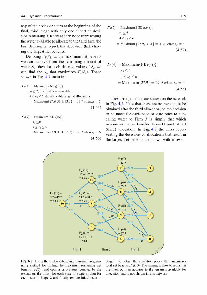
any of the nodes or states at the beginning of thefinal, third, stage with only one allocation deci-sion remaining. Clearly at each node representingthe water available to allocate to the third firm, thebest decision is to pick the allocation (link) hav-ing the largest net benefits.

Denoting F3(S3) as the maximum net benefitswe can achieve from the remaining amount ofwater S3, then for each discrete value of S3 wecan find the x3 that maximizes F3(S3). Thoseshown in Fig. 4.7 include:

F3 7ð Þ ¼ Maximum NB3 x3ð Þf gx3 � 7; the total flow available:

4� x3� 6; the allowable range of allocations

= Maximum 27:9; 31:1; 33:7f g ¼ 33:7when x3 ¼ 6

ð4:55Þ

F3 6ð Þ ¼ Maximum NB3 x3ð Þf gx3 � 6

4� x3 � 6

¼ Maximum 27:9; 31:1; 33:7f g ¼ 33:7when x3 ¼ 6

ð4:56Þ


4� x3 � 6

¼ Maximum 27:9; 31:1f g ¼ 31:1when x3 ¼ 5

ð4:57Þ


4� x3 � 6

¼ Maximum 27:9f g ¼ 27:9 when x3 ¼ 4

ð4:58Þ

These computations are shown on the networkin Fig. 4.8. Note that there are no benefits to beobtained after the third allocation, so the decisionto be made for each node or state prior to allo-cating water to Firm 3 is simply that whichmaximizes the net benefits derived from that last(third) allocation. In Fig. 4.8 the links repre-senting the decisions or allocations that result inthe largest net benefits are shown with arrows.

Fig. 4.8 Using the backward-moving dynamic program-ming method for finding the maximum remaining netbenefits, Fj(Sj), and optimal allocations (denoted by thearrows on the links) for each state in Stage 3, then foreach state in Stage 2 and finally for the initial state in

Stage 1 to obtain the allocation policy that maximizestotal net benefits, F1(10). The minimum flow to remain inthe river, R, is in addition to the ten units available forallocation and is not shown in this network


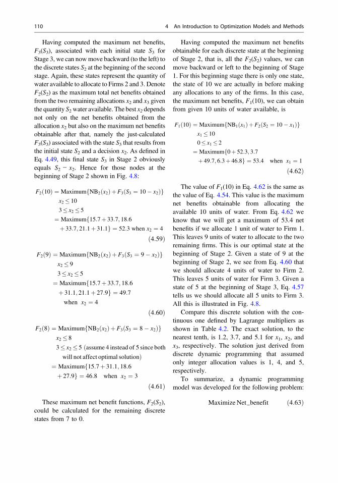
Having computed the maximum net benefits,F3(S3), associated with each initial state S3 forStage 3, we can nowmove backward (to the left) tothe discrete states S2 at the beginning of the secondstage. Again, these states represent the quantity ofwater available to allocate to Firms 2 and 3. DenoteF2(S2) as the maximum total net benefits obtainedfrom the two remaining allocations x2 and x3 giventhe quantity S2 water available. The best x2 dependsnot only on the net benefits obtained from theallocation x2 but also on the maximum net benefitsobtainable after that, namely the just-calculatedF3(S3) associated with the state S3 that results fromthe initial state S2 and a decision x2. As defined inEq. 4.49, this final state S3 in Stage 2 obviouslyequals S2 − x2. Hence for those nodes at thebeginning of Stage 2 shown in Fig. 4.8:

F2 10ð Þ ¼ Maximum NB2 x2ð ÞþF3 S3 ¼ 10� x2ð Þf gx2 � 10

3� x2 � 5

¼ Maximumf15:7þ 33:7; 18:6

þ 33:7; 21:1þ 31:1g ¼ 52:3 when x2 ¼ 4

ð4:59Þ


3� x2 � 5

¼ Maximumf15:7þ 33:7; 18:6

þ 31:1; 21:1þ 27:9g ¼ 49:7

when x2 ¼ 4

ð4:60Þ


3� x2 � 5 ðassume 4 instead of 5 since both

will not affect optimal solutionÞ¼ Maximumf15:7þ 31:1; 18:6

þ 27:9g ¼ 46:8 when x2 ¼ 3

ð4:61Þ

These maximum net benefit functions, F2(S2),could be calculated for the remaining discretestates from 7 to 0.

Having computed the maximum net benefitsobtainable for each discrete state at the beginningof Stage 2, that is, all the F2(S2) values, we canmove backward or left to the beginning of Stage1. For this beginning stage there is only one state,the state of 10 we are actually in before makingany allocations to any of the firms. In this case,the maximum net benefits, F1(10), we can obtainfrom given 10 units of water available, is


0� x1 � 2

¼ Maximumf0þ 52:3; 3:7

þ 49:7; 6:3þ 46:8g ¼ 53:4 when x1 ¼ 1

ð4:62Þ

The value of F1(10) in Eq. 4.62 is the same asthe value of Eq. 4.54. This value is the maximumnet benefits obtainable from allocating theavailable 10 units of water. From Eq. 4.62 weknow that we will get a maximum of 53.4 netbenefits if we allocate 1 unit of water to Firm 1.This leaves 9 units of water to allocate to the tworemaining firms. This is our optimal state at thebeginning of Stage 2. Given a state of 9 at thebeginning of Stage 2, we see from Eq. 4.60 thatwe should allocate 4 units of water to Firm 2.This leaves 5 units of water for Firm 3. Given astate of 5 at the beginning of Stage 3, Eq. 4.57tells us we should allocate all 5 units to Firm 3.All this is illustrated in Fig. 4.8.

Compare this discrete solution with the con-tinuous one defined by Lagrange multipliers asshown in Table 4.2. The exact solution, to thenearest tenth, is 1.2, 3.7, and 5.1 for x1, x2, andx3, respectively. The solution just derived fromdiscrete dynamic programming that assumedonly integer allocation values is 1, 4, and 5,respectively.

To summarize, a dynamic programmingmodel was developed for the following problem:

Maximize Net benefit ð4:63Þ


Subject to

Net benefit ¼ Total return� Total cost

ð4:64Þ

Total return ¼ 12� p1ð Þp1 þ 20� 1:5p2ð Þp2þ 28� 2:5p3ð Þp3

ð4:65Þ

Total cost ¼ 3 p1ð Þ1:30 þ 5 p2ð Þ1:20 þ 6 p3ð Þ1:15ð4:66Þ

p1 � 0:4 x1ð Þ0:9 ð4:67Þ

p2 � 0:5 x2ð Þ0:8 ð4:68Þ

p3 � 0:6 x3ð Þ0:7 ð4:69Þ

x1 þ x2 þ x3 � 10 ð4:70Þ

The discrete dynamic programming version ofthis problem required discrete states Sj repre-senting the amount of water available to allocateto firms j, j + 1, …. It required discrete alloca-tions xj. Next it required the calculation of themaximum net benefits, Fj(Sj), that could beobtained from all firms j, beginning with Firm 3,and proceeding backward as indicated inEqs. 4.71–4.73.

F3 S3ð Þ ¼ maximum NB3 x3ð Þf g over all x3 � S3;

for all discrete S3 values between 0 and 10

ð4:71Þ

F2 S2ð Þ ¼ maximum NB2 x2ð ÞþF3 S3ð Þf gover all x2� S2 and S3 ¼ S2 � x2; 0� S2� 10

ð4:72Þ

F1 S1ð Þ ¼ maximum NB1 x1ð ÞþF2 S2ð Þf gover all x1 � S1 and S2 ¼ S1 � x1 and S1 ¼ 10

ð4:73Þ

The values of each NBj(xj) are obtained fromEqs. 4.51 to 4.53.

To solve for F1(S1) and each optimal alloca-tion xj we must first solve for all values of F3(S3).Once these are known we can solve for all valuesof F2(S2). Given these F2(S2) values, we cansolve for F1(S1). Equations 4.71 need to besolved before Eqs. 4.72 can be solved, andEqs. 4.72 need to be solved before Eqs. 4.73 canbe solved. They need not be solved simultane-ously, and they cannot be solved in reverse order.These three equations are called recursive equa-tions. They are defined for the backward-movingdynamic programming solution procedure.

There is a correspondence between the non-linear optimization model defined by Eqs. 4.63–4.70 and the dynamic programming modeldefined by the recursive Eqs. 4.71–4.73. Notethat F3(S3) in Eq. 4.71 is the same as

F3 S3ð Þ ¼ Maximum NB3 x3ð Þ ð4:74Þ

Subject to

x3 � S3; ð4:75Þ

where NB3(x3) is defined in Eq. 4.53.Similarly, F2(S2) in Eq. 4.72 is the same as

F2 S2ð Þ ¼ MaximumNB2 x2ð ÞþNB3 x3ð Þð4:76Þ

Subject to

x2 þ x3 � S2; ð4:77Þ

where NB2(x2) and NB3(x3) are defined inEqs. 4.52 and 4.53.

Finally, F1(S1) in Eq. 4.73 is the same as

F1 S1ð Þ ¼ MaximumNB1 x1ð ÞþNB2 x2ð ÞþNB3 x3ð Þð4:78Þ

Subject to

x1 þ x2 þ x3 � S1 ¼ 10; ð4:79Þ

where NB1(x1), NB2(x2), and NB3(x3) are definedin Eqs. 4.51–4.53.


Alternatively, F3(S3) in Eq. 4.71 is the same as

F3 S3ð Þ ¼ Maximum 28� 2:5p3ð Þp3 � 6 p3ð Þ1:15ð4:80Þ

Subject to

p3 � 0:6 x3ð Þ0:7 ð4:81Þ

x3 � S3 ð4:82Þ

Similarly, F2(S2) in Eq. 4.72 is the same as

F2 S2ð Þ ¼ Maximum 20� 1:5p2ð Þp2þ 28� 2:5p3ð Þp3� 5 p2ð Þ1:20�6 p3ð Þ1:15

ð4:83Þ

Subject to

p2 � 0:5 x2ð Þ0:8 ð4:84Þ

p3 � 0:6 x3ð Þ0:7 ð4:85Þ

x2 þ x3 � S2 ð4:86Þ

Finally, F1(S1) in Eq. 4.73 is the same as

F1 S1ð Þ ¼ Maximum 12� p1ð Þp1þ 20� 1:5p2ð Þp2 þ 28� 2:5p3ð Þp3� 3 p1ð Þ1:30 þ 5 p2ð Þ1:20 þ 6 p3ð Þ1:15h i

ð4:87Þ

Subject to

p1 � 0:4 x1ð Þ0:9 ð4:88Þ

p2 � 0:5 x2ð Þ0:8 ð4:89Þ

p3 � 0:6 x3ð Þ0:7 ð4:90Þ

x1 þ x2 þ x3 � S1 ¼ 10 ð4:91Þ

The transition function of dynamic program-ming defines the relationship between two

successive states Sj and Sj+1 and the decision xj.In the above example, these transition functionsare defined by Eqs. 4.48–4.50, or, in generalterms for all firms j, by

Sjþ 1 ¼ Sj � xj ð4:92Þ

4.4.3 Forward-Moving SolutionProcedure

We have just described the backward-movingdynamic programming algorithm. In thatapproach at each node (state) in each stage wecalculated the best value of the objective functionthat can be obtained from all further or remainingdecisions. Alternatively one can proceed for-ward, that is, from left to right, through adynamic programming network. For theforward-moving algorithm at each node we needto calculate the best value of the objectivefunction that could be obtained from all pastdecisions leading to that node or state. In otherwords, we need to find how best to get to eachstate Sj+1 at the end of each stage j.

Returning to the allocation example, definefj(Sj+1) as the maximum net benefits from theallocation of water to firms 1, 2, …, j, given theremaining water, state Sj+1. For this example, webegin the forward-moving, but backward-looking,process by selecting each of the ending states in thefirst stage j = 1 and finding the best way to havearrived at (or to have achieved) those ending states.Since in this example there is only one way to getto each of those states, as shown in Fig. 4.7 orFig. 4.8 the allocation decisions, x1, given a valuefor S2 are obvious.

f1 S2ð Þ ¼ maximum NB1 x1ð Þf gx1 ¼ 10� S2

ð4:93Þ

Hence, f1(S2) is simply NB1(10 − S2). Oncethe values for all f1(S2) are known for all discrete


S2 between 0 and 10, move forward (to the right)to the end of Stage 2 and find the best allocationsx2 to have made given each final state S3.

f2 S3ð Þ ¼ maximum NB2 x2ð Þþ f1 S2ð Þf g0� x2 � 10� S3S2 ¼ S3 þ x2

ð4:94Þ

Once the values of all f2(S3) are known for alldiscrete states S3 between 0 and 10, move for-ward to Stage 3 and find the best allocations x3 tohave made given each final state S4.

f3 S4ð Þ ¼ maximum NB3 x3ð Þþ f2 S3ð Þf gfor all discrete S4 between 0 and 10:

0� x3 � 10� S4

S3 ¼ S4 þ x3

ð4:95Þ

Figure 4.9 illustrates a portion of the networkrepresented by Eqs. 4.93–4.95, and the fj(Sj+1)values.

From Fig. 4.9, note the highest total net ben-efits are obtained by ending with 0 remaining

water at the end of Stage 3. The arrow tells usthat if we are to get to that state optimally, weshould allocate 5 units of water to Firm 3. Thuswe must begin Stage 3, or end Stage 2, with10 − 5 = 5 units of water. To get to this state atthe end of Stage 2 we should allocate 4 units ofwater to Firm 2. The arrow also tells us weshould have had 9 units of water available at theend of Stage 1. Given this state of 9 at the end ofStage 1, the arrow tells us we should allocate 1unit of water to Firm 1. This is the same allo-cation policy as obtained using the backward-moving algorithm.

4.4.4 Numerical Solutions

The application of discrete dynamic program-ming to most practical problems will usuallyrequire writing some software. There are nogeneral dynamic programming computer pro-grams available that will solve all dynamic pro-gramming problems. Thus any user of dynamicprogramming will need to write a computerprogram to solve a particular problem unless they

Fig. 4.9 Using theforward-moving dynamicprogramming method forfinding the maximumaccumulated net benefits,fj(Sj + 1), and optimalallocations (denoted by thearrows on the links) thatshould have been made toreach each ending state,beginning with the endingstates in Stage 1, then foreach ending state in Stage 2and finally for the endingstates in Stage 3


do it by hand. Most computer programs writtenfor solving specific dynamic programmingproblems create and store the solutions of therecursive equations (e.g., Eqs. 4.93–4.95) intables. Each stage is a separate table, as shown inTables 4.3, 4.4, and 4.5 for this examplewater-allocation problem. These tables apply toonly a part of the entire problem, namely that partof the network shown in Figs. 4.8 and 4.9. Thebackward solution procedure is used.

Table 4.3 contains the solutions of Eqs. 4.55–4.58 for the third stage. Table 4.4 contains thesolutions of Eqs. 4.59–4.61 for the second stage.Table 4.5 contains the solution of Eq. 4.62 forthe first stage.

From Table 4.5 we see that, given 10 units ofwater available, we will obtain 53.4 net benefits

and to get this we should allocate 1 unit to Firm1. This leaves 9 units of water for the remainingtwo allocations. From Table 4.4 we see that for astate of 9 units of water available we shouldallocate 4 units to Firm 2. This leaves 5 units.From Table 4.3 for a state of 5 units of wateravailable we see we should allocate all 5 of themto Firm 3.

Performing these calculations for variousdiscrete total amounts of water available, sayfrom 0 to 38 in this example, will define anallocation policy (such as the one shown inFig. 4.5 for a different allocation problem) forsituations when the total amount of water is lessthan that desired by all the firms. This policy canthen be simulated using alternative time series ofavailable amounts of water, such as streamflows,

Table 4.3 Computing the values of F3(S3) and optimal allocations x3 for all states S3 in Stage 3

Table 4.4 Computing the values of F2(S2) and optimal allocations x2 for all states S2 in Stage 2


to obtain estimates of the time series (or statis-tical measures of those time series) of net benefitsobtained by each firm, assuming the allocationpolicy is followed over time.

4.4.5 Dimensionality

One of the limitations of dynamic programmingis handling multiple state variables. In ourwater-allocation example, we had only one statevariable: the total amount of water available. Wecould have enlarged this problem to include othertypes of resources the firms require to make theirproducts. Each of these state variables wouldneed to be discretized. If, for example, onlym discrete values of each state variable are con-sidered, for n different state variables (e.g., typesof resources) there are mn different combinationsof state variable values to consider at each stage.As the number of state variables increases, thenumber of discrete combinations of state variablevalues increases exponentially. This is calleddynamic programming’s “curse of dimensional-ity”. It has motivated many researchers to searchfor ways of reducing the number of possiblediscrete states required to find an optimal solu-tion to large multistate-variable problems.

4.4.6 Principle of Optimality

The solution of dynamic programming models ornetworks is based on a principal of optimality

(Bellman 1957). The backward-moving solutionalgorithm is based on the principal that no matterwhat the state and stage (i.e., the particular nodeyou are at), an optimal policy is one that pro-ceeds forward from that node or state and stageoptimally. The forward-moving solution algo-rithm is based on the principal that no matterwhat the state and stage (i.e., the particular nodeyou are at), an optimal policy is one that hasarrived at that node or state and stage in anoptimal manner.

This “principle of optimality” is a very simpleconcept but requires the formulation of a set ofrecursive equations at each stage. It also requiresthat either in the last stage (j = J) for abackward-moving algorithm, or in the first stage(j = 1) for a forward-moving algorithm, thefuture value functions, Fj+1(Sj+1), associated withthe ending state variable values, or past valuefunctions, f0(S1), associated with the beginningstate variable values, respectively, all equal someknown value. Usually that value is 0 but notalways. This condition is needed in order tobegin the process of solving each successiverecursive equation.

4.4.7 Additional Applications

Among the common dynamic programmingapplications in water resources planning arewater allocations to multiple uses, infrastructurecapacity expansion, and reservoir operation.The previous three-user water-allocation problem

Table 4.5 Computing the values of F1(S1) and optimal allocations x1, for all states S1, in Stage 1


(Fig. 4.1) illustrates the first type of application.The other two applications are presented below.

4.4.7.1 Capacity ExpansionHow much infrastructure should be built, whenand why? Consider a municipality that must planfor the future expansion of its water supply sys-tem or some component of that system, such as areservoir, aqueduct, or treatment plant. Thecapacity needed at the end of each future periodt has been estimated to be Dt. The cost, Ct(st, xt)of adding capacity xt in each period t is a functionof that added capacity as well as of the existingcapacity st at the beginning of the period. Theplanning problem is to find that time sequence ofcapacity expansions that minimizes the presentvalue of total future costs while meeting thepredicted capacity demand requirements. This isthe usual capacity expansion problem.

This problem can be written as an optimiza-tion model: The objective is to minimize thepresent value of the total cost of capacityexpansion.

MinimizeXt

Ct st; xtð Þ; ð4:96Þ

where Ct(st, xt) is the present value of the cost ofcapacity expansion xt in period t given an initialcapacity of st.

The constraints of this model define the mini-mum required final capacity in each period t, orequivalently the next period’s initial capacity, st+1,as a function of the known existing capacity s1and each expansion xt up through period t.

stþ 1 ¼ s1 þXs¼1;t

xs for t ¼ 1; 2; . . .; T

ð4:97Þ

Alternatively these equations may be expres-sed by a series of continuity relationships:

stþ 1 ¼ st þ xt for t ¼ 1; 2; . . .; T ð4:98Þ

In this problem, the constraints must alsoensure that the actual capacity st+1 at the end of

each future period t is no less than the capacityrequired Dt at the end of that period.

stþ 1 �Dt for t ¼ 1; 2; . . .; T ð4:99Þ

There may also be constraints on the possibleexpansions in each period defined by a set Ωt offeasible capacity additions in each period t:

xt 2 Xt ð4:100Þ

Figure 4.10 illustrates this type of capacityexpansion problem. The question is how muchcapacity to add and when. It is a significantproblem for several reasons. One is that the costfunctions Ct(st, xt) typically exhibit fixed costsand economies of scale, as illustrated in Fig. 4.11.Each time any capacity is added there are fixed aswell as variable costs incurred. Fixed and variablecosts that show economies of scale (decreasingaverage costs associated with increasing capacityadditions) motivate the addition of excesscapacity, capacity not needed immediately butexpected to be needed in the future to meet anincreased demand for additional capacity.

The problem is also important because anyestimates made today of future demands, costsand interest rates are likely to be wrong. Thefuture is uncertain. Its uncertainties increase thefurther the future. Capacity expansion plannersneed to consider the future if their plans are to becost-effective and not myopic from assuming

Fig. 4.10 A demand projection (solid blue line) and apossible capacity expansion schedule (red line) formeeting that projected demand over time


there is no future. Just how far into the future dothey need to look? And what about the uncer-tainty in all future costs, demands, and interestrate estimates? These questions will be addressedafter showing how the problem can be solved forany fixed-planning horizon and estimates offuture demands, interest rates, and costs.

The constrained optimization model definedby Eqs. 4.96–4.100 can be restructured as amultistage decision-making process and solvedusing either a forward or backward-moving dis-crete dynamic programming solution procedure.The stages of the model will be the time periodst. The states will be either the capacity st+1 at theend of a stage or period t if a forward-movingsolution procedure is adopted, or the capacity st,at the beginning of a stage or period t if abackward-moving solution procedure is used.

A network of possible discrete capacity statesand decisions can be superimposed onto thedemand projection of Fig. 4.9, as shown inFig. 4.12. The solid blue circles in Fig. 4.12represent possible discrete states, St, of the sys-tem, the amounts of additional capacity existingat the end of each period t − 1 or equivalently atthe beginning of period t.

Consider first a forward-moving dynamicprogramming algorithm. To implement this,define ft(st+1) as the minimum cost of achieving acapacity st+1, at the end of period t. Since at thebeginning of the first period t = 1, the accumu-lated least cost is 0, f0(s1) = 0.

Hence, for each final discrete state s2 in staget = 1 ranging from D1 to the maximum demandDT, define

f1 s2ð Þ ¼ min C1 s1; x1ð Þf g in which the discrete x1¼ s2 and s1 ¼ 0

ð4:101ÞMoving to stage t = 2, for the final discrete

states s3 ranging from D2 to DT,

f2 s3ð Þ ¼ min C2 s2; x2ð Þ þ f1 s2ð Þf gover all discrete x2 between 0

and s3 � D1 and s2 ¼ s3 � x2

ð4:102Þ

Moving to stage t = 3, for the final discretestates s4 ranging from D3 to DT,

f3 s4ð Þ ¼min C3 s3; x3ð Þþ f2 s3ð Þf gover all discrete x3between 0

and s4 � D2 and s3 ¼ s4 � x3

ð4:103ÞIn general for all stages t between the first and

last:

ft stþ 1ð Þ ¼ minfCtðst; xtÞþ ft�1 stð Þgover all discrete xt between 0

and stþ 1 � Dt�1 and st ¼ stþ 1 � xt

ð4:104ÞFor the last stage t = T and for the final dis-

crete state sT+1 = DT,

Fig. 4.11 Typical cost function for additional capacitygiven an existing capacity. The cost function shows thefixed costs, C0, required if additional capacity is to beadded, and the economies of scale associated with theconcave portion of the cost function Fig. 4.12 Network of discrete capacity expansion deci-

sions (links) that meet the projected demand


fT sT þ 1ð Þ ¼ minfCTðsT ; xTÞþ fT�1 sTð Þgover all discrete xTbetween 0 andDT � DT�1

where sT ¼ sT þ 1 � xT

ð4:105Þ

The value of fT(sT+1) is the minimum presentvalue of the total cost of meeting the demand forT time periods. To identify the sequence ofcapacity expansion decisions that results in thisminimum present value of the total cost requiresbacktracking to collect the set of best decisions xtfor all stages t. A numerical example will illus-trate this.

A numerical exampleConsider the five-period capacity expansionproblem shown in Fig. 4.12. Figure 4.13 is the

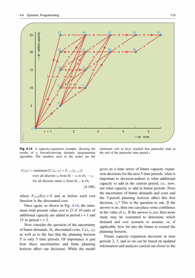
same network with the present value of the ex-pansion costs on each link. The values of thestates, the existing capacities, represented by thenodes, are shown on the left vertical axis. Thecapacity expansion problem is solved onFig. 4.14 using the forward-moving algorithm.

From the forward-moving solution to thedynamic programming problem shown inFig. 4.14, the present value of the cost of theoptimal capacity expansion schedule is 23 unitsof money. Backtracking (moving left against thearrows) from the farthest right node, this sched-ule adds 10 units of capacity in period t = 1, and15 units of capacity in period t = 3.

Next consider the backward-moving algo-rithm applied to this capacity expansion problem.The general recursive equation for abackward-moving solution is

Fig. 4.13 A discrete capacity expansion network show-ing the present value of the expansion costs associatedwith each feasible expansion decision. Finding the best

path through the network can be done using forward orbackward-moving discrete dynamic programming


Ft stð Þ ¼ minimumfCtðst; xtÞþFtþ 1 stþ 1ð Þgover all discrete xt from Dt � st to DT � stfor all discrete states st from Dt�1 to DT

;

ð4:106Þ

where FT+1(DT) = 0 and as before each costfunction is the discounted cost.

Once again, as shown in Fig. 4.14, the mini-mum total present value cost is 23 if 10 units ofadditional capacity are added in period t = 1 and15 in period t = 3.

Now consider the question of the uncertaintyof future demands, Dt, discounted costs, Ct(st, xt),as well as to the fact that the planning horizonT is only 5 time periods. Of importance is justhow these uncertainties and finite planninghorizon affect our decisions. While the model

gives us a time series of future capacity expan-sion decisions for the next 5 time periods, what isimportant to decision-makers is what additionalcapacity to add in the current period, i.e., now,not what capacity to add in future periods. Doesthe uncertainty of future demands and costs andthe 5-period planning horizon affect this firstdecision, x1? This is the question to ask. If theanswer is no, then one can place some confidencein the value of x1. If the answer is yes, then morestudy may be warranted to determine whichdemand and cost scenario to assume, or, ifapplicable, how far into the future to extend theplanning horizon.

Future capacity expansion decisions in timeperiods 2, 3, and so on can be based on updatedinformation and analyses carried out closer to the

Fig. 4.14 A capacity-expansion example, showing theresults of a forward-moving dynamic programmingalgorithm. The numbers next to the nodes are the

minimum cost to have reached that particular state atthe end of the particular time period t


time those decisions are to be made. At thosetimes, the forecast demands and economic costestimates can be updated and the planning hori-zon extended, as necessary, to a period that againdoes not affect the immediate decision. Note thatin the example problem shown in Figs. 4.14 and4.15, the use of 4 periods instead of 5 would haveresulted in the same first-period decision. Thereis no need to extend the analysis to 6 or moreperiods.

To summarize: What is important todecision-makers is what additional capacity toadd now. While the current period’s capacityaddition should be based on the best estimates offuture costs, interest rates and demands, once asolution is obtained for the capacity expansionrequired for this and all future periods up to some

distant time horizon, one can then ignore all butthat first decision, x1: that is, what to add now.Then just before the beginning of the secondperiod, the forecasting and analysis can beredone with updated data to obtain an updatedsolution for what if any capacity to add in period2, and so on into the future. Thus, thesesequential decision making dynamic program-ming models can be designed to be used in asequential decision-making process.

4.4.7.2 Reservoir OperationReservoir operators need to know how muchwater to release and when. Reservoirs designed tomeet demands for water supplies, recreation,hydropower, the environment and/or flood con-trol need to be operated in ways that meet those

Fig. 4.15 A capacity-expansion example, showing theresults of a backward-moving dynamic programmingalgorithm. The numbers next to the nodes are the

minimum remaining cost to have the particular capacityrequired at the end of the planning horizon given theexisting capacity of the state


demands in a reliable and effective manner. Sincefuture inflows or storage volumes are uncertain,the challenge, of course, is to determine the bestreservoir release or discharge for a variety ofpossible inflows and storage conditions that couldexist or happen in each time period t in the future.

Reservoir release policies are often defined inthe form of what are called “rule curves.” Fig-ure 4.17 illustrates a rule curve for a singlereservoir on the Columbia River in the north-western United States. It combines componentsof two basic types of release rules. In both ofthese, the year is divided into various discretewithin-year time periods. There is a specifiedrelease for each value of storage in eachwithin-year time period. Usually higher storage

zones are associated with higher reservoir relea-ses. If the actual storage is relatively low, thenless water is usually released so as to hedgeagainst a continuing water shortage or drought.

Release rules may also specify the desiredstorage level for the time of year. The operator isto release water as necessary to achieve thesetarget storage levels. Maximum and minimumrelease constraints might also be specified thatmay affect how quickly the target storage levelscan be met. Some rule curves define multipletarget storage levels depending on hydrological(e.g., snow pack) conditions in the upstreamwatershed, or on the forecast climate conditionsas affected by ENSO cycles, solar geomagneticactivity, ocean currents and the like.

Fig. 4.16 An example reservoir rule curve specifyingthe storage targets and some of the release constraints,given the particular current storage volume and time ofyear. The release constraints also include the minimum

and maximum release rates and the maximum down-stream channel rate of flow and depth changes that canoccur in each month


Reservoir release rule curves for a year, suchas that shown in Fig. 4.16, define a policy thatdoes not vary from one year to the next. Theactual releases will vary, however, depending onthe inflows and storage volumes that actuallyoccur. The releases are often specified indepen-dently of future inflow forecasts. They are typi-cally based only on existing storage volumes andwithin-year periods—the two axes of Fig. 4.16.

Release rules are typically derived from trialand error simulations. To begin these simulations

it is useful to have at least an approximate idea ofthe expected impact of different alternative poli-cies on various system performance measures orobjectives. Policy objectives could be the maxi-mization of expected annual net benefits fromdownstream releases, reservoir storage volumes,hydroelectric energy and flood control, or theminimization of deviations from particularrelease, storage volume, hydroelectric energy orflood flow targets or target ranges. Discretedynamic programming can be used to obtain

Fig. 4.17 Network representation of the four-seasonreservoir release problem. Given any initial storagevolume St at the beginning of a season t, and an expected

inflow of Qt during season t, the links indicate thepossible release decisions corresponding to those inTable 4.7


initial estimates of reservoir-operating policiesthat meet these and other objectives. The resultsof discrete dynamic programming can beexpressed in the form shown in Fig. 4.17.

A numerical exampleAs a simple example, consider a reservoir havingan active storage capacity of 20 million cubicmeters, or for that matter any specified volumeunits. The active storage volume in the reservoircan vary between 0 and 20. To use discretedynamic programming, this range of possiblestorage volumes must be divided into a set ofdiscrete values. These will be the discrete statevariable values. In this example let the range ofstorage volumes be divided into intervals of 5storage volume units. Hence, the initial storagevolume, St, can assume values of 0, 5, 10, 15, and20 for all periods t.

For each period t, let Qt be the mean inflow,Lt(St, St+1) the evaporation and seepage lossesthat depend on the initial and final storage vol-umes in the reservoir, and Rt the release or dis-charge from the reservoir. Each variable isexpressed as volume units for the period t.

Storage volume continuity requires that ineach period t the initial active storage volume, St,plus the inflow, Qt, less the losses, Lt(St, St+1),and release, Rt, equals the final storage, orequivalently the initial storage, St+1, in the fol-lowing period t + 1. Hence

St þQt � Rt � LtðSt; Stþ 1Þ ¼ Stþ 1 for each period t:

ð4:107Þ

To satisfy the requirement (imposed for con-venience in this example) that each storage vol-ume variable be a discrete value over the rangefrom 0 to 20 in units of 5, the releases, Rt, mustbe such that when Qt − Rt − Lt(St, St+1) is addedto St the resulting value of St+1 is one of the fivediscrete numbers between 0 and 20.

Assume four within-year periods t in each year(kept small for this illustrative example). In thesefour seasons assume the mean inflows, Qt, are 24,12, 6, and 18, respectively. Table 4.6 defines the

evaporation and seepage losses based on differentdiscrete combinations of initial and final storagevolumes for each within-year period t.

Rounding these losses to the nearest integervalue, Table 4.7 shows the net releases associ-ated with initial and final storage volumes. Theyare computed using Eq. 4.107. The informationin Table 4.7 allows us to draw a network repre-senting each of the discrete storage volume states(the nodes), and each of the feasible releases (thelinks). This network for the four seasons t in theyear is illustrated in Fig. 4.17.

This reservoir-operating problem is a multi-stage decision-making problem. As Fig. 4.17illustrates, at the beginning of any season t, thestorage volume can be in any of the five discretestates. Given the state, a release decision is to bemade. This release will depend on the state: theinitial storage volume and the mean inflow, aswell as the losses that may be estimated based onthe initial and final storage volumes, as defined inTable 4.6. The release will also depend on whatis to be accomplished—that is, the objectives tobe satisfied.

For this example, assume there are varioustargets that water users would like to achieve.Downstream water users want reservoir operatorsto meet their flow targets. Individuals who usethe lake for recreation want the reservoir opera-tors to meet storage volume or storage leveltargets. Finally, individuals living on the down-stream floodplain want the reservoir operators toprovide storage capacity for flood protection.Table 4.8 identifies these different targets that areto be met, if possible, for the duration of eachseason t.

Clearly, it will not be possible to meet allthese storage volume and release targets in allfour seasons, given inflows of 24, 12, 6, and 18,respectively. Hence, the objective in this examplewill be to do the best one can: to minimize aweighted sum of squared deviations from each ofthese targets. The weights reflect the relativeimportance of meeting each target in each seasont. Target deviations are squared to reflect the fact


Table 4.6 Evaporation and seepage losses based on initial and final storage volumes for example reservoir-operatingproblem


Table 4.7 Discrete releases associated with initial and final storage volumes for example reservoir-operating problem


that the marginal “losses” associated with devi-ations increase with increasing deviations. Smalldeviations are not as serious as larger deviations,and it is better to have numerous small deviationsrather than a few larger ones.

During the recreation season (periods 2 and 3),deviations below or above the recreation storagelake volume targets are damaging. During theflood season (period 1), any storage volume inexcess of the flood control storage targets of 15reduces the flood storage capacity. Deviationsbelow that flood control target are not penalized.Flood control and recreation storage targets dur-ing each season t apply throughout the season,thus they apply to the initial storage St as well asto the final storage St+1 in appropriate periods t.

The objective is to minimize the sum of totalweighted squared deviations, TSDt, over allseasons t from now on into the future:

MinimizeXt

TSDt ; ð4:108Þ

where

TSDt ¼ wst TS� Stð Þ2 þðTS� Stþ 1Þ2h i

þ wft EStð Þ2 þ ðEStþ 1Þ2h i

þwrt DR2t

� �

ð4:109Þ

In the above equation, when t = 4, the lastperiod of the year, the following period t + 1 = 1,the first period in the following year. Each ESt isthe storage volume in excess of the flood storagetarget volume, TF. Each DRt is the differencebetween the actual release, Rt, and the targetrelease, TRt, when the release is less than the target.

The excess storage, ESt, above the flood targetstorage TF at the beginning of each season t canbe defined by the constraint:

St �TFþESt for periods t ¼ 1 and 2:

ð4:110Þ

The deficit release, DRt, during period t canbe defined by the constraint:

Rt �TRt � DRt for all periods t: ð4:111Þ

The first component of the right side ofEq. 4.109 defines the weighted squared devia-tions from a recreation storage target, TS, at thebeginning and end of season t. In this examplethe recreation season is during periods 2 and 3.The weights, wst, associated with the recreationcomponent of the objective are 1 in periods 2 and3. In periods 1 and 4 the weights, wst, are 0.

The second component of Eq. 4.109 is forflood control. It defines the weighted squared

Table 4.8 Storage volume and release targets for the example reservoir operation problem


deviations associated with storage volumes inexcess of the flood control target volume, TF, atthe beginning and end of the flood season, periodt = 1. In this example, the weights, wft, are 1 forperiod 1 and 0 for periods 2, 3, and 4. Note theconflict between flood control and recreation atthe end of period 1 or equivalently at thebeginning of period 2.

Finally, the last component of Eq. 4.109defines the weighted squared deficit deviationsfrom a release target, TRt, In this example allrelease weights, wrt, equal 1.

Associated with each link in Fig. 4.17 is therelease, Rt, as defined in Table 4.7. Also associ-ated with each link is the sum of weightedsquared deviations, TSDt, that result from theparticular initial and final storage volumes and thestorage volume and release targets identified inTable 4.8. They are computed using Eq. 4.109,with the releases defined in Table 4.7 and targetsdefined in Table 4.8, for each feasible combina-tion of initial and final storage volumes, St andSt+1, for each of the four seasons or periods in ayear. These computed weighted squared devia-tions for each link are shown in Table 4.9.

The goal in this example problem is to find thepath through a multiyear network—each year ofwhich is as shown in Fig. 4.17—that minimizesthe sum of the squared deviations associated witheach of the path’s links. Again, each link’sweighted squared deviations are given inTable 4.9. Of interest is the best path into thefuture from any of the nodes or states (discretestorage volumes) that the system could be in atthe beginning of any season t.

These paths can be found using thebackward-moving solution procedure of discretedynamic programming. This procedure begins atany arbitrarily selected time period or seasonwhen the reservoir presumably produces no fur-ther benefits to anyone (and it does not matterwhen that time is—just pick any time) and pro-ceeds backward, from right to left one stage (i.e.,one time period) at a time, toward the present. Ateach node (representing a discrete storage

volume St and inflow Qt), we can calculate therelease or final storage volume in that period thatminimizes the remaining sum of weightedsquared deviations for all remaining seasons.Denote this minimum sum of weighted squareddeviations for all n remaining seasons t asFnt St;Qtð Þ. This value is dependent on the state

(St, Qt), and stage, t, and the number n ofremaining seasons. It is not a function of thedecision Rt or St+1.

This minimum sum of weighted squareddeviations for all n remaining seasons t is equalto

Fnt St;Qtð Þ ¼ min

Xt¼1;n

TSDtðSt;Rt; Stþ 1Þ

over all feasible values of Rt;

ð4:112Þ

where

Stþ 1 ¼ St þQt � Rt � LtðSt; Stþ 1Þ ð4:113Þ

and

St �K; the capacity of the reservoir ð4:114Þ

The policy we want to derive is called asteady-state policy. Such a policy assumes thereservoir will be operating for a relatively longtime with the same objectives and a repeatablehydrologic time series of seasonal inputs. We canfind this steady-state policy by first assuming thatat some time all future benefits, losses or penal-ties, F

�t ðSt;QtÞ, will be 0.

We can begin in that last season t of reservoiroperation and work backwards toward the pre-sent, moving left through the network one seasont at a time. We can continue for multiple yearsuntil the annual policy begins repeating itselfeach year. In other words, when the optimal Rt

associated with a particular state (St, Qt) is thesame in two or more successive years, and thisapplies for all states (St, Qt) in each season t, asteady-state policy has probably been obtained.


Table 4.9 Total sum of squared deviations, TSDt, associated with initial and final storage volumes

These are calculated using Eqs. 4.109–4.111


(A more definitive test of whether or not asteady-state policy has been reached will bediscussed later.) A steady-state policy will occurif the inflows, Qt, and objectives, TSDt (St, Rt,St+1), remain the same for specific within-yearperiods from year to year. This steady-state pol-icy is independent of the assumption that theoperation will end at some point.

To find the steady-state operating policy forthis example problem, assume the operation endsin some distant year at the end of season 4 (theright-hand side nodes in Fig. 4.17). At the end ofthis season the number of remaining seasons, n,equals 0. The values of the remaining minimumsums of weighted squared deviations, F

�t ðSt;QtÞ

associated with each state (St, Qt), i.e., each node,equal 0. Since for this problem there is no future.Now we can begin the process of finding the bestreleases Rt in each successive season t, movingbackward to the beginning of stage t = 4, thenstage t = 3, then to t = 2, and then to t = 1, andthen to t = 4 of the preceding year, and so on,each move to the left increasing the number ofremaining seasons n by one.

At each stage, or season t, for each discretestate (St, Qt) we can compute the release Rt orequivalently the final storage volume St+1, thatminimizes

Fnt ðSt;QtÞ ¼ MinimumfTSDtðSt;Rt; Stþ 1ÞþFn�1

tþ 1ðStþ 1;Qtþ 1Þg for all 0� St � 20

ð4:115ÞThe decision variable can be either the release,

Rt, or the final storage volume, St+1. If the deci-sion variable is the release, then the constraintson that release Rt are

Rt � St þQt � LtðSt; Stþ 1Þ ð4:116Þ

Rt � St þQt � LtðSt; Stþ 1Þ � 20 the capacityð Þð4:117Þ

and

Stþ 1 ¼ St þQt � Rt � LtðSt; Stþ 1Þ ð4:118Þ

If the decision variable is the final storagevolume, St+1, the constraints on that final storagevolume are

0� Stþ 1 � 20 ð4:119Þ

Stþ 1 � St þQt � LtðSt; Stþ 1Þ ð4:120Þ

and

Rt ¼ St þQt � Stþ 1 � LtðSt; Stþ 1Þ ð4:121Þ

Note that if the decision variable is St+1 inseason t, this decision becomes the state variablein season t + 1. In both cases, the storage vol-umes in each season are limited to discrete values0, 5, 10, 15, and 20.

Tables 4.10, 4.11, 4.12, 4.13, 4.14, 4.15, 4.16,4.17, 4.18 and 4.19 show the values obtainedfrom solving the recursive equations for 10 suc-cessive seasons or stages (2.5 years). Each tablerepresents a stage or season t, beginning withTable 4.10 at t = 4 and the number of remainingseasons n = 1. The data in each table areobtained from Tables 4.7 and 4.9. The last twocolumns of each table represent the best releaseand final storage volume decision(s) associatedwith the state (initial storage volume and inflow).

Note that the policy defining the release orfinal storage for each discrete initial storagevolume in season t = 3 in Table 4.12 is the sameas in Table 4.16, and similarly for season t = 4 inTables 4.13 and 4.17, and for season t = 1 inTables 4.14 and 4.18, and finally for season t = 2in Tables 4.15 and 4.19. The policy differs overeach state, and over each different season, but notfrom year to year for any specified state andseason. This indicates we have reached asteady-state policy. If we kept on computing therelease and final storage policies for precedingseasons, we would get the same policy as thatfound for the same season in the following year.The policy is dependent on the state—the initialstorage volume in this case—and on the season t,


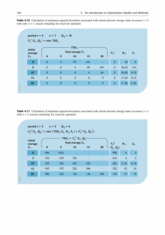
Table 4.10 Calculation of minimum squared deviations associated with various discrete storage states in season t = 4with only n = 1 season remaining for reservoir operation

Table 4.11 Calculation of minimum squared deviations associated with various discrete storage states in season t = 3with n = 2 seasons remaining for reservoir operation


but not on the year. This policy as defined inTables 4.16, 4.17, 4.18 and 4.19 is summarizedin Table 4.20.

This policy can be defined as a rule curve, asshown in Fig. 4.18. It provides a first approxi-mation of a reservoir release rule curve that onecan improve upon using simulation.

Table 4.20 and Fig. 4.18 define a policy thatcan be implemented for any initial storage

volume condition at the beginning of any seasont. This can be simulated under different flowpatterns to determine just how well it satisfies theoverall objective of minimizing the weightedsum of squared deviations from desired, butconflicting, storage and release targets. There areother performance criteria that may also beevaluated using simulation, such as measures ofreliability, resilience, and vulnerability (Chap. 9).

Fig. 4.18 Reservoir rulecurve based on policydefined in Table 4.20. Eachseason is divided intostorage volume zones. Thereleases associated witheach storage volume zoneare specified. Also shownare the storage volumes thatwould result if in each yearthe actual inflows equaledthe inflows used to derivethis rule curve

Table 4.20 The discrete steady-state reservoir-operating policy as computed for this example problem in Tables 4.16,4.17, 4.18 and 4.19


http://dx.doi.org/10.1007/978-3-319-44234-1_9

Assuming the inflows that were used to derivethis policy actually occurred each year, we cansimulate the derived sequential steady-state pol-icy to find the storage volumes and releases thatwould occur in each period, year after year, oncea repetitive steady-state condition were reached.This is done in Table 4.21 for an arbitrary initialstorage volume of 20 in season t = 1. You cantry other initial conditions to verify that itrequires only 2 years at most to reach a repetitivesteady-state policy.

As shown in Table 4.21, if the inflows wererepetitive and the optimal policy was followed,the initial storage volumes and releases would

begin to repeat themselves once a steady-statecondition has been reached. Once reached, thestorage volumes and releases will be the sameeach year (since the inflows are the same). Thesestorage volumes are denoted as a blue line on therule curve shown in Fig. 4.18. The annual totalsquared deviations will also be the same eachyear. As seen in Table 4.21, this annual mini-mum weighted sum of squared deviations for thisexample equals 186. This is what would beobserved if the inflows assumed for this analysisrepeated themselves.

Note from Tables 4.12, 4.13, 4.14, 4.15 and4.16, 4.17, 4.18, 4.19 that once the steady-state

Table 4.21 A simulation of the derived operating policy in Table 4.20

The storage volumes and releases in each period twill repeat themselves each year, after thefirst year. The annual total squareddeviations, TSDt for the specific initial and final storage volumes and release conditions are obtained from Table 4.9


sequential policy has been reached for anyspecified storage volume, St, and season t, theannual difference of the accumulated minimumsum of squared deviations equals a constant,namely the annual value of the objective func-tion. In this case that constant is 186.

Fnþ 1t ðSt;QtÞ � Fn

t ðSt;QtÞ ¼ 186for all St;Qt and t:

ð4:122Þ

This condition indicates a steady-state policyhas been achieved.

This policy in Table 4.21 applies only for theassumed inflows in each season. It does notdefine what to do if the initial storage volumes orinflows differ from those for which the policy isdefined. Initial storage volumes and inflows canand will vary from those specified in the solutionof any deterministic model. One fact is certain:no matter what inflows are assumed in anymodel, the actual inflows will always differ.Hence, a policy as defined in Table 4.20 andFig. 4.18 is much more useful than that inTable 4.21. In Chap. 8 we will modify thisreservoir operation model to define releases orfinal storage volumes as functions of not onlydiscrete storage volumes St but also of discretepossible inflows Qt. However, the policy definedby any relatively simple optimization modelpolicy should be simulated, evaluated, and fur-ther refined in an effort to identify the policy thatbest meets the operating policy objectives.

4.4.8 General Commentson DynamicProgramming

Before ending this discussion of using dynamicprogramming methods for analyzing waterresources planning, management and operatingpolicy problems, we should examine a majorassumption that has been made in each of the

applications presented. The first is that the netbenefits or costs or other objective valuesresulting at each stage of the problem aredependent only on the state and decision variablevalues in each stage. They are independent ofdecisions made at other stages. If the returns atany stage are dependent on the decisions made atother stages, then dynamic programming, withsome exceptions, becomes more difficult toapply. Dynamic programming models can beapplied to design problems, such as the capacityexpansion problem or to operating problems,such as the water-allocation and reservoir oper-ation problems, but rarely to problems havingboth unknown design and operating policydecision variables at the same time. While thereare some tricks that may allow dynamic pro-gramming to be used to find the best solutions toboth design and operating problems encounteredin water resources planning, management andoperating policy studies, other optimizationmethods, perhaps combined with dynamic pro-gramming where appropriate, are often moreuseful.

4.5 Linear Programming

If the objective function and constraints of anoptimization model are all linear, many readilyavailable computer programs exist for finding itsoptimal solution. Surprisingly many waterresource systems problems meet these conditionsof linearity. These linear optimization programsare very powerful, and unlike many other opti-mization methods, they can be applied success-fully to very large optimization problemscontaining many variables and constraints. Manywater resources problems are too large to beeasily solved using nonlinear or dynamic pro-gramming methods. The number of variables andconstraints simply defining mass balances andcapacity limitations in numerous time periods


http://dx.doi.org/10.1007/978-3-319-44234-1_8

can become so big as to preclude the practicaluse of most other optimization methods. Linearprogramming procedures or algorithms for solv-ing linear optimization models are often the mostefficient ways to find solutions to such problems.Hence there is an incentive to convert largeoptimization models to a linear form. Some waysof doing this are discussed later in this chapter.

Because of the availability of computer pro-grams that can solve linear programming prob-lems, linear programming is arguably the mostpopular and commonly applied optimizationalgorithm in practical use today. It is used toidentify and evaluate alternative plans, designsand management policies in agriculture, busi-ness, commerce, education, engineering, finance,the civil and military branches of government,and many other fields.

In spite of its power and popularity, for mostreal-world water resources planning and man-agement problems, linear programming, like theother optimization methods already discussed inthis chapter, is best viewed as a preliminaryscreening tool. Its value is more for reducing thenumber of alternatives for further more detailedsimulations than for finding the best decision.This is not just because approximation methodsmay have been used to convert nonlinear func-tions to linear ones, but more likely because it isdifficult to incorporate all the complexity of thesystem and all the objectives considered impor-tant to all stakeholders into a linear model.Nevertheless, linear programming, like otheroptimization methods, can provide initial designsand operating policy information that simulationmodels require before they can simulate thosedesigns and operating policies.

Equations 4.41 and 4.42 define the generalstructure of any constrained optimization prob-lem. If the objective function F(X) of the vectorX of decision variables xj is linear and if all theconstraints gi(X) in Eq. 4.42 are linear, then themodel becomes a linear programming model.

The general structure of a linear programmingmodel is

Maximize or minimizeXj

Pjxj ð4:123Þ

Subject to

Xj

aijxj � or� bi for i ¼ 1; 2; 3; . . .;m

ð4:124Þ

xj � 0 for j ¼ 1; 2; 3; . . .; n: ð4:125Þ

If any model fits this general form, where theconstraints can be any combination of equalities(=) and inequalities (≥ or ≤), then a large varietyof linear programming computer programs canbe used to find the “optimal” values of all theunknown decision variables xj. Variable non-negativity is enforced within the solution algo-rithms of most commercial linear programmingprograms, eliminating the need to have to specifythese conditions in any particular application.

Potential users of linear programming algo-rithms need to know how to construct linearmodels and how to use the computer programsthat are available for solving them. They do nothave to understand all the mathematical details ofthe solution procedure incorporated in the linearprogramming codes. But users of linear pro-gramming computer programs should understandwhat the solution procedure does and what thecomputer program output means. To begin thisdiscussion of these topics, consider some simpleexamples of linear programming models.

4.5.1 Reservoir StorageCapacity-Yield Models

Linear programming can be used to define stor-age capacity-yield functions for a single or


multiple reservoirs. A storage capacity-yieldfunction defines the maximum constant “de-pendable” reservoir release or yield that will beavailable, at a given level of reliability, duringeach period of operation, as a function of theactive storage volume capacity. The yield fromany reservoir or group of reservoirs will dependon the active storage capacity of each reservoirand the water that flows into each reservoir, i.e.,their inflows. Figure 4.19 illustrates two typicalstorage-yield functions for a single reservoir.

To describe what a yield is and how it can beincreased, consider a sequence of 5 annual flows,say 2, 4, 1, 5, and 3, at a site in an unregulatedstream. Based on this admittedly very limitedrecord of flows, the minimum (historically) “de-pendable” annual flow yield of the stream at thatsite is 1, the minimum observed flow. Assumingthe flow record is representative of what futureflows might be, a discharge of 1 can be “guar-anteed” in each period of record. (In reality, thator any nonzero yield will have a reliability lessthan 1, as will be considered in Chaps. 6 and 10.)

If a reservoir having an active storage capacityof 1 is built, it could store 1 volume unit of flowwhen the flow is greater than 2. It could thenrelease it along with the natural flow when the

natural flow is 1, increasing the minimumdependable flow to 2 units in each year. Storing 2units when the flow is 5, releasing 1 and thenatural flow when that natural flow is 2, andstoring 1 when the flow is 4, and then releasingthe stored 2 units along with the natural flowwhen the natural flow is 1, will permit a yield of3 in each time period with 2 units of activecapacity. This is the maximum annual yield thatis possible at this site, again based on these fiveannual inflows and their sequence. The maxi-mum annual yield cannot exceed the meanannual flow, which in this example is 3. Hence,the storage capacity-yield function equals 1 whenthe active capacity is 0, 2 when the activecapacity is 1, and 3 when the active capacity is 2.The annual yield remains at 3 for any activestorage capacity in excess of 2.

This storage-yield function is dependent notonly on the natural unregulated annual flows butalso on their sequence. For example if thesequence of the same 5 annual flows were 5, 2, 1,3, 4, the needed active storage capacity is 3instead of 2 volume units as before to obtain adependable flow or yield of 3 volume units. Inspite of these limitations of storagecapacity-yield functions, historical records arestill typically used to derive them. (Ways ofaugmenting the historical flow record are dis-cussed in Chap. 6.)

There are many methods available for deriv-ing storage-yield functions. One very versatilemethod, especially for multiple reservoir sys-tems, uses linear programming. Others are dis-cussed in Chap. 10.

To illustrate a storage capacity-yield model,consider a single reservoir that must provide atleast a minimum release or yield Y in each periodt. Assume a record of known (historical or syn-thetic) streamflows at the reservoir site is avail-able. The problem is to find the maximumconstant yield Y obtainable from a given activestorage capacity. The objective is to

Fig. 4.19 Two storage-yield functions for a singlereservoir defining the maximum minimum dependablerelease. These functions can be defined for varying levelsof yield reliability

4.5 Linear Programming 139

http://dx.doi.org/10.1007/978-3-319-44234-1_6

http://dx.doi.org/10.1007/978-3-319-44234-1_10

http://dx.doi.org/10.1007/978-3-319-44234-1_6

http://dx.doi.org/10.1007/978-3-319-44234-1_10

maximize Y ð4:126Þ

This maximum yield is constrained by thewater available in each period, and by thereservoir capacity. Two sets of constraints areneeded to define the relationships among theinflows, the reservoir storage volumes, theyields, any excess release, and the reservoircapacity. The first set of continuity equationsequate the unknown final reservoir storage vol-ume St+1 in period t to the unknown initialreservoir storage volume St plus the knowninflow Qt, minus the unknown yield Y and excessrelease, Rt, if any, in period t. (Losses are beingignored in this example.)

St þQt � Y � Rt ¼ Stþ 1 for each period t¼ 1; 2; 3; . . .; T: T þ 1 ¼ 1

ð4:127Þ

If, as indicated in Eq. 4.127, one assumes thatperiod 1 follows the last period T, it is not nec-essary to specify the value of the initial storagevolume S1 and/or final storage volume ST+1.They are set equal to each other and that variablevalue remains unknown. The resulting“steady-state” solution is based on the inflowsequence that is assumed to repeat itself as wellas the available storage capacity, K.

The second set of required constraints ensuresthat the reservoir storage volumes St at the

beginning of each period t are no greater than theactive reservoir capacity K.

St �K t ¼ l; 2; 3; . . .;T ð4:128Þ

To derive a storage-yield function, the modeldefined by Eqs. 4.126–4.128 must be solved forvarious assumed values of capacity K. Only theinflow values Qt and reservoir active storagecapacity K are assumed known. All other storage,release and yield variables are unknown. Linearprogramming will be able to find their optimalvalues. Clearly, the upper bound on the yieldregardless of reservoir capacity will equal the meaninflow (less any losses if they were included).

Alternatively, one can solve a number of lin-ear programming models that minimize anunknown storage capacity K needed to achievevarious specified yields Y. The resultingstorage-yield functions will be same. The mini-mum capacity needed to achieve a specified yieldwill be the same as the maximum yield obtain-able from the corresponding specified capacityK. However, the specified yield Y cannot exceedthe mean inflow. If an assumed value of the yieldexceeds the mean inflow, there will be no feasi-ble solution to the linear programming model.

Box 4.1 illustrates an example storage-yieldmodel and its solutions to find the storage-yieldfunction. For this problem, and others in thischapter, the program LINGO (freely obtainedfrom www.lindo.com) is used.


http://www.lindo.com

Box 4.1. Example storage capacity-yield model and its solution from LINGO

E02

0903

a

0 5 0 0 0 0 0 5 0 25 15 105 10 5 5 0 5 5 0 0 15 10 5

10 12.5 10 7.5 0 2.5 10 0 0 15 0 2.515 15 10 10 0 15 15 0 0 0 5 018 16 17 11 0 14 18 0 0 0 0 0

:

! Reservoir Storage-Yield Model:Define St as the initial active res. storage, period t,Y as the reliable yield in each period t,Rt as the excess release from the res., period t,Qt as the known inflow volume to the res., period tK as the reservoir active storage volume capacity.;Max = Y ; !Applies to Model 1. Must be omitted for Model 2;Min = K ; !Applies to Model 2. Must be omitted for Model 1;!

Subject to:Mass balance constraints for each of 5 periods t.; S1 + Q1 - Y - R1 = S2;S2 + Q2 - Y - R2 = S3;S3 + Q3 - Y - R3 = S4;S4 + Q4 - Y - R4 = S5;S5 + Q5 - Y - R5 = S1; ! assumes a steady-state condition;! Capacity constraints on storage volumes.;S1 < K; S2 < K; S3 < K; S4 < K; S5 < K;Data:Q1 = 10; Q2 = 5; Q3 = 30; Q4 = 20; Q5 = 15;!Note mean = 16;K = ? ; ! Use for Model 1 only. Allows user to enterany value of K during model run.;Y = ? ; ! Use for Model 2 only. Allows user to enterany value of Y during model run.;Enddata

Before moving to another application of linearprogramming, consider how this storage-yieldproblem, Eqs. 4.126–4.128, can be formulated asa discrete dynamic programmingmodel.Theuse ofdiscrete dynamic programming is clearly not themost efficient way to define a storage-yield func-tion but the problem of finding a storage-yield

function provides a good exercise in dynamicprogramming. The dynamic programming net-work has the same form as shown in Fig. 4.19,where each node is a discrete storage and inflowstate, and the links represent releases. LetFn

t Stð Þ bethe maximum yield obtained given a storagevolume of St at the beginning of period t of a year


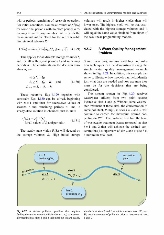
with n periods remaining of reservoir operation.For initial conditions, assume all values of F0

t Stð Þfor some final period t with no more periods n re-maining equal a large number that exceeds themean annual inflow. Then for the set of feasiblediscrete total releases Rt:

Fnt Stð Þ ¼ max min Rt;Fn�1tþ 1ðStþ 1Þ

� �� ð4:129Þ

This applies for all discrete storage volumes Stand for all within-year periods t and remainingperiods n. The constraints on the decision vari-ables Rt are

Rt � St þQt

Rt � St þQt � K; and

Stþ 1 ¼ St þQt � Rt

ð4:130Þ

These recursive Eqs. 4.129 together withconstraint Eqs. 4.130 can be solved, beginningwith n = 1 and then for successive values ofseasons t and remaining periods n, until asteady-state solution is obtained, that is, until

Fnt Stð Þ ¼ Fn�1

t Stð Þfor all values of St and periods t:

ð4:131Þ

The steady-state yields Ft(St) will depend onthe storage volumes St. High initial storage

volumes will result in higher yields than willlower ones. The highest yield will be that asso-ciated with the highest storage volumes and itwill equal the same value obtained from either ofthe two linear programming models.

4.5.2 A Water Quality ManagementProblem

Some linear programming modeling and solu-tion techniques can be demonstrated using thesimple water quality management exampleshown in Fig. 4.21. In addition, this example canserve to illustrate how models can help identifyjust what data are needed and how accurate theymust be for the decisions that are beingconsidered.

The stream shown in Fig. 4.20 receiveswastewater effluent from two point sourceslocated at sites 1 and 2. Without some wastew-ater treatment at these sites, the concentration ofsome pollutant, Pj mg/l, at sites j = 2 and 3, willcontinue to exceed the maximum desired con-centration Pmax

j . The problem is to find the levelof wastewater treatment (waste removed) at sitesi = 1 and 2 that will achieve the desired con-centrations just upstream of site 2 and at site 3 ata minimum total cost.

Fig. 4.20 A stream pollution problem that requiresfinding the waste removal efficiencies (x1, x2) of wastew-ater treatment at sites 1 and 2 that meet the stream quality

standards at sites 2 and 3 at minimum total cost. W1 andW2 are the amounts of pollutant prior to treatment at sites1 and 2


This is the classic water quality managementproblem that is frequently found in the literature,although least-cost solutions have rarely if everbeen applied in practice. There are valid reasonsfor this that we will review later. Nevertheless,this particular problem can serve to illustrate thedevelopment of some linear models for deter-mining data needs as well as for finding, in thiscase, cost-effective treatment efficiencies. Thisproblem can also serve to illustrate graphicallythe general mathematical procedures used forsolving linear programming problems.

The first step is to develop a model that pre-dicts the pollutant concentrations in the stream asa function of the pollutants discharged into it. Todo this we need some notation. Define Wj as themass of pollutant generated at site j (j = 1, 2)each day. Without any treatment and assumingno upstream pollution concentration, the dis-charge of W1 (in units of mass per unit time,(M/T) at site j = 1 results in pollutant concen-tration of P1 in the stream at that site. Thisconcentration, (M/L3) equals the discharge W1

(M/T) divided by the streamflow Q1 (L3/T) atthat site. For example, assuming the concentra-tion is expressed in units of mg/l and the flow isin terms of m3/s, and mass of pollutant dis-charged is expressed as kg/day, and the flowcomponent of the wastewater discharge is neg-ligible compared to the streamflow, the resultingstreamflow concentration P1 at site j = 1 isW1/86.4 Q1:

P1 mg=lð Þ ¼ Mass W1 discharged at site 1 kg=dayð Þ=streamflowQ1 at site 1 m3=s

� �=

kg=106 mg� �

86; 400 s=dayð Þ 103 L=m3� �

¼ W1=86:4Q1

ð4:132Þ

Each unit of a degradable pollutant mass inthe stream at site 1 in this example will decreaseas it travels downstream to site 2. Similarly eachunit of the pollutant mass in the stream at site 2

will decrease as it travels downstream to site 3.The fraction αij of the mass at site i that reachessite j is often assumed to be

aij ¼ exp �ktij� �

; ð4:133Þ

where k is a rate constant (1/time unit) thatdepends on the pollutant and the temperature,and tij is the time (number of time units) it takes aparticle of pollutant to flow from site i to sitej. The actual concentration at the downstreamend of a reach will depend on the streamflow atthat site as well as on the initial pollutant mass,the time of travel and decay rate constant k.

In this example problem, the fraction of pol-lutant mass at site 1 that reaches site 3 is theproduct of the transfer coefficients α12 and α23:

a13 ¼ a12a23 ð4:134Þ

In general, for any site k between sites i and j:

aij ¼ aikakj ð4:135Þ

Knowing the αij values for any pollutant andthe time of flow tij permits the determination ofthe rate constant k for that pollutant and reach, orcontiguous series of reaches, from sites i to j,using Eq. 4.133. If the value of k is 0, the pol-lutant is called a conservative pollutant; salt is anexample of this. Only increased dilution by lesssaline water will reduce its concentration.

For the purposes of determining wastewatertreatment efficiencies or other capital investmentsin infrastructure designed to control the pollutantconcentrations in the stream, some “design”streamflow conditions have to be established.Usually the design streamflow conditions are setat low-flow values (e.g., the lowest monthlyaverage flow expected once in twenty years, orthe minimum 7-day average flow expected oncein ten years). Low design flows are based on theassumption that pollutant concentrations will behigher in low-flow conditions than in higher flow


conditions because of less dilution. Whilelow-flow conditions may not provide as muchdilution, they result in longer travel times, andhence greater reductions in pollutant massesbetween water quality monitoring sites. Hencethe pollutant concentrations may well be greaterat some downstream site when the flow condi-tions are higher than those of the design low-flowvalue.

In any event, given particular design stream-flow and temperature conditions, our first job isto determine the values of these dimensionlesstransfer coefficients αij. They will be independentof the amount of waste discharged into thestream as long as the stream stays aerobic. Todetermine both α12 and α23 in this exampleproblem (Fig. 4.20) requires a number of pollu-tant concentration measurements at sites 1, 2 and3 during design streamflow conditions. Thesemeasurements of pollutant concentrations mustbe made just downstream of the wastewatereffluent discharge at site 1, just upstream anddownstream of the wastewater effluent dischargeat site 2, and at site 3.

Assuming no change in streamflow and noextra pollutant entering the reach that begins atsite 1 and ends just upstream of site 2, the mass(kg/day) of pollutants just upstream of site 2 willequal the mass at site 1, W1, times the transfercoefficient α12:

Mass just upstream of site 2 ¼ W1a12 ð4:136Þ

From this equation and 4.132 one can calcu-late the concentration of pollutants just upstreamof site 2.

The mass of additional pollutant dischargedinto site 2 is W2. Hence the total mass justdownstream of site 2 is W1α12 + W2. At site 3 thepollutant mass will equal the mass just down-stream of site 2, times the transfer coefficient a23.Given a streamflow of Q3 m

3/s and pollutantmasses W1 and W2 kg/day, the pollutant con-centration P3 expressed in mg/l will equal

P3 ¼ ½W1a12 þW2� a23=ð86:4Q3Þ ð4:137Þ

4.5.2.1 Model CalibrationSample measurements are needed to estimate thevalues of each reach’s pollutant transport coeffi-cients aij. Assume five pairs of sample pollutantconcentration measurements have been taken inthe two stream reaches (extending from site 1 tosite 2, and from site 2 to site 3) during designflow conditions. For this example, also assumethat the design streamflow just downstream ofsite 1 and just upstream of site 2 are the same andequal to 12 m3/s. The concentration samplestaken just downstream from site 1 and justupstream of site 2 during this design flow con-dition can be used to solve for the transfercoefficients α12 and α23 after adding error terms.More than one sample is needed to allow formeasurement errors and other random effectssuch as those from varying temperature, wind,incomplete mixing or varying wasteload dis-charges within a day.

Denote the concentrations of each pair ofsample measurements s in the first reach (justdownstream of site 1 and just upstream of site 2)as P1s and P2s and their combined error as Es.Thus

P2s þEs ¼ P1sa12ðQ1=Q2Þ ð4:138Þ

The problem is to find the best estimates ofthe unknown α12. One way to do this is to define“best” as those values of α12 and all Es thatminimize the sum of the absolute values of all theerror terms Es. This objective could be written

MinimizeXs

Esj j ð4:139Þ

The set of Eqs. 4.138 and 4.139 is an opti-mization model. The absolute value signs inEq. 4.139 can be removed by writing each errorterm as the difference between two nonnegativevariables, PEs − NEs. Thus for each sample pair s:


Es ¼ PEs � NEs ð4:140Þ

If any Es is negative, PEs will be 0 and −NEswill equal Es. The actual value of NEs is nonneg-ative. If Es is positive, it will equal PEs, and NEswill be 0. The objective function, Eq. 4.139, thatminimizes the sum of absolute value of error terms,can now be written as one that minimizes the sumof the positive and negative components of Es:

MinimizeXs

ðPEs þNEsÞ ð4:141Þ

Equations 4.139 and 4.140, together withobjective function 4.141 and a set of measure-ments, P1s and P2s, upstream and downstream ofthe reach between sites 1 and 2 define a linearprogramming model that can be solved to findthe transfer coefficient α12. An example illus-trating the solution of this model for the streamreach between site 1 and just upstream of site 2 ispresented in Box 4.2. (In this model the mea-sured concentrations are denoted as SPjs ratherthan Pjs. Again, the program LINGO (www.lindo.com) is used to solve the model).

Box 4.3 contains the model and solution forthe reach beginning just downstream of site 2 tosite 3. In this reach the design streamflow is12.5 m3/s due to the addition of wastewater flowat site 2.

As shown in Boxes 4.2 and 4.3, the values ofthe transfer coefficients are α12 = 0.25 andα23 = 0.60. Thus from Eq. 4.134, α12α23 = α13 = 0.15.

4.5.2.2 Management ModelNow that these parameter values αij are known, awater quality management model can be devel-oped. The water quality management problem,

illustrated in Fig. 4.20, involves finding thefractions xi of waste removal at sites i = 1 and 2that meet the stream quality standards at the endof the two reaches at a minimum total cost.

The pollutant concentration, P2, just upstreamof site 2 that results from the pollutant concen-tration at site 1 equals the total mass of pollutantat site 1 times the fraction α12 that remains at site2, divided by the streamflow Q2 at site 2. Thetotal mass of pollutant at site 1 at the wastewaterdischarge point is the sum of the mass justupstream of the discharge site, P1Q1, plus themass discharged into the stream, W1(1 − x1), atsite 1. The parameter W1 is the total mass ofpollutant entering the treatment plant at site 1.Similarly for site 2. The fraction of wasteremoval, x1, at site 1 is to be determined. Hencethe concentration of pollutant just upstream ofsite 2 is

P2 ¼ ½P1Q1 þW1ð1� x1Þ�a12=Q2 ð4:142Þ

The terms P1 and Q1 are the pollutant con-centration (M/L3) and streamflow (L3/T) justupstream of the wastewater discharge outfall atsite 1. Their product is the mass of pollutant atthat site per unit time period (M/T).

The pollutant concentration, P3, at site 3 thatresults from the pollutant concentration at site 2equals the total mass of pollutant at site 2 timesthe fraction a23. The total mass of pollutant at site2 at the wastewater discharge point is the sum ofwhat is just upstream of the discharge site, P2Q2,plus what is discharged into the stream,W2(1 − x2). Hence the concentration of pollutantat site 3 is

P3 ¼ ½P2Q2 þW2ð1� x2Þ�a23=Q3 ð4:143Þ




Box 4.2. Calibration of water quality model transfer coefficient parameter a12

Equations 4.142 and 4.143 will become thepredictive portion of the water quality manage-ment model. The remaining parts of the modelinclude the restrictions on the pollutant concen-trations just upstream of site 2 and at site 3, andlimits on the range of values that each wasteremoval efficiency, xi, can assume.

Pj �Pmaxj for j ¼ 2 and 3 ð4:144Þ

0� xi � 1:0 for i ¼ 1 and 2: ð4:145Þ

Finally, the objective is to minimize the totalcost of meeting the stream quality standards Pmax

2

and Pmax3 specified in Eqs. 4.144. Letting Ci(xi)

represent the cost function of wastewater treat-ment at sites i = 1 and 2, the objective can bewritten:

Minimize C1 x1ð ÞþC2 x2ð Þ ð4:146Þ

The complete optimization model consists ofEqs. 4.142–4.146. There are four unknowndecision variables, x1; x2, P2, and P3.

Some of the constraints of this optimizationmodel can be combined to remove the twounknown concentration values, P2 and P3.Combining Eqs. 4.142 and 4.144, the concen-tration just upstream of site 2 must be no greaterthan Pmax

2 :


½P1Q1 þW1 1� x1ð Þ�a12=Q2 �Pmax2 ð4:147Þ

Combining Eqs. 4.143 and 4.144, and usingthe fraction α13 (see Eq. 4.134) to predict thecontribution of the pollutant concentration at site1 on the pollutant concentration at Site 3:

P1Q1 þW1 1� x1ð Þ½ �a13 þ W2 1� x2ð Þ½ �a23f g=Q3�Pmax3

ð4:148Þ

Box 4.3. Calibration of water quality model transfer coefficient parameter a23

Equation 4.148 assumes that each pollutantdischarged into the stream can be trackeddownstream, independent of the other pollutantsin the stream. Alternatively, Eq. 4.148 computesthe sum of all the pollutants found at site 2 andthen uses that total mass to compute the con-centration at site 3. Both modeling approachesgive the same results if the parameter values andcost functions are the same.


To illustrate the solution of either of thesemodels, assume the values of the parameters areas listed in Table 4.22. Rewriting the waterquality management model defined byEqs. 4.145–4.148 and substituting the parametervalues in place of the parameters, and recallingthat kg/day = 86.4 (mg/l)(m3/s):

The water quality constraint at site 2,Eq. 4.147, becomes

32ð Þ 10ð Þþ 250; 000 1� x1ð Þ=86:4½ �0:25=12� 20

that when simplified is

x1 � 0:78: ð4:149Þ

The water quality constraint at site 3,Eq. 4.148, becomes

32ð Þ 10ð Þþ 250; 000 1� x1ð Þ=86:4½ �0:15fþ 80; 000 1� x2ð Þ=86:4½ �0:60g=13� 20

that when simplified is

x1 þ 1:28x2 � 1:79: ð4:150ÞRestrictions on fractions of waste removal,

Eq. 4.145, must also be added to this model.The feasible combinations of x1 and x2 can be

shown on a graph, as in Fig. 4.21. This graph is aplot of each constraint, showing the boundariesof the region of combinations of x1 and x2 thatsatisfy all the constraints. This red shaded regionis called the feasible region.

To find the least-cost solution we need the costfunctionsC1(x1) and C2(x2) in Eqs. 4.146. Supposethese functions are not known. Can we determinethe least-cost solutionwithout knowing these costs?Models like the one just developed can be used todetermine just how accurate these cost functions (orthe values of any of the model parameters) need tobe for the decisions being considered.

While the actual cost functions are not knownin this example, their general form can beassumed, as shown in Fig. 4.22. Since thewasteloads produced at site 1 are substantially

Table 4.22 Parameter values selected for the water quality management problem illustrated in Fig. 4.20


greater than those produced at site 2, and givensimilar site, labor, and material cost conditions, itseems reasonable to assume that the cost ofproviding a specified level of treatment at site 1would exceed (or certainly be no less than) thecost of providing the same specified level oftreatment at Site 2. It would also seem the mar-ginal costs at site 1 would be greater than, or atleast no less than, the marginal costs at site 2 for

any given treatment efficiency. The relativepositions of the cost functions shown in Fig. 4.23are based on these assumptions.

Rewriting the cost function, Eq. 4.146, as alinear function converts the model defined byEqs. 4.145–4.148 into a linear programmingmodel. For this example problem, the linearprogramming model can be written as:

0.0

1.5

1.0

0.5

0.0

X 2

X1

0.5 1.0 1.5 2.0

feasible region

equation 157

equation 145

equation 149

equation 150

E02

0103

o

Fig. 4.21 Plot of theconstraints of water qualitymanagement modelidentifying those values ofthe unknown (decision)variables x1 and x2 thatsatisfy all the constraints.These feasible values arecontained in and on theboundaries of the redregion

Fig. 4.22 General form oftotal cost functions forwastewater treatmentefficiencies at sites 1 and 2in Fig. 4.20. The dashedstraight-line slopes c1 andc2 are the average cost perunit (%) removal for 80%treatment. The actualaverage costs clearlydepend on the values of thewaste removal efficienciesx1 and x2, respectively


Minimize c1x1 þ c2x2 ð4:151Þ

Equation 4.151 is minimized subject to con-straints 4.145, 4.149 and 4.150. The values of c1and c2 depend on the values of x1 and x2 and bothpairs are unknown. Even if we knew the values ofx1 and x2 before solving the problem, in thisexample the cost functions themselves (Fig. 4.22)are unknown. Hence, we cannot determine thevalues of the marginal costs c1 and c2. However,we might be able to judge which marginal costwill likely be greater than the other for any par-ticular values of the decision variables x1 and x2.In this example that is all we need to know.

First, assume c1 equals c2. Let c1 x1 + c2 x2equal c and assume c/c1 = 1. Thus the costfunction is x1 + x2 = 1.0. This line can be plottedonto the graph in Fig. 4.21, as shown by line “a”in Fig. 4.23.

Line “a” in Fig. 4.23 represents equal valuesfor c1 and c2, and the total cost, c1 x1 + c2 x2,equal to 1. Keeping the slope of this line constantand moving it upward, representing increasingtotal costs, to line “b”, where it covers the nearestpoint in the feasible region, will identify theleast-cost combination of x1 and x2, againassuming the marginal costs are equal. In thiscase the solution is approximately 80% treatmentat both sites.

Note this particular least-cost solution alsoapplies for any value of c1 greater than c2 (forexample line “c” in Fig. 4.23). If the marginalcost of 80% treatment at site 1 is no less than themarginal cost of 80% treatment at site 2, thenc1 ≥ c2 and indeed the 80% treatment efficiencieswill meet the stream standards for the designstreamflow and wasteload conditions at a totalminimum cost. In fact, from Fig. 4.23 andEq. 4.150, it is clear that c2 has to exceed c1 by amultiple of 1.28 before the least-cost solutionchanges to another solution. For any otherassumption regarding c1 and c2, 80% treatment atboth sites will result in a least-cost solution tomeeting the water quality standards for thosedesign wasteload and streamflow conditions.

If c2 exceeds 1.28c1, as illustrated by line “d”,then the least-cost solution would be x1 = 100%and x2 = 62%. Clearly, in this example themarginal cost, c1, of providing 100% wasteloadremoval at site 1 will exceed the marginal cost,c2, of 60% removal at site 2, and hence, thatcombination of efficiencies would not be aleast-cost one. Thus we can be confident that theleast-cost solution is to remove 80% of the wasteproduced at both waste-generating sites.

Note the least-cost wasteload removal effi-ciencies have been determined without knowingthe cost functions. Why spend money defining

Fig. 4.23 Plots of variousobjective functions (dashedlines) together with theconstraints of the waterquality management model


these functions more precisely? The answer:costs need to be known for financial planning, ifnot for economic analyses. No doubt the actualcosts of installing the least-cost treatment effi-ciencies of 80% will have to be determined forissuing bonds or making other arrangements forpaying the costs. However, knowing theleast-cost removal efficiencies means we do nothave to spend money defining the entire costfunctions Ci(xi). Estimating the construction andoperating costs of achieving just one wastewaterremoval efficiency at each site, namely 80%,should be less expensive than defining the totalcosts for a range of practical treatment plantefficiencies that would be required to define thetotal cost functions, such as shown in Fig. 4.22.

Admittedly this example is relatively simple.It will not always be possible to determine the“optimal” solutions to linear programmingproblems, or other optimization problems, with-out knowing more about the objective functionthan was assumed for this example. However,this exercise illustrates the use of modeling forpurposes other than finding good or “optimal”solutions. Models can help define the necessaryprecision of the data needed to find thosesolutions.

Modeling and data collection and analysisshould take place simultaneously. All too oftenplanning exercises are divided into two stages:data collection and then analysis. Until oneknows what data one will need, and how accuratethose data must be, one need not spend moneyand time collecting them. Conversely, modeldevelopment in the absence of any knowledge ofthe availability and cost of obtaining data canlead to data requirements that are costly, or evenimpossible, to obtain, at least in the time avail-able for decision-making. Data collection andmodel development are activities that should beperformed simultaneously.

Because software is widely available to solvelinear programming programs, because thesesoftware programs can solve very large problemscontaining thousands of variables and con-straints, and finally because there is less chanceof obtaining a local “nonoptimal” solution when

the problem is linear (at least in theory), there isan incentive to use linear programming to solvelarge optimization problems. Especially for largeoptimization problems, linear programming isoften the only practical alternative for finding atleast an approximate optimal solution. Yetmodels representing particular water resourcessystems may not be linear. This motivates the useof methods that can approximate nonlinearfunctions with linear ones, or the use of othersearch algorithms such as those discussed inChap. 5).

The following simple groundwater supplyproblem illustrates the application of some lin-earization methods commonly applied to non-linear separable functions—functions of only oneunknown variable.

These approximation methods typicallyincrease the number of variables and constraintsin a model. Some of these methods require integervariables, or variables that can have values ofonly 0 or 1. There is a practical limit on thenumber of integer variables any linear program-ming software program can handle. Hence, forlarge models there may be a need to performsome preliminary screening designed to reducethe number of alternatives that should be con-sidered in more detail. This example can be usedto illustrate an approach to preliminary screening.

4.5.3 A Groundwater SupplyExample

Consider a water-using industry that plans toobtain water from a groundwater aquifer. Twowellfield sites have been identified. The firstquestion is how much will the water cost, and thesecond, given any specified amount of waterdelivered to the user, is how much should comefrom each wellfield. This situation is illustratedin Fig. 4.24.

Wells and pumps must be installed and oper-ated to obtain water from these two wellfields.The annual cost of wellfield development willdepend on the pumping capacity of the wellfield.Assume that the annual costs associated with


http://dx.doi.org/10.1007/978-3-319-44234-1_5

various capacities QA and QB for Wellfields A andB, respectively, are as shown in Fig. 4.25. Theseare nonlinear functions that contain both fixedand variable costs and hence are discontinuous.The fixed costs result from the fact that some ofthe components required for wellfield develop-ment come in discrete sizes. As indicated in the

figure, the maximum flow capacity of WellfieldsA and B are 17 and 13, respectively.

In Fig. 4.25, the nonlinear functions on theleft have been approximated by piecewise linearfunctions on the right. This is a first step in lin-earizing nonlinear separable functions. Increas-ing the number of linear segments can reduce thedifference between the piecewise linear approxi-mation of the actual nonlinear function and thefunction itself. At the same time it will increasethe number of variables and possibly constraints.

When approximating a nonlinear function by aseries of straight lines, model developers shouldconsider two factors. The first is just how accurateneed be the approximation of the actual functionfor the decisions that will be made, and second isjust how accurate is the actual (in this case non-linear) function in the first place. There is littlevalue in trying to eliminate relatively small errorscaused by the linearization of a function when thefunction itself is highly uncertain. Most cost andbenefit functions, especially those associated withfuture activities, are indeed uncertain.

Fig. 4.24 Schematic of a potential groundwater supplysystem that can serve a water-using industry. Theunknown variables are the flows, QA and QB, from eachwellfield

Fig. 4.25 Annual cost functions associated with the Wellfields A and B as shown in Fig. 4.24. The actual functions areshown on the left, and two sets of piecewise linear approximations are shown on the right


4.5.3.1 A Simplified ModelTwo sets of approximations are shown inFig. 4.26. Consider first the approximationsrepresented by the light blue dot-dash lines.These single straight lines are very crudeapproximations of each function. In this examplethese straight-line cost functions are lowerbounds of the actual nonlinear costs. Hence, theactual costs may be somewhat higher than thoseidentified in the solution of a model.

Using the blue dot-dash linear approximationsin Fig. 4.26, the linear programming model canbe written as follows:

Minimize CostAþCostB ð4:152Þ

Subject to

CostA ¼ 8IA þ 40� 8ð Þ=17½ �QA

linear approximation of C QAð Þð4:153Þ

CostB ¼ 15IB þ 26� 15ð Þ=13½ �QB

linear approximation of C QBð Þð4:154Þ

IA; IB are 0; 1 integer binaryð Þ variablesð4:155Þ

QA � 17IA limitsQA to 17 and forces IA ¼ 1if QA [ 0

ð4:156Þ

QB � 13IB limitsQB to 13 and forces IB ¼ 1if QB [ 0

ð4:157Þ

QA þQB ¼ Qmass balance ð4:158Þ

Q;QA;QB � 0

non-negativity of all decision variables

ð4:159Þ

Q ¼ some specified amount from 0 to 30:

ð4:160Þ

The expressions within the square brackets,[ ], in Eqs. 4.154 and 4.155 above represent theslopes of the dot-dash linear approximations ofthe cost functions. The integer 0, 1 variables arerequired to include the fixed costs in the model.

Solving this linear model for various values ofthe water demand Q provides some interestingresults. Again, they are based on the dot-dashlinear cost functions in Fig. 4.25. As Q increasesfrom 0 to just under 6.8, all the water will comefrom the less expensive Wellfield A. For anyQ from 6.8 to 13, Wellfield B becomes lessexpensive and all the water will come from it. ForanyQ greater than the capacity ofWellfieldB of 13but no greater than the capacity ofWellfield A, 17,all of it will come fromWellfield A. Because of thefixed costs, it is cheaper to use one rather than bothwellfields. Beyond Q = 17, the maximum capac-ity of A, water needs to come from both wellfields.Wellfield B will pump at its capacity, 13, and theadditional water will come from Wellfield A.

Fig. 4.26 Least-costwellfield use given totaldemand Q based on modeldefined by Eqs. 4.152 to4.160


Figure 4.26 illustrates these solutions. Onecan understand why in situations of increasingdemands for Q over time, capacity expansionmodeling might be useful. One would not closedown a wellfield once developed, just to achievewhat would have been a least-cost solution if theexisting wellfield had not been developed.

4.5.3.2 A More Detailed ModelA more accurate representation of these costfunctions may change these solutions for variousvalues of Q, although not significantly. Howeverconsider the more accurate cost minimizationmodel that includes the red solid-line piecewiselinearizations shown in Fig. 4.26.

Minimize CostAþCostB ð4:161Þ

Subject tolinear approximation of cost functions:

CostA ¼ 8IA1 þ 20� 8ð Þ=5½ �QA1f gþ 26IA2 þ ½ 30� 26ð Þ=ð10� 5Þ�QA2f gþ 35IA3 þ ½ 40� 35ð Þ= 17� 10ð Þ�QA3f g

ð4:162Þ

CostB ¼ 15IB1 þ 18� 15ð Þ=3½ �QB1f gþ 18IB2 þ 20� 18ð Þ= 10� 3ð Þ½ �QB2fþ 26� 20ð Þ= 13� 10ð Þ½ �QB3g

ð4:163ÞQA and QB defined.

QA ¼ QA1 þ 5IA2 þQA2ð Þþ 10IA3 þQA3ð Þð4:164Þ

QB ¼ QB1 þ 3IB2 þQB2 þQB3ð Þ ð4:165Þ

IAi and IBi are 0; 1 integer variables

for all segments ið4:166Þ

QA1 � 5IA1QA2 � 10� 5ð ÞIA2;QA3 � 17� 10ð ÞIA3 limitsQAi to width of

segment i and forces IAi ¼ 1 if QAi [ 0

ð4:167Þ

IA1 þ IA2 þ IA3 � 1 limits solution to at most

only one cost function segment i:

ð4:168ÞQB1 � 3IB1;

QB2 � 10� 3ð ÞIB2;QB3 � 13� 10ð ÞIB2 limitsQBi to width of

segment i and forces IBi ¼ 1 if QBi [ 0:

ð4:169ÞIB1 þ IB2 � 1 ð4:170Þ

Q ¼ QA þQB mass balance ð4:171Þ

Q;QA;QB � 0

non-negativityof all decision variables

ð4:172Þ

Q ¼ some specified amount from 0 to 30

ð4:173Þ

Constraint (4.170) limits the solution to atmost only the first segment or to the second andthird segments of the cost function for wellfieldB. Note that a 0, 1 integer variable for the fixedcost of the third segment of this function is notneeded since its slope exceeds that of the secondsegment. However the flow, QB3, in that segmentmust be bounded using the integer 0, 1 variable,IB2, associated with the second segment, asshown in the third of Eqs. 4.169.

The solution to this model, shown in Fig. 4.27,differs from the solution of the simpler model, butonly in the details. Wellfield A supplies all thewater forQ ≤ 4.3. For values ofQ in excess of 4.3up to 13 all the water comes from Wellfield B. Forvalues ofQ in excess of 13 up to 14.8, the capacityof Wellfield B remains at its maximum capacity of13 and Wellfield A provides the additional amountof needed capacity over 13. As Q increases from14.9 to 17, the capacity of Wellfield B drops to 0and the capacity of Wellfield A increases from 14.9to 17. For values ofQ between 17 and 18WellfieldB provides 13, its maximum capacity, and thecapacity of A increases from 4 to 5. For values of


Q from 18.1 to 20, Wellfield B decreases to aconstant 10, and Wellfield A increases from 8.1 to10. For values of Q from 20 to 23, WellfieldA remains at 10 and Wellfield B increases from 10to 13. For values of Q from 23 to 27, WellfieldB again drops to a constant 10 and Wellfield A in-creases from 13 to 17. For values of Q in excess of27,Wellfield A remains at its maximum capacity of17, and Wellfield B increases from 10 to 13.

As in the previous example, this shows theeffect on the least-cost solution when one costfunction has relatively lower fixed and highervariable costs compared with another cost func-tion having relatively higher fixed and lowervariable costs.

4.5.3.3 An Extended ModelIn this example, the simpler model (Eqs. 4.152–4.160) and the more accurate model (Eqs. 4.161–4.173) provided essentially the same allocationsof wellfield capacities associated with a specifiedtotal capacity Q. If the problem contained a lar-ger number of wellfields, the simpler (andsmaller) model might have been able to eliminatesome of these wellfields from further considera-tion. This would reduce the size of any newmodel that approximates the cost functions of theremaining wellfields more accurately.

The model just described, like the capacityexpansion model and water quality managementmodel, is another example of a cost-effectivemodel. The objective was to find the least-cost

way of providing a specified amount of water toa water user. It does not address the problem ofplanning for an increasing demand for Q overtime. Clearly it makes no sense to implement theparticular cost-effective solution for any value ofQ, as shown in Fig. 4.27, as the demand forQ increases, as in this example, from 0 to 30.This is the capacity expansion problem, thesolution of which will benefit from models thattake time into account and that are not static asillustrated previously in this chapter.

Next, consider a cost–benefit analysis inwhich the question is just how much watershould users use. To address this question weassume the user has identified the annual benefitsassociated with various amounts of water. Theannual benefit function, B(Q), and its piecewiselinear approximations, are shown in Fig. 4.28.

The straight, blue, dot-dash linear approxima-tion of the benefit function shown in Fig. 4.28 is anupper bound of the benefits. Incorporating it into amodel that uses the dot-dash linear lower boundapproximations of each cost function, as shown inFig. 4.25 will produce an optimistic solution. It isunlikely that the value of Q that is based on moreaccurate and thus less optimistic benefit and costfunctions will be any greater than the one identi-fied by this simple optimistic model. Furthermore,if any wellfield is not in the solution of this opti-mistic model, with some care we might be able toeliminate that wellfield from further considerationwhen developing a more accurate model.

Fig. 4.27 Least-costwellfield use given totaldemand Q based onEqs. 4.161 to 4.173


Any component of a water resources systemthat does not appear in the solution of a modelthat includes optimistic approximations of per-formance measures that are to be maximized,such as benefits, or that are to be minimized, suchas costs, are candidates for omission in any moredetailed model. This is an example of the processof preliminary screening.

The model defined by Eqs. 4.152–4.160 cannow be modified. Equation 4.160 is eliminatedand the cost minimization objective Eq. 4.152 isreplaced with:

Maximize Benefits� CostAþCostBð Þð4:174Þ

where

Benefits ¼ 10þ 45� 25ð Þ= 21� 9ð Þ½ �Qlinear approximation of B Qð Þ

ð4:175Þ

The solution of this model, Eqs. 4.153–4.159,4.174, and 4.175 (plus the condition that thefixed benefit of 10 only applies if Q > 0, addedbecause it is clear the benefits would be 0 with aQ of 0) indicates that only Wellfield B needs tobe developed, and at a capacity of 10. This wouldsuggest that Wellfield A can be omitted in anymore detailed modeling exercise. To see if thisassumption, in this example, is valid, consider

the more detailed model that incorporates the red,solid-line linear approximations of the cost andbenefit functions shown in Figs. 4.25 and 4.28.

Note that the approximation of the generallyconcave benefit function in Fig. 4.29 will resultin negative values of the benefits for small valuesof Q. For example, when the flow Q, is 0 theapproximated benefits are −10. Yet the actualbenefits are 0 as shown in the left part ofFig. 4.28. Modeling these initial fixed benefitsthe same way as the fixed costs have beenmodeled, using another 0, 1 integer variable,would allow a more accurate representation ofthe actual benefits for small values of Q.

Alternatively, to save having to add anotherinteger variable and constraint to the model, onecan allow the benefits to be negative. If themodel solution shows negative benefits for somesmall value of Q, then obviously the more pre-ferred value of Q, and benefits, would be 0. Thismore approximate trial-and-error approach isoften preferred in practice, especially when amodel contains a large number of variables andconstraints. This is the approach taken here.

4.5.3.4 Piecewise Linear ModelThere are a number of ways of modeling thepiecewise linear concave benefit function shownon the right side of Fig. 4.28. Several are definedin the next several sets of equations. Eachmethod will result in the same model solution.

Fig. 4.28 Benefit function of the amount of water provided to the water user. Piecewise linear approximations of thatfunction of flow are shown on the right


One approach to modeling the concave benefitfunction is to define a new unrestricted (possiblynegative valued) variable. Let this variable beBenefits. When being maximized this variablecannot exceed any of the linear functions thatbound the concave benefit function:

Benefits� � 10þ 25� �10ð Þð Þ=9½ �Q ð4:176Þ

Benefits� 10þ 45� 25ð Þ= 21� 9ð Þ½ �Qð4:177Þ

Benefits� 33þ 50� 45ð Þ= 30� 21ð Þ½ �Qð4:178Þ

Since most linear programming algorithmsassume the unknown variables are nonnegative(unless otherwise specified), unrestricted vari-ables, such as Benefits, can be replaced by thedifference between two nonnegative variables,such as Pben − Nben. Pben will equal Benefits ifits value is greater than 0. Otherwise −Nben willequal Benefits. Thus in place of Benefits inEqs. 4.176–4.178, and those below, one cansubstitute Pben − Nben.

Another modeling approach is to divide thevariable Q into parts, qi, one for each segmenti of the function. These parts sum to Q. Each qi,ranges from 0 to the width of the user-definedsegment i. Thus for the piecewise linear benefitfunction shown on the right of Fig. 4.28:

q1 � 9 ð4:179Þ

q2 � 21� 9 ð4:180Þ

q3 � 30� 21 ð4:181Þ

and

Q ¼ q1 þ q2 þ q3 ð4:182Þ

The linearized benefit function can now bewritten as the sum over all three segments ofeach segment slope times the variable qi:

Benefits ¼ �10þ ½ð25þ 10Þ=9�q1þ 45� 25ð Þ= 21� 9ð Þ½ �q2þ 50� 45ð Þ= 30� 21ð Þ½ �q3

ð4:183Þ

Since the function being maximized is con-cave (decreasing slopes as Q increases), we areassured that each qi + 1 will be greater than 0only if qi is at its upper limit, as defined byconstraint Eqs. 4.179–4.181.

A third method is to define unknown weightswi associated with the breakpoints of the lin-earized function. The value of Q can be expres-sed as the sum of a weighted combination ofsegment endpoint values. Similarly, the benefitsassociated with Q can be expressed as a weightedcombination of the benefits evaluated at thesegment endpoint values. The unknown weightsmust also sum to 1. Hence, for this example:

Benefits ¼ �10ð Þw1 þ 25w2 þ 45w3 þ 50w4

ð4:184Þ

Q ¼ 0w1 þ 9w2 þ 21w3 þ 30w4 ð4:185Þ

1 ¼ w1 þw2 þw3 þw4 ð4:186Þ

For this method to provide the closestapproximation of the original nonlinear function,the solution must include no more than twononzero weights and those nonzero weights mustbe adjacent to each other. For concave functionsthat are to be maximized, this condition will bemet, since any other situation would yield lessbenefits.

The solution to the more detailed modeldefined by Eqs. 4.174, 4.162–4.172, and either4.176–4.178, 4.179–4.183, or 4.184–4.186,


indicates a value of 10 for Q will result in themaximum net benefits. This flow is to come fromWellfield B. This more precise solution is iden-tical to the solution of the simpler model. Clearlythe simpler model could have successfully servedto eliminate Wellfield A from furtherconsideration.

4.5.4 A Review of LinearizationMethods

This section reviews the piecewise linearizationmethods just described and some other approa-ches for incorporating nonlinear conditions intolinear programming models. All of these meth-ods maintain linearity.

If-then-else conditionsThere exist a number of ways “if-then-else” and“and” and “or” conditions (that is, decision trees)can be included in linear programming models.To illustrate some of them, assume X is anunknown decision variable in a model whosevalue may depend on the value of anotherunknown decision variable Y. Assume the maxi-mum value of Y would not exceed Ymax and themaximum value of X would not exceed Xmax.These upper bounds and all the linear constraintsrepresenting “if-then-else” conditions must notrestrict the values of the original decision variableY. Four “if-then-else” (with “and/or”) conditionsare presented below using additional integer 0.1variables, denoted by Z. All the X, Y, and Z vari-ables in the constraints below are assumed to beunknown. These constraints would be included inthe any linear programming model where theparticular “if-then-else” conditions apply.

These illustrations are not unique. At theboundaries of the “if” constraints in the examplesbelow, either of the “then” or “else” conditionscan apply. All variables (X, Y) are assumednonnegative. All variables Z are assumed to be a

binary (0, 1) variables. Note the constraints areall linear.

(a) If Y � 50 then X� 10; else X� 15:Define constraints:

Y � 50 Z þ Ymax 1� Zð ÞY � 50 1� Zð ÞX� 10ZþXmax 1� Zð ÞX� 15 1� Zð Þ

(b) If Y � 50 then X� Y ; else X� Y:Define constraints:

Y � 50Z

Y � 50 1� Zð Þþ YmaxZ

X� Y þXmaxZ

X� Y � Ymax 1� Zð Þ

(c) If Y � 20 or Y � 80 then X ¼ 5; else X� 10:Define constraints:

Y � 20Z1 þ 80Z2 þ Ymax 1� Z1 � Z2ð ÞY � 20Z2 þ 80 1� Z1 � Z2ð ÞZ1 þ Z2 � 1

X� 5 Z1 þ 1� Z1 � Z2ð Þð ÞþXmaxZ2X� 5ðZ1 þð1� Z1 � Z2ÞÞX� 10Z2

(d) If 20 ≤ Y ≤ 50 or 60 ≤ Y ≤ 80, then X ≤ 5,else X ≥ 10.Define constraints:

Y � 20Z1 þ 50Z2 þ 60Z3 þ 80Z4þ Ymax 1� Z1 � Z2 � Z3 � Z4ð Þ:

Y � 20Z2 þ 50Z3 þ 60Z4þ 80 1� Z1 � Z2 � Z3 � Z4ð Þ

Z1 þZ2 þZ3 þZ4 � 1

X� 5 Z2 þ Z4ð ÞþXmax 1� Z2 � Z4ð ÞX� 10 Z1 þ Z3ð Þþ 1� Z1 � Z2 � Z3 � Z4ð Þð Þ


Minimizing the absolute value of the dif-ference between two unknown nonnegativevariables:

Minimize |X − Y| is equivalent to

Minimize D

subject toX � Y �D;

Y � X�D;

X; Y;D� 0:

or

Minimize PDþNDð Þ

subject to

X � Y ¼ PD� ND;

PD;ND;X; Y � 0:

Minimizing the maximum or maximizingthe minimum

Let the set of variables be {X1, X2, X3,…, Xn},Minimizing the maximum of {X1, X2, X3,…, Xn}is equivalent to

Minimize U

subject to

U�Xj; j ¼ 1; 2; 3; . . .; n:

Maximizing the minimum of {X1, X2, X3, …,Xn} is equivalent to

Maximize L

subject to

L�Xj; j ¼ 1; 2; 3; . . .; n:

Linearization of convex functions formaximization or concave function for mini-mization involves 0, 1 binary variables.

Fixed costs in cost functions

Consider functions that have fixed compo-nents if the argument of the function is greaterthan 0.

Cost ¼ C0 þCX if X[ 0;¼ 0 otherwise:

To include these fixed costs in a LP model,define

Cost ¼ C0IþCX

Subject to

X�MI

where M is the maximum value of X, and I is anunknown 0, 1 binary variable.


Minimizing convex functions or maximiz-ing concave functions.

Maximize G Xð Þ ¼ Maximize B

Subject to

I1 þ S1X�B

I2 þ S2X�B

I3 þ S3X�B

Minimize F Xð Þ ¼ S1x1 þ S2x2 þ S3x3Maximize G Xð Þ ¼ S1x1 þ S2x2 þ S3x3

Subject to

X ¼ x1 þ x2 þ x3x1 � a

x2 � b� a


Minimize F Xð Þ ¼ Fð0Þw1 þF að Þw2 þF bð Þw3 þF cð Þw4

Maximize G Xð Þ ¼ Gð0Þw1 þG að Þw2þG bð Þw3 þG cð Þw4

Subject to

X ¼ 0w1 þ aw2 þ bw3 þ c w4

w1 þw2 þw3 þw4 ¼ 1

Minimizing concave functions or maximiz-ing convex functions

Minimize G Xð Þ ffi 5x1 þð20z2 þ 3x2Þþ ð44z3 þ 2x3Þ

Subject to

x1 þð4z2 þ x2Þþ ð12z3 þ x3Þ ¼ X

zs ¼ 0 or 1 for all segments s

x1 � 4z1;

x2 � 8z2;

x3 � 99z3;

z1 þ z2 þ z3 ¼ 1:


Minimizing or maximizing combined con-cave–convex functions

MaximizeC Xð Þ ¼ 5z1 þ 6x1 þ 3x2ð Þþ 53z3 þ 5x3ð Þ

Subject to

x1 þ x2ð Þþ 12z3 þ x3ð Þ ¼ X

x1 � 4z1x2 � 8z1x3 � 99z3z1 þ z3 ¼ 1

z1; z3 ¼ 0; 1

MinimizeCðXÞ ¼ 5z1 þ 6x1ð Þþ 29z2 þ 3x2 þ 5x3ð Þ

Subject to

z1; z2 ¼ 0; 1:

x1 þð4z2 þ x2 þ x3Þ ¼ X

x1 � 4z1x2 � 8z2x3 � 99z2z1 þ z2 � 1

MaximizeC Xð Þ ¼ ð5z1 þ 6x1 þ 3x2Þþ �17z3 þ 5x3ð Þ

Subject to

x1 þ x2ð Þþ x3 ¼ X

z1; z3 ¼ 0; 1

x1 � 4z1x2 � 8z1

x3 � 99z3z1 þ z3 ¼ 1;

MinimizeC Xð Þ ¼ ð5z1 þ 6x1Þþ ð17z2 þ 3x2 þ 5x3Þ

Subject to

x1 þ 4z2 þ x2 þ x3ð Þ ¼ X

z1; z2 ¼ 0; 1:

x1 � 4z1x2 � 12z2x3 � 99z2z1 þ z2 � 1


Maximize or Minimize F(X)

F Xð Þ ¼ ð5z1 þ 6x1Þþ ð35z2 þ 3x2Þþ ð32z3�2x3Þþ 22z4

Subject to

x1 þð4z2 þ x2Þþ ð12z3 þ x3Þþ ð17z4 þ x4Þ ¼ X

x1 � 4z1x2 � 8z2x3 � 5z3x4 � 99z4z1 þ z2 þ z3 þ z4 ¼ 1;

zs ¼ 0; 1 for all segments s

:

4.6 A Brief Review

Before proceeding to other optimization andsimulation methods in the following chapters, itmay be useful to review the topics covered so far.The focus has been on model development aswell as model solution. Several types of waterresources planning and management problemshave been used to illustrate model developmentand solution processes. Like their real-worldcounterparts, the example problems all hadmultiple unknown decision variables and multi-ple constraints. Also like their real-world

counterparts, there are multiple feasible solutionsto each of these problems. Hence, the task is tofind the best solution, or a number of near-bestsolutions. Each solution must satisfy all theconstraints.

Constraints can reflect physical conditions,environmental regulations and/or social or eco-nomic targets. Especially with respect to envi-ronmental or social conditions and goals, it isoften a matter of judgment to decide what isconsidered an objective that is to be minimizedor maximized and what is considered a constraintthat has to be met. For example, do we mini-mize the costs of meeting specified maximumlevels of pollutant concentrations or minimizepollutant concentrations without exceedingspecified costs?

Except for relatively simple problems, the useof these optimization models and methods isprimarily for reducing the number of alternativesthat need to be further analyzed and evaluatedusing simulation methods. Optimization is gen-erally used for preliminary screening—eliminat-ing inferior alternatives before more detailedanalyses are carried out. Presented were someapproaches to preliminary screening involvinghill-climbing, calculus-based Lagrange multi-plier, numerical nonlinear programming, discretedynamic programming, and linear programmingmethods. Each method has its strengths and


limitations. Both linear and nonlinear program-ming models are typically solved using softwarepackages. Many of these software programs arefree and readily available. But before any modelcan be solved, it has to be built. Building modelsis an art and that is what this chapter hasattempted to introduce.

The example problems used to illustrate thesemodeling and model solution methods have beenrelatively simple. However, simple applicationssuch as these can form the foundation of modelsof more complex problems, as will be shown infollowing chapters.

Reference

Bellman, R. E. (1957). Dynamic programming. Princeton,NJ: Princeton University Press.

Additional References(Further Reading)

Bassson, M. S., Allen, R. B., Pegram, G. G. S., & VanRooyen, J. A. (1994). Probabilistic management ofwater resource and hydropower systems. HighlandsRanch, CO: Water Resources Publications.

Beroggi, G. E. G. (1999). Decision modeling in policymanagement: An introduction to analytic concepts.Boston, MA: Kluwer Academic.

Blanchard, B. S., & Fabrycky, W. J. (1998). Systemsengineering and analysis (3rd ed.). Prentice Hall:Upper Saddle River, NJ.

Buras, N. (1966). Dynamic programming and waterresources development, advances in hydroscience(Vol. 3). New York: Academic Press.

Dorfman, R., Jacoby, H. D., & Thomas, H. A., Jr. (1972).Models for managing regional water quality. Cam-bridge, MA: Harvard University Press.

Esogbue, A. O. (Ed.). (1989). Dynamic programming foroptimal water resources systems analysis. PrenticeHall: Englewood Cliffs, NJ.

Hall, W. A., & Dracup, J. A. (1970). Water resourcessystems engineering. New York: McGraw-Hill.

Hillier, F. S., & Lieberman, G. J. (1990a). Introduction tooperations research (5th ed.). New York:McGraw-Hill.

Hillier, F. S., & Lieberman, G. J. (1990b). Introduction tostochastic models in operations research. New York:McGraw-Hill.

Hufschmidt, M. M., & Fiering, M. B. (1966). Simulationtechniques for design of water-resource systems.Cambridge, MA: Harvard University Press.

Kapamoyz, M., Szidarovszky, F., & Zahpaie, B. (2003).Water resources systems analysis. Boca Raton, FL:Lewis.

Loucks, D. P., & da Costa, J. R. (Eds.). (1990). Decisionsupport systems: water resources planning. Berlin:Springer.

Loucks, D. P., Stedinger, J. S., & Haith, D. A. (1981).Water resource systems planning and analysis. Pren-tice Hall: Englewood Cliffs, NJ.

Maass, A., Hufschmidt, M. M., Dorfman, R., Thomas, H.A., Jr., Marglin, S. A., & Fair, G. M. (1962). Designof water-resource systems. Cambridge, MA: HarvardUniversity Press.

Major, D. C., & Lenton, R. L. (1979). Applied waterresources systems planning. Prentice Hall: EnglewoodCliffs, NJ.

Mays, L. W., & Tung, Y.-K. (1992). Hydrosystemsengineering and management. New York:McGraw-Hill.

Newnan, D. G., Lavelle, J. P., & Eschenbach, T. G.(2002). Essentials of engineering economic analysis(2nd ed.). New York: Oxford University Press.

Rardin, R. L. (1998). Optimization in operationsresearch. Prentice Hall: Upper Saddle River, NJ.

Revelle, C. (1999). Optimizing reservoir resources. NewYork: Wiley.

Somlyody, L. (1997). Use of optimization models in riverbasin water quality planning: WATERMATEX’97.In M. B. Beck & P. Lessard (Eds.), Systems analysisand computing in water quality management:Towards a new agenda. London: IWA.

Taylor, B. W., III. (1999). Introduction to managementscience (6th ed.). Prentice Hall: Upper Saddle River,NJ.

Willis, R., & Yeh, W. W.-G. (1987). Groundwatersystems planning and management. Prentice Hall:Englewood Cliffs, NJ.

Winston, W. L. (1994). Operations research: Applicationsand algorithms (3rd edn.). Boston, MA: Duxbury.

Winston, W. L., & Albright, S. C. (2001). Practicalmanagement science (2nd edn.). Pacific Grove, CA:Duxbury.

Wright, J. R., & Houck, M. H. (1995). Water resourcesplanning and managementm, Chap. 37. In W. F. Chen(Ed.), Civil engineering handbook. Boca Raton: CRC.

Wurbs, R. A. (1996). Modeling and analysis of reservoirsystem operations. Prentice Hall: Upper Saddle River,NJ.


Exercises

Engineering economics:

4:1 Consider two alternative water resourceprojects, A and B. Project A will cost$2,533,000 and will return $1,000,000 atthe end of 5 years and $4,000,000 at theend of 10 years. Project B will cost$4,000,000 and will return $2,000,000 atthe end of 5 and 15 years, and another$3,000,000 at the end of 10 years. Pro-ject A has a life of 10 years, and B has alife of 15 years. Assuming an interest rateof 0.1 (10%) per year:

(a) What is the present value of eachproject?

(b) What is each project’s annual netbenefit?

(c) Would the preferred project differ ifthe interest rates were 0.05?

(d) Assuming that each of these projectswould be replaced with a similarproject having the same time stream ofcosts and returns, show that byextending each series of projects to acommon terminal year (e.g.,30 years), the annual net benefits ofeach series of projects will be same asfound in part (b).

4:2 Show that APT

t¼1 ð1þ rÞ�t ¼ ð1þ rÞT�1rð1þ rÞT A,

the present value of a series of equal pay-ments, A, at the end of each year forT years. What is the impact of an increasinginterest rate over time on the present value?

4:3 (a) Show that if compounding occurs atthe end of m equal length periodswithin a year in which the nominalinterest rate is r, then the effectiveannual interest rate, r′, is equal to

r0 ¼ 1þ r

m

� m�1

(b) Show that when compounding is con-tinuous (i.e., when the number ofperiods m → ∞), the compoundinterest factor required to convert apresent value to a future value in yearT is erT. [Hint: Use the fact that

limk!1

ð1þ 1=kÞk ¼ e, the base of natural

logarithms.]

4:4 The term “capitalized cost” refers to thepresent value PV of an infinite series ofend-of-year equal payments, A. Assumingan interest rate of r, show that as the ter-minal period T → ∞, PV = A/r.

4:5 The internal rate of return of any project orplan is the interest rate that equals the pre-sent value of all receipts or income with thepresent value of all costs. Show that theinternal rate of return of projects A and B inExercise 4.1 are approximately 8 and 6%,respectively. These are the interest rates r,for each project, that essentially satisfy theequation

XTt¼0

Rt � Ctð Þð1þ rÞ�t ¼ 0

4:6 In Exercise 4.1, the maximum annualbenefits were used as an economic crite-rion for plan selection. The maximumbenefit–cost ratio, or annual benefits divi-ded by annual costs, is another criterion.Benefit–cost ratios should be no less thanone if the annual benefits are to exceed theannual costs. Consider two projects, Iand II:

Project

I II

Annual benefits 20 2

Annual costs 18 1.5

Annual net benefits 2 0.5

Benefit–cost ratio 1.11 1.3

Exercises 165

What additional information is neededbefore one can determine which project isthe most economical project?

4:7 Bonds are often sold to raise money forwater resources project investments. Eachbond is a promise to pay a specifiedamount of interest, usually semiannually,and to pay the face value of the bond atsome specified future date. The sellingprice of a bond may differ from its facevalue. Since the interest payments arespecified in advance, the current marketinterest rates dictate the purchase price ofthe bond.Consider a bond having a face value of$10,000, paying $500 annually for10 years. The bond or “coupon” interestrate based on its face value is 500/10,000,or 5%. If the bond is purchased for$10,000, the actual interest rate paid to theowner will equal the bond or “coupon”rate. But suppose that one can investmoney in similar quality (equal risk)bonds or notes and receive 10% interest.As long as this is possible, the $10,000,5% bond will not sell in a competitivemarket. In order to sell it, its purchaseprice has to be such that the actual interestrate paid to the owner will be 10%. In thiscase, show that the purchase price will be$6927.The interest paid by the some bonds,especially municipal bonds, may beexempt from state and federal incometaxes. If an investor is in the 30% incometax bracket, for example, a 5% municipaltax-exempt bond is equivalent to about a7% taxable bond. This tax exemptionhelps reduce local taxes needed to pay theinterest on municipal bonds, as well asproviding attractive investment opportu-nities to individuals in high tax brackets.

Lagrange Multipliers4:8 What is the meaning of the Lagrange

multiplier associated with the followingmodel?

Maximize Benefit Xð Þ � Cost Xð ÞSubject to: X� 23

4:9 Assume water can be allocated to threeusers. The allocation, xj, to each use j pro-vides the following returns: R(x1) = (12x1 − x1

2), R(x2) = (8x2 − x22) and

R(x3) = (18x3 − 3x32). Assume that the

objective is to maximize the total return, F(X), from all three allocations and that thesum of all allocations cannot exceed 10.(a) Howmuch would each use like to have?(b) Show that at the maximum total returnsolution the marginal values, ∂(R(xj))/∂xj,are each equal to the shadow price orLagrange multiplier (dual variable) λ asso-ciated with the constraint on the amount ofwater available. (c) Finally, withoutresolving a Lagrange multiplier problem,what would the solution be if 15 units ofwater were available to allocate to the threeusers and what would be the value of theLagrange multiplier?

4:10 In Exercise 4.9, how would the Lagrangemultiplier procedure differ if the objectivefunction, F(X), were to be minimized?

4:11 Assume that the objective was to minimizethe sum of squared deviations of the actualallocations xj from some desired or knowntarget allocations Tj. Given a supply ofwater Q less than the sum of all target al-locations Tj, structure a planning modeland its corresponding Lagrangian. Will aglobal minimum be obtained from solvingthe partial differential equations derivedfrom the Lagrangian? Why?

4:12 Using Lagrange multipliers, prove that theleast-cost design of a cylindrical storagetank of any volume V > 0 has one-third ofits cost in its base and top and two-thirdsof its cost in its side, regardless of the costper unit area of its base or side. (It is thesetypes of rules that end up in handbooks inengineering design.)

4:13 An industrial firm makes two products,A and B. These products require water and


other resources. Water is the scarceresource—they have plenty of other nee-ded resources. The products they make areunique, and hence they can set the unitprice of each product at any value theywant to. However experience tells themthat the higher the unit price for a product,the less amount of that product they willsell. The relationship between unit priceand quantity that can be sold is given bythe following two demand functions.Assume for simplicity that the unit pricefor product A is (8 − A) and for product Bis (6 − 1.5B).

(a) What are the amounts of A and B, andtheir unit prices, that maximize thetotal revenue obtained?

(b) Suppose the total amount of A andB could not exceed some amountTmax. What are the amounts of A andB, and their unit prices, that maximizetotal revenue, if

(i) Tmax = 10(ii) Tmax = 5Water is needed to make each unit ofA and B. The production functionsrelating the amount of water XA nee-ded to make A, and the amount ofwater XB needed to make B, areA = 0.5XA, and B = 0.25XB,respectively.

(c) Find the amounts of A and B and theirunit prices that maximize total revenueassuming the total amount of wateravailable is 10 units.

(d) What is the value of the dual variable,or shadow price, associated with the10 units of available water?

Dynamic programming

4:14 Solve for the optimal integer allocations x1,x2, and x3 for the problem defined byExercise 4.9 assuming the total availablewater is 3 and 4. Also solve for the optimalallocation policy if the total water availableis 7 and each xj must not exceed 4.

4:15 Consider a three-season reservoir opera-tion problem. The inflows are 10, 50 and20 in seasons 1, 2, and 3, respectively.

Find the operating policy that minimizesthe sum of total squared deviations from aconstant storage target of 20 and a con-stant release target of 25 in each of thethree seasons. Develop a discrete dynamicprogramming model that considers only 4discrete storage values: 0, 10, 20 and 30.Assume the releases cannot be less than 10or greater than 40. Show how the model’srecursive equations change depending onwhether the decisions are the releases orthe final storage volumes. Verify theoptimal operating policy is the sameregardless of whether the decision vari-ables are the releases or the final storagevolumes in each period. Which model doyou think is easier to solve? How wouldeach model change if more importancewere given to the desired releases than tothe desired storage volumes?

4:16 Show that the constraint limiting a reser-voir release, rt, to be no greater than the

Quantity of product A Quantity of product B

Po

Unitprice

Po

Unit Price

8 – A 6–1.5B

Exercises 167

initial storage volume, st, plus inflow, it, isredundant to the continuity equationst + it − rt = st + 1.

4:17 Develop a general recursive equation for aforward-moving dynamic programmingsolution procedure for a singlereservoir-operating problem. Define allvariables and functions used. Why is thisnot a very useful approach to finding areservoir-operating policy?

4:18 The following table provides estimates forthe recent values of the costs of additionalwastewater treatment plant capacity nee-ded at the end of each 5-year period for thenext 20 years. Find the capacity expansionschedule that minimizes the present valuesof the total future costs. If there is morethan one least-cost solution, indicatewhich one you think is better, and why?

Discounted cost ofadditional capacity

Total requiredcapacity at end ofperiodUnits of additional

capacity

Periodyears

2 4 6 8 10

1 1–5 12 15 18 23 26 2

2 6–10

8 11 13 15 6

3 11–15

6 8 8

4 16–20

4 10

The cost in each period t must be paid atthe beginning of the period. What was thediscount factor used to convert the costs atthe beginning of each period t to presentvalue costs shown above? In other wordshow would a cost at the beginning ofperiod t be discounted to the beginning ofperiod 1, given an annual interest rate of r?(Only the algebraic expression of the dis-count factor is asked, not the numericalvalue of r.)

4:19 Consider a wastewater treatment plant inwhich it is possible to include five differ-ent treatment processes in series. Thesetreatment processes must together removeat least 90% of the 100 units of influentwaste. Assuming the Ri is the amount ofwaste removed by process i, the followingconditions must hold:

20�R1 � 30

0�R2 � 30

0�R3 � 10

0�R4 � 20

0�R5 � 30

(a) Write the constrained optimization-planning model for finding theleast-cost combination of the removalsRi that together will remove 90% ofthe influent waste. The cost of thevarious discrete sizes of each unitprocess i depend upon the wasteentering the process i as well as theamount of waste removed, as indi-cated in the table below.

Process i 1 2 3 4 5

Influent, Ii Removal, Ri Annual cost = Ci(Ii, Ri)

100 20 5

100 30 10

80 10 3 3 1

80 20 9 2

80 30 13

70 10 4 5 2

70 20 10 3

70 30 15

60 10 6 2 3

60 20 4 6

60 30 9

50 10 7 3 4

50 20 5 8

50 30 10

(continued)


Process i 1 2 3 4 5

Influent, Ii Removal, Ri Annual cost = Ci(Ii, Ri)

40 10 8 5 5

40 20 7 12

40 30 18

30 10 8 8

30 20 10 12

20 10 8

(b) Draw the dynamic programming net-work and solve this problem bydynamic programming. Indicate onthe network the calculations requiredto find the least-cost path from state100 at stage 1 to state 10 at stage 6using both forward- and backward-moving dynamic programming solu-tion procedures.

(c) Could the following conditions beincluded in the original dynamic pro-gramming model and still be solvedwithout requiring R4 to be 0 in the firstcase and R3 to be 0 in the second case?

(i) R4 = 0 if R3 = 0, or(ii) R3 = 0 if R2 ≤ 20.

4:20 The city of Eutro Falls is under a court orderto reduce the amount of phosphorus thatwhich it discharges in its sewage to LakeAlgae. The city presently has threewastewater treatment plants. Each planti currently discharges Pi kg/day of phos-phorus into the lake. Some or all plantsmustreduce their discharges so that the total forthe three plants does not exceed P kg/day.Let Xi be the fraction or percent of thephosphorus removed by additional treat-ment at plant i, and the Ci(Xi) the cost ofsuch treatment ($/year) at each plant i.

(a) Structure a planning model to deter-mine the least-cost (i.e., a cost effec-tive) treatment plant for the city.

(b) Restructure the model for the solutionby dynamic programming. Define the

stages, states, decision variables, andthe recursive equation for each stage.

(c) Now assume P1 = 20; P2 = 15;P3 = 25; and P = 20. Make up somecost data and check the model if itworks.

4:21 Find (draw) a rule curve for operating asingle reservoir that maximizes the sum ofthe benefits for flood control, recreation,water supply and hydropower. Assumethe average inflows in four seasons of ayear are 40, 80 60, 20, and the activereservoir capacity is 100. For an averagestorage S and for a release of R in a sea-son, the hydropower benefits are 2 timesthe square root of the product of S and R,2(SR)0.5, and the water supply benefits are3R0.7 in each season. The recreation ben-efits are 40 − (70 − S)2 in the third sea-son. The flood control benefits are20 − (40 − S)2 in the second season.Specify the dynamic programming recur-sion equations you are using to solve theproblem.

4:22 How would the model defined in Exercise4.21 change if there were a water userupstream of this reservoir and you were tofind the best water-allocation policy forthat user, assuming known benefits asso-ciated with these allocations that are to beincluded in the overall maximum benefitsobjective function?

4:23 Suppose there are four water users along ariver who benefit from receiving waterfrom the river. Each has a water target,i.e., each expects and plans for a specifiedamount. These known water targets are W(1), W(2), W(3), and W(4) for the fourusers, respectively. Show how dynamicprogramming can be used to find twoallocation policies. One is to be based onminimizing the maximum deficit deviationfrom any target allocation. The other is tobe based on minimizing the maximumpercentage deficit from anytarget allocation.

Exercises 169

Gradient “Hill-climbing” methods4:24 Solve Exercise 4.13(b) using hill-climbing

techniques and assuming discrete integervalues and Tmax = 5. For example, whichproduct would you produce if you couldmake only 1 unit of either A or B? If youcould make another unit of A or B, whichwould you make? Continue this processup to 5 units of products A and/or B.

4:25 Under what conditions will hill-climbingmethods for maximization or minimiza-tion not work?

Linear and nonlinear programming4:26 Consider the industrial firm that makes

two products A and B as described inExercise 4.13(b). Using Lingo (or anyother program you wish):

(a) Find the amounts of A and B and theirunit prices that maximize total revenueassuming the total amount of wateravailable is 10 units.

(b) What is the value of the dual variable,or shadow price, associated with the10 units of available water?

(c) Suppose the demand functions are notreally certain. How sensitive are theallocations of water to changes in theparameter values of those functions?How sensitive are the allocations tothe parameter values in the productionfunctions?

4:27 Assume that there are m industries ormunicipalities that discharge their wastes

into a river. Denote the discharge sites bythe subscript i and let Wi be the kg ofwaste discharged into the river each day atthose sites i. To improve the river waterquality downstream, wastewater treatmentplants may be required at each site i. Let xibe the fraction of waste removed bytreatment at each site i. Develop a modelfor estimating how much waste removal isrequired at each site to maintain accept-able water quality in the river at a mini-mum total cost. Use the followingadditional notation:

aij decrease in quality at site j per unit of wastedischarged at site i

qj quality at site j that would result if allcontrolled upstream discharges wereeliminated (i.e., W1 = W2 = 0)

Qj minimum acceptable quality at site jCi cost per unit (fraction) of waste removed at

site i.

4:28 Assume that there are two sites along astream, i = 1, 2, at which waste (BOD) isdischarged. Currently, without anywastewater treatment, the quality (DO), q2and q3, at each of sites 2 and 3 is less thanthe minimum desired, Q2 and Q3, respec-tively. For each unit of waste removed atsite i upstream of site j, the qualityimproves by Aij. How much treatment isrequired at sites 1 and 2 that meets thestandards at a minimum total cost?

Site 1

Site 2Site 3

Park

W1

W2

Stream


Following are the necessary data:

Ci cost per unit fraction of waste treatment atsite i (both C1 and C2 are unknown but forthe same amount of treatment, whatever thatamount, C1 > C2)

Ri decision variables, unknown waste removalfractions at sites i = 1, 2

A12 ¼ 1=20 W1 ¼ 100 Q2 ¼ 6A13 ¼ 1=40 W2 ¼ 75 Q3 ¼ 4A23 ¼ 1=30 q2 ¼ 3 q3 ¼ 1

4:29 Define a linear programming model forfinding the tradeoff between active storagecapacity and the maximum percentagedeviation from a known target storagevolume and a known target release in eachperiod. How could the solution of themodel be used to define a reservoir policy?

4:30 Consider the possibility of building areservoir upstream of three demand sitesalong a river.

The net benefits derived from each usedepend on the reliable amounts of waterallocated to each use. Letting xit be theallocation to use i in period t, the netbenefits for each period t equal

1. 6x1t − x1t2

2. 7x2t − 1.5x2t2

3. 8x3t − 0.5x3t2

Assume the average inflows to thereservoir in each of four seasons of theyear equal 10, 2, 8, 12.

(a) Find the tradeoff between the yield(the expected release that can be

guaranteed in each season) and thereservoir capacity.

(b) Find the tradeoff between the yieldand the maximum total net benefitsthat can be obtained from allocatingthat yield among the three users.

(c) Find the tradeoff between the reservoircapacity and the total net benefits onecan obtain from allocating the totalreleases, not just the reliable yield, tothe downstream users.

(d) Assuming a reservoir capacity of 7,and dividing the release into integerincrements of 2 (i.e., 2, 4, 6 and 8),using linear programming, find theoptimal operating policy. Assume themaximum release cannot exceed 8,and the minimum release cannot beless than 2. How does this solutiondiffer from that obtained usingdynamic programming?

(e) If you were maximizing the total netbenefit obtained from the three usersand if the water available to allocate to

the three users were 15 in a particulartime period, what would be the valueof the Lagrange multiplier or dualvariable associated with the constraintthat you cannot allocate more than 15to the three uses?

(f) There is the possibility of obtainingrecreational benefits in seasons 2 and3 from reservoir storage. No recre-ational benefits can occur in seasons 1and 4. To obtain these benefits facili-ties must be built, and the question isat what elevation (storage volume)should they be built. This is called therecreational storage volume target.

1

2

3

Exercises 171

Recreational benefits in each recre-ation season equal 8 per unit of stor-age target if the actual storage equalsthe storage target. If the actual storageis less than the target the losses are 12per unit deficit—the differencebetween the target and actual storagevolumes. If the actual storage volumeis greater than the target volume thelosses are 4 per unit excess. What isthe reservoir capacity and recreationstorage target that maximizes theannual total net benefits obtained fromdownstream allocations and recreationin the reservoir less the annual cost ofthe reservoir, 3K1.5, where K is thereservoir capacity?

(g) In (f) above, suppose the allocationbenefits and net recreation benefitswere given weights indicating theirrelative importance. What happens tothe relationship between capacityK and recreation target as the totalallocation benefits are given a greaterweight in comparison to recreation netbenefits?

4:31 Using the network representation of thewastewater treatment plant design problemdefined in Exercise 4.19, write a linearprogramming model for defining theleast-cost sequence of unit treatment pro-cess (i.e., the least-cost path through thenetwork). [Hint: Let each decision variablexij indicate whether or not the link betweennodes (or states) i and j connecting twosuccessive stages is on the least-cost oroptimal path. The constraints for eachnode must ensure that what enters thenode must also leave the node.]

4:32 Two types of crops can be grown in par-ticular irrigation area each year. Each unitquantity of crop A can be sold for a pricePA and requires WA units of water, LA unitsof land, FA units of fertilizer, and HA unitsof labor. Similarly, crop B can be sold at aunit price of PB and requires WB, LB, FB

and HB units of water, land, fertilizer, and

labor, respectively, per unit ofcrop. Assume that the available quantitiesof water, land, fertilizer, and labor areknown, and equal W, L, F, and H,respectively.

(a) Structure a linear programming modelfor estimating the quantities of each ofthe two crops that should be producedin order to maximize total income.

(b) Solve the problem graphically, usingthe following data:

Requirementsper unit of

Resource CropA

CropB

Maximum availableresources

Water 2 3 60

Land 5 2 80

Fertilizer 3 2 60

Labor 1 2 40

Unitprice

30 25

(c) Define the meaning of the dual vari-ables, and their values, associated witheach constraint.

(d) Write the dual model of this problemand interpret its objective andconstraints.

(e) Solve the primal and dual models usingan existing computer program, andindicate the meaning of all output data.

(f) Assume that one could purchaseadditional water, land, fertilizer, andlabor with capital that could be bor-rowed from a bank at an annualinterest rate r. How would thisopportunity alter the linear program-ming model? The objective continuesto be a maximization of net income.Assume there is a maximum limit onthe amount of money that can beborrowed from the bank.

(g) Assume that the unit price Pj of cropj is a decreasing linear function(Po

j�bjxj) of the quantity, xj, pro-duced. How could the linear model be


restructured also as to identify notonly how much of each crop to pro-duce, but also the unit price at whicheach crop should be sold in order tomaximize total income?

4:33 Using linear programming model, derivean annual storage-yield function for areservoir at a site having the followingrecord of annual flows:

Year y Flow Qy Year y Flow Qy

1 5 9 3

2 7 10 6

3 8 11 8

4 4 12 9

5 3 13 3

6 3 14 4

7 2 15 9

8 1

(a) Find the values of the storage capacityrequired for yields of 2, 3, 3.5, 4, 4.5,and 5.

(b) Develop a flow chart defining a pro-cedure for finding the yields for vari-ous increasing values of K.

4:34 Water resources planning usually involvesa set of separate tasks. Let the index i de-note each task, and Hi the set of tasks thatimmediately precede task i. The durationof each task i is estimated to be di.

(a) Develop a linear programming modelto identify the starting times of tasksthat minimizes the time, T, required tocomplete the total planning project.

(b) Apply the general model to the fol-lowing planning project:

Task A: Determine planning objectives andstakeholder interests. Duration:4 months.

Task B: Determine structural and nonstructuralalternatives that will influenceobjectives. Duration: 1 month.

Task C: Develop an optimization model forpreliminary screening of alternativesand for estimating tradeoffs amongobjectives. Duration: 1 month.

TaskD:

Identify data requirements and collectdata. Duration: 2 months.

Task E: Develop a data management systemfor the project. Duration: 3 months.

Task F: Develop an interactive shared visionsimulation model with thestakeholdes. Duration: 2 Months.

TaskG:

Work with stakeholders in an effort tocome to a consensus (a shared vision)of the best plan. Duration: 4 months.

TaskH:

Prepare, present and submit a report.Duration: 2 months.

4:35 In Exercise 4.34 suppose the project ispenalized if its completion time exceeds atarget T. The difference between 14 monthsand T months is Δ, and the penalty is P(Δ).You could reduce the time it takes tocomplete task E by one month at a cost of$200, and by two months at a cost of $500.Similarly, suppose the cost of task A couldbe reduced by a month at a cost of $600 andtwo months at a cost of $1400. Construct amodel to find the most economical projectcompletion time. Next modify the linearprogramming model to find the minimumtotal added cost if the total project time is tobe reduced by 1 or 2 months. What is thatadded cost and for which tasks?

A

E

B

C

D

F

G H

Exercises 173

4:36 Solve the reservoir operation problemdescribed in Exercise 4.15 using linearprogramming. If the reservoir capacity isunknown, show how a cost function (thatincludes fixed costs and economies ofscale) for the reservoir capacity could beincluded in the linear programming model.

4:37 An upstream reservoir could be built toserve two downstream users. Each userhas a constant water demand target. Thefirst user’s target is 30; the second user’starget is 50. These targets apply to each of6 within-year seasons. Find the tradeoffbetween the required reservoir capacityand maximum deficit to any user at anytime, for an average year. The averageflows into the reservoir in each of the sixsuccessive seasons are: 40, 80, 100, 130,70, 50.

4:38 Two groundwater well fields can be usedto meet the water demands of a singleuser. The maximum capacity of the A wellfield is 15 units of water per period, andthe maximum capacity of the B well fieldis 10 units of water per period. The annualcost of building and operating each wellfield, each period, is a function of theamount of water pumped and transportedfrom that well field. Three sets of costfunctions are shown below: Construct aLP model and use it to define and then plotthe total least-cost function and the asso-ciated individual well field capacitiesrequired to meet demands from 0 to 25,assuming cost functions 1 and 2 apply towell fields A and B, respectively. Nextdefine another least-cost function andassociated capacities assuming cost func-tions 3 and 4 apply to A and B, respec-tively. Finally define a least-cost functionand associated capacities assuming wellfield cost functions 5 and 6 apply. You cancheck your model results just using com-mon sense—the least-cost functionsshould be obvious, even without usingoptimization.

4:39 Referring to Exercise 4.38 above, assumecost functions 5 and 6 represent the cost ofadding additional capacity to well fieldsA and B, respectively, in any of the next five5-year construction periods, i.e., in the next25 years. Identify and plot the least-costcapacity expansion schedule (one thatminimizes the total present value of currentand future expansions), assuming demandsof 5, 10, 15, 20 and 25 are to be met at theend of years 5, 10, 15, 20 and 25, respec-tively. Costs, including fixed costs, of ca-pacity expansion in each constructionperiod have to be paid at the beginning ofthe construction period. Determine thesensitivity of your solution to the interestrate used to compute present value.

4:40 Consider a crop production probleminvolving three types of crops. How manyhectares of each crop should be planted tomaximize total income?

Resources Max limits Resource requirements

Crops: Corn Wheat Oats

Water 1000/week 3.0 1.0 1.5 units/week/ha

Labor 300/week 0.8 0.2 0.3 person

h/week/ha

Land 625 ha

Yield $/ha 400 200 250

10 5

815

5

2 5

412

53

7

20

1 2

3 4

5 6

14


Show a graph that identifies the tradeoffsamong crops that can be made without reducingthe total income.

4:41 Releases from a reservoir are used forwater supply or for hydropower. Thebenefit per unit of water allocated tohydropower is BH and the benefit per unitof water allocated to water supply is BW.For any given release the differencebetween the allocations to the two usescannot exceed 50% of the total amount ofwater available. Show graphically how todetermine the most profitable allocation ofthe water for some assumed values of BHand BW. From the graph identify whichconstraints are binding and what their“dual prices” mean (in words).

4:42 Suppose there are four water users along ariver who benefit from receiving water.Each has a known water target, i.e., eachexpects and plans for a specified amount.These known water targets are W1, W2,W3, and W4 for the four users, respec-tively. Find two allocation policies. One isto be based on minimizing the maximumdeficit deviation from any target alloca-tion. The other is to be based on mini-mizing the maximum percentage deficitfrom any target allocation.Deficit allocations are allocations that areless than the target allocation. For exampleif a target allocation is 30 and the actualallocation is 20, the deficit is 10. Water inexcess of the targets can remain in theriver. The policies are to indicate what theallocations should be for any particularriver flow Q. The policies can be expres-sed on a graph showing the amount ofQ on the horizontal axis, and each user’sallocation on the vertical axis.Create the two optimization models thatcan be used to find the two policies andindicate how they would be used to define

the policies. What are the unknown vari-ables and what are the known variables?Specify the model in words as well asmathematically.

4:43 In Indonesia there exists a wet seasonfollowed by a dry season each year. In onearea of Indonesia all farmers within anirrigation district plant and grow rice dur-ing the wet season. This crop brings thefarmer the largest income per hectare; thusthey would all prefer to continue growingrice during the dry season. However, thereis insufficient water during the dry seasonto irrigate all 5000 ha of available irriga-ble land for rice production. Assume anavailable irrigation water supply of32 × 106 m3 at the beginning of each dryseason, and a minimum requirement of7000 m3/ha for rice and 1800 m3/ha forthe second crop.

(a) What proportion of the 5000 hashould the irrigation district managerallocate for rice during the dry seasoneach year, provided that all availablehectares must be given sufficient waterfor rice or the second crop?

(b) Suppose that crop production func-tions are available for the two crops,indicating the increase in yield perhectare per m3 of additional water, upto 10, 000 m3/ha for the secondcrop. Develop a model in which thewater allocation per hectare, as well asthe hectares allocated to each crop, isto be determined, assuming a specifiedprice or return per unit of yield of eachcrop. Under what conditions wouldthe solution of this model be the sameas in part (a)?

4:44 Along the Nile River in Egypt, irrigationfarming is practiced for the production ofcotton, maize, rice, sorghum, full and short

Exercises 175

berseem for animal production, wheat,barley, horsebeans, and winter and summertomatoes. Cattle and buffalo are also pro-duced, and together with the crops thatrequire labor, water. Fertilizer, and landarea (feddans). Farm types or managementpractices are fairly uniform, and hence inany analysis of irrigation policies in thisregion this distinction need not be made.Given the accompanying data develop amodel for determining the tons of crops andnumbers of animals to be grown that willmaximize (a) net economic benefits basedon Egyptian prices, and (b) net economicbenefits based on international prices.Identify all variables used in the model.Known parameters:

Ci miscellaneous cost of land preparation perfeddan

PEi Egyptian price per 1000 tons of crop i

PIi international price per 1000 tons of crop i

v value of meat and dairy production peranimal

g annual labor cost per workerf P cost of P fertilizer per tonf N cost of N fertilizer per tonYi yield of crop i, tons/feddana feddans serviced per animalb tons straw equivalent per ton of berseem

carryover from winter to summerrw berseem requirements per animal in winterswh straw yield from wheat, tons per feddansba straw yield from barley, tons per feddanrs straw requirements per animal in summerlNi N fertilizer required per feddan of crop ilPi P fertilizer required per feddan of crop ilim labor requirements per feddan in month m,

man-dayswim water requirements per feddan in month

m, 1000 m3

him land requirements per month, fraction(1 = full month)

Required Constraints (assume knownresource limitations for labor, water, andland):

(a) Summer and winter fodder (berseem)requirements for the animals.

(b) Monthly labor limitations.(c) Monthly water limitations.(d) Land availability each month.(e) Minimum number of animals required

for cultivation.(f) Upper bounds on summer and winter

tomatoes (assume these are known).(g) Lower bounds on cotton areas (as-

sume this is known).

Other possible constraints:

(a) Crop balances.(b) Fertilizer balances.(c) Labor balance.(d) Land balance.

4:45 In Algeria there are two distinct croppingintensities, depending upon the availabilityof water. Consider a single crop that can begrown under intensive rotation or exten-sive rotation on a total of A hectares.Assume that the annual water requirementsfor the intensive rotation policy are16,000 m3 per ha, and for the extensiverotation policy they 4000 m3 per ha. Theannual net production returns are 4000 and2000 dinars, respectively. If the total wateravailable is 320,000 m3, show that as theavailable land area A increases, the rotationpolicy that maximizes total net incomechanges from one that is totally intensive toone that is increasingly extensive.Would the same conclusion hold if insteadof fixed net incomes of 4000 and2000 dinars per hectares of intensive andextensive rotation, the net income depen-ded on the quantity of crop produced?Assuming that intensive rotation producestwice as much produced by extensiverotation, and that the net income per unitof crop Y is defined by the simple linearfunction 5 − 0.05 Y, develop and solve alinear programming model to determinethe optimal rotation policies if A equals20, 50, and 80. Need this net income or


price function be linear to be included in alinear programming model?

4:46 Current stream quality is below desiredminimum levels throughout the stream inspite of treatment at each of the treatmentplant and discharge sites shown below.Currently effluent standards are not being

met, and minimum desired streamflowconcentrations can be met by meetingeffluent standards. All current wastewaterdischarges must undergo additional treat-ment. The issue is where additional treat-ment is to occur and how much.Develop a model to identify cost-effectiveoptions for meeting effluent standardswhere ever wastewater is discharged intothe stream. The decisions variables include

the amount of wastewater to treat at eachsite and then release to the river. Anywastewater at any site that is not under-going additional treatment can be piped toother sites. Identify other issues that couldaffect the eventual decision.

Assume known current wastewater flows at sitei = qi.Additional treatment to meet effluent standardscost = ai þ biðDiÞci where Di is the totalwastewater flow undergoing additional treatmentat site i and ci < 1.Pipeline and pumping for each pipeline segmentcosts approximately αij + β(qij)

γ.where qij is pipeline flow between adjacent sitesi and j and γ < 1.

Open Access This chapter is distributed under the termsof the Creative Commons Attribution-NonCommercial4.0 International License (http://creativecommons.org/licenses/by-nc/4.0/), which permits any noncommercialuse, duplication, adaptation, distribution and reproductionin any medium or format, as long as you give appropriatecredit to the original author(s) and the source, provide alink to the Creative Commons license and indicate ifchanges were made.

The images or other third party material in thischapter are included in the work's Creative Commonslicense, unless indicated otherwise in the credit line; ifsuch material is not included in the work’s CreativeCommons license and the respective action is not per-mitted by statutory regulation, users will need to obtainpermission from the license holder to duplicate, adapt orreproduce the material.

Exercises 177

http://creativecommons.org/licenses/by-nc/4.0/

http://creativecommons.org/licenses/by-nc/4.0/

An Introduction to Optimization Models and Methods

Documents

Transcript of An Introduction to Optimization Models and Methods