An introduction to numerical methods of pseudodifferential operators

Lecture Notes in Mathematics 1949

Editors:J.-M. Morel, CachanF. Takens, GroningenB. Teissier, Paris

C.I.M.E. means Centro Internazionale Matematico Estivo, that is, International Mathematical SummerCenter. Conceived in the early fifties, it was born in 1954 and made welcome by the world mathemat-ical community where it remains in good health and spirit. Many mathematicians from all over theworld have been involved in a way or another in C.I.M.E.’s activities during the past years.

So they already know what the C.I.M.E. is all about. For the benefit of future potential users and co-operators the main purposes and the functioning of the Centre may be summarized as follows: everyyear, during the summer, Sessions (three or four as a rule) on different themes from pure and appliedmathematics are offered by application to mathematicians from all countries. Each session is generallybased on three or four main courses (24−30 hours over a period of 6-8 working days) held fromspecialists of international renown, plus a certain number of seminars.

A C.I.M.E. Session, therefore, is neither a Symposium, nor just a School, but maybe a blend of both.The aim is that of bringing to the attention of younger researchers the origins, later developments, andperspectives of some branch of live mathematics.

The topics of the courses are generally of international resonance and the participation of the coursescover the expertise of different countries and continents. Such combination, gave an excellent opportu-nity to young participants to be acquainted with the most advance research in the topics of the coursesand the possibility of an interchange with the world famous specialists. The full immersion atmosphereof the courses and the daily exchange among participants are a first building brick in the edifice of in-ternational collaboration in mathematical research.

C.I.M.E. Director C.I.M.E. SecretaryPietro ZECCA Elvira MASCOLODipartimento di Energetica “S. Stecco” Dipartimento di MatematicaUniversità di Firenze Università di FirenzeVia S. Marta, 3 viale G.B. Morgagni 67/A50139 Florence 50134 FlorenceItaly Italye-mail: [email protected] e-mail: [email protected]

For more information see CIME’s homepage: http://www.cime.unifi.it

CIME’s activity is supported by:

– Istituto Nationale di Alta Mathematica “F. Severi”– Ministero dell’Istruzione, dell’Universita e della Ricerca

Hans G. Feichtinger · Bernard HelfferMichael P. Lamoureux · Nicolas LernerJoachim Toft

Pseudo-Differential Operators

Quantization and Signals

Lectures given at theC.I.M.E. Summer Schoolheld in Cetraro, ItalyJune 19–24, 2006

Editors:Luigi RodinoM. W. Wong

123

Authors and Editors

Hans G. FeichtingerFaculty of MathematicsUniversity of ViennaNordbergstrasse 151090 Vienna, [email protected]

Bernard HelfferLaboratoire de MathématiqueUniversité Paris-Sud, Bat 42591405 Orsay Cedex, [email protected]

Michael P. LamoureuxUniversity of Calgary2500 University Drive NWT2N 1N4 Calgary, Alberta, [email protected]

Nicolas LernerInstitut de Mathématiques de Jussieu175 rue du ChevaleretUniversité Paris 6, 75013 Paris, [email protected]

Joachim ToftVäxjö UniversityVejdes plats 6,735195 Växjö, [email protected]

Luigi RodinoDipartimento di MatematicaUniversità di TorinoVia Carlo Alberto 1010123 Torino, [email protected]

M.W. WongDepartment of Mathematics and StatisticsYork UniversityKeele Street 4700M3J 1P3 Toronto, Ontario, [email protected]

ISBN: 978-3-540-68266-0 e-ISBN: 978-3-540-68268-4DOI: 10.1007/978-3-540-68268-4

Lecture Notes in Mathematics ISSN print edition: 0075-8434ISSN electronic edition: 1617-9692

Library of Congress Control Number: 2008927361

Mathematics Subject Classification (2000): 35S05, 47G30, 41A05, 35J05

c© 2008 Springer-Verlag Berlin HeidelbergThis work is subject to copyright. All rights are reserved, whether the whole or part of the material isconcerned, specifically the rights of translation, reprinting, reuse of illustrations, recitation, broadcasting,reproduction on microfilm or in any other way, and storage in data banks. Duplication of this publicationor parts thereof is permitted only under the provisions of the German Copyright Law of September 9,1965, in its current version, and permission for use must always be obtained from Springer. Violationsare liable to prosecution under the German Copyright Law.

The use of general descriptive names, registered names, trademarks, etc. in this publication does notimply, even in the absence of a specific statement, that such names are exempt from the relevant protectivelaws and regulations and therefore free for general use.

Cover design: WMXDesign GmbH

Printed on acid-free paper

9 8 7 6 5 4 3 2 1

springer.com

Preface

This volume contains the courses delivered at the CIME meeting“Pseudo-differential Operators, Quantization and Signals” held in Cetraro,Italy, from June 19, 2006 to June 24, 2006 and includes the courses byH.-G. Feichtinger presenting new results for Gabor multipliers on modula-tion and Wiener amalgam spaces, by B. Helffer analyzing non-self-adjointoperators using microlocal techniques, by M. Lamoureux addressing ap-plications of pseudo-differential operators in geophysics, and by N. Lernerapplying the techniques of Wick quantization to problems on subellipticityand lower bounds. The lectures by J. Toft on Schatten–von Neumann classesof Weyl pseudo-differential operators are also included.

This introduction is written for non-specialists. We first recall the basicnotions and give an account of some developments of pseudo-differentialoperators. Our starting point is the class of pseudo-differential operatorsstudied in the 1965 seminal paper of Kohn and Nirenberg published in“Communications on Pure and Applied Mathematics.” Then we give abrief overview of several pre-eminent ancestors and successors in the studyof pseudo-differential operators before and after the Kohn–Nirenberg mile-stone. The connections with quantization envisaged by Hermann Weyl inhis classic “Group Theory and Quantum Mechanics,” first observed byGrossmann, Loupias and Stein in the 1968 paper “Annales de l’InstituteFourier (Grenoble),” will then be described in the context of Wigner trans-forms. These connections give new insights into the role of pseudo-differentialoperators in the analysis of signals and images in the perspectives of Gabortransforms and wavelet transforms. From these come the Stockwell transformthat has numerous applications in geophysics and medical imaging. The re-cently developed mathematical underpinnings of the Stockwell transform willbe highlighted.

1. Pseudo-differential OperatorsThe starting point is the class of classical pseudo-differential operators in-troduced by Kohn and Nirenberg [19] and modified almost immediately byHormander [16] about 40 years ago. To wit, let m ∈ R. Then we let Sm

1,0 or

v

vi Preface

simply Sm be the set of all C∞ functions σ on Rn × Rn such that for allmulti-indices α and β, there exists a positive constant Cα,β for which

|(DαxD

βξ σ)(x, ξ)| ≤ Cα,β(1 + |ξ|)m−|β|

for all x and ξ in Rn. A function σ in Sm is called a symbol of order m.Let σ ∈ Sm. Then we define the pseudo-differential operator Tσ on theSchwartz space S(Rn) by

(Tσϕ)(x) = (2π)−n/2

∫Rn

eix·ξσ(x, ξ)ϕ(ξ) dξ

for all ϕ in S(Rn) and all x in Rn, where

ϕ(ξ) = (2π)−n/2

∫Rn

e−ix·ξϕ(x) dx

for all ξ in Rn. It is easy to prove that Tσ maps S(Rn) into S(Rn) con-tinuously. The most fundamental properties of pseudo-differential operatorswhich are useful in the study of partial differential equations are listed asTheorems 1.1–1.3.

Theorem 1.1. Let σ ∈ S0. Then Tσ, initially defined on S(Rn), can beuniquely extended to a bounded linear operator from L2(Rn) into L2(Rn).

Theorem 1.2. If σ ∈ Sm, then T ∗σ = Tτ , where τ ∈ Sm and

τ ∼∑

µ

(−i)|µ|µ!

∂µx∂

µξ σ.

Here, T ∗σ is the formal adjoint of Tσ.

To recall, the formal adjoint T ∗σ of Tσ is defined by

(Tσϕ,ψ)L2(Rn) = (ϕ, T ∗σψ)L2(Rn)

for all ϕ and ψ in L2(Rn), where ( , )L2(Rn) is the inner product in L2(Rn).

The asymptotic expansion τ ∼∑

µ(−i)|µ|

µ! ∂µx∂

µξ σ means that

τ −∑

|µ|<N

(−i)|µ|µ!

∂µx∂

µξ σ ∈ Sm−N

for all positive integers N .

Theorem 1.3. If σ ∈ Sm1 and τ ∈ Sm2 , then TσTτ = Tλ, where λ ∈ Sm1+m2

and

λ ∼∑

µ

(−i)|µ|µ!

(∂µξ σ)(∂µ

x τ).

Preface vii

The asymptotic expansion

λ ∼∑

µ

(−i)|µ|µ!

(∂µξ σ)(∂µ

x τ)

means that

λ−∑

|µ|<N

(−i)|µ|µ!

(∂µξ σ)(∂µ

x τ) ∈ Sm1+m2−N

for all positive integers N .All these results are very well known and can be found in the books [17]by Hormander [20] by Kumano-go, [23] by Rodino, [29] by Wong andmany others. We can see variants of these results in other settings in thispresentation.

2. Ancestors and SuccessorsEarliest sources of pseudo-differential operators can be traced to problemsfor n-dimensional singular integral equations. The first contributions to thetheory of multi-dimensional singular integrals appear to be those of Tricomi[27] in 1928. To recall, let (r, θ) be the polar coordinates of a generic pointy = (y1, y2) in R2 and define for suitable functions ϕ on R2,

(Pϕ)(x) = limε→0

∫r>ε

h(θ)r2

ϕ(x− y) dy, x ∈ R2.

In general, the integral∫

R2h(θ)r2 ϕ(x− y) dy is not absolutely convergent, but

under the so-called Tricomi condition stipulating that∫ 2π

0

h(θ) dθ = 0

and appropriate assumptions on h and ϕ, the limit exists and (Pϕ)(x) iswell defined for almost all x in R2. If we assume for simplicity that h is C∞

on the unit circle S1 with center at the origin, then P is a bounded linearoperator from L2(R2) into L2(R2). Despite unsuccessful attempts by Tricomiin solving the equation

Pϕ = ψ

by finding another singular integral operator P−1 for which

P−1P = I

andPP−1 = I,

viii Preface

where I is the identity operator, we all know nowadays that this can be doneusing the Fourier transform. Indeed, P can be regarded as the convolutionoperator given by

Pϕ = K ∗ ϕ,

where the singular kernel K given by

K(y) =h(θ)r2

, y = (r, θ) ∈ R2,

has to be suitably seen as a tempered distribution on R2. Applying the Fouriertransform, we get

(Pϕ)∧(ξ) = σ(ξ)ϕ(ξ), ξ ∈ R2,

whereσ(ξ) = 2πK(ξ), ξ ∈ R2.

In view of the Tricomi condition on h ∈ C∞(S1), σ turns out to be C∞ andhomogeneous of degree 0 on R2 \ 0. Hence, apart from the singularity atthe origin, σ is a symbol in S0 depending on ξ only, and with the notationof the preceding section,

P = Tσ.

Furthermore, if σ is elliptic in the sense that there exists a positive constantC such that

|σ(ξ)| ≥ C, ξ ∈ R2,

then σ−1 ∈ S0 and we can define P−1 to be Tσ−1 . Such applications of theFourier transform were not known to Tricomi and it took almost 30 yearsfor mathematicians to come to these simple conclusions. Milestones of thedevelopments in this direction are the works of Giraud [13] in 1934, Calderonand Zygmund [4] in 1952 and Mihlin [21] in 1965. Additional references canbe found in the introduction of [21] and the survey paper [24] of Seeley. Infact, the analysis has been extended to the case when h also depends on x,i.e., the kernel K is a function of x and y given by

K(x, y) =h(x, θ)r2

,

where y = (r, θ). In the final formulation of these results in the setting of Rn,the symbol σ ∈ S0 is the Fourier transform with respect to y of the kernelK(x, y) in terms of the singular integral given by

σ(x, ξ) = limε→0

∫|y|>ε

e−iy·ξK(x, y) dy, x, ξ ∈ Rn.

If σ is elliptic in the sense that there exists a positive constant C such that

|σ(x, ξ)| ≥ C, x, ξ ∈ Rn,

Preface ix

then we still haveσ−1 ∈ S0.

However, it is important to note that Tσ−1 is no longer the inverse of P inthis case. But, as in Theorem 1.3, we obtain

Tσ−1P = I +K1

andPTσ−1 = I +K2,

where K1 and K2 are pseudo-differential operators of order −1. When wetransfer the definition of P to a compact manifold M , the operators K1 andK2 are compact and P is then a Fredholm operator on L2(M). It is remark-able to note that this very rudimentary symbolic calculus with remaindersof order −1 plays an important role in the proof of the Atiyah–Singer indexformula in [1].

In addition to the obvious extension to an arbitrary order m ∈ R, the mostnovel ideas of the Kohn–Nirenberg paper [19] in the context of the theoryof singular integral operators are the precise asymptotic formulas articulatedin Theorems 1.2 and 1.3. Almost immediately after the appearance of thework of Kohn and Nirenberg is the far-reaching calculus of Hormander [16]concerning symbols σ of type (ρ, δ), 0 ≤ δ < ρ ≤ 1. Let us recall that afunction σ in C∞(Rn ×Rn) is a symbol of order m ∈ R and type (ρ, δ) if forall multi-indices α and β, there exists a positive constant Cα,β such that

|(DαxD

βξ σ)(x, ξ)| ≤ Cα,β(1 + |ξ|)m−ρ|β|+δ|α|

for all x and ξ in Rn. Since then, other generalizations and variants of pseudo-differential operators have appeared. Among many interesting classes is thevery general class of pseudo-differential operators developed by Beals [2] in1975 in which the Hormander estimates are replaced by

|(DαxD

βξ σ)(x, ξ)| ≤ Cα,βλ(x, ξ)Ψ(x, ξ)−|β|Φ(x, ξ)|α|

for all x and ξ in Rn, where

Ψ(x, ξ) = (Ψ1(x, ξ), Ψ2(x, ξ), . . . , Ψn(x, ξ))

andΦ(x, ξ) = (Φ1(x, ξ), Φ2(x, ξ), . . . , Φn(x, ξ))

are n-tuples of suitable weight functions, and λ(x, ξ) is now the “order” of thecorresponding pseudo-differential operator. Recasting the calculus of Beals,another achievement is due to Hormander [16] using the Weyl expression forpseudo-differential operators. We refer the readers to [16] for a wide rangeof applications to linear partial differential equations. Weyl quantization is

x Preface

described in the next section, and for the sake of simplicity, we begin witha motivation based on symbols in Sm, i.e., Hormander symbols with ρ = 1and δ = 0.

3. Weyl TransformsLet σ ∈ Sm. Then we can associate to it the pseudo-differential operator Tσ,but Tσ is not the only operator that can be assigned to σ. To see what elsecan be done, let us note that for all ϕ in S(Rn) and all x in Rn,

(Tσϕ)(x) = (2π)−n/2

∫Rn

eix·ξσ(x, ξ)ϕ(ξ) dξ

= (2π)−n

∫Rn

∫Rn

ei(x−y)·ξσ(x, ξ)ϕ(y) dy dξ,

where the last integral is to be understood as an oscillatory integral in whichthe integral with respect to y has to be performed first. With this formula inhand, it requires a huge amount of ingenuity (certainly not logic) to see thatwe can associate to σ another useful linear operator Wσ on S defined by thesame formula with σ(x, ξ) replaced by σ

(x+y

2 , ξ). The linear operator Wσ

can be traced back to the work [28] by Hermann Weyl and hence we call Wσ

the Weyl transform associated to the symbol σ. In fact, we have the followingconnection between Weyl transforms and pseudo-differential operators.

Theorem 3.1. Let σ ∈ Sm. Then there exists a symbol τ in Sm such that

Tσ = Wτ

and there exists a symbol κ in Sm such that

Wσ = Tκ.

Thus, there is a one-to-one correspondence between pseudo-differential op-erators and Weyl transforms. We have the following result, which can bethought of as the fundamental Theorem of pseudo-differential operators.

Theorem 3.2. Let σ ∈ Sm, m ∈ R. Then for all ϕ and ψ in S(Rn),

(Wσϕ,ψ)L2(Rn) = (2π)−n/2

∫Rn

∫Rn

σ(x, ξ)W (ϕ,ψ)(x, ξ) dx dξ,

where W (ϕ,ψ) is the Wigner transform of ϕ and ψ defined by

W (ϕ,ψ)(x, ξ) = (2π)−n/2

∫Rn

e−iξ·pϕ(x+

p

2

)ψ(x− p

2

)dp

for all x and ξ in Rn.

Preface xi

The Wigner transform is a very well-behaved bilinear form on L2(Rn) ×L2(Rn) and it satisfies the so-called Moyal identity or the Plancherel formulato the effect that

‖W (ϕ,ψ)‖L2(R2n) = ‖ϕ‖L2(Rn)‖ψ‖L2(Rn)

for all ϕ and ψ in L2(Rn).A tour de force from Theorems 3.1 and 3.2 shows that we can now definepseudo-differential operators with nonsmooth symbols not in the Hormanderclass Sm. To be specific, we look at symbols in L2(Rn × Rn) only.Let σ ∈ L2(Rn ×Rn). Then we define the Weyl transform Wσ on L2(Rn) by

(Wσf, g)L2(Rn) = (2π)−n/2

∫Rn

∫Rn

σ(x, ξ)W (f, g)(x, ξ) dx dξ

for all f and g in L2(Rn). Then we have the following analogs of Theo-rems 1.1–1.3.

Theorem 3.3. Let σ ∈ L2(Rn × Rn). Then Wσ : L2(Rn) → L2(Rn) is aHilbert–Schmidt operator.

Theorem 3.4. Let σ ∈ L2(Rn×Rn). Then the adjoint W ∗σ of Wσ is given by

W ∗σ = Wσ.

Theorem 3.5. Let σ and τ be symbols in L2(Rn × Rn). Then

WσWτ = Wλ,

where λ ∈ L2(Rn × Rn) and is given by

λ = (2π)−n(σ ∗1/4 τ).

Theorem 3.5, which is attributed to Grossmann, Loupias and Stein [15], tellsus that the product of two Weyl transforms with symbols in L2(Rn × Rn)is again a Weyl transform with symbol in L2(Rn × Rn) and is given by atwisted convolution. Let us recall that the twisted convolution f ∗1/4 g of twomeasurable functions f and g on Cn(= Rn × Rn) is defined by

(f ∗1/4 g)(z) =∫

Cn

f(z − w)g(w)ei[z,w]/4dw

for all z in Cn, where [z, w] is the symplectic form of z and w given by

[z, w] = 2 Im(z · w).

xii Preface

See the books [3] by Boggiatto, Buzano and Rodino, [12] by Folland, [25] byStein and [30] by Wong for details and related topics.

4. Gabor TransformsIf we make a change of variables in the definition of the Wigner transform,then we get for all f and g in L2(Rn), and all x and ξ in Rn,

W (f, g)(x, ξ) = 2ne2ix·ξ(Ggf)(2x, 2ξ),

whereg(x) = g(−x)

for all x in Rn and Ggf is the well-known Gabor transform or the short-timeFourier transform of f with window g given by

(Ggf)(x, ξ) = (2π)−n/2

∫Rn

e−it·ξf(t)g(t− x) dt

for all x and ξ in Rn. In image analysis, we can think of (Ggf)(x, ξ) as thespectral content of the image f with frequency ξ at the point x.Let us now fix a window ϕ in L1(Rn) ∩ L2(Rn) with

∫Rn ϕ(x) dx = 1. Then

the Gabor transform Gϕf of f is given by

(Gϕf)(x, ξ) = (2π)−n/2(f,MξT−xϕ)L2(Rn)

for all x and ξ in Rn, where Mξ and T−x are the modulation operator andthe translation operator given by

(Mξh)(t) = eit·ξh(t)

and(T−xh)(t) = h(t− x)

for all measurable functions h on Rn and all t in Rn. Now, for all x and ξ inRn, we define the function ϕx,ξ on Rn by

ϕx,ξ = MξT−xϕ.

We call the functions ϕx,ξ, x, ξ ∈ Rn, the Gabor wavelets generated from theGabor mother wavelet ϕ by translations and modulations.The usefulness of the Gabor wavelets in signal and image analysis is en-hanced by the following resolution of the identity formula, which allows thereconstruction of a signal or an image from its Gabor spectrum.

Theorem 4.1. For all f in L2(Rn),

f = (2π)−n

∫Rn

∫Rn

(f, ϕx,ξ)L2(Rn)ϕx,ξdx dξ.

Preface xiii

Let σ ∈ L2(Rn×Rn). Then we define the Gabor multiplier Gσ,ϕ : L2(Rn)→L2(Rn) by

(Gσ,ϕf, g)L2(Rn) =∫

Rn

∫Rn

σ(x, ξ)(Gϕf)(x, ξ)(Gϕg)(x, ξ) dx dξ

for all f and g in L2(Rn). Using the Gabor wavelets, we see that Gσ,ϕf isequal to

(2π)−n

∫Rn

∫Rn

σ(x, ξ)(f, ϕx,ξ)L2(Rn)ϕx,ξ dx dξ

for all f in L2(Rn).Gabor multipliers are also known as localization operators, Daubechies oper-ators, anti-Wick quantization and Wick quantization. The following resultsare the analogs of Theorems 1.1–1.3 for Gabor multipliers.

Theorem 4.2. Let σ ∈ L2(Rn × Rn). Then the Gabor multiplier Gσ,ϕ :L2(Rn)→ L2(Rn) is a Hilbert–Schmidt operator.

Theorem 4.3. Let σ ∈ L2(Rn × Rn). Then the adjoint G∗σ,ϕ of Gσ,ϕ is

given byG∗

σ,ϕ = Gσ,ϕ.

Theorem 4.4. Let σ and τ be functions in L2(Rn × Rn). Then

Gσ,ϕGτ,ϕ = Gλ,ϕ,

whereλ = (2π)−n(σ ∗1/2 τ).

In Theorem 4.4, we have a new twisted convolution. To wit, the new twistedconvolution f ∗1/2 g of two measurable functions f and g on Cn, is definedby

(f ∗1/2 g)(z) =∫

Cn

f(z − w) g(w)e(z·w−|w|2)/2dw

for all z in Cn provided that the integral exists. Theorem 4.4 can be foundin the 2000 paper [10] by Du and Wong.The interesting feature with Theorem 4.4 is that the new twisted convolutionf ∗1/2 g of two functions f and g in L2(Rn×Rn) need not be in L2(Rn×Rn).This phenomenon is the motivation for many interesting research papers onthe product of Gabor multipliers. It suffices to mention the works [5] byCoburn, [7] by Cordero and Grochenig and [8] by Cordero and Rodino.What is a Gabor multiplier? Is it something already well known to us? Theanswer is yes.

xiv Preface

Theorem 4.5. Let σ ∈ L2(Rn × Rn). Then

Gσ,ϕ = Wσ∗V (ϕ,ϕ),

whereV (ϕ,ϕ)∧ = W (ϕ,ϕ).

References for the materials in this section are the books [9] by Daubechies,[14] by Grochenig, [31] by Wong and many others.

5. Wavelet TransformsLet ϕ ∈ L2(R) be such that ‖ϕ‖2 = 1 and∫ ∞

−∞

|ϕ(ξ)|2|ξ| dξ <∞.

Then we call ϕ a mother wavelet and ϕ is said to satisfy the admissibilitycondition.Let ϕ be a mother wavelet. Then for all b in R and a in R\0, we can definethe wavelet ϕb,a by

ϕb,a(x) =1√|a|

ϕ

(x− b

a

), x ∈ R.

We call ϕb,a the affine wavelet generated from the mother wavelet ϕ by trans-lation and dilation. To put things in perspective, let b ∈ R and let a ∈ R\0.Then we let Tb be the translation operator as before and Da be the dilationoperator defined by

(Daf)(x) =√|a|f(ax)

for all x in R and all measurable functions f on R. So, the wavelet ϕb,a canbe expressed as

ϕb,a = T−bD1/aϕ.

Let ϕ be a mother wavelet. Then the wavelet transform Ωϕf of a function fin L2(R) is defined to be the function on R× R\0 by

(Ωϕf)(b, a) = (f, ϕb,a)L2(R)

for all b in R and a in R\0. At the heart of the analysis of the wavelettransform is the following resolution of the identity formula.

Theorem 5.1. Let ϕ be a mother wavelet. Then for all functions f and g inL2(R),

(f, g)L2(R) =1cϕ

∫ ∞

−∞

∫ ∞

−∞(Ωϕf)(b, a)(Ωϕg)(b, a)

db da

a2,

Preface xv

where

cϕ = 2π∫ ∞

−∞

|ϕ(ξ)|2|ξ| dξ.

The resolution of the identity formula leads to the reconstruction formulawhich says that

f =1cϕ

∫ ∞

−∞

∫ ∞

−∞(f, ϕb,a)L2(R)ϕb,a

db da

a2

for all f in L2(R). In other words, we have a reconstruction formula for thesignal f from a knowledge of its time-scale spectrum.Let ϕ be a mother wavelet and let σ ∈ L2(R×R). Then we define the waveletmultiplier Ωσ,ϕ : L2(R)→ L2(R) by

Ωσ,ϕf =1cϕ

∫ ∞

−∞

∫ ∞

−∞σ(b, a)(f, ϕb,a)L2(R)ϕb,a

db da

a2

for all f in L2(R).As in the case of the Gabor multipliers, we have the following results.

Theorem 5.2. The wavelet multiplier

Ωσ,ϕ : L2(R)→ L2(R)

is a Hilbert–Schmidt operator.

Theorem 5.3. The adjoint Ω∗σ,ϕ of the wavelet multiplier Ωσ,ϕ is given by

Ω∗σ,ϕ = Ωσ,ϕ.

What is the product of two wavelet multipliers? The answer is not so simpleand seems to depend on the availability of a useful formula for a waveletmultiplier. Some technical information in this direction can be found in thepaper [32] by Wong. If

σ(b, a) = α(a)β(b)

for all b in R and all a in R\0, then Ωσ,ϕ is a paracommutator in the senseof Janson and Peetre [18], and Peng and Wong [22]. If σ is a function of aonly, then Ωσ,ϕ is a paraproduct in the sense of Coifman and Meyer [6]. If σis a function of b only, then Ωσ,ϕ is a Fourier multiplier.

6. Stockwell TransformsLet us recall that for a signal f in L2(R), the Gabor transform (Gϕf)(x, ξ)with respect to the window ϕ gives the time–frequency content of f at timex and frequency ξ by using the window ϕ at time x. The drawback here isthat a window of fixed width is used for all time x. It is more accurate if

xvi Preface

we can have an adaptive window that gives a wide window for low frequencyand a narrow window for high frequency. That this can be done comes fromour experiences with the wavelet transform. Indeed, we see that the windowϕb,a is narrow if the scale a is small and the window is wide when the scaleis big.Now, the Stockwell transform Sϕf with window ϕ of a signal f is defined by

(Sϕf)(x, ξ) = (2π)−1/2|ξ|∫ ∞

−∞e−itξf(t)ϕ(ξ(t− x)) dt

for all x and ξ in R. Formally, we note that for all f in L2(R), all x in R andall ξ in R\0,

(Sϕf)(x, ξ) = (f, ϕx,ξ)L2(R),

whereϕx,ξ = (2π)−1/2MξT−xDξϕ.

Here, the dilation operator Dξ is defined by

(Dξf)(t) = |ξ|f(ξt)

for all t in R and all measurable functions f on R. Besides the modulation,a notable feature in the Stockwell transform is the normalizing factor inthe dilation operator, which is | · | and not | · |1/2 as in the case of thewavelet transforms. These features distinguish the Stockwell transform fromthe wavelet transforms.The Stockwell transform has recently been successfully used in seismic waves[26] by Stockwell, Mansinha and Lowe and in medical imaging [34] by Zhuand others. An attempt in understanding the mathematical underpinningsof the Stockwell transform is underway by Wong and Zhu. See [33] in thisdirection and we describe some of the results therein.

Theorem 6.1. Let ϕ be a window with∫ ∞

−∞ϕ(x)dx = 1.

Then for all f in L1(R) ∩ L2(R),∫ ∞

−∞(Sϕf)(x, ξ) dx = f(ξ)

for all ξ in R.See Fig. 1 for an illustration of Theorem 6.1. In view of Theorem 6.1, we havea reconstruction formula for a signal f in terms of its Stockwell spectrum,which says that

f = F−1ASϕf,

Preface xvii

−1

0

1

2

Am

plitu

de

(a) A Signal

031

(b)

Am

plitu

de o

f its

Fou

rier

Spe

ctru

m(c) Amplitude of its Stockwell Spectrum

Time (s)

Fre

quen

cy (

Hz)

0 20 40 60 80 100 1200

0.1

0.2

0.3

0.4

0.5

Fig. 1 Time–frequency representation of the Stockwell transform: (a) a signal consistingof multiple frequency components (b) the amplitude of the corresponding Fourier spec-trum, i.e., |(Ff)(k)| (c) the contour plotting the amplitude of the corresponding Stockwelltransform, i.e., |(Sf)(τ, k)|

where F−1 is the inverse Fourier transform and A is the time average operatorgiven by

(AF )(ξ) =∫ ∞

−∞F (x, ξ) dx

for all ξ in R and all measurable functions F on R× R.For the second result, we let M be the set of all measurable functions F onR× R such that ∫ ∞

−∞

∣∣∣∣∫ ∞

−∞F (x, ξ) dx

∣∣∣∣2 dξ <∞.

Then M is an indefinite Hilbert space in which the indefinite inner product( , )M is given by

(F,G)M = (AF,AG)L2(R)

for all F and G in M .Then we have a characterization of the Stockwell spectra given by the fol-lowing theorem.

Theorem 6.2. Sϕf : f ∈ L2(R) = M/Z, where

Z = F : R× R→ C : AF = 0.

xviii Preface

Can we reconstruct a signal from its Stockwell spectrum? The answer isyes provided that we choose the right window. To do this, we say that afunction ϕ in L2(R) satisfies the admissibility condition if and only if∫ ∞

−∞

|ϕ(ξ − 1)|2|ξ| dξ <∞.

For a function in L2(R) satisfying the admissibility condition, we define theconstant cϕ by

cϕ =∫ ∞

−∞

|ϕ(ξ − 1)|2|ξ| dξ.

Theorem 6.3. Let ϕ be a function in L2(R) with ‖ϕ‖2 = 1 satisfying theadmissibility condition. Then for all f in L2(R),

f =1cϕ

∫ ∞

−∞

∫ ∞

−∞(f, ϕx,ξ)L2(R)ϕ

x,ξ dx dξ

|ξ| .

Remark: It is important to note that an admissible wavelet ϕ for the Stock-well transform has to satisfy the condition

ϕ(−1) = 0.

So, the Gaussian window that has been used exclusively for the Stockwelltransform in the literature is not admissible.This formula and its discretization can be found in the paper [11] by Du,Wong and Zhu.

L. Rodino,M.W. Wong

References

1. M. F. Atiyah and I. M. Singer, The index of elliptic operators, I, Ann. Math. 87(1968), 484–530.

2. R. Beals, A general calculus of pseudodifferential operators, Duke Math. J. 60 (1975),187–220.

3. P. Boggiatto, E. Buzano and L. Rodino, Global Hypoellipticity and Spectral Theory,Akademie-Verlag, 1996.

4. A. P. Calderon and A. Zygmund, On the existence of certain singular integrals, Acta

Math. 88 (1952), 85–139.5. L. A. Coburn, The Bargmann isometry and Gabor–Daubechies wavelet localiza-

tion operators, in Systems, Approximation, Singular Operators, and Related Topics,Birkhauser, 2001, 169–178.

6. R. R. Coifman and Y. Meyer, Au Dela des Operateurs Pseudo-Differentiels, Asterisque57, 1978.

Preface xix

7. E. Cordero and K. Grochenig, On the product of localization operators, in ModernTrends in Pseudo-Differential Operators, Editors: J. Toft, M. W. Wong and H. Zhu,Birkhauser, 279–295 .

8. E. Cordero and L. Rodino, Wick calculus: a time–frequency approach, Osaka J. Math.42 (2005), 43–63.

9. I. Daubechies, Ten Lectures on Wavelets, SIAM, 1992.10. J. Du and M. W. Wong, A product formula for localization operators, Bull. Korean

Math. Soc. 37 (2000), 77–84.11. J. Du, M. W. Wong and H. Zhu, Continuous and discrete inversion formulas for the

Stockwell transform, Integral Transforms Spect. Funct. 18 (2007), 537–543.12. G. B. Folland, Harmonic Analysis in Phase Space, Princeton University Press, 1989.13. G. Giraud, Equations a integrales principale; etude suivie d’ une application, Ann.

Sci. Ecole Norm. Sup. Paris 51 (1934), 251–372.14. K. Grochenig, Foundations of Time–Frequency Analysis, Birkhauser, 2001.

15. A. Grossmann, G. Loupias and E. M. Stein, An algebra of pseudodifferential operatorsand quantum mechanics in phase space, Ann. Inst. Fourier (Grenoble) 18 (1968),343–368.

16. L. Hormander, Pseudo-differential operators and hypoelliptic equations, in SingularIntegrals, AMS, 1967, 138–183.

17. L. Hormander, The Analysis of Linear Partial Differential Operators III, Springer-Verlag, 1985.

18. S. Janson and J. Peetre, Paracommutators - boundedness and Schatten–von Neumannproperties, Trans. Amer. Math. Soc. 305 (1988), 467–504.

19. J. J. Kohn and L. Nirenberg, An algebra of pseudo-differential operators, Comm. PureAppl. Math. 18 (1965), 269–305.

20. H. Kumano-go, Pseudo-Differential Operators, MIT Press, 1981.21. S. G. Mihlin, Multidimensional Singular Integrals and Integral Equations, Pergamon

Press, 1965.22. L. Peng and M. W. Wong, Compensated compactness and paracommutators,

J. London Math. Soc. 62 (2000), 505–520.23. L. Rodino, Linear Partial Differential Operators in Gevrey Spaces, World Scientific,

1993.24. R. T. Seeley, Elliptic singular equations, in Singular Integrals, AMS, 1967, 308–315.

25. E. M. Stein, Harmonic Analysis: Real-Variable Methods, Orthogonality and Oscilla-tory Integrals, Princeton University Press, 1993.

26. R. G. Stockwell, L. Mansinha and R. P. Lowe, Localization of the complex spectrum:the S transform, IEEE Trans. Signal Processing 44 (1996), 998–1001.

27. F. G. Tricomi, Equazioni integrali contenenti il valor principale di un integrale doppio,

Math. Z. 27 (1928), 87–133.28. H. Weyl, The Theory of Groups and Quantum Mechanics, Dover, 1950.29. M. W. Wong, An Introduction to Pseudo-Differential Operators, Second Edition,

World Scientific, 1999.30. M. W. Wong, Weyl Transforms, Springer-Verlag, 1998.31. M. W. Wong, Wavelet Transforms and Localization Operators, Birkhauser, 2002.32. M. W. Wong, Localization operators on the affine group and paracommutators, in

Progress in Analysis, World Scientific, 2003, 663–669.33. M. W. Wong and H. Zhu, A characterization of the Stockwell spectrum, in Modern

Trends in Pseudo-Differential Operators, Birkhauser, 2007, 251–257.

34. H. Zhu, B. G. Goodyear, M. L. Lauzon, R. A. Brown, G. S. Mayer, L. Mansinha,

A. G. Law and J. R. Mitchell, A new multiscale Fourier analysis for MRI, Med. Phys.

30 (2003), 1134–1141.

Contents

Banach Gelfand Triples for Gabor Analysis . . . . . . . . . . . . . . . . . . . 1H. Feichtinger, F. Luef, and E. Cordero1 Introduction . . . . . . . . . . . . . . . . . . . . . . . . . . . . . . . . . . . . . . . . . . . . . . . . 12 Preliminaries . . . . . . . . . . . . . . . . . . . . . . . . . . . . . . . . . . . . . . . . . . . . . . . 33 Gabor Analysis on L2 . . . . . . . . . . . . . . . . . . . . . . . . . . . . . . . . . . . . . . . . 64 Time–Frequency Representations . . . . . . . . . . . . . . . . . . . . . . . . . . . . . . 95 The Gelfand Triple (S0,L

2,S0′)(Rd ) . . . . . . . . . . . . . . . . . . . . . . . . . . . 12

6 The Spreading Function and Pseudo-Differential Operators . . . . . . . 197 Gabor Multipliers . . . . . . . . . . . . . . . . . . . . . . . . . . . . . . . . . . . . . . . . . . . 29References . . . . . . . . . . . . . . . . . . . . . . . . . . . . . . . . . . . . . . . . . . . . . . . . . . . . 31

Four Lectures in Semiclassical Analysis for Non Self-AdjointProblems with Applications to Hydrodynamic Instability . . . . . 35B. Helffer1 General Introduction . . . . . . . . . . . . . . . . . . . . . . . . . . . . . . . . . . . . . . . . . 352 Lecture 1: The Rayleigh–Taylor Model . . . . . . . . . . . . . . . . . . . . . . . . . 37

2.1 The Rayleigh–Taylor Model: Physical Origin . . . . . . . . . . . . . . . . 372.2 Rayleigh–Taylor Mathematically . . . . . . . . . . . . . . . . . . . . . . . . . . 402.3 Elementary Spectral Theory . . . . . . . . . . . . . . . . . . . . . . . . . . . . . . 412.4 A Crash Course on h-Pseudodifferential Operators . . . . . . . . . . . 422.5 Application for Rayleigh–Taylor: Semi-Classical Analysis

for K(h) . . . . . . . . . . . . . . . . . . . . . . . . . . . . . . . . . . . . . . . . . . . . . . . 442.6 Harmonic Approximation . . . . . . . . . . . . . . . . . . . . . . . . . . . . . . . . 452.7 Instability of Rayleigh–Taylor: An Elementary Approach via

WKB Constructions . . . . . . . . . . . . . . . . . . . . . . . . . . . . . . . . . . . . . 463 Lecture 2: Towards Non Self-Adjoint Models . . . . . . . . . . . . . . . . . . . . 49

3.1 Instability for Kelvin–Helmholtz I: Physical Origin . . . . . . . . . . 493.2 Around the ε-Pseudo-Spectrum . . . . . . . . . . . . . . . . . . . . . . . . . . . 503.3 Around the h-Family-Pseudospectrum . . . . . . . . . . . . . . . . . . . . . 513.4 The Davies Example by Hand . . . . . . . . . . . . . . . . . . . . . . . . . . . . 52

xxi

xxii Contents

3.5 Kelvin–Helmholtz II: Mathematical Analysis . . . . . . . . . . . . . . . . 553.6 Other Toy Models . . . . . . . . . . . . . . . . . . . . . . . . . . . . . . . . . . . . . . . 58

4 Lecture 3: On Semi-Classical Subellipticity . . . . . . . . . . . . . . . . . . . . . 584.1 Introduction . . . . . . . . . . . . . . . . . . . . . . . . . . . . . . . . . . . . . . . . . . . . 584.2 Non Subellipticity: Generic Result . . . . . . . . . . . . . . . . . . . . . . . . . 594.3 Link with the Standard Non-Hypoellipticity Results

for Operators of Principal Type . . . . . . . . . . . . . . . . . . . . . . . . . . . 604.4 Elementary Proof for the Non-Subelliptic Model . . . . . . . . . . . . 604.5 1

2 Semi-Classical Subellipticity . . . . . . . . . . . . . . . . . . . . . . . . . . . . 625 Lecture 4: Other Non Self-Adjoint Models Coming

from Hydrodynamics . . . . . . . . . . . . . . . . . . . . . . . . . . . . . . . . . . . . . . . . . 635.1 Introduction . . . . . . . . . . . . . . . . . . . . . . . . . . . . . . . . . . . . . . . . . . . . 635.2 Quasi-Isobaric Model (Kull and Anisimov) . . . . . . . . . . . . . . . . . 655.3 Stationary Laminar Solution . . . . . . . . . . . . . . . . . . . . . . . . . . . . . . 655.4 From the Physical Parameters to the Relevant Mathematical

Parameters . . . . . . . . . . . . . . . . . . . . . . . . . . . . . . . . . . . . . . . . . . . . . 665.5 The Convection Velocity Model . . . . . . . . . . . . . . . . . . . . . . . . . . . 675.6 The Model for the Ablation Regime . . . . . . . . . . . . . . . . . . . . . . . 695.7 Semi-Classical Regimes for the Ablation Models . . . . . . . . . . . . . 715.8 Subellipticity II: At the Boundary of Σ(a0) . . . . . . . . . . . . . . . . . 73

References . . . . . . . . . . . . . . . . . . . . . . . . . . . . . . . . . . . . . . . . . . . . . . . . . . . . 75

An Introduction to Numerical Methods of PseudodifferentialOperators . . . . . . . . . . . . . . . . . . . . . . . . . . . . . . . . . . . . . . . . . . . . . . . . . . . . 79M.P. Lamoureux and G.F. Margrave1 Signal Processing and Pseudodifferential Operators . . . . . . . . . . . . . . 79

1.1 Introduction to Seismic Imaging . . . . . . . . . . . . . . . . . . . . . . . . . . . 791.2 Introduction to Pseudodifferential Operators . . . . . . . . . . . . . . . . 821.3 A Jump in Dimension . . . . . . . . . . . . . . . . . . . . . . . . . . . . . . . . . . . . 871.4 Boundedness of the Operators . . . . . . . . . . . . . . . . . . . . . . . . . . . . 89

2 Manipulating Pseudodifferential Operators . . . . . . . . . . . . . . . . . . . . . 932.1 Composition of Operators . . . . . . . . . . . . . . . . . . . . . . . . . . . . . . . . 932.2 Asymptotic Series . . . . . . . . . . . . . . . . . . . . . . . . . . . . . . . . . . . . . . . 952.3 Oscillatory Integrals . . . . . . . . . . . . . . . . . . . . . . . . . . . . . . . . . . . . . 962.4 Other Pseudo-Topics . . . . . . . . . . . . . . . . . . . . . . . . . . . . . . . . . . . . 99

3 Numerical Implementations . . . . . . . . . . . . . . . . . . . . . . . . . . . . . . . . . . . 1003.1 Sampling and Quantization Error in Signal Processing . . . . . . . 1003.2 The Discrete Fourier Transform and Periodization Errors . . . . . 1023.3 Direct Numerical Implementation via the DFT . . . . . . . . . . . . . . 1033.4 Operations Count . . . . . . . . . . . . . . . . . . . . . . . . . . . . . . . . . . . . . . . 1063.5 Numerical Implementation via Product-Convolution Operators 1073.6 Almost Diagonalization via Wavelet and Gabor Bases . . . . . . . . 108

4 Gabor Multipliers . . . . . . . . . . . . . . . . . . . . . . . . . . . . . . . . . . . . . . . . . . . 1104.1 Short Time Fourier Transforms and Their Multipliers . . . . . . . . 1104.2 Gabor Transforms and Gabor Multipliers . . . . . . . . . . . . . . . . . . . 113

Contents xxiii

5 Gabor Transforms in Practice . . . . . . . . . . . . . . . . . . . . . . . . . . . . . . . . . 1165.1 Sampled Space . . . . . . . . . . . . . . . . . . . . . . . . . . . . . . . . . . . . . . . . . . 1165.2 Sampling in the Frequency Domain . . . . . . . . . . . . . . . . . . . . . . . . 1195.3 Partitions of Unity and Frequency Subsampling . . . . . . . . . . . . . 1215.4 Uniform POUs . . . . . . . . . . . . . . . . . . . . . . . . . . . . . . . . . . . . . . . . . . 126

6 Seismic Imaging . . . . . . . . . . . . . . . . . . . . . . . . . . . . . . . . . . . . . . . . . . . . . 1306.1 Wavefield Extrapolation . . . . . . . . . . . . . . . . . . . . . . . . . . . . . . . . . . 130

References . . . . . . . . . . . . . . . . . . . . . . . . . . . . . . . . . . . . . . . . . . . . . . . . . . . . 132

Some Facts About the Wick Calculus . . . . . . . . . . . . . . . . . . . . . . . . . 135N. Lerner1 Elementary Fourier Analysis via Wave Packets . . . . . . . . . . . . . . . . . . 135

1.1 The Fourier Transform of Gaussian Functions . . . . . . . . . . . . . . . 1351.2 Wave Packets and the Poisson Summation Formula . . . . . . . . . . 1361.3 Toeplitz Operators . . . . . . . . . . . . . . . . . . . . . . . . . . . . . . . . . . . . . . 140

2 On the Weyl Calculus of Pseudodifferential Operators . . . . . . . . . . . . 1412.1 A Few Classical Facts . . . . . . . . . . . . . . . . . . . . . . . . . . . . . . . . . . . . 1412.2 Symplectic Invariance . . . . . . . . . . . . . . . . . . . . . . . . . . . . . . . . . . . . 1432.3 Composition Formulas . . . . . . . . . . . . . . . . . . . . . . . . . . . . . . . . . . . 145

3 Definition and First Properties of the Wick Quantization . . . . . . . . . 1473.1 Definitions . . . . . . . . . . . . . . . . . . . . . . . . . . . . . . . . . . . . . . . . . . . . . 1473.2 The Garding Inequality with Gain of One Derivative . . . . . . . . . 1513.3 Variations . . . . . . . . . . . . . . . . . . . . . . . . . . . . . . . . . . . . . . . . . . . . . . 152

4 Energy Estimates via the Wick Quantization . . . . . . . . . . . . . . . . . . . . 1564.1 Subelliptic Operators Satisfying Condition (P ) . . . . . . . . . . . . . . 1564.2 Polynomial Behaviour of Some Functions . . . . . . . . . . . . . . . . . . . 1584.3 Energy Identities . . . . . . . . . . . . . . . . . . . . . . . . . . . . . . . . . . . . . . . . 162

5 The Fefferman–Phong Inequality . . . . . . . . . . . . . . . . . . . . . . . . . . . . . . 1645.1 The Semi-Classical Inequality . . . . . . . . . . . . . . . . . . . . . . . . . . . . . 1645.2 The Sjostrand Algebra . . . . . . . . . . . . . . . . . . . . . . . . . . . . . . . . . . . 1655.3 Composition Formulas . . . . . . . . . . . . . . . . . . . . . . . . . . . . . . . . . . . 1665.4 Sketching the Proof . . . . . . . . . . . . . . . . . . . . . . . . . . . . . . . . . . . . . . 1675.5 A Final Comment . . . . . . . . . . . . . . . . . . . . . . . . . . . . . . . . . . . . . . . 172

6 Appendix . . . . . . . . . . . . . . . . . . . . . . . . . . . . . . . . . . . . . . . . . . . . . . . . . . 1726.1 Cotlar’s Lemma . . . . . . . . . . . . . . . . . . . . . . . . . . . . . . . . . . . . . . . . . 172

References . . . . . . . . . . . . . . . . . . . . . . . . . . . . . . . . . . . . . . . . . . . . . . . . . . . . 173

Schatten Properties for Pseudo-Differential Operatorson Modulation Spaces . . . . . . . . . . . . . . . . . . . . . . . . . . . . . . . . . . . . . . . . 175J. Toft1 Introduction . . . . . . . . . . . . . . . . . . . . . . . . . . . . . . . . . . . . . . . . . . . . . . . . 1752 Preliminaries . . . . . . . . . . . . . . . . . . . . . . . . . . . . . . . . . . . . . . . . . . . . . . . 1783 Schatten–Von Neumann Classes for Operators Acting

on Hilbert Spaces . . . . . . . . . . . . . . . . . . . . . . . . . . . . . . . . . . . . . . . . . . . 185

xxiv Contents

4 Schatten–Von Neumann Classes for Operators Actingon Modulation Spaces . . . . . . . . . . . . . . . . . . . . . . . . . . . . . . . . . . . . . . . . 188

5 Continuity and Schatten–Von Neumann Propertiesfor Pseudo-Differential Operators . . . . . . . . . . . . . . . . . . . . . . . . . . . . . . 191

References . . . . . . . . . . . . . . . . . . . . . . . . . . . . . . . . . . . . . . . . . . . . . . . . . . . . 201

List of Participants . . . . . . . . . . . . . . . . . . . . . . . . . . . . . . . . . . . . . . . . . . . 203

Banach Gelfand Triples for GaborAnalysis

H. Feichtinger, F. Luef, and E. Cordero

Abstract It is the purpose of this survey note to show the relevance of aGelfand triple which is closely connected with time–frequency analysis andGabor analysis. The Segal algebra S0(Rd) and its dual can be shown to be –for a large variety of concrete cases – a convenient substitute for the Schwartzspace S(Rd) and it’s dual, the space of tempered distributions S ′(Rd). Thisconcrete pair of Banach spaces is actually a Gelfand triple, which allows to de-scribe in a very intuitive way the properties of the classical Fourier transformand other unitary operators arising in the treatment of various mathemat-ical questions, e.g., multipliers in harmonic analysis. We will demonstratethe usefulness of the Banach Gelfand triple

(S0(Rd),L2(Rd),S0(Rd)

)within

time–frequency analysis, with a special emphasis on questions from time–frequency analysis and Gabor analysis.

1 Introduction

Gabor analysis is often described as “the part of analysis” which in oneway or the other makes use of the family of so-called time–frequency shiftoperators. Here we have to mention first the short-time Fourier transformor sliding-window Fourier transform (in short, STFT), or Dennis Gabor’s

Hans FeichtingerUniversitat Wien, Nordbergstrasse 15, Vienna, Austriae-mail: [email protected]

Franz LuefUniversitat Wien, Nordbergstrasse 15, Vienna, Austria

e-mail: [email protected]

Elena CorderoUniversity of Torino, Turin, Italye-mail: [email protected]

L. Rodino, M.W. Wong (eds.) Pseudo-Differential Operators. Lecture Notes 1in Mathematics 1949.c© Springer-Verlag Berlin Heidelberg 2008

2 H. Feichtinger et al.

claim of 1946, that “every function” can be written as a (double) series oftime–frequency shifted copies (with suitable complex amplitudes). Even if onewants to discuss the subtleties, these operations on different natural functionspaces such as the standard space L2(Rd) of “signals of finite energy” (i.e.,square integrable functions) the question of convergence of the Gabor seriesexpansions, or the stable reconstruction of a signal from a densely sampledSTFT cannot be answered without various extra conditions (typically con-ditions on the smoothness and decay of the window that is used in formingthe STFT).

The correct class of function spaces for time–frequency analysis and Gaboranalysis are the modulation spaces, since they possess an intrinsic descrip-tion in terms of STFT or Gabor frames. The smallest member of this classis Feichtinger’s algebra S0(Rd). Consequently, the dual space S′

0(Rd) of Fe-

ichtinger’s algebra serves as the largest class of functions and distributionsfor the discussion of operators and their properties. In between of S0(Rd) andS′

0(Rd) sits the Hilbert space L2(Rd), actually this triple of Banach spaces

forms a Gelfand triple. The notion of Gelfand triples allows to express map-ping properties of operators (such as the Fourier transform, Gabor frameoperators, etc.) in a convenient way. An important consequence is the de-scription of the mapping properties of a linear operator at three levels: at theinner level such operators may often be described via integrals (or transforma-tions applied to ordinary functions); at the intermediate Hilbert space levelone can describe unitarity properties, while to outer level one can describethe mapping at the level of distributions.

In Sect. 2 we recall basic facts about Bessel sequences, frames and Rieszbasis in Hilbert spaces. In Sect. 3 we discuss Gabor frames and their mainfeatures in the setting of L2(Rd). In Sect. 4 we briefly describe time–frequencyrepresentations, especially the short-time Fourier transform. After thesepreparations we are in the position to introduce in Sect. 5 the key play-ers of our presentation Gelfand triples, and concretely the Gelfand triple(S0(Rd), L2(Rd), S′

0(Rd)). In Sect. 6 we give an overview of the main results

of Feichtinger and Kozek on time–frequency quantization, pseudo-differentialoperators and their spreading function. Additionally we give the reader aflavor of the usefulness of Banach Gelfand triples for Gabor frame operators.In Sect. 7 we conclude our survey note with some results about Gabor mul-tipliers and its relation to localization operators. The topic developed in thissurvey note can be found mainly in [16,18,19].

Notation. We define t2 = t · t, for t ∈ Rd, and xy = x · y is the scalarproduct on Rd.

The Schwartz class is denoted by S(Rd), the space of tempered distri-butions by S ′(Rd). We use the brackets 〈f, g〉 to denote the extension toS(Rd) × S ′(Rd) of the inner product 〈f, g〉 =

∫f(t)g(t)dt on L2(Rd). The

Fourier transform is normalized to be f(ω) = Ff(ω) =∫f(t)e−2πitωdt. We

recall the space of p-summable sequences

Banach Gelfand Triples for Gabor Analysis 3

p(J) =

⎧⎨⎩(an)n∈J : ‖(an)n∈J‖p :=

(∑n∈J

|an|p)1/p

<∞

⎫⎬⎭ .

2 Preliminaries

Let gkk∈J be a family of an infinite dimensional (separable) Hilbert spaceH with inner product 〈·, ·〉. The classical examples are the Hilbert spaceL2(Rd) of (equivalence classes of measurable) functions of finite energy(L2(Rd)-norm) and the sequence space 2(Zd) consisting of square summablecomplex-valued sequences. Similar to the finite dimensional case, we want torepresent a signal f in H as a (now possibly infinite) linear combination ofthe form

f ∼∑k∈J

ckgk .

At this point there a several questions that arise naturally when consideringan infinite sum. First, by convention, we want the sum to converge in the(prescribed) Hilbert-norm, i.e., limK→∞ ‖f −

∑Kk=1 ckgk‖ −→ 0 . Secondly,

the sum should converge to the same limit (preferably f) regardless of thesummation order we choose (known as unconditional convergence). A moresubtle point is that we would like to have a continuous linear dependencybetween the signal f and the coefficients ck in order to avoid pathologicalcases in which small alterations in the signal result in uncontrollable changesin the corresponding coefficient sequence and vice-versa. This technical detailaccounts for numerical stability.

Obviously, all these requirements are trivially fulfilled in the finite dimen-sional case. For an infinite family gk, however, these assumptions haveto be ensured before dealing with decomposition and reconstruction issues.Fortunately, there exists concepts in functional analysis that do exactly fitthese kind of requirements. For a precise description we need the followingdefinitions.

Definition 2.1. A family gk of a Hilbert space H is complete in H if theset of finite linear combination of gk, write span(gk), is dense in H , i.e.,every f in H can be arbitrarily well approximated by elements in span(gk)with respect to the H -norm.

In the mathematical literature complete systems are often called “total”.The definition makes no claim about the “cost” of approximation. In otherwords, it is allowed to use more and more complicated coefficient sequencesas the approximation quality is increased. In particular, total families donot necessarily allow a series expansion of arbitrary elements from the givenHilbert space.


Definition 2.2. The family gkk∈J of a Hilbert space H is a basis for Hif for all f ∈H there exists unique scalars ck(f) such that

f =∑k∈J

ck(f)gk .

Definition 2.3. A family gkk∈J of a Hilbert space H is a Riesz sequenceif there exist bounds A,B > 0 such that

A‖c‖22(J) ≤∥∥∥∑

k∈J

ckgk

∥∥∥2 ≤ B‖c‖22(J) , c ∈ 2(J) .

A Riesz sequence which generates all H is called a Riesz basis for H .

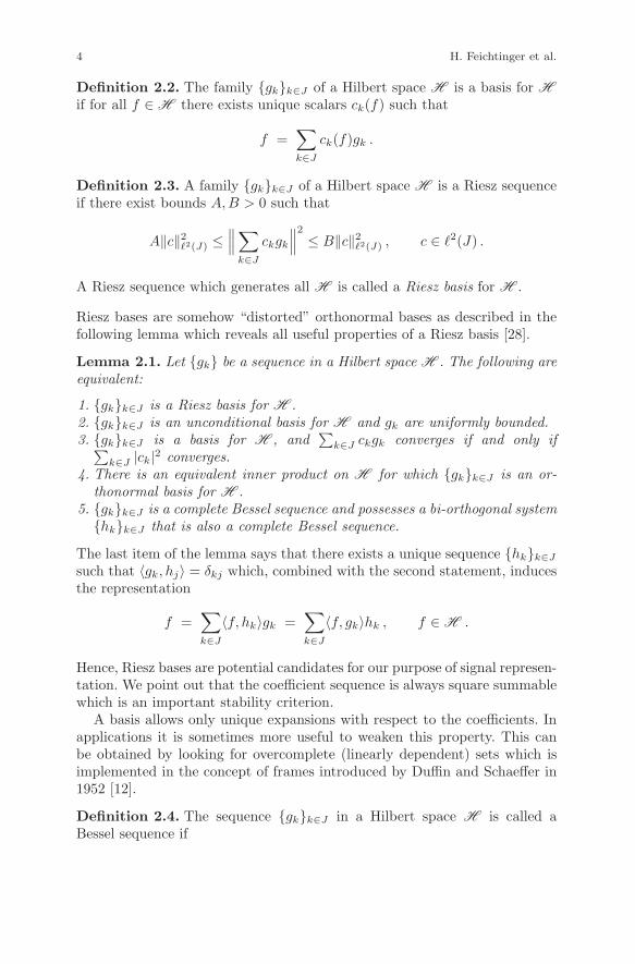
Riesz bases are somehow “distorted” orthonormal bases as described in thefollowing lemma which reveals all useful properties of a Riesz basis [28].

Lemma 2.1. Let gk be a sequence in a Hilbert space H . The following areequivalent:

1. gkk∈J is a Riesz basis for H .2. gkk∈J is an unconditional basis for H and gk are uniformly bounded.3. gkk∈J is a basis for H , and

∑k∈J ckgk converges if and only if∑

k∈J |ck|2 converges.4. There is an equivalent inner product on H for which gkk∈J is an or-

thonormal basis for H .5. gkk∈J is a complete Bessel sequence and possesses a bi-orthogonal systemhkk∈J that is also a complete Bessel sequence.

The last item of the lemma says that there exists a unique sequence hkk∈J

such that 〈gk, hj〉 = δkj which, combined with the second statement, inducesthe representation

f =∑k∈J

〈f, hk〉gk =∑k∈J

〈f, gk〉hk , f ∈H .

Hence, Riesz bases are potential candidates for our purpose of signal represen-tation. We point out that the coefficient sequence is always square summablewhich is an important stability criterion.

A basis allows only unique expansions with respect to the coefficients. Inapplications it is sometimes more useful to weaken this property. This canbe obtained by looking for overcomplete (linearly dependent) sets which isimplemented in the concept of frames introduced by Duffin and Schaeffer in1952 [12].

Definition 2.4. The sequence gkk∈J in a Hilbert space H is called aBessel sequence if

Banach Gelfand Triples for Gabor Analysis 5∑k∈J

|〈f, gk〉|2 <∞ , f ∈H .

Definition 2.5. A family gkk∈J of a Hilbert space H is a frame of H ifthere exist bounds A,B > 0 such that

A‖f‖2 ≤∑k∈J

|〈f, gk〉|2 ≤ B‖f‖2 , f ∈H . (1)

If A = B, then gkk∈J is called a tight frame.

The synthesis map D : 2(J)→H of a frame gkk∈J is defined by

D : (ck)→∑k∈J

ckgk .

Its adjoint D∗ is the analysis operator D∗f = (〈f, gk〉). The frame operatorS is defined by

Sf = DD∗f =∑k∈J

〈f, gk〉gk , f ∈H .

By (1), the frame operator satisfies

A〈f, f〉 ≤ 〈Sf, f〉 ≤ B〈f, f〉 , f ∈H ,

and is, therefore, bounded, positive, and invertible. The inverse operatorS−1 is obviously also positive and has therefore a square root S−1/2 (self-adjoint), [37]. The sequence S−1/2gk is a tight frame with A = B = 1.Indeed,∑

k∈J

〈f, S− 12 gk〉S− 1

2 gk = S− 12

∑k∈J

〈f, S− 12 gk〉gk = S− 1

2S(S− 12 f)

= S− 12S− 1

2Sf = If, ∀ f ∈H .

Every orthonormal basis of H is a Riesz basis of H and every Riesz basisof H is also a frame. The important difference between a Riesz basis and aframe is that the null space N(G) of the synthesis map D of a frame gkk∈J

is in general non-trivial which is equivalent to the statement that the rangeof the analysis map D∗ is a (closed) proper subspace of 2(J).

The sequence gk∈J with gk = S−1gk, is also a frame with frame bounds1/B and 1/A. It is a dual frame for gk in the sense that

f =∑k∈J

〈f, gk〉gk =∑k∈J

〈f, gk〉gk , f ∈H .

Again we see, that frames do indeed fit our purpose for signal analysisand signal recovery. In contrast to Riesz bases, frames have, in general, no


bi-orthogonal relation. Moreover, the dual frame is not unique. The canonicaldual S−1gk is the one that is producing minimal 2 coefficients as alreadyshown in [12]. For alternative dual frames there exist constructive approachesthat rely on the canonical dual. In [4,33], it is shown that any dual frame ofgk can be written as

S−1gk + hk −∑j∈J

〈S−1gk, gj〉hj , (2)

where hk is a Bessel sequence.The lack of uniqueness has the advantage that if one coefficient is missing

out of the sequence 〈f, gk〉, the whole signal can still be completely recoveredas long as gk is a frame but no Riesz basis. Similarly, any frame that is nota Riesz basis is still a frame when discarding single frame elements. Studiesabout the conservation of the frame property when discarding frame elementsare known as excesses of frames [1, 2].

3 Gabor Analysis on L2

We define the Fourier transform of an integrable function by f(ω) =∫

Rd

f(t)e−2πitωdt. The translation operator Tx and the modulation operator Mω

are given by

Txf = f(· − x), Mωf = e2πiω·f(·), x, ω ∈ Rd. (3)

Combined together they give rise to the so-called time–frequency shift π(λ):

π(λ) = MωTx, (x, ω) ∈ R2d. (4)

Note thatπ(λ2)π(λ1) = e2πi(x1ω2−x2ω1)π(λ1)π(λ2)

for λ1 = (x1, ω1), λ2 = (x2, ω2) ∈ R2d.A time–frequency lattice Λ is a discrete subgroup of R2d (= Rd× Rd) with

compact quotient. Its redundancy |Λ| is the reciprocal value of the measureof a fundamental domain for the quotient R2d/Λ.

For a lattice Λ in R2d and a so-called Gabor atom g ∈ L2 we define theassociated Gabor family by

G(g, Λ) = π(λ)gλ∈Λ .

If G(g, Λ) is a frame for L2, we call it a Gabor frame. Since Λ has a groupstructure, the frame operator

Sf =∑λ∈Λ

〈f, π(λ)g〉π(λ)g


has the property that it commutes with all time–frequency shifts of the formπ(λ) for λ ∈ Λ. Therefore, the canonical dual frame of G(g, Λ) is simply givenby G(h,Λ) with h = S−1g. The fact, that a canonical dual frame of a Gaborframe is again a Gabor frame, i.e., generated by a single function, is the keyproperty in many applications. It reduces computational issues to solving thelinear system Sh = g.

A special and widely studied case are separable lattices of the form αZ×βZ

for some positive lattice parameters α and β, whose redundancy is simply(αβ)−1. The prototype of a function generating Gabor frames for such sepa-rable lattices is the Gaussian

ψ(x) = e−πx2σ2. (5)

for some real σ > 0. The Gaussian generates a Gabor frame if and only ifαβ < 1 [31,35,38,39]. We emphasize that for αβ = 1 the Gaussian generatesa unstable generating system for L2(Rd), i.e., the resulting Gabor family iscomplete but coefficient sequences must not be bounded. In this context wemention a central result, the so-called density theorem and refer to [26] fordetailed discussions. An elegant elementary proof of the density theorem hasbeen provided by Janssen [30].

Theorem 3.1. Assume that G(g, α, β) is a frame. Then, αβ ≤ 1. Moreover,G(g, α, β) is a Riesz basis for L2(Rd) if and only if αβ = 1.

In his seminal paper [22], Gabor chose the integer lattice a = b = 1 in R2

and used the Gaussian in order to define a Gabor system with maximaltime–frequency localization. However, as mentioned above, this system isno longer stable though complete, and, indeed, the celebrated Balian–LowTheorem [3,34] states that good time–frequency localization and Gabor Rieszbases are not compatible:

Theorem 3.2 (Balian–Low). If G(g, 1, 1) constitutes a Riesz basis forL2(R), then ∫

R

|g(t)|2t2dt∫

R

|g(ω)|2ω2dω =∞ .

The Balian–Low Theorem reveals a form of uncertainty principle and hasinspired fundamental research, see [26] and references therein.

In the sequel we state some fundamental results of Gabor frames and theGabor frame operator (Gabor frame-type operator). To this end we need thenotion of the adjoint lattice Λ of Λ which is the set of all elements in R2d

that satisfy the commutation property

π(λ)π(λ) = π(λ)π(λ) for all λ ∈ Λ .

Note that Λ is again a lattice of R2d (and that Λ = Λ). Instead of theframe operator we will use the more general notion of a frame-type operator


Sg,γ,Λ associated to the pair (g, γ), where γ takes the role of an “analyzing”and g the role of a “synthesizing” window:

Sg,γ,Λf =∑λ∈Λ

〈f, π(λ)γ〉π(λ)g , f ∈ L2(Rd) .

This sum converges in L2(Rd) for all f ∈ L2(Rd) as long both functions g, γare Bessel atoms for Λ, that is, G(g, Λ) and G(γ, Λ) are Gabor Bessel families.For the fundamental results to hold with respect to norm convergence weneed a little bit more than Bessel sequences. It is that both atoms g (andanalogously γ) satisfy ∑

λ∈Λ|〈g, gλ〉| <∞ , (A′)

also known as the Tolimieri–Orr’s condition. This somewhat technical prop-erty is used for controlling convergence problems (by altering the convergencedefinition Condition (A′) can be weakened). Condition (A′) is in general noteasy to verify. In particular, if Condition (A′) holds for one lattice, there is, ingeneral, no guarantee that it holds also for a different lattice. This problem,however, is overcome by the Feichtinger algebra S0 (Sect. 5) which defines aclass of functions for which Condition (A′) is satisfied for any lattice in R2d.

We summarize the fundamental results of Gabor analysis in the follow-ing theorem that is given in [20] in a slightly more general context. Thestatements go back to the seminal papers [10, 29, 40]. They are, however,all consequences of the fundamental identity of Gabor analysis extensivelystudied in [17].

Theorem 3.3. Let Λ be a lattice in R2d with adjoint lattice Λ. Then, forg, h satisfying (A′), the following holds.

1. (Fundamental Identity of Gabor Analysis)∑λ∈Λ

〈f, π(λ)γ〉〈π(λ)g, h〉 = |Λ|∑

λ∈Λ〈g, π(λ)γ〉〈π(λ)f, h〉 (7)

for all f, h ∈ L2(Rd), where both sides converge absolutely.2. (Wexler–Raz Identity)

Sg,γ,Λf = |Λ| · Sf,γ,Λg (8)

for all f ∈ L2(Rd).3. (Janssen Representation)

Sg,γ,Λ = |Λ|∑

λ∈Λ〈γ, π(λ)g〉π(λ) (9)

where the series converges unconditionally in the strong operator sense.


In Sect. 6 we explicitly derive the Janssen representation of the Gabor frameoperator from advanced concepts in harmonic analysis and provide a muchdeeper insight into this topic.

Another important result is the Ron–Shen Duality Principle which is oftenreferred to [36] although it appeared already in [29] and [10].

Theorem 3.4. Let g ∈ L2(Rd) and Λ be a lattice in R2d with adjoint Λ.Then the Gabor system G(g, Λ) is a frame for L2(Rd) if and only if G(g, Λ)is a Riesz basis for its closed linear span. In this case, the quotient of thetwo frame bounds and quotient of the Riesz bounds (alternatively the condi-tion number of the corresponding frame operator and the Gramian matrix,respectively) coincide.

The last important identity in Gabor Analysis that we want to present inthis section is the Wexler–Raz Biorthogonality Relation which basically saysthat g and γ are dual Gabor windows if and only if Sg,γ,Λ = Id. That is,according to Janssen Representation, exactly the case when

〈γ, π(λ)g〉 = |Λ|−1 δ0,λ .

Alternatively this relation can be described by what is a true biorthogonality(using again Kronecker’s Delta):

〈π(λ′)γ, π(λ)g〉 = |Λ|−1 δλ′,λ .

In the next section we describe basic and more advanced studies in harmonicanalysis that contribute to a better understanding of the Gabor frameoperator.

4 Time–Frequency Representations

Traditionally we extract the frequency information of a signal f by meansof the Fourier transform f(ω) =

∫Rd f(t)e−2πitωdt. If we know f(ω) for all

frequencies ω, then our signal f can be reconstructed by the inversion formulaf(t) =

∫Rd f(ω)e2πitωdω (valid pointwise or in the quadratic mean).

However, in many situations it is of relevance to know, how long eachfrequency appears in the signal f , e.g., for a pianist playing a piece of music.Mathematically this leads to the study of functions S(f)(t, ω) of the signal f ,which describe the time–frequency content of f over “time” t. In the followingwe mention the most prominent time–frequency representations.

In the last century researchers such as E. Wigner, Kirkwood, and Rihaczekhad invented different time–frequency representations [32, 41]. The work ofWigner and Kirkwood was motivated by the description of a particle in quan-tum mechanics by a joint probability distribution of position and momentum


of the particle. More concretely, in 1932 Wigner introduced the first time–frequency representation of a function f ∈ L2(Rd) by

W (f)(x, ω) =∫

Rd

f(x+t

2)f(x− t

2)e−2πiωtdt, (10)

the so called Wigner distribution of f . Later Kirkwood proposed anothertime–frequency representation, which was in a different context rediscoveredby Rihaczek. Both researchers associated to a function f ∈ L2(Rd) the fol-lowing expression

R(f)(x, ω) = f(x)f(ω)e−2πixω,

the Kirkwood–Rihaczek distribution of f .Nowadays, the short-time Fourier transform (STFT) has become the stan-

dard tool for (linear) time–frequency analysis. It is used as a measure of thetime–frequency content of a signal f (energy distribution), but it also estab-lishes a connection to the Heisenberg group.

The STFT provides information about local (smoothness) properties of thesignal f . This is achieved by localization of f near t through multiplicationwith some window function g and a subsequent Fourier transform providinginformation about the frequency content of f in this segment. Typically g isconcentrated around the origin. If g is compactly supported only a segmentof f in some interval or ball around t is relevant, but g can be any non-zeroSchwartz function such as the Gaussian. Overall we have:

Vgf(x, ω) =∫

Rd

f(t)g(t− x)e−2πitωdt, for (x, ω) ∈ R2d, (11)

In 1927 Weyl pointed out that the translation and modulation operatorsatisfy the following commutation relation

TxMω = e−2πixωMωTx, (x, ω) ∈ R2d. (12)

Tx : x ∈ Rd and Mω : ω ∈ Rd are Abelian groups of unitary oper-ators, with the infinitesimal generators given by differentiation and multi-plication operator, respectively. Therefore the commutation relation (12) isthe analogue of Heisenberg’s commutation relation for the differentiation andmultiplication operator.

The time–frequency shifts MωTx for (x, ω) ∈ R2d satisfy the followingcomposition law:

π(x, ω)π(y, η) = e−2πix·ηπ(x+ y, ω + η), (13)

for (x, ω), (y, η) in the time–frequency plane Rd × Rd, i.e., the mapping(x, ω) → π(x, ω) defines (only) a projective representation of the time–frequency plane (viewed as an Abelian group) Rd × Rd. By adding a toral


component, i.e., τ ∈ C with |τ | = 1 one can augment the phase spaceRd × Rd to the so-called Heisenberg group Rd × Rd × T and the mapping(x, ω, τ) → τMωTx defines a (true) unitary representation of the Heisenberggroup [21], the so-called Schrodinger representation. From this point of viewthe definition of Vgf can be interpreted as representation coefficients:

Vgf(x, ω) = 〈f,MωTxg〉, f, g ∈ L2(Rd).

The STFT is linear in f and conjugate linear in g. The choice of thewindow function g influences the properties of the STFT remarkably. Oneexample of a good window class is the Schwartz space of rapidly decreasingfunctions. Later we will discuss another function space, which is perfectlysuited as a good class of windows, Feichtinger’s algebra.

Furthermore, for f, g ∈ L2(Rd) the STFT Vgf is uniformly continuouson R2d, i.e., we can sample the Vgf without problem. This fact is of greatrelevance in the discussion of Gabor frames.

By Parseval’s theorem and an application of the commutation relations(12) we derive the following relation

Vgf(x, ω) = e−2πixωVg f(ω,−x), (14)

which is sometimes called the fundamental identity of time–frequencyanalysis [26]. Equation (14) expresses the fact that the STFT is a jointtime–frequency representation and that the Fourier transform amounts toa rotation of the time–frequency plane Rd × Rd by an angle of π

2 wheneverthe window g is Fourier invariant. Another important consequence of thedefinition of STFT (11) and the commutation relations (12) is the covarianceproperty of the STFT:

Vg(TuMηf)(x, ω) = e−2πiuωVgf(x− u, ω − η). (15)

Later we will draw an important conclusion of the basic identity of time–frequency analysis (14) and the covariance property of the STFT (15): iso-metric Fourier invariance and the invariance under TF-shifts of Feichtinger’salgebra.

As for the Fourier transform there is also a Parseval’s equation for theSTFT which is referred to as Moyal’s formula.

Lemma 4.1 (Moyal’s formula). Let f1, f2, g1, g2 ∈ L2(Rd) then Vg1f1 andVg2f2 are in L2(R2d) and the following identity holds:

〈Vg1f1, Vg2f2〉L2(R2d) = 〈f1, f2〉〈g1, g2〉 . (16)

Moyal’s formula implies that orthogonality of windows g1, g2 resp. of signalsf1, f2 implies orthogonality of their STFT’s. Most importantly we observethat one has for normalized g ∈ L2(Rd) (i.e., with ‖g‖2 = 1):


‖Vgf‖L2(R2d) = ‖f‖L2(Rd),

for all f ∈ L2(Rd), i.e., the STFT is an isometry from L2(Rd) to L2(R2d).Another consequence of Moyal’s formula is an inversion formula for the

STFT. Assume that the analysis window g ∈ L2(Rd) and the synthesis win-dow γ ∈ L2(Rd) satisfy 〈g, γ〉 = 0. Then for f ∈ L2(Rd)

f =1〈g, γ〉

∫∫R2d

〈f, π(x, ω)g〉π(x, ω)γ dxdγ. (17)

We observe that in contrast to the Fourier inversion the building blocks of theSTFT inversion formula are just time–frequency shifts of a square-integrablefunction. Therefore also the Riemannian sums corresponding to this inversionintegral are functions in L2(Rd) and are even norm convergent in L2(Rd) fornice windows (from Feichtinger’s algebra, see later).

5 The Gelfand Triple (S0, L2, S0′)(Rd)

Since Feichtinger’s discovery of the Segal algebra S0(Rd) in 1979 many resultshave shown that S0(Rd) is a good substitute of Schwartz’s space S(Rd) oftest functions (except if one is interested in a discussion of partial differentialequations). Furthermore S0(Rd) has turned out as the appropriate setting forthe treatment of questions in harmonic analysis on Rd (actually on a generallocally compact Abelian group G, even without using their structure theory).In this section we recall well-known properties of S0(Rd) which we will needlater in our discussion of Gabor frame operators. Nowadays the space S0(Rd)is called Feichtinger’s algebra since it is a Banach algebra with respect topointwise multiplication and convolution.

Definition 5.1. A function in f ∈ L2(Rd) is in the subspace S0(Rd) if, forsome non-zero g (called the “window”) in the Schwartz space S(Rd),

‖f‖S0 := ‖Vgf‖L1 =∫∫

Rd×Rd

|Vgf(x, ω)|dxdω <∞.

The space (S0(Rd), ‖ · ‖S0) is a Banach space, for any fixed, non-zero g ∈S0(Rd), and different windows g define the same space and equivalent norms.Since S0(Rd) contains the Schwartz space S(Rd) any Schwartz function issuitable, but also compactly supported functions having an integrable Fouriertransform (such as a trapezoidal or triangular function) are suitable windows.Often it is convenient to use the Gaussian as a window.

The above definition of S0(Rd) [26] (different from the original one [13])allows for an easy derivation of the basic properties of Feichtinger’s algebrain the following lemma.


Lemma 5.1. Let f ∈ S0(Rd), then the following holds:

(1) π(u, η)f ∈ S0(Rd) for (u, η) ∈ Rd × Rd, and ‖π(u, η)f‖S0 = ‖f‖S0 .(2) f ∈ S0(Rd), and ‖f‖S0 = ‖f‖S0 .

Proof. 1. For z = (u, η) in the time–frequency plane Rd × Rd one has:

‖π(u, η)f‖S0 =∫∫

R2d

|Vgf(x− u, ω − η)| dxdω =

=∫∫

R2d

|Vgf(x, ω)| dxdω = C‖f‖S0 .

2. The key of the argument is an application of the fundamental identityof time–frequency analysis (14) to a Fourier invariant window g and theindependence of the definition of S0(Rd) for g ∈ S(Rd). For simplicity wechoose g the (Fourier invariant) Gaussian g0(x) = 2d/4e−πx2

:

‖f‖S0 =∫∫

R2d

|Vg0 f(x, ω)| dxdω =∫∫

R2d

|Vg0 f(x, ω)| dxdω =

∫∫R2d

|Vg0f(−ω, x)| dxdω =∫∫

R2d

|Vg0f(x, ω)| dxdω = ‖f‖S0 .

Later we will need that S0(Rd) is dense and continuously embedded intoLp(Rd) for any p ∈ [1,∞). The original motivation for Feichtinger’s intro-duction of S0(Rd) was the search for a smallest member in the family of alltime–frequency homogenous Banach spaces. For a proof of all these assertionswe refer the reader to the original paper of Feichtinger or Grochenig’s bookon time–frequency analysis [26].

Another reason for usefulness of S0(Rd) is the fact that S0(Rd) is a naturaldomain for the application of Poisson summation [25].

Lemma 5.2. Let Λ be a lattice in Rd and f ∈ S0(Rd) then∑λ∈Λ

f(λ) = |Λ|−1∑

λ⊥∈Λ⊥f(λ⊥) (18)

holds pointwise and with absolute convergence.

Here Λ⊥ is the orthogonal lattice for Λ, e.g., Λ⊥ = (A−1)tZd for Λ = AZd,where A is a non-singular matrix describing Λ.

In 1958 I. M. Gelfand and A. G. Kostyuchenko introduced Gelfand triplesin their study of the spectral theory of self-adjoint operators [23]. They weremotivated by the work of Dirac on the foundations of quantum mechanicsand Schwartz’s theory of distributions.


An important result of linear algebra is the theorem on the existenceof eigenvectors for any self-adjoint linear operator A on Rd. The situationchanges drastically when one passes from the finite to the infinite-dimensionalcase, since it can happen that a unitary operators does not have any (non-zero) eigenvector. Particular examples of such operators are the translationoperator Tx and the modulation operator Mω on L2(Rd). Let us presentan easy argument showing that the translation operator Tx, x = 0, has noeigenvectors in L2(Rd). Assume that f ∈ L2(Rd) satisfies

Txf(t) = af(t), (19)

which by the Fourier transform is equivalent to

M−xf(ω) = af(ω) a.e.. (20)

But this is only possible if the function f equals zero a.e., up to the pointswith e2πiωx = a, i.e., it differs from zero only on a set of measure zero,hence f = 0 and finally f = 0 ∈ L2(Rd). In other words, the translationoperator Tx does not have eigenvectors in the space L2(Rd). On the otherhand we are not too far off with the claim that Tx has the eigenvectors e−2πitω

corresponding to the eigenvalue e2πixω, and the claim that any function fin L2(Rd) can be (kind of) expanded in terms of the eigenvectors e−2πitω,by suitable interpretation of the inversion formula for the Fourier transform(valid pointwise for f ∈ S0(Rd)):

f(t) =∫

Rd

f(ω)e2πitωdω. (21)

Furthermore, the action of the translation operator is given by

Txf(t) =∫

Rd

e2πixω f(ω)e2πitωdω,

which is a continuous analog of the spectral decomposition of a self-adjointoperator in Rd.

More concretely, the system of eigenfunctions e−2πitω : ω ∈ Rd is com-plete in the sense that for any function f in L2(Rd) Parseval’s equality holds∫

Rd

|f(t)|2dt =∫

Rd

|f(ω)|2dω.

The obvious problem is the fact that L2(Rd) does not contain the systemof eigenvectors of the translation operator Tx. But they can be consideredas linear functionals on S0(Rd). This as well es several similar observationssuggests to study operators on a Hilbert space via a dense subspace and itsassociated dual space. In our example it is actually possible to start fromS0(Rd) and construct L2(Rd) as completion of S0(Rd) with respect to normcorresponding to the usual scalar product 〈f, g〉 =

∫Rd f(t)g(t)dt.


In this context it turns out that S0(Rd) has the important additionalproperty that both δ-distributions and the pure frequencies χω(x) = e−2πixω

(for all ω ∈ Rd) are in a natural way elements of S0′(Rd), i.e., define bounded

linear functionals on S0(Rd). This dual space can be defined via STFT asfollows [26]:

S0′(Rd) =

f ∈ S ′(Rd) : ‖f‖S0′(Rd) = ‖Vgf‖L∞ = sup

Rd×Rd

|Vgf(x, ω)| <∞.

It is now easy to verify that δ ∈ S0′(Rd). Indeed, for g ∈ S(Rd), we have

sup(x,ω)∈Rd×Rd

|Vgδ(x, ω))| = sup(x,ω)∈Rd×Rd

|〈δ,MωTxg〉| =

= sup(x,ω)∈Rd×Rd

|g(−x)| = ‖g‖L∞ <∞.

We are now in a situation similar to the one inspiring Gelfand to introducewhat is nowadays called a Gelfand triple. The main idea being the observa-tion, that a triple of spaces – consisting of the Hilbert space itself, a small(topological vector) space contained in the Hilbert space, and its dual – allowsa much better description of the situation. The advantage in our case is thefact that we can even take a Banach space, namely S0(Rd). Hence we canwork with the following formal definition:

Definition 5.2. A (Banach) Gelfand triple consists of some Banach space(B, ‖ · ‖B) which is continuously and densely embedded into some Hilbertspace H , which in turn is w∗-continuously and densely embedded into thedual Banach space (B′, ‖ · ‖B′).

We shall use the symbol (B,H ,B′) for such a triple of spaces. In this settingthe inner product on H extends in a natural way to a pairing between Band B′ (producing an anti-linear functional of the same norm).

As another consequence we mention an extension of an eigenvector of abounded operator on a Hilbert space H . Let A be a linear operator on aBanach space B then a linear functional F is a generalized eigenvector of Ato the eigenvalue λ if

F (Af) = λF (f), for all f ∈ B.

This notion allows to interpret the characters χω(x) = e−2πiωx as generalizedeigenvectors for the translation operator Tx on S0(Rd). Furthermore the set ofgeneralized eigenvectors χω : ω ∈ Rd is complete by Plancherel’s theorem,i.e., if f(ω) = 〈χω, f〉 = 0 for all ω ∈ Rd implies f ≡ 0. This suggests to thinkof the Fourier transform of f at frequency ω as the evaluation of the linearfunctional 〈χω, f〉.

The treatment of the translation operator Tx on L2(Rd) is a particularcase of a general theorem by Gelfand that for any self-adjoint operator A


on a Hilbert space H there exists a nuclear space and a complete system ofgeneralized eigenvectors, see [24]. The advantage of the approach presentedhere is that instead of a (may be complicated) nuclear topological vectorspace a relatively simple-minded Banach space can be used.

The introduction of Gelfand triples does not only offer a better descrip-tion of a self-adjoint operator but it also allows to a simplification of proofs.For example, in the discussion of the Fourier transform F we consider it asan object on S0(Rd) where everything is well-defined and Parseval’s formulaand taking the inverse Fourier transform is justified by the nice propertiesof S0(Rd). By a density argument we get all properties of the Fourier trans-form on the level of L2(Rd). And we obtain an extension of the Fouriertransform to S0

′(Rd) by duality, the so-called generalized Fourier transform.The preceding discussion suggests the following lemma which says that

assertions for an operator on the S0-level are actually statements for L2(Rd)and S0

′, respectively.

Lemma 5.3. The Fourier transform F on Rd has the following properties:

1. F is an isomorphism from S0(Rd) to S0(Rd),2. F is a unitary map between L2(Rd) and L2(Rd),3. F is a weak∗ (as well as a norm-to-norm) continuous bijection from

S0′(Rd) to S0

′(Rd).

Furthermore we have that Parseval’s formula

〈f, g〉 = 〈f , g〉 (22)

is valid for (f, g) ∈ S0(Rd)×S0′(Rd) and therefore on each level of the Gelfand

triple (S0,L2,S0

′)(Rd).

The properties of Fourier transform are expressed by the Gelfand bracket

〈f, g〉(S0,L2,S0′)(Rd) = 〈f , g〉(S0,L2,S0′)(Rd) (23)

which combines the functional brackets of Banach spaces and that of theinner-product for the Hilbert space.

The Fourier transform is a prototype for the notion of a Gelfand tripleisomorphism.

Definition 5.3. If (B1,H1,B′1) and (B2,H2,B

′2) are Gelfand triples then

an operator A is called a [unitary] Gelfand triple isomorphism if

1. A is an isomorphism between B1 and B2.2. A is a [unitary operator resp.] isomorphism from H1 to H2.3. A extends to a weak∗ isomorphism as well as a norm-to-norm continuous

isomorphism between B′1 and B′

2.

In this terminology the Fourier transform is a unitary Gelfand triple isomor-phism of the Gelfand triple automorphism on (S0,L

2,S0′)(Rd) (isomorphism


with itself). In the following lemma we give conditions for the extension of alinear mapping given on S0(Rd) to a unitary mapping on L2(Rd).

Lemma 5.4 (cf. [20]). Let U be a unitary mapping from L2(Rd) toL2(Rd). The mapping U extends to a Gelfand triple isomorphism between(S0,L

2,S0′)(Rd) and (S0,L

2,S0′)(Rd) if and only if the restrictions of U to

S0(Rd) defines a bounded bijective linear mapping from S0(Rd) onto itself.

Due to this lemma we only have to check the properties of U at the S0-level,i.e., to verify the existence of some C > 0 such that

‖Uf‖S0(Rd) ≤ C‖f‖S0(Rd). (24)

The discussion of the Fourier transform F on the Gelfand triple(S0,L

2,S0′)(Rd) allows to think of F as a bounded operator between S0(Rd)

and S0′(Rd) with a distributional kernel k(t, ω) = e−2πitω. The existence

of a distributional kernel holds for any bounded operator between S0(Rd)and S0

′(Rd). This important fact is the so-called kernel theorem for S0(Rd)(cf. [16], Theorem 7.4.2). Before we give a precise description of this impor-tant fact we recall the notion of a Wilson basis. With the help of a Wilsonbasis we can adapt a linear algebra reasoning to the infinite-dimensionalsetting.

In 1991 Daubechies, Jaffard and Journe [9] followed an idea of Wilson intheir construction of an orthonormal basis from a Gabor system G(g, Λ) ofL2(Rd). Wilson suggested that the building blocks π(x, ω)g of an orthonormalbasis of L2(Rd) should be symmetric in ω and should be concentrated at ωand −ω.

Definition 5.4. For g ∈ L2 the associated Wilson system W(g) consists offunctions

ψk,n = cnT k2(Mn + (−1)k+nM−n)g, (k, n) ∈ Zd × N0,

where c0 = 12 and cn = 1√

2for n ≥ 1, ψk,0 = Tkg and ψ2k+1,0 = 0 for k ∈ Z.

They proved the following theorem which shows a method for the construc-tion of a Wilson basis from a Gabor system G(g, 1

2Z× Z). Later Feichtinger,Grochenig, and Walnut [14] showed that Wilson systems provide an uncondi-tional basis for S0(Rd) and S0

′(Rd) endowed with the w∗-topology. ThereforeWilson systems provide us with a natural class of bases for time–frequencyanalysis. The existence of an unconditional basis for S0(Rd) will be very help-ful in our discussion of the kernel theorem for S0(Rd) and their constructionrelies heavily on the functorial properties of S0, cf. [16].

Theorem 5.1. Let G(g, 12Z × Z) be a tight frame for L2(R) with ‖g‖ = 1

and g(x) = g(−x). Then the Wilson system W(g) is an orthonormal basis ofL2(R).


As a corollary we get Wilson bases for L2(Rd) by taking tensor products.

Corollary 5.1. Let W(g) be a Wilson basis for L2(R) and define Ψk,n =∏dj=1 ψrj ,sj

for (r, s) ∈ Zd × N0. Then Ψk,n is an orthonormal basis forL2(Rd).

In applications of mathematics one often has to deal with linear systems.In the discrete and finite case each linear system is a linear mapping from theinput space Rn into the output space Rm of our system and its action is givenby matrix multiplication after a choice of bases in Rn and Rm, respectively(similarly from Cn to Cm using complex matrices).

A linear system in infinite dimensions may be considered as a continuousanalog of matrix multiplication (replacing summation by integration), i.e.,

g(x) = Kf(x) =∫

Rd

k(x, y)f(y)dy.

We can think of the input values f(y) as being listed in an infinite columnvector and k(x, y) as an infinite matrix, the so-called kernel of K, and theintegral

∫Rd k(x, y)f(y)dy providing the entries of the output vector in the

expected way. In signal processing, such a model is known as a linear time-variant system.

For a wide range of function spaces (covering practically all cases rele-vant for applications) and by means of the use of generalized functions thisanalogy can be given a precise mathematical meaning. The natural way of de-scribing this context is via so-called kernel theorems. Although only HilbertSchmidt operators can be described as integral operators with L2-kernels,every bounded linear system A on L2(Rd) can be uniquely described bysome distributional kernel K ∈ S0

′(R2d).Suppose we have an integral operator K with distributional kernel k on

S0(Rd), i.e., we think of K in a weak sense

〈Kf, g〉 = 〈k, g ⊗ f〉, f, g ∈ S0(Rd),

where g ⊗ f denotes the tensor product g(x)f(y), then K is a bounded op-erator between S0(Rd) and S0

′(Rd). Since by duality we deduce that

|〈Kf, g〉| = |〈k, g ⊗ f〉| ≤ ‖k‖S0′‖g ⊗ f‖S0 = ‖k‖S0′‖f‖S0‖g‖S0

is true for all g ∈ S0(Rd), we have that Kf ∈ S0′(Rd). Therefore the operator

K is bounded between S0(Rd) and S0′(Rd) with the following estimate for

the operator norm of K:‖K‖op ≤ ‖k‖S0′ .

The non-trivial aspect of the kernel theorem is that the converse is true.


Theorem 5.2. If K is a bounded operator from S0(Rd) to S0′(Rd), then there

exists a unique kernel k ∈ S0′(R2d) such that 〈Kf, g〉 = 〈k, g ⊗ f〉 for f, g ∈

S0(Rd).

We only sketch a proof and refer the interested reader to the book ofGrochenig [26] for the technical details.

We define the infinite matrix a =(a(l,m),(r,s)

)of the operator K with

respect to a multivariate Wilson basis W(g) by

a(l,m),(r,s) = 〈KΨr,s,Ψl,m〉. (25)

Then the matrix (a) is bounded from 1(Zd×N0) to ∞(Zd×Nd0). We therefore

can define a kernel k for K as in linear algebra by

k =∑

l,m,r,s

a(l,m),(r,s)Ψl,m ⊗Ψr,s. (26)

Now, we know that Ψl,m⊗Ψr,s is an orthonormal basis for L2(R2d) whichyields that k ∈ S0

′(R2d) with weak∗-convergence of the sum.An important corollary of the preceding discussion is the following obser-

vation.

Corollary 5.2. Let (Ψk,n) be an orthonormal Wilson basis for L2(Rd) thenthe coefficient mapping D : f → 〈f,Ψk,n〉 induces a Gelfand triple isomor-phism between (S0,L

2,S0′)(Rd) and (1, 2, ∞)(Zd × Nd).

Proof. Since (Ψk,n) is an orthonormal basis of L2(Rd) the analysis operatorf → 〈f,Ψk,n〉 is an isomorphism between L2(Rd) and 2(Zd × Nd). TheWilson system (Ψk,n) is an unconditional basis for S0(Rd) and therefore theanalysis operator gives an isomorphism between S0(Rd) and 1(Zd×Nd). Byduality we obtain that S0

′(Rd) is isomorph to ∞(Zd × Nd).

6 The Spreading Function and Pseudo-DifferentialOperators

The notion of a Gelfand triple has turned out to be a very fruitful concept forinvestigations in Gabor analysis, see [16], [8], [11]. In this section we presentsome results of Feichtinger and Kozek on Gelfand triples for time–frequencyanalysis. All these results have their origin in the search of a mathematicalframework for problems in signal analysis. Many problems in applications aremodelled as linear time-variant systems (LTV). In the last section we learnedthat a LTV is just an integral operator K acting on signals with finite energy,

Kf(x) =∫

Rd

k(x, y)f(y)dy, f ∈ L2(Rd). (27)


The quality of an integral operator K on L2(Rd) relies on properties of itskernel k. For example integrability conditions on k yield to classes of niceoperators. The most prominent class of operators, the Hilbert–Schmidt oper-ators HS are defined in terms of integrability conditions. Namely, an integraloperator K on L2(Rd) is a Hilbert–Schmidt operator if k ∈ L2(Rd × Rd).

The class of Hilbert–Schmidt operators HS has a natural inner product.Let K1,K2 ∈ HS with kernels k1, k2, respectively. Then

〈K1,K2〉HS := 〈k1, k2〉L2(Rd×Rd) (28)

defines an inner product on HS. The associated Hilbert–Schmidt norm‖K‖HS :=

(〈K1,K2〉HS

)1/2 gives HS the structure of a Hilbert space [37].Furthermore we recall that every Hilbert–Schmidt operator on HS is a com-pact operator on L2(Rd). Recall that a compact operator K on L2(Rd) is ofHilbert–Schmidt type if and only if there exists an orthonormal basis (en)n∈N

in L2(Rd) and a sequence of scalars (λn)n∈N ∈ 2(N) such that

Kf =∑n∈N

λn〈en, f〉en. (29)

The sequence of scalars (λn)n∈N are actually the eigenvalues of K and‖K‖HS =

(∑n∈N|λn|2)1/2. The space of Hilbert–Schmidt operators HS is

not closed in the C∗-algebra K of compact operators on L2(Rd) with respectto the operator norm and there exist compact operators which are not ofHilbert–Schmidt type. But HS is a two-sided ideal in K.

If we choose as orthonormal basis of L2(Rd) a Wilson basis (Ψk,n) then thepreceding observations led to an isomorphism between HS and L2(Zd×Nd).Now we can make use of the concept of Gelfand triples, but this time we takethe Hilbert–Schmidt operators as Hilbert space of an Operator Gelfand triple.We observe that the kernel theorem for S0(Rd) provides us with another classof operators with “smooth kernels”. We write L for the space of boundedlinear operators on a Banach space B. One finds that K ∈ L(S0

′(Rd),S0(Rd))can be identified with kernels k ∈ S0(R2d) and is dense inHS. But the class ofHilbert–Schmidt operators HS is dense in L(S0(Rd),S0

′(Rd)) and therefore(L(S0

′(Rd),S0(Rd)),HS, L(S0(Rd),S0′(Rd))) is indeed a Gelfand triple. In

this setting the kernel theorem can be interpreted as a unitary Gelfand tripleisomorphism between this triple and their kernels in (S0,L

2,S0′)(Rd × Rd).

There is another Gelfand triple isomorphism that associates the HS Gelfandtriple with the Gelfand triple (S0,L

2,S0′)(Rd × Rd): the so-called spreading

symbol of operators.As a motivation we discuss a problem of great practical interest: commu-

nication with cellar phones. In modern communication cellar phones play acrucial rule in everyday life. How do engineers solve the problem of transmit-ting a signal f from a sender A to a receiver B? In the most general situationsender A and receiver B move in different directions with certain velocitieswhich yields to a variation of the path lengths of the transmitted signal f


and due to the Doppler effect to a change of frequencies. Therefore B receivesa signal of the following form

f =∫∫

R2η(K)(x, ω)MωTxfdxdω, (30)

where the function η(K) models the effect of the channel by the amountof time–frequency shifts arising as just described, applied the signal f . Thereceiver B is not interested in the signal f but in the original signal f . Froma mathematical point of view f is just the action of an operator K on thesignal f , i.e., f = Kf . In this picture B has to invert the operator K to getthe information contained in the signal f . Operators of this form are calledpseudo-differential operators and arise naturally in many problems of physics,engineering and mathematics. The function η(K) is the so-called spreadingfunction of the operator K. In the following we look for conditions on thespreading function η(K) which allow an inversion of our pseudo-differentialoperator K.

First, (30) suggests a decomposition of a general operator K on L2(Rd)as a continuous superposition of time–frequency shifts.

K =∫∫

R2d

η(K)(x, ω)MωTxdxdω. (31)

We already know such a decomposition of the identity operator on L2(Rd)since this is the inversion formula for the STFT:

IL2(Rd) =1〈g, γ〉

∫∫R2d

Vgf(x, ω)MωTxdxdω (32)

for g, γ ∈ L2(Rd) with 〈g, γ〉 = 0.The non-commutativity of translation and modulation operators on

L2(Rd) leads to a twisted convolution of the spreading functions of twooperators K and L. Let K,L ∈ L(S0,S0

′) and η(K), η(L) their spreadingfunctions respectively. Then the spreading function of the composition KLis given by twisted convolution of η(K) and η(L):

η(KL)(x, ω) =∫∫

R2η(K)(x′, ω′)η(L)(x− x′, ω − ω′)e−2πix′(ω−ω′)dω′. (33)

The spreading function of the adjoint operator K∗ is given by

η(K∗)(x, ω) = η(K)(−x,−ω) · e−2πixω (34)

and therefore leads to a noncommutative involution. Later we will return tothis topic in the context of Grochenig/Leinert’s resolution of the “irrationalcase”-conjecture [27].

The relation between the kernel k of an operator K from the Gelfandtriple


(L(S0,S0′),HS,L(S0

′,S0)) and its spreading function η(K) is given by thefollowing mapping from Rd × Rd to Rd × Rd

η(K)(x, ω) =∫

Rd

k(y, y − x)e−2πiyωdy, (35)

which is very useful in the calculation of the spreading function of an operatorK. It can be interpreted literally at the lowest level (integrals, etc., exist),and extend by continuity to the “upper levels”. Moreover it can be describedby the fact that it is the unique Gelfand triple isomorphism which mapsTF-shift operators onto the corresponding Dirac measures in the TF-plane(hence reproducing exactly the situation we had in the finite case).

The spreading function of an operator K is an object living on the time–frequency plane Rd× Rd. Therefore a further understanding of its propertiesshould be done according to the structure of Rd× Rd which is closely relatedto the structure of the Euclidean plane Rd×Rd. Namely, the time–frequencyplane is a symplectic manifold, i.e., there exists a non-degenerate 2-formΩ(X,Y ) = y·ω−x·η for two points X = (x, ω), Y = (y, η) in Rd×Rd. Since Ωis non-degenerate there is a unique invertible skew-symmetric linear operatorJ on Rd × Rd such that the symplectic form Ω and the Euclidian innerproduct are related as follows: Ω(X,Y ) = 〈JX,Y 〉 for all X,Y ∈ Rd × Rd.This implies an important fact about the characters of Rd× Rd. Namely, thecharacters are given by χs(X,Y ) = e2πiΩ(X,Y )|X ∈ Rd × Rd for a fixedY ∈ Rd× Rd. Therefore it is natural to analyse a function F on Rd× Rd withthe symplectic Fourier Transform

FsF (X) =∫∫

Rd×Rd

F (Y )e2πiΩ(X,Y )dY (36)

instead of the Fourier transform F induced by the standard inner-product〈·, ·〉 on Rd × Rd. From the relation between symplectic form and inner-product we obtain that the symplectic Fourier transform Fs is just a Fouriertransform followed by a rotation by π

2 since J describes a rotation by π2

around the origin of Rd×Rd. This fact allows us to derive similar statementsfor the symplectic Fourier transform as for the Euclidian Fourier transform:

1. Fs is a unitary mapping from L2(Rd × Rd) onto L2(Rd × Rd).2. F−1

s = Fs (involutive property).3. Fs

(S0(Rd × Rd)

)= S0(Rd × Rd).

By duality we obtain that

Proposition 6.1. The symplectic Fourier transform Fs defines a unitaryGelfand triple automorphism on (S0,L

2,S0′)(Rd × Rd).

Another reason for our choice of S0(R2d) as space of test functions is that thePoisson summation formula for symplectic Fourier transform holds pointwise


and with absolute convergence. Recently, we have shown that the Fundamen-tal Identity of Gabor Analysis can be derived by an application of Poissonsummation to a product of two STFT’s:

Theorem 6.1. Let Λ a lattice in Rd × Rd with adjoint lattice Λ and F ∈S0(R2d). Then ∑

λ∈Λ

F (λ) =1|Λ|∑

λ∈ΛFsF (λ) (37)

holds pointwise and with absolute convergence on both sides.

The spreading function is an important tool for the description of (slowly)time-variant channels in communication theory, but it is not the only sym-bol of associated with a linear operator. In the theory of pseudo-differentialoperators the Kohn–Nirenberg symbol (KN), denoted by σ(K), is used for anoperator K ∈ (S0,L

2,S0′)(Rd × Rd). It is defined as the symplectic Fourier

transform of the spreading function η(K):

σ(x, ω) = Fsη(K) =∫∫

Rd×Rd

η(K)e2πi(y·ω−x·η)dydη, (x, ω) ∈ Rd × Rd.

(38)

If Kf(x) =∫

Rd k(x, y)f(y)dy then σ(K) =∫

Rd k(x, x − y)e−2πiy·ωdy. Insignal analysis σ(K) was introduced by Zadeh and is called the time-varyingtransfer function of a system modelled by K. As an example we mentionthe KN symbol of a rank-one operator f ⊗ g, which describes the mappingh → 〈h, g〉f , is equal to

σ(f ⊗ g)(x, ω) = f(x)g(ω)e−2πix·ω , (x, ω) ∈ Rd × Rd, (39)

the Rihaczek distribution of f against g. For f, g ∈ S0(Rd) we have that theKN-symbol σ(f ⊗ g) ∈ S0(Rd × Rd) which in turn implies (using the lastequation) that (x, ω) → e2πix·ω is a pointwise multiplier on S0(Rd × Rd).

After these preparations we can state one of our main results:

Theorem 6.2. The spreading function K → η(K) is a unitary Gelfand tripleisomorphism from (L(S0

′,S0),HS,L(S0,S0′)) to (S0,L

2,S0′)(Rd × Rd).

Corollary 6.1. The KN symbol of K induces a unitary Gelfand triple iso-morphism between (L(S0

′,S0),HS,L(S0,S0′)) and (S0,L

2,S0′)(Rd × Rd).

Another consequence of the preceding theorem is the following Gelfand-bracket identities for K1,K2 ∈ (L(S0,S0

′),HS,L(S0′,S0)):

〈K1,K2〉(B,HS,B′) = 〈η(k1), η(k2)〉(S0,L2,S0′)(Rd×Rd) (40)

= 〈σ(k1), σ(k2)〉(S0,L2,S0′)(Rd×Rd), (41)

with B = L(S0,S0′) and B′ = L(S0

′,S0) respectively.


The KN symbol of a rank-one operator f ⊗ g, which is the mapping h →〈h, g〉f , is the Rihaczek distribution and by an application of the (inverse)symplectic Fourier transform we get another time–frequency distribution: theSTFT!

Lemma 6.1. For f, g ∈ S0(Rd) the rank-one operator f ⊗ g has a kernel inS0(Rd). Moreover the corresponding spreading function is

η(f ⊗ g)(x, ω) =∫

Rd

f(x)g(y − x)e−2πiy·ωdy (42)

and hence coincides with Vgf ∈ S0(Rd × Rd).

In the light of this result the inversion formula for the STFT is a superpositionof time–frequency shifts with the spreading function of the rank-one operatorg ⊗ γ for g, γ ∈ L2(Rd) with 〈g, γ〉 = 0:

f =1〈g, γ〉

∫∫Rd×Rd

η(f ⊗ g)(x, ω)TxMωγ dxdω. (43)

Recall that in analogy with the characters χω : ω ∈ Rd the time–frequencyshifts π(X) : X = (x, ω) ∈ Rd × Rd would be an orthonormal set withrespect to the Hilbert–Schmidt inner product 〈·, ·〉HS and η(f ⊗ g)(x, ω) =〈f ⊗ g, π(x, ω)〉HS but as in the case of Fourier transform the building blocksπ(X) for X ∈ Rd of our orthonormal system π(X) : X = (x, ω) ∈ Rd × Rdare not Hilbert–Schmidt. As in our treatment of the Fourier transform it isnot so important that the building blocks are elements of our Hilbert spacebut that they allow us to get expressions as they would be an orthonormalset of elements in our Hilbert space.

As a first example we state a generalization of the inversion formula forthe STFT from L2(Rd) to the Gelfand triple (S0,L

2,S0′)(Rd), where for

f ∈ S0′(Rd) the formula is interpreted in a weak sense.

Proposition 6.2. Let g, γ ∈ S0(Rd) with 〈g, γ〉 = 0. Then

f =1〈g, γ〉

∫∫Rd×Rd

η(f ⊗ g)(x, ω)TxMωγ dxdω. (44)

holds for f ∈ (S0,L2,S0

′)(Rd).

That is a special case of a general statement about the spreading function.

Theorem 6.3. Any K ∈ (L(S0,S0′),HS,L(S0

′,S0)) has a representation

K =∫∫

Rd×Rd

〈K,π(x, ω)〉L(S0,S0′) π(x, ω) dxdω (45)


convergent in the strong resp. weak∗-sense. The (complex-valued) amplitudefunction arising in this context, i.e., η(K)(x, ω) = 〈K,π(x, ω)〉L(S0,S0′), iscalled the spreading distribution of the operator K.

The basic tool in the proof is the fact that the spreading representationmaps a time–frequency shift π(x, ω) for (x, ω) ∈ Rd×Rd on the Dirac measureδX at X = (x, ω), i.e., η(π(X)) = δX and the relation between the spreadingfunction and the kernel of an operator K.

The preceding theorem is the mathematical justification of a widely usedstatement that the spreading function of an operator K is a measure for thetime–frequency content of K.

In our intuition we move an operator K over Rd × Rd and want there isa simply relation between the original symbol of K and the symbol after amovement to (x, ω) ∈ Rd × Rd. The KN-symbol of an operator K is shiftedby Tx,ω in the time–frequency plane.

Lemma 6.2. Let K belong to one of the spaces (L(S0′,S0),HS,L(S0

′,S0)),thenπ(x, ω)Kπ(x, ω)∗, the conjugation of K by π(x, ω) ∈ Rd × Rd corresponds totranslation of the KN symbol σ(K),

σ(π(x, ω)Kπ(x, ω)∗) = T(x,ω)

(σ(K)). (46)

This property of the KN symbol is of central importance in our study of theGabor frame operator to which we devote the final part of this section. LetG = (g, Λ) be a Gabor system for a lattice Λ ∈ Rd × Rd. Then the Gaborframe operator Sg,Λ commutes with all time–frequency shifts of the latticeΛ, i.e.,

π(λ)Sg,Λπ(λ)∗ = Sg,Λ, for all λ ∈ Λ. (47)

This fact was the motivation for Feichtinger and Kozek to introduce the classof Λ-invariant operators [16].

Definition 6.1. Let Λ a lattice in Rd × Rd and K an operator concentratedon Λ. Then K is called Λ-invariant if π(λ)K = Kπ(λ) for all λ ∈ Λ.

In the following we want to find the support of the spreading function η(K)of an Λ-invariant operator K ∈ (L(S0,S0

′),HS,L(S0′,S0)). As a first step

towards this result we study spreading representations of K on Rd × Rd.

Lemma 6.3. Let K1,K2 ∈ L(S0,S0′) with spreading function η(K1), η(K2),

respectively. Then

1. η(K1K2)(λ) =∫∫

Rd×Rd η(K1)(µ)η(K2)(λ−µ)ρ(λ−µ, µ)dµ with ρ(X,Y ) =e2πi(y·ω−x·η) for X = (x, ω), Y = (y, η) ∈ Rd × Rd.

2. supp(η(K1)η(K2)) ⊂ supp(K1) + supp(K2).3. |η(K1K2)| = |η(K1)| ∗ |η(K2)| for η(K1), η(K2) ∈ L1

loc(Rd × Rd).


The proof of (1) is a consequence of the commutation relation for time–frequency shifts and the fact that for K1 ∈ L(S0,S0

′) and K2 ∈ L(S0,S0′)

also K1K2 ∈ L(S0′,S0). Now each operator K in L(S0,S0

′) has an absolutelyconvergent spreading representation and therefore our result holds pointwise.The support condition follows from the analogous result for the ordinaryconvolution.

By abstract reasons each Λ-invariant operator K has a representation inthe set of all operators concentrated on Λ = λ ∈ Rd × Rd|π(λ)π(λ) =π(λ)π(λ since K lies in the commutant of the (C∗, von Neumann) algebragenerated by π(λ) : λ ∈ Λ. The set Λ is the so-called adjoint lattice sinceit is the annihilator subgroup of Λ for the symplectic Fourier transform Fs

and if Λ⊥ is the annihilator subgroup of Λ with respect to F then Λ = JΛ⊥.The time–frequency invariance of S0(Rd) implies that K and π(λ)K

are in the Gelfand triple (L(S0,S0′),HS,L(S0

′,S0)), too. Therefore, theΛ-invariance of T translates into a periodicity condition for the symbol σ(K)

σ(K) = Tλ(σ(K)), λ ∈ Λ . (48)

This periodicity condition corresponds to a support condition for the spread-ing function since η(K)(λ) = η(K)(λ)e−2πΩ(λ,µ). But e−2πΩ(λ,µ)|λ ∈ Λ fora fixed µ ∈ Rd × Rd is a group of characters on Rd × Rd yields that

supp(η(K)) ⊂ JΛ⊥ = Λ. (49)

The fact that distributions in S0′(Rd) with support in a discrete subgroup is

a sum of Dirac measures with a bounded sequence of coefficients implies thatfor some bounded sequence (cλ) over Λ

η(K) =∑

λ∈Λcλδλ (50)

with cλ = (K)λ =∫∫

Rd×Rd/Λ σ(K)(µ)e2πiΩ(λ,µ)dµ.Returning to the description in the operator domain we arrive at the fol-

lowing characterization

Theorem 6.4. Let K ∈ (L(S0,S0′),HS,L(S0

′,S0)) and σ(K) the KN sym-bol. Then σ(K) is a Λ-periodic distribution with a symplectic Fourier trans-form supported on Λ0. Furthermore

K =∑

λ∈Λ(K)λπ(λ). (51)

Corollary 6.2. The mapping σ(K) → (K)λ is a unitary Gelfand triple iso-morphism between (S0,L

2,S0′)(Rd × Rd/Λ) and (1, 2, ∞)(Λ).

Note that the time–frequency invariance of S0(Rd) implies the bounded-ness of K on S0(Rd) since


‖K‖L(S0) = ‖∑

λ∈Λ(K)λπ(λ)‖L(S0) ≤

∑λ∈Λ

|(K)λ |. (52)

The next theorem shows that for any Λ-invariant operator K with σ(K) ∈S0

′((Rd × Rd)/Λ) there exists a prototype operator P ∈ L(S0,S0′) such that

periodization of P in the time–frequency plane is corresponds to sampling ofthe spreading function η(P ) on Λ0.

Theorem 6.5. Let K be a Λ-invariant operator with σ(K) ∈ S0′((Rd ×

Rd)/Λ). Then there exists some P ∈ L(S0,S0′) such that its periodization

is exactly K

K =∑λ∈Λ

π(λ)P π(λ)∗ =1|Λ|∑

λ∈Λ〈P, π(λ)〉L(S0,S0′) π(λ). (53)

Remark 6.1. The preceding result is a discrete analog of our spreading repre-sentation for operators in L(S0,S0

′) which in the context of Gabor analysisleads to the so-called Janssen representation of the Gabor frame operator.

The proof of the theorem is based on two important features of the time–frequency plane Rd × Rd:

1. U → π(λ)U π(λ)∗|λ ∈ Λ defines unitary representation of Λ which givesthe Λ-invariance of K.

2. An application of the Poisson summation formula for the symplecticFourier transform to σ(P ) with respect to the lattice Λ maps the peri-odization of

σ(K) =∑λ∈Λ

Tλ(σ(P )) (54)

to the sampling of the spreading function η(P ) on the lattice Λ.

As an application we state that the Gabor frame operator Sg,Λ of a Gaborsystem G(g, Λ) with g ∈ S0(Rd) is generated by shifting a rank-one operatoralong the lattice Λ. In addition we use the fact the spreading function of arank-one operator is the STFT. Altogether we therefore have

Sg,Λ =1|Λ|∑

λ∈Λ〈g, π(λ)γ〉π(λ) (55)

with γ ∈ S0(Rd). Equation (55) is the so-called Jannsen representation of Sg,Λ

which decomposes Sg,Λ into an absolutely convergent series of time–frequencyshifts. In (55) we used implicitly another pleasant property of S0(Rd).

Lemma 6.4. Let g, γ ∈ S0(Rd) and Λ a lattice in Rd×Rd. Then (g, γ) satisfyTolimieri–Orr’s condition (A′):∑

λ∈Λ

|〈g, γλ〉| <∞, (A′).. (A′)


This stability of Condition (A′) for g, γ ∈ S0(Rd) with respect to latticechanges makes Feichtinger’s algebra such an important object in Gaboranalysis. In a recent work Feichtinger and Kaiblinger have drawn some deepconsequences from this fact. Roughly speaking, they proved that the set offunctions in S0(Rd) which generate a Gabor frame is “open” [15].

We close our discussion of the Gabor frame operator with a striking resultof Grochenig/Leinert on the quality of the canonical dual of a Gabor systemG(g, Λ) generated by a window g ∈ S0(Rd).

Theorem 6.6. Let g ∈ S0(Rd) and G(g, Λ) a Gabor frame of L2(Rd). Thenγ0 = S−1

g,Λg is in S0(Rd).

Their proof is based on a noncommutative version of Wiener’s lemma for theBanach algebra 1(Λ) with twisted convolution as product and noncommu-tative involution ∗ as described above for the spreading function of a productof two operators in L(S0,S0

′) and the spreading function of the adjoint of anoperator in L(S0,S0

′). A special case of their main result is that (1, , ∗) is asymmetric Banach algebra. In this context their Wiener lemma is expressedas the inverse-closedness of the Banach algebra

A(Λ) = A ∈ B(L2(Rd)) |A =∑λ∈Λ

aλπ(λ), (aλ) ∈ 1(Λ)

of absolutely convergent time–frequency series in the C∗-algebra C∗(Λ) gen-erated by the time–frequency shifts π(λ) : λ ∈ Λ. In other words, the ar-gument is based on the highly non-trivial fact that a element of A(Λ) whichis invertible in C∗(Λ) has its inverse already in A(Λ).

We end up this section by recalling another way of representing an integraloperator: the Weyl form of a pseudo-differential operator. First, the Wignerdistribution defined in (10) can be generalized to a pair of functions f, g asfollows:

W (f, g)(x, ω) =∫f(x+

t

2)g(x− t

2)e−2πiωt dt. (56)

Then the Weyl operator Lσw of symbol σw ∈ S ′(R2d) is defined by

〈Lσwf, g〉 = 〈σw,W (g, f)〉, f, g ∈ S(Rd). (57)

An easy computation shows that

Lσw =∫∫

R2d

σw(ω,−x)MωTxdxdω,

i.e., Lσw is the operator K defined in (31), with symbol η(K) given by

η(K)(x, ω) = σw(ω,−x).

As a consequence,


Corollary 6.3. The Weyl symbol σw of Lσw induces a unitary Gelfand tripleisomorphism between (L(S0

′,S0),HS,L(S0,S0′)) and (S0,L

2,S0′)(Rd × Rd).

7 Gabor Multipliers

In this section we study the interplay between Gabor multipliers and suitableGelfand triples. A number of basic results can be obtained as a combinationof known facts about both the analysis and the synthesis mapping associatedwith a Gabor or Weyl–Heisenberg family, and the standard properties ofmultiplication operators, acting between Banach sequence spaces, based forexample, on Holder’s inequality. For a detailed treatment of this subject werefer the reader to [19].

Since the atoms used to build Gabor multipliers should generate Besselfamilies with respect to general TF-lattices Λ, windows g will be most of-ten taken from the Segal algebra S0(Rd). In particular, such windows willgenerate Bessel families for all the lattices aZd × bZd Rd × Rd, a > 0, b > 0.

Definition 7.1. Let g1, g2 be two L2-functions, Λ a TF-lattice for Rd, i.e.,a discrete subgroup of the phase space Λ Rd × Rd. Furthermore let m =(m(λ))λ∈Λ be a complex-valued sequence on Λ. Then the Gabor multiplierassociated to the triple (g1, g2, Λ) with (strong or) upper symbol m is given by

Gm(f) = Gg1,g2,Λ,m(f) =∑λ∈Λ

m(λ)〈f, π(λ)g1〉π(λ)g2.

We simply write Gg,Λ,m for the case g1 = g = g2.It is obvious from this definition that Gabor multipliers are essentially (in-

finite) linear combinations of rank-one operators f → 〈f, π(λ)g1〉 π(λ)g2, withcoefficients mλ. Whenever g1 = g = g2 and ‖g‖2 = 1 these building blocksare just the orthogonal projections onto the 1D-subspaces of L2 generated bythe elements of the WH-family (π(λ)g)λ∈Λ. Depending on the properties ofthe analysis window g1, the synthesis window g2 and the multiplier sequencem = (mλ)λ∈Λ the overall operator Gg1,g2,Λ,m is bounded between variousspaces. Typically one would require that both g1 and g2 are Bessel atomswith respect to the given lattice Λ, and that m is bounded. In this case thecoefficient mapping using g1, mapping f to the sequence of sampling valuesof the STFT Vg1f(Λ) maps L2(Rd) into 2(Λ) (by definition), and also thesynthesis mapping c →

∑λ∈Λ cλπ(λ)g2 is bounded from 2(Λ) to L2(Rd),

and thus the overall operator is bounded on L2(Rd).There are many good reasons to assume that the windows g1 and g2 should

be chosen from S0(Rd). Among them notice that S0(Rd) is much larger thanthe Schwartz space S(Rd), used often in such a context just for convenience.On the other hand, L2(Rd) is a too large reservoir, since some of the moreinteresting results described below are not valid for all windows in L2(Rd).


In order to concentrate on the essential properties we shall state some ofour results only for the case g1 = g2 = g, assuming that (g, Λ) generatesa tight Gabor frame. In this particular case a minimal symbolic calculus isvalid, in the sense that the constant multiplier m ≡ 1 yields a multiple of theidentity operator. Summarizing these basic facts we have:

Theorem 7.1. Assume that g ∈ S0(Rd). Then one has:

1. Ifm ∈ ∞(Λ), thenGm = Gg,Λ,m defines a bounded operator on (S0,L2,S0

′),and the operator norm of Gm can be estimated (up to some constant) by‖m‖∞.

2. The Gabor multiplier generated by m(λ) ≡ 1 is a multiple of the identityoperator if and only if (g, Λ) generates a tight Gabor frame.

3. Gm is a compact operator on L2(Rd) and on S0(Rd), if m ∈ co(Λ), i.e.,if m(λ)→ 0 for λ→∞ (in the sense of Λ).

4. If m ∈ 2(Λ), then Gm: S0′(Rd)→ L2(Rd) and L2(Rd)→ S0(Rd).

5. For m ∈ 1(Λ) the operator Gm operator on L2(Rd), maps S0′(Rd) into

S0(Rd).

Proof. These statements follow from the boundedness properties of the co-efficient resp. synthesis mappings (for fixed lattice Λ), as described in somedetail in Sect. 3.3.3 of [20].

Of course it would be possible to make similar statements for other classesof windows. For example, any g ∈ S0

′(Rd) in combination with an 1 mul-tiplier sequence yields still a (compact) linear operator from S0(Rd) intoS0

′(Rd), to mention a rather extreme possible variant. A more traditionalapproach to TF-analysis making use of Schwartz functions and tempered dis-tributions would probably make use of S(Rd) and S ′(Rd) (instead of S0(Rd)and S0

′(Rd)) in the above context.For general pairs (g1, g2) from S0(Rd) an even more compact formulation

of the above theorem using the terminology of Gelfand triples can be given:

Theorem 7.2. For every pair (g1, g2) in S0(Rd), and any TF-lattice Λ, themapping from the strong symbol (multiplier) (m(λ))λ∈Λ to the correspond-ing Gabor multiplier Gg1,g2,Λ,m maps the Gelfand triple (1(Λ), 2(Λ), ∞(Λ))into the bounded operators with kernel in the corresponding Gelfand triple(S0(Rd × Rd),L2(Rd × Rd), S′

0(Rd × Rd)

), i.e., into (B,HS,B′).

In the last part of this section we summarize the mapping properties be-tween the space of symbols and the membership of the resulting Gabor mul-tiplier in one of the typical operator ideals within the bounded operators onthe Hilbert space L2(Rd). Again we fix a pair (g1, g2) in S0(Rd), and theTF-lattice Λ.

Theorem 7.3. Assume that g, g1, g2 are in S0(Rd). Then one has:

1. If m is bounded, then Gg1,g2,Λ,m is a bounded operator on L2(Rd).2. If m is real-valued, then Gg,Λ,m is a self-adjoint operator on L2(Rd).


3. If m ∈ co(Λ), then Gg1,g2,Λ,m is a compact operator on L2(Rd).4. If m∈ 2(Λ), then Gg1,g2,Λ,m is a Hilbert–Schmidt operator on L2(Rd).5. If m ∈ 1(Λ), then Gg1,g2,Λ,m is a trace-class operator on L2(Rd).

Proof. Most of these statements follow from general facts about operatorideal properties of linear operators on L2(Rd) with kernels in the Gelfandtriple (B,HS,B′). Obviously L2-kernels correspond (exactly) to Hilbert–Schmidt operators. On the other hand the operators in B, i.e., with S0-kernels,are absolutely convergent sums of rank-one operators, and hence they aretrace-class. Since the sequences with a finite number of non-zero coefficientsgenerate finite rank operators, the density of such sequences in co(Λ) im-plies (3). Relation (2) is easily verified directly and the main application ofthe symmetry assumption between analysis and synthesis, i.e., the choiceg1 = g2 = g, is the investigation of the eigenvalue behaviour of operatorswith real symbols.

Remark 7.1. The main statements of the above theorem can be summarizedin the terminology of Gelfand triples by saying that for atoms g1, g2 ∈ S0(Rd)the mapping (mλ)λ∈Λ → Gg1,g2,Λ,m maps the Gelfand triple of sequencespaces (1(Λ), 2(Λ), ∞(Λ)) into the Gelfand triple of operator ideals, con-sisting of trace-class operators, HS and the class of all bounded linear oper-ators on L2(Rd).

Remark 7.2. The Gabor multipliers are special cases of the so-called localiza-tion operators. They have been studied by many authors, we refer the readerto [5–7] and references therein.

References

1. R. Balan, P. Casazza, C. Heil, and Z. Landau. Deficits and excesses of frames. Adv.Comput. Math., 18(2-4):93–116, 2003.

2. R. Balan, P. Casazza, C. Heil, and Z. Landau. Excesses of Gabor frames. Appl. Comput.Harmon. Anal., 14(2):87–106, 2003.

3. R. Balian. Un principe d’incertitude fort en theorie du signal on en mecanique quan-tique. C. R. Acad. Sci. Paris, 292:1357–1362, 1981.

4. O. Christensen and Y. C. Eldar. Oblique dual frames and shift-invariant spaces.Appl. and Comp. Harm. Anal., 17(1):48–68, 2004.

5. E. Cordero and K. Grochenig. Time-frequency analysis of Localization operators.J. Funct. Anal., 205(1):107–131, 2003.

6. E. Cordero and K. Grochenig. Necessary conditions for Schatten class localizationoperators, Proc. Amer. Math. Soc., 133:3573–3579, 2005.

7. E. Cordero and K. Grochenig. Symbolic Calculus and Fredholm Property for Local-

ization Operators. J. Fourier Anal. Appl., 2006.8. S. Dahlke, M. Fornasier, and T. Raasch. Adaptive frame methods for elliptic operator

equations. to appear in Adv. Comp. Math., 2005.9. I. Daubechies, S. Jaffard, and J.L. Journe. A simple Wilson orthonormal basis with

exponential decay. SIAM J. Math. Anal., 22(2):554–572, 1991.


10. I. Daubechies, H. J. Landau, and Z. Landau. Gabor time–frequency lattices and theWexler-Raz Identity. J. Four. Anal. and Appl., 1(4):437–478, 1995.

11. M. Dorfler, H. G. Feichtinger, and K. Grochenig. Time–frequency partitions for theGelfand triple (S0, L2, S′

0). Submitted, 2004.12. R. Duffin and A. Schaeffer. A class of nonharmonic Fourier series. Trans. Amer. Math.

Soc., 72:341–366, 1952.13. H. G. Feichtinger, Modulation spaces on locally compact abelian groups, Technical

Report, University Vienna, 1983. and also in Wavelets and Their Applications,M. Krishna, R. Radha, S. Thangavelu, editors, Allied Publishers, 99–140, 2003.

14. H. G. Feichtinger, K. Grochenig, and D. Walnut. Wilson bases and modulation spaces.Math. Nachrichten, 155:7–17, 1992.

15. H. G. Feichtinger and N. Kaiblinger. Varying the time–frequency lattice of Gaborframes. Trans. Am. Math. Soc., 356(5):2001–2023, 2004.

16. H. G. Feichtinger and W. Kozek. Quantization of TF–lattice invariant operators onelementary LCA groups. In H.G. Feichtinger and T. Strohmer, editors, Gabor Analy-

sis and Algorithms: Theory and Applications, chapter 7, pages 233–266. Birkhauser,Boston, 1998.

17. H. G. Feichtinger and F. Luef. Wiener amalgam spaces for the fundamental identityof Gabor analysis. In Proc. Conf. El-Escorial, summer 2004, El-Escorial, 2005. Toappear.

18. H. G. Feichtinger, F. Luef, and T. Werther. A Guided Tour from Linear Algebra tothe Foundations of Gabor Analysis. 2005.

19. H. G. Feichtinger and K. Nowak. A first survey of Gabor multipliers. InH.G. Feichtinger and T. Strohmer, editors, Advances in Gabor Analysis, Appl. Numer.Harmon. Anal., pages 99–128. Birkhauser, 2003.

20. H. G. Feichtinger and G. Zimmermann. A Banach space of test functions for Gaboranalysis. In H. G. Feichtinger and T. Strohmer, editors, Gabor Analysis and Algo-rithms: Theory and Applications, pages 123–170. Birkhauser, Boston, 1998.

21. G. B. Folland. A course in abstract harmonic analysis. Studies in Advanced Mathe-matics. Boca Raton, FL: CRC Press, 1995.

22. D. Gabor. Theory of communication. Proc. IEE (London), 93(III):429–457, November1946.

23. I. M. Gel’fand and A. G. Kostyuchenko. Entwicklung nach Eigenfunktionen von Dif-ferentialoperatoren und anderen Operatoren. Dokl. Akad. Nauk SSSR, 103:349–352,1955.

24. I. M. Gelfand and N. Ya. Vilenkin. Applications of harmonic analysis. New York andLondon: Academic Press. XIV, 1964.

25. K. Grochenig. An uncertainty principle related to the Poisson summation formula.Stud. Math., 121(1):87–104, 1996.

26. K. Grochenig. Foundations of Time–Frequency Analysis. Birkhauser, 2001.27. K. Grochenig and M. Leinert. Wiener’s Lemma for twisted convolution and Gabor

frames. J. Amer. Math. Soc., 17(1):1–18, 2003.28. C. Heil. A basis theory primer. Unpublished Manuscript, July 1997.29. A. J. E. M. Janssen. Duality and biorthogonality for Weyl-Heisenberg frames.

J. Four. Anal. and Appl., 1(4):403–436, 1995.30. A. J. E. M. Janssen. Classroom proof of the density theorem for Gabor systems.

Unpublished Manuscript, 2005.31. N. Kaiblinger. Approximation of the Fourier transform and the dual Gabor window.

J. Fourier Anal. Appl., 11(1):25–42, 2005.32. J. G. Kirkwood. Quantum statistics of almost classical assemblies. Phys. Rev., II. Ser.

44:31–37, 1933.33. S. Li and H. Ogawa. Pseudoframes for subspaces with applications. J. Four. Anal. and

Appl., 10(4):409–431, 2004.34. F. Low. Complete sets of wave packets. In C. DeTar, editor, A Passion for Physics -

Essay in Honor of Geoffrey Chew, pages 17–22. World Scientific, Singapore, 1985.


35. Y. I. Lyubarskii. Frames in the Bargmann space of entire functions. Adv. Soviet Math.,429:107–113, 1992.

36. A. Ron and Z. Shen. Weyl-Heisenberg frames and Riesz basis on L2(Rd). DukeMath. J., 89(2):273–282, 1997.

37. W. Rudin. Functional Analysis. Mc Graw-Hill, 2nd edition, 1991.38. K. Seip and R. Wallsten. Density theorems for sampling and interpolation in the

Bargmann-Fock space II. J. reine angewandte Mathematik, 429:107–113, 1992.39. T. Strohmer. Numerical algorithms for discrete Gabor expansions. In H. G. Feichtinger

and T. Strohmer, editors, Gabor Analysis and Algorithms: Theory and Applications,pages 267–294. Birkhauser, Boston, 1998.

40. J. Wexler and S. Raz. Discrete Gabor expansions. Signal Processing, 21(3):207–220,1990.

41. E. P. Wigner. On the quantum correction for thermo-dynamic equilibrium. Phys. Rerv.Letters, 40:749–759, 1932.

Four Lectures in Semiclassical Analysisfor Non Self-Adjoint Problemswith Applications to HydrodynamicInstability

B. Helffer

Abstract Our aim is to show how semi-classical analysis can be useful inquestions of stability appearing in hydrodynamics. We will emphasize on themotivating examples and see how these problems can be solved or by har-monic approximation techniques used in the semi-classical analysis of theSchrodinger operator or by recently obtained semi-classical versions of esti-mates for operators of principal type (mainly subelliptic estimates). Thesenotes correspond to an extended version of the course given at the schoolin Cetraro. We have in particularly kept the structure of these lectures withan alternance between the motivating examples and the presentation of thetheory. Many of the results which are presented have been obtained in col-laboration with Olivier Lafitte.

1 General Introduction

In Hydrodynamics an important question is to analyze the stability or theinstability of the solutions. This question appears at least at the first stage(analysis of the linearized problem) to be a question of spectral analysis. Thisquestion appears to depend strongly on the various physical parameters. Insome asymptotics regime, this question can be analyzed by techniques comingfrom semi-classical analysis: this means that there is a small parameter hwhich plays in the analysis the role of the Planck constant in an analogousway to the Quantum Mechanics.

We will emphasize on the motivating examples and see how these prob-lems can be solved or by harmonic approximation techniques used in thesemi-classical analysis of the Schrodinger operator or by recently obtained

Bernard HelfferLaboratoire de Mathematiques, Universite Paris-Sud, 91405 Orsay Cedex, Francee-mail: [email protected]


36 B. Helffer

semi-classical versions of estimates for operators of principal type (mainlysubelliptic estimates). In this way, we hope to show that these recent resultsare much more than academic transpositions of former theorems developedmore than thirty years ago when analyzing the main properties of PartialDifferential Equations: local solvability, hypoellipticity, propagation of singu-larities. . . (see Egorov [Eg], Treves [Trev], the treatise by Hormander [Ho3]and references therein).

Actually, we will not need at the moment the most sophisticated theoremsof this theory (see the lectures by N. Lerner [Le]) but the most generic. Wewill give explicit proofs for the simple examples we have. They are basedmainly on two tools: the semiclassical elliptic theory for h-pseudodifferentialoperators and the construction of WKB solutions.

We consider four different models coming from different modelizationsappearing in hydrodynamics. The first one is the Rayleigh–Taylor model.Although the subject has a long story starting with [St] (see also [Cha]),the semi-classical analysis appears in [La1, La2, HelLaf1]. The problem wemeet in this case is self-adjoint and related to the analysis of the bottomof the spectrum for a Schrodinger operator. The three other examples arenot selfadjoint. We will see that we meet problems related to the notionof pseudospectrum. The second one extends the previous one by introducingsome velocity at the surface between the two fluids. This is an extension of theKelvin–Helmholtz classical model which is analyzed in [CCLa]. The third one,the Rayleigh with convection model was studied in [CCLaRa] and is a naturalgeneralization with a convective velocity of the classical Rayleigh problemfor a transition region. The fourth one is called the Kull–Anisimov ablationfront model. It has been analyzed by many physicists and more recently inthe PhD theses of L. Masse [Mas] and V. Goncharov [Go].

Finally as other relevant references, we quote [Ag], [BeSh], [Bo],[BudkoL], [ChLa], [Col], [Da1], [Da3], [GH], [He1], [HeRo1], [HeRo2], [HelSj2],[KeSu], [Kull], [Si2], [Tay].

Organization of the Course

This course is divided in four (unequal) lectures.

Lecture 1 is devoted to the analysis of the Rayleigh–Taylor model. We showhow the initial problem of analyzing the possible instability of the model leadsto a spectral problem for a compact selfadjoint operator which appears to bean h-pseudodifferential operator.

When needed, we will recall various basic things on the h-pseudodifferentialoperators.

We are let to the analysis of the largest eigenvalue of a compact operator.We show that either harmonic analysis or WKB solutions permit to have agood asymptotic of this eigenvalue.

Lecture 2 is devoted to the presentation of some mathematical toolsadapted to the analysis of non-selfadjoint problems. We first start by

Semiclassical Analysis in Hydrodynamics 37

presenting a new example (Kelvin–Helmholtz) as a motivation. We thengive the main definitions related to the pseudo-spectrum. Here we will em-phasize on the “elliptic” h-pseudodifferential theory and on what can bedone by WKB constructions. We then apply the techniques for analyzingour Kelvin–Helmholtz model.

Lecture 3 is devoted to the presentation of the results on subellipticity inthe semi-classical context. We will see how the question of the subellipticityof h-pseudodifferential operators can appear naturally. In comparison withwhat was done in the course of N. Lerner [Le], this will illustrate the mostsimple examples which were presented!

Lecture 4 explains the origin of two other models. We will show that theylead to similar questions for some suitable regimes of parameters. Again, wearrive to the analysis of a system, which can be reduced to a high order nonsymmetric differential operator. We then sketch the mathematical treatmentof these two models. This gives us also a good opportunity for presenting otherresults in subellipticity mainly obtained by Dencker–Sjostrand–Zworski.

2 Lecture 1: The Rayleigh–Taylor Model

2.1 The Rayleigh–Taylor Model: Physical Origin

The starting point for this model is the analysis of the following differentialsystem in R4 = R3

x × Rt. With x = (x1, x2, x3) this system reads:

∂t+ div (u) = 0∂t(u) +∇ · (u⊗ u) +∇p = g .

(1)

The unknowns are u = (u1, u2, u3), the density and the pressure p. We as-sume that g = (0, 0, 1)g. The second line in (1) corresponds to three equationsand reads more explicitly:

∂t(u1) + div ( u1 u) + ∂1p = 0 ;∂t(u2) + div ( u2 u) + ∂2p = 0 ;∂t(u3) + div ( u3 u) + ∂3p = g .

(2)

Here we have used the short notations:

∂t =∂

∂t, ∂i =

∂

∂xifor i = 1, 2, 3 .

The reader can look in the first pages of the book by P.L. Lions [Li] for theway to get these equations from the principles of conservation of mass (forthe first line of (1)) and of momentum (for the second line of (1)).

38 B. Helffer

This system models the so-called Rayleigh–Taylor instability, which occurswhen a heavy fluid is above a light fluid in a gravity field directed from theheavy to the light fluid. We refer to Chap. X in Chandrasekhar’s book [Cha]for a presentation of the theory. Here we intend to study the linear growthrate of this instability in a situation where there is a mixing region. Thislinear growth rate will corresponds to γ in (16) below.

We would like to analyze the linearized problem around a stationary solu-tion (i.e. t-independent):

= ρ0 , u = u0 = 0 , p = p0 , (3)

where ρ0 is assumed to depend only on x3 and p0 and ρ0 are related, asimposed by the second line in (1), by:

∇p0 = ρ0g . (4)

We assume that the perturbation (u, p, ρ) is incompressible that is satisfying:

div u = 0 . (5)

The linearized system takes the form:

∂tρ+ (ρ0)′u3 = 0 ; (6)

ρ0∂tu1 + ∂1p = 0 ; (7)

ρ0∂tu2 + ∂2p = 0 ; (8)

ρ0∂tu3 + ∂3p = gρ . (9)

In order to analyze (at least formally this system) we extract from the systeman equation involving only u3 (by eliminating the other unknowns). This isdone along the following lines.We first differentiate with respect to t (9). This leads to:

ρ0∂2t u3 + ∂t∂3p = g

∂ρ

∂t. (10)

We now use (6) in order to eliminate ∂ρ∂t and get:

ρ0∂2t u3 + ∂t∂3p+ g(ρ0)′(x3)u3 = 0 . (11)

We now differentiate (7) and (8) respectively with respect to x1 and x2. Thisgives:

ρ0∂t∂1u1 + ∂21 p = 0 , (12)

andρ0∂t∂2u2 + ∂2

2 p = 0 . (13)


Differentiating (5) with respect to t and using (12) and (13), we get:

∆12 p = ρ0∂t∂3u3 , (14)

where ∆12 is the Laplacian with respect to the two first variables (x1, x2):

∆12 = ∂21 + ∂2

2 .

It remains to eliminate p between (11) and (14):

∆12

(ρ0∂2

t u3 + (ρ0)′gu3

)+ ∂3ρ

0∂3∂2t u3 = 0 . (15)

We now look for a solution u3 in the form:

R3 × R (x, t) → u3(x1, x2, x3, t) = v(x3) exp(γt+ ik1x1 + ik2x2) , (16)

where:

• v is an unknown real function in L2(R).• γ is a real parameter.• (k1, k2) is in R2 and corresponds to the momentum variables dual to

(x1, x2).

This is what is called in the physical literature the analysis in normal modes.The reader can for example look in the introductory chapter of [Cha] for amore heuristic explanation. This leads to an ordinary differential equation(in the x3-variable) for v:

−(k21 + k2

2)(ρ0γ2v + (ρ0)′gv) + γ2 d

dx3ρ0 d

dx3v = 0 . (17)

Replacing x3 by x (x ∈ R) and dividing by γ2k2 with

k2 = k21 + k2

2 ,

we get: [− 1k2

d

dxρ0 d

dx+ ρ0 + (ρ0)′

g

γ2

]v = 0 . (18)

So we are interested in analyzing for which value of (γ, k) (with γ > 0)there exists a non trivial v satisfying (17).

The choice of γ > 0 corresponds to our interest for instability. Actually, wecould have started by looking at possibly complex γ’s but one immediatelyget as a necessary condition that γ2 should be real and the pure imaginaryγ’s are not interesting for the problem.

40 B. Helffer

2.2 Rayleigh–Taylor Mathematically

In the case of the Rayleigh–Taylor model, as we have seen in (18), the mainpoint is to analyze as a function of δ ∈ R the kernel in L2(R) of:

P (h, δ) := −h2 d

dx(x)

d

dx+ (x) + δ′(x) . (19)

Here h > 0 and (x) ∈ C∞(R) satisfies:

limx→−∞ (x) = ρ− > 0 ,limx→+∞ (x) = ρ+ > 0 , (20)

(x) > 0 , ∀x ∈ R , (21)

ρ− = ρ+ , (22)

lim|x|→+∞

′(x) = 0 . (23)

We look at h → 0 (see1 [HelLaf1] for the case h → +∞). The problemcomes from the analysis of the Euler equations in a gravity field. The physicalparameters are the intensity g of the gravity, a wave number k > 0 and aparameter γ which measures the large time behavior of the solution. Themathematical problem is to determine a pair (u, γ) such that

P

(1k,g

γ2

)u = 0 with u non trivial

This means that the link between the physical parameters (g, k, γ) and themathematical parameters is:

δ =g

γ2, h =

1k. (24)

The physical situation leads to analyze the case δg > 0. This impliesγ2 > 0, and we choose γ > 0.

Note that the instability is only analyzed when

ρ+ = ρ− .

This implies that ′(x) is not identically 0.The most physical case corresponds to:

ρ− > ρ+ , g > 0 ,

so δ is positive and ′ is negative somewhere.

1 In this case the limiting model corresponds to ρ = ρ− for x < 0 and ρ = ρ+ for x > 0.


Generally is assumed monotone but the semi-classical techniques are notlimited to this case.

2.3 Elementary Spectral Theory

First we observe that there is no problem for defining the selfadjoint extensionof P (h, δ) in L2(R) (which is unique starting from C∞

0 (R)) and it is immediatethat P (h, 0) is injective. More precisely, the bottom of its spectrum is strictlypositive.

Definition 2.1. We call generalized spectrum of the family P (h, δ) the setof the δ’s in R such that P (h, δ) is non injective.

The standard analysis of the solution at ∞ for ordinary differential equa-tions shows that, for all δ, the dimension of kerP (h, δ) is zero or one.

The next result is relatively well known (connected to the Birman–Schwinger principle [Si1]).

Proposition 2.1. Under the previous assumptions and assuming in additionthat ′ is not identically 0, then the generalized spectrum P (h, δ) is the unionof two sequences (possibly empty or finite) δ+n et δ−n s.t.:

0 < δ+n < δ+n+1 ,

limn→+∞ δ+n = +∞ ,(25)

0 < −δ−n < −δ−n+1 ,

limn→+∞ δ−n = −∞ .(26)

Proof. If we observe that:

kerP (h, δ) = 0 iff ker(K(h)− 1δ) = 0 , (27)

whereK(h) = −P (h, 0)−

12 ′(x)P (h, 0)−

12 . (28)

the proof is immediately reduced to the standard result for K(h), which is acompact selfadjoint operator.

For the compactness of K(h), we can for example observe that the operatorP (h, 0)−

12 belongs to L(L2(R);H1(R)) and that, under Assumption (23), the

operator of multiplication by ρ′ is compact from H1(R) in L2(R).Note that when ′ < 0, which is the simplest natural physical case, the

operator K(h) is positive.

Let us also mention an a priori “universal” estimate of [CCLaRa]. If u is,for some δ = 0, in the kernel of P (h, δ), we get by taking the scalar productin L2 by u:

42 B. Helffer∫ +∞−∞ (h2u′(x)2 + u(x)2) dx = −δ

∫ +∞−∞ ′(x)u(x)2 dx

= 2δ∫ +∞−∞ u(x)u′(x) dx .

(29)

Using Cauchy–Schwarz, we get:∫ +∞

−∞(x)(1− |δ|

h)(u′(x)2 + u(x)2) dx ≤ 0 . (30)

This implieskerP (h, δ) = 0 , ∀δ ∈]− h, h[ . (31)

Universal upper boundWe could have started from the operator:

−h2−12d

dxd

dx−

12 + 1 + δ

′(x)(x)

,

which shows more clearly the role of the function ′/.One way is to change of functions introducing

u = (x)−12 v .

This shows also that if:

1 + δ′(x)(x)

> 0 , ∀x ∈ R , (32)

then δ is not in the generalized spectrum.

Remark 2.1. The theory can be extended to the cases ρ+ = 0 or ρ− = 0,under Condition (34).

2.4 A Crash Course on h-Pseudodifferential Operators

At least if the profile is regular, the h-pseudodifferential calculus gives aneasy way for getting the extremal eigenvalues of K(h) in the semi-classicallimit. Let us briefly describe this tool.

A family (h ∈]0, h0]) of h-pseudodifferential operators

Ah = Oph(a) ,

associated to a symbol (x, ξ) → a(x, ξ;h) is defined for u ∈ S(Rm) by:

(Oph(a)u)(x) =

(2πh)−m∫

Rm×Rm exp( ih (x− y) · ξ) a(x+y

2 , ξ;h)u(y) dydξ .(33)


The function a is called the Weyl symbol (or h-Weyl symbol if we wantto recall the dependence on h) of Ah. We refer to the book of D. Robert[Rob] for a course on this theory which is specifically semi-classical (and tothe course of N. Lerner [Le] in this volume2) and the assumptions which canbe done on the symbols.

Here it is enough to consider as symbols C∞ (with respect to the variables(x, ξ) ∈ Rn × Rn) functions a s.t., for some given p, p′, q and h0 > 0, thereexists, for all α and β in Nm, constants Cα,β s.t., for all h ∈]0, h0],

|DαxD

βξ a(x, ξ;h)| ≤ Cα,β h

q 〈x〉p−|α|〈ξ〉p′−|β| .

When the symbol satisfies this condition, we write simply a ∈ S(q,p,p′), andthe corresponding operator Op h(a) is said to belong to Op hS

(q,p,p′).This class is an algebra by composition and the composition is just a

multiplication for the principal symbols. Typically, if a ∈ S(q,p,p′) and b ∈S(q1,p1,p′

1), then there exists c in S(q+q1,p+p1,p′+p′1) s.t.:

Op h(a) Op h(b) = Op h(c) ,

andc− ab ∈ S(q+q1+1,p+p1−1,p′+p′

1−1,) .

This leads to the natural definition of “principal symbol”. In the currentsituation, the symbol a ∈ Sq,p,p′

has more properties. It admits the formalexpansion:

a(x, ξ;h) ∼ hq∑j≥0

hjaj(x, ξ) ,

with:aj(x, ξ) ∈ S0,−j,−j ,

and one has, for any N > 0, a good control of the remainders

rN (x, ξ, h) := a(x, ξ;h)− hq∑

0≤j≤N

hjaj(x, ξ) ,

in S(q−N,−N,−N).The symbol a0(x, ξ) is called the principal symbol. The symbol a1(x, ξ) iscalled the subprincipal symbol. We note that the principal symbol is inde-pendent of the quantization (this is not the case for the subprincipal symbol).

We have natural continuity theorems (based on the Calderon–VaillancourtTheorem) in Hs(Rm), where moreover the constants are controlled with re-spect to h.

In addition compact operators on L2(Rn) can be recognized as the oper-ators whose symbol in S(0,0,0) tends to 0 as |x|+ |ξ| → +∞.

2 N. Lerner has a slightly different convention for the quantization. But taking h = 12π

in(33) leads to this convention.

44 B. Helffer

Typically, an operator in Op hS(q,p,p′) with p < 0 and p′ < 0 is compact.

The role of q is to give the size of the norm of the operator with respect to h.Finally, let us briefly discuss invertibility. As the principal symbol of an

operator (sat in Op h(S0,0,0)), is invertible (=elliptic), one can inverse theoperator for h small enough. This is indeed very simple. If Bh is the operatorof h-Weyl symbol 1

a0, then the calculus gives that:

Bh Ah = I + hRh

with Rh ∈ Op h(S(0,−1,−1)).Then the uniform control in L(L2) of Rh gives the invertibility of (I+hRh) inL(L2) and hence the invertibility of Ah. For the invertibility, modulo O(h∞),one can also inverse (I + hRh) by using the Neumann series:

(I + hRh)−1 ∼∑j≥0

(−1)jhj(Rh)j .

2.5 Application for Rayleigh–Taylor: Semi-ClassicalAnalysis for K(h)

Under strong assumptions on , one can use the previous h- pseudodifferentialcalculus. We assume:

|Dαx(x)| ≤ Cα(x)〈x〉−|α| . (34)

This assumption permits to see that:

K(h) = −(−h2 d

dxd

dx+ )−

12 ′(x)(−h2 d

dxd

dx+ )−

12 (35)

is an h-pseudodifferential operator. More precisely it belongs to Op hS(0,0,0).

The operator K(h) appears indeed as the composition of three h-pseudo-differential operators (−h2 d

dxρddx+ρ)−

12 ,−ρ′(x) and again (−h2 d

dxρddx+ρ)−

12 .

So the h-pseudodifferential calculus gives that it is an h-pseudodifferentialoperator.The principal symbol of K(h) is

(x, ξ) → p(x, ξ) = −(ξ2 + 1)−1 ′(x)(x)

. (36)

For the analysis of the extremal eigenvalues, we have first to determinethe extrema of this symbol. If these extrema are non degenerate then wecan apply the harmonic approximation as in [HelSj1]. The tunneling ef-fect together with the decay of the eigenfunctions can also be analyzed(see [BrHe], [HePa]). There is indeed a natural extension of Agmon Estimates


for h-pseudodifferential operators whose symbol admit an holomorphic exten-sion in suitable bands |Im ξ| ≤ R in the ξ variable.This leads to the following computations. We get

∂p∂ξ (x, ξ) = 2ξ ′(x)

(x) (ξ2 + 1)−2 ,∂p∂x (x, ξ) = −(′′(x)(x)− ′(x)2)((x))−2(ξ2 + 1)−1 .

The condition ′(x) = 0 should be excluded because it does not correspondto an extremum of p(x, ξ). So we get:

ξ = 0 ; ′′(x)(x)− ′(x)2 = 0 .

This corresponds to the condition that x0 is a critical point of the mapx → −′(x)/(x).It remains to verify that the extrema are non degenerate. We obtain at acritical point (x0, 0):

∂2p∂ξ2 (x0, 0) = +2′(x0)/(x0)∂2p

∂ξ ∂x (x0, 0) = 0∂2p∂x2 (x0, 0) = −′′′(x0)(x0)−′(x0)

′′(x0)(x0)2

It is then easy to determine if (x0, 0) corresponds to:

• A minimum of p,if ′(x0)/(x0) > 0and ′′′(x0)(x0)− ′(x0)′′(x0)) < 0.

• A maximum of p,if ′(x0)/(x0) < 0and ′′′(x0)(x0)− ′(x0)′′(x0) > 0.

When ρ′ < 0 and ρ > 0, then the maxima of the symbol correspond toξ = 0 and to the x’s such that −ρ′

ρ is maximal.We recall that the simplest physical situation corresponds to ′(x) < 0. In

this case we have only maxima, which actually are the points of interest iflooking for largest eigenvalue.

2.6 Harmonic Approximation

If we are interested in the largest eigenvalue of K(h) a very general theoryhas been developed (of course for Schrodinger, but also for more generalh-pseudodifferential operators).

We just sketch what corresponds to the first approximation. We have justto consider the following harmonic operator associated to a point (x0, 0)corresponding to a maximum of p, and to consider the spectrum of

46 B. Helffer

p(x0, 0) + h

(12∂2p

∂ξ2(x0, 0)D2

y +12∂2p

∂x2(x0, 0)y2

)+ hp1(x0, 0) ,

where p1 is the subprincipal Weyl symbol of K(h), which actually is 0.This operator is consequently

−′(x0)(x0

(1− hD2y)− h

′′′(x0)(x0)− ′(x0)′′(x0)2(x0)2

y2

The largest eigenvalue of this operator (which is semi-bounded fromabove!) is explicitly known and gives the existence of an eigenvalue for K(h)(with some error O(h

32 )).

If there are more than one critical maximum point for p, the largest eigen-value of K(h) is well approximated by the largest (over the maxima of p) ofthe largest eigenvalue of the approximating harmonic oscillators.

2.7 Instability of Rayleigh–Taylor: An ElementaryApproach via WKB Constructions

We present here what simple constructions of WKB solutions can give forthe model of Rayleigh–Taylor. A very detailed analysis have been given in[HelLaf1] extending previous works by Cherfils, Lafitte, Raviart [CCLaRa].Here we present a simpler analysis but this will only give conditions underwhich one can construct approximate solutions in the kernel of P (h, δ).

In the semi-classical situation, we look for a solution in the form

u(x, h) = a(x, h) exp−ϕ(x)h

(37)

near some point x0 (to be determined!) with

a(x, h) ∼∑j≥0

hjaj(x) , (38)

δ(h) ∼∑

j

hjδj (39)

such that

expϕ

h· P (h, δ(h)) · u(h) ∼ 0 . (40)

Here “∼0” means that the right-hand side should be O(h∞).Concretely, we expand exp ϕ

h ·P (h, δ(h)) · u(h) in powers of h and expressthe cancellation of each coefficient of hj .


We get as first eikonal equation

−(x)ϕ′(x)2 + (x) + δ0′(x) = 0 . (41)

In order to have an (exponentially) localized (as h → 0) in a neighborhoodof x0, it is natural to impose the condition that ϕ admits a minimum at x0.So the first condition is:

ϕ′(x0) = 0 . (42)

This leads as a first necessary condition to

(x0) + δ0′(x0) = 0 . (43)

A second necessary condition is obtained by differentiating the eikonalequation:

−′(x)ϕ′(x)2 − 2(x)ϕ′(x)ϕ′′(x) + ′(x) + δ0′′(x) = 0 .

This gives at x0:′(x0) + δ0

′′(x0) = 0 . (44)

We are asking for a non-degenerate minimum of ϕ at x0.Differentiating two times the eikonal equation, we obtain:

−2(x0)(ϕ′′(x0))2 + ′′(x0) + δ0′′′(x0) = 0 (45)

which implies′′(x0) + δ0

′′′(x0) > 0 . (46)

We recover the condition obtained in the previous analysis.Till now, we just looked for a phase. The next step is to determine the am-

plitude. The coefficient δ1 will be determined by looking at the first transportequation:

2(x)ϕ′(x)a′0(x) + ′(x)ϕ′(x)a0(x)+(x)ϕ′′(x)a0(x) + δ1

′(x)a0(x) = 0 . (47)

If we impose the condition3

a0(x0) = 1 ,

a necessary (and actually sufficient) condition for solving is:

(x0)ϕ′′(x0) + δ1′(x0) = 0 . (48)

We then obtain a0 by simple integration:

a′0(x)/a0(x) = (′(x)ϕ′(x) + ϕ′′(x) + δ1′(x)) / (2(x)ϕ′(x)) .

3 This condition corresponds to the idea that we look for the ground state, hence nonvanishing.

48 B. Helffer

The condition (48) permits indeed to extend the right-hand side as a C∞

function and we get explicitly:

a0(x) = exp∫ x

x0

(′(τ)ϕ′(τ) + ϕ′′(τ) + δ1′(τ)) / (2(τ)ϕ′(τ)) dτ . (49)

It is then not difficult to iterate at any order the construction: At each stepthe cancellation of the coefficient of hj in the expansion of exp ϕ

h ·P (h, δ(h)) ·u(h) permits to determine δj and to find aj−1(x), with, for j ≥ 2, the initialcondition

aj−1(x0) = 0 .

We have now constructed a formal solution. Let us recall now how one canassociate to this formal expansion an explicit realization. The first idea is toconsider a finite sum. We let δN (h) =

∑Nj=0 δjh

j and introduce aN (x, h) =∑Nj=0 h

jaj(x) which is well defined in the neighborhood of x0.We then introduce a cut-off χ which localizes in a neighborhood of x0. We

then letuN

χ (x, h) = χ(x)aN (x, h) exp−(ϕ(x)/h) .

Computing P (h, δN (h))uNχ (x, h), we find:

P (h, δN (h))uNχ (x, h)

= (χhNrN (x, h) + χ(x)b0(x, h)) exp−ϕ(x)h ,

(50)

where χ is C∞, with a support disjoint of x0. Here it is important to observethat exp−ϕ(x)

h is exponentially small on the support of χ (here we have usedthat ϕ has a local minimum at x0).

What can we deduce from this construction? Under the previous as-sumptions, P (h, δ) is selfadjoint and we can deduce that, in an interval]−ChN ,+ChN [, the spectrum of P (h, δN (h)) is not empty for h small enough.Assumption (20) permits also to say that near 0 the spectrum is discrete.

This is not the complete answer to our question. But this strongly suggeststhe existence, close to δN (h)) (modulo O(hN )) of an effective δ(h) such thatP (h, δ(h) has a non zero kernel. Note that the answer to this last question iseasier when is strictly monotone. Note that the question is more delicateas for example ρ− = 0. The essential spectrum of P (h, δ) contains indeed 0.The previous analysis (see [HelLaf1]) based on the h-pseudodifferential cal-culus avoids this difficulty (finally artificial) if ′

→ 0 at∞ and if is regular.

Three remarks for ending this first lecture:

• One can take N = +∞ by using a summation procedure a la Borel.The Borel Lemma says that for a given sequence of reals αn (n ∈ N)) onecan always find a C∞ function h → f(h) admitting

∑n αnh

n as Taylorexpansion at 0.


Here we need a version with parameters, but we can define some realiza-tions of

∑∞j=0 δjh

j and∑∞

j=0 hjaj(x), permitting to replace the remainder

O(hN ) by O(h∞).• With more work, one can also hope a result in the analytic category by

using the notion of analytic symbol introduced by J. Sjostrand.We should assume in this case that the function x → (x) is analytic.We warn the reader that this does not mean that the above formal sumsbecome convergent. This simply means that one can prove that, in afixed complex neighborhood of x0, |aj(x)| is bounded by Cj+1j! andthat we have similar estimates for the sequence (δj)j∈N (cf. the worksby J. Sjostrand [Sj1], Helffer–Sjostrand [HelSj1], Klein–Schwarz [KlSc90]).This simply means that, by a “finite” tricky summation (N(h) = C0

h de-pending on h), one gets the existence of ε0 > 0, such that:

P (h, δN(h)(h))uNχ (x, h) = O(exp−ε0

h) exp−ϕ(x)

h. (51)

• Here we have used the self-adjointness property for getting information onthe spectrum. We will now see in the next lecture that for more complicatemodels the selfadjoint character of the problem disappears.

3 Lecture 2: Towards Non Self-Adjoint Models

3.1 Instability for Kelvin–Helmholtz I: Physical Origin

As a motivation, we will start with a generalization of the Kelvin–Helmholtzmodel. We refer to Chap. XI in Chandrasekhar’s book [Cha] for a completeexposition of the origin of the model. This is a generalization [CCLa] of theclassical Kelvin–Helmholtz instability which appears when two fluids movewith different parallel velocities on each side of an interface.

When linearizing along the stationary solution (0,u0, p0) for a given den-sity 0 and a given (this time not zero) velocity u0 (see (3)), where u0 is thefirst component of u0, and following what we have done for Rayleigh–Taylor,we get the following one-dimensional question.Can we analyze in function of the parameters (k1, k2, g, γ, k) with k2 =k21 + k2

2, if the operator

PKH(γ, k1, k2, g) :=

− ddx0

ddx (γ + ik1u0(x))2 + k20(x)(γ + ik1u0(x))2

−ik1(γ + ik1u0(x)) ddx0u

′0(x) + gk2′0((x)

is approximately injective (say for large values of k).

50 B. Helffer

Like in Rayleigh–Taylor which corresponds to k1 =0 (or actually to u0 =0),our semi-classical parameter will be h = 1

k . The parameter γ = Γ0 + iΓ1 isnot necessarily real but we are interested in approximate null solutions forwhich Γ0 is as large as possible (or complementarily) to show that Γ0 shouldnecessarily remain bounded in the regime k large.

So we divide by k2 in the equation above and meet the following semi-classical operator:

Pk(x, hDx) := −h ddx0h

ddx (γ + ik1u0(x))2

+0(x)(γ + ik1u0(x))2

−ihk1(γ + ik1u0(x))h ddx0u

′0(x)

+g′0(x) .

So in this regime k1 is fixed such that |k1| ≤ k = 1h . This last inequality will

not be a restriction in the semi-classical regime.Semi-classically, the principal symbol is given by

p0(x, ξ) := 0(1 + ξ2)(γ + ik1u0(x))2 + g′0(x) . (52)

This symbol is not real, hence the associated operator is clearly not sym-metric and cannot be extended as a selfadjoint operator. Our aim is todescribe a rather systematic strategy for constructing approximate null solu-tions or to decide that we can not construct such solutions. This question isnaturally related to the notion of pseudo-spectra for families (depending inparticular on h but also on other parameters) and adapted to the analysisof h-pseudodifferential operators. This is what we will explain now before totreat the various physical examples including this one.

3.2 Around the ε-Pseudo-Spectrum

Definition 3.1. If A is a closed operator with dense domain D(A) in anHilbert space H, the ε-pseudospectrum σε(A) of A is defined by

σε(A) := z ∈ C | ||(zI −A)−1|| ≥ 1ε.

We take the convention that ||(zI − A)−1|| = +∞ if z ∈ σ(A), where σ(A)denotes the spectrum of A, so it is clear that we always have:

σ(A) ⊂ σε(A) .

When A is selfadjoint (or more generally normal), σε(A) satisfies, by theSpectral Theorem

σε(A) = z ∈ C | d(z, σ(A)) ≤ ε .


So this is only in the case of non self-adjoint operators that this new concept(first appearing in numerical analysis, see Trefethen [Tref]) becomes inter-esting.Although formulated in a rather abstract way, the following result byRoch–Silbermann [RoSi] explains rather well to what corresponds the pseudo-spectrum

σε(A) =⋃

δA∈L(H) s. t. ||δA||L(H)≤εσ(A+ δA) .

In other words, z is in the ε-pseudo-spectrum of A if z is in the spectrum ofsome perturbation A+δA of A with ||δA|| ≤ ε. This is indeed a natural notionthinking of the fact that the models we are analyzing are only approximationsof the real problem and of the fact that the numerical analysis of the modelgoes through the analysis of explicitly computable approximate problems.

3.3 Around the h-Family-Pseudospectrum

We are mainly interested in the semiclassical version of this concept attachedto a family (indexed by h ∈]0, h0]) of operators Ah. Here we are inspiredby various presentations of the subject including [Sj2], [DeSjZw] and [Pra3],without to necessary follow their terminology.

For a given µ ≥ 0, the h-family-pseudospectrum of index µ of a family Ah

(indexed by h ∈]0, h0]) (of closed operators with a dense domain D(Ah) in afixed Hilbert Space H) is defined by

Ψµ((Ah)):= z ∈ C | ∀C > 0,∀h0 > 0 s.t.∃h ∈]0, h0],

||(Ah − z)−1|| ≥ C h−µ .(53)

We can then defineΨ∞((Ah)) =

⋂µ≥0

Ψµ((Ah)) . (54)

May be it is easier to understand the quantifiers by observing that theh-family pseudoresolvent set corresponds to the z such that ∃C > 0 andh0 > 0 such that ∀h ∈]0, h0]

||(Ah − z)−1|| ≤ C h−µ .

If one thinks of applications to Physics, these concepts are more stable byperturbation than the corresponding notion of spectrum and they are for thisreason particularly relevant in the non self-adjoint case. Practically, one willexhibit the existence of this h-family-pseudo-spectrum by constructing qua-simodes or approximate solutions. This leads to another natural definition.

52 B. Helffer

For a given µ ≥ 0, the h-family-quasispectrum of index µ of the family Ah

is defined by

ψµ((Ah)):= z ∈ C | ∀C > 0,∀h0 > 0 s.t.∃h ∈]0, h0],

∃uh ∈ D(Ah) \ 0 s.t.||(Ah − z)uh|| ≤ C hµ||uh|| .

(55)

We can then defineψ∞((Ah)) =

⋂µ≥0

ψµ((Ah)) . (56)

The main point is then that

ψµ((Ah)) ⊂ Ψµ((Ah)) .

Note that the converse is not true (see the discussion in [Pra3]) in general.We will be particularly interested in using these tools when Ah is actually

an h-pseudodifferential operator.The elliptic theory (with suitable conditions at∞) for h-pseudodifferential

operators says for example thatProposition 3.1 (see the book of D. Robert).If z ∈ Σ(p), where

Σ(p) := λ ∈ C , | ∃(xn, ξn) s.t. λ = limn→+∞ p(xn, ξn) , (57)

then z ∈ Ψµ( Op h(p)).This will actually also be true for any Ah = Op h(ph), for which the principalsymbol of Ah is p.

The proof is very easy once an h-pseudodifferential calculus has been con-structed. It is enough to use Op h((p−z)−1) as first approximate inverse andthen to use a Neumann series. The reader can look at the end of Sect. 2.4 formore details.

So the first natural thing to do when analyzing the h-pseudospectrum ofthe family is to analyze the numerical range Σ(p) of its principal symbol.

3.4 The Davies Example by Hand

We present a variant of the proof of the generalization, by Pravda-Starov [Pra1], of the Davies result on the h-family pseudo-spectrum forthe Schrodinger operator

Ah := −h2 d2

dx2+ V (x) .

This proof is inspired by similar proofs in [HelLaf2,Mar].


Remark 3.1. Davies treats a particular case by hand. Then Zworski observesthat it can be interpreted as a semi-classical version of a result for operatorsof principal type (Hormander [Ho1], [Ho2], Duistermaat–Sjostrand [DuSj]).This was pushed further by Dencker–Sjostrand–Zworski [DeSjZw], N. Lerner(together with collaborators) (see in [Le] and references therein), Pravda-Starov [Pra1].

One should of course compare with the selfadjoint result at the bottom ofthe well but here what is crucial is the non-selfadjointness!!

Theorem 3.1 (Davies–Pravda). Let us assume that there exist x0 and zsuch that

z − V (x0) ∈ R+ , (58)

and such that, for an even k ≥ 0,

ImV (j)(x0) = 0 ,∀j ≤ k , (59)

andImV (k+1)(x0) = 0 . (60)

Then z ∈ ψ∞((Ah)).

Some Elementary Proof by a WKB ConstructionThe crucial point is that there exists ξ0 > 0 such that

ξ20 + V (x0) = z .

In other words, there exists (x0, ξ0) such that p(x0, ξ0) = z . Hence, z ∈ Σ(p)as defined in (57) and we are not at the boundary of Σ(p).Following the construction described in the first Lecture (see (37)–(40)), welook for a solution in the form

u(x, h) = a(x, h) exp−ϕ(x)h

(61)

near x0 witha(x, h) ∼

∑j≥0

hjaj(x) , (62)

such thatexp

ϕ

h(Ah − z0)u(·;h) ∼ 0 . (63)

Let us emphasize that (conversely to what was done in the analysis of theRayleigh–Taylor model) we keep z0 fixed and did not look for an expansionz(h) ∼

∑j≥0 zjh

j .Expanding in powers of h and expressing the cancellation of each coefficientof h, we first get an eikonal equation. The phase ϕ (appearing in (61)) shouldsatisfy (we can after a change of notations assume that z = 0:

54 B. Helffer

−ϕ′(x)2 + V (x) = 0 , (64)

where V satisfies by assumption ReV (x0) < 0, (59) and (60).The existence of ϕ(x), with ϕ(x0) = 0 and ϕ′(x0) = iξ0 is evident. So theimportant point, in order to have an approximate eigenfunction which islocalized at x0, is to verify that Reϕ has actually a local minimum at x0.Taking the real and imaginary parts in (64), we get

−Reϕ′(x)2 + Imϕ′(x)2 + ReV (x) = 0 , (65)

and−2Reϕ′(x) · Imϕ′(x) + ImV (x) = 0 , (66)

in a neighborhood of x0.In particular, this implies at x0

Reϕ′(x0) = 0, ξ20 = Imϕ′(x0)2 = −ReV (x0) .

What we now need is to verify that the first non zero derivative of Reϕ atx0 is even and strictly positive.We start from

Reϕ′(x) =ImV (x)

2 Imϕ′(x).

But it is immediate from the assumptions that

Reϕ(j)(x0) = 0 , for j ≤ k + 1 ,

and

Reϕ(k+2)(x0) =ImV (k+1)(x0)

2Imϕ′(x0).

We can now choose the sign of ξ0 in order to have

Reϕ(k+2)(x0) > 0 .

Due to the fact that (∂ξp)(x0, ξ0) = ξ0 = 0, the solution of the transportequations does not create problems like in the case of Rayleigh–Taylor andwe can construct a solution uh = a(x, h) exp−ϕ(x)

h in the neighborhood of x0.Let us briefly show how to treat the cancellation of the coefficient of h whichleads to the so-called first transport equation. This equation reads

2ϕ′(x)a′0(x) + ϕ′′(x)a0(x) = 0 , (67)

with as initial conditiona0(x0) = 1 .

But ϕ′(x0) = iξ0 = 0, so it is immediate to find in a neighborhood of x0 themain amplitude a0 by


a0(x) = exp−12

(∫ x

x0

ϕ′′(τ)ϕ′(τ)

dτ

).

The next equation has the same structure as in (67) except that there is ar.h.s. This equation reads

2ϕ′(x)a′1(x) + ϕ′′(x)a1(x) = a′′o(x) , (68)

with as initial conditiona1(x0) = 0 ,

and has again a unique explicit solution. More generally all the successiveequations read

2ϕ′(x)a′j(x) + ϕ′′(x)aj(x) = a′′j−1(x) , (69)

with as initial conditionaj(x0) = 0 ,

and can be solve by recursion for j ≥ 2.

Remark 3.2. K. Pravda-Starov constructs a solution in the form exp−ϕ(x,h)h

with ϕ(x;h) ∼∑

j hjϕj(x) but this is not really different when working with

a groundstate which is supposed to have no zero.

Remark 3.3. Note that if z ∈ Σ(p), then the elliptic theory says that it isimpossible to construct an approximate solution, so it leaves open only thepoints at the boundary of Σ(p).

3.5 Kelvin–Helmholtz II: Mathematical Analysis

We now come back to our motivating model and see if the ideas behind thetreatment of Davies example are efficient.Note also that our question is a little different and could be reformulated as:For which values of the parameters is 0 in the h-family pseudospectrum ofthe family (with h = 1

k )?So we have to analyze if 0 belongs to Σ(p0), where p0 was defined in (52).

We just do the local analysis (the analysis of the ellipticity at ∞ should beinteresting to do). According to (52), we have:

Re p0(x, ξ) = 0(x)(ξ2 + 1)(Γ 20 − (k1u0(x) + Γ1)2) + g′0(x) ,

Im p0(x, ξ) = 20(x)(ξ2 + 1)Γ0(k1u0(x) + Γ1) .(70)

Assuming thatΓ0 = 0 , (71)

56 B. Helffer

and that0(x) > 0 , ∀x ∈ R , (72)

we observe that

Im p0(x, ξ) = 0 iff k1u0(x) + Γ1 = 0 .

When this condition is satisfied, we get

Re p0(x, ξ) = 0(x)(ξ2 + 1)Γ 20 + g′0(x) .

If′0 < 0 , on R , (73)

then we see (g > 0), that, if

Γ 20 > gmax

x−

′0(x)0(x)

,

then the principal symbol is elliptic.Hence no local approximate null solution can be constructed. 0 does notbelong to the h-family-pseudospectrum of the operator.

We also observe that this condition is the same as for Rayleigh–Taylor (seefor example (32), with in mind (24))!

Conversely, when

Γ 20 < gmax

x−

′0(x)0(x)

,

one can, for any x0 such that

−g ′0(x0)0(x0)

> Γ 20 ,

find some ξ0 = 0 such that

Γ 20 (1 + ξ20) = −g

′0(x0)0(x0)

.

We are now looking on the condition under which the operator Ah, which isnot elliptic at (x0, ξ0) which determines the parameter Γ1 by,

Γ1 = −k1u0(x0) ,

is not subelliptic at this point (we will explain later in the next lecture(Theorem 4.1) what we can do in this case).

The computation of the bracket of Re p0 and Im p0 gives

Re p0, Im p0(x0, ξ0) = 4k1ξ00(x0)2u′0(x0)Γ 30 . (74)


So it is immediate by playing with the sign of k1 (or of ξ0) to get the condition(75) satisfied if u′0(x0) = 0.

A detailed analysis of what is going on for γ = Γ0 + iΓ1 with Γ0 close toΓ0 with

Γ 20 = gmax

x−

′0(x)0(x)

should surely be interesting. The techniques presented at the end of the lastlecture will be helpful.

Here the simplest toy model should be

h2D2x + ik1x ,

the complex Airy operator, which is for k1 = 0 a particular case of Daviesexample and can be also analyzed close to 0 by Dencker–Sjostrand–Zworskiresult.

Let us explain more in detail how we guess this model. We do not tryto be rigorous. For convenience we assume that ′ is strictly negative sothe associated K(h) (see (28)) appearing in the treatment of the Rayleigh–Taylor model is positive. At least locally near a maximum of x → −′(x)

(x) , onecan (this is an interesting exercise in semi-classical analysis) modulo O(h∞)rewrite our problem of research of approximate null solutions in looking forwhich values of γ, the operator√

K(h)− ik1u1(x) + hp1(x, hDx, h, k1, γ))− γ

has approximate null solutions.There is a technique (functional calculus of Helffer–Robert ( [Rob] and

references therein) or direct approach for the square root) for recognizingf(K(h)) as an h-pseudodifferential operator if f is regular. In our case, onecan use a C∞-positive function coinciding with

√t on [2ε0,+∞[ and equal

to a strictly positive constant for t ∈]−∞, ε0].If we forget the dependence on γ in p1, we are facing a very standard

question of h-family-pseudospectrum.The question becomes simply:

Is γ in the pseudospectrum of√K(h)− ik1u1(x) + hp1(x, hDx, h, k1, γ))?

Taking the harmonic approximation of√K(h) at a point where the prin-

cipal symbol of√K(h) (which is the square root of the principal symbol of

K(h)) and the linear approximation of u1 at x0 leads (up to the constants)to the toy model.

58 B. Helffer

3.6 Other Toy Models

Other toy models have been analyzed in detail. Let us mention

h2D2x + ihDx + x2 ,

whose symbol is p(x, ξ) = ξ2 + iξ + x2 (See [DeSjZw], p. 3).The spectrum is easy to determine as given by the sequence 1

4 +(2n+1)h(n ∈ N), the corresponding eigenfunctions being directly related with theHermite functions. This permits to diagonalize the operator BUT in a nonorthonormal basis.

The h-family pseudospectrum is given by the numerical range of the prin-cipal symbol of the operator:

Σ(p) = z ∈ C | |Im z|2 ≤ Re z .

More generally the h-family pseudospectrum of the Schrodinger operators−h2∆+V (x), with V quadratic has been analyzed in great detail in the PhDthesis of Pravda-Starov [Pra3].

Other models appear in connection with the analysis of the resolvent of theFokker–Planck operator (see Risken (for the quadratic case), [Ris], Herau–Nier [HerNi], Helffer–Nier [HelNi], Herau–Sjostrand–Stolk [HerSjSt]) or forother models (See Hager [Ha] and works in progress from Hager–Sjostrand).

4 Lecture 3: On Semi-Classical Subellipticity

4.1 Introduction

The references for this lecture are papers by Davies [Da2], Zworski [Zw],Dencker–Sjostrand–Zworski [DeSjZw], Lerner [Le] (and references therein).

We would like to show how the microlocal techniques (suitably adaptedto the semi-classical context) permit to recover or complete the previousresults. We will see in the last lecture how one can also analyze the transitionbetween the elliptic region and the non elliptic one. We have already seenthat many results of non-existence of approximate null solutions are just theconsequence of “elliptic” semi-classical results. As a second step, we can lookif, at non-elliptic points, some subellipticity condition is satisfied, startingby 1

2 -semi-classical subellipticity. This would again imply the same type ofresults.

Conversely, if the operator is not subelliptic, one can try to constructdirectly WKB solutions in the form a(x, h) exp−ϕ(x)

h with ϕ admitting aminimum at some point x0 or to apply more general theorems in semi-classical analysis. We start in the next subsection by a typical result of thelast alternative.


4.2 Non Subellipticity: Generic Result

The main relevant theorem in our context can be stated in the following way(see [DeSjZw]). One considers an h-pseudodifferential Ah := a(x, hDx) withprincipal symbol a0 and one is looking for a simple criterion under which 0belongs to the h family pseudospectrum of Ah.

Theorem 4.1. Let us assume that at a point (x0, ξ0), we have

a0(x0, ξ0) = 0 , Re a0, Im a0(x0, ξ0) < 0 . (75)

Then there exists an L2-normalized solution uh, whose h-wave front is(x0, ξ0), and such that (x0, ξ0) is not in the h-wave front of Ahuh.

We recall that, for a bounded family of L2 functions vh, we say that a point(y, η) is not in the h-wave front set,4 if there exists a C∞

0 function χ equal to1 in the neighborhood of y, such that (Fhχvh)(ξ) := h−

n2 χvh(ξ/h) = O(h∞)

in a neighborhood of η.Another (equivalent) definition is to use the Fourier–Bros–Iagolnitzer

(which will be familiar to the users of the Gabor transform) as intensivelydeveloped by J. Sjostrand [DiSj].

We say that (x0, ξ0) is not in the h-Wave front set of a bounded family uh

in L2 if the function

(x, ξ) → h−3n4

∫exp

i

h(x− y) · ξ exp− (x− y)2

2huh(y) dy ,

is O(h∞) in some (h-independent) neighborhood of (x0, ξ0).

ApplicationsLet us see what this theorem say for the two examples we have already met:the Davies example and the Kelvin–Helmholtz example.In the first case, we have

Re a0(x, ξ) = ξ2 + ReV (x)− Re z0 , Im a0(x, ξ) = ImV (x)− Im z0 . (76)

The Poisson Bracket at (x0, ξ0) is

Re a0, Im a0(x0, ξ0) = 2ξ0ImV ′(x0) , (77)

and we recall that ξ0 = 0 with ξ20 determined. So if ImV ′(x0) = 0, (whichcorresponds to k = 0 in Davies–Pravda theorem), the non-subelliptic theoremapplies for the right choice of the sign x0.

In the second case, we send back the reader to Formula (74).

4 Another terminology used for example in [Rob] is to speak of frequency set.

60 B. Helffer

4.3 Link with the Standard Non-Hypoellipticity Resultsfor Operators of Principal Type

In the theory of Partial Differential Equations, Theorem 4.1 corresponds toa result of non-hypoellipticity. The basic simplest model is Dx + ixDt, whichis known to be non hypoelliptic microlocally at (0, 0) in the direction (0,−1).Hence it is not hypoelliptic. But one should keep in mind that the link be-tween the two problems is microlocal. As already explained in the lectures byN. Lerner [Le] (see also [Trev]), the link between the two theories is throughthe partial Fourier transform in the t-variable. For an operator in the formDx+ib(x)Dt, we first get the family in τ , Dx+ib(x)τ , that we have to analyzefor |τ | large. With h = 1

|τ | , we get two semi-classical families of operators toanalyze hDx ± ib(x), each one corresponding to a microlocal analysis in thedirection (0, 1) or (0,−1).

4.4 Elementary Proof for the Non-Subelliptic Model

We give an elementary proof (cf. [Mar]) under the additional assumption that

a0(x, iξ) ∈ R , ∀(x, ξ) ∈ R2 , (78)

which appears to be satisfied for the two last physical models, which will beanalyzed in the next section, but is not satisfied for the Davies example andthe Kelvin–Helmholtz model.In this case, we define the real symbol

q0(x, ξ) = a0(x, iξ) , ∀(x, ξ) ∈ R2 ,

and we look for a point (x0, 0) such that

q0(x0, 0) = 0 ,

and for a non negative real phase ϕ defined in a neighborhood of x0 suchthat ϕ(x0) = 0 admitting at x0 a local minimum and solution of

q0(x, ϕ′(x)) = 0 . (79)

Under the condition that ∂ξq0(x0, 0) it is immediate to find ϕ by theimplicit function theorem.

The first natural condition for having a minimum is then to see underwhich condition one has

ϕ′′(x0) > 0 .


Differentiating the eikonal equation (79), we obtain

(∂xq0)(x, ϕ′(x)) + (∂ξq0)(x, ϕ′(x))ϕ′′(x) = 0 ,

hence

ϕ′′(x0) = −∂xq0(x0, 0)∂ξq0(x0, 0)

.

So we are done if the r.h.s. is strictly positive:

−∂xq0(x0, 0)∂ξq0(x0, 0)

> 0 . (80)

Let us now control that this condition can be recognized as the condition ofthe theorem.From the relations

∂xq0(x, ξ) = ∂xa0(x, iξ) , ∂ξq0(x, ξ) = i∂ξa0(x, iξ) ,

we get at any point (x, 0):

∂xIm a0(x, 0) = 0 , ∂ξRe a0(x, 0) = 0∂xRe a0(x, 0 = ∂xq0(x, 0) , ∂ξIm a0(x, 0) = −∂ξq0(x, 0) .

So this gives the relation:

Re a0, Im a0(x, 0) = ∂xq0(x0, 0)∂ξq0(x0, 0) ,

and the result becomes clear.The second step is to construct a quasimode in the form

uh := b(x, h) exp−ϕ(x)h

,

withb(x, h) ∼

∑j≥0

bj(x)hj .

The equation for b0 reads

(∂ξq0)(x, ϕ′(x))b′0(x) +(ϕ′′(x)

2(∂2

ξ q0)(x, ϕ′(x)) + q1(x, ϕ′(x))

)b0(x) = 0 ,

where q1 is the “subprincipal” symbol. One can always solve this equationwith b0(x0) = 1 (see (67)).

Remark 4.1. When the first Poisson bracket of a0 and a0 is 0 (which isequivalent to ∂xq0(x, 0) = 0), one can find a criterion involving higher orderbrackets. See [Pra3], [Mar] and the standard results on subelliptic operatorsobtained in the seventies.

62 B. Helffer

We are in a particular case of the following more general situation. We lookfor solutions of a(x, hDx)uh = O(h∞) which are localized in a neighborhoodof a point (x0, ξ0) such that

a0(x0, ξ0)− z = 0 , (∂ξa0)(x0, ξ0) = 0 .

In addition, we have

−i(ad a0)k(a0, a0)(x0, ξ0) = 0 ,

for k < k0 and−i(ad a0)k0(a0, a0)(x0, ξ0) > 0 ,

where ad p is the operator of commutation

(ad p)q = p, q .

This time we have to take a complex phase.

4.5 12

Semi-Classical Subellipticity

When the principal symbol is not elliptic, the best we can hope is a subellipticresult. The next theorem corresponds to the first (and the most generic) resultof this type.

Theorem 4.2 ( 12 -Subellipticity). If (uh)h∈]0,h0] is an L2 normalized solu-

tion in the domain of Ah such that Ahuh = O(h∞), then if for some (x0, ξ0)we have

a0(x0, ξ0) = 0 , Re a0, Im a0(x0, ξ0) > 0 ,

then (x0, ξ0) does not belong to the h-wave front set of the family uh.

Remark 4.2. In PDE theory this corresponds to the simplest result of mi-crolocal hypoellipticity. The basic simplest model is Dx + ixDt, which isknown to be hypoelliptic (with loss of 1

2 derivatives microlocally at (0, 0) inthe direction (0, 1)).

We will come back later in the last lecture to high order subellipticity.

Remark 4.3. Note that the elliptic theory simply says that if z ∈ Σ(p), thenz is not in the pseudospectrum of −h2∆ + V . So what remains is simply amore precise analysis at ∂Σ(p).

About the ProofWe refer to the lectures of N. Lerner [Le]. Let us just sketch the semi-classicalproof. If we write


Ah = Bh + iCh ,

with Bh and Ch selfadjoint respectively of principal symbol Re a0 and Im a0,the basic point is that

A∗hAh = B2

h + C2h + i[Bh, Ch] ,

and to observe that ih [Bh, Ch] is positive elliptic at the points where Ah is

not elliptic.We can use rather weak forms of the Garding inequality. We refer to the lec-tures of N. Lerner ([Le]) for discussions around this point and the Fefferman–Phong inequality.

Remarks 4.3

• Here we gave the impression that everything is done globally but let us nowemphasize that one has to do very often the argument microlocally.

• Note that we do not really need this result. In the case of the symbol appear-ing in Kelvin–Helmholtz model the sign of the Poisson bracket at (x0, ξ0)is opposite to the sign at (x0,−ξ0).This will not be the case for the two next models for which we will haveξ0 = 0 at the non-elliptic points.

5 Lecture 4: Other Non Self-Adjoint Models Comingfrom Hydrodynamics

5.1 Introduction

The two next models are deduced from the mass conservation and the mo-mentum conservation equation of the Euler equation, and differ through themodelling of the energy equation. For simplicity the systems are written inR2

x,y × Rt (instead of R3x,y,z × Rt).

The density of the fluid satisfies, for some strictly positive constant ρa > 0 ,

ρ(x, y)→ ρa when x→ +∞ ,

and the velocity of the fluid satisfies, for some Va > 0,

U := (u, v)→ (−Va, 0) when x→ +∞ .

ρa is the density of the ablated fluid and Va the modulus of the velocity ofthe ablated fluid.

The Rayleigh model with convection assumes that the perturbation of thevelocity is incompressible. This means that there exists a function U0(x),called the convective velocity, such that

64 B. Helffer

div (U−U0) = 0 .

The system will be denoted by (RC) and writes

(RC)

⎧⎪⎪⎪⎨⎪⎪⎪⎩∂tρ+ ∂x(ρu) + ∂y(ρv) = 0 ,∂t(ρu) + ∂x(ρu2 + p) + ∂y(ρuv) = −ρg ,∂t(ρv) + ∂x(ρuv) + ∂y(ρv2 + p) = 0 ,div (U−U0) = 0 ,

where the unknowns are the density ρ, the velocity (u, v) and the pressure p .The ablation front model uses an energy equation with heat conduction.

The enthalpy is defined byh = CpT , (81)

With T (t, x, y) denoting the temperature of the fluid (at a point x, y and atime t) and Cp being a constant characterizing the calorific capacity of thefluid, the enthalpy satisfies the equation:

ρ(∂t + U · ∇)h− (∂t + U · ∇)p = −divJq (82)

Here Jq is the heat flux given by the Fourier conduction law

Jq = −λ(T )∇T .

In this law, λ(T ) is proportional to a power of the temperature, that is sat-isfying, for some constants κ > 0 and ν > 0,

λ(T ) = κT ν .

Note that these formulas assume that T > 0 and consequently, with p relatedwith T as below in (83) to the condition p > 0. The parameter ν is called theconduction index.We now write the perfect gas relation

p = ρT (Cp − Cv) , (83)

where Cv is the calorific capacity at constant volume. Cp/Cv is 5/3. Startingfrom (82) and then using (81), (83) and the first equation in (RC), we get:

Cp ρT div U + Cv(∂t + U · ∇)ρT + div Jq = 0 . (84)

We shall not analyze this model, in particular because this model has nostationary solution. So the physicists use other models for which we can justexplain (without being in any way rigorous) how they can be obtained.


5.2 Quasi-Isobaric Model (Kull and Anisimov)

The starting point consists in replacing the perfect gas relation by therelation:

ρT = D0 , (85)

where D0 is a constant.Implementing (85) in (84) gives:

D0Cp divU + divJq = 0 .

This constant is identified through the hypothesis that T → Ta, Ta > 0,when x goes to +∞ (temperature of the ablated fluid).

HenceD0 = ρaTa and T =

ρaTa

ρ.

For a derivation of this model, see [KullA], [Go,Mas,La3]. A similar modelarises also in the Low Mach approximation (see [Li]).The system of equations writes

(KA)

⎧⎪⎪⎪⎨⎪⎪⎪⎩∂tρ+ ∂x(ρu) + ∂y(ρv) = 0 ,∂t(ρu) + ∂x(ρu2 + p) + ∂y(ρuv) = −ρg ,∂t(ρv) + ∂x(ρuv) + ∂y(ρv2 + p) = 0 ,div (U− κ

CpρaT ν

a (ρa

ρ )ν∇ρa

ρ ) = 0 ,

where the unknowns are the functions (t, x, y) → (ρ, u, v, p) .Of course we can recover T by the equation ρT = ρaTa , but in this approxi-mation, we will no more impose that the perfect gas relation is satisfied whenpursuing the analysis. So the solution of (KA) will not be satisfied with pconstant as we could have thought by combining previous equations.

5.3 Stationary Laminar Solution

Both systems are studied around a stationary laminar (independent of y andt) solution of the equations.

For the system (RC), we are given an arbitrary convective velocity U0,and for the system (KA) it is deduced from the energy equation. In bothcases a reference length L0 plays an important role (for defining in whichasymptotic regime we are).

For the system of Rayleigh with convection,

U0(x) = (u0(x), 0) ,

66 B. Helffer

withu0(x) = u0(

x

L0) .

For the ablation front model,

L0 = κT ν+1

a

CpρaVa.

We use the rescaled variablex :=

x

L0.

The stationary laminar solution is given by

(x, y) → (ρ0(x), u0(x), 0, p0(x))

withρ0(x) = ρ0( x

L0) , p0(x) = p0( x

L0) .

Here ρ0, u0, p0 are functions on Rρ0(x)u0(x) = −ρaVa ,ddx

(ρ0(x)u0(x)2 + p0(x)

)= −ρ0(x)gL0 .

Note that p0 is determined modulo a constant C0 by:

ρ0(x)u0(x)2 + p0(x) = −gL0

∫ x

0

ρ0(t)dt+ C0 .

Finally, we introduce the adimensionalized density profile (x) which isthe function

(x) =ρ0(x)ρa

.

5.4 From the Physical Parameters to the RelevantMathematical Parameters

Following [CCLaRa], we can now associate with the physical parameters, g,L0, Va, k, the parameters

α =√gkL0

Va, β = Va

√k

g,

and the relevant constants of this study (the constant σc stands for theRayleigh with convection model and the constant σa is characteristic of theablation front model)


h =1kL0

=1αβ

, σc =h

12

β, σa =

h2

β2.

These constants are linked to the reduced wave number

ε = kL0 ,

and the Froude number,

Fr =V 2

a

gL0.

They are linked to α and β through

Fr =β

α, ε = αβ .

From the growth rate γ, we deduce two dimensionless growth rates

γ =γ√gk

,

and

Γ =γ

kVa=

γ

β. (86)

The growth rate γ is the growth rate generally used in the classicalRayleigh–Taylor analysis, and the growth rate Γ is the one relevant in thesemiclassical regime, that we study here.

As a conclusion, Semi-classical analysis can be applied when the FroudeNumber is small enough.

5.5 The Convection Velocity Model

In our rescaled variable x, the linearized system writes (with q4 = r4− q1):

(LRC)

⎧⎪⎪⎪⎪⎨⎪⎪⎪⎪⎩

dq1dx + αγ(2r4 − q1)− αβq3 = 0 ,dq2dx + αγq1 + αβq3 + α

β (2r4 − q1) = 0 ,dq3dx − αβ(q2 + 2q1+q4

)− αγq3 = 0 ,dr4dx − αβq3 = 0 .

Here (q1, q2, q3, q4) correspond to infinitesimal variation of the new un-knowns (ρu, ρu2 + p, ρuv, u).

68 B. Helffer

This system rewrites, with dh = h ddx ,

dh

⎛⎜⎜⎝q1q2q3r4

⎞⎟⎟⎠+

⎛⎜⎜⎝−Γ 0 − Γ2

Γ − β2 0 1 2

β2

− 1 −1 −Γ −1

0 0 −1 0

⎞⎟⎟⎠⎛⎜⎜⎝q1q2q3r4

⎞⎟⎟⎠ = 0 .

The main point is now that we can reduce the analysis of the system to theanalysis of one equation.

Proposition 5.1. The C4-valued function (q1, q2, q3, r4) is a solution of thelinearized system (LRC) if and only if q4 := r4− q1 belongs to the kernel ofthe operator (ELRC),

Pc(x, 1i h

ddx , h, σc, Γ )

:= dh[(dh − Γ)(dh( 1′ (dh − Γ)))− 2

′ (dh − Γ) + h ]

+σ2c+ dh( 1

′ (dh − Γ)) + Γ ( ′ (dh − Γ)− h) .

Here the interesting point is that we have only two effective parameters (h, σc)which will make the discussion about various asymptotic regimes easier. Thesemi-classical regime will correspond to fix σc > 0 and to analyze the questionwhen h→ 0.

The semi-classical principal symbol is

(x, ξ) → P0c (x, ξ) := − 1

′(iξ − Γ)2(ξ2 + 1) + σ2

c . (87)

Assumption 1The profile satisfies:

1. ∈ C∞(R; ]0, 1[)2. limx→−∞ (x) = − ≥ 03. limx→+∞ (x) = + = 14. ′ > 05. lim|x|→+∞

′(x)(x) = 0

Remark 5.1. The reader should be aware that, in comparison with the twofirst models, we have changed the convention in order to be coherent to thereference [HelLaf2] in which the reader can find additional details.

Assumption 2The maximum of ′

is attained at a unique xmax:

0 <′

(xmax) := (ϑmax

c )2 ,


and the map x → ′(x)(x) is strictly increasing over ] − ∞, xmax[ and then

strictly decreasing over ]xmax,+∞[ .

Local Ellipticity ConditionThe imaginary part of the symbol is

ImP0c (x, ξ) =

2ξ′(x)

Γ (x)(ξ2 + 1) .

It is non zero except forξ = 0 .

Looking at the real part restricted to ξ = 0, we obtain that

ReP0c (x, 0) = −Γ 2

2(x)′(x)

+ (x)σ2c .

This leads us to the following local ellipticity condition:

Γ

σc> ϑmax

c .

5.6 The Model for the Ablation Regime

Similarly, the linearization of the system (KA) leads to the following system

(LKA) dhq +M0((x))q = 0 ,

where

q =

⎛⎜⎜⎜⎜⎝q1q2q3p4

q5

⎞⎟⎟⎟⎟⎠ .and the matrix is

M0() =

⎛⎜⎜⎜⎜⎝0 0 hΓν+2 0Γ 0 −1 h

β2 ν+2 0

2 1 −Γ hν 01 0 0 hν −10 0 1 −1 0

⎞⎟⎟⎟⎟⎠ .

Proposition 5.2. The C5-valued function q is a solution of (LKA) if andonly if its fourth component p4 is in the kernel of the operator (ELKA):

70 B. Helffer

Pa(x, 1i dh, h, σa, Γ ) :=[dh(dh − Γ)dh − (dh − Γ)

]×

× ′[dh(dh + hν)− 1− hΓν+1

]+h(dh (dh − Γ) (dh(dh + hν)− 1)

)+h(d2

h − 1) + σa ν+2 .

The principal symbol (in the semi-classical sense) is

P0a(x, ξ, σa, Γ ) =

(x)′(x)

(iξ − Γ(x))(ξ2 + 1)2 + σa(x)ν+2 . (88)

The analysis of the zeroes of the symbol is similar to the other model. Wehave:

ReP0a(x, ξ, σa, Γ ) =

(x)′(x)

(−Γ(x))(ξ2 + 1)2 + σa(x)ν+2 ,

and

ImP0a(x, ξ, σa, Γ ) =

(x)′(x)

ξ(ξ2 + 1)2 .

The zero set of ImP0a is in ξ = 0 and:

ReP0a(x, 0, σa, Γ ) =

(x)′(x)

(−Γ(x)) + σa(x)ν+2 ,

which leads to the analysis of the solutions of:

σa(x)ν′(x) = Γ

orσa(x)2ν+1(1− (x)) = Γ .

Hence we have first to analyze the variation of the function:

[0, 1] t → θ(t) := (1− t)t2ν+1 . (89)

If ν > 0, θ is an application from ]0, 1[ onto ]0, ϑmaxa ], with

ϑmaxa =

(2ν + 1)2ν+1

(2ν + 2)2ν+2. (90)

0 < ϑmaxa < 1 ,

and the maximum in ]0, 1[ is obtained at

tmaxa =

2ν + 12ν + 2

.


For L ∈]0, ϑmaxa [, two solutions of θ(t) = L, satisfying:

0 < t−(L) < tmaxa < t+(L) .

x → (x) is a bijection of R onto ]0, 1[.

For any L ∈]0, ϑmaxa [, there exist two points x±(L) such that

(x±(L)) = t±(L) ,

and consequentlyθ((x±(L))) = L .

We note also that, when ξ = 0,

(∂P0a/∂ξ)(x, 0) = i

(x)′(x)

= 0 ,

which shows that P0a is also of principal type.

Finally when Γσa

> ϑmaxa , is satisfied, one gets the local ellipticity of the

symbol P0a .

5.7 Semi-Classical Regimes for the Ablation Models

Let us emphasize at this stage the analogies between the three last physicalmodels. As in the case of the Kelvin–Helmholtz model, two different “effec-tive” parameters have been exhibited corresponding to each situation of theconvective velocity problem (parameter denoted by σc) and in the ablationfront problem (parameter denoted by σa), together with h. Both problemslead to a h-differential equation on one of the unknowns, and consist in findinga function u(x, h) such that

Pp(x,1ihd

dx, h, σp, Γ )u = 0 ,

where Pp is a fifth or fourth order h-differential operator. The main resultswill take the following form:

Under suitable relations on the reference density profile at x→ ±∞, then, if

Γ ∈]0, ϑmaxp σp[ ,

then 0 belongs to the h-family-pseudospectrum of

Pp(x,1ihd

dx, h, σp, Γ ) .

72 B. Helffer

More precisely there exists xp(Γ, σp) such that there exists a WKB solution of

Ppu = O(h∞)

localized in the neighborhood of the point xp(Γ, σp).

Note that in the three models there is no quantization of Γ . The result iswith this respect quite different from the solution of the problem linked withpure Rayleigh–Taylor instability.

The assumptions are essentially optimal in this semi-classical regime:Under the same assumptions on the density profile, and, for Γ > ϑmax

p σp ,no approximate (in the WKB sense) bounded solution can be constructed, ifh is small enough.

This was a consequence of the ellipticity of the operator for this regime ofoperators. Let us now look at what is obtained by application of Theorem 4.1.

5.7.1 Application to the (ELRC) Model

We start from a0 = Q0c :

a0(x, ξ) = (ξ + iΓ)2(ξ2 + 1) + ′σ2c .

We obtainRe a0(x, ξ) = (ξ2 − Γ 22)(ξ2 + 1) + ′σ2

c ,

andIm a0(x, ξ) = 2Γξ(ξ2 + 1) .

Let us compute the Poisson bracket at (xc, 0)

Re a0, Im a0(xc, 0)= −2Γ(xc)[−2Γ 2(xc)′(xc) + σ2

c (′)′(xc)] ,

which is effectively strictly negative and Theorem 4.1 can be applied.

5.7.2 Application to the (ELKA) Model

The principal symbol is here:

P0a(x, ξ) =

(x)′(x)

(iξ − Γ(x))(ξ2 + 1)2 + σaν+2 . (91)

Because we are interested in null solutions, it is equivalent to apply the cri-terion for

a0(x, ξ) = (iξ − Γ(x))(ξ2 + 1)2 + σa(x)2ν+2(1− (x)) .


We getRe a0 = −Γ(x)(ξ2 + 1)2 + σa(x)2ν+2(1− (x)) ,

andIm a0 = ξ(ξ2 + 1)2 .

A point in a−10 (0) should satisfy ξ = 0, and for the real part:

−Γ(x0) + σa(x0)2ν+1(1− (x0)) = 0 .

Let us compute the Poisson bracket at (x0, 0):

Re a0, Im a0(x0, ξ0) = Γ′(x0)−σa(2ν + 2)′(x0)2ν+1(x0)+σa(2ν + 3)′(x0)2ν+2(x0) .

Dividing by ′(x0) (which is positive), we get that this bracket is negative if:

Γσa

< (2ν + 2)2ν+1(x0) − (2ν + 3)2ν+2(x0)= 2ν+1(x0) ((2ν + 2)− (2ν + 3)(x0)) .

(92)

Hence Theorem 4.1 can be applied if this last condition is verified.

5.8 Subellipticity II: At the Boundary of Σ(a0)

In the case of our example the neighborhood of the maximal Γ , for which onecan construct quasimodes can be analyzed by analyzing the iterated brackets.One can then apply the results, which were recalled in [DeSjZw] which arerelated to the much older theory of the subelliptic operators (see [Ho3] andreferences therein). More recent work have been performed by N. Lerner (Seehis lectures in this conference) and by K. Pravda-Starov in his quite recentPhD [Pra2].

The theorem in [DeSjZw] reads:

Theorem 5.1. We assume that a0 is a C∞ bounded function together withall its derivatives and that our operator is an h-pseudodifferential operatorwith principal symbol (x, ξ) → a0(x, ξ). Then if z0 ∈ ∂Σ(a0) is of finite typefor a0 of order k ≥ 1, then k is even and there exists C > 0 such that, for hsmall enough,

||(A(h)− z0)−1|| ≤ C h−k

k+1 . (93)

Here Σ(a0) is the closure of the numerical range of a0.

The condition that a0 is of finite type for the value z0 is that a0 is ofprincipal type (i.e. ∇x,ξa0(x, ξ) = 0) at any point (x, ξ) such that a0(x, ξ) =z0 and that at these points there is at least one non zero (possibly iterated)bracket of Re a0 and Im a0.

74 B. Helffer

Remarks 5.2

• The authors in [DeSjZw] mention that one can reduce more general casesto this one by use of the functional calculus. This can be verified moredirectly in our case.

• In the case of (ELRC), it is enough to compose on the left by (I−h2∆)−2.In the second case, the situation is a little more delicate. See [HelLaf2].

Let us show how this theorem can be applied in this case, with k = 2.

Application to (ELRC) ModelComing back to this model, we first observe that

Re a0 , Im a0(x, ξ) = −2Γ[−2Γ 2′ + σ2c (′)′] +O(ξ2) , (94)

WhenΓ = Γc := ϑmax

c σc , (95)

we can verify that

a0(xc, 0) = 0 , Re a0 , Im a0(xc, 0) = 0 ,

and that, under the additional assumption that the point xc is a non degen-erate maximum of ′

,

Im a0, Re a0, Im a0(x0, 0) = 0 . (96)

This implies that the operator is of type 2.

Application to the (ELKA) ModelWe consider, after a small change, as principal symbol the function:

(x, ξ) → −Γ(x) + σa(x)2ν+2(1− (x))(1 + ξ2)−2 + iξ . (97)

Here we choose Γ/σa = ϑmaxa , where ϑmax

a is defined in (90). The Pois-son bracket Re a0, Im a0 vanishes at (x0, 0), where x0 is the point such as(x0) = 2ν+1

2ν+2 . Now the computation of the first iterated bracket gives

Im a0 , Im a0 , Re a0(x0, 0)= (2ν + 1)′(x0)2(x0)2ν = 0 . (98)

As in the case of the ellipticity zone, one can eliminate the problem at ∞.

Remark 5.2. The Dencker–Sjostrand–Zworski Theorem shows that there ex-ists C > 0 and h0 such that, when Γ belongs to ]Γp−Ch

23 , Γp] and h ∈]0, h0],

then no approximate solution in the kernel of Pp(x, 1i dh, h, σp, Γ ) exists.


Acknowledgements My first thanks are for O. Lafitte for introducing me to the subjectand for fruitful collaboration [HelLaf1,HelLaf2]. Many preliminary versions of this coursehave been presented to various audiences and in different forms together with him (see forexample [He2], [La2]). I also acknowledge partial support by the programme “Instabiliteshydrodynamiques en fusion par confinement inertiel” supported by the CEA, the IRPHEand the CNRS.

References

[Ag] S. Agmon. Lectures on exponential decay of solutions of second order ellipticequations. Bounds on eigenfunctions of N -body Schrodinger operators. Math-

ematical Notes of Princeton University.[BeSh] F.A. Berezin, and M.A. Shubin. The Schrodinger equation. Mathematics and

its Applications. Kluwer Academic Publishers (1991).[BrHe] M. Brunaud, B. Helffer. Un probleme de double puits provenant de la theorie

statistico-mecanique des changements de phase, (ou relecture d’un cours deM. Kac). LMENS 1991.

[Bo] L.S. Boulton. Non-selfadjoint harmonic oscillator semi-groups and pseudospec-tra. J. Operator Theory 47, p. 413–429 (2002).

[BudkoL] A.B. Budko and M.A. Liberman. Stabilization of the Rayleigh–Taylor instabil-ity by convection in smooth density gradient: W.K.B. analysis. Phys. Fluids,p. 3499–3506 (1992).

[Cha] S. Chandrasekhar. Hydrodynamic and Hydromagnetic stability. Dover publi-cations, inc., New York (1981).

[ChLa] C. Cherfils, and O. Lafitte. Analytic solutions of the Rayleigh equation forlinear density profiles. Physical Review E 62 (2), p. 2967–2970 (2000).

[CCLaRa] C. Cherfils-Clerouin, O. Lafitte, and P-A. Raviart. Asymptotics results for thelinear stage of the Rayleigh–Taylor instability. In Advances in MathematicalFluid Mechanics (Birkhauser) (2001).

[CCLa] J. Cahen, R. Chong-Techer, and O. Lafitte. Expression of the linear groth ratefor a Kelvin–Helmholtz instability appearing in a moving mixing layer. Toappear in M2AN 2006.

[Col] P. Collet. Lecons sur les systemes etendus. Unpublished (2005).[Da1] E.B. Davies. Pseudo-spectra, the harmonic oscillator and complex resonances.

Proc. R. Soc. Lond. A, p. 585–599 (1999).[Da2] E.B. Davies. Semi-classical states for non self-adjoint Schrodinger operators.

Comm. Math. Phys. 200, p. 35–41 (1999).[Da3] E.B. Davies. Pseudo-spectra of differential operators. J. Operator theory 43

(2), p. 243–262 (2000).[DeSjZw] N. Dencker, J. Sjostrand, and M. Zworski. Pseudo-spectra of semi-classical

(Pseudo)differential operators. Comm. in Pure and Applied Mathematics57(4), p. 384–415 (2004).

[DiSj] M. Dimassi and J. Sjostrand. Spectral asymptotics in the semi-classical limit.London Mathematical Society Lecture Note Series 269. Cambridge UniversityPress, Cambridge (1999).

[DuSj] J. Duistermaat and J. Sjostrand. A global construction for pseudo-differentialoperators with non-involutive characteristics. Invent. Math. 20, p. 209–225(1973)

[Eg] Y.V. Egorov. Subelliptic pseudodifferential operators. Soviet Math. Dok. 10,

p. 1056–1059 (1969).[Go] V.N. Goncharov. Selfconsistent stability analysis of ablation fronts in inertial

confinement fusion. PHD of Rochester University (1998).

76 B. Helffer

[GH] Y. Guo and H.J. Hwang. On the dynamical Rayleigh–Taylor instability. Arch.Ration. Mech. Anal. 167, no. 3, p. 235–253 (2003).

[Ha] M. Hager. Instabilite spectrale semi-classique d’operateurs non-autoadjoints.PHD Ecole Polytechnique (2005).

[He1] B. Helffer : Introduction to the semiclassical analysis for the Schrodinger op-erator and applications. Springer lecture Notes in Math., n0 1336 (1988).

[He2] B. Helffer. Analyse semi-classique et instabilite en hydrodynamique. Talk at

“Journees de GrandMaison” Nov. 2003. http://www.math.u-psud.fr/∼ helffer.[HelLaf1] B. Helffer and O. Lafitte. Asymptotic growth rate for the linearized Rayleigh

equation for the Rayleigh–Taylor instability. Asymptot. Anal. 33 (3–4),p. 189–235 (2003).

[HelLaf2] B. Helffer and O. Lafitte. Study of the semi-classical regime for ablationfront models. Archive for Rational Mechanics and Applications. Vol 183 (3),p. 371–409 (2007).

[HelNi] B. Helffer and F. Nier Hypoelliptic estimates and spectral theory for Fokker–Planck operators and Witten Laplacian. Lecture Notes in Mathematics 1862(2005).

[HePa] B. Helffer and B. Parisse : Effet tunnel pour Klein-Gordon, Annales de l’IHP,Section Physique theorique, Vol. 60, n2, p. 147–187 (1994).

[HeRo1] B. Helffer and D. Robert. Calcul fonctionnel par la transformee de Mellin etapplications. Journal of functional Analysis, Vol. 53, n3, oct. 1983.

[HeRo2] B. Helffer and D. Robert. Puits de potentiel generalises et asymptotique semi-classique. Annales de l’IHP (section Physique theorique), Vol. 41, n3, p.291–331 (1984).

[HelSj1] B. Helffer, J. Sjostrand. Multiple wells in the semi-classical limit I. Comm. inPDE 9(4), p. 337–408, (1984).

[HelSj2] B. Helffer, J. Sjostrand. Analyse semi-classique pour l’equation de Harper (avecapplication a l’etude de l’equation de Schrodinger avec champ magnetique)Memoire de la SMF, n034, Tome 116, Fasc. 4, (1988).

[HerNi] F. Herau, F. Nier. Isotropic hypoellipticity and trend to equilibrium for theFokker–Planck equation with high degree potential. Arch. Rat. Mech. Anal.171(2), p. 151–218 (2004).

[HerSjSt] F. Herau, J. Sjostrand and C.C. Stolk Semi-classical subelliptic estimates andthe Kramers–Fokker–Planck equation. Comm. Partial Differential Equations30, no. 4–6, p. 689–760 (2005).

[Ho1] L. Hormander. Differential operators of principal type. Math. Ann. 140,p. 124–146 (1960).

[Ho2] L. Hormander. Differential operators without solutions. Math. Ann. 140, p.169–173 (1960).

[Ho3] L. Hormander. The analysis of Pseudo-differential operators. Grundlehren dermathematischen Wissenschaften 275, Springer, Berlin (1983–1985).

[KeSu] M. Kelbert and I. Suzonov. Pulses and other wave processes in fluids. Kluwer.Acad. Pub. London Soc.

[KlSc90] M. Klein and E. Schwarz. An elementary approach to formal WKB expansionsin Rn. Rev. Math. Phys. 2 (4), p. 441–456 (1990).

[Kull] H.J. Kull. Incompressible description of Rayleigh–Taylor instabilities in laser-ablated plasmas. Phys. Fluids B 1, p. 170–182 (1989).

[KullA] H.J. Kull and S.I. Anisimov. Ablative stabilization in the incompressibleRayleigh–Taylor instability. Phys. Fluids 29 (7), p. 2067–2075 (1986).

[La1] O. Lafitte. Sur la phase lineaire de l’instabilite de Rayleigh–Taylor. Seminairea l’Ecole Polytechnique, Exp. No. XXI, Semin. Equ. Deriv. Partielles, EcolePolytech., Palaiseau (2001).

[La2] O. Lafitte. Quelques rappels sur les instabilites lineaires. Talk at “Journees de

GrandMaison” Nov. 2003.


[La3] O. Lafitte. Linear ablation growth rate for the quasi-isobaric model of Eulerequations with thermal conductivity. In preparation (2006).

[Le] N. Lerner. Some facts about the Wick calculus. Cime Course in Cetraro (June2006).

[Li] P.-L. Lions. Mathematical topics in fluid mechanics. Volume 1 Incompressiblemodels. Oxford Science Publications (1996).

[Mar] J. Martinet. Personal communication and work in progress.[Mas] L. Masse. Etude lineaire de l’instabilite du front d’ablation en fusion par con-

finement inertiel. These de doctorat de l’IRPHE (2001).[Pra1] K. Pravda-Starov. A general result about pseudo-spectrum for Schrodinger

operators. Proc. R. Soc. Lond. A 460, p. 471–477 (2004).[Pra2] K. Pravda-Starov. A complete study of the pseudo-spectrum for the rotated

harmonic oscillator. Journal of the London Math. Soc. (2) 73, p. 745–761(2006).

[Pra3] K. Pravda-Starov. Etude du pseudo-spectre d’operateurs non auto-adjoints.PHD University of Rennes (June 2006).

[Ris] H. Risken. The Fokker–Planck equation. Vol. 18. Springer-Verlag, Berlin(1989).

[Rob] D. Robert. Autour de l’analyse semi-classique. Progress in Mathematics,Birkhauser (1987).

[RoSi] S. Roch and B. Silbermann. C∗-algebras techniques in numerical analysis.J. Oper. Theory 35, p. 241–280 (1996).

[Si1] B. Simon. Functional Integration and Quantum Physics. Academic Press(1979).

[Si2] B. Simon. Semi-classical analysis of low lying eigenvalues I. Non degenerateminima: Asymptotic expansions. Ann. Inst. Henri Poincare 38, p. 295–307(1983).

[Sj1] J. Sjostrand. Singularites analytiques microlocales. Asterisque 95, p. 1–166(1982).

[Sj2] J. Sjostrand. Pseudospectrum for differential operators. Seminaire a l’EcolePolytechnique, Exp. No. XVI, Semin. Equ. Deriv. Partielles, Ecole Polytech.,Palaiseau (2003).

[St] J.W. Strutt (Lord Rayleigh). Investigation of the character of the equilibrium

of an Incompressible Heavy Fluid of Variable Density. Proc. London Math.Society 14, p. 170–177 (1883).

[Tay] G. Taylor. The instability of liquid surfaces when accelerated in a directionperpendicular to their planes. Proc. Roy. Soc. A 301, p. 192–196 (1950).

[Tref] L.N. Trefethen. Pseudospectra of linear operators. Siam Review 39, p. 383–400(1997).

[Trev] F. Treves. A new proof of subelliptic estimates. Comm. Pure Appl. Math. 24,p. 71–115 (1971).

[Zw] M. Zworski. A remark on a paper of E.B. Davies. Proc. Amer. Math. Soc. 129(10), p. 2955–2957 (2001).

An Introduction to NumericalMethods of PseudodifferentialOperators

M.P. Lamoureux and G.F. Margrave

Abstract Pseudodifferential operators were introduced in the mid 1900s asa powerful new tool in the development of the theory of partial differentialequations. More recently, it has been observed that these operators may formthe basis for novel numerical techniques used in the analysis and simulationof physical systems including wave propagation and medical imaging, as wellas for advances in signal processing. This course will focus on the numericalimplementations of pseudodifferential operators and practical applications.Of particular interest are: the variety of ways to implement these opera-tors, including via fast transforms, decomposition into product-convolutionoperators, Gabor multipliers, and wavelet transform; speed of implementa-tions; relation to asymptotic expansions; real experience with numerical im-plementations including in geophysical applications.

1 Signal Processing and Pseudodifferential Operators

1.1 Introduction to Seismic Imaging

These lectures are motivated by a specific physical problem, the imagingof the earth’s subsurface using seismic waves. Mathematically, this problemcan be approximated to be the study of the three-dimensional acoustic waveequation

Michael P. LamoureuxUniversity of Calgary, 2500 University Drive NW, Calgary, AB, Canada T2N 1N4e-mail: [email protected]

Gary MargraveUniversity of Calgary, 2500 University Drive NW, Calgary, AB, Canada T2N 1N4e-mail: [email protected]


80 M.P. Lamoureux and G.F. Margrave

Fig. 1 Seismic wave experiment

∂2ϕ

∂x2+∂2ϕ

∂y2+∂2ϕ

∂z2=

1c2∂2ϕ

∂t2,

where ϕ(x, y, z, t) is the wave function and c = c(x, y, z) is the (non-constant)speed of propagation of the seismic wave. Numerical calculations based onthis equation are key to recovering an image of the subsurface.

In practice, real seismic experiments are performed by exploding dynamiteon the surface (or near surface) of the earth, and recording the vibrationsproduced by the explosive energy using sensitive geophones. The signals ofinterest are those acoustic waves that have propagated down to some inter-esting geological formation and been reflected back to the surface. Figure 1shows a simplified seismic setup, with instruments placed on the surface ofthe earth, and seismic energy traveling along raypaths within the earth. Thegeophones are typically placed at the surface of the earth,1 and are sensitiveenough to record vibrations that have traveled from the dynamite source,down five kilometers or more through rock, and return the same distanceback to the surface. Hundreds of geophones are monitored and the signaldata collected from them are recorded in a computer; dozens of dynamiteblasts are recorded, exploded at different locations, and independently at dif-ferent times. This recorded data is then processed to create an image of thesubsurface, and is often used in the search for hydrocarbons (oil and gas).

In marine seismic imaging, the experiments take place at sea rather thanon land. Typically, thousands of hydrophones attached to floating cables aretowed behind a ship traveling back and forth across a target area. A signal

1 In Vertical Seismic Profiling, or VSP, the geophones may be placed deep within the earth,usually down the borehole of an oilwell.

An Introduction to Numerical Methods of Pseudodifferential Operators 81

Fig. 2 Data collected from a seismic experiment. Reflectors are the images of interest

is initiated by setting off an air gun at the ocean surface, which starts anacoustic wave traveling down through the water and into the ocean floor,which then propagates through the rock in the form of a seismic wave. En-ergy that is reflected back travels through rock, then water, and then to thehydrophones where the data is recorded. It is also possible to use an OceanBottom Cable (OBC), where a string of geophones is actually placed on theocean floor and data recorded directly from the ocean bottom. This is a muchmore expensive setup. In either case, a given marine survey may collect dataover several days, covering dozens of square kilometers of territory. A hugeamount of data can be collected in one ocean survey, often amounting toterabytes of computer files.

The raw data contains much information, and much noise. In Fig. 2, wehave organized the time series data from a sequence of geophones placed ina line, so that a useful raw image appears. The first breaks and ground rollare due to surface propagation of seismic energy, and are considered noise.The hyperbolas represent reflections from interesting geological structures,and contain the information of a true image of the subsurface. Many of thedevelopments in seismic data processing are techniques in signal processingand include steps to remove noise due to first breaks and ground roll (muting,f–k filtering), to straighten the hyperbolas into proper reflectors (migration),and to sharpen the image (deconvolution), among others.

Thus, this problem combines aspects of physical modeling via PDEs, andsignal processing. Time–frequency analysis, and in particular pseudodifferen-tial operators, are well-suited for combining these approaches.


1.2 Introduction to Pseudodifferential Operators

We begin with a function f of a single variable x on the real line R, say time,and define its Fourier transform

f(ξ) =∫

R

f(x)e−2πix·ξ dx,

which represents the function in a dual variable ξ, which we usually thinkof as frequency.2 The inverse Fourier transform returns f from its frequencyrepresentation, so

f(x) =∫

R

f(ξ)e2πix·ξ dξ.

The convolution of two functions f, g is given by the integral

(f ∗ g)(x) =∫

R

f(x− y)g(y) dy

and it will be useful to note that the Fourier transform converts a convolutionof functions in time to a product of functions in frequency

f ∗ g = f · g

and conversely,

f · g = f ∗ g.

Two simple ways to modify a function is to multiply by a function inthe time domain, f(x) → m(x)f(x), or to multiply by a function in thefrequency domain f(ξ) → n(ξ)f(ξ), which by the convolution property isequivalent to convolving f(x) with the corresponding function g(x) whoseFourier transform is g(ξ) = n(ξ). Convolution operators can be characterizedas the only linear shift-invariant operators. Multiplication operators, on theother hand, are precisely those that preserve support (in the x domain).

A pseudodifferential operator is a linear operator K = Kσ on the spaceof functions f(x) that combines both these notions of time and frequencymodifications using a single function of two variables σ(x, ξ). The operatorKσ is defined by inserting the function σ(x, ξ) into the Fourier inversionformula, with

(Kσf)(x) =∫

R

σ(x, ξ)f(ξ)e2πix·ξ dξ.

2 The choice to place the factor 2π in the integral determines a correspondence of physicalunits. If x is measured in seconds, then ξ is measured in Hertz, or cycles per second. If x ismeasured in meters, ξ is spatial frequency and is measured in wavenumber, the reciprocalof wavelength in meters. This choice also makes the Fourier transform a unitary operator.Not all authors use this convention.


Without worrying too much about what types of functions are used here,note that this formula makes sense for any Schwartz class function f and anyreasonable choice of σ, including a tempered distribution. Intuitively, one canthink of the symbol σ(x, ξ) as a prescription of how to modify the functionf simultaneously in the time domain x and the frequency domain ξ.

This particular representation of a pseudodifferential operator is calledthe Kohn–Nirenberg form, which will be the focus in these lectures. It isparticularly well-suited for our study of the wave equation, and in generalfor non-constant coefficient linear PDEs. Let us mention a few other usefulforms. First, let us expand the Kohn–Nirenberg form into a double integral,by writing out the Fourier transform, so

(Kσf)(x) =∫

R

∫R

σ(x, ξ)f(y)e2πi(x−y)·ξ dξ.

The adjoint form, or right quantization, is given by the formula

(Aσf)(x) =∫

R

∫R

σ(y, ξ)f(y)e2πi(x−y)·ξ dydξ.

Notice here we start with the function f(y) in the time domain, modify inthat same domain by multiplying by σ(y, ξ) and then moving to the frequencydomain by taking the forward Fourier transform of the result. The secondintegration is the inverse Fourier transform. The Feynman quantization takethe average of the two, so

(Fσf)(x) =∫

R

∫R

σ(x, ξ) + σ(y, ξ)2

f(y)e2πi(x−y)·ξ dydξ.

The Weyl form interpolates between the x, y variables, so

(Wσf)(x) =∫

R

∫R

σ(x+ y

2, ξ)f(y)e2πi(x−y)·ξ dy dξ.

This can be seen as an interpolation between the Kohn–Nirenberg and adjointforms, as any convex combination of x, y in the integral will give a usefuloperator. We define a general Weyl form as

(Wσ,tf)(x) =∫

R

∫R

σ((1− t)x+ ty, ξ)f(y)e2πi(x−y)·ξ dy dξ

for any real parameter t. Note that Wσ,0 is the Kohn–Nirenberg form, Wσ,1

is the adjoint form, and Wσ,1/2 is the usual Weyl operator. What is specialabout the 1/2 is that the Weyl operator Wσ is self-adjoint when σ is real-valued; this is not the case for the K–N and adjoint forms. Perhaps for thisreason, the Weyl form is often used in quantum mechanics.


We introduce here a new form, called the L-form or line-averaging rep-resentation. The idea is to simply average along the line connecting x to y,thus define

Lσ =∫ 1

0

Wσ,t dt.

More generally, one could include a weighting function g(t) and set

Lσ,g =∫ 1

0

g(t)Wσ,t dt.

However, a more useful generalized L-form includes a weighting function ofthree variables, g(x, y, t) where we define the operator Lσ,g via a weightedsum in the Weyl double integral. That is, we set

(Lσ,gf)(x) =∫

R

∫R

∫ 1

0

g(x, y, t)σ(x+ t(y − x), ξ)f(y)e2πi(x−y)·ξ dt dy dξ.

In fact, it would be very useful to define the L-form using an average alonga curved path connecting points x and y. Such a definition has physicalsignificance. For instance, with seismic waves, the path connecting two pointscould be chosen as the path of least time (Fermat’s principle). In numericalwork, geophysicists already have good computer code for computing suchpaths, so it is reasonable to include them in our calculations.

We have the following:

Theorem 1.1. Suppose the function g(x, y, t) is non-negative, normalized(∫ 10g(x, y, t)dt = 1) and satisfies reciprocity (g(y, x, 1 − t) = g(x, y, t)). The

following hold:

• If σ(x, ξ) = m(x) + n(ξ) + cx · ξ then Lσ,g = Wσ = Fσ.• If σ is real-valued, then Lσ,g is self-adjoint.

This definition is motivated by our experience in wavefield extrapolation.With y representing the source position of a wavefield, and x the target po-sition of the extrapolated wavefield, each of the above operators correspondsto propagating a wave using local information about the velocity, at differentpositions. So Kσ uses velocity at target x to propagate; Aσ uses the velocityat the source y. Neither is physically correct, but they are often close enoughto be useful. The Feynman form uses the average of those two operators,while the Weyl form uses velocity information at the midpoint (x+y)/2. TheL-form uses a (weighted) average of operators all along the line from x to y(Fig. 3).

None of these is exactly correct for wave propagation, but each step givesa better approximation. It is worth noting that the L-form is (numerically)not much more difficult to compute than the Weyl form. To see this, observethat there is a pseudodifferential operator Pτ defined for symbols of threevariables, τ(x, y, ξ), as


Fig. 3 Wavefield extrapolation and the physical meaning of various PsDOs

(Pτ )(x) =∫

R

∫R

τ(x, y, ξ)f(y)e2πi(x−y)·ξ dy dξ.

Given a symbol of two variables σ(x, ξ), we can line-average to get a functionof three variables,

σ(x, y, ξ) =∫ 1

0

g(x, y, t)σ(x+ t(y − x), ξ) dt.

It is simple to verify thatLσ,g = Pσ.

It might seem that symbols of three variables gives the possibility of moretypes of operators. It doesn’t. The following result follows from Schwartz’skernel theorem.

Theorem 1.2. Let B : S → S ′ be a continuous linear operator. Then thereexist symbols (tempered distributions) σ1, σ2, σ3, τ such that

B = Kσ1 = Aσ2 = Wσ3 = Pτ .

It would seem these results are true for the Feynman and L-forms as well,although we have not explicitly checked this.

We return to the Kohn–Nirenberg form. From the Fourier inversion for-mula, it is easy to see that when the symbol σ(x, ξ) is the constant functionone, σ(x, ξ) ≡ 1, that the corresponding linear operator is the identity,

K1 = I,


and more generally, when σ(x, ξ) ≡ λ is a constant function, that the corre-sponding PsDO is a constant times the identity,

Kλ = λI.

If σ(x, ξ) = m(x) is a function of the time variable x only, the PsDO reducesto a simple multiplier function, since by the Fourier inversion formula, wehave

(Kmf)(x) =∫

R

m(x)f(ξ)e2πix·ξ dξ = m(x)∫

R

f(ξ)e2πix·ξ dξ = m(x)f(x).

On the other hand, when σ(x, ξ) = g(ξ) is a function of the frequency variableξ only, then we obtain an operator which is simply multiplication by the g(ξ)in the frequency domain, which reduces to a convolution by the function oftime g,

(Kgf)(x) =∫

R

g(ξ)f(ξ)e2πix·ξ dξ =∫

R

g ∗ f(ξ)e2πix·ξ dξ = (g ∗ f)(x).

An interesting case combining these two operations is obtained by settingσ(x, ξ) = m(x)g(ξ), in which case

Kσ(f)(x) = m(x)(f ∗ g)(x) = (KmKg)f,

which is a product-convolution operator. It is somewhat encouraging that thesymbol for the product KmKg is simply the product of the symbols m andg; however, the order of the product of operators is important. In general,KmKg = KgKm, because the operations of multiplication and convolutiondo not commute. This also indicates that there will be some complicationsin creating a functional calculus for composing operators and symbols.

We are ignoring for the moment important issues such as what are thespaces on which these operators are defined, and what is the class of symbolsσ(x, ξ) for which this becomes a useful theory. In the above examples, it is easyenough to see that everything is well-defined on the Hilbert space of squareintegrable functions L2(R), and the exact norms on the operators Km and Kg

are given by the supremum norms ||m||∞ and ||g||∞ ≤ ||g||L1 , respectively.However, a simple product of these two simple cases, say σ(x, ξ) = m(x)g(ξ)gives a product-convolution operator, whose norm can be extremely difficultto compute. So it is clear there is some complicated properties contained inthese simple symbols.

Pseudodifferential operators generalize the notion of differential operators,which we can see by differentiating f(x) in the Fourier inverse formula,

d

dxf(x) =

d

dx

∫R

f(ξ)e2πix·ξ dξ = 2πi∫

R

ξf(ξ)e2πix·ξ dξ = 2πi(Kξf)(x).


That is, with σ(x, ξ) = ξ, the corresponding PsDO is the linear differentialoperator

Kξ =1

2πid

dx.

More generally, with σ(x, ξ) = a0(x) + a1(x)ξ + a2(x)ξ2 + · · · + am(x)ξm apolynomial in ξ with coefficients aα(x), the corresponding Kohn–Nirenbergpseudodifferential operator is an ordinary m-th order differential operatorwith non-constant coefficients, given by

Kσf(x) =

= a0(x)f(x)+a1(x)1

2πif ′(x)+a2(x)

1(2πi)2

f ′′(x)+· · ·+am(x)1

(2πi)mf (m)(x).

Thus we have a prescription for translating nonconstant coefficient linear dif-ferential operators into pseudodifferential operators, creating a symbol whichis a polynomial in ξ. Pseudodifferential operators are more general, since weare not restricted only to polynomials for the symbol. Note that the deriv-ative operator is not bounded on L2(R), which is not surprising since thefunction σ(x, ξ) = ξ is not bounded on its domain. However, the operatornorm could be controlled by controlling the size of the first derivative. This isour first hint the Sobolev spaces may be important in controlling the normsof these operators,

1.3 A Jump in Dimension

Pseudodifferential operators are effective for the study of partial differentialoperators, and thus we must apply these ideas to functions of several vari-ables. It is very convenient to set some notation so that the dimensionalityof the problem remains rather hidden: our formulas with be correct, but thecomplications hidden by a really nifty trick.

The variable x will now represent a point in n-dimensional space Rn, withx = (x1, x2, . . . , xn). The Fourier dual variable ξ is of the same dimension,ξ = (ξ1, ξ2, . . . , ξn) and their dot product is given as

x · ξ = x1ξ1 + x2ξ2 + · · ·xnξn.

The Fourier transform and inverse formula remain the same, except now weintegrate over n-dimensional space, so

f(ξ) =∫

Rn

f(x)e−2πix·ξ dx,

where of course dx = dx1 dx2 . . . dxn.


A multiindex α = (α1, α2, . . . , αn) is an n-tuple of non-negative integers,whose length is defined as the sum |α| = α1 + · · · + αn and whose factorialis defined as the product α! = (α1!)(α2!) · · · (αn!). The set of multiindices ispartially ordered by the relation α ≥ β if and only if αk ≥ βk for each k.When α ≥ β we can define the binomial coefficient as(

α

β

)=

α!β!(α− β)!

,

which is simply the product of the one-dimensional binomial coefficients(αk

βk

);

when it is not the case that α ≥ β, we define(αβ

)to be zero.

With the multiindex notation, we define monomials in x as

xα = xα11 xα2

2 · · ·xαnn

and mixed partial derivatives as

∂α = ∂α11 ∂α2

2 · · · ∂αnn =

∂|α|

∂xα11 ∂xα2

2 · · · ∂xαnn.

The utility of this compact notation becomes clear when we obtain thefollowing multivariable formulations of the Binomial, Leibniz, and Taylorformulas.

Theorem 1.3 (Binomial formula). For multiindex α and points x, y inRn,

(x+ y)α =∑

β

(α

β

)xβyα−β .

Theorem 1.4 (Leibniz’s formula). For multiindex α and C∞ functions fand g,

∂α(fg) =∑

β

(α

β

)(∂βf)(∂α−βg).

Theorem 1.5 (Taylor’s formula). For a C∞ function f defined on Rn,any two points x, y in Rn, and any positive integer k, we have

f(x+ y) =∑|α|<k

yα

α!∂αf(x) +

∑|α|=k

kyα

α!

∫ 1

0

(1− t)k−1∂αf(x+ ty) dt.

Again, the amazing utility of this multiindex formulation is that the aboveformulas, so familiar from calculus in one variable, appear in exactly thesame form in multidimensions, with the notation of multiindices hiding thecomplications.

Given a function σ(x, ξ) of n-dimensional variables x, ξ ∈ Rn, we definethe pseudodifferential operator Kσ on functions f(x) by the formula


(Kσf)(x) =∫

Rd

σ(x, ξ)f(ξ)e2πix·ξ dξ.

Again, we are ignoring the question of when these integrals are defined, butfor reasonably smooth functions σ and f , with the f vanishing sufficientlyrapidly at infinity, there are no problems.

At some point we have to deal with the fact that our pseudodifferentialoperators carry along an extra factor of 2πi in the derivatives. It is convenientto define a differential operator D and its multiindex powers via the scaling

Dα =1

(2πi)|α|∂|α|

∂xα11 ∂xα2

2 · · · ∂xαnn.

We then see the monomial symbol σ(x, ξ) = ξα produces a pseudodifferentialoperator which is a scaled version of the mixed partials, so

Kξα = Dα.

This is a particularly convenient scaling.More generally, a linear, non-constant coefficient partial differential oper-

ator of order m can be expressed in the form

f →∑

|α|≤m

aα(x)Dαf(x)

which is represented exactly by the pseudodifferential operator Kσ with poly-nomial symbol

σ(x, ξ) =∑

|α|≤m

aα(x)ξα.

By hiding the factor of 2πi in the definition of D, we get a simpler correspon-dence between symbols and operators.

1.4 Boundedness of the Operators

If we have any hope of evaluating these operators numerically, we need toknow that they are bounded operators. Informally, this means if the inputfunction f is small in some norm, then the output function Kσf is alsorelatively small, perhaps in another norm. More precisely, if the error in theinput is small (and numerically, there is always error), then the error in theoutput is small. With an unbounded operator, the output error could bearbitrarily large, and so the numerical computation becomes meaningless.

In many practical situations, one assumes the symbol σ(x, ξ) is zero outsidesome compact set, and otherwise continuous, or at least measurable andreasonably bounded. One might assume so on the grounds that we never


observe signals for arbitrarily large times, or for arbitrarily high frequencies,and thus it is meaningless to apply an operator that modifies the signalbased on these unmeasurable characteristics. It is easy to see that such anoperator is then a bounded operator on the Hilbert space of square integrablefunctions.

Theorem 1.6. Suppose the symbol σ(x, ξ) is square integrable on Rn × Rn.Then the corresponding pseudodifferential operator Kσ is a bounded operatorfrom L2(Rn) into L2(Rn), with operator norm bounded by the L2 norm of σ.

The proof is obtained by computing the inner product of Kσf with an-other L2 function g, and observing this can be rewritten as an inner productin L2(Rn × Rn) of the function σ(x, ξ)e2πix·ξ with the elementary tensor(g ⊗ f)(x, ξ) = g(x)f(ξ). That is,

〈Kσf, g〉L2(Rn) =∫ ∫

σ(x, ξ)f(ξ)e2πix·ξg(x) dx dξ =

= 〈σ(x, ξ)e2πix·ξ, g(x)f(ξ)〉L2(Rn×Rn),

and thus|〈Kσf, g〉| ≤ ||σ||2||f ||2||g||2,

from which the operator norm bound follows.It is worth noting that this L2 norm is a gross overestimate of the operator

norm; for instance, in the case σ(x, ξ) ≡ 1, the L2 norm is unbounded, butthe identity operator has norm one. In fact, it is not too hard to push theabove proof to show the L2 norm of the symbol is a bound on the Hilbert–Schmidt norm of the operator Kσ. Thus, in the case of finite L2 norms, thePsDO is in fact a compact operator.3

A much deeper result is the following:

Theorem 1.7 (Calderon–Vaillancourt). Suppose σ(x, ξ) and all its deriv-atives are bounded. Then Kσ is a bounded operator from L2(Rn) into L2(Rn).The norm of Kσ can be computed from the sup of σ and a finite number ofits derivatives.

We refer the reader to [4] for the details of this theorem and its proof.Notice the theorem tells us a lot about boundedness. One might ask, however,why do the derivative of the symbol have to be bounded? After all, theprevious result on Hilbert–Schmidt operators didn’t look at derivatives. Thereason is simply that the symbol must not oscillate too much, or some bad

3 Without getting too technical, a compact operator is an operator that is well-approximated by finite dimensional linear operators, which of course are matrices. TheHilbert–Schmidt operators are compact operators whose singular values form a square-summable sequence, which says something important about how quickly those finite ma-trices can approximate.


Fig. 4 A function with small L2 norm, but large derivative

behaviour could occur. For instance, a symbol of the form σ(x, ξ) = e−2πix·ξ

is nicely bounded, but its derivatives are not. And this symbol is especiallychosen to cancel the complex exponential built into the definition of thepseudodifferential operator. So here, Kσ = δ0, the Dirac delta function atzero. That is, (Kσf)(x) = f(0), which is surely not continuous on L2; neitheris the output a square integrable function. So yes, the derivatives of thesymbol really do need to be bounded, if we hope to get a bounded operator.

To go further on boundedness result, one must first face the fact thatdifferential operators aren’t usually bounded on a function space like L2(R).For instance, in Fig. 4, we see a sawtooth function which is relatively small inthe L2 norm (norm of about one), but as the slopes of the linear sections arehigh, the L2 norm of the derivative will be large (norm of about 20). Withmore zigzags in the function, the higher the norm of the derivative will be.Thus, we expect a differential map of the form

f → df

dx

to be unbounded on L2(R), as would be a more general partial differentialoperator such as

f →∑

|α|≤m

aα(x)Dαf(x).


However, if we control the size of f and its first m derivatives, we can expectthe output of this partial differential operator to be bounded in L2 (assumingthe coefficients aα are bounded too).

There is a natural way to do this, by introducing a Sobolev space, whichis a Hilbert space with norm || · ||(m) that takes into account the size of thefirst m derivatives. One could define the norm by

||f ||2(m) =∑

|α|≤m

||Dαf(x)||2L2

which captures precisely the notion of controlling the size of the derivatives.However, it is much more convenient to define the Sobolev norm throughthe Fourier transform, recalling that multiplication by ξα in the FT domainis equivalent to differentiation. Thus, the Sobolev norm is defined by theweighted L2 norm in the Fourier domain, with

||f ||2(m) =∫

Rn

|f(ξ)|2(1 + |ξ|2)m dξ.

The set of measurable functions that have finite || · ||(m) norm is denoted byHm(Rd).

This definition extends to any real number m, although for negative m thisbecomes a set of distributions. Note that H0(Rn) = L2(Rn) and the spaceH−m is the dual space of Hm. It is also worth noting the following.

Theorem 1.8. f ∈ Hm(Rn) iff f, ∂1f, ∂2f, . . . , ∂nf ∈ Hm−1(Rn)

That is, a function is in a particular order of Sobolev space if and onlyif the function and its first partial derivatives are in the next lowest orderspace. In particular, f is in Hm(Rd) if and only if f and its m-th order partialderivatives are square-integrable.

With this in mind, it is easy to see that if a function f is in Hm(Rd), thena sum of the form ∑

|α|≤m

aα(x)Dαf(x)

would be square integrable (again, assuming the aα are bounded). That is,in the case of a linear partial differential operator of order m, with boundedcoefficients, we obtain a bounded linear operator Kσ : Hm(Rd) → H0(Rd),where of course σ is the polynomial symbol for the operator,

σ(x, ξ) =∑

|α|≤m

aα(x)ξα.

Noting that the PsDO drops the order of the Sobolev spaces by m, which isthe order of the operator, we might expect a more general result, that theoperator

Kσ : Hs(Rd)→ Hs−m(Rd)


is continuous, for any Sobolev index s. A moment’s reflection reveals, however,that not only do the coefficients aα need to be bounded, but so should theirderivatives of various orders.4

Thus we are led naturally to the notion of symbols spaces, that is, thosefunctions σ(x, ξ) which grow no faster than polynomially in ξ, as with all theirderivatives. Roughly speaking, we want σ(x, ξ) to behave like a polynomialof some order m in variable ξ, so we expect the order of growth to decrease aswe differentiate in ξ. More precisely, we say that σ(x, ξ) is a symbol of orderm, and write σ ∈ Sm, if the function and all its derivatives are of a specificorder

∂αx ∂

βξ σ(x, ξ) ∼ O(|ξ|m−|β|) as ξ →∞.

With this definition in hand, a standard boundedness result is thefollowing:

Theorem 1.9. Suppose σ(x, ξ) is a symbol of order m. Then for every realnumber s, the pseudodifferential operator

Kσ : Hs(Rd)→ Hs−m(Rd)

is bounded.

A proof of this result is available in [4] or [20]. An important stepin the proof shows how to reduce these operators to symbols of orderzero. Skipping the adjoints for simplicity, one sets b = λs−mσλ−s, whereλ(x, ξ) = (1 + |ξ|2)1/2. The corresponding pseudodifferential operator Kb =λs−m(D)Kσλ

−s(D) is order zero. The λ−s(D) will map H0 onto Hs, thenKσ maps Hs to Hs−m and finally λs−m(D) maps things back to H0. Thisstrongly suggests, then that we can implement any pseudodifferential opera-tor by moving up and down Sobolev spaces with powers of λ(D), and reallydo the hard work with an order zero operator on H0.

Thus, all our difficulties with derivatives can be dealt with using the el-liptic, constant coefficient operator λ(D). And we are left with implementinga bounded operator on Hilbert space, from the zero order pseudodifferentialoperator.

2 Manipulating Pseudodifferential Operators

2.1 Composition of Operators

We need formulas for composing pseudodifferential operators, since we alwayswill be reducing to order zero using the λ(D) operator. And there are other

4 Since derivatives of the output will involve derivatives of the coefficients, by the productrule.


specific applications we have in mind, such as trying to find a square root ofan operator for use in wave propagation models.

First, we should observe that there really is some difficulty here. Becauseof our choice to use the Kohn–Nirenberg form for the pseudodifferential oper-ators, certain products of operator are easy. For instance, with one multipliersymbol σ1(x, ξ) = m(x) and one differential symbol σ2(x, ξ) = ξα, we have asimple operator product and simple symbol product

KmKξα = Km(x)ξα .

That is, the symbol for the product operator Kσ = KmKξα is simply thepointwise product σ(x, ξ) = m(x)ξα. However, if we reverse the order ofthe operator product, a more complicated symbol results, since by Leibniz’sformula,

KξαKmf = Dα(m · f) =∑β≤α

(α

β

)(Dβm)(Dα−βf),

and thus the corresponding symbol for the product Kσ = KξαKm, in thisorder, is the polynomial

σ(x, ξ) =∑β≤α

(α

β

)(Dβm)ξα−β =

∑β≤α

1β!

(Dβm)∂βξ ξ

α.

For operator products with more general symbols, we can expect a morecomplicated result. Here it is, and the formula for the adjoint:

Theorem 2.1. Let σ be a symbol of order m, and ρ a symbol of order l.Define the functions σ∗ and σρ by the integrals

σ∗(x, ξ) =∫

Rn×Rn

e−2πiy·ησ(x− y, ξ − η) dy dη

σρ(x, ξ) =∫

Rn×Rn

e−2πiy·ησ(x, ξ − η)ρ(x− y, ξ) dy dη.

Then σ∗ is symbol of order m while σρ is a symbol of order m+ l. Further-more, the corresponding pseudodifferential operators satisfy

K∗σ = Kσ∗ and KσKρ = Kσρ.

That is, we have an exact formula for the adjoint of a symbol, and for thecomposition of two symbols, so that the corresponding operators representthe corresponding compositions of operators. In the next section, we will seesome approximate formulas, but these ones here really are exact. It is a simpleexercise to verify that these formulas work for the simple cases m(x)ξα and


ξαm(x). Try it!5 It is also interesting to note that the adjoint of a Kohn–Nirenberg operator Kσ has a simple representation in the adjoint form (orright quantization), for we can check that

K∗σ = Aσ,

where σ is simply the pointwise complex conjugate of the function σ. Hencethe name for the adjoint form. The Weyl form is even easier, as we can alsoverify that

W ∗σ = Wσ.

However, the composition formulas for these two forms also involve rathercomplex integrals.

2.2 Asymptotic Series

The exact composition formula for the simple case where σ(x, ξ) = ξα andρ(x, ξ) = m(x) gives a finite sum

σρ(x, ξ) =∑β≤α

1β!

(∂βξ ξ

α)(Dβm)(x).

This suggests we might have a general formula for the composition of symbols,involving only derivatives of the symbols, perhaps something such as

σρ ∼∑

β

1β!

(∂βξ σ)(Dβρ).

In fact this formula is true, provided we take an infinite “sum” over all β.And provided we understand the notation ∼ does not mean equality, butequivalence via an asymptotic expansion, which we will define below. Theadjoint symbol also has an asymptotic expansion, as

σ∗ ∼∑

β

1β!∂β

ξ Dβxσ.

So, what’s an asymptotic expansion? The idea is to expand an order-msymbol σ ∈ Sm into a sum of symbols σ0, σ1, σ2, . . . of decreasing order, suchthat the partial sums

∑j<k σj capture the highest order parts of σ. The series

picks off the polynomial parts of the symbol, starting with the highest orderterms and working its way down.

5 You may wish to read ahead on oscillatory integrals, since a delta function appears herewhich may seem troublesome. It’s not.


More precisely, we say σ ∈ Sm is asymptotic to a series∑∞

j=0 σj if eachσj ∈ Sm−j , supp σ ⊂ ∪jsupp σj , and

σ −k−1∑j=0

σj ∈ Sm−k.

Remarkably, given ANY selection of symbols σj ∈ Sm−j we can alwaysfind some symbol σ ∈ Sm with σ ∼

∑σj . In fact, σ is unique modulo

S−∞ = ∩mSm.

Are these things useful? Well, the idea is that the symbol σ differs from∑j<k σj by only a low order symbol, and so the difference between the cor-

responding pseudodifferential operators will be a smoothing operator. Whichis good, in some ways. But, it could be a really large (bounded) smoothingoperator, which could present difficulties for numerical calculations. If one issimply tracking singularities, though, this is not such a bad thing.

Note that here, conditions on the symbol σ are required so that higherorder derivatives have proper order behaviour like |ξ|m−k. So to obtain a goodasymptotic formula, one must choose the symbol class appropriately. If one isnot concerned about asymptotic series, perhaps this careful choice of symbolclass doesn’t matter so much. For instance, in certain applications such asseismic imaging, mathematical models of the earth include nondifferentiable,discontinuous coefficients in the pseudodifferential operators, which do notfit well into the classical theory. But these are perfectly acceptable operatorsfor numerical work.

2.3 Oscillatory Integrals

The integrals

σ∗(x, ξ) =∫

Rn×Rn

e−2πiy·ησ(x− y, ξ − η) dy dη

σρ(x, ξ) =∫

Rn×Rn

e−2πiy·ησ(x, ξ − η)ρ(x− y, ξ) dy dη.

are special cases of oscillatory integrals. The integrals are, in general, notabsolutely convergent, but the oscillatory factor e−2πiy·η make these kinds ofintegrals particularly well-behaved. In fact, the usual “nice” integral proper-ties (change of variable, integration by parts, etc.) will hold.

We abstract a little, and get a slightly more general result. Instead of thespace Rn × Rn, we use any Euclidean space Rd. The function (y, η) → y · ηis a special case of a nondegenerate quadratic form, so we replace it withany real, nondegenerate quadratic form x → q(x) on Rd. The symbols are


replaced with a class of functions called amplitudes, where a function a(x) iscalled an amplitude of order m, written a ∈ Am, if the ratios

∂αa(x)(1 + |x|2)m/2

are bounded in x ∈ Rd, for all multiindices α. This is similar to the sym-bol class Sm discussed in the previous section, except polynomial growth isrequired in all variables.

The corresponding oscillatory integral is defined via a limit, as∫eiq(x)a(x) dx = lim

ε→0

∫eiq(x)a(x)ϕ(εx) dx,

where ϕ(x) is any smooth, Schwartz class function with ϕ(0) = 1. The firstresult of oscillatory integrals is that this definition is independent of the choiceof ϕ and always gives a finite result. In the special case where the amplitudea is an integrable function, a ∈ L1(Rd), the integrand eiq(x)a(x) is absolutelyconvergent and the limit agree with the usual Lebesgue integral.

Here are the results we want:Theorem 2.2.

1. Change of variables: if A is a real, invertible matrix, then∫eiq(Ay)a(Ay)|detA| dy =

∫eiq(x)a(x) dx.

2. Integration by parts:∫eiq(x)a(x)∂αb(x) dx =

∫b(x)(−∂)α(eiq(x)a(x)) dx.

3. Interchange of differentiation, integral:

∂αy

∫eiq(x)a(x, y) dx =

∫eiq(x)∂α

y a(x, y) dx.

4. Fubini’s theorem:∫eir(y)

(∫eiq(x)a(x, y) dx

)dy =∫eiq(x)+ir(y)a(x, y) dx dy.

Why is this interesting? Mainly because it is useful. Physicists use theseresults all the time. For instance, they are very happy to write the identity∫

Rn

e2πix·ξ dξ = δ0(x),

which suggests a certain parameterized, non-convergent integral is equal tothe Dirac delta function (which is actually a distribution, not a proper func-tion). At first glance, this equality seems completely at odds with our usual


understanding of Lebesgue integrals. In particular, the integral on the rightdoes not converge in Lebesgue theory: the integrand is not absolutely con-vergent. However, let’s see how oscillatory integral work for this. Let u(x) bea Schwartz class function, and integrate it against the above, to obtain thedouble integral ∫ ∫

e2πix·ξu(x) dξdx.

Since u is Schartz class, it is an amplitude (in A0), and the function(x, ξ) → 2πx · ξ is a real quadratic form on R2n, so this double integralis in fact an oscillatory integral. We evaluate it by inserting a smooth func-tion ϕ(x, ξ) = χ(ξ)χ(x) say, with χ(0) = 1, and we compute by definitionthat ∫ ∫

e2πix·ξu(x) dξdx = limε→0

∫ ∫e2πix·ξχ(εξ)χ(εx)u(x) dξdx;

integrate over dξ for a Fourier transform

= limε→0

∫ε−nχ(−x/ε)χ(εx)u(x) dx

and now we change variables, x/ε → x

= limε→0

∫χ(−x)χ(ε2x)u(εx) dx

then take the limit inside

= χ(0)u(0)∫χ(−x) dx

compute the inverse Fourier transform

= χ2(0)u(0) = u(0).

In particular, integrating against∫

Rn e2πix·ξ dξ is the same as integrating

against the Dirac delta function, hence we say this integral is equal, as adistribution, to the delta function. Notice this computation via oscillatoryintegrals gives the correct constants in the Dirac delta function, a computa-tion which can be tricky when performed by other means.

Of course, one might prefer this computation:∫ ∫e2πix·ξu(x) dξdx =

∫ (∫e2πix·ξu(x) dx

)dξ

=∫u(−ξ)dξ

=∫ei0·ξu(−ξ)dξ

= u(0).


And what’s wrong with that? Well, the problem is at the first equation, weapplied Fubini’s theorem to change the order of integration, and we don’treally know that it is applicable here. So this computation is suspect.

A very nice illustration of the utility of oscillatory integral is to demon-strate the Poisson summation formula, which can be written as a propertyabout the Fourier transform of a comb of Dirac delta functions:∑

n∈Z

δn =∑n∈Z

δn.

For this author (and many mathematicians), it seems like this would takesome good analytical theory to prove. For others (including many physicists),it is a simple application of what they know in principle from oscillatoryintegrals.

There is a rich theory to oscillatory integrals, the idea is always the same:the integrals have a well-described oscillating part, multiplied by an ampli-tude that is not too badly behaved. For example, the function

E(t, x) =∫

e2πi(ct|ξ|+x·ξ) − e2πi(−ct|ξ|+x·ξ)

−4πc|ξ| dξ

is the difference of two (more general) oscillatory integrals, which satisfies theCauchy problem for the wave equation

1c2∂2E

∂t2−∆E = 0 in R1+n

with initial conditions

E(0, x) = 0,∂E

∂t(0, x) = δ0(x).

One can check this by differentiating under the integral sign, which is legalfor such oscillatory integrals. This example is due to Hormander.

2.4 Other Pseudo-Topics

In most introductory texts on pseudodifferential operators, there is a lot ofattention given to elliptic operators, in particular the question of how toinvert them, or find approximate inverses. This follows analogous theories forelliptic partial differential equations. However, in our applications in seismicimaging we are almost always working with hyperbolic equations, such as thewave equation, and we rarely are inverting these operators. So there is notmuch to say on our practical approach to elliptic equations. It is worth noting,though, that much of the classical theory focuses on elliptic operators, eventhough many of the ideas of PsDOs work perfectly well with other operators.


Pseudodifferential operators are a subset of Fourier integral operators andCalderon–Zygmund operators. If there were time in these lectures, this wouldbe an appropriate place to expand on these operators. We refer the interestedreaders to [4] and [18] for further reference.

3 Numerical Implementations

3.1 Sampling and Quantization Error in SignalProcessing

If you have never tried to digitally processing a signal before, it seem au-dacious that anyone even thinks they can! There are a number of sources ofsignificant errors involved in getting information about a signal f(x) ∈ R intoa computer, besides even the simple measurement errors. We quickly reviewthese issues here. A more complete discussion is available in any good texton digital signal processing, such as [19].

First, there is the aperture problem. Given a function f(x), say of time,you can only observe it for a limited amount of time. You cannot observe itall the way out to infinity, because eventually you will get bored, or die. Soin practice, we can really only observe a signal on some finite interval [a, b].

Next is the sampling problem. We can only observe the signal at a finitenumber of times, as we always have limitation on how much data our com-puter can hold, as well as physical limitation to how often we can perform ameasurement.6 Usually the assumption is that the data is sampled on someuniform lattice or even a rectangular grid; in one dimension, we samples atlinearly spaced points

a, a+∆x, a+ 2∆x, a+ 3∆x, . . . , a+N∆x = b

making measurements of function values

f(a), f(a+∆x), f(a+ 2∆x), f(a+ 3∆x), . . . , f(a+N∆x).

Obviously, there is a lot of missing data in those gaps between sample points.However, the Shannon sampling theorem tells us that if the signal f is ban-dlimited, then it can be reconstructed exactly from those data points, pro-vided ∆x is small enough. How small? Smaller than half the highest frequencyin the support of the Fourier transform f , so

∆x ≤12

1max|ξ| ,

6 Modern instruments can sample at the Gigahertz rate. But that still is a limit!


where max|ξ| means simply the maximum frequency that appears in thesupport of f .7 We could also write this as

max|ξ| ≤ 12

1∆x

,

where the quantity on the right is called the Nyquist rate or Nyquist fre-quency.

Third, there is the quantization problem: a particular sample yn = f(a+n∆x) is a real number, which must be stored to only finite precision in ourfinite computer. The range of the sample is also limited, both by the computerstorage space but also the physical device that measures it.8 So the actualnumber stored will not be the same as the number measured.

The technical details of how one samples, quantizes, and reconstructs areleft up to the engineers who typical build real physical devices to do thesemeasurements. Unfortunately, the devices never perform exactly, since (1) onecannot make a measurement instantaneously,9 (2) one cannot make measure-ments exactly, (3) the measurements must be quantized before sending to thecomputer, and (4) the reconstruction formulas involve basis functions of in-finite length (e.g. sinc functions) which cannot be reproduced exactly withphysical devices.

There are also some annoying mathematical details, such as the fact thatpointwise evaluation of an L2 function is meaningless, and the observationthat the only L2 function which is both of finite aperture and bandlimited isthe zero function.

However, the underlying methodology is that given a signal f , we canstored in the computer a finite string of quantized numbers y0, y1, . . . , yN

and then compute an approximation to f at any time, let’s call itf , such thatthe error

f − f ,

is small. In what sense small? Typically, one assumes small in L2(R), but morerealistically one should use a weighted L2 space, even L2[a, b], or weightedSobolev space, as appropriate. In a badly designed system, of course these er-rors can be very large, on the order of the size of the original signal! Hopefullywe won’t work with too many badly designed systems.10

In summary, the point is that many approximations are swept under therug by the small error assumption. We will continue in this tradition usingour pseudodifferential methods.

7 Notice again here that our good choice of scaling in the Fourier transform eliminates anyextraneous factors of 2π in the sampling theorem.8 Try imagining measuring the voltage of a lightening strike using your digital multimeter!9 Usually an approximation is made instead, of the form 1

h

∫ xn+hxn

f(x) dx for some smallh. A circuit of switches, capacitors, and samplers can compute this integral.10 In seismic, a typical seismic wave is often undersampled in the spatial domain, whichcould be a significant source of error. This can cause problems in imaging.


3.2 The Discrete Fourier Transform and PeriodizationErrors

A somewhat more subtle error is introduced by the common usage of theDiscrete Fourier Transform (DFT) and its more efficient implement via theFast Fourier Transform (FFT).11 This error is called a periodization error,and results from replacing the function f(x) with a periodic version of itself.

Recall the Discrete Fourier Transform of a sequence y0, y1, y2, . . . yN−1of N complex numbers is given by

yk =1√N

N−1∑j=0

yke−2πijk/N .

The√N normalizes this to be a unitary transformation, and so the inverse

is given by a similar formula, with the minus sign omitted in the complexexponential. Note the important use of the factor 2πi which agrees with ourearlier usage.12

The periodization error appears when we attempt to convolve two func-tions f(x) and g(x) using the DFT applied to the sample sequences

yk = f(0 + k∆x), zk = g(0 + k∆x),

where we’ve assumed a zero offset for simplicity. By the convolution theorem,we know that f ∗ g is the inverse Fourier transform of the product of theirFourier transforms, so

f ∗ g(x) = iFT (f · g).

One hopes for the same thing with the sample sequences, but in fact we havea circular convolution,

(y ⊗ z)k =1√N

N−1∑j=0

yjzmod(k−j),

where mod(k − j) is the difference computed modulo N . That is, the convo-lution is computed as if the function g (and equivalently, f) were repeatedperiodically with a period of N∆x. Or another way to say it, if we try toimplement a convolution in the frequency domain through the DFT, we getthat

y ⊗ z = iDFT (yz) = sampled version of f ∗ g.11 Popularized by Cooley and Tukey in 1965, but known to Gauss in 1805. Unfortunately,Gauss neglected to tell his colleagues in computer science about this great numerical timesaver, and thus remained some obscure mathematician untainted by patent royalties.12 Some numerical packages, notably MATLAB, omit the factor of 1

√N in the forward

transform, and compensate by introducing a factor of 1/N in the inverse transform. Insuch a case, neither transform is unitary.


The way to avoid periodization errors is to recognize that a convolutionwill expand the support set of two functions. If f is supported on [0, a] andg is supported on[0, b] then the (non-periodic) convolution is supported on[0, a + b]. So, apply the DFT to sampled signals, where we let the samplescover the longer interval [0, a+ b]. In this case,

y ⊗ z = iDFT (yz) ≈ sampled version of f ∗ g.

Remember that the sample spacing ∆x still depends on the frequency contentof the signals.

The dual problem occurs with multiplication in the time domain. A sim-ple example explains the phenomena. Suppose f(x) = e2πix is sampled atprecisely Nyquist, producing samples

yk = ekπi = (−1)k.

With zk = yk a sampled version of the same signal, we obtain the pointwiseproduct

wk = ykzk ≡ 1,

the constant function. Yet we were expecting the high frequency product

f(x)f(x) = e4πix.

What happened was that this high frequency signal is aliased back to zerofrequency (a constant), which is an error since it does not represent the trueproduct. In the frequency domain, what has happened is that the support ofthe signal was in the interval [−1/2, 1/2], but under the product this supportinterval gets expanded to [−1, 1] which will be aliased. To avoid this aliasing,we must increase the sample rate.

3.3 Direct Numerical Implementation via the DFT

The direct numerical implementation of a pseudodifferential operator Kσ fora given symbol σ(x, ξ) is to take the integral definition

(Kσf)(ξ) =∫

R

σ(x, ξ)f(ξ)e2πix·ξ dξ,

and replace all the functions with their apertured, bandlimited, sampledversions.

For simplicity, we use the same N for the number of samples in both fand f with sample samplings related through the Nyquist relationship. Morespecifically, suppose input function f and its output Kσf are apertured sowe that are interested in its values in the time interval [−A,A], and f is


bandlimited to the frequency interval [−B,B]. The sampling in x is deter-mined by the Nyquist frequency, so

∆x =1

2B=

2AN

,

where the second equality comes from the fact that interval [−A,A] is cut upinto N subintervals. Similarly,

∆ξ =1

2A=

2BN

,

and combining these two we see that

N = 4AB and ∆x∆ξ =1N.

That is, the aperture and bandwidth determine the number of samples N andthe sample spacing in both the time and frequency domains. The functionσ(x, ξ) is sampled on a rectangular grid of N×N points with spacing ∆x×∆ξ.The numerical implementation of Kσ is thus defined by the finite Riemannsum

(Kσ,Nf)(−A+ j∆x) =

=2BN

N−1∑j=0

σ(−A+ j∆x −B + k∆ξ)f(−B + j∆ξ)e2πi(−A+j∆x)·(−B+k∆ξ).

Note the scaling constant 2BN comes from the spacing in the partitions of the

Riemann sum. In the exponential, the j · k term expands to

e2πij·k∆x∆y = e2πijk/N ,

which is precisely the exponential factors that appear in the Discrete FourierTransform. Thus this sum can be computed using the DFT at each x value.

The point is, this direct computation gives a good approximation for op-erators with symbols in class S0.

Theorem 3.1. Suppose σ is in symbol class S0, and f is a Schwartz classfunction. Then

Kσ,Nf → Kσf as N,A,B →∞.

More precisely, we mean the usual smooth construction of an L2 functionfrom the sample points in Kσ,Nf is a function close to Kσf in the L2.

The proof proceeds by noting that Kσ is a continuous linear operator onL2, so small L2 errors in any approximations will remain small. Since f isSchwartz class, its Fourier transform f is smooth and rapidly decreasing.Thus, the difference between a piecewise constant approximation to f trun-cated to interval [−B,B], and f itself, will be small in the L2 norm, for B


and N large enough (and ∆ξ small enough). Note the values of f outsidethis interval will be exponentially small, so the operator Kσ will be small onthis part, so we can throw away that part of the integration. The Riemannsum on the remaining finite interval will be a good approximation for smallsample size. And the reconstruction brings us close to the final output in theL2 sense.

It would be useful to have some rule of thumb on how large to choose A,Band N . Usually, the signals of interest have some natural aperture [−A,A]and effective bandwidth [−B,B]. The symbol σ(x, ξ) should not operate onparts of the signal we don’t see, so it is reasonable to assume the effectivesupport of σ(x, ξ) is in the rectangle [−A,A] × [−B,B], and if it is not, itshould be truncated to this region. To avoid periodization errors, we shouldthen double the aperture to [−2A, 2A] (to avoid Fourier wrap around) anddouble the bandwidth by reducing the sample size by one half, ∆x = 1/4B(to avoid the aliasing problem).

In many applications, these operators are iterated many times. It is notacceptable to keep doubling the aperture and bandwidth. So some otheranalysis is required. Although in many practical situations, one learns to livewith the aliasing and wrap around – not because it is correct, or of smallmagnitude, but simply because practitioners are used to them.

What about symbols of higher order, σ ∈ Sm, for m > 0? Direct dis-cretization will not work. This fact is already understood in signal processingapplications, since the operation of differentiation is not continuous on L2,and thus we expect problems with any pseudodifferential operator of positiveorder. The problem, of course, is that one cannot integrate out to infinityusing the direct method. The usual fix, though, is to recognize that we willhave to ignore these arbitrarily high frequencies, and must truncate or win-dow the symbol σ(x, ξ) to a zero-th order symbol. One slick trick is to replaceσ with the symbol

σB(x, ξ) = Bm σ(x, ξ)(B2 + |ξ|2)m/2

,

which reduces an order m symbol to an order 0 symbol, and doesn’t changethe frequency response too much in the range [−B,B]. If this is too abstract,just imagine the one-dimensional derivative with symbol

σ(x, ξ) = 2πiξ

which will convert to the zero-th order symbol

σB(x, ξ) = 2πiBξ

(B2 + |ξ|2)1/2

and KσBwill be a good approximation to the derivative for band limited

signals. Other smooth windows could be used.


3.4 Operations Count

From the discretized formulas in the previous section, we see the vector sam-ples of Kσ,Nf can be computed as follows:

1. A DFT produces samples of f .2. For each xj , a pointwise product is formed of the row σ(xj , ξk) with f(ξk).3. For each xj , an inverse DFT is performed on the above pointwise product.4. Repeat 2, 3 for all N values of j.

The DFT takes N logN operations. The pointwise product takes N opera-tions, and repeated N times, this is N2 operators. The inverse DFT takesN logN operations, and repeated N times this is N2 logN operations.

The total is thus dominated by the N2 logN operations required to com-plete the many inverse DFTs. Which is a bit shocking, since a linear operatoron N -dimensional space typically requires only N2 operations using a simplematrix-vector multiply.13 So why do we get so excited about this form, whichappears to take many more operations to computer?

This is an important question. One significant reason is that to convertthe K–N form into an N ×N matrix in the standard basis requires the mul-tiplication of two matrices, the σ(xj , ξk) with the discrete Fourier matrix. Ingeneral, this matrix operation is order N3, although we can reduce it to orderN2 logN since there is a Fourier matrix involved. So converting to the K–Noperator to standard form takes about as much work as evaluating the K–Nform directly. In many applications, including our seismic applications, theoperator is created once and then thrown away, so there is no cost savings inconverting the K–N operator to standard form (and trying to save operationsusing fast matrix-vector multiplies).

Another reason is that the behaviour of the operator in the K–N form isquite nice. The DFT is a unitary operator, the coefficients coming from thesymbols σ(x, ξ) a smooth and well behaved, so the combination is a “good”operator. (Where good means, roughly, the numerical behaviour is satisfac-tory.) In contrast, when these K–N operators are converted to standard form,there are often singularities (both actual singularities, and numerical anom-alies) along the diagonal, which will give problems in the numerics.

Finally, the K–N form is preferred because it means something physical,as a time variant linear filter or approximation to a physical differential equa-tion. So plugging in physically realistic symbols gives a physically interestingoperator, and the direct implementation gives a means to compute it directlyfrom the symbol. That has great appeal when one is following some physicalintuition.

There are other forms of pseudodifferential operators. The adjoint formalso take O(N2 logN) operations, because of the DFT in the implementation,just as with the K–N form. The Feynman quantization is the sum of the two,

13 In fact, O(N1+ε) operations are possible using rapid matrix multiply algorithms.


and thus is also O(N2 logN), although it is worth noting it takes twice aslong to compute. The improvements are often worth it.

On the other hand, the Weyl implementation requires orderN3 operations,since each of the N output points requires an order N2 double integral.Unfortunately, it does not appear that the DFT can be inserted to speed upthis computation. The triple-symbol form is the same order of complexity asthe Weyl, and so is the L-quantization, since it can be evaluated as a triplesymbol.

3.5 Numerical Implementation viaProduct-Convolution Operators

It was noted earlier that a convolution operator can be implemented throughthe Fourier transform, thus for the finite sampled signals in a numericalimplementation, a convolution can be done in order N logN operations. Acomponent-wise vector product can be done in only O(N) operations, andthus a single product-convolution operator with symbol σ(x, ξ) = m(x)g(ξ)can be implemented in order N logN steps. If a more general symbol σ(x, ξ)can be expressed as a sum of M elementary products m(x)g(ξ), or is well-approximated by such a sum, then the corresponding pseudodifferential op-erator can be computed in order MN logN steps. In particular, if M is muchsmaller than our sample size, this can lead to very efficient computations.

Sometimes the problem is in a form where the approximation by product-convolution operators is obvious, or the symbol σ(x, ξ) decomposes easilyinto a finite sum of elementary products. However, even when this is notthe case, we can use a finite partition of unity to create an approximatedecompositions.

For instance, let p1(x), p2(x), . . . pJ(x) be a sequence of non-negative func-tions that form a partition of unity in the time domain,∑

j

pj(x) ≡ 1,

and q1(ξ), q2(ξ), . . . qK(ξ) a partition of unity in the frequency domain. As-sume for each pair of indices j, k we can find a point (xj , ξk) so that

σ(x, ξ)− σ(xj , ξk)

is small for all (x, ξ) in the support of the function pj(x)qk(ξ).14 The finitesum of elementary products

σe(x, ξ) =∑j,k

σ(xj , ξk)pj(x)qk(ξ)

14 Usually we start with σ, assume it is slowly varying, take a representative lattice ofpoints (xj , ξk) and build the partition of unity from that grid.


is close to σ by the partition of unity property, and leads to a sum of JKproduct-convolution operators with symbols

σj,k(x, ξ) = pj(x)qk(ξ).

Thus the approximation Kσecan be implemented in order JKN logN oper-

ations.Note that having σe close in magnitude to σ is sufficient for the operators to

be close if the symbols have finite support (by the Hilbert–Schmidt property).For more general operators of order zero, we need to know that σe is a symbolof order zero, and that the approximation is close both for function values,and some of the first few derivatives (by Calderon–Vailliancourt). This willrequire certain smoothness assumptions on the partitions of unity.

These ideas have been implemented by one of our graduate students inthe case of wavefield extrapolation [11].

3.6 Almost Diagonalization via Wavelet and GaborBases

Diagonalizing a matrix is a great way to speed up the calculation of a linearoperator. If Kjk is an N × N matrix, and xk a vector of length N , thecomputation

yj =∑

Kjkxk, for j = 1, . . . , N

required order N2 operations. If the matrix Kjk is diagonal, the operationcount drops to only order N since the sum disappears, and we have

yj = Kjjxj , for j = 1, . . . , N.

The matrix is almost diagonal if the off-diagonal terms are small, in which casewe can approximate the matrix-vector product by summing over a limitedrange of indices, such as

yj ≈∑

|j−k|<R

Kjkxk.

In this case, the order of operations is only RN , which will be much smallerthan N2 if the band range R is small.

Given a finite dimensional linear operator Kσ,N , we can hope to find anorthonormal basis in which the matrix is diagonal, or almost diagonal. Thatis, we look for basis functions fj such that the matrix coefficients in thisbasis, given by

Kjk = 〈Kσ,Nfj , fk〉,


are diagonal, or almost diagonal. Once this is done, it is a simple matter toconvert any input vector f into this basis representation, apply the almostdiagonal operator, and then convert back.

So it is a useful speed up, if you have one operator Kσ and many vectorsf to push through it. However, in many of our applications, we tend to usethe operator Kσ just once, so it is hardly worth the trouble of diagonalizingit. Even if we did, we would compute the diagonal values by somehow eval-uating the linear operator against the particular basis vectors fj so we areback at the same problem. The symbols we use are generated numerically,so there is no analytic expressions that give us the diagonalization directly.So, unfortunately, we do not have any direct experience in computing thesealmost diagonal forms.

Nevertheless, it is an interesting idea to pursue. It is well-known in the liter-ature that Calderon–Zygmund operators are almost diagonalized by wavelets;an excellent reference is by Meyer and Coifman [18]. Pseudodifferential op-erators are a subset of the Calderon–Zygmund operators, and thus are alsoalmost diagonalized by wavelets. Tachizawa has shown that the Wilson basisalmost diagonalizes a pseudodifferential operator. Rochberg and Tachizawashow almost diagonalization of the Weyl operators in a local trigonometricbasis, which we quote here in a simplified form.

Theorem 3.2 (Rochberg and Tachizawa). Let σ be a symbol of orderzero on Rd ×Rd. Then there is a local trigonometric basis gmn indexed bypairs m,n ∈ Zd for which the Weyl operator Wσ is almost diagonal. In fact,the matrix entries in this basis satisfy

|Kmn,m′n′ | = |〈Wσgmn, gm′n′〉| ≤ C

(1 + |m−m′|)d+2(1 + |n− n′|)d+2.

The version of the theorem given in [21] is quite a bit more general, butthe above statement gives the basic idea. Notice as one moves away from thediagonal, the matrix entries rapidly, given by the polynomial term with powerd+ 2. The local trigonometric basis is given by the typical Gabor atoms,

gmn(x) = g(x−m)ein·x

where the basic Gabor atom is a d-fold product,

g(x) = u(x1)× u(x2)× · · · × u(xd, )

where the function u is non-negative, symmetric, supported in [−1, 1] and itstranslates form a partition of unity∑

k∈Z

u(x− k)2 = 1, for all x ∈ R.

One would imagine that similar results would hold for other Gabor-type basiselements.


4 Gabor Multipliers

For this introductory lecture, we will focus on one-dimensional problems, al-though all the technique apply immediately to higher dimensions. Indeed thetheory of Gabor transforms and Gabor multipliers extends nicely to trans-forms on locally compact abelian groups; see for instance [8] and [9]. For moredetails on representation of linear operators by Gabor multipliers, see [7]. Fordetails on Gabor transforms on non-uniform lattices, see [6].

4.1 Short Time Fourier Transforms and TheirMultipliers

The short time Fourier transform (STFT) of a signal f(x) is obtained bywindowing the signal with translates of a basic window function g(x) andperforming the usual Fourier transform on the product. It is defined as afunction Vgf of two variables (x, ξ), which represents local time–frequencyinformation about the signal. The definition of the transform is given by

(Vgf)(x, ξ) =∫

R

f(y)g(y − x)e−2πiy·ξ dy.

For good signal processing behaviour, g is usually chosen as a smooth functionof compact support, or nearly compact support, non-negative, and symmetricabout zero. Something like a Gaussian

g(x) = e−x2

is a typical choice for a window. For reasonable choices of windows g, theoperator Vg is a linear map from the Hilbert space L2(R) into L2(R2). Theadjoint thus maps functions of two variables to functions of one variable, sowith u = u(x, ξ) we have the adjoint formula

(V ∗g u)(x) =

∫ ∫u(y, ξ)g(x− y)e2πiy·ξ dy dξ.

For two (possibly different) L2 windows g, γ we have Moyal’s formula

〈Vgf1, Vγf1〉 = 〈f1, f2〉〈γ, g〉,

from which it follows immediately that

V ∗γ Vgf = 〈γ, g〉f

as well as that the operator norm ||Vg|| = ||g||2, the L2 norm of the windowfunction. Thus we have an obvious inversion formula for the STFT provided


that the inner product 〈γ, g〉 is non-zero. The function g is called the analysiswindow, and γ is the synthesis window. It can be advantageous to choose g, γseparately, to getting different behaviour the analysis and synthesis process.Within certain limits, the windows can be chosen as distributions, and theSTFT then is applied to Schwartz class functions.

Once a signal has been transformed into the time–frequency domain, itis only natural to attempt to modify it using the physical intuition that thevalues (Vgf)(x, ξ) at a particular point (x, ξ) represents a certain amplitudeof energy localized around that particular point. We can modify the signalby changing the amplitude at that point, say by a factor of σ(x, ξ), where σis some symbol function. The map

(Vgf)(x, ξ) → σ(x, ξ)(Vgf)(x, ξ)

represents a modification of the signal in the time–frequency domain, as pre-scribed by the symbol σ. Mapping back to the time domain gives back asignal in time. The composition of the operators

Sσ =1〈g, γ〉V

∗γ MσVg

defined the STFT multiplier Sσ as the product of the STFT transform Vg,a pointwise multiplier Mσ in the t-f domain, and the adjoint transform V ∗

γ .Note that the definition of Sσ depends on the choice of g and γ.

Theorem 4.1. Suppose γ = g = 0. Then considering Sσ as an operator onL2(R):

• σ bounded ⇒ ||Sσ|| ≤ ||Mσ|| = ||σ||L∞ .• S∗

σ = Sσ where σ is the pointwise complex conjugate of σ.• σ real-valued ⇒ Sσ self-adjoint.• σ ≥ 0 ⇒ Sσ ≥ 0.

For unit vector g, the proof proceeds from the identity Sσ = V ∗g MσVg,

where the Vg is an isometry. For instance, the fourth statement follow bywriting Sσ = (Mσ1/2Vg)∗(Mσ1/2Vg), which is a positive operator. This is sim-ilar to results for Wick operators, as discussed in Lerner’s lectures elsewherein this text.

It is interesting to note that we obtain a functional calculus for these STFTmultipliers:

Theorem 4.2. Suppose γ = g = 0. Then considering Sσ as an operator onL2(R):

• S0 = 0, the zero operator, and S1 = I, the identity operator.• Sσ + Sτ = Sσ+τ .• S∗

σ = Sσ.• For Gaussian windows, SσSτ = Sλ, where symbol λ satisfies λ = σ ∗1/2 τ .


The first three statements are proved directly from the definition of Sσ.The fourth statement is essentially contained in a paper by Du and Wong [2]which considers the special case of localization operators where the windowsg, γ are Gaussians. The 1/2 convolution is defined by

(f ∗1/2 g)(z) =∫

C

f(z − w)g(w)e(z·w−|w|2)/2 dw,

where w, z are complex numbers representing the sum of the translation andmodulation. We refer the reader to [2] for details. It is certainly hoped thata similar convolution result will hold for more general windows.

Given the work in our earlier lectures, it is natural to ask the ques-tion: when is a STFT multiplier Sσ equal to a pseudodifferential operator?And what is the connection between the symbols. The answer is remarkablystraightforward.

Theorem 4.3. Suppose σ, τ are smooth symbols and Kσ, Sτ the correspond-ing Kohn–Nirenberg pseudodifferential operator and STFT multiplier, respec-tively.Then Kσ = Sτ if and only if

σs =1〈g, γ〉 (Vgγ)τs,

where σs, τs are the symplectic Fourier transforms of the symbols.15

This result appears at various papers in the literature, including [4], [7],and [23]. What it says essentially is that given a symbol τ that defines aSTFT multiplier, the corresponding pseudodifferential operator Kσ has asymbol that is a smoothed version of τ , since multiplication by the functionVgγ in the Fourier domain is a smoothing operation.

In the case where g, γ are Gaussians, the factor (Vgγ)(x, ξ) is a product oftwo Gaussians, one in x, one in ξ. This is an extreme smoother. Essentiallythis says the only classical pseudodifferential operators that can be imple-mented by STFT multipliers have symbols that are extremely smooth: inthe Fourier domain, they decay like a Gaussian (times at most a polynomial,say). This is something like an analyticity assumption on the symbol. Notethe symbols whose (symplectic) Fourier transform have compact support willfall under this class.

For other windows, it is not usually the case that the STFT factor Vgγfactors as a product of two functions h(x) and k(ξ), although the smoothness

15 The symplectic Fourier transform puts one plus, and one minus, in the exponential, so

σs(y, η) =

∫ ∫σ(x, ξ)e2πi(x·η−y·ξ) dx dξ.


result still holds. Another interesting example is when g, γ are extreme valuewindows, that is, functions of the form

g(x) = et−eαt

, for some α > 0 .

This window has exponential decay in one direction, double exponential decayin the other.

This does suggest an interesting question, as to when the factor Vgγ de-composes into the product of two functions, h(x) and k(ξ). The answer isinteresting:

Theorem 4.4 (In dimension one). Suppose the factor Vgγ factors as aproduct of two functions h(x) and k(ξ). Then one of the following is true:

1. One of g, γ is a Dirac delta function and the other is a constant function.2. Both g, γ are Gaussians.3. Both g, γ are extreme value functions.4. g, γ are translations, rescalings, and/or modulations of the above.

The proof involved a reduction to the solution of a particular differentialequation, which is done in detail in [7].

4.2 Gabor Transforms and Gabor Multipliers

In numerical work, we can never compute the STFT at all points in thetime–frequency plane, so one is quickly led to the notion of sampling in thevariables (x, ξ). The Gabor transform is a sampled version of the STFT, andthe Gabor multiplier is the corresponding multiplier defined on these discreteatoms.16

Fixing a lattice Λ ⊂ R2d and a window function g = g(x), we define theGabor transform Tg as the map from functions on Rd to functions on thelattice Λ by

(Tgf)(λ) = (Vgf)(λ), for all λ = (x, ξ) ∈ Λ.

We say the window g has upper frame bound B ≥ 0 if the operator (Tg)∗Tg

is bounded above by B, as an operator from L2(Rd) to l2(Λ). It has lowerframe bound A if that same positive operator is bounded below by A.

Another window γ is called a dual window to g (relative to the givenlattice) if we have

T ∗γ Tg = I

16 Thus we wish to make a careful distinction between the STFT with its multipliers,which has continuous variables (x, ξ), and the Gabor transform with its multipliers, whichis the sampled version.


which happens if and only if the symmetric result holds: T ∗g Tγ = I. Much

of Gabor theory relates to finding suitable dual windows g and γ for variouslattices.

A Gabor multiplier is defined in the analogous ways as STFT multipli-ers, so

(Gσf) =1〈g, γ〉T

∗γMσTgf.

Note that the operator Gσ ≡ Gσ,g,γ depends on the choice of windows andthe choice of lattice, as well as the symbol σ.

We have a result analogous to the STFT multiplier case.

Theorem 4.5. Suppose windows g, γ form a dual frame for lattice Γ , andσ, τ are bounded symbols on Γ . Then the Gabor multiplier Gσ = Gσ,g,γ is abounded operator on L2(Rd), where:

• G0 = 0, the zero operator, and G1 = I, the identity operator.• Gσ +Gτ = Gσ+τ .• G∗

σ,g,γ = Gσ,γ,g.• For g = γ, we have: σ real-valued⇒ Gσ self-adjoint; σ ≥ 0⇒ Gσ positive.

One might expect to have a product formula, GσGτ = Gστ for somesuitable combination of σ and τ . But a moment’s thought and one realizesthis is impossible in general. For instance, if the windows are chosen withcompact support, a Gabor multiplier can modify a signal only in a local area,which can be measured as a finite distance. The product of two multiplierscan push out to twice that limit, which cannot be recaptured by a singlemultiplier (cf. the result of Du and Wong for localization operators, [2]).

However, one can obtain some useful approximations. We will say a pair ofdual windows are centered if the function C(λ, µ) = 〈π(µ)γ, π(λ)g〉 definedon the lattice Λ × Λ is concentrated along the diagonal λ = µ. It is nothard to construct such dual windows; for instance, g, γ could be Gaussiansof different widths, but the same center.

Theorem 4.6. Suppose the dual windows g, γ for lattice Λ are centered, andσ, τ are symbols with finite support on the lattice. Then the Gabor multipliersare almost diagonal in the t-f domain, so

TgGσf = MσTg + small terms .

And the product of two Gabor multipliers is almost the Gabor multiplier oftheir symbols,

GσGτ = Gστ + small terms

Admittedly, this is an imprecisely stated theorem, perhaps one might callit more of a philosophy. But the idea is the following. On the time–frequencylattice Λ, we can think of the function Tgf as a discrete vector indexed by thelattice. The operator Mσ acts as a diagonal matrix in this representation, sousing the notation (−)λ to index our vector, (−)λµ to index a matrix, we see


(MσTgf)λ = σ(λ)(Tgf)λ.

and(TgT

∗γ )λµ = 〈π(µ)γ, π(λ)g〉 = C(λ, µ),

where C is the concentration function.Under the Gabor transform the Gabor multiplier can be factored as

TgGσf = (TgT∗γ )Mσ(Tgf),

which is the product of two discrete matrices (TgT∗γ ) and Mσ times the vector

(Tgf). This first matrix (TgT∗γ ) is the concentration matrix noted above. So it

is almost diagonal, with diagonal entries 〈γ, g〉. The diagonal of this multiplieswith the diagonal matrix Mσ, and all the off diagonal elements give somethingrelatively small, because of the concentration.

An alternative formula for expressing the function TgGσf ∈ c00(Λ) canbe obtained, showing this as a twisted convolution of the functions Tgγ andMσTgf . The twisted convolution on the lattice is defined by

F ∗′ G(λ) =∑µ∈Λ

e−2πi[λ−µ,µ]F (λ− µ)G(µ)

where [λ− µ, µ] = [(x− y, ξ− η), (y, η)] = y(ξ− η). We calculate the concen-tration function as

C(λ, µ) = e−2πi[λ−µ,µ](Vgγ)(λ− µ),

which is a twisted version of the function Tgγ. Then it is routine to verifythat the following three lattice functions satisfy

(TgGσf) = (Tgγ) ∗′ (MσTgf).

Both the matrix view and the twisted convolution are useful.The product of multiplier formula follows from the equality

GσGτ = T ∗γMσ(TgT

∗γ )MτTg,

where we see the concentration matrix (TgT∗γ ) appears between two diagonal

matrices. So we can multiply diagonal, and have the off diagonal terms onlycontribute a small amount.

In our applications, we seem to implicitly believe the following:

Theorem 4.7. In the limit, as lattice Γ gets denser in the time–frequencyspace,

Gσ = Gσ,g,γ → Sσ

for a suitable choice of windows g, γ that change with the lattice.


That is, we seem to believe that is we sample the symbol σ densely enough,we can choose a lattice and dual window pairs so that the Gabor multiplierGσ is close to the STFT multiplier Sσ. Making this precise depends on theapplication. There are precise results of this form in the literature, for instanceFeichtinger and Nowak [3] give conditions where Gσ converges to Sσ in thetrace class operator norm.

5 Gabor Transforms in Practice

5.1 Sampled Space

Recall the Gabor transform is a sampled version of the STFT, which is atransform on functions on the continuous space Rd. In typical applications,one is never able to measure a true STFT, as the data functions usually arepresented as sampled data series, not functions on the real line. Thus, wecannot compute STFT or Gabor transforms, but something else. We will callthis the Gabor transform on a discrete (sampled) space, or the discrete Gabortransform for simplicity.

The idea is essentially the same. In the one-dimensional case, data is rep-resented as functions in l2(Z). A window function g defined on Z is set, andGabor coefficients are computed as

(Tgf)(n, ξ) =∞∑

k=−∞f(k)g(k − n)e2πikξ.

Note the time–frequency space now is Z×[0, 1], and we can sample along somediscrete lattice within this space. Figure 5 shows a typical implementation,notice the window spacing is much greater than one sample size.

In practice, there are a few problems with this regular structure. First ofall, it might be very useful to use a window that is not only spaced along byan integer number of sample; for instance, a Gaussian shifted by some frac-tional amount could be used. Once some freedom in windowing is allowed, wenext notice that in certain areas the signal may be changing rapidly, while inother areas it may have a more uniform character.17 It would be useful to useshort windows in the first case, to accurately track those changes, and uselarger windows in the second case. The third problem is that when applying atime-varying filter, typically we get edge effects near the sides of any window,and regularly spaced windows will give regularly spaced artifacts. It is impor-tant to point out, of course, that artifacts never appear if one only computes

17 In the seismic problem, this could correspond to areas in the earth where the geologyis complex and changing rapidly, versus other areas where the earth is of a more uniformcharacter.


3

2

1

0

−1

−2

−3−1 0 1 2 3 4 5

Reconstruction

Windows

Signal

6

Fig. 5 Regular window translated along signal space

Gabor coefficients, and then inverts, as the numerical inversion is essentiallyexact. However, when modifying the Gabor coefficients before inverting (aswhen implementing a time-varying filter, or applying a Gabor multiplier),there will be changes in the output signal; unwanted changes we loosely de-scribe as artifacts. Any artifacts, particularly regularly-spaced artifacts, canbe confusing or annoying to the person viewing the Gabor coefficients andcan obfuscate the processed data. For instance, in image processing, one of-ten observes artifacts that lie on a rectangular boundary (the jpeg effect,see [22]). Perhaps a more optimal tiling of the image space could be useful;for instance, the hexagonal tiling shown in Fig. 6 corresponds to an opti-mal packing of discs in the plane. Even a non-periodic tiling might proveto be useful. In our seismic experiments, it is numerically troublesome tohave artifacts that accumulate along the direction of wave propagation, soagain, something other than regular, rectangular division of the image spaceis useful.

Thus, we propose generating a Gabor transform using a collection of win-dows gn, and duals γn which appropriately cover signal space, as in Fig. 7.Although the functions gn are not related to each other by translation, wemay still define the modulation appropriately, as

gmn = Mmgn

and form Gabor coefficients of signal f as

Vmn(f) = 〈f, gmn〉,


Fig. 6 A hexagonal tiling of the plane

1

0.9

0.8

0.7

0.6

0.5

0.4

0.3

0.2

0.1

00 10 20

g1 g2 g3g4

30 40 50 60 70 80 90 100

Fig. 7 A collection of four non-uniform windows covering signal space

and similarly for the reconstruction operator, using the general collection ofdual windows γn rather than a collection of translates.

The next section shows how we avoid rectangular lattices in the fre-quency domain, and Sect. 5.3 pulls this all together to create a general Gabortransform.


5.2 Sampling in the Frequency Domain

In the Gabor transform, the window functions are modified by modulationfunctions which, in one dimension, are simply complex exponential functionsof the form

Pα(j) = e2πiαj for all j ∈ Z,

for some fixed parameter α. In applications, it is common to choose only peri-odic modulation functions, obtained by setting parameter α to be a rationalnumber, say α = m/M . In higher dimensions, one may take a product ofseveral one-dimensional modulation functions, and obtain functions

Pm(j) = e2πim1j1/M1e2πim2j2/M2 . . . e2πimdjd/Md

for all j = (j1, j2, . . . jd) in Zd, where m = (m1,m2, . . .md) is an index in Zd

and M1 . . .Md is some fixed choice of integer denominators. It is convenientto fix a diagonal matrix B with integer entries

B =

⎡⎢⎢⎢⎣M1 0 . . . 00 M2 . . . 0...

.... . .

...0 0 . . . Md

⎤⎥⎥⎥⎦ ,and then express the above modulation function via the standard inner prod-uct on Zd as

Pm(j) = e2πi(B−1m)·j for all j ∈ Zd.

In this form, it is clear that each modulation function is periodic in eachcomponent of j, and the “vector of frequencies” represented by function Pm

is the vector B−1m. Less obvious, but also true, is that there are only finitelymany different functions Pm (as two different indices m,m′ can give thefunctions Pm = Pm′), and a sum of the different Pm gives a delta function.

However, this is too restrictive a class of modulation functions, as es-sentially it restricts us to sampling in the frequency domain with a simplerectangular lattice, in this case the set of points 1

M1Z× 1

M2Z×· · ·× 1

MdZ. Just

as in the time domain, we wished to moved away from rectangular samplelattices, so here too we may do so in the frequency domain.18 The key is usinga more general form for matrix B and considering the lattices these matricesgenerate.

A lattice is, roughly speaking, a regularly spaced collection of points inEuclidean space Rd. More precisely, it is a discrete subgroup of Rd under theoperation of vector addition. The standard example of a discrete lattice is thesubset Zd of points in Euclidean space with integer coordinates. For the Gabor

18 Our approach to lattices is quite a bit different than the symplectic case as consideredby Grochenig [9].


z1

z2

Fig. 8 A non-rectangular lattice in the plane

transform, we are interested in more general lattices that “fill out space,”which is to say, are not confined to some hyperplane in Rd, yet the pointsdon’t “bunch up” into a dense set; such lattices may always be representedas the image of the standard lattice Zd under a linear transformation. Thatis, there is an invertible d × d matrix A ∈ Md(R) with the lattice given asthe set

AZd = Az : z ∈ Zd.

Figure 8 shows a portion of a typical lattice in the plane.In the discussion on modulation functions, the diagonal matrix B defines

a lattice of frequencies, namely the set

B−1Zd = B−1z : z ∈ Zd.

The matrixB also defines a lattice of periodicity for the modulation functions,

BZd = Bz : z ∈ Zd,

which (since B is an integer matrix), is a subset of the standard lattice Zd inRd. By lattice of periodicity, we simply mean that if indices j and j′ differby some integer multiple of B (i.e. j′ − j ∈ BZd), then Pm takes the samevalues there, Pm(j′) = Pm(j).

To generalize the frequency sampling to non-rectangular lattices, fix B tobe any invertible d×d matrix with integer entries, and for any index m ∈ Zd,define modulation function Pm by

Pm(j) = e2πi(B−1m)·j , for all j ∈ Zd.

We also define two equivalence relations on the lattice Zd by

m ∼ m′ iff m−m′ ∈ BZd,


andm ∼∗ m′ iff m−m′ ∈ B∗Zd,

where B∗ is the transpose of matrix B.The following proposition is easily proved in the case where B diagonal;

the proof for general B is given in [6].

Theorem 5.1. Let B be an invertible d×d matrix with integer entries, defin-ing equivalence relations ∼ and ∼∗, and modulation functions Pm : m ∈ Zdas above. Then:

1. Each function Pm is periodic, with j ∼∗ j′ ⇒ Pm(j) = Pm(j′).2. Pm = Pm′ if and only if m ∼ m′.3. There are exactly |detB| different modulation functions Pm, which are

uniquely indexed by some finite cube

M = [0, . . . ,M1 − 1]× [0, . . . ,M2 − 1]× . . .× [0, . . . ,Md − 1] ⊂ Zd.

4. The finite sum of distinct modulation functions

P =∑

m∈M

Pm

is a delta function, with

P (j) =|det(B)| if j ∈ B∗Zd

0 otherwise.

In the following sections, there may be only one fixed modulation matrixB,but in general, the matrix may vary with the choice of window function.

5.3 Partitions of Unity and Frequency Subsampling

A partition of unity is a collection of functions which sum to the constantfunction one; that is, a collection of functions wn which sum as∑

n

wn(j) = 1 for all j ∈ Zd.

For typical signal processing applications, it will be useful to choose the wn

with particular characteristics; say smooth, non-negative, rapidly decreasing,and/or with a well-behaved Fourier transform. In [6] some typical smoothwindow based on splines are given. In the following, however, the only re-striction we might make on each wn is that it have compact (i.e. finite)support. Even this restriction may be dropped: see the remark at the end ofthe section.


Given a partition of unity wn on the set Zd, with each function wn ofcompact support, choose for each index n an invertible integer matrix Bn sothat the lattice B∗

mZd intersects the difference set19

supp(wn)− supp(wn) ≡ j − k : j, k ∈ supp(wn)

only at the origin. That is, choose Bn with entries large enough so that thenon-zero entries in the lattice B∗

mZd are far enough from the (finite) set ofdifferences of pairs of elements in supp(wn).

Then, choose functions gn and γn to form what we call a weighted factor-ization of the partition of unity; that is, gn and γn are chosen with:

1. supp(gn) = supp(γn) = supp(wn)2. γngn|detBn| = wn on the set Zd

For instance, with a non-negative partition of unity, one may choose

gn =(

wn

|detBn|

)p

γn =(

wn

|detBn|

)1−p

for some real parameter 0 ≤ p ≤ 1. (In applications, the choice of p isimportant in controlling the rate of roll-off for a window.)

For each window index n, and for each integer vector m ∈ Zd, the modu-lated version of the window functions are denoted by gmn and γmn and aredefined as

gmn(j) = gn(j)e2πi(B−1n m)·j

γmn(j) = γn(j)e2πi(B−1n m)·j

for all vectors j ∈ Zd. The Gabor transform of function f ∈ l2(Zd) isdefined as

Vmn(f) = 〈f, gmn〉

and the inverse transform given by

f =∑m,n

Vmn(f)γmn.

By this careful choice of window functions, we have the following result.

Theorem 5.2. With this choice of modulated window functions gmn andγmn construction from a partition of unity, we have the exact reconstruc-tion formula

19 The Minkowski difference.


f =∑m,n

〈f, gmn〉γmn

for all functions f ∈ l2(Zd). That is, the Gabor transform with windows gn

has an inverse transform with windows γn.

Proof. We compute∑m,n

〈f, gmn〉γmn(j) =∑

m,n,k

f(k)gn(k)e−2πi(B−1n m)·kγn(j)e2πi(B−1

n m)·j

=∑n,k

f(k)gn(k)γn(j)∑m

e2πi(B−1n m)·(j−k)

where the inner sum (over m) we recognize as the sum of modulation func-tions, which is non-zero only when j − k is in the lattice B∗Zd. The termgn(k)γn(j) is non-zero only when j − k is in the finite difference set

supp(γn)− supp(gn)

which, by construction, is the same set as supp(wn) − supp(wn). But theintersection

B∗Zd ∩ (supp(wn)− supp(wn))

is just the origin, and so the above sum collapses to the non-zero term withj = k, and becomes

=∑

n

f(j)gn(j)γn(j)|detBn|

= f(j)∑

n

wn(j)

= f(j),

since the wn sum to one.

Having chosen the analysis windows gn with small support relative to ma-trix Bn, the frame operator is also in a particularly simply form, as indicatedin the following.

Theorem 5.3. With window functions gm chosen as above, the frame operator

Sf =∑m,n

〈f, gmn〉gmn

is a multiplication operator on l2(Zd), by values

s(j) =∑

n

|gn(j)|2|detBn|.


Proof. We compute the pointwise values

(Sf)(j) =∑m,n

〈f, gmn〉gmn(j)

=∑n,k

f(k)gn(k)gn(j)∑m

e2πi(B−1n m)·(j−k)

which collapses, as in the previous proof, to the sum

=∑

n

f(j)gn(j)gn(j)|detBn|

= f(j)s(j)

with s(j) =∑

n |gn(j)|2|detBn|.

There is a well-developed theory for the expansion of functions bynon-orthogonal families of “basis” functions, namely frame theory, whichis beyond the scope of this article (see for instance [1]). However, it is usefulto insert the following observation, which is relevant to frame theory.

Corollary 5.1. A tight frame is obtained if and only if the functions w′n

defined byw′

n(j) = |gn(j)|2|detBn|

form a partition of unity on Zd, times a fixed constant.

Proof. This is a consequence of the observation that the frame is tight if andonly if the frame operator S is a scalar multiple of the identity; equivalently,that the multiplication operator S with values s(j) is a constant function.Since s(j) =

∑n w

′n(j), tightness is equivalent to the w′

n forming a partitionof unity, up to scaling by some constant.

It is worth observing that if the original partition of unity wn is non-negative, the choice of analysis window

gn =(

wn

|detBn|

)1/2

will give a tight frame. It is also interesting to observe that once an analysiswindow gn is chosen with suitably small support relative to B∗

nZd, then anychoice of dual window with small support (including the canonical dual γc

n =S−1gn) gives rise to a partition of unity, as noted in the following proposition.

Theorem 5.4. Suppose analysis windows gn and matrix Bn are chosen suchthat supp(gn) is finite, and the intersection

B∗nZd ∩ (supp(gn)− supp(gn))


contains only the origin. If γ′n is any choice of dual windows, with supportthe same as the corresponding gn, that satisfies the reconstruction

f =∑m,n

〈f, gmn〉γ′mn for all f ∈ l2(Zd),

then the functionsw′

n = γ′gn|detBn|

form a partition of unity for the set Zd.

Proof. As in the calculation above, we have

f(j) =∑m,n

〈f, gmn〉γ′mn(j)

= f(j)∑

n

γ′n(j)gn(j)|detBn|

= f(j)∑

n

w′n(j).

The only way this equality can hold for all f is if the w′n sum to one.

For the canonical dual γcn = S−1gn, since operator S is simply an invertible

multiplication operator, the support of γcn is the same as the support of

gn, and thus the canonical dual times gn|detBn| forms a partition of unityw′

n. It is important to notice this is usually not the well-designed partitionof unity wn that we started out with, and the canonical dual does notnecessarily have the nice properties, such as smoothness, that we designed inthe factorization. Again, Fig. 9 is a typical example of a poor canonical dual.

2

1.5

1

0.5

0

0 10 20 30 40 50 60 70 80

Gabor window

Dual window

90 100

−0.5

−1

Fig. 9 A window and its spiky dual window


Thus, in standard Gabor theory, there often are partitions of unity lurkingaround in the background. Our approach in this lecture can be summarizedas saying that we begin with a well-designed partition of unity, and createwell-behaved windows from this partition.

Remark: In certain applications, it is convenient to chose some windows withnon-finite support; for instance, in some filtering applications, it is useful toset gn = wn and γn ≡ 1. Technically, this doesn’t quite work, as one recovers(in the reconstruction) a periodization of the original signal. However, all isnot lost: by a good choice of the frequency lattice, one can ensure the recon-struction is exact on the support of signal f , and just ignore the periodizationthat occurs outside the support. More precisely, in many applications, thereis some reasonable finite set F ⊂ Zd such that every signal f of interest hassupport in F ; this set F may be used to truncate the window γn to finitesupport. Given a partition of unity wn, we wish to chose a factorizationwith

wn = γngn|detBn| on set F ,

where for the moment, matrix Bn is unspecified. One can choose supportsfor the windows to lie in the finite set F , and also

supp(γn) ∩ supp(gn) = supp(wn) ∩ F.

Now choose matrix Bn so that

B∗nZd ∩ (supp(γn)− supp(gn)) = 0.

All the result above apply. Thus larger support are possible for γn or gn thanspecified by the partition of unity. However, the price paid is that matrix Bn

may have a large determinant, which means many modulation functions arerequired in analysis and reconstruction.

5.4 Uniform POUs

Notwithstanding our interest in general partitions of unity, it is useful torestrict to the case where the partition arises as a collection of translationsof a single function. More precisely, we wish to analyze functions f in l2(Zd),via translations and modulations of a given window function g along somelattice, and resynthesize it with a dual function γ. To this end, fix g andγ as bounded functions on Rd, translation matrix A ∈ Md(R) an invertibled × d matrix with real entries, and inverse frequency matrix B ∈ Md(Z) aninvertible d× d matrix with integer entries.

We point out explicitly that here, the analysis and synthesis windowsare more generally functions on Euclidean space (for instance, Gaussians),


and one is permitted to translate them by arbitrary real vectors – typically,these windows and their translates are computed on the fly, and there isno need to restrict the translations to the standard lattice. Indeed, in manyapplications, it is advantageous to use these general forms for the windowfunctions. In contrast, the function f is defined on the regular lattice Zd, as itusually comes from sampled data in real applications. One must require somemoderate conditions on the decay of g, γ to ensure the sum of their translatesconverge; piecewise continuous with compact support, or integrable (in Rd)is sufficient for our purposes here. Also note the inverse frequency matrix Bneed not be diagonal, as again there may be advantages to sampling on anon-standard frequency lattice. Integer entries for B, however, are requiredfor the reconstruction theorem.

The set of points An : n ∈ Zd forms a discrete lattice in Rd, while theset Bm : m ∈ Zd forms a sublattice of the discrete lattice Zd. A translateof function g along the lattice AZd is defined by

gn(x) = g(x−An), for all x ∈ Rd,

while the modulation of gn by frequencies B−1m is defined as

gmn(x) = gn(x)e2πi(B−1m)·x, for all x ∈ Rd.

The translations and modulation of the dual window γ are defined similarly.(The order of operation of translation and modulation is important. We havefixed it here with translations first, but observe that in some applications, itis relevant whether one is measuring phase relative to the signal, or relativeto the translated window.)

The discrete Gabor transform (for given A,B, g and γ) is defined as a mapof functions f ∈ l2(Zd) to V (f) ∈ l∞(Zd × Zd) using the Gabor coefficients

Vmn(f) = 〈f, gmn〉 =∑

k

f(k)g(k −An)e−2πi(B−1m)·k,

where 〈, 〉 denotes the usual inner product on l2(Zd). Since the inverse ofmatrix B occurs in the modulation, it is immediately clear that Vmn(f) isperiodic in m, with period B; that is Vmn(f) = Vm′n(f) when m ∼ m′

(modulo BZd). Thus the Gabor transform is completely determined on thefinite quotient set Zd/BZd, and the reconstruction of f may be defined bythe sum

f =∑

m ∈ Zd/BZd,n ∈ Zd

Vmn(f)γmn.

That is, the reconstruction of f is obtained by taking a linear combination oftranslations and modulation γmn of the dual window function γ, using weightsVmn(f), which come from the Gabor transform of f . The remarkable result


is that this reconstruction depends only sparsely on the original function f ;that is, the matrix representing this linear transformation from f to f hasmany zeroes – we only need sum over equivalence classes in the sublatticeB∗Zd.

Theorem 5.5. The reconstruction f satisfies

f(j) = |det(B)|∑

j′∼∗j

c(j, j′)f(j′)

for all j ∈ Zd, where the sum is over all indices j′ equivalent to j moduloB∗Zd, and c is the correlation function between the two functions γ, g overthe lattice generated by A, given as

c(j, j′) =∑

n

γ(j −An)g(j′ −An).

Proof. We compute:

f(j) =∑m,n

Vmn(f)γmn(j)

=∑m,n

Vmn(f)γ(j −An)e2πi(B−1m)·j

=∑m,n

(∑j′

f(j′)g(j′ −An)e−2πi(B−1n)·j′)γ(j −An)e2πi(B−1m)·j

=∑n,j′

f(j′)g(j′ −An)γ(j −An)

[∑m

e2πi(B−1m)·(j−j′)

]=∑n,j′

f(j′)g(j′ −An)γ(j −An)P (j − j′)

where we recognize the last sum over m ∈M as a sum of modulation functionsas in Proposition 5.1, and thus this sum is equal to |detB| when j−j′ ∈ B∗Zd,and zero otherwise. Thus, the sum over j′ collapses to a sum over those j′

equivalent to j modulo B∗Zd, and we write

f(j) = |detB|∑

n,j′∼∗j

f(j′)g(j′ −An)γ(j −An)

= |detB|∑

j′∼∗j

[∑n

g(j′ −An)γ(j −An)

]f(j′)

= |detB|∑

j′∼∗j

c(j, j′)f(j′)

where c(j, j′) =∑

n γ(j −An)g(j′ −An) is the correlation function.


Combining with the results in Sect. 5.3, we obtain the following.

Corollary 5.2. If invertible integer matrix B is chosen so that

(supp(γ)− supp(g)) ∩B∗Zd = 0

and the functions wn = γngn form a partition of unity on Zd, then the re-construction above satisfies

f = |detB|f for all f ∈ l2(Zd).

Proof. As in the previous section, the correlation function

c(j, j′) =∑

n

γ(j −An)g(j′ −An)

is non-zero only when j − j′ is in the set supp(γ) − supp(g). In the sum forthe reconstruction formula, we only get non-zero terms when j − j′ is in thelattice B∗Zd; combined with the observation about where c is non-zero, weconclude the sum collapses, and thus

f(j) = |detB|c(j, j)f(j).

With γngn a partition of unity, these diagonal entries c(j, j) are exactly one,and thus

f(j) = |detB|f(j).

One easy way to obtain a partition of unity over lattice translations issimply to fix a non-negative function v : Rd → R and symmetrize over thelattice AZd. That is, we define

w(x) =v(x)∑

n∈Zd v(x−An)for all x ∈ Rd.

Provided the denominator is never zero, this gives rise to a partition of unityby translating along AZd. A factorization of the partition of unity may beobtained by setting

g(x) = w(x)p

γ = w(x)1−p

for any real parameter 0 ≤ p ≤ 1.Further details on uniform and nonuniform, adaptive partitions of unity

can be found in [5], [10], and [11].


6 Seismic Imaging

6.1 Wavefield Extrapolation

As mentioned earlier, much of our work on numerical PsDOs is motivated bythe seismic imaging problem. One key process is to model the propagationof a seismic wave through the earth, using a numerical simulation. The mainidea is to assume the wavefield is known at some particular plane in the earth,say z = 0 and then predict what the wavefield should be at a deeper levelz > 0 (Fig. 10). (The positive z direction points downwards.)

We begin with the acoustic wave equation:

∂2ϕ

∂x2+∂2ϕ

∂y2+∂2ϕ

∂z2=

1c2∂2ϕ

∂t2,

where ϕ(x, y, z, t) is the wave function and c = c(x, y, z) is the (non-constant)speed of propagation of the seismic wave. We make a simplifying assumptionthat c = c(x, y) depends only on the x and y variables, which is a reasonableassumption if we only propagate the wave through a thin layer. The waveequation can then be rewritten as

∂2ϕ

∂z2=

1c2∂2ϕ

∂t2− ∂2ϕ

∂x2− ∂2ϕ

∂y2

= Kσϕ,

where Kσ is a pseudodifferential operator with symbol

σ(x, y, ξx, ξy, ω) =1

c2(x, y)(2πi)2 ω2 − (2πi)2 ξ2x − (2πi)2 ξ2y

= 4π2

[(ξ2x + ξ2y)− ω2

c2(x, y)

].

Note here that ξx is the Fourier dual variable to spatial coordinate x, ξy is theFourier dual variable to coordinate y, and ω is the Fourier dual variable totime t. Thus ξx, ξy are measured in wavenumber, and ω is a frequency. Alsonote that the symbol σ does not depend on z nor its dual Fourier variable.

Fig. 10 The setup for wavefield extrapolation


Now, assume we can find a square root for the operator Kσ, which is alsoa pseudodifferential operator. This is a big assumption, but let’s go with it.20

ThusKσ = (Kρ)2 ≈ Kρ2 ,

where we have used the pseudodifferential calculus to approximate the squareof an operator with the operator corresponding to the squared symbol ρ2. Wethus expect σ ≈ ρ2, and we can approximately solve for ρ as

ρ(x, y, ξx, ξy, ω) = −2π

√ξ2x + ξ2y −

ω2

c2(x, y),

where we choose the square root so that the symbol ρ is always negativewhen real, or negative when imaginary.21 If there is a concern about the cuspat the zero of the square root, one can smooth it out there with a smoothapproximation to the square root. For simplicity of discussion, we ignore thatissue.

Of course, using asymptotic series, one can hope to get a better approxima-tion for the symbol ρ. Or, using the oscillatory integral formula for combiningsymbols, one can hope to solve for ρ exactly, using the formula for

σ = ρρ.

For now, we go with the above approximation.An exponential symbol τ = τz is now defined, parameterized by variable

z, asτz(x, y, ξx, ξy, ω) = exp(z · ρ(x, y, z, ξx, ξy, ω)).

We use z as a parameter, to make clear that the operator that we are creatingactually acts on a space of functions of three variables x, y, t, and their duals,ξx, ξy, ω, and not including the z, ξz variables. By the choice of signs onthe square root, we guarantee that τz is either oscillatory, or exponentiallydecaying, for each z > 0. We now define an extrapolated version of ϕ at levelz > 0, which depends only on the values of ϕ at z = 0, by applying theoperator Kτz

to the function ϕ(x, y, 0, t). That is, we set

ϕ(x, y, z, t) = Kτzϕ(x, y, 0, t).

To verify that ϕ is almost a solution to the wave equation, we differentiate,and find

20 In fact, this is a Fourier integral operators.21 Or one can choose it to be negative when real, and positive when imaginary. It dependswhether upgoing or downgoing waves are desired. But there is always a unique choice.


∂2ϕ

∂z2(x, y, z, t) = Kρ2τz

ϕ(x, y, 0, t)

= Kστzϕ(x, y, 0, t)

≈ KσKτzϕ(x, y, 0, t)

= Kσϕ(x, y, z, t)

=1c2∂2ϕ

∂t2− ∂2ϕ

∂x2− ∂2ϕ

∂y2

as desired.To summarize, we have an extrapolation formula for ϕ(x, y, z, t) via a

parameterized operator Kτz, given by

ϕ(x, y, z, t) =

=∫

exp

(−2πz

√ξ2x + ξ2y −

ω2

c2(x, y)

)ϕ(ξx, ξy, 0, ω)e2πi(xξx+yξy+tω) dξx dξy dω,

where by ϕ we mean the Fourier transform in only the three variables x, y, t.22

Practical applications of this technique for seismic imaging has been re-ported by our research group in [14]. Closely related to these ideas is thetechnique of wavefield extrapolation using Gabor multipliers (see [11]) aswell as Gabor deconvolution (see [12], [16], [15], [13], [17]) which is a non-stationary generalization of Wiener deconvolution. Computer code based onthese ideas have been implemented and are used competitively in the seismicindustry.

Acknowledgements The authors gratefully acknowledge the support of the C.I.M.E.foundation, the Killam Trusts Foundation, MITACS, NSERC, and NuHAG for their assis-tance with this project.

References

1. I. Daubechies, Ten lectures on wavelets, CBMS-NSF Regional conference series inapplied mathematics, Academic Press, 1992.

2. J. Du and M. W. Wong, A product formula for localization operators, Bulletin of theKorean Mathematical Society, 37 (2000), pp. 77–84.

3. H. G. Feichtinger and K. Nowak, A first survey of Gabor multipliers, Advancesin Gabor analysis, Applied Numerical Harmonic Analysis, Birkhauser, Boston, 2003,pp. 99–128.

22 Some authors prefer to choose the sign in the exponential of the Fourier transform tobe the opposite for the time variable, than for space variables. Such a choice makes adifference between up and down going waves, which is a source of some confusion in theabove formula.


4. G. B. Folland, Harmonic Analysis in Phase Space, vol. 122 of Annals of Mathemat-ical Studies, Princeton University Press, Princeton, New Jersey, 1989.

5. P. Gibson and M. Lamoureux, Maximally symmetric, minimally redundant parti-tions of unity in the plane, Comptes rendus mathematiques, 26 (2004), pp. 65–72.

6. P. C. Gibson, J. Grossman, M. P. Lamoureux, and G. F. Margrave, A fast,discrete Gabor transform by partition of unity. Preprint, 2002.

7. P. C. Gibson, M. P. Lamoureux, and G. F. Margrave, Representation of linearoperators by Gabor multipliers. Preprint, 2003.

8. K. Grochenig, Aspects of Gabor analysis on locally compact abelian groups, GaborAnalysis and Algorithms, H. Feichtinger and T. Strohmer, editors, Birkhauser, Boston,1998, pp. 211–232.

9. , Foundations of time–frequency analysis, Birkhauser, Boston, 2001.10. J. P. Grossman, G. F. Margrave, and M. P. Lamoureux, Constructing adaptive

nonuniform Gabor frames from partitions of unity, tech. rep., CREWES, University

of Calgary, 2002.11. , Fast wavefield extrapolation by phase-shift in the nonuniform Gabor domain,

tech. rep., CREWES, University of Calgary, 2002.12. J. P. Grossman, G. F. Margrave, M. P. Lamoureux, and R. Aggarwala,

Constant-Q wavelet estimation via a nonstationary Gabor spectral model, tech. rep.,CREWES, University of Calgary, 2001.

13. G. F. Margrave, L. Dong, P. C. Gibson, J. P. Grossman, D. C. Henley,V. Iliescu, and M. P. Lamoureux, Gabor deconvolution: extending Wiener’s methodto nonstationarity, The CSEG Recorder, 28 (2003).

14. G. F. Margrave, P. C. Gibson, J. P. Grossman, D. C. Henley, V. Iliescu, andM. P. Lamoureux, The Gabor transform, pseudodifferential operators, and seismicdeconvolution, Integrated Computer-Aided Engineering, 9 (2004), pp. 1–13.

15. G. F. Margrave, D. C. Henley, M. P. Lamoureux, V. Iliescu, andJ. P. Grossman, An update on Gabor deconvolution, tech. rep., CREWES, Universityof Calgary, 2002.

16. G. F. Margrave and M. P. Lamoureux, Gabor deconvolution, tech. rep., CREWES,University of Calgary, 2001.

17. , Gabor deconvolution, The CSEG Recorder, 2006 Special Issue (2006),pp. 30–37.

18. Y. Meyer and R. Coifman, Wavelets: Calderon–Zygmund and Multilinear Operators,vol. 48 of Cambridge studies in advanced mathematics, Cambridge University Press,Cambridge, 1997.

19. A. V. Oppeheim and R. W. Schafer, Discrete-time Signal Processing, Prentice Hall,New Jersey, 1998.

20. X. S. Raymond, Elementary Introduction to the Theory of Pseudodifferential Opera-tors, CRC Press, Florida, 1991.

21. R. Rochberg and K. Tachizawa, Pseudodifferential operators, Gabor frames,

and local trigonometric bases, Gabor Analysis and Algorithms, H. Feichtinger andT. Strohmer, editors, Birkhauser, Boston, 1998, pp. 171–192.

22. G. Strang and T. Nguyen, Wavelets and Filter Banks, Wellesley-Cambridge Press,1997.

23. M. W. Wong, Weyl transforms, Springer-Verlag, 1998.

Some Facts About the Wick Calculus

N. Lerner

Abstract This is a slightly expanded version of a five-hour lecture seriesgiven at Cetraro during the CIME session of June 2006 dedicated to thetopics of Pseudodifferential operators, Quantization and Signal.

1 Elementary Fourier Analysis via Wave Packets

1.1 The Fourier Transform of Gaussian Functions

Let u be a function in the Schwartz class of rapidly decreasing functionsS(Rn): it means that u is a C∞ function on Rn such that for all multi-indices1

α, βsup

x∈Rn

|xα∂βxu(x)| = Cαβ <∞.

A simple example of such a function is e−|x|2 , (|x| is the Euclidean norm ofx) and more generally if A is a symmetric positive definite n× n matrix thefunction

vA(x) = e−π〈Ax,x〉 (1)

belongs to the Schwartz class. The Fourier transform of u is defined as

u(ξ) =∫

Rn

e−2iπx·ξu(x)dx. (2)

Nicolas LernerInstitut de Mathematiques de Jussieu, Universite Paris 6, 175 rue du Chevaleret75013 Paris, Francee-mail: [email protected]

1 α = (α1, . . . , αn) ∈ Nn, xα = xα11 . . . xαn

n , β ∈ Nn, ∂βx = ∂β1

x1 . . . ∂βnxn .


136 N. Lerner

It is an easy matter to check that the Fourier transform sends S(Rn) intoitself.2 Moreover, for A as above, we have

vA(ξ) = (detA)−1/2e−π〈A−1ξ,ξ〉. (3)

In fact, diagonalizing the symmetric matrix A, it is enough to prove theone-dimensional version of (3), i.e. to check∫

e−2iπxξe−πx2dx =∫e−π(x+iξ)2dxe−πξ2

= e−πξ2,

where the second equality can be obtained by taking the ξ-derivative of∫e−π(x+iξ)2dx. Using (3) we calculate for u ∈ S(Rn) and ε > 0, dealing

with absolutely converging integrals,

uε(x) =∫e2iπxξu(ξ)e−πε2|ξ|2dξ

=∫∫

e2iπxξe−πε2|ξ|2u(y)e−2iπyξdydξ

=∫u(y)e−πε−2|x−y|2ε−ndy

=∫ (

u(x+ εy)− u(x))︸︷︷︸

with absolute value≤ε|y|‖u′‖L∞

e−π|y|2dy + u(x).

Taking the limit when ε goes to zero, we get the Fourier inversion formula

u(x) =∫e2iπxξu(ξ)dξ. (4)

So far we have just proved that the Fourier transform is an isomorphism of theSchwartz class and provided an explicit inversion formula. This was devisedto refresh our memory on this topic and we want now to move forward withthe definition of our wave packets.

1.2 Wave Packets and the Poisson SummationFormula

We define for x ∈ Rn, (y, η) ∈ Rn × Rn

ϕy,η(x) = 2n/4e−π(x−y)2e2iπ(x−y)·η = 2n/4e−π(x−y−iη)2e−πη2(5)

2 Just notice that

ξα∂βξ u(ξ) =

∫e−2iπxξ∂α

x (xβu)(x)dx(2iπ)|β|−|α|(−1)|β|.

Some Facts About the Wick Calculus 137

where for ζ = (ζ1, . . . , ζn) ∈ Cn, we set

ζ2 =∑

1≤j≤n

ζ2j . (6)

We note that the function ϕy,η is in S(Rn) and with L2 norm 1. In fact,ϕy,η appears as a phase translation of a normalized Gaussian. The followinglemma introduces the wave packets transform as a Gabor wavelet.

Lemma 1.1. Let u be a function in the Schwartz class S(Rn). We define

Wu(y, η) = 〈u, ϕy,η〉L2(Rn) = 2n/4

∫u(x)e−π(x−y)2e−2iπ(x−y)·ηdx

= 2n/4

∫u(x)e−π(y−iη−x)2dxe−πη2

.

(7)

For u ∈ L2(Rn), the function Tu defined by

(Tu)(y + iη) = eπη2Wu(y,−η) = 2n/4

∫u(x)e−π(y+iη−x)2dx

is an entire function. The mapping u → Wu is continuous from S(Rn) toS(R2n) and isometric from L2(Rn) to L2(R2n). Moreover, we have the re-construction formula

u(x) =∫∫

Rn×Rn

Wu(y, η)ϕy,η(x)dydη. (8)

Proof. For u in S(Rn), we have

Wu(y, η) = e2iπyηΩ1(η, y)

where Ω1

is the Fourier transform with respect to the first variable of theS(R2n) function Ω(x, y) = u(x)e−π(x−y)22n/4. Thus the function Wu belongsto S(R2n). It makes sense to compute

2−n/2〈Wu,Wu〉L2(R2n) =

= limε→0+

∫u(x1)u(x2)e−π[(x1−y)2+(x2−y)2+2i(x1−x2)η+ε2η2]dydηdx1dx2.

Now the last integral on R4n converges absolutely and we can use the Fubinitheorem. Integrating with respect to η involves the Fourier transform of aGaussian function and we get ε−ne−πε−2(x1−x2)

2. Since

2(x1 − y)2 + 2(x2 − y)2 = (x1 + x2 − 2y)2 + (x1 − x2)2,

integrating with respect to y yields a factor 2−n/2. We are left with

138 N. Lerner

〈Wu,Wu〉L2(R2n) =

= limε→0+

∫u(x1) u(x2)e−π(x1−x2)

2/2ε−ne−πε−2(x1−x2)2dx1dx2.

Changing the variables, the integral is

limε→0+

∫u(s+ εt/2) u(s− εt/2)e−πε2t2/2e−πt2dtds = ‖u‖2L2(Rn)

by Lebesgue’s dominated convergence theorem: the triangle inequality andthe estimate |u(x)| ≤ C(1 + |x|)−n−1 imply, with v = u/C,

|v(s+ εt/2) v(s− εt/2)| ≤ (1 + |s+ εt/2|)−n−1(1 + |s+ εt/2|)−n−1

≤ (1 + |s+ εt/2|+ |s− εt/2|)−n−1

≤ (1 + 2|s|)−n−1.

Eventually, this proves that

‖Wu‖2L2(R2n) = ‖u‖2L2(Rn) , (9)

i.e.W : L2(Rn)→ L2(R2n) with W ∗W = idL2(Rn).

Noticing first that∫∫

Wu(y, η)ϕy,ηdydη belongs to L2(Rn) (with a normsmaller than ‖Wu‖L1(R2n)) and applying Fubini’s theorem, we get from thepolarization of (9) for u, v ∈ S(Rn),

〈u, v〉L2(Rn) = 〈Wu,Wv〉L2(R2n)

=∫∫

Wu(y, η)〈ϕy,η, v〉L2(Rn)dydη

=⟨∫∫

Wu(y, η)ϕy,ηdydη, v

⟩L2(Rn)

yielding the result of the lemma u =∫∫

Wu(y, η)ϕy,ηdydη.

The following lemma is in fact the Poisson summation formula for Gaussianfunctions in one dimension.

Lemma 1.2. For all complex numbers z, the following series are absolutelyconverging and ∑

m∈Z

e−π(z+m)2 =∑m∈Z

e−πm2e2iπmz. (10)

Proof. We set ω(z) =∑

m∈Ze−π(z+m)2 . The function ω is entire and

1-periodic since for all m ∈ Z, z → e−π(z+m)2 is entire and for R > 0


sup|z|≤R

|e−π(z+m)2 | ≤ sup|z|≤R

|e−πz2 |e−πm2e2π|m|R ∈ l1(Z).

Consequently, for z ∈ R, we obtain, expanding ω in Fourier series,3

ω(z) =∑k∈Z

e2iπkz

∫ 1

0

ω(x)e−2iπkxdx.

We also check, using Fubini’s theorem on L1(0, 1)× l1(Z)∫ 1

0

ω(x)e−2iπkxdx =∑m∈Z

∫ 1

0

e−π(x+m)2e−2iπkxdx

=∑m∈Z

∫ m+1

m

e−πt2e−2iπktdt

=∫

R

e−πt2e−2iπkt = e−πk2.

So (10) is proved for real z and since both sides are entire functions, weconclude by analytic continuation.

It is now straightforward to get the n-th dimensional version of Lemma 1.2:for all z ∈ Cn, using the notation (6), we have∑

m∈Zn

e−π(z+m)2 =∑

m∈Zn

e−πm2e2iπm·z. (11)

Theorem 1.1 (The Poisson summation formula). Let n be a positiveinteger and u be a function in S(Rn). Then∑

k∈Zn

u(k) =∑

k∈Zn

u(k), (12)

where u stands for the Fourier transform (2).

Proof. We write, according to (8) and to Fubini’s theorem

3 Note that we use this expansion only for a C∞ 1-periodic function. The proof is simple

and requires only to compute 1 + 2Re∑

1≤k≤N e2iπkx =sin π(2N+1)x

sin πx. Then one has to

show that for a smooth 1-periodic function ω such that ω(0) = 0,

limλ→+∞

∫ 1

0

sin λx

sin πxω(x)dx = 0,

which is obvious since for a smooth ν (here we take ν(x) = ω(x)/ sin πx), | ∫ 10

ν(x)sin λxdx| = O(λ−1) by integration by parts.

140 N. Lerner∑k∈Z

n

u(k) =∑

k∈Zn

∫∫Wu(y, η)ϕy,η(k)dydη

=∫∫

Wu(y, η)∑

k∈Zn

ϕy,η(k)dydη.(13)

Now, (11), (5) and (3) give∑k∈Z

n

ϕy,η(k) =∑

k∈Zn

ϕy,η(k),

so that (13), (8) and Fubini’s theorem imply (12).

It is a simple matter to introduce at this point the dual space of the FrechetS(Rn), that is the space S ′(Rn) of tempered distributions (the continuouslinear forms on S(Rn)). We can define the Fourier transform on S ′(Rn) byduality4:

〈T , ϕ〉S′(Rn),S(Rn) = 〈T, ϕ〉S′(Rn),S(Rn), (14)

so that the inversion formula (4) still holds for T ∈ S ′(Rn) and reads

T =ˇT , with 〈T , ϕ〉 = 〈T, ϕ〉, ϕ(x) = ϕ(−x).

Using duality, it is a matter of routine left to the reader to give a versionof Lemma 1.1 for tempered distributions. Now Theorem 1.1 can be given amore compact version saying that the tempered distribution D0 =

∑k∈Zn δk

is such that D0 = D0.We shall need as well a parametric version of wave packets, and we state

here a lemma analogous to Lemma 1.1, whose proof is left to the reader.

1.3 Toeplitz Operators

We define for x ∈ Rn, (λ, y, η) ∈ R∗+ × Rn × Rn,

ϕλy,η(x) = (2λ)n/4e−πλ(x−y)2e2iπ(x−y)·η = (2λ)n/4e−πλ(x−y−iλ−1η)2e−πλ−1η2

.(15)

We note that the function ϕλy,η is in S(Rn) and with L2 norm 1.

Lemma 1.3. Let u be a function in the Schwartz class S(Rn). We define,for (λ, y, η) ∈ R∗

+ × Rn × Rn,

4 In the formula below, we deal with real duality, so that, if T, ϕ are in L2(Rn),〈T, ϕ〉S′(Rn),S(Rn) = 〈T, ϕ〉L2(Rn).


Wλu(y, η) = 〈u, ϕλy,η〉L2(Rn) = (2λ)n/4

∫u(x)e−λπ(x−y)2e−2iπ(x−y)·ηdx

= (2λ)n/4

∫u(x)e−πλ(y−iλ−1η−x)2dxe−πλ−1η2

.

(16)For u ∈ L2(Rn), the function Tλu defined by

(Tλu)(y + iη) = λ−n/4eπλη2Wλu(y,−λη) = 2n/4

∫u(x)e−πλ(y+iη−x)2dx

(17)

is an entire function. The mapping u → Wλu is continuous from S(Rn)to S(R2n) and isometric from L2(Rn) to L2(R2n). Moreover, we have thereconstruction formula for each positive λ,

u(x) =∫∫

Rn×Rn

Wλu(y, η)ϕλy,η(x)dydη. (18)

We shall see in the sequel that the actual role of the Gaussian functions is infact quite limited, except for the very explicit inversion formulas, essentiallydue to (3).

2 On the Weyl Calculus of Pseudodifferential Operators

2.1 A Few Classical Facts

Let a(x, ξ) be a classical Hamiltonian defined on Rn × Rn. The Weyl quan-tization rule associates to this function the operator aw defined on functionsu(x) as

(awu)(x)=∫∫

e2iπ(x−y)·ξ a(x+ y

2, ξ) u(y)dydξ. (19)

For instance we have (x · ξ)w = (x ·Dx +Dx ·x)/2, with Dx = 12iπ

∂∂x whereas

the ordinary quantization rule would map the Hamiltonian x·ξ to the operatorx · Dx. A nice feature of the Weyl quantization rule, introduced in 1928 byHermann Weyl in [Wy], is the fact that real Hamiltonians get quantized by(formally) self-adjoint operators. Let us recall that the classical quantizationof the Hamiltonian a(x, ξ) is given by the operator Op(a) acting on functionsu(x) by

(Op(a)u) (x) =∫e2iπx·ξ a(x, ξ) u(ξ)dξ. (20)

In fact, introducing the following one-parameter group J t = exp 2iπtDx ·Dξ,given by the integral formula

142 N. Lerner

(J ta)(x, ξ) = |t|−n

∫∫e−2iπt−1y·ηa(x+ y, ξ + η)dydη,

we see that(Op(J ta)u

)(x)=∫∫

e2iπ(x−y)·ξ a((1− t)x+ ty, ξ

)u(y)dydξ.

In particular one gets aw = Op(J1/2a). Moreover since(Op(a))∗ = Op(Ja)

we obtain(aw)∗ = Op(J(J1/2a)) = Op(J1/2a) = (a)w,

yielding formal self-adjointness for real a.

Remark 2.1. Many other formulas of quantization yielding formal selfadjoint-ness for real Hamiltonians have been used, e.g. the Feynman quantizationa → aF defined by

(aFu)(x) =∫∫

12(a(x, ξ) + a(y, ξ)

)e2iπ(x−y)·ξu(y)dydξ.

Using the previous notations we see that 2aF = Op(a) + Op(Ja), so that(2aF)∗ = Op(Ja) + Op(J Ja) = Op(Ja) + Op(a) = 2aF

and for a real-valued,(aF)∗ = aF . However, we shall see in Sect. 2.2 that the

important property of symplectic invariance is true for the Weyl quantizationand fails for the Feynman and the ordinary quantizations. Since it turns outthat this symplectic invariance is actually a very important property, we shallstick with the Weyl quantization as our quantization of reference.

Formula (19) can be written as

(awu, v) =∫∫

a(x, ξ)H(u, v)(x, ξ)dxdξ, (21)

where the Wigner function H is defined as

H(u, v)(x, ξ) =∫u(x+

y

2)v(x− y

2)e−2iπy·ξdy. (22)

The mapping (u, v) → H(u, v) is sesquilinear continuous from S(Rn)×S(Rn)to S(R2n) so that aw makes sense for a ∈ S ′(R2n) (here u, v ∈ S(Rn) and S∗stands for the antidual):

〈awu, v〉S∗(Rn),S(Rn) = 〈a,H(u, v)〉S′(R2n),S(R2n).

The Wigner function also satisfies, since H(u, v) is the partial Fourier trans-form of the function (x, y) → u(x+ y/2)v(x− y/2),


‖H(u, v)‖L2(R2n) = ‖u‖L2(Rn) ‖v‖L2(Rn) ,

H(u, v)(x, ξ) = 2n〈σx,ξu, v〉L2(Rn), (23)with (σx,ξu)(y) = u(2x− y) exp−4iπ(x− y) · ξ.

and the phase symmetries σX are unitary and selfadjoint operators onL2(Rn). We have also ([U], [Wy]),

aw =∫

R2n

a(X)2nσXdX =∫

R2n

a(Ξ) exp(2iπΞ ·M)dΞ, (24)

where Ξ ·M = x·x+ξ ·Dx (here Ξ = (x, ξ)). These formulas give in particular

‖aw‖L(L2) ≤ min(2n ‖a‖L1(R2n) , ‖a‖L1(R2n)), (25)

where L(L2) stands for the space of bounded linear maps from L2(Rn) intoitself.

2.2 Symplectic Invariance

As shown below, the symplectic invariance of the Weyl quantization is ac-tually its most important property. Let us consider a finite dimensional realvector space E (the configuration space Rn

x) and its dual space E∗ (the mo-mentum space Rn

ξ ). The phase space is defined as Φ = E ⊕ E∗; its runningpoint will be denoted in general by a capital letter (X = (x, ξ), Y = (y, η)).The symplectic form on Φ is given by

[(x, ξ), (y, η)] = 〈ξ, y〉E∗,E − 〈η, x〉E∗,E , (26)

where 〈·, ·〉E∗,E stands for the bracket of duality. The symplectic group is thesubgroup of the linear group of Φ preserving (26). With

σ =(

0 Id(E∗)−Id(E) 0

),

we have for X,Y ∈ Φ, [X,Y ] = 〈σX, Y 〉Φ∗,Φ, so that the equation of thesymplectic group is A∗σA = σ. One can describe a set of generators for thesymplectic group Sp(n), identifying Φ with Rn

x × Rnξ : the mappings

(x, ξ) → (Tx,t T−1ξ), where T is an automorphism of E, (i)

(xk, ξk) → (ξk,−xk), and the other coordinates fixed, (ii)

(x, ξ) → (x, ξ + Sx), where S is symmetric from E to E∗. (iii)

144 N. Lerner

We then describe the metaplectic group, introduced by Andre Weil [Wi].The metaplectic group Mp(n) is the subgroup of the group of unitary trans-formations of L2(Rn) generated by

(MTu)(x) = |detT |−1/2u(T−1x), where T is an automorphism of E, (j)

Partial Fourier transformation, with respect to xk for k = 1, . . . , n, (jj)

Multiplication by exp(iπ〈Sx, x〉), where S is symmetric from E to E∗.(jjj)

There exists a two-fold covering (the π1 of both Mp(n) and Sp(n) is Z)

π : Mp(n)→ Sp(n)

such that, if χ = π(M) and u, v are in L2(Rn), H(u, v) is their Wignerfunction,

H(Mu,Mv) = H(u, v) χ−1.

This is Segal formula [S] which could be rephrased as follows. Let a ∈ S ′(R2n)and χ ∈ Sp(n). There exists M in the fiber of χ such that

(a χ)w = M∗awM. (33)

In particular, the images by π of the transformations (j), (jj), (jjj) are re-spectively (i), (ii), (iii). Moreover, if χ is the phase translation, χ(x, ξ) =(x+ x0, ξ + ξ0), (33) is fulfilled with M = τx0,ξ0 , the phase translation givenby

(τx0,ξ0u)(y) = u(y − x0) e2iπ〈y− x02 ,ξ0〉.

If χ is the symmetry with respect to (x0, ξ0), M in (33) is, up to a unit factor,the phase symmetry σx0,ξ0 defined above.

Remark 2.2. Going back to the Remark 2.1 on the Feynman quantization, letus prove that this quantization is not invariant by the symplectic group: weassume that n = 1 and consider the symplectic mapping χ(x, ξ) = (x, ξ+Sx)where S is a non-zero real number. We shall prove now that one can find somea ∈ S(R2n) such that

(a χ)F = M∗aFM,

where M is the unitary transformation of L2(R) given by (Mu)(x) =eiπSx2

u(x). We compute

2〈(a χ)Fu, v〉 =∫e2iπ(x−y)ξ

(a(x, ξ + Sx) + a(y, ξ + Sy)

)u(y)v(x)dydxdξ

=∫e2iπ(x−y)(ξ−Sx)a(x, ξ)u(y)v(x)dydxdξ

+∫e2iπ(x−y)(ξ−Sy)a(y, ξ)u(y)v(x)dydxdξ


=∫e2iπ(x−y)ξ

(a(x, ξ)e−iπS(x−y)2 +a(y, ξ)eiπS(x−y)2

)(Mu)(y)(Mv)(x)dydxdξ

so that (a χ)F = M∗KM where the kernel k of the operator K is given by

2k(x, y) = a2(x, y − x)e−iπS(x−y)2 + a2(y, y − x)eiπS(x−y)2 .

On the other hand the kernel l of the operator aF is given by

2l(x, y) = a2(x, y − x) + a2(y, y − x).

Checking the case S = 1, a(x, ξ) = e−π(x2+ξ2), we see that

2k(1, 0) = −e−2π − e−π, 2l(1, 0) = e−2π + e−π,

proving that K = aF and the sought result.

2.3 Composition Formulas

We have the following composition formula awbw = (ab)w with

(ab)(X) = 22n

∫∫e−4iπ[X−Y, X−Z]a(Y )b(Z)dY dZ, (34)

with an integral on R2n × R2n. We can compare this with the ordinary com-position formula,

Op(a)Op(b) = Op(a b)

(cf. (20)) with

(a b)(x, ξ) =∫∫

e−2iπy·ηa(x, ξ + η)b(y + x, ξ)dydη, (35)

with an integral on Rn × Rn. It is convenient to give an asymptotic versionof these compositions formulae, e.g. in the semi-classical case.5 Let m be areal number. A smooth function a(x, ξ, λ) defined on Rn

x × Rnξ × [1,+∞) is

in the symbol class Smscl if for any multi-indices (α, β), we have

γαβ(a) = sup(x,ξ)∈R2n,λ≥1

|DαxD

βξ a(x, ξ, λ)|λ−m+|β| <∞. (36)

Then one has for a ∈ Sm1scl and b ∈ Sm2

scl , the expansion

(ab)(x, ξ) =∑

0≤k<N

2−k∑

|α|+|β|=k

(−1)|β|

α!β!Dα

ξ ∂βxa D

βξ ∂

αx b+ rN (a, b), (37)

5 We use a large parameter λ instead of a small Planck constant h. Writing λ = 1/h willgive back the more familiar picture.

146 N. Lerner

with rN (a, b) ∈ Sm1+m2−Nscl . The beginning of this expansion is thus ab +

12ιa, b, where

a, b =∑

1≤j≤n

∂ξja ∂xj

b− ∂xja ∂ξj

b

is the Poisson bracket and ι = 2πi. The sums inside (37) with k even aresymmetric in a, b and skew-symmetric for k odd. This can be compared tothe classical expansion formula

(a b)(x, ξ) =∑

|α|<N

1α!Dα

ξ a ∂αx b+ tN (a, b), (38)

with tN (a, b) ∈ Sm1+m2−Nscl .

Theorem 2.1. Let m be a real number and a(x, ξ, λ) be in Smscl. Then the

operator awλ−m is bounded on L2(Rn) with a norm bounded above by a semi-norm (36) of a.

This theorem is a consequence of the much more general

Lemma 2.1. Let b(x, ξ) be a function defined on R2n, bounded as well asall its derivatives. Then the operators aw,Op(a),Op(J ta) are bounded onL2(Rn).

Proof. Let us check the classical quantization with u, v ∈ S(Rn), assumingthat b ∈ C∞

c (R2n)

〈b(x,D)u, v〉 =∫e2iπ(x−y)ξb(x, ξ)u(y)v(η)e−2iπxηdηdydxdξ.

Integrating by parts with respect to x gives with a polynomial P

P (Dx)(e2iπx(ξ−η)

)= e2iπx(ξ−η)P (ξ − η),

so that with Pk(ξ) = (1 + |ξ|2)k/2 for k ∈ 2N, we get

〈b(x,D)u, v〉=∫e2iπ(x−y)ξPk(ξ−η)−1(Pk(Dx)b)(x, ξ)u(y)v(η)e−2iπxηdηdydxdξ.

Now we integrate by parts with respect to ξ so that 〈b(x,D)u, v〉 =∫e2iπ(x−y)ξPk(x − y)−1Pk(Dξ)Pk(ξ − η)−1(Pk(Dx)b)(x, ξ)u(y)v(η)e−2iπxηdηdydxdξ.

As a result we obtain that 〈b(x,D)u, v〉 =∑l

∫e2iπ(x−y)ξPk(x− y)−1ϕl(ξ − η)bkl(x, ξ)u(y)v(η)e−2iπxηdηdydxdξ,


where the sum is finite, |ϕl(ζ)| ≤ (1+ |ζ|)−k, bkl = ∂αx ∂

βξ b, with |α| ≤ k, |β|≤

k. We get that 〈b(x,D)u, v〉 is a finite sum of terms of type∫∫e2iπxξbkl(x, ξ)︸︷︷︸

bounded

∫e−2iπyξPk(x − y)−1u(y)dy

∫ϕl(ξ − η)v(η)e−2iπxηdη dxdξ. (39)

Assuming that k > n/2, we get that Pk and ϕl are in L2(Rn). It is thenenough to check that∥∥∥∥∫ e−2iπyξPk(x− y)−1u(y)dy

∥∥∥∥L2(R2n

x,ξ)

≤ C ‖u‖L2(Rn) . (40)

In fact, using (40) we will get from the Cauchy–Schwarz inequality in L2(R2n)that (39) is bounded above by C ′ ‖u‖L2(Rn) ‖v‖L2(Rn), which gives the resultof the lemma. Finally, we have to verify (40), which is indeed obvious since theintegral inside the norm on the lhs of (40) is the partial Fourier transform ofthe L2(R2n

x,y) function Pk(x−y)u(y) whose L2 norm is∥∥P−1

k

∥∥L2(Rn)

‖u‖L2(Rn).

Remark 2.3. The reader may have noticed that this quite original method ofproof, due to I.L.Hwang [H], is also giving the sharp number of derivatives,as proven in [CM] and in particular the result

‖Op(a)‖L(L2(Rn)) ≤ C(n) sup(x,ξ)∈R2n

|α|≤[n/2]+1,|β|≤[n/2]+1

|∂αx ∂

βξ a(x, ξ)|

where [x] stands for the largest integer ≤ x and C(n) depends only on thedimension n.

3 Definition and First Properties of the WickQuantization

3.1 Definitions

Let us consider a symplectic vector space Φ, i.e. a finite dimensional realvector space equipped with a nondegenerate alternate bilinear form σ. Theform σ can be identified to an isomorphism

σ : Φ→ Φ∗, σ∗ = −σ, the form is 〈σX, Y 〉Φ∗,Φ.

Then the dimension of Φ is even: take e1 a nonzero vector in Φ and defineε1 = σ−1e∗1 where e∗1 ∈ Φ∗ is such that 〈e∗1, e1〉Φ∗,Φ = 1. We have thus

〈σε1, e1〉Φ∗,Φ = 〈e∗1, e1〉Φ∗,Φ = 1.

148 N. Lerner

Let us now consider the vector space V(ε1, e1): since the form is alternate,this is a plane (ε1 cannot be proportional to e1 and satisfy 〈σε1, e1〉 = 1)and its symplectic orthogonal Ψ = V(ε1, e1)σ has dimension dimΦ − 2 (σ isnondegenerate); now we can restrict the form σ to Ψ . It is of course bilinearalternate; let us check that it is nondegenerate. Assuming σ(X,Y ) = 0 forsome X ∈ Ψ and all Y ∈ Ψ , we get also since X ∈ V(ε1, e1)σ

σ(X, e1) = σ(X, ε1) = 0

so that X is σ-orthogonal to Φ and thus is zero. Using an induction on the di-mension, we can indeed find a symplectic basis that is a basis ε1, e1, . . . , εn, en,such that

〈σεj , ek〉 = δj,k, 〈σεj , εk〉 = 〈σej , ek〉 = 0.

Writing X =∑

1≤j≤n ξjεj + xjej, Y =∑

1≤j≤n ηjεj + yjej we get back tothe familiar

[X,Y ] = ξ · y − η · x, or σ =∑

j

dξj ∧ dxj .

Let us now assume that our symplectic vector space Φ is equipped with apositive definite quadratic form Q. The form σ can be identified to a skew-symmetric isomorphism A of the Q-Euclidean Φ, via the identity Q(AX,Y ) =〈σX, Y 〉Φ∗,Φ, and this formula implies that

Q(X,AY ) = Q(AY,X) = 〈σY,X〉Φ∗,Φ = −〈σX, Y 〉Φ∗,Φ = −Q(AX,Y )

so that A∗ = −A (duality induced by Q). As a consequence the spectrumof A is purely imaginary and there exist X1, X2 ∈ Φ, λ ∈ R∗, such that(X1, X2) = (0, 0) and

A(X1 + iX2) = iλ(X1 + iX2), i.e. AX1 = −λX2, AX2 = λX1.

This implies that λQ(X1, X2) = Q(AX2, X2) = 0 = Q(X1, X2), so the vec-tors X1, X2 are Q-orthogonal and independent (X2 = αX1 would implyαAX1 = λX1 and λQ(X1, X1) = 0, i.e. X1 = 0 = X2). Moreover theplane V(X1, X2) is invariant by A and its Q-orthogonal (the X such thatQ(X,X1) = Q(X,X2) = 0) coincides with its symplectic orthogonal (the Xsuch that Q(AX,X1) = Q(AX,X2) = 0), so that V(X1, X2)⊥Q is also invari-ant by A. Using an induction on the dimension, we can find a symplectic basisε1, e1, . . . , εn, en, which is also orthogonal for Q, whose expression will be∑

1≤j≤n

λj(ξ2j + x2j ), λj > 0. (41)

A more concise argument (in fact the same) for this simultaneous diagonal-ization is that the Hermitian form iσ can be diagonalized in the complexvector space equipped with the dot product Q. From this short discussion,


we have to keep in mind that a positive definite quadratic form can be re-duced to (41), via a suitable choice of symplectic coordinates. In the case ofa semi-definite quadratic form or in the hyperbolic case, some normal formsare known but the discussion is much more involved; we refer the reader tothe Sect. 21.5 of [Hor85] and to the Theorem 21.5.3 there.

Let Γ be an Euclidean norm on R2n, identified with a 2n× 2n symmetric

matrix; we define Γ σ = σ∗Γ−1σ, where σ =(

0 In

−In 0

). We shall say that

Γ is a symplectic norm whenever Γ = Γ σ. The basic examples of symplecticnorms that we are going to use are

Γλ = λ|dx|2 +|dξ|2λ

=(λIn 00 λ−1In

), (42)

where λ is a positive parameter. Our construction of the Wick quantizationcould be carried out for any symplectic norm, however, for simplicity, we shalllimit ourselves to the norms (42). The following definition contains also someclassical properties.

Definition 3.1. Let Y = (y, η) be a point in R2n and λ > 0. We define firstthe operator

ΣλY =[2ne−2πΓλ(·−Y )

]w. (43)

This is a rank-one orthogonal projection: using the notations (15–16), wehave

ΣλY u = (Wλu)(Y )ϕλ

Y = 〈u, ϕλY 〉L2(Rn)ϕ

λY . (44)

Let a be in L∞(R2n). The Wick(λ) quantization of a is defined as

aWick(λ) =∫

R2n

a(Y )ΣλY dY. (45)

To check (43), starting from (44) is an easy exercise on the Weyl quantizationleft to the reader.

Proposition 3.1. Let λ be a positive number and a be in L∞(R2n). Then

aWick(λ) = W ∗λa

µWλ, 1Wick(λ) = IdL2(Rn) (46)

where Wλ is the isometric mapping from L2(Rn) to L2(R2n) given in (16),and aµ the operator of multiplication by a in L2(R2n). The operator πHλ

=WλW

∗λ is the orthogonal projection on a closed proper subspace Hλ of

L2(R2n). Moreover, we have

‖aWick(λ)‖L(L2(Rn)) ≤ ‖a‖L∞(R2n) , (47)

a(X) ≥ 0 =⇒ aWick(λ) ≥ 0, (48)∥∥ΣλY Σ

λZ

∥∥L(L2(Rn))

≤ 2ne−π2 Γλ(Y −Z). (49)

Moreover the kernel of πH = π1H is e−

π2 ‖X−Y ‖2

e−iπ[X,Y ], [X,Y ] = 〈σX, Y 〉.

150 N. Lerner

Proof. Here we assume that λ = 1 and omit the indexation by λ. The cal-culations are analogous for other positive values of λ. The first propertiesand (48) are immediate consequences of Lemma 1.3. The operator πH is anorthogonal projection on its range, which is the same as the range of W andthe latter is closed since W is isometric. On the other hand, πH is not onto,otherwise πH would be the identity of L2(R2n) and for all u ∈ S(Rn), wewould have

‖u‖2L2(Rn) = 2Re〈Dx1u, ix1u〉L2(Rn) = 2Re〈ξWick1 u, ixWick

1 u〉L2(Rn) =

= 2Re〈ξ1Wu, iπHx1Wu〉L2(R2n) = 2Re〈ξ1Wu, ix1Wu〉L2(R2n) = 0.

Now, with L2(Rn) dot-products, we have

|〈aWicku, v〉| =∣∣∣∣∫

R2n

a(Y )〈ΣY u, v〉dY∣∣∣∣ = ∣∣∣∣∫

R2n

a(Y )〈ΣY u,ΣY v〉dY∣∣∣∣

≤‖a‖L∞(R2n)

∫R2n

‖ΣY u‖L2(Rn) ‖ΣY v‖L2(Rn) dY

≤‖a‖L∞(R2n)

(∫R2n

‖ΣY u‖2L2(Rn) dY

)1/2(∫R2n

‖ΣY v‖2L2(Rn) dY

)1/2

= ‖a‖L∞(R2n) ‖u‖L2(Rn) ‖v‖L2(Rn) ,

yielding (47). For Y,Z ∈ R2n a straightforward computation shows that theWeyl symbol of ΣY ΣZ is, as a function of the variable X ∈ R2n, settingΓ1(T ) = |T |2

e−π2 |Y −Z|2e−2iπ[X−Y,X−Z]2ne−2π|X−Y +Z

2 |2 .

Since for the Weyl quantization, one has ‖aw‖L(L2(Rn)) ≤ 2n ‖a‖L1(R2n) , weget the result (49). The very last assertion is left as an (easy) exercise for thereader.

Remark 3.1. The positivity property (48) is not satisfied for the Weyl quanti-zation since the Wigner functionH(u, u) (see (22)) is not always non-negative,although it is actually positive if u is a Gaussian function. We leave to thereader the computation of

H(u1, u1)(x, ξ) = 4π2ne−2π(|x|2+|ξ|2)(ξ21 + x21 −

14π

)

u1(x) = 2n/4x12π1/2e−π|x|2

which is negative in a neighborhood V of the origin. Now, choosing a non-negative a(x, ξ) ∈ C∞

c (V ) and using (21) we get 〈awu1, u1〉 < 0. On the otherhand we have the familiar

H(u0, u0)(x, ξ) = 2ne−2π(|x|2+|ξ|2), u0(x) = 2n/4e−π|x|2 .


3.2 The Garding Inequality with Gain of OneDerivative

Proposition 3.2. Let m be a real number and p(x, ξ, λ) be a symbol in Smscl

(see (36)). ThenpWick(λ) = pw + r(p)w, (50)

with r(p) ∈ Sm−1scl so that the mapping p → r(p) is continuous. Moreover,

r(p) = 0 if p is a linear form or a constant.

Proof. From the Definition 3.1.1, one has pWick(λ) = pw, with

p(X) =∫

R2n

p(X + Y ) e−2πΓλ(Y )2ndY

= p(X) +∫ 1

0

∫R2n

(1− θ)p′′(X + θY )Y 2e−2πΓλ(Y )2ndY dθ.︸︷︷︸r(p)(X)

(51)

We note now that the estimates (36) of Smscl on p are equivalent to

|p(k)(X)T k| ≤ Ckλm− k

2 Γλ(T )k2 or |p(k)(X)|Γλ

≤ Ckλm− k

2 .

Thus we get

|r(p)(k)(X)|Γλ≤ Ck+2λ

m− k+22

∫R2n

Γλ(Y )e−2πΓλ(Y )2n−1dY,

and since det(Γλ) = 1, the integral above is a constant and this implies thatr ∈ Sm−1

scl . The last point in the proposition follows from the formula (51)showing that r(p) depends linearly on p′′.

Remark 3.2. For further understanding of our results, it would be better touse symbol classes defined by a metric in the phase space, as introduced inthe Chap. 18 of [Hor85]. As we have seen above,

Smscl = S(λm, λ−1Γλ),

that is symbols such that

|a(k)(X)T k| ≤ γk(a)λm− k2 Γλ(T )

k2 ,

or more accurately, for all k ∈ N,

γk(a) = supX∈R

2n,λ≥1,T∈R

2n,Γλ(T )=1

|a(k)(X)T k|λ−m+ k2 < +∞.

152 N. Lerner

The following theorem was proven in 1966 by L.Hormander and a general-ization to systems was given the same year by P.Lax and L.Nirenberg. Thereader can check the Theorem 18.6.14 in [Hor85] for a (much) wider general-ization of this statement. The name given to this inequality by the aforemen-tioned authors was “Sharp Garding inequality”, a terminology that may lookinappropriate nowadays since, in the scalar case, a drastic improvement ofthat sharpness was given in 1978 by C.Fefferman and D.H.Phong in [FP] (seeour Sect. 5 below). However, in the vector-valued case, the Fefferman–Phonginequality is not true in general, as observed in [Br90]; a class of counter-examples were studied more systematically in [P].

Theorem 3.1. Let a(x, ξ, λ) be a symbol in S1scl (cf. (36)), taking nonnegative

values. Then the operator aw is semi-bounded from below in L2(Rn), and moreprecisely, there exists a semi-norm γαβ(a) of a and a constant Cn, dependingonly on the dimension such that

aw + Cnγαβ(a) ≥ 0, as an operator. (52)

Proof. It appears as an immediate consequence of the Proposition 3.2 and of(48): we have from (50)

aw = aWick(λ)−r(a)w, r(a) ∈ S0scl thus −r(a)w ∈ L(L2(Rn)) ,

and from (48) aWick(λ) ≥ 0, yielding the result.

3.3 Variations

In this section, we show that using the method of proof of the Theorem 18.1.14in [Hor85], we can in fact obtain a stronger result than the Theorem 3.1.

Let ϕ(x, ξ) an even L2 function on R2n with L2 norm 1. We define, using(35), Ψ = ϕ∗ ϕ, with ϕ∗ standing for the standard symbol of the adjoint.We note that Ψ is even and that∫∫

Ψ(x, ξ)dx = 1. (53)

In fact, we have

Ψ(x, ξ) =∫∫

ϕ∗(x, ξ + η)ϕ(x+ y, ξ)e−2iπyηdydη

=∫∫∫∫

ϕ(x+ z, ζ + ξ + η)e−2iπzζϕ(x+ y, ξ)e−2iπyηdzdydζdη

=∫∫∫∫

ϕ(x+ z, ξ + η)e−2iπzζϕ(x+ y, ξ)e−2iπy(η−ζ)dzdydζdη


=∫∫∫∫

ϕ(z, η)e−2iπ(z−x)ζϕ(y, ξ)e−2iπ(y−x)(η−ζ−ξ)dzdydζdη

=∫∫

ϕ(y, η)ϕ(y, ξ)e−2iπ(y−x)(η−ξ)dydη,

and since ϕ is even we obtain

Ψ(−x,−ξ) =∫∫

ϕ(y, η)ϕ(y,−ξ)e−2iπ(y+x)(η+ξ)dydη

=∫∫

ϕ(−y,−η)ϕ(−y,−ξ)e−2iπ(−y+x)(−η+ξ)dydη

=∫∫

ϕ(y, η)ϕ(y, ξ)e−2iπ(y−x)(η−ξ)dydη = Ψ(x, ξ).

Moreover we have∫∫Ψ(x, ξ)dxdξ =

∫∫∫∫ϕ(y, η)ϕ(y, ξ)e−2iπ(y−x)(η−ξ)dydxdηdξ =

=∫∫

ϕ(y, ξ)ϕ(y, ξ)dydξ = 1.

We consider now the symbol a defined by

a(x, ξ)=∫∫

a(x+y, ξ+η)Ψ(y, η)dydη =∫∫

a(y, η)Ψ(x−y, ξ−η)dydη. (54)

Recalling the definition of Sect. 2.2, we use the phase translation

(τy,ηu)(x) = u(x− y)e2iπ(x− y2 )η, so that τ∗y,η = τ−y,−η

and we get

0 ≤ τy,ηOp(ϕ∗(x, ξ))Op(ϕ(x, ξ))τ∗y,η = τy,ηOp(Ψ(x, ξ))τ∗y,η =

= Op((x, ξ) → Ψ(x− y, ξ − η)), (55)

since

(τy,ηOp(Ψ(x, ξ))τ∗y,ηu)(x) = e2iπ(x− y2 )η

∫Ψ(x− y, ξ)e2iπ(x−y)ξ τ∗y,ηu(ξ)dξ

= e2iπ(x− y2 )η

∫∫Ψ(x− y, ξ)e2iπ(x−y−z)ξ(τ∗y,ηu)(z)dzdξ

= e2iπ(x− y2 )η

∫∫Ψ(x− y, ξ)e2iπ(x−y−z)ξu(z + y)e−2iπ(z+ y

2 )ηdzdξ

= e2iπ(x− y2 )η

∫∫Ψ(x− y, ξ)e2iπ(x−z)ξu(z)e−2iπ(z− y

2 )ηdzdξ

154 N. Lerner

=∫∫

Ψ(x− y, ξ)e2iπ(x−z)(ξ+η)u(z)dzdξ

=∫∫

Ψ(x− y, ξ − η)e2iπ(x−z)ξu(z)dzdξ

=∫Ψ(x− y, ξ − η)e2iπxξu(ξ)dξ

=(Op((x, ξ) → Ψ(x− y, ξ − η))u

)(x).

From (54) and a ≥ 0, we get

Op(a) =∫∫

a(y, η)Op(Ψ(x− y, ξ − η))dydη ≥ 0, as an operator. (56)

Lemma 3.1. Let a be a function defined on R2n such that a′′ ∈ S00,0 (smooth

bounded functions as well as all their derivatives). Then with a defined in(54), a− a belongs to S0

0,0.

Proof. We have

2a(x, ξ)−2a(x, ξ)=∫∫(

a(x+y, ξ+η)+a(x− y, ξ − η)−2a(x, ξ))Ψ(y, η)dydη

=∫∫

a[2]y,η(x, ξ)Ψ(y, η)dydη,

with

a[2]Y (X) =

∫ 1

−1

(1− |θ|)a′′(X + θY )Y 2dθ, Y = (y, η), X = (x, ξ),

a symbol which belongs to S00,0 with semi-norms controlled by semi-norms of

a′′ × |Y |2. We have

2a(X)− 2a(X) =∫ 1

−1

∫R2n

(1− |θ|)a′′(X + θY )Y 2Ψ(Y )dY dθ.

We may also assume that Ψ belongs to L1(R2n) and is rapidly decreasing,entailing that for all semi-norms γ in S0

0,0,

γ(a − a) ≤∫∫

γ(a[2]y,η)|Ψ(y, η)|dydη <∞.

As a consequence, we get the

Theorem 3.2. Let a be a nonnegative function defined on R2n such that theHessian a′′ ∈ S0

0,0. Then the operators aw and Re(a(x,D)) are semi-boundedfrom below.


Proof. We have from the Lemma 3.1 and the Lemma 2.1

Op(a) ∈ Op(a) + Op(S00,0) ⊂ Op(a) + L(L2(Rn)),

so that using (56), we get that Re Op(a) is semi-bounded from below. We canalso change the quantization and consider a symbol a satisfying the assump-tions of the Theorem 3.2: with aw = Op(J1/2a), we see from our Sect. 2.1that J1/2a ∈ a+ iπDx ·Dξa+ S0

0,0 so that

aw ∈ Op(a) + Op(iπDx ·Dξa) + L(L2(Rn))

and taking real parts of the operators we have

aw ∈ ReOp(a) + ReOp(iπDx ·Dξa) + L(L2(Rn)). (57)

We check now, using that a is real-valued (entailing iπDx ·Dξa ∈ iR),

2 Re Op(iπDx ·Dξa) = Op(iπDx ·Dξa+ JiπDx ·Dξa)= Op((Id−J)iπDx ·Dξa)

which belongs to Op(S00,0). As a consequence, (57) is giving that aw is semi-

bounded from below since Re Op(a) is already proven so.

It is interesting to see that the non-asymptotic result of Theorem 3.3.2 impliesthe asymptotic statement of Theorem 3.1; as a matter of fact, if we considera nonnegative symbol a(x, ξ, λ) in S1

scl, the operator a(x, ξ, λ)w is unitarilyequivalent to a(xλ−1/2, ξλ1/2, λ)w and from the estimates (36), we get thatthe nonnegative symbol

b(x, ξ) = a(xλ−1/2, ξλ1/2, λ)

satisfies indeed the assumptions of the theorem. As a result, the operator bw

(and thus the unitarily equivalent aw) is semi-bounded from below.As said above, that proof of the sharp Garding inequality is borrowed

from [Hor85]. This is a general idea of mollifying the symbol by a normalizedfunction of type ϕ∗ ϕ. Nothing else at this stage is really needed and theclassical so-called coherent states method is simply dealing with a Gaussianfunction ϕ, with the only but no crucial advantage that the computationsof ϕ∗ ϕ can be made explicitly with other Gaussians. This point of view isprecisely the most synthetic and seems suitable to tackle a group situation.

Our last remark is dealing with the standard classes of pseudodifferentialoperators and with the asymptotic point of view, which plays an importantrole for PDE. The standard classes of symbols Sm

ρ,δ on Rn are well-known.Sticking for simplicity with the case ρ = 1, δ = 0 and calling Sm = Sm

1,0, onecan get standard continuity and composition results. However the statementof the sharp Garding inequality is: let a be a nonnegative symbol in S1, then

Re〈Op(a)u, u〉+ C ‖u‖2L2 ≥ 0. (58)

156 N. Lerner

This result is in fact a consequence of Theorem 3.2. Let us sketch the proofof the non-semi-classical (58), using Theorem 3.2:

1. Using a Littlewood–Paley decomposition, one writes

a(x, ξ) =∑ν∈N

ϕν(ξ)a(x, ξ), Op(a) =∑ν∈N

ψν(D)Op(ϕνa)ψν(D) +R

with ψν = 1 on the support of ϕν ; R belongs to S−∞ (it is not completelyobvious because of the summation in ν).

2. We are reduced to prove a semiclassical statement, since the conditionson the derivatives of ϕνa are expressed in terms of the frequency 2ν =1/h. Essentially, the statement to be proven is: for b smooth nonnegativebounded with bounded derivatives the operator h−1Op(b(x, hξ)) is semi-bounded from below (uniformly in h ∈]0, 1]).

3. We note that the previous operator is unitarily equivalent to

h−1Op(b(h1/2x, h1/2ξ))

and that the seminorms in S00,0 of A′′ where

A(x, ξ) = h−1b(h1/2x, h1/2ξ)

are bounded for h ∈]0, 1]. It is indeed the case and we can use Theorem 3.2to conclude.

4 Energy Estimates via the Wick Quantization

4.1 Subelliptic Operators Satisfying Condition (P )

We intend to illustrate in this section the usefulness of Wick quantizationto prove energy estimates. We want to give a simple proof of a well-knowntheorem on subellipticity for differential operators. In this case, the proofof the theorem conjectured in the papers of Egorov [Eg] is known since 1971with the work of Treves [Tr]. Our method here falls short of giving a proofin the general case (i.e. for pseudo-differential operators). Hormander gave acomplete proof in 1979 of the general theorem on subellipticity which can befound in Chap. 27 of [Hor85]. We will go a little beyond the differential case,proving the theorem when the zero set of the imaginary part is included inits critical set (see Theorem 4.2) below. Moreover, we believe that this ele-mentary proof, reducing actually the problem to simple ordinary differentialequations, is a good example of the wave-packet technique.


Let P be a principal type pseudodifferential operator on a manifold Mwhose principal symbol p satisfies condition (ψ):

(ψ)∀z ∈ C, Im(zp) does not change sign from + to −

along the oriented bicharacteristic curves of Re(zp). (59)

Assume also that for some z ∈ C and in some conic open set Ω ⊂ T ∗(M)\0and some integer k

HkRe(zp)(Im(zp)) = 0. (60)

The following condition is equivalent to (ψ) for differential operators

(P )∀z ∈ C, Im(zp) does not change sign

along the oriented bicharacteristic curves of Re(zp). (61)

Theorem 4.1. Let P be a properly supported principal type pseudo-differential operator of order m on a manifold M satisfying (60 − 61).Then P is subelliptic on Ω with loss of k/(k + 1) derivatives: for any real s

u ∈ D′(M), Pu ∈ Hs(Ω) =⇒ u ∈ Hs+m− kk+1 (Ω). (62)

Here, k is necessarily an even integer.

After classical reductions, Theorem 4.1 in n+ 1 dimensions will follow fromTheorem 4.2 below. We need first to state a

Definition 4.1. Let n be an integer and AΛ(t, x, ξ) be a family of smooth

functions on Rt×Rnx×Rn

ξ , depending on a parameter Λ ≥ 1. Let m be a realnumber. We shall say that (A

Λ) ∈ Sm

n if for each (l, α, β) ∈ N× Nn × Nn,

supΛ≥1,(t,x,ξ)∈R2n+1 |(DltD

αxD

βξAΛ)(t, x, ξ)|Λ−m+ |α|+|β|

2 = Clαβ <∞, (63)

suppAΛ⊂ [−1, 1]× x ∈ Rn, |x| ≤ Λ1/2 × ξ ∈ Rn, |ξ| ≤ Λ1/2. (64)

The semi-norms of the family (AΛ) are defined as the constants Clαβ in (63).Note that for each t, the function (x, ξ) → AΛ(t, Λ1/2x,Λ−1/2ξ) belongs toSm

scl as defined by (36).

We can now state the

Theorem 4.2. Let n be an integer and QΛ(t, x, ξ) be a family of smoothfunctions such that (QΛ) ∈ S1

n. Assume moreover that

QΛ(t, x, ξ) = 0 =⇒ dx,ξQΛ(t, x, ξ) = 0. (65)

infΛ≥1,|2t|≤1,

|2x|≤Λ1/2,|2ξ|≤Λ1/2

|Dkt QΛ

(t, x, ξ)|Λ−1 = δ0 > 0. (66)

158 N. Lerner

Let χΛ(t, x, ξ) be a family of smooth functions such that the family(χΛ( t

2 ,x2 ,

ξ2 ))Λ ∈ S0

n. There exists a positive constant δ1, such that, forany u(t, x) ∈ C∞

c ((− 12 ,

12 )t ,S(Rn

x)),

‖Dtu+iQΛ(t, x,Dx)u‖L2(Rn+1)+‖u‖L2(Rn+1)≥δ1Λ

1k+1‖χ

Λ(t, x,Dx)u‖L2(Rn+1) .

(67)

Note that δ1 depends only on the dimension n, δ0 and the semi-norms of thefamilies (QΛ), (χΛ).

Let us note right now that condition (65) is satisfied by nonnegative (andnonpositive) functions. Properties (60–61) imply that, q ≥ 0 or q ≤ 0 in someconic open neighborhood of a point where (60) is satisfied.

4.2 Polynomial Behaviour of Some Functions

Lemma 4.1. Let k ∈ N∗, δ > 0 and C > 0 be given. Let I be an interval ofR and q : I −→ R be a Ck function satisfying

inft∈I|q(k)(t)| ≥ δ. (68)

Then, for any h > 0, the set

t ∈ I, |q(t)| ≤ Chk ⊂ ∪1≤l≤kJl, (69)

where Jl is an interval with length h(αkCδ−1)1/k, αk = 22kk!. As a conse-

quence the Lebesgue measure of t ∈ I, |q(t)| ≤ Chk is smaller than

h(C

δ)1/k4k(k!)1/k ≤ h

(C

δ

)1/k

4k2.

Proof. Let k ∈ N∗, h a positive number and set Ek(h,C, q) = t ∈ I, |q(t)| ≤Chk. Let us first assume k = 1. Assume that t, t0 ∈ E1(h,C, q); then themean value theorem and (68) imply

2Ch ≥ |q(t)− q(t0)| ≥ δ|t− t0|

so that E1(h,C, q) ∩ t, |t − t0| > h2C/δ = ∅: otherwise we would have2Ch > hδ2C/δ. As a result for any t0, t ∈ E1(h,C, q), |t−t0| ≤ h2C/δ. EitherE1(h,C, q) is empty or it is not empty and then included in an interval withlength ≤ h4C/δ.

Let us now assume that k ≥ 2. If Ek(h,C, q) = ∅, (69) is true. We assumethat there exists t0 ∈ Ek(h,C, q), and we write for t ∈ I,


q(t) = q(t0) +∫ 1

0

q′(t0 + θ(t− t0)

)dθ︸︷︷︸

Q(t)

(t− t0). (70)

Then, if t ∈ Ek(h,C, q), we have 2Chk ≥ |Q(t)(t − t0)|. Now, for a givenω > 0, either |t− t0| ≤ ωh/2 and t ∈ [t0−ωh/2, t0 +ωh/2], or |t− t0| > ωh/2and from the previous inequality we infer |Q(t)| ≤ ω−14Chk−1, i.e. we getthat

Ek(h,C, q) ⊂ [t0 − ωh/2, t0 + ωh/2] ∪ Ek−1(h, ω−14C,Q). (71)

But the function Q satisfies the assumptions of the lemma with k − 1, δreplaced by δ/k: in fact for t ∈ I, Q(k−1)(t) =

∫ 10q(k)(t0 + θ(t− t0)

)θk−1dθ,

and if q(k)(t) ≥ δ on I, we get Q(k−1)(t) ≥ δ/k. By induction on k and using(71), we get that

Ek(h,C, q) ⊂ [t0 − ωh/2, t0 + ωh/2] ∪1≤l≤k−1 Jl,

|Jl| ≤ h(4Cω−1kδ−1αk−1)1/(k−1).(72)

We choose now ω = (4Cω−1kδ−1αk−1)1/(k−1), i.e. ωk = 4Cδ−1kαk−1, thatis

ω = (Cδ−14kαk−1)1/k

yielding the result if αk = 4kαk−1, i.e. αk = (4k)(4(k − 1)) . . . (4 × 2)α1 =4k−1k!22 = 22kk!. The proof of the lemma is complete.

Lemma 4.2. Let f : R → [0,+∞) be a C1 function so that (distributionderivative) f ′′ ∈ L∞(R). Then for all x ∈ R,

f ′(x)2 ≤ 2f(x) ‖f ′′‖L∞(R) . (73)

Proof. The following formula is true for f distribution, h ∈ R given :

f(x+ h) = f(x) + f ′(x)h+∫ 1

0

(1− θ)f ′′(x+ θh)dθh2.

Then, since f ∈ C1, for all h ∈ R, we get 0 ≤ f(x)+f ′(x)h+ 12 ‖f ′′‖L∞(R) h

2.

The nonpositivity of the discriminant of this polynomial is given by (73).

It is easy to extend this lemma to functions whose zero set is included in thecritical set :

Remark 4.1. If f : R → R is twice differentiable, f ′′ ∈ L∞ and f ′(x) = 0when f(x) = 0, then

f ′(x)2 ≤ 2|f(x)| ‖f ′′‖L∞(R) . (74)

160 N. Lerner

In fact, for f ∈ C1, F (x) = |f(x)| is such that F ′(x) = f ′(x)f(x)/|f(x)| onf(x) = 0. Moreover, if f(x) = 0 then f ′(x) = 0 so that

F (x+ h)− F (x) = |f(x+ h)| = |f(x) + f ′(x)h+ o(h)| = o(h),

so that F ′(x) = 0 there. We get then that F is C1 with

F ′(x) = s(x)f ′(x), s(x) =f(x)|f(x)| for f(x) = 0, s(x) = 0 elsewhere.

Moreover, if f(x) = 0,

F ′(x+h)−F ′(x) = s(x+h)[f ′(x)+f ′′(x)h+o(h)] = s(x+h)[f ′′(x)h+o(h)].(75)

If f ′′(x) = 0, s(x+h) = sign[f(x)+f ′(x)h+f ′′(x)h2/2+o(h2)] = sign(f ′′(x))for h small enough, we get F ′′(x) = |f ′′(x)| there. If f ′′(x) = 0, we get from(75) that F ′′(x) = 0. We can apply the Lemma 4.2 to F and obtain (74).

Lemma 4.3. Let q be a smooth real-valued function defined on (−1, 1) suchthat

q(t) > 0 and s > t =⇒ q(s) ≥ 0. (76)

Let Φ ∈ C∞c ((−1, 1)) be given. There exists a function S : (−1, 1) →

± 12 ,±

32 such that for any ρ > 0 and Λ ≥ 1,

2Re〈ρDtΦ+ iΛqΦ, iSΦ〉L2(R) ≥ ρ ‖Φ‖2L∞(R) +∫Λ|q(t)||Φ(t)|2dt. (77)

If in addition q satisfies (68)

[γ(k, δ)ρ

+ 2] 2Re〈ρDtΦ+ iΛqΦ, iSΦ〉L2(R) ≥∫

[ Λ|q(t)|+ Λ1

k+1 ] |Φ(t)|2dt,(78)

where γ(k, δ) is a positive constant depending only on k, δ. As a consequencewe have

2[γ(k, δ)ρ

+2] ‖ρDtΦ+ iΛqΦ‖L2(R) ‖Φ‖L2(R) ≥∫

[ Λ|q(t)|+Λ1

k+1 ] |Φ(t)|2dt.

Proof. We define θ = supt ∈ (−1, 1), q(t) < 0 and θ = −1 if this set isempty. The condition (76) implies readily

q(t) sign(t− θ) = |q(t)|.

We compute then, with a given T ∈ (−1, 1), H the characteristic functionof R+,

2Re〈ρDtΦ+iΛqΦ, i[H(t−T )H(T−θ)−H(T−t)H(θ−T )+12

sign(t−θ)]Φ〉L2(R)


= ρ|Φ(T )|2+2H(T−θ)∫ 1

T

Λ|q(t)| |Φ(t)|2dt+2H(θ−T )∫ T

−1

Λ|q(t)| |Φ(t)|2dt+

+∫ 1

−1

Λ|q(t)| |Φ(t)|2dt+ ρ|Φ(θ)|2. (79)

This implies (77). To get (79), we notice first, applying Lemma 4.1 (L standsfor the Lebesgue measure) and (77), that the following inequalities hold:

Λ1

k+1

∫|Φ(t)|2dt = Λ

1k+1

∫|Λq(t)| < Λ

1k+1

|Φ(t)|2dt

+ Λ1

k+1

∫|Λq(t)|≥Λ

1k+1

|Φ(t)|2dt

≤ Λ1

k+1 ‖Φ‖2L∞(R) × L[t ∈ (−1, 1), |q(t)|

≤ Λ− kk+1 ] +

∫|Λq(t)| |Φ(t)|2dt

≤ γ(k, δ) ‖Φ‖2L∞(R) + 2Re〈ρDtΦ+ iΛqΦ, iSΦ〉L2(R)

≤ [2γ(k, δ)

ρ+ 2]Re〈ρDtΦ+ iΛqΦ, iSΦ〉L2(R),

which gives (79). The proof of the Lemma 4.3 is complete.

Lemma 4.4. Let (QΛ) be a family of smooth functions in S1

n(def.4.1.2). As-sume that (66) is satisfied as well as (76) for each q(t) = QΛ(t, x, ξ). Thereexists a constant C, such that for any Φ ∈ C∞

c (Rt × Rnx × Rn

ξ ) supported in

max|2t|, |2xΛ−1/2|, |2ξΛ−1/2| ≤ 1,

the following inequality holds (here RdX = Rn

x×Rnξ and the norms are L2(Rt×

RdX))

C ‖DtΦ+ iQΛΦ‖ ‖Φ‖ ≥ Λ

1k+1 ‖Φ‖2 +

∫∫|QΛ(t,X)||Φ(t,X)|2dtdX. (80)

Moreover, for Φ ∈ C∞c ((−1, 1),S(R2n))

C ‖DtΦ+ iQΛΦ‖ ‖Φ‖ ≥∫∫|QΛ(t,X)||Φ(t,X)|2dtdX. (81)

Note that C depends only on the dimension, the semi-norms of the family(QΛ) and δ0 in (66).

Proof. We want to apply the Lemma 4.3 to

q(t) = Λ−1QΛ(t

2, X), whenever X = (x, ξ) such that max|2x|, |2ξ| ≤ Λ1/2

(82)

162 N. Lerner

with δ in (68) given by 2−kδ0, δ0 defined in (66). From (79), we get, for eachX = (x, ξ) and Ψ(t,X) smooth supported in

|t| < 1× |2xΛ−1/2| ≤ 1 × |2ξΛ−1/2| ≤ 1,

the inequality

2[γ(k, δ)ρ

+ 2]∥∥∥∥ρDtΨ(t,X) + iQ

Λ(t

2, X)Ψ(t,X)

∥∥∥∥L2(Rt)

‖Ψ(t,X)‖L2(Rt)

≥∫

[|QΛ(t

2, X)|+ Λ

1k+1 ]|Ψ(t,X)|2dt. (83)

Integrating (83) with respect to X, the Cauchy–Schwarz inequality gives theresult in (80), with Ψ(t,X) = Φ( t

2 , X) and ρ = 2. To get (81), we only needto use (77) and integrate with respect to X.

4.3 Energy Identities

Lemma 4.5. Let (QΛ) be a family of smooth functions satisfying the assump-tions of the Lemma 4.4. We write Qµ

Λfor the operator of multiplication by

QΛ(t,X) on L2(R2n). If πH is defined in Proposition 3.1 (for λ = 1), wehave the following estimate for the commutator: for any Ψ ∈ L2(R2n)

‖[πH , QµΛ]Ψ‖2L2(R2n) ≤ cnC

∫|QΛ(t,X)||Ψ(X)|2dX + cnC ‖Ψ‖2L2(R2n) , (84)

where cn depends only on the dimension and C = max|α|+|β|=2 C0αβ (theseconstants are the semi-norms of the family (QΛ) defined in (63)).

Proof. From the Proposition 3.1, the kernel of the commutator is

e−π2 |X−Y |2 e−iπ[X,Y ]

[QΛ(t, Y )−Q

Λ(t,X)]

=

e−π2 |X−Y |2e−iπ[X,Y ]

[dXQΛ

(t, Y )(Y −X)−∫ 1

0

QΛ

′′(t, Y +θ(X − Y ))dθ(Y −X)2].

(85)

The second term in the bracket gives rise to a bounded operator, thanks to(63). Since the multiplication by dXQ(t,X) can be estimated by (74), we getthe result of the lemma.

Proof of Theorem 4.2. We apply now the Lemma 4.4 to a function

Φ(t,X) = χ(X)(Wu)(t,X)


where W is given in the Proposition 3.1, u(t, x) is in C∞c ((−1, 1),S(Rn)),

χΛ(X) satisfies (63) with m = 0 and

suppχΛ⊂ X = (x, ξ), 2Λ−1/2|x| ≤ 1, 2Λ−1/2|ξ| ≤ 1. (86)

We get, with L2(Rt × R2nx,ξ) norms

C ‖DtχΛWu+ iQ

Λχ

ΛWu‖ ‖χ

ΛWu‖

≥ Λ1

k+1 ‖χΛWu‖2 +

∫∫|Q

Λ(t,X)| |χ

ΛWu(t,X)|2dtdX, (87)

which implies, with πK = Id−πH ,

C(‖πH [DtWu+ iQ

ΛWu]‖2 + ‖πK [DtWu+ iQ

ΛWu]‖2)1/2

‖Wu‖ ≥

Λ1

k+1 ‖χΛWu‖2 +

∫∫|Q

Λ(t,X)| |χ

ΛWu(t,X)|2dtdX.

(88)Moreover, from the Lemma 4.4 we have

C ‖DtWu+ iQΛWu‖ ‖Wu‖ ≥

∫∫|Q

Λ(t,X)||Wu(t,X)|2dtdX, (89)

We obtain

C ‖W [Dtu+ iW ∗QΛWu]‖ ‖Wu‖+ C ‖[πH , QΛ

]Wu]‖ ‖Wu‖ ≥

Λ1

k+1 ‖χΛWu‖2 +

∫∫|Q

Λ(t,X)||Wu(t,X)|2dtdX.

(90)

Using now the Lemma 4.5, we estimate the bracket in (90):

C ‖W [Dtu+ iW ∗QΛWu]‖ ‖Wu‖

+ C1ε

∫∫|Q

Λ(t,X)||Wu(t,X)|2dtdX + C1ε

−1 ‖Wu‖2

≥ Λ1

k+1 ‖χΛWu‖2 +

∫∫|Q

Λ(t,X)||Wu(t,X)|2dtdX.

(91)

We get (67), choosing ε small enough, using the fact that W is isometric(Proposition 3.1), and that

W ∗QΛW −Q

Λ(t, x,Dx)

is uniformly bounded on L2(Rn)(Proposition 3.1). The proof of Theorem 4.2is complete.

164 N. Lerner

5 The Fefferman–Phong Inequality

5.1 The Semi-Classical Inequality

We consider a function a ∈ C∞(R2n) bounded as well as all its derivatives.The (semi-classical) Fefferman–Phong inequality states that, if a is a nonneg-ative function, there exists C such that, for all u ∈ L2(Rn) and all h ∈ (0, 1)

Re〈a(x, hD)u, u〉L2(Rn) + Ch2 ‖u‖2L2 ≥ 0,

or equivalently (with an a priori different constant C)

a(x, hξ)w + Ch2 ≥ 0.

The constants C above depend only a finite number of derivatives of a. Letus ask our first question:

Q1: How many derivatives of a are needed to control C?

From the proof by Fefferman and Phong ([FP]), it is clear that the numberN of derivatives of a needed to control C should be

N = 4 + ν(n).

Since the proof is using an induction on the dimension, it is not completelyobvious to answer to our question with a reasonably simple ν. We remarkthat, with a unitary equivalence,

h−2a(x, hξ)w ≡ h−2a(xh1/2, h1/2ξ)w.

Defining A(x, ξ) = h−2a(xh1/2, h1/2ξ), we see that the following propertyholds:

A(x, ξ) ≥ 0, A(k) is bounded for k ≥ 4. ()

Bony proved in 1998 ([B99]) that

() =⇒ Aw + C ≥ 0.

Naturally, from the above identities, this implies the Fefferman–Phong in-equality. This result shows a twofold phenomenon:

1. Only derivatives with order ≥ 4 are needed.2. The control of these derivatives is quite weak, of type S0

0,0. In particular,the derivatives of large order do not get small (the class S0

0,0 does nothave an asymptotic calculus).

Our second question is

Q2: Is it possible to relax () by asking only A(4) ∈ A,


where A is a suitable Banach algebra containing S00,0? We shall in fact prove

a result involving a Wiener-type algebra introduced by Sjostrand in [Sjo94].To formulate this, we need first to introduce that algebra.

5.2 The Sjostrand Algebra

Let Z2n be the standard lattice in R2nX and let 1 =

∑j∈Z2n χ0(X − j), χ0 ∈

C∞c (R2n), be a partition of unity. We note χj(X) = χ0(X − j).

Definition 5.1. Let a ∈ S ′(R2n). We shall say that a belongs to A wheneverωa ∈ L1(R2n), with ωa(Ξ) = supj∈Z2n |F(χja)(Ξ)|. A is a Banach algebrafor the multiplication with the norm ‖a‖A = ‖ωa‖L1(R2n).

The next three lemmas are Propositions 1.2.1, 1.2.3 and Lemma A.2.1 in[LM].

Lemma 5.1. We have S00,0 ⊂ S0

0,0;2n+1 ⊂ A ⊂ C0(R2n) ∩ L∞(R2n), whereS0,0;2n+1 is the set of functions defined on R2n such that |(∂α

ξ ∂βxa)(x, ξ)| ≤

Cαβ for |α|+ |β| ≤ 2n+1. The algebra A is stable by change of quantization,i.e. for all t real, a ∈ A ⇐⇒ J ta = exp(2iπtDx ·Dξ)a ∈ A.

We recall that (a1a2)w = aw1 a

w2 with

(a1a2)(X) = 22n

∫∫R2n×R2n

a1(Y1)a2(Y2)e−4iπ[X−Y1,X−Y2]dY1dY2.

Lemma 5.2. The bilinear map a1, a2 → a1a2 is defined on A × A andcontinuous valued in A, which is a (noncommutative) Banach algebra for .The maps a → aw, a(x,D) are continuous from A to L(L2(Rn)).

Lemma 5.3. Let b be a function in A and T ∈ R2n, t ∈ R. Then the functionsτT b, bt defined by τT b(X) = b(X − T ), bt(X) = b(tX) belong to A and

supT∈R2n

‖τT b‖A ≤ C ‖b‖A , ‖bt‖A ≤ (1 + |t|)2nC ‖b‖A .

Remark 5.1 (Comments on the Wiener Lemma). The standard Wiener’slemma states that if a ∈ 1(Zd) is such that u → a ∗ u = Cau is invert-ible as an operator on 2(Zd), then the inverse operator is of the form Cb forsome b ∈ 1(Zd). Sjostrand has proven several types of Wiener lemmas forA ([Sjo95]). First a commutative version, saying that if a ∈ A and 1/a is abounded function, then 1/a belongs to A. Next, a noncommutative versionof the Wiener lemma for the algebra A: if an operator aw with a ∈ A isinvertible as a continuous operator on L2, then the inverse operator is bw

with b ∈ A. In a paper by Grochenig and Leinert ([GL]), the authors proveseveral versions of the noncommutative Wiener lemma, and their definition

166 N. Lerner

of the twisted convolution is indeed very close to (a discrete version of) thecomposition formula above.

The main result of this chapter is the following

Theorem 5.1. There exists a constant C such that, for all nonnegative func-tions a defined on R2n satisfying a(4) ∈ A, the operator aw is semi-boundedfrom below and, more precisely, satisfies

aw + C‖a(4)‖A ≥ 0.

The constant C depends only on the dimension n.

Note that this answers positively to our question (about relaxing the as-sumption on a(4)), and as a byproduct gives the answer 4 + 2n + ε for thenumber of derivatives needed to control C in the Fefferman–Phong inequal-ity.6 Some results of this type were proven by Sjostrand in [Sjo95], namelythe standard Garding inequality with gain of one derivative for his class,a ≥ 0, a′′ ∈ A =⇒ a(x, hξ)w + Ch ≥ 0. A version of the Hormander–Melin inequality with gain of 6/5 of derivatives (see [Hor79]) was given byHerau ([H01]) who used a limited regularity on the symbol a, only such thata(3) ∈ A.

The Chap. 2 implies readily the improvement of the Garding inequal-ity with gain of one derivative. Take a ≥ 0 such that a′′ ∈ A: thenaw = aWick − r(a)w ≥ −r(a)w, with r(a)(X) =

∫ 10

∫R2n(1 − θ)a′′(X +

θY )Y 2e−2π|Y |22ndY dθ. Since A is stable by translation (see the Lemma 5.3),we see that r(a) ∈ A and thus r(a)w is bounded on L2(Rn) from theLemma 5.2.

5.3 Composition Formulas

The next three lemmas are Lemmas 2.2.1, 2.3.1, 2.3.3 in [LM].

Lemma 5.4. Let a be a function defined on R2n such that the fourth deriv-atives a(4) belong to A. Then we have

aw =(a− 1

8πtrace a′′

)Wick

+ ρ0(a(4))w,

with ρ0(a(4)) ∈ A: more precisely ‖ρ0(a(4))‖A ≤ Cn‖a(4)‖A.

One should not expect the quantity a − 18π trace a′′ to be nonnegative: this

quantity will take negative values even in the simplest case a(x, ξ) = x2 + ξ2,

6 This threshold was improved recently by A.Boulkhemair [Bo06] who proved that only4 + n + ε derivatives were needed.


so that the positivity of the quantization expressed by the Lemma 4 is farfrom enough to get our result.

Remark 5.2. We note that, from the Lemma 5.4 and the L2 boundedness ofoperators with symbols in A, the theorem is reduced to proving

a ≥ 0, a(4) ∈ A =⇒(a− 1

8πtrace a′′

)Wick

+ C ≥ 0.

Lemma 5.5. For p, q ∈ L∞(R2n) real-valued with p′′ ∈ L∞(R2n), we have

Re(pWickqWick

)=(pq − 1

4π∇p · ∇q

)Wick

+R,

with ‖R‖L(L2(Rn)) ≤ C(n) ‖p′′‖L∞ ‖q‖L∞ .

Lemma 5.6. For p measurable real-valued function such that p′′, (p′p′′)′,(pp′′)′′ ∈ L∞, we have

pWickpWick =∫ [

p(Z)2 − 14π|∇p(Z)|2

]ΣZdZ + S,

‖S‖L(L2(Rn)) ≤ C(n)(‖p′′‖2L∞ + ‖(p′′p′)′‖L∞ + ‖(pp′′)′′‖L∞

).

Remark 5.3 (Further reduction). To get our theorem, we shall prove

a ≥ 0, a(4) ∈ L∞(R2n) =⇒(a− 1

8πtrace a′′

)Wick

+ C ≥ 0.

We leave now the arguments of harmonic analysis and we will use a structuretheorem on nonnegative C3,1 functions as sum of squares of C1,1 functions

to write the operator(a− 1

8π trace a′′)Wick

as a sum of squares of operators,

up to L2-bounded operators, thanks to the last two lemmas.

5.4 Sketching the Proof

Our main argument relies on a decomposition theorem for nonnegative func-tions as sum of squares.

Theorem 5.2. Let m ∈ N. There exists an integer N and a positive constantC such that the following property holds. Let a be a nonnegative C3,1 functiondefined on Rm such that a(4) ∈ L∞; then we can write

a =∑

1≤j≤N

b2j

168 N. Lerner

where the bj are C1,1 functions such that b′′j , (b′jb

′′j )′, (bjb′′j )′′ ∈ L∞. More

precisely, we have

‖b′′j ‖2L∞ + ‖(b′jb′′j )′‖L∞ + ‖(bjb′′j )′′‖L∞ ≤ C‖a(4)‖L∞ .

Note that this implies that each function bj is such that b2j is C3,1 and thatN and C depend only on the dimension m.

Part of this theorem is a consequence of the classical proof of the Fefferman–Phong inequality in [FP] and of the more refined analysis of Bony ([B99]) (seealso the papers by Guan [Gu97] and Tataru [Ta]). However the control of theL∞ norm of the quantities (b′jb

′′j )′, (bjb′′j )′′ seems to be new and is important

for us.Sketching the proof. We use a Calderon–Zygmund method and define

ρ(x) =(|a(x)|+ |a′′(x)|2

)1/4, Ω = x, ρ(x) > 0,

assuming as we may ‖a(4)‖L∞ ≤ 1. Note that, since ρ is continuous, the setΩ is open. The metric |dx|2/ρ(x)2 is slowly varying in Ω: ∃r0 > 0, C0 ≥ 1such that

x ∈ Ω, |y − x| ≤ r0ρ(x) =⇒ y ∈ Ω,C−10 ≤ ρ(x)

ρ(y)≤ C0.

The constants r0, C0 can be chosen as “universal” constants, thanks to thenormalization on a(4) above. Moreover the nonnegativity of a implies withγj = 1 for j = 0, 2, 4, γ1 = 3, γ3 = 4,

|a(j)(x)| ≤ γjρ(x)4−j , 1 ≤ j ≤ 4.

Remark 5.4. We shall use the following notation: let A be a symmetrick-linear form on real normed vector space V . We define the norm of A by

‖A‖ = sup‖T‖=1

|AT k|.

Since the symmetrized products of T1 ⊗ · · · ⊗ Tk can be written as a linearcombination of k-th powers, that norm is equivalent to the natural norm

|‖A‖ = sup‖Tj‖=1,

1≤j≤k

|AT1 . . . Tk|

and in fact, when V is Euclidean, we have the equality ‖A‖ = |‖A‖ (see [K]).For an arbitrary normed space, the best estimate is |‖A‖ ≤ kk

k! ‖A‖ (see theRemark 3.1.2 in [LM]).

The basic properties of slowly varying metrics are summarized in the follow-ing lemma (see, e.g. Sect. 1.4 in [Hor85]).


Lemma 5.7. Let a, ρ,Ω, r0 be as above. There exists a positive numberr′0 ≤ r0, such that for all r ∈]0, r′0], there exists a sequence (xν)ν∈N of pointsin Ω and a positive number Mr, such that the following properties are satis-fied. We define Uν , U

∗ν , U

∗∗ν as the closed Euclidean balls with center xν and

radius rρν , 2rρν , 4rρν with ρν = ρ(xν). There exist two families of nonnega-tive smooth functions on Rm, (ϕν)ν∈N, (ψν)ν∈N such that∑

ν

ϕ2ν(x) = 1Ω(x), suppϕν ⊂ Uν , ψν ≡ 1 on U∗

ν ,

suppψν ⊂ U∗∗ν ⊂ Ω. Moreover, for all integers l, we have

supx∈Ω,ν∈N

‖ϕ(l)ν (x)‖ρl

ν + supx∈Ω,ν∈N

‖ψ(l)ν (x)‖ρl

ν <∞.

The overlap of the balls U∗∗ν is bounded, i.e.⋂

ν∈NU∗∗

ν = ∅ =⇒ #N ≤Mr.

Moreover, ρ(x) ∼ ρν all over U∗∗ν (i.e. the ratios ρ(x)/ρν are bounded above

and below by a fixed constant, provided that x ∈ U∗∗ν ).

Since a is vanishing on Ωc, we obtain

a(x) =∑ν∈N

a(x)ϕ2ν(x).

Definition 5.2. Let a, ρ,Ω be as above. Let θ be a positive number ≤ θ0,where θ0 < 1/2 is a fixed constant. A point x ∈ Ω is said to be

(1) θ-elliptic whenever a(x) ≥ θρ(x)4,(2) θ-nondegenerate whenever a(x) < θρ(x)4 : we have then ‖a′′(x)‖2 ≥

ρ(x)4/2.Let us first consider the “elliptic” indices ν such that xν is θ-elliptic. For

x ∈ U∗∗ν , we have a(x) ∼ ρ4

ν , so that with

bν(x) = a(x)1/2ψν(x), b2ν = aψ2ν , ϕ2

νb2ν = aϕ2

ν

and on suppϕν (where ψν ≡ 1),⎧⎪⎪⎪⎪⎪⎪⎨⎪⎪⎪⎪⎪⎪⎩

b′ν = 2−1a−1/2a′,b′′ν = −2−2a−3/2a′2 + 2−1a−1/2a′′,b′′′ν = 3× 2−3a−5/2a′3 − 3

4a−3/2a′a′′ + 2−1a−1/2a′′′,

b(4)ν = − 15

16a−7/2a′4 + 9

4a−5/2a′2a′′ − 3

4a−3/2a′′2

−a−3/2a′a′′′ + 12a

−1/2a(4),

yielding easily the result. The whole difficulty is concentrated on thenext case.

170 N. Lerner

The nondegenerate indices ν are those for which xν is θ-nondegenerate.Since a′′ is large, according to our scaling, we may choose the coordinates onUν such that

∂21a(x) ≥ ρ2

ν/2 for |x− xν | ρν .

Since we know also that a is small at some point in Uν (if the constant θ0is suitably chosen, cf. the Lemma A.1.5 in [LM]), we get that ∂1a vanishessomewhere in Uν . From the implicit function theorem, there exists α such that∂1a(α(x′), x′) = 0 and thus, with β = x1−α(x′), R =

(∫ 10(1− t)∂2

1a(α(x′) +

t(x1 − α(x′)), x′)dt)1/2

,

a(x) = a(x1, x′) = R2β2 + a(α(x′), x′) =

=∫ 1

0

(1− t)∂21a(α(x′) + t(x1 − α(x′)), x′

)dt(x1 − α(x′)

)2 + a(α(x′), x′).

We find easily |α(x′) − xν1| ρν , |α′(x′)| 1, |α′′(x′)| ρ−1ν , |α′′′(x′)|

ρ−2ν . Following Bony’s argument, we compute the derivatives of

x′ → a(α(x′), x′) = c(x′).

We have, denoting by ∂2 the x′-partial derivative,

c′ = α′∂1a+ ∂2a = ∂2a,

(here we have used the identity ∂1a(α(x′),x′) ≡ 0),

c′′ = α′∂1∂2a+ ∂22a,

c′′′ = α′′∂1∂2a+ α′2∂21∂2a+ 2α′∂1∂

22a+ ∂3

2a,

c′′′′ = α′′′∂1∂2a+ 3α′′α′∂21∂2a+ 3α′′∂1∂

22a

+ α′3∂31∂2a+ 3α′2∂2

1∂22a+ 3α′∂1∂

32a+ ∂4

2a,

so that |c′| ρ3, |c′′| ρ2, |c′′′| ρ, |c′′′′| 1.

This forces the function B(x) = R(x)2(x1 − α)2 to be C3,1 with a j-thderivative bounded above by ρ4−j

ν (0 ≤ j ≤ 4), since it is the case for a and c.Defining b(x) = R(x)

(x1 − α(x′)

)we see that

a = b2 + c, |(b2)(j)| = |B(j)| ρ4−jν , 0 ≤ j ≤ 4.

As a consequence, we have

R2β2 =

=0︷︸︸︷B(α(x′), x′) +

∈C2,1︷︸︸︷∫ 1

0

∂1B(α(x′) + θ(x1 − α(x′)), x′)dθ β,

|β(j)| ρ1−j , 0 ≤ j ≤ 3,


and since the open set β = 0 is dense,

R2β =∫ 1

0

∂1B(α(x′) + θ(x1 − α(x′)), x′)dθ ∈ C2,1,

|(R2β)(j)| ρ3−jν , 0 ≤ j ≤ 3.

Also we have 0 < R2 = ω ∈ C1,1, ω ∼ ρ2ν and

|ω(j)| ρ2−jν , 0 ≤ j ≤ 2,

entailing that with R = ω1/2,

|R′ =12ω−1/2ω′| 1, |R′′ = −1

4ω−3/2ω′2 +

12ω−1/2ω′′| ρ−1

ν .

Using Leibniz’ formula, we get

(R2β)′′′ = (ωβ)′′′ = ω′′′β + 3ω′′β′ + 3ω′β′′ + ωβ′′′,

which makes sense since ω′′′ is a distribution of order 1 and β is C2,1. Weknow that (ωβ)′′′ is L∞, and since it is also the case of ω′′β′, ω′β′′, ωβ′′′, weget that ω′′′β is bounded. On the other hand we have, since ω = R2,

ω′′′ = 6R′R′′ + 2 R︸︷︷︸C1,1

R′′′︸︷︷︸distributionof order 1

entailing that β(6R′R′′ + 2RR′′′) is L∞ and since it is the case of βR′R′′,we get that βRR′′′ is L∞. With b = Rβ, we get b′b′′ = (R′β + Rβ′)(R′′β +2R′β′ + Rβ′′) and to check that (b′b′′)′ is in L∞, it is enough to check thederivatives of R′′βR′β, R′′βRβ′ which are, up to bounded terms,

R′′′βR′β = R′′′βRR′ βR, R′′′βRβ′

which are bounded according to the estimates above. Note that b′′ is bounded.We want also to verify that (bb′′)′′ is bounded. We use that (b2)(4) is boundedand since we have

(b2)′′′′︸︷︷︸bounded

= 2(b′ ⊗ b′ + bb′′)′′ = 2 (b′ ⊗ b′′ + b′′ ⊗ b′)′︸︷︷︸bounded

+2(bb′′)′′,

we obtain the boundedness of (bb′′)′′. We can conclude by using an inductionon the dimension (c is defined on Rm−1) and a standard argument due toGuan ([Gu97]) on slowly varying metrics.

Lemma 5.8. Let a be a nonnegative function defined on R2n such thata(4) belongs to L∞(R2n). We have from the Theorem 5.2 the identity a =∑

1≤j≤N b2j along with some estimates on each bj and its derivatives. Thenwe have

172 N. Lerner

(a− 1

8πtrace a′′

)Wick

=∑

1≤j≤N

[(bj −

18π

trace b′′j)Wick]2

+R

where R is a L2-bounded operator such that ‖R‖L(L2(Rn)) ≤ C‖a(4)‖L∞(R2n),C depending only on the dimension n.

This lemma is Lemma 3.2.1 in [LM] and is a direct consequence of Sect. 5.3and of the Theorem 5.2. It allows us to obtain the reduction of Remark 5.3and to get the proof of the Theorem 5.1.

5.5 A Final Comment

One may ask the following question: why did we not apply the inductionargument on the Sjostrand algebra A directly, and avoid that complicateddetour with the Wick calculus? The answer to that interrogation is simple:as seen above the Fefferman–Phong induction procedure requires a cuttingprocess (this is the metric dX2/ρ(X)2) and also a bending of the phase space(the function α is not linear). Although the cutting part may respect A,it is not very likely that the rigid affine structure of A would survive thebending. We were somehow forced to push the induction procedure in someother corner, far away from the quantization business, and our theorem onnonnegative functions, although proven by induction on the dimension, iscollecting all the information on lower dimensions.

Finally, as additional referenes to the contents of our lectures, we quote[AM], [BF], [Be], [B04], [BC], [Bo97], [Bo99], [CF], [Fo], [G], [L97], [L98],[L02], [L90], [LN], [Sh].

6 Appendix

6.1 Cotlar’s Lemma

We recall the statement of the celebrated Cotlar’s lemma in a version givenin the paper [BL](Lemma 4.2.3′) (see also [Hor79], [U]).

Lemma 6.1 (Cotlar’s lemma). Let (Ω,M, µ) be a σ-finite measured spacewhere µ is a positive σ-finite measure and let H be a Hilbert space. Let ω →Aω be a weakly measurable mapping from Ω into L(H). We assume that

M = max(

supω∈Ω

∫Ω

‖A∗ωAω′‖1/2

dµ(ω′), supω∈Ω

∫Ω

‖AωA∗ω′‖1/2

dµ(ω′))< +∞.

Then the operator A =∫

ΩAωdµ(ω) is bounded on H with norm less than M .


Lemma 6.2. Let ω be a measurable function defined on R2n×R2n such that

|ω(Y,Z)| ≤ γ0

(1 + |Y − Z|

)N0.

Then the operator∫∫

ω(Y,Z)ΣY ΣZdY dZ is bounded on L2(Rn) withL(L2(Rn)) norm bounded above by a constant depending on γ0, N0.

Proof. Writing

ΣY ΣZΣY ′ΣZ′ = ΣY ΣZ ΣZΣY ′ ΣY ′ΣZ′

we see that it is an immediate consequence of the Lemma 6.1 and of theformula (49).

References

[AM] H. Ando, Y. Morimoto, Wick calculus and the Cauchy problem for some dispersiveequations,Osaka J. Math., 39, (2002), 1, 123–147

[BF] R.Beals, C.Fefferman, On local solvability of linear partial differential equations,Ann. of Math., 97, (1973), 482–498

[Be] F.A. Berezin, Quantization, Math.USSR, Izvest., 8,(1974), 1109-1165[B99] J.M. Bony, Sur l’inegalite de fefferman-phong, Seminaire EDP, Ecole Polytech-

nique (1998-99), Expose 3.[B04] , Decomposition des fonctions positives en sommes de carres, Journees

Equations aux Derivees Partielles, (2004), Expose 3, Ecole Polytech., Palaiseau[BC] J.M. Bony, J.Y. Chemin, Espaces fonctionnels associes, au calcul de Weyl-

Hormander, Bull. Soc. Math. France, 122, (1994), 77-118.[BL] J.M. Bony, N. Lerner, Quantification asymptotique et microlocalisations d’ordre

superieur, Ann. Ec.Norm.Sup., 22, (1989), 337-433.[Bo97] A. Boulkhemair, Remarks on a Wiener type pseudodifferential algebra and Fourier

integral operators, Math.Res.Lett., 4, (1997), 53-67.[Bo99] , L2 estimates for Weyl quantization, J.Func.Anal., 165, (1999), 173–204[Bo06] , Private communication, March 2006.[Br90] R. Brummelhuis, A counterexample to the fefferman–phong inequality for systems,

C.R. Acad. Sci. Paris 310, (1990), serie I, 95–98.[CF] A. Cordoba, C. Fefferman, Wave packets and Fourier integral operators, Comm.

PDE, 3, (1978), (11), 979–1005.[CM] R.D. Coifman, Y. Meyer, Au dela des operateurs pseudo-differentiels, vol. 57,

Asterisque, Societe Mathematique de France, 1978.[Eg] Y. V. Egorov, Subelliptic pseudodifferential operators, Soviet Math. Dok., 10,

(1969), 1056-1059.[FP] C. Fefferman, D.H. Phong, On positivity of pseudo-differential equations,

Proc.Nat.Acad.Sci. 75 (1978), 4673–4674.[Fo] G.B. Folland, Harmonic analysis in phase space, Princeton University Press, An-

nals of Math.Studies, 122, (1989).[G] G. Glaeser, Racine carree d’une fonction differentiable, Ann.Inst.Fourier 13

(1963), 2, 203–210.[Gu97] P. Guan, C2 A priori estimates for degenerate monge-ampere equations, Duke

Math. J. 86 (1997), (2), 323–346.

174 N. Lerner

[GL] K.Grochenig, M.Leinert, Wiener’s lemma for twisted convolution and Gaborframes, J. Amer. Math. Soc., 17 (2004), (1), 1–18.

[H01] F. Herau, Melin-hormander inequality in a wiener type pseudo-differential alge-bra, Ark. Mat. 39 (2001), 2, 311–338.

[Hor79] L. Hormander, The weyl calculus of pseudodifferential operators, Comm. PureAppl. Math. 32 (1979), 3, 360–444.

[Hor85] , The analysis of linear partial differential operators i-iv, Springer Verlag,1983-85.

[H] I.L. Hwang, The l2 boundedness of pseudo-differential operators, Trans. Amer.Math. Soc. 302 (1987), 55–76.

[K] O.D. Kellogg, On bounded polynomials in several variables, Math.Z. 27 (1928),55–64.

[L97] N. Lerner, Energy methods via coherent states and advanced pseudo-differentialcalculus, Multidimensional complex analysis and partial differential equations, ed.

P.Cordaro, H.Jacobowitz, S.Gindikin, Contemporary Mathematics, 205, (1997),

177–201.[L98] , Perturbation and energy estimates, Ann.Sci.ENS, (1998), 31, 843–886.[L02] , Solving pseudo-differential equations, Proceedings of the ICM 2002 in

Beijing, (2002), Higher Education Press, 711–720, II.[L90] , Wick-Wigner functions and tomographic methods, SIAM Journal of

Mathematical Analysis, 21, 1990, (4), 1083–1092.[LM] N. Lerner, Y. Morimoto, On the fefferman–phong inequality and a wiener-type al-

gebra of pseudodifferential operators, preprint (october 2005), http://perso.univ–rennes1.fr/nicolas.lerner/.

[LN] N.Lerner, J.Nourrigat, Lower bounds for pseudo-differential operators, Ann. Inst.Fourier, (1990), 3, 40, 657–682.

[P] A. Parmeggiani, A class of counterexamples to the fefferman–phong inequality forsystems, Comm. Partial Differential Equations 29 (2004), 9–10, 1281–1303.

[S] I. Segal, Transforms for operators and asymptotic automorphisms over a locallycompact abelian group, Math.Scand. (1963), 31– 43.

[Sjo94] J. Sjostrand, An algebra of pseudodifferential operators, Math.Res.Lett. 1 (1994),2, 189–192.

[Sjo95] , Wiener type algebras of pseudodifferential operators, Seminaire EDP,Ecole Polytechnique (1994-95), Expose 4.

[Sh] M. Shubin, Pseudo-differential operators and spectral theory, Springer-Verlag,1985.

[Ta] D. Tataru, On the fefferman–phong inequality and related problems, Comm. Par-tial Differential Equations 27 (2002), (11–12), 2101–2138.

[Tr] F. Treves, A new method of proof of subelliptic estimates, Comm.Pure Appl.Math., 24, (1971), 71–115.

[U] A. Unterberger, Oscillateur harmonique et operateurs pseudo-differentiels,

Ann.Inst.Fourier 29 (1979), 3, 201–221.[Wi] A. Weil, Sur certains groupes d’operateurs unitaires, Acta Math. 111 (1964),

143–211.[Wy] H. Weyl, Gruppentheorie und quantenmechanik, Verlag von S.Hirzel, Leipzig,

1928.

Schatten Propertiesfor Pseudo-Differential Operatorson Modulation Spaces

J. Toft

Abstract Let Mp,q(ω) be the modulation space with parameters p, q and weight

function ω. Also let t ∈ R and assume that a ∈Mp,q(ω). We establish sufficient

and necessary conditions on p, q ∈ [1,∞], ω1, ω2 and ω in order to the pseudo-differential operator at(x,D) should be a Schatten–von Neumann operatorfrom M2,2

(ω1)to M2,2

(ω2)of certain order.

1 Introduction

In [21, 22], Grochenig and Heil present a method, based on time–frequencyanalysis when investigating pseudo-differential operators with non-smoothsymbols belonging to non-weighted modulation spaces. Here they make suit-able Gabor expansions of the symbols, which in some extent reduce theproblems in such way that the symbols are translations and modulationsof a fix and well-known function. In that end, they are able to make a some-what detailed study of compactness, and prove embedding properties betweenSchatten–von Neumann classes of pseudo-differential operators acting on L2,and modulation spaces.

Furthermore, they prove that any pseudo-differential operator with sym-bol in the modulation space M∞,1 (denoted by Sw in [32] by Sjostrand) iscontinuous on any non-weighted modulation space Mp,q. Since L2 = M2,2,it follows in particular that such operators are continuous on L2, a propertywhich was proved by Sjostrand in [31], where modulation spaces were usedas symbol classes for the first time. Furthermore, since S0

0 , the set of func-tions which are bounded together with all their derivatives, is contained in

Joachim ToftDepartment of Mathematics and Systems Engineering, Vaxjo University, Vejdes plats 6,735195 Vaxjo, Swedene-mail: [email protected]


176 J. Toft

M∞,1, it follows from these investigations that any pseudo-differential opera-tor with symbol in S0

0 is continuous on Mp,q. The latter result was remarkedin the L2-case in [31], and for general p and q, the result is a special case ofTheorem 2.1 in [33] by Tachizawa.

Some further improvements and extensions of the results above have beendone since [21, 22, 31–33]. In [5], Boulkemair extend the L2 continuity toFourier integral operators with symbols in M∞,1 and phase functions ofrather general types. In the independent papers [23,39], continuity for pseudo-differential operators with symbol class Mp,q acting on modulation spaces,are considered. In [40] these results were further extended in the case of Weyloperators where the symbols belong to weighted modulation spaces. Somefurther properties concerning embeddings between Schatten–von Neumannclasses in the pseudo-differential calculus and modulation spaces can also befound in [39].

Important parts in this context concern modulation spaces, and their prop-erties. These spaces were introduced by Feichtinger in [10,12] during the pe-riod 1980–1983 as an appropriate family of function and distribution spaces tohave in background when discussing certain problems within time–frequencyanalysis. The basic theory of such spaces were thereafter established andextended by Feichtinger and Grochenig (see, e.g. [11,15,16,20], and the refer-ences therein). Roughly speaking, for an appropriate weight function ω, themodulation space Mp,q

(ω) is obtained by imposing a mixed Lp,q(ω)-norm on the

short-time Fourier transform of a tempered distribution. The non-weightedmodulation space Mp,q is then obtained by choosing ω = 1. In terms of mod-ulation spaces it is sometimes easy to obtain information concerning growthand decay properties, as well as certain localization and regularity propertiesfor distributions.

As additional references in the above contexts, we quote [1,3,6–8,25–27,34].In this paper we make a brief review of the discussions in [42] concern-

ing continuity for pseudo-differential operators in background of modula-tion space theory. More precisely, we consider pseudo-differential operatorswhere the corresponding symbols belong to appropriate modulation spaces,and discuss continuity for such operators when acting on modulation spaces.Especially we are concerned with a somewhat detailed study of continuityand compactness for pseudo-differential operators acting between modula-tion spaces of Hilbert type in terms of Schatten–von Neumann classes. Inparticular we investigate trace-class and Hilbert–Schmidt properties.

Except for the Hilbert–Schmidt case it is in general a hard task to findcomplete characterizations of Schatten–von Neumann classes. One is there-fore forced to find embeddings between such classes and other spaces whichare more convenient. In Sect. 5 we discuss embeddings between such classesand modulation spaces, and generalize certain results in [22, 36, 39]. In con-trast to the latter papers, the situation in Sect. 5 is more complicated de-pending on the fact that we consider operators acting on modulation spaceswhich involve weight functions of general types, instead of operators acting

Schatten Properties for Pseudo-Differential Operators on Modulation Spaces 177

on L2. In particular, by choosing the involved weight functions in appropriateways, we may use our results to discuss Schatten–von Neumann propertiesfor pseudo-differential operators acting between weighted Lebesgue spacesand/or Sobolev spaces of Hilbert type.

The general types of modulation spaces which are involved in the con-tinuity investigations cause new problems comparing to [22, 39, 40]. Theseproblems are overcome by using a related Gabor technique as in [22], lead-ing to a convenient way to expand the symbols, and discretization of cer-tain parts of the problems. The requested results are thereafter obtained byusing techniques in modulation space theory, which are well known withintime–frequency analysis, in combination with certain duality properties forSchatten–von Neumann classes in pseudo-differential calculus, presented inSect. 4, and harmonic analysis.

In order to describe our results in more details we recall the definition ofmodulation spaces. Assume that χ ∈ S (Rm)\0, p, q ∈ [1,∞] and that ω is anappropriate function on R2m, and let τxχ(y) = χ(y−x) when x, y ∈ Rm. (Weuse the same notation for the usual functions and distribution spaces as in,e.g. [24].) Then the modulation space Mp,q

(ω)(Rm) consists of all f ∈ S ′(Rm)

such that

‖f‖Mp,q(ω)

= ‖f‖Mp,q,χ(ω)

≡(∫ (∫

|F (f τxχ)(ξ)ω(x, ξ)|p dx)q/p

dξ)1/q

<∞,(1)

with the obvious modifications when p =∞ and/or q =∞. Here F denotesthe Fourier transform on S ′(Rm), which takes the form

Ff(ξ) = f(ξ) = (2π)−m/2

∫f(x)e−i〈x,ξ〉 dx

when f ∈ S (Rm). Moreover, the function (x, ξ) → F (f τxχ)(ξ) is called theshort-time Fourier transform with window function, or just window, χ for fin the literature. (In the literature, the terms coherent state transform andcoherent state also occur.)

Next assume that t ∈ R is fixed and that a ∈ S (R2m). Then the pseudo-differential operator at(x,D) is the continuous operator on S (Rm) which isdefined by the formula

(at(x,D)f)(x) = (Op(t)(a)f)(x)

= (2π)−m

∫∫a((1− t)x+ ty, ξ)f(y)ei〈x−y,ξ〉 dydξ.

(2)

The definition of at(x,D) extends to any a ∈ S ′(R2m), and then at(x,D) iscontinuous from S (Rm) to S ′(Rm). (See, e.g. [24], or Sect. 2.) If t = 1/2,then at(x,D) is equal to the Weyl operator aw(x,D) for a. If instead t = 0,then the standard (Kohn–Nirenberg) representation a(x,D) is obtained.

178 J. Toft

In Sect. 5 we discuss continuity and Schatten–von Neumann propertiesfor pseudo-differential operators acting on modulation spaces of Hilbert typewhen the operator symbols belong to modulation spaces. In particular wefind appropriate conditions on ω, ω1, ω2 and p, q in order for

at(x,D) : M2,2(ω1)→M2,2

(ω2)

to be a Schatten–von Neumann operator of certain degree when a ∈Mp,q(ω).

Recall that an operator T from M2,2(ω1)

to M2,2(ω2)

belongs to Ip, the set ofSchatten–von Neumann operators of order p ∈ [1,∞], if and only if

sup(∑

|(Tfj , gj)M2(ω2)|p)1/p

<∞,

where the supremum is taken over all orthonormal sequences (fj) in M2,2(ω1)

and (gj) in M2,2(ω2)

. In particular, this implies that I∞ is the set of linear andcontinuous operators, and that T is compact when T ∈Ip and p <∞ (cf.[29,30]). We are then concerned with classification and embedding propertiesfor the set st,p(ω1, ω2) which consists of all a ∈ S ′(R2m) such that at(x,D) ∈Ip. In Sect. 5 we prove that

Mp,q1(ω) ⊆ st,p(ω1, ω2) ⊆Mp,q2

(ω) , (3)

for appropriate choices of q1, q2 and ω. In particular, our investigationsconcern Schatten–von Neumann properties for pseudo-differential operatorswhich map the Sobolev space H2

s1or the weighted Lebesgue space L2

s1to H2

s2

or L2s2

, since each one of these spaces agrees with M2(ω) if ω is chosen in an

appropriate way. Here Hps (Rm) is the Sobolev space of distributions with s

derivatives in Lp, i.e. the set of all f ∈ S ′ such that (1−∆)s/2f ∈ Lp(Rm).

2 Preliminaries

In this section we discuss basic properties for modulation spaces. The proofsare in many cases omitted since they can be found in [4,10–13,15–17,21,35–40].

We start by recalling some properties of the weight functions which areinvolved. We say that the function ω ∈ L∞

loc(Rm) is v-moderate for some

appropriate positive function v ∈ L∞loc(R

m), if there is a constant C > 0such that

ω(x1 + x2) ≤ Cω(x1)v(x2), x1, x2 ∈ Rm. (4)

The function v is then said to moderate ω. If in addition (4) holds for ω = v,then v is said to be a moderate or submultiplicative function.


As in [40] we let P(Rm) denote the cone which consists of all 0 < ω ∈L∞

loc(Rm) such that ω is v-moderate, for some polynomial v on Rm.

Note that if ω ∈ P(Rm), then ω(x) + ω(x)−1 ≤ P (x), x ∈ Rm for somepolynomial P on Rm.

Let ω1 and ω2 be positive functions. If ω2/ω1 is a bounded, then we writeω2 ≺ ω1. They are called equivalent when ω1 ≺ ω2 ≺ ω1, and then and wewrite ω1 ∼ ω2.

If H is a Hilbert space, then its scalar product is denoted by ( · , · )H , or( · , · ) when there are no confusions about the Hilbert space structure.

The duality between a topological vector space and its dual is denoted by〈 · , · 〉. For admissible a and b in S ′(Rm), we set (a, b) = 〈a, b〉, and it isobvious that ( · , · ) on L2 is the usual scalar product.

Next assume that B1 and B2 are topological spaces. Then B1 → B2

means that B1 is continuously embedded in B2. In the case that B1 andB2 are Banach spaces, B1 → B2 is equivalent to B1 ⊆ B2 and ‖x‖B2 ≤C‖x‖B1 , for some constant C > 0 which is independent of x ∈ B1.

Next let V1 and V2 be vector spaces such that V1⊕V2 = Rm and V2 = V ⊥1 ,

and assume that v0 ∈ S ′(V1) and that v(x1, x2) = (v0 ⊗ 1)(x1, x2), wherexj ∈ Vj for j = 1, 2. Then v(x1, x2) is identified with v0(x1), and we setv(x1, x2) = v(x1).

Assume that ω ∈ P(R2m), p, q ∈ [1,∞], and that χ ∈ S (Rm) \ 0. Thenrecall that the modulation space Mp,q

(ω)(Rm) is the set of all f ∈ S ′(Rm) such

that (1) holds. We note that the definition of Mp,q(ω)(R

m) is independent ofthe choice of window χ, and that different choices of χ give rise to equivalentnorms. (See Proposition 2.1 below.)

If ω = 1, then the notation Mp,q is used instead of Mp,q(ω). Moreover we set

Mp(ω) = Mp,p

(ω) and Mp = Mp,p.

Remark 1 We are also concerned with the following family of function anddistribution spaces which are related to the Wiener amalgam spaces. Assumethat p, q ∈ [1,∞] and that ω ∈P(R2m). Then the space W p,q

(ω)(Rm) consists

of all a ∈ S ′(Rm) such that

‖a‖W p,q(ω)

=(∫ (∫

|F (a τxχ)(ξ)ω(x, ξ)|p dξ)q/p

dx)1/q

is finite (cf. Definition 4 in [17]).We recall that W p,q

(ω) = FMp,q(ω0)

when ω0(x, ξ) = ω(−ξ, x) ∈ P(R2m). Infact, let χ(x) = χ(−x) as usual. Then Parseval’s formula and a change ofthe order of integration shows that

|F−1(a τξχ)(x)| = |F (a τxχ)(ξ)|, (5)

and the assertion follows. We refer to [12,17] for more facts about the W p,q(ω)-

spaces.

180 J. Toft

The convention of indicating weight functions with parenthesis is used alsoin other situations. For example, if ω ∈ P(Rm), then Lp

(ω)(Rm) is the set

of all measurable functions f on Rm such that fω ∈ Lp(Rm), i.e. such that‖f‖Lp

(ω)≡ ‖fω‖Lp is finite.

Next we consider the Fourier transform of functions and distributions de-fined on R2m. By interpreting R2m as the phase space with dual variables(y, η), we let the phase space Fourier transform, F , be defined by the formula

(Ff)(y, η) = f(y, η) ≡ (2π)−m

∫∫f(x, ξ)e−i(〈x,η〉+〈y,ξ〉) dxdξ, (6)

when f ∈ L1(R2m), i.e. (Ff)(x, ξ) = (Ff)(ξ, x). Then F is a homeomor-phism on S (R2m) which extends to a homeomorphism on S ′(R2m) and toa unitary map on L2(R2m), since similar facts hold for F .

We use the notation Mp,q(ω), M

p(ω), M

p,q and Mp instead of Mp,q(ω), M

p(ω),

Mp,q and Mp respectively, when F is used instead of F , in the definition ofmodulation spaces.

The following proposition is a consequence of well-known facts in [12]or [21]. Here and in what follows, we let p′ denote the conjugate exponent ofp, i.e. 1/p+ 1/p′ = 1.

Proposition 2.1 Assume that p, q, pj , qj ∈ [1,∞] for j = 1, 2, and thatω, ω1, ω2, v ∈P(R2m) are such that ω is v-moderate. Then the following aretrue:

(1) If χ ∈ S (Rm) \ 0, then f ∈ Mp,q(ω)(R

m) if and only if (1) holds, i.e.Mp,q

(ω)(Rm) is independent of the choice of χ. Moreover, Mp,q

(ω) is a Banachspace under the norm in (1), and different choices of χ give rise to equiv-alent norms.

(2) If p1 ≤ p2, q1 ≤ q2 and ω2 ≺ ω1, then

S (Rm) →Mp1,q1(ω1)

(Rm) →Mp2,q2(ω2)

(Rm) → S ′(Rm).

(3) The sesqui-linear form ( · , · ) on S extends to a continuous map fromMp,q

(ω)(Rm)×Mp′,q′

(1/ω)(Rm) to C. On the other hand, if ‖a‖ = sup |(a, b)|,

where the supremum is taken over all b ∈ Mp′,q′

(1/ω)(Rm) such that

‖b‖Mp′,q′

(1/ω)≤ 1, then ‖ · ‖ and ‖ · ‖Mp,q

(ω)are equivalent norms.

(4) If p, q < ∞, then S (Rm) is dense in Mp,q(ω)(R

m). The dual space of

Mp,q(ω)(R

m) can be identified with Mp′,q′

(1/ω)(Rm), through the form ( · , · )L2 .

Moreover, S (Rm) is weakly dense in M∞(ω)(R

m).

Proposition 2.1 (1) permits us to be rather vague about to the choice ofχ ∈ M1

(v) \ 0 in (1). For example, if C > 0 is a constant and Ω is a subset


of S ′, then ‖a‖Mp,q(ω)≤ C for every a ∈ Ω, means that the inequality holds

for some choice of χ ∈ M1(v) \ 0 and every a ∈ Ω. Evidently, for any other

choice of χ ∈ M1(v) \ 0, a similar inequality is true although C may have to

be replaced by a larger constant, if necessary.Next we discuss weight functions which are common in the applications.

For any s, t ∈ R, set

σt(x) = 〈x〉t, σs,t(x, ξ) = 〈ξ〉s〈x〉t, (7)

when x, ξ ∈ Rm. Then it follows that σt ∈P0(Rm) and σs,t ∈P0(R2m) forevery s, t ∈ R, and σt is σ|t|-moderate and σs,t is σ|s|,|t|-moderate. Obviously,σs(x, ξ) = (1 + |x|2 + |ξ|2)s/2, and σs,t = σt ⊗ σs. Moreover, if ω ∈P(Rm),then ω is σt-moderate provided t is chosen large enough.

For convenience, we use the notations Lps , M

p,qs and Mp,q

s,t instead of Lp(σs),

Mp,q(σs) and Mp,q

(σs,t)respectively.

It is also convenient to letMp,q(ω)(R

m) be the completion of S (Rm) underthe norm ‖·‖Mp,q

(ω). ThenMp,q

(ω) ⊆Mp,q(ω) with equality if and only if p <∞ and

q <∞. It follows that most of the properties which are valid for Mp,q(ω)(R

m),also hold forMp,q

(ω)(Rm).

Remark 2 Assume that p, q, q1, q2 ∈ [1,∞]. Then the following propertiesfor modulation spaces hold:

(1) If q1 ≤ min(p, p′) and q2 ≥ max(p, p′), then Mp,q1 ⊆ Lp ⊆ Mp,q2 . Inparticular, M2 = L2.

(2) S00 = ∩s∈RM

∞,1s,0 .

(3) If ω ∈ P(R2m) is such that ω(x, ξ) = ω(x), then Mp,q(ω)(R

m) → C(Rm)if and only if q = 1.

(4) M1,∞ is a convolution algebra which contains all measures on Rm withbounded mass.

(5) If Ω is a subset of P(R2m) such that for any polynomial P on R2m,there is an element ω ∈ Ω such that P/ω is bounded, then

S (Rm) = ∩ω∈ΩMp,q(ω)(R

m), S ′(Rm) = ∪ω∈ΩMp,q(1/ω)(R

m).

(6) If s, t ∈ R are such that t ≥ 0, then

M2s,0 = H2

s , M20,s = L2

s, and M2t = L2

t ∩H2t .

(See, e.g. [10–12,14–17,21,38–40].)

Next we recall some facts from Chaps. 12 and 13 in [21] concerning exten-sion of the Gabor theory to modulation spaces. Let (xj)j∈I and (ξk)k∈I belattices in Rm, and assume that χ ∈ S (Rm) is fixed and satisfies

182 J. Toft

C−1 ≤∑j∈I

|χ(x− xj)|2 ≤ C, x ∈ Rm, (8)

for some constant C. If (ξk) is sufficiently dense, then it follows from [21] andSect. 7.3 in [24] that there exists a function ψ ∈ S (Rm) such that

f(x) =∑

j,k∈I

cj,k(f)ei〈x,ξk〉χ(x− xj) (9)

=∑

j,k∈I

dj,k(f)ei〈x,ξk〉ψ(x− xj), (9′)

for every f ∈ S ′(Rm), where cj,k(f) and dj,k(f) are the “Fourier coefficients”for f , given by the formulas

cj,k(f) = cj,k = F (fτxjψ)(ξk) and (11)

dj,k(f) = dj,k = F (fτxjχ)(ξk). (11′)

Here the sums converge in S ′(Rm).In order to present some further properties in the case of modulation

spaces, it is convenient to consider the following sequence spaces. Assumethat λ = (λj,k)j,k∈I is a (fix) sequence of non-negative numbers, and thatp, q ∈ [1,∞]. Then let lp,q

(λ) be the Banach space of sequences (cj,k)j,k∈I ofcomplex numbers such that

‖(cj,k)j,k∈I‖lp,q(λ)≡(∑

k

(∑j

|cj,kλj,k|p)q/p)1/q

is finite. Also let p,q(λ) be the completion of all finite sequences (i.e. all se-

quences (cj,k)j,k∈I such that only a finite numbers of cj,k are non-zero) underthe norm ‖ · ‖lp,q

(λ). Furthermore we set lp,q = lp,q

(λ) when λj = 1 for every j,lp(λ) = lp,p

(λ), and similarly for the p,q(λ)-spaces.

The following proposition shows that essential parts of the Gabor theory,in the context of L2-spaces, carry over to modulation spaces. This shows inparticular that there is a convenient way to discretize modulation spaces. Theproof is omitted, since the result follows from Chaps. 12 and 13 in [21].

Proposition 2.2 Let (xj)j∈I be a lattice, ω ∈ P(R2m), and assume thatχ ∈ S (Rm) satisfies (8). Then there is a lattice (ξk)k∈I and a functionψ ∈ S (Rm) such that the following are true:

(1) If f ∈ S ′(Rm), and cj,k(f) and dj,k(f) are given by (11) and (11′)respectively, then (9) and (9′) hold.

(2) If λ = (ω(xj , ξk))j,k and f ∈ S ′(Rm), then the following conditions areequivalent:


(a) f ∈Mp,q(ω)(R

m)

(b) (cj,k(f))j,k ∈ lp,q(λ)

(c) (dj,k(f))j,k ∈ lp,q(λ)

Moreover, if (a)–(c) are fulfilled and in addition p, q <∞, then the sumsin (9) and (9′) converge to f in Mp,q

(ω). Furthermore, the norms f →‖(cj,k(f))j,k‖lp,q

(λ), f → ‖(dj,k(f))j,k‖lp,q

(λ)and ‖ · ‖Mp,q

(ω)are equivalent.

Remark 3 We note that the equivalence (a)–(c) in Proposition 2.2 holds,after Mp,q

(ω) and lp,q(λ) have been replaced by Mp,q

(ω) and p,q(λ) respectively.

Next we discuss (complex) interpolation properties for modulation spaces.Such properties were carefully investigated in [12] for non-weighted modu-lation spaces, and thereafter extended in several directions in [16], were in-terpolation properties for coorbit spaces were established. As a consequenceof [16] we have the following proposition.

Proposition 2.3 Assume that 0 < θ < 1 and that p, q, pj , qj ∈ [1,∞] satisfy

1p

=1− θ

p1+

θ

p2and

1q

=1− θ

q1+

θ

q2.

Also assume that ω1, ω2 ∈P(R2m) and let ω = ω1−θ1 ωθ

2. Then

(Mp1,q1(ω1)

(Rm),Mp2,q2(ω2)

(Rm))[θ] =Mp,q(ω)(R

m).

Next we recall some facts in Chap. XVIII in [24] concerning pseudo-differential operators. Assume that a ∈ S (R2m), and that t ∈ R is fixed.Then the pseudo-differential operator at(x,D) in (2) is a linear and con-tinuous operator on S (Rm), as remarked in the introduction. For generala ∈ S ′(R2m), the pseudo-differential operator at(x,D) is defined as the con-tinuous operator from S (Rm) to S ′(Rm) with distribution kernel

Kt,a(x, y) = (2π)−m/2(F−12 a)((1− t)x+ ty, y − x), (13)

Here F2F is the partial Fourier transform of F (x, y) ∈ S (R2m) with respectto the y-variable. This definition makes sense, since the mappings F2 andF (x, y) → F ((1 − t)x + ty, y − x) are homeomorphisms on S ′(R2m). Wealso note that this definition of at(x,D) agrees with the operator in (2) whena ∈ S (R2m).

Furthermore, any linear and continuous operator T from S (Rm) toS ′(Rm) has a distribution kernel K in S ′(R2m) in view of kernel theorem ofSchwartz. By Fourier’s inversion formula we may then find a unique a ∈ S ′

such that (13) is fulfilled with K = Kt,a. Consequently, for every fixed t ∈ R,there is a one to one correspondence between linear and continuous operators

184 J. Toft

from S (Rm) to S ′(Rm), and Op(t)(S ′(R2m)), the set of all at(x,D) suchthat a ∈ S ′(R2m).

In particular, if a ∈ S ′(R2m) and s, t ∈ R, then there is a unique b ∈S ′(R2m) such that as(x,D) = bt(x,D). By straight-forward applications ofFourier’s inversion formula, it follows that

as(x,D) = bt(x,D) ⇔ b(x, ξ) = ei(t−s)〈Dx,Dξ〉a(x, ξ). (14)

(Cf. Sect. 18.5 in [24].)We may also express the relations between a and b here above in terms

of convolution operators. In fact, by Fourier’s inversion formula it followsthat if t = 0 and Φ(x, ξ) = 〈x, ξ〉/t, then there is a constant c such thateit〈Dx,Dξ〉a = c eiΦ ∗ a. If instead t = 0, then eit〈Dx,Dξ〉a = a = δ ∗ a. Theserelations motivate us to consider continuity properties for operators of theform

f → SΦf ≡ (eiΦ ⊗ δV2) ∗ f, (15)

where δV2 is the delta function on the vector space V2 ⊆ Rm and Φ is a real-valued and non-degenerate quadratic form on V1 = V ⊥

2 . The operator SΦ isessentially a composition of a partial Fourier transform with respect to thevariables in V1 and a non-degenerate matrix AΦ/2. In particular, Fourier’s in-version formula gives that SΦ is a homeomorphism on S (Rm) which extendsuniquely to a homeomorphism on S ′(Rm).

A brief study of the operator SΦ when acting on modulation spaces canbe found in [36, 38, 40, 42]. The following proposition is a restatement ofProposition 1.7 in [42] and seems to be, in this context, the most generalresult. We omit the proof.

Proposition 2.4 Assume that χ ∈ S (Rm), ω ∈ P(R2m), p, q ∈ [1,∞],and that V1, V2 ⊆ Rm are vector spaces such that V2 = V ⊥

1 . Also assume thatΦ is a real-valued and non-degenerate quadratic form on V1, and let AΦ/2 bethe corresponding matrix. If ξ = (ξ1, ξ2) where ξj ∈ Vj for j = 1, 2, then

‖SΦf‖Mp,q,χ(ωΦ)

= ‖f‖Mp,q,ψ(ω)

, where f ∈ S ′(Rm),

ωΦ(x, ξ) = ω(x−A−1Φ ξ1, ξ) and ψ = SΦχ.

(16)

In particular, the following are true:

(1) The map (15) on S ′(Rm) restricts to a homeomorphism from Mp,q(ω)(R

m)to Mp,q

(ωΦ)(Rm).

(2) If t ∈ R, ω0 ∈P(R2m ⊕R2m), and

ωt(x, ξ, y, η) = ω0(x− ty, ξ − tη, y, η),

then the map eit〈Dx,Dξ〉 on S ′(R2m) restricts to a homeomorphism fromMp,q

(ω0)(R2m) to Mp,q

(ωt)(R2m).


We finish the section by giving some remarks on Wigner distributions andWeyl operators of rank one. The Wigner distribution for f ∈ S (Rm) andg ∈ S (Rm) is defined by the formula

Wf,g(x, ξ) = (2π)−m/2

∫f(x− y/2)g(x+ y/2)ei〈y,ξ〉 dy. (17)

For future references we note that the map (f, g) → Wf,g is continuousfrom S (Rm) × S (Rm) to S (R2m) which extends uniquely to continuousmappings from S ′(Rm)×S ′(Rm) to S ′(R2m), and from L2(Rm)×L2(Rm)to L2(R2m). (See [18,35,37].)

Next assume that a ∈ S (R2m) and that f, g ∈ S (Rm). Then it followsfrom (2) with t = 1/2 and straight-forward computations that

(aw(x,D)f, g) = (2π)−m/2(a,Wg,f ), (18)

In particular, (18) and Fourier’s inversion formula imply that if f1, f2 ∈S (Rm), then

aw(x,D)f(x) = (2π)−m/2(f, f2)f1(x) ⇔ a = Wf1,f2 . (19)

Consequently, a Weyl operator is a rank one operator if and only if its symbolis a Wigner distribution.

3 Schatten–Von Neumann Classes for Operators Actingon Hilbert Spaces

In this section we discuss Schatten–von Neumann classes of linear operatorsfrom a Hilbert space H1 to another Hilbert space H2. Such operator classeswere introduced by R. Schatten in [28] in the case H1 = H2 (see also [19,30]).The general situation when H1 is not necessarily equal to H2 have thereafterbeen discussed in [2, 29]. Here we give a short introduction, based on anargument which essentially reduces the situation to the case H1 = H2.

For any Hilbert space H , we let ON(H ) be the set of orthonormal se-quences in H . Assume that T : H1 → H2 is linear, and that p ∈ [1,∞].Then set

‖T‖Ip= ‖T‖Ip(H1,H2) ≡ sup

(∑|(Tfj , gj)H2 |p

)1/p

(20)

(with obvious modifications when p =∞). Here the supremum is taken overall (fj) ∈ ON(H1) and (gj) ∈ ON(H2). Now recall that Ip = Ip(H1,H2),the Schatten–von Neumann class of order p, consists of all linear operators Tfrom H1 to H2 such that ‖T‖Ip(H1,H2) is finite. Obviously, I∞(H1,H2)consists of all continuous operators from H1 to H2. If H1 = H2, then

186 J. Toft

the shorter notation Ip(H1) is used instead of Ip(H1,H2). We also letI(H1,H2) be the set of all linear and compact operators from H1 to H2,and equip this space with the norm ‖ · ‖I∞ as usual. The spaces I1(H1,H2)and I2(H1,H2) are called the sets of trace-class operators and Hilbert–Schmidt operators respectively. These definitions agree with the old oneswhen H1 = H2, and in this case the norms ‖ · ‖I1 and ‖ · ‖I2 agree withthe trace-class norm and Hilbert–Schmidt norm respectively.

Another description of Schatten–von Neumann classes can be obtained interms of singular numbers. Assume first that T above is compact. Then bythe spectral theorem it follows that

Tf =∞∑

j=1

λj(f, gj)H1fj , f ∈H1, (21)

for some sequences (fj)∞j=1 ∈ ON(H2) and (gj)∞j=1 ∈ ON(H1), and somesequence λ1 ≥ λ2 ≥ · · · ≥ 0. Here the numbers λj are called the singu-lar numbers for T , and we use the notation σj(T ) for these numbers, i.e.σj(T )=λj .

There is a canonical way to extend the definition of singular values tobounded operators, which are not necessarily compact. More precisely, forany closed subspace V of H1, set

µV (T ) = supf∈V, ‖f‖H1≤1

‖Tf‖H2 ,

Then let σj(T ) be defined by the formula

σj(T ) = σj,H1,H2(T ) ≡ infdimV ⊥=j−1

µV (T ). (22)

It is straight-forward to verify that σj(T ) agrees with the earlier definitionwhen T is compact. Moreover, T ∈ Ip if and only if (σj(T )) ∈ lp, and

‖T‖Ip= ‖(σj(T ))‖lp . (23)

From now on we assume that the involved Hilbert spaces are separa-ble. Then without loss of generality we may in many situations concerningIp(H1,H2) reduce ourself to the case H1 = H2.

In fact, assume that (f0j ) and (g0

j ) are fixed orthonormal bases for H1 andH2 respectively, and let T0 be the linear map, defined by the formula

T0

(∑αjf

0j

)=∑

αjg0j .

Here (αj) ∈ l2 is arbitrary. Then T0 is an isometric bijection from H1 toH2, T ∗

0 T0 = IdH1 and T0 T ∗0 = IdH2 . Consequently, (fj) → (T0fj) is a

bijection from ON(H1) to ON(H2). This in turn implies that T → T0 T


is an isometric homeomorphism from Ip(H1) to Ip(H1,H2), i.e. there is acanonical identification between Ip(H1) and Ip(H1,H2).

In Propositions 3.1–3.6 below we list some properties for spaces of thetype Ip(H1,H2), which are well known in the case H1 = H2 (see [30]). Thegeneral case, when H1 is not necessarily equal to H2 is now a consequenceof the identification here above and the corresponding results in [30]. In thegeneral case, the results can also be found in [2, 19,29].

Proposition 3.1 Assume that p, pj ∈ [1,∞] for 1 ≤ j ≤ 2 such that p1 <p2 <∞. Also assume that H1 and H2 are separable Hilbert spaces. Then Ip

is a Banach space,

Ip1(H1,H2) ⊆ Ip2(H1,H2) ⊆ I(H1,H2) ⊆ I∞(H1,H2), (24)

and‖T‖I∞ ≤ ‖T‖Ip2

≤ ‖T‖Ip1, T ∈ I∞(H1,H2). (25)

Moreover, equalities in (25) occur if and only if T is a rank one operator,i.e. Tf = (f, g1)H1g2 for some g1 ∈ H1 and g2 ∈ H2, and then ‖T‖Ip

=‖g1‖H1‖g2‖H2 for every p ∈ [1,∞].

The next result concerns algebraic properties for Schatten–von Neumannclasses.

Proposition 3.2 Assume that p, q, r ∈ [1,∞] such that 1/p + 1/q = 1/r.Also assume that Hj for 1 ≤ j ≤ 3 are separable Hilbert spaces. If T1 ∈Ip(H1,H2) and T2 ∈ Iq(H2,H3), then T = T2 T1 ∈ Ir(H1,H3), and

‖T2 T1‖Ir≤ ‖T1‖Ip

‖T2‖Iq. (26)

On the other hand, for any T ∈ Ir(H1,H3), there are operators T1 ∈Ip(H1,H2) and T2 ∈ Iq(H2,H3) such that T = T2 T1 and equality isattained in (26).

Remark 4 Assume that p ∈ [1,∞] and that Hj for j = 1, . . . 4 areHilbert spaces such that H1 → H2, and H3 → H4. Then it follows fromProposition 3.2 that these embeddings induce the embedding Ip(H2,H3) →Ip(H1,H4). This is also a consequence of (23), since it follows from theassumptions that there exists a constant C such that if T is linear from H2

to H3 and j ≥ 1, then σj,H1,H4(T ) ≤ Cσj,H2,H3(T ).

We note that T ∈ Ip(H1,H2) if and only if T ∗ ∈ Ip(H2,H1), in viewof (20). The next proposition deals with duality properties. Here recall thatp′ ∈ [1,∞] denotes the conjugate exponent for p ∈ [1,∞], i.e. 1/p+ 1/p′ = 1.

Proposition 3.3 Assume that p ∈ [1,∞], and that H1 and H2 are separableHilbert spaces. Then the form

(T1, T2) = (T1, T2)H1,H2 ≡ trH1(T∗2 T1)

188 J. Toft

on I1(H1,H2) extends uniquely to a continuous and sesqui-linear form onIp(H1,H2)×Ip′(H1,H2), and for every T1 ∈ Ip and T2 ∈ Ip′ , then

(T1, T2)H1,H2 = (T2, T1)H2,H1

|(T1, T2)H1,H2 | ≤ ‖T1‖Ip‖T2‖Ip′ , ‖T1‖Ip

= sup |(T1, S)H1,H2 |,

where the supremum is taken over all S ∈ Ip′ such that ‖S‖Ip′ ≤ 1. If inaddition p < ∞, then the dual space for Ip(H1,H2) can be identified withIp′(H1,H2) through this form.

In view of Proposition 3.3 we note that I2(H1,H2) is a Hilbert spacewith scalar product (·, ·)H1,H2 , and that the corresponding norm agrees withthe Hilbert–Schmidt norm ‖ · ‖I2 .

The first part of the next proposition follows immediately from Proposi-tion 3.1, since Ip ⊆ I when p <∞, and I1(H1,H2) contains all operatorsof finite rank.

Proposition 3.4 Assume that p ∈ [1,∞), and that H1 and H2 are sep-arable Hilbert spaces. Then I1(H1,H2) is dense in I(H1,H2) and inIp(H1,H2). It is dense in I∞(H1,H2) with respect to the weak∗ topology.

The next proposition deals with spectral properties. Here recall that ∞

is the set of all bounded sequences (λj)j≥1 such that λj → ∞ as j tends toinfinity.

Proposition 3.5 Assume that T ∈ I(H1,H2). Then (21) holds for somechoice of sequences (fj)∞j=1 ∈ ON(H1), (gj)∞j=1 ∈ ON(H2) and λ = (λj)∞j=1 ∈∞, where the sum on the right-hand side in (21) convergences with respectto the operator norm. Moreover, if 1 ≤ p <∞ then T ∈ Ip(H1,H2), if andonly if λ ∈ lp, and then ‖T‖Ip

= ‖λ‖lp and the sum on the right-hand sideof (21) converges with respect to the norm ‖ · ‖Ip

.

The next result concerns interpolation properties.

Proposition 3.6 Assume that p, p1, p2 ∈ [1,∞] and 0 ≤ θ ≤ 1 such that1/p = (1− θ)/p1 + θ/p2. Assume also that H1 and H2 are separable Hilbertspaces. Then the (complex) interpolation space (Ip1 ,Ip2)[θ] is equal to Ip

with equality in norms.

4 Schatten–Von Neumann Classes for Operators Actingon Modulation Spaces

In this section we discuss some properties of Schatten–von Neumann classesof linear operators acting from M2

(ω1)(Rm) to M2

(ω2)(Rm), where ω1, ω2 ∈


P(R2m). We are especially concerned with finding appropriate identificationsof the dual of st,p(ω1, ω2) when p < ∞ (see the introduction or below). Inthe first part we prove that there is a canonical way to identify the dualof st,p(ω1, ω2) with st,p′(ω1, ω2). In the second part we use this property toprove that the dual of st,p(ω1, ω2) can also be identified with st,p′(1/ω1, 1/ω2)through a unique extension of the L2 product from S .

We start by considering Schatten–von Neumann classes in the context ofpseudo-differential calculus. Let t ∈ R, p ∈ [1,∞] and ω1, ω2 ∈ P(R2m)be fixed. From the introduction we recall that st,p(ω1, ω2) consists of alla ∈ S ′(R2m) such that at(x,D) ∈ Ip(M2

(ω1),M2

(ω2)). Also let st,(ω1, ω2) be

the set of all a ∈ S ′(R2m) such that at(x,D) ∈ I(M2(ω1)

,M2(ω2)

), We letst,p(ω1, ω2) and st,(ω1, ω2) be equipped by the norms

‖a‖st,p= ‖a‖st,p(ω1,ω2) ≡ ‖at(x,D)‖Ip(M2

(ω1),M2(ω2))

and ‖ · ‖st,∞ respectively. Since the Weyl quantization is important in ourinvestigations we also use the notations sw

p and sw instead of st,p and st,

respectively when t = 1/2 and p ∈ [1,∞]. In the case ω1 = ω2 = ω, thenwe use the notation st,p(ω) and sw

p (ω) instead of st,p(ω1, ω2) and swp (ω1, ω2)

respectively.

Remark 5 Let ωj ∈ P(R2m) for j = 1, 2, t ∈ R and p ∈ [1,∞]. Thenrecall that different windows ψj and χj in S (Rm) \ 0 give rise to differentnorms ‖ · ‖(j,1) and ‖ · ‖(j,2) for M2

(ωj), j = 1, 2. This in turn implies that

the definition of st,p(ω1, ω2) norm depends on the chosen windows for M2(ωj)

.However, as for M2

(ωj), we claim that st,p(ω1, ω2) is independent of the choice

of windows and that different windows give rise to equivalent norms.In fact, let ‖ · ‖(1) be the st,p(ω1, ω2)-norm when the window for M2

(ωj)is

ψj for j = 1, 2, and let ‖ · ‖(2) be the st,p(ω1, ω2) norm when the window forM2

(ωj)is χj for j = 1, 2. Then

C−1j ‖f‖(j,1) ≤ ‖f‖(j,2) ≤ Cj‖f‖(j,1)

for j = 1, 2, and some positive constants C1 and C2 which are independentof f ∈ S ′(Rm). Hence (22) and (23) show that if C = C1C2, then

C−1‖a‖(1) ≤ ‖a‖(2) ≤ C‖a‖(1), a ∈ S ′(R2m).

This proves the assertion.

In order to avoid ambiguity of the st,p(ω1, ω2) norm, we assume from nowon that the windows for M2

(ω1)and M2

(ω2)are fixed.

From the fact that each linear and continuous operator from S (Rm) toS ′(Rm) is equal to at(x,D), for a unique a ∈ S ′(R2m), it follows thatthe map a → at(x,D) is an isometric homeomorphism from st,p(ω1, ω2) to

190 J. Toft

Ip(M2(ω1)

,M2(ω2)

) when p ∈ [1,∞], and from st,(ω1, ω2) to I(M2(ω1)

,M2(ω2)

).Consequently, most of the properties which are listed in Sect. 3 carry overto the st,p-spaces. Hence Proposition 3.1 shows that st,p(ω1, ω2) is a scaleof Banach spaces which increase with the parameter p ∈ [1,∞]. Moreover,Proposition 3.3 shows that the norm ‖ · ‖st,2(ω1,ω2) in st,2(ω1, ω2) induces ascalar product

(·, ·)st,2 = (·, ·)st,2(ω1,ω2)

and that if p < ∞, then the dual for st,p(ω1, ω2) can be identified withst,p′(ω1, ω2) through a uniquely extension of the st,2(ω1, ω2) product fromst,1(ω1, ω2).

A problem in this context is the somewhat complicated structure of theform (·, ·)st,2(ω1,ω2), compared to, e.g. the scalar product on L2, which ingeneral fits pseudo-differential calculus well. In the remaining part of thesection we therefore focus on a possible replacement of the form (·, ·)st,2 withL2 when discussing duality. From our investigations it turns out that indeedthe dual space of st,p(ω1, ω2) may be identified with st,p′(1/ω1, 1/ω2), by aunique and continuous extension of the L2 product from S .

We start by making some preparations. Assume that ω ∈ P(R2m). ByTheorem 2.1 it follows that the dual for M2

(ω)(Rm) can be identified with

M2(1/ω)(R

m) through the scalar product on L2(Rm). On the other hand, sinceM2

(ω) is a Hilbert space, its dual can also be identified with M2(ω) through the

scalar product on M2(ω). Consequently, there exist unique homeomorphisms

Tω :(M2

(ω)

)∗ →M2(ω) and Rω : M2

(ω) →M2(1/ω)

such that if ∈(M2

(ω)

)∗ and h = Tω ∈M2(ω), then

(f) = (f, h)M2(ω)

= (f,Rωh)L2 , f ∈M2(ω) (27)

andC−1‖Rωh‖M2

(1/ω)≤ ‖‖ = ‖h‖M2

(ω)≤ C‖Rωh‖M2

(1/ω)(28)

for some constant C which is independent of h. We observe that (27) and(28) imply that if (fj)∞j=1 ∈ ON(M2

(ω)) and gk = Rωfk, then

(fj , gk)L2 = δj,k and C−1 ≤ ‖gk‖M2(1/ω)

≤ C. (29)

For convenience we set ONω = ON(M2(ω)), and we let ON∗

ω be the set ofall sequences (gj)∞j=1 in M2

(1/ω) such that gj = Rωfj for some (fj)∞j=1 ∈ON(M2

(ω)). The following characterization of st,p(ω1, ω2) follows immediatelyfrom (18), Proposition 3.5 and the homoeomorphism property of Rω.

Proposition 4.1 Assume that t ∈ R and ω1, ω2 ∈ P(R2m), Also assumethat a ∈ st,(ω1, ω2). Then for some (gj)∞j=1 ∈ ON∗

ω1, (hj)∞j=1 ∈ ONω2 and

λ = (λj)∞j=1 ∈ ∞ it holds


a =∞∑

j=1

λjWhj ,gj(30)

(with convergence with respect to the norm ‖ · ‖st,∞). Moreover, if 1 ≤ p <∞then a ∈ st,p(ω1, ω2), if and only if λ ∈ lp, and then

‖a‖st,p(ω1,ω2) = ‖λ‖lp

for some constant C which is independent of a.On the other hand, if a is given by (30) for some (gj)∞j=1 ∈ ON∗

ω1,

(hj)∞j=1 ∈ ONω2 and λ = (λj)∞j=1 ∈ lp, then a ∈ st,p(ω1, ω2).

As an application of Proposition 4.1 we have the following result. We omitthe proof since it can be found in [42].

Theorem 6 Assume that t ∈ R, p ∈ [1,∞) and that ω1, ω2 ∈ P(R2m).Then the scalar product on L2(R2m) extends uniquely to a duality be-tween st,p(ω1, ω2) and st,p′(1/ω1, 1/ω2), and the dual space for st,p(ω1, ω2)can be identified with st,p′(1/ω1, 1/ω2) through this form. Moreover, if ∈st,p(ω1, ω2)∗ anda ∈ st,p′(1/ω1, 1/ω2) such that (b) = (a, b)L2 when b ∈ st,p(ω1, ω2), then

C−1‖a‖st,p′ (1/ω1,1/ω2) ≤ ‖‖ ≤ C‖a‖st,p′ (1/ω1,1/ω2)

for some constant C which only depends on ω1 and ω2.

Remark 7 Theorem 6 appeared after fruitful discussions with Paolo Bog-giatto.

5 Continuity and Schatten–Von Neumann Propertiesfor Pseudo-Differential Operators

In this section, we discuss continuity and Schatten–von Neumann proper-ties for pseudo-differential operators, when the operator symbols belong toappropriate classes of modulation spaces. In particular we extend some ofthe continuity properties of Sect. 5 in [40]. An important ingredient in theseinvestigations concern continuity properties for the Wigner distributions incontext of modulation spaces, as well as the central role for Wigner distrib-utions in the Weyl calculus of pseudo-differential operators.

First assume that Bj for j = 1, 2, 3 are Frechet spaces such that

S (R2m) → B1 → S ′(R2m), S (Rm) → B2,B3 → S ′(Rm),

192 J. Toft

and that (a, f, g) → (a,Wg,f ) is well-defined and sequently continuous fromB1 × B2 × B3 to C. Then (18) is taken as the definition of aw(x,D)f asan element in B′

3 when f ∈ B2, and it follows that aw(x,D) is a continuousoperator from B2 to B′

3.Next we discuss continuity properties for pseudo-differential operator, and

prove in a moment that if t ∈ R,

1/p1 − 1/p2 = 1/q1 − 1/q2 = 1− 1/p− 1/q, q ≤ p2, q2 ≤ p, (31)

ω1, ω2 and ω are appropriate weight functions and a ∈ Mp,q(ω), then at(x,D)

is continuous from Mp1,q1(ω1)

to Mp2,q2(ω2)

. As a first step we consider continu-ity properties for Wigner distributions in background of modulation spacetheory.

Proposition 5.1 Assume that pj , qj , p, q ∈ [1,∞] are such that p ≤ pj , qj

≤ q, for j = 1, 2, and that

1/p1 + 1/p2 = 1/q1 + 1/q2 = 1/p+ 1/q. (32)

holds. Also assume that ω1, ω2 ∈ P(R2m), and that ω ∈ P(R2m ⊕ R2m)satisfy

ω(x, ξ, y, η) ≤ Cω1(x− y/2, ξ + η/2)ω2(x+ y/2, ξ − η/2). (33)

Then the map (f1, f2) → Wf1,f2 from S ′(Rm) × S ′(Rm) to S ′(R2m)restricts to a continuous mapping from Mp1,q1

(ω1)(Rm) × Mp2,q2

(ω2)(Rm) to

Mp,q(ω)(R

2m), and for some constant C,

‖Wf1,f2‖Mp,q(ω)≤ C‖f1‖Mp1,q1

(ω1)‖f2‖Mp2,q2

(ω2)(34)

when f1, f2 ∈ S ′(Rm).

We omit the proof since the result with proofs can be found in [40,42].Proposition 5.1 can be used to obtain continuity for pseudo-differential

operators when acting on modulation spaces. More precisely, in [40, 42],Proposition 5.1 is used prove the following result. We omit the proof.

Theorem 8 Assume that t ∈ R and p, q, pj , qj ∈ [1,∞] for j = 1, 2, satisfy(31). Also assume that ω ∈P(R2m ⊕R2m) and ω1, ω2 ∈P(R2m) satisfy

ω2(x− ty, ξ + (1− t)η)ω1(x+ (1− t)y, ξ − tη)

≤ Cω(x, ξ, y, η) (35)

for some constant C. If a ∈ Mp,q(ω)(R

2m), then at(x,D) from S (Rm) toS ′(Rm) extends uniquely to a continuous mapping from Mp1,q1

(ω1)(Rm) to

Mp2,q2(ω2)

(Rm).


Moreover, if in addition a ∈ Mp,q(ω), then at(x,D) : Mp1,q1

(ω1)→ Mp2,q2

(ω2)is

compact.

Remark 9 If p = p1 = p2 = ∞ and q = q1 = q2 = 1, or p = q1 = q2 = ∞and q = p1 = p2 = 1 in Theorem 8, then S is not dense in any of theinvolving spaces. However, in spite of these facts, there are no ambiguity inorder to define at(x,D)f when f ∈Mp1,q1 (see, e.g. [42]).

In the case p = q =∞ in Theorem 8, the converse is also true, i.e. we havethe following result.

Theorem 10 Assume that t ∈ R, a ∈ S ′(R2m), ω ∈ P(R2m ⊕ R2m),and ω1, ω2 ∈P(R2m) such that (35) holds. Then the operator at(x,D) fromS (Rm) to S ′(Rm) extends to a continuous mapping from M1

(ω1)(Rm) to

M∞(ω2)

(Rm), if and only if a ∈ M∞(ω)(R

2m).

For the proof we need the following two propositions of independent in-terest, where the first proposition is a slight generalization of Feichtinger–Grochenig’s kernel theorem, named as Schwartz–Grochenig’s kernel theoremin Theorem 4.1 in [40]. (See also Theorem 14.4.1 in [21].)

Proposition 5.2 Assume that m = m1 + m2, ωj ∈ P(R2mj ) for j = 1, 2and ω ∈P(Rm ⊕Rm) such that

ω(x, y, ξ, η) = ω2(x, ξ)/ω1(y,−η). (36)

Also assume that T is a linear and continuous map from S (Rm1) toS ′(Rm2). Then T extends to a continuous mapping from M1

(ω1)(Rm1) to

M∞(ω2)

(Rm2), if and only if it exists an element K ∈M∞(ω)(R

m) such that

(Tf)(x) = 〈K(x, ·), f〉. (37)

Here the right-hand side in (37) should be interpreted as the distributionu, given by the formula 〈u, g〉 = 〈K, g ⊗ f〉, or alternatively, by the formula(u, g) = (K, g ⊗ f), when f ∈ S (Rm1) and g ∈ S (Rm2).

Proof. Assume that T extends to continuous map from M1(ω1)

to M∞(ω2)

. Itfollows from the kernel theorem of Schwartz that (37) holds for some K ∈S ′(Rm). We shall prove that K belongs to M∞

(ω).From the assumptions and Proposition 2.1 (3) it follows that

|(K, g ⊗ f)L2 | ≤ C‖f‖M1(ω1)‖g‖M1

(1/ω2)(38)

holds for some constant C which is independent of f ∈ S (Rm1) and g ∈S (Rm2). By letting χ = g ⊗ f be fixed, and replacing f and g with

fy,η = e−i〈·,η〉f(· − y) and gx,ξ = ei〈·,ξ〉f(· − x),

194 J. Toft

it follows that (38) takes the form

|F (Kτ(x,y)χ)(ξ, η)| ≤ C‖fy,η‖M1(ω1)‖gx,ξ‖M1

(1/ω2). (38′)

We have to analyze the right-hand side of (38′). If v is chosen such thatω1 is v-moderate, and χ1 ∈ S (Rm1) \ 0 is a fixed function, then we obtain

‖fy,η‖M1(ω1)

=∫∫|F (fτz−yχ1)(ζ + η)ω1(z, ζ)| dzdζ

=∫∫|F (fτzχ1)(ζ)ω1(z + y, ζ − η)| dzdζ

≤ Cω1(y,−η)‖f‖M1(v)

= C ′ω1(y,−η).

In the same way we get

‖gx,ξ‖M1(1/ω2)

≤ Cω2(x, ξ)−1.

If these estimates are inserted into (38′), we obtain

|F (Kτ(x,y)χ)(ξ, η)ω(x, y, ξ, η)| ≤ C,

for some constant C which is independent of x, y, ξ and η. By taking thesupremum of the left-hand side it follows that ‖K‖M∞

(ω)< ∞. Hence K ∈

M∞(ω), and the necessity follows.The sufficiency follows by straight-forward computations. The details are

left for the reader. (See also the proof of Theorem 4.1 in [40].) The proof iscomplete.

Proposition 5.3 Assume that a ∈ S ′(R2m), and that K ∈ S ′(R2m) isthe distribution kernel for the Weyl operator aw(x,D). Also assume that p ∈[1,∞], and that ω, ω0 ∈P(R2m ⊕R2m) such that

ω(x, ξ, y, η) = ω0(x− y/2, x+ y/2, ξ + η/2,−ξ + η/2).

Then a ∈ Mp(ω)(R

2m) if and only if K ∈ Mp(ω0)

(R2m). Moreover, if χ ∈S (R2m) and

ψ(x, y) =∫χ((x+ y)/2, ξ)ei〈y−x,ξ〉 dξ,

then ‖a‖Mp,χ

(ω)= ‖K‖Mp,ψ

(ω0).

Proof. By Fourier’s inversion formula, it follows by straight-forward compu-tations that

|F (K τ(x−y/2,x+y/2)ψ)(ξ + η/2,−ξ + η/2)| = |F (a τ(x,ξ)χ)(y, η)|.


The result now follows by applying the Lp(ω)-norm on these expressions. The

proof is complete.

Proof of Theorem 10. In the case t = 1/2, the result follows immediatelyby combining Theorem 8, Proposition 5.2 and Proposition 5.3. For generalt the result is now a consequence of (14) and Proposition 2.4. The proof iscomplete.

Remark 11 Proposition 5.2 was proved in the case that ω1 and 1/ω2 aremoderate functions in [21]. It was proved in the non-weighted case (i.e. ω1 =ω2 = 1) already in [9].

Next we discuss embedding properties between Schatten–von Neumannclasses in pseudo-differential calculus and modulation spaces. As a first stepwe consider Hilbert–Schmidt properties for operators acting on modulationspaces of Hilbert type.

Proposition 5.4 Assume that ω1, ω2 ∈ P(R2m) and ω ∈ P(R2m ⊕R2m)are such that (36) holds, and that T is a linear and continuous operatorfrom S (Rm) to S ′(Rm) with distribution kernel K ∈ S ′(R2m). Then T ∈I2(M2

(ω1),M2

(ω2)), if and only if K ∈M2

(ω)(R2m), and then

‖T‖I2 = ‖K‖M2(ω). (40)

Proof. Let (fj) ∈ ONω1 and (hk) ∈ ONω2 be orthonormal basis forM2

(ω1)(Rm) and M2

(ω2)(Rm) respectively. Then

‖T‖2I2=∑j,k

|(Tfj , hk)M2(ω2)

)|2 =∑j,k

|(K,hk ⊗ fj)M2(ω2)⊗L2 |2 (41)

Next we consider the operator T ′ω0

= IM2(ω2)⊗ R1/ω0 , where ω0(x, ξ) =

ω1(x,−ξ), which acts from M2(ω2)⊗M2

(1/ω0)to M2

(ω2)⊗M2

(ω0)(Hilbert tensor

products). Then (41) gives

‖T‖2I2=∑j,k

|(T ′ω0K,hk ⊗ fj)M2

(ω2)⊗M2(ω1)|2

= ‖T ′ω0K‖2M2

(ω2)⊗M2(ω0)

= ‖K‖2M2(ω2)⊗M2

(1/ω0)= ‖K‖2M2

(ω)

Hence (40) holds, and the proof is complete.

The following result is now an immediate consequence of Proposition 5.4and Proposition 5.3 for p = 2.

196 J. Toft

Proposition 5.5 Assume that a ∈ S ′(R2m), ω1, ω2 ∈ P(R2m) and thatω ∈ P(R2m ⊕ R2m) are such that equality is attained in (35) for t = 1/2and some constant C. Then aw(x,D) ∈ I2(M2

(ω1),M2

(ω2)), if and only if

a ∈ M2(ω)(R

2m). Moreover, for some constant C > 0 it holds

C−1‖a‖M2

(ω)≤ ‖aw(x,D)‖I2 ≤ C‖a‖

M2(ω).

For general Schatten–von Neumann classes, we have the following gener-alization of Proposition 5.5.

Theorem 12 Assume that t ∈ R and p, q, pj , qj ∈ [1,∞] for j = 1, 2, satisfy

p1 ≤ p ≤ p2, q1 ≤ min(p, p′) and q2 ≥ max(p, p′). (42)

Also assume that ω ∈ P(R2m ⊕R2m) and ω1, ω2 ∈ P(R2m) are such thatequality is attained in (35), for some constant C. Then

Mp1,q1(ω) (R2m) → st,p(ω1, ω2) → Mp2,q2

(ω) (R2m) (43)

For the proof we need the following lemma.

Lemma 5.1. Assume that

(xj1)j1∈I1 , (ξj2)j2∈I2 , (yk1)k1∈I1 and (ηk2)k2∈I2

are lattices in Rm. Also assume that ϕ(x) = e−|x|2/2 where x ∈ Rm, ω1, ω2 ∈P(R2m), (fl) ∈ ONω1 , (hl) ∈ ONω2 , and set κl = Rω2hl and

θ1(j, k, l) = F (flτxj1+yk1/2ϕ)(ξj2 − ηk2/2)ω1(xj1 + yk1/2, ξj2 − ηk2/2),

θ2(j, k, l) = F (κlτxj1−yk1/2ϕ)(ξj2 + ηk2/2)/ω2(xj1 − yk1/2, ξj2 + ηk2/2),

where j = (j1, j2) ∈ I1 × I2 ≡ I, k = (k1, k2) ∈ I. Then for some constantC and integer N ≥ 0 it holds

i = 1, 2, (44)∑k∈I

|θ1(j, k, l)|2 ≤ C‖fl‖2M2(ω1)≤ C <∞, (45)

∑k∈I

|θ2(j, k, l)|2 ≤ C‖hl‖2M2(ω2)≤ C <∞. (46)

Proof. Let N ≥ 0 be chosen such that ω1 and ω2 are σN -moderate. Then(44) in the case i = 1 follows if we prove that∑

l

|F (flτzϕ)(ζ)|2 ≤ C‖ϕ‖2M2N/ω1(z, ζ)2


for some constant C which is independent of (z, ζ). Since

F (flτzϕ)(ζ) = (fl, ei〈 · ,ζ〉τzϕ)L2 = (fl,R1/ω1(e

i〈 · ,ζ〉τzϕ))M2(ω1)

and (fl) ∈ ONω1 , we obtain for some χ ∈ S \ 0 that∑l

|F (flτzϕ)(ζ)|2 =∑

l

|(fl,R1/ω1(ei〈 · ,ζ〉τzϕ))M2

(ω1)|2

≤ ‖R1/ω1(ei〈 · ,ζ〉τzϕ)‖2M2

(ω1)≤ C‖ei〈 · ,ζ〉τzϕ‖2M2

(1/ω1)

= C

∫∫|F (ei〈 · ,ζ〉τzϕτxχ)(ξ)/ω1(x, ξ)|2 dxdξ

= C

∫∫|F (ϕτx−zχ)(ξ − ζ)/ω1(x, ξ)|2 dxdξ

= C

∫∫|F (ϕτxχ)(ξ)/ω1(x+ z, ξ + ζ)|2 dxdξ

≤ C ′∫∫|F (ϕτxχ)(ξ)σN (x, ξ)|2 dxdξ/ω1(z, ζ)2

= C ′‖ϕ‖2M2N/ω1(z, ζ)2.

This proves the assertion.The case i = 2 in (44) follows from similar arguments together with the

fact that

F (κlτzϕ)(ζ) = (κl, ei〈 · ,ζ〉τzϕ)L2 = (hl, e

i〈 · ,ζ〉τzϕ)M2(ω2)

.

Next we prove (45). For some lattices (zk1)k1∈I1 and (ζk2)k2∈I2 we have∑k

|θ1(j, k, l)|2 ≤∑k1,k2

|F (flτzk1ϕ)(ζk2)ω1(zk1 , ζk2)|2 ≤ C‖fl‖2M2

(ω1)

for some constant C, where the last inequality follows from Proposition 2.2.This proves (45). By replacing the lattices (zk1) and (ζk2) with other ones, ifnecessary, we obtain∑

k

|θ2(j, k, l)|2 ≤∑k1,k2

|F (κlτzk1ϕ)(ζk2)ω2(zk1 , ζk2)|2

≤ C‖κl‖2M2(1/ω2)

≤ C ′‖hl‖2M2(ω2)

for some constants C and C ′, and (46) follows. The proof is complete.

198 J. Toft

Proof of Theorem 12. We use the same notations as in Lemma 5.1. In viewof Proposition 2.4 it is no restriction to assume that t = 1/2, and thatequalities are attained in (42). Then the result is an immediate consequenceof Proposition 5.5 in the case p = q = 2. Next we consider the case q = 1. LetXj = (xj1 , ξj2) and Yk = (yk1 , ηk2). Then it follows that (Xj)j∈I and (Yk)k∈I

are lattices in R2m. Assume that a ∈ Mp,1(ω). By Proposition 2.2 it follows that

if the lattices here above are chosen sufficiently dense, then

a(X) =∑

j,k∈I

cj,kei〈X,Yk〉(τXj

Wϕ,ϕ)(X),

for some sequence (cj,k)j,k∈I which satisfies

C−1∑j∈I

(∑k∈I

λpj,k

)1/p

≤ C‖a‖Mp,1

(ω)≤ C∑j∈I

(∑k∈I

λpj,k

)1/p

,

λj,k = |cj,kω(xj1 , ξj2yk1 , ηk2)|.

(47)

Here X = (x, ξ) ∈ R2m and 〈X,Yk〉 = 〈x, ηk2〉+〈yk1 , ξ〉. Hence if (fl) ∈ ONω1

and (κl) ∈ ON∗ω2

, then

|(aw(x,D)fl, κl)| ≤∑j,k

|cj,k(ei〈·,Yk〉τXjWϕ,ϕ,Wκl,fl

)|.

By straight-forward computations it follows that

ei〈X,Yk〉(τXjWϕ,ϕ)(X) = eiΦ(Yk,Xj)Wϕ1

j,k,ϕ2j,k,

where Φ is a real-valued quadratic form on R2m ⊕R2m, and

ϕ1j,k(x) = ei〈x,ξj2+ηk2/2〉ϕ(x− xj1 + yk1/2),

ϕ2j,k(x) = ei〈x,ξj2−ηk2/2〉ϕ(x− xj1 − yk1/2).

This gives

|(ei〈·,Yk〉τXjWϕ,ϕ,Wκl,fl

)| = |(Wϕ1j,k,ϕ2

j,k,Wκl,fl

)| = |(ϕ1j,k, κl)(ϕ2

j,k, fl)|

= |θ1(j, k, l)θ2(j, k, l)|ω2(xj1 − yk1/2, ξj2 + ηj/2)ω1(xj1 + yk1/2, ξj2 − ηk2/2)

≤ C|θ1(j, k, l)θ2(j, k, l)|ω(xj1 , ξj2 , yk1 , ηk2),

for some constant C. Hence

|cj,k(ei〈·,Yk〉τXjWϕ,ϕ,Wκl,fl

)| ≤ Cλj,k|θ1(j, k, l)θ2(j, k, l)|.


From these inequalities we obtain

(∑l

|(aw(x,D)fl, κl)|p)1/p

≤ C∑j,k,l

λj,k|θ1(j, k, l)θ2(j, k, l)|

≤ C(J1 + J2)/2,

where

Ji =(∑

l

(∑j,k

λj,k|(θi(j, k, l)|2)p)1/p

, j = 1, 2.

We have to estimate J1 and J2. By Minkowski’s and Holder’s inequalities weget

J1 ≤ C∑

j

(∑l

(∑k

λj,k|θ1(j, k, l)|2)p)1/p

= C∑

j

(∑l

(∑k

(λj,k|θ1(j, k, l)|2/p)|θ1(j, k, l)|2/p′)p)1/p

≤ C∑

j

(∑l

(∑k

λpj,k|θ1(j, k, l)|2

)(∑k

|θ1(j, k, l)|2)p/p′)1/p

.

Now (44)–(47) give

J1 ≤ C1

∑j

((∑k,l

λpj,k|θ1(j, k, l)|2

)sup

l

(∑k

|θ1(j, k, l)|2)p/p′)1/p

≤ C2

(sup

l‖fl‖2/p′

M2(ω1)

)∑j

(∑k

λpj,k

(∑l

|θ1(j, k, l)|2))1/p

≤ C3‖ϕ‖2/p

M2N

∑j∈I

(∑k∈I

λpj,k

)1/p

≤ C4‖a‖Mp,1(ω),

for some constants C1, . . . , C4. In the same way we get J2 ≤ C‖a‖Mp,1

(ω)for

some constant C. Hence it follows from these estimates that(∑l

|(aw(x,D)fl, κl)|p)1/p

≤ C‖a‖Mp,1(ω).

For some constant which is independent of the choice of sequences (fl) and(κl). The result now follows by taking the supremum of the left-hand sidewith respect to all sequences (fl) and (κl).

200 J. Toft

The first embedding in (43) now follows by interpolation of the case q = 1and the case p = q = 2, using Proposition 2.3 and Proposition 3.6. Thesecond embedding in (43) now follows from the first embedding and duality,using Theorem 6. The proof is complete.

Next we present some consequences of Theorem 12 when the weight func-tions ω1 and ω2 are the same and satisfy certain properties which are commonin the applications. It is for example common that the moderate functionv ∈P(R2m) satisfies the symmetry condition

v(x, ξ) = v(−x, ξ) = v(x,−ξ) = v(−x,−ξ), (48)

for every (x, ξ) ∈ R2m.

Corollary 13 Assume that t ∈ R, p, q, pj , qj ∈ [1,∞] for j = 1, 2 are thesame as in Theorem 12, and that ω0 ∈ P(R2m) is v-moderate for somev ∈P(R2m) which satisfies (48). Also let v0(x, ξ, y, η) = v(y, η). Then

Mp1,q1(v0)

⊆ st,p(ω0) ⊆ Mp2,q2(1/v0)

.

Proof. It follows from the assumptions that

C−1v(y, η)−1 ≤ ω0(x− ty, ξ + (1− t)η)ω0(x+ (1− t)y, ξ − tη)

≤ Cv(y, η).

The result is therefore a consequence of Proposition 2.1 (2) and Theorem 12.The proof is complete.

Example 5.6 Assume that t ∈ R and that p, q, pj , qj ∈ [1,∞] for j = 1, 2are the same as in Theorem 12. Then it follows from the Corollary 13 thatthe following are true:

(1) If s ∈ R, thenMp1,q1

|s|,0 ⊆ st,p(σs) ⊆ Mp2,q2−|s|,0;

(2) If s1, s2 ∈ R and v(x, ξ, y, η) = σ|s1|,|s2|(y, η), then

Mp1,q1(v) ⊆ st,p(σs1,s2) ⊆ Mp2,q2

(1/v) .

Remark 14 By using embedding properties in [41] between modulationspaces and Besov spaces, the embeddings in Theorem 12, Corollary 13 andExample 5.6 give rise to embeddings between the st,p spaces and Besov spaces(cf. [42]).

Acknowledgements I am grateful to A. Holst for a careful reading and valuable com-ments, leading to improvement of the language and the content. I also thank P. Boggiatto,N. Kruglyak and I. Asekritova for fruitful discussions. I also thank L. Rodino andM. W. Wong for all support concerning the CIME meeting in Cetraro June 2006.


References

1. J. Bergh and J. Lofstrom Interpolation Spaces, An Introduction, Springer-Verlag,Berlin Heidelberg NewYork, 1976.

2. Birman, Solomyak Estimates for the singular numbers of integral operators(Russian), Usbehi Mat. Nauk. 32, (1977), 17–84.

3. P. Boggiatto, E. Cordero, K. Grochenig Generalized Anti-Wick Operators with Sym-bols in Distributional Sobolev spaces, Integr. equ. oper. theory (4), textbf48 (2004),427–442.

4. P. Boggiatto, J. Toft Embeddings and compactness for generalized Sobolev-Shubinspaces and modulation spaces, Appl. Anal. (3) 84 (2005), 269–282.

5. A. Boulkemair Remarks on a Wiener type pseudodifferential algebra and Fourierintegral operators, Math. Res. L. 4 (1997), 53–67.

6. L2 estimates for Weyl quantization, J. Funct. Anal. 165 (1999), 173–204.

7. E. Cordero, K. Grochenig Time–Frequency Analysis of Localization Operators, J.Funct. Anal. (1) 205 (2003), 107–131.

8. M. Dimassi, J. Sjostrand Spectral Asymptotics in the Semi-Classical Limit, vol 268,London Math. Soc. Lecture Note Series, Cambridge University Press, Cambridge,New York, Melbourne, Madrid, 1999.

9. H. G. Feichtinger Un espace de Banach de distributions temperes sur les groupeslocalement compacts abeliens (French), C. R. Acad. Sci. Paris Ser. A-B 290 17(1980), A791–A794.

10. H. G. Feichtinger Banach spaces of distributions of Wiener’s type and interpolation,in: Ed. P. Butzer, B. Sz. Nagy and E. Gorlich (Eds), Proc. Conf. Oberwolfach,Functional Analysis and Approximation, August 1980, Int. Ser. Num. Math. 69Birkhauser Verlag, Basel, Boston, Stuttgart, 1981, pp. 153–165.

11. Banach convolution algebras of Wiener’s type, in: Proc. Functions, Series,Operators in Budapest, Colloquia Math. Soc. J. Bolyai, North Holland Publ. Co.,Amsterdam Oxford NewYork, 1980.

12. Modulation spaces on locally compact abelian groups. Technical report,University of Vienna, Vienna, 1983; also in: M. Krishna, R. Radha, S. Thangavelu(Eds) Wavelets and their applications, Allied Publishers Private Limited, NewDehliMumbai Kolkata Chennai Hagpur Ahmedabad Bangalore Hyderbad Lucknow, 2003,pp.99–140.

13. Atomic characterizations of modulation spaces through Gabor-type represen-tations, in: Proc. Conf. on Constructive Function Theory, Rocky Mountain J. Math.19 (1989), 113–126.

14. H. G. Feichtinger and P. Grobner Banach Spaces of Distributions Defined by De-composition Methods, I, Math. Nachr. 123 (1985), 97–120.

15. H. G. Feichtinger and K. H. Grochenig Banach spaces related to integrable grouprepresentations and their atomic decompositions, I, J. Funct. Anal. 86 (1989), 307–340.

16. Banach spaces related to integrable group representations and their atomicdecompositions, II, Monatsh. Math. 108 (1989), 129–148.

17. Gabor frames and time–frequency analysis of distributions, J. FunctionalAnal. (2) 146 (1997), 464–495.

18. G. B. Folland Harmonic analysis in phase space, Princeton U. P., Princeton, 1989.

19. I. C. Gohberg, M. G. Krein Introduction to the theory of linear non-selfadjointoperators in Hilbert space (Russian), Izdat. Nauka, Moscow, 1965.

202 J. Toft

20. K. H. Grochenig Describing functions: atomic decompositions versus frames,Monatsh. Math.112 (1991), 1–42.

21. Foundations of Time–Frequency Analysis, Birkhauser, Boston, 2001.

22. K. H. Grochenig and C. Heil Modulation spaces and pseudo-differential operators,Integral Equations Operator Theory (4) 34 (1999), 439–457.

23. Modulation spaces as symbol classes for pseudodifferential operators in:M. Krishna, R. Radha, S. Thangavelu (Eds) Wavelets and their applications,Allied Publishers Private Limited, NewDehli Mumbai Kolkata Chennai HagpurAhmedabad Bangalore Hyderbad Lucknow, 2003, pp. 151–170.

24. L. Hormander The Analysis of Linear Partial Differential Operators, vol I, III,

Springer-Verlag, Berlin Heidelberg NewYork Tokyo, 1983, 1985.

25. S. Pilipovic, N. Teofanov Wilson Bases and Ultramodulation Spaces, Math. Nachr.242 (2002), 179–196.

26. On a symbol class of Elliptic Pseudodifferential Operators, Bull. Acad. SerbeSci. Arts 27 (2002), 57–68.

27. M. Reed, B. Simon Methods of modern mathematical physics, Academic Press,London New York, 1979.

28. R. Schatten Norm ideals of completely continuous operators, Springer, Berlin, 1960.

29. B. W. Schulze, N. N. Tarkhanov Pseudodifferential operators with operator-valuedsymbols. Israel Math. Conf. Proc. 16, 2003.

30. B. Simon Trace ideals and their applications I, London Math. Soc. Lecture NoteSeries, Cambridge University Press, Cambridge London New York Melbourne, 1979.

31. J. Sjostrand An algebra of pseudodifferential operators, Math. Res. L. 1 (1994),185–192.

32. Wiener type algebras of pseudodifferential operators, Seminaire Equationsaux Derivees Partielles, Ecole Polytechnique, 1994/1995, Expose n IV.

33. K. Tachizawa The boundedness of pseudo-differential operators on modulationspaces, Math. Nachr. 168 (1994), 263–277.

34. N. Teofanov Ultramodulation spaces and pseudodifferential operators, EndowmentAndrejevic, Beograd, 2003.

35. J. Toft Continuity and Positivity Problems in Pseudo-Differential Calculus, Thesis,Department of Mathematics, University of Lund, Lund, 1996.

36. Subalgebras to a Wiener type Algebra of Pseudo-Differential operators, Ann.Inst. Fourier (5) 51 (2001), 1347–1383.

37. Continuity properties for non-commutative convolution algebras with appli-cations in pseudo-differential calculus, Bull. Sci. Math. (2) 126 (2002), 115–142.

38. Modulation spaces and pseudo-differentianl operators, Research Report2002:05, Blekinge Institute of Technology, Karlskrona, 2002.

39. Continuity properties for modulation spaces with applications to pseudo-differential calculus, I, J. Funct. Anal. (2), 207 (2004), 399–429.

40. Continuity properties for modulation spaces with applications to pseudo-differential calculus, II, Ann. Global Anal. Geom., 26 (2004), 73–106.

41. Convolution and embeddings for weighted modulation spaces in: P. Boggiatto,R. Ashino, M. W. Wong (eds) Advances in Pseudo-Differential Operators, OperatorTheory: Advances and Applications 155, Birkhauser Verlag, Basel 2004, pp. 165–186.

42. Continuity and Schatten–von Neumann properties for Pseudo-DifferentialOperators on modulation spaces in: J. Toft, M. W. Wong, H. Zhu (eds) Modern

Trends in Pseudo-Differential Operators, Operator Theory: Advances and Applica-tions, Birkhauser Verlag, Basel 2007.

List of Participants

1. Boggiatto [email protected]. Torino, Italy

2. Bordeaux Montrieux [email protected] Polytechnique, France

3. Buzano [email protected]. Torino, Italy

4. Camperi [email protected]. Torino, Italy

5. Cappiello [email protected]. Ferrara, Italy

6. Catania [email protected]. Pisa, Italy

7. Ciraolo [email protected]. Firenze, Italy

8. Concetti [email protected]. Torino, Italy

9. Cordero [email protected]. Torino, Italy

10. Dasgupta [email protected] Univ., Canada

11. De Donno [email protected]. Torino, Italy

12. Feichtinger [email protected]. Wien, Austria (lecturer)

13. Fernandez Rosell [email protected]. Valencia, Spain

14. Galbis Verdu [email protected]. Valencia, Spain

15. Garello [email protected]. Torino, Italy

16. Helffer [email protected]. Paris-Sud, France(lecturer)

17. Khmelynitskaya [email protected] State Univ., Russia

18. Labate [email protected] Carolina State Univ., USA

19. Lamoureux [email protected],Canada(lecturer)

203

204 List of Participants

20. Lerner [email protected]. Rennes, France (lecturer)

21. Luef [email protected]. Wien, Austria

22. Martinet [email protected]. Orsay Paris-Sud 11, France

23. Obukhovskii [email protected] St. For. AcademyRussia

24. Oliaro [email protected]. Torino, Italy

25. Rodino [email protected]. Torino, Italy (editor)

26. Teofanov [email protected]. Novi Sad, Serbia

27. Toft [email protected]. Vaxjo, Sweden (seminars)

28. Wong Man [email protected] Univ., Canada (editor)

29. Yashagin [email protected] State Univ., Russia

30. Yu [email protected] Univ., Canada

31. Zakharova [email protected] State Univ., Russia

32. Zanelli [email protected]. Padov., Italy

LIST OF C.I.M.E. SEMINARS

Published by C.I.M.E

1954 1. Analisi funzionale

2. Quadratura delle superficie e questioni connesse

3. Equazioni differenziali non lineari

1955 4. Teorema di Riemann-Roch e questioni connesse

5. Teoria dei numeri

6. Topologia

7. Teorie non linearizzate in elasticita, idrodinamica, aerodinamic

8. Geometria proiettivo-differenziale

1956 9. Equazioni alle derivate parziali a caratteristiche reali

10. Propagazione delle onde elettromagnetiche automorfe

11. Teoria della funzioni di piu variabili complesse e delle funzioni

1957 12. Geometria aritmetica e algebrica (2 vol.)

13. Integrali singolari e questioni connesse

14. Teoria della turbolenza (2 vol.)

1958 15. Vedute e problemi attuali in relativita generale

16. Problemi di geometria differenziale in grande

17. Il principio di minimo e le sue applicazioni alle equazioni funzionali

1959 18. Induzione e statistica

19. Teoria algebrica dei meccanismi automatici (2 vol.)

20. Gruppi, anelli di Lie e teoria della coomologia

1960 21. Sistemi dinamici e teoremi ergodici

22. Forme differenziali e loro integrali

1961 23. Geometria del calcolo delle variazioni (2 vol.)

24. Teoria delle distribuzioni

25. Onde superficiali

1962 26. Topologia differenziale

27. Autovalori e autosoluzioni

28. Magnetofluidodinamica

1963 29. Equazioni differenziali astratte

30. Funzioni e varieta complesse

31. Proprieta di media e teoremi di confronto in Fisica Matematica

1964 32. Relativita generale

33. Dinamica dei gas rarefatti

34. Alcune questioni di analisi numerica

35. Equazioni differenziali non lineari

1965 36. Non-linear continuum theories

37. Some aspects of ring theory

38. Mathematical optimization in economics

Published by Ed. Cremonese, Firenze

1966 39. Calculus of variations

40. Economia matematica

41. Classi caratteristiche e questioni connesse

42. Some aspects of diffusion theory

1967 43. Modern questions of celestial mechanics

44. Numerical analysis of partial differential equations

45. Geometry of homogeneous bounded domains

1968 46. Controllability and observability

47. Pseudo-differential operators

48. Aspects of mathematical logic

1969 49. Potential theory

50. Non-linear continuum theories in mechanics and physics and their applications

51. Questions of algebraic varieties

1970 52. Relativistic fluid dynamics

53. Theory of group representations and Fourier analysis

54. Functional equations and inequalities

55. Problems in non-linear analysis

1971 56. Stereodynamics

57. Constructive aspects of functional analysis (2 vol.)

58. Categories and commutative algebra

1972 59. Non-linear mechanics

60. Finite geometric structures and their applications

61. Geometric measure theory and minimal surfaces

1973 62. Complex analysis

63. New variational techniques in mathematical physics

64. Spectral analysis

1974 65. Stability problems

66. Singularities of analytic spaces

67. Eigenvalues of non linear problems

1975 68. Theoretical computer sciences

69. Model theory and applications

70. Differential operators and manifolds

Published by Ed. Liguori, Napoli

1976 71. Statistical Mechanics

72. Hyperbolicity

73. Differential topology

1977 74. Materials with memory

75. Pseudodifferential operators with applications

76. Algebraic surfaces

Published by Ed. Liguori, Napoli & Birkhauser

1978 77. Stochastic differential equations

78. Dynamical systems

1979 79. Recursion theory and computational complexity

80. Mathematics of biology

1980 81. Wave propagation

82. Harmonic analysis and group representations

83. Matroid theory and its applications

Published by Springer-Verlag

1981 84. Kinetic Theories and the Boltzmann Equation (LNM 1048)

85. Algebraic Threefolds (LNM 947)

86. Nonlinear Filtering and Stochastic Control (LNM 972)

1982 87. Invariant Theory (LNM 996)

88. Thermodynamics and Constitutive Equations (LNP 228)

89. Fluid Dynamics (LNM 1047)

1983 90. Complete Intersections (LNM 1092)

91. Bifurcation Theory and Applications (LNM 1057)

92. Numerical Methods in Fluid Dynamics (LNM 1127)

1984 93. Harmonic Mappings and Minimal Immersions (LNM 1161)

94. Schrodinger Operators (LNM 1159)

95. Buildings and the Geometry of Diagrams (LNM 1181)

1985 96. Probability and Analysis (LNM 1206)

97. Some Problems in Nonlinear Diffusion (LNM 1224)

98. Theory of Moduli (LNM 1337)

1986 99. Inverse Problems (LNM 1225)

100. Mathematical Economics (LNM 1330)

101. Combinatorial Optimization (LNM 1403)

1987 102. Relativistic Fluid Dynamics (LNM 1385)

103. Topics in Calculus of Variations (LNM 1365)

1988 104. Logic and Computer Science (LNM 1429)

105. Global Geometry and Mathematical Physics (LNM 1451)

1989 106. Methods of nonconvex analysis (LNM 1446)

107. Microlocal Analysis and Applications (LNM 1495)

1990 108. Geometric Topology: Recent Developments (LNM 1504)

109. H∞ Control Theory (LNM 1496)

110. Mathematical Modelling of Industrial Processes (LNM 1521)

1991 111. Topological Methods for Ordinary Differential Equations (LNM 1537)

112. Arithmetic Algebraic Geometry (LNM 1553)

113. Transition to Chaos in Classical and Quantum Mechanics (LNM 1589)

1992 114. Dirichlet Forms (LNM 1563)

115. D-Modules, Representation Theory, and Quantum Groups (LNM 1565)

116. Nonequilibrium Problems in Many-Particle Systems (LNM 1551)

1993 117. Integrable Systems and Quantum Groups (LNM 1620)

118. Algebraic Cycles and Hodge Theory (LNM 1594)

119. Phase Transitions and Hysteresis (LNM 1584)

1994 120. Recent Mathematical Methods in Nonlinear Wave Propagation (LNM 1640)

121. Dynamical Systems (LNM 1609)

122. Transcendental Methods in Algebraic Geometry (LNM 1646)

1995 123. Probabilistic Models for Nonlinear PDE’s (LNM 1627)

124. Viscosity Solutions and Applications (LNM 1660)

125. Vector Bundles on Curves. New Directions (LNM 1649)

1996 126. Integral Geometry, Radon Transforms and Complex Analysis (LNM 1684)

127. Calculus of Variations and Geometric Evolution Problems (LNM 1713)

128. Financial Mathematics (LNM 1656)

1997 129. Mathematics Inspired by Biology (LNM 1714)

130. Advanced Numerical Approximation of Nonlinear Hyperbolic

Equations

(LNM 1697)

131. Arithmetic Theory of Elliptic Curves (LNM 1716)

132. Quantum Cohomology (LNM 1776)

1998 133. Optimal Shape Design (LNM 1740)

134. Dynamical Systems and Small Divisors (LNM 1784)

135. Mathematical Problems in Semiconductor Physics (LNM 1823)

136. Stochastic PDE’s and Kolmogorov Equations in Infinite Dimension (LNM 1715)

137. Filtration in Porous Media and Industrial Applications (LNM 1734)

1999 138. Computational Mathematics driven by Industrial Applications (LNM 1739)

139. Iwahori-Hecke Algebras and Representation Theory (LNM 1804)

140. Hamiltonian Dynamics - Theory and Applications (LNM 1861)

141. Global Theory of Minimal Surfaces in Flat Spaces (LNM 1775)

142. Direct and Inverse Methods in Solving Nonlinear Evolution

Equations

(LNP 632)

2000 143. Dynamical Systems (LNM 1822)

144. Diophantine Approximation (LNM 1819)

145. Mathematical Aspects of Evolving Interfaces (LNM 1812)

146. Mathematical Methods for Protein Structure (LNCS 2666)

147. Noncommutative Geometry (LNM 1831)

2001 148. Topological Fluid Mechanics to appear

149. Spatial Stochastic Processes (LNM 1802)

150. Optimal Transportation and Applications (LNM 1813)

151. Multiscale Problems and Methods in Numerical Simulations (LNM 1825)

2002 152. Real Methods in Complex and CR Geometry (LNM 1848)

153. Analytic Number Theory (LNM 1891)

154. Inverse Problems and Imaging (LNM 1943)

2003 155. Stochastic Methods in Finance (LNM 1856)

156. Hyperbolic Systems of Balance Laws (LNM 1911)

157. Symplectic 4-Manifolds and Algebraic Surfaces (LNM 1938)

158. Mathematical Foundation of Turbulent Viscous Flows (LNM 1871)

2004 159. Representation Theory and Complex Analysis (LNM 1931)

160. Nonlinear and Optimal Control Theory (LNM 1932)

161. Stochastic Geometry (LNM 1892)

2005 162. Enumerative Invariants in Algebraic Geometry and String Theory (LNM 1947)

163. Calculus of Variations and Non-linear Partial Differential Equations (LNM 1927)

164. SPDE in Hydrodynamic. Recent Progress and Prospects (LNM 1942)

2006 165. Pseudo-Differential Operators (LNM 1949)

166. Mixed Finite Elements, Compatibility Conditions, and Applications (LNM 1939)

167. Multiscale Problems in the Life Sciences. From Microscopic

to Macroscopic

(LNM 1940)

168. Quantum Transport (LNM 1946)

2007 169. Geometric Analysis and Partial Differential Equations to appear

170. Nonlinear Optimization to appear

171. Arithmetic Geometry to appear

2008 172. Nonlinear Partial Differential Equations and Applications announced

173. Holomorphic Dynamical Systems announced

174. Level Set and PDE based Reconstruction Methods:

Applications to Inverse Problems and Image Processing

announced

175. Mathematical models in the manufacturing of glass, polymers

and textiles

announced

Lecture Notes in MathematicsFor information about earlier volumesplease contact your bookseller or SpringerLNM Online archive: springerlink.com

Vol. 1766: H. Hennion, L. Hervé, Limit Theorems forMarkov Chains and Stochastic Properties of DynamicalSystems by Quasi-Compactness (2001)Vol. 1767: J. Xiao, Holomorphic Q Classes (2001)Vol. 1768: M. J. Pflaum, Analytic and Geometric Studyof Stratified Spaces (2001)Vol. 1769: M. Alberich-Carramiñana, Geometry of thePlane Cremona Maps (2002)Vol. 1770: H. Gluesing-Luerssen, Linear Delay-Differential Systems with Commensurate Delays: AnAlgebraic Approach (2002)Vol. 1771: M. Émery, M. Yor (Eds.), Séminaire de Prob-abilités 1967-1980. A Selection in Martingale Theory(2002)Vol. 1772: F. Burstall, D. Ferus, K. Leschke, F. Pedit,U. Pinkall, Conformal Geometry of Surfaces in S4 (2002)Vol. 1773: Z. Arad, M. Muzychuk, Standard IntegralTable Algebras Generated by a Non-real Element ofSmall Degree (2002)Vol. 1774: V. Runde, Lectures on Amenability (2002)Vol. 1775: W. H. Meeks, A. Ros, H. Rosenberg, TheGlobal Theory of Minimal Surfaces in Flat Spaces.Martina Franca 1999. Editor: G. P. Pirola (2002)Vol. 1776: K. Behrend, C. Gomez, V. Tarasov, G. Tian,Quantum Comohology. Cetraro 1997. Editors: P. de Bar-tolomeis, B. Dubrovin, C. Reina (2002)Vol. 1777: E. García-Río, D. N. Kupeli, R. Vázquez-Lorenzo, Osserman Manifolds in Semi-Riemannian Ge-ometry (2002)Vol. 1778: H. Kiechle, Theory of K-Loops (2002)Vol. 1779: I. Chueshov, Monotone Random Systems(2002)Vol. 1780: J. H. Bruinier, Borcherds Products on O(2,1)and Chern Classes of Heegner Divisors (2002)Vol. 1781: E. Bolthausen, E. Perkins, A. van der Vaart,Lectures on Probability Theory and Statistics. Ecole d’Eté de Probabilités de Saint-Flour XXIX-1999. Editor:P. Bernard (2002)Vol. 1782: C.-H. Chu, A. T.-M. Lau, Harmonic Functionson Groups and Fourier Algebras (2002)Vol. 1783: L. Grüne, Asymptotic Behavior of Dynamicaland Control Systems under Perturbation and Discretiza-tion (2002)Vol. 1784: L. H. Eliasson, S. B. Kuksin, S. Marmi, J.-C.Yoccoz, Dynamical Systems and Small Divisors. Cetraro,Italy 1998. Editors: S. Marmi, J.-C. Yoccoz (2002)Vol. 1785: J. Arias de Reyna, Pointwise Convergence ofFourier Series (2002)Vol. 1786: S. D. Cutkosky, Monomialization of Mor-phisms from 3-Folds to Surfaces (2002)Vol. 1787: S. Caenepeel, G. Militaru, S. Zhu, Frobeniusand Separable Functors for Generalized Module Cate-gories and Nonlinear Equations (2002)Vol. 1788: A. Vasil’ev, Moduli of Families of Curves forConformal and Quasiconformal Mappings (2002)

Vol. 1789: Y. Sommerhäuser, Yetter-Drinfel’d Hopf alge-bras over groups of prime order (2002)Vol. 1790: X. Zhan, Matrix Inequalities (2002)Vol. 1791: M. Knebusch, D. Zhang, Manis Valuationsand Prüfer Extensions I: A new Chapter in CommutativeAlgebra (2002)Vol. 1792: D. D. Ang, R. Gorenflo, V. K. Le, D. D. Trong,Moment Theory and Some Inverse Problems in PotentialTheory and Heat Conduction (2002)Vol. 1793: J. Cortés Monforte, Geometric, Control andNumerical Aspects of Nonholonomic Systems (2002)Vol. 1794: N. Pytheas Fogg, Substitution in Dynamics,Arithmetics and Combinatorics. Editors: V. Berthé, S.Ferenczi, C. Mauduit, A. Siegel (2002)Vol. 1795: H. Li, Filtered-Graded Transfer in Using Non-commutative Gröbner Bases (2002)Vol. 1796: J.M. Melenk, hp-Finite Element Methods forSingular Perturbations (2002)Vol. 1797: B. Schmidt, Characters and Cyclotomic Fieldsin Finite Geometry (2002)Vol. 1798: W.M. Oliva, Geometric Mechanics (2002)Vol. 1799: H. Pajot, Analytic Capacity, Rectifiability,Menger Curvature and the Cauchy Integral (2002)Vol. 1800: O. Gabber, L. Ramero, Almost Ring Theory(2003)Vol. 1801: J. Azéma, M. Émery, M. Ledoux, M. Yor(Eds.), Séminaire de Probabilités XXXVI (2003)Vol. 1802: V. Capasso, E. Merzbach, B. G. Ivanoff,M. Dozzi, R. Dalang, T. Mountford, Topics in SpatialStochastic Processes. Martina Franca, Italy 2001. Editor:E. Merzbach (2003)Vol. 1803: G. Dolzmann, Variational Methods for Crys-talline Microstructure – Analysis and Computation(2003)Vol. 1804: I. Cherednik, Ya. Markov, R. Howe, G.Lusztig, Iwahori-Hecke Algebras and their Representa-tion Theory. Martina Franca, Italy 1999. Editors: V. Bal-doni, D. Barbasch (2003)Vol. 1805: F. Cao, Geometric Curve Evolution and ImageProcessing (2003)Vol. 1806: H. Broer, I. Hoveijn. G. Lunther, G. Vegter,Bifurcations in Hamiltonian Systems. Computing Singu-larities by Gröbner Bases (2003)Vol. 1807: V. D. Milman, G. Schechtman (Eds.), Geomet-ric Aspects of Functional Analysis. Israel Seminar 2000-2002 (2003)Vol. 1808: W. Schindler, Measures with Symmetry Prop-erties (2003)Vol. 1809: O. Steinbach, Stability Estimates for HybridCoupled Domain Decomposition Methods (2003)Vol. 1810: J. Wengenroth, Derived Functors in FunctionalAnalysis (2003)Vol. 1811: J. Stevens, Deformations of Singularities(2003)

Vol. 1812: L. Ambrosio, K. Deckelnick, G. Dziuk,M. Mimura, V. A. Solonnikov, H. M. Soner, Mathemat-ical Aspects of Evolving Interfaces. Madeira, Funchal,Portugal 2000. Editors: P. Colli, J. F. Rodrigues (2003)Vol. 1813: L. Ambrosio, L. A. Caffarelli, Y. Brenier,G. Buttazzo, C. Villani, Optimal Transportation and itsApplications. Martina Franca, Italy 2001. Editors: L. A.Caffarelli, S. Salsa (2003)Vol. 1814: P. Bank, F. Baudoin, H. Föllmer, L.C.G.Rogers, M. Soner, N. Touzi, Paris-Princeton Lectures onMathematical Finance 2002 (2003)Vol. 1815: A. M. Vershik (Ed.), Asymptotic Combi-natorics with Applications to Mathematical Physics.St. Petersburg, Russia 2001 (2003)Vol. 1816: S. Albeverio, W. Schachermayer, M. Tala-grand, Lectures on Probability Theory and Statistics.Ecole d’Eté de Probabilités de Saint-Flour XXX-2000.Editor: P. Bernard (2003)Vol. 1817: E. Koelink, W. Van Assche (Eds.), OrthogonalPolynomials and Special Functions. Leuven 2002 (2003)Vol. 1818: M. Bildhauer, Convex Variational Problemswith Linear, nearly Linear and/or Anisotropic GrowthConditions (2003)Vol. 1819: D. Masser, Yu. V. Nesterenko, H. P. Schlick-ewei, W. M. Schmidt, M. Waldschmidt, DiophantineApproximation. Cetraro, Italy 2000. Editors: F. Amoroso,U. Zannier (2003)Vol. 1820: F. Hiai, H. Kosaki, Means of Hilbert SpaceOperators (2003)Vol. 1821: S. Teufel, Adiabatic Perturbation Theory inQuantum Dynamics (2003)Vol. 1822: S.-N. Chow, R. Conti, R. Johnson, J. Mallet-Paret, R. Nussbaum, Dynamical Systems. Cetraro, Italy2000. Editors: J. W. Macki, P. Zecca (2003)Vol. 1823: A. M. Anile, W. Allegretto, C. Ringhofer,Mathematical Problems in Semiconductor Physics.Cetraro, Italy 1998. Editor: A. M. Anile (2003)Vol. 1824: J. A. Navarro González, J. B. Sancho de Salas,C ∞ – Differentiable Spaces (2003)Vol. 1825: J. H. Bramble, A. Cohen, W. Dahmen, Mul-tiscale Problems and Methods in Numerical Simulations,Martina Franca, Italy 2001. Editor: C. Canuto (2003)Vol. 1826: K. Dohmen, Improved Bonferroni Inequal-ities via Abstract Tubes. Inequalities and Identities ofInclusion-Exclusion Type. VIII, 113 p, 2003.Vol. 1827: K. M. Pilgrim, Combinations of ComplexDynamical Systems. IX, 118 p, 2003.Vol. 1828: D. J. Green, Gröbner Bases and the Computa-tion of Group Cohomology. XII, 138 p, 2003.Vol. 1829: E. Altman, B. Gaujal, A. Hordijk, Discrete-Event Control of Stochastic Networks: Multimodularityand Regularity. XIV, 313 p, 2003.Vol. 1830: M. I. Gil’, Operator Functions and Localiza-tion of Spectra. XIV, 256 p, 2003.Vol. 1831: A. Connes, J. Cuntz, E. Guentner, N. Hig-son, J. E. Kaminker, Noncommutative Geometry, Mar-tina Franca, Italy 2002. Editors: S. Doplicher, L. Longo(2004)Vol. 1832: J. Azéma, M. Émery, M. Ledoux, M. Yor(Eds.), Séminaire de Probabilités XXXVII (2003)Vol. 1833: D.-Q. Jiang, M. Qian, M.-P. Qian, Mathemati-cal Theory of Nonequilibrium Steady States. On the Fron-tier of Probability and Dynamical Systems. IX, 280 p,2004.Vol. 1834: Yo. Yomdin, G. Comte, Tame Geometry withApplication in Smooth Analysis. VIII, 186 p, 2004.

Vol. 1835: O.T. Izhboldin, B. Kahn, N.A. Karpenko,A. Vishik, Geometric Methods in the Algebraic Theoryof Quadratic Forms. Summer School, Lens, 2000. Editor:J.-P. Tignol (2004)Vol. 1836: C. Nastasescu, F. Van Oystaeyen, Methods ofGraded Rings. XIII, 304 p, 2004.Vol. 1837: S. Tavaré, O. Zeitouni, Lectures on Probabil-ity Theory and Statistics. Ecole d’Eté de Probabilités deSaint-Flour XXXI-2001. Editor: J. Picard (2004)Vol. 1838: A.J. Ganesh, N.W. O’Connell, D.J. Wischik,Big Queues. XII, 254 p, 2004.Vol. 1839: R. Gohm, Noncommutative Stationary Pro-cesses. VIII, 170 p, 2004.Vol. 1840: B. Tsirelson, W. Werner, Lectures on Probabil-ity Theory and Statistics. Ecole d’Eté de Probabilités deSaint-Flour XXXII-2002. Editor: J. Picard (2004)Vol. 1841: W. Reichel, Uniqueness Theorems for Vari-ational Problems by the Method of TransformationGroups (2004)Vol. 1842: T. Johnsen, A. L. Knutsen, K3 Projective Mod-els in Scrolls (2004)Vol. 1843: B. Jefferies, Spectral Properties of Noncom-muting Operators (2004)Vol. 1844: K.F. Siburg, The Principle of Least Action inGeometry and Dynamics (2004)Vol. 1845: Min Ho Lee, Mixed Automorphic Forms,Torus Bundles, and Jacobi Forms (2004)Vol. 1846: H. Ammari, H. Kang, Reconstruction of SmallInhomogeneities from Boundary Measurements (2004)Vol. 1847: T.R. Bielecki, T. Björk, M. Jeanblanc, M.Rutkowski, J.A. Scheinkman, W. Xiong, Paris-PrincetonLectures on Mathematical Finance 2003 (2004)Vol. 1848: M. Abate, J. E. Fornaess, X. Huang, J. P.Rosay, A. Tumanov, Real Methods in Complex and CRGeometry, Martina Franca, Italy 2002. Editors: D. Zait-sev, G. Zampieri (2004)Vol. 1849: Martin L. Brown, Heegner Modules and Ellip-tic Curves (2004)Vol. 1850: V. D. Milman, G. Schechtman (Eds.), Geomet-ric Aspects of Functional Analysis. Israel Seminar 2002-2003 (2004)Vol. 1851: O. Catoni, Statistical Learning Theory andStochastic Optimization (2004)Vol. 1852: A.S. Kechris, B.D. Miller, Topics in OrbitEquivalence (2004)Vol. 1853: Ch. Favre, M. Jonsson, The Valuative Tree(2004)Vol. 1854: O. Saeki, Topology of Singular Fibers of Dif-ferential Maps (2004)Vol. 1855: G. Da Prato, P.C. Kunstmann, I. Lasiecka,A. Lunardi, R. Schnaubelt, L. Weis, Functional AnalyticMethods for Evolution Equations. Editors: M. Iannelli,R. Nagel, S. Piazzera (2004)Vol. 1856: K. Back, T.R. Bielecki, C. Hipp, S. Peng,W. Schachermayer, Stochastic Methods in Finance, Bres-sanone/Brixen, Italy, 2003. Editors: M. Fritelli, W. Rung-galdier (2004)Vol. 1857: M. Émery, M. Ledoux, M. Yor (Eds.), Sémi-naire de Probabilités XXXVIII (2005)Vol. 1858: A.S. Cherny, H.-J. Engelbert, SingularStochastic Differential Equations (2005)Vol. 1859: E. Letellier, Fourier Transforms of InvariantFunctions on Finite Reductive Lie Algebras (2005)Vol. 1860: A. Borisyuk, G.B. Ermentrout, A. Friedman,D. Terman, Tutorials in Mathematical Biosciences I.Mathematical Neurosciences (2005)

Vol. 1861: G. Benettin, J. Henrard, S. Kuksin, Hamilto-nian Dynamics – Theory and Applications, Cetraro, Italy,1999. Editor: A. Giorgilli (2005)Vol. 1862: B. Helffer, F. Nier, Hypoelliptic Estimates andSpectral Theory for Fokker-Planck Operators and WittenLaplacians (2005)Vol. 1863: H. Führ, Abstract Harmonic Analysis of Con-tinuous Wavelet Transforms (2005)Vol. 1864: K. Efstathiou, Metamorphoses of HamiltonianSystems with Symmetries (2005)Vol. 1865: D. Applebaum, B.V. R. Bhat, J. Kustermans,J. M. Lindsay, Quantum Independent Increment Pro-cesses I. From Classical Probability to Quantum Stochas-tic Calculus. Editors: M. Schürmann, U. Franz (2005)Vol. 1866: O.E. Barndorff-Nielsen, U. Franz, R. Gohm,B. Kümmerer, S. Thorbjønsen, Quantum IndependentIncrement Processes II. Structure of Quantum LévyProcesses, Classical Probability, and Physics. Editors: M.Schürmann, U. Franz, (2005)Vol. 1867: J. Sneyd (Ed.), Tutorials in Mathematical Bio-sciences II. Mathematical Modeling of Calcium Dynam-ics and Signal Transduction. (2005)Vol. 1868: J. Jorgenson, S. Lang, Posn(R) and EisensteinSeries. (2005)Vol. 1869: A. Dembo, T. Funaki, Lectures on Probabil-ity Theory and Statistics. Ecole d’Eté de Probabilités deSaint-Flour XXXIII-2003. Editor: J. Picard (2005)Vol. 1870: V.I. Gurariy, W. Lusky, Geometry of MüntzSpaces and Related Questions. (2005)Vol. 1871: P. Constantin, G. Gallavotti, A.V. Kazhikhov,Y. Meyer, S. Ukai, Mathematical Foundation of Turbu-lent Viscous Flows, Martina Franca, Italy, 2003. Editors:M. Cannone, T. Miyakawa (2006)Vol. 1872: A. Friedman (Ed.), Tutorials in Mathemati-cal Biosciences III. Cell Cycle, Proliferation, and Cancer(2006)Vol. 1873: R. Mansuy, M. Yor, Random Times and En-largements of Filtrations in a Brownian Setting (2006)Vol. 1874: M. Yor, M. Émery (Eds.), In Memoriam Paul-André Meyer - Séminaire de Probabilités XXXIX (2006)Vol. 1875: J. Pitman, Combinatorial Stochastic Processes.Ecole d’Eté de Probabilités de Saint-Flour XXXII-2002.Editor: J. Picard (2006)Vol. 1876: H. Herrlich, Axiom of Choice (2006)Vol. 1877: J. Steuding, Value Distributions of L-Functions(2007)Vol. 1878: R. Cerf, The Wulff Crystal in Ising and Percol-ation Models, Ecole d’Eté de Probabilités de Saint-FlourXXXIV-2004. Editor: Jean Picard (2006)Vol. 1879: G. Slade, The Lace Expansion and its Applica-tions, Ecole d’Eté de Probabilités de Saint-Flour XXXIV-2004. Editor: Jean Picard (2006)Vol. 1880: S. Attal, A. Joye, C.-A. Pillet, Open QuantumSystems I, The Hamiltonian Approach (2006)Vol. 1881: S. Attal, A. Joye, C.-A. Pillet, Open QuantumSystems II, The Markovian Approach (2006)Vol. 1882: S. Attal, A. Joye, C.-A. Pillet, Open QuantumSystems III, Recent Developments (2006)Vol. 1883: W. Van Assche, F. Marcellàn (Eds.), Orthogo-nal Polynomials and Special Functions, Computation andApplication (2006)Vol. 1884: N. Hayashi, E.I. Kaikina, P.I. Naumkin,I.A. Shishmarev, Asymptotics for Dissipative NonlinearEquations (2006)Vol. 1885: A. Telcs, The Art of Random Walks (2006)Vol. 1886: S. Takamura, Splitting Deformations of Dege-nerations of Complex Curves (2006)

Vol. 1887: K. Habermann, L. Habermann, Introduction toSymplectic Dirac Operators (2006)Vol. 1888: J. van der Hoeven, Transseries and Real Dif-ferential Algebra (2006)Vol. 1889: G. Osipenko, Dynamical Systems, Graphs, andAlgorithms (2006)Vol. 1890: M. Bunge, J. Funk, Singular Coverings ofToposes (2006)Vol. 1891: J.B. Friedlander, D.R. Heath-Brown,H. Iwaniec, J. Kaczorowski, Analytic Number Theory,Cetraro, Italy, 2002. Editors: A. Perelli, C. Viola (2006)Vol. 1892: A. Baddeley, I. Bárány, R. Schneider, W. Weil,Stochastic Geometry, Martina Franca, Italy, 2004. Editor:W. Weil (2007)Vol. 1893: H. Hanßmann, Local and Semi-Local Bifur-cations in Hamiltonian Dynamical Systems, Results andExamples (2007)Vol. 1894: C.W. Groetsch, Stable Approximate Evalua-tion of Unbounded Operators (2007)Vol. 1895: L. Molnár, Selected Preserver Problems onAlgebraic Structures of Linear Operators and on FunctionSpaces (2007)Vol. 1896: P. Massart, Concentration Inequalities andModel Selection, Ecole d’Été de Probabilités de Saint-Flour XXXIII-2003. Editor: J. Picard (2007)Vol. 1897: R. Doney, Fluctuation Theory for LévyProcesses, Ecole d’Été de Probabilités de Saint-FlourXXXV-2005. Editor: J. Picard (2007)Vol. 1898: H.R. Beyer, Beyond Partial Differential Equa-tions, On linear and Quasi-Linear Abstract HyperbolicEvolution Equations (2007)Vol. 1899: Séminaire de Probabilités XL. Editors:C. Donati-Martin, M. Émery, A. Rouault, C. Stricker(2007)Vol. 1900: E. Bolthausen, A. Bovier (Eds.), Spin Glasses(2007)Vol. 1901: O. Wittenberg, Intersections de deuxquadriques et pinceaux de courbes de genre 1, Intersec-tions of Two Quadrics and Pencils of Curves of Genus 1(2007)Vol. 1902: A. Isaev, Lectures on the AutomorphismGroups of Kobayashi-Hyperbolic Manifolds (2007)Vol. 1903: G. Kresin, V. Maz’ya, Sharp Real-Part Theo-rems (2007)Vol. 1904: P. Giesl, Construction of Global LyapunovFunctions Using Radial Basis Functions (2007)Vol. 1905: C. Prévot, M. Röckner, A Concise Course onStochastic Partial Differential Equations (2007)Vol. 1906: T. Schuster, The Method of ApproximateInverse: Theory and Applications (2007)Vol. 1907: M. Rasmussen, Attractivity and Bifurcationfor Nonautonomous Dynamical Systems (2007)Vol. 1908: T.J. Lyons, M. Caruana, T. Lévy, DifferentialEquations Driven by Rough Paths, Ecole d’Été de Proba-bilités de Saint-Flour XXXIV-2004 (2007)Vol. 1909: H. Akiyoshi, M. Sakuma, M. Wada,Y. Yamashita, Punctured Torus Groups and 2-BridgeKnot Groups (I) (2007)Vol. 1910: V.D. Milman, G. Schechtman (Eds.), Geo-metric Aspects of Functional Analysis. Israel Seminar2004-2005 (2007)Vol. 1911: A. Bressan, D. Serre, M. Williams,K. Zumbrun, Hyperbolic Systems of Balance Laws.Cetraro, Italy 2003. Editor: P. Marcati (2007)Vol. 1912: V. Berinde, Iterative Approximation of FixedPoints (2007)

Vol. 1913: J.E. Marsden, G. Misiołek, J.-P. Ortega,M. Perlmutter, T.S. Ratiu, Hamiltonian Reduction byStages (2007)Vol. 1914: G. Kutyniok, Affine Density in WaveletAnalysis (2007)Vol. 1915: T. Bıyıkoglu, J. Leydold, P.F. Stadler,Laplacian Eigenvectors of Graphs. Perron-Frobenius andFaber-Krahn Type Theorems (2007)Vol. 1916: C. Villani, F. Rezakhanlou, Entropy Methodsfor the Boltzmann Equation. Editors: F. Golse, S. Olla(2008)Vol. 1917: I. Veselic, Existence and Regularity Prop-erties of the Integrated Density of States of RandomSchrödinger (2008)Vol. 1918: B. Roberts, R. Schmidt, Local Newforms forGSp(4) (2007)Vol. 1919: R.A. Carmona, I. Ekeland, A. Kohatsu-Higa, J.-M. Lasry, P.-L. Lions, H. Pham, E. Taflin,Paris-Princeton Lectures on Mathematical Finance 2004.Editors: R.A. Carmona, E. Çinlar, I. Ekeland, E. Jouini,J.A. Scheinkman, N. Touzi (2007)Vol. 1920: S.N. Evans, Probability and Real Trees. Ecoled’Été de Probabilités de Saint-Flour XXXV-2005 (2008)Vol. 1921: J.P. Tian, Evolution Algebras and their Appli-cations (2008)Vol. 1922: A. Friedman (Ed.), Tutorials in MathematicalBioSciences IV. Evolution and Ecology (2008)Vol. 1923: J.P.N. Bishwal, Parameter Estimation inStochastic Differential Equations (2008)Vol. 1924: M. Wilson, Littlewood-Paley Theory andExponential-Square Integrability (2008)Vol. 1925: M. du Sautoy, L. Woodward, Zeta Functionsof Groups and Rings (2008)Vol. 1926: L. Barreira, V. Claudia, Stability of Nonauto-nomous Differential Equations (2008)Vol. 1927: L. Ambrosio, L. Caffarelli, M.G. Crandall,L.C. Evans, N. Fusco, Calculus of Variations and Non-Linear Partial Differential Equations. Cetraro, Italy 2005.Editors: B. Dacorogna, P. Marcellini (2008)Vol. 1928: J. Jonsson, Simplicial Complexes of Graphs(2008)Vol. 1929: Y. Mishura, Stochastic Calculus for FractionalBrownian Motion and Related Processes (2008)Vol. 1930: J.M. Urbano, The Method of Intrinsic Scaling.A Systematic Approach to Regularity for Degenerate andSingular PDEs (2008)Vol. 1931: M. Cowling, E. Frenkel, M. Kashiwara,A. Valette, D.A. Vogan, Jr., N.R. Wallach, RepresentationTheory and Complex Analysis. Venice, Italy 2004.Editors: E.C. Tarabusi, A. D’Agnolo, M. Picardello(2008)Vol. 1932: A.A. Agrachev, A.S. Morse, E.D. Sontag,H.J. Sussmann, V.I. Utkin, Nonlinear and Optimal Con-trol Theory. Cetraro, Italy 2004. Editors: P. Nistri, G. Ste-fani (2008)Vol. 1933: M. Petkovic, Point Estimation of Root FindingMethods (2008)Vol. 1934: C. Donati-Martin, M. Émery, A. Rouault,C. Stricker (Eds.), Séminaire de Probabilités XLI (2008)Vol. 1935: A. Unterberger, Alternative PseudodifferentialAnalysis (2008)Vol. 1936: P. Magal, S. Ruan (Eds.), Structured Popula-tion Models in Biology and Epidemiology (2008)Vol. 1937: G. Capriz, P. Giovine, P.M. Mariano (Eds.),Mathematical Models of Granular Matter (2008)Vol. 1938: D. Auroux, F. Catanese, M. Manetti, P. Seidel,B. Siebert, I. Smith, G. Tian, Symplectic 4-Manifolds

and Algebraic Surfaces. Cetraro, Italy 2003. Editors:F. Catanese, G. Tian (2008)Vol. 1939: D. Boffi, F. Brezzi, L. Demkowicz, R.G.Durán, R.S. Falk, M. Fortin, Mixed Finite Elements,Compatibility Conditions, and Applications. Cetraro,Italy 2006. Editors: D. Boffi, L. Gastaldi (2008)Vol. 1940: J. Banasiak, V. Capasso, M.A.J. Chap-lain, M. Lachowicz, J. Miekisz, Multiscale Problems inthe Life Sciences. From Microscopic to Macroscopic.Bedlewo, Poland 2006. Editors: V. Capasso, M. Lachow-icz (2008)Vol. 1941: S.M.J. Haran, Arithmetical Investigations.Representation Theory, Orthogonal Polynomials, andQuantum Interpolations (2008)Vol. 1942: S. Albeverio, F. Flandoli, Y.G. Sinai, SPDE inHydrodynamic. Recent Progress and Prospects. Cetraro,Italy 2005. Editors: G. Da Prato, M. Röckner (2008)Vol. 1943: L.L. Bonilla (Ed.), Inverse Problems and Imag-ing. Martina Franca, Italy 2002 (2008)Vol. 1944: A. Di Bartolo, G. Falcone, P. Plaumann,K. Strambach, Algebraic Groups and Lie Groups withFew Factors (2008)Vol. 1945: F. Brauer, P. van den Driessche, J. Wu (Eds.),Mathematical Epidemiology (2008)Vol. 1946: G. Allaire, A. Arnold, P. Degond, T.Y. Hou,Quantum Transport. Modelling, Analysis and Asymp-totics. Cetraro, Italy 2006. Editors: N.B. Abdallah,G. Frosali (2008)Vol. 1947: D. Abramovich, M. Marino, M. Thaddeus,R. Vakil, Enumerative Invariants in Algebraic Geo-metry and String Theory. Cetraro, Italy 2005. Editors:K. Behrend, M. Manetti (2008)Vol. 1948: F. Cao, J-L. Lisani, J-M. Morel, P. Musé,F. Sur, A Theory of Shape Identification (2008)Vol. 1949: H.G. Feichtinger, B. Helffer, M.P. Lamoureux,N. Lerner, J. Toft, Pseudo-Differential Operators. Quan-tization and Signals. Cetraro, Italy 2006. Editors:L. Rodino, M.W. Wong (2008)Vol. 1950: M. Bramson, Stability of Queueing Networks,Ecole d’ Eté de Probabilités de Saint-Flour XXXVI-2006(2008)

Recent Reprints and New EditionsVol. 1702: J. Ma, J. Yong, Forward-Backward Stochas-tic Differential Equations and their Applications. 1999 –Corr. 3rd printing (2007)Vol. 830: J.A. Green, Polynomial Representations ofGLn, with an Appendix on Schensted Correspondenceand Littelmann Paths by K. Erdmann, J.A. Green andM. Schoker 1980 – 2nd corr. and augmented edition(2007)Vol. 1693: S. Simons, From Hahn-Banach to Monotonic-ity (Minimax and Monotonicity 1998) – 2nd exp. edition(2008)Vol. 470: R.E. Bowen, Equilibrium States and the ErgodicTheory of Anosov Diffeomorphisms. With a preface byD. Ruelle. Edited by J.-R. Chazottes. 1975 – 2nd rev.edition (2008)Vol. 523: S.A. Albeverio, R.J. Høegh-Krohn, S. Maz-zucchi, Mathematical Theory of Feynman Path Integral.1976 – 2nd corr. and enlarged edition (2008)Vol. 1764: A. Cannas da Silva, Lectures on SymplecticGeometry 2001 – Corr. 2nd printing (2008)

LECTURE NOTES IN MATHEMATICS 123Edited by J.-M. Morel, F. Takens, B. Teissier, P.K. Maini

Editorial Policy (for Multi-Author Publications: Summer Schools/IntensiveCourses)

1. Lecture Notes aim to report new developments in all areas of mathematics and theirapplications - quickly, informally and at a high level. Mathematical texts analysing newdevelopments in modelling and numerical simulation are welcome. Manuscripts should bereasonably self-contained and rounded off. Thus they may, and often will, present not onlyresults of the author but also related work by other people. They should provide sufficientmotivation, examples and applications. There should also be an introduction making thetext comprehensible to a wider audience. This clearly distinguishes Lecture Notes fromjournal articles or technical reports which normally are very concise. Articles intended fora journal but too long to be accepted by most journals, usually do not have this “lecturenotes” character.

2. In general SUMMER SCHOOLS and other similar INTENSIVE COURSES are held topresent mathematical topics that are close to the frontiers of recent research to an audienceat the beginning or intermediate graduate level, who may want to continue with this area ofwork, for a thesis or later. This makes demands on the didactic aspects of the presentation.Because the subjects of such schools are advanced, there often exists no textbook, and soideally, the publication resulting from such a school could be a first approximation to sucha textbook. Usually several authors are involved in the writing, so it is not always simpleto obtain a unified approach to the presentation.For prospective publication in LNM, the resulting manuscript should not be just a col-

lection of course notes, each of which has been developed by an individual author withlittle or no co-ordination with the others, and with little or no common concept. The sub-ject matter should dictate the structure of the book, and the authorship of each part orchapter should take secondary importance. Of course the choice of authors is crucial to thequality of the material at the school and in the book, and the intention here is not to belittletheir impact, but simply to say that the book should be planned to be written by theseauthors jointly, and not just assembled as a result of what these authors happen to submit.This represents considerable preparatory work (as it is imperative to ensure that the

authors know these criteria before they invest work on a manuscript), and also consider-able editing work afterwards, to get the book into final shape. Still it is the form that holdsthe most promise of a successful book that will be used by its intended audience, ratherthan yet another volume of proceedings for the library shelf.

3. Manuscripts should be submitted either to Springer’s mathematics editorial in Heidelberg,or to one of the series editors. Volume editors are expected to arrange for the refereeing, tothe usual scientific standards, of the individual contributions. If the resulting reports can beforwarded to us (series editors or Springer) this is very helpful. If no reports are forwardedor if other questions remain unclear in respect of homogeneity etc, the series editors maywish to consult external referees for an overall evaluation of the volume. A final decisionto publish can be made only on the basis of the complete manuscript; however a prelim-inary decision can be based on a pre-final or incomplete manuscript. The strict minimumamount of material that will be considered should include a detailed outline describing theplanned contents of each chapter.Volume editors and authors should be aware that incomplete or insufficiently close to

final manuscripts almost always result in longer evaluation times. They should also beaware that parallel submission of their manuscript to another publisher while under con-sideration for LNM will in general lead to immediate rejection.

4. Manuscripts should in general be submitted in English. Final manuscripts should containat least 100 pages of mathematical text and should always include– a general table of contents;– an informative introduction, with adequate motivation and perhaps some historicalremarks: it should be accessible to a reader not intimately familiar with the topictreated;

– a global subject index: as a rule this is genuinely helpful for the reader.Lecture Notes volumes are, as a rule, printed digitally from the authors’ files. We stronglyrecommend that all contributions in a volume be written in LaTeX2e. To ensure bestresults, authors are asked to use the LaTeX2e style files available from Springer’s web-server at

ftp://ftp.springer.de/pub/tex/latex/svmultt1/ (for summer schools/tutorials).

Additional technical instructions are available on request from: [email protected]. Careful preparation of the manuscripts will help keep production time short besidesensuring satisfactory appearance of the finished book in print and online. After ac-ceptance of the manuscript authors will be asked to prepare the final LaTeX sourcefiles (and also the corresponding dvi-, pdf- or zipped ps-file) together with the finalprintout made from these files. The LaTeX source files are essential for producingthe full-text online version of the book. For the existing online volumes of LNM see:www.springerlink.com/content/110312

The actual production of a Lecture Notes volume takes approximately 12 weeks.6. Volume editors receive a total of 50 free copies of their volume to be shared with the au-thors, but no royalties. They and the authors are entitled to a discount of 33.3% on the priceof Springer books purchased for their personal use, if ordering directly from Springer.

7. Commitment to publish is made by letter of intent rather than by signing a formal contract.Springer-Verlag secures the copyright for each volume. Authors are free to reuse materialcontained in their LNM volumes in later publications: a brief written (or e-mail) requestfor formal permission is sufficient.

Addresses:

Professor J.-M. Morel, CMLA,Ecole Normale Superieure de Cachan,61 Avenue du President Wilson,94235 Cachan Cedex, FranceE-mail: [email protected]

Professor F. Takens, Mathematisch Instituut,Rijksuniversiteit Groningen, Postbus 800,9700 AV Groningen, The NetherlandsE-mail: [email protected]

Professor B. Teissier,Institut Mathematique de Jussieu,UMR 7586 du CNRS,Equipe “Geometrie et Dynamique”,175 rue du Chevaleret75013 Paris, FranceE-mail: [email protected]

For the “Mathematical Biosciences Subseries” of LNM:

Professor P.K. Maini, Center for Mathematical BiologyMathematical Institute, 24-29 St Giles,Oxford OX1 3LP, UKE-mail: [email protected]

Springer, Mathematics Editorial I, Tiergartenstr. 17,69121 Heidelberg, Germany,Tel.: +49 (6221) 487-8410Fax: +49 (6221) 4876-8259E-mail: [email protected]

An introduction to numerical methods of pseudodifferential operators

Documents

Transcript of An introduction to numerical methods of pseudodifferential operators