2004-002 physics and numerical methods of optman: a ...

JAERII - Data/Code JP0450393

2004-002

PHYSICS AND NUMERICAL METHODS OF OPTMAN:A COUPLED-CHANNELS METHOD BASED ON

SOFT-ROTATOR MODEL FOR A DESCRIPTION OFCOLLECTIVE NUCLEAR STRUCTURE AND EXCITATIONS

March 2004

Efrern Sh.Soukhovitskil*,Gennadij B.Morogovskil*

Satoshi CH 1`13A, Osamu IWAMOTO and Tokio FUKAHORI

E3 * IM -T )3 M R PR

Japan Atomic Energy Research Institute

-) ARF 51 "FITU-C� '7- L*

-Lt � t, H *-P -7- ) J e 3t PfT 4f 3t fH W5E A W X3 9 - 1 9

31- (T319-1195

This report is issued irregularly.

Inquiries about availability of the reports should be addressed to Research

Information Division, Department of Intellectual Resources, Japan Atomic Energy

Research Institute, Tokai-mura, Naka-gun, lbaraki-ken T319-1195, Japan.

(DJapan Atomic Energy Research Institute, 2004

WUMI-1 H * 9 T ] 3t �W

JAERI-Data/Code 2004-002

Physics and Numerical Methods of OPTMAN A Coupled-channelsMethod Based on Soft-rotator Model for a Description of Collective

Nuclear Structure and Excitations

Efrem Sh. Soukhovitskii*, Gennadij B. Morogovskii*, Satoshi CHIBA,

Osamu IWAMOTO and Tokio FUKAHORI

Department of Nuclear Energy Systems

Tokai Research Establishment

Japan Atomic Energy Research Institute

Tokai-mura, Naka-gun, lbaraki-ken

(Received January 30, 2004)

This report gives a detailed description of the theory and computational algorithms

of modernized coupled-channels optical model code OPTMAN based on the soft-rotator

model for the collective nuclear structure and excitations. This work was performed un-

der the Project Agreement B-521 with the International Science and Technology Center

(Moscow), financing party of which is Japan. As a result of this work, the computational

method of OPTMAN was totally updated, and an user-friendly interface was attached.

Keywords: OPTMAN, Soft-rotator Model, Coupled-channels Method, ISTC 13-521,Theory, Numerical Algorithms, Interface

Joint Institute for Energy and Nuclear Research


&I 7

El *JqTJ]fff AW*403tPff T 1, zV - A -7- 4 3t n

Efrem Sh. Soukhovitskli* Gennadij B. Morogovskii* +1 tk file

i �Ko rm MM t(2004 I 30 E ^Y)N)

MiLOSiAL krz,Vrlftirg�IE LItZ at n - F OPTMANt:33ttZ)R*O)R5-,64L RIAM7)1/ �f ) x OSM �--ff (ISTC -EA �' V) ) 7,

�; - �' � B-521 L L, -C, F1 0) 4�* CD T -NT b I'L IC V I Z *7p 12 �; I- �' � t-- I

0 P T M A N � :13 & f 75 R I-Ah At U 7 ;rL I -M - Y- 7 LI'

*493UR 319-1195 n 24


Contents

1 . In tro d u ctio n ..................................................................................... 1

2. Description of the Soft-rotator M odel ............................................................ 2

3. O ptical Potential and Channel Coupling ......................................................... 9

3.1 The Main Essence of the CC built on Soft-rotator Nuclear Model .......................... 14

4. Solutions of Scattering Problem s ............................................................... 15

4.1 Accurate Solution of Coupled-channels System for Radial Functions and Matching ........ 16

4.2 Iterative Approach to Solve a System of Coupled Equations ............................... 18

4.3 Asymptotic Wave Functions Used to be Matched with Numerical Solutions ............... 21

5. C-matrix and Coupled Channels Optical Model Predictions ..................................... 22

5.1 Legendre Polynomial Expansion of Angular Distributions of Scattered Particles ........... 23

6. Energy Dependence of Optical Potential Parameters ............................................ 24

7. Relativistic Generalization of Non-relativistic Schr6dinger Equation ............................. 27

8. Potential A djustm ent .......................................................................... 27

9. A nalysis of B (E 2) data ......................................................................... 28

10 . C on clu sio n .................................................................................... 28

A cknow ledgernents ................................................................................ 29

R eferen ces ........................................................................................ 30


El

1 . air,& . .... ... ... . .... .... ... .... .... .... ... . ... .... . ... .... ... .... .... .... .... ... .... .. .. .... ... ..2 . . . . . . . . . . . . . . . . . . . . . . . . . . . . . . . . .. . . . . . . . . . . . . . . . . . . . . . . . . . . . . . . . . . . . . . . . . . . . . . . . . . . . 2

3. t A, L 4 - -V �- A, ............................................................ 9

3 .1 < -f- -r ............................................ 14

4. R & P M O N ...................................................... I ............................ 15

4.1 MRAORM:nt.) L -z ;, --f- / Y ................................. 16

4. 2 I - -r ;, �- ) 1, en .............................................. 18

4.3 M AN L -7 ;, --f- t� L)-Z O A A M AR ....................................................... 21

5. GfTYIJ L f- t :/ �-Aew��efgtU- I Z Vffif* .................................................. 22

5.1 M t 0) I 3)-;4i tZ # t A :; -r �, A, * lAxUA rTj ...................................... 23

6. .7- � : -r )1/,/ �i A - y 0) -r �, )1,:V - JA 4 1t ................................................ 24

7. 4 � f H � I AA M -�, -- � L I � -f I � V - ) Y fy A 0) M n4.7 M - IR I L ......................................... 27

8 . If, 7r :/ -�/ -V All 0) x ............................................................................ 2 7

9. B (E 2) -T - Y 0) V W ............................................................................ 28

1 0 . -M IV ..................................... ....................... ........... ................... 2 8

X t� .... .... .... ... .... .. ... ... .... ... .... ... . .... ... .... .... ... . ... . ... .... ... . . ... ... .... .... ... 2 9

. . . . . . . . . . . . . . . . . . . . . . . . . . . . . . . . . . . . . . . . . . . . . . . . . . . . . . . . . . . . . . . . . . . . . . . . . . . . . . . . . . . . . . . . . .3 0

iv


1. INTRODUCTION

For more than twenty years, an original coupled-channels optical model code OPTMAN

has been developed at Joint Institute of Energy and Nuclear Research to investigate nucleon-

nucleus interaction mechanisms and as a basic too] for nuclear data evaluation for reactor

design and other applications. Results of such activities for, e.g., 235u, 239PU, 236u, 233 U,

211 Pu etc., were included in evaluated Nuclear Data Library BROND [11 of former Soviet

Union. Except for the standard rigid rotator and harmonic vibrator coupling scheme encoded

in widely-used JUPITER 2] and ECIS 3 codes, level-coupling schemes based on a non-axial

soft-rotator model are included for the even-even nuclei in OPTMAN. This allows account

of stretching of soft nuclei by rotations, which results in change of equilibrium deformations

for excited collective states compared with that of the ground state. This is a critical point

for reliable predictions 46] based on the coupled-channels method.

Over many years, OPTMAN was developed and used for evaluation of reactor oriented

nuclear data. So it was written originally considering only neutrons as the projectile with

possible upper incident energy of about 2MeV. In 1995-1998, this code was successfully

used as a theoretical base for nuclear data evaluation for minor actinides carried out in

the framework of ISTC Project CIS-03-95, financial party of which was Japan. In 1997

OPTMAN code was installed at Nuclear Data Center of Japan Atomic Energy Research

Institute and an active collaboration started. After that time, many new options were

added to the code following demands from a broad range of applications: power reactors,

shielding design, radiotherapy, transmutations of nuclear wastes and nucleosynthesis.

Calculations with OPTMAN are now possible both for neutrons and protons as the

projectile, and the upper incident nucleon energy is extended to at least 200 MeV 7]. Current

version of soft-rotator model of OPTMAN takes into account the non-axial quadrupole,

octupole and hexadecapole deformations, and 02, 3 and vibrations with account of

nuclear volume conservation. With these options, OPTMAN is able to analyze the collective

level structure, E2, E3, E4 -y-transition probabilities and reaction data in a self-consistent

manner, which makes results of such analyses more reliable. We have found that this model

was flexible enough so that OPTMAN can b applied not only to heavy rotational nuclei


[8,9], but can be applied very successfully even to a very light nucleus, namely 2C 10,11] and

light one Si 121, and also to vibrational nuclei such as 12 Cr 13], "Fe 14,151 and 18 Ni [16].

In the mean time, energy dependence of the optical potential has been continuously improved

guided by physical principles. Now, such features as the igh-energy saturation behaviour

consistent with Dirac phenomenology, relativistic generalizaion of Elton and Madland, and

properties stemming from tbenuclear matter theory are taken into consideration.

Therefore, OPTMAN has capabilities applicable for analyses of nucleon interaction with

light, medium and heavy nuclei for a wide energy range, which will be crucially important

to fulfill many nuclear-data demands. Nevertheless, the code, especially the mathematical

algorithms are not described in detail before, so it may be still a "black box" for most

of the users. On the other hand, large computational resources available today made a

complete modernization of the code possible. Furtheremore, currently available theoretical

approaches were included with some new, more accurate advanced mathematical solutions

and algorithms. They have made the code a user-friendly program complex for coupled-

channels optical model calculations.

This report gives a description of the physics and computation algorithms developed

and incorporated into modernized OPTMAN code according to the ISTC B-521 Project's

Working Plan, financing party of which is Japan.

2. DESCRIPTION OF THE SOFT-ROTATOR MODEL

We as�ume that the low-lying excited states observed in even-even non-spherical nuclei

can be described as a combination of rotation, 3-quadrupole and octupole vibrations, and

-y-quadrupole vibration. Instant nuclear shapes that correspond to such excitations can be

presented 17,18] in a body fixed system:

R( / = Rorfl(0% �p')

Ro I E,3,\mY\t,(O',it

II 2 COS t Y0 (0 �0 + I sin 7 Y22 (O', �0' + Y2-2 O',V2_

2 -


+ 03 COS 77Y30(0', (P') + 1 sin 71 (Y32 (O', (P') + Y-2 O',v/2

+b40Y40(0', �P') E b4p(Y4,.(0',�0')+Y4-g(0',�P'))IL=2,4

To simplify the calculations, we assume that internal octupole variables satisfy additional

conditions:

03±1 = 3±3 = 0, 032 = 3-2, (2)

which are admissible in the case for the first excited states 191.

The Hamiltonian ft of the soft-rotator model consists of the kinetic energy terms for the

rotation of the non-axial nuclei with quadrupole, hexadecapole and octupole deformations,

the 2-, 7-quadrupole and octupole vibrations, and te vibrational potentials ignoring a

coupling between the three vibration modes [5]:h2 1 ii A2

+ +02 �20 V(

2B2 132 2 2B3 + �2 _t + V 02) + V (3), (3)2 2

where

04 (4)T02 = T4 2-y-2 a'32 '32

T- = sin 3-y &y (sin 3-y a-Y (5)

9 03 9 T03 = - 03 (9,33 3 3 (6)

3

The symbol denotes the operator of deformed nuclear rotational energy expressed in

terms of the angular momentum operator and principal moments of inertia

3 i2 3 ji2E = E - (7)i=1 Ji i = I ji 2 + ji, 3 + ji, 4,

Here, J!)) stands for the principal moments of inertia in the direction of the Z'Ah axis in the

body-fixed system due to quadrupole, octupole and hexadecapole deformations depending

on A=2 3 and 4 respectively. The symbol ii denotes the projection of the angular momen-

tum operator on the i-th axis of the body-fixed coordinate, 2o -the quadrupole equilibrium

- 3 -


deformation parameter at the ground state .S.) and B\ -the mass parameter for multi-

polarity of A. The eigenfunctions Q of operator 3) are defined in the space of six dynamical

variables: 02 < 00, -0 < 3 < 00, < < ')r, < 27r, 0 < 02 !� 7r3 - - 3

and <_ 03 < 27r with the volume element d = 031 sin 3yjd02d,33d^yd0j sin 02dO2dO3. Here2

20A is the measure of nucleus deformation with multipolarity A. Below we con-

sider nuclei that are hard with respect to octupole transverse and hexadecapole vibrations.

For nuclei of shapes determined by Eq. (1), JA) is given by 20]i

j i(2) - 4B '32 Sin(_y - 2/37ri), (i = L. 3) (8)2 2

j(3) 02 1 2 J51 - 4B3 3 2 Cos 7 + 4 sin 271 (9)

j(3) 02 1 2 \/-1-52 - 4B3 3 2 Cos 77 - 4 sin 2 + 1 (10)

j(3) 02 2 ,3 - 4B3 3 sin (11)

i (4)= 4B4 5 b 2 2 2 3 ___ 4ob42 + \7b42b44 (12)40 4b42 + b44 + _V/10b2 2

(4) 2 2 2 3J2 = 4B4 2 b4 + 4b42 + b44 2 VlOb4ob4 - V/7b42b44 (13)

j(4) 2 23 = 4B4 (2b42 + 8b44) (14)

with b4, that can be presented as 21]:

N = 34 (V/7/12 COS 4 + �[5/12 sin S4 os 74 (15)

b4 = 4 �I /2 sin 4 sin -y4, (16)

N = 04V'1/2 (�[5/12 Cos J - �7/12 sin 4 COS 74 (17)

with parameters q, 4, and -y4 determining the non-axiality of octupole and hexadecapole

deformations.

For convenience, let us rewrite the operator as

1 3 ji2 (18)

F� 1: -(2) .(3) .(4)14B2�_2 j=1 i + a32Jj + a42jj

where '(1) j(A) 14B '32 and aA2 = B,\1B2)(0,\1,32 )2 . To solve the Schr,5dinger equation inJi i A

a perturbative way, we expand Eq. (18) around the minima of the potential energy of the

quadrupole and octupole vibrations, i.e. 20, yo and 30:

- 4 -


1 3 Ji2

2 1: -(2) -(3) (4)TB2#2 =1 ji + a323i + a42j'i 62=020

f=-fo03 = 1930

+ ji2 b

-�2) '�3) �4) ',2 =,,o[it + a323, + a42j, I 'Y = YO

,6 = 930

ji2 2a320 03 030 #2 - 020 + - - -

3 (2) -(3) �4) ±030 020aa32 i + a32Jj + a42j, 02 020

-Y = -Y00 =930

ji2 02 - 020

2a420 � � + - - - (19)aa42 -�2) (3 (4) 1 1

[it + a32ji i + 42i , 02=,620 020Y=-fo

,03 =;330

where aA20 (B,\/B2)(O,\o/,320 2 and sign in front of 030 denotes that we bear in mind that

even-even octupole deformed nuclei must have two minima at ±03o of the potential energy

that correspond to two symmetric octupole shapes. These nuclei are characterized by the

double degeneration of levels, which is washed out as a result of tunneling transition through

a barrier separating those nuclear shapes with opposite values of octupole deformation which

is expressed as 22,23]:

3h 2 h 2V(03) + _0)2 (20)

8B3032 2B3[j4C 020

Owing to centrifugal forces caused by nuclear rotation, equilibrium octupole deformation

changes as 33 = 2C in direct proportion t 02- It is shown in 24] that, along with the

choice of potential in the form of Eq. 20), this enables us to reproduce various patterns

of level-energy intervals observed experimentally for positive and negative parity bands of

even-even nuclei

Let us solve the Schr6dinger equation in the zeroth order approximation for the expansion

(0-20-312)IVS-of the rotational-energy operator t. Assuming that 2 3 In 3_YU, we arrive at

the following equation for u,

2 2 2 2 1 3h 92U h 02U h 92U h Ji2

+ U(902 02 CqF2 02 9-y2 2 (2) .(3) (4)2B2 2 2B3 2 2B2 2 �B202 4 i=1 ji + a32Jj + a423i '92=�'20

'Y='YO,63=030

+ [V(02) + h 2 4 h 2 1 sin 2 3,�_T 62 130 V(,Y _ u = Eu. 21)

2B3p4022 2 02 232 2B2 2 4 sin 3-y

-


The quadrupole and octupole variables in 21) are separated now. Therefore, the function

u can be factorized into these variables. Thus we can write as

U (22)

where

+ Cn,6,

�9nO3 \/2 [XnO3 (� ± Xn,, (,-) 11 (23)

,r� c F co (24)

Here Xn, (�) are oscillator functions that satisfy the equation:

h2 2 h2 (C T- CO), Xn,33 (�) hw,:(n + 1/2)Xn,, (,±), (25)+2B3 2B3p'�

where the frequency is given by w = hl(B3p 2), nO3 0, 1 2- and Cn is the normalizationC 03

constant. The superscript ± on the eigenfunctions of Eq. 23) specifies their symmetry under

the transformation co -to. Nuclear states of positive parity are described by symmetric

combinations of the oscillator functions, while states of negative parity are represented by

antisymmetric combinations.

The function O' 02, 1h 0) satisfies the equation

202,920± 2 a2 2 3h h 7P± h2 + (9-y2 �3) �4)

2B2 /32 2B2 2B2 i=1 ji + a321, + a42' 32=020-Y=-YO03 =030

)32 h2 9 sin2 37 ±022 V 02) + Oo VO (-Y - + E E O' (26)2B2 4 sin2 37 n,6, 21

where E' hw,(n,6, 12) T & is the energy of octupole longitudinal surface vibrations,n,9.3

and 2Sn is the energy splitting of a doubly degenerate level due to the tunneling effect.

The only difference between equation 26) and the analogous equation (considered in

detail in [5]) for vibrational and rotational state of positive parity in non-axial deformed even-

even nuclei is due to the necessity of taking account of the dependence of the eigenfunctions

of the rotation operator on the parity of the states under consideration. If K is even (as

in our case), these functions have the form

(D+ (O) JIMK, ±) A T (27)IM IK)

K>O

- 6 -


where

JIMK,4- = ((2I+1)/(l67r2(1 + Ko)) )1/2 ID, K(O ± (-I)IDI (28)M M-K(o)]

the symbol DM+K(O) being the rotation function. In even-even nuclei, rotational bands

formed by positive parity levels are described by the wave functions IMK, +) of a rigid

rotator, which transform according to the irreducible representation A of the D2 group.

Bands formed by negative-parity levels with even K are described by the functions I IMK,

that realize the irreducible representation of the same group 241.

Using the results from [5], we can obtain the eigenvalues of the nuclear Hamiltonian

predicting the energies of rotational-vibrational states (with allowance for the quadrupole

and octupole deformability of an even-even nucleus in the zeroth order approximation of

expansion) in the form

E± hwo I (v± n,,,6,,np2 12) x 4 - 3/P,�n 1/2I'm-, no, n02 IT -,n,3,

P020 2 ++ - (Vn - VO,) + + C f2 IT n03 003

2 P, ', np I Yo

1 96020 2 + 2

+ 2 P6n 2 (Vn-, VO ) + EI-r + CnO3 f0p., (29)-y n,3 I Y0

where c 2" E± and I�nln,6, is a root of the equation

np, .,3,

I) p3 +4 2 +(pl±rnyno, n-yn,9. -(Vn - VOJ + ± + C± - (30)

020 2 IT n,33 003� to

where hLoo, 110201 yyo and -yo are the model parameters to be adjusted to reproduce

experimentally-known band structures. The hwo parameter denotes an overall scale fac-

tor of the level energies, 100201 ttyo and p, are related to the elasticity constants Of 2-, 7-

and octupole vibrations, respectively and 0 is the equilibrium point of the 7-vibration.

Other quantities in the above equation are to be determined in the following way. The

quantity v, denotes the eigenvalue of the -y-vibration corresponding to the quantum number

of n1 The quantity is the eigenvalues of the asymmetric-rotator Hamiltonian 25,26]

corresponding to the first term of the r.h.s. of Eq. 19),

0,I) 44Tr IMT IT MT' (31)

7 -


The symbol v, is determined by a system of two equations corresponding to the boundary

conditions for 7-vibrations, and n. is the number of the solutions:

Vf2 7r_n - 0

Y-YO 3 1 (32)vl'2 7r 0

V'� __ (n + -YO)P-YO 3

where v,,'Y denotes a solution of an oscillator equation

d + v., Y 2] V n- = 0, (33)Idy2

which is a linear combination of two independent solutions:

Vn ( = C., [Dvny (y) + a.-f VVn' MI (34)

where DnIf denotes the well-known Weber function (see 27]). The symbol vi�.-ynO3np. is

determined also by the boundary conditions 32). For the 02 variable, however, one of the

boundaries is at infinity where te functin V in the above equation diverges. Therefore, this

reduces the possible solution of equation 33) to be

v.(y = cD,(y), (35)

so tat VILn,63 nL3�2 is determined by the following equation,

D,± N/2 M n , n P' 4 - 3 0. (36)

Irn-y np3 n62 /1,320 M.'Ynp,

Finally, we can write the full wave function for the soft-rotator Hamiltonian as

_ 32C± C,,-'9' Oi 3 E JIMK ± A'

IMrn-,n,93 n62 Prn-fnp, n62 vF2 /si`n3-y K>O IK

• D,± vf2 13�Irn7np3nA. 020jiI±rn'Yn,63 n62 (132 In-ynp,

• Vn, v'2 b - -yo)] Xno, 7-,+ ± X.�,' 7',-)] (37)I/1'YO

with

21 020PI±rnn,9,3 (38)OL-Y'03 =

-


which denotes the equilibrium deformation of the stretched rotating nucleus for state

and

3 (v., - vo,) + A +IL2 IT n 03 0,63

±4 + "O (39)/102ITn�ynp, M.,yn,63

being the nucleus softness for this state. The correction AE± to thewith Y021,nnp, ITn-yn'33 n#2

energy of rotational-vibrational states due to linear terms of expansion 19) can be easily

calculated by a perturbative way. If we consider n9 = (as states with nO > lie above

the experimentally resolved ones), this correction is given by

2 3 1,2

1-0, B 2 4)± 1 I:AE± hwo (0 IMT () jf2) �3) �4) IM

ITnn,6, =O)no2 2 B 9a32 + a32i + a42i (1,± , (0)020 2 02 =020= YO

133 = 030

X /1,2t": ::F 1 erfc (Eo /p,,.! (I/Y2)

e-,2/g2 E0 e_,2/0, J ±I'n n13 n32 03 020 -,f7r ro Vf7r 0 Irn,. 03 "62 I-y.'63 n,92

B4o2 3 j,2D± (0) j�2) !3) 4)± (O) X J±-yn np2 [(y 1)/y'] (40)4 IM I IMB 49a'. j'(4 I 03

2 42 + a32i T a2 32 =020 Irnyn n,32Y= -Y0 133

,33 =030

where

J±,n11n'63n'32 PWI f (y)D, V2_ _Mn�yn03

PrIn'yn,'.3n�2 0 I ny no. n62 /-'ITnyn0, (Y

vF2 :�Inln,3 dy• D,* Y PIllrln,,n� n' 11

02 I'T'n, n'03

2 V2 1/2

X D11± Y PI�n-ynp,f000 rny n,9. n,32 IL17-n-ynp, dy

1/2

2 v 2 (Y dyl (41)• fo"o D +f r I n , n.3 n I I Wly n,'.3 PI n .3

3. OPTICAL POTENTIAL AND CHANNEL COUPLING

Multipoles of the deformed nuclear potential arising from deformed nuclear shape are

determined by expanding it in a Taylor series, considering (FA"0AY\,(0',�0')) in Eq.(1 to

be small:

9


V(r, R(O', V(r, RO) + I". &V(r, R) Rot 0,\4Y4(0', V'))t, (42)1: aR' t!t=1 R(01,W')=R0 A A

in which body fixed coordinates ', VI) can be easily converted to the Laboratory ones by

using the rotation function D:

YA,( IV) DA, AA(0, V), (43)V

so that coupling potential can be written in a form:

Voupj(rj0j VI 71)3,\) v'(r)0A`--`0" 1: Q("-nA'A"--A`)* YVA (0, V). (44)Al A VAt-M---n>0 VA

Here, v(r = 81V(,,R) with the deformed optical nuclear potential taken to be aMI 1R(&1,W')=R0

standard spherical form, but now with the account of deformed instant nuclear shapes:

V(r, R(OI VRfR(r, R(O', VI))

I d Wv [afv(r, R(O' I (I - a)fw(r, R(O'+' 4WDaD dr fD(r) R( I V V I IM

+ 1 ) (V W,�' I d"�, + - - fso (r, R(01, VI)) o- L + VC,,. (r, R(O', V')), (45)/1 7c r dr

where the form factors are given as

f = [I + exp (r - Ri(O', VI)) /ai]-' Ri(O',V' = Rr0(0',V' = rA 1/3 ro (', V'), (46)

fw = expf - ((r - Rw (', VI)) law)% Rw(O',V' = Rr,3(0',V' = rwAl ro(o, V

with r,3(o, ') as defined by Eq. (1). The subscripts = R, V, D and so denote the real

volume, imaginary volume, imaginary surface and real spin-orbit potentials.

For the reasons mentioned above, we need the potential expansion expressed with an ev-

ident dependence on deformation. For Coulomb potential ,,,I(r, R(O', VI)), such expansion

with an evident dependence on the deformations becomes possible as we follow the sugges-

tion of Satchler et a. 28], using a multipole expansion of the Coulomb potential ,"I for

a charged ellipsoid with a uniform charge density within the Coulomb radius RC and zero

outside. Up to the second order Of 0AYAA, it reads:

ZZ'e, rVC0U (r, R(O', 3 - 2 (Rc - r) + ZZ'e'O(r - R)2R, RC r

- 10


3ZZ'e 2r-'R-('+')O(R, - r) + R-' r-(\+')O(r - R)] PXAY\A)Alu 2A + 1 C C

3ZZ'e 21: -�A- - r) (A + 2)R\ r-(\+')O(r[(I - A)r\R-('+')O(Rc - R)]C CA IL

X (A'A"OO I AO) Y\'U� (48)A'A" (47r)1/2A

where Z, Z are charges of incident particle and nucleus, A (2A + 1I', while the symbol

0 means the vector addition, i.e.

(0,v (A'A"p'y I A) (49)

and 0(r = 1, if r > and 0(r) = 0, if r < 0. This form of expantion gives contributions to

V'(r) for t = and 2 in addition to the couplings coming from the nuclear potential.

Coulomb potential deformation results in a dependence on r of the coupling potential

multipoles as rA-1 so that induced error for matching at radius R must be of order of

R-', and hence the matching radius must be significantly increased or Coulomb correction

procedure must be applied 29]. As potential multipole A determines angular momentum

transfer, it is important for excitaion of the J = 2 level (for ground state with = )

but much less for levels with higher spins.

The Coulomb potential used in the present work included some modifications to formula

(48). Instead of the spherical term, which is ZZ"2 3 _ r2 ] (R, - r) + ZZ"20(r - R)2Rc I R, r

for uniform charge density within the Coulomb radius RC and zero outside, one can use

Coulomb potential spherical term calculated taking into account the diffuseness of the charge

distribution with charge density form factor equal to f = + cxp (r - R) /ac]-'. Our

model involves quadrupole, octupole and hexadecapole instant nuclear deformations, i.e.

the Coulomb expansion of the potential can in principle give additional coupling strength

between collective states with an angular momentum transfer of to 8. However, in the

Coulomb expansion used in this model, we truncate the dynamic square terms which lead

to zero angular momentum transfer. This is equivalent to introducing a dynamic negative

deformation 000 in the radial expansion given in Eq. (1):

A000 I),\ (47r)1/2 P\ 9 0000, (50)

A


which is required as a condition to conserve the nuclear volume, i. C. the nuclear charge 25].

This correction is necessary to have the correct asymptotic behavior for the spherical term

of the Coulomb potential which must be equal to ZZle2/r. The additional coupling due to

the Coulomb potential was obtained in the same manner as for the nuclear one 301 with

deformed radii as described above.

As we consider to be dynamic in the soft-rotator nuclear model, nuclear shape

described in Eq. (1) will violate nuclear mass conservation. To conserve nuclear mass for

uniform nuclear density case, one must add a dynamic negative deformation 000 to the radial

expansion given in Eq. (1). This is required as the condition to conserve the nuclear volume

[251 which is equivalent to mass and nuclear charge conservation for uniform nuclear and

nuclear charge density case adopted in 25]. So the radius describing shape of nuclei with

constant volume becomes

/ ' = Ro I ,3ooYoo + E,3,\4Y\,.(

R(O 0 (51)AJU

Additional,300 deformation leads to additional zero nuclear potential multipole that couples

levels with equal spin and parity .

In case of nuclear density with diffuseness, one must use the following zero multipole

deformation,30'0 to conserve nuclear mass 31].

O'f (r, R, a) r 2dr

Ro Ox 2

,30'O XO - (52)2a l uu af (r, R, a) r2dr

ax XOr-R r-ROHere f (r, R, a) = f (x) denotes the nuclear density form factor, x = a , and xO a

We can write the above eqution as follows since integrals in it are just constants,

00 = Q31300. (53)

In our code we use nuclear real potential form factor fR(r, R, a) instead of nuclear density

form factor. As Qa appears to be close to unity, we take substitution of nuclear density form

factor by real potential one as an acceptable approximation. Such an approximation leads

to simultaneous conservation of nuclear volume and real potential volume integral in nuclear

- 12 -


shape oscillations, so there is an additional reason to use it. Thus considering nuclear mass

and nuclear charge conservation, the multipoles of the deformed nuclear potential arising

from deformed nuclear shape are determined by expanding nuclear potential in a Taylor

series, now considering 00'oYoo + 1: (O', �o')) in Eq. 1) to be small:

"'. at V (r, R) tV (r, R(O', V (r, Ro) + Ro OO'oYoo + (O', (54)E MI t!t=1 R(O",P,)=Ro A'U

One can see that account of nuclear volume conservation leads to additional zero multipole

term starting with the first nuclear potential derivative, which will additionally couple states

with equal spins and parity Pand themselves. This term is proportional to PAp) 2 and must

be taken into account, as account of terms up to (�,\,,J' is necessary to describe experimental

data consistently 32].

Starting with full wave function which is defined by wave functions of nucleon +nuclei

system 2]

�P± r-' 1: R.j.j.(r)j(1.s)J.; I7n02n_,n0,,; JM)

Jnlj,

1: R.i.j.(r) E (jrjI,,LmjMnjJM)Yj.j.?7,,,QIn Mn T n'Y np, n3., (55)Jnlnj� 'ninM]n

and inserting it in the Schr6dinger equation we are coming to the equation for radial wave

functions:

d 2 1(1 + 1) + k 2 21i Ventr (r) RnIj 2y E Vnljn'lljl (r)R.,Ij,(r) (56)dr 2 r 2 n h2 It2 n/l/j/

with a coupling potential Vnij,.,Ij, (r) for coupling built on soft-rotator nuclear Hamiltonian

wave functions:

V(r)nlj,.Illjl ((1s) Prno2nno,; JMJ v'(r)o' -,...-n,3,n . onA Al Allt-m-n>0

X Q(tm..nA'A"..A ... *yVjZ Vt, (0, (I's)]"; n' n' J M)02 03

Vp

vr 7r

(fj'3t-m...-,n'3Tx v'(r) . ,n,A A Al

t t-m-n>0

jII'00jV0)W(j'Ij'I; vj)w(ljlj, 8V)

I/

• (ITn,, I',r'n' (57)

13 -


Here I and If) parts of initial and final states nuclear wave functions depending on dif-

ferent modes of variables 0\, while 1n,) is the rest part of the full nuclear wave func-

tion, holding dependence of nuclear level rotational quantum numbers I, T and non-axiality

-y-oscillations.

In rigid rotator or harmonic oscillator case, system of coupled equations has the same

form as Eq. 56), but coupling potential V(r)..Ij,.,Ij, differs and can be found in 2.

3.1 The Main Essence of the CC built on Soft-rotator Nuclear Model

As our wave functions are factorized to different oscillation modes, the matrix element

in the fourth line of Eq. 57) can be also factorized:

1-m,,,-n,3,, .,3,n(fIOA A v Ov (58)

Here II,\) and If,\) stand for factorized parts of initial and final states nuclear wave functions,

describing A-multipole oscillations.

In Rigid Case:

(fAjO'I',\ = G.S.10'IG.S. = ((fAjO,\IZ,\)) = = t

J I A A AG.S.'

In Case of Soft-Rotator wave functions:

(f \ 1,3' I,\) : (fA10'1 " ) :� (G-S.1,3t IG.S.) ((fAlOt 1',\))t 7� OtA A A Al AG.S.-

Usually for initial and final states from one band

( I t\ I IA) (G. S. I Ot I G. S.) > I

and can be less than unity for interband case.

For quadrupole oscillations (fA=2I02tIZA=2 = 2tOJ±rn-ynOn,92 [yt], with J'7n7no3n,62 PA

11r1n,',n,, n� PT'n,'Y n,.3 n �

determined by Eq.(41). So it is easy to understand that enhancement of the coupling

strength compared with the rigid-rotator model 2 arises because the dynamic variables in

deformed nuclear optical potential expansion are averaged over the wave functions of the

- 14 -


appropriate collective nuclear shape motions given by the solutions of the soft-rotator model

Hamiltonian solutions. Such enhancement is equal to (AI0\IfA)10\G.S. and this ratio is usu-

ally greater than unity, as a soft-rotating nucleus is rotating with increasing velocity for

collective states with higher spins I and thus is increasingly stretched due to the centrifugal

force, so that equilibrium deformations 0\I, for states with higher spins I are greater than

equilibrium G.S. deformation 0AG.S.. As the deformation potential energy O,\) of the soft

rotator model in terms of nuclear softness i,\ is considered to be - -' 0A - OAG.S.)', the

coupling enhancement is larger for nuclei with larger softness Y\ and vanishes for nuclei with

small y\. Of course this also concerns the functions cos -� and sin appearing in matrix ele-

ment (ITn-- I IQ,,---nA'A11..AfF1 )*II I,r'n' ) of Eq. 57), which are in turn averaged over non-axialityVA I

-y-vibrations eigenfunctions. Such enhancements are different for different combinations of

initial and final states, and also depend on the powers of potential expansion t. In this

way, the soft-rotator model predicts the redistribution of coupling strength, i.e. the particle

current between the channels, which in turn changes the estimates of direct level excitation

cross sections without introducing additional assumptions and/or parameters.

4. SOLUTIONS OF SCATTERING PROBLEMS

Let us rewrite system of equations 56) in more convenient form:

d 2 fj (r)2 Vk(r)fk(r)_ (59)

dr k

To solve the scattering problem, we need to find the normalized solutions fn' (r) which,3

in asymptotic region where nuclear forces become absent, must become an incoming plane

wave with a unit current plus an outgoing wave in initial i channel and pure outgoing

waves in all other final channels

fn' (r) �jj F, (7, r) + Ci (I, (7, r) + GI, 7, r)) (60)j k3

where Fl(77,r) and Gj(qr) are Coulomb functions, that are already normalized to a unit

current, and Cij-matrix describes scattering. The symbol denotes the Sommerfeld param-

eter

- 15


ZZ'C 2Y

h 2 k (61)

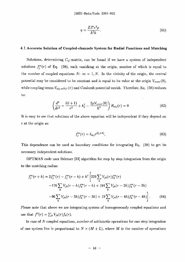
4.1 Accurate Solution of Coupled-channels System for Radial Functions and Matching

Solutions, determining Cij-matrix, can be found if we have a system of independent

solutions fj-(r) of Eq. 59), each vanishing at the origin, number of which is equal to

the number of coupled equations N m = N. In the vicinity of the origin, the central

potential may be considered to be constant and is equal to its value at the origin Ventr(O),

while coupling terms V1jnillif (r) and Coulomb potential vanish. Therefore, Eq. 56) reduces

to:

d 2 ly + 1) 2 21L Vmt r (0)- + k - RnIj 0 (62)

(dr' r2 n h2

It is easy to see that solutions of the above equation will be independent if they depend on

r at the origin as:

(63)

This dependence can be used as boundary conditions for integrating Eq. 59) to get its

necessary independent solutions.

OPTMAN code uses St6rmer 33] algorithm for step by step integration from the origin

to the matching radius:

fj'(r + h = 2fj(r - f(r - h) + h' 229 E Vk (r) fk' (r)

-176E Vk(r - h) fk' (r h) + 194 EVk( - 2h)fk(r - 2h)

k k

-96E Vjk(r - 3h)fk(r - 3h) + 19E Vk(r - 4h)fk(r - 4h) (64)

k k

Please note that above we are integrating system of homogeneously coupled equations and

use that f "(r = Ek Vik(r)fk(r).

In case of N coupled equations, number of arithmetic operations for one step integration

of one system line is proportional to N x (M + L), where M is the number of operations

- 16 -


necessary to calculate coupling potential Vk, and L (- 10) denotes number of arithmetic

operations necessary to make summations and multiplications for each k for one step integra-

tions using Eq. 64) with all components preliminary prepared. Then number of arithmetic

operations for one step integration for all system lines is proportional to N x N x (M + L) If

K is the number of integration steps, number of arithmetic operations necessary to get one

independent solution of coupled equation system is proportional to N' x (M + L) x K. And to

get N independent solutions, necessary for matching, we need N' x (M + L) x K. So number

of arithmetic operations in suggested algorithm and thus computational time grows as the

number of coupled equations in the power of three. In case for three levels with spins 2,

4+, N = 2I + 1) is equal to 15. If we include 6 level in coupling scheme, N becomes 28,

almost twice so that Mand thus necessary computational time becomes - times longer.

Soft-rotator model describes at least collective levels from 34 low lying bands, including

negative parity one. It is shown that coupling of the first levels from this bands cannot be

ignored in reliable optical calculations. For such calculations N may be 0 and more. One

can evaluate typical number of arithmetic operations, thus computational time, considering

that typical number of integration steps from origin to the matching radius is about 100-200

and number of operations necessary to calculate coupling potential Vk, Eq. 57) due to it

complicity is about 60 for neutrons and 180 for protons, yet most potential elements V are

be calculated in advance and can be used repeatedly. Such algorithm requests about - 0'

arithmetic operations to solve typical coupled-channels system of equations. Please note

that running scattering problem we need solutions for a number of coupled-channels sys-

tems for each spin and parity J, giving significant contribution to calculated cross-sections

(about 100 for 200 MeV incident energies). It can be concluded that suggested algorithm

is rather time consuming. Looking at Eq. 64) one can see that for one step integration

for any of integrated solutions fn(r) potential Vk(r) is the same, so once it is organized we

can perform one step integration for all solutions f(r) simultaneously. In this case number

of arithmetic operations necessary for integration for all independent solutions reduces to

N 2 x (M + L) x K N'x (N - ) x L x K = N 2 x K x (M + L + (N - ) x L). One can see

that for lar e N suggested algorithm of simultaneous fT(r) functions integration is about9

- 17


MIL ;z: 6 - 20 times quicker. This quicker algorithm is now realized in subroutine SOSIT.

After independent solutions f-(r) are found, one can easily get Cij-matrix, matching

the solutions to have the desired asymptotic wave functions behavior. Matching approach

used in our code is suggested by 3].

We consider, that numerical solution f(r) is a linear combination of the normalized

solutions fn'(r), each having an incoming wave with a unit current only for channel so

that for asymptotic radius R region we can write:

Mi 'Cij [Fj(R h) + iGj(R + h)] (65)

fj-(R ± h) a j(R + hji + k-

Then, we can determine matrices

A .. j fj (R + h)G (R - h - f (R - h)Gj (R + h) ani j i -Cij

3(R + h)GI(R - h - Fj(R - h)Gj(R + h) kj

Bmj fn(R + h)Fj(R - h - fm(R - h)G3(R - h) ami Cij 1 (66)Fj(R + h)G3(R - h - F3(R - h)Gj(R + h)

giving matching equations:

Bmj (Am + Cii. (67)

One can see that it is necessary to invert (Am + Bmi) matrix with complex elements de-

termined by Eq. 66) to get Cij elements.

The normalized solutions fn'(r) can be easily determined as:j

rkfn'(r) CikB�,'f�n(r). (68)j M 3

km kk

4.2 Iterative Approach to Solve a System of Coupled Equations

The algorithm described above for accurate solution of coupled-channels system is quick,

but is still rather time consuming, as to get one solution with necessary asymptotic behavior

we need to get N independent solutions first. "Sequential iteration method for coupled

equations" - ECIS, developed by J. Raynal 34] is also realized in OPTMAN code. It is

-


more quicker, but faces iteration convergence problem for some specific scattering cases. We

modernized this algorithm improving its convergence.

Let us rewrite Eq. 59), presenting coupling in line 1' of system of coupled equations as

inhomogeneous term of homogeneous uncoupled equation:

d'fj (r)= Vj (r) f (r) + 1: V k (r) fk (r). (69)

dr2 kAj

If we have some n-order iteration solution fjn(r) of Eq. 69) we can find next iteration

fjn+'(r) solution by integrating step-by-step by radius the following inhomogeneous equa-

tions:

d2 fjn I (r) n+'(r) + Wj(r)= Vjj (r) fj (70)

dr2

with Wj(r = EkEj Vjk(r)fkn(r). To solve the scattering problem, derived solution fjn+'(r)

must have the right asymptotic physical behavior at the infinity - a plane incoming wave

with a unit current for initial channels, otherwise no incoming plane wave plus a spherical

outgoing wave.

First we match non-normalized derived solution fjn+'(r), that gives:

fjn+'(r = AFI, (r) + B (I, (r) + GI, (r)) . (71)

To get the normalized g + 1(r) with the right asymptotic form Eq. 60), let us recollect

that we can add any homogeneous solution to inhomogeneous ones, and it will be still the

solution of inhomogeneous one. If normalized homogeneous solution f(r) has the following

asymptotic form:

fY(r) F (r) + C (I, (r) + GI, r)) (72)3 .7

normalized function should be

fn+l fn+'(r - (A - ij)fj"(r), (73)j

where i mean wave functions with scattering through ground state. It is easy to see that

normalizing Eq. 73) determines Cij-matrix to be: Ci = - C(A -

- 19


Modified Numerov method 35] is applied to integrate inhornogeneous equation 70). For

inhomogeneous equation:

f " (r = V (r) f (r) + W (r), (74)

the integration algorithms is:

�(r + h = 2(r - �(r - h) + u(r) + [W(r + h) + 10W(r) + W(r - h)] 12

with u(r = (h2V(r) + h4V2 (r)/12)�(r) and f(r = �(r) + u(r)/12.

Original ECIS code 34] uses homogeneous solutions of Eq. 70) as zeroth order iteration

approximation fjo(r)Sij. To improve iterations convergence imaginary part of the diagonal

potential V(r) for such zeroth order iteration approximation solutions must be enlarged

by a factor (I 02). This can be easily understood if one recollects that predictions of

inelastic scattering by spherical optical model need such enlargement of the central imaginary

potential to give results similar to coupled-channels predictions. Number of arithmetic

operations necessary for such coupled-channels solution is N' x M x K x I; here N, M

and K are defined before, while I is the number of iterations necessary to convergence, it is

usually not high - ) and decreases as the incident energy increases or coupling decreases

(conditions determining reliable DWBA approach, which as one can see is the first iteration

results). Number of arithmetic operations necessary to solve a system of coupled equations

for fixed spin Y' using this algorithm is almost the same as the accurate solution algorithm

described before with simultaneous independent solutions integration, if number of iterations

L - 0 . But for the systems with high spin J one iteration is usually enough for solution,

as absolute contribution of such states is small, so that high relative solution errors for

states with such J are acceptable, that makes iteration algorithm much more effective.

Nevertheless there are many special cases in which iteration procedure using homogeneous

solutions of Eq. 70) as zeroth order iteration approximation do not converge. In this case

we suggest to use wave functions from accurate coupled-channels solutions Eq. 68) for

coupled system with truncated rank to be used as zeroth order approximations. For such

functions, found with coupling of only several levels that are mostly strong coupled, number

of coupled equations is small, allowing a quick solution. These solutions describe ground

- 20 -


and first xcited states wave functions much more accurately than simple homogeneous

solutions, as now ground state wave functions used as zeroth order approximation already

account existence of coupling with the most strongly coupled excited levels and thus can be

used as starting approximations, allowing converging the problems that do not converge in

simple approach.

4.3 Asymptotic wave functions used to be matched with numerical solutions

Numerical solutions should be matched with Coulomb wave functions FI(kr) and G(kr),

that are solutions of Eq. 56) in the outer region were nuclear potential vanishes and system

becomes uncoupled. Coulomb functions are the solutions of the following equation:

U'II(P) [1(1 + 1lp' + 2q/p::F 1] u(p = 0, (75)

sign T- is for te channels with positive and negative (opened and closed) channels, p = kr

and = ZZ'e2 . For positive energies FI(kr) and G(kr) are two Coulomb functions 27]hTk.-

regular and irregular at p = . In case of = they are reduced to spherical Bessel and

Neuman functions multiplied by p:

,7rP)112F (p = 2 J1+112(P = Pl(P)

Gi(p) = _1)1(1)1/2 J-(1+112)(P = -I)'P]-I(P = P?71(P), (76)2

that can be easily calculated by recurrence 36].

For closed channels and > the only solution allowed from physical point of view is

the Whittaker function, which is exponentially decreasing:

ul(p = W-77,1 + 1/2,2p). (77)

But for matching procedures of accurate solutions of Eq. 65) and iteration ones of Eq.

(71), we need also linear independent exponentially increasing solution. Both these functions

are not easily calculated with high accuracy for the set of appearing 1, and values. On

the other hand, values of decreasing and increasing functions may differ by too many orders

of magnitude, that can make numerical matching inaccurate. To get the Coulomb functions

- 21 -


for closed channels with necessary accuracy it was decided to consider them to be unity

at R - h matching point and get their values at R + h point by several step numerical

integration of Eqs. 75). Such integration gives correct relative function values with very

high accuracy, as integration is done on a very short variable interval of 2h. The accuracy

of the calculated functions is checked using Wronskian relationship:

Fl(p)G'(p - GI(p)F,'(p = const, (78)1

so that Wronskian for calculated FI(p) and G(p) functions is checked to be the same at

k(R - h) and k(R + h) matching points

It is quite clear that such a definition gives functions with arbitrary normalization, but

for closed channels we are not interested in absolute value of appropriate C-matrix element

of Eq. 60) as there is no current of scattered particles through these channels.

5. C-MATRIX AND COUPLED CHANNELS OPTICAL MODEL PREDICTIONS

Using the C-matrix, all optical model cross-sections can be calculated.

Differential nucleon scattering cross-section with excitation of n-th level averaged over

incoming particle spin s and nuclear target spin I, projection M (scattering of unpolarized

nucleon with unpolarized target) can be calculated as:

dan )] Cj, j'.J' C*j� -2 j2- 2- - 2 exp [40,1F 'j, jI 3132 2dQ 2k (2I, + 1) I 'j, 112i".122E I or'2 II,

'I 2)IJ2'1124J2 1'2

12 X PL (COS 0) - )11+12-L 1 + _1)1'1+12-L

4 + I I I

X( 'I .21/2 1/2 LO) 12 - 12 LO) W(Ji 'I J2 .2; I, L) W (J " 2i'; I, L)J 3132 3 3 31 2

E(V + 1) Re [exp(ZorI,)f* (O)Cj� lnlljl I P� (Cos 0).+ lfc(o) 2 (79)ki(2I, + 1) j,11 III

where a, and qn = pZZ'e 2/h2 k,, are the corresponding Coulomb phase shift and Som-

merfeld parameter accordingly. fO = - exp 2i [ai - l In sin 02] is the Coulomb2kl sin2 0/2

amplitude, which vanishes in case of neutron scattering.

- 22 -


Integrated scattering cross-sections 0, can be derived from Eq. 79). Please note, that

due to Coulomb discontinuity at zero angle, such integration is impossible for elastic proton

scattering:

27r Cj 2Un 2 (2J + 1) (80)

k, (2I, + 1) jjlj, ini

Total neutron cross section UnT is determined by optical theorem 36]:

27r 1:(2J + ) m Cj (81)OrnT k 2(21, + 1) jjj 11ji1j,I

and compound formation cross section is:

27 - I Cj 'jjj 12un = 2 iij

Uc = UnT E(2J+ lmcjjllj- (82)n ki (2h + 1) jji n11jf

Generalized transmission coefficients are determined by Eq. (82):

TJ=4 ImCjjllj- E lCjjlf 12 (83)n1fil

5.1 Legendre Polynomial Expansion of Angular Distributions of Scattered Particles

Formula 79) allows to calculate angular distributions of scattered nucleons to be com-

pared with experimentally measured. On the other hand, OPTMAN code intends to present

such angular distributions as Legendre polynomial expansion giving coefficients of such ex-

pansion to be used in evaluated nuclear data files.

According to ENDF-6 Formats Manual 37], angular distributions for neutrons (File 4,

LTT=1), which is also applicable to inelastically scattered protons (File 6 LAW=2), may

be presented as

du,, Un NL 2L + 127r E �2 aL(E)PL(cosO). (84)

L=O

One can see from formula 79) that aL(E) are ral numbers and can be presented (please note,

that term with Coulomb amplitude vanishes for neutrons and inelastic proton scattering)

as:

- 23 -


2 227r I z Cjl *J2 1 2 3132 2aL(E = exp kal' c] ill ll2j2,nl2'j2'k 2(2L + 1)(2h + 1) E I jlnl'ljl'c

J1 J2 l 21112

j'l 32 "I 2

X + +

4X( 'I .21/2 - 12 LO) 1/2 - 12 LO) W(Ji .I J2j2; I, L)W(Jlj'J2j'; II L), (85)

3 3 3132

with maximum L number NL = max(l' I').2 1

In case of elastically scattered protons presence of Coulomb amplitude must be taken

into account. According to ENDF-6 Formats Manual 37] angular distributions for protons

(File 6 LAW=5) may be presented as:

2 ML

du,, - 771 771 Re exp Vq In (sin 2 0/2 2L I aL(E) PL(cos 0)ffi 4k 2sin40/2 sin 20/2 E 21 L=O

NL 2L I+ 1: � �bL(E) PL(cos 0). (86)

L=O 2

Comparing ENDF-6 format formula with 79) gives aL(E)

aL(E = 1 1:(2J, + IC"' (87)Ik 2(2L + 1)(2I, + 1) Jljl lLjlLjl

with maximum L umber ML = max(11). These aL(E) have complex values, while bL(E)

are real and similar to aL(E) for neutrons:

WI I. -2 -2 - - - -bL(E) exp I Cj�jl"�J' Cj2 'JI 2 JJ23112ill li2j2,nl'j2

k,2(2L + 1)(2I, + 1) J1 I 21112 2

J'l '2 "I 2

I [1 + -1)11+12-L] 1 + _1)1',+12-L

4

X j1j2I/2 - 12 I LO) j' 21/2 - 12 LO) WJ131 J232; I, L) W(Jlj'J2 -7 '2; I, L), (88)

with the only difference that bL(E) coefficients are not scaled by /27r value.

6. ENERGY DEPENDENCE OF OPTICAL POTENTIAL PARAMETERS

Options of OPTMAN code on the energy dependence of optical potential parameters

allow different possibilities. The reason is that there is significant difference for optical po-

tentials used in spherical and CC calculations. In spherical case, optical model calculations

- 24 -


for a certain incident energy request the knowledge of the potential only for a specified in-

cident energy, while CC calculations request inherent optical potential energy dependence

due to account of energy losses for different coupled channels. As we intend to allow OPT-

MAN CC code to analyze data in a wide energy region (at least up to 200 MeV incident

energies) both for neutrons and protons simultaneously, we keep a global form of optical

potential which incorporates the energy dependence of potential, that is derived by consid-

ering the dispersion relationship as proposed by Delaroche et a. 38], and the high-energy

saturation behavior consistent with the Dirac phenomenology. The imaginary components

of this potential form vanish at at Fermi energy (property stemming from nuclear matter

theory). Such an energy dependence allows data analysis without unphysical discontinuities

in the whole energy range of interest both for neutrons and protons (constant potential

terms, allowing simple potential linear dependencies, shown by bold characters below for

imaginary surface, volume and spin-orbit potentials, can be also used, but please note that

being non-zero, they do not vanish at Fermi energies):

VR (VR + VRE* + VE *2 + VRE *3 + DISP e`RE' I+ A - 2Z]R + V DISP A

VR R

+CCOUI ZZ, �OCOU (E*), (89)AI/3

wD [wDDISP + _ 1) Z' 1 CWiSO A - 2ZI e-,\DE.. E*S + WD+WD E*, (90)A E*S + WIDDS

WV WVDISp E*S V WE* (9 )-3-+Wo+ VE*S + WIDVA.�E'

Vs = VIC (92)

WS = WDISP E*S + WOso E*S + WIDS_ so+WS'OE*. (93)

so

Here, E = Ep- Ef,.,,), with Ep - energy of the projectile and Ep - the Fermi energy,

determined as Ef ., (Z, A) = - [S, (Z, A) S (Z A + 1)] for neutrons and E (Z A)2 f

[Sp(Z, A) Sp(Z + 1 A + 1)] for protons, where Si(Z, A) denotes the separation energy

of nucleon from a nucleus labeled by Z and A, while Z, Z and A are charges of incident par-

ticle, nucleus and nucleus mass number, respectively. As we intend to analyze neutron and

proton scattering data simultaneously, we want to have unique optical potential for nucleons

with form suggested by Ref. 38] plus a term C,IZZ'IA 1/3�0".", (E*) describing the Coulomb

- 25 -


correction to the real optical potential and isospin terms (-I)Z'+'C,,i..(A - 2)1A�p,,j�,,,(E*)

and (1)z'+'C i,,(A - 2Z)/A -�p,,j,,(E*). We assumed that energy dependences of �Oj,,,(E*)

and �o,,,,j,,,(E*) are the same as those of real and imaginary surface potentials (see Eq.

(89,90)), while �o..,(E*) can be constant (just unity) or considered to be the minus derivative

of Eq. 89) so that

(p�..I(Ep = (ARVR'-5Pe_'\RE - VR - 2VR2E* + 3VRE*) 1 + 1) ZI +IC". A - ZDISPVR + VR

(94)

DISP, wVDISP, wSDISPThe parameters WIDD, WIDV, WD 0 AD and AR were taken to be

equal for neutrons and protons. We consider, that Lane model 39] works, therefore the

neutron-proton optical potential difference of the suggested potential stems from the isospin

terms, the Coulomb correction terms and difference of the neutron-proton Fermi energies.

Real rR and Coulomb rc potential radii can be considered to be energy dependent as

experimental data analises 838] indicate dispersion-like energy dependence:

0 CRE*SrR(E* = rR (95)

E*s + WILR

0 CcE*Src(E* = rc � 1 (96)E*S + WILC

Potential diffusenesses ai can be energy dependent, reflecting that they may grow or

decrease with nuclear excitation energy:

a = ao + aE* (97)i i

with al assumed to be zero above an energy Eb,,,,,d-D

If energy losses due to collective levels excitation as compared to the nucleon incident

energies involved in the analysis are noticeable, the dependence of the local optical potential

for different channels can be taken into account as:

Vf = Ep - E + Ef2

where and f denote initial and final channels, while Ei and Ef the corresponding level

energies.

- 26 -


7. RELATIVISTIC GENERALIZATION OF NON-RELATIVISTIC

SCHR6DINGER EQUATION

Upper boundary of incident energy of the OPTMAN code is supposed to be about

200 MeV, so our non-relativistic Schr6dinger formalism involved relativistic generalization

suggested by Elton 40]. The nucleon wave number k was taken in the relativistic form:

(hk) = E - (MPCI)2] /C2 (98)

where E denotes the total energy of projectile, Mp the projectile rest mass, and the light

velocity. To allow non-relativistic motion of the target with rest mass MT, incident particle

mass Mp was replaced with the relativistic projectile energy E in reduced mass formulae, so

that the quantity k and optical potential values were multiplied by a coefficient:

1 (99)1 + EI(MTC2)

Following Elton's 40] suggestions, we multiply optical otential strengths except for the spin-

orbit and Coulomb terms by a factor K(E), as a relativistic optical potential generalization.

Elton 40] suggests it to be EI(MPC2). Therefore, the factor grows without limit as the

projectile energy E grows. We use this factor as suggested by Madland 41], K(E =

2E/(E + M,,C2), which saturates at 2 as incident energy grows, as it looks more physical and

allows easier fitting of experimental data. Of course, optical potential can be in any case

fitted to the experimental data without such multiplier, so that such relativistic correction

can be included while fitting. However, we agree with Elton 40] that it is advantageous to

separate out known relativistic factor in the central potential", as this may allow successful

extrapolation of optical potential from low incident projectile energy region to higher and

vice versa. One can see that for low energies all these relativistic generalization factors have

non-relativistic kinematic limit.

8. POTENTIAL ADJUSTMENT

Such best fit optical potential parameters can be fund by automatic minimization of 2

value:

- 27 -


2 N 1 K. doij1dQe.i - doijIffie.p 2 + M 2

N+M+L+3 _I�E AuijldQexp Aij=1( atotevall+ Se

L Orreac Crreacevali2 0 _ So 2 S, - S, 2 cal R 2+ ali .I eV cal �,al eval (100)

i=1 AO'reaeevali AseV., AS,'Val ) + ("AReval I

here K is the number of angles for which angular distribution is measured for incident

energy i, and the number of such energies is N, while numbers of total and reaction cross-

section data are M and L, respectively. The symbols So, S' and R' denote s-, p-wave

strength functions and scattering radius, respectively. All the other optical observable, if

any, can be also included in X 2search criteria.

9. ANALYSIS OF B(E2) DATA

The -y-transition probability B(EA) of soft rotator model can also be calculated. For

instance B(E2) calculated in homogeneously charged deformed ellipsoid approximation ac-

counting linear terms of inner b2, dynamic variables (higher terms can be taken into consid-

eration, see ( 25] is

Q2

B(E2; Inn,3,ne2 -+ Ir'n'n' n 5-6 0 ATKAPKIY 3 2 167r 1/2KKI> [1 + SOK)(I + SKI)l

x [(nyl cos yln') [(I'2K'OIIK) + (-I),'(1'2 - KIK)SK0 JKKI

+�1/2(nl sin yln') [1'2K'2JIK)SKK1+2 + (I'2K - 21IK)SKKI-2

2

+(-I),'(1'2 - K2JIK)�K,2-K1]] 12 1Tn-yn)33n02 [y] (101)

11r1n.',n,',3n�-

here J JTn-yn,63np2 [y] is enhancement factor due to nuclei softness determined by Eq.(41).Vr'n' , n.3 n�

10. CONCLUSION

According to the ISTC B-521 Project's Working Plan we finalized mod ernizing OPT-

MAN code's computational approaches and new, more accurate numerical algorithms be-

came possible now due to available large computational resources. We developed two mod-

ernized algorithms for solution of coupled channels equations in scattering problem. First is

- 28 -


the accurate system solution, which is 620 times faster than previously used. Second quick

solution algorithm is the iteration one with the improved convergence. We also improved

the accuracy of matching procedure in case of charged scattered particles. More grounded

optical potential parameters dependences guided by physical principles made it possible a

global optical potential search. All the algorithms are already included in the currently

modernized code OPTMAN. Users of the code can choose one of these algorithms when

running optical calculations. Instead, OPTMAN code has a capability to select the optimal

option, depending on the number of couple equations, on the coupling strength, incident

particle energy, and system spin. Current version of modernized OPTMAN code was used

to find best fit nuclear optical parameters for 12c [iii, 24,26Mg [42] , 28-3OSi [12] and 12 Cr

[13]. They are already used for predictions of cross sections for 2C, natural Si and Mg for

Japanese high energy nuclear data evaluation.

Acknowledgements

The authors are grateful to guidance of the late Dr. Y. Kikuchi who had started the

collaboration among authors. They also thank members of JAERI nuclear data center for

helpful comments and supports.

29 -


REFERENCES

[1] A.I. Blokhin, A.V. Ignatjuk, V.N. Manokhin et al., BROND-2, Library of Recommended

Evaluated Neutron Data, Documentation of Data Files, Yudernie Konstanty, issues 23

in English 1991).

[21 T. Tamura, Rev. Mod. Phys. 37, 679 1965).

[3] J. Raynal, Optical Model and Coupled-Cannel Calculations in Nuclear Physics, IAEA

SMR-9/8, IAEA 1970).

[4] Y.V. Porodzinskii and E.S. Sukhovitskii, Phys. of Atom. Nucl. 59, 247 1996).

[5] Y.V. Porodzinskii and E.S. Sukhovitskii, Sov. J. Nucl. Phys. 53, 41 1991).

[6] Y.V. Porodzinskii and E.S. Sukhovitskii, Sov. J. Nucl. Phys. 54, 570 1991).

[7] E.S. Soukhovitskii and S. Chiba, J. Nucl. Sci. Technol. Suppl 2 697(2002).

[8] ES. Sukhovitskii, 0. Iwamoto, S. Chiba and T. Fukahori, J. Nucl. Sci. Technol 3, 120

(2000).

[9] E.S. Soukhovitskii and S. Chiba, J. Nucl. Sci. Technol. Suppl 2 144 2002).

[10] S. Chiba, 0. Iwamoto, Y. Yamanouti, M. Sugimoto, M. Mizurnoto, K. Hasegawa, E.S.

Sukhovitskii, Y.V. Porodzinskil and Y. Watanabe, Nucl. Phys A 624, 305 1997).

[111 S. Chiba, 0. Iwamoto, E. S. Sukhovitskii, Y. Watanabe and T. Fukahori, J. Nucl. Sch

Technol. 37, 498 2000).

[12] W. Sun, Y. Watanabe, E. Sh. Sukhovitskii, 0. Iwamoto and S. Chiba, J. of Nucl. Sci.

and Technol. 40, 635 2003).

[13] E.S. Sukhovitskil, S. Chiba, J.-Y. Lee, BA. Kim and S.-W. Hong, J. Nucl. Sci. Technol.

40, 69(2003).

[14] J.Y. LeeE. Sh. Sukhovitskii, Y.-O. Lee, J. Chang, S. Chiba and 0. Iwamoto, J. Korean

Phys. Soc. 38, 88 2001).

- 30 -


[15] E.S. Sukhovitskii, S. Chiba, J.-Y. Lee, Y.-O. Lee, J. Chang, T. Maruyama and .

Iwamoto, J. Nucl. Sci. Technol. 39, 816 2002).

[16] E.S. Sukhovitskii, Y.-O. Lee, J. Chang, S. Chiba and 0. Iwamoto, Phys. Rev. C62,

044605 2000).

[17] A. Bohr and B.R. Mottelson, Nuclear Structure, Vol. H, Nuclear Deformations, p.195,

W. A. Benjamin Inc. 1975).

[18] A.S. Davydov, Vozbuzhdcnnye sostoyaniya atomnykh yader Excited States of Atomic

Nuclei), Moscow: Atomizdat 1969).

[19] P.O. Lipas and J.P. Davidson, Nucl. Phys. 26, 80 1961).

[201 F. Todd Baker, Nucl. Phys. A331, 39 1979).

[21] S.G. Rohozinski and A. Sobiczewski, Acta. Phys. Polon. B 12, 1001 1981).

[22] I.M. Strutinsky, Atomic Energy 4 150 1956).

[23] S. Flugge, Practical Quantum Mechanics, Springer-Verlag, Berlin-Heidelberg-New York,

1971.

[24] A.Ya. Dzyublik and V.Yu. Denisov, Yad. Fiz. 56, 30(1993).

[25] J.M. Eisenberg and W. Greiner, Nuclear Models, North-Holland 1970).

[26] A.S. Davydov and G.F. Filippov, Nucl. Phys. 8, 237(1958).

[27] M. Abramowitz and I.A. Stegun, Handbook of Mathematical Functions, Dover Publica-

tions, New York(1965).

[281 R. H. Bassel, R. M. Drisko, and C. R. Satchler, Oak Ridge National Laboratory Report

ORNL-3240, 1962).

[291 J. Rainal, Phys. Rev. C23, 2571 1980).

[301 E.S. Sukhovitskii, S. Chiba, 0. Iwamoto and Porodzinskii, Nucl. Phys A 640, 147

(1998).

- 31 -


[31] E.S. Sukhovitskii, S. Chiba, 0. Iwamoto, Nucl. Pbys A 646, 147 (1999).

[321 Y. Kikuchi, INDC(FR)-5/L, 1972).

[331 C. Stormer, Arch. Sci. Phys. 63 1907).

[341 J. Raynal, Equations coupWes et DWBA, Report LYCEN,6804, Aussois 1968).

[35] B.V. Numerov, Monthly Notices Roy. Astr. Soc. 84, 592 1924) and M.A. Melkonoff J.

Raynal, T. Sawada ., Methods Comput. Phys. 6 Academic Press, NY 1966).

[36] P.E.Hodgson, The Optical Model of Elastic Scattering, The Clarendon Press, Oxford

(196,3).

[371 ENDF-6 Formats Manual, Report IAEA-NDS-76, Rev. 6 April 2001, edited by V.

McLane.

[381 J.P. Delaroche, Y. Wang and Rappoport, Phys. ReV., C39, 391 1989).

[391 A.M. Lane, Phys. Rev.Lett. 8, 171 1962); A.M. Lane, Nucl. Phys. 35, 676 1962).

[40] R.L.B. Elton, Nuovo Cimento XLII B, 277 1966).

[41] D. G. Madland, A. J. Sierk, Proc. Int. Conf. on Nuclear Data for Science and Technology,

Vol 1, p 202, Trieste, 1997.

[42] W. Sun et al., to be published.

- 32 -

M old,; M al, (SI) �-- 9� x A

I SI *M fttlomllhwo 2 I14 M �7x tl - tP 0 SE5 Siffuno.

It m H min, h, d 101� E

-t �, kg P�F loll p

MI s 1, L lo,? TTU A t 10, GA �fj ? i ff. L, eV 10, IV' M

Al MCI fj�, 41 u 10, hcd t da

10,7 7 rad I eV=L 60218 x 107 �5 7 sr I u - 1 660 54 x I - kg lo-, d

10-2 + C

0-1 m

3 Pq ff CD k SI tel I 10-1Ito SI T ft A 4 SI �- it IC 4 IC I0 n

PIL 7 T LX ft �6 Ili ft� io-12 p

lo- 7 IF07

N m-kg/s' A- �I, 7, r Ajf IL, Pa N/m' b 01)

A, j N-m A, bar7 w J/s A, 1. AI 5 1 1 F U4 K W V I IN, Pi M

r2 c A-s ci I9854tf1JHICI7,. ttz-L, I eVc % FL, La F V W/A F15� R ISID 1u MlMt CODATA CD 19864FMIZ

% -4 7 79 F F C/V V rad W IC �-M % r 't - I- f, V/A rem 2. A 4 (I T. / v 1,, 7 - A,--j y 7, S AN - IL tftl rich,FE Wb V-s I jk� 0 I nm- IO- m

I b- 100 fm'- 10- m'7 T Wb/rn'9 11 Wb/A I bar-O I MPa - IO'Pa 3. baHl, JISIC�IAU*ODL)�,�-A*)*14

;K P 'c 1 Gal I CM/Sl 1-IM/S2 A IC 5N - 2 CD Lt t-CLIL, - �/ Im cd srIL, �I 7, Ix Im/m, 1 Ci 37 x 10 " Bq 4. EC%1MfT-S-'T.`WC�1bar, barnISI

S-1 1 R=2.58 x IO-T/kg--< �7 I, j�, Bq Y FMV+OTf-,i-J mmHg;�-A20)h-r:y9-f Gy J/kg I rad = I Gy = 10-'Gy IC ti c L L

M ji, SvI J/kg rm- I cSv= 10 'Sv

A A

N(=10'dyn) kgf lbf ff. Wa,=10bar) kgf/cm' atm mmHg(Torr) lbf/in'(psi)

1 0.101972 0.224809 110.1972 9.86923 7.50062 x 10' 145.038

9.80665 1 2.20462 J) 0.0980665 1 0.967841 735.559 14.2233

4.44822 0.453592 1 0.101325 1.03323 1 760 14.6959

I Pa-s(N-s/rn')= IO POt7�0(g/(cm-s)) 1.33322 x 10-' 135951 x 10-' 1.31579 x 10 1 1.93368 x 10-'

I m/s= 10'St( Y (CM,/s) 6.89476 x IO-' I 703070 x IO 6.80460 x 102 51.7149 1

- 0'erg) kgf m kW h Ca I 42�y Btu ft lbf eV I a] 4.18605 J

1 0.101972 2.77778 x 10 0.238889 q.47813 x IO-' 0.737562 6.24150 x 10 4.184d (AfL-T)

9.80665 1 2.72407 x 10 2.34270 9.29487 x 10 7.23301 6.12082 x 10" 4.1855 J ( 1 5 T)

3.6 x O' 3.67098 x 10' 1 8.59999 x 0 3412.13 2.65522 x 10' 2.246 94 x 2 4.1868 J

4.18605 0.426858 1 16279 x 10 1 :3.96759 x 10 3.08747 2.612 72 x IO I T_ V. I Ps (ILN ))

1055.06 107.586 2.93072 x 10- 252.042 1 778.172 6.58515 x 10" = 75 kgf m/s

1.35582 0.138255 3.76616 x 10- 0.323890 1.28506 x - 1 8.46233 x IO" = 735.499 W

1.60218 x 10 " 1.63377 x lo 2 4.45050 x 10-1 382743 x 10-211 1.518 57 x I - 1 18171 x I -

Bq ci W G y rad y 11� C/kg R 0 V remV 44 la -1 2.70270 x I - 1 0 1 3876 I 10041. IIA

3.7 x I I 0.01 1 2.58 x 10 0.01 1

(86 T 12 fl 26 H ]MI.

U,

CL

CL

IDCL

CD

SL

C-)C>

ID

CL

2004-002 physics and numerical methods of optman: a ...

Documents

Transcript of 2004-002 physics and numerical methods of optman: a ...