Variable mesh optimization for continuous optimization problems
Upload
khangminh22Category
view
2download
0
HAL Id: tel-01681286https://tel.archives-ouvertes.fr/tel-01681286
Submitted on 11 Jan 2018
HAL is a multi-disciplinary open accessarchive for the deposit and dissemination of sci-entific research documents, whether they are pub-lished or not. The documents may come fromteaching and research institutions in France orabroad, or from public or private research centers.
L’archive ouverte pluridisciplinaire HAL, estdestinée au dépôt et à la diffusion de documentsscientifiques de niveau recherche, publiés ou non,émanant des établissements d’enseignement et derecherche français ou étrangers, des laboratoirespublics ou privés.
Development of optimization methods for land-use andtransportation models
Thomas Capelle
To cite this version:Thomas Capelle. Development of optimization methods for land-use and transportation models.Computer Aided Engineering. Université Grenoble Alpes, 2017. English. NNT : 2017GREAM008.tel-01681286

THESEPour obtenir le grade de
DOCTEUR DE L’UNIVERSITE DE GRENOBLESpecialite : Mathematiques et Informatique
Arrete ministeriel : 7 Aout 2006
Presentee par
Thomas Capelle
These dirigee par Peter Sturmet codirigee par Arthur Vidard
preparee au sein du Laboratoire Jean Kuntzmannet de l’Ecole Doctorale Mathematiques, Sciences et Technologiesde l’Information, Informatique
Recherche sur des methodesd’optimisation pour la mise enplace de modeles integres detransport et usage des solsDevelopment of optimisation methods forland-use and transportation models
These soutenue publiquement le 15/02/2017,devant le jury compose de :
Nabil LayaıdaInria, PresidentMichael BattyUniversity College London, RapporteurVincent HilaireUniversite de Technologie de Belfort-Montbeliard, RapporteurTomas de la BarraUniversidad Central de Venezuela, ExaminateurNicolas CoulombelUniversite Paris-Est, ExaminateurPeter SturmInria, Directeur de theseArthur VidardInria, Co-Directeur de these


Acknowledgements: The writing of this thesis took place within the STEEP team at
INRIA Grenoble, in offices G104, E101 (also a little bit in the office of Jean-Yves and Luciano).
I could never have done this research without the support of all the people I met here.
In the first place, I would like to thank my director of theses, Peter Sturm. To work
under your guidance it’s a breeze, you always guided the “aprenti - chercheur” in each phase
all along the thesis, with a "Zen" and precise look, exactly what one has need of. I would
also like to thank you for your availability and your commitment to all the challenges of this
work. Finally, I am grateful of your human qualities and I am proud to have found in you a
friend.
I would like to thank my co-director Arthur Vidard. Even if you were not on the site of
INRIA, I could always count on you. Particularly, I found extremely useful and reassuring your
commitment on the numerical / mathematical issues during the thesis. I am convinced that
a great deal of reformulation results are possible thanks to the afternoons working on Tranus
equations. Your good humour and availability were very appreciated.
I would like to thank my colleague and friend Laurent Gilquin. We shared a great part of
the thesis together, and even if you are not very good in ping-pong, we were able to make
an article together. I would also like to thank my collaborators Brian J. Morton and Fausto
Lo Feudo for allowing me to carry out my research on the Tranus models that they have so
well developed. I would also like to express my gratitude to Tomás de la Barra for believing
in this project. Thank you for participating in my jury of thesis and I hope that the work
realised here will be able to integrate to Tranus.
I would also like to thank Mr. Michael Batty and Dr. Vincent Hillaire for their interest in
this research by committing themselves to being rapporteurs, and to Nicolas Coulombel for
agreeing to participate in the jury. I would also like to thank Nabil Layaida for agreeing to
preside over the jury.
No one doubts that without Marie-Anne, this thesis would not have taken place. Thank
you for your good availability, your mood and your mastery of the French bureaucracy.
This acknowledgment would be incomplete if I did not thank all members of the STEEP
team (present and past). Particularly Jean-Yves, thank you for the political discussion / food
/ variety at the cafeteria, and all the snacks you provided to well feed this thesis.
Finally, I would like to thank my dear wife for her enthusiastic and loving daily support.
The end of this research process gave two fruits, in your hands you have the first one, the
second, is our always smiling son Hector. I think the later is more successful, but it is research
“in progress”.
These thanks can not be completed without a thought for my first fan: my mother. His
v

Acknowledgements
presence and encouragement are for me the founding pillars of what I am and what I do.
vi

Abstract: Land use and transportation integrated (LUTI) models aim at representing
the complex interactions between land use and transportation offer and demand within a
territory. They are principally used to assess different alternative planning scenarios, via the
simulation of their tendential impacts on patterns of land use and travel behaviour. Setting up
a LUTI model requires the estimation of several types of parameters to reproduce as closely as
possible, observations gathered on the studied area (socio-economic data, transport surveys,
etc.). The vast majority of available calibration approaches are semi-automatic and estimate
one subset of parameters at a time, without a global integrated estimation.
In this work, we improve the calibration procedure of Tranus, one of the most widely
used LUTI models, by developing tools for the automatic and simultaneous estimation of
parameters. Among the improvements proposed we replace the inner loop estimation of
endogenous parameters (known as shadow prices) by a proper optimisation procedure. To
do so, we carefully inspect the mathematics and micro-economic theories involved in the
computation of the various model equations. To propose an efficient optimisation solution,
we decouple the entire optimisation problem into equivalent smaller problems. The validation
of our optimisation algorithm is then performed in synthetic models where the optimal set of
parameters is known.
Second, in our goal to develop a fully integrated automatic calibration, we developed
an integrated estimation scheme for the shadow prices and a subset of hard to calibrate
parameters. The scheme is shown to outperform calibration quality achieved by the classical
approach, even when carried out by experts. We also propose a sensitivity analysis to identify
influential parameters, this is then coupled with an optimisation algorithm to improve the
calibration of the selected parameters.
Third, we challenge the classical viewpoint adopted by Tranus and various other LUTI
models, that calibration should lead to model parameters for which the model output perfectly
fits observed data. This may indeed cause the risk of producing overfitting (as for Tranus,
by using too many shadow price parameters), which will in turn undermine the models’
predictive capabilities. We thus propose a model selection scheme that aims at achieving a
good compromise between the complexity of the model (in our case, the number of shadow
prices) and the goodness of fit of model outputs to observations. Our experiments show that
at least two thirds of shadow prices may be dropped from the model while still giving a near
perfect fit to observations.
The contribution outlined above are demonstrated on Tranus models and data from three
metropolitan areas, in the USA and Europe.
Keywords: LUTI, Tranus, land use, calibration, optimisation.
vii

Abstract
viii

Résumé: Les modèles intégrés d’usage des sols et de transport (LUTI) visent à représen-
ter les interactions complexes entre l’usage des sols et l’offre et la demande de transport sur le
territoire. Ils sont principalement utilisés pour évaluer différents scénarios de planification, par
la simulation de leurs effets tendanciels sur les modes d’usage des sols et les comportements
de déplacement. La mise en place d’un modèle LUTI nécessite l’estimation de plusieurs
types de paramètres pour reproduire le plus fidèlement possible les observations recueillies
sur la zone étudiée (données socio-économiques, enquêtes de transport, etc.). La grande
majorité des approches de calibration disponibles sont semi-automatiques et estiment un
sous-ensemble de paramètres à la fois, sans estimation globale intégrée.
L’objectif de ce travail est d’améliorer la procédure de calibration de Tranus, l’un des
modèles LUTI les plus utilisés, en développant des outils pour l’estimation automatique et
simultanée des paramètres. Parmi les améliorations proposées, nous remplaçons l’estimation
de la boucle interne des paramètres endogènes (connus sous le nom de “shadow prices”)
par une procédure d’optimisation appropriée. Pour cela, nous examinons attentivement les
mathématiques et les théories micro-économiques à la base des différentes équations du
modèle. Nous proposons une solution d’optimisation efficace, en divisant l’ensemble du
problème d’optimisation en problèmes équivalents plus petits. Nous validons alors notre
algorithme avec des modèles synthétiques où l’ensemble optimal de paramètres est connu.
Deuxièmement, notre objectif de développer une calibration automatique entièrement
intégrée, nous développons un schéma d’estimation intégré pour les “shadow prices” et un
sous-ensemble de paramètres difficiles à estimer. Le système se révèle être supérieur à la
qualité de calibration obtenue par l’approche classique, même lorsqu’elle est effectuée par des
experts. Nous proposons également une analyse de sensibilité pour identifier les paramètres
influents, que nous combinons à un algorithme d’optimisation pour améliorer la calibration
des paramètres sélectionnés.
Troisièmement, nous contestons le point de vue classique adopté par Tranus et divers
modèles LUTI, selon lequel la calibration devrait déterminer des paramètres pour lesquels les
résultats de la modélisation correspondent parfaitement aux données observées. Cela peut en
effet entraîner un risque de sur-paramétrisation (pour Tranus, en utilisant trop de paramètres
de “shadow prices”), qui limiterait les capacités prédictives du modèle. Nous proposons donc
un procédé de sélection des paramètres afin d’obtenir un bon compromis entre la complexité
du modèle (dans notre cas, le nombre de “shadow prices”) et la qualité de l’ajustement des
résultat de la modélisation aux observations. Nos expériences montrent qu’au moins les deux
tiers des “shadow prices” peuvent être supprimés tout en conservant un ajustement presque
parfait aux observations.
ix

Résumé
La contribution décrite ci-dessus est démontrée sur des modèles Tranus de 3 régions
métropolitaines, aux États-Unis et en Europe.
Mots clefs: LUTI, Tranus, usage de sol, calibration, optimisation.
x

Contents
Acknowledgements v
Abstract vii
Résumé ix
Introduction 1
Introduction (Français) 5
1 State of the art and background material 91.1 LUTI models literature review . . . . . . . . . . . . . . . . . . . . . . . . . 9
1.1.1 How is Calibration done in some LUTI models? . . . . . . . . . . . . 11
1.2 Local Optimisation . . . . . . . . . . . . . . . . . . . . . . . . . . . . . . . 15
1.2.1 Gradient Descent . . . . . . . . . . . . . . . . . . . . . . . . . . . . 16
1.2.2 Gauss-Newton . . . . . . . . . . . . . . . . . . . . . . . . . . . . . 16
1.2.3 Levenberg-Marquardt . . . . . . . . . . . . . . . . . . . . . . . . . . 17
1.2.4 Broyden-Fletcher-Goldfarb-Shannon . . . . . . . . . . . . . . . . . . 17
1.2.5 Stochastic optimisation: EGO algorithm . . . . . . . . . . . . . . . . 18
1.3 The Logit model . . . . . . . . . . . . . . . . . . . . . . . . . . . . . . . . 20
1.3.1 Consumer Surplus . . . . . . . . . . . . . . . . . . . . . . . . . . . 22
1.3.2 Properties of Logit models . . . . . . . . . . . . . . . . . . . . . . . 23
2 Description of Tranus 252.1 General structure of the model . . . . . . . . . . . . . . . . . . . . . . . . . 25
2.2 The land use and activity module . . . . . . . . . . . . . . . . . . . . . . . . 28
2.2.1 The demand functions . . . . . . . . . . . . . . . . . . . . . . . . . 31
2.2.2 Substitution Probabilities . . . . . . . . . . . . . . . . . . . . . . . . 33
xi

Contents
2.3 Location Probabilities and Logit scaling issues . . . . . . . . . . . . . . . . . 35
3 Calibration of the Tranus land use module: shadow price estimation 373.1 Calibration as currently done in Tranus . . . . . . . . . . . . . . . . . . . . . 38
3.2 Reformulating calibration as an optimisation problem . . . . . . . . . . . . . 39
3.3 Land use sectors (non transportable sectors) . . . . . . . . . . . . . . . . . 41
3.4 Transportable sectors . . . . . . . . . . . . . . . . . . . . . . . . . . . . . . 43
3.5 Summary of proposed approach and a numerical example . . . . . . . . . . . 45
3.5.1 Example of shadow price estimation with the optimisation approach
(Example C) . . . . . . . . . . . . . . . . . . . . . . . . . . . . . . 46
3.5.2 Numerical aspects . . . . . . . . . . . . . . . . . . . . . . . . . . . 51
3.6 Testing the proposed calibration methodology against the one implemented
in Tranus . . . . . . . . . . . . . . . . . . . . . . . . . . . . . . . . . . . . 52
3.6.1 Generation of synthetic scenarios for performance assessment . . . . 53
3.6.2 Examples of synthetic scenario generation . . . . . . . . . . . . . . . 55
3.6.3 Equilibrium prices in synthetic scenario: 1 economical sector, 2 zones 57
3.6.4 Reducing the number of shadow prices, early results . . . . . . . . . 58
4 Optimisation of other parameters than shadow prices 614.1 Parameters to Calibrate . . . . . . . . . . . . . . . . . . . . . . . . . . . . . 62
4.2 Simultaneous estimation of shadow prices and land use substitution parameters 63
4.2.1 Observed consumption preferences . . . . . . . . . . . . . . . . . . . 66
4.3 Sensitivity analysis and simultaneous calibration of shadow prices and marginal
utility of income . . . . . . . . . . . . . . . . . . . . . . . . . . . . . . . . . 68
4.3.1 Sensitivity Analysis . . . . . . . . . . . . . . . . . . . . . . . . . . . 68
4.3.2 Obtaining the λn parameters . . . . . . . . . . . . . . . . . . . . . . 70
5 Experimental results on real scenarios 735.1 North Carolina Tennessee (NCT) model . . . . . . . . . . . . . . . . . . . . 73
5.2 Mississippi model (MS) . . . . . . . . . . . . . . . . . . . . . . . . . . . . . 81
5.2.1 Sensitivity Analysis Results for the MS model . . . . . . . . . . . . . 82
5.2.2 Results of the subsequent iterative optimisation . . . . . . . . . . . . 85
5.3 Grenoble model . . . . . . . . . . . . . . . . . . . . . . . . . . . . . . . . . 88
5.3.1 Calibration of substitution sub-model . . . . . . . . . . . . . . . . . 88
5.3.2 Using observed ranking of housing preferences to initialise penalising
factors . . . . . . . . . . . . . . . . . . . . . . . . . . . . . . . . . . 92
xii

Contents
Conclusions 95Implementation . . . . . . . . . . . . . . . . . . . . . . . . . . . . . . . . . . . . 97
Future possibilities . . . . . . . . . . . . . . . . . . . . . . . . . . . . . . . . . . . 97
Conclusions (Français) 99Implementation . . . . . . . . . . . . . . . . . . . . . . . . . . . . . . . . . . . . 101
Possibilités futures . . . . . . . . . . . . . . . . . . . . . . . . . . . . . . . . . . . 101
References 103
Appendices 111
A Details on Tranus’ shadow price iteration scheme 113
B Demand functions of the Tranus Grenoble model 115
C Definition of generalised Sobol’ indices 117
xiii

Contents
xiv

Introduction
Most of today’s population lives in cities and urbanised areas. Much of the planet’s energy
consumption, pollution, waste generation etc. happens there, which makes it important to
consider urban areas in efforts aiming at sustainable development. The latter is, among oth-
ers, addressed by transportation and land use planning, where land use here loosely refers to
the spatial distribution of economic and other activities. Transportation and land use plan-
ning were traditionally carried out in a decoupled manner: although land use is naturally a
main input for transportation planning, the impact of changes in transportation infrastructure
or policies, on land use, was often ignored. One typical such impact is urban sprawl, whose
causes include the dynamic feedbacks between transportation and land use. Neglecting such
feedbacks in modelling systems that assist decision making, may lead to incorrect assess-
ments of transportation plans for instance. LUTI (land-use and transportation integrated)
models aim at representing the complex interactions between land use and transportation
offer and demand within a territory. They are mainly used to evaluate different alternative
planning scenarios, by simulating their tendential impacts on patterns of land use and travel
behaviour. Since the early 60’s LUTI modelling has attracted researchers that aimed to
model the complex economical relations in urban areas; a good overview of the evolution
and history of LUTI modelling can be found in (Wegener 2004). Setting up a LUTI model
requires the estimation of several types of parameters to reproduce as closely as possible, ob-
servations gathered on the studied area (socio-economic data, transport surveys, etc.). The
vast majority of available calibration approaches are semi-automatic, estimating one subset
of parameters at a time, without a global integrated estimation. Automatic calibration of
LUTI model is not a common practice; an exception has been proposed for the Meplan model
(Abraham 2000).
We consider Tranus (de la Barra 1982; de la Barra 1989), an open source LUTI model that
is widely used. Tranus is a classical LUTI models, with two separated modules: the activity
module and the transport module. The activity module, is an equilibrium type model based
1

Introduction
on micro-economic principles that balance the offer and demand of the different economical
sectors that interact at each level. Economical sectors are considered in the broad sense,
amongst them we have: land, goods, salaries, housing, transportation demand, etc. Also, the
price paid for each economical sector has to be balanced with respect to offer and demand,
thus there are two equilibria that have to be achieved, offer versus demand and (production)
cost versus prices. The transportation module, computes the costs of transportation and
assigns the demand to the network. Both modules interact back and forth until a general
equilibrium is achieved.
The calibration process is usually done by an expert modeller who iteratively tunes a
group of parameters to reproduce as closely as possible the observations gathered in the
area of study. This process is usually done manually, with little to no automation, adjusting
the different economical parameters (for example, the demand curves for different goods in a
specific geographical zone). At the same time, Tranus computes internally a set of adjustment
coefficients (called shadow prices in Tranus) that correct the utilities and account for un-
modelled effects. These endogenous variables help the model achieve a better response and
fit more precisely to the observed data.
In this thesis we address several shortcomings of the classical approach of calibration used
in Tranus. We propose the reformulation of the heuristic calibration algorithm used in the
land use and activity module as an optimisation problem. Later, we extend this approach
by having a closer look at the inner loop that computes the shadow prices and propose an
efficient methodology for their estimation by decoupling the calibration in smaller problems.
To be able to do this, we have to carefully investigate the system of equations that are
computed in the activity module. We also introduce auxiliary variables, which enables a
closed form computation instead of an iterative one. This in turn makes it possible to
use sophisticated numerical optimisation methods and opens the door to the simultaneous
estimation of different parameter types of the model. The ultimate goal of this approach is
to simultaneously calibrate the various parameters of Tranus’ inner and outer loops.
Overview of the dissertation
To be able to formulate a semi-automatic calibration of Tranus, it was first necessary to
construct a literature review of the state-of-the-art in urban modelling. Chapter 1 describes
the various operational LUTI models available and the corresponding calibration approaches.
It also builds a theoretical background on the numerical methods and discrete choice models
utilised all along this work.
2

Chapter 2 describes Tranus’ mathematical formulation, particularly for the land use and
activity module (from now on, land use module). We expose the various equations involved
in the calibration of the land use, also the demand functions and discrete choice models are
presented.
Chapter 3 is all about calibration of the land use module, first we present the traditional
calibration approach to estimate the so-called “shadow prices” which are endogenous parame-
ters of the model, and latter the reformulation of the calibration as an optimisation problem.
This chapter is the core of the thesis, and particular detail is given for the different types of
sectors. At the end of the chapter a comprehensive numerical example is given to illustrate
our methodology. We also present a detailed methodology for the construction of synthetic
scenarios based on real calibrated study areas. These synthetic scenarios have a perfect fit
without the need of shadow prices (usually we set their value to zero), enabling us to validate
our optimisation algorithms knowing the ground truth values of the shadow prices. A simple
example is presented to understand the problematic of synthetic scenario generation and the
corresponding equilibrium prices problem. Finally, we question the rationale of usual calibra-
tion approaches for Tranus (and other LUTI models), which consists in estimating parameters
for which the model reproduces observations exactly. In Tranus, this is achieved by enriching
the underlying macro-economic model with the already mentioned auxiliary variables, the
shadow prices. While this allows to correct for unavoidable un-modeled effects, it also bears
the risk of over-parameterisation/overfitting. We propose a model selection scheme, aiming
at a compromise between model complexity (here, number of shadow prices) and goodness of
fit to observations, reducing the risk of overfitting and increasing the likelihood of achieving
good predictions with a model. After the reformulation of the computation of the shadow
prices as an optimisation problem, we are able to include in the optimisation scheme other
parameters (than the shadow prices).
In Chapter 4, we deal with the calibration of other Tranus parameters. First we propose
a semi-automatic calibration for the penalising factors. These parameters aim to represent
the preferences of residential choice of the various household types of the model. The main
idea is to include external data (when available) to guess a good starting point for the
optimisation which then improves them. This is possible after examining the equations that
create the interactions between households and housing, and decoupling the optimisation in
smaller problems. Finally, we present a sensitivity analysis to identify influential parameters
for transportable sectors. Once the influential sectors are selected, an optimisation algorithm
finds the parameters values that improve the calibration.
The last chapter, Chapter 5 presents the methodology applied to real scenarios. We first
3

Introduction
apply our optimisation methodology to two North-American models, particularly to improve
the penalising factors, and later, to a model of the Grenoble urban area.
4

Introduction (Français)
La plupart de la population mondiale vit dans des villes et zones urbaines. Par conséquent, la
plus grande partie de la consommation d’énergie, de la pollution, de la génération de déchets,
de la planète, s’y concentre, d’où l’importance de considérer les zones urbaines dans les
efforts visant au développement durable. Celui-ci doit être pris en compte, entre autres, par
le transport et l’aménagement du territoire, c’est-à-dire à la répartition spatiale des activités
économiques et autres. Jusqu’à présent, la planification du transport et de l’aménagement du
territoire a été menée en pratique de manière découplée: bien que l’aménagement du territoire
soit logiquement une contribution principale à la planification des transports, l’impact des
changements dans les infrastructures ou les politiques de transport sur l’aménagement du
territoire a souvent été ignoré. Un impact typique de ce type est l’étalement urbain, dont les
causes incluent les réactions dynamiques entre le transport et l’aménagement du territoire.
En négligeant ces rétroactions dans les systèmes de modélisation qui assurent la prise de
décision, cela peut conduire à des évaluations incorrectes des plans de transport par exemple.
Les modèles LUTI (aménagement et transport intégrés) visent à représenter les interactions
complexes entre l’aménagement du territoire et l’offre et la demande de transport et la
demande sur un territoire. Ils sont principalement utilisés pour évaluer différents scénarios de
planification alternatifs, en simulant leurs impacts tendanciels sur les modèles d’aménagement
du territoire et les comportements de déplacement. Depuis les années 60, la modélisation
LUTI a attiré des chercheurs qui visaient à modéliser les relations économiques complexes
dans les zones urbaines; Un bon aperçu de l’évolution et de l’histoire de la modélisation LUTI
se trouve dans (Wegener 2004). La mise en place d’un modèle LUTI nécessite l’estimation de
plusieurs types de paramètres pour reproduire le plus près possible, les observations recueillies
dans la zone étudiée (données socio-économiques, enquêtes sur les transports, etc.). La
grande majorité des approches de calibration disponibles sont semi-automatiques, c’est-à-
dire estimant un sous-ensemble de paramètres à la fois, sans une estimation globale intégrée.
La calibration automatique des modèle LUTI n’est pas une pratique courante; Une exception
5

Introduction
a été proposée pour le modèle Meplan (Abraham 2000).
Nous considérons Tranus (de la Barra 1982; de la Barra 1989), un modèle LUTI open
source largement utilisé. Tranus est un modèle LUTI classique, avec deux modules séparés:
le module d’activité et le module de transport. Le module d’activité est un modèle de type “à
équilibre” basé sur des principes micro-économiques qui équilibrent l’offre et la demande des
différents secteurs économiques qui interagissent à chaque niveau. Les secteurs économiques
sont considérés au sens large, parmi lesquels nous avons: le sol, les biens, les salaires, le
logement, la demande de transport, etc. De plus, le prix payé pour chaque secteur économique
doit être équilibré par rapport à l’offre et à la demande, il existe donc deux équilibres qui
doivent être atteints: offre par rapport à la demande et coûts de production par rapport
aux prix. Le module de transport, calcule les coûts de transport et attribue la demande au
réseau. Les deux modules interagissent l’un après l’autre jusqu’à ce qu’un équilibre général
soit atteint.
Le processus de calibration est habituellement réalisé par un modélisateur expert qui
ajuste de manière itérative un groupe de paramètres pour reproduire aussi précisément que
possible les observations recueillies dans le domaine d’étude. Ce processus se fait générale-
ment manuellement, avec peu ou pas d’automatisation, en ajustant les différents paramètres
économiques (par exemple, les courbes de demande pour différents produits dans une zone
géographique spécifique). Parallèlement, Tranus calcule en interne un ensemble de coeffi-
cients d’ajustement (appelés prix sombres dans Tranus) qui corrigent les utilites et représen-
tent des effets non modélisés. Ces variables endogènes aident le modèle à obtenir une
meilleure réponse et s’adapter plus précisément aux données observées.
Dans cette thèse, nous abordons plusieurs lacunes de l’approche classique de calibration
utilisée dans Tranus. Nous proposons la reformulation de l’algorithme de calibration heuris-
tique utilisé dans le module usage des sols et activités en tant que un problème d’optimisation.
Par ailleurs, nous étendons cette approche en examinant de plus près la boucle interne qui
calcule les prix sombres (shadow prices) et proposons une méthodologie efficace pour leur es-
timation en découplant la calibration en petits problèmes. Pour pouvoir le faire, nous devons
étudier attentivement le système d’équations qui sont calculées dans le module d’activité.
Nous introduisons également des variables auxiliaires, ce qui permet un calcul de forme fermé
au lieu d’un itératif. Cela permet à la fois d’utiliser des méthodes d’optimisation numérique
sophistiquées et ouvre la voie à l’estimation simultanée de différents types de paramètres
du modèle. Le but ultime de cette approche est de calibrer simultanément les différents
paramètres des boucles interne et externe de Tranus.
6

Résumé de la dissertation
Pour pouvoir formuler une calibration semi-automatique de Tranus, il fallait d’abord con-
struire une bibliographie de l’état de l’art dans la modélisation urbaine. Le chapitre 1 décrit
les différents modèles opérationnels LUTI disponibles et les approches de calibration corre-
spondantes. Il génère également un historique théorique sur les méthodes numériques et les
modèles de choix discrets (discrete choice) utilisés tout au long de ce travail.
Le chapitre 2 décrit la formulation mathématique de Tranus, en particulier pour le module
d’usage des sols et activités (à partir de maintenant, module d’usage des sols). Nous exposons
les différentes équations impliquées dans la calibration de l’usage des sols, ainsi que les
fonctions de demande et les modèles discrets sont présentés.
Le chapitre 3 porte sur la calibration du module d’utilisation des sols, nous présentons
d’abord l’approche de calibration traditionnelle pour estimer les «prix sombres», qui sont
des paramètres endogènes du modèle, et la reformulation de la calibration comme problème
d’optimisation . Ce chapitre est le noyau de la thèse, et des détails particuliers sont donnés
pour les différents types de secteurs. À la fin du chapitre, un exemple numérique complet
est donné pour illustrer notre méthodologie. Nous proposons également une méthodologie
détaillée pour la construction de scénarios synthétiques basés sur des zones d’étude cali-
brées réelles. Ces scénarios synthétiques ont un ajustement parfait sans avoir besoin de prix
sombres (en général, nous mettons leur valeur à zéro), nous permettant de valider nos algo-
rithmes d’optimisation en connaissant les valeurs réelles des prix sombres. Un exemple simple
est présenté pour comprendre la problématique de la génération de scénarios synthétiques
et le problème des prix d’équilibre correspondants. Enfin, nous interrogeons la logique des
approches de calibration habituelles pour Tranus (et d’autres modèles LUTI), qui consiste à
estimer les paramètres pour lesquels le modèle reproduit exactement les observations. Dans
Tranus, cela se réalise en enrichissant le modèle macroéconomique sous-jacent avec les vari-
ables auxiliaires déjà mentionnées, les prix sombres. Bien que cela permette de corriger des
effets non modélisés inévitables, il risque également de sur-paramétrer le modèle. Nous pro-
posons un schéma de sélection de modèle (model selection), visant à a faire un compromis
entre la complexité du modèle (ici, le nombre de prix sombres) et la qualité de l’ajustement
aux observations, en réduisant le risque d’overfit et en augmentant la probabilité d’obtenir de
bonnes prédictions avec le modèle. Après la reformulation du calcul des prix sombres en tant
que problème d’optimisation, nous pouvons inclure dans le schéma d’optimisation d’autres
paramètres (que les prix sombres).
Au chapitre 4, nous traitons la calibration d’autres paramètres de Tranus. D’abord,
7

Introduction
nous proposons une calibration semi-automatique pour les facteurs de pénalisation (penalising
factors). Ces paramètres visent à représenter les préférences du choix résidentiel des différents
types de ménages du modèle. L’idée principale est d’inclure des données externes (lorsqu’elles
sont disponibles) pour estimer un bon point de départ pour l’optimisation qui les améliore
ensuite. Ceci est possible après avoir examiné les équations qui créent les interactions entre les
ménages et le logement, et le découpage de l’optimisation en de plus petits problèmes. Enfin,
nous présentons une analyse de sensibilité pour identifier les paramètres influents pour les
secteurs transportables. Une fois que les secteurs influents sont sélectionnés, un algorithme
d’optimisation trouve calcule les valeurs de paramètres qui améliorent la calibration.
Le dernier chapitre, chapitre 5, présente la méthodologie appliquée aux scénarios réels.
Nous appliquons d’abord notre méthodologie d’optimisation à deux modèles nord-américains,
en particulier pour améliorer les facteurs de pénalisation et, ensuite, sur un modèle de la zone
urbaine de Grenoble.
8

Chapter 1
State of the art and backgroundmaterial
“Not all economic models that are computationally challenging, interesting, and important
conform to linear, quadratic, or other standard nonlinear programming formulations. Rather,
such models require the solution of highly nonlinear equations systems using nonstandard
and innovative, iterative algorithms that exploit the special features of those equations.” A.
Anas, 2007
In this chapter we propose a brief review on LUTI models, particularly focusing on the
calibration. We are interested in how calibration is performed in the various available LUTI
models, specially the ones that perform this with optimisation tools. Then, we review the
basic numerical optimisation algorithms used in this thesis, we formulate this methods adapted
to the quantities that we need to optimise in latter sections. Finally, we propose a quick review
and properties of logit discrete choice models. We explore the basic properties needed for
the computation of our Tranus equations.
1.1 LUTI models literature review
A fundamental goal of Land Use – Transport Interaction (LUTI) models is to capture the
strong interplay between land use and transportation in metropolitan areas or other territo-
ries. Inherently, sector-specific models, transport and urban alike, cannot take this interaction
into account and thus miss one side of the story. LUTI models aim to fill this gap, and ul-
9

Chapter 1. State of the art and background material
timately to provide better decision helping tools for urban and regional long term planning.
Lowry was the first to build a computable sound LUTI model (Lowry 1964), based on gravity
theory. In the 60’s data collection and computers were not powerful enough to handle more
complex dynamics, leading to a partial abandoning of urban models (see Lee 1973, for a
discussion on these points). During the period 1970-1990 there were many developments in
micro economic theories, mainly in discrete choice models (McFadden 1974; Ortuzar 1983;
Train 2003; Ortuzar and Willumsen 2011) to spark a new generation of models. In 1994,
Wegener (Wegener 1994; Wegener 2004) lists twelve operational LUTI models and later in
2004 upgrades the list to twenty and classifies them according to a number of measures
(Comprehensiveness, Model Structure, Theory, Modelling Techniques, Dynamics, Data Re-
quirements, Calibration and Validation, Operationality and Actual Applications). Also driven
by the US government and the Clean Air Act, the US Department of Energy commissioned
an evaluation of vehicle travel reduction strategies to a consulting firm (Southworth 1995).
This study describes many of the models described in Wegener’s but work in a more detailed
way. It discusses many issues related to policy analysis, for instance the overlapping of model
validation with calibration. It also provides performance analysis and discusses practical issues
that would help a wider application of LUTI tools. However, interest in LUTI models has risen
again in the 2000s and their number and complexity have been growing steadily ever since.
This goes hand in hand with increasing expectations from end users as well as with new the-
oretical developments and a drastic increase in computational capacities, the latter enabling
for instance the development of micro-simulation models. Another very detailed review on
LUTI models is (Simmonds and Echenique 1999). In this work, three families of LUTI mod-
els are distinguished; static models (DSCMOD, IMREL, MUSSA), spatial economics models
(MEPLAN, TRANUS, PECAS, RUBMRIO) and activity based models (UrbanSim, Delta,
IRPUD). Static models are models based originally upon the analogies with statistical me-
chanics (“entropy”) pioneered by Alan Wilson in the 1970s. Spatial economic models propose
an aggregated approach based on equilibrium principles, while activity based models focus
on the system dynamics aiming at more detailed representation of the different processes of
change affecting the activities considered and the space which they occupy. Another arti-
cle that present a brief description of the main Land Use models available is (Timmermans
2006). Timmermans’ work covers many urban models and LUTI models, for Tranus he gives
a very good insight.
10

1.1. LUTI models literature review
1.1.1 How is Calibration done in some LUTI models?
We are interested in operational LUTI models, models that have been applied to study areas
and more importantly, we are interested in the calibration associated techniques. Back in
1973, Lee in his article “Requiem for large scale models” (Lee 1973) claimed that it was one
of the fundamental flaws of large-scale models that there did not exist reliable and efficient
techniques for calibrating their parameters, i.e. determining those values of the parameters
of their equations that yielded the best correspondence of the model results with observations
from reality. This article was mostly criticising the black box approach and the difficulty to
validate a model to assess if it is really doing what we want them to do. Calibration is very
hard when one can not understand the effect of the parameters on the model output. From
the same author, twenty years later (Lee 1994) he still advocates for transparency, replicability
and pragmatic evaluation (to make possible to conclude that a LUTI model is better than
alternative ones). Even if many progresses have been made in econometrics, optimisation
and computer algorithms, the problem still exists, as Wegener’s put in 2004: “There has
been almost no progress in the methodology to calibrate dynamic or quasi-dynamic models.
In the face of this dilemma, the insistence of some modellers on ’estimating’ every model
equation appears almost an obsession. It would probably be more effective to concentrate
instead on model validation, i.e. the comparison of model results with observed data over
a longer period.”–(Wegener 2004) It is still very expensive to perform calibration of a LUTI
model, and validation is often forgotten. In this issues, (Prados et al. 2015) gives a good
insight on how we could make LUTI models operational.
The majority of papers published about LUTI models and their applications do not ex-
plicitly explain the calibration procedure. We can also say the same about the models, they
mostly only give guidelines to calibration, even if this task takes months or years, and enor-
mous resources, very little detail is given as how do we instantiate one of these models. In
this thesis we are interested in automatic or semi-automatic calibration of LUTI models, in
this section we will try to assess for which models such techniques have been used or de-
veloped. Optimisation has been used extensively as an econometric technique to calibrate
“externally” parts of these models (sometimes called submodels/submodules), for instance
max-likehood optimisation is a recurrent technique to calibrate the discrete choice submodels
that many LUTI share. But, we are looking for a more integrated approach, where opti-
misation is utilised to automatically calibrate the response of the model, or at least part of
it. Computer power has grown immensely in the last 10 years, and as Michael Batty said
in 1976: “The trial and error method of searching for best-parameter values by running the
model exhaustively through a range of parameter values or combinations thereof represents
11
Chapter 1. State of the art and background material
a somewhat blunt approach to model calibration. The process of calibrating an urban model
of this kind involves the use of techniques to find parameter values which optimise some
criterion measuring the goodness of fit of the model’s predictions to the real situation. For
example, it may be decided that by minimising the sum of the squared deviations between
predictions and observations, the best parameter values can be found” –(Batty 1976) -we
are looking for this type of framework.
Here we present some of the most popular operational LUTI models and published cali-
bration procedures, this list is not exhaustive and is based on the one listed by Hunt (Hunt,
Kriger, and Miller 2005).
The MEPLAN model has been the result of various works in urban and regional planning
for the last 40 years under the direction of Marcial Echenique (Echenique et al. 1990). It is
a commercial software sold by Marcial’s company ME&P. MEPLAN sets the interaction of
two different markets: land use and transportation. The model was used by Hunt and Abra-
ham to model the Sacramento area in the U.S. introducing automatic and semi-automatic
tools for the calibration, mostly based on least squares optimisation. In (Abraham and Hunt
2000) they proposed a submodel calibration approach, utilising extra data during calibration.
This approach is effective when for instance one disposes of disaggregate data or when the
submodels may be used separately. They also propose a simultaneous calibration approach,
highlighting the advantages and disadvantages of each approach. Finally, they expose a se-
quential calibration, mostly for nested logit parameters for the location choices. For example,
in (Abraham and Hunt 1997) they estimated various zone specific constants in this way. The
details of the methodology can be found in Abraham’s PhD thesis (Abraham 2000), we found
much inspiration from his work.
The PECAS model is developed by the consulting firm HBA-SPECTO (HBA Specto
Incorporated 2007; Hunt and Abraham 2003). PECAS takes as inspiration MEPLAN, and
the methodology developed for Sacramento. It utilises as calibration technique least squares
minimisation with analytic formulation of derivatives (Zhong, Hunt, and Abraham 2007).
There is almost no documentation of PECAS and the user base is limited.
The Pirandello model is a french LUTI developed mainly by Jean Delons for the Vinci com-
pany. Various econometric techniques are used for the calibration of the different modules,
but optimisation is used for the calibration of the firm location module (Delons, Coulombel,
and Leurent 2008), gradient descent is systematically used to calibrate parameters or groups
of parameters, allowing a model’s partial adjustments1. Some insights in these procedures
are available in the Calibration Report from Vinci (Delons and Chesneau 2013). One recent
1Private communication with Jean Delons
12

1.1. LUTI models literature review
application in France can be found in (Nguyen-Luong 2012) but no detail is given about how
these optimisation techniques are applied to the calibration.
Alex Anas (Anas and Liu 2007) proposes a LUTI model called RELU-TRAN where all
parameters have economic significance, so estimation should be possible using available tech-
niques from the literature, for instance, elasticities have been estimated for a number of
relations (location demand with respect to commuting time, housing demand with respect to
rent, labor supply with respect to wage, etc). Calibration is a mixture of fixing parameters at
reasonable values within ranges found in literature (Anas and Hiramatsu 2013) and tweaking
to fit the model to data as closely as possible. Internally, the model finds an equilibrium of
the 656 equations using the Newton’s algorithm. In the 2007 article, testing of convergence
and robustness is mentioned, mostly to evaluate the stability of the equilibrium solution.
UrbanSim is a highly popular agent-based model developed by Paul Waddell (Waddell
1998a; Waddell 1998b; Waddell 2002) that also includes demographic change modelling and
household formation. It is not strictly a LUTI model, because it relies on an external trans-
portation model to complete the integration and it is widely used in this way. (Kakaraparthi
and Kockelman 2011; Deymier and Nicolas 2005; Waddell, Franklin, and Britting 2003), are
three recent applications. It is a highly disaggregated model compared to other operational
models. For instance, the Eugene-Springfield implementation has 111 household types and
could be run using a large weighted sample of observed households. UrbanSim is open source
now and has a large community of users. Calibration requires use of standard regression
techniques for bid functions, and multinomial or nested logit for the location choice mod-
els. An approach to assess model sensitivity and calibrate the whole model is presented in
(Ševčíková, Raftery, and Waddell 2007).
The ITLUP (Putman 1994) framework has been developed and applied by Stephen Put-
man at the University of Pennsylvania, Philadelphia, USA, over 25 years. ITLUP consists of
two modules: DRAM and EMPAL, and has over a dozen US applications (Putman 1997),
although over 40 calibrations have been performed across the USA and elsewhere. In (Duthie
et al. 2007) a comparative analysis between Telum (a particular version of ITLUP) and Ur-
banSim is presented for Austin, Texas. Detailed information on Telum calibration, mentioning
the gradient descent method for the original model and Nelder-Mead’s simplex method for
the modified version developed in this paper. It is also noted that the ITLUP equations are
non-linear, so a global optimal solution cannot be guaranteed. Also from this study, in (Krish-
namurthy and Kockelman 2007) a sensitivity analysis by Monte Carlo simulation is presented
with very little detail about the calibration. The model is treated as a black box.
Tranus is an open-source widely used LUTI created by Tomás de la Barra (de la Barra
13

Chapter 1. State of the art and background material
1982; de la Barra 1989; de la Barra 1998; de la Barra 1999) that has a very active community
of users. There have been many applications of Tranus in America (North, central and south)
and Europe. Some applications of Tranus are; for the city of Belo Horizonte in Brazil (Pupier
2013) but very little detail is given on how the calibration was done, for Lille in France
where most of the calibration was done by Fausto Lo Feudo (Lo Feudo 2014), where ad-hoc
procedures and econometric techniques were utilised. Another expert in Tranus calibration is
Brian Morton, researcher at University of North Carolina at Chapel Hill, who has developed
large scale Tranus models for the Mississippi region and the North Carolina –Tennessee region
(Morton, Poros, and Huegy 2012; Morton, Song, et al. 2014). Most of the calibration is done
with various econometric procedures and ad-hoc submodule calibration. Some optimisation
is used with simple solvers to find better parameter estimation. Besides these cases, most
of the calibration is done by experts from consulting firms (Modelistica and Stratec are
very experienced2). There is very little detail on how the calibration is done and if there is
some automatic or at least sequential calibration performed. Curve fitting and max-likehood
estimation is sometimes performed to calibrate certain parameters. There is no complete and
standard automatic or sequential calibration methodology developed for Tranus until now.
MUSSA (Modelo de Uso de Suelo para Santiago, Chile) is an operational land use model
developed by Francisco Martínez and Pedro Donoso from University of Chile (Martínez 1996;
Martínez and Donoso 2010). It connects to the transportation model ESTRAUS to obtain a
fully connected LUTI model. Recently the model has been acquired by the company Cube and
it is a module for the Cube platform called Cube-Land (Martínez 2011). It is a random bid
and supply model with a rigorous application of microeconomic theory (like RELUTRANS),
where each parameter has an economic interpretation. The model consists of a series of
non-linear fixed point equations where the solution is obtained with an iterative approach
based on gradient descent techniques. The calibration is performed with microeconomic
techniques, for instance it utilises maximum likelihood techniques for the estimation of the
willingness to pay (Lerman and Kern 1983). There are no automatic or semi automatic
calibration techniques developed for MUSSA.
Similar issues can be found in other type of models than LUTI. For instance, for travel
demand models, it is usual to maximise a likelihood function. Transforming the model equa-
tions to linear form, and then performing linear regression over the parameters (Ortuzar and
Willumsen 2011). For unconstrained spatial interaction models, (Chisholm and O’Sullivan
1973) utilises this technique, the unconstrained case is non-linear, so the method of the least
squares can be used to estimate the model parameters. For other urban and transportation
2Modelistica: http://modelistica.com, Stratec: http://stratec.be
14

1.2. Local Optimisation
application of least squares minimisation, see chapter “calibration as non-linear optimisation”
in (Batty 1976).
This review of LUTI models tries to illustrate examples where optimisation techniques
have been used to calibrate or validate LUTI models (or parts of them). There are many other
LUTI models around, but we have decided to particularly look at models that have details
about the calibration and how the models work internally. The main idea behind the calibration
as an optimisation problem is introducing a statistical measure of model’s performance,
and estimate the parameters such that they optimise this quantity. The techniques vary,
depending on the type of problem.
In the next section we will introduce the optimisation algorithms utilised in this thesis.
1.2 Local Optimisation
In this section we will briefly introduce the non-linear optimisation techniques used in our
work. A large part of our proposed approach on calibration of Tranus is based on numerical
optimisation. In general terms, we will utilise numerical optimisation to find the parameters
that make our model to reproduce as closely as possible the observed data. Our analysis will
be carried out with a goodness-of-fit function called chi-squared error function with weights
generally set to 1. Even if we have not introduced yet the quantities utilised by Tranus, we
will denote the quantity to be fitted as X0 (we will later see that X0 represents the base year’s
production) and we will develop our analysis with respect to this quantity). The general case
consists of a non-linear vector function as follows (also called response function):
X : Rn −→ Rm
σσσ 7−→ X(σσσ) = (X1(σσσ), ..., Xm(σσσ)) .
Here, σσσ is the vector of parameters and the response function X(σσσ) depends on the value of
these parameters. Also, we consider a set of observations (points): X0 = Xk0 , k = 1, ..., mand a set of weights: W = w k , k = 1, ..., m. The quantity that one would like to minimise
is the chi-square function χ2:
χ2(σσσ) =
m∑k=1
[Xk(σσσ)−Xk0
w k
]2
.
From the latter equation we can see that if a value of σσσ is found such that χ2(σσσ) = 0, then
for all k we have Xk(σσσ) − Xk0 = 0. This means that our response function reproduces the
15

Chapter 1. State of the art and background material
observations perfectly. We can also write the χ2 function in vector form:
χ2(σσσ) = (X(σσσ)− X0)TW(X(σσσ)− X0) (1.1)
here, (·)T denotes the transpose operator.
In Tranus, we are handling high dimensional non-linear response functions, so minimisation
of χ2(σσσ) has to be carried out with numerical methods. We will present a quick review of the
most common iterative methods. All the methods presented try to find a way of perturbing
an initial value of σσσ to reduce the value of χ2. The quantity X(σσσ)− X0 is called the vector
of residuals.
1.2.1 Gradient Descent
This method, as the name says it, carries out a downhill exploration of the surface of the
function to find the lowest value. The direction chosen to update the parameters is the
opposite of the gradient of the function. This method works well on simple functions and
for large problems, this method is sometimes the only viable option. We can compute the
gradient of χ2 with respect to the parameters σσσ (in vector form):
∂χ2
∂σσσ= 2(X(σσσ)− X0)TW
∂X(σσσ)
∂σσσ
∂X(σσσ)
∂σσσis the jacobian matrix of productions with respect to parameters σσσ. We will denote
from now on this matrix as J.
The gradient descent method updates the parameters in the direction of the steepest
descent, by a step of length λ, the perturbation for the gradient descent method is given by
the quantity:
∆GD = λJTW (X(σσσ)− X0) .
where ∆GD is the update for the gradient descent method.
1.2.2 Gauss-Newton
The Gauss-Newton algorithm can only be used to minimise the sum of squared function
values (least squares problems) and unlike the Newton’s method, it has the advantage that
second derivatives, which can be challenging to compute, are not required. Gauss-Newton
takes into consideration the first order Taylor polynomial approximation of the response to
16

1.2. Local Optimisation
update the step. Let us suppose that X can be approximated by:
X(σσσ + ∆) ≈ X(σσσ) + J ∆ (1.2)
Inserting (1.2) in the objective function; gives the following approximation:
χ2(σσσ + ∆) ≈ XTW X+ XT0W X0 − 2XTW X0 − 2(X− X0)TW J∆ + ∆T JTW J∆ (1.3)
following the assumption that X has a linear approximation near σ (cf. equation (1.2)) and
that the residuals are small, we obtain that χ2 is approximately quadratic in the perturbation
∆. Also, we can identify the quadratic term of equation (1.3) as an approximation of the
hessian matrix for χ2, given by ′JTW J. With this in mind, the optimal value for ∆ that
minimises χ2 can be computed imposing ∂χ2
∂∆ = 0. Hence:
∂χ2
∂∆(σσσ + ∆) ≈ −2(X− X0)TW J+ 2∆T JTW J = 0 ,
obtaining the normal equations for Gauss-Newton method:
[JTW J]∆GN = JTW (X− X0) .
As the reader can realise, the update of the step requires inverting a linear system.
1.2.3 Levenberg-Marquardt
This is a combination of both gradient descent and Gauss-Newton, taking both types of
parameter updates into consideration:
[JTW J+ λI]∆LM = JTW (X− X0) .
If λ = 0, the method is purely Gauss-Newton, if λ is large, the method moves towards
gradient descent. The initial values for λ are usually large, starting the algorithm with small
steps in the steepest descent direction. As the solution improves, the value of λ is decreased,
approaching the Gauss-Newton method, accelerating the solution to the local minimum.
1.2.4 Broyden-Fletcher-Goldfarb-Shannon
In numerical optimisation, the Broyden-Fletcher-Goldfarb-Shannon (BFGS) algorithm is an
iterative method for solving unconstrained nonlinear optimisation problems (Broyden 1970).
17

Chapter 1. State of the art and background material
The BFGS method approximates Newton’s method replacing the objective function by a
quadratic model, the key difference with Newton’s is that the Hessian of the cost function is
approximated by a matrix B that is not updated in each iteration (similar to what is done in
Gauss-Newton). However, BFGS has proven to have good performance even for non-smooth
optimisations. The variant called BFGS-B (Byrd, Lu, and Nocedal 1995) can handle box
constraints and it what we use to solve most of our constrained optimisation.
For a comprehensive survey on non-linear optimisation techniques we suggest the reader
to refer to the book (Nocedal and Wright 2006).
1.2.5 Stochastic optimisation: EGO algorithm
The stochastic optimisation procedure presented in this section corresponds to the Efficient
Global Optimisation (EGO) algorithm introduced in (Jones, Schonlau, and Welch 1998).
The main idea underlying the EGO algorithm is to fit a response surface, often denoted by
metamodel, to data collected by evaluating the complex numerical model at a few points.
The metamodel is then used in place of the numerical model to optimise the parameters.
The metamodel used in the EGO algorithm is a Gaussian process defined as follows:
g :
Rd → R
x = (x1, . . . , xd) 7→ z = g(x) = µ(x) + ε(x)
where x are the parameters selected with the sensitivity analysis, z a scalar output of the
numerical model, d the dimension of the input space, µ the model trend and ε is a centered
stationary Gaussian process ε(x) ∼ N(0, Kχ). χ denotes the structure of the covariance
matrix Kχ of ε. Let x i , x j denote two points of Rd , χ = r, θ, σ with (Kχ)i ,j = σ2rθ(x i−x j)where:
• rθ(.) is the correlation function chosen here to be the Matèrn 5/2 function,
• σ2 is the variance of g,
• θ are the hyperparameters of r .
The parameters µ, σ and θ are estimated by maximum likelihood. In the following, Z denotes
the random variable modelling the output z .
Expected Improvement Once the metamodel is fitted, it is used by the algorithm to search
for a minimum candidate. The EGO algorithm uses a searching criterion called “expected
18

1.2. Local Optimisation
improvement” that balances local and global search. Let x be a candidate point, the expected
improvement evaluated at x writes as follows:
EIχ(x) = E[max(zmin − Z, 0)],
where zmin is the current minimum of the metamodel. A numerical expression of EIχ(x)
can be derived. Let Z denote the BLUE (Best Linear Unbiased Estimator) , see (Jones,
Schonlau, and Welch 1998) of Z and σZits standard deviation, the following expression for
EIχ(x) is obtained:
EIχ(x) = (zmin − z(x))φN
(zmin − z(x)
σz
)+ σz fN
(zmin − z(x)
σz
)where φN is the normal cumulative distribution function and fN is the normal probability
density function. The first term of EIχ(x) is a local minimum search term whereas the
second term corresponds to a global search of uncertainty regions. The main steps of the
EGO algorithm can be summarised as follows:
1. generate a design of experiments and evaluate the numerical model on these points (for
our study case, presented in section 5.2.2, we evaluate the model around 100 times),
2. fit the metamodel with both the design of experiments and the associated model out-
puts,
3. search a new evaluation point using the expected improvement criterion,
4. evaluate the numerical model on this new point and re-estimate the parameters of the
meta-model (θ, σ),
5. repeat steps 3 to 5 until a stopping criterion is reached.
For the choice of the stopping criterion, on can look at the value of the expected improvement.
Indeed, a value of the expected improvement close to zero indicates that the input space
has been sufficiently explored. Thus, a lower bound on the expected improvement can be
selected as the stopping criterion. Here, we set the lower bound equal to 10−5. Thus, the
stopping criterion writes:
EIχ(x) ≤ 10−5
To ensure that the EGO algorithm finishes, we also fix a maximum number of iterations
equal to 200. The two R packages “DiceOptim” and “DiceDesign” developed by (Roustant,
Ginsbourger, and Deville 2012) are used to implement the EGO algorithm.
19

Chapter 1. State of the art and background material
1.3 The Logit model
As Tranus uses logit models as fundamental micro-economic tools to model discrete choices,
we found important to add a small introduction to readers that are not familiar with this type
of theory. The scope of this section is only limited to the basic notion needed to understand
this thesis. We encourage the reader to read (Train 2003; Ortuzar and Willumsen 2011) for
a comprehensive overview of discrete choice theory and transport modelling.
In this section we will review the classical logit random utility theory and some of useful
properties. The original logit formulation stems from Luce (Luce 1959). It makes assump-
tions about the characteristics of the choice probabilities and the independence of irrelevant
alternatives (IIA). The latter means that the ratio of probabilities of choosing between two
alternatives namely i and k only depends on the attributes of alternatives i and k , no matter
what other alternatives are available.
We will utilise the same notation as K. Train in his book (Train 2003).
Let us consider an individual n facing a choice among J alternatives. Each of the alterna-
tives j ∈ J has an associated net utility Unj . The utility that the modeller observes can be
decomposed in two parts, (1) a measurable part known by the modeller and (2) an unknown
random part which reflects the tastes and characteristics of the individual. Together they
form:
Unj = V nj + εnj . (1.4)
This functional form permits that two individuals with apparently the same attributes and
facing the same choice could choose different alternatives, and that some individuals may
select an option that maybe is not the best. We have to assume some homogeneity in the
population to be able to do such a decomposition, that’s why we often segment the market,
for instance in Tranus we do so by population categories or socio-economic categories. This
enables the groups to face the same sets of alternatives sets and have the same constraints.
The premise of the rational choice model comes from the idea that the individual n will
choose the alternative j that gives him the higher satisfaction (utility), this translates in:
Unj ≥ Uni , ∀i ∈ J
and with the decomposition proposed in (1.4):
V nj − V ni ≥ εni − εnj , ∀i ∈ J . (1.5)
20

1.3. The Logit model
The logit formulation comes from assuming that the error terms εnj are independently, iden-
tically distributed extreme values (also called Gumbel and type I extreme values), where the
density for each term is given by:
f (εnj ) = e−εnj e−e
−εnj (1.6)
and the cumulative distribution of an extreme value random variable is:
F (εnj ) = e−e−εnj (1.7)
The clever part is that the difference between two extreme values follows a logistic dis-
tribution, i.e. if we set: δnij = εni − εnj , then:
F (δnij) =eδ
nij
1 + eδnij
(1.8)
Equation (1.8) is often utilised to reference the binomial (2 choice) logit formulation.
The shape of the distribution is not as important as the assumption of independent
error terms. This means that the random part of one choice does not affect the random
part of another alternative, it is a fairly restrictive assumption (other models that lift this
assumption are described in chapters 4-6 of (Train 2003)). The researcher has to find the
good specification of V nj (find the good combination of parameters to put in the observed
utility for each population type) to make irrelevant the error term of another alternative. If
the observed utility is specified well, the error term can be considered just as white noise.
Following McFadden (McFadden 1974), the probability of the individual n choosing al-
ternative j is:
P nj = P(V nj + εnj > V nj + εni : ∀i 6= j)
= P(εni < εnj + V nj − V ni : ∀i 6= j) (1.9)
the latter expression is the cumulative distribution of εni evaluated at εnj +V nj −V nj . Replacingequation (1.7) in (1.9) we can derive the conditional probabilities:
P nj | εnj =∏i 6=je−e
−(εnj
+V nj−V ni
)
(1.10)
21

Chapter 1. State of the art and background material
integrating over all εnj :
P nj =
∫ ∞−∞
(P nj | εnj ) · fεnj dεnj (1.11)
=
∫ ∞−∞
∏i 6=je−e
−(εnj
+V nj−V ni
)
· e−εnj e−e−εnj dεnj (1.12)
noting that Vi − Vi = 0, we can include the j term inside the product:
P nj =
∫ ∞−∞
(∏i
e−e−(εn
j+V nj−V ni
)
)· dεnj
=
∫ ∞−∞
e−∑
i e−(εn
j+V nj−V ni
)
· dεnj
=
∫ ∞−∞
e−εnj
∑i e−(V n
j−V ni
)
· dεnj
=1∑
i e−(V nj −V
ni )
=eV
nj∑
i eV ni
(1.13)
thus obtaining the classic multinomial logit formulation in equation (1.13). The observed
utility is usually considered to be linear in the parameters (in Tranus, all logit models are
specified as being linear in the utility), assuming a simple expression for the observed utility:
V nj =∑k θkjz
njk , where θkj represents the parameter for attribute k for choice j , and the
vector znjk is the observed variable for individual n, for attribute k and choice j , then the
probabilities are as follows:
P nj =e∑
k θkjznjk∑
i e∑
k θkiznik
(1.14)
here the θ parameters are assumed constant among all individuals of the homogeneous cluster
but may vary across alternatives. This assumption is fairly practical, as it makes the log-
likehood function concave (McFadden 1974), so the calibration via numerical maximisation
of the log-likehood function is very efficient with softwares such as Biogeme (Bierlaire 2016)
or R (Roustant, Ginsbourger, and Deville 2012).
1.3.1 Consumer Surplus
One of the attractive features about logit models is that the computation of the expected
consumer surplus is very simple. By definition, the consumer surplus is the utility in monetary
terms that the person receives in the choice situation. The rational individual chooses the
22

1.3. The Logit model
alternative that gives the maximum utility, CSn = 1/λn maxi Uni , where λ
n is the marginal
utility of income for person n, so the division by λn translates the utility in money terms.
As stated above, the researcher does not observe Uni , so he has to calculate the expected
consumer surplus using the observed utilities V ni :
E(CSn) = 1/λn[maxiV ni + εni ]
if the utilities are linear with respect to income, and the error terms are iid extreme values,
Williams (Williams 1977) showed that the latter expression can be re-written as:
E(CSn) = 1/λn log(∑i
eVni ) + C (1.15)
where C is a constant, representing the fact that the absolute value of the utility can not
be identified. This constant is irrelevant as the policy makers will be interested in evaluating
the change in expected consumer surplus. The consumer surplus of logit models is used
extensively in Tranus, often called “composite cost”, when utilities are negative.
1.3.2 Properties of Logit models
Discrete choice models in general have many properties, we encourage the reader to review
the book “Discrete Choice Methods with Simulation” from Kenneth Train (Train 2003) to
have a complete overview of discrete choice theory in general. We will only list some algebraic
properties that are needed to do some of the computations of our optimisation approach for
Tranus. Thus, derivatives of logit models are particularly important for us. If the observed
utility for an individual of type n choosing j changes with respect to a parameter znj , we can
write this change as:
∂P nj∂znj
=∂
∂znj
[eV
nj /∑i
eVni
]
=eV
nj∑
i eV ni
∂V nj∂znj
−eV
nj
(∑i eV ni )2
eVnj∂V nj∂znj
=∂V nj∂znj
(P nj − (P nj )2) (1.16)
23

Chapter 1. State of the art and background material
and for znl , l 6= j :
∂P nj∂znl
=∂
∂znl
[eV
nj /∑i
eVni
]
= −eV
nj
(∑i eV ni )2
eVnl
∂V nj∂znl
=∂V nj∂znl
P nj Pnl (1.17)
Another interesting property is that adding a constant to all alternatives does not alter
the value of the choice probabilities. Suppose we have a set of observed utilities V nj , j ∈ Jand we add a constant K to all alternatives, redefining V nj = V nj +K, then:
P nj (V ) =e V
nj∑
i eV ni
=eV
nj +K∑
i eV ni +K
=eK
eK·eV
nj∑
i eV ni
= P nj (V )
Hence, utilities are only defined up to an additive constant.
24
Chapter 2
Description of Tranus
“Tranus simulates the location of activities in space, land use, the real estate market and
the transportation system. It may be applied to urban or regional scales. It is specially
designed for the simulation of the probable effects of projects and policies of different kinds
in cities and regions, and to evaluate the effects from economic, financial and environmental
points of view. The most worthy characteristic of the TRANUS system is the way in which
all components of the urban or regional system are closely integrated, such as the location
of activities, land use and the transport system. These elements are related to each other
in an explicit way, according to a theory that was developed for this purpose. In this way
the movements of people or freight are explained as the results of the economic and spatial
interactions between activities, the transport system and the real estate market. In turn, the
accessibility that results from the transport system influences the location and interaction
between activities, also affecting land rent. Economic evaluation is also part of the integrated
modeling and theoretical formulation, providing the necessary tools for the analysis of policies
and projects.” -(de la Barra 1999)
In this chapter we will present the Tranus LUTI model. First we present a brief description
of the general structure of the model. Secondly, a detailed description of the land use and
activity module is provided, we present all the equations that are necessary to construct our
calibration methodology.
2.1 General structure of the model
Tranus is an integrated land use and transportation (LUTI) modelling software developed by
Modelistica, the consulting firm of Tomas de la Barra, (de la Barra 1982; de la Barra 1989;
25

Chapter 2. Description of Tranus
de la Barra 1998; de la Barra 1999). It provides a framework for modelling land use and
transportation in an integrated manner. It can be used at urban, regional or even national
scale. The area of study is divided in spatial zones and economical sectors; the basic concepts
of the original input-output model (see Leontief and Strout 1963) have been generalised and
given a spatial dimension. The concept of sectors is more general than in the traditional
definition. It may include the classical sectors in which the economy is divided (agriculture,
manufacturing, mining, etc.), factors of production (capital, land and labour), population
groups, employment, floorspace, land, energy, or any other that is relevant to the spatial
system being represented. Tranus combines two main modules: the land use and activity
and the transportation modules. The main components of both modules are shown in Figure
2.1. Within each subsystem a distinction is made between demand and supply elements that
interact to generate a state of equilibrium.
Figure 2.1: Main elements of the land use-transport system -from the mathematical descrip-tion of Tranus (de la Barra 1999)
The land use and activity module simulates a spatial economic system by modelling the
locations of activities and the interactions between economic sectors for a specific time period.
The transportation module, on the other hand, dispatches the travel demand induced by the
activity model and assigns it to the transport supply.
Both modules are linked together, serving both as input and output for each other. In
this way the movements of people or freight are explained as the results of the economic and
26

2.1. General structure of the model
Figure 2.2: Schematic overview of Tranus.
spatial interaction between activities, the transport system and the real estate market. In turn,
the accessibility that results from the transport system influences the location and interaction
between activities, also affecting land rent. The two modules use discrete choice logit models
(McFadden 1974; McFadden and Train 2000), linked together in a consistent way. This
includes activity-location, land-choice, and multi-modal path choice and trip assignment.
First, the land use module needs to achieve equilibrium between offer and demand, and
equilibrium between the price paid and the cost of producing each economic sector. This
is done at current transportation costs and disutilities. Secondly, the transportation module
takes as input the transport demand and equilibrates the transportation network to satisfy
the given demand.
Both modules are run iteratively until a general equilibrium status is found. This is
achieved when neither land use nor transportation, evolve anymore, as illustrated in Figure
2.2.
27

Chapter 2. Description of Tranus
2.2 The land use and activity module
In this thesis we only work with the land use and activity module, (from now on land use
module). Our main goal is to improve this module by making the calibration of the parameters
involved easier. We consider the input needed (for the calibration of the land use and activity
module) from the transport module as data readily available. This technique of “freezing” the
transportation system is already used by Tranus modellers for the calibration of floorspace
sectors and land. To do so, we have to make the distinction between two types of economic
sectors: transportable and non-transportable sectors. The main difference between these,
is that transportable sectors can be consumed in a different place from where they were
produced. As an example, the demand for coal from a metal industry can be satisfied by a
mining industry located in another region. On the other hand, a typical non-transportable
sector is floorspace: land is consumed where it is “produced”.
Transportable sectors generate flux, that induces transport demand, which ultimately in-
fluences transportation costs. Non-transportable sectors, on the other hand, neither require
transportation nor generate fluxes. Usually, three types of economic sectors are classified:
land or floorspace, households and businesses. Land is usually composed of two or three types
of residential floorspace (e.g. detached houses, apartments, mobile homes), and commercial
floorspace of offices and stores. Households are usually classified by socio-economic level,
based on income or the household composition. Business sectors comprise industries (whose
output is mainly destined for exportation), services (schools, universities, recreational) and
commerce. The standard approach for the consumption chain is as follows: Industry has
a demand for labour (households) and service businesses. Households also consume ser-
vices, and services also require labour, thus “consume households”. Finally, all businesses and
households consume land. For instance, households will locate in residential zones, and the
feedback of household and business “consumption” will induce home-to-work trips (see Lowry
1964). This process results in economic exchanges, sometimes inducing flux (transportable
sectors) and sometimes in-place consumption (land). The offer and demand is equilibrated
and a set of equilibrium prices for each economic sector is attained.
The land use module’s objective is to find an equilibrium between the production and
demand of all economic sectors and zones of the modelled region. To attain the equilibrium,
various parameters and functions are used to represent the behaviour of the different economic
agents. Among these parameters are demand elasticities, attractiveness of geographical
zones, technical coefficients, etc. In the following, we introduce the parts of the terminology,
parameters and equations used in Tranus that are relevant to this paper. See (de la Barra
28

2.2. The land use and activity module
Figure 2.3: Sketch of computations in the land use and activity module.
1999) for a complete description.
• Productions: Xni expresses how many “items” of an economic sector n are present/pro-
duced in a zone i .
• Demands: Dmni expresses how many items of a sector n are demanded by the part of
sector m located in zone i .
• Prices: pni defines the price of (one item of) sector n located in zone i .
It is important to realise that “price” in the case of land, is the actual rent, whereas the price
of a household is derived from the salary.
Productions, demands and prices form part of a dynamic system of equations. These
equations depend on one another, and are linked by a list of equations that need to be
computed one after another. This is detailed in (de la Barra 1999). A graphical representa-
tion of this feedback is represented in Figure 2.3. For instance, demand induces production
and vice-versa. The iteration scheme is as follows: prices of a current iteration translate
into intermediate variables (that will not be detailed here) which enables the computation
of demand and consumption costs (noted as c in Figure 2.3). This is done based on the
current transportation costs and disutilities. Once demand and costs are known, the current
production is computed and fed back to compute a new set of prices, for a next iteration.
The process is bottom-up, starting with land use prices and exogenous production and de-
mand up to the production (destined for exportation outside the study area) and prices of
transportable sectors. All the above computations are repeated until convergence is attained
in productions X and prices p at the same time (convergence in these two sets of variables
implies convergence in all others).
In the following, we only show those model equations that are relevant to this work.
Demand is computed for all combinations of zone i , demanding (consuming) sector m and
29
Chapter 2. Description of Tranus
demanded sector n:
Dmni = (X∗mi +Xmi ) amni Smni (2.1)
Dni = D∗ni +∑m
Dmni (2.2)
where X∗mi is the given exogenous production (for exports), Xmi the induced endogenous
production obtained in the previous iteration (or initial values), and D∗ni exogenous demand.
Dni in (2.2) then gives the total demand for sector n in zone i .
The coefficient amni is the demand function of sector n by sector m in the zone i , as an
example: if m is a household sector and n a housing type, it represents how many square
meters of n are needed by m in zone i, see section 2.2.1. The coefficient Smni is the
substitution proportion of sector n when consumed by sector m in zone i (explained in detail
in section 2.2.2).
In parallel to demand, one computes the utility of all pairs of production and consumption
zones, j and i :
Unij = λn(pnj + hnj ) + tnij . (2.3)
Here, λn is the marginal utility of income for sector n and tnij represents transport disutility.
Since utilities and disutilities are difficult to model mathematically (they include subjective
factors such as the value of time spent in transportation), Tranus incorporates adjustment
parameters hnj , so-called shadow prices, amongst the model parameters to be estimated.
From utility, we compute the probability that the production of sector n demanded in
zone i , is located in zone j . Every combination of n, i and j is computed:
P rnij =Anj e
−βnUnij∑l A
nl e−βnUni l
. (2.4)
Here, l ranges over all zones, Anj represents attractiveness of zone j for sector n and βn is
the dispersion parameter for the multinomial logit model expressed by the above (see 1.3 for
the logit model definition). We will consider a standard formulation of the logit model, and
not a scaled version, more details about this in 2.3.
From these probabilities, new productions are then computed for every combination of
sector n, production zone j and consumption zone i :
Xnij = Dni P rnij . (2.5)
30

2.2. The land use and activity module
Total production of sector n in zone j , is then:
Xnj =∑i
Xnij (2.6)
=∑i
Dni P rnij . (2.7)
Given the computed demand and production, consumption costs are computed as
cni =
∑j X
nij
(pnj + tmnij
)Dni
(2.8)
where tmnij is the monetary cost of transporting one item of sector n from a production zone
j to a consumption zone i .
These finally determine the new prices:
pmi = V Ami +∑n
amni Smni cni (2.9)
where V Ami is value added by the production of an item of sector m in zone i , to the sum of
values of the input items.
The above represent the main equations of the land use module. We will detail each
quantity as we need them in the rest of the work.
2.2.1 The demand functions
The demand functions that are present in equations (2.1) and (2.9) are a substantial part
of the land use module. Their main role consists in assessing how many units of a certain
sector will be consumed at a given price. We will give the formal definition of these functions
and then illustrate with an example. The general form of the demand function is:
amni (pni ) = minmn + (maxmn −minmn) exp(−δmnpni ) (2.10)
Where minmn and maxmn represent the minimum and maximum values of consumption of
economic sector n by sector m, and δmn is the elasticity to price of sector m when consuming
sector n. We will often call the difference:
gapmn = maxmn −minmn (2.11)
31

Chapter 2. Description of Tranus
The parameter δmn acts as a sensitivity to price of sector n.
Elasticities:
0.1 0.2 0.3
5 10 15 20 25Price per sqm
40
50
60
70
80
90
100
Demand in sqm
Figure 2.4: Demand curves for different elasticity values.
To illustrate the behaviour of such functions we give the following example. Let us con-
sider the demand for apartments by three different socio economic groups high_income,
medium_income,low_income with corresponding elasticities 0.1, 0.2, 0.3. We will as-
sume that the values minmn = 30 and maxmn = 100 are the same for all household types.
The demand functions are given by equation (2.12).
am,apartment = 30 + 70e−δmp, m ∈ high_income, medium_income,low_income (2.12)
From figure 2.4 we can observe that at any given price p, each household type (represented
by their elasticities) will demand a different size of apartment. These functions are also
known as unitary consumption.
The coefficient amni exposed in equation (2.10) is one of the fundamental variables of the
land use and activity module, it is an important part in the calibration to estimate correctly
the demand curves for residential floorspace.
From the demand curves, one can compute the total expenditure by multiplying the
demand by the price:
Emni (p) = pni · amni= pni · (minmn + (maxmn −minmn)e−δ
mnpni ) (2.13)
32

2.2. The land use and activity module
Elasticities:
0.1 0.2 0.3
5 10 15 20 25Price per sqm
200
400
600
800
Expenditure
Figure 2.5: Expenditure curves for different elasticity values.
The expenditure by socio-economic sector is monotonic with prices (see figure 2.5 for the
expenditures in the above example). This quantity is used for computing the substitution sub
model. The calibration of the demand functions is generally done externally, using available
data and various econometric techniques. For instance, in (Lo Feudo 2014) the min and
max parameters are estimated using the floorspace consumption and the available surface in
each geographical zone, with an optimisation procedure in Excel.
2.2.2 Substitution Probabilities
From equation (2.1) we have that the demand for sector n by sector m is computed as
the product of the production of sector m by the demand function of sector m consuming
sector n for each given zone.This result is then multiplied by the proportion of sector m that
actually consumes n. These proportions are the substitution probabilities. The substitution
probabilities are computed with equation:
Smni =W ni exp(−σmωmnamni (pni + hni ) · [pni + hni ])∑
l∈KmW li exp (−σmωmlamli (pli + hli ) · [pli + hli ])
. (2.14)
Here, Km represents the set of substitutes that sector m has access to. Using Tranus
terminology, W ni is an “attractor”, a parameter that represents attributes of floor space sector
n other than cost (utility); it is specified (and potentially calibrated) for each zone in which
33

Chapter 2. Description of Tranus
sector n is present. The demand function (2.10) is evaluated in the adjusted price p + h, so
the demand coefficient amni is also a function of the prices and shadow prices. It is important
to remember that prices are considered an input for the land sectors. ωmn is the penalising
factor of sector n, it indicates the preference of consumption (lower values indicate higher
preferences) and σm is the logit dispersion parameter for household type m.
From the expenditure equation (2.13), one can derive the product ωmn · amni · (pni +
hni ). This quantity is called penalised expenditure, and it is the utility term that drives the
substitution probabilities logit formula.
To fix ideas, let us say m is a low-income socio-economic sector that can consume three
types of housing: small apartments, mobile homes, detached houses. These housing types
are substitutes to one another, and the low-income household will have to choose between
them. Let us assume that in zone i there are 100 low income households. We will consider
that the shadow prices h are equal to zero and the attractors W are equal to 1.
Table 2.1: Substitution probabilities for dispersion parameter σ = 0.01
Type of housing Price Demand [amni ] Expenditure [p · amni ] σ ω σ · ω· expenditure S
small app. 10 22 220 0.01 2 4.4 55%mobile home 7 30 210 3 6.3 8%detached house 12 40 480 1 4.8 37%
Table 2.2: Substitution probabilities for dispersion parameter σ = 0.02
Type of housing Price Demand [amni ] Expenditure [p · amni ] σ ω σ · ω· expenditure S
small app. 10 22 220 0.02 2 8.8 67%mobile home 7 30 210 3 12.6 2%detached house 12 40 480 1 9.6 31%
From table 2.1, we have that 55 low-income households will consume small appartements,
8 mobile homes and 37 detached housing. We can change the value of the dispersion pa-
rameter σ and obtain different proportions, but the preferences are maintained. See table 2.2.
As the product of σ ∗ ω is not easily identifiable, in the rest of this work, we will set
σm = 1 and only consider ωmn as the parameter to calibrate. In section 4.2 we will develop
further on the calibration of the substitution sub-model.
34

2.3. Location Probabilities and Logit scaling issues
2.3 Location Probabilities and Logit scaling issues
The location probabilities are the link between the transport module and the activity module.
Through this variables, the transport costs and disutilities impact the location of commerce,
households and industry. From equation (2.3), we see that the drivers of the choice prob-
ability are corrected prices (via shadow prices) and the transport disutilities tnij . The choice
probability is in the form of a logit discrete choice formulation among all the possible zones
(c.f. section 1.3). As transport disutilities are also computed from a composite cost from a
logit choice, this is a consistent way of defining the location probabilities.
In Tranus, usually a scaled logit model is used. This means that instead of the one
proposed in (2.4), the utility term Unij is replace by their normalised version:
Unij =Unij
minl Uni l
(2.15)
Replacing the utilities by their normalised counterpart completely changes the behaviour of
the probabilities. This simple example with only two choices illustrates the behaviour of scaled
utilities.
Example 2. If we consider U1 = 5 and U2 = 10, with the simplest logit formula,
P1 =e−5
e−5 + e−10= 99.3%, P2 =
e−10
e−5 + e−10= 0.7%
and for the scaled logit, U1 = 5/5 = 1 and U2 = 10/5 = 2
P1 =e−1
e−1 + e−2= 73.1%, P2 =
e−2
e−1 + e−2= 26.9%
that is closer to the proportional distribution.
Changing the utilities to U1 = 1005 and U2 = 1010 does not affect the classic logit (see
1.3: Properties of Logit models) :
P1 =e−1005
e−1005 + e−1010= 99.3%, P2 =
e−1010
e−1005 + e−1010= 0.7%
and the scaled logit:
P1 = 50.1%, P2 = 49.9%
This modification is there to smooth the model and make it behave closer to an inversely
proportional distribution. We understand that the idea behind this choice is to make the
35
Chapter 2. Description of Tranus
model more stable. The problem we see with this is that we loose the simplicity of the logit
probabilities, and the underlying behaviour that only sees the differences in utilities. One
could argue that in the case of transportation costs or distances the later approach makes
more sense, as the user will not be able to differentiate a route of length 1005 over 1010.
Another inconvenient of this approach is that the composite cost, can not be computed
with the traditional log-sum formula (McFadden 1974). Also, it makes the utility functions
non differentiable, and for our optimisation approach on calibration, been able to compute
partial derivatives of the cost function is essential. In the rest of this thesis we always consider
non scaled “standard” logit models (for the substitution and location probabilities).
Anyway, we propose an elegant solution that could attain the same effect in the proba-
bilities would be to consider a multiplicative error term for the utilities (instead of additive).
Multiplicative error discrete choice model have been used before, and a good literature re-
view on non linear error terms in random utility models can be found in (Matzkin 2007).
The most recent work in multiplicative error discrete choice models is from (Fosgerau and
Bierlaire 2009). The later, gives a detailed mathematical description of the formulation and
calibration of these type of models. These models have proven to be effective and as simple
to calibrate that the standard multinomial logit. The advantage of these type of models, is
that we get the desired behaviour in the distribution, and keep a closed form expression that
is differentiable. Another simple solution, is to choose the dispersion parameters accordingly,
to reduce the relative difference between the utilities. The latter, is what we did in this work.
36
Chapter 3
Calibration of the Tranus land usemodule: shadow price estimation
In this chapter we will present the estimation of the endogenous variables called the shadow
prices. These quantities are very important to a Tranus model, and act as correcting terms
of the utility functions, helping the model to reproduce the observed data.
First, we will present the different parameters involved in the calibration and how the
calibration is done in Tranus. Secondly, we will reformulate the calibration as an optimisation
problem, proposing different techniques for non-transportable and transportable economical
sectors. After explaining the separation of the problem, a simple but detailed example is
presented.The latter will help the reader to grasp the functioning and the order in which
equations are computed. Then, we present a methodology to create synthetic scenarios based
on real ones. This methodology permits us to create a model that has a known equilibrium
point with known optimal shadow prices and prices. This is important if one wants to assess
the performance of our algorithms, and identify how the convergence is performing. We also
give a brief example of why this problem is relevant, exposing that even for small problems,
the solution is not obvious. A discussion of some numerical issues encountered during the
optimisation is presented. Finally we present a model selection methodology developed for
the shadow prices variables. We compare a model with reduced number of shadow prices
against the standard model with the whole set of shadow prices, this is done with respect to
model fit.
37

Chapter 3. Calibration of the Tranus land use module: shadow price estimation
3.1 Calibration as currently done in Tranus
In the domain of LUTI models, usually calibration comprises the whole construction of the
model, i.e. defining the economic sectors, gathering the data, defining the zoning of the
study area, etc. In this work, calibration is the process of estimating the model parameters
only, once the model definition has been made by the modeller.
The calibration process consists in adjusting the model parameters so as to be able to
reproduce a base year’s data in the study area. Obtaining a good calibration is a long process,
that is usually performed by experts and can take months. A mix of tools are used to estimate
the various parameters of the model. Econometrical, ad-hoc procedures and interactive trial-
and-error can be counted among the tools used by experts to obtain a good fitting model.
For the calibration phase, parameters are separated in three sets:
i. Parameters that are computed externally using the appropriate data and econometrical
techniques.
ii. The adjustment parameters hnj of the utilities (2.3), known as shadow prices.
iii. The remaining parameters (for example the penalisation factors and logit dispersion
parameters).
After computing the external parameters (set i), and giving initial values to set iii, the model
iterates until convergence. The iteration process is constructed in such a way, that the shadow
prices will be adjusted to force the productions to reproduce the observed productions X0 in
the study area. These variables will “try” to compensate for the other parameters to have a
perfect fit; they act as correction terms to compensate for parts of the utility that are not
represented by the model. One wants to make the values of the shadow prices as small as
possible. This process of parameter calibration is done repeatedly until the expert modeller
is satisfied with the parameters and the values of the shadow prices.
The computation of the shadow prices is automatically done as follows at the end of each
iteration (cf. figure 2.3 and the equations exposed in section 2.2):
hn,t+1i = (hn,ti + pn,ti )
Xn,tiXn0,i
− pn,t+1i . (3.1)
The shadow prices for the next iteration t + 1 increase proportionally to the excess of com-
puted, as compared to observed, productions. The actual computation is a little more
complicated than this, it relies on a smoothing factor to reduce the rate of change of the
38

3.2. Reformulating calibration as an optimisation problem
prices in each iteration, averaging the last two iterations. The details about this technique
can be found in the Appendix A
Our main motivations are to replace the sequential calibration process outlined above by
a process that rigorously estimates as many parameters as possible, taking into account all
available constraints and assumptions in a systematic manner, to automatise as much as
possible the calibration process, and to make it more reproducible. We believe that a natural
way of achieving these goals is to explicitly formulate the calibration process in terms of a
cost function (or possibly, as a multi-criteria decision problem) that is to be minimised or
maximised, with respect to a set of constraints, when given. This is the case in the existing
approach, where the estimation of shadow prices and other parameters is done without a
definition of a cost function. Formulating calibration via explicit cost functions enables to
use the rich variety of optimisation algorithms existing in the literature and in numerical
libraries.
A first step in this direction concerns the estimation of shadow prices, a second step deals
with the automatic estimation of both shadow prices and other parameters; these two steps
are described in the following.
3.2 Reformulating calibration as an optimisation problem
It is important to notice that a calibration of the land use module involves the estimation of
all the parameters of the model to make productions as close as possible to the base year
data.
To reformulate the calibration as an optimisation problem, we must compute shadow
prices that make the productions as similar as possible to the observed productions. This can
be written as an optimisation problem:
minh
‖X(h)− X0‖2 . (3.2)
Here, h is a vector containing all shadow prices, X0 the vector of observed productions, and
X(h) the vector of productions computed by the model, after convergence of the iterative
process shown in figure 2.3. The dependency of X(h) on the shadow prices is visible from
equations (2.3) to (2.7). Each evaluation of the productions X(h) involves the convergence
of the dynamic system exposed in Figure 2.3. Each evaluation of the cost function involves
the convergence of the dynamic system in productions as well as prices.
This double convergence problem can be avoided by including the prices amongst the
39

Chapter 3. Calibration of the Tranus land use module: shadow price estimation
variables to be optimised, instead of leaving them as endogenous variables. Moreover, one
can compute directly productions that are in equilibrium for a given set of shadow prices and
prices. To do so, we observe that the computation of demand and production involves a set
of linear equations (2.1), (2.2), (2.5), and (2.7). If we re-organise these equations, knowing
that only productions are needed in our cost function, we may only need to compute these.
To do so, we substitute Dni in equation (2.5) using equations (2.1) and (2.2), giving:
Xnij =
D∗ni +
∑m
(X∗mi +Xmi ) amni Smni
P rnij . (3.3)
Upon substituting this into (2.7), we obtain the following linear system in Xnj :
∀j, n Xnj =∑i
D∗ni +
∑m
X∗mi amni Smni
P rnij +
∑i
∑m
amni Smni P rnijXmi . (3.4)
If presented in matrix form, this correspond in genral to a matrix of size M ·N where M is the
number of zones, and N is the number of sectors. By construction, the solution of this linear
system represents an equilibrium of production and demand: solving the system of equations
(3.4) for all productions (all sectors n and all zones j) and then computing demands using
equation (2.2), gives a set of productions and demands that are consistent with one another.
The most usual optimisation methods require the computation of partial derivatives of
the cost function (Nocedal and Wright 2006). This is still difficult for the cost function (3.2).
Each evaluation of the productions involves solving a linear system of the type (3.4). An
analytical solution seems out of reach even for models with few sectors and zones. Estimating
the gradient numerically via finite differences, is possible but rather costly. It would require
at least one evaluation of X(h) per shadow price to estimate, each evaluation requiring
the solution of the linear system (3.4). Moreover, even if productions computed this way
are in equilibrium, the prices p still need to iterate until convergence is obtained. Indeed,
convergence in prices is only obtained when consumption costs equal corresponding prices
(cf. equations (2.8) and (2.9) as well as figure 2.3).
These remaining difficulties can be solved as follows. First, for a successful calibration,
we want to have the computed productions equal to the observed base year productions X0.
This correspond to the usual rationale for Tranus models 1. Hence, we can simply impose
this condition by replacing productions in the right hand side of (3.4), with the observed base
1Achieving perfect equality between observed productions and productions generated by the model, is ingeneral possible since there are as many shadow prices to adjust, as there are observed productions. In section3.6.4, we discuss ideas for alternative rationales.
40

3.3. Land use sectors (non transportable sectors)
year productions. This approach enables us to compute the productions directly, without the
need to solve a linear system. Similarly, this simplifies the analytical computation of the cost
function’s derivatives.
To address the second problem (equilibrium of prices), we add the prices explicitly to the
set of parameters to be optimised. We use the current values of prices, and compare them
against the prices computed by the model in the next iteration, cf. (2.9). The difference
between the current prices and the ones computed by the model trough equations (2.3) to
(2.8), is added to (3.2), in order to form a new cost function:
minh,p
‖X(h, p,X0)− X0‖2 + ‖p(h, p,X0)− p‖2 . (3.5)
Here, p is the vector of prices computed by the model using (2.9) and the notation X(h, p,X0)
shows that modelled productions are computed as explained above by substituting observed
productions X0 into the right-hand side of (3.4).
The above cost function has a closed-form that permits us to compute the derivatives
directly. No more iterations or waiting for convergence is required in this approach. The
cost function (3.5) is of (non-linear) least squares type, meaning that any least squares
optimisation approach can be used; in our work we apply the Levenberg-Marquardt method
(Levenberg 1944).
Let us also note that other choices than the L2 norm would of course be possible to
define the cost function of (3.5). We may also weight the two terms differently, in order
to favour equilibrium in production over that in prices or vice-versa in cases where a global
equilibrium cannot be reached.
So far, we have not used any specificities of activity sectors in the outlined approach. This
is done in the following two sections, first for non-transportable and then for transportable
sectors.
3.3 Land use sectors (non transportable sectors)
Land is a very peculiar economical sector, it must be consumed where it is produced. By
“land”, we understand here floorspace sectors or housing sectors. Moreover, land does not
consume other economical sectors and the amount of available land is fixed. For the cali-
bration purpose, the prices for land sectors are known, this means the pni variables for the
calibration year are considered as input and do not need to be computed. This translates
into a simplified set of equations for the computation of production of land. We have to
41

Chapter 3. Calibration of the Tranus land use module: shadow price estimation
detail two extra equations to understand how this enters our optimisation scheme. First, as
land is non-transportable, the location probability (2.4) vanishes, so equation (2.7) can be
re-written as:
Xni = D∗ni +∑m
(X∗m0i +Xm0i ) amni Smni . (3.6)
If we consider that the demand functions parameters (minmn,maxmn and δmn) are cali-
brated externally, and since the price of land is known, amni is only a function of the shadow
price hni . Also, the substitution probability Smni is only a function of shadow prices associated
to the same zone i . As land prices are known, we can clearly see that the production of land
Xni is only a function of the shadow prices of the land sectors of the same geographical zone
i (there is no dependency on other zones). Of course we have interactions with other eco-
nomical sectors in the same zone, but in practice, the number of economical sectors is much
smaller than the number of zones, which leads to optimisation problems (one per zone) that
are very small, with the number of variables equal to that of land sectors. We can re-write
the optimisation problem (3.5) as one optimisation problem for each geographical zone i :
∀i minhi
‖Xi(hi , X0)−Xi0‖2 (3.7)
Just as an example, for the North-Carolina-1 model (see later), there are only 3 land sectors:
apartments, mobile-homes, detached houses.
Once the optimisation is done for each geographical zone and the shadow prices for land
are computed, we can proceed to computing the optimal shadow prices of the transportable
sectors (see next section). We will further exploit this feature of the model to obtain an
automated calibration of the substitution parameters.
From equation (3.7), we need to compute partial derivatives for the production with
respect to shadow prices, thus enabling the solution via gradient based methods (see section
1.2). We will compute the partial derivatives for the productions Xni .
Derivative estimation:In the following, we will note the penalised expenditure as Umni = −ωmnamni (pni + hni ). Let
us consider m and m′ as consuming sectors, n as land use sector and q ∈ Km (the set of
possible substitutes for sector m, see 2.10). The partial derivatives that we need to compute,
42

3.4. Transportable sectors
are given in the following. First:
∂amni∂hqi
=
−δmngapmne−δmn(pni +hni ) q = n
0 q 6= n(3.8)
The well known logit derivatives for Smni are:
∂Smni∂hqi
=
∂Umni∂hni
[Smni − Smni
2]
q = n
−∂Umqi∂hqi
Smni Smqi q 6= n
(3.9)
if q 6= n, ∂Umni
∂hqi= 0, then for q = n:
∂Umni∂hni
= −ωmn[∂amni∂hni
(pni + hni ) + amni ]
= −ωmn[amni − δmngapmn(pni + hni )e−δmn(pni +hni )] (3.10)
With these results, we can compute the partial derivatives of the production function exposed
in (3.6):
∂Xni∂hqi
= ∂
∑m(Xm0i +X∗m0i ) amni Smni
∂hqi
=∑m
(Xm0i +X∗m0i )∂
∂hqi[amni Smni ]
=∑m
(Xm0i +X∗m0i ) [∂amni∂hqi
Smni + amni∂Smni∂hqi
] (3.11)
Based on this analytical computation of partial derivatives and eventually, of the gradient
of our cost function (3.7), we can optimise the latter using gradient-based optimisers (or
others), such as gradient descent, LM, etc. (cf. section 1.2).
3.4 Transportable sectors
Transportable sectors, are economical sectors that consume (and can be consumed) in a
different location from where they are produced. Housing and commerce are examples of
43

Chapter 3. Calibration of the Tranus land use module: shadow price estimation
such sectors. For this type of sector, it is common practice in Tranus to consider the
demand functions amni as constant and to use substitution probabilities Smni = 1, i.e., there
is no substitution considered between transportable economic sectors. Let us look at the
total demand for a transportable sector n in zone i , under these assumptions:
Dni = D∗ni +∑m
amni Smni︸︷︷︸1
(Xmi +X∗mi )
This implies that the total demand Dni is not a function of the prices or the shadow prices,
and enables the computation of the total demand Dni (2.2) for each transportable sector n
and geographical zone i . As we want to compute the demand for the base year production, we
replace the Xmi from above by the base year production Xm0i , thus transforming the demand
into a constant that does not change between iterations (it depends neither on prices nor on
shadow prices):
Dni = D∗ni +∑m
amni (Xm0i +X∗mi )
If we come back to the initial computations of induced production X from equation (2.7),
Xnj =∑i
Dni P rnij ,
we only need to determine the values of the location probabilities P rnij . If we go back to the
definition of the location probabilities (2.4) and the underlying utilities (2.3), we realise that
the utility makes no distinction between the price and shadow price part, so if we set a new
variable:
φnj = pnj + hnj (3.12)
the location probability can be computed as a function of φ. Instead of posing the induced
production as a function of (h, p,X0), we can look at the induced production X(φ,X0) as
a function of φ. Obtaining the optimal values of φ that minimise the difference between
computed and observed productions, is the solution to the following problem:
minφ
‖X(φ)− X0‖2 . (3.13)
Since the location probability P rnij is a function only of the φn variables for the same sector n,
we get one optimisation problem for each economical sector n. Each of these optimisation
problems is relatively simple and small to moderate in size, there are as many variables as
geographical zones. The gradient of the cost function can be computed analytically using
44

3.5. Summary of proposed approach and a numerical example
the well known derivatives of the logit probability P r :
∂P rnij∂φnk
=
−λnβn[P rnij − P rnij
2]
k = j
λnβnP rnijP rnik k 6= j
(3.14)
We use the Levenberg-Marquardt method to solve each optimisation problem (3.13) for
each sector n. Once all the optimal values of φ have been computed, we can compute the
prices by solving the linear system (2.9) for prices. Doing so allows us to finally recover the
shadow prices from φ, subtracting the prices from the respective optimal φ values.
One consideration that one has to deal with, is that the location probabilities P r follow
a logit formulation, so the utilities can only be identified up to a constant per economical
sector (as shown in section 1.3.2). This is a known property of logit models. As the prices
are obtained from equation (2.9), this approach is considerably simpler and more stable than
solving the double-objective optimisation approach proposed in (3.5), moreover, it exploits
every little detail of the formulation of each function of the model. It also permits to calibrate
incrementally, starting by the land use sectors and then obtaining the calibration of the
transportable sectors. From the mathematical point of view it is also simpler, because the
large optimisation problem in (3.5) is now decoupled into smaller ones, with fewer variables,
allowing the modeller to finish the calibration of one set of variables before moving to the
next stage.
3.5 Summary of proposed approach and a numerical example
To summarise, in the case of land use (non-transportable) sectors, there is one small op-
timisation problem to be solved for each geographical zone, whereas for the transportable
sectors, we have one optimisation problem per economic sector.
We encountered some numerical issues relied to the fact the the location probability
would vanish for large values of the utility function; this behaviour is explained in 3.5.2.
So far, we have presented in sections 3.3 and 3.4 an optimisation methodology to compute
the shadow prices for non transportable and transportable sectors. As the shadow prices are
the endogenous adjustment factors computed internally in the calibration phase to obtain a
good model fit, it may seem complex for someone who is not familiarised with Tranus to
understand how these quantities influence the results. To build an automatic calibration of
Tranus, one has to address this issue first to be able to obtain convergence in the observed
quantities, namely induced productions and prices. Once this is achieved, and a robust way
45

Chapter 3. Calibration of the Tranus land use module: shadow price estimation
to compute the endogenous shadow prices is found, one can expand the methodology to
include other parameters in the optimisation scheme (see next section). We now give a
concrete numerical example for a simple model, to illustrate setp-by-step, the workings of
the proposed calibration approach.
3.5.1 Example of shadow price estimation with the optimisation approach(Example C)
In this section we will present a step by step computation of Tranus equations and our
optimisation approach applied to a simple scenario. This is the basic scenario for testing
Tranus functionality and it is readily available from Tranus website.
The scenario “Example C” has 5 economical sectors, and 3 geographical zones. A brief
description of the respective economical sectors is presented in table 3.1.
Table 3.1: Example C: Economical sectors description
Number Name Type
1 Basic Employment Exogenous2 Service Employment Transportable3 Low Income Household Transportable4 High Income Household Transportable5 Land Non transportable
There is only one land use sector, this model doesn’t have substitution. Traditionally,
the substitution in Tranus is only used between land use sectors. In table 3.2 we present a
summary of the demand functions. Only elastic demand functions are considered for land
consumption. This is also a standard practice in Tranus modelling. Table 3.2 presents the
parameters of the demand functions (2.10).
Land (sector 5) shadow prices calibration
As there is only one floorspace sector, we can easily write explicitly the equations correspond-
ing to the production of this sector. For this model exogenous demand is zero for all sectors,
so from equation (3.6) we have:
X5i =
4∑k=1
ak5i S
k5i X
ki , i = 1, 2, 3,
46

3.5. Summary of proposed approach and a numerical example
Table 3.2: Demand functions parameters
m n Min Max Elasticities δmn
1 3 1.998969 1.998969 0.01 4 1.248126 1.248126 0.01 5 0.004 0.01 -7e-012 3 1.609238 1.609238 0.02 4 1.448615 1.448615 0.02 5 0.003 0.009 -8e-013 2 0.1203459 0.1203459 0.03 5 0.003 0.008 -7e-014 2 0.1532743 0.1532743 0.04 5 0.005 0.012 -6e-01
here Xki = Xki +X∗ki (induced and exogenous production). The following table presents the
base year’s data, reproducing this data is the goal of our calibration. For the land sector
(sector 5) we have to fit the productions to 66, 110 and 128 respectively.
Table 3.3: Base year’s data
Sector Zone ExogProd X∗0 InducedPro X0 Price
1 1 5000 0 N/A1 2 800 0 N/A1 3 1100 0 N/A2 1 0 3500 N/A2 2 0 700 N/A2 3 0 900 N/A3 1 0 4000 N/A3 2 0 13000 N/A3 3 0 5000 N/A4 1 0 1500 N/A4 2 0 3000 N/A4 3 0 11500 N/A5 1 0 66 2.55 2 0 110 1.25 3 0 128 1.8
As one can see from Table 3.3, a sector has Exogenous or Induced Production, but not
both. So from now on, we will drop the hat from X and just write X. So the calibration of
sector 5 can be written as 3 optimisation problems, one per geographical zone:
minh5i
‖X5i (h5
i )−X50i‖2, i = 1, 2, 3 (3.15)
with only one variable per problem, the corresponding shadow price. In fact, the quantity X5i
47

Chapter 3. Calibration of the Tranus land use module: shadow price estimation
can be simplified, as there is only one land sector, there is no substitution, hence Smni = 1:
X5i =
4∑k=1
ak5i X
ki , i = 1, 2, 3,
So, for instance the explicit equation for the production of land in zone 1 comes from:
X51 = 1500
(0.005 + 0.008 e
−35
(h51+2.5)
)+ 3500
(0.003 + 0.006 e
−45
(h51+2.5)
)+ 4000
(0.003 + 0.005 e
−710
(h51+2.5)
)+ 5000
(0.004 + 0.006 e
−710
(h51+2.5)
)The cost functions (3.15) can be plotted, see figure 3.1
Zones :
1 2 3
-1.0 -0.5 0.0 0.5 1.0Shadow price
20
40
60
80
100Objective Function
Figure 3.1: Objective functions (3.15) near their optimal values h5 =
(−0.062,−0.271,−0.388)
Transportable sectors (2,3,4) shadow prices calibration
In this section we will present the methodology exposed in 3.4 to compute the prices and
shadow prices of transportable sectors. As one can see from table 3.3, we don’t know the
prices of sectors 1,2,3 and 4. Also, from table 3.2 we can notice that for transportable
sectors the demand functions amni are constant (or set to their min value). If we go back to
the equations of how total demand is computed (2.2):
Dni = D∗ni +∑m
amni (Xm0i +X∗mi )
48

3.5. Summary of proposed approach and a numerical example
we can completely compute demands as constants that do not depend on prices nor shadow
prices, see table 3.4.
Table 3.4: Demands Dni per sector and zone.
ZoneSector 1 2 3
2 711.29505 2024.3196 2364.383953 15627.178 2725.6418 3647.18014 11310.7825 2012.5313 2676.6921
From demands, one can compute productions Xnj using equation (2.7) as follows:
Xnj =∑i
Dni P rnij
The logit P rnij comes from equation (2.4) and is a function of the location utility defined in
equation (2.3): Unij = (pnj +hnj ) + tnij . We will utilise the same notation as in section 3.4, let’s
define φnj = hnj +pnj . We will rewrite the utility function as Unij = φnj + tnij . The transportation
disutilities tnij come from the transportation module and they are given as input to the land
use module (table 3.5, left).
Table 3.5: Left: (tnij) Transportation disutilities per sector and pair of zones. Right: (tmnij)Transportation costs per sector and pair of zones.
Sector 2z/z 1 2 3
1 0.386 1.286 1.5552 2.651 0.618 2.0613 2.742 2.411 0.723
Sector 31 2 3
1 0.564 1.879 1.8982 1.076 0.323 1.6263 1.121 1.462 0.336
Sector 41 2 3
1 0.765 3.693 2.5502 1.801 0.540 1.8363 1.220 2.438 0.366
Sector 2z/z 1 2 3
1 0.377 1.255 1.3652 1.616 0.345 1.1503 1.593 1.051 0.315
Sector 31 2 3
1 0.133 0.680 0.4442 0.539 0.114 0.3813 0.423 0.443 0.127
Sector 41 2 3
1 0.567 1.889 2.3432 1.262 0.379 1.6613 1.829 1.459 0.438
The location probabilities are a function of our new variable φ, each location probability
is dependent on the same sector and all zones’ φ variable, P rnij (φnk : ∀k), this comes
49

Chapter 3. Calibration of the Tranus land use module: shadow price estimation
from the fact that P r is a logit probability, and the denominator has all possible choices,
hence, involves all other zones. We will denote φn· = φnkk the vector for all zones. The
optimisation problem we must solve is as follows:
minφn·‖Xnj (φn· )−Xn0j‖2, n = 2, 3, 4 (3.16)
As for the non-transportable sectors, we have separated optimisation problems, but instead,
one per economical sector. However, these problems are larger, with as many variables as
zones (3 for this example). The optimal solution is presented in the following table (table
3.6):
Table 3.6: Optimal values of the φ.
ZoneSector 1 2 3
2 4.288 5.482 5.6223 1.520 0.477 0.5884 2.355 0.093 0.854
These values represent the sum of p + h, so to identify both parameters separately we
must look at the equations that impose equilibrium in prices. These equations are equation
(2.8) and (2.9). First, in equation (2.8) we can replace Xnij/Dni by P r
nij using equation (2.5).
As we have found the optimal values of φ, the location probabilities are determined by these
values. So prices have to satisfy the following linear system:
pmi = V Ami +∑n
amni
∑j
P rnij(pnj + tmnij
)(3.17)
The coefficients tmnij represent the monetary costs of traveling (these values come from the
transportation module) and are presented in the right side of table 3.5.
Finally we solve the linear system in prices (3.17) to obtain:
Table 3.7: Equilibrium Prices
ZoneSector 1 2 3
2 6.781 4.413 4.1983 0.864 0.867 0.8554 1.104 1.107 1.092
and the corresponding shadow prices are obtained by subtracting the prices from the φ.
50
3.5. Summary of proposed approach and a numerical example
Table 3.8 presents the final shadow price values, these values are centered (we subtracted
the median per economical sector). Subtracting a constant from all terms entering a logit
does not change its value (in our case, the location probabilities) logit does not change the
probabilities.
Table 3.8: Shadow Prices: computed values and, in brackets, percentage of these valuesrelative to prices for the same sector and zone
ZoneSector 1 2 3
2 -2.493 (-36.7) 1.069 (24.2) 1.424 (33.9)3 0.656 (75.9) -0.390 (-44.9) -0.266 (-31.1)4 1.251 (113.3) -1.014 (-91.5) -0.238 (-21.7)
3.5.2 Numerical aspects
Local optimisation may converge to local minima. We observed this in practice, depending
on the setting of the parameter β and on the starting point for the φ. An observation that
seemed strange at first sight, was as follows. When estimating the φ for one sector, after
convergence, the residuals of the cost function were all non-zero (besides for two zones for
which observed production was zero). Further, all these residuals, besides for one zone,
were exactly equal to one another and the residuals summed up to approximately zero. This
seemingly strange behaviour has an explanation, as follows.
First, it must be noted that the sum of computed productions, does not depend on the
values of the φ: ∑j
Xnj =∑j
∑i
Dni P rnij =
∑i
Dni
∑j
P rnij︸ ︷︷ ︸1
=∑i
Dni
If the data is consistent, then the sum of computed productions must equal that of
observed ones: ∑j
Xnj =∑j
Xn0j
Hence, the sum of residuals must be equal to zero, as was observed in practice.
The other issue concerned the fact that all non-zero residuals but one, were exactly
equal to one another. This can be explained as follows. For one zone j , the value of φjwas sufficiently large at some stage of the estimation, so that the computed probabilities
51

Chapter 3. Calibration of the Tranus land use module: shadow price estimation
P ri j effectively became equal to zero, for all i : the absolute value of the argument of the
exponential exp(−β(λφj+ti j)) became so large that the exponential effectively got evaluated
to zero. This in turn means that the computed production for that zone, also was computed
as zero since ∑j
Xnj =∑j
∑i
Dni P rnij︸︷︷︸
0
= 0
Hence, the residual for zone j is non-zero, and actually equal the (oposite of the) observed
production X0j . Since the sum of residuals over all zones must equal zero, as shown above,
we must have: ∑k 6=j
(Xk −X0k) = −X0j
Remember that the cost function to be minimised is the sum of squared residuals; as for
the zones other than j , this means:
min∑k 6=j
(Xk −X0k)2
It can be shown that given the constraint that the sum of residuals must equal a known
value, the cost function is a minimum if that known value is equally apportioned to the
residuals, i.e. if all the residuals are equal to that value, divided by the number of residuals:
∀k 6= j : Xk −X0k = −X0j∑k 6=j 1
This explains the observation made in practice, described above. This problem can be
avoided by choosing a different starting point for the optimisation algorithm.
In the previous sections, we proposed and optimisation reformulation of the land use
module for Tranus. We still need to validate this methodology against the current Tranus
implementation in practice. In the next section we propose to address this by comparing both
methodologies.
3.6 Testing the proposed calibration methodology against theone implemented in Tranus
One of the main challenges with Tranus calibration is to make the model converge. Even
for experienced modellers, obtaining a set of parameters that produces a successful output
52
3.6. Testing the proposed calibration methodology against the one implemented in Tranus
for the land use and activity module is very time consuming. The iterative approach utilised
by Tranus to estimate the endogenous parameters (namely shadow prices) is somewhat
deficient, and fails to converge most of the time if the other parameters are not near the
“good” values. Even for reasonably good parameters, where production and demand are in
equilibrium, sometimes the iterative approach oscillates and does not converge. Without
convergence, the output produced by Tranus has no sense and it is often very difficult to
identify why the convergence was not attained. So far, we have proposed an optimisation
methodology that replaces the traditional iterative approach (see section 3.2) and always
produces an output. The idea of this section is to compare how our approach fares against
the standard Tranus program.
3.6.1 Generation of synthetic scenarios for performance assessment
The evaluation of a LUTI calibration is a difficult process, mainly due to the noise in the data
and the fact that obtaining ground truth information is almost impossible. Our optimisation
scheme needs as input the base years’ productions and parameters (X0, parameters). Then,
the calibration is done against this information. We could think of a model that does not need
the shadow prices to attain a perfect fit, hence, create a synthetic scenario where a “perfect”
fit is achieved with shadow prices set to zero. To generate this “perfect fit” scenario, we have
to solve a subproblem of the original calibration optimisation problem exposed in (3.5), where
we do not consider the observed productions. We only need to obtain equilibrium in prices,
and compute the values of the induced productions afterwards. To do so, we replace the
consumption cost equation (2.8) in the prices (2.9), and by identifying the location probability
as P rnij = Xnij/Dni , we obtain the following system:
pmi = V Ami +∑n
amni Smni
∑j
P rnij (h, p) ·(pnj + tmnij
)︸ ︷︷ ︸
p(h,p)
. (3.18)
The dependence of the location-choice probability makes this system hard to solve even
for small models. Our approach to solve this fixed-point equation is to solve the following
optimisation problem (see section 3.6.3):
minp
‖p(h, p)− p‖2 . (3.19)
We have to make sure that the solution of (3.19) is a set of prices that are in equilibrium, that
is for which p = p. After obtaining convergence in the prices, we compute the productions and
53

Chapter 3. Calibration of the Tranus land use module: shadow price estimation
then use them as observed base year productions in our synthetic scenario. This methodology
produces a scenario where the optimal value of the shadow prices is zero (by construction)
and that reproduces the base years’ productions perfectly. We could also set the shadow
prices value to any other value than zero here. The generation of such a synthetic scenario
enables us to test our calibration methodology and optimisation algorithms against a known
optimal value (shadow prices equal to zero).
For testing purpose, we propose a way of generating data sets that correspond to pro-
ductions X equal to the input productions X0 for a given set of shadow prices h0.
If we consider a fixed set of shadow prices h0, we need to obtain prices that are in
equilibrium. To do so, we solve (2.9) until convergence is reached for the given set of
shadow prices h0. We iterate until the value of X and p from one iteration to the next one
remains constant, obtaining a pair (X, p) that has attained convergence. It is important
to notice that given h0 fixed, when p attains an equilibrium status, the production X is in
equilibrium too. Doing so, is equivalent to solving the optimisation problem exposed in (3.19)
Our first approach was for a given scenario,replace the value of X0 with the output X
attained on the convergence of the system. Doing so does not work, as the output value
of X is calculated using the input value X0. More specifically, the attractor Ani of the logit
formulation for the location probability (2.4) depends explicitly X0, as shown by the following
equation:
Ani = W ni
(∑k
bnkXk0i
)αn(3.20)
where W ni is the input attractor variable for zone i and sector n, bnk and αn are technical
coefficients. As the computed production depends on the location probabilities, the computed
X is a function of X0, the base year production. We need to modify the values of W ni as
follows:
W ni =
Ani(∑k b
nkX
ki
)αnSo, to set X as the equilibrium production, we rewrite both X0 and W :
X0 ← X
W ← W
Doing this, we can have a scenario that perfectly reproduces the base year’s production for
a given set of shadow prices h0. In practice we use h0 = 0.
54

3.6. Testing the proposed calibration methodology against the one implemented in Tranus
3.6.2 Examples of synthetic scenario generation
We present two synthetic scenarios created with the methodology exposed above. The first
model is the classic Tranus example C (see 3.5.1) and the second model is based on a real
scenario for the Mississippi region.
Example C:We consider the same example exposed previously in section 3.5.1, a simple model that
allows to illustrate the methodology for generating synthetic scenarios with perfect fit (with
“ground truth” shadow prices equal to zero). We applied our approach to the Example_C
model from Tranus website2, a small model with 3 zones and 5 sectors. First, we generated
synthetic data from that model as described just above, with shadow prices hni = 0 for each
sector n and zone i . As expected, the cost function is zero at h = 0, and increases its value
when we get away from the optimum. The cost function appears to be locally convex near
the optimal value, cf. figure 3.3.
If we consider for example sector 1 and zone 1, we can plot a “slice” of the cost function
(3.5) near the optimal value h11 = 0, p1
1 = 2.676 as shown in figure 3.2 and figure 3.3. Here
we can observe that as the shadow price gets larger the cost increases up to a plateau state
(X11 (h)→ 0). In the case of the price p, if we move away from the optimal value p = 2.676,
the cost increases quadratically.
We tested the robustness of the optimisation scheme with 1,000 random initial sets of
shadow price values; the optimisation procedure outlined in section 3.2 always converged to
the ground truth solution. The initial values of shadow prices in these random trials were
generated from a uniform distribution in [−10, 10], which is a stringent test (prices are in
the interval [0, 4] and nearly all shadow prices of a model are in practice smaller than the
corresponding prices).
−4−3−2−1 0 1 2 3 4
h
0
2
4
6
8
10
12
14
f(h,p
)
−4−3−2−1 0 1 2 3 4
h
0
2
4
6
8
10
12
14
f(h,p
)
−4−3−2−1 0 1 2 3 4
h
0
2
4
6
8
10
12
14
f(h,p
)
Figure 3.2: Slices of the cost function along h1i , for each zone i ∈ [1, 2, 3].
2http://www.tranus.com/tranus-english
55
Chapter 3. Calibration of the Tranus land use module: shadow price estimation
Figure 3.3: Plot of cost function for a given pair (h11, p
11) near the optimal value (0, 2.676).
Real life model: Mississippi modelWe also applied the same procedure to a Tranus model for Mississippi (consisting of 102
zones and 12 economical sectors) modified by our synthetic data methodology. After setting
the desired value for the shadow prices to h = 0, we tried 10,000 random initial sets of
shadow prices values; and the algorithm proved to converge to the correct shadow prices for
every single starting point. As for the calibration procedure implemented in Tranus’ release,
it failed to converge when starting values were too far away from the zero vector. We
considered initial shadow prices uniformly distributed in the interval [ε · −pmax , ε · pmax ],
where ε is a parameter in [0, 1] and pmax is the maximum observed price. As ε increases, the
initial shadow prices can take values further away from the optimal solution h∗ = 0. These
initial values are representative of the expected values of shadow prices as one would like that
shadow prices do not exceed prices. Table 3.9 presents the convergence status for each value
of ε (1,000 random values where taken for each ε). We observe that the iterative approach
of Tranus fails to converge as the initial values get further away from the true solution.
Table 3.9: Comparison of calibration algorithms for the Mississippi model. Shown are thepercentage of random trials for which the algorithms converged to the correct solution.
ε value: 0.1 0.2 0.3 0.4 0.5 0.6 0.7 0.8 0.9 1.0
Tranus 100% 100% 63% 3% 0% 0% 0% 0% 0% 0%Our algorithm 100% 100% 100% 100% 100% 100% 100% 100% 100% 100%
56

3.6. Testing the proposed calibration methodology against the one implemented in Tranus
3.6.3 Equilibrium prices in synthetic scenario: 1 economical sector, 2 zones
In this section we present a simple example that shows that the equilibrium pricing problem
necesary to construct synthetic scenarios exposed in section 3.6.1 can be complicated, and
that uniqueness of the solution is not guaranteed. Let us consider only one economical
sector m = 1 (we will just drop the exponent m in the following) and two geographical zones
i , j ∈ 1, 2. Let us consider no substitution, i.e. S111 = S11
2 = 1. The equilibrium condition
(3.18) can be re-written by two equations:
p1 = V A1 + a1 · P r11 · p1 + a1 · P r12 · (p2 + tm12)
p2 = V A2 + a2 · P r21 · (p1 + tm21) + a2 · P r22 · p2 (3.21)
It is important to notice that tm11 = tm22 = 0. This simple case is very sensitive to
the values of the different parameters. We managed to find combinations of the different
parameters (V A, ai and tmi j) that give rise to multiple solutions, one solution or no solution
at all, for the prices, see Figure 3.4. The curves where very sensitive to the demand coefficient
ai . This example shows that modifying a certain parameter can shift the whole set of prices
to a different equilibrium, and that the modeller has to be aware of this behaviour.
Figure 3.4: Contour plot of equations (3.21) for three different combinations of (V A, aiand tmi j). The intersection points are feasible solutions (in p1 and p2) of equations (3.21).From left to right: no solution, one solution and multiple solutions.
We were curious to know if this problem had multiple solutions, and even in this simple
case it had proven to be complex. This gives us a starting point to further investigate the
problem of potential existence of multiple fixed points for our calibration problems, even
though in practice we have not observed problems of convergence to wrong local minima.
57

Chapter 3. Calibration of the Tranus land use module: shadow price estimation
3.6.4 Reducing the number of shadow prices, early results
Figure 3.5: The graphs show ratios of calibrated shadow prices over prices. Left: when allshadow prices are estimated (in this case, the fit of computed to observed productions isperfect). Right: here only one third of shadow prices are estimated, the others are set tozero. The fit is not perfect but good (3%, see text). Note that the scales of the two graphsare different. One can observe that on the right-hand side, shadow price to price ratios arenot much larger than on the left-hand side, another indicator that it is plausible to excludemany shadow prices from the calibration.
We propose a model selection scheme to reduce the number of shadow prices needed to
have a model reproduce the observed data. The classical approach is to iteratively modify
the parameters until a perfect fit is achieved (with near zero cost function), when this is
achieved the modeller will look at the values of the shadow prices as a quality test for the
calibration. If the shadow prices are large, it means that the model has to compensate
the various effects of the other economical parameters to attain a perfect fit. Thus, the
modeller will tweak economical parameters (such as dispersion parameters) to maintain the
perfect fit but with smaller shadow prices. A calibration will be completed when the model
reproduces the observed data perfectly and the values of the shadow prices are small (for
some economical sectors we will ask their variance to be small instead). As there are as many
shadow prices as observations we are trying to fit (there is one shadow price per observed
production) the risk of overfitting is possible, which will in turn undermine the predictive
capabilities of the model. What we propose, is sacrificing the perfect fit of the cost function,
in order to lower the number of parameters to calibrate, particularly shadow prices. To find
the optimal trade-off between how many shadow prices we keep in the model and the desired
value of the cost function is something that will have to be discussed with the community
of modellers. What we propose here, is a simple model selection scheme that instead of
58

3.6. Testing the proposed calibration methodology against the one implemented in Tranus
having one shadow price per economical sector and zone, we keep only one shadow price
per geographical zone. Doing so enables us to exploit the fact that we have independent
optimisation problems for each geographical zone for land (non transportable sectors).
For the Mississippi model (see section 5.2 for more details), as there are only 3 economical
sectors for land, we reduce by two thirds the complexity of the model. The calibration of the
remaining third of shadow prices gave rise to a residual fit of the cost function of only 3%
(ratio of residuals over observed productions). Selecting the shadow prices to be kept in the
model is easily done for the land sectors (non-transportable), because the prices (rents) are
known. We achieved this, by computing the optimal shadow prices from (3.2) and setting to
zero the “small” shadow prices. Followed by a re-calibration of the remaining shadow prices.
One can adjust the threshold used to declare shadow prices as being small to a desired level
in the cost function, thus keeping more or less shadow prices. We also see in Figure 3.5 that
the values of the shadow prices relatively to the prices have not seen a large increase.
59

Chapter 3. Calibration of the Tranus land use module: shadow price estimation
60

Chapter 4
Optimisation of other parametersthan shadow prices
In the previous chapter we reformulated the calibration of Tranus as an optimisation problem.
This was mainly done to solve the issues encountered with the estimation of the endogenous
parameters called shadow prices. We replaced the original iterative scheme, by a proper
optimisation problem with a cost function. In this chapter we will explore how to add other
parameters (beside the shadow prices) to the optimisation formulation. We will be particu-
larly interested in the parameters involved in the calibration of the non-transportable sectors
(namely land and floorspace) as they seem to be the hardest to calibrate in practice.
First we propose a simultaneous estimation of the substitution probabilities and the
shadow prices. These parameters are the drivers of the land use module, as they shape the
way in which the households consume housing in the study area. We present this method-
ology that was originally developed with Brian J. Morton for the North Carolina Model and
present a two phase technique to estimate the penalising factors of the substitution model.
Then, we extend this technique to include observed consumption constraints to reproduce
more accurately the choices of housing observed in the population.
Finally, building on the idea of simultaneous estimation of parameters, we present a
sensitivity analysis to other relevant parameters this time for the transportable sectors of the
model (dispersion parameters and attractor weights). We construct a stochastic optimisation
technique to improve the values of the parameters identified as the most sensitive ones.
Finally, we present an analytical estimation of the marginal utilities of income as a function
of the parameters estimated by this stochastic optimisation.
61

Chapter 4. Optimisation of other parameters than shadow prices
4.1 Parameters to Calibrate
In the previous chapter, we presented a classification of the different types of parameters that
are involved in the calibration of Tranus. We also presented a reformulation of the calibration
as an optimisation problem, mainly to solve the issue of the calibration of the endogenous
parameters called shadow prices. Now that the calibration of the shadow prices is done
explicitly with an optimisation methodology, we can propose to include other parameters in
the optimisation to be estimated at the same time. Table 4.1 presents all the parameters
that need to be calibrated in the land use module, showing where in the computations they
are involved, a brief description of their meaning and the type of calibration commonly used
to obtain their value (these are the same 3 sets as exposed in section 3.1) . Even if many
parameters are estimated externally with available data, very frequently some adjusting is done
in Tranus afterwards. Note how the shadow prices are present in three of the intermediate
variables. Here m and n are both sectors (if both occur then m refers to a sector consuming
n) whereas i and j refer to zones.
Table 4.1: Parameters to Calibrate
Intermediate model variables Parameter Description Type of Calibration
amni minmn The minimum consumption (i)maxmn The maximum consumption (i)δmn Demand Elasticity (i)-(iii)hni Shadow price (ii)
P r nij λn Marginal utility of Income (i)-(iii)βn Logit dispersion parameter (iii)hni Shadow price (ii)
Smni σn Logit dispersion parameter (iii)ωmn Penalising factor (iii)hni Shadow price (ii)
Ani bnk Attractor weight for sector k by sector n (iii)
After concertation with modellers, mainly with Brian J. Morton (a senior modeller in
Tranus) and Tomás de la Barra, we decided that the first parameter set that needed some type
of automatic calibration concerned the substitution probabilities (Smni ). These probabilities
are the main drivers of the land use and activity model, and are generally very hard to estimate.
In the following, we will present a methodology to estimate these quantities.
62

4.2. Simultaneous estimation of shadow prices and land use substitution parameters
4.2 Simultaneous estimation of shadow prices and land use sub-stitution parameters
As stated in the introduction, one would like to have a simultaneous estimation of the whole
set of parameters. In this section we present one step in this direction: we have constructed
a two-phase algorithm that permits the estimation of the shadow prices and the substitution
parameters within the same problem formulation. We have chosen the penalising factors in
the substitution sub model because these are very hard to calibrate parameters, as relevant
data are not readily available.
The functionality of substitution models is rather broad, encompassing goods and services
other than floor space and agents other than households. In practice, substitution models
typically apply to households’ consumption of land for residential purposes, businesses’ con-
sumption of floor space for offices and factories, and construction companies’ consumption
of land for building sites. For instance, rich people prefer detached housing, but could also
live in apartments if they are well located.
The scheme proposed exploits the fact that the substitution sub model is used for land
sectors, where we have already a simplified computation of the productions, as explained in
section 3.3. Tranus models include a discrete choice sub-model that represents the house-
holds’ ability to choose among different types of residential buildings (i.e., floor space). The
model is driven by the substitution probabilities (cf. equation (2.14):
Smni =W ni exp(−ωmnamni · (pni + hni ))∑
l∈KmW li exp (−ωmlamli · (pli + hli ))
.
Here, Km represents the set of substitutes that sector m has access to, for example, for “rich”
households m, this could be Km = condos, detached houses. Using Tranus terminology,
W ni is an “attractor”, a parameter that represents attributes of floor space sector n other than
cost (utility); it is specified (and potentially calibrated) for each zone in which sector n is
present. From equation (2.10) we can see that the demand coefficient amni is also a function
of the prices and shadow prices. It is important to remember that prices are known for land
sectors. This sub model, has two parts to be estimated, first the demand functions amni and
the substitution probabilities Smni . The first, is generally estimated externally, using data
from land use consumption per socio-economic category delivering good results in general.
The latter, is much more complicated to estimate, because the substitution preferences are
aspects of the model which can not be directly associated with observed data.
63

Chapter 4. Optimisation of other parameters than shadow prices
We propose a hybrid and multiphase process for calibrating substitution models. In the
first phase, certain parameters’ initial values are estimated with a multinomial logistic regres-
sion (Train 2003). In the subsequent phases, mathematical optimisation is used to fine-tune
the estimated parameters and to calibrate the other substitution model parameters. With
our proposed approach, the process of determining parameter values is fast, replicable, and
entirely transparent. Another important benefit is that substitution models are less likely to
be overfitted, which is a hazard with the current and universally used calibration practice that
sets floor space and land “attractors” to the value of base production (see below).
1. Phase 1: estimating parameters’ initial values with multinomial logistic regres-sion. The substitution model’s parameters are estimated with multinomial logistic
regression (McFadden 1974). The data that are essential for estimation are household
level observations on floor space consumption, housing expenditure, and the Tranus
sector to which the household belongs. The dependent variable in the regression is the
choice of floor space sector, and the independent variable is the housing expenditure.
The regressions are conducted separately for each household sector, and they yield es-
timates of −ωmn (the negative of the penalising factor) for each combination of floor
space sector n and household sector m.
A constant is not included in the regressions1. Assuming that the coefficients on
expenditure have the expected negative sign, the absolute values of the coefficients are
the penalising factors’ initial values.
2. Phase 2: fine tuning the penalising factors. The penalising factors estimated in
Phase 1 probably still need to be fine tuned to reduce the differences between the
predicted production of floor space and the observed production of floor space. Fine
tuning probably would also be necessary to achieve reasonable values of the floor space
sectors’ shadow prices.
If we consider all of Tranus’ parameters fixed except the penalising factors ω, and
include these parameters in the optimisation problem presented in (3.5), we obtain the
following cost function:
f (h, ω) = ‖X(X0, h, ω)− X0‖2 . (4.1)
We would like to find values of ω that reduce the corresponding shadow prices as much1If the attractors W n
i are different from 1, the constant in the logistic regression could account for someof their value.
64

4.2. Simultaneous estimation of shadow prices and land use substitution parameters
as possible (refer to section 3.1 for the rationale of doing so). We propose to solve the
following equation:
minω∈Ω
f (h = 0, ω) (4.2)
where Ω is a set of bounds on the penalising factors ω. We use a gradient based algo-
rithm to solve this problem (see section 1.2), and the starting point for the optimisation
is the set of values obtained from the Multinomial Logistic regression of Phase 1. If
we call ω∗ the solution of (4.2), then the final values for the shadow prices for the land
use sectors are:
h∗ = arg minh
f (h, ω∗) .
Derivative estimation:For an efficient optimisation, we provide analytical estimates of the partial derivatives of
the cost function to the optimiser. Following the derivative estimation exposed for the
non-transportable sectors in section 3.3, we can compute the necessary derivatives for the
optimisation problem proposed above. Let us consider m and m′ as consuming sectors, n as
land use sector and q ∈ Km. From equation (3.6), one can compute the derivatives with
respect to the penalising factor ω as follows:
∂Xni∂ωm
′q=∑m∈Kn
(Xm0i +X∗m0i )amni∂Smni∂ωm
′q
= (Xm′
0i +X∗m′
0i )am′n
i
∂Sm′n
i
∂ωm′q
(4.3)
where:
∂Smni∂ωmq
=
−amni (pni + hni )[Smni − (Smni )2
]q = n
amqi (pqi + hqi )Smni Smqi q 6= n(4.4)
replacing (4.4) in Equation (4.3) we finally obtain the derivatives necessary for the Phase 2
optimisation algorithm:
∂Xni∂ωmq
=
−(Xm0i +X∗m0i )(amni )2(pni + hni )[Smni − (Smni )2
]q = n
(Xm0i +X∗m0i )amni amqi (pqi + hqi )Smni Smqi q 6= n
Results for this methodology are presented for two real case scenarios in the next section.
65
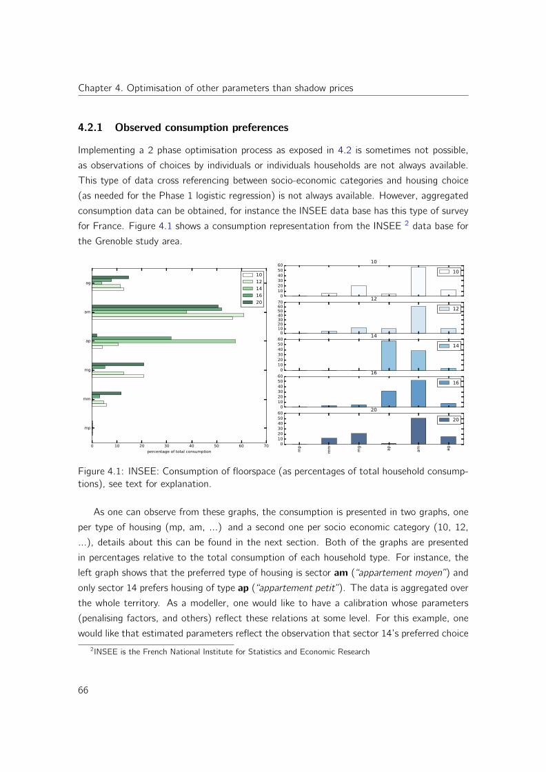
Chapter 4. Optimisation of other parameters than shadow prices
4.2.1 Observed consumption preferences
Implementing a 2 phase optimisation process as exposed in 4.2 is sometimes not possible,
as observations of choices by individuals or individuals households are not always available.
This type of data cross referencing between socio-economic categories and housing choice
(as needed for the Phase 1 logistic regression) is not always available. However, aggregated
consumption data can be obtained, for instance the INSEE data base has this type of survey
for France. Figure 4.1 shows a consumption representation from the INSEE 2 data base for
the Grenoble study area.
0 10 20 30 40 50 60 70
percentage of total consumption
mp
mm
mg
ap
am
ag
10
12
14
16
200
102030405060
10
10
010203040506070
12
12
0102030405060
14
14
0102030405060
16
16
mp
mm
mg
ap
am ag
0102030405060
20
20
Figure 4.1: INSEE: Consumption of floorspace (as percentages of total household consump-tions), see text for explanation.
As one can observe from these graphs, the consumption is presented in two graphs, one
per type of housing (mp, am, ...) and a second one per socio economic category (10, 12,
...), details about this can be found in the next section. Both of the graphs are presented
in percentages relative to the total consumption of each household type. For instance, the
left graph shows that the preferred type of housing is sector am (“appartement moyen”) and
only sector 14 prefers housing of type ap (“appartement petit”). The data is aggregated over
the whole territory. As a modeller, one would like to have a calibration whose parameters
(penalising factors, and others) reflect these relations at some level. For this example, one
would like that estimated parameters reflect the observation that sector 14’s preferred choice2INSEE is the French National Institute for Statistics and Economic Research
66
4.2. Simultaneous estimation of shadow prices and land use substitution parameters
was housing type ap.
We will consider this survey data as constraint to our Phase 2 optimisation scheme
proposed in the previous section. We took different approaches to do so. The first idea
was to construct some initial parameters that represented the behaviour observed in the
surveys. For the penalising factors, one can construct relations between parameters for each
household type and induce the type of consumption desired in the population. For instance,
we could rank the consumption for a household type and then optimise the parameters around
these initial values. The optimisation is carried out with intervals around these initial values.
Suppose we called the initial values ωmn0 m,n, then the optimisation is as follows:
minω∈Ω‖X(X0, h, ω)− X0‖2 (4.5)
in the restricted set Ω = [ωmn0 − εmn, ωmn0 + εmn],∀m, n, where εmn dictates how far away
from the initial values ωmn0 one can explore. Such constraints are called box constraints, and
are suitable to be solved using the BFGS-B algorithm exposed in 1.2. This technique works
very well, and the optimisation preserves the consumption preferences observed to a certain
level. In the next chapter we present results of this methodology for the Grenoble model.
Secondly we propose an optimisation problem with hard constraints on the observed
consumption. To do so, we need to look at consumptions and how this translates to our
Tranus demand equations. We can easily compute the number of housing units of each type
consumed per each household type per zone, by multiplying the number of households of the
considered type in the considered zone, Xmi , with the proportion of housing of type n that this
household consumes, i.e. Smni . As we know from the observed data how many households
of each type we have in each zone, we can replace Xmi by Xm0i . It is just like equation (3.6).
If we call Cmn0 the consumptions from the survey (such as those shown in 4.1), we can write
down the constraints as:
∑i
Smni ∗Xm0i − Cmn0 = 0, ∀m, n (4.6)
We can add this term to the objective function exposed in Phase 2 (4.1) with a weight
parameter α to obtain the following modified cost function:
f (h, ω, α) = ‖X(X0, h, ω)−X0‖2 + α‖∑i
Smni ∗Xm0i − Cmn0 ‖2 . (4.7)
We would like to find the values of ω that reduce the corresponding shadow prices. We
67
Chapter 4. Optimisation of other parameters than shadow prices
propose to solve the following problem:
minω∈Ω
f (h = 0, ω, α) (4.8)
The derivatives for the constraints (4.6) can be computed analytically using the derivatives
of the logit formulation (cf. equation (4.4)) as follows:
∂
∂ωmq[∑i
Smni ∗Xm0i ] =∑i
∂Smni∂ωmq
∗Xm0i (4.9)
4.3 Sensitivity analysis and simultaneous calibration of shadowprices and marginal utility of income
In this section we present the work exposed in (Arnaud et al. 2016) where a sensitivity analysis
is performed over the Tranus land use module. First a brief introduction to the methodology is
presented, technical details about the sensitivity analysis theory can be found in the appendix
C. Secondly, a simultaneous estimation of the shadow prices of transportable sectors and
their corresponding marginal utility of income is developed. This framework is then tested
on the Mississippi Tranus Model.
4.3.1 Sensitivity Analysis
Sensitivity analysis studies how the uncertainty on an output of a mathematical model can
be attributed to sources of uncertainty among the inputs. There are two main classes of
sensitivity analyses called local and global sensitivity analysis. The former addresses sensitivity
relatively to a nominal value of a given parameter. The latter examines sensitivity on the
whole set of variations of the parameter. Here, the focus is put on global sensitivity analysis
with the aim of identifying the most influential parameters of the land use module of Tranus.
Among the large number of available approaches to perform a global sensitivity analysis, we
review the generalisation of the variance-based method introduced by Sobol’ (Sobol 1993)
that relies on the estimation of generalised Sobol’ indices (Gamboa et al. 2014).
After introducing the successful semi-automatic calibration techniques for estimating the
penalising factors in previous sections, we decided to identify how we could improve the
calibration of parameters associated with transportable sectors. Transportable sectors are
68

4.3. Sensitivity analysis
mainly driven by the logistic location probabilities (2.4):
P rnij =Anj exp
(−βnUnij
)∑l A
nl exp
(−βnUni l
) .
the parameters relevant to this equation are Anj , βn and Unij . Parameters Anj represent the
attractiveness of zone j for sector n, and are governed by the following equation (equation
(3.20)):
Anj = W nj
(∑k
bnkXk0i
)where W n
j is not calibrated in Tranus and taken as input (actually, as a common practice it
is set equal to the base’s year production or simply set to 1), so the only parameters left to
calibrate are the cross-consumption parameters bnk . These parameters reflect the influence
of other economical sectors on the location of activities, for instance, households of a certain
type, could be attracted to live in zones where commerce is present. Often, the matrix bnk is
set to the identity matrix for convenience and simplicity, but cross interactions exist in reality.
At the same time, the dispersion coefficients βn of the logit probabilities are also calibrated.
As we have already shown in previous sections, the measure of calibration of Tranus land
use module is the shadow price parameter. Given initial values of the parameters for a sector
n ∈ N , the land use and activity module estimates the adjustment parameters hn = (hni )i∈Z
of the utilities (2.3), known as shadow prices. They compensate the utilities to replicate the
base year production X0. To compute the shadow prices for transportable sectors we solve
the optimisation problem exposed in equation (3.2):
hn = arg minhn
‖X(hn)− X0‖2 .
This problem is solved as exposed in section 3.4. Figure 4.2 gives a scheme of the inputs
and outputs considered for each transportable sector n.
Figure 4.2: Inputs and outputs of the land use and activity module for the sector n generatingflux.
69
Chapter 4. Optimisation of other parameters than shadow prices
The input parameters fall into different categories:
• logit dispersion parameters βn are involved in Equation (2.4),
• cross-consumption parameters bnl , l 6= n, l ∈ N , are involved in Equation (3.20)
We will also consider the parameter λn involved in the computation of the utilities Unij , this
parameter is the marginal utility of income, and sets the tradeoff between prices and transport
disutilities:
• parameter λn is involved in Equation (2.3).
The outputs considered are built upon a new quantity called normalised shadow price. The
normalised shadow price hni corresponds to the percentage of the price pni corrected by the
shadow price hni , that is:
hni = 100×hn,ipn,i
, ∀i (4.10)
We set hn = (hni )i , the vector of normalised shadow prices relative to the sector n.
This is the typical Tranus evaluation quantity called “adjust factor” that one obtains after
the calibration with the Tranus software module LCAL. The two outputs considered are the
following:
i) the variance of the normalised shadow prices: Var[hn]. Here the variance is taken across
all zones, so we have the variance for each economical sector n.
ii) the maximum of the normalised shadow prices: maxi|hni |
For each sector n, a good calibration would be one that results in small values of the nor-
malised shadow prices particularly in term of variance. Minimising the variance of the nor-
malised shadow prices is a general consensus reached by both modellers and users of Tranus.
This is due to the nature of the logit probabilities for the transportable sectors (the probability
is invariant to an additive constant, as explained in section 1.3.2).
Once the sensitivity analysis identifies the parameters that are influential on the out-
puts exposed above, we proceed to compute optimal values for these using the stochastic
optimisation algorithm EGO (see section 1.2.5).
4.3.2 Obtaining the λn parameters
Once we have found the optimal values for the selected parameters βn and bnk , we can
compute the value of the λn parameter analytically. The basic idea is to start from a good
70

4.3. Sensitivity analysis
guess of the logit dispersion parameters (βn) and from there, find the optimal values of the
marginal utilities (λn) to minimise the variance of the shadow prices for the corresponding
economic sector. This methodology explicits the dependency of λn on βn, showing that the
optimal value of λn is a function of βn.
The parameter λn is involved in the location probabilities equation (Equation 2.3)
Unij = λn(pnj + hnj ) + tnij ,∀(i , j) (4.11)
The optimal value of λn cannot be retrieved directly from equation (4.11) as the quantity
(pnj + hnj ) is estimated as a whole during the internal optimisation of the shadow prices. To
overcome this problem, we introduce an auxiliary variable, similar as what we did in section
3.4:
φnj = λn(pnj + hnj ),∀j
With this new variable, equation (4.11) can be rewritten as follows:
Unij = φnj + tnij ,∀(i , j) (4.12)
Recall that the shadow prices are price-correcting additive factors that are calibrated to
obtain a small variance. From equation (4.12), we can express the optimal value of λn that
minimises the variance of the shadow prices. We set φn = (φnj )j∈Z with all other parameters
fixed, in particular the parameters estimated with the EGO algorithm (see section 1.2.5).
The corresponding calibration problem can be written as:
φn∗ = arg minφn
‖X(φn)− X0‖2 . (4.13)
Recall that we have pn = (pnj )j and hn = (hnj )j the vectors of prices and shadow prices.
Once the optimal value φn∗ is obtained, the equilibrium prices pn∗ can be computed solving
a linear system (analogously to what was shown in section 3.4). Then, the shadow prices
are expressed as follows:
hn =φn∗
λn− pn∗ .
From this, the following problem can be posed:
minλn
Var[φn∗λn− pn∗
]
71
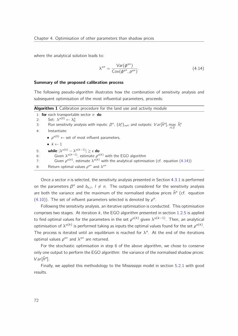
Chapter 4. Optimisation of other parameters than shadow prices
where the analytical solution leads to:
λn∗ =Var(φn∗)
Cov(φn∗, pn∗). (4.14)
Summary of the proposed calibration process
The following pseudo-algorithm illustrates how the combination of sensitivity analysis and
subsequent optimisation of the most influential parameters, proceeds:
Algorithm 1 Calibration procedure for the land use and activity module1: for each transportable sector n do2: Set: λn(0) ← λn03: Run sensitivity analysis with inputs: βn, bnl n 6=l and outputs: V ar [hn],max
i∈Zhni
4: Instantiate:
• ρn(0) ← set of most influent parameters,
• k ← 1
5: while |λn(k) − λn(k−1)| ≥ ε do6: Given λn(k−1), estimate ρn(k) with the EGO algorithm7: Given ρn(k), estimate λn(k) with the analytical optimisation (cf. equation (4.14))
8: Return optimal values ρn∗ and λn∗
Once a sector n is selected, the sensitivity analysis presented in Section 4.3.1 is performed
on the parameters βn and bn,l , l 6= n. The outputs considered for the sensitivity analysis
are both the variance and the maximum of the normalised shadow prices hn (cf. equation
(4.10)). The set of influent parameters selected is denoted by ρn.
Following the sensitivity analysis, an iterative optimisation is conducted. This optimisation
comprises two stages. At iteration k , the EGO algorithm presented in section 1.2.5 is applied
to find optimal values for the parameters in the set ρn(k) given λn(k−1). Then, an analytical
optimisation of λn(k) is performed taking as inputs the optimal values found for the set ρn(k).
The process is iterated until an equilibrium is reached for λn. At the end of the iterations
optimal values ρn∗ and λn∗ are returned.
For the stochastic optimisation in step 6 of the above algorithm, we chose to conserve
only one output to perform the EGO algorithm: the variance of the normalised shadow prices:
V ar [hn].
Finally, we applied this methodology to the Mississippi model in section 5.2.1 with good
results.
72

Chapter 5
Experimental results on real scenarios
In this chapter we present the main results of our methodology to real Tranus models. For all
tested scenarios we have utilised our optimisation methodology to compute parameters for
the model calibration. In parallel with our methodology we have utilised the Tranus software,
always verifying that the results produced are the same. As the models are real scenarios
in current projects, we need to ensure that the parameters we found with our optimisation
approaches can be utilised directly in Tranus.
The first two scenarios were constructed by Brian J. Morton and helped to develop the
methodology to simultaneously estimate the shadow prices and substitution probabilities (see
section 4.2). These scenarios were already carefully calibrated and what we propose here is
an improvement on a model that was already performing well. The third scenario is for the
Grenoble urban area, and is developed by Fausto Lo Feudo and Brian J. Morton. This scenario
is not yet fully calibrated and has been a good test ground to improve our methodology to
adapt it to newly created Tranus models.
5.1 North Carolina Tennessee (NCT) model
The North Carolina - Tennessee model comprises 38 geographical zones and 12 economical
sectors. This model was made available by our partner and friend Brian Morton, with whom
we have collaborated to develop the integrated calibration proposed above. We will only
describe the model and methodology relevant to our work, the details can be found in the
technical report (Morton, Song, et al. 2014). Table 5.1 describes the various economical
sectors included in this model.
For this model, we only focus on the non-transportable sectors, as the transportable part
73

Chapter 5. Experimental results on real scenarios
Number Name Type
1 AFFHM Exogenous2 Commercial Transportable3 Other industries Exogenous11 Single person Transportable12 Married couple (with children) Transportable13 Married couple Transportable14 Other families Transportable15 65 yrs and older Transportable16 All other HHs Transportable31 1-unit housing Housing32 Multiunit housing Housing33 Mobile homes Housing
Table 5.1: NCT: Economical sectors description
was already very well developed. This was our first model to test the methodology to optimise
the penalising factors of the substitution sub-model presented in 4.2. Going back to equation
(3.6), for the NCT model we do have substitution between the three housing sectors (31, 32
and 33). So the substitution probabilities Smni are relevant and have to be calibrated. The
substitution probabilities are given by a logit formula as shown in equation (2.14), we present
the equation here again:
Smni =W ni exp(−ωmnamni · (pni + hni ))∑
l∈KmW li exp (−ωmlamli · (pli + hli ))
.
The coefficients W ni represent attractors of sectors n in zones i and are set to the base’s
year production of the corresponding sector. In this section we present the application of
the two phase approach exposed in section 4.2. This technique consists in tuning the values
of the penalising factors (ω’s) to improve the model fitting. To assess the quality of the
fit we look at the values of the corresponding shadow prices. One wants to make these as
small as possible. This is basically done by computing the productions of housing sectors
without shadow prices (setting their value to zero) and adjusting the penalising factors to
make productions as close as possible to base year’s data.
As a baseline, we compute the shadow prices when the penalising factors are set to 1,
(ωmn = 1,∀m, n) to have an initial value to compare against. Usually, when no information is
available to adequately estimate initial penalising factors, the values are set to 1 (or all to the
same value) to represent the absence of preferences in housing choices. Here, shadow prices
are estimated using the method of section 3.3, based on the cost function shown in equation
74

5.1. North Carolina Tennessee (NCT) model
0 5 10 15 20 25 30 35
zones
25
20
15
10
shadow
pri
ce %
0 5 10 15 20 25 30 35
zones
10
0
10
20
30
shadow
pri
ce %
0 5 10 15 20 25 30 35
zones
0
10
20
30
40
50
60
shadow
pri
ce %
Figure 5.1: Shadow prices as percentage of prices for sectors 31, 32 and 33, for all zones.
Sector Mean Std Min Max
31 -17.518 3.611 -25.830 -6.73932 6.937 9.838 -15.807 37.35433 30.265 9.851 0.000 60.830
Table 5.2: Statistics of shadow prices computed over their initial values.
(3.7). As this model has three housing sectors (31, 32 and 33) we will present the results by
three graphs, one per sector. Figure 5.1 presents the shadow prices of each housing sector
for all zones. Shadow prices are presented as a percentage of the corresponding price for
each zone, as this is the standard Tranus practice. In Tranus terminology, these values are
called "adjusts".
The corresponding mean and standard deviation computed across the zones are presented
in table 5.2. From figure 5.1 and table 5.2 we can observe that sector 31 is overpriced (the
shadow prices are negative, pushing expenditures down) compared to the other two. The
standard practice for Tranus would be to tune the value of ωm,31 to make the sector 31
more attractive, in this case, to decrease their value and to reduce the penalised expenditure
ωmnamni · (pni + hni ). This manual technique is very tricky, as modifying the value of a single
penalising factor, affects the choices for all other sectors. For this model we had data on
actual choices of households, so a logistic regression can be performed to estimate an initial
value for the whole set of penalising factors.
Phase 1: estimating parameters’ initial values with multinomial logistic regression.To do this, we recognise the term in the utility function amni · pni as the expenditure of
household of type m, consuming housing type n in zone i . There is one multinomial logit
per household type, and as we don’t have data independently per zone, we estimated the
penalising factors for all zones. The data utilised for the regression is as shown in Table 5.3.
The column “Weight” represents the population weight coefficient, Hhtype is the household
75
Chapter 5. Experimental results on real scenarios
Weight Hhtype Housing Choice Expenditure
3943.3 12 33 2032400.8 11 33 5821912.3 11 32 5212269.8 15 31 1705.7...
......
...
Table 5.3: Example of data available for a logistic regression of penalising factors ω, for theNCT model.
Sector 11 Sector 12 Sector 13 Sector 14 Sector 15 Sector 16
31 -1.123 -1.103 -0.709 -0.488 -1.152 -1.58832 -1.303 -1.549 -1.050 -0.763 -1.363 -1.70333 -1.343 -1.317 -0.899 -0.684 -1.459 -1.761
Table 5.4: Penalising factors after phase 1 (computed by logistic regression).
type, Housing Choice is the actual choice and Expenditure is the corresponding monthly
expenditure (amni ·pni ). The results of the logistic regressions are presented in table 5.4. The
regression was made without sign, so the values presented are for (−ωmn). The regression
was made without a constant either.
The shadow prices computed with the penalising factors obtained with the logistic re-
gression are presented in figure 5.2 and table 5.5 summarises the statistics of those shadow
prices.
0 5 10 15 20 25 30 35
zones
25
20
15
10
shadow
pri
ce %
0 5 10 15 20 25 30 35
zones
10
0
10
20
30
shadow
pri
ce %
0 5 10 15 20 25 30 35
zones
0
10
20
30
40
50
60
shadow
pri
ce %
Figure 5.2: Shadow prices as percentage of prices for sectors 31, 32 and 33 for all zones.After phase 1.
Figure 5.3 compares the initial values of the ω (equal to 1) and the results from the
logistic regression. The red lines are the prices, the blue (dotted) lines are the prices plus
shadow prices resulting for ω values set to one and the green lines (solid) are the resulting
prices plus shadow prices after the logistic regression. We present one graph per housing
sector (from top to bottom sectors 31, 32 and 33). Prices and shadow prices are absolute
76

5.1. North Carolina Tennessee (NCT) model
Sector Mean Std Min Max
31 -7.562 2.916 -16.872 -1.88132 -2.321 8.411 -22.768 20.02333 14.181 6.422 0.000 34.491
Table 5.5: Statistics of shadow prices, after phase 1 (logistic regression of penalising factors).
values (not percentages).
0 19 38 zones
0.4848
0.6591
$
0 19 38 zones
0.0000
0.9426
$
0 19 38 zones
0.0000
0.8673
$
ph+p (omega=1)h+p (phase 1)
Figure 5.3: Original ω values against phase 1 values. Red curves show prices, blue curvesprices plus shadow prices with ω’s set to 1, green is h+ p after the logistic regression on theω values. Top to bottom represent sectors 31, 32 and 33 for all zones. We have opted forline plots instead of bar plot because for comparison purposes this is visually better, even ifdata are discrete.
One would want the value of price plus shadow price (p+ h) to be as close as possible to
p, meaning that shadow prices are small. As we can see, for sector 31 the green curve is now
between the blue and red one (strictly better), for sector 32 (second graph) the green curve
is closer than the initial guess, is somehow better. In sector 33, we get the same behaviour
as for sector 31, so is also better than the initial guess. We can also look at the statistics,
and comparing both tables 5.2 and 5.5 we can assess huge gains in the mean and standard
deviation tabs.
77

Chapter 5. Experimental results on real scenarios
Phase 2: Tuning the penalising factors. The penalising factors exposed in table 5.4 are
fine tuned. The problem we are solving is exposed in equations (4.1)-(4.2). This methodology
takes as input the penalising factors estimated with the logistic regression from phase 1, and
fine tune them to obtain a better fitting. We can limit the search space to avoid to go too
far away from the penalising factors estimated with actual data. To do this we consider an
interval around the penalising factor estimated with the regression, and limit the search to a
percentage of the original value. This means that for a particular penalising factor ω we limit
the search to the interval ((1− δ) ∗ ω, (1 + δ) ∗ ω). We present results with δ equal to 10%
and 20%. Figure 5.4 presents the comparative results between phase 1 and the optimisation
constrained to 10%. As we can see, the results are strictly better. The greatest gain is done
by sector 31, now the green curve is even closer to the red one.
0 19 38 zones
0.5431
0.6591
$
0 19 38 zones
0.0000
0.8477
$
0 19 38 zones
0.0000
0.7112
$
ph+p (phase 1)h+p (phase 2, 10%)
Figure 5.4: Phase 1 compared against the optimisation tuning of phase 2 with 10% searchrange.
With this methodology in mind, we skip directly to figure 5.5 where the search space is
enlarged to 20% and the fit is almost perfect. Figure 5.6 further shows that shadow prices
are small for almost all zones and sectors. It is normal to have some zones where the fit is
bad, as the model is a simplification of reality such that one can not expect that the housing
choice is only reflected by prices. Table 5.6 presents the statistics of this last phase, average
values (first columns) are very low, and standard the deviation has also been reduced for all
sectors.
78

5.1. North Carolina Tennessee (NCT) model
0 19 38 zones
0.5431
0.6656
$
0 19 38 zones
0.0000
0.8477
$
0 19 38 zones
0.0000
0.7112
$
ph+p (phase 1)h+p (phase 2, 20%)
Figure 5.5: Values from phase 1 compared against the optimisation tuning of phase 2 with a20% search range. Note how the green lines (prices + shadow prices) almost coincide withthe red one (prices) is almost over the prices (red line) after phase 2
0 5 10 15 20 25 30 35
zones
32101234
shadow
pri
ce %
0 5 10 15 20 25 30 35
zones
15
10
5
0
5
10
shadow
pri
ce %
0 5 10 15 20 25 30 35
zones
10
5
0
5
shadow
pri
ce %
Figure 5.6: Final Shadow prices as percentage of prices for sectors 31, 32 and 33 for allzones (after phase 2 with a 20% search range).
Sector Mean Std Min Max
31 -0.048 1.719 -3.748 4.51732 -1.705 6.149 -16.919 10.82533 0.103 4.389 -12.603 9.599
Table 5.6: Phase 2 shadow price statistics. (20% search range)
Computing optimal penalising factors without logistic regression (without phase 1).Often, data to build a logistic regression is not available when constructing a LUTI model,
we wanted to verify that the optimisation algorithm provides good results even without this
starting point. Figure 5.7 shows the results of our algorithm starting from the default values
79

Chapter 5. Experimental results on real scenarios
ω = 1 against the values obtained after the two stage optimisation (phase 1 and 2). The
blue curve represents the previous sections phase 1 - phase 2 estimation results and the green
curve is obtained after applying only the phase 2 optimisation with initial values set to ω = 1.
We can see that the results are similar, with the blue curve (phase 1 - phase 2 estimation)
almost identical to green curve (optimisation without prior logistic regression). We also
present the statistics for this technique in table 5.7.
0 19 38 zones
0.60203
0.65910
$
0 19 38 zones
0.0000
0.8477
$
0 19 38 zones
0.0000
0.6658
$
ph+p (phase 2)h+p (free)
Figure 5.7: Values from phase 2 compared against the optimisation tuning starting from basevalues (without prior logistic regression).
Sector Mean Std Min Max
31 -0.036 1.749 -4.110 4.05832 -2.114 6.244 -18.008 11.16133 -0.211 4.543 -12.988 9.096
Table 5.7: Shadow price statistics without previous logistic regression.
80
5.2. Mississippi model (MS)
5.2 Mississippi model (MS)
This Tranus model of the Mississippi region comprises the Chickasaw, Lee, Pontotoc, and
Union Counties, including the areas of the four largest towns, which are Houston, Tupelo,
Pontotoc, and New Albany. The analysis zones are census block groups, of which there
are 103; there are 12 economic sectors divided in 3 types of employment, 6 socio economic
categories of households and 3 types of floorspace (land). We have the same distribution of
economic sectors as int the NCT model, exposed in table 5.1.
After the successful application of our substitution probabilities optimisation for the NCT
model, we applied the same methodology to the MS model. For this model we did not have
access to survey data to establish a logistic regression (phase 1), but as we could observe for
the NCT model, starting from penalising factors equal to 1 yields similar results as starting
from a logistic regression (see previous section).
0 51 103 zones
0.578
0.742
$
0 51 103 zones
0.000
1.067
$
0 51 103 zones
0.0000
0.7046
$
ph+p (omega=1)h+p (phase 2)
Figure 5.8: Values from phase 2 compared against the optimisation tuning starting from basevalues (without prior logistic regression).
In figure 5.8 we have the resulting prices and shadow prices for the 3 floorspace sectors.
The green curves are the result of our methodology, the blue dotted curves are the values
obtained after setting the penalising factors to one (ω = 1). We can observe that the
penalising factors estimated with the optimisation algorithm produce an excellent fit, almost
positioning the green curves all along the prices (red curves). It is a clear improvement over
81

Chapter 5. Experimental results on real scenarios
the default values (blue curves). Statistics on the computed shadow prices are given in table
5.8. We can conclude that this strategy of tuning the penalising factors has an immense
impact on the values of the shadow prices, proving to be useful way to fine tune the calibration
of floorspace sectors.
Sector Mean Std Min Max
31 -0.029 1.749 -5.118 4.13132 -1.122 9.363 -32.436 33.99433 1.362 9.768 -15.524 84.807
Table 5.8: Shadow prices statistics for MS model after optimisation (phase 2).
In the next part, we will see that more has to be taken into account than fitting base
year’s productions and reducing shadow prices if one wants a good model in the sense that
it reproduces plausible output.
5.2.1 Sensitivity Analysis Results for the MS model
In section 4.3 we presented a sensitivity analysis methodology to identify influent parameters
of the land use module. To discover the relations between different economical sectors,
the sensitivity analysis is performed, thus giving the relations that are more relevant to
calibration. We will consider the MS Mississipi model exposed in 5.2 (12 economical sectors
and 103 geographical zones). The economical sectors relevant to this methodology are the
transportable sectors, the ones that have a non zero location probability, as the MS model
has the same sector composition as the NCT model, the reader can consult the table 5.1 for
the sector description. The model has 7 transportable sectors: 6 household types (sectors
11, 12, 13, 14, 15 and 16) and 1 commercial sector (sector 2). As explained in section 4.3,
the idea behind this research is to help the calibration of the cross-relation dictated by the
bkn coefficients, that sadly, most models only set as the identity matrix.
A total of 7 sensitivity analyses are performed, one for each transportable sector. For
each sensitivity analysis, the 12 following parameters are considered:
• The logit dispersion parameter βn (cf. equation (2.4) ).
• The 11 parameters bnl , for all sectors l 6= n (cf. equation (3.20)).
In Table 5.9 are listed the distribution of each parameter used as support for the sensitivity
analyses. These distributions were selected by expertise, as each model is different, a good
82

5.2. Mississippi model (MS)
parameters labels distributions
βn 1 U(2, 10)
bnl 2, . . . , 12 U(0, 1)
Table 5.9: Distributions of the 12 parameters, U(a, b) stands for the uniform distributionwith support [a, b].
0.0
0.1
0.2
0.3
0.4
0.5
0.6
S1 S2 S3 S4 S5 S6 S7 S8 S9 S10 S11 S12
first−order indicesconfidence intervals
Figure 5.9: First-order indices estimation forthe 12 parameters of sector 4. S1 corre-sponds to β4, S2 to b4
1, S3 to b4
2 and soon.
0.00
0.10
0.20
0.30
S1,2 S1,8 S2,4S2,10S3,7 S4,5S4,11S5,10S6,10S7,11S9,10
second−order indicesconfidence intervals
Figure 5.10: Second-order indices es-timation for the 12 parameters ofsector 4. The second order in-dexes are given in the following order:(1, 2), ..., (1, 12), (2, 3), ..., (2, 12), (3, 4), ....
range of a priori possible values needs to be explored. The Sobol’ index Sk will refer to the
parameter labeled by k , this is standard practice in the field of sensitivity analysis, so for
instance, S1 will always correspond to the logit dispersion parameter βn of the sector under
analysis, and S2, ...S12 the corresponding cross relations bnl parameters. (without including
the case l = n)
The outputs considered are the variance and the maximum of the normalised shadow
prices, as introduced in Section 4.3. The approach proposed is to use the replication pro-
cedure presented in appendix C to estimate first-order and second-order generalised Sobol’
indices of these parameters. Asymptotic confidence intervals can be computed for first-order
Sobol’ indices (Tissot and Prieur 2014).
Before presenting the main results, we propose to illustrate the selection procedure of
the influent parameters for a sector. Figures 5.9 and 5.10 show the results obtained for
the estimation of first-order and second-order indices relative to Sector 4. The dashed line
represents the threshold value used for selecting the influent parameters.
83

Chapter 5. Experimental results on real scenarios
For the estimation of first-order indices, a size N = 5 × 10³ was chosen for the two
replicated Latin Hypercubes required by the replication procedure (details of the replication
procedure can be found in the appendix C). Looking at the results, the parameters β4 and
b410 are the most influent (cf. figure 5.10). Since the sum of the first-order indices is less
than 75% it is interesting to study the second-order indices.
For the estimation of second-order indices, a size N = 472 was selected for the two
replicated randomised orthogonal arrays required by the replication method. The two black
points of figure 5.10 correspond to the two most influent interactions: β4 ∗ b410 and β4 ∗ b4
11.
The number of bootstrap replications used to compute the confidence intervals equals 1000.
In conclusion, only 3 of the 12 parameters of the sector 4 are significantly influent either
directly by their main effects or through their second-order interactions: β4, b410 and b4
11.
The same procedure is performed for the other sectors. For each sector n, the set
comprised of the most influent parameters selected by the sensitivity analysis is listed in
Table 5.10. The last column of the table gives the proportion of the model’s variance
explained by the selected parameters. This proportion is calculated by multiplying the sum of
the generalised Sobol’ indices of the first two columns by 100. Looking at the results, only 3
parameters appear to be overall the most influent: βn, bn10 and bn11, n ∈ 2, 4, 5, 6, 7, 8, 9.
sector first-order second-order selected parameters: ρ variance explained (in percentage)
2 β2 none β2 33
4 β4, b410 β4 ∗ b4
10, β4 ∗ b4
11 β4, b410, b
411 95
5 β5, b510 β5 ∗ b5
10, β5 ∗ b5
11 β5, b510, b
511 89
6 β6, b610, b
611 β6 ∗ b6
10 β6, b610, b
611 90
7 β7, b710 none β7, b7
10 85
8 β8, b810 β8 ∗ b8
10 β8, b810 89
9 β9, b910, β9 ∗ b9
10 β9, b910 93
Table 5.10: Most influent parameters selected by the sensitivity analysis based on maineffects and second-order interactions.
These results fall within our range of expectations. The parameter βn is a dispersion
parameter of a multinomial logit function (see Equation (2.4)). A slight variation of this
parameter leads to a significant change in the calculation of the probabilities of localisation.
Both parameters bn10 and bn11 act as weights in the attractiveness for sector n. These two
parameters are more prone to be influent than the other bnl since sectors 10 and 11 correspond
84

5.2. Mississippi model (MS)
to the two main floorspace types.
5.2.2 Results of the subsequent iterative optimisation
Following the results of the above sensitivity analysis, for each transportable sector n, we
proceed to find the set of parameters (βn, bnk , λn) minimising the variance of hn. The initial
value λn0 (Step 3 of Algorithm 1, see section 4.3) instantiating the parameter λn is obtained
by expertise, or just set to 1. The results obtained in terms of variance and maximum of the
normalised shadow prices are compared to those obtained with a former ad hoc procedure (the
parameters calibrated with a classical calibration approach, without optimisation or automatic
calibration). The number of initial evaluations performed to fit the metamodel for the set of
parameters (βn, bnk , λn) of each sector n is the following:
• 21 evaluations for sector 2,
• 51 evaluations for sector 4 to 6.
• 41 evaluations for sector 7 to 9.
The quality of the fitting is assessed by diagnostic plots (fitted values against response
values, standardised residuals, Q-Q plots of standardised residuals) based on leave-one-out
cross validation results (see (Roustant, Ginsbourger, and Deville 2012) for further details).
For each sector n, the evaluations include the one for the optimal set of parameters obtained
with the ad hoc procedure.
Table 5.11 summarises the results obtained with both the ad hoc procedure and our iter-
ative optimisation. The “Optimal params.” tab gives the estimated values of the parameters
exposed in table 5.10 and λn∗ denotes the optimal values of the parameters obtained at the
end of both approaches for each transportable sector n. The column gain represents the
improvement (in percentage) of the variance obtained with our iterative estimation relatively
to the one obtained with the ad hoc procedure conducted by experts.
Looking at the results, we observe that the values of the variance and maximum of the
normalised shadow prices obtained with the ad hoc procedure are heterogeneous. Further-
more, the value of the maximum is quite high for some sectors (up to 20% of the price). The
results obtained with our iterative optimisation are relatively homogeneous except for sectors
2 and 8. The discrepancy observed for these two sectors comes from the quality of their
respective datasets. Indeed, the data relative to commercial business (sector 2) are easy to
collect thus of high quality and quantity. At the opposite, data relative to the 65 years and
older households (sector 8) are quite complex to collect and often lacking precision.
85

Chapter 5. Experimental results on real scenarios
sector n procedure Optimal params. λn∗ variance hn max hn gain
2 ad hoc 2 0.005 0.32 2.95 98%
iterative 4.03 0.43 7× 10⁻³ 0.11
4 ad hoc (2, 0, 0) 0.001 13.66 24.95 83%
iterative (6.49, 0.38, 0) 0.001 2.26 7.63
5 ad hoc (2, 0, 0) 0.001 5.35 14.83 47%
iterative (2.50, 0.02, 0.79) −0.013 2.85 8.88
6 ad hoc (2, 0, 0) 0.001 5.90 16.65 63%
iterative (6.64, 0.05, 0.79) −0.003 2.18 7.72
7 ad hoc (2, 0) 0.001 8.73 19.67 61%
iterative (9.17, 1) 0.001 3.40 8.23
8 ad hoc (2, 0) 0.001 9.50 20.58 15%
iterative (5.72, 0.97) 0.001 8.08 15.03
9 ad hoc (2, 0) 0.001 7.36 17.6 64%
iterative (9.29, 0.95) 0.001 2.66 6.82
Table 5.11: Variance and maximum of the normalised shadow prices hn obtained with bothad hoc procedures and our iterative optimisation.
The main observation is that an improvement in terms of both variance and maximum
of the normalised shadow prices is observed for all sectors when using our approach. Figure
5.11 gives an illustration of this improvement. The black bars represent the values obtained
with the ad hoc procedure, the grey bars those obtained with our iterative approach. A
significant diminution for both the variance and maximum criteria is observed. Furthermore
and most importantly our approach is drastically faster than the ad hoc procedure conducted
by experts. Our calibration procedure requires a few hours compared to several days (up to
weeks) for the ad hoc procedure.
As a final remark, we decided here to conserve only the best set of parameters (βn∗, bnk∗, λn∗)
obtained with our calibration procedure. (Ciuffo and Azevedo 2014) proposed an alternative
where a metamodel is fitted and several best sets of parameters are selected. It is true
that for complex systems such as LUTI model, the best solution of the EGO optimisation
probably corresponds to only one of the many combinations of the inputs that provide the
model a sufficiently robustness. The method of (Ciuffo and Azevedo 2014) has the merit
of investigating the behaviours of the model for various combinations and allows to derive
uncertainty margins of the outputs. Adapting this methodology to our calibration procedure
86

5.2. Mississippi model (MS)
2 4 5 6 7 8 9sectors
varia
nce
02
46
810
12
ad−hociterative
2 4 5 6 7 8 9sectors
max
imum
05
1015
20
ad−hociterative
Figure 5.11: Variance (left figure) and maximum (right figure) of the normalised shadowprices obtained with both the ad hoc procedure (referred to as ad hoc) and our iterativeoptimisation (referred to as iterative)
of Tranus would be an interesting complementary work.
87

Chapter 5. Experimental results on real scenarios
5.3 Grenoble model
The Grenoble model is developed by Fausto Lo Feudo, Brian J. Morton and the AURG
(Agence d’urbanisme de la région grenobloise). It aims to model the Grenoble (France)
urban and peri-urban area. It is a large model, with 213 zones and 22 economical sectors.
During a model conception, the first thing to do for the non-transportable sectors is to
estimate the prices for the housing market. The latter is done at the same time as the
estimation of the demand functions, particularly the demand for land. We will not discuss
here how these intermediate variables are estimated and we will consider them as input for
our methodology.
Table 5.12 describes the economical sectors of the model. Sectors 10, 12, 14, 16 and
20 represent household types. Sectors 101 through 108 represent the housing offer. The
model differentiates between urban and rural housing types, for instance sector 101 is urban
medium size apartments and sector 102 is rural medium size apartments. The details of the
demand functions can be seen in the appendix B.
Number Name Type
10 Actifs_ref Household11 Actifs_autres Household12 Partiellement Household13 Partiellement_2 Household14 Etudiant_ref Household100 maisons_petit Housing101 maisons_moyen Housing102 maisons_moyen_rural Housing103 maisons_grand Housing104 maisons_grand_rural Housing105 apt_petits Housing106 apt_moyens Housing107 apt_moyens_rural Housing108 apt_grands Housing
Table 5.12: Economical sectors description of the Grenoble model (only relevant sectors arepresented).
5.3.1 Calibration of substitution sub-model
For this model we did not have individual data on floorspace consumption, so a logistic
regression was not possible. We applied the same methodology as for the Mississippi model,
starting from penalising factors set to one and optimising with our scheme to obtain a better
88

5.3. Grenoble model
model fit. Figure 5.12 presents the shadow prices before (ω = 1) and after optimisation
(Phase 2). The results show better fitting in all sectors besides sectors 100 and 105 where
we think prices may have been underestimated, also some zones have very high shadow price
values, increasing the variance considerably.
0 114 229 zones0.00
67.32
$
0 114 229 zones0
44
$
0 114 229 zones0
34
$
0 114 229 zones0
36
$
0 114 229 zones0
27
$
0 114 229 zones0.00
72.65
$
0 114 229 zones0.00
37.84
$
0 114 229 zones0
28
$
0 114 229 zones0.00
30.68
$
p
h+p (omega=1)
h+p (phase 2)
Figure 5.12: Top to bottom, sectors 100, 101, 102, 103, 104, 105, 106, 107, 108. Valuesfrom phase 2 compared against values with ω’s set to 1. Blue (dotted) lines represents thedefault ω’s (set to 1), green lines are the values after the optimisation, and the red lines arethe prices.
Even if this results look good, the consumption preferences embodied by the estimated
ω’s, are not all plausible. The consumption preferences dictate an economical sense, for
instance, richer households would prefer bigger housing and so on, and the results have shifted
the consumptions from this desired behaviour (see section 4.2.1 for details on consumption
preferences).
89

Chapter 5. Experimental results on real scenarios
0 10 20 30 40 50 60 70
percentage of total consumption
mp
mm
mg
ap
am
ag
10
12
14
16
200
102030405060
10
10
010203040506070
12
12
0102030405060
14
14
0102030405060
16
16
mp
mm
mg
ap
am ag
0102030405060
20
20
Figure 5.13: INSEE: Consumption of floorspace (as percentages of total household con-sumptions).
The INSEE1 data base has information on consumption preferences. Figure 5.13 presents
this information for the 5 household types as percentages of total household consumption.
The data is presented with only 6 types of housing, actually aggregating sectors 101 and 102
as mm, sectors 103 and 104 as mg and sectors 106 and 107 as am. Sectors 100 (mp),105 (ap) and 108 (ag) are left alone. Hence, no distinction is made between urban or rural
housing.
From figure 5.14 we observe that the driver of the housing market is sector 10 (active
population), seconded by sector 20 (retired) and then sector 16 (inactive). One would want
this behaviour to be preserved after the optimisation of the ω parameters. We will add the
consumption preferences to the analysis of the model fitting.
How do our results from the optimisation compare to the INSEE data?
The standard output proposed by Tranus is the demands Dmni (see equation (2.2)),
these demands are in square meters, so if one wants to have the actual units consumed we
have to compute them using the substitution probabilities Smni . These probabilities are a
distribution over all possible consumed sectors, so for each household sector m and each
zone i , we have a logit formulation with as many choices as housing possibilities. For our
case, we have 5 consuming sectors (10, 12, 14, 16 and 20) and 6 INSEE types of housing
1INSEE is the French National Institute for Statistics and Economic Research.
90

5.3. Grenoble model
10
12
14
16
20
0
5000
10000
15000
20000
housi
ng u
nit
s
mp
mm
mg
ap
am
ag
Figure 5.14: INSEE: Consumption of floorspace (total housing units consumed of eachhousing type).
(as explained before). We can easily compute the number of housing units of each type
consumed by each household type by multiplying the number of households in each zone
(Xmi ) with the proportion of housing of type n that this household type consumes (Smni ). It
is just like equation (3.6), but without the demand functions that transform the results in
square meters.
Figure 5.15 presents the consumption preferences after the optimisation results presented
at the beginning of this section (Housing sectors are aggregated to be compared to INSEE
sector types). The results are similar to the INSEE preferences, only sector 14 has a different
behaviour, consuming more medium apartments than small ones. This inverted behaviour
could be explained by the apartment sharing of students in the Grenoble area, even if the
model has not implemented this specifically (allowing partial consumption of housing, for
instance rooms) the data is telling us something.
91

Chapter 5. Experimental results on real scenarios
0 10 20 30 40 50 60percentage of total consumption
mp
mm
mg
ap
am
ag
1012141620
05
1015202530354045
10
10
05
1015202530354045
12
12
01020304050
14
14
0102030405060
16
16
mp
mm
mg
ap
am ag
05
1015202530354045
20
20
Figure 5.15: Consumption of floorspace after optimisation of penalising factors.
5.3.2 Using observed ranking of housing preferences to initialise penalisingfactors
In this part we propose another way of estimating an initial guess of the penalising factors
using the information from the INSEE data.
0 10 20 30 40 50 60 70 80 90
percentage of total consumption
mp
mm
mg
ap
am
ag
10
12
14
16
2005
1015202530354045
10
10
05
10152025303540
12
12
0102030405060708090
14
14
05
1015202530354045
16
16
mp
mm
mg
ap
am ag
0
10
20
30
40
5020
20
Figure 5.16: Consumption of floorspace, after optimisation (as percentages of total house-hold consumptions).
The idea is to rank the preferences according to the INSEE data shown by figures 5.13
92

5.3. Ranking of housing preferences
0 114 229 zones0.00
69.67
$
0 114 229 zones0.00
72.67
$
0 114 229 zones0
34
$
0 114 229 zones0.00
48.16
$
0 114 229 zones0
27
$
0 114 229 zones0.0
309.5
$
0 114 229 zones0.00
58.12
$
0 114 229 zones0.00
60.93
$
0 114 229 zones0.00
47.91
$
p
h+p (initial ranking)
h+p (phase 2)
Figure 5.17: Values of prices and shadow prices before and after the optimisation of theranked penalising factors.
and 5.14; we chose values among 1, 2, 3, 4 for the penalising factors. So, for instance,
sector 10 prefers medium apartments (am), so the associated penalising factor is the lowest
possible, hence to 1. Conversely, sector 10 dislikes small houses (mp) so the penalising factor
is set highest, hence to 4. We propose this ranking scheme to have a better initial guess for
the penalising factors and also to preserve the order in which each household type consumes
housing. This should produce results that are closer to the observed consumption.
After this initial guess, the optimisation procedure is applied. Figure 5.16 presents results
of the optimisation procedure with initial guess from the ranking exposed above. We also
present the shadow prices before and after the optimisation. From the consumptions exposed
in figure 5.16 we observe that the consumption preferences are still close to the INSEE data,
and not very different from the starting guess. Also, figure 5.17 shows that even if the initial
93

Chapter 5. Experimental results on real scenarios
guess shadow prices were bad (blue dotted line) the results after the optimisation are very
close to desired values (green line close to red).
We have presented a trade-off between a pure optimisation of penalising factors and
balancing between actual revealed preferences from available data. This is another tool
for modellers that have access to this type of consumption preferences instead of actual
observations allowing a logistic regression. Compared to MS and NCT models, the Grenoble
model is in a developing stage while both American models were almost finished and with
very good calibration already. For the American models, improving the values of shadow
prices was easier because the starting point was already very good and stable. The strategies
proposed for the Grenoble area gives insight into actual calibration of penalising factors for
a new model.
We are currently working on implementing the constrained optimisation exposed in section
4.2.1, that includes observed housing preferences as constraints in the optimisation of the
penalising factors.
94

Conclusions
The Tranus LUTI framework is a very powerful tool and the modelling possibilities are end-
less. However, the complexity of such large scale models is something that can not be
underestimated, making the calibration and utilisation of these tools very expensive.
In this thesis, we have contributed with a reformulation of the land use module that
simplifies the calibration process. To do this reformulation, we had to present in a different
way the equations involved in the computation of the land use module, exploiting the very
basics of the mathematics that are behind the microeconomic models used, establishing the
needed cost function (and derivatives) for the optimisation algorithms to succeed.
A lot of time and effort has been put to understand the various interactions between the
parameters to be able to divide the calibration in smaller problems, thus leading to the two
stage optimisation finally proposed in chapter 3 (for non-transportable and then transportable
sectors). For instance, the reformulation for the transportable sectors exposed in section 3.4
is not evident, and only became possible after working with the equations analytically as
shown in the numerical example in section 3.5.1. The optimisation approach is more stable
and clear than the classical approach, and enables the use of powerful optimisation algorithms
currently available, solving the occasional non convergence issues of the previous approach.
To be able to test our optimisation approach for the calibration of the shadow prices,
we have proposed a “first for Tranus” procedure for generating synthetic data that is simple
and straightforward, enabling us to try and benchmark our methodologies. This procedure
could also be used to perform validation of the model, creating a “present” as well as a
synthetic “future” scenario to compare the predictive capabilities of Tranus. The latter, is
not as simple as it sounds, and could be considered as one perspective for future work. Also,
in predictive mode, the land use module reformulation that we proposed in this thesis would
need to be adjusted, as the technique of exploiting the base’s year production (cf. section
3.2 and equation (3.5)) would not be possible.
The proposed methodology for reducing the number of shadow prices needs additional
95

Conclusions
fine tuning, but is a first step in what we consider a promising direction. We believe that the
model “as it is” with one shadow price per observation bears a risk of overfitting. Determining
which shadow prices have to be removed may not be completely automisable, and the expert
eye of the modeller has to have the last call.
The simultaneous calibration of different parameter types is a potentially very powerful
tool. The results that we have for both American models and the undergoing Grenoble model
have proven to be useful and saved many trial and error sessions. For the American models
the improvements were easier to obtain as both models were already calibrated and produced
good results. Also, the available data for the logistic regression permit us to establish the
two phase algorithm proposed in section 4.2. Here, we have taken models that were already
calibrated, and improved their calibration directly. On the other side, the tools developed for
the Grenoble model, a model that is in early development, have proven to help the calibration
of the substitution parameters enabling modellers to obtain results that are plausible and
reproduce the observed data.
Another important point about the methodology to calibrate the penalising factors, is
that it is possible to apply these techniques via a program completely outside the Tranus
software, adjusting the parameters and then feeding them to Tranus. As much as one would
like that the Tranus software would include the optimisation methodology, this approach
enables us to already work with real-life operational models. The full integration of this
methodology in Tranus would need the re-implementation of the land use module, to include
the whole computation of shadow prices as an optimisation problem. Doing so, would have
many benefits, for instance we could apply this idea of simultaneous optimisation to other
“hard” to calibrate parameters. A fully integrated and automatic calibration is our dream.
We also presented a sensitivity analysis for Tranus, based on the generalisation of the
replication procedure to select the most influential parameters of the model. An application
to the study area of Mississippi was presented where our methodology was compared to a
former ad hoc calibration procedure in terms of variance and maximum of the normalised
adjustment shadow prices. Our approach showed a significant improvement on both criteria
reducing the value of the variance by a large margin with a drastic gain of time. These results
have proven that our methodology is useful to outperform calibration of such models. The
next step would consist in verifying if the optimal values found for the parameters ensure
better predicting capabilities when evaluating alternative planning scenarios.
96
Implementation
The current implementation of Tranus is modular, with one program per sub-module: land
calibration (LCAL), transport costs (COST), land use predictive module (LOC), transport
module (TRANS), etc. The communication between each of these modules is done via text
files an binary files, based on this we decided to replace the land use calibration module LCAL
with our implementation based on the optimisation techniques. For the implementation of
our land use module we have used Python (Rossum and Drake 2006) with the scientific and
numerical libraries: numpy and scipy. Both of these libraries permit to replace much of the
iterative approach of computing the shadow prices with matrix operations and vectorised
functions. This translates in fast and easy to read code, that resembles very much the
equations listed in section 2.2. As said above, our code can run in parallel to Tranus software,
enabling modellers to partially calibrate certain parameters and then moving to Tranus to
continue their work.
Future possibilities
The most obvious application of this work would be for Tranus to embrace the reformu-
lation of the land use module as an optimisation problem. This could be done, first by
separating the land use module in two parts: transportable and non-transportable. Then the
non-transportable sub-module could be implemented with the penalising factors calibration
techniques exposed in this thesis. Also, the integration of the calibration of the demand func-
tions could be added at the same time. Even if the demand functions are currently calibrated
externally, one could think of an integrated calibration of both the penalising factors and the
demand functions. As shown in section 4.2, the demand functions and prices are the input to
computing the penalised expenditure which defines the substitution probabilities. Also, the
demand functions are strictly related to the observed prices of the housing market and the
socio-economic segmentation of households, so developing tools to help modellers estimate
prices and demand functions at the same time, would be much appreciated.
We also think it is crucial to explore more the potential overfitting issues related to the
number of shadow prices present in the current state of Tranus. The synthetic scenario
generation could be used to test this hypothesis, validating the performance of the predictive
capabilities of Tranus when some shadow prices are removed. The shadow prices were initially
added to correct for the un-modelled effects in the utilities, making the model fit the observed
data perfectly. Determining which shadow prices are really necessary, and at what level of fit
97

Future possibilities
we would like to reproduce observed data is a question for a whole other thesis, but tools such
as sensitivity analysis could be used to identify which shadow prices can be removed safely,
as it is probable that the set of shadow prices varies from model to model. One possible
methodology to test the model selection scheme would be to compare the model outputs for
two time periods, to determine if noise in the base year productions could really propagate
to the shadow prices and undermine the predictive capabilities of the model.
Another issue encountered during this thesis is related to the formulation of the logit
probabilities in Tranus. As a common practice, Tranus uses scaled utilities as exposed in
section 2.3. Scaled utilities are used to trick the logit formulation to ignore one of their
fundamental properties, the invariance of the probabilities to an additive constant (cf. section
1.3.2). If this behaviour is not desired, maybe it would be a wise idea to migrate from the
logit formulation to another discrete choice model, for instance, as proposed in section 2.3,
to a multiplicative error term discrete choice model. From our point of view, moving Tranus
to this type of model would not be complicated, and all the optimisation framework developed
in this thesis would still work, as these functions are differentiable and have a very concise
formulation. Indeed, their formulation is very similar to the logit model, with the same type
of properties for the derivatives. A good article about this type of models is (Fosgerau and
Bierlaire 2009).
98

Conclusions
Le modèle Tranus est un outil très puissant et les possibilités de modélisation sont infinies.
Cependant, la complexité de tels modèles à grande échelle ne doit pas être sous-estimée, car
elle rend la calibration et l’utilisation de ces outils très coûteux.
Dans cette thèse, nous avons contribué à une reformulation du module d’usage des
sols qui simplifie le processus de calibration. Pour cela, nous avons dû présenter d’une
manière différente les équations impliquées dans le calcul du module d’usage des sols, en ex-
ploitant les bases fondamentales des mathématiques derrière les modèles microéconomiques
utilisés, en établissant une fonction de coût (et les dérivées) nécessaires pour les algorithmes
d’optimisation. Beaucoup de temps et d’efforts ont permis de comprendre les différentes
interactions entre les paramètres pour pouvoir diviser la calibration en petits problèmes, con-
duisant ainsi à l’optimisation en deux étapes finalement proposée au chapitre 3 (pour les
secteurs non transportables et ensuite transportables). Par exemple, la reformulation pour
les secteurs transportables exposés dans la section 3.4 n’est pas évidente, et n’est possible
qu’après avoir travaillé avec les équations analytiquement, comme indiqué dans l’exemple
numérique dans la section 3.5.1. L’approche d’optimisation est plus stable et plus claire que
l’approche classique et permet d’utiliser des algorithmes d’optimisation puissants actuelle-
ment disponibles, résolvant les problèmes occasionnels de non convergence de l’approche
précédente.
Pour pouvoir tester notre approche d’optimisation pour la calibration des prix sombres,
nous avons proposé une procédure simple et directe “first for Tranus” pour générer des données
synthétiques, ce qui nous permet d’évaluer nos méthodologies. Cette procédure pourrait
également être utilisée pour effectuer la validation du modèle, en créant un scénario “présent”
ainsi qu’un scénario “futur” synthétique pour comparer les capacités prédictives de Tranus. Ce
dernier n’est pas aussi simple qu’il le semble et pourrait être considéré comme une perspective
pour des travaux futurs. En outre, en mode prédictif, la reformulation du module d’usage
des sols que nous proposons dans cette thèse devrait être ajustées, puisque les productions
99

Conclusions (Français)
ne seront plus égales aux productions de l’année de base, voir section 3.2 et équation (3.5)).
La méthodologie proposée pour réduire le nombre de prix sombres nécessite un ajuste-
ment précis, mais constitue une première étape dans ce que nous considérons comme une
direction prometteuse. Nous croyons que le modèle «en tant que tel», avec un prix sombre
par observation, risque d’être surparamétré. Déterminer quels prix sombres doivent être sup-
primés peut ne pas être entièrement automatisable, et l’œil expert du modélisateur doit avoir
le dernier appel.
La calibration simultanée de différents types de paramètres est un outil potentiellement
très puissant. Les résultats que nous avons pour les modèles américains et le modèle de
Grenoble en cours se sont révélés utiles et ont évité des nombreuses sessions d’essai et
d’erreur. Pour les modèles américains, les améliorations ont été plus faciles à obtenir, car les
deux modèles étaient déjà calibrés et produisaient des bons résultats. De plus, la disponibilité
des données pour la régression logistique nous a permis d’établir l’algorithme en deux phases
proposé dans la section 4.2. Ici, nous avons pris des modèles déjà calibrés et amélioré leur
calibration directement. D’autre part, les outils développés pour le modèle de Grenoble,
un modèle qui est en cours de développement, ont prouvé leur aide pour la calibration des
paramètres de substitution permettant aux modélisateurs d’obtenir des résultats plausibles
et de reproduire les données observées.
Un autre point important de la méthodologie pour calibrer les facteurs de pénalisation
est qu’il est possible d’appliquer ces techniques via un programme complètement en dehors
du logiciel Tranus, en ajustant les paramètres puis en les alimentant vers Tranus. Bien qu’il
serait idéal que le logiciel Tranus inclue la méthodologie d’optimisation, cette approche nous
permet déjà de travailler avec des modèles opérationnels réels. L’intégration complète de
cette méthodologie à Tranus nécessiterait la réintégration du module d’usage des sols, afin
d’inclure tout le calcul des prix sombres comme un problème d’optimisation. Cela pourrait
avoir de nombreux avantages, par exemple, nous pourrions appliquer cette idée d’optimisation
simultanée à d’autres paramètres «difficiles» à calibrer. Une calibration entièrement intégrée
et automatique bien évidemment optimale.
Nous avons également présenté une analyse de sensibilité pour Tranus, en fonction de
la généralisation de la procédure de “réplication” pour sélectionner les paramètres les plus
influents du modèle. Une application à la zone d’étude du Mississippi a été présentée où
notre méthodologie a été comparée à une ancienne procédure de calibrage ad hoc en termes
de variance et au maximum des prix sombres normalisé. Notre approche a montré une
amélioration significative sur les deux critères réduisant la valeur de la variance par une large
marge avec un gain de temps drastique. Ces résultats ont prouvé que notre méthodologie est
100

utile pour surpasser l’étalonnage de ces modèles. La prochaine étape consisterait à vérifier si
les valeurs optimales trouvées pour les paramètres garantissent une meilleure prédiction des
capacités lors de l’évaluation de scénarios de planification alternatifs.
Implementation
L’implémentation actuelle de Tranus est modulaire, avec un programme par sous-module:
la calibration d’usage des sols (LCAL), les coûts de transport (COST), le module prédictif
(LOC), le module de transport (TRANS), etc. La communication entre chacun des modules
sont effectués via des fichiers texte et des fichiers binaires. En fonction de cela, nous avons
décidé de remplacer le module de calibration d’usage des sols LCAL par notre implémentation
basée sur les techniques d’optimisation. Pour la mise en œuvre de notre module d’usage des
sols, nous avons utilisé Python (Rossum and Drake 2006) avec les bibliothèques scientifiques
et numériques: numpy et scipy. Ces deux bibliothèques permettent de remplacer une grande
partie de l’approche itérative du calcul des prix sombres par des opérations matricielles et
des fonctions vectorisées. Cela se traduit par un code rapide et facile à lire, qui ressemble
beaucoup aux équations répertoriées dans la section 2.2. Comme indiqué ci-dessus, notre
code peut fonctionner parallèlement au logiciel Tranus, permettant aux modélisateurs de
calibrer partiellement certains paramètres et puis de passer sur Tranus pour continuer leur
travail.
Possibilités futures
L’application la plus évidente de ce travail serait que Tranus accepte la reformulation du
module d’usage des sols en tant que problème d’optimisation. Cela pourrait être fait, d’abord
en séparant le module d’usage des sols en deux parties: transportable et non transportable.
Ensuite, le sous-module non transportable pourrait être implémentée avec les techniques de
calibration des facteurs de pénalisation exposées dans cette thèse. En outre, l’intégration
de la calibration des fonctions de demande pourrait être ajoutée en même temps. Même si
les fonctions de demande sont actuellement calibrés à l’extérieur, on pourrait penser à une
calibration qui intègre à la fois des facteurs de pénalisation et des fonctions de demande.
Comme le montre la section 4.2, les fonctions et les prix de la demande sont la base du
calcul des dépenses pénalisées qui définissent les probabilités de substitution. En outre, les
fonctions de demande sont strictement liées aux prix observés du marché du logement et à
la segmentation socioéconomique des ménages, de sorte que l’élaboration d’outils pour aider
101

Conclusions (Français)
les modélisateurs à estimer les prix et les fonctions de demande en même temps serait très
appréciée.
Nous pensons également qu’il est essentiel d’explorer davantage les problèmes potentiels
d’overfit liés au nombre de prix sombre présents dans l’état actuel de Tranus. La génération
du scénario synthétique pourrait être utilisée pour tester cette hypothèse, en validant la per-
formance des capacités prédictives de Tranus lorsque certains prix fictifs sont supprimés. Les
prix sombres ont d’abord été ajoutés pour corriger les effets non modélisés dans les utilitaires,
ce qui permet au modèle de s’adapter parfaitement aux données observées. Déterminer quels
sont les prix sombres qui sont vraiment nécessaires, et à quel niveau d’ajustement nous aime-
rions reproduire les données observées est une question pour toute une autre thèse, mais des
outils tels que l’analyse de sensibilité pourraient être utilisés pour identifier les prix sombres
pouvant être supprimés en toute sécurité. Il est probable que l’ensemble des prix sombres
varie d’un modèle à l’autre. Une méthodologie possible pour tester le schéma de sélection du
modèle serait de comparer les résultats du modèle pour deux périodes afin de déterminer si le
bruit dans les productions de l’année de base pourrait vraiment se propager aux prix sombres
et nuire aux capacités prédictives du modèle.
102

References
[1] J. E. Abraham. “Parameter Estimation in Urban Models: Theory and Application to
a Land Use Transport Interaction Model of the Sacramento, California Region”. PhD
Thesis. University of Calgary, Canada, 2000.
[2] J. E. Abraham and J. D. Hunt. “Parameter Estimation Strategies for Large-Scale Urban
Models”. In: Transportation Research Record: Journal of the Transportation Research
Board 1722.1 (2000), pp. 9–16.
[3] J. E. Abraham and J. D. Hunt. “Specification and Estimation of a Nested Logit Model
of Home. Workplaces and commuter Mode Choices by Multiple Owker Households”.
In: Transportation Research Record 1606 (1997), pp. 17–24.
[4] A. Anas and T. Hiramatsu. “The economics of cordon tolling: General equilibrium and
welfare analysis”. In: Economics of Transportation 2.1 (Mar. 2013), pp. 18–37. ISSN:
22120122. DOI: 10.1016/j.ecotra.2012.08.002. URL: http://linkinghub.
elsevier.com/retrieve/pii/S221201221200007X (visited on 08/10/2016).
[5] A. Anas and Y. Liu. “A regional economy, land use, and transportation model (RELU-
TRAN): formulation, algorithm design, and testing”. In: Journal of Regional Science
47.3 (2007), pp. 415–455.
[6] E. Arnaud et al. “Sensitivity Analysis and Optimisation of a Land Use and Transport
Integrated Model”. In: Journal de la Société Française de Statistique (2016).
[7] M. Batty. Urban Modelling. Cambridge: Cambridge University Press, 1976. 408 pp.
ISBN: 9780521134361.
[8] M. Bierlaire. PythonBiogeme: a short introduction. Tech. rep. Transport, Mobility Lab-
oratory, School of Architecture, Civil, and Environmental Engineering, Ecole Polytech-
nique Fédérale de Lausanne, Switzerland., 2016.
[9] C. G. Broyden. “The convergence of a class of double-rank minimization algorithms”.
In: Journal of the Institute of Mathematics and Its Applications 6 (1970), pp. 76–90.
103

References
[10] R. H. Byrd, P. Lu, and J. Nocedal. “A Limited Memory Algorithm for Bound Con-
strained Optimization”. In: SIAM Journal on Scientific and Statistical Computing 16.5
(1995), pp. 1190–1208.
[11] Chisholm and O’Sullivan. Freight flows and spatial aspects of the British economy.
Cambridge University Press, 1973.
[12] B. Ciuffo and C. L. Azevedo. “A Sensitivity-Analysis-Based Approach for the Calibra-
tion of Traffic Simulation Models”. In: IEEE Trans. Intell. Transp. Syst. 15.3 (2014),
pp. 1298–1309.
[13] T. de la Barra. Improved logit formulations for integrated land use, transport and envi-
ronmental models. Ed. by Lundqvist, Mattsson, and Ki. 288-307. Springer, Berlin/Heidelberg/New
York, 1998.
[14] T. de la Barra. Integrated Land Use and Transport Modelling. Cambridge University
Press, 1989.
[15] T. de la Barra.Mathematical description of TRANUS. Tech. rep. Modelistica, Caracas,
Venezuela, 1999. URL: http://www.tranus.com/tranus-english.
[16] T. de la Barra. “Modelling regional energy use: a land use, transport and energy evalua-
tion model”. In: Environment and Planning B: Planning and Design, 9 (1982), pp. 429–
443.
[17] J. Delons and J. B. Chesneau. PIRANDELLO’S CALIBRATION: APPROACH AND
METHODOLOGY. Tech. rep. Vinci, 2013.
[18] J. Delons, N. Coulombel, and F. Leurent. “PIRANDELLO an integrated transport and
land-use model for the Paris area. 2008.” In: hal-00319087 (2008).
[19] G. Deymier and J. Nicolas. Modèles d’interaction entre transport et urbanisme : état
de l’art et choix du modèle pour le projet SIMBAD. Rapport intermédiaire n 1 du
projet Simbad. Laboratoire d’Économie des Transports, Lyon, 2005.
[20] J. Duthie et al. “Applications of integrated models of land use and transport: A com-
parison of ITLUP and UrbanSim land use models”. In: 54 th Annual North American
Meetings of the Regional Science Association International. Savannah, Georgia, USA,
2007.
[21] M. Echenique et al. “The MEPLAN models of Bilbao, Leeds and Dortmund”. In: Trans-
port Reviews 10.4 (1990), pp. 309–322.
104

References
[22] M. Fosgerau and M. Bierlaire. “Discrete choice models with multiplicative error terms”.
In: Transportation Research Part B 43 (2009), pp. 494–505.
[23] F. Gamboa et al. “Sensitivity analysis for multidimensional and functional outputs”. In:
Electron. J. Statist. 8.1 (2014), pp. 575–603.
[24] HBA Specto Incorporated. PECAS - for Spatial Economic Modelling, Theoretical For-
mulation. System Documentation Technical Memorandum 1. 2007. URL: http://
www.hbaspecto.com/pecas/downloads/files/PECASTheoreticalFormulation.
pdf.
[25] W. Hoeffding. “A class of statistics with asymptotically normal distributions”. In: Annals
of Mathematical Statistics 19.3 (1948), pp. 293–325.
[26] J. D. Hunt and J. E. Abraham. “Design and Application of the PECAS Land Use
Modelling System”. In: 8th International Conference on Computers in Urban Planning
and Urban Management (CUPUM). Sendai, Japan, 2003.
[27] J. D. Hunt, D. S. Kriger, and E. J. Miller. “Current operational urban land-use-transport
modelling frameworks: A review”. In: Transport Reviews 25.3 (2005), pp. 329–376.
[28] G. M. Hyman. “The Calibration of Trip Distribution Models”. In: Environment and
Planning 1.3 (1969), pp. 105–112.
[29] A. Janon et al. “Asymptotic normality and efficiency of two Sobol’ index estimators”.
In: ESAIM Probab. Stat. 18 (2014), pp. 342–364.
[30] D. R. Jones, M. Schonlau, and W. J. Welch. Efficient Global Optimization of Expensive
Black-Box Functions. 1998.
[31] S. Kakaraparthi and K. Kockelman. “Application of UrbanSim to the Austin, Texas,
Region: Integrated-Model Forecasts for the Year 2030”. In: Journal of Urban Planning
& Development 137.3 (2011), pp. 238–247.
[32] S. Krishnamurthy and K. Kockelman. “Propagation of Uncertainty in Transportation
Land Use Models. Investigation of DRAM-EMPAL and UTPP Predictions in Austin,
Texas”. In: Transportation Research Record 1831 (2007), pp. 219–229.
[33] D. B. Lee. “Requiem for large scale models”. In: Journal of the American Institute of
Planners 39.3 (1973), pp. 163–178. URL: http://www.geog.ucsb.edu/~cook/220/
Readings/Wk4_Lee.pdf.
[34] D. B. Lee. “Retrospective on Large-Scale Urban Models”. In: Journal of the American
Planning Association 60.1 (1994).
105

References
[35] W. Leontief and A. Strout. Multi-Regional Input-Output Analysis. Structural Interde-
pendence and Economic Development. London: Mcmillan, 1963.
[36] S. Lerman and C. Kern. “Hedonic theory, bid rents, and willingness-to-pay: some ex-
tensions of Ellickson’s results.” In: Journal of Urban Economics 13.3 (1983), pp. 358–
363.
[37] K. Levenberg. “A Method for the Solution of Certain Non-Linear Problems in Least
Squares”. In: Quarterly of Applied Mathematics 2 (1944), pp. 164–168.
[38] F. Lo Feudo. “Un scénario TOD pour la région Nord-Pas-de-Calais : enseignements
d’une modélisation intégrée transport-usage du sol”. PhD thesis. Univeristy Lille 1 and
University of Calabria, 2014.
[39] I. Lowry. A Model of Metropolis. Tech. rep. Memorandum RM-4035-RC. Santa Mon-
ica, California: The RAND Corporation, 1964.
[40] R. D. Luce. Individual choice behavior: a theoretical analysis. Wiley, 1959.
[41] T. A. Mara and O. R. Joseph. “Comparison of some efficient methods to evaluate the
main effect of computer model factors”. In: Journal of Statistical Computation and
Simulation 78.2 (2008), pp. 167–178.
[42] F. Martínez. “Discover Cube Land: Economic-based Land Use Forecasting Tool”. 2011.
[43] F. Martínez. “MUSSA: Land Use Model for Santiago City”. In: Transportation Re-
search Record: Journal of the Transportation Research Board 1552.-1 (Jan. 1, 1996),
pp. 126–134. DOI: 10.3141/1552-18. URL: http://dx.doi.org/10.3141/1552-18
(visited on 09/13/2013).
[44] F. Martínez and P. Donoso. MUSSA: a behavioural land use equilibrium model with
location externalities, planning regulations and pricing policies. 2010, p. 14.
[45] R. Matzkin. “Nonparametric identification.” In: Handbook of Econometrics. Ed. by J.
Heckman and E. Leamer. Vol. 6, part 2. Elsevier, 2007. Chap. 73, pp. 5307–5368.
[46] D. McFadden. “Conditional logit analysis of qualitative choice behaviour”. In: Frontiers
in Econometrics - Academic Press New York (1974), pp. 105–142.
[47] D. McFadden and K. Train. “Mixed MNL Models for Discrete Response”. In: Journal
of Applied Econometrics 15 (2000), pp. 447–470.
[48] H. Monod, C. Naud, and D. Makowski. “Uncertainty and sensitivity analysis for crop
models”. In: Elsevier, 2006. Chap. 3, pp. 55–100.
106

References
[49] B. J. Morton, J. Poros, and J. Huegy. A Regional Land Use Transportation Decision
Support Tool for Mississippi. Tech. rep. University of North Carolina at Chapel Hill,
Mississippi State University, and North Carolina State University, 2012.
[50] B. J. Morton, Y. Song, et al. IMPACTS OF LAND USE ON TRAVEL BEHAVIOR
IN SMALL COMMUNITIES AND RURAL AREAS : Prepared for the NCHRP Trans-
portation Research Board Of The National Academies. Tech. rep. The University of
North Carolina at Chapel Hill and North Carolina State University, 2014.
[51] D. Nguyen-Luong. “Les modèles transport-urbanisme : de la théorie à la pratique”. In:
Transports 474 (2012), pp. 14–19.
[52] J. Nocedal and S. Wright. Numerical Optimization. 2nd Edition. New York: Springer-
Verlag, 2006.
[53] J. d. D. Ortuzar. “Fundamentals of discrete multimodal choice modelling”. In: Transport
Reviews 2 (1983), pp. 47–78.
[54] J. d. D. Ortuzar and L. G. Willumsen. Modelling Transport. Fourth Edition. Wiley,
2011.
[55] E. Prados et al. To make LUTI models operational toolsfor planning. Tech. rep. Trans-
port and Mobility Laboratory Ecole Polytechnique Fédérale de Lausanne, 2015.
[56] N. Pupier. “Construction and Calibration of a Land-Use and Transport Interaction
Model of a Brazilian City – Application to Simulate the Impacts of a Large Public
Intervention on the Demand for Transport at the Metropolitan Scale”. Master Thesis.
KTH Stockholm, 2013.
[57] S. H. Putman. “Integrated land use and transportation models: an overview of progress
with DRAM and EMPAL, with suggestions for further research.” In: 73rd Annual Meet-
ing of the Transportation Research Board. 1994.
[58] S. H. P. Associates, ed. LINKAGES. Towsend, DE, 1997.
[59] G. van Rossum and F. L. Drake. Python Reference Manual. 2006.
[60] O. Roustant, D. Ginsbourger, and Y. Deville. “DiceKriging, DiceOptim: Two R Pack-
ages for the Analysis of Computer Experiments by Kriging-Based Metamodeling and
Optimization”. In: J.Stat.Softw Volume 51.3 (2012).
[61] H. Ševčíková, A. E. Raftery, and P. Waddell. “Assessing Uncertainty in Urban Simula-
tions using Bayesian Melding”. In: Transportation Research Part B: Methodological 41
(2007), pp. 652–669.
107
References
[62] D. Simmonds and M. Echenique. Review of land-use/transport interaction models.
London: Department of the Environment, Transport and the Regions, 1999.
[63] I. Sobol. “Sensitivity estimates for non linear mathematical models”. In:Math Modelling
Comput Exp 1.407-414 (1993).
[64] F. Southworth. A Technical Review of Urban Land Use–Transportation Models as Tools
for Evaluating Vehicle Travel Reduction Strategies. ORNL-6881. Oakridge National
Laboratory, 1995.
[65] H. Timmermans. Modelling Land Use and Transportation Dynamics: Methodological
Issues, State-of-Art, and Applications in Developing Countries. Urban Planning Group,
Eindhoven University of Technology, The Netherlands, 2006.
[66] J. Y. Tissot and C. Prieur. “A Randomized Orthogonal Array-based procedure for the
estimation of first- and second-order Sobol’ indices”. In: J. Statist. Comput. Simulation
85 (2014), pp. 1358–1381.
[67] K. Train. Discrete Choice Methods with Simulation. Cambridge University Press, 2003.
[68] P. Waddell. “An urban simulation model for integrated policy analysis and planning:
residential location and housing market components of UrbanSim”. In: paper presented
at the 8th World Conference on Transport Research (1998).
[69] P. Waddell. “UrbanSim: modeling urban development for land use, transportation and
environmental planning”. In: Journal of the American Planning Association 68.3 (2002),
pp. 297–314.
[70] P. Waddell. Urbansim overview:http://urbansim.org. (Visited on 1998).
[71] P. Waddell, J. Franklin, and J. Britting. UrbanSim: development, application and inte-
gration with the Wasatch Front Regional Travel Model. Center for Urban Simulation
and Policy Analysis, University of Washington, 2003.
[72] M. Wegener. “Operational Urban Models State of the Art”. In: Journal of the American
Planning Association 60.1 (1994), pp. 17–29.
[73] M. Wegener. “Overview of Land-Use Transport Models”. In: Transport Geography and
Spatial Systems. Ed. by D. A. Hensher and K. Button. Handbook in Transport. Perg-
amon/Elsevier, 2004, pp. 127–146.
[74] H. Williams. “On the formation of travel demand models and economic evaluation
measures of user benefit”. In: Environment and Planning A 9.3 (1977), pp. 285–344.
108

References
[75] M. Zhong, J. D. Hunt, and J. E. Abraham. “Design and Development of a Statewide
Land Use Transport Model for Alberta”. In: Journal of Transportation Systems Engi-
neering and Information Technology 7.1 (2007), pp. 79–91.
109

References
110

Appendices
111


Appendix A
Details on Tranus’ shadow priceiteration scheme
The work from Hyman (Hyman 1969) represent the first attempt to propose a systematic
calibration for spatial interaction models. He proposes an iterative scheme and utilises the
average trip length S as the calibration indicator. The iterative approach computes in each
iteration the new parameters λ as a fraction of the previous iteration Sn and the observed
value S∗. This example with the details of the computation of S can be found in (Batty
1976). Equation (A.1) explicits the relationship between the parameter λn+1 in iteration
n + 1, and iteration n.
λn+1 = λnSn
S∗(A.1)
Hyman, also suggested a linear interpolation procedure to speed up the convergence of the
system. Thus utilising the computed values of two previous iterations, as shown in equation
(A.2).
λn+1 = λn−1 Sn − S∗
Sn − Sn−1+ λn
S∗ − Sn−1
Sn − Sn−1(A.2)
This may seem irrelevant, but Tranus computation of shadow prices parameters are computed
exactly with this technique. As we presented in equation (3.1), the shadow price iterative
estimation is performed with the updating of the current shadow prices and prices based on
the excess of production of the previous iteration. It also utilises a linear interpolation utilising
a convergence value from the previous iteration, Algorithm 2 explicits this behaviour.
Line 6 utilises the value λn that comes from the previous iteration, evaluating if the prices
and production have converged already, (λn = 1 in case of convergence). In line 7, a global
parameter called damp is used to smooth further the computations. This values is computed
113

Chapter A. Details on Tranus’ shadow price iteration scheme
Algorithm 2 Shadow prices computation algorithm
1: procedure newPrices(zone i , sector n, λn)2: if Xni 6= Xn0i then3: newP r ice = (pni + hni )
XniXn0i
4: else5: newP r ice = (pni + hni )
6: newP r ice = (pni + hni )λn + (1− λn) · newP r ice7: newP r ice = (pni + hni ) · (1− damp) + damp · newP r ice8: pni = newP r ice − hni9: return pni , h
ni
as damp = 1/(1+ε), where ε is chosen by the user in the interface (called smoothing factor).
Users usually starts with values of ε around 2 or 3 (damp = 1/3, 1/4) and gradually reduces
the value to end up with values close to ε = 1 (damp = 1/2).
114

Appendix B
Demand functions of the TranusGrenoble model
In table B.1 we have the various parameters of the demand functions for the Grenoble model
presented in section 5.3. The Min and Max values of the demand functions (cf. equation
(2.10)) are the same across socio-economic categories, i.e. the demand functions of sector
10 (Actifs reference) and 12 (Partiellement) for housing type 100 mp have the same Min
and Max, and only differ on the elasticity value (0.0222 and 0.02775 respectively).
115
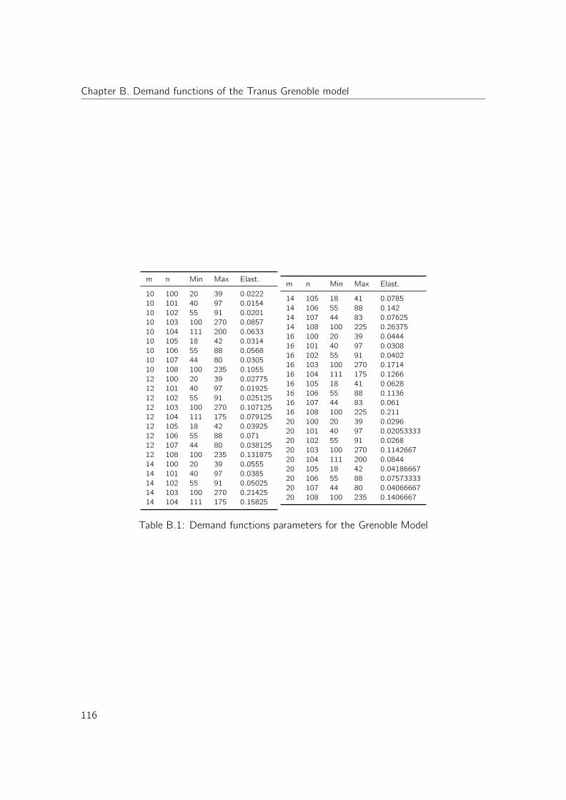
Chapter B. Demand functions of the Tranus Grenoble model
m n Min Max Elast.
10 100 20 39 0.022210 101 40 97 0.015410 102 55 91 0.020110 103 100 270 0.085710 104 111 200 0.063310 105 18 42 0.031410 106 55 88 0.056810 107 44 80 0.030510 108 100 235 0.105512 100 20 39 0.0277512 101 40 97 0.0192512 102 55 91 0.02512512 103 100 270 0.10712512 104 111 175 0.07912512 105 18 42 0.0392512 106 55 88 0.07112 107 44 80 0.03812512 108 100 235 0.13187514 100 20 39 0.055514 101 40 97 0.038514 102 55 91 0.0502514 103 100 270 0.2142514 104 111 175 0.15825
m n Min Max Elast.
14 105 18 41 0.078514 106 55 88 0.14214 107 44 83 0.0762514 108 100 225 0.2637516 100 20 39 0.044416 101 40 97 0.030816 102 55 91 0.040216 103 100 270 0.171416 104 111 175 0.126616 105 18 41 0.062816 106 55 88 0.113616 107 44 83 0.06116 108 100 225 0.21120 100 20 39 0.029620 101 40 97 0.0205333320 102 55 91 0.026820 103 100 270 0.114266720 104 111 200 0.084420 105 18 42 0.0418666720 106 55 88 0.0757333320 107 44 80 0.0406666720 108 100 235 0.1406667
Table B.1: Demand functions parameters for the Grenoble Model
116
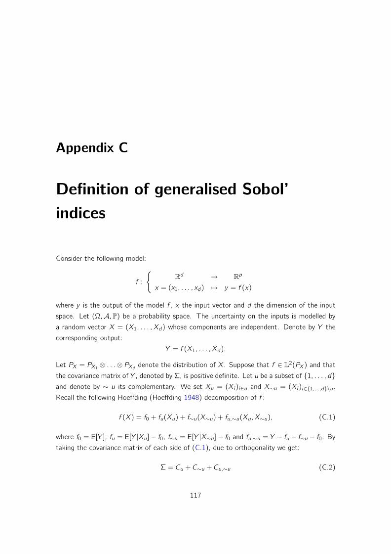
Appendix C
Definition of generalised Sobol’indices
Consider the following model:
f :
Rd → Rp
x = (x1, . . . , xd) 7→ y = f (x)
where y is the output of the model f , x the input vector and d the dimension of the input
space. Let (Ω,A,P) be a probability space. The uncertainty on the inputs is modelled by
a random vector X = (X1, . . . , Xd) whose components are independent. Denote by Y the
corresponding output:
Y = f (X1, . . . , Xd).
Let PX = PX1⊗ . . .⊗ PXd denote the distribution of X. Suppose that f ∈ L2(PX) and that
the covariance matrix of Y , denoted by Σ, is positive definite. Let u be a subset of 1, . . . , dand denote by ∼ u its complementary. We set Xu = (Xi)i∈u and X∼u = (Xi)i∈1,...,d\u.
Recall the following Hoeffding (Hoeffding 1948) decomposition of f :
f (X) = f0 + fu(Xu) + f∼u(X∼u) + fu,∼u(Xu, X∼u), (C.1)
where f0 = E[Y ], fu = E[Y |Xu]− f0, f∼u = E[Y |X∼u]− f0 and fu,∼u = Y − fu − f∼u − f0. Bytaking the covariance matrix of each side of (C.1), due to orthogonality we get:
Σ = Cu + C∼u + Cu,∼u (C.2)
117

Chapter C. Definition of generalised Sobol’ indices
Let M be a matrix of dimensions p × p, Equation (C.2) can be projected on a scalar as
follows:
Tr(MΣ) = Tr(MCu) + Tr(MC∼u) + Tr(MCu,∼u) (C.3)
where Tr denote the trace operator. Following (C.3) and under the condition Tr(Σ) 6= 0,
the M-generalized Sobol’ index is defined as follows:
Su(M; f ) =Tr(MCu)
Tr(MΣ).
Su(M; f ) is a M-sensitivity measure of Y to the inputs in u. In (Gamboa et al. 2014), the
authors show that the only good choice for M is the matrix identity Idp. With this choice,
the formula for the generalized Sobol’ index reduces to:
Su(f ) =Tr(Cu)
Tr(Σ). (C.4)
When u = (v , w) is a 2-subset of 1, . . . , d, the influence of the interaction between
v and w is quantified by the second-order generalized Sobol’ index defined by: S(v,w)(f ) −Sv (f )− Sw (f ).
Classical estimation of Su(f ) The classical estimation procedure for Su(f ) is a general-
ization of the one used in the univariate case (Sobol 1993). The procedure consists of a
Monte-Carlo pick-freeze method. In the pick-freeze method, the Sobol index is viewed as the
regression coefficient between the output of the model and its pick-freezed replication. This
replication is obtained by holding the value of the variable of interest Xu (frozen variable)
and by sampling the other variables X∼u (picked variables).
We set Y u = f (Xu, X′∼u) where X ′∼u is an independent copy of X∼u. Let N > 0 be an
integer and Y1, . . . , YN (resp. Y u1 , . . . , YuN ) be N independent copies of Y (resp. Y u) where:
Yi = (Yi ,1, . . . , Yi ,p), Y ui = (Y ui,1, . . . , Yui,p), ∀ i ∈ 1, . . . , N.
As in (Janon et al. 2014; Monod, Naud, and Makowski 2006), the following estimator of
Su(f ) is constructed:
Su(f ) =
p∑l=1
(1N
N∑i=1
Yi ,lYui,l −
(1N
N∑i=1
Yi ,l+Yui,l
2
)2)
p∑l=1
(1N
N∑i=1
Y 2i ,l+(Y ui,l )
2
2 −(
1N
N∑i=1
Yi ,l+Yui,l
2
)2) (C.5)
118
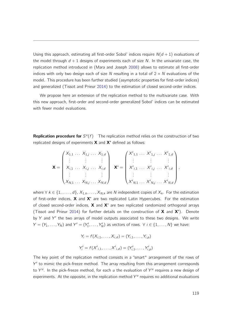
Using this approach, estimating all first-order Sobol’ indices require N(d + 1) evaluations of
the model through d + 1 designs of experiments each of size N. In the univariate case, the
replication method introduced in (Mara and Joseph 2008) allows to estimate all first-order
indices with only two design each of size N resulting in a total of 2 × N evaluations of the
model. This procedure has been further studied (asymptotic properties for first-order indices)
and generalized (Tissot and Prieur 2014) to the estimation of closed second-order indices.
We propose here an extension of the replication method to the multivariate case. With
this new approach, first-order and second-order generalized Sobol’ indices can be estimated
with fewer model evaluations.
Replication procedure for Su(f ) The replication method relies on the construction of two
replicated designs of experiments X and X’ defined as follows:
X =
X1,1 . . . X1,j . . . X1,d
......
...
Xi ,1 . . . Xi ,j . . . Xi ,d...
......
XN,1 . . . XN,j . . . XN,d
X’ =
X ′1,1 . . . X′1,j . . . X
′1,d
......
...
X ′i ,1 . . . X′i ,j . . . X
′i ,d
......
...
X ′N,1 . . . X′N,j . . . X
′N,d
,
where ∀ k ∈ 1, , . . . , d, X1,k , . . . , XN,k are N independent copies of Xk . For the estimation
of first-order indices, X and X’ are two replicated Latin Hypercubes. For the estimation
of closed second-order indices, X and X’ are two replicated randomized orthogonal arrays
(Tissot and Prieur 2014) for further details on the construction of X and X’). Denote
by Y and Y ′ the two arrays of model outputs associated to these two designs. We write
Y = (Y1, . . . , YN) and Y ′ = (Y ′1, . . . , Y′N) as vectors of rows. ∀ i ∈ 1, . . . , N we have:
Yi = f (Xi ,1, . . . , Xi ,d) = (Yi ,1, . . . , Yi ,p)
Y ′i = f (X ′i ,1, . . . , X′i ,d) = (Y ′i ,1, . . . , Y
′i ,p)
The key point of the replication method consists in a “smart" arrangement of the rows of
Y ′ to mimic the pick-freeze method. The array resulting from this arrangement corresponds
to Y u. In the pick-freeze method, for each u the evaluation of Y u requires a new design of
experiments. At the opposite, in the replication method Y u requires no additional evaluations
119

Chapter C. Definition of generalised Sobol’ indices
of the model. Let π denote the permutation used to re-arrange Y ′, ∀ i ∈ 1, . . . , N:
Y ui = f (X ′π(i),1, . . . , X′π(i),d) = (Y ′π(i),1, . . . , Y
′π(i),p),
Let u = u1, . . . , um ⊂ 1, . . . , d. From a design point of view, π is chosen to insure that:
X ′π(uj ),1 = Xuj ,1, ∀ j ∈ 1, . . . , m,
thus insuring that both Y and Y u are evaluated on the same u coordinates. Su(f ) is then
estimated using formula (C.5) with both Y and Y u. For the sake of clarity of the paper, we
choose to not further explained the choice of π. The interested reader can find a detailed
description in (Tissot and Prieur 2014).
120

121
Copyright © 2022 FDOKUMEN