Development and Optimization of Methods for Accelerated ...

POUR L'OBTENTION DU GRADE DE DOCTEUR ÈS SCIENCES

acceptée sur proposition du jury:

Prof. D. Van De Ville, président du juryProf. J.-Ph. Thiran, Dr G. Krüger, directeurs de thèse

Prof. K. T. Block, rapporteurProf. D. G. Norris, rapporteurDr O. Reynaud, rapporteur

Development and Optimization of Methods for

Accelerated Magnetic Resonance Imaging

THÈSE NO 8237 (2018)

ÉCOLE POLYTECHNIQUE FÉDÉRALE DE LAUSANNE

PRÉSENTÉE LE 23 MARS 2018

À LA FACULTÉ DES SCIENCES ET TECHNIQUES DE L'INGÉNIEUR

LABORATOIRE DE TRAITEMENT DES SIGNAUX 5

PROGRAMME DOCTORAL EN GÉNIE ÉLECTRIQUE

Suisse2018

PAR

Tom HILBERT

It is the tension between creativity and skepticism that has produced

the stunning and unexpected findings of science.

— Carl Sagan

Meiner Familie. . .

AcknowledgementsI joined the ACIT group for the first time in 2009. Since then, I have had countless projects,

internships and theses to finish. Today, eight years later, I’m finishing my third and (hopefully)

last thesis, my dissertation. I would like to thank my colleagues and friends who always helped

me and made this period a great part of my life. However, there are a few people I would like

to thank personally.

Back in 2009, I was certainly far below the average age in the ACIT group. Despite of being just

at the beginning of my academic career (4th semester in my bachelor studies), you, Gunnar,

believed in my skills and kept finding funding and hiring me for various projects from which I

learned so much. I want to thank you for your support and trust that shaped my career and

led me all the way to the end of my PhD, and hopefully, more to come.

In my very first project I was supervised by probably the coolest PhD student in the lab. It

makes me laugh when I think back to my worries of what I should wear on my first day, only

to see Tobi coming around the corner in shorts and a funny t-shirt. Eight years later, Tobi

is the head of the ACIT group and is not only supervising me, but also 12 other knowledge

seeking researchers. I want to thank you, Tobi, for always being both a good supervisor and a

friend. I learned countless things (e.g. how to properly name a word document or operate a

several million dollar MRI scanner) from you over these many years and I’m looking forward

to continuing this great endeavour.

I would like to thank you, Jean-Philippe, for providing me the opportunity to work in the

great environment of the LTS5. The diverse projects and expertise of you and your lab are

extraordinary, and I want to thank you for welcoming me to the LTS5 family so kindly.

Despite being very nervous at the beginning, I will remember my thesis exam as a rather

pleasant experience. I want to thank my jury, Prof. David J. Norris, Prof. Kai T. Block, and Dr.

Oliver Reynaud, and the committee president Prof. Dimitri Van De Ville for the interesting

discussions and for their precious time.

One reason why I actually manage to get out of bed every morning and take the crowded

metro to the office is the ACIT team. I could always rely on the support of the team and this

gave me the motivation to keep on going. Béné, thank you for all the years of teamwork, and

one day I hope I’ll be at least a little bit as organized as you. Thank you, Ricardo, for not only

critically proofreading this thesis, but also for your discussions about work, your crazy projects

and politics during pasta with Pesto Rosso and beer at home. Thank you, Davide, for sharing

your deep knowledge in programming that always comes along with either a kind insult or

wisdom from the book of Mormons. Thank you, Mario, Maryna, Pavel, John, and Bobo, for

v

Acknowledgements

the great time in our little PhD office, where we prayed to the gods of Bollywood and always

had something to laugh about. Thank you, Kieran, Jonas and Alexis, for helping me when I

got stuck with problems that seemed unsolvable, and for always asking the difficult questions

during presentations. I also had the pleasure to supervise two very smart Master students,

Emilie and Gian-Franco. Thank you for being patient with my first attempts at supervision.

My gratitude goes also to the many interns and students that created so many memorable

moments. Luca, yes I’ll try deep learning. Alexandra, my stomach still hurts from all the Haribo.

Theo, I miss the epic Fridays. Pascal, I still cannot speak nor understand Swiss-German.

I had the honor to work together with great minds in the field of MRI, without whom this thesis

would have much fewer innovative ideas. Thank you, Tilman, for being so generous to provide

your code and knowledge upon which I built my PhD work. I want to send a big thanks to

the bSSFP gurus in Basel. It was always fun to work with you, Oliver and Damien, and it is

impressive that the flow of ideas never stopped. My gratitude goes also to the simultaneous-

multi-slice experts, David, Jenni, Laurent, and Jose in Nijmegen and their patients in answering

my countless questions about PINS pulses. I also was given the opportunity to visit the CAI2R

at the New York University for a month. Thank you, Martijn and Tobias B., for making this

possible and also Thomas B., Thomas V., Florian for welcoming me so kindly.

In the research of new clinical tools in radiology, one obviously has to consider the feedback of

the expert radiologists. I want to send my gratitude to Prof. Meuli, Prof. Maeder, Dr. Hagman

and Dr. Omoumi for always providing constructive critique on our new ideas, no matter how

unreasonable they may seem, and providing the input that was necessary to steer my research

into the right direction.

I was also part of a team of researchers and developers in Erlangen. Thank you, Heiko, for

letting me being a part of this team despite the long distance. Thank you, Michael, Christoph,

Elisabeth, Alto, Esther and Rainer, for all the support and ideas.

Probably the most social, but also least productive, period of my PhD was spent in the open

space of the LTS5. I want to thank you, Didrik, Vijay, Maryna, Gabriel, and all the other people

who shared an amazing time, crazy nights in the bar Giraffe and a fair amount of Cuvée des

Trolls with me.

Needless to say that everything that I present in this thesis did not work right away. It required

dozens of nights in the basement of the CHUV at the scanner. One motivation to keep

commuting between EPFL and CHUV was the group of Mathias. Although you guys think that

Neuro MRI is boring, you, Jessica, Ruud, Simo, Gabri, Andrew, Giulia, Emeline and Roberto

made me feel welcome and we have became good friends over the years. Thank you.

Tesekkürler, Esi, for your frequent phone calls that allowed us to stay connected, although we

both continued on different paths after the master studies. I am pretty sure that some paper

drafts would still not be finished without your virtual “Arschtritt”.

Thank you, Chris and Caroline, for baring with my three hour dumpling stuffing and two hour

sushi rolling workshops that ended with a feast. I cannot even imagine a boring evening or

skiing day when you guys are around. Also thank you, Chris, for kicking my “inner-swine-dog”.

I appreciate it, even though it may not seem like it.

Murat and Marili, it seems like I have known you for ages now and I want to send my warm

vi

Acknowledgements

thanks for all the quality time we spent together travelling, hiking, cooking, skiing, dancing,

sailing and all the great activities that balance out the work stress.

Another factor that I need in order to unwind is music. The weekly noise-making with “The

Available” in the bunker of EPFL has helped to forget the bugs and disappointing results.

Thank you, Chica, João (Hendrix), João (the wise), Joaquin and Dan, for not getting mad when

I hit the drums even louder after a rough day.

Usually, I did not seem stressed when I was working on this thesis. However, there is one

person that knows the truth. Nora, thank you for dealing with the-nervewracking-me that

surfaces the moment I come home. I Kant thank you enough for your kindness, heartwarming

care and inspiration.

Liebe Omas, ich bin euch so sehr dankbar für eure Unterstützung und dass Ihr es mir nicht

übel nimmt dass ich mich entschied so weit weg von Zuhause zu leben. Ich bin froh dass Ihr

mich in Lausanne besucht habt und dass Ihr jetzt auch versteht warum ich diesen Ort so sehr

mag.

Marci, Du warst schon immer ein Vorbild und vielleicht hätte ich nie studiert wenn ich nicht

damals mit dir in Dresden probe-studiert hätte. So viele Jahre später, werden wir beide zu „Dr.

Hilbert“ und das sogar im selben Monat. Vielen Dank!

Vati und Mutti. Mit eurer Liebe und Unterstützung habt Ihr mich erst im kleinen Crossen

gedeihen lassen und raus in die weite Welt geschickt. Danke dass Ihr immer, in guten sowie

auch schlechten Zeiten, für mich da wart und mich immer frei entscheiden lassen habt was

ich mit meinen Leben mache. Danke für alles.

Lausanne, 2 November 2017 T. H.

vii

AbstractMagnetic resonance imaging (MRI) has yielded great success as a medical imaging modality

in the past decades, and its excellent soft tissue contrast is used in clinical routine to support

diagnosis today. However, MRI is still facing challenges. For example, the acquisition time

is long in comparison to computed tomography, especially when directly measuring tissue

properties with quantitative MRI. This thesis presents new approaches to accelerate quantita-

tive MRI acquisitions without decreasing the accuracy, using analytical and numerical signal

models.

A quantitative acquisition to map the transverse relaxation T2 was first accelerated by com-

bining parallel imaging with model-based reconstruction. It was demonstrated that the

combination leads to an improved artifact behaviour in comparison to a model-based re-

construction alone, facilitating higher acceleration factors. The technique was optimized to

obtain T2 maps from the brain, knee, prostate and liver, with good initial results. The idea of

combining methods was continued by introducing simultaneous multi slice acquisition to the

T2 mapping approach. Furthermore, a numerical simulation rather than an analytical solution

was used in the model-based reconstruction, resulting in a fast undersampled acquisition that

also accounts for transmit field inhomogeneity. This approach yielded more accurate and

faster acquired T2 values.

Magnetic resonance fingerprinting (MRF) is a recently introduced model-based reconstruction

that promises to provide multiple quantitative maps using a fast pseudo-random acquisition.

However, similar to other model-based approaches, MRF depends on how well the model de-

scribes the measured signal. It was demonstrated in this work that the estimated quantitative

maps may be systematically biased if the model does not account for magnetization transfer

effects. To this end, a simplified numerical model was proposed, that includes magnetization

transfer, and yields more accurate quantitative values.

The same approach was translated to bSSFP acquisitions, where banding artifacts are a major

limitation: the analytical model of a phase-cycle bSSFP acquisition was used to separate signal

effects of the human tissue from signal effects due to magnetic field inhomogeneity. The

separation allowed the removal of typical signal voids in bSSFP images. A compressed sensing

reconstruction was employed to avoid additional acquisition time.

In summary, this thesis has introduced new approaches to employ signal models in different

applications, with the aim of either accelerating an acquisition, or improving the accuracy

of an existing fast method. These approaches may help to make the next step away from

qualitative towards a fully quantitative MR imaging modality, facilitating precision medicine

ix

Acknowledgements

and personalized treatment.

Keywordsmagnetic resonance imaging; quantitative imaging; acquisition acceleration; model-based

reconstruction

x

ZusammenfassungMagnet Resonanz Tomographie (MRT) hat in den letzten Jahrzehnten einen großen Erfolg

erzielt und mit einem exzellentem Weichgewebekontrast wird es heute im klinischen Alltag

genutzt um Diagnosen zu unterstützen. Jedoch stellt sich der MRT immer noch Herausforde-

rungen. Zum Beispiel ist die Aufnahmezeit lang im Vergleich zu der Computer Tomographie,

besonders wenn Gewebeeigenschaften direkt mit quantitativer Bildgebung gemessen werden.

In diesen Zusammenhang studiert diese Dissertation neue Ansätze, unter der Verwendung

von Signalmodellen, um quantitative MRT Bildgebung zu beschleunigen ohne die Genauigkeit

zu verringern.

Eine quantitative Messung der transversalen Relaxation T2 wurde zunächst beschleunigt

indem parallel Bildgebung mit modellbasierter Rekonstruktion kombiniert wurde. Es wurde

gezeigt dass die Kombination zu einem besseren Bildfehlerverhalten führt im Vergleich zu

einer alleinigen modellbasierten Rekonstruktion. Die neue Methodik wurde optimiert für die

Messung von T2 Karten im Kopf, im Knie, der Prostata und der Leber und zeigte gute initiale

Ergebnisse.

Die Idee Methoden zu kombinieren wurde fortgesetzt indem Simultane-Multiple-Schichten

Aufnahme in der T2 Kartographie eingeführt wurde. Weiterhin wurde eine numerische Simu-

lation anstatt einer analytischen Lösung in der modellbasierten Rekonstruktion verwendet,

was zu einer schnellen unterabgetasteten Messung führte welche auch Inhomogenität im

Radiofrequenzfeld beachtet. Somit konnten akkurater und schneller gemessene T2 Werte

erreicht werden.

Magnetresonanz-Fingerprinting (MRF) ist eine modellbasierte Rekonstruktion die vor kurzem

vorgestellt wurde und verspricht mehrere quantitative Karten mit einer schnellen pseudozufäl-

ligen Aufnahme bereit zu stellen. Jedoch ist MRF, wie andere modellbasierte Ansätze, abhängig

von wie genau das Model das gemessene Signal beschreibt. In dieser Arbeit wurde gezeigt,

dass die geschätzten quantitativen Karten einen systematischen Fehler haben können wenn

Magnetisierungstransfer nicht beachtet wird. Daher wurde ein vereinfachtes numerisches Mo-

del vorgeschlagen das Magnetisierungstransfer einbezieht und somit akkurater quantitative

Werte erzielte.

Derselbe Ansatz wurde auf bSSFP Messungen übertragen bei denen Bildfehler ein große Li-

mitierung sind: das analytische Model einer Phasenzyklen bSSFP Messung wurde genutzt

um Signaleffekte vom Menschlichen Gewebe von Signaleffekten durch Magnetfeldinhomo-

genität zu trennen. Die Trennung ermöglicht die Entfernung des typischen Signalabfalls in

bSFFP Bildern. Eine compressed sensing Rekonstruktion wurde verwendet um zusätzliche

xi

Acknowledgements

Aufnahmezeit zu verhindern.

Zusammenfassend, diese Dissertation hat neue Ansätze zur Verwendung von Signalmodellen

in verschiedenen Anwendungen vorgestellt, mit dem Ziel eine Aufnahme zu beschleunigen

oder die Genauigkeit einer bereits existierenden Methodik zu verbessern. Diese Ansätze mögen

dabei helfen den nächsten Schritt, weg von qualitativ in Richtung einer quantitativen Magne-

tresonanztomographie zu machen, um präzise Medizin und personalisierte Behandlung zu

ermöglichen.

SchlüsselwörterMagnet Resonanz Tomographie; Quantitative Bildgebung; beschleunigte Messung; Modellba-

sierte Rekonstruktion

xii

Contents

Acknowledgements v

Abstract (English/Deutsch) ix

List of figures xv

List of tables xviii

Introduction 1

1 Introduction 1

1.1 Aim and structure of the thesis . . . . . . . . . . . . . . . . . . . . . . . . . . . . . 3

2 Background 5

2.1 Nuclear Magnetic Resonance . . . . . . . . . . . . . . . . . . . . . . . . . . . . . . 5

2.2 Spatial Encoding . . . . . . . . . . . . . . . . . . . . . . . . . . . . . . . . . . . . . 9

2.2.1 Slice Selective Excitation - 2D Imaging . . . . . . . . . . . . . . . . . . . . 11

2.2.2 In-Plane Localization . . . . . . . . . . . . . . . . . . . . . . . . . . . . . . 12

2.2.3 Non Selective Excitation – 3D Imaging . . . . . . . . . . . . . . . . . . . . 14

2.3 MR Pulse Sequence Designs . . . . . . . . . . . . . . . . . . . . . . . . . . . . . . . 15

2.3.1 Spin-Echo sequence . . . . . . . . . . . . . . . . . . . . . . . . . . . . . . . 15

2.3.2 Gradient Recalled Echo Sequence . . . . . . . . . . . . . . . . . . . . . . . 17

2.3.3 Magnetization Preparation . . . . . . . . . . . . . . . . . . . . . . . . . . . 18

2.4 Instrumentation . . . . . . . . . . . . . . . . . . . . . . . . . . . . . . . . . . . . . . 19

2.5 Quantitative Magnetic Resonance Imaging . . . . . . . . . . . . . . . . . . . . . . 21

2.5.1 T2 Mapping . . . . . . . . . . . . . . . . . . . . . . . . . . . . . . . . . . . . 22

2.5.2 T1 Mapping . . . . . . . . . . . . . . . . . . . . . . . . . . . . . . . . . . . . 23

2.5.3 Multi Parametric Mapping . . . . . . . . . . . . . . . . . . . . . . . . . . . 24

2.5.4 Synthetic Contrasts . . . . . . . . . . . . . . . . . . . . . . . . . . . . . . . . 25

2.6 Accelerated MRI . . . . . . . . . . . . . . . . . . . . . . . . . . . . . . . . . . . . . . 25

2.6.1 K-Space and Sequence Sampling Techniques . . . . . . . . . . . . . . . . 26

2.6.2 Parallel Imaging . . . . . . . . . . . . . . . . . . . . . . . . . . . . . . . . . . 26

2.6.3 Compressed Sensing . . . . . . . . . . . . . . . . . . . . . . . . . . . . . . . 28

2.6.4 Model-Based Reconstruction . . . . . . . . . . . . . . . . . . . . . . . . . . 29

2.6.5 Simultaneous Multi Slice . . . . . . . . . . . . . . . . . . . . . . . . . . . . 30

xiii

Contents

3 Accelerated T2 Mapping Combining Parallel MRI and Model-Based Reconstruction 33

3.1 Introduction . . . . . . . . . . . . . . . . . . . . . . . . . . . . . . . . . . . . . . . . 33

3.2 Materials and Methods . . . . . . . . . . . . . . . . . . . . . . . . . . . . . . . . . . 35

3.2.1 Acquisition . . . . . . . . . . . . . . . . . . . . . . . . . . . . . . . . . . . . . 35

3.2.2 Reconstruction . . . . . . . . . . . . . . . . . . . . . . . . . . . . . . . . . . 36

3.2.3 Artificial Undersampling for Ground-Truth Comparison . . . . . . . . . . 36

3.2.4 Acquisition of Undersampled Data and Reproducibility . . . . . . . . . . 38

3.3 Results . . . . . . . . . . . . . . . . . . . . . . . . . . . . . . . . . . . . . . . . . . . 38

3.3.1 Artificial Undersampling for Ground-Truth Comparison . . . . . . . . . . 38

3.3.2 Acquisition of Undersampled Data and Reproducibility . . . . . . . . . . 40

3.4 Discussion . . . . . . . . . . . . . . . . . . . . . . . . . . . . . . . . . . . . . . . . . 41

4 Fast Model-Based T2 Mapping using SAR-Reduced Simultaneous-Multi-Slice Excita-

tion 45

4.1 Introduction . . . . . . . . . . . . . . . . . . . . . . . . . . . . . . . . . . . . . . . . 46

4.2 Materials and Methods . . . . . . . . . . . . . . . . . . . . . . . . . . . . . . . . . . 46

4.2.1 Acquisition . . . . . . . . . . . . . . . . . . . . . . . . . . . . . . . . . . . . . 46

4.2.2 Reconstruction . . . . . . . . . . . . . . . . . . . . . . . . . . . . . . . . . . 48

4.2.3 In Vivo Studies . . . . . . . . . . . . . . . . . . . . . . . . . . . . . . . . . . 52

4.2.4 Phantom Studies . . . . . . . . . . . . . . . . . . . . . . . . . . . . . . . . . 52

4.3 Results . . . . . . . . . . . . . . . . . . . . . . . . . . . . . . . . . . . . . . . . . . . 53

4.3.1 In Vivo Studies . . . . . . . . . . . . . . . . . . . . . . . . . . . . . . . . . . 53

4.3.2 Phantom Studies . . . . . . . . . . . . . . . . . . . . . . . . . . . . . . . . . 54

4.3.3 SAR Aspects . . . . . . . . . . . . . . . . . . . . . . . . . . . . . . . . . . . . 54

4.3.4 Computational Requirements . . . . . . . . . . . . . . . . . . . . . . . . . 55

4.4 Discussion . . . . . . . . . . . . . . . . . . . . . . . . . . . . . . . . . . . . . . . . . 55

5 Mitigating the Effect of Magnetization Transfer in Magnetic Resonance Fingerprint-

ing 61

5.1 Introduction . . . . . . . . . . . . . . . . . . . . . . . . . . . . . . . . . . . . . . . . 61

5.2 Theory . . . . . . . . . . . . . . . . . . . . . . . . . . . . . . . . . . . . . . . . . . . 62

5.2.1 Common Model of Magnetization Transfer . . . . . . . . . . . . . . . . . . 63

5.2.2 Simplified Model . . . . . . . . . . . . . . . . . . . . . . . . . . . . . . . . . 63

5.3 Methods . . . . . . . . . . . . . . . . . . . . . . . . . . . . . . . . . . . . . . . . . . 66

5.3.1 In-Vivo Experiments . . . . . . . . . . . . . . . . . . . . . . . . . . . . . . . 66

5.3.2 In Silico Experiments . . . . . . . . . . . . . . . . . . . . . . . . . . . . . . . 68

5.3.3 In Vitro Experiments . . . . . . . . . . . . . . . . . . . . . . . . . . . . . . . 68

5.4 Results . . . . . . . . . . . . . . . . . . . . . . . . . . . . . . . . . . . . . . . . . . . 68

5.4.1 In Vivo Experiments . . . . . . . . . . . . . . . . . . . . . . . . . . . . . . . 68

5.4.2 In Silico Experiments . . . . . . . . . . . . . . . . . . . . . . . . . . . . . . . 70

5.4.3 In Vitro Experiments . . . . . . . . . . . . . . . . . . . . . . . . . . . . . . . 71

5.5 Discussion . . . . . . . . . . . . . . . . . . . . . . . . . . . . . . . . . . . . . . . . . 72

xiv

Contents

6 True constructive interference in the steady state 77

6.1 Introduction . . . . . . . . . . . . . . . . . . . . . . . . . . . . . . . . . . . . . . . . 77

6.2 Methods . . . . . . . . . . . . . . . . . . . . . . . . . . . . . . . . . . . . . . . . . . 80

6.2.1 Acquisition . . . . . . . . . . . . . . . . . . . . . . . . . . . . . . . . . . . . . 80

6.2.2 Reconstruction . . . . . . . . . . . . . . . . . . . . . . . . . . . . . . . . . . 81

6.2.3 Simulations and Imaging . . . . . . . . . . . . . . . . . . . . . . . . . . . . 82

6.3 Results . . . . . . . . . . . . . . . . . . . . . . . . . . . . . . . . . . . . . . . . . . . 84

6.4 Discussion . . . . . . . . . . . . . . . . . . . . . . . . . . . . . . . . . . . . . . . . . 87

7 Conclusion 93

7.1 Achieved Results . . . . . . . . . . . . . . . . . . . . . . . . . . . . . . . . . . . . . 93

7.2 Clinical Impact of this Work . . . . . . . . . . . . . . . . . . . . . . . . . . . . . . . 94

7.3 Outlook . . . . . . . . . . . . . . . . . . . . . . . . . . . . . . . . . . . . . . . . . . . 96

Bibliography 105

Publications 107

Curriculum Vitae 111

xv

List of Figures

1.1 The first MRI apparatus . . . . . . . . . . . . . . . . . . . . . . . . . . . . . . . . . 2

1.2 Modern MRI . . . . . . . . . . . . . . . . . . . . . . . . . . . . . . . . . . . . . . . . 3

2.1 Protons outside and inside a magnetic field . . . . . . . . . . . . . . . . . . . . . 6

2.2 Excitation of spins . . . . . . . . . . . . . . . . . . . . . . . . . . . . . . . . . . . . 7

2.3 Relaxation of spins . . . . . . . . . . . . . . . . . . . . . . . . . . . . . . . . . . . . 8

2.4 Relaxation Curves . . . . . . . . . . . . . . . . . . . . . . . . . . . . . . . . . . . . . 9

2.5 Example sequence diagram . . . . . . . . . . . . . . . . . . . . . . . . . . . . . . . 10

2.6 Slice selection . . . . . . . . . . . . . . . . . . . . . . . . . . . . . . . . . . . . . . . 11

2.7 K-space frequencies . . . . . . . . . . . . . . . . . . . . . . . . . . . . . . . . . . . 12

2.8 Frequency encoding . . . . . . . . . . . . . . . . . . . . . . . . . . . . . . . . . . . 13

2.9 Phase encoding . . . . . . . . . . . . . . . . . . . . . . . . . . . . . . . . . . . . . . 14

2.10 Spin Echo (SE) sequence design . . . . . . . . . . . . . . . . . . . . . . . . . . . . 16

2.11 Gradient Recalled Echo (GRE) sequence design . . . . . . . . . . . . . . . . . . . 17

2.12 Balanced Steady State Free Precession (bSSFP) sequence design . . . . . . . . . 18

2.13 Inversion recovery magnetization preparation . . . . . . . . . . . . . . . . . . . . 19

2.14 Instrumentation of a MRI scanner . . . . . . . . . . . . . . . . . . . . . . . . . . . 21

2.15 Number of publications in quantitative MRI . . . . . . . . . . . . . . . . . . . . . 21

2.16 T1 mapping with the MP2RAGE . . . . . . . . . . . . . . . . . . . . . . . . . . . . 23

2.17 Multi-parametric mapping with TESS . . . . . . . . . . . . . . . . . . . . . . . . . 24

2.18 Reconstructing partially parallel acquired data with GRAPPA . . . . . . . . . . . 27

2.19 Sparse representation in the wavelet-domain . . . . . . . . . . . . . . . . . . . . 28

2.20 Model-based reconstruction . . . . . . . . . . . . . . . . . . . . . . . . . . . . . . 29

2.21 Simultaneous-Multi-Slice reconstruction. . . . . . . . . . . . . . . . . . . . . . . 30

3.1 Sampling pattern of MARTINI and GRAPPATINI . . . . . . . . . . . . . . . . . . . 35

3.2 Results of artificial undersampling . . . . . . . . . . . . . . . . . . . . . . . . . . . 39

3.3 Results of undersampled acquisitions. . . . . . . . . . . . . . . . . . . . . . . . . . 40

3.4 T2 maps and simulated contrasts in different organs . . . . . . . . . . . . . . . . 42

4.1 Simulations-Multi-Slice CPMG sequence . . . . . . . . . . . . . . . . . . . . . . . 47

4.2 Employed sampling pattern for acceleration. . . . . . . . . . . . . . . . . . . . . . 47

4.3 Reconstructing Simulations-Multi-Slice and undersampled CPMG data . . . . . 49

4.4 Stimulated echo effects in CPMG acquisitions. . . . . . . . . . . . . . . . . . . . . 50

xvii

List of Figures

4.5 In Vivo results for undersampled SMS T2 mapping. . . . . . . . . . . . . . . . . . 53

4.6 Reproducibility of T2 values. . . . . . . . . . . . . . . . . . . . . . . . . . . . . . . 56

4.7 Results of phantom experiment . . . . . . . . . . . . . . . . . . . . . . . . . . . . 57

4.8 Simulated Contrasts with SMS-CPMG acquisitions. . . . . . . . . . . . . . . . . . 58

5.1 Magnetization transfer models . . . . . . . . . . . . . . . . . . . . . . . . . . . . . 66

5.2 Magnetization transfer fingerprinting sequence . . . . . . . . . . . . . . . . . . . 67

5.3 Magnetization transfer effects with and without two-pool model . . . . . . . . . 69

5.4 MT-MRF in vivo results from all subjects . . . . . . . . . . . . . . . . . . . . . . . 70

5.5 Quantitative values in regions of interest. . . . . . . . . . . . . . . . . . . . . . . . 71

5.6 Example fingerprints . . . . . . . . . . . . . . . . . . . . . . . . . . . . . . . . . . . 72

5.7 Simulation of model violations . . . . . . . . . . . . . . . . . . . . . . . . . . . . . 73

5.8 Phantom results of MT-MRF . . . . . . . . . . . . . . . . . . . . . . . . . . . . . . 74

6.1 Performance of various combination methods. . . . . . . . . . . . . . . . . . . . 79

6.2 Acquisition scheme for trueCISS . . . . . . . . . . . . . . . . . . . . . . . . . . . . 80

6.3 Simulations of regularization of trueCISS . . . . . . . . . . . . . . . . . . . . . . . 83

6.4 Fitting Robustness of trueCISS . . . . . . . . . . . . . . . . . . . . . . . . . . . . . 85

6.5 Sparse representation with trueCISS . . . . . . . . . . . . . . . . . . . . . . . . . . 86

6.6 TrueCISS versus CISS in phantom . . . . . . . . . . . . . . . . . . . . . . . . . . . 88

6.7 TrueCISS parametric maps. . . . . . . . . . . . . . . . . . . . . . . . . . . . . . . . 89

6.8 TrueCISS versus CISS in vivo . . . . . . . . . . . . . . . . . . . . . . . . . . . . . . 90

xviii

List of Tables

2.1 Relaxation times . . . . . . . . . . . . . . . . . . . . . . . . . . . . . . . . . . . . . . 8

2.2 Image parameters and contrast . . . . . . . . . . . . . . . . . . . . . . . . . . . . . 16

3.1 Acquisition parameters . . . . . . . . . . . . . . . . . . . . . . . . . . . . . . . . . 37

4.1 T2 values within regions of interest. . . . . . . . . . . . . . . . . . . . . . . . . . . 54

xix

1 Introduction

Technical advances in radio communication during World War II allowed the discovery of

’Nuclear induction’ shortly after the end of the war in 1945. Bloch and Rabi [1] as well as

Purcell and Pound [2] independently found that voltage can be registered within a coil close

to a sample within a magnetic field, after it was irradiated with a radio-frequency (RF) pulse

– thereby discovering the nuclear magnetic resonance (NMR) signal. Shortly after, in 1949,

Hahn accidentally discovered the spin echo; an additional NMR signal that can be measured

when applying a second RF pulse after a short time delay [3]. The spin echo allowed the

measurement of relaxation effects [4], which, in 1971, Damadian used to differentiate between

healthy and cancerous tissues in mice [5]. These results provided a simple metric, which was,

the first proof of concept for the diagnostic use of magnetic resonance.

In 1974, Damadian developed a machine that allowed the spatial encoding of the NMR signal,

which is believed to have produced the first image of the human body, launching the era of

magnetic resonance imaging (MRI). Figure 1.1 shows a schematic drawing of the apparatus

from the US Patent [6] and an example of an image acquired with this machine [7]. The

apparatus had only a small field of view (FOV) where the magnetic field was homogeneous,

and from which the NMR signal could be retrieved. Therefore, the table where the subject

laid had to be moved within this FOV in order to spatially encode the image, resulting in a

long acquisition time and a low resolution. The following years saw dramatic improvements

in the entire field, leading up to MRI as we know it today. In 1973, Lauterbur proposed the use

of magnetic field gradients to spatially encode the NMR signal along one dimension, using

similar image reconstruction methods as in computed tomography (CT)[8]. This method

drastically reduced acquisition time, while improvements in resolution came about in 1974

with an invention of Sir Mansfield [9]; he used selective excitation to sensitize the acquisition to

a single image slice. To encode the third and last spatial dimension in the NMR signal, Kumar

et al. proposed the two-dimensional Fourier imaging approach in 1975 [10], a method which is

still used today. Since the 1970’s, image contrast, quality and resolution have all been improved

by development of better hardware and acquisition techniques. Commercialization and the

serial production of magnets in the last decades have facilitated the worldwide distribution of

1

Chapter 1. Introduction

Figure 1.1: (a) A schematic drawing from the US patent describing Damadian’s apparatus

that resembles the first MRI. (b) An example image acquired with this apparatus, showing a

transversal slice of human lungs.

MRI to hospitals, where it is now used in clinical routine, being a crucial part of the diagnostic

process. These achievements were also recognized by the Nobel Committee in 1952, 1991,

2002 and 2003, awarding researchers in this field for their contributions.

One of the main advantages of MRI over other imaging methods in clinical use is its excellent

soft tissue contrast. For example, in CT images, the intensity difference between white matter

and grey matter is far less pronounced than in MRI. This renders MRI especially valuable for

neuronal and muscular-skeletal applications. Furthermore, MRI is not relying on ionizing

radiation, unlike CT imaging. Figure 1.2 shows a modern MRI scanner from 2017, and a brain

image acquired with this machine, comparable to the apparatus design and acquisition from

1977 (Figur 1.1).

Despite the dramatic improvement of MRI techniques, the acquisition of a series of images

with different contrasts requires on average 15 minutes, depending on the investigated body

region. That is significantly slower than a usual CT exam, and leads to increased patient

discomfort, complex scheduling, and a decreased cost-benefit ratio, in conjunction with high

maintenance costs. Furthermore, the acquired images are often not standardized, since differ-

ent institutions use customized image acquisition protocols and different scanner hardware.

Efforts have been made in the past to standardize imaging protocols by matching contrasts

across institutions, vendors and field strengths, facilitating better reproducibility. One such

example is the Alzheimer’s disease Neuroimaging Initiative (ADNI) which has collected over

1700 datasets to date, and published open access imaging protocols tailored for scanning

Alzheimer’s patients [11]. Nevertheless, conventional MRI images are a qualitative measure,

meaning that the contrast is mostly affected by tissue proper-ties, but still depends on many

other hardware-related and physiological effects, preventing direct comparison across patients.

The difficulties to run studies with non-standardized images ask for new techniques to avoid

influences from experimental conditions. By contrast, quantitative MRI (qMRI) aims to directly

2

1.1. Aim and structure of the thesis

Figure 1.2: (a) Picture of a modern magnetic resonance imaging scanner (MAGNETOM Skyra,

Siemens, Germany), and (b) an image of the brain that is possible with such a scanner.

measure tissue properties, ideally independent from the experimental conditions. In qMRI,

tissue properties are expressed as quantitative values with physical units, analogous to the

measurement of systolic and diastolic blood pressure, expressed in mmHg. This technique

spatially maps the measured tissue properties resulting in an image called a quantitative

map. This facilitates comparisons either within one patient at multiple time points in order to

extract a trend of tissue alternation (intra-subject), or between a tissue property of a patient

and a normative range derived from a healthy cohort in order to detect abnormal values (inter-

subject). Although quantitative measures have proven to be a good biomarker for disease in

the very early days of NMR [5], it has not been established in clinical routine yet, partly because

qMRI often requires even longer acquisition times than conventional weighted MRI. An entire

field of MRI research has been devoted to overcoming these limitations, with the final goal to

move MRI from a qualitative to a standardized quantitative examination, facilitating precision

medicine and personalized treatment in the future. One key step towards reaching this goal is

to reduce the acquisition time, while retaining or improving the accuracy and precision of the

estimated quantitative value.

1.1 Aim and structure of the thesis

This work focuses on optimizing and developing image acquisition and reconstruction meth-

ods to obtain quantitative image information faster than conventional imaging techniques.

The aim is to reduce the scan time enough to facilitate a routine use of these imaging tech-

niques in a clinical setting, without compromising image quality.

In Chapter 2, the state of the art in MRI is described, starting from basic physics to quantitative

imaging and acquisition acceleration techniques.

3

Chapter 1. Introduction

Chapter 3 introduces a method that aims at combining two acceleration techniques, parallel

imaging and model-based reconstruction, to acquire a whole-brain, quantitative map of the

transverse relaxation in less than 2 minutes. In doing so, the advantages of both methods are

combined, resulting in a better artifact behaviour and higher acceleration factors.

Based on Chapter 3, Chapter 4 continues the idea of combining different acceleration tech-

niques for fast quantitative mapping of the transverse relaxation. A method is introduced

where simultaneous-multi-slice pulses enable the acquisition of different sections of the brain

at the same time, accelerating the acquisition. A new reconstruction is presented that sepa-

rates the signals from the different slices, and uses a model-based reconstruction to obtain

the quantitative values.

Since model-based reconstruction relies on the accuracy of the physical model to reconstruct

data, Chapter 5 focuses on how an over-simplified model may bias the quantification of

relaxation. Using the example of magnetic resonance fingerprinting (MRF), it is demonstrated

that physical models are often an approximation of the underlying micro-structure in human

tissue, and that magnetization transfer can cause a bias in the relaxation estimation. Further,

a new model is introduced that accounts for magnetization transfer and mitigates this bias.

In Chapter 6, multiple quantitative maps are estimated on a single balanced Steady State Free

Precession (bSSFP) acquisition. Some of these maps represent tissue properties, others repre-

sent scanner imperfections. If accurately estimated, scanner imperfections can be separated

and removed from the image contrast, resulting in a more standardized acquisition. This

improvement is realized via compressed sensing reconstruction, without requiring additional

scan time.

Finally, in Chapter 7, the thesis is concluded and a future outlook for the introduced methods

is discussed.

4

2 Background

In this Chapter, the basics of MRI are introduced, starting with the physical principals of nu-

clear magnetic resonance, how an image is generated using these principles and the required

instrumentation. Afterwards, a short introduction into quantitative MRI will be given and

methods for quantifying relaxation described. Finally, the Chapter ends with a summary of

acceleration methods which are already used in fast MRI today. More detailed descriptions

and analytical solutions can be found in Haacke et al. [13].

2.1 Nuclear Magnetic Resonance

Protons, in particular hydrogen nuclei, have a naturally occurring spin that gives them a

magnetic moment. Thus, protons can be seen as small magnets whose magnetization is

described by a vector M . Since protons are usually randomly distributed and oriented, the

sum of their magnetization vectors, the net magnetization, is null (see also Figure 2.1a).

However, when a strong external magnetic field (B0) is applied, the magnetization vectors of

the protons either align in the direction (parallel) or against the direction (anti-parallel) of this

external magnetic field. Depending on the field strength, there are more parallel spins (low

energy state) than anti-parallel spins (high energy state), therefore a net magnetization exist

along the direction of the magnetic field (see also Figure 2.1b).

Furthermore, the spinning protons precess about the axis of the B0 field, whereas precession

corresponds to the gyration of the spinning axis of the proton about the axis in direction of the

magnetic field, similar to a dreidel wobbling around the axis of the earth’s gravitational field.

The precessional frequency ω0, also referred to as the Larmor frequency or resonance fre-

quency, is proportional to the field strength of the main magnetic field B0 by the gyromagnetic

ratio γ:

ω0 = γB0 (2.1)

The aforementioned magnetization vector M of a proton can be described in a coordinate

5

Chapter 2. Background

Figure 2.1: (a) Protons which are outside a strong magnetic field are randomly distributed

and oriented, therefore the sum of their magnetization (net magnetization) is zero. (b) Protons

within a strong magnetic field align with the field parallel or anti-parallel, generating a small

net magnetization.

system with x, y and z axis, with Mz being the longitudinal component along the B0 field

and a transverse component Mx y in the x-y-plane. Since the spins precess, the gyration is

causing a small rotating magnetization component in the x-y-plane. However, the protons are

not precessing in phase and thus the net magnetization in the x-y-plane is zero. This state,

with magnetization vectors precessing about the magnetic field with zero net magnetization

in the transverse plane and with a net magnetization along the z-axis is called equilibrium

magnetization (M0).

Magnetic resonance is the exchange of energy between the spins and an electromagnetic

radio frequency (RF) pulse and can be used to change the state of the magnetization vector.

However, only spins with the same precessional frequency as the RF pulse frequency will

respond and absorb energy. This absorption of energy is called excitation and, on a quantum

level, will bring some spins to a higher energy state and into phase coherence. On a greater

level, the vector of the net magnetization spirals into the transverse plane as illustrated in

Figure 2.2a. From the perspective of a rotating frame of reference, meaning that the coordinate

system rotates about the main direction of the magnetic field (z-axis) in the Larmor frequency,

the excitation corresponds to rotating the net magnetization into the direction of the RF pulses

magnetic field B1 as illustrated in Figure 2.2b. The flip-angle α of this rotation depends on the

amplitude B1 and duration tRF of the RF pulse:

α= γB1tRF (2.2)

For example, a 90◦ excitation pulse flips the magnetization vector fully into the transverse

plane. Therefore, no longitudinal magnetization Mz is left (i.e. equal amount of parallel

and anti-parallel spins) and all spins are in phase (i.e. full phase coherence) and generate a

transverse magnetization Mx y after the pulse.

6

2.1. Nuclear Magnetic Resonance

Figure 2.2: (a) Irradiating the equilibrium magnetization with a radio-frequency pulse causes

the magnetization vector to spiral into the transverse plane, a process called excitation. (b) In a

rotating frame of reference, the excitation corresponds to a rotation of the magnetization vector

into the transverse plane, example shown for a 90◦ pulse. Green vectors indicate the equilibrium

magnetization and blue vectors indicate the magnetization vector after the excitation.

After the RF pulse was applied, the magnetization vector returns to the equilibrium magneti-

zation, a process called relaxation. This process can be divided in spin-lattice and spin-spin

relaxation.

The spin-lattice or longitudinal relaxation corresponds to spins returning to their original,

low-level energy state and is illustrated in Figure 2.3a. This loss in energy corresponds to

transferring heat to the external environment (“lattice”), causing an exponential regrowth of

longitudinal magnetization Mz over time t , depending on the relaxation constant T1:

Mz = M0(1−e(−t/T1)) (2.3)

The spin-spin or transverse relaxation corresponds to the dephasing (i.e. spins losing their

phase coherence) in the transverse plane and is illustrated in Figure 2.3b. The magnetic field of

the spins interact with each other resulting in variations of their precessional rate, causing an

exponential decay of transverse net magnetization Mx y over time depending on the relaxation

constant T2:

Mx y = M0e−t/T2 (2.4)

Furthermore, the spins in the sample are often exposed to local variations in the main mag-

netic field, for example due to the chemical environment (e.g. iron deposition), hardware

imperfections or air-tissue boundaries (e.g. at the nasal cavity). The precession frequencies

of the spins vary even more due to these slight local variations resulting in an even faster

7


Figure 2.3: Illustration of (a) longitudinal relaxation due to spin-lattice interactions and (b)

transverse relaxation due to spin-spin interaction and local field differences leading to a dephas-

ing of spin (grey), reducing the net transverse magnetization (blue). (c) The free induction decay

(FID) measured in a coil close to the sample (the Larmor frequency is reduced for visualization

purposes).

dephasing. Therefore, the apparent transverse relaxation (T ∗2 ) is even faster resulting in a

rapid exponential decrease in transverse magnetization Mx y .

The NMR signal is the voltage that can be measured in a coil located close to the sample. This

induced voltage originates from the fluctuation of the magnetic field caused by the transverse

magnetization Mx y . It is nearly impossible to directly measure the longitudinal magnetization

since the NMR signal is very small (e.g. 1µT ) in comparison to the main magnetic field (e.g.

1.5T ). Therefore, only the transverse magnetization can be measured after a RF pulse was

applied. After the application, the magnitude of the measured signal decreases exponentially

with T ∗2 as illustrated in Figure 2.3c. This NMR signal is usually referred to as Free Induction

Decay (FID).

Hahn discovered the spin-echo [3]; it is an additional NMR signal that can be registered in

the coils after irradiating the sample again with an RF pulse. The effect is due to rephasing

Tissue 1.5T 3T

T1/ms T2/ms T1/ms T2/ms

Grey Matter 950 100 1331 110

White Matter 600 80 832 79.6

Cerebrospinal fluid 4500 2200 - -

Table 2.1: T1 and T2 relaxation parameters for hydrogen of different human brain tissue at 1.5

T and 3 T static field strength. These values are only approximated [12, 13].

8

2.2. Spatial Encoding

Figure 2.4: Example curves of transverse relaxation (continuous lines) and longitudinal relax-

ation (dashed lines) for white matter (T2 = 80 ms, T1 = 832 ms) and grey matter (T2 = 110 ms, T1

= 1331 ms).

spins after they initially dephased due to spin-spin interactions and local field variations (T ∗2 ).

For example, when first applying an 90◦ RF pulse, an FID is registered in the coils that decays

with T ∗2 . When applying a second 180◦ pulse, the phase angle of the spins is inverted. Since

they still precess in the same direction and frequency (within the rotating frame of reference),

they start to rephase (increase spin coherence). This increase in coherence can be registered

in nearby coils and is called spin-echo. After the spins refocused, they start to loose phase

coherence again and the echo signal decreases again. Only the coherence that was lost due to

local field differences can be refocused within the spin echo and the signal due to spin-spin

interactions cannot be recovered. Therefore, the amplitude of the spin echo depends on T2

and the echo-time T E (similar to equation 2.4):

MT E = M0e−T E/T2 (2.5)

Human tissues have very different relaxation times. Example relaxation times at 1.5 and 3 T are

shown in Table 2.1. These differences are the reason for the good soft tissue contrast in MRI,

since the NMR signal highly depends on the relaxation time. Example T1 and T2 relaxation

curves are shown in Figure 2.4.

2.2 Spatial Encoding

The previous section described how an NMR signal is formed and how different relaxation

properties influence the signal behaviour. However, the measured signal originates always

from the entire sample, thus no spatial information is encoded within the signal. In the

9


following section, it is described how an image is formed from the NMR signal using magnetic

field gradients and RF pulses in pulse sequences.

Figure 2.5: A gradient recalled echo sequence diagram

with transmit and receive radio frequency (RF+/-) and

magnetic field gradients (Gx , Gy , Gz ).

Magnetic field gradients are ad-

ditional magnetic fields that are

added to the static main field B0.

In contrary to the static main field,

gradients can be toggled on and

off (gradient pulse) and are not ho-

mogeneous. In fact, they are lin-

ear across the scanner. For ex-

ample, a linear gradient in the z-

direction Gz (along the main mag-

netic field) is positive at one end

of the bore and strengthens the

main magnetic field. It is negative

at the other end of the bore and

thus decreases the strength of the

magnetic field. Between these two

points the magnetic field changes

linearly, whereas the gradient amplitude defines the slope of this linear field (higher ampli-

tude results in steeper slope). This brings the advantage that spins precess with a frequency

depending on their spatial location in z-direction, since the Larmor frequency depends on the

magnetic field strength:

ω(z) = γ(B0 + zGz ) (2.6)

Similar to the example of a gradient in z-direction, gradients can be applied in the remaining

spatial dimensions: x-gradient (left-right), y-gradient (top-bottom).

The sequential application of RF pulses and gradient pulses are the foundation of spatially

encoding the NMR signal. The order and timing of how these pulses are performed is described

in pulse sequence diagrams. Figure 2.5 shows the example sequence diagram of a basic

gradient-recalled-echo (GRE) sequence, illustrating the components which are required to

spatially encode the NMR signal (RF pulses and gradients in all directions) with the vertical

axis indicating amplitude and the horizontal axis indicating time.

In summary, the spatial encoding consists of three parts: slice selective excitation, phase

encoding and frequency encoding. The following sections detail these three steps on the

example of a GRE sequence shown in Figure 2.5.

10


2.2.1 Slice Selective Excitation - 2D Imaging

Figure 2.6: Relationship between RF pulse and

gradient pulse to perform slice selective excita-

tion. Clip art of Siemens Healthineers was used

in this figure.

Probably the most straight-forward method

for spatially encoding the NMR signal is to re-

strict the acquisition to a selected slice (plane

within the MRI scanner) by applying a gra-

dient pulse (blue in Figure 2.5) simultane-

ously with the excitation pulse (green in Fig-

ure 2.5). As previously mentioned, adding

a magnetic field gradient results in a spatial

dependency of the precessional frequency.

Since only spins with the same precessional

frequency as the RF pulse absorb energy (i.e.

are resonant, see also Equation 2.1), only a

fraction of the spins can be excited by ap-

plying an RF pulse with a range of frequen-

cies (bandwidth) to selectively excite only

certain spins. Figure 2.6 demonstrates the

relationship of the RF pulse properties and

excited slice. The centre frequency of the

pulse ωRF can be adjusted to move the slice

location depending on the slice gradient Gz

(see also equation 2.6). The thickness of the

slice can be adjusted by either changing the

pulse bandwidth ∆ω or the amplitude of the

gradient Gz :

∆z =∆ω

γGz(2.7)

When applying the slice-selection gradient,

spins will be exposed to different local field strengths across the slice profile (z-direction).

This leads to a loss in spin coherence that should be “rewinded” after the application of the

pulse. This is performed by applying an additional gradient pulse with the opposite slope and

approximately half the gradient moment (area under curve (AUC) of the gradient pulse). In

Figure 2.5, this is shown as an additional Gz gradient (blue) with negative amplitude.

One major limitation of MRI sequences with slice selective excitation is the decrease in signal

to noise ratio (SNR). The total signal intensity is decreased because the signal only comes from

spins that were in the selected frequency range. Another limitation is the shape of the slice-

profile. The ideal slice profile would be of a rectangular shape, meaning that the B1 is constant

through the slice in z-direction by applying a boxcar function of frequencies. According to

the Bloch simulations, the waveform of the RF pulse has to be a sinc-function with infinite

11


pulse duration to do so. Obviously, this is not feasible in reality and thus the slices-profiles

are often non-ideal, e.g. with a Gaussian shaped B1 profile, resulting in various different flip

angles across the slice.

2.2.2 In-Plane Localization

Figure 2.7: (left) K-space (magnitude and phase) of a MR

image. (middle) The same k-space however with only the

low frequencies and (right) only the high frequencies.

The most common approach to

spatially encode the spins within a

slice (in-plane) is the Fourier imag-

ing approach [10]. It is based on

the Fourier theorem, stating that

any signal, such as a 2D image, can

be represented with a set of spatial

frequencies. The common repre-

sentation for these spatial frequen-

cies is the Fourier space or in MR

terminology, the k-space. K-space

is complex valued and every loca-

tion in k-space represents a cer-

tain spatial frequency in the image

with the corresponding magnitude

and phase. For example, samples

in the k-space centre have low fre-

quencies and represent the image

contrast. Samples in the k-space

periphery correspond to high fre-

quencies and represent the edges

of an image as it is illustrated in Fig-

ure 2.7. The inverse Fourier trans-

form of k-space results in the im-

age.

In the example of sampling k-space in a Cartesian sampling scheme, the sampling can be

divided into two parts: frequency encoding and phase encoding. Frequency encoding is

performed by applying a gradient during the sampling of the MR signal (black in Figure 2.5).

Therefore, the MR signal will not be a single sinusoid but a mixture of many frequencies,

whereas the frequency depends on the location of the spins. Therefore the measured MR

signal s(t ) is frequency encoded and defined as:

s(t ) =∫

x

ρ(x)e−iγGx xt d x, (2.8)

12


with ρ denoting the spin density. For example, as demonstrated in Figure 2.8, assuming there

are three objects at different spatial positions (circle, square, and triangle), the spins of these

objects will precess at different frequencies due to the magnetic field gradient Gx . Therefore,

the received MR signal is an integral of each individual signal from the objects and is thus

composed of different frequencies. The 1D Fourier transform of this MR signal results in a

projection of the different objects. In k-space, this corresponds to measuring an entire line of

samples along the x-axis (also referred to as read-out) through the k-space centre.

Figure 2.8: Frequency encoding of

the MR signal by applying a gradient

during sampling results in spins con-

tributing to the signal with different

frequencies depending on their loca-

tion.

Phase encoding is used in order to encode the last spa-

tial domain (in this case the y-direction). It relies on

repeating the frequency encoding experiment; with

applying a different gradient Gy (red in Figure 2.5) for

a certain time ∆ty prior to the sampling of the signal.

By applying this gradient, spins will dephase depend-

ing on their location along the y-direction as demon-

strated in Figure 2.9. After applying the gradient, spins

will return to precess at the same frequency, however,

the accumulated phase difference remains. The MR

signal that is acquired afterwards is thus phase en-

coded and defined as:

s(t ) =∫

x

∫

y

ρ(x, y)e(Gx xt+Gy∆ty y)d x d y (2.9)

In k-space, this corresponds to shifting the acquired k-

space line in the y-direction. The stronger the applied

gradient, the further away is the acquired line from the

k-space centre. This also means that for a high resolu-

tion image with an example matrix size of 256x256, the

process of phase encoding and frequency encoding

has to be repeated 256 times since so many lines are

required. This leads to the typically long acquisition

times of MRI. Also because it cannot be repeated im-

mediately since spins usually require a longer time to

fully relax (mostly depending on T1). Usually, a long

delay between excitation pulses, termed repetition

time TR, with up to 4 s is required (depending on the sequence) before another k-space line is

acquired. In the previous example of a matrix with 256 lines, it would require a total of 17:04

min to acquire the k-space of a single slice. This highly depends on the sequence type (see

section 2.3). Furthermore, new acceleration techniques were developed and are described in

section 2.6.

To summarize, with the Fourier imaging approach, gradients are used to manipulate the

13


Figure 2.9: Accumulated phase of spins after applying no Gradient (top) a gradient with low

amplitude (middle) and a gradient with high amplitude (bottom) along the y-direction.

MR signal in a way that all frequencies in k-space (k-space samples) are measured. After all

samples were received (k-space is fully sampled), an inverse Fourier transform is applied to

obtain the MR image.

2.2.3 Non Selective Excitation – 3D Imaging

Optionally to a sequence design using slice selection, a non-selective RF pulse can be used for

excitation. Hence, no slice selecting gradient Gz is applied during the application of the RF

pulse. Therefore, all spins within the homogeneous field of the scanner and not just within a

2D plane get excited. Consequently, acquisitions using this type of excitation are termed 3D

sequences.

When using a 3D sequence, an additional dimension has to be spatially encoded by phase

encoding. Therefore, not only a gradient in y-direction Gy but also a gradient in z-direction Gz

is applied for a certain amount of time ∆tz prior to the frequency encoding step. Consequently,

14

2.3. MR Pulse Sequence Designs

k-space becomes 3D and the acquired MR signal is defined as:

s(t ) =∫

x

∫

y

∫

z

ρ(x, y, z)e(Gx xt+Gy∆ty y+Gz∆tz z)d x d y d z (2.10)

The final image volume is than achieved by performing a 3D Fourier transform.

Using this 3D approach, the MR signal is obtained from all spins within the scanner and

therefore the SNR increases in comparison to a 2D approach with only a restricted amount of

spins. Nevertheless, more repetitions are required to fill the entire 3D k-space, resulting in

longer acquisition times. Furthermore, some sequence designs may not even be possible in

3D due to specific absorption rate (SAR) limitations.

The SAR quantifies how much energy is absorbed by the tissue and is defined as:

S AR =1

V

∫

r

ω(r ) |E(r )|2

ρ(r )dr (2.11)

with ω denoting the tissue conductivity, V the sample volume and E the electrical field of an

RF pulse. The absorption of energy results in a temperature increase of the tissue that may

pose safety problems. Therefore, an international guideline was defined that limits the SAR of

MR sequences. Non-selective 3D pulses often result in much higher SAR in comparison to 2D

pulses. Consequently, in some cases, they cannot be used due to safety constraints.

Despite the limitations, 3D imaging allows for isotropic high-resolution images (e.g. 1 mm x 1

mm x 1 mm voxel size) and may become standard in future clinical routine.

2.3 MR Pulse Sequence Designs

The contrast in an MR image highly depends on the order and configuration of the applied

RF and gradient pulses, i.e. the sequence design. Every sequence design has advantages and

disadvantages. This variability has produced numerous variations that were published ever

since the NMR signal was discovered.

In previous sections the gradient echo sequence (see section 2.2) and a spin-echo (see section

2.1) were briefly explored. In the following sections, it is described how to use these types of

MR acquisitions techniques to samples frequencies in k-space and how the contrast of the

resulting images is manipulated by changing parameters in the sequence design.

2.3.1 Spin-Echo sequence

The spin-echo (SE) sequence is based on the discovery of Hahn that spins can be refocused

after the application of an additional RF pulse to generate an additional NMR signal (see 2.1

15


Figure 2.10: (left) An example of a spin-echo sequence, (middle) the corresponding k-space

trajectory and (right) an example image with TE = 100 ms and TR = 3 s.

for more detail). A basic SE sequence is illustrated in Figure 2.10. First a slice-selective 90◦

excitation pulse is applied. In k-space, this corresponds to starting the trajectory in the k-space

centre. Subsequently, the phase encoding and the frequency prewinder gradients are applied

to move the trajectory away from the k-space centre (required for spatial encoding). Then, at

half way through the echo time, a 180◦ RF pulse is applied that inverts the phase of the spins

causing them to refocus. Finally, a conventional frequency encoding is performed to sample a

k-space line during the SE.

The advantage of this sequence is that the inversion of the phase cancels the effects of local field

inhomogeneity. Hence, the image contrasts mostly depends on the equilibrium magnetization

M0 and the transverse relaxation T2, whereas a long TE increases the sensitivity to T2. However,

when choosing a short TR, the spins do not have enough time to fully relax (according to

T1) before the next excitation pulse is applied. Therefore, various different contrasts can be

achieved with a spin-echo sequence depending on TE and TR as summarized in Table 2.2.

Short TE Long TE

Short TR T1-weighted (commonly not performed)

Long TR Proton-density-weighted T2-weighted

Table 2.2: Image contrast of a spin-echo sequence depending on echo-time TE and repetition

time TR.

It should be noted that multiple spin-echoes can be generated within one TR when applying

multiple refocusing pulses. This variant of the spin echo sequence is usually referred to as

multi-echo spin-echo (MESE). It is also called Carr-Purcell-Meiboom-Gill (CPMG) sequence if

there is a 90◦ phase shift between excitation and refocusing pulse. The signal amplitude of

each echo in a CPMG sequence decrease corresponding to T2 relaxation and can thus be used

to quantify T2 (see section 2.5.1). Optionally, these multiple echoes can be used to sample

multiple k-space lines within one TR to accelerate the acquisition, usually referred to as fast

16

2.3. MR Pulse Sequence Designs

Figure 2.11: (left) An example of a gradient-recalled echo sequence, (middle) the corresponding

k-space trajectory and (right) an example image with TE = 4.3 ms.

spin-echo (see section 2.6.1).

2.3.2 Gradient Recalled Echo Sequence

The GRE sequence starts with an excitation pulse. The flip-angle of this pulse can be varied

and is usually lower than 90◦. Again, in k-space, this corresponds to starting the trajectory at

the centre as illustrated in Figure 2.11. The magnetization that was flipped into the transverse

plane is then dephased by applying the phase-encoding and frequency prewinder gradients.

This corresponds to moving the k-space trajectory away from the k-space centre. Subsequently,

frequency encoding is performed to sample one line in k-space. Since there was no 180◦ pulse

to invert the phase, the acquired signal is also dependent on local field inhomogeneity (T ∗2 )

and inhomogeneity of the main magnetic field (B0) that usually result in signal voids close to

air-tissue boundaries (e.g. above the nasal cavity). An advantage of the GRE sequence is that

not all the longitudinal magnetization is flipped into the transverse plane (depending on the

flip-angle). Hence, spins require less time to return to the equilibrium magnetization and a

short TR can be used, yielding faster acquisition times than a SE sequence.

If the GRE sequence has a very short TR (i.e. TR « T2), then besides a not fully relaxed T1 mag-

netization, also a residual transverse magnetization is present before the next excitation pulse

is applied. If this magnetization is undesired, for example for T1-weighted contrasts, a gradient

or RF spoiler can be applied to destroy the transverse magnetization. The sequence is than

usually referred to as spoiled gradient recalled echo (SPGR) or fast-low-angle-shot (FLASH)

sequence. The resulting contrast mostly depends on T ∗2 (longer TE, more T ∗

2 -weighting) and

T1 (higher flip-angle, more T1-weighting).

In some cases, the residual transverse magnetization is desired. Therefore no spoilers are

applied and the contrast depends on the ratio T1/T2. Furthermore, the phase is rewinded

to avoid a dependency to the phase encoding. Moreover, to avoid artifacts from rapid flow

(e.g. blood-flow); the integral of the applied gradients in all directions should be zero by

17


Figure 2.12: (left) An example of a balanced steady state free precession sequence, (middle)

the corresponding k-space trajectory and (right) an example image showing typical banding

artifacts in the frontal lobe, above the nasal cavity and cerebellum.

the end of the TR. In k-space, this corresponds to returning to the centre before the next

excitation is applied as illustrated in Figure 2.12. The sequence is usually referred to as

balanced Steady State Free Precession (bSSFP) sequence. The short TR and the T1/T2 contrast

results in a fast sequence that has an excellent SNR. Therefore, bSSFP is often used to acquire

high resolution images, e.g. of the nerves in the inner ear. However, the MR signal is very

sensitive to inhomogeneity in the main magnetic field B0. Therefore, bSSFP images often

exhibit signal-voids that are referred to as banding artifacts.

2.3.3 Magnetization Preparation

The previously described sequence designs have a typical contrast which often depends on

the used sequence parameters. Magnetization preparation can be applied to further weight

the contrast towards a tissue property. For example, an adiabatic 180◦ pulse can be applied

to fully invert the equilibrium magnetization. Afterwards, spins return to the equilibrium

magnetization depending on T1 relaxation according to:

Mz (t ) = M0(1−2e−t/T1 ) (2.12)

Hence, a T1 contrast is imprinted into the contrast if a conventional imaging sequence is used

to acquire k-space after a delay (in-version time TI). This type of magnetization preparation

is called inversion recovery. The most famous acquisition types that use inversion recovery

are magnetization prepared rapid acquisition GRE (MPRAGE) and fluid attenuated inversion

recovery (FLAIR)

MPRAGE uses an inversion pulse to imprint a strong T1 contrast into the image before it

uses a fast GRE sequence to sample the MRI signal. In the example of the brain, an excellent

contrast between white matter (WM) and grey matter (GM) is achieved due to the differences

18

2.4. Instrumentation

Figure 2.13: (left) Recovery of longitudinal magnetization in different tissues after an inversion

pulse and example inversion times (TI). (right) Example MPRAGE and FLAIR contrast of a

multiple sclerosis patient with a white matter lesion indicated with white arrows.

of the relaxation curves at the inversion time T IMPR AGE . In contrary, FLAIR imaging uses

the inversion recovery to null the signal from cerebrospinal fluid (CSF). To that end, T IF L AI R

is selected to be at the time when the magnetization of CSF is zero. Consequently, the fast

spin-echo sequence that is typically used to sample k-space has no signal from CSF and

imprints an additional T2 contrast. This combined contrast of nulled CSF and T2-weighting is

often used in clinical routine to search for lesions.

Figure 2.13 shows example relaxation curves of different brain tissues after an inversion pulse

and example images for an MPRAGE and FLAIR sequence of a multiple sclerosis patient.

Other known magnetization preparation methods are T2 preparation to imprint T2 relaxation,

fat-saturation to remove the signal of fat or magnetization-transfer preparation to imprint the

presence of macromolecules, diffusion and perfusion among many others.

2.4 Instrumentation

In the previous sections, the methods to go from protons, over a NMR signal, to an image

were explained mentioning necessary components such as an external static field (B0), a RF

field (B1), field gradients (Gx ,Gy ,Gz ) and coils that receive the NMR signal. The following

paragraphs give a brief overview of the used instrumentation of these components and how

they enable to generate an image on a typical clinical scanner.

A homogeneous main static field (B0) is a fundamental component of a MRI scanner. Different

types of magnets were developed in the past: superconducting magnets, permanent magnets,

and resistive and electromagnets. The most common type in clinical scanners is the supercon-

ducting magnet. It uses a strong current in a coil around the opening (bore) of the scanner to

generate a horizontal magnetic field. The coil is made from conductors that have ideally no

19


resistance so that the current strength never decreases (superconductor). Helium is used as a

cryogenic cooling fluid to cool down the superconductor to almost absolute zero temperature

(−273.15◦C ) and reduce the resistance to almost zero. For superconducting magnets, the

magnetic field is permanent, meaning that the field can only be ramped down by boiling off

the liquid helium (quench). Usually this strong magnetic field extends beyond the magnet in

all directions and thus poses a security risk. Most modern scanners are actively shielded to

reduce these fringe fields. Actively shielded magnets use a coil design with opposite currents

around the main coil to partially cancel the field outside the scanner.

In order to excite spins, a RF field (B1) is required. Usually, a coil to excite the body (bodycoil) is

built into the scanner hull to apply this RF field. The same coil can be switch from transmit to

receive mode and thus be used to measure the NMR signal. The sensitivity of a coil to the signal

from spins also depends on the distance between them. Therefore, coils are often designed

for specific body-parts in order to place them closer to the region of interest. Examples are

the head/neck-, foot/ankle-, spine-, and rectal-coils. The sensitivity of a coil can be spatially

mapped resulting in sensitivity maps often used in modern reconstruction algorithms. The

specialized coils often have more than one coil-element and are than referred to as multi-

channel coil or coil-array. A modern, commercial head/neck coil can have up to 64 channels

that facilitates higher acceleration of imaging sequences as explained in more detail in section

“2.6 Accelerated MRI”.

Since the frequencies used in MRI are in bandwidths similarly to the frequencies we use in

other life situations (e.g. radio and communication), the scanner room is shielded to avoid

interference with the NMR signal. The RF shielding is realized by surrounding the scanner

with a Faraday cage. Therefore, the scanner door has to be shut during scanning to close the

cage. A set of three gradient coils (one for each spatial dimension) are integrated directly into

the bore of the scanner and are used to produce spatially varying field strengths required for

image encoding. The fields are generated by inducing a carefully controlled current into the

coils as defined by the pulse sequence design. The loud noise that can be heard during the

MRI acquisition originates from these gradient coils, because the conducting material vibrates

due to rapidly changing currents.

In the example of a MRI scanner of Siemens (Erlangen, Germany), a network of three comput-

ers is used to control the scanner and execute the desired sequences. The host computer is the

interface to the technician who operates the scanner by registering the patient information and

selecting the desired imaging protocols. Once a sequence is started, the Scanner Control Unit

is used to calculate and perform the required voltage and waveform for gradient and RF-pulses

by directly controlling the scanner hardware. The received and analogue-digital converted

MR signal is then send to the image reconstruction computer that applies the appropriate

calculations to compute the image that will be finally displayed on the host computer.

Figure 2.14 shows a schematic drawing of all mentioned components and their connections.

20

2.5. Quantitative Magnetic Resonance Imaging

Figure 2.14: Schematic drawing of a MRI scanner and its components that are required to

generate an image. Clip art of Siemens Healthineers was used in this figure.

2.5 Quantitative Magnetic Resonance Imaging

Figure 2.15: Number of publications per year according

to PubMed search with the query “quantitative magnetic

resonance imaging”.

The sequence designs introduced

in the previous chapter are all qual-

itative measures, meaning that the

image contrast may be weighted

towards a tissue property, but the

intensities are not directly linked

to a tissue property. Furthermore,

intensities will vary when chang-

ing any sequence parameters (e.g.

TR, TE and TI). Also, the contrast

may depend on experimental con-

ditions such as the B0 homogene-

ity in a GRE sequence. To achieve

better comparison, qMRI aims at

directly measuring the tissue property, independent from the used sequence, hardware and

parameters.

In general, qMRI often acquires multiple qualitative images whereas one sequence parameter

is varied for each acquisition which changes the signal intensity. A model of the spin behaviour

is used to link this change in signal intensity to one or more tissue properties. Since multiple

acquisitions are required, qMRI often results in long acquisition times. Furthermore, the

accuracy of the quantification often depends on the accuracy of the spin model. Hence, in

qMRI, there is a balance between acquisition-time and accuracy, resulting in sheer endless

published methods in qMRI as shown by the number of publications by year in Figure 2.15.

The following sections will focus on the quantification of T1 and T2 starting from the more

21


basic methods and continue with more sophisticated faster acquisition methods.

2.5.1 T2 Mapping

The most straight forward approach to quantify T2 is using a SE sequence. As discussed earlier,

the amplitude of a spin-echo depends on the tissue properties M0, T2 and the sequence

parameter TE (see equation 2.5). Therefore, to quantitatively map T2, a spin-echo sequence

can be used to acquire multiple images with different TE’s. Subsequently, a voxel-wise fitting is

performed to find the best combination of T2 and M0 to represent the acquired data with the

mono-exponential signal-model (equation 2.5). Notably, this assumes that the longitudinal

magnetization fully recovers during the TR.

This approach often yields very accurate T2 values. Its major drawback is the required ac-

quisition time. For example, to acquire a T2 map with a spin-echo sequence of a matrix size

256x256; with a TR of 4 s and only two echo times TE. The resulting acquisition time is approx-

imately 34 min (TR x Number of Lines x Number of TE). However, sampling only two echoes

will lead to high noise susceptibility. Therefore 16 echoes are commonly used, which linearly

scales the acquisition time to 4:32h. Obviously, such long acquisition times are impractical

and not feasible in a clinical setting.

To accelerate the acquisition, a CPMG sequence can be used to sample all echoes within a

single TR by applying multiple 180◦ refocusing pulses. The example above would then result

in an acquisition time of 17 min (TR x Number of Lines) which is much shorter in comparison

to 4:32h. This approach has become the standard for quantitative T2 mapping, but is still

rarely used in clinical routine.

One problem arises when using a CPMG sequence for quantitative T2 mapping. The signal-

model (equation 2.5) only applies if the used refocusing pulses accurately invert the phase

of the spins, which requires a homogeneous B1 field and ideal (rectangular) slice profiles

(see section 2.2.1). Since these requirements are difficult or even impossible to achieve, the

acquired signal diverts from the signal-model. An additional T1 related signal is superimposed

on the mono-exponential decay which is called stimulated echo and causes an overestimation

of T2. Several methods were proposed to mitigate this effect, for example by ignoring the first

echo [14], estimating and removing the systematic bias [15] or directly fitting the stimulated-

echo signal model [16, 17, 18].

Alternatively, other sequence designs can be used to estimate T2, e.g. by using a GRE acqui-

sition. However, the GRE contrast does not directly depend on T2, but a T2 magnetization

preparation can be used to imprint a T2 contrast. Again, this has to be repeated for various

different T2 weightings and the corresponding signal model has to be fitted to this series

of images. This approach is still sensitive to B1 inhomogeneity and is influenced by T1 but

showed good results in cardiac imaging [19]. A major advantage of the method is that it only

requires a 180◦ pulse in the magnetization preparation but not in the actual acquisition of the

22

2.5. Quantitative Magnetic Resonance Imaging

image. Therefore, it can be used as a 3D sequence without exceeding SAR limitations.

2.5.2 T1 Mapping

The most basic and probably most accurate approach for quantitative T1 mapping is using

an inversion recovery in combination with a SE sequence. After an adiabatic inversion pulse,

the longitudinal magnetization returns to the equilibrium magnetization according to T1.

Therefore, when acquiring multiple spin-echo images at different inversion times TI, the signal-

model of the recovery (equation 2.12) can be fitted to estimate M0 and T1. This combination

results in long and impractical acquisition times, similar to T2 mapping with a single SE

sequence.

Therefore, the Look-Locker approach aims at sampling the recovery curve at multiple TI within

a single TR by tipping the magnetization into the transverse plane during the recovery with

only a small flip-angle and performing a GRE readout. This allows getting images at different

TI in a shorter acquisition time than a SE inversion recovery approach. However, the fitted

T1 values will be biased because the signal-model does not fully apply any more, since the

magnetization gets partially flipped into the transverse plane. A retrospective correction has

to be applied to correct this systematic bias.

Figure 2.16: The GRE images (magnitude and phase) at different inversion times (T I1 and T I2)

that are used to generate the typical MP2RAGE contrast at 3T and 7T. Additionally, a T1 map

is generated. This figure is from the original publication of Marques et al. [20] (License-No.:

4191921011271).

The MP2RAGE [20] sequence is a similar approach that further shortens the scan time. It

was originally developed to generate bias-free T1 weighted images as shown in Figure 2.16.

To that end, two GRE image readouts are used after an inversion pulse to sample multiple

k-space lines for two images at two different TI’s. During the image reconstruction, these two

23


images are combined in a way that the intensity bias cancels. Therefore, the resulting contrast

depends mostly on T1. This direct dependency can be simulated (e.g. Bloch simulations) and

used to estimate a T1 map.

Variable-flip-angle (VFA) T1 mapping is yet another way to quantify the longitudinal relaxation.

It uses multiple SPGR acquisitions where the T1 weighting is varied by changing the flip-angle

α. The measured transverse magnetization mostly depends on the TR, T1, α and K (mixture of

M0 and T ∗2 ) according to the signal model:

Mx y = K1−e

− T RT1

1−cosαe− T R

T1

sinα (2.13)

The T1 map is estimated by fitting this signal model to the data. Nevertheless, the accuracy

highly depends on the homogeneity of the B1 field and often requires a retrospective correction

of the values according to an estimate of the B1 inhomogeneity.

2.5.3 Multi Parametric Mapping

Figure 2.17: Example echoes (F1, F0 and F−1)

from a TESS sequence and example T1 and T2

maps of a spherical phantom. This figure is

from the original publication of Heule et al. [21]

(License-No.: 4191920363996).

Besides the classical approaches that aim at

either mapping T1 or T2, multi-parametric

mapping approaches aim at estimating them

simultaneously.

For example Driven-Equilibrium Single-

Pulse Observation of T1 and T2 (DESPOT1

and DESPOT2) [22] estimates first T1 using

a SPGR sequence in a VFA approach. Sub-

sequently, a bSSPF sequence is acquired.

Therefore, T2 can be derived since its con-

trast depends on the T1/T2 ratio and T1 is

known from the SPGR sequence. DESPOT

proved to provide relaxation values as a 3D

sequence with short acquisition time, how-

ever, is sensitive to B1 inhomogeneity (see

also the VFA-SPGR approach) and the typical

banding artifacts of bSSFP acquisitions.

Another approach to simultaneously map T1

and T2 is triple echo steady state (TESS) [21].

It is based on an unbalanced steady state sequence, meaning it is a GRE sequence with a TR «

T2 and the integral off the gradient moment is not zero. In this configuration, the sequence

generates three echoes within a single TR as shown in Figure 2.17. The relative amplitudes

of these echoes depend on T1 and T2 and thus a signal-model can be fitted to estimate the

24

2.6. Accelerated MRI

two parameters. TESS shows good accuracy on estimating T2, however the estimation of T1

appears underestimated and B1 sensitive. Furthermore, the acquisition is sensitive to flow

and motion since it is an unbalanced SSFP sequence.

Probably the most recent and prominent approach for multi-parametric mapping is MR

fingerprinting (MRF) [23]. MRF moves away from a classical sequence design with steady

states towards a pseudo-random acquisition. The signal response (fingerprint) is ideally

unique for each combination of tissue properties. To map T1 and T2, spin-models are used

to create a dictionary of simulated signal responses for a range of T1 and T2 values (e.g.

using Bloch or the extended-phase-graph (EPG) simulations). The actual acquired signal

is compared with each dictionary entry. The T1 and T2 values of the entry that best fits the

acquired signal are assumed to be the real tissue properties. This innovative approach had a

large impact in the MR community and may be a big leap towards a fully quantitative MRI

exam. However, the accuracy of T1 and T2 depends on how well the spin-model reflects

the actual micro structure of the tissue, leaving potential room for improvement to this new

technology.

2.5.4 Synthetic Contrasts

Ever since MRI was introduced to the clinical work flow, radiologists were trained and many

medical guidelines were developed on images with weighted contrast. When suddenly intro-

ducing qMRI to the clinic, this experience and guidelines would be lost. This may also be one

of many reasons why the transition from qualitative to quantitative MRI is a long term process.

One way to address this problem is synthetic weighted contrast. The parametric maps that

were determined with qMRI techniques could be used in conjunction with the known signal-

models to artificially create images with the same contrast as conventional imaging. In this

way, the well-known contrast, on which radiologists were trained, is provided besides the

quantitative information.

For example, after estimating T2 and M0, the forward signal-model of the spin-echo sequence

(equation 2.5) can be used to generate a T2 weighted image with any TE. With that approach,

the conventional image contrast is generated synthetically from a qMRI sequence without

requiring additional weighted sequences. The conventional imaging techniques may than be

replaced by qMRI techniques if the synthetic contrast is at least equally good as the conven-

tional contrast.

2.6 Accelerated MRI

One major disadvantage of MRI in comparison to other imaging modalities, such as CT, is

the long acquisition time required to sample the entire k-space. In the past, an entire field of

research has focused on accelerating the MR acquisition. Several approaches were proposed in

25


the course of this research. In the following sections, some of these approaches are presented.

2.6.1 K-Space and Sequence Sampling Techniques

Segmented acquisitions are one of many ways to accelerate MRI. In segmented approaches,

it is attempted to generate multiple echoes within a single TR that allows sampling multiple

k-space lines. The acquisition is faster since now less TR’s are required to fully sample k-space.

For example, the segmented acquisition of a T2-weighted image, usually named “Rapid Ac-

quisition with Relaxation Enhancement” (RARE) or fast spin-echo (FSE) [24] is filling k-space

using multiple refocusing pulses after excitation in order to acquire multiple k-space lines

within one TR. Further acceleration can be achieved by using the Gradient- and Spin-Echo

(GRASE) technique, which generates multiple gradient echoes on top of a spin echo [25].

These gradient echoes are exploited to acquire multiple different k-space lines on a spin-echo,

yielding even more lines per TR. However, filling k-space with data acquired at different echo

times leads to blurring. Moreover, the addition of gradient echoes may lead to unwanted

sensitivity to magnetic field inhomogeneity (B0) and susceptibility differences (T ∗2 ).

Partial Fourier imaging is another technique to accelerate an acquisition. This technique

samples only a fraction of k-space >50% and exploits the conjugate symmetry of k-space in the

image reconstruction. However, in doing so, the resulting image becomes more susceptible to

system imperfections.

Interleaved slice sampling is a widely used acceleration technique in 2D imaging. Sequence

designs with a short acquisition but long TR (e.g. spin-echo) have a long unused delay until

another excitation is performed. Interleaved slice sampling exploits this down-time and

performs the data acquisition of other slices.

2.6.2 Parallel Imaging

MR data is sampled in the Fourier domain (k-space) and it can be mathematically shown that

a certain amount of data has to be sampled to allow reconstructing of an image free of aliasing

artifacts (termed the Nyquist-Shannon sampling theorem). However, parts of the sampled

k-space data might be redundant or prior knowledge might be used to synthesize parts of

the data, which offers the possibility to sample less (undersample) data than the Nyquist

theorem demands. This leads to a reduction in acquisition time, because in a typical scan

the acquisition time scales with the amount of data sampled. More advanced reconstruction

techniques are required to incorporate prior-knowledge about the expected MR signal within

the reconstruction to exploit redundancies in the data and thus facilitate undersampling.

Parallel imaging techniques such as generalized autocalibrating partially parallel acquisition

(GRAPPA) [26] and sensitivity encoding (SENSE) [27] are prominent examples of undersampled

acquisitions and are commonly used in clinical routine. These techniques exploit the data

26


redundancy generated by multiple receiver coils in order to recover missing k-space samples,

thus reconstructing an artifact free image.

Figure 2.18: Illustration of the linear depen-

dency in parallel imaging, using multiple re-

ceiver channels. This figure is from the original

publication of Griswold et al. [26] (License-No.:

4191920647937).

GRAPPA assumes that a missing k-space sam-

ple (target sample) can be interpolated by a

linear combination of its neighbours and its

representation in all receiver coils (source

samples) as it is illustrated in Figure 2.18.

This prior knowledge is used to retrieve miss-

ing k-space lines by first, train this linear de-

pendency (autocalibration), and second, use

the previously learned dependencies to syn-

thesize missing k-space points.

The linear dependency of a k-space sample

to its neighbouring samples can be mathe-

matically described using a matrix represen-

tation as following,

t =W ∗ s, (2.14)

where t is a vector of one target sample rep-

resented in each coil element and s a vector

of source samples for each coil element. The

linear dependency between vector t and s is described by a matrix of weights W . GRAPPA

assumes that these weights are identical for each sample in k-space. Thus, the weights can be

determined by fitting them in a least squares sense onto a fully sampled calibration dataset

using the following equation:

W = T ∗SH (SH S)−1, (2.15)

where T and S are matrices containing multiple target t and source vectors s, collected from

the calibration dataset. Finally, the previously found weights are used to synthesize missing

samples (target samples) by applying equation 2.14 onto its neighbours (source samples).

K-space is fully sampled after the missing samples were reconstructed and a direct inverse

Fourier transform and coil combination (e.g. sum of squares reconstruction) are applied to

retrieve the desired image without major aliasing artifacts.

In contrary to GRAPPA, the parallel imaging approach SENSE performs the reconstruction in

image space. It requires an estimate of the coil sensitivities which is derived from either a fully

sampled k-space centre or an additional low-resolution acquisition. This prior knowledge can

then be used to remove the undersampling artifacts (folding) from the image, for example by

27


using a conjugate gradient SENSE reconstruction (cg-Sense). In a cg-SENSE reconstruction,

an inverse problem is formulated that models the entire reconstruction process in a cost

function:

X = argminX

1

2

N∑

c=0

‖PF {Sc X }−Yc‖22 , (2.16)

with X denoting the current estimate of the image, P the binary sampling mask, F the Fourier

transform, S the coil sensitivities, Y the undersampled data and N the number of coils. A

conjugate gradient descent [28] is used to minimize this cost-function, iteratively removing

the image artifacts. This cost-function is often the basis for iterative image reconstructions

such as compressed sensing.

2.6.3 Compressed Sensing

Figure 2.19: An example image (left) and its

sparse representation in the wavelet-domain

(right).

Another approach, compressed sensing, is a

technique introduced in signal processing by

Donoho in 2006 [29] and first applied in MRI

by Lustig et al. [30]. Compressed sensing

uses the prior knowledge that the acquired

image has a sparse representation in some

basis as shown in an example for the wavelet

domain in Figure 2.19. In other words, com-

pressed sensing assumes that the MR image

is compressible. For a compressed sensing

acquisition, k-space is incoherently sampled,

thus noise-like artifacts appear in the image

when a direct inverse Fourier transform is

performed. To remove the artifacts caused

by the undersampling, an iterative reconstruction similar to cg-SENSE is used, but with the

addition of regularization that enforces sparsity by penalizing coefficients in some domain

(e.g. Wavelet, finite difference) with a l1-norm:

X = argminX

1

2

N∑

c=0

‖PF {Sc X }−Yc‖22 +λ |Ψ {X }|1 (2.17)

with Ψ denoting the wavelet transform and λ a regularization parameter which is usually

manually tuned to adjust how much sparsity is enforced.

Usually, acquisitions for quantitative imaging possess an additional dimension besides the

spatial dimensions which is used for the fitting of the signal model. This dimension is referred

to as parametric dimension and is for example the TE direction in T2 mapping. This domain

28


is exploited by compressed sensing algorithms by finding an operator that transforms this

dimension into a sparse representation, facilitating higher acceleration factors compared to a

compressed sensing reconstruction using only spatial regularization. Velikina et al. describes

the basic concept of compressed sensing in parametric mapping [31]. Another compressed

sensing approach for quantitative mapping was proposed by Doneva et al., suggesting a sparse

representation by applying an over-complete dictionary, learned from the data model [32].

2.6.4 Model-Based Reconstruction

Model-based iterative reconstruction algorithms use a physical model of the signal as prior

information. In conjunction with an iterative reconstruction, this prior information allows

to recover missing samples in undersampled k-space. In doing so, the model-parameters

are fitted directly to the undersampled data, recovering the missing samples and resulting in

quantitative maps.

Figure 2.20: An illustration of model-based reconstruction for quantitative T2 mapping.

Various methods were proposed for different sequences with their respective signal-model

29


[14, 17, 33, 34, 35]. In the following, a model-based reconstruction is explained on the example

of quantitative T2 mapping with a CPMG sequence that corresponds to the signal-model of a

mono-exponential decay (see equation 2.5).

As illustrated in Figure 2.20 the reconstruction is started by calculating an initial guess of the

M0 image and the T2 map by standard fitting of the undersampled data. Subsequently, the

forward signal model is applied to calculate simulated image data for all scanned TE times, i.e.

a set of estimated T2-weighted contrast images.

These images are Fourier-transformed. In order to compare only k-space points which were

actually sampled, the resulting estimated k-spaces are multiplied by a binary mask repre-

senting the employed block-sampling scheme (“artificial subsampling”). Subsequently, the

difference between the actually measured data and the estimated k-space data are calculated.

The l2-norm of this residual k-space yields a cost value.

Having this cost value, the algorithm checks whether the error between its estimation and the

measured data meets a fixed termination criterion. If the criterion is not met, the iterative

reconstruction tries to improve the M0 and T2 estimations. To this end, a CG descent optimizer

is used, which needs the derivative maps for all fitted parameters. This process is repeated

until one of two stop criteria is fulfilled: either an error threshold is reached or the maximal

number of iterations.

2.6.5 Simultaneous Multi Slice

With simultaneous-multi-slice (SMS), data of several slices can be measured at the same time

rather than sequentially. This approach facilitates promising acceleration factors in 2D MRI,

because usually many different slices need to be acquired, for example to cover the whole

brain. To that end, the conventional acquisition and reconstruction needs to be modified.

Figure 2.21: Example for the simultaneous acquisition of two slices

with the overlaying slices for each coil-element (left) and the with

Slice-GRAPPA (SG) separated coil-combined slices (right).

First, In order to acquire

multiple slices simultane-

ously, the standard RF

pulse of the measurement

needs to be adapted to

excite multiple slices at

the same time. This is

achieved by multiplexing

the excitation-RF pulses

of individual slices, yield-

ing a multi-band RF-pulse

which enables simultane-

ous acquisition of slices [36]. However, this approach increases the power deposition dramati-

cally such that the SAR limits are easily exceeded, which is a major limitation of multi-band

30


acquisitions. Power independent of Number of Slices (PINS) RF-pulses addresses this problem

and is a method to excite multiple slices with low-power by multiplying existing RF pulses

with a Dirac comb function. This multiplication is similar to undersampling and thus causes

aliasing along the slice direction. Therefore, a comb of slices is excited without increasing the

power deposition [37].

Second, when applying a direct inverse Fourier transform on data of simultaneously ac-

quired imaging slices, all slices will be aliased within the resulting image. Therefore, the

reconstruction needs to separate the data of each single slice prior to the standard recon-

struction. Split-slice-GRAPPA (SG) [38] is one method to perform such a separation. It uses

the prior-knowledge of linear dependencies between multiple receiver coils, similar to the

parallel-imaging technique GRAPPA (see also section 2.6.2). First, these linear dependencies

need to be trained on calibration data; rapidly acquired, low resolution images with single-slice

excitation pulses. After the separation of the data, the k-space is reconstructed in a standard

fashion, e.g. using a direct Fourier transform and sum-of-square coil combination.

More recently, controlled aliasing SMS was introduced, proposing to shift the signal from

different simultaneously excited slices relative to each other, rendering their separation sig-

nificantly more robust. The slice shifts can be introduced by varying the RF phases [39] or by

applying short gradient blip pulses [40].

31

3 Accelerated T2 Mapping Combining

Parallel MRI and Model-Based Recon-

structionThe content of the following Chapter is based on the draft of the article: “Accelerated T2 Mapping

Combining Parallel MRI and Model-Based Reconstruction - GRAPPATINI” with planned sub-

mission to the Jorunal of Magnetic Resonance Imaging (JMRI). The manuscript was co-authored

by Tilman J. Sumpf, Elisabeth Weiland, Jens Frahm, Jean-Philippe Thiran, Reto Meuli, Tobias

Kober and Gunnar Krueger. All co-authors contributed to the idea and reviewed the manuscript.

Abstract: The purpose of this chapter is to accelerate T2 quantification and simultaneously

generate synthetic T2-weighted (T2-w) image contrast for clinical research and routine. A

recently developed model-based approach for rapid T2 and M0 quantification (MARTINI),

which is based on undersampled k-space data, was extended by parallel imaging (GRAPPA) to

enable high-resolution T2 mapping with simultaneous access to T2-w images within less than 2

min for the entire brain. The accuracy and reproducibility of the accelerated T2 quantification

was assessed. Validations comprised MRI studies of an experimental phantom and the brain,

knee, prostate and liver from healthy volunteers. Synthetic T2-w images were generated from

computed T2 and M0 maps and compared to conventional fast spin-echo (SE) images. The

experimental results demonstrate that GRAPPATINI with up to 10-fold accelerated acquisitions

provides T2 maps and synthetic T2-w images consistent with reconstructions of full k-space

CPMG-type acquisitions. Synthetic T2-w contrasts from various body regions closely resemble

conventional fast SE images. In conclusion, GRAPPATINI provides highly reproducible and fast

whole-brain T2 maps and arbitrary synthetic T2-w images in clinically compatible acquisition

times of less than 2 min. These abilities are expected to support more widespread clinical

applications of quantitative T2 mapping.

3.1 Introduction

Quantitative mapping promises to improve both clinical and neuroscientific applications of

MRI [41]. Extending the widespread clinical use of T2-w MRI, quantitative T2 measurements

are expected to facilitate the diagnosis of clinically relevant pathologies such as seen in

neurodegenerative, inflammatory, or cartilage diseases [42]. The classical approach to T2

33

Chapter 3. Accelerated T2 Mapping Combining Parallel MRI and Model-Based

Reconstruction

mapping is a CPMG sequence [43]. As discussed in section 2.5.1 "T2 Mapping", such an

acquisition becomes very long – for example, T2 mapping of the whole brain at 1 mm in-plane

resolution may require more than 15 min. Besides open issues in cross-platform capabilities

and reproducibility, such long scan times are an obstacle for an initial clinical exploration.

A prominent method for accelerating such acquisitions is undersampling k-space with respect

to the Nyquist-Shannon theorem and using prior knowledge to recover the non-sampled

data. A widely established undersampling technique is parallel imaging, coarsely divided

into k-space-based methods (e.g. Generalized autocalibrating partially parallel acquisition =

GRAPPA) [26] and image-based methods (e.g. Sensitivity Encoding = SENSE) [27] as described

in more detail in section 2.6.2 "Parallel Imaging".

Another category of accelerated parametric mapping techniques are model-based reconstruc-

tions, which incorporate physical or physiological signal models as prior knowledge in an

iterative reconstruction which is described in section 2.6.4 "Model-Based Reconstruction". A

technique of particular interest to this work is termed “Model-based Accelerated Relaxometry

by Iterative Non-linear Inversion” (MARTINI) [14]. Assuming a mono-exponential T2 decay,

MARTINI recovers missing samples by estimating T2 maps directly on undersampled k-space

data. Notably, MARTINI ignores the first spin echo (SE) to mitigate T2 overestimation due to

stimulated echoes.

The multitude of acceleration methods and their respective advantages and limitations give

rise to the question to what extent they are orthogonal and whether some of these techniques

can be advantageously combined. This work follows this idea by combining GRAPPA with

MARTINI in order to exploit prior knowledge from both local k-space dependencies and the

signal model of a CPMG sequence. The clinical motivation for this combination is to establish

a 2D whole-brain T2 mapping protocol at reasonable resolution and within an acquisition time

of < 2 min that achieves similar reproducibility and image quality as the previously reported

5-fold accelerated MARTINI acquisition. Furthermore, such protocol also allows for the

simultaneous generation of synthetic T2-w images with contrasts comparable to conventional

fast SE acquisitions.

34

3.2. Materials and Methods

3.2 Materials and Methods

All acquisitions were performed at 3 T (Magnetom Skyra and Trio, Siemens, Germany) using a

commercially available 20-channel, 32-channel and 64-channel head coil, 15-channel knee

coil and 64-channel body coil. Prior to scanning, informed written consent was obtained from

each volunteer.

3.2.1 Acquisition

Figure 3.1: (1a) MARTINI sampling pattern and (1b)

the proposed GRAPPATINI sampling pattern with black

squares indicating sampled and white squares non-

sampled data for an exemplary image matrix with 60

phase encoding lines and 16 echoes. The readout dimen-

sion is orthogonal to the shown k-space plain. The red line

indicates the k-space centre with zero phase-encoding.

The green samples in the GRAPPATINI pattern indicate

the sampled first echo lines used for GRAPPA calibration.

The blue squares indicate non-sampled k-space lines that

are reconstructed using GRAPPA only.

For T2 mapping with MARTINI,

a CPMG sequence with a block-

sampling pattern was suggested

[14]. This pattern continuously

samples segments (blocks) of k-

space, shifting the k-space position

of sub-sequent sampling blocks in

the echo dimension by one block

width. The block width is defined

by the number of phase-encoding

steps divided by the MARTINI ac-

celeration factor (AF). An exem-

plary block-sampling is shown in

Figure 3.1a. In the following, we will

refer to the sequence using this un-

dersampling pattern as the “MAR-

TINI sequence”.

Here, we suggest achieving an even

higher reduction in scan time by

further undersampling the blocks.

To that end, a classic parallel imag-

ing scheme with two-fold accel-

eration is used, i.e. only every

other (phase-encoding) line is ac-

quired. Since the first echo is not

used in the MARTINI reconstruc-

tion, the reference lines necessary

for GRAPPA are obtained by filling a central part of k-space with the first spin echo of each

phase-encoding step. Therefore, in this implementation, no additional scan time is required

to acquire a calibration dataset for the GRAPPA reconstruction. An exemplary GRAPPATINI

sampling scheme is shown in Figure 3.1b (reference lines marked in green). In the following,

we will refer to the sequence using this undersampling pattern as the “GRAPPATINI sequence”.

35


Reconstruction

3.2.2 Reconstruction

First, a 3x3 GRAPPA kernel was calculated from the central k-space data, sampled with the

first echo (green in Figure 3.1b). This is accomplished by linear fitting weights that describe

the dependency of the calibration data to their corresponding neighbouring samples as

described in literature [26]. The subsequent GRAPPA reconstruction uses this kernel to recover

the missing lines (blue in Figure 3.1b) within all sampling blocks. The resulting blocks are

continuous and thus constitute a standard MARTINI dataset as illustrated in Figure 3.1a.

Lastly, the MARTINI reconstruction was employed to obtain T2 and M0 maps based on the

block-sampled data by minimizing a cost function as described previously [14]:

M0,T2 = arg minM0,T2

1

2

N∑

c=0

∑

t∈T E

∥

∥

∥

∥

PF

{

Sc M0 exp

(

−t

T2

)}

−Yt ,c

∥

∥

∥

∥

2

2

, (3.1)

where T E is the vector of echo times, P a binary mask representing the sampling pattern, F

the discrete Fourier transform operator, M0 the equilibrium magnetization, Yt ,c the actually

acquired k-space data from coil element c at echo time t , N the number of receiver coils,

and Sc the complex coil sensitivities. The coil sensitivities were computed using the NLINV

algorithm [44] modified to estimate the global image phase. Notably, algorithms such as

ESPIRiT [45] cannot be used since they calculate the relative phase between coils only, which

would require estimating the global image phase in the model as well. Subsequent to the

computation of T2 and M0 maps, synthetic T2-w images with arbitrary TE values can be

generated using the forward signal model (i.e. a mono-exponential decay) for comparison

with clinical routine T2-w image contrasts.

3.2.3 Artificial Undersampling for Ground-Truth Comparison

Fully sampled k-space data of phantom and in vivo experiments were retrospectively un-

dersampled by zeroing the respective k-space samples to mimic MARTINI and GRAPPATINI

experiments. This artificial undersampling enables comparison to the ground truth as calcu-

lated from the fully sampled data.

A multi-purpose phantom (five compartments with different concentrations of MnC l2 ·4H2O,

Siemens E-38-19-195-K2130) was used to assess the performance of the methods. For that pur-

pose, k-space was fully sampled with a standard 2D CPMG sequence and protocol parameters

as shown in Table 3.1. Reference T2 values from the phantom were obtained by performing a

mono-exponential fit on multiple single-echo SE acquisitions.

In addition, three healthy volunteers were scanned using the same sequence parameters.

The phantom and volunteer studies were retrospectively undersampled and reconstructed

according to both MARTINI (5- and 10-fold) and GRAPPATINI (10-fold) sampling schemes.

Prior work [14] and experience-based qualitative radiological assessment let us choose a 5-fold

MARTINI whole-brain protocol as a benchmark. This benchmark protocol was found to repre-

36


Bra

inK

ne

eP

rost

ate

Liv

er

a.

CP

MG

b.

GR

AP

PA

TIN

Ic.

Fa

stS

Ed

.G

RA

PP

AT

INI

e.

Fa

stS

Ef.

GR

AP

PA

TIN

Ig

.F

ast

SE

h.

GR

AP

PA

TIN

Ii.

Fa

stS

E

TA

17

:23

min

3:4

6m

in2

:37

min

6:2

2m

in2

:52

min

4:1

9m

in5

:27

min

3A

ve

rag

es

2:5

0m

in2

:01

min

2A

ve

rag

es

Ac

ce

lera

tio

nF

ull

ysa

mp

led

10

-fo

ldF

ac

tor

9,

GR

AP

PA

2

6-f

old

Fa

cto

r9

,

GR

AP

PA

2

10

-fo

ldF

ac

tor

11

,

GR

AP

PA

2

10

-fo

ldF

ac

tor

9,

GR

AP

PA

2

TR

65

20

ms

40

00

ms

40

00

ms

48

80

0m

s3

79

0m

s5

29

0m

s7

50

0m

s5

84

9m

s6

47

4m

s

TE

9m

s1

0.9

ms

77

ms

10

ms

80

ms

10

.8m

s1

00

ms

8.8

ms

10

0m

s

Ec

ho

es

17

16

11

01

16

11

61

Ma

trix

16

0x

19

25

12

x2

70

51

2x

27

02

60

x3

20

26

0x

32

03

20

x2

70

32

0x

32

04

00

x2

60

44

8x

20

6

Re

solu

tio

n1

.1x

1.1

x3

mm

30

.4x

0.8

x3

mm

30

.4x

0.8

x3

mm

30

.6x

0.5

x3

mm

30

.6x

0.5

x3

mm

30

.6x

0.6

x3

.5m

m3

0.6

x0

.6x

3.5

mm

30

.8x

0.8

x6

mm

30

.9x

0.9

x5

mm

3

Sli

ce

s3

04

34

33

63

62

02

01

61

6

Co

nc

ate

na

tio

ns

12

12

11

11

1

Ta

ble

3.1

:S

equ

ence

pa

ram

eter

so

fa

llse

qu

ence

sa

nd

exp

erim

ents

emp

loye

din

this

stu

dy.

37


Reconstruction

sent a good compromise between acquisition time and image quality. For evaluation of the

reconstruction quality, the resulting T2 maps were compared to the MARTINI reconstruction

of the fully sampled k-space by calculating the root-mean-squared difference (RMSD) and by

visual inspection of the relative difference (criteria = contrast and apparent SNR).

3.2.4 Acquisition of Undersampled Data and Reproducibility

In contrast to validations using retrospective undersampling, truly undersampled acquisitions

applied a slightly modified gradient pattern, which theoretically may lead to a different artefact

pattern than in retrospectively undersampled data, e.g. due to slightly modified eddy currents,

differences in motion sensitivity etc. Therefore, one healthy volunteer was scanned with

a GRAPPATINI prototype sequence (Table 3.1a, yielding TA = 1:44 min) implementing the

sampling pattern as illustrated in Figure 3.1b, a MARTINI sequence (TA = 3:27 min) and a fully

sampled CPMG sequence (TA = 17:23 min) with the same parameters.

For initial exploration of the reproducibility of the proposed sequence, the same GRAPPATINI

sequence (with TA = 1:44 min) was used to scan and rescan five additional healthy volunteers

without repositioning. Regions of interest (ROIs) were manually drawn within the white

matter (WM) of the frontal lobe and the Globus Pallidus in order to calculate the intra-subject

scan-rescan standard deviation (SD) and the inter-subject SD between subjects within these

ROIs.

In order to demonstrate the potential for a more widespread use of GRAPPATINI in clinically

feasible acquisition times, high-resolution T2 maps from the brain, knee, prostate and liver

were acquired in healthy volunteers. Synthetic T2-w image contrasts were generated and

visually compared to conventional T2-w images, acquired at similar resolution using a fast SE

sequence (sequence parameters in Table 3.1b-i). All images were calculated on the scanner’s

image reconstruction computer equipped with a 16-core processor (Intel(R) Xeon(R) CPU E5,

2.1GHz) and 8 GB of RAM yielding reconstruction times of 2 min for the entire slice group

depending on the image matrix size.

3.3 Results

3.3.1 Artificial Undersampling for Ground-Truth Comparison

T2 maps of the phantom experiments and their relative difference to the fully sampled re-

construction are shown in Figure 3.2a. The mean T2 values in the various compartments (T2

ranging from 18 to 150 ms) deviated less than 5% for 5-fold MARTINI and 10-fold GRAPPA-

TINI reconstructions, except for the compartment with the shortest T2 = 18 ms where values

deviated 8% on average. The 10-fold MARTINI deviates further especially for compartments

with short T2 values (18 ms with 55 % error, 25 ms with 14% error). The 10-fold GRAPPATINI

T2 map mostly resembled the 5-fold MARTINI reconstruction though at a subtle increase in

38

3.3. Results

noise. These qualitative observations were confirmed by the RMSD (Figure 3.2e). The RMSD

of the GRAPPATINI reconstruction is 2.6% higher than the 5-fold MARTINI but well below the

RMSD of the 10-fold MARTINI reconstruction (28.7% higher than 5-fold MARTINI), although it

requires the same acquisition time. Due to stimulated echo signals, the T2 values of all CPMG

acquisition are usually overestimated in comparison to the single-echo SE acquisition (see

Figure 3.3a) as already reported in literature [15]. Together, the phantom experiments revealed

an approximate overestimation of 20% for most of the T2 range except for short T2 (<20 ms)

with an overestimation of 70%.

Figure 3.2: T2 maps and relative difference to ground truth, full k-space acquisition for a (2a)

multi-purpose phantom, (2b-d) in vivo experiments using MARTINI (acceleration 5 and 10)

and GRAPPATINI (acceleration 10) based on retrospective undersampling of fully sampled data.

(2e) The root mean squared distance (RMSD) of the reconstructed data to the fully sampled data

from all experiments in comparison.

Phantom results were confirmed by retrospectively undersampled in vivo data of three healthy

volunteers. Figure 3.2b-d shows the reconstructed T2 maps and relative difference. Similarly,

aliasing artifacts are observed to increase when going from 5-fold to 10-fold accelerated

MARTINI, whereas a comparison of 5-fold MARTINI to 10-fold GRAPPATINI reveals a marginal

increase in noise (average 30.4% increase in SD within WM ROI across subjects) in the centre

of the brain. In general, the observed artifacts of the GRAPPATINI reconstruction resemble the

artifacts of the 5-fold MARTINI reconstruction, although the acquisition time is halved.

Aliasing was observed especially in vessels (e.g. sagittal sinus) where flow signals potentially

result in a violation of the T2 signal model. These artifacts appear less severe in GRAPPATINI

when compared to 10-fold MARTINI. The RMSD behaves similarly to what was observed in

the phantom experiment: when going from 5-fold to 10-fold MARTINI, the RMSD increased

37.6% on average which is more than using GRAPPATINI (average RMSD increase 4.3%) (see

also Figure 3.2e).

39


Reconstruction

Figure 3.3: (a) Mean T2 and its standard deviation of all reconstructions in comparison to the

values obtained with a single-echo SE sequence. (b) T2 maps for comparison calculated based

on a fully sampled sequence (TA 17:32 min), a 5-fold undersampled MARTINI sequence (TA 3:27

min) and a 10-fold undersampled GRAPPATINI sequence (TA 1:44 min). (c) Mean T2 values

within regions of interest in the frontal white matter (red) and Globus Pallidus from six healthy

subjects that were scanned twice. Error bars indicate the standard deviation within the region

of interest and the coloured ranges the standard deviation across subjects.

3.3.2 Acquisition of Undersampled Data and Reproducibility

Additional data of a healthy volunteer which was obtained by truly undersampled GRAPPATINI

in comparison to MARTINI and a fully sampled CPMG sequence is shown in Figure 3.3b.

Similar to the retrospective undersampling, the 10-fold GRAPPATINI reconstruction resembles

the 5-fold MARTINI results except for an increase in noise. Therefore, we conclude that the

modified gradient pattern when using a truly undersampled acquisition does not appear to

introduce additional artifacts.

For initial assessment of the reproducibility in T2 measurements, back-to-back scans (no

repositioning) with GRAPPATINI were performed in six subjects. The mean T2 of ROIs in the

frontal WM and Globus Pallidus were computed in all subjects (see Figure 3.3c). The mean T2

values between scan and rescan showed a standard deviation of 0.21 ms in the frontal lobe WM

and 0.32 ms for the Globus Pallidus. Furthermore, mean T2 values between subjects showed a

≈10x higher standard deviation of 2.09 ms in the frontal lobe WM and 3.25 ms in the Globus

Pallidus. Exploratory high resolution T2 maps, simulated T2-w images, and conventional

fast SE images with similar T2 weighting of brain, knee, prostate and liver applications are

shown in Figure 3.4. Simulated contrasts from the brain acquisitions still yield reasonable SNR

levels (0.96 µL voxel size) and closely resemble contrasts of the conventional T2-w images.

In contrast to the brain, T2 maps of the knee exhibit a higher SNR due to the coil geometry.

Prostate T2 maps show a good contrast between transitional and peripheral zone. Liver T2

40

3.4. Discussion

maps, however, exhibit some motion artifacts although the free-breathing sequence was

triggered using a navigator at the liver dome.

3.4 Discussion

Phantom and in vivo results demonstrate that the combination of GRAPPA and MARTINI

provides T2 maps very comparable to those from MARTINI in only half the acquisition time

(TA = 1:44 min for whole-brain studies at 1 mm in-plane). The 10-fold GRAPPATINI appears to

provide improved artifact behaviour in comparison to 10-fold MARTINI and usually closely

resembles a 5-fold MARTINI reconstruction, except for an increase in noise (30.4% see results)

due to the higher degree of undersampling and noise amplification by GRAPPA.

Model-based reconstructions are typically sensitive to signal behaviour that deviates from

the model used in the cost function. In the case of T2 mapping, a mono-exponential decay

approximates quite well the signal evolution when excluding the first echo to minimize stimu-

lated echo contributions. However, it is a simplified model that does not take into account

effects like blood flow, partial volume, multiple components (e.g. due to myelin), stimulated

echoes and motion, among many others. In both MARTINI and GRAPATINI reconstructions,

signal energy that violates the model is distributed as aliasing artefact depending on the

undersampling pattern. For that reason, aliasing artifacts become stronger and have lower

frequencies with increasing MARTINI acceleration factors, i.e. decreasing width of sampling

blocks. GRAPPATINI enables a reduction of the acquisition time while maintaining the k-space

block size, maintaining similar residual artifacts of the MARTINI reconstruction while gaining

in acquisition time. Inversely, GRAPPATINI could be used to double the block size while

maintaining the acquisition time which consequently reduces aliasing artifacts.

MARTINI intrinsically includes a multi-channel image reconstruction by using complex coil

sensitivities within its cost function (equation 3.1). The question arises why the 10-fold accel-

erated SENSE-based reconstruction is outperformed by 5x2-fold accelerated GRAPPATINI,

which results in more benign image artifacts in the presence of model violations. It is our

understanding that this improved artefact behaviour originates from the fact that GRAPPA

recovers k-space lines by only relying on local k-space dependencies as a model. Therefore,

the reconstruction is less sensitive to signal violations along the T2 decay, inaccuracies of the

coil-sensitivity maps used in MARTINI, or other potential model violations.

GRAPPATINI, however, introduces additional noise in the resulting T2 maps. It is well known

that the SNR scales with 1

g�

AF(AF denoting the acceleration factor, g being impacted by

coil design) when undersampling an MRI dataset [46]. When not considering any effect of

the regularization during reconstruction, a loss of 30% in SNR is expected when adding the

additional GRAPPA, which is in line with the experimental observation in this work (see Figure

3.2).

B1 field inhomogeneity and finite RF pulse durations lead to imprecise refocusing pulses

41


Reconstruction

Figure 3.4: T2 maps and simulated T2 contrasts of the brain, knee, prostate and liver acquired

with the GRAPPATINI sequence. For comparison, T2 contrasts acquired with a conventional fast

SE sequence are shown as well.

which do not imprint a 180◦ flip angle across the slice profile and represent a fundamental

challenge in quantification attempts. The resulting stimulated echoes are a well-known

effect in CPMG-based T2-mapping techniques; they mix longitudinal magnetization (i.e. T1-

governed components) into the measured signal. Subsequent mono-exponential fitting of this

signal will yield overestimated T2 values, especially if the first echo is not discarded. Phantom

experiments in this work revealed a ≈20% overestimation for this particular set of sequence

parameters and even higher overestimation for short T2 values (< 20 ms). Despite the high

overestimation, which represents a bias to an accurate T2 quantification, the measured T2

values were reproducible for both intra- (< 0.4 ms SD) and inter- (< 4 ms SD) subject within

the same scanner platform. Depending on study type (longitudinal or cross-sectional) such

variability will allow to detect pathological abnormalities of this magnitude. As an alternative

solution for coping with stimulated echoes, signal models were proposed by either using

Bloch simulations [18] or direct analytical solutions [16, 17], resulting in more accurate but not

necessarily more reproducible T2 estimation. A model-based approach that also addresses

stimulated echoes is proposed in [17].

42

3.4. Discussion

In comparison to MR fingerprinting [23, 47], the proposed method provides a single tissue

parameter and generates synthetic T2-w images, whereas MR fingerprinting estimates multiple

parameters simultaneously (e.g. T1 and T2). In terms of limitations as mentioned above (such

as blood flow, partial volume, multiple components (e.g. due to myelin), stimulated echoes,

magnetization transfer effects, motion and others), both methodologies are susceptible to

respective violations. Further investigations may explore the sensitivities of each approach to

the individual sources of image artifacts and will be addressed in Chapter 5.

The synthetic T2-w images showed similar contrast and noise in comparison to conventional

fast SE images. Observed contrast differences in the absence of artifacts may arise from dis-

carding the first echo in the GRAPPATINI reconstruction, whereas this echo usually contributes

to fast SE MRI. Furthermore, the synthetic T2-w images have the advantage that no k-space

data from different echoes is mixed and thus avoids T2 blurring as present in fast SE sequences,

occurs. Furthermore, the TE of the image can be changed retrospectively. Therefore, in the

absence of other artifacts such as motion, a single GRAPPATINI acquisition may even lead be

a more representative characterization of the object and potentially replace multiple fast SE

acquisitions with different T2-weighting, gaining total acquisition time. For example, knee

acquisitions, where typically three different contrasts (proton density as well as intermediate

and strong T2-weighting) are acquired, could be optimized by using a single GRAPPATINI

acquisition.

In conclusion, this work demonstrates the feasibility of combining model-based MARTINI

reconstruction with GRAPPA parallel imaging to further accelerate T2 mapping with simul-

taneous access to synthetic T2 contrasts. The results reveal a more robust reconstruction

of parametric maps with less aliasing artifacts in comparison to a conventional MARTINI

reconstruction at the same acceleration. Although the additional undersampling by GRAPPA

slightly decreases SNR, a two-fold time gain is expected to offer an acceptable compromise for

a wide variety of clinical applications. GRAPPATINI allows for a determination of quantita-

tive T2 maps in clinically feasible acquisition and reconstruction times, which opens up the

proposed method to an extensive clinical exploration. Lastly, initial assessments of the scan-

rescan reproducibility of quantitative T2 measurements in selected brain ROI are promising,

as the intra-subject scan-rescan deviations appear ≈10x smaller compared to the inter-subject

differences that are dominated by the biological origin of tissue properties.

43

4 Fast Model-Based T2 Mapping using

SAR-Reduced Simultaneous-Multi-

Slice ExcitationThe content of the following Chapter is based on the draft of the article: “Fast Model-based T2

Mapping using SAR-Reduced Simultaneous-Multi-Slice Excitation” with planned submission to

Magnetic Resonance in Medicine (MRM). The manuscript was co-authored by Jennifer Schulz,

Lauren J. Bains, José P. Marques, Reto Meuli, Jean-Philippe Thiran, Gunnar Krueger, David G.

Norris and Tobias Kober. All co-authors contributed to the idea and Tobias Kober reviewed the

manuscript.

Abstract: The purpose of this chapter is to obtain high-resolution T2 maps from the whole

brain in two minutes by combining low-power simultaneous multi-slice excitation pulses

with an adapted undersampling pattern and a model-based reconstruction. A multi-echo

spin-echo sequence was modified to acquire multiple slices simultaneously using power

independent N-Slices (PINS) pulses, ensuring low specific absorption rate requirements.

In addition, the acquisition was undersampled to achieve further acceleration. Data was

reconstructed by subsequently applying parallel imaging to separate signals from different

slices, and a model-based reconstruction to estimate quantitative T2 from the undersampled

data in each slice. The employed signal model is based on extended phase graph simulations

that also account for non-ideal slice profiles and B1 inhomogeneity. In-vivo experiments with

three healthy subjects were performed to compare accelerated T2 maps to fully sampled single

slice acquisitions. T2 values were compared using manually drawn regions of interest in the

white matter of the frontal lobe and the Globus pallidus. The accuracy of the T2 values was

assessed with phantom experiments by comparing the T2 values to single-echo spin echo

measurements. In-vivo results showed that conventional multi-echo spin-echo, simultaneous

multi-slice and undersampling results in similar mean T2 values within regions of interest

when using the proposed reconstruction technique. However, both SMS and undersampling

results in higher standard deviations (≈ 6 ms) in comparison to a conventional sequence ( 3

ms). The T2 values were reproducible between scan and rescan within subjects and were

in similar ranges across subjects. Phantom experiments were used to demonstrate that the

model-based reconstruction accurately estimates T2 and is able to account for non-ideal slice

profiles and B1-field inhomogeneity. The proposed method is a fast T2 mapping technique that

45

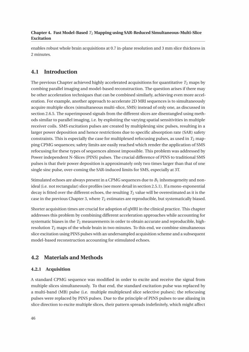
Chapter 4. Fast Model-Based T2 Mapping using SAR-Reduced Simultaneous-Multi-Slice

Excitation

enables robust whole brain acquisitions at 0.7 in-plane resolution and 3 mm slice thickness in

2 minutes.

4.1 Introduction

The previous Chapter achieved highly accelerated acquisitions for quantitative T2 maps by

combing parallel imaging and model-based reconstruction. The question arises if there may

be other acceleration techniques that can be combined similarly, achieving even more accel-

eration. For example, another approach to accelerate 2D MRI sequences is to simultaneously

acquire multiple slices (simultaneous multi-slice, SMS) instead of only one, as discussed in

section 2.6.5. The superimposed signals from the different slices are disentangled using meth-

ods similar to parallel imaging, i.e. by exploiting the varying spatial sensitivities in multiple

receiver coils. SMS excitation pulses are created by multiplexing sinc pulses, resulting in a

larger power deposition and hence restrictions due to specific absorption rate (SAR) safety

constraints. This is especially the case for multiplexed refocusing pulses, as used in T2 map-

ping CPMG sequences; safety limits are easily reached which render the application of SMS

refocusing for these types of sequences almost impossible. This problem was addressed by

Power independent N-Slices (PINS) pulses. The crucial difference of PINS to traditional SMS

pulses is that their power deposition is approximately only two times larger than that of one

single sinc pulse, over-coming the SAR-induced limits for SMS, especially at 3T.

Stimulated echoes are always present in a CPMG sequences due to B1 inhomogeneity and non-

ideal (i.e. not rectangular) slice profiles (see more detail in section 2.5.1). If a mono-exponential

decay is fitted over the different echoes, the resulting T2 value will be overestimated as it is the

case in the previous Chapter 3, where T2 estimates are reproducible, but systematically biased.

Shorter acquisition times are crucial for adoption of qMRI in the clinical practice. This chapter

addresses this problem by combining different acceleration approaches while accounting for

systematic biases in the T2 measurements in order to obtain accurate and reproducible, high-

resolution T2 maps of the whole brain in two minutes. To this end, we combine simultaneous

slice excitation using PINS pulses with an undersampled acquisition scheme and a subsequent

model-based reconstruction accounting for stimulated echoes.

4.2 Materials and Methods

4.2.1 Acquisition

A standard CPMG sequence was modified in order to excite and receive the signal from

multiple slices simultaneously. To that end, the standard excitation pulse was replaced by

a multi-band (MB) pulse (i.e. multiple multiplexed slice selective pulses); the refocusing

pulses were replaced by PINS pulses. Due to the principle of PINS pulses to use aliasing in

slice direction to excite multiple slices, their pattern spreads indefinitely, which might affect

46


Figure 4.1: CPMG sequence diagram with transmit and receive radio-frequency (RF+/-),

slice-, phase- and frequency-encoding gradients (Gs ,Gp ,G f ). Excitation is performed with

a multiband-pulse (blue) and refocusing with PINS pulses (red). Additionally, gradient blips

(green) were added for controlled aliasing of slices along the phase-encoding direction.

areas of the body which are not in the intended FOV. Therefore, initial usage was restricted to

sagittal slices (moving the aliasing into R-L direction). Due to the use of a classical MB pulse

for excitation and PINS pulses only for refocusing, the full flexibility in slice positioning is

ensured while the advantageous SAR characteristics of the PINS pulses are exploited, bearing

in mind that the main SAR deposition in a CPMG acquisition is due to the repeated refocusing.

Lastly, gradient blips were added to the sequence to achieve controlled aliasing along the

phase encoding direction, depending on the slice location as previously described in literature

[40]. The corresponding sequence diagram is shown in Figure 4.1.

Figure 4.2: Example undersampling patterns for 3-fold and 5-fold acceleration. White samples

are skipped during acquisition and black squares indicate sampled k-space points. The red line

marks the k-space centre, thus samples with zero phase encoding.

47


Excitation

Furthermore, the sequence was undersampled using a block-sampling scheme as originally

suggested in [14], i.e. only a segment (block) of k-space is sampled in each echo, whereas

the blocks are shifted along the phase-encoding direction between echoes. Example sam-

pling patterns for 60 phase-encoding steps and acceleration factors of three and five are

sown in Figure 4.2. To ensure an equal distribution of sampling blocks within k-space, the

following heuristic was used: (i) number of phase-encoding lines should be dividable by the

undersampling factor and (ii) the undersampling factor itself should be an odd number.

Prior to the modified CPMG sequence, a short spoiled GRE sequence was acquired (matrix

size 64x64, TE = 1.91 ms, TR = 228 ms, FOV and slice thickness matched with SMS CPMG

sequence), sampling reference lines to train the kernels for the slice-GRAPPA reconstruction.


All numerical simulations, data analysis and visualizations were performed using MATLAB

R2012a (The MathWorks Inc., Natick MA, USA).

Data was reconstructed by subsequently applying a split-slice-GRAPPA and a model-based

iterative algorithm. First, GRAPPA kernels were trained on the external gradient echo data. In

order to have fully sampled k-spaces, data from adjacent echoes were collapsed, i.e. assuming

three-fold acceleration, undersampled data from three consecutive echoes were combined

to form one fully sampled k-space, similar to multi-echo RARE images [24]. The split-slice

GRAPPA algorithm was then applied on the multiple of full k-space datasets as previously

reported [38]. Fully sampled RARE-type k-space datasets for each slice were thus obtained.

Subsequently, the data for each slice was de-collapsed to yield the same block-wise under-

sampled data structure as before, yet now for each slice. An illustration of the reconstruction

pipeline and how data was collapsed is shown in Figure 4.3a.

At this point, the k-space data resembles a single-slice, block-undersampled dataset and

any model-based reconstruction algorithm that can handle this sampling could be used to

estimate T2, e.g. assuming a mono-exponential decay [14] or using a generating function

that accounts for stimulated echoes [17]. However, the conjugate gradient algorithms used

in these methods estimate T2 and M0 directly from k-space data using a single cost function.

To achieve a stable convergence for a robust reconstruction of T2 maps, additional measures

have to be introduced, e.g. a gradient scaling to account for differences in the magnitude of

T2 and M0 values or repeated restarts of the conjugate gradient algorithm. To avoid similar

data-dependent measures, we propose a split algorithm similar to [48]. This algorithm will be

referred to as “Split Algorithm for Fast T2 mapping”, short SAFT.

SAFT, as illustrated in Figure 4.3b, splits the optimization problem in multiple sub-problems

resulting in a three step algorithm: Step A is optimizing the correspondence to the acquired

data (data consistency), step B is optimizing the correspondence to the signal model (model

consistency), and Step C employs spatial regularization for a more robust reconstruction.

48


These steps are repeated iteratively to estimate the free variables of the model (T2, B1 and M0)

and are explained in more detail in the following sections.

Figure 4.3: a.) The application of split-slice GRAPPA on the undersampled k-space data to

separate the signal from different slices. Prior to the application of the kernel, the data sampling

blocks (red, blue and green) from multiple echoes are collapsed to yield full k-space data. b.)

Illustration of the model-based reconstruction that estimates T2, M0 and B1 maps by iteratively

improving data consistency, model consistency and regularization.

Step A: Data Consistency

The data consistency cost term models the imaging process including undersampling, Fourier

transformation and coil combination and is very similar to a typical cg-SENSE reconstruction

with an additional term enforcing the signal model onto the data. The images X at each

echo-time TE is estimated by minimizing the difference to the k-space data Y as follows:

X = argminX

1

2

∑

t∈T E

(

N∑

c=0

∥

∥PF {Sc X (t )}−Yt ,c

∥

∥

22 +α‖X (t )−Xm(t )‖2

2

)

, (4.1)

where S are the complex coil-sensitivities, N the number of coils, F the Fourier transform

operator, and P the sampling mask. The weight α enforces similarity to CPMG images Xm

which are consistent with the signal model, i.e. images synthesised from the latest T2, B1 and

M0 estimates (see step B). Since Xm is calculated in the next step and is yet unknown, the

similarity weight α is set to zero to avoid any model influence in the first iteration.

Step B: Signal Model Consistency

The model consistency cost term uses the current image estimate X from the data consistency

(step A) to obtain the current best fit to the signal model. Theoretically, any signal model

49


Excitation

(e.g. analytical stimulated echo, Bloch simulations, mono-exponential decay etc.) and any

fitting method (e.g. dictionary, log-linear or least-squares) can be used here. In order to use a

numerical signal model, we decided to use the same approach as MR fingerprinting [23, 47],

i.e. a dictionary fitting that matches the data to a model calculated using the extended phase

graph (EPG) [49] methodology. To that end, the EPG algorithm from Weigel et al. [50] was

used to simulate the CPMG signals for a range of T2 values (5 ms, 6 ms, . . . 100 ms, 200 ms . . .

4000 ms), and B1 efficiency factors (0.6, 0.62 . . . 1) and a fixed M0=1. Furthermore, different

B1 depositions due to imperfect slice profiles were accounted for by discretizing both the

excitation and refocusing slice profiles into 65 bins. After simulating each bin, the signals

were summed across the profile and stored in a dictionary together with the respective T2

and B1 used during simulation. An example slice profile for the MB excitation and the PINS

refocusing are shown in Figure 4.4 together with simulated signals. To perform the fitting, a

brute force search was used to find the best match for each voxel in image X with a simulated

signal in the dictionary. The better the signal decay in the voxel matches a dictionary entry, the

greater is the dot-product between the two signal-vectors. Therefore, the dictionary entry with

the highest dot-product is assumed to be the most representative for this voxel. As a result,

the parameters that were used to simulate this entry can be attributed to this voxel. During

the simulation of the dictionary entry, M0 is fixed (M0=1). Therefore, before calculating the

dot-product, the signals need to be normalized to account for variations in M0. Scaling factors

are calculated with ssi m = ‖vsi m‖−12 for the signal in the dictionary entry and sacq =

∥

∥vacq

∥

∥

−1

2

for the acquired signal in the voxel, where vsi m and vacq denote the discrete signal decays

respectively. The equilibrium magnetization is then estimated using these scaling factors

following M0 = ssi m/sacq .

Figure 4.4: (left) Example slice-profiles of the multi-band excitation (cyan) and PINS refocusing

(purple) for 3 mm slice thickness. (right) Signals simulated with the extended phase graph (EPG)

formalism for a CPMG sequence with ∆T E = 10 ms and 16 echoes and tissue properties T2 = 60

ms and T1 = 800 ms with a rectangular slice-profile (green) and the SMS slice profile without

(blue) and with transmit field inhomogeneity (red).

50


The entire process of step B is comparable to maximizing the dot-product between the CPMG

images X and the simulated signals of the EPG sequence depending on T2, M0 and B1:

T2

M0

B1

= arg max

T2,M0,B1

X ·M0EPG (T2,B1) . (4.2)

Step C: Spatial Regularization

In a last step, prior knowledge on the characteristics of the T2 and B1 maps is exploited to

regularize the results obtained in the signal model consistency step (step B). B1 biases manifest

themselves as smooth variations across the FOV. This is imposed on the obtained B1 map by

convoluting it with a 2D Gaussian kernel G:

B ′1 = B1 ∗G(σ). (4.3)

where σ is the standard deviation of the kernel. Furthermore, we assume the T2 map to

be sparse in the Wavelet domain. Subsequent application of a Wavelet transform Ψ, a soft-

threshold T with the strength λ, and the inverse wavelet transform imposes this regularization:

T ′2 =Ψ

−1T (ΨT2,λ) . (4.4)

Subsequently, the regularized parameter maps T ′2,B ′

1 together with M0 (from step B) are used

in the forward EPG signal model to calculate CPMG images for all echo times Xm(t ) based on

the current (T ′2, B ′

1, M0) estimates:

Xm = M0EPG(

T ′2,B ′

1

)

. (4.5)

The intensities of Xm are model consistent, since they were calculated using the numerical

signal model (EPG simulation).

Iterative Loop and Convergence

Subsequently, a new iteration is started feeding the CPMG images Xm , which were calculated

based on the current estimate of T2, B1 and M0 into the data consistency term (equation 4.1)

in step A. Notably, the similarity weighting α is set to a value greater than zero after the first

iteration. The process of alternatively calculating step A, B and C is then repeated until a

maximum number of 15 iterations is reached. For all reconstructions, a manually tuned

Gaussian kernel (σ=3 mm), wavelet soft-threshold (λ=10 ms) and similarity weight (α=1) were

used.

51


Excitation

4.2.3 In Vivo Studies

All measurements and calibrations were performed on a clinical 3T whole-body system (MAG-

NETOM Skyra, Siemens Healthcare GmbH, Erlangen, Germany) with actively shielded mag-

netic field gradient coils using a commercially available 64-channel head/neck coil. Prior to

scanning, informed written consent was obtained from all volunteers.

Data from three healthy volunteers were acquired using the proposed undersampled CPMG-

PINS sequence (Figure 4.1) with a slice acceleration factor of five (i.e. five slices are acquired

simultaneously) and three different undersampling factors: R=1 (i.e. fully sampled), R=3

and R=5. Relevant sequence parameters were: TR=3s, 16 echoes with ∆TE=10 ms, matrix

size 320 x 210, FOV 220 x 192 mm2, 50 slices, 3 mm slice thickness with 0.3 mm slice gap.

The acquisition times for the different combinations of acceleration factors resulted in 10:30

min for 5-fold (5x1) acceleration, 3:30 min for 15-fold (5x3) and 2:06 min for 25-fold (5x5)

acceleration. The measurement of the low-resolution GRE sequence (matrix size 64 x 64,

FOV 220 x 192) required to calculate kernels for the split-slice-GRAPPA reconstruction added

another 14 s acquisition time. To study the reproducibility of the T2 values, the 25-fold (5x5)

accelerated acquisition was repeated without repositioning the volunteer in order to evaluate

the scan-rescan variability of the obtained T2 values in manually drawn regions of interest

(ROI).

For comparison, a fully sampled standard single-slice excitation CPMG sequence was acquired

using the same sequence parameters, except for the number of slices, which had to be set to

ten to keep the same repetition time as in the prototype sequence. The acquisition time for

this 10-slices comparison scan was 10:30 min. In theory, comparable slice coverage would

result in a scan time of 52:30 min (5 x 10:30 min) using the standard sequence. ROIs were

manually drawn in the white matter (WM) of the frontal lobe and the Globus Pallidus (GP) to

compare T2 values.

4.2.4 Phantom Studies

Phantom experiments were performed to quantitatively validate the T2 values estimated

with the proposed method. To that end, a multi-purpose phantom (five compartments with

different concentrations of MnC l2 ·4H2O, Siemens E-38-19-195-K2130) was scanned using

the same protocols as in the in-vivo studies. Additionally, multiple single-echo spin-echo

acquisitions with different TE’s (10 ms, 15 ms, 20 ms, 40 ms, 80 ms, 150 ms) were performed in

order to estimate the ground truth T2 values within the compartments using a non-linear fit.

52

4.3. Results

Figure 4.5: Axial slices from the T2 maps of all volunteers that were reconstructed with the

proposed method and acquired with different methods, left to right: the gold standard single-

slice CPMG, SMS CPMG and undersampled SMS CPMG (R = 3 and R = 5).

4.3 Results

4.3.1 In Vivo Studies

T2 maps from the single-slice CPMG and the SMS CPMG sequences with different acceleration

factors are shown in Figure 4.5. Note that the single-slice CPMG values are considered the gold-

standard measurement. A similar overall T2 value range is observed in the SMS CPMG maps

compared to the gold standard. The maps from the accelerated slice-GRAPPA reconstruction

with and without additional undersampling exhibit non-uniform noise amplification. These

findings are supported by comparing T2 values drawn from the ROIs (see Table 4.1): overall,

mean values of the SMS CPMG measurement are in good agreement; the acquisition of

multiple slices however introduces an increase in standard deviations (SD). As an example,

the T2 values in the WM frontal lobe show a mean value of 65.6 ± 2.1 ms in single-slice CPMG

versus 63.4 ± 4.8 ms in SMS CPMG. A slight additional increase in SD is observed in the

53


Excitation

Standard CPMG

fully sampled

SMS CPMG

5(5x1)-fold

SMS CPMG

15(5x3)-fold

SMS CPMG

25(5x5)-fold White

White Matter Volunteer 1 65.6 ± 2.1 63.4 ± 4.8 62.9 ± 5.4 64.2 ± 5.0

(Frontal Lobe) Volunteer 2 61.7 ± 3.1 61.5 ± 5.2 62.4 ± 5.6 62.0 ± 6.2

Volunteer 3 70.4 ± 2.5 71.3 ± 5.4 69.9 ± 4.0 66.9 ± 4.6

Globus Pallidus Volunteer 1 54.6 ± 4.4 53.1 ± 6.1 52.8 ± 7.7 51.8 ± 7.9

Volunteer 2 46.4 ± 4.0 46.8 ± 6.8 46.9 ± 7.7 45.8 ± 10.5

Volunteer 3 56.6 ± 3.9 57.4 ± 7.1 57.2 ± 8.5 54.9 ± 8.0

Table 4.1: Mean and standard deviation of T2 values (in ms) within regions of interest manually

drawn into the white matter of the frontal lobe and Globus Pallidus, for each subject and T2

sequence.

undersampled SMS acquisitions, while the mean T2 values stay in good agreement with the

gold standard.

The same ROI’s were used to compare T2 values between scan and rescan within one subject

and across subjects. The mean and standard deviation in ROIs of the WM and GP for each

subject between scans are shown in Figure 4.6. The T2 values differ 0.6 ms on average between

scan and rescan and exhibit a low variation between scans (SD = 0.39 ms in WM, 0.43 ms in

GP). The T2 values across all subjects (within a similar age range of 27 ± 2 years) also show a

small standard deviation (2.79 ms in WM, 4.40 in GP).

4.3.2 Phantom Studies

Figure 4.7 shows an agreement plot of the T2 values from the different accelerated acquisitions

with T2 values of the single-slice, single spin-echo acquisition. All acquisitions agree well

with the reference values. However, T2 is slightly overestimated (≈2 ms), especially for the

undersampled acquisition at lower T2 values (< 30 ms). Furthermore, the standard deviations

for low (< 20 ms) and high T2 values (> 140 ms) are larger (≈8 ms versus ≈3 ms), presumably

due to the fact that too little short echo times (for measuring low T2 values) or too little long

echo times (for long T2 values) are sampled with the used echo spacing and number of echoes.

4.3.3 SAR Aspects

The main motivation for the proposed sequence design of using a classical MB excitation and

PINS refocusing pulses was to obtain a CPMG sequence that is able to acquire many slices

(e.g. 50), and echoes (e.g. 16) at a short TR (e.g. 3 s) without exceeding the SAR limitations

at 3T. Pulse simulations were used to calculate the B 21 for every used pulse and showed that

the expected SAR reduction was achieved since the PINS refocusing pulses deposit similar

power (B 21 = 6.3 mT 2) in comparison to the standard single-slice refocusing pulse (B 2

1 = 6.9

mT 2), although it refocuses four more slices. This low power deposition of the PINS pulses

facilitated the use of this sequence design despite the approximately five times higher B 21 of

54

4.4. Discussion

the multi-band excitation (11.1 mT 2) in comparison to the single-slice excitation (B 21 = 2.7

mT 2). With this configuration the SMS CPMG sequence was on average at 60% of the SAR

limit for 50 slices during the in-vivo experiments. Contrary, the single-slice CPMG sequence

reached 40% of the SAR limit, but only for the acquisition of 10 slices.

4.3.4 Computational Requirements

The image reconstruction of one dataset with 50 slices requires approximately 7 hours on an

office computer with 16 GB of RAM and an Intel Core i7-3770K CPU @3.50GHz running a 64bit

Windows 7 operating system.

The algorithm has its peak memory footprint when the split-slice GRAPPA kernel is applied

and highly depends on the matrix size of k-space. In the case of the in-vivo experiments this

corresponds to approximately 5.5 GB (matrix size 320 x 210, 16 echoes, 64 coils, 5 simultaneous

slices). Ironically, due to the collapsing of the undersampled k-space prior to the kernel

application, the footprint is linearly reduced by the undersampling factor R.

4.4 Discussion

We have shown that the proposed multi-band/PINS simultaneous multi-slice sequence design

combined with regular undersampling and an EPG signal model applied with dictionary fitting

yields accurate T2 maps of the whole brain with high resolution in two minutes.

The results show that the employed slice-profile-sensitive EPG simulation takes the major

artifactual effects on the signal into account, notably stimulated echoes originating from

incomplete refocusing of the spins which are inevitable due to B+1 field inhomogeneity and

non-ideal slice profiles. However, the model is still an approximation and does not account

for the detailed micro-structure of human tissue. One main assumption of the model used in

this work is that it models only one compartment, i.e. one single isochronal with a specific

T2 relaxation time per voxel. This is obviously a simplification and will not account for

differently behaving compartments such as intra- and extracellular water compartments.

Furthermore, the model does not take magnetization transfer (MT) between free water protons

and macromolecules into account which may affect the signal. Future work should hence

focus on studying in more detail how these effects bias the T2 estimation. Ideally, the model

should be extended to fully incorporate these effects and additional tissue properties; this

will however decrease the computational stability of the fitting and require either additional

signal encoding or an optimised reconstruction to keep the same acquisition times. It should

be noted, however, that despite these shortcomings, the T2 values measured here are in good

agreement with the gold-standard single-slice single spin-echo acquisition.

When accelerating, both SMS and the additional undersampling result in amplification of

noise, which manifests in increasing standard deviations at higher acceleration factors. Never-

55


Excitation

Figure 4.6: Mean T2 values of scan and rescan for each subject with error bars indicating the

standard deviation. Red are values from the white matter in the frontal lobe and blue from the

Globus Pallidus. The dashed lines indicate the mean across all subjects and the filled area its

standard deviation.

theless, the accuracy of the estimation remains unbiased. Furthermore, despite the increased

standard deviations, T2 values were reproducible in scan-rescan acquisitions and across sub-

jects. This is an important observation since reproducibility is probably even more important

than accuracy in a clinical context; for example, in a multiple sclerosis follow-up measurement,

T2 maps have to be comparable and even small changes might indicate pathology, e.g. an

increased inflammation of the “normal appearing white matter”, something which is very hard

to observe by the naked eye.

The original motivation of using PINS pulses instead of multi-band pulses were the SAR limita-

tions, which especially come into play at 3T: the application of multiple 180◦ RF pulses easily

exceeds the SAR limits, even with conventional single-slice acquisitions. We demonstrated

that the power deposition per slice is lower with the proposed pulse scheme. Such a scheme

may hence enable using spin-echo-based T2 mapping at ultra-high fields, i.e. 7T and beyond.

One major limitation of the proposed method is that the reconstruction algorithm is rather

complex in comparison to a direct Fourier Transform and mono-exponential fitting. This com-

plexity involves multiple regularization parameters (α, λ, σ) and rather long computational

times. The regularization parameters were manually optimized as it is common practice in

56

4.4. Discussion

Figure 4.7: Mean T2 values within five different compartments of a phantom from the different

acquisitions reconstructed with the proposed SAFT algorithm against the reference values

derived from a Spin-Echo sequence. Error bars indicate the standard deviation and the markers

were horizontally jittered to minimize overlaps.

compressed sensing [30]. In future works, these parameters should be automatically adapted,

also depending on image content, and maybe altered in each iteration. The long computa-

tional time of the reconstruction algorithm still prohibits its use in clinical routine. However,

the performance of the current implementation on an office computer can certainly be im-

proved with code optimization, parallelization across slices and hardware acceleration on an

image reconstruction server.

An alternative combination of SMS and model-based reconstruction could be realized by

solving it as a single inverse problem rather than two subsequently applied reconstructions.

To that end, one has to also model the aliasing of the simultaneously acquired slices and their

respective coil sensitivities within the data consistency term (equation 4.1). However, we

avoided this approach since this will further increase the computational costs and we also

assume that combining the reconstruction into a single inverse problem may result in a worse

artifact behaviour and robustness towards model-violations (e.g. blood-flow, inaccurate coil

sensitivities).

57


Excitation

Figure 4.8: Simulated T2 weighted contrasts from all volunteers in comparison to conventional

T2 weighted RARE images. From left to right: single-slice standard CPMG sequence, SMS CPMG

sequence and undersampled SMS CPMG sequence (R = 3 and R = 5) in comparison to the gold

standard RARE image. An alternative

For the integration in a clinical work-flow, it can be beneficial to synthesise conventional

T2-weighted contrasts from the quantitative M0 and T2 maps. That allows providing clinicians

with a regular contrast which is widely used in clinical practice while having the additional

quantitative information. An example of synthesised contrast compared to real TSE acquisi-

tions can be seen in Figure 4.8.

In future work, multi-PINS pulses, a combination of multi-band and PINS pulses [51], should

be explored for quantitative mapping. These pulses may allow reducing the slice thickness

without worsening the slice profile. Furthermore, applying a wave gradient during read-out

[52] could help to further reduce inter-slice leakage in the slice-GRAPPA reconstruction and

should be explored as well.

PINS-SAFT may be used to explore other clinical applications of quantitative T2 mapping in

a standard clinical setting. For example, in abdominal imaging, where a greater amount of

slices could be acquired within a single breath-hold or even during a free-breathing sequence

triggered to acquire multiple slices at end-expiration. However, we only demonstrated a proof

58

4.4. Discussion

of concept here and larger clinical studies are required to further validate the T2 values and

the synthetically generated T2-weighted contrast.

In conclusion, a new sequence design was proposed that enables undersampled SMS CPMG

acquisitions at 3T without exceeding SAR limits. The proposed combination of split-slice

GRAPPA and a model-based reconstruction that accounts for stimulate echoes resulted in

accurate and reproducible T2 values in phantom and in in-vivo experiments of three healthy

volunteers.

59

5 Mitigating the Effect of Magnetiza-

tion Transfer in Magnetic Resonance

FingerprintingThe content of the following Chapter is based on the draft of the article: “Mitigating the Effect

of Magnetization Transfer in Magnetic Resonance Fingerprinting” currently under a major

revision in NeuroImage. The article manuscript was co-authored by Tobias Kober, Tiejun Zhao,

Kai Tobias Block, Florian Knoll, Jean-Philippe Thiran, Gunnar Krueger, Daniel K Sodickson and

Martijn A Cloos. All co-authors contributed to the idea and reviewed the manuscript.

Abstract: Magnetic Resonance Fingerprinting (MRF) is a promising new model-based tech-

nique for rapid quantitative imaging. Like with all model-based techniques, its robustness

and accuracy depends on the validity of the underlying assumptions. In the case of MRF,

it is generally assumed that the spin dynamics can be adequately described by the Bloch

Equations, acting on a single pool of spins. In this work, we show that interactions between the

solid spin pool and the free pool, called magnetization transfer (MT), can affect the MRF signal

train and that the strength of the MT effect is primarily dependent on the radio-frequency

(RF) bandwidth. In vivo experiments are performed to study the impact of MT on the esti-

mated T1 and T2 values. Subsequently, an alternative model, which explicitly incorporates

MT, is proposed to correct the T1 and T2 values and to mitigate their dependence on the RF

bandwidth. The proposed method is tested with phantom and in vivo data, and the results

are compared to literature values. Furthermore, simulations are performed to evaluate the

robustness of the suggested numerical model to violations of the underlying assumptions. In

conclusion, the proposed method allows for more accurate estimation of tissue relaxation in

the presence of macromolecules by introducing a signal model accounting for MT into the

image reconstruction.

5.1 Introduction

Quantitative magnetic resonance (MR) measurements strive to estimate tissue-specific pa-

rameters with minimal experimental bias. Until recently, such methods have mostly fo-

cused on relatively simple spin evolutions for which analytic signal solutions can be derived.

Early techniques developed to measure the relaxation time, for example, relied on a series of

61

Chapter 5. Mitigating the Effect of Magnetization Transfer in Magnetic Resonance

Fingerprinting

inversion-recovery measurements to estimate the longitudinal relaxation time (T1) [53, 54]

and spin-echo measurements to estimate the transverse relaxation time (T2) [43, 55]. Although

such measurements can provide excellent results, they are generally too long to be used in

routine clinical examinations.

For years, the search for faster methods has strived to obtain a balance between acquisition

speed, model simplicity, accuracy, and precision [31, 33, 56]. One of the most widely used

approaches in the last years is the DESPOT1 and DESPOT2 technique [22], combining four (or

more) fast measurements to quantify both T1 and T2. Although DESPOT12 is fast and SNR

efficient, it is also sensitive to experimental imperfections [57, 58] and magnetization transfer

(MT) effects [59].

The impact of MT is especially high in the brain, and it was shown that it has significant

correlations with myelin content and axonal count [60]. Therefore, MT can also be exploited

as a biomarker for neurological disease where the myelination of the brain is altered, e.g.

multiple sclerosis [61]. However, MT effects cannot be described by basic Bloch Equations

used in most fast quantitative MRI techniques. If a comprehensive spin model is applied to

these sequences, a dependency on additional experimental factors, such as the RF bandwidth,

becomes apparent; this dependency can influence the T1 or T2 estimation accuracy. In theory,

all of these effects can be corrected using information from additional measurements, but

each additional scan increases the acquisition time and adds complexity, such as requirement

for co-registration in the case of inter-scan motion. Moreover, each additional parameter

increases the complexity of the analytical form of the signal model.

Recently, a new framework for quantitative MRI, magnetic resonance fingerprinting (MRF),

has been proposed [23]. MRF moves the focus away from monotone sequences that drive the

spins in a steady-state with analytic solutions. Instead, it uses more diverse sequence patterns

that produce continuously changing transient states, paired with a numerical signal model.

The additional degrees of freedom that become available with MRF enable faster imaging and

provide the opportunity to deliberately entangle and encode multiple tissue properties and

experimental conditions within a single measurement. MRF has sparked great interest in the

research community, as it may enable moving from qualitative to quantitative MRI with short

examination times, which would result in an extremely powerful tool for neuroscience and

various clinical applications. The role of MT effects on MRF, however, has not been explored.

In this work, we first demonstrate that the quantification of T1 and T2 values, based on MRF

measurements, may be influenced by MT. Subsequently, we show that this bias can be avoided

by incorporating a more comprehensive numerical signal model in combination with a small

modification to the acquisition scheme.

5.2 Theory

The original MR fingerprinting implementation was modelled based on the basic Bloch Equa-

tions. These equations describe the spin dynamics assuming that the sample in each voxel

62

5.2. Theory

can be characterized by a single T1 and T2 relaxation constant in combination with the proton

density PD (here denoted as M0) that scales the overall magnitude of the signal [23]. This

model accurately describes simple phantoms, such as those containing homogeneous com-

partments with different relaxation times. However, as for most quantitative MRI techniques,

this model is only an approximation for the heterogeneous microscopic structure present

in organic samples. In addition to the fact that each voxel may contain multiple free water

compartments, each containing a different chemical environment with distinct effective T1

and T2 [62, 63], it also does not take into account that there is physical interaction between

hydrogen atoms in free water molecules and those bound to macro-molecules, known as the

MT effect. The partial influence of different T1 and T2 contributions in a single voxel leads to a

reproducible best single-compartment model fit. However, neglecting the dynamic interaction

between free and bound hydrogen atoms may result in a sequence- and protocol-dependent

T1 and T2 bias. Such dependencies are obviously contrary to the idea of quantitative MR and

should thus be minimized. In the next section, we will first outline the common model for

magnetization transfer, as detailed by Henkelman et al. [64], from which we will subsequently

construct a simplified model for use in our fingerprinting signal framework.

5.2.1 Common Model of Magnetization Transfer

The magnetization-transfer effect is typically described with a two-pool model as illustrated

in Figure 5.1a. The two pools represent the net magnetization produced by hydrogen atoms

in free water and those bound to macromolecules. The equilibrium magnetization of these

pools is denoted as M0 f and M0b . The spectral distribution of the pools, a narrow Lorentzian

for free water and a wide super-Lorentzian for the bound pool, depend on the transverse

relaxation times T2 f and T2b , respectively. A detailed description of the line shapes can be

found in Morrison et al. [65]. Due to the differences in line shape, a given RF-pulse affects

each of these pools differently. In particular, the amount of saturation depends on the overlap

between the pulse bandwidth and the spectral distribution of the spin pool, i.e. pulses with

a larger bandwidth will saturate the solid pool more quickly. After (partial) saturation, their

magnetization will return to equilibrium. In principle, each compartment can have a different

characteristic longitudinal relaxation time (T1 f and T1b in Figure 5.1a). In addition, the two

pools exchange magnetization with each other at a fixed rate, described with one constant

for each direction (kb and k f ). For a more detailed description of common MT models, see

Henkelman et al. [64].

5.2.2 Simplified Model

The original fingerprinting methods, which rely on the basic Bloch Equations or the Extended

Phase Graph Formalism [49], consider only the T1 f and T2 f relaxation constant in combi-

nation with the proton density PD and, in some cases, experimental conditions, such as

inhomogeneities in the main magnetic field B0 [23] or variations in the radio-frequency field

B1 [47]. Considering that the proton density PD (here denoted as M0 f ) scales the overall

63


Fingerprinting

magnitude of the signal, these dictionaries are generally limited to three or four dimensions.

Each new model parameter adds an additional dimension to the dictionary – scaling up

the computational efforts necessary to create and use them. Thus, including the additional

five dimensions required for the common MT model leads to impractical, if not infeasible,

computational times for both creating the dictionary with the necessary Bloch simulations and

the reconstruction itself. Furthermore, the typical MRF sequence design may not encode all

these parameters strongly enough to perform reliable dictionary fitting. Therefore, we propose

a simplified MT model that condenses the additional degrees of freedom into one single

parameter MT ∗. Although this parameter no longer reflects a quantitative MT estimation, it is

designed to estimate the MT bias and enables more accurate estimation of free water pool T1 f

and T2 f relaxation times.

The simplified model is realized by discretizing the longitudinal magnetization of the bound

pool into multiple Nb frequency bands (1-100 Hz, 101-200 Hz, ... , 9.901-10.000 Hz). At the

beginning of the simulation, the magnitude of the longitudinal magnetization Mzb , in each

band i , depends on M0b and the bound pool frequency line shape G :

Mzb,i = MobGi . (5.1)

Here, we used the super-Lorentzian line shape with the assumption that T2b=10 µs, based on

the previously reported value range of 9-11 µs [65, 66]. When applying an RF pulse, only a

fraction of the bound pool bands is saturated. The level of saturation depends on the shape,

flip angle, and bandwidth of the pulse. In the numerical simulation, saturation is performed

by multiplying the longitudinal magnetization Mzb with a Gaussian saturation profile W for

each band i . Therefore, the longitudinal magnetization after saturation Mzb+1 is defined as:

Mzb+1,i = Mzb,i Wi . (5.2)

For illustration, two exemplary super-Lorentzian line shapes G and exemplary saturation

profiles W are shown in Figure 5.1c-d. Following each RF pulse, the longitudinal magnetiza-

tion of the bound pool relaxes back towards the equilibrium state. Therefore, a relaxation

operator is applied using the assumption from [66] that T1b = 1s. To this end, the longitudinal

magnetization of the bound pool Mzb within each band i is changed during one TR (denoted

as t) to Mzb+1, following:

Mzb+1,i = Mzb+1,i E1 +M0bGi (1−E1) (5.3)

with E1 = exp(−t/T1).

Furthermore, the exchange of magnetization between the bound and free water pool is simu-

lated by applying an exchange operator, as previously suggested by Gloor et al. [67], which

64

5.2. Theory

mainly depends on the exchange rate parameters k f and kb as well as the equilibrium magne-

tizations M0 f and M0b . One additional consideration that must be taken into account during

application of the exchange operator is the discretization of the slice profile into Nf different

flip-angle bins [23], [47] and the discretization of the bound pool into different frequency

bands. Typically, the slice profile is binned to account for B+1 variations across the slice profile.

Therefore, the transfer of magnetization from the free pool to each band in the bound pool was

calculated based on the sum over the slice profile. Conversely, the transfer of magnetization to

each bin in the slice profile is calculated based on the sum over the line shape of the bound

pool. Thus, the longitudinal magnetization of the bound pool Mzb and the free water pool

Mz f change according to:

Mzb+1,i = Mzb,i exp(−kb t )+(

N f∑

k=0

Mz f ,k

)

M0bGi

(

1−exp(−kb t ))

, (5.4)

Mz f +1,k = Mz f ,k exp(−k f t )+(

Nb∑

i=0

Mzb,i

)

M0 f

(

1−exp(−k f t ))

, (5.5)

The exchange rates are known to be linked through the fractional pool size at equilibrium

(kb = k f /M0b). In the simulation, the equilibrium magnetization of the free pool is fixed to 1 –

note that the PD is ultimately determined by the ratio between the simulated and measured

signal. In the simplified model, the effect of MT can thus be narrowed down to two variables,

the exchange rate k f and the bound pool size M0b , which can be condensed into a single

scaling variable MT ∗ when using literature values and the assumption of having the same

ratio between k f and M0b : k f = MT ∗x40s−1 and M0b = MT ∗x0.13 [68]. A schematic drawing

of the simplified model is shown in Figure 5.1b, where the above-introduced assumptions are

shown in rectangular boxes and the free parameters that need to be estimated in circles.

Notably, besides fixing parameters to literature values and condensing two parameters into

a single MT ∗ parameter, multiple major assumptions were made to simplify the common

MT model. First, the contribution of signal from the transverse magnetization of the bound

pool is neglected during the simulation because the reported T2b values of the bound pool

(≈9-11 µs) are orders of magnitudes shorter than the TR in the sequence (typically 7-11 ms).

Therefore, the transverse magnetization of the bound pool will dephase completely before

the application of the next pulse, or even the readout. Second, following [67], the subsequent

application of saturation, relaxation, and exchange operators assume that these effects can be

decoupled and still yield a good approximation in comparison to solving the differential Bloch

Equations.

65


Fingerprinting

Figure 5.1: (a) Illustration of the common magnetization-transfer model with two pools and

(b) simplification of the model, with boxes indicating fixed and circles indicating varying model

parameters. (c) Line shape of the bound pool for different T2b relaxation parameters and (d)

saturation profiles of pulses with different durations and flip angles in the same frequency

domain.

5.3 Methods

5.3.1 In-Vivo Experiments

To study the impact of MT, we used the prototype sequence design and reconstruction algo-

rithm of PnP-MRF, originally proposed by Cloos et al. [47], as basis and included the simplified,

two-pool MT model in the reconstruction. Four different configurations were evaluated. First,

we compared the measured T1 f and T2 f values obtained when using 2 ms vs. 4 ms long exci-

tation pulses (bandwidth 1500Hz vs. 750Hz) in the standard PnP-MRF sequence to validate

that there is an observable MT effect at all. The third and fourth sequence configurations

incorporated a change of the RF pulse duration at set time intervals in the RF train, as shown

in Figure 5.2. We will refer to the process of changing the RF bandwidth as “MT encoding” in

the rest of the paper since it introduces MT-dependent modulations of the signal, i.e. encodes

MT in the fingerprints. For one dataset, the duration was varied between 1.5 ms and 3 ms, for

the other between 2 ms and 4 ms, corresponding to 2000 Hz / 1000 Hz and 1500 Hz / 750 Hz,

respectively.

All datasets were reconstructed as described by Cloos et al. [47], each using the corresponding

66

5.3. Methods

Figure 5.2: Sequence design used in this study with a train of flip angles and constant TR

according to the PnP-MRF sequence. The pulse duration of MT encoding (red lines) is varied

throughout the sequence.

dictionary with either a one-pool or two-pool model. The dictionary for the first two exper-

iments using constant pulse durations was computed based on the single-pool Extended

Phase Graph Formalism, including an eight-bin slice profile. Only eight bins were used since

increasing the numbers of bins did not show differences in the fingerprints in a separate test

(not shown). The more comprehensive, two-pool Extended Phase Graph Model was used to

create dictionaries for both MT-encoded sequences (for each combination of variable pulse

durations individually) and the standard PnP-MRF sequence (constant pulse duration). For

both models, the transmit field B+1 is a free variable and, thus, an additional dimension in the

dictionary.

All experiments were performed using a whole-body 3-Tesla MRI system (MAGNETOM Skyra

with TimTX TrueShape, Siemens Healthcare, Erlangen, Germany). The built-in birdcage body

coil was used for excitation, and a standard 24-channel phased-array head/neck coil was used

for reception. An axial slice through the brain of four healthy volunteers was imaged using

a matrix size of 160x160, 240mm FOV, 5mm slice thickness, TR of 7ms, and 10 radial spokes

per time point. For three of the volunteers, an additional high-resolution acquisition was

performed (320x320 matrix size, all other parameters remained unchanged).

The study was approved by our institutional review board (IRB). Written informed consent

was obtained prior to the examination.

67


Fingerprinting

5.3.2 In Silico Experiments

Following the sequence parameterization used for the in-vivo experiments, several theoretical

limits of the proposed simplified MT model were evaluated. Since the proposed simplified MT

model assumes fixed values for T1b , T2b and a fixed ratio between M0b and k f , the possible

bias caused by the violation of these assumptions was studied. To that end, fingerprints were

generated using the two-pool model and a range of values for each parameter. The resulting

fingerprints were then matched with the dictionary constructed using the fixed literature

values. The resulting estimates of T1 and T2 were subsequently compared to the original

values used to generate these fingerprints.

5.3.3 In Vitro Experiments

We assume that the bias observed in biological samples when changing the RF bandwidth

originates from MT. There-fore, there should not be any bandwidth dependency when imaging

a manganese chloride phantom. Furthermore, the acquisition with MT encoding and using a

two-pool model should result in the same values as the gold standard and not show any MT

bias, i.e. MT ∗=0. To test this hypothesis, the same experiment as in vivo was performed on

an in-house-built manganese chloride-doped phantom with seven compartments. The T1

and T2 values from the different pulse durations and spin models were compared to the gold-

standard values estimated with multiple single-slice single spin-echo and inversion-recovery

acquisitions (TR = 6.5 s, 192 x 192 matrix, 192 mm x 192 mm FOV, TI = 25, 50, 100, 200, 400,

800, 1600, 3200, 6400 ms, TE = 12, 18, 24, 36, 48, 72, 96, 144, 192, 288, 384 ms).

5.4 Results

5.4.1 In Vivo Experiments

T1 and T2 maps obtained with acquisitions using constant pulse durations of 2 ms and 4 ms

show a clear difference (Figure 5.3a). Although the T1 maps appear almost identical, the T2

values obtained with the shorter pulse duration are lower. However, both seem to overestimate

T1 systematically compared to literature values [69] (T1 ≈1.1 s versus T1 ≈0.8 s) T2 maps

acquired with both pulse durations underestimate the T2 of white matter when compared to

literature values [69] (T2 = 40 ms versus T2 = ≈60 ms).

Figure 5.3b shows the T1 f , T2 f and MT ∗ maps of the same subject obtained from the data

acquired using the sequence with MT encoding and a two-pool model. Now, both the T1 f

and T2 f maps show values in the same range as reported in literature and appear less depen-

dent on the pulse duration. The MT ∗ bias maps show a difference between the two pulse

durations – MT ∗ values are generally higher for the 4/2ms compared to the 3/1.5ms pulse

durations. The MT ∗ bias maps show the strongest effect in white matter, a weaker effect in

grey matter, and no MT bias in cerebrospinal fluid, which correlates with the myelination of a

68

5.4. Results

Figure 5.3: (a) Representative example of one subject showing quantitative T1 and T2 maps

reconstructed from acquisitions with different RF pulse durations and a dictionary that does not

account for magnetization transfer effects and (b) the same slice acquired with varying pulse

duration (MT encoding) reconstructed using individual dictionaries that take into account the

MT ∗ bias.

healthy brain. Furthermore, all maps experience more noise in comparison to the single-pool

model, presumably due to the additional dimension in the dictionary. These results could be

reproduced in all subjects for both the lower- and higher-resolution settings. Quantitative

maps from all subjects obtained with MT encoding and the two-pool model are shown in

Figure 5.4a. Notably, a strong MT bias is consistently observable in the corpus callosum, which

could be linked to the higher fibre density and, thus, higher myelin content - i.e. increased

presence of macro molecules - in these regions. The quantitative maps acquired at higher

resolution, as example shown for one subject in Figure 5.4b, exhibit lower SNR, but T1 and T2

values are comparable to the low-resolution acquisitions Figure 5.5a-b show the mean T1 and

T2 values from all subjects within the occipital white matter in a box plot. Notably, T2 values

between different pulse duration settings considering only a single pool show a significant

difference (p = 0.03), whereas using MT encoding and a two-pool model, values do not show a

significant difference any more. Furthermore, the acquisitions using the two-pool model and

MT-encoding yield T1 and T2 values closer to literature values.

69


Fingerprinting

Figure 5.4: (a) Quantitative T1, T2 and MT ∗ maps obtained with MT-encoding (3/1.5 ms pulse

durations) and a two-pool model. (b) Example quantitative maps acquired with the same

protocol parameters but in higher resolution.

5.4.2 In Silico Experiments

Fingerprints obtained from the dictionaries simulated with and without taking into account

MT are compared in Figure 5.6. The two simulated tissues “A” (no MT) and “B” (with MT)

show different signal evolutions (Figure 5.6a). In particular, the Steady-State Free-Precession

(SSFP) section of the sequence results in lower signal intensity due to the loss of longitudinal

magnetization transferred to the bound pool. This signal drop is similar to a fingerprint with

shorter T2, longer T1, and no MT effect and creates thus ambiguous dictionary entries (Figure

5.6b). It may explain the overestimation of T1 and underestimation of T2 observed in the in

vivo experiments (Figure 5.3a). Even if the MT effect is modelled, the dictionary still contains

fingerprints that cannot be mapped uniquely to one combination of T1 and T2 since very

similar signal evolutions are simulated using a different set of tissue properties (Figure 5.6b).

Varying the pulse duration in the RF train (MT encoding) reduces this ambiguity, allowing MT

effects to be distinguished from T2 (Figure 5.6c).

Simulated fingerprints that deliberately violate the assumptions in the simplified MT model

were matched to the proposed dictionary that was built assuming fixed values for T1b , T2b ,

M0b , and k f . The T1 f , T2 f , and MT ∗ observed in these experiments are plotted in Figure 5.7.

In general, the model appears to be relatively insensitive to such variations. It can be observed

that deviations from the proposed assumptions may lead to variations in the quantification of

MT ∗, but do not affect the estimation of the relaxation parameters that characterize the free

70

5.4. Results

Figure 5.5: The estimated mean relaxation values (c) T2 and (d) T1, measured in occipital white

matter of all subjects (N = 4). Wilcoxon rank-sum tests show only in the single-pool T2 values

a significant difference (p = 0.03, see also asterisk) between pulse durations. Horizontal lines

indicate expected literature values.

water pool. In more detail, the MT model assumes that T1b equals T1 f , and it can be seen that

the quantification is fairly robust to violations of this assumption. However, a small linear bias

of T1 f can be observed when the T1b of the bound pool is varied in a range of 200 ms around

the correct assumption. Furthermore, T1 f and T2 f are very stable when T2b is varied, meaning

that the estimation is rather independent from the line shape of the bound pool. Stronger

effects can be seen when the bound pool size (as a fraction of the free-water pool size) or

the exchange rate is varied. A proportional bias in the quantification of MT can be observed,

which compensates for the violation of the assumption and, thus, still yields accurate T1 f and

T2 f estimates. In conclusion, the simulations demonstrate that the assumptions mainly affect

the quantification of the MT pool and allow for more accurate estimation of the free-water

pool relaxation if MT effects are present.

5.4.3 In Vitro Experiments

The quantitative T1 and T2 values obtained from the phantom experiments in comparison

to the gold-standard methods for both the single- and two-pool model are shown in Figure

5.8. Estimations from the single-pool model, two-pool model, and different pulse durations

result in similar T1 and T2 values that showed no significant difference to the gold-standard

methods. However, values from the two-pool model showed higher standard deviation, which

presumably originates from fitting an additional parameter (MT ∗). Furthermore, the results

71


Fingerprinting

Figure 5.6: Comparison of different fingerprints generated using the proposed model to demon-

strate the effect of MT. (a) Comparison of finger-prints with identical relaxation (T1=800 ms,

T2=60 ms) but with (grey) and without (red) MT. (b) Comparison of the same fingerprint with

MT effect (grey) to a fingerprint without MT but different relaxation (green, T1=1100 ms, T2=40

ms), demonstrating the ambiguity of the resulting signal evolutions. (c) Demonstration of

the same fingerprint (T1=800 ms, T2=60 ms, MT ∗=1) but with the difference when using MT

encoding (orange) in comparison to constant pulse duration (grey).

appear to be unaffected by changing the pulse duration, and the two-pool model only shows

noise in the MT ∗ map, which indicates that the previously observed bias is a biological effect

that is not present in a typical phantom, further supporting the theory that the bias originates

from MT.

5.5 Discussion

Our results provide evidence of the possible influence of MT when using MRF to quantify T1

and T2 values in the brain. Therefore, we propose a signal model that encompasses MT bias to

eliminate these effects from MRF quantification measurements.

When using the PnP-MRF sequence, the observed T2 value of white matter is dependent on the

RF pulse duration and, in general, appears to underestimate T2 and overestimate T1 compared

to literature values. Notably, this bias is not present in in-vitro experiments, which indicates

that it originates from the biochemical complexity of the in-vivo environment that cannot be

captured using a phantom containing uniform liquid samples. These observations are in line

with the predictions from the theoretical model. Shorter pulse duration, i.e. broader pulse

bandwidth, saturates the bound pool more rapidly, which results in a loss of magnetization in

the free-water pool due to magnetization transfer.

The introduced simplified two-pool MT model reflects the micro-structure within the voxel

better, thus resulting in more accurate T1 and T2 estimations. However, this model was highly

simplified by including many assumptions, e.g. by fixing model parameters to literature

72

5.5. Discussion

Figure 5.7: Estimated quantitative T1 f , T2 f , and MT ∗ values (black) compared to the ground

truth used in the simulation of the fingerprint (blue dotted line) in dependency of violating

the assumption of fixed T1b , T2b , M0b , and k f . The parameter combination where all the

assumptions are met is marked with a red dotted line.

values. Furthermore, it is assumed that brain tissue has not more than two pools and multiple

compartments, and physiological effects such as diffusion and perfusion are neglected. The

proposed model is thus still an approximation of the actual micro-structure and biochemical

environment. Ideally, the simulation of the fingerprints would use a complete model of tissue

micro-structure. Apart from the computational time needed to compute such a dictionary, the

fitting robustness would likely suffer as many of the more subtle effects are poorly encoded

within the fingerprint. For example, although MT is better reflected in the fingerprint by

varying the pulse duration during the sequence, the difference is still small and, thus, yields

relatively noisy MT ∗ bias maps as seen in our experiments. In a more general scope, one

open research question is thus how much detail is required to model tissue micro-structure

and how well these effects can be encoded within a fingerprint. In the opinion of the authors,

the first and foremost criterion is the reproducibility of the tissue property estimation, which

should be independent from sequence parameters. With the proposed two-pool model, the

applied PnP-MRF sequence has become less dependent on the pulse duration and, therefore,

provides improved reproducibility. Although the two-pool model relies on certain assumptions

regarding the measured sample, the estimation error caused by possible violations of these

73


Fingerprinting

Figure 5.8: Exemplary quantitative maps from a phantom obtained with MT encoding and a

two-pool model (3 ms and 1.5 ms varying pulse duration). The mean and standard deviation of

the compartments from the different methods, constant pulse duration (PNP 2 ms and 4 ms)

and MT encoding (MT 4 ms and 3 ms), are plotted against gold-standard values obtained from

single spin-echo and inversion-recovery sequences.

assumptions will mainly be reflected in the MT ∗ and not in the estimation of T1 and T2,

as it was demonstrated in the performed simulations. As a consequence, the signal model

proposed here does not allow for quantification of MT.

Alternatively, one could also attempt to minimize MT bias effects by desensitizing the se-

quence. For example, a longer TR will allow the bound pool to recover more longitudinal

magnetization between excitation pulses but leads to less efficient acquisition times. Further-

more, longer pulse durations with a narrower saturation profile in the frequency domain could

be considered to minimize the effect on the bound pool. However, longer pulse duration will

also require longer TR, leading again to a less efficient acquisition. The sequence design, i.e.

flip angles and spoilers, has an impact on the MT effect as well. Here, the experiments used

the PnP-MRF sequence design. Other sequence designs or reconstruction methods may be

less sensitive to MT and may result in a different bias, in terms of effect size and direction

(overestimation vs. underestimation). This should be further investigated.

Future work should also focus on the phantom design to better reflect the micro-structure

of tissue and to incorporate multiple pools or compartments. The performed phantom

experiments did not show any dependency on pulse duration whereas the in-vivo experiments

did. Therefore, quantitative validation of the MT effect is difficult, as standardized phantoms

to measure the impact are not available.

For simplicity, all experiments were performed using a single-slice acquisition. The acquisition

of multiple slices, interleaved or sequential, will introduce further saturation of the bound

pool that needs to be accounted for in the spin history: the on-resonant pulses from other

slices cause off-resonance saturation of the bound pool elsewhere, depending on the relative

slice distance and used slice-selection gradient [70]. The model proposed here can be easily

74

5.5. Discussion

extended to interleaved multi-slice acquisition by applying additional shifted saturation

profiles, as shown in Figure 5.2, according to the slice order. This modification will, however,

restrict the slice parameters of the acquisition protocol to the trained dictionary.

In general, the MT effect and its impact on the accuracy of the relaxation estimation should

be further studied in the context of MR fingerprinting. The model proposed here should

be further investigated to improve SNR efficiency and to explore the possibility of a more

complete quantification of the MT parameters, e.g. independently fitting the exchange rate

and fractional pool size. Quantitative MT would be of high interest for application in the brain,

as the myelin sheaths surrounding the axons mainly consist of macromolecules. Therefore, it

may potentially be applicable as an early marker for demyelination.

In conclusion, it was demonstrated that the MRF relaxation parameter estimation can be

influenced by the RF pulse duration. Based on the hypothesis that these effects are caused

by MT, the numerical model used to simulate the fingerprints was extended to a simplified

two-pool model. Additionally, the original PnP-MRF sequence design was modified to apply

different pulse durations in the RF train to better differentiate between MT and T2 effects in

the fingerprint. The proposed modification provided parametric maps that are shown to be

less dependent on the pulse duration. The obtained quantitative values correspond well with

those reported in the literature.

75

6 True constructive interference in the

steady state

The content of the following Chapter is based on the postprint version of the article: “True con-

structive interference in the steady state (trueCISS)” published in Magnetic Resonance Imaging

(DOI: 10.1002/mrm.26836). The article was co-authored by Damien Nguyen, Jean-Philippe

Thiran, Gunnar Krueger, Tobias Kober and Oliver Bieri. Damien Nguyen contributed equally to

this work and the remaining co-authors contributed to the idea and reviewed the manuscript.

Abstract: The purpose of this chapter is to introduce a novel time-efficient method, termed

true constructive interference in the steady state (trueCISS), that not only solves the problem

of banding artifacts for balanced steady-state free precession (bSSFP) but also provides its

genuine, that is, true, on-resonant signal. After a compressed sensing reconstruction from a

set of highly under-sampled phase-cycled bSSFP scans, the local off-resonance, relaxation

time ratio, and equilibrium magnetization are voxel-wise estimated using a dictionary-based

fitting routine. Subsequently, on-resonant bSSFP images are generated using the previously

estimated parameters. Due to the high undersampling factors used, the acquisition time is

not prolonged with respect to a standard CISS acquisition. From a set of 16 phase-cycled SSFP

scans in combination with an eightfold undersampling, both phantom and in vivo whole-brain

experiments demonstrate that banding successfully can be removed. Additionally, trueCISS

allows the derivation of synthetic bSSFP images with arbitrary flip angles, which enables image

contrasts that may not be possible to acquire in practice due to safety constraints. TrueCISS

offers banding-free bSSFP images with on-resonant signal intensity and without requiring

additional acquisition time compared to conventional methods.

6.1 Introduction

In the last decades, the use of steady-state free precession (SSFP) sequences rapidly has in-

creased. Among the different variants first introduced by Carr in 1958 for NMR spectroscopy

[71], balanced SSFP (bSSFP) in particular offers the highest signal-to-noise ratio (SNR) per

unit of time among all MRI sequences [72]. However, bSSFP imaging is prone to field inhomo-

geneities [71, 73] that may lead to signal voids; these appear as dark bands in the image and

77

Chapter 6. True constructive interference in the steady state

thus frequently are referred to as banding artifacts.

Commonly, banding is addressed by a series of multiple bSSFP acquisitions with different radio

frequency (RF) phase-cycling schemes, in combination with a suitable reconstruction method,

such as maximum-intensity projection [73], complex sum [74], sum of squares and magnitude

sum [75], or other [76]. The most common approach, termed constructive interference in

the steady state (CISS), acquires only two phase cycles and combines them with a maximum-

intensity projection, offering a good trade-off between acquisition time and banding artifact

reduction. A major drawback of these image-based combinations is that the derived pixel

intensity no longer reflects the genuine, that is, on-resonant bSSFP signal magnitude typically

presumed for quantification techniques based on bSSFP sequences. For low flip angle bSSFP

acquisitions, these methods tend to modify the intrinsic bSSFP signal (see Figure 6.1c–d),

which can impede the radiological assessment because clinicians usually are more familiar

with the on-resonant, that is, genuine, bSSFP contrasts.

An introductory example of this behaviour is presented in Figure 6.1, showing the signal

behaviour and contrast difference (to the on-resonant signal) for various multiple acquisition

techniques based on the bSSFP magnetization derived with the Freeman-Hill formula [77]

(T1/T2 = 870/70 ms, repetition time (TR) = 5 ms and off-resonances between 0◦ and 360◦)

for a flip angle of 15◦ (Figure 6.1a,c) and for a flip angle of 50◦ (Figure 6.1b,d). Generally, the

combined signal and thus the contrast, as generated with the various reconstruction methods,

deviates from the genuine bSSFP signal properties and strongly depends on the flip angle as

well as on the tissue properties. Typically, the prominent T1/T2 image contrast, as commonly

associated with bSSFP, only can be achieved over the complete frequency spectrum in the limit

of a 90◦ flip angle [77]. Furthermore, most of the multiple-acquisition combination techniques

assume that the steady-state signal resembles a plateau within the passband region, that is,

for off-resonances within ±1/(3 TR) for phase-cycled bSSFP, which only is true in the high

flip angle regime. This may pose considerable problems due to specific absorption rate (SAR)

limitations; especially at higher field strengths.

Consequently, it is much more advantageous to use parameter estimation techniques to

derive bSSFP artifact free images from a signal model coupled with an optimization algorithm

[78, 79, 80, 81]. To the best of our knowledge, the most recent work was reported by Björk et al.

[79], in which the Freeman-Hill formula [77] was fitted onto four phase-cycled bSSFP images

using a linearised signal model in combination with linear least-square fitting followed by a

Gauss-Newton non-linear search (LORE-GN).

Generally, parameter estimation techniques require multiple phase-cycled acquisitions to

provide a well-conditioned framework for the fitting procedure. Obviously, this leads to longer

acquisition times compared to a conventional CISS acquisition requiring only two phase

cycles. In this regard, the acceleration of exhaustive data scans using compressed sensing

techniques has become more and more practicable, overall providing high acceleration factors

[30] especially for applications with additional dimensions such as the time domain in car-

78

6.1. Introduction

Figure 6.1: MIP CSum and MSum reconstruction of 16 phase-cycled complex bSSFP profiles

for T1/T2 = 870/70 ms, repetition time=5 ms, for a flip angle of 15◦ (a) and for a flip angle of 50◦

(b). For completeness, a single bSSFP frequency response profile also is shown, indicating the

on-resonant signal amplitude (X). Relative deviation between the on-resonant bSSFP signal

amplitude and the average combined signal intensity for the various methods for a low flip

angle 15◦ (c) and a high flip angle (d). Note how the contrast between tissues is more dependent

on their relaxation time properties in the low flip angle regime. bSSFP, balanced steady-state free

precession; CSum, complex sum; MIP, maximum intensity projection; MSum, magnitude sum;

T1, longitudinal relaxation time; T2, transverse relaxation time; TR, repetition time; on-res,

on-resonant;comb, combined.

diovascular imaging [82]. The acquisition of multiple phase cycles within the CISS sequence

reflects such an additional dimension with redundant information, allowing high acceleration

factors, as already demonstrated by Cukur et al. [83] and Ilicak et al. [84].

In this article, we propose to use a compressed sensing reconstruction in combination with a

dictionary-based parameter estimation technique to retrieve the genuine bSSFP signal (i.e.,

independent from a multiple-acquisition combination technique and used flip angle) from a

set of highly undersampled bSSFP scans with different phase-cycling schemes. The estimated

parameters are then used to reconstruct artifact free images with a pixel intensity that reflects

the true, on-resonant, bSSFP signal amplitude. Due to the high undersampling, this results

in scan times comparable to conventional CISS imaging. In addition, because all relevant

parameters (i.e., M0 and T1/T2) are known, synthetic bSSFP contrast images can be derived

from these data, which are not directly measurable in practice.

79


Figure 6.2: Diagram of a true constructive interference in the steady state acquisition in which

each blue block represents an undersampled 3D bSSFP acquisition with different RF phase-

cycling scheme (RF phase increment). Initially, some dummy TRs (green block) are played out to

allow transition into steady state. In between the bSSFP acquisitions, a fixed number of dummy

TRs (red blocks) are played out with linearly increasing RF phase increments (from φ j to φ j+1)

to mitigate transient effects (a). Exemplary k-space sampling pattern for a scan with a phase-

encoding matrix size of 320x320. White pixels indicate sampled k-space locations, whereas

black pixels show ignored k-space points (b). bSSFP, balanced steady-state free precession; RF,

radiofrequency; TR, repetition time.

6.2 Methods

6.2.1 Acquisition

A conventional bSSFP sequence was modified to acquire within a single scan a set of N

acquisitions with constant but distinct RF phase increments (φi ). Throughout this work, we

only consider the simplest scheme of equidistantly distributed RF phase increments:

φi =2π

N

(

j −1)

, j = 1,2, ..., N . (6.1)

A schematic representation of the acquisition scheme can be found in Figure 6.2a.

To shorten the overall scan time, a highly undersampled pseudo-random phase-encoding

scheme, based on a variable-density Poisson disk distribution [85][86, 87, 88], was imple-

mented to generate a different incoherent sampling pattern for each phase cycle. Additionally,

elliptical scanning, that is, skipping of k-space samples at the edges of k-space [88]; and partial

Fourier, that is, omitting parts of k-space by allowing the compressed sensing algorithm to

intrinsically exploit its complex conjugate symmetry (see chapter 13.7 in [13]), are applied to

further reduce scan time. A fully sampled reference region in the centre of k-space is acquired

for every phase-cycled scan to estimate the coil sensitivities used during reconstruction [45].

An exemplary sampling pattern for a single acquisition is shown in Figure 6.2b.

80

6.2. Methods


We consider a train of RF pulses with a constant flip angle, α, and a constant RF phase

increment, φ, in combination with balanced gradient moments. As commonly done, finite RF

pulse effects as well as magnetization transfer (MT) and diffusion effects are neglected. In the

limit of a TR much smaller than the transverse (T2) and longitudinal (T1) relaxation times, the

complex bSSFP signal is approximatively given by (see also ref [89]),

M+(α,φ j ,Φ,Λ) ≈ M0

2∣

∣cos(

Φ−φ j

)∣

∣sinα

1+cosα+2cos(

Φ−φ j

)

+(

4Λ−2cos(

Φ−φ j

)

sin2(

α2

)) (6.2)

In Equation 6.2 M0 denotes the equilibrium magnetization;Λ≡ T1/T2 refers to the relaxation

time ratio; φ refers to the RF pulse phase increment (see also Equation 6.1); and Φ refers to

the local phase offset due to field inhomogeneities. TrueCISS images are reconstructed as

outlined below. In short,

1. A compressed sensing reconstruction is used to recover all missing samples from the

incoherent undersampled acquisition scheme. This results in a series of fully sampled

bSSFP images featuring different RF phase increments φ j .

2. From the signal model (see also Equation 6.2), the three parameters (M0, Λ, and Φ) are

estimated using a dictionary-based fitting algorithm.

3. An on-resonant bSSFP signal image, termed true-CISS, is derived from the parameter

maps.

The compressed sensing reconstruction of the undersampled bSSFP data combines a Fourier

transformation (F ) across the φ-dimension and a wavelet transformation (Ψ) in the spatial

domain [30, 31, 90] as sparse regularization. The first of the sparsifying transformations relies

on the inherent periodic nature of the bSSFP signal along the phase-cycle dimension. Because

of that property, the bSSFP profile can be expressed as a Fourier series [91] with rapidly

decaying Fourier coefficient amplitudes, thus providing a sparse representation. This result

can also be derived rigorously using the Fourier representation of the SSFP signal, also known

as SSFP configuration theory [92]. The following cost function was used for the optimization

problem:

L (Yc ,λ) =1

2

∑

c

∥

∥PFx y {Cc X }−Yc

∥

∥

2

2+λ

∣

∣Ψx y

{

Fφ {X }}∣

∣

1(6.3)

where the first term ensures consistency between measured and estimated data, and the

second term enforces sparsity. In Equation 6.3, X refers to the estimated fully sampled bSSFP

image series, Cc to the complex coil sensitivities, Yc to the measured under-sampled k-space

81


data, P to the sampling pattern represented as a binary mask, and λ is a regularization pa-

rameter. The cost function is minimized using the split algorithm proposed in [48], which

provides better conditioning of the optimization problem and thus results in faster conver-

gence as compared to conventional techniques. Calculation of the complex coil sensitivities

was performed in two steps: the first order SSFP echo image was estimated using a Fourier

analysis of the fully sampled k-space centres [93], then the coil sensitivities were computed

using an eigenvalue-based estimation [45] on the previously obtained image.

After the compressed-sensing reconstruction, a dictionary based algorithm is used to yield

voxel-wise estimates for M0, Λ, and Φ from Equation 6.2 because Equation 6.2 has multi-

ple local minima and is not differentiable at φ−Φ ={

12π, 3

2π}

. In contrast to conventional

optimization algorithms such as gradient descent methods, dictionary-based fitting only

requires knowledge of the forward signal model. To that end, a dictionary of signals with

Λ = {1,1.1,1.2, ...,30} and Φ ={

0◦,5◦,10◦, ...,355◦}

is generated from Equation 6.2 for M0 = 1

and the actual imaging parameters that were used to acquire the data (i.e., φ j and α). This

allows comparison of the acquired signal in each voxel to the simulated signals in the dictio-

nary using the squared norm (L2-norm) of the difference as a distance metric. The dictionary

entry with the smallest distance to the measured data is considered the best least-squares

approximation of the acquired signal. Its corresponding Λ and Φ values are then attributed

to the voxel. Because M0 is fixed during the training of the dictionary, the simulated and

acquired signals need to be normalized to account for variations in M0 before the comparison.

To that end, scaling factors are calculated with ssi m = ‖Msi m‖−12 for the simulated signal in

the dictionary and sacq =∥

∥Macq

∥

∥

−1

2for the actual acquired signal, in which Msi m and Macq

denote the discrete signals, respectively. The equilibrium magnetization is then estimated

using these scaling factors with M0 = ssi m/sacq .

Finally, genuine on-resonant bSSFP images, termed true constructive interference in the

steady state (trueCISS), are reconstructed from Equation 6.2 in the limit of (φ−Φ) → 0 in

combination with the estimated M0 and Λ parameter maps. Moreover, synthetic image

contrasts, such as images featuring a different flip angle than the measured one, can be

derived. It also is possible to adjust the flip angle independently for each voxel to locally

maximize the bSSFP signal, termed maxCISS, using [13]:

Mmax |Θ=Θopt≈

1

2M0Λ

−1/2 wher e Θopt ≈ cos−1

(

Λ−1

Λ+1

)

(6.4)

6.2.3 Simulations and Imaging

All numerical simulations, data analysis, and visualizations were performed using MatLab

8.5 (MathWorks, Natick MA). Measurements and calibrations were performed on a clinical 3T

whole-body system (Magnetom Prisma, Siemens, Erlangen, Germany) with actively shielded

magnetic field gradient coils using a commercially available 20-channel head coil. Prior to

scanning, informed written consent was obtained from each volunteer taking part in this

82

6.2. Methods

Figure 6.3: A simulated complex bSSFP profile with Λ = 10.4 (continuous line, top) with black

indicating the magnitude, blue real- and red imaginary-values and circles the sampled phase-

cycles. Its discretized signal was Fourier-transformed into configuration space (3b, green). The

configuration space has six zero coefficients (37.5%) after applying a low soft-threshold of 6 (3b,

purple). The inverse Fourier transform of the signal after applying the threshold diverges from

the original (3c, circles) causing an overestimation in the dictionary fitting (Λ∗= 11.6). (c) Bias

of Λ and (d) amount of zero coefficients for all combinations of Λ and soft-thresholds.

study.

Similar to every other compressed sensing regularization, the zeroing of coefficients in the

sparse domain can introduce undesirable reconstruction artifacts that subsequently could

bias the estimation of Λ. To study the impact of the regularization, a set of complex bSSFP

profiles were simulated, with Λ ranging from 1 to 20; Φ = 180◦ and M0 = 1. To deliberately

introduce regularization artifacts, all the profiles were Fourier-transformed into configuration

space, and a range of soft thresholds (1–8) were applied to achieve zero coefficients, that is,

sparsity. Subsequently, the signal was inverse Fourier-transformed back to a bSSFP profile and

compared to the simulated ground truth. Subsequently, the previously described dictionary

fitting was performed on the obtained profiles to evaluate the impact of the introduced

regularization artifacts on the estimation of Λ.

83


Dictionary-based fitting algorithms became more popular in recent years and proved to be

powerful tools, for example, in MR fingerprinting applications [23]. Applying it to a bSSFP

sequence only requires a simple adaption of the method. However, the sequence design

and signal properties are different and the dictionary fitting may behave in another manner,

requiring a thorough analysis to avoid systematic biases and ensure accuracy. To that end,

an additional experiment was performed, simulating bSSFP profiles with different relaxation

time ratios Λ (1-30) for a fixed flip angle (15◦) and fixed local phase offset (Φ= 180◦) in the

presence of white Gaussian noise at different SNR levels (5–100). The dictionary fitting was

then used to estimate the relaxation time ratio, and its deviation from the known truth was

calculated. This was repeated 128 times to calculate two fitting quality measures: the mean

error and the standard deviation (SD) of the error. A similar experiment was then performed

using a range of local phase offsets (0−360◦) and a fixed relaxation time ratio (Λ = 10).

Phantom imaging was performed on a manganese doped spherical phantom composed of

0.125 mM MnC l2 dissolved in water (with T1/T2 ratio of 870 ms/70 ms ≈ 12, similar to human

tissues, measured by gold standard T1 and T2 relaxation methods) and about 14 cm in diameter.

TrueCISS imaging was performed with 16 phase cycles using an eight fold undersampled k-

space in combination with a TR/echo time (TE) of 4.48 ms/2.24 ms, a flip angle a of 15◦, a

resolution of 1x1x1mm3 (192x192x192 matrix size), a bandwidth of 501 Hz/px, and RF phase

increments φ j according to Equation 6.1, yielding an overall scan time of 5:56 minutes. During

the acquisition, a linear frequency offset gradient was applied over the whole field of view to

induce multiple banding artifacts within the image. A reference CISS image was acquired with

the same resolution, bandwidth, and flip angle using an unmodified product sequence with a

TR/TE of 7.13 ms/3.31 ms, yielding a comparable total acquisition time of 5:31 minutes.

One in vivo 3D human whole-brain trueCISS dataset was acquired using the same prototype

sequence, with 16 phase cycles and eight fold undersampling in combination with a TR/TE

of 6.36 ms/3.18 ms, α = 15◦, 1x1xmm3 resolution (256x256x176 matrix size), bandwidth 250

Hz/px, and RF phase increments φ j following Equation 6.1, resulting in a total scan time of

about 10:15 minutes. For comparison, a 3D CISS image dataset also was acquired with the

same resolution but having a TR/TE of 7.87 ms/3.59 ms, α = 50◦, and bandwidth 337 Hz/

px, completed within 9:04 min. Contrary to the phantom experiment, different sequence

parameters were used for the CISS acquisition because parameters as used for trueCISS would

have led to significant banding residuals and would not be used in clinical routine.

6.3 Results

To demonstrate the effects of regularization artifacts, the 16 phase-cycling samples of an

exemplary simulated complex bSSFP profile (Λ = 10.4) are shown in Figure 6.3a. Its shape in

the configuration space is shown in Figure 6.3b (green). After a moderate soft threshold (=6)

was applied (Figure 6.3b, purple), 37.5% of the coefficients in the configuration space are zero,

indicating that the Fourier transform achieves a sufficient sparsity. The regularization artifacts

84

6.3. Results

Figure 6.4: (a) Mean error of Λ depending on the SNR with Φ = 180◦ and (c) the standard

deviation of the Λ error. (b) Mean error of Φ depending on the SNR with Λ = 10 and (c) the

standard deviation of the Φ error.

induced by the soft threshold only have a small impact on the shape of the bSSFP profile

(Figure 6.3c, circles) and lead to a slight overestimation (Λ∗ = 11.6). The obtained sparsity and

introduced error in Λ for the simulated range of Λ and soft thresholds are shown in Figure

6.3d,e. To summarize these results, with higher Λ, more zero coefficients can be achieved

after Fourier transformation and soft-thresholding due to its higher sparsity. However, the

dictionary fitting overestimates Λ with stronger regularization artifacts, especially when Λ is

high.

The mean and SD of the error in the dictionary fitting are shown in Figure 6.4. The simulations

with a high SNR (>30) show a very low bias and a good accuracy of the parameter estimation.

A small step-wise error is visible due to the restriction of the dictionary fitting to a discrete set

of solutions. The estimation of lower Λ appears to be more accurate than for higher values,

85


Figure 6.5: (a) Illustrative images from a set of N = 16 bSSFP scans with different RF phase

increments, and (b) corresponding sparse representation by subsequently applying a Fourier

transformation along the phase cycles and a spatial wavelet-transformation.

which could be due to the more distinctive shape of a low Λ at low flip angle (15◦), allowing

for good estimates even for a bad SNR (≈10). On the other hand, the accuracy of the Φ error

is rather independent from the actual Φ value and remains high without bias until it drops

drastically (e.g., at SNR=15 with Λ = 10).

Illustrative axial images from the 16 highly undersampled phase-cycled bSSFP manganese-

doped spherical phantom datasets (with RF phase increments following 6:1) are shown in

Figure 6.5a after the proposed compressed sensing reconstruction. Note that a linear frequency

gradient was applied from left to right to artificially induce banding artifacts. The required

sparsity after the proposed wavelet and Fourier transformation becomes evident by the low

number of non-zeros coefficients present in the transformed image (Figure 6.5b).

Corresponding trueCISS parameter maps are given in Figure 6.6a–c in axial orientation. Gen-

erally, because transmit field inhomogeneities (B1) are not accounted for, Λ maps reflect the

expected B1-related smooth variation from the centre toward the rim of the phantom. Resid-

86

6.4. Discussion

ual small-scale variations, how-ever, which appear to be rather related to the superimposed

B0 field inhomogeneity, can be perceived on both Λ and M0 parameter maps but become

less intense in the final trueCISS image (Figure 6.6d) and have a magnitude smaller than

truncation artifacts, as can be seen in the intensity profile. For reference, a 15◦ CISS image is

shown in Figure 6.6e using an unmodified product sequence. Banding-related residual signal

modulations become accentuated in the conventional CISS image due to the low flip angle

scan.

Exemplary parameter maps estimated from the high resolution in vivo 3D whole-brain true-

CISS acquisition are given in Figure 6.7 in sagittal orientation. As can be expected and as

reflected by the field map (Figure 6.7c), severe field inhomogeneities toward the neck, cavities,

and outer parts of the brain tissue emanate due to the rather long TR used for the bSSFP

acquisition at 3T. Overall, the parametric maps of M0 and Λ exhibit the expected contrast

between white and grey matter resulting from differences in proton densities and relaxation

times. As for the phantom, some residual B1 bias can be perceived in Λ; however, it appears

less pronounced.

TrueCISS image reconstructions with flip angles of 15◦ (native) and 50◦ (synthetic), as well

as a maxCISS image reconstruction (see also Equation 6.4), are shown in Figure 6.8. For

comparison, a standard 50◦ flip angle CISS image also is shown (Figure 6.8d). Compared to

the standard CISS sequence, all trueCISS images achieve a greater suppression of banding

artifacts, most noticeable in regions suffering from strong field inhomogeneities, such as

the region superior to the nasal cavity. The trueCISS image with a native flip angle of 15◦

(Figure 6.8a) provides a good contrast between white and grey matter, whereas the maxCISS

with the optimal flip angle in each voxel (Figure 6.8b) provides the highest signal intensities

throughout and a better contrast in deep grey matter structures. The synthetic trueCISS image

derived for a flip angle of 50◦ (Figure 6.8c) provides a similar contrast as the conventional CISS

sequence (Figure 6.8d) but suffers from slight blurring, as can be seen in the thalamus region.

Furthermore, in comparison to the conventional CISS, small vessels are not visible.

6.4 Discussion

The results demonstrate that banding-free images can be reconstructed from a set of highly

undersampled phase cycled bSSFP acquisitions using compressed sensing in combination

with a dictionary-based estimation of the intrinsic bSSFP signal-dominating parameters.

This combination allows for better image quality, with overall scan times comparable to

conventional 3D CISS imaging.

TrueCISS imaging provides the true, that is, on-resonant, bSSFP signal amplitude, thus facili-

tating the use of quantitative imaging methods that rely on accurate bSSFP signal estimation.

Moreover, high flip angle trueCISS images can be synthesized from low flip angle bSSFP data

to enhance its prominent fluid–tissue contrast. Generally, low flip angle bSSFP imaging is

advantageous because it not only mitigates MT effects [94] but also allows scanning with

87


Figure 6.6: Parametric maps obtained from a dictionary based fitting of phase-cycled bSSFP

datasets and correspond to the initial magnetization M0 (a), the relaxation time ratio Λ (b) and

the local phase offset ∆Φ (c). Phantom images reconstructed based on the proposed TrueCISS

method, with an intensity profile in red, (d) and from a conventional CISS acquisition, with an

intensity profile in cyan (e). Both acquisitions were performed with a flip-angle of 15◦ and a

linear frequency offset gradient (left to right) to generate banding artifacts.

low SAR. Consequently, synthetic trueCISS imaging may represent a valuable alternative if

SAR-intensive sequences such as CISS and SPACE or conventional bSSFP protocols fail due

to safety constraints. This is especially interesting at ultrahigh field strengths in which the

application of SAR in-tense sequences is challenging.

The synthetic contrast, as provided by maxCISS, reflects the maximum bSSFP signal intensities

in each voxel for the underlying tissue properties (i.e., T1/T2). This contrast not only is

impossible to acquire in practice but also renders the maxCISS signal independent of the

transmit field inhomogeneity (B+1 ). Thus, the proposed maxCISS image contrast might be of

particular interest in clinical applications in which a strong B1 variation is expected or the

images contain many different types of tissues and the tuning for a reasonable flip angle is

challenging (e.g., knee, abdomen).

The noise behaviour in the image should be considered when generating synthetic contrasts

from the parameter maps that divert from the original sequence protocol (e.g., different

flip angle). The synthesization may result in heterogeneous noise amplifications or reduc-

88

6.4. Discussion

Figure 6.7: The parametric maps that were obtained by the dictionary based fitting and corre-

spond to the initial magnetization M0 (a), the relaxation time ratio Λ (b) and the local phase

offset ∆Φ (c).

tion because the signal intensity scales non-linearly, depending on the underlying contrast

parameters (i.e., M0, T1/T2, and flip angle).

The steady-state magnetization M0 image should be proton density-weighted and therefore

exhibit poor contrast between white and grey matter. However, we observe a greater contrast

than expected, which may be due to an asymmetry of the bSSFP profile in some locations not

accounted for in the signal model. These asymmetries were more closely studied in [95] and

also may be the reason for the subtle B0 effects in the phantom experiment. Other physical

effects, which are neglected in the model, contribute to the estimate of M0 as well. Therefore,

we consider M0 not a quantitative estimation of proton density; rather, it serves as a parameter

used to accommodate multiple physical effects.

A limitation of the proposed method arises from the spatial regularization used in the com-

pressed sensing reconstruction and the partial Fourier sampling of k-space that introduce

blurring in the resulting images. Furthermore, simulations demonstrate that the sparsity that

can be achieved with the Fourier transform across phase cycles greatly depends on T1/T2 and

flip angle because lower T1/T2 and lower flip angles result in sharper transitions in the bSSFP

profile. Additionally, the sparsity will depend on the amount of acquired phase cycles because

data tend to become sparser as the dimensionality of the observation matrix increases. These

limitations of the regularization should be taken into account when optimizing sequence pro-

tocols because they may prohibit high acceleration factors and cause regularization artifacts,

resulting in an overestimation of Λ during the dictionary fitting. Generally, more advanced

regularization techniques, such as joint total variation along the phase cycles [96], could be

used to further mitigate residual blurring. Another possible method to reduce blurring is to

acquire fewer phase cycles and use the gained time to sample more k-space samples for each

phase cycle. However, this may lead to an ill-posed fitting of the tissue parameters after the

compressed sensing reconstruction.

89


Figure 6.8: Axial and sagittal slices of trueCISS images with the native flip-angle of 15◦ (a),

maxCISS with the optimal flip-angle (b) and a flip-angle of 50◦ (c) compared to the conventional

CISS image (d). Note that the subject slightly moved between the trueCISS and CISS acquisition.

The arrow points to residual banding artifacts that can be seen on the CISS image.

Another source of error in the reconstruction is the accuracy of the coil sensitivities used in the

compressed sensing algorithm. The accuracy of the coil-sensitivity estimate can be flawed if

the field of view of the acquisition is too small and folding artifacts appear. This is a common

problem in compressed sensing reconstructions and thus affects the quality of the resulting

trueCISS images.

Moreover, the model-fitting procedure might introduce errors in the obtained images. Its

overall accuracy depends on the ability to correctly estimate the bSSFP signal parameters

in each voxel. Any non-modelled difference due to hardware-related inconsistencies or

physiological processes will result in biased estimates of M0, Λ, and Φ, which are visible as

a sub-optimal banding artifact removal in the final images. For example, severe intra-voxel

susceptibility gradients could lead to a local transition of balanced to unbalanced, or even

to a completely dephased SSFP signal at the echo-time. A decrease of the voxel size might

be considered to mitigate those problems. Another more general problem is that the fitting

procedure might become more sensitive with lower SNR. A correct fitting is therefore only

guaranteed with sufficient resolution and the use of multiple receiver coils.

The methods proposed in this work address two different aspects: First, lengthy acquisition

90

6.4. Discussion

times are reduced by undersampling and a compressed sensing reconstruction using the

Fourier transformed bSSFP profile as sparse domain. Second, banding artifacts that become

even more severe with low flip angles are removed by using a dictionary-fitting algorithm and

synthetic contrasts.

In conclusion, a compressed sensing reconstruction of a series of highly undersampled phase-

cycled bSSFP images in combination with a dictionary-based fitting algorithm can be used to

reconstruct banding artifact-free genuine bSSFP images, which we termed trueCISS. Moreover,

synthetic bSSFP contrast images can be derived from the intrinsic parameter estimates, for

example, the flip angle independent maxCISS signal, or enhanced tissue–fluid contrast images

achieved at high flip angles, which are not possible to acquire directly due to either physical or

safety constrains. From this, trueCISS might help to extend bSSFP imaging to a wider range of

clinical applications.

91

7 Conclusion

7.1 Achieved Results

This work has contributed in multiple ways to the field of model-based MRI acquisitions and

reconstructions, especially with regards to quantitative MRI. A part from scientific curiosity

and the will to explore the presented ideas, the main goal was to aim for clinical applicability

and relevance of the developed methods.

A fast quantitative mapping approach, GRAPPATINI, was developed, that combines the advan-

tages of parallel imaging in k-space (GRAPPA) and a model-based reconstruction (MARTINI).

With this new method, it is possible to acquire whole-brain T2 maps in less than two minutes

acquisition time. This is ten times faster than an acquisition without undersampling. Using

a mono-exponential decay as signal model, the typical 20% overestimation of the T2 values

was observed. Nonetheless, T2 values were reproducible between scan and rescan (< 0.4 ms

SD) and across subjects (< 4 ms SD, notably including physiological differences), although

stimulated echoes were not accounted for in the signal model. Furthermore, imaging proto-

cols were developed and optimized for several bodyparts to enable a wide range of clinical or

clinical research applications of this technique.

GRAPPATINI confirmed the validity of the concept to apply GRAPPA kernels prior to a model-

based reconstruction. This led to the idea to combine model-based reconstructions with SMS,

as SMS reconstructions also employ GRAPPA kernels to disentangle the signal from different

slices. To that end, a conventional CPMG sequence was modified, yielding a new sequence

design that used classical multiband pulses for excitation and PINS pulses for refocusing in

order to acquire the undersampled k-space. Five simultaneously acquired slices in combina-

tion with five-fold undersampling yielded a much faster acquisition (2:06 min) in comparison

to the conventional CPMG acquisition (52:30 min) while conserving the desired quantitative

information. A major advantage of using PINS pulses is their low power deposition, enabling

imaging protocols that are not possible with a conventional CPMG sequence, due to SAR

limitations. A split-slice GRAPPA algorithm and a newly developed model-based reconstruc-

tion (SAFT) were used to reconstruct the data. Contrary to MARTINI, SAFT used numerical

93

Chapter 7. Conclusion

simulations rather than an analytical model to recover missing k-space lines. This provided

the advantage of being able to account for stimulated echoes by incorporating slice profiles

while simultaneously estimating B1 maps. The new approach exhibited similar reproducibility

as GRAPPATINI (< 0.45 ms scan-rescan SD, < 4 .5 ms across subject SD), but with the addition

that T2 values were no longer overestimated and agreed with reference values in phantom

experiments.

The difference in accuracy between models that account for stimulated echoes versus models

that only assume a mono-exponential decay demonstrated the dependency of model-based

reconstructions on the underlying signal model. This dependency also applies to a more

recent and widely discussed model-based approach, magnetic resonance fingerprinting. In

the studies described in this thesis, it was discovered that the estimation of T1 and T2 may be

biased by magnetization transfer effect based on the observation from in-vivo experiments

that this bias changes depending on the used pulse bandwidth. To this end, a simplified

numerical model was proposed, which accounts for magnetization transfer; resulting maps

showed more accurate T1 and T2 estimations and mitigated the undesired pulse bandwidth

dependency.

In a last study, a model-based approach was used to remove banding artifacts in bSSFP ac-

quisitions, which constitute a major limitation of this family of MRI sequences. To that end,

an analytical signal model of a phase-cycled bSSFP profile was used to estimate two tissue

properties, equilibrium magnetization and relaxation time ratio, together with the local phase

offset caused by B1 inhomogeneity. This facilitated the separation of tissue properties and

effects from the experimental condition, allowed to generate synthetic contrasts (trueCISS

contrast) without local phase-offset, and thus, without banding artifacts. Since the fitting re-

quired more phase cycles than a conventional CISS acquisition, the necessary additional scan

time was counterbalanced by an incoherently undersampled acquisition and a compressed

sensing reconstruction.

In summary, the main contribution of this work is to propose and study various signal mod-

els and to employ them in newly developed reconstruction techniques to accelerate image

acquisition or improve imaging quality, especially in the field of quantitative MRI.

7.2 Clinical Impact of this Work

The fast quantitative T2 imaging approach, GRAPPATINI, was implemented as an online

reconstruction on a scanner platform (Siemens) and distributed as a prototype to various

collaboration partners worldwide. Today, the prototype is installed on approximately 100 MRI

scanners where it is used for research purposes on a daily basis.

In the following paragraphs, initial results from selected pilot studies performed by collaborat-

ing scientist using this prototype are briefly discussed.

94

7.2. Clinical Impact of this Work

The prototype was used by Gil et al. to study the impact of fiber orientation on T2 values [97].

They showed that T2 values vary depending on the relative orientation of fibres to the main

magnetic field. The measured T2 values were separated in isotropic and anisotropic compo-

nents. This relaxation information is complementary to diffusion-weighted MR imaging and

the authors speculate that this may help to better understand white matter pathology in the

future.

The synthetic T2-weighted contrasts which can be calculated online in parallel with the

GRAPPATINI reconstruction allowed the integration of this technique into clinical research.

Since T2 mapping is common in orthopaedics, especially in knee MRI, clinical collaborators

tested the feasibility of this approach in this bodypart. Due to the wide spread of biological T2

values in knee tissue (compared to brain tissue); multiple fast SE contrasts with different T2

weighting are usually acquired. Roux et al. showed that these contrasts can be achieved faster

acquiring quantitative maps and generating synthetic images with GRAPPATINI [98]. Further

work is ongoing, trying to prove the clinical validity of the synthesized contrasts – which will

help to integrate GRAPPATINI in other clinical protocols, with the advantage of measuring

quantitative information while the classical radiological contrast can be generated “for free”.

Ongoing work by Raudner et al. explores T2 values in the lumbar and cervical spine based on

an optimized GRAPPATINI protocol [99]. The current study focuses on the correlation of T2

values in the spinal discs with back pain. Future work will aim at using T2 values to locate the

origin of the pain, and may provide crucial information prior to surgery.

Furthermore, the prototype is used in yet unpublished studies, to detect and categorize

cancerous tissue in the prostate, comparing results to image guided biopsies (University

Hospital Jena, Germany), as well as to build databases for normative T2 values in the pancreas

with the aim to detect diffuse pancreatic lesions (University Hospital Lausanne, Switzerland).

Another study is focusing on the brain maturation in neonates and its impact on T2 values

with the goal to early detect abnormal brain maturation (University Hospital Tours, France).

In the future, the prototype should be extended by the PINS-SMS method presented here. The

additional acceleration and the possibility to acquire more slices may help to use it in other

organs, e.g. in other abdominal regions, where only a short time during end-expiration or

during a breath hold is available to acquire a T2 map. With SMS, it would be possible to cover

a bigger FOV in a shorter acquisition time that may be a step towards whole-body T2 mapping.

The low power deposition of the PINS pulses may also allow using the new method at higher

field strength.

The proposed model of magnetization transfer in MRF may not have a direct impact in clinics

today. However, it may help to raise awareness in the research community to integrate this

potential source of error in the employed MRF signal models so that this method yields more

accurate and robust mapping results for future integration in clinical protocols.

Finally, the trueCISS method may allow the future use of bSSFP acquisition at ultra-high field,

95

Chapter 7. Conclusion

since it provides banding free images even when small flip angles are used. Doing so, high

resolution 3D images are feasible without exceeding SAR limitations. Nguyen et al. already

showed first in-vivo trueCISS images at 9.5T field strength without banding artifacts [100].

Furthermore, the method is of interest to mitigate artifacts in orthopaedics where implants

can disturb the main magnetic field [101].

7.3 Outlook

A natural continuation of the present work is to further improve the accuracy and reproducibil-

ity of the proposed quantitative mapping techniques. Ideally, these efforts and the work of

the entire qMRI community lead to consensus on ground truth quantitative reference values

– initial efforts are already ongoing as the proposal of a standardized quantitative phantom

shows [102]. Other standardized tests and open access data may be one way to move MRI to a

fully quantitative imaging modality, where values are independent from the used sequence,

imaging protocol, and hardware.

Future development should also focus on moving away from 2D, and towards 3D T2 mapping,

in order to enable acquisitions with higher SNR and isotropic resolutions. Various approaches

are already established and could be further explored to achieve this goal, e.g. by using T2

magnetization preparation and a 3D FLASH image acquisition. Numerical simulations, as

proposed in this work, could be used for fitting to avoid biases due to T1 relaxation and B1

inhomogeneity. First initial results showed a good accuracy of T2 values, but still suffer from

long acquisition times [103]. 3D T2 mapping approaches may benefit from model-based

reconstruction as well. Alternatively, multiple 2D CPMG acquisitions could be combined in a

super resolution reconstruction to achieve high resolution images similar to 3D imaging, with

the advantage that already explored signal models could be employed [104].

The work of this thesis only focused on the development and optimization of acquisition

and reconstruction techniques. With these techniques fast quantitative mapping is possible;

however, the path to a routine use still requires more research and validation studies. For now,

the quantitative maps are “just another contrast”, providing comparable information indepen-

dent from hardware etc., but currently no additional clinical information for the radiologist.

The comparability of MRI however enables establishing ranges of normal quantitative values

for biological tissues. This has a great potential to help finding subtle pathological tissue

alter-nations that cannot be observed with the naked eye. To that end, it is required to build

a database of quantitative maps from healthy volunteers as well as develop statistical tools

to compare a newly acquired quantitative map to the database to detect abnormal tissue. A

large population-wide database for a wide variety of organs, and automated machine learning

tools to detect abnormalities may support the future radiologist on the way towards precision

medicine and personalized treatment.

96

Bibliography

[1] F Bloch and I I Rabi. Atoms in Variable Magnetic Fields. Rev. Mod. Phys., 17(2-3):237–244,

apr 1945.

[2] E M Purcell, H C Torrey, and R V Pound. Resonance Absorption by Nuclear Magnetic

Moments in a Solid. Phys. Rev., 69(1-2):37–38, jan 1946.

[3] E.L. Hahn. Spin Echoes. Physical Review, 80(4):580–594, 1950.

[4] N. Bloembergen, E. Purcell, and R. Pound. Relaxation Effects in Nuclear Magnetic

Resonance Absorption. Physical Review, 73(7):679–712, 1948.

[5] Raymond Damadian. Tumor Detection by Nuclear Magnetic Resonance. Science,

171(3976):1151–1153, 1971.

[6] Raymond Damadian. Apparatus and method for detecting cancer in tissue, 1974.

[7] M Goldsmith, R Damadian, M Stanford, and M Lipkowitz. NMR in cancer: XVIII. A

superconductive NMR magnet for a human sample. Physiological chemistry and physics,

9(1):105–108, 1977.

[8] P C Lauterbur, D M Kramer, W V House, and C N Chen. Zeugmatographic High-

Resolution Nuclear Magnetic-Resonance Spectroscopy - Images of Chemical Inho-

mogeneity Within Macroscopic Objects. Journal Of The American Chemical Society,

97:6866–6868, 1975.

[9] a N Garroway, P K Grannell, and P Mansfield. Image formation in NMR by a selective

irradiative process. Journal of Physics C: Solid State Physics, 7(24):L457–L462, 1974.

[10] A Kumar, D Welti, and R R Ernst. Imaging of macroscopic objects by NMR Fourier

zeugmatography. Naturwissenschaften, 62(1):34, jan 1975.

[11] Clifford R Jack, Matt A Bernstein, Nick C Fox, Paul Thompson, Gene Alexander, Danielle

Harvey, Bret Borowski, Paula J Britson, Jennifer L Whitwell, Chadwick Ward, Anders M

Dale, Joel P Felmlee, Jeffrey L Gunter, Derek L G Hill, Ron Killiany, Norbert Schuff,

Sabrina Fox-Bosetti, Chen Lin, Colin Studholme, Charles S DeCarli, Gunnar Krueger,

Heidi A Ward, Gregory J Metzger, Katherine T Scott, Richard Mallozzi, Daniel Blezek,

97

Bibliography

Joshua Levy, Josef P Debbins, Adam S Fleisher, Marilyn Albert, Robert Green, George

Bartzokis, Gary Glover, John Mugler, and Michael W Weiner. The Alzheimer’s Disease

Neuroimaging Initiative (ADNI): MRI methods. Journal of magnetic resonance imaging :

JMRI, 27(4):685–91, apr 2008.

[12] Janaka P. Wansapura, Scott K. Holland, R. Scott Dunn, and William S. Ball. NMR relax-

ation times in the human brain at 3.0 Tesla. Journal of Magnetic Resonance Imaging,

9(4):531–538, 1999.

[13] E Mark Haacke, Robert W Brown, Michael R Thompson, and Ramesh Venkatesan.

Magnetic Resonance Imaging: Physical Principles and Sequence Design, volume 1st.

1999.

[14] Tilman J. Sumpf, Martin Uecker, Susann Boretius, and Jens Frahm. Model-based nonlin-

ear inverse reconstruction for T2 mapping using highly undersampled spin-echo MRI.

Journal of Magnetic Resonance Imaging, 34(2):420–428, 2011.

[15] Daniel Neumann, Martin Blaimer, Peter M. Jakob, and Felix A. Breuer. Simple recipe

for accurate T2 quantification with multi spin-echo acquisitions. Magnetic Resonance

Materials in Physics, Biology and Medicine, 27(6):567–577, 2014.

[16] N. N. Lukzen, M. V. Petrova, I. V. Koptyug, A. A. Savelov, and R. Z. Sagdeev. The generating

functions formalism for the analysis of spin response to the periodic trains of RF pulses.

Echo sequences with arbitrary refocusing angles and resonance offsets. Journal of

Magnetic Resonance, 196(2):164–169, 2009.

[17] Tilman J. Sumpf, Andreas Petrovic, Martin Uecker, Florian Knoll, and Jens Frahm. Fast T2

mapping with improved accuracy using undersampled spin-echo MRI and model-based

reconstructions with a generating function. IEEE Transactions on Medical Imaging,

33(12):2213–2222, 2014.

[18] Noam Ben-Eliezer, Daniel K. Sodickson, and Kai Tobias Block. Rapid and accurate

T2 mapping from multi-spin-echo data using bloch-simulation-based reconstruction.

Magnetic Resonance in Medicine, 73(2):809–817, 2015.

[19] Ruud B. Van Heeswijk, Davide Piccini, Hélène Feliciano, Roger Hullin, Juerg Schwitter,

and Matthias Stuber. Self-navigated isotropic three-dimensional cardiac T2 mapping.


[20] José P. Marques, Tobias Kober, Gunnar Krueger, Wietske van der Zwaag, Pierre François

Van de Moortele, and Rolf Gruetter. MP2RAGE, a self bias-field corrected sequence for

improved segmentation and T1-mapping at high field. NeuroImage, 49(2):1271–1281,

2010.

[21] Rahel Heule, Carl Ganter, and Oliver Bieri. Triple echo steady-state (TESS) relaxometry.


98

Bibliography

[22] Sean C L Deoni, Terry M. Peters, and Brian K. Rutt. Determination of Optimal Angles

for Variable Nutation Proton Magnetic Spin-Lattice, T1, and Spin-Spin, T2, Relaxation

Times Measurement. Magnetic Resonance in Medicine, 51(1):194–199, 2004.

[23] Dan Ma, Vikas Gulani, Nicole Seiberlich, Kecheng Liu, Jeffrey L Sunshine, Jeffrey L Duerk,

and Mark A Griswold. Magnetic resonance fingerprinting. (1). Nature, 495(7440):187–

192, 2013.

[24] J. Hennig, A. Nauerth, and H. Friedburg. RARE imaging: A fast imaging method for

clinical MR. Magnetic Resonance in Medicine, 3(6):823–833, 1986.

[25] K Oshio and D a Feinberg. GRASE (Gradient- and spin-echo) imaging: a novel fast MRI

technique. Magnetic resonance in medicine : official journal of the Society of Magnetic

Resonance in Medicine / Society of Magnetic Resonance in Medicine, 20:344–349, 1991.

[26] Mark A. Griswold, Peter M. Jakob, Robin M. Heidemann, Mathias Nittka, Vladimir Jellus,

Jianmin Wang, Berthold Kiefer, and Axel Haase. Generalized Autocalibrating Partially

Parallel Acquisitions (GRAPPA). Magnetic Resonance in Medicine, 47(6):1202–1210, 2002.

[27] Klaas P. Pruessmann, Markus Weiger, Markus B. Scheidegger, and Peter Boesiger. SENSE:

Sensitivity encoding for fast MRI. Magnetic Resonance in Medicine, 42(5):952–962, 1999.

[28] William W. Hager and Hongchao Zhang. A New Conjugate Gradient Method with

Guaranteed Descent and an Efficient Line Search. SIAM J. Opt., 16(1):170–192, 2005.

[29] D L Donoho. Compressed sensing. IEEE Transactions on Information Theory, 52(4):1289–

1306, 2006.

[30] Michael Lustig, David Donoho, and John M. Pauly. Sparse MRI: The application of

compressed sensing for rapid MR imaging. Magnetic Resonance in Medicine, 58(6):1182–

1195, 2007.

[31] Julia V. Velikina, Andrew L. Alexander, and Alexey Samsonov. Accelerating MR parameter

mapping using sparsity-promoting regularization in parametric dimension. Magnetic

Resonance in Medicine, 70(5):1263–1273, 2013.

[32] Mariya Doneva, Peter Börnert, Holger Eggers, Christian Stehning, Julien Sénégas, and

Alfred Mertins. Compressed sensing reconstruction for magnetic resonance parameter

mapping. Magnetic Resonance in Medicine, 64(4):1114–1120, 2010.

[33] Kai Tobias Block, Martin Uecker, and Jens Frahm. Model-based iterative reconstruction

for radial fast spin-echo MRI. IEEE Transactions on Medical Imaging, 28(11):1759–1769,

2009.

[34] Xiaoqing Wang, Volkert Roeloffs, Jakob Klosowski, Zhengguo Tan, Dirk Voit, Martin

Uecker, and Jens Frahm. Model-based T1 mapping with sparsity constraints using

single-shot inversion-recovery radial FLASH, 2017.

99

Bibliography

[35] Johannes Tran-Gia, Tobias Wech, Thorsten Bley, and Herbert Köstler. Model-based

acceleration of Look-Locker T1 mapping. PLoS ONE, 10(4), 2015.

[36] David J. Larkman, Joseph V. Hajnal, Amy H. Herlihy, Glyn A. Coutts, Ian R. Young, and

Gsta Ehnholm. Use of multicoil arrays for separation of signal from multiple slices

simultaneously excited. Journal of Magnetic Resonance Imaging, 13(2):313–317, 2001.

[37] David G. Norris, Peter J. Koopmans, Rasim Boyacioglu, and Markus Barth. Power inde-

pendent of number of slices (PINS) radiofrequency pulses for low-power simultaneous

multislice excitation. Magnetic Resonance in Medicine, 66(5):1234–1240, 2011.

[38] Stephen F. Cauley, Jonathan R. Polimeni, Himanshu Bhat, Lawrence L. Wald, and Kawin

Setsompop. Interslice leakage artifact reduction technique for simultaneous multislice

acquisitions. Magnetic Resonance in Medicine, 72(1):93–102, 2014.

[39] Felix A. Breuer, Martin Blaimer, Robin M. Heidemann, Matthias F. Mueller, Mark A.

Griswold, and Peter M. Jakob. Controlled aliasing in parallel imaging results in higher

acceleration (CAIPIRINHA) for multi-slice imaging. Magnetic Resonance in Medicine,

53(3):684–691, 2005.

[40] Kawin Setsompop, Borjan A. Gagoski, Jonathan R. Polimeni, Thomas Witzel, Van J.

Wedeen, and Lawrence L. Wald. Blipped-controlled aliasing in parallel imaging for

simultaneous multislice echo planar imaging with reduced g-factor penalty. Magnetic


[41] Sean C L Deoni. Quantitative relaxometry of the brain. Topics in magnetic resonance

imaging : TMRI, 21(2):101–13, 2010.

[42] Hai Ling Margaret Cheng, Nikola Stikov, Nilesh R. Ghugre, and Graham A. Wright.

Practical medical applications of quantitative MR relaxometry, 2012.

[43] H. Y. Carr and E. M. Purcell. Effects of diffusion on free precession in nuclear magnetic

resonance experiments. Physical Review, 94(3):630–638, 1954.

[44] Martin Uecker, Thorsten Hohage, Kai Tobias Block, and Jens Frahm. Image reconstruc-

tion by regularized nonlinear inversion - Joint estimation of coil sensitivities and image

content. Magnetic Resonance in Medicine, 60(3):674–682, 2008.

[45] Martin Uecker, Peng Lai, Mark J. Murphy, Patrick Virtue, Michael Elad, John M. Pauly,

Shreyas S. Vasanawala, and Michael Lustig. ESPIRiT - An eigenvalue approach to

autocalibrating parallel MRI: Where SENSE meets GRAPPA. Magnetic Resonance in

Medicine, 71(3):990–1001, 2014.

[46] Felix A. Breuer, Stephan A R Kannengiesser, Martin Blaimer, Nicole Seiberlich, Peter M.

Jakob, and Mark A. Griswold. General formulation for quantitative G-factor calculation

in GRAPPA reconstructions. Magnetic Resonance in Medicine, 62(3):739–746, 2009.

100

Bibliography

[47] Martijn A Cloos, Florian Knoll, Tiejun Zhao, K Block, Mary Bruno, CG Wiggins, and

DK Sodickson. Multiparamatric imaging with heterogenous radiofrequency fields.

Nature Communication, in press:1–10, 2016.

[48] Feng Huang, Yunmei Chen, Wotao Yin, Wei Lin, Xiaojing Ye, Weihong Guo, and Arne

Reykowski. A rapid and robust numerical algorithm for sensitivity encoding with sparsity

constraints: Self-feeding sparse SENSE. Magnetic Resonance in Medicine, 64(4):1078–

1088, 2010.

[49] Juergen Hennig, Matthias Weigel, and Klaus Scheffler. Calculation of Flip Angles for Echo

Trains with Predefined Amplitudes with the Extended Phase Graph (EPG)-Algorithm:

Principles and Applications to Hyperecho and TRAPS Sequences. Magnetic Resonance

in Medicine, 51(1):68–80, 2004.

[50] Matthias Weigel. Extended phase graphs: Dephasing, RF pulses, and echoes - Pure and

simple, 2015.

[51] Cornelius Eichner, Lawrence L. Wald, and Kawin Setsompop. A low power radiofre-

quency pulse for simultaneous multislice excitation and refocusing. Magnetic Resonance

in Medicine, 72(4):949–958, 2014.

[52] Borjan A. Gagoski, Berkin Bilgic, Cornelius Eichner, Himanshu Bhat, P. Ellen Grant,

Lawrence L. Wald, and Kawin Setsompop. RARE/Turbo Spin Echo imaging with Si-

multaneous MultiSlice Wave-CAIPI. Magnetic Resonance in Medicine, 73(3):929–938,

2015.

[53] D. C. Look and D. R. Locker. Time saving in measurement of NMR and EPR relaxation

times. Review of Scientific Instruments, 41(2):250–251, 1970.

[54] I L Pykett, B R Rosen, F S Buonanno, and T J Brady. Measurement of spin-lattice

relaxation times in nuclear magnetic resonance imaging. Physics in medicine and

biology, 28:723–729, 1983.

[55] S. Meiboom and D. Gill. Modified spin-echo method for measuring nuclear relaxation

times. Review of Scientific Instruments, 29(8):688–691, 1958.

[56] Tao Zhang, John M. Pauly, and Ives R. Levesque. Accelerating parameter mapping with

a locally low rank constraint. Magnetic Resonance in Medicine, 73(2):655–661, 2015.

[57] Kyunghyun Sung, Bruce L. Daniel, and Brian A. Hargreaves. Transmit B 1 + field inho-

mogeneity and T1 estimation errors in breast DCE-MRI at 3 tesla. Journal of Magnetic

Resonance Imaging, 38(2):454–459, 2013.

[58] Samuel A Hurley, Vasily L Yarnykh, Kevin M Johnson, Aaron S Field, Andrew L Alexander,

and Alexey A Samsonov. Simultaneous variable flip angle-actual flip angle imaging

method for improved accuracy and precision of three-dimensional T1 and B1 measure-

ments. MAGNETIC RESONANCE IN MEDICINE, 68(1):54–64, 2012.

101

Bibliography

[59] Jing Zhang, Shannon H. Kolind, Cornelia Laule, and Alex L. MacKay. How does mag-

netization transfer influence mcDESPOT results? Magnetic Resonance in Medicine,

74(5):1327–1335, 2015.

[60] Klaus Schmierer, Francesco Scaravilli, Daniel R. Altmann, Gareth J. Barker, and David H.

Miller. Magnetization transfer ratio and myelin in postmortem multiple sclerosis brain.

Annals of Neurology, 56(3):407–415, 2004.

[61] Irene M. Vavasour, Kenneth P. Whittall, Alex L. MacKay, David K B Li, Galina Vorobeychik,

and Donald W. Paty. A comparison between magnetization transfer ratios and myelin

water percentages in normals and multiple sclerosis patients. Magnetic Resonance in

Medicine, 40(5):763–768, 1998.

[62] Debra et al. McGivney. A Bayesian Approach to the Partial Volume Problem in Magnetic

Resonance Fingerprinting. In Proc. Intl. Soc. Mag. Reson. Med. Vol. 23., Toronto, Canada,

2015.

[63] Sunli et al. Tang. Multi-Compartment MR Fingerprinting Via Reweighted-L1-Norm

Regularization. In Proc. Intl. Soc. Mag. Reson. Med. Vol. 25., Honolulu, USA, 2017.

[64] R. M. Henkelman, G. J. Stanisz, and S. J. Graham. Magnetization transfer in MRI: A

review, 2001.

[65] C Morrison, G Stanisz, and R M Henkelman. Modeling Magnetization Transfer for

biological-like systems using a semi-solid pool with a super-lorentzian lineshape and

dipolar reservoir. J. Magn. Reson., Series B, 108(2):103–113, 1995.

[66] Greg J. Stanisz, A. Kecojevic, M. J. Bronskill, and R. M. Henkelman. Characterizing

white matter with magnetization transfer and T2. Magnetic Resonance in Medicine,

42(6):1128–1136, 1999.

[67] M Gloor, Klaus Scheffler, and Oliver Bieri. Quantitative magnetization transfer imaging

using balanced SSFP. Magnetic Resonance in Medicine, 60(3):691–700, 2008.

[68] Hunter R. Underhill, Chun Yuan, and Vasily L. Yarnykh. Direct quantitative comparison

between cross-relaxation imaging and diffusion tensor imaging of the human brain at

3.0 T. NeuroImage, 47(4):1568–1578, 2009.

[69] Jorge Zavala Bojorquez, St??phanie Bricq, Clement Acquitter, Fran??ois Brunotte, Paul M.

Walker, and Alain Lalande. What are normal relaxation times of tissues at 3 T?, 2017.

[70] Giles E. Santyr. Magnetization transfer effects in multislice MR imaging. Magnetic

Resonance Imaging, 11(4):521–532, 1993.

[71] H Carr. Steady-State Free Precession in Nuclear Magnetic Resonance. Physical Review,

112(5):1693–1701, 1958.

102

Bibliography

[72] Klaus Scheffler and Stefan Lehnhardt. Principles and applications of balanced SSFP

techniques. European Radiology, 13(11):2409–2418, 2003.

[73] J. W. Casselman, R. Kuhweide, M. Deimling, W. Ampe, I. Dehaene, and L. Meeus. Con-

structive interference in steady state-3DFT MR imaging of the inner ear and cerebello-

pontine angle. American Journal of Neuroradiology, 14(1):47–57, 1993.

[74] Shreyas S. Vasanawala, John M. Pauly, and Dwight G. Nishimura. Linear combination

steady-state free precession MRI. Magnetic Resonance in Medicine, 43(1):82–90, 2000.

[75] Neal K. Bangerter, Brian A. Hargreaves, Shreyas S. Vasanawala, John M. Pauly, Garry E.

Gold, and Dwight G. Nishimura. Analysis of Multiple-Acquisition SSFP. Magnetic


[76] Tolga Çukur, Neal K. Bangerter, and Dwight G. Nishimura. Enhanced spectral shaping in

steady-state free precession imaging. Magnetic Resonance in Medicine, 58(6):1216–1223,

2007.

[77] Ray Freeman and H. D W Hill. Phase and intensity anomalies in fourier transform NMR.

Journal of Magnetic Resonance (1969), 4(3):366–383, 1971.

[78] Tobias Knopp, Holger Eggers, Hannes Dahnke, Jürgen Prestin, and Julien Senegas.

Iterative off-resonance and signal decay estimation and correction for multi-echo MRI.

IEEE Transactions on Medical Imaging, 28(3):394–404, 2009.

[79] Marcus Björk, R. Reeve Ingle, Erik Gudmundson, Petre Stoica, Dwight G. Nishimura,

and Joëlle K. Barral. Parameter estimation approach to banding artifact reduction in

balanced steady-state free precession. Magnetic resonance in medicine, 72(3):880–892,

2014.

[80] Qing San Xiang and Michael N. Hoff. Banding artifact removal for bSSFP imaging with

an elliptical signal model. Magnetic Resonance in Medicine, 71(3):927–933, 2014.

[81] Michael N. Hoff, Jalal B. Andre, and Qing San Xiang. Combined geometric and alge-

braic solutions for removal of bSSFP banding artifacts with performance comparisons.


[82] M Lustig, J M Santos, D Donoho, and J M Pauly. k-t SPARSE: high frame rate dynamic

MRI exploiting spatio-temporal sparsity. Proceedings of ISMRM, Seattle, 50(5):2420,

2006.

[83] Tolga Cukur. Accelerated phase-cycled SSFP imaging with compressed sensing. IEEE

Transactions on Medical Imaging, 34(1):107–115, 2015.

[84] Efe Ilicak, Lutfi Kerem Senel, Erdem Biyik, and Tolga Çukur. Profile-encoding recon-

struction for multiple-acquisition balanced steady-state free precession imaging, 2016.

103

Bibliography

[85] Robert Bridson. Fast Poisson Disk Sampling in Arbitrary Dimensions. Engineering,

pages 1–1, 2006.

[86] Herman Tulleken. Poisson disk sampling. Dev. Mag, 21:21–25, 2008.

[87] S. S. Vasanawala, M. J. Murphy, M. T. Alley, P. Lai, K. Keutzer, J. M. Pauly, and M. Lustig.

Practical parallel imaging compressed sensing MRI: Summary of two years of experience

in accelerating body MRI of pediatric patients. In Proceedings - International Symposium

on Biomedical Imaging, pages 1039–1043, 2011.

[88] Daniel Brenner, Rüdiger Stirnberg, Eberhard D. Pracht, and Tony Stöcker. Two-

dimensional accelerated MP-RAGE imaging with flexible linear reordering. Magnetic

Resonance Materials in Physics, Biology and Medicine, 27(5):455–462, 2014.

[89] Oliver Bieri. An analytical description of balanced steady-state free precession with

finite radio-frequency excitation. Magnetic Resonance in Medicine, 65(2):422–431, 2011.

[90] M. Guerquin-Kern, M. Haberlin, K. P. Pruessmann, and M. Unser. A fast wavelet-based

reconstruction method for magnetic resonance imaging. IEEE Transactions on Medical

Imaging, 30(9):1649–1660, 2011.

[91] Y. Zur, M. L. Wood, and L. J. Neuringer. Motion insensitive, steady state free precession

imaging. Magnetic Resonance in Medicine, 16(3):444–459, 1990.

[92] Ir Marinus T Vlaardingerbroek and Ir Jacques A den Boer. Partitioning of the Magneti-

zation into Configurations. In Magnetic Resonance Imaging, pages 423–472. Springer,

2003.

[93] Damien Nguyen and Oliver Bieri. Motion-insensitive rapid configuration relaxometry,

2016.

[94] Oliver Bieri and K. Scheffler. On the origin of apparent low tissue signals in balanced

SSFP. Magnetic Resonance in Medicine, 56(5):1067–1074, 2006.

[95] Karla L. Miller, Stephen M. Smith, and Peter Jezzard. Asymmetries of the balanced SSFP

profile. Part II: White matter. Magnetic Resonance in Medicine, 63(2):396–406, 2010.

[96] Itthi Chatnuntawech, Berkin Bilgic, Adrian Martin, Kawin Setsompop, and Elfar Adal-

steinsson. Fast reconstruction for accelerated multi-slice multi-contrast MRI. In Pro-

ceedings - International Symposium on Biomedical Imaging, volume 2015-July, pages

335–338, 2015.

[97] Rita Gil, Diana Khabipova, Marcel Zwiers, Tom Hilbert, Tobias Kober, and Jose P Mar-

ques. An in vivo study of the orientation-dependent and independent components of

transverse relaxation rates in white matter. NMR in biomedicine, 29(12):1780–1790, dec

2016.

104

Bibliography

[98] M Roux, T Hilbert, J-B Ledoux, T Kober, and P Omoumi. Buy one, get two for free:

simultaneous knee T2 mapping and morphological analysis on synthetic images using

grappatini. Osteoarthritis and Cartilage, 24:S301—-S302, 2016.

[99] R Raudner, T Hilbert, T Kober, V Juras, C Kronnerwetter, D Stelzeneder, and S Trattnig.

GRAPPATINI put to use: How MSK applications profit from highly undersampled T2

mapping and synthetic contrasts. In Proc. Intl. Soc. Mag. Reson. Med., 2017.

[100] Damien Nguyen, Tom Hilbert, Philipp Ehses, Klaus Scheffler, Jean-Philippe Thiran,

Oliver Bieri, and Tobias Kober. On-resonant balanced Steady-State Free Precession

imaging at 9.4T. In Proc. Intl. Soc. Mag. Reson. Med. 24, Singapore, 2016.

[101] Damien Nguyen, Tom Hilbert, Thiran Jean-Philippe, Tobias Kober, and Oliver Bieri.

Metal implant imaging using highly undersampled phase-cycled 3D bSSFP. In Proc.

Intl. Soc. Mag. Reson. Med. 24, Singapore, 2016.

[102] S E Russek, M Boss, E F Jackson, D L Jennings, J L Evelhoch, J L Gunter, and A G Sorensen.

Characterization of NIST/ISMRM MRI system phantom. In Proc. Intl. Soc. Mag. Reson.

Med, page 2456, 2012.

[103] Emilie Priscille Claire Mussard, Tom Hilbert, Christoph Forman, Reto Meuli, Jean-

Philippe Thiran, and Tobias Kober. High-resolution 3D T2 mapping of the Brain Using

T2-prepared Cartesian Spiral Phyllotaxis FLASH and Compressed Sensing. In Intl. Soc.

Mag. Reson. Med. 25, 2017.

[104] Tom Hilbert, Jose P Marques, Jean-Philippe Thiran, Reto Meuli, Gunnar Krueger, and

Tobias Kober. Model-Based Super-Resolution Reconstruction of T2 Maps. In Proc. Intl.

Soc. Mag. Reson. Med., 2017.

105

PEER-REVIEWED JOURNAL AND PROCEEDINGS PAPERS

Hilbert T.*, Nguyen D.*, Thiran J. P., Krueger G., Kober T., Bieri O.

True constructive interference in the steady state (trueCISS).

Magnetic Resonance in Medicine. 2017:10.1002/mrm.26836

*equal contributions

Hilbert T., Sumpf T., Weiland E., Frahm J., Thiran J.P., Meuli R., Kober T., Krueger G.

Accelerated T2 Mapping Combining Parallel MRI and Model-Based Reconstruction – GRAPPATINI

Planned submission to Jorunal of Magnetic Resonance Imaging (JMRI), September 2017

Hilbert T., Kober T., Zhao T., Block K.T., Knoll F., Thiran J.P., Krueger G., Sodickson D.K., Cloos M.

Mitigating the Effect of Magnetization Transfer in Magnetic Resonance Fingerprinting

Submitted to Neuroimage July 2017, Major Revision September 2017

Hilbert T., Schulz J., Bains L.J., Marques J.P., Meuli R., Thiran J.P., Krueger G., Norris D.G., Kober T.

Fast Model-based T2 Mapping using SAR-Reduced Simultaneous-Multi-Slice Excitation

Drafted for submission to Magnetic Resonance in Medicine, September 2017

Waszak M., Falkovskiy P., Hilbert T., Bonnier G., Maréchal B., Meuli R., Gruetter R., Kober T., Krueger G.

Prospective head motion correction using FID-guided on-demand image navigators.

Magnetic Resonance in Medicine. 2017:10.1002/mrm.26364

Gil R., Khabipova D., Zwiers M., Hilbert T., Kober T., Marques JP.

An in vivo study of the orientation-dependent and independent components of transverse relaxation rates in white matter.

NMR Biomed., 29: 1780–1790. doi:. 10.1002/nbm.3616

PATENT APPLICATIONS

Hilbert T., Krüger G., Kober T.

Verfahren zur Aufnahme einer Parameterkarte mit einer Magnetresonanzeinrichtung und Magnetresonanzeinrichtung.

DE102014206395.7, Date of filing: April 3, 2014

Hilbert T., Krüger G.

Phase-encode ghosting detection and mitigation in MRI.

EP14194280.5, Date of filing: November 21, 2014

Hilbert T., Kober T, Bieri O., Nguyen D., Krüger G.

Apparatus and method for improving bSSFP in Magnetic Resonance Imaging.

EP15167175.7, Date of filing: May 11, 2015

Hilbert T., Kober T.

Iterative Rekonstruktion von quantitativen MR-Bildern

Date of filing: March 22, 2017

107

WORK-IN-PROGRESS PACKAGES

Hilbert T., Kober T.

GRAPPATINI – Model-based Accelerated T2 Mapping

Version 1, VB17A/VD13A – Siemens WIP No. 832 – March 2014

Version 2, VD13A/VD13C/VD13D - Siemens WIP No. 899 – September 2014

Version 3, VD13A/VD13D/VE11A - Siemens WIP No. 899B – April 2015

Version 3, VD13D/VE11A/VE11C - Siemens WIP No. 899C – July 2016

ABSTRACTS ACCEPTED FOR INTERNATIONAL CONFERENCES

ISMRM 2012 – Melbourne, Australia

Annual Meeting of the International Society for Magnetic Resonance in Medicine 20

Maréchal B., Kober T., Hilbert T., Ribes D., Chevrey N., Roche A.,Thiran J.P., Meuli R., Krueger G.

Automated quality control in MR-based brain morphometry

ISMRM 2014 – Milan, Italy


Hilbert T., Kober T., Sumpf TJ., Tan Z., Frahm J, Falkovskiy P., Meyer H., Bendl R., Thiran JP., Meuli R., Krueger G.

MARTINI and GRAPPA - When Speed is Taste

ISMRM 2015 – Toronto, Canada


Hilbert T., Nguyen D., Kober T., Thiran JP., Krueger G., Bieri O. Oral: TrueCISS: Genuine bSSFP Signal Reconstruction from Undersampled Multiple-Acquisition SSFP Using Model-Based It-

erative Non-Linear Inversion

Babayeva M., Falkovskiy P., Kober T., Hilbert T., Bonnier G., Maréchal B., Tisdall D, Kouwe A., Meuli R., Gruetter R., Krue-

ger G.

Oral: Prospective motion correction with FID-triggered image navigators

ISMRM 2016 – Singapore


Hilbert T., Schulz J., Bains LJ., Marques JP., Meuli R., Thiran JP., Krueger G., Norris DG., Kober T.

Oral: Fast Quantitative T2 Mapping using Simultaneous-Multi-Slice and Model-Based Reconstruction

Hilbert T., Thiran JP., Meuli R., Krueger G, Kober T.

SAFT: Split-Algorithm for Fast T2 Mapping

Hilbert T., Kober T., Thiran JP., Meuli R., Krueger G.

Phase-Encode Ghosting Detection using Multi-Channel Coil Arrays

Hilbert T., Nguyen D., Thiran JP, Krueger G, Bieri O., Kober T.

Fast 3D Acquisition for Quantitative Mapping and Synthetic Contrasts Using MIRACLE and trueCISS

Hilbert T., Nguyen D., Thiran JP., Krueger G., Kober T., Bieri O.

trueFLASH: Model-Based Iterative T1 Mapping using Variable-Flip-Angle Fast Low-Angle Shot

Nguyen D., Hilbert T., Kober T., Bieri O.

Oral: Metal implant imaging using highly undersampled phase-cycled 3D bSSFP

Nguyen D, Hilbert T., Ehses P., Scheffler K., Bieri O., Kober T.

On-resonant balanced Steady-State Free Precession imaging at 9.4 T

108

Mussard E., Hilbert T., Meuli R., Thiran JP, Kober T.

Accelerated MP2RAGE Imaging Using Sparse Iterative Reconstruction

Omoumi P., Hilbert T., Roux M., Ledoux JB, van Heeswijk RB., Meuli R., Kober T.

Buy one, get three for free: Simultaneous Knee T2 Mapping and Morphological Analysis On Synthetic Contrasts Using

GRAPPATINI

Gil R., Khabipova D., Zwiers M., Hilbert T., Kober T., Marques JP

Assessing the (ani)sotropic component of R2 as a mean of studying White Matter properties

SMRA 2016 – Chicago, USA

Society for Magnetic Resonance Angiography 28

Lugand E., Yerly J., Hilbert T., Colotti R., Kober T., Stuber M., Heeswijk R.B.

Do signal averaging and undersampling with compressed sensing cancel each other, or is there something to be gained by

combining them? A fluorine-19 MRI study

ISMRM 2017 – Honolulu, USA


Hilbert T., Kober T., Zhao T., Block K.T., Yu Z., Thiran J.P., Krueger G., Sodickson D.K., Cloos M.

Oral: Mitigating the Effect of Magnetization Transfer in Magnetic Resonance Fingerprinting

Hilbert T., Marques J.P., Thiran J.P., Meuli R., Krueger G., Kober T.

Model-Based Super-Resolution Reconstruction of T2 Maps

Hilbert T., Roche R., Granziera C., Bonnier G., O’Brien K., Meuli R., Stöcker T., Falkovskiy P., Thiran JP., Krueger G., Kober T.

A T2 Template Map from a Healthy Cohort to Identify Localized Anomalies in Single Subjects

Bonnier G., Hilbert T., Albrecht D, Loggia M., Granziera C.

The MRI signature of glia activation: a PET-MRI study using PBR28 radioligand and MR relaxometry

Mussard E., Hilbert T., Forman C., Meuli R, Thiran J.P., Kober T.

High-resolution 3D T2 mapping of the Brain Using T2-prepared Cartesian Spiral Phyllotaxis FLASH and Compressed Sensing

Raudner R., Hilbert T., Kober T., Juras V., Kronnerwetter C., Stelzeneder D., Trattnig S.

GRAPPATINI put to use: How MSK applications profit from highly undersampled T2 mapping and synthetic contrasts

Darçot E., Yerly J., Hilbert T., Colotti R., Pellegrin M, Najdenovska E., Kober T., Stuber M., Heeswijk R.B.

Compressed Sensing with Undersampling and Signal Averaging Reduces Motion Artifacts in Fluorine-19 MRI

Bonnier G., Roche A., Kober T., Hilbert T., Krueger G., Granziera C.

Personalized deviation map to assess diffuse and focal brain damage

109

PERSONAL INFORMATION

Name Tom Hilbert

Date of birth January 27, 1989

Place of birth Gera, Germany

Nationality German

E-mail address [email protected]

EDUCATION

Ph.D. Studies École Polytechnique Fédéral de Lausanne

2013 – today Doctoral Program of Electrical Engineering under the supervision of

Prof. Jean-Philippe Thiran and Dr. Gunnar Krueger

Master Studies Ruprecht-Karls University Heidelberg/ Hochschule Heilbronn

2011–2013 Medical Computer Science

Thesis: Accelerated Quantitative Mapping of Relaxation Times in MRI

Bachelor Studies University of Applied Science Stralsund

2007-2011 Medical Computer Science and Biomedical Engineering

Thesis: Performance Optimization of a Tissue Classification Algorithm

Secondary School SBBS Technik Gera

2005-2007 Major: Electrical Engineering

WORK EXPERIENCE

Siemens Advanced Clinical Imaging Technology, Lausanne

8/2009-3/2013 Development and performance optimization for MRI related algorithms

HANSE-Klinikum Interdisciplinary Sleeping Laboratory, Stralsund

7/2008-7/2009 Technical assistant and patient care

Rhön-Klinikum Medical and Cardiac Technology Department, Bad Berka

4/2008-5/2008 Medical equipment maintenance and assisting on working with a heart-lung machine

Klinikum Jena Klinikum der Schiller Universität, Jena

8/2007-8/2007 Electronical patient record implementation and automatization

ADG Apotheken Dienstleistungsgesellschft mbH Pharmacy Software Gera

7/2007-7/2007 Technical costumer service for pharmacy warehouse software

Silbitz Guss Steel Mill Maintenance Department, Silbitz

9/2005-7/2006 Install and maintain industrial equipment

111

Development and Optimization of Methods for Accelerated ...

Documents

Transcript of Development and Optimization of Methods for Accelerated ...