
Interior Point Methods for Linear Optimization
519
Interior Point Methods for Linear Optimization C. Roos, T. Terlaky, J.-Ph. Vial
Transcript of Interior Point Methods for Linear Optimization

Interior Point Methods forLinear Optimization
C. Roos, T. Terlaky, J.-Ph. Vial


Dedicated to our wives
Gerda, Gabriella and Marie
and our children
Jacoline, Geranda, Marijn
Viktor
Benjamin and Emmanuelle


Contents
List of figures . . . . . . . . . . . . . . . . . . . . . . . . . . . . . . . . . . . . xv
List of tables . . . . . . . . . . . . . . . . . . . . . . . . . . . . . . . . . . . . xvii
Preface . . . . . . . . . . . . . . . . . . . . . . . . . . . . . . . . . . . . . . . . xix
Acknowledgements . . . . . . . . . . . . . . . . . . . . . . . . . . . . . . . . xxiii
1 Introduction . . . . . . . . . . . . . . . . . . . . . . . . . . . . . . . . . . 11.1 Subject of the book . . . . . . . . . . . . . . . . . . . . . . . . . . . . . 11.2 More detailed description of the contents . . . . . . . . . . . . . . . . . 21.3 What is new in this book? . . . . . . . . . . . . . . . . . . . . . . . . . 51.4 Required knowledge and skills . . . . . . . . . . . . . . . . . . . . . . . 61.5 How to use the book for courses . . . . . . . . . . . . . . . . . . . . . . 61.6 Footnotes and exercises . . . . . . . . . . . . . . . . . . . . . . . . . . 81.7 Preliminaries . . . . . . . . . . . . . . . . . . . . . . . . . . . . . . . . 8
1.7.1 Positive definite matrices . . . . . . . . . . . . . . . . . . . . . 81.7.2 Norms of vectors and matrices . . . . . . . . . . . . . . . . . . 81.7.3 Hadamard inequality for the determinant . . . . . . . . . . . . 111.7.4 Order estimates . . . . . . . . . . . . . . . . . . . . . . . . . . . 111.7.5 Notational conventions . . . . . . . . . . . . . . . . . . . . . . . 11
I Introduction: Theory and Complexity 13
2 Duality Theory for Linear Optimization . . . . . . . . . . . . . . . . 152.1 Introduction . . . . . . . . . . . . . . . . . . . . . . . . . . . . . . . . . 152.2 The canonical LO-problem and its dual . . . . . . . . . . . . . . . . . 182.3 Reduction to inequality system . . . . . . . . . . . . . . . . . . . . . . 192.4 Interior-point condition . . . . . . . . . . . . . . . . . . . . . . . . . . 202.5 Embedding into a self-dual LO-problem . . . . . . . . . . . . . . . . . 222.6 The classes B and N . . . . . . . . . . . . . . . . . . . . . . . . . . . . 242.7 The central path . . . . . . . . . . . . . . . . . . . . . . . . . . . . . . 27
2.7.1 Definition of the central path . . . . . . . . . . . . . . . . . . . 272.7.2 Existence of the central path . . . . . . . . . . . . . . . . . . . 29
2.8 Existence of a strictly complementary solution . . . . . . . . . . . . . 352.9 Strong duality theorem . . . . . . . . . . . . . . . . . . . . . . . . . . . 38
viii Contents
2.10 The dual problem of an arbitrary LO problem . . . . . . . . . . . . . . 402.11 Convergence of the central path . . . . . . . . . . . . . . . . . . . . . . 43
3 A Polynomial Algorithm for the Self-dual Model . . . . . . . . . . . 473.1 Introduction . . . . . . . . . . . . . . . . . . . . . . . . . . . . . . . . . 473.2 Finding an ε-solution . . . . . . . . . . . . . . . . . . . . . . . . . . . . 48
3.2.1 Newton-step algorithm . . . . . . . . . . . . . . . . . . . . . . . 503.2.2 Complexity analysis . . . . . . . . . . . . . . . . . . . . . . . . 50
3.3 Polynomial complexity result . . . . . . . . . . . . . . . . . . . . . . . 533.3.1 Introduction . . . . . . . . . . . . . . . . . . . . . . . . . . . . 533.3.2 Condition number . . . . . . . . . . . . . . . . . . . . . . . . . 543.3.3 Large and small variables . . . . . . . . . . . . . . . . . . . . . 573.3.4 Finding the optimal partition . . . . . . . . . . . . . . . . . . . 583.3.5 A rounding procedure for interior-point solutions . . . . . . . . 623.3.6 Finding a strictly complementary solution . . . . . . . . . . . . 65
3.4 Concluding remarks . . . . . . . . . . . . . . . . . . . . . . . . . . . . 70
4 Solving the Canonical Problem . . . . . . . . . . . . . . . . . . . . . . 714.1 Introduction . . . . . . . . . . . . . . . . . . . . . . . . . . . . . . . . . 714.2 The case where strictly feasible solutions are known . . . . . . . . . . 72
4.2.1 Adapted self-dual embedding . . . . . . . . . . . . . . . . . . . 734.2.2 Central paths of (P ) and (D) . . . . . . . . . . . . . . . . . . . 744.2.3 Approximate solutions of (P ) and (D) . . . . . . . . . . . . . . 75
4.3 The general case . . . . . . . . . . . . . . . . . . . . . . . . . . . . . . 784.3.1 Introduction . . . . . . . . . . . . . . . . . . . . . . . . . . . . 784.3.2 Alternative embedding for the general case . . . . . . . . . . . 784.3.3 The central path of (SP2) . . . . . . . . . . . . . . . . . . . . . 804.3.4 Approximate solutions of (P ) and (D) . . . . . . . . . . . . . . 82
II The Logarithmic Barrier Approach 85
5 Preliminaries . . . . . . . . . . . . . . . . . . . . . . . . . . . . . . . . . . 875.1 Introduction . . . . . . . . . . . . . . . . . . . . . . . . . . . . . . . . . 875.2 Duality results for the standard LO problem . . . . . . . . . . . . . . . 885.3 The primal logarithmic barrier function . . . . . . . . . . . . . . . . . 905.4 Existence of a minimizer . . . . . . . . . . . . . . . . . . . . . . . . . . 905.5 The interior-point condition . . . . . . . . . . . . . . . . . . . . . . . . 915.6 The central path . . . . . . . . . . . . . . . . . . . . . . . . . . . . . . 955.7 Equivalent formulations of the interior-point condition . . . . . . . . . 995.8 Symmetric formulation . . . . . . . . . . . . . . . . . . . . . . . . . . . 1035.9 Dual logarithmic barrier function . . . . . . . . . . . . . . . . . . . . . 105
6 The Dual Logarithmic Barrier Method . . . . . . . . . . . . . . . . . 1076.1 A conceptual method . . . . . . . . . . . . . . . . . . . . . . . . . . . . 1076.2 Using approximate centers . . . . . . . . . . . . . . . . . . . . . . . . . 1096.3 Definition of the Newton step . . . . . . . . . . . . . . . . . . . . . . . 110

Contents ix
6.4 Properties of the Newton step . . . . . . . . . . . . . . . . . . . . . . . 1136.5 Proximity and local quadratic convergence . . . . . . . . . . . . . . . . 1146.6 The duality gap close to the central path . . . . . . . . . . . . . . . . 1196.7 Dual logarithmic barrier algorithm with full Newton steps . . . . . . . 120
6.7.1 Convergence analysis . . . . . . . . . . . . . . . . . . . . . . . . 1216.7.2 Illustration of the algorithm with full Newton steps . . . . . . . 122
6.8 A version of the algorithm with adaptive updates . . . . . . . . . . . . 1236.8.1 An adaptive-update variant . . . . . . . . . . . . . . . . . . . . 1256.8.2 The affine-scaling direction and the centering direction . . . . . 1276.8.3 Calculation of the adaptive update . . . . . . . . . . . . . . . . 1276.8.4 Illustration of the use of adaptive updates . . . . . . . . . . . . 129
6.9 A version of the algorithm with large updates . . . . . . . . . . . . . . 1306.9.1 Estimates of barrier function values . . . . . . . . . . . . . . . 1326.9.2 Estimates of objective values . . . . . . . . . . . . . . . . . . . 1356.9.3 Effect of large update on barrier function value . . . . . . . . . 1386.9.4 Decrease of the barrier function value . . . . . . . . . . . . . . 1406.9.5 Number of inner iterations . . . . . . . . . . . . . . . . . . . . 1426.9.6 Total number of iterations . . . . . . . . . . . . . . . . . . . . . 1436.9.7 Illustration of the algorithm with large updates . . . . . . . . . 144
7 The Primal-Dual Logarithmic Barrier Method . . . . . . . . . . . . 1497.1 Introduction . . . . . . . . . . . . . . . . . . . . . . . . . . . . . . . . . 1497.2 Definition of the Newton step . . . . . . . . . . . . . . . . . . . . . . . 1507.3 Properties of the Newton step . . . . . . . . . . . . . . . . . . . . . . . 1527.4 Proximity and local quadratic convergence . . . . . . . . . . . . . . . . 154
7.4.1 A sharper local quadratic convergence result . . . . . . . . . . 1597.5 Primal-dual logarithmic barrier algorithm with full Newton steps . . . 160
7.5.1 Convergence analysis . . . . . . . . . . . . . . . . . . . . . . . . 1617.5.2 Illustration of the algorithm with full Newton steps . . . . . . . 1627.5.3 The classical analysis of the algorithm . . . . . . . . . . . . . . 165
7.6 A version of the algorithm with adaptive updates . . . . . . . . . . . . 1687.6.1 Adaptive updating . . . . . . . . . . . . . . . . . . . . . . . . . 1687.6.2 The primal-dual affine-scaling and centering direction . . . . . 1707.6.3 Condition for adaptive updates . . . . . . . . . . . . . . . . . . 1727.6.4 Calculation of the adaptive update . . . . . . . . . . . . . . . . 1727.6.5 Special case: adaptive update at the µ-center . . . . . . . . . . 1747.6.6 A simple version of the condition for adaptive updating . . . . 1757.6.7 Illustration of the algorithm with adaptive updates . . . . . . . 176
7.7 The predictor-corrector method . . . . . . . . . . . . . . . . . . . . . . 1777.7.1 The predictor-corrector algorithm . . . . . . . . . . . . . . . . 1817.7.2 Properties of the affine-scaling step . . . . . . . . . . . . . . . . 1817.7.3 Analysis of the predictor-corrector algorithm . . . . . . . . . . 1857.7.4 An adaptive version of the predictor-corrector algorithm . . . . 1867.7.5 Illustration of adaptive predictor-corrector algorithm . . . . . . 1887.7.6 Quadratic convergence of the predictor-corrector algorithm . . 188
7.8 A version of the algorithm with large updates . . . . . . . . . . . . . . 1947.8.1 Estimates of barrier function values . . . . . . . . . . . . . . . 196

x Contents
7.8.2 Decrease of barrier function value . . . . . . . . . . . . . . . . . 1997.8.3 A bound for the number of inner iterations . . . . . . . . . . . 2047.8.4 Illustration of the algorithm with large updates . . . . . . . . . 209
8 Initialization . . . . . . . . . . . . . . . . . . . . . . . . . . . . . . . . . . 213
III The Target-following Approach 217
9 Preliminaries . . . . . . . . . . . . . . . . . . . . . . . . . . . . . . . . . . 2199.1 Introduction . . . . . . . . . . . . . . . . . . . . . . . . . . . . . . . . . 2199.2 The target map and its inverse . . . . . . . . . . . . . . . . . . . . . . 2219.3 Target sequences . . . . . . . . . . . . . . . . . . . . . . . . . . . . . . 2269.4 The target-following scheme . . . . . . . . . . . . . . . . . . . . . . . . 231
10 The Primal-Dual Newton Method . . . . . . . . . . . . . . . . . . . . 23510.1 Introduction . . . . . . . . . . . . . . . . . . . . . . . . . . . . . . . . . 23510.2 Definition of the primal-dual Newton step . . . . . . . . . . . . . . . . 23510.3 Feasibility of the primal-dual Newton step . . . . . . . . . . . . . . . . 23610.4 Proximity and local quadratic convergence . . . . . . . . . . . . . . . . 23710.5 The damped primal-dual Newton method . . . . . . . . . . . . . . . . 240
11 Applications . . . . . . . . . . . . . . . . . . . . . . . . . . . . . . . . . . 24711.1 Introduction . . . . . . . . . . . . . . . . . . . . . . . . . . . . . . . . . 24711.2 Central-path-following method . . . . . . . . . . . . . . . . . . . . . . 24811.3 Weighted-path-following method . . . . . . . . . . . . . . . . . . . . . 24911.4 Centering method . . . . . . . . . . . . . . . . . . . . . . . . . . . . . 25011.5 Weighted-centering method . . . . . . . . . . . . . . . . . . . . . . . . 25211.6 Centering and optimizing together . . . . . . . . . . . . . . . . . . . . 25411.7 Adaptive and large target-update methods . . . . . . . . . . . . . . . . 257
12 The Dual Newton Method . . . . . . . . . . . . . . . . . . . . . . . . . 25912.1 Introduction . . . . . . . . . . . . . . . . . . . . . . . . . . . . . . . . . 25912.2 The weighted dual barrier function . . . . . . . . . . . . . . . . . . . . 25912.3 Definition of the dual Newton step . . . . . . . . . . . . . . . . . . . . 26112.4 Feasibility of the dual Newton step . . . . . . . . . . . . . . . . . . . . 26212.5 Quadratic convergence . . . . . . . . . . . . . . . . . . . . . . . . . . . 26312.6 The damped dual Newton method . . . . . . . . . . . . . . . . . . . . 26412.7 Dual target-updating . . . . . . . . . . . . . . . . . . . . . . . . . . . . 266
13 The Primal Newton Method . . . . . . . . . . . . . . . . . . . . . . . . 26913.1 Introduction . . . . . . . . . . . . . . . . . . . . . . . . . . . . . . . . . 26913.2 The weighted primal barrier function . . . . . . . . . . . . . . . . . . . 27013.3 Definition of the primal Newton step . . . . . . . . . . . . . . . . . . . 27013.4 Feasibility of the primal Newton step . . . . . . . . . . . . . . . . . . . 27213.5 Quadratic convergence . . . . . . . . . . . . . . . . . . . . . . . . . . . 27313.6 The damped primal Newton method . . . . . . . . . . . . . . . . . . . 27313.7 Primal target-updating . . . . . . . . . . . . . . . . . . . . . . . . . . . 275
Contents xi
14 Application to the Method of Centers . . . . . . . . . . . . . . . . . . 27714.1 Introduction . . . . . . . . . . . . . . . . . . . . . . . . . . . . . . . . . 27714.2 Description of Renegar’s method . . . . . . . . . . . . . . . . . . . . . 27814.3 Targets in Renegar’s method . . . . . . . . . . . . . . . . . . . . . . . 27914.4 Analysis of the center method . . . . . . . . . . . . . . . . . . . . . . . 28114.5 Adaptive- and large-update variants of the center method . . . . . . . 284
IV Miscellaneous Topics 287
15 Karmarkar’s Projective Method . . . . . . . . . . . . . . . . . . . . . 28915.1 Introduction . . . . . . . . . . . . . . . . . . . . . . . . . . . . . . . . . 28915.2 The unit simplex Σn in IRn . . . . . . . . . . . . . . . . . . . . . . . . 29015.3 The inner-outer sphere bound . . . . . . . . . . . . . . . . . . . . . . . 29115.4 Projective transformations of Σn . . . . . . . . . . . . . . . . . . . . . 29215.5 The projective algorithm . . . . . . . . . . . . . . . . . . . . . . . . . . 29315.6 The Karmarkar potential . . . . . . . . . . . . . . . . . . . . . . . . . 29515.7 Iteration bound for the projective algorithm . . . . . . . . . . . . . . . 29715.8 Discussion of the special format . . . . . . . . . . . . . . . . . . . . . . 29715.9 Explicit expression for the Karmarkar search direction . . . . . . . . . 30115.10The homogeneous Karmarkar format . . . . . . . . . . . . . . . . . . . 304
16More Properties of the Central Path . . . . . . . . . . . . . . . . . . 30716.1 Introduction . . . . . . . . . . . . . . . . . . . . . . . . . . . . . . . . . 30716.2 Derivatives along the central path . . . . . . . . . . . . . . . . . . . . 307
16.2.1 Existence of the derivatives . . . . . . . . . . . . . . . . . . . . 30716.2.2 Boundedness of the derivatives . . . . . . . . . . . . . . . . . . 30916.2.3 Convergence of the derivatives . . . . . . . . . . . . . . . . . . 314
16.3 Ellipsoidal approximations of level sets . . . . . . . . . . . . . . . . . . 315
17 Partial Updating . . . . . . . . . . . . . . . . . . . . . . . . . . . . . . . 31717.1 Introduction . . . . . . . . . . . . . . . . . . . . . . . . . . . . . . . . . 31717.2 Modified search direction . . . . . . . . . . . . . . . . . . . . . . . . . 31917.3 Modified proximity measure . . . . . . . . . . . . . . . . . . . . . . . . 32017.4 Algorithm with rank-one updates . . . . . . . . . . . . . . . . . . . . . 32317.5 Count of the rank-one updates . . . . . . . . . . . . . . . . . . . . . . 324
18 Higher-Order Methods . . . . . . . . . . . . . . . . . . . . . . . . . . . 32918.1 Introduction . . . . . . . . . . . . . . . . . . . . . . . . . . . . . . . . . 32918.2 Higher-order search directions . . . . . . . . . . . . . . . . . . . . . . . 33018.3 Analysis of the error term . . . . . . . . . . . . . . . . . . . . . . . . . 33518.4 Application to the primal-dual Dikin direction . . . . . . . . . . . . . 337
18.4.1 Introduction . . . . . . . . . . . . . . . . . . . . . . . . . . . . 33718.4.2 The (first-order) primal-dual Dikin direction . . . . . . . . . . 33818.4.3 Algorithm using higher-order Dikin directions . . . . . . . . . . 34118.4.4 Feasibility and duality gap reduction . . . . . . . . . . . . . . . 34118.4.5 Estimate of the error term . . . . . . . . . . . . . . . . . . . . . 342

xii Contents
18.4.6 Step size . . . . . . . . . . . . . . . . . . . . . . . . . . . . . . . 34318.4.7 Convergence analysis . . . . . . . . . . . . . . . . . . . . . . . . 345
18.5 Application to the primal-dual logarithmic barrier method . . . . . . . 34618.5.1 Introduction . . . . . . . . . . . . . . . . . . . . . . . . . . . . 34618.5.2 Estimate of the error term . . . . . . . . . . . . . . . . . . . . . 34718.5.3 Reduction of the proximity after a higher-order step . . . . . . 34918.5.4 The step-size . . . . . . . . . . . . . . . . . . . . . . . . . . . . 35318.5.5 Reduction of the barrier parameter . . . . . . . . . . . . . . . . 35418.5.6 A higher-order logarithmic barrier algorithm . . . . . . . . . . 35618.5.7 Iteration bound . . . . . . . . . . . . . . . . . . . . . . . . . . . 35718.5.8 Improved iteration bound . . . . . . . . . . . . . . . . . . . . . 358
19 Parametric and Sensitivity Analysis . . . . . . . . . . . . . . . . . . . 36119.1 Introduction . . . . . . . . . . . . . . . . . . . . . . . . . . . . . . . . . 36119.2 Preliminaries . . . . . . . . . . . . . . . . . . . . . . . . . . . . . . . . 36219.3 Optimal sets and optimal partition . . . . . . . . . . . . . . . . . . . . 36219.4 Parametric analysis . . . . . . . . . . . . . . . . . . . . . . . . . . . . . 366
19.4.1 The optimal-value function is piecewise linear . . . . . . . . . . 36819.4.2 Optimal sets on a linearity interval . . . . . . . . . . . . . . . . 37019.4.3 Optimal sets in a break point . . . . . . . . . . . . . . . . . . . 37219.4.4 Extreme points of a linearity interval . . . . . . . . . . . . . . . 37719.4.5 Running through all break points and linearity intervals . . . . 379
19.5 Sensitivity analysis . . . . . . . . . . . . . . . . . . . . . . . . . . . . . 38719.5.1 Ranges and shadow prices . . . . . . . . . . . . . . . . . . . . . 38719.5.2 Using strictly complementary solutions . . . . . . . . . . . . . . 38819.5.3 Classical approach to sensitivity analysis . . . . . . . . . . . . . 39119.5.4 Comparison of the classical and the new approach . . . . . . . 394
19.6 Concluding remarks . . . . . . . . . . . . . . . . . . . . . . . . . . . . 398
20 Implementing Interior Point Methods . . . . . . . . . . . . . . . . . . 40120.1 Introduction . . . . . . . . . . . . . . . . . . . . . . . . . . . . . . . . . 40120.2 Prototype algorithm . . . . . . . . . . . . . . . . . . . . . . . . . . . . 40220.3 Preprocessing . . . . . . . . . . . . . . . . . . . . . . . . . . . . . . . . 405
20.3.1 Detecting redundancy and making the constraint matrix sparser 40620.3.2 Reducing the size of the problem . . . . . . . . . . . . . . . . . 407
20.4 Sparse linear algebra . . . . . . . . . . . . . . . . . . . . . . . . . . . . 40820.4.1 Solving the augmented system . . . . . . . . . . . . . . . . . . 40820.4.2 Solving the normal equation . . . . . . . . . . . . . . . . . . . . 40920.4.3 Second-order methods . . . . . . . . . . . . . . . . . . . . . . . 411
20.5 Starting point . . . . . . . . . . . . . . . . . . . . . . . . . . . . . . . . 41320.5.1 Simplifying the Newton system of the embedding model . . . . 41820.5.2 Notes on warm start . . . . . . . . . . . . . . . . . . . . . . . . 418
20.6 Parameters: step-size, stopping criteria . . . . . . . . . . . . . . . . . . 41920.6.1 Target-update . . . . . . . . . . . . . . . . . . . . . . . . . . . 41920.6.2 Step size . . . . . . . . . . . . . . . . . . . . . . . . . . . . . . . 42020.6.3 Stopping criteria . . . . . . . . . . . . . . . . . . . . . . . . . . 420
20.7 Optimal basis identification . . . . . . . . . . . . . . . . . . . . . . . . 421

Contents xiii
20.7.1 Preliminaries . . . . . . . . . . . . . . . . . . . . . . . . . . . . 42120.7.2 Basis tableau and orthogonality . . . . . . . . . . . . . . . . . . 42220.7.3 The optimal basis identification procedure . . . . . . . . . . . . 42420.7.4 Implementation issues of basis identification . . . . . . . . . . . 427
20.8 Available software . . . . . . . . . . . . . . . . . . . . . . . . . . . . . 429
Appendix A Some Results from Analysis . . . . . . . . . . . . . . . . . . 431
Appendix B Pseudo-inverse of a Matrix . . . . . . . . . . . . . . . . . . 433
Appendix C Some Technical Lemmas . . . . . . . . . . . . . . . . . . . . 435
Appendix D Transformation to canonical form . . . . . . . . . . . . . . 445D.1 Introduction . . . . . . . . . . . . . . . . . . . . . . . . . . . . . . . . . 445D.2 Elimination of free variables . . . . . . . . . . . . . . . . . . . . . . . . 446D.3 Removal of equality constraints . . . . . . . . . . . . . . . . . . . . . . 448
Appendix E The Dikin step algorithm . . . . . . . . . . . . . . . . . . . 451E.1 Introduction . . . . . . . . . . . . . . . . . . . . . . . . . . . . . . . . . 451E.2 Search direction . . . . . . . . . . . . . . . . . . . . . . . . . . . . . . . 451E.3 Algorithm using the Dikin direction . . . . . . . . . . . . . . . . . . . 454E.4 Feasibility, proximity and step-size . . . . . . . . . . . . . . . . . . . . 455E.5 Convergence analysis . . . . . . . . . . . . . . . . . . . . . . . . . . . . 458
Bibliography . . . . . . . . . . . . . . . . . . . . . . . . . . . . . . . . . . . . 461
Author Index . . . . . . . . . . . . . . . . . . . . . . . . . . . . . . . . . . . . 479
Subject Index . . . . . . . . . . . . . . . . . . . . . . . . . . . . . . . . . . . 483
Symbol Index . . . . . . . . . . . . . . . . . . . . . . . . . . . . . . . . . . . . 495


List of Figures
1.1 Dependence between the chapters. . . . . . . . . . . . . . . . . . . . . 73.1 Output Full-Newton step algorithm for the problem in Example I.7. . 535.1 The graph of ψ. . . . . . . . . . . . . . . . . . . . . . . . . . . . . . . . 935.2 The dual central path if b = (0, 1). . . . . . . . . . . . . . . . . . . . . 985.3 The dual central path if b = (1, 1). . . . . . . . . . . . . . . . . . . . . 996.1 The projection yielding s−1∆s. . . . . . . . . . . . . . . . . . . . . . . 1126.2 Required number of Newton steps to reach proximity 10−16. . . . . . . 1156.3 Convergence rate of the Newton process. . . . . . . . . . . . . . . . . . 1166.4 The proximity before and after a Newton step. . . . . . . . . . . . . . 1176.5 Demonstration no.1 of the Newton process. . . . . . . . . . . . . . . . 1176.6 Demonstration no.2 of the Newton process. . . . . . . . . . . . . . . . 1186.7 Demonstration no.3 of the Newton process. . . . . . . . . . . . . . . . 1196.8 Iterates of the dual logarithmic barrier algorithm. . . . . . . . . . . . . 1256.9 The idea of adaptive updating. . . . . . . . . . . . . . . . . . . . . . . 1266.10 The iterates when using adaptive updates. . . . . . . . . . . . . . . . . 1306.11 The functions ψ(δ) and ψ(−δ) for 0 ≤ δ < 1. . . . . . . . . . . . . . . 1356.12 Bounds for bT y. . . . . . . . . . . . . . . . . . . . . . . . . . . . . . . . 1386.13 The first iterates for a large update with θ = 0.9. . . . . . . . . . . . . 1477.1 Quadratic convergence of primal-dual Newton process (µ = 1). . . . . 1587.2 Demonstration of the primal-dual Newton process. . . . . . . . . . . . 1597.3 The iterates of the primal-dual algorithm with full steps. . . . . . . . . 1657.4 The primal-dual full-step approach. . . . . . . . . . . . . . . . . . . . . 1697.5 The full-step method with an adaptive barrier update. . . . . . . . . . 1707.6 Iterates of the primal-dual algorithm with adaptive updates. . . . . . . 1787.7 Iterates of the primal-dual algorithm with cheap adaptive updates. . . 1787.8 The right-hand side of (7.40) for τ = 1/2. . . . . . . . . . . . . . . . . 1857.9 The iterates of the adaptive predictor-corrector algorithm. . . . . . . 1907.10 Bounds for ψµ(x, s). . . . . . . . . . . . . . . . . . . . . . . . . . . . . 1987.11 The iterates when using large updates with θ = 0.5, 0.9, 0.99 and 0.999. 2129.1 The central path in the w-space (n = 2). . . . . . . . . . . . . . . . . . 22510.1 Lower bound for the decrease in φw during a damped Newton step. . . 24411.1 A Dikin-path in the w-space (n = 2). . . . . . . . . . . . . . . . . . . . 25414.1 The center method according to Renegar. . . . . . . . . . . . . . . . . 28115.1 The simplex Σ3. . . . . . . . . . . . . . . . . . . . . . . . . . . . . . . 29015.2 One iteration of the projective algorithm (x = xk). . . . . . . . . . . . 29418.1 Trajectories in the w-space for higher-order steps with r = 1, 2, 3, 4, 5. 33419.1 A shortest path problem. . . . . . . . . . . . . . . . . . . . . . . . . . 363

xvi List of figures
19.2 The optimal partition of the shortest path problem in Figure 19.1. . . 36419.3 The optimal-value function g(γ). . . . . . . . . . . . . . . . . . . . . . 36919.4 The optimal-value function f(β). . . . . . . . . . . . . . . . . . . . . . 38319.5 The feasible region of (D). . . . . . . . . . . . . . . . . . . . . . . . . . 39019.6 A transportation problem. . . . . . . . . . . . . . . . . . . . . . . . . . 39420.1 Basis tableau. . . . . . . . . . . . . . . . . . . . . . . . . . . . . . . . . 42320.2 Tableau for a maximal basis. . . . . . . . . . . . . . . . . . . . . . . . 426E.1 Output of the Dikin Step Algorithm for the problem in Example I.7. . 459

List of Tables
2.1. Scheme for dualizing. . . . . . . . . . . . . . . . . . . . . . . . . . . . . 433.1. Estimates for large and small variables on the central path. . . . . . . 583.2. Estimates for large and small variables if δc(z) ≤ τ . . . . . . . . . . . . 616.1. Output of the dual full-step algorithm. . . . . . . . . . . . . . . . . . . 1246.2. Output of the dual full-step algorithm with adaptive updates. . . . . . 1296.3. Progress of the dual algorithm with large updates, θ = 0.5. . . . . . . 1456.4. Progress of the dual algorithm with large updates, θ = 0.9. . . . . . . 1466.5. Progress of the dual algorithm with large updates, θ = 0.99. . . . . . . 1467.1. Output of the primal-dual full-step algorithm. . . . . . . . . . . . . . . 1637.2. Proximity values in the final iterations. . . . . . . . . . . . . . . . . . . 1647.3. The primal-dual full-step algorithm with expensive adaptive updates. . 1777.4. The primal-dual full-step algorithm with cheap adaptive updates. . . . 1777.5. The adaptive predictor-corrector algorithm. . . . . . . . . . . . . . . . 1897.6. Asymptotic orders of magnitude of some relevant vectors. . . . . . . . 1917.7. Progress of the primal-dual algorithm with large updates, θ = 0.5. . . 2107.8. Progress of the primal-dual algorithm with large updates, θ = 0.9. . . 2117.9. Progress of the primal-dual algorithm with large updates, θ = 0.99. . . 2117.10. Progress of the primal-dual algorithm with large updates, θ = 0.999. . 21116.1. Asymptotic orders of magnitude of some relevant vectors. . . . . . . . 310


Preface
Linear Optimization1 (LO) is one of the most widely taught and applied mathematicaltechniques. Due to revolutionary developments both in computer technology andalgorithms for linear optimization, ‘the last ten years have seen an estimated six ordersof magnitude speed improvement’.2 This means that problems that could not be solved10 years ago, due to a required computational time of one year, say, can now be solvedwithin some minutes. For example, linear models of airline crew scheduling problemswith as many as 13 million variables have recently been solved within three minuteson a four-processor Silicon Graphics Power Challenge workstation. The achievedacceleration is due partly to advances in computer technology and for a significantpart also to the developments in the field of so-called interior-point methods for linearoptimization.Until very recently, the method of choice for solving linear optimization problems
was the Simplex Method of Dantzig [59]. Since the initial formulation in 1947, thismethod has been constantly improved. It is generally recognized to be very robust andefficient and it is routinely used to solve problems in Operations Research, Business,Economics and Engineering. In an effort to explain the remarkable efficiency of theSimplex Method, people strived to prove, using the theory of complexity, that thecomputational effort to solve a linear optimization problem via the Simplex Methodis polynomially bounded with the size of the problem instance. This question is stillunsettled today, but it stimulated two important proposals of new algorithms for LO.The first one is due to Khachiyan in 1979 [167]: it is based on the ellipsoid techniquefor nonlinear optimization of Shor [255]. With this technique, Khachiyan proved thatLO belongs to the class of polynomially solvable problems. Although this result hashad a great theoretical impact, the new algorithm failed to deliver its promises inactual computational efficiency. The second proposal was made in 1984 by Karmar-kar [165]. Karmarkar’s algorithm is also polynomial, with a better complexity bound
1 The field of Linear Optimization has been given the name Linear Programming in the past. Theorigin of this name goes back to the Dutch Nobel prize winner Koopmans. See Dantzig [60].Nowadays the word ‘programming’ usually refers to the activity of writing computer programs,and as a consequence its use instead of the more natural word ‘optimization’ gives rise to confusion.Following others, like Padberg [230], we prefer to use the name Linear Optimization in thebook. It may be noted that in the nonlinear branches of the field of Mathematical Programming(like Combinatorial Optimization, Discrete Optimization, Semidefinite Optimization, etc.) thisterminology has already become generally accepted.
2 This claim is due to R.E. Bixby, professor of Computational and Applied Mathematics at RiceUniversity, and director of CPLEX Optimization, Inc., a company that markets algorithms forlinear and mixed-integer optimization. See the news bulletin of the Center For Research on ParallelComputation, Volume 4, Issue 1, Winter 1996. Bixby adds that parallelization may lead to ‘at leasteight orders of magnitude improvement—the difference between a year and a fraction of a second!’

xx Preface
than Khachiyan, but it has the further advantage of being highly efficient in practice.After an initial controversy it has been established that for very large, sparse problems,subsequent variants of Karmarkar’s method often outperform the Simplex Method.Though the field of LO was considered more or less mature some ten years ago, after
Karmarkar’s paper it suddenly surfaced as one of the most active areas of research inoptimization. In the period 1984–1989 more than 1300 papers were published on thesubject, which became known as Interior Point Methods (IPMs) for LO.3 Originallythe aim of the research was to get a better understanding of the so-called ProjectiveMethod of Karmarkar. Soon it became apparent that this method was related toclassical methods like the Affine Scaling Method of Dikin [63, 64, 65], the LogarithmicBarrier Method of Frisch [86, 87, 88] and the Center Method of Huard [148, 149],and that the last two methods could also be proved to be polynomial. Moreover, itturned out that the IPM approach to LO has a natural generalization to the relatedfield of convex nonlinear optimization, which resulted in a new stream of researchand an excellent monograph of Nesterov and Nemirovski [226]. Promising numericalperformances of IPMs for convex optimization were recently reported by Breitfeldand Shanno [50] and Jarre, Kocvara and Zowe [162]. The monograph of Nesterovand Nemirovski opened the way into another new subfield of optimization, calledSemidefinite Optimization, with important applications in System Theory, DiscreteOptimization, and many other areas. For a survey of these developments the readermay consult Vandenberghe and Boyd [48].As a consequence of the above developments, there are now profound reasons why
people may want to learn about IPMs. We hope that this book answers the need ofprofessors who want to teach their students the principles of IPMs, of colleagues whoneed a unified presentation of a desperately burgeoning field, of users of LO who wantto understand what is behind the new IPM solvers in commercial codes (CPLEX, OSL,. . .) and how to interpret results from those codes, and of other users who want toexploit the new algorithms as part of a more general software toolbox in optimization.Let us briefly indicate here what the book offers, and what does it not. Part I
contains a small but complete and self-contained introduction to LO. We deal withthe duality theory for LO and we present a first polynomial method for solving an LOproblem. We also present an elegant method for the initialization of the method,using the so-called self-dual embedding technique. Then in Part II we present acomprehensive treatment of Logarithmic Barrier Methods. These methods are appliedto the LO problem in standard format, the format that has become most popular inthe field because the Simplex Method was originally devised for that format. Thispart contains the basic elements for the design of efficient algorithms for LO. Severaltypes of algorithm are considered and analyzed. Very often the analysis improves theexisting analysis and leads to sharper complexity bounds than known in the literature.In Part III we deal with the so-called Target-following Approach to IPMs. This is aunifying framework that enables us to treat many other IPMs, like the Center Method,in an easy way. Part IV covers some additional topics. It starts with the descriptionand analysis of the Projective Method of Karmarkar. Then we discuss some more
3 We refer the reader to the extensive bibliography of Kranich [179, 180] for a survey of theliterature on the subject until 1989. A more recent (annotated) bibliography was given by Roosand Terlaky [242]. A valuable source of information is the World Wide Web interior point archive:http://www.mcs.anl.gov/home/otc/InteriorPoint.archive.html.

Preface xxi
interesting theoretical properties of the central path. We also discuss two interestingmethods to enhance the efficiency of IPMs, namely Partial Updating, and so-calledHigher-Order Methods. This part also contains chapters on parametric and sensitivityanalysis and on computational aspects of IPMs.It may be clear from this description that we restrict ourselves to Linear Optim-
ization in this book. We do not dwell on such interesting subjects as Convex Optim-ization and Semidefinite Optimization, but we consider the book as a preparation forthe study of IPMs for these types of optimization problem, and refer the reader to theexisting literature.4
Some popular topics in IPMs for LO are not covered by the book. For example,we do not treat the (Primal) Affine Scaling Method of Dikin.5 The reason for thisis that we restrict ourselves in this book to polynomial methods and until now thepolynomiality question for the (Primal) Affine Scaling Method is unsettled. Insteadwe describe in Appendix E a primal-dual version of Dikin’s affine-scaling methodthat is polynomial. Chapter 18 describes a higher-order version of this primal-dualaffine-scaling method that has the best possible complexity bound known until nowfor interior-point methods.Another topic not touched in the book is (Primal-Dual) Infeasible Start Methods.
These methods, which have drawn a lot of attention in the last years, deal with thesituation when no feasible starting point is available.6 In fact, Part I of the bookprovides a much more elegant solution to this problem; there we show that any givenLO problem can be embedded in a self-dual problem for which a feasible interiorstarting point is known. Further, the approach in Part I is theoretically more efficientthan using an Infeasible Start Method, and from a computational point of view is notmore involved, as we show in Chapter 20.We hope that the book will be useful to students, users and researchers, inside and
outside the field, in offering them, under a single cover, a presentation of the mostsuccessful ideas in interior-point methods.
Kees Roos
Tamas Terlaky
Jean-Philippe Vial
Preface to the 2005 edition
Twenty years after Karmarkar’s [165] epoch making paper interior point methods(IPMs) made their way to all areas of optimization theory and practice. The theory ofIPMs matured, their professional software implementations significantly pushed theboundary of efficiently solvable problems. Eight years passed since the first editionof this book was published. In these years the theory of IPMs further crystallized.One of the notable developments is that the significance of the self-dual embedding
4 For Convex Optimization the reader may consult den Hertog [140], Nesterov and Nemirovski [226]and Jarre [161]. For Semidefinite Optimization we refer to Nesterov and Nemirovski [226],Vandenberghe and Boyd [48] and Ramana and Pardalos [236]. We also mention Shanno andBreitfeld and Simantiraki [252] for the related topic of barrier methods for nonlinear programming.
5 A recent survey on affine scaling methods was given by Tsuchiya [272].6 We refer the reader to, e.g., Potra [235], Bonnans and Potra [45], Wright [295, 297], Wright and
Ralph [296] and the recent book of Wright [298].

xxii Preface
model –that is a distinctive feature of this book– got fully recognized. Leading linearand conic-linear optimization software packages, such as MOSEK7 and SeDuMi8 aredeveloped on the bedrock of the self-dual model, and the leading commercial linearoptimization package CPLEX9 includes the embedding model as a proposed option tosolve difficult practical problems.This new edition of this book features a completely rewritten first part. While
keeping the simplicity of the presentation and accessibility of complexity analysis,the featured IPM in Part I is now a standard, primal-dual path-following Newtonalgorithm. This choice allows us to reach the so-far best known complexity result inan elementary way, immediately in the first part of the book.As always, the authors had to make choices when and how to cut the expansion of
the material of the book, and which new results to include in this edition. We cannotresist mentioning two developments after the publication of the first edition.The first development can be considered as a direct consequence of the approach
taken in the book. In our approach properties of the univariate function ψ(t), as definedin Section 5.5 (page 92), play a key role. The book makes clear that the primal-, dual-and primal-dual logarithmic barrier function can be defined in terms of ψ(t), andas such ψ(t) is at the heart of all logarithmic barrier functions; we call it now thekernel function of the logarithmic barrier function. After the completion of the bookit became clear that more efficient large-update IPMs than those considered in thisbook, which are all based on the logarithmic barrier function, can be obtained simplyby replacing ψ(t) by other kernel functions. A large class of such kernel functions,that allowed to improve the worst case complexity of large-update IPMs, is the familyof self-regular functions, which is the subject of the monograph [233]; more kernelfunctions were considered in [32].A second, more recent development, deals with the complexity of IPMs. Until now,
the best iteration bound for IPMs is O(√nL), where n denotes the dimension of the
problem (in standard from), and L the binary input size of the problem. In 1996, Toddand Ye showed that O( 3
√nL) is a lower bound for the iteration complexity of IPMs
[267]. It is well known that the iteration complexity highly depends on the curlinessof the central path, and that the presence of redundancy may severely affect thiscurliness. Deza et al. [61] showed that by adding enough redundant constraints to theKlee-Minty example of dimension n, the central path may be forced to visit all 2n
vertices of the Klee-Minty cube. An enhanced version of the same example, where thenumber of inequalities is N = O(22nn3), yields an O(
√N/logN) lower bound for the
iteration complexity, thus almost closing (up to a factor of logN) the gap with thebest worst case iteration bound for IPMs [62].Instructors adapting the book as textbook in a course may contact the authors at
<[email protected]> for obtaining the ”Solution Manual” for the exercises andgetting access to a user forum.
March 2005 Kees RoosTamas TerlakyJean-Philippe Vial
7 MOSEK: http://www.mosek.com8 SeDuMi: http://sedumi.mcmaster.ca9 CPLEX: http://cplex.com

Acknowledgements
The subject of this book came into existence during the twelve years following 1984when Karmarkar initiated the field of interior-point methods for linear optimization.Each of the authors has been involved in the exciting research that gave rise to thesubject and in many cases they published their results jointly. Of course the bookis primarily organized around these results, but it goes without saying that manyother results from colleagues in the ‘interior-point community’ are also included. Weare pleased to acknowledge their contribution and at the appropriate places we havestrived to give them credit. If some authors do not find due mention of their workwe apologize for this and invoke as an excuse the exploding literature that makes itdifficult to keep track of all the contributions.To reach a unified presentation of many diverse results, it did not suffice to make
a bundle of existing papers. It was necessary to recast completely the form in whichthese results found their way into the journals. This was a very time-consuming task:we want to thank our universities for giving us the opportunity to do this job.We gratefully acknowledge the developers of LATEX for designing this powerful text
processor and our colleagues Leo Rog and Peter van der Wijden for their assistancewhenever there was a technical problem. For the construction of many tables andfigures we used MATLAB; nowadays we could say that a mathematician withoutMATLAB is like a physicist without a microscope. It is really exciting to study thebehavior of a designed algorithm with the graphical features of this ‘mathematicalmicroscope’.We greatly enjoyed stimulating discussions with many colleagues from all over the
world in the past years. Often this resulted in cooperation and joint publications.We kindly acknowledge that without the input from their side this book could nothave been written. Special thanks are due to those colleagues who helped us duringthe writing process. We mention Janos Mayer (University of Zurich, Switzerland) forhis numerous remarks after a critical reading of large parts of the first draft andMichael Saunders (Stanford University, USA) for an extremely careful and usefulpreview of a later version of the book. Many other colleagues helped us to improveintermediate drafts. We mention Jan Brinkhuis (Erasmus University, Rotterdam)who provided us with some valuable references, Erling Andersen (Odense University,Denmark), Harvey Greenberg and Allen Holder (both from the University of Coloradoat Denver, USA), Tibor Illes (Eotvos University, Budapest), Florian Jarre (Universityof Wurzburg, Germany), Etienne de Klerk (Delft University of Technology), PanosPardalos (University of Florida, USA), Jos Sturm (Erasmus University, Rotterdam),and Joost Warners (Delft University of Technology).Finally, the authors would like to acknowledge the generous contributions of

xxiv Acknowledgements
numerous colleagues and students. Their critical reading of earlier drafts of themanuscript helped us to clean up the new edition by eliminating typos and usingtheir constructive remarks to improve the readability of several parts of the books. Wemention Jiming Peng (McMaster University), Gema Martinez Plaza (The Universityof Alicante) and Manuel Vieira (University of Lisbon/University of Technology Delft).Last but not least, we want to express warm thanks to our wives and children. They
also contributed substantially to the book by their mental support, and by forgivingour shortcomings as fathers for too long.

1
Introduction
1.1 Subject of the book
This book deals with linear optimization (LO). The object of LO is to find the optimal(minimal or maximal) value of a linear function subject to linear constraints on thevariables. The constraints may be either equality or inequality constraints.1 Fromthe point of view of applications, LO possesses many nice features. Linear models arerelatively simple to create. They can be realistic enough to give a proper account of theproblems at hand. As a consequence, LO models have found applications in differentareas such as engineering, management, logistics, statistics, pattern recognition, etc.LO is also very relevant to economic theory. It underlies the analysis of linear activitymodels and provides, through duality theory, a nice insight into the price mechanism.However, we will not deal with applications and modeling. Many existing textbooks
teach more about this.2
Our interest will be mainly in methods for solving LO problems, especially InteriorPoint Methods (IPM’s). Renewed interest in these methods for solving LO problemsarose after the seminal paper of Karmarkar [165] in 1984. The overwhelming amountof research of the last ten years has been tremendously prolific. Many new algorithmswere proposed and almost all of these algorithms have been shown to be efficient, atleast from a theoretical point of view. Our first aim is to present a comprehensive andunified treatment of many of these new methods.It may not be surprising that exploring a new method for LO should lead to a new
view of the theory of LO. In fact, a similar interaction between method and theoryis well known for the Simplex Method; in the past the theory of LO and the SimplexMethod were intimately related. The fundamental results of the theory of LO concernstrong duality and the existence of a strictly complementary solution. Our second aimwill be to derive these results from limiting properties of the so-called central path ofan LO problem.Thus the very theory of LO is revisited. The central path appears to play a key role
both in the development of the theory and in the design of algorithms.
1 The more general optimization problem arising when the objective function and/or the constraintsare nonlinear is not considered. It may be pointed out that LO is the first building block in thedevelopment of the theory of nonlinear optimization. Algorithmically, LO is also widely used innonlinear and integer optimization, either as a subroutine in a more complicated algorithm or asa starting point of a specialized algorithm.
2 The book of Williams [293] is completely devoted to the design of mathematical models, includinglinear models.

2 Introduction
As a consequence, the book can be considered a self-contained treatment of LO.The reader familiar with the subject of LO will easily recognize the difference fromthe classical approach to the theory. The Simplex Method in essence explores thepolyhedral structure of the domain (or feasible region) of an LO problem. Accordingly,the classical approach to the theory of LO concentrates on the polyhedral structure ofthe domain. On the other hand, the IPM approach uses the central path as a guide tothe set of optimal solutions, and the theory follows by studying the limiting propertiesof this path.3 As we will see, the limit of the central path is a strictly complementarysolution. Strictly complementary solutions play a crucial role in the theory as presentedin Part I of the book. Also, in general, the output of a well-designed IPM for LO is astrictly complementary solution. Recall that the Simplex Method generates a so-calledbasic solution and that such solutions are fundamental in the classical theory of LO.From the practical point of view it is most important to study the sensitivity of
an optimal solution under perturbations in the data of an LO problem. This is thesubject of Sensitivity (or Parametric or Postoptimal) Analysis. Our third aim will beto present some new results in this respect, which will make clear the well-known factthat the classical approach has some inherent weaknesses. These weaknesses can beovercome by exploring the concept of the optimal partition of an LO problem whichis closely related to a strictly complementary solution.
1.2 More detailed description of the contents
As stated in the previous section, we intend to present an interior point approachto both the theory of LO and algorithms for LO (design, convergence, complexityand asymptotic behavior). The common thread through the various parts of the bookwill be the prominent role of strictly complementary solutions; this notion plays acrucial role in the IPM approach and distinguishes the new approach from the classicalSimplex based approach.Part I of the book consists of Chapters 2, 3 and 4. This part is a self-contained
treatment of LO. It provides the main theoretical results for LO, as well as apolynomial method for solving the LO problem. The theory of LO is developed inChapter 2. This is done in a way that is probably new for most readers, even for thosewho are familiar with LO. As indicated before, in IPM’s a fundamental element isthe central path of a problem. This path is introduced in Chapter 2 and the dualitytheory for LO is derived from its properties. The general theory turns out to followeasily when considering first the relatively small class of so-called self-dual problems.The results for self-dual problems are extended to general problems by embeddingany given LO problem in an appropriate self-dual problem. Chapter 3 presents analgorithm that solves self-dual problems in polynomial time. It may be emphasizedthat this algorithm yields a so-called strictly complementary solution of the givenproblem. Such a solution, in general, provides much more information on the set of
3 Most of the fundamental duality results for LO will be well known to many of the readers; they canbe found in any textbook on LO. Probably the existence of a strictly complementary solution isless well known. This result has been shown first by Goldman and Tucker [111] and will be referredto as the Goldman–Tucker theorem. It plays a crucial role in this book. We get it as a byproductof the limiting behavior of the central path.

Introduction 3
optimal solutions than an optimal basic solution as provided by the Simplex Method.The strictly complementary solution is obtained by applying a rounding procedure toa sufficiently accurate approximate solution. Chapter 4 is devoted to LO problems incanonical format, with (only) nonnegative variables and (only) inequality constraints.A thorough discussion of the special structure of the canonical format provides somespecialized embeddings in self-dual problems. As a byproduct we find the centralpath for canonical LO problems. We also discuss how an approximate solution for thecanonical problem can be obtained from an approximate solution of the embeddingproblem.The two main components in an iterative step of an IPM are the search direction
and the step-length along that direction. The algorithm in Part I is a rather simpleprimal-dual algorithm based on the primal-dual Newton direction and uses a verysimple step-length rule: the step length is always 1. The resulting Full-Newton StepAlgorithm is polynomial and straightforward to implement. However, the theoreticaliteration bound derived for this algorithm, although polynomial, is relatively poorwhen compared with algorithms based on other search strategies. Therefore, moreefficient methods are considered in Part II of the book; they are so-called LogarithmicBarrier Methods. For reasons of compatibility with the existing literature, on boththe Simplex Method and IPM’s, we abandon the canonical format (with nonnegativevariables and inequality constraints) in Part II and use the so-called standard format(with nonnegative variables and equality constraints).In order to make Part II independent of Part I, in Chapter 5 we revisit duality
theory and discuss the relevant results for the standard format from an interior pointof view. This includes, of course, the definition and existence of the central paths forthe (primal) problem in standard form and its dual problem (which has free variablesand inequality constraints). Using a symmetric formulation of both problems we seethat any method for the primal problem induces in a natural way a method for the dualproblem and vice versa. Then, in Chapter 6, we focus on the Dual Logarithmic BarrierMethod; according to the previous remark the analysis can be naturally, and easily,transformed to the primal case. The search direction here is the Newton direction forminimizing the (classical) dual logarithmic barrier function with barrier parameter µ.Three types of method are considered. First we analyze a method that uses full Newtonsteps and small updates of the barrier parameter µ. This gives another central-path-following method that admits the best possible iteration bound. Secondly, we discussthe use of adaptive updates of µ; this leaves the iteration bound unchanged, butenhances the practical behavior. Finally, we consider methods that use large updatesof µ and a bounded number of damped Newton steps between each pair of successivebarrier updates. The (theoretical worst-case) iteration bound is worse than for thefull Newton step method, but this seems to be due to the poor analysis of this typeof method. In practice large-update methods are much more efficient than the fullNewton step method. This is demonstrated by some (small) examples. Chapter 7,deals with the Primal-Dual Logarithmic Barrier Method. It has basically the samestructure as Chapter 6. Having defined the primal-dual Newton direction, we dealfirst with a full primal-dual Newton step method that allows small updates in thebarrier parameter µ. Then we consider a method with adaptive updates of µ, andfinally methods that use large updates of µ and a bounded number of damped primal-dual Newton steps between each pair of successive barrier updates. In-between we

4 Introduction
also deal with the Predictor-Corrector Method. The nice feature of this method isits asymptotic quadratic convergence rate. Some small computational examples areincluded that highlight the better performance of the primal-dual Newton methodcompared with the dual (or primal) Newton method. The methods used in Part IIneed to be initialized with a strictly feasible solution.4 Therefore, in Chapter 8 wediscuss how to meet this condition. This concludes the description of Part II.At this stage of the book, the reader will have encountered the main theoretical
ideas underlying efficient implementations of IPM’s for LO. He will have been exposedto many variants of IPM’s, dual and primal-dual methods with either full or dampedNewton steps.5 The search directions in these methods are Newton directions. All thesemethods, in one way or another, use the central path as a guideline to optimality. PartIII is devoted to a broader class of IPM’s, some of which also follow the central path butothers do not. In Chapter 9 we introduce the unifying concepts of target sequence andTarget-following Methods. In the Logarithmic Barrier Methods of Part II the targetsequence always consists of points on the central path. Other IPM’s can be simplycharacterized by their target sequence. We present some examples in Chapter 11,where we deal with weighted-path-following methods, a Dikin-path-following method,and also with a centering method that can be used to compute the so-called weighted-
analytic center of a polytope. Chapters 10, 12 and 13 present respectively primal-dual,dual and primal versions of Newton’s method for following a given target sequence.Finally, concluding Part III, in Chapter 14 we describe a famous interior-point method,due to Renegar and based on the center method of Huard; we show that it nicely fitsin the framework of target-following methods, with the targets on the central path.Part IV is entitled Miscellaneous Topics: it contains material that deserves a place
in the book but did not fit well in any of the previous three parts. The reader willhave noticed that until now we have not discussed the very first polynomial IPM,the Projective Method of Karmarkar. This is because the mainstream of research intoIPM’s diverged from this method soon after 1984.6 Because of the big influence thisalgorithm had on the field of LO, and also because there is still a small ongoing streamof research in this direction, it deserves a place in this book. We describe and analyzeKarmarkar’s method in Chapter 15. Surprisingly enough, and in contrast with allother methods discussed in this book, both in the description and the analysis of Kar-markar’s method we do not refer to the central path; also, the search direction differsfrom the Newton directions used in the other methods. In Chapter 16 we return to thecentral path. We show that the central path is differentiable and study the asymptotic
4 A feasible solution is called strictly feasible if no variable or inequality constraint is at (one of) itsbound(s).
5 In the literature, full-step methods are often called short-step methods and damped Newton stepmethods long-step methods or large-step methods. In damped-step methods a line search is made ineach iteration that aims to (approximately) minimize a barrier (or potential) function. Therefore,these methods are also known as potential reduction methods.
6 There are still many textbooks on LO that do not deal with IPM’s. Moreover, in some othertextbooks that pay attention to IPM’s, the authors only discuss the Projective Method of Kar-markar, thereby neglecting the important developments after 1984 that gave rise to the efficientmethods used in the well-known commercial codes, such as CPLEX and OSL. Exceptions, in thisrespect, are Bazaraa, Sherali and Shetty [37], Padberg [230] and Fang and Puthenpura [74], whodiscuss the existence of other IPM’s in a separate section or chapter. We also mention Saigal [249],who gives a large chapter (of 150 pages) on a topic not covered in this book, namely (primal)affine-scaling methods. A recent survey on these methods is given by Tsuchiya [272].

Introduction 5
behavior of the derivatives when the optimal set is approached. We also show that wecan associate with each point on the central path two homothetic ellipsoids centered atthis point so that one ellipsoid is contained in the feasible region and the other ellipsoidcontains the optimal set. The next two chapters deal with methods for acceleratingIPM’s. Chapter 17 deals with a technique called partial updating, already proposed inKarmarkar’s original paper. In Chapter 18 we consider so-called higher-order methods.The Newton methods used before are considered to be first-order methods. It is shownthat more advanced search directions improve the iteration bound for several first ordermethods. The complexity bound achieves the best value known for IPM’s nowadays.We also apply the higher-order-technique to the Logarithmic Barrier Method.Chapter 19 deals with Parametric and Sensitivity Analysis. This classical subject
in LO is of great importance in the analysis of practical linear models. Almost anytextbook includes a section about it and many commercial optimization packages offeran option to perform post-optimal analysis. Unfortunately, the classical approach,based on the use of an optimal basic solution, has some inherent weaknesses. Theseweaknesses are discussed and demonstrated. We follow a new approach in this chapter,leading to a better understanding of the subject and avoiding the shortcomings ofthe classical approach. The notions of optimal partition and strictly complementarysolution play an important role, but to avoid any misunderstanding, it should beemphasized that the new approach can also be performed when only an optimal basicsolution is available.After all the efforts spent in the book to develop beautiful theorems and convergence
results the reader may want to get some more evidence that IPM’s work well inpractice. Therefore the final chapter is devoted to the implementation of IPM’s.Though most implementations more or less follow the scheme prescribed by thetheory, there is still a large stretch between the theory and an efficient implementation.Chapter 20 discusses some of the important implementation issues.
1.3 What is new in this book?
The book offers an approach to LO and to IPM’s that is new in many aspects.7 First,the derivation of the main theoretical results for LO, like the duality theory and theexistence of a strictly complementary solution from properties of the central path, isnew. The primal-dual algorithm for solving self-dual problems is also new; equippedwith the rounding procedure it yields an exact strictly complementary solution. Thederivation of the polynomial complexity of the whole procedure is surprisingly simple.8
The algorithms in Part II, based on the logarithmic barrier method, are knownfrom the literature, but their analysis contains many new elements, often resultingin much sharper bounds than those in the literature. In this respect an important(and new) tool is the function ψ, first introduced in Section 5.5 and used throughthe rest of the book. We present a comprehensive discussion of all possible variantsof these algorithms (like dual, primal and primal-dual full-step, adaptive-update and
7 Of course, the book is inspired by many papers and results of many colleagues. Thinking over theseresults often led to new insights, new algorithms and new ways to analyze these algorithms.
8 The approach in Part I, based on the embedding of a given LO problem in a self-dual problem,suggests some new and promising implementation strategies.

6 Introduction
large-update methods). We also deal with the — from the practical point of viewvery important — predictor-corrector method, and show that this method has anasymptotically quadratic convergent rate. We also discuss the techniques of partialupdating and the use of higher-order methods. Finally, we present a new approach tosensitivity analysis and discuss many computationally aspects which are crucial forefficient implementation of IPM’s.
1.4 Required knowledge and skills
We wanted to write a book that presents the most prominent results on IPM’s in aunified and comprehensive way, with a full development of the most important items.Especially Part I can be considered as an elementary introduction to LO, contai-ning both a complete derivation of the duality theory as well as an easy-to-analyzepolynomial algorithm.The mathematical tools that are used do not go beyond standard calculus and linear
algebra. Nevertheless, people educated in the Simplex based approach to LO will needsome effort to get acquainted with the formalism and the mathematical manipulations.They have struggled with the algebra of pivoting, the new methods do not refer topivoting.9 However, the tools used are not much more advanced than those that wererequired to master the Simplex Method. We therefore expect that people will quicklyget acquainted with the new tools, just as many generations of students have becomefamiliar with pivoting.In general, the level of the book will be accessible to any student in Operations
Research and Mathematics, with 2 to 3 years of basic training in calculus and linearalgebra.
1.5 How to use the book for courses
Owing to the importance of LO in theory and in practice, it must be expected thatIPM’s will soon become a popular topic in Operations Research and other fields whereLO is used, such as Business, Economics and Engineering. More and more institutionswill open courses dedicated to IPM’s for LO. It has been one of our purposes to collectin this book all relevant material from research papers, survey papers, etc. and to strivefor a cohesive and easily accessible source for such courses.The dependence between the chapters is demonstrated in Figure 1.1. This figure
indicates some possible reading paths through the book. For newcomers in the fieldwe recommend starting with Part I, consisting of Chapters 2, 3 and 4. This part ofthe book can be used for a basic course in LO, covering duality theory and offeringa first and easy-to-analyze polynomial algorithm: the Full-Newton Step Algorithm.Part II deals with LO problems in standard format. Chapter 5 covers the dualitytheory and Chapters 6 and 7 deal with several interesting variants of the Logarithmic
9 However, numerical analysts who want to perform the actual implementation really need tomaster advanced sparse linear algebra, including pivoting strategies in matrix factorization. SeeChapter 20.

Introduction 7
2 3 4
16
5
6 7
8
17 18 20
11
12 13 14
9
10
15 19
q
❯❲
Figure 1.1 Dependence between the chapters.
Barrier Method that underly the efficient solvers in existing commercial optimizationpackages. For readers who know the Simplex Method and who are familiar with theLO problem in standard format, we made Part II independent of Part I; they mightwish to start their reading with Part II and then proceed with Part I.Part III, on the target-following approach, offers much new understanding of the
principles of IPM’s, as well as a unifying and easily accessible treatment of otherIPM’s, such as the method of Renegar (Chapter 14). This part could be part of amore advanced course on IPM’s.Chapter 15 contains a relatively simple description and analysis of Karmarkar’s
Projective Method. This chapter is almost independent of the previous chapters andhence can be read at any stage.Chapters 16, 17 and 18 could find a place in an advanced course. The value of
Chapter 16 is purely theoretical and is recommended to readers who want to delvemore deeply into properties of the central path. The other two chapters, on the otherhand, have more practical value. They describe and apply two techniques (partialupdating and higher-order methods) that can be used to enhance the efficiency ofsome methods.We consider Chapter 19 to be extremely important for users of LO who are interested
in the sensitivity of their models to perturbations in the input data. This chapter isindependent of almost all the previous chapters.Finally, Chapter 20 is relevant for readers who are interested in implementation

8 Introduction
issues. It assumes a basic understanding of many theoretical concepts for IPM’s andof advanced numerical algebra.
1.6 Footnotes and exercises
It may be worthwhile to devote some words to the positioning of footnotes andexercises in this book. The footnotes are used to refer to related references, or tomake a small digression from the main thrust of the reasoning. We preferred to placethe footnotes not at the end of each chapter but at the bottom of the page they referto. We have treated exercises in the same way. They often have a goal similar tofootnotes, namely to highlight a result closely related to results discussed in the book.
1.7 Preliminaries
We assume that the reader is familiar with the basic concepts of linear algebra, such aslinear (sub-)space, linear (in-)dependence of vectors, determinant of a (square) matrix,nonsingularity of a matrix, inverse of a matrix, etc. We recall some basic concepts andresults in this section.10
1.7.1 Positive definite matrices
The space of all square n × n matrices is denoted by IRn×n. A matrix A ∈ IRn×n
is called a positive definite matrix if A is symmetric and each of its eigenvalues ispositive.11 The following statements are equivalent for any symmetric matrix A:
(i) A is positive definite;(ii) A = CTC for some nonsingular matrix C;(iii) xTAx > 0 for each nonzero vector x.
A matrix A ∈ IRn×n is called a positive semi-definite matrix if A is symmetricand its eigenvalues are nonnegative. The following statements are equivalent for anysymmetric matrix A:
(i) A is positive semi-definite;(ii) A = CTC for some matrix C;(iii) xTAx ≥ 0 for each vector x.
1.7.2 Norms of vectors and matrices
In this book a vector x is always an n-tuple (x1, x2, . . . , xn) in IRn. The numbersxi (1 ≤ i ≤ n) are called the coordinates or entries of x. Usually we think of x as a
10 For a more detailed treatment we refer the reader to books like Bellman [38], Birkhoff andMacLane [41], Golub and Van Loan [112], Horn and Johnson [147], Lancester and Tismenets-ky [181], Ben-Israel and Greville [39], Strang [259] and Watkins [289].
11 Some authors do not include symmetry as part of the definition. For example, Golub and VanLoan [112] call A positive definite if (iii) holds without requiring symmetry of A.

Introduction 9
column vector and of its transpose, denoted by xT , as a row vector. If all entries of xare zero we simply write x = 0. A special vector is the all-one vector, denoted by e,whose coordinates are all equal to 1. The scalar product of x and s ∈ IRn is given by
xT s =n∑
i=1
xisi.
We recall the following properties of norms for vectors and matrices. A norm (orvector norm) on IRn is a function that assigns to each x ∈ IRn a nonnegative number‖x‖ such that for all x, s ∈ IRn and α ∈ IR:
‖x‖ > 0, if x 6= 0
‖αx‖ = |α| ‖x‖‖x+ s‖ ≤ ‖x‖+ ‖s‖ .
The Euclidean norm is defined by
‖x‖2 =
√√√√n∑
i=1
x2i .
When the norm is not further specified, ‖x‖ will always refer to the Euclidean norm.The Cauchy–Schwarz inequality states that for x, s ∈ IRn:
xT s ≤ ‖x‖ ‖s‖ .
The inequality holds with equality if and only if x and s are linearly dependent.For any positive number p we also have the p-norm, defined by
‖x‖p =
(n∑
i=1
|xi|p) 1
p
.
The Euclidean norm is the special case where p = 2 and is therefore also called the2-norm. Another important special case is the 1-norm:
‖x‖1 =
n∑
i=1
|xi| .
Letting p go to infinity we get the so-called infinity norm:
‖x‖∞ = limp→∞
‖x‖p .
We have‖x‖∞ = max
1≤i≤n|xi| .
For any positive definite n× n matrix A we have a vector norm ‖.‖A according to
‖x‖A =√xTAx.

10 Introduction
For any norm the unit ball in IRn is the set
x ∈ IRn : ‖x‖ = 1 .
By concatenating the columns of an n× n matrix A (in the natural order), A can be
considered a vector in IRn2
. A function assigning to each A ∈ IRn×n a real number ‖A‖is called a matrix norm if it satisfies the conditions for a vector norm and moreover
‖AB‖ ≤ ‖A‖ ‖B‖ ,
for all A,B ∈ IRn×n. A well-known matrix norm is the Frobenius norm ‖.‖F , which issimply the vector 2-norm applied to the matrix:
‖A‖F =
√√√√n∑
i=1
n∑
j=1
A2ij .
Every vector norm induces a matrix norm according to
‖A‖ = max‖x‖=1
‖Ax‖ .
This matrix norm satisfies
‖Ax‖ ≤ ‖A‖ ‖x‖ , ∀x ∈ IRn.
The vector 1-norm induces the matrix norm
‖A‖1 = max1≤j≤n
n∑
i=1
|Aij | ,
and the vector ∞-norm induces the matrix norm
‖A‖∞ = max1≤i≤n
n∑
j=1
|Aij | .
‖A‖1 is also called the column sum norm and ‖A‖∞ the row sum norm. Note that
‖A‖∞ =∥∥AT
∥∥1.
Hence, if A is symmetric then ‖A‖∞ = ‖A‖1. The matrix norm induced by the vector2-norm is, by definition,
‖A‖2 = max‖x‖
2=1
‖Ax‖2 .
This norm is also called the spectral matrix norm. Observe that it differs from theFrobenius norm (consider both norms for A = I, where I = diag (e)). In general,
‖A‖2 ≤ ‖A‖F .

Introduction 11
1.7.3 Hadamard inequality for the determinant
For an n× n matrix A with columns a1, a2, . . . , an its determinant satisfies
det(A) = volume of the parallelepiped spanned by a1, a2, . . . , an.
This interpretation of the determinant implies the inequality
det(A) ≤ ‖a1‖2 ‖a2‖2 . . . ‖an‖2 ,
which is known as the Hadamard inequality.12
1.7.4 Order estimates
Let f and g be functions from the positive reals to the positive reals. In many estimatesthe following definitions will be helpful.
• We write f(x) = O(g(x)) if there exists a positive constant c such that f(x) ≤ cg(x),for all x > 0.
• We write f(x) = Ω(g(x)) if there exists a positive constant c such that f(x) ≥ cg(x),for all x > 0.
• We write f(x) = Θ(g(x)) if there exist positive constants c1 and c2 such thatc1g(x) ≤ f(x) ≤ c2g(x), for all x > 0.
1.7.5 Notational conventions
The identity matrix usually is denoted as I; if the size of I is not clear from thecontext we use a subscript like in In to specify that it is the n × n identity matrix.Similarly, zero matrices and zero vectors usually are denoted simply as 0; but if thesize is ambiguous, we use subscripts like in 0m×n to specify the size. The all-one vectoris always denoted as e, and if necessary the size is specified by a subscript.For any x ∈ IRn we often denote the diagonal matrix diag (x) by the corresponding
capital X . For example, D = diag (d). The componentwise product of two vectorsx, s ∈ IRn, known as the Hadamard product of x and s is denoted compactly by xs.13
The i-th entry of xs is xisi. In other words, xs = Xs = Sx. As a consequence we havefor the scalar product of x and s,
xT s = eT (xs),
which will be used repeatedly later on. Similarly we use x/s for the componentwisequotient of x and s. This kind of notation is also used for unitary operations. Forexample, the i-th entry of x−1 is x−1
i and the i-th entry of√x is
√xi. This notation
is consistent as long as componentwise operations are given precedence over matrixoperations. Thus, if A is a matrix then Axs = A(xs).
12 See, e.g., Horn and Johnson [147], page 477.13 In the literature this product is known as the Hadamard product of x and s. It is often denoted byx•s. Throughout the book we will use the shorter notation xs. Note that if x and s are nonnegativethen xs = 0 holds if and only if xT s = 0.


Part I
Introduction: Theory and
Complexity


2
Duality Theory for LinearOptimization
2.1 Introduction
This chapter introduces the reader to the main theoretical results in the field of linearoptimization (LO). These results concern the notion of duality in LO. An LO problemconsists of optimizing (i.e., minimizing or maximizing) a linear objective function
subject to a finite set of linear constraints. The constraints may be equality constraints
or inequality constraints. If the constraints are inconsistent, so that they do not allowany feasible solution, then the problem is called infeasible, otherwise feasible. In thelatter case the feasible set (or domain) of the problem is not empty; then there are twopossibilities: the objective function is either unbounded or bounded on the domain. Inthe first case, the problem is called unbounded and in the second case bounded. Theset of optimal solutions of a problem is referred to as the optimal set; the optimal setis empty if and only if the problem is infeasible or unbounded.For any LO problem we may construct a second LO problem, called its dual problem,
or shortly its dual. A problem and its dual are closely related. The relation can beexpressed nicely in terms of the optimal sets of both problems. If the optimal set of oneof the two problems is nonempty, then neither is the optimal set of the other problem;moreover, the optimal values of the objective functions for both problems are equal.These nontrivial results are the basic ingredients of the so-called duality theory forLO.The duality theory for LO can be derived in many ways.1 A popular approach in
textbooks to this theory is constructive. It is based on the Simplex Method. Whilesolving a problem by this method, at each iterative step the method generates so-
1 The first duality results in LO were obtained in a nonconstructive way. They can be derived fromsome variants of Farkas’ lemma [75], or from more general separation theorems for convex sets. See,e.g., Osborne [229] and Saigal [249]. An alternative approach is based on direct inductive proofsof theorems of Farkas, Weyl and Minkowski and derives the duality results for LO as a corollaryof these theorems. See, e.g., Gale [91]. Constructive proofs are based on finite termination of asuitable algorithm for solving either linear inequality systems or LO problems. A classical methodfor solving linear inequality systems in a finite number of steps is Fourier-Motzkin elimination.By this method we can decide in finite time if the system admits a feasible solution or not. See,e.g., Dantzig [59]. This can be used to proof Farkas’ lemma from which the duality results forLO then easily follow. For the LO problem there exist several finite termination methods. Oneof them, the Simplex Method, is sketched in this paragraph. Many authors use such a method toderive the duality results for LO. See, e.g., Chvatal [55], Dantzig [59], Nemhauser and Wolsey [224],Papadimitriou and Steiglitz [231], Schrijver [250] and Walsh [287].

16 I Theory and Complexity
called multipliers associated with the constraints. The method terminates when themultipliers turn out to be feasible for the dual problem; then it yields an optimalsolution both for the primal and the dual problem.2
Interior point methods are also intimately linked with duality theory. The keyconcept is the so-called central path, an analytic curve in the interior of the domain ofthe problem that starts somewhere in the ‘middle’ of the domain and ends somewherein the ‘middle’ of the optimal set of the problem. The term ‘middle’ in this context willbe made precise later. Interior point methods follow the central path (approximately)as a guideline to the optimal set.3 One of the aims of this chapter is to show that theaforementioned duality results can be derived from properties of the central path.4
Not every problem has a central path. Therefore, it is important in this framework todetermine under which condition the central path exists. It happens that this conditionimplies the existence of the central path for the dual problem and the points on thedual central path are closely related to the points on the primal central path. As aconsequence, following the primal central path (approximately) to the primal optimalset goes always together with following the dual central path (approximately) to thedual optimal set. Thus, when the primal and dual central paths exist, the interior-point approach yields in a natural way the duality theory for LO, just as in the case ofthe Simplex Method. When the central paths do not exist the duality results can beobtained by a little trick, namely by embedding the given problem in a larger problemwhich has a central path. Below this approach will be discussed in more detail.We start the whole analysis, in the next section, by considering the LO problem in
the so-called canonical form. So the objective is to minimize a linear function over aset of inequality constraints of greater-than-or-equal type with nonnegative variables.Since every LO problem admits a canonical representation, the validity of the
duality results in this chapter naturally extend to arbitrary LO problems. Usuallythe canonical form of an LO problem is obtained by introducing new variables and/orconstraints. As a result, the number of variables and/or constraints may be doubled.In Appendix D.1 we present a specific scheme that transforms any LO problem that isnot in the canonical form to a canonical problem in such a way that the total numberof variables and constraints does not increase, and even decreases in many cases.We show that solving the canonical LO problem can be reduced to finding a solution
of an appropriate system of inequalities. In Section 2.4 we impose a condition on thesystem—the interior-point condition— and we show that this condition is not satisfiedby our system of inequalities. By expanding the given system slightly however we getan equivalent system that satisfies the interior-point condition. Then we construct aself-dual problem5 whose domain is defined by the last system. We further show thata solution of the system, and hence of the given LO problem, can easily be obtained
2 The Simplex Method was proposed first by Dantzig [59]. In fact, this method has many variantsdue to various strategies for choosing the pivot element. When we refer to the Simplex Methodwe always assume that a pivot strategy is used that prevents cycling and thus guarantees finitetermination of the method.
3 This interpretation of recent interior-point methods for LO was proposed first by Megiddo [200].The notion of central path originates from nonlinear (convex) optimization; see Fiacco andMcCormick [77].
4 This approach to the duality theory has been worked out by Guler et al. [133, 134].5 Problems of this special type were considered first by Tucker [274], in 1956.

I.2 Duality Theory 17
from a so-called strictly complementary solution of the self-dual problem.Thus the canonical problem can be embedded in a natural way into a self-
dual problem and using the existence of a strictly complementary solution for theembedding self-dual problem we derive the classical duality results for the canonicalproblem. This is achieved in Section 2.9.The self-dual problem in itself is a trivial LO problem. In this problem all variables
are nonnegative. The problem is trivial in the sense that the zero vector is feasibleand also optimal. In general the zero vector will not be the only optimal solution.If the optimal set contains nonzero vectors, then some of the variables must occurwith positive value in an optimal solution. Thus we may divide the variables into twogroups: one group contains the variables that are zero in each optimal solution, andthe second group contains the other variables that may occur with positive sign in anoptimal solution. Let us call for the moment the variables in the first group ‘good’variables and those in the second group ‘bad’ variables.We proceed by showing that the interior-point condition guarantees the existence
of the central path. The proof of this fact in Section 2.7 is constructive. From thelimiting behavior of the central path when it approaches the optimal set, we derivethe existence of a strictly complementary solution of the self-dual problem. In suchan optimal solution all ‘good’ variables are positive, whereas the ’bad’ variables arezero, of course. Next we prove the same result for the case where the interior-pointcondition does not hold. From this we derive that every (canonical) LO problem thathas an optimal solution, also has a strictly complementary optimal solution.It may be clear that the nontrivial part of the above analysis concerns the existence
of a strictly complementary solution for the self-dual problem. Such solutions playa crucial role in the approach of this book. Obviously a strictly complementarysolution provides much more information on the optimal set of the problem thanjust one optimal solution, because variables that occur with zero value in a strictlycomplementary solution will be zero in any optimal solution.6
One of the surprises of this chapter is that the above results for the self-dual problemimmediately imply all basic duality results for the general LO problem. This is shownfirst for the canonical problem in Section 2.9 and then for general LO problems inSection 2.10; in this section we present an easy-to-remember scheme for writing downthe dual problem of any given LO problem. This involves first transforming the givenproblem to a canonical form, then taking the dual of this problem and reformulatingthe canonical dual so that its relation to the given problem becomes more apparent.The scheme is such that applying it twice returns the original problem. Finally,although the result is not used explicitly in this chapter, but because it is interestingin itself, we conclude this chapter with Section 2.11 where we show that the centralpath converges to an optimal solution.
6 The existence of strictly complementary optimal solutions was shown first by Goldman andTucker [111] in 1956. Balinski and Tucker [33], in 1969, gave a constructive proof.

18 I Theory and Complexity
2.2 The canonical LO-problem and its dual
We say that a linear optimization problem is in canonical form if it is written in thefollowing way:
(P ) mincTx : Ax ≥ b, x ≥ 0
, (2.1)
where the matrix A is of size m × n, the vectors c and x are in IRn and b in IRm.Note that all the constraints in (P ) are inequality constraints and the variablesare nonnegative. Each LO-problem can be transformed to an equivalent canonicalproblem.7 Given the above canonical problem (P ), we consider a second problem,denoted by (D) and called the dual problem of (P ), given by
(D) maxbT y : AT y ≤ c, y ≥ 0
. (2.2)
The two problems (P ) and (D) share the matrix A and the vectors b and c in theirdescription. But the role of b and c has been interchanged: the objective vector c of(P ) is the right-hand side vector of (D), and, similarly, the right-hand side vector bof (P ) is the objective vector of (D). Moreover, the constraint matrix in (D) is thetransposed matrix AT , where A is the constraint matrix in (P ). In both problems thevariables are nonnegative. The problems differ in that (P ) is a minimization problemwhereas (D) is a maximization problem, and, moreover, the inequality symbols in theconstraints have opposite direction.8,9
At this stage we make a crucial observation.
Lemma I.1 (Weak duality) Let x be feasible for (P ) and y for (D). Then
bT y ≤ cTx. (2.3)
Proof: If x is feasible for (P ) and y for (D), then x ≥ 0, y ≥ 0, Ax ≥ b and AT y ≤ c.As a consequence we may write
bT y ≤ (Ax)T y = xT(AT y
)≤ cTx.
This proves the lemma.
Hence, any y that is feasible for (D) provides a lower bound bT y for the value of cTx,whenever x is feasible for (P ). Conversely, any x that is feasible for (P ) provides anupper bound cTx for the value of bT y, whenever y is feasible for (D). This phenomenonis known as the weak duality property. We have as an immediate consequence thefollowing.
Corollary I.2 If x is feasible for (P ) and y for (D), and cTx = bT y, then x is optimalfor (P ) and y is optimal for (D).
7 For this we refer to any text book on LO. In Appendix D it is shown that this can be achievedwithout increasing the numbers of constraints and variables.
8Exercise 1 The dual problem (D) can be transformed into canonical form by replacing theconstraint AT y ≤ c by −AT y ≥ −c and the objective max bT y by min−bT y. Verify that thedual of the resulting problem is exactly (P ).
9Exercise 2 Let the matrix A be skew-symmetric, i.e., AT = −A, and let b = −c. Verify that then(D) is essentially the same problem as (P ).

I.2 Duality Theory 19
The (nonnegative) difference
cTx− bT y (2.4)
between the primal objective value at a primal feasible x and the dual objective valueat a dual feasible y is called the duality gap for the pair (x, y). We just establishedthat if the duality gap vanishes then x is optimal for (P ) and y is optimal for (D).Quite surprisingly, the converse statement is also true: if x is an optimal solution of(P ) and y is an optimal solution of (D) then the duality gap vanishes at the pair(x, y). This result is known as the strong duality property in LO. One of the aims ofthis chapter is to prove this most important result. So, in this chapter we will not usethis property, but prove it!Thus our starting point is the question under which conditions an optimal pair (x, y)
exists with vanishing duality gap. In the next section we reduce this question to thequestion if some system of linear inequalities is solvable.
2.3 Reduction to inequality system
In this section we consider the question whether (P ) and (D) have optimal solutionswith vanishing duality gap. This will be true if and only if the inequality system
Ax ≥ b, x ≥ 0,
−AT y ≥ −c, y ≥ 0,
bT y − cTx ≥ 0
(2.5)
has a solution. This follows by noting that x and y satisfy the inequalities in the firsttwo lines if and only if they are feasible for (P ) and (D) respectively. By Lemma I.1this implies cTx − bT y ≥ 0. Hence, if we also have bT y − cTx ≥ 0 we get bT y = cTx,proving the claim.If κ = 1, the following inequality system is equivalent to (2.5), as easily can be
verified.
0m×m A −b−AT 0n×n c
bT −cT 0
y
x
κ
≥
0m
0n
0
, x ≥ 0, y ≥ 0, κ ≥ 0. (2.6)
The new variable κ is called the homogenizing variable. Since the right-hand sidein (2.6) is the zero vector, this system is homogeneous: whenever (y, x, κ) solves thesystem then λ(y, x, κ) also solves the system, for any positive λ. Now, given anysolution (x, y, κ) of (2.6) with κ > 0, (x/κ, y/κ, 1) yields a solution of (2.5). Thismakes clear that, in fact, the two systems are completely equivalent unless everysolution of (2.6) has κ = 0. But if κ = 0 for every solution of (2.6), then it follows thatno solution exists with κ = 1, and therefore the system (2.5) cannot have a solution inthat case. Evidently, we can work with the second system without loss of informationabout the solution set of the first system.
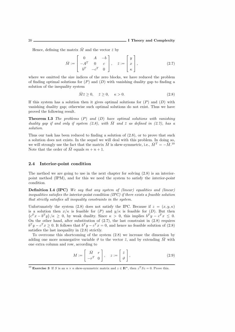
20 I Theory and Complexity
Hence, defining the matrix M and the vector z by
M :=
0 A −b−AT 0 c
bT −cT 0
, z :=
y
x
κ
, (2.7)
where we omitted the size indices of the zero blocks, we have reduced the problemof finding optimal solutions for (P ) and (D) with vanishing duality gap to finding asolution of the inequality system
Mz ≥ 0, z ≥ 0, κ > 0. (2.8)
If this system has a solution then it gives optimal solutions for (P ) and (D) withvanishing duality gap; otherwise such optimal solutions do not exist. Thus we haveproved the following result.
Theorem I.3 The problems (P ) and (D) have optimal solutions with vanishingduality gap if and only if system (2.8), with M and z as defined in (2.7), has asolution.
Thus our task has been reduced to finding a solution of (2.8), or to prove that sucha solution does not exists. In the sequel we will deal with this problem. In doing so,we will strongly use the fact that the matrix M is skew-symmetric, i.e., MT = −M .10
Note that the order of M equals m+ n+ 1.
2.4 Interior-point condition
The method we are going to use in the next chapter for solving (2.8) is an interior-point method (IPM), and for this we need the system to satisfy the interior-point
condition.
Definition I.4 (IPC) We say that any system of (linear) equalities and (linear)inequalities satisfies the interior-point condition (IPC) if there exists a feasible solutionthat strictly satisfies all inequality constraints in the system.
Unfortunately the system (2.8) does not satisfy the IPC. Because if z = (x, y, κ)is a solution then x/κ is feasible for (P ) and y/κ is feasible for (D). But then(cTx− bT y
)/κ ≥ 0, by weak duality. Since κ > 0, this implies bT y − cTx ≤ 0.
On the other hand, after substitution of (2.7), the last constraint in (2.8) requiresbT y − cTx ≥ 0. It follows that bT y − cTx = 0, and hence no feasible solution of (2.8)satisfies the last inequality in (2.8) strictly.To overcome this shortcoming of the system (2.8) we increase the dimension by
adding one more nonnegative variable ϑ to the vector z, and by extending M withone extra column and row, according to
M :=
[M r
−rT 0
], z :=
[z
ϑ
], (2.9)
10Exercise 3 If S is an n× n skew-symmetric matrix and z ∈ IRn, then zTSz = 0. Prove this.

I.2 Duality Theory 21
wherer = em+n+1 − Mem+n+1, (2.10)
with em+n+1 denoting an all-one vector of length m+ n+ 1. So we have
M =
0 A −b−AT 0 c
bT −cT 0
r
−rT 0
, r =
em −Aen + b
en +AT em − c
1− bT em + cT en
, z =
y
x
κ
ϑ
(2.11)
The order of the matrix M is m+ n+ 2. To simplify the presentation, in the rest ofthis chapter we denote this number as n:
n = m+ n+ 2.
Letting q be the vector of length n given by
q :=
[0n−1
n
], (2.12)
we consider the systemMz ≥ −q, z ≥ 0. (2.13)
We make two important observations. First we observe that the matrix M is skew-symmetric. Secondly, the system (2.13) satisfies the IPC. The all-one vector does thework, because taking z = en−1 and ϑ = 1, we have
Mz + q =
[M r
−rT 0
][en−1
1
]+
[0
n
]=
[Men−1 + r
−rT en−1 + n
]=
[en−1
1
]. (2.14)
The last equality is due to the definition of r, which implies Men−1 + r = en−1 and
−rT en−1 + n = −(en−1 − Men−1
)Ten−1 + n = −eTn−1en−1 + n = 1,
where we used eTn−1Men−1 = 0 (cf. Exercise 3, page 20).The usefulness of system (2.13) stems from two facts. First, it satisfies the IPC
and hence can be treated by an interior-point method. What this implies willbecome apparent in the next chapter. Another crucial property is that there is acorrespondence between the solutions of (2.8) and the solutions of (2.13) with ϑ = 0.To see this it is useful to write (2.13) in terms of z and ϑ:
[M r
−rT 0
][z
ϑ
]+
[0
n
]≥ 0, z ≥ 0, ϑ ≥ 0.
Obviously, if z = (z, 0) satisfies (2.13), this implies M z ≥ 0 and z ≥ 0, and hence zsatisfies (2.8). On the other hand, if z satisfies (2.8) then M z ≥ 0 and z ≥ 0; as aconsequence z = (z, 0) satisfies (2.13) if and only if −rT z + n ≥ 0, i.e., if and only if
rT z ≤ n.
If rT z ≤ 0 this certainly holds. Otherwise, if rT z > 0, the positive multiple nz/rT z ofz satisfies rT z ≤ n. Since a positive multiple preserves signs, this is sufficient for ourgoal. We summarize the above discussion in the following theorem.

22 I Theory and Complexity
Theorem I.5 The following three statements are equivalent:
(i) Problems (P ) and (D) have optimal solutions with vanishing duality gap;(ii) If M and z are given by (2.7) then (2.8) has a solution;(iii) If M and z are given by (2.11) then (2.13) has a solution with ϑ = 0 and κ > 0.
Moreover, system (2.13) satisfies the IPC.
2.5 Embedding into a self-dual LO-problem
Obviously, solving (2.8) is equivalent to finding a solution of the minimization problem
(SP0) min0T z : M z ≥ 0, z ≥ 0
(2.15)
with κ > 0. In fact, this is the way we are going to follow: our aim will be to findout whether this problem has a(n optimal) solution with κ > 0 or not. Note thatthe latter condition makes our task nontrivial. Because finding an optimal solution of(SP0) is trivial: the zero vector is feasible and hence optimal. Also note that (SP0) isin the canonical form. However, it has a very special structure: its feasible domain ishomogeneous and since M is skew-symmetric, the problem (SP0) is a self-dual problem(cf. Exercise 2, page 18). We say that (SP0) is a self-dual embedding of the canonicalproblem (P ) and its dual problem (D).If the constraints in an LO problem satisfy the IPC, then we simply say that the
problem itself satisfies the IPC. As we established in the previous section, the self-dualembedding (SP0) does not satisfy the IPC, and therefore, from an algorithmic pointof view this problem is not useful.In the previous section we reduced the problem of finding optimal solutions (P ) and
(D) with vanishing duality gap to finding a solution of (2.13) with ϑ = 0 and κ > 0.For that purpose we consider another self-dual embedding of (P ) and (D), namely
(SP ) minqT z : Mz ≥ −q, z ≥ 0
. (2.16)
The following theorem shows that we can achieve our goal by solving this problem.
Theorem I.6 The system (2.13) has a solution with ϑ = 0 and κ > 0 if and only ifthe problem (SP ) has an optimal solution with κ = zn−1 > 0.
Proof: Since q ≥ 0 and z ≥ 0, we have qT z ≥ 0, and hence the optimal value of (SP )is certainly nonnegative. On the other hand, since q ≥ 0 the zero vector (z = 0) isfeasible, and yields zero as objective value, which is therefore the optimal value. SinceqT z = nϑ, we conclude that the optimal solutions of (2.16) are precisely the vectors zsatisfying (2.13) with ϑ = 0. This proves the theorem.
We associate to any vector z ∈ IRn its slack vector s(z) as follows.
s(z) :=Mz + q. (2.17)
Then we have
z is a feasible for (SP ) ⇐⇒ z ≥ 0, s(z) ≥ 0.

I.2 Duality Theory 23
As we established in the previous section, the inequalities defining the feasible domainof (SP ) satisfy the IPC. To be more specific, we found in (2.14) that the all-one vectore is feasible and its slack vector is the all-one vector. In other words,
s(e) = e. (2.18)
We proceed by giving a small example.
Example I.7 By way of example we consider the case where the problems (P ) and(D) are determined by the following constraint matrix A, and vectors b and c:11
A =
[1
0
], b =
[1
−1
], c =
[2].
According to (2.7) the matrix M is then equal to
M =
0 A −b−AT 0 c
bT −cT 0
=
0 0 1 −1
0 0 0 1
−1 0 0 2
1 −1 −2 0
and according to (2.10), the vector r becomes
r = e− Me =
1
1
1
1
−
0
1
1
−2
=
1
0
0
3
,
Thus, by (2.11) and (2.12), we obtain
M =
0 0 1 −1 1
0 0 0 1 0
−1 0 0 2 0
1 −1 −2 0 3
−1 0 0 −3 0
, q =
0
0
0
0
5
.
Hence, the self-dual problem (SP ), as given by (2.16), gets the form
min
5ϑ :
0 0 1 −1 1
0 0 0 1 0
−1 0 0 2 0
1 −1 −2 0 3
−1 0 0 −3 0
z1z2z3z4z5
+
0
0
0
0
5
≥ 0,
z1z2z3
z4 = κ
z5 = ϑ
≥ 0
. (2.19)
Note that the all-one vector is feasible for this problem and that its surplus vectoralso is the all-one vector. This is in accordance with (2.18). As we shall see later on,it means that the all-one vector is the point on the central path for µ = 1. ♦
11 cf. Example D.5 (page 449) in Appendix D.

24 I Theory and Complexity
Remark I.8 In the rest of this chapter, and the next chapter, we deal with the problem(SP ). In fact, our analysis does not only apply to the case that M and q have thespecial form of (2.11) and (2.12). Therefore we extend the applicability of our analysisby weakening the assumptions on M and q. Unless stated otherwise below we onlyassume the following:
MT = −M, q ≥ 0, s(e) = e. (2.20)
The last two variables in the vector z play a special role. They are the homogenizingvariable κ = zn−1, and ϑ = zn. The variable ϑ is called the normalizing variable,because of the following important property.
Lemma I.9 One haseT z + eT s(z) = n+ qT z. (2.21)
Proof: The identity in the lemma is a consequence of the orthogonality property (cf.Exercise 3, page 20)
uTMu = 0, ∀u ∈ IRn. (2.22)
First we deduce that for every z one has
qT z = zT (s(z)−Mz) = zT s(z)− zTMz = zT s(z). (2.23)
Taking u = e− z in (2.22) we obtain
(z − e)T (s(z)− s(e)) = 0.
Since s(e) = e, eT e = n and zT s(z) = qT z, the relation (2.21) follows.
It follows from Lemma I.9 that the sum of the positive coordinates in z and s(z)is bounded above by n + qT z. Note that this is especially interesting if z is optimal,because then qT z = 0. Hence, if z is optimal then
eT z + eT s(z) = n. (2.24)
Since z and s(z) are nonnegative this implies that the set of optimal solutions isbounded.Another interesting feature of the LO-problem (2.16) is that it is self-dual: the dual
problem is(DSP ) max
−qTu : MTu ≤ q, u ≥ 0
;
since M is skew-symmetric, MTu ≤ q is equivalent to −Mu ≤ q, or Mu ≥ −q,and maximizing −qTu is equivalent to minimizing qTu, and thus the dual problem isessential the same problem as (2.16).The rest of the chapter is devoted to our main task, namely to find an optimal
solution of (2.16) with κ > 0 or to establish that such a solution does not exist.
2.6 The classes B and N
We introduce the index sets B and N according to
B := i : zi > 0 for some optimal zN := i : si(z) > 0 for some optimal z .

I.2 Duality Theory 25
So, B contains all indices i for which an optimal solution z with positive zi exists. Wealso write zi ∈ B if i ∈ B. Note that we certainly have ϑ /∈ B, because ϑ is zero inany optimal solution of (SP ). The main question we have to answer is whether κ ∈ Bholds or not. Because if κ ∈ B then there exists an optimal solution z with κ > 0,in which case (P ) and (D) have optimal solutions with vanishing duality gap, andotherwise not.The next lemma implies that the sets B and N are disjoint. In this lemma, and
further on, we use the following notation. To any vector u ∈ IRk, we associate thediagonal matrix U whose diagonal entries are the elements of u, in the same order. Ifalso v ∈ IRk, then Uv will be denoted shortly as uv. Thus uv is a vector whose entriesare obtained by multiplying u and v componentwise.
Lemma I.10 Let z1 and z2 be feasible for (SP ). Then z1 and z2 are optimal solutionsof (SP ) if and only if z1s(z2) = z2s(z1) = 0.
Proof: According to (2.23) we have for any feasible z:
qT z = zT s(z). (2.25)
As a consequence, z ≥ 0 is optimal if and only if s(z) ≥ 0 and zT s(z) = 0. Since, by(2.22),
(z1 − z2
)TM(z1 − z2
)= 0,
we have (z1 − z2
)T (s(z1)− s(z2)
)= 0.
Expanding the product on the left and rearranging the terms we get
(z1)T s(z2) + (z2)T s(z1) = (z1)T s(z1) + (z2)T s(z2).
Now z1 is optimal if and only if (z1)T s(z1) = 0, by (2.25), and similarly for z2. Hence,since z1, z2, s(z1) and s(z2) are all nonnegative, z1 and z2 are optimal if and only if
(z1)T s(z2) + (z2)T s(z1) = 0,
which is equivalent to
z1s(z2) = z2s(z1) = 0,
proving the lemma.
Corollary I.11 The sets B and N are disjoint.
Proof: If i ∈ B ∩N then there exist optimal solutions z1 and z2 of (SP ) such thatz1i > 0 and si(z
2) > 0. This would imply z1i si(z2) > 0, a contradiction with Lemma
I.10. Hence B ∩N is the empty set.
By way of example we determine the classes B and N for the problem consideredin Example I.7.

26 I Theory and Complexity
Example I.12 Consider the self-dual problem (SP ) in Example I.7, as given by(2.19):
min
5ϑ :
0 0 1 −1 1
0 0 0 1 0
−1 0 0 2 0
1 −1 −2 0 3
−1 0 0 −3 0
z1z2z3z4z5
+
0
0
0
0
5
≥ 0,
z1z2z3
z4 = κ
z5 = ϑ
≥ 0
.
For any z ∈ IR5 we have
s(z) =
z3 − z4 + z5z4
2z4 − z1z1 − z2 − 2z3 + 3z5
5− z1 − 3z4
=
z3 − κ+ ϑ
κ
2κ− z1z1 − z2 − 2z3 + 3ϑ
5− z1 − 3κ
Now z is feasible if z ≥ 0 and s(z) ≥ 0, and optimal if moreover zs(z) = 0. Soz = (z1, z2, z3, κ, ϑ) is optimal if and only if
z1z2z3κ
ϑ
≥ 0,
z3 − κ+ ϑ
κ
2κ− z1z1 − z2 − 2z3 + 3ϑ
5− z1 − 3κ
≥ 0,
z1 (z3 − κ+ ϑ) = 0
z2κ = 0
z3 (2κ− z1) = 0
κ (z1 − z2 − 2z3 + 3ϑ) = 0
ϑ (5− z1 − 3κ) = 0
.
Adding the equalities at the right we obtain 5ϑ = 0, which gives ϑ = 0, as it should.Substitution gives
z1z2z3κ
0
≥ 0,
z3 − κ
κ
2κ− z1z1 − z2 − 2z35− z1 − 3κ
≥ 0,
z1 (z3 − κ) = 0
z2κ = 0
z3 (2κ− z1) = 0
κ (z1 − z2 − 2z3) = 0
ϑ = 0
.
Note that if κ = 0 then the inequality 2κ − z1 ≥ 0 implies z1 = 0, and then theinequality z1 − z2 − 2z3 ≥ 0 gives also z2 = 0 and z3 = 0. Hence, z = 0 is the onlyoptimal solution for which κ = 0. So, let us assume κ > 0. Then we deduce from thesecond and fourth equality that z2 = 0 and z1− z2− 2z3 = 0. This reduces our systemto
z1 = 2z30
z3κ
0
≥ 0,
z3 − κ
κ
2κ− 2z30
5− 2z3 − 3κ
≥ 0,
2z3 (z3 − κ) = 0
z2 = 0
z3 (2κ− 2z3) = 0
0 = 0
ϑ = 0
.
The equations at the right make clear that either z3 = 0 or z3 = κ. However, theinequality z3−κ ≥ 0 forces z3 > 0 since κ > 0. Thus we find that any optimal solution

I.2 Duality Theory 27
has the form
z =
2κ
0
κ
κ
0
, s(z) =
0
κ
0
0
5− 5κ
, 0 ≤ κ ≤ 1. (2.26)
This implies that in this example the sets B and N are given by
B = 1, 3, 4 , N = 2, 5 . ♦
In the above example the union of B and N is the full index set. This is not anincident. Our next aim is to prove that this always holds. 12,13,14,15 As a consequencethese sets form a partition of the full index set 1, 2, . . . , n; it is the so-called optimal
partition of (SP ). This important and nontrivial result is fundamental to our purposebut its proof requires some effort. It highly depends on properties of the central path
of (SP ), which is introduced in the next section.
2.7 The central path
2.7.1 Definition of the central path
Recall from (2.14) that s(e) = e, where e (as always) denotes the all-one vector ofappropriate length (in this case, n). As a consequence, we have a vector z such thatzisi(z) = 1 (1 ≤ i ≤ n), which, using our shorthand notation can also be expressed as
z = e ⇒ zs(z) = e. (2.27)
Now we come to a very fundamental notion, both from a theoretical and algorithmicpoint of view, namely the central path of the LO-problem at hand. The underlying
12 Exercise 4 Following the same approach as in Example I.7 construct the embedding problem forthe case where the problems (P ) and (D) are determined by
A =
[10
], b =
[10
], c =
[2],
and, following the approach of Example I.12, find the set of all optimal solutions and the optimalpartition.
13 Exercise 5 Same as in Exercise 4, but now with
A =
[10
], b =
[11
], c =
[2].
14 Exercise 6 Same as in Exercise 4, but now with
A =
[10
], b =
[1β
], c =
[2], β > 0.
15 Exercise 7 Same as in Exercise 4, but now with
A =
[10
], b =
[1β
], c =
[2], β < 0.

28 I Theory and Complexity
theoretical property is that for every positive number µ there exist a nonnegativevector z such that
zs(z) = µe, z ≥ 0, s(z) ≥ 0, (2.28)
and moreover, this vector is unique. If µ = 1, the existence of such a vector isguaranteed by (2.27). Also note that if we put µ = 0 in (2.28) then the solutionsare just the optimal solutions of (SP ). As we have seen in Example I.12 there maymore than one optimal solution. Therefore, if µ = 0 the system (2.28) may havemultiple solutions. The following lemma is of much interest. It makes clear that forµ > 0 the system (2.28) has at most one solution.
Lemma I.13 If µ > 0, then there exists at most one nonnegative vector z such that(2.28) holds.
Proof: Let z1 and z2 to nonnegative vectors satisfying (2.28), and let s1 = s(z1)and s2 = s(z2). Since µ > 0, z1, z2, s1, s2 are all positive. Define ∆z := z2 − z1, andsimilarly ∆s := s2 − s1. Then we may easily verify that
M∆z = ∆s (2.29)
z1∆s+ s1∆z +∆s∆z = 0. (2.30)
Using that M is skew-symmetric, (2.22) implies that ∆zT∆s = 0, or, equivalently,
eT (∆z∆s) = 0. (2.31)
Rewriting (2.30) gives(z1 +∆z)∆s+ s1∆z = 0.
Since z1 +∆z = z2 > 0 and s1 > 0, this implies that no two corresponding entries in∆z and ∆s have the same sign. So it follows that
∆z∆s ≤ 0. (2.32)
Combining (2.31) and (2.32), we obtain ∆z∆s = 0. Hence either (∆z)i = 0 or(∆s)i = 0, for each i. Using (2.30) once more, we conclude that (∆z)i = 0 and(∆s)i = 0, for each i. Hence ∆z = ∆s = 0, whence z1 = z2 and s1 = s2. This provesthe lemma.
To prove the existence of a solution to (2.28) requires much more effort. We postponethis to the next section. For the moment, let us take the existence of a solution to(2.28) for granted and denote it as z(µ). We call it the µ-center of (SP ). The set
z(µ) : µ > 0
of all µ-centers represents a parametric curve in the feasible region of (SP ). This curveis called the central path of (SP ). Note that
qT z(µ) = s(µ)T z(µ) = µn. (2.33)
This proves that along the central path, when µ approaches zero, the objective valueqT z(µ) monotonically decreases to zero, at a linear rate.

I.2 Duality Theory 29
2.7.2 Existence of the central path
In this section we give an algorithmic proof of the existence of a solution to (2.28).Starting at z = e we construct the µ-center for any µ > 0. This is done by using theso-called Newton direction as a search direction. The results in this section will alsobe used later when dealing with a polynomial-time method for solving (SP ).
Newton direction
Assume that z is a positive solution of (SP ) such that its slack vector s = s(z) ispositive, and let ∆z denote a displacement in the z-space. Our aim is to find ∆z suchthat z +∆z is the µ-center. We denote
z+ := z +∆z,
and the new slack vector as s+:
s+ := s(z+) =M(z +∆z) + q = s+M∆z.
Thus, the displacement ∆s in the s-space is simply given by
∆s = s+ − s =M∆z.
Observe that ∆z and ∆s are orthogonal, since by (2.22):
(∆z)T ∆s = (∆z)T M∆z = 0. (2.34)
We want ∆z to be such that z+ becomes the µ-center, which means (z +∆z)(s+∆s) = µe, or
zs+ z∆s+ s∆z +∆z∆s = µe.
This equation is nonlinear, due to the quadratic term ∆z∆s. Applying Newton’smethod, we omit this nonlinear term, leaving us with the following linear systemin the unknown vectors ∆z and ∆s:
M∆z −∆s = 0, (2.35)
z∆s+ s∆z = µe− zs. (2.36)
This system has a unique solution, as easily may be verified, by using that M isskew-symmetric and z > 0 and s > 0.16,17 The solution ∆z is called the Newtondirection. Since we omitted the quadratic term ∆z∆s in our calculation of the Newton
16Exercise 8 The coefficient matrix of the system (2.35-2.36) of linear equations in ∆z and ∆s is
[M −IS Z
].
As usual, Z = diag (z) and S = diag (s), with z > 0 and s > 0, and I denotes the identity matrix.Show that this matrix is nonsingular.
17 Exercise 9 Let M be a skew-symmetric matrix of size n × n and Z and S positive diagonalmatrices of the same size as M . Then the matrix S + ZM is nonsingular. Prove this.

30 I Theory and Complexity
direction, z+∆z will (in general) not be the µ-center, but hopefully it will be a goodapproximation. In fact, using (2.36), after the Newton step one has
z+s(z+) = (z +∆z)(s+∆s) = zs+ (z∆s+ s∆z) + ∆z∆s = µe+∆z∆s. (2.37)
Comparing this with our desire, namely z+s(z+) = µe, we see that the ‘error’ isprecisely the quadratic term ∆z∆s. Using (2.22), we deduce from (2.37) that
(z+)Ts(z+) = µeT e = µn, (2.38)
showing that after the Newton step the duality gap already has the desired value.
Example I.14 Let us compute the Newton step at z = e for the self-dual problem(SP ) in Example I.7, as given by (2.19), with respect to some µ > 0. Sincez = s(z) = e, the equation (2.36) reduces to
∆s+∆z = µe− e = (µ− 1)e.
Hence, by substitution into (2.35) we obtain
(M + I)∆z = (µ− 1)e.
It suffices to know the solution of the equation (M + I) ζ = e, because then ∆z =(µ− 1)ζ. Thus we need to solve ζ from
1 0 1 −1 1
0 1 0 1 0
−1 0 1 2 0
1 −1 −2 1 3
−1 0 0 −3 1
ζ =
1
1
1
1
1
,
which gives the unique solution
ζ =
(−1
3,8
9,4
9,1
9, 1
)T
.
Hence
∆z = (µ− 1)
(−1
3,8
9,4
9,1
9, 1
)T
, (2.39)
and
∆s =M∆z = (µ− 1) (e− ζ) = (µ− 1)
(4
3,1
9,5
9,8
9, 0
)T
. (2.40)
After the Newton step we thus have
z+s+ = (z +∆z) (s+∆s) = zs+ (∆z +∆s) + ∆z∆s
= e+ (µ− 1)e+∆z∆s = µ e+∆z∆s
= µ e+(µ− 1)2
81(−36, 8, 20, 8, 0)T . ♦

I.2 Duality Theory 31
Proximity measure
To measure the quality of any approximation z of z(µ), we introduce a proximity
measure δ(z, µ) that vanishes if z = z(µ) and is positive otherwise. To this end weintroduce the variance vector of z with respect to µ as follows:
v :=
√zs(z)
µ, (2.41)
where all operations are componentwise. Note that
zs(z) = µe ⇔ v = e.
The proximity measure δ(z, µ) is now defined by18
δ(z, µ) := 12
∥∥v − v−1∥∥ . (2.42)
Note that if z = z(µ) then v = e and hence δ(z, µ) = 0, and otherwise δ(z, µ) > 0. Weshow below that if δ(z, µ) < 1 then the Newton process quadratically fast converges toz(µ). For this we need the following lemma, which estimates the error term in termsof the proximity measure. In this lemma ‖.‖ denotes the Eucledian norm (or 2-norm)and ‖.‖∞ the Chebychev norm (or infinity norm) of a vector.
Lemma I.15 If δ := δ(z, µ), then ‖∆z∆s‖∞ ≤ µδ2 and ‖∆z∆s‖ ≤ µδ2√2.
Proof: Componentwise division of (2.36) byõ v =
√zs yields
√z
s∆s+
√s
z∆z =
√µ(v−1 − v
).
The terms at the left represent orthogonal vectors whose componentwise productis ∆z∆s. Applying Lemma C.4 in Appendix C to these vectors, and using that∥∥v−1 − v
∥∥ = 2δ, the result immediately follows.
Quadratic convergence of the Newton process
We are now ready for the main result on the Newton direction.
Theorem I.16 If δ := δ(z, µ) < 1, then the Newton step is strictly feasible, i.e.,z+ > 0 and s+ > 0. Moreover,
δ(z+, µ) ≤ δ2√2(1− δ2)
.
18 In the analysis of interior-point methods we always need to introduce a quantity that measures the‘distance’ of a feasible vector z to the central path or to the µ-center. This can be done in manyways as becomes apparent in the course of this book. In the coming chapters we make use of avariety of so-called proximity measures. Most of these measures are based on the simple observationthat z is equal to the µ-center if and only if v = e and z is on the central path if and only if thevector zs(z) is a scalar multiple of the all-one vector.

32 I Theory and Complexity
Proof: Let 0 ≤ α ≤ 1, zα = z+α∆z and sα = s+α∆s. We then have, using (2.36),
zαsα = (z + α∆z)(s+ α∆s) = zs+ α (z∆s+ s∆z) + α2∆z∆s
= zs+ α (µe− zs) + α2∆z∆s = (1− α)zs+ α (µe+ α∆z∆s)
By Lemma I.15,
µe+ α∆z∆s ≥ µe − α ‖∆z∆s‖∞ e ≥ µ(1− αδ2) e > 0.
Hence, since (1 − α)zs ≥ 0, we have zαsα > 0, for all α ∈ [0, 1]. Therefore, thecomponents of zα and sα cannot vanish when α ∈ [0, 1]. Hence, since z > 0 and s > 0,by continuity, zα and sα must be positive for any such α, especially for α = 1. Thisproves the first statement in the lemma.Now let us turn to the proof of the second statement. Let δ+ := δ(z+, µ) and let v+
be the variance vector of z+ with respect to µ:
v+ =
√z+s+
µ.
Then, by definition,
2δ+ =∥∥(v+)−1 − v+
∥∥ =∥∥(v+)−1
(e− (v+)2
)∥∥ . (2.43)
Recall from (2.37) that z+s+ = µe+∆z∆s. In other words,
(v+)2
= e+∆z∆s
µ.
Substitution into (2.43) gives
2δ+ =
∥∥∥∥∥∥−∆z∆s
µ√e+ ∆z∆s
µ
∥∥∥∥∥∥≤
∥∥∥∆z∆sµ
∥∥∥√1−
∥∥∥∆z∆sµ
∥∥∥∞
≤ δ2√2√
1− δ2.
The last inequality follows by using Lemma I.15 twice. Thus the proof is complete.
Theorem I.16 implies that when δ ≤ 1/√2, then after a Newton step the proximity to
the µ-center satisfies δ(z+, µ) ≤ δ2. In other words, Newton’s method is quadraticallyconvergent.
Example I.17 Using the self-dual problem (SP ) in Example I.7 again, we considerin this example feasibility of the Newton step, and the proximity measure before andafter Newton step at z = e for several values of µ, to be specified below. We will seethat the Newton step performs much better than Theorem I.16 predicts! In ExampleI.14 we found the values of ∆z and ∆s. Using these values we find for the new iterate:
z+ = e+ (µ− 1)
(−1
3,8
9,4
9,1
9, 1
)T
,

I.2 Duality Theory 33
and since s = s(e) = e,
s+ = e+ (µ− 1)
(4
3,1
9,5
9,8
9, 0
)T
.
Hence the Newton step is feasible, i.e., z+ and s+ are nonnegative, if and only if
0.25 ≤ µ ≤ 4,
as easily may be verified. For any such µ we have
δ(z, µ) =1
2
∥∥∥∥√µ e− e√
µ
∥∥∥∥ =1
2
∣∣∣∣√µ− 1√
µ
∣∣∣∣ ‖e‖ =
√5
2
∣∣∣∣√µ− 1√
µ
∣∣∣∣ .
Note that Theorem I.16 guarantees feasibility only if δ(z, µ) ≤ 1. This holds if5µ2 − 14µ+ 5 ≤ 0, which is equivalent to
0.4202 ≈ 1
5
(7− 2
√6)≤ µ ≤ 1
5
(7 + 2
√6)≈ 2.3798.
The same theorem guarantees quadratically convergence if δ(z, µ) ≤ 1/√2, which
holds if and only if
0.5367 ≈ 1
5
(6−
√11)≤ µ ≤ 1
5
(6 +
√11)≈ 1.8633.
By way of example, consider the case where µ = 0.5. Then we have δ(z, µ) = 14
√10 ≈
0.7906 and, by Theorem I.16, δ(z+, µ) ≤ 512
√3 ≈ 0.7217. Let us compute the actual
value of δ(z+, µ). For µ = 0.5 we have
z+ = e− 1
2
(−1
3,8
9,4
9,1
9, 1
)T
=
(7
6,5
9,7
9,17
18,1
2
)T
,
and since s = s(e) = e,
s+ = e− 1
2
(4
3,1
9,5
9,8
9, 0
)T
=
(1
3,17
18,13
18,5
9, 1
)T
.
Therefore,(v+)2
=z+s+
µ=
(7
9,85
81,91
81,85
81, 1
)T
.
Finally, we compute δ(z+, µ) by using
4δ(z+, µ)2 =∥∥v+ − (v+)−1
∥∥2 =
5∑
i=1
(v+i)2
+
5∑
i=1
(v+i)−2 − 10.
Note that the first sum equals (z+)Ts+/µ = 2nµ = 5. The second sum equals 5.0817.
Thus we obtain 4δ(z+, µ)2 = 0.0817, which gives δ(z+, µ) = 0.1429. ♦

34 I Theory and Complexity
Existence of the central path
Now suppose that we know the µ-center for µ = µ0 > 0 and let us denote z0 = z(µ0).Note that this is true for µ0 = 1, with z0 = e, because es(e) = e. So e is the µ-centerfor µ = 1.Since z0s(z0) = µ0e, the v-vector for z0 with respect to an arbitrary µ > 0 is given
by
v =
√z0s(z0)
µ=
õ0e
µ=
õ0
µe.
Hence we have δ(z0, µ) ≤ 1√2if and only if
1
2
∣∣∣∣∣
õ0
µ−√µ
µ0
∣∣∣∣∣ ‖e‖ ≤ 1√2.
Using ‖e‖ =√n, one may easily verify that this holds if and only if
1
β≤ µ
µ0≤ β, β := 1 +
1
n+
√1
n2+
2
n. (2.44)
Now starting the Newton process at z0, with µ fixed, and such that µ satisfies (2.44),we can generate an infinite sequence z0, z1, · · · zk, · · · such that
δ(zk, µ
)≤ 1
22k−1.
Hencelimk→∞
δ(zk, µ
)= 0.
The generated sequence has at least one accumulation point z∗, since the iteratesz1, · · · zk, · · · lie in the compact set
eT z + eT s(z) = n (1 + µ) , z ≥ 0, s(z) ≥ 0,
due to (2.21) and (2.38). Since δ (z∗, µ) = 0, we obtain z∗s (z∗) = µe. Due to LemmaI.13, z∗ is unique. This proves that the µ-center exists if µ satisfies (2.44) with µ0 = 1,i.e., if
1
β≤ µ ≤ β.
By redefining µ0 as one of the endpoints of the above interval we can repeat the aboveprocedure, and extend the interval where the µ-center exists to
1
β2≤ µ ≤ β2.
and so on. After applying the procedure k times the interval where the µ-centercertainly exists is given by
1
βk≤ µ ≤ βk.

I.2 Duality Theory 35
For arbitrary µ > 0, we have to apply the above procedure at most
|logµ|log β
times, to prove the existence of the µ-center. This completes the proof of the existenceof the central path.It may be worth noting that, using n ≥ 2 and log(1 + t) ≥ t
1+t for t ≥ 0,19
log β = log
(1 +
1
n+
√1
n2+
2
n
)≥ log
(1 +
√2
n
)≥
√2n
1 +√
2n
=
√2√
n+√2≥ 1√
2n.
Hence the number of times that we have to apply the above described procedure toobtain the µ-center is bounded above by
√2n |logµ| . (2.45)
We have just shown that the system (2.28) has a unique solution for every positive µ.The solution is called the µ-center, and denoted as z(µ). The set of all µ-centers is acurve in the interior of the feasible region of (SP ). The definition of the µ-center, asgiven by (2.28), can be equivalently given as the unique solution of the system
Mz + q = s, z ≥ 0, s ≥ 0
zs = µe,(2.46)
with M and z as defined in (2.11), and s = s(z), as in (2.17).20,21,22
2.8 Existence of a strictly complementary solution
Now that we have proven the existence of the central path we can use it as a guideto the optimal set, by letting the parameter µ approach to zero. As we show in thissection, in this way we obtain an optimal solution z such that z + s(z) > 0.
Definition I.18 Two nonnegative vectors a and b in IRn are said to be complementaryvectors if ab = 0. If moreover a+ b > 0 then a and b are called strictly complementaryvectors.
19 See, e.g., Exercise 39, page 133.20
Exercise 10 Using the definitions of z and q, according to (2.11) and (2.12), show that ϑ(µ) = µ.21
Exercise 11 In this exercise a skew-symmetric M and four vectors q(i), i = 1, 2, 3, 4 are given asfollows:
M =
[0 1−1 0
], q(1) =
[00
], q(2) =
[10
], q(3) =
[01
], q(4) =
[11
].
For each of the four cases q = q(i), i = 1, 2, 3, 4, one is asked to verify (1) if the system (2.46) hasa solution if µ > 0 and (2) if the first equation in (2.46) satisfies the IPC, i.e., has a solution withz > 0 and s > 0.
22Exercise 12 Show that z(µ) is continuous (and differentiable) at any positive µ. (Hint: Applythe implicit function theorem (cf. Proposition A.2 in Appendix A) to the system (2.46)).

36 I Theory and Complexity
Recall that optimality of z means that zs(z) = 0, which means that z and s(z) arecomplementary vectors. We are going to show that there exists an optimal vector zsuch that z and s(z) are strictly complementary vectors. Then for every index i, eitherzi > 0 or si(z) > 0. This implies that the index sets B and N , introduced in Section2.5 form a partition of the index set, the so-called optimal partition of (SP ).It is convenient to introduce some more notation.
Definition I.19 If z is a nonnegative vector, we define its support, denoted by σ(z),as the set of indices i for which zi > 0:
σ(z) = i : zi > 0 .
Note that if z is feasible then zs(z) = 0 holds if and only if σ(z) ∩ σ(s(z)) = ∅.Furthermore, z is a strictly complementary optimal solution if and only if it is optimaland σ(z) ∪ σ(s) = 1, 2, . . . , n.
Theorem I.20 (SP ) has an optimal solution z∗ with z∗ + s(z∗) > 0.
Proof: Let µk∞k=1 be a monotonically decreasing sequence of positive numbersµk such that µk → 0 if k → ∞, and let s(µk) := s (z(µk)). Due to Lemma I.9the set (z(µk), s(µk)) lies in a compact set, and hence it contains a subsequenceconverging to a point (z∗, s∗), with s∗ = s(z∗). Since z(µk)
T s(µk) = nµk → 0, wehave (z∗)T s∗ = 0. Hence, from (2.25), qT z∗ = 0. So z∗ is an optimal solution.We claim that (z∗, s∗) is a strictly complementary pair. To prove this, we apply the
orthogonality property (2.22) to the points z∗ and z(µk), which gives
(z(µk)− z∗)T (s(µk)− s∗) = 0.
Rearranging the terms, and using z(µk)T s(µk) = nµk and (z∗)T s∗ = 0, we arrive at
∑
j∈σ(z∗)
z∗j sj(µk) +∑
j∈σ(s∗)
zj(µk)s∗j = nµk.
Dividing both sides by µk and recalling that zj(µk)sj(µk) = µk, we obtain
∑
j∈σ(z∗)
z∗jzj(µk)
+∑
j∈σ(s∗)
s∗jsj(µk)
= n.
Letting k → ∞, the first sum on the left becomes equal to the number of positivecoordinates in z∗. Similarly, the second sum becomes equal to the number of positivecoordinates in s∗. The sum of these numbers being n, we conclude that the optimalpair (z∗, s∗) is strictly complementary.23,24
23 By using a similar proof technique it can be shown that the limit of z(µ) exists if µ goes to zero.In other words, the central path converges. The limit point is (of course) a uniquely determinedoptimal solution of (SP ), which can further be characterized as the so-called analytic center of theset of optimal solutions (cf. Section 2.11).
24 Let us also mention that Theorem I.20 is a special case of an old result of Goldman and Tucker whichstates that every feasible linear system of equalities and inequalities has a strictly complementarysolution [111].

I.2 Duality Theory 37
By Theorem I.20 there exists a strictly complementary solution z of (SP ). Havingsuch a solution, the classes B and N simply follow from
B = i : zi > 0 , N = i : si(z) > 0 .
Now recall from Theorem I.5 and Theorem I.6 that the problems (P ) and (D) haveoptimal solutions with vanishing duality gap if and only if (SP ) has an optimal solutionwith κ > 0. Due to Theorem I.20 this can be restated as follows.
Corollary I.21 The problems (P ) and (D) have optimal solutions with vanishingduality gap if and only if κ ∈ B.
Let us consider more in detail the implications of κ ∈ B for the problems (SP0), andmore importantly, for (P ) and (D).Theorem I.20 implies the existence of a strictly complementary optimal solution z
of (SP ). Let z be such an optimal solution. Then we have
zs(z) = 0, z + s(z) > 0, z ≥ 0, s(z) ≥ 0.
Now using s(z) =Mz + q and ϑ = 0, and also (2.11) and (2.12), we obtain
z =
y
x
κ
0
≥ 0, s(z) =
Ax− κb
−AT y + κc
bT y − cTx
n−[yT , xT , κ
]r
≥ 0.
Neglecting the last entry in both vectors, it follows that
z :=
y
x
κ
≥ 0, s(z) := M z =
Ax− κb
−AT y + κc
bT y − cTx
≥ 0, (2.47)
and moreover,
zs(z) = 0, z + s(z) > 0, z ≥ 0, s(z) ≥ 0. (2.48)
This shows that z is a strictly complementary optimal solution of (SP0). Hence thenext theorem requires no further proof.
Theorem I.22 (SP0) has an optimal solution z with z + s(z) > 0.
Note that (2.47) and (2.48) are homogeneous in the variables x, y and κ. So, assumingκ ∈ B, without loss of generality we may put κ = 1. Then we come to
y ≥ 0,
x ≥ 0,
1 ≥ 0,
Ax− b ≥ 0,
c−AT y ≥ 0,
bT y − cTx ≥ 0,
y (Ax − b) = 0,
x(c−AT y
)= 0,
bT y − cTx = 0,
y + (Ax− b) > 0,
x+(c−AT y
)> 0,
1 +(bT y − cTx
)> 0.

38 I Theory and Complexity
This makes clear that x is feasible for (P ) and y is feasible for (D), and becausecTx = bT y these solutions are optimal with vanishing duality gap. We get a littlemore information from the above system, namely
y (Ax− b) = 0,
x(c−AT y
)= 0,
y + (Ax− b) > 0,
x+(c−AT y
)> 0.
The upper two relations show that the dual vector y and the primal slack vectorAx − b are strictly complementary, whereas the lower two relations express that theprimal vector x and the dual slack vector c − AT y are strictly complementary. Thusthe following is also true.
Theorem I.23 If κ ∈ B then the problems (P ) and (D) have optimal solutions thatare strictly complementary with the slack vector of the other problem. Moreover, theoptimal values of (P ) and (D) are equal.
An intriguing question is of course what can be said about the problems (P ) and (D)if κ /∈ B, i.e., if κ ∈ N . This question is completely answered in the next section.
2.9 Strong duality theorem
We start by proving the following lemma.
Lemma I.24 If κ ∈ N then there exist vectors x and y such that
x ≥ 0, y ≥ 0, Ax ≥ 0, AT y ≤ 0, bT y − cTx > 0.
Proof: Let κ ∈ N . Substitution of κ = 0 in (2.47) and (2.48) yields
y ≥ 0,
x ≥ 0,
0 ≥ 0,
Ax ≥ 0,
−AT y ≥ 0,
bT y − cTx ≥ 0,
y (Ax) = 0,
x(AT y
)= 0,
0(bT y − cTx
)= 0,
y +Ax > 0,
x−AT y > 0,
0 +(bT y − cTx
)> 0.
It follows that the vectors x and y are as desired, thus the lemma is proved.
Let us call an LO-problem solvable if it has an optimal solution, and unsolvable
otherwise. Note that an LO-problem can be unsolvable for two possible reasons: thedomain of the problem is empty, or the domain is not empty but the objective functionis unbounded on the domain. In the first case the problem is called infeasible and inthe second case unbounded.
Theorem I.25 If κ ∈ N then neither (P ) nor (D) has an optimal solution.
Proof: Let κ ∈ N . By Lemma I.24 we then have vectors x and y such that
x ≥ 0, y ≥ 0, Ax ≥ 0, AT y ≤ 0, bT y − cTx > 0. (2.49)

I.2 Duality Theory 39
By the last inequality we cannot have bT y ≤ 0 and cTx ≥ 0. Hence,
either bT y > 0 or cTx < 0. (2.50)
Suppose that (P ) is not infeasible. Then there exists x∗ such that
x∗ ≥ 0 and Ax∗ ≥ b.
Using (2.49) we find that x∗ + x ≥ 0 and A(x∗ + x) ≥ b. So x∗ + x is feasible for (P ).We can not have bT y > 0, because this would lead to the contradiction
0 < bT y ≤ (Ax∗)T y = x∗T (AT y) ≤ 0,
since x∗ ≥ 0 and AT y ≤ 0. Hence we have bTy ≤ 0. By (2.50) this implies cTx < 0.But then we have for any positive λ that x∗ + λx is feasible for (P ) and
cT (x∗ + λx) = cTx∗ + λcTx,
showing that the objective value goes to minus infinity if λ grows to infinity. Thus wehave shown that (P ) is either infeasible or unbounded, and hence (P ) has no optimalsolution.The other case can be handled in the same way. If (D) is feasible then there exists
y∗ such that y∗ ≥ 0 and AT y∗ ≤ c. Due to (2.49) we find that y∗ + y ≥ 0 andAT (y∗ + y) ≤ c. So y∗ + y is feasible for (D). We then can not have cTx < 0, becausethis gives the contradiction
0 > cTx ≥(AT y∗
)Tx = y∗T (Ax) ≥ 0,
since y∗ ≥ 0 and Ax ≥ 0. Hence cTx ≥ 0. By (2.50) this implies bT y > 0. But then wehave for any positive λ that y∗ + λy is feasible for (D) and
bT (y∗ + λy) = bT y∗ + λbT y.
If λ grows to infinity then the last expression goes to infinity as well, so (D) is anunbounded problem. Thus we have shown that (D) is either infeasible or unbounded.This completes the proof.
The following theorem summarizes the above results.
Theorem I.26 (Strong duality theorem) For an LO problem (P ) in canonicalform and its dual problem (D) we have the following two alternatives:
(i) Both (P ) and (D) are solvable and there exist (strictly complementary) optimalsolutions x for (P ) and y for (D) such that cTx = bT y.
(ii) Neither (P ) nor (D) is solvable.
This theorem is known as the strong duality theorem. It is the result that weannounced in Section 2.2. It implies that if one of the problems (P ) and (D) is solvablethen the other problem is solvable as well and in that case the duality gap vanishesat optimality. So the optimal values of both problems are then equal.
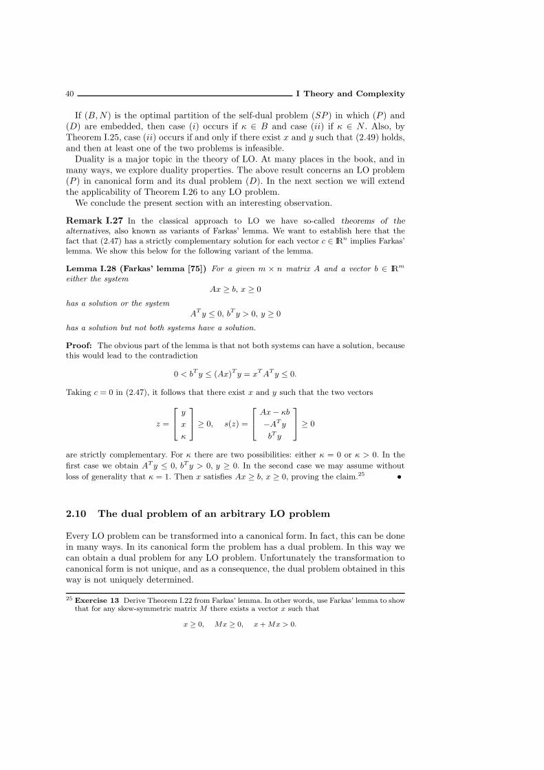
40 I Theory and Complexity
If (B,N) is the optimal partition of the self-dual problem (SP ) in which (P ) and(D) are embedded, then case (i) occurs if κ ∈ B and case (ii) if κ ∈ N . Also, byTheorem I.25, case (ii) occurs if and only if there exist x and y such that (2.49) holds,and then at least one of the two problems is infeasible.Duality is a major topic in the theory of LO. At many places in the book, and in
many ways, we explore duality properties. The above result concerns an LO problem(P ) in canonical form and its dual problem (D). In the next section we will extendthe applicability of Theorem I.26 to any LO problem.We conclude the present section with an interesting observation.
Remark I.27 In the classical approach to LO we have so-called theorems of the
alternatives, also known as variants of Farkas’ lemma. We want to establish here that thefact that (2.47) has a strictly complementary solution for each vector c ∈ IRn implies Farkas’lemma. We show this below for the following variant of the lemma.
Lemma I.28 (Farkas’ lemma [75]) For a given m × n matrix A and a vector b ∈ IRm
either the system
Ax ≥ b, x ≥ 0
has a solution or the system
AT y ≤ 0, bT y > 0, y ≥ 0
has a solution but not both systems have a solution.
Proof: The obvious part of the lemma is that not both systems can have a solution, becausethis would lead to the contradiction
0 < bT y ≤ (Ax)T y = xTAT y ≤ 0.
Taking c = 0 in (2.47), it follows that there exist x and y such that the two vectors
z =
y
x
κ
≥ 0, s(z) =
Ax− κb
−AT y
bT y
≥ 0
are strictly complementary. For κ there are two possibilities: either κ = 0 or κ > 0. In the
first case we obtain AT y ≤ 0, bT y > 0, y ≥ 0. In the second case we may assume without
loss of generality that κ = 1. Then x satisfies Ax ≥ b, x ≥ 0, proving the claim.25 •
2.10 The dual problem of an arbitrary LO problem
Every LO problem can be transformed into a canonical form. In fact, this can be donein many ways. In its canonical form the problem has a dual problem. In this way wecan obtain a dual problem for any LO problem. Unfortunately the transformation tocanonical form is not unique, and as a consequence, the dual problem obtained in thisway is not uniquely determined.
25 Exercise 13 Derive Theorem I.22 from Farkas’ lemma. In other words, use Farkas’ lemma to showthat for any skew-symmetric matrix M there exists a vector x such that
x ≥ 0, Mx ≥ 0, x+Mx > 0.

I.2 Duality Theory 41
The aim of this section is to show that we can find a dual problem for any givenproblem in a unique and simple way, so that when taking the dual of the dual problemwe get the original problem, in its original description.Recall that three types of variables can be distinguished: nonnegative variables, free
variables and nonpositive variables. Similarly, three types of constraints can occurin an LO problem: equality constraints, inequality constraints of the ≤ type andinequality constraints of the ≥ type. For our present purpose we need to consider theLO problem in its most general form, with all types of constraint and all types ofvariable. Therefore, we consider the following problem as the primal problem:
(P ) min
c0
c1
c2
T x0
x1
x2
:
A0x0 +A1x
1 +A2x2 = b0
B0x0 +B1x
1 +B2x2 ≥ b1
C0x0 + C1x
1 + C2x2 ≤ b2
, x1 ≥ 0, x2 ≤ 0
,
where, for each i = 0, 1, 2, Ai, Bi and Ci are matrices and bi, ci and xi are vectors,and the sizes of these matrices and vectors, which we do not further specify, are suchthat all expressions in the problem are well defined.Now let us determine the dual of this problem. We first put it into canonical form.26
To this end we replace the equality constraint by two inequality constraints and wemultiply the ≤ constraint by −1. Furthermore, we replace the nonpositive variable x2
by x3 = −x2 and the free variable x0 by x+ − x− with x+ and x− nonnegative. Thisyields the following equivalent problem:
minimize
c0
−c0c1
−c2
T
x+
x−
x1
x3
subject to
A0 −A0 A1 −A2
−A0 A0 −A1 A2
B0 −B0 B1 −B2
−C0 C0 −C1 C2
x+
x−
x1
x3
≥
b0
−b0b1
−b2
,
x+
x−
x1
x3
≥ 0.
In terms of vectors z1, z2, z3, z4 that contain the appropriate nonnegative dualvariables, the dual of this problem becomes
maximize
b0
−b0b1
−b2
T
z1
z2
z3
z4
26 The transformations carried out below lead to an increase of the numbers of constraints andvariables in the problem formulation. They are therefore ‘bad’ from a computational point of view.But our present purpose is purely theoretical. In Appendix D it is shown how the problem can beput in canonical form without increasing these numbers.

42 I Theory and Complexity
subject to
AT0 −AT
0 BT0 −CT
0
−AT0 AT
0 −BT0 CT
0
AT1 −AT
1 BT1 −CT
1
−AT2 AT
2 −BT2 CT
2
z1
z2
z3
z4
≤
c0
−c0c1
−c2
,
z1
z2
z3
z4
≥ 0.
We can easily check that the variables z1 and z2 only occur together in the combinationz1 − z2. Therefore, we can replace the variables by one free variable y0 := z1 − z2.This reduces the problem to
maximize
b0
b1
−b2
T y0
z3
z4
subject to
AT0 BT
0 −CT0
−AT0 −BT
0 CT0
AT1 BT
1 −CT1
−AT2 −BT
2 CT2
y0
z3
z4
≤
c0
−c0c1
−c2
,[z3
z4
]≥ 0.
In this problem the first two blocks of constraints can be taken together into one blockof equality constraints:
max
b0
b1
−b2
T y0
z3
z4
:
AT0 y
0 +BT0 z
3 − CT0 z
4 = c0
AT1 y
0 +BT1 z
3 − CT1 z
4 ≤ c1
−AT2 y
0 −BT2 z
3 + CT2 z
4 ≤ −c2,
[z3
z4
]≥ 0
.
Finally we multiply the last block of constraints by -1, we replace the nonnegativevariable z3 by y1 = z3 and the nonnegative variable z4 by the nonpositive variabley2 = −z4. This transforms the dual problem to its final form, namely
(D) max
b0
b1
b2
T y0
y1
y2
:
AT0 y
0 +BT0 y
1 + CT0 y
2 = c0
AT1 y
0 +BT1 y
1 + CT1 y
2 ≤ c1
AT2 y
0 +BT2 y
1 + CT2 y
2 ≥ c2, y1 ≥ 0, y2 ≤ 0
.
Comparison of the primal problem (P ) with its dual problem (D), in its finaldescription, reveals some simple rules for the construction of a dual problem forany given LO problem. First, the objective vector and the right-hand side vector areinterchanged in the two problems, and the constraint matrix is transposed. At firstsight it may not be obvious that the types of the dual variables and the dual constraintscan be determined. We need to realize that the vector y0 of dual variables relates tothe first block of constraints in the primal problem, y1 to the second block and y2 tothe third block of constraints. Then the relation becomes obvious: equality constraintsin the primal problem yield free variables in the dual problem, inequality constraintsin the primal problem of type ≥ yield nonnegative variables in the dual problem, andinequality constraints in the primal problem of type ≤ yield nonpositive variables inthe dual problem. For the types of dual constraint we have similar relations. Here the

I.2 Duality Theory 43
vector of primal variables x0 relates to the first block of constraints in the dual problem,x1 to the second block and x2 to the third block of constraints. Free variables in theprimal problem yield equality constraints in the dual problem, nonnegative variablesin the primal problem yield inequality constraints of type ≤ in the dual problem, andnonpositive variables in the primal problem yield inequality constraints of type ≥ inthe dual problem. Table 2.1. summarizes these observations, and as such provides asimple scheme for writing down a dual problem for any given minimization problem.To get the dual of a maximization problem, one simply has to use the table from theright to the left.
Primal problem (P) Dual problem (D)
min cTx max bT y
equality constraint free variable
inequality constraint ≥ variable ≥ 0
inequality constraint ≤ variable ≤ 0
free variable equality constraint
variable ≥ 0 inequality constraint ≤variable ≤ 0 inequality constraint ≥
Table 2.1. Scheme for dualizing.
As indicated before, the dualizing scheme is such that when it is applied twice, theoriginal problem is returned. This easily follows from Table 2.1., by inspection.27
2.11 Convergence of the central path
We already announced in footnote 23 (page 36) that the central path has a uniquelimit point in the optimal set. Because this result was not needed in the rest of thischapter, we postponed its proof to this section. We also characterize the limit pointas the so-called analytic center of the optimal set of (SP ).As before, we assume that the central path of (SP ) exists. Our aim is to investigate
the behavior of the central path as µ tends to 0. From the proof of Theorem I.20 weknow that the central path has a subsequence converging to an optimal solution. Thiswas sufficient for proving the existence of a strictly complementary solution of (SP ).However, as we show below, the central path itself converges. The limit point z∗ and
27 Exercise 14 Using the results of this chapter prove that the following three statements areequivalent:
(i) (SP ) satisfies the interior-point condition;
(ii) the level sets Lγ :=(z, s(z)) : qT z ≤ γ, s(z) =Mz + q ≥ 0, z ≥ 0
of qT z are bounded;
(iii) the optimal set of (SP ) is bounded.

44 I Theory and Complexity
its surplus vector s∗ := s(z∗) form a strictly complementary optimal solution pair,and hence determine the optimal partition (B,N) of (SP ).The optimal set of (SP ) is given by
SP∗ =(z, s) : Mz + q = s, z ≥ 0, s ≥ 0, qT z = 0
.
This makes clear that SP∗ is the intersection of the affine space(z, s) : Mz + q = s, qT z = 0
with the nonnegative orthant of IR2n.At this stage we need to define the analytic center of SP∗. We give the definition
for the more general case of an arbitrary (nonempty) set that is the intersection of anaffine space in IRp and the nonnegative orthant of IRp.
Definition I.29 (Analytic center) 28 Let the nonempty and bounded set T be theintersection of an affine space in IRp with the nonnegative orthant of IRp. We definethe support σ(T ) of T as the subset of the full index set 1, 2, . . . , p given by
σ(T ) = i : ∃x ∈ T such that xi > 0 .The analytic center of T is defined as the zero vector if σ(T ) is empty; otherwise it isthe vector in T that maximizes the product
∏
i∈σ(T )
xi, x ∈ T . (2.51)
If the support of the set T in the above definition is nonempty then the convexity ofT implies the existence of a vector x ∈ T such that xσ(T ) > 0. Moreover, if σ(T ) isnonempty then the maximum value of the product (2.51) exists since T is bounded.Since the logarithm of the product (2.51) is strictly concave, the maximum value (if itexists) is attained at a unique point of T . Thus the above definition uniquely definesthe analytic center for any bounded subset that is the intersection of an affine spacein IRp with the nonnegative orthant of IRp.Due to Lemma I.9 any pair (z, s) ∈ SP∗ satisfies
eT z + eT s(z) = n.
This makes clear that the optimal set SP∗ is bounded. Its analytic center thereforeexists. We now show that the central path converges to this analytic center. The proofvery much resembles that of Theorem I.20.29
28 The notion of analytic center of a polyhedron was introduced by Sonnevend [257]. It plays a crucialrole in the theory of interior-point methods.
29 The limiting behavior of the central path as µ approaches zero has been an important subject inresearch on interior-point methods for a long time. In the book by Fiacco and McCormick [77]the convergence of the central path to an optimal solution is investigated for general convexoptimization problems. McLinden [197] considered the limiting behavior of the path for monotonecomplementarity problems and introduced the idea for the proof-technique of Theorem I.20, whichwas later adapted by Guler and Ye [135]. Megiddo [200] extensively investigated the properties ofthe central path, which motivated Monteiro and Adler [218], Tanabe [261] and Kojima, Mizunoand Yoshise [178] to investigate primal-dual methods. Other relevant references for the limitingbehavior of the central path are Adler and Monteiro [3], Asic, Kovacevic-Vujcic and Radosavljevic-Nikolic [28], Guler [131], Kojima, Mizuno and Noma [176], Monteiro and Tsuchiya [222] andWitzgall, Boggs and Domich [294], Halicka [137], Wechs [290] and Zhao and Zhu [321].

I.2 Duality Theory 45
Theorem I.30 The central path converges to the analytic center of the optimal setSP∗ of (SP ).
Proof: Let (z∗, s∗) be an accumulation point of the central path, where s∗ = s(z∗).The existence of such a point has been established in the proof of Theorem I.20. Letµk∞k=1 be a positive sequence such that µk → 0 and such that (z(µk), s(µk)), withs(µk) = s(z(µk)), converges to (z∗, s∗). Then z∗ is optimal, which means z∗s∗ = 0,and z∗ and s∗ are strictly complementary, i.e, z∗ + s∗ > 0.Now let z be optimal in (SP ) and let s = Mz + q be its surplus vector. Applying
the orthogonality property (2.22) to the points z and z(µ) we obtain
(z(µk)− z)T (s(µk)− s) = 0.
Rearranging terms and using z(µk)T s(µk) = nµk and (z)T s = 0, we get
n∑
j=1
zjsj(µk) +n∑
j=1
sjzj(µk) = nµk.
Since the pair (z∗, s∗) is strictly complementary and (z, s) is an arbitrary optimal pair,we have for each coordinate j:
z∗j = 0 ⇒ zj = 0, s∗j = 0 ⇒ sj = 0.
Hence, zj = 0 if j /∈ σ(z∗) and sj = 0 if j /∈ σ(s∗). Thus we may write∑
j∈σ(z∗)
zjsj(µk) +∑
j∈σ(s∗)
sjzj(µk) = nµk.
Dividing both sides by µk = zj(µk)sj(µk), we get
∑
j∈σ(z∗)
zjzj(µk)
+∑
j∈σ(s∗)
sjsj(µk)
= n.
Letting k → ∞, it follows that
∑
j∈σ(z∗)
zjz∗j
+∑
j∈σ(s∗)
sjs∗j
= n.
Using the arithmetic-geometric-mean inequality we obtain
∏
j∈σ(z∗)
zjz∗j
∏
j∈σ(s∗)
sjs∗j
1/n
≤ 1
n
∑
j∈σ(z∗)
zjz∗j
+∑
j∈σ(s∗)
sjs∗j
= 1.
Obviously, the above inequality implies∏
j∈σ(z∗)
zj∏
j∈σ(s∗)
sj ≤∏
j∈σ(z∗)
z∗j∏
j∈σ(s∗)
s∗j .
This shows that (z∗, s∗) maximizes the product∏
j∈σ(z∗) zj∏
j∈σ(s∗) sj over the
optimal set. Hence the central path of (SP ) has only one accumulation point when µapproaches zero and this is the analytic center of SP∗.

46 I Theory and Complexity
Example I.31 Let us compute the limit point of the central path of the self-dualproblem (SP ) in Example I.7, as given by (2.19). Recall from (2.26) in Example I.12that any optimal solution has the form
z =
2κ
0
κ
κ
0
, s(z) =
0
κ
0
0
5− 5κ
, 0 ≤ κ ≤ 1,
from which the sets B and N follow:
B = 1, 3, 4 , N = 2, 5 .
Hence we have for any optimal z,
∏
j∈B
zj∏
j∈N
sj(z) = 2κ4 (5− 5κ) = 10(κ4 − κ5
).
This product is maximal for κ = 0.8, so the analytical center of the optimal set isgiven by 30,31,32,33
z =
1.6
0
0.8
0.8
0
, s(z) =
0
0.8
0
0
1
.
♦
The convergence of the central path when µ goes to zero implies the boundedness ofthe coordinates of z(µ) and s(µ) for any finite section of the central path. Of course,this also follows from Lemma I.9 and (2.33).34
30Exercise 15 Find the analytic center of the self-dual problem considered in Exercise 4 (page 27).
31Exercise 16 Find the analytic center of the self-dual problem considered in Exercise 5 (page 27).
32Exercise 17 Find the analytic center of the self-dual problem considered in Exercise 6 (page 27).
33Exercise 18 Find the analytic center of the self-dual problem considered in Exercise 7 (page 27).
34 Exercise 19 For any positive µ consider the set
SPµ :=(z, s) : Mz + q = s, z ≥ 0, s ≥ 0, qT z = qT z(µ)
.
Using the same proof-technique as for Theorem I.30, show that the pair (z(µ), s(µ)) is the analyticcenter of this set.

3
A Polynomial Algorithm for theSelf-dual Model
3.1 Introduction
The previous chapter made clear that any (canonical) LO problem can be solved byfinding a strictly complementary solution of a specific self-dual problem that satisfiesthe interior-point assumption. In particular, the self-dual problem has the form
(SP ) minqT z : Mz ≥ −q, z ≥ 0
,
where M is a skew-symmetric matrix and q a nonnegative vector. Deviating from thenotation in Chapter 2 we denote the order of M as n (instead of n). Then, accordingto (2.12) the vector q has the form
q :=
[0n−1
n
]. (3.1)
Note that due to the definition of the matrix M we may assume that n ≥ 5.Like before, we associate to any vector z ∈ IRn its slack vector s(z):
s(z) :=Mz + q. (3.2)
As a consequence we have
z is a feasible for (SP ) if and only if z ≥ 0 and s(z) ≥ 0.
Also recall that the all-one vector e is feasible for (SP ) and its slack vector is theall-one vector (cf. Theorem I.5):
s(e) = e. (3.3)
Assuming that the entries inM and q are integral (or rational), we show in this chapterthat we can find a strictly complementary solution of (SP ) in polynomial time. Thismeans that we present an algorithm that yields a strictly complementary solution of(SP ) after a number of arithmetic operations that is bounded by a polynomial in thesize of (SP ).
Remark I.32 The terminology is taken from complexity theory. For our purpose it is notnecessary to have a deep understanding of this theory. Major contributions to complexity

48 I Theory and Complexity
theory were given by Cook [56], Karp [166], Aho, Hopcroft and Ullman [5], and Garey andJohnson [92]. For a survey focusing on linear and combinatorial optimization problems werefer the reader to Schrijver [250]. Complexity theory distinguishes between easy and hardproblems. In this theory a problem consists of a class of problem instances, so ‘the’ LOproblem consists of all possible instances of LO problems; here we restrict ourselves to LOproblems with integral input data.1 A problem is called solvable in polynomial time (or simplypolynomial or easy) if there exists an algorithm that solves each instance of the problem ina time that is bounded above by a polynomial in the size of the problem instance; otherwisethe problem is considered to be hard. In general the size of an instance is defined as thelength of a binary string encoding the instance. For the problem (SP ) such a string consistsof binary encodings of the entries in the matrix M and the vector q. Note that the binaryencoding of a positive integer a requires a string of length 1 + ⌈log2(1 + |a|)⌉. (The first 1serves to encode the sign of the number.) If the entries in M and q are integral, the totallength of the string for encoding (SP ) becomes
n∑
i=1
(1 + ⌈log2 (1 + |qi|)⌉) +n∑
i,j=1
(1 + ⌈log2 (1 + |Mij |)⌉) =
n(n+ 1) +
n∑
i=1
⌈log2 (1 + |qi|)⌉ +n∑
i,j=1
⌈log2 (1 + |Mij |)⌉ . (3.4)
Instead we work with the smaller number
L = n(n+ 1) + log2 Π, (3.5)
where Π is the product of all nonzero entries in q and M . Ignoring the integrality operators,
we can show that the expression in (3.4) is less than 2L. In fact, one can easily understand
that the number of operations of an algorithm is polynomial in (3.4) if and only if it is
bounded by a polynomial in L. •We consider the number L, as given by (3.5), as the size of (SP ). In fact we use
this number only once. In the next section we present an algorithm that generates apositive vector z such that zT s(z) ≤ ε, where ε is any positive number, and we derivea bound for the number of iterations required by the algorithm. Then, in Section 3.3,we show that this algorithm can be used to find a strictly complementary solution of(SP ) and we derive an iteration bound that depends on the so-called condition number
of (SP ). Finally, we show that the iteration bound can be bounded from above by apolynomial in the quantity L, which represents the size of (SP ).
3.2 Finding an ε-solution
After all the theoretical results of the previous sections we are now ready to presentan algorithm that finds a strictly complementary solution of (SP ) in polynomial time.The working horse in the algorithm is the Newton step that was introduced in Section2.7.2. It will be convenient to recall its definition and some of its properties.
1 We could easily have included LO problems with rational input data in our considerations, becauseif the entries in M and q are rational numbers then after multiplication of these entries with theirsmallest common multiple, all entries become integral. Thus, each problem instance with rationaldata can easily be transformed to an equivalent problem with integral data.

I.3 Polynomial Algorithm 49
Given a positive vector z such that s = s(z) > 0, the Newton direction ∆z at zwith respect to µ (or the µ-center z(µ)) is uniquely determined by the linear system(cf. (2.35) – (2.36))
M∆z −∆s = 0, (3.6)
z∆s+ s∆z = µe− zs. (3.7)
Substituting (3.6) into (3.7) we get 2
(S + ZM)∆z = µe− zs.
Since the matrix S + ZM is invertible (cf. Exercise 9, page 29), it follows that
∆z = (S + ZM)−1
(µe − zs) (3.8)
∆s = M∆z. (3.9)
The result of the Newton step is denoted as
z+ := z +∆z;
the new slack vector is then given by
s+ := s(z+) =M(z +∆z) + q = s+M∆z.
The vectors ∆z and ∆s are orthogonal, by (2.34). After the Newton step the objectivevalue has the desired value nµ, by (2.38):
qT z = sT z = nµ. (3.10)
The variance vector of z with respect to µ is defined by (cf. (2.41))3:
v :=
√zs(z)
µ. (3.11)
This implieszs(z) = µe ⇔ v = e. (3.12)
We use δ(z, µ) as a measure for the proximity of z to z(µ). It is defined by (cf. (2.42))
δ(z, µ) := 12
∥∥v − v−1∥∥ . (3.13)
If z = z(µ) then v = e and hence δ(z, µ) = 0, otherwise δ(z, µ) > 0. If δ(z, µ) < 1then the Newton step is feasible, and if δ(z, µ) < 1/
√2 then the Newton process
quadratically fast converges to z(µ). This is a consequence of the next lemma (cf.Theorem I.16).
Lemma I.33 If δ := δ(z, µ) < 1, then the Newton step is strictly feasible, i.e., z+ > 0and s+ > 0. Moreover,
δ(z+, µ) ≤ δ2√2(1− δ2)
.
2 Here, as usual, Z = diag (z) and S = diag (s).3
Exercise 20 If we define d :=√z/s, where s = s(z), then show that the Newton step ∆z satisfies
(I +DMD)∆z =z
v
(v−1 − v
)= µs−1 − z.

50 I Theory and Complexity
3.2.1 Newton-step algorithm
The idea of the algorithm is quite simple. Starting at z = e, we choose µ < 1 suchthat
δ(z, µ) ≤ 1√2, (3.14)
and perform a Newton step targeting at z(µ). After the step the new iterate zsatisfies δ(z, µ) ≤ 1
2 . Then we decrease µ such that (3.14) holds for the new valuesof z and µ, and repeat the procedure. Note that after each Newton step we haveqT z = zT s(z) = nµ. Thus, if µ approaches zero, then z will approach the set ofoptimal solutions. Formally the algorithm can be stated as follows.
Full-Newton step algorithm
Input:An accuracy parameter ε > 0;a barrier update parameter θ, 0 < θ < 1.
beginz = e; µ := 1;while nµ ≥ ε dobegin
µ := (1− θ)µ;z := z +∆z;
endend
Note that the reduction of the barrier parameter µ is realized by the multiplicationwith the factor 1 − θ. In the next section we discuss how an appropriate value of theupdate parameter θ can be obtained, so that during the course of the algorithm theiterates are kept within the region where Newton’s method is quadratically convergent.
3.2.2 Complexity analysis
At the start of the algorithm we have µ = 1 and z = z(1) = e, whence qT z = n andδ(z, µ) = 0. In each iteration µ is first reduced with the factor 1 − θ and then theNewton step is made targeting the new µ-center. It will be clear that the reductionof µ has effect on the value of the proximity measure. This effect is fully described bythe following lemma.
Lemma I.34 Let z > 0 and µ > 0 be such that s = s(z) > 0 and qT z = nµ. Moreover,let δ := δ(z, µ) and µ′ = (1− θ)µ. Then
δ(z, µ′)2 = (1 − θ)δ2 +θ2n
4(1− θ).

I.3 Polynomial Algorithm 51
Proof: Let δ+ := δ(z, µ′) and v =√zs/µ, as in (3.11). Then, by definition,
4(δ+)2 =
∥∥∥∥√1− θ v−1 − v√
1− θ
∥∥∥∥2
=
∥∥∥∥√1− θ
(v−1 − v
)− θv√
1− θ
∥∥∥∥2
.
From zT s = nµ it follows that ‖v‖2 = n. This implies
vT(v−1 − v
)= n− ‖v‖2 = 0.
Hence, v is orthogonal to v−1 − v. Therefore,
4(δ+)2 = (1 − θ)∥∥v−1 − v
∥∥2 + θ2 ‖v‖21− θ
= (1 − θ)∥∥v−1 − v
∥∥2 + nθ2
1− θ.
Since∥∥v−1 − v
∥∥ = 2δ, the result follows.
Lemma I.35 Let θ = 1√2n
. Then at the start of each iteration we have
qT z = nµ and δ(z, µ) ≤ 1
2(3.15)
Proof: At the start of the first iteration we have µ = 1 and z = e, so qT z = n andδ(z, µ) = 0. Therefore (3.15) certainly holds at the start of the first iteration. Nowsuppose that (3.15) holds at the start of some iteration. We show that (3.15) then alsoholds at the start of the next iteration. Let δ = δ(z, µ). When the barrier parameteris updated to µ′ = (1− θ)µ, Lemma I.34 gives
δ(z, µ′)2 = (1− θ) δ2 +θ2n
4(1− θ)≤ 1− θ
4+
1
8(1− θ)≤ 3
8.
The last inequality can be understood as follows. Due to n ≥ 2 we have 0 ≤ θ ≤1/
√4 = 1/2. The left hand side expression in the last inequality is a convex function
of θ. Its value at θ = 0 as well as at θ = 1/2 equals 3/8, hence its value does notexceed 3/8 for θ ∈ [0, 1/2].Since 3/8 ≤ 1/2, it follows that after the µ-update δ(z, µ′) ≤ 1/
√2. Hence, by
Lemma I.33, after performing the Newton step we certainly have δ(z+, µ′) ≤ 1/2.Finally, by (3.10), qT z+ = nµ′. Thus the lemma has been proved.
How many iterations are needed by the algorithm? The answer is provided by thefollowing lemma.
Lemma I.36 After at most ⌈1
θlog
n
ε
⌉
iterations we have nµ ≤ ε.
Proof: Initially, the objective value is n and in each iteration it is reduced by thefactor 1 − θ. Hence, after k iterations we have µ = (1 − θ)k. Therefore, the objectivevalue, given by qT z(µ) = nµ, is smaller than, or equal to ε if
(1− θ)kn ≤ ε.

52 I Theory and Complexity
Taking logarithms, this becomes
k log (1− θ) + logn ≤ log ε.
Since − log (1− θ) ≥ θ, this certainly holds if
kθ ≥ logn− log ε = logn
ε.
This implies the lemma.
The above results are summarized in the next theorem which requires no furtherproof.
Theorem I.37 If θ = 1√2n
then the algorithm requires at most
⌈√2n log
n
ε
⌉
iterations. The output is a feasible z > 0 such that qT z = nµ ≤ ε and δ(z, µ) ≤ 12 .
This theorem shows that we can get an ε-solution z of our self-dual model with ε assmall as desirable.4
A crucial question for us is whether the variable κ = zn−1 is positive or zero inthe limit, when µ goes to zero. In practice, for small enough ε it is usually no seriousproblem to decide which of the two cases occurs. In theory, however, this means thatwe need to know what the optimal partition of the problem is. As we explain in thenext section, the optimal partition can be found in polynomial time. This requiressome further analysis of the central path.
Example I.38 In this example we demonstrate the behavior of the Full-Newton stepalgorithm by applying it to the problem (SP ) in Example I.7, as given in (2.19) onpage 23. According to Theorem I.37, with n = 5, the algorithm requires at most
⌈√10 log
5
ε
⌉
iterations. For ε = 10−3 we have log (5/ε) = log 5000 = 8.5172, and we get 27 as anupper bound for the number of iterations. When running the algorithm with this εthe actual number of iterations is 22. The actual values of the output of the algorithmare
z = (1.5999, 0.0002, 0.8000, 0.8000, 0.0002)T
and
s(z) = (0.0001, 0.8000, 0.0002, 0.0002, 1.0000)T .
The left plot in Figure 3.1 shows how the coordinates of the vector z := (z1, z2, z3, z4 =κ, z5 = ϑ), which contains the variables in the problem, develop in the course of thealgorithm. The right plot does the same for the coordinates of the surplus vectors(z) := (s1, s2, s3, s4, s5). Observe that z and s(z) converge nicely to the limit pointof the central path of the sample problem as given in Example I.31. ♦
4 It is worth pointing out that if we put ε = nµ in the iteration bound of Theorem I.37 we getexactly the same bound as given by (2.45).

I.3 Polynomial Algorithm 53
0 5 10 15 200
0.2
0.4
0.6
0.8
1
1.2
1.4
1.6
0 5 10 15 200
0.2
0.4
0.6
0.8
1
1.2
1.4
1.6
iteration numberiteration number
z1
z2
z3
κ
ϑ
s1
s2
s3
s4
s5
Figure 3.1 Output Full-Newton step algorithm for the problem in Example I.7.
3.3 Polynomial complexity result
3.3.1 Introduction
Having a strictly complementary solution z of (SP ), we also know the optimal partition(B,N) of (SP ), as defined in Section 2.6. For if z is a strictly complementary solutionof (SP ) then we have zs(z) = 0 and z + s(z) > 0, and the optimal partition followsfrom5
B = i : zi > 0N = i : si(z) > 0 .
Definition I.39 The restriction of a vector z ∈ IRn to the coordinates in a subset Iof the full index set 1, 2, . . . , n is denoted by zI .
Hence if z is a strictly complementary solution of (SP ) then
zB > 0, zN = 0, sB(z) = 0, sN (z) > 0.
Now let z be any feasible solution of (SP ). Then, by Lemma I.10, with z1 = z, z2 = zwe obtain that z is optimal if and only if zs(z) = zs(z) = 0. This gives
z is optimal for (SP ) ⇐⇒ zN = 0 and sB(z) = 0.
5 It may be sensible to point out that if, conversely, the optimal partition is known, then it is notobvious at all how to find a strictly complementary solution of (SP ).

54 I Theory and Complexity
As a consequence, the set SP∗ of optimal solutions of (SP ) is completely determinedby the optimal partition (B,N) of (SP ). We thus may write
SP∗ = z ∈ SP : zN = 0, sB(z) = 0 ,
where SP denotes the feasible region of (SP ).Assuming that M and q are integral we show in this section that a strictly
complementary solution of (SP ) can be found in polynomial time. We divide thework into a few steps. First we apply the Full-Newton step algorithm with a suitable(small enough) value of the accuracy parameter ε. This yields a positive solution zof (SP ) such that s(z) is positive as well and such that the pair (z, s(z)) is almoststrictly complementary in the sense that for each index i one of the positive coordinatesin the pair (zi, si(z)) is large and the other is small. To distinguish between ‘large’and ‘small’ coordinates we introduce the so-called condition number of (SP ). Weare able to specify ε such that the large coordinates of z are in B and the smallcoordinates of z in N . The optimal partition of (SP ) can thus be derived fromthe almost strictly complementary solution z provided by the algorithm. Then, inSection 3.3.6, a rounding procedure is described that yields a strictly complementarysolution of (SP ) in polynomial time.
3.3.2 Condition number
Below, (B,N) always denotes the optimal partition of (SP ), and SP∗ the optimal setof (SP ). We first introduce the following two numbers:
σzSP := min
i∈Bmaxz∈SP∗
zi , σsSP := min
i∈Nmaxz∈SP∗
si(z) .
By convention we take σzSP = ∞ if B is empty and σs
SP = ∞ if N is empty. Since theoptimal set SP∗ is bounded, σz
SP is finite if B is nonempty and σsSP is finite if N is
nonempty. Due to the definition of the sets B and N both numbers are positive, andsince B and N cannot be both empty at least one of the two numbers is finite. As aconsequence, the number
σSP := min σzSP , σ
sSP
is positive and finite. This number plays a crucial role in the further analysis and iscalled the condition number of (SP ).6 Using that z and s(z) are complementary ifz ∈ SP∗ we can easily verify that σSP can also be written as
σSP := min1≤i≤n
maxz∈SP∗
zi + si(z) .
Example I.40 Let us calculate the condition number of our sample problem (2.19)in Example I.7. We found in Example I.12 that any optimal solution z has the form
6 This condition number seems to be a natural quantity for measuring the degree of hardness of(SP ). The smaller the number the more difficult it is to find a strictly complementary solution.In a more general context, it was introduced by Ye [311]. See also Ye and Pardalos [314]. For adiscussion of other condition numbers and their relation to the size of a problem we refer the readerto Vavasis and Ye [280].

I.3 Polynomial Algorithm 55
as given by (2.26), namely
z =
2κ
0
κ
κ
0
, s(z) =
0
κ
0
0
5− 5κ
, 0 ≤ κ ≤ 1.
Hence we have for any optimal z,
z + s(z) =
2κ
κ
κ
κ
5− 5κ
, 0 ≤ κ ≤ 1.
To find the condition number we need to find the maximum values of each of thevariables in in this vector. These values are 2, 1, 1, 1 (for κ = 1) and 5 (for κ = 0),respectively. The minimum of these maximal values being 1, the condition number ofour sample problem (2.19) turns out to be 1.7,8,9,10 ♦
In the above example we were able to calculate the condition number of a givenproblem. We see below that when we know the condition number of a problem wecan profit from it in the solution procedure. In general, however, the calculation ofthe condition number is at least as hard as solving the problem. Hence, in general, wehave to solve a problem without knowing its condition number. In such cases there isa cheap way to get a lower bound for the condition number. We proceed by derivingsuch a lower bound for σSP in terms of the data of the problem (SP ). We introducesome more notation.
Definition I.41 The submatrix of M consisting of the elements in the rows whoseindices are in I and the columns whose indices are in J is denoted by MIJ .
Using this convention, we have for any vector z and its surplus vector s = s(z): sBsN
=
MBB MBN
MNB MNN
zBzN
+
qBqN
. (3.16)
Recall from the previous section that the vector z is optimal if and only if z and s arenonnegative, zN = 0 and sB = 0. Hence we have qT z = qTBzB. Due to the existence of
7Exercise 21 Using the results of Exercise 4 (page 27), prove that the condition number of theself-dual problem in question equals 5/4.
8Exercise 22 Using the results of Exercise 5 (page 27), prove that the condition number of theself-dual problem in question equals 5/4.
9Exercise 23 Using the results of Exercise 6 (page 27), prove that the condition number of theself-dual problem in question equals 5/(1 + β) if β ≥ 2 and otherwise 5β/(2(1 + β)).
10Exercise 24 Using the results of Exercise 7 (page 27), prove that the condition number of theself-dual problem in question equals 5/(4 − β) if β ≤ −1 and otherwise −5β/(4 − β).

56 I Theory and Complexity
a strictly complementary solution z, for which zB is positive, we conclude that
qB = 0. (3.17)
Thus it becomes clear that a vector z and its surplus vector s are optimal for (SP ) ifand only if zB ≥ 0, zN = 0, sB = 0, sN ≥ 0 and
0
sN
=
MBB MBN
MNB MNN
zB
0
+
0
qN
.
This is equivalent toMBB 0BN
MNB −INN
zBsN
=
0B
−qN
, zB ≥ 0, zN = 0, sB = 0, sN ≥ 0. (3.18)
Note that any strictly complementary solution z gives rise to a positive solution ofthis system. For the calculation of σSP we need to know the maximal value of eachcoordinate of the vector (zB, sN ) when this vector runs through all possible solutionsof (3.18). Then σSP is just the smallest of all these maximal values.At this stage we may apply Lemma C.1 in Appendix C to (3.18), which gives us an
easy to compute lower bound for σSP .
Theorem I.42 The condition number σSP of (SP ) satisfies
σSP ≥ 1∏nj=1 ‖Mj‖
,
where Mj denotes the j-th column of M .
Proof: Recall that the optimal set of (SP ) is determined by the equation (3.18). Also,by Lemma I.9 we have eT z + eT s(z) = n, showing that the optimal set is bounded.As we just established, the system (3.18) has a positive solution, and hence we mayapply Lemma C.1 to (3.18) with
A =
(MBB 0BN
MNB −INN
).
The columns in A made up by the two left blocks are the columns Mj of M withj ∈ B, whereas the columns made up by the two right blocks are unit vectors. Thuswe obtain that the maximal value of each coordinate of the vector (zB, sN ) is boundedbelow by the quantity
1∏j∈B ‖Mj‖
.
With the definition of σSP this implies
σSP ≥ 1∏j∈B ‖Mj‖
≥ 1∏nj=1 ‖Mj‖
.
The last inequality is an obvious consequence of the assumption that all columns inM are nonzero and integral. Hence the theorem has been proved.

I.3 Polynomial Algorithm 57
3.3.3 Large and small variables
It will be convenient to call the coordinates of z(µ) that are indexed by B thelarge coordinates of z(µ), and the other coordinates the small coordinates of z(µ).Furthermore, the coordinates of sN (µ) are called the large coordinates of s(µ), andthe coordinates of sB(µ) small coordinates of s(µ). The next lemma provides lowerbounds for the large coordinates and upper bounds for the small coordinates of z(µ)and s(µ). This lemma implies that the large coordinates of z(µ) and s(µ) are boundedaway from zero along the central path, and there exists a uniform lower bound that isindependent of µ. Moreover, the small coordinates are bounded above by a constanttimes µ, where the constant depends only on the data in the problem (SP ). In otherwords, the order of magnitude of the small coordinates is O(µ). The bounds in thelemma use the condition number σSP of (SP ).
Lemma I.43 For any positive µ we have
zi(µ) ≥σSP
n, i ∈ B,
si(µ) ≤nµ
σSP, i ∈ B,
zi(µ) ≤nµ
σSP, i ∈ N,
si(µ) ≥σSP
n, i ∈ N.
Proof: First let i ∈ N and let z be an optimal solution such that si := si(z) ismaximal. Then the definition of the condition number σSP implies that si ≥ σSP .Applying the orthogonality property (2.22) to the points z and z(µ) we obtain
(z(µ)− z)T (s(µ)− s) = 0,
which givesz(µ)T s+ s(µ)T z = nµ.
This implieszi(µ)si ≤ z(µ)T s ≤ nµ.
Dividing by si and using that si ≥ σSP we obtain
zi(µ) ≤nµ
si≤ nµ
σSP.
Since zi(µ)si(µ) = µ, it also follows that
si(µ) ≥σSP
n.
This proves the second and fourth inequality in the lemma. The other inequalities areobtained in the same way. Let i ∈ B and let z be an optimal solution such that ziis maximal. Then the definition of the condition number σSP implies that zi ≥ σSP .Applying the orthogonality property to the points z and z(µ) we obtain in the sameway as before
si(µ)zi ≤ s(µ)T z ≤ nµ.
From this we deduce thatsi(µ) ≤
nµ
zi≤ nµ
σSP.

58 I Theory and Complexity
Using once more z(µ)s(µ) = µe we find
zi(µ) ≥σSP
n,
completing the proof of the lemma.11,12
We collect the results of the above lemma in Table 3.1..
i ∈ B i ∈ N
zi(µ) ≥ σSP
n ≤ nµσSP
si(µ) ≤ nµσSP
≥ σSP
n
Table 3.1. Estimates for large and small variables on the central path.
The lemma has an important consequence. If µ is so small that
nµ
σSP<σSP
n
then we have a complete separation of the small and the large variables. This meansthat if a point z(µ) on the central path is given so that
µ <σSP
2
n2,
then we can determine the optimal partition (B,N) of (SP ).In the next section we show that the Full-Newton step algorithm can produce a
point z in the neighborhood of the central path with this feature, namely that it givesa complete separation of the small and the large variables.
3.3.4 Finding the optimal partition
Theorem I.37 states that after at most⌈√
2n logn
ε
⌉(3.19)
11Exercise 25 Let 0 < µ < µ. Using the orthogonality property (2.22), show that for each i(1 ≤ i ≤ n),
zi(µ)
zi(µ)+si(µ)
si(µ)≤ 2n.
12 The result in Exercise 25 can be improved to
zi(µ)
zi(µ)+si(µ)
si(µ)≤ n,
which implieszi(µ) ≤ nzi(µ), si(µ) ≤ nsi(µ).
For a proof we refer the reader to Vavasis and Ye [281].

I.3 Polynomial Algorithm 59
iterations the Full-Newton step algorithm yields a feasible solution z such thatqT z = nµ ≤ ε and δ(z, µ) ≤ 1
2 . We show in this section that if µ is small enoughwe can recognize the optimal partition (B,N) from z, and such z can be found ina number of iterations that depends only on the dimension n and on the conditionnumber σSP of (SP ).We need a simple measure for the distance of z to the central path. To this end, for
each positive feasible vector z with s(z) > 0, we define the number δc(z) as follows:
δc(z) :=max (zs(z))
min (zs(z)). (3.20)
Observe that δc(z) = 1 if and only if zs(z) is a multiple of the all-one vector e. Thisoccurs precisely if z lies on the central path. Otherwise we have δc(z) > 1. We considerδc(z) as an indicator for the ‘distance’ of z to the central path.13
Lemma I.44 If δ(z, µ) ≤ 12 then δc(z) ≤ 4.
Proof: Using the variance vector v of z, with respect to the given µ > 0, we maywrite
δc(z) =max
(µv2)
min (µv2)=
max(v2)
min (v2).
Using (3.13), it follows from δ(z, µ) ≤ 12 that
∥∥v − v−1∥∥ ≤ 1.
Without loss of generality we assume that the coordinates of v are ordered such that
v1 ≥ v2 ≥ . . . ≥ vn.
Then δc(z) = v21/v2n. Now consider the problem
max
v21v2n
:∥∥v − v−1
∥∥ ≤ 1
.
The optimal value of this problem is an upper bound for δc(z). One may easily verifythat the optimal solution has vi = 1 if 1 < i < n, v1 =
√2 and vn = 1/
√2. Hence the
optimal value is 4.14 This proves the lemma.
13 In the analysis of interior-point methods we always need to introduce a quantity that measures the‘distance’ of a feasible vector x to the central path. This can be done in many ways as becomesapparent in the course of this book. In the coming chapters we make use of a variety of so-calledproximity measures. All these measures are based on the simple observation that x is on the centralpath if and only if the vector xs(x) is a scalar multiple of the all-one vector.
14 Exercise 26 Prove that
max
v21v2n
:
n∑
i=1
(vi −
1
vi
)2
≤ 1
= 4.

60 I Theory and Complexity
Lemma I.45 Let z be a feasible solution of (SP ) such that δc(z) ≤ τ . Then, withs = s(z), we have
zi ≥σSP
τn, i ∈ B,
si ≤zT s
σSP, i ∈ B,
zi ≤zT s
σSP, i ∈ N,
si ≥σSP
τn, i ∈ N.
Proof: The proof is basically the same as the proof of Lemma I.43. It is a little morecomplicated because the estimates now concern a point off the central path. Fromδc(z) ≤ τ we conclude that there exist positive numbers τ1 and τ2 such that ττ1 = τ2and
τ1 ≤ zisi ≤ τ2, 1 ≤ i ≤ n. (3.21)
When we realize that these inequalities replace the role of the identity zi(µ)si(µ) = µin the proof of Lemma I.43 the generalization becomes almost straightforward. Firstsuppose that i ∈ N and let z be an optimal solution such that si := si(z) ismaximal. Then, from to the definition of σSP , it follows that si ≥ σSP . Applyingthe orthogonality property (2.22) to the points z and z, we obtain in the same way asbefore
zisi ≤ zT s ≤ zT s.
Hence, dividing both sides by si and using that si ≥ σSP we get
zi ≤zT s
σSP.
From the left inequality in (3.21) we also have zisi ≥ τ1. Hence we must have
si ≥τ1σSP
zT s.
The right inequality in (3.21) gives zT s ≤ nτ2. Thus
si ≥τ1σSP
nτ2=σSP
nτ.
This proves the second and fourth inequality in the lemma. The other inequalitiesare obtained in the same way. If i ∈ B and z is an optimal solution such that zi ismaximal, then zi ≥ σSP . Applying the orthogonality property (2.22) to the points zand z we obtain
sizi ≤ sT z ≤ zT s.
Thus we get
si ≤zT s
zi≤ zT s
σSP.
Using once more that zisi ≥ τ1 and zT s ≤ nτ2 we obtain
zi ≥τ1σSP
zT s≥ τ1σSP
nτ2=σSP
nτ,
completing the proof of the lemma.

I.3 Polynomial Algorithm 61
i ∈ B i ∈ N
zi ≥ σSP
τn ≤ zT sσSP
si(z) ≤ zT sσSP
≥ σSP
τn
Table 3.2. Estimates for large and small variables if δc(z) ≤ τ .
The results of the above lemma are shown in Table 3.2.. We conclude that if zT sis so small that
zT s
σSP<σSP
τn
then we have a complete separation of the small and the large variables. Thus we maystate without further proof the following result.
Lemma I.46 Let z be a feasible solution of (SP ) such that δc(z) ≤ τ . If
zT s(z) <σSP
2
τn
then the optimal partition of (SP ) follows from
B = i : zi > si(z) and N = i : zi < si(z) . (3.22)
This lemma is the basis of our next result.
Theorem I.47 After at most
⌈√2n log
4n2
σSP2
⌉(3.23)
iterations, the Full-Newton step algorithm yields a feasible (and positive) solution z of(SP ) that reveals the optimal partition (B,N) of (SP ) according to (3.22).
Proof: Let us run the Full-Newton step algorithm with ε = σ2SP / (4n). Then Theorem
I.37 states that we obtain a feasible z with zT s(z) ≤ σ2SP / (4n) and δ(z, µ) ≤ 1/2.
Lemma I.44 implies that δc(z) ≤ 4. By Lemma I.46, with τ = 4, this z gives a completeseparation between the small variables and the large variables. By Theorem I.37, therequired number of iterations for the given ε is at most
⌈√2n log
4n2
σSP2
⌉
which is equal to the bound given in the theorem. Thus the proof is complete.
62 I Theory and Complexity
Example I.48 Let us apply Theorem I.47 to the self-dual problem (2.19) in ExampleI.7. Then n = 5 and, according to Example I.40 (page 54), σSP = 1. Thus the iterationbound (3.23) in Theorem I.47 becomes
⌈√10 log (100)
⌉= ⌈14.5628⌉ = 15.
With the help of Figure 3.1 (page 53) we can now determine the optimal partitionand we find
B = 1, 3, 5 , N = 2, 4 ,in agreement with the result of Example I.12. ♦
3.3.5 A rounding procedure for interior-point solutions
We have just established that the optimal partition of (SP ) can be found after afinite number of iterations of the Full-Newton step algorithm. The required numberof iterations is at most equal to the number given by (3.23). After this number ofiterations the small variables and the large variables are well enough separated fromeach other to reveal the classes B and N that constitute the optimal partition.The aim of this section and the next section is to show that if B has been fixed then
a strictly complementary solution of (SP ) can be obtained with little extra effort.15
First we establish that the class B is not empty.
Lemma I.49 The class B in the optimal partition of (SP ) is not empty.
Proof: If B is the empty set then z = 0 is the only optimal solution. Since, byTheorem I.20, this solution must be strictly complementary we must have s(z) > 0.Since s(z) = Mz + q = q, we find q > 0. This contradicts that q has zero entries, by(3.1). This proves the lemma.
Assuming that the optimal partition (B,N) has been determined, with B nonempty,we describe a rounding procedure that can be applied to any positive vector z withpositive surplus vector s(z) to yield a vector z such that z and its surplus vectors = s(z) are complementary (in the sense that zN = sB = 0) but not necessarilynonnegative. In the next section we run the algorithm an additional number ofiterations to get a sharper separation between the small and the large variables andwe show that the rounding procedure yields a strictly complementary solution inpolynomial time.Let us have a positive vector z with positive surplus vector s(z). Recall from (3.16),
page 55, that sBsN
=
MBB MBN
MNB MNN
zBzN
+
qBqN
.
15 It is generally believed that interior-point methods for LO never generate an exact optimal solutionin polynomial time (Andersen and Ye [11]). In fact, Ye [308] showed in 1992 that a strictlycomplementary solution can be found in polynomial time by all the known O(n3L) interior-pointmethods. See also Mehrotra and Ye [208]. The rounding procedure described in this chapter isessentially the same as the one presented in these two papers and leads to finite termination of thealgorithm.

I.3 Polynomial Algorithm 63
This implies thatsB =MBBzB +MBNzN + qB.
Since qB = 0, by (3.17), ξ = zB satisfies the system of equations in the unknownvector ξ given by
MBB ξ = sB −MBNzN . (3.24)
Note that zB is a ‘large’ solution of (3.24), because the entries of zB are large variables.On the other hand we can easily see that (3.24) must have more solutions. This followsfrom the existence of a strictly complementary solution of (SP ), because for any suchsolution z we derive from zN = 0 and sB(z) = 0 that MBB zB = 0. Since zB > 0, itfollows that the columns ofMBB are linearly dependent, and hence (3.24) has multiplesolutions.Now let ξ be any solution of (3.24) and consider the vector z defined by
zB = zB − ξ, zN = 0.
For the surplus vector s = s(z) of z we have
sB =MBB zB +MBN zN =MBB zB =MBB (zB − ξ) = 0.
So we have zN = sB = 0, which means that the vectors z and s are complementary. Itwill be clear, however, that the vectors z and s are not necessarily nonnegative. Thisholds only if
zB = zB − ξ ≥ 0,
and
sN =MNB zB +MNN zN + qN =MNB (zB − ξ) + qN = sN −MNNzN −MNBξ ≥ 0.
We conclude that if (3.24) admits a solution ξ that satisfies the last two inequalitiesthen z is a solution of (SP ). Moreover, if ξ satisfies these inequalities strictly, so that
zB − ξ > 0, sN −MNNzN −MNBξ > 0, (3.25)
then z is a strictly complementary solution of (SP ). In the next section we show thatsolving (3.24) by Gaussian elimination gives such a solution, provided the separationbetween the small and the large variables is sharp enough.
Example I.50 In this example we show that the Full-Newton step algorithmequipped with the above described rounding procedure solves the sample problem(2.19) in Example I.7 in one iteration. Recall from Example I.14 that the Newton stepin the first iteration is given by (2.39) and (2.40). Since in this iteration µ = 1 − θ,substituting θ = 1/
√10, we find
∆z = − 1√10
(−1
3,8
9,4
9,1
9, 1
)T
= − (−0.1054, 0.2811, 0.1405, 0.0351, 0.3162)T,
and
∆s = − 1√10
(4
3,1
9,5
9,8
9, 0
)T
= − (0.4216, 0.0351, 0.1757, 0.2811, 0.0000)T.

64 I Theory and Complexity
Hence, after one iteration the new iterate is given by
z = (1.1054, 0.7189, 0.8595, 0.9649, 0.6838)T ,
ands = (0.5784, 0.9649, 0.8243, 0.7189, 1.0000)
T.
Let us compute the sets B and N , as defined by (3.22). This gives
B = 1, 3, 4 , N = 2, 5 .It is worth mentioning that these are already the classes of the optimal partition ofthe problem. This becomes clear by applying the rounding procedure at z with respectto the partition (B,N). The matrix MBB is given by
MBB =
0 1 −1
−1 0 2
1 −2 0
.
We have
MBBzB =
0 1 −1
−1 0 2
1 −2 0
1.1054
0.8595
0.9649
=
−0.1054
0.8243
−0.6135
.
So we need to find a ‘small’ solution ζ of the system
MBBzB =
0 1 −1
−1 0 2
1 −2 0
ζ =
−0.1054
0.8243
−0.6135
.
A solution of this system is
ζ =
0.0000
0.3067
0.4122
.
The rounded solution is now defined by
zB = zB − ζ =
1.1054
0.8595
0.9649
−
0.0000
0.3067
0.4122
=
1.1054
0.5527
0.5527
, zN = 0.
Hence the rounded solution is
z = (1.1054, 0.0000, 0.5527, 0.5527, 0.0000)T .
The corresponding slack vector is
s(z) =Mz + q = (0.0000, 0.5527, 0.0000, 0.0000, 2.2365)T .
Since z and s(z) are nonnegative and complementary, z is optimal. Moreover, z+s(z) >0, so z is a strictly complementary solution. Hence we have solved the sample problemin one iteration. ♦

I.3 Polynomial Algorithm 65
Remark I.51 In the above example we used for ξ the least norm solution of (3.24). Thisis the solution of the minimization problem
min ‖ξ‖ : MBBξ = MBBzB .Formally the least norm solution can be described as
ξ = M+BBMBBzB ,
where M+BB denotes the generalized inverse (cf. Appendix B) of MBB . We may then write
zB − ξ =(IBB −M+
BBMBB
)zB ,
where IBB is the identity matrix of appropriate size.There are different ways to obtain a suitable vector ξ. Note that our aim is to obtain a
ξ such that zB − ξ is positive. This is equivalent to eB − z−1B ξ > 0, which certainly holds if∥∥z−1
B ξ∥∥ < 1. An alternative approach might therefore be to use the solution of
min∥∥z−1
B ξ∥∥ : MBBξ =MBBzB
,
which givesξ = ZB (MBBZB)+MBBzB ,
as easily may be verified. •Of course, we were lucky in the above example in two ways: the first iterate already
determined the optimal partition and, moreover, at this iterate the rounding procedureyielded a strictly complementary solution. In general more iterations will be necessaryto find the optimal partition and once the optimal partition has been found therounding procedure may not yield a strictly complementary solution at once. But,as we see in the next section, after sufficiently many iterations we can always find anexact solution of any problem in this way, and the required number of iterations canbe bounded by a (linear) polynomial of the size of the problem.
3.3.6 Finding a strictly complementary solution
In this section we assume that the optimal partition (B,N) of (SP ) is known. In theprevious section we argued that it may be assumed without loss of generality thatthe set B is not empty. In this section we show that when we run the algorithm anadditional number of iterations, the rounding procedure of the previous section can beused to construct a strictly complementary solution of (SP ). The additional numberof iterations depends on the size of B and is aimed at creating a sufficiently largedistance between the small and the large variables.We need some more notation. First, ω will denote the infinity norm of M :
ω := ‖M‖∞ = max1≤i≤n
n∑
j=1
|Mij | .
Second, B∗ denotes the subset of B for which the columns in MBB are nonzero, andthird, the number πB is defined by
πB :=
1 if B∗ = ∅,∏
j∈B∗
‖(MBB)j‖ otherwise.

66 I Theory and Complexity
Lemma I.52 Let z be a feasible solution of (SP ) such that δc(z) ≤ τ = 4. If
zT s(z) ≤ σ2SP
4n(1 + ω)2πB√|B|
,
with ω and πB as defined above, then a strictly complementary solution can be foundin
O(|B∗|3)arithmetical operations.
Proof: Suppose that z is positive solution of (SP ) with positive surplus vectors = s(z) such that δc(z) ≤ 4 and zT s ≤ ε, where
ε :=σ2SP
4n(1 + ω)2πB√|B|
. (3.26)
Recall that the entities |B|, ω and πB are all at least 1 and also, by Lemma I.45, thatthe small variables in z and s are less than ε/σSP and the large variables are at leastσSP /(4n).We now show that the system (3.24) has a solution ξ whose coordinates are small
enough, so thatzB − ξ > 0, sN −MNNzN −MNBξ > 0. (3.27)
We need to distinguish between the cases whereMBB is zero and nonzero respectively.We first consider the case where MBB = 0. Then ξ = 0 satisfies (3.24) and for this
ξ the condition (3.27) for the rounded solution z to be strictly complementary reducesto the single inequality
sN −MNNzN > 0. (3.28)
This inequality is satisfied if MNN = 0. Otherwise, if MNN 6= 0, since zN is small wemay write
‖MNNzN‖∞ ≤ ‖MNN‖∞ ‖zN‖∞ ≤ ‖M‖∞ε
σSP=
εω
σSP.
Hence, since sN is large, (3.28) certainly holds if
εω
σSP<σSP
4n,
which is equivalent to
ε <σ2SP
4nω.
Since this inequality is implied by the hypothesis of the lemma, we conclude that therounding procedure yields a strictly complementary solution if MBB = 0.Now consider the case where MBB 6= 0. Then we solve (3.24) by Gaussian
elimination. This goes as follows. Let B1 and B2 be two subsets of B such thatMB1B2is
a nonsingular square submatrix of MBB with maximal rank, and let ζ be the uniquesolution of the equation
MB1B2ζ = sB1
−MB1NzN .

I.3 Polynomial Algorithm 67
From Cramer’s rule we know that the i-th entry of ζ, with i ∈ B2, is given by
ζi =detM
(i)B1B2
detMB1B2
,
whereM(i)B1B2
is the matrix arising by replacing the i-th column inMB1B2by the vector
sB1−MB1NzN . Since the entries ofMB1B2
are integral and this matrix is nonsingular,the absolute value of its determinant is at least 1. As a consequence we have
|ζi| ≤∣∣∣detM (i)
B1B2
∣∣∣ .
The right-hand side is no larger than the product of the norms of the columns in the
matrix M(i)B1B2
, due to the inequality of Hadamard (cf. Section 1.7.3). Thus
|ζi| ≤ ‖sB −MBNzN‖∏
j∈B2\i‖(MB1B2
)j‖ ≤ ‖sB −MBNzN‖ πB. (3.29)
The last inequality follows because the norm of each nonzero column in MBB is atleast 1, and πB is the product of these norms.Since sB and zN are small variables we have
‖sB‖∞ ≤ ε
σSP
and‖MBNzN‖∞ ≤ ‖MBN‖∞ ‖zN‖∞ ≤ ‖M‖∞ ‖zN‖∞ ≤ εω
σSP.
Therefore
‖sB −MBNzN‖ ≤√|B| ‖sB −MBNzN‖∞ ≤
√|B| ε (1 + ω)
σSP.
Substituting this inequality in (3.29), we obtain
|ζi| ≤ε(1 + ω)πB
√|B|
σSP.
Defining ξ byξB2
= ζ, ξi = 0, i ∈ B \B2,
the vector ξ satisfies (3.24), becauseMB1B2is a nonsingular square submatrix ofMBB
with maximal rank and because sB−MBNzN (=MBBzB) belongs to the column spaceof MBB. Hence we have shown that Gaussian elimination yields a solution ξ of (3.24)such that
‖ξ‖∞ ≤ ε(1 + ω)πB√|B|
σSP. (3.30)
Applying the rounding procedure of the previous section to z, using ξ, we obtainthe vector z defined by
zB = zB − ξ, zN = 0,

68 I Theory and Complexity
and the surplus vector s = s(z) satisfies sB = 0. So z is complementary. We proceedby showing that z is a strictly complementary solution of (SP ) by proving that ξsatisfies the condition (3.25), namely
zB = zB − ξ > 0, sN = sN −MNNzN −MNBξ > 0.
We first establish that zB is positive. This is now easy. The coordinates of zB arelarge and the nonzero coordinates of ξ are bounded above by the right-hand side in(3.30). Therefore, zB will be positive if
ε(1 + ω)πB√|B|
σSP<σSP
4n,
or, equivalently,
ε <σ2SP
4n(1 + ω)πB√|B|
,
and this is guaranteed by the hypothesis in the lemma.We proceed by estimating the coordinates of sN . First we write
‖MNNzN +MNBξ‖∞ = ‖(MNN MNB)‖∞∥∥∥∥(
zNξ
)∥∥∥∥∞
≤ ‖M‖∞∥∥∥∥(
zNξ
)∥∥∥∥∞.
Using (3.30) and the fact that zN is small we obtain
‖MNNzN +MNBξ‖∞ ≤ ωmax
(ε
σSP,ε(1 + ω)πB
√|B|
σSP
)=εω(1 + ω)πB
√|B|
σSP.
Here we used again that πB ≥ 1 and |B| ≥ 1. Hence, since the coordinates of sN arelarge, the coordinates of sN will be positive if
εω(1 + ω)πB√|B|
σSP<σSP
4n,
or, equivalently, if
ε <σ2SP
4nω(1 + ω)πB√|B|
,
and this follows from the hypothesis in the lemma.Thus we have shown that the condition for z being strictly complementary is
satisfied. Finally, the calculation of ζ can be performed by Gaussian elimination andthis requires O(|B∗|3) arithmetic operations. Thus the proof is complete.
The next theorem now easily follows from the last lemma.
Theorem I.53 Using the notation introduced above, the Full-Newton step algorithmyields a feasible solution z for which the rounding procedure yields a strictly compl-ementary solution of (SP ), after at most
⌈√2n log
4n2(1 + ω)2πB√|B|
σ2SP
⌉
iterations.

I.3 Polynomial Algorithm 69
Proof: By Lemma I.52 the rounding procedure yields a strictly complementarysolution if we run the Full-Newton step algorithm with
ε =σ2SP
4n(1 + ω)2πB√|B|
.
By Theorem I.37 for this value of ε the Full-Newton step algorithm requires at most
⌈√2n log
4n2(1 + ω)2πB√|B|
σ2SP
⌉
iterations. This proves the theorem.
Remark I.54 The result in Theorem I.53 can be used to estimate the number of arithmeticoperations required by the algorithm in a worst-case situation. This number can be boundedby a polynomial of the size L of (SP ) (cf. Remark I.32), as we show. We thus establish thatthe method proposed in this chapter solves the self-dual model in polynomial time. As aconsequence, by the results of the previous chapter, it also solves the canonical LO problemin polynomial time.
The iteration bound in the theorem is worst if B contains all indices. Ignoring the integralityoperator, and denoting the number of iterations by K, the iteration bound becomes
K ≤√2n log
4n2√n (1 + ω)2πM
σ2SP
,
where
πM :=
n∏
j=1
‖Mj‖ .
By Theorem I.42 we have
σSP ≥ 1∏n
j=1‖Mj‖
=1
πM
.
Substituting this we get the upper bound
K ≤√2n log
(4n
52 (1 + ω)2π3
M
), (3.31)
for the number of iterations. A rather pessimistic estimate yields
π2M =
n∏
j=1
(n∑
i=1
M2ij
)≤ nnΠ2.
This follows by expanding the product in the middle, which gives nn terms, each of whichis bounded above by Π2, where Π is defined in Remark I.32 as the product of all nonzeroentries in q and M . We also have the obvious (and very pessimistic) inequality ω ≤ Π, whichimplies 1 + ω ≤ 2Π. Substituting these pessimistic estimates in (3.31) we obtain
K ≤√2n log
(4n
52 (2Π)2
(nnΠ2
) 32
)=
√2n log
(16n
3n+5
2 Π5).

70 I Theory and Complexity
This can be further reduced. One has
log(16n
3n+5
2 Π5)
= log 16 +3n+ 5
2log n+ 5 log Π
< 3 +1
2(3n+ 5) (n− 1) +
7
2log2 Π
=1
2
(3n2 + 2n+ 1 + 7 log2 Π
)
<7
2(n(n+ 1) + log2 Π) .
The first inequality is due to log 16 = 2.7726 < 3, log n ≤ n − 1 and log Π = 0.6931 log2 Π,and the second inequality holds because 7n(n+ 1) > 3n2 + 2n+ 1 for all n.
Finally, using the definition (3.5) of the size L(= n(n+ 1) + log2 Π)), we obtain
K <7
2
√2nL < 5
√nL.
Thus the claim has been proved. •
3.4 Concluding remarks
The analysis in this chapter is based on properties of the central path of (SP ). Tobe more specific, on the property that when one moves along the central path to theoptimal set, the separation between the large and small variables becomes apparent.We showed that the Full-Newton step algorithm together with a simple roundingprocedure yields a polynomial algorithm for solving a canonical LP problem; theiteration bound is 5
√nL, where L is the binary input size of the problem.
In the literature many other polynomial-time interior-point algorithms have beenpresented. We will encounter many of these algorithms in the rest of the book. Almostall of these algorithms are based on a Newton-type search direction. At this stage wewant to mention an interesting exception, which is based on an idea of Dikin and thatalso can be used to solve in polynomial time the self-dual problem that we consideredin this and the previous chapter. In fact, an earlier version of this book used theDikin Step Algorithm in this part of the book. The iteration bound that we couldobtain for this algorithm was 7nL. Because it leads to a better iteration bound, in thisedition we preferred to use the Full-Newton step algorithm. But because the DikinStep Algorithm is interesting in itself, and also because further on in the book we willdeal with Dikins method, we decided to keep a full description and analysis of theDikin Step Algorithm in the book. It can be found in Appendix F.16
16 The Dikin Step Algorithm was investigated first by Jansen et al. [156]; the analysis of the algorithmused in this chapter is based on a paper of Ling [182]. By including higher-order components inthe search direction, the complexity can be improved by a factor
√n, thus yielding a bound of the
same order as for the Full-Newton step algorithm. This has been shown by Jansen et al. [160]. Seealso Chapter 18.

4
Solving the Canonical Problem
4.1 Introduction
In Chapter 2 we discussed the fact that every LO problem has a canonical descriptionof the form
(P ) mincTx : Ax ≥ b, x ≥ 0
.
The matrix A is of size m×n and the vectors c and x are in IRn and b in IRm. In thischapter we further discuss how this problem, and its dual problem
(D) maxbT y : AT y ≤ c, y ≥ 0
,
can be solved by using the algorithm of the previous chapter for solving a self-dualembedding of both problems. With
M :=
0 A −b−AT 0 c
bT −cT 0
, z :=
y
x
κ
, (4.1)
as in (2.7), the embedding problem is given by (2.15). It is the self-dual homogeneousproblem
(SP0) min0T z : M z ≥ 0, z ≥ 0
(4.2)
In Chapter 3 we showed that a strictly complementary solution z of (SP0) can befound in polynomial time. If a strictly complementary solution z has κ > 0 thenx = x/κ is an optimal solution of (P ), and if κ = 0 then (P ) (and also its dual (D))must be either unbounded or infeasible. This was shown in Section 2.8, where we alsofound that any strictly complementary solution of (SP0) with κ > 0 provides a strictlycomplementary pair of solutions (x, y) for (P ) and (D). Thus x is primal feasible andy dual feasible. The complementarity means that
x(c−AT y
)= 0, y (Ax − b) = 0,
and the strictness of the complementarity that
x+(c−AT y
)> 0, y + (Ax− b) > 0.
Obviously these results imply that every LO problem can be solved exactly inpolynomial time. The aim of this chapter is to make a more thorough investigation of

72 I Theory and Complexity
the consequences of the results in Chapter 2 and Chapter 3. We restrict ourselves tothe canonical model.The algorithm for the self-dual model, presented in Section 3.2, requires knowledge
of a positive z such that the surplus vector s(z) = Mz of z is positive. However, suchz does not exist, as we argued in Section 2.4. But then, as we showed in the samesection, we can embed (SP0) in a slightly larger self-dual problem, named (SP ) andgiven by (cf. (2.16)),
(SP ) minqT z : Mz ≥ −q, z ≥ 0
. (4.3)
for which the constraint matrix has one extra row and one extra column, so that anystrictly complementary solution of (SP ) induces a strictly complementary solutionof (SP0). Hence, applying the algorithm to the larger problem (SP ) yields a strictlycomplementary solution of (SP0), hence also for (P ) and (D) if these problems aresolvable.It should be noted that both the description of the Full-Newton Step algorithm
(page 50) and its analysis apply to any problem of the form (4.3) that satisfies theIPC, provided that the matrix M is skew-symmetric and q ≥ 0. In other words, wedid not exploit the special structure of the matrix M , as given by (2.11), neither didwe use the special structure of the vector q, as given by (2.12).Also note that if the embedding problem is ill-conditioned, in the sense that the
condition number σSP is small, we are forced to run the Full-Newton step algorithmwith a (very) small value of the accuracy parameter. In practice, due to limitations ofmachine precision, it may happen that we cannot reach the state at which an exactsolution of (SP ) can be found. In that case the question becomes important of whatconclusions can be drawn for the canonical problem (P ) and its dual problem (D)when an ε-solution for the embedding self-dual problem is available.The aim of this chapter is twofold. We want to present two other embeddings of
(SP0) that satisfy the IPC. Recall that the embedding in Chapter 2 did not requireany foreknowledge about the problems (P ) and (D). We present another embeddingthat can also be used for that case. A crucial question that we want to investigate is ifwe can then decide whether the given problems have optimal solutions or not withoutusing the rounding procedure. Obviously, this amounts to deciding whether we haveκ > 0 in the limit or not. This will be the subject in Section 4.3.Our first aim, however, is to consider an embedding that applies if both (P ) and
(D) have a strictly feasible solution and such solutions are know in advance. This caseis relatively easy, because we then know for sure that κ > 0 in the limit.
4.2 The case where strictly feasible solutions are known
We start with the easiest case, namely when strictly feasible solutions of (P ) and (D)are given. Suppose that x0 ∈ IRn and y0 ∈ IRm are strictly feasible solutions of (P )and (D) respectively:
x0 > 0, s(x0) = Ax0 − b > 0 and y0 > 0, s(y0) = c−AT y0 > 0.

I.4 Solving the Canonical Problem 73
4.2.1 Adapted self-dual embedding
Let
M :=
0 A −b 0
−AT 0 c 0
bT −cT 0 1
0 0 −1 0
, z :=
y
x
κ
ϑ
, q :=
0
0
0
2
,
and consider the self-dual problem
(SP1) minqT z : Mz + q ≥ 0, z ≥ 0
.
Note that q ≥ 0. We proceed by showing that this problem has a positive solutionwith positive surplus vector. Let
ϑ0 := 1 + cTx0 − bT y0.
The weak duality property implies that cTx0 − bT y0 ≥ 0. If cTx0 − bT y0 = 0 then x0
and y0 are optimal and we are done. Otherwise we have ϑ0 > 1. We can easily checkthat for
z0 :=
y0
x0
1
ϑ0
we have
s(z0) :=Mz0 + q =
Ax0 − b
c−AT y0
bT y0 − cTx0 + ϑ0
−1 + 2
=
s(x0)
s(y0)
1
1
,
so both z0 and its surplus vector are positive.1 Now let z be a strictly complementarysolution of (SP1). Then we have, for suitable vectors y and x and scalars κ and ϑ,
z :=
y
x
κ
ϑ
≥ 0, s(z) =
Ax − κb
κc−AT y
bT y − cT x+ ϑ
2− κ
≥ 0, zs(z) = 0, z + s(z) > 0.
Since the optimal objective value is zero, we have ϑ = 0. On the other hand, wecannot have κ = 0, because this would imply the contradiction that either (P ) or (D)is infeasible. Hence we conclude that κ > 0. This has the consequence that x = x/κis feasible for (P ) and y = y/κ is feasible for (D), as follows from the feasibility of z.The complementarity of z and s(z) now yields that
s (κ) := bT y − cT x = 0.
1Exercise 27 If it happens that we have a primal feasible x0 and a dual feasible y0 such thatx0s(y0) = µen and y0s(x0) = µem for some positive µ, find an embedding satisfying the IPC suchthat z0 is on its central path.

74 I Theory and Complexity
Thus it follows that x/κ is optimal for (P ) and y/κ is optimal for (D). Finally, thestrict complementarity of z and s(z) gives the strict complementarity of this solutionpair.
4.2.2 Central paths of (P ) and (D)
At this stage we want to point out an interesting and important consequence of theexistence of strictly feasible solutions of (P ) and (D). In that case we can define centralpaths for the problems (P ) and (D). This goes as follows. Let µ be an arbitrary positivenumber. Then the µ-center of (SP1) is determined as the unique solution of the system(cf. (2.46), page 35)
Mz + q = s, z ≥ 0, s ≥ 0
zs = µ em+n+2.(4.4)
In other words, there exist unique nonnegative x, y, κ, ϑ such that
Ax− κb ≥ 0, κc−AT y ≥ 0, bT y − cTx+ ϑ ≥ 0, 2− κ ≥ 0
and, moreover
y (Ax− κb) = µem
x(κc−AT y
)= µen
κ(bT y − cTx+ ϑ
)= µ
ϑ (2− κ) = µ.
(4.5)
An immediate consequence is that all the nonnegative entities mentioned above arepositive. Surprisingly enough, we can compute the value of κ from (4.4). Taking theinner product of both sides in the first equation with z, while using the orthogonalityproperty, we get qT z = zT s. The second equation in (4.4) gives zT s = (n+m+ 2)µ.Due to the definition of q we obtain2
2ϑ = (n+m+ 2)µ. (4.6)
In fact, this relation expresses that the objective value qT z = 2ϑ along the centralpath equals the dimension of the matrixM times µ, already established in Section 2.7.Substitution of the last equation in (4.5) into (4.6) yields
2ϑ = (n+m+ 2)ϑ (2− κ) .
Since ϑ > 0, after dividing by ϑ it easily follows that
κ =2(n+m+ 1)
n+m+ 2. (4.7)
Substitution of the values of κ and ϑ in the third equation gives
cTx− bT y
κ=ϑ
κ− µ
κ2=ϑκ− µ
κ2=
(n+m)µ
κ2=
(n+m) (n+m+ 2)2
4 (n+m+ 1)2 µ.
2 The relation can also be obtained by adding all the equations in (4.5).
I.4 Solving the Canonical Problem 75
Now, defining
x =x
κ, y =
y
κ, ϑ =
ϑ
κ, µ =
µ
κ2,
and using the notation
s(x) := Ax− b
s(y) := c−AT y,
we obtain that the positive vectors x and y are feasible for (P ) and (D) respectivelywith s(x) and s(y) positive, and moreover,
y s(x) = µ em
x s(y) = µ en.(4.8)
If µ runs through the interval (0,∞) then µ runs through the same interval, sinceκ is constant. We conclude that for every positive µ there exist positive vectors xand y that are feasible for (P ) and (D) respectively and are such that x, y and theirassociated surplus vectors s(x) and s(y) satisfy (4.8).Our next aim is to show that the system (4.8) cannot have more than one solution
with x and y feasible for (P ) and (D). Suppose that x and y are feasible for (P ) and(D) and satisfy (4.8). Then it is quite easy to derive a solution for (4.5) as follows.First we calculate κ from (4.7). Then taking µ = κ2µ, we can find ϑ from (4.6). Finally,the values x = κx and y = κy satisfy (4.5). Since the solution of (4.5) is unique, itfollows that the solution of (4.8) is unique as well. Thus we have shown that for eachpositive µ the system (4.8) has a unique solution with x and y feasible for (P ) and(D).Denoting the solution of (4.8) by x(µ) and y(µ), we obtain the central paths of (P )
and (D) by letting µ run through all positive values. Summarizing the above results,we have proved the following.
Theorem I.55 Let (x(µ), y(µ), κ(µ), ϑ(µ)) denote the point on the central path of(SP1) corresponding to the barrier parameter value µ. Then we have κ(µ) = κ with
κ =2(n+m+ 1)
n+m+ 2.
If µ = µ/κ2, then x(µ) = x(µ)/κ and y(µ) = y(µ)/κ are the points on the centralpaths of (P ) and (D) corresponding to the barrier parameter µ. As a consequence wehave
cT x− bT y = xT s(y) + yT s(x) = (n+m)µ.
4.2.3 Approximate solutions of (P ) and (D)
Our aim is to solve the given problem (P ) by solving the embedding problem (SP1).The Full-Newton step algorithm yields an ε-solution, i.e. a feasible solution z of (SP1)such that qT z ≤ ε, where ε is some positive number. Therefore, it is of great importanceto see how we can derive approximate solutions for (P ) and (D) from any such solutionof (SP1). In this respect the following lemma is of interest.

76 I Theory and Complexity
Lemma I.56 Let z = (y, x, κ, ϑ) be a positive solution of (SP1). If
x =x
κ, y =
y
κ,
then x is feasible for (P ), y is feasible for (D), and the duality gap at the pair (x, y)satisfies
cT x− bT y ≤ ϑ
κ.
Proof: Since z is feasible for (SP1), we have
Ax− κb ≥ 0
−AT y + κc ≥ 0
bT y − cTx+ ϑ ≥ 0
−κ+ 2 ≥ 0.
With x and y as defined in the theorem it follows that Ax ≥ b, AT y ≤ c and
cT x− bT y ≤ ϑ
κ,
thus proving the lemma.
The above lemma makes clear that it is important for our goal to have a solutionz = (y, x, κ, ϑ) of (SP1) for which the quotient ϑ/κ is small. From (4.7) in Section4.2.2 we know that along the central path the variable κ is constant and given by
κ =2(n+m+ 1)
n+m+ 2.
Hence, along the central path we have the following inequality:
cT x− bT y ≤ (n+m+ 2)ϑ
2(n+m+ 1).
For large-scale problems, where n+m is large, this means that the duality gap at thefeasible pair (x, y) is about ϑ/2.Unfortunately our algorithm for solving (SP1) generates a feasible solution z that
is not necessarily on the central path. Hence the above estimate for the duality gapat (x, y) is no longer valid. However, we show now that the estimate is ‘almost’ validbecause the solution z generated by the algorithm is close to the central path. To bemore precise, according to Lemma I.44 z satisfies δc(z) ≤ τ , where τ = 4, and wherethe proximity measure δc(z) is defined by
δc(z) =max (zs(z))
min (zs(z)).
Recall that δc(z) = 1 if and only if zs(z) is a multiple of the all-one vector e. Thisoccurs precisely if z lies on the central path. Otherwise we have δc(z) > 1. Now wecan prove the following generalization of Lemma I.56.

I.4 Solving the Canonical Problem 77
Lemma I.57 Let τ ≥ 1 and let z = (y, x, κ, ϑ) be a feasible solution of (SP1) suchthat δc(z) ≤ τ . If
x =x
κ, y =
y
κ,
then x is feasible for (P ), y is feasible for (D), and the duality gap at the pair (x, y)satisfies
cT x− bT y <n+m+ 2
2(n+m+ 2− τ)ϑ.
Proof: Recall from (2.23) that qT z = zT s(z). Since qT z = 2ϑ, the average value ofthe products zisi(z) is equal to
2ϑ
n+m+ 2.
From δc(z) ≤ τ we deduce the following bounds:3,4
2ϑ
τ (n+m+ 2)≤ zisi(z) ≤
2τϑ
n+m+ 2, 1 ≤ i ≤ m+ n+ 2. (4.9)
The lemma is obtained by applying these inequalities to the last two coordinates of z,which are κ and ϑ. Application of (4.9) to zi = ϑ yields the inequalities
2ϑ
τ (n+m+ 2)≤ ϑ (2− κ) ≤ 2τϑ
n+m+ 2.
After division by ϑ and some elementary reductions, this gives the following boundson κ:
2(n+m+ 2− τ)
n+m+ 2≤ κ ≤ 2 (τ(n+m+ 2)− 1)
τ (n+m+ 2). (4.10)
Application of the left-hand side inequality in (4.9) to zi = κ leads to
κ(bT y − cTx+ ϑ
)≥ 2ϑ
τ (n+m+ 2).
Using the upper bound for κ in (4.10) we obtain
bT y − cTx+ ϑ ≥ 2ϑ
τ (n+m+ 2)
τ (n+m+ 2)
2 (τ(n+m+ 2)− 1)=
ϑ
τ(n +m+ 2)− 1.
Hence,
cTx− bT y ≤ ϑ− ϑ
τ(n+m+ 2)− 1=τ(n+m+ 2)− 2
τ(n+m+ 2)− 1ϑ < ϑ.
Finally, dividing both sides of this inequality by κ, and using the lower bound for κin (4.10), we obtain
cT x− bT y =cTx− bT y
κ<
n+m+ 2
2(n+m+ 2− τ)ϑ.
3 These bounds are sufficient for our purpose. Sharper bounds could be obtained from the nextexercise.
4Exercise 28 Let x ∈ IRn
+ and τ ≥ 1. Prove that if eT x = nσ and τ min(x) ≥ max(x) then
σ
τ≤ nσ
1 + (n− 1)τ≤ xi ≤
τnσ
n+ τ − 1≤ τσ, 1 ≤ i ≤ n.

78 I Theory and Complexity
This proves the lemma.5
For large-scale problems the above lemma implies that the duality gap at the feasiblepair (x, y) is about ϑ/2, provided that τ is small compared with n+m.
4.3 The general case
4.3.1 Introduction
This time we assume that there is no foreknowledge about (P ) and (D). It may wellbe that one of the problems is infeasible, or both. This raises the question of whetherthe given problems have any solution at all. This question must be answered by thesolution method. In fact, the method that we presented in Chapter 3 perfectly answersthe question. In the next section, we present an alternative self-dual embedding. Thenew embedding problem can be solved in exactly the same way as the embeddingproblem (SP ) in Chapter 3, and by using the rounding procedure described there, wecan find a strictly complementary solution. Then the answer to the above question isgiven by the value of the homogenizing variable κ. If this variable is positive then both(P ) and (D) have optimal solutions; if it is zero then at least one of the two problemsis infeasible. Our aim is to develop some tools that may be helpful in deciding if κ ispositive or not without using the rounding procedure.
4.3.2 Alternative embedding for the general case
Let x0 and y0 be arbitrary positive vectors of dimension n andm respectively. Definingpositive vectors s0 and t0 by the relations
x0s0 = en, y0t0 = em,
we consider the self-dual problem
(SP2) minqT z : Mz + q ≥ 0, z ≥ 0
,
where M and q are given by
M :=
0mm A −b b
−AT 0nn c c
bT −cT 0 β
−bT −cT −β 0
, q :=
0m
0n
0
n+m+ 2
,
with
b = t0 + b−Ax0
5Exercise 29 Using the sharper bounds for zisi(z) obtainable from Exercise 28, and using thenotation of Lemma I.57, derive the following bound for the duality gap:
cT x− bT y ≤ (n+m+ 1 + τ) ((n+m + 1) τ − 1)
2τ (n+m+ 1)2ϑ.

I.4 Solving the Canonical Problem 79
c = s0 − c+AT y0
β = 1− bT y0 + cTx0.
Taking
z0 :=
y0
x0
1
1
we then have
Mz0 + q =
Ax0 − b+ b
−AT y0 + c+ c
bTy0 − cTx0 + β
−bT y0 − cTx0 − β
+
0m
0n
0
n+m+ 2
=
t0
s0
1
1
.
Except for the last entry in the last vector this is obvious. For this entry we write
−bT y0 − cTx0 − β = −(t0 + b−Ax0
)Ty0 −
(s0 − c+AT y0
)Tx0 − β
= −(t0)Ty0 − bT y0 +
(x0)TAT y0
−(s0)Tx0 + cTx0 −
(y0)TAx0 − β
= −m− bT y0 − n+ cTx0 − β = −m− n− 1,
whence−bTy0 − cTx0 − β + n+m+ 2 = 1.
We conclude that z0 is a positive solution of (SP2) with a positive surplus vector.Moreover, since x0s0 = en and y0t0 = em, this solution lies on the central path of(SP2) and the corresponding barrier parameter value is 1. It remains to show that if astrictly complementary solution of (SP2) is available then we can solve problems (P )and (D). Therefore, let
y
x
κ
ϑ
be a strictly complementary solution. Then, since the optimal value of (SP2) is zero,we have ϑ = 0. As a consequence, the vector
z :=
y
x
κ
is a strictly complementary solution of
min
0m
0n
0
T y
x
κ
:
0mm A −b−AT 0nn c
bT −cT 0
y
x
κ
≥
0m
0n
0
,
y
x
κ
≥ 0
.

80 I Theory and Complexity
This is the problem (SP0), that we introduced in Chapter 2. We can duplicate thearguments used there to conclude that if κ is positive then the pair (x/κ, y/κ) providesstrictly complementary optimal solutions of (P ) and (D), and if κ is zero then oneof the two problems is infeasible and the other is unbounded, or both problems areinfeasible.Thus (SP2) provides a self-dual embedding for (P ) and (D). Moreover, z0 provides
a suitable starting point for the Full-Newton step algorithm. It is the point on thecentral path of (SP2) corresponding to the barrier parameter value 1.
4.3.3 The central path of (SP2)
In this section we point out some properties of the central path of the problem (SP2).Let µ be an arbitrary positive number. Then the µ-center of (SP2) is determined asthe unique solution of the system (cf. (2.46), page 35)
Mz + q = s, z ≥ 0, s ≥ 0
zs = µ em+n+2.(4.11)
This solution defines the point on the central path of (SP2) corresponding to thebarrier parameter value µ. Hence there exists unique positive x, y, κ, ϑ such that
Ax − κb+ ϑb > 0
κc−AT y + ϑc > 0
s(κ) := bT y − cTx+ ϑβ > 0
s(ϑ) := n+m+ 2− bT y − cTx− κβ > 0
(4.12)
and, moreover,
y(Ax− κb+ ϑb
)= µem
x(κc−AT y + ϑc
)= µen
κ(bT y − cTx+ ϑβ
)= µ
ϑ(n+m+ 2− bT y − cTx− κβ
)= µ.
(4.13)
Just as in Section 4.2.2 we take the inner product of both sides with z in the firstequation of (4.11). Using the orthogonality property, we obtain qT z = zT s. The secondequation in (4.11) gives zT s = (n+m+ 2)µ. Due to the definition of q we obtain
(n+m+ 2)ϑ = (n+m+ 2)µ,
which gives ϑ = µ. Since ϑs(ϑ) = µ, by the fourth equation in (4.13), we concludethat s(ϑ) = 1. Since
s(ϑ) = n+m+ 2− bT y − cTx− κβ
this leads tobT y + cTx+ κβ = n+m+ 1. (4.14)

I.4 Solving the Canonical Problem 81
Using ϑ = µ, the third equality in (4.13) can be rewritten as
κ(bT y − cTx
)= µ− µκβ,
which gives
κβ = 1 +κ
µ
(cTx− bT y
).
Substituting this in (4.14) we get
bT y + cTx+κ
µ
(cTx− bT y
)= n+m,
which is equivalent to
(κc+ µc)T x−(κb− µb
)Ty = µ(n+m). (4.15)
This relation admits a nice interpretation. The first two inequalities in (4.12) showthat x is feasible for the perturbed problem
min(κc+ µc)
Tx : Ax ≥ κb− µb, x ≥ 0
,
and y is feasible for the dual problem
max(κb− µb
)Ty : AT y ≤ κc+ µc, y ≥ 0
.
For these perturbed problems the duality gap at the pair (x, y) is µ(n + m), from(4.15). Now consider the behavior along the central path when µ approaches zero.Two cases can occur: either κ converges to some positive value, or κ goes to zero. Inboth cases the duality gap converges to zero. Roughly speaking, the limiting values ofx and y are optimal solutions for the perturbed problems. In the first case, when κconverges to some positive value, asymptotically the first perturbed problem becomesequivalent to (P ). We simply have to replace the variable x by κx. Also, the secondproblem becomes equivalent to (D): replace the variable y by κy. In the second casehowever, when κ goes to zero in the limit, then asymptotically the perturbed problemsbecome
min0Tx : Ax ≥ 0, x ≥ 0
,
andmax
0Ty : AT y ≤ 0, y ≥ 0
.
As we know, one of the problems (P ) and (D) is then infeasible and the otherunbounded, or both problems are infeasible.When dealing with a solution method for the canonical problem, the method
must decide which of these two cases occurs. In this respect we make an interestingobservation. Clearly the first case occurs if and only if κ ∈ B and the second case if andonly if κ ∈ N , where (B,N) is the optimal partition of (SP2). In other words, whichof the two cases occurs depends on whether κ is a large variable or a small variable.Note that the variable ϑ is always small; in the present case we have ϑ(µ) = µ, foreach µ > 0. Recall from Lemma I.43 that the large variables are bounded below by

82 I Theory and Complexity
σSP /n and the small variables above by nµ/σSP . Hence, if κ is a large variable thenκ ≥ σSP /n implies
ϑ
κ=µ
κ≤ nµ
σSP.
This implies that the quotient ϑ/κ goes to zero if µ goes to zero. On the other hand,if κ is a small variable then
κ
ϑ≤ nµ
ϑσSP=
n
σSP,
proving that the quotient κ/ϑ is bounded above. Therefore, if µ goes to zero, κ2/ϑgoes to zero as well, and hence ϑ/κ2 goes to infinity. Thus we may state the followingwithout further proof.
Theorem I.58 If κ is a large variable then
limµ↓0
ϑ
κ= lim
µ↓0ϑ
κ2= 0,
and if κ is a small variable then
limµ↓0
ϑ
κ2= ∞.
The above theorem provides another theoretical tool for distinguishing between thetwo possible cases.
4.3.4 Approximate solutions of (P ) and (D)
Assuming that an ε-solution z = (y, x, κ, ϑ) for the embedding problem (SP2) is given,we proceed by investigating what information this gives on the embedded problem (P )and its dual (D). With
x :=x
κ, y :=
y
κ,
the feasibility of z for (SP2) implies the following inequalities:
Ax ≥ b− ϑκ b
AT y ≤ c+ ϑκ c
cT x− bT y ≤ ϑκβ
κ(bT x+ cT y + β
)≤ n+m+ 2.
(4.16)
Clearly we cannot conclude that x is feasible for (P ) or that y is feasible for (D). Butx is feasible for the perturbed problem
(P ′) min
(c+
ϑ
κc
)T
x : Ax ≥ b− ϑ
κb, x ≥ 0
,
and y is feasible for its dual problem
(D′) max
(b − ϑ
κb
)T
y : AT y ≤ c+ϑ
κc, y ≥ 0
.
We have the following lemma.

I.4 Solving the Canonical Problem 83
Lemma I.59 Let z = (y, x, κ, ϑ) be a feasible solution of (SP2) with κ > 0. If
x =x
κ, y =
y
κ,
then x is feasible for (P ′), y is feasible for (D′), and the duality gap at the pair (x, y)for this pair of perturbed problems satisfies
(c+
ϑ
κc
)T
x−(b− ϑ
κb
)T
y ≤ (n+m+ 2)ϑ
κ2.
Proof: We have already established that x is feasible for (P ′) and y is feasible for(D′). We rewrite the duality gap for the perturbed problems (P ′) and (D′) at the pair(x, y) as follows:
(c+
ϑ
κc
)T
x−(b − ϑ
κb
)T
y = cT x− bT y +ϑ
κ
(cT x+ bT y
).
The third inequality in (4.16) gives
cT x− bT y ≤ ϑ
κβ
and the fourth inequality
cT x+ bT y ≤ n+m+ 2
κ− β.
Substitution gives
(c+
ϑ
κc
)T
x−(b− ϑ
κb
)T
y ≤ ϑ
κβ +
ϑ
κ
(n+m+ 2
κ− β
)=
(n+m+ 2)ϑ
κ2,
proving the lemma.
The above lemma seems to be of interest only if κ is a large variable. For if ϑ/κand ϑ/κ2 are small enough then the lemma provides a pair of vectors (x, y) such thatx and y are ‘almost’ feasible for (P ) and (D) respectively and the duality gap at thispair is small. The error in feasibility for (P ) is given by the vector (ϑ/κ)b and theerror in feasibility for (D) by the vector (ϑ/κ)c, whereas the duality gap with respectto (P ) and (D) equals approximately
cT x− bT y.


Part II
The Logarithmic Barrier
Approach

5
Preliminaries
5.1 Introduction
In the previous chapters we showed that every LO problem can be solved in polynomialtime. This was achieved by transforming the given problem to its canonical form andthen embedding it into a self-dual model. We proved that the self-dual model canbe solved in polynomial time. Our proof was based on the algorithm in Chapter 3that uses the Newton direction as search direction. As we have seen, this algorithm isconceptually simple and allows a quite elementary analysis. For the theoretical purposeof Part I of the book this algorithm therefore is an ideal choice.From the practical point of view, however, there exist more efficient algorithms.
The aim of this part of the book is to deal with a class of algorithms that has arelatively long history, going back to work of Frisch [88] in 1955. Frisch was the firstto propose the use of logarithmic barrier functions in LO. The idea was worked out byLootsma [185] and in the classical book of Fiacco and McCormick [77]. After 1984, theyear when Karmarkar’s paper [165] raised new interest in the interior-point approachto LO, the so-called logarithmic barrier approach also began a new life. It becamethe basis of a wide class of polynomial time algorithms. Variants of the most efficientalgorithms in this class found their way into commercial optimization packages likeCPLEX and OSL.1
The aim of this part of the book is to provide a thorough introduction to thesealgorithms. In the literature of the last decade these interior-point algorithms weredeveloped for LO problems in the so-called standard format:
(P ) mincTx : Ax = b, x ≥ 0
,
where A is an m×n matrix of rankm, c, x ∈ IRn, and b ∈ IRm. This format also servedas the standard for the literature on the Simplex Method. Because of its historicalstatus, we adopt the standard format for this part of the book.We want to point out, however, that all results in this part can easily be adapted
to any other format, including the self-dual model of Part I. We only have to define asuitable logarithmic barrier function for the format under consideration.A disadvantage of the change from the self-dual to the standard format is that it
leads to some repetition of results. For example, we need to establish under whatconditions the problem (P ) in standard format has a central path, and so on. In fact,
1 CPLEX is a product of CPLEX Optimization, Inc. OSL stands for Optimization Subroutine Libraryand is the optimization package of IBM.
88 II Logarithmic Barrier Approach
we could have derived all these results from the results in Chapter 2. But, instead, tomake this part of the book more accessible for readers who are better acquainted withthe standard format rather than the less known self-dual format, we decided to makethis part self-contained.Readers who went through Part I may only be interested in methods for solving the
self-dual problem
(SP ) minqTx : Mx ≥ −q, x ≥ 0
,
with q ≥ 0 and MT = −M . Those readers may be advised to skip the rest of thischapter and continue with Chapters 6 and 7. The relevance of these chapters forsolving (SP ) is due to the fact that (SP ) can easily be brought into the standardformat by introducing a surplus vector s to create equality constraints. Since x and sare nonnegative, this yields (SP ) in the standard format:
(SPS) minqTx : Mx− s = −q, x ≥ 0, s ≥ 0
.
In this part of the book we take the classical duality results for the standard formatof the LO problem as granted. We briefly review these results in the next section.
5.2 Duality results for the standard LO problem
The standard format problem (P ) has the following dual problem:
(D) maxbT y : AT y + s = c, s ≥ 0
,
where s ∈ IRn and y ∈ IRm. We call (D) the standard dual problem. The feasibleregions of (P ) and (D) are denoted by P and D, respectively:
P := x : Ax = b, x ≥ 0 ,
D :=(y, s) : AT y + s = c, s ≥ 0
.
If P is empty we call (P ) infeasible, otherwise feasible. If (P ) is feasible and theobjective value cTx is unbounded below on P , then (P ) is called unbounded, otherwisebounded. We use similar terminology for the dual problem (D).Since we assumed that A has full (row) rankm, we have a one-to-one correspondence
between y and s in the pairs (y, s) ∈ D. In order to facilitate the discussion we feelfree to refer to any pair (y, s) ∈ D either by y ∈ D or s ∈ D. The (relative) interiorsof P and D are denoted by P+ and D+:
P+ := x : Ax = b, x > 0 ,
D+ :=(y, s) : AT y + s = c, s > 0
.
We recall the well known and almost trivial weak duality result for the LO problemin standard format.

II.5 Preliminaries 89
Proposition II.1 (Weak duality) Let x and s be feasible for (P ) and (D), respect-ively. Then cTx−bTy = xT s ≥ 0. Consequently, cTx is an upper bound for the optimalvalue of (D), if it exists, and bT y is a lower bound for the optimal value of (P ), if itexists. Moreover, if the duality gap xT s is zero then x is an optimal solution of (P )and (y, s) is an optimal solution of (D).
Proof: The proof is straightforward. We have
0 ≤ xT s = xT (c−AT y) = cTx− (Ax)T y = cTx− bT y. (5.1)
This implies that cTx is an upper bound for the optimal objective value of (D), andbT y is a lower bound for the optimal objective value of (P ), and, moreover, if theduality gap is zero then the pair (x, s) is optimal.
A direct consequence of Proposition II.1 is that if one of the problems (P ) and(D) is unbounded, then the other problem is infeasible. The classical duality resultsfor the primal and dual problems in standard format boil down to the following tworesults. The first result is the Duality Theorem (due to von Neumann, 1947, [227]),and the second result will be referred to as the Goldman–Tucker Theorem (Goldmanand Tucker, 1956, [111]).
Theorem II.2 (Duality Theorem) If (P ) and (D) are feasible then both problemshave optimal solutions. Then, if x ∈ P and (y, s) ∈ D, these are optimal solutionsif and only if xT s = 0. Otherwise neither of the two problems has optimal solutions:either both (P ) and (D) are infeasible or one of the two problems is infeasible and theother one is unbounded.
Theorem II.3 (Goldman–Tucker Theorem) If (P ) and (D) are feasible thenthere exists a strictly complementary pair of optimal solutions, that is an optimalsolution pair (x, s) satisfying x+ s > 0.
It may be noted that these two classical results follow immediately from the results inPart I.2 For future use we also mention that (P ) is infeasible if and only if there existsa vector y such that AT y ≤ 0 and bTy > 0, and (D) is infeasible if and only if thereexists a vector x ≥ 0 such that Ax = 0 and cTx < 0. These statements are examplesof theorems of the alternatives and easily follow from Farkas’ lemma.3
We denote the set of all optimal solutions of (P ) by P∗ and similarly D∗ denotes theset of optimal solutions of (D). Of course, P∗ is empty if and only if (P ) is infeasibleor unbounded, and D∗ is empty if and only if (D) is infeasible or unbounded. Notethat the Duality Theorem (II.2) implies that P∗ is empty if and only if D∗ is empty.
2 Exercise 30 Derive Theorem II.2 and Theorem II.3 from Theorem I.26.3
Exercise 31 Using Farkas’ lemma (cf. Remark I.27), prove:
(i) either the system Ax = b, x ≥ 0 or the system AT y ≤ 0, bT y > 0 has a solution;
(ii) either the system AT y ≤ c or the system Ax = 0, x ≥ 0, cTx < 0 has a solution.

90 II Logarithmic Barrier Approach
5.3 The primal logarithmic barrier function
We start by introducing the so-called logarithmic barrier function for the primalproblem (P ). This is the function gµ(x) defined by
gµ(x) := cTx− µn∑
j=1
log xj , (5.2)
where µ is a positive number called the barrier parameter, and x runs through allprimal feasible vectors that are positive. The domain of gµ is the set P+.The use of logarithmic barrier functions in LO was first proposed by Frisch [88] in
1955. By minimizing gµ(x), we try to realize two goals at the same time, namely tofind a primal feasible vector x for which cTx is small and such that the barrier term∑n
j=1 log xj is large. Frisch observed that the minimization of gµ(x) can be done easilyby using standard techniques from nonlinear optimization. The barrier parameter canbe used to put more emphasis on either the objective value cTx of the primal LOproblem (P ), or on the barrier term. Intuitively, by letting µ take a small (positive)value, we may expect that a minimizer of gµ(x) will be a good approximation for anoptimal solution of (P ). It has taken approximately 40 years to make clear that thisis a brilliant idea, not only from a practical but also from a theoretical point of view.In this part of the book we deal with logarithmic barrier methods for solving both theprimal problem (P ) and the dual problem (D), and we show that when worked outin an appropriate way, the resulting methods solve both (P ) and (D) in polynomialtime.
5.4 Existence of a minimizer
In the logarithmic barrier approach a major question is whether the barrier functionhas a minimizing point or not. This section is devoted to this question, and we presentsome necessary and sufficient conditions. One of these (mutually equivalent) conditionswill be called the interior-point condition. This condition is fundamental not only forthe logarithmic barrier approach, but as we shall see, for all interior-point approaches.Note that the definition of gµ(x) can be extended to the set IRn
++ of all positivevectors x, and that gµ(x) is differentiable on this set. We can easily verify that thegradient of gµ is given by
∇gµ(x) = c− µx−1,
and the Hessian matrix by
∇2gµ(x) = µX−2.
Obviously, the Hessian is positive definite for any x ∈ IRn++. This means that gµ(x)
is strictly convex on IRn++. We are interested in the behavior of gµ on its domain,
which is the set P+ of the positive vectors in the primal feasible space. Since P+
is the intersection of IRn++ and the affine space x : Ax = b, it is a relatively open
subset of IRn++. Therefore, the smallest affine space containing P+ is the affine space

II.5 Preliminaries 91
x : Ax = b, and the linear space parallel to it is the null space N (A) of A:
N (A) = x : Ax = 0 .
Taking D = IRn++ and C = P+, we may now apply Proposition A.1. From this we
conclude that gµ has a minimizer if and only if there exists an x ∈ P+ such that
c− µx−1 ⊥ N (A).
Since the orthogonal complement of the null space of A is the row space of A, it followsthat x ∈ P+ is a minimizer of gµ if and only if there exists a vector y ∈ IRm such that
c− µx−1 = AT y.
By putting s := µx−1, which is equivalent to xs = µe, it follows that gµ has aminimizer if and only if there exist vectors x, y and s such that
Ax = b, x > 0,
AT y + s = c, s > 0, (5.3)
xs = µe.
We thus have shown that this system represents the optimality conditions for theprimal logarithmic barrier minimization problem, given by
(Pµ) mingµ(x) : x ∈ P+
.
We refer to the system (5.3) as the KKT system with respect to µ.4
Note that the condition x > 0 can be relaxed to x ≥ 0, because the third equation in(5.3) forces strict inequality. Similarly, the condition s > 0 can be replaced by s ≥ 0.Thus, the first equation in (5.3) is simply the feasibility constraint for the primal
problem (P ) and the second equation is the feasibility constraint for the dual problem(D). For reasons that we shall make clear later on, the third constraint is referred toas the centering condition with respect to µ.
5.5 The interior-point condition
If the KKT system has a solution for some positive value of the barrier parameter µ,then the primal feasible region contains a positive vector x, and the dual feasible regioncontains a pair (y, s) with positive slack vector s. In short, both P and D contain apositive vector. At this stage we announce the surprising result that the converse isalso true: if both P and D contain a positive vector, then the KKT system has asolution for any positive µ. This is a consequence of the following theorem.
Theorem II.4 Let µ > 0. Then the following statements are equivalent:
(i) both P and D contain a positive vector;
4 The reader who is familiar with the theory of nonlinear optimization will recognize in this systemthe first-order optimality conditions, also known as Karush–Kuhn–Tucker conditions, for (Pµ).

92 II Logarithmic Barrier Approach
(ii) there exists a (unique) minimizer of gµ on P+;(iii) the KKT system (5.3) has a (unique) solution.
Proof: The equivalence of (ii) and (iii) has been established above. We have alsoobserved already the implication (iii) ⇒ (i). So the proof of the theorem will becomplete if we show (i) ⇒ (ii). The proof of this implication is more sophisticated.Assuming (i), there exist vectors x0 and y0 such that x0 is feasible for (P ) and y0
is feasible for (D), x0 > 0 and s0 := c− AT y0 > 0. Taking K = gµ(x0)and defining
the level set LK of gµ by
LK :=x ∈ P+ : gµ(x) ≤ K
,
we have x0 ∈ LK , so LK is not empty. Since gµ is continuous on its domain, it sufficesto show that LK is compact. Because then gµ has a minimizer, and since gµ is strictlyconvex this minimizer is unique. Thus to complete the proof we show below that LK
is compact.Let x ∈ LK . Using Proposition II.1 we have
cTx− bTy0 = xT s0,
so, in the definition of gµ(x) we may replace cTx by bTy0 + xT s0:
gµ(x) = cTx− µ
n∑
j=1
log xj = bT y0 + xT s0 − µ
n∑
j=1
log xj .
Since xT s0 = eT(xs0)and eT e = n, this can be written as
gµ(x) = eT(xs0 − e
)− µ
n∑
j=1
logxjs
0j
µ+ n− nµ logµ+ bT y0 + µ
n∑
j=1
log s0j ,
or, equivalently,
eT(xs0 − e
)− µ
n∑
j=1
logxjs
0j
µ= gµ(x)− n+ nµ logµ− bT y0 − µ
n∑
j=1
log s0j .
Hence, using gµ(x) ≤ K and defining K by
K := K − n+ nµ logµ− bT y0 − µ
n∑
j=1
log s0j ,
we obtain
eT(xs0 − e
)− µ
n∑
j=1
logxjs
0j
µ≤ K. (5.4)
Note that K does not depend on x.Now let the function ψ : (−1,∞) → IR be defined by
ψ(t) = t− log(1 + t). (5.5)

II.5 Preliminaries 93
Then, also using eT e = n, we may rewrite (5.4) as follows:
µ
n∑
j=1
ψ
(xjs
0j
µ− 1
)≤ K. (5.6)
The rest of the proof is based on some simple properties of the function ψ(t),5 namely
• ψ(t) ≥ 0 for t > −1;
• ψ is strictly convex;
• ψ(0) = 0;
• limt→∞ ψ(t) = ∞;
• limt↓−1 ψ(t) = ∞.
In words: ψ(t) is strictly convex on its domain and minimal at t = 0, with ψ(0) = 0;moreover, ψ(t) goes to infinity if t goes to one of the boundaries of the domain (−1,∞)of ψ. Figure 5.1 depicts the graph of ψ.
−1 −0.5 0 0.5 1 1.5 2 2.5 3 3.5 40
0.25
0.5
0.75
1
1.25
1.5
1.75
2
t
ψ(t)
Figure 5.1 The graph of ψ.
Since ψ is nonnegative on its domain, each term in the above sum is nonnegative.Therefore,
µψ
(xjs
0j
µ− 1
)≤ K, 1 ≤ j ≤ n.
Now using that ψ(t) is strictly convex, zero at t = 0, and unbounded if t goes to −1or to infinity, it follows that there must exist unique nonnegative numbers a and b,
5 E. Klafszky drew our attention to the fact that this function is known in the literature. It wasused in a different context for measuring discrepancy between two positive vectors in IRn. SeeCsiszar [58] and Klafszky, Mayer and Terlaky [169].

94 II Logarithmic Barrier Approach
with a < 1, such that
ψ(−a) = ψ(b) =K
µ.
We conclude that
−a ≤xjs
0j
µ− 1 ≤ b, 1 ≤ j ≤ n,
which gives
µ(1− a)
s0j≤ xj ≤
µ(1 + b)
s0j, 1 ≤ j ≤ n.
Since 1 − a > 0, this shows that each coordinate of the vector x belongs to a finiteand closed interval on the set (0,∞) of positive real numbers. As a consequence, sincethe level set LK is a closed subset of the Cartesian product of these intervals, LK iscompact. Thus we have shown that (ii) holds.
The first condition in Theorem II.4 will be referred to as the interior-point condition.Let us point out once more that the word ‘unique’ in the second statement comes fromthe fact that gµ is strictly convex, which implies that gµ has at most one minimizer.The equivalence of (ii) and (iii) now justifies the word ‘unique’ in the third statement.
Remark II.5 It is possible to give an elementary proof (i.e., without using the equivalenceof (ii) and (iii) in Theorem II.4) of the fact that the KKT system (5.3) cannot have morethan one solution. This goes as follows. Let x1, y1, s1 and x2, y2, s2 denote two solutions of theequation system (5.3). Define ∆x := x2 − x1, and similarly ∆y := y2 − y1 and ∆s := s2 − s1.Then we may easily verify that
A∆x = 0 (5.7)
AT∆y +∆s = 0 (5.8)
x1∆s+ s1∆x+∆s∆x = 0. (5.9)
From (5.7) and (5.8) we deduce that ∆sT∆x = 0, or
eT∆x∆s = 0. (5.10)
Rewriting (5.9) gives
(x1 +∆x)∆s+ s1∆x = 0.
Since x1 + ∆x = x2 > 0 and s1 > 0, this implies that no two corresponding entries in ∆xand ∆s have the same sign. So it follows that
∆x∆s ≤ 0. (5.11)
Combining (5.10) and (5.11), we obtain ∆x∆s = 0. Hence either (∆x)i = 0 or (∆s)i = 0,
for each i. Using (5.9), we conclude that (∆x)i = 0 and (∆s)i = 0, for each i. Hence x1 = x2
and s1 = s2. Consequently, AT (y1 − y2) = 0. Since rank (A) = m, the columns of AT are
linearly independent and it follows that y1 = y2. This proves the claim. •

II.5 Preliminaries 95
5.6 The central path
Theorem II.4 has several important consequences. First we remark that the interior-point condition is independent of the barrier parameter. Therefore, since this conditionis equivalent to the existence of a minimizer of the logarithmic barrier function gµ,if such a minimizer exists for some (positive) µ, then it exists for all µ. Hence, theinterior point condition guarantees that the KKT system (5.3) has a unique solutionfor every positive value of µ. These solutions are denoted throughout as x(µ), y(µ)and s(µ), and we call x(µ) the µ-center of (P ) and (y(µ), s(µ)) the µ-center of (D).The set
x(µ) : µ > 0of all primal µ-centers represents a parametric curve in the feasible region P of (P )and is called the central path of (P ). Similarly, the set
(y(µ), s(µ)) : µ > 0
is called the central path of (D).
Remark II.6 It may worthwhile to point out that along the primal central path the primalobjective value cTx(µ) is monotonically decreasing and along the dual central path the dualobjective value bT y(µ) is monotonically increasing if µ decreases. In fact, in both cases themonotonicity is strict unless the objective value is constant on the feasible region, and in thelatter case the central path is just a point. Although we will not use these results we includehere the proof for the primal case.6 Recall that x(µ) is the (unique) minimizer of the primallogarithmic barrier function
gµ(x) = cTx− µ
n∑
j=1
log xj ,
as given by (5.2), when x runs through the positive vectors in P . First we deal with thecase when the primal objective value is constant on P . We have the following equivalentstatements:
(i) cTx is constant for x ∈ P ;(ii) x(µ) is constant for µ > 0;(iii) x(µ1) = x(µ2) for some µ1 and µ2 with 0 < µ1 < µ2;(iv) there exists a ξ ∈ IRn such that s(µ) = µξ for µ > 0.
The proof is easy. If (i) holds then the minimizer of gµ(x) is independent of µ, and hencex(µ) is constant for all µ > 0, which means that (ii) holds. The implication (ii) ⇒ (iii) isobvious. Assuming (iii), let ξ be such that x(µ1) = x(µ2) = ξ. Since s(µ1) = µ1ξ
−1 ands(µ2) = µ2ξ
−1 we have
AT y(µ1) + µ1ξ−1 = c, AT y(µ2) + µ2ξ
−1 = c.
This implies(µ2 − µ1) c = AT (µ2y(µ1)− µ1y(µ2)) ,
6 The idea of the following proof is due to Fiacco and McCormick [77]. They deal with the moregeneral case of a convex optimization problem and prove the monotonicity of the objective valueonly for the primal central path. We also refer the reader to den Hertog, Roos and Vial [146] fora different proof. The proof for the dual central path is similar to the proof for the primal centralpath and is left to the reader.

96 II Logarithmic Barrier Approach
showing that c belongs to the row space of A. This means that (i) holds.7 Thus we haveshown the equivalence of (i) to (iii). The equivalence of (ii) and (iv) is immediate fromx(µ)s(µ) = µe for all µ > 0.
Now consider the case where the primal objective value is not constant on P . Letting0 < µ1 < µ2 and x1 = x(µ1) and x2 = x(µ2), we claim that cTx1 < cTx2. The aboveequivalence (i) ⇔ (iii) makes it clear that x1 6= x2. The rest of the proof is based onthe fact that gµ(x) is strictly convex. From this we deduce that gµ1
(x1) < gµ1(x2) and
gµ2(x2) < gµ2
(x1). Hence
cTx1 − µ1
n∑
j=1
log x1j < cTx2 − µ1
n∑
j=1
log x2j (5.12)
and
cTx2 − µ2
n∑
j=1
log x2j < cTx1 − µ2
n∑
j=1
log x1j . (5.13)
The sums in these inequalities can be eliminated by multiplying both sides of (5.12) by µ2
and both sides of (5.13) by µ1, and then adding the resulting inequalities. Thus we find
µ2cTx1 + µ1c
Tx2 < µ2cTx2 + µ1c
Tx1,
which is equivalent to(µ2 − µ1)
(cTx1 − cTx2
)< 0.
Since µ2 − µ1 > 0 we obtain cTx1 < cTx2, proving the claim. •It is obvious that if one of the problems (P ) and (D) is infeasible, then the interior-
point condition cannot be satisfied, and hence the central paths do not exist. Butfeasibility of both (P ) and (D) is not enough for the existence of the central paths:the central paths exist if and only if both the primal and the dual feasible regioncontain a positive vector. In that case, when the interior-point condition is satisfied,the central path can be obtained by solving the KKT system.Unfortunately, the KKT system is nonlinear, and hence in general it will not be
possible to solve it explicitly. In order to understand better the type of nonlinearity,we show that the KKT system can be reformulated as a system of m polynomialequations of degree at most n, in the m coordinates of the vector y. This goes asfollows. From the second and the third equations we derive that
x = µ(c−AT y
)−1.
Substituting this in the first equation we obtain
µA(c−AT y
)−1= b. (5.14)
If we multiply each of the m equations in this system by the product of the ncoordinates of the vector c−AT y, which are linear in the m coordinates yj , we arriveat m polynomial equations of degree at most n in the coordinates of y.We illustrate this by a simple example.
7Exercise 32 Assume that (P ) and (D) satisfy the interior point condition. Prove that the primalobjective value is constant on the primal feasible region P if and only if c = AT λ for some λ ∈ IRm,and the dual objective value is constant on the dual feasible region D if and only if b = 0.

II.5 Preliminaries 97
Example II.7 Consider the case where 8
A =
[1 −1 0
0 0 1
], c =
1
1
1
.
For the moment we do not further specify the vector b. The left-hand side of (5.14)becomes
µA(c−AT y
)−1= µ
[1 −1 0
0 0 1
]
1− y1
1 + y1
1− y2
−1
=
2µy11− y21µ
1− y2
.
This means that the KKT system (5.3) is equivalent to the system of equations
2µy11− y21µ
1− y2
=
b1
b2
,
1− y1
1 + y1
1− y2
≥ 0.
We consider this system for special choices of the vector b. Obviously, if b2 ≤ 0 thenthe system has no solution, since µ > 0 and 1− y2 ≥ 0. Note that the second equationin Ax = b then requires that x3 ≤ 0, showing that the primal feasible region does notcontain a positive vector in that case. Hence, the central path exists only if b2 > 0.Without loss of generality we may put b2 = 1. Then we find
y2 = 1− µ.
Now consider the case where b1 = 0:
b =
[0
1
].
Then we obtain y1 = 0 from the first equation, and hence for each µ > 0:
x(µ) = (µ, µ, 1)
s(µ) = (1, 1, µ)
y(µ) = (0, 1− µ).
Thus we have found a parametric representation of the central paths of (P ) and (D).They are straight half lines in this case. The dual central path (in the y-space) isshown in Figure 5.2.
8 Note that these data are the same as in the examples D.5, D.6 and D.7 in Appendix D. Theseexamples differ only in the vector b.

98 II Logarithmic Barrier Approach
−1.5 −1 −0.5 0 0.5 1 1.5
−4
−3
−2
−1
0
1
y1
y2
central path
Figure 5.2 The dual central path if b = (0, 1).
Let us also consider the case where b1 = 1:
b =
[1
1
].
The first equation in the reduced KKT system then becomes
y21 + 2µy1 − 1 = 0,
giving
y1 = −µ±√1 + µ2.
The minus sign gives y1 ≤ −1, which implies s2 = 1 + y1 ≤ 0. Since 1 + y1 must bepositive, the unique solution for y1 is determined by the plus sign:
y1 = −µ+√1 + µ2.
With y(µ) found, the calculation of s(µ) and x(µ) is straightforward, and yields aparametric representation of the central paths of (P ) and (D). We have for eachµ > 0:
x(µ) =
(1
2
(µ+ 1 +
√1 + µ2
),1
2
(−1 + µ+
√1 + µ2
), 1
)
s(µ) =(1 + µ−
√1 + µ2, 1− µ+
√1 + µ2, µ
)
y(µ) =(−µ+
√1 + µ2, 1− µ
).
The dual central path in the y-space is shown in Figure 5.3.

II.5 Preliminaries 99
−1.5 −1 −0.5 0 0.5 1 1.5
−4
−3
−2
−1
0
1
y1
y2
central path
Figure 5.3 The dual central path if b = (1, 1).
Note that in the above examples the limit of the central path exists if µ approacheszero, and that the limit point is an optimal solution. In fact this property of the centralpath is at the heart of the interior-point methods for solving the problems (P ) and(D). The central path is used as a guideline to the optimal solution set. ♦
5.7 Equivalent formulations of the interior-point condition
Later on we need other conditions that are equivalent to the interior-point condition.In this section we deal with one of them.Let x be feasible for the primal problem, and (y, s) for the dual problem. Then,
omitting y, we call (x, s) a primal-dual pair. From Proposition II.1 we recall that theduality gap for this pair is given by
cTx− bT y = xT s.
We now derive an important consequence of the interior point condition on the levelsets of the duality gap. In doing so, we shall use a simple relationship that we state,for further use, as a lemma. The relation in the lemma is an immediate consequenceof the orthogonality of the row space and the null space of the matrix A.
Lemma II.8 Assume x ∈ P and s ∈ D. Then for all primal-dual feasible pairs (x, s),
xT s = sTx+ xT s− xT s.

100 II Logarithmic Barrier Approach
Proof: From the feasibility assumption, the vectors x− x and s− s are orthogonal,since the first vector belongs to the null space of A while the second is in the row spaceof A. Expanding the scalar product (x− x)T (s− s) and equating it to zero yields theresult.
Theorem II.9 Let the interior-point assumption hold. Then, for each positive K, theset of all primal-dual feasible pairs (x, s) such that xT s ≤ K is bounded.
Proof: By the interior-point assumption there exists a positive primal-dual feasiblepair (x, s). Substituting K for xT s in Lemma II.8, we get
sTx+ xT s ≤ K + xT s.
This implies that both sTx and xT s are bounded. Since x > 0 and s > 0, we concludethat all components of x and s must also be bounded.
We can restate Theorem II.9 by saying that the interior-point condition implies thatall level sets of the duality gap are bounded. Interestingly enough, the converse is alsotrue. If all level sets of the duality gap are bounded, then the interior point conditionis satisfied. This is a consequence of our next result.9
Theorem II.10 Let the feasible regions of (P ) and (D) be nonempty. Then thefollowing statements are equivalent:
(i) both P and D contain a positive vector;(ii) the level sets of the duality gap are bounded;(iii) the optimal sets of (P ) and (D) are bounded.
Proof: The implication (i) ⇒ (ii) is just a restatement of Theorem II.9. Theimplication (ii) ⇒ (iii) is obvious, because optimal solutions of (P ) and (D) arecontained in any nonempty level set of the duality gap. The implication (iii) ⇒ (i) inthe theorem is nontrivial and can be proved as follows.Since the feasible regions of (P ) and (D) are nonempty we have optimal solutions
x∗ and (y∗, s∗) for (P ) and (D). First assume that the optimal set of (P ) is bounded.Since x ∈ P is optimal for (P ) if and only if xT s∗ = 0, this set is given by
P∗ =x : Ax = b, x ≥ 0, xT s∗ = 0
.
The boundedness of P∗ implies that the problem
maxx
eTx : Ax = b, x ≥ 0, xT s∗ = 0
is bounded, and hence it has an optimal solution. Since x and s∗ are nonnegative, theproblem is equivalent to
maxx
eTx : Ax = b, x ≥ 0, xT s∗ ≤ 0
.
9 This result was first established by McLinden [197, 198]. See also Megiddo [200].
II.5 Preliminaries 101
Hence, the dual of this problem is feasible. The dual is given by
miny,λ
bT y : AT y + λs∗ ≥ e, λ ≥ 0
.
Let (y, λ) be feasible for this problem. Then we have AT y + λs∗ ≥ e. If λ = 0 thenAT y ≥ e, which implies
AT (y∗ − y) = AT y∗ −AT y ≤ c− e,
and hence y∗ − y is dual feasible with positive slack vector. Now let λ > 0. Then,replacing s∗ by c−AT y∗ in AT y + λs∗ ≥ e we get
AT y + λ(c−AT y∗
)≥ e.
Dividing by the positive number λ we obtain
AT(y∗ − y
λ
)+e
λ≤ c,
showing that y∗ − y/λ is feasible for (D) with a positive slack vector.We proceed by assuming that the (nonempty!) optimal set of (D) is bounded. The
same arguments apply in this case. Using that (y, s) ∈ D is optimal for (D) if andonly if sTx∗ = 0, the dual optimal set is given by
D∗ =(y, s) : AT y + s = c, s ≥ 0, sTx∗ = 0
.
The boundedness of D∗ implies that the problem
maxy,s
eT s : AT y + s = c, s ≥ 0, sTx∗ = 0
is bounded and hence has an optimal solution. This implies that the problem
maxy,s
eT s : AT y + s = c, s ≥ 0, sTx∗ ≤ 0
is also feasible and bounded. Hence, the dual problem, given by
minx,η
cTx : Ax = 0, x+ ηx∗ ≥ e, η ≥ 0
,
is feasible and bounded as well. We only use the feasibility. Let (x, η) be a feasiblesolution. Then x + ηx∗ ≥ e and Ax = 0. If η = 0 then we have x∗ + x ≥ e > 0 andA (x∗ + x) = Ax+Ax∗ = b, whence x∗ + x is a positive vector in P . If η > 0 then wewrite
A
(x
η+ x∗
)=
1
ηAx+Ax∗ = b,
yielding that the positive vector x/η+x∗ is feasible for (P ). Thus we have shown that(iii) implies (i), completing the proof.
Each of the three statements in Theorem II.10 deals with properties of both (P )and (D). We also have two one-sided versions of Theorem II.10 in which we have three

102 II Logarithmic Barrier Approach
equivalent statements where each statement involves a property of (P ) or a propertyof (D). We state these results as corollaries, in which a primal level set means any setof the form
x ∈ P : cTx ≤ K
and a dual level set means any set of the form
y ∈ D : bT y ≥ K
,
where K may be any real number. The first corollary follows.
Corollary II.11 Let the feasible regions of (P ) and (D) be nonempty. Then thefollowing statements are equivalent:
(i) P contains a positive vector;(ii) the level sets of the dual objective are bounded;(iii) the optimal set of (D) is bounded.
Proof: Recall that the hypothesis in the corollary implies that the optimal sets of(P ) and (D) are nonempty. The proof is cyclic, and goes as follows.(i) ⇒ (ii): Letting x ∈ P , with x > 0, we show that each level set of the dual
objective is bounded. For any number K let DK be the corresponding level set of thedual objective:
DK =(y, s) ∈ D : bT y ≥ K
.
Then (y, s) ∈ DK implies
sT x = cT x− bT y ≤ cT x−K.
Since x > 0, the i-th coordinate of s must be bounded above by (cT x − K)/xi.Therefore, DK is bounded.(ii) ⇒ (iii): This implication is trivial, because the optimal set of (D) is a level set
of the dual objective.(iii) ⇒ (i): This implication has been obtained as part of the proof of Theorem II.10.
The proof of the second corollary goes in the same way and is therefore omitted.
Corollary II.12 Let the feasible regions of (P ) and (D) be nonempty. Then thefollowing statements are equivalent:
(i) D contains a positive vector;(ii) the level sets of the primal objective are bounded;(iii) the optimal set of (P ) is bounded.
We conclude this section with some interesting consequences of these corollaries.We assume that the feasible regions P and D are nonempty.
Corollary II.13 D is bounded if and only if the null space of A contains a positivevector.

II.5 Preliminaries 103
Proof: The dual feasible region remains unchanged if we put b = 0. In that case Dcoincides with the optimal set D∗ of (D), and this is the only nonempty dual level set.Hence, Corollary II.11 yields that D is bounded if and only if P contains a positivevector. Since b = 0 this gives the result.
Corollary II.14 P is bounded if and only if the row space of A contains a positivevector.
Proof: The primal feasible region remains unchanged if we put c = 0. Now P coincideswith the primal optimal set P∗ of (P ), and Corollary II.12 yields that D is boundedif and only if D contains a positive vector. Since c = 0 this gives the result.
Note that the word ‘positive’ in the last two corollaries could be replaced by the word‘negative’, because a linear space contains a positive vector if and only if it containsa negative vector. An immediate consequence of Corollary II.13 and Corollary II.14 isas follows.
Corollary II.15 At least one of the two sets P and D is unbounded.
Proof: If both sets are bounded then there exist a positive vector x and a vector ysuch that Ax = 0 and AT y > 0. This gives the contradiction
0 = (Ax)Ty = xT
(AT y
)> 0.
The result follows.
Remark II.16 If (P ) and (D) satisfy the interior-point condition then for every positive
µ we have a primal-dual pair (x, s) such that xs = µe. Letting µ go to infinity, it follows that
for each index i the product xisi goes to infinity. Therefore, at least one of the coordinates
xi and si must be unbounded. It can be shown that exactly one of these two coordinates is
unbounded and the other is bounded. This is an example of a coordinatewise duality property.
We will not go further in this direction here, but refer the reader to Williams [291, 292] and
to Guler et al. [134]. •
5.8 Symmetric formulation
In this chapter we dealt with the LO problem in standard form
(P ) mincTx : Ax = b, x ≥ 0
,
and its dual problem
(D) maxbT y : AT y + s = c, s ≥ 0
.
Note that there is an asymmetry in problems (P ) and (D). The constraints in (P ) and(D) are equality constraints, but in (P ) all variables are nonnegative, whereas in (D)we also have free variables, in y. Note that we could eliminate s in the formulation of
104 II Logarithmic Barrier Approach
(D), leaving us with the inequality constraints AT y ≤ c, so this would not remove theasymmetry in the formulations.We could have avoided the asymmetry by using a different format for problem (P ),
but because the chosen format is more or less standard in the literature, we decidedto use the standard format in this chapter and to accept its inherent asymmetry. Notethat the asymmetry is also reflected in the KKT system. This is especially true forthe first two equations, because the third equation is symmetric in x and s.In this section we make an effort to show that it is quite easy to obtain a perfect
symmetry in the formulations. This has some practical value. It implies that everyconcept, or result, or algorithm for one of the two problems, has its natural counterpartfor the other problem. It will also highlight the underlying geometry of an LO problem.Let us define the linear space L as the null space of the matrix A:
L = Ax = 0 : x ∈ IRn , (5.15)
and let L⊥ denote the orthogonal complement of L. Then, due to a well known resultin linear algebra, L⊥ is the row space of the matrix A, i.e.,
L⊥ =AT y : y ∈ IRm
. (5.16)
Now let x be any vector satisfying Ax = b. Then x is primal feasible if x ∈ x+ L andx ∈ IRn
+. So the primal problem can be reformulated as
(P ′) mincTx : x ∈ (x+ L) ∩ IRn
+
.
So, (P ) amounts to minimizing the linear function cTx over the intersection of theaffine space x+ L and the nonnegative orthant IRn
+.We can put (D) in the same format by eliminating the vector y of free variables.
To this end we observe that s ∈ IRn is feasible for (D) if and only if s ∈ c+ L⊥ ands ∈ IRn
+. Given any vector s ∈ c+ L⊥, let y be such that AT y + s = c. Then
bT y = (Ax)Ty = xTAT y = xT (c− s) = cT x− xT s. (5.17)
Omitting the constant cT x, it follows that solving (D) is equivalent to solving theproblem
(D′) minxT s : s ∈ (c+ L⊥) ∩ IRn
+
.
Thus we see that the dual problem amounts to minimizing the linear function xT sover the intersection of the affine space c + L⊥ and the nonnegative orthant IRn
+.The similarity with reformulation (P ′) is striking: both problems are minimizationproblems, the roles of the vectors x and c are interchanged, and the underlying linearspaces are each others orthogonal complement. An immediate consequence is also thatthe dual of the dual problem is the primal problem.10 The KKT conditions can nowbe expressed in a way that is completely symmetric in x and s:
x ∈ (x+ L) ∩ IRn+, x > 0,
s ∈ (c+ L⊥) ∩ IRn+, s > 0, (5.18)
xs = µe.
10 The affine spaces c+L⊥ and x+L intersect in a unique point ξ ∈ IRn. Hence, we could even takec = x = ξ.

II.5 Preliminaries 105
Due to (5.17), we conclude that on the dual feasible region, bT y and xT s sum up tothe constant cT x.
5.9 Dual logarithmic barrier function
We conclude this chapter by introducing the dual logarithmic barrier function, usingthe symmetry that has now become apparent. Recall that for any positive µ the primalµ-center x(µ) has been characterized as the minimizer of the primal logarithmic barrierfunction gµ(x), as given by (5.2):
gµ(x) = cTx− µ
n∑
j=1
log xj .
Using the symmetry, we obtain that the dual µ-center s(µ) can be characterized asthe minimizer of the function
hµ(s) := xT s− µ
n∑
j=1
log sj , (5.19)
where s runs through all positive dual feasible slack vectors. According to (5.17), wemay replace xT s by cT x− bTy. Omitting the constant cT x, it follows that (y(µ), s(µ))is the minimizer of the function
kµ(y, s) = −bTy − µ
n∑
j=1
log sj .
The last function is usually called the dual logarithmic barrier function. Recall that forany dual feasible pair (y, s), hµ(s) and kµ(y, s) differ by a constant only. It may often
be preferable to use hµ(s), because then we only have to deal with the nonnegativeslack vectors, and not with the free variable y. It will be convenient to refer also tohµ(s) as the dual logarithmic barrier function.From now on we assume that the interior point condition is satisfied, unless
stated otherwise. As a consequence, both the primal and the dual logarithmic barrierfunctions have a minimizer, for each µ > 0. These minimizers are denoted by x(µ)and s(µ) respectively.


6
The Dual Logarithmic BarrierMethod
In the previous chapter we introduced the central path of a problem as the setconsisting of all µ-centers, with µ running through all positive real numbers. Usingthis we can now easily describe the basic idea behind the logarithmic barrier method.We do so for the dual problem in standard format:
(D) maxbT y : AT y + s = c, s ≥ 0
.
Recall that any method for the dual problem can also be used for solving the primalproblem, because of the symmetry discussed in Section 5.8. The dual problem has theadvantage that its feasible region—in the y-space—can be drawn if its dimension issmall enough (m = 1, 2 or 3). This enables us to illustrate graphically some aspectsof the methods to be described below.
6.1 A conceptual method
We assume that we know the µ-centers y(µ) and s(µ) for some positive µ = µ0. Lateron, in Chapter 8, we show that this assumption can be made without loss of generality.Given s(µ), the primal µ-center x(µ) follows from the relation
x(µ)s(µ) = µe.
Now the duality gap for the pair of µ-centers is given by
cTx(µ) − bT y(µ) = x(µ)T s(µ) = nµ.
The last equality follows since we have for each i that
xi(µ)si(µ) = µ.
It follows that if µ goes to zero, then the duality gap goes to zero as well. As aconsequence we have that if µ is small enough, then the pair (y(µ), s(µ)) is ‘almost’optimal for the dual problem. This can also be seen by comparing the dual objectivevalue bT y(µ) with the optimal value of (D). Denoting the optimal value of (P ) and(D) by z∗ we know from Proposition II.1 that
bTy(µ) ≤ z∗ ≤ cTx(µ),

108 II Logarithmic Barrier Approach
so we have
z∗ − bT y(µ) ≤ cTx(µ)− bT y(µ) = x(µ)T s(µ) = nµ,
and
cTx(µ)− z∗ ≤ cTx(µ)− bT y(µ) = x(µ)T s(µ) = nµ.
Thus, if µ is chosen small enough, the primal objective value cTx(µ) and the dualobjective value bT y(µ) can simultaneously be driven arbitrarily close to the optimalvalue. We thus have to deal with the question of how to obtain the µ-centers for smallenough values of µ.Now let µ∗ be obtained from µ by
µ∗ := (1− θ)µ,
where θ is a positive constant smaller than 1. We may expect that if θ is not too large,the µ∗-centers will be close to the given µ-centers.1 For the moment, let us assumethat we are able to calculate the µ∗-centers, provided θ is not too large. Then thefollowing conceptual algorithm can be used to find ε-optimal solutions of both (P )and (D).
Conceptual Logarithmic Barrier Algorithm
Input:An accuracy parameter ε > 0;a barrier update parameter θ, 0 < θ < 1;the center (y(µ0), s(µ0)) for some µ0 > 0.
beginµ := µ0;while nµ ≥ ε dobeginµ := (1− θ)µ;s := s(µ);
endend
Recall that, given the dual center s(µ), the primal center x(µ) can be calculatedimmediately from the centering condition at µ. Hence, the output of this algorithmis a feasible primal-dual pair of solutions for (P ) and (D) such that the duality gapdoes not exceed ε. How many iterations are needed by the algorithm? The answer isprovided by the following lemma.
1 This is a consequence of the fact that the µ-centers depend continuously on the barrier parameterµ, due to a result of Fiacco and McCormick [77]. See also Chapter 16.

II.6 Dual Logarithmic Barrier Method 109
Lemma II.17 If the barrier parameter µ has the initial value µ0 and is repeatedlymultiplied by 1− θ, with 0 < θ < 1, then after at most
⌈1
θlog
nµ0
ε
⌉
iterations we have nµ ≤ ε.
Proof: Initially the duality gap is nµ0, and in each iteration it is reduced by thefactor 1− θ. Hence, after k iterations the duality gap is smaller than ε if
(1− θ)k nµ0 ≤ ε.
The rest of the proof goes in the same as in the proof of Lemma I.36. Taking logarithmswe get
k log (1− θ) + log(nµ0) ≤ log ε.
Since − log (1− θ) ≥ θ, this certainly holds if
kθ ≥ log(nµ0)− log ε = lognµ0
ε.
This implies the lemma.
To make the algorithm more practical, we have to avoid the exact calculation of theµ-center s(µ). This is the subject of the following sections.
6.2 Using approximate centers
Recall that any µ-center is the minimizer for the corresponding logarithmic barrierfunction. Therefore, by minimizing the corresponding logarithmic barrier function wewill find the µ-center. Since the logarithmic barrier function has a positive definiteHessian, Newton’s method is a natural candidate for this purpose. If we know theµ-center, then defining µ∗ by µ∗ := (1 − θ)µ, just as in the preceding section, wecan move to the µ∗-center by applying Newton’s method to the logarithmic barrierfunction corresponding to µ∗, starting at the µ-center. Having reached the µ∗-center,we can repeat this process until the barrier parameter has become small enough. Infact this would yield an implementation of the conceptual algorithm of the precedingsection. Unfortunately, however, after the update of the barrier parameter to µ∗, tofind the µ∗-center exactly infinitely many Newton steps are needed. To restrict thenumber of Newton steps between two successive updates of the barrier parameter, wedo not calculate the µ∗-center exactly, but instead use an approximation of it. Ourfirst aim is to show that this can be done in such a way that only one Newton stepis taken between two successive updates of the barrier parameter. Later on we dealwith a different approach where the number of Newton steps between two successiveupdates of the barrier parameter may be larger than one.In the following sections we are concerned with a more detailed analysis of the
use of approximate centers. In the analysis we need to measure the proximity ofan approximate center to the exact center. We also have to study the behavior of

110 II Logarithmic Barrier Approach
Newton’s method when applied to the logarithmic barrier function. We start in thenext section with the calculation of the Newton step. Then we proceed to defining aproximity measure and deal with some related properties. After this we can formulatethe algorithm, and analyze it.
6.3 Definition of the Newton step
In this section we assume that we are given a dual feasible pair (y, s), and, by applyingNewton’s method to the dual logarithmic barrier function corresponding to the barrierparameter value µ, we try to find the minimizer of this function, which is the pair(y(µ), s(µ)). Recall that the dual logarithmic barrier function is the function kµ(y, s)defined by
kµ(y, s) := −bT y − µ
n∑
i=1
log si,
where (y, s) runs through all dual feasible pairs with positive slack vector s. Recallalso that y and s are related by the dual feasibility condition
AT y + s = c, s ≥ 0,
and since we assume that A has full rank, this defines a one-to-one correspondencebetween the components y and s in dual feasible pairs. As a consequence, we canconsider kµ(y, s) as a function of s alone. In Section 5.8 we showed that kµ(y, s) differsonly by the constant cT x from
hµ(s) = xT s− µ
n∑
j=1
log sj ,
provided Ax = b.Our present aim is to compute the minimizer s(µ) of hµ(s). Assuming s 6= s(µ), we
construct a search direction by applying Newton’s method to hµ(s). We first calculate
the first and second derivatives of hµ(s) with respect to s, namely
∇hµ(s) = x− µs−1, ∇2hµ(s) = µS−2,
where, as usual, S = diag (s). The Newton step ∆s— in the s-space — is the minimizerof the second-order approximation of hµ(s+∆s) at s, which is given by
t(∆s) := hµ(s) +(x− µs−1
)T∆s+
1
2∆sTµS−2∆s,
subject to the condition that s+∆s is dual feasible. The latter means that there exists∆y such that
AT (y +∆y) + s+∆s = c.
Since AT y + s = c, this is equivalent to
AT∆y +∆s = 0
II.6 Dual Logarithmic Barrier Method 111
for some ∆y.We make use of an (n−m)×n matrix H whose null space is equal to the row space
of A. Then the condition on ∆s simply means that H∆s = 0, which is equivalent to
∆s ∈ null space of H.
Using Proposition A.1, we find that ∆s minimizes t(∆s) if and only if
∇t(∆s) = x− µs−1 + µs−2∆s ⊥ null space of H.
It is useful to restate these conditions in terms of the matrix HS:2
sx− µe+ µs−1∆s ⊥ null space of HS,
andµs−1∆s ∈ null space of HS.
Therefore, writing
sx− µe = −µs−1∆s+(sx− µe+ µs−1∆s
),
we have a decomposition of the vector sx − µe into two components, with the firstcomponent in the null space of HS and the second component orthogonal to thenull space of HS. Stated otherwise, µs−1∆s is the orthogonal projection of µe − sxinto the null space of HS. Hence we have shown that
µs−1∆s = PHS (µe− sx) . (6.1)
From this relation the Newton step ∆s can be calculated. Since the projection matrixPHS
3 is given by
PHS = I − SHT(HS2HT
)−1HS,
we obtain the following expression for ∆s:
∆s = s(I − SHT
(HS2HT
)−1HS
)(e− sx
µ
).
Recall that x may be any vector such that Ax = b. It follows that the right-handside in (6.1) must be independent of x. It is left to the reader to verify that this isindeed true.4,5,6 We are now going to explore this in a surprising way with extremelyimportant consequences.
2 Exercise 33 Let S be a square and nonsingular matrix and H be any other matrix such that theproduct HS is well defined. Then x ∈ null space of H if and only if S−1x ∈ null space of HS, andx ⊥ null space of H if and only if Sx ⊥ null space of HST . Prove this.
3 For any matrix Q the matrix of the orthogonal projection onto the null space of Q is denoted asPQ.
4Exercise 34 Show that PHS (s∆x) = 0 whenever A∆x = 0.
5 Exercise 35 The Newton step in the y-space is given by
∆y =(AS−2AT
)−1(b
µ− AS−1e
).
Prove this. (Hint: Use that AT∆y +∆s = 0.)6 Observe that the computation of ∆s requires the inversion of the matrix HS2HT , and the
computation of ∆y the inversion of the matrix AS−2AT . It is not clear in general which of the twoinversions is more attractive from a computational point of view.

112 II Logarithmic Barrier Approach
If we let x run through the affine space Ax = b then the vector µe−sx runs throughanother affine space that is parallel to the null space of AS−1. Now using that
null space of AS−1 = row space of HS,
we conclude that the affine space consisting of all vectors µe − sx, with Ax = b, isorthogonal to the null space of HS. This implies that these two spaces intersect in aunique point. Hence there exists a unique vector x satisfying Ax = b such that µe−sxbelongs to the null space of HS. We denote this vector as x(s, µ). From its definitionwe have
PHS (µe − sx(s, µ)) = µe− sx(s, µ),
thus yielding the following expression for the Newton step:
µs−1∆s = µe− sx(s, µ). (6.2)
Figure 6.1 depicts the situation.
µ∆ss = µe− sx(s, µ)
µe− sx : Ax = b
null space of HS
nullspace
ofAS−1=
row
space
ofHS
Figure 6.1 The projection yielding s−1∆s.
Another important feature of the vector x(s, µ) is that it minimizes the 2-norm ofµe−sx in the affine space Ax = b. Hence, x(s, µ) can be characterized by the property
x(s, µ) = argminx ‖µe− sx‖ : Ax = b . (6.3)
We summarize these results in a theorem.
Theorem II.18 Let s be any positive dual feasible slack vector. Then the Newtonstep ∆s at s with respect to the dual logarithmic barrier function corresponding to thebarrier parameter value µ satisfies (6.2), with x(s, µ) as defined in (6.3).
II.6 Dual Logarithmic Barrier Method 113
6.4 Properties of the Newton step
We denote the result of the Newton step at s by s+. Thus we may write
s+ := s+∆s = s(e + s−1∆s
).
A major question is whether s+ is feasible or not. Another important question iswhether x(s, µ) is primal feasible. In this section we deal with these two questions,and we show that both questions allow a perfect answer.We start with the feasibility of s+. Clearly, s+ is feasible if and only if s+ is
nonnegative, and this is true if and only if
e + s−1∆s ≥ 0. (6.4)
We conclude that the (full) Newton step is feasible if (6.4) is satisfied.Let us now consider the vector x(s, µ). By definition, it satisfies the equation Ax = b,
so if it is nonnegative, then x(s, µ) is primal feasible. We can derive a simple conditionfor that. From (6.2) we obtain that
x(s, µ) = µs−1(e− s−1∆s
). (6.5)
We conclude that x(s, µ) is primal feasible if and only if
e − s−1∆s ≥ 0. (6.6)
Combining this result with (6.4) we state the following lemma.
Lemma II.19 If the Newton step ∆s satisfies
−e ≤ s−1∆s ≤ e
then x(s, µ) is primal feasible, and s+ = s+∆s is dual feasible.
Remark II.20 We make an interesting observation. Since s is positive, (6.6) isequivalent to
s−∆s ≥ 0.
Note that s−∆s is obtained by moving from s in the opposite direction of the Newtonstep. Thus we conclude that x(s, µ) is primal feasible if and only if a backward Newtonstep yields a dual feasible point for the dual problem.
We conclude this section by considering the special case where ∆s = 0. From (6.2)we deduce that this occurs if and only if sx(s, µ) = µe, i.e., if and only if s and x(s, µ)satisfy the centering condition with respect to µ. Since s and x(s, µ) are positive, theysatisfy the KKT conditions. Now the unicity property gives us that x(s, µ) = x(µ)and s = s(µ). Thus we see that the Newton step at s is equal to the zero vector if andonly if s = s(µ). This could have been expected, because s(µ) is the minimizer of thedual logarithmic barrier function.

114 II Logarithmic Barrier Approach
6.5 Proximity and local quadratic convergence
Lemma II.19 in the previous section states under what conditions the Newton stepyields feasible solutions on both the dual and the primal side. This turned out to bethe case when
−e ≤ s−1∆s ≤ e.
Observe that these inequalities can be rephrased simply by saying that the infinitynorm of the vector s−1∆s does not exceed 1. We refer to s−1∆s as the Newton step∆s scaled by s, or, in short, the scaled Newton step at s.In the analysis of the logarithmic barrier method we need a measure for the ‘distance’
of s to the µ-center s(µ). The above observation might suggest that the infinity normof the scaled Newton step could be used for that purpose. However, it turns out tobe more convenient to use the 2-norm of the scaled Newton step. So we measure theproximity of s to s(µ) by the quantity7
δ(s, µ) :=∥∥s−1∆s
∥∥ . (6.7)
At the end of the previous section we found that the Newton step ∆s vanishes if andonly if s is equal to s(µ). As a consequence we have
δ(s, µ) = 0 ⇐⇒ s = s(µ).
The obvious question that we have to deal with is about the improvement in theproximity to s(µ) after a feasible Newton step. The next theorem provides a veryelegant answer to this question. In the proof of this theorem we need a differentcharacterization of the proximity δ(s, µ), which is an immediate consequence ofTheorem II.18, namely
δ(s, µ) =
∥∥∥∥e−sx(s, µ)
µ
∥∥∥∥ =1
µminx
‖µe− sx‖ : Ax = b . (6.8)
We have the following result.
Theorem II.21 If δ(s, µ) ≤ 1, then x(s, µ) is primal feasible, and s+ = s + ∆s isdual feasible. Moreover,
δ(s+, µ) ≤ δ(s, µ)2.
Proof: The first part of the theorem is an obvious consequence of Lemma II.19,because the infinity norm of s−1∆s does not exceed its 2-norm and hence does notexceed 1. Now let us turn to the proof of the second statement. Using (6.8) we write
δ(s+, µ) =1
µminx
∥∥µe− s+x∥∥ : Ax = b
.
7Exercise 36 If s = s(µ) then we know that µs−1 is primal feasible. Now let δ = δ(s, µ) > 0 andconsider x = µs−1. Let Q = AS−2AT . Then Q is positive definite, and so is its inverse. HenceQ−1 defines a norm that we denote as ‖.‖Q−1 . Thus, for any z ∈ IRn:
‖z‖Q−1 =√zTQ−1z.
Measuring the amount of infeasibility of x in the sense of this norm, prove that
‖Ax− b‖Q−1 = µδ.

II.6 Dual Logarithmic Barrier Method 115
Substituting for x the vector x(s, µ) we obtain the inequality
δ(s+, µ) ≤ 1
µ
∥∥µe− s+x(s, µ)∥∥ . (6.9)
The vector µe− s+x(s, µ) can be reduced as follows:
µe− s+x(s, µ) = µe− (s+∆s)x(s, µ) = µe− sx(s, µ)−∆sx(s, µ).
From (6.2) this implies
µe−s+x(s, µ) = µs−1∆s−∆sx(s, µ) = (µe− sx(s, µ)) s−1∆s = µ(s−1∆s
)2. (6.10)
Thus we obtain, by substitution of this equality in (6.9),
δ(s+, µ) ≤∥∥∥(s−1∆s
)2∥∥∥ ≤∥∥s−1∆s
∥∥∞∥∥s−1∆s
∥∥ .
Now from the obvious inequality ‖z‖∞ ≤ ‖z‖, with z = s−1∆s, the result follows.
Theorem II.21 implies that after a Newton step the proximity to the µ-centeris smaller than the square of the proximity before the Newton step. In otherwords, Newton’s method is quadratically convergent. Moreover, the theorem definesa neighborhood of the µ-center s(µ) where the quadratic convergence occurs, namely
s ∈ D : δ(s, µ) < 1 . (6.11)
This result is extremely important. It implies that when the present iterate s is closeto s(µ), then only a small number of Newton steps brings us very close to s(µ). Forinstance, if δ(s, µ) = 0.5, then only 6 Newton steps yield an iterate with proximityless than 10−16. Figure 6.2 shows a graph depicting the required number of steps to
0 0.1 0.2 0.3 0.4 0.5 0.6 0.7 0.8 0.93
4
5
6
7
8
9
δ(x, µ)
number
ofNew
tonsteps
Figure 6.2 Required number of Newton steps to reach proximity 10−16.
reach proximity 10−16 when starting at any given value of the proximity in the interval(0, 1).

116 II Logarithmic Barrier Approach
We can also consider it differently. If we repeatedly apply Newton steps, starting ats0 = s, then after k Newton steps the resulting point, denoted by sk, satisfies
δ(sk, µ) ≤ δ(s0, µ)2k
.
Hence, taking logarithms on both sides,
− log δ(sk, µ) ≥ −2k log δ(s0, µ),
see Figure 6.3 (page 116).
0 1 2 3 4 5 60
10
20
30
40
50
60
70
iteration number k
lower
boundfor
−logδ(s
k,µ)
−logδ(s
0,µ
)
Figure 6.3 Convergence rate of the Newton process.
The above algebraic proof of the quadratic convergence property is illustratedgeometrically by Figure 6.4 (page 117). Like in Figure 6.1, in Figure 6.4 thenull space of HS and the row space of HS are represented by perpendicular axes.From (6.1) we know that the orthogonal projection of any vector µe − sx, withAx = b, into the null space of HS yields µs−1∆s. Hence the norm of this projectionis equal to µδ(s, µ). In other words, µδ(s, µ) is equal to the Euclidean distance fromthe affine space µe− sx : Ax = b to the origin. Therefore, the proximity after theNewton step, given by µδ(s+, µ), is the Euclidean distance from the affine spaceµe− s+x : Ax = b to the origin. The affine space µe− s+x : Ax = b contains
the vector µe−s+x(s, µ), which is equal to µ(s−1∆s
)2, from (6.10). Hence, µδ(s+, µ)
does not exceed the norm of this vector.The properties of the proximity measure δ(s, µ) described in Theorem II.21 are
illustrated graphically in the next example. In this example we draw some level curvesfor the proximity measure for some fixed value of the barrier parameter µ, and weshow how the Newton step behaves when applied at some points inside and outsidethe region of quadratic convergence, as given by (6.11). We do this for some simpleproblems.
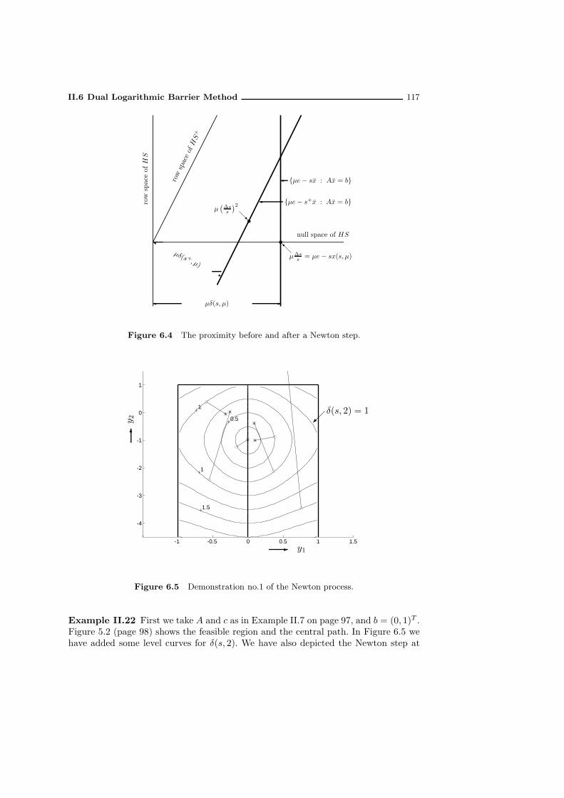
II.6 Dual Logarithmic Barrier Method 117
µ∆ss = µe− sx(s, µ)
µ(∆ss
)2
µe− sx : Ax = b
µe− s+x : Ax = b
µδ(s, µ)
µδ(s+, µ)
null space of HS
row
space
ofHS
rowspaceofHS
+
Figure 6.4 The proximity before and after a Newton step.
-1 -0.5 0 0.5 1 1.5
-4
-3
-2
-1
0
1
0.5
1
1
1.5
y1
y 2
δ(s, 2) = 1
Figure 6.5 Demonstration no.1 of the Newton process.
Example II.22 First we take A and c as in Example II.7 on page 97, and b = (0, 1)T .Figure 5.2 (page 98) shows the feasible region and the central path. In Figure 6.5 wehave added some level curves for δ(s, 2). We have also depicted the Newton step at

118 II Logarithmic Barrier Approach
several points in the feasible region. The respective starting points are indicated bythe symbol ‘o’, and the resulting point after a Newton step by the symbol ‘∗’; the twopoints are connected by a straight line to indicate the Newton step.Note that, in agreement with Theorem II.21, when starting within the region of
quadratic convergence, i.e., when δ(s, µ) < 1, the Newton step is not only feasible, butthere is a significant decrease in the proximity to the 2-center. Also, when startingoutside the region of quadratic convergence, i.e., when δ(s, µ) ≥ 1, it may happen thatthe Newton step leaves the feasible region.In Figure 6.6 we depict similar results for the problem defined in Example II.7 with
b = (1, 1)T .
-1 -0.5 0 0.5 1 1.5
-4
-3
-2
-1
0
1
1
0.5
1.5
y1
y 2
δ(s, 2) = 1
Figure 6.6 Demonstration no.2 of the Newton process.
Finally, Figure 6.7 depicts the situation for a new, less regular, problem. It is definedby
A =
[−2 1 1 0 1 −1 0
1 1 −1 1 0 0 −1
], b =
[2
1
], c =
1
4
1
2
2
0
0
.
This figure makes clear that after a Newton step the proximity to the 2-center mayincrease. Concluding this example, we may state that inside the region of quadraticconvergence our proximity measure provides perfect control over the Newton process,

II.6 Dual Logarithmic Barrier Method 119
0 0.5 1 1.5 2
0
0.5
1
1.5
2 1
1.25
1.25
y1
δ(s, 2) = 1
y 2
Figure 6.7 Demonstration no.3 of the Newton process.
but outside this region it has little value. ♦
6.6 The duality gap close to the central path
A nice feature of the µ-center s = s(µ) is that the vector x = µs−1 is primal feasible,and the duality gap for the primal-dual pair (x, s) is given by nµ. One might askabout the situation when s is close to s(µ). The next theorem provides a satisfactoryanswer. It states that for small values of the proximity δ(s, µ) the duality gap for thepair (x(s, µ), s) is close to the gap for the µ-centers.
Theorem II.23 Let δ := δ(s, µ) ≤ 1. Then the duality gap for the primal-dual pair(x(s, µ), s) satisfies
nµ (1− δ) ≤ sTx(s, µ) ≤ nµ (1 + δ) .
Proof: From Theorem II.21 we know that x(s, µ) is primal feasible. Hence, for theduality gap we have
sTx(s, µ) = sT(µs−1
(e− s−1∆s
))= µeT
(e− s−1∆s
).
Since the coordinates of the vector e−s−1∆s lie in the interval [1− δ, 1+ δ], the resultfollows.

120 II Logarithmic Barrier Approach
Remark II.24 The above estimate for the duality gap is not as sharp as it could be, but issufficient for our goal. Nevertheless, we want to point out that the Cauchy–Schwarz inequalitygives stronger bounds. We have
sTx(s, µ) = µeT(e− s−1∆s
)= nµ− µeT s−1∆s.
Hence ∣∣sTx(s, µ)− nµ∣∣ = µ
∣∣eT s−1∆s∣∣ ≤ µ ‖e‖
∥∥s−1∆s∥∥ = µ
√nδ,
and it follows that
nµ
(1− δ√
n
)≤ sTx(s, µ) ≤ nµ
(1 +
δ√n
).
•
6.7 Dual logarithmic barrier algorithm with full Newton steps
We can now describe an algorithm using approximate centers. We assume that we aregiven a pair (y0, s0) ∈ D and a µ0 > 0 such that (y0, s0) is close to the µ0-center inthe sense of the proximity measure δ(s0, µ0). In the algorithm the barrier parametermonotonically decreases from the initial value µ0 to some small value determined bythe desired accuracy. In the algorithm we denote by p(s, µ) the Newton step ∆s ats ∈ D+ to emphasize the dependence on the barrier parameter µ.
Dual Logarithmic Barrier Algorithm with full Newton steps
Input:A proximity parameter τ , 0 ≤ τ < 1;an accuracy parameter ε > 0;(y0, s0) ∈ D and µ0 > 0 such that δ(s0, µ0) ≤ τ ;a fixed parameter θ, 0 < θ < 1.
begins := s0; µ := µ0;while nµ ≥ (1− θ)ε dobegins := s+ p(s, µ);µ := (1− θ)µ;
endend
We prove the following theorem.
Theorem II.25 If τ = 1/√2 and θ = 1/(3
√n), then the Dual Logarithmic Barrier
Algorithm with full Newton steps requires at most⌈3√n log
nµ0
ε
⌉

II.6 Dual Logarithmic Barrier Method 121
iterations. The output is a primal-dual pair (x, s) such that xT s ≤ 2ε.
6.7.1 Convergence analysis
The proof of Theorem II.25 depends on the following lemma. The lemma generalizesTheorem II.21 to the case where, after the Newton step corresponding to the barrierparameter value µ, the barrier parameter is updated to µ+ = (1− θ)µ. Taking θ = 0in the lemma we get back the result of Theorem II.21.
Lemma II.26 8 Assuming δ(s, µ) ≤ 1, let s+ be obtained from s by moving along theNewton step ∆s = p(s, µ) at s corresponding to the barrier parameter value µ, and letµ+ = (1− θ)µ. Then we have
δ(s+, µ+)2 ≤ δ(s, µ)4 +θ2n
(1− θ)2.
Proof: By definition we have
δ(s+, µ+) =1
µ+minx
∥∥µ+e − s+x∥∥ : Ax = b
Substituting for x the vector x(s, µ) we obtain the inequality:
δ(s+, µ+) ≤ 1
µ+
∥∥µ+e− s+x(s, µ)∥∥ =
∥∥∥∥e−s+x(s, µ)
µ(1− θ)
∥∥∥∥ .
From (6.10) we deduce that
s+x(s, µ) = µ(e−
(s−1∆s
)2).
Substituting this, while simplifying the notation by using
h := s−1∆s,
we get
δ(s+, µ+) ≤∥∥∥∥e −
e − h2
1− θ
∥∥∥∥ =
∥∥∥∥h2 − θ
1− θ
(e− h2
)∥∥∥∥ . (6.12)
To further simplify the notation we replace θ/ (1− θ) by ρ. Then taking squares ofboth sides in the last inequality we obtain
δ(s+, µ+)2 ≤∥∥h2∥∥2 − 2ρ
(h2)T (
e− h2)+ ρ2
∥∥e− h2∥∥2 .
Since ‖h‖ = δ(s, µ) ≤ 1 we have
0 ≤ e− h2 ≤ e.
Hence we have (h2)T (
e− h2)≥ 0,
∥∥e− h2∥∥2 ≤ ‖e‖2 .
8 This lemma and its proof are due to Ling [182]. It improves estimates used by Roos and Vial [245].

122 II Logarithmic Barrier Approach
Using this, and also that ‖e‖2 = n, we obtain
δ(s+, µ+)2 ≤∥∥h2
∥∥2 + ρ2 ‖e‖2 ≤ ‖h‖4 + ρ2n = δ(s, µ)4 + ρ2n,
thus proving the lemma.
Remark II.27 It may be noted that a weaker result can be obtained in a more simple wayby applying the triangle inequality to (6.12). This yields
δ(s+, µ+) ≤∥∥h2∥∥+ θ
1− θ
∥∥e− h2∥∥ ≤ δ(s, µ)2 +
θ√n
1− θ.
This result is strong enough to derive a polynomial iteration bound, but the resulting bound
will be slightly weaker than the one in Theorem II.25. •The proof of Theorem II.25 goes now as follows. Taking θ = 1/(3
√n), we have
θ√n
1− θ=
13
1− 13√n
≤1323
=1
2.
Hence, applying the lemma, we obtain
δ(s+, µ+)2 ≤ δ(s, µ)4 +1
4.
Therefore, if δ(s, µ) ≤ τ = 1/√2, then we obtain
δ(s+, µ+)2 ≤ 1
4+
1
4=
1
2,
which implies that δ(s+, µ+) ≤ 1/√2 = τ. Thus it follows that after each iteration of
the algorithm the property
δ(s, µ) ≤ τ
is maintained. The iteration bound in the theorem is an immediate consequence ofLemma I.36. Finally, if s is the dual iterate at termination of the algorithm, and µ thevalue of the barrier parameter, then with x = x(s, µ), Theorem II.23 yields
sTx(s, µ) ≤ nµ (1 + δ(s, µ)) ≤ nµ (1 + τ) ≤ 2nµ.
Since upon termination we have nµ ≤ ε, it follows that sTx(s, µ) ≤ 2ε. This completesthe proof of the theorem.
6.7.2 Illustration of the algorithm with full Newton steps
In this section we start with a straightforward application of the logarithmic barrieralgorithm. After that we devote some sections to modifications of the algorithm thatincrease the practical efficiency of the algorithm without destroying the theoreticaliteration bound.

II.6 Dual Logarithmic Barrier Method 123
As an example we solve the problem with A and c as in Example II.7, and withbT = (1, 1). Written out, the (dual) problem is given by
max y1 + y2 : −1 ≤ y1 ≤ 1, y2 ≤ 1 .
and the primal problem is
min x1 + x2 + x3 : x1 − x2 = 1, x3 = 1, x ≥ 0 .
We can start the algorithm at y = (0, 0) and µ = 2, because we then have s = (1, 1, 1)and, since x = (2, 1, 1) is primal feasible,
δ(s, µ) ≤∥∥∥∥sx
µ− e
∥∥∥∥ =
∥∥∥∥∥∥
0− 1
2− 1
2
∥∥∥∥∥∥=
1√2.
With ε = 10−4, the dual logarithmic barrier algorithm needs 53 iterations to generatethe primal feasible solution x = (1.000015, 0.000015, 1.000000) and the dual feasiblepair (y, s) with y = (0.999971, 0.999971) and s = (0.000029, 1.999971, 0.000029). Therespective objective values are cTx = 2.000030 and bT y = 1.999943, and the dualitygap is 0.000087.Table 6.1. (page 124) shows some quantities generated in the course of the algorithm.
For each iteration the table shows the values of nµ, the first coordinate of x(s, µ), thecoordinates of y, the first coordinate of s, the proximity δ = δ(s, µ) before and theproximity δ+ = δ(s+, µ) after the Newton step at y to the µ-center, and, in the lastcolumn, the barrier update parameter θ, which is constant in this example.The columns for δ and δ+ in Table 6.1. are of special interest. They make clear
that the behavior of the algorithm differs from what might be expected. The analysiswas based on the idea of maintaining the proximity of the iterates below the valueτ = 1/
√2 = 0.7071, so as to stay in the region where Newton’s method is very efficient.
Therefore we updated the barrier parameter in such a way that just before the Newtonstep, i.e., just after the update of the barrier parameter, the proximity should reachthe value τ . The table makes clear that in reality the proximity takes much smallervalues (soon after the start). Asymptotically the proximity before the Newton step isalways 0.2721 and after the Newton step 0.0524.This can also be seen from Figure 6.8, which shows the relevant part of the feasible
region and the central path. The points y are indicated by small circles and the exactµ-centers as asterisks. The above observation becomes very clear in this figure: soonafter the start the circles and the asterisks can hardly be distinguished. The figurealso shows at each iteration the region where the proximity is smaller than τ , thusindicating the space where we are allowed to move without leaving the region ofquadratic convergence. Instead of using this space the algorithm moves in a verynarrow neighborhood of the central path.
6.8 A version of the algorithm with adaptive updates
The example in the previous section has been discussed in detail in the hope that thereader will now understand that there is an easy way to reduce the number of iterations

124 II Logarithmic Barrier Approach
It. nµ x1 y1 y2 s1 δ δ+ θ
0 6.000000 2.500000 0.000000 0.000000 1.000000 0.6124 0.2509 0.19251 4.845299 2.255388 0.250000 −0.500000 0.750000 0.0901 0.0053 0.19252 3.912821 1.969957 0.285497 −0.606897 0.714503 0.2491 0.0540 0.19253 3.159798 1.749168 0.342068 −0.234058 0.657932 0.2003 0.0303 0.19254 2.551695 1.578422 0.403015 −0.022234 0.596985 0.2334 0.0420 0.19255 2.060621 1.447319 0.467397 0.184083 0.532603 0.2285 0.0379 0.19256 1.664054 1.347011 0.532510 0.337370 0.467490 0.2406 0.0416 0.19257 1.343807 1.270294 0.595745 0.466322 0.404255 0.2438 0.0421 0.19258 1.085191 1.211482 0.654936 0.568477 0.345064 0.2500 0.0441 0.19259 0.876346 1.166207 0.708650 0.651736 0.291350 0.2537 0.0453 0.192510 0.707693 1.131170 0.756184 0.718677 0.243816 0.2574 0.0467 0.192511 0.571498 1.103907 0.797423 0.772849 0.202577 0.2601 0.0477 0.192512 0.461513 1.082581 0.832650 0.816552 0.167350 0.2624 0.0486 0.192513 0.372695 1.065815 0.862383 0.851862 0.137617 0.2643 0.0493 0.192514 0.300969 1.052577 0.887244 0.880369 0.112756 0.2658 0.0499 0.192515 0.243048 1.042085 0.907881 0.903393 0.092119 0.2670 0.0504 0.192516 0.196273 1.033741 0.924914 0.921985 0.075086 0.2680 0.0508 0.192517 0.158500 1.027088 0.938910 0.936999 0.061090 0.2688 0.0511 0.192518 0.127997 1.021771 0.950370 0.949123 0.049630 0.2695 0.0513 0.192519 0.103364 1.017513 0.959728 0.958915 0.040272 0.2700 0.0515 0.192520 0.083472 1.014098 0.967352 0.966821 0.032648 0.2704 0.0517 0.192521 0.067407 1.011356 0.973553 0.973207 0.026447 0.2707 0.0518 0.192522 0.054435 1.009152 0.978589 0.978363 0.021411 0.2710 0.0519 0.192523 0.043959 1.007378 0.982674 0.982527 0.017326 0.2712 0.0520 0.192524 0.035499 1.005950 0.985986 0.985890 0.014014 0.2714 0.0521 0.192525 0.028667 1.004800 0.988668 0.988605 0.011332 0.2716 0.0521 0.192526 0.023150 1.003873 0.990839 0.990798 0.009161 0.2717 0.0522 0.192527 0.018695 1.003125 0.992596 0.992569 0.007404 0.2718 0.0522 0.192528 0.015097 1.002522 0.994017 0.993999 0.005983 0.2718 0.0523 0.192529 0.012192 1.002036 0.995165 0.995154 0.004835 0.2719 0.0523 0.192530 0.009845 1.001643 0.996094 0.996087 0.003906 0.2720 0.0523 0.192531 0.007951 1.001327 0.996845 0.996840 0.003155 0.2720 0.0523 0.192532 0.006421 1.001071 0.997451 0.997448 0.002549 0.2720 0.0523 0.192533 0.005185 1.000865 0.997941 0.997939 0.002059 0.2721 0.0523 0.192534 0.004187 1.000698 0.998337 0.998336 0.001663 0.2721 0.0523 0.192535 0.003381 1.000564 0.998657 0.998656 0.001343 0.2721 0.0524 0.192536 0.002731 1.000455 0.998915 0.998915 0.001085 0.2721 0.0524 0.192537 0.002205 1.000368 0.999124 0.999124 0.000876 0.2721 0.0524 0.192538 0.001781 1.000297 0.999292 0.999292 0.000708 0.2721 0.0524 0.192539 0.001438 1.000240 0.999429 0.999428 0.000571 0.2721 0.0524 0.192540 0.001161 1.000194 0.999539 0.999538 0.000461 0.2721 0.0524 0.192541 0.000938 1.000156 0.999627 0.999627 0.000373 0.2721 0.0524 0.192542 0.000757 1.000126 0.999699 0.999699 0.000301 0.2721 0.0524 0.192543 0.000612 1.000102 0.999757 0.999757 0.000243 0.2722 0.0524 0.192544 0.000494 1.000082 0.999804 0.999804 0.000196 0.2722 0.0524 0.192545 0.000399 1.000066 0.999841 0.999841 0.000159 0.2722 0.0524 0.192546 0.000322 1.000054 0.999872 0.999872 0.000128 0.2722 0.0524 0.192547 0.000260 1.000043 0.999897 0.999897 0.000103 0.2722 0.0524 0.192548 0.000210 1.000035 0.999917 0.999917 0.000083 0.2722 0.0524 0.192549 0.000170 1.000028 0.999933 0.999933 0.000067 0.2722 0.0524 0.192550 0.000137 1.000023 0.999946 0.999946 0.000054 0.2722 0.0524 0.192551 0.000111 1.000018 0.999956 0.999956 0.000044 0.2722 0.0524 0.192552 0.000089 1.000015 0.999964 0.999964 0.000036 0.2722 0.0524 0.192553 0.000072 1.000015 0.999971 0.999971 0.000029 − − −
Table 6.1. Output of the dual full-step algorithm.
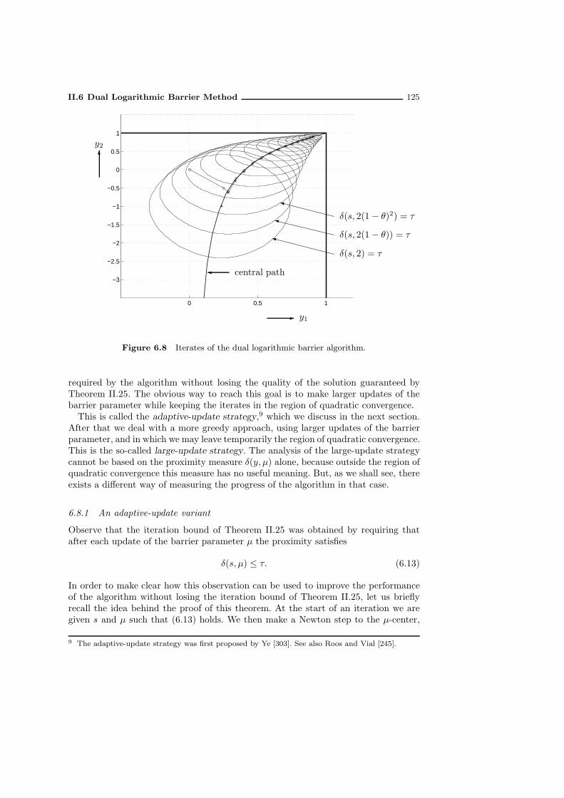
II.6 Dual Logarithmic Barrier Method 125
0 0.5 1
−3
−2.5
−2
−1.5
−1
−0.5
0
0.5
1
y1
δ(s, 2) = τ
② δ(s, 2(1− θ)) = τ
② δ(s, 2(1− θ)2) = τ
②
central path
y2
Figure 6.8 Iterates of the dual logarithmic barrier algorithm.
required by the algorithm without losing the quality of the solution guaranteed byTheorem II.25. The obvious way to reach this goal is to make larger updates of thebarrier parameter while keeping the iterates in the region of quadratic convergence.This is called the adaptive-update strategy,9 which we discuss in the next section.
After that we deal with a more greedy approach, using larger updates of the barrierparameter, and in which we may leave temporarily the region of quadratic convergence.This is the so-called large-update strategy. The analysis of the large-update strategycannot be based on the proximity measure δ(y, µ) alone, because outside the region ofquadratic convergence this measure has no useful meaning. But, as we shall see, thereexists a different way of measuring the progress of the algorithm in that case.
6.8.1 An adaptive-update variant
Observe that the iteration bound of Theorem II.25 was obtained by requiring thatafter each update of the barrier parameter µ the proximity satisfies
δ(s, µ) ≤ τ. (6.13)
In order to make clear how this observation can be used to improve the performanceof the algorithm without losing the iteration bound of Theorem II.25, let us brieflyrecall the idea behind the proof of this theorem. At the start of an iteration we aregiven s and µ such that (6.13) holds. We then make a Newton step to the µ-center,
9 The adaptive-update strategy was first proposed by Ye [303]. See also Roos and Vial [245].

126 II Logarithmic Barrier Approach
(y+, s+)y(µ)
y(µ+)
δ(s+, µ+) = τ
central path
δ(s+, µ) = τ
δ(s+, µ) = τ2
Figure 6.9 The idea of adaptive updating.
which yields s+, and we have
δ(s+, µ) ≤ τ2. (6.14)
Then we update µ to a smaller value µ+ = (1 − θ)µ such that
δ(s+, µ+) ≤ τ, (6.15)
and we start the next iteration. Our estimates in the proof of Theorem II.25 were suchthat it has become clear that the value θ = 1/(3
√n) guarantees that (6.15) will hold.
But from the example in the previous section we know that actually the new proximitymay be much smaller than τ . In other words, it may well happen that using the givenvalue of θ we start the next iteration with an s+ and a µ+ such that δ(s+, µ+) is(much) smaller than τ .It will be clear that this opens a way to speed up the algorithm without degrading
the iteration bound. For if we take θ larger than the value θ = 1/(3√n) used in
Theorem II.25, thus enforcing a deeper update of the barrier parameter in such a waythat (6.15) still holds, then the analysis in the proof of Theorem II.25 remains validbut the number of iterations decreases. The question arises of how deep the updatemight be. In other words, we have to deal with the problem that we are given s+ andµ such that (6.14) holds, and we ask how large we can take θ in µ+ = (1− θ)µ so that(6.15) holds with equality:
δ(s+, µ+) = τ.
See Figure 6.9. Note that we know beforehand that this value of θ is at leastθ = 1/(3
√n).
To answer the above question we need to introduce the so-called affine-scaling
direction and the centering direction at s.

II.6 Dual Logarithmic Barrier Method 127
6.8.2 The affine-scaling direction and the centering direction
From (6.1) we recall that the Newton step at s to the µ-center is given by
µs−1∆s = PHS (µe− sx) ,
so we may write
∆s = SPHS
(e − sx
µ
)= SPHS (e)− 1
µSPHS (sx) .
The directions
∆cs := SPHS (e) (6.16)
and
∆as := −SPHS (sx) (6.17)
are called the centering direction and the affine-scaling direction respectively. Note thatthese two directions depend only on the iterate s and not on the barrier parameter µ.Now the Newton step at s to the µ-center can be written as
∆s = ∆cs+1
µ∆as.
By definition (6.7), the proximity δ(s, µ) is given by δ(s, µ) :=∥∥s−1∆s
∥∥. Thus we have
δ(s, µ) =
∥∥∥∥dc +
1
µda∥∥∥∥ ,
where
dc = s−1∆cs, da = s−1∆as
are the scaled centering and affine-scaling directions respectively.
6.8.3 Calculation of the adaptive update
Now that we know how the proximity depends on the barrier parameter we are ableto solve the problem posed above. We assume that we have an iterate s such that forsome µ > 0 and 0 < τ < 1/
√2,
δ := δ(s, µ) ≤ τ2,
and we ask for the smallest value µ+ of the barrier parameter such that
δ(s, µ+) = τ.
Clearly, µ+ is the smallest positive root of the equation
δ(s, µ) =
∥∥∥∥dc +
1
µda∥∥∥∥ = τ. (6.18)

128 II Logarithmic Barrier Approach
Note that in the case where b = 0, the dual objective value is constant on the dualfeasible region and hence s is optimal.10,11 We assume that da 6= 0. This is true if andonly if b 6= 0. It then follows from (6.18) that δ(s, µ) depends continuously on µ andgoes to infinity if µ approaches zero. Hence, since τ > τ2, equation (6.18) has at leastone positive solution.Squaring both sides of (6.18), we arrive at the following quadratic equation in 1/µ:
1
(µ)2‖da‖2 + 2
µ(da)T dc + ‖dc‖2 − τ2 = 0. (6.19)
The two roots of (6.19) are given by
−(da)T dc ±√((da)T dc)
2 − ‖da‖2(‖dc‖2 − τ2
)
‖da‖2.
We already know that at least one of the roots is positive. Hence, although we do notknow the sign of the second root, we may conclude that 1/µ∗, where µ∗ is the value ofthe barrier parameter we are looking for, is equal to the larger of the two roots. Thisgives, after some elementary calculations,
µ∗ =‖dc‖2 − τ2
(da)T dc +
√((da)T dc)
2 − ‖da‖2(‖dc‖2 − τ2
) .
It is interesting to observe that it is easy to characterize the situation that bothroots of (6.18) are positive. By considering the constant term in the quadratic equation
(6.19) we see that both roots are positive if and only if ‖dc‖2 − τ2 > 0. From (6.18) itfollows that ‖dc‖ = δ(s,∞). Thus, both roots are positive if and only if
δ(s,∞) > τ.
Obviously this situation occurs only if
(da)Tdc < 0.
Thus we find the interesting result
δ(s,∞) > τ ⇒ (da)T dc < 0.
At the central path, when δ(s, µ) = 0, we have da = −µdc, so in that case the aboveimplication is obvious.
10 Exercise 37 Show that da = 0 if and only if b = 0.11 Exercise 38 Consider the case b = 0. Then the primal feasibility condition is Ax = 0, x ≥ 0,
which is homogeneous in x. Show that x(s, µ) = µx(s, 1) for each µ > 0, and that δ(s, µ) isindependent of µ. Taking s = s(1), it now easily follows that s(µ) = s(1) for each µ > 0. Thismeans that the dual central path is a point in this case, whereas the primal central path is astraight half line. If s and µ > 0 are such that δ(s, µ) < 1 then the Newton process convergesquadratically to s(1), which is the analytic center of the dual feasible region. See also Roos andVial [243] and Ye [310].
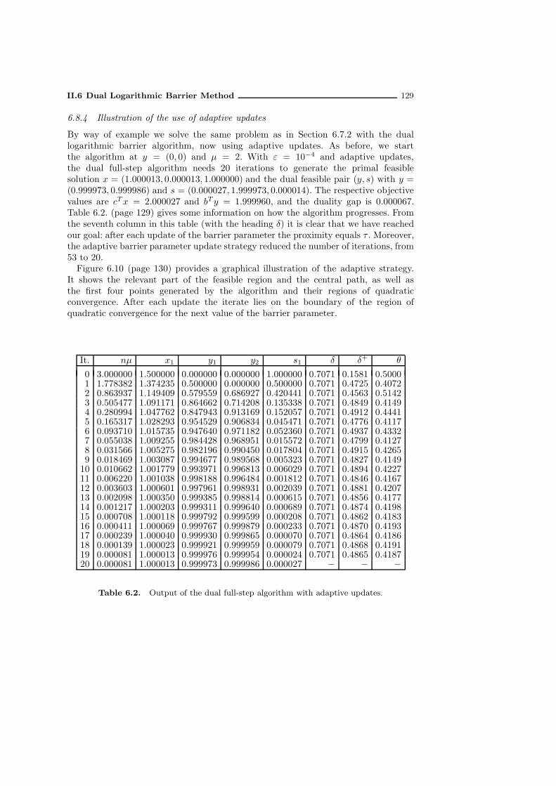
II.6 Dual Logarithmic Barrier Method 129
6.8.4 Illustration of the use of adaptive updates
By way of example we solve the same problem as in Section 6.7.2 with the duallogarithmic barrier algorithm, now using adaptive updates. As before, we startthe algorithm at y = (0, 0) and µ = 2. With ε = 10−4 and adaptive updates,the dual full-step algorithm needs 20 iterations to generate the primal feasiblesolution x = (1.000013, 0.000013, 1.000000) and the dual feasible pair (y, s) with y =(0.999973, 0.999986) and s = (0.000027, 1.999973, 0.000014). The respective objectivevalues are cTx = 2.000027 and bT y = 1.999960, and the duality gap is 0.000067.Table 6.2. (page 129) gives some information on how the algorithm progresses. Fromthe seventh column in this table (with the heading δ) it is clear that we have reachedour goal: after each update of the barrier parameter the proximity equals τ . Moreover,the adaptive barrier parameter update strategy reduced the number of iterations, from53 to 20.Figure 6.10 (page 130) provides a graphical illustration of the adaptive strategy.
It shows the relevant part of the feasible region and the central path, as well asthe first four points generated by the algorithm and their regions of quadraticconvergence. After each update the iterate lies on the boundary of the region ofquadratic convergence for the next value of the barrier parameter.
It. nµ x1 y1 y2 s1 δ δ+ θ
0 3.000000 1.500000 0.000000 0.000000 1.000000 0.7071 0.1581 0.50001 1.778382 1.374235 0.500000 0.000000 0.500000 0.7071 0.4725 0.40722 0.863937 1.149409 0.579559 0.686927 0.420441 0.7071 0.4563 0.51423 0.505477 1.091171 0.864662 0.714208 0.135338 0.7071 0.4849 0.41494 0.280994 1.047762 0.847943 0.913169 0.152057 0.7071 0.4912 0.44415 0.165317 1.028293 0.954529 0.906834 0.045471 0.7071 0.4776 0.41176 0.093710 1.015735 0.947640 0.971182 0.052360 0.7071 0.4937 0.43327 0.055038 1.009255 0.984428 0.968951 0.015572 0.7071 0.4799 0.41278 0.031566 1.005275 0.982196 0.990450 0.017804 0.7071 0.4915 0.42659 0.018469 1.003087 0.994677 0.989568 0.005323 0.7071 0.4827 0.414910 0.010662 1.001779 0.993971 0.996813 0.006029 0.7071 0.4894 0.422711 0.006220 1.001038 0.998188 0.996484 0.001812 0.7071 0.4846 0.416712 0.003603 1.000601 0.997961 0.998931 0.002039 0.7071 0.4881 0.420713 0.002098 1.000350 0.999385 0.998814 0.000615 0.7071 0.4856 0.417714 0.001217 1.000203 0.999311 0.999640 0.000689 0.7071 0.4874 0.419815 0.000708 1.000118 0.999792 0.999599 0.000208 0.7071 0.4862 0.418316 0.000411 1.000069 0.999767 0.999879 0.000233 0.7071 0.4870 0.419317 0.000239 1.000040 0.999930 0.999865 0.000070 0.7071 0.4864 0.418618 0.000139 1.000023 0.999921 0.999959 0.000079 0.7071 0.4868 0.419119 0.000081 1.000013 0.999976 0.999954 0.000024 0.7071 0.4865 0.418720 0.000081 1.000013 0.999973 0.999986 0.000027 − − −
Table 6.2. Output of the dual full-step algorithm with adaptive updates.

130 II Logarithmic Barrier Approach
0 0.5 1
−3
−2.5
−2
−1.5
−1
−0.5
0
0.5
1
y1
δ(s, 2) = τ
②
central path
y2
Figure 6.10 The iterates when using adaptive updates.
6.9 A version of the algorithm with large updates
In this section we consider a more greedy approach than the adaptive strategy, usinglarger updates of the barrier parameter. As before, we assume that we have an iterates and a µ > 0 such that s belongs to the region of quadratic convergence around theµ-center. In fact we assume that12
δ(s, µ) ≤ τ =1√2.
Starting at s we want to reach the region of quadratic convergence around the µ+-center, with
µ+ = (1− θ)µ,
and we assume that θ is so large that s lies outside the region of quadratic convergencearound the µ+-center. In fact, it may well happen that δ(s, µ+) is much larger than 1.It is clear that the analysis of the previous sections, where we always took full Newtonsteps for the target value of the barrier parameter, is then no longer useful: this analysiswas based on the nice behavior of Newton’s method in a close neighborhood of theµ+-center. Being outside this region, we can no longer profit from this nice behaviorand we need an alternative approach.Now remember that the target center s(µ+) can be characterized as the (unique)
12 We could have taken a different value for τ , for example τ = 1/2, but the choice τ = 1/√2 seems
to be natural. The analysis below supports our choice. In the literature the choice τ = 1/2 is verypopular (see, e.g., [140]). It is easy to adapt the analysis below to this value.

II.6 Dual Logarithmic Barrier Method 131
minimizer of the dual logarithmic barrier function
kµ+(y, s) = −bT y − µ+n∑
j=1
log sj
and that this function is strictly convex on the interior of the dual feasible region.Hence, the difference
kµ+(y, s)− kµ+(y(µ+), s(µ+))
vanishes if and only if s = s(µ+) and is positive elsewhere. The difference can thereforebe used as another indicator for the ‘distance’ from s to s(µ+). That is exactly whatwe plan to do. Outside the region of quadratic convergence the barrier function valuewill act as a measure for proximity to the µ-center. We show that when moving in thedirection of the Newton step at s the barrier function decreases, and that by choosingan appropriate step-size we can guarantee a sufficient decrease of the barrier functionvalue. In principle, the step-size can be obtained from a one-dimensional line searchin the Newton direction so as to minimize the barrier function in this direction. Basedon these ideas we derive an upper bound for the required number of damped Newton
steps to reach the vicinity of s(µ+); the upper bound will be a function of θ.The algorithm is described on page 131. We refer to the first while-loop in the
Dual Logarithmic Barrier Algorithm with Large Updates
Input:A proximity parameter τ = 1/
√2;
an accuracy parameter ε > 0;a variable damping factor α;an update parameter θ, 0 < θ < 1;(y0, s0) ∈ D and µ0 > 0 such that δ(s0, µ0) ≤ τ .
begins := s0; µ := µ0;while nµ ≥ ε dobeginµ := (1− θ)µ;while δ(s, µ) ≥ τ dobegins := s+ αp(s, µ);(The damping factor α must be such that kµ(y, s) decreasessufficiently. The default value is 1/(1 + δ(s, µ)).)
endend
end
algorithm as the outer loop and to the second while-loop as the inner loop. Each

132 II Logarithmic Barrier Approach
execution of the outer loop is called an outer iteration and each execution of the innerloop an inner iteration. The required number of outer iterations depends only on thedimension n of the problem, on µ0 and ε, and on the (fixed) barrier update parameterθ. This number immediately follows from Lemma I.36. The main task in the analysisof the algorithm is to derive an upper bound for the number of iterations in the innerloop. For that purpose we need some lemmas that estimate barrier function valuesand objective values in the region of quadratic convergence around the µ-center. Sincethese estimates are interesting in themselves, and also because their importance goesbeyond the analysis of the present algorithm with line searches alone, we discuss themin separate sections.
6.9.1 Estimates of barrier function values
We start with the barrier function values. Our goal is to estimate dual barrier functionvalues in the region of quadratic convergence around the µ-center. It will be convenientnot to deal with the barrier function itself, but to scale it by the barrier parameter.Therefore we introduce
hµ(s) :=1
µkµ(y, s) =
−bTyµ
−n∑
j=1
log sj .
Let us point out once more that y is omitted in the argument of hµ(s) because of theone-to-one correspondence between y and s in dual feasible pairs (y, s). We also usethe primal barrier function scaled by µ:
gµ(x) :=1
µgµ(x) =
cTx
µ−
n∑
j=1
log xj .
Recall that both barrier functions are strictly convex on their domain and that s(µ)and x(µ) are their respective minimizers. Therefore, defining
φpµ(x) := gµ(x) − gµ(x(µ)), φdµ(s) := hµ(s)− hµ(s(µ)),
we have φdµ(s) ≥ 0, with equality if and only if s = s(µ), and also φpµ(x) ≥ 0, withequality if and only if x = x(µ). As a consequence, defining
φµ(x, s) := φpµ(x) + φdµ(s), (6.20)
where (x, s) is any pair of positive primal and dual feasible solutions, we haveφµ(x, s) ≥ 0, and the equality holds if and only if x = x(µ) and s = s(µ). Thefunction φµ : P+ × D+ → IR+ is called the primal-dual logarithmic barrier function
with barrier parameter µ. Now the following lemma is almost obvious.
Lemma II.28 Let x > 0 be primal feasible and s > 0 dual feasible. Then
φpµ(x) = φµ (x, s(µ)) ≤ φµ(x, s) and φdµ(s) = φµ (x(µ), s) ≤ φµ(x, s).
Proof: The inequalities in the lemma are immediate from (6.20) since φpµ(x) and
φdµ(s) are nonnegative. Similarly, the equalities follow since φpµ (x(µ)) = φdµ (s(µ)) = 0.Thus the lemma has been proved.

II.6 Dual Logarithmic Barrier Method 133
In the sequel, properties of the function φµ form the basis of many of our estimates.These estimates follow from properties of the univariate function
ψ(t) = t− log(1 + t), t > −1, (6.21)
as defined in (5.5).13 The definition of ψ is extended to any vector z = (z1, z2, . . . , zn)satisfying z + e > 0 according to
Ψ(z) =n∑
j=1
ψ(zj) =n∑
j=1
(zj − log(1 + zj)) = eT z −n∑
j=1
log(1 + zj). (6.22)
We now make a crucial observation, namely that the barrier functions φµ(x, s), φpµ(x)
and φdµ(s) can be nicely expressed in terms of the function Ψ.
Lemma II.29 Let x > 0 be primal feasible and s > 0 dual feasible. Then
(i) φµ(x, s) = Ψ(
xsµ − e
);
(ii) φpµ(x) = Ψ(
xs(µ)µ − e
);
(iii) φdµ(s) = Ψ(
x(µ)sµ − e
).
Proof: 14 First we consider item (i). We use that cTx − bTy = xT s and cTx(µ) −bT y(µ) = x(µ)T s(µ) = nµ. Now φµ(x, s) can be reduced as follows:
φµ(x, s) = hµ(s) + gµ(x) − (hµ(s(µ)) + gµ(x(µ)))
=xT s
µ−
n∑
j=1
log xjsj −x(µ)T s(µ)
µ+
n∑
j=1
log zj(µ)sj(µ)
=xT s
µ−
n∑
j=1
log xjsj − n+ n logµ.
Since xT s = eT (xs) and eT e = n, we find the following expression for φµ(x, s):15
φµ(x, s) = eT(sx
µ− e
)−
n∑
j=1
logxjsjµ
= Ψ
(sx
µ− e
). (6.23)
This proves the first statement in the lemma. The second statement follows bysubstituting s = s(µ) in the first statement, and using Lemma II.28. Similarly, thethird statement follows by substituting x = x(µ) in the first statement.
13 Exercise 39 Let t > −1. Prove that
ψ
( −t1 + t
)+ ψ(t) =
t2
1 + t.
14 Note that the dependence of φµ(x, s) on x and s is such that it depends only on the coordinatewiseproduct xs of x and s.
15Exercise 40 Considering (6.23) as the definition of φµ(x, s), and without using the properties ofψ, show that φµ(x, s) is nonnegative, and zero if and only if xs = µe. (Hint: Use the arithmetic-geometric-mean inequality.)

134 II Logarithmic Barrier Approach
Now we are ready to derive lower and upper bounds for the value of the duallogarithmic barrier function in the region of quadratic convergence around the µ-center. These bounds heavily depend on the following two inequalities:
ψ (‖z‖) ≤ Ψ(z) ≤ ψ (−‖z‖) , z > −e. (6.24)
The second inequality is valid only if ‖z‖ < 1. The inequalities in (6.24) arefundamental for our purpose and are immediate consequences of Lemma C.2 inAppendix C.16,17
Lemma II.30 18 Let δ := δ(s, µ). Then
φdµ(s) ≥ δ − log(1 + δ) = ψ(δ).
Moreover, if δ < 1, then
φdµ(s) ≤ φµ(x(s, µ), s) ≤ −δ − log(1− δ) = ψ(−δ).
Proof: By applying the inequalities in (6.24) to (6.23) we obtain for any positiveprimal feasible x:
ψ
(∥∥∥∥sx
µ− e
∥∥∥∥)
≤ φµ(x, s) ≤ ψ
(−∥∥∥∥sx
µ− e
∥∥∥∥), (6.25)
where the second inequality is valid only if the norm of xs/µ − e does not exceed 1.Using (6.8) we write
δ = δ(s, µ) =
∥∥∥∥e−sx(s, µ)
µ
∥∥∥∥ ≤∥∥∥∥e−
sx
µ
∥∥∥∥ .
Hence, by the monotonicity of ψ(t) for t ≥ 0,
ψ(δ) ≤ ψ
(∥∥∥∥sx
µ− e
∥∥∥∥),
16 At least one of the inequalities in (6.24) shows up in almost every paper on interior-point methods.As far as we know, all usual proofs use the power series expansion of log(1 + x),−1 < x < 1 anddo not characterize the case of equality, at least not explicitly. We give an elementary proof inAppendix C (page 435).
17 Exercise 41 Let z ∈ IRn. Prove that
z ≥ 0 ⇒ Ψ(z) ≤ nψ
(‖z‖√n
)≤ ‖z‖2
2
−e < z ≤ 0 ⇒ Ψ(z) ≥ nψ
(−‖z‖√n
)≥ ‖z‖2
2.
18 This lemma improves a similar result of den Hertog et al. [146] and den Hertog [140]. Theimprovement is due to a suggestion made by Osman Guler [130] during a six month stay atDelft in 1992, namely to use the primal logarithmic barrier function in the analysis of the duallogarithmic barrier method. This approach not only simplifies the analysis significantly, but alsoleads to sharper estimates. It may be appropriate to mention that even stronger bounds for φµ(x, s)will be derived in Lemma II.69, but there we use a different proximity measure.

II.6 Dual Logarithmic Barrier Method 135
for any positive primal feasible x. Taking x = x(µ) and using the left inequality in(6.25) and the third statement in Lemma II.29, we get
ψ(δ) ≤ ψ
(∥∥∥∥sx(µ)
µ− e
∥∥∥∥)
≤ φµ(x(µ), s) = φdµ(s),
proving the first inequality in the lemma. For the proof of the second inequality in thelemma we assume δ < 1 and put x = x(s, µ) in the right inequality in (6.25). Thisgives
φµ(x(s, µ), s) ≤ ψ
(−∥∥∥∥sx(s, µ)
µ− e
∥∥∥∥)
= ψ(−δ).
By Lemma II.28 we also have φdµ(s) ≤ φµ(x(s, µ), s). Thus the lemma follows.
The functions ψ(δ) and ψ(−δ), for 0 ≤ δ < 1, play a dominant role in many of theestimates below. Figure 6.11 shows their graphs.
0 0.2 0.4 0.6 0.8 10
0.25
0.5
0.75
1
1.25
1.5
1.75
2
2.25
2.5
2.75
3
δ
ψ(δ)
❯
ψ(−δ)
❯
Figure 6.11 The functions ψ(δ) and ψ(−δ) for 0 ≤ δ < 1.
6.9.2 Estimates of objective values
We proceed by considering the dual objective value bT y in the region of quadraticconvergence around the µ-center. Using that x(µ)s(µ) = µe and cTx(µ) − bT y(µ) =x(µ)T s(µ) = nµ, we write
bT y(µ)− bT y = cTx(µ)− nµ− bT y = sTx(µ) − nµ = eT (sx(µ) − µe)
= µeT(sx(µ)
µ− e
)= µeT
(s
s(µ)− e
). (6.26)

136 II Logarithmic Barrier Approach
Applying the Cauchy–Schwarz inequality to the expression for bT y(µ)− bT y in (6.26),we obtain ∣∣bT y(µ)− bT y
∣∣ ≤ µ√n
∥∥∥∥s
s(µ)− e
∥∥∥∥ . (6.27)
We assume δ := δ(s, µ) < 1/√2. It seems reasonable then to expect that the norm of
the vector
hs :=s
s(µ)− e =
sx(µ)
µ− e
will not differ too much from δ. In any case, that is what we are going to show. It willthen follow that the absolute value of bT y(µ)− bT y is of order µδ
√n.
Note that hs can be written as
hs =s− s(µ)
s(µ),
and hence ‖hs‖ measures the relative difference between s and s(µ). We also introducea similar vector for any primal feasible x > 0:
hx :=xs(µ)
µ− e =
x
x(µ)− e =
x− x(µ)
x(µ).
Using that x − x(µ) and s − s(µ) are orthogonal, as these vectors belong to the nullspace and row space of A, respectively, we may write
hTx hs =
(x− x(µ)
x(µ)
)T (s− s(µ)
s(µ)
)=
1
µ(x − x(µ))T (s− s(µ)) = 0.
This makes clear that hx and hs are orthogonal as well. In the rest of this section wework with x = x(s, µ) and derive upper bounds for ‖hx‖ and ‖hs‖. It is convenient tointroduce the vector
h = hx + hs.
The next lemma implicitly yields an upper bound for ‖h‖.
Lemma II.31 Let δ = δ(s, µ) < 1 and x = x(s, µ). Then ψ(‖h‖) ≤ ψ(−δ).
Proof: Using Lemma II.29 we may rewrite (6.20) as
φµ(x, s) = Ψ(hx) + Ψ(hs).
By the first inequality in (6.24) we have
Ψ(hx) ≥ ψ(‖hx‖) and Ψ(hs) ≥ ψ(‖hs‖).
Applying the first inequality in (6.24) to the 2-dimensional vector (‖hx‖ , ‖hs‖), weobtain
ψ(‖hx‖) + ψ(‖hs‖) ≥ ψ(‖h‖).Here we used that hx and hs are orthogonal. Substitution gives
φµ(x, s) ≥ ψ(‖h‖).
II.6 Dual Logarithmic Barrier Method 137
On the other hand, by Lemma II.30 we have φµ(x, s) ≤ ψ(−δ), thus completing theproof.
Let us point out that we can easily deduce from Lemma II.31 an interestingupper bound for ‖h‖ if δ < 1. It can then be shown that ψ(‖h‖) ≤ ψ(−δ) implies‖h‖ ≤ δ/(1− δ).19,20 This implies that ‖h‖ ≤ 1 if δ ≤ 1/2. However, for our purposethis bound is not strong enough. We prove a stronger result that implies that ‖h‖ ≤ 1if δ < 1/
√2.
Lemma II.32 Let δ = δ(s, µ) ≤ 1/√2. Then ‖h‖ <
√2.
Proof: By Lemma II.31 we have ψ(‖h‖) ≤ ψ(−δ). Since ψ(−δ) is monotonicallyincreasing in δ, this implies
ψ(‖h‖) ≤ ψ(−1/√2) = 0.52084.
Sinceψ(
√2) = 0.53284 > 0.52084,
and ψ(t) is monotonically increasing for t ≥ 0, we conclude that ‖h‖ <√2.
We now have the following result.
Lemma II.33 21 Let δ := δ(s, µ) ≤ 1/√2. Then
‖hs‖ =
∥∥∥∥s
s(µ)− e
∥∥∥∥ ≤√1−
√1− 2δ2.
Moreover, if x = x(s, µ) then also
‖hx‖ =
∥∥∥∥x
x(µ)− e
∥∥∥∥ ≤√1−
√1− 2δ2.
Proof: Lemma II.32 implies that
‖hx + hs‖ = ‖h‖ <√2.
On the other hand, since
xs
µ− e =
xs
x(µ)s(µ)− e = (e + hx)(e + hs)− e = hx + hs + hxhs,
with x = x(s, µ), and using (6.8), it follows that
‖hx + hs + hxhs‖ = δ ≤ 1√2.
19 Exercise 42 Let 0 ≤ t < 1. Prove that
ψ
( −t1 + t
)≤ t2
2(1 + t)≤ ψ(t) ≤ t2
2≤ ψ(−t) ≤ t2
2(1 − t)≤ ψ
(t
1− t
).
Also show that the first two inequalities are valid for any t > 0.20
Exercise 43 Let 0 ≤ δ < 1 and r ≥ 0 be such that ψ(r) ≤ ψ(−δ). Prove that r ≤ δ/(1 − δ).21 For δ ≤ 1/2 this lemma was first shown by Gonzaga (private communication, Delft, 1994).

138 II Logarithmic Barrier Approach
At this stage we may apply the fourth uv-lemma (Lemma C.8 in Appendix C) withu = hx and v = hs, to obtain the lemma.
We are now ready for the main result of this section.
Theorem II.34 If δ = δ(s, µ) ≤ 1/√2 then
∣∣bT y(µ)− bTy∣∣ ≤ µ
√n
√1−
√1− 2δ2.
Proof: Recall from (6.27) that
∣∣bT y(µ)− bT y∣∣ ≤ µ
√n ‖hs‖ .
Substituting the bound of Lemma II.33 on ‖hs‖, the theorem follows.
0 0.1 0.2 0.3 0.4 0.5 0.6 0.70
0.2
0.4
0.6
0.8
1
δ
δ
√1−
√1− 2δ2
❯
Figure 6.12 The graphs of δ and√
1−√1− 2δ2 for 0 ≤ δ ≤ 1/
√2.
Figure 6.12 (page 138) shows the graphs of δ and√1−
√1− 2δ2. It is clear that
for small values of δ (δ ≤ 0.3 say) the functions can hardly be distinguished.
6.9.3 Effect of large update on barrier function value
We start by considering the effect of an update of the barrier parameter on thedifference between the dual barrier function value and its minimal value. Moreprecisely, we assume that for given dual feasible s and µ > 0 we have δ = δ(s, µ) ≤1/
√2, and we want to estimate
φdµ+(s) = hµ+(s)− hµ+(s(µ+)),
where µ+ = µ(1− θ) for 0 ≤ θ < 1. Note that Lemma II.30 gives the answer if θ = 0:
φdµ(s) ≤ ψ(−δ).

II.6 Dual Logarithmic Barrier Method 139
For the general case, where θ > 0, we write
φdµ+(s) = hµ+(s)− hµ+(s(µ+))
= hµ+(s)− hµ+(s(µ)) + hµ+(s(µ))− hµ+(s(µ+))
= hµ+(s)− hµ+(s(µ)) + φdµ+(s(µ)), (6.28)
and we treat the first two terms and the last term in the last expression separately.
Lemma II.35 In the above notation,
hµ+(s)− hµ+(s(µ)) ≤ ψ(−δ) + θ√n
1− θ
√1−
√1− 2δ2.
Proof: Just using definitions we write
hµ+(s)− hµ+(s(µ)) =−bTyµ+
−n∑
j=1
log sj +bT y(µ)
µ++
n∑
j=1
log sj(µ)
= −n∑
j=1
log sj +
n∑
j=1
log sj(µ) +bT y(µ)− bT y
µ+
= hµ(s)− hµ(s(µ)) +bT y(µ)− bTy
µ+− bT y(µ)− bT y
µ
= φdµ(s) +θ
1− θ
bT y(µ)− bTy
µ.
Applying Lemma II.30 to the first term in the last expression, and Theorem II.34 tothe second term gives the lemma.
Lemma II.36 In the above notation,
φdµ+(s(µ)) ≤ φµ+(x(µ), s(µ)) = nψ
(θ
1− θ
).
Proof: The inequality follows from Lemma II.28. The equality is obtained as follows.From (6.23),
φµ+(x(µ), s(µ)) = eT(s(µ)x(µ)
µ+− e
)−
n∑
j=1
logxj(µ)sj(µ)
µ+.
Since x(µ)s(µ) = µe and µ+ = (1− θ)µ, this can be simplified to
φµ+(x(µ), s(µ)) = eT(µe
µ+− e
)−
n∑
j=1
logµ
µ+
= eT(
e
1− θ− e
)−
n∑
j=1
log1
1− θ
= n
(θ
1− θ− log
(1 +
θ
1− θ
))
= nψ
(θ
1− θ
).

140 II Logarithmic Barrier Approach
This completes the proof.
Combining the results of the last two lemmas we find the next lemma.
Lemma II.37 Let δ(s, µ) ≤ 1/√2 for some dual feasible s and µ > 0. Then, if
µ+ = µ(1− θ) with 0 ≤ θ < 1, we have
φdµ+(s) ≤ ψ
(−1√2
)+θ√n
1− θ+ nψ
(θ
1− θ
).
Proof: The lemma follows from (6.28) and the bounds provided by the previouslemmas, by substitution of δ = 1/
√2.
With s, µ and µ+ as in the last lemma, our aim is to estimate the number of dampedNewton steps required to reach the vicinity of the µ+-center when starting at s. Tothis end we proceed by estimating the decrease in the barrier function value during adamped Newton step.
6.9.4 Decrease of the barrier function value
In this section we consider a damped Newton step to the µ-center at an arbitrarypositive dual feasible s and we estimate its effect on the barrier function value. Theanalysis also yields a suitable value for the damping factor α. The result of the dampedNewton step is denoted by s+, so
s+ = s+ α∆s, (6.29)
where ∆s denotes the full Newton step.
Lemma II.38 Let δ = δ(s, µ). If α = 1/(1 + δ) then the damped Newton step (6.29)is feasible and it reduces the barrier function value by at least δ − log(1 + δ). In otherwords,
φdµ(s)− φdµ(s+) ≥ δ − log(1 + δ) = ψ(δ).
Proof: First recall from (6.5) in Section 6.5 that the Newton step ∆s is determinedby
x(s, µ) = µs−1(e− s−1∆s
).
We denote x(s, µ) briefly as x. With
z :=∆s
s= e− xs
µ,
the damped Newton step can be described as follows:
s+ = s+ α∆s = s(e+ αz).
Since s+ is feasible if and only if it is nonnegative, the step is certainly feasible ifα ‖z‖ < 1. Since δ = ‖z‖, the value for α specified by the lemma satisfies this condition,

II.6 Dual Logarithmic Barrier Method 141
and hence the feasibility of s+ follows. Now we consider the decrease in the dual barrierfunction value during the step. We may write
φdµ(s)− φdµ(s+) = hµ(s)− hµ(s
+)
=−bT yµ
−n∑
j=1
log sj −−bTy+µ
+
n∑
j=1
log s+j .
=bT y+ − bT y
µ+
n∑
j=1
log (1 + α zj) .
The difference bT y+ − bT y can be written as follows:
bT y+ − bT y = cTx− bT y −(cTx− bT y+
)= xT s− xT s+
= −αxT (sz) = −α eT (xs) z = αµeT (z − e)z.
Thus we obtain
φdµ(s)− φdµ(s+) = αeT (z − e)z +
n∑
j=1
log (1 + α zj)
= α eT z2 −
eT (αz)−
n∑
j=1
log (1 + α zj)
= α δ2 −Ψ(α z).
Since ‖αz‖ < 1 we may apply the right-hand side inequality in (6.24), which givesΨ(α z) ≤ ψ (−α ‖z‖) = ψ (−αδ), whence
φdµ(s)− φdµ(s+) ≥ α δ2 − ψ(−αδ) = α δ2 + α δ + log(1− α δ).
As a function of α, the right-hand side expression is increasing for 0 ≤ α ≤ 1/(1 + δ),as can be easily verified, and it attains its maximal value at α = 1/(1 + δ), which isthe value specified in the lemma. Substitution of this value yields the bound in the

142 II Logarithmic Barrier Approach
lemma. Thus the proof is complete.22,23
We are now ready to estimate the number of (inner) iterations between twosuccessive updates of the barrier parameter.
6.9.5 Number of inner iterations
Lemma II.39 The number of (inner) iterations between two successive updates of thebarrier parameter is no larger than
⌈3
(θ√n
1− θ+ 1
)2⌉.
Proof: From Lemma II.37 we know that after the update of µ we have
φdµ+(s) ≤ ψ(−τ) + θ√n
1− θ+ nψ
(θ
1− θ
),
where τ = 1/√2. The algorithm repeats damped Newton steps as long the iterate s
satisfies δ = δ(s, µ+) > τ . In that case the step decreases the barrier function valueby at least ψ(δ), by Lemma II.38. Since δ > τ , the decrease is at least
ψ(τ) = 0.172307.
As soon as the barrier function value has reached ψ(τ) we are sure that δ(s, µ+) ≤ τ ,from Lemma II.30. Hence, the number of inner iterations is no larger than
⌈1
ψ(τ)
(ψ(−τ) − ψ(τ) +
θ√n
1− θ+ nψ
(θ
1− θ
))⌉.
The rest of the proof consists in reducing this expression to the one in the lemma.First, using that ψ(−τ) = 0.52084, we obtain
ψ(−τ)− ψ(τ)
ψ(τ)=
0.34853
0.172307≤ 3.
22 Exercise 44 In the proof of Lemma II.38 we found the following expression for the decrease inthe dual barrier function value:
φdµ(s)− φdµ(s+) = α eT z2 −Ψ(αz),
where α denotes the size of the damped Newton step. Show that the decrease is maximal for theunique step-size α determined by the equation
eT z2 =
n∑
j=1
αz2j
1 + αzj
and that for this value the decrease is given by
Ψ
(αz
e+ αz
).
23 It is interesting to observe that Lemma II.38 provides a second proof of the first statement inLemma II.30, namely
φdµ(s) ≥ ψ(δ),
where δ := δ(s, µ). This follows from Lemma II.38, since φdµ(s+) ≥ 0.
II.6 Dual Logarithmic Barrier Method 143
Furthermore, using ψ(t) ≤ t2/2 for t ≥ 0 we get24
nψ
(θ
1− θ
)≤ nθ2
2(1− θ)2. (6.30)
Finally, using that 1/ψ(τ) < 1/6 we obtain the following upper bound for the numberof inner iterations:
⌈3 +
6θ√n
1− θ+
3nθ2
(1 − θ)2
⌉=
⌈3
(θ√n
1− θ+ 1
)2⌉.
This proves the lemma.
Remark II.40 It is tempting to apply Lemma II.39 to the case where θ = 1/(3√n). We
know that for that value of θ one full Newton step keeps the iterate in the region of quadratic
convergence around the µ+-center. Substitution of this value in the bound of Lemma II.39
however yields that at least 6 damped Newton steps are required for the same purpose. This
disappointing result reveals a weakness of the above analysis. The weakness probably stems
from the fact that the estimate of the number of inner iterations in one outer iteration is based
on the assumption that the decrease in the barrier function value is given by the constant
ψ(τ ). Actually the decrease is at least ψ(δ). Since in many inner iterations, in particular in
the iterations immediately after the update of the barrier parameter, the proximity δ may be
much larger than τ , the actual number of iterations may be much smaller than the pessimistic
estimate of Lemma II.39. This is the reason why for the algorithm with large updates there
exists a gap between theory and practice. In practice the number of inner iterations is much
smaller than the upper bound given by the lemma. Hopefully future research will close this
gap.25 •
6.9.6 Total number of iterations
We proceed by estimating the total number of iterations required by the algorithm.
Theorem II.41 To obtain a primal-dual pair (x, s), with x = x(s, µ), such thatxT s ≤ 2ε, at most ⌈
1
θ
⌈3
(θ√n
1− θ+ 1
)2⌉log
nµ0
ε
⌉
iterations are required by the logarithmic barrier algorithm with large updates.
24 A different estimate arises by using Exercise 39, which implies ψ(t) ≤ t2/(1 + t) for t > −1. Hence
nψ
(θ
1− θ
)≤ nθ2
1− θ,
which is sharper than (6.30) if θ > 12. The use of (6.30) however does not deteriorate the order of
our estimates below.25
Exercise 45 Let δ = δ(s, µ) > 0 and x = x(s, µ). Then the vector z = (xs/µ)− e has at least onepositive coordinate. Prove this. Hence, if z has only one nonzero coordinate then this coordinateequals ‖z‖. Show that in that case the single damped Newton step with step-size α = 1/(1 + δ)yields s+ = s(µ).

144 II Logarithmic Barrier Approach
Proof: The number of outer iterations follows from Lemma I.36. The bound in thetheorem is obtained by multiplying this number by the bound of Lemma II.39 forthe number of inner iterations per outer iteration and rounding the product, if notintegral, to the smallest integer above it.
We end this section by drawing two conclusions. If we take θ to be a fixed constant(independent of n), for example θ = 1/2, the iteration bound of Theorem II.41 becomes
O(n log
nµ0
ε
).
For such values of θ we say that the algorithm uses large updates. The number ofinner iterations per outer iteration is then O(n).If we take θ = ν/
√n for some fixed constant ν (independent of n), the iteration
bound of Theorem II.41 becomes
O(√
n lognµ0
ε
),
provided that n is large enough (n ≥ ν2 say). It has become common to say that thealgorithm uses medium updates. The number of inner iterations per outer iteration isthen bounded by a constant, depending on ν.In the next section we give an illustration.
6.9.7 Illustration of the algorithm with large updates
We use the same sample problem as before (see Sections 6.7.2 and 6.8.4) and solveit using the dual logarithmic barrier algorithm with large updates. We do this forseveral values of the barrier update parameter θ. As before, we start the algorithm aty = (0, 0) and µ = 2, and the accuracy parameter is set to ε = 10−4. For θ = 0.5,Table 6.3. (page 145) lists the algorithm’s progress.The table needs some explanation. The first two columns contain counters for the
outer and inner iterations, respectively. The algorithm requires 16 outer and 16 inneriterations. The table shows the effect of each outer iteration, which involves an updateof the barrier parameter, and also the effect of each inner iteration, which involves amove in the dual space. During a barrier parameter update the dual variables y ands remain unchanged, but, because of the change in µ, the primal variable x(s, µ) andthe proximity attain new values. After each update, damped Newton steps are takenuntil the proximity reaches the value τ . In this example the number of inner iterationsper outer iteration is never more than one. Note that we can guarantee the primalfeasibility of x only if the proximity is at most one. Since the table shows only thesecond coordinate of x (and also of s), infeasibility of x can only be detected from thetable if x2 is negative. In this example this does not occur, but it occurs in the nextexample, where we solve the same problem with θ = 0.9.With θ = 0.9, Table 6.4. (page 146) shows that in some iterations x is infeasible
indeed. Moreover, although the number of outer iterations is much smaller than inthe previous case (5 instead of 16), the total number of iterations is almost the same(14 instead of 16). Clearly, and understandably, the deeper updates make it harder toreach the new target region.

II.6 Dual Logarithmic Barrier Method 145
Outer Inner nµ x2 y1 y2 s2 δ
0 0 6.000000 1.500000 0.000000 0.000000 1.000000 0.61241 3.000000 0.500000 0.000000 0.000000 1.000000 0.7071
1 3.000000 0.690744 0.292893 0.000000 1.292893 0.22292 1.500000 0.230248 0.292893 0.000000 1.292893 1.3081
2 1.500000 0.302838 0.519549 0.433260 1.519549 0.29603 0.750000 0.105977 0.519549 0.433260 1.519549 1.7316
3 0.750000 0.138696 0.717503 0.696121 1.717503 0.36184 0.375000 0.056177 0.717503 0.696121 1.717503 2.0059
4 0.375000 0.065989 0.847850 0.840792 1.847850 0.40505 0.187500 0.029627 0.847850 0.840792 1.847850 2.1632
5 0.187500 0.032120 0.920315 0.918672 1.920315 0.43676 0.093750 0.015201 0.920315 0.918672 1.920315 2.2575
6 0.093750 0.015842 0.959178 0.958681 1.959178 0.45917 0.046875 0.007704 0.959178 0.958681 1.959178 2.3176
7 0.046875 0.007866 0.979268 0.979161 1.979268 0.47448 0.023438 0.003878 0.979268 0.979161 1.979268 2.3556
8 0.023438 0.003920 0.989548 0.989516 1.989548 0.48449 0.011719 0.001946 0.989548 0.989516 1.989548 2.3793
9 0.011719 0.001956 0.994747 0.994740 1.994747 0.490710 0.005859 0.000975 0.994747 0.994740 1.994747 2.3937
10 0.005859 0.000977 0.997366 0.997364 1.997366 0.494511 0.002930 0.000488 0.997366 0.997364 1.997366 2.4023
11 0.002930 0.000488 0.998681 0.998680 1.998681 0.496812 0.001465 0.000244 0.998681 0.998680 1.998681 2.4074
12 0.001465 0.000244 0.999340 0.999340 1.999340 0.498213 0.000732 0.000122 0.999340 0.999340 1.999340 2.4103
13 0.000732 0.000122 0.999670 0.999670 1.999670 0.499014 0.000366 0.000061 0.999670 0.999670 1.999670 2.4120
14 0.000366 0.000061 0.999835 0.999835 1.999835 0.499415 0.000183 0.000031 0.999835 0.999835 1.999835 2.4130
15 0.000183 0.000031 0.999917 0.999917 1.999917 0.499716 0.000092 0.000015 0.999917 0.999917 1.999917 2.4135
16 0.000092 0.000015 0.999959 0.999959 1.999959 0.4998
Table 6.3. Progress of the dual algorithm with large updates, θ = 0.5.
This is even more true in the last example where we take θ = 0.99. Table 6.5.(page 146) shows the result. The number of outer iterations is only 3, but the totalnumber of iterations is still 14. This leads us to the important observation that thedeep update strategy has its limits. On the other hand, the number of iterations iscompeting with the methods using full Newton steps, and is significantly less than theiteration bound of Theorem II.41.

146 II Logarithmic Barrier Approach
Outer Inner nµ x2 y1 y2 s2 δ
0 0 6.000000 1.500000 0.000000 0.000000 1.000000 0.61241 0.600000 −0.300000 0.000000 0.000000 1.000000 5.3385
1 0.600000 0.014393 0.394413 0.631060 1.394413 2.41122 0.600000 0.108620 0.762163 0.722418 1.762163 0.5037
2 0.060000 −0.005240 0.762163 0.722418 1.762163 16.89043 0.060000 0.008563 0.906132 0.922246 1.906132 4.72364 0.060000 0.010057 0.967364 0.961475 1.967364 1.13065 0.060000 0.010098 0.977293 0.978223 1.977293 0.1716
3 0.006000 0.000891 0.977293 0.978223 1.977293 14.32476 0.006000 0.000994 0.992649 0.992275 1.992649 3.92087 0.006000 0.001001 0.996651 0.996769 1.996651 0.91438 0.006000 0.001001 0.997834 0.997808 1.997834 0.1277
4 0.000600 0.000099 0.997834 0.997808 1.997834 13.99569 0.000600 0.000100 0.999254 0.999264 1.999254 3.8257
10 0.000600 0.000100 0.999676 0.999673 1.999676 0.888311 0.000600 0.000100 0.999782 0.999783 1.999782 0.1224
5 0.000060 0.000010 0.999782 0.999783 1.999782 13.950812 0.000060 0.000010 0.999926 0.999926 1.999926 3.812813 0.000060 0.000010 0.999967 0.999968 1.999967 0.884714 0.000060 0.000010 0.999978 0.999978 1.999978 0.1216
Table 6.4. Progress of the dual algorithm with large updates, θ = 0.9.
Outer Inner nµ x2 y1 y2 s2 δ
0 0 6.000000 1.500000 0.000000 0.000000 1.000000 0.61241 0.060000 −0.480000 0.000000 0.000000 1.000000 60.4235
1 0.060000 −0.133674 0.407010 0.797740 1.407010 28.29662 0.060000 0.008587 0.906680 0.860655 1.906680 7.02683 0.060000 0.009852 0.949767 0.964246 1.949767 1.72704 0.060000 0.010099 0.978068 0.974574 1.978068 0.2919
2 0.000600 −0.000021 0.978068 0.974574 1.978068 166.48355 0.000600 0.000086 0.992297 0.993722 1.992297 48.28326 0.000600 0.000099 0.998161 0.997593 1.998161 13.74387 0.000600 0.000100 0.999183 0.999394 1.999183 3.69138 0.000600 0.000100 0.999720 0.999656 1.999720 0.82249 0.000600 0.000100 0.999781 0.999792 1.999781 0.1013
3 0.000006 0.000001 0.999781 0.999792 1.999781 149.481710 0.000006 0.000001 0.999939 0.999934 1.999939 43.472711 0.000006 0.000001 0.999980 0.999981 1.999980 12.435912 0.000006 0.000001 0.999994 0.999993 1.999994 3.365513 0.000006 0.000001 0.999997 0.999997 1.999997 0.757314 0.000006 0.000001 0.999998 0.999998 1.999998 0.0949
Table 6.5. Progress of the dual algorithm with large updates, θ = 0.99.

II.6 Dual Logarithmic Barrier Method 147
We conclude this section with a graphical illustration of the algorithm, with θ = 0.9.Figure 6.13 shows the first outer iteration, which consists of 2 inner iterations.
0 0.5 1
−3
−2.5
−2
−1.5
−1
−0.5
0
0.5
1
y1
δ(s, 2) = τ
②
δ(s, 0.2) = τ
central path
y2
Figure 6.13 The first iterates for a large update with θ = 0.9.


7
The Primal-Dual LogarithmicBarrier Method
7.1 Introduction
In the previous chapter we dealt extensively with the dual logarithmic barrier approachto the LO problem. It has become clear that Newton’s method, when applied to findthe minimizer of the dual logarithmic barrier function, yields a search direction ∆s inthe dual space that allows us to follow the dual central path (approximately) to thedual optimal set. We were able to show that an ε-solution of (D) can be obtained in anumber of iterations that is proportional to the product of the logarithm of the initialduality gap divided by the desired accuracy, and
√n (for the full-step method and the
medium-update method) or n (for the large-update method). Although the drivingforce in the dual logarithmic barrier approach is the desire to solve the dual problem(D), it also yields an ε-solution of the primal problem (P ). The problem (P ) also playsa crucial role in the analysis of the method. For example, the Newton step ∆s at (y, s)for the barrier parameter value µ is described by the primal variable x(s, µ). Moreover,the convergence proof of the method uses the duality gap cTx(s, µ)− bT y. Finally, theanalysis of the medium-update and large-update versions of the dual method stronglydepend on the properties of the primal-dual logarithmic barrier function φµ(x, s).The aim of this chapter is to show that we can benefit from the primal problem not
only in the analysis but also in the design of the algorithm. The idea is to solve boththe dual and the primal problem simultaneously, by taking in each iteration a step∆s in the dual space and a step ∆x in the primal space. Here, the search directions∆s and ∆x still have to be defined. This is done in the next section. Again, Newton’sname is given to the search directions, but now the search directions arise from aniterative method — also due to Newton — for solving the system of equations definingthe µ-centers of (P ) and (D).In the following paragraphs we follow the same program as for the dual algorithms:
we first introduce a proximity measure, then we deal with full-step methods, with bothfixed and adaptive updates of the barrier parameter, and finally we consider methodsthat use deep (but fixed) updates and damped Newton steps.For the sake of clarity, it might be useful to emphasize that it is not our aim to
take for ∆s the dual Newton step and for ∆x its counterpart, the primal Newton step.For this would mean that we were executing two algorithms simultaneously, namelythe dual logarithmic barrier algorithm and the primal logarithmic barrier algorithm.
150 II Logarithmic Barrier Approach
Apart from the fact that this makes no sense, it doubles the computational work(roughly speaking). Instead, we define the search directions ∆s and ∆x in a newway and we show that the resulting algorithms, called primal-dual algorithms, allowsimilar theoretical iteration bounds to their dual (or primal) counterparts. In practice,however, primal-dual methods have a very good reputation. Many computationalstudies give support to this reputation. This is especially true for the so-calledpredictor-corrector method, which is discussed in Section 7.7.
7.2 Definition of the Newton step
In this section we are given a positive primal-dual feasible pair (x, (y, s)), and someµ > 0. Our aim is to define search directions ∆x,∆y,∆s that move in the direction ofthe µ-center x(µ), y(µ), s(µ). In fact, we want the new iterates x+∆x, y+∆y, s+∆sto satisfy the KKT system (5.3) with respect to µ. After substitution this yields thefollowing conditions on ∆x,∆y,∆s:
A(x +∆x) = b, x+∆x > 0,
AT (y +∆y) + s+∆s = c, s+∆s > 0,
(x+∆x)(s+∆s) = µe.
If we neglect for the moment the inequality constraints, then, since Ax = b andAT y + s = c, this system can be rewritten as follows:
A∆x = 0,
AT∆y +∆s = 0, (7.1)
s∆x+ x∆s+∆x∆s = µe− xs.
Unfortunately, this system of equations in ∆x,∆y and ∆s is nonlinear, because of theterm ∆x∆s in the third equation. To overcome this difficulty we simply neglect thisquadratic term, according to Newton’s method for solving nonlinear equations, andwe obtain the linear system
A∆x = 0,
AT∆y +∆s = 0, (7.2)
s∆x+ x∆s = µe− xs.
Below we show that this system determines the displacements ∆x,∆y and ∆suniquely. We call them the primal-dual Newton directions and these are the directionswe are going to use.
Theorem II.42 The system (7.2) has a unique solution, namely
∆y =(AXS−1AT
)−1 (b− µAs−1
)
∆s = −AT∆y
∆x = µs−1 − x− xs−1∆s.

II.7 Primal-Dual Logarithmic Barrier Method 151
Proof: We divide the third equation in (7.2) coordinatewise by s, and obtain
∆x+ xs−1∆s = µs−1 − x. (7.3)
Multiplying this equation from the left by A, and using that A∆x = 0 and Ax = b,we get
AXS−1∆s = µAs−1 −Ax = µAs−1 − b.
The second equation gives ∆s = −AT∆y. Substituting this we find
AXS−1AT∆y = b− µAs−1.
Since A is an m× n matrix of rank m, the matrix AXS−1AT has size m×m and isnonsingular, so the last equation determines ∆y uniquely as specified in the theorem.Now ∆s follows uniquely from ∆s = −AT∆y. Finally, (7.3) yields the expression for∆x.1
Remark II.43 In the analysis below we do not use the expressions just found for the search
directions in the primal and the dual space. But it is important to see that their computation
requires the solution of a linear system of equations with AXS−1AT as coefficient matrix.
We refer the reader to Chapter 20 for a discussion of computational issues related to efficient
solution methods for such systems. •
Remark II.44 We can easily deduce from Theorem II.42 that the primal-dual directionsfor the y- and the s-space differ from the dual search directions used in the previous chapter.For example, the dual direction for y was given by
(AS−2AT
)−1
(b
µ− As−1
)
whereas the primal-dual direction is given by
(AXS−1AT
)−1 (b− µAs−1
).
The difference is that the scaling matrix S−2 in the dual case is replaced by the scaling matrix
XS−1/µ in the primal-dual case. Note that the two scaling matrices coincide if and only if
XS = µI , which happens if and only if x = x(µ) and s = s(µ). In that case both expressions
vanish, since then µAs−1 = Ax = b. We conclude that if s 6= s(µ) then the dual directions
in the y- and in the s-space differ from the corresponding primal-dual directions. A similar
result holds for the search direction in the primal space. It may be worthwhile to point out
that the dual search direction at y depends only on y itself and the slack vector s = c−AT y,
whereas the primal-dual direction at y also depends on the given primal variable x. •
1 Exercise 46 An alternative proof of the unicity property in Theorem II.42 can be obtained byshowing that the matrix in the linear system (7.2) is nonsingular. This matrix is given by
[A 0 0
0 AT I
S 0 X
].
Prove that this matrix in nonsingular.

152 II Logarithmic Barrier Approach
7.3 Properties of the Newton step
We denote the result of the (full) Newton step at (x, y, s) by (x+, y+, s+):
x+ = x+∆x, y+ = y +∆y, s+ = s+∆s.
Note that the new iterates satisfy the affine equations Ax+ = b and AT y+ + s+ = c,since A∆x = 0 and AT∆y + ∆s = 0, so we only have to concentrate on the sign ofthe vectors x+ and s+. We call the Newton step feasible if x+ and s+ are nonnegativeand strictly feasible if x+ and s+ are positive. The main aim of this section is to findconditions for feasibility and strict feasibility of the (full) Newton step.First we deal with two simple lemmas.2
Lemma II.45 ∆x and ∆s are orthogonal.
Proof: Since A∆x = 0, ∆x belongs to the null space of A, and since ∆s = −AT∆y,∆s belongs to the row space of A. Since these spaces are orthogonal, the lemma follows.
If x+ and s+ are nonnegative (positive), then their product is nonnegative (positive)as well. We may write
x+s+ = (x+∆x)(s +∆s) = xs+ (s∆x+ x∆s) + ∆x∆s.
Since s∆x+ x∆s = µe− xs this leads to
x+s+ = µe+∆x∆s. (7.4)
Thus it follows that x+ and s+ are feasible only if µe + ∆x∆s is nonnegative.Surprisingly enough, the converse is also true. This is the content of our next lemma.
Lemma II.46 The primal-dual Newton step is feasible if and only if µe+∆x∆s ≥ 0and strictly feasible if and only if µe+∆x∆s > 0.
Proof: The ‘only if’ part of both statements in the lemma follows immediately from(7.4). For the proof of the converse part we introduce a step length α, 0 ≤ α ≤ 1, andwe define
xα = x+ α∆x, yα = y + α∆y, sα = s+ α∆s.
We then have x0 = x, x1 = x+ and similar relations for the dual variables. Hence wehave x0s0 = xs > 0. The proof uses a continuity argument, namely that x1 and s1
are nonnegative if xαsα is positive for all α in the open interval (0, 1). This argumenthas a simple geometric interpretation: x1 and s1 are feasible if and only if the opensegment connecting x0 and x1 lies in the interior of the primal feasible region, and theopen segment connecting s0 and s1 lies in the interior of the dual feasible region. Nowwe write
xαsα = (x+ α∆x)(s + α∆s) = xs+ α (s∆x+ x∆s) + α2∆x∆s.
2 One might observe that some of the results in this and the next section are quite similar toanalogous results in Section 2.7.2 in Part I for the Newton step for the self-dual model. To keepthe treatment here self-supporting we do not invoke these results, however.
II.7 Primal-Dual Logarithmic Barrier Method 153
Using s∆x+ x∆s = µe− xs gives
xαsα = xs+ α (µe − xs) + α2∆x∆s.
Now suppose µe+∆x∆s ≥ 0. Then it follows that
xαsα ≥ xs+ α (µe − xs)− α2µe = (1− α) (xs+ αµe) .
Since xs and e are positive it follows that xαsα > 0 for 0 ≤ α < 1. Hence, none of theentries of xα and sα vanish for 0 ≤ α < 1. Since x0 and s0 are positive, this impliesthat xα > 0 and sα > 0 for 0 ≤ α < 1. Therefore, by continuity, the vectors x1 ands1 cannot have negative entries. This completes the proof of the first statement in thelemma. Assuming µe+∆x∆s > 0, we derive in the same way
xαsα > xs+ α (µe − xs)− α2µe = (1− α) (xs+ αµe) .
This implies that x1s1 > 0. Hence, by continuity, x1 and s1 must be positive, provingthe second statement in the lemma.
We proceed with a discussion of the vector ∆x∆s. From (7.4) it is clear that theerror made by neglecting the second-order term in the nonlinear system (7.1) is givenby this vector. It represents the so-called second-order effect in the Newton step.Therefore it will not be surprising that the vector ∆x∆s plays a crucial role in theanalysis of primal-dual methods.It is worth considering the ideal case where the second-order term vanishes. If
∆x∆s = 0, then ∆x and ∆s solve the nonlinear system (7.1). By Lemma II.46 theNewton iterates x+ and s+ are feasible in this case. Hence they satisfy the KKTconditions. Now the unicity property gives us that x+ = x(µ) and s+ = s(µ). Thuswe see that the Newton process is exact in this case: it produces the µ-centers in oneiteration.3
In general the second-order term is nonzero and the new iterates do not coincidewith the µ-centers. But we have the surprising property that the duality gap alwaysassumes the same value as at the µ-centers, where the duality gap equals nµ.
Lemma II.47 If the primal-dual Newton step is feasible then (x+)Ts+ = nµ.
Proof: Using (7.4) and the fact that the vectors ∆x and ∆s are orthogonal, theduality gap after the Newton step can be written as follows:
(x+)Ts+ = eT
(x+s+
)= eT (µe+∆x∆s) = µeT e = nµ.
This proves the lemma.
In the general case we need some quantity for measuring the progress of theNewton iterates on the way to the µ-centers. As in the case of the dual logarithmicbarrier method we start by considering a ‘full-step method’. We then deal with
3Exercise 47 Let (x, s) be a positive primal-dual feasible pair with x = x(µ). Show that theNewton process is exact in this case, with ∆x = 0 and ∆s = s(µ) − s. (A similar results holds ifs = s(µ), and follows in the same way.)

154 II Logarithmic Barrier Approach
an ‘adaptive method’, in which the barrier parameter is updated ‘adaptively’, andthen turn to the ‘large-update method’, which uses large fixed updates and dampedNewton steps. For the large-update method we already have an excellent candidatefor measuring proximity to the µ-centers, namely the primal-dual logarithmic barrierfunction φµ(x, s). For the full-step method and the adaptive method we need a newmeasure that is introduced in the next section.
7.4 Proximity and local quadratic convergence
Recall that for the dual method we have used the Euclidean norm of the Newton step∆s scaled by s as a proximity measure. It is not at all obvious how this successfulapproach can be generalized to the primal-dual case. However, there is a natural wayof doing this, but we first have to reformulate the linear system (7.2) that defines theNewton directions in the primal-dual case. To this end we introduce the vectors
d :=
√x
s, u :=
√xs
µ.
Using d we can rescale x and s to the same vector, namely u:
d−1x√µ
= u,dsõ= u.
Now we scale ∆x and ∆s similarly to dx and ds:
d−1∆x√µ
=: dx,d∆s√µ
=: ds. (7.5)
For easy reference in the future we write
x+ = x+∆x =√µ d (u+ dx) (7.6)
s+ = s+∆s =√µ d−1 (u+ ds) (7.7)
and, using (7.4),
x+s+ = µe +∆x∆s = µ (e+ dxds) . (7.8)
Thus we may restate Lemma II.46 without further proof as follows.
Lemma II.48 The primal-dual Newton step is feasible if and only if
e+ dxds ≥ 0 (7.9)
and strictly feasible if and only if
e+ dxds > 0. (7.10)
Since
∆x∆s = µdxds, (7.11)

II.7 Primal-Dual Logarithmic Barrier Method 155
the orthogonality of ∆x and ∆s implies that the scaled displacements dx and ds areorthogonal as well. Now we may reformulate the left-hand side in the third equationof the KKT system as follows:
s∆x+ x∆s =√µ(sddx + xd−1ds
)= µu (dx + ds) ,
and the right-hand side can be rewritten as
µe− xs = µe− µu2 = µu(u−1 − u
).
The third equation can then be restated simply as
dx + ds = u−1 − u.
On the other hand, the first and the second equations can be reformulated asADdx = 0and (AD)T dy + ds = 0, where
dy =∆y√µ.
We conclude that the scaled displacements dx, dy and ds satisfy
ADdx = 0
(AD)T dy + ds = 0
dx + ds = u−1 − u.
(7.12)
The first two equations show that the vectors dx and ds belong to the null space andthe row space of the matrix AD respectively. These two spaces are orthogonal andthe row space of AD is equal to the null space of the matrix HD−1, where H is anymatrix whose null space is equal to the row space of A, as defined in Section 6.3 (page111). The last equation makes clear that dx and ds form the orthogonal componentsof the vector u−1 − u in these complementary subspaces. Therefore, we find4,5
dx = PAD(u−1 − u) (7.13)
ds = PHD−1(u−1 − u). (7.14)
The orthogonality of dx and ds also implies
‖dx‖2 + ‖ds‖2 =∥∥u−1 − u
∥∥2 . (7.15)
Note that the displacements dx, ds (and also dy) are zero if and only if u−1 − u = 0.In this case x, y and s coincide with the respective µ-centers. It will be clear thatthe quantity
∥∥u−1 − u∥∥ is a natural candidate for measuring closeness to the pair of
4Exercise 48 Verify that the expressions for the scaled displacements dx and ds in (7.13) and(7.14) are in accordance with Theorem II.42.
5 Exercise 49 Show thatPAD + PHD−1 = I,
where I denotes the identity matrix in IRn. Also show that
PAD = D−1HT(HD−2HT
)−1HD−1, PHD−1 = DAT
(AD2AT
)−1AD.

156 II Logarithmic Barrier Approach
µ-centers. It turns out that it is more convenient not to use the norm of u−1−u itself,but to divide it by 2. Therefore, we define
δ(x, s;µ) :=1
2
∥∥u−1 − u∥∥ =
1
2
∥∥∥∥√xs
µ−√
µ
xs
∥∥∥∥ . (7.16)
By (7.15), δ(x, s;µ) is simply half of the Euclidean norm of the concatenation of thesearch direction vectors ∆x and ∆s after some appropriate scaling.6,7,8
In the previous section we discussed that the quality of the Newton step greatlydepends on the second-order term ∆x∆s. Recall that this term, when expressed inthe scaled displacements, equals µdxds. We proceed by showing that the vector dxdscan be nicely bounded in terms of the proximity measure.
Lemma II.49 Let (x, s) be any positive primal-dual pair and suppose µ > 0. Ifδ := δ(x, s;µ), then ‖dxds‖∞ ≤ δ2 and ‖dxds‖ ≤ δ2
√2.
Proof: Since the vectors dx and ds are orthogonal, the lemma follows immediatelyfrom the first uv−lemma (Lemma C.4 in Appendix C) by noting that dx+ds = u−1−uand
∥∥u−1 − u∥∥ = 2δ.
We are now ready for the main result of this section (Theorem II.50 below), whichis the primal-dual analogue of Theorem II.21 for the dual logarithmic barrier method.
Theorem II.50 If δ := δ(x, s;µ) ≤ 1, then the primal-dual Newton step is feasible,i.e., x+ and s+ are nonnegative. Moreover, if δ < 1, then x+ and s+ are positive and
δ(x+, s+;µ) ≤ δ2√2(1− δ2)
.
6 This proximity measure was introduced by Jansen et al. [157]. In the context of primal-dualmethods, most authors used a different but closely related proximity measure. See Section 7.5.3.Because of the analogy with the proximity measure in the dual case, and also because of its naturalinterpretation as the norm of the scaled Newton direction, we prefer the proximity measure asdefined by (7.16). Another motivation for the use of this measure is that it allows sharper estimatesin the analysis of the primal-dual methods. This will become clear later.
7Exercise 50 Let δ = δ(x, s;µ). In general the vector x = µs−1 is not primal feasible, and thevector s = µx−1 not dual feasible. The aim of this exercise is to show that the deviation fromfeasibility can be measured in a natural way. Defining
Gp = AD2AT , Gd = HD−2HT ,
we have‖Ax− b‖
G−1p
=√µ ‖ds‖ , ‖Hs−Hc‖
G−1
d
=√µ ‖dx‖ .
As a consequence, prove that
‖Ax− b‖2G
−1p
+ ‖Hs−Hc‖2G
−1
d
= 4µδ2.
8 Exercise 51 Prove that
δ(x, s;µ) =
√√√√1
2
n∑
i=1
(cosh log
xisi
µ− 1
)=
√√√√n∑
i=1
sinh2(1
2log
xisi
µ
).

II.7 Primal-Dual Logarithmic Barrier Method 157
Proof: Since δ := δ(x, s;µ) ≤ 1, Lemma II.49 implies that ‖dxds‖∞ ≤ 1. Now LemmaII.48 yields that the primal-dual Newton step is feasible, thus proving the first partof the theorem. Now let us turn to the proof of the second statement. Obviously, thesame arguments as for the first part show that if δ < 1 then x+ and s+ are positive.Let δ+ := δ(x+, s+;µ) and
u+ :=
√x+s+
µ.
Then we have, by definition,
2δ+ =∥∥(u+)−1 − u+
∥∥ =∥∥(u+)−1
(e− (u+)2
)∥∥ .
Recall from (7.8) thatx+s+ = µ (e + dxds) .
Hence,
u+ =√e+ dxds.
Substitution gives
2δ+ =
∥∥∥∥dxds√e+ dxds
∥∥∥∥ ≤ ‖dxds‖√1− ‖dxds‖∞
.
Now using the bounds in Lemma II.49 we obtain
2δ+ ≤ δ2√2√
1− δ2.
Dividing both sides by 2 we arrive at the result in the theorem.
Theorem II.50 makes clear that the primal-dual Newton method is quadraticallyconvergent in the region
(x, s) ∈ P ×D : δ(x, s;µ) ≤ 1√
2= 0.7071
, (7.17)
where we have δ+ ≤ δ2. It is clear that Theorem II.50 has no value if the upper boundfor δ(x+, s+;µ) is not smaller than δ, which is the case if δ ≥
√2/3 = 0.8165.
As for the dual Newton method, we provide a graphical example to illustrate howthe primal-dual Newton process behaves.
Example II.51 We use the same problem as in Example II.7 with b = (1, 1)T . SoA, b and c are given by
A =
[1 −1 0
0 0 1
], c =
1
1
1
, b =
[1
1
].
Instead of drawing a graph in the dual (or primal) space we take another approach. Weassociate with each primal-dual pair (x, s) the positive vector w = xs, and representthis vector by a point in the so-called w-space, which is the interior of the nonnegative

158 II Logarithmic Barrier Approach
0.5
0.707
00
1
1
2
2
3
3
4
4w1
w2
central path
δ(w, 1) = 1√2
Figure 7.1 Quadratic convergence of primal-dual Newton process (µ = 1).
orthant of IRn, with n = 3. Note that δ(x, s;µ) = 0 if and only if x = x(µ) ands = s(µ), and that in that case xs = µe. Hence, in the w-space the central path isrepresented by the half-line µe, µ > 0. Figure 7.1 shows the level curves (in the w-space) for the proximity values τ = 1/
√2 and τ2 with respect to µ = 1, and also how
the Newton step behaves when applied at some points on the boundary of the regionof quadratic convergence. This figure depicts the w-space projected onto its first twocoordinates. The starting point for a Newton step is always indicated by the symbol‘o’, and the point resulting from the step by the symbol ‘∗’.9 The curve connectingthe two points shows the intermediate values of xs on the way from the starting pointto the point after the full Newton step. The points on these curves represent
xαsα = (x + α∆x)(s + α∆s) = xs+ α (x∆s+ s∆x) + α2∆x∆s, 0 ≤ α ≤ 1,
where (x0, s0) is the starting point of the iteration and (x1, s1) the result of the fullNewton step. If there were no second-order effects (i.e., if ∆x∆s = 0) then this curvewould be a straight line. So the curvature of the line connecting the point before andafter a step is an indication of the second-order effect. Note that after the Newtonstep the new proximity value is always smaller than τ2 = 1/2, in agreement withTheorem II.50. In fact, one may observe that often the decrease in the proximity tothe 1-center is much more significant.
9 The starting points in this example were obtained by using theory that will be developed later inthe book, in Part III. There we show that for any positive vector w ∈ IRn there exists a primal-dualpair (x, s) such that xs = w and we also deal with methods that yield such a pair. For each startingpoint the first two entries of w can be read from the figure; for the third coordinate of w we tookthe value 1, the value of w3 at the 1-center, since x(1)s(1) = e.
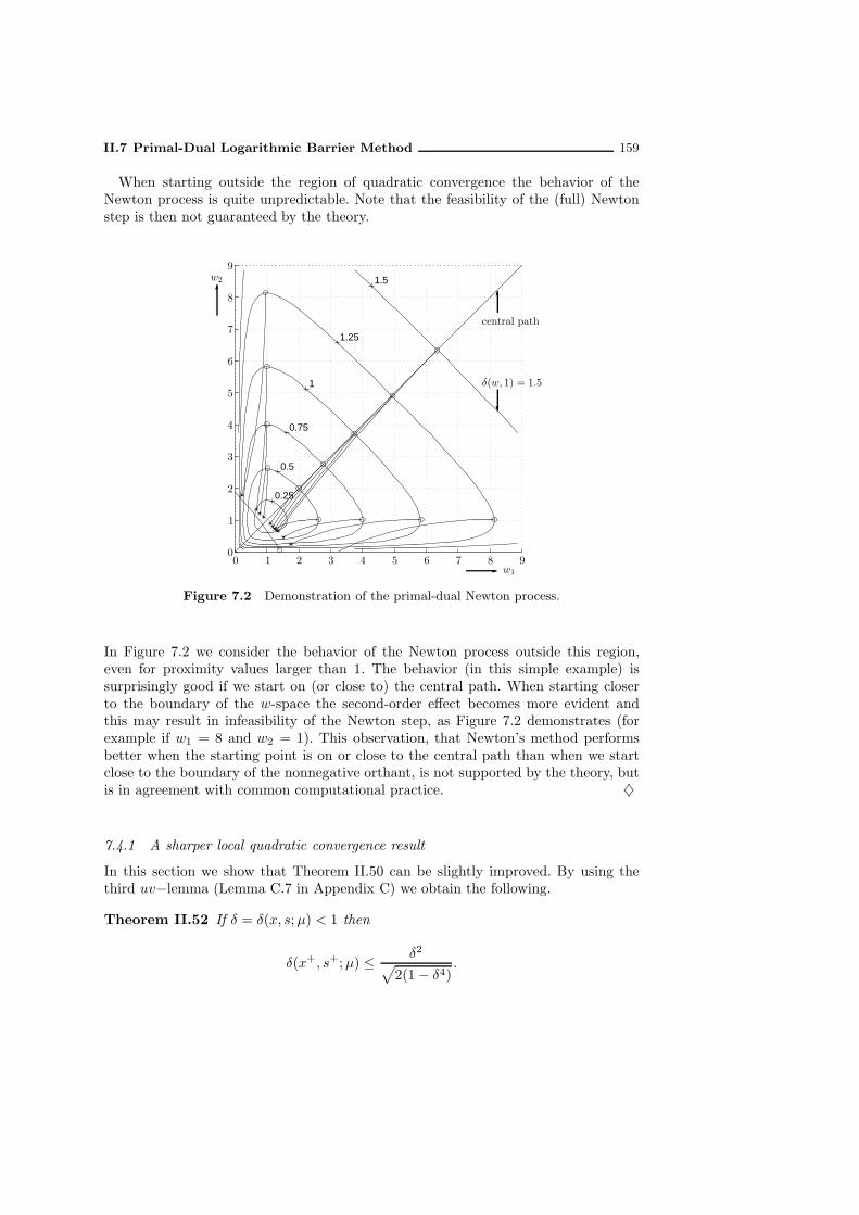
II.7 Primal-Dual Logarithmic Barrier Method 159
When starting outside the region of quadratic convergence the behavior of theNewton process is quite unpredictable. Note that the feasibility of the (full) Newtonstep is then not guaranteed by the theory.
0.25
0.5
0.75
1
1.25
1.5
00
1
1
2
2
3
3
4
4
5
5
6
6
7
7
8
8
9
9w1
w2
central path
δ(w, 1) = 1.5
Figure 7.2 Demonstration of the primal-dual Newton process.
In Figure 7.2 we consider the behavior of the Newton process outside this region,even for proximity values larger than 1. The behavior (in this simple example) issurprisingly good if we start on (or close to) the central path. When starting closerto the boundary of the w-space the second-order effect becomes more evident andthis may result in infeasibility of the Newton step, as Figure 7.2 demonstrates (forexample if w1 = 8 and w2 = 1). This observation, that Newton’s method performsbetter when the starting point is on or close to the central path than when we startclose to the boundary of the nonnegative orthant, is not supported by the theory, butis in agreement with common computational practice. ♦
7.4.1 A sharper local quadratic convergence result
In this section we show that Theorem II.50 can be slightly improved. By using thethird uv−lemma (Lemma C.7 in Appendix C) we obtain the following.
Theorem II.52 If δ = δ(x, s;µ) < 1 then
δ(x+, s+;µ) ≤ δ2√2(1− δ4)
.

160 II Logarithmic Barrier Approach
Proof: From the proof of Theorem II.50 we recall the definitions of δ+ and u+, andthe relation
u+ =√e+ dxds.
Since dx and ds are orthogonal this implies that ‖u+‖2 = n. Now we may write
4(δ+)2 =∥∥(u+)−1 − u+
∥∥2 =∥∥(u+)−1
∥∥2 +∥∥u+
∥∥2 − 2n
=∥∥(u+)−1
∥∥2 − n = eT(
e
e+ dxds− e
).
Application of Lemma C.7 to the last expression (with u = dx and v = ds) yields theresult of the theorem, since ‖dx + ds‖ = 2δ, with δ < 1.
7.5 Primal-dual logarithmic barrier algorithm with full Newtonsteps
In this section we investigate a primal-dual algorithm using approximate centers. Thealgorithm is described below. It is assumed that we are given a positive primal-dualpair (x0, s0) ∈ P+ ×D+ and µ0 > 0 such that (x0, s0) is close to the µ0-center in thesense of the proximity measure δ(x0, s0;µ0). In the algorithm ∆x and ∆s denote theprimal-dual Newton step, as defined before.
Primal-Dual Logarithmic Barrier Algorithm with full Newton steps
Input:A proximity parameter τ , 0 ≤ τ < 1;an accuracy parameter ε > 0;(x0, s0) ∈ P+ × D+ and µ0 > 0 such that (x0)T s0 = nµ0 andδ(x0, s0;µ0) ≤ τ ;a barrier update parameter θ, 0 < θ < 1.
beginx := x0; s := s0; µ := µ0;while nµ ≥ (1− θ)ε dobeginx := x+∆x;s := s+∆s;µ := (1− θ)µ;
endend
We have the following theorem. The proof will follow below.

II.7 Primal-Dual Logarithmic Barrier Method 161
Theorem II.53 If τ = 1/√2 and θ = 1/
√2n, then the Primal-Dual Logarithmic
Barrier Algorithm with full Newton steps requires at most
⌈√2n log
nµ0
ε
⌉
iterations. The output is a primal-dual pair (x, s) such that xT s ≤ ε.
7.5.1 Convergence analysis
Just as in the dual case the proof depends on a lemma that quantifies the effect onthe proximity measure of an update of the barrier parameter to µ+ = (1− θ)µ.
Lemma II.54 Let (x, s) be a positive primal-dual pair and µ > 0 such that xT s = nµ.Moreover, let δ := δ(x, s;µ) and let µ+ = (1 − θ)µ. Then
δ(x, s;µ+)2 = (1− θ)δ2 +θ2n
4(1− θ).
Proof: Let δ+ := δ(x, s;µ+) and u =√xs/µ. Then, by definition,
4(δ+)2 =
∥∥∥∥√1− θu−1 − u√
1− θ
∥∥∥∥2
=
∥∥∥∥√1− θ
(u−1 − u
)+
θu√1− θ
∥∥∥∥2
.
From xT s = nµ it follows that ‖u‖2 = n. Hence, u is orthogonal to u−1 − u:
uT(u−1 − u
)= n− ‖u‖2 = 0.
Therefore,
4(δ+)2 = (1− θ)∥∥u−1 − u
∥∥2 + θ2 ‖u‖21− θ
.
Finally, since∥∥u−1 − u
∥∥ = 2δ and ‖u‖2 = n the result follows.
The proof of Theorem II.53 now goes as follows. At the start of the algorithm wehave δ(x, s;µ) ≤ τ = 1/
√2. After the primal-dual Newton step to the µ-center we
have, by Theorem II.50, δ(x+, s+;µ) ≤ 1/2. Also, from Lemma II.47, (x+)T s+ = nµ.Then, after the barrier parameter is updated to µ+ = (1 − θ)µ, with θ = 1/
√2n,
Lemma II.54 yields the following upper bound for δ(x+, s+;µ+):
δ(x+, s+;µ+)2 ≤ 1− θ
4+
1
8(1− θ)≤ 3
8.
Assuming n ≥ 2, the last inequality follows since its left hand side is a convex functionof θ, whose value is 3/8 both in θ = 0 and θ = 1/2. Since θ ∈ [0, 1/2], the left handside does not exceed 3/8. Since 3/8 < 1/2, we obtain δ(x+, s+;µ+) ≤ 1/
√2 = τ. Thus,
after each iteration of the algorithm the property
δ(x, s;µ) ≤ τ

162 II Logarithmic Barrier Approach
is maintained, and hence the algorithm is well defined. The iteration bound in thetheorem follows from Lemma I.36. Finally, since after each full Newton step theduality gap attains its target value, by Lemma II.47, the duality gap for the pair (x, s)generated by the algorithm is at most ε. This completes the proof of the theorem.
Remark II.55 It is worthwhile to discuss the quality of the iteration bound in TheoremII.53. For that purpose we consider the hypothetical situation where the Newton step ineach iteration is exact. Then, putting δ+ = δ(x+, s+, µ+), after the update of the barrierparameter we have
4(δ+)2 =θ2n
1− θ,
and hence we have δ+ ≤ 1/√2 only if θ2n ≤ 2(1− θ). This occurs only if θ <
√2/n. Hence,
if we maintain the property δ(x, s;µ) ≤ 1/√2 after the update of the barrier parameter, then
the iteration bound will never be smaller than⌈√
n
2log
nµ0
ε
⌉. (7.18)
Note that the iteration bound of Theorem II.53 is only a factor 2 worse than the ‘ideal’iteration bound (7.18). Recall that the bound (7.18) assumes that the Newton step is exactin each iteration. In this respect it is interesting to indicate that for larger values of n theresult of Theorem II.53 can be improved so that it becomes closer to the ‘ideal’ iterationbound. But then we need to use the stronger quadratic convergence result of Theorem II.52.If we take θ = 1/
√n, then by using Lemma II.54 and Theorem II.52, we may easily verify
that the property δ(x, s;µ) ≤ τ = 1/√2 is maintained if
1
4(1− θ)+
1− θ
6≤ 1
2.
This holds if θ ≤ 0.36602, which corresponds to n ≥ 8. Thus, for n ≥ 8 the iteration boundof Theorem II.53 can be improved to
⌈√n log
nµ0
ε
⌉. (7.19)
This iteration bound is the best among all known iteration bounds for interior-point methods.
It differs by only a factor√2 from the ideal bound (7.18). •
7.5.2 Illustration of the algorithm with full Newton steps
We use the same sample problem as before (see Sections 6.7.2, 6.8.4 and 6.9.7). Asstarting point we use the vectors x = (2, 1, 1), y = (0, 0) and s = (1, 1, 1), and sincexT s = 4, we take the initial value of the barrier parameter µ equal to 4/3. We caneasily check that δ(x, s;µ) = 0.2887. So these data can indeed be used to initialize thealgorithm. With ε = 10−4, the algorithm generates the data collected in Table 7.1..As before, Table 7.1. contains one entry (the first) of the vectors x and s. The seventhcolumn contains the values of the proximity δ = δ(x, s;µ) before the Newton step, andthe eighth column the proximity δ+ = δ(x+, s+;µ) after the Newton step at (x, s) tothe current µ-center.

II.7 Primal-Dual Logarithmic Barrier Method 163
It. nµ x1 y1 y2 s1 δ δ+ θ
0 4.000000 2.000000 0.000000 0.000000 1.000000 0.2887 0.0000 0.4082
1 2.367007 2.000000 0.333333 −0.333333 0.666667 0.4596 0.0479 0.4082
2 1.400680 1.510102 0.442200 0.210998 0.557800 0.4611 0.0586 0.4082
3 0.828855 1.267497 0.601207 0.533107 0.398793 0.4618 0.0437 0.4082
4 0.490476 1.148591 0.744612 0.723715 0.255388 0.4608 0.0271 0.4082
5 0.290240 1.085283 0.843582 0.836508 0.156418 0.4601 0.0162 0.4082
6 0.171750 1.049603 0.905713 0.903253 0.094287 0.4598 0.0096 0.4082
7 0.101633 1.029055 0.943610 0.942750 0.056390 0.4597 0.0057 0.4082
8 0.060142 1.017089 0.966423 0.966122 0.033577 0.4596 0.0034 0.4082
9 0.035589 1.010076 0.980058 0.979953 0.019942 0.4596 0.0020 0.4082
10 0.021060 1.005950 0.988174 0.988137 0.011826 0.4596 0.0012 0.4082
11 0.012462 1.003516 0.992993 0.992980 0.007007 0.4596 0.0007 0.4082
12 0.007375 1.002079 0.995850 0.995846 0.004150 0.4596 0.0004 0.4082
13 0.004364 1.001230 0.997543 0.997542 0.002457 0.4596 0.0002 0.4082
14 0.002582 1.000728 0.998546 0.998545 0.001454 0.4596 0.0001 0.4082
15 0.001528 1.000430 0.999139 0.999139 0.000861 0.4596 0.0001 0.4082
16 0.000904 1.000255 0.999491 0.999491 0.000509 0.4596 0.0001 0.4082
17 0.000535 1.000151 0.999699 0.999699 0.000301 0.4596 0.0000 0.4082
18 0.000317 1.000089 0.999822 0.999822 0.000178 0.4596 0.0000 0.4082
19 0.000187 1.000053 0.999894 0.999894 0.000106 0.4596 0.0000 0.4082
20 0.000111 1.000031 0.999938 0.999938 0.000062 0.4596 0.0000 0.4082
21 0.000066 1.000018 0.999963 0.999963 0.000037 0.4596 0.0000 0.4082
22 0.000039 1.000011 0.999978 0.999978 0.000022 − − −
Table 7.1. Output of the primal-dual full-step algorithm.
Comparing the results in Table 7.1. with those in the corresponding table for thedual algorithm with full steps (Table 6.1., page 124), the most striking differences arethe number of iterations and the behavior of the proximity measure. In the primal-dualcase the number of iterations is 22 (instead of 53). This can be easily understood fromthe fact that we could use the larger barrier update parameter θ = 1/
√2n (instead of
θ = 1/(3√n)).
The second difference is probably more important. In the primal-dual case Newton’smethod is much more efficient than in the dual case. This is especially evident in thefinal iterations where both methods show very stable behavior. In the dual case theproximity takes in these iterations the values 0.2722 (before) and 0.0524 (after theNewton step), whereas in the primal-dual case these values are respectively 0.4596 and0.0000. Note that in the dual case the effect of the Newton step is slightly better thanthe quadratic convergence result of Theorem II.21. In the primal-dual case, however,the effect of the Newton step is much better than predicted by Theorem II.50, andeven much better than the improved quadratic convergence result of Theorem II.52.

164 II Logarithmic Barrier Approach
The figures in Table 7.1. justify the statement (at least for this sample problem, butwe observed the same phenomenon in other experiments) that asymptotically theprimal-dual Newton method is almost exact.
Remark II.56 It is of interest to have a closer (and more accurate) look at the proximityvalues in the final iterations. They are given in Table 7.2. (page 164). These figures show that
It. δ δ+
11 0.45960642869434 0.00069902816289
12 0.45960584496214 0.00041365328341
13 0.45960564054812 0.00024478048789
14 0.45960556896741 0.00014484936548
15 0.45960554390189 0.00008571487895
16 0.45960553512461 0.00005072193012
17 0.45960553205110 0.00003001478966
18 0.45960553097480 0.00001776130347
19 0.45960553059816 0.00001051028182
20 0.45960553046642 0.00000621947704
21 0.45960553041942 0.00000368038542
Table 7.2. Proximity values in the final iterations.
in the final iterations, where Newton’s method is almost exact, the quality of the methodgradually improves. After the step the proximity decreases monotonically. In fact, surprisinglyenough, the rate of decrease of subsequent values of the proximity after the step is almostconstant (0.59175). Remember that the barrier parameter µ also decreases at a linear rateby a factor 1 − θ, where θ = 1/
√2n. In our case we have n = 3. This gives θ = 0.4082 and
1− θ = 0.59175, precisely the rate of decrease in δ+. Before the Newton step the proximityis almost constant (0.4596). Not surprisingly, this is precisely the value of θ
√n/(2(1 − θ)).
Thus, our numerical experiment gives rise to a conjecture:
Conjecture II.57 Asymptotically the quality of the primal-dual Newton step graduallyimproves. The proximity before the step converges to some constant and the proximity after thestep decreases monotonically to zero with a linear convergence rate. The rate of convergenceis equal to 1− θ.
This observed behavior of the primal-dual Newton method has no theoretical justification at
the moment. •We conclude this section with a graphical illustration. Figure 7.3 shows on two
graphs the progress of the algorithm in the w-space (cf. Example II.51 on page 157).In both figures the w-space is projected onto its first two coordinates. The differencebetween the two graphs is due to the scaling of the axes. On the left graph the scaleis linear and on the right graph it is logarithmic. As in Example II.51, the curvesconnecting the subsequent iterates show the intermediate values of xs on the way tothe next iterate. The graphs show that after the first iteration the iterates follow thecentral path quite accurately.

II.7 Primal-Dual Logarithmic Barrier Method 165
10−6 10−5 10−4 10−3 10−2 10−1 100 10110−6
10−5
10−4
10−3
10−2
10−1
100
101
00
1
1
2
2
3
3
4
4
5
5
w1
w2
w1
w2
central path
δ(w, µ1) = τ
Figure 7.3 The iterates of the primal-dual algorithm with full steps.
7.5.3 The classical analysis of the algorithm
In this section we give a different analysis of the primal-dual logarithmic barrieralgorithm with full Newton steps. The analysis uses the proximity measure
σ(x, s;µ) :=
∥∥∥∥xs
µ− e
∥∥∥∥ ,
which is very common in the literature on primal-dual methods.10
Because of its widespread use, it seems useful to show in this section how the analysiscan be easily adapted to the use of the classical proximity measure. In fact, the onlything we have to do is find suitable analogues of the quadratic convergence result inTheorem II.50 and the barrier update result of Lemma II.54.
Theorem II.58 11 If σ := σ(x, s;µ) ≤ 2/(1 +
√1 +
√2)= 0.783155, then the pri-
mal-dual Newton step is feasible. Moreover, in that case
σ(x+, s+;µ) ≤ σ2
2√2(1− σ)
.
Proof: First we derive from∥∥u2 − e
∥∥ = σ the obvious inequality
1− σ ≤ u2i ≤ 1 + σ, 1 ≤ i ≤ n.
10 It was introduced by Kojima, Mizuno and Yoshise [178] and used in many other papers. See, e.g.,Gonzaga [124], den Hertog [140], Marsten Shanno and Simantiraki [196], McShane, Monma andShanno [199], Mehrotra and Sun [205], Mizuno [215], Monteiro and Adler [218], Todd [262, 264],Zhang and Tapia [319].
11 This result is due to Mizuno [212].

166 II Logarithmic Barrier Approach
This implies∥∥u−2
∥∥∞ ≤ 1
1− σ. (7.20)
From (7.4) we recall that
x+s+ = µe+∆x∆s.
Hence, using (7.11), we have 12,13
σ(x+, s+;µ) :=
∥∥∥∥x+s+
µ− e
∥∥∥∥ =∥∥∥∥∆x∆s
µ
∥∥∥∥ = ‖dxds‖ .
By the first uv-lemma (Lemma C.4 in Appendix C) we have
‖dxds‖ ≤ 1
2√2‖dx + ds‖2 =
1
2√2
∥∥u−1 − u∥∥2 .
Using (7.20) we write
∥∥u−1 − u∥∥2 =
∥∥u−1(e − u2)∥∥2 ≤
∥∥u−2∥∥∞∥∥e− u2
∥∥2 ≤ σ2
1− σ.
Hence we get
σ(x+, s+;µ) ≤ σ2
2√2(1− σ)
.
Since σ(x+, s+;µ) = ‖dxds‖, feasibility of the new iterates is certainly guaranteed ifσ(x+, s+;µ) ≤ 1, from (7.9). This condition is certainly satisfied if
σ2
2√2(1− σ)
≤ 1,
and this inequality holds if and only if σ ≤ 2/(1 +
√1 +
√2), as can easily be
verified. The theorem follows.
12 Exercise 52 This exercise provides an alternative proof of the first inequality in Lemma C.4. Letu and v denote vectors in IRn and δ > 0 (δ ∈ IR). First prove that
minu,v
u1v1 :
n∑
i=1
uivi = 0,
n∑
i=1
(u2i + v2i
)= 4δ2
= δ2.
Using this, show that if u and v are orthogonal and ‖u+ v‖ = 2δ then ‖uv‖∞ ≤ δ2.13 Exercise 53 This exercise provides tighter version of the second inequality in Lemma C.4. Let u
and v denote vectors in IRn and δ > 0 (δ ∈ IR). First prove that
maxu,v
n∑
i=1
u2i v2i :
n∑
i=1
uivi = 0,
n∑
i=1
(u2i + v2i
)= 4δ2
=
nδ4
n− 1.
Using this show that if u and v are orthogonal and ‖u+ v‖ = 2δ then ‖uv‖ ≤ δ2√2.

II.7 Primal-Dual Logarithmic Barrier Method 167
Lemma II.59 Let (x, s) be a positive primal-dual pair and µ > 0 such that xT s = nµ.Moreover, let σ := σ(x, s;µ) and let µ+ = (1− θ)µ. Then we have
σ(x, s;µ+) =
√σ2 + θ2n
1− θ.
Proof: Let σ+ := σ(x, s;µ+), with xT s = nµ. Then, by definition,
(σ+)2 =
∥∥∥∥xs
(1− θ)µ− e
∥∥∥∥2
=1
(1− θ)2
∥∥∥∥xs
µ− e + θe
∥∥∥∥2
.
The vectors e and xs/µ− e are orthogonal, as easily follows. Hence
∥∥∥∥xs
µ− e+ θe
∥∥∥∥2
=
∥∥∥∥xs
µ− e
∥∥∥∥2
+ ‖θe‖2 = σ2 + θ2n.
The lemma follows.
From the above results, it is clear that maintaining the property σ(x, s : µ) ≤ τduring the course of the algorithm amounts to the following condition on θ:
1
1− θ
√τ4
8(1− τ)2+ nθ2 ≤ τ. (7.21)
For any given τ this inequality determines how deep the updates of the barrierparameter are allowed to be. Since the full Newton step must be feasible we mayassume that
τ ≤ 2
1 +√1 +
√2= 0.783155.
Squaring both sides of (7.21) gives
τ4
8(1− τ)2+ nθ2 ≤ τ2(1 − θ)2.
This implies nθ2 ≤ τ2, and hence the parameter θ must satisfy θ ≤ τ/√n.
The iteration bound of Lemma I.36 becomes smaller for larger values of θ. Our aimhere is to show that for the best possible choice of θ the iteration bound resultingfrom the classical analysis cannot be better than the bound of Theorem II.53. Forthat purpose we may assume that n is so large that 1− θ ≈ 1. Then the condition onθ becomes
τ4
8(1− τ)2+ nθ2 ≤ τ2,
or equivalently,
nθ2 ≤ τ2 − τ4
8(1− τ)2. (7.22)
Note that the right-hand side expression must be nonnegative, which holds only if
τ ≤ 2√2
1 + 2√2= 0.738796.

168 II Logarithmic Barrier Approach
We can easily verify that the right-hand side expression in (7.22) is maximal if
7τ3 − 22τ2 + 24τ − 8 = 0,
which occurs for τ = 0.60155. Substituting this value in (7.22) we obtain
nθ2 ≤ 0.258765,
which amounts to
θ ≤ 0.508689√n
≈ 1
2√n.
Obviously, this upper bound for θ is too optimistic. The above argument makes clearthat by using the ‘classical’ proximity measure σ(x, s;µ) in the analysis of the primal-dual method with full Newton steps, the iteration bound obtained with the proximitymeasure δ(x, s;µ) cannot be improved.
7.6 A version of the algorithm with adaptive updates
7.6.1 Adaptive updating
We have seen in Section 7.5 that when the property
δ(x, s;µ) ≤ τ =1√2
(7.23)
is maintained after the update of the barrier parameter, the values of the barrierupdate parameter θ are limited by the upper bound θ <
√2/n, and therefore, the
iteration bound cannot be better than the ‘ideal’ bound⌈√
n
2log
nµ0
ε
⌉.
Thus, larger updates of the barrier parameter are possible only when abandoning theidea that property (7.23) must hold after each update of the barrier parameter.To make clear how this can be done without losing the iteration bound of
Theorem II.53, we briefly recall the idea behind the proof of this theorem. Aftereach Newton step we have a primal-dual pair (x, s) and µ > 0 such that
δ(x, s;µ) ≤ τ =τ2√
2(1− τ2). (7.24)
Then we update µ to a smaller value µ+ = (1 − θ)µ such that
δ(x, s;µ+) ≤ τ, (7.25)
and we perform a Newton step to the µ+-center, yielding a primal-dual pair (x+, s+)such that δ(x+, s+;µ+) ≤ τ . Figure 7.4 illustrates this.Why does this scheme work? It works because every time we perform a Newton
step the iterates x and s are such that xs is in the region around the µ-center where

II.7 Primal-Dual Logarithmic Barrier Method 169
central path
µ
µ+ = (1− θ)µ
xs
x+s+
δ(x, s, µ) = τ
δ(x, s, µ+) = τ
xT s = nµ+
xT s = nµ❨
......................................................................
......................................................................
Figure 7.4 The primal-dual full-step approach.
Newton’s method behaves well. The theory guarantees that if the proximity does notexceed the parameter τ = 1/
√2 then we stay within this region. However, in practice
the region where Newton’s method behaves well may be much larger.Thus we can adapt our strategy to this phenomenon and choose the smallest barrier
parameter µ+ = (1− θ)µ so that after the Newton step to the µ+-center the iteratessatisfy δ(x+, s+;µ+) ≤ τ . Therefore, let us consider the following problem:
Given a primal-dual pair (x, s) and µ > 0 such that δ := δ(x, s;µ) ≤ τ ,find the largest θ such that after the Newton step at (x, s) with barrierparameter value µ+ = (1− θ)µ we have δ+ = δ(x+, s+;µ+) ≤ τ .
Here we use the parameter τ instead of τ , because until now τ referred to the proximitybefore the Newton step, whereas τ is an upper bound for the proximity just after theNewton step. It is natural to take for τ the value 1/2, because this is an upper boundfor the proximity after the Newton step when the proximity before the step is 1/
√2.
Our aim in this section is to investigate how deep the updates can be taken, so as toenhance the performance of the algorithm as much as possible. See Figure 7.5.14 Justas in the case of the dual method with adaptive updates, we need to introduce theso-called primal-dual affine-scaling and primal-dual centering directions at (x, s).
14 The idea of using adaptive updates of the barrier parameter in a primal-dual method can be foundin, e.g., Jarre and Saunders [163].

170 II Logarithmic Barrier Approach
central path
µ
µ+ = (1− θ)µ
xs
x+s+
δ(x, s, µ) = τ
δ(x, s, µ+) = τ
xT s = nµ+
xT s = nµ❨
......................................................................
......................................................................
Figure 7.5 The full-step method with an adaptive barrier update.
7.6.2 The primal-dual affine-scaling and centering direction
We first recall some definitions and properties from Section 7.4. With
d =
√x
s, u =
√xs
µ,
the vectors x and s can be scaled by d to the vector u as follows:
d−1x√µ
=dsõ= u.
The same scaling applied to the Newton steps ∆x and ∆s yields the scaled Newtonsteps dx and ds:
dx =d−1∆x√
µ, ds =
d∆s√µ,
and these satisfy
dx + ds = u−1 − u.
Moreover, the vectors dx and ds are orthogonal. They are the components of the vectoru−1 − u in the null space of AD and the null space of HD−1 respectively:
dx = PAD(u−1 − u) (7.26)
ds = PHD−1(u−1 − u). (7.27)

II.7 Primal-Dual Logarithmic Barrier Method 171
In this section we work mainly with the scaled Newton steps dx and ds. Thelast expressions yield a natural way of separating these directions into a so-calledaffine-scaling component and a centering component. Remark Guoyong Gu: termcentering component not natural!! The (scaled) centering directions are definedby
dcx = PAD(u−1), dcs = PHD−1 (u−1), (7.28)
and the (scaled) affine directions by
dax = −PAD(u), das = −PHD−1 (u). (7.29)
Now we have the obvious relations
dx = dcx + dax
ds = dcs + das
and
dcx + dcs = u−1
dax + das = −u.
The unscaled centering and affine-scaling directions are defined in the obvious way:∆ax :=
õddax, etc. For the sake of completeness we list these definitions below and
we also give some alternative expressions which can straightforwardly be verified.
∆ax :=√µddax = −√
µDPAD(u) = −DPAD(√xs)
∆as :=√µd−1das = −√
µD−1PHD−1 (u) = −D−1PHD−1 (√xs)
∆cx :=√µddcx =
√µDPAD(u−1) = µDPAD( e√
xs)
∆cs :=√µd−1dcs =
√µD−1PHD−1(u−1) = µD−1PHD−1 ( e√
xs).
Note that the affine-scaling directions ∆ax and ∆as depend only on the iterates x ands and not on the barrier parameter µ. For the centering directions we have that ∆cx/µand ∆cs/µ depend only on the iterates x and s and not on the barrier parameter µ.Also note that if we are on the central path, i.e., if x = x(µ) and s = s(µ), then wehave u = e. This implies u−1−u = 0, whence dx = ds = 0. Hence, on the central pathwe have dax = −dcx and das = −dcs.For future reference we observe that the above definitions imply the obvious relations
∆x = ∆ax+∆cx
∆s = ∆as+∆cs,
(7.30)
which show that the (unscaled) full Newton step (∆x,∆s) — at (x, s) and for thebarrier parameter value µ — can be nicely decomposed in its affine scaling and itscentering component.
172 II Logarithmic Barrier Approach
7.6.3 Condition for adaptive updates
In this section we start to deal with the problem stated before. Let (x, s) be a positiveprimal-dual pair and µ > 0 such that δ = δ(x, s;µ) ≤ τ . We want to investigate howlarge θ can be so that after the Newton step at (x, s) with barrier parameter valueµ+ = (1 − θ)µ we have δ+ = δ(x+, s+;µ+) ≤ τ . We derive a condition for the barrierupdate parameter θ that guarantees the desired behavior.The vector u, the scaled search directions dx and ds and their (scaled) centering
components dcx, dcs and (scaled) affine components dax, d
as , have the same meaning as
in the previous section; the entities u, dax and das depend on the given value µ of thebarrier parameter. The scaled search directions at (x, s) with barrier parameter valueµ+ are denoted by d+x and d+s . Letting ∆x and ∆s denote the (unscaled) Newtondirections with respect to µ+, we have
s∆x+ x∆s = µ+e− xs,
and therefore, also using (7.11),
x+s+ = µ+e+∆x∆s = µ+(e+ d+x d
+s
).
By Lemma II.48, the step is feasible if e+ d+x d+s ≥ 0, and this certainly holds if
∥∥d+x d+s∥∥∞ ≤ 1.
Moreover, from the proof of Theorem II.50 we recall that the proximity δ+ :=δ(x+, s+;µ+) of the new pair (x+, s+) with respect to the µ+-center is given by
2δ+ =
∥∥∥∥∥d+x d
+s√
e+ d+x d+s
∥∥∥∥∥ .
This implies that we have δ+ ≤ τ if and only if∥∥∥∥∥
d+x d+s√
e+ d+x d+s
∥∥∥∥∥
2
≤ 4τ2.
In the sequel we use the weaker condition∥∥d+x d+s
∥∥2 ≤ 4τ2(1−
∥∥d+x d+s∥∥∞), (7.31)
which we refer to as the condition for adaptive updating. A very important observationis that when this condition is satisfied, the Newton step is feasible. Because, if (7.31)holds, since the left-hand side expression is nonnegative, the right-hand side expressionmust be nonnegative as well, and hence ‖d+x d+s ‖∞ ≤ 1. Thus, in the further analysiswe may concentrate on the condition for adaptive updating (7.31).
7.6.4 Calculation of the adaptive update
We proceed by deriving upper bounds for the 2-norm and the infinity norm of thevector d+x d
+s . It is convenient to introduce the vector
u :=
√xs
µ+.

II.7 Primal-Dual Logarithmic Barrier Method 173
We then have
u =
√xs
µ+=
√xs
(1− θ)µ=
u√1− θ
.
Hence, using this and (7.26),
d+x = PAD
(u−1 − u
)=
√1− θPAD
(u−1
)− 1√
1− θPAD (u)
and
d+s = PHD−1
(u−1 − u
)=
√1− θPHD−1
(u−1
)− 1√
1− θPHD−1 (u) .
Now using (7.28) and (7.29) we obtain
d+x =√1− θ dcx +
dax√1− θ
(7.32)
d+s =√1− θ dcs +
das√1− θ
. (7.33)
Note that d+x can be rewritten in the following way:
√1− θdcx +
dax√1− θ
=√1− θ (dcx + dax) +
(1√1− θ
−√1− θ
)dax
=√1− θdx +
θ√1− θ
dax.
Since d+s can be reformulated in exactly the same way we find
d+x =√1− θdx +
θ√1− θ
dax
d+s =√1− θds +
θ√1− θ
das .
Multiplication of both expressions gives
d+x d+s = (1− θ)dxds + θ (dxd
as + dsd
ax) +
θ2
1− θdaxd
as . (7.34)
At this stage we see how the coordinates of the vector d+x d+s depend on θ. The
coordinates of (1− θ)d+x d+s are quadratic functions of θ:
(1− θ)d+x d+s = (1− θ)2dxds + θ(1 − θ) (dxd
as + dsd
ax) + θ2daxd
as .
When multiplying the condition (7.31) for adaptive updating by (1−θ)2, this conditioncan be rewritten as
4τ2(1− θ)2 −∥∥(1 − θ)d+x d
+s
∥∥2 ≥ 4τ2(1 − θ)∥∥(1− θ)d+x d
+s
∥∥∞ . (7.35)
Now denoting the left-hand side member by p(θ) and the i-th coordinate of the vector(1− θ)d+x d
+s by qi(θ), with τ given, we need to find the largest positive θ that satisfies
the following inequalities:
p(θ) ≥ 4τ2(1− θ)qi(θ), 1 ≤ i ≤ n
p(θ) ≥ −4τ2(1− θ)qi(θ), 1 ≤ i ≤ n.

174 II Logarithmic Barrier Approach
Since p(θ) is a polynomial of degree 4 in θ, and each qi(θ) is a polynomial of degree2 in θ, the largest positive θ satisfying each single one of these 2n inequalities can befound straightforwardly by solving a polynomial equation of degree 4. The smallest ofthe 2n positive numbers obtained in this way (some of them may be infinite, but notall of them!) is the value of θ determined by the condition of adaptive updating. Thuswe have shown that the largest θ satisfying the condition for adaptive updating canbe found by solving 2n polynomial equations of degree 4.15
Below we deal with a second approach. We consider a further relaxation of thecondition for adaptive updating that requires the solution of only one quadraticequation. Of course, this approach yields a smaller value of θ than the above procedure,which gives the exact solution of the condition (7.31) for adaptive updating. Beforeproceeding it is of interest to investigate the special case where we start at the µ-centersx = x(µ) and s = s(µ).
7.6.5 Special case: adaptive update at the µ-center
When we start with x = x(µ) and s = s(µ), we established earlier that u = e,dx = ds = 0, dax = −dcx and das = −dcs. Substituting this in (7.34) we obtain
d+x d+s =
θ2
1− θdaxd
as .
Now we can use the first uv-lemma (Lemma C.4 in Appendix C) to estimate the2-norm and the infinity norm of daxd
as . Since d
ax + das = −u = −e, we obtain
‖daxdas‖ ≤ n
2√2, ‖daxdas‖∞ ≤ n
4.
Substitution in (7.31) gives
θ4n2
8(1− θ)2≤ 4τ2
(1− θ2n
4(1− θ)
).
This can be rewritten asθ4n2
8(1− θ)2+τ2θ2n
1− θ≤ 4τ2,
which is equivalent to
(θ2n
2√2(1− θ)
+ τ2√2
)2
≤ 4τ2 + 2τ4,
orθ2n
1− θ≤ 2
√2(√
4τ2 + 2τ4 − τ2√2).
Substituting τ = 1/2 givesθ2n
1− θ≤ 2.
15 In fact, more efficient procedures exist for solving the condition for adaptive updating, but hereour only aim has been to show that there exists an efficient procedure for finding the maximalvalue of the parameter θ satisfying the condition for adaptive updating.

II.7 Primal-Dual Logarithmic Barrier Method 175
This result has its own interest. The bound obtained is exactly the ‘ideal’ bound for θderived in Section 7.5 for the hypothetical situation where the Newton step is exact.Here we obtained a better bound without this assumption, but under the more realisticassumption that we start at the µ-centers x = x(µ) and s = s(µ).
7.6.6 A simple version of the condition for adaptive updating
We return to the general case, and show how a weakened version of the condition foradaptive updating ∥∥d+x d+s
∥∥2 ≤ 4τ2(1−
∥∥d+x d+s∥∥∞)
can be reduced to a quadratic inequality in θ. With
d+ := d+x + d+s ,
the first uv-lemma (Lemma C.4 in Appendix C) implies that
∥∥d+x d+s∥∥ ≤ ‖d+‖2
2√2,
∥∥d+x d+s∥∥∞ ≤ ‖d+‖2
4.
Substituting these bounds in the condition for adaptive updating we obtain the weakercondition
‖d+‖48
≤ 4τ2
(1− ‖d+‖2
4
).
Rewriting this as (∥∥d+∥∥2 + 4τ2
)2≤ 32τ2 + 16τ4,
we obtain ∥∥d+∥∥2 ≤
√32τ2 + 16τ4 − 4τ2.
Substituting τ = 1/2 leads to the condition∥∥d+
∥∥2 ≤ 2. (7.36)
From the expressions (7.32) and (7.33) for d+x and d+s , and also using that dcx+dcs = u−1
and dax + das = −u, we find
d+ =√1− θ u−1 − u√
1− θ.
From this expression we can calculate the norm of d+:
∥∥d+∥∥2 = (1 − θ)
∥∥u−1∥∥2 + ‖u‖2
1− θ− 2n.
Since ‖u‖2 = n and∥∥u−1
∥∥2 = n+ 4δ2, where δ = δ(x, s;µ), we obtain
∥∥d+∥∥2 = (1− θ)
(n+ 4δ2
)+
n
1− θ− 2n = 4(1− θ)δ2 +
θ2n
1− θ. 16
16 Since∥∥d+
∥∥ = 2δ(x, s : µ+) this analysis yields in a different way the same result as in Lemma II.54,
namely
δ(x, s;µ+)2 = (1 − θ)δ2 +θ2n
4(1 − θ).

176 II Logarithmic Barrier Approach
Putting this in (7.36) we obtain the following condition on θ:
4(1− θ)δ2 +θ2n
1− θ≤ 2.
The largest θ satisfying this inequality is given by
θ =
√2n+ 1− 4nδ2 + 4δ2 − 1
n+ 4δ2. (7.37)
With this value of θ we are sure that when starting with δ(x, s;µ) = δ, after the Newtonstep with barrier parameter value µ+ = (1−θ)µ we have δ(x+, s+;µ+) ≤ 1/2. If δ = 0,the above expression reduces to
θ =2
1 +√2n+ 1
≤ 1√2n
and if δ = 1/2 to
θ =1√n+ 1
, 17
as easily may be verified. Hence, when using cheap adaptive updates the actual valueof θ varies from iteration to iteration but it always lies between the above two extremevalues. The ratio between these extreme values is about
√2. As a consequence, the
speedup factor is bounded above by (approximately)√2.
7.6.7 Illustration of the algorithm with adaptive updates
With the same example as in the previous illustrations, and the same initializationof the algorithm as in Section 7.5.2, we experiment in this section with two adaptive-update strategies. First we consider the most expensive strategy, and calculate thebarrier update parameter θ from (7.35). In this case we need to solve 2n polynomialinequalities of degree four. The algorithm, with ε = 10−4, then runs as shown inTable 7.3.. As before, Table 7.3. contains one entry (the first) of the vectors x ands. A new column shows the value of the barrier update parameter in each iteration.The fast increase of this parameter to almost 1 is surprising. It results in very fastconvergence of the method: only 5 iterations yield the desired accuracy.When we calculate θ according to (7.37), the performance of the algorithm is as
shown in Table 7.4.. Now 15 iterations are needed instead of 6. In this example inthe final iterations θ seems to stabilize around the value 0.58486. This implies thatthe convergence rate for the duality gap is linear. This is in contrast with the otherapproach, where the convergence rate for the duality gap appears to be quadratic.Unfortunately, at this time no theoretical justification for a quadratic convergence
rate of the adaptive version of the full-step method exists. For the moment we leave
17 We could have used this value of θ in Theorem II.53, leading to the iteration bound
⌈√n+ 1 log
nµ0
ε
⌉
for the Primal-Dual Logarithmic Barrier Algorithm with full Newton steps.

II.7 Primal-Dual Logarithmic Barrier Method 177
It. nµ x1 y1 y2 s1 δ δ+ θ
0 4.000000 2.000000 0.000000 0.000000 1.000000 0.2887 0.7071 0.679623
1 1.281509 1.093836 0.333333 0.572830 0.666667 0.7071 0.7071 0.846142
2 0.197170 1.010191 0.888935 0.934277 0.111065 0.7071 0.7071 0.976740
3 0.004586 1.000224 0.997391 0.998471 0.002609 0.7071 0.7071 0.999460
4 0.000002 1.000000 0.999999 0.999999 0.000001 0.7071 0.1472 0.999999
5 0.000000 1.000000 1.000000 1.000000 0.000000 − − −
Table 7.3. The primal-dual full-step algorithm with expensive adaptive updates.
It. nµ x1 y1 y2 s1 δ δ+ θ
0 4.000000 2.000000 0.000000 0.000000 1.000000 0.2887 0.2934 0.5348471 1.860612 1.286871 0.333333 0.379796 0.666667 0.2934 0.1355 0.5343572 0.866381 1.138033 0.698479 0.711206 0.301521 0.1355 0.0670 0.5457153 0.393584 1.063707 0.865026 0.868805 0.134974 0.0670 0.0308 0.5478904 0.177943 1.029247 0.939865 0.940686 0.060135 0.0308 0.0140 0.5484385 0.080352 1.013307 0.973046 0.973216 0.026954 0.0140 0.0063 0.5485546 0.036275 1.006028 0.987874 0.987908 0.012126 0.0063 0.0028 0.5485787 0.016375 1.002726 0.994534 0.994542 0.005466 0.0028 0.0013 0.5485838 0.007392 1.001231 0.997535 0.997536 0.002465 0.0013 0.0006 0.5485849 0.003337 1.000556 0.998887 0.998888 0.001113 0.0006 0.0003 0.548584
10 0.001506 1.000251 0.999498 0.999498 0.000502 0.0003 0.0001 0.54858411 0.000680 1.000113 0.999773 0.999773 0.000227 0.0001 0.0001 0.54858412 0.000307 1.000051 0.999898 0.999898 0.000102 0.0001 0.0000 0.54858413 0.000139 1.000023 0.999954 0.999954 0.000046 0.0000 0.0000 0.54858414 0.000063 1.000010 0.999979 0.999979 0.000021 0.0000 0.0000 0.54858415 0.000028 1.000005 0.999991 0.999991 0.000009 − − −
Table 7.4. The primal-dual full-step algorithm with cheap adaptive updates.
this topic with the conclusion that the above comparison between the ‘expensive’ andthe ‘cheap’ adaptive update full-step method suggests that it is worth spending extraeffort in finding as large values for θ as possible.We conclude the section with a graphical illustration of the adaptive updating
strategy. Figure 7.6 shows on two graphs the progress of the algorithm with theexpensive update. The graphs show the first two coordinates of the iterates in thew-space. The left graph has a linear scale and the right graph a logarithmic scale.Figure 7.7 concerns the case when cheap updates are used.
7.7 The predictor-corrector method
In the previous section it became clear that the Newton step can be decomposed into anaffine-scaling component and a centering component. Using the notations introduced

178 II Logarithmic Barrier Approach
10−7 10−6 10−5 10−4 10−3 10−2 10−1 100 10110−7
10−6
10−5
10−4
10−3
10−2
10−1
100
101
00
0.5
0.5
1
1
1.5
1.5
2
2w1
w2
w1
w2
central path
δ(w, µ1) = τ
µ1e
Figure 7.6 Iterates of the primal-dual algorithm with adaptive updates.
there, we recall from Section 7.6.2 that the (scaled) centering components are givenby
dcx = PAD(u−1), dcs = PHD−1 (u−1),
and the (scaled) affine components by
dax = −PAD(u), das = −PHD−1 (u),
where
d =
√x
s, u =
√xs
µ.
10−7 10−6 10−5 10−4 10−3 10−2 10−1 100 10110−7
10−6
10−5
10−4
10−3
10−2
10−1
100
101
00
0.5
0.5
1
1
1.5
1.5
2
2
2.5
2.5
3
3w1
w2
w1
w2
central path
δ(w, µ1) = τ
µ1e
Figure 7.7 Iterates of the primal-dual algorithm with cheap adaptive updates.

II.7 Primal-Dual Logarithmic Barrier Method 179
We also recall the relations
dx = dcx + dax
ds = dcs + das
and
dcx + dcs = u−1
dax + das = −u.
The unscaled centering and affine-scaling components are given by
∆ax =√µddax, ∆as =
√µd−1das
and∆cx =
√µddcx, ∆cs =
√µd−1dcs;
as a consequence we have
∆ax∆as = µdaxdas , ∆cx∆cs = µdcxd
cs.
It is interesting to consider the effect of moving along these directions. Let us define
xa(θ) = x+ θ∆ax
xc = x+∆cx
sa(θ) = s+ θ∆as
sc = s+∆cs.
We say that xa(θ) and sa(θ) result from an affine-scaling step of size θ at (x, s). Inpreparation for the next lemma we first establish the following two relations:
x∆as+ s∆ax = −xs (7.38)
x∆cs+ s∆cx = µe. (7.39)
These relations easily follow from the previous ones. We show this for the first of thetwo relations. We first write
x∆as =√µxd−1das = µudas ,
ands∆ax =
√µsddax = µudax.
Adding the last two equalities we get (7.38):
x∆as+ s∆ax = µu (dax + das) = −µu2 = −xs.
Now we can prove
Lemma II.60 Let xT s = nµ. Assuming feasibility of the steps, the affine-scaling stepreduces the duality gap by a factor 1− θ and the step along the centering componentsdoubles the duality gap.

180 II Logarithmic Barrier Approach
Proof: We have
xa(θ)sa(θ) = (x+ θ∆ax) (s+ θ∆as) = xs+ θ (x∆as+ s∆ax) + θ2∆ax∆as.
Using (7.38) we find
xa(θ)sa(θ) = (1− θ)xs + θ2∆ax∆as.
Using that ∆ax and ∆as are orthogonal we obtain
(xa(θ))Tsa(θ) = eT
((1− θ)xs+ θ2∆ax∆as
)= (1− θ)xT s,
proving the first statement. For the second statement we write
xcsc = (x+∆cx) (s+∆cs) = xs+ (x∆cs+ s∆cx) + ∆cx∆cs.
Substitution of (7.39) gives
xcsc = xs+ µe + θ2∆cx∆cs.
Thus we obtain
(xc)Tsc = eT
(xs+ µe+ θ2∆cx∆cs
)= xT s+ µeT e = 2nµ.
This completes the proof.
Recall from (7.30) that the (unscaled) full Newton step (∆x,∆s) at (x, s) — withbarrier parameter value µ — can be decomposed in its affine scaling and its centeringcomponent. The above lemma makes clear that in the algorithms we dealt with before,the reduction in the duality gap during a (full) Newton step is delivered by the affine-scaling component in the Newton step. The centering component in the Newton stepforces the iterates to stay close to the central path.When solving a given LO problem, we wish to find a primal-dual pair with a
duality gap close to zero. We want to reduce the duality gap as fast as possible tozero. Therefore, it becomes natural to consider algorithms that put more emphasis onthe affine-scaling component. That is the underlying idea of the predictor-corrector
method which is the subject of this section. Note that when the full affine-scaling step(with step-size 1) is feasible, it produces a feasible pair with duality gap zero, andhence it yields an optimal solution pair in a single step. This makes clear that the fullaffine step will be infeasible in general.In the predictor-corrector method, instead of combining the two directions in a
single Newton step, we decompose the Newton step into two steps, an affine-scaling

II.7 Primal-Dual Logarithmic Barrier Method 181
step first and, next, a so-called pure centering step.18 Since a full affine-scaling stepis infeasible, we use a damping parameter θ. By taking θ small enough we enforcefeasibility of the step, and at the same time gain control over the loss of proximityto the central path. The aim of the centering step is to restore the proximity to thecentral path. This is obtained by using a Newton step with barrier parameter valueµ, where nµ is equal to the present duality gap. Such a step leaves the duality gapunchanged, by Lemma II.47.
7.7.1 The predictor-corrector algorithm
In the description of the predictor-corrector algorithm below (page 182), ∆x and ∆sdenote the full Newton step at (x, s) with the current value of the barrier parameterµ, and ∆ax and ∆as denote the full affine-scaling step at the current iterate (x, s).Observe that according to Lemma II.60 the damping factor θ for the affine-scalingstep can also be interpreted as an updating parameter for the barrier parameter µ.We have the following theorem.
Theorem II.61 If τ = 1/2 and θ = 1/(2√n), then the Predictor-Corrector Algorithm
requires at most ⌈2√n log
nµ0
ε
⌉
iterations. The output is a primal-dual pair (x, s) such that xT s ≤ ε.
The proof of this result is postponed to Section 7.7.3. It requires a careful analysisof the affine-scaling step, which is the subject of the next section. Let us note nowthat the iteration bound is a factor
√2 worse than the bound in Theorem II.53 for
the algorithm with full Newton steps. Moreover, each major iteration in the predictor-corrector algorithm consists of two steps: the centering step (also called the corrector
step) and the affine-scaling step (also called the predictor step).
7.7.2 Properties of the affine-scaling step
The purpose of this section is to analyze the effect of an affine-scaling step with sizeθ on the proximity measure. As before, (x, s) denotes a positive primal-dual pair. We
18 The idea of breaking down the Newton direction into its affine-scaling and its centering componentseems to be due to Mehrotra [205]. The method considered in this chapter was proposed first byMizuno, Todd and Ye [217]; they were the first to use the name predictor-corrector method. Theanalysis in this chapter closely resembles their analysis. Like them we alternate (single) primal-dual affine-scaling steps and (single) primal-dual centering steps. An earlier paper of Sonnevend,Stoer and Zhao [258] is based on similar ideas, except that they use multiple centering steps. Itsoon appeared that one could prove that the method asymptotically has a quadratic convergencerate (see, e.g., Mehrotra [206, 205], Ye et al. [317], Gonzaga and Tapia [126, 127], Ye [309] andLuo and Ye [188].). Quadratic convergence of the primal-dual predictor-corrector method is thesubject in Section 7.7.6. A dual version of the predictor-corrector method was considered by Barnes,Chopra and Jensen [36]; they showed polynomial-time convergence with an O(nL) iteration bound.Mehrotra’s variant of the primal-dual predictor-corrector method will be discussed in Chapter 20. Itsignificantly cuts down the computational effort to achieve the greatest practical efficiency amongall interior-point methods. See, e.g., Lustig, Marsten and Shanno [192]. As a consequence themethod has become very popular.

182 II Logarithmic Barrier Approach
Predictor-Corrector Algorithm
Input:A proximity parameter τ , 0 ≤ τ < 1;an accuracy parameter ε > 0;(x0, s0) ∈ P ×D, µ0 > 0 with (x0)T s0 = nµ0, δ(x0, s0;µ0) ≤ τ ;a barrier update parameter θ, 0 < θ < 1.
beginx := x0; s := s0; µ := µ0;while nµ ≥ (1− θ)ε dobeginx := x+∆x;s := s+∆s;x := x+ θ∆ax;s := s+ θ∆as;µ := (1− θ)µ;
endend
assume that µ > 0 is such that xT s = nµ, and δ := δ(x, s;µ). Recall from (7.16) that
δ =1
2
∥∥u−1 − u∥∥ = 1
2
∥∥∥∥e− u2
u
∥∥∥∥ ,
where
u =
√xs
µ.
We need a simple bound on the coordinates of the vector u.
Lemma II.62 Let ρ(δ) := δ +√1 + δ2. Then
1
ρ(δ)≤ ui ≤ ρ(δ), 1 ≤ i ≤ n.
Proof: Since ui is positive for each i, we have
−2δui ≤ 1− u2i ≤ 2δui.
This implies
u2i − 2δui − 1 ≤ 0 ≤ u2i + 2δui − 1.
Rewriting this as
(ui − δ)2 − 1− δ2 ≤ 0 ≤ (ui + δ)
2 − 1− δ2

II.7 Primal-Dual Logarithmic Barrier Method 183
we obtain
(ui − δ)2 ≤ 1 + δ2 ≤ (ui + δ)2 ,
which implies
ui − δ ≤ |ui − δ| ≤√1 + δ2 ≤ ui + δ.
Thus we arrive at
−δ +√1 + δ2 ≤ ui ≤ δ +
√1 + δ2 = ρ(δ).
For the left-hand expression we write
−δ +√1 + δ2 =
1
δ +√1 + δ2
=1
ρ(δ).
This proves the lemma.
Now we can prove the following.
Lemma II.63 Let the pair (x+, s+) result from an affine-scaling step at (x, s) withstep-size θ. If xT s = nµ and δ := δ(x, s;µ) < τ , then we have δ+ := δ(x+, s+; (1 −θ)µ) ≤ τ if θ satisfies the inequality
θ2n
1− θ≤ 2
√2
(τ
√4
ρ(δ)2+ 4δρ(δ)
√2 + 2τ2 − 2δρ(δ)− τ2
√2
). (7.40)
For fixed τ , the right-hand side expression in (7.40) is a monotonically decreasingfunction of δ.
Proof: From the proof of Lemma II.60 we recall that
x+s+ = (1− θ)xs + θ2∆ax∆as.
This can be rewritten as
x+s+ = µ((1 − θ)u2 + θ2daxd
as
).
Defining
u+ :=
√x+s+
(1− θ)µ,
we thus have(u+)2
= u2 +θ2daxd
as
1− θ.
The proximity after the affine-scaling step satisfies
δ+ =1
2
∥∥∥(u+)−1
(e−
(u+)2)∥∥∥ ≤ 1
2
∥∥∥(u+)−1∥∥∥∞
∥∥∥e−(u+)2∥∥∥ .

184 II Logarithmic Barrier Approach
We proceed by deriving bounds for the last two norms. First we consider the secondnorm:
∥∥∥e−(u+)2∥∥∥ =
∥∥∥∥e− u2 − θ2daxdas
1− θ
∥∥∥∥ ≤∥∥e− u2
∥∥+ θ2
1− θ‖daxdas‖
≤∥∥e− u2
∥∥+ θ2n
2√2(1− θ)
.
For the last inequality we applied the first uv-lemma (Lemma C.4 in Appendix C) to
the vectors dax and das and further utilized ‖u‖2 = n. From Lemma II.62, we furtherobtain ∥∥e− u2
∥∥ =
∥∥∥∥ue− u2
u
∥∥∥∥ ≤ ‖u‖∞∥∥∥∥e− u2
u
∥∥∥∥ ≤ 2δρ(δ).
For the estimate of∥∥∥(u+)−1
∥∥∥∞
we write, using Lemma II.62 and the first uv-lemmaonce more,
(u+i)2 ≥ u2i −
θ2
1− θ‖daxdas‖∞ ≥ 1
ρ(δ)2− θ2n
4(1− θ).
We conclude, by substitution of these estimates, that
δ+ ≤2δρ(δ) + θ2n
2√2(1−θ)
2√
1ρ(δ)2 − θ2n
4(1−θ)
.
Hence, δ+ ≤ τ holds if
(2δρ(δ) +
θ2n
2√2(1− θ)
)2
≤ 4τ2
ρ(δ)2− θ2nτ2
1− θ. (7.41)
This can be rewritten as
(2δρ(δ) +
θ2n
2√2(1− θ)
)2
+ 2τ2√2
(2δρ(δ) +
θ2n
2√2(1− θ)
)≤ 4τ2
ρ(δ)2+ 4τ2δρ(δ)
√2,
or equivalently,
(2δρ(δ) +
θ2n
2√2(1− θ)
+ τ2√2
)2
≤ 4τ2
ρ(δ)2+ 4τ2δρ(δ)
√2 + 2τ4.
By taking the square root we get
2δρ(δ) +θ2n
2√2(1 − θ)
+ τ2√2 ≤ τ
√4
ρ(δ)2+ 4δρ(δ)
√2 + 2τ2.
By rearranging terms this can be rewritten as
θ2n
2√2(1− θ)
≤ τ
√4
ρ(δ)2+ 4δρ(δ)
√2 + 2τ2 − 2δρ(δ)− τ2
√2.

II.7 Primal-Dual Logarithmic Barrier Method 185
This implies the first statement in the lemma. For the proof of the second statementwe observe that the inequality (7.40) in the lemma is equivalent to the inequality(7.41). We can easily verify that the left-hand side expression in (7.41) is increasing inboth δ and θ and the right-hand side expression is decreasing in both δ and θ. Hence,if θ satisfies (7.41) for some value of δ, then the same value of θ satisfies (7.41) alsofor smaller values of δ. Since the inequalities (7.40) and (7.41) are equivalent, the lastinequality has the same property: if θ satisfies (7.40) for some value of δ, then thesame value of θ satisfies (7.40) also for smaller values of δ. This implies the secondstatement in the lemma and completes the proof.
0 0.1 0.2 0.3 0.40
0.5
1
1.5
2
δ = δ(x, s;µ)
upper bound for θ2n1−θ
Figure 7.8 The right-hand side of (7.40) for τ = 1/2.
Figure 7.8 shows the graph of the right-hand side of (7.40) as a function of δ.With the above lemma the analysis of the predictor-corrector algorithm can easily
be accomplished. We do this in the next section. At the end of this section we applythe lemma to the special case where we start the affine-scaling step at the µ-centers.Then δ = 0 and ρ(δ) = 1. Substitution of these values in the lemma yields that theproximity after the step does not exceed τ if
θ2n
1− θ≤ 2
√2(τ√4 + 2τ2 − τ2
√2).
Note that this bound coincides with the corresponding bound obtained in Section 7.6.5for an adaptive update at the µ-center with the full-step method.
7.7.3 Analysis of the predictor-corrector algorithm
In this section we provide the proof of Theorem II.61. Taking τ = 1/2 and θ = 1/(2√n)
we show that each iteration starts with x, s and µ such that δ(x, s;µ) ≤ τ. This makesthe algorithm well defined, and implies the result of the theorem.

186 II Logarithmic Barrier Approach
The corrector step is simply a Newton step to the µ-center. By Theorem II.50 (onpage 156) the result is a pair (x, s) such that
δ := δ(x, s;µ) ≤14√
2(1− 14 )
=1√24.
Now we apply Lemma II.63 to this pair (x, s). This lemma states that the affine stepwith step-size θ leaves the proximity with respect to the barrier parameter (1 − θ)µsmaller than (or equal to) τ if θ satisfies (7.40) and, moreover, that for fixed τ theright-hand side of (7.40) is monotonically decreasing in δ. For δ = 1/
√24 we have
ρ(δ) =1√24
+
√1 +
1
24=
√3
2.
Substitution of the given values in the right-hand side of (7.40) yields the value0.612626 (cf. Figure 7.8, with δ = 1/
√24 = 0.204124). Hence (7.40) is certainly
satisfied ifθ2n
1− θ≤ 0.612626.
If θ = 1/(2√n) this condition is satisfied for each n ≥ 1. This proves Theorem II.61.
Remark II.64 In the above analysis we could also have used the improved quadraticconvergence result of Theorem II.52. However, this does not give a significant change. Afterthe centering step the proximity satisfies
δ := δ(x, s;µ) ≤14√
2(1− 116)=
1√30,
and the condition on θ becomes a little weaker, namely:
θ2n
1− θ≤ 0.768349. •
7.7.4 An adaptive version of the predictor-corrector algorithm
As stated before, the predictor-corrector method is the most popular interior-pointmethod for solving LO problems in practice. But this is not true for the version wedealt with in the previous section. When we update the barrier parameter each timeby the factor 1 − θ, with θ = 1/(2
√n), as in that algorithm, the required number of
iterations will be as predicted by Theorem II.61. That is, each iteration reduces theduality gap by the constant factor 1− θ and hence the duality gap reaches the desiredaccuracy in a number of iterations that is proportional to
√n. The obvious way to
reduce the number of iterations is to use adaptive updates of the barrier parameter.The following lemma is crucial.
Lemma II.65 Let the pair (x+, s+) result from an affine-scaling step at (x, s) withstep-size θ. If xT s = nµ and δ := δ(x, s;µ) < τ , then δ+ := δ(x+, s+;µ(1 − θ)) ≤ τ if
θ2
1− θ‖daxdas‖ ≤ 2τ
(√1
ρ(δ)2+ 2δρ(δ) + τ2 − τ
)− 2δρ(δ). (7.42)

II.7 Primal-Dual Logarithmic Barrier Method 187
Proof: The proof is a slight modification of the proof of Lemma II.63. We recall fromthat proof that the proximity after the affine-scaling step satisfies
δ+ =1
2
∥∥∥(u+)−1
(e−
(u+)2)∥∥∥ ≤ 1
2
∥∥∥(u+)−1∥∥∥∞
∥∥∥e−(u+)2∥∥∥ ,
where, as before,(u+)2
= u2 +θ2daxd
as
1− θ,
dax and das denote the scaled affine-scaling components, and u =√xs/µ. We also recall
some estimates: ∥∥∥e−(u+)2∥∥∥ ≤
∥∥e− u2∥∥+ θ2
1− θ‖daxdas‖ ,
and ∥∥e− u2∥∥ ≤ 2δρ(δ).
Moreover,(u+i)2 ≥ u2i −
θ2
1− θ‖daxdas‖∞ ≥ 1
ρ(δ)2− θ2
1− θ‖daxdas‖ .
By substitution of these estimates we obtain
δ+ ≤2δρ(δ) + θ2
1−θ ‖daxdas‖2√
1ρ(δ)2 − θ2
1−θ ‖daxdas‖.
Hence, δ+ ≤ τ holds if
(2δρ(δ) +
θ2
1− θ‖daxdas‖
)2
≤ 4τ2
ρ(δ)2− 4θ2τ2
1− θ‖daxdas‖ .
This can be rewritten as(2δρ(δ) +
θ2
1− θ‖daxdas‖
)2
+ 4τ2(2δρ(δ) +
θ2
1− θ‖daxdas‖
)≤ 4τ2
ρ(δ)2+ 8τ2δρ(δ),
or equivalently,
(2δρ(δ) +
θ2
1− θ‖daxdas‖+ 2τ2
)2
≤ 4τ2
ρ(δ)2+ 8τ2δρ(δ) + 4τ4.
By taking the square root we get
2δρ(δ) +θ2
1− θ‖daxdas‖+ 2τ2 ≤ 2τ
√1
ρ(δ)2+ 2δρ(δ) + τ2,
which reduces to
θ2
1− θ‖daxdas‖ ≤ 2τ
(√1
ρ(δ)2+ 2δρ(δ) + τ2 − τ
)− 2δρ(δ).
This completes the proof.
From this lemma we derive the next theorem.

188 II Logarithmic Barrier Approach
Theorem II.66 If τ = 1/3 then the property δ(x, s;µ) ≤ τ is maintained in eachiteration if θ is taken equal to
θ =2
1 +√1 + 13 ‖daxdas‖
.
Proof: We only need to show that when we start some iteration with x, s and µ suchthat δ(x, s;µ) ≤ τ, then after this iteration the property δ(x, s;µ) ≤ τ is maintained.By Theorem II.50 (on page 156) the result of the corrector step is a pair (x, s) such
that
δ := δ(x, s;µ) ≤19√
2(1− 19 )
=1
12.
Now we apply Lemma II.65 to (x, s). By this lemma the affine step with step-size θleaves the proximity with respect to the barrier parameter (1 − θ)µ smaller than (orequal to) τ if θ satisfies (7.42). For δ = 1/12 we have ρ(δ) = 1.0868. Substitution ofthe given values in the right-hand side expression yields 0.308103, which is greaterthan 4/13. The right-hand side is monotonic in δ, as can be verified by elementarymeans, so smaller values of δ yield larger values than 4/13. Thus the proximity afterthe affine-scaling step does not exceed τ if θ satisfies
θ2
1− θ‖daxdas‖ ≤ 4
13.
Wemay easily verify that the value in the theorem satisfies this condition with equality.Hence the proof is complete.
7.7.5 Illustration of adaptive predictor-corrector algorithm
With the same example as in the previous illustrations, and the same initialization,the adaptive predictor-corrector algorithm, with ε = 10−4, runs as shown in Table 7.5.(page 189). Each iteration consists of two steps: the corrector step (with θ = 0) andthe affine-scaling step (with θ as given by Theorem II.66). Table 7.5. shows that only7 iterations yield the desired accuracy. After the corrector step the proximity is alwaysvery small, especially in the final iterations. This is the same phenomenon as observedpreviously, namely that the Newton process is almost exact. For the affine-scaling stepswe see the same behavior as in the full-step method with adaptive updates. The valueof the barrier update parameter increases very quickly to 1. As a result the dualitygap goes very quickly to zero. This is not accidental. It is a property of the predictor-corrector method with adaptive updates, as shown in the next section. Figure 7.9(page 190) shows on two graphs the progress of the algorithm in the w-space.
7.7.6 Quadratic convergence of the predictor-corrector algorithm
It is clear that the rate of convergence in the predictor-corrector method depends onthe values taken by the barrier update parameter θ. We show in this section that the

II.7 Primal-Dual Logarithmic Barrier Method 189
It. nµ x1 y1 y2 s1 δ θ
1 4.000000 2.000000 0.000000 0.000000 1.000000 0.2887 0.0000001 4.000000 2.000000 0.333333 −0.333333 0.666667 0.0000 0.6012422 1.595030 1.278509 0.493665 0.468323 0.506335 0.1576 0.0000002 1.595030 1.334918 0.606483 0.468323 0.393517 0.0085 0.6280303 0.593303 1.088217 0.780899 0.802232 0.219101 0.1486 0.0000003 0.593303 1.108991 0.822447 0.802232 0.177553 0.0031 0.7526484 0.146755 1.019821 0.941805 0.951082 0.058195 0.1543 0.0000004 0.146755 1.025085 0.952333 0.951082 0.047667 0.0008 0.9076235 0.013557 1.001775 0.994513 0.995481 0.005487 0.1568 0.0000005 0.013557 1.002265 0.995492 0.995481 0.004508 0.0001 0.9898266 0.000138 1.000018 0.999944 0.999954 0.000056 0.1575 0.0000006 0.000138 1.000023 0.999954 0.999954 0.000046 0.0000 0.9998947 0.000000 1.000000 1.000000 1.000000 0.000000 0.1576 0.0000007 0.000000 1.000000 1.000000 1.000000 0.000000 0.0000 1.000000
Table 7.5. The adaptive predictor-corrector algorithm.
rate of convergence eventually becomes quadratic. To achieve a quadratic convergencerate it must be true that in the limit, (1−θ)µ is of the orderO(µ2), so that 1−θ = O(µ).In this section we show that the value of θ in Theorem II.66 has this property. Thefollowing lemma makes clear that for our purpose it is sufficient to concentrate on themagnitude of the norm of the vector daxd
as .
Lemma II.67 The value of the barrier update parameter θ in Theorem II.66 satisfies
1− θ ≤ 13
4‖daxdas‖ .
Hence, the rate of convergence for the adaptive predictor-corrector method is quadraticif ‖daxdas‖ = O(µ).
Proof: The lemma is an easy consequence of properties of the function f : [0,∞) →IR+ defined by
f(x) = 1− 2
1 +√1 + 13x
.
The derivative is given by
f ′(x) =13
√1 + 13x
(1 +
√1 + 13x
)2
and the second derivative by
f ′′(x) =−169
(1 + 3
√1 + 13x
)
2 (1 + 13x)32
(1 +
√1 + 13x
)3 .

190 II Logarithmic Barrier Approach
10−8 10−7 10−6 10−5 10−4 10−3 10−2 10−1 100 101
10−8
10−7
10−6
10−5
10−4
10−3
10−2
10−1
100
101
00
0.5
0.5
1
1
1.5
1.5
2
2
2.5
2.5
3
3w1 w1
w2
w2
w1
w2
central path
δ(w, µ1) = τ
µ1e
Figure 7.9 The iterates of the adaptive predictor-corrector algorithm.
This implies that f is monotonically increasing and concave. Since f ′(0) = 13/4, itfollows that f(x) ≤ 13x/4 for each x ≥ 0. Putting x = ‖daxdas‖ gives the lemma.
We need one more basic fact in the analysis below. This concerns the optimal setsP∗ and D∗ of the primal and dual problems. Defining the index sets
B := i : xi > 0 for some x ∈ P∗
andN := i : si > 0 for some s ∈ D∗ ,
we know that these sets are disjoint, because xT s = 0 whenever x ∈ P∗ and s ∈ D∗.We need the far from obvious fact that each index i, 1 ≤ i ≤ n, belongs either toB or N .19 As a consequence, the sets B and N form a partition of the index seti : 1 ≤ i ≤ n. This partition is called the optimal partition of the problems (P )and (D).The behavior of the components of the vectors dax and das strongly depends
on whether a component belongs to one set of the optimal partition or to thecomplementary set. Table 7.6. summarizes some facts concerning the order ofmagnitude of the components of various vectors of interest. From this table weread, for example, that xB = Θ(1) and ∆axN = O(µ). According to the definitionof the symbols Θ and O this means that there exist positive constants c1, c2, c3 suchthat c1e ≤ xB ≤ c2e and ∆axN ≤ c3µ.
20 In our case it is important to stress that
19 This is the content of the Goldman–Tucker Theorem (Theorem II.3), an early result in the theoryof Linear Optimization that has often been considered exotic. The original proof was based onFarkas’ lemma (see, e.g., Schrijver [250], pp. 95–96). In Part I of this book we have shown thatthe corresponding result for the self-dual model is a natural byproduct of the limiting behavior ofthe central path. We also refer the reader to Guler et al. [134], who derived the Goldman–TuckerTheorem from the limiting behavior of the central path for the standard format. Guler and Ye [135]showed that interior-point algorithms — in a wide class — keep the iterates so close to the centralpath that these algorithms yield the optimal partition of the problem.
20 See Section 1.7.4 for definitions of the order symbols O and Θ.

II.7 Primal-Dual Logarithmic Barrier Method 191
Vector B N
1 x Θ(1)∗ Θ(µ)
2 s Θ(µ) Θ(1)∗
3 u Θ(1) Θ(1)
4 d Θ( 1√µ ) Θ(
õ)
5 dax O(µ)∗ O(1)
6 das O(1) O(µ)∗
7 ∆ax O(µ)∗ O(µ)
8 ∆as O(µ) O(µ)∗
Table 7.6. Asymptotic orders of magnitude of some relevant vectors.
these constants are independent of the iterates x, s and of the value µ of the barrierparameter. They depend only on the problem data A, b and c. Some of the statementsin the table are almost trivial; the more difficult ones are indicated by an asterisk.Below we present the relevant proofs.Let us temporarily postpone the proof of the statements in Table 7.6. and show
that the order estimates given in the table immediately imply quadratic convergenceof the adaptive predictor-corrector method.
Theorem II.68 The adaptive predictor-corrector method is asymptotically quadrati-cally convergent.
Proof: From Table 7.6. we deduce that each component of the vector daxdas is bounded
by O(µ). From our conventions this implies that daxdas = O(µ). Hence the result follows
from Lemma II.67.
The rest of this section is devoted to proving the estimates in Table 7.6.. Note thatat the start of an affine-scaling step we have δ = δ(x, s;µ) ≤ 1/12, from the proof ofTheorem II.66. This property will be used several times in the sequel. We start withline 3 in the table.Line 3: With δ ≤ 1/12, Lemma II.62 implies that each component ui of u satisfies
0.92013 ≤ 1
ρ(δ)≤ ui ≤ ρ(δ) ≤ 1.0868.
This proves that u = Θ(1).

192 II Logarithmic Barrier Approach
Lines 1 and 2: We start with the estimates for xB and sB. We need the followingtwo positive numbers:21
σp := mini∈B
maxxi : x ∈ P∗
σd := mini∈N
maxsi : s ∈ D∗.
Note that these numbers depend only on the data of the problem and not on theiterates. Moreover, due to the existence of a strictly complementary optimal solutionpair, both numbers are positive. Now let i ∈ B and let x ∈ P∗ be such that xi ismaximal. Then, using that xi ≥ σp > 0, we may write
si =sixixi
≤ sT x
xi≤ sT x
σp.
Since x is optimal, cT x ≤ cTx. Hence, with y such that s = c−AT y, we have
sT x = cT x− bT y ≤ cTx− bT y = sTx = nµ,
so that
si ≤nµ
σp, ∀i ∈ B.
This implies that sB = O(µ). From the third line in Table 7.6. we derive thatxBsB = µu2B = Θ(µ). The last two estimates imply that
(xB)−1 =
sBΘ(µ)
=O(µ)
Θ(µ)= O(1).
This implies that xB is bounded away from zero. On the other hand, since the pair(x, s) has duality gap nµ and hence, by Theorem II.9 (on page 100), belongs to abounded set, we have xB = O(1). Thus we may conclude that xB = Θ(1). Since wealso have xBsB = Θ(µ), it follows that sB = Θ(µ). In exactly the same way we derivethat sN = Θ(1) and xN = Θ(µ).Line 4: The estimates in the fourth line follow directly from the definition of d and
the estimates for x and s in the first two lines.Line 5 and 6: We obtain an order estimate for (dax)N and (das )B by the following
simple argument. By its definition dax is the component of the vector −u in the nullspace of the matrix AD. Hence we have ‖dax‖ ≤ ‖u‖ =
√n. Therefore, dax = O(1).
Since (dax)N is a subvector of dax, we must also have (dax)N = O(1). A similar argumentapplies to (das)B .The estimates for (dax)B and (das)N are much more difficult to obtain. We only deal
with the estimate for (dax)B; the result for (das )N can be obtained in a similar way.
21 These quantities were introduced by Ye [311]. See also Vavasis and Ye [280]. The numbers σpand σd closely resemble the numbers σxSP and σsSP for the self-dual model, as introduced inSection 3.3.2 of Part I. According to the definition of the condition number σSP for the self-dualmodel, the smallest of the two numbers σp and σd is a natural candidate for a condition numberfor the standard problems (P ) and (D). We refer the reader to the above-mentioned papers for adiscussion of other condition numbers and their mutual relations.

II.7 Primal-Dual Logarithmic Barrier Method 193
The main force in the derivation below is the observation that dax can be written asthe projection on the null space of AD of a vector that vanishes on the index set B.22
This can be seen as follows. We may write
dax = −PAD(u) = − 1√µPAD(
√xs) = − 1√
µPAD(ds).
Now let (y, s) be any dual optimal pair. Then
s = c−AT y = AT y + s−AT y = s+AT (y − y),
so we have
ds = ds+ (AD)T (y − y).
This means that ds − ds belongs to the row space of AD. The row space beingorthogonal to the null space of AD, it follows that
PAD(ds) = PAD(ds).
Thus we obtain
dax = − 1√µPAD(ds). (7.43)
Since s is dual optimal, all its positive coordinates belong to the index set N , andhence we have sB = 0. Now we can rewrite (7.43) in the following way:
−√µ dax = argminh
(‖ds− h‖2 : ADh = 0
),
or equivalently,
−√µ dax = argminh
(‖dB sB − hB‖2 + ‖dN sN − hN‖2 : ABDBhB +ANDNhN = 0
).
This means that the solution of the last minimization problem is given by hB =−√
µ (dax)B and hN = −√µ (dax)N . Hence, substituting the optimal value for hN as
above, and also using that sB = 0, we obtain
−√µ (dax)B = argminhB
(‖hB‖2 : ABDBhB =
õANDN (dax)N
).
Stated otherwise, −√µ (dax)B can be characterized as the vector of smallest norm in
the affine space
S = ξ : ABDBξ =√µANDN (dax)N .
Now consider the least norm solution of the equation ABz =õANDN (dax)N . This
solution is given by
z∗ =√µA+
BANDN (dax)N ,
22 We kindly acknowledge that the basic idea of the analysis below was communicated privately to usby our colleague Gonzaga. We also refer the reader to Gonzaga and Tapia [127] and Ye et al. [317];these papers deal with the asymptotically quadratic convergence rate of the predictor-correctormethod.

194 II Logarithmic Barrier Approach
where A+B denotes the pseudo-inverse23 of the matrix AB. It is obvious that D−1
B z∗
belongs to the affine space S. Hence, −√µ(dax)B being the vector of smallest norm in
S, we obtain
‖√µ (dax)B‖ ≤∥∥D−1
B z∗∥∥ =
√µ∥∥D−1
B A+BANDN (dax)N
∥∥ ,
or, dividing both sides byõ,
‖(dax)B‖ ≤∥∥D−1
B A+BANDN (dax)N
∥∥ .
This implies
‖(dax)B‖ ≤∥∥D−1
B
∥∥ ∥∥A+B
∥∥ ‖AN‖ ‖DN‖ ‖(dax)N‖ .
Since, by convention,∥∥A+
B
∥∥ and ‖AN‖ are bounded by O(1), and the order of mag-nitudes of the other norms on the right-hand side multiply to O(µ), we obtain that‖(dax)B‖ = O(µ). This implies the entry (dax)B = O(µ) in the table.Line 7 and 8: These lines are not necessary for the proof of Theorem II.68. We only
add them because of their own interest. They immediately follow from the previouslines in the table and the relations
∆x =√µddx, ∆s =
√µ d−1ds.
This completes the proof of all the entries in Table 7.6..
7.8 A version of the algorithm with large updates
The primal-dual methods considered so far share the property that the iterates stayclose to the central path. More precisely, each generated primal-dual pair (x, s) belongsto the region of quadratic convergence around some µ-center. In this section weconsider an algorithm in which the iterates may temporarily get quite far from thecentral path, because of a large, but fixed, update of the barrier parameter. Then, byusing damped Newton steps, we return to the neighborhood of the point of the centralpath corresponding to the new value of the barrier parameter. The algorithm is thenatural primal-dual analogue of the dual algorithm with large updates in Section 6.9.Just as in the dual case, when the iterates leave the neighborhood of the central paththe proximity measure for the full-step method, δ(x, s;µ), becomes less relevant as ameasure for closeness to the central path. It will be of no surprise that in the primal-dual case the primal-dual logarithmic barrier function φµ(x, s) is a perfect tool for thisjob. Recall from (6.23), on page 133, that φµ(x, s) is given by
φµ(x, s) = Ψ
(xs
µ− e
)= eT
(xs
µ− e
)−
n∑
j=1
logxjsjµ
, (7.44)
and from Section 6.9 (page 130) that φµ(x, s) is nonnegative on its domain (the setof all positive primal-dual pairs), is strictly convex, has a (unique) minimizer, namely
23 See Appendix B.

II.7 Primal-Dual Logarithmic Barrier Method 195
(x, s) = (x(µ), s(µ)) and, finally that φµ(x(µ), s(µ)) = 0.24
The algorithm is described below (page 195). As usual, ∆x and ∆s denote theNewton step at the current pair (x, s) with the barrier parameter equal to its currentvalue µ. The first while-loop in the algorithm is called the outer loop and the second
Primal-Dual Logarithmic Barrier Algorithm with Large Updates
Input:A proximity parameter τ ;an accuracy parameter ε > 0;a variable damping factor α;a fixed barrier update parameter θ, 0 < θ < 1;(x0, s0) ∈ P ×D and µ0 > 0 such that δ(x0, s0;µ0) ≤ τ .
beginx := x0; s := s0; µ := µ0;while nµ ≥ ε dobeginµ := (1− θ)µ;while δ(x, s;µ) ≥ τ dobeginx := x+ α∆x;s := s+ α∆s;(The damping factor αmust be such that φµ(x, s) decreasessufficiently. Lemma II.72 gives a default value for α.)
endend
end
while-loop the inner loop. Each execution of the outer loop is called an outer iteration
and each execution of the inner loop an inner iteration. The required number of outeriterations depends only on the dimension n of the problem, on µ0 and ε, and on the(fixed) barrier update parameter θ. This number immediately follows from LemmaI.36 and is given by ⌈
1
θlog
nµ0
ε
⌉.
Just as in the dual case, the main task in the analysis of the algorithm is the estimationof the number of iterations between two successive updates of the barrier parameter.
24Exercise 54 Let the positive primal-dual pair (x, s) be given. We want to find µ > 0 such thatφµ(x, s) is minimal. Show that this happens if µ = xT s/n and verify that for this value of µ wehave
φµ(x, s) = Ψ
(nxs
xT s− e
)= n log
xT s
n−
n∑
j=1
log xjsj .

196 II Logarithmic Barrier Approach
This is the purpose of the next sections. We first derive some estimates of φµ(x, s) interms of the proximity measure δ(x, s;µ).
7.8.1 Estimates of barrier function values
The estimates in this section are of the same type as the estimates in Section 6.9.1for the dual case.25 Many of these estimates there were given in terms of the functionψ : (−1,∞) → IR determined by (5.5):
ψ(t) = t− log(1 + t),
which is nonnegative on its domain, strictly convex and zero at t = 0. For z ∈ IRn,with z + e > 0, we defined in (6.22), page 133,
Ψ(z) =
n∑
j=1
ψ(zj). (7.45)
The estimates in Section 6.9.1 were given in terms of the dual proximity measureδ(y, µ). Our aim is to derive similar estimates, but now in terms of the primal-dualproximity measure δ(x, s;µ).Let (x, s) be any positive primal-dual pair and µ > 0. Then, with u as usual:
u =
√xs
µ,
we may write
φµ(x, s) = eT(u2 − e
)−
n∑
j=1
log u2j = Ψ(u2 − e
).
Using this we prove the next lemma.
Lemma II.69 Let δ := δ(x, s;µ) and ρ(δ) := δ +√1 + δ2. Then
ψ
(−2δ
ρ(δ)
)≤ φµ(x, s) ≤ ψ (2δρ(δ)) .
The first (second) inequality holds with equality if and only if one of the coordinatesof u attains the value ρ(δ) (1/ρ(δ)) and all other coordinates are equal to 1.
Proof: Fixing δ, we consider the behavior of Ψ(u2 − e
)on the set
T :=u ∈ IRn :
∥∥u−1 − u∥∥ = 2δ, u ≥ 0
.
Note that this set is invariant under inverting coordinates of u. Because of theinequality
ψ(t− 1) > ψ
(1
t− 1
), t > 1, (7.46)
25 The estimates in this section are new and dramatically improve existing estimates from theliterature. See, e.g., Monteiro and Adler [218], Mizuno and Todd [216], Jansen et al. [157] andden Hertog [140].

II.7 Primal-Dual Logarithmic Barrier Method 197
whose elementary proof is left as an exercise 26, this implies that u ≥ e if u maximizesΨ(u2 − e) on T and u ≤ e if u minimizes Ψ(u2 − e) on T .Consider first the case where u is a maximizer of Ψ on the set T . The first-order
optimality conditions are
u2 − e
u22u = 2λ
(u− e
u3
), (7.47)
where λ ∈ IR. This can be rewritten as
u2(u2 − e
)= λ
(u2 − e
) (u2 + e
).
It follows that each coordinate of u satisfies
ui = 1 or u2i = λ(u2i + 1
).
Since u > 0, we may conclude from this that the coordinates of u that differ from 1are mutually equal. Suppose that u has k such coordinates, and that their commonvalue is ν. Note that k > 0, unless δ = 0, in which case the lemma is trivial. Therefore,we may assume that k ≥ 1. Now, since u ∈ T ,
k
(1
ν− ν
)2
= 4δ2,
which gives ∣∣∣∣1
ν− ν
∣∣∣∣ =2δ√k.
Since u is a maximizer, we have ν ≥ 1, and hence
ν = ρ
(δ√k
).
Therefore, using thatρ(t)2 − 1 = 2tρ(t), t ∈ IR, (7.48)
we obtain
Ψ(u2 − e
)= kψ
(ν2 − 1
)= kψ
(2δ√kρ
(δ√k
)).
The expression on the right-hand side is decreasing as a function of k.27 Hence themaximal value is attained if k = 1, and this value equals ψ (2δ ρ (δ)). The secondinequality in the lemma follows.The first inequality is obtained in the same way. If u is a minimizer of Ψ on the set
T , then the first-order optimality conditions (7.47) imply in the same way as before
26Exercise 55 Derive (7.46) from the inequalities in Exercise 42 (page 137).
27Exercise 56 Let δ and ρ(δ) be as defined in Lemma II.69, and let k ≥ 1. Prove that
kψ
(2δ√kρ
(δ√k
))= kψ
(2δ2 + 2δ
√δ2 + k
k
)
and that this expression is maximal if k = 1.

198 II Logarithmic Barrier Approach
that the coordinates of u that differ from 1 are mutually equal. Assuming that u hask such coordinates, and that their common value is ν again, we now have ν ≤ 1, andhence
ν =1
ρ(
δ√k
) .
Using (7.48), it follows that
1
ρ(t)2− 1 =
1− ρ(t)2
ρ(t)2=
−2tρ(t)
ρ(t)2=
−2t
ρ(t).
Hence we may write
Ψ(u2 − e
)= kψ
(ν2 − 1
)= kψ
−2δ√k ρ(
δ√k
)
.
The expression on the right-hand side is increasing as a function of k.28 Hence theminimal value is attained if k = 1, and this value equals ψ (−2δ/ρ (δ)). Thus the proofof the lemma is complete.
0 0.5 1 1.5 20
1
2
3
4
δ = δ(x, s;µ)
ψ (2δρ(δ))
❯
ψ(
−2δρ(δ)
)
Figure 7.10 Bounds for ψµ(x, s).
28Exercise 57 Let δ and ρ(δ) be as defined in Lemma II.69, and let k ≥ 1. Prove that
kψ
−2δ
√k ρ
(δ√k
)
= kψ
( −2δ
δ +√δ2 + k
)
and that this expression is minimal if k = 1.

II.7 Primal-Dual Logarithmic Barrier Method 199
Figure 7.10 shows the graphs of the bounds in Lemma II.69 for φµ(x, s) as a functionof the proximity δ.
Remark II.70 It may be worthwhile to discuss the quality of these bounds. Both boundsare valid for all (nonnegative) values of the proximity. Especially for the upper bound thisis worth noting. Proximity measures known in the literature do not have this feature. Forexample, with the popular measure ∥∥∥∥
xs
µ− e
∥∥∥∥all known upper bounds grow to infinity if the measure approaches 1. The upper bound ofLemma II.69 goes to infinity only if our proximity measure goes to infinity.
The lower bound goes to infinity as well if if our proximity measure goes to infinity, due
to the fact that −2δ/ρ(δ) converges to -1 if δ goes to infinity. This is a new feature, which
will be used below in the analysis of the large-update method. On the other hand, it must be
noted that the lower bound grows very slowly if δ increases. For example, if δ = 1, 000, 000
then the lower bound is only 28.0168. •
7.8.2 Decrease of barrier function value
Suppose again that (x, s) is any positive primal-dual pair and µ > 0. In this section weanalyze the effect on the barrier function value of a damped Newton step at (x, s) tothe µ-center. With u as defined before, the Newton displacements ∆x and ∆s satisfy
x∆s+ s∆x = µe− xs.
Let x+ and s+ result from a damped Newton step of size α at (x, s). Then we have
x+ = x+ α∆x, s+ = s+ α∆s.
Using the scaled displacements dx and ds, defined in (7.5), page 154, we can also write
x+ =√µ d (u+ αdx) , s+ =
√µ d−1 (u+ αds) .
As a consequence,
x+s+ = µ (u+ αdx) (u+ αds) = µ(u2 + α
(e− u2
)+ α2dxds
).
Here we used that u (dx + ds) = e− u2, which follows from
dx + ds = u−1 − u. (7.49)
Now, defining
u+ :=
√x+s+
µ,
it follows that(u+)2
= (u+ αdx) (u+ αds) = u2 + α(e− u2
)+ α2dxds. (7.50)
Subtracting e we get
(u+)2 − e = (1 − α)
(u2 − e
)+ α2dxds.

200 II Logarithmic Barrier Approach
Note that the orthogonality of dx and ds implies that eTdxds = 0. Using this we findthe following expression for φµ(x
+, s+):
φµ(x+, s+) = eT
((u+)2 − e
)−
n∑
j=1
log(u+j)2
= (1− α) eT(u2 − e
)−
n∑
j=1
log(u+j)2.
The next lemma provides an expression for the decrease of the barrier function valueduring a damped Newton step.
Lemma II.71 Let δ = δ(x, s;µ) and let α be such that the pair (x+, s+) resultingfrom the damped Newton step of size α is feasible. Then we have
φµ(x, s) − φµ(x+, s+) = 4αδ2 −Ψ
(αdxu
)− Ψ
(αdsu
).
Proof: For the moment let us denote ∆ := φµ(x, s) − φµ(x+, s+). Then we have
∆ = eT(u2 − e
)−
n∑
j=1
log u2j − (1− α)eT(u2 − e
)+
n∑
j=1
log(u+j)2
= αeT(u2 − e
)+
n∑
j=1
log
(u+juj
)2
.
Since (u+)2
= (u+ αdx) (u+ αds)
we may write (u+
u
)2
=
(e+ α
dxu
)(e+ α
dsu
).
Substituting this we obtain
∆ = αeT(u2 − e
)+
n∑
j=1
log
(u+juj
)2
= αeT(u2 − e
)+
n∑
j=1
log
(1 + α
(dx)juj
)+
n∑
j=1
log
(1 + α
(ds)juj
).
Observe that, by the definition of Ψ,
n∑
j=1
log
(1 + α
(dx)juj
)= αeT
(dxu
)−Ψ
(αdxu
)
and, similarly,
n∑
j=1
log
(1 + α
(ds)juj
)= αeT
(dsu
)−Ψ
(αdsu
).

II.7 Primal-Dual Logarithmic Barrier Method 201
Substituting this in the last expression for ∆ we arrive at
∆ = αeT(u2 − e
)+ αeT
(dxu
)+ αeT
(dsu
)−Ψ
(αdxu
)−Ψ
(αdsu
).
Using (7.49) once more, the coefficients of α in the first three terms can be takentogether as follows:
eT(u2 − e+
dx + dsu
)= eT
(u2 − e+
(u−2 − e
))= eT
(u−1 − u
)2.
Thus we obtain
∆ = α∥∥u−1 − u
∥∥2 −Ψ
(αdxu
)−Ψ
(αdsu
).
Since∥∥u−1 − u
∥∥ = 2δ, the lemma follows.29,30
We proceed by deriving a lower bound for the expression in the above lemma. Thenext lemma also specifies a value of the damping parameter α for which the decreasein the barrier function value attains the lower bound.
Lemma II.72 Let δ = δ(x, s;µ) and let α = 1/ω − 1/(ω + 4δ2), where
ω :=
√∥∥∥∥∆x
x
∥∥∥∥2
+
∥∥∥∥∆s
s
∥∥∥∥2
=
√∥∥∥∥dxu
∥∥∥∥2
+
∥∥∥∥dsu
∥∥∥∥2
.
Then the pair (x+, s+) resulting from the damped Newton step of size α is feasible.Moreover, the barrier function value decreases by at least ψ(2δ/ρ(δ)). In other words,
φµ(x, s) − φµ(x+, s+) ≥ ψ
(2δ
ρ(δ)
).
29 Exercise 58 Verify that∆x
x=dx
u,
∆s
s=ds
u.
30 Exercise 59 Using Lemma II.71, show that the decrease in the primal-dual barrier function valueafter a damped step of size α can be written as:
∆ := φµ(x, s)− φµ(x+, s+) = α ‖dx‖2 + α ‖ds‖2 −Ψ
(αdx
u
)−Ψ
(αds
u
).
Now let z be the concatenation of the vectors dx and ds. Then we may write
∆ = α ‖z‖2 −Ψ
(α z
u
).
Using this, show that the decrease is maximal for the unique step-size α determined by the equation
eT z2 = eT
(α(
zu
)2
e+ α zu
),
and that for this value the decrease is given by
Ψ
( −αzu+ αz
)= Ψ
( −αdxu+ αdx
)+Ψ
( −αdsu+ αds
).

202 II Logarithmic Barrier Approach
Proof: Assuming feasibility of the damped step with size α, we know fromLemma II.71 that the decrease in the barrier function value is given by
∆ := 4αδ2 − Ψ
(αdxu
)−Ψ
(αdsu
).
We now apply the right-hand side inequality in (6.24), page 134, to the vector in IR2n
obtained by concatenating the vectors αdx/u and αds/u. Note that the norm of thisvector is given by αω, with ω as defined in the lemma, and that αω < 1 for the valueof α specified in the lemma. Then we obtain
∆ ≥ 4αδ2 − ψ (−αω) = 4αδ2 + αω + log (1− αω) . (7.51)
As a function of α, the derivative of the right-hand side expression is given by
4δ2 + ω − ω
1− αω=
4δ2(1− αω)− αω2
1− αω.
From this we see that the right-hand side expression in (7.51) is increasing for
0 ≤ α ≤ α :=4δ2
ω (ω + 4δ2)=
1
ω− 1
ω + 4δ2,
and decreasing for larger values of α. Hence it attains its maximal value at α = α,which is the value specified in the lemma. Moreover, since the barrier function is finitefor 0 ≤ α ≤ α, the damped Newton step of size α is feasible. Substitution of α = α in(7.51) yields the following bound for ∆:
∆ ≥ 4δ2
ω+ log
ω
ω + 4δ2=
4δ2
ω− log
(1 +
4δ2
ω
)= ψ
(4δ2
ω
).
In this bound we may replace ω by a larger value, since ψ(t) is monotonically increasingfor t nonnegative. An upper bound for ω can be obtained as follows:
ω =
√∥∥∥∥dxu
∥∥∥∥2
+
∥∥∥∥dsu
∥∥∥∥2
≤∥∥u−1
∥∥∞
√‖dx‖2 + ‖ds‖2 =
∥∥u−1∥∥∞∥∥u−1 − u
∥∥ .
Since∥∥u−1
∥∥∞ ≤ ρ(δ), by Lemma II.62, page 182, and
∥∥u−1 − u∥∥ = 2δ we obtain
ω ≤ 2δρ(δ). (7.52)
Substitution of this bound yields
∆ ≥ ψ
(2δ
ρ(δ)
),
completing the proof.31
31 Exercise 60 With ω as defined in Lemma II.72, show that
ω ≥ 2δ
ρ(δ).
Using this and (7.52), prove that the step-size α specified in Lemma II.72 satisfies
1
2ρ(δ) (2ρ(δ) + δ)≤ α =
δ2
ω (ω + δ2)≤ ρ(δ)2
2 (2 + δρ(δ)).

II.7 Primal-Dual Logarithmic Barrier Method 203
Remark II.73 The same analysis as in Lemma II.72 can be applied to the case wheredifferent step-sizes are taken for the x-space and the s-space. Let x+ = x + α∆x ands+ = s + β∆s, with α and β such that both steps are feasible. Then the decrease in theprimal-dual barrier function value is given by
∆ := φµ(x, s)− φµ(x+, s+) = α ‖dx‖2 −Ψ
(αdxu
)+ β ‖ds‖2 −Ψ
(βdsu
).
Defining ω1 := ‖dx/u‖, the x-part of the right-hand side can be bounded by
∆1 := α ‖dx‖2 −Ψ(αdxu
)≥ ψ
(‖dx‖2ω1
),
and this bound holds with equality if
α = α :=1
ω1− 1
ω1 + ‖dx‖2.
Similarly, defining ω2 := ‖ds/u‖, the s-part of the right-hand side can be bounded by
∆2 := β ‖ds‖2 −Ψ(βdsu
)≥ ψ
(‖ds‖2ω2
),
and this bound holds with equality if
β = β :=1
ω2− 1
ω2 + ‖ds‖2.
Hence,
∆ = ∆1 +∆2 ≥ ψ
(‖dx‖2ω1
)+ ψ
(‖ds‖2ω2
).
We can easily verify that
ω1 ≤ ρ(δ) ‖dx‖ , ω2 ≤ ρ(δ) ‖ds‖ .
Using the monotonicity of ψ, it follows that
∆1 ≥ ψ
(‖dx‖ρ(δ)
), ∆2 ≥ ψ
(‖ds‖ρ(δ)
).
We obtain in this way
∆ = ∆1 +∆2 ≥ ψ
(‖dx‖ρ(δ)
)+ ψ
(‖ds‖ρ(δ)
).
Finally, applying the left inequality in (6.24) to the right-hand side expression, we can easilyderive that
∆ ≥ ψ
√
‖dx‖2 + ‖ds‖2ρ(δ)2
= ψ
(2δ
ρ(δ)
).

204 II Logarithmic Barrier Approach
Note that this is exactly the same bound as obtained in Lemma II.72. Thus, different step-
sizes in the x-space and s-space give in this analysis no advantage over equal step-sizes in
both spaces. This contradicts an earlier (and incorrect) result of Roos and Vial in [246].32 •For our goal it is of interest to derive the following two conclusions from the above
lemma. First, if δ(x, s;µ) = 1/√2 then a damped Newton step reduces the barrier
function by at least 0.182745, which is larger than 1/6. On the other hand for largervalues of δ(x, s;µ) the lower bound for the reduction in the barrier function valueseems to be rather poor. It seems reasonable to expect that the reduction grows toinfinity if δ goes to infinity. However, if δ goes to infinity then 2δ/ρ(δ) goes to 1,and hence the lower bound in the lemma is bounded by the rather small constantψ(1) = 1− log 2.33
7.8.3 A bound for the number of inner iterations
As before, we assume that we have an iterate (x, s) and µ > 0 such that (x, s) belongsto the region around the µ-center determined by
δ = δ(x, s;µ) ≤ τ,
for some positive τ . Starting at (x, s) we count the number of inner iterations neededto reach the corresponding region around the µ+-center, with
µ+ = (1− θ)µ.
Implicitly it is assumed that θ is so large that (x, s) lies outside the region of quadraticconvergence around the µ+-center, but this is not essential for the analysis below.Recall that the target centers x(µ+) and s(µ+) are the (unique) minimizers of theprimal-dual logarithmic barrier function φµ+(x, s), and that the value of this functionis an indicator for the ‘distance’ from (x, s) to (x(µ+), s(µ+)).We start by considering the effect of an update of the barrier parameter to
µ+ = (1 − θ)µ with 0 ≤ θ < 1, on the barrier function value. Note that LemmaII.69 gives the answer if θ = 0:
φµ(x, s) ≤ ψ(2δρ(δ)).
32 Exercise 61 In this exercise we consider the case where different step-sizes are taken for the x-space and the s-space. Let x+ = x+ α∆x and s+ = s+ β∆s, with α and β such that both stepsare feasible. Prove that the decrease in the primal-dual barrier function value is given by
∆ := φµ(x, s)− φµ(x+, s+) = α ‖dx‖2 + β ‖ds‖2 −Ψ
(αdx
u
)−Ψ
(βds
u
).
Using this, show that the decrease is maximal for the unique step-sizes α and β determined by theequations
eT (dx)2 = eT
(α(dxu
)2
e+ α dxu
), eT (ds)
2 = eT
(β(dsu
)2
e+ β dsu
),
and that for these values of α and β the decrease is given by
Ψ
( −αdxu+ αdx
)+Ψ
(−βdsu+ βds
).
33 We want to explicitly show the inherent weakness of the lower bound in Lemma II.72 in the hopethat it will stimulate the reader to look for a stronger result.
II.7 Primal-Dual Logarithmic Barrier Method 205
For the general case, with θ > 0, we have the following lemma.
Lemma II.74 Using the above notation, we have
φµ+(x, s) ≤ φµ(x, s) +2δρ(δ)θ
√n
1− θ+ nψ
(θ
1− θ
).
Proof: The proof is more or less straightforward. The vector u is defined as usual.
φµ+(x, s) = eT(
u2
1− θ− e
)−
n∑
j=1
logu2j
1− θ
= eT(u2 − e
)−
n∑
j=1
log u2j + eT(
u2
1− θ− u2
)+ n log(1− θ)
= φµ(x, s) +θeTu2
1− θ+ n log(1− θ)
= φµ(x, s) +θ
1− θuT(u− u−1
)+
θn
1− θ+ n log(1 − θ).
The second term in the last expression can be bounded by using
uT(u− u−1
)≤ ‖u‖
∥∥u− u−1∥∥ ≤ 2δρ(δ)
√n.
The first inequality is simply the Cauchy–Schwarz inequality and the second inequalityfollows from
∥∥u−1 − u∥∥ = 2δ and ‖u‖ ≤ √
n ‖u‖∞ ≤ √nρ(δ), where we used
Lemma II.62, page 182. We also have
θn
1− θ+ n log(1 − θ) = n
(θ
1− θ− log
(1 +
θ
1− θ
))= nψ
(θ
1− θ
).
Substitution yields
φµ+(x, s) ≤ φµ(x, s) +2δρ(δ)θ
√n
1− θ+ nψ
(θ
1− θ
),
and hence the lemma has been proved.
Now we are ready to estimate the number of (inner) iterations between twosuccessive updates of the barrier parameter.
Lemma II.75 For given θ (0 < θ < 1), let
R :=θ√n
1− θ.
Then, when
τ =
√R
2√1 +
√R,
the number of (inner) iterations between two successive updates of the barrierparameter is not larger than
2
1 +
√θ√n
1− θ
4.

206 II Logarithmic Barrier Approach
Proof: Suppose that δ = δ(x, s;µ) ≤ τ . Then it follows from Lemma II.74 that afterthe update of the barrier parameter to µ+ = (1− θ)µ we have
φµ+(x, s) ≤ φµ(x, s) +2δρ(δ)θ
√n
1− θ+ nψ
(θ
1− θ
).
By Lemma II.69 we have φµ(x, s) ≤ ψ (2δρ(δ)). Using the monotonicity of ψ and,since δ ≤ τ , 2δρ(δ) ≤ 2τρ(τ) we obtain
φµ+(x, s) ≤ ψ (2τρ(τ)) +2τρ(τ)θ
√n
1− θ+ nψ
(θ
1− θ
).
Application of the inequality ψ(t) ≤ t2/2 for t ≥ 0 to the first and the third termsyields
φµ+(x, s) ≤ 2τ2ρ(τ)2 +2τρ(τ)θ
√n
1− θ+
nθ2
2(1− θ)2=
(τρ(τ)
√2 +
θ√n√
2(1− θ)
)2
.
The algorithm repeats damped Newton steps until the iterate (x, s) satisfies δ =δ(x, s;µ+) ≤ τ . Each damped step decreases the barrier function value by at leastψ (2τ/ρ(τ)). Hence, after
1
ψ(
2τρ(τ)
)(τρ(τ)
√2 +
θ√n√
2(1 − θ)
)2
(7.53)
iterations the value of the barrier function will have reached (or bypassed) the valueψ (2τ/ρ(τ)). From Lemma II.69, using that ψ (2τ/ρ(τ)) < ψ (−2τ/ρ(τ)), the iterate(x, s) then certainly satisfies δ(x, s;µ+) ≤ τ , and hence (7.53) provides an upperbound for the number of inner iterations between two successive updates of the barrierparameter.The rest of the proof consists in manipulating this expression. First, using ψ(t) ≥
t2/(2(1 + t)) and 0 ≤ 2τ/ρ(τ) ≤ 1, we obtain
ψ
(2τ
ρ(τ)
)≥
4τ2
ρ(τ)2
2(1 + 2τ
ρ(τ)
) =2
1 + 2τρ(τ)
τ2
ρ(τ)2≥ τ2
ρ(τ)2.
Substitution reduces the upper bound (7.53) to
⌈ρ(τ)2
τ2
(τρ(τ)
√2 +
θ√n√
2(1 − θ)
)2⌉=
⌈2
(ρ(τ)2 +
θρ(τ)√n
2τ(1− θ)
)2⌉.
For fixed θ the number of inner iterations is a function of τ . Note that this functiongoes to infinity if τ goes to zero or to infinity. Our aim is to determine τ such thatthis function is minimized. To this end we consider
T (τ) := ρ(τ)2 +ρ(τ)R
2τ,
II.7 Primal-Dual Logarithmic Barrier Method 207
with R as given in the lemma. The derivative of T (τ) with respect to τ can be simplifiedto
T ′(τ) =4τ2ρ(τ)2 −R
2τ2√1 + τ2
.
Hence T (τ) is minimal if
2τρ(τ) =√R.
We can solve this equation for τ . It can be rewritten as
ρ(τ)2 − 1 =√R,
which gives
ρ(τ) =
√1 +
√R.
Hence,
τ =1
2
(ρ(τ)− 1
ρ(τ)
)=
1
2
(√1 +
√R− 1√
1 +√R
)=
√R
2√1 +
√R. (7.54)
Substitution of this value in T (τ) gives
T (τ) = ρ(τ)2 +ρ(τ)R
2τ= 1 +
√R+
R(1 +
√R)
√R
=(1 +
√R)2.
For the value of τ given by (7.54) the number of inner iterations between two successiveupdates of the barrier parameter will not be larger than
⌈2(1 +
√R)4⌉
=
2
1 +
√θ√n
1− θ
4,
which proves the lemma.
Remark II.76 Note that for small values of θ, so that θ√n is bounded by a constant, the
above lemma implies that the number of inner iterations between two successive updates ofthe barrier parameter is bounded by a constant. For example, with θ = 1/
√2n, which gives
(for large values of n) τ = 0.309883, this number is given by⌈2
(1 +
√1√2
)4⌉= 23.
Unfortunately the constant is rather large. Because, if τ = 0.309883 then we know that after
an update with θ = 1/√2n one full Newton step will be sufficient to reach the vicinity of
the new target. In fact, it turns out that the bound has the same weakness as the bound
in Theorem II.41 for the dual case. As discussed earlier, this weak result is due to the poor
analysis. •In practice the number of inner iterations is much smaller than the number predicted
by the lemma. This is illustrated by some examples in the next section. But first we

208 II Logarithmic Barrier Approach
formulate the main conclusion of this section, namely that the primal-dual logarithmicbarrier method with large updates is polynomial. This is the content of our final resultin this section.
Theorem II.77 The following expression is an upper bound for the total number ofiterations required by the logarithmic barrier algorithm with line searches:
1
θ
2
1 +
√θ√n
1− θ
4log
nµ0
ε
.
Here it is assumed that τ is chosen as in Lemma II.75:
τ =
√R
2√1 +
√R, where R =
θ√n
1− θ.
If θ ≤ n/(n+√n) the output is a primal-dual pair (x, s) such that xT s ≤ 2ε.
Proof: The number of outer iterations follows from Lemma I.36. The bound in thetheorem is obtained by multiplying this number by the bound of Lemma II.75 forthe number of inner iterations per outer iteration and rounding the product, if notintegral, to the smallest integer above it. Finally, for the last statement we use theinequality
xT s ≤(1 +
2δρ(δ)√n
)nµ,
where δ = δ(x, s;µ); the elementary proof of this inequality is left as an exercise.34,35
For the output pair (x, s) we may apply this inequality with δ ≤ τ . Since
τ =
√R
2√1 +
√R, ρ(τ) =
√1 +
√R,
we have 2τρ(τ) =√R. Now θ ≤ n/(n+
√n) implies that R ≤ n, and hence we obtain
that xT s ≤ 2nµ ≤ 2ε.
Just as in the dual case, we draw two conclusions from the last theorem. If we takefor θ a fixed constant (independent of n), for example θ = 1/2, the algorithm is calleda large-update algorithm and the iteration bound of Theorem II.77 becomes
O(n log
nµ0
ε
).
34Exercise 62 Let (x, s) be a positive primal-dual pair and µ > 0. If δ = δ(x, s;µ), prove that
∣∣xT s− nµ∣∣ = µ
∣∣uT(u− u−1
)∣∣ ≤ 2δρ(δ)√n
nµ.
35Exercise 63 The bound in Exercise 62 is based on the estimate ‖u‖ ≤ ρ(δ)
√n. Prove the sharper
estimate
‖u‖ ≤ ρ
(δ√n
)√n.

II.7 Primal-Dual Logarithmic Barrier Method 209
If we take θ = ν/√n for some fixed constant ν (independent of n), the algorithm is
called a medium-update algorithm and the iteration bound of Theorem II.77 becomes
O(√
n lognµ0
ε
),
provided that n is large enough (n ≥ ν2 say).
7.8.4 Illustration of the algorithm with large updates
We use the same sample problem as in the numerical examples given before, and solvethis problem using the primal-dual logarithmic barrier algorithm with large updates.We use the same initialization as before, namely x = (2, 1, 1), y = (0, 0), s = (1, 1, 1)and µ = 4/3. We do this for the values 0.5, 0.9, 0.99 and 0.999 of the barrier updateparameter θ. It may be interesting to mention the values of the parameter τ , as givenby Lemma II.75, for these values of θ. With n = 3, these values are respectively0.43239, 0.88746, 1.74397 and 3.18671. The progress of the algorithm for the threesuccessive values of θ is shown in Tables 7.7. (page 210), 7.8., 7.9. and 7.10. (page211). The tables need some explanation. They show only the first coordinates of xand of s. As in the corresponding tables for the dual case, the tables not only havelines for the inner iterations, but also for the outer iterations, which multiply the valueof the barrier parameter by the fixed factor 1−θ. The last column shows the proximityto the current µ-center. The proximity value δ increases in the outer iterations anddecreases in the inner iterations.The tables clearly demonstrate the advantages of the large-update strategy. The
number of inner iterations between two successive updates of the barrier parameter isnever more than two.In the last table (with θ = 0.999) the sample problem is solved in only 3 iterations,
which is the best result obtained so far. The practical behavior is significantly betterthan the theoretical analysis justifies. This is typical, and the same phenomenon occursfor larger problems than the small sample problem.We conclude this section with a graphical illustration of the algorithm, in Figure
7.11 (page 212).

210 II Logarithmic Barrier Approach
Outer Inner nµ x1 y1 y2 s1 δ
0 0 4.000000 2.000000 0.000000 0.000000 1.000000 0.28871 2.000000 2.000000 0.000000 0.000000 1.000000 0.6455
1 2.000000 1.372070 0.313965 0.313965 0.686035 0.23342 1.000000 1.372070 0.313965 0.313965 0.686035 0.6838
2 1.000000 1.158784 0.649743 0.666131 0.350257 0.15593 0.500000 1.158784 0.649743 0.666131 0.350257 0.6237
3 0.500000 1.082488 0.835475 0.835249 0.164525 0.05874 0.250000 1.082488 0.835475 0.835249 0.164525 0.6031
4 0.250000 1.041691 0.916934 0.916776 0.083066 0.02815 0.125000 1.041691 0.916934 0.916776 0.083066 0.6115
5 0.125000 1.020805 0.958399 0.958395 0.041601 0.01476 0.062500 1.020805 0.958399 0.958395 0.041601 0.6111
6 0.062500 1.010423 0.979157 0.979156 0.020843 0.00737 0.031250 1.010423 0.979157 0.979156 0.020843 0.6129
7 0.031250 1.005201 0.989597 0.989598 0.010403 0.00398 0.015625 1.005201 0.989597 0.989598 0.010403 0.6111
8 0.015625 1.002606 0.994789 0.994789 0.005211 0.00199 0.007812 1.002606 0.994789 0.994789 0.005211 0.6129
9 0.007812 1.001300 0.997399 0.997399 0.002601 0.001510 0.003906 1.001300 0.997399 0.997399 0.002601 0.6111
10 0.003906 1.000651 0.998697 0.998697 0.001303 0.000711 0.001953 1.000651 0.998697 0.998697 0.001303 0.6129
11 0.001953 1.000325 0.999350 0.999350 0.000650 0.001212 0.000977 1.000325 0.999350 0.999350 0.000650 0.6112
12 0.000977 1.000163 0.999674 0.999674 0.000326 0.000613 0.000488 1.000163 0.999674 0.999674 0.000326 0.6129
13 0.000488 1.000081 0.999837 0.999837 0.000163 0.001114 0.000244 1.000081 0.999837 0.999837 0.000163 0.6112
14 0.000244 1.000041 0.999919 0.999919 0.000081 0.000515 0.000122 1.000041 0.999919 0.999919 0.000081 0.6129
15 0.000122 1.000020 0.999959 0.999959 0.000041 0.001216 0.000061 1.000020 0.999959 0.999959 0.000041 0.6112
16 0.000061 1.000010 0.999980 0.999980 0.000020 0.0005
Table 7.7. Progress of the primal-dual algorithm with large updates, θ = 0.5.

II.7 Primal-Dual Logarithmic Barrier Method 211
Outer Inner nµ x1 y1 y2 s1 δ
0 0 4.000000 2.000000 0.000000 0.000000 1.000000 0.28871 0.400000 2.000000 0.000000 0.000000 1.000000 2.4664
1 0.400000 1.051758 0.263401 0.684842 0.736599 1.15102 0.400000 1.078981 0.875555 0.861676 0.124445 0.0559
2 0.040000 1.078981 0.875555 0.861676 0.124445 2.54173 0.040000 1.004551 0.976424 0.983729 0.023576 0.3661
3 0.004000 1.004551 0.976424 0.983729 0.023576 2.78384 0.004000 1.000621 0.998596 0.998677 0.001404 0.0447
4 0.000400 1.000621 0.998596 0.998677 0.001404 2.45335 0.000400 1.000066 0.999867 0.999868 0.000133 0.0070
5 0.000040 1.000066 0.999867 0.999868 0.000133 2.45436 0.000040 1.000007 0.999987 0.999987 0.000013 0.0027
Table 7.8. Progress of the primal-dual algorithm with large updates, θ = 0.9.
Outer Inner nµ x1 y1 y2 s1 δ
0 0 4.000000 2.000000 0.000000 0.000000 1.000000 0.28871 0.040000 2.000000 0.000000 0.000000 1.000000 8.5737
1 0.040000 2.000000 0.000000 0.000000 1.000000 4.25302 0.040000 1.004883 0.251292 0.743825 0.748708 0.0816
2 0.000400 1.004883 0.251292 0.743825 0.748708 8.76203 0.000400 1.007772 0.987570 0.986233 0.012430 0.4532
3 0.000004 1.007772 0.987570 0.986233 0.012430 9.59614 0.000004 1.000038 0.999743 0.999834 0.000257 0.0392
Table 7.9. Progress of the primal-dual algorithm with large updates, θ = 0.99.
Outer Inner nµ x1 y1 y2 s1 δ
0 0 4.000000 2.000000 0.000000 0.000000 1.000000 0.28871 0.004000 2.000000 0.000000 0.000000 1.000000 27.3587
1 0.004000 1.000977 0.250006 0.749018 0.749994 13.66842 0.004000 1.000481 0.999268 0.998990 0.000732 0.3722
2 0.000004 1.000481 0.999268 0.998990 0.000732 22.48723 0.000004 1.000000 0.999998 0.999999 0.000002 0.2066
Table 7.10. Progress of the primal-dual algorithm with large updates, θ = 0.999.
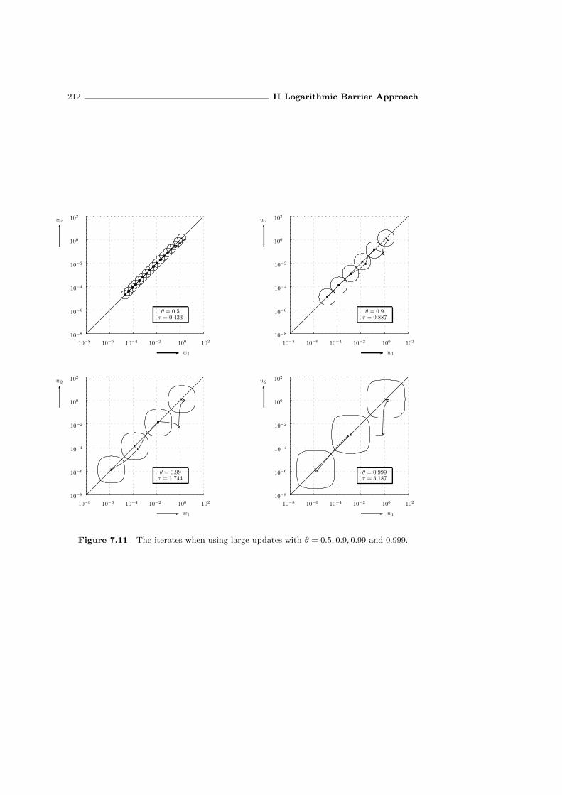
212 II Logarithmic Barrier Approach
10−810−8
10−810−8
10−610−6
10−610−6
10−410−4
10−410−4
10−210−2
10−210−2
100100
100100
102102
102102
10−810−8
10−810−8
10−610−6
10−610−6
10−410−4
10−410−4
10−210−2
10−210−2
100100
100100
102102
102102
w1w1
w1w1
w2
w2
w2
w2
θ = 0.5τ = 0.433
θ = 0.9τ = 0.887
θ = 0.99τ = 1.744
θ = 0.999τ = 3.187
Figure 7.11 The iterates when using large updates with θ = 0.5, 0.9, 0.99 and 0.999.
8
Initialization
All the methods of this part of the book assume the availability of a starting pointon or close to the central path of the problem. Sometimes such a point is known, butmore often we have no foreknowledge of the problem under consideration. For thesecases we provide in this chapter a transformation of the problem yielding an equivalentproblem for which a point on the central path is available. This transformation is basedon results in Part I and is described below in detail.1
Suppose that we want to solve the problem (P ) in standard format:
(P ) mincTx : Ax = b, x ≥ 0
,
where A is an m× n matrix of rank m, c, x ∈ IRn, and b ∈ IRm. Let I be a subset ofthe full index set 1, 2, . . . , n such that the submatrix AI of A has size m×m and isnonsingular. Thus, AI is a basis for (P ). After reordering the columns of A, we maywrite
A = (AI AJ) ,
where J denotes the complement of I. Now Ax = b can be rewritten as
AIxI +AJxJ = b,
which is equivalent toxI = A−1
I (b−AJxJ ) .
As a consequence we have
cTx = cTI xI + cTJ xJ = cTI A−1I (b−AJxJ) + cTJ xJ = cTI A
−1I b+
(cJ − AT
JA−TI cI
)TxJ .
Hence, omitting the constant cTI A−1I b we can reformulate (P ) as
(P c) min(cJ − AT
JA−TI cI
)TxJ : A−1
I (b−AJxJ ) ≥ 0, xJ ≥ 0,
or equivalently,
(P c) min(cJ −AT
JA−TI cI
)TxJ : −A−1
I AJxJ ≥ −A−1I b, xJ ≥ 0
.
1 We want to point out an advantage of the approach in this chapter over the approach in the exis-ting literature. The technique of embedding a given standard form problem in a homogeneous andself–dual problem was introduced by Ye, Todd and Mizuno [316] in 1994. See also Wu, Wu andYe [299]; their final model contains free variables. In our approach the occurrence of free variablesis avoided by first reducing the given standard problem to a canonical problem. For a differentapproach to the initialization problem we refer to, e.g., Lustig [189, 190].

214 II Logarithmic Barrier Approach
Thus we have transformed (P ) to the equivalent problem (P c), which is in canonicalformat. Chapter 4 describes how we can embed any canonical model in a self-dualmodel so that a strictly complementary solution of the latter model either yields astrictly complementary solution of the canonical problem or makes clear that thecanonical problem is infeasible or unbounded. Moreover, for the embedding problemwe have a point on its central path available. If we apply such an embedding to (P c),the resulting self-dual model may be given by
(SP c) minqT ξ : Mξ ≥ −q, ξ ≥ 0
,
where M is skew-symmetric and q ≥ 0. Let ξ(µ) be a given point on the central pathof (SP c) for some positive µ. Now (SP c) can be written in the standard form byassociating the surplus vector σ(ξ) :=Mξ+ q with any ξ. We then may rewrite (SP c)as
(SSP c) minqT ξ : Mξ − σ = −q, ξ ≥ 0, σ ≥ 0
,
and we haveξ(µ)σ(ξ(µ)) = µe,
where e is an all-one vector of appropriate size. Note that (SSP c) is in the standardformat. We can rewrite it as
(P ) mincT x : Ax = b, x ≥ 0
,
with
A =[M −I
], c =
[q
0
], b = −q.
The problem (P ) is in the standard format and hence the methods of this chaptercan be used to yield an ε-solution of (P ) provided that we have a solution on or closeto its central path. We now show that this condition is satisfied by showing that theµ-center of (P ) is known. To this end we need to consider also the dual problem of(P ), namely
(D) maxbT y : AT y + s = c, s ≥ 0
.
For the slack vector s we have
s = c− AT y =
[q −MT y
y
]=
[q +My
y
].
Here we used that MT = −M . Now with the definition
x :=
[ξ(µ)
σ(ξ(µ))
], y =: ξ(µ),
x is feasible for (P ) and y is feasible for (D). The feasibility of y follows by consideringits slack vector:
s =
[q +My
y
]=
[q +Mξ(µ)
ξ(µ)
]=
[σ(ξ(µ))
ξ(µ)
].

II.8 Initialization 215
For the product of x and s we have
xs =
[ξ(µ)
σ(ξ(µ))
] [σ(ξ(µ))
ξ(µ)
]=
[ξ(µ)σ(ξ(µ))
σ(ξ(µ))ξ(µ)
]=
[µe
µe
].
This proves that x is the µ-center of (P ), as required.By way of example we apply the above transformation to the sample problem used
throughout this part of the book.
Example II.78 Taking A and c as in Example II.7 (page 97), and b = (1, 1)T , wehave
A =
[1 −1 0
0 0 1
], b =
[1
1
], c =
1
1
1
,
and (P ) is the problem
(P ) min x1 + x2 + x3 : x1 − x2 = 1, x3 = 1, x ≥ 0 .
The first and the third column of A form a basis. With the index set I definedaccordingly, the matrix AI is the identity matrix. Then we express x1 and x3 interms of x2: [
x1
x3
]=
[1 + x2
1
].
Using this we eliminate x1 and x3 from (P ) and we obtain the canonical problem (P c):
(P c) min
2x2 + 2 :
[1
0
]x2 ≥
[−1
−1
], x2 ≥ 0
.
Being unrealistic, but just to demonstrate the transformation process for this simplecase, we do not assume any foreknowledge and embed this problem in a self-dualproblem as described in Section 4.3.2 Taking 1 for x0 and s0, and for y0 and t0 theall-one vector of length 2, the self-dual embedding problem is given by (SP c) with
M =
0 0 1 1 −1
0 0 0 1 0
−1 0 0 2 0
−1 −1 −2 0 5
1 0 0 −5 0
, q =
0
0
0
0
5
.
Now the all-one vector is feasible for (SP c) and its surplus vector is also the all-onevector, as easily can be verified. It follows that the all-one vector is the point on thecentral path for µ = 1. Adding surplus variables to this problem we get a problem inthe standard format with 5 equality constraints and 10 variables. Solving this problem
2Exercise 64 The canonical problem (P c) contains an empty row. Remove this row and thenperform the embedding. Show that this leads to the same solution of (P c).

216 II Logarithmic Barrier Approach
with the large-update logarithmic barrier method (with θ = 0.999 and ε = 10−4), wefind in 4 iterations the strictly complementary solution
ξ = (0, 0, 0,4
5, 0,
4
5,4
5,8
5, 0, 1).
The slack vector is
σ(ξ) = (4
5,4
5,8
5, 0, 1, 0, 0, 0,
4
5, 0).
Note that the first five coordinates of ξ are equal to the last five coordinates of σ(ξ)and vice versa. In fact, the first five coordinates of ξ form a solution of the self-dualembedding (SP c) of (P c). The homogenizing variable, the fourth entry in ξ, is positive.Therefore, we have found an optimal solution of (P c). The optimal value of x2 in (P c),the third coordinate in the vector ξ, is given by x2 = 0. Hence x = (1, 0, 1) is optimalfor the original problem (P ). ♦
A clear disadvantage of the above embedding procedure seems to be that it increasesthe size of the problem. If the constraint matrix A of (P ) has size m×n then the finalstandard form problem that we have to solve has size (n + 2) × 2(n + 2). However,when the procedure is implemented efficiently the amount of extra computation canbe reduced significantly. In fact, the computation of the search direction for the largerproblem can be organized in such a way that it requires the solution of three linearsystems with the same matrix of size (m+2)×(m+2). This is explained in Chapter 20.

Part III
The Target-following
Approach


9
Preliminaries
9.1 Introduction
In this part we deal again with the problems (P ) and (D) in the standard form:
(P ) mincTx : Ax = b, x ≥ 0
,
(D) maxbT y : AT y ≤ c
.
As before, the matrix A is of size m×n with full row rank and the vectors c and x arein IRn and b in IRm. Assuming that the interior-point condition is satisfied we recallfrom Theorem II.4 that the KKT system (5.3)
Ax = b, x ≥ 0,
AT y + s = c, s ≥ 0, (9.1)
xs = µe
has a unique solution for every positive value of µ. These solutions are called the µ-centers of (P ) and (D). The above result is fundamental for the algorithms analyzedin Part II. When µ runs through the positive real line then the solutions of the KKTsystem run through the central paths of (P ) and (D); the methods in Part II justapproximately follow the central path to the optimal sets of (P ) and (D). Thesemethods were called logarithmic barrier methods because the points on the centralpath are minimizers of the logarithmic barrier functions for (P ) and (D). For obviousreasons they have also become known under the name central-path-following methods.In each (outer) iteration of such a method the value of the parameter µ is fixedand starting at a given feasible solution of (P ) and/or (D) a good approximation isconstructed of the µ-centers of (P ) and (D). Numerically the approximate solutionsare obtained either by using Newton’s method for solving the KKT system or byusing Newton’s method for minimizing the logarithmic barrier function of (P ) and(D). In the first case Newton’s method provides displacements for both (P ) and (D);then we speak of a primal-dual method. In the second case Newton’s method providesa displacement for either (P ) or (D), depending on whether the logarithmic barrierfunction of (P ) or (D) is used in Newton’s method. This gives the so-called primal
methods and dual methods respectively. In all cases the result of an (outer) iterationis a primal-dual pair approximating the µ-centers and such that the duality gap isapproximately nµ.

220 III Target-following Approach
In this part we present a generalization of the above results. The starting point isthe observation that if the vector µe on the right-hand side of the KKT system (9.1)is replaced by any positive vector w then the resulting system still has a (unique)solution. Thus, for any positive vector w the system
Ax = b, x ≥ 0,
AT y + s = c, s ≥ 0, (9.2)
xs = w
has a unique solution, denoted by x(w), y(w), s(w).1 This result is interesting in itself.It means that we can associate with each positive vector w the primal-dual pair(x(w), s(w)).2 The map ΦPD associating with any w > 0 the pair (x(w), s(w)) willbe called the target map associated with (P ) and (D). In the next section we discussits existence and also some interesting properties.In the present context, it is convenient to refer to the interior of the nonnegative
orthant in IRn as the w-space. Any (possibly infinite) sequence of positive vectorswk (k = 1, 2, . . .) in the w-space is called a target sequence. If a target sequenceconverges to the origin, then the duality gap eTwk for the corresponding pair in thesequence ΦPD(wk) converges to zero. We are especially interested in target sequencesof this type for which the sequence ΦPD(wk) is convergent as well, and for which thelimiting primal-dual pair is strictly complementary. In Section 9.3 we derive a sufficientcondition on target sequences (converging to the origin) that yields this property. Wealso give a condition such that the limiting pair consists of so-called weighted-analytic
centers of the optimal sets of (P ) and (D).With any central-path-following method we can associate a target sequence on the
central path by specifying the values of the barrier parameter µ used in the successive(outer) iterations. The central-path-following method can be interpreted as a methodthat takes the points on the central path as intermediate targets on the way to theorigin. Thus it becomes apparent how the notion of central-path-following methodscan be generalized to target-following methods, which (approximately) follow arbitrarytarget sequences. To develop this idea further we need numerical procedures that canbe used to obtain a good approximation of the primal-dual pair corresponding tosome specified positive target vector. Chapters 10, 12 and 13 are devoted to suchprocedures. The basic principle is again Newton’s method. Chapter 10 describes aprimal-dual method, Chapter 12 a dual method, and Chapter 13 a primal method.The target-following approach offers a very general framework for the analysis
of almost all known interior-point methods. In Chapter 11 we analyze some of themethods of Part II in this framework. We also deal with some other applications,including a target-following method that is based on the Dikin direction, as introducedin Appendix E. Finally, in Chapter 14 we deal with the so-called method of centers.This method will be described and after putting it into the target-following frameworkwe provide a new and relatively easy analysis of the method.
1 This result, which establishes a one-to-one correspondence between primal-dual pairs (x, s) andpositive vectors in IRn, was proved first in Kojima et al. [175]. Below we present a simple alternativeproof. Mizuno [212, 214] was the first to use this property in the design of an algorithm.
2 Here, as before, we use that any dual feasible pair (y, s) can be uniquely represented by either yor s. This is due to the assumption that A has full row rank.

III.9 Preliminaries 221
9.2 The target map and its inverse
Our first aim in this section is to establish that the target map ΦPD is well defined.That is, we need to show that for any positive vector w ∈ IRn the system (9.2) hasa unique solution. To this end we use a modification of the primal-dual logarithmicbarrier as given by (6.23). Replacing the role of the vector µe in this function by thevector w, we consider the modified primal-dual logarithmic barrier function definedby
φw(x, s) =1
max (w)
n∑
j=1
wjψ
(xjsjwj
− 1
). (9.3)
Here the function ψ has its usual meaning (cf. (5.5), page 92). The scaling factor1/max(w) serves to scale φw(x, s) in such a way that φw(x, s) coincides with theprimal-dual logarithmic barrier function (7.44) in Section 7.8 (page 194) if w is on thecentral path.3
Note that φw(x, s) is defined for all positive primal-dual pairs (x, s). Moreover,φw(x, s) ≥ 0 and the equality holds if and only if xs = w. Hence, the weighted KKTsystem (9.2) has a solution if and only if the minimal value of φw is 0.By expanding φw(x, s) we get
max (w)φw(x, s) =
n∑
j=1
wj
(xjsjwj
− 1− logxjsjwj
)
=
n∑
j=1
xjsj −n∑
j=1
wj −n∑
j=1
wj log xjsj +
n∑
j=1
wj logwj
= xT s−n∑
j=1
wj log xjsj − eTw +
n∑
j=1
wj logwj . (9.4)
Neglecting for the moment the constant part, that is the part that does not dependon x and s, we are left with the function
xT s−n∑
j=1
wj log xjsj. (9.5)
This function is usually called a weighted primal-dual logarithmic barrier function
with the coefficients of the vector w as weighting coefficients. Since xT s = cTx− bT y,the first term in (9.5) is linear on the domain of φw(x, s). The second term, called thebarrier term, is strictly convex and hence it follows that φw(x, s) is strictly convex onits domain.
3 If w = µe then max (w) = µ and hence
φw(x, s) =1
µ
n∑
j=1
µψ
(xjsj
µ− 1
)=
n∑
j=1
ψ
(xjsj
µ− 1
)= Ψ
(xs
µ− e
);
this is precisely the primal-dual logarithmic barrier function φµ(x, s) as given by (6.23) and (7.44),and that was used in the analysis of the large-update central-path-following logarithmic barriermethod.
222 III Target-following Approach
In the sequel we need a quantity to measure the distance from a positive vector wto the central path of the w-space. Such a measure was introduced in Section 3.3.4 in(3.20). We use the same measure here, namely
δc(w) :=max (w)
min (w). (9.6)
Now we are ready to derive the desired result by adapting Theorem II.4 and its proofto the present case. With w fixed, for given K ∈ IR the level set LK of φw is definedby
LK =(x, s) : x ∈ P+, s ∈ D+, φw(x, s) ≤ K
.
Theorem III.1 Let w ∈ IRn and w > 0. Then the following statements are equivalent:
(i) (P ) and (D) satisfy the interior-point condition.(ii) There exists K ≥ 0 such that the level set LK is nonempty and compact.(iii) There exists a (unique) primal-dual pair (x, s) minimizing φw with x and s both
positive.(iv) There exist (unique) x, s ∈ IRn and y ∈ IRm satisfying (9.2);(v) For each K ≥ 0 the level set LK is nonempty and compact.
Proof: (i) ⇒ (ii): Assuming (i), there exists a positive x0 ∈ P+ and a positives0 ∈ D+. With K = φw
(x0, s0
)the level set LK contains the pair
(x0, s0
). Thus, LK
is not empty, and we need to show that LK is compact. Let (x, s) ∈ LK . Then, by thedefinition of LK ,
n∑
i=1
wiψ
(xisiwi
− 1
)≤ Kmax (w).
Since each term in the sum is nonnegative, this implies
ψ
(xisiwi
− 1
)≤ Kmax (w)
min (w)= Kδc(w), 1 ≤ i ≤ n.
Since ψ is strictly convex on its domain and goes to infinity at its boundaries, thereexist unique positive numbers a and b, with a < 1, such that
ψ(−a) = ψ(b) = Kδc(w).
We conclude that−a ≤ xisi
wi− 1 ≤ b, 1 ≤ i ≤ n,
which giveswi(1 − a) ≤ xisi ≤ wi(1 + b), 1 ≤ i ≤ n. (9.7)
From the right-hand side inequality we deduce that
xT s ≤ (1 + b)eTw.
We proceed by showing that this and (i) imply that the coordinates of x and s canbe bounded above. Since A(x− x0) = 0, the vector x− x0 belongs to the null space of

III.9 Preliminaries 223
A. Similarly, s− s0 = AT (y0 − y) implies that s− s0 lies in the row space of A. Therow space and the null space of A are orthogonal and hence we have
(x− x0)T (s− s0) = 0. (9.8)
Writing this asxT s0 + sTx0 = xT s+ (x0)T (s0)
and using xT s ≤ (1 + b)eTw, we find
xT s0 + sTx0 ≤ (1 + b)eTw + (x0)T (s0). (9.9)
Since sTx0 ≥ 0, x ≥ 0, and s0 > 0, this implies for each index i that
xis0i ≤ xT s0 + sTx0 ≤ (1 + b)eTw + (x0)T (s0),
whence
xi ≤(1 + b)eTw + (x0)T (s0)
s0i,
proving that the coordinates of the vector x are bounded above. The coordinates ofthe vector s are bounded above as well. This can be derived from (9.9) in exactly thesame way as for the coordinates of x. Using xT s0 ≥ 0, s ≥ 0, and x0 > 0, we obtainfor each index i that
si ≤(1 + b)eTw + (x0)T (s0)
x0i.
Thus we have shown that the level set LK is bounded. We proceed by showing thatLK is compact. Each si being bounded above, the left inequality in (9.7) implies thatxi is bounded away from zero. In fact, we have
xi ≥(1− a)wi
si≥ (1− a)x0iwi
(1 + b)eTw + (x0)T (s0).
In the same way we derive that for each i,
si ≥(1− a)wi
xi≥ (1− a)s0iwi
(1 + b)eTw + (x0)T (s0).
We conclude that for each i there exist positive numbers αi and βi with 0 < αi ≤ βi,such that
αi ≤ xi, si ≤ βi, 1 ≤ i ≤ n.
Thus we have proved the inclusion
LK ⊆n∏
i=1
[αi, βi]× [αi, βi].
The set on the right-hand side lies in the positive orthant of IRn × IRn, and being theCartesian product of closed intervals, it is compact. Since φw is continuous, and welldefined on this set, it follows that LK is compact. Thus we have shown that (ii) holds.
224 III Target-following Approach
(ii) ⇒ (iii): Suppose that (ii) holds. Then, for some nonnegative K the level set LK
is nonempty and compact. Since φw is continuous, it follows that φw has a minimizer(x, s) in LK . Moreover, since φw is strictly convex, this minimizer is unique. Finally,from the definition of φw , ψ ((xisi/wi)− 1) must be finite, and hence xisi > 0 for eachi. This implies that x > 0 and s > 0, proving (iii).
(iii) ⇒ (iv): Suppose that (iii) holds. Then φw has a (unique) minimizer. Since thedomain P+ × D+ of φw is open, (x, s) ∈ P+ × D+ is a minimizer of φw if and onlyif the gradient of φw is orthogonal to the linear space parallel to the smallest affinespace containing P+ × D+ (cf. Proposition A.1). This linear space is determined bythe affine system
Ax = 0, Hs = 0,
where H is a matrix such that its row space is the null space of A and vice versa. Thegradient of φw with respect to the coordinates of x satisfies
max (w)∇xφw(x, s) = s− w
x,
and with respect to the coordinates of s we have
max (w)∇sφw(x, s) = x− w
s.
Application of Proposition A.1 yields that ∇xφw(x, s) must lie in the row space of Aand ∇sφw(x, s) must lie in the row space of H . These two spaces are orthogonal, andhence we obtain (
s− w
x
)T (x− w
s
)= 0.
This can be rewritten as
(s− w
x
)TXS−1
(s− w
x
)= 0.
Since XS−1 is a diagonal matrix with positive elements on the diagonal, this implies
∥∥∥s− w
x
∥∥∥ = 0.
Hence,
s− w
x= 0,
whence xs = w. This proves that (x, s) is a minimizer of φw if and only if (x, s) satisfies(9.2). Hence (iv) follows from (iii).
(iv) ⇒ (i): Let (x, s) be a solution of (9.1). Since w > 0 and x and s are nonnegative,both x and s are positive. This proves that (P ) and (D) satisfy the interior-pointcondition.Thus it has been shown that statements (i) to (iv) in the theorem are equivalent. We
finally prove that statement (v) is equivalent with each of these statements. Obviously(v) implies (ii). On the other hand, assuming that statements (i) to (iv) hold, let x ands solve (9.2). Then we have x > 0, s > 0 and xs = w. This implies that φw(x, s) = 0,as easily follows by substitution. Now let K be any nonnegative number. Then the

III.9 Preliminaries 225
level set LK contains the pair (x, s) and hence it is nonempty. Finally, from the aboveproof of the implication (i) ⇒ (ii) it is clear that LK is compact. This completes theproof of the theorem.
If the interior-point condition is satisfied, then the target map ΦPD provides atool for representing any positive primal-dual pair (x, s) by the positive vector xs,which is the inverse image of the pair (x, s). The importance of this feature cannotbe overestimated. It means that the interior of the nonnegative orthant in IRn canbe used to represent all positive primal-dual pairs. As a consequence, the behaviorof primal-dual methods that generate sequences of positive primal-dual pairs, can bedescribed in the nonnegative orthant in IRn. Obviously, the central paths of (P ) and(D) are represented by the bisector µe : µ > 0 of the w-space; in the sequel werefer to the bisector as the central path of the w-space. See Figure 9.1.
w1
w2
central path
duality gap constant
Figure 9.1 The central path in the w-space (n = 2).
For central-path-following methods the target sequence is a sequence on this pathconverging to the origin. The iterates of these methods are positive primal-dual pairs‘close’ to the target points on the central path, in the sense of some proximity measure.In the next sections we deal with target sequences that are not necessarily on thecentral path.
Remark III.2 We conclude this section with an interesting observation, namely that thetarget map of (P ) and (D) contains so much information that we can reconstruct the data A, band c from the target map.4 This can be shown as follows. We take partial derivatives with
4 This result was established by Crouzeix and Roos [57] in an unpublished note.

226 III Target-following Approach
respect to the coordinates of w in the weighted KKT system (9.2). Denoting the Jacobiansof x, y and s simply by x′, y′ and s′ respectively, we have
x′ =∂x
∂w, y′ =
∂y
∂w, s′ =
∂s
∂w,
where the (i, j) entry of x′ is the partial derivative ∂xi/∂wj , etc. Note that x′ and s′ aren× n matrices and y′ is an m× n matrix. Thus we obtain
Ax′ = 0,
AT y′ + s′ = 0, (9.10)
Xs′ + Sx′ = Inn,
where I denotes the identity matrix of size n× n.5 The third equation is equivalent to
s′ = X−1(Inn − Sx′) .
Using also the second equation we get
AT y′ = X−1(Sx′ − Inn
). (9.11)
Since y′ is an m× n matrix of rank m there exists an n×m matrix R such that y′R = Imm.Multiplying (9.11) from the right by R we obtain
AT = AT Imm = AT y′R = X−1(Sx′ − Inn
)R,
which determines the matrix A uniquely. Finally, for any positive w, the vectors b and c
follow from b = Ax(w) and c = AT y(w) + s(w). •
9.3 Target sequences
Let us consider a target sequence
w0, w1, w2, . . . , wk, . . . (9.12)
which converges to the origin. The vectors wk in the sequence are positive and
limk→∞
wk = 0.
As a consequence, for the duality gap eTwk at wk we have limk→∞ eTwk = 0; thisimplies that the accumulation points of the sequence
ΦPD
(w0),ΦPD
(w1),ΦPD
(w2), . . . ,ΦPD
(wk), . . . (9.13)
are optimal primal-dual pairs.6 In the sequel (x∗, s∗) denotes any such optimal primal-dual pair.
5 Since the matrix of system (9.10) is nonsingular, the implicit function theorem (cf. Proposition A.2in Appendix A) implies the existence of all the relevant partial derivatives.
6Exercise 65 By definition, an accumulation point of the sequence (9.13) is a primal-dual pairthat is the limiting point of some convergent subsequence of (9.13). Verify the existence of such aconvergent subsequence.

III.9 Preliminaries 227
We are especially interested in target sequences for which the accumulation pairs(x∗, s∗) are strictly complementary. We prove below that this happens if the targetsequence lies in some cone neighborhood of the central path defined by
δc(w) ≤ τ,
where τ is fixed and τ ≥ 1. Recall that δc(w) ≥ 1, with equality if and only if w is onthe central path. Also, δc(w) is homogeneous in w: for any positive scalar λ and forany positive vector w we have
δc(λw) = δc(w).
As a consequence, the inequality δc(w) ≤ τ determines a cone in the w-space.In Theorem I.20 we showed for the self-dual model that the limiting pairs of any
target sequence on the central path are strictly complementary optimal solutions. Ournext result not only implies an analogous result for the standard format but it extendsit to target sequences lying inside a cone around the central path in the w-space.
Theorem III.3 Let τ ≥ 1 and let the target sequence (9.12) be such that δc(wk) ≤ τ
for each k. Then every accumulation pair (x∗, s∗) of the sequence (9.13) is strictlycomplementary.
Proof: For each k = 1, 2, . . ., let (xk, sk) := ΦPD(wk). Then we have
xksk = wk, k = 1, 2, . . . .
Now let (x∗, s∗) be any accumulation point of the sequence (9.13). Then thereexists a subsequence of the given sequence whose primal-dual pairs converge to(x∗, s∗). Without loss of generality we assume that the given sequence itself is such asubsequence. Since xk − x∗ and sk − s∗ belong respectively to the null space and therow space of A, these vectors are orthogonal. Hence,
(xk − x∗
)T (sk − s∗
)= 0.
Expanding the product and rearranging terms, we get
(x∗)T sk + (s∗)T xk =(sk)Txk + (s∗)T x∗.
Using that(sk)Txk = eTwk and (x∗)T s∗ = 0, we arrive at
∑
j∈σ(x∗)
x∗jskj +
∑
j∈σ(s∗)
s∗jxkj = eTwk, k = 1, 2, . . . .
Here σ(x∗) denotes the support of x∗ and σ(s∗) the support of s∗.7 Using thatxksk = wk, we can write the last equation as
∑
j∈σ(x∗)
wkj x
∗j
xkj+
∑
j∈σ(s∗)
wkj s
∗j
skj= eTwk, k = 1, 2, . . . .
7 The support of a vector is defined in Section 2.8, Definition I.19, page 36.
228 III Target-following Approach
Now let ε be a (small) positive number such that
1 + ε
nε> τ.
Then, since (x∗, s∗) is the limit of the sequence (xk, sk)∞k=0, there exists a naturalnumber K such that
x∗jxkj
≤ 1 + ε ands∗jskj
≤ 1 + ε
for each j (1 ≤ j ≤ n) and for all k ≥ K. Hence, for k ≥ K we have
eTwk ≤ (1 + ε)
∑
j∈σ(x∗)
wkj +
∑
j∈σ(s∗)
wkj
.
If the pair (x∗, s∗) is not strictly complementary, there exists an index i that does notbelong to the union σ(x∗) ∪ σ(s∗) of the supports of x∗ and s∗. Then we have
∑
j∈σ(x∗)
wkj +
∑
j∈σ(s∗)
wkj ≤ eTwk − wk
i .
Substitution giveseTwk ≤ (1 + ε)
(eTwk − wk
i
).
This implies(1 + ε)wk
i ≤ εeTwk.
The average value of the elements of wk is eTwk/n. Since δc(wk) ≤ τ , the average
value does not exceed τwki . Hence, e
Twk ≤ nτwki . Substituting this we obtain
(1 + ε)wki ≤ nετwk
i .
Now dividing both sides by wki we arrive at the contradiction
1 + ε ≤ nετ.
This proves that (x∗, s∗) is strictly complementary.
If a target sequence satisfies the condition in Theorem III.3 for some τ ≥ 1, it isclear that the ratios between the coordinates of the vectors wk are bounded. In fact,
1
τ≤ wk
i
wkj
≤ τ
for all k and for all i and j. For target sequences on the central path these ratios areall equal to one, so the limits of the ratios exist if k goes to infinity. In general we areinterested in target sequences for which the limits of these ratios exist when k goes toinfinity. Since the ratios between the coordinates do not change if wk is multiplied bya positive constant, this happens if and only if there exists a positive vector w∗ suchthat
limk→∞
nwk
eTwk= w∗, (9.14)

III.9 Preliminaries 229
and then the limiting values of the ratios are given by the ratios between thecoordinates of w∗. Note that we have eTw∗ = n, because the sum of the coordinatesof each vector nwk/eTwk is equal to n. Also note that if a target sequence satisfies(9.14), we may find a τ ≥ 1 such that δc(w
k) ≤ τ for each k. In fact, we may take
τ = maxi,j,k
wki
wkj
.
Hence, by Theorem III.3, any accumulation pair (x∗, s∗) for such a sequence is strictlycomplementary.Our next result shows that if (9.14) holds then the limiting pair (x∗, s∗) is unique
and can be characterized as a weighted-analytic center of the optimal sets of (P ) and(D). Let us first define this notion.
Definition III.4 (Weighted-analytic center) Let the nonempty and bounded setT be the intersection of an affine space in IRp with the nonnegative orthant of IRp. Wedefine the support σ(T ) of T as the subset of the full index set 1, 2, . . . , p given by
σ(T ) = i : ∃x ∈ T such that xi > 0 .
If w is any positive vector in IRp then the corresponding weighted-analytic center ofT is defined as the zero vector if σ(T ) is empty, otherwise it is the vector in T thatmaximizes the product ∏
i∈σ(T )
xwi
i , x ∈ T . (9.15)
If the support of T is not empty then the convexity of T implies the existence of avector x ∈ T such that xσ(T ) > 0. Moreover, if σ(T ) is not empty then the maximumvalue of the product (9.15) exists since T is bounded. Since the product (9.15) isstrictly concave, the maximum value is attained at a unique point of T . The abovedefinition generalizes the notion of analytic center, as defined by Definition I.29 andit uniquely defines the weighted-analytic center (for any positive weighting vector w)for any bounded subset that is the intersection of an affine space in IRp with thenonnegative orthant of IRn. 8
Below we apply this notion to the optimal sets of (P ) and (D). If a target sequencesatisfies (9.14) then the next result states that the sequence of its primal-dual pairsconverges to the pair of weighted-analytic centers of the optimal sets of (P ) and (D).
Theorem III.5 Let the target sequence (9.12) be such that (9.14) holds for somew∗, and let (x∗, s∗) be an accumulation point of the sequence (9.13). Then x∗ is theweighted-analytic center of P∗ with respect to w∗, and s∗ is the weighted-analyticcenter of D∗ with respect to w∗.
Proof: We have already established that the limiting pair (x∗, s∗) is strictly comp-lementary, from Theorem III.3. As a consequence, the support of the optimal set P∗
8 Exercise 66 Let w be any positive vector in IRp and let the bounded set T be the intersection ofan affine space in IRp with the nonnegative orthant of IRp. Show that the weighted-analytic center(with w as weighting vector) of T coincides with the analytic center of T if and only if w is a scalarmultiple of the all-one vector.

230 III Target-following Approach
of (P ) is equal to the support σ(x∗) of x∗, and the support of the optimal set D∗ of(D) is equal to the support σ(s∗) of s∗.Now let x be optimal for (P ) and s for (D). Applying the orthogonality property
to the pairs (x, s) and (xk, sk) := ΦPD(wk) we obtain
(xk − x)T (sk − s) = 0.
Expanding the product and rearranging terms, we get
(x)Tsk + (s)
Txk =
(sk)Txk + (s)
Tx.
Since(sk)Txk = eTwk and (x)T s = 0, we get
∑
j∈σ(x∗)
xjskj +
∑
j∈σ(s∗)
sjxkj = eTwk, k = 1, 2, . . . .
Here we have also used that σ(x) ⊂ σ(x∗) and σ(s) ⊂ σ(s∗). Using xksk = wk wehave
∑
j∈σ(x∗)
wkj xj
xkj+
∑
j∈σ(s∗)
wkj sj
skj= eTwk, k = 1, 2, . . . .
Multiplying both sides by n/eTwk we get
∑
j∈σ(x∗)
nwkj
eTwk
xj
xkj+
∑
j∈σ(s∗)
nwkj
eTwk
sj
skj= n, k = 1, 2, . . . .
Letting k → ∞, it follows that
∑
j∈σ(x∗)
w∗j xj
x∗j+
∑
j∈σ(s∗)
w∗j sj
s∗j= n.
At this stage we apply the geometric inequality,9 which states that for any two positivevectors α and β in IRn,
n∏
j=1
(αj
βj
)βi
≤(∑n
j=1 αi∑nj=1 βi
)∑n
j=1βi
.
We apply this inequality with β = w∗ and
αj =w∗
j xj
x∗j(j ∈ σ(x∗)), αj =
w∗j sj
s∗j(j ∈ σ(s∗)).
Thus we obtain, using that the sum of the weights w∗j equals n,
∏
j∈σ(x∗)
(xjx∗j
)w∗
j ∏
j∈σ(s∗)
(sjs∗j
)w∗
j
≤
1
n
∑
j∈σ(x∗)
w∗j xj
x∗j+
∑
j∈σ(s∗)
w∗j sj
s∗j
n
= 1.
9 When β is the all-one vector e, the geometric inequality reduces to the arithmetic-geometric-meaninequality. For a proof of the geometric inequality we refer to Hardy, Littlewood and Polya [139].

III.9 Preliminaries 231
Substituting s = s∗ in the above inequality we get
∏
j∈σ(x∗)
xw∗
j
j ≤∏
j∈σ(x∗)
x∗jw∗
j ,
and substituting x = x∗ gives
∏
j∈σ(s∗)
sw∗
j
j ≤∏
j∈σ(s∗)
s∗jw∗
j .
This shows that x∗ maximizes the product
∏
i∈σ(x∗)
xw∗
j
j
and s∗ the product ∏
i∈σ(s∗)
sw∗
j
j
over the optimal sets of (P ) and (D) respectively. Hence the proof is complete.
9.4 The target-following scheme
We are ready to describe more formally the main idea of the target-following approach.Assume we are given some positive primal-dual feasible pair (x0, s0). Put w0 := x0s0
and assume that we have a sequence
w0, w1, . . . , wk, . . . , wK (9.16)
of points wk in the w-space with the following property:
Given the primal-dual pair for wk, with 0 ≤ k < K, it is ‘easy’ to computethe primal-dual pair for wk+1.
We call such a sequence a traceable target sequence of length K.If a traceable sequence of length K is available, then we can solve the given
problem pair (P ) and (D), up to the precision level eTwK , in K iterations. The k-thiteration in this method would consist of the computation of the primal-dual target-pair corresponding to the target point wk. Conceptually, the algorithm is described asfollows (page 232).Some remarks are in order. Firstly, in practice the primal-dual pair (x(w), s(w))
corresponding to an intermediate target w is not computed exactly. Instead wecompute it approximately, but so that the approximating pair is close to w in thesense of a suitable proximity measure.Secondly, the target sequence is not necessarily prescribed beforehand. It may be
generated in the course of the algorithm. Both cases occurred in Chapter 7. Forexample, the primal-dual logarithmic barrier algorithm with full Newton steps in

232 III Target-following Approach
Conceptual Target-following Algorithm
Input:A positive primal-dual pair (x0, s0);a final target vector w.
beginw := x0s0;while w is not ‘close’ to w dobegin
choose an ‘intermediate’ target w;compute x(w) and s(w);w := x(w)s(w);
endend
Section 7.5 uses intermediate targets of the form w = µe, and each subsequent target isgiven by (1−θ)w, with θ fixed. The same is true for the primal-dual logarithmic barrieralgorithm with large updates in Section 7.8. In contrast, the primal-dual logarithmicbarrier algorithm with adaptive updates (cf. Section 7.6.1) defines its target pointsadaptively.Thirdly, if we say that the primal-dual pair corresponding to a given target can
be computed ‘easily’, we mean that we have an efficient numerical procedure forfinding this primal-dual pair, at least approximately. The numerical method is alwaysNewton’s method, either for solving the KKT system defining the primal-dual pair, orfor finding the minimizer of a suitable barrier function. When full Newton steps aretaken, the target must be close to where we are, and one step must yield a sufficientlyaccurate approximation of the primal-dual pair for this target. In the literature,methods of this type are usually called short-step methods when the target sequenceis prescribed, and adaptive-step methods if the target sequence is defined adaptively.We call them full-step methods. If subsequent targets are at a greater distance weare forced to use damped Newton steps. The number of Newton steps necessary toreach the next target (at least approximately) may then become larger than one. Toachieve polynomiality we need to guarantee that this number can be bounded eitherby a constant or by some suitable function of n, e.g., O(
√n) or O(n). We refer to
such methods as multistep methods. They appear in the literature as medium-step
methods and large-step methods.In general, a primal-dual target-following algorithm is based on some finite
underlying target sequence w0, w1, . . . , wk = w. The final target w is a vector withsmall duality gap eT w if we are optimizing, but other final targets are allowable aswell; examples of both types of target sequence are given in Chapter 11 below. Thegeneral structure is as follows.

III.9 Preliminaries 233
Generic (Primal-Dual) Target-following Algorithm
Input:A positive primal-dual pair (x0, s0) such that x0s0 = w0;a final target vector w.
beginx = x0, s = s0, w := w0;while w is not ‘close’ to w dobegin
replace w by the next target in the sequence;while xs is not ‘close’ to w dobegin
apply Newton steps at (x, s) with w as targetend
endend
For each target in the sequence the next target can be prescribed (in advance), butit can also be defined adaptively. If it is close to the present target then a single (full)Newton step may suffice to reach the next target, otherwise we apply a multistepmethod, using damped Newton steps.The target-following approach is more general than the standard central-path-
following schemes that appear in the literature. The vast majority of the latter usetarget sequences on the central path.10 We show below, in Chapter 11, that manyclassical results in the literature can be put in the target-following scheme and thatthis scheme often dramatically simplifies the analysis.First, we derive the necessary numerical tools in the next chapter. This amounts
to generalizing results obtained before in Part II for the case where the target is onthe central path to the case where it is off the central path. We first analyze the fullprimal-dual Newton step method and the damped primal-dual Newton step methodfor computing the primal-dual pair corresponding to a given target vector. To this endwe introduce a proximity measure, and we show that the full Newton step methodis quadratically convergent. For the damped Newton method we show that a singlestep reduces the primal-dual barrier function by at least a constant, provided that theproximity measure is bounded below by a constant. We then have the basic ingredients
10 There are so many papers on the subject that it is impossible to give an exhaustive list. Wemention a few of them. Short-step methods along the central path can be found in Renegar [237],Gonzaga [118], Roos and Vial [245], Monteiro and Adler [218] and Kojima et al. [178]. We alsorefer the reader to the excellent survey of Gonzaga [124]. The concept of target-following methodswas introduced by Jansen et al. [159]. Closely related methods, using so-called α-sequences, wereconsidered before by Mizuno for the linear complementarity problem in [212] and [214]. The firstresults on multistep methods were those of Gonzaga [121, 122] and Roos and Vial [244]. We alsomention den Hertog, Roos and Vial [146] and Mizuno, Todd and Ye [217]. The target-followingscheme was applied first to multistep methods by Jansen et al. [158].

234 III Target-following Approach
for the analysis of primal-dual target-following methods.The results of the next chapter are used in Chapter 11 for the analysis of several
interesting algorithms. There we restrict ourselves to full Newton step methods becausethey give the best complexity results. Later we show that the target-following conceptis also useful when dealing with dual or primal methods. We also show that the primal-dual pair belonging to a target vector can be efficiently computed by such methods.This is the subject of Chapters 12 and 13.

10
The Primal-Dual Newton Method
10.1 Introduction
Suppose that a positive primal-dual feasible pair (x, s) is given as well as some targetvector w > 0. Our aim is to find the primal-dual pair (x(w), s(w)). Recall that to thedual feasible slack vector s belongs a unique y such that AT y + s = c. The vector inthe y-space corresponding to s(w) is denoted by y(w). In this section we define searchdirections ∆x,∆y,∆s at the given pair (x, s) that are aimed to bring us closer to thetarget pair (x(w), s(w)) corresponding to w. The search directions in this section areobtained by applying Newton’s method to the weighted KKT system (9.2), page 220.The approach closely resembles the treatment in Chapter 7. There the target was onthe central path, but now the target may be any positive vector w. It will becomeclear that the results of Chapter 7 can be generalized almost straightforwardly to thepresent case. To avoid tiresome repetitions we to omit detailed arguments when theyare similar to arguments used in Chapter 7.
10.2 Definition of the primal-dual Newton step
We want the iterates x+∆x, y+∆y, s+∆s to satisfy the weighted KKT system (9.2)with respect to the target w. So we want ∆x,∆y and ∆s to satisfy
A(x +∆x) = b, x+∆x ≥ 0,
AT (y +∆y) + s+∆s = c, s+∆s ≥ 0,
(x+∆x)(s+∆s) = w.
Neglecting the inequality constraints, we can rewrite this as follows:
A∆x = 0,
AT∆y +∆s = 0, (10.1)
s∆x+ x∆s+∆x∆s = w − xs.
Newton’s method amounts to linearizing this system by neglecting the second-orderterm ∆x∆s in the third equation. Thus we obtain the linear system
A∆x = 0,
AT∆y +∆s = 0, (10.2)
s∆x+ x∆s = w − xs.

236 III Target-following Approach
Comparing this system with (7.2), page 150, in Chapter 7, we see that the onlydifference occurs in the third equation, where the target vector w replaces the targetµe on the central path. In particular, both systems have the same matrix. Since thismatrix is nonsingular (cf. Theorem II.42, page 150, and Exercise 46, page 151), system(10.2) determines the displacements ∆x,∆y and ∆s uniquely. We call them the primal-dual Newton directions at (x, s) corresponding to the target w.1,2,3 It may be worthpointing out that computation of the displacements ∆x,∆y and ∆s amounts to solvinga positive definite system with the matrix AXS−1AT , just like when the target is onthe central path.
10.3 Feasibility of the primal-dual Newton step
In this section we investigate the feasibility of the (full) Newton step. As before, theresult of the Newton step at (x, y, s) is denoted by (x+, y+, s+), so
x+ = x+∆x, y+ = y +∆y, s+ = s+∆s.
Since the new iterates satisfy the affine equations we only have to deal with thequestion of whether x+ and s+ are nonnegative or not. We have
x+s+ = (x+∆x)(s +∆s) = xs+ (s∆x+ x∆s) + ∆x∆s.
Since s∆x+ x∆s = w − xs this leads to
x+s+ = w +∆x∆s. (10.3)
Hence, x+ and s+ are feasible only if w +∆x∆s is nonnegative. The converse is alsotrue. This is the content of the next lemma.
Lemma III.6 The primal-dual Newton step at (x, s) to the target w is feasible if andonly if w +∆x∆s ≥ 0.
Proof: The proof uses exactly the same arguments as the proof of Lemma II.46; wesimply need to replace the vector µe by w. We leave it to the reader to verify this.
Note that Newton’s method is exact when the second-order term ∆x∆s vanishes.In that case we have x+s+ = w. This means that the pair (x+, s+) is the image of wunder the target map, whence x+ = x(w) and s+ = s(w).In general ∆x∆s will not be zero and Newton’s method will not be exact. However,
the duality gap always assumes the correct value eTw after the Newton step.
1Exercise 67 Prove that the system (10.2) has a unique solution, namely
∆y =(AXS−1AT
)−1 (b− AWs−1
)
∆s = −AT∆y
∆x = ws−1 − x− xs−1∆s.2
Exercise 68 When w = 0 in (10.2), the resulting directions coincide with the primal-dual affine-scaling directions introduced in Section 7.6.2. Verify this.
3Exercise 69 When w = µe and µ = xT s/n in (10.2), the resulting directions coincide with theprimal-dual centering directions introduced in Section 7.6.2. Verify this.

III.10 Primal-Dual Newton Method 237
Lemma III.7 If the primal-dual Newton step is feasible then (x+)Ts+ = eTw.
Proof: This is immediate from (10.3) because the vectors ∆x and ∆s are orthogonal.
In the following sections we further analyze the primal-dual Newton method. Thisrequires a quantity for measuring the progress of the Newton iterates on the way tothe pair ΦPD(w). As may be expected, two cases could occur. In the first case thepresent pair (x, s) is ‘close’ to ΦPD(w) and full Newton steps are feasible. In that casethe full Newton step method is (hopefully, and locally) quadratically convergent. Inthe second case the present pair (x, s) is ‘far’ from ΦPD(w) and the full Newton stepmay not be feasible. Then we are forced to take damped Newton steps and we mayexpect no more than a linear convergence rate. In both cases we need a new quantityfor measuring the proximity of the current iterate to the target vector w. The nextsection deals with the first case and the second case is considered in Section 10.5. Itwill be no surprise that we use the weighted primal-dual barrier function φw(x, s) inSection 10.5 to measure progress of the method.
10.4 Proximity and local quadratic convergence
Recall from (7.16), page 156, that in the analysis of the central-path-following primal-dual method we measured the distance of the pair (x, s) to the target µe by thequantity
δ(x, s;µ) =1
2
∥∥∥∥√µe
xs−√xs
µe
∥∥∥∥ .
This can be rewritten as
δ(x, s;µ) =1
2õ
∥∥∥∥µe − xs√
xs
∥∥∥∥ .
Note that the right-hand side measures, in some way, the distance in the w-spacebetween the inverse image µe of the pair of µ-centers (x(µe), s(µe)) and the primal-dual pair (x, s).4 For a general target vector w we adapt this measure to
δ(xs, w) :=1
2√min (w)
∥∥∥∥w − xs√
xs
∥∥∥∥ . (10.4)
The quantity on the right measures the distance from the coordinatewise product xsto w. It is defined for (ordered) pairs of vectors in the w-space. Therefore, and becauseit will be more convenient in the future, we express this feature by using the notation
4 This observation makes clear that the proximity measure δ(x, s;µ) ignores the actual data of theproblems (P ) and (D), which is contained in A, b and c. Since the behavior of Newton’s methoddoes depend on these data, it follows that the effect of a (full) Newton step on the proximitymeasure depends on the data of the problem. This reveals the weakness of the analysis of thefull-step method (cf. Chapter 6.7). It ignores the actual data of the problem and only provides aworst-case analysis. In contrast, with adaptive updates (cf. Chapter 6.8) the data of the problemare taken into account and, as a result, the performance of the method is improved.

238 III Target-following Approach
δ(xs, w) instead of the alternative notation δ(x, s;w). We prove in this section thatthe Newton method is quadratically convergent in terms of this proximity measure.5
As before we use scaling vectors d and u. The definition of u needs to be adaptedto the new situation:
d :=
√x
s, u :=
√xs
w. (10.5)
Note that xs = w if and only if u = e. We also introduce a vector v according to
v =√xs.
With d we can rescale both x and s to the vector v:6
d−1x = v, ds = v.
Rescaling ∆x and ∆s similarly:
d−1∆x =: dx, d∆s =: ds, (10.6)
we see that∆x∆s = dxds.
Consequently, the orthogonality of ∆x and ∆s implies that the scaled displacementsdx and ds are orthogonal as well. Now we may reduce the left-hand side in the thirdequation of the KKT system as follows:
s∆x+ x∆s = sdd−1∆x+ xd−1d∆s = v (dx + ds) ,
so the third equation can be restated simply as
dx + ds = v−1 (w − xs) .
5Exercise 70 The definition (10.4) of the primal-dual proximity measure δ = δ(xs, w) implies that
2δ(xs, w) ≥∥∥∥ w − xs√
w√xs
∥∥∥ =
∥∥∥√
w
xs−√
xs
w
∥∥∥ .
Using this and Lemma II.62, prove
1
ρ(δ)≤√
xisi
wi
≤ ρ(δ), 1 ≤ i ≤ n.
6 Here we deviate from the approach in Chapter 7. The natural generalization of the approach therewould be to rescale x and s to u:
d−1x√w
= u,ds√w
=: u,
and then rescale ∆x and ∆s accordingly to
d−1∆x√w
=: dx,d∆s√w
=: ds.
But then we have∆x∆s = wdxds
and we lose the orthogonality of dx and ds with respect to the standard inner product. This couldbe resolved by changing the inner product in such a way that orthogonality is preserved. We leaveit as an (interesting) exercise to the reader to work this out. Here the difficulty is circumvented byusing a different scaling.
III.10 Primal-Dual Newton Method 239
On the other hand, the first and second equations can be reformulated as ADdx = 0and (AD)T dy + ds = 0, where dy = ∆y. We conclude that the scaled displacementsdx, dy and ds satisfy
ADdx = 0(AD)T dy + ds = 0
dx + ds = v−1 (w − xs) .(10.7)
Using the same arguments as in Chapter 7 we conclude that dx and ds form thecomponents of v−1 (w − xs) in the null space and the row space of AD, respectively.Note that w − xs represents the move we want to make in the w-space. Therefore wedenote it as ∆w. It is also convenient to use a scaled version dw of ∆w, namely
dw := v−1 (w − xs) = v−1∆w. (10.8)
Then we havedx + ds = dw (10.9)
and, since dx and ds are orthogonal,
‖dx‖2 + ‖ds‖2 = ‖dw‖2 . (10.10)
This makes clear that the scaled displacements dx, ds (and also dy) are zero if andonly if dw = 0. In that case x, y and s coincide with their values at w. An immediateconsequence of the definition (10.4) of the proximity δ(xs, w) is
δ(xs, w) =‖dw‖
2√min (w)
. (10.11)
The next lemma contains upper bounds for the 2-norm and the infinity norm of thesecond-order term dxds.
Lemma III.8 We have ‖dxds‖∞ ≤ 14 ‖dw‖
2and ‖dxds‖ ≤ 1
2√2‖dw‖2.
Proof: The lemma follows immediately by applying the first uv-lemma (Lemma C.4)to the vectors dx and ds.
Lemma III.9 The Newton step is feasible if δ(xs, w) ≤ 1.
Proof: Lemma III.6 guarantees feasibility of the Newton step if w+∆x∆s ≥ 0. Since∆x∆s = dxds this certainly holds if the infinity norm of the quotient dxds/w does notexceed 1. Using Lemma III.8 and (10.11) we may write
∥∥∥∥dxdsw
∥∥∥∥∞
≤ ‖dxds‖∞min (w)
≤ ‖dw‖24min (w)
= δ(xs, w)2 ≤ 1.
This implies the lemma.
We are ready for the main result of this section, which is a perfect analogue ofTheorem II.50, where the target is on the central path.

240 III Target-following Approach
Theorem III.10 If δ := δ(xs;w) ≤ 1, then the primal-dual Newton step is feasibleand (x+)T s+ = eTw. Moreover, if δ < 1 then
δ(x+s+, w) ≤ δ2√2(1− δ2)
.
Proof: The first part of the theorem is a restatement of Lemma III.9 and Lemma III.7.We proceed with the proof of the second statement. By definition,
δ(x+s+, w)2 =1
4min (w)
∥∥∥∥w − x+s+√
x+s+
∥∥∥∥2
.
Recall from (10.3) that x+s+ = w +∆x∆s = w + dxds. Using also Lemma III.8 and(10.11), we write
min(x+s+
)≥ min (w) − ‖dxds‖∞ ≥ min (w)− 1
4‖dw‖2 = min (w)
(1− δ2
).
Thus we find, by substitution,
δ(x+s+, w)2 ≤ ‖w − x+s+‖24 (1− δ2)min (w)2
=‖dxds‖2
4 (1− δ2)min (w)2.
Finally, using the upper bound for ‖dxds‖ in Lemma III.8 and also using (10.11) oncemore, we obtain
δ(x+s+, w)2 ≤ ‖dw‖432 (1− δ2)min (w)2
=δ4
2 (1− δ2).
This implies the theorem.7
It is clear that the above result has value only if the given pair (x, s) is closeenough to the target vector w. It guarantees quadratic convergence to the targetif δ(xs, w) ≤ 1/
√2. Convergence is guaranteed only if δ(xs, w) ≤
√2/3. For larger
values of δ(xs, w) we need a different analysis. Then we measure progress of the iteratesin terms of the barrier function φw(x, s) and we use damped Newton steps. This isthe subject of the next section.
10.5 The damped primal-dual Newton method
As before, we are given a positive primal-dual pair (x, s) and a target vector w > 0.Let x+ and s+ result from a damped Newton step of size α at (x, s). In this section
7 Recall from Lemma C.6 in Section 7.4.1 that we have the better estimate
δ(x+s+;w) ≤ δ2√2(1 − δ4)
if the target w is on the central path. We were not able to get the same result if w is off the centralpath. We leave this as a topic for further research.

III.10 Primal-Dual Newton Method 241
we analyze the effect of a damped Newton step — at (x, s) and for the target w — onthe value of the barrier function φw(x, s) (as defined on page 221). We have
x+ = x+ α∆x, s+ = s+ α∆s,
where α denotes the step-size, and 0 ≤ α ≤ 1. Using the scaled displacements dx andds as defined in (10.6), we may also write
x+ = d (v + αdx) , s+ = d−1 (v + αds) ,
where v =√xs. As a consequence,
x+s+ = (v + αdx) (v + αds) = v2 + αv (dx + ds) + α2dxds.
Sincev (dx + ds) = w − xs = w − v2,
we obtainx+s+ = v2 + α
(w − v2
)+ α2dxds. (10.12)
Now, definingv+ :=
√x+s+,
we have (v+)2
= (v + αdx) (v + αds) (10.13)
and (v+)2 − v2 = α
(w − v2
)+ α2dxds. (10.14)
The next theorem provides a lower bound for the decrease of the barrier function valueduring a damped Newton step. The bound coincides with the result of Lemma II.72if w is on the central path and becomes worse if the ‘distance’ from w to the centralpath increases.
Theorem III.11 Let δ = δ(xs, w) and let α = 1/ω − 1/(ω + 4δ2/δc(w)), where8
ω :=
√∥∥∥∥∆x
x
∥∥∥∥2
+
∥∥∥∥∆s
s
∥∥∥∥2
=
√∥∥∥∥dxv
∥∥∥∥2
+
∥∥∥∥dsv
∥∥∥∥2
.
Then the pair (x+, s+) resulting from the damped Newton step of size α is feasible.Moreover,
φw(x, s)− φw(x+, s+) ≥ ψ
(2δ
δc(w)ρ(δ)
).
Proof: It will be convenient to express max (w)φw(x, s), given by (9.4), page 221, interms of v =
√xs. We obviously have
max (w)φw(x, s) = eT v2 −n∑
j=1
wj log v2j − eTw +
n∑
j=1
wj logwj .
8 Exercise 71 Verify that∆x
x=dx
v,
∆s
s=ds
v.

242 III Target-following Approach
Hence we have the following expression for max (w)φw(x+, s+):
max (w)φw(x+, s+) = eT
(v+)2 −
n∑
j=1
wj log(v+j)2 − eTw +
n∑
j=1
wj logwj .
With ∆ := φw(x, s)− φw(x+, s+), subtracting both expressions yields
max (w)∆ = eT(v2 −
(v+)2)
+
n∑
j=1
wj log
(v+j)2
v2j.
Substitution of (10.13) and (10.14) gives
max (w)∆ = −αeT(w − v2
)+
n∑
j=1
wj log
(1 + α
(dx)jvj
)+
n∑
j=1
wj log
(1 + α
(ds)jvj
).
Here we took advantage of the orthogonality of dx and ds in omitting the termcontaining eTdxds. The definition of ψ implies
log
(1 + α
(dx)jvj
)= α
(dx)jvj
− ψ
(α(dx)jvj
)
and a similar result for the terms containing entries of ds. Substituting this we obtain
max (w)∆ = −αeT(w − v2
)+ αeT
(wdxv
)+ αeT
(wdsv
)
−n∑
j=1
wj
(ψ
(α(dx)jvj
)+ ψ
(α(ds)jvj
)).
The contribution of the terms on the left of the sum can be reduced to α ‖dw‖2. Thisfollows because
−(w − v2
)+w (dx + ds)
v= −vdw +
wdwv
=
(w − v2
)dw
v=vd2wv
= d2w.
It can easily be understood that the sum attains its maximal value if all the coordinatesof the concatenation of the vectors αdx/v and αds/v are zero except one, and thenonzero coordinate, for which wj must be maximal, is equal to minus the norm of thisconcatenated vector. The norm of the concatenation of αdx/v and αds/v being αω,we arrive at
max (w)∆ ≥ α ‖dw‖2 −max (w)ψ (−αω)= 4αδ2 min (w) −max (w)ψ (−αω) .
This can be rewritten as
∆ ≥ 4αδ2
δc(w)− ψ (−αω) = 4αδ2
δc(w)+ αω + log (1− αω) . (10.15)

III.10 Primal-Dual Newton Method 243
The derivative of the right-hand side expression with respect to α is
4δ2
δc(w)+ ω − ω
1− αω,
and it vanishes only for the value of α specified in the lemma. As in the proof ofLemma II.72 (page 201) we conclude that the specified value of α maximizes the lowerbound for ∆ in (10.15), and, as a consequence, the damped Newton step of the specifiedsize is feasible. Substitution in (10.15) yields, after some elementary reductions, thefollowing bound for ∆:
∆ ≥ 4δ2
ωδc(w)− log
(1 +
4δ2
ωδc(w)
)= ψ
(4δ2
ωδc(w)
).
In this bound we may replace ω by a larger value, since ψ(t) is monotonically increasingfor t nonnegative. An upper bound for ω can be obtained as follows:
ω =
√∥∥∥∥dxv
∥∥∥∥2
+
∥∥∥∥dsv
∥∥∥∥2
≤ ‖dw‖min (v)
=2δ√min (w)
min (v).
Let the index k be such that min (v) = vk. Then we may write
2δ√min (w)
min (v)=
2δ√min (w)
vk≤ 2δ
√wk
vk= 2δ
√wk
xksk= 2δu−1
k ,
where u denotes the vector defined in (10.5). The coordinates of u can be boundednicely by using the function ρ(δ) defined in Lemma II.62 (page 182). This can beachieved by reducing δ = δ(xs, w), as given in (10.4), in the following way:
δ =1
2√min (w)
∥∥∥∥w − xs√
xs
∥∥∥∥ =1
2
∥∥∥∥√
w
min (w)
(√w
xs−√xs
w
)∥∥∥∥ ≥ 1
2
∥∥u−1 − u∥∥ .
Hence we have∥∥u−1 − u
∥∥ ≤ 2δ. Applying Lemma II.62 it follows that the coordinatesof u and u−1 are bounded above by ρ(δ) (cf. Exercise 70, page 238). Hence we mayconclude that
ω ≤ 2δρ(δ).
Substitution of this bound in the last lower bound for ∆ yields
∆ ≥ ψ
(2δ
δc(w)ρ(δ)
),
completing the proof.
The damped Newton method will be used only if δ = δ(xs, w) ≥ 1/√2, because
for smaller values of δ full Newton steps give quadratic convergence to the target. Forδ = δ(xs, w) ≥ 1/
√2 we have
2δ
ρ(δ)≥
√2
1√2+√1 + 1
2
=2
1 +√3=
√3− 1 = 0.73205,

244 III Target-following Approach
so outside the region of quadratic convergence around the target w, a damped Newtonstep reduces the barrier function value by at least
ψ
(0.73205
δc(w)
).
0 1 2 3 4 5 6 7 8 9 100
0.04
0.08
0.12
0.16
0.2
δc(w)
ψ(
0.73205δc(w)
)
Figure 10.1 Lower bound for the decrease in φw during a damped Newton step.
The graph in Figure 10.1 depicts this function for 1 ≤ δc(w) ≤ 10.
Remark III.12 The above analysis is based on the barrier function φw(x, s) defined in(9.3). We showed in (9.4) and (9.5) that, up to a constant factor max (w), the variable partin this function is given by the weighted primal-dual logarithmic barrier function
xT s−n∑
j=1
wj log xjsj .
In this function the weights occur in the barrier term.We want to point out that there exists an alternative way to analyze the damped Newton
method by using a barrier function for which the weights occur in the objective term. Consider
φw(x, s) := eT(xs
w− e)−
n∑
j=1
logxjsjwj
=
n∑
j=1
ψ
(xjsjwj
− 1
)= Ψ
(xs
w− e). (10.16)
Clearly φw(x, s) is defined for all positive primal-dual pairs (x, s). Moreover, φw(x, s) ≥ 0and the equality holds if and only if xs = w. Hence, the solution of the weighted KKT system(9.2) is characterized by the fact that it satisfies the equation φw(x, s) = 0. The variable partof φw(x, s) is given by
eTxs
w−
n∑
j=1
log xjsj ,

III.10 Primal-Dual Newton Method 245
which has the weights in the objective term. It has recently been shown by de Klerk, Roos
and Terlaky [172] that this function can equally well serve in the analysis of the damped
Newton method. In fact, Theorem III.11 remains true if φw is replaced by φw. This might
be surprising because, whereas φw is strictly convex on its domain, φw is not convex unless
w is on the central path.9 •
9Exercise 72 Let (x, s) be any positive primal-dual pair. Show that
φw(x, s) ≤ φw(x, s).


11
Applications
11.1 Introduction
In this Chapter we present some examples of traceable target sequences. The examplesare chosen to cover the most prominent primal-dual methods and results in theliterature. We restrict ourselves to sequences that can be traced by full Newton steps.1
To keep the presentation simple, we make a further assumption, namely thatNewton’s method is exact in its region of quadratic convergence. In other words,we assume that the algorithm generates exact primal-dual pairs for the respectivetargets in the target sequence. In a practical algorithm the generated primal-dualpairs will never exactly match their respective targets. However, our assumption doesnot change the order of magnitude for the obtained iteration bounds. In fact, at thecost of a little more involved analysis we can obtain the same iteration bounds for apractical algorithm, except for a small constant factor. This can be understood fromthe following theorem, where we assume that we are given a ‘good’ approximationfor the primal-dual pair (x(w), s(w)) corresponding to the target w and we considerthe effect of an update of the target to w. We make clear that δ(xs, w) ≈ δ(w, w) ifδ(xs, w) is small.Thus, we assume that the proximity δ = δ(xs, w) is small. Recall that the quadratic
convergence property of Newton’s method justifies this assumption. If δ ≤ 1/√2 then
in no more than 6 full Newton steps we are sure that a primal-dual pair (x, s) isobtained for which δ(xs, w) ≤ 10−10. Thus, if K denotes the length of the targetsequence, 6K additional Newton steps are sufficient to work with ‘exact’ primal-dualpairs, at least from a computational point of view.
Theorem III.13 Let the primal-dual pair (x, s) and the target w be such that δ =δ(xs, w). Then, for any other target vector w we have
δ(xs, w) ≤√
min (w)
min (w)δ + ρ(δ) δ(w, w).
1 The motivation for this choice is that full Newton steps give the best iteration bounds. The resultsin the previous chapter for the damped Newton step provide the ingredients for the analysis oftarget-following methods using the multistep strategy. Target sequences for multistep methodswere treated extensively by Jansen in [151]. See also Jansen et al. [158].

248 III Target-following Approach
Proof: We may write
δ(xs, w) =1
2√min (w)
∥∥∥∥xs− w√
xs
∥∥∥∥ =1
2√min (w)
∥∥∥∥xs− w + w − w√
xs
∥∥∥∥ .
Using the triangle inequality we get
δ(xs, w) ≤ 1
2√min (w)
∥∥∥∥xs− w√
xs
∥∥∥∥+1
2√min (w)
∥∥∥∥w − w√xs
∥∥∥∥ .
This implies
δ(xs, w) ≤√
min (w)
min (w)δ(xs, w) +
1
2√min (w)
∥∥∥∥√w
xs
w − w√w
∥∥∥∥ .
From the result of Exercise 70 on page 238, this can be reduced to
δ(xs, w) ≤√
min (w)
min (w)δ + ρ(δ)δ(w, w),
completing the proof.
In the extreme case where δ(xs, w) = 0, we have xs = w and hence δ(xs, w) =δ(w, w). In that case the bound in the lemma is sharp, since δ = 0 and ρ(0) = 1. If δis small, then the first term in the bound for δ(xs, w) will be small compared to thesecond term. This follows by noting that the square root can be bounded by
√min (w)
min (w)≤√wk
wk≤ ρ (δ(w, w)) . (11.1)
Here the index k is such that min (w) = wk.2 Since ρ(δ) ≈ 1 if δ ≈ 0, we conclude
that δ(xs, w) ≈ δ(w, w) if δ is small.
11.2 Central-path-following method
Central-path-following methods were investigated extensively in Part II. The aim ofthis section is twofold. It provides a first (and easy) illustration of the use of the target-following approach, and it yields one of the main results of Part II in a relatively cheapway.The target points have the form w = µe, µ > 0. When at the target w, we let the
next target point be given by
w = (1 − θ)w, 0 < θ < 1.
2 When combining the bounds in Theorem III.13 and (11.1) one gets the bound
δ(xs, w) ≤ ρ (δ(w, w)) δ(xs, w) + ρ (δ(xs,w)) δ(w, w),
which has a nice symmetry, but which is weaker than the bound of Theorem III.13.

III.11 Applications 249
Then some straightforward calculations yield δ(w, w):
δ(w, w) =1
2√min (w)
∥∥∥∥w − w√
w
∥∥∥∥ =θ∥∥√µe
∥∥2√(1− θ)µ
=θ√n
2√1− θ
.
Assuming that n ≥ 4 we find that
δ(w, w) ≤ 1√2
if θ =1√n.
Hence, by Lemma I.36, a full Newton step method needs
√n log
nµ0
ε
iterations3 to generate an ε-solution when starting at w0 = µ0e.
11.3 Weighted-path-following method
With a little extra effort, we can also analyze the case where the target sequence lies onthe half line w = µw0, µ > 0, for some fixed positive vector w0. This half line is a so-called weighted path in the w-space. The primal-dual pairs on it converge to weighted-analytic centers of the optimal sets of (P ) and (D), due to Theorem III.5. Note thatwhen using a target sequence of this type we can start the algorithm everywhere in thew-space. However, as we shall see, not using the central path diminishes the efficiencyof the algorithm.Letting the next target point be given by
w = (1 − θ)w, 0 < θ < 1, (11.2)
we obtain
δ(w, w) =1
2√min (w)
∥∥∥∥w − w√
w
∥∥∥∥ =‖θ√w‖
2√(1− θ)min (w)
=θ
2√1− θ
∥∥∥∥√
w
min (w)
∥∥∥∥ .
Using δc(w), as defined in (9.6), page 222, which measures the proximity of w to thecentral path, we may write
∥∥∥∥√
w
min (w)
∥∥∥∥ ≤ ‖e‖√
max (w)
min (w)=√nδc(w).
Thus we obtain
δ(w, w) ≤ θ√nδc(w)
2√1− θ
.
3 Formally, we should round the iteration bound to the smallest integer exceeding it. For simplicity weomit the corresponding rounding operator in the iteration bounds in this chapter; this is commonpractice in the literature.

250 III Target-following Approach
Assuming n ≥ 4 again, we find that
δ(w, w) ≤ 1√2
if θ =1√
nδc(w).
Hence, when starting at w0, we are sure that the duality gap is smaller than ε afterat most
√nδc(w0) log
eTw0
ε(11.3)
iterations. Here we used the obvious identity δc(w0) = δc(w). Comparing this result
with the iteration bound of the previous section we observe that we introduce a factor√δc(w0) > 1 into the iteration bound by not using the central path.4
The above result indicates that in some sense the central path is the best path tofollow to the optimal set. When starting further from the central path the iterationbound becomes worse. This result gives us evidence of the very special status of thecentral path among all possible weighted paths to the optimal set.
11.4 Centering method
If we are given a primal-dual pair (x0, s0) such that w0 = x0s0 is not on the centralpath, then instead of following the weighted path through w0 to the origin, we can usean alternative strategy. The idea is first to move to the central path and then followthe central path to the origin. We know already how to follow the central path. Butthe other problem, moving from some point w0 in the w-space to the central path, isnew. This problem has become known as the centering problem.5,6
The centering problem can be solved by using a target sequence starting at w0 andending on the central path. We shall propose a target sequence that converges in
√n log δc(w
0) (11.4)
iterations.7 The iteration bound (11.4) can be obtained as follows. Let w be obtainedfrom some point w outside the central path by replacing each entry wi such that
wi < (1 + θ)min (w)
4 Primal-dual weighted-path-following methods were first proposed and discussed by Megiddo [200].Later they were also analyzed by Ding and Li [67]. A primal version was studied by Roos and denHertog [241].
5 The centering approach presented here was proposed independently by den Hertog [140] and Miz-uno [212].
6 Exercise 73 The centering problem includes the problem of finding the analytic center of apolytope. Why?
7 Note that the quantity δc(w0) appears under a logarithm. This is very important from the viewpointof complexity analysis. If the weights were initially determined from a primal-dual feasible pair(x0, s0), we can say that δc(w0) has the same input length as the two points. It is reasonable toassume that this input length is at most equivalent to the input length of the data of the problem,but there is no real reason to state that it is strictly smaller. Since an algorithm is claimed to bepolynomial only when the bound on the number of iterations is a function of the logarithm of thelength of the input data, it is better to have the quantity δc(w0) under the logarithm.

III.11 Applications 251
by (1 + θ)min (w), where θ is some positive constant satisfying 1 + θ ≤ δc(w). It thenfollows that
δc(w) =δc(w)
1 + θ.
Using that 0 ≤ wi − wi ≤ θmin (w) we write
δ(w, w) =1
2√min (w)
∥∥∥∥w − w√
w
∥∥∥∥ ≤ 1
2√(1 + θ)min (w)
∥∥∥∥θmin (w) e√
w
∥∥∥∥ .
This implies
δ(w, w) ≤ θ
2√(1 + θ)
∥∥∥∥∥
√min (w) e√
w
∥∥∥∥∥ ≤ θ
2√(1 + θ)
‖e‖ =θ√n
2√1 + θ
≤ θ√n
2,
so we have
δ(w, w) ≤ 1√2
if θ =
√2√n.
At each iteration, δc(w) decreases by the factor 1 + θ. Thus, when starting at w0, wecertainly have reached the central path if the iteration number k satisfies
(1 + θ)k ≥ δc(w0).
Substituting the value of θ and then taking logarithms, we obtain
k log
(1 +
√2√n
)≥ log δc(w
0).
If n ≥ 3, this inequality is satisfied if8
k√n≥ log δc(w
0).
Thus we find that no more than
√n log δc(w
0) (11.5)
iterations bring the iterate onto the central path. This proves the iteration bound(11.4) for the centering problem.The above-described target sequence ends at the point max (w) e on the central
path. From there on we can follow the central path as described in Section 11.2 andwe reach an ε-solution after a total of
√n
(log δc(w
0) + lognmax (w0)
ε
)(11.6)
8 If n ≥ 3 then we have
log
(1 +
√2√n
)≥ 1√
n.

252 III Target-following Approach
iterations.Note that this bound for a strategy that first centralizes and then optimizes is better
than the one we obtained for the more direct strategy (11.2) of following a sequencealong the weighted path. In fact the bound (11.6) is the best one known until nowwhen the starting point lies away from the central path.
Remark III.14 The above centering strategy pushes the small coordinates of w0 upwardto max (w0). We can also consider the more obvious strategy of moving the large coordinatesof w0 downward to min (w0). Following a similar analysis we obtain
δ(w, w) ≤ θ√nδc(w0)
2.
Hence,
δ(w, w) ≤ 1√2
if θ =
√2√
nδc(w0).
As a consequence, in the resulting iteration bound, which is proportional to 1/θ, the quantity
δc(w0) does not appear under the logarithm. This makes clear that we get a slightly worse
result than (11.5) in this case.9 •
11.5 Weighted-centering method
The converse of the centering problem consists in finding a primal-dual pair (x, s)such that the ratios between the coordinates of xs are prescribed, when a point on thecentral path is given. If w1 is a positive vector whose coordinates have the prescribedweights, then we want to find feasible x and s such that xs = λw1 for some positive λ.In fact, the aim is not to solve this problem exactly; it is enough if we find a primal-dual pair such that δ(xs, λw1) ≤ 1/
√2 for some positive λ. This problem is known as
the weighted-centering problem.10
Let the primal-dual pair be given for the point w0 = µe on the central path, withµ > 0. We first rescale the given vector w1 by a positive scalar factor in such a way
9Exercise 74 Another strategy for reaching the central path from a given vector w0 can be definedas follows. When at w, we define w as follows. As long as max(w) > (1+θ)min(w) do the following:
wi =
min(w) + θmin(w), if wi < (1 + θ)min(w),
max(w)− θmin(w), if wi ≥ (1 + θ)min(w) and wi > max(w)− θmin(w),
wi, otherwise.
Analyze this strategy and show that the iteration bound is the same as (11.5), but when the centralpath is reached the duality gap is (in general) smaller, yielding a slight improvement of (11.6).
10 The treatment of the weighted-centering problem presented here was first proposed by Mizuno [214].It closely resembles our approach to the centering problem. See also Jansen et al. [159, 158] andJansen [151]. A special case of the weighted-centering problem was considered by Atkinson andVaidya [29] and later also by Freund [85] and Goffin and Vial [102]. Their objective was to find theweighted-analytic center of a polytope. Our approach generates the weighted-analytic center of theprimal polytope P if we take c = 0, and the weighted-analytic center of the dual polytope D if wetake b = 0. The approach of Atkinson and Vaidya was put into the target-following framework byJansen et al. [158]. See also Jansen [151]. The last two references use two nested traceable targetsequences. The result is a significantly simpler analysis as well as a better iteration bound thanAtkinson and Vaidya’s bound.
III.11 Applications 253
thatmax (w1) = µ,
and we construct a traceable target sequence from w0 to w1. When we put w := w0,the coordinates of w corresponding to the largest coordinates of w1 have their correctvalue. We gradually decrease the other coordinates of w to their correct value by usinga similar technique as in the previous section. Let w be obtained from w by redefiningeach entry wi according to
wi := max(w1
i , wi − (1− θ)min (w)),
where θ is some positive constant smaller than one. Note that wi can never becomesmaller than w1
i and if it has reached this value then it remains constant in subsequenttarget vectors. Hence, this process leaves the ‘correct’ coordinates of w — those havethe larger values — invariant, and it decreases the other coordinates by (1−θ)min (w),or less if undershooting should occur. Thus, we have
min (w) ≥ (1− θ)min (w),
with equality, except possibly for the last point in the target sequence, and
0 ≤ wi − wi ≤ θmin (w).
To make the sequence traceable, θ cannot be taken too large. Using the last twoinequalities we write
δ(w, w) =1
2√min (w)
∥∥∥∥w − w√
w
∥∥∥∥ ≤ 1
2√(1 − θ)min (w)
∥∥∥∥θmin (w) e√
w
∥∥∥∥ .
This gives
δ(w, w) ≤ θ
2√(1− θ)
∥∥∥∥∥
√min (w) e√
w
∥∥∥∥∥ ≤ θ
2√(1− θ)
‖e‖ =θ√n
2√1− θ
.
As before, assuming n ≥ 4 we get
δ(w, w) ≤ 1√2
if θ =1√n.
Before the final iteration, which puts all entries of w at their correct values, eachiteration increases δc(w) by the factor 1/ (1− θ). We certainly have reached w1 if theiteration number k satisfies
1
(1 − θ)k≥ δc(w
1).
Taking logarithms, this inequality becomes
−k log (1− θ) ≥ log δc(w1)
and this certainly holds ifkθ ≥ log δc(w
1),
since θ ≤ − log (1− θ). Substitution of θ = 1/√n yields that no more than
√n log δc(w
1)
iterations bring the iterate to w1.

254 III Target-following Approach
11.6 Centering and optimizing together
In Section 11.4 we discussed a two-phase strategy for the case where the initial primal-dual feasible pair (x0, s0) is not on the central path. The first phase is devoted tocentralizing and the second phase to optimizing. Although this strategy achieves thebest possible iteration bound obtained so far, it is worth considering an alternativestrategy that combines the two phases at the same time.Let w0 := x0s0 and consider the function f : IR+ → IRn
+ defined by
f(θ) :=w0
e+ θw0, θ ≥ 0. (11.7)
The image of f defines a path in the w-space starting at f(0) = w0 and converging tothe origin when θ goes to infinity. See Figure 11.1.
w1
w2
central path
Dikin-path
w0
Figure 11.1 A Dikin-path in the w-space (n = 2).
We refer to this path as the Dikin-path in the w-space starting at w0.11 It may easilybe checked that if w1 lies on the Dikin-path starting at w0, then the Dikin-path
11 Dikin, well known for his primal affine-scaling method for LO, did not consider primal-dualmethods. Nevertheless, the discovery of this path in the w-space has been inspired by his work.Therefore, we gave his name to it. The relation with Dikin’s work is as follows. The direction ofthe tangent to the Dikin-path is obtained by differentiating f(θ) with respect to θ. This yields
df(θ)
dθ=
−(w0)2
(e+ θw0)2= −f(θ)2.
This implies that the Dikin-path is a trajectory of the vector field −w2 in the w-space. Withoutgoing further into it we refer the reader to Jansen, Roos and Terlaky [156] where this field wasused to obtain the primal-dual analogue of the so-called primal affine-scaling direction of Dikin [63].This is precisely the direction used in the Dikin Step Algorithm, in Appendix E.

III.11 Applications 255
starting at w1 is just the continuation of the path starting at w0.12 Asymptotically,the Dikin-path becomes tangent to the central path, because for very large values ofθ we have
f(θ) ≈ e
θ.
We can easily establish that along the path the proximity to the central path isimproving. This goes as follows. Let w := f(θ). Then, using that f preserves theordering of the coordinates,13 we may write
δc(w) =
max (w0)1+θmax (w0)
min (w0)1+θmin (w0)
= δc(w0)
1 + θmin (w0)
1 + θmax (w0)≤ δc(w
0). (11.8)
The last inequality is strict if δc(w0) > 1. Also, the duality gap is decreasing. This
follows because
eTw := eTw0
e+ θw0≤ eTw0
1 + θmin (w0)< eTw0.
Consequently, the Dikin-path achieves the two goals that were assigned to it. Itcentralizes and optimizes at the same time.Let us now try to devise a traceable target sequence along the Dikin-path. Suppose
that w is a point on this path. Without loss of generality we may assume thatw = f(0) = w0. Let w := f(θ) for some positive θ. Then we have
δ(w, w) =1
2√min (w)
∥∥∥∥w − w√
w
∥∥∥∥ =1
2√min (w)
∥∥∥∥w
e+θw − w√w
∥∥∥∥ ,
which can be simplified to
δ(w, w) =1
2√min (w)
∥∥∥∥∥θw
32
e+ θw
∥∥∥∥∥ .
Using that f preserves the ordering of the coordinates we further deduce
δ(w, w) =
√1 + θmin (w)
2√min (w)
∥∥∥∥∥θw
32
e+ θw
∥∥∥∥∥ ≤√max (w)
2√min (w)
∥∥∥∥θw√e+ θw
∥∥∥∥ ,
which gives
δ(w, w) ≤√δc(w)
2
∥∥∥∥θw√e+ θw
∥∥∥∥ .
Finally, since e+ θw > e, we get
δ(w, w) ≤ 1
2θ√δc(w) ‖w‖ .
12Exercise 75 Show that if w1 lies on the Dikin-path starting at w0, then the Dikin-path startingat w1 is just the continuation of the path starting at w0.
13Exercise 76 Let w0
1 ≤ w02 ≤ . . . ≤ w0
n and w := f(θ), with f(θ) as defined in (11.7). Prove thatfor each positive θ we have w1 ≤ w2 ≤ . . . ≤ wn.

256 III Target-following Approach
So we have
δ(w, w) ≤ 1√2
if θ =
√2
‖w‖√δc(w)
.
We established above that the duality gap is reduced by at least the factor 1+θmin (w).Replacing θ by its value defined above, we have
1 + θmin (w) = 1 +
√2min (w)
‖w‖√δc(w)
≥ 1 +
√2min (w)
max (w)√nδc(w)
= 1 +
√2
δc(w)√nδc(w)
.
Using δc(w) < δc(w0), we deduce in the usual way that after
δc(w0)√nδc(w0) log
eTw0
ε(11.9)
iterations the duality gap is smaller than ε.For large values of δc(w
0) this bound is significantly worse than the bounds obtainedin the previous sections when starting off the central path. It is even worse —by a factor δc(w
0) — than the bound for the weighted-path-following method inSection 11.3. The reason for this weak result is that in the final step, just before(11.9), we replaced δc(w) by δc(w
0). Thus we did not fully explore the centralizingeffect of the Dikin-path, which implies that in the final iterations δc(w) tends to 1.To improve the bound we shall look at the process in a different way. Instead of
directly estimating the number of target moves until a suitable duality gap is achieved,we shall concentrate on the number of steps that are required to get close to the centralpath, a state that can be measured for instance by δc(w) < 2.Using (11.8) and substituting the value of θ, we obtained
δc(w) = δc(w)1 + θmin (w)
1 + θmax (w)= δc(w)
‖w‖√δc(w) + min (w)
√2
‖w‖√δc(w) + max (w)
√2.
This can be written as
δc(w) = δc(w)
(1−
√2 (max (w) −min (w))
‖w‖√δc(w) + max (w)
√2
).
Using that ‖w‖ ≤ max (w)√n and max (w) = δc(w)min (w) we obtain
δc(w) ≤ δc(w)
1−
√2 (δc(w) − 1)
δc(w)(√
nδc(w) +√2)
.
Now assuming n ≥ 6 and δc(w) ≥ 2 we get√2 (δc(w)− 1)
δc(w)(√
nδc(w) +√2) ≥ 1
2√nδc(w)
.
This can be verified by elementary means. As a consequence, under these assumptions,
δc(w) ≤ δc(w)
(1− 1
2√nδc(w)
).

III.11 Applications 257
Hence, using that δc(w) ≤ δc(w0), after k iterations we have
δc(w) ≤(1− 1
2√nδc(w0)
)k
δc(w0).
By the usual arguments, it follows that δc(w) ≤ 2 after at most
2√nδc(w0) log
δc(w0)
2
iterations. The proximity to the central path is then at most 2. Now from (11.9) itfollows that the number of iterations needed to reach an ε-solution does not exceed
2√2n log
eTw0
ε.
By adding the two numbers, we obtain the iteration bound
√n
(2√2 log
eTw0
ε+ 2√δc(w0) log
δc(w0)
2
).
Note that this bound is better than the previous bound (11.9) and also better thanthe bound (11.3) for following the weighted central path. But it is still worse than thebound (11.6) for the two-phase strategy.
11.7 Adaptive and large target-update methods
The complexity bounds derived in the previous sections are based on a worst-caseanalysis of full Newton step methods. Each target step is chosen to be short enoughso that, in any possible instance, proximity will remain under control. Moreover, thetarget step is not at all influenced by the particular primal-dual feasible pair. As aconsequence, for an implementation of a full-step target-following method the requiredrunning time may give rise to some disappointment.It then becomes tempting to take larger target-updates. An obvious improvement
would be to relate the target move to the primal-dual feasible pair and to make themove as large as possible while keeping proximity to the primal-dual feasible pairunder control; in that case a full Newton step still yields a new primal-dual feasiblepair closer to the target and the process may be repeated. This enhancement of thefull-step strategy into the so-called adaptive step or maximal step strategy does notimprove the overall theoretical complexity bound, but it has a dramatic effect on theefficiency, especially on the asymptotic convergence rate.14
Despite this nice asymptotic result, the steps in the adaptive-step method may ingeneral be too short to produce a really efficient method. In practical applications itis often wise to work with larger target-updates. One obvious shortcoming of a large
14 In a recent paper [125], Gonzaga showed that the maximal step method — with some additionalsafeguard steps — is asymptotically quadratically convergent; i.e., in the final iterations the dualitygap converges to zero quadratically. Gonzaga also showed that the iterates converge to the analyticcenters of the optimal sets of (P ) and (D).

258 III Target-following Approach
target-update is that the full Newton step may cause infeasibility. To overcome thisdifficulty one must use a damped Newton step. The progress is then measured bythe primal-dual barrier logarithmic function φw(x, s) analyzed in Section 10.5. Usingthe results of that section, iteration bounds for the damped Newton method can bederived for large-update versions of the target sequences dealt with in this chapter.In accordance with the results in Chapter 7 for the logarithmic barrier central-path-following method, the iteration bounds are always a factor
√n worse than those for
the full-step methods. We feel that it goes beyond the aim of this chapter to give adetailed report of the results obtained in this direction. We refer the reader to thereferences mentioned in the course of this chapter.15
15 In this connection it may be useful to mention again the book of Jansen [151], which contains athorough treatment of the target-following approach. Jansen also deals with methods using largetarget-updates. He provides some additional examples of traceable target sequences that can beused to simplify drastically the analysis of existing methods, such as the cone-affine-scaling methodof Sturm and Zhang [260] and the shifted barrier method of Freund [84]. These results can also befound in Jansen et al. [158].

12
The Dual Newton Method
12.1 Introduction
The results in the previous sections have made clear that the image of a given targetvector w > 0 under the target map ΦPD(w) can be computed provided that we aregiven some positive primal-dual pair (x, s). If the given pair (x, s) is such that xsis close to w, Newton’s method can be applied to the weighted KKT system (9.2).Starting at (x, s) this method generates a sequence of primal-dual pairs converging toΦPD(w). The distance from the pair (x, s) to w is measured by the proximity measureδ(xs, w) in (10.4):
δ(xs, w) :=1
2√min (w)
∥∥∥∥w − xs√
xs
∥∥∥∥ .
If δ(xs, w) ≤ 1/√2 then the primal-dual method converges quadratically to ΦPD(w).
For larger values of δ(xs, w) we could realize a linear convergence rate by using dampedNewton steps of appropriate size. The sketched approach is called primal-dual becauseit uses search steps in both the x-space and the s-space at each iteration.The aim of this chapter and the next is to show that the same goal can be realized
by moving only in the primal space or the dual space. Assuming that we are given apositive primal feasible solution x, a primal method moves in the primal space untilit reaches x(w). Similarly, a dual method starts at some given dual feasible solution(y, s) with s > 0, and moves in the dual space until it reaches (y(w), s(w)). We dealwith dual methods in the next sections, and consider primal methods in the nextchapter. In both cases the search direction is obtained by applying Newton’s methodto a suitable weighted logarithmic barrier function. The general framework of a dualtarget-following algorithm is described on page 260. The underlying target sequencestarts at w0 and ends at w.
12.2 The weighted dual barrier function
The search direction in a dual method is obtained by applying Newton’s method tothe weighted dual logarithmic barrier function φdw(y), given by
φdw(y) :=−1
min (w)
(bT y +
n∑
i=1
wi log si
), (12.1)

260 III Target-following Approach
Generic Dual Target-following Algorithm
Input:A dual feasible pair (y0, s0) such that y0 = y
(w0); s0 = s
(w0);
a final target vector w.
beginy := y0; s = s0;w := w0;while w is not ‘close’ to w dobegin
replace w by the next target in the sequence;while (y, s) is not ‘close’ to (y(w), s(w)) dobegin
apply Newton steps at (y, s) to the target wend
endend
with s = c − AT y. In this section we prove that φdw(y) attains its minimal value aty(w). In the next section it turns out that φdw(y) is strictly convex. The first propertycan easily be derived from the primal-dual logarithmic barrier function φw used inSection 10.5. With w fixed, we consider φw at the pair (x(w), s). Starting from (9.4),page 221, and using x(w)T s = cTx(w) − bT y and x(w)s(w) = w we write
max (w)φw(x(w), s) = x(w)T s−n∑
j=1
wj log xj(w)sj − eTw +n∑
j=1
wj logwj
= x(w)T s−n∑
j=1
wj log sj − eTw +n∑
j=1
wj log sj(w)
= cTx(w) − bT y −n∑
j=1
wj log sj − eTw +
n∑
j=1
wj log sj(w)
= min (w)φdw(y) + cTx(w) − eTw +
n∑
j=1
wj log sj(w).
Since w is fixed, this shows that min (w)φdw(y) and max (w)φw(x(w), s) differ by aconstant. Since φw(x(w), s) attains its minimal value at s(w), it follows that φdw(y)must attain its minimal value at y(w).1
1Exercise 77 For each positive primal-dual pair (x, s), prove that
φw(x, s) = φw(x, s(w)) + φw(x(w), s).
III.12 Dual Newton Method 261
12.3 Definition of the dual Newton step
Let y be dual feasible and w > 0. We denote the gradient of φdw(y) at y by gdw(y) andthe Hessian by Hd
w(y). These are
gdw(y) :=−1
min (w)
(b−AWs−1
)
and
Hdw(y) :=
1
min (w)AWS−2AT ,
as can be easily verified. Note that Hdw(y) is positive definite. It follows that φdw(y) is
a strictly convex function.The Newton step at y is given by
∆y = −Hdw(y)
−1gdw(y) =(AWS−2AT
)−1 (b−AWs−1
). (12.2)
Since y(w) is the minimizer of φdw(y) we have ∆y = 0 if and only if y = y(w). Wemeasure the proximity of y with respect to y(w) by a suitable norm of ∆y, namelythe norm induced by the positive definite matrix Hd
w(y):
δd(y, w) := ‖∆y‖Hdw(y).
We call this the Hessian norm of ∆y. We show below that it is an appropriategeneralization of the proximity measure used in Section 6.5 (page 114) for the analysisof the dual logarithmic barrier approach. More precisely, we find that both measurescoincide if w is on the central path.Using the definition of the Hessian norm of ∆y = −Hd
w(y)−1gdw(y) we may write
δd(y, w) =√∆yTHd
w(y)∆y =√gdw(y)
THdw(y)
−1gdw(y). (12.3)
Remark III.15 The dual proximity measure δd(y,w) can be characterized in a differentway as follows:
δd(y, w) =1√
min (w)minx
∥∥∥d−1(x− w
s
)∥∥∥ : Ax = b,
where
d :=
√w
s. (12.4)
We want to explain this here, because later on, for the primal method this characterizationprovides a natural way of defining a primal proximity measure.
Let x satisfy Ax = b. We do not require x to be nonnegative. Replacing b by Ax in theabove expression (12.2) for ∆y and using d from (12.4), we obtain
∆y =(AD2AT
)−1 (Ax− AWs−1
).
This can be rewritten as
∆y =(AD2AT
)−1ADd−1
(x− ws−1
)=(AD2AT
)−1AD
sx− w√w
.

262 III Target-following Approach
The corresponding displacement in the slack space is given by ∆s = −AT∆y. This implies
d∆s = − (AD)T(AD2AT
)−1AD
sx− w√w
.
This makes clear that −d∆s is equal to the orthogonal projection of the vector (sx− w) /√w
into the row space of AD. Hence, we have
d∆s = −sx(s,w)− w√w
,
where
x(s,w) = argminx
∥∥∥∥sx− w√
w
∥∥∥∥ : Ax = b
.
Lemma III.16 below implies
δd(y,w) =1√
min (w)‖d∆s‖ .
The claim follows. •
12.4 Feasibility of the dual Newton step
Let y+ result from the Newton step at y:
y+ := y +∆y.
If we define∆s := −AT∆y,
the slack vector for y+ is just s+∆s, as easily follows. The Newton step is feasible ifand only if s+∆s ≥ 0. It is convenient to introduce the vector v according to
v :=
√w
min (w). (12.5)
Note that v ≥ e and v = e if and only if w is on the central path. Now we can provethe next lemma. From this lemma it becomes clear that δd(y, w) coincides with theproximity measure δ(y, µ), defined in (6.7), page 114, if w = µe.
Lemma III.16
δd(y, w) =
∥∥∥∥v∆s
s
∥∥∥∥ ≥∥∥∥∥∆s
s
∥∥∥∥ ≥∥∥∥∥∆s
s
∥∥∥∥∞.
If δd(y, w) ≤ 1 then y∗ = y +∆y is dual feasible.
Proof: Using (12.3) and the above expression for Hdw(y), we write
δd(y, w)2 = ∆yTHdw(y)∆y =
1
min (w)∆yTAWS−2AT∆y.
III.12 Dual Newton Method 263
Replacing AT∆y by −∆s and also using the definition (12.5) of v, we get
δd(y, w)2 = ∆sTV 2S−2∆s =
∥∥∥∥v∆s
s
∥∥∥∥2
.
Thus we obtain
δd(y, w) =
∥∥∥∥v∆s
s
∥∥∥∥ ≥∥∥∥∥∆s
s
∥∥∥∥ ≥∥∥∥∥∆s
s
∥∥∥∥∞.
The first inequality follows because v ≥ e, and the second inequality is trivial. Thisproves the first part of the lemma. For the second part, assume δd(y, w) ≤ 1. Thenwe derive from the last inequality in the first part of the lemma that |∆s| ≤ s, whichimplies s+∆s ≥ 0. The lemma is proved.
12.5 Quadratic convergence
The aim of this section is to generalize the quadratic convergence result of the dualNewton method in Theorem II.21, page 114, to the present case.2
Theorem III.17 δd(y+, w) ≤ δd(y, w)2.
Proof: By definition
δd(y+, w)2 = gdw(y+)THd
w(y+)−1gdw(y
+).
The main part of the proof consists of the calculation of Hdw(y
+) and gdw(y+).
It is convenient to work with the matrix
B := AV (S +∆S)−1.
Using B we writeHd
w(y+) = AV 2 (S +∆S)
−2AT = BBT .
Note that BBT is nonsingular because A has full row rank. For gdw(y+) we may write
gdw(y+) =
−1
min (w)
(b−AW (s+∆s)−1
)
=−1
min (w)
(b−AWs−1 + AW
(e
s− e
s+∆s
)).
The first two terms form gdw(y). Replacing W in the third term by min (w)V 2, weobtain
gdw(y+) = gdw(y)−AV 2 ∆s
s (s+∆s).
2 An alternative proof of Theorem III.17 can be given by generalizing the proof of Theorem II.21;this approach is followed in Jansen et al. [157] and also in the next chapter, where we deal withthe analogous result for primal target-following methods. The proof given here seems to be new,and is more straightforward.

264 III Target-following Approach
Sincegdw(y) = −Hd
w(y)∆y = −AV 2S−2AT∆y = AV 2S−2∆s
we get
gdw(y+) = AV 2
(∆s
s2− ∆s
s (s+∆s)
)= AV 2
((∆s)
2
s2 (s+∆s)
).
The definition of B enables us to rewrite this as
gdw(y+) = BV
(∆s
s
)2
.
Substituting the derived expressions for Hdw(y
+) and gdw(y+) in the expression for
δd(y+, w)2 we find
δd(y+, w)2 =
(V
(∆s
s
)2)T
BT(BBT
)−1B V
(∆s
s
)2
.
Since BT(BBT
)−1B is a projection matrix,3 this implies
δd(y+, w)2 ≤(V
(∆s
s
)2)T
V
(∆s
s
)2
=
∥∥∥∥∥V(∆s
s
)2∥∥∥∥∥
2
,
whence
δd(y+, w) ≤∥∥∥∥∥V(∆s
s
)2∥∥∥∥∥ ≤
∥∥∥∥∆s
s
∥∥∥∥∞
∥∥∥∥V∆s
s
∥∥∥∥ .
Finally, using Lemma III.16, the theorem follows.
12.6 The damped dual Newton method
In this section we consider a damped Newton step to a target vector w > 0 at anarbitrary dual feasible y with positive slack vector s = c−AT y. We use the dampingfactor α and move from y to y+ = y+α∆y. The resulting slack vector is s+ = c−AT y+.Obviously s+ = s+α∆s, where ∆s = −AT∆y. We prove the following generalizationof Lemma II.38.
Theorem III.18 Let δ = δd(y, w). If α = 1/(δc(w)+δ) then the damped Newton stepof size α is feasible and
φdw(y)− φdw(y+) ≥ δc(w)ψ
(δ
δc(w)
).
3 It may be worth mentioning here how the proof can be adapted to the case where A does nothave full row rank. First, δd(y, w) can be redefined by replacing the inverse of the Hessian matrixHd
w(y) in (12.3) by its generalized inverse. Then, in the proof of Theorem III.17 we may use thegeneralized inverse of BBT instead of its inverse. We then also have that
BT(BBT
)+B
is a projection matrix and hence we can proceed in the same way.

III.12 Dual Newton Method 265
Proof: Defining ∆ := φdw(y)− φdw(y+), we have
∆ =−1
min (w)
(bT y − bT y+ −
n∑
i=1
wi logs+isi
),
or equivalently,
∆ =−1
min (w)
(−αbT∆y −
n∑
i=1
wi log
(1 +
α∆sisi
)).
Using the definition of the function ψ, we can write this as
∆ =−1
min (w)
(−αbT∆y −
n∑
i=1
wi
(α∆sisi
− ψ
(α∆sisi
))).
Thus we obtain
∆ =1
min (w)
(αbT∆y + αwT ∆s
s−
n∑
i=1
wiψ
(α∆sisi
)).
The first two terms between the outer brackets can be reduced to αmin (w) δ2. To thisend we write
bT∆y + wT ∆s
s=(b−AWs−1
)T∆y = −min (w) gdw(y)
T∆y.
Since ∆y = −Hdw(y)
−1gdw(y), we get
bT∆y + wT ∆s
s= min (w)δ2,
proving the claim. Using the same argument as in the proof of Theorem III.11, it caneasily be understood that the sum between the brackets attains its maximal value if allthe coordinates of the vector α∆s/s are zero except one, and the nonzero coordinate,for which wj must be maximal, is equal to minus the norm of this vector. Thus weobtain
∆ ≥ 1
min (w)
(αmin (w) δ2 −max (w)ψ
(−α
∥∥∥∥∆s
s
∥∥∥∥))
= α δ2 − δc(w)ψ
(−α
∥∥∥∥∆s
s
∥∥∥∥).
Now also using Lemma III.16 and the monotonicity of ψ we obtain
∆ ≥ α δ2 − δc(w)ψ (−αδ) = αδ2 + δc(w) (αδ + log (1− αδ)) .
It is easily verified that the right-hand side expression is maximal if α = 1/(δc(w)+δ).Substitution of this value yields
∆ ≥ δ + δc(w) log
(1− δ
δc(w) + δ
)= δ − δc(w) log
(1 +
δ
δc(w)
).

266 III Target-following Approach
This can be written as
∆ ≥ δc(w)
(δ
δc(w)− log
(1 +
δ
δc(w)
))= δc(w)ψ
(δ
δc(w)
),
completing the proof.
12.7 Dual target-updating
When analysing a dual target-following method we need to quantify the effect ofan update of the target on the proximity measure. We derive the dual analogue ofTheorem III.13 in this section. We assume that (y, s) is dual feasible and δ = δd(y, w)for some target vector w, and letting w∗ be any other target vector we derive anupper bound for δd(y, w∗). We have the following result, in which δ (w∗, w) measuresthe ‘distance’ from w∗ to w according to the primal-dual proximity measure introducedin (10.4):
δ(w∗, w) :=1
2√min (w)
∥∥∥∥w − w∗√w∗
∥∥∥∥ . (12.6)
Theorem III.19
δd(y, w∗) ≤√min(w)√min(w∗)
(∥∥∥∥√
w
w∗
∥∥∥∥∞δd(y, w) + 2δ (w∗, w)
).
Proof: By definition δd(y, w∗) satisfies
δd(y, w∗) =∥∥gdw∗(y)
∥∥Hd
w∗(y)−1 =
∥∥∥∥−1
min (w∗)
(b−AW ∗s−1
)∥∥∥∥Hd
w∗(y)−1
.
This implies
δd(y, w∗) =1
min (w∗)
∥∥b−AWs−1 −A (W ∗ −W ) s−1∥∥Hd
w∗(y)−1 .
Using the triangle inequality we derive from this
δd(y, w∗) ≤ min (w)
min (w∗)
∥∥gdw(y)∥∥Hd
w∗(y)−1 +
1
min (w∗)
∥∥A (W ∗ −W ) s−1∥∥Hd
w∗(y)−1 .
We have4
Hdw∗(y) =
1
min (w∗)AW ∗S−2AT =
1
min (w∗)AW ∗WW
S−2AT
1
min (w∗)min
(w∗
w
)AWS−2AT
=min (w)
min (w∗)min
(w∗
w
)Hd
w(y).
4 The meaning of the symbol ‘’ below is as follows. For any two square matrices P and Q we writeP Q (or P Q) if the matrix P −Q is positive semidefinite. If this holds and Q is nonsingularthen P must also be nonsingular and Q−1 P−1. This property is used here.
III.12 Dual Newton Method 267
Hence
Hdw∗(y)−1 min (w∗)
min (w)
∥∥∥ ww∗
∥∥∥∞Hd
w(y)−1.
We use this inequality to estimate the first term in the above estimate for δd(y, w∗):
min (w)
min (w∗)
∥∥gdw(y)∥∥Hd
w∗(y)−1 ≤ min (w)
min (w∗)
√min(w∗)min(w)
∥∥∥ ww∗
∥∥∥∞
∥∥gdw(y)∥∥Hd
w(y)−1
=
√min (w)
min (w∗)
∥∥∥ ww∗
∥∥∥∞δd(y, w).
For the second term it is convenient to use the positive vector v∗ defined by
v∗ =
√w∗
min (w∗),
and the matrix B defined by B = AS−1. Then we have
Hdw∗(y) = B (V ∗)2 BT
and
A (W ∗ −W ) s−1 = B (w∗ − w) ,
so we may write
∥∥A (W ∗ −W ) s−1∥∥2Hd
w∗(y)−1 = (B (w − w∗))T
(B (V ∗)2 BT
)−1
B (w − w∗)
=((V ∗)−1 (w − w∗)
)TH (V ∗)−1 (w − w∗) ,
where
H = (BV ∗)T(B (V ∗)2BT
)−1
BV ∗.
Clearly, H = H2. Thus, H is a projection matrix, whence H I. Therefore,
∥∥A (W ∗ −W ) s−1∥∥2Hd
w∗(y)−1 ≤
∥∥∥(V ∗)−1(w − w∗)
∥∥∥2
= min (w∗)
∥∥∥∥w − w∗√w∗
∥∥∥∥2
.
The last equality follows by using the definition of v∗. Thus we obtain
1
min (w∗)
∥∥A (W ∗ −W ) s−1∥∥Hd
w∗(y)−1 ≤ 1√
min (w∗)
∥∥∥∥w − w∗√w∗
∥∥∥∥ .
Substituting the obtained bounds we arrive at
δd(y, w∗) ≤√
min (w)
min (w∗)
∥∥∥ ww∗
∥∥∥∞δd(y, w) +
1√min (w∗)
∥∥∥∥w − w∗√w∗
∥∥∥∥ .

268 III Target-following Approach
Finally, using the definition of the primal-dual proximity measure δ (w∗, w), accordingto (10.4), we may write
1√min (w∗)
∥∥∥∥w − w∗√w∗
∥∥∥∥ =2δ (w∗, w)
√min (w)√
min (w∗), (12.7)
and the theorem follows.
In the special case where w∗ = (1 − θ)w the above result reduces to
δd(y, w∗) ≤ 1√1− θ
(δd(y, w)√
1− θ+
θ√1− θ
‖w‖min (w)
)=
1
1− θ
(δd(y, w) +
θ ‖w‖min (w)
).
Moreover, if w = µe, this gives
δd(y, w∗) ≤ 1
1− θ
(δd(y, w) + θ
√n).

13
The Primal Newton Method
13.1 Introduction
The aim of this chapter is to show that the idea of a target-followingmethod can also berealized by moving only in the primal space. Starting at a given positive primal feasiblesolution x a primal method moves in the primal space until it reaches x(w) wherew denotes an intermediate (positive) target vector. The search direction follows byapplying Newton’s method to a weighted logarithmic barrier function. This function isintroduced in the next section. Its minimizer is precisely x(w). Hence, by taking (full ordamped) Newton steps with respect to this function we can (approximately) computex(w). The general framework of a primal target-following algorithm is described below.
Generic Primal Target-following Algorithm
Input:A primal feasible vector x0 such that x0 = x
(w0);
a final target vector w.
beginx := x0;w := w0;while w is not ‘close’ to w dobegin
Replace w by the next target in the sequence;while x is not ‘close’ to x(w) dobegin
Apply Newton steps at x to the target wend
endend
The underlying target sequence starts at w0 and ends — via some intermediate targetvectors — at w.

270 III Target-following Approach
13.2 The weighted primal barrier function
The search direction in a primal method is obtained by applying Newton’s method tothe weighted primal barrier function given by
φpw(x) :=1
min (w)
cTx−
n∑
j=1
wj log xj
. (13.1)
We first establish that φpw(x) attains its minimal value at x(w). This easily followsby using the barrier function φw in the same way as for the dual weighted barrierfunction. Starting from (9.4), on page 221, and using xT s(w) = cTx − bT y(w) andx(w)s(w) = w we write
max (w)φw(x, s(w)) = xT s(w) −n∑
j=1
wj log xjsj(w) − eTw +
n∑
j=1
wj logwj
= xT s(w) −n∑
j=1
wj log xj − eTw +
n∑
j=1
wj log xj(w)
= cTx−n∑
j=1
wj log xj − bT y(w)− eTw +
n∑
j=1
wj log xj(w)
= min (w)φpw(x)− bT y(w) − eTw +n∑
j=1
wj log xj(w).
This implies that x(w) is a unique minimizer of φpw(x).
13.3 Definition of the primal Newton step
Let x be primal feasible and let w > 0. We denote the gradient of φpw(x) at x by gpw(x)and the Hessian by Hp
w(x). These are
gpw(x) :=1
min (w)
(c− w
x
)
and
Hpw(x) :=
1
min (w)WX−2 = V 2X−2,
where V = diag (v), with v as defined in (12.5) in the previous chapter. Note thatHp
w(x) is positive definite. It follows that φpw(x) is a strictly convex function.The calculation of the Newton step ∆x is a little complicated by the fact that we
want x + ∆x to stay in the affine space Ax = b. This means that ∆x must satisfyA∆x = 0. The Newton step at x is then obtained by minimizing the second-orderTaylor polynomial at x subject to this constraint. Thus, ∆x is the solution of
min∆x
∆xT gpw(x) +
1
2∆xTHp
w(x)∆x : A∆x = 0
.

III.13 Primal Newton Method 271
The optimality conditions for this minimization problem are
gpw(x) +Hpw(x)∆x = ATu
A∆x = 0,
where the coordinates of u ∈ IRm are Lagrange multipliers. We introduce the scalingvector d according to
d :=x√w.
Observe that Hpw(x) = D−2/min (w). The optimality conditions can be rewritten as
−d−1∆x+min (w) (AD)T u = d(c− w
x
)
AD(d−1∆x) = 0,
which shows that −d−1∆x is the orthogonal projection of d (c− w/x) into the nullspace of AD:
−d−1∆x = PAD
(d(c− w
x
))=⇒ ∆x = −DPAD
(xc− w√
w
). (13.2)
Remark III.20 When w = µe we have d = x/√µ. Since AD and AX have the same null
space, we have PAD = PAX . Therefore, in this case the Newton step is given by
∆x = − 1√µXPAX
(xc− µe√
µ
)= −XPAX
(Xc
µ− e
).
This search direction is used in the so-called primal logarithmic barrier method, which is
obtained by applying the results of this chapter to the case where the targets are on the
central path. It is the natural analogue of the dual logarithmic barrier method treated in
Chapter 6. •We introduce the following proximity measure to quantify the distance from x to
x(w):
δp(x,w) =1√
min (w)miny,s
∥∥∥d(s− w
x
)∥∥∥ : AT y + s = c. (13.3)
This measure is inspired by the measure (6.8) for the dual logarithmic barrier method,introduced in Section 6.5.1 Let us denote by s(x,w) the minimizing s in (13.3).
Lemma III.21 We have
δp(x,w) =
∥∥∥∥v∆x
x
∥∥∥∥ =1√
min(w)
∥∥∥∥x s(x,w) − w√
w
∥∥∥∥ .
Proof: For the proof of the first equality we eliminate s in (13.3) and write
miny,s
∥∥∥d(s− w
x
)∥∥∥ : AT y + s = c= min
y
∥∥∥d(c− w
x
)−DAT y
∥∥∥.
1 Similar proximity measures were used in Roos and Vial [245], and Hertog and Roos [142] for primalmethods, and in Mizuno [212, 214] and Jansen et al. [159] for primal-dual methods.

272 III Target-following Approach
Let y denote the solution of the last minimization problem. Then
d(c− w
x
)= DAT y + PAD
((d(c− w
x
)).
Thus we obtaind(c− w
x
)−DAT y = PAD
(d(c− w
x
)).
From (13.2),
PAD
(d(c− w
x
))= −d−1∆x.
Hence we get
δp(x,w) =1√
min (w)‖d−1∆x‖ =
1√min (w)
∥∥∥∥√w∆x
x
∥∥∥∥ =
∥∥∥∥v∆x
x
∥∥∥∥ ,
proving the first equality in the lemma. The second equality in the lemma follows fromthe definition of s(x,w).2
From the above proof and (13.2) we deduce that
d−1∆x = −xs(x,w) − w√w
. (13.4)
Also observe that the lemma implies that, just as in the dual case, the proximitymeasure is equal to the ‘Hessian–norm’ of the Newton step:
δp(x,w) = ‖∆x‖Hpw(x) .
13.4 Feasibility of the primal Newton step
Let x+ result from the Newton step at x:
x+ := x+∆x.
The Newton step is feasible if and only if x + ∆x ≥ 0. Now we can prove the nextlemma.
Lemma III.22 If δp(x,w) ≤ 1 then x∗ = x+∆x is primal feasible.
Proof: From Lemma III.21 we derive
δp(x,w) =
∥∥∥∥v∆x
x
∥∥∥∥ ≥∥∥∥∥∆x
x
∥∥∥∥ ≥∥∥∥∥∆x
x
∥∥∥∥∞.
Hence, if δp(x,w) < 1, then |∆x| ≤ x, which implies x+∆x ≥ 0. The lemma follows.
2Exercise 78 If δp(x, w) ≤ 1 then s(x,w) is dual feasible. Prove this.

III.13 Primal Newton Method 273
13.5 Quadratic convergence
We proceed by showing that the primal Newton method is quadratically convergent.
Theorem III.23 δp(x+, w) ≤ δp(x,w)2.
Proof: Using the definition of δp(x+, w) we may write
δp(x+, w) =1√
min(w)
∥∥∥∥x+s(x+, w)− w√
w
∥∥∥∥
≤ 1√min(w)
∥∥∥∥x+s(x,w) − w√
w
∥∥∥∥
≤ 1(√
min(w))2 ‖x+s(x,w) − w‖.
Denote s := s(x,w). From (13.4) we obtain
s∆x = sdd−1∆x = −dsx s− w√w
= −x s(x s− w)
w.
This implies
‖x+s− w‖ = ‖(x+∆x)s− w‖ =
∥∥∥∥xs− w − xs(xs − w)
w
∥∥∥∥ =
∥∥∥∥(xs− w)2
w
∥∥∥∥ .
Combining the above relations, we get
δp(x+, w) ≤ 1(√
min(w))2
∥∥∥∥∥
(xs− w√
w
)2∥∥∥∥∥ ≤
(1√
min(w)
∥∥∥∥xs− w√
w
∥∥∥∥
)2
= δp(x,w)2.
This completes the proof.
13.6 The damped primal Newton method
In this section we consider a damped primal Newton step to a target vector w > 0 atan arbitrary positive primal feasible x. The damping factor is again denoted by α andwe move from x to x+ = x + α∆x. After Theorem III.18 it will be no surprise thatwe have the following result.
Theorem III.24 Let δ = δp(x,w). If α = 1/(δc(w) + δ) then the damped Newtonstep of size α is feasible and
φpw(x)− φpw(x+) ≥ δc(w)ψ
(δ
δc(w)
).

274 III Target-following Approach
Proof: Defining ∆ := φpw(x) − φpw(x+), we have
∆ =1
min (w)
(cTx− cTx+ +
n∑
i=1
wi logx+ixi
),
or equivalently,
∆ =1
min (w)
(−αcT∆x+
n∑
i=1
wi log
(1 +
α∆xixi
)).
Using the definition of the function ψ, this can be rewritten as
∆ =1
min (w)
(−αcT∆x+
n∑
i=1
wi
(α∆xixi
− ψ
(α∆xixi
))).
Thus we obtain
∆ =1
min (w)
(−αcT∆x+ αwT ∆x
x−
n∑
i=1
wiψ
(α∆xixi
)).
We reduce the first two terms between the outer brackets to αmin (w) δ2:
−cT∆x+ wT ∆x
x= −
(c− w
x
)T∆x,
and from (13.2),
−(c− w
x
)T∆x =
(d(c− w
x
))TPAD
(d(c− w
x
))
=∥∥∥PAD
(d(c− w
x
))∥∥∥2
=∥∥d−1∆x
∥∥2 .
Since d = x/√w this implies
−(c− w
x
)T∆x = min (w) δ2,
proving the claim. The sum between the brackets can be estimated in the same wayas for the dual method. Thus we obtain
∆ ≥ 1
min (w)
(αmin (w) δ2 −max (w)ψ
(−α
∥∥∥∥∆x
x
∥∥∥∥))
= α δ2 − δc(w)ψ
(−α∥∥∥∥∆x
x
∥∥∥∥),
yielding exactly the same lower bound for ∆ as in the dual case. Hence we can usethe same arguments as we did there to complete the proof.

III.13 Primal Newton Method 275
13.7 Primal target-updating
We derive the primal analogue of Theorem III.19 in this section. We assume that x isprimal feasible and δ = δp(x,w) for some target vector w. For any other target vectorw∗ we need to derive an upper bound for δp(x,w∗). The result is completely similarto Theorem III.19, but the proof must be adapted to the primal context.
Theorem III.25
δp(x,w∗) ≤√min(w)√min(w∗)
(∥∥∥∥√
w
w∗
∥∥∥∥∞δp(x,w) + 2δ (w∗, w)
).
Proof: By Lemma III.21,
δp(x,w∗) =1√
min (w∗)
∥∥∥∥x s(x,w∗)− w∗
√w∗
∥∥∥∥ ,
where s(x,w∗) satisfies the affine dual constraint AT y+s = c and minimizes the abovenorm. Hence, since s(x,w) satisfies the affine dual constraint, replacing s(x,w∗) bys(x,w) we obtain
δp(x,w∗) ≤ 1√min (w∗)
∥∥∥∥x s(x,w) − w∗
√w∗
∥∥∥∥
=1√
min (w∗)
∥∥∥∥x s(x,w) − w + w − w∗
√w∗
∥∥∥∥ .
Using the triangle inequality we derive from this
δp(x,w∗) ≤ 1√min (w∗)
∥∥∥∥x s(x,w) − w√
w∗
∥∥∥∥+1√
min (w∗)
∥∥∥∥w − w∗√w∗
∥∥∥∥ .
The second term can be reduced by using (12.7) and then the theorem follows if thefirst term on the right satisfies
1√min (w∗)
∥∥∥∥x s(x,w) − w√
w∗
∥∥∥∥ ≤√
min (w)
min (w∗)
∥∥∥ ww∗
∥∥∥∞δp(x,w). (13.5)
This inequality can be obtained by writing
1√min (w∗)
∥∥∥∥x s(x,w) − w√
w∗
∥∥∥∥ =1√
min (w∗)
∥∥∥∥√w√w∗
x s(x,w) − w√w
∥∥∥∥
≤ 1√min (w∗)
√∥∥∥ ww∗
∥∥∥∞
∥∥∥∥x s(x,w) − w√
w
∥∥∥∥
=
√min (w)
min (w∗)
∥∥∥ ww∗
∥∥∥∞δp(x,w).
Hence the theorem follows.


14
Application to the Method ofCenters
14.1 Introduction
Shortly after Karmarkar published his projective algorithm for linear optimiz-ation, some authors pointed out possible links with earlier literature. Gill etal. [97] noticed the close similarity between the search directions in Karmarkar’salgorithm and in the logarithmic barrier approach extensively studied by Fiaccoand McCormick [77]. At the same time, Renegar [237] proposed an algorithm withO(
√nL) iterations, an improvement over Karmarkar’s algorithm. Renegar’s scheme
was a clever implementation of Huard’smethod of centers [148]. Again, there were clearsimilarities, but equivalence was not established. For a while, the literature seemedto develop in three approximately independent directions. The first stream dealt withextensions of Karmarkar’s algorithm and was identified with the notion of projectivetransformation and projective space.1 This is the topic of the next chapter. The secondstream of research was a revival and a new interpretation of the logarithmic approach.We amply elaborated on that approach in Part II of this book. The third streamprolonged Renegar’s contribution. Not so much has been done in this framework.2
After a decade of active research, it has become apparent that the links betweenthe three approaches are very tight. They only reflect different ways of looking at thesame thing. From one point of view, the similarity between the method of centersand the logarithmic barrier approach is striking. In both cases, the progress towardsoptimality is triggered by a parameter that is gradually shifted to its optimal value.The iterations are performed in the primal, dual or primal-dual spaces; they are madeof Newton steps or damped Newton steps that aim to catch up with the parametervariation. The parameter updates are either small enough to allow full Newton stepsand the method is of a path-following type with an O(
√nL) iteration bound; or, the
updates are large and the method performs line searches along Newton’s directionwith the aim of reducing a certain potential. The parameter in the logarithmic barrierapproach is the penalty coefficient attached to the logarithm; in the method of centers,the parameter is a bound on the optimal objective function value. In the logarithmicbarrier approach, the parameter is gradually moved to zero. In the method of centers,
1 For survey papers, we refer the reader to Anstreicher [17, 24], Goldfarb and Todd [109],Gonzaga [123, 124], den Hertog and Roos [142] and Todd [265].
2 In this connection we cite den Hertog, Roos and Terlaky [143] and den Hertog [140].

278 III Target-following Approach
the parameter is monotonically shifted to the optimal value of the LO problem.A similar link exists between Renegar’s method of centers and the variants
of Karmarkar’s method introduced by de Ghellinck and Vial [95] and Todd andBurrell [266]. Those variants use a parameter — a lower bound in case of aminimization problem — that is triggered to its optimal value. If this parameteris kept fixed, the projective algorithm computes an analytic center3 that is the dualof the center used by Renegar. Consequently, there also exist path-following schemesfor the projective algorithm, see Shaw and Goldfarb [254], and Goffin and Vial [103];these are very close to Renegar’s method.In this chapter we concentrate on the method of centers. Our aim is to show that the
method can be described and analyzed quite well in the target-following framework.4
14.2 Description of Renegar’s method
The method of centers (or center method) can easily be described by considering thebarrier function used by Renegar.5 Assuming the knowledge of a strict lower bound zfor the optimal value of the dual problem (D) he considers the function
φR(y, z) := −q log(bT y − z)−n∑
i=1
log si,
where q is some positive number and s = c − AT y. His method consists of finding(an approximation of) the minimizer y(z) of this barrier function by using Newton’smethod. Then the lower bound z is enlarged to
z = z + θ(bT y(z)− z) (14.1)
3 The computation of analytic centers can be performed via variants of the projective algorithm. Inthis connection, we cite Atkinson [29] and Goffin and Vial [102].
4 The method of centers has an interest of its own. First, the approach formalizes Huard’s schemeand supports Huard’s intuition of an efficient interior-point algorithm. There are also close linkswith Karmarkar’s method that are made explicit in Vial [285]. Second, the method of centersoffers a natural framework for cutting plane methods. Cutting plane methods could be describedin short as a way to solve an LO problem with so many (possibly infinite) inequality constraintsthat we cannot even enumerate them in a reasonable computational time. The only possibility isto generate them one at a time, as they seem needed to insure feasibility eventually. Generatingcuts from a center, and in particular, from an analytic center, appears to be sound from boththe theoretical and the practical point of views. The idea of using analytic centers in this contextwas alluded to by Sonnevend [257] and fully worked out by Goffin, Haurie and Vial [99]. Seedu Merle [209] and Gondzio et al. [115] for a detailed description of the method, and e.g., Bahn etal. [31] and Goffin et al. [98] for results on large scale programs. Let us mention that the complexityanalysis of a conceptual method of analytic centers was given first by Atkinson and Vaidya [30]and Nesterov [225]. An implementable version of the method using approximate analytic centersis analyzed by Goffin, Luo and Ye [100], Luo [186], Ye [312], Goffin and Sharifi-Mokhtarian [101],Altman and Kiwiel [7], Kiwiel [168], and Goffin and Vial [104]. Besides, to highlight the similaritybetween the method of centers and the logarithmic barrier approach it is worth noting thatlogarithmic barrier methods also allow a natural cutting plane scheme based on adding and deletingconstraints. We refer the reader to den Hertog [140], den Hertog, Roos and Terlaky [145], den Hertoget al. [141] and Kaliski et al. [164]. For a complexity analysis of a special variant of this methodwe refer the reader to Luo, Roos and Terlaky [187].
5 The notation used here differs from the notation of Renegar. This is partly due to the fact thatRenegar dealt with a solution method for the primal problem whereas we apply his approach tothe dual problem.
III.14 Method of Centers 279
for some positive θ such that z is again a strict lower bound for the optimal value andthe process is repeated. Renegar showed that this scheme can be used to construct anε-solution of (D) in at most
O(√
n logbT y0 − z0
ε
)
iterations, where the superscript 0 refers to initial values, as usual. In this way he wasthe first to obtain this iteration bound.The algorithm can be described as follows.
Renegar’s Method of Centers
Input:A strict lower bound z0 for the optimal value of (D);a dual feasible y0 such that y0 is ‘close’ to y(z0);a positive number q ≥ √
n;an update parameter θ, 0 < θ < 1.
beginy := y0; z := z0;while bTy − z ≥ ε dobeginz = z + θ
(bT y − z
);
while y is not ‘close’ to y(z) dobegin
Apply Newton steps at y aiming at y(z)end
endend
14.3 Targets in Renegar’s method
Let us now look at how this approach fits into the target-following concept. First weobserve that φR can be considered as the barrier term in a weighted barrier functionfor the dual problem when we add the constraint bT y ≥ z to the dual constraints andgive the extra constraint the weight q. Giving the extra constraint the index 0, andindexing the other constraints by 1 to n as usual, we have the vector of weights
w = (q, 1, 1, . . . , 1).
The second observation is that Renegar’s barrier function is exactly the weighted dualbarrier function φdw (cf. (12.1) on page 259) for the problem
(DR) max0T y : AT y + s = c, −bTy + s0 = −z, s ≥ 0, s0 ≥ 0
.
280 III Target-following Approach
The feasible region of this problem is just the feasible region of (D) cut by the objective
constraint bT y ≥ z. Since the objective function is trivial, each feasible point is optimal.As a consequence, the weighted central path of (DR) is a point and hence this point,which is the minimizer of φR, is just the weighted-analytic center (according to w)of the feasible region of (D) cut by the objective constraint (cf. Theorem III.5 onpage 229).The dual problem of (DR) is the following homogeneous problem:
(PR) mincT x− x0z : Ax− x0b = 0, x ≥ 0, x0 ≥ 0
.
Applying Theorem III.1 (page 222), we see that the optimality conditions forφR(y, z) = φdw(y) are given by
Ax− x0b = 0, x, x0 ≥ 0,
AT y + s = c, s ≥ 0,
bT y − s0 = z, s0 ≥ 0, (14.2)
xs = e,
x0s0 = q.
The third and fifth equations imply
x0 =q
s0=
q
bT y − z. (14.3)
Hence, defining
x :=x
x0=bT y − z
qx
we get
Ax = b, x ≥ 0,
AT y + s = c, s ≥ 0, (14.4)
xs = µz e,
where
µz :=bT y(z)− z
q, (14.5)
with y(z) denoting the minimizer of Renegar’s barrier function φR(y). We concludethat y(z) can be characterized in two ways. First, it is the weighted-analytic centerof the feasible region of (D) cut by the objective constraint bT y ≥ z and, second, itis the point on the central path of (D) corresponding to the above barrier parametervalue µz . Figure 14.1 depicts the situation.
In the course of the center method the lower bound z is gradually updated to theoptimal value of (D) and after each update of the lower bound the correspondingminimizer y(z) is (approximately) computed. Since y(z) represents the dual part ofthe primal-dual pair belonging to the vector µze in the w-space, we conclude that thecenter method can be considered as a central-path-following method.

III.14 Method of Centers 281
b
y(z)bT y ≥ z
Figure 14.1 The center method according to Renegar.
14.4 Analysis of the center method
It will be clear that in the analysis of his method Renegar had to deal with the questionof how far the value of the lower bound z can be enlarged — according to (14.1) —so that the minimizer y of φR(y, z) can be computed efficiently; hereby it may beassumed that the minimizer y of φR(y, z) is known.6 The answer to this questiondetermines the speed of convergence of the method. As we know, the answer dependson the proximity δ(µze, µze) of the present target vector µze to the new target vectorµze. Thus, we have to estimate the proximity δ(µze, µze), where z is given by (14.1).Further analysis below is a little complicated by the fact that the new target vectorµze is not known, since
µz =bT y(z)− z
q
depends on the unknown minimizer y(z) of φR(y, z). To cope with this complicationwe need some further estimates.Let (x(z), y(z), s(z)) denote the solution of (14.4), so it is the point on the central
path of (P ) and (D) corresponding to the strict lower bound z for the optimal value.Then the duality gap at this point is given by
cTx(z)− bT y(z) = nµz =n(bT y(z)− z
)
q.
6 As far as the numerical procedure for the computation of the minimizer of Renegar’s barrierfunction is concerned, it may be clear that there are a lot of possible choices. Renegar presenteda dual method in [237]. His search direction is the Newton direction for minimizing φR. In ourframework this amounts to applying the dual Newton method for the computation of the primal-dual pair corresponding to the target vector w for the problems (PR) and (DR); this method hasbeen discussed in Section 12.2. Obviously, the same goal can be achieved by using any efficientcomputational — primal, dual or primal-dual — method for the computation of the primal-dualpair corresponding to the target vector µze for (P ) and (D).

282 III Target-following Approach
This identity can be written as
cTx(z)− z
bT y(z)− z=n+ q
q= 1 +
n
q. (14.6)
Denoting the optimal value by z∗ we have cTx(z) ≥ z∗. Hence
z∗ − z ≤(1 +
n
q
)(bT y(z)− z
).
Also observe that when we know x(z) and y(z) then the lower bound z can bereconstructed: solving z from (14.6) and (14.5) respectively we get
z =(n+ q) bT y(z)− q cTx(z)
n= bT y(z)− qµz .
For the updated lower bound z we thus find the expression
z = bT y(z)− qµz + θ(bT y(z)− z
)= bT y(z)− qµz + θqµz = bT y(z)− (1− θ) qµz .
Since bT y(z) is a lower bound for the optimal value, this relation makes clear that weare able to guarantee that z is a strict lower bound for the optimal value only if θ < 1.
Lemma III.26 The dual objective value bT y(z) is monotonically increasing, whereasthe primal objective value cTx(z) and bT y(z) − z are monotonically decreasing if zincreases.7
Proof: We first prove the second part of the lemma. To this end we use the weightedprimal barrier function for (PR),
φpw,z(x, x0) = cT x− x0z − q log x0 −
n∑
i=1
log xi.
The dependence of this function on the lower bound z is expressed by the correspond-ing subindex. Now let z and z be two strict lower bounds for the optimal value of(P ) and (D) and z > z. Since
(x(z), x0(z)
)minimizes φpw,z(x, x
0) and(x(z), x0(z)
)
minimizes φpw,z(x, x0) we have
φpw,z
(x(z), x0(z)
)≤ φpw,z
(x(z), x0(z)
), φpw,z
(x(z), x0(z)
)≤ φpw,z
(x(z), x0(z)
).
Adding these inequalities, we get
φpw,z
(x(z), x0(z)
)+ φpw,z
(x(z), x0(z)
)≤ φpw,z
(x(z), x0(z)
)+ φpw,z
(x(z), x0(z)
).
Evaluating the expressions in these inequalities and omitting the common terms onboth sides — the terms in which the parameters z and z do not occur — we find
−x0(z)z − x0(z)z ≤ −x0(z)z − x0(z)z,
7 This lemma is taken from den Hertog [140]. The proof below is a slight variation on his proof. Theproof technique is due to Fiacco and McCormick [77] and can be applied to obtain monotonicityof the objective value along the central path in a much wider class of convex problems. We referthe reader to den Hertog, Roos and Terlaky [144] and den Hertog [140].

III.14 Method of Centers 283
or equivalently,(z − z)
(x0(z)− x0(z)
)≥ 0.
This implies x0(z)− x0(z) ≥ 0, or
x0(z) ≥ x0(z).
By (14.3) this is equivalent to
bT y(z)− z ≤ bT y(z)− z.
Thus we have shown that bT y(z)− z is monotonically decreasing if z increases. Thisimplies that µz is also monotonically decreasing if z increases. The rest of the lemmafollows because along the central path the dual objective value is increasing and theprimal objective value is decreasing. The proof of this property of the central pathcan be found in Remark II.6 (page 95).
Now let z be given by (14.1). Then we may write
cTx(z)− z
cTx(z)− z=cTx(z)− z − θ
(bT y(z)− z
)
cTx(z)− z.
By the above lemma we have cTx(z) ≤ cTx(z). Hence, using also (14.6) we get
cTx(z)− z
cTx(z)− z≤ 1− θ
(bT y(z)− z
)
cTx(z)− z= 1− θq
n+ q.
Using (14.6) once more we derive
bT y(z)− z
bT y(z)− z=cTx(z)− z
cTx(z)− z,
and sobT y(z)− z
bT y(z)− z≤ 1− θq
n+ q.
Therefore we obtain the following relation between µz and µz:
µz ≤(1− θq
n+ q
)µz. (14.7)
For the moment we deviate from Renegar’s approach by taking as a new target thevector
w :=
(1− θq
n+ q
)w, (14.8)
where w = µze. Instead of Renegar’s target vector µze we use w as a target vector.Due to the inequality (14.7) this means that we slow down the progress to optimalitycompared with Renegar’s approach. We show, however, that the modified strategystill yields an O(
√nL) iteration bound, just as Renegar’s approach. Assuming n ≥ 4,
the argument used in Section 11.2 implies that
δ(µze, w) ≤1√2
ifθq
n+ q=
1√n.

284 III Target-following Approach
Hence, when
θ =n+ q
q√n, (14.9)
the primal-dual pair belonging to the target w can be computed efficiently, to anydesired accuracy.Since the barrier parameter, and hence the duality gap, at the new target is reduced
by the factor 1− θq/ (n+ q) we obtain an ε-solution after at most
n+ q
θqlog
eTw0
ε=
√n log
eTw0
ε
iterations. Here w0 denotes the initial point in the w-space.Note that the parameter q disappeared in the iteration bound. In fact, the above
analysis, based on the updating scheme (14.8), works for every positive value of q andgives the same iteration bound for each value of q.On the other hand, when using Renegar’s scheme, the update goes via the strict
lower bound z. As we established before, it is then necessary to keep θ < 1. SoRenegar’s approach only works if q satisfies n+q < q
√n. This amounts to the following
condition on q:
q ≥ n√n− 1
>√n.
Renegar, in [237], recommended q = n and θ = 1/(13
√q). Den Hertog [140], who
simplified the analysis significantly, used q ≥ 2√n and θ = 1/
(8√q). In both cases
the iteration bound is of the same order of magnitude as the bound derived above.8
14.5 Adaptive- and large-update variants of the center method
In the logarithmic barrier approach, we used a penalty parameter to trigger thealgorithm. By letting the parameter go to zero in a controlled way, we could drivethe pairs of dual solutions to optimality. The crux of the analysis was the updatingscheme: small, adaptive or large updates, with results of variable complexity. Small oradaptive updates allow relatively small reductions of the duality gap — by a factor1 − O (1/
√n) — in O(1) Newton steps between two successive updates, and achieve
global convergence in O(√nL) iterations. Large updates allow sharp decreases of the
duality gap — by a factor 1 − Θ(1) — but require more Newton steps (usually asmany as O(n)) between two successive updates and lead to global convergence inO(nL) iterations. A similar situation occurs for target-following methods, where thealgorithm is triggered by the targets; the target sequence can be designed such thatsimilar convergence results arise for small, adaptive and large updates respectively.The method of this chapter, the (dual) center method of Renegar, has a different
triggering mechanism: a lower bound on the optimal objective value. The idea is to
8 For q = n we obtain from (14.9) θ = 2/√n and for q ≥ 2
√n we get θ ≤ 1/2 + 1/
√n. These
values for θ are larger than the respective values used by Renegar and Den Hertog. We shouldnote however that this is, at least partly, due to the fact that the analysis of both Renegar andden Hertog is based on the use of approximate central solutions whereas we made the simplifyingassumption that exact central solutions are computed for each value of µz .
III.14 Method of Centers 285
move this bound up to the point where the objective is set near to its optimal value. Forany such lower bound z the dual polytope AT y ≤ c is cut by the objective constraintbT y ≥ z and the (ideal) new iterate is a weighted-analytic center of the cut polytope.The weighting vector treats all the constraints in AT y ≤ c equally but it gives extraemphasis to the objective constraint by the factor q. Enlarging q, pushes the newiterate in the direction of the optimal set. This opens the way to adaptive- and large-update versions of Renegar’s method. Appropriate values for q can easily be found.To see this it suffices to recall from (14.7) that the duality gap between two successiveupdates of the lower bound reduces by at least the factor
1− θq
n+ q.
For example, q = n and θ = 1/2 give a reduction of the duality gap by at least 3/4.It is clear that the reduction factor for the duality gap can be made arbitrarily smallby choosing appropriate values for q and θ (0 < θ < 1). We then get out of thedomain of quadratic convergence, but by using damped Newton steps we can reachthe new weighted-analytic center in a controlled number of steps. From this it willbe clear that the updates of the lower bound can be designed in such a way thatadaptive- or large-update versions of the center method arise and that the complexityresults will be similar to those for the logarithmic barrier method. These ideas canbe worked out easily in the target-following framework. In fact, if Renegar’s methodis modified according to the updating scheme (14.8), the results immediately followfrom the corresponding results for the logarithmic barrier approach.9
9 Adaptive and large-update variants of the center method are analyzed by den Hertog [140].


Part IV
Miscellaneous Topics


15
Karmarkar’s Projective Method
15.1 Introduction
It has been pointed out before that recent research in interior-point methods for LOhas been motivated by the appearance of the seminal paper [165] of Karmarkar in1984. Despite its extraordinary power of stimulation of the scientific community, Kar-markar’s so-called projective method seemed to remain a very particular method,remotely related to the huge literature to which it gave rise. Significantly many papersappeared on the projective algorithm itself,1 but the link with other methods, inparticular Renegar’s, has not drawn much attention up to recently.2 The decayinginterest for the primal projective method is also due to a poorer behavior on solvingpractical optimization problems.3 In this chapter we provide a simplified descriptionand analysis of the projective method and we also relate it to the other methodsdescribed in this book.Karmarkar considered the very special problem
(PK) mincTx : Ax = 0, eTx = n, x ≥ 0
,
where, as before, A is an m × n matrix of rank m, and e denotes the all-one vector.Karmarkar made two seemingly restrictive assumptions, namely that the optimal valuecTx∗ of the problem is known and has value zero, and secondly, that the all-one vectore is feasible for (PK). Note that the problem (PK) is trivial if cT e = 0. Then theall-one vector e is an optimal solution. So we assume throughout that this case isexcluded. As a consequence we have
cT e > 0. (15.1)
1 Papers in that stream were written by Anstreicher [14, 15, 16, 18, 19, 20, 21, 22, 23, 24], Freund [83,85], de Ghellinck and Vial [95, 96], Goffin and Vial [102, 103], Goldfarb and Mehrotra [105, 106, 107],Goldfarb and Xiao [110], Goldfarb and Shaw [108], Shaw and Goldfarb [254], Gonzaga [117, 119],Roos [239], Vial [282, 283, 284], Xu, Yao and Chen [300], Yamashita [301], Ye [304, 305, 306, 307],Ye and Todd [315] and Todd and Burrell [266]. We also refer the reader to the survey papersAnstreicher [17, 24], Goldfarb and Todd [109], Gonzaga [123, 124], den Hertog and Roos [142] andTodd [265].
2 See Vial [285, 286].3 In their comparison between the primal projective method and a primal-dual method, Fraley and
Vial [80, 81] concluded to the superiority of the later for solving optimization problems. However,it is worth mentioning that the projective algorithm has been used with success in the computationof analytic centers in an interior-point cutting plane algorithm; in particular, Bahn et al. [31] andGoffin et al. [98] could solve very large decomposition problems with this approach.

290 IV Miscellaneous Topics
Later on it is made clear that the model (PK) is general enough for our purpose.If it can be solved in polynomial time then the same is true for every LO problem.
15.2 The unit simplex Σn in IRn
The feasible region of (PK) is contained in the unit simplex in IRn. This simplex playsa crucial role in the projective method. We denote it by Σn:
Σn =x ∈ IRn : eTx = n, x ≥ 0
.
Obviously4 the all-one vector e belongs to Σn and lies at the heart of it. The spherein IRn centered at e and with radius ρ is denoted by B(e, ρ). The analysis of theprojective method requires knowledge of the smallest sphere B(e,R) containing Σn aswell as the largest sphere B(e, r) whose intersection with the hyperplane eTx = n iscontained in Σn.It can easily be understood that R is equal to the Euclidean distance from the center
e of Σn to the vertex (n, 0, . . . , 0). See Figure 15.1, which depicts Σ3. We have
(3, 0, 0)
x1
(0, 3, 0)x2
(0, 0, 3)
x3
r
R
e = (1, 1, 1)
(0, 32 ,32 )
(32 , 0,32 )
(32 ,32 , 0)
(0, 0, 0)
Figure 15.1 The simplex Σ3.
R =√(n− 1)2 + (n− 1)12 =
√n(n− 1).
Similarly, r is equal to the Euclidean distance from e to the center of one of the faces
4 It might be worthwhile to indicate that the dimension of the polytope Σn is n− 1, since this is thedimension of the hyperplane eTx = n, which is the smallest affine space containing Σn.

IV.15 Karmarkar’s Projective Method 291
of Σn, such as (0, nn−1 , . . . ,
nn−1 ), and therefore
r =
√
1 + (n− 1)
(n
n− 1− 1
)2
=
√n
n− 1.
Assuming n > 1, we thus haver
R=
1
n− 1.
15.3 The inner-outer sphere bound
As usual, let P denote the feasible region of the given problem (PK). Then we maywrite P as
P = Ω ∩ x ∈ IRn : x ≥ 0 ,where Ω is the affine space determined by
Ω =x ∈ IRn : Ax = 0, eTx = n
.
Now consider the minimization problem
mincTx : x ∈ Ω ∩B(e, r)
.
This problem can be solved explicitly. Since Ω is an affine space containing the centere of the sphere B(e, r), the intersection of the two sets is a sphere of radius r in alower-dimensional space. Hence the minimum value of cTx over Ω ∩ B(e, r) occursuniquely at the point
z1 := e − rp,
where p is the vector of unit length whose direction is obtained by projecting the vectorc into the linear space parallel to Ω. Similarly, when x runs through Ω ∩B(e,R), theminimal value will be attained uniquely at the point
z2 := e−Rp.
SinceΩ ∩B(e, r) ⊆ P ⊆ Ω ∩B(e,R),
and the minimal value over P is given as zero, we must have
cT z2 ≤ 0 ≤ cT z1.
This can be rewritten as
cT e− RcTp ≤ 0 ≤ cT e− rcT p.
The left inequality and (15.1) imply
cT p ≥ cT e
R> 0.

292 IV Miscellaneous Topics
Hence,
cT z1 = cT e− rcT p ≤ cT e − r
RcT e =
(1− 1
n− 1
)cT e.
Thus, starting at the feasible point e we may construct in this way the new feasiblepoint z1 whose objective value, compared with the value at e, is reduced by the factor1− 1/(n− 1).At this stage we note that we want the new point to be positive. The above procedure
may end at the boundary of the simplex. This can be prevented by introducing a step-size α ∈ (0, 1) and using the point
z := e− αrp
as the new iterate. Below α ≈ 1/2 will turn out to be a good choice. The objectivevalue is then reduced by the factor
1− α
n− 1.
It is clear that the above procedure can be used only once. The reduction factor forthe objective value is 1− r/R, where r/R is the ratio between the radius of the largestinscribed sphere and the radius of the smallest circumscribed sphere for the feasibleregion. This ratio is maximal at the center e of the feasible region. If we approach theboundary of the region the ratio goes to zero and the reduction factor goes to 1 andwe cannot make enough progress to get an efficient method.Here Karmarkar made a brilliant contribution. His idea is to transform the problem
to an equivalent problem by using a projective transformation that maps the newiterate back to the center e of the simplex Σn. We describe this transformation in thenext section. After the transformation the procedure can be repeated and the objectivevalue is reduced by the same factor. After sufficiently many iterations, a feasible pointcan be obtained with objective value as close to zero as we wish.
15.4 Projective transformations of Σn
Let d > 0 be any positive vector. With IRn+ denoting the set of nonnegative vectors in
IRn, the projective transformation Td : IRn+ \ 0 → Σn is defined by
Td : x 7→ ndx
dTx=
ndx
eT (dx).
Note that Td can be decomposed into two transformations: a coordinate-wise scalingx 7→ dx and a global scaling x 7→ nx/eTx. The first transformation is defined foreach x, and is linear; the second transformation — which coincides with Te — isonly defined if eTx is nonzero, and is nonlinear. As a consequence, Td is a nonlineartransformation.It may easily be verified that Td maps the simplex Σn into itself and that it is
invertible on Σn; the inverse on Σn is simply
Td−1 : x 7→ nd−1x
eT (d−1x).

IV.15 Karmarkar’s Projective Method 293
The projective transformation has some important properties.
Proposition IV.1 For each d > 0 the projective transformation Td is a one-to-onemap of the simplex Σn onto itself. The intersection of Σn with the linear subspacex : Ax = 0 is mapped to the intersection of Σn with another subspace of thesame dimension, namely
x : AD−1x = 0
. Besides, the transformation is positively
homogeneous of degree zero; that is, for any λ > 0,
Td(λx) = Td(x).
Proof: The first statement is immediate. To prove the second statement, let x ∈ Σn.Then Ax = 0 if and only if Ad−1dx = 0, which is equivalent to AD−1Td(x) = 0. Thisimplies the second statement. The last statement is immediate from the definition.
Now let z be a feasible and positive point. For any nonzero x ∈ P there exists aunique ξ ∈ Σn such that x = Tz(ξ). We have Ax = 0 if and only if AZξ = 0 and
cTx = cTTz(ξ) = cTnzξ
eT (zξ)=n (Zc)
Tξ
eT (zξ).
Hence the problem (PK) can be reformulated as
min
n (Zc)
Tξ
eT (zξ): AZξ = 0, eT ξ = n, ξ ≥ 0
.
Note that the objective of this problem is nonlinear. But we know that the optimalvalue is zero and this can happen only if (Zc)
Tξ = 0. So we may replace the nonlinear
objective by the linear objective (Zc)Tξ and, changing the variable ξ back to x, we
are left with the linear problem
(PKS) min(Zc)
Tx : AZx = 0, eTx = n, x ≥ 0
.
Note that the feasibility of z implies Az = 0, whence AZe = 0, showing that e isfeasible for the new problem. Thus we can use the procedure described in Section 15.3to construct a new feasible point for the transformed problem so that the objectivevalue is reduced by a factor 1− α/ (n− 1). The new point is obtained by minimizingthe objective over the inscribed sphere with radius αr:
min(Zc)
Tx : AZx = 0, eTx = n, ‖x− e‖ ≤ αr
.
15.5 The projective algorithm
We can now describe the algorithm as follows.

294 IV Miscellaneous Topics
Projective Algorithm
Input:An accuracy parameter ε > 0.
beginx := e;while cTx ≥ ε dobegin
z := argminξ
(Xc)T ξ : AXξ = 0, eT ξ = n, ‖ξ − e‖ ≤ αr
;
x := Tx(z);
endend
As long as the objective value at the current iterate x is larger than the thresholdvalue ε, the problem is rescaled by the projective transformation Tx−1 . This makes theall-one vector feasible. Then the new iterate z for the transformed problem is obtainedby minimizing the objective value over the inscribed sphere with radius αr. After thisthe inverse of the map Tx−1 — that is Tx — is applied to z and we get a point thatis feasible for the original problem (PK) again. This is repeated until the objectivevalue is small enough. Figure 15.2 depicts one iteration of the algorithm.
e
Σnc
xk
xk+1
optimal solution Ax = 0
e
ΣnXc
z
optimal solution
AXξ = 0
‖ξ − e‖ = αr
Tx−1
Tx
Figure 15.2 One iteration of the projective algorithm (x = xk).
In the next section we derive an iteration bound for the algorithm. Unfortunately, theanalysis of the algorithm cannot be based on the reduction of the objective value ineach iteration. This is because the objective value is not preserved under the projectivetransformation. This is the price we pay for the linearization of the nonlinear problem

IV.15 Karmarkar’s Projective Method 295
after each projective transformation. Here, again, Karmarkar proposed an elegantsolution. The progress of the method can be measured by a suitable potential function.We introduce this function in the next section.
15.6 The Karmarkar potential
Karmarkar used the following potential function in the analysis of his method.
φK(x) = n log cTx−n∑
i=1
log xi.
The usefulness of this function depends on two lemmas.
Lemma IV.2 If x ∈ Σn then
cTx ≤ exp
(φK(x)
n
).
Proof: Since eTx = n, using the geometric-arithmetic-mean inequality we may write
n∑
i=1
log xi ≤ n logeTx
n= n log 1 = 0.
Therefore
φK(x) = n log cTx−n∑
i=1
log xi ≥ n log cTx,
which implies the lemma.
Lemma IV.3 Let x and z be positive vectors in Σn and y = Tx(z). Then
φK (x)− φK (y) = n log(Xc)
Te
(Xc)T z+
n∑
i=1
log zi.
Proof: First we observe that φK(x) is homogeneous of degree zero in x. In otherwords, for each positive λ we have
φK(λx) = φK(x).
As a consequence we have
φK(y) = φK (Tx(z)) = φK
(nxz
eT (xz)
)= φK (xz) ,
as follows by taking λ = n/eT (xz). Therefore,
φK(x) − φK(y) = φK(x)− φK (xz) = n logcTx
cT (xz)−
n∑
i=1
logxixizi
,

296 IV Miscellaneous Topics
from which the lemma follows.
Applying the above lemma with z = e − αrp we can prove that each iteration ofthe projective algorithm decreases the potential by at least 0.30685 when choosing αappropriately.
Lemma IV.4 Taking α = 1/(1 + r), each iteration of the projective algorithmdecreases the potential function value by at least 1− log 2 = 0.30685.
Proof: By Lemma IV.3, at any iteration the potential function value decreases bythe amount
∆ = n log(Xc)T e
(Xc)Tz+
n∑
i=1
log zi.
Recall that Xc is the objective vector in the transformed problem. Since the objectivevalue of the transformed problem is reduced by at least a factor 1 − αr/R andz = e− αrp, we obtain
∆ ≥ −n log(1− αr
R
)+
n∑
i=1
log (1− αrpi) . (15.2)
For the first term we write
−n log(1− αr
R
)= n
(αrR
+ ψ(−αrR
))=αnr
R+ nψ
(−αrR
)= αr2 + nψ
(−αrR
).
Here, and below we use the function ψ as defined in (5.5), page 92. The second termin (15.2) can be written as
n∑
i=1
log (1− αrpi) = −αreT p−n∑
i=1
ψ (−αrpi) = −n∑
i=1
ψ (−αrpi) .
Here we have used the fact that eT p = 0. By the right-hand side inequality in (6.24),on page 134, the above sum can be bounded above by ψ (−αr ‖p‖). Since ‖p‖ = 1 weobtain
∆ ≥ αr2 + nψ(−αrR
)− ψ (−αr) .
Omitting the second term, which is nonnegative, we arrive at
∆ ≥ αr2 − ψ (−αr) = αr2 + αr + log (1− αr) .
The right-hand side expression is maximal if α = 1/ (1 + r). Substitution of this valueyields
∆ ≥ r + log
(1− r
1 + r
)= r − log (1 + r) = ψ (r) .
Since r =√n/(n− 1) > 1 we have ψ (r) > ψ (1) = 1−log 2, and the proof is complete.

IV.15 Karmarkar’s Projective Method 297
15.7 Iteration bound for the projective algorithm
The convergence result is as follows.
Theorem IV.5 After no more than
n
ψ(1)log
cT e
ε
iterations the algorithm stops with a feasible point x such that cTx ≤ ε.
Proof: After k iterations the iterate x satisfies
φK(x) − φK(e) < −kψ(1).
Since φK(e) = n log cT e,
φK(x) < n log cT e− kψ(1).
Using Lemma IV.2, we obtain
cTx ≤ exp
(φK(x)
n
)< exp
(n log cT e− kψ(1)
n
).
The stopping criterion is thus certainly met as soon as
exp
(n log cT e− kψ(1)
n
)≤ ε.
Taking logarithms of both sides we get
n log cT e− kψ(1) ≤ n log ε,
or equivalently,
k ≥ n
ψ(1)log
cT e
ε,
which yields the bound in the theorem.
15.8 Discussion of the special format
The problem (PK) solved by the Projective Method of Karmarkar has a special formatthat is called the Karmarkar format. Except for the so-called normalizing constraint
eTx = n, the constraints in (PK) are homogeneous. Furthermore, it is assumed thatthe optimal value is zero and that some positive feasible vector is given.5 We may
5 In fact, Karmarkar assumed that the all-one vector e is feasible, but it is sufficient if some givenpositive vector w is feasible. In that case we can use the projective transformation Tw−1 as definedin Section 15.4, to transform the problem to another problem in the Karmarkar format and forwhich the all-one vector is feasible.

298 IV Miscellaneous Topics
wonder how the Projective Method could be used to solve an arbitrary LO problemthat is not given in the Karmarkar format.6
Clearly problem (PK) is in the standard format and, since its feasible region iscontained in the unit simplex Σn in IRn, the feasible region is bounded. Finally, sincethe all-one vector is feasible, (PK) satisfies the interior-point condition. In this sectionwe first show that a problem (P ) in standard format can easily be reduced to the Kar-markar format whenever the feasible region P of (P ) is bounded and the interior-pointcondition is satisfied. Secondly, we discuss how a general LO problem can be put inthe format of (PK).Thus, let the feasible region P of the standard problem
(P ) mincTx : Ax = b, x ≥ 0
be bounded and let it contain a positive vector. Now let the pair (y, s) be optimal forthe dual problem
(D) maxbT y : AT y + s = c, s ≥ 0
.
Then we have, for any primal feasible x,
sTx = cTx− bT y.
So sTx and cTx differ by the constant bT y and hence the problem
(P ′) minsTx : Ax = b, x ≥ 0
has the same optimal set as (P ). Since s is dual optimal, the optimal value of (P ′) iszero. Since the feasible region P is bounded, we deduce from Corollary II.14 that therow space of the constraint matrix A contains a positive vector. That is, there existsa λ ∈ IRm such that
v := ATλ > 0.
Now, definingν := bTλ,
we have for any feasible x,
vTx =(ATλ
)Tx = λTAx = λT b = ν.
6 The first assumption on a known optimal value for a problem in the Karmarkar format was removedby Todd and Burrell [266]. They used a simple observation that for any ζ, the objective cTx − ζis equivalent to (c − (ζ/n) e)T x. If ζ = ζ∗, the optimal value of problem (PK), the assumptionof a zero optimal value is verified for the problem with the new objective. If ζ < ζ∗, Todd andBurrell were able to show that the algorithm allows an update of the lower bound ζ by a simplelinear ratio test after finitely many iterations; the overall procedure has the same complexity as theoriginal algorithm of Karmarkar. The second assumption of a known interior feasible solution wasremoved by Ghellinck and Vial [95] by using a different projective embedding. They also used thesame parametrization as Todd and Burrell and thus produced the first combined phase I – phaseII interior-point algorithm, simultaneously resolving optimality and feasibility. They also pointedout that the projective algorithm was truly a Newton method. The update of the bound in theirmethod is done by an awkward quadratic test. Fraley [79] was able to replace the quadratic test bya simpler linear ratio test. To remain consistent with Part I of the book, we shall not dwell uponthose approaches, but rather use a homogeneous self-dual embedding, and analyze the behavior ofKarmarkar algorithm on the embedding problem.

IV.15 Karmarkar’s Projective Method 299
Since there exists a positive primal feasible x and v is positive, it follows thatν = vTx > 0. We may write
νAx = νb =(vTx
)b = b
(vTx
)=(bvT
)x.
Hence, (νA− bvT
)x = 0.
DefiningA′ := νA− bvT ,
we conclude thatP =
x : A′Tx = 0, vTx = ν
,
and hence (P ′) can be reformulated as
(P ′) minsTx : A′x = 0, vTx = ν, x ≥ 0
,
where ν > 0. This problem can be rewritten as
(P ′′) min(sv−1
)Tx :
(A′V −1
)x = 0, eT x = n, x ≥ 0
,
where the new variable x relates to the old variable x according to x = nvx/ν. Since(P ) satisfies the interior-point condition, this condition is also satisfied by (P ′). Hence,the problem (P ′′) is not only equivalent to the given standard problem (P ), butit satisfies all the conditions of the Karmarkar format: except for the normalizingconstraint the constraints are homogeneous, the optimal value is zero, and somepositive feasible vector is given. Thus we have shown that any standard primal problemfor which the feasible set is bounded has a representation in the Karmarkar format.7
Our second goal in this section is to point out that any given LO problem canbe transformed to a problem in the Karmarkar format. Here we use some resultsfrom Chapter 2. First, the given problem can be put in the canonical format,where all constraints are inequality constraints and the variables are nonnegative (seeAppendix D.1). Then we can embed the resulting canonical problem — and its dualproblem— in a homogeneous self-dual problem, as described in Section 2.5 (cf. (2.15)).Thus we arrive at a problem of the form
min0Tx : Mx ≥ 0, x ≥ 0
,
whereM is skew-symmetric (M = −MT ) and we need to find a strictly complementarysolution for this problem. We proceed by reducing this problem to the Karmarkarformat.First we use the procedure described in Section 2.5 to embed the above self-dual
problem in a self-dual problem that satisfies the interior-point condition. As before,let the vector r be defined by
r := e−Me.
7 It should be noted that this statement has only theoretical value; to reduce a given standardproblem with bounded feasible region to the Karmarkar format we need a dual feasible pair (y, s)with s > 0; in general such a pair will not be available beforehand.

300 IV Miscellaneous Topics
Now consider the self-dual model in IRn+1 given by
min
[0
n+ 1
]T [x
ξ
]:
[M r
−rT 0
] [x
ξ
]+
[0
n+ 1
]≥[0
0
],
[x
ξ
]≥ 0
.
Taking(x, ξ) = (e, 1) ,
we get [M r
−rT 0
][x
ξ
]+
[0
n+ 1
]=
[Me+ r
−rT e+ n+ 1
]=
[e
1
],
as can easily be verified. By introducing the surplus vector (s, η), we can write theinequality constraints as equality constraints and get the equivalent problem
min
ξ :
[M r
−rT 0
][x
ξ
]−[s
η
]=
[0
−n− 1
],
[x
ξ
],
[s
η
]≥ 0
. (15.3)
We replaced the objective (n+ 1)ξ by ξ; this is allowed since the optimal objective is0. Note that the all-one vector ((x, ξ, s, η) = (e, 1, e, 1)) is feasible for (15.3) and theoptimal value is zero. When summing up all the constraints we obtain
eTMx+ eT rξ − eT s− rTx− η = −n− 1.
Since r = e−Me and eTMe = 0, this reduces to
eTx+ eT s+ ξ + η = (n+ 1)(1 + ξ). (15.4)
We can replace the last equality constraint in (15.3) by (15.4). Thus we arrive at theproblem
min
ξ :
[M r −I 0
eT 1 eT 1
]
x
ξ
s
η
=
[0
(n+ 1)(1 + ξ)
],
x
ξ
s
η
≥ 0
. (15.5)
Instead of this problem we consider
min
ξ :
[M r −I 0
eT 1 eT 1
]
x
ξ
s
η
=
[0
2(n+ 1)
],
x
ξ
s
η
≥ 0
. (15.6)
We established above that the all-one vector is feasible for (15.5); obviously this impliesthat the all-one vector is also feasible for (15.6). It follows that the problem (15.6)is in the Karmarkar format and hence it can be solved by the projective method.Any optimal solution (x∗, ξ∗, s∗, η∗) of (15.6) has ξ∗ = 0. It is easily verified that(x∗, ξ∗, s∗, η∗) /2 is feasible for (15.5) and also optimal.
IV.15 Karmarkar’s Projective Method 301
Thus we have shown how any given LO problem can be embedded into a problemthat has the Karmarkar format and for which the all-one vector is feasible. We shouldnote however that solving the given problem by solving the embedding problemrequires a strictly complementary solution of the embedding problem. Thus we areleft with an important question, namely, does the Projective Method yield a strictlycomplementary solution? A positive answer to this question has been given byMuramatsu and Tsuchiya [223]. Their proof uses the fact that there is a close relationbetween Karmarkar’s method and the primal affine-scaling method of Dikin8whenapplied to the homogeneous problem obtained by omitting the normalizing constraintin the Karmarkar format. The next two sections serve to highlight this relation. Wefirst derive an explicit expression for the search direction in the Projective Method. Theresult is that this direction can be interpreted as a primal logarithmic barrier directionfor the homogeneous problem. Then we show that the homogeneous problem hasoptimal value zero and that any strictly complementary solution of the homogeneousproblem yields a solution of the Karmarkar format.
15.9 Explicit expression for the Karmarkar search direction
It may be surprising that in the discussion of Karmarkar’s approach there is no mentionof some issues that were crucial in the methods discussed in the rest of this book. Themost striking example of this is the complete absence of the central path in Kar-markar’s approach. Also, whereas the search direction in all the other methods isobtained by applying Newton’s method — either to a logarithmic barrier functionor to the centering conditions — the search direction in the Projective Method isobtained from a different perspective. The aim of this section is to derive an explicitexpression for the search direction in the Projective Method. In this way we establisha surprising relation with the Newton direction in the primal logarithmic method forthe homogeneous problem arising when the normalizing constraint in the Karmarkarformat is neglected.Let x be a positive vector that is feasible for (PK). Recall from Section 15.5 that
the new iterate x+ in the Projective Algorithm is obtained from x+ = Tx(z) where
z = argminξ
(Xc)
Tξ : AXξ = 0, eT ξ = n, ‖ξ − e‖ ≤ αr
.
Here r denotes the radius of the maximal inscribed sphere in the simplex Σn and α isthe step-size. From this we can easily derive that9
z = e+ α∆z,
where
∆z = argmin∆ξ
(Xc)
T∆ξ : AX∆ξ = 0, eT∆ξ = 0, ‖∆ξ‖ = r
.
8 For a brief description of the primal affine-scaling method of Dikin we refer to the footnote onpage 339.
9 We assume throughout that cTx is not constant on the feasible region of (PK). With thisassumption the vector z is uniquely defined.

302 IV Miscellaneous Topics
By writing down the first-order optimality conditions for this minimization problemwe obtain
AX∆z = 0
eT∆z = 0
Xc = XAT y + σe + η∆z (15.7)
‖∆z‖ = r,
where σ, η ∈ IR and y ∈ IRm. Multiplying the third equation from the left by AX andusing the first equation and
AXe = Ax = 0, (15.8)
we getAX2c = AX2AT y,
whencey =
(AX2AT
)−1AX2c.
Substituting this in the third equation of (15.7) gives
σe + η∆z = Xc−XAT(AX2AT
)−1AX2c
=(I − (AX)
T (AX2AT
)−1AX
)Xc
= PAX (Xc) . (15.9)
Taking the inner product with e on both sides, while using eT∆z = 0 and eT e = n,we get
nσ = eTPAX (Xc) .
Since AXe = 0, according to (15.8), e belongs to the null space of AX and hence
PAX (e) = e. (15.10)
Using this we write
eTPAX (Xc) = (Xc)TPAX (e) = (Xc)
Te = cTx. (15.11)
Thus we obtain nσ = cTx. Substituting this in (15.9) we get
η∆z = PAX (Xc)− cTx
ne = PAX
(Xc− cTx
ne
).
The second equality follows by using (15.10) once more. Up to its sign, the value ofthe factor η now follows from ‖∆z‖ = r. This implies
∆z = ±rPAX
(Xc− cT x
n e)
∥∥∥PAX
(Xc− cT x
n e)∥∥∥. (15.12)
Here we assumed that the vector
χ := PAX
(Xc− cTx
ne
)= PAX (Xc)− cTx
ne (15.13)

IV.15 Karmarkar’s Projective Method 303
is nonzero. This is indeed true. We leave this fact as an exercise to the reader.10Thesign in (15.12) follows by using that we are minimizing (Xc)
T∆z. So we must have
(Xc)T∆z ≤ 0. In this respect the following observation is crucial. By using the
Cauchy–Schwarz inequality we may write
cTx = (Xc)Te = (Xc)
TPAX (e) = eTPAX (Xc) ≤ √
n ‖PAX (Xc)‖ .
Note that this inequality holds with equality only if PAX (Xc) is a scalar multiple of e.This would imply that ∆z is a scalar multiple of e. Since eT∆z = 0 and ‖∆z‖ = r > 0this case cannot occur. Thus we obtain
‖PAX (Xc)‖ > cTx√n.
As a consequence,
(Xc)TPAX
(Xc− cTx
ne
)= (Xc)
TPAX (Xc)− cTx
n(Xc)
TPAX (e)
= ‖PAX (Xc)‖2 −(cTx
)2
n> 0.
We conclude from this that (Xc)T∆z ≤ 0 holds only for the minus sign in (15.12).
Thus we find∆z = − rχ
‖χ‖ . (15.14)
We proceed by deriving an expression for x+. We have
x+ = Tx(z) =nxz
xT z=nx (e+ α∆z)
xT (e+ α∆z)= x+
(nx (e+ α∆z)
xT (e+ α∆z)− x
).
So the displacement in the x-space is given by the expression between the brackets.This expression can be reduced as follows. We have
nx (e+ α∆z)
xT (e+ α∆z)− x =
nx (e+ α∆z)− xT (e+ α∆z)x
xT (e+ α∆z)= α
nx (∆z)− xT (∆z)x
xT (e+ α∆z).
Here we used that eTx = n. Hence we may write
x+ = x+ α∆x,
where
∆x =nx (∆z)− xT (∆z)x
xT (e+ α∆z). (15.15)
Using (15.14) the enumerator in the last expression can be reduced as follows:
nx (∆z)− xT (∆z)x = −nrxχ‖χ‖ +r(xTχ
)x
‖χ‖ =rx
‖χ‖((xTχ
)e− nχ
).
10Exercise 79 Show that the assumption (15.1) implies that cTx is positive on the (relative) interiorof the feasible region of (PK). Derive from this that the vector χ is nonzero, for any feasible xwith x > 0.

304 IV Miscellaneous Topics
Using the definition (15.13) of χ and eTx = n, we may write(xTχ
)e − nχ =
(xTPAX (Xc)− cTx
)e− nPAX (Xc) +
(cTx
)e
=(xTPAX (Xc)
)e− nPAX (Xc)
= nµPAX
(e− Xc
µ
)
where
µ =xTPAX (Xc)
n. (15.16)
So we have
nx (∆z)− xT (∆z)x =rnµ
‖χ‖ XPAX
(e− Xc
µ
).
Substituting this relation in the above expression (15.15) for ∆x gives
∆x =rnµ
‖χ‖ xT (e+ α∆z)XPAX
(e− Xc
µ
)(15.17)
Thus we have found an explicit expression for the search direction ∆x used in theProjective Method of Karmarkar.11 Note that this direction is a scalar multiple of
−XPAX
(Xc
µ− e
)
and that this is precisely the primal logarithmic barrier direction12 at x for the barrierparameter value µ, given by (15.16), for the homogeneous problem
(PKH) mincTx : Ax = 0, x ≥ 0
.
Note also that problem (PKH) arises when the normalizing constraint in (PK) isneglected. We consider the problem (PKH) in more detail in the next section.
15.10 The homogeneous Karmarkar format
In this section we want to point out a relation between the primal logarithmic barriermethod when applied to the homogeneous problem (PKH) and the Projective Methodof Karmarkar. It is assumed throughout that (PK) satisfies the assumptions of theKarmarkar format. Recall that (PKH) is given by
(PKH) mincTx : Ax = 0, x ≥ 0
.
We first show that the optimal value of (PKH) is zero. Otherwise there exists anonnegative vector x satisfying Ax = 0 such that cTx < 0. But then
Te(x) =nx
eTx
11 Show that cT∆x, with ∆x given by (15.17), is negative if and only if
(cT x)xTPAX (Xc) > n ‖PAX (Xc)‖2 .
12 See Remark III.20 on page 271.

IV.15 Karmarkar’s Projective Method 305
is feasible for (PK) and satisfies cTTe(x) < 0, contradicting the fact that the optimalvalue of (PK) is zero. The claim follows.13
It is clear that any optimal solution of (PK) is nonzero and optimal for (PKH).So (PKH) will have a nonzero optimal solution x. Now, if x is optimal then λx isoptimal as well for any nonnegative λ. Therefore, since (PKH) has a nonzero optimalsolution, the optimal set of (PKH) is unbounded. This implies, by Corollary II.12(page 102), that the dual problem (DKH) of (PKH), given by
(DKH) max0T y : AT y + s = c, s ≥ 0
,
does not contain a strictly feasible solution. Thus, (DKH) cannot satisfy the interior-point condition. As a consequence, the central paths of (PKH) and (DKH) do notexist.Note that any nonzero feasible solution x of (PKH) can be rescaled to Te(x) so
that it becomes feasible for (PK). All scalar multiples λx, with λ ≥ 0, are feasible for(PKH), so we have a one-to-one correspondence between feasible solutions of (PK)and feasible rays in (PKH). Therefore, we can neglect the normalizing constraintin (PK) and just look for a nonzero optimal solution of (PKH). The behavior ofthe affine-scaling direction on (PKH) has been carefully analyzed by Tsuchiya andMuramatsu [273]. The results of this paper form the basis of the paper [223] bythe same authors in which they prove that the Projective Method yields a strictlycomplementary solution of (PK).14
13 A different proof of the claim can be obtained as follows. The dual problem of (PK) is
(DK) max0T y + nζ : AT y + ζe+ s = c, s ≥ 0
.
This problem has an optimal solution and, due to Karmarkar’s assumption, its optimal value iszero. Thus it follows that (y, ζ) is optimal for (DK) if and only if ζ = 0 and y is an optimal solutionof
(DKH) max0T y : AT y + s = c, s ≥ 0
.
By dualizing (DKH) we regain the problem (PKH), and hence, by the duality theorem the optimalvalue of (PKH) must be zero.
14Exercise 80 Let x be feasible for (PKH) and positive and let µ > 0. Then, defining the numberδ(x, µ) by
δ(x, µ) := miny,s
∥∥∥xsµ
− e
∥∥∥ : AT y + s = c
,
we have δ(x, µ) ≥ 1. Prove this.


16
More Properties of the CentralPath
16.1 Introduction
In this chapter we reconsider the self-dual problem
(SP ) minqTx : Mx ≥ −q, x ≥ 0
,
where the matrix M is of size n × n and skew-symmetric, and the vector q isnonnegative.We assume that the central path of (SP ) exists, and our aim is to further investigate
the behavior of the central path, especially as µ tends to 0. As usual, we denote theµ-center by x(µ) and its surplus vector by s(µ) = s (x(µ)). From Theorem I.30 (onpage 45) we know that the central path converges to the analytic center of the optimalset SP∗ of (SP ). The limit point x∗ and s∗ := s(x∗) form a strictly complementaryoptimal solution pair, and hence determine the optimal partition of (SP ), which isdenoted by π = (B,N).We first deal with the derivatives of x(µ) and s(µ) with respect to µ. In the next
section we prove their existence. In Section 16.2.2 we show that the derivatives arebounded, and we also investigate the limits of the derivatives when µ approaches zero.In a final section we show that there exist two homothetic ellipsoids that are centered
at the µ-center and which respectively contain, and are contained in, an appropriatelevel set of the objective value qTx.
16.2 Derivatives along the central path
16.2.1 Existence of the derivatives
A fundamental result in the theory of interior point methods is the existence anduniqueness of the solution of the system
F (w, x, s) =
[Mx+ q − s
xs− w
]= 0, x ≥ 0, s ≥ 0
308 IV Miscellaneous Topics
for all positive w.1The solution is denoted by x(w) and s(w).
Remark IV.6 It is possible to give an elementary proof of the fact that the equationF (w, x, s) = 0 cannot have more than one solution. This goes as follows. Let x1, s1 and x2, s2
denote two solutions of the equation. Define ∆x := x2 − x1, and ∆s := s2 − s1. Then itfollows from Mx1 + s1 =Mx2 + s2 = q that
M∆x = ∆s.
Since M is skew symmetric it follows that ∆xT∆s = ∆xTM∆x = 0, so
eT (∆x∆s) = 0. (16.1)
From x1s1 = x2s2 = w we derive that if x1j = x2
j holds for some j then also s1j = s2j , and viceversa. In other words,
(∆x)j = 0 ⇔ (∆s)j = 0, j = 1, · · · , n. (16.2)
Also, if x1j ≤ x2
j for some j, then s1j ≥ s2j , and if x1j ≥ x2
j then s1j ≤ s2j . Thus we have
(∆x)j (∆s)j ≤ 0, j = 1, · · · , n.
Using (16.1) we obtain(∆x)j (∆s)j = 0, j = 1, · · · , n.
This, together with (16.2) yields that (∆x)j = 0 and (∆s)j = 0, for each j. Hence we conclude
that ∆x = ∆s = 0. Thus we have shown x2 = x1 and s2 = s1, proving the claim.2 •With z = (x, s), the gradient matrix (or Jacobian) of F (w, x, s) with respect to z is
∇zF (w, x, s) =
[M −IS X
],
where S and X are the diagonal matrices corresponding to x and s, respectively. Thismatrix is independent of w and depends continuously on x, s and is nonsingular (cf.Exercise 8). Hence we may apply the implicit function theorem.3 Since F (w, x, s) isinfinitely many times differentiable the same is true for x(w) and s(w), and we have
[∂x∂w∂s∂w
]=
[M −IS X
]−1 [0
I
]
On the central path we have w = µe, with µ ∈ (0,∞). Let us consider the moregeneral situation where w is a function of a parameter t, such that w(t) > 0 for allt ∈ T with T an open interval T ⊆ IR. Moreover, we assume that w is in the class C∞
of infinitely differentiable functions. Then the first-order derivatives of x(t) and s(t)with respect to t are given by
[x′(t)
s′(t)
]=
[M −IS(t) X(t)
]−1 [0
w′(t)
]. (16.3)
1 This result follows from Theorem II.4 if w = µe. For arbitrary w > 0 a proof similar to that ofTheorem III.1 can be given.
2 A more general result, for the case where M is a so-called P0-matrix, is proven in Kojima etal. [175].
3 Cf. Proposition A.2.
IV.16 More Theoretical Results 309
Changing notation, and denoting x′(t) by x(1), and similar for s and w, using inductionwe can easily obtain the higher-order derivatives. Actually, we have
[x(k)
s(k)
]=
[M −IS(t) X(t)
]−1 [0
w
]
where
w = w(k) −k−1∑
i=1
(ki
)x(k−i)s(i).
If w is analytic in t then so are x and s.4
When applying the above results to the case where x = x(µ) and s = s(µ), withµ ∈ (0,∞), it follows that all derivatives with respect to µ exist and that x and sdepend analytically on µ.
16.2.2 Boundedness of the derivatives
Recall that the point x(µ) and its surplus vector s(µ) are uniquely determined by thesystem of equations
Mx+ q = s, x ≥ 0, s ≥ 0,
xs = µe.(16.4)
Taking derivatives with respect to µ in (16.4) we find, as a special case of (16.3),
Mx = s
xs+ sx = e.(16.5)
The derivatives of x(µ) and s(µ) with respect to µ are now denoted by x and srespectively. In this section we derive bounds for the derivatives.5 These bounds areused in the next section to study the asymptotic behavior of the derivatives when µapproaches zero. Since we are interested only in the asymptotic behavior, we assumein this section that µ is bounded above by some fixed positive number µ.Table 16.1. (page 310) summarizes some facts concerning the order of magnitude of
the components of various vectors of interest. We are interested in the dependence onµ. All other problem dependent data (like the condition number σSP , the dimensionn of the problem, etc.) are considered as constants in the analysis below.From Table 16.1. we read that, e.g., xB(µ) = Θ(1) and xN (µ) = O(1). For the
meaning of the symbols Θ and O we refer to Section 1.7.4. See also page 190. It isimportant to stress that the constants hidden in the order symbols are independent
4 This follows from an extension of the implicit function theorem. We refer the reader to, e.g.,Fiacco [76], Theorem 2.4.2, page 36. See also Halicka [137], Wechs [290] and Zhao and Zhu [321].
5 We restrict ourselves to first-order derivatives. The asymptotic behavior of the derivatives has beenconsidered by Adler and Monteiro [3], Witzgall, Boggs and Domich [294] and Ye et al. [313]. Wealso mention Guler [131], who also considers the higher-order derivatives and their asymptoticbehavior, both when µ goes to zero and when µ goes to infinity. A very interesting result in hispaper is that all the higher-order derivatives vanish if µ approaches infinity, which indicates thatthe central path is asymptotically linear at infinity.

310 IV Miscellaneous Topics
Vector B N
1 x(µ) Θ(1) Θ(µ)
2 s(µ) Θ(µ) Θ(1)
3 d(µ) Θ( 1√µ ) Θ(
õ)
4 x(µ) O(1) O(1)
5 s(µ) O(1) O(1)
Table 16.1. Asymptotic orders of magnitude of some relevant vectors.
of the vectors x, s and of the value µ of the barrier parameter. They depend only onthe problem data M and q and the upper bound µ for µ.The statements in the first two lines of the table almost immediately follow from
Lemma I.43 on page 57. For example, for i ∈ B the lemma states nxi(µ) ≥ σSP , whereσSP is the condition number of (SP ). This means that xi(µ) is bounded below by aconstant. But, since xi(µ) is bounded on the finite section 0 < µ ≤ µ of the centralpath, as a consequence of Lemma I.9 (page 24), xi(µ) is also bounded above by aconstant. This justifies the statement xi(µ) = Θ(1). Since, xi(µ)si(µ) = µ, this alsoimplies si(µ) = Θ(µ). This explains the first two lines for the B-part. The estimatesfor the N -parts of xi(µ) and si(µ) are derived in the same way.The third line shows order estimates for the vector d(µ), given by
d(µ) =
√x(µ)
s(µ).
These estimates immediately follow from the first two lines of the table. It remains todeal with the last two lines in the table, which concern the derivatives.In the rest of this section we omit the argument µ and write simply x instead of
x(µ). This gives no rise to confusion. We start by writing the second equation in (16.5)in a different way. Dividing both sides by
√xs, and using that xs = µe we get
ds+ d−1x =e√µ. (16.6)
Note that the orthogonality of x and s — which is immediate from the first equationin (16.5) since M is skew-symmetric — implies that the vectors ds and d−1x areorthogonal as well. Hence we have
‖ds‖2 +∥∥d−1x
∥∥2 =
∥∥∥∥e√µ
∥∥∥∥2
=n
µ.
Consequently
‖ds‖ ≤√n√µ,
∥∥d−1x∥∥ ≤
√n√µ.

IV.16 More Theoretical Results 311
This implies
‖dB sB‖ ≤√n√µ,
∥∥d−1N xN
∥∥ ≤√n√µ.
The third line in the table gives dB = Θ(1/√µ). This together with the left-hand side
inequality implies sB = O(1). Similarly, the right-hand side inequality implies thatxN = O(1). Thus we have settled the derivatives of the small coordinates.It remains to deal with the estimates for the derivatives of the large coordinates,
xB and sN . This is the harder part. We need to characterize the scaled derivatives dsand d−1x in a different way.
Lemma IV.7 Let x be any vector in IRn and s = s(x). Then[d−1x
ds
]=
1
µP(MD −D−1)
[ds
d−1x
].
Here P(MD −D−1) denotes the orthogonal projection onto the null space of the matrix(MD −D−1
), where D is the diagonal matrix of d.6
Proof: Letting I denote the identity matrix of size n× n, we multiply both sidesin (16.6) by DMD − I. This gives
(DMD − I)(ds+ d−1x
)= (DMD − I)
eõ.
By expanding the products we get
DMx− ds+DMD2s− d−1x = DMDe√µ− e√
µ.
With Mx = s this simplifies to
DMD2s− d−1x = DMDe√µ− e√
µ,
and this can be rewritten as
e√µ− d−1x = DMD
e√µ−DMD2s = DMD
(e√µ− ds
)
= −DMT D
(e√µ− ds
).
6 Exercise 81 Using the notation of Lemma IV.7, let x run through all vectors in IRn. Then thevector [
ds
d−1x
]
runs through an affine space parallel to the row space of the matrix[MD −D−1
]. This space
intersects the null space of[MD −D−1
]in a unique point. Using this, prove that there exists
a vector x in IRn such that
µxs(µ) = x(µ)s
µsx(µ) = s(µ)x,
where s = s(x).

312 IV Miscellaneous Topics
Using this we write
[e√µ − d−1xe√µ − ds
]=
[−DMT
D−1
]D
(e√µ− ds
)
= −[MD −D−1
]TD
(e√µ− ds
).
This shows that the vector on the left belongs to the row space of the matrix(MD −D−1
). Observing that, on the other hand,
[MD −D−1
] [ d−1x
ds
]= 0,
which means that the vector of scaled derivatives[d−1x
ds
](16.7)
belongs to the null space of the matrix(MD −D−1
), we conclude that the vector
(16.7) can be characterized as the orthogonal projection of the vector
[eõeõ
]
into the null space of(MD −D−1
). In other words,
[d−1x
ds
]= P(MD −D−1)
[eõeõ
].
Since xs = µe, we may replace the vector e by√xs/µ. Now using that
√xs = ds =
d−1x, we get [d−1x
ds
]=
1
µP(MD −D−1)
[ds
d−1x
].
Finally, let x be any vector in IRn and s = s(x). Then we may write
[ds
d−1x
]−[
ds
d−1x
]=
[d (s− s)
d−1 (x− x)
]=
[DM (x− x)
d−1 (x− x)
]
=
[−DMT (x− x)
d−1 (x− x)
]= −
[MD −D−1
]T(x− x) .
The last vector is in the row space of[MD −D−1
], and hence we have
P(MD −D−1)
[ds
d−1x
]= P(MD −D−1)
[ds
d−1x
],

IV.16 More Theoretical Results 313
proving the lemma.
Using Lemma IV.7 with x = x∗ and s = s∗ we have
µ
[d−1x
ds
]= argminh,k∈IRn
∥∥∥∥∥
[ds∗ − h
d−1x∗ − k
]∥∥∥∥∥
2
:[MD −D−1
] [ hk
]= 0
.
Hence, the unique solution of the above least squares problem is given by
h = µd−1x, k = µds.
The left-hand side of the constraint in the problem can be split as follows:
[MBDB −D−1
N
] [ hBkN
]+[MNDN −D−1
B
] [ hNkB
]= 0.
Substituting the optimal values for hN and kB we find that hB and kN need to satisfy
[MBDB −D−1
N
] [ hBkN
]= −µ
[MNDN −D−1
B
] [ d−1N xN
dB sB
]
= −µ[MN −IB
] [ xNsB
].
Since x∗N = 0 and s∗B = 0 we obtain the following characterization of the derivativesfor the large coordinates:
µ
[d−1B xB
dN sN
]=
argminhB ,kN
∥∥∥∥∥
[hB
kN
]∥∥∥∥∥
2
:[MBDB −D−1
N
] [ hBkN
]= −µ
[MN −IB
] [ xNsB
] .
(16.8)Now let z = (zB, zN) be the least norm solution of the equation
[MB −IN
] [ zBzN
]= −µ
[MN −IB
] [ xNsB
].
Then we have[zB
zN
]= −µ
[MB −IN
]+ [MN −IB
] [ xNsB
](16.9)
where[MB −IN
]+denotes the pseudo-inverse7 of the matrix
[MB −IN
]. It is
obvious thathB = d−1
B zB, kN = dNzN
7 See Appendix B.

314 IV Miscellaneous Topics
is feasible for (16.8). It follows that
∥∥∥∥∥
[µd−1
B xB
µdN sN
]∥∥∥∥∥ ≤[d−1B zB
dNzN
].
From Table 16.1. we know that d−1B = Θ(
√µ) and dN = Θ(
õ), so it follows that
∥∥∥∥∥
[µd−1
B xB
µdN sN
]∥∥∥∥∥ ≤ Θ(√µ)
∥∥∥∥∥
[zB
zN
]∥∥∥∥∥ .
Moreover, we have already established that
xN = O(1), sB = O(1).
Hence, using also (16.9),z = µO(1),
where the constant in the order symbol now also contains the norm of the matrix(MB − IN )
+(MN − IB). Note that this matrix, and hence also its norm, depends
only on the data of the problem. Substitution yields, after dividing both sides by µ,
[d−1B xB
dN sN
]= Θ(
õ)O(1).
Using once more d−1B = Θ(
√µ) and dN = Θ(
õ), we finally obtain
[xB
sN
]= O(1),
completing the proof of the estimates in the table.
16.2.3 Convergence of the derivatives
Consider the second equation in (16.5):
xs+ sx = e.
Recall that x and s are orthogonal. Since xs = µe, the vectors xs and sx are orthogonalas well, so this equation represents an orthogonal decomposition of the all-one vectore. It is interesting to consider this decomposition as µ goes to zero. This is done in thenext theorem. Its proof uses the results of the previous section, which are summarizedin Table 16.1..
Theorem IV.8 If µ approaches zero, then xs and sx converge to complementary0, 1-vectors. The supports of their limits are B and N , respectively.
Proof: For each index i we have
xisi + sixi = 1.

IV.16 More Theoretical Results 315
Now let i ∈ B and let µ approach zero. Then si → 0. Since xi is bounded, it followsthat sixi → 0. Therefore, xisi → 1. Similarly, if i ∈ N , then xi → 0. Since si isbounded, xisi → 0 and hence sixi → 1. This implies the theorem.
The next theorem is an immediate consequence of Theorem IV.8 and requires nofurther proof. It establishes that the derivatives of the small variables converge if µapproaches zero.8
Theorem IV.9 We have limµ↓0 xN = (s∗N )−1 and limµ↓0 sB = (x∗B)−1.
16.3 Ellipsoidal approximations of level sets
In this section we discuss another property of µ-centers. Namely, that there exist twohomothetic ellipsoids that are centered at the µ-center and which respectively contain,and are contained in, an appropriate level set of the objective function qTx. In thissection we keep µ > 0 fixed.For any K ≥ 0 we define the level set
MK :=x : x ≥ 0, s(x) =Mx+ q ≥ 0, qTx ≤ K
. (16.10)
Since qTx(µ) = nµ, we have x(µ) ∈ MK if and only if nµ ≤ K. Note that M0
represents the set of optimal solutions of (SP ), since qTx ≤ 0 if and only if qTx = 0.Hence M0 = SP∗.For any number r ≥ 0 we also define the ellipsoid
E(µ, r) :=x :
∥∥∥∥x
x(µ)− e
∥∥∥∥2
+
∥∥∥∥s(x)
s(µ)− e
∥∥∥∥2
≤ r2
.
Note that the norms in the defining inequality of this ellipsoid vanish if x = x(µ), sothe analytic center x(µ) is the center of the ellipsoid E(µ, r).Theorem IV.10 E(µ, 1) ⊆ Mµ(n+
√n) and M0 ⊆ E(µ, n).
Proof: Assume x ∈ E(µ, 1). We denote s(x) simply by s. To prove the first inclusionwe need to show that x ≥ 0, s = s(x) ≥ 0 and qTx ≤ µ (n+
√n).
To simplify the notation we make use once more of the vectors hx and hs introducedin Section 6.9.2, namely
hx =x
x(µ)− e, hs =
s
s(µ)− e, (16.11)
or equivalently,
hx =x− x(µ)
x(µ), hs =
s− s(µ)
s(µ).
8 Theorem IV.9 gives only the limiting values of the derivatives of the small variables and says nothingabout convergence of the derivatives for the large coordinates. For this we refer to Guler [131], whoshows that all derivatives converge when µ approaches zero along a weighted path. In fact, heextends this result to all higher-order derivatives and he gets similar results for the case where µapproaches infinity.

316 IV Miscellaneous Topics
Obviously, hx and hs are orthogonal. Hence, defining
h := hx + hs,
we find‖h‖2 = ‖hx‖2 + ‖hs‖2 ≤ 1.
Hence ‖hx‖ ≤ 1. We easily see that this implies x ≥ 0. Similarly, ‖hs‖ ≤ 1 impliess ≥ 0. Thus it remains to show that qTx ≤ µ (n+
√n). Since
(hx + e) (hs + e) =xs
x(µ)s(µ)=xs
µ,
and on the other hand
(hx + e) (hs + e) = hxhs + hx + hs + e = hxhs + h+ e,
we get
h =xs
µ− e− hxhs. (16.12)
Taking the inner product of both sides with the all-one vector, while using once morethat hx and hs are orthogonal, we arrive at
eTh =xT s
µ− eT e =
qTx
µ− n. (16.13)
This givesqTx = µ
(n+ eTh
).
Finally, applying the Cauchy–Schwarz inequality to eTh, while using ‖h‖ ≤ 1, we get
qTx ≤ µ (n+ ‖e‖) = µ(n+
√n),
proving the first inclusion in the theorem.To prove the second inclusion, let x be optimal for (SP ). Then qTx = 0, and hence,
from (16.13), eTh = −n. Since x ≥ 0 and s ≥ 0, (16.11) gives hx ≥ −e and hs ≥ −e.Thus we find h ≥ −2e. Now consider the maximization problem
maxh
‖h‖2 : eTh = −n, h ≥ −2e
, (16.14)
and let h be a solution of this problem. Then, for arbitrary i and j, with 1 ≤ i < j ≤ n,hi and hj solve the problem
maxhi,hj
h2i + h2j : hi + hj = hi + hj , hi ≥ −2, hj ≥ −2
,
We easily understand that this implies that either hi = −2 or hj = −2. Thus, hmust have n − 1 coordinates equal to −2 and the remaining coordinate equal to−n− (n− 1)(−2) = n− 2, and hence,
∥∥h∥∥2 = (n− 1)4 + (n− 2)2 = n2.
Therefore, ‖h‖ ≤ n. This means that x ∈ E(µ, n), and hence the theorem follows.9
9 Exercise 82 Using the notation of this section, prove that
Mnµ ⊆ E(µ, 2n).

17
Partial Updating
17.1 Introduction
In this chapter we deal with a technique that can be applied to almost everyinterior-point algorithm to enhance the theoretical efficiency by a factor
√n. The
technique is called partial updating, and was introduced by Karmarkar in [165]. Hisprojective algorithm, as presented in Chapter 15, needs O(nL) iterations and O(n3)arithmetic operations per iteration. Thus, in total the projective algorithm requiresO(n4L) arithmetic operations. Karmarkar showed that this complexity bound canbe reduced to O(n3.5L) arithmetic operations by using partial updating. It has sincebecome apparent that the same technique can be applied to many other interior-pointalgorithms with the same effect: a reduction of the complexity bound by a factor
√n.1
The partial updating technique can be described as follows. In an interior-pointmethod for solving the problems (P ) and (D) — in the standard format of Part II— each search direction is obtained by solving a linear system involving a matrix ofthe form AD2AT , where the scaling matrix D = diag (d) is a positive diagonal matrixdepending on the method. In a primal-dual method we have D2 = XS−1, in a primalmethod D = X , and in a dual method D = S−1. The matrix D varies from iterationto iteration, due to the variations in x and/or s. We assume that A is m × n withrank m. Without partial updating the computation of the search directions requiresat each iteration O(n3) arithmetic operations for factorization of the matrix AD2AT
and only O(n2) operations for all the other required arithmetic operations.Although the matrix AD2AT varies from iteration to iteration, it seems reasonable
to expect that the variations are not too large, and that the matrix at the next iterationis related in some sense to the current matrix. In other words, the calculation of thesearch direction in the next iteration might benefit from earlier calculations. In someway, that goal is achieved by the use of partial updating.To simplify the discussion we assume for the moment that at some iteration the
scaling matrix is the identity matrix I and at the next iteration D. Then, if ai denotesthe i-th column of A, we may write
AD2AT =
n∑
i=1
d2i aiaTi =
n∑
i=1
aiaTi +
n∑
i=1
(d2i − 1
)aia
Ti .
1 See for example Anstreicher [20], Anstreicher and Bosch [25, 26], Bosch [46], Bosch and Anstrei-cher [47], den Hertog, Roos and Vial [146], Gonzaga [118], Kojima, Mizuno and Yoshise [177],Mehrotra [204], Mizuno [213], Monteiro and Adler [219], Roos [240], Vaidya [276] and Ye [306].

318 IV Miscellaneous Topics
Hence
AD2AT = AAT +n∑
i=1
(d2i − 1
)aia
Ti ,
showing that AD2AT arises by adding the n rank-one matrices(d2i − 1
)aia
Ti to AAT .
Now consider the hypothetical situation that di = 1 for every i, except for i = 1. Thenwe have
AD2AT = AAT +(d21 − 1
)a1a
T1
and AD2AT is a so-called rank-one modification of AAT . By the well known Sherman-Morrison formula2 we then have
(AD2AT
)−1=(AAT
)−1 −(d21 − 1
) (AAT
)−1a1a
T1
(AAT
)−1
1 + (d21 − 1)aT1 (AAT )−1a1.
This expression makes clear that the inverse of AD2AT is equal to the inverse of AAT
plus a scalar multiple of the rank-one matrix vvT , where
v =(AAT
)−1a1.
We say that(AD2AT
)−1is a rank-one update of
(AAT
)−1. The computation of a
rank-one update requires O(n2) arithmetic operations, as may easily be verified.In the general situation, when all the entries of d differ from 1, the inverse of the
matrix AD2AT can be obtained by applying n rank-one updates to the inverse ofAAT . This still requires O(n3) arithmetic operations.The underlying idea for the partial updating technique is to perform only those
rank-one updates that correspond to coordinates i of d for which∣∣d2i − 1
∣∣ exceedssome threshold value. A partial updating algorithm maintains an approximation dof d and uses AD2AT instead of AD2AT ; the value of di is updated to its correctvalue if it deviates too much from di. Each update of an entry in d necessitatesmodification of the inverse (or factorization) of AD2AT . But each such modificationcan be accomplished by a rank-one update, and this requires only O(n2) arithmeticoperations.3 The success of the partial updating technique comes from the fact thatit can reduce the total number of rank-one updates in the course of an algorithm bya factor
√n.
The analysis of an interior-point algorithm with partial updating consists of twoparts. First we need to show that the modified search directions, obtained by usingthe scaling matrix d instead of d, are sufficiently accurate to maintain the polynomialcomplexity of the original algorithm; this amounts to showing that the modifiedalgorithm has a worst-case iteration count of the same order of magnitude as the
2Exercise 83 Let Q,R, S, T be matrices such that the matrices Q and Q + RST are nonsingularand R and S are n× k matrices of rank k ≤ n. Prove that
(Q+ RST )−1 = Q−1 −Q−1R(I + STQ−1R)−1STQ−1.
The Sherman-Morrison formula arises by taking R = S = a, where a is a nonzero vector [136].3 We refer the reader to Shanno [251] for more details of rank-one updates of a Cholesky factorization
of a matrix of the form AD2AT .

IV.17 Partial Updating 319
original algorithm. Then, secondly, we have to count the total number of rank-oneupdates in the modified algorithm.As indicated above, the partial updating technique can be applied to a wide class of
interior-point algorithms. Below we demonstrate its use only for the dual logarithmicbarrier method with full Newton steps, which was analyzed in Chapter 6.
17.2 Modified search direction
Recall from Exercise 35 (page 111) that the search direction in the dual logarithmicbarrier method is given by
∆y =(AS−2AT
)−1(b
µ−AS−1e
).
More precisely, this is the search direction at y, with s = c − AT y > 0, and for thebarrier parameter value µ. In the sequel we use instead
∆y =(AS−2AT
)−1(b
µ−AS−1e
),
where s is such that s = λs with
λi ∈(1
σ, σ
), 1 ≤ i ≤ n, (17.1)
for some fixed real constant σ > 1. The corresponding displacement in the s-space isgiven by
∆s = −AT∆y = −AT(AS−2AT
)−1(b
µ−AS−1e
). (17.2)
Letting x be such that Ax = b we may write
s−1∆s = −(AS−1
)T (AS−2AT
)−1
AS−1Λ
(sx
µ− e
),
showing that −s−1∆s equals the orthogonal projection of the vector
Λ
(sx
µ− e
)
into the row space of the matrix AS−1. Since the row space of the matrix AS−1 isequal to the null space of HS, where H is the same matrix as used in Chapter 6 —and defined in Section 5.8, page 111 — we have
s−1∆s = −PHS
(Λ
(sx
µ− e
)). (17.3)
Note that if λ = e then the above expression coincides with the expression for thedual Newton step in (6.1). Defining
x(s, µ) = argminx
∥∥∥∥Λ(sx
µ− e
)∥∥∥∥ : Ax = b
, (17.4)

320 IV Miscellaneous Topics
and using the same arguments as in Section 6.5 we can easily verify that
PHS
(Λ
(sx
µ− e
))= Λ
(sx(s, µ)
µ− e
)=sx(s, µ)
µ− λ,
yielding the following expression for the modified Newton step:
s−1∆s = Λ
(e− sx(s, µ)
µ
). (17.5)
17.3 Modified proximity measure
The proximity of s to s(µ) is measured by the quantity
δ(s, µ) :=
∥∥∥∥∆s
s
∥∥∥∥ . (17.6)
From (17.5) it follows that the modified Newton step ∆s vanishes if and only ifsx(s, µ) = µe, which holds if and only if x(s, µ) = x(µ) and s = s(µ). As a consequencewe have
δ(s, µ) = 0 ⇐⇒ s = s(µ).
An immediate consequence of (17.4) and (17.5) is
δ(s, µ) =
∥∥∥∥Λ(e− sx(s, µ)
µ
)∥∥∥∥ = minx
∥∥∥∥Λ(sx
µ− e
)∥∥∥∥ : Ax = b
. (17.7)
The next lemma shows that the modified proximity δ(s, µ) has a simple relation withthe standard proximity measure δ(s, µ).
Lemma IV.11
δ(s, µ)
σ≤ δ(s, µ) ≤ σδ(s, µ).
Proof: Using (17.7) and max (λ) ≤ σ we may write
δ(s, µ) =
∥∥∥∥Λ(e − sx(s, µ)
µ
)∥∥∥∥ ≤∥∥∥∥Λ(e− sx(s, µ)
µ
)∥∥∥∥
≤ ‖d‖∞∥∥∥∥e−
sx(s, µ)
µ
∥∥∥∥ ≤ σδ(s, µ).
On the other hand we have
δ(s, µ) =
∥∥∥∥e−sx(s, µ)
µ
∥∥∥∥ ≤∥∥∥∥Λ
−1Λ
(e − sx(s, µ)
µ
)∥∥∥∥
≤∥∥d−1
∥∥∞
∥∥∥∥Λ(e− sx(s, µ)
µ
)∥∥∥∥ ≤ σδ(s, µ).
This implies the lemma.
The next lemma generalizes Lemma II.26 in Section 6.7.
IV.17 Partial Updating 321
Lemma IV.12 Assuming δ(s, µ) ≤ 1, let s+ be obtained from s by moving along themodified Newton step ∆s at s for the barrier parameter value µ, and let µ+ = (1−θ)µ.Assuming that s+ is feasible, we have
δ(s+, µ+) ≤ σ
√δ(s, µ)4 +
θ2n
(1− θ)2+
(σ2 − 1
)δ(s, µ)
1− θ.
Proof: By definition,
δ(s+, µ+) = minx
∥∥∥∥e−s+x
µ+
∥∥∥∥ : Ax = b
.
Substituting for x the vector x(s, µ) and replacing µ+ by µ(1 − θ) we obtain thefollowing inequality:
δ(s+, µ+) ≤∥∥∥∥e −
s+x(s, µ)
µ(1− θ)
∥∥∥∥ . (17.8)
Simplifying the notation by using
h :=∆s
s=
∆s
λs, (17.9)
we may rewrite (17.5) assx(s, µ) = µ
(e− λ−1h
). (17.10)
Using this and (17.9) we get
s+x(s, µ) = (s+∆s) x(s, µ) = (s+ λsh) x(s, µ)
= (e+ λh) sx(s, µ) = µ (e+ λh)(e− λ−1h
).
Substituting this into (17.8) we obtain
δ(s+, µ+) ≤∥∥∥∥∥e−
(e+ λh)(e− λ−1h
)
1− θ
∥∥∥∥∥ =
∥∥∥∥∥e−e− h2 +
(λ− λ−1
)h
1− θ
∥∥∥∥∥ .
This can be rewritten as
δ(s+, µ+) ≤∥∥∥∥∥h
2 − θ(e− h2
)
1− θ−(λ− λ−1
)h
1− θ
∥∥∥∥∥ .
The triangle inequality now yields
δ(s+, µ+) ≤∥∥∥∥∥h
2 − θ(e− h2
)
1− θ
∥∥∥∥∥+∥∥∥∥∥
(λ− λ−1
)h
1− θ
∥∥∥∥∥ . (17.11)
The first norm resembles (6.12) and, since ‖h‖ ≤ 1, can be estimated in the same way.This gives ∥∥∥∥∥h
2 − θ(e− h2
)
1− θ
∥∥∥∥∥
2
≤ ‖h‖4 + θ2n
(1− θ)2 .
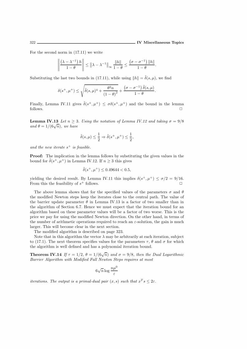
322 IV Miscellaneous Topics
For the second norm in (17.11) we write
∥∥∥∥∥
(λ− λ−1
)h
1− θ
∥∥∥∥∥ ≤∥∥λ− λ−1
∥∥∞
‖h‖1− θ
≤(σ − σ−1
)‖h‖
1− θ.
Substituting the last two bounds in (17.11), while using ‖h‖ = δ(s, µ), we find
δ(s+, µ+) ≤√δ(s, µ)4 +
θ2n
(1− θ)2+
(σ − σ−1
)δ(s, µ)
1− θ.
Finally, Lemma IV.11 gives δ(s+, µ+) ≤ σδ(s+, µ+) and the bound in the lemmafollows.
Lemma IV.13 Let n ≥ 3. Using the notation of Lemma IV.12 and taking σ = 9/8and θ = 1/(6
√n), we have
δ(s, µ) ≤ 1
2⇒ δ(s+, µ+) ≤ 1
2,
and the new iterate s+ is feasible.
Proof: The implication in the lemma follows by substituting the given values in thebound for δ(s+, µ+) in Lemma IV.12. If n ≥ 3 this gives
δ(s+, µ+) ≤ 0.49644 < 0.5,
yielding the desired result. By Lemma IV.11 this implies δ(s+, µ+) ≤ σ/2 = 9/16.From this the feasibility of s+ follows.
The above lemma shows that for the specified values of the parameters σ and θthe modified Newton steps keep the iterates close to the central path. The value ofthe barrier update parameter θ in Lemma IV.13 is a factor of two smaller than inthe algorithm of Section 6.7. Hence we must expect that the iteration bound for analgorithm based on these parameter values will be a factor of two worse. This is theprice we pay for using the modified Newton direction. On the other hand, in terms ofthe number of arithmetic operations required to reach an ε-solution, the gain is muchlarger. This will become clear in the next section.The modified algorithm is described on page 323.Note that in this algorithm the vector λ may be arbitrarily at each iteration, subject
to (17.1). The next theorem specifies values for the parameters τ , θ and σ for whichthe algorithm is well defined and has a polynomial iteration bound.
Theorem IV.14 If τ = 1/2, θ = 1/(6√n) and σ = 9/8, then the Dual Logarithmic
Barrier Algorithm with Modified Full Newton Steps requires at most
6√n log
nµ0
ε
iterations. The output is a primal-dual pair (x, s) such that xT s ≤ 2ε.

IV.17 Partial Updating 323
Dual Log. Barrier Algorithm with Modified Full Newton Steps
Input:A proximity parameter τ , 0 ≤ τ < 1;an accuracy parameter ε > 0;(y0, s0) ∈ D and µ0 > 0 such that δ(s0, µ0) ≤ τ ;a barrier update parameter θ, 0 < θ < 1;a threshold value σ, σ > 1.
begins := s0; µ := µ0;while nµ ≥ ε dobegin
Choose any λ satisfying (17.1);s := s+∆s, ∆s from (17.2);µ := (1− θ)µ;
endend
Proof: According to Lemma IV.13 the algorithm is well defined. The iteration boundis an immediate consequence of Lemma I.36. Finally, the duality gap of the final iteratecan be estimated as follows. For the final iterate s we have δ(s, µ) ≤ 1/2, with nµ ≤ ε.Taking x = x(s, µ) it follows from (17.10) that
sT x(s, µ) = nµ− µhTλ−1.
Since ∣∣hTλ−1∣∣ ≤
∥∥λ−1∥∥ ‖h‖ ≤ σδ(s, µ)
√n ≤ 9n/16 ≤ n,
we obtain
sT x(s, µ) ≤ 2nµ ≤ 2ε.
The proof is complete.
17.4 Algorithm with rank-one updates
We now present a variant of the algorithm in the previous section in which the vectorλ used in the computation of the modified Newton step is prescribed. See page 324.Note that at each iteration the vector s is updated in such a way that the vector λ
used in the computation of the modified Newton step satisfies (17.1). As a consequence,the iteration bound for the algorithm is given by Theorem IV.14. Hence, the algorithmyields an exact solution of (D) in O (
√nL) iterations. Without using partial updates
— which corresponds to giving the threshold parameter σ the value 1 — the bound for
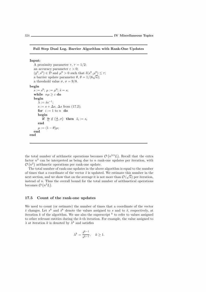
324 IV Miscellaneous Topics
Full Step Dual Log. Barrier Algorithm with Rank-One Updates
Input:A proximity parameter τ , τ = 1/2;an accuracy parameter ε > 0;(y0, s0) ∈ D and µ0 > 0 such that δ(s0, µ0) ≤ τ ;a barrier update parameter θ, θ = 1/(6
√n);
a threshold value σ, σ = 9/8.
begins := s0; µ := µ0; s = s;while nµ ≥ ε dobeginλ := ss−1;s := s+∆s, ∆s from (17.2);for i := 1 to n dobegin
if sisi/∈(1σ , σ
)then si := si
end
µ := (1− θ)µ;end
end
the total number of arithmetic operations becomes O(n3.5L
). Recall that the extra
factor n3 can be interpreted as being due to n rank-one updates per iteration, withO(n2)arithmetic operations per rank-one update.
The total number of rank-one updates in the above algorithm is equal to the numberof times that a coordinate of the vector s is updated. We estimate this number in thenext section, and we show that on the average it is not more than O (
√n) per iteration,
instead of n. Thus the overall bound for the total number of arithmetical operationsbecomes O
(n3L
).
17.5 Count of the rank-one updates
We need to count (or estimate) the number of times that a coordinate of the vectors changes. Let sk and sk denote the values assigned to s and to s, respectively, atiteration k of the algorithm. We use also the superscript k to refer to values assignedto other relevant entities during the k-th iteration. For example, the value assigned toλ at iteration k is denoted by λk and satisfies
λk =sk−1
sk−1, k ≥ 1.

IV.17 Partial Updating 325
Moreover, denoting the modified Newton step on iteration k by ∆sk, we have
∆sk = sk − sk−1 = sk−1hk = λksk−1hk, k ≥ 1. (17.12)
Note that the algorithm is initialized so that s0 = s0 and these are the values of s ands just before the first iteration.Now consider the i-th coordinate of s. Suppose that si is updated at iteration
k1 ≥ 0 and next updated at iteration k2 > k1. Then the updating rule implies thatthe sequence
sk1+1i
sk1
i
,sk1+2i
sk1+1i
, . . . ,sk2−1i
sk2−2i
,sk2
i
sk2−1i
has the property that the last entry lies outside the interval (1/σ, σ) whereas all theother entries lie inside this interval. Since
sk1
i = sk1
i = sk1+1i = . . . = sk2−1
i
we can rewrite the above sequence as
sk1+1i
sk1
i
,sk1+2i
sk1
i
, . . . ,sk2−1i
sk1
i
,sk2
i
sk1
i
. (17.13)
Hence, with
pj := sk1+ji , 0 ≤ j ≤ K := k2 − k1, (17.14)
the sequence
p0, p1, . . . , pK (17.15)
has the propertypjp0
∈(1
σ, σ
), 1 ≤ j < K (17.16)
andpKp0
/∈(1
σ, σ
). (17.17)
Our estimate of the number of rank-one updates in the algorithm depends on atechnical lemma on such sequences. The proof of this lemma (Lemma IV.15 below)requires another technical lemma that can be found in Appendix C (Lemma C.3).
Lemma IV.15 Let σ ≥ 1 and let p0, p1, . . . , pK be a finite sequence of positivenumbers satisfying (17.16) and (17.17). Then
K−1∑
j=0
∣∣∣∣pj+1 − pj
pj
∣∣∣∣ ≥ 1− 1
σ. (17.18)
Proof: We start with K = 1. Then we need to show∣∣∣∣p1 − p0p0
∣∣∣∣ =∣∣∣∣p1p0
− 1
∣∣∣∣ ≥ 1− 1
σ.

326 IV Miscellaneous Topics
If p1/p0 ≤ 1/σ then ∣∣∣∣p1p0
− 1
∣∣∣∣ = 1− p1p0
≥ 1− 1
σ
and if p1/p0 ≥ σ then∣∣∣∣p1p0
− 1
∣∣∣∣ =p1p0
− 1 ≥ σ − 1 ≥ σ − 1
σ= 1− 1
σ.
We proceed with K ≥ 2. It is convenient to denote the left-hand side expressionon (17.18) by g(p0, p1, . . . , pK). We start with an easy observation: if pj+1 = pj forsome j (0 ≤ j < K) then g(p0, p1, . . . , pK) does not change if we remove pj+1 fromthe sequence. So without loss of generality we may assume that no two subsequentelements in the given sequence p0, p1, . . . , pK are equal.Now let the given sequence p0, p1, . . . , pK be such that g(p0, p1, . . . , pK) is minimal.
For 0 < j < K we consider the two terms in g(p0, p1, . . . , pK) that contain pj . Thecontribution of these two terms is given by
∣∣∣∣pj − pj−1
pj−1
∣∣∣∣+∣∣∣∣pj+1 − pj
pj
∣∣∣∣ =∣∣∣∣1−
pjpj−1
∣∣∣∣+∣∣∣∣∣1−
pj+1
pj−1
pj
pj−1
∣∣∣∣∣ . (17.19)
Since p0, p1, . . . , pK minimizes g(p0, p1, . . . , pK), when fixing pj−1 and pj+1, pj mustminimize (17.19). If pj+1 ≤ pj−1 then Lemma C.3 (page 437) implies that
pjpj−1
= 1 orpjpj−1
=pj+1
pj−1.
This means thatpj = pj−1 or pj = pj+1.
Hence, in this case the sequence has two subsequent elements that are equal, whichhas been excluded above. We conclude that pj+1 > pj−1. Applying Lemma C.3 oncemore, we obtain
pjpj−1
=
√pj+1
pj−1.
Thus it follows thatpj−1 < pj =
√pj−1pj+1 < pj+1
for each j, 0 < j < K, showing that the sequence p0, p1, . . . , pK is strictly increasingand each entry pj in the sequence, with 0 < j < K, is the geometric mean of thesurrounding entries. This implies that the sequence pj/p0, 1 ≤ j ≤ K, is geometricand we have
pjp0
= αj , 1 ≤ j ≤ K,
where
α =
√p2p0
> 1.
In that case we must have pK
p0≥ σ and hence α satisfies αK ≥ σ. Since
g(p0, p1, . . . , pK) =
K−1∑
j=0
∣∣∣∣pj+1
pj− 1
∣∣∣∣ =K−1∑
j=0
(α− 1) = K (α− 1) ,

IV.17 Partial Updating 327
the inequality in the lemma follows if
K (α− 1) ≥ 1− 1
αK.
This inequality holds for each natural number K and for each real number α ≥ 1.This can be seen by reducing the right-hand side as follows:
1− 1
αK=
αK − 1
αK=
(α− 1)(αK−1 + . . . + α+ 1
)
αK
= (α− 1)(α−1 + α−2 . . . + α−K
)< K (α− 1) .
This completes the proof.
Now the next lemma follows easily.
Lemma IV.16 Suppose that the component si of s is updated at iteration k1 and nextupdated at iteration k2 > k1. Then
k2−1∑
k=k1
∣∣∣∣∣∆sk+1
i
ski
∣∣∣∣∣ ≥ 1− 1
σ,
where ∆sk+1i denotes the i-th coordinate of the modified Newton step at iteration k+1.
Proof: Applying Lemma IV.15 to the sequence p0, p1, . . . , pK defined by (17.14) weget
k2−1∑
k=k1
∣∣∣∣∣sk+1i − skiski
∣∣∣∣∣ ≥ 1− 1
σ.
Since sk+1 − sk = ∆sk+1 by definition, the lemma follows.
Theorem IV.17 Let N denote the total number of iterations of the algorithm and ni
the total number of updates of si. Then
n∑
i=1
ni ≤ 6N√n.
Proof: Recall from (17.12) that
∆sk+1 = λk+1skhk+1.
Hence, for 1 ≤ i ≤ n,∆sk+1
i
ski= λk+1
i hk+1i .
Now Lemma IV.16 implies
N∑
k=1
∣∣λki hki∣∣ =
N−1∑
k=0
∣∣λk+1i hk+1
i
∣∣ ≥ ni
(1− 1
σ
).

328 IV Miscellaneous Topics
Taking the sum over i we obtain
n∑
i=1
ni ≤σ
σ − 1
N∑
k=1
n∑
i=1
∣∣λki hki∣∣ .
The inner sum can be bounded above by
n∑
i=1
∣∣λki hki∣∣ ≤ σ
n∑
i=1
∣∣hki∣∣ = σ
∥∥hk∥∥1≤ σ
∥∥hk∥∥√n.
Since∥∥hk
∥∥ = δ(sk, µk) ≤ τ we obtain
n∑
i=1
ni ≤σ
σ − 1
N∑
k=1
στ√n =
Nσ2τ√n
σ − 1.
Substituting the values of σ and τ specified in the algorithm proves the theorem.
Finally, using the iteration bound of Theorem IV.14 and that each rank-one updaterequires O(n2) arithmetic operations, we may state our final result without furtherproof.
Theorem IV.18 The Full Step Dual Logarithmic Barrier Algorithm with Rank-OneUpdates requires at most
36n3 lognµ0
ε
arithmetic operations. The output is a primal-dual pair (x, s) such that xT s ≤ 2ε.

18
Higher-Order Methods
18.1 Introduction
In a target-following method the Newton directions ∆x and ∆s to a given targetpoint w in the w-space,1 and at a given positive primal-dual pair (x, s), are obtainedby solving the system (10.2):
A∆x = 0,
AT∆y +∆s = 0, (18.1)
s∆x+ x∆s = ∆w,
where ∆w = w − xs. Recall that this system was obtained by neglecting the second-order term ∆x∆s in the third equation of the nonlinear system (10.1), given by
A∆x = 0,
AT∆y +∆s = 0, (18.2)
s∆x+ x∆s+∆x∆s = ∆w.
An exact solution — (∆ex,∆ey,∆es) say — of (18.2) would yield the primal-dual paircorresponding to the target w, because
(x+∆ex) (s+∆es) = w,
as can easily be verified. Unfortunately, finding an exact solution of the nonlinearsystem (18.2) is hard from a computational point of view. Therefore, following aclassical approach in mathematics when dealing with nonlinearity, we linearize thesystem, and use the solutions of the linearized system (18.1). Denoting its solutionsimply by (∆x,∆y,∆s), the primal-dual pair (x+∆x, s+∆s) satisfies
(x+∆x) (s+∆s) = w −∆x∆s,
and hence, the ‘error’ after the step is given by ∆x∆s. Thus, this error represents theprice we have to pay for using a solution of the linearized system (18.1). We refer toit henceforth as the second-order effect.
1 We defined the w-space in Section 9.1, page 220; it is simply the interior of the nonnegative orthantin IRn.

330 IV Miscellaneous Topics
Clearly, the second-order effect strongly depends on the actual data of the problemunder consideration.2
It would be very significant if we could eliminate the above described second-ordereffect, or at least minimize it in some way or another. One way to do this is to useso-called higher-order methods.3 The Newton method used so far is considered to be afirst-order method. In the next section the search directions for higher-order methodsare introduced. Then we devote a separate section (Section 18.3) to the estimate of the(higher-order) error term Er(α), where r ≥ 1 denotes the order of the search directionand α the step-size. The results of Section 18.3 are applied in two subsequent sections.In Section 18.4 we first discuss and extend the definition of the primal-dual Dikindirection, as introduced in Appendix E for the self-dual problem, to a primal-dualDikin direction for the problems (P ) and (D) in standard format. Then we considera higher-order version of this direction, and we show that the iteration bound canbe reduced by the factor
√n without increasing the complexity per iteration. Then,
in Section 18.5 we apply the results of Section 18.3 to the primal-dual logarithmicbarrier method, as considered in Chapter 7 of Part II. This section is based on apaper of Zhao [320]. Here the use of higher-order search directions does not improvethe iteration bound when compared with the (first-order) full Newton step method.Recall that in the full Newton step method the iterates stay very close to the centralpath. This can be expressed by saying this method keeps the iterates in a ‘narrowcone’ around the central path. We shall see that a higher-order method allows theiterates to stay further away from the central path, which makes such a method a‘wide cone’ method.
18.2 Higher-order search directions
Suppose that we are given a positive primal-dual pair (x, s) and we want to find theprimal-dual pair corresponding to w := xs + ∆w for some displacement ∆w in thew-space. Our aim is to generate suitable search directions ∆x and ∆s at (x, s). Oneway to derive such directions is to consider the linear line segment in the w-spaceconnecting xs with w. A parametric representation of this segment is given by
xs+ α∆w, 0 ≤ α ≤ 1.
2 In the w-space the ideal situation is that the curve (x+ α∆x) (s+ α∆s) , 0 ≤ α ≤ 1, moves fromxs in a straight line to the target w. As a matter of fact, the second-order effect ‘blows’ the curveaway from this straight line segment. Considering α as a time parameter, we can think of theiterate (x+ α∆x) (s+ α∆s) as the trajectory of a vessel sailing from xs to w and of the second-order effect as a wind blowing it away from its trajectory. To reach the target w the bargemancan put over the helm now and then, which in our context is accomplished by updating the searchdirection. In practice, a bargeman will anticipate the fact that the wind is (locally) constant and hecan put the helm in a fixed position that prevents the vessel being driven from its correct course.It may be interesting to mention a computer game called Schiet OpTM , designed by Brinkhuisand Draisma, that is based on this phenomenon [51]. It requires the player to find an optimal pathin the w-space to the origin.
3 The idea of using higher-order search directions as presented in this chapter is due to Monteiro,Adler and Resende [220], and was later investigated by Zhang and Zhang [318], Hung and Ye [150],Jansen et al. [160] and Zhao [320]. The idea has been applied also in the context of a predictor-corrector method by Mehrotra [202, 205].

IV.18 Higher-Order Methods 331
To any point of this segment belongs a primal-dual pair and we denote this pair by(x(α), s(α)).4 Since x(α) and s(α) depend analytically5 on α there exist x(i) and s(i),with i = 0, 1, . . ., such that
x(α) =
∞∑
i=0
x(i)αi, s(α) =
∞∑
i=0
s(i)αi, 0 ≤ α ≤ 1. (18.3)
Obviously, x(0) = x = x(0) and s(0) = s = s(0). From Ax(α) = b, for each α ∈ [0, 1],we derive
Ax(0) = b, Ax(i) = 0, i ≥ 1. (18.4)
Similarly, there exist unique y(i) and s(i), i = 0, 1, . . ., such that
AT y(0) + s(0) = c, AT y(i) + s(i) = 0, i ≥ 1. (18.5)
Furthermore, from
x(α)s(α) = xs+ α∆w,
by expanding x(α) and s(α) and then equating terms with equal powers of α, we getthe following relations:
x(0)s(0) = xs (18.6)
x(0)s(1) + s(0)x(1) = ∆w (18.7)k∑
i=0
x(i)s(k−i) = 0, k = 2, 3, . . . . (18.8)
The first relation implies once more that x(0) = x and s(0) = s. Using this and (18.4),(18.5) and (18.7) we obtain
Ax(1) = 0
AT y(1) + s(1) = 0 (18.9)
sx(1) + xs(1) = ∆w.
4 In other chapters of this book x(α) denotes the α-center on the primal central path. To avoid anymisunderstanding it might be appropriate to emphasize that in this chapter x(α) — as well as s(α)— has a different meaning, as indicated.
5 Note that x(α) and s(α) are uniquely determined by the relations
Ax(α) = b, x > 0,
AT y(α) + s(α) = c, s > 0,
x (α) s(α) = xs+ α∆w.
Obviously, the right-hand sides in these relations depend linearly (and hence analytically) on α.Since the Jacobian matrix of the left-hand side is nonsingular, the implicit function theorem (cf.Proposition A.2 in Appendix A) implies that x(α), y(α) and s(α) depend analytically on α. Seealso Section 16.2.1.

332 IV Miscellaneous Topics
This shows that x(1) and s(1) are just the primal-dual Newton directions at (x, s) forthe target w = xs+∆w.6 Using (18.4), (18.5) and (18.8) we find that the higher-ordercoefficients x(k), y(k) and s(k), with k ≥ 2, satisfy the linear system
Ax(k) = 0
AT y(k) + s(k) = 0 (18.10)
sx(k) + xs(k) = −k−1∑
i=1
x(i)s(k−i), k = 2, 3, . . . ,
thus finding a recursive expression for the higher-order coefficients. The remarkablething here is that the coefficient matrix in (18.10) is the same as in (18.9). This has theimportant consequence that as soon as the standard (first-order) Newton directionsx(1) and s(1) have been calculated from the linear system (18.9), the second-orderterms x(2) and s(2) can be computed from a linear system with the same coefficientmatrix. Having x(2) and s(2), we can compute x(3) and s(3), and so on. Hence, from acomputational point of view the higher-order terms x(k) and s(k), with k ≥ 2, can beobtained relatively cheaply.Assuming that the computation of the Newton directions requires O(n3) arithmetic
operations, the computation of each subsequent pair(x(k), s(k)
)of higher-order
coefficients requires O(n2) arithmetic operations. For example, if we compute thepairs
(x(k), s(k)
)for k = 1, 2, . . . , n, this doubles the computational cost per iteration.
There is some reason to expect, however, that we will obtain a more accurate searchdirection; this may result in a speedup that justifies the extra computational burdenin the computation.By truncating the expansion (18.3), we define the primal-dual Newton directions of
order r at (x, s) with step-size α by
∆r,αx :=
r∑
i=1
x(i)αi, ∆r,αs :=
r∑
i=1
s(i)αi. (18.11)
Moving along these directions we arrive at
xr(α) := x+∆r,αx, sr(α) := s+∆r,αs.
Recall that we started this section by taking w = xs+∆w as the target point in thew-space. Now that we have introduced the step-size α it is more natural to consider
w(α) := xs+ α∆w
as the target. In the following lemma we calculate xr(α) sr(α), which is the next iteratein the w-space, and hence obtain an expression for the deviation from the target w(α)after the step.
6Exercise 84 Verify that y(1) can be solved from (18.9) by the formula
y(1) = −(AXS−1AT
)−1AS−1∆w.
This generalizes the expression for the logarithmic barrier direction in Exercise 35, page 111. Giveny(1), s(1) and x(1) follow from
s(1) = −AT y(1), x(1) = S−1(∆w − xs(1)
).

IV.18 Higher-Order Methods 333
Lemma IV.19
xr(α) sr(α) = xs+ α∆w +2r∑
k=r+1
αk
(r∑
i=k−r
x(i)s(k−i)
).
Proof: We may write
xr(α) := x+∆r,αx =
r∑
i=0
x(i)αi,
and we have a similar expression for sr(α). Therefore,
xr(α) sr(α) =
(r∑
i=0
x(i)αi
)(r∑
i=0
s(i)αi
). (18.12)
The right-hand side can be considered as a polynomial in α of degree 2r. We considerthe coefficient of αk for 0 ≤ k ≤ 2r. If 0 ≤ k ≤ r then the coefficient of αk is given by
k∑
i=0
x(i)s(k−i),
By (18.8), this expression vanishes if k ≥ 2. Furthermore, if k = 1 the expression isequal to ∆w, by (18.7) and if k = 0 it is equal to xs, by (18.6). So it remains toconsider the coefficient of αk on the right-hand side of (18.12) for r+ 1 ≤ k ≤ 2r. Forthese values of k the corresponding coefficient in (18.12) is given by
r∑
i=k−r
x(i)s(k−i).
Hence, collecting the above results, we get
xr(α) sr(α) = xs+ α∆w +
2r∑
k=r+1
αk
(r∑
i=k−r
x(i)s(k−i)
). (18.13)
This completes the proof.
In the next section we further analyze the error term
Er(α) :=
2r∑
k=r+1
αk
(r∑
i=k−r
x(i)s(k−i)
). (18.14)
We conclude this section with two observations. First, taking r = 1 we get
E1(α) = α2x(1)s(1) = α2∆x∆s,
where ∆x and ∆s are the standard primal-dual Newton directions at (x, s). This is inaccordance with earlier results (see, e.g., (10.12)). If we use a first-order Newton step

334 IV Miscellaneous Topics
then the error is of order two in α. In the general case, of a step of order r, the errorterm Er(α) is of order r + 1 in α.The second observation concerns the orthogonality of the search directions in the x-
and s-spaces. It is immediate from the first two equations in (18.9) and (18.10) that
(x(i))T
s(j) = 0, ∀i ≥ 1, ∀j ≥ 1.
As a consequence,
(∆r,αx)T∆r,αs = 0,
and also, from Lemma IV.19,
(xr(α))Tsr(α) = eT (xs+ α∆w) = eT w(α).
Thus, after the step with size α, the duality gap is equal to the gap at the target w(α).Figure 18.1 illustrates the use of higher-order search directions.
0 1 2 3 40
1
2
3
4
w1
w2
target
start
r = 1
r = 2r = 3
r = 4r = 5
Figure 18.1 Trajectories in the w-space for higher-order steps with r = 1, 2, 3, 4, 5.

IV.18 Higher-Order Methods 335
18.3 Analysis of the error term
The main task in the analysis of the higher-order method is to estimate the error termEr(α), given by (18.14). Our first estimation is very loose. We write
‖Er(α)‖ ≤2r∑
k=r+1
αk
∥∥∥∥∥
r∑
i=k−r
x(i)s(k−i)
∥∥∥∥∥ ≤2r∑
k=r+1
αkr∑
i=k−r
∥∥∥x(i)s(k−i)∥∥∥ , (18.15)
and we concentrate on estimating the norms in the last sum. We use the vectors d andv introduced in Section 10.4:
d =
√x
s, v =
√xs. (18.16)
Then the third equation in (18.9) can be rewritten as
d−1x(1) + ds(1) =∆w
v(18.17)
and the third equation in (18.10) as
d−1x(k) + ds(k) = −v−1k−1∑
i=1
x(i)s(k−i), k = 2, 3, . . . . (18.18)
Since x(k) and s(k) are orthogonal for k ≥ 1, the vectors d−1x(k) and ds(k) areorthogonal as well. Therefore,
∥∥∥d−1x(k)∥∥∥2
+∥∥∥ds(k)
∥∥∥2
=∥∥∥d−1x(k) + ds(k)
∥∥∥2
, k ≥ 1.
Hence, defining
q(k) := d−1x(k) + ds(k), k ≥ 1, (18.19)
we have for each k ≥ 1,
∥∥∥d−1x(k)∥∥∥ ≤
∥∥∥q(k)∥∥∥ ,
∥∥∥ds(k)∥∥∥ ≤
∥∥∥q(k)∥∥∥ ,
and as a consequence, for 1 ≤ i ≤ k − 1 we may write
∥∥∥x(i)s(k−i)∥∥∥ =
∥∥∥d−1x(i)ds(k−i)∥∥∥ ≤
∥∥∥d−1x(i)∥∥∥∥∥∥ds(k−i)
∥∥∥ ≤∥∥∥q(i)
∥∥∥∥∥∥q(k−i)
∥∥∥ . (18.20)
Substitution of these inequalities in the bound (18.15) for Er(α) yields
‖Er(α)‖ ≤2r∑
k=r+1
αkr∑
i=k−r
∥∥∥q(i)∥∥∥∥∥∥q(k−i)
∥∥∥ . (18.21)
We proceed by deriving upper bounds for∥∥q(k)
∥∥ , k ≥ 1.

336 IV Miscellaneous Topics
Lemma IV.20 For each k ≥ 1,
∥∥∥q(k)∥∥∥ ≤ ϕk
∥∥v−1∥∥k−1
∞
∥∥∥q(1)∥∥∥k
, (18.22)
where the integer sequence ϕ1, ϕ2, . . . is defined recursively by ϕ1 = 1 and
ϕk =
k−1∑
i=1
ϕiϕk−i. (18.23)
Proof: The proof is by induction on k. Note that (18.22) holds trivially if k = 1.Assume that (18.22) holds for
∥∥q(ℓ)∥∥ if 1 ≤ ℓ < k. We complete the proof by deducing
from this assumption that the lemma is also true for∥∥q(k)
∥∥. For k ≥ 2 we obtain from
the definition (18.19) of q(k) and (18.18) that
q(k) = −v−1k−1∑
i=1
x(i)s(k−i).
Hence, using (18.20),
∥∥∥q(k)∥∥∥ ≤
∥∥v−1∥∥∞
k−1∑
i=1
∥∥∥q(i)∥∥∥∥∥∥q(k−i)
∥∥∥ .
At this stage we apply the induction hypothesis to the last two norms, yielding
∥∥∥q(k)∥∥∥ ≤
∥∥v−1∥∥∞
k−1∑
i=1
ϕi
∥∥v−1∥∥i−1
∞
∥∥∥q(1)∥∥∥i
ϕk−i
∥∥v−1∥∥k−i−1
∞
∥∥∥q(1)∥∥∥k−i
,
which can be simplified to
∥∥∥q(k)∥∥∥ ≤
∥∥v−1∥∥k−1
∞
∥∥∥q(1)∥∥∥k k−1∑
i=1
ϕiϕk−i.
Finally, using (18.23) the lemma follows.
The solution of the recursion (18.23) with ϕ1 = 1 is given by7
ϕk =1
k
(2k − 2
k − 1
). (18.24)
This enables us to prove our next result.
Lemma IV.21 For each k = r + 1, . . . , 2r,
r∑
i=k−r
∥∥∥q(i)∥∥∥∥∥∥q(k−i)
∥∥∥ ≤ 22k−3
k
∥∥v−1∥∥k−2
∞
∥∥∥q(1)∥∥∥k
.
7Exercise 85 Prove that (18.24) is the solution of the recursion in (18.23) satisfying ϕ1 = 1 (cf.,e.g., Liu [184]).
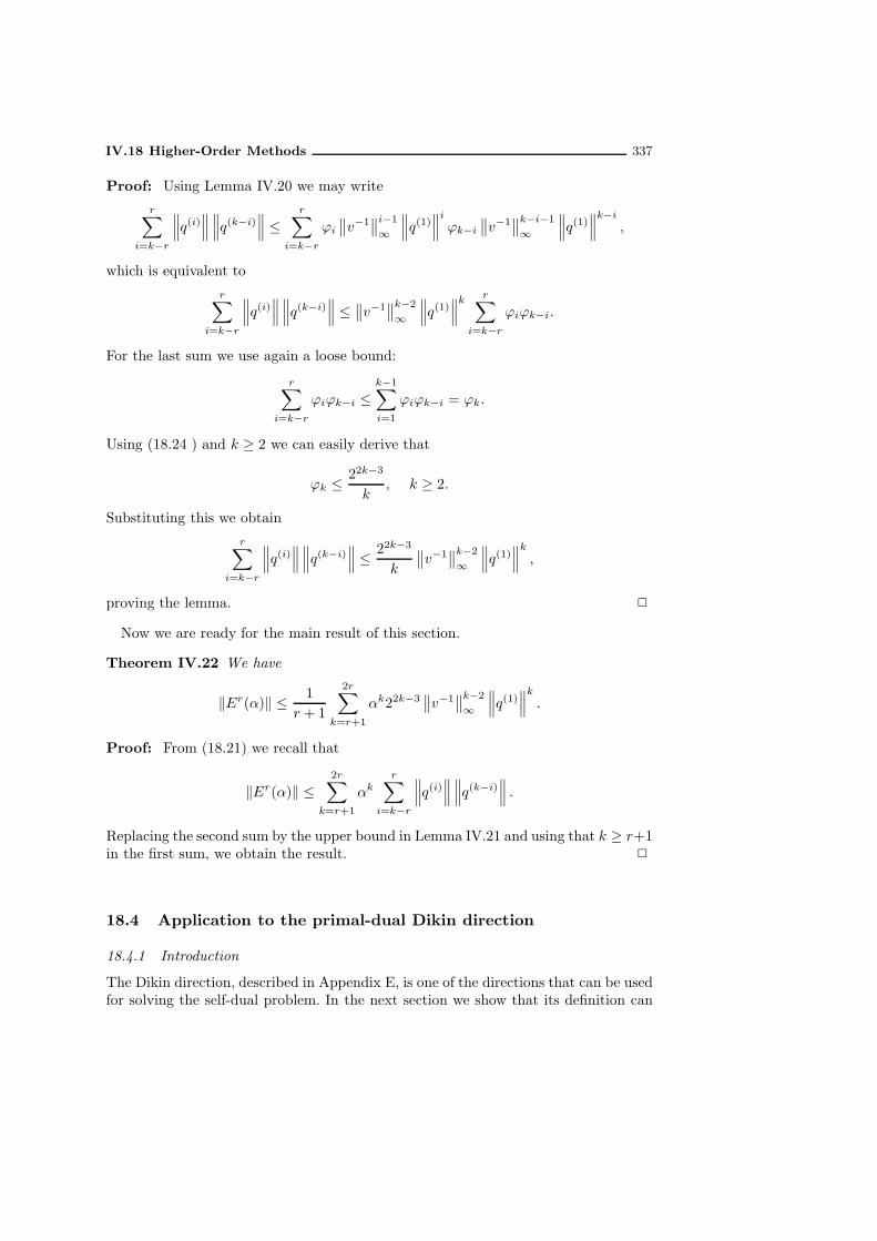
IV.18 Higher-Order Methods 337
Proof: Using Lemma IV.20 we may write
r∑
i=k−r
∥∥∥q(i)∥∥∥∥∥∥q(k−i)
∥∥∥ ≤r∑
i=k−r
ϕi
∥∥v−1∥∥i−1
∞
∥∥∥q(1)∥∥∥i
ϕk−i
∥∥v−1∥∥k−i−1
∞
∥∥∥q(1)∥∥∥k−i
,
which is equivalent to
r∑
i=k−r
∥∥∥q(i)∥∥∥∥∥∥q(k−i)
∥∥∥ ≤∥∥v−1
∥∥k−2
∞
∥∥∥q(1)∥∥∥k r∑
i=k−r
ϕiϕk−i.
For the last sum we use again a loose bound:
r∑
i=k−r
ϕiϕk−i ≤k−1∑
i=1
ϕiϕk−i = ϕk.
Using (18.24 ) and k ≥ 2 we can easily derive that
ϕk ≤ 22k−3
k, k ≥ 2.
Substituting this we obtain
r∑
i=k−r
∥∥∥q(i)∥∥∥∥∥∥q(k−i)
∥∥∥ ≤ 22k−3
k
∥∥v−1∥∥k−2
∞
∥∥∥q(1)∥∥∥k
,
proving the lemma.
Now we are ready for the main result of this section.
Theorem IV.22 We have
‖Er(α)‖ ≤ 1
r + 1
2r∑
k=r+1
αk22k−3∥∥v−1
∥∥k−2
∞
∥∥∥q(1)∥∥∥k
.
Proof: From (18.21) we recall that
‖Er(α)‖ ≤2r∑
k=r+1
αkr∑
i=k−r
∥∥∥q(i)∥∥∥∥∥∥q(k−i)
∥∥∥ .
Replacing the second sum by the upper bound in Lemma IV.21 and using that k ≥ r+1in the first sum, we obtain the result.
18.4 Application to the primal-dual Dikin direction
18.4.1 Introduction
The Dikin direction, described in Appendix E, is one of the directions that can be usedfor solving the self-dual problem. In the next section we show that its definition can

338 IV Miscellaneous Topics
easily be adapted to problems (P ) and (D) in standard format. It will become clearthat the analysis of the self-dual model also applies to the standard model and viceversa. Although we don’t work it out here, we mention that use of the (first-order)Dikin direction leads to an algorithm for solving the standard model that requires atmost
τn log
(x0)Ts0
ε
iterations, where (x0, s0) denotes the initial primal-dual pair, ε is an upper boundfor the duality gap upon termination of the algorithm and τ an upper bound for thedistance of the iterates to the central path.8 The complexity per iteration is O(n3), asusual. This is in accordance with the bounds in Appendix E for the self-dual model. Byusing higher-order versions of the Dikin direction the complexity can be improved by a
factor (τn)r−1
2r . Note that this factor goes to√τn if r goes to infinity. The complexity
per iteration is O(n3 + rn2). Hence, when taking r = n, the complexity per iterationremains O(n3). In that case we show that the iteration bound is improved by thefactor
√τn. When τ = O(1), which can be assumed without loss of generality, we
obtain the iteration bound
O(√n log
(x0)Ts0
ε
),
which is the best iteration bound for interior point methods known until now.
18.4.2 The (first-order) primal-dual Dikin direction
Let (x, s) be a positive primal-dual pair for (P ) and (D) and let ∆x and ∆s denotedisplacements in the x-space and the s-space. Moving along ∆x and ∆s we arrive at
x+ := x+∆x, s+ := s+∆s.
The new iterates will be feasible if
A∆x = 0, AT∆y +∆s = 0,
where ∆y represents the displacement in the y-space corresponding to ∆s, and bothx+ and s+ are nonnegative. Since ∆x and ∆s are orthogonal, the new duality gap isgiven by
(x+)Ts+ = xT s+ xT∆s+ sT∆x.
8 Originally, the Dikin direction was introduced for the standard format. See Jansen, Roos andTerlaky [156].

IV.18 Higher-Order Methods 339
Replicating Dikin’s idea, just as in Section E.2, we replace the nonnegativity conditionsby the condition9
∥∥∥∥∆x
x+
∆s
s
∥∥∥∥ ≤ 1.
This can be rewritten as
∥∥∥∥x+ − x
x+s+ − s
s
∥∥∥∥ ≤ 1,
showing that the new iterates are sought within an ellipsoid, called the Dikin ellipsoid
at the given pair (x, s). Since our aim is to minimize the duality gap, we consider theoptimization problem
min
eT (s∆x+ x∆s) : A∆x = 0, AT∆y +∆s = 0,
∥∥∥∥∆x
x+
∆s
s
∥∥∥∥ ≤ 1
. (18.25)
The crucial observation is that (18.25) determines the displacements ∆x and ∆suniquely. The arguments are almost the same as in Section E.2. Using the vectorsd and v in (18.16), x and s can be rescaled to the same vector v:
d−1x = v, ds = v.
As usual, we rescale ∆x and ∆s accordingly to
dx := d−1∆x, ds := d∆s. (18.26)
Then∆x
x=dxv,
∆s
s=dsv,
and moreover,
∆x∆s = dxds.
9
Dikin introduced the so-called primal affine-scaling direction at a primal feasible x (x > 0) byminimizing the primal objective cT (x+∆x) over the ellipsoid
∥∥∥∆xx
∥∥∥ ≤ 1,
subject to A∆x = 0. So the primal affine-scaling direction is determined as the unique solution of
min
cT∆x : A∆x = 0,
∥∥∥∆xx
∥∥∥ ≤ 1
.
Dikin showed convergence of the primal affine-scaling method ([63, 64, 65]) under some non-degeneracy assumptions. Later, without nondegeneracy assumptions, Tsuchiya [268, 270] provedconvergence of the method with damped steps. Dikin and Roos [66] proved convergence of a full-step method for the special case that the given problem is homogeneous. Despite many attempts,until now it has not been possible to show that the method is polynomial. For a recent surveypaper we refer the reader to Tsuchiya [272]. The approach in this section seems to be the naturalgeneralization to the primal-dual framework.

340 IV Miscellaneous Topics
Also, the scaled displacements dx and ds are orthogonal. Now the vector occurring inthe ellipsoidal constraint in (18.25) can be reduced to
∆x
x+
∆s
s=dx + ds
v.
Moreover, the variable vector in the objective of problem (18.25) can be written as
s∆x+ x∆s = xs
(∆x
x+
∆s
s
)= v (dx + ds) .
Withdw := dx + ds, (18.27)
the vectors dx and ds are uniquely determined as the orthogonal components of dw inthe null space and row space of AD, so we have
dx = PAD (dw) (18.28)
ds = dw − dx. (18.29)
Thus we can solve the problem (18.25) by solving the much simpler problem
min
vT dw :
∥∥∥∥dwv
∥∥∥∥ ≤ 1
. (18.30)
The solution of (18.30) is given by
dw = − v3
‖v2‖ = − (xs)32
‖xs‖ .
It follows that dx and ds are uniquely determined by the system
ADdx = 0
(AD)Tdy + ds = 0
dx + ds = dw.
In terms of the unscaled displacements this can be rewritten as
A∆x = 0
AT∆y +∆s = 0 (18.31)
s∆x+ x∆s = ∆w,
where
∆w = vdw = − v4
‖v2‖ = − (xs)2
‖xs‖ . (18.32)
We conclude that the solution of the minimization problem (18.25) is uniquelydetermined by the linear system (18.31). Hence the (first-order) Dikin directions ∆xand ∆s are the Newton directions at (x, s) corresponding to the displacement ∆win the w-space, as given by (18.32). We therefore call ∆w the Dikin direction in thew-space.In the next section we consider an algorithm using higher-order Dikin directions.
Using the estimates of the error term Er(α) in the previous section we analyze thisalgorithm in subsequent sections.

IV.18 Higher-Order Methods 341
18.4.3 Algorithm using higher-order Dikin directions
For the rest of this section, ∆w denotes the Dikin direction in the w-space as givenby (18.32). For r = 1, 2, . . . and for some fixed step-size α that is specified later, thecorresponding higher-order Newton steps of order r at (x, s) are given by (18.11). Theiterates after the step depend on the step-size α. To express this dependence we denotethem as x(α) and s(α) as in Section 18.2. We consider the following algorithm.
Higher-Order Dikin Step Algorithm for the Standard Model
Input:An accuracy parameter ε > 0;a step-size parameter α, 0 < α ≤ 1;a positive primal-dual pair
(x0, s0
).
beginx := x0; s := s0;while xT s ≥ ε dobeginx := x(α) = x+∆r,αx;s := s(α) = s+∆r,αs
endend
Below we analyze this algorithm. Our aim is to keep the iterates (x, s) within somecone
δc(xs) =max (xs)
min (xs)≤ τ
around the central path, for some fixed τ > 1; τ is chosen such that
δc(x0s0) ≤ τ.
18.4.4 Feasibility and duality gap reduction
As before, we use the superscript + to refer to entities after the higher-order Dikinstep of size α at (x, s). Thus,
x+ := x(α) = x+∆r,αx,
s+ := s(α) = s+∆r,αs,
and from Lemma IV.19,
x+s+ = x(α)s(α) = xs+ α∆w + Er(α), (18.33)
where the higher-order error term Er(α) is given by (18.14).The step-size α is feasible if the new iterates are positive. Using the same (simple
continuity) argument as in the proof of Lemma E.2, page 455, we get the followingresult.

342 IV Miscellaneous Topics
Lemma IV.23 If α is such that x(α)s(α) > 0 for all α satisfying 0 ≤ α ≤ α, thenthe step-size α is feasible.
Lemma IV.23 implies that the step-size α is feasible if
xs+ α∆w + Er(α) ≥ 0, 0 ≤ α ≤ α.
At the end of Section 18.2 we established that after the step the duality gap attainsthe value eT (xs+ α∆w). This leads to the following lemma.
Lemma IV.24 If the step-size α is feasible then
(x+)Ts+ ≤
(1− α√
n
)xT s.
Proof: We have
(x+)Ts+ = eT
(xs− α
(xs)2
‖xs‖
)= xT s− α ‖xs‖ .
The Cauchy–Schwarz inequality implies
‖xs‖ =1√n‖e‖ ‖xs‖ ≥ eT (xs)√
n=xT s√n,
and the lemma follows.
18.4.5 Estimate of the error term
By Theorem IV.22 the error term Er(α) satisfies
‖Er(α)‖ ≤ 1
8 (r + 1)
2r∑
k=r+1
αk22k∥∥v−1
∥∥k−2
∞
∥∥∥q(1)∥∥∥k
.
In the present case we have, from (18.19), (18.17) and (18.32),
q(1) =∆w
v= − v3
‖v2‖ .
Hence ∥∥∥q(1)∥∥∥ =
∥∥∥∥v3
‖v2‖
∥∥∥∥ ≤ ‖v‖∞∥∥∥∥v2
‖v2‖
∥∥∥∥ = ‖v‖∞ = max (v).
Therefore,
∥∥v−1∥∥∞
∥∥∥q(1)∥∥∥ ≤ max (v)
min (v)=
√max (xs)
min (xs)=√δc(xs) ≤
√τ .
Substituting this we get
‖Er(α)‖ ≤ 1
8 (r + 1)
∥∥v−1∥∥−2
∞
2r∑
k=r+1
αk22k(√τ)k
=min (xs)
8 (r + 1)
2r∑
k=r+1
(4α
√τ)k.
(18.34)

IV.18 Higher-Order Methods 343
18.4.6 Step size
Assuming δc(x, s) ≤ τ , with τ > 1, we establish a bound for the step-size α such thatthis property is maintained after a higher-order Dikin step. The analysis follows thesame lines as the analysis in Section E.4 of the algorithm for the self-dual model withfirst-order Dikin steps. As there, we derive from δc(x, s) ≤ τ the existence of positivenumbers τ1 and τ2 such that
τ1e ≤ xs ≤ τ2e, with τ2 = ττ1. (18.35)
Without loss of generality we take
τ1 = min (xs).
The following lemma generalizes Lemma E.4.
Lemma IV.25 Let τ > 1. Suppose that δc(xs) ≤ τ and let τ1 and τ2 be such that(18.35) holds. If the step-size α satisfies
α ≤ min
‖xs‖2τ2
,1
4√τ,
1
4√τ
r
√2τ1
√τ
‖xs‖
,
then we have δc(x+s+) ≤ τ .
Proof: Using (18.33) and the definition of ∆w we obtain
x+s+ = x(α)s(α) = xs+ α∆w + Er(α) = xs− α (xs)2
‖xs‖ + Er(α).
Using the first bound on α in the lemma, we can easily verify that the map
t 7→ t− αt2
‖xs‖
is an increasing function for t ∈ [0, τ2]. Application of this map to each component ofthe vector xs gives
(τ1 −
ατ21‖xs‖
)e ≤ xs− α (xs)
2
‖xs‖ ≤(τ2 −
ατ22‖xs‖
)e.
It follows that(τ1 −
ατ21‖xs‖
)e+ Er(α) ≤ x+s+ ≤
(τ2 −
ατ22‖xs‖
)e+ Er(α).
Hence, assuming for the moment that the Dikin step of size α is feasible, we certainlyhave δ(x+s+) ≤ τ if
τ
((τ1 −
ατ21‖xs‖
)e+ Er(α)
)≥(τ2 −
ατ22‖xs‖
)e+ Er(α).

344 IV Miscellaneous Topics
Since τ2 = ττ1, this reduces to
α
(τ22 − ττ21‖xs‖
)e+ (τ − 1)Er(α) ≥ 0.
Since τ22 − ττ21 = (τ − 1) τ1τ2 we can divide by τ − 1, thus obtaining
ατ1τ2‖xs‖ e+ Er(α) ≥ 0.
This inequality is certainly satisfied if
‖xs‖ ‖Er(α)‖ ≤ ατ1τ2.
Using the upper bound (18.34) for Er(α) it follows that we have δ(x+s+) ≤ τ if α issuch that
‖xs‖min (xs)
8 (r + 1)
2r∑
k=r+1
(4α
√τ)k ≤ ατ1τ2.
Since min (xs) = τ1, this inequality simplifies to
‖xs‖8 (r + 1)
2r∑
k=r+1
(4α
√τ)k ≤ ατ2.
The second bound in the lemma implies that 4α√τ < 1. Therefore, the last sum is
bounded above by2r∑
k=r+1
(4α
√τ)k ≤ r
(4α
√τ)r+1
.
Substituting this we arrive at the inequality
r ‖xs‖ (4α√τ )r+1
8 (r + 1)≤ ατ2.
Omitting the factor r/(r+ 1), we can easily check that this inequality certainly holdsif
α ≤ 1
4√τ
r
√2τ1
√τ
‖xs‖ ,
which is the third bound on α in the lemma. Thus we have shown that for each step-size α satisfying the bounds in the lemma, we have δ(x+s+) ≤ τ . But this implies thatthe coordinates of x+s+ do not vanish for any of these step-sizes. By Lemma IV.23this also implies that the given step-size α is feasible. Hence the lemma follows.

IV.18 Higher-Order Methods 345
18.4.7 Convergence analysis
With the result of the previous section we can now derive an upper bound for thenumber of iterations needed by the algorithm.
Lemma IV.26 Let 4/n ≤ τ ≤ 4n. Then, with the step-size
α =1
4√τ
r
√2√τn,
the Higher-Order Dikin Step Algorithm for the Standard Model requires at most
4√τn
r
√√τn
2log
(x0)Ts0
ε
iterations.10 The output is a feasible primal-dual pair (x, s) such that δc(xs) ≤ τ andxT s ≤ ε.
Proof: Initially we are given a feasible primal-dual pair (x0, s0) such that δc(x0s0) ≤
τ. The given step-size α guarantees that these properties are maintained after eachiteration. This can be deduced from Lemma IV.25, as we now show. It suffices to showthat the specified value of α meets the bound in Lemma IV.25. Since τn ≥ 4 we have
α =1
4√τ
r
√2√τn
≤ 1
4√τ,
showing that α meets the second bound. Since ‖xs‖ ≤ τ2√n we have
2τ1√τ
‖xs‖ ≥ 2τ1√τ
τ2√n
=2√τ
τ√n=
2√τn,
which implies that α also meets the third bound in Lemma IV.25. Finally, for the firstbound in the lemma, we may write
‖xs‖2τ2
≥ τ1√n
2τ2=
√n
2τ≥ 1
4√τ.
The last inequality follows because τ ≤ 4n. Thus we have shown that α meets thebounds in Lemma IV.25. As a consequence, the property δc(xs) ≤ τ is maintainedduring the course of the algorithm. This also implies that the algorithm is well definedand, hence, the only remaining task is to derive the iteration bound in the lemma. ByLemma IV.24, each iteration reduces the duality gap by a factor 1− θ, where
θ =α√n=
1
4√τn
r
√2√τn.
10 When r = 1 the step-size becomes
α =1
2τ√n,
which is a factor of 2 smaller than the step-size in Section E.5. As a consequence the iterationbound is a factor of 2 worse than in Section E.5. This is due to a weaker estimate of the errorterm.

346 IV Miscellaneous Topics
Hence, by Lemma I.36, the duality gap satisfies xT s ≤ ε after at most
1
θlog
nµ0
ε= 4
√τn
r
√√τn
2log
(x0)Ts0
ε
iterations. This completes the proof.
Recall that each iteration requires O(n3 + rn2
)arithmetic operations. In the rest
of this section we take the order r of the search direction equal to r = n. Then thecomplexity per iteration is still O
(n3)just as in the case of a first-order method. The
iteration bound of Lemma IV.26 then becomes
4√τn
n
√√τn
2log
(x0)Ts0
ε.
Now, assuming τ ≤ 4n, we have
n
√√τn
2≤ n
√n.
The last expression is maximal for n = 3 and is then equal to 1.44225. Thus we maystate without further proof the following theorem.
Theorem IV.27 Let 4/n ≤ τ ≤ 4n and r = n. Then the Higher-Order Dikin StepAlgorithm for the Standard Model stops after at most
6√τn log
(x0)Ts0
ε
iterations. Each iteration requires O(n3) arithmetic operations.
For τ = 2, which can be taken without loss of generality, the iteration bound ofTheorem IV.27 becomes
O(√n log
(x0)Ts0
ε
),
which is the best obtainable bound.
18.5 Application to the primal-dual logarithmic barrier method
18.5.1 Introduction
In this section we apply the higher-order approach to the (primal-dual) logarithmicbarrier method. If the target value of the barrier parameter is µ, then the searchdirection in the w-space at a given primal-dual pair (x, s) is given by
∆w = µe− xs.
We measure the proximity from (x, s) to the target µe by the usual measure
δ(xs, µ) =1
2
∥∥∥∥√xs
µe−√µe
xs
∥∥∥∥ =1
2õ
∥∥∥∥µe− xs√
xs
∥∥∥∥ . (18.36)
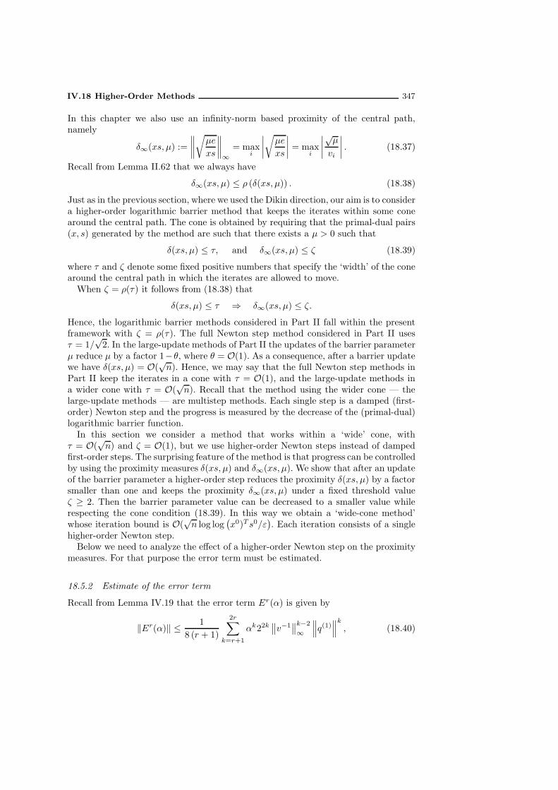
IV.18 Higher-Order Methods 347
In this chapter we also use an infinity-norm based proximity of the central path,namely
δ∞(xs, µ) :=
∥∥∥∥√µe
xs
∥∥∥∥∞
= maxi
∣∣∣∣√µe
xs
∣∣∣∣ = maxi
∣∣∣∣√µ
vi
∣∣∣∣ . (18.37)
Recall from Lemma II.62 that we always have
δ∞(xs, µ) ≤ ρ (δ(xs, µ)) . (18.38)
Just as in the previous section, where we used the Dikin direction, our aim is to considera higher-order logarithmic barrier method that keeps the iterates within some conearound the central path. The cone is obtained by requiring that the primal-dual pairs(x, s) generated by the method are such that there exists a µ > 0 such that
δ(xs, µ) ≤ τ, and δ∞(xs, µ) ≤ ζ (18.39)
where τ and ζ denote some fixed positive numbers that specify the ‘width’ of the conearound the central path in which the iterates are allowed to move.When ζ = ρ(τ) it follows from (18.38) that
δ(xs, µ) ≤ τ ⇒ δ∞(xs, µ) ≤ ζ.
Hence, the logarithmic barrier methods considered in Part II fall within the presentframework with ζ = ρ(τ). The full Newton step method considered in Part II usesτ = 1/
√2. In the large-update methods of Part II the updates of the barrier parameter
µ reduce µ by a factor 1−θ, where θ = O(1). As a consequence, after a barrier updatewe have δ(xs, µ) = O(
√n). Hence, we may say that the full Newton step methods in
Part II keep the iterates in a cone with τ = O(1), and the large-update methods ina wider cone with τ = O(
√n). Recall that the method using the wider cone — the
large-update methods — are multistep methods. Each single step is a damped (first-order) Newton step and the progress is measured by the decrease of the (primal-dual)logarithmic barrier function.In this section we consider a method that works within a ‘wide’ cone, with
τ = O(√n) and ζ = O(1), but we use higher-order Newton steps instead of damped
first-order steps. The surprising feature of the method is that progress can be controlledby using the proximity measures δ(xs, µ) and δ∞(xs, µ). We show that after an updateof the barrier parameter a higher-order step reduces the proximity δ(xs, µ) by a factorsmaller than one and keeps the proximity δ∞(xs, µ) under a fixed threshold valueζ ≥ 2. Then the barrier parameter value can be decreased to a smaller value whilerespecting the cone condition (18.39). In this way we obtain a ‘wide-cone method’whose iteration bound is O(
√n log log
(x0)T s0/ε
). Each iteration consists of a single
higher-order Newton step.Below we need to analyze the effect of a higher-order Newton step on the proximity
measures. For that purpose the error term must be estimated.
18.5.2 Estimate of the error term
Recall from Lemma IV.19 that the error term Er(α) is given by
‖Er(α)‖ ≤ 1
8 (r + 1)
2r∑
k=r+1
αk22k∥∥v−1
∥∥k−2
∞
∥∥∥q(1)∥∥∥k
, (18.40)

348 IV Miscellaneous Topics
where v =√xs. In the present case, (18.19) and (18.17) give
q(1) =∆w
v=µe− xs√
xs.
Hence, using (18.36) and denoting δ(xs, µ) by δ, we find
∥∥∥q(1)∥∥∥ = 2
√µ δ ≤ 2
√µ τ.
Furthermore by using (18.37) and putting δ∞ := δ∞(xs, µ) we have
∥∥v−1∥∥∞ =
1õ
∥∥∥∥√
µ
xs
∥∥∥∥∞
=δ∞√µ≤ ζ√
µ.
Substituting these in (18.40) we get11
‖Er(α)‖ ≤ µ
8(r + 1)δ2∞
2r∑
k=r+1
(8αδδ∞)k ≤ µ
8(r + 1)ζ2
2r∑
k=r+1
(8ατζ)k. (18.41)
Below we always make the natural assumption that α ≤ 1. Moreover, δ and δ∞ alwaysdenote δ(xs, µ) and δ∞(xs, µ) respectively.
Lemma IV.28 Let the step-size be such that α ≤ 1/ (8δδ∞). Then
‖Er(α)‖ ≤ rµ
r + 1
(8αδδ∞)r+1
8δ2∞.
Proof: Since 8αδδ∞ ≤ 1, we have
2r∑
k=r+1
(8αδδ∞)k ≤ r (8αδδ∞)
r+1.
Substitution in (18.41) gives the lemma.
Corollary IV.29 Let δ ≤ τ , δ∞ ≤ ζ and α ≤ 1/ (8τζ). Then
‖Er(α)‖ ≤ rµ
r + 1
(8ατζ)r+1
8ζ2.
11 For r = 1 the derived bound for the error term gives∥∥E1(1)
∥∥ ≤ 4µδ2, as follows easily. It is
interesting to compare this bound with the error bound in Section 7.4 (cf. Lemma II.49), which
amounts to∥∥E1(1)
∥∥ ≤ µδ2√2. Although the present bound is weaker by a factor of 2
√2 for r = 1,
it is sharp enough for our present purpose. It is also sharp enough to derive an O(√n) complexity
bound for r = 1 with some worse constant than before. Our main interest here is the case wherer > 1.

IV.18 Higher-Order Methods 349
18.5.3 Reduction of the proximity after a higher-order step
Recall from (18.13) that after a higher-order step of size α we have
xr(α)sr(α) = xs+ α∆w + Er(α) = xs+ α(µe − xs) + Er(α).
We considerw(α) := xs+ α(µe− xs)
as the (intermediate) target during the step. The new iterate in the w-space is denotedby w(α), so
w(α) = xr(α)sr(α).
As a consequence,w(α) = w(α) + Er(α). (18.42)
The proximities of the new iterate with respect to the µ-center are given by
δ(w(α), µ) =1
2
∥∥∥∥∥
√w(α)
µ−√
µ
w(α)
∥∥∥∥∥
and
δ∞(w(α), µ) =
∥∥∥∥√
µ
w(α)
∥∥∥∥∞.
Ideally the proximities after the step would be δ(w(α), µ) and δ∞(w(α), µ). We firstderive an upper bound for δ(w(α), µ) and δ∞(w(α), µ) respectively in terms of τ , ζand the step-size α.
Lemma IV.30 We have
(i) δ(w(α), µ) ≤√1− α δ,
(ii) δ∞(w(α), µ) ≤√α+ (1 − α)δ2∞.
Proof: It is easily verified that for any positive vector w, by their definitions (18.36)and (18.37), both δ(w, µ)2 and δ∞(w, µ)2 are convex functions of w. Since
w(α) = xs+ α (µe− xs) = α (µe) + (1− α)xs, 0 ≤ α ≤ 1,
w(α) is a convex combination of µe and xs. Hence, by the convexity of δ(w, µ)2,
δ(w(α), µ)2 ≤ α δ(µe, µ)2 + (1 − α) δ(xs, µ)2.
Since δ(µe, µ) = 0, the first statement of the lemma follows.The proof of the second claim is analogous. The convexity of δ∞(xs, µ)2 gives
δ∞(w(α), µ)2 ≤ α δ∞(µe, µ)2 + (1− α) δ∞(xs, µ)2.
Since δ∞(µe, µ) = 1, the lemma follows.
It is very important for our purpose that when the pair (x, s) satisfies the conecondition (18.39) for µ > 0, then after a higher-order step at (x, s) to the µ-center,

350 IV Miscellaneous Topics
the new iterates also satisfy the cone condition. The next corollary of Lemma IV.30is a first step in this direction. It shows that w(α) satisfies the cone condition. Recallthat w(α) = w(α) if the higher-order step is exact. Later we deal with the case wherethe higher-order step is not exact (cf. Theorem IV.35 below). This requires carefulestimation of the error term Er(α).
Corollary IV.31 Let δ ≤ τ and δ∞ ≤ ζ, with ζ ≥ 2. Then we have
(i) δ(w(α), µ) ≤√1− α τ ≤ (1 − α
2 )τ ;
(ii) δ∞(w(α), µ) ≤√α+ (1 − α)ζ2 ≤
(1− 3α
8
)ζ ≤ ζ.
Proof: The first claim is immediate from the first part of Lemma IV.30, since δ ≤ τand
√1− α ≤ 1 − α/2. For the proof of the second statement we write, using the
second part of Lemma IV.30 and ζ ≥ 2,
√α+ (1− α)δ2∞ ≤
√α+ (1− α)ζ2 ≤
√αζ2
4+ (1− α)ζ2
=
√(1− 3α
4
)ζ2 ≤
(1− 3α
8
)ζ ≤ ζ.
Thus the corollary has been proved.
The next lemma provides an expression for the ‘error’ in the proximities after thestep. We use the following relation, which is an obvious consequence of (18.42):
w(α)
µ=w(α)
µ
(e+
Er(α)
w(α)
). (18.43)
Lemma IV.32 Let α be such that
∥∥∥∥Er(α)
w(α)
∥∥∥∥∞
≤√5− 1
2.
Then we have
(i) δ(w(α), µ) ≤ δ(w(α), µ) +√1 + δ(w(α), µ)2
∥∥∥Er(α)w(α)
∥∥∥;
(ii) δ∞(w(α), µ) ≤ δ∞(w(α), µ)(1 +
∥∥∥Er(α)w(α)
∥∥∥∞
).
Proof: Using (18.43) we may write
δ(w(α), µ) =1
2
∥∥∥∥∥∥
√w(α)
µ
(e+
Er(α)
w(α)
)−√
µ
w(α)
(e+
Er(α)
w(α)
)−1∥∥∥∥∥∥.
To simplify the notation we omit the argument α in the rest of the proof and weintroduce the notation
λ :=Er(α)
w(α),
IV.18 Higher-Order Methods 351
so that
δ(w(α), µ) =1
2
∥∥∥∥√w
µ(e+ λ)−
õ
w(e+ λ)
−1
∥∥∥∥ .
Since √wµ (e+ λ) −
√µw (e+ λ)
−1=
√wµ −
õw +
√wµ
((e+ λ)
12 − e
)−√
µw
((e+ λ)−
12 − e
),
application of the triangle inequality gives
δ(w(α), µ) ≤ δ(w(α), µ) +1
2
∥∥∥∥√w
µ
((e+ λ)
12 − e
)−√µ
w
((e + λ)
− 12 − e
)∥∥∥∥ . (18.44)
Denoting the i-th coordinate of the vector under the last norm by zi, we have
zi =
√wi
µ
((1 + λi)
12 − 1
)−√
µ
wi
((1 + λi)
− 12 − 1
).
This implies
|zi| ≤√wi
µ
∣∣∣(1 + λi)12 − 1
∣∣∣+√
µ
wi
∣∣∣(1 + λi)− 1
2 − 1∣∣∣ .
The hypothesis of the lemma implies |λi| ≤ (√5 − 1)/2. Now using some elementary
inequalities,12 we get
|zi| ≤√wi
µ|λi|+
õ
wi|λi| =
(√wi
µ+
õ
wi
)|λi| .
Since
(√wi
µ+
õ
wi
)2
= 4 +
(√wi
µ−√
µ
wi
)2
≤ 4 +
∥∥∥∥√w
µ−√µ
w
∥∥∥∥2
∞
and ∥∥∥∥√w
µ−√µ
w
∥∥∥∥2
∞≤∥∥∥∥√w
µ−√µ
w
∥∥∥∥2
= 4δ(w(α), µ)2,
we conclude that
|zi| ≤ 2√1 + δ(w(α), µ)2 |λi| , 1 ≤ i ≤ n.
Hence‖z‖ ≤ 2
√1 + δ(w(α), µ)2 ‖λ‖ .
12 Exercise 86 Prove the following inequalities:
∣∣∣(1 + λ)12 − 1
∣∣∣ ≤ |λ| , −1 ≤ λ ≤ 1,
∣∣∣(1 + λ)−12 − 1
∣∣∣ ≤ |λ| , 1−√5
2≤ λ ≤ 1.

352 IV Miscellaneous Topics
Substituting this in (18.44) proves the first statement of the lemma.The proof of the second statement in the lemma is analogous. We write
δ∞(w(α), µ) =
∥∥∥∥√
µ
w(α)
∥∥∥∥∞
=
∥∥∥∥∥∥
õ
w(α)
(e+
Er(α)
w(α)
)−1∥∥∥∥∥∥∞
=
∥∥∥∥√
µ
w(α)(e+ λ)
−1
∥∥∥∥∞
=
∥∥∥∥√
µ
w(α)+
õ
w(α)
((e+ λ)−
12 − e
)∥∥∥∥∞
≤∥∥∥∥√
µ
w(α)
∥∥∥∥∞
+
∥∥∥∥√
µ
w(α)
∥∥∥∥∞
∥∥∥(e + λ)−12 − e
∥∥∥∞.
Using again the results of Exercise 86 we can simplify this to
δ∞(w(α), µ) ≤ δ∞(w(α), µ) + δ∞(w(α), µ) ‖λ‖∞= δ∞(w(α), µ)
(1 +
∥∥∥∥Er(α)
w(α)
∥∥∥∥∞
),
proving the lemma.
The following corollary easily follows from Lemma IV.32 and Corollary IV.31.
Corollary IV.33 Let δ ≤ τ and δ∞ ≤ ζ, with ζ ≥ 2. If α is such that
∥∥∥∥Er(α)
w(α)
∥∥∥∥∞
≤√5− 1
2,
then we have
(i) δ(w(α), µ) ≤ (1 − α2 )τ +
√1 + τ2
∥∥∥Er(α)w(α)
∥∥∥;
(ii) δ∞(w(α), µ) ≤(1− 3
8α) (
1 +∥∥∥Er(α)
w(α)
∥∥∥∞
)ζ.
We proceed by finding a step-size α that satisfies the hypothesis of Lemma IV.32and Corollary IV.33.
Lemma IV.34 With δ and ζ as in Corollary IV.33, let the step-size α be such thatα ≤ 1/(8τζ). Then
∥∥∥∥Er(α)
w(α)
∥∥∥∥ ≤ r
8(r + 1)(8ατζ)
r+1
and α satisfies the hypothesis of Lemma IV.32 and Corollary IV.33.
Proof: We may write
∥∥∥∥Er(α)
w(α)
∥∥∥∥ ≤∥∥∥∥
e
w(α)
∥∥∥∥∞
‖Er(α)‖ =1
µ
∥∥∥∥√
µe
w(α)
∥∥∥∥2
∞‖Er(α)‖ ≤ ζ2
µ‖Er(α)‖ ,

IV.18 Higher-Order Methods 353
where the last inequality follows from Corollary IV.31. Now using Corollary IV.29 wehave
∥∥∥∥Er(α)
w(α)
∥∥∥∥ ≤ r
8(r + 1)(8ατζ)
r+1,
proving the first part of the lemma. The second part follows from the first part byusing 8ατζ ≤ 1:
∥∥∥∥Er(α)
w(α)
∥∥∥∥∞
≤∥∥∥∥Er(α)
w(α)
∥∥∥∥ ≤ r
8(r + 1)<
√5− 1
2,
completing the proof.
Equipped with the above results we can prove the next theorem.
Theorem IV.35 Let δ ≤ τ , δ∞ ≤ ζ, with ζ ≥ 2, and α ≤ 1/(8τζ). Then
(i) δ(w(α), µ) ≤(1− α
2
)τ + r
8(r+1)
√1 + τ2 (8ατζ)
r+1;
(ii) δ∞(w(α), µ) ≤(1− 3
8α) (
1 + r8(r+1) (8ατζ)
r+1)ζ.
Proof: For the given step-size the hypothesis of Corollary IV.33 is satisfied, byLemma IV.34. From Lemma IV.34 we also deduce the second inequality in
∥∥∥∥Er(α)
w(α)
∥∥∥∥∞
≤∥∥∥∥Er(α)
w(α)
∥∥∥∥ ≤ r
8(r + 1)(8ατζ)
r+1.
Substituting these inequalities in Corollary IV.33 yields the theorem.
18.5.4 The step-size
In the sequel the step-size α is given the value
α =1
8τζ r
√(r + 1)ζ
√1 + τ2
, (18.45)
where δ = δ(xs, µ) ≤ τ and δ∞ = δ∞(xs, µ) ≤ ζ. It is assumed that ζ ≥ 2. Thenext theorem makes clear that after a higher-order step with the given step-size α theproximity δ is below a fixed fraction of τ and the proximity δ∞ below a fixed fractionof ζ.
Theorem IV.36 If the step-size is given by (18.45) then
δ(w(α), µ) ≤(1− α(r2 + 1)
2 (r + 1)2
)τ.
Moreover,
δ∞(w(α), µ) ≤(1− α
8
)ζ.

354 IV Miscellaneous Topics
Proof: The proof uses Theorem IV.35. This theorem applies because for the givenvalue of α we have
α =1
8τζ r
√(r + 1)ζ
√1 + τ2
≤ 1
8τζ,
whence 8ατζ ≤ 1. Hence, by the first statement in Theorem IV.35,
δ(w(α), µ) ≤(1− α
2
)τ +
r
8(r + 1)
√1 + τ2 (8ατζ)r+1 . (18.46)
The second term on the right can be reduced by using the definition of α:
δ(w(α), µ) ≤(1− α
2
)τ +
r
8(r + 1)
√1 + τ2
8ατζ
(r + 1)ζ√1 + τ2
=
(1− α
2+
rα
(r + 1)2
)τ
=
(1− r2 + 1
2(r + 1)2α
)τ.
This proves the first statement. The second claim follows in a similar way from thesecond statement in Theorem IV.35:
δ∞(w(α), µ) ≤(1− 3
8α
)(1 +
r
8(r + 1)(8ατζ)r+1
)ζ
=
(1− 3
8α
)(1 +
r
8(r + 1)
8ατζ
(r + 1)ζ√1 + τ2
)ζ
=
(1− 3
8α
)(1 +
r
(r + 1)2ατ√1 + τ2
)ζ
<
(1− 3
8α
)(1 +
rα
(r + 1)2
)ζ
≤(1− 3
8α
)(1 +
1
4α
)ζ
≤(1− α
8
)ζ.
In the last but one inequality we used that r/(r+1)2 is monotonically decreasing if rincreases (for r ≥ 1).
18.5.5 Reduction of the barrier parameter
In this section we assume that δ = δ(xs, µ) ≤ τ , where τ is any positive number. Aftera higher-order step with step-size α, given by (18.45), we have by Theorem IV.36,
δ(w(α), µ) ≤ (1− β) δ,
where
β =α(r2 + 1)
2(r + 1)2. (18.47)

IV.18 Higher-Order Methods 355
Below we investigate how far µ can be decreased after the step while keeping theproximity δ less than or equal to τ . Before doing this we observe that
δ∞(xs, µ) =
∥∥∥∥√µe
xs
∥∥∥∥∞
is monotonically decreasing as µ decreases. Hence, we do not have to worry about δ∞when µ is reduced. Defining
µ+ := (1− θ)µ,
we first deal with a lemma that later gives an upper bound for δ(w(α), µ+).13
Lemma IV.37 Let (x, s) be a positive primal-dual pair and suppose µ > 0. Ifδ := δ(xs, µ) and µ+ = (1 − θ)µ then
δ(xs, µ+) ≤ 2δ + θ√n
2√1− θ
.
Proof: By the definition of δ(xs, µ+),
δ(xs, µ+) =1
2
∥∥∥∥∥
√xs
µ+e−√µ+e
xs
∥∥∥∥∥ .
To simplify the notation in the proof we use u =√xs/µ. Then we may write
δ(xs, µ+) =1
2
∥∥∥∥u√1− θ
−√1− θu−1
∥∥∥∥ =1
2
∥∥∥∥√1− θ
(u− u−1
)+
θu√1− θ
∥∥∥∥ .
Using the triangle inequality and14 also
‖u‖ ≤∥∥u− u−1
∥∥+√n = 2δ +
√n,
we get
δ(xs, µ+) ≤ δ√1− θ +
θ ‖u‖2√1− θ
≤ δ√1− θ +
θ (2δ +√n)
2√1− θ
=2δ + θ
√n
2√1− θ
,
proving the lemma.
13 A similar result was derived in Lemma II.54, but under the assumption that xT s = nµ. Thisassumption will in general not be satisfied in the present context, and hence we have a weakerbound.
14 Exercise 87 For each positive number ξ we have
|ξ| ≤∣∣∣ξ − 1
ξ
∣∣∣+ 1.
Prove this and derive that for each positive vector u the following inequality holds:
‖u‖ ≤∥∥u− u−1
∥∥+√n.

356 IV Miscellaneous Topics
Theorem IV.38 Let δ = δ(xs, µ) ≤ τ , δ∞ = δ∞(xs, µ) ≤ ζ, with ζ ≥ 2. Takingfirst a higher-order step at (x, s), with α according to (18.45), and then updating thebarrier parameter to µ+ = (1− θ)µ, where
θ =2βτ
2τ +√n=
ατ(r2 + 1)
(r + 1)2(2τ +√n), (18.48)
we have δ(w(α), µ+) ≤ τ and δ∞(w(α), µ+) ≤ ζ.
Proof: The second part of Theorem IV.36 implies that after a step of the givensize δ∞(w(α), µ) ≤ ζ. We established earlier that δ∞ monotonically decreases when µdecreases. As a result we have δ∞(w(α), µ+) ≤ ζ. Now let us estimate δ(w(α), µ+).After a higher-order step with step-size α as given by (18.45), we have by the firstpart of Theorem IV.36,
δ(w(α), µ) ≤(1− α(r2 + 1)
2(r + 1)2
)δ(xs, µ) = (1− β) δ,
with β as defined in (18.47). Also using Lemma IV.37 we obtain
δ(w(α), µ+) ≤ 2δ(w(α), µ) + θ√n
2√1− θ
≤ 2 (1− β) δ + θ√n
2√1− θ
.
Since δ ≤ τ , we certainly have δ(w(α), µ+) ≤ τ if
2(1− β)τ + θ√n
2√1− θ
≤ τ.
This inequality can be rewritten as
2(1− β)τ + θ√n ≤ 2τ
√1− θ.
Using√1− θ ≥ 1− θ the above inequality certainly holds if
2(1− β)τ + θ√n ≤ 2τ(1− θ).
It is easily verified that the value of θ in (18.48) satisfies this inequality with equality.Thus the proof is complete.
18.5.6 A higher-order logarithmic barrier algorithm
Formally the logarithmic barrier algorithm using higher-order Newton steps can bedescribed as below.

IV.18 Higher-Order Methods 357
Higher-Order Logarithmic Barrier Algorithm
Input:A natural number r, the order of the search directions;a positive number τ , specifying the cone;a primal-dual pair
(x0, s0
)and µ0 > 0 such that δ(x0s0, µ0) ≤ τ .
ζ := max(2, δ∞(x0s0, µ0)
);
a step-size parameter α, from (18.45);an update parameter θ, from (18.48);an accuracy parameter ε > 0;
beginx := x0; s := s0; µ := µ0;while xT s ≥ ε dobeginx := x(α) = x+∆r,αx;s := s(α) = s+∆r,αs;µ := (1− θ)µ
endend
A direct consequence of the specified values of the step-size α and update parameterθ is that the properties δ(xs, µ) ≤ τ and δ∞(xs, µ) ≤ ζ are maintained in the course ofthe algorithm. This follows from Theorem IV.38 and makes the algorithm well-defined.
18.5.7 Iteration bound
In the further analysis of the algorithm we choose
τ =√n and r = n.
At the end of each iteration of the algorithm we have
δ(xs, µ) ≤ τ =√n.
As a consequence (cf. Exercise 62),
xT s ≤(1 +
2τρ(τ)√n
)nµ =
(1 + 2ρ
(√n))nµ ≤ 4
(1 +
√n)nµ.
Hence xT s ≤ ε holds if
4(1 +
√n)nµ ≤ ε,
or
µ ≤ ε
4n (1 +√n).
358 IV Miscellaneous Topics
Recall that at each iteration the barrier parameter is reduced by a factor 1− θ, with
θ =ατ(r2 + 1)
(r + 1)2 (2τ +√n)
=α(n2 + 1)
3(n+ 1)2≥ α
6. (18.49)
The last inequality holds for all n ≥ 1. Using Lemma I.36 we find that the number ofiterations does not exceed
6
αlog
4 (1 +√n)nµ0
ε.
Substituting α in (18.45) and τ =√n, we get
6
α= 48ζ
√n
n
√(n+ 1)ζ
√1 + n.
For n ≥ 1 we haven
√(n+ 1)
√1 + n ≤ 2
√2 = 2.8284,
with equality only if n = 1. Thus we find
6
α≤ 136 ζ
n+1
n
√n.
Thus we may state the next theorem without further proof.
Theorem IV.39 The Higher-Order Logarithmic Barrier Algorithm needs at most
136 ζn+1
n
√n log
4 (1 +√n)nµ0
ε
iterations. Each iteration requires O(n3) arithmetic operations. The output is a primal-dual pair (x, s) such that xT s ≤ ε.
When starting the algorithm on the central path, with µ0 =(x0)Ts0/n, we have ζ = 2.
In that case δ∞(xs, µ) ≤ 2 at each iteration and the iteration bound of Theorem IV.39becomes
544√n log
4 (1 +√n)nµ0
ε= O
(√n log
√nnµ0
ε
). (18.50)
In fact, as long as ζ = O(1) the iteration bound is given by the right-hand expressionin (18.50). Note that this bound has the same order of magnitude as the best knowniteration complexity bound.When (x0, s0) is far from the central path, the value of ζ may be so large that the
iteration bound of Theorem IV.39 becomes very poor. Note that ζ can be as large as
ρ(τ), which would give an extra factor O(n
n+1
2n
)in (18.50). However, a more careful
analysis yields a much better bound, as we show in the next section.
18.5.8 Improved iteration bound
In this section we consider the situation where the algorithm starts with a high valueof ζ. Recall from the previous section that if τ =
√n then ζ is always bounded by
IV.18 Higher-Order Methods 359
ζ ≤ ρ (√n) = O (
√n). Now the second part of Theorem IV.36 implies that after a
higher-order step at (x, s) to the µ-center we have
δ∞(w(α), µ) ≤(1− α
8
)ζ.
Reducing µ to µ+ = (1− θ)µ we get
δ∞(w(α), µ+) ≤ (1− θ)(1− α
8
)ζ.
Now using the lower bound (18.49) for θ it follows that
δ∞(w(α), µ+) ≤(1− α
6
)(1− α
8
)ζ.
Since 0 ≤ α ≤ 1 we have(1− α
6
) (1− α
8
)≤(1− α
4
). Hence
δ∞(w(α), µ+) ≤(1− α
4
)ζ.
Substituting the value of α, while using
8n
√(n+ 1) ζ
√1 + n ≤ 8 n
√(n+ 1) ρ
(√n)√
1 + n ≤ 55,
we obtain
δ∞(w(α), µ+) ≤ ζ − ζ
220τζ= ζ − 1
220√n,
showing that δ∞(xs, µ) decreases by at least 1/ (220√n) in one iteration. Obviously,
we can redefine ζ according to
ζ := max(2, δ∞(w(α), µ+)
)≤ max
(2, ζ − 1
220√n
)
in the next iteration and continue the algorithm with this new value. In this way ζreaches the value 2 in no more than
220√n(ζ0 − 2
)= O
(ζ0√n)
iterations, where ζ0 = δ∞(x0s0, µ0). From then on ζ keeps the value 2, and the numberof additional iterations is bounded by (18.50). Hence we may state the followingimprovement of Theorem IV.39 without further proof.
Theorem IV.40 The Higher-Order Logarithmic Barrier Algorithm needs at most
O(ζ0√n+
√n log
4√nnµ1
ε
).
iterations. Each iteration requires O(n3) arithmetic operations. The output is a primal-dual pair (x, s) such that xT s ≤ ε.
In this theorem µ1 denotes the value of the barrier parameter attained at the firstiteration for which ζ = 2. Obviously, µ1 ≤ µ0.


19
Parametric and SensitivityAnalysis
19.1 Introduction
Many commercial optimization packages for solving LO problems not only solve theproblem at hand, but also provide additional information on the solution. This addedinformation concerns the sensitivity of the solution produced by the package to pert-urbations in the data of the problem. In this chapter we deal with a problem (P ) instandard format:
(P ) mincTx : Ax = b, x ≥ 0
.
The dual problem (D) is written as
(D) maxbT y : AT y + s = c, s ≥ 0
.
The input data for both problems consists of the matrix A, which is of size m × n,and the vectors b ∈ IRm and c ∈ IRn. The optimal value of (P ) and (D) is denoted byzA(b, c), with zA(b, c) = −∞ if (P ) is unbounded and (D) infeasible, and zA(b, c) = ∞if (D) is unbounded and (P ) infeasible. If (P ) and (D) are both infeasible then zA(b, c)is undefined. We call zA the optimal-value function for the matrix A.The extra information provided by solution packages concerns only changes in the
vectors b and c. We also restrict ourselves to such changes. It will follow from theresults below that zA(b, c) depends continuously on the vectors b and c. In contrast,the effect of changes in the matrix A is not necessarily continuous. The next exampleprovides a simple illustration of this phenomenon.1
Example IV.41 Consider the problem
min x2 : αx1 + x2 = 1, x1 ≥ 0, x2 ≥ 0 ,
where α ∈ IR. In this example we have A = (α 1), b = (1) and c = (0 1)T . We caneasily verify that zA(b, c) = 0 if α > 0 and zA(b, c) = 1 if α ≤ 0. Thus, if zA(b, c) isconsidered a function of α, a discontinuity occurs at α = 0. ♦
Thus. the dependence of zA(b, c) on the entries in b and c is more simple than thedependence of zA(b, c) on the entries in A.
1 For some results on the effect of changes in A we refer the reader to Mills [210] and Gal [89].

362 IV Miscellaneous Topics
We develop some theory in this chapter for the analysis of one-dimensionalparametric perturbations of the vectors b and c. Given a pair of optimal solutionsfor (P ) and (D), we present an algorithm in Section 19.4.5 for the computationof the optimal-value function under such a perturbation. Then, in Section 19.5 weconsider the special case of sensitivity analysis, also called postoptimal analysis. Thisclassical topic is treated in almost all (text-)books on LO and implemented in almostall commercial optimization packages for LO. We show in Section 19.5.1 that the so-called ranges and shadow prices of the coefficients in b and c can be obtained by solvingauxiliary LO problems. In Section 19.5.3 we briefly discuss the classical approach tosensitivity analysis, which is based on the use of an optimal basic solution and thecorresponding optimal basis. Although the classical approach is much cheaper from acomputational point of view, it yields less information and can easily be misinterpreted.This is demonstrated in Section 19.5.4, where we provide a striking example of theinherent weaknesses of the classical approach.
19.2 Preliminaries
The feasible regions of (P ) and (D) are denoted by
P := x : Ax = b, x ≥ 0 ,D :=
(y, s) : AT y + s = c, s ≥ 0
.
Assuming that (P ) and (D) are both feasible, the optimal sets of (P ) and (D) aredenoted by P∗ and D∗. We define the index sets B and N by
B := i : xi > 0 for some x ∈ P∗ ,
N := i : si > 0 for some (y, s) ∈ D∗ .The Duality Theorem (Theorem II.2) implies that B ∩ N = ∅, and the Goldman–Tucker Theorem (Theorem II.3) that
B ∪N = 1, 2, . . . , n.
Thus, B and N form a partition of the full index set. This (ordered) partition, denotedby π = (B,N), is the optimal partition of problems (P ) and (D). It is obvious thatthe optimal partition depends on b and c.
19.3 Optimal sets and optimal partition
In the rest of this chapter we assume that b and c are such that (P ) and (D) haveoptimal solutions, and π = (B,N) denotes the optimal partition of both problems. Bydefinition, the optimal partition is determined by the sets of optimal solutions for (P )and (D). In this section it is made clear that, conversely, the optimal partition providesessential information on the optimal solution sets P∗ and D∗. The next lemma followsimmediately from the Duality Theorem and is stated without proof.

IV.19 Parametric and Sensitivity Analysis 363
Lemma IV.42 Let x∗ ∈ P∗ and (y∗, s∗) ∈ D∗. Then
P∗ =x : x ∈ P , xT s∗ = 0
,
D∗ =(y, s) : (y, s) ∈ D, sTx∗ = 0
.
As before, we use the notation xB and xN to refer to the restriction of a vectorx ∈ IRn to the coordinate sets B and N respectively. Similarly, AB denotes therestriction of A to the columns in B and AN the restriction of A to the columnsin N . Now the sets P∗ and D∗ can be described in terms of the optimal partition.
Lemma IV.43 Given the optimal partition (B,N) of (P ) and (D), the optimal setsof both problems are given by
P∗ = x : x ∈ P , xN = 0 ,D∗ = (y, s) : (y, s) ∈ D, sB = 0 .
Proof: Let x∗, s∗ be any strictly complementary pair of solutions of (P ) and (D), and(x, s) an arbitrary pair of feasible solutions. Then, from Lemma IV.42, x is optimalfor (P ) if and only if xT s∗ = 0. Since s∗B = 0 and s∗N > 0, we have xT s∗ = 0 if andonly if xN = 0, thus proving that P∗ consists of all primal feasible x for which xN = 0.Similarly, if (y, s) ∈ D then this pair is optimal if and only if sTx∗ = 0. Since x∗B > 0and x∗N = 0, this occurs if and only if sB = 0, thus proving that D∗ consists of alldual feasible s for which sB = 0.
To illustrate the meaning of Lemma IV.43 we give an example.
Example IV.44 Figure 19.1 shows a network with given arc lengths, and we ask fora shortest path from node s to node t.Denoting the set of nodes in this network by V and the set of arcs by E, any path
from s to t can be represented by a 0-1 vector x of length |E|, whose coordinates areindexed by the arcs, such that xe = 1 if and only if arc e belongs to the path. Thelength of the path is then given by
∑
e∈E
cexe, (19.1)
4 6
3 6 4 3
4 5
4 4 5
3 3 2
5 5 3
5 7 6
s t
Figure 19.1 A shortest path problem.

364 IV Miscellaneous Topics
where ce denote the length of arc e, for all e ∈ E. Furthermore, denoting e = (v, w)if arc e points from node v to node w (with v ∈ V and w ∈ V ), and denoting xe byxvw, x will satisfy the following balance equations:
∑
v∈V
xsv = 1
∑
v∈V
xvu =∑
v∈V
xuv, u ∈ V \ s, t (19.2)
∑
v∈V
xvt = 1
Now consider the LO problem consisting of minimizing the linear function (19.1)subject to the linear equality constraints in (19.2), with all variables xe, e ∈ E,nonnegative. This problem has the standard format: it is a minimization problemwith equality constraints and nonnegative variables. Solving this problem with aninterior-point method we find a strictly complementary solution, and hence the optimalpartition of the problem. In this way we have computed the optimal partition (B,N)of the problem. Since in this example there is a 1-to-1 correspondence between thearcs and the variables, we may think of B and N as a partition of the arcs in thenetwork.
4 6
3 6 4 3
4 5
4 4 5
3 3 2
5 5 3
5 7 6
s t
Figure 19.2 The optimal partition of the shortest path problem in Figure 19.1.
In Figure 19.2 we have drawn the network once more, but now with the arcs in Bsolid and the arcs in N dashed. The meaning of Lemma IV.43 is that any path froms to t using only solid arcs is a shortest path, and all shortest paths use exclusivelysolid arcs. In other words, the set B consists of all arcs in the network which occur insome shortest path from s to t and the set N contains arcs in the network which donot belong to any shortest path from s to t.2 ♦2 Exercise 88 Consider any network with node set V and arc set E and let s and t be two distinct
nodes in this network. If all arcs in the network have positive length, then the set B, consisting ofall arcs in the network which occur in at least one shortest path from s to t, does not contain a(directed) circuit. Prove this.

IV.19 Parametric and Sensitivity Analysis 365
The next result deals with the dimensions of the optimal sets P∗ and D∗. Here, asusual the (affine) dimension of a subset of IRk is the dimension of the smallest affinesubspace in IRk containing the subset.
Lemma IV.45 We have
dimP∗ = |B| − rank (AB)
dimD∗ = m− rank (AB).
Proof: The optimal set of (P ) is given by
P∗ = x : Ax = b, xB ≥ 0, xN = 0 ,
and hence the smallest affine subspace of IRn containing P∗ is given by
x : ABxB = b, xN = 0 .
The dimension of this affine space is equal to the dimension of the null space of AB.Since this dimension is given by |B| − rank (AB), the first statement follows.For the proof of the second statement we use that the dual optimal set can be
described by
D∗ =(y, s) : AT y + s = c, sB = 0, sN ≥ 0
.
This is equivalent to
D∗ =(y, s) : AT
By = cB, ATNy + sN = cN , sB = 0, sN ≥ 0
.
The smallest affine subspace containing this set is
(y, s) : AT
By = cB, ATNy + sN = cN , sB = 0
.
Obviously sN is uniquely determined by y, and any y satisfying ATBy = cB yields
a point in this affine space. Hence the dimension of the affine space is equal to thedimension of the null space of AT
B. Since m is the number of columns of ATB, the
dimension of the null space of ATB equals m− rank (AB). This completes the proof.
Lemma IV.45 immediately implies that (P ) has a unique solution if and only ifrank (AB) = |B|. Clearly this happens if and only if the columns in AB are linearlyindependent. Also, (D) has a unique solution if and only if rank (AB) = m, whichhappens if and only if the rows in AB are linearly independent.3
3 It has become common practice in the literature to call the problem (P ) degenerate if (P ) or(D) have multiple optimal solutions. Degeneracy is an important topic in LO. In the contextof the Simplex Method it is well known as a source of difficulties. This is especially true whendealing with sensitivity analysis. See, e.g., Gal [90] and Greenberg [128]. But also in the contextof interior-point methods the occurrence of degeneracy may influence the behavior of the method.We mention some references: Gonzaga [120], Guler et al. [132], Todd [263], Tsuchiya [269, 271],Hall and Vanderbei [138].

366 IV Miscellaneous Topics
19.4 Parametric analysis
In this section we start to investigate the effect of changes in b and c on the optimal-value function zA(b, c). We consider one-dimensional parametric perturbations of band c. So we want to study
zA(b + β∆b, c+ γ∆c)
as a function of the parameters β and γ, where ∆b and ∆c are given perturbation
vectors. From now on the vectors b and c are fixed, and the variations come fromthe parameters β and γ. In fact, we restrict ourselves to the cases that the variationsoccur only in one of the two vectors b and c. In other words, taking γ = 0 we considervariations in β and taking β = 0 we consider variations in γ.If γ = 0, then (Pβ) will denote the perturbed primal problem and (Dβ) its dual.
The feasible regions of these problems are denoted by Pβ and Dβ . Similarly, if β = 0,then (Dγ) will denote the perturbed dual problem and (Pγ) its dual and the feasibleregions of these problems are Dγ and Pγ . Observe that the feasible region of (Dβ) issimply D and the feasible region of (Pγ) is simply P . We use the superscript ∗ to referto the optimal set of each of these problems.We assume that b and c are such that (P ) and (D) are both feasible. Then zA(b, c)
is well defined and finite. It is convenient to introduce the following notations:
b(β) := b+ β∆b, c(γ) := c+ γ∆c,
f(β) := zA(b(β), c), g(γ) := zA(b, c(γ)).
Here the domain of the parameters β and γ is taken as large as possible. Let us considerthe domain of f . This function is defined as long as zA(b(β), c) is well defined. Sincethe feasible region of (Dβ) is constant when β varies, and since we assume that (Dβ)is feasible for β = 0, it follows that (Dβ) is feasible for all values of β. Therefore,f(β) is well defined if the dual problem (Dβ) has an optimal solution and f(β) is notdefined (or infinity) if the dual problem (Dβ) is unbounded. By the Duality Theoremit follows that f(β) is well defined if and only if the primal problem (Pβ) is feasible.In exactly the same way it can be understood that the domain of g consists of all γfor which (Dγ) is feasible (and (Pγ) bounded).
Lemma IV.46 The domains of f and g are convex.
Proof: We give the proof for f . The proof for g is similar and therefore omitted.Let β1, β2 ∈ dom (f) and β1 < β < β2. Then f(β1) and f(β2) are finite, which meansthat both Pβ1
and Pβ2are nonempty. Let x1 ∈ Pβ1
and x2 ∈ Pβ2. Then x1 and x2
are nonnegative and
Ax1 = b+ β1∆b, Ax2 = b+ β2∆b.
Now consider
x := x1 +β − β1β2 − β1
(x2 − x1
)=
(β2 − β) x1 + (β − β1)x2
β2 − β1.

IV.19 Parametric and Sensitivity Analysis 367
Note that x is a convex combination of x1 and x2 and hence x is nonnegative. Weproceed by showing that x ∈ Pβ. Using that A
(x2 − x1
)= (β2 − β1)∆b this goes as
follows:
Ax = Ax1 +β − β1β2 − β1
A(x2 − x1
)
= b+ β1∆b+β − β1β2 − β1
(β2 − β1)∆b
= b+ β1∆b+ (β − β1)∆b
= b+ β∆b.
This proves that (Pβ) is feasible and hence β ∈ dom (f), completing the proof.
The domains of f and g are in fact closed intervals on the real line. This followsfrom the above lemma, and the fact that the complements of the domains of f and gare open subsets of the real line. The last statement is the content of the next lemma.
Lemma IV.47 The complements of the domains of f and g are open subsets of thereal line.
Proof: As in the proof of the previous lemma we omit the proof for g because itis similar to the proof for f . We need to show that the complement of dom(f) isopen. Let β /∈ dom (f). This means that (Dβ) is unbounded. This is equivalent to theexistence of a vector z such that
AT z ≤ 0, (b+ β∆b)T z > 0.
Fixing z and considering β as a variable, the set of all β satisfying the strict inequality(b+ β∆b)
Tz > 0 is an open interval. For all β in this interval (Dβ) is unbounded.
Hence the domain of f is open. This proves the lemma.
A consequence of the last two lemmas is the next theorem, which requires no furtherproof.
Theorem IV.48 The domains of f and g are closed intervals on the real line.4
Example IV.49 Let (D) be the problem
maxy=(y1,y2)
y2 : y2 ≤ 1 .
In this case b = (0, 1) and c = (1). Note that (D) is feasible and bounded. The setof all optimal solutions consists of all (y1, 1) with y1 ∈ IR. Now let ∆b = (1, 0), andconsider the effect of replacing b by b+ β∆b, and let f(β) be as defined above. Then
f(β) = maxy=(y1,y2)
y2 + βy1 : y2 ≤ 1 .
4 To avoid misunderstanding we point out that a singleton a (a ∈ IR) is also considered as a closedinterval.

368 IV Miscellaneous Topics
We can easily verify that the perturbed problem is unbounded for all nonzero β. Hencethe domain of f is the singleton 0.5 ♦
19.4.1 The optimal-value function is piecewise linear
In this section we show that the functions f(β) and g(γ) are piecewise linear on theirdomains. We start with g(γ).
Theorem IV.50 g(γ) is continuous, concave and piecewise linear.
Proof: By definition,
g(γ) = minc(γ)Tx : x ∈ P
.
For each γ the minimum value is attained at the central solution of the perturbedproblem (Pγ). This solution is uniquely determined by the optimal partition of (Pγ).Since the number of partitions of the full index set 1, 2, . . . , n is finite, we may write
g(γ) = minc(γ)Tx : x ∈ T
,
where T is a finite subset of P . For each x ∈ T we have
c(γ)Tx = cTx+ γ∆cTx,
which is a linear function of γ. Thus, g(γ) is the minimum of a finite set of linearfunctions.6 This implies that g(γ) is continuous, concave and piecewise linear, provingthe theorem.
Theorem IV.51 f(β) is continuous, convex and piecewise linear.
Proof: The proof goes in the same way as for Theorem IV.50. By definition,
f(β) = maxb(β)T y : y ∈ D
.
For each β the maximum value is attained at a central solution (y∗, s∗) of (D). Nows∗ is uniquely determined by the optimal partition of (D) and b(β)T y∗ is constant forall optimal y∗. Associating one particular y∗ with any possible slack s∗ arising in thisway, we obtain that
f(β) = maxb(β)T y : y ∈ S
,
where S is a finite subset of D. For each y ∈ S, we have
b(β)T y = bT y + β∆bT y,
5Exercise 89 With (D) and f(β) as defined in Example IV.49 we consider the effect on the domainof f when some constraints are added. When the constraint y1 ≥ 0 is added to (D), the domain off becomes (−∞, 0]. When the constraint y1 ≤ 0 is added to (D), the domain of f becomes [0,∞)and when both constraints are added the domain of f becomes (−∞,∞). Prove this.
6 Exercise 90 Prove that the minimum of a finite family of linear functions, each defined on thesame closed interval, is continuous, concave and piecewise linear.

IV.19 Parametric and Sensitivity Analysis 369
which is a linear function of β. This makes clear that f(β) is the maximum of a finiteset of linear functions. Therefore, f(β) is continuous, convex and piecewise linear, asrequired.
The values of β where the slope of the optimal-value function f(β) changes arecalled break points of f , and any interval between two successive break points of f iscalled a linearity interval of f . In a similar way we define break points and linearityintervals for g.
Example IV.52 For any γ ∈ IR consider the problem (Pγ) defined by
(Pγ) min x1 + (3 + γ)x2 + (1 − γ)x3
s.t. x1 + x2 + x3 = 4, x1, x2, x3 ≥ 0.
In this case b is constant and the perturbation vector for c = (1, 3, 1) is
∆c = (0, 1,−1).
The dual problem is
(Dγ) max 4y : y ≤ 1, y ≤ 3 + γ, y ≤ 1− γ .
From this it is obvious that the optimal value is given by
g(γ) = 4min (1, 3 + γ, 1− γ) .
The graph of the optimal-value function g(γ) is depicted in Figure 19.3. Note that
−5 −4 −3 −2 −1 0 1 2 3−5
−4
−3
−2
−1
0
1
2
3
4
5
γ
g(γ)
Figure 19.3 The optimal-value function g(γ).
g(γ) is piecewise linear and concave. The break points of g occur for γ = −2 andγ = 0. ♦

370 IV Miscellaneous Topics
19.4.2 Optimal sets on a linearity interval
For any β in the domain of f we denote the optimal set of (Pβ) by P∗β and the optimal
set of (Dβ) by D∗β .
Theorem IV.53 If f(β) is linear on the interval [β1, β2], where β1 < β2, then thedual optimal set D∗
β is constant (i.e. invariant) for β ∈ (β1, β2).
Proof: Let β ∈ (β1, β2) be arbitrary and let y ∈ D∗βbe arbitrary as well. Since y is
optimal for (Dβ) we have
f(β) = b(β)T y = bT y + β∆bT y,
and, since y is dual feasible for all β,
b (β1)T y = bT y + β1∆b
T y ≤ f(β1), b (β2)T y = bT y + β2∆b
T y ≤ f(β2).
Hence we find
f(β1)− f(β) ≥(β1 − β
)∆bT y, f(β2)− f(β) ≥
(β2 − β
)∆bT y.
The linearity of f on [β1, β2] implies
f(β)− f(β1)
β − β1=f(β2)− f(β)
β2 − β.
Now using that β2 − β > 0 and β1 − β < 0 we obtain
∆bT y ≤ f(β2)− f(β)
β2 − β=f(β)− f(β1)
β − β1≤ ∆bT y.
Hence, the last two inequalities are equalities, and the slope of f on the closed interval[β1, β2] is just ∆bT y. This means that the derivative of f with respect to β on theopen interval (β1, β2) satisfies
f ′(β) = ∆bT y, ∀β ∈ (β1, β2) ,
or equivalently,
f(β) = bT y + β∆bT y = b (β)T y, ∀β ∈ (β1, β2) .
We conclude that y is optimal for any (Dβ) with β ∈ (β1, β2). Since y was arbitraryin D∗
β, it follows that
D∗β ⊆ D∗
β , ∀β ∈ (β1, β2) .
Since β was arbitrary in the open interval (β1, β2), the above argument applies to anyβ ∈ (β1, β2); so we also have
D∗β⊆ D∗
β , ∀β ∈ (β1, β2) .
We may conclude that D∗β⊆ D∗
βand D∗
β⊆ D∗
β, which gives D∗
β= D∗
β. The theorem
follows.
The above proof reveals that ∆bT y must have the same value for all y ∈ D∗β and for
all β ∈ (β1, β2). So we may state the following.

IV.19 Parametric and Sensitivity Analysis 371
Corollary IV.54 Under the hypothesis of Theorem IV.53,
f ′(β) = ∆bT y, ∀β ∈ (β1, β2) , ∀y ∈ D∗β.
By continuity we may write
f(β) = bT y + β∆bT y = b (β)Ty, ∀β ∈ [β1, β2].
This immediately implies another consequence.
Corollary IV.55 Under the hypothesis of Theorem IV.53 let D∗(β1,β2)
:= D∗β for
arbitrary β ∈ (β1, β2). Then
D∗(β1,β2)
⊆ D∗β1, D∗
(β1,β2)⊆ D∗
β2.
In the next result we deal with the converse of the implication in Theorem IV.53.
Theorem IV.56 Let β1 and β2 > β1 be such that D∗β1
= D∗β2. Then D∗
β is constantfor all β ∈ [β1, β2] and f(β) is linear on the interval [β1, β2].
Proof: Let y ∈ D∗β1
= D∗β2. Then
f(β1) = b (β1)T y, f(β2) = b (β2)
T y.
Consider the linear function h:
h(β) = b (β)Ty = (b+ β∆b)
Ty, ∀β ∈ [β1, β2].
Then h coincides with f at β1 and β2. Since f is convex this implies
f(β) ≤ h(β), ∀β ∈ [β1, β2].
Now y is feasible for all β ∈ [β1, β2]. Since f(β) is the optimal value of (Dβ), it followsthat
f(β) ≥ b(β)T y = (b+ β∆b)Ty = h(β).
Therefore, f coincides with h on [β1, β2]. As a consequence, f is linear on [β1, β2] andy is optimal for (Dβ) whenever β ∈ [β1, β2]. Since y is arbitrary in D∗
β1= D∗
β2this
implies that D∗β1
= D∗β2
is a subset of D∗β for any β ∈ (β1, β2). By Theorem IV.53, and
Corollary IV.55 we also have the converse inclusion. The dual optimal set on (β1, β2)is therefore constant, and the proof is complete.
Each of the above results about f(β) has its analogue for g(γ). We state these resultswithout further proof.7 The omitted proofs are straightforward modifications of theabove proofs.
Theorem IV.57 If g(γ) is linear on the interval [γ1, γ2], where γ1 < γ2, then theprimal optimal set P∗
γ is constant for γ ∈ (γ1, γ2).
7 Exercise 91 Prove Theorem IV.57, Corollary IV.58, Corollary IV.59 and Theorem IV.60.

372 IV Miscellaneous Topics
Corollary IV.58 Under the hypothesis of Theorem IV.57,
g′(γ) = ∆cTx, ∀γ ∈ (γ1, γ2) , ∀x ∈ P∗γ .
Corollary IV.59 Under the hypothesis of Theorem IV.57 let P∗(γ1,γ2)
:= P∗γ for
arbitrary γ ∈ (γ1, γ2). Then
P∗(γ1,γ2)
⊆ P∗γ1, P∗
(γ1,γ2)⊆ P∗
γ2.
Theorem IV.60 Let γ1 and γ2 > γ1 be such that P∗γ1
= P∗γ2. Then P∗
γ is constantfor all γ ∈ [γ1, γ2] and g(γ) is linear on the interval [γ1, γ2].
19.4.3 Optimal sets in a break point
Returning to the function f , we established in the previous section that if β ∈ dom(f)is not a break point of f then the quantity ∆bT y is constant for all y ∈ D∗
β . In thissection we will see that this property is characteristic for ‘nonbreak’ points.If the domain of f has a right extreme point then we may consider the right
derivative at this point to be ∞, and if the domain of f has a left extreme pointthe left derivative at this point may be taken as −∞. Then β is a break point of f ifand only if the left and the right derivatives of f at β are different. This follows fromthe definition of a break point. Denoting the left and the right derivatives by f ′
−(β)and f ′
+(β) respectively, the convexity of f implies that at a break point β we have
f ′−(β) < f ′
+(β).
If dom (f) has a right extreme point, it is convenient to consider the open intervalat the right of this point as a linearity interval where both f and its derivative are∞. Similarly, if dom (f) has a left extreme point, we may consider the open intervalat the left of this point as a linearity interval where f is ∞ and its derivative −∞.Obviously, these extreme linearity intervals are characterized by the fact that on theintervals the primal problem is infeasible and the dual problem unbounded. The dualproblem is unbounded if and only if the set D∗
β of optimal solutions is empty.
Lemma IV.61 8 Let β, β− and β+ belong to the interior of dom(f) such that β+
belongs to the open linearity interval just to the right of β and β− to the open linearityinterval just to the left of β. Moreover, let y+ ∈ D∗
β+ and y− ∈ D∗β− . Then
f ′−(β) = min
y
∆bT y : y ∈ D∗
β
= ∆bT y−
f ′+(β) = max
y
∆bT y : y ∈ D∗
β
= ∆bT y+.
Proof: We give the proof for f ′+(β). The proof for f ′
−(β) goes in the same way andis omitted. Since y+ is optimal for D∗
β+ we have
(b+ β+∆b)T y+ = f(β+) ≥ (b+ β+∆b)T y, ∀y ∈ D∗β .
8 This lemma can also be obtained as a special case of a result of Mills [210]. His more general resultgives the directional derivatives of the optimal-value function with respect to any ‘admissible’perturbation of A, b and c; when only b is perturbed it gives the same result as the lemma.

IV.19 Parametric and Sensitivity Analysis 373
We also have y+ ∈ D∗β , from Theorem IV.53 and Corollary IV.55. Therefore,
(b+ β∆b)Ty+ = (b + β∆b)
Ty, ∀y ∈ D∗
β .
Subtracting both sides of this equality from the corresponding sides in the lastinequality gives
(β+ − β
)∆bT y+ ≥
(β+ − β
)∆bT y, ∀y ∈ D∗
β .
Dividing both sides by the positive number β+ − β we get
∆bT y+ ≥ ∆bT y, ∀y ∈ D∗β ,
thus proving thatmax
y
(∆bT y : y ∈ D∗
β
)= ∆bT y+.
Since f ′+(β) = ∆bT y+, from Corollary IV.54, the lemma follows.
The above lemma admits a nice generalization that is also valid if β is an extremepoint of the domain of f .
Theorem IV.62 Let β ∈ dom (f) and let x∗ be any optimal solution of (Pβ). Thenthe derivatives at β satisfy
f ′−(β) = min
y,s
∆bT y : AT y + s = c, s ≥ 0, sTx∗ = 0
f ′+(β) = max
y,s
∆bT y : AT y + s = c, s ≥ 0, sTx∗ = 0
.
Proof: As in the previous lemma, we give the proof for f ′+(β) and omit the proof for
f ′−(β). Consider the optimization problem
maxy,s
∆bT y : AT y + s = c, s ≥ 0, sTx∗ = 0
. (19.3)
First we establish that if β belongs to the interior of dom(f) then this is exactly thesame problem as the maximization problem in Lemma IV.61. This follows because ifAT y + s = c, s ≥ 0, then (y, s) is optimal for (Dβ) if and only if sTx∗ = 0, since x∗
is an optimal solution of the dual problem (Pβ) of (Dβ). If β belongs to the interiorof dom (f) then the theorem follows from Lemma IV.61. Hence it remains to dealwith the case where β is an extreme point of dom (f). It is easily verified that if β isthe left extreme point of dom (f) then we can repeat the arguments in the proof ofLemma IV.61. Thus it remains to prove the theorem if β is the right extreme point ofdom (f). Since f ′
+(β) = ∞ in that case, we need to show that the above maximizationproblem (19.3) is unbounded.Let β be the right extreme point of dom(f) and suppose that the problem (19.3) is
not unbounded. Let us point out first that (19.3) is feasible. Its feasible region is justthe optimal set of the dual (Dβ) of (Pβ). Since (Pβ) has as an optimal solution, (Dβ)has an optimal solution as well. This implies that (Dβ) is feasible. Therefore, (19.3)is feasible as well. Hence, if (19.3) is not unbounded, the problem itself and its dualhave optimal solutions. The dual problem is given by
minξ,λ
cT ξ : Aξ = ∆b, ξ + λx∗ ≥ 0
.

374 IV Miscellaneous Topics
We conclude that there exists a vector ξ ∈ IRn and a scalar λ such that Aξ =∆b, ξ + λx∗ ≥ 0. This implies that we cannot have ξi < 0 and x∗i = 0. In otherwords,
x∗i = 0 ⇒ ξi ≥ 0.
Hence, there exists a positive ε such that x := x∗ + εξ ≥ 0. Now we have
Ax = A (x∗ + εξ) = Ax∗ + εAξ = b+ (β + ε)∆b.
Thus we find that (Pβ+ε) admits x as a feasible point. This contradicts the assumptionthat β is the right extreme point of dom (f). We conclude that (19.3) is unbounded,proving the theorem.
The picture becomes more complete now. Note that Theorem IV.62 is valid for anyvalue of β in the domain of f . The theorem reestablishes that at a ‘nonbreak’ point,where the left and right derivative of f are equal, the value of ∆bT y is constant when yruns through the dual optimal set D∗
β . But it also makes it clear that at a break point,
where the two derivatives are different, ∆bT y is not constant when y runs through thedual optimal set D∗
β . Then the extreme values of ∆bT y yield the left and the rightderivatives of f at β; the left derivative is the minimum and the right derivative themaximal value of ∆bT y when y runs through the dual optimal set D∗
β .It is worth pointing out another consequence of Lemma IV.61 and Theorem IV.62.
Using the notation of the lemma we have the inclusions
D∗β− ⊆ D∗
β , D∗β+ ⊆ D∗
β ,
which follow from Corollary IV.55 if β is not an extreme point of dom (f). If β is theright extreme point then D∗
β+ is empty, and if it is the left extreme point then D∗β− is
empty as well; hence the above inclusions hold everywhere. Now suppose that β is anonextreme break point of f . Then letting y run through the set D∗
β− we know that
∆bT y is constant and equal to the left derivative of f at β, and if y runs through D∗β+
then ∆bT y is constant and equal to the right derivative of f at β and, finally, if yruns through D∗
β then ∆bT y is not constant. Thus the three sets must be mutuallydifferent. As a consequence, the above inclusions must be strict. Moreover, since theleft and the right derivatives at β are different, the sets D∗
β− and D∗β+ are disjoint.
Thus we may state the following.
Corollary IV.63 Let β be a nonextreme break point of f and let β+ and β− be asdefined in Lemma IV.61. Then we have
D∗β− ⊂ D∗
β , D∗β+ ⊂ D∗
β , D∗β− ∩ D∗
β+ = ∅,
where the inclusions are strict.9
9 Exercise 92 Using the notation of Lemma IV.61 and Corollary IV.63, we have
D∗β−
∪ D∗β+ ⊆ D∗
β .
Show that the inclusion is always strict. (Hint: use the central solution of (Dβ).)

IV.19 Parametric and Sensitivity Analysis 375
Two other almost obvious consequences of the above results are the followingcorollaries.10
Corollary IV.64 Let β be a nonextreme break point of f and let β+ and β− be asdefined in Lemma IV.61. Then
D∗β− =
y ∈ D∗
β : ∆bT y = ∆bT y−, D∗
β+ =y ∈ D∗
β : ∆bT y = ∆bT y+.
Corollary IV.65 Let β be a nonextreme break point of f and let β+ and β− be asdefined in Lemma IV.61. Then
dimD∗β− < dimD∗
β , dimD∗β+ < dimD∗
β .
Remark IV.66 It is interesting to consider the dual optimal set D∗β when β runs from
−∞ to ∞. To the left of the smallest break point (the break point for which β is minimal)
the set D∗β is constant. It may happen that D∗
β is empty there, due to the absence of optimal
solutions for these small values of β. This occurs if (Dβ) is unbounded (which means that
(Pβ) is infeasible) for the values of β on the farthest left open linearity interval. Then, at the
first break point, the set D∗β increases to a larger set, and as we pass to the next open linearity
interval the set D∗β becomes equal to a proper subset of this enlarged set. This process repeats
itself at every new break point: at a break point of f the dual optimal set expands itself, and
as we pass to the next open linearity interval it shrinks to a proper subset of the enlarged
set. Since the derivative of f is monotonically increasing when β runs from −∞ to ∞, every
new dual optimal set arising in this way differs from all previous ones. In other words, every
break point of f and every linearity interval of f has its own dual optimal set.11 •We state the dual analogues of Lemma IV.61 and Theorem IV.62 and their
corollaries without further proof.12
Lemma IV.67 Let γ, γ− and γ+ belong to the interior of dom (g), γ+ to the openlinearity interval just to the right of γ, and γ− to the open linearity interval just tothe left of γ. Moreover, let x+ ∈ P∗
γ+ and x− ∈ P∗γ−. Then
g′−(γ) = maxx
∆cTx : x ∈ P∗
γ
= ∆cTx−
g′+(γ) = minx
∆cTx : x ∈ P∗
γ
= ∆cTx+.
Theorem IV.68 Let γ ∈ dom (g) and let (y∗, s∗) be any optimal solution of (Dγ).Then the derivatives at γ satisfy
g′−(γ) = maxx
∆cTx : Ax = b, x ≥ 0, xT s∗ = 0
g′+(γ) = minx
∆cTx : Ax = b, x ≥ 0, xT s∗ = 0
.
10 Exercise 93 Prove Corollary IV.64 and Corollary IV.65.11 Exercise 94 The dual optimal sets belonging to two different open linearity intervals of f are
disjoint. Prove this. (Hint: use that the derivatives of f on the two intervals are different.)12 Exercise 95 Prove Lemma IV.67, Theorem IV.68, Corollary IV.69, Corollary IV.70 and Corolla-
ry IV.71.

376 IV Miscellaneous Topics
Corollary IV.69 Let γ be a nonextreme break point of g and let γ+ and γ− be asdefined in Lemma IV.67. Then
P∗γ− ⊂ P∗
γ , P∗γ+ ⊂ P∗
γ , P∗γ− ∩ P∗
γ+ = ∅,where the inclusions are strict.13
Corollary IV.70 Let γ be a nonextreme break point of g and let γ+ and γ− be asdefined in Lemma IV.67. Then
P∗γ− =
x ∈ P∗
γ : ∆cTx = ∆cTx−, P∗
γ+ =x ∈ P∗
γ : ∆cTx = ∆cTx+.
Corollary IV.71 Let γ be a nonextreme break point of g and let γ+ and γ− be asdefined in Lemma IV.67. Then
dimP∗γ− < dimP∗
γ , dimP∗γ+ < dimP∗
γ .
The next example illustrates the results of this section.
Example IV.72 We use the same problem as in Example IV.52. For any γ ∈ IR theproblem (Pγ) is defined by
(Pγ) min x1 + (3 + γ)x2 + (1− γ)x3
s.t. x1 + x2 + x3 = 4, x1, x2, x3 ≥ 0,
and the dual problem is
(Dγ) max 4y : y ≤ 1, y ≤ 3 + γ, y ≤ 1− γ .The perturbation vector for c = (1, 3, 1) is
∆c = (0, 1,−1).
The graph of g is depicted in Figure 19.3 (page 369). The break points of g occur atγ = −2 and γ = 0.For γ < −2 the optimal solution of (Pγ) is x = (0, 4, 0), and then ∆cTx = 4. At the
break point γ = −2 the primal optimal solution set is given by
x = (x1, x2, 0) : x1 + x2 = 4, x1 ≥ 0, x2 ≥ 0 .The extreme values of ∆cTx on this set are 4 and 0. The maximal value occurs forx = (0, 4, 0) and the minimal value for x = (4, 0, 0). Hence, the left and right derivativesof g at γ = −2 are given by these values. If −2 < γ < 0 then the optimal solution ofthe primal problem is given by x = (4, 0, 0) and ∆cTx = 0, so the derivative of g is 0in this region. At the break point γ = 0 the primal optimal solution set is given by
x = (x1, 0, x3) : x1 + x3 = 4, x1 ≥ 0, x3 ≥ 0 .The extreme values of ∆cTx on this set are 0 and −4. The left and right derivativesof g at γ = 0 are given by these values. The maximal value occurs for x = (4, 0, 0)and the minimal value for x = (0, 0, 4). Observe that in this example the primaloptimal solution set at every break point has dimension 1, whereas in the open linearityintervals the optimal solution is always unique. ♦
13Exercise 96 Find an example where P∗
γ−= ∅ and P∗
γ 6= ∅.

IV.19 Parametric and Sensitivity Analysis 377
19.4.4 Extreme points of a linearity interval
In this section we assume that β belongs to the interior of a linearity interval [β1, β2].Given an optimal solution of (Dβ) we show how the extreme points β1 and β2 of the
linearity interval containing β can be found by solving two auxiliary LO problems.
Theorem IV.73 Let β be arbitrary and let (y∗, s∗) be any optimal solution of (Dβ).
Then the extreme points of the linearity interval [β1, β2] containing β follow from
β1 = minβ,x
β : Ax = b+ β∆b, x ≥ 0, xT s∗ = 0
β2 = maxβ,x
β : Ax = b+ β∆b, x ≥ 0, xT s∗ = 0
.
Proof: We only give the proof for β1.14 Consider the minimization problem
minβ,x
β : Ax = b+ β∆b, x ≥ 0, xT s∗ = 0
. (19.4)
We first show that this problem is feasible. Since (Dβ) has an optimal solution, itsdual problem (Pβ) has an optimal solution as well. Letting x be optimal for (Pβ), we
can easily verify that β = β and x = x are feasible for (19.4).We proceed by considering the case where (19.4) is unbounded. For any β ≤ β
there exists a vector x that satisfies Ax = b + β∆b, x ≥ 0, xT s∗ = 0. Now (y∗, s∗)is feasible for (Dβ) and x is feasible for (Pβ). Since xT s∗ = 0, x is optimal for(Pβ) and (y∗, s∗) is optimal for (Dβ). The optimal value of both problems is givenby b(β)T y∗ = bT y∗ + β∆bT y∗. This means that β belongs to the linearity intervalcontaining β. Since this holds for any β ≤ β, the left boundary of this linearityinterval is −∞, as it should be.It remains to deal with the case where (19.4) has an optimal solution, say (β∗, x∗).
We then have Ax∗ = b + β∗∆b = b(β∗), so x∗ is feasible for (Pβ∗). Since (y∗, s∗)is feasible for (Dβ∗) and x∗T s∗ = 0 it follows that x∗ is optimal for (Pβ∗) and(y∗, s∗) is optimal for (Dβ∗). The optimal value of both problems is given byb(β∗)T y∗ = bT y∗ + β∗∆bT y∗. This means that β∗ belongs to the linearity intervalcontaining β, and it follows that β∗ ≥ β1.On the other hand, from Corollary IV.55 the pair (y∗, s∗) is optimal for (Dβ1
). Nowlet x be optimal for (Pβ1
). Then we have
Ax = b(β1) = b+ β1∆b, x ≥ 0, xT s∗ = 0,
which shows that the pair (β1, x) is feasible for the above minimization problem. Thisimplies that β∗ ≤ β1. Hence we obtain that β∗ = β1. This completes the proof.
If β is not a break point then there is only one linearity interval containing β, andhence this must be the linearity interval [β1, β2], as given by Theorem IV.73.It is worth pointing out that if β is a break point there are three linearity intervals
containing β, namely the singleton interval [β, β] and the two surrounding linearityintervals. In the singleton case, the linearity interval [β1, β2] given by Theorem IV.73may be any of these three intervals, and which one it is depends on the given optimal
14Exercise 97 Prove the second part (on β2) of Theorem IV.73.
378 IV Miscellaneous Topics
solution (y∗, s∗) of (Dβ). It can easily be understood that the linearity interval at
the right of β will be found if (y∗, s∗) happens to be optimal on the right linearityinterval. This occurs when ∆bT y∗ = f ′
+(β), due to Corollary IV.64. Similarly, thelinearity interval at the left of β will be found if (y∗, s∗) is optimal on the left linearityinterval and this occurs when ∆bT y∗ = f ′
−(β), also due to Corollary IV.64. Finally, if
f ′−(β) < ∆bT y∗ < f ′
+(β), (19.5)
then we have β1 = β2 = β in Theorem IV.73. The last situation seems to be mostinformative. It clearly indicates that β is a break point of f , which is not apparentin the other two situations. Knowing that β is a break point of f we can find thetwo one-sided derivatives of f at β as well as optimal solutions for the two intervalssurrounding β from Theorem IV.62. In the light of this discussion the following resultis of interest. It shows that the above ambiguity can be avoided by the use of strictlycomplementary optimal solutions.
Theorem IV.74 Let β be a break point and let (y∗, s∗) be a strictly complementaryoptimal solution of (Dβ). Then the numbers β1 and β2 given by Theorem IV.73 satisfy
β1 = β2 = β.
Proof: If (y∗, s∗) is a strictly complementary optimal solution of (Dβ) then it uniquelydetermines the optimal partition of (Dβ) and this partition differs from the optimal
partitions corresponding to the optimal sets of the linearity intervals surrounding β.Hence (y∗, s∗) does not belong to the optimal sets of the linearity intervals surroundingβ. From Corollary IV.64 it follows that ∆bT y∗ satisfies (19.5), and the theorem follows.
It is not difficult to state the corresponding results for g. We do this below, omittingthe proofs, and then provide an example of their use.15
Theorem IV.75 Let γ be arbitrary and let x∗ be any optimal solution of (Pγ). Thenthe extreme points of the linearity interval [γ1, γ2] containing γ follow from
γ1 = minγ,y,s
γ : AT y + s = c+ γ∆c, s ≥ 0, sTx∗ = 0
γ2 = maxγ,y,s
γ : AT y + s = c+ γ∆c, s ≥ 0, sTx∗ = 0
.
Theorem IV.76 Let γ be a break point and let x∗ be a strictly complementaryoptimal solution of (Pγ). Then the numbers γ1 and γ2 given by Theorem IV.75 satisfyγ1 = γ2 = γ.
Example IV.77 We use the same problem as in Example IV.72. Using the notationof Theorem IV.75 we first determine the linearity interval for γ = −1. We can easilyverify that x = (4, 0, 0) is optimal for (P−1). Hence the extreme points γ1 and γ2 ofthe linearity interval containing γ follow by minimizing and maximizing γ over theregion
γ : y ≤ 1, y ≤ 3 + γ, y ≤ 1− γ, 4(1− y) = 0 .15 Exercise 98 Prove Theorem IV.75 and Theorem IV.76.

IV.19 Parametric and Sensitivity Analysis 379
The last constraint implies y = 1, so the other constraints reduce to 1 ≤ 3 + γ and1 ≤ 1− γ, which gives −2 ≤ γ ≤ 0. Hence the linearity interval containing γ = −1 is[−2, 0].When γ = 1, x = (0, 0, 4) is optimal for (P1), and the linearity interval containing
γ follows by minimizing and maximizing γ over the region
γ : y ≤ 1, y ≤ 3 + γ, y ≤ 1− γ, 4(1− γ − y) = 0 .
The last constraint implies y = 1 − γ. Now the other constraints reduce to 1− γ ≤ 1and 1 − γ ≤ 3 + γ, which is equivalent to γ ≥ 0. So the linearity interval containingγ = 1 is [0,∞).When γ = −3, x = (0, 4, 0) is optimal for (P−3), and the linearity interval containing
γ follows by minimizing and maximizing γ over the region
γ : y ≤ 1, y ≤ 3 + γ, y ≤ 1− γ, 4(3 + γ − y) = 0 .
The last constraint implies y = 3+γ, and the other constraints reduce to 3+γ ≤ 1 and3 + γ ≤ 1 − γ, which is equivalent to γ ≤ −2. Thus, the linearity interval containingγ = −3 is (−∞,−2].Observe that the linearity intervals just calculated agree with Figure 19.3.Finally we demonstrate the use of Theorem IV.76 at a break point. Taking γ = 0,
we see that x = (4, 0, 0) is optimal for (P0), and we need to minimize and maximize γover the region
γ : y ≤ 1, y ≤ 3 + γ, y ≤ 1− γ, 4(1− y) = 0 .
This gives −2 ≤ γ ≤ 0 and we find the linearity interval [−2, 0] left from 0. This isbecause x = (4, 0, 0) is also optimal on this interval. Recall from Example IV.72 thatthe optimal set at γ = 0 is given by
x = (x1, 0, x3) : x1 + x3 = 4, x1 ≥ 0, x3 ≥ 0 .
Thus, instead of the optimal solution x = (4, 0, 0) we may equally well use the strictlycomplementary solution x = (2, 0, 2). Then we need to minimize and maximize γ overthe region
γ : y ≤ 1, y ≤ 3 + γ, y ≤ 1− γ, 2(1− y) + 2(1− γ − y) = 0 .
The last constraint amounts to γ = 2− 2y. Substitution in the third constraint yieldsy ≤ −1 + 2y or y ≥ 1. Because of the first constraint we get y = 1, from which itfollows that γ = 0. Thus, γ1 = γ2 = 0 in accordance with Theorem IV.76. ♦
19.4.5 Running through all break points and linearity intervals
Using the results of the previous sections, we present in this section an algorithm thatyields the optimal-value function for a one-dimensional perturbation of the vector bor the vector c. We first deal with a one-dimensional perturbation of b by a scalarmultiple of the vector ∆b; we state the algorithm for the calculation of the optimal-value function and then prove that the algorithm finds all break points and linearity

380 IV Miscellaneous Topics
intervals. It will then be clear how to treat a one-dimensional perturbation of c; westate the corresponding algorithm and its convergence result without further proof.We provide examples for both cases.Assume that we are given optimal solutions x∗ of (P ) and (y∗, s∗) of (D). In the
notation of the previous sections, the problem (Pβ) and its dual (Dβ) arise by replacingthe vector b by b(β) = b+β∆b; the optimal value of these problems is denoted by f(β).So we have f(0) = cTx∗ = bT y∗. The domain of the optimal-value function is (−∞,∞)and f(β) = ∞ if and only if (Dβ) is unbounded. Recall from Theorem IV.51 that f(β)is convex and piecewise linear. Below we present an algorithm that determines f on thenonnegative part of the real line. We leave it to the reader to find some straightforwardmodifications of the algorithm, yielding an algorithm that generates f on the otherpart of the real line.16 The algorithm is as follows.17
The Optimal Value Function f(β), β ≥ 0
Input:An optimal solution (y∗, s∗) of (D);a perturbation vector ∆b.
begink := 1; y0 := y∗; s0 = s∗; ready:=false;while not ready dobegin
Solve maxβ,xβ : Ax = b+ β∆b, x ≥ 0, xT sk−1 = 0
;
if this problem is unbounded: ready:=trueelse let (βk, x
k) be an optimal solution;begin
Solve maxy,s∆bT y : AT y + s = c, s ≥ 0, sTxk = 0
;
if this problem is unbounded: ready := trueelse let (yk, sk) be an optimal solution;k := k + 1;
endend
end
The next theorem states that the above algorithm finds the successive break pointsof f on the nonnegative part of the real line, as well as the slopes of f on the successivelinearity intervals.
Theorem IV.78 The algorithm terminates after a finite number of iterations. If Kis the number of iterations upon termination then β1, β2, . . . , βK are the successive
16 Exercise 99 When the two maximization problems in the algorithm are changed into minimiza-tion problems, the algorithm yields the break points and linearity intervals for negative values ofβ. Prove this.
17 After the completion of this section the same algorithm appeared in a recent paper of Monteiroand Mehrotra [221] and the authors became aware of the fact that these authors already publishedthe algorithm in 1992 [207].

IV.19 Parametric and Sensitivity Analysis 381
break points of f on the nonnegative real line. The optimal value at βk (1 ≤ k ≤ K)is given by cTxk and the slope of f on the interval (βk, βk+1) (1 ≤ k < K) by ∆bT yk.
Proof: In the first iteration the algorithm starts by solving
maxβ,x
β : Ax = b+ β∆b, x ≥ 0, xT s0 = 0
,
where s0 is the slack vector in the given optimal solution (y0, s0) = (y∗, s∗) of(D) = (D0). This problem is feasible, because (P ) has an optimal solution x∗ and(β, x) = (0, x∗) satisfies the constraints. Hence the first auxiliary problem is eitherunbounded or it has an optimal solution (β1, x
1). By Theorem IV.73 β1 is equal tothe extreme point at the right of the linearity interval containing 0. If the problemis unbounded (when β1 = ∞) then f is linear on (0,∞) and the algorithm stops;otherwise β1 is the first break point to the right of 0. (Note that it may happen thatβ1 = 0. This certainly occurs if 0 is a break point of f and the starting solution (y∗, s∗)is strictly complementary.) Clearly x1 is primal feasible at β = β1. Since (y1, s1) isdual feasible at β = β1 and (x1)T s1 = 0 we see that x1 is optimal for (Pβ1
). Hencef(β1) = cTx1. Also observe that (y1, s1) is dual optimal at β1. (This also follows fromCorollary IV.55.)Assuming that the second half of the algorithm occurs, when the above problem has
an optimal solution, the algorithm proceeds by solving a second auxiliary problem,namely
maxy,s
∆bT y : AT y + s = c, s ≥ 0, sTx1 = 0
.
By Theorem IV.62 the maximal value is equal to the right derivative of f at β1. If theproblem is unbounded then β1 is the largest break point of f on (0,∞) and f(β) = ∞for β > β1. In that case we are done and the algorithm stops. Otherwise, when theproblem is bounded, the optimal solution (y1, s1) is such that ∆bT y1 is equal to theslope on the linearity interval to the right of β1, by Lemma IV.61. Moreover, fromCorollary IV.64, (y1, s1) is dual optimal on the open linearity interval to the right ofβ1. Hence, at the start of the second iteration (y1, s1) is an optimal solution at theopen interval to the right of the first break point on [0,∞). Thus we can start thesecond iteration and proceed as in the first iteration. Since each iteration produces alinearity interval, and f has only finitely many such intervals, the algorithm terminatesafter a finite number of iterations.
Example IV.79 Consider the primal problem
(P ) min x1 + x2 + x3 : x1 − x2 = 0, x3 = 1, x = (x1, x2, x3) ≥ 0
and its dual(D) max y2 : −1 ≤ y1 ≤ 1, y2 ≤ 1 .
Hence, in this case we have
A =
[1 −1 0
0 0 1
], c =
1
1
1
, b =
[0
1
].

382 IV Miscellaneous Topics
We perturb the vector b by a scalar multiple of
∆b =
[1
−1
]
to
b(β) = b+ β∆b =
[0
1
]+ β
[1
−1
]=
[β
1− β
],
and use the algorithm to find the break points and linearity intervals of f(β) =z (b(β), c).Optimal solutions of (P ) and (D) are given by
x∗ = (0, 0, 1), y∗ = (0, 1), s∗ = (1, 1, 0).
Thus, entering the first iteration of the algorithm we consider
maxβ,x
β : x1 − x2 = β, x3 = 1− β, x ≥ 0, x1 + x2 = 0 .
From x ≥ 0, x1 + x2 = 0 we deduce that x1 = x2 = 0 and hence β = 0. Thus we findthe first break point and the optimal value at this break point:
β1 = 0, x1 = (0, 0, 1), f(β1) = cTx1 = 1.
We proceed with the second auxiliary problem:
maxy
y1 − y2 : −1 ≤ y1 ≤ 1, y2 ≤ 1, 1− y2 = 0 .
It follows that y2 = 1 and y1 − y2 = y1 − 1 is maximal if y1 = 1. Thus we find anoptimal solution (y1, s1) for the linearity interval just to the right of β1 and the slopeof f on this interval:
y1 = (1, 1), s1 = (0, 2, 0), f ′+(β1) = ∆bT y1 = 0.
In the second iteration the first auxiliary problem is
maxβ,x
β : x1 − x2 = β, x3 = 1− β, x ≥ 0, 2x2 = 0 ,
which is equivalent to
maxβ,x
β : β = x1, β = 1− x3, x ≥ 0, x2 = 0 .
Clearly the maximum value of β is attained at x1 = 1 and x3 = 0. Thus we find thesecond break point and the optimal value at this break point:
β2 = 1, x1 = (1, 0, 0), f(β2) = cTx2 = 1.
The second auxiliary problem becomes

IV.19 Parametric and Sensitivity Analysis 383
−4 −3 −2 −1 0 1 2−1
0
1
2
3
4
5
6
7
8
9
β
f(β)
Figure 19.4 The optimal-value function f(β).
maxy
y1 − y2 : −1 ≤ y1 ≤ 1, y2 ≤ 1, 1− y1 = 0 ,
which is equivalent to
maxy
1− y2 : y2 ≤ 1, y1 = 1 .
Clearly this problem is unbounded. Hence f ′+(β2) = ∞ and we are done. For larger
values of β the primal problem (Pβ) becomes infeasible and the dual problem (Dβ)unbounded.We proceed by calculating f(β) for negative values of β. Using Exercise 99 (page 380,
the first auxiliary problem, in the first iteration, becomes simply
minβ,x
β : x1 − x2 = β, x3 = 1− β, x ≥ 0, x1 + x2 = 0 .
We can easily verify that this problem has the same solution as its counterpart, whenwe maximize β. This is due to the fact that β = 0 is a break point of f . We find, asbefore,
β1 = 0, x1 = (0, 0, 1), f(β1) = cTx1 = 1.
We proceed with the second auxiliary problem:
miny
y1 − y2 : −1 ≤ y1 ≤ 1, y2 ≤ 1, 1− y2 = 0 .
Since y2 = 1 we have y1 − y2 = y1 − 1 and this is minimal if y1 = −1. Thus we findan optimal solution (y1, s1) for the linearity interval just to the left of β1 = 0 and theslope of f on this interval:
y1 = (−1, 1), s1 = (2, 0, 0), f ′−(β1) = ∆bT y1 = −2.

384 IV Miscellaneous Topics
In the second iteration the first auxiliary problem becomes
minβ,x
β : x1 − x2 = β, x3 = 1− β, x ≥ 0, 2x1 = 0 ,
which is equivalent to
minβ,x
β : β = −x2, β = 1− x3, x ≥ 0, x1 = 0 .
Obviously this problem is unbounded. This means that f(β) is linear on the negativereal line, and we are done. Figure 19.4 (page 383) depicts the optimal-value functionf(β) as just calculated. ♦
When the vector c is perturbed by a scalar multiple of ∆c to c(γ) = c + γ∆c,the algorithm for the calculation of the optimal value function g(γ) can be stated asfollows. Recall that g is concave. That is why the second auxiliary problem in thealgorithm is a minimization problem.18
The Optimal Value Function g(γ), γ ≥ 0
Input:An optimal solution x∗ of (P );a perturbation vector ∆c.
beginready:=false;k := 1;x0 := x∗;while not ready dobegin
Solve maxγ,y,sγ : AT y + s = c+ γ∆c, s ≥ 0, sTxk−1 = 0
;
if this problem is unbounded: ready:=trueelse let (γk, y
k, sk) be an optimal solution;begin
Solve minx
∆cTx : Ax = b, x ≥ 0, xT sk = 0
;
if this problem is unbounded: ready:=trueelse let xk be an optimal solution;k := k + 1;
endend
end
The above algorithm finds the successive break points of g on the nonnegative realline as well as the slopes of g on the successive linearity intervals. The proof uses
18 Exercise 100 When the maximization problem in the algorithm is changed into a minimizationproblem and the minimization into a maximization problem, the algorithm yields the break pointsand linearity intervals for negative values of γ. Prove this.

IV.19 Parametric and Sensitivity Analysis 385
arguments similar to the arguments in the proof of Theorem IV.78 and is thereforeomitted.
Theorem IV.80 The algorithm terminates after a finite number of iterations. If Kis the number of iterations upon termination then γ1, γ2, . . . , γK are the successivebreak points of g on the nonnegative real line. The optimal value at γk (1 ≤ k ≤ K)is given by bT yk and the slope of g on the interval (γk, γk+1) (1 ≤ k < K) by ∆cTxk.
The next example illustrates the use of the above algorithm.
Example IV.81 In Example IV.72 we considered the primal problem
(P ) min x1 + 3x2 + x3 : x1 + x2 + x3 = 4, x1, x2, x3 ≥ 0
and its dual problem
(D) max 4y : y ≤ 1, y ≤ 3, y ≤ 1 ,
with the perturbation vector
∆c = (0, 1,−1)
and we calculated the linearity intervals from Lemma IV.67. This required theknowledge of an optimal primal solution for each interval. Theorem IV.80 enablesus to find these intervals from the knowledge of an optimal solution x∗ of (P ) only.Entering the first iteration of the above algorithm with x∗ = (4, 0, 0) we consider
maxγ,y
γ : y ≤ 1, y ≤ 3 + γ, y ≤ 1− γ, 4(1− y) = 0 .
We can easily see that y = 1 is optimal with γ = 0. Thus we find the first break pointand the optimal value at this break point:
γ1 = 0, y1 = 1, s1 = (0, 2, 0), g(γ1) = bT y1 = 4.
The second auxiliary problem is now given by:
minx
x2 − x3 : x1 + x2 + x3 = 4, x1, x2, x3 ≥ 0, 2x2 = 0 .
It follows that x2 = 0 and x2 − x3 = −x3 is minimal if x3 = 4 and x1 = 0. Thus wefind an optimal solution x1 for the linearity interval just to the right of γ1 and theslope of g on this interval:
x1 = (0, 0, 4), g′+(γ1) = ∆cTx1 = −4.
In the second iteration the first auxiliary problem is
maxγ,y
γ : y ≤ 1, y ≤ 3 + γ, y ≤ 1− γ, 4(1− γ − y) = 0 .
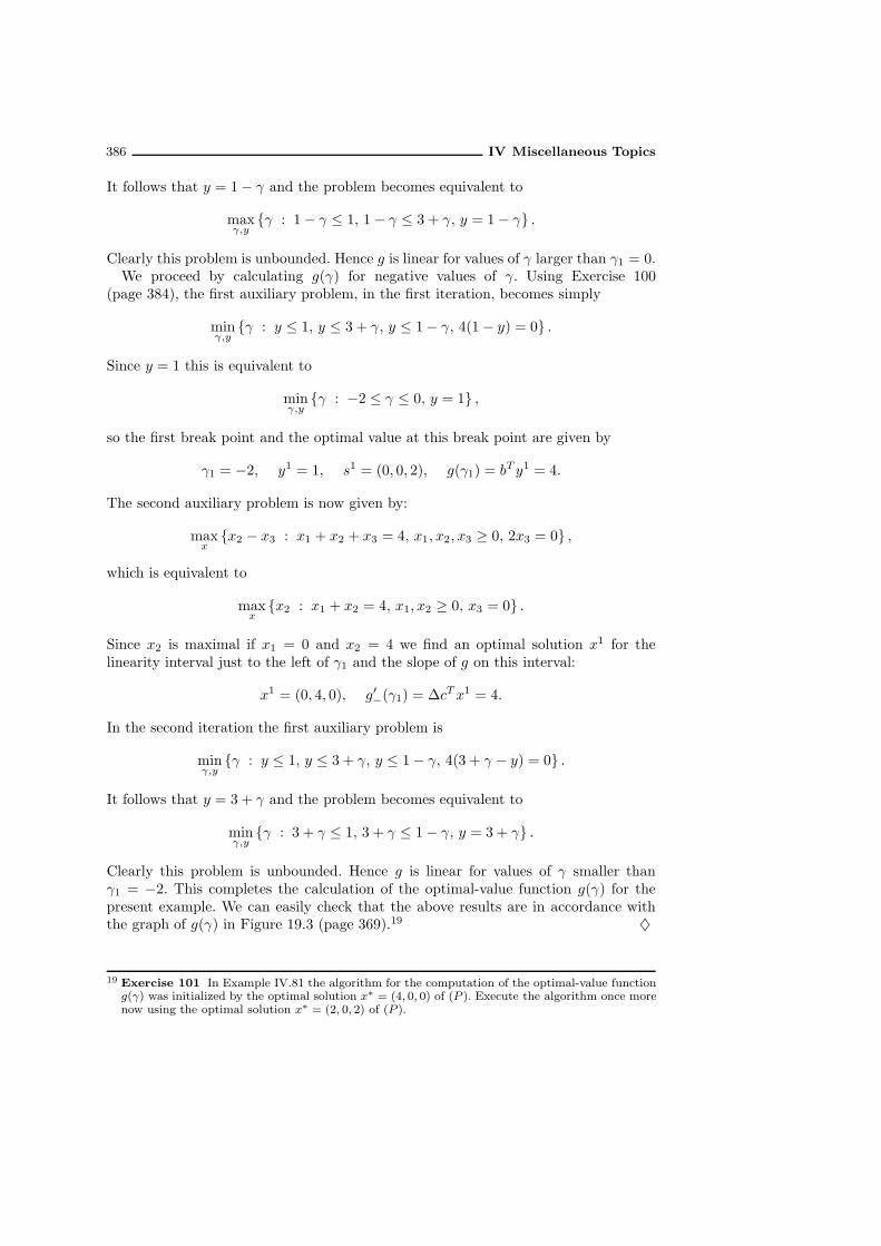
386 IV Miscellaneous Topics
It follows that y = 1− γ and the problem becomes equivalent to
maxγ,y
γ : 1− γ ≤ 1, 1− γ ≤ 3 + γ, y = 1− γ .
Clearly this problem is unbounded. Hence g is linear for values of γ larger than γ1 = 0.We proceed by calculating g(γ) for negative values of γ. Using Exercise 100
(page 384), the first auxiliary problem, in the first iteration, becomes simply
minγ,y
γ : y ≤ 1, y ≤ 3 + γ, y ≤ 1− γ, 4(1− y) = 0 .
Since y = 1 this is equivalent to
minγ,y
γ : −2 ≤ γ ≤ 0, y = 1 ,
so the first break point and the optimal value at this break point are given by
γ1 = −2, y1 = 1, s1 = (0, 0, 2), g(γ1) = bT y1 = 4.
The second auxiliary problem is now given by:
maxx
x2 − x3 : x1 + x2 + x3 = 4, x1, x2, x3 ≥ 0, 2x3 = 0 ,
which is equivalent to
maxx
x2 : x1 + x2 = 4, x1, x2 ≥ 0, x3 = 0 .
Since x2 is maximal if x1 = 0 and x2 = 4 we find an optimal solution x1 for thelinearity interval just to the left of γ1 and the slope of g on this interval:
x1 = (0, 4, 0), g′−(γ1) = ∆cTx1 = 4.
In the second iteration the first auxiliary problem is
minγ,y
γ : y ≤ 1, y ≤ 3 + γ, y ≤ 1− γ, 4(3 + γ − y) = 0 .
It follows that y = 3 + γ and the problem becomes equivalent to
minγ,y
γ : 3 + γ ≤ 1, 3 + γ ≤ 1− γ, y = 3 + γ .
Clearly this problem is unbounded. Hence g is linear for values of γ smaller thanγ1 = −2. This completes the calculation of the optimal-value function g(γ) for thepresent example. We can easily check that the above results are in accordance withthe graph of g(γ) in Figure 19.3 (page 369).19 ♦
19 Exercise 101 In Example IV.81 the algorithm for the computation of the optimal-value functiong(γ) was initialized by the optimal solution x∗ = (4, 0, 0) of (P ). Execute the algorithm once morenow using the optimal solution x∗ = (2, 0, 2) of (P ).

IV.19 Parametric and Sensitivity Analysis 387
19.5 Sensitivity analysis
Sensitivity analysis is the special case of parametric analysis where only one coefficientof b, or c, is perturbed. This means that the perturbation vector is a unit vector. Thederivative of the optimal-value function to a coefficient is called the shadow price andthe corresponding linearity interval the range of the coefficient. When dealing withsensitivity analysis the aim is to find the shadow prices and ranges of all coefficientsin b and c. Of course, the current value of a coefficient may or may not be a breakpoint. In the latter case, when the current coefficient is not a break point, it belongsto an open linearity interval and the range of the coefficient is just this closed linearityinterval and its shadow price the slope of the optimal-value function on this interval.If the coefficient is a break point, then we have two shadow prices, the left-shadow
price, which is the left derivative of the optimal-value function at the current value,and the right-shadow price, the right derivative of the optimal-value function at thecurrent value.20
19.5.1 Ranges and shadow prices
Let x∗ be an optimal solution of (P ) and (y∗, s∗) an optimal solution of (D). Withei denoting the i-th unit vector (1 ≤ i ≤ m), the range of the i-th coefficient biof b is simply the linearity interval of the optimal-value function zA(b + βei, c) thatcontains zero. From Theorem IV.73, the extreme points of this linearity interval followby minimizing and maximizing β over the set
β : Ax = b+ βei, x ≥ 0, xT s∗ = 0
.
With bi considered as a variable, its range of bi follows by minimizing and maximizingbi over the set
bi : Ax = b, x ≥ 0, xT s∗ = 0. (19.6)
The variables in this problem are x and bi. For the shadow prices of bi we useTheorem IV.62. The left- and right-shadow prices of bi follow by minimizing andmaximizing eTi y = yi over the set
yi : AT y + s = c, s ≥ 0, sTx∗ = 0
. (19.7)
Similarly, the range of the j-th coefficient cj of c is equal to the linearity interval of theoptimal-value function zA(b, c + γej) that contains zero. Changing cj into a variableand using Theorem IV.75, we obtain the extreme points of this linearity interval byminimizing and maximizing cj over the set
cj : AT y + s = c, s ≥ 0, sTx∗ = 0
. (19.8)
20 Sensitivity analysis is an important topic in the application oriented literature on LO. Some relevantreferences, in chronological order, are Gal [89], Gauvin [93], Evans and Baker [72, 73], Akgul [6],Knolmayer [173], Gal [90], Greenberg [128], Rubin and Wagner [247], Ward and Wendell [288],Adler and Monteiro [4], Mehrotra and Monteiro [207], Jansen, Roos and Terlaky [153], Jansen,de Jong, Roos and Terlaky [152] and Greenberg [129]. It is surprising that in the literature onsensitivity analysis it is far from common to distinguish between left- and right-shadow prices. Oneof the early exceptions was Gauvin [93]; this paper, however, is not mentioned in the historicalsurvey on sensitivity analysis of Gal [90].

388 IV Miscellaneous Topics
In this problem the variables are the vectors y and s and also cj . For the shadowprices of cj we use Theorem IV.68. The left- and right-shadow prices of cj follow byminimizing and maximizing eTj x = xj over the set
xj : Ax = b, x ≥ 0, xT s∗ = 0
. (19.9)
Some remarks are in order. If bi is not a break point, which becomes evident if theextreme values in (19.6) both differ from bi, then we know that the left- and right-shadow prices of bi are the same and these are given by y∗i . In that case there is noneed to solve (19.7). On the other hand, when bi is a break point, it is clear fromthe discussion following the proof of Theorem IV.73 that there are three possibilities.When the range of bi is determined by solving (19.6) the result may be one of thetwo linearity intervals surrounding bi; in that case y∗i is the shadow price of bi onthis interval. This happens if and only if the given optimal solution y∗ is such thaty∗i is an extreme value in the set (19.7). The third possibility is that the extremevalues in the set (19.6) are both equal to bi. This certainly occurs if y∗ is a strictlycomplementary solution of (D). In each of the three cases it becomes clear after (19.6)is solved, that bi is a break point, and the left- and right-shadow prices at bi can befound by determining the extreme values of (19.7). Clearly similar remarks apply tothe ranges and shadow prices of the coefficients of the vector c.
19.5.2 Using strictly complementary solutions
The formulas for the ranges and shadow prices of the coefficients of b and c can besimplified when the given optimal solutions x∗ of (P ) and (y∗, s∗) of (D) are strictlycomplementary. Let (B,N) denote the optimal partition of (P ) and (D). Then wehave x∗B > 0, x∗N = 0 and s∗B = 0, s∗N > 0. As a consequence, we have xT s∗ = 0 in(19.6) and (19.9) if and only if xN = 0. Similarly, sTx∗ = 0 holds in (19.7) and (19.8)if and only if sB = 0.Using this we can reformulate (19.6) as
bi : Ax = b, xB ≥ 0, xN = 0 , (19.10)
and (19.7) as
yi : AT y + s = c, sB = 0, sN ≥ 0
. (19.11)
Similarly, (19.8) can be rewritten as
cj : AT y + s = c, sB = 0, sN ≥ 0
, (19.12)
and (19.9) as
xj : Ax = b, xB ≥ 0, xN = 0 . (19.13)

IV.19 Parametric and Sensitivity Analysis 389
We proceed with an example.21
Example IV.82 Consider the (primal) problem (P ) defined by
min x1 + 4x2 + x3 + 2x4 + 2x5
s.t. −2x1 + x2 + x3 + x5 −x6 = 0
x1 + x2 − x3 + x4 −x7 = 1
x1, x2, x3, x4, x5, x6, x7 ≥ 0.
The dual problem (D) is
max y2
s.t. −2y1 + y2 ≤ 1 (1)
y1 + y2 ≤ 4 (2)
y1 − y2 ≤ 1 (3)
y2 ≤ 2 (4)
y1 ≤ 2 (5)
−y1 ≤ 0 (6)
−y2 ≤ 0 (7)
Problem (D) can be solved graphically. Its feasible region is shown in Figure 19.5(page 390).
Since we are maximizing y2 in (D), the figure makes clear that the set of optimalsolutions is given by
D∗ = (y1, y2) : 0.5 ≤ y1 ≤ 2, y2 = 2 ,
and hence the optimal value is 2. Note that all slack values can be positive at anoptimal solution except the slack value of the constraint y2 ≤ 2. This means that theset N in the optimal partition (B,N) equals N = 1, 2, 3, 5, 6, 7. Hence, B = 4.Therefore, at optimality only the variable x4 can be positive. It follows that
P∗ = x ∈ P : x1 = x2 = x3 = x5 = x6 = x7 = 0 = (0, 0, 0, 1, 0, 0, 0) ,
and (P ) has a unique solution: x = (0, 0, 0, 1, 0, 0, 0).
21 Exercise 102 The ranges and shadow prices can also be found by solving the corresponding dualproblems. For example, the maximal value of bi in (19.10) can be found by solving
minbT y : AT
By ≥ 0, yi = −1
and the minimal value by solving
maxbT y : AT
By ≤ 0, yi = −1.
Formulate the dual problems for the other six cases.

390 IV Miscellaneous Topics
−1 −0.5 0 0.5 1 1.5 2 2.5 3−1
−0.5
0
0.5
1
1.5
2
2.5
3
y1
y2
(1) (2)
(3)
(4)
(5)
(6)
(7)
Figure 19.5 The feasible region of (D).
The next table shows the result of a complete sensitivity analysis. It shows theranges and shadow prices for all coefficients of b and c, where these vectors have theirusual meaning. For each coefficient that is a break point we give the shadow price as aclosed interval; the extreme values of this interval are the left- and right-shadow pricesof the coefficient. In this example this happens only for b1. The range of a break pointconsists of the point itself; the table gives this point. On the other hand, for ‘nonbreakpoints’ the range is a proper interval and the shadow price is a number.
Coefficient Range Shadow prices
b1 = 0 0 [ 12 , 2]
b2 = 1 [0,∞) 2
c1 = 1 [−2,∞) 0
c2 = 4 [ 52 ,∞) 0
c3 = 1 [− 32 ,∞) 0
c4 = 2 [0, 3] 1
c5 = 2 [ 12 ,∞) 0
c6 = 0 [−2,∞) 0
c7 = 0 [−2,∞) 0
We perform the sensitivity analysis here for b1 and c4.
Range and shadow prices for b1
Using (19.10) the range of b1 follows by minimizing and maximizing b1 over the system
0 = b1x4 = 1.

IV.19 Parametric and Sensitivity Analysis 391
The solution of this system is unique: x4 = 1 and b1 = 0, so the range of b1 is theinterval [0, 0]. This means that b1 = 0 is a break point.
The left- and right-shadow prices of b1 follow by minimizing and maximizing y1over y ∈ D∗. The minimal value is 0.5 and the maximal value 2, so the left- andright-shadow prices 0.5 and 2.
Range and shadow price for c4
The range of c4 is found by using (19.12). This amounts to minimizing and maximizingc4 over the system
−2y1 + y2 ≤ 1
y1 + y2 ≤ 4
y1 − y2 ≤ 1
y2 = c4
y1 ≤ 2
y1 ≥ 0
y2 ≥ 0.
This optimization problem can easily be solved by using Figure 19.5. It amounts tothe question of which values of y2 are feasible when the fourth constraint is removedin Figure 19.5. We can easily verify that all values of y2 in the closed interval [0, 3](and no other values) satisfy. Therefore, the range of c4 is this interval. The shadowprice of c4 is given by eT4 x = x4 = 1. ♦
19.5.3 Classical approach to sensitivity analysis
Commercial optimization packages for the solution of LO problems usually offer thepossibility of doing sensitivity analysis. The sensitivity analysis in many existingcommercial optimization packages is based on the naive approach presented in firstyear textbooks. As a result, the outcome of the sensitivity analysis is often confusing.We explain this below.The ‘classical’ approach to sensitivity analysis is based on the Simplex Method for
solving LO problems.22 The Simplex Method produces a so-called basic solution of
22 With the word ‘classical’ we want to refer to the approach which dominates the literature, especiallywell known textbooks dealing with parametric and/or sensitivity analysis. This approach has ledto the existing misuse of parametric optimization in commercial packages. This misuse is howevera shortcoming of the packages and by no means a shortcoming in the whole existing theoreticalliterature. In this respect we want to refer the reader to Nozicka, Guddat, Hollatz and Bank [228].In this book the parametric issue is correctly handled in terms of the Simplex Method, polyhedrons,faces of polyhedra etc. Besides parameterizing either the objective vector or the right-hand sidevector, much more general parametric issues are also discussed. The following citation is takenfrom this book: Den qualitativen Untersuchungen in den meisten erschienenen Aufsatzen undBuchern liegt das Simplexverfahren zugrunde. Zwangslaufig unterliegen alle derartig gewonnenenAussagen den Schwierigkeiren, die bei Beweisfuhrungen mit Hilfe der Simplexmethode im Falle derEntartung auftreten. In einigen Arbeiten wurde ein rein algebraischer Weg verfolgt, der in gewisseSpezialfallen zu Resultaten fuhrte, im allgemeinen aber bisher keine qualitative Analyse erlieferte.

392 IV Miscellaneous Topics
the problem. It suffices for our purpose to know that such a solution is determinedby an optimal basis. Assuming that A is of size m × n and rank (A) = m, a basis isa nonsingular m ×m submatrix AB′ of A and the corresponding basic solution x isdetermined by
AB′xB′ = b, xN ′ = 0,
where N ′ consists of the indices not in B′. Defining a vector y by
ATB′y = cB′ ,
and denoting the slack vector of y by s, we have sB′ = 0. Since xN ′ = 0, it followsthat xs = 0, proving that x and s are complementary vectors. Hence, if xB′ and sN ′
are nonnegative then x is optimal for (P ) and (y, s) is optimal for (D). In that caseAB′ is called an optimal basis for (P ) and (D). A main result in the Simplex basedapproach to LO is that such an optimal basis always exists — provided the assumptionthat rank (A) = m is satisfied — and the Simplex Method generates such a basis. Fora detailed description of the Simplex Method and its underlying theory we refer thereader to any (text-)book on LO.23
Any optimal basis leads to a natural division of the indices into m basic indices andn−m nonbasic indices, thus yielding a partition (B′, N ′) of the index set. We call thisthe optimal basis partition induced by the optimal basis B′. Obviously, an optimalbasis partition need not be an optimal partition. In fact, this observation is crucial aswe show below.The classical approach to sensitivity analysis amounts to applying the ‘formulas’
(19.10) – (19.13) for the ranges and shadow prices, but with the optimal basis partition(B′, N ′) instead of the optimal partition (B,N). It is clear that in general (B′, N ′)is not necessarily the optimal partition because (P ) and (D) may have more thanone optimal basis. The outcome of the classical analysis will therefore depend onthe optimal basis AB′ . Hence, correct implementations of the classical approach maygive rise to different ‘ranges’ and ‘shadow prices’.24 The next example illustrates thisphenomenon. In a subsequent section a further example is given, where we applyseveral commercial optimization packages to a small transportation problem.
Example IV.83 For problems (P ) and (D) in Example IV.82 we have three optimalbases. These are given in the table below. The column at the right gives the ‘ranges’for c4 for each of these bases.
Basis B′ ‘Range’ for c4
1 1, 4 [1, 3]
2 2, 4 [2, 3]
3 4, 5 [1, 2]
We get three different ‘ranges’, depending on the optimal basis. Let us do thecalculations for the first optimal basis in the table. The ‘range’ of c4 is found by
23 See, e.g., Dantzig [59], Papadimitriou and Steiglitz [231], Chvatal [55], Schrijver [250], Fang andPuthenpura [74] and Sierksma [256].
24 We put the words range and shadow price between quotes if they refer to ranges and shadow pricesobtained from an optimal basis partition (which may differ from the unique optimal partition).

IV.19 Parametric and Sensitivity Analysis 393
using (19.12) with (B,N) such that B = B′ = 1, 4. This amounts to minimizingand maximizing c4 over the system
−2y1 + y2 = 1
y1 + y2 ≤ 4
y1 − y2 ≤ 1
y2 = c4
y1 ≤ 2
y1 ≥ 0
y2 ≥ 0.
Using Figure 19.5 we can easily solve this problem. The question now is which valuesof y2 are feasible when the fourth constraint is removed in Figure 19.5 and the firstconstraint is active. We can easily verify that this leads to 1 ≤ y2 ≤ 3, thus yieldingthe closed interval [1, 3] as the ‘range’ for c4. The other two ‘ranges’ can be found inthe same way by keeping the second and the fifth constraints active, respectively.A commercial optimization package provides the user with one of the three ranges
in the table, depending on the optimal basis found by the package. Observe that eachof the three ranges is a subrange of the correct range, which is [0, 3]. Note that thecurrent value 2 of c4 lies in the open interval, whereas for two of the ‘ranges’ in thetable, 2 is an extreme point. This might lead to the wrong conclusion that 2 is a breakpoint of the optimal-value function. ♦
It can easily be understood that the ‘range’ obtained from an optimal basis partitionis always a subinterval of the whole linearity interval. Of course, sometimes thesubinterval may coincide with the whole interval. For the shadow prices a similarstatement holds. At a ‘nonbreak point’ an optimal basis partition yields the correctshadow price. At a break point, however, an optimal basis partition yields one ‘shadowprice’, which may be any number between the left- and the right-shadow price. Theexample in the next section demonstrates this behavior very clearly.Before proceeding with the next section we must note that from a computational
point of view, the approach using an optimal basis partition is much cheaper than usingthe optimal partition. In the latter case we need to solve some auxiliary LO problems— in the worst case four for each coefficient. When the optimal partition (B,N) isreplaced by an optimal basis partition (B′, N ′), however, it becomes computationallyvery simple to determine the ‘ranges’ and ‘shadow prices’.For example, consider the ‘range’ problem for bi. This amounts to minimizing and
maximizing bi over the set
bi : Ax = b, xB′ ≥ 0, xN ′ = 0 .Since AB′ is nonsingular, it follows that
xB′ = A−1B′ b,
and hence the condition xB′ ≥ 0 reduces to
A−1B′ b ≥ 0.

394 IV Miscellaneous Topics
This is a system of m linear inequalities in the coefficient bi, with i fixed, and hence itssolution can be determined straightforwardly. Note that the system is feasible, becausethe current value of bi is such that the system is satisfied. Hence, the solution is aclosed interval containing the current value of bi.
19.5.4 Comparison of the classical and the new approach
For the comparison we use a simple problem, arising when transporting commodities(of one type) from three distribution centers to three warehouses. The supply values atthe three distribution centers are 2, 6 and 5 units respectively, and the demand valueat each of the three warehouses is just 3. We assume that the costs for transportationof one unit of commodity from a distribution center to a warehouse is independentof the distribution center and the warehouse, and this cost is equal to one (unit ofcurrency). The aim is to meet the demand at the warehouses at minimal cost. Thisproblem is depicted in Figure 19.6 by means of a network. The left three nodes inthis network represent the distribution centers and the right three nodes the threewarehouses. The arcs represent the transportation routes from the distribution centersto the warehouses. The supply and demand values are indicated at the respectivenodes. The transportation problem consists of assigning ‘flow’ values to the arcs in
a3 = 5
a2 = 6
a1 = 2
3 = b3
3 = b2
3 = b1
Figure 19.6 A transportation problem.
the network so that the demand is met and the supply values are respected; this mustbe done in such a way that the cost of the transportation to the demand nodes isminimized. Because of the choice of cost coefficients, the total cost is simply the sumof all arc flow values. Since the total demand is 9, this is also the optimal value forthe total cost value. Note that there are many optimal flows; this is due to the factthat all arcs are equally expensive. So far, everything is trivial.
Sensitivity to demand and supply values
Now we want to determine the sensitivity of the optimal value to perturbations ofthe supply and demand values. Denoting the supply values by a = (a1, a2, a3) andthe demand values by b = (b1, b2, b3), we can determine the ranges of these values by

IV.19 Parametric and Sensitivity Analysis 395
hand.For example, when b1 is changed, the total demand becomes 6 + b1 and this is the
optimal value as long as such a demand can be met by the present supply. This leadsto the condition
6 + b1 ≤ 2 + 6 + 5 = 13,
which yields b1 ≤ 7. For larger values of b1 the problem becomes infeasible. Whenb1 = 0, the arcs leading to the first demand node have zero flow value in any optimalsolution. This means that 0 is a break point, and the range of b1 is [0, 7]. Because ofthe symmetry in the network for the demand nodes, the range for b2 and b3 will bethe same interval.When a1 is changed, the total supply becomes 11+ a1 and this will be sufficient as
long as11 + a1 ≥ 9,
which yields a1 ≥ −2. The directed arcs can only handle nonnegative supply values,and hence the range of a1 is [0,∞). Similarly, the range for a2 follows from
7 + a2 ≥ 9,
which yields the range [2,∞) for a2, and the range for a3 follows from
8 + a3 ≥ 9,
yielding the range [1,∞) for a3.To compare these ranges with the ‘ranges’ provided by the classical approach, we
made a linear model of the above problem, solved it using five well-known commercialoptimization packages, and performed a sensitivity analysis with these packages. Weused the following linear standard model:
min∑3
i=1
∑3j=1 xij
s.t. x11 + x12 + x13 + s1 = 2
x21 + x22 + x23 + s2 = 6
x31 + x32 + x33 + s3 = 5
x11 + x21 + x31 − d1 = 3
x12 + x22 + x32 − d2 = 3
x13 + x23 + x33 − d3 = 3
xij , si, dj ≥ 0, i, j = 1, 2, 3.
The meaning of the variables is as follows:
xij : the amount of transport from supply node i to demand node j,
si : excess supply at supply node i,
dj : shortage of demand at node j,
where i and j run from 1 to 3.

396 IV Miscellaneous Topics
The result of the experiment is shown in the table below.25 The columns correspondto the supply and the demand coefficients. Their current values are put betweenbrackets. The rows in the table corresponding to the five packages26 CPLEX, LINDO,PC-PROG, XMP and OSL show the ‘ranges’ produced by these packages. The lastrow contains the ranges calculated before by hand.27
‘Ranges’ of supply and demand values
LO package a1(2) a2(6) a3(5) b1(3) b2(3) b3(3)
CPLEX [0,3] [4,7] [1,∞) [2,7] [2,5] [2,5]
LINDO [1,3] [2,∞) [4,7] [2,4] [1,4] [1,7]
PC-PROG [0,∞) [4,∞) [3,6] [2,5] [0,5] [2,5]
XMP [0,3] [6,7] [1,∞) [2,3] [2,3] [2,7]
OSL [0,3] [4,7] (−∞,∞) [2,7] [2,5] [2,5]
Correct range [0,∞) [2,∞) [1,∞) [0,7] [0,7] [0,7]
The table clearly demonstrates the weaknesses of the classical approach. Sensitivityanalysis is considered to be a tool for obtaining information about the bottlenecksand degrees of freedom in the problem. The information provided by the commercialoptimization packages is confusing and hardly allows a solid interpretation. Forexample, in our example problem there is obvious symmetry between the demandnodes. None of the five packages gives evidence of this symmetry.
Remark IV.84 As stated before, the ‘ranges’ and ‘shadow prices’ provided by the classicalapproach arise by applying the formulas (19.10) – (19.13) for the ranges and shadow prices,but replacing the optimal partition (B,N) by the optimal basis partition (B′, N ′). Indeed,the ‘ranges’ in the table can be reconstructed in this way. We will not do this here, but toenable the interested reader to perform the relevant calculations we give the optimal basispartitions used by the packages. If the optimal basis partition is (B′, N ′), it suffices to knowthe variables in B′ for each of the five packages. These ‘basic variables’ are given in the nexttable.
LO package Basic variables
CPLEX x12 x21 x22 x23 x31 s3
LINDO x11 x23 x31 x32 x33 s2
PC-PROG x22 x23 x31 x33 s1 s2
XMP x13 x21 x22 x23 x33 s3
OSL x12 x21 x22 x23 x31 s3
25 The dual problem has a unique solution in this example. These are the shadow prices for thedemand and supply values. All packages return this unique solution, namely 0 for the supplyvalues — due to the excess of supply — and 1 for the demand values.
26 For more information on these packages we refer the reader to Sharda [253].27 The ‘range’ provided by the IBM package OSL (Optimization Subroutine Library) for a3 is not
a subrange of the correct range; this must be due to a bug in OSL. The correct ‘range’ for theoptimal basis partition used by OSL is [1,∞).

IV.19 Parametric and Sensitivity Analysis 397
Note that CPLEX and OSL use the same optimal basis. The output of their sensitivity
analysis differs, however. As noted before, the explanation of this phenomenon is that the
OSL implementation of the classical approach must contain a bug. •The sensitivity analysis for the cost coefficients cij is considered next. The results
are similar, as we shall see.
Sensitivity to cost coefficients
The current values of the cost coefficients cij are all 1. As a consequence each feasibleflow on the network is optimal if the sum of the flow values xij equals 9. When oneof the arcs becomes more expensive, then the flow on this arc can be rerouted overthe other arcs and the optimal value remains 9. Hence the right-shadow price of eachcost coefficient equals 0. On the other hand, if one of the arc becomes cheaper, thenit becomes attractive to let this arc carry as much flow as possible. The maximal flowvalues for the arcs are 2 for the arcs emanating from the first supply node and 3 forthe other arcs. Since for each arc there exists an optimal solution of the problem inwhich the flow value on that arc is zero, a decrease of 1 in the cost coefficient for thearcs emanating from the first supply node leads to a decrease of 2 in the total cost,and for the other arcs the decrease in the total cost is 3. Thus we have found theleft- and right-shadow prices of the cost coefficients. Since the left- and right-shadowprices are all different, the current value of each of the cost coefficients is a breakpoint. Obviously, the linearity interval to the left of this break point is (−∞, 1] andthe linearity interval to the right of it is [1,∞).In the next table the ‘shadow prices’ provided by the five commercial optimization
packages are given. The last row in the table contains the correct values of the left-and right-shadow prices, as just calculated.
‘Shadow prices’ of cost coefficients
LO package c11 c12 c13 c21 c22 c23 c31 c32 c33
CPLEX 0 2 0 2 1 3 1 0 0
LINDO 2 0 0 0 0 2 1 3 1
PC-PROG 0 0 0 0 3 1 3 0 2
XMP 0 0 2 3 3 0 0 0 1
OSL 0 2 0 2 1 3 1 0 0
Correct values [2,0] [2,0] [2,0] [3,0] [3,0] [3,0] [3,0] [3,0] [3,0]
Note that in all cases the ‘shadow price’ of a package lies in the interval betweenthe left- and right-shadow prices.The last table shows the ‘ranges’ of the packages and the correct left- and right-hand
side ranges for the cost coefficients.28 It is easy to understand the correct ranges. Forexample, if c11 increases then the corresponding arc becomes more expensive than theother arcs, and hence will not be used in an optimal solution. On the other hand, if
28 In this table we use shorthand notation for the infinite intervals [1,∞) and (-∞,1]. The interval[1,∞) is denoted by [1, ) and the interval (-∞,1] by ( ,1].
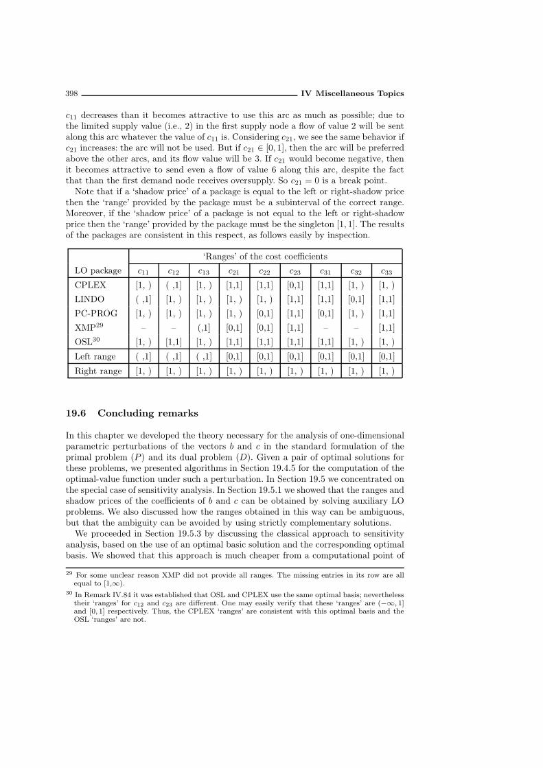
398 IV Miscellaneous Topics
c11 decreases than it becomes attractive to use this arc as much as possible; due tothe limited supply value (i.e., 2) in the first supply node a flow of value 2 will be sentalong this arc whatever the value of c11 is. Considering c21, we see the same behavior ifc21 increases: the arc will not be used. But if c21 ∈ [0, 1], then the arc will be preferredabove the other arcs, and its flow value will be 3. If c21 would become negative, thenit becomes attractive to send even a flow of value 6 along this arc, despite the factthat than the first demand node receives oversupply. So c21 = 0 is a break point.Note that if a ‘shadow price’ of a package is equal to the left or right-shadow price
then the ‘range’ provided by the package must be a subinterval of the correct range.Moreover, if the ‘shadow price’ of a package is not equal to the left or right-shadowprice then the ‘range’ provided by the package must be the singleton [1, 1]. The resultsof the packages are consistent in this respect, as follows easily by inspection.
‘Ranges’ of the cost coefficients
LO package c11 c12 c13 c21 c22 c23 c31 c32 c33
CPLEX [1, ) ( ,1] [1, ) [1,1] [1,1] [0,1] [1,1] [1, ) [1, )
LINDO ( ,1] [1, ) [1, ) [1, ) [1, ) [1,1] [1,1] [0,1] [1,1]
PC-PROG [1, ) [1, ) [1, ) [1, ) [0,1] [1,1] [0,1] [1, ) [1,1]
XMP29 – – (,1] [0,1] [0,1] [1,1] – – [1,1]
OSL30 [1, ) [1,1] [1, ) [1,1] [1,1] [1,1] [1,1] [1, ) [1, )
Left range ( ,1] ( ,1] ( ,1] [0,1] [0,1] [0,1] [0,1] [0,1] [0,1]
Right range [1, ) [1, ) [1, ) [1, ) [1, ) [1, ) [1, ) [1, ) [1, )
19.6 Concluding remarks
In this chapter we developed the theory necessary for the analysis of one-dimensionalparametric perturbations of the vectors b and c in the standard formulation of theprimal problem (P ) and its dual problem (D). Given a pair of optimal solutions forthese problems, we presented algorithms in Section 19.4.5 for the computation of theoptimal-value function under such a perturbation. In Section 19.5 we concentrated onthe special case of sensitivity analysis. In Section 19.5.1 we showed that the ranges andshadow prices of the coefficients of b and c can be obtained by solving auxiliary LOproblems. We also discussed how the ranges obtained in this way can be ambiguous,but that the ambiguity can be avoided by using strictly complementary solutions.We proceeded in Section 19.5.3 by discussing the classical approach to sensitivity
analysis, based on the use of an optimal basic solution and the corresponding optimalbasis. We showed that this approach is much cheaper from a computational point of
29 For some unclear reason XMP did not provide all ranges. The missing entries in its row are allequal to [1,∞).
30 In Remark IV.84 it was established that OSL and CPLEX use the same optimal basis; neverthelesstheir ‘ranges’ for c12 and c23 are different. One may easily verify that these ‘ranges’ are (−∞, 1]and [0, 1] respectively. Thus, the CPLEX ‘ranges’ are consistent with this optimal basis and theOSL ‘ranges’ are not.

IV.19 Parametric and Sensitivity Analysis 399
view. On the other hand, much less information is usually obtained and the informationis often confusing. In the previous section we provided a striking example by presentingthe sensitivity information provided by five commercial optimization packages for asimple transportation problem.The shortcomings of the classical approach are well known among experts in the
field. At several places in the literature these experts raised their voices to warn of thepossible implications of using the classical approach. By way of example we include acitation of Rubin and Wagner [247]:
Managers who build their own microcomputer linear programming models
are apt to misuse the resulting shadow prices and shadow costs. Fallacious
interpretations of these values can lead to expensive mistakes, especially
unwarranted capital investments.
As a result of the unreliability of the sensitivity information provided by computerpackages, the reputation of sensitivity analysis as a tool for obtaining informationabout the bottlenecks and degrees of freedom has suffered a lot. Many potential usersof such information do not use it, because they want to avoid the pitfalls that areinherent in the classical approach.The theory developed in this chapter provides a solid base for reliable sensitivity
modules in future generations of computer packages for LO.


20
Implementing Interior PointMethods
20.1 Introduction
Several polynomial interior-point algorithms were discussed in the previous chapters.Interior point algorithms not only provide the best theoretical complexity for LOproblems but allow highly efficient implementations as well. Obviously not allpolynomial algorithms are practically efficient. In particular, all full Newton stepmethods (see, e.g., Section 6.7) are inefficient in practice. However variants likethe predictor-corrector method (see Section 7.7) and large-update methods (seeSection 6.9) allow efficient implementations. The aim of this chapter is to give somehints on how some of these interior point algorithms can be converted into efficientimplementations. To reach this goal several problems have to be dealt with. Someof these problems have been at least partially discussed earlier (e.g., the embeddingproblem in Chapter 2) but need further elaboration. Some other topics (e.g., methodsof sparse numerical linear algebra, preprocessing) have not yet been touched.By reviewing the various interior-point methods we observe that they are all based
on similar assumptions and are built up from similar ingredients. We can extract thefollowing essential elements of interior-point methods (IPMs).
Appropriate problem form. All algorithms assume that the LO problem satisfiescertain assumptions. The problem must be in an appropriate form (e.g., thecanonical form or the standard form). In the standard form the coefficient matrixAmust have full row rank. Techniques to bring a given LO problem to the desiredform, and at the same time to eliminate redundant constraints and variables,are called preprocessing and are discussed in Section 20.3.
Search direction. The search direction in interior-point methods is always a Newtondirection. To calculate this direction we have to solve a system of linearequations. Except for the right-hand side and the scaling, this system is thesame for all the methods. Computationally the solution of the system amountsto factorizing a square matrix and then solving the triangular systems byforward or backward substitution. The factorization is the most expensive partof an iteration. Without efficient sparse linear algebra routines, interior-pointmethods would not be practical. Various elements of sparse matrix techniques arediscussed in Section 20.4. A straightforward idea for reducing the computational

402 IV Miscellaneous Topics
cost is to reuse the same factorization. This leads to the idea of second- andhigher-order methods discussed in Section 20.4.3.
Interior point. The interior-point assumption is presupposed, i.e. that both theprimal and the dual problem have a strictly positive (preferably centered) initialsolution. Most LO problems do not have such a solution, but still have to besolved. A theoretically appealing and at the same time practical method isto embed the problem in a self-dual model, as discussed in Chapter 2. Theembedding model is revisited and elaborated on in Section 20.5.
Reoptimization. In practice it often happens that several variants of the same LOproblem need to be solved successively. One might expect that the solution of anearlier version would be a good starting point for a slightly modified problem.For this so-called warm start problem the embedding model also provides a goodsolution as discussed in Section 20.5.2.
Parameters: Step size, stopping criteria. The iterates in IPMs should stay insome neighborhood of the central path. Theoretically good step-sizes can resultin hopelessly slow convergence in practice. A practical step-size selection ruleis discussed. At some point, when the duality gap is small, the calculation isterminated. The theoretical criteria are typically far beyond today’s machineprecision. A practical criterion is presented in Section 20.6.
Optimal basis identification. It is not an essential element of interior-point meth-ods, but sometimes it still might be important1 to find an optimal basis. Thenwe need to provide the ability to ‘cross over’ from an interior solution to a basicsolution. An elegant strongly polynomial algorithm is presented in Section 20.7.
20.2 Prototype algorithm
In most practical LO problems, in addition to the equality and inequality constraints,the variables have lower and upper bounds. Thus we deal with the primal problem inthe following form:
minx
cTx : Ax ≥ b, x ≤ bu, x ≥ 0
, (20.1)
where c, x, bu ∈ IRn, b ∈ IRm, and the matrix A is of size m× n. Now its dual is
maxy,yu
bT y − bTu yu : AT y − yu ≤ c, y ≥ 0, yu ≥ 0
, (20.2)
where y ∈ IRm and yu ∈ IRn. Let us denote the slack variables in the primal problem(20.1) by
z = Ax− b, zu = bu − x
and in the dual problem (20.2) by
s = c+ yu −AT y,
1 Here we might think about linear integer optimization when cutting planes are to be generated tocut off the current nonintegral optimal solution.

IV.20 Implementing Interior Point Methods 403
respectively. Here we assume not only that the problem pair satisfies the interior-pointassumption, but also that a strictly positive solution (x, zu, z, s, yu, y) > 0 is given,satisfying all the constraints in (20.1) and (20.2) respectively. How to solve theseproblems without the explicit knowledge of an interior point is discussed in Section20.5.The central path of the pair of problems given in (20.1) and (20.2) is defined as
the set of solutions (x(µ), zu(µ), z(µ)) > 0 and (s(µ), yu(µ), y(µ)) > 0 for µ > 0 of thesystem
Ax− z = b,
x+ zu = bu,
AT y − yu + s = c, (20.3)
xs = µe,
zuyu = µe,
zy = µe,
where e is the vector of all ones with appropriate dimension.Observe that the first three of the above equations are linear and force primal and
dual feasibility of the solution. The last three equations are nonlinear. They become thecomplementarity conditions when µ = 0, which together with the feasibility constraintsprovides optimality of the solutions. The actual duality (or complementarity) gap gcan easily be computed:
g = xT s+ zTu yu + zT y,
which equals (2n+m)µ on the central path .One iteration of a primal-dual algorithmmakes one step of Newton’s method applied
to system (20.3) with a given µ; then µ is reduced and the procedure is repeated aslong as the duality gap is larger than a predetermined tolerance.Given a solution (x, zu, z) > 0 of (20.1) and (s, yu, y) > 0 of (20.2) the Newton
direction for (20.3) is obtained by solving a system of linear equations. This systemcan be written as follows, where the ordering of the variables is chosen so that thestructure of the coefficient matrix becomes apparent.
0 A −I 0 0 0AT 0 0 −I 0 I0 I 0 0 I 00 S 0 0 0 X0 0 0 Zu Yu 0Z 0 Y 0 0 0
∆y∆x∆z∆yu∆zu∆s
=
000
µe− xsµe− zuyuµe− zy
. (20.4)
In making a step, in order to preserve the positivity of (x, zu, z) and (s, yu, y), a step-size α usually smaller than one (a damped Newton step) is chosen.Let us have a closer look at the Newton system. From the last four equations in
(20.4) we can easily derive
∆zu = −∆x,
∆s = x−1(µe − xs− s∆x),
∆yu = z−1u (µe − zuyu − yu∆zu) = z−1
u (µe− zuyu + yu∆x), (20.5)
∆z = y−1(µe− yz − z∆y).

404 IV Miscellaneous Topics
With these relations, (20.4) reduces to
[D2 A
AT −D−2
][∆y
∆x
]=
[r
h
], (20.6)
where
D2 = ZY −1
D−2 = SX−1 + YuZ−1u
r = y−1(µe − yz)
h = z−1u (µe− zuyu)− x−1(µe− xs).
The solution of the reduced Newton system (20.6) is the computationally most involvedstep of any interior point method. The system (20.6) in this form is a symmetricindefinite system and is referred to as the augmented system. If the second equationin the augmented system is multiplied by −1 a system with a positive definite (butunsymmetric) matrix is obtained.The augmented system (20.6) is equivalent to
∆x = D2(AT∆y − h)
and (AD2AT +D2
)∆y = r +AD2h. (20.7)
The last equation is referred to as the normal equation.2 The way to solve the systems(20.6) and (20.7) efficiently is discussed in detail in Section 20.4.After system (20.6) or (20.7) is solved, using formulas (20.5) we obtain the solution
of (20.4). Now the maximal feasible step lengths αP for the primal (x, z, zu) and αD forthe dual (s, y, yu) variables are calculated. Then these step-sizes are slightly reducedby a factor α0 < 1 to avoid reaching the boundary. The new iterate is computed as
xk+1 := xk + α0αP∆x,
zk+1u := zku + α0αP∆zu,
zk+1 := zk + α0αP∆z,
sk+1 := sk + α0αD∆s,
yk+1u := yku + α0αD∆yu,
yk+1 := yk + α0αD∆y.
(20.9)
After the step, the parameter µ is updated and the process is repeated. A prototypealgorithm can be summarized as follows.
2Exercise 103 Show that if first ∆y is calculated from the system (20.6) as a function of ∆x thefollowing formulas arise:
∆y = −D−2(A∆x− r)
and (ATD−2A+ D−2
)∆x = ATD−2r − h. (20.8)
Observe that this symmetric formulation allows for further utilization of the structure of the normalequation. We are free to choose between (20.7) and (20.8) depending on which has a nicer sparsitystructure.

IV.20 Implementing Interior Point Methods 405
Prototype Primal–Dual Algorithm
Input:An accuracy parameter ε > 0;(x0, z0u, z
0) and (s0, y0u, y0); interior solutions for (20.1) and (20.2);
parameter α0 < 1; µ0 > 0.
begin(x, zu, z, s, yu, y) = (x0, z0u, z
0, s0, y0u, y0); µ := µ0;
while (2n+m)µ ≥ ε dobegin
reduce µsolve (20.4) to obtain (∆x,∆zu,∆z,∆s,∆yu,∆y);determine αP and αD;update (x, zu, z, yu, y, s) by (20.9)
endend
Before discussing all the ingredients in more detail we make an important observation.Solving a problem with individual upper bounds on the variables does not requiresignificantly more computational effort than solving the same problem without suchupper bounds. In both cases the augmented system (20.6) and the normal equation(20.7) have the same size. The extra costs per iteration arising from the upper boundsare just O(n), namely some extra ratio tests to determine the maximal possible stepssizes and some extra vector manipulations (see equations (20.5)).3
20.3 Preprocessing
An important issue for all implementations is to transform the problem into anappropriate form, e.g., to the canonical form with upper bounded variables (20.1), andto reduce the problem size in order to reach a minimal representation of the problem.This aim is quite plausible. A smaller problem needs less memory to store, usually feweriterations of the algorithm, and if the transformation reduces the number of nonzerocoefficients or improves the sparsity structure then fewer arithmetic operations periteration are needed. A minimal representation should be free of redundancies, impliedvariables and inequalities. In general it is not realistic to strive to find the minimalrepresentation of a given problem. But by analysing the structure of the problem it isoften possible to reduce the problem size significantly. In fact, almost all large-scale LOproblems contain redundancies in practice. The use of modeling languages and matrixgenerators easily allows the generation of huge models. Modelers choose to formulatemodels that are easy to understand and modify; this often leads to the introduction
3Exercise 104 Check that the computational cost per iteration increases just by O(n) if individualupper bounds are imposed on the variables.

406 IV Miscellaneous Topics
of superfluous variables and redundant constraints. To remove at least most of theseredundancies is, however, a nontrivial task; this is the aim of preprocessing.As we have already indicated, computationally the most expensive part of an
interior-point iteration is calculating the search direction, to solve the normal equation(20.7) or the augmented system (20.6). With a compact formulation the speedup canbe significant.4
20.3.1 Detecting redundancy and making the constraint matrix sparser
By analysing the sparsity pattern of the matrix A, one can frequently reduce theproblem size. The aim of the sparsity analysis is to reduce the number of nonzeroelements in the constraint matrix A; this is done by elementary matrix operations.In fact, as a consequence, the sparsity analysis mainly depends on just the nonzerostructure of the matrix A and it is largely independent of the magnitude of thecoefficients.
1. First we look for pairs of constraints with the same nonzero pattern. If we have two(in-)equality constraints which are identical — up to a scalar multiplier — thenone of these constraints is removed from the problem. If one of them is an equalityconstraint and the other an inequality constraint then the inequality constraint isdropped. If they are opposite inequalities then they are replaced by one equalityconstraint.
2. Linearly dependent constraints are removed. (Dependency can easily be detectedby using elimination.)
3. Duplicate columns are removed.4. To improve the sparsity pattern of the constraint matrix A further we first put
the constraints into equality form. Then by adding and subtracting constraintswith appropriate multipliers, we can eliminate several nonzero entries.5 Duringthis process we have to make sure that the resulting sparser system is equivalentto the original one. Mathematically this means that we look for a nonsingularmatrix Q ∈ IRm×m such that the matrix QA is as sparse as possible. Such sparserconstraints in the resulting equivalent formulation
QAx = Qb
might be much more suitable for a direct application of the interior-point solver.6
4 Preprocessing is not a new idea, but has enjoyed much attention since the introduction of interior-point methods. This is due to the fact that the realized speedup is often larger than for the SimplexMethod. For further reading we refer the reader to, e.g., Brearley, Mitra and Williams [49], Adler etal. [1], Lustig, Marsten and Shanno [191], Andersen and Andersen [9], Gondzio [113], Andersen [8],Bixby [42], Lustig, Marsten and Shanno [193] and Andersen et al. [10].
5 As an illustration let us consider two constraints aTkx = bk and aTj x = bj where σ(ak) ⊆ σ(aj ).
(Recall that σ(x) = i | xi 6= 0 .) Now if we define aj = aj + λak and bj = bj + λbk , where λ
is chosen so that σ(aj) ⊂ σ(aj ), then the constraint aTj x = bj can be replaced by aTj x = bj while
the number of nonzero coefficients is reduced by at least one.6 Exact solution of this Sparsity Problem is an NP-complete problem (Chang and McCormick [54])
but efficient heuristics (Adler et al. [1], Chang and McCormick [54] and Gondzio [113]) usuallyproduce satisfactory nonzero reductions in A. The algorithm of Gondzio [113], for example, looksfor a row of A that has a sparsity pattern that is a subset of the sparsity pattern of other rows anduses it to eliminate nonzero elements from these rows.

IV.20 Implementing Interior Point Methods 407
20.3.2 Reducing the size of the problem
In general, finding all redundancies in an LO problem is a more difficult problem thansolving the problem; hence, preprocessing procedures use a great variety of simpleinspection techniques to detect obvious redundancies. These techniques are very cheapand fast, and are applied repeatedly until the problem cannot be reduced by thesetechniques any more. Here we discuss a small collection of commonly used reductionprocedures.
1. Empty rows and columns are removed.2. A fixed variable (xj = uj) can be substituted out of the problem.3. A row with a single variable defines a simple bound; after an appropriate bound
update the row can be removed.4. We call variable xj a free column singleton if it contains a single nonzero coefficient
and there are neither lower nor upper bounds imposed on it. In this case the variablexj can be substituted out of the problem. As a result both the variable xj and theconstraint in which it occurs are eliminated. The same holds for so-called impliedfree variables, i.e., for variables for which implied bounds (discussed later on) areat least as tight as the original bounds.
5. All the free variables can be eliminated by making them a free singleton column byeliminating all but one coefficient in their columns. Here we recall the techniquesthat were discussed in Theorem D.1 in which the LO problem was reduced tocanonical form. In the elimination steps we have to pay special attention to thesparsity, by choosing elements in the elimination steps that reduce the number ofnonzero coordinates in A or, at least, produce the smallest amount of new nonzeroelements.
6. Trivial lower and upper bounds for each constraint i are determined. If
bi =∑
j:aij<0aijbuj , and bi =
∑
j:aij>0aijbuj , (20.10)
then clearly
bi ≤∑
j
aijxj ≤ bi. (20.11)
Observe that due to the nonnegativity of x, for the bounds we have bi ≤ 0 ≤ bi.If the inequalities (20.11) are at least as tight as the original constraint, then theconstraint i is redundant. If one of them contradicts the original i-th constraint, thenthe problem is infeasible. In some special cases (e.g.: ‘less than or equal to’ row withbi = bi, ‘greater than or equal to’ row with bi = bi, or equality row for which biis equal to one of the limits bi or bi) the constraint in the optimization problembecomes a forcing one. This means that the only way to satisfy the constraint isto fix all variables that appear in it on their appropriate bounds. Then all of thesevariables can be substituted out of the problem.
7. From the constraint limits (20.10), implied variable bounds can be derived(remember, we have 0 ≤ x ≤ bu). Assume that for an inequality constraint thebounds (20.11) are derived. Then for each k such that aik > 0 we have
bi + aikxk ≤∑
j
aijxj ≤ bi

408 IV Miscellaneous Topics
and for each k such that aik < 0 we have
bi + aik(xk − uk) ≤∑
j
aijxj ≤ bi.
Now the new implied bounds from row i are easily derived as
xk ≤ u′
k = (bi − bi)/aik for all k : aik > 0,
xk ≥ l′
k = uk + (bi − bi)/aik for all k : aik < 0.
If these bounds are tighter than the original ones, then the variable bounds areimproved.
8. Apply the same techniques to the dual problem.
The application of all presolve techniques described so far often results in impressivereductions of the initial problem formulation. Once the solution for the reducedproblem is found, we have to recover the complete primal and dual solutions for theoriginal problem. This phase is called postprocessing.
20.4 Sparse linear algebra
As became clear in Section 20.2, the computationally most intensive part of an interior-point algorithm is to solve either the augmented system (20.6):
[D2 AAT −D−2
] [∆y∆x
]=
[rh
], (20.12)
or the normal equation (20.7):(AD2AT +D2
)∆y = q, (20.13)
where q = r + AD2h. At each iteration one of the systems (20.12) or (20.13) has tobe solved. In the subsequent iterations only the diagonal scaling matrices D and Dand the right-hand sides are changing. The nonzero structure of the augmented andnormal matrices remains the same in all the iterations. For an efficient implementationit is absolutely necessary to design numerical routines that make use of this constantsparsity structure.
20.4.1 Solving the augmented system
To solve the augmented system (20.12) a well-established technique, the Bunch–Parlett factorization7 may be used. Observe that the coefficient matrix of (20.12)is nonsingular, symmetric and indefinite. The Bunch–Parlett factorization of thesymmetric indefinite matrix has the form
P
[D2 AAT −D−2
]PT = LΛLT , (20.14)
7 For the original description of the algorithm we refer to Bunch and Parlett [53]. For furtherapplication to solving least squares problems we refer the reader to Arioli, Duff and de Rijk [27],Bjork [44] and Duff [68].

IV.20 Implementing Interior Point Methods 409
for some permutation matrix P , where Λ is an indefinite block diagonal matrix with1×1 and 2×2 blocks and L is a lower triangular matrix. The factorization is basicallyan elimination (Gaussian) algorithm, in which we have to specify at each stage whichrow and which column is used for the purpose of elimination.In the Bunch–Parlett factorization, to produce a sparse and numerically stable L
and Λ at each iteration the system is dynamically analyzed. Thus it may well happenthat at each iteration structurally different factors are generated. This means thatin the choice of the element that is used for the elimination, both the sparsity andstability of the triangular factor are considered. Within these stability and sparsityconsiderations we have a great deal of freedom in this selection; we are not restrictedto the diagonal elements (one possible trivial choice) of the coefficient matrix. Theefficiency depends strongly on the heuristics used in the selection strategy.The relatively expensive so-called analyze phase is frequently skipped and the same
structure is reused in subsequent iterations and updated only occasionally when thenumerical properties make it necessary. A popular selection rule is detecting ‘dense’columns and rows (with many nonzero coefficients) and eliminating first in thediagonal positions of D2 and D−2 in the augmented matrix (20.12) correspondingto sparse rows and columns. The dense structure is pushed to the last stage offactorization as a dense window. In general it is unclear what threshold density shouldbe used to separate dense and sparse structures. When the number of nonzeros in densecolumns is significantly larger than the average number of entries in sparse columnsthen it is easy to determine a fixed threshold value. Whenever more complicatedsparsity structures appear, more sophisticated heuristics are needed.8
20.4.2 Solving the normal equation
The other popular method for calculating the search direction is to solve the normalequation (20.13). The method of choice in this case is the sparse Cholesky factorization:
P(AD2AT +D2
)PT = LΛLT , (20.15)
for some permutation matrix P , where L is a lower triangular matrix and Λ is a positivedefinite diagonal matrix. It should be clear from the derivation of the normal equationthat the normal equation approach can be considered as a special implementation ofthe augmented system approach. More concretely this means that we first eliminateeither ∆x or ∆y by using all the diagonal entries of either D−2 orD2. Thus the normalequation approach is less flexible but, on the other hand, the coefficient matrix to befactorized is symmetric positive definite, and both the matrix and its factors have aconstant sparsity structure.The Cholesky factorization of (20.15) exists for any positiveD2 and D2. The sparsity
structure of L is independent of these diagonal matrices and hence is constant in alliterations if the same elimination steps are performed. Consequently it is sufficientto analyze the structure just once and determine a good ordering of the rows and
8 To discuss these heuristics is beyond the scope of this chapter. The reader can find detaileddiscussion of the advantages and disadvantages of the normal equation approach in the nextsection and in the papers Andersen et al. [10], Duff et al. [69], Fourer and Mehrotra [78], Gondzioand Terlaky [116], Maros and Meszaros [195], Turner [275], Vanderbei [277] and Vanderbei andCarpenter [278].

410 IV Miscellaneous Topics
columns in order to obtain sparse factors. To determine such an ordering involvesconsiderable computational effort, but it is the basis of a successful implementationof the Cholesky factorization in interior-point methods. This is the analyze phase.More formally, we have to find a permutation matrix P such that the Choleskyfactor of P (AD2AT + D2)PT is the sparsest possible. Due to the difficulty of thisproblem, heuristics are used in practice to find such a good permutation.9 Two efficientheuristics, namely the minimum degree and the minimum local fill-in orderings, areparticularly useful in interior-point method implementations. These heuristics aredescribed briefly below.
Minimum degree ordering
Since the matrix to be factorized is positive definite and symmetric the eliminationcan be restricted to the diagonal elements. This limitation preserves the symmetryand positive definiteness of the Schur complement. Let us assume that in the k-thstep of the Gaussian elimination the i-th row of the Schur complement contains ni
nonzero entries. If this row is used for the elimination, then the elimination requires
fi =1
2(ni − 1)2, (20.16)
floating point operations (flops). The number fi estimates the computational effortand gives an overestimate of the fill-in that can result from the elimination. The bestchoice of row i at step k is the one that minimizes fi.
10
Minimum local fill-in ordering
Let us observe that, in general, fi in (20.16) considerably overestimates the numberof fill-ins at a given iteration of the elimination process because it does not take intoaccount the fact that in many positions of the predicted fill-in, nonzero entries alreadyexist. It is possible that another candidate that seems to be worse in terms of (20.16)would produce less fill-in because in the elimination, mainly existing nonzero entrieswould be updated. The minimum local fill-in ordering takes locally the real fill-in intoaccount. As a consequence, each step is more expensive but the resulting factors aresparser. This higher cost has to be paid once in the analyze phase.
Disadvantages of the normal equations approach
The normal equations approach shows uniformly good performance when applied tothe solution of the majority of linear programs. Unfortunately, it suffers from a seriousdrawback. The presence of dense columns in A might be catastrophic if they are nottreated with extra care. A dense column of A with k nonzero elements creates a k× kdense submatrix (dense window) of the normal matrix (20.13). Such dense columnsdo not seriously influence the efficiency of the augmented system approach.
9 Yannakakis [302] proved that finding the optimal permutation is an NP-complete problem.10 The function fi is Markowitz’s merit function [194]. Interpreting this process in terms of the
elimination graph (cf. George and Liu [94]), we can see that it is equivalent to the choice of thenode in the graph that has the minimum degree (this gave the name to this heuristic).
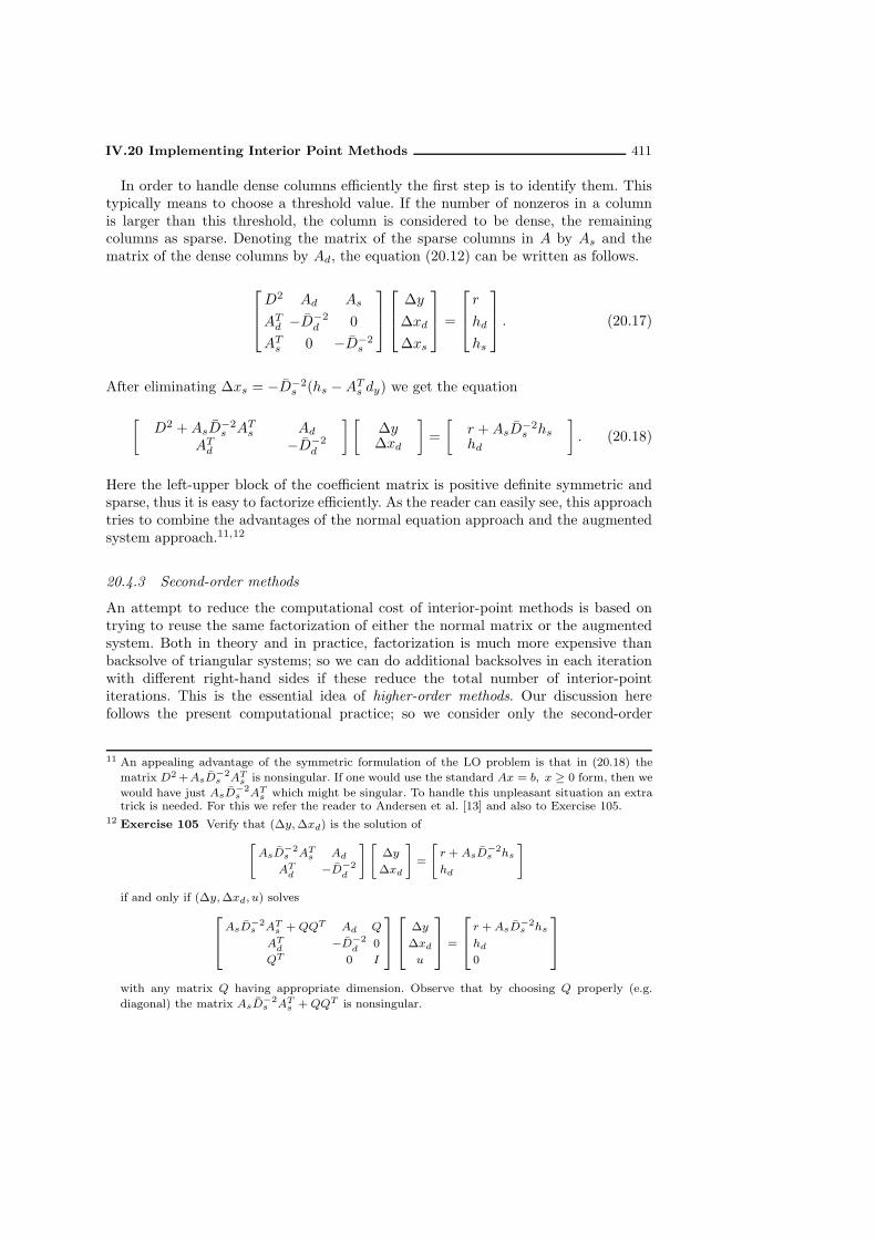
IV.20 Implementing Interior Point Methods 411
In order to handle dense columns efficiently the first step is to identify them. Thistypically means to choose a threshold value. If the number of nonzeros in a columnis larger than this threshold, the column is considered to be dense, the remainingcolumns as sparse. Denoting the matrix of the sparse columns in A by As and thematrix of the dense columns by Ad, the equation (20.12) can be written as follows.
D2 Ad As
ATd −D−2
d 0
ATs 0 −D−2
s
∆y
∆xd
∆xs
=
r
hd
hs
. (20.17)
After eliminating ∆xs = −D−2s (hs −AT
s dy) we get the equation
[D2 +AsD
−2s AT
s Ad
ATd −D−2
d
] [∆y∆xd
]=
[r +AsD
−2s hs
hd
]. (20.18)
Here the left-upper block of the coefficient matrix is positive definite symmetric andsparse, thus it is easy to factorize efficiently. As the reader can easily see, this approachtries to combine the advantages of the normal equation approach and the augmentedsystem approach.11,12
20.4.3 Second-order methods
An attempt to reduce the computational cost of interior-point methods is based ontrying to reuse the same factorization of either the normal matrix or the augmentedsystem. Both in theory and in practice, factorization is much more expensive thanbacksolve of triangular systems; so we can do additional backsolves in each iterationwith different right-hand sides if these reduce the total number of interior-pointiterations. This is the essential idea of higher-order methods. Our discussion herefollows the present computational practice; so we consider only the second-order
11 An appealing advantage of the symmetric formulation of the LO problem is that in (20.18) the
matrix D2+AsD−2s AT
s is nonsingular. If one would use the standard Ax = b, x ≥ 0 form, then we
would have just AsD−2s AT
s which might be singular. To handle this unpleasant situation an extratrick is needed. For this we refer the reader to Andersen et al. [13] and also to Exercise 105.
12Exercise 105 Verify that (∆y,∆xd) is the solution of
[AsD
−2s AT
s Ad
ATd
−D−2d
][∆y
∆xd
]=
[r + AsD
−2s hs
hd
]
if and only if (∆y,∆xd, u) solves
AsD
−2s AT
s +QQT Ad Q
ATd
−D−2d
0
QT 0 I
∆y
∆xdu
=
r +AsD
−2s hs
hd0
with any matrix Q having appropriate dimension. Observe that by choosing Q properly (e.g.
diagonal) the matrix AsD−2s AT
s +QQT is nonsingular.

412 IV Miscellaneous Topics
predictor-corrector method that is implemented in several codes with great success.13
Predictor-corrector technique
This predictor-corrector method has two components. The first is an adaptive choiceof the barrier parameter µ; the other is a second-order approximation of the centralpath .The first step in the predictor-corrector algorithm is to compute the primal-dual
affine-scaling (predictor) direction. This is the solution of the Newton system (20.4)with µ = 0 and is indicated by ∆a. It is easy to see that if a step of size α is takenin the affine-scaling direction, then the duality gap is reduced by α; i.e. if a large stepcan be made in this direction then significant progress is made in the optimization. Ifthe feasible step-size in the affine-scaling direction is small, we expect that the currentpoint is close to the boundary; thus centering is needed and µ should not be reducedtoo much.In the predictor-corrector algorithm, first the predicted duality gap is calculated
that results from a step along the primal-dual affine-scaling direction. To this end,when the affine-scaling direction is computed, the maximum primal (αa
P ) and dual(αa
D) feasible step sizes are determined that preserve nonnegativity of (x, zu, z) and(s, yu, y). Then the predicted duality gap
ga = (x + αaP∆
ax)T (s+ αaD∆as) + (zu + αa
P∆azu)
T (yu + αaD∆ayu)
+(z + αaP∆
az)T (y + αaD∆ay)
is computed and is used to determine a target point
µ =(gag
)2 gan
(20.19)
on the central path . Here ga/n relates to the central point with the same duality gap
that the predictor affine step would produce, and the factor (ga/g)2 pushes the target
further towards optimality in a way that depends on the achieved reduction of thepredictor step. Now the second-order component of the predictor-corrector directionis computed. Ideally we would like to compute a step such that the next iterate isperfectly centered, i.e.,
(x+∆x)(s +∆s) = µe,
(zu +∆zu)(yu +∆yu) = µe,
(z +∆z)(y +∆y) = µe,
13 The second-order predictor-corrector technique presented here is due to Mehrotra [205]; from acomputational point of view the method is very successful. The higher than order 2 methods —discussed in Chapter 18 — are implementable too, but to date computational results with methodsof order higher than 2 are quite disappointing. See Andersen et al. [10]. Mehrotra was motivatedby the paper of Monteiro, Adler and Resende [220], who were the first to introduce the primal-dualaffine-scaling direction and higher-order versions of the primal-dual affine-scaling direction; theyelaborated on a computational paper of Adler, Karmarkar, Resende and Veiga [2] that uses thedual affine-scaling direction and higher-order versions of it.

IV.20 Implementing Interior Point Methods 413
or equivalently
x∆s+ s∆x = −xs+ µe−∆x∆s,
zu∆yu + yu∆zu = −zuyu + µe−∆zu∆yu,
z∆y + y∆z = −zy + µe−∆z∆y.
Usually, in the computation of the Newton direction the second-order terms
∆x∆s, ∆zu∆yu, ∆z∆y
are neglected (recall (20.4)). Instead of neglecting the second-order term, the affinedirections
∆ax,∆as, ∆azu∆ayu, ∆
az∆ay
are used as the predictions of the second-order effect. One step of the algorithm canbe summarized as follows.
• Solve (20.4) with µ = 0, resulting in the affine step (∆ax,∆azu,∆az) and
(∆as,∆ayu,∆ay).
• Calculate the maximal feasible step lengths αaP and αa
D.• Calculate the predicted duality gap ga and µ by (20.19).• Solve the corrected Newton system
A∆x −∆z = 0
∆x+∆zu = 0
AT∆y −∆yu +∆s = 0
x∆s+ s∆x = −xs+ µe−∆ax∆as, (20.20)
zu∆yu + yu∆zu = −zuyu + µe−∆azu∆ayu,
z∆y + y∆z = −zy + µe−∆az∆ay.
• Calculate the maximal feasible step lengths αP and αD and make a damped stepby using (20.9).14
Finally, observe that a single iteration of this second-order predictor-corrector primal-dual method needs two solves of the same large, sparse linear system (20.4) and (20.20)for two different right-hand sides. Thus the same factorization can be used twice.
20.5 Starting point
The self-dual embedding problem is an elegant theoretical construction for handlingthe starting point problem. At the same time it can also be the basis of an efficientimplementation. In this section we show that solving the slightly larger embedding
14 This presentation of the algorithm follows the paper of Mehrotra [205]. It differs from the 2-ordermethod of Chapter 18.

414 IV Miscellaneous Topics
problem does not increase the computational cost significantly.15 Before presentingthe embedding problem, we summarize some of its surprisingly nice properties.
1. The embedding problem is self-dual: the dual problem is identical to the primalone.
2. It is always feasible. Furthermore, the interior of the feasible set of the embeddingproblem is also nonempty; hence the optimal faces are bounded (from TheoremII.10). So interior-point methods always converge to an optimal solution.
3. Optimality of the original problem is detected by convergence, independently ofthe boundedness or unboundedness of the optimal faces of the original problem.
4. Infeasibility of the original problem is detected by convergence as well.16 Primal,dual or primal and dual rays for the original problems are identified to prove dual,primal or dual and primal infeasibility (cf. Theorem I.26).
5. For the embedding problem a perfectly centered initial pair can always beconstructed.
6. It allows an elegant handling of the warm start problem.7. The embedding problem can be solved with any method that generates a strictly
complementary solution; if the chosen method is polynomial, it solves the originalproblem with essentially the same complexity bound. Thus we can achieve the bestpossible complexity bounds for solving an arbitrary problem.
Self-dual embedding
We consider problems (20.1) and (20.2). To formulate the embedding problem weneed to introduce some further vectors in a way similar to that of Chapter 2. We startwith
x0 > 0, z0u > 0, z0 > 0, s0 > 0, y0u > 0, y0 > 0, κ0 > 0, ϑ0 > 0, ρ0 > 0, ν0 > 0,
where x0, z0u, s0, y0u ∈ IRn, y0, z0 ∈ IRm and κ0, ϑ0, ρ0, ν0 ∈ IR are arbitrary. Then we
define b ∈ IRm, bu, c ∈ IRn, the scaled error at the arbitrary initial interior solutions(recall the construction in Section 4.3), and parameters β, γ ∈ IR as follows:
bu =1
ϑ0(buκ
0 − x0 − z0u)
b =1
ϑ0(bκ0 −Ax0 + z0)
c =1
ϑ0(cκ0 + y0u −AT y0 − s0)
β =1
ϑ0(cTx0 − bTy0 + bTu y
0u + ν0)
15 Such embedding was first introduced by Ye, Todd and Mizuno [316] using the standard formproblems (20.29) and (20.30). They discussed most of the advantages of this embedding and showedthat Mizuno, Todd and Ye’s [217] predictor-corrector algorithms solve the LO problem in O(
√nL)
iterations, yielding the first infeasible IPM with this complexity. Somewhat later Jansen, Roos andTerlaky [155] presented the self-dual problem for the symmetric form primal-dual pair in a conciseintroduction to the theory of LO based on IPMs.
16 The popular so-called infeasible-start methods detect unboundedness or infeasibility of the originalproblem by divergence of the iterates.

IV.20 Implementing Interior Point Methods 415
γ = βκ0 + bT y0 − buy0u − cTx0 + ρ0
=1
ϑ0[(x0)T s0 + (y0u)
T z0u + (y0)T z0 + κ0ρ0] + ρ0 > 0.
It is worth noting that if x0 is strictly feasible for (20.1), κ0 = 1, z0 = Ax0 − b andz0u = bu − x0, then b = 0 and bu = 0. Also if (y0, y0u) is strictly feasible for (20.2),κ0 = 1 and s0 = c − AT y + y0u, then c = 0. In some sense the vectors b, bu and cmeasure the amount of scaled infeasibility of the given vectors x0, z0, z0u, s
0, y0, y0u.Now consider the following self-dual LO problem:
(SP) min γϑ
s.t. −x +buκ −buϑ ≥ 0
Ax −b κ +b ϑ ≥ 0
yu −AT y +c κ −c ϑ ≥ 0
−bTuyu +bTy −cTx +β ϑ ≥ 0
bTu yu −bTy +cTx −β κ ≥ −γyu ≥ 0, y ≥ 0, x ≥ 0, κ ≥ 0, ϑ ≥ 0.
Let us denote the slack variables for the problem (SP ) by zu, z, s, ν and ρrespectively. By construction the positive solution x = x0, z = z0, zu = z0u, s =s0, y = y0, yu = y0u, κ = κ0, ϑ = ϑ0, ν = ν0, ρ = ρ0 is interior feasible for problem(SP). Also note that if, e.g., we choose x = x0 = e, z = z0 = e, zu = z0u = e, s =s0 = e, y = y0 = e, yu = y0u = e, κ = κ0 = 1, ϑ = ϑ0 = 1, ν = ν0 = 1, ρ = ρ0 = 1,then this solution with µ = 1 is a perfectly centered initial solution for problem (SP).The following theorem follows easily in the same way as Theorem I.20.17
Theorem IV.85 The embedding (SP ) of the given problems (20.1) and (20.2) hasthe following properties:
(i) The self-dual problem (SP ) is feasible and hence both primal and dual feasible.Thus it has an optimal solution.
(ii) For any optimal solution of (SP), ϑ∗ = 0.(iii) (SP ) always has a strictly complementary optimal solution (y∗u, y
∗, x∗, κ∗, ϑ∗).(iv) If κ∗ > 0, then x∗/κ∗ and (y∗, y∗u)/κ
∗ are strictly complementary optimalsolutions of (20.1) and (20.2) respectively.
(v) If κ∗ = 0, then either (20.1) or (20.2) or both are infeasible.
Solving the embedding model needs just slightly more computation per iterationthan solving problem (20.1). This small extra effort is the cost of having severalimportant advantages: having a centered initial starting point, detecting infeasibilityby convergence, applicability of any IPM without degrading theoretical complexity.The rest of this section is devoted to showing that the computation of the Newtondirection for the embedding problem (SP ) reduces to almost the same sized augmented(20.6) or normal equation (20.7) systems as in the case of (20.1).
17 Exercise 106 Prove this theorem.

416 IV Miscellaneous Topics
In Chapter 3 the self-dual problem
(SP ) minqT x : Mx ≥ −q, x ≥ 0
,
was solved, whereM is of size n×n and skew-symmetric and q ∈ IRn+. Given an initial
positive solution (x, s) > 0, where s =Mx+ q, a Newton step for problem (SP ) witha value µ > 0 was given as
∆s =M∆x,
where ∆x is the solution of the system
(M + X−1S)∆x = µx−1 − s. (20.21)
Now we have to analyze how the positive definite system (20.21) can be efficientlysolved in the case of problem (SP). For this problem we have x = (yu, y, x, κ, ϑ),s = (zu, z, s, ν, ρ) and
M =
0 0 −I bu −bu0 0 A −b b
I −AT 0 c −c−bTu bT −cT 0 β
bTu −bT cT −β 0
and q =
0
0
0
0
γ
.
Hence the Newton equation (20.21) can be written as
Y −1u Zu 0 −I bu −bu0 Y −1Z A −b b
I −AT X−1S c −c−bTu bT −cT ν
κ β
bTu −bT cT −β ρϑ
∆yu
∆y
∆x
∆κ
∆ϑ
=
µy−1u − zu
µy−1 − z
µx−1 − s
µ 1κ − ν
µ 1ϑ − ρ
. (20.22)
From the first and the second equation it easily follows that
∆yu = YuZ−1u (∆x − bu∆κ+ bu∆ϑ+ µy−1
u − zu)
and
∆y = Y Z−1(−A∆x+ b∆κ− b∆ϑ+ µy−1 − z).
We simplify the notation by introducing
Wu := Z−1u Yu.

IV.20 Implementing Interior Point Methods 417
Then, by substituting the value of ∆yu in (20.22) we find18
Y −1Z A −b b
−AT X−1S +Wu c−Wubu −c+Wubu
bT −cT − bTuWuνκ + bTuWubu β − bTuWubu
−bT cT + bTuWu −β − bTuWubuρϑ + bTuWubu
∆y
∆x
∆κ
∆ϑ
=
r1
r2
r3
r4
, (20.23)
where for simplicity the right-hand side elements are denoted by r1, . . . , r4. Now if wemultiply the second block of equations (corresponding to the right-hand side r2) in(20.23) by −1, a system analogous to the augmented system (20.6) of problem (20.1) isobtained. The difference is that here we have two additional constraints and variables.For the solution of this system, the factorization of the matrix may happen in thesame way, but the last two rows and columns (these are typically dense) should beleft to the last two steps of the factorization. A 2× 2 dense window for (∆κ,∆ϑ) thenremains.If we further simplify (20.23) by substituting the value of ∆y, the analogue to the
normal equation system of the problem (SP ) is produced. For simplicity the scalarshere are denoted by η1, . . . , η8 and r5, r6, r7.
19,20
ATZ−1Y A+X−1S + Z−1u Yu η1 η2
η3 η4 η5
η6 η7 η8
∆x
∆κ
∆ϑ
=
r5
r6
r7
. (20.24)
18 Exercise 107 Verify that
r1
r2
r3
r4
=
µy−1 − z
µx−1 − s− (µz−1u − yu)
µ 1κ− ν + bTu (µz−1
u − yu)
µ 1ϑ− ρ− bTu (µz−1
u − yu)
.
19 Exercise 108 Verify that
η1 = c−Wubu −ATZ−1Y b
η2 = −c+Wubu +ATZ−1Y b
η3 = −cT − bTuWu − bTZ−1Y A
η4 = νκ−1 + bTuWubu + bTZ−1Y b
η5 = β − bTuWubu − bTZ−1Y b
η6 = cT + bTuWu + bTZ−1Y A
η7 = −β − bTuWubu − bTZ−1Y b
η8 = ρϑ−1 + bTuWubu + bTZ−1Y b
and
r5 = µx−1 − s− (µz−1u − yu) +AT (µz−1 − y)
r6 = µκ−1 − ν + bTu (µz−1u − yu)− bT (µz−1 − y)
r7 = µϑ−1 − ρ− bTu (µz−1u − yu) + bT (µz−1 − y).
20 Exercise 109 Develop similar formulas for the normal equation if ∆x is eliminated instead of∆y. Compare the results with (20.7) and (20.8).

418 IV Miscellaneous Topics
20.5.1 Simplifying the Newton system of the embedding model
As mentioned with respect to the augmented system, we easily verify that thedifference between the normal equations of problem (20.1) and the embedding problem(SP ) is that here two additional constraints and variables are present. Note that thelast two rows and columns in (20.23) and (20.24) are neither symmetric nor skew-symmetric. The reader might think that these two extra columns deteriorate theefficiency of the algorithm (it requires two additional back-solves for the computationof the Newton direction) and hence make the embedding approach less attractivein practice. However, the computational cost can easily be reduced by a simpleobservation. First, note that for any interior solution (yu, y, x, κ, ϑ) the duality gap(see also Exercise 10 on page 35) is equal to
2γϑ.
Second, remember that in Lemma II.47 we have proved that in a primal-dual methodthe target duality gap is always reached after a full Newton step. Since the dualitygap on the central path with the value µ equals to
2(m+ 2n+ 2)µ
and thus, the target duality gap is determined by the target value µ+ = (1− θ)µ, thestep ∆ϑ can directly be calculated.
∆ϑ = ϑ+ − ϑ =µ+ − µ
γ(m+ 2n+ 2) = −θµ
γ(m+ 2n+ 2)
As a result we conclude that the value of ∆ϑ in (20.24) is known, thus it can simplybe substituted in the Newton system and the system (20.23) reduces to almost theoriginal size. This simplification allows to implement IPMs based on the self-dualembedding model efficiently, the cost per iteration is only one extra back-solve.
20.5.2 Notes on warm start
Many practical problems need the solution of a sequence of similar linear programswhere small perturbations are made to b and/or c (possibly also in A). As long as theseperturbations are small, we naturally expect that the optimal solutions are not far fromeach other and restarting the optimization from the solution of the old problem (warmstart) should be more efficient than solving the problem from scratch.21
The difficulty in the IPM warm start comes from the fact that the old optimalsolution is very close to the boundary (this is a necessity since all optimal solutions inan LO problem are on the boundary of the feasible set) and well centered. This point,in the perturbed problem, still remains close to the boundary or becomes infeasible,but even if it remains feasible it is very poorly centered. Consequently, the IPMmakes a long sequence of short steps because the iterates cannot get away from theboundary. Therefore for an efficient warm start we need a well-centered point close to
21 Some early attempts to solve such problems are due to Freund [84] who uses shifted barriers, andPolyak [234] who applies modified barrier functions. For further elaboration of the literature see,e.g., Lustig, Marsten and Shanno [193], Gondzio and Terlaky [116] and Andersen et al. [10].

IV.20 Implementing Interior Point Methods 419
the old optimal one or an efficient centering method (to get far from the boundary)to overcome these difficulties. These two possibilities are discussed briefly below.Independent of the approach chosen it would be wise to save a well-centered almost
optimal solution (say, with 10−2 relative duality gap) that is still sufficiently far awayfrom the boundary.
• Centered solutions for warm start in (SP ) embedding. Among the specta-cular properties of the (SP ) embedding listed in the previous section, the ability toconstruct always perfectly centered initial interior points was mentioned. The oldwell-centered almost optimal solution x∗, z∗, z∗u, s
∗, y∗, y∗u, κ∗, ϑ∗, ρ∗, ν∗ can
be used as the initial point for embedding the perturbed problem. As we have seenin Section 20.5, b, c, β and γ can always be redefined so that the above solutionstays well centered. The construction allows simultaneous perturbations of b, bu,c and even the matrix A. Additionally, it extends to handling new constraints orvariables added to the problem (e.g., in buildup or cutting plane schemes). In thesecases, we can keep the solution for the old coordinates (let µ be the actual barrierparameter) and set the initial value of the new complementary variables equal to√µ. This results in a perfectly centered initial solution.
• Efficient centering. If the old solution remains feasible, but is badly centered, wemight proceed with this solution without making a new embedding. The commonapproach is to use a path-following method for the recentering process; it usestargets on the central path . Because of the weak performance of Newton’s methodfar off the central path, this approach is too optimistic for a warm start. The target-following method discussed in Part III (Section 11.4) offers much more flexibilityin choosing achievable targets, thus leading to efficient ways of centering. A targetsequence that improves centrality allows larger steps and therefore speeds up thecentering and, as a consequence, the optimization process.22
20.6 Parameters: step-size, stopping criteria
20.6.1 Target-update
The easiest way to ensure that all iterates remain close to the central path is todecrease µ by a very small amount at each iteration. This provides the best theoreticalworst-case complexity, as we have seen in discussing full Newton step methods. Thesemethods demonstrate hopelessly slow convergence in practice and their theoreticalworst-case complexity is identical to their practical performance.In large-update methods the barrier parameter is reduced much faster than the theory
suggests. To preserve polynomial convergence of these methods in theory, severalNewton steps are computed between two reductions of µ (update of the target) untilthe iterate is in a sufficiently small neighborhood of the central path . In practice thismultistep strategy is ignored and at each reduction of µ, at each target-update, onlyone Newton step is made. A drawback of this strategy is that the iterates might get
22 Computational results based on centering target sequences are presented in Gondzio [114] andAndersen et al. [10].

420 IV Miscellaneous Topics
far away from the central path or from the target point, and the efficiency of theNewton method might deteriorate. A careful strategy for updating µ and for step-length selection reduces the danger of this negative scenario.At an interior iterate the current duality gap is given by
g = xT s+ zTu yu + zT y,
which is equal to (2n +m)µ if the iterate is on the central path . The central pointwith the same duality gap as the current iterate belongs to the value
µ =xT s+ zTu yu + zT y
2n+m.
The target µ value is chosen so that the target duality gap is significantly smaller, butdoes not put the target too far away. Thus we take
µnew = (1− θ)xT s+ zTu yu + zTy
2n+m, (20.25)
where θ ∈ [0, 1]. The value θ = 0 corresponds to pure centering, while θ < 1 aims toreduce the duality gap. A solid but still optimistic update is θ = 3
4 .23
20.6.2 Step size
Although there is not much supporting theory, current implementations use very largeand different step-sizes in the primal and dual spaces.24 All implementations use avariant of the following strategy. First the maximum possible step-sizes are computed:
αP := max α > 0 : (x, z, zu) + α(∆x,∆z,∆zu) ≥ 0,and αD := max α > 0 : (s, y, yu) + α(∆s,∆y,∆yu) ≥ 0,
and these step-sizes are slightly reduced by a factor α0 = 0.99995 to ensure that thenew point is strictly positive. Although this aggressive, i.e. very large, choice of α0
is frequently reported to be the best, we must be careful and include a safeguard tohandle the case when α0 = 0.99995 turns out to be too aggressive.
20.6.3 Stopping criteria
Interior point algorithms terminate when the duality gap is small enough and thecurrent solution is feasible for the original problems (20.1) and (20.2), or when the
23 In the published literature, iteration counts larger than 50 almost never occur and most frequentlyiteration numbers around 20 are reported. Taking this number as a target iteration count andassuming that (in contrast to the theoretical worst-case analysis) Newton’s method provides iteratesalways close to the target point, we can calculate how large the target-update (how small (1− θ))should be to reach the desired accuracy within the required number of iterations. Thus, for aproblem with 104 variables and a centered initial solution with µ = 1 and aiming for a solutionwith 8 digits of accuracy, we have to reduce the duality gap by a factor of 1012 in 20 iterations.By straightforward calculation we can easily verify that the value θ = 3
4is an appropriate choice
for this purpose.24 Kojima, Megiddo and Mizuno [174] proved global convergence of a primal-dual method that allows
such large step-sizes in most iterations.

IV.20 Implementing Interior Point Methods 421
infeasibility is small enough. The practical tolerances are larger than the theoreticalbounds that guarantee identification of an exact solution; this is a common drawbackof all numerical algorithms for solving LO problems. To obtain a sensible solution theduality gap and the measure of infeasibility should be related to the problem data.Relative primal infeasibility is related to the length of the vectors b and bu, dualinfeasibility is related to the length of the vector c, and the duality gap is related tothe actual objective value. A solution with p digits relative accuracy is guaranteed bythe stopping criteria presented here:
||Ax− z − b||1 + ||b|| ≤ 10−p and
||x+ zu − bu||1 + ||bu||
≤ 10−p, (20.26)
||c−AT y + yu − s||1 + ||c|| ≤ 10−p, (20.27)
|cTx− (bT y − bTu yu)|1 + |cTx| ≤ 10−p. (20.28)
An 8-digit solution (p = 8) is typically required in the literature. Let us observethat conditions (20.26–20.28) still depend on the scaling of the problem and somehowuse the assumption that the coefficients of the vectors b, bu, c are about the samemagnitude as those of the matrix A — preferably near 1.An important note is needed here. The theoretical worst-case bound O(
√n log 1
ε )is still far from computational practice. It is still extremely pessimistic; in practicethe number of iterations is something like O(log n). It is rare that the currentimplementations of interior-point methods use more than 50 iterations to reach an8-digit optimal solution.
20.7 Optimal basis identification
20.7.1 Preliminaries
An optimal basis identification procedure is an algorithm that generates an optimal
basis and the related optimal basic solutions from an arbitrary primal-dual optimalsolution pair. In this section we briefly recall the notion of an optimal basis. In orderto ease the discussion we use the standard format:
mincTx : Ax = b, x ≥ 0
, (20.29)
where c, x,∈ IRn, b ∈ IRm, and the matrix A is of size m× n. The dual problem is
maxbT y : AT y + s = c, s ≥ 0
, (20.30)
where y ∈ IRm and s ∈ IRn. We assume that A has rankm. A basis AB is a nonsingularrank m submatrix of A, where the set of column indices of AB is denoted by B. Abasic solution of the primal problem (20.29) is a vector x where all the coordinates inN = 1, . . . , n−B are set to zero and the basis coordinates form the unique solutionof the equation ABxB = b. The corresponding dual basic solution is defined as theunique solution of AT
By = cB, along with sB = 0 and sN = cN −ATN y. It is clear from

422 IV Miscellaneous Topics
this definition that a primal-dual pair (x, s) of basic solutions is always complementary,and hence, if both x and s are feasible, they are primal and dual optimal, respectively.A basic solution is called primal (dual) degenerate if at least one component of xB(sN ) is zero.There might be two reasons in practice to require an optimal basic solution for an
LO problem.
1. If the given problem is a mixed integer LO problem then some or all of the variablesmust be integer. After solving the continuous relaxation we have to generate cutsto cut off the nonintegral optimal solution. To date, such cuts can be generatedonly if an optimal basic solution is available.25 Up till now there has been only oneattempt to design a cut generation procedure within the interior-point setting (seeMitchell [211]).
2. In practical applications of LO, a sequence of slightly perturbed problems oftenhas to be solved. This is the case in combinatorial optimization when new cutsare added to the problem or if a branch and bound algorithm is applied. Also if,e.g., in production planning models the optimal solutions for different scenariosare calculated and compared, we need to solve a sequence of slightly perturbedproblems. When such closely related problems are solved, we expect that theprevious optimal solution can help to solve the new problem faster. Although somemethods for potentially efficient warm start were discussed in Section 20.5.2, insome cases it might be advantageous in practice to use Simplex type solvers initiatedwith an old optimal basis.
In this section we describe how an optimal basic solution can be obtained from anyoptimal solution pair of the problem.
20.7.2 Basis tableau and orthogonality
We introduce briefly the notions of basis tableau and pivot transformation and weshow how orthogonal vectors can be obtained from a basis tableau. Let A be theconstraint matrix, with columns aj for 1 ≤ j ≤ n, and let AB be a basis chosen fromthe columns of A. The basis tableau QB corresponding to B is defined by the equation
ABQB = A. (20.31)
Because this gives no rise to confusion we write below Q instead of QB. The rows ofQ are naturally indexed by the indices in B and the columns by 1, 2, . . . , n. If i ∈ Band j = 1, 2, . . . , n the corresponding element of Q is denoted by qij . See Figure 20.1(page 423). It is clear that qij is the coefficient of ai in the unique basis representationof the vector aj :
aj =∑
i∈Bqijai.
For j ∈ B this implies
qij =
1 if i = j,
0 otherwise,
25 The reader may consult the books of Schrijver [250] and Nemhauser and Wolsey [224] to learnabout combinatorial optimization.

IV.20 Implementing Interior Point Methods 423
· · · j · · ·
i ∈ B
. .
. .
. .
i · · · qij · · ·
. .
. .
. .
Figure 20.1 Basis tableau.
Thus, if j ∈ B, the corresponding column in Q is a unit vector with its 1 in the rowcorresponding to j. Hence, by a suitable reordering of columns QB — the submatrixof Q consisting of the columns indexed by B — becomes an identity matrix. It isconvenient for the reasoning if this identity matrix occupies the first m columns.Therefore, by permuting the columns of Q by a permutation matrix P we write
QP =[I QN
], (20.32)
where QN denotes the submatrix of Q arising when the columns of QB are deleted.In the next section, where we present the optimal basis identification procedure,
we will need a well-known orthogonality property of basis tableaus.26 This propertyfollows from the obvious matrix identity
[I QN
] QN
−I
= 0.
Because of (20.32) this can be written as
QP
QN
−I
= 0. (20.33)
Defining
R := P
QN
−I
, (20.34)
we have rankQ = m, rankR = n −m and QR = 0. We associate with each index avector in IRn as follows. If i ∈ B, q(i) will denote the corresponding row of Q and ifj ∈ N then q(j) is the corresponding column of R.
Clearly, the vectors q(i), i ∈ B, span the row space of Q = QB and the vectors q(j),j ∈ N , span the column space of R. Since these spaces are orthogonal, they are each
26 See, e.g., Rockafellar [238] or Klafszky and Terlaky [171].

424 IV Miscellaneous Topics
others orthogonal complement. Note that the row space of Q is the same as the rowspace of A. We thus see that the above spaces are independent of the basis B.Now let AB′ be another basis for A and let q′(j) denote the vector associated with
an index j 6∈ B′. Then the aforementioned orthogonality property states that
q(i) ⊥ q′(j)
for all i ∈ B and j 6∈ B′. This is an obvious consequence of the observation in theprevious paragraph.It is well known that the basis tableau for B′ can be obtained from the tableau for
B by performing a sequence of pivot operations. A pivot operation replaces a basisvector ai, i ∈ B by a nonbasic vector aj, j /∈ B, where qij 6= 0.27
Example IV.86 For better understanding let us consider a simple numerical exam-ple. The following two basic tableaus can be transformed into each other by a singlepivot.
a1 a2 a3 a4 a5 a1 a2 a3 a4 a5
a5 2 1 3 0 1 a2 2 1 3 0 1
a4 –1 –1 4 1 0 a4 1 0 7 1 1
It is easy to check that for the first tableau q(3) = (0, 0,−1, 4, 3) and for the second
tableau q(4) = (1, 0, 7, 1, 1), and that these vectors are orthogonal.28,29 ♦
20.7.3 The optimal basis identification procedure
Given any complementary solution, the algorithm presented below constructs anoptimal basis in at most n iterations.30 Since the iteration count and thus the numberof necessary arithmetic operations depends only on the dimension of the problem andis independent of the actual problem data, the algorithm is called strongly polynomial.The algorithm can be initialized with any optimal (and thus complementary)
solution pair (x, s). This pair defines a partition of the index set as follows:
B = i | xi > 0, N = i : si > 0, T = i : xi = si = 0.
27 Exercise 110 Let i ∈ B, where AB is a basis. For any j 6∈ B such that qij 6= 0 show thatB′ = (B \ i) ∪ j also defines a basis, and the tableau for B′ can be obtained from the tableaufor B by one pivot operation.
28 Exercise 111 For each of the tableaus in Example IV.86, give the permutation matrix P and thematrix R according to (20.33) and (20.34).
29 Exercise 112 For each of the tableaus in Example IV.86, give a full bases of the row space of thetableau and of its orthogonal complement.
30 The algorithm discussed here was proposed by Megiddo [201]. He has also proved that an optimalbasis cannot be constructed only from a primal or dual optimal solution in strongly polynomialtime unless there exists a strongly polynomial algorithm for solving the LO problem. The problemof constructing a vertex solution from an interior-point solution has also been considered byMehrotra [203].

IV.20 Implementing Interior Point Methods 425
As we have seen in Section 3.3.6, interior-point methods produce a strictly comple-mentary optimal solution and hence such a solution gives a partition with T = ∅. Butbelow we deal with the general case and we allow T to be nonempty.The optimal basis identification procedure consists of three phases. In the first phase
a so-called maximal basis is constructed. A basis of A is called maximal with respectto (x, s) if
• it has the maximum possible number of columns from AB ,• it has the maximum possible number of columns from (AB , AT ).
Then, in the second and third phases, independently of each other, primal and dualelimination procedures are applied to produce primal and dual feasible basic solutionsrespectively.Note that a maximal basis is not unique and not necessarily primal and/or dual
feasible. A maximal basis can be found by the following simple pivot algorithm.Because of the assumption rank (A) = m, all the artificial basis vectors e1, · · · , em
Initial basis
Input:Optimal solution pair (x, s) and the related partition (B,N, T );artificial basis an+1 = e1, · · · , an+m = em;B = n+ 1, · · · , n+m.
Output:A maximal basis B ⊆ 1, · · · , n.
beginwhile qij 6= 0, i > n, j ∈ AB dobegin
pivot on position (i, j) (ai leaves and aj enters the basis);B := (B \ i) ∪ j .
end
while qij 6= 0, i > n, j ∈ AT dobegin
pivot on position (i, j) (ai leaves and aj enters the basis);B := (B \ i) ∪ j .
end
while qij 6= 0, i > n, j ∈ AN dobegin
pivot on position (i, j) (ai leaves and aj enters the basis);B := (B \ i) ∪ j .
endend
are eliminated from the basis at termination. Since the AB part is investigated first,the number of basis vectors from AB is maximal; similarly the number of basis vectorsfrom [AB , AT ] is also maximal. In a practical implementation, special attention must

426 IV Miscellaneous Topics
be given to the selection of the pivot elements in the above algorithm. Typically thereis lot of freedom in the pivot selection, since a large number of leaving and/or enteringvariables could be selected at each iteration.31 The structure of the basis tableauresulting from the algorithm is visualized in Figure 20.2. Note that the tableau isnever computed in practice; just the basis, in a factorized form. The tableau form isused just to ease the explanation and understanding.
AB AT AN
1
i ∈ B ∩B . . .
11
i ∈ B ∩ T 0. . .
11
i ∈ B ∩N 0 0. . .
1
Figure 20.2 Tableau for a maximal basis.
We proceed by a primal and a dual phase, performed independently of each other.They make the basis primal and dual feasible, respectively.Observe that in the elimination step of the first while-loop of the primal phase the
columns of ABare dependent. Hence there exists a nonzero solution of A
BxB = 0.32 In
the elimination step the ‘maximal’ property of the basis is lost, but it is restored in the
second while-loop. As we can see, the Primal phase works only on the(A
B, A
T
)part
of the matrix A. In fact it reduces the ABpart to an independent set of column vectors.
At termination the maximal basis is primal feasible and x is the corresponding primalfeasible basic solution, i.e., xB = A−1
B b ≥ 0 and xN = 0. The number of eliminations inthe first while-loop is at most |B| − rank (B) and the number of pivots in the secondwhile-loop is also at most |B| − rank (B).The Dual phase presented below works on the (AT , AN ) part. It reduces AN and
extends AT so that no vector from AN remains in the basis.Note that in the elimination step of the first while-loop the rank of [AB , AT
]
is less than m.33 In the elimination step the ‘maximal’ property of the basis is
31 We would like to choose always the pivot element that produces the least fill-in in the inverse basis.For this pivot selection problem many heuristics are possible. It can at least locally be optimized by,e.g., the heuristic Markowitz rule (recall Section 20.4). Implementation issues related to optimalbasis identification procedures are discussed in Andersen and Ye [11], Andersen et al. [10] andBixby and Saltzman [43].
32 In fact, an appropriate x can be read from the tableau. Because of the orthogonality property any
vector q(j) for j ∈ B − B can be used. In a practical implementation the tableau is not available;
only the (factorized) basis matrix QB is available. But then a vector q(j) can be obtained bycomputing a single nonbasic column of the tableau.
33 For an appropriate s we can choose any vector q(i) for i ∈ N ∩ B; so only one row of the tableauhas to be computed at each execution of the first while-loop.

IV.20 Implementing Interior Point Methods 427
Primal phase
Input:Optimal solution pair (x, s) and the related partition (B,N, T );maximal basis B.
Output:A maximal basis B ⊆ 1, · · · , n;optimal solution (x, s), partition (B,N, T ) with B ⊂ B.
begin
while B 6⊆ B dobegin
beginlet x be such that A
BxB= 0, x
T∪N= 0, x 6= 0;
eliminate a(t least one) coordinate of x, let x := x− ϑx ≥ 0;
B := σ(x), T := 1, . . . , n \(B ∪N
);
end
while qij 6= 0, i ∈ T ∩ B, j ∈ B dobegin
pivot on position (i, j) (ai leaves, aj enters the basis);B := (B \ i) ∪ j .
endend
end
lost but is restored in the second while-loop. At termination the maximal basisis dual feasible and s is the corresponding dual feasible basic solution, i.e., sN =cN −AT
N (A−1B )T cB and sB = 0. The number of eliminations in the first while-loop is
at most m− rank (AB , AT ) and the number of pivots in the second while-loop is alsoat most m− rank (AB , AT ).To summarize, by first constructing a maximal basis and then performing the primal
and dual phases, the above algorithm generates an optimal basis after at most niterations. First we need at most m pivots to construct the maximal basis, then in theprimal phase |B| − rank (B) and in the dual phase m − rank (AB , AT ) pivots follow.Finally, to verify the n-step bound, observe that after the initial maximal basis isconstructed, each variable might enter the basis at most once.
20.7.4 Implementation issues of basis identification
In the above basis identification algorithm it is assumed that a pair of exactprimal/dual optimal solutions is known. This is never the case in practice. Interiorpoint algorithms generate only a sequence converging to optimal solutions and becauseof the finite precision of computations the solutions are neither exactly feasible norcomplementary. Somehow we have to make a decision about which variables are
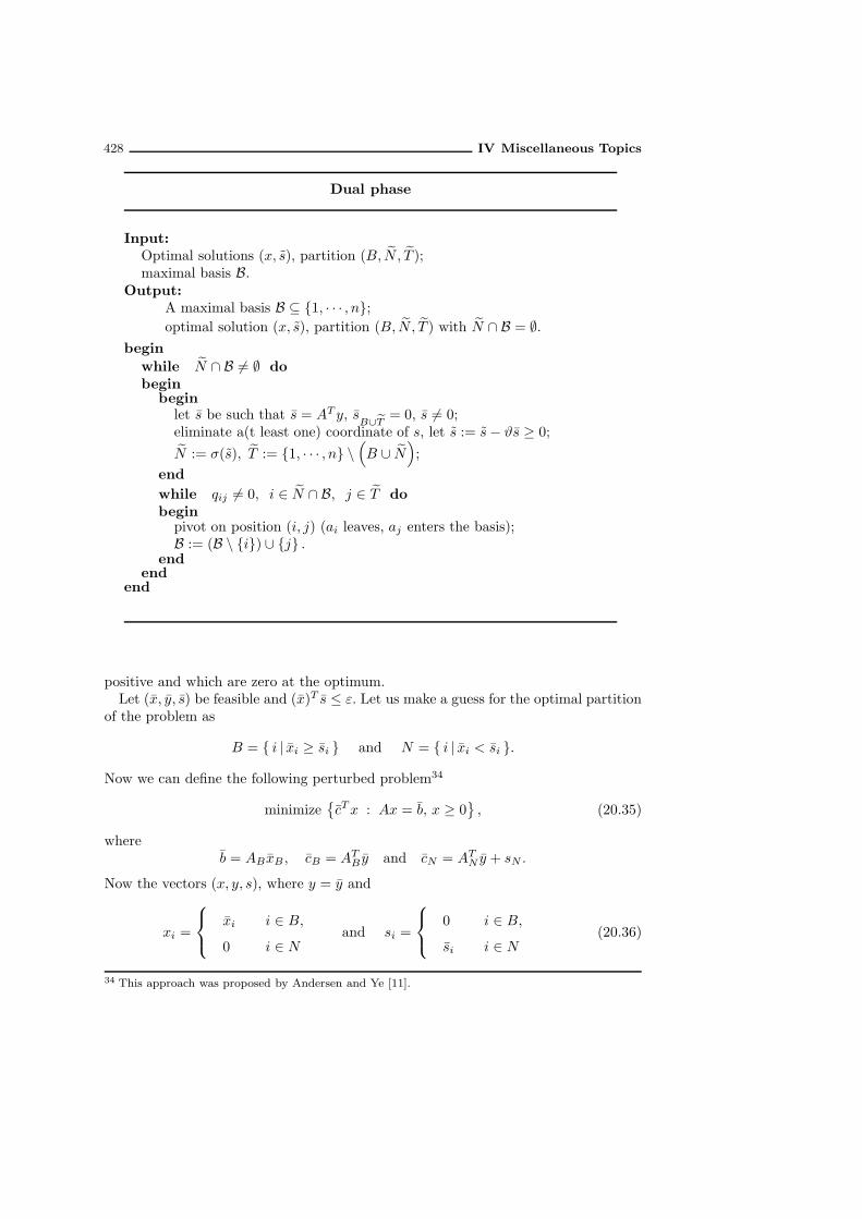
428 IV Miscellaneous Topics
Dual phase
Input:Optimal solutions (x, s), partition (B, N , T );maximal basis B.
Output:A maximal basis B ⊆ 1, · · · , n;optimal solution (x, s), partition (B, N , T ) with N ∩ B = ∅.
begin
while N ∩ B 6= ∅ dobegin
beginlet s be such that s = AT y, s
B∪T= 0, s 6= 0;
eliminate a(t least one) coordinate of s, let s := s− ϑs ≥ 0;
N := σ(s), T := 1, · · · , n \(B ∪ N
);
end
while qij 6= 0, i ∈ N ∩ B, j ∈ T dobegin
pivot on position (i, j) (ai leaves, aj enters the basis);B := (B \ i) ∪ j .
endend
end
positive and which are zero at the optimum.Let (x, y, s) be feasible and (x)T s ≤ ε. Let us make a guess for the optimal partition
of the problem as
B = i | xi ≥ si and N = i | xi < si .
Now we can define the following perturbed problem34
minimizecTx : Ax = b, x ≥ 0
, (20.35)
whereb = ABxB , cB = AT
B y and cN = ATN y + sN .
Now the vectors (x, y, s), where y = y and
xi =
xi i ∈ B,
0 i ∈ Nand si =
0 i ∈ B,
si i ∈ N(20.36)
34 This approach was proposed by Andersen and Ye [11].

IV.20 Implementing Interior Point Methods 429
are strictly complementary optimal solutions of (20.35).35 If ε is small enough,then the partition (B,N) is the optimal partition of (20.29) (recall the results ofTheorem I.47 and observe that the proof does not depend on the specific algorithm,just on the centrality condition and the stopping precision). Thus problems (20.29)and (20.35) share the same partition and the same set of optimal bases. As anoptimal complementary solution for (20.35) is available, the above basis identificationalgorithm can be applied to this perturbed problem. The resulting optimal basis,within a small margin of error (depending on ε), is an optimal basis for (20.29).
20.8 Available software
After twenty years of intensive research, IPMs are now well understood both in theoryand practice. As a result a number of sophisticated implementations exist of IPMs forLO. Below we give a list of some of these codes; some of them contain both a Simplexand an IPM solver. They are capable to solve linear problems on a PC in some minutesthat were hardly solvable on a super computer fifteen years ago.
CPLEX (CPLEX/ BARRIER) (CPLEX Optimization, Inc.). For informationcontact http://www.cplex.com.CPLEX is leading the market at this moment. It is a most complete and robust
package. It contains a primal and a dual Simplex solver, an efficient interior-pointimplementation with cross-over,36 a good mixed-integer code, a network and a qua-dratic programming solver. It is supported by most modelling languages and availablefor most platforms.
XPRESS-MP (DASH Optimization). For information contact the vendor’s WEBpage: http://www.dashoptimization.com.An excellent package including Simplex and IPM solvers. It is almost as complete
as CPLEX.
CLP (The LO solver on COIN-OR). For more information contacthttp://www.coin-or.org/cgi-bin/cvsweb.cgi/COIN/Clp/.COIN-OR’s LO package is written by the IBM Lo team. Like CPLEX, CLP contains
both Simplex and IPM solvers. It is capable to solve linear and quadratic optimizationproblems.
LOQO. Available from http://www.princeton.edu/~rvdb/.LOQO is developed by Vanderbei (Department of Operations Research and
Financial Engineering, Princeton University, Princeton, NJ 08544, USA). It is arobust implementation of a primal-dual infeasible-start IPM for convex quadraticoptimization. LOQO is a commercial package, like CPLEX and OSL, but it is availablefor academic purposes for a modest license fee.
35 Producing a reliable guess for the optimal partition is a nontrivial task. The simple methodpresented by (20.36) seems to work reasonably well in practice. See El-Bakry, Tapia andZhang [71, 70]. However, Andersen and Ye [11] report good results by using a more sophisticatedindicator to predict the optimal partition (B,N) based on the primal-dual search direction.
36 Close to optimality the solver rounds the IPM solution to a (not necessarily optimal) basic solutionand switches to the Simplex solver, that generates an optimal basic solution.

430 IV Miscellaneous Topics
HOPDM. Available fromhttp://www.maths.ed.ac.uk/~gondzio/software/hopdm.html.HOPDM is developed by Gondzio (School of Mathematics, The University of
Edinburgh, Edinburgh, Scotland). It implements a higher order primal-dual method.It is in the public domain — in a form of FORTRAN source files — for academicpurposes.
BPMPD. Available from http://www.sztaki.hu/~meszaros/bpmpd/.Meszaros’ BPMPD, is an implementation of a primal-dual predictor-corrector IPM
including both the normal and augmented system approach. The code is available asan executable file for academic purposes.
LIPSOL. Available from http://www.caam.rice.edu/~yzhang/.Zhang’s LIPSOL is written in MATLAB and FORTRAN. It is an implementation
of the primal-dual predictor-corrector method. One of its features is the use of theMATLAB programming language, which makes its use relatively easy.
PCx. Available from http://www-fp.mcs.anl.gov/otc/Tools/PCx/.This code was developed by Czyzyk, Mehrotra and Wrightat the Argonne National
Lac, Chicago.. It is a stand alone C implementation of an infeasible primal-dualpredictor corrector IPM. PCx is freely available, but is not public domain software
McIPM. Available from http://www.cas.mcmaster.ca/~oplab/index.html.This code was developed at the Advanced Optimization Lab, McMaster University
by Zhu, Peng and Terlaky. McIPM is written in MATLAB and C. It is a uniqueimplementation of a Self-Regular primal-dual predictor-corrector IPM and it is basedon the self-dual embedding model. The use of the MATLAB makes its use relativelyeasy. It is freely available under an open source license.
More information about codes for linear optimization, either for commercial or researchpurposes, are available at the World Wide Web site of LP FAQ (LP Frequently AskedQuestions) at
• http://www-unix.mcs.anl.gov/otc/Guide/faq/linear-programming-faq.html
• ftp://rtfm.mit.edu/pub/usenet/sci.answers/linear-programming-faq

Appendix A
Some Results from Analysis
In Part II we need a result from convex analysis. We include its elementary proof inthis appendix for the sake of completeness. A closely related result can be found inBazaraa et al. [37] (Theorem 3.4.3 and Corollary 1, pp. 101–102). Recall that a subsetC of IRk is called relatively open if C is open in the smallest affine subspace of IRk
containing C.
Proposition A.1 Let f : D → IR be a differentiable function, where D ⊆ IRk is anopen set, and let C be a relatively open convex subset of D such that f is convex onC. Moreover, let L denote the subspace parallel to the smallest affine space containingC. Then, x∗ ∈ C minimizes f over C iff
∇f(x∗) ⊥ L. (A.1)
Proof: Since f is convex on C, we have for any x, x∗ ∈ C,
f(x) ≥ f(x∗) +∇f(x∗)T (x− x∗).
Since x− x∗ ∈ L, the sufficiency of condition (A.1) follows immediately. To prove thenecessity of (A.1), consider xt = x∗+t(x−x∗), with t ∈ IR. The convexity of C impliesthat if 0 ≤ t ≤ 1, then xt ∈ C. Moreover, since C is open, we also have xt ∈ C whent ≥ −a for some positive a. Since f is differentiable, we have
∇f(x∗)T (x− x∗) = limt↓0
f(xt)− f(x∗)t
= limt↑0
f(xt)− f(x∗)t
.
Now let x∗ ∈ C minimize f . Since f(xt) ≥ f(x∗), letting t→ 0 we have that the firstlimit must be nonnegative, and the second nonpositive. Hence both limits are zero. Sowe have ∇f(x∗)T (x− x∗) = 0, ∀x ∈ C. Thus (A.1) follows.
At several places in the book we mention the implicit function theorem. Thereexists many forms of this theorem. See, e.g., Franklin [82], Buck [52], Fiacco [76] orRudin [248]. We cite here a version of Bertsekas [40] (Proposition A.25, pp. 554).1
Proposition A.2 (Implicit Function Theorem) Let f : IRn+m → IRm be afunction of w ∈ IRn and z ∈ IRm such that:
1 In fact, Proposition A.25 in Bertsekas [40] contains a typo. It says that f : IRn+m → IRn insteadof f : IRn+m → IRm.

432 Some Results from Analysis
(i) There exist w ∈ IRn and z ∈ IRm such that f (w, z) = 0.(ii) f is continuous and has a continuous and nonsingular gradient matrix (or
Jacobian) ∇zf (w, z) in an open set containing (w, z).
Then there exists open sets Sw ⊆ IRn and Sz ⊆ IRm containing w and z, respectively,and a continuous function φ : Sw → Sz such that z = φ(w) and f (w, φ(w)) = 0 forall w ∈ Sw. The function φ is unique in the sense that if w ∈ Sw, z ∈ Sz, andf (w, z) = 0, then z = φ(w). Furthermore, if for some p > 0, f is p times continuouslydifferentiable the same is true for φ, and we have
∇φ(w) = − (∇zf (w, φ(w)))−1 ∇wf (w, φ(w)) .
Appendix B
Pseudo-inverse of a Matrix
We are interested in the least norm solution of the linear system of equations
Ax = b,
where A is an m×n matrix of rank r, and b ∈ IRm. We assume that a solution exists,i.e., b belongs to the column space of A.First we consider the case where r = n. Then the columns of A are linearly
independent and hence the solution is unique. It is obtained by premultiplicationof the system by AT : ATAx = AT b. Since ATA is nonsingular we find
x = (ATA)−1AT b (r = n).
We proceed with the case where r = m < n. Then Ax = b has multiple solutions.The least norm solution is characterized by the fact that it is orthogonal to the nullspace of A. So in this case the solution belongs to the row space of A and hence canbe written as x = ATλ, λ ∈ IRm. This implies that AATλ = b. This time AAT isnonsingular, and we obtain that λ = (AAT )−1b, whence
x = AT (AAT )−1b (r = m).
Finally we consider the general case, without making any assumption on the rank ofA. We start by decomposing A as follows:
A = A1A2,
where A1 is an m × r matrix of rank r, and A2 is an r × n matrix of rank r.There are many ways to realize such a decomposition. One way is the well-knownLU decomposition of A.1
Now Ax = b can be rewritten as A1A2x = b. Since A1 has full column rank we arein the first situation, and hence it follows that
A2x = (AT1 A1)
−1AT1 b.
Thus our problem is reduced to finding a least norm solution of the last system. SinceA2 has full row rank we are now in the second situation, and hence it follows that
x = AT2 (A2A
T2 )
−1(AT1 A1)
−1AT1 b.
1 See, e.g., the book of Strang [259].

434 Pseudo-inverse of a Matrix
Thus we have found the least norm solution of Ax = b. Defining the matrix A+
according toA+ = AT
2 (A2AT2 )
−1(AT1 A1)
−1AT1 , (B.1)
we conclude that the least norm solution of Ax = b is given by x = A+b.The matrix A+ is called the pseudo-inverse of A. We can easily verify that A+
satisfies the following relations:
AA+A = A, (B.2)
A+AA+ = A+, (B.3)
(AA+)T = AA+, (B.4)
(A+A)T = A+A. (B.5)
Theorem B.1 The equations (B.2) to (B.5) determine A+ uniquely.
Proof: We already have seen that a solution exists. Suppose that we have twosolutions, X1 and X2 say. From (B.2) and (B.5) we derive that X1AA
T = AT , andX2AA
T = AT . So (X1 −X2)AAT = 0. This implies (X1 −X2)AA
T (X1 −X2)T = 0,
and hence we must have (X1 −X2)A = 0. This means that the columns of X1 −X2
belong to the left null space of A. On the other hand (B.3) and (B.4) imply thatAX1X
T1 = XT
1 , and AX2XT2 = XT
2 . Hence A(X1XT1 − X2X
T2 ) = XT
1 − XT2 . This
means that the columns of X1 − X2 belong to the column space of A. Since thecolumn space and the left null space of A are orthogonal this implies that X1 = X2.
There is another interesting way to describe the pseudo-inverse A+ of A, whichuses the so-called singular value decomposition (SV D) of A. Let r denote the rankof A, and let λ1, λ2, · · · , λr denote the nonzero (hence positive) eigenvalues of AAT .Furthermore, let Q1 and Q2 denote orthogonal matrices such that the first r columnsof Q1 constitute a basis of the column space of A, and the first r columns of Q2
constitute a basis of the row space of A. Then, if Σ denotes the m× n matrix whoseonly nonzero elements are Σ11,Σ22, · · · ,Σrr, with
Σii = σi :=√λi, 1 ≤ i ≤ r,
then we haveA = Q1ΣQ
T2 .
This is the SVD of A, and the numbers σi, 1 ≤ i ≤ r are called the singular valuesof A.Using Theorem B.1 we can easily verify that Σ+ is the n ×m matrix whose only
nonzero elements are the first r diagonal elements, and these are the inverses of thesingular values of A. Then, using Theorem B.1 once more, we can easily check thatA+ is given by
A+ = Q2Σ+QT
1 .
Appendix C
Some Technical Lemmas
Lemma C.1 Let A be an m×n matrix with columns Aj and b a vector of dimensionm such that the set
S := x : Ax = b, x ≥ 0is bounded and contains a positive vector. Moreover, let all the entries in A and b beintegral. Then for each i, with 1 ≤ i ≤ n,
maxx
xi : x ∈ S ≥ 1∏nj=1 ‖Aj‖
.
Proof: Observe that each column Aj of A must be nonzero, due to the boundednessof S. Fixing the index i, let x ∈ S be such that xi is maximal. Note that such an xexists since S is bounded. Moreover, since S contains a positive vector, we must havexi > 0. Let J be the support of x:
J = j : xj > 0 .
We assume that x is such that the cardinality of its support is minimal. Then thecolumns of the submatrix AJ of A are linearly independent. This can be shown asfollows. Let there exist a nonzero vector λ ∈ IRn such that
∑
j∈J
λjAj = 0,
and λk = 0 for each k /∈ J . Then Aλ = 0. Hence, if ε is small enough, x ± ελ hasthe same support as x and is positive on J . Moreover, x ± ελ ∈ S. Since the i-thcoordinate cannot exceed xi it follows that λi = 0. Since S is bounded, at least oneof the coordinates of λ must be negative, because otherwise S would contain the rayx + ελ, ε > 0. By increasing the value of ε until one of its coordinates reaches zerowe get a vector in S with less than |J | nonzero coordinates and for which the i-thcoordinate still has value xi. This contradicts the assumption that x has minimalsupport among such vectors, thus proving that the columns of the submatrix AJ of Aare linearly independent.Now let AKJ be any nonsingular submatrix of AJ . Here K denotes a suitable subset
of the row indices 1, 2, · · · ,m of A. Then we have
AKJxJ = bK ,

436 Some Technical Lemmas
since the coordinates xj of x with j /∈ J are zero. We can solve xi from this equationby using Cramer’s rule. 1 This yields
xi =detA′
KJ
detAKJ, (C.1)
where A′KJ denotes the matrix arising from AKJ by replacing the i-th column by bK .
We know that xi > 0. This implies |detA′KJ | > 0. Since all the entries in the matrix
A′KJ are integral the absolute value of its determinant is at least 1. Thus we find
xi ≥1
|detAKJ |.
Now using that |detAKJ | is bounded above by the product of the norms of its columns,due to the well-known Hadamard inequality2 for determinants, we find3
xi ≥1∏
j∈J ‖AKj‖≥ 1∏
j∈J ‖Aj‖≥ 1∏n
j=1 ‖Aj‖.
The second inequality is obvious and the last inequality follows since A has no zerocolumns and hence the norm of each column of A is at least 1. This proves the lemma.
We proceed with a proof of the two basic inequalities in (6.24) on page 134. Theproof uses standard techniques for proving elementary inequalities.4
Lemma C.2 Let z ∈ IRn, and α ≥ 0. Then each of the two inequalities
ψ (α ‖z‖ ) ≤ Ψ(αz) ≤ ψ (−α ‖z‖)
holds whenever the involved expressions are well defined. The left (right) inequalityholds with equality if and only if one of the coordinates of z equals ‖z‖ ( −‖z‖,respectively) and the remaining coordinates are zero.
Proof: Fixing z we introduce
g(α) := ψ (α ‖z‖)
and
G(α) := Ψ (αz) =
n∑
i=1
ψ (αzi) ,
where α is such that αz > −e and α ‖z‖ > −1. Both functions are twice differentiablewith respect to α. Using that ψ′(t) = 1− 1/t we obtain
g′(α) =α ‖z‖2
1 + α ‖z‖ , G′(α) =n∑
i=1
αz2i1 + αzi
1 The idea of using Cramer’s rule in this way was applied first by Khachiyan [167].2 cf. Section 1.7.3.3 The idea of using Hadamard’s inequality for deriving bounds on the coordinates of xi from (C.1)
was applied earlier by Klafszky and Terlaky [170] in a similar context.4 The proof is due to Jiming Peng [232].

Some Technical Lemmas 437
and
g′′(α) =‖z‖2
(1 + α ‖z‖)2, G′′(α) =
n∑
i=1
z2i
(1 + αzi)2 .
Now consider the case where α ≥ 0. Then using zi ≤ ‖z‖ we may write
G′′(α) =n∑
i=1
z2i
(1 + αzi)2 ≥
n∑
i=1
z2i
(1 + α ‖z‖)2=
‖z‖2
(1 + α ‖z‖)2= g′′(α).
So G(α) − g(α) is convex for α ≥ 0. Since
g(0) = G(0) = 0, g′(0) = G′(0) = 0 (C.2)
it follows that G(α) ≥ g(α) if α ≥ 0. This proves the left hand side inequality in thelemma.The right inequality follows in the same way. Let α ≥ 0 be such that e + αz > 0
and 1− α ‖z‖ > 0. Using 1 + αzi ≥ 1− α ‖z‖ > 0 we may write
G′′(α) =n∑
i=1
z2i
(1 + αzi)2 ≤
n∑
i=1
z2i
(1− α ‖z‖)2=
‖z‖2
(1− α ‖z‖)2= g′′(−α).
This implies that G(α)−g(−α) is concave for α ≥ 0. Using (C.2) once more we obtainG(α) ≤ g(−α) if α ≥ 0, which is the right hand side inequality in the lemma.
Note that in both cases equality occurs only if z2i = ‖z‖2 for some i. Since theremaining coordinates are zero in that case, the lemma follows.
We proceed with another technical lemma that is used in the proof of Lemma IV.15in Chapter 17 (page 325).
Lemma C.3 Let p be a positive number and let f : IR+ → IR+ be defined by
f(x) := |1− x|+∣∣∣1− p
x
∣∣∣ .
If p ≥ 1 then f attains its minimal value at x =√p, and if 0 < p ≤ 1 then f attains
its minimal value at x = 1 and at x = p.
Proof: First consider the case p ≥ 1. If x ≤ 1 then we have
f(x) = 1− x+p
x− 1 =
p
x− x.
Hence, if x ≤ 1 the derivative of f is given by
f ′(x) = − p
x2− 1 < 0.
Thus, f is monotonically decreasing if x ≤ 1. If x ≥ p then we have
f(x) = x− 1 + 1− p
x= x− p
x

438 Some Technical Lemmas
and the derivative of f is given by
f ′(x) = 1 +p
x2> 0,
proving that f is monotonically increasing if x ≥ p. For 1 ≤ x ≤ p we have
f(x) = x− 1 +p
x− 1 = x+
p
x− 2.
Now the derivative of f is given by
f ′(x) = 1− p
x2
and the second derivative by
f ′′(x) =2p
x3> 0.
Hence f is convex if x ∈ [1, p]. Putting f ′(x) = 0 we get x =√p, proving the first part
of the lemma.The case p ≤ 1 is treated as follows. If x ≤ p then
f(x) = 1− x+p
x− 1 =
p
x− x,
and, as before, f is monotonically decreasing. If x ≥ 1 then
f(x) = x− 1 + 1− p
x= x− p
x
and f is monotonically increasing. Now let p ≤ x ≤ 1. Then
f(x) = 1− x+ 1− p
x= 2− x− p
x.
Hence f is concave if x ∈ [p, 1], and f has local minima at x = p and x = 1. Sincef(1) = f(p) = 1− p the second part of the lemma follows.
The rest of this appendix is devoted to some properties of the componentwiseproduct uv of two orthogonal vectors u and v in IRn. The first two lemmas givesome upper bounds for the 2-norm and the infinity norm of uv.
Lemma C.4 (First uv-lemma) If u and v are orthogonal in IRn, then
‖uv‖∞ ≤ 1
4‖u+ v‖2 , ‖uv‖ ≤
√2
4‖u+ v‖2 .
Proof: We may write
uv =1
4
((u + v)2 − (u− v)2
). (C.3)
From this we derive the componentwise inequality
−1
4(u− v)2 ≤ uv ≤ 1
4(u + v)2.

Some Technical Lemmas 439
This implies
−1
4‖u− v‖2 e ≤ uv ≤ 1
4‖u+ v‖2 e.
Since u and v are orthogonal, the vectors u − v and u + v have the same norm, andhence the first inequality in the lemma follows. For the second inequality we derivefrom (C.3) that
‖uv‖2 = eT (uv)2=
1
16eT((u+ v)2 − (u− v)2
)2 ≤ 1
16eT((u + v)4 + (u− v)4
).
Since eT z4 ≤ ‖z‖4 for any z ∈ IRn, we obtain
‖uv‖2 ≤ 1
16
(‖u+ v‖4 + ‖u− v‖4
). (C.4)
Using again that ‖u− v‖ = ‖u+ v‖, we confirm the second inequality.
The next lemma provides a second upper bound for ‖uv‖.Lemma C.5 (Second uv-lemma) 5 If u and v are orthogonal in IRn, then ‖uv‖ ≤1√2‖u‖ ‖v‖ .
Proof: Recall from (C.4) that
‖uv‖2 ≤ 1
16
(‖u+ v‖4 + ‖u− v‖4
).
Now first assume that u and v are unit vectors, i.e., ‖u‖ = ‖v‖ = 1. Then the
orthogonality of u and v implies that ‖u+ v‖4 = ‖u− v‖4 = 4, whence ‖uv‖2 ≤ 1/2.In the general case, if u or v is not a unit vector, then if one of the two vectors is thezero vector, the lemma is obvious. Else we may write
‖uv‖ = ‖u‖ ‖v‖∥∥∥∥u
‖u‖v
‖v‖
∥∥∥∥ .
Now applying the above result for the case of unit vectors to u/ ‖u‖ and v/ ‖v‖ weobtain the lemma.
The bound for ‖uv‖ in Lemma C.5 is stronger than the corresponding bound inLemma C.4. This easily follows by using ab ≤ 1
2
(a2 + b2
)with a = ‖u‖ and b = ‖v‖.
It may be noted that the last inequality provides also an alternative proof for thebound for ‖uv‖∞ in Lemma C.5.For the proof of the third uv-lemma we need the next lemma.
Lemma C.6 6 Let γ be a vector in IRp such that γ > −e and eTγ = σ. Then if eitherγ ≥ 0 or γ ≤ 0,
p∑
i=1
−γi1 + γi
≤ −σ1 + σ
;
equality holds if and only if at most one of the coordinates of γ is nonzero.
5 For the case in which u and v are unit vectors, this lemma has been found by several authors.See, e.g., Mizuno [214], Jansen et al. [154], Gonzaga [125]. The extension to the general case inLemma C.5 is due to Gonzaga (private communication). We will refer to this lemma as the seconduv-lemma.
6 This lemma and the next lemma are due to Ling [182, 183].

440 Some Technical Lemmas
Proof: The lemma is trivial if γ = 0, so we may assume that γ is nonzero. For theproof of the lemma we use the function f : (−1,∞)p → IR defined by
f(γ) :=
p∑
i=1
−γi1 + γi
.
We can easily verify that f is convex (its Hessian is positive definite). Observe that∑pi=1 γi/σ = 1 and, since either γ ≥ 0 or γ ≤ 0, γi/σ ≥ 0. Therefore we may write
f(γ) = f
(p∑
i=1
γiσσei
)≤
p∑
i=1
γiσf(σei) =
p∑
i=1
γiσ
( −σ1 + σ
)=
−σ1 + σ
,
where ei denotes the i-th unit vector in IRp. This proves the inequality in the lemma.Note that the inequality holds with equality if γ = σei, for some i, and that in allother cases the inequality is strict since the Hessian of f is positive definite. Thus thelemma has been proved.
Using the above lemmas we prove the next lemma.
Lemma C.7 (Third uv-lemma) Let u and v be orthogonal in IRn, and suppose‖u+ v‖ = 2r with r < 1. Then
eT(
e
e+ uv− e
)≤ 2r4
1− r4.
Proof: The first uv-lemma implies that ‖uv‖∞ ≤ r2 < 1. Hence, putting β := uv wehave eTβ = 0 and −e < β < e. Now let
I+ := i : βi > 0,I− := i : βi < 0.
Then∑
i∈I+
βi = −∑
i∈I−
βi.
Let σ denote this common value. Using Lemma C.6 twice, with respectively γi = bifor i ∈ I+ and γi = bi for i ∈ I−, we obtain
eT(
e
e + uv− e
)= eT
(e
e+ β− e
)=
n∑
i=1
−βi1 + βi
=∑
i∈I+
−βi1 + βi
+∑
i∈I−
−βi1 + βi
≤ −σ1 + σ
+σ
1− σ=
2σ2
1− σ2.
The last expression is monotonically increasing in σ. Hence we may replace it by anupper bound, which can be obtained as follows:
σ =1
2
n∑
i=1
|βi| =1
2
n∑
i=1
|uivi| ≤1
4
n∑
i=1
(u2i + v2i
)=
1
4‖u+ v‖2 = r2.

Some Technical Lemmas 441
Substitution of this bound for σ yields the lemma.
Lemma C.8 (Fourth uv-lemma) Let u and v be orthogonal in IRn and suppose‖u+ v‖ ≤
√2 and δ = ‖u+ v + uv‖ ≤ 1/
√2. Then
‖u‖ ≤√1−
√1− 2δ2.
Proof: It is convenient for the proof to introduce the vector
z = u+ v,
and to denote r := ‖z‖. Since u and v are orthogonal there exists a ϕ, 0 ≤ ϕ ≤ π/2,such that
‖u‖ = r cosϕ, ‖v‖ = r sinϕ. (C.5)
Note that if the angle ϕ equals π/4 then r = ‖z‖ ≤√2 implies that ‖u‖ = ‖v‖ < 1.
But for the general case we only know that 0 ≤ ϕ ≤ π/2 and hence at first sight weshould expect that the norms of ‖u‖ and ‖v‖ may well exceed 1. However, it will turnout below that the second condition in the lemma, namely δ = ‖u+ v + uv‖ ≤ 1/
√2,
restricts the values of ϕ to a small neighborhood of π/4, depending on δ, thus yieldingthe tighter upper bound for ‖u‖ in the lemma. Of course, the symmetry with respectto u and v implies the same upper bound for ‖v‖.We have
δ = ‖u+ v + uv‖ ≥ ‖u+ v‖ − ‖uv‖ = ‖z‖ − ‖uv‖ . (C.6)
Applying the second uv-lemma (Lemma C.5) we find
‖uv‖ ≤ 1√2‖u‖ ‖v‖ =
1√2r2 cosϕ sinϕ =
r2 sin 2ϕ
2√2
.
Substituting this in (C.6) we obtain
δ ≥ r − r2 sin 2ϕ
2√2
. (C.7)
The lemma is trivial if either ϕ = 0 or ϕ = π/2, because then either u = 0 or u = z.In the latter case, v = 0, whence ‖u‖ = δ. Since (cf. Figure 6.12, page 138)
δ ≤√1−
√1− 2δ2,
the claim follows. Therefore, from now on it is assumed that
0 < ϕ <π
2.
Thus, sin 2ϕ > 0 and (C.7) is equivalent to
(sin 2ϕ) r2 − 2r√2 + 2ϕ
√2 ≥ 0.

442 Some Technical Lemmas
The left-hand side expression is quadratic in r and vanishes if
r =
√2
sin 2ϕ
(1±
√1− δ
√2 sin 2ϕ
).
The plus sign gives a value larger than√2. Thus we obtain
r ≤√2
sin 2ϕ
(1−
√1− δ
√2 sin 2ϕ
)=
2δ
1 +√1− δ
√2 sin 2ϕ
.
Consequently, using 0 < ϕ < π/2,
‖u‖ = r cosϕ ≤ 2δ cosϕ
1 +√1− δ
√2 sin 2ϕ
.
We proceed by considering the function
f(ϕ) :=2δ cosϕ
1 +√1− δ
√2 sin 2ϕ
, 0 ≤ ϕ ≤ π/2,
with δ√2 ≤ 1. Clearly this function is nonnegative and differentiable on the interval
[0, π/2]. Moreover, f(0) = δ and f(π/2) = 0. On the open interval (0, π/2) thederivative of f with respect to ϕ is zero if and only if
− sinϕ
(1 +
√1− δ
√2 sin 2ϕ
)+δ√2 cosϕ cos 2ϕ√1− δ
√2 sin 2ϕ
= 0.
This reduces to
− sinϕ
√1− δ
√2 sin 2ϕ− sinϕ
(1− δ
√2 sin 2ϕ
)+ δ
√2 cosϕ cos 2ϕ = 0,
which can be rewritten as
δ√2 cosϕ− sinϕ = sinϕ
√1− δ
√2 sin 2ϕ.
Taking squares we obtain
2δ2 cos2 ϕ+ sin2 ϕ− δ√2 sin 2ϕ = sin2 ϕ− δ
√2 sin2 ϕ sin 2ϕ,
which simplifies to
2δ2 cos2 ϕ = δ√2 sin 2ϕ
(1− sin2 ϕ
)= δ
√2 sin 2ϕ cos2 ϕ.
Dividing by δ√2 cos2 ϕ we find the surprisingly simple expression
sin 2ϕ = δ√2.
We assume that δ is positive, because if δ = 0 the lemma is trivial. Then sin 2ϕ = δ√2
admits two values for ϕ on the interval [0, π/2], one at each side of π/4. Since we are

Some Technical Lemmas 443
maximizing f we have to take the value to the left of π/4. For this value, cos 2ϕ ispositive. Therefore we may write
f(ϕ) =2δ cosϕ
1 +√1− sin2 2ϕ
=2δ cosϕ
1 + cos 2ϕ=
2δ cosϕ
2 cos2 ϕ=
δ
cosϕ.
Now cosϕ can be solved from the equation 2 cosϕ sinϕ = δ√2. Taking the larger of
the two roots we obtain
cosϕ =1√2
√1 +
√1− 2δ2.
For this value of ϕ we have
f(ϕ) =δ√2√
1 +√1− 2δ2
=δ√2√
2δ2
√1−
√1− 2δ2 =
√1−
√1− 2δ2.
Clearly this value is larger than the values at the boundary points ϕ = 0 and ϕ = π/2.Hence it gives the maximum value of r cosϕ on the whole interval [0, π/2]. Thus thelemma follows.


Appendix D
Transformation to canonical form
D.1 Introduction
It is almost obvious that every LO problem can be rewritten in the canonical form givenby (P ). To see this, some simple observations are sufficient. First, any maximizationproblem can be turned into a minimization problem by multiplying the objectivefunction by −1. Second, any equality constraint aTx = b can be replaced by thetwo inequality constraints aTx ≤ b, aTx ≥ b, and any inequality constraint aTx ≤ bis equivalent to −aTx ≥ −b. Third, any free variable x, with no sign requirements,can be written as x = x+ − x−, with x+ and x− nonnegative. By applying thesetransformations to any given LO problem, we get an equivalent problem that has thecanonical form of (P ). The new problem is equivalent to the given problem in thesense that the new problem is feasible if and only if the given problem is feasible, andunbounded if and only if the given problem is unbounded, and, moreover, if the givenproblem has (one or more) optimal solutions then these can be found from the optimalsolution(s) of the new problem.The approach just sketched is quite popular in textbooks,1 despite the fact
that in practice, when dealing with solution methods, it has a number of obviousshortcomings. First, it increases the number of constraints and/or variables in theproblem description. Each equality constraint is removed at the cost of an extraconstraint, and each free variable is removed at the cost of an extra variable. Especiallywhen the given problem is a large-scale problem it may be desirable to keep thedimensions of the problem as small as possible. Apart from this shortcoming theapproach is even more inappropriate when dealing with an interior-point solutionmethod. It will become clear later on that it is then essential to have a feasible regionwith a nonempty interior so that the level sets for the duality gap are bounded.However, when an equality constraint is replaced by two inequality constraints, thesetwo inequalities cannot have positive slack values for any feasible point. This meansthat the interior of the feasible region is empty after the transformation. Moreover,the nonnegative variables introduced by eliminating a free variable are unbounded:when the same constant is added to the two new variables their difference remains thesame. Hence, if in the original problem the level sets of the duality gap were bounded,we would lose this property in the new formulation of the problem.For deriving theoretical results, the above properties of the described transforma-
tions may give no problems at all. In fact, an example of an application of this type is
1 See, e.g., Schrijver [250], page 91, and Padberg [230], page 23.

446 Transformation to canonical form
given in Section 2.10. However, when it is our aim to solve a given LO problem, the ap-proach cannot be recommended, especially if the solution method is an interior-pointmethod.The purpose of this section is to show that there exists an alternative approach
that has an opposite effect on the problem size: it reduces the size of the problem.Moreover, if the original problem has a nonempty interior feasible region then so hasthe transformed problem, and if the level sets in the original problem are boundedthen they are bounded after the transformation as well. In this approach, outlinedbelow, each equality constraint and each free variable in the original problem reduces
the number of variables or the number of constraints by one. Stated more precisely,we have the following result.
Theorem D.1 Let (P ) be an LO problem with m constraints and n variables.Moreover let (P ) have m0 equality constraints and n0 free variables. Then there existsan equivalent canonical problem for which the sum of the number of constraints andthe number of variables is not more than n+m− n0 −m0.
Proof: In an arbitrary LO problem we distinguish between the following types ofvariable: nonnegative variables, free variables and nonpositive variables.2 Similarly,three types of constraints can occur: equality constraints, inequality constraints of theless-than-or-equal-to (≤) type and inequality constraints of the greater-than-or-equal-to (≥) type. It is clear that nonpositive variables can be replaced by nonnegativevariables at no cost by taking the opposites as new variables. Also, inequalityconstraints of the less-than-or-equal-to type can be turned into inequality constraintsof the greater-than-or-equal-to type through multiplication by −1. In this way we cantransform the problem to the following form at no cost:
(P ) min
[c0
c1
]T [x0
x1
]:
A0x0 +A1x
1 = b0
B0x0 +B1x
1 ≥ b1, x1 ≥ 0
,
where, for i = 0, 1, Ai and Bi are matrices and bi, ci and xi are vectors. The vectorx0 contains the n0 free variables, and there are m0 equality constraints. The variablesin x1 are nonnegative, and their number is n− n0, whereas the number of inequalityconstraints is m−m0. The sizes of the matrices and the vectors in (P ) are such thatall expressions in the problem are well defined and need no further specification.
D.2 Elimination of free variables
In this section we discuss the elimination of free variables, thus showing how to obtaina problem in which all variables are nonnegative. We may assume that the matrix
2 A variable xi in (P ) is called a nonnegative variable if (P ) contains an explicit constraint xi ≥ 0and a nonpositive variable if there is a constraint xi ≤ 0 in (P ); all remaining variables are calledfree variables. For the moment this classification of the variables is sufficient for our goal. But itmay be useful to discuss the role of bounds on the variables. In this proof we consider any constraintof the form xi ≥ ℓ or xi ≤ u, with ℓ and u nonzero, as an inequality constraint. If the problemrequires a variable xi to satisfy ℓ ≤ xi ≤ u then we can save one constraint by a simple shift of xi:defining x′i := xi − ℓ, the new variable is nonnegative and is bounded above by x′i ≤ u− ℓ.

Transformation to canonical form 447
[A0 A1] has full row rank. Otherwise the set of equality constraints is redundantor inconsistent. If the system is not inconsistent, we can eliminate some of theseconstraints until the above condition on the rank is satisfied, i.e., rank (A0 A1) = m0.Introducing a surplus vector x2, we can write the inequality constraints as
B0x0 +B1x
1 − x2 = b1, x2 ≥ 0.
The constraints in the problem are then represented by the equality system
[A0 A1 0B0 B1 −Im−m0
]x0
x1
x2
=
[b0
b1
], x1 ≥ 0, x2 ≥ 0,
where Im−m0denotes the identity matrix of size (m−m0)× (m−m0). We now have
m equality constraints and n+m−m0 variables. Grouping together the nonnegativevariables, we may write the last system as
[F G ]
[x0
z
]=
[b0
b1
], z =
[x1
x2
]≥ 0,
where x0 contains the free variables, as before, and the variables in z are nonnegative.Note that, as a consequence of the above rank condition, the matrix [F G] has fullrow rank. The size of F is m× n0 and the size of G is m× (n− n0 +m−m0).Let us denote the rank of F by r. The we obviously have r ≤ n0. Then, using
Gaussian elimination, we can express r free variables in the remaining variables. Wesimply have to pivot on free variables as long as possible. So, as long as free variablesoccur in the problem formulation we choose a free variable and a constraint in whichit occurs. Then, using this (equality) constraint, we express the free variable in theother variables and by substitution eliminate it from the other constraints and fromthe objective function. Since F has rank r, we can do this r times, and after reorderingvariables and equations if necessary, the constraints get the form
[Ir H Dr
0 0 D
]x0
x0
z
=
[dr
d
], x1 =
[x0
x0
], z ≥ 0, (D.1)
where Ir is the r × r identity matrix, which is multiplied with x0, the vector of theeliminated free variables, and H is an r × (n0 − r) matrix, which is multiplied withx0, the vector of free variables that are not eliminated; the columns of Dr and Dcorrespond to the nonnegative variables in z. Moreover, since the variables x0 havebeen eliminated from the objective function, there exist vectors cH and cD such thatthe objective function has the form
cTH x0 + cTDz. (D.2)
We are left with m equalities. The first r equalities express the free variables in x0 inthe remaining variables, while the remaining m−r equalities contain no free variables.Observe that the first r equalities do not impose a condition on the feasibility of thevector z; they simply tell us how the values of the free variables in x0 can be calculatedfrom the remaining variables.

448 Transformation to canonical form
We conclude that the problem is feasible if and only if the system
Dz = d, z ≥ 0 (D.3)
is feasible. Assuming this, for an any z satisfying (D.3) we can choose the vector x0
arbitrarily and then compute x0 such that the resulting vector satisfies (D.1). So fixingz, and hence also fixing its contribution cTDz to the objective function (D.2), we canmake the objective value arbitrary small if the vector cH is nonzero. Since the variablesin x0 do not occur in the objective function, it follows from this that the problem isunbounded if cH is nonzero.So, if the problem is not unbounded then cH = 0. In that case it remains to solve
the problem(P ′) min
cTDz : Dz = d, z ≥ 0
,
where D is an (m − r) × (n− n0 +m−m0) matrix and this matrix has rank m− r.Note that (P ′) is in standard format.
D.3 Removal of equality constraints
We now show how problem (P ′) can be reduced to canonical form. This goes by usingthe same pivoting procedure as above. Choose a variable and an equality constraint inwhich it occurs. Use the constraint to express the chosen variable in the other variablesand then eliminate this variable from the other constraints and the objective function.Since A has rank m− r we can repeat this process m− r times and then we are leftwith expressions for the m − r eliminated variables in the remaining (nonnegative)variables. The number of the remaining variables is
n− n0 +m−m0 − (m− r) = n− n0 + r −m0.
Now the nonnegativity conditions on the m − r eliminated variables result in m − rinequality constraints for the remaining n−n0 + r−m0 variables. So we are left withm− r inequality constraints that contain n− n0 + r−m0 variables. The sum of thesenumbers being n+m− n0 −m0, the theorem has been proved.
Before giving an example of the above reduction we make some observations.
Remark D.2 When dealing with an LO problem, it is most often desirable to havean economical representation of the problem. Theorem D.1 implies that whenever themodel contains equality constraints or free variables, then the size of the constraintmatrix can be reduced by transforming the problem to a canonical form. As aconsequence, when we consider the dimension of the constraint matrix as a measure ofthe size of the model, then any minimal representation of the problem has a canonicalform. Of course, here it is assumed that in any such representation, nonpositivevariables are replaced by nonnegative variables and ≤ inequalities by ≥ inequalities;these transformations do not change the dimension of the constraint matrix. In thisconnection it may be useful to point out that the representation obtained by thetransformation in the proof of Theorem D.1 may be far from a minimal representation.Any claim of this type is poorly founded. For example, if the given problem is infeasible

Transformation to canonical form 449
then a representation with one constraint and one variable exists. But to find outwhether the problem is infeasible one really has to solve it.
Remark D.3 It may happen that after the above transformations we are left with acanonical problem
(P ) mincTx : Ax ≥ b, x ≥ 0
,
for which the matrix A has a zero row. In that case we can reduce the problem further.If the i-th row of A is zero and bi ≤ 0 then the i-th row of A and the i-th entry of bcan be removed. If bi > 0 then we may decide that the problem is infeasible.
Remark D.4 Also if A has a zero column further reduction is possible. If the j-thcolumn of A is zero and cj > 0 then we have xj = 0 in any optimal solution and thiscolumn and the corresponding entry of c can be deleted. If cj < 0 then the problem isunbounded. Finally, if cj = 0 then xj may be given any (nonnegative) value. For thefurther analysis of the problem we may delete the j-th column of A and the entry cjin c.
Example D.5 By way of example we consider the problem
(EP ) max y1 + y2 : −1 ≤ y1 ≤ 1, y2 ≤ 1 . (D.4)
This problem has two variables and three constraints, so the constraint matrix has size3 × 2. Since the two variables are free (cf. Footnote 2), Theorem D.1 guarantees theexistence of a canonical description of the problem for which the sum of the numbersof rows and columns in the constraint matrix is at most 3 (= 5 − 2). Following thescheme of the proof of Theorem D.1 we construct such a canonical formulation. First,by introducing nonnegative slack variables for the three inequality constraints, wechange all constraints into equality constraints:
−y1 + s1 = 1
y1 + s2 = 1
y2 + s3 = 1.
The free variables y1 and y2 can be eliminated by using
y1 = s1 − 1
y2 = 1− s3,
and since y1 + y2 = s1 − s3 we obtain the equivalent problem
max s1 − s3 : s1 + s2 = 2, s1, s2, s3 ≥ 0 .By elimination of s2 this reduces to
max s1 − s3 : s1 ≤ 2, s1, s3 ≥ 0 . (D.5)
The problem is now reduced to the dual canonical form, as given by (2.2), with thefollowing constraint matrix A, right-hand side vector c and objective vector b:
A =
[1
0
], c =
[2], b =
[1
−1
].

450 Transformation to canonical form
Note that the constraint matrix in this problem has size 2 × 1, and the sum of thedimensions is 3, as expected. ♦
In the above example the optimal solution y = (1, 1) is unique. We consider belowtwo modifications of the sample problem (EP ) by changing the objective function. Inthe first modification we use the objective function y1; then the optimal set consistsof all y = (1, y2) with y2 ≤ 1. The optimal solution is no longer unique. The secondmodification has objective function y1 − y2; then the problem is unbounded, as caneasily be seen.
Example D.6 In this example we consider the problem
max y1 : −1 ≤ y1 ≤ 1, y2 ≤ 1 . (D.6)
As in the previous example we can introduce nonnegative slack variables s1, s2 and s3and then eliminate the variables y1, y2 and s2, arriving at the canonical problem
max s1 : s1 ≤ 2, s1, s3 ≥ 0 . (D.7)
Here we have replaced the objective y1 = s1 − 1 simply by s1, thereby omitting theconstant−1, which is irrelevant for the optimization. The dependence of the eliminatedvariables on the variables in this problem is the same as in the previous example:
y1 = s1 − 1
y2 = 1− s3
s2 = 2− s1.
The constraint matrix A and the right-hand side vector c in the dual canonicalformulation are the same as before; only the objective vector b has changed:
A =
[1
0
], c =
[2], b =
[1
0
]. ♦
Example D.7 Finally we consider the unbounded problem
max y1 − y2 : −1 ≤ y1 ≤ 1, y2 ≤ 1 . (D.8)
In this case the optimal set is empty. To avoid repetition we immediately state thecanonical model:
max s1 + s3 : s1 ≤ 2, s3 ≥ 0 . (D.9)
The dependence of the eliminated variables on the variables in this problem isthe same as in the previous example. The matrix A and vectors c and b are now
A =
[1
0
], c =
[2], b =
[1
1
]. ♦

Appendix E
The Dikin step algorithm
E.1 Introduction
In this appendix we reconsider the self-dual problem
(SP ) minqT z : Mz ≥ −q, z ≥ 0
. (E.1)
as given by (2.16) and we present a simple algorithm for solving (SP ) different fromthe full-Newton step algorithm of Section 3. Recall that we may assume without lossof generality that x = e is feasible and s(e) = Me + q = e, so e is the point on thecentral path of (SP ) corresponding to the value 1 of the barrier parameter. Moreover,at this point the objective value equals n, the order of the skew-symmetric matrix M .To avoid the trivial case n = 1 (when M = 0), we assume below that n ≥ 2.The algorithm can be described roughly as follows. Starting at x0 = e the algorithm
approximately follows the central path until the objective value reaches some (small)target value ε. This is achieved by moving from x0 along a direction — more or lesstangent to the central path — to the next iterate x1, in such a way that x1 is close tothe central path again, but with a smaller objective value. Then we repeat the sameprocedure until the objective has become small enough.In the next section we define the search direction used in the algorithm.1 Then,
in Section E.3 the algorithm is defined and in subsequent sections the algorithm isanalyzed. This results in an iteration bound, in Section E.5.
E.2 Search direction
Let x be a positive solution of (SP ) such that its surplus vector s = s(x) is positive,and let ∆x denote a displacement in the x-space. For the moment we neglect thenonnegativity conditions in (SP ). Then, the new iterate x+ is given by
x+ := x+∆x,
1 After the appearance of Karmarkar’s paper in 1984, Barnes [34] and Vanderbei, Meketon andFreedman [279] proposed a simplified version of Karmarkar’s algorithm. Later, their algorithmappeared to be just a rediscovery of the primal affine-scaling method proposed by Dikin [63] in1967. See also Barnes [35]. The search direction used in this chapter can be considered as a primal-dual variant of the affine-scaling direction of Dikin (cf. the footnote on page 339) and is thereforenamed the Dikin direction. It was first proposed by Jansen, Roos and Terlaky [156].

452 The Dikin step algorithm
and the new surplus vector s+ follows from
s+ := s(x+) =M(x+∆x) + q = s+M∆x.
The displacement ∆s in the s-space is simply given by
∆s = s+ − s =M∆x,
and, hence, the two displacements are related by
M∆x−∆s = 0. (E.2)
This implies, by the orthogonality property (2.22), that ∆x and ∆s are orthogonal:
(∆x)T∆s = (∆x)
TM∆x = 0. (E.3)
The inequality constraints in (SP ) require that
x+∆x ≥ 0, s+∆s ≥ 0.
In fact, we want to stay in the interior of the feasible region, so we need to finddisplacements ∆x and ∆s such that
x+∆x > 0, s+∆s > 0.
Following an idea of Dikin [63, 65], we replace the nonnegativity conditions by requiringthat the next iterates (x +∆x, s + ∆s) belong to a suitable ellipsoid. We define thisellipsoid by requiring that ∥∥∥∥
∆x
x+
∆s
s
∥∥∥∥ ≤ 1, (E.4)
and call this ellipsoid in IR2n the Dikin ellipsoid.
Remark E.1 It may be noted that when there are no additional conditions on thedisplacements ∆x and ∆s, then the Dikin ellipsoid is highly degenerate in the sense thatit contains a linear space. For then the equation s∆x+x∆s = 0 determines an n-dimensionallinear space that is contained in it. However, when intersecting the Dikin ellipsoid with thelinear space (E.2), we get a bounded set. This can be seen as follows. The pair (∆x,∆s)belongs to the Dikin ellipsoid if and only if (E.4) holds. Now (E.4) can be rewritten as
∥∥∥s∆x+ x∆s
xs
∥∥∥ ≤ 1.
By substitution of ∆s =M∆x this becomes
∥∥∥s∆x+ xM∆x
xs
∥∥∥ ≤ 1,
which is equivalent to ∥∥(XS)−1 (S +XM) ∆x∥∥ ≤ 1.
The matrix (XS)−1 (S +XM) is nonsingular, and hence ∆x is bounded. See also Exercise 9
(page 29) and Exercise 113 (page 453). •

The Dikin step algorithm 453
Our aim is to minimize the objective value qTx = xT s. The new objective value is
(x+∆x)T (s+∆s) = xT s+ xT∆s+ sT∆x.
Here we have used that ∆x and ∆s are orthogonal, from (E.3). Now minimizingthe new objective value over the Dikin ellipsoid amounts to solving the followingoptimization problem:
min
sT∆x+ xT∆s : M∆x−∆s = 0,
∥∥∥∥∆x
x+
∆s
s
∥∥∥∥ ≤ 1
. (E.5)
We proceed by showing that this problem uniquely determines the search directionvectors. For this purpose we rewrite (E.5) as follows.
min
(xs)
T
(∆x
x+
∆s
s
): M∆x−∆s = 0,
∥∥∥∥∆x
x+
∆s
s
∥∥∥∥ ≤ 1
. (E.6)
The vector
ξ :=∆x
x+
∆s
s
must belong to the unit ball. When we neglect the affine constraint ∆s = M∆x in(E.6) we get the relaxation
min(xs)
Tξ : ‖ξ‖ ≤ 1
.
This problem has a trivial (and unique) solution, namely
ξ = − xs
‖xs‖ .
Thus, if we can find ∆x and ∆s such that
∆x
x+
∆s
s= − xs
‖xs‖ (E.7)
∆s = M∆x (E.8)
then ∆x and ∆s will solve (E.5). Multiplying both sides of (E.7) with xs yields
s∆x+ x∆s = − x2s2
‖xs‖ . (E.9)
Now substituting (E.8) we get2,3
(S +XM)∆x = −x2s2
‖xs‖ .
2 As usual, X = diag (x) and S = diag (s).3
Exercise 113 If we define d :=√x/s then show that the Dikin step ∆x can be rewritten as
∆x = −D (I +DMD)−1 x32 s
32
‖xs‖ .

454 The Dikin step algorithm
Thus we have found the solution of (E.5), namely
∆x = − (S +XM)−1 x2s2
‖xs‖ (E.10)
∆s = M∆x. (E.11)
We call ∆x the Dikin direction or Dikin step at x for the self-dual model (SP ). In thenext section we present an algorithm that is based on the use of this direction, and insubsequent sections we prove that this algorithm solves (SP ) in polynomial time.
E.3 Algorithm using the Dikin direction
The reader should be aware that we have so far not discussed whether the Dikin stepyields a feasible point. Before stating our algorithm we need to deal with this. For themoment it suffices to point out that in the algorithm we use a step-size parameter α.Starting at x we move in the direction along the Dikin step ∆x to x+α∆x. The valueof α is specified later on. The algorithm can now be described as follows.
Dikin Step Algorithm for the Self-dual Model
Input:An accuracy parameter ε > 0;a step-size parameter α, 0 < α ≤ 1;x0 > 0 such that s(x0) > 0.
beginx := x0; s := s(x);while xT s ≥ ε dobeginx := x+ α∆x (with ∆x from (E.10));s := s(x);
endend
Below we analyze this algorithm and provide a default value for the step-sizeparameter α for which the Dikin step is always feasible. This makes the algorithmwell defined. In the analysis of the algorithm we need a measure for the ‘distance’ ofan iterate x to the central path . To this end, for each positive feasible vector x withs(x) > 0, we use the number δc(x) as introduced earlier in (3.20):
δc(x) :=max (xs(x))
min (xs(x)). (E.12)
Below, in Theorem E.8 we show that the algorithm needs no more than O(τn)iterations to produce a solution x with xT s(x) ≤ ε, where τ depends on x0 according

The Dikin step algorithm 455
toτ = max
(2, δc(x
0)).
Recall that it may be assumed without loss of generality that x0 lies on the centralpath, in which case δc(x
0) = 1 and τ = 2.
E.4 Feasibility, proximity and step-size
We proceed by a condition on the step-size that guarantees the feasibility of the newiterates. Let us say that the step-size α is feasible if the new iterate and its surplusvector are positive. Then we may state the following result. In this lemma, and furtheron, we simply write s for s(x).
Lemma E.2 Let α ≥ 0, xα = x+α∆x and sα = s+α∆s. If α is such that xαsα > 0for all α satisfying 0 ≤ α ≤ α, then the step-size α is feasible.
Proof: If α satisfies the hypothesis of the lemma then the coordinates of xα and sα
cannot vanish for any α ∈ [0, α]. Hence, since x0s0 > 0, by continuity, xα and sα mustbe positive for any such α.
We use the superscript + to refer to entities after the Dikin step of size α at x:
x+ := x+ α∆x,
s+ := s+ α∆s.
Consequently,
x+s+ = (x + α∆x)(s + α∆s) = xs+ α (x∆x+ s∆s) + α2∆x∆s.
Using (E.9), we obtain
x+s+ = xs− αx2s2
‖xs‖ + α2∆x∆s. (E.13)
Recall that the objective value is given by qTx = xT s. In the next lemma we investigatethe reduction of the objective value during a feasible Dikin step with size α.
Lemma E.3 If the step-size α is feasible then
(x+)Ts+ ≤
(1− α√
n
)xT s.
Proof: Using (E.13) and the fact that ∆x and ∆s are orthogonal, the objective value
(x+)Ts+ after the step can be expressed as follows.
(x+)Ts+ = xT s− αeT
x2s2
‖xs‖ = xT s− α ‖xs‖ .
The Cauchy–Schwarz inequality implies
xT s = eT (xs) ≤ ‖e‖ ‖xs‖ =√n ‖xs‖ .

456 The Dikin step algorithm
Substitution gives(x+)Ts+ ≤
(1− α√
n
)xT s.
Hence the lemma follows.
Now let τ ≥ 1 be some constant. We assume that we are given a feasible x such thatδc(x) ≤ τ . Our aim is to find a step-size α such that these properties are maintainedafter the Dikin step.One easily verifies that δc(x) ≤ τ holds if and only if there exist positive numbers
τ1 and τ2 such thatτ1e ≤ xs ≤ τ2e, with τ2 = ττ1.
Obvious choices are τ1 = min(xs) and τ2 = max(xs). Only then one has δc(x) = τ . Inthe sequel we assume that x is feasible and δc(x) ≤ τ . Note that this implies x > 0and s > 0.
Lemma E.4 If the step-size α satisfies
α ≤ 1
τ√n, (E.14)
then the map
t 7→ t− αt2
‖xs‖ (E.15)
is monotonically increasing for t ∈ [0, τ2].
Proof: The lemma holds if the derivative of the map in the lemma is nonnegativefor t ∈ [0, τ2]. So we need to show that 1 − 2αt/ ‖xs‖ ≥ 0 for t ∈ [0, τ2]. Since n ≥ 2we have
α ≤ 1
τ√n=
τ1τ2√n≤ τ1
√n
2τ2=
‖τ1e‖2τ2
≤ ‖xs‖2τ2
. (E.16)
Hence, using t ∈ [0, τ2], we may write
2αt
‖xs‖ ≤ 2ατ2‖xs‖ ≤ 1.
This implies the lemma.
In the sequel we assume that α satisfies (E.14). By Lemma E.4 the map (E.15) isthen monotonically increasing for t ≤ τ2. Since τ1e ≤ xs ≤ τ2e, by applying this mapto the components of xs we get
(τ1 − α
τ21‖xs‖
)e ≤ xs− α
x2s2
‖xs‖ ≤(τ2 − α
τ22‖xs‖
)e.
Substitution into (E.13) gives
(τ1 − α
τ21‖xs‖
)e+ α2∆x∆s ≤ x+s+ ≤
(τ2 − α
τ22‖xs‖
)e+ α2∆x∆s, (E.17)

The Dikin step algorithm 457
thus yielding lower and upper bounds for the entries of x+s+.A crucial part of the analysis consists of finding a bound for the last term in (E.17).
For that purpose we use Lemma C.4 in Appendix C. The first statement in this lemma(with u = d−1∆x and v = d∆s, where d =
√x/s) gives
‖∆x∆s‖∞ =∥∥(d−1∆x
)(d∆s)
∥∥∞ ≤ 1
4
∥∥d−1∆x+ d∆s∥∥2 =
1
4
∥∥∥∥s∆x+ x∆s√
xs
∥∥∥∥2
.
Now using (E.9) we get
‖∆x∆s‖∞ ≤ 1
4
∥∥∥∥√xs
xs
‖xs‖
∥∥∥∥2
≤ 1
4‖xs‖∞
∥∥∥∥xs
‖xs‖
∥∥∥∥2
=1
4‖xs‖∞ ≤ τ2
4. (E.18)
Lemma E.5 When assuming (E.14), the step size α is feasible if
α ≤√2 (2τ − 1)
τ. (E.19)
Proof: Using (E.18) we derive from the left-hand side inequality in (E.17) that
x+s+ ≥(τ1 − α
τ21‖xs‖
)e− α2 τ2
4e. (E.20)
The step size α is feasible if and only if x+s+ is a positive vector. Due to (E.14) we
have α ≤ ‖xs‖2τ2
(cf. (E.16)). Hence x+s+ certainly is positive if
(τ1 −
τ212τ2
)− α2 τ2
4= τ1
(1− 1
2τ− α2 τ
4
)> 0.
One easily verifies that the last inequality is equivalent to the inequality in the lemma.
Lemma E.6 4 Assuming (E.14), (E.19), and δc(x) ≤ τ , let
α ≤ 4(τ − 1)
τ + 1
1
τ√n.
Then x+ is feasible and δc(x+) ≤ τ .
Proof: Obviously, (E.20) yields a lower bound for min(x+s+). In the same way,by using (E.18) once more, the right-hand side inequality in (E.17) yields an upperbound, namely
x+s+ ≤(τ2 − α
τ22‖xs‖
)e+ α2 τ2
4e. (E.21)
Now it follows from (E.20) and (E.21) that
δc(x+) ≤
τ2 − ατ22
‖xs‖ + α2τ24
τ1 − ατ21
‖xs‖ − α2τ24
=τ2τ1
1− ατ2‖xs‖ + α2
4
1− ατ1‖xs‖ − α2τ
4
= τ
1 +
α(τ1−τ2)‖xs‖ + α2(τ+1)
4
1− ατ1‖xs‖ − α2τ
4
.
4 In the previous edition of this book our estimate for δc(x+) contained a technical error. We kindlyacknowledge the authors Zoltan and Szabolcs of [322] for pointing this out.

458 The Dikin step algorithm
This makes clear that δc(x+) ≤ τ holds if
α(τ1 − τ2)
‖xs‖ +α2(τ + 1)
4≤ 0.
Using τ1 ≤ τ2 and ‖xs‖ ≤ τ2√n, one easily obtains the upper bound for α in the
lemma.
Note that if τ ≥ 2 then 4(τ − 1)/ (τ + 1) > 1. Hence the bound in Lemma E.6is then weaker than the bounds in Lemma E.4 and Lemma E.5. Therefore, withoutfurther proof we may state the main result of this section.
Theorem E.7 Let τ ≥ 2 and α = 1/(τ√n). Then α is feasible, and δc(x) ≤ τ implies
δc(x∗) ≤ τ .
E.5 Convergence analysis
We are now ready for deriving an upper bound for the number of iterations neededby the algorithm.
Theorem E.8 Let τ := max(2, δc(x
0))and α = 1/ (τ
√n). Then the Dikin Step
Algorithm for the Self-dual Model requires at most⌈τn log
qTx0
ε
⌉
iterations. The output is a feasible solution x such that δc(x) ≤ τ and qTx ≤ ε.
Proof: Initially we are given a feasible x = x0 > 0 such that δc(x) ≤ τ . Since τ ≥ 2these properties are maintained during the execution of the algorithm, by TheoremE.7. Initially the objective value equals qTx0. Each iteration reduces the objectivevalue by a factor 1 − 1/(nτ), by Lemma E.3. Hence, after k iterations the objectivevalue is smaller than ε if (
1− 1
nτ
)k
qTx0 ≤ ε.
Taking logarithms, this becomes
k log
(1− 1
nτ
)+ log(qTx0) ≤ log ε.
Since
log
(1− 1
nτ
)≤ − 1
nτ,
this certainly holds if k satisfies
− k
nτ≤ − log(qTx0) + log ε = − log
qTx0
ε.
This implies the theorem.

The Dikin step algorithm 459
Example E.9 In this example we demonstrate the behavior of the Dikin StepAlgorithm by applying it to the problem (SP ) in Example I.7, as given in (2.19)(page 23). The same problem was solved earlier by the Full-Newton Step Algorithmin Example I.38.We initialize the algorithm with z = e. Then Theorem E.8, with τ = 2 and n = 5,
yields that the algorithm requires at most⌈10 log
5
ε
⌉
iterations. For ε = 10−2 we have log (5/ε) = log 500 = 6.2146, and we get 63 as anupper bound for the number of iterations. When running the algorithm with this εthe actual number of iterations is 58. The output of the algorithm is
z = (1.5985, 0.0025, 0.7998, 0.8005, 0.0020)
ands(z) = (0.0012, 0.8005, 0.0025, 0.0025, 1.0000).
The left plot in Figure E.1 shows how the coordinates of the vector z develop in thecourse of the algorithm. The right plot does the same for the coordinates of the surplusvector s = s(z). Observe that z and s(z) converge to the same solution as found in
0 20 40 600
0.2
0.4
0.6
0.8
1
1.2
1.4
1.6
s3
0 20 40 600
0.2
0.4
0.6
0.8
1
1.2
1.4
1.6
iteration numberiteration number
z1
z3
κ
ϑ
s1
s2
s3
s4
s5
Figure E.1 Output of the Dikin Step Algorithm for the problem in Example I.7.
Example I.38 by the Full-Newton Step Algorithm, but the number of iterations ishigher. ♦


Bibliography
[1] I. Adler, N.K. Karmarkar, M.G.C. Resende, and G. Veiga. Data structures and pro-gramming techniques for the implementation of Karmarkar’s algorithm. ORSA J. onComputing, 1:84–106, 1989.
[2] I. Adler, N.K. Karmarkar, M.G.C. Resende, and G. Veiga. An implementation of Kar-markar’s algorithm for linear programming. Mathematical Programming, 44:297–335,1989. Errata in Mathematical Programming, 50:415, 1991.
[3] I. Adler and R.D.C. Monteiro. Limiting behavior of the affine scaling continuoustrajectories for linear programming problems. Mathematical Programming, 50:29–51,1991.
[4] I. Adler and R.D.C. Monteiro. A geometric view of parametric linear programming.Algorithmica, 8:161–176, 1992.
[5] A.V. Aho, J.E. Hopcroft, and J.D. Ullman. The Design and Analysis of ComputerAlgorithms. Addison-Wesley, Reading, Mass., 1974.
[6] M. Akgul. A note on shadow prices in linear programming. J. Operational ResearchSociety, 35:425–431, 1984.
[7] A. Altman and K.C. Kiwiel. A note on some analytic center cutting plane methodsfor convex feasibility and minimization problems. Computational Optimization andApplications, 5, 1996.
[8] E.D. Andersen. Finding all linearly dependent rows in large-scale linear programming.Optimization Methods and Software, 6:219–227, 1995.
[9] E.D. Andersen and K.D. Andersen. Presolving in linear programming. MathematicalProgramming, 71:221–245, 1995.
[10] E.D. Andersen, J. Gondzio, Cs. Meszaros, and X. Xu. Implementation of interiorpoint methods for large scale linear programming. In T. Terlaky, editor, Interior PointMethods of Mathematical Programming, pp. 189–252. Kluwer Academic Publishers,Dordrecht, The Netherlands, 1996.
[11] E.D. Andersen and Y. Ye. Combining interior-point and pivoting algorithms for linearprogramming. Management Science, 42(12):1719–1731, 1996.
[12] K.D. Andersen. A modified Schur complement method for handling dense columnsin interior-point methods for linear programming. ACM Transactions MathematicalSoftware, 22(3):348–356, 1996.
[13] E.D. Andersen, C. Roos, T. Terlaky, T. Trafalis and J.P. Warners. The use of low-rankupdates in interior-point methods. In: Ed. Y. Yuan, Numerical Linear Algebra and
Optimization, pp. 1–12. Science Press, Beijing, China, 2004.
[14] K.M. Anstreicher. A monotonic projective algorithm for fractional linear programming.Algorithmica, 1(4):483–498, 1986.

462 Bibliography
[15] K.M. Anstreicher. A strengthened acceptance criterion for approximate projections inKarmarkar’s algorithm. Operations Research Letters, 5:211–214, 1986.
[16] K.M. Anstreicher. A combined Phase I – Phase II projective algorithm for linear pro-gramming. Mathematical Programming, 43:209–223, 1989.
[17] K.M. Anstreicher. Progress in interior point algorithms since 1984. SIAM News, 22:12–14, March 1989.
[18] K.M. Anstreicher. The worst-case step in Karmarkar’s algorithm. Mathematics ofOperations Research, 14:294–302, 1989.
[19] K.M. Anstreicher. Dual ellipsoids and degeneracy in the projective algorithm for linearprogramming. Contemporary Mathematics, 114:141–149, 1990.
[20] K.M. Anstreicher. A standard form variant and safeguarded linesearch for the modifiedKarmarkar algorithm. Mathematical Programming, 47:337–351, 1990.
[21] K.M. Anstreicher. A combined phase I – phase II scaled potential algorithm for linearprogramming. Mathematical Programming, 52:429–439, 1991.
[22] K.M. Anstreicher. On the performance of Karmarkar’s algorithm over a sequence ofiterations. SIAM J. on Optimization, 1(1):22–29, 1991.
[23] K.M. Anstreicher. On interior algorithms for linear programming with no regularityassumptions. Operations Research Letters, 11:209–212, 1992.
[24] K.M. Anstreicher. Potential reduction algorithms. In T. Terlaky, editor, Interior PointMethods of Mathematical Programming, pp. 125–158. Kluwer Academic Publishers,Dordrecht, The Netherlands, 1996.
[25] K.M. Anstreicher and R.A. Bosch. Long steps in a O(n3L) algorithm for linear pro-gramming. Mathematical Programming, 54:251–265, 1992.
[26] K.M. Anstreicher and R.A. Bosch. A new infinity-norm path following algorithm forlinear programming. SIAM J. on Optimization, 5:236–246, 1995.
[27] M. Arioli, I.S. Duff, and P.P.M. de Rijk. On the augmented system approach to sparseleast-squares problems. Numer. Math., 55:667–684, 1989.
[28] M.D. Asic, V.V. Kovacevic-Vujcic, and M.D. Radosavljevic-Nikolic. A note on limi-ting behavior of the projective and the affine rescaling algorithms. ContemporaryMathematics, 114:151–157, 1990.
[29] D.S. Atkinson and P.M. Vaidya. A scaling technique for finding the weighted analyticcenter of a polytope. Mathematical Programming, 57:163–192, 1992.
[30] D.S. Atkinson and P.M. Vaidya. A cutting plane algorithm that uses analytic centers.Mathematical Programming, 69(69), 1995.
[31] O. Bahn, J.-L. Goffin, O. du Merle, and J.-Ph. Vial. A cutting plane method fromanalytic centers for stochastic programming. Mathematical Programming, 69(1):45–73,1995.
[32] Y.Q. Bai, M. Elghami, and C. Roos. A comparative study of kernel functions forprimal-dual interior-point algorithms in linear optimization. SIAM J. on Optimization,15(1):101–128, 2004.
[33] M.L. Balinski and A.W. Tucker. Duality theory of linear programs: a constructiveapproach with applications. SIAM Review, 11:499–581, 1969.
[34] E.R. Barnes. A variation on Karmarkar’s algorithm for solving linear programmingproblems. Mathematical Programming, 36:174–182, 1986.

Bibliography 463
[35] E.R. Barnes. Some results concerning convergence of the affine scaling algorithm.Contemporary Mathematics, 114:131–139, 1990.
[36] E.R. Barnes, S. Chopra, and D.J. Jensen. The affine scaling method with centering.Technical Report, Dept. of Mathematical Sciences, IBM T. J. Watson Research Center,P. O. Box 218, Yorktown Heights, NY 10598, USA, 1988.
[37] M.S. Bazaraa, H.D. Sherali, and C.M. Shetty. Nonlinear Programming: Theory andAlgorithms. John Wiley & Sons, New York (second edition), 1993.
[38] R. Bellman. Introduction to Matrix Analysis. Volume 12 of SIAM Classics in AppliedMathematics. SIAM, Philadelphia, 1995.
[39] A. Ben-Israel and T.N.E. Greville. Generalized Inverses: Theory and Applications.John Wiley & Sons, New York, USA, 1974.
[40] D.P. Bertsekas. Nonlinear Programming. Athena Scientific, Belmont, Massachusetts,1995.
[41] G. Birkhoff and S. MacLane. A Survey of Modern Algebra. Macmillan, New York,1977.
[42] R.E. Bixby. Progress in linear programming. ORSA J. on Computing, 6:15–22, 1994.
[43] R.E. Bixby and M.J. Saltzman. Recovering an optimal LP basis from an interior pointsolution. Operations Research Letters, 15(4):169–178, 1994.
[44] A. Bjork. Numerical Methods for Least Squares Problems. SIAM, Philadelphia, 1996.
[45] J.F. Bonnans and F.A. Potra. Infeasible path-following algorithms for linear comple-mentarity problems. Mathematics of Operations Research, 22(2), 378–407, 1997.
[46] R.A. Bosch. On Mizuno’s rank one updating algorithm for linear programming. SIAMJ. on Optimization, 3:861–867, 1993.
[47] R.A. Bosch and K.M. Anstreicher. On partial updating in a potential reduction linearprogramming algorithm of Kojima, Mizuno and Yoshise. Algorithmica, 9(1):184–197,1993.
[48] S.E. Boyd and L. Vandenberghe. Semidefinite programming. SIAM Review, 38(1):49–96, 1996.
[49] A.L. Brearley, G. Mitra, and H.P. Williams. Analysis of mathmetical programming pro-blems prior to applying the simplex algorithm. Mathematical Programming, 15:54–83,1975.
[50] M.G. Breitfeld and D.F. Shanno. Computational experiene with modified log-barriermethods for nonlinear programming. Annals of Operations Research, 62:439–464, 1996.
[51] J. Brinkhuis and G. Draisma. Schiet OpTM . Special Report, Econometric Institute,Erasmus University, Rotterdam, 1996.
[52] R.C. Buck. Advanced Calculus. International Series in Pure and Apllied Mathematics.Mac-Graw Hill Book Company, New York (third edition), 1978.
[53] J.R. Bunch and B.N. Parlett. Direct methods for solving symmetric indefinit systemsof linear equations. SIAM J. on Numerical Analysis, 8:639–655, 1971.
[54] S.F. Chang and S.T. McCormick. A hierachical algorithm for making sparse matricessparse. Mathematicaal Programming, 56:1–30, 1992.
[55] V. Chvatal. Linear programming. W.H. Freeman and Company, New York, USA, 1983.
[56] S.A. Cook. The complexity of theorem-proving procedures. In Proceedings of ThirdAnnual ACM Symposium on Theory of Computing, pp. 151–158. ACM, New York,1971.
464 Bibliography
[57] J.P. Crouzeix and C. Roos. On the inverse target map of a linear programming problem.Unpublished Manuscript, University of Clermont, France, 1994.
[58] I. Csiszar. I-divergence geometry of probability distributions and minimization pro-blems. Annals of Probability, 3:146–158, 1975.
[59] G.B. Dantzig. Linear Programming and Extensions. Princeton Univ. Press, Princeton,New Jersey, 1963.
[60] G.B. Dantzig. Linear programming. In J.K. Lenstra, A.H.G. Rinnooy Kan, andA. Schrijver, editors, History of mathmetical programming. A collection of personalreminiscences. CWI, North–Holland, The Netherlands, 1991.
[61] A. Deza, E. Nematollahi, R. Peyghami and T. Terlaky. The central path visits all thevertices of the Klee-Minty cube. AdvOl-Report #2004/11. McMaster Univ., Hamilton,Ontario, Canada.
[62] A. Deza, E. Nematollahi and T. Terlaky. How good are interior point methods? Klee-Minty cubes tighten iteration-complexity bounds. AdvOl-Report #2004/20. McMasterUniv., Hamilton, Ontario, Canada.
[63] I.I. Dikin. Iterative solution of problems of linear and quadratic programming. DokladyAkademii Nauk SSSR, 174:747–748, 1967. Translated in Soviet Mathematics Doklady,8:674–675, 1967.
[64] I.I. Dikin. On the convergence of an iterative process. Upravlyaemye Sistemi, 12:54–60,1974. (In Russian).
[65] I.I. Dikin. Letter to the editor. Mathematical Programming, 41:393–394, 1988.
[66] I.I. Dikin and C. Roos. Convergence of the dual varaibles for the primal affine scalingmethod with unit steps in the homogeneous case. J. of Optimization Theory andApplications, 95:305–321, 1997.
[67] J. Ding and T.Y. Li. An algorithm based on weighted logarithmic barrier functions forlinear complementarity problems. Arabian J. for Science and Engineering, 15(4):679–685, 1990.
[68] I.S. Duff. The solution of large-scale least-squares problems on supercomputers. Annalsof Operations Research, 22:241–252, 1990.
[69] I.S. Duff, N.I.M. Gould, J.K. Reid, J.A. Scott, and K. Turner. The factorization ofsparse symmetric indefinite matrices. IMA J. on Numerical Analysis, 11:181–204, 1991.
[70] A.S. El-Bakry, R.A. Tapia, and Y. Zhang. A study of indicators for identifying zerovariables in interior-point methods. SIAM Review, 36(1):45–72, 1994.
[71] A.S. El-Bakry, R.A. Tapia, and Y. Zhang. On the convergence rate of Newton interior-point methods in the absence of strict complementarity. Computational optimizationand Applications, 6:157-167, 1996.
[72] J.R. Evans and N.R. Baker. Degeneracy and the (mis)interpretation of sensitivityanalysis in linear programming. Decision Sciences, 13:348–354, 1982.
[73] J.R. Evans and N.R. Baker. Reply to ‘On ranging cost coefficients in dual degeneratelinear programming problems’. Decision Sciences, 14:442–443, 1983.
[74] S.-Ch. Fang and S. Puthenpura. Linear optimization and extensions: theory and algo-rithms. Prentice Hall, Englewood Cliffs, New Jersey 07632, 1993.
[75] J. Farkas. Theorie der einfachen Ungleichungen. J. Reine und Angewandte Mathematik,124:1–27, 1902.

Bibliography 465
[76] A.V. Fiacco. Introduction to Sensitivity and Stability Analysis in Nonlinear Program-ming, volume 165 of Mathematics in Science and Engineering. Academic Press, NewYork, 1983.
[77] A.V. Fiacco and G.P. McCormick. Nonlinear Programming: Sequential UnconstrainedMinimization Techniques. John Wiley & Sons, New York, 1968. Reprint: Volume 4 ofSIAM Classics in Applied Mathematics, SIAM Publications, Philadelphia, PA 19104–2688, USA, 1990.
[78] R. Fourer and S. Mehrotra. Solving symmetric indefinite systems in an interior-pointmethod for linear programming. Mathematical Programming, 62:15–40, 1993.
[79] C. Fraley. Linear updates for a single-phase projective method. Operations ResearchLetters, 9:169–174, 1990.
[80] C. Fraley and J.-Ph. Vial. Numerical study of projective methods for linear pro-gramming. In S. Dolecki, editor, Optimization: Proceedings of the 5th French-GermanConference in Castel-Novel, Varetz, France, October 1988, volume 1405 of Lecture Notesin Mathematics, pp. 25–38. Springer Verlag, Berlin, West-Germany, 1989.
[81] C. Fraley and J.-Ph. Vial. Alternative approaches to feasibility in projective methodsfor linear programming. ORSA J. on Computing, 4:285–299, 1992.
[82] P. Franklin. A Treatise on Advanced Calculus. John Wiley & Sons, New York (fifthedition), 1955.
[83] R.M. Freund. An analogous of Karmarkar’s algorithm for inequality constrained linearprograms, with a ’new’ class of projective transformations for centering a polytope.Operations Research Letters, 7:9–13, 1988.
[84] R.M. Freund. Theoretical efficiency of a shifted barrier function algorithm for linearprogramming. Linear Algebra and Its Applications, 152:19–41, 1991.
[85] R.M. Freund. Projective transformation for interior-point algorithms, and a super-linearly convergent algorithm for the w-center problem. Mathematical Programming,58:385–414, 1993.
[86] K.R. Frisch. Principles of linear programming—the double gradient form of the loga-rithmic potential method. Memorandum, Institute of Economics, University of Oslo,Oslo, Norway, October 1954.
[87] K.R. Frisch. La resolution des problemes de programme lineaire par la methode dupotential logarithmique. Cahiers du Seminaire D’Econometrie, 4:7–20, 1956.
[88] K.R. Frisch. The logarithmic potential method for solving linear programming pro-blems. Memorandum, University Institute of Economics, Oslo, 1955.
[89] T. Gal. Postoptimal analyses, parametric programming and related topics. Mac-GrawHill Inc., New York/Berlin, 1979.
[90] T. Gal. Shadow prices and sensitivity analysis in linear programming under degeneracy,state-of-the-art-survey. OR Spektrum, 8:59–71, 1986.
[91] D. Gale. The Theory of Linear Economic Models. McGraw–Hill, New York, USA, 1960.
[92] M.R. Garey and D.S. Johnson. Computers and Intractability: a Guide to the Theoryof NP-completeness. Freeman, San Francisco, 1979.
[93] J. Gauvin. Quelques precisions sur les prix marginaux en programmation lineaire.INFOR, 18:68–73, 1980. (In French).
[94] A. George and J.W.-H. Liu. Computing Solution of Large Sparse Positive DefiniteSystems. Prentice-Hall, Englewood Cliffs, NJ, 1981.

466 Bibliography
[95] G. de Ghellinck and J.-Ph. Vial. A polynomial Newton method for linear programming.Algorithmica, 1(4):425–453, 1986.
[96] G. de Ghellinck and J.-Ph. Vial. An extension of Karmarkar’s algorithm for solving asystem of linear homogeneous equations on the simplex. Mathematical Programming,39:79–92, 1987.
[97] P.E. Gill, W. Murray, M.A. Saunders, J.A. Tomlin, and M.H. Wright. On projectedNewton barrier methods for linear programming and an equivalence to Karmarkar’sprojective method. Mathematical Programming, 36:183–209, 1986.
[98] J.-L. Goffin, J. Gondzio, R. Sarkissian, and J.-Ph. Vial. Solving nonlinear multicom-modity flow problems by the analytic center cutting plane method. MathematicalProgramming, 76:131–154, 1997.
[99] J.-L. Goffin, A. Haurie, and J.-Ph. Vial. Decomposition and nondifferentiable optimi-zation with the projective algorithm. Management Science, 38(2):284–302, 1992.
[100] J.-L. Goffin, Z.-Q. Luo, and Y. Ye. Complexity analysis of an interior cutting plane forconvex feasibility problems. SIAM J. on Optimization, 6(3), 1996.
[101] J.-L. Goffin and F. Sharifi-Mokhtarian-Mokhtarian. Primal-dual-infeasible Newtonapproach for the analytic center deep-cutting plane method. J. Optim. Theory Appl.,101(1):35–58, 1999.
[102] J.-L. Goffin and J.-Ph. Vial. On the computation of weighted analytic centers and dualellipsoids with the projective algorithm. Mathematical Programming, 60:81–92, 1993.
[103] J.-L. Goffin and J.-Ph. Vial. Short steps with Karmarkar’s projective algorithm forlinear programming. SIAM J. on Optimization, 4:193–207, 1994.
[104] J.-L. Goffin and J.-Ph. Vial. Shallow, deep and very deep cuts in the analytic centercutting plane method. Math. Program., 84(1, Ser. A):89–103, 1999.
[105] D. Goldfarb and S. Mehrotra. Relaxed variants of Karmarkar’s algorithm for linearprograms with unknown optimal objective value. Mathematical Programming, 40:183–195, 1988.
[106] D. Goldfarb and S. Mehrotra. A relaxed version of Karmarkar’s method. MathematicalProgramming, 40:289–315, 1988.
[107] D. Goldfarb and S. Mehrotra. A self-correcting version of Karmarkar’s algorithm. SIAMJ. on Numerical Analysis, 26:1006–1015, 1989.
[108] D. Goldfarb and D.X. Shaw. On the complexity of a class of projective interior pointmethods. Mathematics of Operations Research, 20:116–134, 1995.
[109] D. Goldfarb and M.J. Todd. Linear Programming. In G.L. Nemhauser, A.H.G. RinnooyKan, and M.J. Todd, editors, Optimization, volume 1 of Handbooks in OperationsResearch and Management Science, pp. 141–170. North Holland, Amsterdam, TheNetherlands, 1989.
[110] D. Goldfarb and D. Xiao. A primal projective interior point method for linear pro-gramming. Mathematical Programming, 51:17–43, 1991.
[111] A.J. Goldman and A.W. Tucker. Theory of linear programming. In H.W. Kuhn andA.W. Tucker, editors, Linear Inequalities and Related Systems, Annals of MathematicalStudies, No. 38, pp. 53–97. Princeton University Press, Princeton, New Jersey, 1956.
[112] G.H. Golub and C.F. Van Loan. Matrix Computations. Johns Hopkins UniversityPress, Baltimore (second edition), 1989.
[113] J. Gondzio. Presolve analysis of linear programs prior to applying the interior pointmethod. INFORMS J. on Computing, 9:73–91,1997.

Bibliography 467
[114] J. Gondzio. Multiple centrality corrections in a primal-dual method for linear program-ming. Computational Optimization and Applications, 6:137–156, 1996.
[115] J. Gondzio, O. du Merle, R. Sarkissian, and J.-Ph. Vial. ACCPM - a library forconvex optimization based on an analytic center cutting plane method. European J. ofOperational Research, 94:206–211, 1996.
[116] J. Gondzio and T. Terlaky. A computational view of interior point methods for linearprogramming. In J.E. Beasley, editor, Advances in Linear and Integer Programming,pp. 103–185. Oxford University Press, Oxford, Great Britain, 1996.
[117] C.C. Gonzaga. A simple representation of Karmarkar’s algorithm. Technical Report,Dept. of Systems Engineering and Computer Science, COPPE Federal University ofRio de Janeiro, 21941 Rio de Janeiro, RJ, Brazil, May 1988.
[118] C.C. Gonzaga. An algorithm for solving linear programming problems in O(n3L)operations. In N. Megiddo, editor, Progress in Mathematical Programming: InteriorPoint and Related Methods, pp. 1–28. Springer Verlag, New York, 1989.
[119] C.C. Gonzaga. Conical projection algorithms for linear programming. MathematicalProgramming, 43:151–173, 1989.
[120] C.C. Gonzaga. Convergence of the large step primal affine-scaling algorithm forprimal nondegenerate linear programs. Technical Report ES–230/90, Dept. of SystemsEngineering and Computer Science, COPPE Federal University of Rio de Janeiro,21941 Rio de Janeiro, RJ, Brazil, September 1990.
[121] C.C. Gonzaga. Large step path-following methods for linear programming, Part I:Barrier function method. SIAM J. on Optimization, 1:268–279, 1991.
[122] C.C. Gonzaga. Large step path-following methods for linear programming, Part II:Potential reduction method. SIAM J. on Optimization, 1:280–292, 1991.
[123] C.C. Gonzaga. Search directions for interior linear programming methods. Algorith-mica, 6:153–181, 1991.
[124] C.C. Gonzaga. Path-following methods for linear programming. SIAM Review, 34(2):167–227, 1992.
[125] C.C. Gonzaga. The largest step path following algorithm for monotone linear comple-mentarity problems. Mathematical Programming, 76(2):309–332, 1997.
[126] C.C. Gonzaga and R.A. Tapia. On the convergence of the Mizuno–Todd–Ye algorithmto the analytic center of the solution set. SIAM J. on Optimization, 7: 47–65, 1997.
[127] C.C. Gonzaga and R.A. Tapia. On the quadratic convergence of the simplified Mizuno–Todd–Ye algorithm for linear programming. SIAM J. on Optimization, 7:66–85, 1997.
[128] H.J. Greenberg. An analysis of degeneracy. Naval Research Logistics Quarterly, 33:635–655, 1986.
[129] H.J. Greenberg. The use of the optimal partition in a linear programming solution forpostoptimal analysis. Operations Research Letters, 15:179–186, 1994.
[130] O. Guler, 1994. Private communication.
[131] O. Guler. Limiting behavior of the weighted central paths in linear programming.Mathematical Programming, 65(2):347–363, 1994.
[132] O. Guler, D. den Hertog, C. Roos, T. Terlaky, and T. Tsuchiya. Degeneracy in interiorpoint methods for linear programming: A survey. Annals of Operations Research,46:107–138, 1993.

468 Bibliography
[133] O. Guler, C. Roos, T. Terlaky, and J.-Ph. Vial. Interior point approach to the theoryof linear programming. Cahiers de Recherche 1992.3, Faculte des Sciences Economiqueet Sociales, Universite de Geneve, Geneve, Switzerland, 1992.
[134] O. Guler, C. Roos, T. Terlaky, and J.-Ph. Vial. A survey of the implications of thebehavior of the central path for the duality theory of linear programming. ManagementScience, 41:1922–1934, 1995.
[135] O. Guler and Y. Ye. Convergence behavior of interior-point algorithms. MathematicalProgramming, 60(2):215–228, 1993.
[136] W. W. Hager. Updating the inverse of a matrix. SIAM Review, 31(2):221–239, June1989.
[137] M. Halicka. Analytical properties of the central path at the boundary point in linearprogramming. Mathematical Programming, 84:335-355, 1999.
[138] L.A. Hall and R.J. Vanderbei. Two-third is sharp for affine scaling. Operations ResearchLetters, 13:197–201, 1993.
[139] G.H. Hardy, J.E. Littlewood, and G. Polya. Inequalities. Cambridge University Press,Cambridge, Cambridge, 1934.
[140] D. den Hertog. Interior Point Approach to Linear, Quadratic and Convex Programming,volume 277 of Mathematics and its Applications. Kluwer Academic Publishers,Dordrecht, The Netherlands, 1994.
[141] D. den Hertog, J.A. Kaliski, C. Roos, and T. Terlaky. A logarithmic barrier cuttingplane method for convex programming. Annals of Operations Reasearch, 58:69–98,1995.
[142] D. den Hertog and C. Roos. A survey of search directions in interior point methods forlinear programming. Mathematical Programming, 52:481–509, 1991.
[143] D. den Hertog, C. Roos, and T. Terlaky. A potential reduction variant of Renegar’sshort-step path-following method for linear programming. Linear Algebra and ItsApplications, 152:43–68, 1991.
[144] D. den Hertog, C. Roos, and T. Terlaky. On the monotonicity of the dual objectivealong barrier paths. COAL Bulletin, 20:2–8, 1992.
[145] D. den Hertog, C. Roos, and T. Terlaky. Adding and deleting constraints in thelogarithmic barrier method for LP. In D.-Z. Du and J. Sun, editors, Advancesin Optimization and Approximation, pp. 166–185. Kluwer Academic Publishers,Dordrecht, The Netherlands, 1994.
[146] D. den Hertog, C. Roos, and J.-Ph. Vial. A complexity reduction for the long-steppath-following algorithm for linear programming. SIAM J. on Optimization, 2:71–87,1992.
[147] R.A. Horn and C.R. Johnson. Matrix Analysis. Cambridge University Press, Cambrid-ge, UK, 1985.
[148] P. Huard. Resolution of mathmetical programming with nonlinear constraints by themethod of centers. In J. Abadie, editor, Nonlinear Programming, pp. 207–219. NorthHolland, Amsterdam, The Netherlands, 1967.
[149] P. Huard. A method of centers by upper-bounding functions with applications. In J.B.Rosen, O.L. Mangasarian, and K. Ritter, editors, Nonlinear Programming: Proceedingsof a Symposium held at the University of Wisconsin, Madison, Wisconsin, USA, May1970, pp. 1–30. Academic Press, New York, USA, 1970.

Bibliography 469
[150] P. Hung and Y. Ye. An asymptotically O(√nL)-iteration path-following linear pro-
gramming algorithm that uses long steps. SIAM J. on Optimization, 6:570–586, 1996.
[151] B. Jansen. Interior Point Techniques in Optimization. Complexity, Sensitivity andAlgorithms, volume 6 of Applied Optimization. Kluwer Academic Publishers, Dordrecht,The Netherlands, 1997.
[152] B. Jansen, J.J. de Jong, C. Roos, and T. Terlaky. Sensitivity analysis in linearprogramming: just be careful! European Journal of Operations Research, 101:15–28,1997.
[153] B. Jansen, C. Roos, and T. Terlaky. An interior point approach to postoptimaland parametric analysis in linear programming. Technical Report 92–21, Faculty ofTechnical Mathematics and Computer Science, TU Delft, NL–2628 CD Delft, TheNetherlands, April 1992.
[154] B. Jansen, C. Roos, and T. Terlaky. A family of polynomial affine scaling algorithmsfor positive semi-definite linear complementarity problems. SIAM J. on Optimization,7(1):126–140, 1997.
[155] B. Jansen, C. Roos, and T. Terlaky. The theory of linear programming : Skew symmetricself-dual problems and the central path. Optimization, 29:225–233, 1994.
[156] B. Jansen, C. Roos, and T. Terlaky. A polynomial Dikin-type primal-dual algorithmfor linear programming. Mathematics of Operations Research, 21:341–353, 1996.
[157] B. Jansen, C. Roos, T. Terlaky, and J.-Ph. Vial. Primal-dual algorithms for linearprogramming based on the logarithmic barrier method. J. of Optimization Theory andApplications, 83:1–26, 1994.
[158] B. Jansen, C. Roos, T. Terlaky, and J.-Ph. Vial. Long-step primal-dual target-followingalgorithms for linear programming. Mathematical Methods of Operations Research,44:11–30, 1996.
[159] B. Jansen, C. Roos, T. Terlaky, and J.-Ph. Vial. Primal-dual target-following algo-rithms for linear programming. Annals of Operations Research, 62:197–231, 1996.
[160] B. Jansen, C. Roos, T. Terlaky, and Y. Ye. Improved complexity using higher-ordercorrectors for primal-dual Dikin affine scaling. Mathematical Programming, 76:117–130,1997.
[161] F. Jarre. Interior-point methods for classes of convex programs. In T. Terlaky, editor,Interior Point Methods of Mathematical Programming, pp. 255–296. Kluwer AcademicPublishers, Dordrecht, The Netherlands, 1996.
[162] F. Jarre, M. Kocvara, and J. Zowe. Optimal truss design by interior-point methods.SIAM J. on Optimization, 8(4):1084–1107, 1998.
[163] F. Jarre and M.A. Saunders. An adaptive primal-dual method for linear programming.COAL Newsletter, 19:7–16, August 1991.
[164] J. Kaliski, D. Haglin, C. Roos, and T. Terlaky. Logarithmic barrier decompositionmethods for semi-infinite programming. International Transactions in OperationsResearch 4:285–303, 1997.
[165] N.K. Karmarkar. A new polynomial-time algorithm for linear programming. Combi-natorica, 4:373–395, 1984.
[166] R.M. Karp. Reducibility among combinatorial problems. In R.E. Miller and J.W.Thatcher, editors, Complexity of computer computations, pp. 85–103. Plenum Press,New York, 1972.

470 Bibliography
[167] L.G. Khachiyan. A polynomial algorithm in linear programming. Doklady AkademiiaNauk SSSR, 244:1093–1096, 1979. Translated into English in Soviet MathematicsDoklady 20, 191–194.
[168] K.C. Kiwiel. Complexity of some cutting plane methods that use analytic centers.Mathematical Programming, 74(1), 1996.
[169] E. Klafszky, J. Mayer, and T. Terlaky. Linearly constrained estimation by mathmeticalprogramming. European J. of Operational Research, 34:254–267, 1989.
[170] E. Klafszky and T. Terlaky. On the ellipsoid method. Szigma, 20(2–3):196–208, 1988.In Hungarian.
[171] E. Klafszky and T. Terlaky. The role of pivoting in proving some fundamental theoremsof linear algebra. Linear Algebra and its Applications, 151:97–118, 1991.
[172] E. de Klerk, C. Roos, and T. Terlaky. A nonconvex weighted potential function forpolynomial target following methods. Annals of Operations Reasearch, 81:3–14, 1998.
[173] G. Knolmayer. The effects of degeneracy on cost-coefficient ranges and an algorithmto resolve interpretation problems. Decision Sciences, 15:14–21, 1984.
[174] M. Kojima, N. Megiddo, and S. Mizuno. A primal-dual infeasible-interior-point algo-rithm for linear programming. Mathematical Programming, 61:263–280, 1993.
[175] M. Kojima, N. Megiddo, T. Noma, and A. Yoshise. A unified approach to interiorpoint algorithms for linear complementarity problems, volume 538 of Lecture Notes inComputer Science. Springer Verlag, Berlin, Germany, 1991.
[176] M. Kojima, S. Mizuno, and T. Noma. Limiting behavior of trajectories by a conti-nuation method for monotone complementarity problems. Mathematics of OperationsResearch, 15(4):662–675, 1990.
[177] M. Kojima, S. Mizuno, and A. Yoshise. A polynomial-time algorithm for a class oflinear complementarity problems. Mathematical Programming, 44:1–26, 1989.
[178] M. Kojima, S. Mizuno, and A. Yoshise. A primal-dual interior point algorithm forlinear programming. In N. Megiddo, editor, Progress in Mathematical Programming:Interior Point and Related Methods, pp. 29–47. Springer Verlag, New York, 1989.
[179] E. Kranich. Interior point methods for mathmetical programming: A bibliography.Discussion Paper 171, Institute of Economy and Operations Research, FernUniversitatHagen, P.O. Box 940, D–5800 Hagen 1, West–Germany, May 1991. Available throughNETLIB, see Kranich [180].
[180] E. Kranich. Interior-point methods bibliography. SIAG/OPT Views-and-News, AForum for the SIAM Activity Group on Optimization, 1:11, 1992.
[181] P. Lancester and M. Tismenetsky. The Theory of Matrices with Applications. AcademicPress, Orlando (second edition), 1985.
[182] P.D. Ling. A new proof of convergence for the new primal-dual affine scaling interior-point algorithm of Jansen, Roos and Terlaky. Working paper, University of East-Anglia,Norwich, England, 1993.
[183] P.D. Ling. A predictor-corrector algorithm. Working Paper, University of East Anglia,Norwich, England, 1993.
[184] C.L. Liu. Introduction to Combinatorial Mathematics. Mac-Graw Hill Book Company,New York, 1968.
[185] F.A. Lootsma. Numerical Methods for Nonlinear Optimization. Academic Press,London, UK, 1972.
Bibliography 471
[186] Z.-Q. Luo. Analysis of a cutting plane method that uses weighted analytic center anmultiple cuts. SIAM J. on Optimization, 7(3):697–716, 1997.
[187] Z.-Q. Luo, C. Roos, and T. Terlaky. Complexity analysis of a logarithmic barrierdecomposition method for semi-infinite linear programming. Applied NumericalMathematics, 29:379–394, 1999.
[188] Z.-Q. Luo and Y. Ye. A genuine quadratically convergent polynomial interior pointalgorithm for linear programming. In D.-Z. Du and J. Sun, editors, Advances inOptimization and Approximation, pp. 235–246. Kluwer Academic Publishers, Dord-recht, The Netherlands, 1994.
[189] I.J. Lustig. An analysis of an available set of linear programming test problems.Computers and Operations Research, 16:173–184, 1989.
[190] I.J. Lustig. Phase 1 search directions for a primal-dual interior point method for linearprogramming. Contemporary Mathematics, 114:121–130, 1990.
[191] I.J. Lustig, R.E. Marsten, and D.F. Shanno. Computational experience with a primal-dual interior point method for linear programming. Linear Algebra and Its Applications,152:191–222, 1991.
[192] I.J. Lustig, R.E. Marsten, and D.F. Shanno. On implementing Mehrotra’s predictor-corrector interior point method for linear programming. SIAM J. on Optimization,2:435–449, 1992.
[193] I.J. Lustig, R.E. Marsten, and D.F. Shanno. Interior point methods for linear program-ming :Computational state of the art. ORSA J. on Computing, 6(1):1–14, 1994.
[194] H.M. Markowitz. The elimination form of the inverse and its application to linearprogramming. Management Science, 3:255–269, 1957.
[195] I. Maros and Cs. Meszaros. The role of the augmented system in interior point methods.European J. of Operational Research, 107(3):720–736, 1998.
[196] R.E. Marsten, D.F. Shanno and E.M. Simantiraki. Interior point methods for linearand nonlinear programming. In I.A. Duff and A. Watson, editors, The state of the artin numerical analysis (York, 1996), volume 63 of Inst. Math. Appl. Conf. Ser. NewSer., pages 339–362. Oxford Univ. Press, New York, 1997.
[197] L. McLinden. The analogue of Moreau’s proximation theorem, with applications to thenonlinear complementarity problem. Pacific J. of Mathematics, 88:101–161, 1980.
[198] L. McLinden. The complementarity problem for maximal monotone multifunctions.In R.W. Cottle, F. Giannessi, and J.L. Lions, editors, Variational Inequalities andComplementarity Problems, pp. 251–270. John Wiley and Sons, New York, 1980.
[199] K.A. McShane, C.L. Monma, and D.F. Shanno. An implementation of a primal-dualinterior point method for linear programming. ORSA J. on Computing, 1:70–83, 1989.
[200] N. Megiddo. Pathways to the optimal set in linear programming. In N. Megiddo,editor, Progress in Mathematical Programming: Interior Point and Related Methods,pp. 131–158. Springer Verlag, New York, 1989. Identical version in Proceedings of the6th Mathematical Programming Symposium of Japan, Nagoya, Japan, pp. 1–35, 1986.
[201] N. Megiddo. On finding primal- and dual-optimal bases. ORSA J. on Computing,3:63–65, 1991.
[202] S. Mehrotra. Higher order methods and their performance. Technical Report 90–16R1,Dept. of Industrial Engineering and Management Science, Northwestern University,Evanston, IL 60208, USA, 1990. Revised July 1991.

472 Bibliography
[203] S. Mehrotra. Finding a vertex solution using an interior point method. Linear Algebraand Its Applications, 152:233–253, 1991.
[204] S. Mehrotra. Deferred rank-one updates in O(n3L) interior point algorithm. J. of theOperations Research Society of Japan, 35:345–352, 1992.
[205] S. Mehrotra. On the implementation of a (primal-dual) interior point method. SIAMJ. on Optimization, 2(4):575–601, 1992.
[206] S. Mehrotra. Quadratic convergence in a primal-dual method. Mathematics of Opera-tions Research, 18:741–751, 1993.
[207] S. Mehrotra and R.D.C. Monteiro. Parametric and range analysis for interior pointmethods. Mathematical Programming, 74:65–82, 1996.
[208] S. Mehrotra and Y. Ye. On finding the optimal facet of linear programs. MathematicalProgramming, 62:497–515, 1993.
[209] O. du Merle. Mise en œuvre et developpements de la methode de plans coupants basessur les centres analytiques. PhD thesis, Faculte des Sciences Economiques et Sociales,Universite de Geneve, 1995. In French.
[210] H.D. Mills. Marginal values of matrix games and linear programs. In H.W. Kuhn andA.W. Tucker, editors, Linear Inequalities and Related Systems, Annals of MathematicalStudies, No. 38, pp. 183–193. Princeton University Press, Princeton, New Jersey, 1956.
[211] J.E. Mitchell. Fixing variables and generating classical cutting planes when using aninterior point branch and cut method to solve integer programming problems. EuropeanJ. of Operational Research, 97:139–148, 1997.
[212] S. Mizuno. AnO(n3L) algorithm using a sequence for linear complementarity problems.J. of the Operations Research Society of Japan, 33:66–75, 1990.
[213] S. Mizuno. A rank-one updating interior algorithm for linear programming. ArabianJ. for Science and Engineering, 15(4):671–677, 1990.
[214] S. Mizuno. A new polynomial time method for a linear complementarity problem.Mathematical Programming, 56:31–43, 1992.
[215] S. Mizuno. A primal-dual interior point method for linear programming. The Proceedingof the Institute of Statistical Mathematics, 40(1):27–44, 1992. In Japanese.
[216] S. Mizuno and M.J. Todd. An O(n3L) adaptive path following algorithm for a linearcomplementarity problem. Mathematical Programming, 52:587–595, 1991.
[217] S. Mizuno, M.J. Todd, and Y. Ye. On adaptive-step primal-dual interior-point al-gorithms for linear programming. Mathematics of Operations Research, 18:964–981,1993.
[218] R.D.C. Monteiro and I. Adler. Interior-path following primal-dual algorithms: Part I:Linear programming. Mathematical Programming, 44:27–41, 1989.
[219] R.D.C. Monteiro and I. Adler. Interior path-following primal-dual algorithms: Part II:Convex quadratic programming. Mathematical Programming, 44:43–66, 1989.
[220] R.D.C. Monteiro, I. Adler, and M.G.C. Resende. A polynomial-time primal-dual affinescaling algorithm for linear and convex quadratic programming and its power seriesextension. Mathematics of Operations Research, 15:191–214, 1990.
[221] R.D.C. Monteiro and S. Mehrotra. A general parametric analysis approach andits implications to sensitivity analysis in interior point methods. MathematicalProgramming, 72:65–82, 1996.

Bibliography 473
[222] R.D.C. Monteiro and T. Tsuchiya. Limiting behavior of the derivatives of certaintrajectories associated with a monotone horizontal linear complementarity problem.Mathematics of Operations Research 21(4):793–814, 1996.
[223] M. Muramatsu and T. Tsuchiya. Convergence analysis of the projective scaling al-gorithm based on a long-step homogeneous affine scaling algorithm. MathematicalProgramming, 72:291–305, 1996.
[224] G.L. Nemhauser and L.A. Wolsey. Integer and Combinatorial Optimization. J. Wiley& Sons, New York, 1988.
[225] Y. Nesterov. Cutting plane algorithms from analytic centers: efficiency estimates.Mathematical Programming, 69(1), 1995.
[226] Y. Nesterov and A.S. Nemirovskii. Interior Point Polynomial Methods in ConvexProgramming: Theory and Algorithms. SIAM Publications. SIAM, Philadelphia, USA,1993.
[227] J. von Neumann. On a maximization problem. Manuscript, Institute for AdvancedStudies, Princeton University, Princeton, NJ 08544, USA, 1947.
[228] F. Nozicka, J. Guddat, H. Hollatz, and B. Bank. Theorie der linearen parametrischenOptimierung. Akademie-Verlag, Berlin, 1974.
[229] M.R. Osborne. Finite Algorithms in Optimization and Data Analysis. John Wiley &Sons, New York, USA, 1985.
[230] M. Padberg. Linear Optimization and Extensions, volume 12 of Algorithmis and Com-binatorics. Springer Verlag, Berlin, West–Germany, 1995.
[231] C.H. Papadimitriou and K. Steiglitz. Combinatorial optimization. Algorithms andcomplexity. Prentice–Hall, Inc., Englewood Cliffs, New Jersey, 1982.
[232] J. Peng. Private communication.
[233] J. Peng, C. Roos and T. Terlaky. Self-Regularity: A New Paradigm for Primal-DualInterior Point Methods. Princeton University Press, 2002.
[234] R. Polyak. Modified barrier functions (theory and methods). Mathematical Program-ming, 54:177–222, 1992.
[235] F.A. Potra. A quadratically convergent predictor-corrector method for solving linearprograms from infeasible starting points. Mathematical Programming, 67(3):383–406,1994.
[236] M.V. Ramana and P.M. Pardalos. Semidefinite programming. In T. Terlaky, editor,Interior Point Methods of Mathematical Programming, pp. 369–398. Kluwer AcademicPublishers, Dordrecht, The Netherlands, 1996.
[237] J. Renegar. A polynomial-time algorithm, based on Newton’s method, for linear pro-gramming. Mathematical Programming, 40:59–93, 1988.
[238] R.T. Rockafellar. The elementary vectors of a subspace of IRN . In R.C. Bose and T.A.Dowling, editors, Combinatorial Mathematics and Its Applications: Proceedings NorthCaroline Conference, Chapel Hill, 1967, pp. 104–127. The University of North CarolinePress, Chapel Hill, North Caroline, 1969.
[239] C. Roos. New trajectory-following polynomial-time algorithm for linear programmingproblems. J. of Optimization Theory and Applications, 63:433–458, 1989.
[240] C. Roos. An O(n3L) approximate center method for linear programming. In S. Dolecki,editor, Optimization: Proceedings of the 5th French–German Conference in Castel–Novel, Varetz, France, October 1988, volume 1405 of Lecture Notes in Mathematics,pp. 147–158. Springer Verlag, Berlin, West–Germany, 1989.

474 Bibliography
[241] C. Roos and D. den Hertog. A polynomial method of approximate weighted centers forlinear programming. Technical Report 89–13, Faculty of Mathematics and ComputerScience, TU Delft, NL–2628 BL Delft, The Netherlands, 1989.
[242] C. Roos and T. Terlaky. Advances in linear optimization. In M. Dell’Amico, F. Maffioli,and S. Martello, editors, Annotated Bibliographies in Combinatorial Optimization, pp.95–114. John Wiley & Sons, New York, USA, 1997.
[243] C. Roos and J.-Ph. Vial. Analytic centers in linear programming. Technical Report88–74, Faculty of Mathematics and Computer Science, TU Delft, NL–2628 BL Delft,The Netherlands, 1988.
[244] C. Roos and J.-Ph. Vial. Long steps with the logarithmic penalty barrier functionin linear programming. In J. Gabszevwicz, J.F. Richard, and L. Wolsey, editors,Economic Decision–Making: Games, Economics and Optimization, dedicated to J.H.Dreze, pp. 433–441. Elsevier Science Publisher B.V., Amsterdam, The Netherlands,1989.
[245] C. Roos and J.-Ph. Vial. A polynomial method of approximate centers for linear pro-gramming. Mathematical Programming, 54:295–305, 1992.
[246] C. Roos and J.-Ph. Vial. Achievable potential reductions in the method of Kojima etal. in the case of linear programming. Revue RAIRO–Operations Research, 28:123–133,1994.
[247] D.S. Rubin and H.M. Wagner. Shadow prices: tips and traps for managers and instruc-tors. Interfaces, 20:150–157, 1990.
[248] W. Rudin. Principles of Mathematical Analysis. Mac-Graw Hill Book Company, NewYork, 1978.
[249] R. Saigal. Linear Programming, A modern integrated analysis. International seriesin operations research & management. Kluwer Academic Publishers, Dordrecht, TheNetherlands, 1995.
[250] A. Schrijver. Theory of Linear and Integer Programming. John Wiley & Sons, NewYork, 1986.
[251] D.F. Shanno. Computing Karmarkar projections quickly. Mathematical Programming,41:61–71, 1988.
[252] D.F. Shanno, M.G. Breitfeld, and E.M. Simantiraki. Implementing barrier methods fornonlinear programming. In T. Terlaky, editor, Interior Point Methods of MathematicalProgramming, pp. 369–398. Kluwer Academic Publishers, Dordrecht, The Netherlands,1996.
[253] R. Sharda. Linear programming software for personal computers: 1995 survey. OR/MSToday, pp. 49–57, October 1995.
[254] D.X. Shaw and D. Goldfarb. A path-following projective interior point method forlinear programming. SIAM J. on Optimization, 4:65–85, 1994.
[255] N.Z. Shor. Quadratic optimization problems. Soviet J. of Computer and System Scien-ces, 25:1–11, 1987.
[256] G. Sierksma. Linear and integer programming, volume 245 ofMonographs and Textbooksin Pure and Applied Mathematics. Marcel Dekker Inc., New York, second edition, 2002.Theory and practice, With 1 IBM-PC floppy disk (“INTPM, a version of Karmarkar’sInterior Point Method”) by J. Gjaltema and G. A. Tijssen (3.5 inch; HD).

Bibliography 475
[257] Gy. Sonnevend. An “analytic center” for polyhedrons and new classes of global algo-rithms for linear (smooth, convex) programming. In A. Prekopa, J. Szelezsan, andB. Strazicky, editors, System Modelling and Optimization: Proceedings of the 12thIFIP–Conference held in Budapest, Hungary, September 1985, volume 84 of LectureNotes in Control and Information Sciences, pp. 866–876. Springer Verlag, Berlin, West–Germany, 1986.
[258] Gy. Sonnevend, J. Stoer, and G. Zhao. On the complexity of following the centralpath by linear extrapolation in linear programming. Methods of Operations Research,62:19–31, 1990.
[259] G. Strang. Linear Algebra and its Applications. Harcourt Brace Jovanovich, Orlando,Florida, USA, 1988.
[260] J.F. Sturm and S. Zhang. An O(√nL) iteration bound primal-dual cone affine scaling
algorithm. Mathematical Programming, 72:177–194, 1996.
[261] K. Tanabe. Centered Newton methods and Differential Geometry of Optimization.Cooperative Research Report 89. The Institute of Statistical Mathematics, Tokyo,Japan, 1996. (Contains 38 papers related to the subject).
[262] M.J. Todd. Recent developments and new directions in linear programming. In M.Iri and K. Tanabe, editors, Mathematical Programming: Recent Developments andApplications, pp. 109–157. Kluwer Academic Press, Dordrecht, The Netherlands, 1989.
[263] M.J. Todd. The effects of degeneracy, null and unbounded variables on variants ofKarmarkar’s linear programming algorithm. In T.F. Coleman and Y. Li, editors, Large-Scale Numerical Optimization. Volume 46 of SIAM Proceedings in Applied Mathematics,pp. 81–91. SIAM, Philadelphia, PA, USA, 1990.
[264] M.J. Todd. A lower bound on the number of iterations of primal-dual interior-pointmethods for linear programming. In G.A. Watson and D.F. Griffiths, editors, NumericalAnalysis 1993, volume 303 of Pitman Research Notes in Mathematics, pp. 237–259.Longman Press, Harlow, 1994. See also [267].
[265] M.J. Todd. Potential-reduction methods in mathmetical programming. MathematicalProgramming, 76 (1), 3–45, 1997.
[266] M.J. Todd and B.P. Burrell. An extension of Karmarkar’s algorithm for linear pro-gramming using dual variables. Algorithmica, 1(4):409–424, 1986.
[267] M.J. Todd and Y. Ye. A lower bound on the number of iterations of long-step and po-lynomial interior-point linear programming algorithms. Annals of Operations Research,62:233–252, 1996.
[268] T. Tsuchiya. Global convergence of the affine scaling methods for degenerate linearprogramming problems. Mathematical Programming, 52:377–404, 1991.
[269] T. Tsuchiya. Degenerate linear programming problems and the affine scaling method.Systems, Control and Information, 34(4):216–222, April 1990. (In Japanese).
[270] T. Tsuchiya. Global convergence property of the affine scaling methods for primal dege-nerate linear programming problems. Mathematics of Operations Research, 17(3):527–557, 1992.
[271] T. Tsuchiya. Quadratic convergence of Iri–Imai algorithm for degenerate linear pro-gramming problems. J. of Optimization Theory and Applications, 87(3):703–726, 1995.
[272] T. Tsuchiya. Affine scaling algorithm. In T. Terlaky, editor, Interior Point Methods ofMathematical Programming, pp. 35–82. Kluwer Academic Publishers, Dordrecht, TheNetherlands, 1996.

476 Bibliography
[273] T. Tsuchiya and M. Muramatsu. Global convergence of the long-step affine scalingalgorithm for degenerate linear programming problems. SIAM J. on Optimization,5(3):525–551, 1995.
[274] A.W. Tucker. Dual systems of homogeneous linear relations. In H.W. Kuhn andA.W. Tucker, editors, Linear Inequalities and Related Systems, Annals of MathematicalStudies, No. 38, pp. 3–18. Princeton University Press, Princeton, New Jersey, 1956.
[275] K. Turner. Computing projections for the Karmarkar algorithm. Linear Algebra andIts Applications, 152:141–154, 1991.
[276] P.M. Vaidya. An algorithm for linear programming which requires O((m + n)n2+(m+ n)1.5nL) arithmetic operations. Mathematical Programming, 47:175–201, 1990.
[277] R.J. Vanderbei. Symmetric quasi-definite matrices. SIAM J. on Optimization, 5(1):100–113, 1995.
[278] R.J. Vanderbei and T.J. Carpenter. Symmetric indefinite systems for interior pointmethods. Mathematical Programming, 58:1–32, 1993.
[279] R.J. Vanderbei, M.S. Meketon, and B.A. Freedman. A modification of Karmarkar’slinear programming algorithm. Algorithmica, 1(4):395–407, 1986.
[280] S.A. Vavasis and Y. Ye. Condition numbers for polyhedra with real number data.Operations Research Letters, 17:209–214, 1995.
[281] S.A. Vavasis and Y. Ye. A primal-dual interior point method whose running timedepends only on the constraint matrix. Mathematical Programming, 74:79–120, 1996.
[282] J.-Ph. Vial. A fully polynomial time projective method. Operations Research Letters,7(1), 1988.
[283] J.-Ph. Vial. A unified approach to projective algorithms for linear programming. InS. Dolecki, editor, Optimization: Proceedings of the 5th French–German Conferencein Castel–Novel, Varetz, France, October 1988, volume 1405 of Lecture Notes inMathematics, pp. 191–220. Springer Verlag, Berlin, West–Germany, 1989.
[284] J.-Ph. Vial. A projective algorithm for linear programming with no regularity condition.Operations Research Letters, 12(1), 1992.
[285] J.-Ph. Vial. A generic path-following algorithm with a sliding constraint and its ap-plication to linear programming and the computation of analytic centers. TechnicalReport 1996.8, LOGILAB/Management Studies, University of Geneva, Switzerland,1996.
[286] J.-Ph. Vial. A path-following version of the Todd-Burrell procedure for linear program-ming. Mathematical Methods of Operations Research, 46(2):153–167, 1997.
[287] G.R. Walsh. An Introduction to Linear Programming. John Wiley & Sons, New York,USA, 1985.
[288] J.E. Ward and R.E. Wendell. Approaches to sensitivity analysis in linear programming.Annals of Operations Research, 27:3–38, 1990.
[289] D.S. Watkins. Fundamentals of Matrix Computations. John Wiley & Sons, New York,1991.
[290] M. Wechs. The analyticity of interior-point-paths at strictly complementary solutionsof linear programs. Optimization Methods and Software, 9:209–243, 1998.
[291] A.C. Williams. Boundedness relations for linear constraints sets. Linear Algebra andIts Applications, 3:129–141, 1970.

Bibliography 477
[292] A.C. Williams. Complementarity theorems for linear programming. SIAM Review,12:135–137, 1970.
[293] H.P. Williams. Model Building in Mathematical Programming. John Wiley & Sons,New York, USA (third edition), 1990.
[294] C. Witzgall, P.T. Boggs, and P.D. Domich. On the convergence behavior of trajectoriesfor linear programming. Contemporary Mathematics, 114:161–187, 1990.
[295] S.J. Wright. An infeasible-interior-point algorithm for linear complementarity pro-blems. Mathematical Programming, 67(1):29–52, 1994.
[296] S.J. Wright and D. Ralph. A superlinear infeasible-interior-point algorithm for mono-tone nonlinear complementarity problems. Mathematics of Operations Research,21(4):815–838, 1996.
[297] S.J. Wright. A path-following infeasible-interior-point algorithm for linear complemen-tarity problems. Optimization Methods and Software, 2:79–106, 1993.
[298] S.J. Wright. Primal-Dual Interior-Point Methods. SIAM, Philadelphia, 1996.
[299] F. Wu, S. Wu, and Y. Ye. On quadratic convergence of the O(√nL)-iteration hom-
ogeneous and self-dual linear programming algorithm. Annals of Operations Research,87: 393–406, 1999.
[300] S.R. Xu, H.B. Yao, and Y.Q. Chen. An improved Karmarkar algorithm for linearprogramming and its numerical tests. Mathematica Applicata, 5(1):14–21, 1992. (InChinese, English summary).
[301] H. Yamashita. A polynomially and quadratically convergent method for linear pro-gramming. Working Paper, Mathematical Systems Institute, Inc., Tokyo, Japan, 1986.
[302] M. Yannakakis. Computing the minimum fill-in is NP-complete. SIAM J. on AlgebraicDiscrete Methods, pp. 77–79, 1981.
[303] Y. Ye. Interior algorithms for linear, quadratic, and linearly constrained convex pro-gramming. PhD thesis, Dept. of Engineering Economic Systems, Stanford University,Stanford, CA 94305, USA, 1987.
[304] Y. Ye. Karmarkar’s algorithm and the ellipsoid method. Operations Research Letters,6:177–182, 1987.
[305] Y. Ye. A class of projective transformations for linear programming. SIAM J. onComputing, 19:457–466, 1990.
[306] Y. Ye. An O(n3L) potential reduction algorithm for linear programming. MathematicalProgramming, 50:239–258, 1991.
[307] Y. Ye. Extensions of the potential reduction algorithm for linear programming. J. ofOptimization Theory and Applications, 72(3):487–498, 1992.
[308] Y. Ye. On the finite convergence of interior-point algorithms for linear programming.Mathematical Programming, 57:325–335, 1992.
[309] Y. Ye. On the q-order of convergence of interior-point algorithms for linear program-ming. In Wu Fang, editor, Proceedings Symposium on Applied Mathematics. ChineseAcademy of Sciences, Institute of Applied Mathematics, 1992.
[310] Y. Ye. A potential reduction algorithm allowing column generation. SIAM J. onOptimization, 2:7–20, 1992.
[311] Y. Ye. Toward probabilistic analysis of interior-point algorithms for linear program-ming. Mathematics of Operations Research, 19:38–52, 1994.

478 Author Index
[312] Y. Ye. Complexity analysis of the analytic center cutting plane method that usesmultiple cuts. Mathematical Programming, 76(1):211–221, 1997.
[313] Y. Ye, O. Guler, R.A. Tapia, and Y. Zhang. A quadratically convergent O(√nL)-
iteration algorithm for linear programming. Mathematical Programming, 59:151–162,1993.
[314] Y. Ye and P.M. Pardalos. A class of linear complementarity problems solvable inpolynomial time. Linear Algebra and Its Applications, 152:3–17, 1991.
[315] Y. Ye and M.J. Todd. Containing and shrinking ellipsoids in the path-following algo-rithm. Mathematical Programming, 47:1–10, 1990.
[316] Y. Ye, M.J. Todd, and S. Mizuno. An O(√nL)-iteration homogeneous and self-dual
linear programming algorithm. Mathematics of Operations Research, 19:53–67, 1994.
[317] Y. Ye, O. Guler, R.A. Tapia, and Y. Zhang. A quadratically convergent O(√nL)
iteration algorithm for linear programming. Mathematical Programming, 59:151–162,1993.
[318] L. Zhang and Y. Zhang. On polynomiality of the Mehrotra-type predictor-correctorinterior-point algorithms. Mathematical Programming, 68:303–318, 1995.
[319] Y. Zhang and R.A. Tapia. Superlinear and quadratic convergence of primal-dualinterior-point methods for linear programming revisited. J. of Optimization Theoryand Applications, 73(2):229–242, 1992.
[320] G. Zhao. Interior point algorithms for linear complementarity problems based on largeneighborhoods of the central path. SIAM J. on Optimization, 8(2):397–413, 1998.
[321] G. Zhao and J. Zhu. Analytical properties of the central trajectory in interior pointmethods. In D-Z. Du and J. Sun, editors, Advances in Optimization and Approximation,pp. 362–375. Kluwer Academic Publishers, Dordrecht, The Netherlands, 1994.
[322] M. Zoltan and T. Szabolcs. Iteraciofuggetlen lepeshossz es lepesbecsles a Dikin-algoritmus alkalmazasaban a linearis programozasi feladatra. Alkalmazott MatematikaiLapok, 26:365–379, 2009.

Author Index
Abadie, J., 468Adler, I., 44, 165, 196, 233, 309, 317, 330,
387, 406, 412, 461, 472Aho, A.V., 48, 461Akgul, M., 387, 461Altman, A., 278, 461Andersen, E.D., xxiii, 62, 406, 409, 412,
418, 419, 426, 428, 429, 461Andersen, K.D., 406, 411, 461Anstreicher, K.M., 277, 289, 317, 461–463Arioli, M., 408, 462Asic, M.D., 44, 462Atkinson, D.S., 252, 278, 462
Bahn, O., 278, 289, 462Baker, N.R., 387, 464Balinski, M.L., 17, 462Bank, B., 391, 473Barnes, E.R., 181, 451, 462, 463Bazaraa, M.S., 4, 431, 463Beasley, R., 466Bellman, R., 8, 463Ben-Israel, A., 8, 463Bertsekas, D.P., 431, 463Birkhoff, G., 8, 463Bixby, R.E., xix, 406, 426, 463Bjork, A., 408, 463Boggs, P.T., 44, 309, 476Bonnans, J.F., xxi, 463Bosch, R.A., 317, 462, 463Bose, R.C., 473Boyd, S.E., xx, xxi, 463Brearley, A.L., 406, 463Breitfeld, M.G., xx, xxi, 463, 474Brinkhuis, J., xxiii, 330, 463Buck, R.C., 431, 463Bunch, J.R., 408, 463Burrell, B.P., 278, 289, 298, 475
Carpenter, T.J., 409, 475Chang, S.F., 406, 463Chen, Y.Q., 289, 477Chopra, S., 181, 463Chvatal, V., 15, 392, 463Coleman, T.F., 475Cook, S.A., 48, 463Cottle, R.W., 471Crouzeix, J.P., 225, 464Csiszar, I., 93, 464Czyzyk, J., 430
Dantzig, G.B., xix, 15, 16, 392, 464Dell’Amico, M., 473Dikin, I.I., xx, xxi, 4, 70, 220, 254–256,
301, 330, 337–341, 343, 345–347,451–456, 458, 464
Ding, J., 250, 464Dolecki, S., 465, 473, 476Domich, P.D., 44, 309, 476Dowling, T.A., 473Dreze, J.H., 473Draisma, G., 330, 463Du, D.-Z., 468, 470Duff, I.S., 408, 409, 462, 464, 471
El-Bakry, A.S., 429, 464Evans, J.R., 387, 464
Fang, S.-Ch., 4, 392, 464Farkas, J., 15, 89, 190, 464Fiacco, A.V., 16, 44, 87, 95, 108, 277, 282,
309, 431, 464Fourer, R., 409, 465Fraley, C., 289, 298, 465Franklin, P., 431, 465Freedman, B.A., 451, 475Freund, R.M., 252, 258, 289, 418, 465Frisch, K.R., xx, 87, 90, 465

480 Author Index
Gabszevwicz, J., 473Gal, T., 361, 365, 387, 465Gale, D., 15, 465Garey, M.R., 48, 465Gauvin, J., 387, 465George, A., 410, 465Ghellinck, G. de, 278, 289, 298, 465Giannessi, F., 471Gill, P.E., 277, 465Goffin, J.L., 252, 278, 289, 462, 466Goldfarb, D., 277, 278, 289, 466, 474Goldman, A.J., 2, 17, 36, 89, 466Golub, G.H., 8, 466Gondzio, J., 278, 406, 409, 418, 419, 430,
461, 466Gonzaga, C.C., 137, 165, 181, 193, 233,
257, 277, 289, 317, 365, 439, 467Gould, N.I.M., 464Greenberg, H.J., xxiii, 365, 387, 467Greville, T.N.E., 8, 463Griffiths, D.F., 475Guddat, J., 391, 473Guler, O., 16, 44, 103, 190, 309, 315, 365,
467, 477
Haglin, D., 469Halicka, M., 44, 309, 468Hall, L.A., 365, 468Hardy, G.H., 230, 468Haurie, A., 278, 466Hertog, D. den, xxi, 95, 134, 165, 196, 233,
250, 271, 277, 278, 282, 284, 285,289, 317, 467, 468, 473
Holder, A., xxiiiHollatz, H., 391, 473Hopcroft, J.E., 48, 461Horn, R.A., 8, 11, 468Huard, P., xx, 4, 277, 468Hung, P., 330, 468
Illes, T., xxiiiIri, M., 475
Jansen, B., 70, 156, 196, 233, 247, 252,254, 258, 263, 271, 330, 338, 387,414, 439, 451, 468, 469
Jarre, F., xx, xxi, xxiii, 169, 469Jensen, D.J., 181, 463Johnson, C.R., 8, 11Johnson, D.S., 48, 465, 468Jong, J.J. de, 387, 468
Kaliski, J.A., 278, 468, 469Karmarkar, N.K., xix, xx, xxiii, 1, 4, 5, 7,
87, 277, 278, 289, 292, 295, 297–301, 304, 317, 412, 451, 461, 469
Karp, R.M., 48, 469Khachiyan, L.G., xix, xx, 436, 469Kiwiel, K.C., 278, 461, 469Klafszky, E., 93, 423, 436, 469Klerk, E. de , xxiii, 245, 469Knolmayer, G., 387, 470Kocvara, M., xx, 469Kojima, M., 44, 165, 220, 233, 308, 317,
420, 470Koopmans, Tj.C., xixKovacevic-Vujcic, V.V., 44, 462Kranich, E., xx, 470Kuhn, H.W., 466, 472, 475
Lancester, P., 8, 470Lenstra, J.K., 464Li, T.Y., 250, 464, 475Ling, P.D., 70, 121, 439, 470Lions, J.L., 471Littlewood, J.E., 230, 468Liu, C.L., 336, 470Liu, J.W.-H., 410, 465Lootsma, F.A., 87, 470Luo, Z.-Q., 181, 278, 466, 470Lustig, I.J., 181, 213, 406, 418, 470, 471
Meszaros, Cs., 409, 430, 461, 471Mac Lane, S., 8, 463Maffioli, F., 473Mangasarian, O.L., 468Markowitz, H.M., 410, 426, 471Maros, I., 409, 471Marsten, R.E., 165, 181, 406, 418, 471Martello, S., 473Mayer, J., xxiii, 93, 469McCormick, S.T., 16, 44, 87, 95, 108, 277,
282, 406, 463, 464McLinden, L., 44, 100, 471McShane, K.A., 165, 471Megiddo, N., 16, 44, 100, 250, 420, 424,
467, 470, 471Mehrotra, S., 62, 165, 181, 289, 317, 330,
380, 387, 409, 412, 413, 424, 430,465, 466, 471, 472
Meketon, M.S., 451, 475Merle, O. du, 278, 462, 466, 472Miller, R.E., 469

Author Index 481
Mills, H.D., 361, 372, 472Minkowski, H., 15Mitchell, J.E., 422, 472Mitra, G., 406, 463Mizuno, S., 44, 165, 181, 196, 213, 220,
233, 250, 252, 271, 317, 414, 439,470, 472, 477
Monma, C.L., 165, 471Monteiro, R.D.C., 44, 165, 196, 233, 309,
317, 330, 380, 387, 412, 461, 471,472
Muramatsu, M., 301, 305, 472, 475Murray, W., 465
Nemhauser, G.L., 15, 422, 466, 472Nemirovski, A.S., xx, xxi, 472Nesterov, Y.E., xx, xxi, 278, 472Neumann, J. von, 89, 473Newton, I., 3–6, 29–32, 34, 48–52, 54,
58, 59, 61–63, 68–70, 72, 75,80, 87, 109–116, 118, 120, 121,123, 125, 127, 128, 130, 131,140, 142–144, 149, 150, 152–154,156–165, 167–172, 175–177, 180,181, 186, 188, 194, 195, 199–202,204, 206, 207, 219, 220, 231–241, 243–245, 247, 249, 257–259,261–264, 269–273, 277, 278, 281,284, 285, 298, 301, 319, 320, 322,325, 329, 330, 332, 333, 340, 341,347, 401, 403, 404, 412, 413, 415,416, 418–420
Nozicka, F., 391, 473Noma, T., 44, 470
Osborne, M.R., 15, 473
Polya, G., 230, 468Padberg, M., xix, 4, 445, 473Papadimitriou, C.H., 15, 392, 473Pardalos, P.M., xxi, xxiii, 54, 473, 477Parlett, B.N., 408, 463Peng, J., 430, 436, 473Polyak, R., 418, 473Potra, F.A., xxi, 463, 473Prekopa, A., 474Puthenpura, S., 4, 392, 464
Radosavljevic-Nikolic, M.D., 44, 462Ralph, D., xxi, 476Ramana, M.V., xxi, 473Reid, J.K., 464
Renegar, J., 4, 7, 233, 277–281, 283–285,289, 473
Resende, M.G.C., 330, 412, 461, 472Richard, J.F., 473Rijk, P.P.M. de, 408, 462Rinnooy Kan, A.H.G., 464, 466Ritter, K., 468Rockafellar, R.T., 423, 473Roos, C., xx, 95, 121, 125, 128, 204, 225,
233, 245, 250, 254, 271, 277, 278,282, 289, 317, 338, 339, 387, 414,451, 461, 464, 467–470, 473, 474
Rosen, J.B., 468Rubin, D.S., 387, 399, 474Rudin, W., 431, 474
Saigal, R., 4, 15, 474Saltzman, M.J., 426, 463Sarkissian, R., 466Saunders, M.A., xxiii, 169, 465, 469Schrijver, A., 15, 48, 190, 392, 422, 445,
464, 474Scott, J.A., 464Shanno, D.F., xx, xxi, 165, 181, 318, 406,
418, 463, 471, 474Sharda, R., 396, 474Sharifi-Mokhtarian, F., 278, 466Shaw, D.X., 278, 289, 466, 474Sherali, H.D., 4, 463Shetty, C.M., 4, 463Shor, N.Z., xix, 474Sierksma, G., 392Simantiraki, E.M., xxi, 165, 471, 474Sonnevend, Gy., 44, 181, 278, 474Steiglitz, K., 15, 392, 473Stoer, J., 181, 474Strang, G., 8, 433, 474Strazicky, B., 474Sturm, J., xxiii, 258, 474Sun, J., 165, 468, 470Szelezsan, J., 474
Tanabe, T., 44, 474, 475Tapia, R.A., 165, 181, 193, 429, 464, 467,
477Terlaky, T., xx, 93, 245, 254, 277, 278,
282, 338, 387, 409, 414, 418, 423,430, 436, 451, 461, 462, 466–470,473–475
Thatcher, J.W., 469Tismenetsky, M., 8, 470

482 Author Index
Todd, M.J., 165, 181, 196, 213, 233, 277,278, 289, 298, 365, 414, 466, 472,475, 477
Tomlin, J.A., 465Trafalis, T., 461Tsuchiya, T., xxi, 4, 44, 301, 305, 339, 365,
467, 472, 475Tucker, A.W., 2, 16, 17, 36, 89, 462, 466,
472, 475Turner, K., 409, 464, 475
Ullman, J.D., 48, 461
Vaidya, P.M., 252, 278, 317, 462, 475Van Loan, C.F., 8, 466Vandenberghe, L., xx, xxi, 463Vanderbei, R.J., 365, 409, 429, 451, 468,
475Vavasis, S.A., 54, 58, 192, 476Veiga, G., 412, 461Vial, J.P., 95, 121, 125, 128, 204, 233,
252, 271, 278, 289, 298, 317, 462,465–469, 473, 474, 476
Wagner, H.M., 387, 399, 474Walsh, G.R., 15, 476Ward, J.E., 387, 476Warners, J.P., xxiii, 461Watkins, D.S., 8, 476Watson, A., 471, 475Wechs, M., 44, 309, 476Wendell, R.E., 387, 476Weyl, H., 15Williams, A.C., 103, 476Williams, H.P., 1, 406, 463Witzgall, C., 44, 309, 476Wolsey, L.A., 15, 422, 472, 473Wright, M.H., 465Wright, S.J., xxi, 430, 476Wu, F., 213, 476Wu, S., 213, 476
Xiao, D., 289, 466Xu, S.R., 289, 477Xu, X., 461
Yamashita, H., 289, 477Yannakakis, M., 410, 477Yao, H.B., 289, 477Ye, Y., 44, 54, 58, 62, 125, 128, 181, 190,
192, 193, 213, 233, 278, 289, 309,
317, 330, 414, 426, 428, 429, 461,466–472, 475–477
Yoshise, A., 44, 165, 317, 470
Zhang, L., 330, 477Zhang, S., 258, 474Zhang, Y., 165, 330, 429, 430, 464, 477Zhao, G., 44, 181, 309, 330, 474, 478Zhu, J., 44, 309, 430, 478Zowe, J., xx, 469

Subject Index
1-norm, 9, see Symbol Index, ‖.‖12-norm, 9, see Symbol Index, ‖.‖2p-norm, 9, see Symbol Index, ‖.‖p∞-norm, 9, see Symbol Index, ‖.‖∞µ-center, 28, see Symbol Index, x(µ), y(µ),
z(µ) and s(µ)adaptive-step methods, see Target-following
Methodsadaptive-update strategy
dual case, 125primal-dual case, 169
affine-scaling component, 171, see affine-scaling direction
affine-scaling directiondual, 127primal-dual, 171, 179
affine-scaling step of size θ, 179algorithms
Conceptual Logarithmic Barrier Al-gorithm, 108, 107–109
Conceptual Target-following Algo-rithm, 232
Dikin Step Algorithm for Self-dualModel, 454
Dual Logarithmic Barrier Algorithm,107–149
with adaptive updates, 123–129with full Newton steps, 120, 120–
123with large updates, 131, 130–149
Dual Logarithmic Barrier Algorithmwith Modified Full Newton Steps,323
Full Step Dual Logarithmic BarrierAlgorithm with Rank-One Up-dates, 324, 317–328
Full-Newton Step Algorithm for Self-dual Model, 50, 47–70
Generic Dual Target-following Algo-rithm, 260
Generic Primal Target-following Al-gorithm, 269
Generic Target-following Algorithm,233
Higher-Order Dikin Step Algorithmfor the Standard Model, 341,337–346
Higher-Order Logarithmic BarrierAlgorithm, 357, 346–359
Karmarkar’s Projective Method, 294,289–305
Method of Centers, 277–285Predictor-Corrector Algorithm, 182,
177–194Primal-Dual Logarithmic Barrier Al-
gorithm, 149–209with adaptive updates, 168–177with full Newton steps, 160, 150–
168with large updates, 195, 194–209
Renegar’s Method of Centers, 277–285
Target-following Methods, 235–275all-one vector, see eanalytic center, 43
definition, 44dual feasible region, 128level set, 46limit of central path, 45
analyticity of the central path, see centralpath
analyze phase, see implementation aspectsarithmetic-geometric-mean inequality, 133asymptotic behavior, 2asymptotic behavior of central path, 4, see
central path

484 Subject Index
backward dual Newton step, 113barrier parameter, 132
standard problem, 90
barrier term, 221basic indices, 392
basic solution, 2, 391, see implementationaspects
basis for (P ), 213
basis identification procedure, see imple-mentation aspects
basis tableau, see implementation aspectsbinary encoding, 48, see complexity the-
orybounded dual feasible region, 103
bounded level set, 100, 103, 222, 445
bounded primal feasible region, 103bounded problem, 15
BPMPD, 430
break points, see Parametric AnalysisBunch–Parlett factorization, see imple-
mentation aspects
canonical form
see canonical problem, 16
canonical modelsee canonical problem, 16
canonical problem, 17, 18
approximate solutions, 76, 83central path, 75
definition, 16, 18
dual problem, 18, 71duality gap, 19
duality theorem, 39
embeddingif interior solutions are known, 72
in general, 78
homogenizing variable, see SymbolIndex, κ
KKT conditions, 74normalizing variable, see Symbol
Index, ϑprimal problem, 18, 71
strictly complementary solution, 17,37, 38
strong duality property, 19, 39
strong duality theorem, 39transformation into, 445
weak duality property, 18
Cauchy–Schwarz inequality, 9, 120, 136,205, 303, 316, 342, 456
centering component, 171, see centeringdirection
centering condition, 91centering direction
dual, 127primal-dual, 171, 179
centering method, 4, see Target-followingMethods
centering problem, 250central path, 1, 16, 27, 28
algorithmic proof, 29analyticity, 309asymptotic behavior, 4, 309canonical model, 73–76, 79–82derivatives, 226, 307, 309, 315differentiability, 4, 307existence, 29–35, 90–99general, xxi, 1–5, 7implementation aspects, 403, 412,
418–420, 451, 454, 455Karmarkar format, 301, 305self-dual problem, 16, 17, 23, 27, 28,
31, 35, 36, 43–46, 52, 57–60, 70,307–310, 322
standard model, 87, 95–99, 107, 117,123, 128, 129, 149, 158, 159, 164,171, 180, 181, 190, 194, 213–215, 219–222, 225, 227, 228, 233,235, 236, 239–241, 245, 249–252,254–257, 261, 262, 271, 280–283,330, 331, 338, 341, 347, 358
straight, 97, 128uniqueness, 28
central-path-following methods, 219Cholesky factorization, see implementa-
tion aspectsCLP, 429column sum norm, 10Combinatorial Optimization, xixcomplementary vectors, 35complete separation, 58complexity, 2, 5, 70, 234, 284, 298, 318,
401, 415, 419complexity analysis, 250, 278complexity bounds, see iteration bounds,
xx, xxi, 5, 257, 317, 338, 348,358, 414
complexity theory, xixbinary encoding, 48polynomial time, 47size of a problem instance, 47

Subject Index 485
solvable in polynomial time, 48Conceptual Logarithmic Barrier Algo-
rithm, 108, 107–109iteration bound, 108
condition for adaptive updating, 172
condition number, 48, 54
cone neighborhood, 227
cone-affine-scaling, 258constraint matrix, 18
corrector step, 181, see predictor-correctormethod
CPLEX, xix, xx, 4, 87, 396–398, 429
cutting plane methods, 278
damped Newton step, 131
damped-step methods, 4
damping parameter, 181
degenerate problem, 365dense columns and rows, see implementa-
tion aspects
derivatives of x(µ) and s(µ), see centralpath
differentiability of central path, 4, seecentral path
Dikin direction, 451, 454
Dikin ellipsoid, 339, 452Dikin step, 454
Dikin Step Algorithm for Self-dual Model,454
duality gap reduction, 455
feasible step-size, 455
high-order variant, 337
iteration bound for ε-solution, 458
proximity measure, 454search direction, 453
Dikin-path, 254
Dikin-path-following method, 4, see Target-following Methods
dimension optimal sets, 365, see standardproblem
directional derivatives, see ParametricAnalysis
Discrete Optimization, xix
distance to the central path, see proximitymeasure
domain, 15
dual canonical problem, 18, see canonicalproblem
definition, 18
dual level set, 102
Dual Logarithmic Barrier Algorithm, 107–149
with adaptive updates, 123–129affine-scaling direction, 127centering direction, 127illustration, 129
with full Newton steps, 120, 120–123convergence analysis, 121–122illustration, 122–123iteration bound, 120Newton step ∆s, 111proximity measure, 114quadratic convergence, 114–119scaled Newton step, 112
with large updates, 131, 130–149illustrations, 144–149iteration bound, 143step-size, 140, 143
Dual Logarithmic Barrier Algorithm withModified Full Newton Steps, 323
iteration bound, 322dual methods, 219dual of general LO problem, 40dual problem, 15dual standard problem, see standard
problemDual Target-following Method, see Target-
following Methodsduality gap, 19duality in LO, 15Duality Theorem, 89, 362, 366dualizing scheme, 43
elimination of free variables, 446ellipsoid method, xixequality constraints, 15examples
calculation of central path, 97classical sensitivity analysis, 392condition number, 54Dikin Step Algorithm, 458, 459Dual Logarithmic Barrier Algorithm
with adaptive updates, 129with full Newton steps, 122with large update, 144
dual Newton process, 116initialization, 215Newton step Algorithm, 52optimal partition, 62, 363optimal set, 363optimal-value function, 361, 369

486 Subject Index
at a break point, 378computation, 381, 385domain, 367
Predictor-Corrector Algorithm, 188Primal-Dual Logarithmic Barrier Al-
gorithmwith adaptive updates, 176with full Newton steps, 162with large updates, 209
primal-dual Newton process, 157quadratic convergence Newton pro-
cess, 116quadratic convergence primal-dual
Newton process, 157reduction to canonical format, 449,
450rounding procedure, 63self-dual embedding, 23, 26, 27, 30,
32, 46, 55, 449, 450sensitivity analysis, 389shadow prices, 376shortest path problem, 363
Farkas’ lemma, 15, 40, 89feasible problem, 15feasible set, 15feasible solution, 15feasible step-size
Dikin Step Algorithm, 455finite termination, 15, 16, 62first-order method, 330floating point operations, see implementa-
tion aspectsflops, see floating point operationsfree variables, 446Frobenius norm, 10full index set, 27Full Step Dual Logarithmic Barrier Algo-
rithm with Rank-One Updates,324, 317–328
modified proximity measure, 320–323modified search direction, 319–320required number of arithmetic oper-
ations, 328Full-Newton Step Algorithm for Self-dual
Model, 50, 47–70iteration bound for ε-solution, 52iteration bound for exact solution, 68iteration bound for optimal partition,
61polynomiality, 69
proximity measure, 49, 59rounding procedure, 62–65search direction, 49
full-step methods, 4, see Target-followingMethods
Gaussian elimination, see implementationaspects
generalized inverse, 65, 264, see pseudo-inverse
geometric inequality, 230Goldman–Tucker Theorem, 2, 89, 190,
362gradient matrix, 308, see Jacobian
Hadamard inequality, 11, 436Hadamard product, 11Hessian norm, 261Higher-Order Dikin Step Algorithm for
the Standard Model, 341, 337–346
bound for the error term, 342convergence analysis, 345–346duality gap reduction, 342feasible step-sizes, 342, 343first-order direction, 340, 338–340iteration bound, 338, 346
Higher-Order Logarithmic Barrier Algo-rithm, 357, 346–359
barrier parameter update, 356bound for the error term, 348convergence analysis, 357–359improved iteration bound, 359iteration bound, 358proximity after a step, 353, 349–354step-size, 353
higher-order methods, 5, 329–359Schiet OpTM , 330search directions, 330–334
analysis of error term, 335–337error term, 333illustration, 334second-order effect, 329upper bound for error term, 337
homogeneous, 22homogenizing variable, 19HOPDM, 430
implementation aspects, 401–430analyze phase, 410augmented system

Subject Index 487
definition, 404solution of, 408
basic solutiondual degeneracy, 422primal degeneracy, 422
basis tableau, 422Bunch–Parlett factorization, 408Cholesky factorization, 409dense columns and rows, 409floating point operations, 410Gaussian elimination, 410Markowitz’s merit function, 410maximal basis, 425normal equation
advantages and disadvantages, 409definition, 404solution of, 409structure, 404
optimal basis, 421optimal basis identification, 421–430ordering
minimum degree, 410minimum local fill-in, 410
pivot transformation, 422preprocessing, 405–408
detecting redundancy, 406reduction of the problem size, 407
Schur complement, 410second-order predictor-corrector method,
411simplify the Newton system, 418sparse linear algebra, 408–413starting point, 413–419
self-dual embedding, 414step-size, 420stopping criteria, 420–421warm start, 418–419
implicit function theorem, 226, 308, 309,331, 431
inequality constraints, 15infeasible problem, 15, 38infinity norm, 9inner iteration, 132, 195inner loop, 131, 195input size of an LO problem, see Linterior-point condition, 16, 20
standard problem, 94interior-point method, 20interior-point methods, xix, 16IPC, 20IPM, 20
iteration bounds, 3, 5, 48, 122, 125, 144,145, 150, 162, 167, 168, 247,250–252, 254, 257, 258, 277, 284,294, 318, 322, 330, 338, 345, 347
Conceptual Logarithmic Barrier Al-gorithm, 108
Dikin Step Algorithm, 70, 458Dual Logarithmic Barrier Algorithm
with full Newton steps, 120, 125with large updates, 143
Dual Logarithmic Barrier Algorithmwith Modified Full Newton Steps,322
Full-Newton Step Algorithm, 52, 68Higher-Order Dikin Step Algorithm
for the Standard Model, 346Higher-Order Logarithmic Barrier
Algorithm, 358, 359Karmarkar’s Projective Method, 297Newton Step Algorithm, 69, 70Primal-Dual Logarithmic Barrier Al-
gorithmwith full Newton steps, 161, 168with large updates, 208
Renegar’s Method of Centers, 279
Jacobian, 226, 308, 331, 432
Karmarkar format, see Symbol Index,(PK), 297
definition, 289discussion, 297–301dual homogeneous version, 305dual version, 305homogeneous version, see Symbol
Index, (PKH), 304–305Karmarkar’s Projective Method, 294,
289–305decrease potential function, 296iteration bound, 297potential function, 295search direction, 304, 301–304step-size, 296unit simplex in IRn, see Symbol
Index, Σn
illustration for n = 3, 290inner-outer sphere bound, 292inverse of the transformation Td,
293projective transformation, see Sym-
bol Index, Td

488 Subject Index
properties of Td, 293radius largest inner sphere, see
Symbol Index, rradius smallest outer sphere, see
Symbol Index, RKarush–Kuhn–Tucker conditions, 91, see
KKT conditionsKKT conditions
canonical problem, 74standard problem, 91uniqueness of solution, 92, 222
large coordinates, 54, 57large updates, 144large-step methods, 4, see Target-following
Methodslarge-update algorithm, 208large-update strategy, 125left-shadow price, see Sensitivity Analysislevel set
ellipsoidal approximation, 315of φw(x, s), 222of gµ(x), 92of duality gap, 100, 103, 445of primal objective, 102
LINDO, 396–398linear constraints, 1, 15linear function, 1linear optimization, see LOlinear optimization problem, 15Linear Programming, xixlinearity interval, see Parametric AnalysisLIPSOL, 430LO, xixlogarithmic barrier function, 87
standard dual problem, 105standard primal problem, 90
logarithmic barrier method, xx, 3, 219dual method, 107
Newton step, 111primal method, 271
Newton step, 271primal-dual method, 149, 150
Newton step, 150see also Target-following Methods,
219long-step methods, 4LOQO, 429lower bound for σSP , 56
Markowitz’s merit function, see imple-mentation aspects
Mathematical Programming, xixmatrix norm, 10maximal basis, see implementation as-
pectsmaximal step, see adaptive-step methodsMcIPM, 430medium updates, 144medium-step methods, see Target-following
Methodsmedium-update algorithm, 209Method of Centers, 277–285minimum degree, see implementation as-
pectsminimum local fill-in, see implementation
aspectsµ-center
(P ) and (D), 95multipliers, 16multistep-step methods, see Target-following
Methods
Newton direction, 29–31, 49self-dual problem, 29
definition, 29feasibility, 32quadratic convergence, 31, 32
Newton stepto µ-center
dual case, 110primal-dual case, 161
to target wdual case, 261primal case, 271primal-dual case, 236
nonbasic indices, 392nonnegative variables, 446nonpositive variables, 446normal equation, see implementation as-
pectsnormalizing constraint, 297normalizing variable, 24
objective function, 15objective vector, 18optimal basic solution, 362optimal basis, 362, 392, see implementa-
tion aspectsoptimal basis identification, see imple-
mentation aspectsoptimal basis partition, see Sensitivity
Analysis

Subject Index 489
optimal partition, 2, 27, 36, see standardproblem
standard problem, 190optimal set, 15optimal-value function, see Parametric
Analysisoptimizing, 15orthogonality property, 24OSL, xx, 4, 87, 396–398outer iteration, 132, 195outer iteration bound, 108outer loop, 131, 195
Parametric Analysis, 361–386optimal-value function, see Symbol
Index, zA(b, c), f(β) and c(γ)algorithm for f(β), 380algorithm for g(γ), 384break points, 369directional derivatives, 372domain, 367examples, 361, 367, 369, 376, 378,
381, 385extreme points of linearity inter-
val, 377, 378linearity interval, 369one-sided derivatives, 372, 373, 375piecewise linearity, 368
perturbation vectors, see SymbolIndex, ∆b and ∆c
perturbed problems, see Symbol In-dex, (Pβ) and (Dγ)
dual problem of (Dγ), see SymbolIndex, (Pγ)
dual problem of (Pβ), see SymbolIndex, (Dβ)
feasible region (Dγ), see SymbolIndex, Dγ
feasible region (Pβ), see SymbolIndex, Pβ
partial updating, 5, 317–328Dual Logarithmic Barrier Algorithm
with Modified Full Newton Steps,323
Full Step Dual Logarithmic BarrierAlgorithm with Rank-One Up-dates, 324
rank-one modification, 318rank-one update, 318Sherman-Morrison formula, 318
path-following method, 4
central path, 248Dikin-path, 254primal or dual, see logarithmic bar-
rier method and center methodweighted path, 249
PC-PROG, 396–398PCx, 430perturbed problems, see Parametric Anal-
ysispivot transformation, see implementation
aspectspolynomial time, see complexity theory,
48, see complexity theorypolynomially solvable problems, xixpositive definite matrix, 8positive semi-definite matrix, 8postoptimal analysis, see Sensitivity Anal-
ysispotential reduction methods, 4predictor step, 181, see predictor-corrector
methodPredictor-Corrector Algorithm, 182, 177–
194adaptive version, 186–194convergence analysis, 185–194illustration, 188iteration bound, 181second-order version, see implemen-
tation aspectspredictor-corrector method, 150, see Predictor-
Corrector Algorithmpreprocessing, see implementation aspectsprimal affine-scaling, 339primal affine-scaling method, 339, 451primal canonical problem, 18, see canoni-
cal problemdefinition, 18
primal level set, 102primal logarithmic barrier method, 304primal methods, 219primal standard problem, see standard
problem, see standard problemPrimal Target-following Method, see Target-
following Methodsprimal-dual affine-scaling, 169primal-dual algorithms, 150primal-dual centering, 169Primal-Dual Logarithmic Barrier Algo-
rithm, 149–209duality gap after Newton step, 153example Newton process, 159

490 Subject Index
feasibility of Newton step, 152, 154initialization, 213–216local quadratic convergence, 156, 159Newton step, 150, 150–154proximity measure, 156with adaptive updates, 168–177
affine-scaling direction, 171, 179centering direction, 171, 179cheap adaptive update, 176condition for adaptive updating,
172, 173illustration, 176–177
with full Newton steps, 160, 150–168classical analysis, 165–168convergence analysis, 161–162illustration, 162–164iteration bound, 161
with large updates, 195, 194–209illustrations, 209iteration bound, 208step-size, 201
primal-dual logarithmic barrier function,132
primal-dual method, 219primal-dual pair, 99Primal-Dual Target-following Method, see
Target-following MethodsProjective Method, 277, see Karmarkar’s
Projective Methodproximity measures, 31, 59
δc(w), 222, 227δc(x), 454δc(z), 59δd(y, w), 261δp(x,w), 271, 272δ(w∗, w), 266δ(z, µ), 49δ(x, s;µ), 156, 237δ(xs,w), 237δ(s, µ), 114σ(x, s;µ), 165
pseudo-inverse, 194, 313, 433–434
quadratic convergencedual case, 114primal-dual case, 156
ranges, see Sensitivity and/or ParametricAnalysis
rank-one modification, see partial updat-ing
rank-one update, see partial updatingreliable sensitivity modules, 399removal of equality constraints, 448Renegar’s method, see Renegar’s Method
of CentersRenegar’s Method of Centers, 279
adaptive and large-update variants,284–285
analysis, 281–284as target-following method, 279–280barrier function, see Symbol Index,
φR(y, z)description, 278iteration bound, 279lower bound update, 278
right-hand side vector, 18right-shadow price, see Sensitivity Analy-
sisrounding procedure, 3, 54row sum norm, 10
scaled Newton step, 114scaling matrix, 151, 317scheme for dualizing, 43Schiet OpTM , see higher-order methodsSchur complement, see implementation
aspectssearch direction, 451second-order effect
higher-order methods, 329self-dual embedding, 22self-dual model, see self-dual problemself-dual problem, 13, 16, 24
central pathconvergence, 43, 45derivatives, 309–315
condition number, see Symbol Index,σSP
definition, 22, 71, 72, 451ellipsoidal approximations of level
sets, 315–316limit central path, 36objective value, 24, 25, 48, 50, 61, 66,
454, 455optimal partition, 36polynomial algorithm, 50, 47–70,
454proximity measure, 31strictly complementary solution, 35–
37strong duality theorem, 38

Subject Index 491
Semidefinite Optimization, xixSensitivity Analysis, 387–399
classical approach, 391–399computationally cheap, 393optimal basis partition, 392pitfalls, 399ranges depend on optimal basis,
392results of 5 commercial packages,
394–398definition, 387example, 389left- and right-shadow prices of bi,
387, 388left- and right-shadow prices of cj ,
388left-shadow price, 387range of bi, 387, 388range of cj , 387, 388range of a coefficient, 387right-shadow price, 387shadow price of a coefficient, 387
shadow prices, see Sensitivity and/orParametric Analysis
Sherman-Morrison formula, 318, see par-tial updating
shifted barrier method, 258short-step methods, 4, see Target-following
MethodsSimplex Method, xix, xx, 1–3, 6, 7, 15, 16,
87, 365, 391, 392, 406singular value decomposition, 434size of a problem instance, see complexity
theoryskew-symmetric matrix, 18, 20–22, 24, 28,
29, 47, 214, 299, 307, 310, 416slack vector, 22, 47small coordinates, 54, 57solvable in polynomial time, see complex-
ity theorysolvable problem, 38sparse linear algebra, see implementation
aspectsspectral matrix norm, 10standard dual problem
logarithmic barrier function, 105standard format, 87, see standard prob-
lem, 448standard primal problem
logarithmic barrier function, 90standard problem
barrier parameter, 90barrier term, 90central path
definition, 95duality gap, 107examples, 96–99monotonicity, 95
classical duality resultscomplementarity, 89strong duality, 89weak duality, 88, 89
coordinatewise duality, 103dual adaptive-update algorithm, 123–
129illustration, 129
dual algorithms, 107–149dual barrier function, see Symbol
Index, kµ(y, s)decrease after step, 140, 140–142effect of an update, 140, 138–140
dual full-step algorithm, 120, 120–123
dual large-update algorithm, 131,130–149
dual problem, 88, 103, 107duality gap
close to central path, 119on central path, 89, 99
estimates of dual objective values,138, 135–138
interior-point condition, 94equivalent conditions, 100
KKT conditions, 91optimal partition, see Symbol Index,
π = (B,N)optimal sets, 100, see Symbol Index,
P∗ and D∗
determined by dual optimal solu-tion, 363
determined by optimal partition,363
dimensions, 365example, 363
orthogonality property, 99predictor-corrector algorithm, 182,
177–194primal barrier function, 90, see Sym-
bol Index, gµ(x)primal problem, 87, 103primal-dual adaptive-update algo-
rithm, 168–177

492 Subject Index
primal-dual algorithms, 149–209primal-dual barrier function, see Sym-
bol Index, φµ(x, s)decrease after step, 201, 199–204effect of an update, 205
primal-dual full-step algorithm, 160,150–168
primal-dual large-update algorithm,195, 194–209
strictly complementary solution, 89symmetric formulation, 103–105
starting point, see implementation aspectsstep of size α
damped Newton step, 140, 154, 199,202, 232, 240, 241, 258, 403
decrease barrier function, 140, 199,201, 202, 241, 296, 347
Dikin step, 455feasibility, 152, 154, 236, 239, 262,
272, 342, 343, 455higher-order Dikin step, 341, 349
step-size, see implementation aspectsstopping criteria, see implementation as-
pectsstrict complementarity
standard format, 89strictly complementary solution, 2strictly complementary vectors, 35strictly feasible, 4strong duality property, 19strong duality theorem, 39support of a vector, 36
target map, see Symbol Index, ΦPD, seeTarget-following Methods
target pair, see Target-following Methodstarget sequence, 4, see Target-following
Methodstarget vector, see Target-following Meth-
odsTarget-following Method, 4Target-following Methods, 235–275
adaptive and large target-update,257–258
adaptive-step methods, 232dual method, 260, 259–268
barrier function, 259effect of target update, 266feasibility of Newton step, 262linear convergence for damped
step, 264
local quadratic convergence, 263Newton step, 261proximity measure, 261
examples, 247–285centering method, 250–252central-path-following, 248–249Dikin-path-following method, 254–
257method of centers, 277–285Renegar’s method of centers, 277–
285weighted-centering method, 252–
253weighted-path-following, 249–250
full-step methods, 232large-step methods, 232medium-step methods, 232multistep-step methods, 232primal method, 269, 269–275
barrier function, 270effect of target update, 275feasibility of Newton step, 272linear convergence for damped
step, 273local quadratic convergence, 273Newton step, 271proximity measure, 271, 272
primal-dual method, 233, 235–245barrier function, 221duality gap after Newton step, 237feasibility of Newton step, 236, 239linear convergence for damped
steps, 241local quadratic convergence, 240Newton step, 235, 236proximity measure, 237, 266
proximity measure, 222short-step methods, 232target map, 220target pair, 235target sequence, 220
properties, 226–231target vector, 235traceable target sequence, 231
theorems of the alternatives, 40traceable target sequence, see Target-
following Methodstypes of constraint
equality, 446inequality
greater-than-or-equal-to, 446

Subject Index 493
less-than-or-equal-to, 446types of variable
free, 446nonnegative, 446nonpositive, 446
unbounded problem, 15, 38unit ball in IRn, 10unsolvable problem, 38
vanishing duality gap, 19, 37variance vector, 31, 49, 59
warm start, see implementation aspectsweak duality, 18weak duality property, 18weighted dual logarithmic barrier func-
tion, 259, see Symbol Index,φdw(y)
weighted path, 249weighted primal barrier function, 270weighted primal logarithmic barrier func-
tion, see Symbol Index, φpw(x)
weighted primal-dual logarithmic barrierfunction, 221, see Symbol Index,φw(x, s)
weighted-analytic center, 4, 220, 229definition, 229limit of target sequence, 229
weighted-centering problem, 252weighted-path-following method, 4, see
Target-following Methodsweighting coefficients, 221w-space, 220
XMP, 396–398XPRESS-MP, 429


Symbol Index
(D′), 82(D)
canonical form, 18, 71standard form, 88, 103, 107, 219, 298,
361(DK), 305(DKH), 305(D′), 104(D), 214(Dβ), 366(Dγ), 366(EP ), 449(P ′′), 299(P ′), 82, 298, 299, 448(P )
canonical form, 18, 71, 449standard form, 87, 103, 213, 219, 298,
361(PK), 289(PKH), 304(PKS), 293(P ′), 104(P ), 214(Pβ), 366(P c), 213, 214(Pγ), 366(Pµ), 91(SP ), 22, 47, 72, 88, 307, 416, 451(SP0), 71(SP1), 73(SP2), 78(SP0), 22(SSP ), 88(SP c), 214(SSP c), 214
Acanonical form, 18
Karmarkar form, 289standard form, 87, 298, 361
‖.‖1, 9‖.‖2, 9‖.‖p, 9‖.‖∞, 9
B, 24, 190b
canonical form, 18standard form, 87, 298, 361
b(β), 366B∗, 65
ccanonical form, 18Karmarkar form, 289standard form, 87, 298, 361
c(γ), 366
d, 170, 238ds, 170, 238das , 171dcs, 171dx, 170, 238dax, 171dcx, 171D, 88Dβ , 366Dγ , 366D+, 88D∗, 89, 190, 362
dimension, 365from optimal solution of (P ), 363
∆b, 366∆c, 366∆s, 49, 150, 452∆as, 171

496 Symbol Index
∆cs, 171∆x, 150, 451∆z, 49∆ax, 171∆cx, 171∆y, 150δc(w), 222, 227δc(x), 454δc(z), 59δd(y, w), 261δd(y, w), 261δp(x,w), 271, 272∆s, 29δ(w∗, w), 266δ(z, µ), 49δ(x, s;µ), 156, 237δ(xs,w), 237∆z, 29δ(s, µ), 114δ(x,µ), 305
e, 9E(µ, r), 315
f(β), 366
g(γ), 366gµ(x), 90
scaled, see gµ(x)gµ(x), 132
H , 111hµ(s), 105, 110
scaled, see hµ(s)hµ(s), 132
κ, 19kµ(y, s), 105, 110
see also hµ(s), 105
L, 48, 70L, 104L⊥, 104
M , 21M , 20, 23, 71MBB , 55MBN , 55MIJ , 55MK , 315MNB , 55MNN , 55
N , 24, 190N (A), 91n, 21
O, 11Ω, 11ω, 65
P , 88Pβ , 366Pγ , 366P+, 88P∗, 89, 190, 362
dimension, 365from optimal solution of (D), 363
φdµ(s), 132φpµ(x), 132φdµ(s)
properties, 133, 134φdµ(s)
properties, 132φpµ(x)
properties, 132φµ(x, s), 132
properties, 132–134ΦPD, 220
existence, 222, 221–226φpµ(x)
properties, 133φR(y, z), 278φdw(y), 260φpw(x), 270φw(x, s), 221πB , 65π = (B,N), 362PQ, 111ψ
graph, 93graphs of ψ(δ) and ψ(−δ), 135properties, 93, 133, 137, 197, 198
Ψproperties, 134
q, 21qB , 55qN , 55
R, 290, see Σn
r, 21, 291, see Σn
ρ(δ), 182
s(µ), 95

Symbol Index 497
sα, 158, 455sB, 55sB(z), 53sB(z), 53σSP , 54
lower bound, 56σ(x, s;µ), 165σd, 192σp, 192Σn, 290
illustration for n = 3, 290σsSP , 54σ(z), 36σzSP , 54sN , 55sN(z), 53SP, 54s+, 455SP∗, 44, 54s(z), 53s(z), 53s(z), 22
Td, 292properties, 293
Θ, 11ϑ, 21zB, 53zN , 53
u, 170, 238
v, 238
w-space, 220
x(µ), 95xα, 158, 455x+, 455
y(µ), 95
z, 21z(µ), 28zA(b, c), 361zB, 55z, 20, 23, 71zI , 53zN , 53, 55