AN INTERIOR POINT ALGORITHM FOR MINIMUMSUM-OF-SQUARES CLUSTERING∗

O. DU MERLE† , P. HANSEN‡ , B. JAUMARD§ , AND N. MLADENOVIC¶

SIAM J. SCI. COMPUT. c© 2000 Society for Industrial and Applied MathematicsVol. 21, No. 4, pp. 1485–1505

Abstract. An exact algorithm is proposed for minimum sum-of-squares nonhierarchical cluster-ing, i.e., for partitioning a given set of points from a Euclidean m-space into a given number of clustersin order to minimize the sum of squared distances from all points to the centroid of the cluster towhich they belong. This problem is expressed as a constrained hyperbolic program in 0-1 variables.The resolution method combines an interior point algorithm, i.e., a weighted analytic center col-umn generation method, with branch-and-bound. The auxiliary problem of determining the enteringcolumn (i.e., the oracle) is an unconstrained hyperbolic program in 0-1 variables with a quadratic nu-merator and linear denominator. It is solved through a sequence of unconstrained quadratic programsin 0-1 variables. To accelerate resolution, variable neighborhood search heuristics are used both toget a good initial solution and to solve quickly the auxiliary problem as long as global optimalityis not reached. Estimated bounds for the dual variables are deduced from the heuristic solutionand used in the resolution process as a trust region. Proved minimum sum-of-squares partitions aredetermined for the first time for several fairly large data sets from the literature, including Fisher’s150 iris.

Key words. classification and discrimination, cluster analysis, interior-point methods, combi-natorial optimization

AMS subject classifications. 62H30, 90C51, 90C27

PII. S1064827597328327

1. Introduction. Cluster analysis addresses the following general problem: Giv-en a set of entities, find subsets, or clusters, which are homogeneous and/or wellseparated (Hartigan [25], Gordon [15], Kaufman and Rousseeuw [28], Mirkin [36]).This problem has many applications in engineering, medicine, and both the naturaland the social sciences. The concepts of homogeneity and separation can be madeprecise in many ways. Moreover, a priori constraints, or in other words a structure,can be imposed on the clusters. This leads to many clustering problems and evenmore algorithms.

The most studied and used methods of cluster analysis belong to two categories:hierarchical clustering and partitioning. Hierarchical clustering algorithms give a hier-archy of partitions, which are jointly composed of clusters either disjoint or includedone into the other. Those algorithms are agglomerative or, less often, divisive. In thefirst case, they proceed from an initial partition, in which each cluster contains a sin-gle entity, by successive merging of pairs of clusters until all entities are in the sameone. In the second case, they proceed from an initial partition with all entities in thesame cluster, by successive bipartitions of one cluster at a time until all entities areisolated, one in each cluster. The best partition is then chosen from the hierarchy ofpartitions obtained, usually in an informal way. A graphical representation of results,

∗Received by the editors October 3, 1997; accepted for publication (in revised form) February10, 1999; published electronically March 6, 2000. This research has been supported by the FondsNational de la Recherche Scientifique Suisse, NSERC-Canada, and FCAR-Quebec.

http://www.siam.org/journals/sisc/21-4/32832.html†GERAD, Faculty of Management, McGill University, Montreal, Canada.‡GERAD, Ecole des HEC, Departement des Methodes Quantitatives de Gestion, Montreal,

Canada (pierreh@umontreal.ca).§GERAD, Ecole Polytechnique, Montreal, Canada.¶GERAD, Ecole des HEC, Montreal, Canada.

1485

1486 O. DU MERLE, P. HANSEN, B. JAUMARD, AND N. MLADENOVIC

such as a dendrogram or an espalier (Hansen, Jaumard, and Simeone [23]), is usefulfor that purpose. Hierarchical clustering methods use an objective (sometimes im-plicit) function locally, i.e., at each iteration. With the exception of the single linkagealgorithm (Johnson [27], Gower and Ross [17]) which maximizes the split of all parti-tions obtained (Delattre and Hansen [2]), hierarchical algorithms do not give optimalpartitions for their criterion after several agglomerations or divisions. In contrast,partitioning algorithms assume given the number of clusters to be found (or use it asa parameter) and seek to optimize exactly or approximately an objective function.

Among many criteria used in cluster analysis, the minimum sum of squared dis-tances from each entity to the centroid of the cluster to which it belongs—or minimumsum-of-squares for short—is one of the most used. It is a criterion for both homogene-ity and separation as minimizing the within-clusters sum-of-squares is equivalent tomaximizing the between-clusters sum-of-squares.

Both hierarchical and nonhierarchical procedures for minimum sum-of-squaresclustering (MSSC) have long been used. Ward’s [45] method is a hierarchical agglom-erative one. It fits in Lance and Williams’s [32] general scheme for agglomerativehierarchical clustering and can therefore be implemented in O(N2 logN), where Nis the number of entities considered. Moreover, using chains of near-neighbors, anO(N2) implementation can be obtained (Benzecri [1], Murtagh [38]). Divisive hier-archical clustering is more difficult. If the dimension m of the space to which theentities to be classified belong is fixed, a polynomial algorithm in O(Nm+1 logN)can be obtained (Hansen, Jaumard, and Mladenovic [22]). In practice, problems withm = 2, N ≤ 20000; m = 3, N ≤ 1000; m = 4, N ≤ 200 can be solved in reasonablecomputing time. Otherwise, one must use heuristics.

Postulating a hierarchical structure for the partitions obtained for MSSC is astrong assumption. In most cases direct minimization of the sum-of-squares criterionamong partitions with a given number M of clusters appears to be preferable. Thishas traditionally been done with heuristics, the best known of which is KMEANS [33](see, e.g., Gordon and Henderson [16] and Gordon [15] for surveys of these heuristics).KMEANS proceeds from an initial partition to local improvements by reassignment ofone entity at a time and recomputation of the two centroids of clusters to which thisentity belonged and now belongs, until stability is reached. The procedure is repeateda given number of times to obtain a good local optimum.

It has long been known that entities in two clusters are separated by the hyper-plane perpendicular to the line joining their centroids and intersecting it at its middlepoint; see, e.g., Gordon and Henderson [16]. This implies that an optimal partitioncorresponds to a Voronoi diagram. Such a property can be exploited in heuristics butdoes not lead to an efficient exact algorithm as enumeration of Voronoi diagrams istime-consuming, even in two-dimensional space (Inaba, Katoh, and Imai [26]).

Not much work appears to have been devoted, until now, to exact resolution ofMSSC. The problem was formulated mathematically by Vinod [44] and Rao [39] butlittle was done there for its resolution. Koontz, Narendra, and Fukunaga [31] proposea branch-and-bound algorithm which was refined by Diehr [3]. Bounds are obtained intwo ways: First, the sum-of-squares for entities already assigned to the same clusterduring the resolution is a lower bound. Second, the set of entities to be clustered maybe divided into subsets of smaller size and the sum of the sum-of-squares for eachof these subsets is also a lower bound. Using these bounds for all subsets but oneand assigning the entities of the last is then done. After they are assigned, the processcontinues with entities of the second subset and so forth. The bounds used tend not to

MINIMUM SUM OF SQUARES CLUSTERING 1487

be very tight, and consequently, the problems solved are not very large, i.e., N ≤ 60,with two exceptions. These are two problems with 120 entities in R

2 belonging totwo or four very well separated clusters. Such examples might not be representativeof what this branch-and-bound algorithm might do on real data sets of comparablesize, and it points to a difficulty in evaluating branch-and-bound algorithms by thesize of the largest instance solved. Indeed, consider an example of MSSC with Nentities divided into M clusters which are each within a unit ball in R

m. Assumethese balls are pairwise at least N units apart. Then any reasonable heuristic will givethe optimal partition and any branch-and-bound algorithm will confirm its optimalitywithout branching as any misclassification more than doubles the objective functionvalue, and hence, should one be made, the bound would exceed the incumbent value.Note that N, M, and m can be arbitrarily large.

In this paper we investigate an exact algorithm for MSSC. The problem is ex-pressed as a constrained hyperbolic program in 0-1 variables with a sum-of-ratio ob-jective. This compact formulation is shown to be equivalent to an extended one withan exponential number of columns corresponding to all possible clusters. The reso-lution method combines an interior point algorithm, i.e., the weighted version of theanalytic center cutting plane method (ACCPM) of Goffin, Haurie, and Vial [13] withbranch-and-bound. The auxiliary problem of determining the entering column (i.e.,the oracle) is an unconstrained hyperbolic program in 0-1 variables with a quadraticnumerator and linear denominator. It is solved using Dinkelbach’s lemma [4], by asequence of unconstrained quadratic 0-1 programs. Moreover, to accelerate resolution,variable neighborhood search heuristics are used both to get a good initial solutionand to solve quickly the auxiliary problem as long as global optimality is not reached.Estimated bounds for the dual variables are deduced from the heuristic solution andused in the resolution process as a trust region. Proved minimum sum-of-squares par-titions are determined for the first time for several fairly large data sets from theliterature, including Fisher’s 150 iris [9].

Both the compact and the extended formulation are given in the next section,where their relationship is also studied. Basic components of our algorithm as wellas several strategies are explained in section 3, while refinements, which accelerateit considerably, are discussed in section 4. Computational results and conclusions aregiven in section 5.

2. Model.

2.1. Compact formulation. The MSSC problem may be formulated mathe-matically in several ways, which suggest different possible algorithms. We first con-sider a straightforward formulation.

Let O = {o1, . . . , oN} denote a set of N entities to be clustered. These entitiesare points in m-dimensional Euclidean space R

m. Let PM = {C1, . . . , CM} denote apartition of O in M classes, or clusters, i.e.,

Cj �= ∅ ∀j; Ci

⋂Cj = ∅ ∀i, j �= i;

M⋃j=1

Cj = O.

Introducing binary variables xjk such that

xjk =

{1 if entity ok belongs to cluster Cj ,0 otherwise,

1488 O. DU MERLE, P. HANSEN, B. JAUMARD, AND N. MLADENOVIC

the minimum sum-of-squares clustering problem may be expressed as follows:

Min

M∑j=1

N∑k=1

xjk‖ok − zj‖2

subject to (s.t.)

M∑j=1

xjk = 1, k = 1, . . . , N,

xjk ∈ {0, 1}, j = 1, . . . ,M, k = 1, . . . N,

(1)

where zj denotes the centroid of the cluster Cj .The algorithms of Koontz, Narendra, and Fukunaga [31] and Diehr [3] are based

on such a formulation. Recall now that Huygens’ theorem (e.g., Edwards and Cavalli-Sforza [8]) states that the sum of squared distances from all points of a given set toits centroid is equal to the sum of squared distances between pairs of points of thisset divided by its cardinality. Hence for any cluster Cj

∑k:ok∈Cj

‖ok − zj‖2 =∑

k,l:ok,ol∈Cj

‖ok − ol‖2|Cj | .

Therefore (1) may be written

MinM∑j=1

N−1∑k=1

N∑l=k+1

dklxjkxjl

N∑k=1

xjk

s.t.

M∑j=1

xjk = 1, k = 1, . . . , N,

xjk ∈ {0, 1}, j = 1, . . . ,M, k = 1, . . . , N,

(2)

where dkl = ‖ok − ol‖2.This formulation was first given by Vinod [44] and Rao [39]. Moreover, one can

observe that equality constraints of (2) may be replaced by

M∑j=1

xjk ≥ 1,(3)

since a solution with an entity that belongs to several clusters, i.e., a covering of Owhich is not a partition, cannot be optimal.

The program (2) (or its variant with inequality constraint (3)) is a constrainedhyperbolic program in 0-1 variables with a sum-of-ratios objective, N constraints, andN ×M binary variables. It does not lead itself to an easy resolution.

2.2. Extended formulation. Partitioning problems of cluster analysis can beeasily expressed by considering all possible clusters. This was already done by Rao[39]. Consider any cluster Ct and let

ct =1

|Ct|∑

k,l:ok,ol∈Ct

dkl

MINIMUM SUM OF SQUARES CLUSTERING 1489

denote the sum-of-squares for Ct. Then let

akt =

{1 if entity ok belongs to cluster Ct,0 otherwise.

The extended formulation of MSSC can be written

Min∑t∈T

ctyt

s.t.∑t∈T

aktyt = 1, k = 1, . . . , N,∑t∈T

yt = M,

yt ∈ {0, 1}, t ∈ T,

(4)

where T = {1, . . . , 2N − 1}. This is a set partitioning problem with a side constraint.Again, equality constraints in (4) can be replaced by inequalities:∑

t∈T

aktyt ≥ 1, k = 1, . . . , N,(5)

and ∑t∈T

yt ≤M.(6)

Variables yt are equal to 1 if cluster Ct is in the optimal partition and to 0otherwise. The first set of constraints in (4) (resp., constraints (5)) expresses thateach entity belongs to a (resp., at least one) cluster, and the next constraint in (4)(resp., constraint (6)) expresses that the optimal partition contains exactly (resp., atmost) M clusters. The program (4) (resp., with inequality constraints (5) and (6)) isa large linear partitioning (resp., covering) problem with one additional constraint onthe number of variables at 1. The number of variables is exponential in the numberN of entities. Therefore this problem cannot be written explicitly and solved in astraightforward way unless N is small. Fortunately, as shown below, the column-generation technique of linear programming (Gilmore and Gomory [10]) can be usedtogether with branch-and-bound to solve exactly large instances.

2.3. Relationship between formulations. There is a close relationship be-tween the two formulations of MSSC. To show this, consider the Lagrangian relaxationof the compact formulation:

Maxλk≥0

Minxjk∈{0,1}

M∑j=1

N−1∑k=1

N∑l=k+1

dklxjkxjl

N∑k=1

xjk

−N∑

k=1

M∑j=1

λk(xjk − 1)

,(7)

where the λk are the Lagrange multipliers. As, in absence of constraints, the minimumof a sum is equal to the sum of minima of its terms, problem (7) is equivalent to

Maxλk≥0

N∑k=1

λk +

M∑j=1

Minxjk∈{0,1}

N−1∑k=1

N∑l=k+1

dklxjkxjl

N∑k=1

xjk

−N∑

k=1

λkxjk

.(8)

1490 O. DU MERLE, P. HANSEN, B. JAUMARD, AND N. MLADENOVIC

Observe that index j does not appear in the data of the minimization. Hence (8) canbe written after removing j:

Maxλk≥0

(N∑

k=1

λk +Mf(λ)

),(9)

where

f(λ) = Minxk∈{0,1}

N−1∑k=1

N∑l=k+1

dklxkxl

N∑k=1

xk

−N∑

k=1

λkxk

.(10)

Several remarks are in order. First f(λ) is the lower envelope of a set of linearfunctions corresponding to all possible values of x. Hence it is piecewise linear andconcave. Second, f(λ) is nonpositive, as the expression to be minimized in (10) isequal to −λ1 for x1 = 1, xk = 0, k �= 1, and λ1 ≥ 0. Third, this expression can bewritten as the ratio of a quadratic function to a linear function in 0-1 variables (usingthe fact that x2

k = xk for binary variables):

f(λ) = Minxk∈{0,1}

N−1∑k=1

N∑l=k+1

(dkl − λk − λl)xkxl −N∑

k=1

λkxk

N∑k=1

xk

.(11)

Fourth, the optimal value of (9) is not larger than that of the compact formula-tion (2) of which it is a relaxation (see, e.g., Minoux [35]).

From concavity of f(λ) one has

f(λ) ≤ f(λt) +

N∑k=1

gtk(λk − λtk)(12)

for any vector λt ≥ 0, where gt ∈ ∂f(λt), i.e., gt is a subgradient of f at λt. In ourcase one such subgradient is −xt, where xt is an (not necessarily unique) optimalsolution of (10) for λt. Moreover,

f(λt)−N∑

k=1

gtkλtk =

N−1∑k=1

N∑l=k+1

dklxtkx

tl

N∑k=1

xtk

which is equal to ct, the cost of the cluster Ct defined by xt. Hence (12) is one of thehyperplanes defining f(λ). Let T ′ denote the index set of vectors xt corresponding to

MINIMUM SUM OF SQUARES CLUSTERING 1491

all such hyperplanes. Then (9) may be written

Max Mz +

N∑k=1

λk,

s.t. z +

N∑k=1

xtkλk ≤ ct ∀t ∈ T ′,

λk ≥ 0, k = 1, . . . , N,z ≤ 0.

(13)

The dual of this linear program, with dual variables denoted by yt, is

Min∑t∈T ′

ctyt

s.t.∑t∈T ′

xtkyt ≥ 1, k = 1, . . . , N,∑t∈T ′

yt ≤M,

yt ≥ 0, t ∈ T ′,

(14)

and setting

akt =

{1 if xtk = 1,0 otherwise,

one sees that (14) is equal to the linear relaxation of the extended formulation (4)except for the fact that variables with index t ∈ T\T ′ have been deleted. Such variablescorrespond to redundant constraints in (13). Indeed, assume this is not the case. Thenthere exists λ ∈ R

n+, z ∈ R−, xr, and cr with r ∈ T\T ′ such that

z +

N∑k=1

xtkλk ≤ ct ∀t ∈ T ′

and

z +

N∑k=1

xrkλk > cr.

This implies, replacing cr by its value, that

z >

N−1∑k=1

N∑l=k+1

dklxrkx

rl

N∑k=1

xrk

−N∑

k=1

xrkλk.(15)

As the right-hand side of (15) is the objective of the minimization problem (10)in which variables xk are fixed at xrk, it is larger than or equal to this minimum f(λ),contradicting z ≤ f(λ)∀ ≥ 0.

We have thus shown that the Lagrangian relaxation of the compact formulationis equivalent to the linear relaxation of the extended formulation. This equivalencewill be exploited in the algorithm of the next section.

From now on program (14) will be referred to as the primal, while program (13)will be called the dual, in order to conform with usual convention in the descriptionof column generation algorithms.

1492 O. DU MERLE, P. HANSEN, B. JAUMARD, AND N. MLADENOVIC

3. Algorithm. The extended formulation of MSSC, i.e., problem (4), will besolved by combining a column generation procedure with branch-and-bound. In thedual, resolution of the continuous relaxation of problem (4) can be viewed as a cutting-plane, or outer-approximation, method applied to solve problem (9). Cuts are iter-atively added to the restricted dual, i.e., one considers an increasing subset of rowsof (13) or equivalently, an increasing subset of columns of (14). Strategies for solv-ing this problem are discussed in the following subsection. The auxiliary problem offinding the cuts (or columns in the primal) is examined in subsection 3.2. Branchingis discussed in subsection 3.3. Several refinements, i.e., finding an initial solution,using it to bound the dual variables, and weighting appropriately constraints in thecutting-plane method to ease resolution of the auxiliary problem, will be described inthe next section.

3.1. Strategies for solving the linear relaxation. We consider three strate-gies for solving the Lagrangian relaxation of MSSC. They correspond to different waysof choosing the Lagrange multipliers λ. For all three strategies the stopping criterionis defined by an ε relative duality gap where epsilon is a small positive number (e.g.,10−6). Lower bounds θl are given by the value of the Lagrangian problem, i.e., for agiven λ

θl =

N∑k=1

λk +Mf(λ).

Upper bounds θu vary with the strategy and will be given below. The relativeduality gap is defined as θu−θl

max(θl,1).

A first strategy is that of Kelley [29] in which at each iteration λ is chosen as theoptimal solution of the current restricted dual. This corresponds, viewing the methodas a column generation one, to the minimum reduced cost criterion of the simplexalgorithm in the primal. It is the most frequently used strategy in column-generationalgorithms. However, it suffers from very slow convergence for the MSSC problem.Indeed, as solutions to this problem are massively primal degenerate, after an optimalsolution has been found many further iterations may be needed to prove its optimality.

In this case, the upper bound θu on the optimal value of the Lagrangian relax-ation (9) is given by the optimal value of the restricted dual (13) (or of the restrictedprimal (14)).

A second strategy aims at stabilizing the column generation procedure, using abundle method in l1 norm (Hansen et al. [21], du Merle et al. [7]). A linear penalizationterm is then added to the current restricted dual:

λs+1 = Arg Max Mz +

N∑k=1

λk − µ

N∑k=1

|λk − λk|,

s.t. z +

N∑k=1

xtkλk ≤ ct, t = 1, . . . , s,

λk ≥ 0, k = 1, . . . , N,z ≤ 0,

(16)

where λ is the best known value for λ and µ is a parameter. Problem (16) can be

MINIMUM SUM OF SQUARES CLUSTERING 1493

reformulated as a linear program by addition of 2N new variables and N constraints:

λs+1 = Arg Max Mz +

N∑k=1

λk − µ

N∑k=1

(uk + vk),

s.t. z +

N∑k=1

xtkλk ≤ ct, t = 1, . . . , s,

λk + uk − vk = λk, k = 1, . . . , N,λk, uk, vk ≥ 0, k = 1, . . . , N,z ≤ 0.

(17)

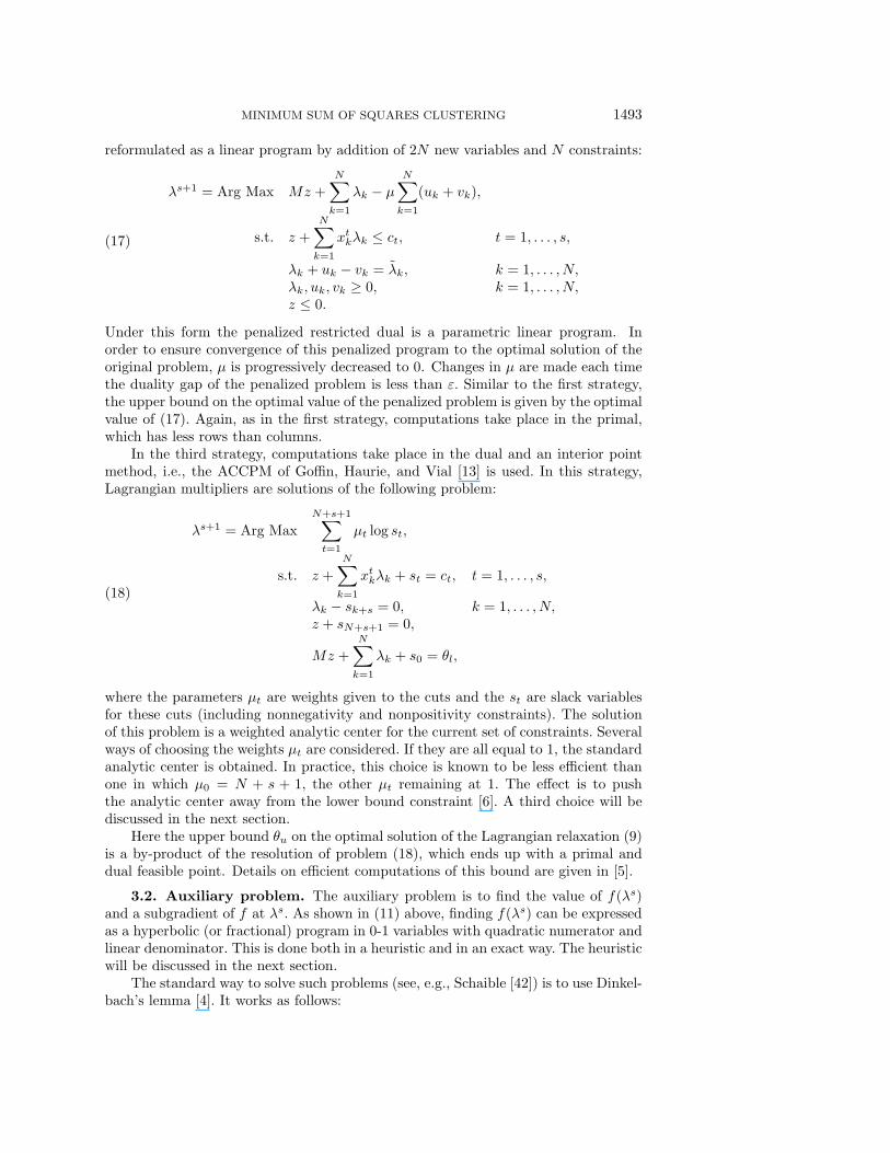
Under this form the penalized restricted dual is a parametric linear program. Inorder to ensure convergence of this penalized program to the optimal solution of theoriginal problem, µ is progressively decreased to 0. Changes in µ are made each timethe duality gap of the penalized problem is less than ε. Similar to the first strategy,the upper bound on the optimal value of the penalized problem is given by the optimalvalue of (17). Again, as in the first strategy, computations take place in the primal,which has less rows than columns.

In the third strategy, computations take place in the dual and an interior pointmethod, i.e., the ACCPM of Goffin, Haurie, and Vial [13] is used. In this strategy,Lagrangian multipliers are solutions of the following problem:

λs+1 = Arg Max

N+s+1∑t=1

µt log st,

s.t. z +

N∑k=1

xtkλk + st = ct, t = 1, . . . , s,

λk − sk+s = 0, k = 1, . . . , N,z + sN+s+1 = 0,

Mz +N∑

k=1

λk + s0 = θl,

(18)

where the parameters µt are weights given to the cuts and the st are slack variablesfor these cuts (including nonnegativity and nonpositivity constraints). The solutionof this problem is a weighted analytic center for the current set of constraints. Severalways of choosing the weights µt are considered. If they are all equal to 1, the standardanalytic center is obtained. In practice, this choice is known to be less efficient thanone in which µ0 = N + s + 1, the other µt remaining at 1. The effect is to pushthe analytic center away from the lower bound constraint [6]. A third choice will bediscussed in the next section.

Here the upper bound θu on the optimal solution of the Lagrangian relaxation (9)is a by-product of the resolution of problem (18), which ends up with a primal anddual feasible point. Details on efficient computations of this bound are given in [5].

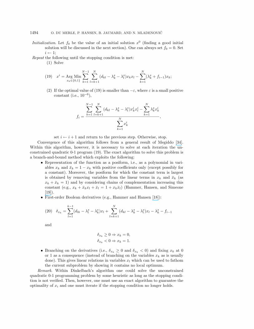
3.2. Auxiliary problem. The auxiliary problem is to find the value of f(λs)and a subgradient of f at λs. As shown in (11) above, finding f(λs) can be expressedas a hyperbolic (or fractional) program in 0-1 variables with quadratic numerator andlinear denominator. This is done both in a heuristic and in an exact way. The heuristicwill be discussed in the next section.

The standard way to solve such problems (see, e.g., Schaible [42]) is to use Dinkel-bach’s lemma [4]. It works as follows:

1494 O. DU MERLE, P. HANSEN, B. JAUMARD, AND N. MLADENOVIC

Initialization. Let f0 be the value of an initial solution x0 (finding a good initialsolution will be discussed in the next section). One can always set f0 = 0. Seti← 1;

Repeat the following until the stopping condition is met:(1) Solve

xi = Arg Minxk∈{0,1}

N−1∑k=1

N∑l=k+1

(dkl − λsk − λs

l )xkxl −N∑

k=1

(λsk + fi−1)xk;(19)

(2) If the optimal value of (19) is smaller than −ε, where ε is a small positiveconstant (i.e., 10−6),

fi =

N−1∑k=1

N∑l=k+1

(dkl − λsk − λs

l )xikx

il −

N∑k=1

λskx

ik

N∑k=1

xik

,

set i← i+ 1 and return to the previous step. Otherwise, stop.

Convergence of this algorithm follows from a general result of Megiddo [34].Within this algorithm, however, it is necessary to solve at each iteration the un-constrained quadratic 0-1 program (19). The exact algorithm to solve this problem isa branch-and-bound method which exploits the following:

• Representation of the function as a posiform, i.e., as a polynomial in vari-ables xk and xk = 1 − xk with positive coefficients only (except possibly fora constant). Moreover, the posiform for which the constant term is largestis obtained by removing variables from the linear terms in xk and xk (asxk + xk = 1) and by considering chains of complementation increasing thisconstant (e.g., xk + xkxl + xl = 1 + xkxl) (Hammer, Hansen, and Simeone[19]).• First-order Boolean derivatives (e.g., Hammer and Hansen [18]):

δxk=

k−1∑l=1

(dlk − λsl − λs

k)xl +

N∑l=k+1

(dkl − λsk − λs

l )xl − λsk − fi−1(20)

and

δxk≥ 0⇒ xk = 0,

δxk< 0⇒ xk = 1.

• Branching on the derivatives (i.e., δxk≥ 0 and δxk

< 0) and fixing xk at 0or 1 as a consequence (instead of branching on the variables xk as is usuallydone). This gives linear relations in variables xl which can be used to fathomthe current subproblem by showing it contains no local optimum.

Remark. Within Dinkelbach’s algorithm one could solve the unconstrainedquadratic 0-1 programming problem by some heuristic as long as the stopping condi-tion is not verified. Then, however, one must use an exact algorithm to guarantee theoptimality of xi and one must iterate if the stopping condition no longer holds.

MINIMUM SUM OF SQUARES CLUSTERING 1495

3.3. Branching rule. As the solution of the continuous relaxation of the ex-tended formulation (4) is not necessarily integer, a branching rule must be specified.We use the (now) standard one in column generation, due to Ryan and Foster [41]. Itconsists of finding two rows i1 and i2 such that there are two columns t1 and t2 withfractional variables at the optimum and such that

ai1t1 = ai2t1 = 1

and(21)

ai1t2 = 1, ai2t2 = 0.

Such rows and columns necessarily exist in any noninteger optimal solution of thecontinuous relaxation of a partitioning problem [41]. While we solve a covering prob-lem (with one additional constraint) such an optimal solution satisfies the constraintsas equalities and hence this result still holds.

This branching is done by imposing on the one hand the constraint

xi1 = xi2 ,(22)

i.e., both entities will be in the same cluster, and on the other hand

xi1 + xi2 ≤ 1,(23)

i.e., the two entities cannot be in the same cluster. (Of course, in both subproblemsthere will be clusters containing neither of the entities, i.e., one may have xi1 = xi2 =0.) These constraints could be added to the master problem, but it is more efficientto remove the columns in the current reduced master problem which do not satisfythem and then introduce them in the auxiliary problem. The effect in the auxiliaryproblem of constraint (22) is to reduce by one the number of variables and updatecoefficients, while constraint (23) can be imposed by setting di1i2 to an arbitrary largevalue. Hence the form of the auxiliary problem is unchanged.

The branching rule so defined can be made more precise by choosing from thepairs of rows and columns satisfying condition (21) that one which is best accordingto another criterion, e.g., having fractional variables the closest possible to 1/2. Suchrefinements have not been investigated in detail as for MSSC branching appears tobe rare in practice and the resulting trees are very small.

Note that the branching rule described above can also be viewed as one for thecompact formulation (2), to which one adds the constraint (22) or (23). Then the firstpossibility mentioned above corresponds to dualizing these constraints in addition tothe inequality constraints (3) while the second amounts to not doing so, hence havingthem as constraints in the auxiliary problem (10) obtained when relaxing problem (2).

Note also that instead of removing the columns which violate the branching con-straint or giving them a large value in the objective function, one may modify themby removal or addition of an entity to satisfy his constraint and update their value inthe objective function. This is due to the fact that all clusters are a priori feasible.

4. Refinements.

4.1. Heuristics. As already mentioned, heuristics can be used in several placesin order to accelerate the algorithm whose principles have been described in the pre-vious section. In some cases, such as when using Kelley’s strategy, the effect of such

1496 O. DU MERLE, P. HANSEN, B. JAUMARD, AND N. MLADENOVIC

heuristics is quite drastic. They can be used to (i) find an initial solution of prob-lem (2), (ii) find a solution of the auxiliary problem (11), and, possibly, (iii) finda solution of the unconstrained quadratic 0-1 program (19) which arises when solv-ing (11).

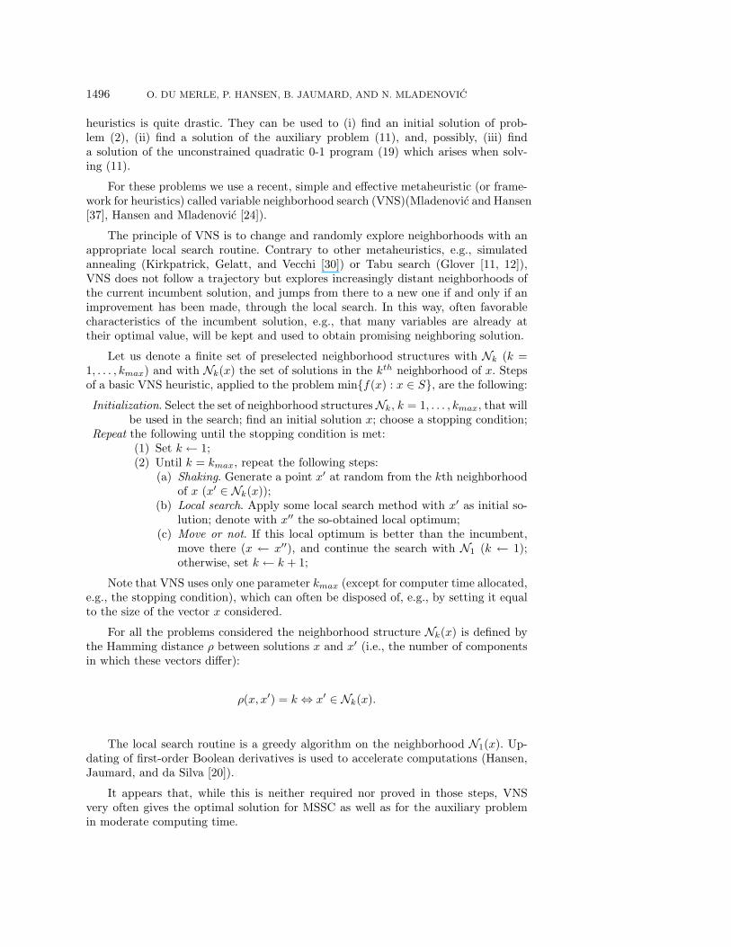
For these problems we use a recent, simple and effective metaheuristic (or frame-work for heuristics) called variable neighborhood search (VNS)(Mladenovic and Hansen[37], Hansen and Mladenovic [24]).

The principle of VNS is to change and randomly explore neighborhoods with anappropriate local search routine. Contrary to other metaheuristics, e.g., simulatedannealing (Kirkpatrick, Gelatt, and Vecchi [30]) or Tabu search (Glover [11, 12]),VNS does not follow a trajectory but explores increasingly distant neighborhoods ofthe current incumbent solution, and jumps from there to a new one if and only if animprovement has been made, through the local search. In this way, often favorablecharacteristics of the incumbent solution, e.g., that many variables are already attheir optimal value, will be kept and used to obtain promising neighboring solution.

Let us denote a finite set of preselected neighborhood structures with Nk (k =1, . . . , kmax) and with Nk(x) the set of solutions in the kth neighborhood of x. Stepsof a basic VNS heuristic, applied to the problem min{f(x) : x ∈ S}, are the following:Initialization. Select the set of neighborhood structuresNk, k = 1, . . . , kmax, that will

be used in the search; find an initial solution x; choose a stopping condition;Repeat the following until the stopping condition is met:

(1) Set k ← 1;(2) Until k = kmax, repeat the following steps:

(a) Shaking. Generate a point x′ at random from the kth neighborhoodof x (x′ ∈ Nk(x));

(b) Local search. Apply some local search method with x′ as initial so-lution; denote with x′′ the so-obtained local optimum;

(c) Move or not. If this local optimum is better than the incumbent,move there (x ← x′′), and continue the search with N1 (k ← 1);otherwise, set k ← k + 1;

Note that VNS uses only one parameter kmax (except for computer time allocated,e.g., the stopping condition), which can often be disposed of, e.g., by setting it equalto the size of the vector x considered.

For all the problems considered the neighborhood structure Nk(x) is defined bythe Hamming distance ρ between solutions x and x′ (i.e., the number of componentsin which these vectors differ):

ρ(x, x′) = k ⇔ x′ ∈ Nk(x).

The local search routine is a greedy algorithm on the neighborhood N1(x). Up-dating of first-order Boolean derivatives is used to accelerate computations (Hansen,Jaumard, and da Silva [20]).

It appears that, while this is neither required nor proved in those steps, VNSvery often gives the optimal solution for MSSC as well as for the auxiliary problemin moderate computing time.

MINIMUM SUM OF SQUARES CLUSTERING 1497

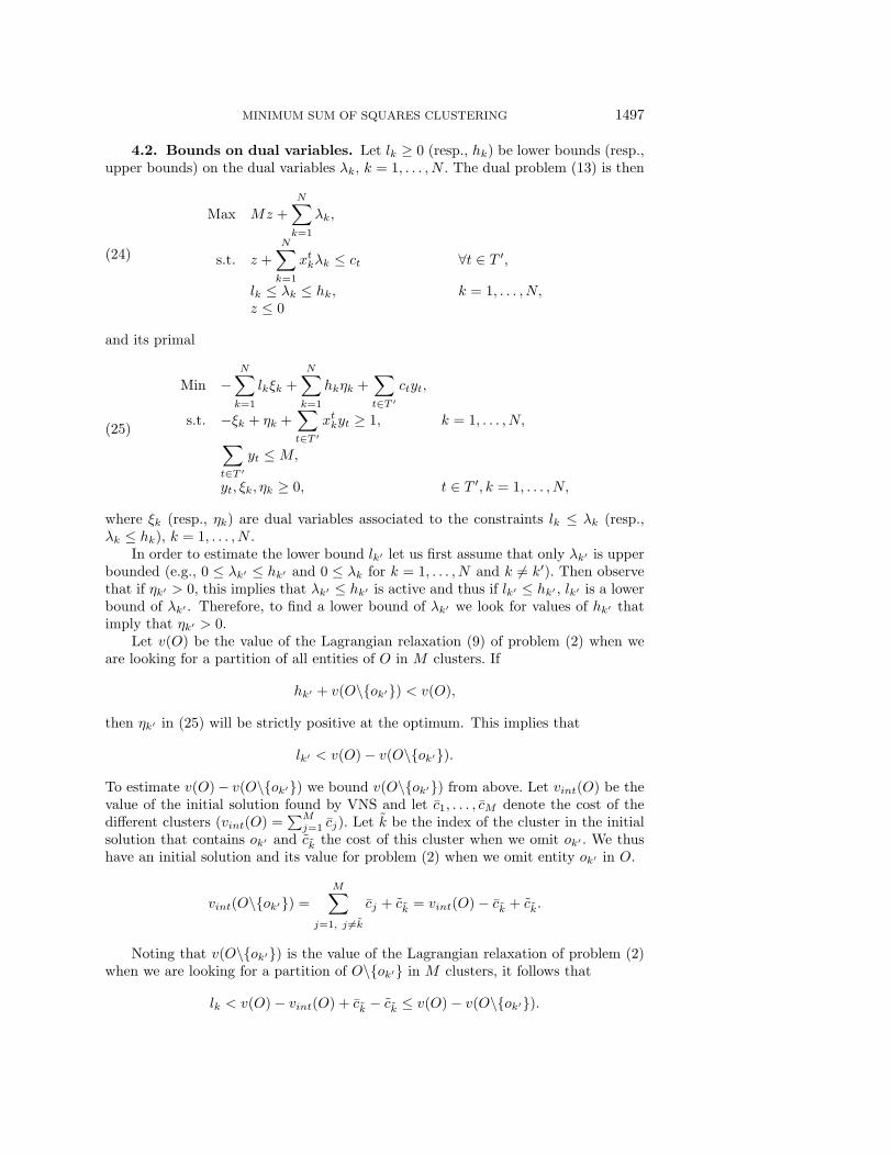
4.2. Bounds on dual variables. Let lk ≥ 0 (resp., hk) be lower bounds (resp.,upper bounds) on the dual variables λk, k = 1, . . . , N . The dual problem (13) is then

Max Mz +N∑

k=1

λk,

s.t. z +

N∑k=1

xtkλk ≤ ct ∀t ∈ T ′,

lk ≤ λk ≤ hk, k = 1, . . . , N,z ≤ 0

(24)

and its primal

Min −N∑

k=1

lkξk +

N∑k=1

hkηk +∑t∈T ′

ctyt,

s.t. −ξk + ηk +∑t∈T ′

xtkyt ≥ 1, k = 1, . . . , N,∑t∈T ′

yt ≤M,

yt, ξk, ηk ≥ 0, t ∈ T ′, k = 1, . . . , N,

(25)

where ξk (resp., ηk) are dual variables associated to the constraints lk ≤ λk (resp.,λk ≤ hk), k = 1, . . . , N .

In order to estimate the lower bound lk′ let us first assume that only λk′ is upperbounded (e.g., 0 ≤ λk′ ≤ hk′ and 0 ≤ λk for k = 1, . . . , N and k �= k′). Then observethat if ηk′ > 0, this implies that λk′ ≤ hk′ is active and thus if lk′ ≤ hk′ , lk′ is a lowerbound of λk′ . Therefore, to find a lower bound of λk′ we look for values of hk′ thatimply that ηk′ > 0.

Let v(O) be the value of the Lagrangian relaxation (9) of problem (2) when weare looking for a partition of all entities of O in M clusters. If

hk′ + v(O\{ok′}) < v(O),

then ηk′ in (25) will be strictly positive at the optimum. This implies that

lk′ < v(O)− v(O\{ok′}).

To estimate v(O)− v(O\{ok′}) we bound v(O\{ok′}) from above. Let vint(O) be thevalue of the initial solution found by VNS and let c1, . . . , cM denote the cost of thedifferent clusters (vint(O) =

∑Mj=1 cj). Let k be the index of the cluster in the initial

solution that contains ok′ and ck the cost of this cluster when we omit ok′ . We thushave an initial solution and its value for problem (2) when we omit entity ok′ in O.

vint(O\{ok′}) =M∑

j=1, j =k

cj + ck = vint(O)− ck + ck.

Noting that v(O\{ok′}) is the value of the Lagrangian relaxation of problem (2)when we are looking for a partition of O\{ok′} in M clusters, it follows that

lk < v(O)− vint(O) + ck − ck ≤ v(O)− v(O\{ok′}).

1498 O. DU MERLE, P. HANSEN, B. JAUMARD, AND N. MLADENOVIC

The value of v(O) being unknown, it has to be estimated. As VNS often findsthe optimal solution of (2) and again often there is no integrality gap, the differencev(O)− vint(O) was considered as 0 and lk′ set to ck − ck. This implies that one mustcheck that the constraint lk′ ≤ λk′ is not active at the optimum of the Lagrangianrelaxation (9). Should it be active, the bound lk′ must be reduced and the resolutionof (9) resumed.

The procedure just described shows how to evaluate the lower bounds on λk oneat a time. The values so obtained are still valid when all lk are put together. Again,because v(O) − vint(O) is assumed to be null, we must check for bounds which aretight at the optimum, modify them, and resume the resolution if so.

Similarly, one can show that

hk′ > v(O ∪ {ok′})− v(O),

where v(O∪{ok′}) denotes the value of the Lagrangian relaxation of a partition of Owith two copies of ok′ into M clusters. Then noting that

v(O ∪ {ok′}) < vint(O) + cj − cj ,

where cj j �= k is the cost of the cluster Cj to which ok′ is added, to minimize theright-hand side one chooses Cj such that the resulting cj − cj is minimum. Hence

hk′ > vint(O)− v(O) + cj − cj ≥ v(O ∪ {ok′})− v(O).

As before, we assume that vint(O) − v(O) is equal to 0 and add a procedure tocheck if the bound hk′ = cj − cj is active at the optimum.

4.3. Weights on cuts. The most time-consuming step of the algorithm is theresolution of the auxiliary problem through a sequence of unconstrained quadratic0-1 programming problems. As long as the relative duality gap is greater than ε theauxiliary problem (11) is solved by the VNS heuristic, which is fairly fast. However,when no relative duality gap is observed, one must check if the dual variables areoptimal and therefore solve the auxiliary problem with the exact branch-and-boundalgorithm. For large instances, this algorithm is time-consuming and its use, in fact,limits the size of problems which can be solved exactly.

One may note that there is some flexibility in the way the coefficients in thesubproblem, i.e., the dual variables at the current iteration, are selected. Indeed, asthe optimal solution, in which the number M of clusters is usually much smaller thanthe number N of entities, is massively primal degenerate (N + 1−M basic variablesbeing equal to 0 when this optimal solution is integer) there is a large polytope ofoptimal solutions in the dual. To prove optimality of the linear relaxation of (4) (orequivalently of problem (9)) has been attained one must check the value of the lowerbound θl. The question is then, “Which values should be selected in this polytope tomake the resolution of (19) the easiest possible?”

As the branch-and-bound algorithm relies on the first-order Boolean derivatives(20), one may look for values which will make them fixed variables as soon as possible.Observe then that reducing λk makes condition δxk

≥ 0⇒ xk = 0 more likely to hold.(This augments the constant term as well as all coefficients of the linear terms in (20).)To achieve this goal with ACCPM we weight the upper bound constraints λk ≤ hkby a constant much larger than for the other constraints. (In practice a value of 100for the upper bound constraints and 1 for the other constraints, except for the lowerbound on the problem value for which we keep the value µ0 = N + s+ 1, gives goodresults.)

MINIMUM SUM OF SQUARES CLUSTERING 1499

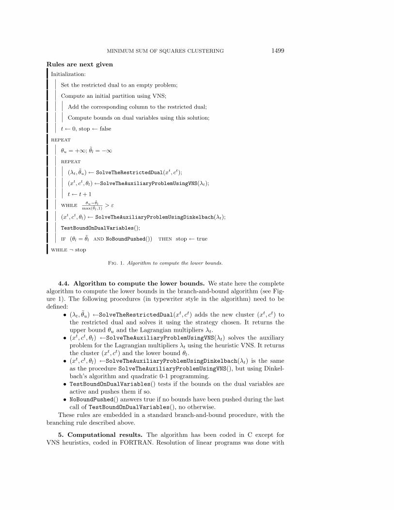
Rules are next given

Initialization:

Set the restricted dual to an empty problem;

Compute an initial partition using VNS;

Add the corresponding column to the restricted dual;

Compute bounds on dual variables using this solution;

t← 0, stop ← false

repeat

θu = +∞; θl = −∞repeat

(λt, θu)← SolveTheRestrictedDual(xt, ct);

(xt, ct, θl)←SolveTheAuxiliaryProblemUsingVNS(λt);

t← t+ 1

while θu−θlmax(θl,1)

> ε

(xt, ct, θl)← SolveTheAuxiliaryProblemUsingDinkelbach(λt);

TestBoundOnDualVariables();

if (θl = θl and NoBoundPushed()) then stop ← true

while ¬ stop

Fig. 1. Algorithm to compute the lower bounds.

4.4. Algorithm to compute the lower bounds. We state here the completealgorithm to compute the lower bounds in the branch-and-bound algorithm (see Fig-ure 1). The following procedures (in typewriter style in the algorithm) need to bedefined:

• (λt, θu) ←SolveTheRestrictedDual(xt, ct) adds the new cluster (xt, ct) tothe restricted dual and solves it using the strategy chosen. It returns theupper bound θu and the Lagrangian multipliers λt.

• (xt, ct, θl) ←SolveTheAuxiliaryProblemUsingVNS(λt) solves the auxiliaryproblem for the Lagrangian multipliers λt using the heuristic VNS. It returnsthe cluster (xt, ct) and the lower bound θl.

• (xt, ct, θl) ←SolveTheAuxiliaryProblemUsingDinkelbach(λt) is the sameas the procedure SolveTheAuxiliaryProblemUsingVNS(), but using Dinkel-bach’s algorithm and quadratic 0-1 programming.• TestBoundOnDualVariables() tests if the bounds on the dual variables areactive and pushes them if so.• NoBoundPushed() answers true if no bounds have been pushed during the lastcall of TestBoundOnDualVariables(), no otherwise.

These rules are embedded in a standard branch-and-bound procedure, with thebranching rule described above.

5. Computational results. The algorithm has been coded in C except forVNS heuristics, coded in FORTRAN. Resolution of linear programs was done with

1500 O. DU MERLE, P. HANSEN, B. JAUMARD, AND N. MLADENOVIC

CPLEX 3.0, and for solving the convex problem (18) we used ACCPM’s library [14],slightly modified to incorporate a branch-and-bound scheme and to permit setting ofappropriate weights. Results were obtained using a SUN ULTRA 200 MHz stationwith g++ (Option -O4) C compiler and f77 (Option -O4 -xcg92) FORTRAN compiler.

Extensive comparisons were made using some standard problems from the clusteranalysis literature (Ruspini’s 75 points in the Euclidean plane [40], Spath’s 89 postalzones problem in three dimensions [43], and Fisher’s celebrated 150 iris problem infour dimensions [9]).

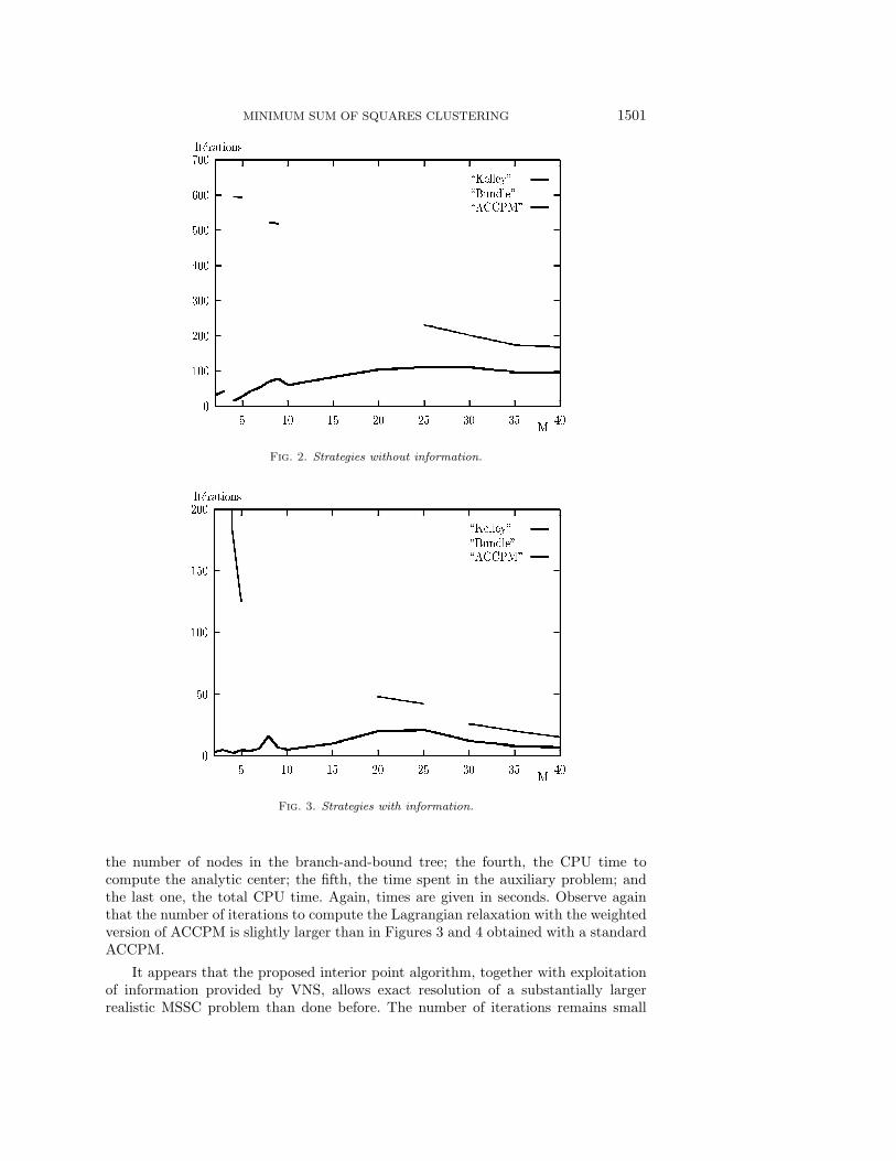
We next comment in detail on results for Ruspini’s data. As most of the time isspent in the resolution of the auxiliary problem, it is fair to compare resolution strate-gies by their number of iterations for solving the linear relaxation. These numbers forM = 2 to 10 and 15, 20, 25, 30, 35, and 40 are represented in Figures 2 and 3. Forthe results of Figure 2 no information was used, i.e., no initial solution nor bounds onthe dual variables. As often observed when using column generation, Kelley’s strategyis not efficient and the cases M = 2 and 3 could not be solved. The bundle methodin l1-norm allows solution of these two cases but is not much quicker than Kelley’sstrategy for M large. ACCPM is the most efficient strategy for all M and particularlyfor the more realistic case of M small. The number of iterations is always small, e.g.,about 100 for M = 40 a case where at least 40 columns must be generated.

Information was exploited for the results of Figure 3, i.e., an initial heuristic solu-tion was found by VNS, bounds on the dual variables were computed, and the columnscorresponding to the clusters of the heuristic solution as well as the modified clustersdefined when computing the dual bounds were added. The reduction in number ofiterations due to this information is drastic for all strategies and all values ofM . WithKelley’s strategy all instances can then be solved. Ranking of strategies remains thesame as in the former case. The number of iterations of ACCPM for M small is fewand never exceeds 25. It is often smaller than M .

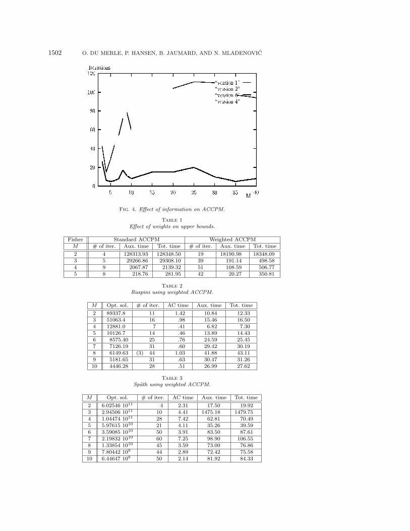
Figure 4 shows the effect of information on Ruspini’s problem with the beststrategy (i.e., ACCPM). The first plot, “version 1,” gives the number of iterationswhen no information was used. The second plot, “version 2,” gives the number ofiterations when the clusters found with the initial heuristic are added at the outset.In the third plot, “version 3,” we initially add also the clusters obtained during thecomputation of the dual bounds, and in the last one, “version 4,” we also add thosebounds.

The effect of the weights on the upper bounds are displayed in Table 1 usingFisher’s iris data, ACCPM, and initial information. The first column gives values ofM ; the second, the number of iterations for solving the Lagrangian relaxation; thethird, the time spent in the auxiliary problem when solved exactly with Dinkelbach’salgorithm; and the fourth, the total CPU time. The next three columns give the sameinformation as columns 2 to 4 but using a weighted version of ACCPM instead ofthe standard one. Times are given in seconds. Observe that the number of iterationsto compute the Lagrangian relaxation with the weighted version of ACCPM is largerthan in the standard version, a consequence of looking for small values for λk. However,the reduction of the time for solving the auxiliary problem more than compensatesfor this increase for the more realistic case of M small.

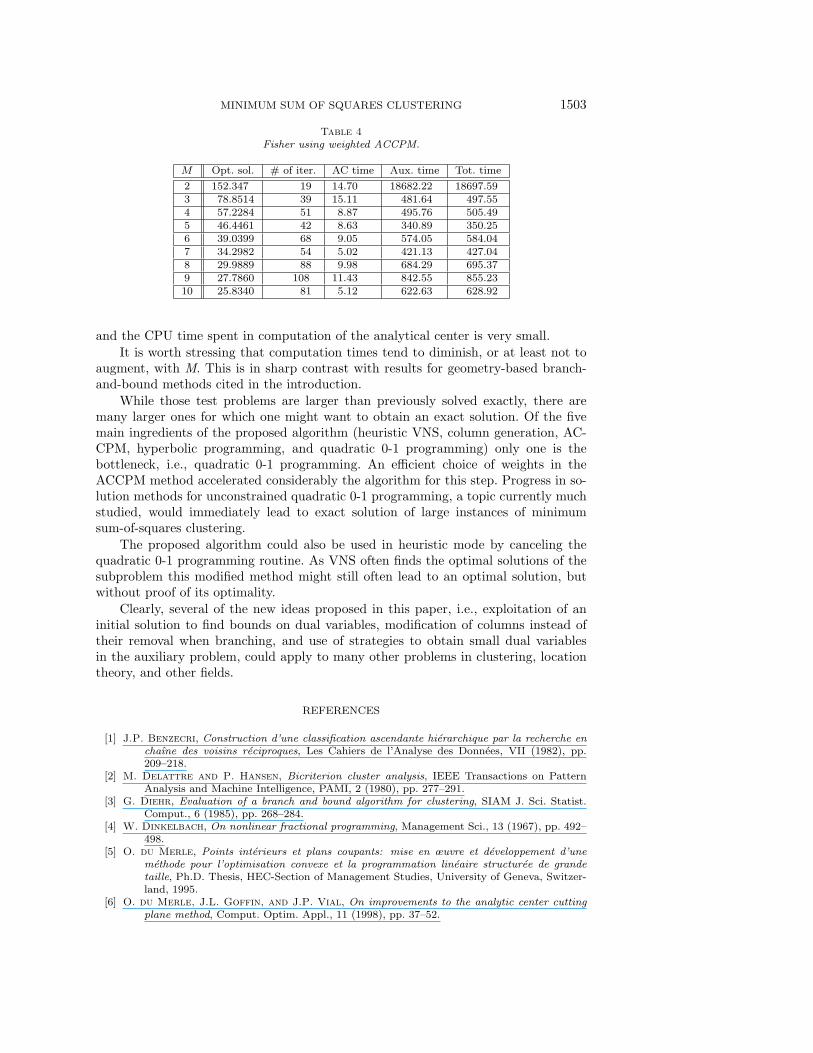
Computational results using a weighted version of ACCPM and initial informationfor the problems of Ruspini [40], Spath [43], and Fisher [9] are given in Tables 2–4.The first column gives values of M ; the second, optimal solutions; the third, numberof iterations for solving the Lagrangian relaxation and when needed, in parentheses,

MINIMUM SUM OF SQUARES CLUSTERING 1501

Fig. 2. Strategies without information.

Fig. 3. Strategies with information.

the number of nodes in the branch-and-bound tree; the fourth, the CPU time tocompute the analytic center; the fifth, the time spent in the auxiliary problem; andthe last one, the total CPU time. Again, times are given in seconds. Observe againthat the number of iterations to compute the Lagrangian relaxation with the weightedversion of ACCPM is slightly larger than in Figures 3 and 4 obtained with a standardACCPM.

It appears that the proposed interior point algorithm, together with exploitationof information provided by VNS, allows exact resolution of a substantially largerrealistic MSSC problem than done before. The number of iterations remains small

1502 O. DU MERLE, P. HANSEN, B. JAUMARD, AND N. MLADENOVIC

Fig. 4. Effect of information on ACCPM.

Table 1Effect of weights on upper bounds.

Fisher Standard ACCPM Weighted ACCPMM # of iter. Aux. time Tot. time # of iter. Aux. time Tot. time

2 4 128313.93 128348.50 19 18190.98 18348.093 5 29266.86 29308.10 39 191.14 498.584 9 2067.87 2139.32 51 108.59 506.775 8 218.76 281.95 42 20.27 350.81

Table 2Ruspini using weighted ACCPM.

M Opt. sol. # of iter. AC time Aux. time Tot. time

2 89337.8 11 1.42 10.84 12.333 51063.4 16 .98 15.46 16.504 12881.0 7 .41 6.82 7.305 10126.7 14 .46 13.89 14.436 8575.40 25 .76 24.59 25.457 7126.19 31 .60 29.42 30.198 6149.63 (3) 44 1.03 41.88 43.119 5181.65 31 .63 30.47 31.2610 4446.28 28 .51 26.99 27.62

Table 3Spath using weighted ACCPM.

M Opt. sol. # of iter. AC time Aux. time Tot. time

2 6.02546 1011 4 2.31 17.50 19.923 2.94506 1011 10 4.41 1475.18 1479.754 1.04474 1011 28 7.42 62.81 70.495 5.97615 1010 21 4.11 35.26 39.596 3.59085 1010 50 3.91 83.50 87.617 2.19832 1010 60 7.25 98.90 106.558 1.33854 1010 45 3.59 73.00 76.869 7.80442 109 44 2.89 72.42 75.5810 6.44647 109 50 2.14 81.92 84.33

MINIMUM SUM OF SQUARES CLUSTERING 1503

Table 4Fisher using weighted ACCPM.

M Opt. sol. # of iter. AC time Aux. time Tot. time

2 152.347 19 14.70 18682.22 18697.593 78.8514 39 15.11 481.64 497.554 57.2284 51 8.87 495.76 505.495 46.4461 42 8.63 340.89 350.256 39.0399 68 9.05 574.05 584.047 34.2982 54 5.02 421.13 427.048 29.9889 88 9.98 684.29 695.379 27.7860 108 11.43 842.55 855.2310 25.8340 81 5.12 622.63 628.92

and the CPU time spent in computation of the analytical center is very small.

It is worth stressing that computation times tend to diminish, or at least not toaugment, with M. This is in sharp contrast with results for geometry-based branch-and-bound methods cited in the introduction.

While those test problems are larger than previously solved exactly, there aremany larger ones for which one might want to obtain an exact solution. Of the fivemain ingredients of the proposed algorithm (heuristic VNS, column generation, AC-CPM, hyperbolic programming, and quadratic 0-1 programming) only one is thebottleneck, i.e., quadratic 0-1 programming. An efficient choice of weights in theACCPM method accelerated considerably the algorithm for this step. Progress in so-lution methods for unconstrained quadratic 0-1 programming, a topic currently muchstudied, would immediately lead to exact solution of large instances of minimumsum-of-squares clustering.

The proposed algorithm could also be used in heuristic mode by canceling thequadratic 0-1 programming routine. As VNS often finds the optimal solutions of thesubproblem this modified method might still often lead to an optimal solution, butwithout proof of its optimality.

Clearly, several of the new ideas proposed in this paper, i.e., exploitation of aninitial solution to find bounds on dual variables, modification of columns instead oftheir removal when branching, and use of strategies to obtain small dual variablesin the auxiliary problem, could apply to many other problems in clustering, locationtheory, and other fields.

REFERENCES

[1] J.P. Benzecri, Construction d’une classification ascendante hierarchique par la recherche enchaıne des voisins reciproques, Les Cahiers de l’Analyse des Donnees, VII (1982), pp.209–218.

[2] M. Delattre and P. Hansen, Bicriterion cluster analysis, IEEE Transactions on PatternAnalysis and Machine Intelligence, PAMI, 2 (1980), pp. 277–291.

[3] G. Diehr, Evaluation of a branch and bound algorithm for clustering, SIAM J. Sci. Statist.Comput., 6 (1985), pp. 268–284.

[4] W. Dinkelbach, On nonlinear fractional programming, Management Sci., 13 (1967), pp. 492–498.

[5] O. du Merle, Points interieurs et plans coupants: mise en œuvre et developpement d’unemethode pour l’optimisation convexe et la programmation lineaire structuree de grandetaille, Ph.D. Thesis, HEC-Section of Management Studies, University of Geneva, Switzer-land, 1995.

[6] O. du Merle, J.L. Goffin, and J.P. Vial, On improvements to the analytic center cuttingplane method, Comput. Optim. Appl., 11 (1998), pp. 37–52.

1504 O. DU MERLE, P. HANSEN, B. JAUMARD, AND N. MLADENOVIC

[7] O. du Merle, D. Villeneuve, J. Desrosiers, and P. Hansen, Stabilized column generation,Discrete Math., 194 (1999), pp. 229–237.

[8] A.W.F. Edwards and L.L. Cavalli-Sforza, A method for cluster analysis, Biometrics, 21(1965), pp. 362–375.

[9] R.A. Fisher, The use of multiple measurements in taxonomic problems, Ann. Eugenics, VIIpart II (1936), pp. 179–188.

[10] P.C. Gilmore and R.E. Gomory, A linear programming approach to the cutting stock problem,Oper. Res., 9 (1961), pp. 849–859.

[11] F. Glover, Tabu search—Part I, ORSA J. Comput., 1 (1989), pp. 190–206.[12] F. Glover, Tabu search—Part II, ORSA J. Comput., 2 (1990), pp. 4–32.[13] J.-L. Goffin, A. Haurie, and J.-P. Vial, Decomposition and nondifferentiable optimization

with the projective algorithm, Management Sci., 38 (1992), pp. 284–302.[14] J. Gondzio, O. du Merle, R. Sarkissian, and J.-P. Vial, ACCPM—A library for con-

vex optimization based on an analytic center cutting plane method, European Journal ofOperational Research, 94 (1996), pp. 206–211.

[15] A.D. Gordon, Classification: Methods for the Exploratory Analysis of Multivariate Data,Chapman and Hall, New York, 1981.

[16] A.D. Gordon and J.T. Henderson, An algorithm for Euclidean sum of squares classification,Biometrics, 33 (1977), pp. 355–362.

[17] J.C. Gower and G.J.S. Ross, Minimum spanning trees and single linkage cluster analysis,Appl. Statistics, 18 (1969), pp. 54–64.

[18] P.L. Hammer and P. Hansen, Logical relations in quadratic 0-1 programming, Rev. RoumaineMath. Pures Appl., 26 (1981), pp. 421–429.

[19] P.L. Hammer, P. Hansen, and B. Simeone, Roof duality, complementation and persistencyin quadratic 0–1 optimization, Math. Programming, 28 (1984), pp. 121–155.

[20] P. Hansen, B. Jaumard, and E. da Silva, Average-linkage divisive hierarchical clustering, J.Classification, to appear.

[21] P. Hansen, B. Jaumard, S. Krau, and O. du Merle, A Column Generation Algorithm forthe Weber Multisource Problem, in preparation.

[22] P. Hansen, B. Jaumard, and N. Mladenovic, Minimum sum of squares clustering in a lowdimensional space, J. Classification, 15 (1998), pp. 37–55.

[23] P. Hansen, B. Jaumard, and B. Simeone, Espaliers, a generalization of dendrograms, J.Classification, 13 (1996), pp. 107–127.

[24] P. Hansen and N. Mladenovic, An introduction to variable neighborhood search, in Meta-heuristics. Advances and Trends in Local Search Paradigms for Optimization, S. Voss, S.Martello, I.M. Osman, and C. Roucairol, eds., Kluwer, Dordrect, The Netherlands, 1998,pp. 433–458.

[25] J.A. Hartigan, Clustering Algorithms, Wiley, New York, 1975.[26] M. Inaba. N. Katoh, and H. Imai, Applications of weighted Voronoi diagrams and random-

ization to variance-based k-clustering, in Proceedings of the 10th ACM Symposium onComputational Geometry, Stony Brook, NY, 1994, pp. 332–339.

[27] S.C. Johnson, Hierarchical clustering schemes, Psychometrika, 32 (1967), pp. 241–245.[28] L. Kaufman and P.J. Rousseeuw, Finding Groups in Data: An Introduction to Cluster

Analysis, Wiley, New York, 1990.[29] J.E. Kelley, The cutting-plane method for solving convex programs, J. SIAM, 8 (1960), pp.

703–712.[30] S. Kirkpatrick, C.D. Gelatt, Jr., and M.P. Vecchi, Optimization by simulated annealing,

Science, 20 (1983), pp. 671–680.[31] W.L.G. Koontz, P.M. Narendra, and K. Fukunaga, A branch and bound clustering algo-

rithm, IEEE Trans. Comput., C–24 (1975), pp. 908–915.[32] G.N. Lance and W.T. Williams, A general theory of classificatory sorting strategies. 1.

Hierarchical systems, The Computer J., 9 (1967), pp. 373–380.[33] J.B. MacQueen, Some methods for classification and analysis of multivariate observations,

in Proceedings of 5th Berkeley Symposium on Mathematical Statistics and Probability, 2,Berkeley, CA, 1967, pp. 281–297.

[34] N. Megiddo, Combinatorial optimization with rational objective functions, Math. Oper. Res.,4 (1979), pp. 414–424.

[35] M. Minoux, Programmation mathematique: theorie et algorithmes, Tome 2, Dunod (Bordas),Paris, 1983.

[36] B. Mirkin, Mathematical Classification and Clustering, Kluwer, Dordrecht, The Netherlands,1996.

MINIMUM SUM OF SQUARES CLUSTERING 1505

[37] N. Mladenovic and P. Hansen, Variable neighborhood search, Comput. Oper. Res., 24 (1997),pp. 1097–1100.

[38] F. Murtagh, A survey of recent advances in hierarchical clustering algorithms, Comput. J.,26 (1983), pp. 329–340.

[39] M.R. Rao, Cluster analysis and mathematical programming, J. Amer. Statist. Assoc., 66(1971), pp. 622–626.

[40] E.H. Ruspini, Numerical methods for fuzzy clustering, Inform. Sciences, 2 (1970), pp. 319–350.[41] D.M. Ryan and B.A. Foster, An integer programming approach to scheduling, in Computer

Scheduling of Public Transport Urban Passenger Vehicle and Crew Scheduling, A. Wren,ed., North-Holland, Amsterdam, 1981, pp. 269–280.

[42] S. Schaible, Fractional programming, in Handbook of Global Optimization, R. Horst and P.M.Pardalos, eds., Kluwer, Dordrecht, The Netherlands, 1995, pp. 495–608.

[43] H. Spath, Cluster Analysis Algorithms for Data Reduction and Classification of Objects, EllisHorwood, Chichester, UK, 1980.

[44] H.D. Vinod, Integer programming and the theory of grouping, J. Amer. Statist. Assoc., 64(1969), pp. 506–519.

[45] J.H. Ward, Jr., Hierarchical grouping to optimize an objective function, J. Amer. Statist.Assoc., 58 (1963), pp. 236–244.