A two-level interior-point decomposition algorithm for multi-stage stochastic capacity planning and...

280 Int. J. Mathematics in Operational Research, Vol. 3, No. 3, 2011

A two-level interior-point decomposition algorithm

for multi-stage stochastic capacity planning and

technology acquisition

Lila Rasekh and Jacques Desrosiers*

HEC Montreal,3000 Chemin de la Cote-Sainte-Catherine,Montreal Quebec Canada, H3T 2A7E-mail: [email protected]: [email protected]*Corresponding author

Abstract: Manufacturing flexibility is recognised as one of the keystrategies to address uncertain future products demand. Therefore, agrowing need exists to investigate the strategic aspect of flexibility.To capture the different aspects of market flexibility in the face ofthis dynamic demand, this paper focuses on the role of product,volume, and expansion flexibility in the context of the multi-stagestochastic program. Moreover, we implement a two-level, interior-pointdecomposition algorithm based on the Analytic Center Cutting PlaneMethod (ACCPM) to solve the model. The central prices obtained by theACCPM provides a fast convergence and promising computational resultsin terms of the number of iterations.

Keywords: column generation; interior point method; ACCPM;analytic centre cutting plane method; stochastic optimisation; flexiblemanufacturing.

Reference to this paper should be made as follows: Rasekh, L. andDesrosiers, J. (2011) ‘A two-level interior-point decomposition algorithmfor multi-stage stochastic capacity planning and technology acquisition’,Int. J. Mathematics in Operational Research, Vol. 3, No. 3, pp.280–294.

Biographical notes: Lila Rasekh holds a PhD in Management Sciencefrom HEC-Montreal and McGill University in Canada. She currentlyworks in the Decision Science Team of Revenue Management at WaltDisney World (WDW). Her work focuses on hotel, cruise, golf course andmerchandise revenue management at WDW.

Jacques Desrosiers is a Head of the Department of Management Sciencesat HEC Montréal, received his PhD in Mathematics at the University ofMontréal (1979). He is Full Professor since 1989 and a member of theGERAD Operations Research Center. His main research interests includelarge-scale optimisation by column generation for vehicle routing and crewscheduling in air, rail and urban transportation. Finally, he is co-founder(1992) of Ad Opt Technologies (a Kronos division since 2004), whichcommercialises the Altitude software system for the management of airtransport operations.

Copyright © 2011 Inderscience Enterprises Ltd.

A two-level interior-point decomposition algorithm 281

1 Introduction

Manufacturing flexibility is recognised as one of the key strategies to addressuncertain future products demand. Flexibility is regarded as an adaptive responseto an uncertain environment in which it enhances the competitive advantage for amanufacturer or a service provider. Therefore, a growing need exists to investigatethe strategic aspect of flexibility.

A body of scholarly research has been developed over the years, see for exampleChen et al. (2002), Li et al. (2003) and Sethi and Sethi (1990), to explore the manyfacets of manufacturing flexibility. Among them, Sethi and Sethi (1990) providesa taxonomy for the classification of different kinds of flexibilities throughout theentire manufacturing chain, from the acquisition of the raw material to the deliveryto the final customers. This paper emphasises the expansion, product, volume andmarket flexibilities according to their classification.

Expansion flexibility allows many companies to adopt a consistent growthstrategy. Such organisations retain flexibility by investing slowly and keeping theiroptions open for gradual growth. The aforementioned trend is seen particularly inthe electric utility industry where the gradual investment on the capacity balancesout the advantage of having a costly large plant. By having a large plant insteadof two or three smaller ones, companies reduce the unit costs, and therefore, thecoherent decision would be to gradually invest in the new capacity and add a largeplant each time.

Alternatively, product and volume flexibilities help companies to be responsiveto market changes by quickly introducing a new product design or adjusting theproduction volume upward or downward within a wide variable range. Since thefuture design and volume of a product are unknown, an acquisition of flexiblemachinery – or in other words, flexible technology – is essential to beingmore adaptiveto change. The car industry is a good example of a flexible technology acquisition thatsupports the assembly of different models in the same production line.

Finally, market flexibility is regarded as overall manufacturer adaptability to theenvironment that fluctuates constantly. The market fluctuates because of the fast paceof technological innovations, shorter product life cycles and changes in consumers’behaviour. As the market changes in a dynamic fashion, companies may need to adopta new product design, acquire a new technology or cope with volume fluctuation.

To capture the different aspects of market flexibility in the face of this dynamicdemand, this paper focuses on the role of product, volume and expansion flexibilityin the context of the multi-stage stochastic program. By using this multi-stageprogram, one can capture the evolution of the demand across the planning horizon.Technology acquisition or facility expansion can be obtained once in each periodbefore the realisation of the random demand, the recourse action would be to eitherhave an inventory for excess production or to be penalised for not meeting thedemand of certain customers.

2 Literature review

Given a finite number of stages, scenarios and their probabilities, the capacityexpansion and technology acquisition problem is a large-scale optimisation model,

282 L. Rasekh and J. Desrosiers

which is tractable by decomposition. Decomposition methods are ways of solvinga sequence of optimisation problems whose size vary increasingly based onthe information feedback given by the method used. Hence, the decompositionalgorithms reduce the size of the problem to make it solvable. The classicaldecomposition tools for linear programming problems trace back to Lübbeckeand Desrosiers (2005) and Benders (1962). These decomposition principles aretranslated into the L-shaped method (Van Slyke and Wets, 1969) in stochastic linearprogramming. The L-shaped method has been extended to the nested decompositionmethod and developed as a computer code for linear multi-stage recourse problems(Birge, 1985; Gassman, 1990). In Rasekh and Desrosiers (2008), we studied threealternative decomposition algorithms for solving multi-stage recourse problem.

The L-shaped method is viewed as a simplex-based decomposition principle incontrast to a method such as the Analytic Centre Cutting Plane Method (ACCPM)(Goffin et al., 1992; Babonneau et al., 2006, 2007), which is based on an interiorpoint algorithm. The ACCPM combines the interior point algorithm with the cuttingplane technique to provide a powerful tool for solving large-scale optimisationproblems. The ACCPM was first implemented for solving two-stage stochasticprogramming with recourse in Bahn et al. (1995). This specialised implementation issuccessfully used for practical applications such as the telecommunication networkproblem in Andrade et al. (2004). A two-level decomposition algorithm via ACCPMis also addressed in Elhedhli and Goffin (2005) to solve production-distributionproblem. In this paper, we implement a new two-level decomposition method basedon the ACCPM to solve large-scale capacity planning and technology acquisitionproblems under uncertainty. The resulting algorithm is then compared against thetwo-level simplex-based classical column generation technique.

The decomposition methods that are used for solving stochastic programscan be classified into three categories:

• direct methods that solve the deterministic equivalent to a stochastic programby using a simplex or interior point algorithm (Birge and Holmes, 1992;Berkelaar et al., 2005; Colombo et al., 2006)

• cutting plane algorithms that are mostly based on the Benders’ decompositionof the primal formulation (Bahn et al., 1995; Van Slyke and Wets, 1969; Zhao,2001)

• Lagrangian-based, dual decomposition methods (Rockafellar and Wets, 1991,1992).

Cutting plane algorithms such as the L-shaped method are initially designed andutilised for solving the two-stage stochastic program and can extend to multi-stageas the nested decomposition method (Birge, 1985; Gassman, 1990). The nesteddecomposition method is a simplex-based decomposition algorithm.

In this paper, we consider a two-level interior-point-based decompositionalgorithm that consists of two master programs and a subproblem. Both masterprograms have Dantzig-Wolfe reformulations that are solved by the ACCPM toprovide central dual prices. Note that the combination of the second master programand its subproblem acts as a subproblem for the first master. Alternatively, ourproblem is also decomposed by using the classical Dantzig-Wolfe reformulationand column generation technique where both master programs are solved by the


simplex algorithm for the sake of comparison. In both decomposition approaches,the subproblem in the second level is always solved by the simplex method. In theclassical Dantzig-Wolfe decomposition approach, columns are generated by usingthe dual extreme points of the restricted master program, whereas the two-levelACCPM takes advantage of using the central dual prices, i.e., the dual centralpoints that lie in the relative interior of the dual feasible region. This strategyintroduces a different venue in approaching the column generation scheme. Notethat the recent developments in classical Dantzig-Wolfe decomposition and columngeneration focus on regularisation and stabilisation techniques (Ben Amor andDesrosiers, 2006; Oukil et al., 2007) to provide better dual prices.

Furthermore, our implementation is a serious step toward the efficient use of theinterior point method within the framework of the multi-stage stochastic program.Previous efforts (Berkelaar et al., 2005; Colombo et al., 2006) are limited to utilisingthe interior-point method in solving the deterministic equivalent to a multi-stagestochastic program. However, our algorithm uses an interior-point method in acutting plane (column generation) context rather than a direct solution to thedeterministic equivalent problem.

This paper is organised as follows. In Section 2, we provide the formulation ofa multi-stage technology acquisition and capacity expansion model. In Section 3,we address a two-level decomposition approach that leads to the column generationtechnique. In particular, we introduce the notions of the restricted master problemand the subproblem in each level. In Section 4, we deal with solving the restrictedmaster programs by using the ACCPM and present a pseudo-code for the two-levelACCPM. In Section 5, we discuss the computational experiments; and finally, inSection 6, we present our concluding remarks.

3 The technology acquisition and capacity expansion model

The technology acquisition and capacity expansion model can be viewed as asingle plant model with multiple production capacity and a capability for inventoryholding. The goal here is to maximise profits in multi-periods of uncertain productdemand. The multi-stage stochastic program consists of T planning periods (stages)with stochastic demand and a stage zero that is characterised by a deterministicdemand. The indices, variables and input parameters used in the model are denotedas follows:

Indices

N : Number of products

T : Number of stages (periods) in the planning horizon

Kt: Number of scenarios in planning stage t, t = 1, . . . , T

α(kt): Inventory index for scenario kt.

Variables

Xi0: Amount of product i manufactured in stage 0, i= 1, . . . , N

Xitkt : Amount of product i manufactured in stage t under scenario kt,

i= 1, . . . , N , t = 1, . . . , T , kt = 1, . . . , Kt


Ii0: Inventory of product i at the end of stage 0, i= 1, . . . , N

Iitkt: Inventory of product i at the end of stage t under scenario kt,

i= 1, . . . , N , t = 1, . . . , T , kt = 1, . . . , Kt

Y0: Unsatisfied demand for product i in stage 0, i= 1, . . . , N

Yitkt : Unsatisfied demand for product i in stage t under scenario kt,i= 1, . . . , N , t = 1, . . . , T , kt = 1, . . . , Kt

Uit: Additional capacity at the beginning of stage t for product i,t = 1, . . . , T .

Parameters

U0: Initial capacity at stage 0

pi0: Marginal profit or price for product i at stage 0, i= 1, . . . , N

pitkt : Marginal profit or price for product i at stage t under scenario kt,i= 1, . . . , N , t = 1, . . . , T , kt = 1, . . . , Kt

hi0: Unit holding cost for product i at stage 0, i = 1, . . . , N

hitkt : Unit holding cost for product i at stage t under scenario kt,i= 1, . . . , N , t = 1, . . . , T kt = 1, . . . , Kt

cditkt: Unit penalty cost for not meeting the demand for product i at

stage t under scenario kt, i= 1, . . . , N , t = 1, . . . , T , kt = 1, . . . , Kt

Ptkt : Probability of scenario kt in stage t, t = 1, . . . , T , kt = 1, . . . , Kt.

Given the above definitions, a general T -stage model can be formulated as follows:

[TSM ] : maxN∑

i=1

(pi0 Xi0 − hi0 Ii0 − cdi0 Yi0) −N∑

i=1

T∑

t=1

cit Uit

+N∑

i=1

T∑

t=1

Kt∑

k=1

Ptk pitk Xitk −N∑

i=1

T∑

t=1

Kt∑

k=1

Ptk hitk Iitk

−N∑

i=1

T∑

t=1

Kt∑

k=1

Ptk cditk Yitk

s.t.N∑

i=1

Xi0 ≤ U0, (1)

Xi0 − Ii0 ≤ di, i = 1, . . . , N, (2)N∑

i=1

Xitkt ≤ U0 +N∑

i=1

T∑

t=1

Uit, t = 1, . . . , T, kt = 1, . . . , Kt, (3)

Ii0 + Xi1k1 − Ii1k1 ≤ di1k1 , i = 1, . . . , N, k1 = 1, . . . , K1, (4)

Iitα(kt) + Xitkt − Iitkt ≤ ditkt, i = 1, . . . , N, t = 1, . . . T,

α(kt) = 1, . . . , Kt−1, (5)

IiTkT= 0, kT = 1, . . . , KT , (6)

X, Y, I, U ≥ 0,


where Yi0 =∑N

i=1(di0 − xi0) and Yitkt=

∑Ni=1

∑Tt=1

∑Kt

k=1(ditkt− xitkt

).In [TMS], constraint (1) refers to the capacity constraint in stage 0, whileconstraint (2) specifies that the demand must be satisfied as much as possible instage 0. In stages t = 1, . . . , T , constraint (3) represents the capacity restriction.Constraint (4) forces the demand to be satisfied in stage 1, and constraint (5) forcesthe demand to be satisfied in the rest of the stages. Constraint (6) insures theinventory to be zero at the end of the planning horizon.

4 A two-level decomposition algorithm

The solving of multi-stage stochastic programming problems requires efficientalgorithm, since the resulting MSP problems are extremely large-scale programs.Software packages built on simplex or interior point algorithms can solve instancesof stochastic programming problems efficiently if their special structure is fullyexploited. However, the exploitation of this structure is not always evident instochastic programming. The recourse structure in [TMS] formulation enablesprogrammers to take advantage of the dual block-angular structure of themulti-stage stochastic program to decompose it into two levels. To demonstrate howthe decomposition is performed, without loss of generality, we consider the followingthree-stage formulation of [TMS]. This formulation consists of a deterministic stage(stage 0) and two other stages with stochastic variables, where the first stage hasm scenarios while the second stage has n = m2 scenarios. In the three-stage model,x is the vector of variables associated with stage 0, whereas y1 = {y1

1 , y12 , . . . , y1

m}and y2 = {y2

1 , y22 , . . . , y2

n} are the vectors of variables associated with the first stageand the second stage, respectively. The cost structure consists of the direct cost cof stage 0, and the expected costs of the stochastic variables in the first stage andsecond stage denoted by q1 and q2, respectively. Then, the generic primal three-stagestochastic program can be formulated as follows:

[Primal] : max cT x + q1y1 + q2y2s.t. A x = b

T1x + W1 y1 = h1,T2y1 + W2 y2 = h2,x, y1, y2 ≥ 0.

To ease the notation, we rename the right-hand side of the above model as: b = cλ,h1 = cπ and h2 = cµ. Then, the generic dual problem is the following:

[Dual] : min cTλ λ + cT

π π + cTµ µ

s.t. AT λ + TT1 π ≤ c,

WT1 π + TT

2 µ ≤ q1,

WT2 µ ≤ q2,

where λ, π and µ are the dual vectors associated with stage zero, stage one and stagetwo, respectively.

The primal stochastic linear recourse program is a deterministic equivalentprogram, and its constraint matrix has a dual block-angular structure. Furthermore,


its dual constraints matrix has a primal block-angular structure. Therefore, theprimal program is amendable to an approach by Benders’ decomposition, whereasthe dual program can be challenged by the Dantzig-Wolfe reformulation andcolumn generation techniques. These two approaches are equivalent by duality.

In this paper, we look at the stochastic dual program and decompose it alongthe scenarios. Hence, by utilising the Dantzig-Wolfe reformulation, the ACCPMand column generation can solve the three-stage problem in two levels by wayof the following procedure. In the first level, the decomposition is composed of amaster program that is solved by the ACCPM, and subproblems. Each subproblemdecomposes into a second-level master program that is also solved by the ACCPMand subproblems that are solved by the simplex method. Figure 1 illustrates thetwo-level decomposition along the scenarios for a three-stage stochastic program.The left-hand side of Figure 1 illustrates the first-level partitioning, whereas theright-hand side shows how a subproblem in the second stage is decomposed into amaster program and its subproblems.

Figure 1 Two-level decomposition along the scenarios

To observe how the two-level decomposition is done on the dual program, keepthe first constraint, AT λ + TT

1 π ≤ c, in the master (as the complicating constraint).Then, assuming that the subproblem [SP1] is bounded, the (λ, π, µ) can be expressedas a convex combination of the extreme points (λp, πp, µp), p ∈ P :

(λ, π, µ) =∑

p

(λp, πp, µp)θp,

∑

p

θp = 1,

θp ≥ 0, p ∈ P.

Therefore, the master problem at the first level becomes:

[MP ] : min z∗MP = cT

λ (∑

p λpθp) + cTπ (

∑p πpθp) + cT

µ (∑

p µpθp)s.t. AT (

∑p λpθp) + TT

1 (∑

p πpθp) ≤ c,∑

p θp = 1,

θp ≥ 0, p ∈ P.


Now in [MP], let α1 be the vector of the dual variables on the first set of constraintsand αθ be the dual variable associated with the convexity row. Thus, the subproblemat the first level can be written as:

[SP1] : min z∗SP1 = [cT

λ − Aα1]λ+[cTπ − T1α1]π+cT

µ µ − αθ

s.t. WT1 π + TT

2 µ ≤ q1,

WT2 µ ≤ q2.

This subproblem is a linear program that also can be decomposed into a masterprogram and its subproblems. Hence, the natural linking constraints would bethe first set in [SP1] that links variables π and µ. This linking structure remainsin the second master program. Assuming that the subproblem [SP11] is bounded,the (λ, π, µ) can be expressed as a convex combination of the extreme points(λq, πq, µq), q ∈ Q:

(λ, π, µ) =∑

q

(λq, πq, µq)θq,

∑

q

θq = 1,

θq ≥ 0, q ∈ Q.

Hence, the second master program appears as follows:

[MP1] : z∗MP1 = min

[cTλ − Aα1

]( ∑q λqσq

)+

[cTπ − T1α1

]( ∑q πqσq

)

+cTµ

( ∑q µqσq

)

s.t. WT1 (

∑q πqσq) + TT

2 (∑

q µqσq) ≤ q1,∑q σq = 1,

σq ≤ 0, q ∈ Q.

Similar to what was done above, let α2 be the vector of dual variables on the firstset of constraints in [MP1] and ασ be the dual variable associated with the convexityrow. Thus, the second subproblem appears as follows:

[SP11] : min z∗SP11 =

[cTλ − Aα1

]λ +

[cTπ − T1α1 − W1α2

]π

+[cµ − T2α2

]µ − ασ

s.t. WT2 µ ≤ q2.

Note that the Dantzig-Wolfe reformulation is done in the first and secondmaster programs. The second master program is a subproblem for the firstmaster, providing columns to be dynamically added to the first master program.Moreover, the second subproblem provides columns to be added to the secondmaster.


5 ACCPM

The ACCPM (Goffin et al., 1992) combines the interior point algorithm with cuttingplane technique to provide a powerful tool for solving the large-scale optimisationproblems in general and stochastic programs in particular. The ACCPM has asuperior global convergence property and is amendable to decomposition methods.In solving Technology Acquisition Model (TSM), we take advantage of the fact thatthe convergence rate of the ACCPM is insensitive to the problem scale (Gondzioet al., 1997). This unique property allows us to solve a larger scale problem by usingalmost the same number of iterations as the smaller ones.

As explained in the previous section, we design a two-level decompositionalgorithm for solving a class of multi-stage stochastic programs. Using thisalgorithm, we solve the master problems, namely [MP] and [MP1] with the ACCPM.The following section describes how the ACCPM is implemented in the masterprograms.

5.1 Solving the master problems

The decomposition principle along with the dynamic column generation techniqueimposed on the dual of a stochastic program works with a small subset of columnsof the full master programs in [MP] or [MP1]. This subset of columns forms therestricted master program that in general format can be represented as follows:

z∗RMP = min{cT

r y : ATr y ≤ b},

where Ar and cr represent the subset of columns of the full master and theirassociated cost vector, respectively. Index r is a particular iteration at the masterprogram level.

At a given iteration, ACCPM solves a restricted master problem – namely[RMP] associated with [MP], and [RMP1] associated with [MP1] to send thequery points (central dual prices) to the oracle (subproblem). In addition, thesolution of the restricted master program provides a feasible primal solution tothe full master, which updates the upper bound, z, in each level, for example,z1 = min{z1, z

∗RMP } for the first level or z2 = min{z2, z

∗RMP1} for the second

level program. In return, the oracles [SP1] and [SP11] generate columns to beadded to their corresponding master program. The stopping criteria imposed on theproblem measures the solutions of the restricted master program against that ofthe full master at optimality. This means that the algorithm stops iterating whenthe restricted master program demonstrates a solution that is nearly optimal to thefull master program. Moreover, the ACCPM uses a column generation techniqueto localise the polyhedron within the current relaxed feasible region related to[MP] or [MP1], in which their optimal solutions exist. Such polyhedrons are calledlocalisation sets. On the basis of that, we define the localisation set as follows:

Lz = {y : cTr y ≥ z, AT

r y ≤ b},

where z is a lower bound provided by the oracle to the master program and isdenoted by

z1 = max{z1, z1 + z∗SP1}


for the first master program [MP] and

z2 = max{z2, z2 + z∗SP11}

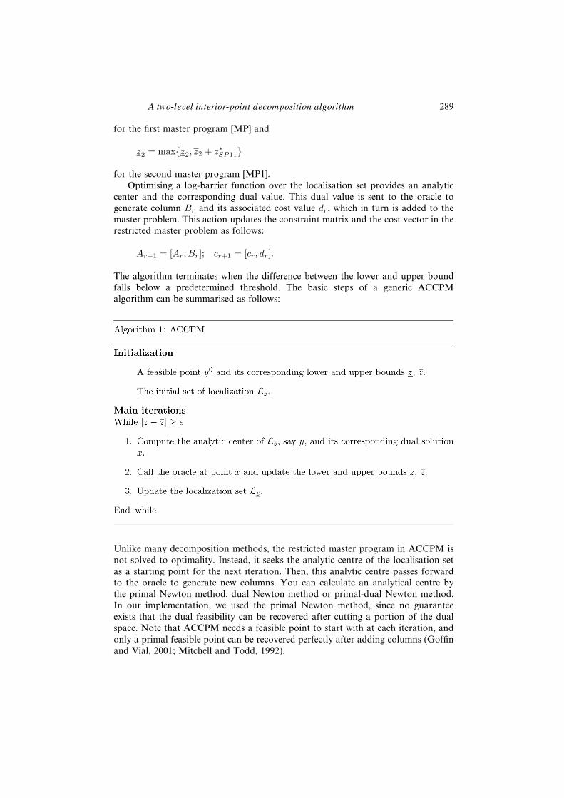
for the second master program [MP1].Optimising a log-barrier function over the localisation set provides an analytic

center and the corresponding dual value. This dual value is sent to the oracle togenerate column Br and its associated cost value dr, which in turn is added to themaster problem. This action updates the constraint matrix and the cost vector in therestricted master problem as follows:

Ar+1 = [Ar, Br]; cr+1 = [cr, dr].

The algorithm terminates when the difference between the lower and upper boundfalls below a predetermined threshold. The basic steps of a generic ACCPMalgorithm can be summarised as follows:

Unlike many decomposition methods, the restricted master program in ACCPM isnot solved to optimality. Instead, it seeks the analytic centre of the localisation setas a starting point for the next iteration. Then, this analytic centre passes forwardto the oracle to generate new columns. You can calculate an analytical centre bythe primal Newton method, dual Newton method or primal-dual Newton method.In our implementation, we used the primal Newton method, since no guaranteeexists that the dual feasibility can be recovered after cutting a portion of the dualspace. Note that ACCPM needs a feasible point to start with at each iteration, andonly a primal feasible point can be recovered perfectly after adding columns (Goffinand Vial, 2001; Mitchell and Todd, 1992).


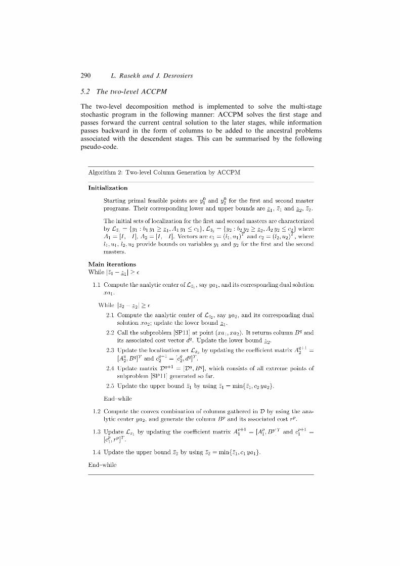
5.2 The two-level ACCPM

The two-level decomposition method is implemented to solve the multi-stagestochastic program in the following manner: ACCPM solves the first stage andpasses forward the current central solution to the later stages, while informationpasses backward in the form of columns to be added to the ancestral problemsassociated with the descendent stages. This can be summarised by the followingpseudo-code.


Note that in the above algorithm, we need the convex combination of all columnsthat are generated in the second loop to be passed forward as a new column to thefirst loop (the first master problem). Therefore, in 2.4, we design matrix D to gatherall the columns that are generated so far in the second loop. In the implementationof Dantzig-Wolfe, each time that we enter the second loop, we keep the previouslygenerated columns, whereas in ACCPM matrix D is reset to the empty matrix. In theabove pseudo-code, the convex combination of the columns that is gathered in D isdenoted by Bp.

6 Computational experiments

For the computational experiments, we implemented the two-level decompositionalgorithm on the capacity expansion and TSM. The code is written in MATLABversion 7.1 for both the two-level ACCPM and the two-level Dantzig-Wolfe. In theDantzig-Wolfe decomposition approach, the two linear relaxation of the restrictedmaster problems and the subproblem are solved using LINPROG, the build-inlibrary within MATLAB 7.1. Moreover, in the two-level ACCPM, the two linearrelaxation of the restricted master problems are solved with an in-house version ofACCPM (with a duality gap set at 10−4), and the subproblem is solved by usingLINPROG. TSM proposes a multi-stage stochastic program that models demandthrough a scenario tree and can accommodate any discrete demand distributionwith any number of products. We explored this possibility to create different jointprobability distributions of two products demand, so to be able to compare thetwo-level ACCPM against the two-level Dantzig-Wolfe in different dimensions.For example, in the first row of Table 1, 2-Demand means that we have two typesof forecasted demand (= Ds), with probability ps, s = 1, 2. Since we consider twoproducts, it generates 4 possible scenarios in the first stage and 16 scenarios inthe second stage. Similarly, the scenarios can be constructed through 3-Demand,4-Demand, 5-Demand and 8-Demand, processes that generate 81, 256, 625 and 4096scenarios, respectively.

The decomposition and partitioning procedure is done on the dual of TSMto take advantage of decomposing the problem along the stages. In terms of thenumber of variables on the dual problem, we solved a range of problems from63 variables to 12,483 variables, whereas the number of constraints ranged from54 to 8,454. The MATLAB limitations did not allow us to make the constraintmatrix beyond 12,483 × 8 454, which corresponds to the 8-Demand model. Thefeatures of the test problems are presented in Table 1.

An inner iteration of both ACCPM and Dantzig-Wolfe (DW) corresponds to aninner loop of the program in which the second master problem and the subprobleminteract. Alternatively, an outer iteration corresponds to an outer loop where thefirst master program interacts with the information received from the inner loop.As is presented in Table 1, the number of outer iterations in both ACCPM and DWare comparable for the aforementioned problem sizes. However, the real differenceis in terms of the number of inner iterations, where ACCPM performed much better,


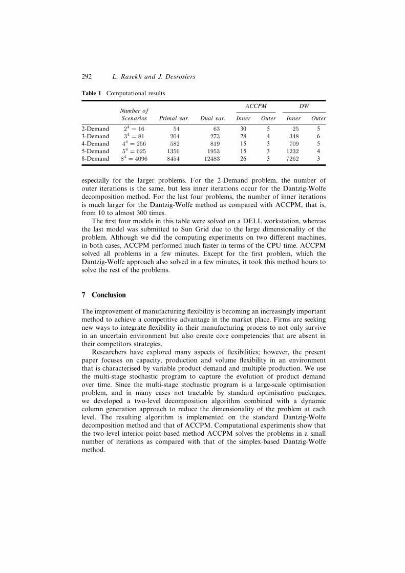
Table 1 Computational results

ACCPM DWNumber ofScenarios Primal var. Dual var. Inner Outer Inner Outer

2-Demand 24 = 16 54 63 30 5 25 53-Demand 34 = 81 204 273 28 4 348 64-Demand 44 = 256 582 819 15 3 709 55-Demand 54 = 625 1356 1953 15 3 1232 48-Demand 84 = 4096 8454 12483 26 3 7262 3

especially for the larger problems. For the 2-Demand problem, the number ofouter iterations is the same, but less inner iterations occur for the Dantzig-Wolfedecomposition method. For the last four problems, the number of inner iterationsis much larger for the Dantzig-Wolfe method as compared with ACCPM, that is,from 10 to almost 300 times.

The first four models in this table were solved on a DELL workstation, whereasthe last model was submitted to Sun Grid due to the large dimensionality of theproblem. Although we did the computing experiments on two different machines,in both cases, ACCPM performed much faster in terms of the CPU time. ACCPMsolved all problems in a few minutes. Except for the first problem, which theDantzig-Wolfe approach also solved in a few minutes, it took this method hours tosolve the rest of the problems.

7 Conclusion

The improvement of manufacturing flexibility is becoming an increasingly importantmethod to achieve a competitive advantage in the market place. Firms are seekingnew ways to integrate flexibility in their manufacturing process to not only survivein an uncertain environment but also create core competencies that are absent intheir competitors strategies.

Researchers have explored many aspects of flexibilities; however, the presentpaper focuses on capacity, production and volume flexibility in an environmentthat is characterised by variable product demand and multiple production. We usethe multi-stage stochastic program to capture the evolution of product demandover time. Since the multi-stage stochastic program is a large-scale optimisationproblem, and in many cases not tractable by standard optimisation packages,we developed a two-level decomposition algorithm combined with a dynamiccolumn generation approach to reduce the dimensionality of the problem at eachlevel. The resulting algorithm is implemented on the standard Dantzig-Wolfedecomposition method and that of ACCPM. Computational experiments show thatthe two-level interior-point-based method ACCPM solves the problems in a smallnumber of iterations as compared with that of the simplex-based Dantzig-Wolfemethod.


References

Andrade, R., Lisser, A., Maculan, N. and Plateau, G. (2004) ‘Telecommunication networkcapacity design for uncertain demand’, Computational Optimization and Applications,Vol. 29, No. 2, pp.127–146.

Bahn, O., du Merle, O., Goffin, J-L. and Vial, J-Ph. (1995) ‘A cutting plane method fromanalytic centers for stochastic programming’, Mathematical Programming, Vol. 69,pp.45–73.

Babonneau, F., du Merle, O. and Vial, J-P. (2006) ‘Solving large-scale linear multicommodityflow problems with an active set strategy and proximal-ACCPM’, Operations Research,Vol. 54, No. 1, pp.184–197.

Baboneau, F., Beltran, C., Haurie, A., Tadonki, C. and Vial, J-Ph. (2007) ‘Proximal-ACCPM:a versatile oracle based optimization method’, Optimisation, Econometric and FinancialAnalysis, Springer Berlin Heidelberg, pp.69–92.

Ben Amor, H. and Desrosiers, J. (2006) ‘A proximal trust-region algorithm for columngeneration stabilization’, Computers and Operations Research, Vol. 33, No. 4,pp.910–927.

Birge, J.R. (1985) ‘Decomposition and partitioning methods for multi-stage stochastic linearprogram’, Operations Research, Vol. 33, pp.989–1007.

Birge, J.R. and Holmes, D.F. (1992) ‘Efficient solution of two-stage stochastic linearprograms using interior point methods’, Computational Optimization and Applications,Vol. 1, pp.245–276.

Benders, J.F. (1962) ‘Partitioning procedure for solving mixed-variables programmingproblems’, Numerische Mathematik, Vol. 4, pp.238–252.

Berkelaar, A., Gromicho, J.A., Kouwenberg, R. and Zhang, S. (2005) ‘A primal-dual decomposition algorithm for multi-stage stochastic convex programming’,Mathematical Programming A, Vol. 104, pp.153–177.

Chen, Z., Li, S. and Tirupati, D. (2002) ‘A scenario-based stochastic programming approachfor technology and capacity planning’, Computers and Operations Research, Vol. 7,pp.781–806.

Colombo, M., Gondzio, J. and Grothyey, A. (2006) A Warm Start for Large-scale StochasticLinear Programs, Technical Report MS-06-004, School of Mathematics, University ofEdinburgh.

Elhedhli, S. and Goffin, J-L. (2005) ‘Efficient production-distribution system design’,Management Science, Vol. 51, No. 7, pp.1151–1164.

Gassman, H.I. (1990) ‘MSLiP: a computer code for the multi-stage stochastic linearprogramming problem’, Mathematical Programming, Vol. 47, No. 3, pp.407–423.

Goffin, J-L., Haurie, A. and Vial J-P. (1992) ‘Decomposition and nondifferentiableoptimization with the projective algorithm’, Management Science, Vol. 38, No. 2,pp.284–302.

Goffin, J-L. and Vial, J-P. (2001) ‘Multiple cuts in analytic center cutting plane method’,SIAM Journal of Optimization, Vol. 11, No. 1, pp.266–288.

Gondzio, J., Sarkissian, R. and Vial, J-P. (1997) ‘Using an interior point method forthe master problem in a decomposition approach’, European Journal of OperationsResearch, Vol. 101, pp.577–587.

Lübbecke, M.E. and Desrosiers, J. (2005) ‘Selected topics in column generation’, OperationsResearch, Vol. 53, No. 6, pp.1007–1023.

Li, S., Loulou, R. and Rahman, A. (2003) ‘Technological progress and technologyacquisition: strategic decision under uncertainty’, Production and OperationsManagement, Vol. 12, No. 1, pp.102–119.


Mitchell, J.E. and Todd, M. (1992) ‘Solving combinatorial optimization problems usingKarmarkar’s algorithm’, Mathematical Programming, Vol. 56, pp.245–284.

Oukil, A., Ben Amor, H., Desrosiers, J. and El Gueddari, H. (2007) ‘Stabilisedcolumn generation for highly degenerate multiple-depot vehicle scheduling problems’,Computers and Operations Research, Vol. 34, No. 3, pp.817–834.

Rasekh, L. and Desrosiers, J. (2008) ‘Solving multi-stage stochastic, in-house productionand outsourcing planning by two-level decomposition’, International J. Mathematics inOperations Research, Vol. 2, No. 2, pp.129–150.

Rockafellar, R.T. and Wets, R.J.B. (1991) Scenario and policy aggregation in optimizationunder uncertainty’, Mathematics of Operations Research, Vol. 16, No. 1, pp.119–147.

Rockafellar, R.T. and Wets, R.J.-B. (1992) ‘A Lagrangian finite generation techniquefor solving linear-quadratic problems in stochastic programming’, MathematicalProgramming, Vol. 28, pp.63–93.

Sethi, A.K. and Sethi, S.P. (1990) ‘Flexibilty in manufacturing: a survey’, International J.Flexible Manufacturing Systems, Vol. 2, pp.289–328.

Van Slyke, R. and Wets, R.J-B. (1969) ‘L-shaped linear programs with application to optimalcontrol and stochastic programming’, SIAM Journal on Applied Mathematics, Vol. 17,pp.638–663.

Zhao, G. (2001) ‘A log-barrier method with Benders decomposition for solving two-stagestochastic linear programs’, Mathematical Programming, Vol. 90, No. 3, pp.507–536.

A two-level interior-point decomposition algorithm for multi-stage stochastic capacity planning and...

Documents

Transcript of A two-level interior-point decomposition algorithm for multi-stage stochastic capacity planning and...