Optimization Models and Methods for

Planning Wireless Mesh Networks

E. Amaldi, A. Capone, M. Cesana, I. Filippini, F. Malucelli

Dipartimento Elettronica e InformazionePolitecnico di Milano

Milano, Italy,{amaldi, capone, cesana, filippini, malucell}@elet.polimi.it

Abstract

In this paper novel optimization models are proposed for planning Wireless MeshNetworks (WMNs), where the objective is to minimize the network installationcost while providing full coverage to wireless mesh clients. Our mixed integer lin-ear programming models allow to select the number and positions of mesh routersand access points, while accurately taking into account traffic routing, interference,rate adaptation, and channel assignment. We provide the optimal solutions of threeproblem formulations for a set of realistic-size instances (with up to 60 mesh de-vices) and discuss the effect of different parameters on the characteristics of theplanned networks. Moreover, we propose and evaluate a relaxation-based heuristicfor large-sized network instances which jointly solves the topology/coverage plan-ning and channel assignment problems. Finally, the quality of the planned networksis evaluated under different traffic conditions through detailed system level simula-tions.

Key words: Wireless Mesh Networks, Planning, Topology, Coverage, ChannelAssignment, Discrete Optimization.

1 Introduction

Wireless Mesh Networking is widely recognized as a promising and cost ef-fective solution for providing wireless connectivity to mobile users eventuallycompeting with wired broadband access technologies. Such success is mainlydue to the high flexibility of the mesh networking paradigm which has manyadvantages in terms of self-configuration capability and reduced installationcost.

Preprint submitted to Elsevier 23 January 2008

Wireless Mesh Networks (WMNs) are composed of a mix of fixed and mobilenodes interconnected through multi-hop wireless links. Unlike in flat MobileAd hoc Networks (MANETs), the wireless mesh network devices are hierarchi-cally organized in terms of networking functionalities and hardware capabili-ties [1]. Roughly speaking, wireless mesh network devices are of three types:Mesh Routers (MRs), Mesh Access Points (MAPs) and Mesh Clients (MCs).The functionality of both the MRs and the MAPs is twofold: they act as classi-cal access points towards the MCs, whereas they have the capability to set upa Wireless Distribution System (WDS) by connecting to other mesh routersor access points through point to point wireless links. Both MRs and MAPsare often fixed and electrically powered devices. Furthermore, the MAPs aregeared with some kind of broadband wired connectivity (LAN, ADSL, fiber,etc.) and act as gateways toward the wired backbone. MCs are users terminalsconnected to the network through MAPs or MRs.

In this type of network architecture, a limited number of MAPs connectedto the wired realm can potentially provide low-cost internet connectivity to alarge number of MCs. This is substantially different from other wireless accessnetworks (2G/3G cellular systems, WLAN hot spots), where all wireless accesspoints are directly connected to the wired backbone.

Several features have a strong impact on the performance of a general wire-less mesh network, including the number of radio interfaces for each device,the number of available radio channels, the access mechanism, the routingstrategies and the specific wireless technology used to implement the meshparadigm. Moreover, since network deployments can involve thousands of de-vices (MAPs, MRs, and MCs), manual tuning and re-configuration are veryunpractical and the automatic planning and optimization of the network cov-erage and topology is of utmost importance to efficiently provide the requiredservices [5].

The problem of planning WMNs differs from that of planning other wire-less networks, such as cellular systems [4] or WLANs [6]. In the latter cases,network planning is almost entirely driven by geographical coverage. Sincewireless transceivers are also gateways towards the wired backbone, their po-sitions/configurations depend only on local connectivity constraints, betweenend users and the closest network device.

In the case of WMNs, the traffic to/from the wired backbone has to be routedon a path connecting the MR to one MAP at least, thus, besides ensuring localconnectivity between MCs and MRs (or MAPs), a multi-hop path needs to beset up in the WDS between each end user and one MAP at least (multi-hopconnectivity constraint). Moreover, unlike 2G and 3G systems, each candi-date site can host either MAPs or MRs, with different installation costs. Infact, MAPs are often more expensive than MRs since they must be directly

2

connected to the wired backbone and might be more powerful in terms ofprocessing and transmission capabilities. Thus, in designing WMNs one mustsimultaneously consider radio coverage of end users (MCs), as in classical radioplanning for wireless access networks [3], and traffic routing, as in the designof wired networks [7].

In this paper, we propose optimization models for coverage and topology plan-ning of WMNs with multiple radio interfaces and multiple orthogonal chan-nels available at each interface. Our mathematical integer linear programmingmodels aim at minimizing the overall installation cost by jointly optimizing thenumber/locations of MRs and MAPs, and the channel assignment, while tak-ing into account both the local and the multihop connectivity requirements. Weprovide optimal solutions for a set of realistic medium-scale synthetic networkinstances and discuss the effect of different parameters on the characteristicsof the solutions. Moreover, we present a heuristic approach to solve large-sizeinstances with an accuracy of 5% with respect to the optimum. Finally, theplanned instances are evaluated through detailed system level simulations withns2 [26].

The paper is organized as follows. In Section 2 we summarize related workand comment on the novel contributions of our approach. In Section 3 weintroduce a basic version of the optimization model for planning WMNs, andwe report and discuss numerical results. In Section 4 we show how to accountfor interference in the optimization model, and we propose a heuristic algo-rithm to solve large-size network instances. Section 5 describes the completeoptimization model accounting also for multiple radio interface and multiplechannels available at each interface. Since the complete model formulation ishard to solve at optimum for large networks, we also present a heuristic al-gorithm which jointly optimizes mesh devices choice/positioning and channelassignment. In Section 6 we comment on the quality of the planning approachby obtaining the throughput of planned networks through system level sim-ulations in ns2. Section 7 contains concluding remarks and future researchdirections.

2 Related Work and Contributions

Even if commercial solutions are already available, many aspects of WMNs arestill under investigation. The intrinsic flexibility of the WMNs poses stringentresearch challenges at different layers and a huge research effort is nowadaysdevoted to the optimization of protocols and the design of algorithms to sup-port mesh networking.

The most popular research fields on mesh networking include Medium Access

3

Control and routing protocols, mobility management and security issues. SinceWMNs are wireless multi-hop networks relying on a Wireless DistributionSystem to transport the information, the impact of the interference amongdifferent wireless links may dramatically affect the overall network capacity[19]. It is commonly recognized that the use of wireless devices (routers andaccess points) with multiple wireless Network Interface Cards (NICs) highlyreduces the impact of the interference consequently increasing the capacity ofthe wireless mesh network [8]–[13].

Substantial previous work aims at providing optimized protocols for WMNs.In [8] So et al. propose a multichannel MAC protocol for the single interfacetransceiver case, whereas in [9] the authors study the case of multiple radiointerface per wireless node by adapting the channel access protocol. Das etal. present two integer linear programming models to solve the fixed channelassignment problem with multiple radio interfaces [10], while [11] and [12,13]address the joint problems of channel assignment and routing, and providedifferent formulations of the corresponding optimization problem.

In most of the previous work, the network topology (MAPs and MRs locations)is assumed to be given and the goal is to optimize the channel assignmentand/or the routing. In the present work, instead, we model the radio planningproblem of WMNs, providing quantitative methods to optimize the number,positions and physical parameters of MRs and MAPs while controlling theoverall topology of the network.

So far little attention has been devoted to planning WMNs or general fixedmulti-hop wireless networks. So et al. [14] propose an optimization modelfor the topology planning of WMNs with non-linear constraints, aimed atminimizing the overall installation cost. The non-linear formulation is solvedvia Benders decomposition. In [15] Wang et al. describe a heuristic approachto tackle the same problem of MRs deployment. Unlike in our approach, thesetwo papers consider the case of a single and pre-defined MAP to the Internetand optimize the positions of MRs only. On the other hand, our approachendorses also the positioning of MAPs.

In [16], the authors focus on locating internet transit access points (corre-sponding to MAPs in the terminology adopted in this paper) in wireless neigh-borhood networks. Heuristic methods and a lower bound are provided, whenadopting an interference model according to which interference perceived bya traffic flow grows linearly with the number of wireless hops traversed. Thesame problem and a similar modelling approach is studied in [17]. Since thepositions of all the other nodes (MRs) are given and such nodes are also theonly traffic ending points in the network, the problem considered in [16,17]is actually a subproblem of the one proposed in this paper, where the cover-age part is omitted. Moreover, we consider a more detailed interference model

4

based on a fluidic version [18] of the protocol interference model [19]. The prob-lem in [16] was previously proposed in [20] for TDMA-based WMNs under theform of a slot scheduling problem.

3 Basic model

We first describe a basic version of the mathematical programming model forWMN planning and then extend it so as to capture the important aspects ofinterference and multiple channels. We will proceed in three steps not only toprogressively add increasing levels of detail and complexity, but also becauseour three resulting models (basic, interference aware, multi channel ones) areuseful in practice depending on the specific network scenario, as we show lateron.

Let us consider the network description presented in Figure 1.

j

l

yjl

wjN

zj

i

xij

NWired backbone

MAPMRTP

j

l

yjl

wjN

zj

i

xij

NWired backbone

MAPMRTP

Fig. 1. WMN planning problem description.

As in other coverage problems for wireless access networks [5], let S = {1, . . . , m}denote the set of candidate positions where to install mesh devices (Candi-date Sites, CSs) and I = {1, . . . , n} the set of traffic concentration points(Test Points, TPs). A special node N represents the wired backbone network.The cost associated to installing a MR in CS j is denoted by cj, while theadditional cost required to install a MAP in CS j is denoted by pj, j ∈ S. Thetotal cost for installing a MAP in CS j is therefore given by (cj + pj).

The traffic generated by each TP i is given by parameter di, i ∈ I. The trafficcapacity of the wireless link between CSs j and l is denoted by ujl, j, l ∈ S,while the capacity of the radio access interface of CS j is denoted by vj, j ∈ S.

For each TP i in I, Si = {j(i)1 , j

(i)2 , . . . , j

(i)Li} denotes the ordered subset of CSs

5

that can cover i, where the CSs are ordered according to the non-increasingreceived signal strength.

The connectivity parameters define which network elements can be connectedthrough wireless links. They depend on TPs and CSs locations and channelconditions and can be determined by using proper propagation prediction tools(e.g., empirical channel models like Hata’s one [22], sophisticated ray tracingtools [23], or even field measurements). Note that propagation prediction is outof the scope of this paper and, as in most of the works on radio planning (seee.g. [3]-[6]), we assume that propagation parameters are given. In particular,we consider the coverage parameter:

aij =

1 if a MAP or MR in CS j covers TP i

0 otherwise,

for each pair i ∈ I, j ∈ S, and the wireless connectivity parameters:

bjl =

1 if CS j and l can be connected with a link

0 otherwise.

for each j, l ∈ S.

Decision variables of the problem include TP assignment variables xij, i ∈I, j ∈ S:

xij =

1 if TP i is assigned to CS j

0 otherwise,

installation variables zj, j ∈ S:

zj =

1 if a MAP or a MR is installed in CS j

0 otherwise,

wired backbone connection variables wjN , j ∈ S (if zj = 1, wjN denote if j isconnected to the wired network N , i.e. if it is a MAP or a MR):

wjN =

1 if a MAP is installed in CS j

0 otherwise,

wireless connection variables yjl, j, l ∈ S:

yjl =

1 if there is a wireless link between CS j and l

0 otherwise,

6

and finally flow variables fjl which denote the traffic flow routed on link (j, l),where the special variable fjN denotes the traffic flow on the wired link betweenMAP j and the backbone network.

Given the above parameters and variables, the WMN planning problem canbe formulated as follows:

min∑

j∈S

(cjzj + pjwjN) (1)

s.t. ∑

j∈S

xij = 1 ∀i ∈ I (2)

xij ≤ zjaij ∀i ∈ I, ∀j ∈ S (3)∑

i∈I

dixij +∑

l∈S

(flj − fjl)− fjN = 0 ∀j ∈ S (4)

flj + fjl ≤ ujlyjl ∀j, l ∈ S (5)∑

i∈I

dixij ≤ vj ∀j ∈ S (6)

fjN ≤ MwjN ∀j ∈ S (7)

yjl ≤ zj, yjl ≤ zl ∀j, l ∈ S (8)

yjl ≤ bjl ∀j, l ∈ S (9)

zj(i)`

+Li∑

h=`+1

xij

(i)h

≤ 1 ∀` = 1, . . . , Li − 1,∀i ∈ I (10)

xij, zj, yjl, wjN ∈ {0, 1} ∀i ∈ I, ∀j, l ∈ S (11)

The objective function (1) accounts for the total cost of the network includinginstallation costs cj and costs pj related to the connection of MAP to thewired backbone. If for some practical reason only a MR and not a MAP can beinstalled in CS j, the corresponding variable wjN is set to zero. Constraints (2)provide full coverage of all TPs, while constraints (3) are coherence constraintsassuring respectively that a TP i can be assigned to CS j only if a device (MAPor MR) is installed in j and if i is within the coverage set of j.

Constraints (4), which define the flow balance in node j, are typical of classicalmulti-commodity flow problems. The term

∑i∈I dixij is the total traffic related

to assigned TPs,∑

l∈S flj is the total traffic received by j from neighboringnodes,

∑l∈S fjl is the total traffic transmitted by j to neighboring nodes, and

fjN is the traffic transmitted to the wired backbone. Even if these constraintsassume that traffic from TPs is transmitted to the devices to which they areassigned and that this traffic is finally delivered by the network to the wiredbackbone, without loss of generality we can assume that di accounts for thesum of traffic in the uplink (from TPs to the WMN) and in the downlink (fromWMN to the TPs) since radio resources are shared in the two directions.

7

Constraints (5) impose that the total flow on the link between device j andl does not exceed the capacity of the link itself (ujl). As already mentionedabove, these constraints account for the flows in either directions (fjl and flj)since they share the same radio resources. Constraints (6) impose for all theMCs’ traffic serviced by a network device (MAP or MR) not to exceed thecapacity of the wireless link used for the access, while constraints (7) forcesthe flow between device j and the wired backbone to zero if device j is not aMAP. The parameter M is used to limit the capacity of the installed MAP.

Constraints (8) and (9) defines the existence of a wireless link between CS jand CS l, depending on the installation of nodes in j and l and wireless connec-tivity parameters bjl. The constraints expressed by (10) force the assignmentof a TP to the best CS in which a MAP or MR is installed according to aproper sorting criteria (such as the received signal strength), while constraints(11) restrict the decision variables to take binary values.

Note that the yjl variables can be eliminated from this basic formulation bycombining constraints (5) and (8), that is by replacing in the right-hand sideof constraints (5) yjl by zj and zl.

The resulting model is obviously NP-hard since it includes the set coveringand the multi-commodity flow problems as special cases.

The formulation presented so far considers fixed transmission rates for bothwireless access interface and wireless distribution system, thus it will be re-ferred to as Fixed Rate Model (FRM) throughout the paper. The FRM canbe easily extended to account for transmission rate adaptation.

For the wireless distribution system, it suffices to let the parameters ujl ap-propriately depend on the propagation conditions between CSs j and l. Noother modification to the model formulation is required.

Rate adaptation in the wireless access network can be accounted for by slightlymodifying constraints (6). We consider several concentric regions centered ineach CS, assigning to each region a maximum rate value. All the TPs fallingin one of these regions can communicate with the node in the CS by using thespecific rate of the region. Obviously, regions with more favorable propagationconditions can exploit higher rates.

Formally, for any given CS j we define a set of concentric regions Rkj = 1, ..., K

and the set Ikj ⊆ I containing all the TPs falling in the k-th region of CS j.

Such sets can be determined for each CS j by using the incidence variables

akij =

1 if a TP i falls within region k of the CS j

0 otherwise.

8

Fig. 2. Rate adaptation regions around CS j.

For a given CS j, each of these regions is assigned a maximum capacity vkj . In

Figure 3 three capacity regions are defined around CS j: the nearest region tothe CS has a maximum capacity v1

j = 3, while in the most external one themaximum capacity drops to v3

j = 1.

Based on the above definitions, rate adaptation in the wireless access partof the network is accounted for by substituting the constraints (6) with thefollowing new constraints:

∑

k∈Rj

∑i∈Ik

jdixij

vkj

≤ 1 ∀j ∈ S. (12)

The resulting model with constraints (12) will be referred to as Rate Adapta-tion Model (RAM) throughout the paper.

3.1 Numerical results

To get some insight on the proposed WMN design approach, we investigate thecharacteristics of the networks obtained with the basic models by evaluatingthe impact of different parameters like the number of CSs, the traffic demandsfrom the MCs and the installation costs.

To this end, we have implemented a generator of WMN planning instanceswhich considers specific parameter settings and makes some assumptions onpropagation and device features. Obviously, these assumptions do not affectthe proposed model which is general and can be applied to any problem in-stance. The instance generator considers a square area with edge L = 1000m, and it randomly draws the position of m CSs and of n = 100 TPs. Thecoverage area for the access part of a mesh node is assumed to be a circularregion with radius RA = 100 m. Only feasible instances where each TP iscovered by at least one CS are considered. The range of the wireless backbone

9

(a) d=600Kb/s (b) d=3Mb/s

Fig. 3. Sample WMNs planned by the FRM with increasing traffic demands of theMCs and finite capacity of the installed MAPs (M = 128Mb/s).

links is set to RB = 250 m, while the capacities of the access links, vj, andbackbone links, ujl, are both set to 54 Mb/s for all j and l. The capacity Mof the links connecting MAPs to the wired network is either infinite or equalto 128 Mb/s. The ratio between the cost of a MR and a MAP is β (β = 1/10unless otherwise specified).

All the results reported in this section correspond to optimal solutions of theconsidered instances obtained by building the Mixed Integer Linear Program-ming (MILP) model with AMPL [24] and by solving it with CPLEX [25] ona workstation equipped with a INTEL Pentium (TM) processor with CPUsoperating at 3GHz, and with 1024Mbyte of RAM.

Given the number and the positions of both CSs and TPs, the quality of thedeployed WMN and the overall installation cost depend on two parameters:the traffic demand d of the MCs and the ratio between the MR and MAPinstallation costs β.

Figure 3 reports an example of the planned networks obtained with the FRMfor the same instance with two different requirements on the end user traffic,d = 600Kb/s and d = 3Mb/s for all MCs, and with a finite capacity of thelinks connecting MAPs to the wired network (M = 128Mb/s). Black squaresrepresent the installed MAPs, triangles the installed MRs and crosses the MCspositions. Dotted lines express the association between a MC and a MR, whilesolid lines indicate that MRs and MAPs are within communication range andthe link is used for transmitting traffic. As expected, when the traffic demandsincrease, the number of installed MAPs increases as well in order to convey theMCs’ traffic towards the wired realm. On the other hand, the total numberof MRs and wireless links is almost the same in the two networks. Indeed,the overall network capacity is mainly limited by the capacity of the links

10

(a) d=600Kb/s (b) d=3Mb/s

Fig. 4. Sample WMNs planned by the FRM with increasing traffic demands of theMCs and infinite capacity of the installed MAPs (M unbounded).

Table 1Optimal solutions of FRM with finite capacity of the installed MAPs (M =128Mb/s).

d=600Kb/s

MAP MR Links Time (s)

m=30 2.2 23.7 21.5 0.40

m=40 1.4 24 22.5 1.43

m=50 1.2 24.1 22.9 4.69

d=3Mb/s

MAP MR Links Time (s)

m=30 4 23.6 20.2 0.63

m=40 3.4 23.7 21 10.93

m=50 3.3 23.9 21.6 32.88

connecting MAPs to the wired backbone. If we remove the MAP capacityconstraints (M is unbounded) the networks obtained with the FRM, shown inFigure 4, are quite different. In this case there is only one MAP installed forboth traffic values, but the number of MRs and wireless links is significantlyhigher for d = 3Mb/s.

Tables 1 and 2 summarize the characteristics of the solutions obtained with theFRM when varying the number of CSs for the instances with M = 128Mb/sand M unbounded, respectively. For each pair (m, d) the tables report thenumber of installed MRs, the number of installed MAPs, the number of wire-less links of the WDS and the processing time to get the optimal solution.The results are averages over 20 WMN planning instances.

11

Table 2Optimal solutions of FRM with infinite capacity of the installed MAPs (M un-bounded).

d=600Kb/s

MAP MR Links Time (s)

m=30 2.3 23.4 18.6 1.28

m=40 1.4 27.4 26.2 2.2

m=50 1.1 28.4 29 18.16

d=3Mb/s

MAP MR Links Time (s)

m=30 2.8 24.2 20.7 0.68

m=40 1.8 28.1 27.8 5.47

m=50 1.1 31 35.5 4.72

Table 1 suggests two main comments. First, we observe that, as in Figure3, also for average results the number of installed MAPs increases when thetraffic demand is increased. Second, for a given traffic value d, increasing thenumber of CSs to 50 also increases the probability for a MC to be connectedto a MAP through a multi-hop wireless path. Therefore, fewer MAPs andmore MRs tend to be installed. On the other hand, for a lower number of CSs(30), more MAPs are installed since not all the MCs can be connected to theMAPs through multi-hop wireless paths. In other words, the solution space isbigger for larger values of m and solutions providing connectivity at a lowercost (installing more MRs than MAPs) are favored.

Averaged results in Table 2 also confirm the behavior shown in Figure 4 wherethe solutions provided by the model are such that an increase in the trafficdemands implies an increase in the dimension of the WDS which is used toconvey the traffic, both in terms of installed MRs and in terms of wirelesslinks composing the WDS.

The number of installed MAPs and MRs clearly depends also on the installa-tion cost ratio β between a simple wireless router and a mesh access point. Ifthe cost for installing a MAP is much higher than the one spent for installinga MR, the proposed model tends to install fewer MAPs and multiple MRs.On the other hand, when the cost ratio tends to one only MAPs tend to beinstalled.

Figure 5 illustrates this effect by showing the network layout in the case oftraffic demand d = 3Mb/s and unbounded MAP capacity when varying theinstallation costs. A larger value of the parameter β leads to a planned networkwith multiple MAPs installed. If the installation cost of MAPs is much higherthan the one of MRs, the incidence of the MAPs installation cost on the overall

12

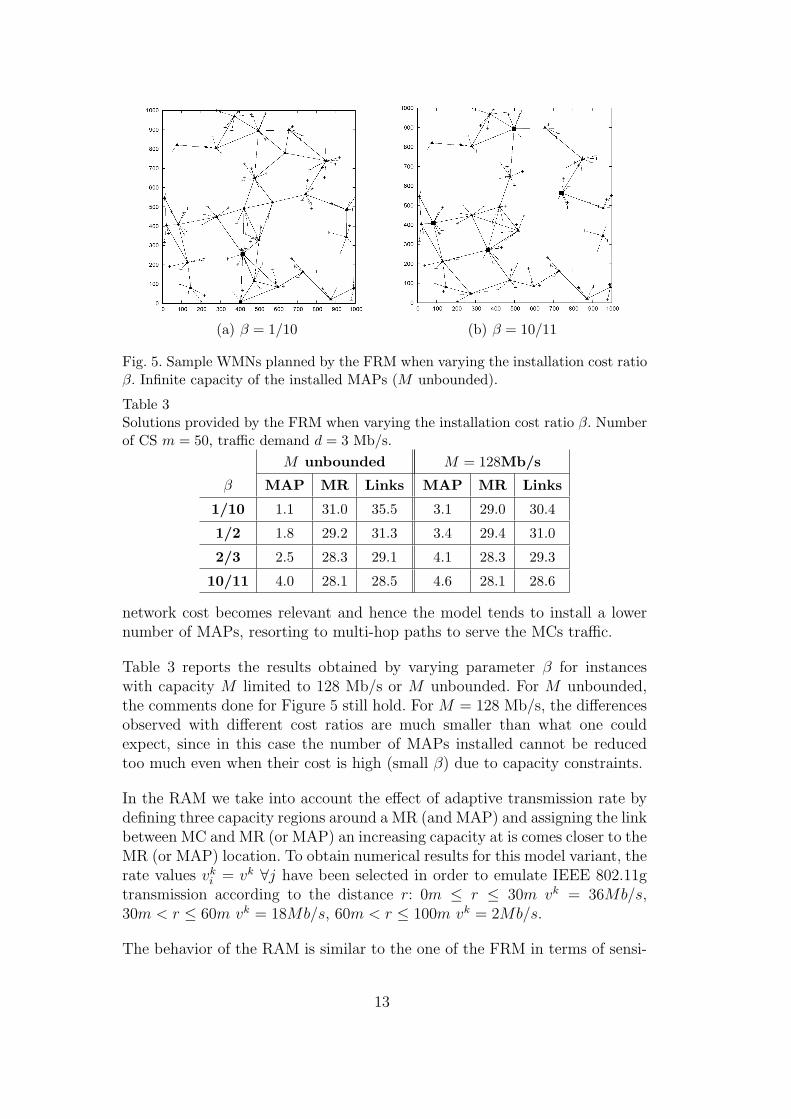
(a) β = 1/10 (b) β = 10/11

Fig. 5. Sample WMNs planned by the FRM when varying the installation cost ratioβ. Infinite capacity of the installed MAPs (M unbounded).

Table 3Solutions provided by the FRM when varying the installation cost ratio β. Numberof CS m = 50, traffic demand d = 3 Mb/s.

M unbounded M = 128Mb/s

β MAP MR Links MAP MR Links

1/10 1.1 31.0 35.5 3.1 29.0 30.4

1/2 1.8 29.2 31.3 3.4 29.4 31.0

2/3 2.5 28.3 29.1 4.1 28.3 29.3

10/11 4.0 28.1 28.5 4.6 28.1 28.6

network cost becomes relevant and hence the model tends to install a lowernumber of MAPs, resorting to multi-hop paths to serve the MCs traffic.

Table 3 reports the results obtained by varying parameter β for instanceswith capacity M limited to 128 Mb/s or M unbounded. For M unbounded,the comments done for Figure 5 still hold. For M = 128 Mb/s, the differencesobserved with different cost ratios are much smaller than what one couldexpect, since in this case the number of MAPs installed cannot be reducedtoo much even when their cost is high (small β) due to capacity constraints.

In the RAM we take into account the effect of adaptive transmission rate bydefining three capacity regions around a MR (and MAP) and assigning the linkbetween MC and MR (or MAP) an increasing capacity at is comes closer to theMR (or MAP) location. To obtain numerical results for this model variant, therate values vk

i = vk ∀j have been selected in order to emulate IEEE 802.11gtransmission according to the distance r: 0m ≤ r ≤ 30m vk = 36Mb/s,30m < r ≤ 60m vk = 18Mb/s, 60m < r ≤ 100m vk = 2Mb/s.

The behavior of the RAM is similar to the one of the FRM in terms of sensi-

13

Table 4Quality of the solutions provided by the RAM.

d=200Kb/s

MAP MR Links Time (s)

m=30 2.80 23.80 21.00 2.24

m=40 1.70 24.60 22.90 9.66

m=50 1.20 24.40 23.20 46.83

d=600Kb/s

MAP MR Links Time (s)

m=30 2.80 25.40 22.60 2.24

m=40 1.70 26.00 24.30 13.25

m=50 1.20 26.10 24.90 61.37

tivity to the model parameters. Table 4 summarizes the characteristics of thesolutions obtained with the RAM when varying the number of CSs. Note thatthe traffic values d used in this case are lower than the ones used for the FRMsince the link rates are in the average lower. Thus, higher values of d may leadto unfeasible instances.

4 Interference Aware Model

Although wireless technologies like IEEE 802.16 mesh mode and IEEE 802.11multi-radio mesh networks allow to limit the impact of interference by parti-tioning radio resources among wireless links using several frequencies or sub-carriers, the interference effect on the access capacity and on the capacity ofwireless distribution system (wireless links connecting mesh nodes) must betaken into account. We focus here on the case of IEEE 802.11 and assumethat all MAPs and MRs share the same radio channel for the access part anduse another shared channel for the backbone links. Since transmissions be-tween MAPs or MRs and MCs occur on the same channel and the CSMA/CA(Carrier Sense Multiple Access Collision Avoidance) protocol is adopted toregulate channel access, a single transmission at a time is allowed in the cov-erage range [6]. The impact of interference on the access capacity can then beaccounted for by modifying in the RAM constraints (12) as follows:

∑

k∈Rj

∑i∈Ik

jdi

vkj

≤ 1 + Mj(1− zj) ∀j ∈ S, (13)

14

Fig. 6. Example of interference set associated to link (j, l).

where Mj is the smallest constant that is large enough to ensure that theinequality is always satisfied when zj = 0 (regardless of the other variablevalues). Whenever zj = 1 the left-hand side is obviously required to be at most1. Note that here all TPs in the coverage range of a given CS are considered,rather than considering only those TPs assigned to the node in CS j as inconstraints (12).

The interference limiting effect on the wireless link capacities is more difficultto account for, since it depends on the network topology and the multipleaccess protocol. Considering the protocol interference model proposed in [19],we can define sets of links that cannot be active simultaneously. These setsdepend on the specific multiple access protocol considered. In the case ofCSMA/CA, adopted by IEEE 802.11, each set Cjl associated to a link (j, l)includes all those links that are one and two hops away in the mesh-networkgraph (links that connect j and l to their neighbors and their neighbors to theneighbors of their neighbors). Figure 6 illustrates an example of interferenceset (links in bold) associated to link (j, l).

To each set Cjl we can associate a constraint on the flows crossing its links:

∑

(k,h)∈Cjl

fkh

ukh

≤ 1 + Mjl(1− yjl) ∀j, l ∈ S, (14)

where the constant Mjl is such that the inequality is always satisfied whenyjl = 0 and the left-hand side is required to be at most 1 when yjl = 1. Ob-viously, by describing the capacity limitation due to set Cjl with a constrainton the flows crossing its links, we make an approximation since we considera fluidic (continuous) model of a discrete problem [18]. However, the effectof this approximation and the one due to traffic dynamics can be accountedfor by properly reducing the capacity values ukh. Through simulation of IEEE802.11 multi-hop networks we have estimated that a reduction of 5% is suffi-cient to achieve consistent results. Adding to the RAM model constraints (14)and replacing (12) with (13) we obtain the Interference Aware Model (IAM),

15

which considers the impact of interference on both the access capacity andthe wireless distribution system capacity.

Table 5 reports the results obtained with the IAM for the special case inwhich rate adaptation is not included. Since the parameter settings are thesame adopted for the FRM, results in Tables 5 and 1 can be directly compared.The sets Cjl have been determined by considering the IEEE 802.11 multipleaccess scheme.

Table 5Optimal solutions of IAM without rate adaptation.

d=600Kb/s

MAP MR Links Time (s)

m=30 3.40 22.20 19.40 4.37

m=40 2.50 23.10 20.90 258.09

m=50 2.30 23.40 21.60 1,706.63

d=3Mb/s

MAP MR Links Time (s)

m=30 8.50 22.00 14.20 4.16

m=40 7.80 22.50 16.10 53.98

m=50 7.70 23.40 17.80 1,345.32

We observe that the number of MAPs installed is much higher and the numberof links in the WDS lower with respect to the FRM case. This is due tothe capacity reduction of wireless links that favors solutions where MRs andMAPs are interconnected through paths with a small number of hops. Infact, with short paths between MRs and MAPs the effect of interference isweaker. Obviously, short paths require a higher number of MAPs. Anothersignificant difference between the FRM and the IAM results is the computingtime which is much higher for IAM in most of the cases. Expectedly, this isdue to the structure of constraints (14) which involve several flow variables.Similar comments also hold for the IAM with rate adaptation.

4.1 Relaxation-based heuristic

Since solving large-scale instances of IAM is computationally challenging, wehave developed a heuristic approach based on the linear relaxation of theMIP formulation. The rationale of the proposed algorithm is the following: wedetermine an optimal solution of an easier continuous relaxation of the IAMand exploit it to derive useful information about the structure of an optimalsolution of the IAM. A candidate solution of IAM is obtained by appropriatelyrounding the optimal solution of the IAM relaxation where all but one group

16

of binary variables can take fractional values in [0, 1]. Finally, the candidatesolution for the IAM is improved applying local changes.

The proposed algorithm proceeds in four steps.

Step 1 - Solve Continuous Relaxation. Solve to optimality the IAM relaxationwhere the MR installation variables zj and the TP-MR assignment variablesxij are fractional, and only the MAP installation variables wjN are binary.Since experimentally more than 90% of the zj are binary (within 10−9 preci-sion) and all the remaining relaxed variables are very close to 0 or 1, we setthe zj that are binary to 0 or 1 and we round up or down the other zj.

Step 2 - Find Candidate Solution. A candidate solution is obtained by solv-ing the IAM relaxation with zj fixed in Step 1 and with the variables wjN andxij binary. Clearly, the flows may be infeasible with respect to the given capac-ities, as the MR locations have been obtained with fractional TP assignmentvariables xij.

Step 3 - Refinement Phase. Three refinement moves are applied to improvethe candidate solution found in Step 2 and, in case, to make it feasible. Theserefinements aim at reducing the number of MAPs by installing new MRs toconnect isolate regions of the Wireless Distribution System. The three movesare:

• Add one MR. Order the installed MRs according to increasing number ofneighbors where a device has been installed. Add one MR in one of theempty neighbors of the most isolated MR and get evidence for the newWMN’s feasibility by solving the IAM relaxation with zj fixed, wjN binaryand xij fractional.

• Delete one MR. Consider CSs in the reverse order (those with the largestnumber of installed MRs in their 1-hop neighborhood first), delete the firstone in the list and get evidence for feasibility as above.

• Add k simultaneous MRs. Proceed as in the “Add one MR” move but,instead of picking single MRs, add k random selected MRs among the bestones considered. The k value depends on the cost ratio β between MR andMAP.

Note that the number and positions of installed MAPs may change at eachmove since the solution of the IAM relaxation can modify the value of thebinary variables wjN . The three moves are combined in the following way:the first refinement phase consists in alternating NADD Add one MR movesand NDEL Delete one MR moves until no improvement is achieved. Then, thesecond phase starts performing Nk−ADD Add k simultaneous MRs moves. Ifafter an addition of MRs an improvement is obtained, that is, at least one MAPis deleted, the algorithm executes NDEL Delete one MR moves. Notice thatsuch moves aim at trimming possible useless MRs caused by a MAP deletion.

17

Computational results are obtained with NADD = 20 − 30, NDEL = 10 − 20,Nk−ADD = 30−40, and k = 4. The pseudo code of the Refine Solution is givenin 1.

Algorithm 1 Refine Solution1: repeat2: for i = 1 to NADD do3: Add One MR4: end for5: for j = 1 to NDEL do6: Delete One MR7: end for8: until Solution improved9: for i = 1 to Nk−ADD do

10: Add k MR11: if Solution improved then12: for j = 1 to NDEL do13: Delete One MR14: end for15: end if16: end for

Step 4 - Check Feasibility. The feasibility of the solution found is checked bysolving the IAM model with zj fixed after the Refinement Phase and all wjN

and xij binary. Experimentally, we always get a feasible assignment.

Table 6 reports the computational results provided by the relaxation-basedheuristic as well as the optimal solutions for instances with 30, 40, and 50CSs. All network’s costs (MAP cost equal to 10 and MR cost equal to 1) andcomputing times are averaged on 20 instances. In the first two columns, thevalues in the brackets indicate the standard deviation in percent with respectto the average.

Our relaxation-based heuristic is very effective for large instances: it yieldsnear-optimal solutions with a relative gap of at most 5% in less than 20% ofthe computing time required to solve the mixed integer linear programmingIAM model.

5 Multiple channel model

As far as the interference is concerned, the basic models (FRM and RAM)and IAM can be considered two extreme cases corresponding, respectively, tothose scenarios where enough channels and radio interfaces are available inthe mesh nodes so that interference can be neglected, and to those scenarios

18

Table 6Solutions of the relaxation-based heuristic for IAM and optimal solutions of FRM.

d=600Kb/s

Heuristic value Heuristic time Opt value / time % gap

m=30 53.48 (0.097) 62.95 (0.52) 53.48 / 4.37 0

m=40 48.04 (0.11) 128.5 (0.4) 46.35 /258.9 3.64

m=50 45.85 (0.09) 233.44 (0.26) 45.03 / 1706.63 1.82

d=3Mb/s

Heuristic value Heuristic time Opt value / time % gap

m=30 101.85 (0.094) 39.05 (0.27) 101 / 4.16 0.84

m=40 101.95 (0.1) 89.25 (0.36) 97.11 / 53.98 4.95

m=50 94.25 (0.09) 214.31 (0.24) 89.68 / 1345.32 5.1

where only one channel is available for the WDS. In all the other intermediatescenarios, channel assignment to mesh nodes must be taken into account inthe optimization model.

Let us assume that a set F of Q channels is available and that each mesh nodeis equipped with B radio cards. To extend the RAM to the case with multiplechannels, we consider for each pair q ∈ F and j ∈ S the installation variable

zqj =

1 if an interface of a MAP or a MR is installed in CS j

and is assigned channel q

0 otherwise,

for each triple q ∈ F and j, l ∈ S, the link variable

yqjl =

1 if there is a wireless link between CS j and l on channel q

0 otherwise,

and the flow variable

f qjl =

1 traffic flow between CS j and l on channel q

0 otherwise.

We also need, for each j ∈ S, a new variable tj which takes the value 1 if amesh node is installed in j and 0 otherwise.

By replacing in the objective function the variables zj with the new ones tjand by modifying the constraints of the RAM to include the channels, weobtain the MILP formulation:

19

min∑

j∈S

(cjtj + pjwjN) (15)

∑

j∈S

xij = 1 ∀i ∈ I (16)

xij ≤∑

q∈F

zqj aij ∀i ∈ I, ∀j ∈ S (17)

∑

i∈I

dixij +∑

l∈S,q∈F

(f q

lj − f qjl

)− fjN = 0 ∀j ∈ S (18)

f qlj + f q

jl ≤ ujlyqjl ∀j, l ∈ S, ∀q ∈ F (19)

∑

(k,h)∈Cjl

f qkh

ukh

≤ 1 + M qjl(1− yq

jl) ∀j, l ∈ S, ∀q ∈ F (20)

∑

k∈Rj

∑i∈Ik

jdi

vkj

≤ 1 + M qj (1− zq

j ) ∀j ∈ S, ∀q ∈ F (21)

fjN ≤ MwjN ∀j ∈ S (22)

yqjl ≤ zq

j , yqjl ≤ zq

l ∀j, l ∈ S, ∀q ∈ F (23)

yqjl ≤ bjl ∀j, l ∈ S, ∀q ∈ F (24)

tj(i)`

+Li∑

h=`+1

xij

(i)h

≤ 1 ∀` = 1, . . . , Li − 1, ∀i ∈ I (25)

where M , M qj and M q

jl are appropriate constants. To limit the maximumnumber of channels assigned to a mesh node by a constant B, we need theadditional set of constraints:

∑

q∈F

zqj ≤ B ∀j ∈ S. (26)

To define the new variables tj, we also include:

tj ≥ zqj ∀j ∈ S, ∀q ∈ F. (27)

Finally, the variable domains are

xij, zqj , yq

jl, wjN , tj ∈ {0, 1}; f qjl, fjN ≥ 0; ∀i ∈ I, ∀j, l ∈ S, ∀q ∈ F. (28)

The resulting model, which accounts for channel assignment to multi-radiodevices, is referred to as Multi-Channel Model (MCM).

Table 7 reports the computational results obtained for the MCM when Q = 11channels and B = 3 radio interfaces, which are typical values for the IEEE802.11a technology. The formulations are solved with the MILP solver ofCPLEX version 10.

Overall the results are quite similar to those obtained with the FRM in termsof installed MAPs, MRs and links (see Table 1). On the other hand, MCM

20

Table 7Solutions provided by the MCM without rate adaptation.

d=600Kb/s

MAP MR Links Time (s)

m=30 2.25 23.75 21.60 2.99

m=40 1.45 24.00 22.60 73.43

m=50 1.25 24.05 22.85 393.38

d=3Mb/s

MAP MR Links Time (s)

m=30 4.00 23.65 20.55 9.79

m=40 3.40 23.75 21.30 141.18

m=50 3.30 23.65 21.35 673.52

turns out to be much harder to solve with a state-of-the-art MILP solverthan the other models. Indeed, within a computing time limit of four hours,only 80% of the instances are solved to optimality and are reported in thetable. Therefore, the MCM can be directly used to plan multi-channel/multi-radio WMNs only when the number of available channels and interfaces isvery limited. In the other cases, we exploit the information on the networkstructure provided by the single-channel FRM/RAM to design an effectiveheuristic algorithm.

5.1 Two-phase heuristic

We subdivide the problem described by the MCM into two subproblems. Sincethe networks obtained with 802.11 channels and only three interfaces are verysimilar to those planned without considering the interference, we first locatethe MR and MAP and determine the routing flows in the Wireless DistributionSystem by solving the Basic model (FRM) to optimality. Then the followingthree steps are carried out iteratively.

Step 1 - Color Links. Try to color each link so that each node is incident toat most three colors (as at most three interfaces per node are allowed). Linksare considered by non-increasing traffic load and the color with the smallestload in a given multi-hop neighborhood is assigned. In particular, the coloris selected based on the local interference (2-hop) plus a “look-ahead” termintroduced by considering up to 4-hops. In order to reduce feasibility problemsdue to interference sets overlapping, we want to avoid that links with heavy

21

load and the same channel are within 4 hops. Therefore, even if we neglectcapacity constraints when assigning channels, we look for a solution that aimsat minimizing possible violations.

Step 2 - Check Interference Feasibility. Check the assignment’s feasibility byevaluating the capacity constraint for each interference set. If no constraint isviolated, the obtained network is feasible and the procedure stops. Otherwisego to Step 3 .

Step 3 . If any capacity constraints on the interference sets is violated, increasethe traffic demands (by 1%) and solve the new FRM model (Solve FRM ).Consider only the MR and MAP locations of this new FRM solution and thenreroute original demands by solving a min-cost flow (with unit costs) on thenew network defined by the zj and wj variables (Re-Route Traffic). Noticethat capacities vj and ulk remain unchanged. By rerouting the demands weobtain the new traffic flows, and hence the new link loads. Go to Step 1 .

Pseudocode for the two-phase heuristic is in 2.

Algorithm 2 Two-Phase Heuristic

1: Solve FRM2: Feasible Solution := FALSE3: repeat4: Color links5: if Feasible interference then6: Feasible Solution := TRUE7: else8: Increase traffic demands9: Solve FRM

10: Re-route traffic11: end if12: until Feasible Solution = TRUE

Table 8 summarizes the results obtained by solving the MCM with the MILPsolver and by applying the two-phase heuristic. For three instance sizes –30,40, and 50 CSs– with MAP cost equal to 10 and MR cost equal to 1, the totalnetwork’s cost and solution time are reported, averaged on 20 instances. In thelow-traffic case, we reach optimality for almost all the instances in very shortcomputing time, that is, in a few seconds even for the largest instances. Inthe high-traffic case the performance and the solution time are slightly worse,however the error gap is below 5.2% and the computing time is at most 30%of that required to solve the MILP for the largest instances.

The proposed heuristic allows us to tackle much larger instances in reasonablecomputing time. In Figure 7 we report an example of network obtained con-sidering 1000 TPs (1 Mb/s traffic per TP) and 600 CSs on a 2000 × 2000m

22

Table 8Solutions provided by the two-phase heuristic for MCM without rate adaptation.

d=600Kb/sm Heuristic value Heuristic time Opt value/time % gap

30 44.128 (0.15) 0.4 (1.22) 44.127 / 2.99 0

40 37.20 (0.15) 1.6 (0.75) 37.19 / 73.43 0.01

50 35.76 (0.11) 4.68 (1.06) 35.76 / 393.38 0

d=3Mb/sm Heuristic value Heuristic time Opt value/time % gap

30 63.07 (0.12) 11.3 (1.60) 59.97 / 9.79 5.17

40 56.04 (0.1) 42 (1.55) 54.69 / 141.18 2.46

50 55.21 (0.1) 133.19 (1.65) 54.01 / 673.52 2.23

0

200

400

600

800

1000

1200

1400

1600

1800

2000

0 200 400 600 800 1000 1200 1400 1600 1800 2000

Fig. 7. Example of large network planned with the proposed heuristic for the MCM.

area. The solution contains 105 installed devices: 12 of them are MAPs, whilethe remaining 93 are MRs. The WDS is formed by 99 wireless links and thesolution time is below 1 hours.

6 Network Performance Evaluation via Simulation

The main goal of this section is to assess the impact of the assumptions madein the optimization models on the performance of the planned networks. Tothis end, we have run system level simulations with ns-2 [26], a discrete eventsimulation platform widely used by the networking research community. Themain differences between the optimization models and the simulations are re-

23

lated to traffic and interference. Indeed, traffic is fluidic in the models andpacket-based in the simulations, and the interference is modelled with inter-ference sets in the optimization framework, whereas simulations run a realisticversion of the IEEE 802.11 MAC.

In order to define the simulation scenario and get more insights on the per-formance of the planned WMNs, we consider the solutions provided by theIAM which is the most critical one due to the assumptions on the impact ofinterference on the network capacity.

Given the set of installed MRs and MAPs, and the corresponding traffic de-mands, we first derive the routing matrix by solving the model to be repro-duced in the simulations. Therefore, we solve a multi-commodity min-cost flowlinear programming (LP) model using the given network topology and assign-ing to each link a capacity equal to the flow provided by the solution of theplanning problem. As the planning model takes into consideration interfer-ence and capacity constraints when defining traffic flows in the network, therouting provided by the multi-commodity model is guaranteed to be a feasiblesolution.

The linear programming model considers two sets of variables: lrmij variables

representing the flow through the link between nodes i and j originated fromnode r and directed to MAP m, and am

r variables expressing the amount oftraffic demand from node r that is routed to MAP m. In addition, we havethe link capacity Cij equal to the flow fij of the planning model and the totaldemand of node r, Dr, obtained summing all demands of TPs associated tor, that is: ∑

i∈TP

dixir.

The LP model formulation is the following:

min∑

i,j,r∈MR,m∈MAP

lrmij (29)

such that

∑

j∈MR:j 6=i

lrmji −

∑

j∈MR:j 6=i

lrmij =

−amr i = r

amr i = m

0 other.

∀i, r ∈ MR, m ∈ MAP (30)

∑

m∈MAP

amr = Dr ∀r ∈ MR (31)

∑

r∈MR,m∈MAP

(lrmij + lrm

ji

)≤ Cij ∀i, j ∈ MR (32)

(33)

24

Test Point demand [kbit/s]

500 1000 1500 2000 2500 3000 3500

Acc

urac

y [%

]

75

80

85

90

95

100

30 Candidate sites40 Candidate sites

Fig. 8. Simulation results: ratio between delivered traffic and nominal traffic (UDPflows).

where (29) is the objective function aiming at minimizing the total flow onnetwork links. Constraints (30) are flow balancing constraints that force therouting of traffic demands, according to the traffic partition among availableMAPs. Constraints (31) ensure that traffic demand Dr of each MR r is routedto MAPs. Finally, constraints (32) limit the flow on each link to the valueobtained by the planning model. The variable set lrm

ji defines the routing of allflows into the network, from their originating MR to their destination MAPs.

By using the network topology provided by the planning model and the routingprovided by the multi-commodity model, we derive a simulation scenario whichis comparable to the modelled one.

We have used the CMU monarch’s wireless extension [28] of ns2 version 29running 802.11 MAC layer and NOAH routing module [27]. We have intro-duced modifications to NOAH module to account for route splitting based onsource/destination pairs. We have run simulations with CBR traffic on top ofUDP and TCP. In case of TCP we have also considered reverse routes andACK traffic overhead. The transmitting power has been selected so as to havethe same communication and interference range considered in the model. Fi-nally, the transmission rate on wireless links have been set equal to the valueconsidered in the model according to the adaptive modulation scheme.

Figures 8 and 9 show the results for the UDP and TCP cases, respectively. Theaccuracy is computed as the ratio between the traffic received at MAPs andthe total injected traffic that is equal to the nominal value used to plan thenetwork. For instances with 30-40 CSs, the simulated scenario is able to routetowards MAPs more than 95% of UDP traffic. This shows that the actualnetwork capacity is very close to the traffic value used to plan it with theproposed optimization model. Therefore, the assumptions made in the model

25

Test Point demand [kbit/s]

500 1000 1500 2000 2500 3000 3500

Acc

urac

y [%

]

75

80

85

90

95

10030 Candidate sites40 Candidate sites

Fig. 9. Simulation results: ratio between delivered traffic and nominal traffic (TCPflows).

do not affect the quality of the planned network. With TCP traffic, instead, theratio drops down to approximately 80%. This is mainly due to retransmissionsand timeout expirations that make TCP not able to fully exploit the availablecapacity. It is worth noting that this well known effect can be observed on anynetwork and is not due to an insufficient capacity of the planned network.

7 Conclusion

In this paper we addressed the WMNs planning problem in terms of decidingtypes (either MAP or MR), positions and configuration of the network de-vices to be deployed. We have proposed a set of optimization models basedon mathematical programming whose objective function is the minimizationof the overall network installation cost while taking into account the coverageof the end users, the wireless connectivity in the wireless distribution system,the management of the traffic flows, and channels assigned to radio inter-faces. Technology dependent issues such as rate adaptation and interferenceeffect have also been considered. Moreover, we have proposed relaxation-basedheuristic algorithms to obtain very good solutions in reasonable computationtime.

In order to validate the optimization approach proposed, we have gener-ated synthetic instances of WMNs and solved them to the optimum usingAMPL/CPLEX varying several network parameters. On the same instanceswe have run the proposed heuristics. The numerical results we gathered showthat the models are able to capture the effect on the network configurationof all relevant parameters, providing a promising framework for the planning

26

of WMNs. Moreover, we have shown that the heuristics are able to providesolutions always very close to the optimum and to tackle large instances.

Finally, we assessed the quality of the networks planned using our optimizationframework by simulation. Simulation results shows that the capacity of theplanned networks is very close to the nominal value used in the model andthat the impact of the assumptions made in the models is negligible.

References

[1] I.F. Akyildiz, X. Wang, A Survey on Wireless Mesh Networks, IEEE Com.Mag., Sept. 2005, vol. 43, no. 9, pp. 23–30.

[2] http://grouper.ieee.org/groups/802/

[3] R. Mathar, T. Niessen, Optimum positioning of base stations for cellular radionetworks, Wireless Networks, 2000, vol. 6(4), pp. 421-428.

[4] E. Amaldi, A. Capone, F. Malucelli, Planning UMTS Base Station Location:Optimization Models with Power Control and Algorithms, IEEE Trans. onWireless Comm., Sept. 2003, vol. 2, no. 5, pp. 939–952.

[5] A. Eisenblatter, H.F. Geerd, Wireless network design: solution-orientedmodeling and mathematical optimization, IEEE Wireless Communications, vol.13, no. 6, Dec. 2006, pp. 8–14.

[6] S. Bosio, A. Capone, M. Cesana, Radio Planning of Wireless Local AreaNetworks, ACM/IEEE Trans. on Networking, vol. 15, no. 6, Dec. 2007, pp.1414–1427.

[7] M. Pioro, D. Medhi, Routing, Flow, and Capacity Design in Communicationand Computer Networks, Morgan Kaufmann Publishers, 2004.

[8] J. So, N. Vaidya, Multi-Channel MAC for ad hoc Networks: Handling Multi-Channel Hidden Terminals using a Single Transceiver, in proc. of ACMMOBIHOC 2004, pp. 222-233.

[9] A. Adya et al., A Multi-Radio Unification Protocol for IEEE 802.11 WirelessNetworks, in proc. of IEEE BROADNETS 2004, pp. 344–354.

[10] A.K Das, H.M.K. Alazemi, R. Vijayakumar, S. Roy, Optimization models forfixed channel assignment in wireless mesh networks with multiple radios, inproc. of IEEE SECON 2005, pp. 463–474.

[11] M. Alicherry, R. Bhatia, L. E. Li, Multi-radio, multi-channel communication:Joint channel assignment and routing for throughput optimization in multi-radiowireless mesh networks, in proc. of ACM MOBICOM 2005, pp. 58–72.

27

[12] A. Raniwala, T. Chiueh, Architecture and Algorithms for an IEEE 802.11-BasedMulti-Channel Wireless Mesh Network, in proc. of IEEE INFOCOM 2005, vol.3, pp. 2223–2234.

[13] A. Raniwala, K. Gopalan, and T. C. Chiueh, Centralized channel assignmentand routing algorithms for multichannel wireless mesh networks, ACM MC2R,Apr. 2004, Vol. 8, No. 2, pp. 50–65.

[14] A. So and B. Liang, Minimum cost configuration of relay and channelinfrastructure in heterogeneous wireless mesh networks, in proc. of IFIPNetworking, May 2007.

[15] J. Wang, B. Xie, K. Cai, and D. P. Agrawal, Efficient Mesh Router Placementin Wireless Mesh Networks, in proc. of IEEE MASS 2007, Oct. 2007.

[16] R. Chandra, L. Qiu, K. Jain, M. Mahdian, Optimizing the placement ofintegration points in multi-hop wireless networks, in proc. of IEEE ICNP 2004,pp. 271–282.

[17] B. He, B. Xie, and D.P. Agrawal, Optimizing the Internet Gateway Deploymentin a Wireless Mesh Network, in proc. of IEEE MASS 2007, Oct. 2007

[18] M. Kodialam, T. Nandagopal, Characterizing the Capacity Region in Multi-Radio Multi-Channel Wireless Mesh Networks, in proc. of ACM MOBICOM2005, pp. 73–87.

[19] P. Gupta and P.R Kumar, The capacity of wireless networks, IEEE Trans. onInf. Theory, Mar. 2000, vol. 46, no. 2, pp. 388–404.

[20] Y. Bejerano, Efficient integration of multi-hop wireless and wired networks withQoS constraints, in proc. of ACM MOBICOM 2002, pp. 215–226.

[21] K. Tutschku, Demand-based radio network planning of cellular mobilecommunication systems, in proc. of IEEE INFOCOM 1998, vol. 3, pp. 1054–1061.

[22] M. Hata, Empirical formula for propagation loss in land mobile radio services,IEEE Trans. on Vehicular Technology, vol. 29, Aug. 1980, pp. 317-325.

[23] J.W. McKown, R.L. Hamilton, Ray tracing as a design tool for radio networks,IEEE Network, vol. 5, no. 6, Nov 1991, pp. 27–30.

[24] R. Fourer, D. M. Gay, and B. W. Kernighan, AMPL, A modeling language formathematical programming, 1993.

[25] ILOG CPLEX 10.0 user’s manual, http://www.ilog.com/products/cplex/.

[26] Network Simulator ns-2, Information Sciences Institure (ISI), University ofSouthern California, http://nsnam.isi.edu/nsnam/.

[27] NO Ad-Hoc Routing Agent (NOAH), Ecole Polytechnique Federale deLausanne, http://icapeople.epfl.ch/widmer/uwb/ns-2/noah/

28

[28] Wireless and Mobility Extensions to ns-2, Monarch Project, Rice University,http://www.monarch.cs.rice.edu/cmu-ns.html.

[29] E. Amaldi, A. Capone, M. Cesana, F. Malucelli, Optimization Models for theRadio Planning of Wireless Mesh Networks, in proc. of IFIP Networking 2007,May 2007.

29