Local heuristic for the refinement of multi-path routing in wireless mesh networks
37
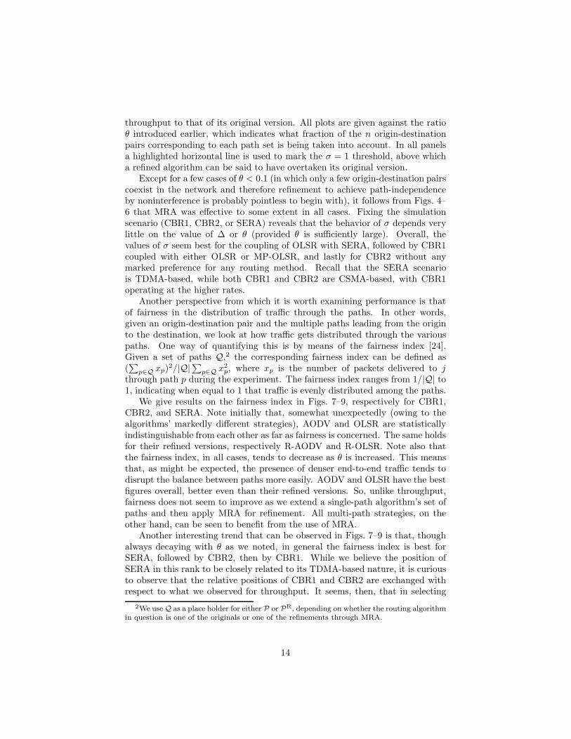
arXiv:1203.1905v1 [cs.NI] 8 Mar 2012 Local Heuristic for the Refinement of Multi-Path Routing in Wireless Mesh Networks Fabio R. J. Vieira 1,2, * Jos´ e F. de Rezende 3 Valmir C. Barbosa 1 Serge Fdida 2 1 Programa de Engenharia de Sistemas e Computa¸ c˜ao,COPPE Universidade Federal do Rio de Janeiro Caixa Postal 68511, 21941-972 Rio de Janeiro - RJ, Brazil 2 Laboratoire d’Informatique de Paris 6 4, Place Jussieu, 75252 Paris Cedex 05, France 3 Programa de Engenharia El´ etrica, COPPE Universidade Federal do Rio de Janeiro Caixa Postal 68504, 21941-972 Rio de Janeiro - RJ, Brazil Abstract We consider wireless mesh networks and the problem of routing end-to- end traffic over multiple paths for the same origin-destination pair with minimal interference. We introduce a heuristic for path determination with two distinguishing characteristics. First, it works by refining an ex- tant set of paths, determined previously by a single- or multi-path routing algorithm. Second, it is totally local, in the sense that it can be run by each of the origins on information that is available no farther than the node’s immediate neighborhood. We have conducted extensive computa- tional experiments with the new heuristic, using AODV and OLSR, as well as their multi-path variants, as underlying routing methods. For two dif- ferent CSMA settings (as implemented by 802.11) and one TDMA setting running a path-oriented link scheduling algorithm, we have demonstrated that the new heuristic is capable of improving the average throughput network-wide. When working from the paths generated by the multi-path routing algorithms, the heuristic is also capable to provide a more evenly distributed traffic pattern. Keywords: Wireless mesh networks, Multi-path routing, Path coupling, Disjoint paths, Mutual interference. * Corresponding author ([email protected]). 1
-
Upload
independent -
Category
Documents
-
view
5 -
download
0
Transcript of Local heuristic for the refinement of multi-path routing in wireless mesh networks
arX
iv:1
203.
1905
v1 [
cs.N
I] 8
Mar
201
2
Local Heuristic for the Refinement of Multi-Path
Routing in Wireless Mesh Networks
Fabio R. J. Vieira1,2,∗
Jose F. de Rezende3
Valmir C. Barbosa1
Serge Fdida2
1Programa de Engenharia de Sistemas e Computacao, COPPE
Universidade Federal do Rio de Janeiro
Caixa Postal 68511, 21941-972 Rio de Janeiro - RJ, Brazil2Laboratoire d’Informatique de Paris 6
4, Place Jussieu, 75252 Paris Cedex 05, France3Programa de Engenharia Eletrica, COPPE
Universidade Federal do Rio de Janeiro
Caixa Postal 68504, 21941-972 Rio de Janeiro - RJ, Brazil
Abstract
We consider wireless mesh networks and the problem of routing end-to-end traffic over multiple paths for the same origin-destination pair withminimal interference. We introduce a heuristic for path determinationwith two distinguishing characteristics. First, it works by refining an ex-tant set of paths, determined previously by a single- or multi-path routingalgorithm. Second, it is totally local, in the sense that it can be run byeach of the origins on information that is available no farther than thenode’s immediate neighborhood. We have conducted extensive computa-tional experiments with the new heuristic, using AODV and OLSR, as wellas their multi-path variants, as underlying routing methods. For two dif-ferent CSMA settings (as implemented by 802.11) and one TDMA settingrunning a path-oriented link scheduling algorithm, we have demonstratedthat the new heuristic is capable of improving the average throughputnetwork-wide. When working from the paths generated by the multi-pathrouting algorithms, the heuristic is also capable to provide a more evenlydistributed traffic pattern.
Keywords: Wireless mesh networks, Multi-path routing, Path coupling,Disjoint paths, Mutual interference.
∗Corresponding author ([email protected]).
1
1 Introduction
Wireless mesh networks (WMNs) have lately been recognized as having great po-tential to provide the necessary networking infrastructure for communities andcompanies, as well as to help address the problem of providing last-mile connec-tions to the Internet [33, 43]. However, mutual radio interference among the net-work’s nodes can easily reduce the throughput as network density grows abovea certain threshold [7] and therefore compromise the entire endeavor. Such in-terference is caused by the attempted concomitant communication among nodesof the same network and constitutes the most common cause of the network’sthroughput’s falling short of being satisfactory (hardly reaching a fraction ofthat of a wired network [21]). A promising approach to tackle the reduction ofmutual interference seems to be to combine routing algorithms with some inter-ference avoidance approach, such as power control, link scheduling, or the useof multi-channel radios [2]. In fact, this type of network interference problemhas been addressed by a considerable number of different strategies to be foundin the literature [12, 13, 1, 41, 11, 51, 44, 4].
An alternative approach that presents itself naturally is the use of multi-path routing to distribute traffic among multiple paths sharing the same originand the same destination, since in principle it can help with both path recov-ery and load balancing better than the use of single-path strategies. It may,in addition, lead to better throughput values over the entire network [26, 5].But while these benefits accrue only insofar as they relate to how the multi-ple paths interfere with one another [46, 45], unfortunately this aspect of theproblem is not commonly addressed by multi-path strategies. What happens asa consequence is that, though promising by virtue of adopting multiple pathsto accommodate the same end-to-end traffic, in general such strategies fail toperform as desired because they do not tackle the interference problem duringpath discovery. The single noteworthy exception here seems to be the algorithmreported in [49], but it uses geographic information (like localization aided byGPS) to find paths with sufficient spatial separation so as not to interfere withone another. In our view this weakens the approach somewhat, since such typeof information may not always be available [14]. Moreover, the correspondingalgorithm relies on the solution of an NP-hard problem on an input that hasthe size of the network [50], so the solution may be unattainable in practice.
Here we propose a different approach to alleviate the effects of interferencein multi-path routing. Our approach is based on two general principles. First,that it is to work as a refinement phase over existing routing algorithms, therebyinherently preserving, to the fullest possible extent, the advantages of any givenrouting method. Second, that it is to rely only on information that is locallyavailable to the common origin of any given set of multiple paths leading tothe same destination. That is, only information that the origin can obtain bycommunicating with its direct neighbors in the WMN should be used. Oneintended consequence of the latter, in particular, is that refining the set ofpaths departing from any common origin should be easily implementable bystraightforward message passing, and moreover, that any required calculation
2

by that node should be amenable to being carried out efficiently even if itinvolves the solution of a computationally difficult problem. In order to complywith these two principles, our approach operates on a previously established setof paths leading from a common origin, say i, to a common destination, say j.It operates exclusively on the neighborhood information stored at node i itselfor at any of its neighbors, say k, such that k participates in some of the i-to-jpaths, as well as on the information stored at these same nodes regarding therouting of packets to node j. Once node i has acquired all this information, anundirected graph Gij is constructed that represents every possible interferencethat can occur as packets get forwarded toward j by those of i’s neighbors thatare on i-to-j paths. Solving a well-known NP-hard problem (that of finding amaximum weighted independent set) on this typically small graph serves as aheuristic to decide which of the i-to-j paths to keep and which to discard.
It is important to note that, being determined with reference to graph Gij ,the resulting set contains no two paths that interfere with each other as far asnode i’s neighbors are concerned, except of course for the inevitable interferencethat may occur as packets leave i or reach j. In our view, this provides asharp contrast between our approach and others that aim at weaker forms ofindependence between the paths, for example by seeking paths that are merelyedge- or node-disjoint [27, 28, 47, 13, 3, 41, 52, 30, 51, 53]. This is so because, asremarked elsewhere (e.g., [37]), independence by edge-disjointness encompassesindependence by node-disjointness, which in turn encompasses independence bynoninterference. Of course, the highest an independence relation’s level in thishierarchy the easiest it is to implement it as the multiple paths are discovered(not coincidentally, the simple exchange of tokens between nodes suffices toproduce edge- or node-disjoint path sets [29]).
We proceed in the following manner. First we state the problem in graph-theoretic terms and give our solution in Section 2. Then we move, in Section 3, toa presentation of the methodology we followed in conducting our computationalexperiments. Our results are given in Section 4 and involve comparisons withsome prominent routing algorithms, viz. AODV [38], AOMDV [31], OLSR [23],and MP-OLSR [54]. We used these algorithms both as stand-alone methodsand as bases to our own heuristic. Our results include throughput and fairness[24] comparisons based both on NS2.34 [35] simulations and on the SERA linkscheduling algorithm [48]. We continue in Section 5 with further discussionsand conclude in Section 6.
2 Problem formulation and heuristic
For i and j any two distinct nodes of the WMN, we begin by assuming thatsome routing protocol already established a set Pij of paths directed from ito j. Another key element is that, since we seek to establish independenceby noninterference, an interference model, along with its assumptions, must beselected. Our choice is the protocol-based interference model, together with theassumption that a node’s communication and interference radii are the same.
3
Should a different model be selected or the two radii be significantly different,the only effect would be for the graph construction process outlined below, onceadapted accordingly, to produce a different graph (in particular, the interferenceradius could be chosen appropriately in order for the protocol-based interferencemodel to mimic the physical interference model [42]).
Under the assumptions of the protocol-based interference model, the com-munication/interference radius is fixed at some value R, which we take to bethe same for all nodes. It follows that two nodes are neighbors of each otherin the WMN if and only if the Euclidean distance between them is no greaterthan R. Moreover, since every link may transmit in both directions for errorcontrol, it also follows that two links can interfere with each other if either one’stransmitter or receiver is a neighbor of the other’s transmitter or receiver [8]. Aswill become apparent shortly, this has important implications when modelinginterference, since links that share no nodes can still interfere with one another.
In keeping with the locality principle outlined in Section 1, we work on thepremise that a node k’s knowledge is limited to the set Nk of its neighbors andthe set Nextk(i, j) ⊆ Nk of neighbors to which it may forward packets sent bynode i to node j (assuming k 6= j). Set Nextk(i, j), obviously, depends on thej-bound paths that leave i and go through node k. The problem we study isthat of eliminating from Pij the fewest possible paths (in a weighted sense, tobe discussed later) so that the remaining path set, henceforth denoted by PR
ij ,contains no mutually interfering paths except at i or j. However, owing onceagain to the issue of locality, we forgo both optimality and feasibility a prioriand settle for a heuristic instead. That is, for the sake of locality we admitthe possibility that, in the end, neither will the selected paths be collectivelyoptimal nor will the absence of interference among them be guaranteed (exceptat those paths’ second hops, which will be non-interfering relative to one anothernecessarily).
Before proceeding, we tackle two special cases. The first one is that in whichPij contains the single-link path that connects i directly to j. In this case, welet PR
ij be the singleton that contains that path, since no other arrangement canpossibly do better. The second special case is that in which |Pij | = 1, providedthe single path contained in Pij has at least two links, and is motivated by thesituations in which Pij originates from single-path routing. In this case, weenlarge Pij before feeding it to our path-selection heuristic. Letting node k besuch that Nexti(i, j) = {k}, we do this enlargement of Pij by including in itas many paths from Pkj as possible, each suitably prefixed by the new origini, provided none of the new paths is weightier than the one initially in Pij . Ifenlargement turns out to be impossible, then the problem becomes moot for Pij
and we let PR
ij = Pij .We are then in position to introduce our refinement algorithm for multi-path
routing, henceforth referred to by the acronym MRA (for multi-path refinementalgorithm). The goal of MRA is to create an undirected graphGij correspondingto the path set Pij and to extract from it the information necessary to determinePR
ij . This graph’s node set, henceforth denoted by V , has one node for each ofthe paths in Pij . Its edge set, denoted by E, is constructed in such a way as to
4
represent every interference possibility that can be inferred solely from the setsNk and Nextk(i, j) for every k ∈ Ni that participates in at least one of the pathsin Pij . Once graph Gij is built, finding a maximum weighted independent setin it (i.e., a subset of V containing no two nodes joined by an edge in E andbeing as weighty as possible) provides the best possible approximate decisionon which of the paths in Pij should constitute PR
ij , namely those correspondingto the nodes in the maximum weighted independent set that was found.
MRA proceeds as given next, following the introduction of some auxiliarynomenclature. Given two neighboring WMN nodes, say k and k′, we are inter-ested in the following two possibilities for the pair k, k′. A type-A pair is partof at least one path in Pij in such a way that k′ ∈ Nextk(i, j) with k ∈ Ni ork ∈ Nextk′(i, j) with k′ ∈ Ni. In a type-B pair, both k and k′ belong to atleast one path in Pij as well, but not the same path. Moreover, at least one ofthem is a member of Ni while the other, if not in Ni as well, is in Nextl(i, j) forsome other l ∈ Ni. Note that type-A and -B pairs constitute all the structuralinformation that node i can gather by strictly local communication from itsneighborhood Ni in the WMN. In the case of a type-A pair, we let Paths(k, k′)be the set of i-to-j paths to which the pair belongs.
(1) Let V have one node for each path in Pij . Add one further node to V foreach type-B pair of neighboring WMN nodes. We refer to these additionalnodes as temporary nodes.
(2) Construct E as follows:
i. Let k, k′ and l, l′ be two pairs of neighboring WMN nodes, each pairbeing of type A or B. If it holds that k = l, k = l′, k′ = l, or k′ = l′,then add an edge to E between each node corresponding to a path inPaths(k, k′) (if the pair is of type A) or the corresponding temporarynode (if the pair is of type B) to each node corresponding to a path inPaths(l, l′) (if the pair is of type A) or the corresponding temporarynode (if the pair is of type B).
ii. Connect any two nodes in V by an edge if, after the previous step,the distance between them is 2.
iii. Remove all temporary nodes from V and all edges that touch themfrom E.
(3) Find a maximum weighted independent set of Gij and output PR
ij accord-ingly.
In these steps, graph Gij starts out as a graph with |Pij | nodes and getsenlarged by the addition of temporary nodes that represent some of the pos-sibilities of off-path interference as nodes in Ni engage in transmitting packets(Step (1)). Then it receives edges to account for the assumptions of the protocol-based interference model (Steps (2).i and (2).ii) and is after that stripped of alltemporary nodes to end up with |Pij | nodes once again (Step (2).iii). Step (2).ii,in particular, accounts for interference in the WMN when a link’s transmitter or
5
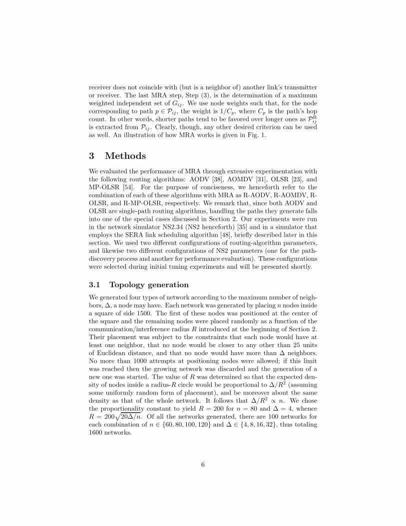
receiver does not coincide with (but is a neighbor of) another link’s transmitteror receiver. The last MRA step, Step (3), is the determination of a maximumweighted independent set of Gij . We use node weights such that, for the nodecorresponding to path p ∈ Pij , the weight is 1/Cp, where Cp is the path’s hopcount. In other words, shorter paths tend to be favored over longer ones as PR
ij
is extracted from Pij . Clearly, though, any other desired criterion can be usedas well. An illustration of how MRA works is given in Fig. 1.
3 Methods
We evaluated the performance of MRA through extensive experimentation withthe following routing algorithms: AODV [38], AOMDV [31], OLSR [23], andMP-OLSR [54]. For the purpose of conciseness, we henceforth refer to thecombination of each of these algorithms with MRA as R-AODV, R-AOMDV, R-OLSR, and R-MP-OLSR, respectively. We remark that, since both AODV andOLSR are single-path routing algorithms, handling the paths they generate fallsinto one of the special cases discussed in Section 2. Our experiments were runin the network simulator NS2.34 (NS2 henceforth) [35] and in a simulator thatemploys the SERA link scheduling algorithm [48], briefly described later in thissection. We used two different configurations of routing-algorithm parameters,and likewise two different configurations of NS2 parameters (one for the path-discovery process and another for performance evaluation). These configurationswere selected during initial tuning experiments and will be presented shortly.
3.1 Topology generation
We generated four types of network according to the maximum number of neigh-bors, ∆, a node may have. Each network was generated by placing n nodes insidea square of side 1500. The first of these nodes was positioned at the center ofthe square and the remaining nodes were placed randomly as a function of thecommunication/interference radius R introduced at the beginning of Section 2.Their placement was subject to the constraints that each node would have atleast one neighbor, that no node would be closer to any other than 25 unitsof Euclidean distance, and that no node would have more than ∆ neighbors.No more than 1000 attempts at positioning nodes were allowed; if this limitwas reached then the growing network was discarded and the generation of anew one was started. The value of R was determined so that the expected den-sity of nodes inside a radius-R circle would be proportional to ∆/R2 (assumingsome uniformly random form of placement), and be moreover about the samedensity as that of the whole network. It follows that ∆/R2 ∝ n. We chosethe proportionality constant to yield R = 200 for n = 80 and ∆ = 4, whenceR = 200
√
20∆/n. Of all the networks generated, there are 100 networks foreach combination of n ∈ {60, 80, 100, 120} and ∆ ∈ {4, 8, 16, 32}, thus totaling1600 networks.
6
(a) 1
k1
k2
k3
k4
k6
k2 k6
k5
k6
d x c
bea
(b)
d x c
bea
(c) d c
bea
(d)
x
:
i
i
i
i
i j
j
j
j
je
d :
c :
b :
a :k
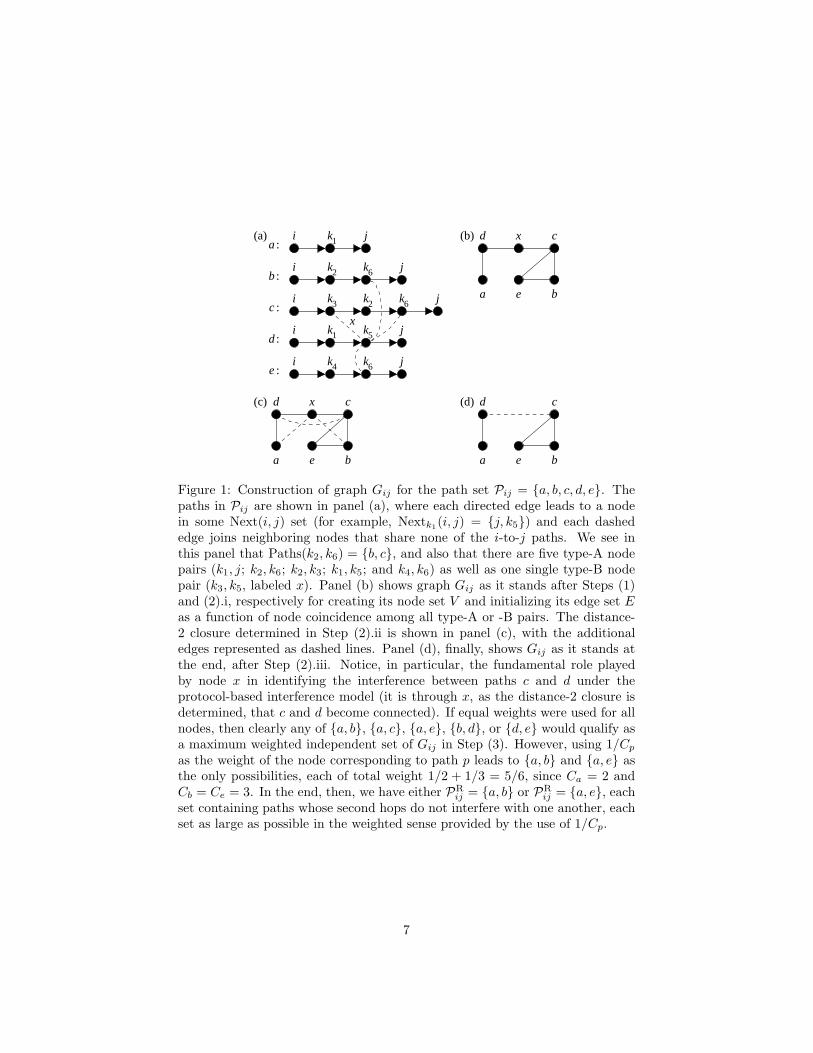
Figure 1: Construction of graph Gij for the path set Pij = {a, b, c, d, e}. Thepaths in Pij are shown in panel (a), where each directed edge leads to a nodein some Next(i, j) set (for example, Nextk1
(i, j) = {j, k5}) and each dashededge joins neighboring nodes that share none of the i-to-j paths. We see inthis panel that Paths(k2, k6) = {b, c}, and also that there are five type-A nodepairs (k1, j; k2, k6; k2, k3; k1, k5; and k4, k6) as well as one single type-B nodepair (k3, k5, labeled x). Panel (b) shows graph Gij as it stands after Steps (1)and (2).i, respectively for creating its node set V and initializing its edge set Eas a function of node coincidence among all type-A or -B pairs. The distance-2 closure determined in Step (2).ii is shown in panel (c), with the additionaledges represented as dashed lines. Panel (d), finally, shows Gij as it stands atthe end, after Step (2).iii. Notice, in particular, the fundamental role playedby node x in identifying the interference between paths c and d under theprotocol-based interference model (it is through x, as the distance-2 closure isdetermined, that c and d become connected). If equal weights were used for allnodes, then clearly any of {a, b}, {a, c}, {a, e}, {b, d}, or {d, e} would qualify asa maximum weighted independent set of Gij in Step (3). However, using 1/Cp
as the weight of the node corresponding to path p leads to {a, b} and {a, e} asthe only possibilities, each of total weight 1/2 + 1/3 = 5/6, since Ca = 2 andCb = Ce = 3. In the end, then, we have either PR
ij = {a, b} or PR
ij = {a, e}, eachset containing paths whose second hops do not interfere with one another, eachset as large as possible in the weighted sense provided by the use of 1/Cp.
7
3.2 Path discovery
For each of the 1600 networks we randomly generated 100 sets of node pairs tofunction as origin-destination pairs (instances of the i, j pair we have been usingthroughout). Each set comprises n pairs and no node was allowed to appearmore than once in any set as an origin. For each of the node-pair sets andeach of the four routing algorithms (AODV, AOMDV, OLSR, and MP-OLSR)we obtained n path sets (instances of Pij). Likewise, for each of the node-pairsets and each of the four refined routing algorithms (R-AODV, R-AOMDV,R-OLSR, and R-MP-OLSR) we obtained another n path sets (instances of PR
ij).For each routing algorithm, the discovery of each Pij instance (i.e., for a
single origin and a single destination) proceeded as follows. After loading thenetwork topology onto NS2 we conducted a 15-second simulation with one flowagent for the single origin i and the single destination j, using a CBR of one1000-byte packet per second. The remaining pairs were handled likewise afterresetting the simulator. We remark that this one-pair-at-a-time strategy, asopposed to generating paths for all n pairs in the same set concomitantly, wasmeant to minimize packet loss due to path overload and also to avoid the possibleinterference of a previously discovered path with the discovery of a new one. Ofcourse, this argument is only valid for on-demand routing algorithms (AODVand its variants depend on network load, while the OLSR variants always findidentical paths for the same network topology), but we proceeded in this wayin all cases. As a consequence, our experiments are entirely reproducible.
We set NS2 to its default configuration, but employed the DRAND MACprotocol [40] to avoid collisions in the path-discovery process. To adjust theradius R we also set the parameter RXThresh (RXT) to the appropriate valuegiven by the program threshold.cc (cf. the NS2 manual). We used the im-plementations of the AODV, OLSR, and AOMDV routing agents available inversion 2.34 of NS2 and the MP-OLSR routing agent available at [32]. ForAOMDV, we made the small modifications proposed by [56] to discover onlynode-disjoint paths with at most K paths for each origin-destination pair ofnodes. We adopted these modifications because node-disjoint paths are clearlymore interference-free than otherwise. We chose K = 5 because it achieved thebest throughput values for 2 ≤ K ≤ 7. The same modifications were effected onMP-OLSR (as proposed by [57]). Out of the same range for K, and for the samereason as above, we used K = 3 for ∆ ∈ {4, 8} and K = 5 for ∆ ∈ {16, 32}.
3.3 Performance evaluation
Once we fix a value for n and a value for ∆, there are 104 path sets on whichto evaluate the performance of MRA. Each of these sets is relative to n origin-destination pairs. In our experiments, we randomly grouped these pairs into nsets, each containing a different number of origin-destination pairs (i.e., one setcontaining a single pair, another containing two pairs, and so on), and simulatedthe network’s behavior in transporting predominantly heavy traffic from theorigins to the destinations. We use OD to denote the set of pairs in question,
8
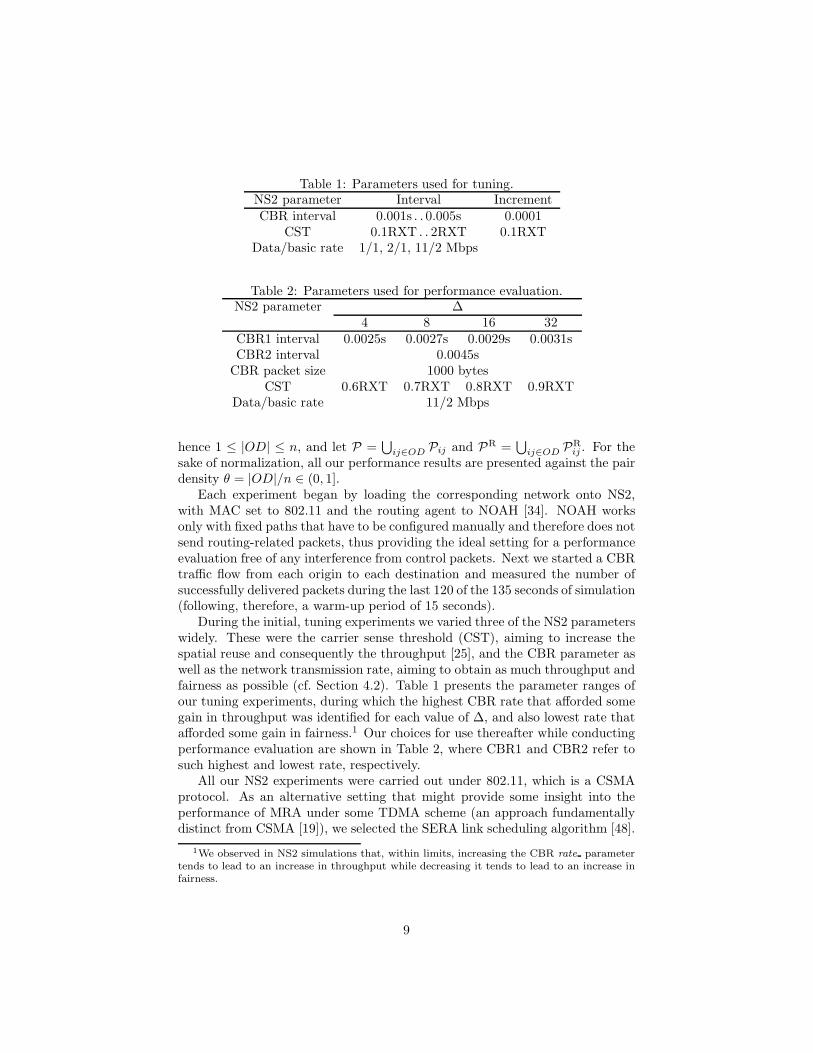
Table 1: Parameters used for tuning.NS2 parameter Interval IncrementCBR interval 0.001s . . 0.005s 0.0001
CST 0.1RXT . . 2RXT 0.1RXTData/basic rate 1/1, 2/1, 11/2 Mbps
Table 2: Parameters used for performance evaluation.NS2 parameter ∆
4 8 16 32CBR1 interval 0.0025s 0.0027s 0.0029s 0.0031sCBR2 interval 0.0045sCBR packet size 1000 bytes
CST 0.6RXT 0.7RXT 0.8RXT 0.9RXTData/basic rate 11/2 Mbps
hence 1 ≤ |OD| ≤ n, and let P =⋃
ij∈OD Pij and PR =⋃
ij∈OD PR
ij . For thesake of normalization, all our performance results are presented against the pairdensity θ = |OD|/n ∈ (0, 1].
Each experiment began by loading the corresponding network onto NS2,with MAC set to 802.11 and the routing agent to NOAH [34]. NOAH worksonly with fixed paths that have to be configured manually and therefore does notsend routing-related packets, thus providing the ideal setting for a performanceevaluation free of any interference from control packets. Next we started a CBRtraffic flow from each origin to each destination and measured the number ofsuccessfully delivered packets during the last 120 of the 135 seconds of simulation(following, therefore, a warm-up period of 15 seconds).
During the initial, tuning experiments we varied three of the NS2 parameterswidely. These were the carrier sense threshold (CST), aiming to increase thespatial reuse and consequently the throughput [25], and the CBR parameter aswell as the network transmission rate, aiming to obtain as much throughput andfairness as possible (cf. Section 4.2). Table 1 presents the parameter ranges ofour tuning experiments, during which the highest CBR rate that afforded somegain in throughput was identified for each value of ∆, and also lowest rate thatafforded some gain in fairness.1 Our choices for use thereafter while conductingperformance evaluation are shown in Table 2, where CBR1 and CBR2 refer tosuch highest and lowest rate, respectively.
All our NS2 experiments were carried out under 802.11, which is a CSMAprotocol. As an alternative setting that might provide some insight into theperformance of MRA under some TDMA scheme (an approach fundamentallydistinct from CSMA [19]), we selected the SERA link scheduling algorithm [48].
1We observed in NS2 simulations that, within limits, increasing the CBR rate parametertends to lead to an increase in throughput while decreasing it tends to lead to an increase infairness.
9
SERA seeks to schedule the links of a set of paths while striving to maximizethroughput on those paths. It is therefore quite well suited to the task athand. The throughput that our SERA simulator provides is given in terms oftime slots, so in order to achieve a meaningful basis for comparing CSMA- andTDMA-based results a translation is needed of such throughput figures intothose provided by NS2 in the CSMA experiments. We did this by resortingto a very simple NS2 simulation to determine the duration of a time slot. Inthis experiment, a node sends packets to another and the time for successfuldeliveries is recorded. Since this time is conceptually the same that in SERAis taken to be a time slot, the translation from one setting to the other can beaccomplished easily. Using the parameter values shown in Table 2, we found atime-slot duration of 0.002 seconds. This is the duration we use, together withthe ND-BF numbering scheme for SERA and its B parameter set to 2 (cf. [48]).
4 Computational results
We divide our results into two categories. First we present a statistical analysisof the networks generated and the path sets obtained by the original routingalgorithms and by their refinements through the use of MRA. Then we presentthe ratios of the refined algorithms’ throughputs to those of their correspondingoriginals (absolute values are given in Figs. A.1–A.3) and also fairness figures.For the purpose of conciseness we report only on the n = 120 results, since theyare qualitatively similar to those related to the other three values of n we used.In Section 5, though, we do discuss some of the quantitative differences thatwere observed.
4.1 Properties of the networks generated
The 1600 networks we generated are that same that were used in [48]. We re-fer the reader to Section 8.1 of that publication for a variety of the networks’statistical properties, such as the occurrence of topologies structured in someparticular way and some of their structure-related distributions. Here we con-centrate on presenting those properties that pertain to routing both before andafter refinement, since they are the ones we have found useful in helping explainthe throughput results we present later.
The average path multiplicity (number of paths) per origin-destination pairin the path sets P and PR is given in Table 3 for every combination of ∆ and|OD|. Note that MP-OLSR is absent from the table in spite of being a multi-path algorithm, the reason being that in this case the K parameter does notwork as an upper bound (as it does for AOMDV), but rather as the fixed numberof paths to be found. We observe in the table that the average path multiplicityincreases monotonically with ∆ for fixed |OD|, which is expected from the well-known fact that the number of possible paths between the same two nodesgrows with ∆ in arbitrary graphs [22]. On the other hand, increasing |OD| forfixed ∆ causes very little variation, probably owing to the method we used to
10
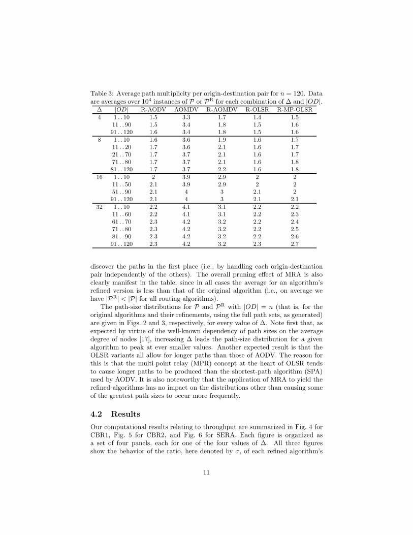
Table 3: Average path multiplicity per origin-destination pair for n = 120. Dataare averages over 104 instances of P or PR for each combination of ∆ and |OD|.
∆ |OD| R-AODV AOMDV R-AOMDV R-OLSR R-MP-OLSR
4 1 . . 10 1.5 3.3 1.7 1.4 1.511 . . 90 1.5 3.4 1.8 1.5 1.691 . . 120 1.6 3.4 1.8 1.5 1.6
8 1 . . 10 1.6 3.6 1.9 1.6 1.711 . . 20 1.7 3.6 2.1 1.6 1.721 . . 70 1.7 3.7 2.1 1.6 1.771 . . 80 1.7 3.7 2.1 1.6 1.881 . . 120 1.7 3.7 2.2 1.6 1.8
16 1 . . 10 2 3.9 2.9 2 211 . . 50 2.1 3.9 2.9 2 251 . . 90 2.1 4 3 2.1 291 . . 120 2.1 4 3 2.1 2.1
32 1 . . 10 2.2 4.1 3.1 2.2 2.211 . . 60 2.2 4.1 3.1 2.2 2.361 . . 70 2.3 4.2 3.2 2.2 2.471 . . 80 2.3 4.2 3.2 2.2 2.581 . . 90 2.3 4.2 3.2 2.2 2.691 . . 120 2.3 4.2 3.2 2.3 2.7
discover the paths in the first place (i.e., by handling each origin-destinationpair independently of the others). The overall pruning effect of MRA is alsoclearly manifest in the table, since in all cases the average for an algorithm’srefined version is less than that of the original algorithm (i.e., on average wehave |PR| < |P| for all routing algorithms).
The path-size distributions for P and PR with |OD| = n (that is, for theoriginal algorithms and their refinements, using the full path sets, as generated)are given in Figs. 2 and 3, respectively, for every value of ∆. Note first that, asexpected by virtue of the well-known dependency of path sizes on the averagedegree of nodes [17], increasing ∆ leads the path-size distribution for a givenalgorithm to peak at ever smaller values. Another expected result is that theOLSR variants all allow for longer paths than those of AODV. The reason forthis is that the multi-point relay (MPR) concept at the heart of OLSR tendsto cause longer paths to be produced than the shortest-path algorithm (SPA)used by AODV. It is also noteworthy that the application of MRA to yield therefined algorithms has no impact on the distributions other than causing someof the greatest path sizes to occur more frequently.
4.2 Results
Our computational results relating to throughput are summarized in Fig. 4 forCBR1, Fig. 5 for CBR2, and Fig. 6 for SERA. Each figure is organized asa set of four panels, each for one of the four values of ∆. All three figuresshow the behavior of the ratio, here denoted by σ, of each refined algorithm’s
11
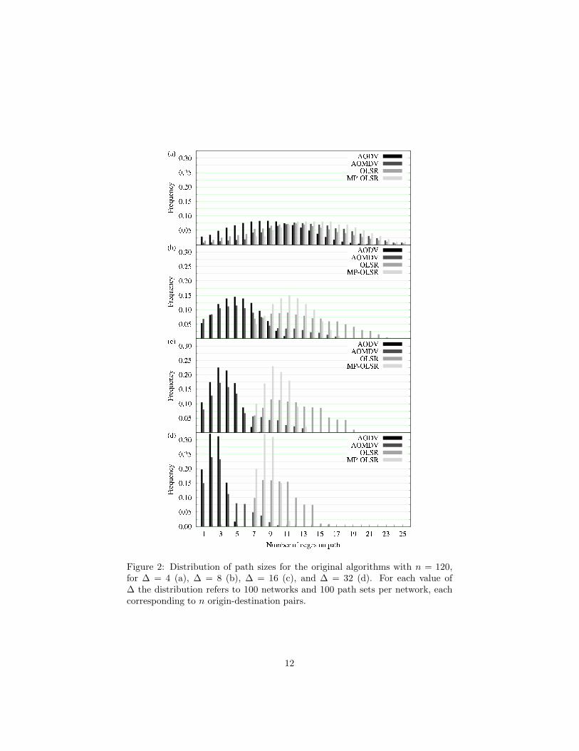
Figure 2: Distribution of path sizes for the original algorithms with n = 120,for ∆ = 4 (a), ∆ = 8 (b), ∆ = 16 (c), and ∆ = 32 (d). For each value of∆ the distribution refers to 100 networks and 100 path sets per network, eachcorresponding to n origin-destination pairs.
12
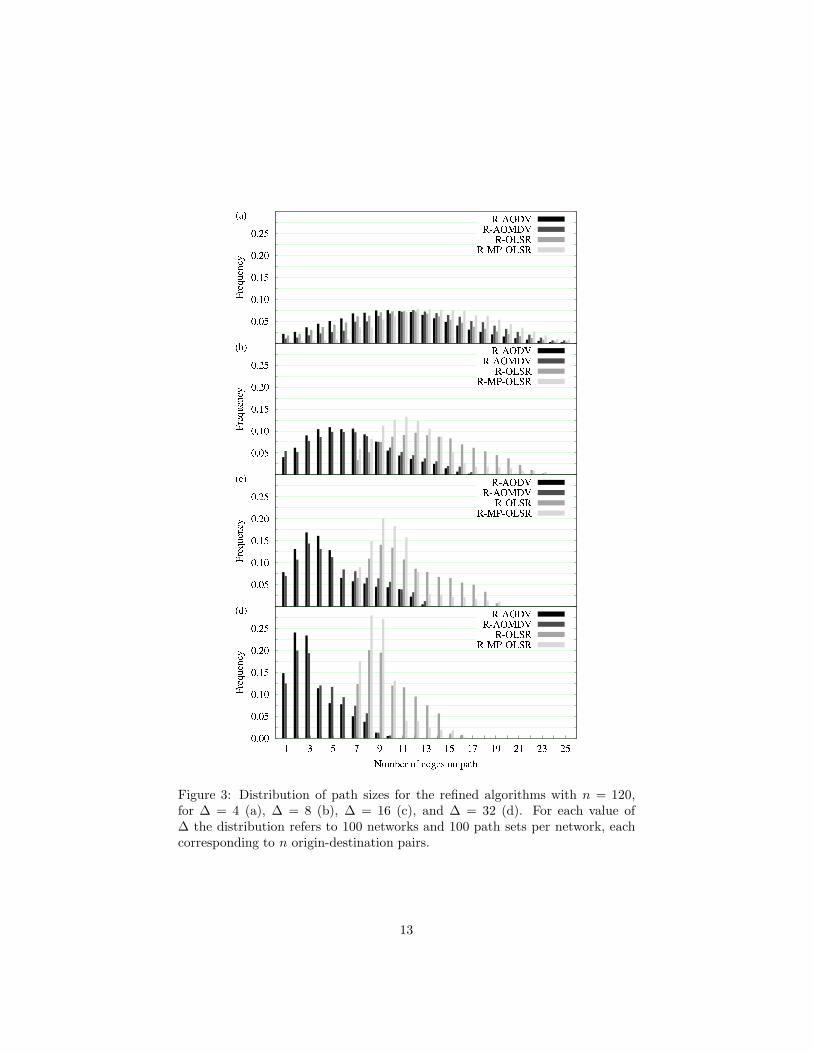
Figure 3: Distribution of path sizes for the refined algorithms with n = 120,for ∆ = 4 (a), ∆ = 8 (b), ∆ = 16 (c), and ∆ = 32 (d). For each value of∆ the distribution refers to 100 networks and 100 path sets per network, eachcorresponding to n origin-destination pairs.
13
throughput to that of its original version. All plots are given against the ratioθ introduced earlier, which indicates what fraction of the n origin-destinationpairs corresponding to each path set is being taken into account. In all panelsa highlighted horizontal line is used to mark the σ = 1 threshold, above whicha refined algorithm can be said to have overtaken its original version.
Except for a few cases of θ < 0.1 (in which only a few origin-destination pairscoexist in the network and therefore refinement to achieve path-independenceby noninterference is probably pointless to begin with), it follows from Figs. 4–6 that MRA was effective to some extent in all cases. Fixing the simulationscenario (CBR1, CBR2, or SERA) reveals that the behavior of σ depends verylittle on the value of ∆ or θ (provided θ is sufficiently large). Overall, thevalues of σ seem best for the coupling of OLSR with SERA, followed by CBR1coupled with either OLSR or MP-OLSR, and lastly for CBR2 without anymarked preference for any routing method. Recall that the SERA scenariois TDMA-based, while both CBR1 and CBR2 are CSMA-based, with CBR1operating at the higher rates.
Another perspective from which it is worth examining performance is thatof fairness in the distribution of traffic through the paths. In other words,given an origin-destination pair and the multiple paths leading from the originto the destination, we look at how traffic gets distributed through the variouspaths. One way of quantifying this is by means of the fairness index [24].Given a set of paths Q,2 the corresponding fairness index can be defined as(∑
p∈Qxp)
2/|Q|∑
p∈Qx2p, where xp is the number of packets delivered to j
through path p during the experiment. The fairness index ranges from 1/|Q| to1, indicating when equal to 1 that traffic is evenly distributed among the paths.
We give results on the fairness index in Figs. 7–9, respectively for CBR1,CBR2, and SERA. Note initially that, somewhat unexpectedly (owing to thealgorithms’ markedly different strategies), AODV and OLSR are statisticallyindistinguishable from each other as far as fairness is concerned. The same holdsfor their refined versions, respectively R-AODV and R-OLSR. Note also thatthe fairness index, in all cases, tends to decrease as θ is increased. This meansthat, as might be expected, the presence of denser end-to-end traffic tends todisrupt the balance between paths more easily. AODV and OLSR have the bestfigures overall, better even than their refined versions. So, unlike throughput,fairness does not seem to improve as we extend a single-path algorithm’s set ofpaths and then apply MRA for refinement. All multi-path strategies, on theother hand, can be seen to benefit from the use of MRA.
Another interesting trend that can be observed in Figs. 7–9 is that, thoughalways decaying with θ as we noted, in general the fairness index is best forSERA, followed by CBR2, then by CBR1. While we believe the position ofSERA in this rank to be closely related to its TDMA-based nature, it is curiousto observe that the relative positions of CBR1 and CBR2 are exchanged withrespect to what we observed for throughput. It seems, then, that in selecting
2We use Q as a place holder for either P or PR, depending on whether the routing algorithmin question is one of the originals or one of the refinements through MRA.
14
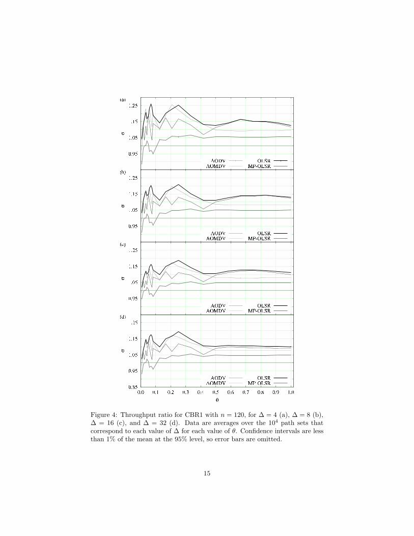
Figure 4: Throughput ratio for CBR1 with n = 120, for ∆ = 4 (a), ∆ = 8 (b),∆ = 16 (c), and ∆ = 32 (d). Data are averages over the 104 path sets thatcorrespond to each value of ∆ for each value of θ. Confidence intervals are lessthan 1% of the mean at the 95% level, so error bars are omitted.
15
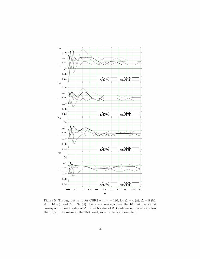
Figure 5: Throughput ratio for CBR2 with n = 120, for ∆ = 4 (a), ∆ = 8 (b),∆ = 16 (c), and ∆ = 32 (d). Data are averages over the 104 path sets thatcorrespond to each value of ∆ for each value of θ. Confidence intervals are lessthan 1% of the mean at the 95% level, so error bars are omitted.
16
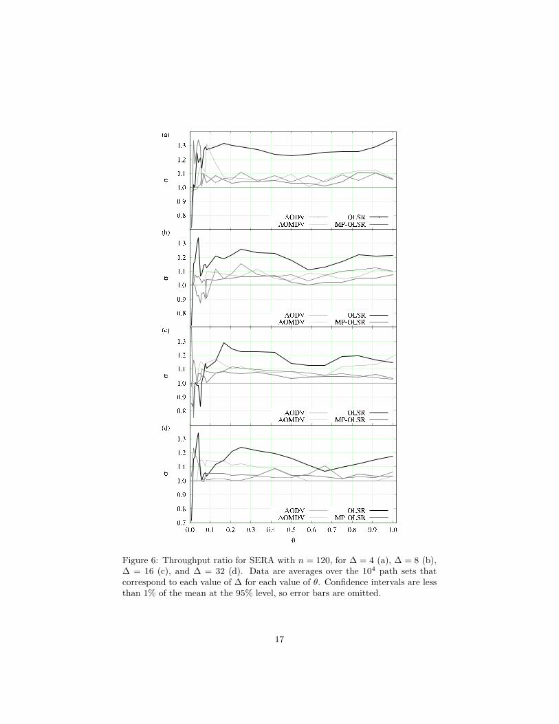
Figure 6: Throughput ratio for SERA with n = 120, for ∆ = 4 (a), ∆ = 8 (b),∆ = 16 (c), and ∆ = 32 (d). Data are averages over the 104 path sets thatcorrespond to each value of ∆ for each value of θ. Confidence intervals are lessthan 1% of the mean at the 95% level, so error bars are omitted.
17
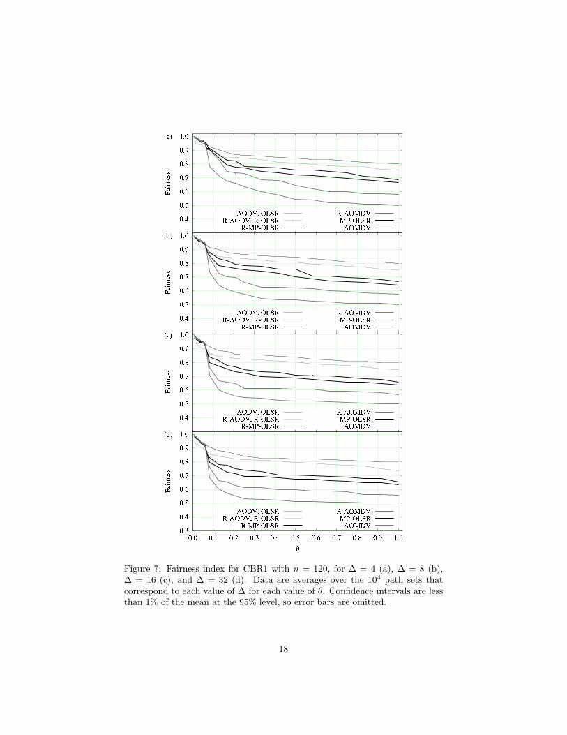
Figure 7: Fairness index for CBR1 with n = 120, for ∆ = 4 (a), ∆ = 8 (b),∆ = 16 (c), and ∆ = 32 (d). Data are averages over the 104 path sets thatcorrespond to each value of ∆ for each value of θ. Confidence intervals are lessthan 1% of the mean at the 95% level, so error bars are omitted.
18

Figure 8: Fairness index for CBR2 with n = 120, for ∆ = 4 (a), ∆ = 8 (b),∆ = 16 (c), and ∆ = 32 (d). Data are averages over the 104 path sets thatcorrespond to each value of ∆ for each value of θ. Confidence intervals are lessthan 1% of the mean at the 95% level, so error bars are omitted.
19
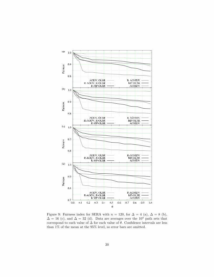
Figure 9: Fairness index for SERA with n = 120, for ∆ = 4 (a), ∆ = 8 (b),∆ = 16 (c), and ∆ = 32 (d). Data are averages over the 104 path sets thatcorrespond to each value of ∆ for each value of θ. Confidence intervals are lessthan 1% of the mean at the 95% level, so error bars are omitted.
20

between the rates associated with CBR1 and CBR2 one is automatically forcedto favor throughput over fairness or conversely.
Our definition of the fairness index given above is only one of the possibilitiesin the context of multi-path routing. Another alternative is to coalesce all pack-ets delivered from one origin, say i, to one destination, say j, into a single num-ber xij and then compute the fairness index as (
∑
ij∈OD xij)2/|OD|
∑
ij∈OD x2
ij .Proceeding in this way would shift the focus of the fairness index from pathsto origin-destination pairs. We give no detailed results on this alternative, butdo provide an example with SERA in Fig. A.4. There is clearly great similaritywith the results in Fig. 9, but the numbers tend to be higher.
5 Discussion
As we remarked earlier, we have provided no results for n ∈ {60, 80, 100} be-cause, essentially, they are indistinguishable from those of n = 120 in qualitativeterms. We do remark, however, that a few noteworthy quantitative differenceswere observed. For example, in the case of SERA a higher throughput ratio σwas sometimes observed for reduced n but the same value of the pair densityθ. This stems not only from the fact that the average path size decreases asn decreases, but more generally from the fact that the number of links for thesame θ is lower in the smaller networks, thus fewer links interfere with one an-other and fewer links have to be scheduled. Such improvement in the value ofσ, therefore, seems to depend on the network’s path-size distribution.
As we noted briefly in Section 4.2, often OLSR and MP-OLSR turned outto be the routing methods most prone to benefit from the refinement providedby MRA. One clue as to why this is so may be already present in Table 3,where the refined versions of these two methods have some of the lowest pathmultiplicities overall, thence a tendency to incur less interference. However,this holds also for the refined version of AODV, so there has to be some otherdistinguishing aspect. While our data are not sufficient to provide a definitiveanswer, we believe the two methods’ superiority to be owed to a combination ofMRA (which attempts to reduce path multiplicity to lower interference) withthe MPR concept that is intrinsic to the OLSR variants (which in turn attemptsto provide an initial set of paths as spatially distributed as possible). As forAODV, the SPA at its core probably produces paths that are less spatiallyseparated [55, 10].
In a related vein, the results of Section 4.2 also point at SERA as providingsuperior throughput results vis-a-vis those of CBR1 and CBR2, and similarlyfor CBR1 with respect to CBR2. Because such results refer to throughputgains after refinement by MRA, more detailed data are needed for a directcomparison of throughputs. These are shown in Figs. A.5–A.7, which clearlyconfirm the rank. Once again the reason for this is not totally clear, but itmay be a manifestation of SERA’s properties rather than of the superiority ofits underlying TDMA scheme over the CSMA protocols of CBR1 and CBR2.
21

After all, a considerable amount of research has been directed toward the TDMAversus CSMA question, without however reaching an agreement [16, 20, 15, 9].
Another curiosity related to this issue of how SERA compares to CBR1 andCBR2 has to do with the total absence of traffic on some paths. While SERAprecludes this from occurring as a matter of design principle, unused pathsdo occur in the other two cases. During the corresponding NS2 simulationsthis persisted even if simulation times were extended or the synchronization ofmultiple CBRs was reordered or entirely removed.3 As it turns out, it seemsthat certain paths remained unused so that throughput could be increased onother paths. Data on the most critical cases, viz. those in which no packets atall were delivered for an origin-destination pair, are shown in Figs. A.8 and A.9.Examining these data confirms our expectation that the single-path algorithmsshould be less prone to the occurrence of such extreme cases. It also revealsthat both R-AOMDV and R-MP-OLSR had fewer such occurrences than theircorresponding originals (i.e., MRA seems to have attenuated the problem).
6 Concluding remarks
MRA is a heuristic for the refinement of routing paths in WMNs. It was devel-oped with multi-path routing algorithms in mind but works also on single-pathalgorithms (through a manipulation of its input to obtain multiple paths fromthe overall set of single paths). MRA is fully local, in the sense that it dependsonly on information that is readily available to each node and its immediateneighborhood in the network. Being local means that the extra control traffic itmay entail is negligible, especially if we consider that it need happen only oncefor a fixed set of paths. It involves the solution of an NP-hard problem, thatof finding a maximum weighted independent set in a graph, but the inputs in-volved are typically very small, leading to negligible running times if comparedto arbitrary graphs [36].
Our computational experiments with MRA on a TDMA setting (SERA) andtwo CSMA settings (CBR1 and CBR2) revealed improvements in throughputof up to 30% for both the AODV and OLSR routing methods and their multi-path variants. The latter were also improved by MRA in terms of fairness.Finding out just how close these improvements come to the very best that canbe achieved is an open problem that involves solving the path-pruning problemglobally. This problem is NP-hard as the one solved by MRA, but its input,relating to the WMN in a global scale, is much more sizable.
Another interesting aspect for further investigation is the effect of MRA onmulti-radio networks. In such schemes the network’s path density can be dras-tically reduced for a given frequency, thus potentially benefiting MRA. Con-versely, it may also be possible to use MRA to achieve the desirable goal ofminimizing the number of radios [6, 39]. Further research is also needed on thetrade-off that clearly exists between obtaining spatially separated paths or rel-
3As these appear to be commonly occurring problems of NS2 agents.
22
atively short ones. While the former is good for non-interference, disregardingthe latter may lead to throughput loss on the relatively longer paths.
Acknowledgments
We acknowledge partial support from CNPq, CAPES, a FAPERJ BBP grant,and a scholarship grant from Universite Pierre et Marie Curie. All compu-tational experiments were carried out on the Grid’5000 experimental testbed,which is being developed under the INRIA ALADDIN development action withsupport from CNRS, RENATER, and several universities as well as other fund-ing bodies (see https://www.grid5000.fr).
References
[1] M. Abolhasan. A review of routing protocols for mobile ad hoc networks.Ad Hoc Netw., 2:1–22, 2004.
[2] I. F. Akyildiz, X. Wang, and W. Wang. Wireless mesh networks: a survey.Comput. Netw., 47:445–487, 2005.
[3] M. Alicherry, R. Bhatia, and L. E. Li. Joint channel assignment and routingfor throughput optimization in multiradio wireless mesh networks. IEEE
J. Sel. Area Commun., 24:1960–1971, 2006.
[4] C. H. P. Augusto, C. B. Carvalho, M. W. R. da Silva, and J. F. de Rezende.REUSE: a combined routing and link scheduling mechanism for wirelessmesh networks. Comput. Commun., 34:2207–2216, 2011.
[5] C. H. P. Augusto, C. B. Carvalho, M. W. R. Silva, and J. F. de Rezende.The impact of joint routing and link scheduling on the performance ofwireless mesh networks. In Proceedings of the IEEE LCN 2010, pages 80–87, 2010.
[6] P. Bahl, A. Adya, J. Padhye, and A. Walman. Reconsidering wirelesssystems with multiple radios. Comput. Commun. Rev., 34:39–46, October2004.
[7] A. Balachandran, G. M. Voelker, and P. Bahl. Wireless hotspots: currentchallenges and future directions. Mob. Netw. Appl., 10:265–274, 2005.
[8] H. Balakrishnan, C. L. Barrett, V. S. A. Kumar, M. V. Marathe, andS. Thite. The distance-2 matching problem and its relationship to theMAC-layer capacity of ad hoc wireless networks. IEEE J. Sel. Area Com-
mun., 22:1069–1079, 2004.
[9] S. Banaouas and P. Muhlethaler. Performance evaluation of TDMA versusCSMA-based protocols in SINR models. In Proceedings of the EW 2009,pages 113–117, 2009.
23
[10] S. R. Biradar, K. Majumder, S. K. Sarkar, and Puttamadappa C. Perfor-mance evaluation and comparison of AODV and AOMDV. Int. J. Comput.
Sci. Eng., 2:373–377, 2010.
[11] M. E. M. Campista, P. M. Esposito, I. M. Moraes, L. H. M. Costa, O. C. M.Duarte, D. G. Passos, C. V. N. Albuquerque, D. C. M. Saade, and M. G.Rubinstein. Routing metrics and protocols for wireless mesh networks.IEEE Netw., 22:6–12, January 2008.
[12] Y. Chun, L. Qin, L. Yong, and S. MeiLin. Routing protocols overview anddesign issues for self-organized network. In Proceedings of the WCC ICCT
2000, pages 1298–1303, 2000.
[13] R. L. Cruz and A. V. Santhanam. Optimal routing, link scheduling andpower control in multihop wireless networks. In Proceedings of the IEEE
INFOCOM 2003, pages 702–711, 2003.
[14] I. Demirkol, C. Ersoy, and F. Alagoz. MAC protocols for wireless sensornetworks: a survey. IEEE Commun. Mag., 44:115–121, April 2006.
[15] A. Dhekne, N. Uchat, and B. Raman. Implementation and evaluation ofa TDMA MAC for WiFi-based rural mesh networks. In Proceedings of the
NSDR 2009, 2009.
[16] J. Ding, L. Zhao, S. R. Medidi, and K. M. Sivalingam. MAC protocols forUltra-Wide-Band (UWB) wireless networks: impact of channel acquisitiontime. In Proceedings of the SPIE ITCOM 2002, pages 1953–1954, 2002.
[17] G. A. Dirac. Some theorems on abstract graphs. Proc. Lond. Math. Soc.,s3-2:69–81, 1952.
[18] A. Gotta, F. Potorti, and R. Secchi. Simulating dynamic bandwidth al-location on satellite links. In Proceeding of the WNS2 2006, pages 8–17,2006.
[19] A. Chandra V. Gummalla and J. O. Limb. Wireless medium access controlprotocols. IEEE Commun. Surv. Tutor., 3:2–15, Second Quarter 2000.
[20] G. P. Gupta and A. K. Pandey. Performance comparison of ad hoc routingprotocols over IEEE 802.11 DCF and TDMA MAC layer protocols. InProceedings of the NCC 2007, pages 183–187, 2007.
[21] P. Gupta and P. R. Kumar. The capacity of wireless networks. IEEE Trans.
Inf. Theory, 46:388–404, 2000.
[22] A. J. Hoffman. On the polynomial of a graph. Am. Math. Month., 70:30–36,1963.
[23] P. Jacquet, P. Muhlethaler, T. Clausen, A. Laouiti, A. Qayyum, and L. Vi-ennot. Optimized link state routing protocol for ad hoc networks. InProceedings of the IEEE INMIC 2001, pages 62–68, 2001.
24
[24] R. Jain, D.-M. Chiu, and W. Hawe. A quantitative measure of fairness anddiscrimination for resource allocation in shared computer systems. http://arxiv.org/abs/cs.NI/9809099, 1998.
[25] T.-S. Kim, H. Lim, and J. C. Hou. Improving spatial reuse through tuningtransmit power, carrier sense threshold, and data rate in multihop wirelessnetworks. In Proceedings of the MobiCom 2006, pages 366–377, 2006.
[26] S. Ktari, H. Labiod, and M. Frikha. Load balanced multipath routing inmobile ad hoc network. In Proceedings of the IEEE ICCS 2006, pages 1–5,2006.
[27] S. J. Lee and M. Gerla. Split multipath routing with maximally disjointpaths in ad hoc networks. In Proceedings of the IEEE ICC 2001, pages3201–3205, 2001.
[28] S.-J. Lee, W. Su, and M. Gerla. Wireless ad hoc multicast routing withmobility prediction. Mob. Netw. Appl., 6:351–360, 2001.
[29] X. Li and L. Cuthbert. On-demand node-disjoint multipath routing inwireless ad hoc networks. In Proceedings of the IEEE LCN 2004, pages419–420, 2004.
[30] X. Lin and S. Rasool. A distributed joint channel-assignment, schedul-ing and routing algorithm for multi-channel ad-hoc wireless networks. InProceedings of the INFOCOM 2007, pages 1118–1126, 2007.
[31] M. K. Marina and S. R. Das. Ad hoc on-demand multipath distance vectorrouting. Mob. Comput. Commun. Rev., 6:92–93, July 2002.
[32] MP-OLSR routing agent for NS-2. http://jiaziyi.com/MP-OLSR.php,2008.
[33] N. Nandiraju, D. Nandiraju, L. Santhanam, B. He, J. Wang, and D. P.Agrawal. Wireless mesh networks: current challenges and future directionsof web-in-the-sky. IEEE Wirel. Commun., 14:79–89, August 2007.
[34] NO Ad-Hoc routing agent (NOAH). http://icapeople.epfl.ch/widmer/uwb/ns-2/noah/, 2004.
[35] The network simulator NS-2. http://www.isi.edu/nsnam/ns/, 1989.
[36] P. M. Pardalos and N. Desai. An algorithm for finding a maximum weightedindependent set in an arbitrary graph. J. Comput. Math., 38:163–175, 1991.
[37] M. R. Pearlman, Z. J. Haas, P. Sholander, and S. S. Tabrizi. On the impactof alternate path routing for load balancing in mobile ad hoc networks. InProceedings of the MobiHoc 2000, pages 3–10, 2000.
[38] C. E. Perkins and E. M. Royer. Ad-hoc on-demand distance vector routing.In Proceedings of the WMCSA 1999, pages 90–100, 1999.
25
[39] A. Raniwala and T.-C. Chiueh. Architecture and algorithms for an IEEE802.11-based multi-channel wireless mesh network. In Proceedings of the
IEEE INFOCOM 2005, pages 2223–2234, 2005.
[40] I. Rhee, A. Warrier, J. Min, and L. Xu. DRAND: distributed random-ized TDMA scheduling for wireless ad-hoc networks. In Proceedings of the
MobiHoc 2006, pages 190–201, 2006.
[41] I. Sheriff and E. Belding Royer. Multipath selection in multi-radio meshnetworks. In Proceedings of the BROADNETS 2006, pages 1–11, 2006.
[42] Y. Shi, Y. T. Hou, J. Liu, and S. Kompella. How to correctly use theprotocol interference model for multi-hop wireless networks. In Proceedings
of the MobiHoc 2009, pages 239–248, 2009.
[43] M. Siekkinen, V. Goebel, T. Plagemann, K.-A. Skevik, M. Banfield, andI. Brusic. Beyond the future Internet—requirements of autonomic net-working architectures to address long term future networking challenges.In Proceedings of the FTDCS 2007, pages 89–98, 2007.
[44] V. Srikanth, A. C. Jeevan, B. Avinash, T. S. Kiran, and S. S. Babu. Areview of routing protocols in wireless mesh networks. Int. J. Comput.
Appl., 1:47–51, 2010.
[45] M. Tarique, K. E. Tepe, S. Adibi, and S. Erfani. Survey of multipathrouting protocols for mobile ad hoc networks. J. Netw. Comput. Appl.,32:1125–1143, 2009.
[46] J. Tsai and T. Moors. A review of multipath routing protocols: from wire-less ad hoc to mesh networks. http://citeseerx.ist.psu.edu/viewdoc/download?doi=10.1.1.84.5817&rep=rep1&type=pdf, 2006.
[47] A. Tsirigos and Z. J. Haas. Multipath routing in the presence of frequenttopological changes. IEEE Commun. Mag., 39:132–138, November 2001.
[48] F. R. J. Vieira, J. F. de Rezende, V. C. Barbosa, and S. Fdida. Schedul-ing links for heavy traffic on interfering routes in wireless mesh networks.Comput. Netw., 2012. To appear.
[49] S. Waharte and R. Boutaba. Totally disjoint multipath routing in multihopwireless networks. In Proceedings of the IEEE ICC 2006, pages 5576–5581,2006.
[50] S. Waharte and R. Boutaba. On the probability of finding non-interferingpaths in wireless multihop networks. In Proceedings of the IFIP TC6 2008,volume 4982 of Lecture Notes in Computer Science, pages 914–921, Berlin,Germany, 2008. Springer.
[51] J. Wang, P. Du, W. Jia, L. Huang, and H. Li. Joint bandwidth allocation,element assignment and scheduling for wireless mesh networks with MIMOlinks. Comput. Commun., 31:1372–1384, 2008.
26
[52] W. Wang, Y. Wang, X.-Y. Li, W.-Z. Song, and O. Frieder. Efficientinterference-aware TDMA link scheduling for static wireless networks. InProceedings of the MobiCom 2006, pages 262–273, 2006.
[53] X. Wang and J. J. Garcia-Luna-Aceves. Embracing interference in ad hocnetworks using joint routing and scheduling with multiple packet reception.Ad Hoc Netw., 7:460–471, 2009.
[54] J. Yi, A. Adnane, S. David, and B. Parrein. Multipath optimized link staterouting for mobile ad hoc networks. Ad Hoc Netw., 9:28–47, 2011.
[55] J. Yi, E. Cizeron, S. Hamma, and B. Parrein. Simulation and performanceanalysis of MP-OLSR for mobile ad hoc networks. In Proceedings of the
IEEE WCNC 2008, pages 2235–2240, 2008.
[56] Y. Yuan, H. Chen, and M. Jia. An optimized Ad-hoc On-demandMultipathDistance Vector (AOMDV) routing protocol. In Proceedings of the APCC
2005, pages 569–573, 2005.
[57] X. Zhou, Y. Lu, and B. Xi. A novel routing protocol for ad hoc sensornetworks using multiple disjoint paths. In Proceedings of the BROADNETS
2005, pages 944–948, 2005.
27

A Supplementary figures
28
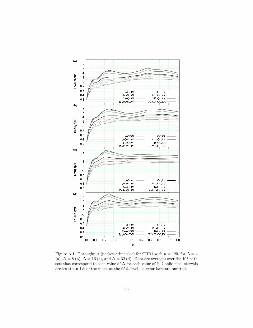
Figure A.1: Throughput (packets/time slot) for CBR1 with n = 120, for ∆ = 4(a), ∆ = 8 (b), ∆ = 16 (c), and ∆ = 32 (d). Data are averages over the 104 pathsets that correspond to each value of ∆ for each value of θ. Confidence intervalsare less than 1% of the mean at the 95% level, so error bars are omitted.
29

Figure A.2: Throughput (packets/time slot) for CBR2 with n = 120, for ∆ = 4(a), ∆ = 8 (b), ∆ = 16 (c), and ∆ = 32 (d). Data are averages over the 104 pathsets that correspond to each value of ∆ for each value of θ. Confidence intervalsare less than 1% of the mean at the 95% level, so error bars are omitted.
30
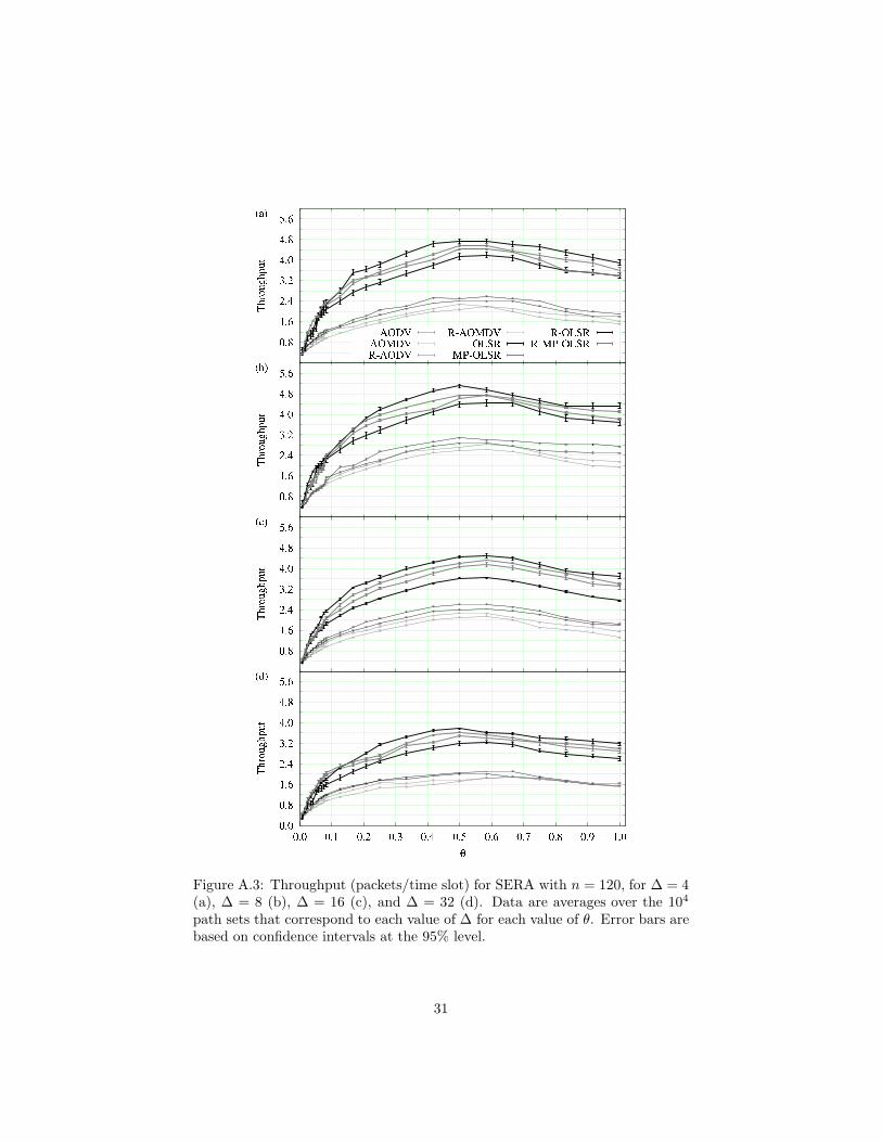
Figure A.3: Throughput (packets/time slot) for SERA with n = 120, for ∆ = 4(a), ∆ = 8 (b), ∆ = 16 (c), and ∆ = 32 (d). Data are averages over the 104
path sets that correspond to each value of ∆ for each value of θ. Error bars arebased on confidence intervals at the 95% level.
31
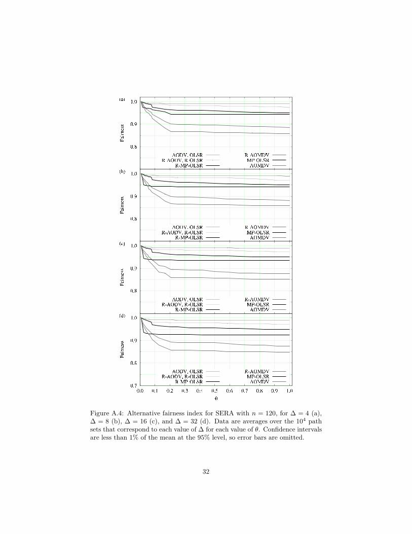
Figure A.4: Alternative fairness index for SERA with n = 120, for ∆ = 4 (a),∆ = 8 (b), ∆ = 16 (c), and ∆ = 32 (d). Data are averages over the 104 pathsets that correspond to each value of ∆ for each value of θ. Confidence intervalsare less than 1% of the mean at the 95% level, so error bars are omitted.
32

Figure A.5: Ratio of SERA’s throughput to that of CBR1 with n = 120, for∆ = 4 (a), ∆ = 8 (b), ∆ = 16 (c), and ∆ = 32 (d). Data are averages over the104 path sets that correspond to each value of ∆ for each value of θ. Confidenceintervals are less than 1% of the mean at the 95% level, so error bars are omitted.
33
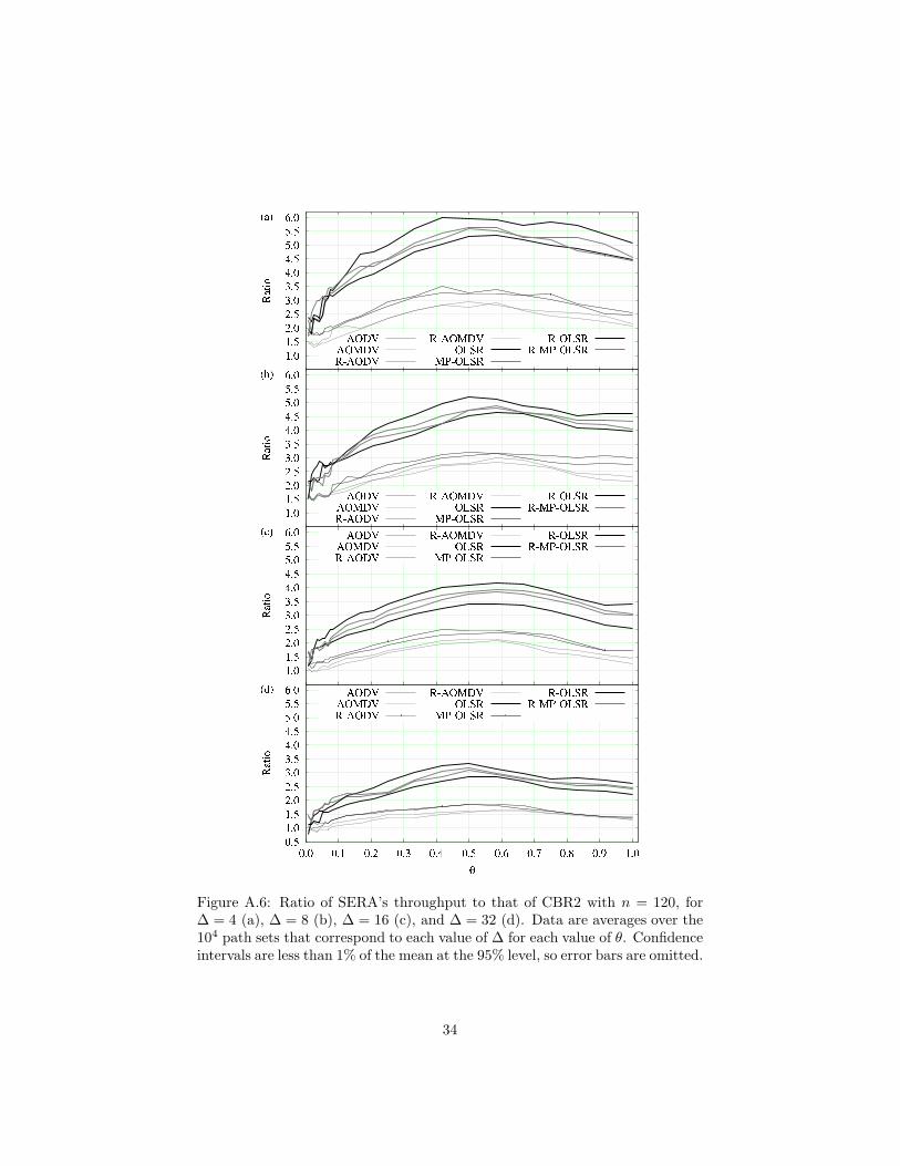
Figure A.6: Ratio of SERA’s throughput to that of CBR2 with n = 120, for∆ = 4 (a), ∆ = 8 (b), ∆ = 16 (c), and ∆ = 32 (d). Data are averages over the104 path sets that correspond to each value of ∆ for each value of θ. Confidenceintervals are less than 1% of the mean at the 95% level, so error bars are omitted.
34

Figure A.7: Ratio of CBR1’s throughput to that of CBR2 with n = 120, for∆ = 4 (a), ∆ = 8 (b), ∆ = 16 (c), and ∆ = 32 (d). Data are averages over the104 path sets that correspond to each value of ∆ for each value of θ. Confidenceintervals are less than 1% of the mean at the 95% level, so error bars are omitted.
35

Figure A.8: Distribution of the number of origin-destination pairs without anytraffic in CBR1 with n = 120, for ∆ = 4 (a), ∆ = 8 (b), ∆ = 16 (c), and ∆ = 32(d). Data are averages over the 104 path sets that correspond to each value of∆.
36
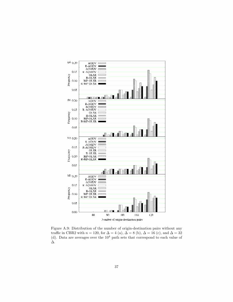
Figure A.9: Distribution of the number of origin-destination pairs without anytraffic in CBR2 with n = 120, for ∆ = 4 (a), ∆ = 8 (b), ∆ = 16 (c), and ∆ = 32(d). Data are averages over the 104 path sets that correspond to each value of∆.
37