1A Novel Cache Distribution HeuristicAlgorithm for a Mesh of Caches and ItsPerformance EvaluationJorge Escorcia, Dipak Ghosal*, and Dilip SarkarDepartment of Computer ScienceUniversity of Miami, Coral Gables, FL 33124*Department of Computer ScienceUniversity of California, Davis, CA 95616e-mails: sarkar@cs.miami.edu, ghosal@cs.ucdavis.eduAbstractThe widespread use of the Internet has created two problems: document retrieval latency andnetwork tra�c. Caching of documents \close" to users has helped to alleviate both problems.Di�erent caching policies have been proposed/implemented to make best use of limited availablecache at each caching server. A mesh of caching servers, aided by di�erent data di�usion algorithmsand the natural hierarchical structure of the Internet topology, has increased \virtual" size ofcache. Yet the size of available cache is small compared to the total size of all documents served,and remains a major resource constraint. In this work, we looked at how to improve documentdownload time, by distributing a �xed amount of total storage in a network or mesh of caches. Theintuition behind our cache distribution approach is to give more storage to the caching nodes inthe network which experience more tra�c, in the hopes that this will reduce the average latency ofdocument retrieval in the network. A heuristic was developed to estimate tra�c at each cache of anetwork. From this tra�c estimation, each cache then receives a corresponding percentage of thetotal storage capacity of the network. Through extensive simulation it is found that the proposedcache distribution algorithm can reduce latency up to 80% over prior work that includes bothHarvest-type and demand-driven data di�usion algorithms. Furthermore, the best improvementwas achieved in a cache range that corresponds to practical, real world cache ranges.

2I. IntroductionAs the (World Wide) Web connects information sources or origin servers around the world, usersfrom everywhere attempt to access these sources. Due to the ease and low cost of access, boththe number of users and documents are growing dramatically [21]; per user network tra�c is alsoincreasing. When a user accesses a faraway document, the time it takes to download (latency)could be unacceptably high. Moreover, when a user or a group of users connected to a network-neighborhood repeatedly access a faraway document, the tra�c on the network, and hence thedemand for bandwidth is increased.An e�ective method for reducing both latency and network tra�c is to use shared caches [1], [10],[18], [19], [25]. A mesh of cooperative caches are connected as a network, and they can directly orindirectly share documents stored in them. Some of these caches provide direct access to the clients;these are called proxy caches. Others are called caching servers and provide direct or indirect accessto other caches (see Section IV-B for more details about network model). As a mesh, caches providethe e�ect of a \large virtual" cache with a higher hit rate, improved access to the origin servers,reduction in document downloading time, and reduction in network tra�c.The two most commonly employed mesh caching methods are (a) hierarchical and (b) directory-based methods [23], [25]. In the directory-based method, when a request for a document arrives ata caching server, if the caching server has the document in its local cache, it serves it from there.Otherwise, the caching server queries a mapping service to locate the document in the cachingmesh. In the case of a hit, the document is fetched from the peer-caching server. In the case of amiss, the document is fetched from the origin server.In hierarchical caching, the caching servers in a mesh are (logically) organized in a hierarchy.National caches connected to the backbone network are on the top of the hierarchy [2], [8], [9].Regional caches are connected to national caches and occupy the next lower level in the hierarchy.Subregional caches are connected at the next lower level to regional caches, and institutional cachesserve as the \gateways" to subregional caches. This hierarchy naturally �ts with the standardtopology of the Internet. Because of this natural hierarchical topology, the directory based cachingmethod could be implemented at one or two levels of the hierarchy, and not at all levels of thehierarchy.To exploit the hierarchical topology of the Internet, the Harvest project originated a data di�usionscheme (will be referred to as Scheme I in this paper) that has led to popular commercial products(such as NetCache) and public-domain products (such as Squid) [12]. The Harvest, or Harvest-

3derived data di�usion schemes replicate documents on the mesh hierarchy using a simple strategy:whenever a document is retrieved from an origin or a caching server, it is replicated on every cachealong the path to the client. Although this data di�usion scheme greatly reduces the latency andnetwork tra�c, it can be improved many ways. One would get signi�cant improvement, by notreplicating relatively \unpopular" documents, if it would replace a \popular" document [21].Demand driven data di�usion schemes replicate documents only if they are relatively popular atthat cache. There are two approaches to achieve this replication process. In a top-down protocol, adocument is replicated at a cache's child if it appears to be very popular and may create a hot-spot.This protocol is aimed at avoiding hot-spots, and will work well in conjunction with an appropriatehashing technique [4], [13], [15]. To implement this technique, signi�cant changes will be necessaryin currently used caching strategies.The bottom-up approach replicates a document at a cache only when a relatively large numberof requests for a document are observed [21]. In Section II-B, we present this demand driven datadi�usion strategy and we refer to this as Scheme II.Even if we had the best/optimal data di�usion scheme, another practical problem needs tobe addressed: the size of available storage or cache. We use cache size and storage capacityinterchangeably. Analysis of access logs from [22] shows that the storage capacity at a server (unlessspeci�ed, will refer to a proxy or a caching server) is less than three percent of all documents servedby it [16]. Thus, one could think that storage capacity is a limited resource. In our study, weassume that total amount of available storage on all the servers in a mesh of caches is constant.Moreover, it is assumed that available storage can be distributed among the servers as desired.Under these assumptions, a natural question is to ask: how to distribute total available storage tothe servers for minimizing latency in document downloading, and also reduce network tra�c?In this work we propose and evaluate a storage distribution heuristic. The intuition behind ourstorage distribution heuristic is that a server with more expected tra�c should get a bigger shareof the available storage. A heuristic was developed to estimate tra�c at each cache of a network.From this tra�c estimation, each cache then receives a corresponding percentage of the total storagecapacity of the network. The proposed storage distribution heuristic is presented in Section III.Simulation has been the most common method for evaluation of caching algorithms for a proxycache server [11]. Two possible sources of input data for simulation are traces of requests froma cache server, or synthetic/arti�cially generated requests. Trace data now available for a singlecaching server can be used for realistic evaluation of di�erent caching algorithms running at a proxy

4server. However, simulation study of any data di�usion scheme requires trace data of an entiremesh of caches, but these are not readily available. Hence, for our study we use synthetic dataderived from actual server logs. Our simulation model is presented in Section IV. Our observationsfrom the simulation study are presented and discussed in Section V. Results show that our cachedistribution heuristic achieves up to 80% latency improvement in Harvest-type and demand-drivendata di�usion algorithms (when compared to equal size cache in all servers). Furthermore, the bestimprovement was achieved in a cache range that corresponds to practical, real world cache ranges.Section VI discusses the �ndings and possible future directions of study.II. Hierarchical CachingIn a hierarchical cache organization, each caching node has a parent, siblings, and children. Theterm \neighbor" is used to refer to parent or siblings that are one cache-hop away. The protocolthat caches in a caching hierarchy use is the Internet Cache Protocol (ICP) [24]. The requestresolution protocol in hierarchical caching is as follows: When a cache receives a request, it checkswhether it has the requested objected. If it has the object, it satis�es the request by serving theobject from its cache. If it does not have the object, it multicasts an ICP request to its neighbors. Ifone of the neighbors has the object, a neighbor hit, then the object is retrieved from that neighbor.If multiple neighbors have the object, the object is retrieved from the neighbor with the lowestmeasured latency. If none of the neighbors has the object, a neighbor miss, which is determinedfrom a negative ICP response or a timeout, the request is either forwarded to a parent or sentdirectly to the origin server. The origin server is the initial and permanent repository of the object.Forwarding the request to a parent simply repeats the process. If the request misses at each levelof the hierarchy, a top-level parent fetches the object from the origin server, caches it, and passesit down the hierarchy to the leaf node that originated the request.There are two key objectives in the design of hierarchical caches. The �rst is to ensure thatpopular objects are cached at the lower levels of the hierarchy, while less popular objects arecached at the higher levels. The second objective is to ensure that when there is a cache miss ata particular caching server, the request is satis�ed by a caching server in the same or higher level,thereby precluding the need for the request object to be served by the origin server. These twoobjectives reduce the latency perceived by the user and the overall network tra�c. Both objectives,especially the �rst, depend on the data di�usion strategy and the cache replacement strategy. Thesestrategies determine how the objects are placed in the caching hierarchy. In the next two sections

5we present two such data di�usion strategies.A. Harvest SchemeThe data di�usion strategy in the Harvest scheme replicates objects in the caching mesh bycaching the objects at every node along the path when it comes down the hierarchy [8]. Themotivation for caching the object at all the nodes in the downward path is that subsequent requestsfor the object would have multiple points in the caching hierarchy from where it could get satis�ed,thus decreasing the likelihood that the request would need to be satis�ed by the origin server.When the cache space at a node is full, and a new object is to be cached, a previously cachedobject must be dropped from the cache. This is what is referred to as the cache replacementstrategy. Harvest-derived schemes can support di�erent cache replacement strategies, such as LFUand LRU. Finally, in Harvest-derived schemes when an object is dropped from the cache, neitherthe object itself, nor any meta-information regarding the object, is passed up the hierarchy.B. A Demand-Driven Data Di�usion Algorithm (D4)We shall refer to this algorithm as the D4 algorithm. The D4 algorithm uses a reference countingscheme as part of its cache replacement strategy [21]. Each cache in the mesh maintains a referencecount for all the objects for which it has received a request over some time interval. This meta-information is maintained even when the object is not in the cache. When a node receives an objectrequest, it increases the reference count for that object. If the object is in the node' s cache, itserves the request, otherwise it forwards the request to the next node along the path to the originserver, which is then handled recursively. When the object comes down, after being served at somehigher level, each node along the path uses an LFU replacement strategy to determine whether ornot to cache the object when the cache space is full. The reference count is used as the frequencymeasure. When an object is dropped from a cache, its reference count measured at that node ispassed up to the next node (parent node) along the path to the origin server. The parent node addsthis reference count to its own reference count for the object. If the parent cache has the object itdoes nothing. If it does not have the object, it determines what the result would be of trying tocache the object at that instant using the new reference count. If the decision was that the objectwould be cached, nothing is done. However, if the decision was that the object would be dropped,the parent sends up the reference count it received from the child to its own parent, which is thenhandled recursively. The motivation here is to propagate the meta-information to the right pointin the hierarchy, i.e., a node where an object is already cached or a node which determines it would

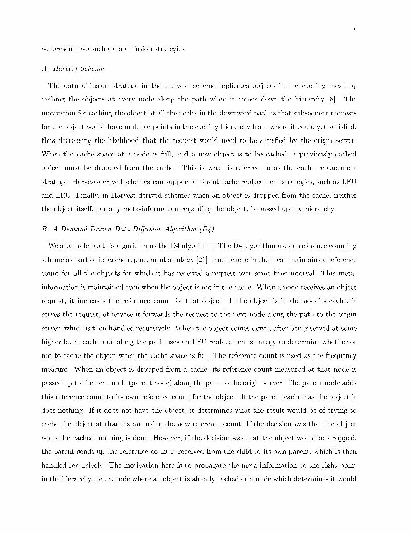
6be able to cache the object the next time it comes around.Furthermore, in this scheme, when a node receives a request for an object that already has anunsatis�ed request, the reference count for the object is increased. The node then determineswhether to generate meta-information regarding the request and pass it up the hierarchy. Theprocedure here is analogous to the one before. The motivation is to propagate the meta-informationto the point where the object is cached or \expected" to be cached.III. A Cache Distribution AlgorithmThe motivation behind distributing the cache is to maximize the bene�ts of caching. Given alimited amount of cache in the network, placing more cache in the nodes which experience moretra�c, while keeping the average cache per node over the whole network the same, may improvethe overall latency of the network. Since the cache size of the whole network is �xed, placingmore cache at one node means reducing cache at another node. The cache distribution algorithmdetermines how much cache to place at each node by giving an estimate of how much tra�c eachparticular node may experience. The following de�nitions are introduced to explain the algorithm.A. De�nitionsDe�nition 1: A network topology is a graph NT (V;E), where V = fv1; v2; :::; vng is thenonempty set of n nodes of the network, and E = e1; e2; :::; em is the set of m edges, such thatei = (vi1 ; vi2), and vi1 ; vi2 2 V . The set V is the union of the set of origin servers (OS), the set ofcaching servers (CS), and the set of proxy servers (PS). Thus, V = OS [ CS [ PS. Also, in ourstudy OS \CS = ;; CS \ PS = ;, and OS \ PS = ;.Example: Figure 1 is a sample network to illustrate the de�nitions and the cache distributionalgorithm. The set V of nodes in this network are fA;B; a; b; c; d; e; f; g; hg and the set E of edgesare f(A; a); (a; b); (a; c); (a; d); (a; e); (B; d); (b; c); (b; f); (c; d); (c; g); (d; h)g. Furthermore, the set oforigin servers (OS) is fA;Bg, the set of caching servers (CS) is fa; b; c; dg; and the set of proxyservers (PS) is fe; f; g; hg. It is readily seen that the union of OS;CS, and PS is V , and that theintersection of OS;CS, and PS is null.De�nition 2: A layered network LN(V 0; FL;E0) is a subgraph of network topology NT (V;E),where V 0 � V , E0 � E, and FL � V 0. The set of nodes V 0 of LN(V 0; FL;E0) are partitioned intosubsets L1; L2; :::; Ll, where L1 = FL is the �rst layer of the layered network. There is no edge

7origin server

caching server

proxy servere

origin server

caching server

proxy server

b c

f

e

A

a

b

f

A

c

gg

dd

hh

BB

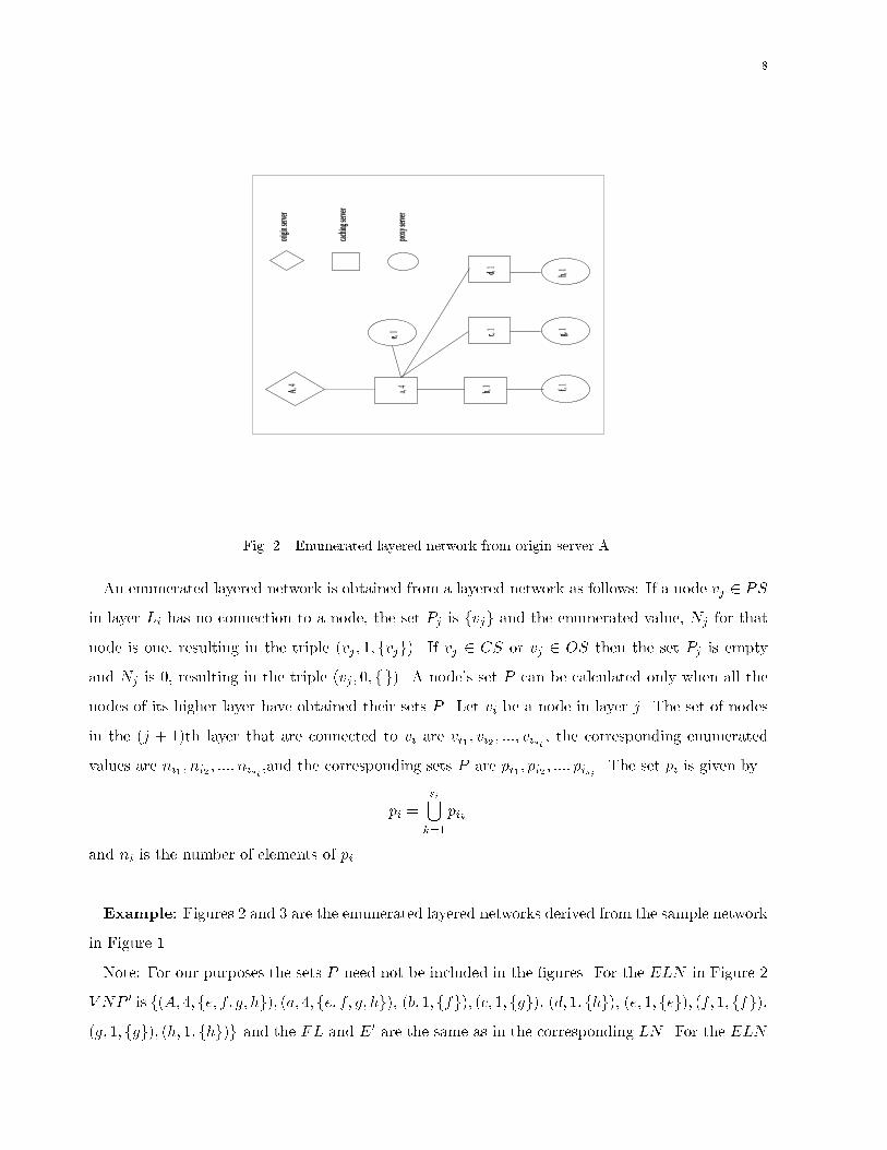
Fig. 1. An example network.between two nodes of a layer. The �rst layer L1 is connected to only the nodes of the layer L2.The nodes of a layer Li can only be connected to the nodes of the layer Li�1 and Li+1. Naturally,the nodes of layer Ll are only connected to the nodes of layer Ll�1.Example: From the network in Figure 1 we create two layered networks as shown in Figures2, 3. The numbers in the �gures will be explained in the next de�nition. In Figure 2, FL = fAgso L1 = fAg; L2 = fag; L3 = fb; c; d; eg and L4 = ff; g; hg. Also, E0 = f(A; a); (a; b); (a; c); (a; d);(a; e); (b; f); (c; g); (d; h)g. In Figure 3, FL = fBg so L1 = fBg; L2 = fdg; L3 = fa; c; hg; L4 =fb; e; gg; and L5 = ffg. Finally, E0 = f(B; d); (d; a); (d; h); (d; c); (a; e); (a; b); (c; b); (c; g); (b; f)g.Note: For our purposes, nodes of OS and CS are included in the layered network only when theyare the FL or when they have connections to layers above and below.De�nition 3: An Enumerated Layered Network, ELN(V NP 0; FL;E0), where V NP 0 = f(v1; N1; P1),(v2; N2; P2); :::; (vn; Nn; Pn)g, is obtained from a LN(V 0; FL;E0) such that Pi � V 0 and Ni is thenumber of elements in Pi.

8ori

gin se

rver

cachin

g serv

er

proxy

serve

re

origin

serve

r

cachin

g serv

er

proxy

serve

r

bc

f

e, 1

A a, 4 b, 1 f, 1

c, 1 gg, 1

dd, 1

hh, 1

A, 4

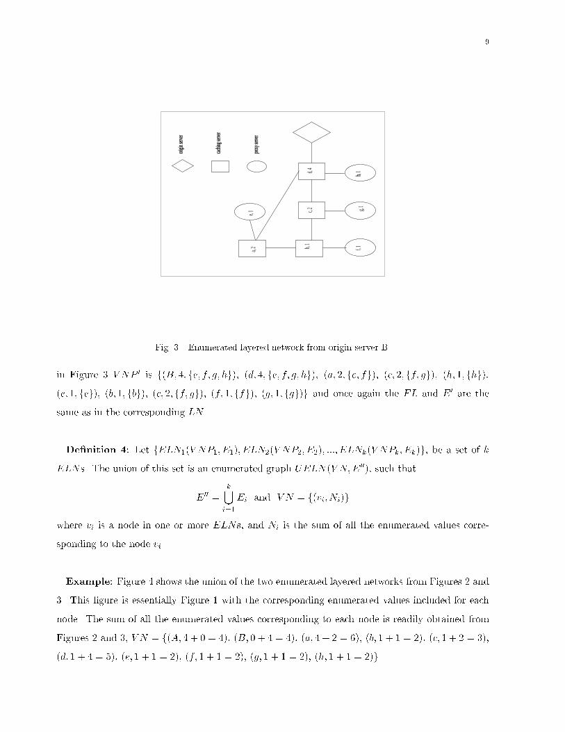
Fig. 2. Enumerated layered network from origin server A.An enumerated layered network is obtained from a layered network as follows: If a node vj 2 PSin layer Li has no connection to a node, the set Pj is fvjg and the enumerated value, Nj for thatnode is one, resulting in the triple (vj ; 1; fvjg). If vj 2 CS or vj 2 OS then the set Pj is emptyand Nj is 0, resulting in the triple (vj ; 0; f g). A node's set P can be calculated only when all thenodes of its higher layer have obtained their sets P . Let vi be a node in layer j. The set of nodesin the (j + 1)th layer that are connected to vi are vi1 ; vi2 ; :::; visi , the corresponding enumeratedvalues are ni1 ; ni2 ; :::; nisi ,and the corresponding sets P are pi1 ; pi2 ; :::; pisi . The set pi is given bypi = si[k=1 pikand ni is the number of elements of pi.Example: Figures 2 and 3 are the enumerated layered networks derived from the sample networkin Figure 1.Note: For our purposes the sets P need not be included in the �gures. For the ELN in Figure 2V NP 0 is f(A; 4; fe; f; g; hg); (a; 4; fe; f; g; hg); (b; 1; ffg); (c; 1; fgg); (d; 1; fhg); (e; 1; feg); (f; 1; ffg);(g; 1; fgg); (h; 1; fhg)g and the FL and E0 are the same as in the corresponding LN . For the ELN

9ori

gin se

rver

cachin

g serv

er

proxy

serve

r

origin

serve

r

cachin

g serv

er

proxy

serve

r

h

e, 1a, 2 b,

1c, 2

d, 4

f, 1g,

1h,

1

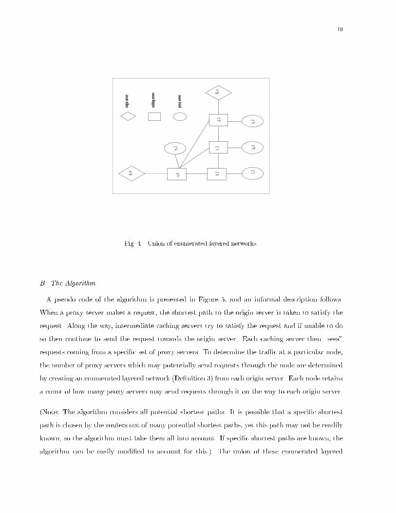
Fig. 3. Enumerated layered network from origin server B.in Figure 3 V NP 0 is f(B; 4; fe; f; g; hg); (d; 4; fe; f; g; hg); (a; 2; fe; fg); (c; 2; ff; gg); (h; 1; fhg);(e; 1; feg); (b; 1; fbg); (c; 2; ff; gg); (f; 1; ffg); (g; 1; fgg)g and once again the FL and E0 are thesame as in the corresponding LN .De�nition 4: Let fELN1(V NP1; E1); ELN2(V NP2; E2); :::; ELNk(V NPk; Ek)g, be a set of kELNs. The union of this set is an enumerated graph UELN(V N;E00); such thatE00 = k[i=1Ei and V N = f(vi; Ni)gwhere vi is a node in one or more ELNs, and Ni is the sum of all the enumerated values corre-sponding to the node vi.Example: Figure 4 shows the union of the two enumerated layered networks from Figures 2 and3. This �gure is essentially Figure 1 with the corresponding enumerated values included for eachnode. The sum of all the enumerated values corresponding to each node is readily obtained fromFigures 2 and 3, V N = f(A; 4 + 0 = 4); (B; 0 + 4 = 4); (a; 4 + 2 = 6); (b; 1 + 1 = 2); (c; 1 + 2 = 3);(d; 1 + 4 = 5); (e; 1 + 1 = 2); (f; 1 + 1 = 2); (g; 1 + 1 = 2); (h; 1 + 1 = 2)g.

10ori

gin se

rver

cachin

g serv

er

proxy

serve

r

origin

serve

r

cachin

g serv

er

proxy

serve

r

A, 4

a, 6e, 2

b, 2

c, 3d,

5B,

4

f, 2g,

2h,

2

Fig. 4. Union of enumerated layered networks.B. The AlgorithmA pseudo code of the algorithm is presented in Figure 5, and an informal description follows.When a proxy server makes a request, the shortest path to the origin server is taken to satisfy therequest. Along the way, intermediate caching servers try to satisfy the request and if unable to doso then continue to send the request towards the origin server. Each caching server then \sees"requests coming from a speci�c set of proxy servers. To determine the tra�c at a particular node,the number of proxy servers which may potentially send requests through the node are determinedby creating an enumerated layered network (De�nition 3) from each origin server. Each node retainsa count of how many proxy servers may send requests through it on the way to each origin server.(Note: The algorithm considers all potential shortest paths. It is possible that a speci�c shortestpath is chosen by the routers out of many potential shortest paths, yet this path may not be readilyknown, so the algorithm must take them all into account. If speci�c shortest paths are known, thealgorithm can be easily modi�ed to account for this.) The union of these enumerated layered

11let CT be the total amount of cache to be distributed;let OS be the set of origin servers;for each osi 2 OSfconstruct layered networks, LN(Vi; osi; Ei);construct enumerated networks, ELN(V NPi; osi; Ei);gconstruct union of enumerated layered networks, UELN , bytaking the union of the enumerated layered networks, ELNs;let N = kXi=1Ni;let ci be the available cache at each node vi;for each node vi; ci �= ((Ni=N) � CT );Fig. 5. Pseudo code for the cache distribution algorithm.networks (De�nition 4) then gives us the total counts assigned to each node in the network. Thepercentage of the total count is determined for each node, which correlates to the percentage ofcache each node should receive. Since we are using whole numbers to represent cache size, somerounding is introduced, so further manipulation of the numbers may be required to keep the totalcache size of the network equivalent to the original size before redistribution. The following sectionillustrates an example of the algorithm.C. An ExampleWe revisit Figures 1 - 4 one more time to give a complete example of the cache distribution algo-rithm. From the example network in Figure 1 we create two layered networks, one from server Aand one from server B, as shown in Figures 2 and 3, respectively, and ignoring the numbers. Note:Since caching is only performed by the caching and proxy servers, the origin servers are included inthe layered networks only when they serve as the �rst layer in the network. Furthermore, cachingservers are included in the network only when they have a connection to a layer above and a layerbelow. The next step is to create an enumerated layered network from each of the layered networkswhich are also shown in Figures 2 and 3. Finally, the union of these enumerated layer networks isdetermined as shown in Figure 4. Once the union of the enumerated layered networks is determinedwe have the total enumeration value for each node. This number provides the basis for distributing

12a b c d e f g h TotalA 4 1 1 1 1 1 1 1 11B 2 1 2 4 1 1 1 1 13Total 6 2 3 5 2 2 2 2 24% 25.00 8.33 12.50 20.83 8.33 8.33 8.33 8.33 99.98Calculated Cache Size 10 3 5 8 3 3 3 3 38Final Cache Size 11 3 5 9 3 3 3 3 40TABLE IResults of cache distribution.the cache.The cache distribution results are shown in Table I. In this example we assume the total availablecache in the network is 40, so if we were to distribute the cache evenly among the proxy serversand caching servers, each would receive a cache size of 5. The �rst step in distributing the cache isdetermining each node's percentage of enumeration over the whole network. Note: Since the originservers do not perform caching, their enumeration values are not considered in these calculations.To distribute the cache, the node's count percentage is multiplied by the total cache in the network.As the �gure shows, the calculated cache size for each node does not add up to 40 simply becausea rounding error is introduced. To compensate for this, the cache sizes of individual nodes areadjusted to make the total cache size of the redistributed cache an even 40.IV. Simulation ModelTo study the e�ects of the cache distribution using the novel algorithm proposed here, the oper-ation of a mesh of caches is simulated. Both the data di�usion algorithms described in Section IIwere implemented in the simulated environment. The simulator is a C++ program, which makesextensive use of LEDA [17] object libraries, and is an extended version of the simulator used inthe study reported in [21]. The extended version is discussed in the next section. The inputs tothe simulator make up the network topology and the request pro�le for each object. The networktopology is speci�ed in Graph Meta Language (GML) format, which also speci�es the cache size ofeach node and the bandwidths of individual links.

13A. Simulator ExtensionThe simulator was extended to accommodate di�erent cache sizes for the nodes. The originalsimulator only allowed for all the nodes to have the same cache size. The GML format providesthe means to assign the di�erent cache sizes, so for each topology at each average cache size twoGML �les were created, one with cache distribution and one without. The original simulator wouldonly need two GML �les (one for each topology) to run the simulations. Our simulations requireda total of 40 GML �les. Each topology was simulated using 10 di�erent average cache sizes, soeach topology requires 20 GML �les, 10 with cache distribution and 10 without cache distribution.Lastly, the program code was modi�ed in order to read in this new cache attribute in the GML�les.B. Network ModelThe network consists of three types of nodes, namely proxy servers, origin servers and intermedi-ate caching servers. Proxy servers are the leaf nodes in the network where requests are generated.Origin servers are the initial storing place of the requested objects. Intermediate caching serversreside somewhere along the path from the proxy servers to the origin servers. Note that only theproxy servers and intermediate caching servers perform caching. Origin servers contain the sameset of objects throughout the entire run of the simulation. The nodes are connected by bidirectionallinks with a speci�ed bandwidth. Each node also performs the function of forwarding packets tothe next hop.When an object is to be transmitted through the network it is �rst split into packets. Thesepackets are then sent to their destination where they arrive in order and reassembled there. Thepath taken through the network is always the shortest path between the sender and the receiver.The link and node models were carefully constructed to ensure fairness among multiple connec-tions. Consider a node that simultaneously starts transmitting a large �le and a small �le to thesame node. If all the packets of the large �le are sent �rst, the then the large �le would reach thedestination prior to any of the packets of the small �le. The large �le ends up monopolizing thelink, which is unfair.To handle the above scenario properly, in the node, arriving packets are queued on a per-connection basis, so that packets belonging to di�erent connections occupy di�erent queues. Inthis way packets from di�erent connections do not a�ect each other. A node can transmit multiplepackets to a link at the same time as long as the packets belong to di�erent connections. Packets

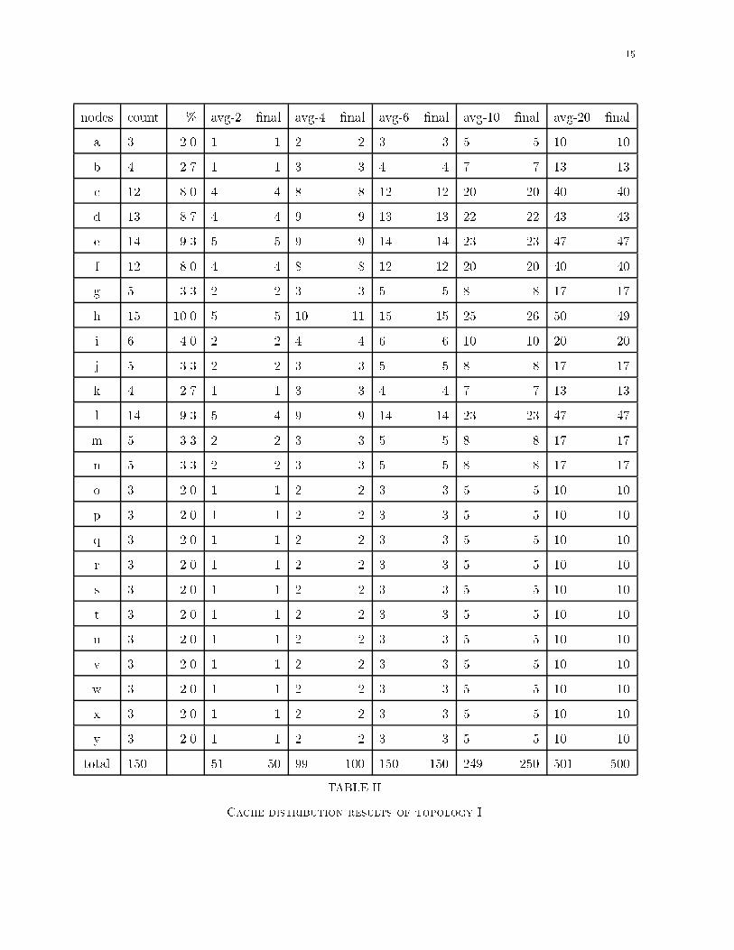
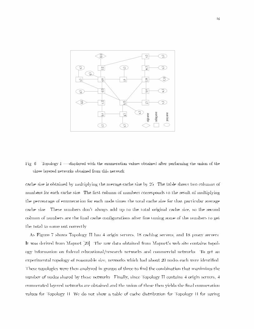
14within a queue are transmitted to the appropriate link in order, so a packet cannot be placed on alink until the previous one packet has been completely transmitted.C. Request GenerationThe request pro�le for an object is a piece-wise linear graph that plots the request rate for theobject over time. The plotted request rate for the object is its request rate in the aggregate, i.e.,the sum total of the rates at which requests are generated for the object by all the proxy serversin the network. Once the aggregate request pro�le for an object is determined, it is broken upinto per proxy server request pro�les. This is done by taking a �xed set of points from the piece-wise linear graph and then for each point, distributing the corresponding request rate among theproxy servers. This distribution is pseudo-uniform, i.e., each proxy server's share of the aggregaterequest rate lies within a bounded interval of the uniform distribution value. Once the per proxyserver request pro�les are determined, the actual request generation in the simulator takes placeas follows. To generate a request for an object O at proxy server P at time T, the request rate forO at P at instant T is taken. If this rate is �, then the inter-arrival time is obtained by modelingthe incoming stream of requests for O at P as a Poisson process with mean �.Finally, the 90/10 rule [3] was used to assign the request rates to the objects. Consequently, 10%of the objects are marked as popular and the aggregate request rates for these popular objects arescaled up by a factor of 81 times the corresponding rate for the unpopular objects. Both popularand unpopular objects are uniformly distributed across the origin servers of the particular network.D. Network TopologiesIn our simulation we considered two di�erent mesh like topologies, which we refer to as TopologyI and Topology II, and shown in Figures 6 and 7 respectively. Topology I is looked at in depth forthe purposes of demonstrating the cache distribution algorithm.Topology I was obtained by taking the backbone mesh of a major carrier services provider andattaching proxy servers to it. Topology I has 3 origin servers, 15 caching servers, and 11 proxyservers. Figure 6 shows the network topology as well as the enumeration values obtained afterperforming the union of the three layered networks obtained from this network. Table II shows theresults after performing the cache distribution algorithm given the enumeration values of TopologyI. As the table shows, the cache distribution algorithm is applied using various cache sizes. Thesecache sizes correspond to the �rst 6 of the 10 cache sizes that were used to run the simulation.Since there are a total of 25 caching nodes in the network the total available cache for each average

15nodes count % avg-2 �nal avg-4 �nal avg-6 �nal avg-10 �nal avg-20 �nala 3 2.0 1 1 2 2 3 3 5 5 10 10b 4 2.7 1 1 3 3 4 4 7 7 13 13c 12 8.0 4 4 8 8 12 12 20 20 40 40d 13 8.7 4 4 9 9 13 13 22 22 43 43e 14 9.3 5 5 9 9 14 14 23 23 47 47f 12 8.0 4 4 8 8 12 12 20 20 40 40g 5 3.3 2 2 3 3 5 5 8 8 17 17h 15 10.0 5 5 10 11 15 15 25 26 50 49i 6 4.0 2 2 4 4 6 6 10 10 20 20j 5 3.3 2 2 3 3 5 5 8 8 17 17k 4 2.7 1 1 3 3 4 4 7 7 13 13l 14 9.3 5 4 9 9 14 14 23 23 47 47m 5 3.3 2 2 3 3 5 5 8 8 17 17n 5 3.3 2 2 3 3 5 5 8 8 17 17o 3 2.0 1 1 2 2 3 3 5 5 10 10p 3 2.0 1 1 2 2 3 3 5 5 10 10q 3 2.0 1 1 2 2 3 3 5 5 10 10r 3 2.0 1 1 2 2 3 3 5 5 10 10s 3 2.0 1 1 2 2 3 3 5 5 10 10t 3 2.0 1 1 2 2 3 3 5 5 10 10u 3 2.0 1 1 2 2 3 3 5 5 10 10v 3 2.0 1 1 2 2 3 3 5 5 10 10w 3 2.0 1 1 2 2 3 3 5 5 10 10x 3 2.0 1 1 2 2 3 3 5 5 10 10y 3 2.0 1 1 2 2 3 3 5 5 10 10total 150 51 50 99 100 150 150 249 250 501 500TABLE IICache distribution results of topology I

16

A,11

p, 3

a, 3o, 3

q, 3

r, 3b, 4

c, 12

d, 13

f, 12

e,14

B, 11

s, 3g, 5

h, 15

i, 6t, 3

u, 3

j, 5k, 4

l, 14

m , 5

n ,5

w, 3

v, 3C,

11x, 3

y, 3

origin

serve

r

cachin

g serv

er

proxy

server

Fig. 6. Topology I | displayed with the enumeration values obtained after performing the union of thethree layered networks obtained from this network.cache size is obtained by multiplying the average cache size by 25. The table shows two columns ofnumbers for each cache size. The �rst column of numbers corresponds to the result of multiplyingthe percentage of enumeration for each node times the total cache size for that particular averagecache size. These numbers don't always add up to the total original cache size, so the secondcolumn of numbers are the �nal cache con�gurations after �ne tuning some of the numbers to getthe total to come out correctly.As Figure 7 shows Topology II has 4 origin servers, 18 caching servers, and 18 proxy servers.It was derived from Mapnet [20]. The raw data obtained from Mapnet's web site contains topol-ogy information on federal educational/research networks and commercial networks. To get anexperimental topology of reasonable size, networks which had about 20 nodes each were identi�ed.These topologies were then analyzed in groups of three to �nd the combination that maximizes thenumber of nodes shared by these networks. Finally, since Topology II contains 4 origin servers, 4enumerated layered networks are obtained and the union of these then yields the �nal enumerationvalues for Topology II. We do not show a table of cache distribution for Topology II for saving

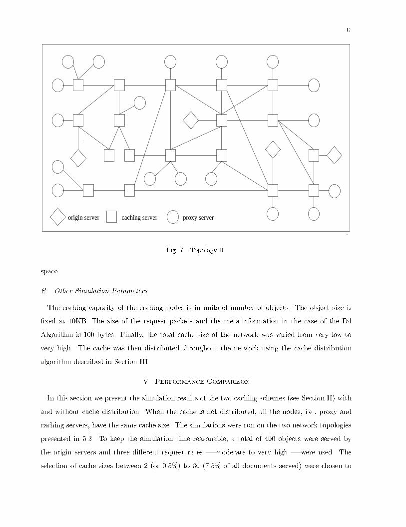
17

origin server caching server proxy serverFig. 7. Topology II.space.E. Other Simulation ParametersThe caching capacity of the caching nodes is in units of number of objects. The object size is�xed at 10KB. The size of the request packets and the meta-information in the case of the D4Algorithm is 100 bytes. Finally, the total cache size of the network was varied from very low tovery high. The cache was then distributed throughout the network using the cache distributionalgorithm described in Section III.V. Performance ComparisonIn this section we present the simulation results of the two caching schemes (see Section II) withand without cache distribution. When the cache is not distributed, all the nodes, i.e., proxy andcaching servers, have the same cache size. The simulations were run on the two network topologiespresented in 5.3. To keep the simulation time reasonable, a total of 400 objects were served bythe origin servers and three di�erent request rates | moderate to very high | were used. Theselection of cache sizes between 2 (or 0.5%) to 30 (7.5% of all documents served) were chosen to

18

0

10

20

30

40

50

60

70

80

5 10 15 20 25 30

Per

cent

age

late

ncy

redu

ctio

h

Average cache size

Request rate = 0.01Request rate = 0.008Request rate = 0.006

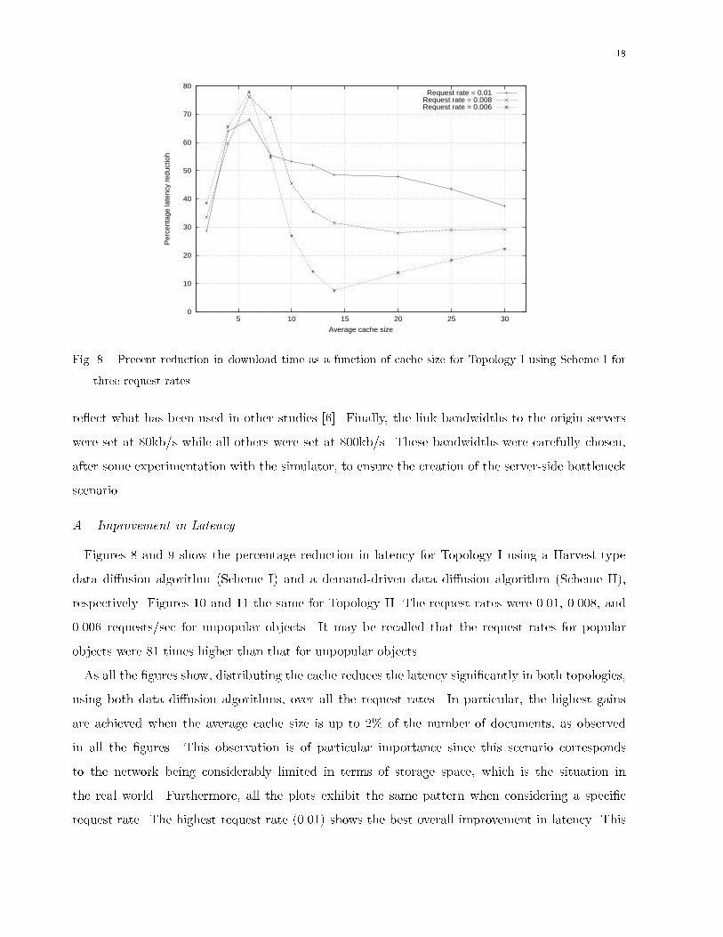
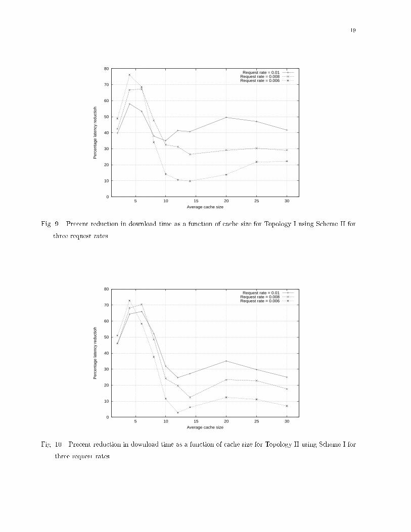
Fig. 8. Precent reduction in download time as a function of cache size for Topology I using Scheme I forthree request rates.re ect what has been used in other studies [6]. Finally, the link bandwidths to the origin serverswere set at 80kb/s while all others were set at 800kb/s. These bandwidths were carefully chosen,after some experimentation with the simulator, to ensure the creation of the server-side bottleneckscenario.A. Improvement in LatencyFigures 8 and 9 show the percentage reduction in latency for Topology I using a Harvest-typedata di�usion algorithm (Scheme I) and a demand-driven data di�usion algorithm (Scheme II),respectively. Figures 10 and 11 the same for Topology II. The request rates were 0.01, 0.008, and0.006 requests/sec for unpopular objects. It may be recalled that the request rates for popularobjects were 81 times higher than that for unpopular objects.As all the �gures show, distributing the cache reduces the latency signi�cantly in both topologies,using both data di�usion algorithms, over all the request rates. In particular, the highest gainsare achieved when the average cache size is up to 2% of the number of documents, as observedin all the �gures. This observation is of particular importance since this scenario correspondsto the network being considerably limited in terms of storage space, which is the situation inthe real world. Furthermore, all the plots exhibit the same pattern when considering a speci�crequest rate. The highest request rate (0.01) shows the best overall improvement in latency. This

19

0

10

20

30

40

50

60

70

80

5 10 15 20 25 30

Per

cent

age

late

ncy

redu

ctio

h

Average cache size

Request rate = 0.01Request rate = 0.008Request rate = 0.006

Fig. 9. Precent reduction in download time as a function of cache size for Topology I using Scheme II forthree request rates.

0

10

20

30

40

50

60

70

80

5 10 15 20 25 30

Per

cent

age

late

ncy

redu

ctio

h

Average cache size

Request rate = 0.01Request rate = 0.008Request rate = 0.006

Fig. 10. Precent reduction in download time as a function of cache size for Topology II using Scheme I forthree request rates.

20

0

10

20

30

40

50

60

70

80

5 10 15 20 25 30

Per

cent

age

late

ncy

redu

ctio

h

Average cache size

Request rate = 0.01Request rate = 0.008Request rate = 0.006

Fig. 11. Precent reduction in download time as a function of cache size for Topology II using Scheme II forthree request rates.again is of particular importance since this corresponds to very high network tra�c, which is thesituation under which better caching schemes are of greatest importance. In a network with lowcongestion, better caching schemes will naturally bene�t less because the lower tra�c gives way tolower latency regardless of the caching scheme. This trend is observed in all the �gures. As therequest rate decreases, the overall gains in latency also decrease.VI. ConclusionIn this work we looked at a speci�c facet of caching as it applies to the Web. Speci�cally, welooked at how to improve document download time, by distributing a �xed amount of total storagein a mesh of caching servers. We studied the e�ect of our cache distribution by simulating two datadi�usion schemes for hierarchical caches The intuition behind this approach is to give more storageto the caching nodes in the network which experience more tra�c, in the hopes that this will reducethe overall latency of the network. A heuristic was developed to estimate tra�c at each cache of anetwork. From this tra�c estimation, each cache then receives a corresponding percentage of thetotal storage capacity of the network.The results show a signi�cant improvement in overall network latency after application of thiscache distribution algorithm, speci�cally at very modest storage capacities. This observation isof particular importance since these modest storage capacities correspond to practical, real world

21cache ranges. We compared the performance of this algorithm versus a caching scheme in whichall nodes of a network receive an equal amount of storage. The cache distribution algorithm byno means produces an optimal distribution of the cache, yet the results indicate that clever cacheplacement is an area of caching which can signi�cantly improve performance of the network.A recent study has found a similar problem, called the cache location problem, to be NP-hardfor general network [27]. The results directly do not apply to the hierarchical caching networkswe have studied. Thus, an open problem is �nding a polynomial-time optimal algorithm for cachedistribution, if it exists; or proving that our problem is also NP-hard. Another problem is developingan analytical method for evaluation of the proposed heuristic. A desirable extension of the workreported here is to implement it over a real-world mesh of caching servers, and then study theperformance of our algorithm. However, this would require collaboration with a major InternetService Provider (ISP). We plan to explore the possibility of such a study in the near future. Inthis study we not only plan to measure percentile improvement of average latency, but also theactual latency in seconds. The objective is to �nd the threshold value of latency that makes aperceptual di�erence to the end users. References[1] M. Abrams, C. Standridge, G. Abdulla, S. Williams, and E. A. Fox, \Caching Proxies: Limitations and Poten-tials," in Proceedings 4th International WWW Conference, Boston, December 1995.[2] R. Alonso and M. Blaze, \Dynamic hierarchical caching for large-scale distributed �le systems," in Proceedingsof the Twelvth International Conference on Distributed Computing Systems, June 1992.[3] M. F. Arlitt and C. L. Williamson, \Web server workload characterization: the search for invariants," 1996 ACMSIGMETRICS International Conference on Measurement and Modeling of Computer Systems, Philadelphia, PA,USA, Vol. 24, No. 1:126-37, 1996.[4] A. Bestavros, \Demand-based document dissemination to reduce tra�c and balance load in distributed infor-mation systems," in Proceedings of the 1995 Seventh IEEE Symposium on Parallel and Distributed Processing,San Antonio, TX, October 1995.[5] A. Bestavros, R. L. Carter, and M. E. Crovella, \Application-Level Document Caching in the Internet," TechnicalReport BU-CS-95-002, Boston U., CS Dept., Boston, MA 02215, March 1995.[6] L. Breslau, P. Cao, L. Fan, G. Phillips, S. Shenker, \Web Caching and Zipf-like Distributions: Evidence andImplications," Proceedings of IEEE INFOCOM 99, 1999.[7] S. Bhattacharjee, K. Calvert, and E. W. Zegura, \Self-Organizing Wide Area Network Caches," in Proceedingsof IEEE INFOCOM 98, San Francisco, CA, March 1998.[8] C. M. Bowman, P. B. Danzig, D. R. Hardy, U. Manber, and M. F. Schwartz, \Harvest: A scalable, customizablediscovery and access system," Technical Report CU-CS-732-94, University of Colorado, Boulder, 1994.

22[9] A. Chankhunthod, P. B. Danzig, C. Neerdaels, M. F. Schwartz, and K. Worrel, \A Hierarchical Internet ObjectCache," in Proceedings of the 1996 USENIX Technical Conference, San Diego, CA, Jan 1996.[10] P. B. Danzig, M. F. Schwartz, and R. S. Hall, \A case for caching �le objects inside internetworks," in ProceedingsACM SIGCOMM 92 Conference, Aug 1992, 281-292.[11] B. D. Davidson, \A Survey of Proxy Cache Evaluation Techniques", in 4th International Caching Workshop,San Jose, CA, 1999.[12] S. Gadde, J. Chase, and M. Rabinovich, \A taste of crispy squid", in Proceedings of the Workshop on InternetService Performance (WISP'98), June 1998.[13] J. Gwertzman and M. Seltzer, \The Case for Geographical Push-caching" in Proceedings of the 1995 Workshopon Hot Operating systems, 1995.[14] The Harvest Home Page <URL: http://harvest.transarc.com>[15] D. Karger, E. Lehman, T. Leighton, M. Levine, D. Lewin, R. Panigrahy, \Consistent Hashing and RandomTrees: Distributed Caching Protocols for Relieving Hot Spots on the World Wide Web," STOC 97, El Paso,TX, 1997.[16] T. P. Kelly, Y. M. Chan, S. Jamin, and J. K. MacKie-Mason, \Biased Replacement Policies for Web Caches:Di�erential Quality-of-Service and Aggregate User Value," Fourth International Web Caching Workshop, SanDiego, CA, March 31 - April 2, 1999.[17] The LEDA Home Page <URL: http://www.mpi-sb.pg.de/LEDA/leda.html>[18] A. Luotonen and K. Altis, \World-Wide Web Proxies", Computer Networks and ISDN systems, Vol 27, 1994.[19] A. Luotonen, Web Proxy Servers, Prentice Hall, 1997[20] The Mapnet Web Page <URL: http://www.mapnet.com>[21] R. Mukhopadhayay, A New Demand-driven Data Di�usion Algorithm for Hierarchical Caching, Master's Thesis,Department of Computer Science, University of California at Davis, Davis, CA 95616, June 1999.[22] National Laboratory for Applied Network Research, Anonymized access logs, ftp://ftp.ircache.net/Traces[23] P. Rodriguez, C. Spanner, and E. W. Biersack, \Web caching architectures: Hierarchical and distributedcaching," in Proceedings of the 4th International Web Caching Workshop, San Diego, April 1999.[24] RFC2186,2187, <URL: http://ircache.nlanr.net/Cache/reading.html>[25] R. Tewari, M. Dahlin, H. Vin, and J. Kay, \Design Considerations for Distributed Caching on the Internet,"The 19th IEEE International Conference on Distributed Computing Systems (ICDCS), May 1999.[26] L. Zhang, S. Floyd, and V. Jacobson, \Adaptive Web Caching," in Proceedings of the NLANR Web CacheWorkshop, June 1997.[27] P. Krishnan, D. Raz, and Y. Shavitt, \The Cache Location Problem," IEEE/ACM Transactions on Networking,Vol. 8, No. 5, pp. 568 - 581, October 2000.