An Introduction to Electrical Instrumentation and Measurement ...
461
B. A. Gregory An Introduction to ELECTRICAL INSTRUMENTATION AND MEASUREMENT SYSTEMS Second Edition A Halsted Press Book
-
Upload
khangminh22 -
Category
Documents
-
view
0 -
download
0
Transcript of An Introduction to Electrical Instrumentation and Measurement ...
B. A. Gregory
An Introduction to ELECTRICAL INSTRUMENTATION AND MEASUREMENT SYSTEMSSecond Edition
A Halsted Press Book

An Introduction to Electrical Instrumentation and Measurement Systems

An Introduction to Electrical Instrumentation and Measurement Systems
A guide to the use, selection, and limitations of electrical instruments and measurement systems
B.A. GregorySenior Lecturer Specialising in Electrical Instrumentation, Department of Electrical and Electronic Engineering, Brighton Polytechnic
Second Edition
A Halsted Press Book
JOHN WILEY & SONS New York
©B. A. Gregory 1973, 1981
All rights reserved. No part of this publication may be reproduced or transmitted, in any form or by any means, without permission.
First edition 1973Reprinted 1975 (with corrections), 1977Second edition 1981
Published in Great Britain byThe Macmillan Press Ltd
Published in the U.S.A.by Halsted Press, a Division ofJohn Wiley & Sons, Inc., New York
Printed in Hong Kong
Library of Congress Cataloging in Publication Data
Gregory, B AAn introduction to electrical instrumentation and
measurement systems.
“A Halsted Press book.”First ed. published in 1973 under title: An
introduction to electrical instrumentation.Includes index.1. Electric measurements. 2. Electric meters.
I. Title.TK275.G73 1981 621.37'4 80-22869ISBN 0-470-27092-6
Contents
Preface ix
1. Introduction 1
1.1 Methods of Measurement 41.2 Display Methods 161.3 Accuracy 221.4 Input Characteristics 371.5 Waveform 411.6 Interference 491.7 Selection 51
2. Analogue Instruments 53
2.1 Moving Coil Instruments 532.2 The Electrodynamic Instrument 972.3 Other Pointer Instruments 1032.4 Energy Meters 1 j 32.5 Solid State Indicators 1142.6 The Cathode Ray Oscilloscope 1152.7 Instrumentation Tape Recorders 134
3. Comparison Methods 145
3.1 D.C. Potentiometer I453.2 A.C. Potentiometer 1553.3 D.C. Bridges I553.4 A.C. Bridges 166
vi CONTENTS
4. Digital Instruments 186
4.1 Counters 1864.2 Multi-function Digital Voltmeters 2054.3 ‘Intelligent’ Instruments 2154.4 Hybrid Instruments 221
5. Transducers 234
5.1 Resistance Change Transducers 2385.2 Reactance Change Transducers 2555.3 Semiconductor Devices 2615.4 Self-generating Transducers 2645.5 Ultrasonic Transducers 2725.6 Digital Transducers 272
6. Signal Conditioning 277
6.1 Voltage Scaling 2776.2 Current Scaling 2876.3 Attenuators 2946.4 Filters 2996.5 Probes 3086.6 Modulation and Sampling 3166.7 Analogue Processing 3196.8 Digital-Analogue Conversion 329
7. Interference and Screening 331
7.1 Environmental Effects 3317.2 Component Impurities 3347.3 Coupled Interference 3417.4 Noise Rejection Specifications 349
8. Instrument Selection and Specification Analysis 360
8.1 Instrument Selection 3608.2 Specification Analysis 363
9. Instrumentation Systems 379
9.1 System Design 3799.2 Analogue Systems 3809.3 Digital Systems 384
CONTENTS vii
10. Problems and Exercises 398
10.1 Principles 39810.2 Analogue Instruments 40010.3 Null or Comparison Measurements 40410.4 Digital Instruments 40810.5 Transducers 41010.6 Signal Conditioning 41110.7 Interference 41310.8 Selection 41510.9 Systems 42110.10 Answers 422
Appendix I: Units, Symbols and Conversion Factors 425
Appendix II: Dynamic Behaviour of Moving Coil Systems 430
Appendix III: Equations to Determine the components of a Resistive‘T’ Attenuator Pad 437
Index 439


Preface
Our ability to measure a quantity determines our knowledge of that quantity, and since the measuring of electrical quantities—or other parameters in terms of electrical quantities—is involved in an ever expanding circle of occupations ofcontemporary life, it is essential for the practising engineer to have a thoroughknowledge of electrical instrumentation and measurement systems. This isespecially so since in addition to his own requirements, he may be called upon to advise others who have no electrical knowledge at all.
This book is primarily intended to assist the student following an electrical or electronic engineering degree course to adopt a practical approach to his measure-ment problems. It will also be of use to the engineer or technician, who nowfinds himself involved with measurements in terms of volts, ampères, ohms, watts, etc., and faced with an ever increasing variety of instruments from a simplepointer instrument to a complex computer-controlled system. Thus, the object of this book is to help the engineer, or instrument user, to select the right form of instrument for an application, and then analyse the performance of the com-petitive instruments from the various manufacturers in order to obtain theoptimum instrument performance for each measurement situation.
During that period of my career when I was employed in the research depart-ment of an industrial organisation I was, at times, appalled by the lack of ability exhibited by some graduates in selecting a suitable, let alone the best, instrument to perform quite basic measurements. Since entering the field of higher education to lecture in electrical measurements and instrumentation, my philosophy hasbeen to instruct students to consider each measurement situation on its merits and then select the best instrument for that particular set of circumstances. Such an approach must of course include descriptions of types of instruments, and be presented so that the student understands the functioning and limitations ofeach instrument in order to be able to make the optimum selection.
There will undoubtedly be comments on and criticisms of this version and forthose of the previous edition I am grateful. In this second edition, I have updated the material of the 1973 edition, taking into account the many changes that

x PREFACE
have occurred in instrumentation during the past six years; I have also addedinstructional problems (a deficiency of the first edition).
I have made appreciable rearrangements to the book, largely to accommodate the changes in instrumentation that have resulted from the developments in integrated circuits, such as the microprocessor, which has made possible program-mable and calculating facilities within instruments. Hence, the general theme of the book is to describe the techniques used to produce the various types of instrument available and illustrate their description with examples of manu-facturers’ specifications. Unfortunately there is a limit to the amount that can be included in a book of realistic size (and price). I have therefore omitted speciali-sed topics such as medical instruments, chemical analysis, radio frequency measurements, acoustic measurements and programming. The last of these topics it might be argued should be included, for more and more instrumentation will involve the use of programmable devices, be it the purpose-built microprocessor- controlled instrumentation system, or the computer-operated system in which a high level language is used. I would suggest that programming instruction is better documented by the expert rather than by myself. To assist the reader with difficulties of this and other kinds, there is a list of references for further reading at the end of each chapter.
I would like to thank all the instrument manufacturers who have willingly assisted me in producing this volume by providing application notes, specifica-tions, reproductions of articles, and also their obliging field engineers. I have endeavoured to acknowledge all sources of diagrams and other material, but Ihope that any oversights will be excused. I should also like to thank my colleagues in the Department of Electrical and Electronic Engineering at Brighton Polytechnic for their assistance and encouragement; in particular my thanks are due to Doctors R. Miller, R. Thomas and K. Woodcock, for reading and comment-ing on various parts of the manuscript, also to Brenda Foster for patience and effort in typing the manuscript.
B. A. GREGORY
1Introduction
Scientific and technical instruments have been defined as devices used in observ-ing, measuring, controlling, computing or communicating. Additionally the same source* states that: ‘Instruments and instrument systems refine, extend or supplement human facilities and abilities to sense, perceive, communicate, remember, calculate or reason’.
The principal concern of this book is to describe instruments and their attributes so that the magnitudes of, and variations in, electrical, mechanical, and other quantities may be monitored in an optimised manner for any measurement situation. Before describing any instruments in detail it is desirable to consider the questions that must be answered before making any measurement.
(a) What is the most suitable method of performing the measurement?(b) How should the result be displayed?(c) What tolerance on the measured value is acceptable?(d) How will the presence of the instrument affect the signal?(e) How will the signal waveshape affect the instrument’s performance?(f) Over what range of frequencies does the instrument perform correctly?(g) Will the result obtained be affected by external influences?
These questions presuppose the possibility of being able to select an instru-ment without any restrictions—a situation unlikely to occur in practice where limitations of availability will be present, or if a new instrument is being pur-chased, financial restrictions are likely to apply. Thus, as in solving any engineer-ing problem, a compromise between the ideal and the real will provide the solution.
However, so that the above questions can be honestly answered, the points they raise are discussed in the following sections.
* Encyclopedia of Science and Technology (McGraw-Hill, London, 1971)
2 AN INTRODUCTION TO ELECTRICAL INSTRUMENTATION
1.1 METHODS OF MEASUREMENT
When a measurement is to be made the procedures, instruments, inter-connec-tions and conditions under which the measurement is to be made must be detailed or specified. On completion of the measurement a record of all the parameters relevant to these conditions must be carefully noted so that when it is necessary to repeat the measurement the original conditions can be faithfully reproduced.
Appreciation of the methods used in instrumentation and measurements can be assisted by categorising them into three broad groups under the headings of analogue, comparison and digital methods. It must, however, be realised that the developments in electronic engineering have resulted in an increasing mixture ofthese three basic groups to produce the most satisfactory instrument for a particular purpose.
1.1.1 Analogue techniques
Analogue measurements are those involved in continuously monitoring the magnitude of a signal or measurand (quantity to be measured).
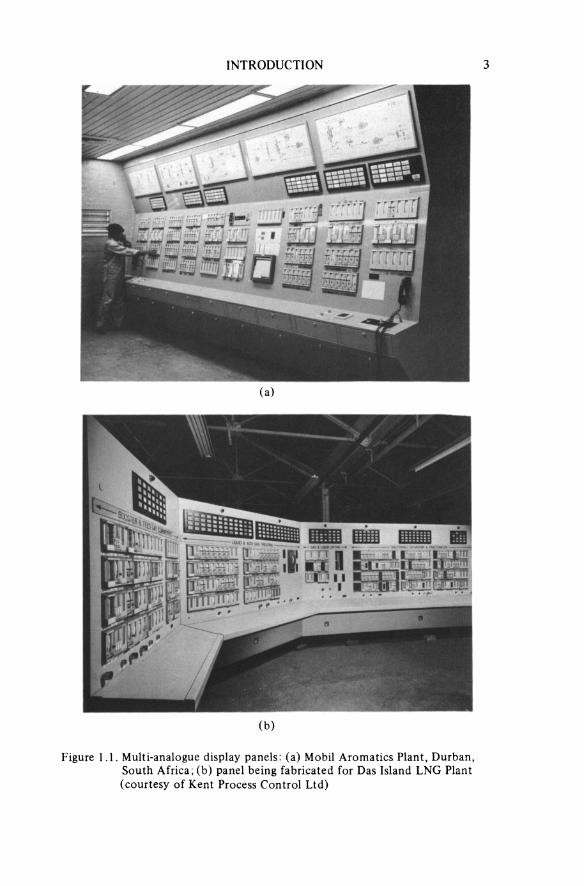
The use of analogue instrumentation is very extensive, and while digital instruments are ever increasing in number, versatility and application, it is likely that analogue devices will remain in use for many years and for some applications seem unlikely to be replaced by digital devices; for example, it is possible for an operator to assimilate a far greater amount of information from a multi-analogue display (figure 1.1) than from a multi-digital display of the same information. However a gradual increase in the number of hybrid instruments does seem very likely.
A large number of analogue instruments are electromechanical in nature, making use of the fact that when an electric current flows along a conductor, the conductor becomes surrounded by a magnetic field. This property is used in electromechanical instruments to obtain the deflection of a pointer: (a) by the interaction of the magnetic field around a coil with a permanent magnet; (b) between ferromagnetic vanes in the coil’s magnetic field; or (c) through the interaction of the magnetic fields produced by a number of coils.
Constraining these forces to form a turning movement produces a deflecting torque = Gf(i) newton metres (N m), which is a function of the current in the instrument’s coil and the geometry and type of coil system. To obtain a stable display it is necessary to equate the deflection torque with an opposing or con-trol torque. The magnitude of this control torque must increase with the angular deflection of the pointer and this is arranged by using spiral springs or a ribbon suspension so that the control torque = CO N m, where 3 is the angular deflection in radians and C is the control constant in newton metres per radian and will depend on the material and geometry of the control device. [1]
The moving parts of the instrument will have a moment of inertia (J) and when a change in the magnitude of deflection takes place an acceleration torque
INTRODUCTION 3
(a)
(b)
Figure 1.1. Multi-analogue display panels: (a) Mobil Aromatics Plant, Durban, South Africa; (b) panel being fabricated for Das Island LNG Plant (courtesy of Kent Process Control Ltd)
4 AN INTRODUCTION TO ELECTRICAL INSTRUMENTATION
(J d2θ/dt2 N m) will be present. Since the movable parts are attached to a con-trol spring they combine to form a mass-spring system and in order to prevent excessive oscillations when the magnitude of the electrical input is changed, a damping torque (D dθ/dt N m) must be provided that will only act if the mov-able parts are in motion. The method by which this damping torque is applied may be
(a) eddy current—where currents induced in a conducting sheet attached to the movement produce a magnetic field opposing any change in position.
(b) pneumatic-in this method a vane is attached to the instrument movement, and the resistance of the surrounding air to the motion of the vane provides the required damping. Fluid damping is an extension of this principle, a small vane then being constrained to move in a container filled with a suitably viscous fluid (see section 2.1.4).
(c) electromagnetic—movement of a coil in a magnetic field produces a current in the coil which opposes the deflecting current and slows the response of the instrument. The magnitude of the opposing current will be dependent on the resistance of the circuit to which the instrument is connected.
Combining the above torques, the equation of motion for a pointer instru-ment becomes
(1.1)
which will have a steady state solution
(1.2)
and a dynamic or transient solution of the form (see appendix II)
(1.3)
where A and B are arbitrary constants and
(1.4)
and
(1.5)
For a particular instrument C and J are fixed in magnitude during manufacture, but D (the amount of damping) may be varied. This results in three possible modes of response to a transient
(a) when D2/4J2 > C/J—for which the roots λ1 and λ2 are real and unequal, and is known as the overdamped case, curve (a) in figure 1.2
INTRODUCTION 5
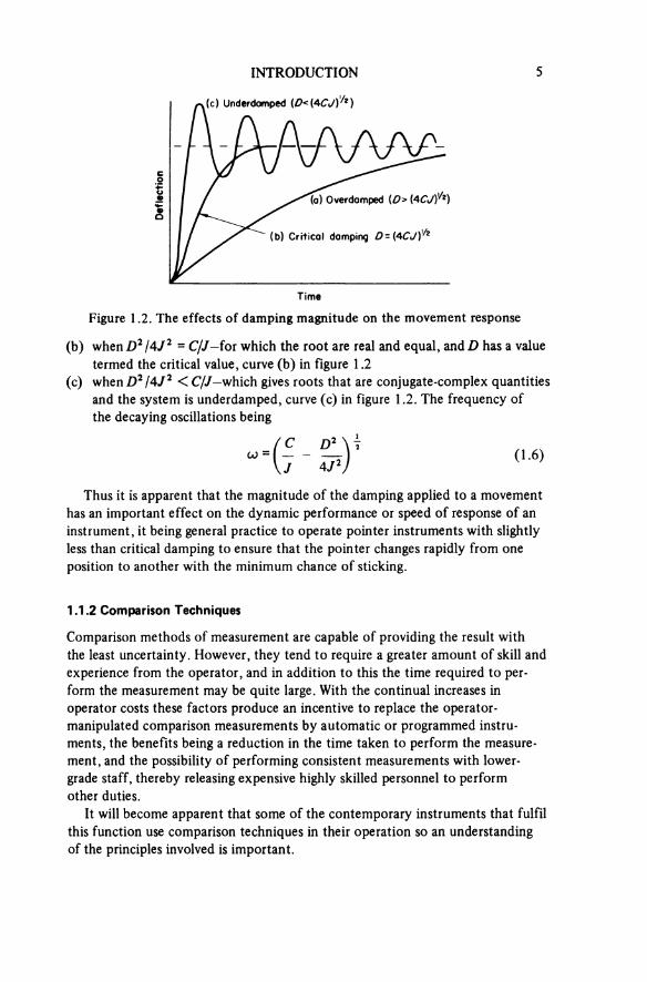
Figure 1.2. The effects of damping magnitude on the movement response
Defle
ctio
n
Time
(a) Overdamped
(b) Critical damping
(c) Underdamped
(b) when D2/4J2 = C/J—for which the root are real and equal, and D has a value termed the critical value, curve (b) in figure 1.2
(c) when D2/4J2 < C/J—which gives roots that are conjugate-complex quantities and the system is underdamped, curve (c) in figure 1.2. The frequency of the decaying oscillations being
(1.6)
Thus it is apparent that the magnitude of the damping applied to a movementhas an important effect on the dynamic performance or speed of response of an instrument, it being general practice to operate pointer instruments with slightly less than critical damping to ensure that the pointer changes rapidly from one position to another with the minimum chance of sticking.
1.1.2 Comparison Techniques
Comparison methods of measurement are capable of providing the result with the least uncertainty. However, they tend to require a greater amount of skill and experience from the operator, and in addition to this the time required to per-form the measurement may be quite large. With the continual increases in operator costs these factors produce an incentive to replace the operator- manipulated comparison measurements by automatic or programmed instru-ments, the benefits being a reduction in the time taken to perform the measure-ment, and the possibility of performing consistent measurements with lower- grade staff, thereby releasing expensive highly skilled personnel to perform other duties.
It will become apparent that some of the contemporary instruments that fulfilthis function use comparison techniques in their operation so an understanding of the principles involved is important.
6 AN INTRODUCTION TO ELECTRICAL INSTRUMENTATION
Substitution Methods
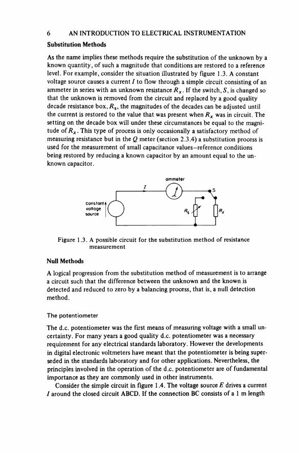
As the name implies these methods require the substitution of the unknown by aknown quantity, of such a magnitude that conditions are restored to a reference level. For example, consider the situation illustrated by figure 1.3. A constant voltage source causes a current I to flow through a simple circuit consisting of an ammeter in series with an unknown resistance Rx. If the switch, S, is changed so that the unknown is removed from the circuit and replaced by a good quality decade resistance box, Rs, the magnitudes of the decades can be adjusted until the current is restored to the value that was present when Rx was in circuit. The setting on the decade box will under these circumstances be equal to the magni-tude of Rx. This type of process is only occasionally a satisfactory method ofmeasuring resistance but in the Q meter (section 2.3.4) a substitution process is used for the measurement of small capacitance values—reference conditions being restored by reducing a known capacitor by an amount equal to the un-known capacitor.
Figure 1.3. A possible circuit for the substitution method of resistance measurement
constantvoltagesource
ammeter
Null Methods
A logical progression from the substitution method of measurement is to arrange a circuit such that the difference between the unknown and the known is detected and reduced to zero by a balancing process, that is, a null detection method.
The potentiometer
The d.c. potentiometer was the first means of measuring voltage with a small un-certainty. For many years a good quality d.c. potentiometer was a necessary requirement for any electrical standards laboratory. However the developments in digital electronic voltmeters have meant that the potentiometer is being super-seded in the standards laboratory and for other applications. Nevertheless, the principles involved in the operation of the d.c. potentiometer are of fundamental importance as they are commonly used in other instruments.
Consider the simple circuit in figure 1.4. The voltage source E drives a current I around the closed circuit ABCD. If the connection BC consists of a 1 m length
INTRODUCTION 7
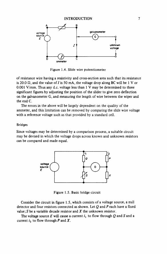
Figure 1.4. Slide wire potentiometer
voltage source
E
galvanometer
unknownvoltage
of resistance wire having a resistivity and cross-section area such that its resistance is 20.0 Ω, and the value of I is 50 mA, the voltage drop along BC will be 1 V or 0.001 V/mm. Thus any d.c. voltage less than 1 V may be determined to three significant figures by adjusting the position of the slider to give zero deflection on the galvanometer G, and measuring the length of wire between the wiper and the end C.
The errors in the above will be largely dependent on the quality of the ammeter, and this limitation can be removed by comparing the slide wire voltage with a reference voltage such as that provided by a standard cell.
Bridges
Since voltages may be determined by a comparison process, a suitable circuit may be devised in which the voltage drops across known and unknown resistors can be compared and made equal.
Figure 1.5. Basic bridge circuit
voltagesourceE
Consider the circuit in figure 1.5, which consists of a voltage source, a null detector and four resistors connected as shown. Let Q and P each have a fixed value; S be a variable decade resistor and X the unknown resistor.
The voltage source E will cause a current i1 to flow through Q and S and a current i2 to flow through P and X.
8 AN INTRODUCTION TO ELECTRICAL INSTRUMENTATION
At balance, that is, a zero reading on the null detector
and
Hence
or
(1.7)
In the simplest case P = Q and X the unknown is equal to the setting on the decade box. This type of arrangement is generally very much more satisfactory than the substitution method described earlier, for any variations in the magni-tude of the voltage source will not affect the balance condition and the value found for the unknown—a situation that cannot be guaranteed when the substi-tution method is being used.
This basic form of bridge circuit is called a Wheatstone bridge, and it is of extreme importance in instrumentation. It is described in detail in section 3.3.
1.1.3 Digital Techniques
Most digital instruments display the measurand in discrete numerals thereby eliminating the parallax error, and reducing the human errors associated with analogue pointer instruments. In general digital instruments have superior accuracy to analogue pointer instruments, and many incorporate automatic pol-arity and range indication which reduces operator training, measurement error, and possible instrument damage through overload. In addition to these features many digital instruments have an output facility enabling permanent records of measurements to be made automatically.
Digital instruments are, however, usually more expensive than analogue instruments. They are also sampling devices, that is, the displayed quantity is a discrete measurement made, either at one instant in time, or over an interval of time, by using digital electronic techniques.
Sampling of data
Whenever a continuous signal is to be measured by a sampling process care must be exercised to ensure that the sampling rate is sufficiently fast for all the varia-tions in the measurand to be reconstructed. If the sampling rate is too low, details of the fluctuation in the continuous wave will be lost whereas if the sampling
INTRODUCTION 9
rate is too high an unnecessary amount of data will be collected and processed. The limiting requirement for the frequency of sampling is that it must be at least twice the highest frequency component of the signal being sampled in order that the measured signal may be reconstructed in its original form. [2]
In a good many situations the amplitude of the measurand can be considered to be constant, for example the magnitude of a direct voltage, and then the sampling rate can be slowed down to one which simply confirms that the measurand does have a constant value.
Transmission of data
Having sampled the measurand it will be necessary to transmit the information from one part of the system to another. The transmission of digital data may be accomplished either in a parallel or a serial mode.
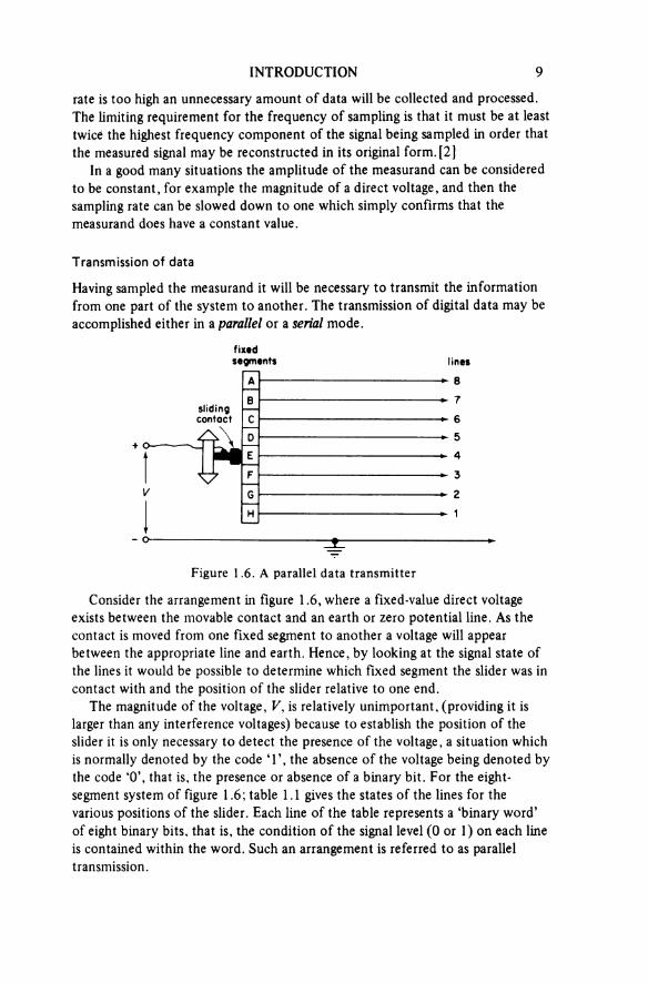
Figure 1.6. A parallel data transmitter
fixedsegments lines
slidingcontact
Consider the arrangement in figure 1.6, where a fixed-value direct voltage exists between the movable contact and an earth or zero potential line. As the contact is moved from one fixed segment to another a voltage will appear between the appropriate line and earth. Hence, by looking at the signal state of the lines it would be possible to determine which fixed segment the slider was in contact with and the position of the slider relative to one end.
The magnitude of the voltage, V, is relatively unimportant, (providing it is larger than any interference voltages) because to establish the position of the slider it is only necessary to detect the presence of the voltage, a situation which is normally denoted by the code ‘1’, the absence of the voltage being denoted by the code ‘0’, that is, the presence or absence of a binary bit. For the eight- segment system of figure 1.6; table 1.1 gives the states of the lines for the various positions of the slider. Each line of the table represents a ‘binary word’ of eight binary bits, that is, the condition of the signal level (0 or 1) on each line is contained within the word. Such an arrangement is referred to as parallel transmission.
10 AN INTRODUCTION TO ELECTRICAL INSTRUMENTATION
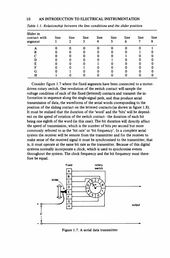
Table 1.1. Relationship between the line conditions and the slider position
Slider in contact with line line line line line line line linesegment 1 2 3 4 5 6 7 8
A 0 0 0 0 0 0 0 1B 0 0 0 0 0 0 1 0C 0 0 0 0 0 1 0 0D 0 0 0 0 1 0 0 0E 0 0 0 1 0 0 0 0F 0 0 1 0 0 0 0 0G 0 1 0 0 0 0 0 0H 1 0 0 0 0 0 0 0
Consider figure 1.7 where the fixed segments have been connected to a motor driven rotary switch. One revolution of the switch contact will sample the voltage condition of each of the fixed (lettered) contacts and transmit the in-formation in sequence along the single-signal path, and thus produce serial transmission of data, the waveforms of the serial words corresponding to the position of the sliding contact on the lettered contacts (as shown in figure 1.8).It must be realised that the duration of the ‘word’ and the ‘bits’ will be depend-ent on the speed of rotation of the switch contact—the duration of each bit being one eighth of the word (in this case). The bit duration will directly affectthe speed of transmission, which is the number of bits per second but more commonly referred to as the ‘bit rate’ or ‘bit frequency’. In a complete serial system the receiver will be remote from the transmitter and for the receiver to make sense of the received signal it must be synchronised to the transmitter, that is, it must operate at the same bit rate as the transmitter. Because of this digital systems normally incorporate a clock, which is used to synchronise events throughout the system. The clock frequency and the bit frequency must there-fore be equal.
Figure 1.7. A serial data transmitter
slider
fixed rotaryswitch
output
INTRODUCTION 11
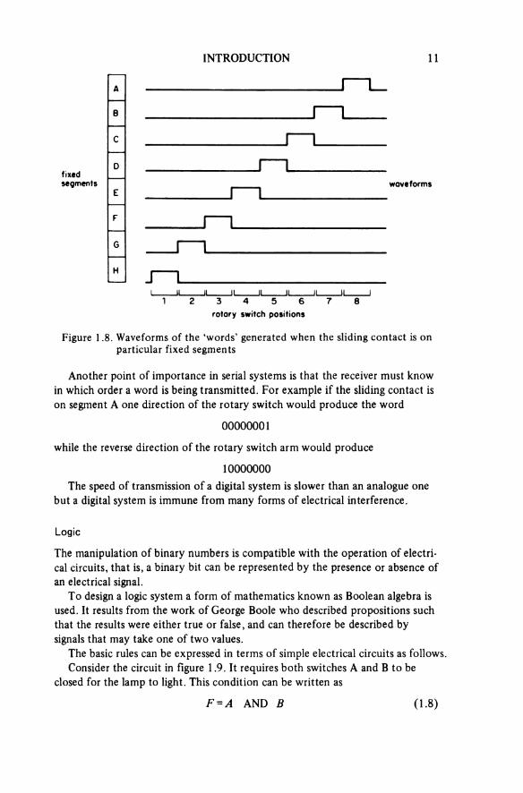
rotary switch positions
fixedsegments waveforms
Figure 1.8. Waveforms of the ‘words’ generated when the sliding contact is on particular fixed segments
Another point of importance in serial systems is that the receiver must know in which order a word is being transmitted. For example if the sliding contact is on segment A one direction of the rotary switch would produce the word
00000001
while the reverse direction of the rotary switch arm would produce
10000000The speed of transmission of a digital system is slower than an analogue one
but a digital system is immune from many forms of electrical interference.
Logic
The manipulation of binary numbers is compatible with the operation of electri-cal circuits, that is, a binary bit can be represented by the presence or absence of an electrical signal.
To design a logic system a form of mathematics known as Boolean algebra is used. It results from the work of George Boole who described propositions such that the results were either true or false, and can therefore be described by signals that may take one of two values.
The basic rules can be expressed in terms of simple electrical circuits as follows.Consider the circuit in figure 1.9. It requires both switches A and B to be
closed for the lamp to light. This condition can be written as
(1.8)

12 AN INTRODUCTION TO ELECTRICAL INSTRUMENTATION
voltagesource lamp
Figure 1.9. Simple equivalent circuit of AND gate
where the Boolean variable F takes the value 1 when the lamp is lit and 0 when it is unlit. Similarly A and B have the values 0 when open and 1 when closed.
The negations or compliments of these conditions are written as A and B and would indicate their having values of 1 when open and 0 when closed.
Equation 1.8 may alternatively be written as
(1.9)
or even
(1.10)
In every case the equations must be read as F equals A AND B.
voltagesource
lamp
Figure 1.10. Simple equivalent circuit of OR gate
The circuit in figure 1.10 shows a situation in which the lamp is lit if either A OR B is closed.
This represents the logical OR function and is written as
(1.11)
Alternatively this is written as
(1.12)
Again this plus sign must not be confused with the arithmetic version and equation 1.12 must be read as
This analogy with simple circuits may be carried further to illustrate the operation of the basic logic functions. [3] It must be appreciated, however, that in digital electronics the switches are replaced by semi-conductor components [4]

INTRODUCTION 13
which in the simplest case are a diode and resistor arrangement, while in most instrumentation L.S.I. (large scale integrated) circuits will be incorporated to perform the logic functions.
In either case the components of digital electronics may be represented by a set of logic gates for which the BS and IEC symbols are shown in figure 1.11.
Logicfunction
AND
OR
NAND
NOR
BS 3939 IEC
Figure 1.11. BS and IEC symbols for basic two input logic gates
The use of logic gates to realise a situation can be illustrated by considering the Boolean expression:
(113)
Using simple AND and OR gates, figure 1.12 can be drawn up where the AB and CD terms are each realised by using two input AND gates, the outputs from these being applied to a two input OR gate.
Figure 1.12. Realisation of the Boolean expression F = AB + CD
The NAND and NOR gates provide outputs which are the compliments of those produced by the basic AND and OR gates. This is shown in the symbols in figure 1.11.
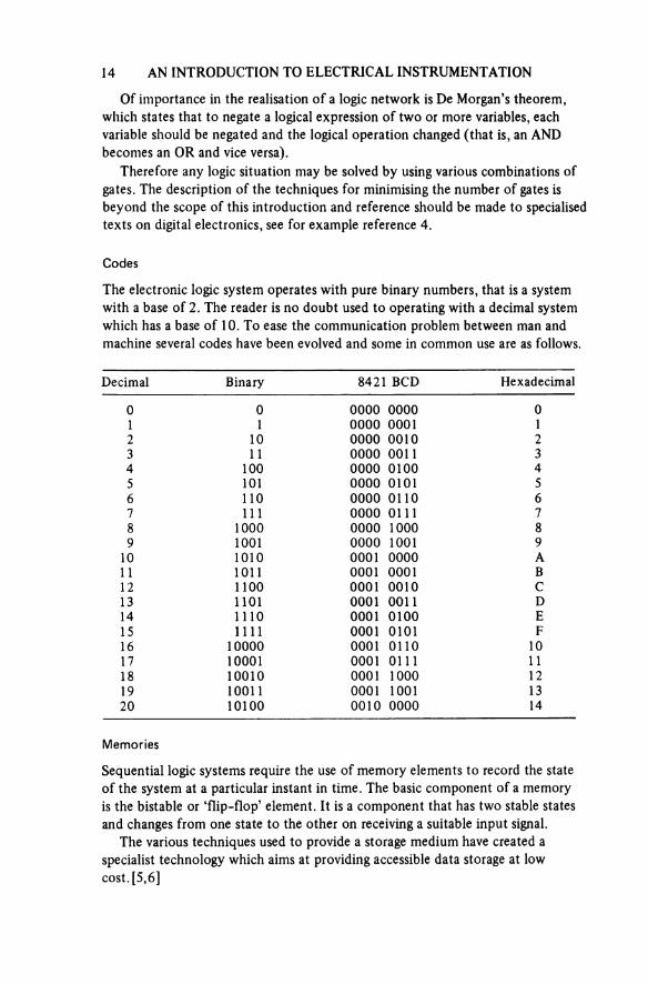
Decimal Binary 8421 BCD Hexadecimal
0 0 0000 0000 01 1 0000 0001 12 10 0000 0010 23 11 0000 0011 34 100 0000 0100 45 101 0000 0101 56 110 0000 0110 67 111 0000 0111 78 1000 0000 1000 89 1001 0000 1001 9
10 1010 0001 0000 A11 1011 0001 0001 B12 1100 0001 0010 C13 1101 0001 0011 D14 1110 0001 0100 E15 1111 0001 0101 F16 10000 0001 0110 1017 10001 0001 0111 1118 10010 0001 1000 1219 10011 0001 1001 1320 10100 0010 0000 14
14 AN INTRODUCTION TO ELECTRICAL INSTRUMENTATION
Of importance in the realisation of a logic network is De Morgan’s theorem, which states that to negate a logical expression of two or more variables, each variable should be negated and the logical operation changed (that is, an AND becomes an OR and vice versa).
Therefore any logic situation may be solved by using various combinations ofgates. The description of the techniques for minimising the number of gates is beyond the scope of this introduction and reference should be made to specialised texts on digital electronics, see for example reference 4.
Codes
The electronic logic system operates with pure binary numbers, that is a system with a base of 2. The reader is no doubt used to operating with a decimal system which has a base of 10. To ease the communication problem between man and machine several codes have been evolved and some in common use are as follows.
Memories
Sequential logic systems require the use of memory elements to record the state of the system at a particular instant in time. The basic component of a memory is the bistable or ‘flip-flop’ element. It is a component that has two stable states and changes from one state to the other on receiving a suitable input signal.
The various techniques used to provide a storage medium have created a specialist technology which aims at providing accessible data storage at low cost. [5,6]
INTRODUCTION 15
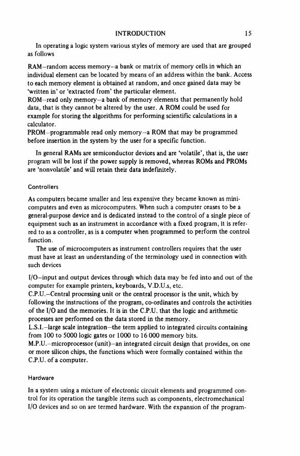
In operating a logic system various styles of memory are used that are grouped as follows
RAM-random access memory-a bank or matrix of memory cells in which an individual element can be located by means of an address within the bank. Access to each memory element is obtained at random, and once gained data may be ‘written in’ or ‘extracted from’ the particular element.ROM-read only memory—a bank of memory elements that permanently hold data, that is they cannot be altered by the user. A ROM could be used for example for storing the algorithms for performing scientific calculations in a calculator.PROM—programmable read only memory—a ROM that may be programmed before insertion in the system by the user for a specific function.
In general RAMs are semiconductor devices and are ‘volatile’, that is, the user program will be lost if the power supply is removed, whereas ROMs and PROMs are ‘nonvolatile’ and will retain their data indefinitely.
Controllers
As computers became smaller and less expensive they became known as mini-computers and even as microcomputers. When such a computer ceases to be a general-purpose device and is dedicated instead to the control of a single piece ofequipment such as an instrument in accordance with a fixed program, it is refer-red to as a controller, as is a computer when programmed to perform the control function.
The use of microcomputers as instrument controllers requires that the user must have at least an understanding of the terminology used in connection with such devices
I/O—input and output devices through which data may be fed into and out of the computer for example printers, keyboards, V.D.U.s, etc.C.P.U.—Central processing unit or the central processor is the unit, which by following the instructions of the program, co-ordinates and controls the activities of the I/O and the memories. It is in the C.P.U. that the logic and arithmeticprocesses are performed on the data stored in the memory.L.S.I.—large scale integration—the term applied to integrated circuits containing from 100 to 5000 logic gates or 1000 to 16 000 memory bits.M.P.U.—microprocessor (unit)—an integrated circuit design that provides, on one or more silicon chips, the functions which were formally contained within the C.P.U. of a computer.
Hardware
In a system using a mixture of electronic circuit elements and programmed con-trol for its operation the tangible items such as components, electromechanical I/O devices and so on are termed hardware. With the expansion of the program-
16 AN INTRODUCTION TO ELECTRICAL INSTRUMENTATION
mable capabilities of L.S.I. many functions that were achieved by hardwired logic can now be performed by programmed instructions.
Software
This term is used to describe the program of instructions stored in the memory and used to direct the system so as to perform the desired sequence of opera-tions. The development time for software is lengthy and in consequence in many installations the software is more expensive than the hardware. User’s software (developed specifically for a user’s application) is difficult to replace and so duplicate copies must be stored in safety.
Firmware
This is the software that has been embodied in the hardware, that is, programmed into ROM or PROM. This definition [7] may be an over-simplification, but the term firmware may certainly be used [8] to describe software in a ROM or PROM which is not essential to the function of a system and which the user may accept or reject depending on his requirements.
ProgrammingThe writing of programs to perform specific functions or operations on the measurand will, in a ‘computer’ controlled system be in a high level language such as BASIC, ALGOL or FORTRAN. In a dedicated or purpose-built system, using a microprocessor as the controller, the programming will of necessity be inmachine code. The writing of programs in machine code is expensive for it is a lengthy process requiring considerable skill and experience (see reference 15 and reference 19 of chapter 4).
System operation
The selection, by the user, of an operational or functional program (see section 4.3.2) from the controller’s soft or firmware, simply requires the entry of coded instructions via a keyboard. In a dedicated system this is likely to be a simple entry of one or two digits, while in a ‘computer’ controlled system it may be necessary to first insert the appropriate cassette or floppy disc [5] into the container.
1.2 DISPLAY METHODS
In selecting a single instrument or a number of instruments to form a measure-ment system a decision that must be made at a fairly early stage is whether the visual presentation should be analogue or digital in form.
The major advantage of analogue displays is that an operator can assimilate a

INTRODUCTION 17
very much greater amount of information from an analogue display than from a digital display in the same period of time. A clear example of this is that a graph of the variation of one function relative to another is much quicker to interpret than the same data in tabular form.
1.2.1 Analogue Displays
The displays used in analogue instruments can be divided into those associated with pointer instruments and those providing some form of graphical display.
Pointer Instruments
Reading interpretation
One of the problems associated with pointer instruments is the misinterpretation of a reading due to parallax, that is, if the user is incorrectly positioned so that instead of looking vertically down onto the pointer and scale, an angled view is made. This will result in an incorrect observation as illustrated by figure 1.13. To assist the user in removing this source of reading error many better quality analogue instruments have a pointer in the form of a fine blade and a mirror adjacent to the scale, in which the reflection of pointer can be aligned (see figure 1.14).
Figure 1.13. Illustration of parallax error: (a) angled view with error, (b) correct view of same reading
(a) (b)
A further problem in the use of an analogue pointer instrument is the inter-polation of pointer position between scale markings. In some instruments this problem is alleviated by an arrangement of the form illustrated in figure 1.14.
From the above it should be apparent that a certain amount of skill is required to correctly interpret the reading on a pointer instrument. It should also be appreciated that the limit of resolution on an analogue scale is approximately 0.4 mm and readings that imply greater resolution are really due to the imagina-tion of the user.
18 AN INTRODUCTION TO ELECTRICAL INSTRUMENTATION
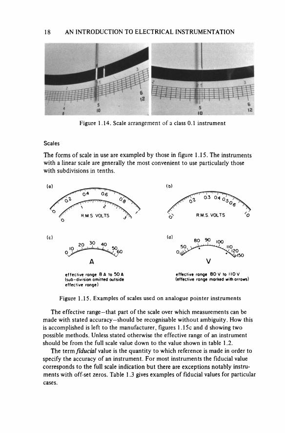
Figure 1.14. Scale arrangement of a class 0.1 instrument
Scales
The forms of scale in use are exampled by those in figure 1.15. The instruments with a linear scale are generally the most convenient to use particularly those with subdivisions in tenths.
Figure 1.15. Examples of scales used on analogue pointer instruments
(o) (b)
(c)
effective range 8 A to 50 A (sub-division omitted outside effective range)
(d)
effective range 80 V to 110 V (effective range marked with arrows)
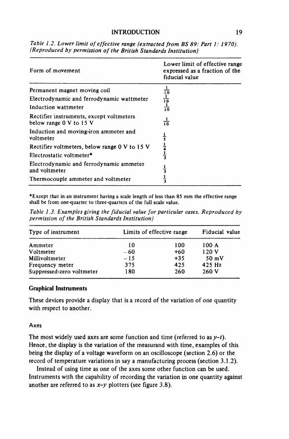
The effective range—that part of the scale over which measurements can he made with stated accuracy-should be recognisable without ambiguity. How this is accomplished is left to the manufacturer, figures 1.15c and d showing two possible methods. Unless stated otherwise the effective range of an instrument should be from the full scale value down to the value shown in table 1.2.
The term fiducial value is the quantity to which reference is made in order to specify the accuracy of an instrument. For most instruments the fiducial value corresponds to the full scale indication but there are exceptions notably instru-ments with off-set zeros. Table 1.3 gives examples of fiducial values for particular cases.
INTRODUCTION 19
Table 1.2. Lower limit of effective range (extracted from BS 89: Part 1: 1970). (Reproduced by permission of the British Standards Institution)
Form of movementLower limit of effective range expressed as a fraction of the fiducial value
Permanent magnet moving coil 1/10
Electrodynamic and ferrodynamic wattmeter 1/10
Induction wattmeter 1/10
Rectifier instruments, except voltmeters below range 0 V to 1 5 V
1/10
Induction and moving-iron ammeter and voltmeter
1/5
Rectifier voltmeters, below range 0 V to 1 5 V 14
Electrostatic voltmeter* 1/3
Electrodynamic and ferrodynamic ammeter and voltmeter
1/3
Thermocouple ammeter and voltmeter 1/3
*Except that in an instrument having a scale length of less than 85 mm the effective range shall be from one-quarter to three-quarters of the full scale value.
Table 1.3. Examples giving the fiducial value for particular cases. Reproduced by permission of the British Standards Institution)
Type of instrument Limits of effective range Fiducial value
Ammeter 10 100 100 AVoltmeter -60 +60 120 VMinivoltmeter -15 +35 50 mVFrequency meter 375 425 425 HzSuppressed-zero voltmeter 180 260 260 V
Graphical Instruments
These devices provide a display that is a record of the variation of one quantity with respect to another.
Axes
The most widely used axes are some function and time (referred to as y-t). Hence, the display is the variation of the measurand with time, examples of this being the display of a voltage waveform on an oscilloscope (section 2.6) or the record of temperature variations in say a manufacturing process (section 3.1.2).
Instead of using time as one of the axes some other function can be used. Instruments with the capability of recording the variation in one quantity against another are referred to as x-y plotters (see figure 3.8).

20 AN INTRODUCTION TO ELECTRICAL INSTRUMENTATION
One form of display that is particularly useful in waveform analysis is the presentation of the amplitude of the frequency components of a signal against frequency—an arrangement that is illustrated by the spectrum analyser (see figures 1.30 and 4.28).
Permanency of Display
If a graphical display is necessary as a function of the chosen instrumentation a factor that must be considered is if the record can be temporary or must be permanent.
If the latter is required either photographic techniques or some form of ‘pen and paper’ writing system (see section 2.1.3) must be used. The filing of quantities of recorded data can create reference and storage problems hence the use of temporary or ‘nonpermanent’ records is often desirable. The obvious example of this is the oscilloscope (section 2.6) where in a conventional instrument the path of the electron beam across the tube face only remains visible for a very brieftime but by modifications to the tube and the use of certain phosphors a trace can be stored for a considerable time. A more recent development (section 4.4.3) is the use of a volatile digital store to record a waveform.
1.2.2 Digital
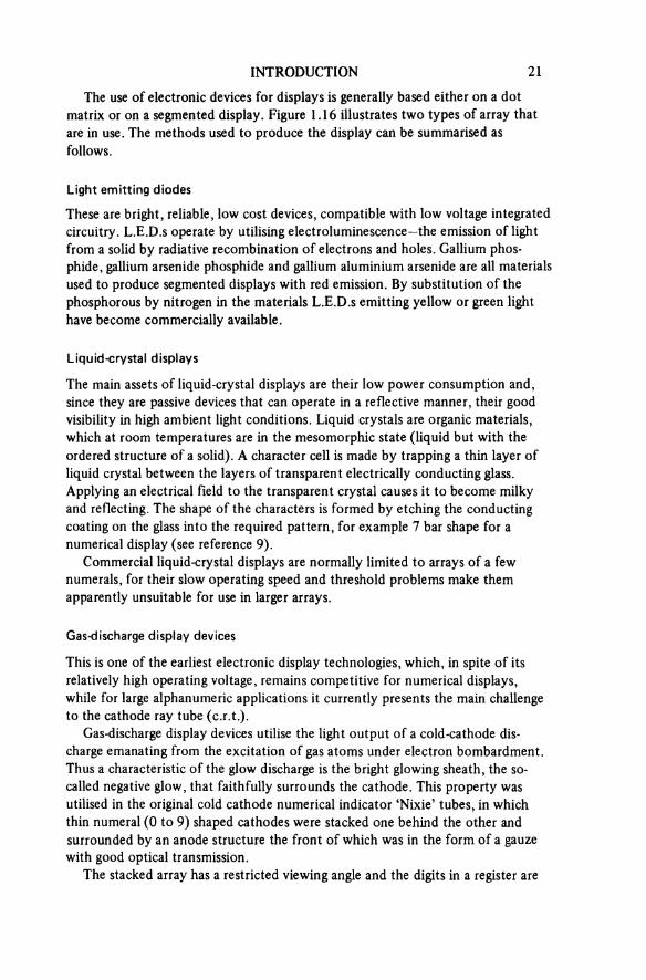
The principal advantage of a digital display is that it removes ambiguity, there-fore eliminating a considerable amount of ‘operator error’ or misinterpretation. Unfortunately it often creates a false confidence—‘I can see it, therefore it must be correct’; but this is not necessarily true (see section 1.3.2 and chapter 8). However, the concern here is to outline the methods currently in use [9] for displaying data in digital form—an area which is subject to considerable research effort and consequent change. One such area has been the need for an alpha-numeric display rather than a simple numeric display. This requirement results from the incorporating of programming capability into instruments, thereby creating a need for a visual operator-instrument interface for communication.
(a) (b)
Figure 1.16. Digital displays: (a) dot matrix, (b) bar arrangement
INTRODUCTION 21
The use of electronic devices for displays is generally based either on a dot matrix or on a segmented display. Figure 1.16 illustrates two types of array that are in use. The methods used to produce the display can be summarised as follows.
Light emitting diodes
These are bright, reliable, low cost devices, compatible with low voltage integrated circuitry. L.E.D.s operate by utilising electroluminescence—the emission of light from a solid by radiative recombination of electrons and holes. Gallium phos-phide, gallium arsenide phosphide and gallium aluminium arsenide are all materials used to produce segmented displays with red emission. By substitution of the phosphorous by nitrogen in the materials L.E.D.s emitting yellow or green light have become commercially available.
Liquid-crystal displays
The main assets of liquid-crystal displays are their low power consumption and,since they are passive devices that can operate in a reflective manner, their good visibility in high ambient light conditions. Liquid crystals are organic materials, which at room temperatures are in the mesomorphic state (liquid but with the ordered structure of a solid). A character cell is made by trapping a thin layer of liquid crystal between the layers of transparent electrically conducting glass. Applying an electrical field to the transparent crystal causes it to become milkyand reflecting. The shape of the characters is formed by etching the conducting coating on the glass into the required pattern, for example 7 bar shape for a numerical display (see reference 9).
Commercial liquid-crystal displays are normally limited to arrays of a few numerals, for their slow operating speed and threshold problems make them apparently unsuitable for use in larger arrays.
Gas-discharge display devices
This is one of the earliest electronic display technologies, which, in spite of its relatively high operating voltage, remains competitive for numerical displays, while for large alphanumeric applications it currently presents the main challenge to the cathode ray tube (c.r.t.).
Gas-discharge display devices utilise the light output of a cold-cathode dis-charge emanating from the excitation of gas atoms under electron bombardment. Thus a characteristic of the glow discharge is the bright glowing sheath, the so- called negative glow, that faithfully surrounds the cathode. This property was utilised in the original cold cathode numerical indicator ‘Nixie’ tubes, in which thin numeral (0 to 9) shaped cathodes were stacked one behind the other andsurrounded by an anode structure the front of which was in the form of a gauze with good optical transmission.
The stacked array has a restricted viewing angle and the digits in a register are

22 AN INTRODUCTION TO ELECTRICAL INSTRUMENTATION
not in the same plane. These factors coupled with the fashionable use of seven- segment displays has led to the adaptation of this technology to produce gas discharge displays using seven cathode bars and a common anode per numeral. The electrical characteristics of the device make it particularly suitable for use in multiple units of up to 16 numerals in a single envelope.
The gas-discharge technology also lends itself to multi-segment and dot matrix arrays for alphanumeric displays. The ultimate, so far, being the so-called plasma panels for displaying up to 3000 characters. [10]
Cathode ray tube
The use of the c.r.t. for alphanumeric display is now becoming commonplace with its use in visual display units (V.D.U.s) as computer terminals. Variations on the basic c.r.t. specifically for alphanumeric applications have been devised, [9] and it should be appreciated that an increasing number of sophisticated oscillo-scopes (see section 2.6.1) include alphanumeric information with the displayed waveform on the tube face.
Other displays
As indicated at the start of this section this is an area of intense developmentand numerous techniques are under investigation as reviewed by Weston. [9] Perhaps the most promising at the present time are the electroluminescent, the electrochromic, the electrophoretic and the magneto-optic bubble displays.
Choice of display
In general the customer has no say in the type of display fitted to an instrument, it being an integral part of the instrument design. However, the properties of importance to the user must be the size of the display and its visibility under the operating conditions. Indirectly of consequence will be the power consumption of the display and the circuitry driving it.
1.3 ACCURACY
The appropriate British Standard [11] defines the accuracy of a measuring instrument as
The quality which characterizes the ability of a measuring instrument to give indications equivalent to the true value of the quantity measured.
It then proceeds to note that
The quantitive expression of this concept should be in terms of un-certainty.
INTRODUCTION 23
1.3.1 Values and Uncertainty
True value
Various terms are used in connection with the value assigned to a quantity. Of greatest importance is its actual or true value. It must be realised that it is impossible to determine exactly the true value of any quantity : the value assigned to a quantity will always have a tolerance or uncertainty associated with it. In some instances this tolerance is very small, say I part in 109, and the true value is approached but it can never be determined exactly.
Nominal value
The nominal value, usually of a component, is the one given it by a manufacturer, for example, a 10 kΩ resistor. Such a value must be accompanied by a tolerance, say, ±10 per cent and the interpretation of the complete statement is that the true value of the resistor is between 9.9 kΩ and 10.1 kΩ.
Measured value
This is the value indicated by an instrument or determined by a measurement process. It must be accompanied by a statement of the uncertainty or the possible limit of error associated with the measurement.
Tolerance and uncertainty
From the above definitions the accuracy of a measurement must be quoted as a tolerance or uncertainty in measurement. For example, if a measurement on a particular resistance gave the result
102.5 Ω ± 0.2 Ω
the uncertainty in the measurement would be ± 0.2 Ω and the true value of the resistor will he somewhere between 102.3 Ω and 102.7 Ω.
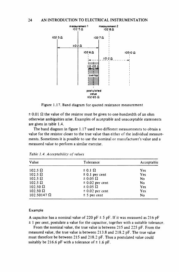
If the same resistor were measured by a different instrument and the value 102.8 Ω ± 0.2 Ω were obtained, a narrowing of the band within which the true value must he is possible. For from the second measurement it is apparent that the true value must be between 102.6 Ω and 103.0 Ω; hence by combining the two measurements the true value must lie between 102.6 Ω and 102.7 Ω. It is therefore possible to estimate or postulate that the value of the resistor is
102.65 Ω ± 0.05 Ω
This type of situation can be represented by the ‘band diagram’ in figure 1.17.
In assigning a tolerance to a value, the two parts of the complete statement must be compatible, that is to say if a tolerance on a resistor is quoted as
24 AN INTRODUCTION TO ELECTRICAL INSTRUMENTATION
Figure 1.17. Band diagram for quoted resistance measurement
measurement 1102.5 Ω
measurement 2 102.8 Ω
overlap
postulated value
102.65 Ω
± 0.01 Ω the value of the resistor must be given to one-hundredth of an ohm otherwise ambiguities arise. Examples of acceptable and unacceptable statements are given in table 1.4.
The band diagram in figure 1.17 used two different measurements to obtain a value for the resistor closer to the true value than either of the individual measure-ments. Sometimes it is possible to use the nominal or manufacturer’s value and a measured value to perform a similar exercise.
Table 1.4. Acceptability of values
Value Tolerance Acceptable
102.5 Ω ± 0.1 Ω Yes102.5 Ω ± 0.1 per cent Yes102.5 Ω ± 0.05 Ω No102.5 Ω ± 0.02 per cent No102.50 Ω ± 0.05 Ω Yes102.50 Ω ± 0.02 per cent Yes102.50147 Ω ± 5 per cent No
Example
A capacitor has a nominal value of 220 pF ± 5 pF. If it was measured as 216 pF ± 1 per cent, postulate a value for the capacitor, together with a suitable tolerance
From the nominal value, the true value is between 215 and 225 pF. From the measured value, the true value is between 213.8 and 218.2 pF. The true value must therefore be between 215 and 218.2 pF. Thus a postulated value could suitably be 216.6 pF with a tolerance of ± 1.6 pF.
INTRODUCTION 25
Note Such a statement should be realistic in terms of values
(a) Anything less than the nearest tenth of a picofarad requires very carefully controlled measuring conditions (see section 7.2).
(b) Care must be taken to ensure that the tolerance includes all possible values for the true value of the component.
T3.2 Errors
Error of measurement
The error in a measurement is defined as the algebraic difference between the indicated (or measured) value and the true value. [11]
It has been suggested in the previous section that the true value can never be found so in practice the ‘true value’ is replaced by ‘the conventional true value’ which is the value the measurand can be realistically accepted as having.
An alternative approach is that the error of indication of an instrument (A) can only be determined by its performance when compared with a reference instrument (B). Therefore the uncertainty of measurement associated with B must be very much less than that allowable on A.
Example
An ammeter under test indicates a reading of 0.87 A while the same current pro-duces on a reference ammeter a reading of 0.900 A ± 0.001 A.
The error of measurement for the class 2 instrument is thus
0.87 — 0.900 A = -0.030 A
The tolerance on the reference value has been ignored and provided such a tolerance is less than one-tenth of the quoted tolerance on the instrument under test such a procedure is acceptable. Should one wish to be pedantic, however, the error of the instrument under investigation could be given as —0.030 A ±0.001 A when indicating 0.87 A at T °C on the date of measurement.
The details of the reference instrument and the method of measurement should also be given.
Arising from this example it is apparent that the ‘correction’ that should be applied to the reading would, in this case, be +0.03 A and the percentage errror in reading (or indication) would be 100 × (—0.03/0.87) or —3.45 per cent.
Although, by using a calibration process, it is possible to establish the errors associated with a particular instrument, when an operator and a number of instruments are involved in a measurement, an assessment of the total possible error or limit of uncertainty must be made, for it must be established that the requirements of the measurement have been satisfied.
Sources of error
The possible causes of error, which may or may not be present can be summarised as follows.
26 AN INTRODUCTION TO ELECTRICAL INSTRUMENTATION
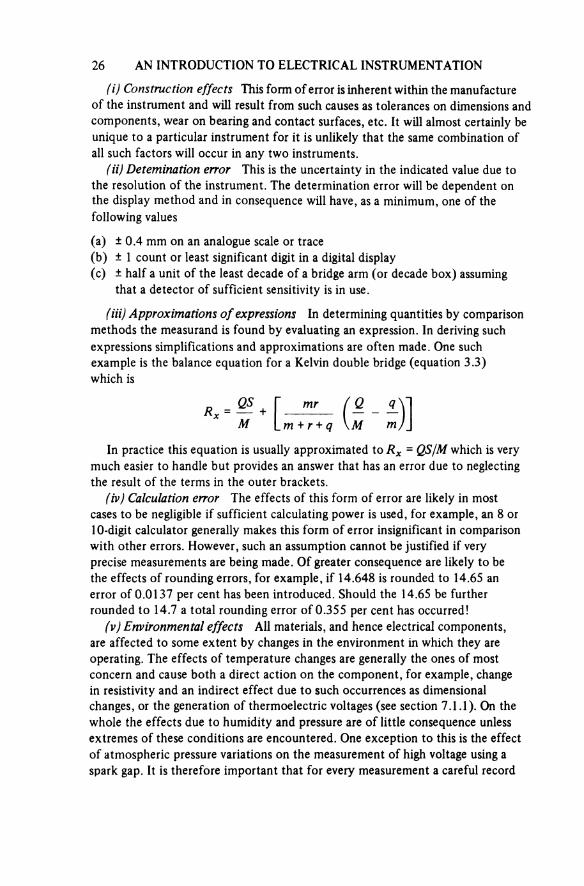
(i) Construction effects This form of error is inherent within the manufacture of the instrument and will result from such causes as tolerances on dimensions and components, wear on bearing and contact surfaces, etc. It will almost certainly be unique to a particular instrument for it is unlikely that the same combination of an such factors will occur in any two instruments.
(ii) Determination error This is the uncertainty in the indicated value due to the resolution of the instrument. The determination error will be dependent on the display method and in consequence will have, as a minimum, one of the following values
(a) ±0.4 mm on an analogue scale or trace(b) ± 1 count or least significant digit in a digital display(c) ± half a unit of the least decade of a bridge arm (or decade box) assuming
that a detector of sufficient sensitivity is in use.
(iii) Approximations of expressions In determining quantities by comparison methods the measurand is found by evaluating an expression. In deriving such expressions simplifications and approximations are often made. One such example is the balance equation for a Kelvin double bridge (equation 3.3) which is
In practice this equation is usually approximated to Rx = QS/M which is very much easier to handle but provides an answer that has an error due to neglecting the result of the terms in the outer brackets.
(iv) Calculation error The effects of this form of error are likely in most cases to be negligible if sufficient calculating power is used, for example, an 8 or 10-digit calculator generally makes this form of error insignificant in comparisonwith other errors. However, such an assumption cannot be justified if very precise measurements are being made. Of greater consequence are likely to be the effects of rounding errors, for example, if 14.648 is rounded to 14.65 an error of 0.0137 per cent has been introduced. Should the 14.65 be further rounded to 14.7 a total rounding error of 0.355 per cent has occurred!
(v) Environmental effects AU materials, and hence electrical components,are affected to some extent by changes in the environment in which they are operating. The effects of temperature changes are generally the ones of most concern and cause both a direct action on the component, for example, change in resistivity and an indirect effect due to such occurrences as dimensional changes, or the generation of thermoelectric voltages (see section 7.1.1). On the whole the effects due to humidity and pressure are of little consequence unlessextremes of these conditions are encountered. One exception to this is the effect of atmospheric pressure variations on the measurement of high voltage using a spark gap. It is therefore important that for every measurement a careful record
INTRODUCTION 27
is made of temperature, pressure and humidity so that if required a suitable allowance can be made when assessing the total uncertainty in the measurement.
(vi) Ageing effects As equipment gets older slight changes may occur in some of the components and these may be such as to affect the performance of instru-ments. It is therefore necessary to ensure that instruments are checked or calibrated at regular intervals to ensure: (a) no faults in operation have occurred; (b) they are performing within their specification; and (c) that any changes occurring due to age are noted.
(vii) Strays and residuals Among the possible effects of age is a build-up ofdeposits on surfaces. Such conditions can affect contact resistances, and surface leakage resistance. The first of these may be of consequence in the values of the lowest decade of a resistor box while the second is of importance between the terminals of an instrument with a high input resistance. While these forms of error may be monitored and allowed for by the calibration process, they may be reduced to negligible proportions by correct maintenance. Of a more randomnature are the effects of the impedance (resistance, inductance and capacitance) of the connections between a measurand and an instrument. In general these effects are made small by using short connections of suitable conductor. This problem is particularly relevant at high frequencies when considerable skill must be exercised to overcome their effects.
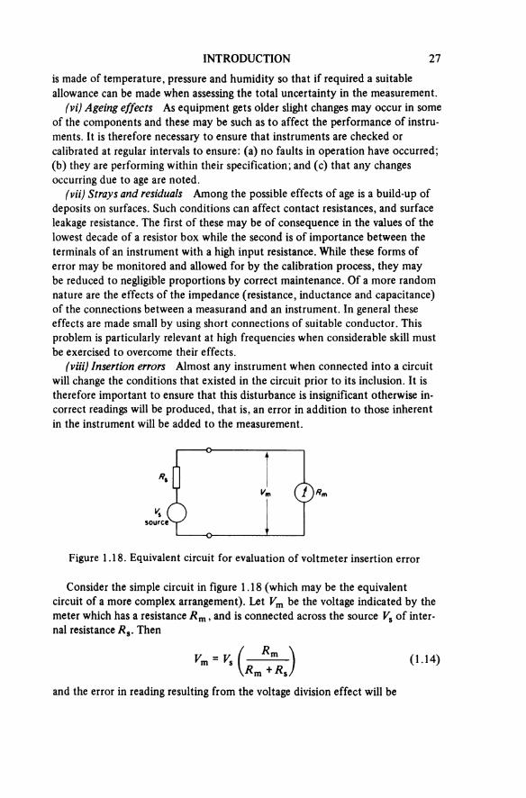
(viii) Insertion errors Almost any instrument when connected into a circuit will change the conditions that existed in the circuit prior to its inclusion. It istherefore important to ensure that this disturbance is insignificant otherwise in-correct readings will be produced, that is, an error in addition to those inherent in the instrument will be added to the measurement.
Figure 1.18. Equivalent circuit for evaluation of voltmeter insertion error
source
Consider the simple circuit in figure 1.18 (which may be the equivalent circuit of a more complex arrangement). Let Vm be the voltage indicated by themeter which has a resistance Rm, and is connected across the source Vs of inter-nal resistance Rs. Then
(114)
and the error in reading resulting from the voltage division effect will be
28 AN INTRODUCTION TO ELECTRICAL INSTRUMENTATION
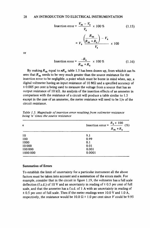
Insertion error = (1.15)
or
Insertion error = (1.16)
By making Rm equal to nRS, table 1.5 has been drawn up, from whichit can be seen that Am needs to be very much greater than the source resistance for the insertion error to be negligible, a point which must be borne in mind when, say, a digital voltmeter having an input resistance of 10 MΩ and a specified accuracy of ± 0.005 per cent is being used to measure the voltage from a source that has an output resistance of 10 kΩ. An analysis of the insertion effects of an ammeter in comparison with the resistance of a circuit will produce a table similar to 1.5 except in the case of an ammeter, the meter resistance will need to be 1/n of the circuit resistance.
Table 1.5. Magnitude of insertion error resulting from voltmeter resistance being ‘n’ times the source resistance
nRs × 100
Insertion error = ---------- (%)Rm + Rs
10 9.1100 0.991000 0.110 000 0.01100 000 0.0011000 000 0.0001
Summation of Errors
To establish the limit of uncertainty for a particular instrument all the above factors must be taken into account and a summation of the errors made. For example, consider that in the circuit in figure 1.19, the voltmeter has a full scale deflection (f.s.d.) of 10 v and an uncertainty in reading of ± 0.5 per cent of full scale, and that the ammeter has a f.s.d. of 1 A with an uncertainty in reading of ± 0.5 per cent of full scale. Then if the meter readings were 10.0 V and 1.0 A, respectively, the resistance would be 10.0 Ω ± 1.0 per cent since V could be 9.95
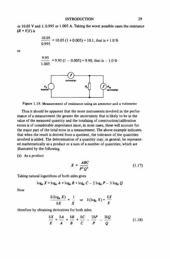
INTRODUCTION 29
or 10.05 V and /, 0.995 or 1.005 A. Taking the worst possible cases the resistance (R = V/I) is
= 10.1, that is + 1.0%
or
9.90, that is — 1.0 %
Figure 1.19. Measurement of resistance using an ammeter and a voltmeter
source
ammeter
voltmeter
Thus it should be apparent that the more instruments involved in the perfor-mance of a measurement the greater the uncertainty that is likely to be in the value of the measured quantity and the totalising of construction/calibration errors is of considerable importance since, in most cases, these will account for the major part of the total error in a measurement. The above example indicates that when the result is derived from a quotient, the tolerance of the quantities involved is added. The determination of a quantity may, in general, be represent ed mathematically as a product or a sum of a number of quantities, which are illustrated by the following.
(a) As a product
(1.17)
Taking natural logarithms of both sides gives
Now
therefore by obtaining derivatives for both sides
(1.18)
30 AN INTRODUCTION TO ELECTRICAL INSTRUMENTATION
But in practice the maximum possible error in X is the quantity it is desired to ascertain, and this will only be obtained if the moduli of the terms are used. Thus the maximum error in X would be
(1.19)
(b) As a sum
x = y + z + p
The error in this case is obtained as follows. The maximum value of x is
x + δx = y + δy + z + δz + p + δp
The minimum value of x is
x — δx = y — δy + z — δz + p — δp
Thus the error in x is
± δx = ± (δy + δz + δp)
or
(1.20)
and if the errors of y, z and p had been given as percentages
(1.21)
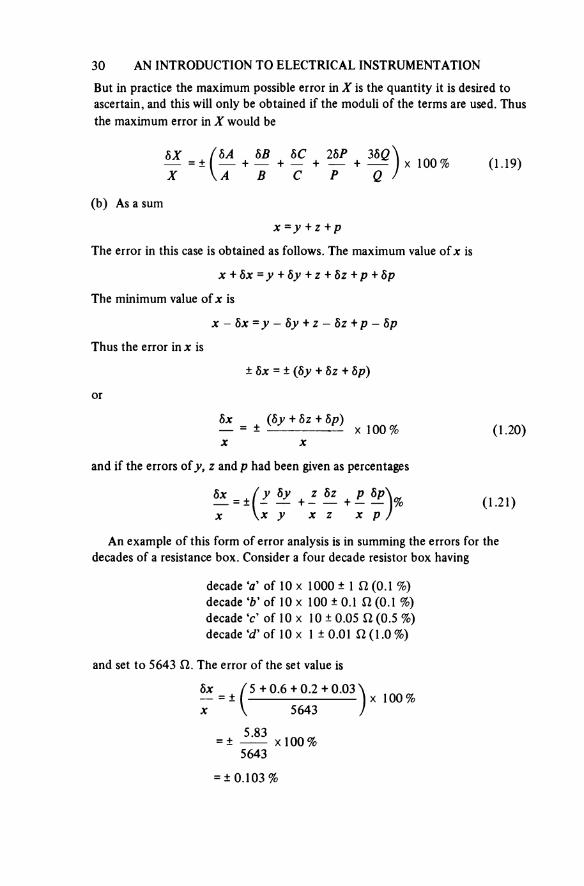
An example of this form of error analysis is in summing the errors for the decades of a resistance box. Consider a four decade resistor box having
decade ‘a’ of 10 × 1000 ± 1 Ω (0.1 %) decade ‘b’ of 10 × 100 ± 0.1 Ω (0.1 %) decade ‘c’ of 10 × 10 ± 0.05 Ω (0.5 %) decade ‘d’ of 10 × 1 ± 0.01 Ω (1.0 %)
and set to 5643 Ω. The error of the set value is
= ± 0.103%
INTRODUCTION 31
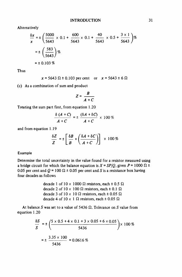
Alternatively
= ± 0.103%
Thus
x = 5643 Ω ± 0.103 per cent or x = 5643 ± 6 Ω
(c) As a combination of sum and product
Treating the sum part first, from equation 1.20
and from equation 1.19
Example
Determine the total uncertainty in the value found for a resistor measured using a bridge circuit for which the balance equation is X = SP/Q, given P = 1000 Ω ± 0.05 per cent and Q = 100 Ω ± 0.05 per cent and S is a resistance box having four decades as follows
decade 1 of 10 × 1000 Ω resistors, each ± 0.5 Ωdecade 2 of 10 × 100 Ω resistors, each ± 0.1 Ω decade 3 of 10 × 10 Ω resistors, each ± 0.05 Ω decade 4 of 10 × 1 Ω resistors, each ± 0.05 Ω
At balance S was set to a value of 5436 Ω. Tolerance on S value from equation 1.20
= 0.0616%
32 AN INTRODUCTION TO ELECTRICAL INSTRUMENTATION
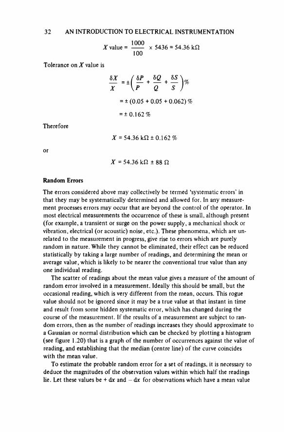
X value = = 54.36 kΩ
Tolerance on X value is
= ± 0.162%
Therefore
X = 54.36 kΩ ± 0.162%
or
X = 54.36 kΩ ± 88 Ω
Random Errors
The errors considered above may collectively be termed ‘systematic errors’ in that they may be systematically determined and allowed for. In any measure-ment processes errors may occur that are beyond the control of the operator. In most electrical measurements the occurrence of these is small, although present (for example, a transient or surge on the power supply, a mechanical shock or vibration, electrical (or acoustic) noise, etc.). These phenomena, which are un-related to the measurement in progress, give rise to errors which are purely random in nature. While they cannot be eliminated, their effect can be reduced statistically by taking a large number of readings, and determining the mean or average value, which is likely to be nearer the conventional true value than any one individual reading.
The scatter of readings about the mean value gives a measure of the amount of random error involved in a measurement. Ideally this should be small, but the occasional reading, which is very different from the mean, occurs. This rogue value should not be ignored since it may be a true value at that instant in time and result from some hidden systematic error, which has changed during the course of the measurement. If the results of a measurement are subject to ran-dom errors, then as the number of readings increases they should approximate to a Gaussian or normal distribution which can be checked by plotting a histogram (see figure 1.20) that is a graph of the number of occurrences against the value of reading, and establishing that the median (centre line) of the curve coincides with the mean value.
To estimate the probable random error for a set of readings, it is necessary to deduce the magnitudes of the observation values within which half the readings lie. Let these values be + dx and — dx for observations which have a mean value

INTRODUCTION 33
Figure 1.20. Histograms with normal distributions
num
ber o
f occ
uren
ces
mean
deviation from mean value
of x, then the probability of a reading lying within ± dx of x is 50 per cent and the probable random error may be quoted as ± dx.
A more precise method of evaluating the randomness of a set of observations is to calculate the standard deviation for the distribution. Since the sum of the deviations for all the points in a distribution will be zero, the standard deviation for a set of observations is obtained by calculating the square root of the mean of the sum of the squared deviations that is
where x is the mean value, x is an individual value, and N is the number of values.
For a normal distribution the chance of a valid point lying outside ± 1.96σ is 5 per cent and outside ± 3.09σ is 0.2 per cent. Also for a normal distribution the probable random error is 0.6745σ. The magnitude of σ is a clear indication of the quality of the distribution; in figure 1.20 the curve A would have a σ of 1 while for curve B σ = 3.
1.3.3 Specifications
To define limits of uncertainty in their operation all instruments are manufactur ed to a specification. This may be a national standard relating to a type of instrument, for example that relating to direct-acting electrical indicating instru- ments, [13] or a statement of performance issued by the manufacturer (see section 8.2).
34 AN INTRODUCTION TO ELECTRICAL INSTRUMENTATION
Pointer instruments
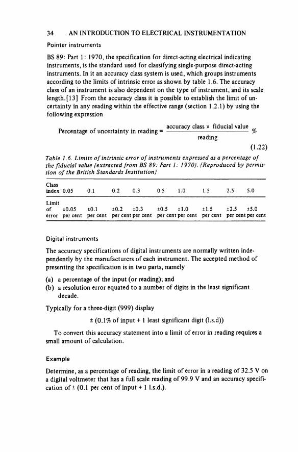
BS 89: Part 1: 1970, the specification for direct-acting electrical indicating instruments, is the standard used for classifying single-purpose direct-acting instruments. In it an accuracy class system is used, which groups instruments according to the limits of intrinsic error as shown by table 1.6. The accuracy class of an instrument is also dependent on the type of instrument, and its scale length. [13] From the accuracy class it is possible to establish the limit of un-certainty in any reading within the effective range (section 1.2.1) by using the following expression
Percentage of uncertainty in readingaccuracy class × fiducial value
reading%
(1.22)Table 1.6. Limits of intrinsic error of instruments expressed as a percentage of the fiducial value (extracted from BS 89: Part 1: 1970). (Reproduced by permis-sion of the British Standards Institution)
Classindex 0.05 0.1 0.2 0.3 0.5 1.0 1.5 2.5 5.0
Limitof ±0.05 ±0.1 ±0.2 ±0.3 ±0.5 ±1.0 ±1.5 ±2.5 ±5.0error per cent per cent per cent per cent per cent per cent per cent per cent per cent
Digital instruments
The accuracy specifications of digital instruments are normally written inde-pendently by the manufacturers of each instrument. The accepted method of presenting the specification is in two parts, namely
(a) a percentage of the input (or reading); and(b) a resolution error equated to a number of digits in the least significant
decade.
Typically for a three-digit (999) display
± (0.1% of input + 1 least significant digit (l.s.d))
To convert this accuracy statement into a limit of error in reading requires a small amount of calculation.
Example
Determine, as a percentage of reading, the limit of error in a reading of 32.5 V on a digital voltmeter that has a full scale reading of 99.9 V and an accuracy specifi-cation of ± (0.1 per cent of input + 1 l.s.d.).
INTRODUCTION 35
Contribution from first part of specification
0.1 % of input ≡ 0.1 % of reading
This may not be strictly correct but unless the instrument is well outside specifi-cation it is a realistic assumption.
Contribution from second part of specification, in a reading of 32.5 V
1 l.s.d. = 0.1 V
1 l.s.d. ≡ 0.307 %
Thus the limit of error = ± (0.1 + 0.307) %
= ± 0.407 %
Undoubtedly this is an inconvenient process and when using a particular instrument a considerable saving in effort (and time) can be made by drawing up a curve of limit of error in reading against reading so that the uncertainty in a reading can be quickly established (see section 8.2).
It should be appreciated that the accuracy specification as stipulated above will only apply at a particular temperature or over a band of temperature and it may be necessary to add to the uncertainty in a reading a tolerance for tempera-ture effects, a topic which is also covered in section 8.2.
1.3.4 Standards
So that it can be established that instruments are within their specification it isnecessary to maintain a set of reference or standard quantities.
An instrument manufacturer will have a set of reference instruments and from time to time these will be sent to a calibration centre for checking. The calibration centres will in turn have instruments that are checked against the national standards.
Organisations such as the National Physical Laboratory (N.P.L.) of the United Kingdom, the National Bureaux of Standards (N.B.S.) of the United States and their equivalents in other countries have expended considerable effort in determining the absolute value of electrical quantities (see appendix I). Thatis to say quantities such as the ohm, the ampere and the farad have been deter-mined in terms of the fundamental quantities of mass, length and time with the greatest possible precision although uncertainty still exists in their exact values, even if it is only a few parts in 1 000 000 000.
Such precise determinations of electrical quantities are necessary so that com-parisons of the standards used in every country may be made, and engineers and scientists throughout the world may have a common set of references: for example, 1 Russian volt = 1 American volt = 1 U.K. volt = 1 Australian volt, and
36 AN INTRODUCTION TO ELECTRICAL INSTRUMENTATION
so on, hence performance of equipment and measurement of physical phenomena are made on a common basis.
In electrical measurements, the standards of greatest importance are those of current resistance, capacitance and frequency, it being possible to derive other quantities such as voltage and power from those listed. The absolute determina-tion of electrical quantities is in itself a science and an appreciation of their necessity should be sufficient at this stage, where the absolute standards can be considered to be the reference by which derived or ‘material’ standards are calibrated.
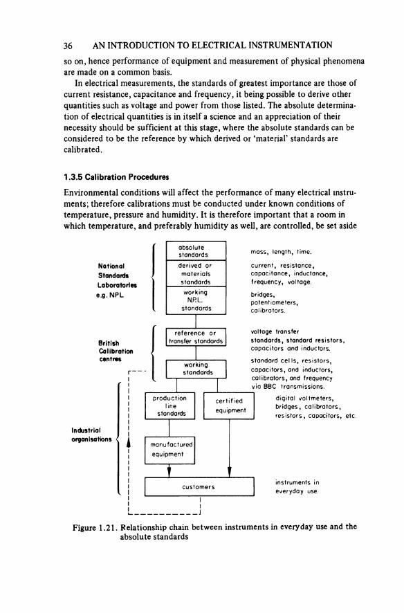
1.3.5 Calibration Procedures
Environmental conditions will affect the performance of many electrical instru-ments; therefore calibrations must be conducted under known conditions of temperature, pressure and humidity. It is therefore important that a room in which temperature, and preferably humidity as well, are controlled, be set aside
absolutestandards mass, length, time.
National Standards Laboratories e.g. NPL
derived or materials standards
current, resistance, capacitance, inductance frequency, voltage.
workingN.P.L.
standards
bridges,potentiometers,calibrators.
BritishCalibrationcentres
reference or transfer standards
voltage transferstandards, standard resistors, capacitors and inductors.
workingstandards
standard cells, resistors, capacitors, and inductors, calibrators, and frequency via BBC transmissions.
productionline
standards
certifiedequipment
digital voltmeters, bridges, calibrators, resistors, capacitors, etc.
Industrialorganisations
manufacturedequipment
customersinstruments in everyday use.
Figure 1.21. Relationship chain between instruments in everyday use and the absolute standards
INTRODUCTION 37solely for the calibration of instruments. The requirements for approval of a laboratory under the British Calibration Service (B.C.S.) scheme [14] are for the temperature to be maintained at 20 °C ± 2 °C (or 23 °C ± 2 °C) and the relative humidity to be between the limits of 35 per cent and 70 per cent. The effects of variations in atmospheric pressure on the performance of electrical instruments are in general small, except in the measurement of high voltages by sphere-gap breakdown where they are of extreme importance and must be allowed for. However, the facility to measure atmospheric pressure in a calibration room for electrical instruments should not be overlooked as it may constitute an undetect-ed systematic error in a particular measurement. For example, the dielectric constant of air is pressure dependent.
The hierarchy of reference between instruments in daily engineering use and the national or absolute standards can be summarised by diagram in figure 1.21.
Electrical instruments are usually calibrated either by comparing performance with a similar but superior instrument, or by using a source of selectable ampli-tude, this latter form generally being known as a calibrator. In either situation the uncertainty in the reference should be less than a quarter of the specified uncertainty in the instrument under calibration. [14]
1.4 INPUT CHARACTERISTICS
It has been shown (section 1.3.2) that the input resistance of an instrument is of extreme importance as the magnitude of that parameter will affect the distur-bance the instrument causes when it is inserted in a circuit. Other input characteristics that must be considered when selecting an instrument are described in the following sections.
1.4.1 Sensitivity
The sensitivity of an instrument should either be quoted in terms of the number of units for full scale indication, or as a unit of deflection. Examples of these are 1 A full scale deflection, 10 mm/μA and 0.1 μA/mm. For digital instruments the sensitivity is usually quoted in terms of the resolution (1 l.s.d.) for the most sensitive range. For example, ‘10 μV on the 100 mV range’, although on occa-sions the sensitivity is only deducible from the range and the display, for example, ‘2 V range and 3½ digits (1999)’.
1.4.2 Scaling
Most instruments have an effective range that extends from 10 per cent to 100 per cent of the full scale value. However, many signals will be outside the effect-ive range, those that are too large requiring scaling down by some division process while those that are too small will require amplification.
38 AN INTRODUCTION TO ELECTRICAL INSTRUMENTATION
Current division
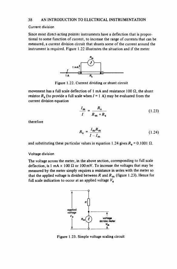
Since most direct-acting pointer instruments have a deflection that is propor-tional to some function of current, to increase the range of currents that can bemeasured, a current division circuit that shunts some of the current around the instrument is required. Figure 1.22 illustrates the situation and if the meter
Figure 1.22. Current dividing or shunt circuit
movement has a full scale deflection of 1 mA and resistance 100 Ω, the shunt resistor Rs (to provide a full scale when I = 1 A) may be evaluated from the current division equation
(1.23)
therefore
(1.24)
and substituting these particular values in equation 1.24 gives Rs = 0.1001 Ω.
Voltage division
The voltage across the meter, in the above section, corresponding to full scale deflection, is 1 mA × 100 Ω or 100 mV. To increase the voltages that may be measured by the meter simply requires a resistance in series with the meter so that the applied voltage is divided between R and Rm (figure 1.23). Hence for full scale indication to occur at an applied voltage Va
appliedvoltage
voltage across meter
Figure 1.23. Simple voltage scaling circuit
INTRODUCTION 39
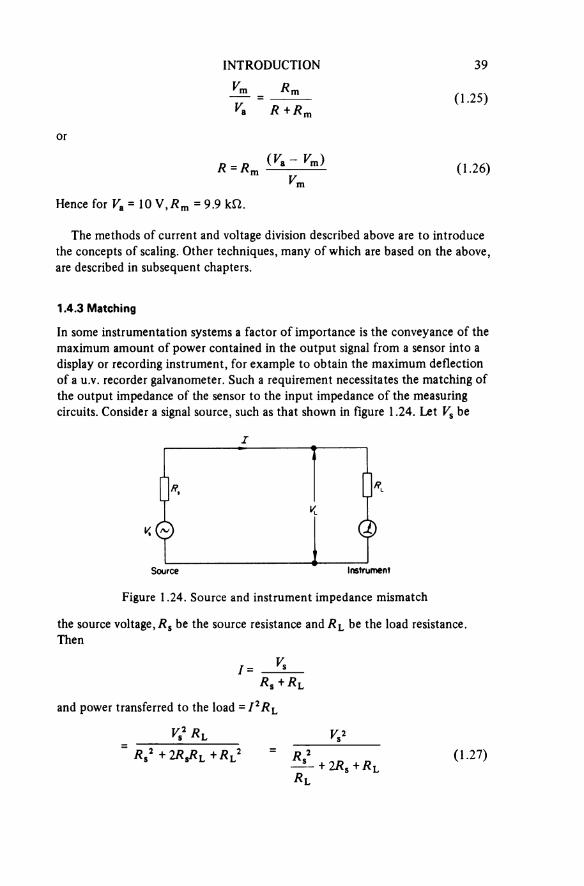
(1.25)
or
(1.26)
Hence for Va = 10 V, Rm = 9.9 kΩ.
The methods of current and voltage division described above are to introduce the concepts of scaling. Other techniques, many of which are based on the above, are described in subsequent chapters.
1.4.3 Matching
In some instrumentation systems a factor of importance is the conveyance of the maximum amount of power contained in the output signal from a sensor into a display or recording instrument, for example to obtain the maximum deflection of a u.v. recorder galvanometer. Such a requirement necessitates the matching ofthe output impedance of the sensor to the input impedance of the measuring circuits. Consider a signal source, such as that shown in figure 1.24. Let Vs be
Figure 1.24. Source and instrument impedance mismatch
Source Instrument
the source voltage, Rs be the source resistance and RL be the load resistance. Then
and power transferred to the load = I2RL
(1.27)
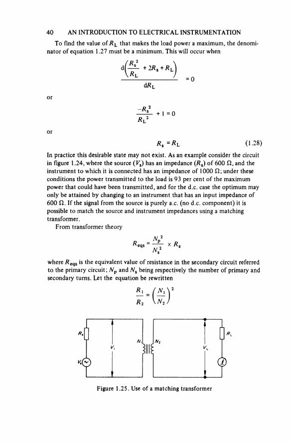
40 AN INTRODUCTION TO ELECTRICAL INSTRUMENTATION
To find the value of RL that makes the load power a maximum, the denomi-nator of equation 1.27 must be a minimum. This will occur when
or
or
(1.28)
In practice this desirable state may not exist. As an example consider the circuit in figure 1.24, where the source (Vs) has an impedance (Rs) of 600 Ω, and theinstrument to which it is connected has an impedance of 1000 Ω; under these conditions the power transmitted to the load is 93 per cent of the maximum power that could have been transmitted, and for the d.c. case the optimum may only be attained by changing to an instrument that has an input impedance of 600 Ω. If the signal from the source is purely a.c. (no d.c. component) it is possible to match the source and instrument impedances using a matching transformer.
From transformer theory
where Reqs is the equivalent value of resistance in the secondary circuit referred to the primary circuit; Np and Ns being respectively the number of primary and secondary turns. Let the equation be rewritten
Figure 1.25. Use of a matching transformer
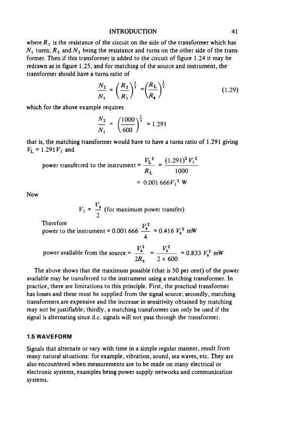
INTRODUCTION 41
where R1 is the resistance of the circuit on the side of the transformer which has N1 turns; R2 and N2 being the resistance and turns on the other side of the trans former. Then if this transformer is added to the circuit of figure 1.24 it may be redrawn as in figure 1.25, and for matching of the source and instrument, the transformer should have a turns ratio of
(1.29)
which for the above example requires
that is, the matching transformer would have to have a turns ratio of 1.291 giving VL = 1.291 V1 and
power transferred to the instrument =
Now
(for maximum power transfer)
Thereforepower to the instrument =
power available from the source =
The above shows that the maximum possible (that is 50 per cent) of the power available may be transferred to the instrument using a matching transformer. In practice, there are limitations to this principle. First, the practical transformer has losses and these must be supplied from the signal source; secondly, matching transformers are expensive and the increase in sensitivity obtained by matching may not be justifiable; thirdly, a matching transformer can only be used if the signal is alternating since d.c. signals will not pass through the transformer.
1.5 WAVEFORM
Signals that alternate or vary with time in a simple regular manner, result from many natural situations: for example, vibration, sound, sea waves, etc. They are also encountered when measurements are to be made on many electrical or electronic systems, examples being power supply networks and communication systems.
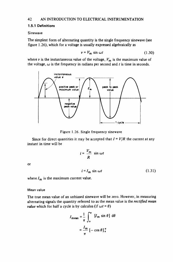
42 AN INTRODUCTION TO ELECTRICAL INSTRUMENTATION
1.5.1 Definitions
Sinewave
The simplest form of alternating quantity is the single frequency sinewave (see figure 1.26), which for a voltage is usually expressed algebraically as
(130)
where v is the instantaneous value of the voltage, Vm is the maximum value of the voltage, ω is the frequency in radians per second and t is time in seconds.
Figure 1.26. Single frequency sinewave
instantaneous value e
positive peak or maximum value
peak to peak value
negative peak value
Since for direct quantities it may be accepted that I = V/R the current at any instant in time will be
or
(131)
where Im is the maximum current value
Mean value
The true mean value of an unbiased sinewave will be zero. However, in measuring alternating signals the quantity referred to as the mean value is the rectified mean value which for half a cycle is by calculus (if ωt = θ)
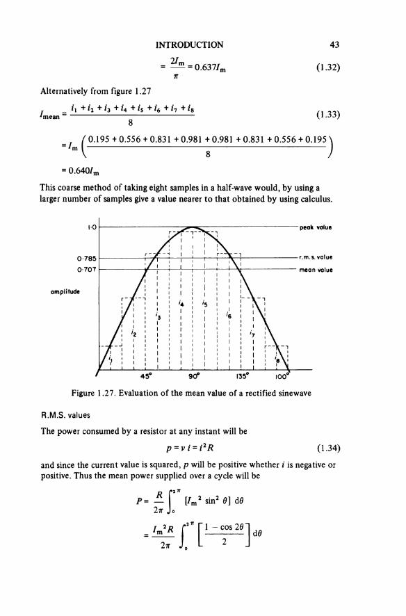
INTRODUCTION 43
(1.32)
Alternatively from figure 1.27
(1.33)
This coarse method of taking eight samples in a half-wave would, by using a larger number of samples give a value nearer to that obtained by using calculus.
Figure 1.27. Evaluation of the mean value of a rectified sinewave
peak value
r.m.s. value
mean value
amplitude
R.M.S. values
The power consumed by a resistor at any instant will be
(1.34)
and since the current value is squared, p will be positive whether i is negative or positive. Thus the mean power supplied over a cycle will be
44 AN INTRODUCTION TO ELECTRICAL INSTRUMENTATION
(1.35)
If the mean power is defined as the alternating power equivalent of that produced by direct voltage and current
Therefore
(1.36)
This effective value of the alternating current which is equivalent to the direct value is normally known as the root-mean-square or r.m.s. value. It is of consider-able importance and unless stated otherwise the value quoted for alternating quantities is assumed to be the r.m.s. value, and conventionally denoted by the capital letter, for example, / or V.
If the signal is nonperiodic the r.m.s. value may be established by a procedure similar to that in equation 1.33, that is
(1.37)
Using the values of figure 1.27
Similarly it may be shown that the r.m.s. value of a voltage wave is
(1.38)
Form factor and crest factor
These terms which are constantly used in connection with measurements of alternating quantities are defined using the expressions
form factor =r.m.s. value
mean value(1.39)
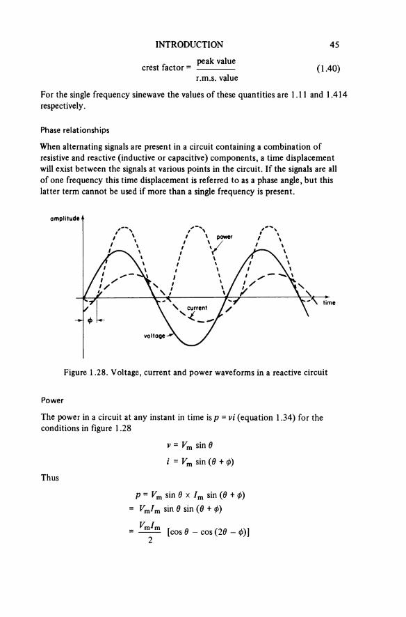
INTRODUCTION 45
crest factor =peak value
r.m.s. value(1.40)
For the single frequency sinewave the values of these quantities are 1.11 and 1.414 respectively.
Phase relationships
When alternating signals are present in a circuit containing a combination of resistive and reactive (inductive or capacitive) components, a time displacement will exist between the signals at various points in the circuit. If the signals are all of one frequency this time displacement is referred to as a phase angle, but this latter term cannot be used if more than a single frequency is present.
Figure 1.28. Voltage, current and power waveforms in a reactive circuit
amplitude
power
currenttime
voltage
Power
The power in a circuit at any instant in time is p = vi (equation 1.34) for the conditions in figure 1.28
Thus
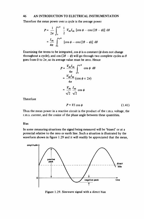
46 AN INTRODUCTION TO ELECTRICAL INSTRUMENTATION
Therefore the mean power over a cycle is the average power
Examining the terms to be integrated, cos ϕ is a constant (ϕ does not change throughout a cycle), and cos (2θ — ϕ) will go through two complete cycles as θ goes from 0 to 2π, so its average value must be zero. Hence
Therefore
(1.41)
Thus the mean power in a reactive circuit is the product of the r.m.s. voltage, the r.m.s. current, and the cosine of the phase angle between these quantities.
Bias
In some measuring situations the signal being measured will be ‘biased’ or at a potential relative to the zero or earth line. Such a situation is illustrated by the waveform shown in figure 1.29 and it will readily be appreciated that the mean,
Figure 1.29. Sinewave signal with a direct bias
amplitude
positivepeak
directbias
negative peak time

INTRODUCTION 47
peak and other values characteristic of a signal referred to above will be affected by the presence of a bias; a condition which can create considerable difficulties in some measurement situations.
1.5.2 Harmonics
It is conveniently assumed that alternating signals are single frequency sinusoidal waveforms. Although this is fortunately a satisfactory assumption for many situations the presence of harmonics in signal waveforms cannot always be ignored, and their magnitudes must be established, either by using Fourier analysis or by a suitably designed electronic instrument that displays the un-known waveform as its frequency components.
Figure 1.30. Presentation of a multi-frequency waveform on time and frequency axes
Figure 1.30 presents a waveform that consists of a fundamental, a third and a fifth harmonic both as a function of time and of frequency, the three-dimensional arrangement attempting to link the two.
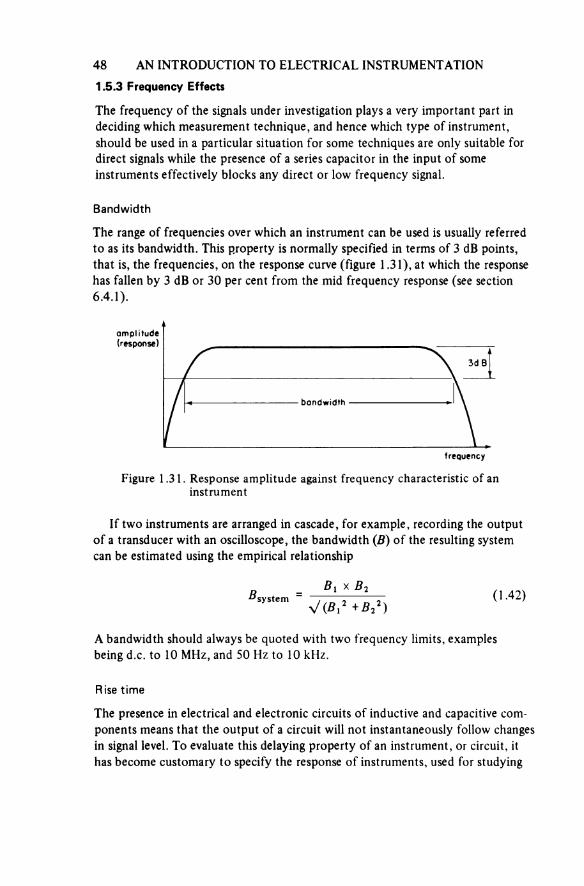
48 AN INTRODUCTION TO ELECTRICAL INSTRUMENTATION
1.5.3 Frequency Effects
The frequency of the signals under investigation plays a very important part in deciding which measurement technique, and hence which type of instrument, should be used in a particular situation for some techniques are only suitable for direct signals while the presence of a series capacitor in the input of some instruments effectively blocks any direct or low frequency signal.
Bandwidth
The range of frequencies over which an instrument can be used is usually referred to as its bandwidth. This property is normally specified in terms of 3 dB points, that is, the frequencies, on the response curve (figure 1.31), at which the response has fallen by 3 dB or 30 per cent from the mid frequency response (see section 6.4.1).
Figure 1.31. Response amplitude against frequency characteristic of an instrument
amplitude(response)
3 dB
bandwidth
frequency
If two instruments are arranged in cascade, for example, recording the output of a transducer with an oscilloscope, the bandwidth (B) of the resulting system can be estimated using the empirical relationship
(1.42)
A bandwidth should always be quoted with two frequency limits, examples being d.c. to 10 MHz, and 50 Hz to 10 kHz.
Rise time
The presence in electrical and electronic circuits of inductive and capacitive com-ponents means that the output of a circuit will not instantaneously follow changes in signal level. To evaluate this delaying property of an instrument, or circuit, it has become customary to specify the response of instruments, used for studying

INTRODUCTION 49
fast pulses, in terms of their rise time—the time interval measured from 10 to 90 per cent of a step change (see figure 2.61). This quantity should not be confused with the time constant of a circuit which is the value given to the time interval from the start to 63.2 per cent of the final value of a step change (see section 6.4.1).
1.6 INTERFERENCE
Measurements involving small electrical signals can be seriously affected by the presence of interference, that is, the displayed quantity will be the sum of the desired signal and unwanted or interference signals. It is therefore necessary to ensure that instruments and connections are adequately protected from, and capable of rejecting, interference signals.
1.6.1 Environmental Interference
The interference signals grouped under this heading are those related to effects dependent on such quantities as temperature, humidity, pressure, atmospheric pollutants, and so on.
The effects of temperature on the performance of an instrument are normally allowed for within the terms of the specification, that is, the quoted values are stated to hold over a range of temperatures, outside of which a further allowance to the measurement uncertainty must be made.
The effects of atmospheric pollutants require consideration of the environ-ment in which the instrument is going to be used, for it must be realised that dust, moisture and fumes from some soldering fluxes can have unrealised effects on the signal measured (see section 7.1.2).
1.6.2 Coupled Interference
Electrostatic coupling
When a conductor A is maintained at a potential relative to zero (earth) potential, it will be enveloped in an electrostatic field (see figure 1.32a). If another conduc-tor B, insulated from earth, is introduced into this electrostatic field it will attain a potential dependent on its size and its position in the field (see figure 1.32b), and should the potential of conductor A be alternating then the con-ductor B will ‘pick up’ an alternating voltage. This linking by means of an electrostatic field is termed capacitive coupling and may cause considerable interference problems in measurement circuits. To shield the conductor B from the electrostatic field of A simply requires the inserting of a conducting sheet, held at zero potential, between the two conductors as in figure 1.32c.

50 AN INTRODUCTION TO ELECTRICAL INSTRUMENTATION
Figure 1.32. Conductor and shield in an electrostatic field
(a) (b)
(c)
Electromagnetic coupling
Any current-carrying conductor is surrounded by a magnetic field, the strength of this field depending on the magnitude of the current, and should it be alternat-ing, voltages will be induced in any conducting material that is positioned within this magnetic field. Thus any signal carrying connection passing near a current carrying conductor will be magnetically coupled to it, and an interference voltage will be induced in the signal carrying conductor. One of three forms of magnetic shielding may be used to reduce electromagnetic interference, these being
(a) Conducting shield. The positioning of a thick conducting sheet around the component or lead to be screened; then magnetic flux entering the conduct-ing sheet induces currents which themselves produce a magnetic flux to oppose the applied field.
(b) Magnetic shield. The positioning of a high permeability path around the component to be screened so that the magnetic flux of the interference field is diverted into the shield and away from the component. (Note: the thick-ness of the shield required in both (a) and (b) will be a function of

INTRODUCTION 51(c) Lead twisting. By arranging equipment so that the coupling between the
magnetic field source and the signal carrying connections is either cancelledout, or kept to a minimum. The former requirement may be met by ensuring that the two leads connecting a source to an instrument follow an identical path, and such an arrangement is greatly assisted by twisting the two leads together. The latter requirement can only be fulfilled by ensuring that the signal carrying conductors are remote from any source of magnetic flux.
In practice the most likely sources of electromagnetic interference are 50 Hz transformers and inductors, and all signal carrying conductors should be kept well clear of such items. If two, or more, inductors have to be used in a circuit they should be arranged for minimum coupling, that is their axes should be arranged at 90° to each other.
1.7 SELECTION
This introductory chapter began by posing a number of questions relating to the selection process that can be adopted to ensure the performance of a measure-ment in a satisfactory manner. Although the preceding pages cannot have answered these questions completely, hopefully they will have made the reader pause and wonder whether, in the past, he has always made measurements with sufficient forethought.
To reinforce the importance of those questions, they are restated here so that the reader may remember them when next making a measurement.
(a) What is the most suitable method of measurement?(b) How should the result be displayed?(c) What tolerance on the measured value is acceptable?(d) How will the presence of the instrument affect the signal?(e) How will the signal wave-shape affect the instrument’s performance?(f) Over what range of frequencies does the instrument perform correctly?(g) What will the effects of interference be on the result obtained?
It should be realised that this set of questions is a starting point—a more detailed set of conditions and requirements are contained in chapter 8.
REFERENCES
1 C. T. Baldwin, Fundamentals of Electrical Measurements (Harrap, London,1961)
2 S. Stein and J. Jay Jones, Modern Communication Principles (McGraw-Hill,New York, 1967)
3 E. C. Bell and R. W. Whitehead, Basic Electrical Engineering and Instrument-ation (Crosby Lockwood Staples, London, 1977)
4 N. M. Morris, Digital Electronic Circuits and Systems (Macmillan, Londonand Basingstoke, 1974)
52 AN INTRODUCTION TO ELECTRICAL INSTRUMENTATION
5 D. Moralee, Floppy discs, the storage medium for microprocessor systems.Electronics Power, 24 (1978) 637-41
6 K. Baker, Solid-state serial memories—the role of bubbles and c.c.d.s.Electronics Power, 24 (1978) 647-52
7 R. Squires, An introduction to microprocessors, Kent tech. Rev., 25 (1979)20-4
8 E. Huggins, Microprocessors and Microcomputers, their use and programming(Macmillan, London and Basingstoke, 1979)
9 G. F. Weston, Alphanumeric display, Proc. I.E.E., 125 (1978)10 J. Smith, Experimental storage display panels using d.c. gas discharges with-
out resistors, I.E.E.E. Trans. electronic Devices, 22 (1975) 642-911 BS 5233: 1975 Glossary of terms used in metrology12 A. Simpson, Testing Methods and Reliability, Electronics (Macmillan,
London and Basingstoke, 1976)13 BS 89: Part 1: 1970 Single purpose direct acting electrical indicating instru-
ments and their accessories14 British Calibration Service, General Criteria for Laboratory Approval
(London, 1967)
2Analogue Instruments
An analogue device is one in which the operation and output are continuously variable and bear a fixed relationship to the input.
In section 1.1 the concepts of analogue instruments were outlined and for the purpose of this chapter analogue instruments have been divided into four groups
(a) those in which a ‘moving coil movement’ is used as the sensing element(b) those in which some other form of electromechanical sensing element is used(c) the instruments that use a cathode ray tube (c.r.t.) as the display medium(d) the instruments that use magnetic tape as a storage medium.
2.1 MOVING COIL INSTRUMENTS
The principle used in the construction of this type of instrument is that current passing through a conductor generates a magnetic field around the conductor and if this field is arranged to interact with a permanent magnetic field, a force acts on the current carrying conductor. If the conductor (that is, the coil) is con-strained to move in a rotary manner an angular deflection or movement propor-tional to the current may be obtained, resulting in an instrument that has a linear scale but which, due to its inertia, can only respond to steady state and slowly varying quantities. The linearity of scale is an extremely useful feature and accounts for the use of moving coil instruments as the display in many complex electronic instruments.
The general arrangement of the moving coil instrument is indicated in figure 2.1. The permanent magnet system has over the years been considerably reduced in size due to the improvements in magnet design as better materials have become available.
The coil may be air cored or mounted on a metal former; if the latter is present it will contribute to the damping of the instrument (eddy currents) but will add to the inertia of the movement.
If an air-cored coil offset from the axis of rotation (figure 2.2) is used, the
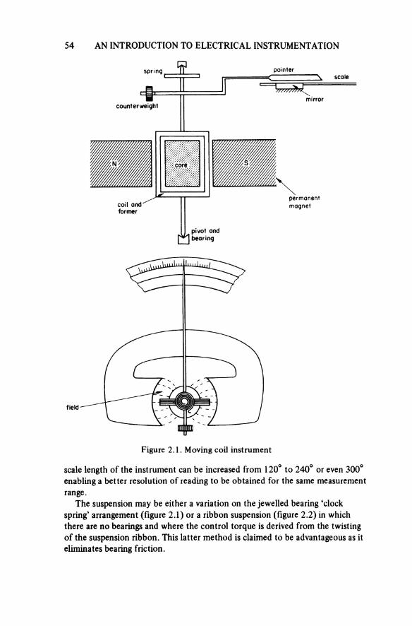
54 AN INTRODUCTION TO ELECTRICAL INSTRUMENTATION
Figure 2.1. Moving coil instrument
spring
counterweight
pointerscale
mirror
N core s
coil and former
permanentmagnet
pivot and bearing
field
scale length of the instrument can be increased from 120° to 240° or even 300° enabling a better resolution of reading to be obtained for the same measurement range.
The suspension may be either a variation on the jewelled bearing ‘clock spring’ arrangement (figure 2.1) or a ribbon suspension (figure 2.2) in which there are no bearings and where the control torque is derived from the twisting of the suspension ribbon. This latter method is claimed to be advantageous as it eliminates bearing friction.
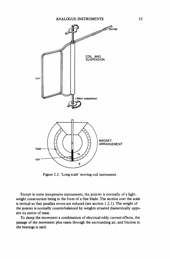
ANALOGUE INSTRUMENTS 55
Figure 2.2. ‘Long scale’ moving coil instrument
pointer
COIL AND SUSPENSION
coil
ribbon suspension
MAGNETARRANGEMENT
field
coil
Except in some inexpensive instruments, the pointer is normally of a light-weight construction being in the form of a fine blade. The section over the scale is vertical so that parallax errors are reduced (see section 1.2.1). The weight of the pointer is normally counterbalanced by weights situated diametrically oppo-site its centre of mass.
To damp the movement a combination of electrical eddy current effects, the passage of the movement plus vanes through the surrounding air, and friction in the bearings is used.
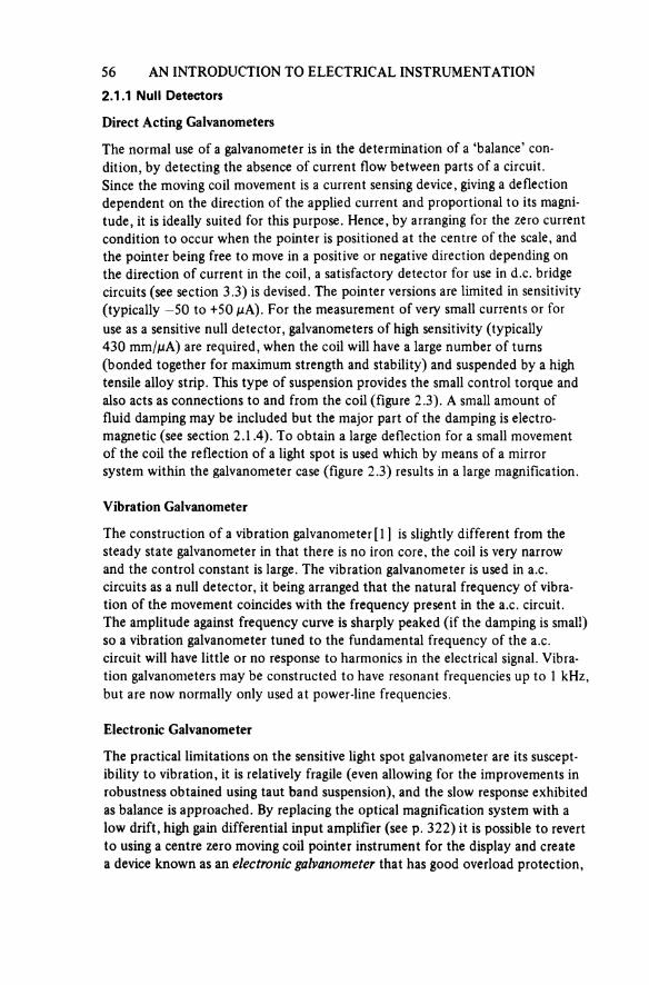
56 AN INTRODUCTION TO ELECTRICAL INSTRUMENTATION
2.1.1 Null Detectors
Direct Acting Galvanometers
The normal use of a galvanometer is in the determination of a ‘balance’ con-dition, by detecting the absence of current flow between parts of a circuit.Since the moving coil movement is a current sensing device, giving a deflection dependent on the direction of the applied current and proportional to its magni-tude, it is ideally suited for this purpose. Hence, by arranging for the zero current condition to occur when the pointer is positioned at the centre of the scale, andthe pointer being free to move in a positive or negative direction depending on the direction of current in the coil, a satisfactory detector for use in d.c. bridge circuits (see section 3.3) is devised. The pointer versions are limited in sensitivity (typically —50 to +50 μA). For the measurement of very small currents or for use as a sensitive null detector, galvanometers of high sensitivity (typically 430 mm/μA) are required, when the coil will have a large number of turns (bonded together for maximum strength and stability) and suspended by a high tensile alloy strip. This type of suspension provides the small control torque and also acts as connections to and from the coil (figure 2.3). A small amount of fluid damping may be included but the major part of the damping is electro-magnetic (see section 2.1.4). To obtain a large deflection for a small movement of the coil the reflection of a light spot is used which by means of a mirror system within the galvanometer case (figure 2.3) results in a large magnification.
Vibration Galvanometer
The construction of a vibration galvanometer [1] is slightly different from the steady state galvanometer in that there is no iron core, the coil is very narrow and the control constant is large. The vibration galvanometer is used in a.c. circuits as a null detector, it being arranged that the natural frequency of vibra-tion of the movement coincides with the frequency present in the a.c. circuit.The amplitude against frequency curve is sharply peaked (if the damping is small) so a vibration galvanometer tuned to the fundamental frequency of the a.c. circuit will have little or no response to harmonics in the electrical signal. Vibra-tion galvanometers may be constructed to have resonant frequencies up to 1 kHz, but are now normally only used at power-line frequencies.
Electronic Galvanometer
The practical limitations on the sensitive light spot galvanometer are its suscept-ibility to vibration, it is relatively fragile (even allowing for the improvements in robustness obtained using taut band suspension), and the slow response exhibited as balance is approached. By replacing the optical magnification system with a low drift, high gain differential input amplifier (see p. 322) it is possible to revert to using a centre zero moving coil pointer instrument for the display and create a device known as an electronic galvanometer that has good overload protection,

ANALOGUE INSTRUMENTS 57
Figure 2.3. Light spot moving coil galvanometer: (a) galvanometer movement, (b) optical system
(a)
tension spring
mirror
coil
mognet
suspensionstrip
(b)
graduatedscale
mirror
galvanometermovement
lightsource
hairline
is less susceptible to vibration, is easily read in a well-lit environment, is compact, portable (if battery powered), may have a current sensitivity greater than tradi-tional galvanometers, and have an output that is suitable for feeding to a chart recorder. [2]
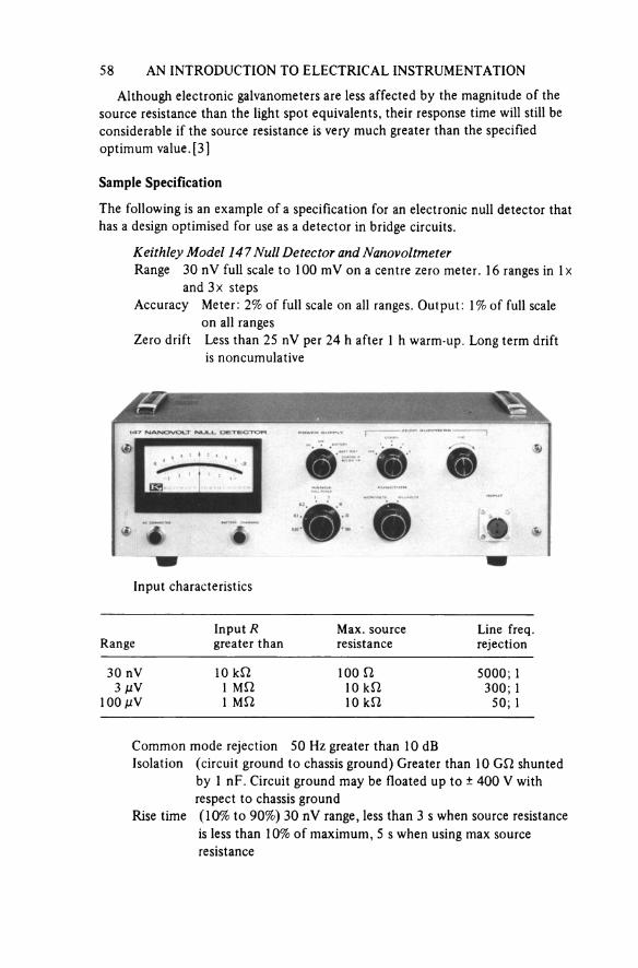
58 AN INTRODUCTION TO ELECTRICAL INSTRUMENTATION
Although electronic galvanometers are less affected by the magnitude of the source resistance than the light spot equivalents, their response time will still be considerable if the source resistance is very much greater than the specified optimum value. [3]
Sample Specification
The following is an example of a specification for an electronic null detector that has a design optimised for use as a detector in bridge circuits.
Keithley Model 147 Null Detector and NanovoltmeterRange 30 nV full scale to 100 mV on a centre zero meter. 16 ranges in 1×
and 3× stepsAccuracy Meter: 2% of full scale on all ranges. Output: 1% of full scale
on all rangesZero drift Less than 25 nV per 24 h after 1 h warm-up. Long term drift
is noncumulative
Input characteristics
RangeInput R greater than
Max. source resistance
Line freq. rejection
30 nV 10 kΩ 100 Ω 5000;13 μV 1 MΩ 10 kΩ 300; 1
100 μV 1 MΩ 10 kΩ 50; 1
Common mode rejection 50 Hz greater than 10 dBIsolation (circuit ground to chassis ground) Greater than 10 GΩ shunted
by 1 nF. Circuit ground may be floated up to ± 400 V with respect to chassis ground
Rise time (10% to 90%) 30 nV range, less than 3 s when source resistance is less than 10% of maximum, 5 s when using max source resistance
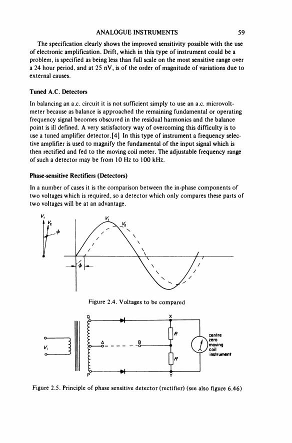
ANALOGUE INSTRUMENTS 59
The specification clearly shows the improved sensitivity possible with the use of electronic amplification. Drift, which in this type of instrument could be a problem, is specified as being less than full scale on the most sensitive range over a 24 hour period, and at 25 nV, is of the order of magnitude of variations due to external causes.
Tuned A.C. Detectors
In balancing an a.c. circuit it is not sufficient simply to use an a.c. microvolt-meter because as balance is approached the remaining fundamental or operating frequency signal becomes obscured in the residual harmonics and the balance point is ill defined. A very satisfactory way of overcoming this difficulty is to use a tuned amplifier detector. [4] In this type of instrument a frequency selec-tive amplifier is used to magnify the fundamental of the input signal which is then rectified and fed to the moving coil meter. The adjustable frequency range of such a detector may be from 10 Hz to 100 kHz.
Phase-sensitive Rectifiers (Detectors)
In a number of cases it is the comparison between the m-phase components of two voltages which is required, so a detector which only compares these parts of two voltages will be at an advantage.
Figure 2.4. Voltages to be compared
Figure 2.5. Principle of phase sensitive detector (rectifier) (see also figure 6.46)
centrezeromovingcoilinstrument
60 AN INTRODUCTION TO ELECTRICAL INSTRUMENTATION
Consider two voltages (figure 2.4) which are of different magnitudes and have a small phase angle between them, it being desired to compare only the com-ponent of V2 in phase with V1.
Let the voltage V1 be applied to a transformer whose secondary winding is centre-tapped and connected to the circuit in figure 2.5. In the positive half-cycle of V1 current will flow round the path XBAQ and the meter would deflect, say, to the right; in the negative half of the cycle current would flow round the path YBAP the meter deflecting to the left; but, providing the frequency of V1 was greater than a few hertz, the resulting meter deflection would be zero, that is the true average over one cycle.
Suppose the link AB is now removed and the voltage V2 is applied between these points. The total voltage driving current around path XBAQ in the positive half-cycle is then the sum of V1 and V2 and the meter needle will deflect further to the right. However, during the negative half-cycle when P is negative to A, B is also negative to A, and the resulting voltage driving current around YBAP is (V1 — V2) and the meter deflection to the left will have been reduced. Thus the average deflection of the meter over a complete cycle will be to the right of the centre zero, the magnitude of this deflection depending on the relative magni-tudes of V1 and V2.
If V2 were antiphase (180° out of phase) with V1 the average deflection for one cycle would be to the left. Thus a detector is obtained which is sensitive to magnitude and capable of comparing the relative phase of a single voltage with a reference.
The circuit discussed above can be used satisfactorily in practice, an alterna-tive being to interchange the reference voltage V1 and the signal voltage V2. A possible addition can be a smoothing capacitor across the moving coil meter.
To reduce the vibration effects on the pointer of the moving coil meter, circuits which yield a full wave rectification are advantageous (see also section 6.6). [5]
2.1.2 Multimeters
The properties of the moving coil movement, in particular its linear scale and good sensitivity (torque to weight ratio), have resulted in its use for the display in multi-range instruments designed either for a single function or for multi-function applications. The latter are more commonly referred to as multimeters. To provide the current ranges in such instruments, shunts could be used, while the voltage ranges may be obtained by the use of series resistors.
Direct Acting Instruments
Direct current ranges
The sensitivity of the movement that is used in a multimeter will be such that full scale deflection would be obtained when a current of (typically) 50 μA
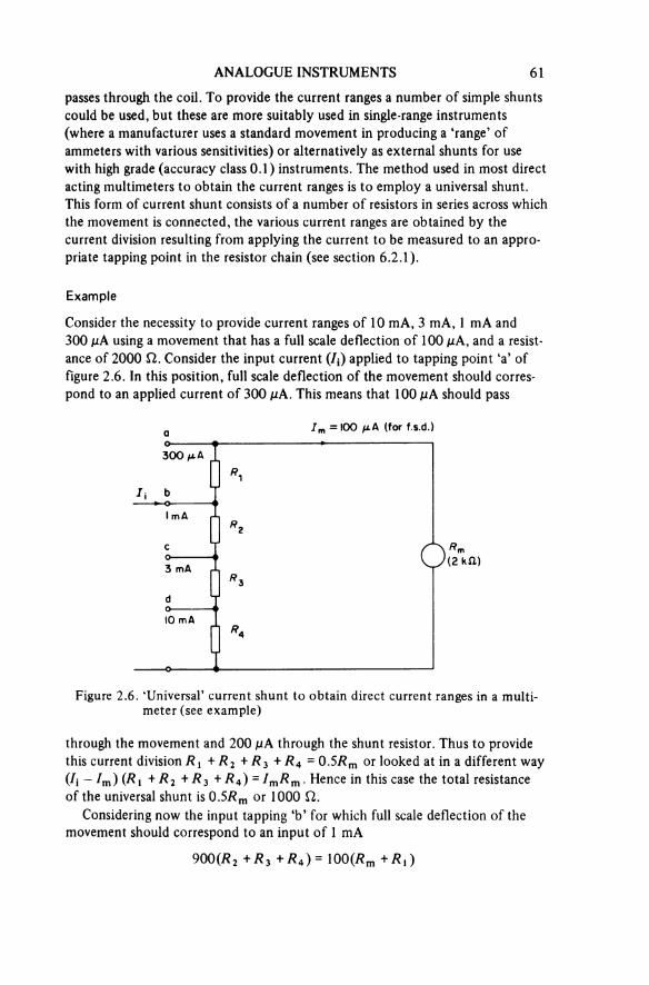
ANALOGUE INSTRUMENTS 61
passes through the coil. To provide the current ranges a number of simple shunts could be used, but these are more suitably used in single-range instruments(where a manufacturer uses a standard movement in producing a ‘range’ of ammeters with various sensitivities) or alternatively as external shunts for use with high grade (accuracy class 0.1) instruments. The method used in most direct acting multimeters to obtain the current ranges is to employ a universal shunt. This form of current shunt consists of a number of resistors in series across whichthe movement is connected, the various current ranges are obtained by the current division resulting from applying the current to be measured to an appro-priate tapping point in the resistor chain (see section 6.2.1).
Example
Consider the necessity to provide current ranges of 10 mA, 3 mA, 1 mA and 300 μA using a movement that has a full scale deflection of 100 μA, and a resist-ance of 2000 Ω. Consider the input current (Ii) applied to tapping point ‘a’ of figure 2.6. In this position, full scale deflection of the movement should corres-pond to an applied current of 300 μA. This means that 100 μA should pass
Figure 2.6. ‘Universal’ current shunt to obtain direct current ranges in a multi meter (see example)
through the movement and 200 μA through the shunt resistor. Thus to provide this current division R1 + R2 + R3 + R4 = 0.5Rm or looked at in a different way (Ii — Im) (R1 + R2 + R3 + R4) =ImRm. Hence in this case the total resistance of the universal shunt is 0.57Rm or 1000 Ω.
Considering now the input tapping ‘b’ for which full scale deflection of the movement should correspond to an input of 1 mA
900(R2 + R3 + R4 ) = 100(Rm + R1)

62 AN INTRODUCTION TO ELECTRICAL INSTRUMENTATION
9(1000 — R1)= 2000 + R1
7000= 10R1
R1 = 700 Ω
and by similar calculations
R2 = 200 Ω
R3 = 70 Ω
R4 = 30 Ω
In a practical multimeter as many as seven or eight direct current ranges are provided by this kind of technique.
Direct voltage ranges
To obtain the multiplicity of voltage ranges required for the production of a ver-satile instrument, one of the two methods shown in figure 2.7 may be used. The chain arrangement shown in figure 2.7a may be claimed to save space, whereas the separate resistor arrangement (as in figure 2.7b) is claimed to have the advantage that should one range be overloaded and the series resistor damagedthe other ranges are unaffected. In either case it is common to refer to the input resistance of the instrument as ‘so many’ Ω/V (for example 10000 Ω/V) so that the total input resistance on the 1 V range would be 10 000 Ω, on the 3 V range 30000 Ω, on the 10 V range 100000 Ω and so on.
This would mean that for the 2000 Ω movement considered in the above example, in the chain arrangement R1 = 10000 — 2000 = 8000 Ω, R2 =20000 Ω, R3 = 70000 Ω, etc., while in the separate resistor arrangement Ra = 8000 Ω, Rb = 28 000 Ω, Rc = 98 000 Ω, and so on. It should be noted that in some manufacturers’ specifications the quantity (Ω/V) is quoted as the sensitivity and while the relationship between the accepted definition (section 1.44) and Ω/V is not immediately obvious, it should be appreciated that Ω/V ≡ V/I/V ≡ V2/I.
Resistance ranges
To utilise the moving coil movement for the measurement of resistance requires the provision of a source. In most multimeters this takes the form of one or more dry cells depending on the magnitude of resistances that can be measured, andthe number of ranges provided. The methods used to perform this type of measurement are illustrated in figure 2.8, and are referred to as:
(a) the series arrangement in which the unknown is connected in series with the meter movement so that full scale deflection will correspond to an unknown resistance of 0 Ω and be on the right hand side of the scale; or
(b) the shunt arrangement in which the unknown is connected in parallel with
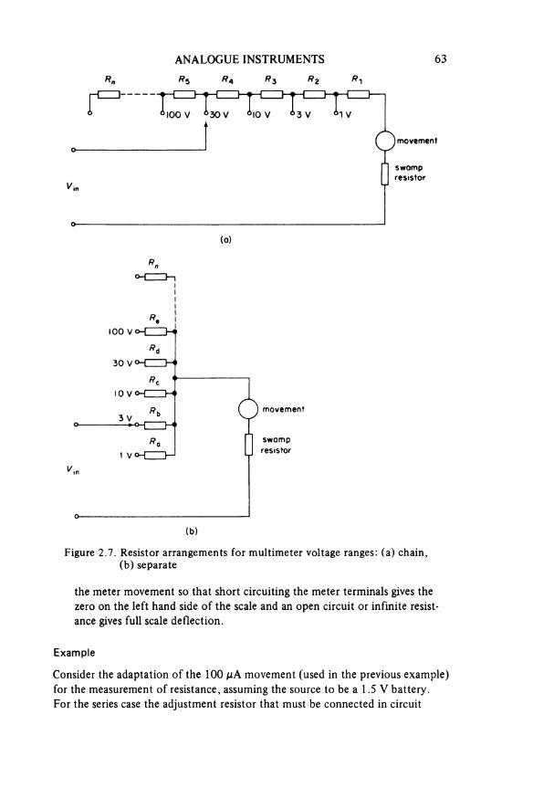
ANALOGUE INSTRUMENTS 63
Figure 2.7. Resistor arrangements for multimeter voltage ranges: (a) chain, (b) separate
(a)
movement
swampresistor
(b)
movement
swampresistor
the meter movement so that short circuiting the meter terminals gives the zero on the left hand side of the scale and an open circuit or infinite resist-ance gives full scale deflection.
Example
Consider the adaptation of the 100 μA movement (used in the previous example) for the measurement of resistance, assuming the source to be a 1.5 V battery.For the series case the adjustment resistor that must be connected in circuit
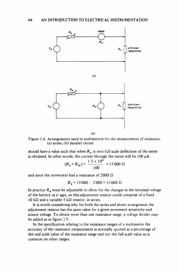
64 AN INTRODUCTION TO ELECTRICAL INSTRUMENTATION
Figure 2.8. Arrangements used in multimeters for the measurement of resistance (a) series, (b) parallel circuit
(a)
unknownresistance
(b)
unknownresistance
should have a value such that when Rx is zero full scale deflection of the meter is obtained. In other words, the current through the meter will be 100 μA.
and since the movement had a resistance of 2000 Ω
In practice Ra must be adjustable to allow for the changes in the terminal voltage of the battery as it ages, so this adjustment resistor could comprise of a fixed 10 kΩ and a variable 5 kΩ resistor, in series.
It is worth considering why for both the series and shunt arrangement the adjustment resistor has the same value for a given movement sensitivity and source voltage. To obtain more than one resistance range, a voltage divider may be added as in figure 2.9.
In the specification relating to the resistance ranges of a multimeter the accuracy of the resistance measurement is normally quoted as a percentage of the mid scale value of the resistance range and not the full scale value as is common on other ranges.
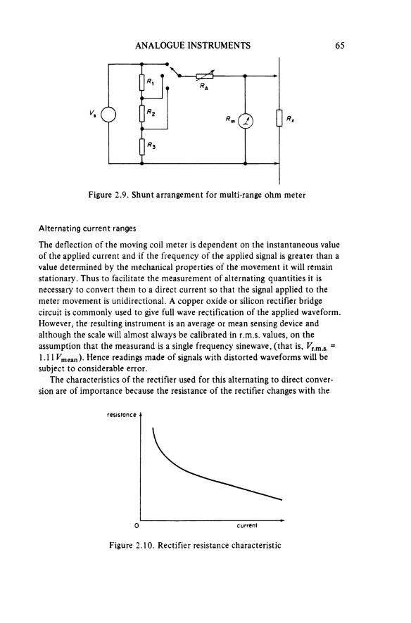
ANALOGUE INSTRUMENTS 65
Figure 2.9. Shunt arrangement for multi-range ohm meter
Alternating current ranges
The deflection of the moving coil meter is dependent on the instantaneous value of the applied current and if the frequency of the applied signal is greater than a value determined by the mechanical properties of the movement it will remain stationary. Thus to facilitate the measurement of alternating quantities it is necessary to convert them to a direct current so that the signal applied to the meter movement is unidirectional. A copper oxide or silicon rectifier bridge circuit is commonly used to give full wave rectification of the applied waveform. However, the resulting instrument is an average or mean sensing device and although the scale will almost always be calibrated in r.m.s. values, on the assumption that the measurand is a single frequency sinewave, (that is, Vr.m.s. = 1.11 Vmean). Hence readings made of signals with distorted waveforms will be subject to considerable error.
The characteristics of the rectifier used for this alternating to direct conver-sion are of importance because the resistance of the rectifier changes with the
Figure 2.10. Rectifier resistance characteristic
resistance
current
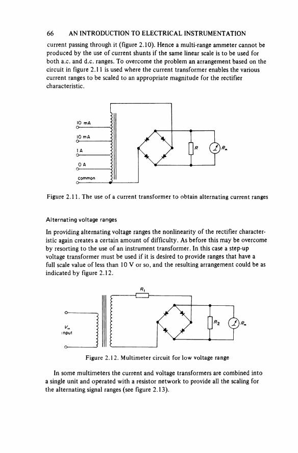
66 AN INTRODUCTION TO ELECTRICAL INSTRUMENTATION
current passing through it (figure 2.10). Hence a multi-range ammeter cannot be produced by the use of current shunts if the same linear scale is to be used for both a.c. and d.c. ranges. To overcome the problem an arrangement based on the circuit in figure 2.11 is used where the current transformer enables the various current ranges to be scaled to an appropriate magnitude for the rectifier characteristic.
Figure 2.11. The use of a current transformer to obtain alternating current ranges
Alternating voltage ranges
In providing alternating voltage ranges the nonlinearity of the rectifier character-istic again creates a certain amount of difficulty. As before this may be overcome by resorting to the use of an instrument transformer. In this case a step-up voltage transformer must be used if it is desired to provide ranges that have a full scale value of less than 10 V or so, and the resulting arrangement could be as indicated by figure 2.12.
Figure 2.12. Multimeter circuit for low voltage range
In some multimeters the current and voltage transformers are combined into a single unit and operated with a resistor network to provide all the scaling for the alternating signal ranges (see figure 2.13).

ANALOGUE INSTRUMENTS 67
Figure 2.13. A circuit arrangement that uses a combined current and voltage transformer
Sample Specification
The specification example is for the instrument which, for many years, has been the name synonymous with multimeters. It is interesting to compare the input resistance of this instrument on the 1000 V ranges with the same quantity on the specifications of digital multimeters (see section 4.2.2).
Avo Model 8 mk5 and TS1 mk2Ranges d.c. volts: 100 mV, 3 V, 10 V, 30 V, 100 V, 300 V, 600 V,
1000 V, 3000 Va.c. volts: 3 V, 10 V, 100 V, 300 V, 600 V, 1000 V, 3000 V d.c. current: 50 μA, 300 μA, 1 mA, 10 mA, 100 mA, 1 A, 10 A a.c. current: 10 mA, 100 mA, 1 A, 10 A
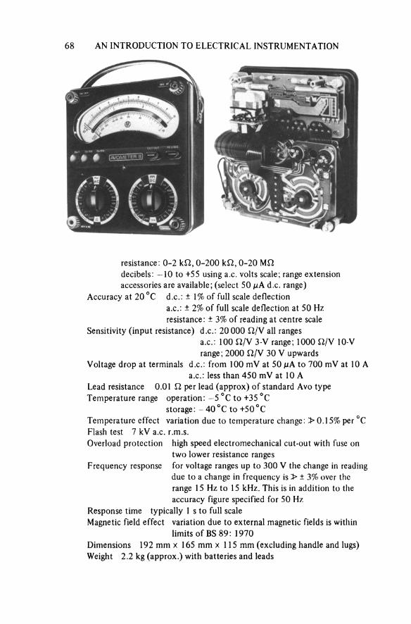
68 AN INTRODUCTION TO ELECTRICAL INSTRUMENTATION
resistance: 0-2 kΩ, 0-200 kΩ, 0-20 MΩdecibels: —10 to +55 using a.c. volts scale; range extensionaccessories are available; (select 50 μA d.c. range)
Accuracy at 20 °C d.c.: ± 1% of full scale deflectiona.c.: ± 2% of full scale deflection at 50 Hz resistance: ± 3% of reading at centre scale
Sensitivity (input resistance) d.c.: 20 000 Ω/V all rangesa.c.: 100 Ω/V 3-V range; 1000 Ω/V 10-V range; 2000 Ω/V 30 V upwards
Voltage drop at terminals d.c.: from 100 mV at 50 μA to 700 mV at 10 A a.c.: less than 450 mV at 10 A
Lead resistance 0.01 Ω per lead (approx) of standard Avo type Temperature range operation: —5 °C to +35 °C
storage: —40°C to +50°CTemperature effect variation due to temperature change : > 0.15% per °C Flash test 7 kV a.c. r.m.s.Overload protection high speed electromechanical cut-out with fuse on
two lower resistance rangesFrequency response for voltage ranges up to 300 V the change in reading
due to a change in frequency is > ± 3% over the range 15 Hz to 15 kHz. This is in addition to the accuracy figure specified for 50 Hz
Response time typically 1 s to full scaleMagnetic field effect variation due to external magnetic fields is within
limits of BS 89: 1970Dimensions 192 mm × 165 mm × 115 mm (excluding handle and lugs) Weight 2.2 kg (approx.) with batteries and leads
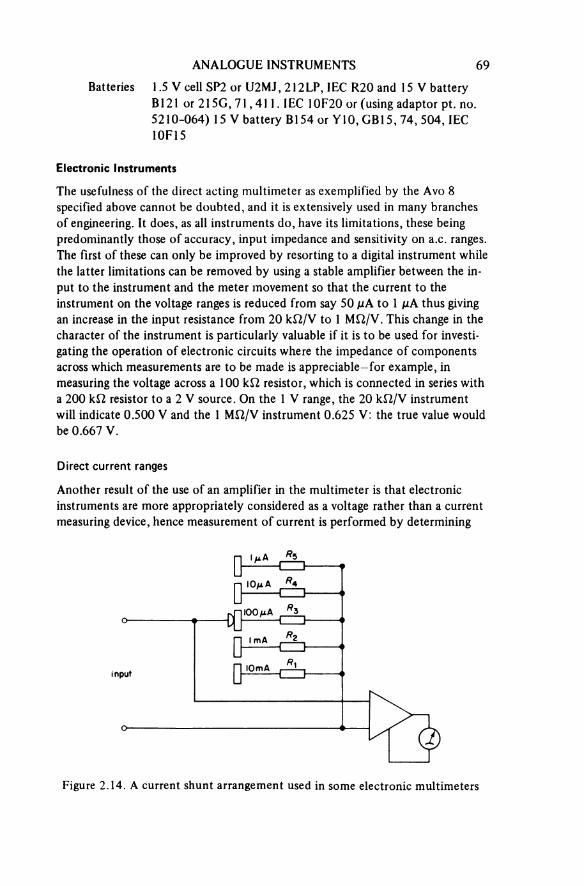
ANALOGUE INSTRUMENTS 69
Batteries 1.5 V cell SP2 or U2MJ, 212LP, IEC R20 and 15 V battery B121 or 215G, 71, 411. IEC 10F20 or (using adaptor pt. no. 5210-064) 15 V battery B154 or Y10, GB15, 74, 504, IEC 10F15
Electronic Instruments
The usefulness of the direct acting multimeter as exemplified by the Avo 8 specified above cannot be doubted, and it is extensively used in many branches of engineering. It does, as all instruments do, have its limitations, these being predominantly those of accuracy, input impedance and sensitivity on a.c. ranges. The first of these can only be improved by resorting to a digital instrument while the latter limitations can be removed by using a stable amplifier between the in-put to the instrument and the meter movement so that the current to the instrument on the voltage ranges is reduced from say 50 μA to 1 μA thus giving an increase in the input resistance from 20 kΩ/V to 1 MΩ/V. This change in the character of the instrument is particularly valuable if it is to be used for investi-gating the operation of electronic circuits where the impedance of components across which measurements are to be made is appreciable—for example, in measuring the voltage across a 100 kΩ resistor, which is connected in series with a 200 kΩ resistor to a 2 V source. On the 1 V range, the 20 kΩ/V instrument will indicate 0.500 V and the 1 MΩ/V instrument 0.625 V: the true value would be 0.667 V.
Direct current ranges
Another result of the use of an amplifier in the multimeter is that electronic instruments are more appropriately considered as a voltage rather than a current measuring device, hence measurement of current is performed by determining
Figure 2.14. A current shunt arrangement used in some electronic multimeters
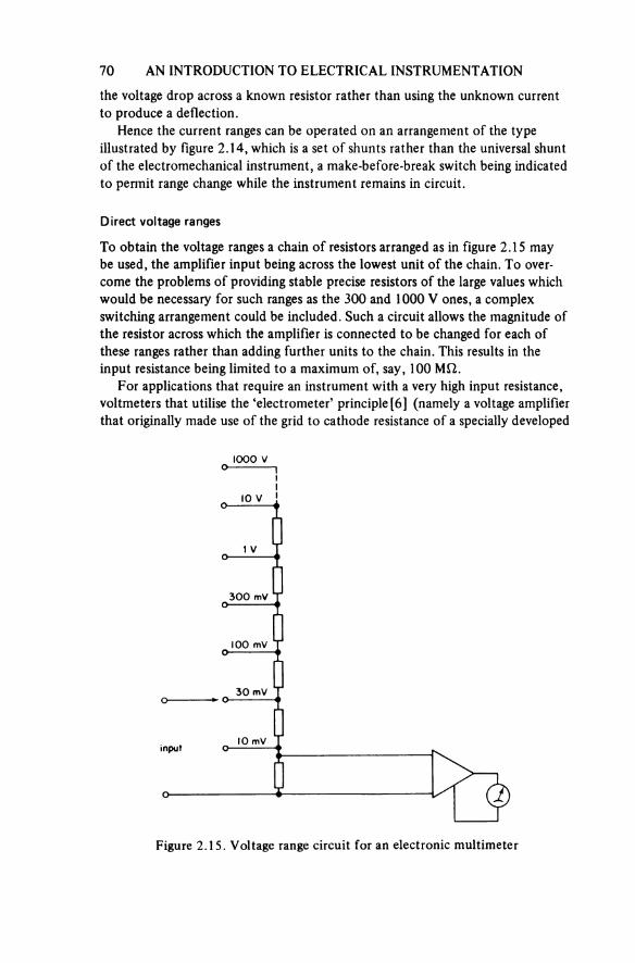
70 AN INTRODUCTION TO ELECTRICAL INSTRUMENTATION
the voltage drop across a known resistor rather than using the unknown current to produce a deflection.
Hence the current ranges can be operated on an arrangement of the type illustrated by figure 2.14, which is a set of shunts rather than the universal shunt of the electromechanical instrument, a make-before-break switch being indicated to permit range change while the instrument remains in circuit.
Direct voltage ranges
To obtain the voltage ranges a chain of resistors arranged as in figure 2.15 may be used, the amplifier input being across the lowest unit of the chain. To over-come the problems of providing stable precise resistors of the large values which would be necessary for such ranges as the 300 and 1000 V ones, a complex switching arrangement could be included. Such a circuit allows the magnitude of the resistor across which the amplifier is connected to be changed for each of these ranges rather than adding further units to the chain. This results in the input resistance being limited to a maximum of, say, 100 MΩ.
For applications that require an instrument with a very high input resistance, voltmeters that utilise the ‘electrometer’ principle [6] (namely a voltage amplifier that originally made use of the grid to cathode resistance of a specially developed
Figure 2.15. Voltage range circuit for an electronic multimeter
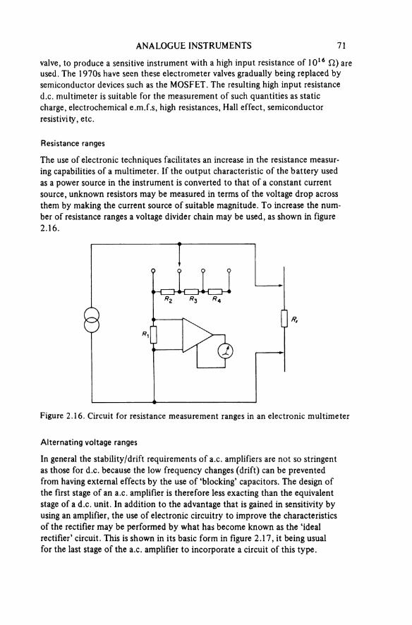
ANALOGUE INSTRUMENTS 71
valve, to produce a sensitive instrument with a high input resistance of 1016 Ω) are used. The 1970s have seen these electrometer valves gradually being replaced by semiconductor devices such as the MOSFET. The resulting high input resistance d.c. multimeter is suitable for the measurement of such quantities as static charge, electrochemical e.m.f.s, high resistances, Hall effect, semiconductor resistivity, etc.
Resistance ranges
The use of electronic techniques facilitates an increase in the resistance measur-ing capabilities of a multimeter. If the output characteristic of the battery usedas a power source in the instrument is converted to that of a constant current source, unknown resistors may be measured in terms of the voltage drop across them by making the current source of suitable magnitude. To increase the num her of resistance ranges a voltage divider chain may be used, as shown in figure 2.16.
Figure 2.16. Circuit for resistance measurement ranges in an electronic multimeter
Alternating voltage ranges
In general the stability/drift requirements of a.c. amplifiers are not so stringent as those for d.c. because the low frequency changes (drift) can be prevented from having external effects by the use of ‘blocking’ capacitors. The design of the first stage of an a.c. amplifier is therefore less exacting than the equivalent stage of a d.c. unit. In addition to the advantage that is gained in sensitivity by using an amplifier, the use of electronic circuitry to improve the characteristics of the rectifier may be performed by what has become known as the ‘ideal rectifier’ circuit. This is shown in its basic form in figure 2.17, it being usual for the last stage of the a.c. amplifier to incorporate a circuit of this type.
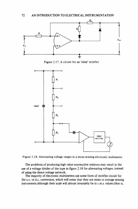
72 AN INTRODUCTION TO ELECTRICAL INSTRUMENTATION
Figure 2.17. A circuit for an ‘ideal’ rectifier
Figure 2.18. Alternating voltage ranges in a mean sensing electronic multimeter
input
idealrectifier
The problems of producing high value nonreactive resistors may result ill the use of a voltage divider of the type in figure 2.18 for alternating voltages, instead of using the direct voltage network.
The majority of electronic multimeters use some form of rectifier circuit for the a.c. to d.c. conversion, which will mean that they are mean or average sensing instruments although their scale will almost invariably be in r.m.s. values (that is,
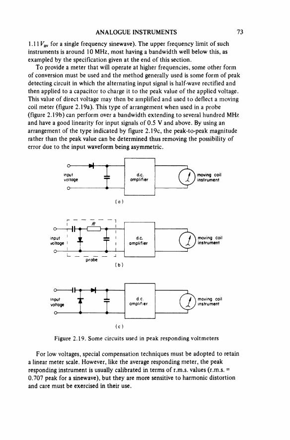
ANALOGUE INSTRUMENTS 73
1.11 Vav for a single frequency sinewave). The upper frequency limit of such instruments is around 10 MHz, most having a bandwidth well below this, as exampled by the specification given at the end of this section.
To provide a meter that will operate at higher frequencies, some other form of conversion must be used and the method generally used is some form of peak detecting circuit in which the alternating input signal is half-wave rectified and then applied to a capacitor to charge it to the peak value of the applied voltage. This value of direct voltage may then be amplified and used to deflect a moving coil meter (figure 2.19a). This type of arrangement when used in a probe (figure 2.19b) can perform over a bandwidth extending to several hundred MHz and have a good linearity for input signals of 0.5 V and above. By using an arrangement of the type indicated by figure 2.19c, the peak-to-peak magnitude rather than the peak value can be determined thus removing the possibility of error due to the input waveform being asymmetric.
Figure 2.19. Some circuits used in peak responding voltmeters
(a)
inputvoltage
d.c.amplifier
moving coil instrument
(b)
inputvoltage
probe
d.c.amplifier
moving coil instrument
(c)
inputvoltage
d.c.amplifier
moving coil instrument
For low voltages, special compensation techniques must be adopted to retain a linear meter scale. However, like the average responding meter, the peak responding instrument is usually calibrated in terms of r.m.s. values (r.m.s. = 0.707 peak for a sinewave), but they are more sensitive to harmonic distortion and care must be exercised in their use.
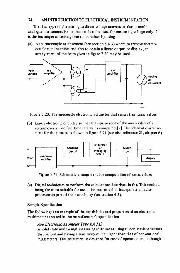
74 AN INTRODUCTION TO ELECTRICAL INSTRUMENTATION
The final type of alternating to direct voltage conversion that is used in analogue instruments is one that tends to be used for measuring voltage only. It is the technique of sensing true r.m.s. values by using
(a) A thermocouple arrangement (see section 5.4.3) where to remove thermo-couple nonlinearities and also to obtain a linear output or display, an arrangement of the form given in figure 2.20 may be used.
Figure 2.20. Thermocouple electronic voltmeter that senses true r.m.s. values
inputvoltage amplifier
d.c.amplifier
movingcoilinstrument
(b) Linear electronic circuitry so that the square root of the mean value of a voltage over a specified time interval is computed. [7] The schematic arrange-ment for the process is shown in figure 2.21 (see also reference 21, chapter 6).
Figure 2.21. Schematic arrangement for computation of r.m.s. values
input precisionrectifier
squaringcircuit
integratoror
averaging over T
squareroot
display
(c) Digital techniques to perform the calculations described in (b). This method being the most suitable for use in instruments that incorporate a micro-processor as part of their capability (see section 4.3).
Sample Specification
The following is an example of the capabilities and properties of an electronic multimeter as stated in the manufacturer’s specification.
Avo Electronic Avometer Type EA 113A solid state multi-range measuring instrument using silicon semiconductors throughout and having a sensitivity much higher than that of conventional multimeters. The instrument is designed for ease of operation and although
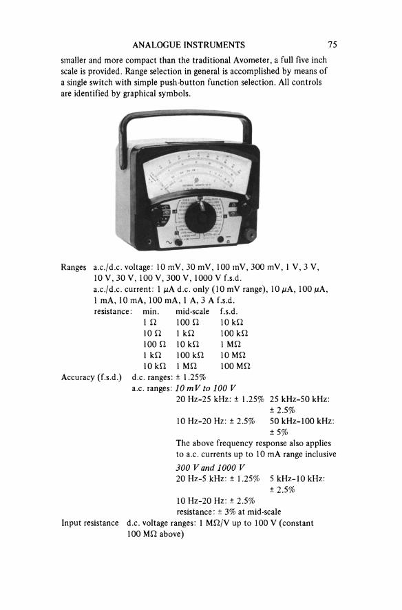
ANALOGUE INSTRUMENTS 75
smaller and more compact than the traditional Avometer, a full five inch scale is provided. Range selection in general is accomplished by means of a single switch with simple push-button function selection. All controls are identified by graphical symbols.
Ranges a.c./d.c. voltage: 10 mV, 30 mV, 100 mV, 300 mV, 1 V, 3 V,10 V, 30 V, 100 V, 300 V, 1000 V f.s.d.a.c./d.c. current: 1 μA d.c. only (10 mV range), 10 μA, 100 μA,1 mA, 10 mA, 100 mA, 1 A, 3 A f.s.d. resistance: min. mid-scale f.s.d.
1 Ω 100 Ω 10 kΩ10 Ω 1 kΩ 100 kΩ100 Ω 10 kΩ 1 MΩ1 kΩ 100 kΩ 10 MΩ10 kΩ 1 MΩ 100 MΩ
Accuracy (f.s.d.) d.c. ranges: ± 1.25%a.c. ranges: 10 mV to 100 V
20 Hz-25 kHz: ± 1.25% 25 kHz-50 kHz:± 2.5%
10 Hz-20 Hz: ± 2.5% 50 kHz-100 kHz:±5%
The above frequency response also applies to a.c. currents up to 10 mA range inclusive 300 V and 1000 V20 Hz-5 kHz: ± 1.25% 5 kHz-10 kHz:
± 2.5%10 Hz-20 Hz: ±2.5% resistance: ± 3% at mid-scale
Input resistance d.c. voltage ranges: 1 MΩ/V up to 100 V (constant 100 MΩ above)
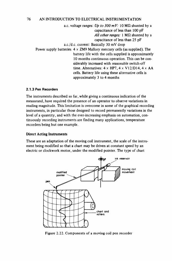
76 AN INTRODUCTION TO ELECTRICAL INSTRUMENTATION
a.c. voltage ranges: Up to 300 mV: 10 MΩ shunted by a capacitance of less than 100 pF All other ranges: 1 MΩ shunted by a capacitance of less than 25 pF
a.c./d.c. current: Basically 30 mV drop Power supply batteries 4 × ZM9 Mallory mercury cells (as supplied). The
battery life with the cells supplied is approximately10 months continuous operation. This can be con-siderably increased with reasonable switch-off time. Alternatives: 4 × HP7, 4 × V12/D14, 4 × AA cells. Battery life using these alternative cells is approximately 3 to 4 months
2.1.3 Pen Recorders
The instruments described so far, while giving a continuous indication of themeasurand, have required the presence of an operator to observe variations in reading magnitude. This limitation is overcome in some of the graphical recording instruments, in particular those designed to record permanently variations in the level of a quantity, and with the ever-increasing emphasis on automation, con-tinuously recording instruments are finding many applications, temperature recorders being but one example.
Direct Acting Instruments
These are an adaptation of the moving coil instrument, the scale of the instru-ment being modified so that a chart may be driven at constant speed by an electric or clockwork motor, under the modified pointer. The type of chart
Figure 2.22. Components of a moving coil pen recorder
ink reservoir
modifiedpointer
moving coil movement
pen
chart and rollers
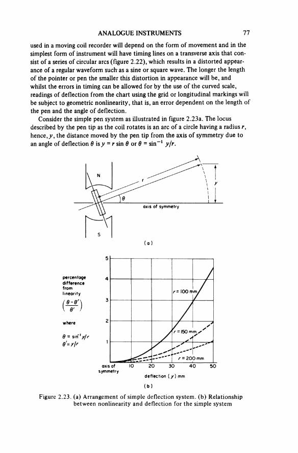
ANALOGUE INSTRUMENTS 77
used in a moving coil recorder will depend on the form of movement and in the simplest form of instrument will have timing lines on a transverse axis that con-sist of a series of circular arcs (figure 2.22), which results in a distorted appear-ance of a regular waveform such as a sine or square wave. The longer the length of the pointer or pen the smaller this distortion in appearance will be, and whilst the errors in timing can be allowed for by the use of the curved scale, readings of deflection from the chart using the grid or longitudinal markings will be subject to geometric nonlinearity, that is, an error dependent on the length of the pen and the angle of deflection.
Consider the simple pen system as illustrated in figure 2.23a. The locus described by the pen tip as the coil rotates is an arc of a circle having a radius r,hence, y, the distance moved by the pen tip from the axis of symmetry due to an angle of deflection θ is y = r sin θ or θ = sin-1 y/r.
Figure 2.23. (a) Arrangement of simple deflection system. (b) Relationship between nonlinearity and deflection for the simple system
(a )
axis of symmetry
(b)
percentagedifferencefromlinearity
axis of symmetry
deflection (y) mm
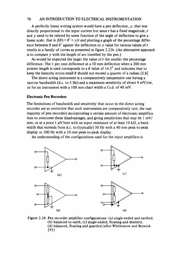
78 AN INTRODUCTION TO ELECTRICAL INSTRUMENTATION
A perfectly linear writing system would have a pen deflection, y, that was directly proportional to the input current but since r has a fixed magnitude, r and y need to be related by some function of the angle of deflection to give a linear scale, that is f(θ) = θ' = y/r and plotting a graph of the percentage differ-ence between θ and θ' against the deflection or y value for various values of r results in a family of curves as presented in figure 2.23b. (An alternative approach is to compare y with the length of arc travelled by the pen.)
As would be expected the larger the value of r the smaller the percentage difference. The 1 per cent difference at a 50 mm deflection when a 200 mm pointer length is used corresponds to a θ value of 14.5° and indicates that to keep the linearity errors small θ should not exceed a quarter of a radian. [5,8]
The direct acting instrument is a comparatively inexpensive one having a narrow bandwidth (d.c. to 5 Hz) and a maximum sensitivity of about 4 mV/cm, or for an instrument with a 100 mm chart width a f.s.d. of 40 mV.
Electronic Pen Recorders
The limitations of bandwidth and sensitivity that occur in the direct acting recorder are so restrictive that such instruments are comparatively rare, the vast majority of pen recorders incorporating a certain amount of electronic amplifica-tion to overcome these disadvantages, and giving sensitivities that may be 1 mV/ mm, or at a price 1 μV/mm with an input resistance of at least 10 kΩ, a band-width that extends from d.c. to (typically) 50 Hz with a 40 mm peak-to-peak display or 100 Hz with a 10 mm peak-to-peak display.
An understanding of the configurations used for the input amplifiers is
Figure 2.24. Pen recorder amplifier configurations: (a) single-ended and earthed, (b) balanced to earth, (c) single-ended, floating and shielded,(d) balanced, floating and guarded (after Whitlemore and Beswick [9])
(a)
(b)
(c)
(d)
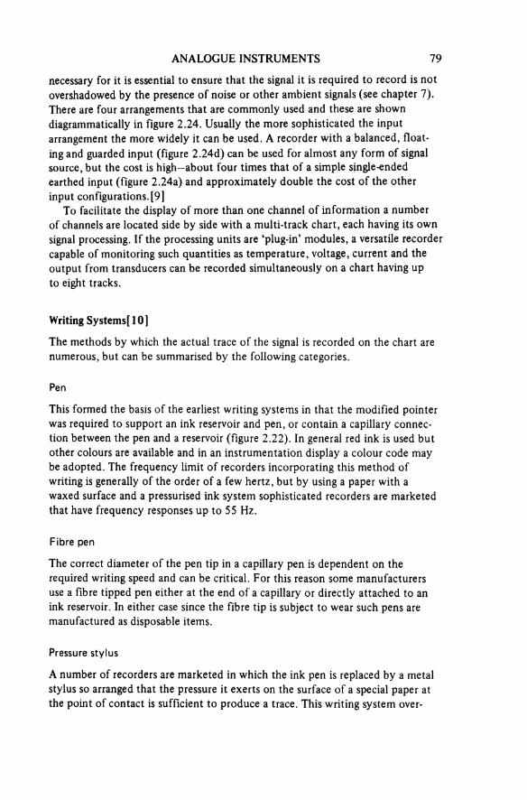
ANALOGUE INSTRUMENTS 79
necessary for it is essential to ensure that the signal it is required to record is not overshadowed by the presence of noise or other ambient signals (see chapter 7). There are four arrangements that are commonly used and these are shown diagrammatically in figure 2.24. Usually the more sophisticated the input arrangement the more widely it can be used. A recorder with a balanced, float-ing and guarded input (figure 2.24d) can be used for almost any form of signal source, but the cost is high—about four times that of a simple single-ended earthed input (figure 2.24a) and approximately double the cost of the other input configurations. [9]
To facilitate the display of more than one channel of information a number of channels are located side by side with a multi-track chart, each having its own signal processing. If the processing units are ‘plug-in’ modules, a versatile recorder capable of monitoring such quantities as temperature, voltage, current and the output from transducers can be recorded simultaneously on a chart having up to eight tracks.
Writing Systems [10]
The methods by which the actual trace of the signal is recorded on the chart are numerous, but can be summarised by the following categories.
Pen
This formed the basis of the earliest writing systems in that the modified pointer was required to support an ink reservoir and pen, or contain a capillary connec-tion between the pen and a reservoir (figure 2.22). In general red ink is used but other colours are available and in an instrumentation display a colour code may be adopted. The frequency limit of recorders incorporating this method of writing is generally of the order of a few hertz, but by using a paper with a waxed surface and a pressurised ink system sophisticated recorders are marketed that have frequency responses up to 55 Hz.
Fibre pen
The correct diameter of the pen tip in a capillary pen is dependent on the required writing speed and can be critical. For this reason some manufacturers use a fibre tipped pen either at the end of a capillary or directly attached to an ink reservoir. In either case since the fibre tip is subject to wear such pens are manufactured as disposable items.
Pressure stylus
A number of recorders are marketed in which the ink pen is replaced by a metal stylus so arranged that the pressure it exerts on the surface of a special paper at the point of contact is sufficient to produce a trace. This writing system over-
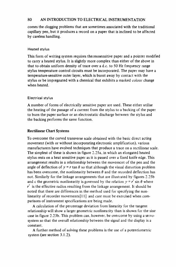
80 AN INTRODUCTION TO ELECTRICAL INSTRUMENTATION
comes the clogging problems that are sometimes associated with the traditional capillary pen, but it produces a record on a paper that is inclined to be affected by careless handling.
Heated stylus
This form of writing system requires thermosensitive paper and a pointer modified to carry a heated stylus. It is slightly more complex than either of the above in that to obtain uniform density of trace over a d.c. to 50 Hz frequency range stylus temperature control circuits must be incorporated. The paper may have a temperature-sensitive outer layer, which is burnt away by contact with the stylus or be impregnated with a chemical that exhibits a marked colour change when heated.
Electrical stylus
A number of forms of electrically sensitive paper are used. These either utilise the heating of the passage of a current from the stylus to a backing of the paper to burn the paper surface or an electrostatic discharge between the stylus and the backing performs the same function.
Rectilinear Chart Systems
To overcome the curved transverse scale obtained with the basic direct acting movement (with or without incorporating electronic amplification), various manufacturers have evolved techniques that produce a trace on a rectilinear scale. The simplest of these is shown in figure 2.25a, in which an elongated heated stylus rests on a heat sensitive paper as it is passed over a fixed knife edge. This arrangement results in a relationship between the movement of the pen and the angle of deflection of y = r tan θ so that although the visual distortion problem has been overcome, the nonlinearity between θ and the recorded deflection has not. Similarly for the linkage arrangements that are illustrated by figures 2.25b and c the geometric nonlinearity is governed by the relation y = r' sin θ where r is the effective radius resulting from the linkage arrangement. It should be noted that there are differences in the method used for specifying the non-linearity of recorder movements [11] and care must be exercised when com-parisons of instrument specifications are being made.
A calculation of the percentage deviation from linearity for the tangent relationship will show a larger geometric nonlinearity than is shown for the sine case in figure 2.23b. This problem can. however, be overcome by using a servo-system so that the overall relationship between the signal and the display is a constant.
A further method of solving these problems is the use of a potentiometric system (see section 3.1.2).
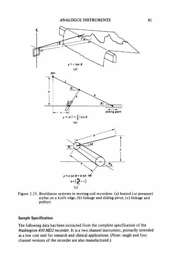
ANALOGUE INSTRUMENTS 81
Figure 2.25. Rectilinear systems in moving coil recorders: (a) heated (or pressure) stylus on a knife edge, (b) linkage and sliding pivot, (c) linkage and pulleys
(a)
(b)
(c)
Sample Specification
The following data has been extracted from the complete specification of the Washington 400 MD2 recorder. It is a two channel instrument, primarily intended as a low cost unit for research and clinical applications. (Note: single and four channel versions of the recorder are also manufactured.)
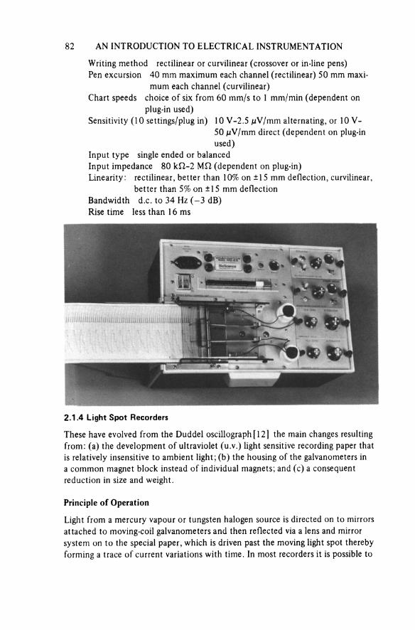
82 AN INTRODUCTION TO ELECTRICAL INSTRUMENTATION
Writing method rectilinear or curvilinear (crossover or in-line pens)Pen excursion 40 mm maximum each channel (rectilinear) 50 mm maxi-
mum each channel (curvilinear)Chart speeds choice of six from 60 mm/s to 1 mm/min (dependent on
plug-in used)Sensitivity (10 settings/plug in) 10 V-2.5 μV/mm alternating, or 10 V-
50 μV/mm direct (dependent on plug-in used)
Input type single ended or balancedInput impedance 80 kΩ-2 MΩ (dependent on plug-in)Linearity: rectilinear, better than 10% on ±15 mm deflection, curvilinear,
better than 5% on ±15 mm deflectionBandwidth d.c. to 34 Hz (—3 dB)Rise time less than 16 ms
2.1.4 Light Spot Recorders
These have evolved from the Duddel oscillograph [12] the main changes resulting from: (a) the development of ultraviolet (u.v.) light sensitive recording paper that is relatively insensitive to ambient light; (b) the housing of the galvanometers in a common magnet block instead of individual magnets; and (c) a consequent reduction in size and weight.
Principle of Operation
Light from a mercury vapour or tungsten halogen source is directed on to mirrors attached to moving-coil galvanometers and then reflected via a lens and mirror system on to the special paper, which is driven past the moving light spot thereby forming a trace of current variations with time. In most recorders it is possible to
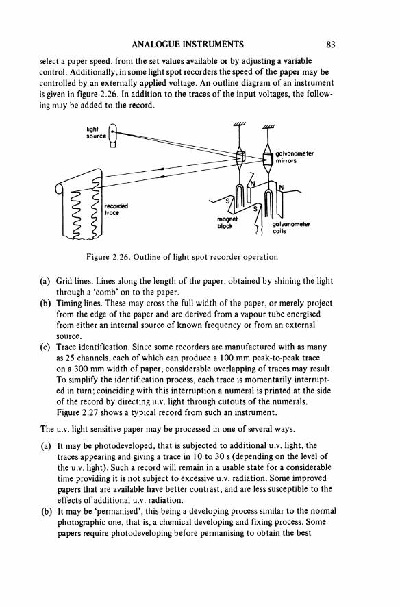
ANALOGUE INSTRUMENTS 83select a paper speed, from the set values available or by adjusting a variable control. Additionally, in some light spot recorders the speed of the paper may be controlled by an externally applied voltage. An outline diagram of an instrument is given in figure 2.26. In addition to the traces of the input voltages, the follow-ing may be added to the record.
Figure 2.26. Outline of light spot recorder operation
lightsource
galvanometermirrors
recordedtrace
magnetblock galvanometer
coils
(a) Grid lines. Lines along the length of the paper, obtained by shining the light through a ‘comb’ on to the paper.
(b) Timing lines. These may cross the full width of the paper, or merely project from the edge of the paper and are derived from a vapour tube energised from either an internal source of known frequency or from an external source.
(c) Trace identification. Since some recorders are manufactured with as many as 25 channels, each of which can produce a 100 mm peak-to-peak trace on a 300 mm width of paper, considerable overlapping of traces may result. To simplify the identification process, each trace is momentarily interrupt-ed in turn; coinciding with this interruption a numeral is printed at the side of the record by directing u.v. light through cutouts of the numerals.Figure 2.27 shows a typical record from such an instrument.
The u.v. light sensitive paper may be processed in one of several ways.
(a) It may be photodeveloped, that is subjected to additional u.v. light, the traces appearing and giving a trace in 10 to 30 s (depending on the level of the u.v. light). Such a record will remain in a usable state for a considerable time providing it is not subject to excessive u.v. radiation. Some improved papers that are available have better contrast, and are less susceptible to the effects of additional u.v. radiation.
(b) It may be ‘permanised’, this being a developing process similar to the normal photographic one, that is, a chemical developing and fixing process. Some papers require photodeveloping before permanising to obtain the best

Figure 2.27. Trace from Bell & Howell 5-137 u.v. recorder fitted with 7-320 fluid damped galvanometers. Kodak paper was used at a speed of 1 m/s
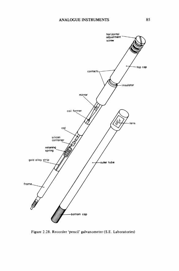
ANALOGUE INSTRUMENTS 85
Figure 2.28. Recorder ‘pencil’ galvanometer (S.E. Laboratories)
horizontaladjustmentscrew
top capcontacts
insulator
mirror
coil former
lens
coil
siliconcontainer
retainingspring
gold alloyouter tube
frame
bottom cap

86 AN INTRODUCTION TO ELECTRICAL INSTRUMENTATION
results, whilst others give the best results if additional exposure to u.v. light is avoided; in consequence, the maker’s instructions for one type of paper must not be considered to apply to all papers.
(c) If a record is obtained with a good contrast by photodeveloping, it ispossible to obtain short lengths of permanent record by some of the photo-copying processes. If this is done, the record will quickly deteriorate (due to the additional exposure to u.v. light). However, once one photocopy has been obtained any number may be made by photocopying the photocopy.
Recorder galvanometers
These are often described as pencil galvanometers (many makes being about 75 mm long and 3 to 6 mm in diameter), and are fitted side by side into the recorder magnet block. As indicated above they are moving coil galvanometers, having a small mass and inertia, a restoring or control torque provided by the ribbon suspension, and a damping torque provided either by electromagnetic means, that is, depending on the resistance of the external circuit, or by internal fluid damping. [13, 14] Figure 2.28 shows the main features of a typical recorder galvanometer in which a moving coil system suspended by a torsion strip is mounted in a cylindrical frame, housed in a cylindrical container. The surface- aluminised mirror attached to the moving coil system, coincides with a lens to focus the light projected on to it. The aluminium wire coil is wound as a loop around two formers, the number of turns determining the galvanometer sensitiv-ity. One end of the coil is taken to the frame and the other to the top insulated section of the container. It should be noted that although one end of the galvano-meter coil is connected to its frame, galvanometers in a common magnet block are electrically isolated from each other.
A complete understanding of the performance of recorder galvanometers is essential in order that true records of waveforms are obtained when using a u.v. recorder. It is indicated above that the u.v. recorder galvanometer is a mass-spring system and, as such, will have a resonant frequency (that is, at some frequency dependent on its moment of inertia, suspension stiffness and mass, it will have a large deflection amplitude for a small input signal). Such a characteristic in a device to obtain records of waveform is extremely undesirable and must be removed by suitably damping the movement of the galvanometer.
Damping
Two methods of damping are common in connection with u.v. recorder galvano-meters, namely: (a) fluid; and (b) electromagnetic damping. The amount of damping used is of vital importance, for if the galvanometer is over-damped its deflection amplitude will decrease as frequency is increased, while an under-damped galvanometer will produce excessive deflections for frequencies near its natural or resonant frequency. Thus a compromise must be made, and curves of
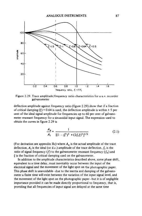
ANALOGUE INSTRUMENTS 87
Figure 2.29. Trace amplitude/frequency ratio characteristics for a u.v. recorder galvanometer
ampl
itude
frequency ratio
deflection amplitude against frequency ratio (figure 2.29) show that if a fraction of critical damping (ζ) = 0.64 is used, the deflection amplitude is within ± 5 per cent of the ideal signal amplitude for frequencies up to 60 per cent of galvano-meter resonant frequency for a sinusoidal input signal. The expression used to obtain the curves in figure 2.29 is
(2.1)
(For derivation see appendix IIc) where Aa is the actual amplitude of the trace deflection, Ai is the ideal (or d.c.) amplitude of the trace deflection, fT is the ratio of signal frequency (f) to the galvanometer resonant frequency (f0) and f is the fraction of critical damping used on the galvanometer.
In addition to the amplitude characteristics described above, some phase shift, equivalent to a time delay, must inevitably occur between the input of the electrical signal and the movement of the light spot on the photographic paper. This phase shift is unavoidable-due to the inertia and damping of the galvano-meter a finite time will exist between the variation of the input signal level, and the movement of the light spot on the photographic paper—but it is of negligible importance provided it can be made directly proportional to frequency, that is, providing that all frequencies of input signal are delayed at the same time

88 AN INTRODUCTION TO ELECTRICAL INSTRUMENTATION
interval. The relationship between phase shift (0) and frequency ratio (fr) may be shown to be
(2.2)
(see appendix IIc).
Curves plotted using this expression (figure 2.30) show that the desired linear relationship is approximately obtained with ζ = 0.64, and this, fortunately, is the fraction of critical damping, which gives the optimum amplitude performance for a recorder galvanometer.
Figure 2.30. Phase shift/frequency ratio characteristics for a u.v, recorder galvanometer
phas
e shi
ft (d
egre
es)
frequency ratio
To illustrate the effect of frequency and ζ value on the phase shift in a record-ing, first consider a 50 Hz signal applied to a galvanometer that has a resonant frequency of 500 Hz and is provided with fractional damping of 0.64. Then from equation 2.2
or
= 0.41 ms or 410 μs
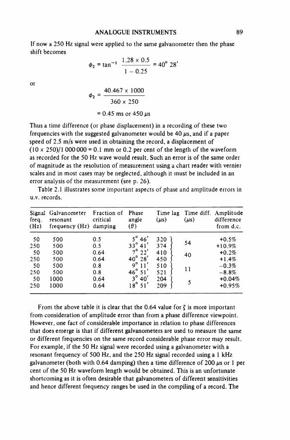
ANALOGUE INSTRUMENTS 89
If now a 250 Hz signal were applied to the same galvanometer then the phase shift becomes
or
Thus a time difference (or phase displacement) in a recording of these two frequencies with the suggested galvanometer would be 40 μs, and if a paper speed of 2.5 m/s were used in obtaining the record, a displacement of (10 × 250)/1 000 000 = 0.1 mm or 0.2 per cent of the length of the waveform as recorded for the 50 Hz wave would result. Such an error is of the same order of magnitude as the resolution of measurement using a chart reader with vernier scales and in most cases may be neglected, although it must be included in an error analysis of the measurement (see p. 26).
Table 2.1 illustrates some important aspects of phase and amplitude errors in u.v. records.
Signalfreq.(Hz)
Galvanometer resonant frequency (Hz)
Fraction ofcriticaldamping
Phaseangle(θ)
Time lag (μs)
Time diff. (μs)
Amplitude difference from d.c.
50 500 0.5 5° 46' 320 54 +0.5%250 500 0.5 33° 41' 374 +10.9%
50 500 0.64 7° 22' 410 40 +0.2%250 500 0.64 40° 28' 450 +1.4%
50 500 0.8 9° 11' 510 11 —0.3%250 500 0.8 46° 51' 521 —8.8%
50 1000 0.64 3° 40' 204 5 +0.04%250 1000 0.64 18° 51' 209 +0.95%
From the above table it is clear that the 0.64 value for ζ is more important from consideration of amplitude error than from a phase difference viewpoint. However, one fact of considerable importance in relation to phase differences that does emerge is that if different galvanometers are used to measure the same or different frequencies on the same record considerable phase error may result. For example, if the 50 Hz signal were recorded using a galvanometer with a resonant frequency of 500 Hz, and the 250 Hz signal recorded using a 1 kHz galvanometer (both with 0.64 damping) then a time difference of 200 μs or 1 per cent of the 50 Hz waveform length would be obtained. This is an unfortunate shortcoming as it is often desirable that galvanometers of different sensitivities and hence different frequency ranges be used in the compiling of a record. The
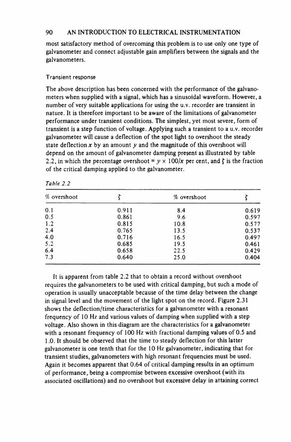
90 AN INTRODUCTION TO ELECTRICAL INSTRUMENTATION
most satisfactory method of overcoming this problem is to use only one type of galvanometer and connect adjustable gain amplifiers between the signals and the galvanometers.
Transient response
The above description has been concerned with the performance of the galvano-meters when supplied with a signal, which has a sinusoidal waveform. However, a number of very suitable applications for using the u.v. recorder are transient in nature. It is therefore important to be aware of the limitations of galvanometer performance under transient conditions. The simplest, yet most severe, form of transient is a step function of voltage. Applying such a transient to a u.v. recorder galvanometer will cause a deflection of the spot light to overshoot the steady state deflection x by an amount y and the magnitude of this overshoot will depend on the amount of galvanometer damping present as illustrated by table 2.2, in which the percentage overshoot = y × 100/x per cent, and ζ is the fraction of the critical damping applied to the galvanometer.
Table 2.2
% overshoot ζ % overshoot ζ
0.1 0.911 8.4 0.6190.5 0.861 9.6 0.5971.2 0.815 10.8 0.5772.4 0.765 13.5 0.5374.0 0.716 16.5 0.4975.2 0.685 19.5 0.4616.4 0.658 22.5 0.4297.3 0.640 25.0 0.404
It is apparent from table 2.2 that to obtain a record without overshoot requires the galvanometers to be used with critical damping, but such a mode of operation is usually unacceptable because of the time delay between the change in signal level and the movement of the light spot on the record. Figure 2.31 shows the deflection/time characteristics for a galvanometer with a resonant frequency of 10 Hz and various values of damping when supplied with a step voltage. Also shown in this diagram are the characteristics for a galvanometer with a resonant frequency of 100 Hz with fractional damping values of 0.5 and 1.0. It should be observed that the time to steady deflection for this latter galvanometer is one tenth that for the 10 Hz galvanometer, indicating that for transient studies, galvanometers with high resonant frequencies must be used. Again it becomes apparent that 0.64 of critical damping results in an optimumof performance, being a compromise between excessive overshoot (with its associated oscillations) and no overshoot but excessive delay in attaining correct
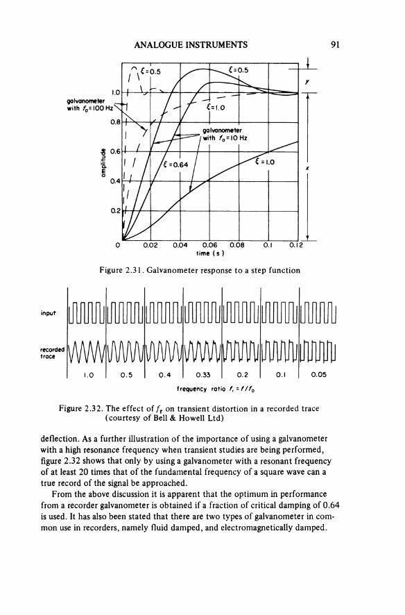
ANALOGUE INSTRUMENTS 91
Figure 2.31. Galvanometer response to a step function
ampl
itude
galvanometer with f0 = 100 Hz
galvanometer with f0 = 10 Hz
time (s)
Figure 2.32. The effect of fr on transient distortion in a recorded trace (courtesy of Bell & Howell Ltd)
input
recordedtrace
frequency ratio
deflection. As a further illustration of the importance of using a galvanometer with a high resonance frequency when transient studies are being performed, figure 2.32 shows that only by using a galvanometer with a resonant frequency of at least 20 times that of the fundamental frequency of a square wave can a true record of the signal be approached.
From the above discussion it is apparent that the optimum in performance from a recorder galvanometer is obtained if a fraction of critical damping of 0.64 is used. It has also been stated that there are two types of galvanometer in com-mon use in recorders, namely fluid damped, and electromagnetically damped.

92 AN INTRODUCTION TO ELECTRICAL INSTRUMENTATION
Fluid damped galvanometers
These derive their damping from a fluid-filled compartment within the galvano-meter casing, their performance being relatively unaffected by the impedance of the external circuit (provided that it is > 20 Ω but < 2000 Ω). However, they may be affected by temperature, and fluid damped galvanometers should there-fore be used in a magnet block which is maintained at constant temperature.
Electromagnetically damped galvanometer
The magnitude of damping applied to the movement of an electromagnetically damped galvanometer is dependent on the resistance of the circuit to which it is connected. For example, a galvanometer connected to a low resistance circuit will be heavily damped, while one connected to a high resistance circuit will be lightly damped. This is best understood by considering a galvanometer not connected to a circuit; if the galvanometer movement is mechanically twisted through an angle and then released, it will swing back to the zero position, generating a voltage at its terminals. If the terminals are connected to a resist-ance, a current will flow causing a force in the galvanometer opposing the change in position of the galvanometer coil, and the smaller the resistance, the larger the current will be, and so too the greater the damping force.
Since the amount of damping has a profound effect on the galvanometer per-formance, the magnitude of resistance that the electromagnetically damped galvanometer ‘sees’ is of importance. Manufacturers of recorder galvanometers therefore specify the magnitude of resistance (RD) that a galvanometer must ‘see’ in order to operate with the optimum of 0.64 of critical damping.
Galvanometer Scaling Circuits
To provide the galvanometer with this required damping resistance (and simultaneously, suitably scale the magnitude of the signal so that a trace of sensible amplitude is produced), it will in general be necessary to adopt one of three procedures.
A source of large amplitude
There will be a peak voltage drop (vg) across the galvanometer, which is equal to the product of the galvanometer’s resistance and the peak of the signal current. When the source has a greater peak amplitude than the voltage across the galvano meter, then a circuit of the form in figure 2.33 can suitably be used for scaling the signal and damping the galvanometer.
The magnitudes of Ra and Rb are evaluated from
(2.3)
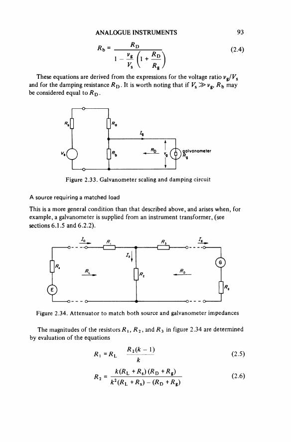
ANALOGUE INSTRUMENTS 93
(2.4)
These equations are derived from the expressions for the voltage ratio vg/Vs and for the damping resistance RD. It is worth noting that if Vs >> vg, Rb may be considered equal to RD.
Figure 2.33. Galvanometer scaling and damping circuit
galvanometer
A source requiring a matched load
This is a more general condition than that described above, and arises when, for example, a galvanometer is supplied from an instrument transformer, (see sections 6.1.5 and 6.2.2).
Figure 2.34. Attenuator to match both source and galvanometer impedances
The magnitudes of the resistors R1, R2, and R3 in figure 2.34 are determined by evaluation of the equations
(2.5)
(2.6)
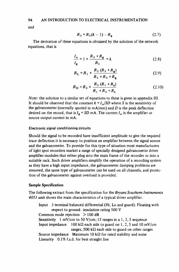
94 AN INTRODUCTION TO ELECTRICAL INSTRUMENTATION
and
(2.7)
The derivation of these equations is obtained by the solution of the network equations, that is
(2.8)
(2.9)
(2.10)
Note: the solution to a similar set of equations to these is given in appendix HI It should be observed that the constant k = IO/SD where S is the sensitivity of the galvanometer (normally quoted in mA/mm) and D is the peak deflection desired on the record, that is Ig = SD mA. The current IO is the amplifier or source output current in mA.
Electronic signal conditioning circuits
Should the signal to be recorded have insufficient amplitude to give the required trace deflection it is necessary to position an amplifier between the signal source and the galvanometer. To provide for this type of situation most manufacturers of light spot recorders market a range of specially designed galvanometer driver amplifier modules that either plug into the main frame of the recorder or into a suitable rack. Such driver amplifiers simplify the operation of a recording system as they have a high input impedance, the galvanometer damping problems are removed, the same type of galvanometer can be used on all channels, and protec-tion of the galvanometer against overload is provided.
Sample Specification
The following extract from the specification for the Bryans Southern Instruments 4051 unit shows the main characteristics of a typical driver amplifier.
Input 3 terminal balanced differential (Hi, Lo and guard). Floating with respect to ground-insulation rating 500 V
Common mode rejection > 100 dBSensitivity 1 mV/cm to 50 V/cm; 15 ranges in a 1, 2, 5 sequence Input impedance 100 kΩ each side to guard on 1, 2, 5 and 10 mV/cm
ranges; 500 kΩ each side to guard on other ranges Source impedance Maximum 10 kΩ for rated stability and noise Linearity 0.1% f.s.d. for best straight line
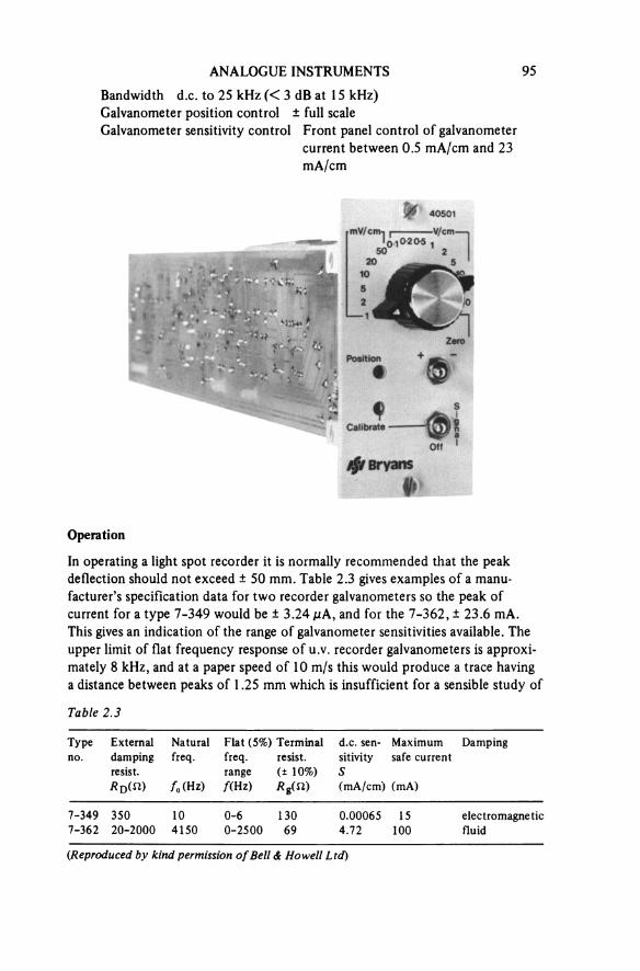
ANALOGUE INSTRUMENTS 95
Bandwidth d.c. to 25 kHz (< 3 dB at 15 kHz)Galvanometer position control ± full scaleGalvanometer sensitivity control Front panel control of galvanometer
current between 0.5 mA/cm and 23 mA/cm
Operation
In operating a light spot recorder it is normally recommended that the peak deflection should not exceed ± 50 mm. Table 2.3 gives examples of a manu-facturer’s specification data for two recorder galvanometers so the peak of current for a type 7-349 would be ± 3.24 μA, and for the 7-362, ± 23.6 mA.This gives an indication of the range of galvanometer sensitivities available. The upper limit of flat frequency response of u.v. recorder galvanometers is approxi-mately 8 kHz, and at a paper speed of 10 m/s this would produce a trace having a distance between peaks of 1.25 mm which is insufficient for a sensible study of
Table 2.3
Typeno.
Externaldampingresist.Rd (ω )
Naturalfreq.
f0(Hz)
Flat (5%) freq. range f(Hz )
Terminalresist.(± 10%) Rg(Ω)
d.c. sen-sitivity s(mA/cm)
Maximum safe current
(mA)
Damping
7-349 35O 10 0-6 130 0.00065 15 electromagnetic7-362 20-2000 4150 0-2500 69 4.72 100 fluid
(Reproduced by kind permission of Bell & Howell Ltd)
96 AN INTRODUCTION TO ELECTRICAL INSTRUMENTATION
the waveform. These high frequency galvanometers are however vital in transient studies. The limit of frequency to which a u.v. recorder can be used will depend on the magnitude of the displayed trace, and the paper speed, but as a guide a trace with a peak-to-peak deflection of 5 cm is recognisable as a sinewave pro-viding the length of one cycle is greater than 10 mm.
Galvanometer Selection Factors
In selecting a galvanometer it is important to choose one to comply with the following.
(a) A flat frequency range in excess of the frequency of the highest harmonic of importance in the a.c. signal (a low frequency galvanometer may be used asa low pass filter to remove unwanted ‘noise’ from a signal). Alternatively if transients are being studied, the galvanometer’s resonant frequency should be at least 20 times that of the ‘fundamental’ frequency of the transient, thus demonstrating the necessity for the manufacture of galvanometers with high resonant frequencies, for example a galvanometer with an f0 of at least 1000 Hz should be used when recording the effects of a step change in the load on a 50 Hz supply.
(b) A sufficiency of sensitivity so that a satisfactory magnitude of deflection on the record may be obtained, it being appreciated that the larger the trace the smaller the error due to the uncertainty in measuring deflections on the trace.
The final selection of a galvanometer will invariably be a compromise between the two requirements given above, and the limitations of the circuit to which the galvanometer is to be connected. From the specification data in table 2.3 it is apparent that the sensitivity of a galvanometer is inversely proportional to the flat frequency response, and a galvanometer with a sufficiency of sensitivity and frequency range may be unobtainable. The sensitivity problem is, of course, overcome by using galvanometer driver amplifiers which unfortunately add to the cost of the system.
Calibration
Having selected a suitable galvanometer and signal conditioning circuitry, it is sensible to calibrate the complete system before using it to take measurements. The most satisfactory method of performing such a calibration is to replace the measurand by a signal of known amplitude and monitor the resulting trace deflection. If several levels of known or calibrating signal are used to obtain short lengths of trace, a mean signal-to-deflection constant of calibration may be derived. This procedure must be followed for each galvanometer and its match-ing circuit, for each application of the recorder.
ANALOGUE INSTRUMENTS 97
Applications
It has already been indicated that the range of frequencies over which the light spot recorder can generally be used is for alternating signals having a fundamental frequency from zero up to 400 or 500 Hz depending on the paper speeds avail-able on the recorder being used. The recording of higher frequencies is possible on the few recorders with very high (10 m/s) paper speed. The application of the recorder is suitable in any situation where a trace of a waveform is required, and resolves to the problem of scaling the signal to be measured to a suitable magni-tude, while ensuring that the matching requirements of a particular galvanometer are met.
The commonest method of scaling voltages is to use a resistance divider or to use a galvanometer driver amplifier with a suitable sensitivity selector.
Current waveforms are obtained by recording the voltage drop across a known resistance. Having recorded traces of voltage and/or current waveform it is possible to determine their frequency and any phase differences between traces (using the known time scale projected on to the record by the time markers), remembering that the resolution of reading is of the order of 0.3 to 0.5 mm and corrections for unequal galvanometer phase shift must be included.
Typical applications of the u.v. recorder are in recording regulation transients of generators, the performance of control systems, the outputs of transducers, and the magnitudes of low frequency signals which cannot be measured by Pointer instruments. The development of PLZT electro-optic materials [30, 31] has led to the marketing (in 1980), by Bell and Howell Ltd, of a ‘galvanomter- less’ light spot recorder, which is capable of simultaneously monitoring 28 sinewave signals of frequencies up to 5 kHz.
2.2 THE ELECTRODYNAMIC INSTRUMENT
2.2.1 Principle
This instrument, often termed a dynamometer, relies for its deflecting torque on the interaction of the magnetic fields produced by a pair of fixed air-cored coils and a third air-cored coil capable of angular movement and suspended within the fixed coils (figure 2.35). The deflecting torque produced within the instrument is proportional to the product of the current in the moving coil (Im) and that in the fixed coil (If), that is, torque a ImIf.Note: This is an approximation, since the torque is also dependent on the initial angle between the axes of the coils. [12] Also, in some instruments, known as ferrodynamic instruments, the electrodynamic effect is increased by the presence of ferromagnetic material.
This instrument is suitable for the measurement of direct and alternating current, voltage and power. If no iron is present within the coil system the magnetic fields are weak and to obtain sufficient deflecting torque requires coils of either a large number of turns or capable of carrying a moderate current. The control torque is derived from a helical spring and the movement damped by air resistance.
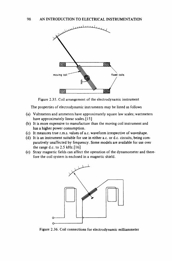
98 AN INTRODUCTION TO ELECTRICAL INSTRUMENTATION
Figure 2.35. Coil arrangement of the electrodynamic instrument
moving coil fixed coils
The properties of electrodynamic instruments may be listed as follows
(a) Voltmeters and ammeters have approximately square law scales; wattmeters have approximately linear scales. [15]
(b) It is more expensive to manufacture than the moving coil instrument and has a higher power consumption.
(c) It measures true r.m.s. values of a.c. waveform irrespective of waveshape.(d) It is an instrument suitable for use in either a.c. or d.c. circuits, being com-
paratively unaffected by frequency. Some models are available for use over the range d.c. to 2.5 kHz. [16]
(e) Stray magnetic fields can affect the operation of the dynamometer and there fore the coil system is enclosed in a magnetic shield.
Figure 2.36. Coil connections for electrodynamic milliammeter

ANALOGUE INSTRUMENTS 99
2.2.2 Application
Ammeter and Voltmeter
For the measurement of small currents (5 to 100 mA) the instrument would be arranged to have the fixed and moving coils connected in series (figure 2.36). To convert such an instrument to a voltmeter simply requires the addition of a suit-able series resistance. For measuring larger currents (up to 20 A) it becomes impracticable to pass the full value of current through the moving coil, so this is then shunted by low resistance (figure 2.37). This arrangement could be used for still larger currents, but in most cases it is better to use a current transformer (see section 6.2.2) and an ammeter with a f.s.d. of 5 A.
Figure 2.37. Coil connections for electrodynamic ammeter
Wattmeter
For many years the electrodynamometer has been the instrument normally used for measuring power in a.c. circuits. The digital wattmeter is beginning to supplant it but the cost of replacement means that for some years the electro-dynamometer will continue to be used at supply line frequencies for power measurement.
Since deflection in the dynamometer is proportional to the product of the two currents, it is usual to make the current in the moving coil proportional to the circuit voltage and to make the fixed coils carry the load current (figure 2.38). Depending on the relative magnitudes of the currents in the fixed and moving coils the wattmeter should be connected as in figure 2.39a or figure 2.39c so that the minimum error in the measurement of power in a load is made. In figure 2.39a the current coil will produce a force proportional to the load current only, but the voltage coil (moving) will produce a force proportional to the volt-age across the load plus the current coil. However, in figure 2.39c the current coil (fixed) produces a force proportional to the sum of the currents in the load and in the voltage coil, while the voltage coil produces a force proportional to the voltage across the load. In either case correction for the error may be made but the wattmeter should always be connected to indicate with minimum error.
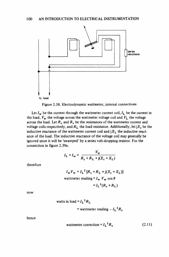
100 AN INTRODUCTION TO ELECTRICAL INSTRUMENTATION
Figure 2.38. Electrodynamic wattmeter, internal connections
seriesresistance
to load
Let IW be the current through the wattmeter current coil, IL be the current in the load, Vw the voltage across the wattmeter voltage coil and VL the voltage across the load. Let Rc and Rv be the resistances of the wattmeter current and voltage coils respectively, and RL the load resistance. Additionally, let jXc be the inductive reactance of the wattmeter current coil and jXL the inductive react-ance of the load. The inductive reactance of the voltage coil may generally be ignored since it will be ‘swamped’ by a series volt-dropping resistor. For the connection in figure 2.39a.
therefore
wattmeter reading =
now
watts in load =
= wattmeter reading — IL2RC
hence
wattmeter correction = IL2Rc (2.11)
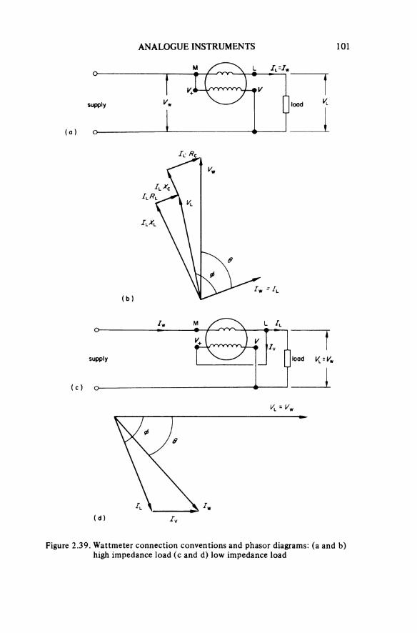
ANALOGUE INSTRUMENTS 101
Figure 2.39. Wattmeter connection conventions and phasor diagrams: (a and b) high impedance load (c and d) low impedance load
(a)
supply load
(b)
(c)
supply load
(d)
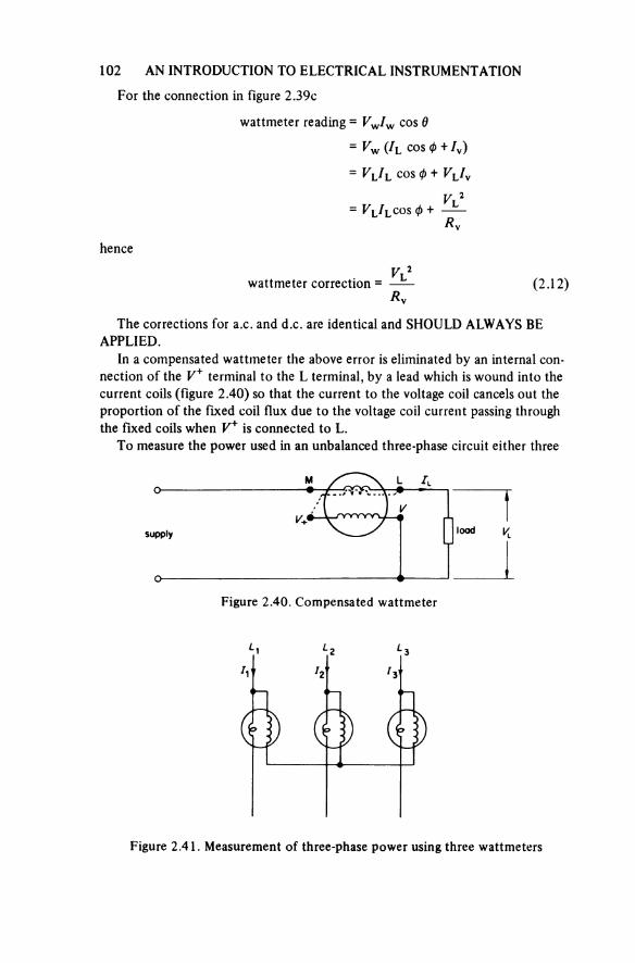
1 02 AN INTRODUCTION TO ELECTRICAL INSTRUMENTATION
For the connection in figure 2.39c
wattmeter reading =
hence
wattmeter correction = (2.12)
The corrections for a.c. and d.c. are identical and SHOULD ALWAYS BE APPLIED.
In a compensated wattmeter the above error is eliminated by an internal con-nection of the V+ terminal to the L terminal, by a lead which is wound into the current coils (figure 2.40) so that the current to the voltage coil cancels out the proportion of the fixed coil flux due to the voltage coil current passing through the fixed coils when V+ is connected to L.
To measure the power used in an unbalanced three-phase circuit either three
Figure 2.40. Compensated wattmeter
supply load
Figure 2.41. Measurement of three-phase power using three wattmeters
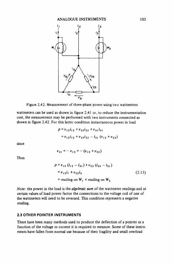
ANALOGUE INSTRUMENTS 103
Figure 2.42. Measurement of three-phase power using two wattmeters
wattmeters can be used as shown in figure 2.41 or, to reduce the instrumentation cost, the measurement may be performed with two instruments connected as shown in figure 2.42. For this latter condition instantaneous power in load
since
Thus
(2.13)
reading on W1 + reading on W2
Note: the power in the load is the algebraic sum of the wattmeter readings and at certain values of load power factor the connections to the voltage coil of one of the wattmeters will need to be reversed. This condition represents a negative reading.
2.3 OTHER POINTER INSTRUMENTS
There have been many methods used to produce the deflection of a pointer as a function of the voltage or current it is required to measure. Some of these instru-ments have fallen from normal use because of their fragility and small overload
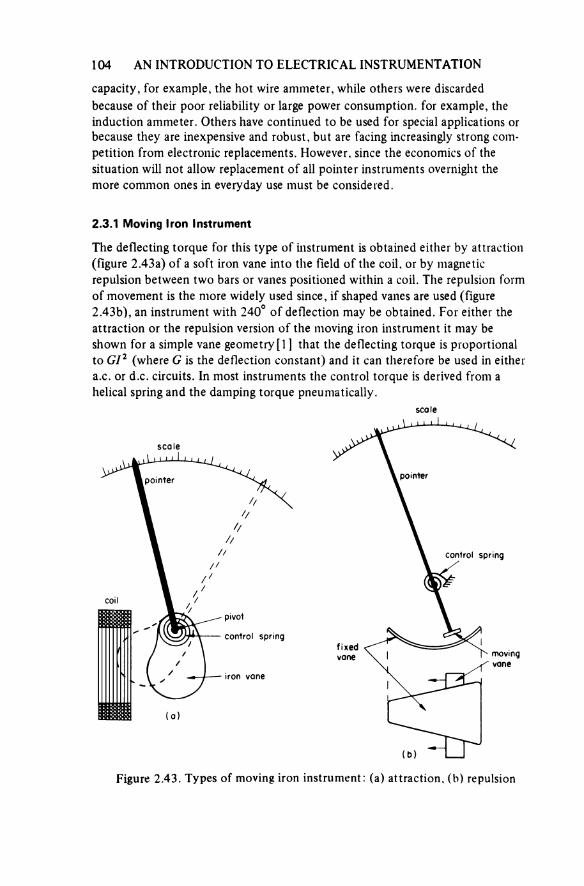
104 AN INTRODUCTION TO ELECTRICAL INSTRUMENTATION
capacity, for example, the hot wire ammeter, while others were discarded because of their poor reliability or large power consumption, for example, the induction ammeter. Others have continued to be used for special applications or because they are inexpensive and robust, but are facing increasingly strong com-petition from electronic replacements. However, since the economics of the situation will not allow replacement of all pointer instruments overnight the more common ones in everyday use must be considered.
2.3.1 Moving Iron Instrument
The deflecting torque for this type of instrument is obtained either by attraction (figure 2.43a) of a soft iron vane into the field of the coil, or by magnetic repulsion between two bars or vanes positioned within a coil. The repulsion form of movement is the more widely used since, if shaped vanes are used (figure 2.43b), an instrument with 240° of deflection may be obtained. For either the attraction or the repulsion version of the moving iron instrument it may be shown for a simple vane geometry [1] that the deflecting torque is proportional to GI2 (where G is the deflection constant) and it can therefore be used in either a.c. or d.c. circuits. In most instruments the control torque is derived from a helical spring and the damping torque pneumatically.
Figure 2.43. Types of moving iron instrument: (a) attraction, (b) repulsion
(a)
scale
pointer
coil
pivot
control spring
iron vane
(b)
scale
pointer
control spring
fixedvane moving
vane
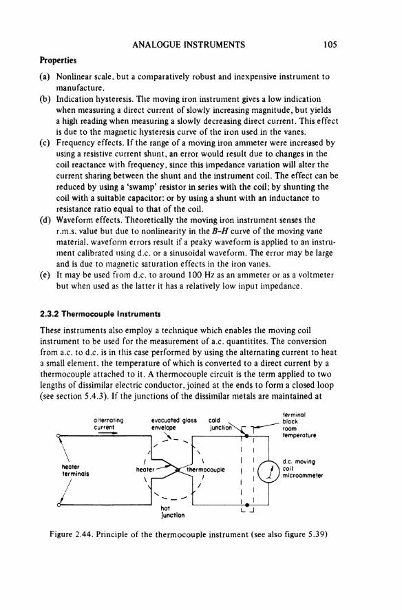
ANALOGUE INSTRUMENTS 105Properties
(a) Nonlinear scale, but a comparatively robust and inexpensive instrument to manufacture.
(b) Indication hysteresis. The moving iron instrument gives a low indication when measuring a direct current of slowly increasing magnitude, but yieldsa high reading when measuring a slowly decreasing direct current. This effect is due to the magnetic hysteresis curve of the iron used in the vanes.
(c) Frequency effects. If the range of a moving iron ammeter were increased by using a resistive current shunt, an error would result due to changes in the coil reactance with frequency, since this impedance variation will alter the current sharing between the shunt and the instrument coil. The effect can be reduced by using a ‘swamp’ resistor in series with the coil; by shunting the coil with a suitable capacitor; or by using a shunt with an inductance to resistance ratio equal to that of the coil.
(d) Waveform effects. Theoretically the moving iron instrument senses the r.m.s. value but due to nonlinearity in the B-H curve of the moving vane material, waveform errors result if a peaky waveform is applied to an instru-ment calibrated using d.c. or a sinusoidal waveform. The error may be large and is due to magnetic saturation effects in the iron vanes.
(e) It may be used from d.c. to around 100 Hz as an ammeter or as a voltmeter but when used as the latter it has a relatively low input impedance.
2.3.2 Thermocouple Instruments
These instruments also employ a technique which enables the moving coil instrument to be used for the measurement of a.c. quantities. The conversion from a.c. to d.c. is in this case performed by using the alternating current to heat a small element, the temperature of which is converted to a direct current by a thermocouple attached to it. A thermocouple circuit is the term applied to two lengths of dissimilar electric conductor, joined at the ends to form a closed loop (see section 5.4.3). If the junctions of the dissimilar metals are maintained at
Figure 2.44. Principle of the thermocouple instrument (see also figure 5.39)
alternatingcurrent
heaterterminals
evacuated glass envelope
heater
hotJunction
coldjunction
thermocouple
terminalblockroomtemperature
d.c. moving coilmicroammeter
106 AN INTRODUCTION TO ELECTRICAL INSTRUMENTATION
different temperatures a current which may be measured by a sensitive moving coil instrument flows in the loop. Since this current is approximately proportional to the temperature difference between the hot and cold junctions, and if the cold junction is maintained at a constant temperature, the current in the moving coil instrument will be proportional to the temperature of the heater, which in turnis dependent on the r.m.s. or heating effect of the current in the heater. In many instruments of this type the terminals of the moving coil instrument will form the cold junction as in figure 2.44, and will be subject to the variations in ambient temperature. However, these variations are generally insignificant (say 10 to 25 °C) compared with the temperatures of the heater which may be of the order of 1000 °C for the heater current corresponding to full scale deflection.
It should be noted that if a thermocouple is being used to measure the tem-perature of an object it is often more satisfactory to open circuit the dissimilar metal loop and measure, using an instrument with a high input impedance, the voltage that appears across the open circuit.
Properties
(a) Measures true r.m.s. value of an alternating current irrespective of its waveshape.
(b) Wide frequency range. May be used from d.c. up to the megahertz range, but pointer vibrations may be experienced at low frequencies (less than 10 Hz).
(c) Fragile, having a low overload capacity. Normally exceeding a 50 per cent overload will melt the heater element.
(d) May have a higher impedance than moving-iron or electrodynamic instruments.
(e) Nonlinear scale. The temperature of the heater will be proportional to current squared, also the temperature/voltage characteristic of a thermo-couple is slightly nonlinear.
Applications
The main use is as an r.m.s. sensing milliammeter, and consequently when used with a series resistor it becomes a voltmeter. However, if it is intended that the instrument shall be used at high frequencies, it is important for the series resist-ance to be ‘pure’, that is, nonreactive, or its impedance, and hence the current in the heater will change with frequency (see section 7.2.2).
The thermocouple instrument is one of the few methods of determining the true r.m.s. value of an a.c. waveform (see p. 74). For precise measurement, the heater/hot junction and the cold junction are situated in an evacuated container and the d.c. output measured by a good quality digital voltmeter or potentio-meter (see pp. 147 and 210). By this technique the a.c. to d.c. conversion

ANALOGUE INSTRUMENTS 107
may be performed with an error of less than 0.05 per cent over a range of frequencies from 20 Hz to 1 MHz; it also applies for higher frequencies (50 MHz), but with reduced accuracy. Reference 17 describes the construction of a thermal converter with a sensitivity of 1 part in 106.
2.3.3 Electrostatic Instruments
This type of instrument depends on the forces set up between charged plates to obtain a deflecting torque. The total force is proportional to the product of the charges on the plates and since the charge on a conducting plate is proportional to voltage the deflecting torque of an electrostatic instrument is proportional toV2. The deflecting torque is derived from the force acting on a moving vane that is suspended in fixed quadrant-shaped boxes, as in figure 2.45. The control torque is derived from a spring system and damping is usually pneumatic.
Figure 2.45. Electrostatic voltmeter vane arrangement
movingvane
fixedvanes
Properties
(a) Measures true r.m.s. values, because the deflecting torque is proportional to V2 and can therefore be used as a transfer instrument.
(b) Used for d.c., and for a.c. where it constitutes a capacitive load, thus limiting its general application to frequencies below 100 Hz. However, it may be used to radio frequencies where it can be employed for aerial tuning, although its use for applications other than measuring power frequency high voltages is now comparatively rare.
(c) It is a comparatively fragile and expensive instrument.(d) A high input impedance instrument, for direct voltages its input resistance
being that of the leakage path through the insulation.(e) Nonlinear scale, approximately square law, but this may be modified by the
shape of the vanes.
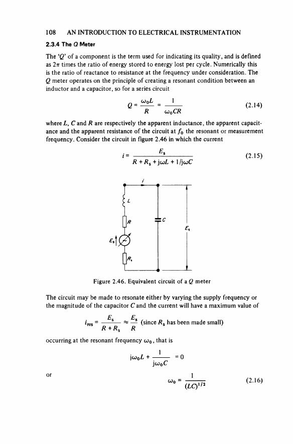
108 AN INTRODUCTION TO ELECTRICAL INSTRUMENTATION
2.3.4 The Q Meter
The ‘Q’ of a component is the term used for indicating its quality, and is defined as 2π times the ratio of energy stored to energy lost per cycle. Numerically thisis the ratio of reactance to resistance at the frequency under consideration. The Q meter operates on the principle of creating a resonant condition between an inductor and a capacitor, so for a series circuit
(2.14)
where L, C and R are respectively the apparent inductance, the apparent capacit-ance and the apparent resistance of the circuit at f0 the resonant or measurementfrequency. Consider the circuit in figure 2.46 in which the current
(2.15)
Figure 2.46. Equivalent circuit of a Q meter
The circuit may be made to resonate either by varying the supply frequency or the magnitude of the capacitor C and the current will have a maximum value of
(since Rs has been made small)
occurring at the resonant frequency ωo, that is
or(2.16)
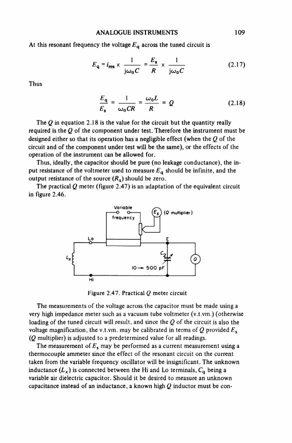
ANALOGUE INSTRUMENTS 109
At this resonant frequency the voltage Eq across the tuned circuit is
(2.17)
Thus
(2.18)
The Q in equation 2.18 is the value for the circuit but the quantity really required is the Q of the component under test. Therefore the instrument must be designed either so that its operation has a negligible effect (when the Q of the circuit and of the component under test will be the same), or the effects of the operation of the instrument can be allowed for.
Thus, ideally, the capacitor should be pure (no leakage conductance), the in-put resistance of the voltmeter used to measure Eq should be infinite, and the output resistance of the source (Rs) should be zero.
The practical Q meter (figure 2.47) is an adaptation of the equivalent circuit in figure 2.46.
Figure 2.47. Practical Q meter circuit
Variable
frequency(Q multiplier)
The measurements of the voltage across the capacitor must be made using a very high impedance meter such as a vacuum tube voltmeter (v.t.vm.) (otherwise loading of the tuned circuit will result, and since the Q of the circuit is also the voltage magnification, the v.t.vm. may be calibrated in terms of Q provided Es (Q multiplier) is adjusted to a predetermined value for all readings.
The measurement of Es may be performed as a current measurement using a thermocouple ammeter since the effect of the resonant circuit on the current taken from the variable frequency oscillator will be insignificant. The unknown inductance (Lx) is connected between the Hi and Lo terminals, Cq being a variable air dielectric capacitor. Should it be desired to measure an unknown capacitance instead of an inductance, a known high Q inductor must be con-
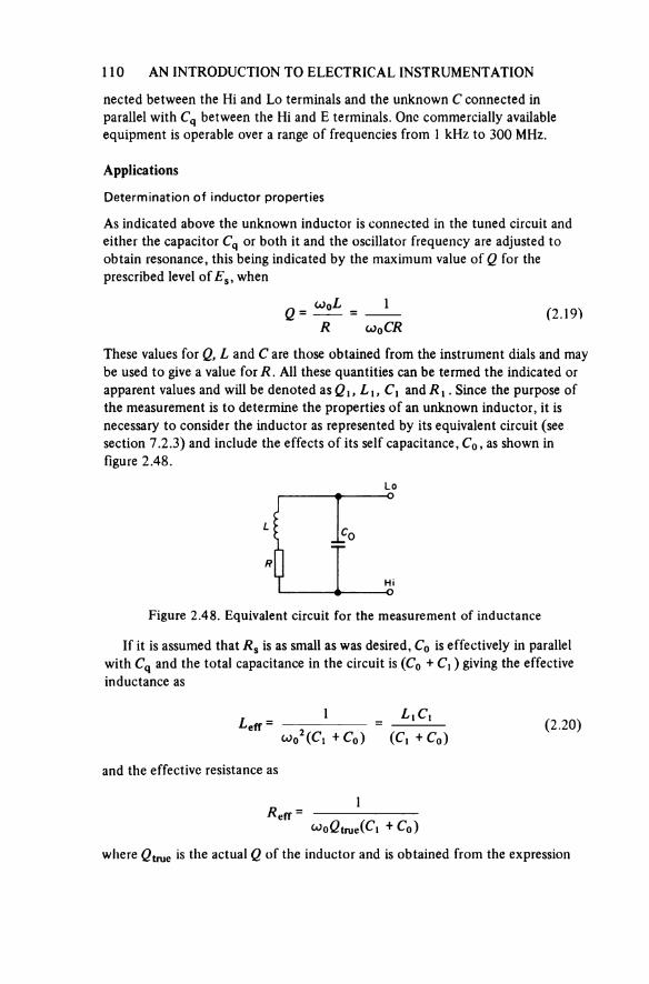
110 AN INTRODUCTION TO ELECTRICAL INSTRUMENTATION
nected between the Hi and Lo terminals and the unknown C connected in parallel with Cq between the Hi and E terminals. One commercially available equipment is operable over a range of frequencies from 1 kHz to 300 MHz.
Applications
Determination of inductor properties
As indicated above the unknown inductor is connected in the tuned circuit and either the capacitor Cq or both it and the oscillator frequency are adjusted to obtain resonance, this being indicated by the maximum value of Q for the prescribed level of Es, when
(2.19)
These values for Q, L and C are those obtained from the instrument dials and may be used to give a value for R. All these quantities can be termed the indicated or apparent values and will be denoted as Qx, L1, C1 and R1. Since the purpose of the measurement is to determine the properties of an unknown inductor, it is necessary to consider the inductor as represented by its equivalent circuit (see section 7.2.3) and include the effects of its self capacitance, Co, as shown in figure 2.48.
Figure 2.48. Equivalent circuit for the measurement of inductance
If it is assumed that Rs is as small as was desired, Co is effectively in parallel with Cq and the total capacitance in the circuit is (Co + C1) giving the effective inductance as
(2.20)
and the effective resistance as
where Qtrue is the actual Q of the inductor and is obtained from the expression
ANALOGUE INSTRUMENTS
An explanation for this can be appreciated by remembering that in fact C0 is distributed throughout the inductor so the apparent Q (or voltage across the inductor) will be less than the true value by an amount due to C0. Hence
(2.21)
Equations 2.20 and 2.21 both require the evaluation of C0 , the self capacitance of the inductor, and a Q meter may be used to determine this as follows.
(a) Setting Cq to the maximum value C1 (typically 500 pF), a resonant fre-quency may be obtained. Let this be f1. Then
(2.22)
(b) Doubling this frequency so that f2 = 2f1 and adjusting Cq for resonance gives
Then
Therefore
(2.23)
and is the self-capacitance of the coil under test. Note: This assumes that Leff is independent of frequency, an assumption that is not always valid (see section 7.2.3). Also, the true value of an inductor is the one to which Leff tends at low frequencies.
Determination of capacitor properties
The properties of a capacitor that it may be desirable to determine are capacit-ance, loss angle and leakage resistance.
(a) Small values of capacitance (< 500 pF). The determination of capacit-ance is straightforward provided it is less than the maximum value of Cq. The measurement is performed by selecting a suitable, high Q, known inductor, connecting it between the Hi and Lo terminals and obtaining a resonance with
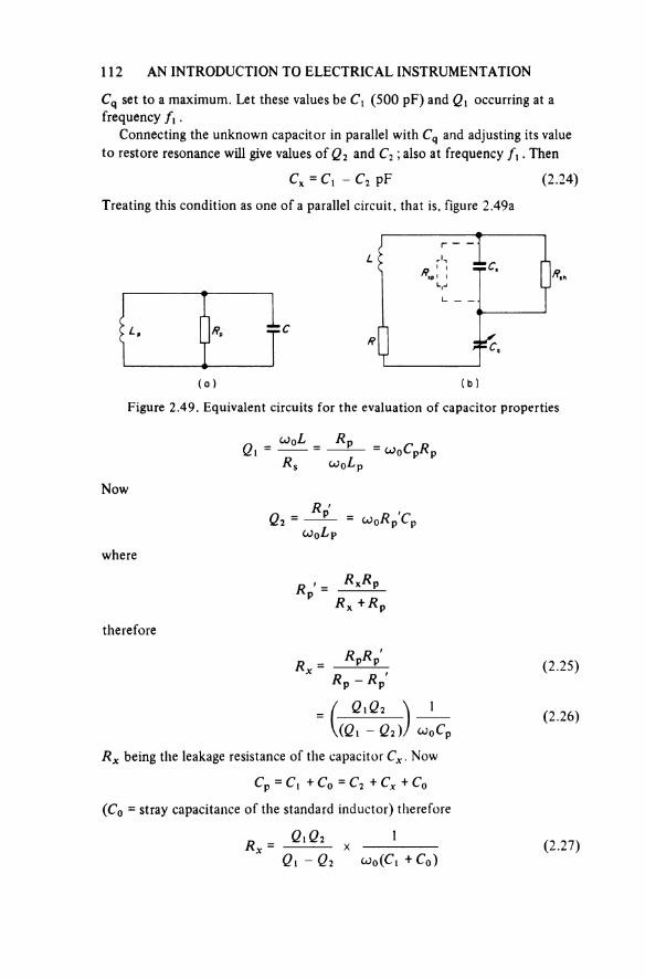
112 AN INTRODUCTION TO ELECTRICAL INSTRUMENTATION
Cq set to a maximum. Let these values be C1 (500 pF) and Q1 occurring at afrequency f1.
Connecting the unknown capacitor in parallel with Cq and adjusting its value to restore resonance will give values of Q2 and C2 ; also at frequency f1 . Then
(2.24)
Treating this condition as one of a parallel circuit, that is, figure 2.49a
Figure 2.49. Equivalent circuits for the evaluation of capacitor properties
(a) (b)
Now
where
therefore
(2.25)
(2.26)
Rx being the leakage resistance of the capacitor Cx. Now
(Co = stray capacitance of the standard inductor) therefore
(2.27)
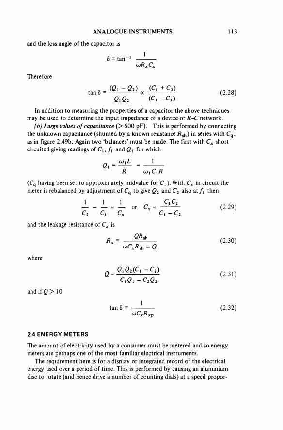
ANALOGUE INSTRUMENTS 113
and the loss angle of the capacitor is
Therefore
(2.28)
In addition to measuring the properties of a capacitor the above techniques may be used to determine the input impedance of a device or R-C network.
(b) Large values of capacitance (> 500 pF). This is performed by connectingthe unknown capacitance (shunted by a known resistance Rsh) in series with Cq,as in figure 2.49b. Again two ‘balances’ must be made. The first with Cx shortcircuited giving readings of C1, f1 and Q1 for which
(Cq having been set to approximately midvalue for C1). With CX in circuit the meter is rebalanced by adjustment of Cq to give Q2 and C2 also at f1 then
(2.29)
and the leakage resistance of Cx is
(2.30)
where
(2.31)
and if Q > 10
(2.32)
2.4 ENERGY METERS
The amount of electricity used by a consumer must be metered and so energy meters are perhaps one of the most familiar electrical instruments.
The requirement here is for a display or integrated record of the electrical energy used over a period of time. This is performed by causing an aluminium disc to rotate (and hence drive a number of counting dials) at a speed propor-
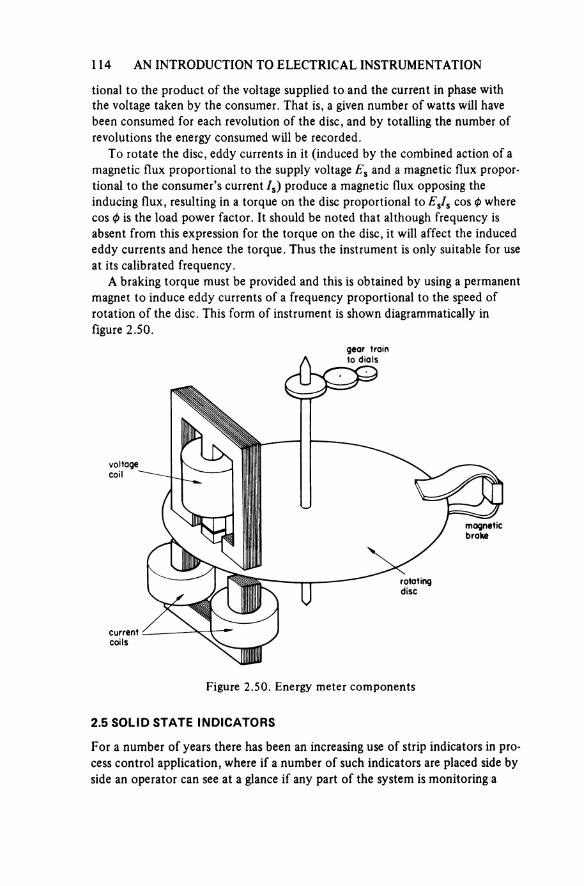
114 AN INTRODUCTION TO ELECTRICAL INSTRUMENTATION
tional to the product of the voltage supplied to and the current in phase with the voltage taken by the consumer. That is, a given number of watts will have been consumed for each revolution of the disc, and by totalling the number of revolutions the energy consumed will be recorded.
To rotate the disc, eddy currents in it (induced by the combined action of a magnetic flux proportional to the supply voltage Es and a magnetic flux propor-tional to the consumer’s current Is) produce a magnetic flux opposing theinducing flux, resulting in a torque on the disc proportional to ESIS cos ϕ wherecos ϕ is the load power factor. It should be noted that although frequency is absent from this expression for the torque on the disc, it will affect the induced eddy currents and hence the torque. Thus the instrument is only suitable for use at its calibrated frequency.
A braking torque must be provided and this is obtained by using a permanent magnet to induce eddy currents of a frequency proportional to the speed of rotation of the disc. This form of instrument is shown diagrammatically in figure 2.50.
Figure 2.50. Energy meter components
gear train to dials
voltagecoil
magneticbrake
rotatingdisc
currentcoils
2.5 SOLID STATE INDICATORS
For a number of years there has been an increasing use of strip indicators in pro cess control application, where if a number of such indicators are placed side by side an operator can see at a glance if any part of the system is monitoring a
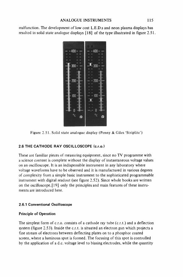
ANALOGUE INSTRUMENTS 115
malfunction. The development of low cost L.E.D.s and neon plasma displays has resulted in solid state analogue displays [18] of the type illustrated in figure 2.51
Figure 2.51. Solid state analogue display (Penny & Giles ‘Striplite’)
2.6 THE CATHODE RAY OSCILLOSCOPE (c.r.o.)
These are familiar pieces of measuring equipment, since no TV programme with a science content is complete without the display of instantaneous voltage values on an oscilloscope. It is an indispensable instrument in any laboratory where voltage waveforms have to be observed and it is manufactured in various degrees of complexity from a simple basic instrument to the sophisticated programmable instrument with digital readout (see figure 2.52). Since whole books are written on the oscilloscope, [19] only the principles and main features of these instru-ments are introduced here.
2.6.1 Conventional Oscilloscope
Principle of Operation
The simplest form of c.r.o. consists of a cathode ray tube (c.r.t.) and a deflection system (figure 2.53). Inside the c.r.t. is situated an electron gun which projects a fine stream of electrons between deflecting plates on to a phosphor coated screen, where a luminous spot is formed. The focusing of this spot is controlled by the application of a d.c. voltage level to biasing electrodes, while the quantity
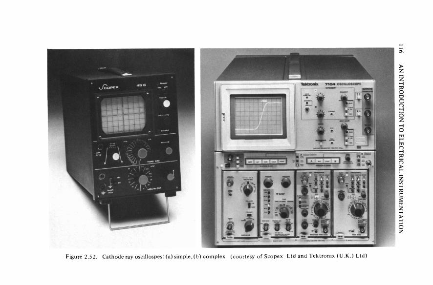
116 A
N INT
ROD
UCT
ION TO ELE
CTRICA
L INST
RUM
ENTA
TION
Figure 2.52. Cathode ray oscilloscopes: (a) simple, (b) complex (courtesy of Scopex Ltd and Tektronix (U.K.) Ltd)
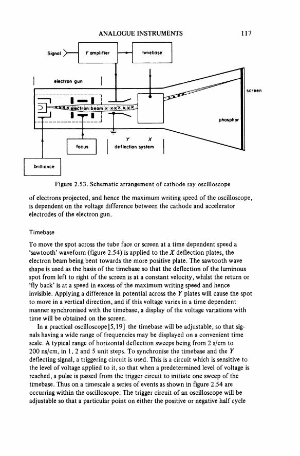
ANALOGUE INSTRUMENTS 117
Figure 2.53. Schematic arrangement of cathode ray oscilloscope
Signal Y amplifier timebase
electron gun
electron beam
screen
phosphor
focus deflection system
brilliance
of electrons projected, and hence the maximum writing speed of the oscilloscope, is dependent on the voltage difference between the cathode and accelerator electrodes of the electron gun.
Timebase
To move the spot across the tube face or screen at a time dependent speed a ‘sawtooth’ waveform (figure 2.54) is applied to the X deflection plates, the electron beam being bent towards the more positive plate. The sawtooth wave shape is used as the basis of the timebase so that the deflection of the luminous spot from left to right of the screen is at a constant velocity, whilst the return or ‘fly back’ is at a speed in excess of the maximum writing speed and hence invisible. Applying a difference in potential across the Y plates will cause the spot to move in a vertical direction, and if this voltage varies in a time dependent manner synchronised with the timebase, a display of the voltage variations with time will be obtained on the screen.
In a practical oscilloscope [5, 19] the timebase will be adjustable, so that sig-nals having a wide range of frequencies may be displayed on a convenient time scale. A typical range of horizontal deflection sweeps being from 2 s/cm to 200 ns/cm, in 1, 2 and 5 unit steps. To synchronise the timebase and the Y deflecting signal, a triggering circuit is used. This is a circuit which is sensitive to the level of voltage applied to it, so that when a predetermined level of voltage is reached, a pulse is passed from the trigger circuit to initiate one sweep of the timebase. Thus on a timescale a series of events as shown in figure 2.54 are occurring within the oscilloscope. The trigger circuit of an oscilloscope will be adjustable so that a particular point on either the positive or negative half cycle
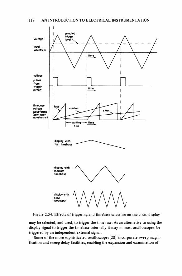
118 AN INTRODUCTION TO ELECTRICAL INSTRUMENTATION
Figure 2.54. Effects of triggering and timebase selection on the c.r.o. display
voltage
inputwaveform
selected trigger level
time
voltagepulsesfromtriggercircuit time
timebase voltage waveforms (saw tooth waveforms)
fast mediumslow
waitingtime
time
display with fast timebase
display withmediumtimebase
display with slowtimebase
may be selected, and used, to trigger the timebase. As an alternative to using the display signal to trigger the timebase internally it may in most oscilloscopes, be triggered by an independent external signal.
Some of the more sophisticated oscilloscopes [20] incorporate sweep magni-fication and sweep delay facilities, enabling the expansion and examination of

ANALOGUE INSTRUMENTS 119
Figure 2.55. C.R.O. display using sweep magnification and delay
beam 1
beam 2 lox expansion of the signal of beam 1
particular points in a waveform which occur some time after a suitable triggering point has occurred. Figure 2.55 illustrates the type of display that is possible with these facilities.
Vertical amplifiers
The direct application of the vertical or Y signal to the deflection plates would severely limit the versatility and sensitivity of the oscilloscope. To overcome both these difficulties a range ‘attenuator’ and amplifier arrangement is inserted between the incoming signal and the deflection plates. The steps of sensitivity are usually given in terms of mV or V/div. of deflection, and arranged in a 1 -2-5 sequence. The range of sensitivities varies between oscilloscopes but in a general purpose instrument will probably be from 5 mV/div. to 20 V/div; a division is commonly 8 mm. As with the electrical pointer instruments the inclusion of an amplifier, while bringing the benefits of increased input impedance and sensitivity, introduces drift problems, limitations of bandwidth and accuracy. In general the most sensitive (50 μV/div) oscilloscope ranges have the narrowest bandwidth (for example, d.c. to 150 kHz) while the less sensitive ranges of some oscilloscopes extend into the region of hundreds of megahertz. To remove the effects on the display of d.c. drift in the circuit under investigation, most Y input amplifiers have an a.c. or d.c. mode of operation switch, which enables a blocking capacitor to be inserted in the input connection thus isolating the drift voltages from the input amplifier in the a.c. mode. Care must be exercised, however, when using this facility, for it is possible to introduce considerable distortion into the display of certain waveforms, for example low and medium frequency square waves (see figure 2.56).
The above assumes that all voltages are measured with respect to earth or ground potential. This is not always so, since it may be desirable to display the voltage waveform across a component in a line, that is, both ends of the com-

120 AN INTRODUCTION TO ELECTRICAL INSTRUMENTATION
Figure 2.56. Distortion using a.c. input switch position when displaying square wave
ponent having a potential to earth. To overcome this problem some oscilloscopes’ vertical amplifiers are manufactured with two inputs so that either input with respect to earth may be displayed or the difference between the two inputs may be displayed. This form of input amplifier is known as a differential input amplifier (see section 6.7.1).
X-Y display
As an alternative to the timebase circuits which may be connected to the X plates, most oscilloscopes have an uncalibrated X amplifier while some dual beam instru-ments have the facility for using one of the Y amplifiers as an X amplifier. This enables the display of loops or Lissajous’ figures to be made (see figure 2.60 below).
'Z' modulator
The strength of the electron beam leaving the electron gun will depend on the voltage difference between its grid and the cathode. If a pulse of voltage were applied, via a blocking capacitor, to the grid it would be possible to blank out the display for the duration of the pulse. This is the purpose of the ‘Z mod.’ terminal available on many oscilloscopes, and enables part of a display to be either reduced or increased in luminosity.
Sampling oscilloscopes
The continuous display on an oscilloscope is, at present, limited to frequencies in the 50 to 300 MHz range, depending on the oscilloscope design. Above this order of frequency sampling techniques must be used to obtain a satisfactory display, which may be made up from as many as 1000 dots of luminescence. The vertical deflection for each dot is obtained from progressively later points in each successive cycle of the input waveform (figure 2.57). The horizontal deflection of the electron beam is obtained by the application of a staircase waveform to the X deflection plates.
Sampling techniques may not, of course, be used for the display of transient waveforms.
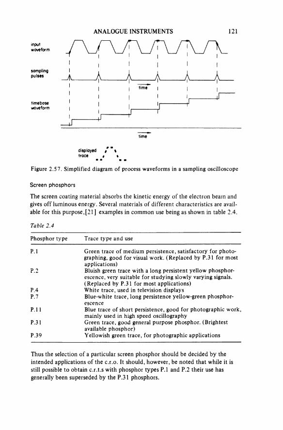
ANALOGUE INSTRUMENTS 121
Figure 2.57. Simplified diagram of process waveforms in a sampling oscilloscope
inputwaveform
samplingpulses
time
timebasewaveform
time
displayedtrace
Screen phosphors
The screen coating material absorbs the kinetic energy of the electron beam and gives off luminous energy. Several materials of different characteristics are avail-able for this purpose, [21] examples in common use being as shown in table 2.4.
Table 2.4
Phosphor type Trace type and use
P.1 Green trace of medium persistence, satisfactory for photo-graphing, good for visual work. (Replaced by P.31 for most applications)
P.2 Bluish green trace with a long persistent yellow phosphor-escence, very suitable for studying slowly varying signals. (Replaced by P.31 for most applications)
P.4 White trace, used in television displaysP.7 Blue-white trace, long persistence yellow-green phosphor-
escenceP.11 Blue trace of short persistence, good for photographic work,
mainly used in high speed oscillographyP.31 Green trace, good general purpose phosphor. (Brightest
available phosphor)P.39 Yellowish green trace, for photographic applications
Thus the selection of a particular screen phosphor should be decided by the intended applications of the c.r.o. It should, however, be noted that while it is still possible to obtain c.r.t.s with phosphor types P.1 and P.2 their use has generally been superseded by the P.31 phosphors.
122 AN INTRODUCTION TO ELECTRICAL INSTRUMENTATION
Multiple trace displays
In many instances it is necessary to compare one signal with another. To facilitate this, multiple trace displays are obtainable as follows.
(a) The use of two electron guns within the same cathode ray tube. This method produces an instrument known as a dual beam oscilloscope, in which the electron beams of the two channels are completely independent of each other. This effect may also be produced by a single electron gun, the output from it being split into two independently controllable electron beams.
(b) Using a single electron gun and producing a double trace by switching the Y deflection plates from one input signal to another for alternate sweeps of the screen. The eye interprets this as a continuous simultaneous display of the input signals although it is a sampled display. An oscilloscope using this technique, known as alternate mode, may only be used as a single channelinstrument for recording transient phenomena.
(c) Switching the input to the Y deflection plates from one input signal ampli-fier to another at a rate not governed by the duration of the sweep; that is, the traces of each channel of input are built up from a series of dots as the electron beam receives a deflection derived from a particular input channel. This technique, known as chopped mode, may be used for multi-channel transient investigations.
Methods (b) and (c) reduce the cost of producing a multi-channel oscilloscope, it being possible to use either of these techniques to obtain a display of more than two channels.
Oscilloscope Accessories
To increase the versatility of an oscilloscope, various accessories are available for use with it, or built into it.
Calibrators
Many oscilloscopes have a built in reference source of voltage, which usually takes the form of a 1 kHz, square waveform of either a single magnitude or of selectable magnitudes. This facility enables the oscilloscope timebase and ampli-fiers to be checked for accuracy of calibration each time the oscilloscope is used. Should the calibration be found to be outside the specified limits for a particular instrument, the setting up procedures stipulated in the manufacturer’s handbook should be performed by authorised personnel.
Probes
This topic is dealt with in chapter 6, but briefly the necessity for their use arises from the problem of ensuring that a circuit under investigation is unaffected by the presence of the measuring instrument. If the frequency in the said circuit is
ANALOGUE INSTRUMENTS 123
high then the capacitance of the cable conveying the signal to the oscilloscope will present the circuit under test with a low impedance. To reduce the errors that this would produce, a probe (having a high impedance) must be used at the measuring end of the connecting cable.
Cameras
The best method of obtaining permanent records of oscilloscope traces for analysis is to use photography. Special cameras are available for this purpose and are of the following two types.
(a) 35 mm, usually a prefocused unit bolted over the tube face. Some cameras have a fixed lens aperture, the exposure being simply controlled by hand operation of a flap shutter. More sophisticated units incorporate aperture and exposure control. The types of 35 mm film in common use are pan-chromatic and special blue sensitive films, which are faster and thus more suitable for the recording of high speed transients. Both of these give a ‘negative’ record, that is, a black trace on a transparent background, from which prints in the form of a white trace on a black background may be made. A third type of 35 mm photograph is obtainable by using recording paper, which results in a black trace on a white background. These are, however, difficult to enlarge.
(b) Polaroid film. This is almost ‘instant’ photography, a permanent record being obtained in 10 to 20 s. This process is considerably more expensive in materials than 35 mm photography, although the relative cost may be reduced by using the facility of some of these cameras to be moved relative to the screen, making it possible to place several traces (exposures) on one print. The camera is again prefocused, but normally provided with aperture and exposure controls. The record obtained on Polaroid film is a white trace on a black background—a print—and as such is difficult to reproduce.
Note: Time is money, and if only a few photographs are to be made, Polaroid photography is usually the most economical method.
Applications
The major and obvious use of the c.r.o. is that it enables the operator to ‘see’ what is happening to waveforms in a circuit—an extremely useful facility. In addition to this qualitative approach, by suitable use of the controls for the time base, vertical amplifiers and other facilities a considerable amount of quantitive information can also be obtained from the display. However, it must be remem-bered that the accuracy of direct measurements made using an oscilloscope is rarely better than ± 3 per cent on either the X or Y axes, and is therefore really a display instrument with facilities enabling the estimation of magnitudes of voltage and time.
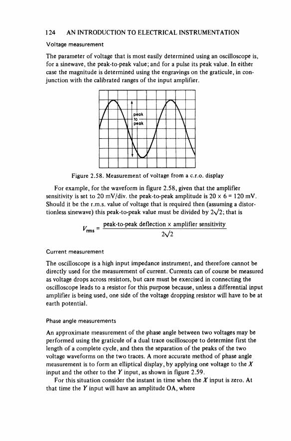
124 AN INTRODUCTION TO ELECTRICAL INSTRUMENTATION
Voltage measurement
The parameter of voltage that is most easily determined using an oscilloscope is for a sinewave, the peak-to-peak value; and for a pulse its peak value. In either case the magnitude is determined using the engravings on the graticule, in con-junction with the calibrated ranges of the input amplifier.
Figure 2.58. Measurement of voltage from a c.r.o. display
peak to peak
For example, for the waveform in figure 2.58, given that the amplifier sensitivity is set to 20 mV/div. the peak-to-peak amplitude is 20 × 6 = 120 mV Should it be the r.m.s. value of voltage that is required then (assuming a distor-tionless sinewave) this peak-to-peak value must be divided by 2√2; that is
V = rmspeak-to-peak deflection × amplifier sensitivity
2√2
Current measurement
The oscilloscope is a high input impedance instrument, and therefore cannot be directly used for the measurement of current. Currents can of course be measurer as voltage drops across resistors, but care must be exercised in connecting the oscilloscope leads to a resistor for this purpose because, unless a differential inpul amplifier is being used, one side of the voltage dropping resistor will have to be at earth potential.
Phase angle measurements
An approximate measurement of the phase angle between two voltages may be performed using the graticule of a dual trace oscilloscope to determine first the length of a complete cycle, and then the separation of the peaks of the two voltage waveforms on the two traces. A more accurate method of phase angle measurement is to form an elliptical display, by applying one voltage to the X input and the other to the Y input, as shown in figure 2.59.
For this situation consider the instant in time when the X input is zero. At that time the Y input will have an amplitude OA, where
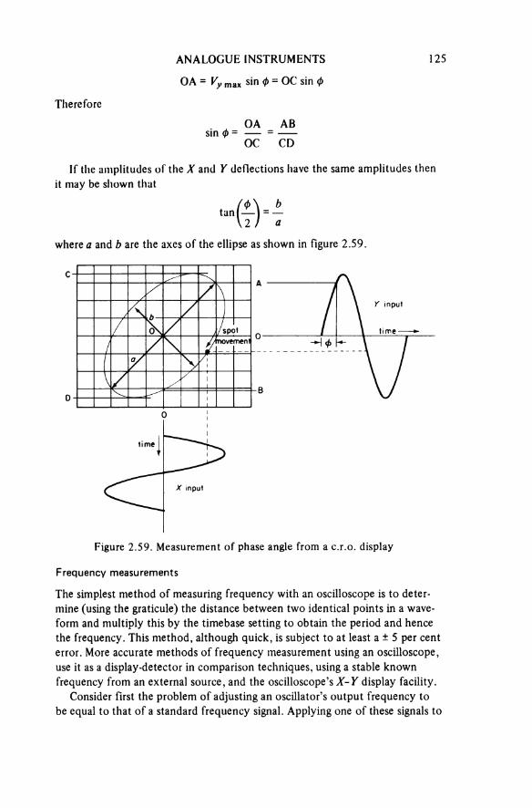
ANALOGUE INSTRUMENTS 125
OA = Vy max sin ϕ = OC sin ϕ
Therefore
If the amplitudes of the X and Y deflections have the same amplitudes then it may be shown that
where a and b are the axes of the ellipse as shown in figure 2.59
Figure 2.59. Measurement of phase angle from a c.r.o. display
spotmovement
Y input
time
time
X input
Frequency measurements
The simplest method of measuring frequency with an oscilloscope is to deter-mine (using the graticule) the distance between two identical points in a wave-form and multiply this by the timebase setting to obtain the period and hence the frequency. This method, although quick, is subject to at least a ± 5 per cent error. More accurate methods of frequency measurement using an oscilloscope, use it as a display-detector in comparison techniques, using a stable known frequency from an external source, and the oscilloscope’s X-Y display facility.
Consider first the problem of adjusting an oscillator’s output frequency to be equal to that of a standard frequency signal. Applying one of these signals to

1 26 AN INTRODUCTION TO ELECTRICAL INSTRUMENTATION
the X plates of the oscilloscope and the other to the Y plates will result in an ellipse-type display, which will vary in shape at a rate dependent on the difference between the two signals. As the oscillator’s frequency is adjusted to be equal to the standard frequency the rotations of the ellipse will become slower and when the two frequencies are equal will cease altogether. Thus it becomes apparent that the difference between two signals which have approximately equal frequency may be determined by counting the ‘rotations’ of the ellipse in a known time. In this manner extremely accurate frequency comparisons may be made using an oscilloscope. For example, if an oscillator’s output frequency changes with
Figure 2.60. Lissajous’ figures and the corresponding input signals on the X and Y axes
horizontal or X input
vertical or Y input display
horizontal or X input
vertical or Y input display

ANALOGUE INSTRUMENTS 127respect to a 1 kHz standard by one cycle (one rotation of the display) in 10 s then the difference in frequency between the two is one-tenth of a Hz or 0.01 per cent.
For multiples of a standard frequency, Lissajous’ figures (figure 2.60) are used. The actual pattern of these displays will depend on the time displacement of the signals as well as their ratio, but at a particular time displacement for each ratio of frequencies a symmetrical pattern is obtainable, and under these conditions the ratio of peaks or loops on the left hand side to those on the top edge of the Lissajous’ figure correspond to the frequency ratio of the signals applied to the X and Y inputs of the oscilloscope. Large ratios of frequency are difficult to interpret, apart from the complexity of the pattern, as any slight change in one of the frequencies will cause the pattern to roll. A method of overcoming the pattern complexity problem is to use ‘roulette’ patterns.
Another method of determining frequency ratios using an oscilloscope is to supply a common frequency signal to the X and Y inputs, these voltages having a 90° phase shift (to give a circular display), and applying a higher frequency signal to the Z modulator input. This higher frequency signal varies the intensity of the circular display, there being one bright and one dark section, for each multiple of X-Y input frequency. This method, although giving a display which is easy to interpret, is limited in application to exact multiples of input frequen-cies, with the additional requirement that the Z input frequency must be larger than the X-Y input.
Rise time measurements
When pulse waveforms are being studied, a property of considerable importance is the rise time of the pulse. The rise time of a step function is normally defined as the time interval for the change from 10 per cent to 90 per cent of the final
Figure 2.61. Rise time and overshoot measurements on the c.r.o. display of a step function
overshoot
rise
time
distance
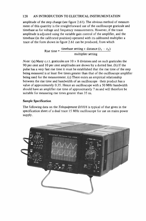
1 28 AN INTRODUCTION TO ELECTRICAL INSTRUMENTATION
amplitude of the step change (see figure 2.61). The obvious method of measure-ment of this quantity is the straightforward use of the oscilloscope graticule and timebase as for voltage and frequency measurements. However, if the trace amplitude is adjusted using the variable gain control of the amplifier, and the timebase (in the calibrated position) operated with its calibrated multiplier a trace of the form shown in figure 2.61 can be produced, from which
Rise time =timebase setting × distance (t1 — t2)
multiplier setting
Note: (a) Many c.r.t. graticules are 10 × 8 divisions and on such graticules the 90 per cent and 10 per cent amplitudes are shown by a dotted line, (b) If the pulse has a very fast rise time it must be established that the rise time of the step being measured is at least five times greater than that of the oscilloscope amplifier being used for the measurement. (c) There exists an empirical relationship between the rise time and bandwidth of an oscilloscope- their product has a value of approximately 0.35. Hence an oscilloscope with a 50 MHz bandwidth should have an amplifier rise time of approximately 7 ns and will therefore be suitable for measuring rise times greater than 35 ns.
Sample Specification
The following data on the Telequipment D1016 is typical of that given in the specification sheet of a dual trace 15 MHz oscilloscope for use on mains power supply.
ANALOGUE INSTRUMENTS I 29
Vertical system Two input channelsBandwidth: d.c. coupled d.c. to 15 MHz (-3 dB): a.c. coupled 8 Hz to 15 MHz (—3 dB): rise time: 24 nsDeflection factors: 5 mV/div. to 20 V/div. in 12 calibrated steps (1-2-5 sequence)A × 5 gain switch extends each amplifier sensitivity to 1 mV/div. at a bandwidth of d.c. to 4 MHz (-3 dB)Maximum scan: amplitude 8 div (6 div at 15 MHz): voltage measurement accuracy ± 5%Input impedance: 1 MΩ + 45 pF (approx.) Input conditions: switched choice of d.c. a.c. or ground; the third position grounds the input of the attenuator but not the signal inputMaximum input voltage: 500 V d.c. or a.c. peak Operating modes: channel 2 only: channels 1 and 2 chopped or alterna-ted. The alternate/chop mode is selected by the secs/div switch (chop mode 0.2 s/div. to 2 ms/div. and alternate from 1 ms/div. to 0.2 μs/div. ADD CH1 and CH2 are algebraically added and an invert switch is avail-able for CH2X-Y CH2 is the vertical input and CH1 becomes the horizontal input. Bandwidth is d.c. to 2 MHz (—3 dB). Phase error less than 3° at 100 kHz
Horizontal SystemSweep speeds: 0.2 s/div. to 0.2 μs/div. in 19 calibrated steps (1-2-5 sequence)A × 5 magnifier provides maximum sweep speeds of 40 ns/div.A variable uncalibrated control provides continuous coverage between stepped ranges extending the slowest sweep range to 0.5 s/div.Time measurement accuracy: normal ± 5%: × 5 ± 7% (approx)
TriggeringBandwidth: 15 MHz on both auto and normal positions. TV triggers at field rate from 0.2 s/div. to 100 μs/div. and line rate from 50 μs/div. to 0.2 μs/div.Sources: internal channel 2. External. Line.Sensitivity: internal 0.5 div.: external 0.5 V (approx)Polarity: Positive or negativeTrigger level: variable control selects virtually any point of the positive or negative slope of the input signal. This control is inoperative in the TV position
External XBandwidth: d.c. coupled d.c. to 2 MHz (—3 dB); a.c. coupled 10 Hz to 2 MHz (—3 dB)Sensitivity: 1 V/div. (approx)Input impedance: 280 kΩ + 30 pF (approx)
CRTDisplay area: 8 div. × 10 div. (1 div. = 1 cm)

130 AN INTRODUCTION TO ELECTRICAL INSTRUMENTATION
Phosphor: P31Accelerating potential: 18 kV Z modulation: 15 V amplitude, d.c. coupled
CalibratorOutput voltage: 250 mV peak-to-peak Wave shape: a vertical step at the screen centre Frequency: at sweep repetition rate Accuracy: ± 2%
Power requirementsMains voltages: 100-125 V or 200-250 V Frequency: 48-440 Hz Consumption: 50 VA (approx)
Dimensions and weight Height 1 60 mm Width 300 mmDepth 420 mm Weight 8.0 kg
2.6.2 Storage Oscilloscopes
The purpose of this form of c.r.o. is to provide the display of a waveform such that it remains in existence after the signal has ceased. Depending on the proper-ties of the particular instrument, the duration of the image retention is control-lable from a few seconds to hours. The techniques used to achieve this are: phosphor storage, mesh storage and digital storage (see section 4.4.3).
Phosphor storage
The phosphor or bistable storage oscilloscope [5,22] uses a c.r.t. which is similar to a conventional one but with a phosphor doped so as to provide two stable states which are sometimes referred to as written and unwritten. Other important differences from the conventional c.r.t. are the presence of flood guns—which are used to cover the viewing area with low-velocity electrons—to ensure that the written trace remains visible, and a collector electrode which is a transparent metal coating between the phosphor and the screen (see figure 2.62). Direct view bistable storage is based on a secondary emission principle, it being arranged that the two stable potentials (or states) of the storage target area are such that one is approximately the flood gun potential and the other near the collector potential. When the writing beam is scanned across the screen it dis-lodges secondary electrons and the written area charges positively and changes from the first stable state to the second. The electrons from the flood guns strike the written area with sufficient velocity to dislodge enough secondary electrons to keep the written area positively charged and visible. To erase a displayed wave-form the collector is first raised to the positive potential so that the entire screen
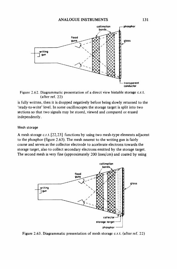
ANALOGUE INSTRUMENTS 131
Figure 2.62. Diagrammatic presentation of a direct view bistable storage c.r.t. (after ref. 22)
writinggun
floodguns
collimation bands
phosphor
glass
transparentconductor
is fully written, then it is dropped negatively before being slowly returned to the ‘ready-to-write’ level. In some oscilloscopes the storage target is split into two sections so that two signals may be stored, viewed and compared or erased independently.
Mesh storage
A mesh storage c.r.t. [22, 23] functions by using two mesh-type elements adjacent to the phosphor (figure 2.63). The mesh nearest to the writing gun is fairly coarse and serves as the collector electrode to accelerate electrons towards the storage target, also to collect secondary electrons emitted by the storage target. The second mesh is very fine (approximately 200 lines/cm) and coated by using
Figure 2.63. Diagrammatic presentation of mesh storage c.r.t. (after ref. 22)
writinggun
flood
collimation bands
glass
collectorstorage target
phosphor

132 AN INTRODUCTION TO ELECTRICAL INSTRUMENTATION
thin film techniques with a layer of dielectric, it being on this insulation that the storage occurs.
In the storage mode the flood guns cover the entire storage target with a con-tinuous stream of low-velocity electrons, which are prevented from reaching thephosphor screen except where a trace has been written on the storage mesh. An accelerating potential between the storage mesh and an aluminised layer on the phosphor attracts the electrons from the flood guns to the phosphor resulting in a bright high contrast display of the trace originally written on the storage mesh.
The density of the writing beam striking the storage mesh determines the amount of positive charge on the dielectric. This in turn determines the quantity of flood electrons reaching the phosphor and hence the brightness of the stored trace. It is this ability to store and display changes in intensity that leads to this type of storage being termed ‘halftone storage’. A characteristic of halftonestorage is that the unwritten parts of the storage mesh, begin with time to ‘fade positive’, that is to say the whole of the storage mesh will gradually become positively charged due to positive ion generation in the flood electron system, and when this has occurred the trace will be lost for the whole screen is then in a written state. To prevent this from occurring the entire screen may be slowly erased during operation by applying variable width pulses to the storage mesh, a process that is usually controlled by a front panel control normally labelled ‘persistence’.
A further development of the mesh storage system is the introduction of athird mesh between the storage mesh and the screen. This third mesh has a bi-stable property and the resultant c.r.t., known as transfer storage, has a consider-ably longer store time and a much faster writing speed than the halftone tube.
2.6.3 Recording Oscilloscopes
The conventional method of obtaining a permanent record of a waveform is to photograph the trace on a conventional oscilloscope, or for lower frequencies to use a u.v. recorder. However, by using an oscilloscope fitted with a fibre-opticcathode ray tube, [24] the advantages of the u.v. recording process can be com-bined with the advantages of the virtually inertia-free deflection system of the conventional c.r.o.
The cathode ray tube used in a fibre-optic recording oscilloscope is essentially the same as that in a conventional c.r.o. except that the normal faceplate of the tube is replaced by one made from short optical glass fibres (see figure 2.64).The recording paper is held in intimate contact with the glass by a spring-loaded plate, so that the optical transfer of the image on the phosphor to the sensitive emulsion on the paper is performed with the maximum efficiency.
When a waveform is being recorded, the traces on the c.r.t. are obscured and because of this some instruments of this type have an additional monitor tube that simultaneously displays the signal being recorded.
In addition to being able to use this instrument as a conventional oscilloscope

ANALOGUE INSTRUMENTS 133
Figure 2.64. Recording using a c.r.t. with a fibre-optic faceplate: (a) conventional c.r.t. and camera (luminous output only partially used), (b) fibre- optic c.r.t. (film in direct contact with transmitted light) (courtesy of Medelec Ltd)
(a)
plain glass faceplate
aluminising
emulsion
camera recordingfilm
phosphor
(b)
fibre optic stack
aluminising
spring loaded plate
phosphor
emulsionsurface
recordingpaper
Figure 2.65. The raster mode achieves paper economy and simplifies comparison between successive responses to a series of similar stimuli
and produce single-frame records of waveforms, continuous records of waveforms may be obtained by driving the paper past the tube face while the electron beam is deflected across it. This technique produces a multi-channel record similar to
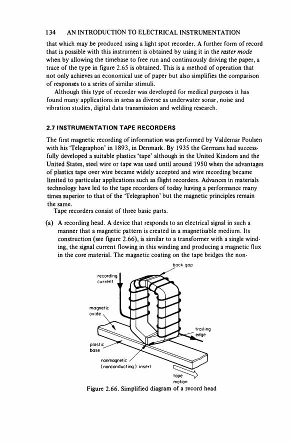
134 AN INTRODUCTION TO ELECTRICAL INSTRUMENTATION
that which may he produced using a light spot recorder. A further form of record that is possible with this instrument is obtained by using it in the raster mode when by allowing the timebase to free run and continuously driving the paper, a trace of the type in figure 2.65 is obtained. This is a method of operation that not only achieves an economical use of paper but also simplifies the comparison of responses to a series of similar stimuli.
Although this type of recorder was developed for medical purposes it has found many applications in areas as diverse as underwater sonar, noise and vibration studies, digital data transmission and welding research.
2.7 INSTRUMENTATION TAPE RECORDERS
The first magnetic recording of information was performed by Valdemar Poulsen with his ‘Telegraphon’ in 1893, in Denmark. By 1935 the Germans had success-fully developed a suitable plastics ‘tape’ although in the United Kindom and the United States, steel wire or tape was used until around 1950 when the advantages of plastics tape over wire became widely accepted and wire recording became limited to particular applications such as flight recorders. Advances in materials technology have led to the tape recorders of today having a performance many times superior to that of the ‘Telegraphon’ but the magnetic principles remain the same.
Tape recorders consist of three basic parts.
(a) A recording head. A device that responds to an electrical signal in such a manner that a magnetic pattern is created in a magnetisable medium. Its construction (see figure 2.66), is similar to a transformer with a single wind-ing, the signal current flowing in this winding and producing a magnetic flux in the core material. The magnetic coating on the tape bridges the non-
Figure 2.66. Simplified diagram of a record head
back gap
recordingcurrent
magnetic oxide
trailingedge
plasticbase
nonmagnetic (nonconducting) insert
tapemotion
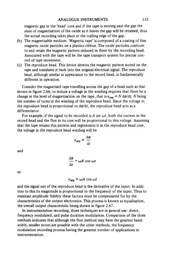
ANALOGUE INSTRUMENTS 135
magnetic gap in the ‘head’ core and if the tape is moving past the gap the state of magnetisation of the oxide as it leaves the gap will be retained, thus the actual recording takes place at the trailing edge of the gap.
(b) The magnetisable medium. ‘Magnetic tape’ is composed of a coating of fine magnetic oxide particles on a plastics ribbon. The oxide particles conform to and retain the magnetic pattern induced in them by the recording head. Associated with the tape will be the tape transport system for precise con-trol of tape movement.
(c) The reproduce head. This device detects the magnetic pattern stored on the tape and translates it back into the original electrical signal. The reproduce head, although similar in appearance to the record head, is fundamentally different in operation.
Consider the magnetised tape travelling across the gap of a head such as that shown in figure 2.66; to induce a voltage in the winding requires that there be a change in the level of magnetisation on the tape, that is erep « N dϕ/dt, N being the number of turns in the winding of the reproduce head. Since the voltage in the reproduce head is proportional to dϕ/dt, the reproduce head acts as a differentiator.
For example, if the signal to be recorded is A sin ωt, both the current in the record head and the flux in its core will be proportional to this voltage. Assumingthat the tape retains this pattern and regenerates it in the reproduce head core, the voltage in the reproduce head winding will be
and
so
and the signal out of the reproduce head is the derivative of the input. In addi-tion to this its magnitude is proportional to the frequency of the input. Thus to maintain amplitude fidelity these factors must be compensated for by the characteristics of the output electronics. This process is known as equalisation, the overall output characteristic being shown in figure 2.67.
In instrumentation recording, three techniques are in general use: direct, frequency modulated, and pulse duration modulation. Comparison of the three methods indicates that although the first method may have the greatest band-width, smaller errors are possible with the other methods, the frequency modulation recording process having the greatest number of applications in instrumentation.
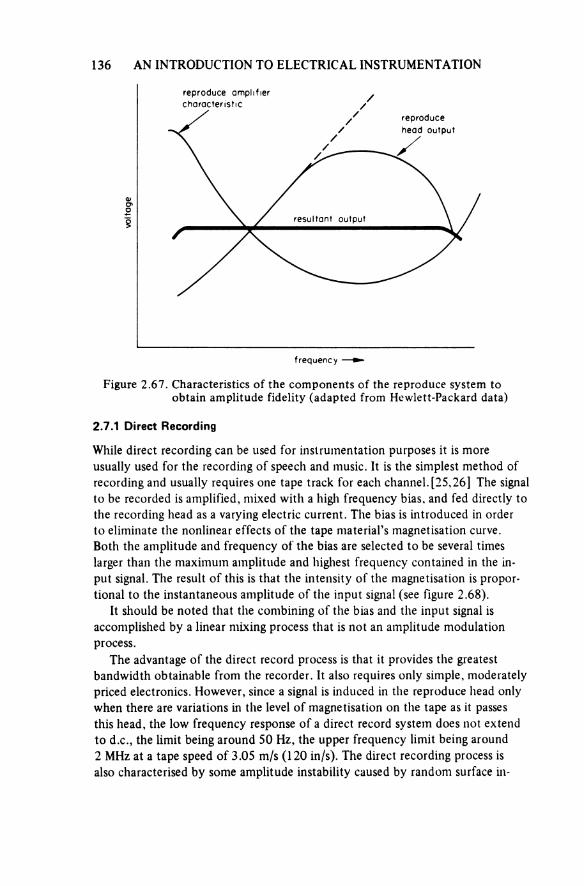
136 AN INTRODUCTION TO ELECTRICAL INSTRUMENTATION
Figure 2.67. Characteristics of the components of the reproduce system to obtain amplitude fidelity (adapted from Hewlett-Packard data)
reproduce amplifier characteristic
reproduce head output
volta
ge
resultant output
frequency
2.7.1 Direct Recording
While direct recording can be used for instrumentation purposes it is more usually used for the recording of speech and music. It is the simplest method of recording and usually requires one tape track for each channel. [25, 26] The signal to be recorded is amplified, mixed with a high frequency bias, and fed directly to the recording head as a varying electric current. The bias is introduced in order to eliminate the nonlinear effects of the tape material’s magnetisation curve.Both the amplitude and frequency of the bias are selected to be several times larger than the maximum amplitude and highest frequency contained in the in-put signal. The result of this is that the intensity of the magnetisation is propor-tional to the instantaneous amplitude of the input signal (see figure 2.68).
It should be noted that the combining of the bias and the input signal is accomplished by a linear mixing process that is not an amplitude modulation process.
The advantage of the direct record process is that it provides the greatest bandwidth obtainable from the recorder. It also requires only simple, moderately priced electronics. However, since a signal is induced in the reproduce head only when there are variations in the level of magnetisation on the tape as it passes this head, the low frequency response of a direct record system does not extend to d.c., the limit being around 50 Hz, the upper frequency limit being around 2 MHz at a tape speed of 3.05 m/s (120 in/s). The direct recording process is also characterised by some amplitude instability caused by random surface in-

ANALOGUE INSTRUMENTS 137
Figure 2.68. Classical representation of ‘direct recording’ (adapted from Hewlett-Packard data)
recorded magnetisation
approximately linear sections
reproduced signal
mixture of signal and frequency bias
signal to record head
homogeneities in the tape coating. At long wavelengths (low frequencies) the amplitude variations caused by this may only be a few per cent; however for frequencies near the upper bandwidth limit for a given tape speed, amplitude variations can exceed 10 per cent and momentary decreases of over 50 per cent (called ‘dropouts’) may occur. This also indicates one of the difficulties associated with magnetically recording digital data.
Direct recording should therefore only be used when maximum bandwidth is required and amplitude variations are not unacceptable. If maximum bandwidth with relative freedom from dropouts is required, a single input signal can be recorded on several channels simultaneously.
In sound recording the ear will average amplitude variation errors, and whilst the audio tape recorder utilises the direct recording process, it is seldom satis-factory to use an audio recorder for instrumentation purposes. The former is designed to take advantage of the rather peculiar spectral energy characteristics of speech and music, whereas an instrumentation recorder must have a uniform response over its entire range.
2.7.2 Frequency Modulated Recording
Frequency modulation overcomes some of the basic limitations of direct record-ing at the cost of reducing the high frequency response. The bandwidth of the recording may be extended down to d.c. and the reproduced signal is not signifi-cantly degraded by amplitude variation effects. In the f.m. recording system, a
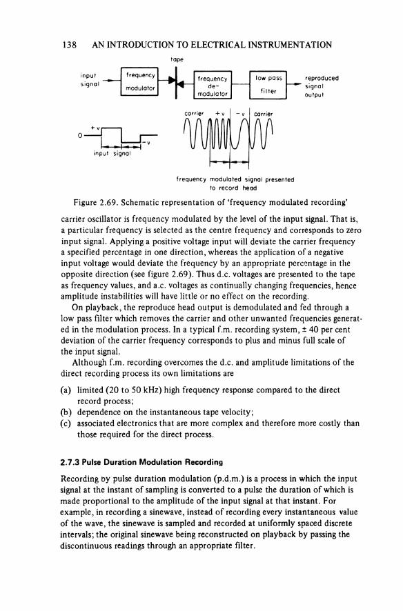
138 AN INTRODUCTION TO ELECTRICAL INSTRUMENTATION
Figure 2.69. Schematic representation of ‘frequency modulated recording’
inputsignal
frequency
modulatorfrequency
de-modulator
low pass
filter
reproducedsignaloutput
input signal
carrier carrier
frequency modulated signal presented to record head
carrier oscillator is frequency modulated by the level of the input signal. That is, a particular frequency is selected as the centre frequency and corresponds to zero input signal. Applying a positive voltage input will deviate the carrier frequency a specified percentage in one direction, whereas the application of a negative input voltage would deviate the frequency by an appropriate percentage in the opposite direction (see figure 2.69). Thus d.c. voltages are presented to the tape as frequency values, and a.c. voltages as continually changing frequencies, hence amplitude instabilities will have little or no effect on the recording.
On playback, the reproduce head output is demodulated and fed through a low pass filter which removes the carrier and other unwanted frequencies generat-ed in the modulation process. In a typical f.m. recording system, ± 40 per cent deviation of the carrier frequency corresponds to plus and minus full scale of the input signal.
Although f.m. recording overcomes the d.c. and amplitude limitations of the direct recording process its own limitations are
(a) limited (20 to 50 kHz) high frequency response compared to the direct record process;
(b) dependence on the instantaneous tape velocity;(c) associated electronics that are more complex and therefore more costly than
those required for the direct process.
2.7.3 Pulse Duration Modulation Recording
Recording by pulse duration modulation (p.d.m.) is a process in which the input signal at the instant of sampling is converted to a pulse the duration of which is made proportional to the amplitude of the input signal at that instant. For example, in recording a sinewave, instead of recording every instantaneous value of the wave, the sinewave is sampled and recorded at uniformly spaced discrete intervals; the original sinewave being reconstructed on playback by passing the discontinuous readings through an appropriate filter.

Figure 2.70. Schematic diagram of pulse duration modulation recording system
synchronising reference 86 input signals
multiplexer(scanner)
modulator
record amplifier
tape
reproduce amplifier
demodulator
synch.ref.
decommutator
filters
reproducedsignals
d.c. bias
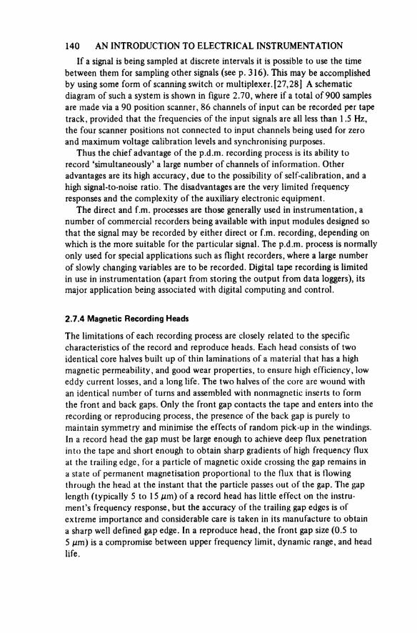
140 AN INTRODUCTION TO ELECTRICAL INSTRUMENTATION
If a signal is being sampled at discrete intervals it is possible to use the time between them for sampling other signals (see p. 316). This may be accomplished by using some form of scanning switch or multiplexer. [27,28] A schematic diagram of such a system is shown in figure 2.70, where if a total of 900 samples are made via a 90 position scanner, 86 channels of input can be recorded per tape track, provided that the frequencies of the input signals are all less than 1.5 Hz, the four scanner positions not connected to input channels being used for zero and maximum voltage calibration levels and synchronising purposes.
Thus the chief advantage of the p.d.m. recording process is its ability to record ‘simultaneously’ a large number of channels of information. Other advantages are its high accuracy, due to the possibility of self-calibration, and a high signal-to-noise ratio. The disadvantages are the very limited frequency responses and the complexity of the auxiliary electronic equipment.
The direct and f.m. processes are those generally used in instrumentation, a number of commercial recorders being available with input modules designed so that the signal may be recorded by either direct or f.m. recording, depending on which is the more suitable for the particular signal. The p.d.m. process is normally only used for special applications such as flight recorders, where a large number of slowly changing variables are to be recorded. Digital tape recording is limited in use in instrumentation (apart from storing the output from data loggers), its major application being associated with digital computing and control.
2.7.4 Magnetic Recording Heads
The limitations of each recording process are closely related to the specificcharacteristics of the record and reproduce heads. Each head consists of two identical core halves built up of thin laminations of a material that has a high magnetic permeability, and good wear properties, to ensure high efficiency, low eddy current losses, and a long life. The two halves of the core are wound with an identical number of turns and assembled with nonmagnetic inserts to form the front and back gaps. Only the front gap contacts the tape and enters into the recording or reproducing process, the presence of the back gap is purely to maintain symmetry and minimise the effects of random pick-up in the windings. In a record head the gap must be large enough to achieve deep flux penetration into the tape and short enough to obtain sharp gradients of high frequency flux at the trailing edge, for a particle of magnetic oxide crossing the gap remains in a state of permanent magnetisation proportional to the flux that is flowing through the head at the instant that the particle passes out of the gap. The gap length (typically 5 to 15 μm) of a record head has little effect on the instru-ment’s frequency response, but the accuracy of the trailing gap edges is of extreme importance and considerable care is taken in its manufacture to obtain a sharp well defined gap edge. In a reproduce head, the front gap size (0.5 to 5 μm) is a compromise between upper frequency limit, dynamic range, and head life.
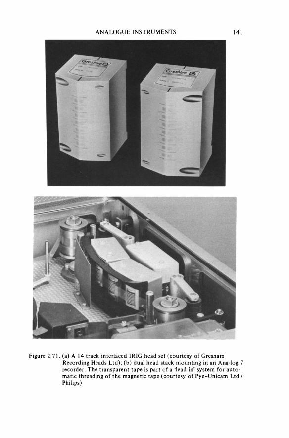
ANALOGUE INSTRUMENTS 141
Figure 2.71. (a) A 14 track interlaced IRIG head set (courtesy of GreshamRecording Heads Ltd); (b) dual head stack mounting in an Ana-log 7 recorder. The transparent tape is part of a ‘lead in’ system for auto-matic threading of the magnetic tape (courtesy of Pye-Unicam Ltd / Philips)
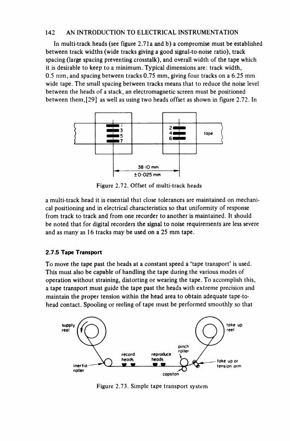
142 AN INTRODUCTION TO ELECTRICAL INSTRUMENTATION
In multi-track heads (see figure 2.71a and b) a compromise must be established between track widths (wide tracks giving a good signal-to-noise ratio), track spacing (large spacing preventing crosstalk), and overall width of the tape which it is desirable to keep to a minimum. Typical dimensions are: track width,0.5 mm, and spacing between tracks 0.75 mm, giving four tracks on a 6.25 mm wide tape. The small spacing between tracks means that to reduce the noise level between the heads of a stack, an electromagnetic screen must be positioned between them, [29] as well as using two heads offset as shown in figure 2.72. In
Figure 2.72. Offset of multi-track heads
a multi-track head it is essential that close tolerances are maintained on mechani-cal positioning and in electrical characteristics so that uniformity of response from track to track and from one recorder to another is maintained. It should be noted that for digital recorders the signal to noise requirements are less severe and as many as 16 tracks may be used on a 25 mm tape.
2.7.5 Tape Transport
To move the tape past the heads at a constant speed a ‘tape transport’ is used. This must also be capable of handling the tape during the various modes of operation without straining, distorting or wearing the tape. To accomplish this, a tape transport must guide the tape past the heads with extreme precision and maintain the proper tension within the head area to obtain adequate tape-to- head contact. Spooling or reeling of tape must be performed smoothly so that
Figure 2.73. Simple tape transport system
supplyreel
take up reel
inertiaroller
recordheads
reproduceheads
pinchroller
take up or tension arm
capstan
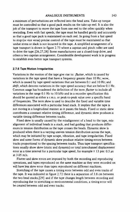
ANALOGUE INSTRUMENTS 143a minimum of perturbations are reflected into the head area. Take-up torque must be controlled so that a good pack results on the take-up reel. It is also the job of the transport to move the tape from one reel to the other quickly when rewinding. Even with fast speeds, the tape must be handled gently and accurately so that a good tape pack is maintained on each reel. In going from a fast speed to stop (or vice versa) precise control of the tape must be maintained so that undue stress or slack is not incurred in the tape. A simplified arrangement of a tape transport is shown in figure 2.73 where a capstan and pinch roller are used to drive the tape. [26, 27, 28] Some manufacturers use a closed-loop drive, and others a two capstan arrangement. Considerable development work is in progress to establish even better tape transport systems.
2.7.6 Tape Motion Irregularities
Variations in the motion of the tape give rise to: flutter, which is caused by variations in the tape speed that have a frequency greater than 10 Hz; WoW,which is caused by tape speed variations that are between 0.1 and 10 Hz; and drift, which denotes variations in the tape speed accuracy that are below 0.1 Hz. Common usage has broadened the definition of the term flutter to include an variations in the range 0.1 Hz to 10 kHz and in a recorder specification this should be quoted as either a r.m.s. or peak-to-peak value over a specific band of frequencies. The term skew is used to describe the fixed and variable time differences associated with a particular head stack. It implies that the tape is not moving in a longitudinal manner as it passes the heads. Fixed or static skew contributes a constant relative timing difference, and dynamic skew produces a variable timing difference between tracks.
Fixed skew is usually caused by the misalignment of a head to the tape, mis-alignment of individual heads in a stack, and bad guiding that produces differ-ences in tension distribution as the tape crosses the heads. Dynamic skew is produced when there is a varying uneven tension distribution across the tape, which may be initiated by tape scrape, vibration, and tape irregularities. Fixed skew and some forms of dynamic skew produce relative timing errors between tracks proportional to the spacing between tracks. Thus tape transport specifica-tions usually show skew (static and dynamic) or total interchannel displacement error as a time interval for a particular tape speed, for example ± 13 pm: 0.5 μs at 3.05 m/s.
Flutter and skew errors are imposed by both the recording and reproducingoperations, and tapes reproduced on the same machine as they were recorded on will have less skew error than tapes reproduced on different machines.
Stretching of the tape causes a timing error between odd and even tracks of the tape. It was indicated in figure 2.72 there is a separation of 3.8 cm between the two head stacks, [29] and if the tape changes length between recording and reproducing due to stretching or environmental conditions, a timing error will be created between odd and even tracks.
144 AN INTRODUCTION TO ELECTRICAL INSTRUMENTATION
Properties
The advantages of the tape recorder, compared with the data logger (section 9.3.1), are that it facilitates a continuous record of a number of signals, which may have a wide range of frequencies, to be made simultaneously. This has distinct advantages in the study of transient and ‘once only’ situations, for example, car crashing at road research establishments. When using a tape recorder it is possible to ‘playback’ a recording any number of times without deterioration of the record: it is also possible to change the time scale between recording and reproducing a signal, that is, a ‘fast’ occurrence may be recorded with a fast tape speed (1.52 or 3.05 m/s) but for analysis of the signals the tape could be played back at a slow speed 4.76 or 2.38 cm/s), enabling the recorded signal to be traced on an X-Y plotter (see p. 154). The reverse time scaling procedure is also possible, that is a slow process could be recorded with a tape speed of (say) 2.38 cm/s and repro-duced from a tape speed of 1.52 m/s.
Some instrumentation tape recorders have ‘level’ sensing circuits on the input so that if the instrument is being used for data recording and a preset limit on the magnitude of the input signal is exceeded, an alarm indicator may be operated.
The main disadvantage of the instrumentation tape recorder is that the recorded signals on the tape are in no way visual, and must be reproduced before any analysis may be performed.
REFERENCES
1 E. W. Golding and F. C. Widdis, Electrical Measurements and MeasuringInstruments (Pitman, London, 1963)
2 J. J. Instruments-New Generation Measurements, Vol II (J. J. LloydInstruments Ltd, Southampton, 1970)
3 Measurement Notes 1977 Catalogue (Keithley Instruments, Cleveland, Ohio)4 S. D. Prenski, Electronic Instrumentation, 2nd Ed. (Prentice-Hall, Englewood
Cliffs, N.J., 1971)5 B. M. Oliver and J. M. Cage, Electronic Measurements and Instrumentation
(McGraw-Hill, New York, 1971)6 Electrometer Measurements, 2nd Ed. (Keithley Instruments, Cleveland,
Ohio, 1977)7 R. N. Reeder, Measuring true rms voltages, Electron. Engng News, 49
(1977) 61-38 T291: Unit 14 Instrumentation, Recording (Open University Press, 1974)9 W. K. Whittemore and R. Beswick, Direct writing chart recorders, Electronics
Power, 23 (1977) 49-5510 D. R. Davis and C. K. Michener, Graphic recorder writing systems, HP Jl, 20
(1968) 2-711 R. Beswick and A. R. Thompson, Linearity-finding a way through the
specification maze. Control Instrumn., 8 (1976) 34-7
ANALOGUE INSTRUMENTS 145
12 H. Buckingham and E. M. Price, Principles of Electrical Measurements(English University Press, London, 1955)
13 P. J. S. Ashley, Buying electronic equipment 5: ultraviolet recorders. ElectlElectron. Techn Engr, 6 (1972) 8-16
14 The Galvanometer Users’ Handbook (Consolidated Electrodynamics Corpora-tion/Bell & Howell, Basingstoke, 1971)
15 C. T. Baldwin, Fundamentals of Electrical Measurements (Harrap, London.1961)
16 A. H. M. Arnold, Audio frequency power measurement by dynamometerwattmeters, Proc. LEE, 102 (1955) 192-203
17 F. J. Wilkins, T. H. Deacon and R. S. Becker, Multi-junction thermal conver-ter, an accurate a.c./d.c. transfer instrument, Proc I.E.E, 112 (1965) 794-805
18 Design evaluation of the Penny & Giles Striplite indicator, Engng Mater.Design, 20 (1976) 29-31
19 R. Van Erk, Oscilloscopes (McGraw-Hill, New York. 1978)20 Understanding delaying sweep: Service scope No. 50 (Tektronix U.K. Ltd,
1968)21 Phosphor data, Tektronix Catalogue 1980 (Tektronix Inc., Beaverton, Oreg.)22 Three new instruments. 3 kinds of storage, Tekscope, 4 (1972) 2-623 Storage expands your oscilloscope measuring capabilities, Tekscope, 7
(1975) 12-1524 J. R. Huntingford. Fibre optic recording oscilloscopes, Electron, 37 (1973)
45-5125 E. A. Read. Analogue recording, Electron. Equip. News, 12 (1970) 20-526 Magnetic Tape Recording Handbook, Hewlett-Packard Application Note 89
(1967)27 C. B. Pears, Jr (ed.), Magnetic Recording in Science and Industry (Van
Nostrand Reinhold. New York, 1967)28 G. L. Davis. Magnetic Tape Instrumentation (McGraw-Hill, New York,
1961)29 IRIG Telemetry Standards, Document No. 106-69 (Defence Documentation
Centre for Scientific and Technical Information, Ministry of Technology, Orpington, Kent)
30 A. S. Krause, HR-2000 A new state of the art in data recordings. Measure-ments and Control (October 1979) 87-9
31 N. E. Samek and W. R. Raymond, A PLZT electro-optic shutter array, Instrument Society of America Instrumentation Symposium (May 1979) 488-500
3Comparison Methods
The methods described in this chapter could, as an alternative, have been termed ‘null methods’—the purpose of the measurement process being to reduce the difference between a known and an unknown quantity to zero, that is so a null can be indicated. Inherently, such methods have a greater precision than direct measurements; for example, by using a detector that has a resolution of a micro-volt it is possible to compare in terms of microvolts two voltages that have magnitudes of the order of, say, 1 V. The accuracy of such methods must, how-ever, depend on the limits of error that apply to the ‘known’ or ‘standard’ quantity used.
3.1 D.C. POTENTIOMETER
3.1.1 Commercial Arrangements
The 1 m potentiometer used to describe the principle of operation in section 1.1.2 would be unwieldy in a practical situation but if two movable contacts are used, one on a shorter slide wire and the other on fixed lengths of resistance wire,a more compact instrument can be constructed. If the circuit in figure 1.4 is thus modified to that in figure 3.1, where the slide wire now has a length of 0.1 m and a resistance of 2 Ω connected in series with fifteen 2 Ω resistors, the total voltage drop (with a current of 50 mA) will be 1.6 V.
To standardise or calibrate such a potentiometer it is necessary to connect the divider voltage, via switch S, to the standard cell. Then, with the movable contact set at points such that the voltage appearing on the divider should be equal to the standard cell voltage, adjustment of the variable resistor R is made until the value of current in the potentiometer circuit causes these voltages to be equal, this being apparent when the galvanometer deflection (at maximum sensitivity) is zero.
The switch S can then be changed to connect the divider voltage, via the galvanometer, to the unknown and the divider contacts moved until balance is
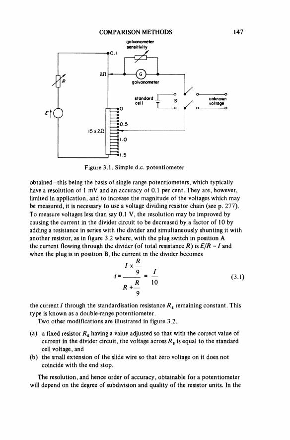
COMPARISON METHODS 147
Figure 3.1. Simple d.c. potentiometer
galvanometer sensitivity
galvanometer
standardcell
unknownvoltage
obtained—this being the basis of single range potentiometers, which typically have a resolution of 1 mV and an accuracy of 0.1 per cent. They are, however, limited in application, and to increase the magnitude of the voltages which may be measured, it is necessary to use a voltage dividing resistor chain (see p. 277). To measure voltages less than say 0.1 V, the resolution may be improved by causing the current in the divider circuit to be decreased by a factor of 10 by adding a resistance in series with the divider and simultaneously shunting it with another resistor, as in figure 3.2 where, with the plug switch in position A the current flowing through the divider (of total resistance R) is E/R = I and when the plug is in position B, the current in the divider becomes
(3.1)
the current I through the standardisation resistance R3 remaining constant. This type is known as a double-range potentiometer.
Two other modifications are illustrated in figure 3.2.
(a) a fixed resistor R3 having a value adjusted so that with the correct value of current in the divider circuit, the voltage across Rs is equal to the standard cell voltage, and
(b) the small extension of the slide wire so that zero voltage on it does not coincide with the end stop.
The resolution, and hence order of accuracy, obtainable for a potentiometer will depend on the degree of subdivision and quality of the resistor units. In the
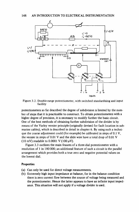
148 AN INTRODUCTION TO ELECTRICAL INSTRUMENTATION
Figure 3.2. Double-range potentiometer, with switched standardising and input facility
standard cell
inputs
potentiometers so far described the degree of subdivision is limited by the num-ber of steps that it is practicable to construct. To obtain potentiometers with a higher degree of precision, it is necessary to modify further the basic circuit.One of the best methods of obtaining further subdivision of the divider is by means of the Varley vernier principle (originally devised for fault location in sub marine cables), which is described in detail in chapter 6. By using such a techni-que the coarse adjustment could (for example) be calibrated in steps of 0.1 V, the vernier in steps of 0.01 V and the slide wire have a total drop of 0.01 V (10 mV) readable to 0.0001 V (100 μV).
Figure 3.3 outlines the main features of a three-dial potentiometer with a resolution of 1 in 180 000 ; an additional feature of such a circuit is the parallel arrangement which provides both a true zero and negative potential values on the lowest dial.
Properties
(a) Can only be used for direct voltage measurements.(b) Extremely high input impedance at balance, for in the balance condition
there is zero current flow between the source of voltage being measured and the potentiometer. Hence the latter appears to have an infinite input imped-ance. This situation will not apply if a voltage divider is used.
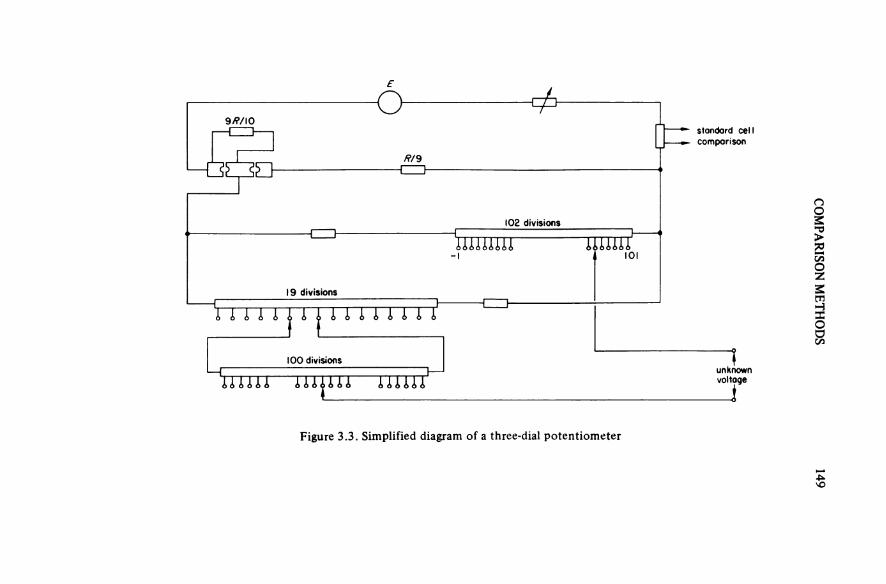
CO
MPA
RISON M
ETHO
DS 149
Figure 3.3. Simplified diagram of a three-dial potentiometer
standard cell comparison
102 divisions
19 divisions
100 divisionsunknownvoltage
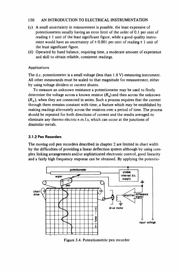
150 AN INTRODUCTION TO ELECTRICAL INSTRUMENTATION
(c) A small uncertainty in measurement is possible, the least expensive of potentiometers usually having an error limit of the order of 0.1 per cent of reading ± 1 unit of the least significant figure, while a good quality instru-ment would have an uncertainty of ± 0.001 per cent of reading ± 1 unit of the least significant figure.
(d) Operated by hand balance, requiring time, a moderate amount of experience and skill to obtain reliable, consistent readings.
Applications
The d.c. potentiometer is a small voltage (less than 1.8 V) measuring instrument. All other measurands must be scaled to that magnitude for measurement, either by using voltage dividers or current shunts.
To measure an unknown resistance a potentiometer may be used to firstly determine the voltage across a known resistor (Rs) and then across the unknown(Rx), when they are connected in series. Such a process requires that the currentthrough them remains constant with time, a feature which may be established by making readings alternately across the resistors over a period of time. The process should be repeated for both directions of current and the results averaged to eliminate any thermo electric e.m.f.s, which can occur at the junctions of dissimilar metals.
3.1.2 Pen Recorders
The moving coil pen recorders described in chapter 2 are limited in chart width by the difficulties of providing a linear deflection system although by using com-plex linking arrangements and/or sophisticated electronic control, good linearity and a fairly high frequency response can be obtained. By applying the potentio-
Figure 3.4. Potentiometric pen recorder
potentiometer
wiperstable
internal d.c. supply
chartdrive amplifier difference
signal
drive motor
input voltage
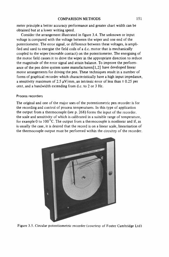
COMPARISON METHODS 151
meter principle a better accuracy performance and greater chart width can be obtained but at a lower writing speed.
Consider the arrangement illustrated in figure 3.4. The unknown or input voltage is compared with the voltage between the wiper and one end of the potentiometer. The error signal, or difference between these voltages, is ampli-fied and used to energise the field coils of a d.c. motor that is mechanically coupled to the wiper (movable contact) on the potentiometer. The energising of the motor field causes it to drive the wiper in the appropriate direction to reduce the magnitude of the error signal and attain balance. To improve the perform-ance of the pen drive system some manufacturers [1, 2] have developed linear motor arrangements for driving the pen. These techniques result in a number of forms of graphical recorder which characteristically have a high input impedance, a sensitivity maximum of 2.5 μV/mm, an intrinsic error of less than ± 0.25 per cent, and a bandwidth extending from d.c. to 2 or 3 Hz.
Process recorders
The original and one of the major uses of the potentiometric pen recorder is for the recording and control of process temperatures. In this type of application the output from a thermocouple (see p. 268) forms the input of the recorder, the scale and sensitivity of which is calibrated in a suitable range of temperature, for example 0 to 100 °C. The output from a thermocouple is nonlinear and if, as is usually the case, it is desired that the record is on a linear scale, linearisation of the thermocouple output must be performed within the circuitry of the recorder.
Figure 3.5. Circular potentiometric recorder (courtesy of Foster Cambridge Ltd)

152 AN INTRODUCTION TO ELECTRICAL INSTRUMENTATION
The chart for such a recorder may be rectangular or circular, and driven (as a function of time) by a motor synchronised to the supply frequency. To change the chart speed alteration is made to the gear ratio in the chart drive gear train. In the case of the circular recorder (see figure 3.5) one revolution of the chart usually takes 24 hours or sometimes 7 days. It is this circular form of recorder that commonly incorporates level switches, which can be used to actuate an alarm if a preset level is exceeded; alternatively these switches can be used for off/on control purposes.
Rectangular strip chart recorders may also incorporate control features: additionally many models are available in which one movement may be used to log several inputs. This feature may be performed either by having several pens whose travel overlaps each other and can be used to monitor up to six inputs simultaneously (figure 3.6), or by replacing the pen with a print wheel geared to
Figure 3.6. A six-channel potentiometric recorder (courtesy of Chessel Ltd)
a selector switch so that when a particular input is connected to the balancing circuit, a point in an identifying colour, or character, is printed on the chart.This form of multi-point recorder may monitor as many as 24 inputs although 6 is a more usual number. A recent development [3] using digital storage and thermal printing has resulted in a multi-channel recorder with a built-in dock, so that, in response to a command, the continuous recording of three identifiable traces is interrupted and time, day and information on up to eight other channels may be printed on the chart.
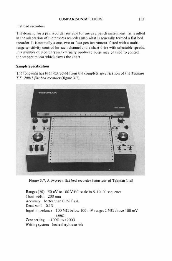
COMPARISON METHODS 153
Flat bed recorders
The demand for a pen recorder suitable for use as a bench instrument has resulted in the adaptation of the process recorder into what is generally termed a flat bed recorder. It is normally a one, two or four-pen instrument, fitted with a multi-range sensitivity control for each channel and a chart drive with selectable speeds. In a number of recorders an externally produced pulse may be used to control the stepper motor which drives the chart.
Sample Specification
The following has been extracted from the complete specification of the Tekman T.E. 200/1 flat bed recorder (figure 3.7).
Figure 3.7. A two-pen flat bed recorder (courtesy of Tekman Ltd)
Ranges (20) 50 μV to 100 V full scale in 5-10-20 sequence Chart width 200 mm Accuracy better than 0.3% f.s.d.Deadband 0.1%Input impedance 100 MΩ below 100 mV range: 2 MΩ above 100 mV
rangeZero setting — 100% to +200%Writing system heated stylus or ink

154 AN INTRODUCTION TO ELECTRICAL INSTRUMENTATION
Input floating, asymmetricalChart drive 23 selectable speeds, from 10 mm/s to 10 mm/h or can be
actuated by external pulse; chart may be driven in forward and reverse directions
The above indicates the scope of signal amplitudes that can be recorded with a typical flat bed recorder.
X-Y Plotters
The preceding forms of recorder have all had time as one of their axes, however, a number of applications exist where it is desirable that both axes should be capable of representing some function other than time. To devise such a recorder it is necessary that the pen is free to move simultaneously in two directions, at right angles to each other. (The other possibility, that of moving the chart, is sometimes used.) By using two potentiometric systems, one to move the pen along a carriage and the other to move the carriage along the recorder, a mechani-cal transport system fulfilling this requirement is produced. Figure 3.8 shows such a plotter which may be fitted with either a multi-range (5 μV/mm to 1 V/mm) or single-range (variable gain) input amplifier on both axes.
The illustrated recorder has a maximum velocity on the Y axis of 2 m/s, and on the X axis of 1.5 m/s giving a slewing speed of 2.5 m/s over a plotting area of 420 × 297 mm (A3).
The slewing speed is the maximum writing speed obtainable when both the X
Figure 3.8. The Bryans Southern X-Y recorder detailed in the text

COMPARISON METHODS 155
and Y drives are operating at maximum velocity. It is therefore equal to (Ux2 + Uy2)1/2, where UX and Uy are the X and Y velocities respectively.
The writing speed when recording a sinewave signal will be dependent on the velocity and acceleration characteristics of the pen drive mechanism, [3] for below a frequency, ω equal to the acceleration divided by velocity, the peak recording amplitude, A, is velocity limited (A = v/ω) and above ω recording amplitude is acceleration limited (A = a/ω2f Although this is a simplification of the true situation it does indicate that for the Bryans Southern 50 000 recorder, which has an acceleration from rest of 68 m/s2 , frequencies below 5.4 Hz are velocity limited while those above this frequency are acceleration limited.
Typical applications of the X-Y plotter are in drawing stress-strain curves, characteristics of semiconductors, frequency response curves, or the provision of any other information in graphical form. The presentation of such information has been enhanced by developments such as those described in references 4 and 5 where IEC BUS compatible instruments (see section 9.3.2) provide the pos-sibilities of adding printed data and details to graphs or the use of colours for identification/clarification in the presentation of the graphical record.
3.1.3 Linear Indicators
The servo balancing potentiometric system may be used to provide an analogue bar or strip display by linking a colour change in an endless belt to the potentio-meter’s wiper. Such an indicator may be incorporated in a recorder as shown in figure 3.6 or it may be used alone as a linear indicator providing a display visible from a considerable distance. The characteristics of this type of device should be compared with the device described in section 2.5.
3.2 A.C. POTENTIOMETER
As the potentiometer proved to be such a powerful instrument for the precision measurement of direct voltages, its application to the measurement of alternating voltages was an obvious extension of its utility. [6] There were, however, diffi-culties to be overcome: first the measurement of phase, and second the standard-isation of the potentiometer.
The measurement of phase was performed in one of two ways: either by rotating the measuring voltage until it was in phase with the unknown, or by using two components of voltage at right angles, their magnitudes being adjusted until the phasor sum of the two components balanced the unknown voltage. The former of these techniques produced the ‘polar’ potentiometer and the latter the ‘co-ordinate’ potentiometer. The problems of standardisation were overcome by standardising on d.c. and using a transfer instrument to reproduce the d.c. calibrated condition at the operating frequency.
A combination of the operational difficulties and the developments in devices such as phase sensitive detectors have resulted in the almost complete disappear-
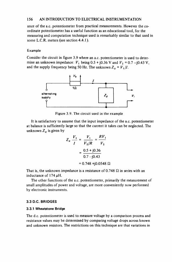
156 AN INTRODUCTION TO ELECTRICAL INSTRUMENTATION
ance of the a.c. potentiometer from practical measurements. However the co-ordinate potentiometer has a useful function as an educational tool, for the measuring and computation technique used is remarkably similar to that used in some L.C.R. meters (see section 4.4.1).
Example
Consider the circuit in figure 3.9 where an a.c. potentiometer is used to deter-mine an unknown impedance: V1 being 0.5 +j0.36 V and V2 = 0.7 —j0.43 V, and the supply frequency being 50 Hz. The unknown Zx = V1/I.
Figure 3.9. The circuit used in the example
alternatingsupply
It is satisfactory to assume that the input impedance of the a.c. potentiometer at balance is sufficiently large so that the current it takes can be neglected. The unknown Zx is given by
That is, the unknown impedance is a resistance of 0.748 Ω in series with an inductance of 174 μH.
The other functions of the a.c. potentiometer, primarily the measurement of small amplitudes of power and voltage, are more conveniently now performed by electronic instruments.
3.3 D.C. BRIDGES
3.3.1 Wheatstone Bridge
The d.c. potentiometer is used to measure voltage by a comparison process and resistance values may be determined by comparing voltage drops across known and unknown resistors. The restrictions on this technique are that variations in
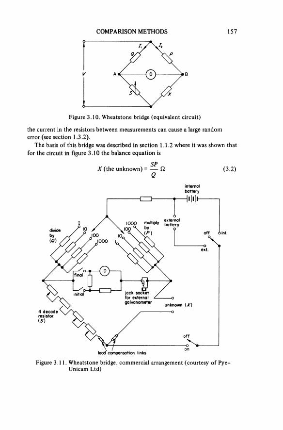
COMPARISON METHODS 157
Figure 3.10. Wheatstone bridge (equivalent circuit)
the current in the resistors between measurements can cause a large random error (see section 1.3.2).
The basis of this bridge was described in section 1.1.2 where it was shown that for the circuit in figure 3.10 the balance equation is
X (the unknown) (3.2)
Figure 3.11. Wheatstone bridge, commercial arrangement (courtesy of Pye Unicam Ltd)
internalbattery
divideby(Q)
multiplyby(P)
externalbattery
off int.
ext.
final
initial jack socket for external galvanometer unknown (X)
4 decaderesistor(5)
off
onlead compensation links
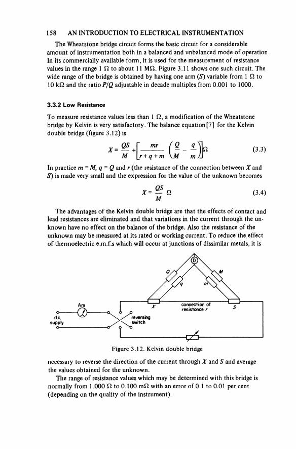
158 AN INTRODUCTION TO ELECTRICAL INSTRUMENTATION
The Wheatstone bridge circuit forms the basic circuit for a considerable amount of instrumentation both in a balanced and unbalanced mode of operation. In its commercially available form, it is used for the measurement of resistance values in the range 1 Ω to about 11 MΩ. Figure 3.11 shows one such circuit. The wide range of the bridge is obtained by having one arm (S) variable from 1 Ω to 10 kΩ and the ratio P/Q adjustable in decade multiples from 0.001 to 1000.
3.3.2 Low Resistance
To measure resistance values less than 1 Ω, a modification of the Wheatstone bridge by Kelvin is very satisfactory. The balance equation [7] for the Kelvin double bridge (figure 3.12) is
(3.3)
In practice m = M, q = Q and r (the resistance of the connection between X and S) is made very small and the expression for the value of the unknown becomes
(3.4)
The advantages of the Kelvin double bridge are that the effects of contact and lead resistances are eliminated and that variations in the current through the un-known have no effect on the balance of the bridge. Also the resistance of theunknown may be measured at its rated or working current. To reduce the effect of thermoelectric e.m.f.s which will occur at junctions of dissimilar metals, it is
Figure 3.12. Kelvin double bridge
Am
d.c.supply
reversingswitch
connection of resistance r
necessary to reverse the direction of the current through X and S and average the values obtained for the unknown.
The range of resistance values which may be determined with this bridge is normally from 1.000 Ω to 0.100 mΩ with an error of 0.1 to 0.01 per cent (depending on the quality of the instrument).
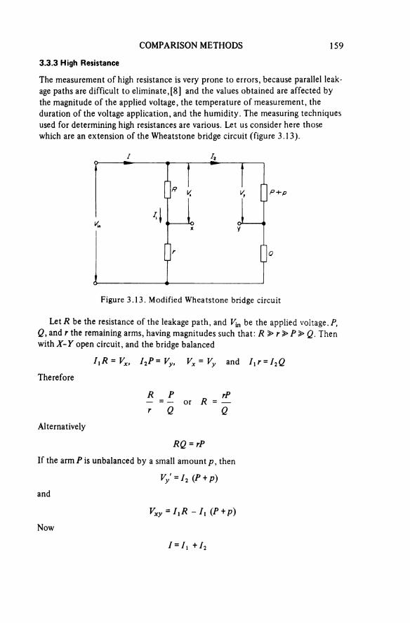
COMPARISON METHODS 1593.3.3 High Resistance
The measurement of high resistance is very prone to errors, because parallel leak-age paths are difficult to eliminate, [8] and the values obtained are affected by the magnitude of the applied voltage, the temperature of measurement, the duration of the voltage application, and the humidity. The measuring techniques used for determining high resistances are various. Let us consider here those which are an extension of the Wheatstone bridge circuit (figure 3.13).
Figure 3.13. Modified Wheatstone bridge circuit
Let R be the resistance of the leakage path, and Vin be the applied voltage. P, Q, and r the remaining arms, having magnitudes such that: R > r > P > Q. Then with X-Y open circuit, and the bridge balanced
Therefore
Alternatively
If the arm P is unbalanced by a small amount p, then
and
Now
160 AN INTRODUCTION TO ELECTRICAL INSTRUMENTATION
and
Therefore
(since QR = rP). Now
Thus
The terms pR, pr and rQ will all be much smaller than PR and may therefore be neglected, giving
(3.5)
Thus the voltage applied to a detector connected between X and Y will be proportional to a fractional change (p/P) in the arm P, and provides a method of measuring resistances up to 100 GΩ. For example, using a 1 kV supply, r = 1 MΩ, P = 1 kΩ, Q = 1 Ω, and p = 10 Ω, gives
The detector used in such a circuit may be a sensitive galvanometer (sensitivity 1 mm deflection per pA) or alternatively an electronic detector could be used, when the input current could be as low as 0.1 pA.
Such an instrument would have a very high input impedance (for example the input stage could contain an electrometer valve (see p. 71). and this provides
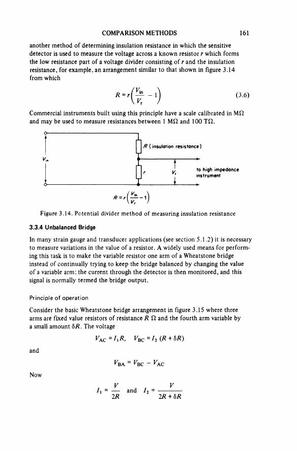
COMPARISON METHODS 161
another method of determining insulation resistance in which the sensitive detector is used to measure the voltage across a known resistor r which forms the low resistance part of a voltage divider consisting of r and the insulation resistance, for example, an arrangement similar to that shown in figure 3.14 from which
(3.6)
Commercial instruments built using this principle have a scale calibrated in MΩ and may be used to measure resistances between 1 MΩ and 100 TΩ.
Figure 3.14. Potential divider method of measuring insulation resistance
R (insulation resistance)
to high impedance instrument
3.3.4 Unbalanced Bridge
In many strain gauge and transducer applications (see section 5.1.2) it is necessary to measure variations in the value of a resistor. A widely used means for perform-ing this task is to make the variable resistor one arm of a Wheatstone bridge instead of continually trying to keep the bridge balanced by changing the value of a variable arm: the current through the detector is then monitored, and this signal is normally termed the bridge output.
Principle of operation
Consider the basic Wheatstone bridge arrangement in figure 3.15 where three arms are fixed value resistors of resistance R Ω and the fourth arm variable by a small amount δR. The voltage
and
Now

162 AN INTRODUCTION TO ELECTRICAL INSTRUMENTATION
Therefore
(3.7)
This expression indicates that providing δR is small, VAB ∞ δR, and if δR is less than 7 per cent of R, this assumption of proportionality is justifiable, that is Vab = V(δR/4R). The current through the detector will depend on its imped-ance and the total equivalent impedance between the detector and the voltagesource, that is the impedance the detector ‘sees’. This impedance is known as the Thévenin impedance zth and is calculated by replacing the source by its internal impedance and computing the impedance of the resultant network (see figure 3.16).
Figure 3.15. Unbalanced Wheatstone bridge
Figure 3.16. Rearrangement of unbalanced Wheatstone bridge (detector open circuit)

COMPARISON METHODS 163
In general the impedance of the voltage source used in conjunction with such a circuit will be very small and Rs may be taken as zero. This simplifies the calculation of Zth considerably for then
(3.8)
and if δR << R
Figure 3.17. Equivalent circuit of figure 3.16
The circuit may be redrawn as figure 3.17, where Rg is the internal resistance of the detector, hence the detector current
(3.9)
(VAB being the voltage which would occur at the terminals AB if the detector were open circuit). Such a circuit will produce only small output voltages whichcan be used to drive a sensitive pointer instrument or pen recorder movement. The output of such a system can be increased by using more than one variable arm, for example as shown in figure 3.18, from which
Figure 3.18. Unbalanced bridge with two variable arms
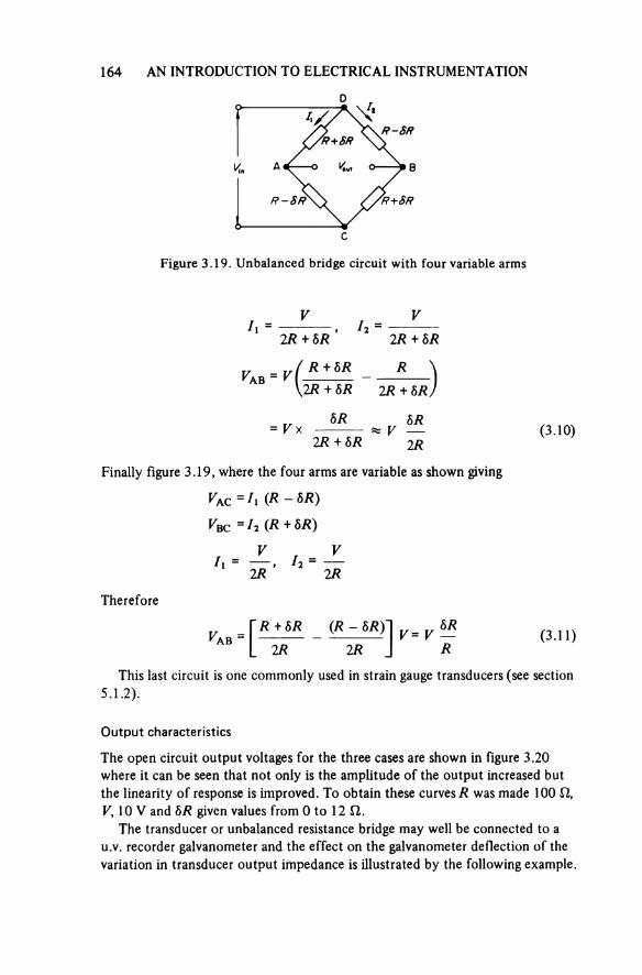
164 AN INTRODUCTION TO ELECTRICAL INSTRUMENTATION
Figure 3.19. Unbalanced bridge circuit with four variable arms
(3.10)
Finally figure 3.19, where the four arms are variable as shown giving
Therefore
(3.11)
This last circuit is one commonly used in strain gauge transducers (see section 5.1.2).
Output characteristics
The open circuit output voltages for the three cases are shown in figure 3.20 where it can be seen that not only is the amplitude of the output increased but the linearity of response is improved. To obtain these curves R was made 100 Ω, V, 10 V and δR given values from 0 to 12 Ω.
The transducer or unbalanced resistance bridge may well be connected to a u.v. recorder galvanometer and the effect on the galvanometer deflection of the variation in transducer output impedance is illustrated by the following example.
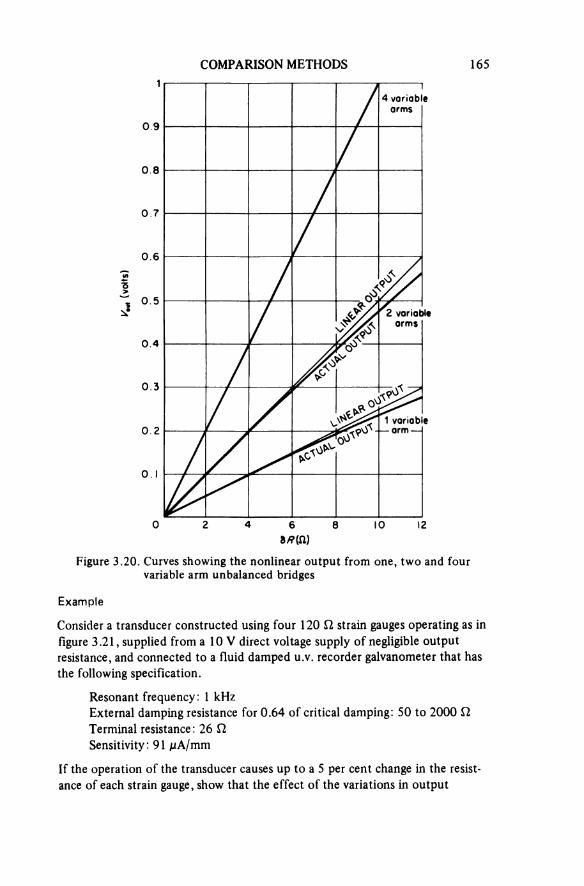
COMPARISON METHODS 165
Figure 3.20. Curves showing the nonlinear output from one, two and four variable arm unbalanced bridges
4 variable arms
2 variable arms
1 variable arm
Example
Consider a transducer constructed using four 120 Ω strain gauges operating as in figure 3.21, supplied from a 10 V direct voltage supply of negligible output resistance, and connected to a fluid damped u.v. recorder galvanometer that has the following specification.
Resonant frequency: 1 kHzExternal damping resistance for 0.64 of critical damping: 50 to 2000 Ω Terminal resistance: 26 Ω Sensitivity: 91 μA/mm
If the operation of the transducer causes up to a 5 per cent change in the resist-ance of each strain gauge, show that the effect of the variations in output

166 AN INTRODUCTION TO ELECTRICAL INSTRUMENTATION
impedance resulting from the operation of the transducer will be small compared with tolerances on other components of the system.
δR for 5 per cent change in R is 6 Ω. Therefore
Rth at limit =
open circuit Vab =
output current to galvanometer =
Hence
deflection =
= 37.71 mm
If δR values ignored
theoretical deflection = = 37.6341 mm
Henceerror in deflection = 0.201%
Since the tolerance on the galvanometer will be at least ± 5 per cent the effect of δR values on the transducer output resistance is negligible.
Note: Although the above statement is generally true, should δR be a relatively large percentage of R its effect on Rth cannot be neglected.
Figure 3.21. Circuit and reduced equivalent circuit in example
galvan-ometer
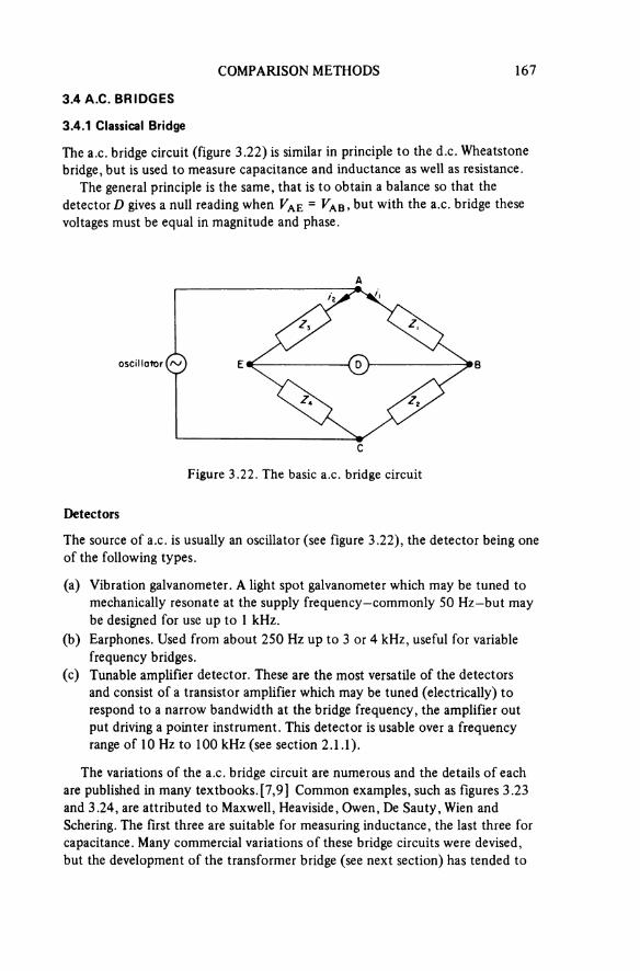
COMPARISON METHODS 167
3.4 A.C. BRIDGES
3.4.1 Classical Bridge
The a.c. bridge circuit (figure 3.22) is similar in principle to the d.c. Wheatstone bridge, but is used to measure capacitance and inductance as well as resistance.
The general principle is the same, that is to obtain a balance so that the detector D gives a null reading when Vae = VAB, but with the a.c. bridge these voltages must be equal in magnitude and phase.
Figure 3.22. The basic a.c. bridge circuit
oscillator
Detectors
The source of a.c. is usually an oscillator (see figure 3.22), the detector being one of the following types.
(a) Vibration galvanometer. A light spot galvanometer which may be tuned to mechanically resonate at the supply frequency—commonly 50 Hz—but may be designed for use up to 1 kHz.
(b) Earphones. Used from about 250 Hz up to 3 or 4 kHz, useful for variable frequency bridges.
(c) Tunable amplifier detector. These are the most versatile of the detectors and consist of a transistor amplifier which may be tuned (electrically) to respond to a narrow bandwidth at the bridge frequency, the amplifier out put driving a pointer instrument. This detector is usable over a frequency range of 10 Hz to 100 kHz (see section 2.1.1).
The variations of the a.c. bridge circuit are numerous and the details of each are published in many textbooks. [7, 9] Common examples, such as figures 3.23 and 3.24, are attributed to Maxwell, Heaviside, Owen, De Sauty, Wien and Schering. The first three are suitable for measuring inductance, the last three for capacitance. Many commercial variations of these bridge circuits were devised, but the development of the transformer bridge (see next section) has tended to
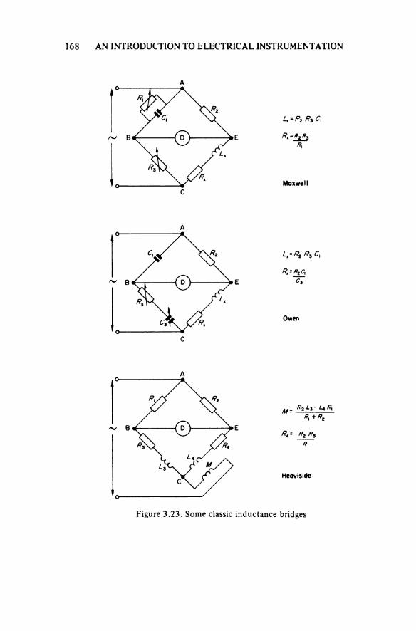
168 AN INTRODUCTION TO ELECTRICAL INSTRUMENTATION
Figure 3.23. Some classic inductance bridges
Maxwell
Owen
Heaviside
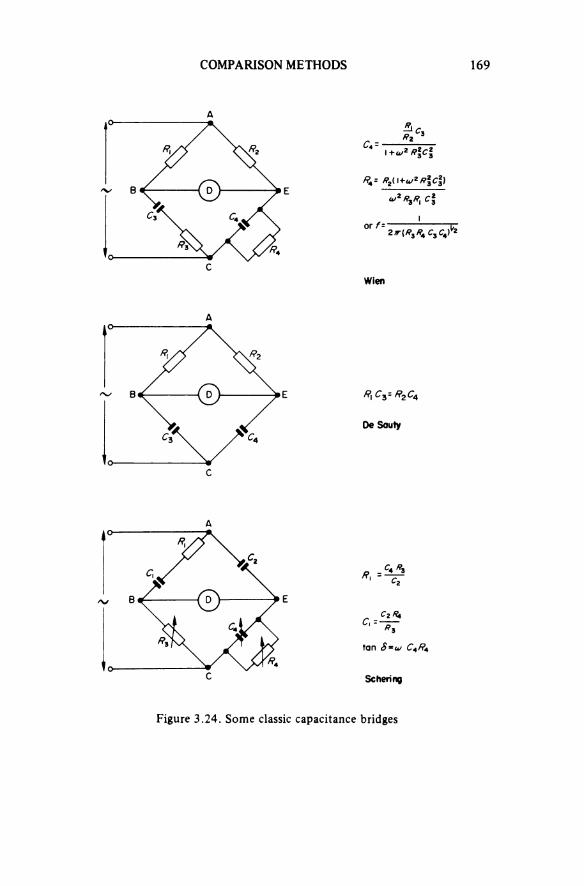
COMPARISON METHODS 169
Figure 3.24. Some classic capacitance bridges
Wien
De Sauty
Schering
1 70 AN INTRODUCTION TO ELECTRICAL INSTRUMENTATION
supplant them. The current developments in component meters (see section 4.4.1) will undoubtedly continue the trend of replacing manually balanced bridges by automatic electronic equipment.
A bridge that is still used in high voltage work is the Schering bridge, and to demonstrate the principles of determining the balance conditions for a.c. bridges this will be considered in detail.
The balance conditions derived assume a series circuit for the unknown C1, R1. At balance
in magnitude and phase
Therefore
(3.12)
and
giving
(3.13)
From equations 3.12 and 3.13
Therefore
Equating real terms

COMPARISON METHODS 171
Therefore
(3.14)
Equating imaginary terms
Therefore
(3.15)
Also tan δ, the loss angle of the unknown capacitor for the series case, = ωC1R1. Therefore
(3.16)
For high voltage application, C2 would be a standard high voltage capacitor (see figure 7.16).
3.4.2 Single-ratio Transformer Bridges
Due to the accuracy and versatility of ratio transformers (see section 6.1.4), anumber of forms of a.c. bridge circuit incorporating these devices, as ratio arms, have been developed and have proved very satisfactory when making precise measurements. Examples of their application are as follows.
Resistance measurement
The arrangement of the ratio transformer into a simple bridge for comparison of resistance values is quite straightforward as shown by figure 3.25. The current through Rx (the unknown) is
Figure 3.25. Resistance measurement using a ratio transformer
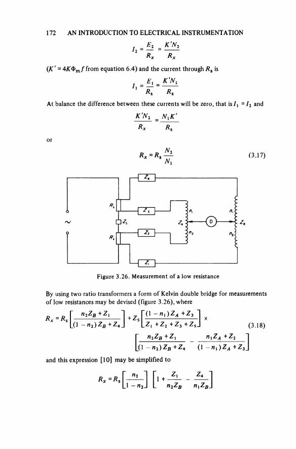
172 AN INTRODUCTION TO ELECTRICAL INSTRUMENTATION
(K' = 4KΦmf from equation 6.4) and the current through Rs is
At balance the difference between these currents will be zero, that is I1 = I2 and
or
(3.17)
Figure 3.26. Measurement of a low resistance
By using two ratio transformers a form of Kelvin double bridge for measurements of low resistances may be devised (figure 3.26), where
and this expression [10] may be simplified to
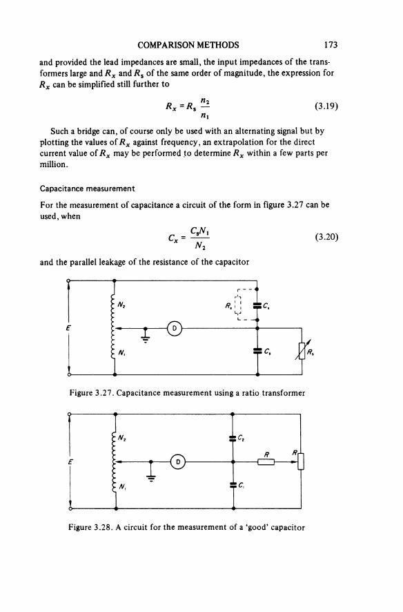
COMPARISON METHODS 173
and provided the lead impedances are small, the input impedances of the trans-formers large and Rx and Rs of the same order of magnitude, the expression for Rx can be simplified still further to
(3.19)
Such a bridge can, of course only be used with an alternating signal but byplotting the values of Rx against frequency, an extrapolation for the direct current value of Rx may be performed to determine Rx within a few parts permillion.
Capacitance measurement
For the measurement of capacitance a circuit of the form in figure 3.27 can be used, when
(3.20)
and the parallel leakage of the resistance of the capacitor
Figure 3.27. Capacitance measurement using a ratio transformer
Figure 3.28. A circuit for the measurement of a ‘good’ capacitor

174 AN INTRODUCTION TO ELECTRICAL INSTRUMENTATION
(3.21)
An alternative arrangement of this circuit, sometimes used in connection with capacitance transducers (see section 5.2.1), is shown in figure 3.28 where provid-ed the parallel leakage resistance of both capacitors is large, the resistance effects can be neglected and
Other uses [11, 12]
Other application examples of the auto or ratio transformer are in the measure-ment of small phase angles, the converting of a fixed standard into a variable one, the determination of amplifier gain and transformer ratios, and as a precision voltage divider.
However, in practice it must be appreciated that the ratio transformer is not ideal and in all its uses that involve drawing a load current through part of the winding, allowance should be made for the resistance and inductance of the wind-ings. The equivalent circuit which represents the ratio transformer is shown in figure 3.29. The values of Rs and Ls will vary with ratio setting and the error they introduce must be added to the no-load error, which is the value normally quoted.
Figure 3.29. Simplified equivalent circuit of a ratio transformer
input
output
3.4.3 Transformer Double-ratio Bridges
The transformer bridges described so far have had a similarity with the classical bridges in that at balance, a voltage equality exists and there is no resultant current flow through the detector. An alternative to this would be to arrange that, at balance, the current flowing through the unknown was equal and oppo-site to that through the standard or known impedance, the detector indicating this equality.
Consider the circuit in figure 3.30 where the ‘ideal’ voltage transformer has a secondary winding of N1 turns with a tapping at N2 turns, so that voltages E1 and E2 are applied to impedances Zx and Zs respectively, resulting in currents

COMPARISON METHODS 175
Figure 3.30. Basic circuit of a double-ratio transformer bridge
startvoltagetransformer
currentcomparator
I1 and I2 flowing in the windings n1 and n2 of the current comparator.The ampere turns n1I1 and n2I2 will produce fluxes in the core of the com-
parator that will oppose each other and a balance condition will be attained when the resultant flux is zero, this being indicated by the voltage in the winding connected to the detector also being zero. Thus, at balance
(3.22)
Now
and
Therefore
(3.23)
If ZX is resistive
(3.24)
If Zx is capacitive
or
(3.25)
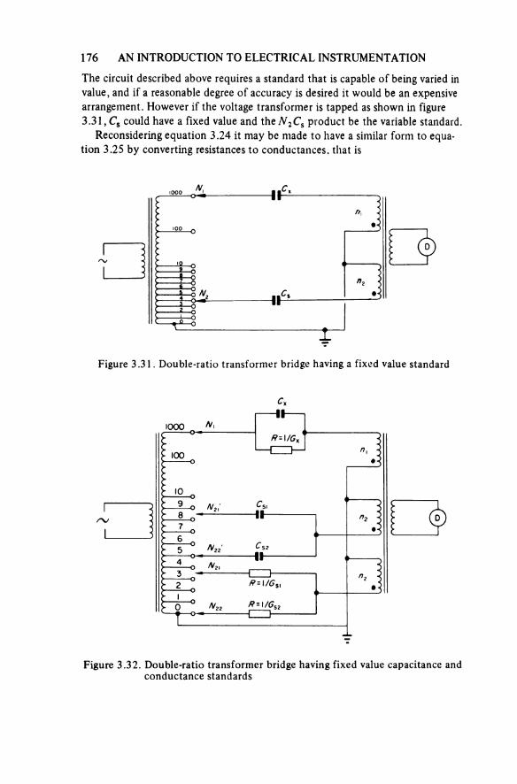
176 AN INTRODUCTION TO ELECTRICAL INSTRUMENTATION
The circuit described above requires a standard that is capable of being varied in value, and if a reasonable degree of accuracy is desired it would be an expensive arrangement. However if the voltage transformer is tapped as shown in figure 3.31, Cs could have a fixed value and the N2Cs product be the variable standard.
Reconsidering equation 3.24 it may be made to have a similar form to equa-tion 3.25 by converting resistances to conductances, that is
Figure 3.31. Double-ratio transformer bridge having a fixed value standard
Figure 3.32. Double-ratio transformer bridge having fixed value capacitance and conductance standards
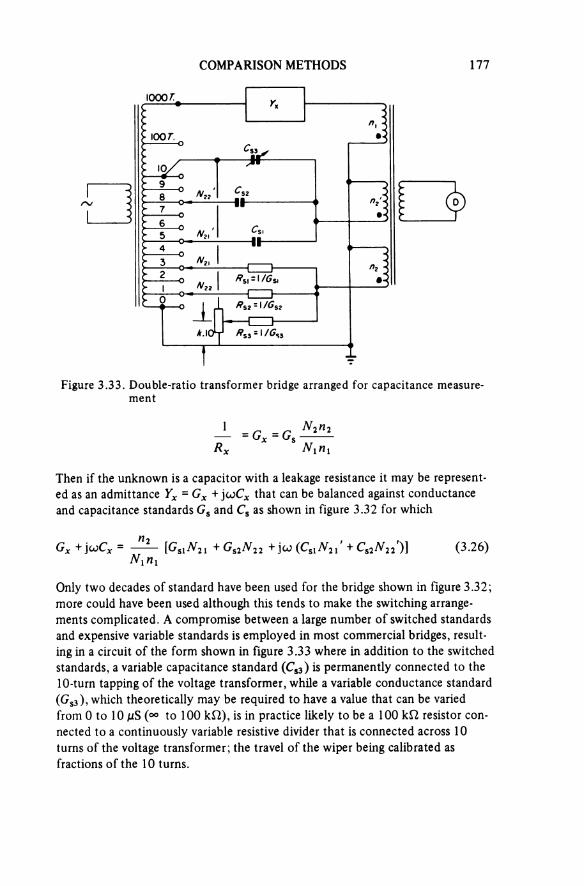
COMPARISON METHODS 177
Figure 3.33. Double-ratio transformer bridge arranged for capacitance measure-ment
Then if the unknown is a capacitor with a leakage resistance it may be represent ed as an admittance Yx = Gx + jωCx that can be balanced against conductance and capacitance standards Gs and Cs as shown in figure 3.32 for which
(3.26)
Only two decades of standard have been used for the bridge shown in figure 3.32; more could have been used although this tends to make the switching arrange-ments complicated. A compromise between a large number of switched standards and expensive variable standards is employed in most commercial bridges, result-ing in a circuit of the form shown in figure 3.33 where in addition to the switched standards, a variable capacitance standard (Cs3) is permanently connected to the 10-turn tapping of the voltage transformer, while a variable conductance standard (Gs3), which theoretically may be required to have a value that can be varied from 0 to 10 μS (∞ to 100 kΩ), is in practice likely to be a 100 kΩ resistor con-nected to a continuously variable resistive divider that is connected across 10 turns of the voltage transformer; the travel of the wiper being calibrated as fractions of the 10 turns.
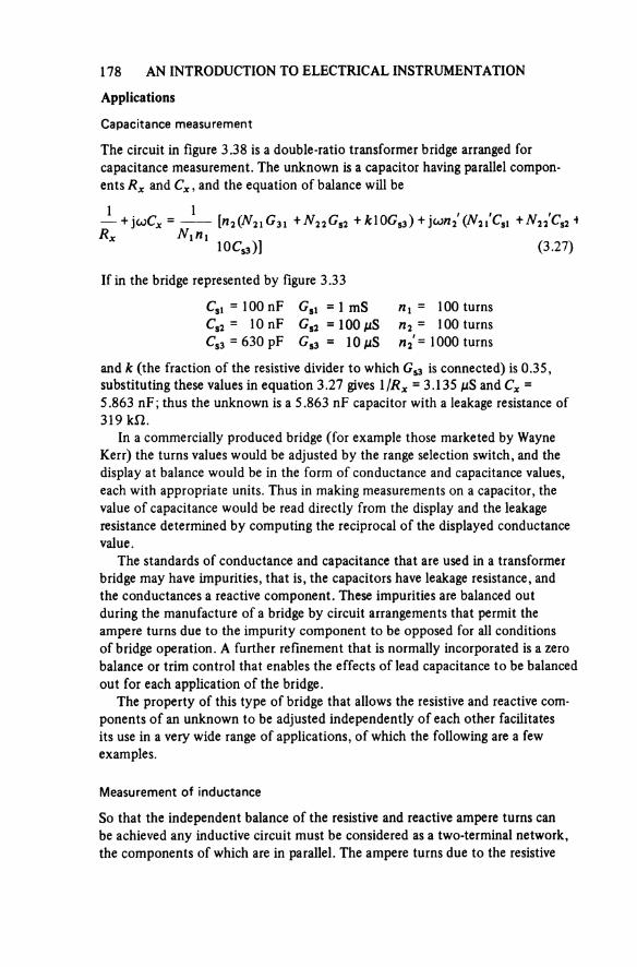
178 AN INTRODUCTION TO ELECTRICAL INSTRUMENTATION
Applications
Capacitance measurement
The circuit in figure 3.38 is a double-ratio transformer bridge arranged for capacitance measurement. The unknown is a capacitor having parallel compon-ents Rx and Cx, and the equation of balance will be
(3.27)
If in the bridge represented by figure 3.33
Cs1 = 100 nF Cs2 = 10 nF Cs3 = 630 pF
Gs1 = 1 mS Gs 2 = 100 μS Gs 3 = 10 μS
n1 = 100 turnsn2 = 100 turns n2' = 1000 turns
and k (the fraction of the resistive divider to which Gs3 is connected) is 0.35, substituting these values in equation 3.27 gives 1/RX = 3.135 μS and Cx =5.863 nF; thus the unknown is a 5.863 nF capacitor with a leakage resistance of 319 kΩ.
In a commercially produced bridge (for example those marketed by Wayne Kerr) the turns values would be adjusted by the range selection switch, and the display at balance would be in the form of conductance and capacitance values,each with appropriate units. Thus in making measurements on a capacitor, the value of capacitance would be read directly from the display and the leakage resistance determined by computing the reciprocal of the displayed conductance value.
The standards of conductance and capacitance that are used in a transformer bridge may have impurities, that is, the capacitors have leakage resistance, and the conductances a reactive component. These impurities are balanced outduring the manufacture of a bridge by circuit arrangements that permit the ampere turns due to the impurity component to be opposed for all conditions of bridge operation. A further refinement that is normally incorporated is a zero balance or trim control that enables the effects of lead capacitance to be balanced out for each application of the bridge.
The property of this type of bridge that allows the resistive and reactive com-ponents of an unknown to be adjusted independently of each other facilitates its use in a very wide range of applications, of which the following are a few examples.
Measurement of inductance
So that the independent balance of the resistive and reactive ampere turns can be achieved any inductive circuit must be considered as a two-terminal network, the components of which are in parallel. The ampere turns due to the resistive
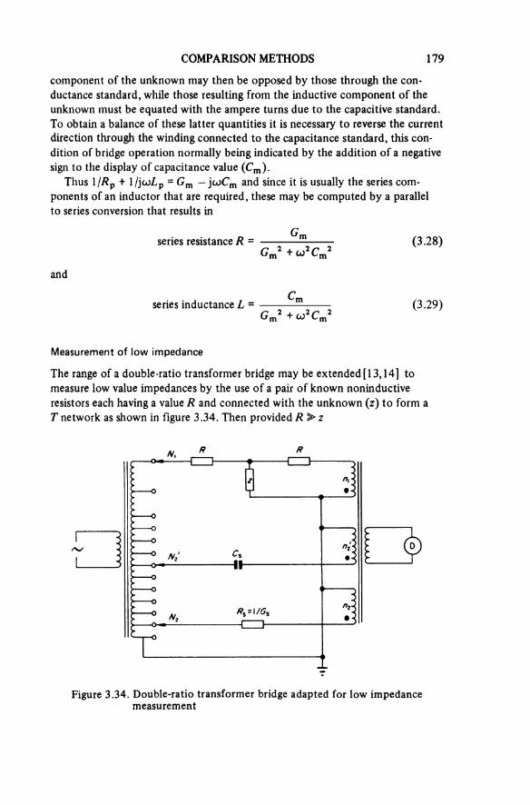
COMPARISON METHODS 179
component of the unknown may then be opposed by those through the con-ductance standard, while those resulting from the inductive component of theunknown must be equated with the ampere turns due to the capacitive standard. To obtain a balance of these latter quantities it is necessary to reverse the current direction through the winding connected to the capacitance standard, this con-dition of bridge operation normally being indicated by the addition of a negative sign to the display of capacitance value (Cm).
Thus l/Rp + 1/jωLp = Gm — jωCm and since it is usually the series com-ponents of an inductor that are required, these may be computed by a parallel to series conversion that results in
series resistance R =
and
series inductance L =
(3.28)
(3.29)
Measurement of low impedance
The range of a double-ratio transformer bridge may be extended [13, 14] to measure low value impedances by the use of a pair of known noninductive resistors each having a value R and connected with the unknown (z) to form a T network as shown in figure 3.34. Then provided A >> z
Figure 3.34. Double-ratio transformer bridge adapted for low impedance measurement

180 AN INTRODUCTION TO ELECTRICAL INSTRUMENTATION
or for a calibrated bridge
(3.30)
Measurements of components 'in situ'
One of the greatest advantages of double-ratio transformer bridges is the ability to use them for the measurement of components whilst these remain connected in a circuit. To appreciate how this is possible it is necessary to consider the trans formers that are used in the construction of the double-ratio bridge. If these transformers were ‘ideal’, that is if they had zero leakage reactance, zero winding resistance, and zero magnetisation loss, the impedances Ze and Zi in figure 3.35
Figure 3.35. Measurement of components ‘in situ’ using a double-ratio transformer bridge
would be zero, and the voltage applied to Zu (the unknown) would be unaffected by current flowing through Zx. In addition to this all the current flowing through Zu would flow into the n1 winding, since Iy = (ZiIu)/(Zi + Zy). In practice Ze and Zi will have small finite values and a correction must be applied to the values read from the balanced bridge. It may be shown that to a close approximation the true value of the unknown impedance
(3.31)
The impedances Ze and Zi must be determined (for a particular range of the bridge) by measurements on a separate delta network that contains known values for Zx and Zy.
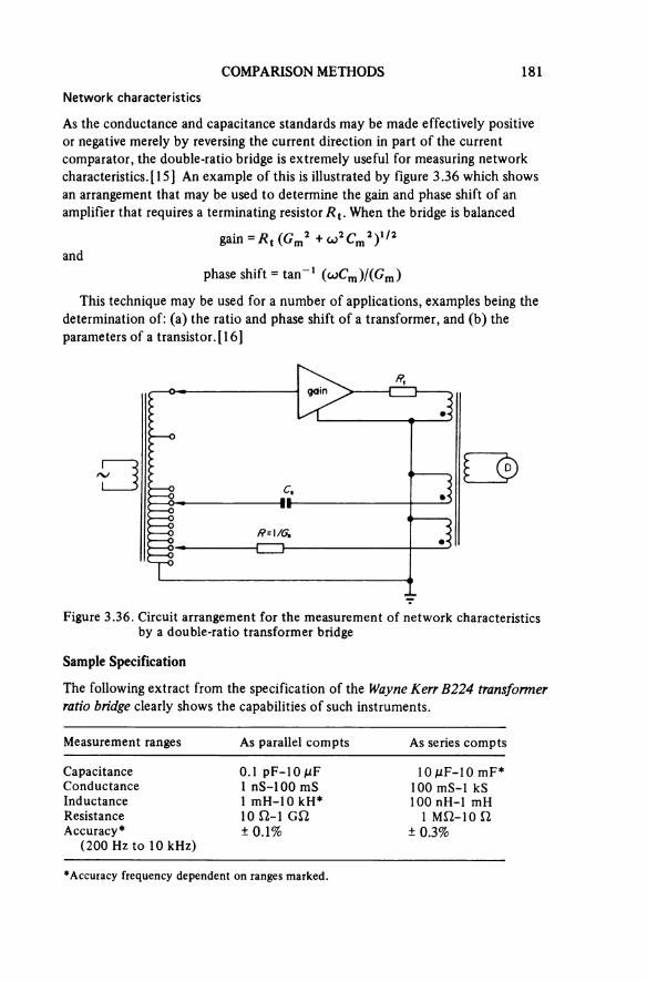
COMPARISON METHODS 181
Network characteristics
As the conductance and capacitance standards may be made effectively positive or negative merely by reversing the current direction in part of the current comparator, the double-ratio bridge is extremely useful for measuring network characteristics. [15] An example of this is illustrated by figure 3.36 which shows an arrangement that may be used to determine the gain and phase shift of an amplifier that requires a terminating resistor Rt. When the bridge is balanced
gain =and
phase shift =
This technique may be used for a number of applications, examples being the determination of: (a) the ratio and phase shift of a transformer, and (b) the parameters of a transistor. [16]
Figure 3.36. Circuit arrangement for the measurement of network characteristics by a double-ratio transformer bridge
Sample Specification
The following extract from the specification of the Wayne Kerr B224 transformer ratio bridge clearly shows the capabilities of such instruments.
Measurement ranges As parallel compts As series compts
Capacitance 0.1 pF-10μF 10 μF-10 mF*Conductance 1 nS-100 mS 100 mS-1 kSInductance 1 mH-10 kH* 100 nH-1 mHResistance 10 Ω-l GΩ 1 MΩ-10 ΩAccuracy*
(200 Hz to 10 kHz)± 0.1% ± 0.3%
*Accuracy frequency dependent on ranges marked.
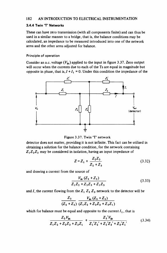
182 AN INTRODUCTION TO ELECTRICAL INSTRUMENTATION
3.4.4 Twin 'T' Networks
These can have zero transmission (with all components finite) and can thus be used in a similar manner to a bridge, that is, the balance conditions may be calculated, an impedance to be measured introduced into one of the network arms and the other arms adjusted for balance.
Principle of operation
Consider an a.c. voltage (Vin) applied to the input in figure 3.37. Zero output will occur when the currents due to each of the Ts are equal in magnitude but opposite in phase, that is, I + I1 = 0. Under this condition the impedance of the
Figure 3.37. Twin ‘T’ networkdetector does not matter, providing it is not infinite. This fact can be utilised in obtaining a solution for the balance condition, for the network containing Z1Z2Z3 may be considered in isolation, having an input impedance of
(3.32)and drawing a current from the source of
(3.33)
and /, the current flowing from the Z1 Z2 Z3 network to the detector will be
which for balance must be equal and opposite to the current I1, that is
(3.34)

COMPARISON METHODS 183
and since Vm ≠ 0
(3.35)
and is the condition for balance.The advantage of a twin T arrangement over the conventional bridge circuit is
that it may be used at higher frequencies. This is due to its arrangement which makes it possible to operate with one side of both the source and the detector earthed—a feature which makes shielding much easier than in operating a bridge.
The twin T is also used as a rejection filter and as the feedback network on a tuned amplifier in a frequency selective detector.
3.5 Self-balancing Bridges
The principle of comparison methods is that an operator is required to perform manual operations to reduce the detected signal to a minimum. In some instances this can be a lengthy procedure, requiring experience of a particular type of bridge to obtain rapid operation. Thus in circumstances that dictate a bridge measurement as the only satisfactory method and many measurements are to be made, automatic or self-balancing bridges have been devised.
Principle of operation
As stated above the operation of balancing a bridge is to reduce the error signal presented to the detector to a minimum. Thus in a bridge using a resistance ratio the automatic operation is fairly simple, being basically similar to that used in a potentiometric recorder (see section 3.1.2), that is the error signal is amplified and used to energise the field windings of a motor coupled to the movable con-tact on a resistance divider, for example figure 3.38 where Rx = RS(R2/R1).
Figure 3.38. Self-balancing d.c. Wheatstone bridge
amp.
d.c.supply
mech.link
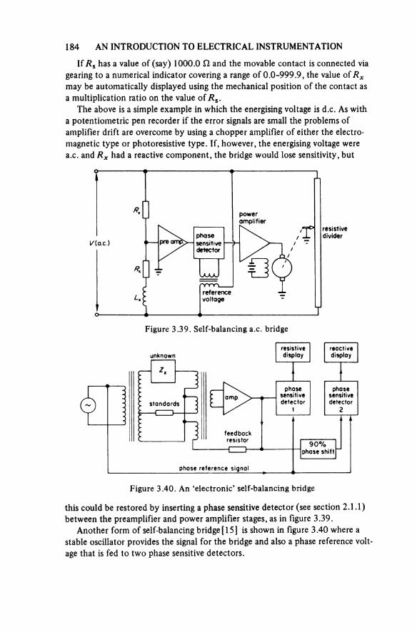
184 AN INTRODUCTION TO ELECTRICAL INSTRUMENTATION
If Rs has a value of (say) 1000.0 Ω and the movable contact is connected via gearing to a numerical indicator covering a range of 0.0-999.9, the value Of Rx may be automatically displayed using the mechanical position of the contact as a multiplication ratio on the value of Rs.
The above is a simple example in which the energising voltage is d.c. As with a potentiometric pen recorder if the error signals are small the problems of amplifier drift are overcome by using a chopper amplifier of either the electro-magnetic type or photoresistive type. If, however, the energising voltage were a.c. and Rx had a reactive component, the bridge would lose sensitivity, but
Figure 3.39. Self-balancing a.c. bridge
preamp.phasesensitivedetector
poweramplifier
resistivedivider
referencevoltage
Figure 3.40. An ‘electronic’ self-balancing bridge
unknownresistivedisplay
reactivedisplay
standardsamp.
phasesensitivedetector
1
phasesensitivedetector
2
feedbackresistor
90% phase shift
phase reference signal
this could be restored by inserting a phase sensitive detector (see section 2.1.1) between the preamplifier and power amplifier stages, as in figure 3.39.
Another form of self-balancing bridge [15] is shown in figure 3.40 where a stable oscillator provides the signal for the bridge and also a phase reference volt age that is fed to two phase sensitive detectors.
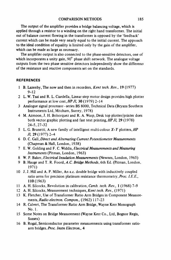
COMPARISON METHODS 185
The output of the amplifier provides a bridge balancing voltage, which is applied through a resistor to a winding on the right hand transformer. The initial out of balance current flowing in the transformer is opposed by the ‘feedback’ current which can be made very nearly equal to the initial current. The approach to the ideal condition of equality is limited only by the gain of the amplifier, which can be made as large as necessary.
The amplifier output is also connected to the phase-sensitive detectors, one of which incorporates a unity gain, 90° phase shift network. The analogue voltage outputs from the two phase sensitive detectors independently show the differencf of the resistance and reactive components set on the standards.
REFERENCES
1 B. Lazenby, The now and then in recorders, Kent tech. Rev., 19 (1977)9-12
2 L. W. Tsai and R. L. Ciardeπa, Linear step motor design provides high plotterperformance at low cost, HP Jl, 30 (1979) 2-14
3 Analogue signal processor—series BS 8000, Technical Data (Bryans SouthernInstruments Ltd, Mitcham, Surrey, 1978)
4 M. Azmoon, J. H. Bohorquez and R. A. Warp, Desk top plotter/printer doesboth vector graphic plotting and fast text printing, HP Jl, 29 (1978) 24-5, 27-32
5 L. G. Brunetti, A new family of intelligent multi-colour X-Y plotters, HPJl, 29 (1977) 2-4
6 D.C. Gall, Direct and Alternating Current Potentiometer Measurements(Chapman & Hall, London, 1938)
7 E. W. Golding and F. C. Widdis, Electrical Measurements and MeasuringInstruments (Pitman, London, 1963)
8 W. P. Baker, Electrical Insulation Measurements (Newnes, London, 1965)9 B. Hauge and T. R. Foord, A.C. Bridge Methods, 6th Ed. (Pitman, London,
1971)10 J. J. Hill and A. P. Miller, An a.c. double bridge with inductively coupled
ratio arms for precision platinum resistance thermometry, Proc. I.E.E., 110 (1963)
11 A. H. Silcocks, Revolution in calibration, Camb. tech. Rev., 1 (1968) 7-912 A. H. Silcocks, Measurement techniques, Kent tech. Rev., (1971)1 3 K. Fletcher, Use of Transformer Ratio Arm Bridges in Component Measure-
ments, Radio electron. Compon., (1962) 117-2314 R. Calvert, The Transformer Ratio Arm Bridge, Wayne Kerr Monograph
No. 1.15 Some Notes on Bridge Measurement (Wayne Kerr Co., Ltd, Bognor Regis,
Sussex)16 B. Rogal, Semiconductor parameter measurements using transformer ratio-
arm bridges. Proc. Instn Electron., 4
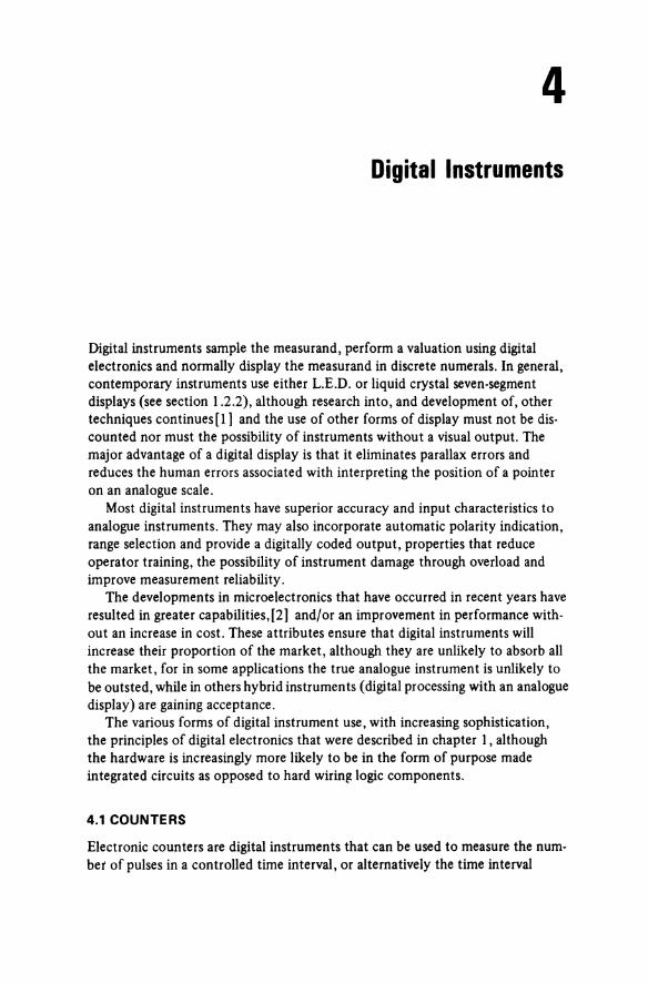
4Digital Instruments
Digital instruments sample the measurand, perform a valuation using digital electronics and normally display the measurand in discrete numerals. In general, contemporary instruments use either L.E.D. or liquid crystal seven-segment displays (see section 1.2.2), although research into, and development of, other techniques continues [1] and the use of other forms of display must not be dis-counted nor must the possibility of instruments without a visual output. The major advantage of a digital display is that it eliminates parallax errors andreduces the human errors associated with interpreting the position of a pointer on an analogue scale.
Most digital instruments have superior accuracy and input characteristics to analogue instruments. They may also incorporate automatic polarity indication, range selection and provide a digitally coded output, properties that reduce operator training, the possibility of instrument damage through overload and improve measurement reliability.
The developments in microelectronics that have occurred in recent years have resulted in greater capabilities, [2] and/or an improvement in performance with-out an increase in cost. These attributes ensure that digital instruments will increase their proportion of the market, although they are unlikely to absorb all the market, for in some applications the true analogue instrument is unlikely to be outsted, while in others hybrid instruments (digital processing with an analogue display) are gaining acceptance.
The various forms of digital instrument use, with increasing sophistication, the principles of digital electronics that were described in chapter 1, although the hardware is increasingly more likely to be in the form of purpose made integrated circuits as opposed to hard wiring logic components.
4.1 COUNTERS
Electronic counters are digital instruments that can be used to measure the num-ber of pulses in a controlled time interval, or alternatively the time interval

DIGITAL INSTRUMENTS 187
between pulses. The accuracy of measurements made using counters is largely dependent on an internal oscillator. Electronic counters are marketed with various frequency ranges and measurement capabilities.
4.1.1 Principle of Operation
A digital counter may be considered to consist of a number of operational blocks which may be interconnected in different ways to perform the various time dependent measurements. The ‘core’ of this type of instrument will, of course, be the digital circuits that perform the count, and these are based on the following.
When a group of bistables (see section 1.1.3) are connected together so that they store related information, they are collectively termed a register. Registers of certain forms can be arranged to count pulses either synchronously or asynchronously.
Asynchronous counters
In these the pulses to be counted are applied to the input end of the array, and the process of adding each pulse to the count has to be completed before the ‘carry bit’ is propagated from the first to the second stage. This second stage has carry bits added to it until it produces a carry bit which is passed to the third stage, and so on. In counting a pulse train the carry bits will appear to ‘ripple’through the counter, and for this reason an asynchronous counter is sometimes referred to as a ‘ripple-through’ counter. A three-stage asynchronous counter using J-K bistables (flip-flops) is illustrated in figure 4.1a, and for such an arrangement the count proceeds as prescribed in table 4.1. Starting from an initial condition in which all the stages are set to zero, when a total of seven pulses have been applied to the counter all the outputs are in the ‘1’ state, and the application of an eighth pulse will cause them all to fall to zero. Since the time taken for each change to propagate to the following stage is tx (figures 4.1a and b) it will take ntx s for the pulse causing this fall to zero to ‘ripple through’ an n stage counter, thus creating a restriction on the speed or maximum count-ing rate of a counter of this form.
Synchronous counters
In this form of counter the counting sequence is controlled by means of a clock pulse and all the changes in output from the bistables occur in synchronism. This effectively eliminates the propagation delay associated with ripple-through counters. To avoid the possibility (when feedback connections are made) of in-stability in the completed counter, ‘master-slave’ bistables are invariably used in synchronous counters. In operation the appropriate input signals are simultan-eously gated into the master stages of all the bistables in the counter and when

188 AN INTRODUCTION TO ELECTRICAL INSTRUMENTATION
Figure 4.1. A ripple-through pure binary counter
(a)
inputpulses
bistable 1 FF1
bistable 2 FF2
bistable 3 FF3
tofollowingstages
resetline
inputpulses
time
(b)
Q1 time
Q2 time
Q3 time
(c)
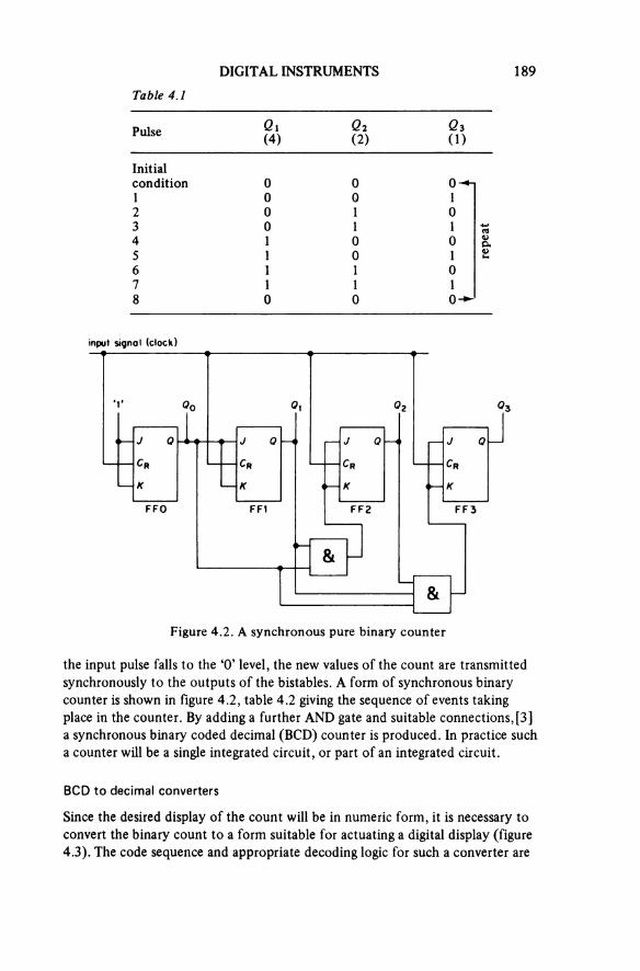
DIGITAL INSTRUMENTS 189Table 4.1
Pulse Q1(4)
Q2(2)
Q3(1)
Initialcondition 0 0 01 0 o 12 0 1 03 0 1 14 1 0 05 1 0 16 1 1 07 1 1 18 0 0 0
repe
at
Figure 4.2. A synchronous pure binary counter
input signal (clock)
the input pulse fans to the ‘0’ level, the new values of the count are transmitted synchronously to the outputs of the bistables. A form of synchronous binary counter is shown in figure 4.2, table 4.2 giving the sequence of events taking place in the counter. By adding a further AND gate and suitable connections, [3] a synchronous binary coded decimal (BCD) counter is produced. In practice such a counter will be a single integrated circuit, or part of an integrated circuit.
BCD to decimal converters
Since the desired display of the count will be in numeric form, it is necessary to convert the binary count to a form suitable for actuating a digital display (figure 4.3). The code sequence and appropriate decoding logic for such a converter are
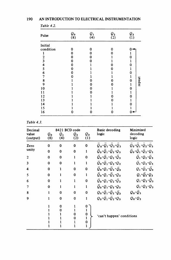
190 AN INTRODUCTION TO ELECTRICAL INSTRUMENTATION
Table 4.2.
Pulse Q0(8)
Q1(4)
Q2(2)
Q3(1)
Initialcondition 0 0 0 0
1 0 0 0 12 0 0 1 03 0 0 1 14 0 1 0 05 0 1 0 16 0 1 1 07 0 1 1 18 1 0 0 09 1 0 0 1
10 1 0 1 011 1 0 1 112 1 1 0 013 1 1 0 114 1 1 1 015 1 1 1 116 0 0 0 0
repe
at
Decimalvalue(output)
8421 BCD code Basic decoding logic
Minimiseddecodinglogic
Q0(8)
Q1(4)
Q2(2)
Q3(1)
Zero 0 0 0 0 Q0-Q1 *Q2’Q3 Q0-Q. •Q2,Q3unity 0 0 0 1 Q0’Q1’Q2’Q3 Q0’Ql •Q2"Q32 0 0 1 0 Q0*Q1 *Q2 *Q3 Q1 ’Q2 ’Q33 0 0 1 1 Q0'Q1*Q2'Q3 Q1 *Q2 *Q34 0 1 0 0 Q0’Q1-Q2-Q3 Q1 ’Q2 ’Q35 0 1 0 1 Q0-Q1 ,Q2,Q3 Ql’Q2"Q36 0 1 1 0 Q0*Q1*Q2*Q3 Q1*Q2*Q37 0 1 1 1 Q0’Q1 *Q2 ’Q3 Q1 *Q2 ’Q38 1 0 0 0 Q0’Ql-Q2-Q3 QO*Q39 1 0 0 1 Q0-Q1 *Q2*Q3 QO*Q3
1 0 1 01 0 1 11 1 0 0 ‘can’t happen’ conditions1 1 0 11 1 1 01 1 1 1
Table 4.3.
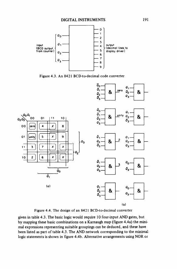
DIGITAL INSTRUMENTS 191
Figure 4.3. An 8421 BCD-to-decimal code converter
input(BCD output from counter)
output(decimal lines to display driver)
Figure 4.4. The design of an 8421 BCD-to-decimal converter
(a)
(b)
given in table 4.3. The basic logic would require 10 four-input AND gates, but by mapping these basic combinations on a Karnaugh map (figure 4.4a) the mini-mal expressions representing suitable groupings can be deduced, and these have been listed as part of table 4.3. The AND network corresponding to the minimal logic statements is shown in figure 4.4b. Alternative arrangements using NOR or
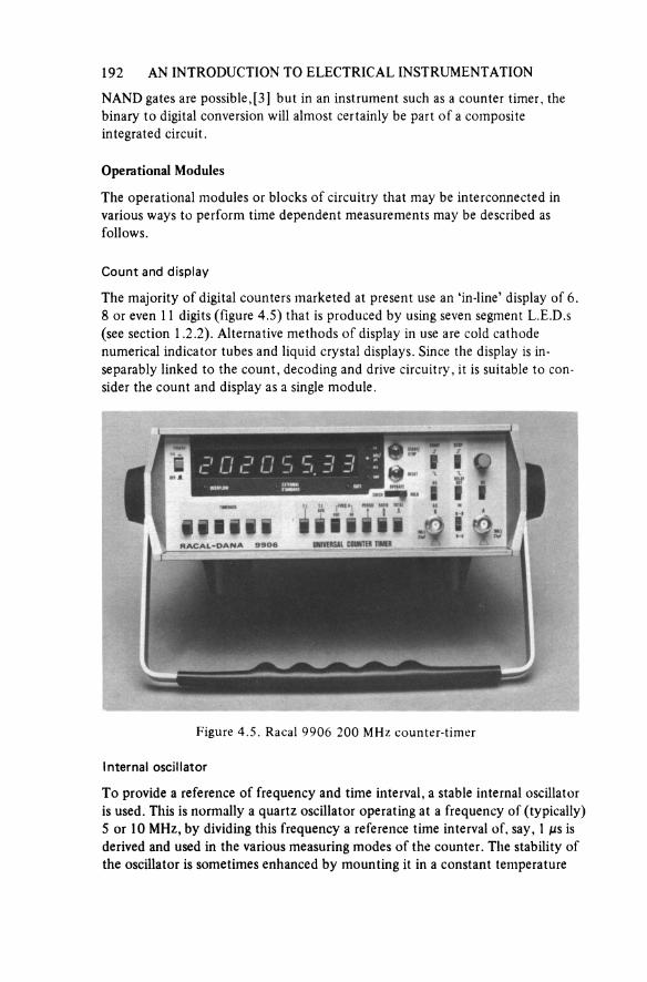
192 AN INTRODUCTION TO ELECTRICAL INSTRUMENTATION
NAND gates are possible, [3] but in an instrument such as a counter timer, the binary to digital conversion will almost certainly be part of a composite integrated circuit.
Operational Modules
The operational modules or blocks of circuitry that may be interconnected in various ways to perform time dependent measurements may be described as follows.
Count and display
The majority of digital counters marketed at present use an ‘in-line’ display of 6, 8 or even 11 digits (figure 4.5) that is produced by using seven segment L.E.D.s (see section 1.2.2). Alternative methods of display in use are cold cathode numerical indicator tubes and liquid crystal displays. Since the display is in-separably linked to the count, decoding and drive circuitry, it is suitable to con-sider the count and display as a single module.
Figure 4.5. Racal 9906 200 MHz counter-timer
Internal oscillator
To provide a reference of frequency and time interval, a stable internal oscillator is used. This is normally a quartz oscillator operating at a frequency of (typically) 5 or 10 MHz, by dividing this frequency a reference time interval of, say, 1 μs is derived and used in the various measuring modes of the counter. The stability of the oscillator is sometimes enhanced by mounting it in a constant temperature
DIGITAL INSTRUMENTS 193
‘oven’ within the instrument, when stabilities of 1 part in 108 or better are obtainable, a necessary precaution if frequencies of 500 MHz to the nearest hertz are to be measured. [4]
The accuracy of the reference oscillator is commonly quoted in terms of its stability between calibration checks. An example of a typical specification is as follows.
Frequency StandardFrequency: 5 MHzTemperature stability: ± 8 parts in 106 over the temperature range 0 to
+ 55 °C. ± 3 parts in 106 over the temperature range +20 to 40 °C
Averaging ageing rate: ± 1 part in 106 per month, three months after delivery but less than ± 1 part in 105 in the first year
Frequency standard output: 1 MHz T.T.L. compatible rectangular wave
To this some manufacturers add an allowance for the effects on the frequency standard due to line voltage variations, but as these effects are small many manu-facturers omit them.
From the above specification it can be estimated that the limit of error (or un certainty) in the accuracy of the frequency standard for such a counter when six months old is < ± 6 parts in 106 if operated between 20 and 40 °C (3 parts from temperature and 3 parts from ageing).
Decade dividers
To provide a suitable range of operation for a counter timer a number (six or seven) of cascaded decade dividers are used to divide either the incoming signal or the frequency from the internal oscillator. The number of decades of division being used in a particular application is decided either by the operation of a front panel switch or by the instrument’s control logic in the ‘auto’ mode of operation.
By way of an example seven decades of division would permit the production, from a 1 MHz reference, of time intervals of 1 μs, 10 μs, 100 μs, 1 ms, 10 ms,100 ms, 1 s and 10 s.
Main gate
To control the interval over which pulses are applied to the display unit, a gate is incorporated. It is arranged as a pulse operated switch so that one command pulse opens the gate (start) thereby allowing the passage of pulses to be counted. The next command pulse closes the gate and thus stops the flow of pulses to be counted.
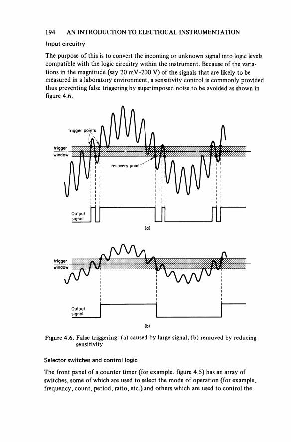
194 AN INTRODUCTION TO ELECTRICAL INSTRUMENTATION
Input circuitry
The purpose of this is to convert the incoming or unknown signal into logic levels compatible with the logic circuitry within the instrument. Because of the varia-tions in the magnitude (say 20 mV-200 V) of the signals that are likely to be measured in a laboratory environment, a sensitivity control is commonly provided thus preventing false triggering by superimposed noise to be avoided as shown in figure 4.6.
Figure 4.6. False triggering: (a) caused by large signal, (b) removed by reducing sensitivity
(a)
trigger
triggerwindow
recovery point
Outputsignal
(b)
triggerwindow
outputsignal
Selector switches and control logic
The front panel of a counter timer (for example, figure 4.5) has an array of switches, some of which are used to select the mode of operation (for example, frequency, count, period, ratio, etc.) and others which are used to control the

DIGITAL INSTRUMENTS 195
duration of the measurement sample, [5] by selecting the magnitude of decade divider used. The switches that are used to select the mode of operation can, in some instruments, be used to activate the control logic so that either the counter continuously samples and displays the incoming signal, or a single sample is made on demand and ‘held’ on display. A number of instruments have an ‘auto’ or automatic ranging capability in their frequency mode of operation and in this condition their control circuits adjust the duration of the sample so that the display contains the maximum number of digits.
The above modules can be interconnected to perform the various time dependent measurements, although it must be mentioned that not every counter timer can perform all the following functions.
4.1.2 Totalise or Count
This is the simplest count function consisting of routing the pulses to be counted through the main gate which may be started and stopped either manually (by push button switches) or by some externally derived pulses (see figure 4.7), the display thus recording the total number of pulses received during the interval between the start and stop signals. The decade dividers have been included in the diagram for in some instruments it is possible to use them to divide the incoming signal so that instead of every pulse being counted only one in 10, or power of 10 is counted.
Figure 4.7. Schematic diagram for totalising or count measurement
decimal counter and display
inputsignal
shapingcircuits
maingate
start/stop command signals
oscillator
decode dividers
The uncertainty in a measurement of a count will be the determination error in the count (normally ± 1 least significant digit) plus the uncertainty in the time interval over which the count is made, this latter quantity being a function of how the time interval is measured and how the command signals are produced.
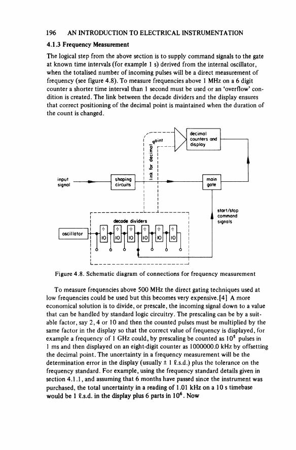
196 AN INTRODUCTION TO ELECTRICAL INSTRUMENTATION
4.1.3 Frequency Measurement
The logical step from the above section is to supply command signals to the gate at known time intervals (for example 1 s) derived from the internal oscillator, when the totalised number of incoming pulses will be a direct measurement of frequency (see figure 4.8). To measure frequencies above 1 MHz on a 6 digit counter a shorter time interval than 1 second must be used or an ‘overflow’ con-dition is created. The link between the decade dividers and the display ensures that correct positioning of the decimal point is maintained when the duration of the count is changed.
Figure 4.8. Schematic diagram of connections for frequency measurement
decimal counters and display
link fo
r dec
imal
point
inputsignal
shapingcircuits
maingate
start/stopcommandsignalsdecade dividers
oscillator
To measure frequencies above 500 MHz the direct gating techniques used at low frequencies could be used but this becomes very expensive. [4] A more economical solution is to divide, or prescale, the incoming signal down to a value that can be handled by standard logic circuitry. The prescaling can be by a suit-able factor, say 2,4 or 10 and then the counted pulses must be multiplied by the same factor in the display so that the correct value of frequency is displayed, for example a frequency of 1 GHz could, by prescaling be counted as 105 pulses in 1 ms and then displayed on an eight-digit counter as 1000000.0 kHz by offsetting the decimal point. The uncertainty in a frequency measurement will be the determination error in the display (usually ± 1 l.s.d.) plus the tolerance on the frequency standard. For example, using the frequency standard details given in section 4.1.1, and assuming that 6 months have passed since the instrument was purchased, the total uncertainty in a reading of 1.01 kHz on a 10 s timebase would be 1 l.s.d. in the display plus 6 parts in 106. Now

DIGITAL INSTRUMENTS 197
actual display would be 01.0100 kHz
Therefore
limit of uncertainty =
= ±0.0105%
To calculate the uncertainty in measurement for each reading is a laborious process and so an accuracy curve of the form shown in figure 4.9 can be drawn, by using the information given in the manufacturer’s specification. For example, for the Racal-Dana 9901 in the frequency measurement mode:
Frequency range: d.c. to 50 MHz (direct)Coupling: a.c. 10 Hz to 50 MHz; d.c. to 10 MHzGate times: Manual—1 ms to 100 s in decade steps. Automatic-gate times
up to 1 s are selected automatically to avoid overspill. Hysteresis avoids undesirable range changing for small frequency changes
The curves in figure 4.9 are for the 9901 six months after purchase when operated in an ambient temperature between 20 and 40 °C. It is apparent that to obtain the minimum uncertainty in a frequency value the gate times having an unbroken line should be used. For example 20 kHz measured with a 10 s gate, 200 kHz with a 1 s gate and so on, the steps in the unbroken line corresponding to changes in gate time. Note: When operated outside these temperatures or more than three months after recalibration, appropriate additions should be made to the limit of uncertainty in a reading. Also, Racal-Dana Instruments market an alterna-tive version of this instrument (identified as the 9905), which has an eight digit display and a specified frequency range of 10 Hz to 200 MHz; 10 Hz to 30 MHz direct, and 10 MHz to 200 MHz prescaled by 4.
4.1.4 Period and Multiple-period Measurement
The period of a waveform may be defined as the time interval between identical points in successive cycles, for example positive going zero crossings. It is also the reciprocal of frequency. Since the internal oscillator of a counter produces pulses with a known time interval between them referred to as a ‘clock unit’, period measurements are made by counting the number of clock units which occur during one cycle of the unknown frequency, the unknown frequency being used to open and close the main gate. Period measurements enable more accurate determination of low frequency signals to be made than would be obtained using a direct frequency measurement due to the increased resolution possible, although an allowance for the trigger error must be made.
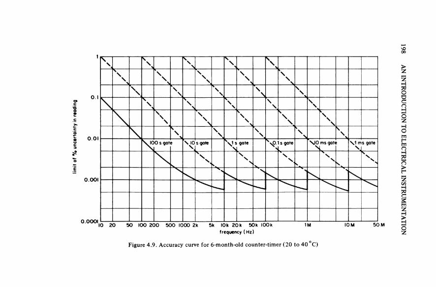
198 A
N INTRO
DU
CTION
TO ELECTRICA
L INSTR
UM
ENTA
TION
Figure 4.9. Accuracy curve for 6-month-old counter-timer (20 to 40 °C)
limit o
f % u
ncer
tain
ty in
read
ing
frequency (Hz)
100 s gate 10 s gate 1 s gate 0.1s gate 10 ms gate 1 ms gate

DIGITAL INSTRUMENTS 199
The resolution for medium frequency signals can be increased and the trigger error decreased by routing the input signal via the decade dividing assemblies (see figure 4.10), the number of cycles (n) of input over which the clock units are counted then being increased by powers of 10. To facilitate the display of the average period of the number of cycles, the energisation of decimal point L.E.D.s in the display is linked to the switches used to select the value of n. Hence, if the clock unit is 1 μs, and an n value of 10 is selected, a decimal point L.E.D. between the least significant decade and the least decade but one will be illuminated.
Figure 4.10. Arrangement for multiple period averaging
decimal counter and display
link f
or de
cimal
point
inputsignal
shapingcircuits
maingote
start/stopcommandsignals
oscillator
decade dividers
Sample Specification
The specification for single and multiple period measurements for the Racal-Dana 9901 is as follows.
Input: channel A Range: 1 μs to 1 sClock unit: 1 μs (a.c. or d.c. coupling)
Periods averaged: 1 to 105 in decade multiples
Accuracy: ± 0.3%
Number of periods averaged± Frequency standard stability
± determination error (1 l.s.d.)Bandwidth: automatically reduced to 10 MHz (3 dB) when period selected

200 AN INTRODUCTION TO ELECTRICAL INSTRUMENTATION
Thus in measuring a frequency of, say, 20 Hz which has a period of 0.05 s or 50000 μs, the limit of uncertainty in measurement would on the six-month-old counter be
or ± 0.3026 per cent. If the measurement were made over 10 cycles, a display of 50000.0 μs would have been obtained and the tolerance on the measurement ± 0.0308 per cent. As with the frequency measurement method it is inconvenient to have to calculate the tolerance on each reading; an accuracy curve as shown in figure 4.11 gives a rapid evaluation of the uncertainty in measurement. As before this has been drawn for the six-month-old counter when operated at tempera-tures between 20 and 40 °C.
Inspection of these curves shows marked differences to those of direct frequency measurement (figure 4.9). First, they slope in the opposite direction, and second at low frequencies there is a marked step increase in the uncertainty in measurement when n is decreased from 100 to 10 to 1. This is due to the effect of the trigger error on the total uncertainty in measurement.
The curves for n = 1, 10 and 100 have been extended with a broken line to show the extension of frequency range possible by using the overflow indication. Such a mode of operation may, for example, be used when measuring a frequency of 2.1 Hz. Using n = 1 would give a reading of 476190 μs ± 0.3 per cent but switching to the n = 10 condition, a reading of 761905 μs ± 0.031 per cent is given together with an overflow indication. The total value for the latter reading would be 4761905 ± 0.03 per cent effectively obtaining a seven-decade reading from a six-digit display. With care this technique can be extended to obtain aneight-decade reading, on a six-digit instrument.
If the families of curves in figures 4.9 and 4.11 are superimposed as in 4.12 it becomes apparent which frequencies can be measured with the smallest uncert-ainties by the two methods. It should, however, be remembered that if a frequency is measured by the multi-period method the determination of the tolerance on the value of the frequency must include an allowance for calcula-tion error and unless a 10 or more digit calculator is used this may be significant.
The performance of this reciprocal calculation is inconvenient and for the measurement of low frequencies counters incorporating arithmetic processors, [6] and termed reciprocal computing frequency meters, have been developed. These instruments have the advantages over the conventional instrument when measur-ing low frequencies of greater resolution, shorter measuring time and a display of frequency value as opposed to a period. The Feedback FM610 is an example of such an instrument and has a frequency range from 0.0011 Hz to 10 MHz.

Figure 4.11. Curves of limit of uncertainty in single and multiple period measurements against frequency
limit
of %
unc
erta
inty
in re
adin
g
frequency (Hz)
overflow
overflow
overflow
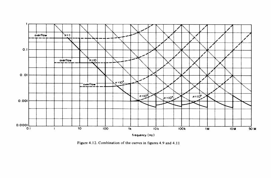
Figure 4.12. Combination of the curves in figures 4.9 and 4.11
frequency (Hz)
overflow
overflow
overflow
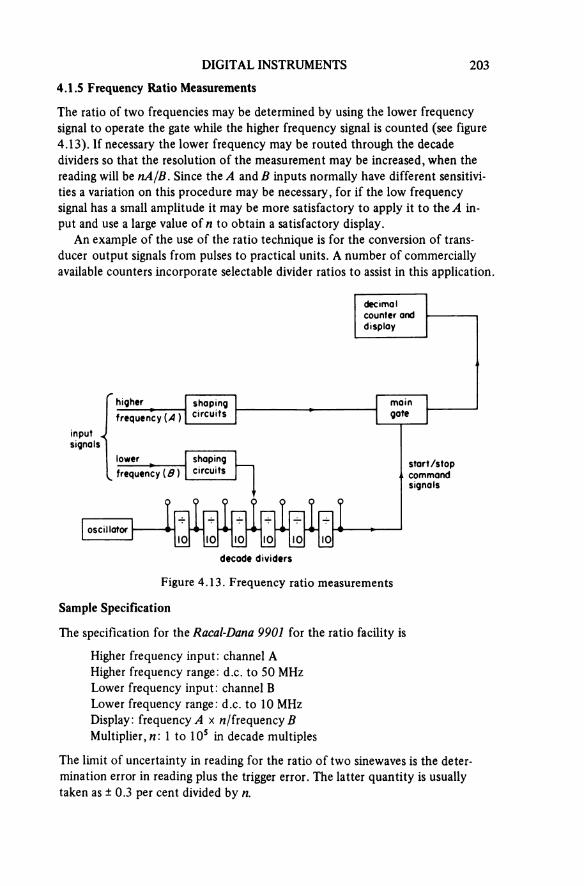
DIGITAL INSTRUMENTS 203
4.1.5 Frequency Ratio Measurements
The ratio of two frequencies may be determined by using the lower frequency signal to operate the gate while the higher frequency signal is counted (see figure 4.13). If necessary the lower frequency may be routed through the decade dividers so that the resolution of the measurement may be increased, when the reading will be nA/B. Since the A and B inputs normally have different sensitivi-ties a variation on this procedure may be necessary, for if the low frequency signal has a small amplitude it may be more satisfactory to apply it to the A in-put and use a large value of n to obtain a satisfactory display.
An example of the use of the ratio technique is for the conversion of trans-ducer output signals from pulses to practical units. A number of commercially available counters incorporate selectable divider ratios to assist in this application
Figure 4.13. Frequency ratio measurements
decimal counter and display
inputsignals
higherfrequency (A)
shapingcircuits
maingate
lowerfrequency (8)
shapingcircuits start/stop
commandsignals
oscillator
decade dividers
Sample Specification
The specification for the Racal-Dana 9901 for the ratio facility is
Higher frequency input: channel A Higher frequency range: d.c. to 50 MHz Lower frequency input: channel B Lower frequency range: d.c. to 10 MHz Display: frequency A × n/frequency BMultiplier, n: 1 to 105 in decade multiples
The limit of uncertainty in reading for the ratio of two sinewaves is the deter-mination error in reading plus the trigger error. The latter quantity is usually taken as ± 0.3 per cent divided by n.

204 AN INTRODUCTION TO ELECTRICAL INSTRUMENTATION
4.1.6 Time Interval Measurements
In this mode of operation (figure 4.14) a clock unit of suitable duration, say, 1 μs, or 1 ms can be selected to measure the time interval between positive or nega-tive going zero crossings of a single input wave or of two separate input signals.
Such a facility is suitable for measuring the positive or negative parts of a square wave, or a repetitive pulse wave.
Figure 4.14. Time interval measurements
decimal counter and display
maingate
oscillator
commandsignals
decade dividers
startsignal
triggerslopeselection
stopsignal
triggerslopeselection
The 9901 time interval specification is
Input channel: single line, channel B; double line, start channel B stop channel A
Time range: 100 ns to 104 s (2.8 h approx.)Clock units: 100 ns to 10 ms Coupling: d.c.Start/stop signals: electrical or contactTrigger slope selection: electrical—positive or negative slopes can be
selected on both start and stop signals; contact- opening or closure can be selected on both start and stop signals
A variation is time interval averaging in which a fixed clock unit (for example 100 ns) can be used to average the time interval over a number of cycles. This is arranged by connecting the oscillator to the main gate and routing the stop command pulse through the decade dividers.
DIGITAL INSTRUMENTS 205
4.2 MULTI FUNCTION DIGITAL VOLTMETERS
The multi-function digital meter is very much a product of the developments in solid state electronics that have resulted in cost savings and improved reliability. These instruments have evolved from the basic digital voltmeters that appeared in the 1960s and have since improved in scope and accuracy of measurement. Apart from digital panel meters there are few instruments now manufactured that only measure direct voltages, most having many alternating and direct, volt-age and current ranges as well as resistance measuring ranges. However, since the multi-function meter is based on the digital voltmeter an appreciation of the techniques commonly used to convert a direct (analogue) voltage to a digital display is desirable.
4.2.1 Analogue to Digital Conversion [7, 9]
There are four main methods used in the construction of digital voltmeters for the conversion of an analogue signal to its digital equivalent. These are
(a) successive approximation method(b) ramp or voltage to time conversion technique(c) voltage to frequency method(d) dual slope technique.
The first and last of these are the methods perhaps of greatest importance, although the middle two are used by some manufacturers as indeed are some specially developed conversion techniques. [9]
Successive approximation method
This is the fastest and one of the most stable of the basic analogue to digital conversion techniques. Instruments using this method work automatically in a similar manner to the operator of a laboratory d.c. potentiometer. In the succes-sive approximation d.v.m. (see figure 4.15) a voltage divider network, with coarse and fine steps, is connected via switches to a voltage comparator (analogous to the potentiometer operator’s galvanometer), which compares the internal voltage with the unknown. The output of the comparator feeds the logic circuits which control the steps on the voltage divider network. A measure-ment sequence usually selects the largest steps of the internal voltage first, the magnitude of the steps decreasing until the null point is reached.
The high speed of measurement possible with this technique only applies if the unknown voltage is noise free. If it is not, filters must be fitted and the speed of operation is very much reduced.
The errors associated with a d.v.m. using this method of conversion will depend on

206 AN INTRODUCTION TO ELECTRICAL INSTRUMENTATION
Figure 4.15. Simplified schematic diagram of a successive approximation digital voltmeter
display
logiccircuits
switchinganddividernetwork
voltagecomparator
referencevoltage
inputvoltage
(a) the resolution of the comparator(b) the precision of the voltage divider network which is normally resistive but
in some good quality instruments may be an inductive divider, and(c) the stability of the reference voltage.
The overall performance of this type of converter may also be limited by the divider switch characteristics.
The successive approximation conversion is now less commonly used in d.v.m.s but finds application in high speed data-acquisition, waveform sampling, auto-matic test and process control systems.
Ramp method
This method of conversion utilises a digital counter technique. A carefully defined, internally generated, voltage ramp is fed to two voltage comparators (see figure 4.1 6). When the ramp voltage, which may have either a positive or negative slope and a polarity in opposition to the input, is equal to one level of the input voltage (say earth) the ground comparator emits a command (start) signal to a gate which opens and permits the passage of pulses from a crystal oscillator to a digital counter. When the level of the input voltage is equal to the ramp voltage the second comparator produces a command signal to close the gate and prevent further counting. With suitable scaling the count may be made of equal magnitude to the difference in the two levels of the input voltage. The factors affecting the errors of a d.v.m. using this conversion technique are
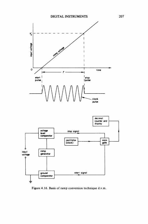
DIGITAL INSTRUMENTS 207
Figure 4.16. Basis of ramp conversion technique d.v.m.
inpu
t vol
tage
time
startpulse
stoppulse
clockpulse
decimal counter and display
voltagelevelcomparator
stop signal
oscillator(clock)
maingate
inputvoltage
rampgenerator
groundcomparator
start signal

208 AN INTRODUCTION TO ELECTRICAL INSTRUMENTATION
(a) the linearity of the ramp voltage, which is normally generated by using an amplifier with capacitive feedback
(b) the stability of the crystal oscillator, which commonly operates at 1 MHz, and
(c) the precision with which the voltage comparators can make coincidence measurements.
As with instruments using the successive approximation method of conversion the measurement rate for input voltages having a noise content is reduced by the inclusion of filter circuits.
Voltage to frequency method [8]
Although this method also uses a counter technique the mode of operation is fundamentally different to the ramp technique. In the voltage to frequency conversion a signal is generated such that its frequency is precisely related to the differences in the levels of the input voltage. This frequency is then counted over a fixed time interval, usually 1 cycle of power line frequency, which results in a high rejection of mains noise signal without the use of filters. A schematic diagram of the components of a voltage to frequency d.v.m. is shown in figure 4.17.
Figure 4.17. Schematic diagram for a voltage to frequency d.v.m.
decimal counter and display
inputvoltage
voltagetofrequencyconverter
gate
commandsignals
fixed timeintervalgenerator
The errors of a d.v.m. using this technique are dependent on
(a) the accuracy and linearity of the voltage to frequency conversion, which is not as inherently stable or accurate as the successive approximation method
(b) the precision of the time interval over which the frequency measurement is made, which may be made small by using crystal control, and
(c) the internal reference or calibration voltage.
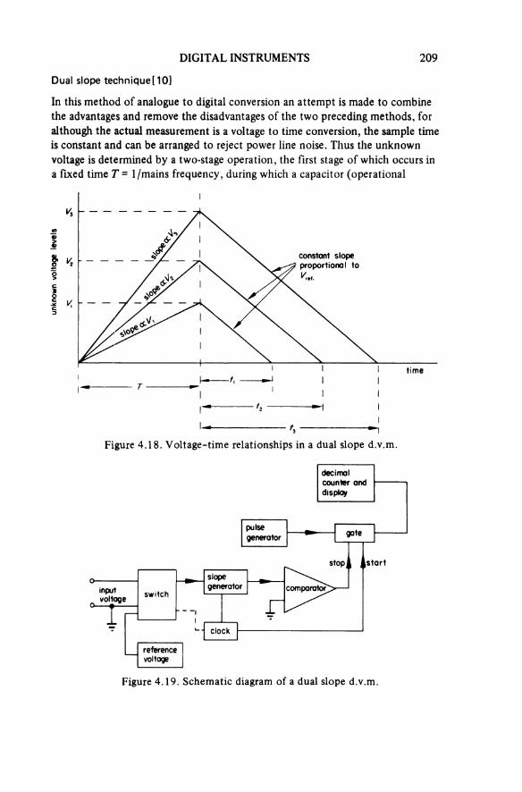
DIGITAL INSTRUMENTS 209
Dual slope technique [10]
In this method of analogue to digital conversion an attempt is made to combinethe advantages and remove the disadvantages of the two preceding methods, for although the actual measurement is a voltage to time conversion, the sample time is constant and can be arranged to reject power line noise. Thus the unknown voltage is determined by a two-stage operation, the first stage of which occurs in a fixed time T = 1/mains frequency, during which a capacitor (operational
Figure 4.18. Voltage-time relationships in a dual slope d.v.m.
unkn
own v
olta
ge lev
els
constant slope proportional to Vref.
time
Figure 4.19. Schematic diagram of a dual slope d.v.m.
decimal counter and display
pulsegenerator gate
stop start
inputvoltage switch
slopegenerator comparator
clock
referencevoltage
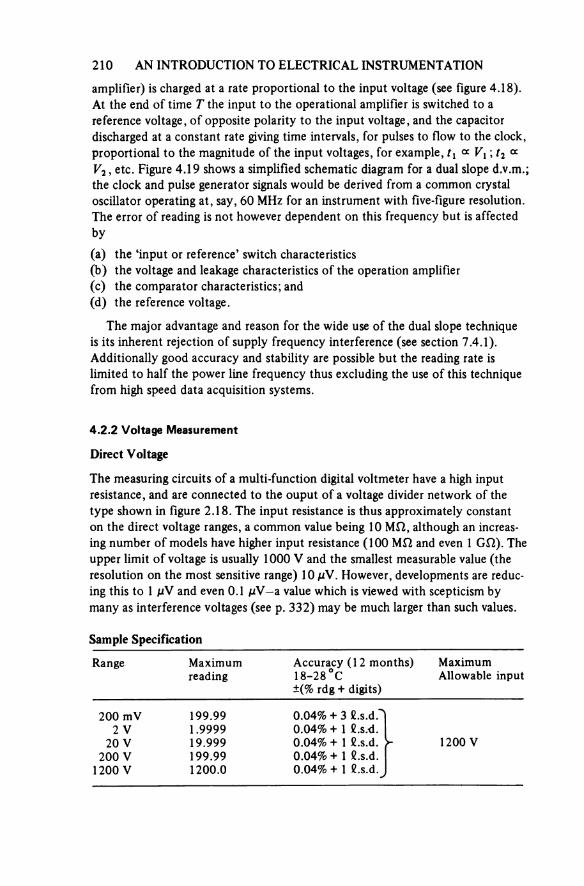
210 AN INTRODUCTION TO ELECTRICAL INSTRUMENTATION
amplifier) is charged at a rate proportional to the input voltage (see figure 4.18). At the end of time T the input to the operational amplifier is switched to a reference voltage, of opposite polarity to the input voltage, and the capacitor discharged at a constant rate giving time intervals, for pulses to flow to the clock, proportional to the magnitude of the input voltages, for example, t1 ∞ V1 ; t2 ∞ V2, etc. Figure 4.19 shows a simplified schematic diagram for a dual slope d.v.m.; the clock and pulse generator signals would be derived from a common crystal oscillator operating at, say, 60 MHz for an instrument with five-figure resolution. The error of reading is not however dependent on this frequency but is affected by(a) the ‘input or reference’ switch characteristics(b) the voltage and leakage characteristics of the operation amplifier(c) the comparator characteristics; and(d) the reference voltage.
The major advantage and reason for the wide use of the dual slope technique is its inherent rejection of supply frequency interference (see section 7.4.1). Additionally good accuracy and stability are possible but the reading rate is limited to half the power line frequency thus excluding the use of this technique from high speed data acquisition systems.
4.2.2 Voltage Measurement
Direct Voltage
The measuring circuits of a multi-function digital voltmeter have a high input resistance, and are connected to the ouput of a voltage divider network of the type shown in figure 2.18. The input resistance is thus approximately constant on the direct voltage ranges, a common value being 10 MΩ, although an increas-ing number of models have higher input resistance (100 MΩ and even 1 GΩ). The upper limit of voltage is usually 1 000 V and the smallest measurable value (the resolution on the most sensitive range) 10 μV. However, developments are reduc-ing this to 1 μV and even 0.1 μV—a value which is viewed with scepticism by many as interference voltages (see p. 332) may be much larger than such values.
Sample Specification
Range Maximumreading
Accuracy (12 months) 18-28°C ±(% rdg + digits)
Maximum Allowable input
200 mV 199.99 0.04% + 3 l.s.d.2 V 1.9999 0.04% + 1 l.s.d.
20 V 19.999 0.04% + 1 l.s.d. 1200 V200 V 199.99 0.04%+ 1 l.s.d.
1200 V 1200.0 0.04% + 1 l.s.d.
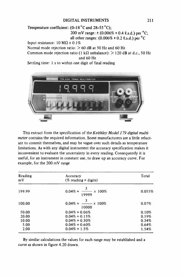
ReadingmV
Accuracy(% reading + digits)
Total
199.993
0.04%+ ------- × 100%19999
0.055%
100.003
0.04%+ × 100%10000
0.07%
50.00 0.04% + 0.06% 0.10%20.00 0.04%+ 0.15% 0.19%10.00 0.04% + 0.30% 0.34%5.00 0.04% + 0.60% 0.64%2.00 0.04% + 1.5% 1.54%
DIGITAL INSTRUMENTS 211
Temperature coefficient: (0-18 °C and 28-55 °C);200 mV range: ± (0.006% + 0.4 l.s.d.) per °C; all other ranges: (0.006% + 0.2 l.s.d.) per °C
Input resistance: 10 MΩ ±0.1%Normal mode rejection ratio: > 60 dB at 50 Hz and 60 HzCommon mode rejection ratio (1 kΩ unbalance): > 120 dB at d.c., 50 Hz
and 60 HzSettling time: 1 s to within one digit of final reading
This extract from the specification of the Keithley Model 1 79 digital multi-meter contains the required information. Some manufacturers are a little reluct ant to commit themselves, and may be vague over such details as temperature limitations. As with any digital instrument the accuracy specification makes it inconvenient to evaluate the uncertainty in every reading. Consequently it is useful, for an instrument in constant use, to draw up an accuracy curve. For example, for the 200 mV range
By similar calculations the values for each range may be established and a curve as shown in figure 4.20 drawn.
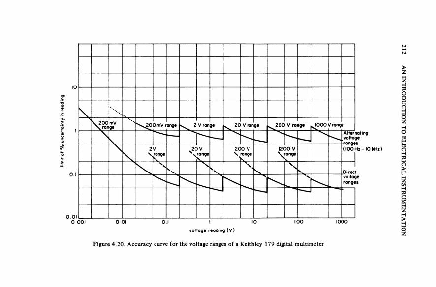
212 A
N INTRO
DU
CTION TO ELECTRIC
AL IN
STRU
MEN
TATIO
N
Figure 4.20. Accuracy curve for the voltage ranges of a Keithley 179 digital multimeter
limit o
f % un
cert
aint
y in r
eadi
ng
voltage reading (V)
200 mV range 200 mV range 2 V range 20 V range 200 V ronge 1000 V range
Alternatingvoltageranges(100 Hz-10 kHz)2V
range20 V
range200 V
range1200 V range
Directvoltageranges
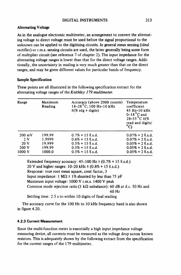
DIGITAL INSTRUMENTS 213
Alternating Voltage
As in the analogue electronic multimeter, an arrangement to convert the alternat-ing voltage to direct voltage must be used before the signal proportional to the unknown can be applied to the digitising circuits. In general mean sensing (ideal rectifier) or r.m.s. sensing circuits are used, the latter generally being some form of multiplier circuit (see reference 7 of chapter 2). The input impedance for the alternating voltage ranges is lower than that for the direct voltage ranges. Addi-tionally, the uncertainty in reading is very much greater than that on the direct ranges, and may be given different values for particular bands of frequency.
Sample Specification
These points are all illustrated in the following specification extract for the alternating voltage ranges of the Keithley I 79 multimeter.
Range MaximumReading
Accuracy (above 2000 counts) 18-28°C; 100 Hz-10kHz ±(% rdg + digits)
Temperaturecoefficient45 Hz-10 kHz 0-18 °C and 28-55 °C±(% read and digits/ °C)
200 mV 199.99 0.7%+ 15 l.s.d. 0.07% + 2 l.s.d.2 V 1.9999 0.6% + 15 l.s.d. 0.07% + 2 l.s.d.
20 V 19.999 0.5%+ 15 l.s.d. 0.05% + 2 l.s.d.200 V 199.99 0.5%+ 15 l.s.d. 0.05% + 2 l.s.d.
1000 V 1000.0 0.5%+ 15 l.s.d. 0.05% + 2 l.s.d.
Extended frequency accuracy: 45-100 Hz ± (0.7% + 15 l.s.d.)20 V and higher ranges: 10-20 kHz ± (0.8% + 15 l.s.d.)Response: true root mean square, crest factor, 3Input impedance: 1 MΩ ± 1% shunted by less than 75 pFMaximum input voltage: 1000 V r.m.s. 1400 V peakCommon mode rejection ratio (1 kΩ unbalance): 60 dB at d.c. 50 Hz and
60 HzSettling time: 2.5 s to within 10 digits of final reading
The accuracy curve for the 100 Hz to 10 kHz frequency band is also shown in figure 4.20.
4.2.3 Current Measurement
Since the multi-function meter is essentially a high input impedance voltage measuring device, all currents must be measured as the voltage drop across known resistors. This is adequately shown by the following extract from the specification for the current ranges of the 179 multimeter.
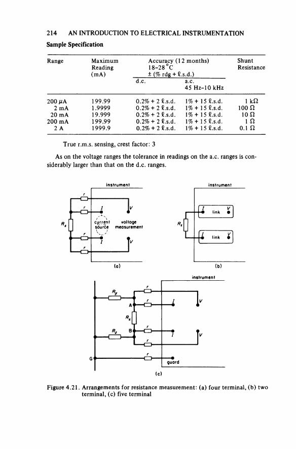
214 AN INTRODUCTION TO ELECTRICAL INSTRUMENTATION
Sample Specification
Range MaximumReading(mA)
Accuracy (12 months)18-28 °C ± (% rdg + l.s.d.)
ShuntResistance
d.c. a.c.45 Hz-10 kHz
200 μA 199.99 0.2% + 2 l.s.d. 1%+ 15 l.s.d. 1 kΩ2 mA 1.9999 0.2% + 2 l.s.d. 1%+ 15 l.s.d. 100 Ω
20 mA 19.999 0.2% + 2 l.s.d. 1%+ 15 l.s.d. 10Ω200 mA 199.99 0.2% + 2 l.s.d. 1%+ 15 l.s.d. 1 Ω
2 A 1999.9 0.2% + 2 l.s.d. 1%+ 15 l.s.d. 0.1 Ω
True r.m.s. sensing, crest factor: 3
As on the voltage ranges the tolerance in readings on the a.c. ranges is con-siderably larger than that on the d.c. ranges.
Figure 4.21. Arrangements for resistance measurement: (a) four terminal, (b) two terminal, (c) five terminal
(a)
instrument
currentsource
voltagemeasurement
(b)
instrument
link
link
(c)
instrument
guard

DIGITAL INSTRUMENTS 215
4.2.4 Resistance Ranges
To measure resistance with a digital instrument it is necessary to provide, withinthe instrument, one or more constant current sources, the magnitude of the un-known resistance being derived from the voltage drop across it. If the instrument on its lowest resistance range has a resolution that is better than 0.1 Ω, four- terminal resistance measurement should be provided (figure 4.21a) as the resistance of the connecting leads, which may well be in excess of 10 mΩ, will add to the reading. On instruments that have this four-terminal facility it is customary for sliding links to be provided so that for measurements of large value resistances on the less sensitive ranges a two-terminal resistance measurement can be adequate if lead lengths are made reasonably short.
In some instruments a five-wire system is available. [11, 12] The fifth wire provides a means of ‘guarding out’ unwanted current paths by maintaining G in figure 4.21c at the same potential as A, thus allowing in-circuit testing.
Sample Specification
The specification for the resistance ranges of the Keithley 179 is as follows, there being a choice between a high (Hi) or low (Lo) current through the unknown resistance.
Range MaximumReading
Accuracy (1 2 months) 18-28 °C ± (% rdg + l.s.d.)
Temp, coefficient 0-18 °C and 28- 55°C±(%rdg + l.s.d.)
High count: 2 kΩ — _— —max. voltage 20 kΩ 19.999 0.04% + 1 l.s.d. 0.003% + 0.2 l.s.d.across un- 200 kΩ 199.99 0.04% + 1 l.s.d. 0.003% + 0.2 l.s.d.known 2 V 2000 kΩ 1999.9 0.04% + 1 l.s.d. 0.003% + 0.2 l.s.d.
20 MΩ 19.999 0.10%+ 1 l.s.d. 0.02% + 0.2 l.s.d.
Low count: 2 kΩ 1.9999 0.15%+ 15 l.s.d. 0.02% + 2 l.s.d.max. voltage 20 kΩ 19.999 0.15%+ 15 l.s.d. 0.02% + 2 l.s.d.across un- 200 kΩ 199.99 0.15%+ 15 l.s.d. 0.02% + 2 l.s.d.known 0.2 V 2000 kΩ 1999.9 0.15%+ 15 l.s.d. 0.03% + 2 l.s.d.
20 MΩ — — —
The ‘low’ condition of operation has obviously a poorer accuracy specifica tion but can be a very useful facility when making measurements on semi-conductor components, such as switching diodes.
4.3 'INTELLIGENT' INSTRUMENTS
As inferred at the beginning of this chapter the developments that are occurring in micro-electronics are influencing the design and capabilities of digital instru-ments at a faster rate than any others. This growth of ability has led to the use
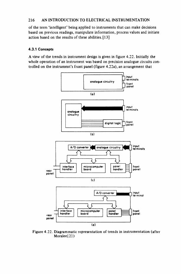
216 AN INTRODUCTION TO ELECTRICAL INSTRUMENTATION
of the term ‘intelligent’ being applied to instruments that can make decisions based on previous readings, manipulate information, process values and initiate action based on the results of these abilities. [13]
4.3.1 Concepts
A view of the trends in instrument design is given in figure 4.22. Initially the whole operation of an instrument was based on precision analogue circuits con trolled on the instrument’s front panel (figure 4.22a), an arrangement that
Figure 4.22. Diagrammatic representation of trends in instrumentation (after Moralee [2])
(a)
inputterminals
analogue circuitryfrontpanel
(b)
analoguecircuitry
inputterminals
digital logic frontpanel
(c)
A/D converter analogue circuitry inputterminals
rearpanel
interfacehandler
microcomputerboard
panelhandler
frontpanel
(d)
A/D converter inputterminal
rearpanel
interfacehandler
microcomputerboard
panelhandler
frontpanel
DIGITAL INSTRUMENTS 217
required the operator to directly control all aspects of the measuring process. Particularly in more complex instruments, it led to problems in the design of the front panel controls, which were required to handle complex multi-way switching and sequencing introducing additional sources of measurement error.
To solve some of these front panel control problems, instrument designers began to incorporate control circuits inside the instrument, initially by using relays, and then T.T.L. (figure 4.22b). Some of these controllers developed into complete hard-wired processor systems; thereby freeing the operator from the detailed operation of the measuring circuits, and simplifying the design of the instruments front panel, for example, digital voltmeters that are completely auto ranging.
The shift towards the use of digital controllers was therefore under way before the introduction of the microprocessor and the associated L.S.I. compon-ents. The availability of these powerful, low-cost programmable devices completed the trend towards the controller based system or ‘architecture’, which character-ises the generation of instruments represented by figure 4.22c.
In such an approach to instrument design, the microprocessor is the centre of the instrument’s operation, controlling all the other circuitry by means of a central data bus. Hence analogue inputs may be switched through various ana-logue circuits, under control of the microprocessor, to a final analogue-to-digital converter, which in turn produces an output that can be read by the micro-processor for further manipulation, storage or display. It may be argued that the only function of the analogue circuitry in such a situation is to condition the in-puts for the A/D converter, and as the range of inputs acceptable to A/D conver-ters increases the need for ‘front end’ analogue circuitry will decrease, and ultimately disappear (figure 4.22d).
The use of a microprocessor in the design of an instrument results in a number of benefits. It allows the use of very simple front panels, commonly based on a standard numeric keyboard. This makes the instrument easier to use, allowing the operator to set up complex measuring sequences with a few key strokes by calling up of coded measuring processes. The microprocessor can also change the measuring sequence in response either to the measurand or to external signals if the instrument is interfaced to other devices (see section 9.3.2).
Internally, the most important result of including a microprocessor in the instrument is the capability of performing calculations on the readings of the measurand and relating the readings to stored reference values.
4.3.2 Voltage Facilities
Since the greatest number of measurands are, or can be, presented as voltages,an examination of the more common functions that can be performed on voltages is worth considering.
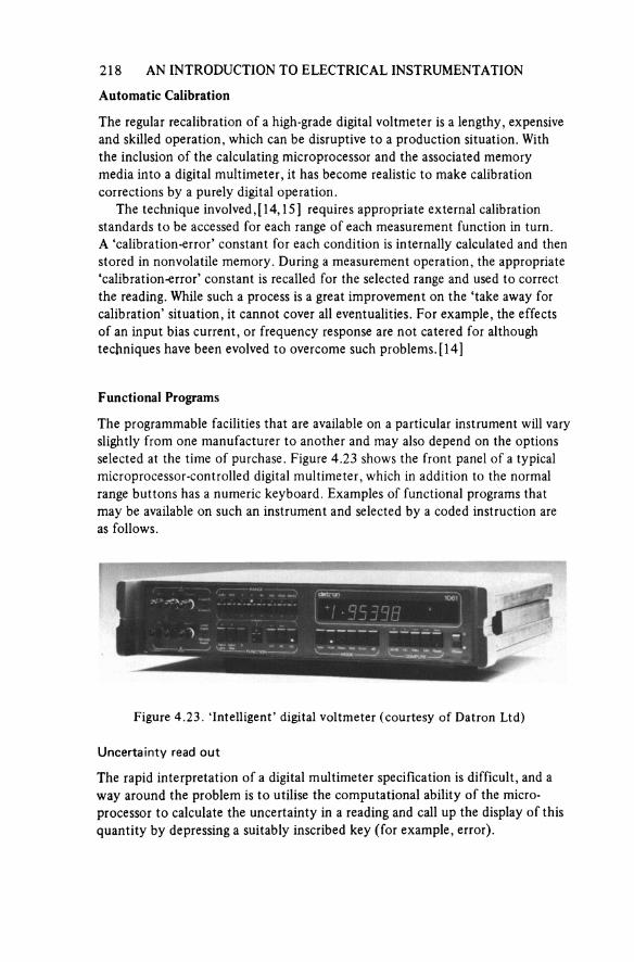
218 AN INTRODUCTION TO ELECTRICAL INSTRUMENTATION
Automatic Calibration
The regular recalibration of a high-grade digital voltmeter is a lengthy, expensive and skilled operation, which can be disruptive to a production situation. With the inclusion of the calculating microprocessor and the associated memory media into a digital multimeter, it has become realistic to make calibration corrections by a purely digital operation.
The technique involved, [14, 15] requires appropriate external calibration standards to be accessed for each range of each measurement function in turn.A ‘calibration-error’ constant for each condition is internally calculated and then stored in nonvolatile memory. During a measurement operation, the appropriate ‘calibration-error’ constant is recalled for the selected range and used to correct the reading. While such a process is a great improvement on the ‘take away for calibration’ situation, it cannot cover all eventualities. For example, the effects of an input bias current, or frequency response are not catered for although techniques have been evolved to overcome such problems. [14]
Functional Programs
The programmable facilities that are available on a particular instrument will vary slightly from one manufacturer to another and may also depend on the options selected at the time of purchase. Figure 4.23 shows the front panel of a typical microprocessor-controlled digital multimeter, which in addition to the normal range buttons has a numeric keyboard. Examples of functional programs that may be available on such an instrument and selected by a coded instruction are as follows.
Figure 4.23. ‘Intelligent’ digital voltmeter (courtesy of Datron Ltd)
Uncertainty read out
The rapid interpretation of a digital multimeter specification is difficult, and a way around the problem is to utilise the computational ability of the micro-processor to calculate the uncertainty in a reading and call up the display of this quantity by depressing a suitably inscribed key (for example, error).
DIGITAL INSTRUMENTS 219
Percentage deviation
By using the numerical keyboard a particular value, V, is entered. Each reading, x, is compared with the entered value and then displayed as a percentage devia-tion so that
displayed value
Multiplication
Each measurement is multiplied by a constant that has been entered using the keyboard. Such a constant may be greater or less than unity and if there is a linear relationship between, say, the voltage output from a transducer and the measurand in engineering units this facility may be used to provide a display in the appropriate units.
Offset
In many situations it is desirable to know the variations in a quantity above a fixed or reference level. By keying-in the appropriate offset level the display can be made the difference between the measured value and the offset. If this facility and the multiply program are used in conjunction with each other theoutput from a transducer in a current transmission system (see section 6.7.3) can be displayed in engineering units.
Ratios
Various ratio facilities are possible, the simplest being the division of the measure-ment by a preset constant. Some instruments, by using additional rear input sockets, can be programmed to sample two inputs in turn and compute either the direct ratio of these, or compute the logarithm of the ratio and display the result in decibels. This is a useful facility for measurements of gain, attenuation, noise levels, etc.
Maximum and minimum
The level of voltage may vary for a number of reasons. It may therefore be desirable to store the maximum and minimum of such excursions, replacing existing recorded values when these are exceeded and to determine the magni-tude of the peak-to-peak excursions. It must be possible to display each of these quantities and the magnitude of the most recent sample. The display of each of these quantities will be initiated by appropriately coded keystrokes.
220 AN INTRODUCTION TO ELECTRICAL INSTRUMENTATION
Limits
A limits program would compare the sample with set levels, compute the num-ber of samples exceeding high limits, low limits and within the set limits.
Statistics
The facility to calculate and display the number of measurements in a given time, their average, standard deviation, and the r.m.s. of their values are all possible useful statistical manipulations.
Linearisation
The relationship between the output voltage and temperature for a thermocouple (see section 5.4.3) is nonlinear. By suitable programming, the sensed voltage can be converted to degrees Kelvin, or Celsius, for any one of the commonly used types of thermocouple.
Time
Since a clock needs to be built into the instrument it is sensible to be able to programme for readings to be made at and/or during defined time intervals, which are, of course, limited by the measuring speed of the instrument.
Combination of programmes
The details of operation for these intelligent instruments will vary between manu-facturers and the capabilities will largely depend on the decisions made at the time of purchase although many instruments can have their capabilities extended by the addition of circuit boards for specific functions.
4.3.3 Resistance Measurement
The programmable instruments described in the preceding section will usually have a resistance measuring capability and can therefore be used in an inspection situation for (say) verifying that resistors are within acceptance levels. Other applications are the determination of resistance ratios, variations in magnitude, etc. These programmable instruments may therefore be useful in quality control applications.
The existence of a microprocessor within a multi-function meter provides the possibility of a ratiometer technique for resistance measurement. Figure 4.24 shows the principle involved where by measuring Vit V2, V3 and V4, Rx may be calculated from
and
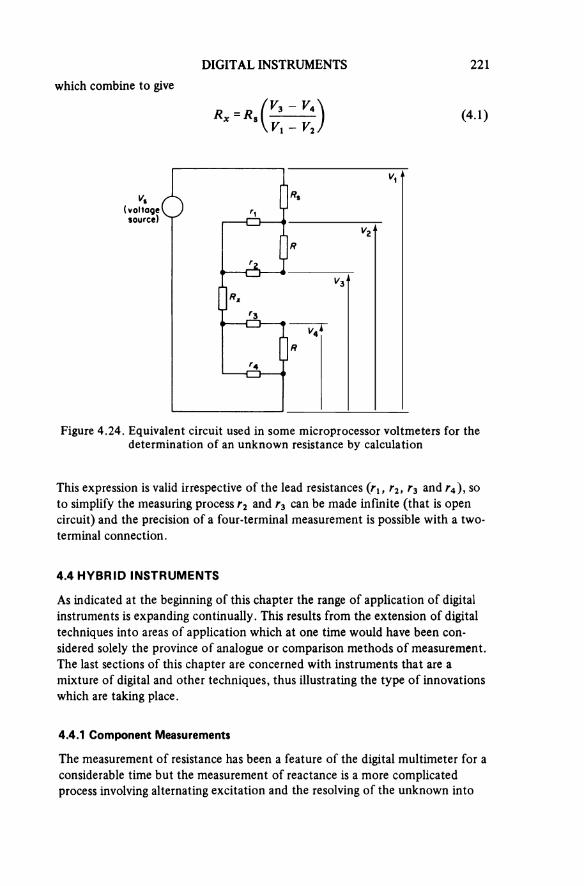
DIGITAL INSTRUMENTS 221which combine to give
(4.1)
Figure 4.24. Equivalent circuit used in some microprocessor voltmeters for the determination of an unknown resistance by calculation
(voltagesource)
This expression is valid irrespective of the lead resistances (r1, r2, r3 and r4), so to simplify the measuring process r2 and r3 can be made infinite (that is open circuit) and the precision of a four-terminal measurement is possible with a two- terminal connection.
4.4 HYBRID INSTRUMENTS
As indicated at the beginning of this chapter the range of application of digital instruments is expanding continually. This results from the extension of digital techniques into areas of application which at one time would have been con-sidered solely the province of analogue or comparison methods of measurement. The last sections of this chapter are concerned with instruments that are a mixture of digital and other techniques, thus illustrating the type of innovations which are taking place.
4.4.1 Component Measurements
The measurement of resistance has been a feature of the digital multimeter for a considerable time but the measurement of reactance is a more complicated process involving alternating excitation and the resolving of the unknown into
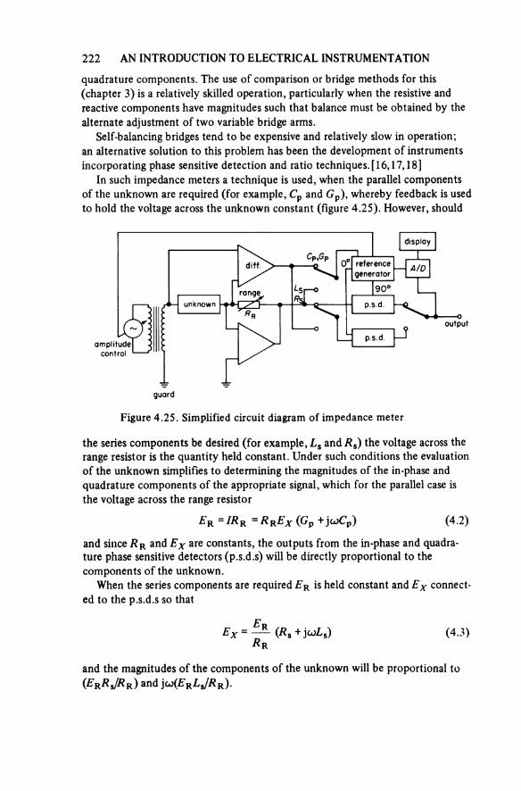
222 AN INTRODUCTION TO ELECTRICAL INSTRUMENTATION
quadrature components. The use of comparison or bridge methods for this (chapter 3) is a relatively skilled operation, particularly when the resistive and reactive components have magnitudes such that balance must be obtained by the alternate adjustment of two variable bridge arms.
Self-balancing bridges tend to be expensive and relatively slow in operation; an alternative solution to this problem has been the development of instruments incorporating phase sensitive detection and ratio techniques. [16, 17, 18]
In such impedance meters a technique is used, when the parallel components of the unknown are required (for example, Cp and GP), whereby feedback is used to hold the voltage across the unknown constant (figure 4.25). However, should
Figure 4.25. Simplified circuit diagram of impedance meter
display
diff. referencegenerator A/D
unknownrange
p.s.d.
output
amplitudecontrol
p.s.d.
the series components be desired (for example, Ls and Rs) the voltage across the range resistor is the quantity held constant. Under such conditions the evaluation of the unknown simplifies to determining the magnitudes of the m-phase and quadrature components of the appropriate signal, which for the parallel case is the voltage across the range resistor
(4.2)
and since Rr and Ex are constants, the outputs from the m-phase and quadra-ture phase sensitive detectors (p.s.d.s) will be directly proportional to the components of the unknown.
When the series components are required ER is held constant and Ex connect ed to the p.s.d.s so that
(4.3)
and the magnitudes of the components of the unknown will be proportional to (ErRs/Rr) and jω(ErLs/Rr).
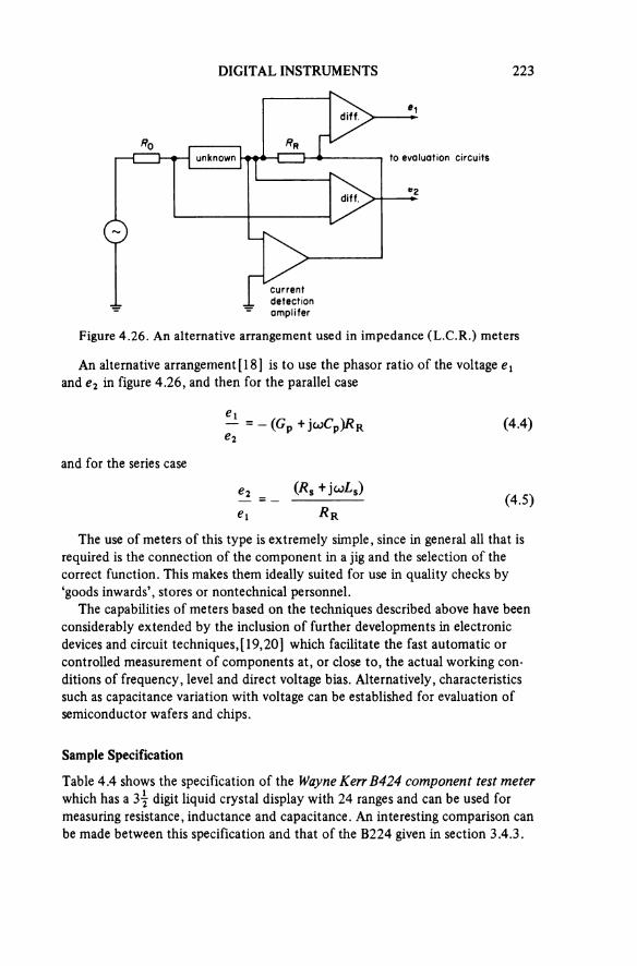
DIGITAL INSTRUMENTS 223
Figure 4.26. An alternative arrangement used in impedance (L.C.R.) meters
diff.
unknown to evaluation circuits
diff.
currentdetectionamplifer
An alternative arrangement [18] is to use the phasor ratio of the voltage e1 and e2 in figure 4.26, and then for the parallel case
(4.4)
and for the series case
(4.5)
The use of meters of this type is extremely simple, since in general all that is required is the connection of the component in a jig and the selection of the correct function. This makes them ideally suited for use in quality checks by ‘goods inwards’, stores or nontechnical personnel.
The capabilities of meters based on the techniques described above have been considerably extended by the inclusion of further developments in electronic devices and circuit techniques, [19, 20] which facilitate the fast automatic or controlled measurement of components at, or close to, the actual working con-ditions of frequency, level and direct voltage bias. Alternatively, characteristics such as capacitance variation with voltage can be established for evaluation of semiconductor wafers and chips.
Sample Specification
Table 4.4 shows the specification of the Wayne Kerr B424 component test meter which has a 3½ digit liquid crystal display with 24 ranges and can be used formeasuring resistance, inductance and capacitance. An interesting comparison can be made between this specification and that of the B224 given in section 3.4.3.
224 AN INTRODUCTION TO ELECTRICAL INSTRUMENTATION
Table 4.4. Measurement ranges of the Wayne Kerr 424 component test meter
Unknown As parallel components
As series components
Capacitance 0.1 pF-200 nF 1 nF-20 mFInductance 10 mH-2 kH 0.1 μH-2 HResistance 100 Ω-20 MΩ 10 mΩ-20 kΩ
Accuracy: ± (0.25% of reading + 1 digit); (0 >10).Frequency: The underlined values are measured at 1 kHz, other values are measured at 100 Hz.
4.4.2 Power Measurement
The measurement of the power consumed by a load requires the determination of the product of the instantaneous values of the appropriate voltage and current. This can be performed by analogue techniques using a multiplier, [17] by patent-ed techniques, [21] or if the current and voltage are suitably sampled and stored the average power may be computed. In most commercially available instruments an analogue technique is used to determine the power, the output from the multiplying circuits being connected to an A/D converter so that a digital display of the power is provided.
The input impedance of the voltage circuits for an instrument of this type is very much greater than for an electrodynamometer while the input resistance of the current ranges may be much less than for a direct acting instrument. Addition ally, the range of power that the electronic instrument can measure will in general be greater than that of the conventional instrument, although the uncertainty in measurement may be greater.
4.4.3 Recorders
The development of high speed A/D converters, together with the availability of low cost memory circuits, has led to the production of digital storage oscillo-scopes. One instrument of this type, shown schematically in figure 4.27, uses a 1024 × 8 bit memory; the general operation of the oscilloscope is described below.
The incoming signal waveform is fed into an A/D converter, which works at a speed determined by the timebase speed control up to a maximum of 1.8 MHz. The digital output of the converter is fed into the memory, the eight vertical bits giving a resolution of 1 part in 256 (0.4 per cent) and the 1024 points giving a horizontal resolution of approximately 0.1 per cent on a single trace or 0.2 per cent when two traces are stored each as 512 points.
To view the waveform, the information is read from the memory, passed through a D/A converter and the resultant signal displayed on the c.r.t. screen. A ‘refresh’ or ‘roll’ mode of operation is also available and in that condition the in-
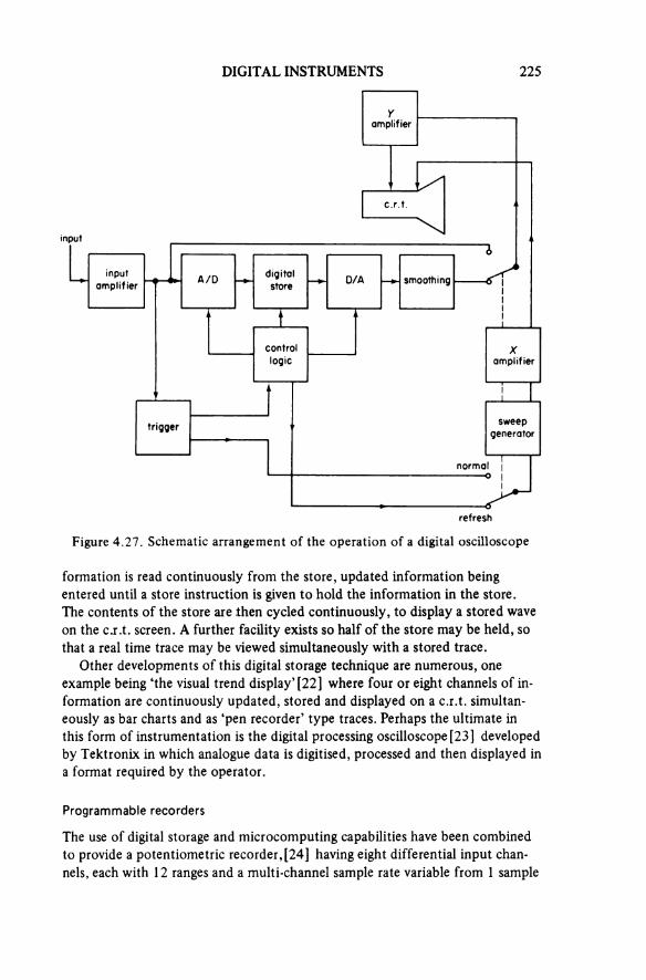
DIGITAL INSTRUMENTS 225
Figure 4.27. Schematic arrangement of the operation of a digital oscilloscope
Yamplifier
c.r.t.
input
inputamplifier A/D digital
store D/A smoothing
controllogic
Xamplifier
trigger sweepgenerator
normal
refresh
formation is read continuously from the store, updated information being entered until a store instruction is given to hold the information in the store.The contents of the store are then cycled continuously, to display a stored wave on the c.r.t. screen. A further facility exists so half of the store may be held, so that a real time trace may be viewed simultaneously with a stored trace.
Other developments of this digital storage technique are numerous, one example being ‘the visual trend display’ [22] where four or eight channels of in-formation are continuously updated, stored and displayed on a c.r.t. simultan-eously as bar charts and as ‘pen recorder’ type traces. Perhaps the ultimate in this form of instrumentation is the digital processing oscilloscope [23] developed by Tektronix in which analogue data is digitised, processed and then displayed in a format required by the operator.
Programmable recorders
The use of digital storage and microcomputing capabilities have been combined to provide a potentiometric recorder, [24] having eight differential input chan-nels, each with 12 ranges and a multi-channel sample rate variable from 1 sample
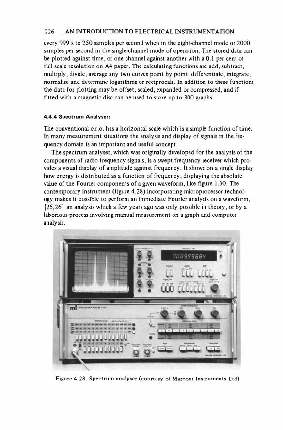
226 AN INTRODUCTION TO ELECTRICAL INSTRUMENTATION
every 999 s to 250 samples per second when in the eight-channel mode or 2000 samples per second in the single-channel mode of operation. The stored data can be plotted against time, or one channel against another with a 0.1 per cent of full scale resolution on A4 paper. The calculating functions are add, subtract, multiply, divide, average any two curves point by point, differentiate, integrate, normalise and determine logarithms or reciprocals. In addition to these functions the data for plotting may be offset, scaled, expanded or compressed, and if fitted with a magnetic disc can be used to store up to 300 graphs.
4.4.4 Spectrum Analysers
The conventional c.r.o. has a horizontal scale which is a simple function of time. In many measurement situations the analysis and display of signals in the fre-quency domain is an important and useful concept.
The spectrum analyser, which was originally developed for the analysis of the components of radio frequency signals, is a swept frequency receiver which pro-vides a visual display of amplitude against frequency. It shows on a single display how energy is distributed as a function of frequency, displaying the absolute value of the Fourier components of a given waveform, like figure 1.30. The contemporary instrument (figure 4.28) incorporating microprocessor technol-ogy makes it possible to perform an immediate Fourier analysis on a waveform, [25,26] an analysis which a few years ago was only possible in theory, or by a laborious process involving manual measurement on a graph and computer analysis.
Figure 4.28. Spectrum analyser (courtesy of Marconi Instruments Ltd)
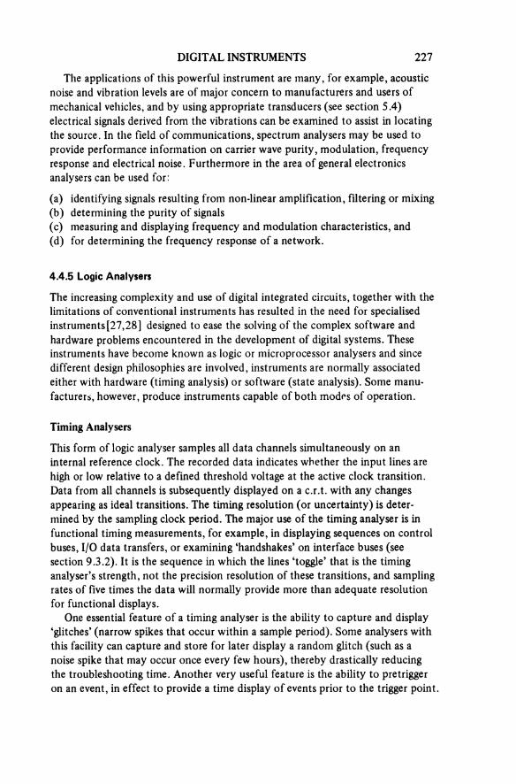
DIGITAL INSTRUMENTS 227
The applications of this powerful instrument are many, for example, acoustic noise and vibration levels are of major concern to manufacturers and users of mechanical vehicles, and by using appropriate transducers (see section 5.4) electrical signals derived from the vibrations can be examined to assist in locating the source. In the field of communications, spectrum analysers may be used to provide performance information on carrier wave purity, modulation, frequency response and electrical noise. Furthermore in the area of general electronics analysers can be used for:
(a) identifying signals resulting from non-linear amplification, filtering or mixing(b) determining the purity of signals(c) measuring and displaying frequency and modulation characteristics, and(d) for determining the frequency response of a network.
4.4.5 Logic Analysers
The increasing complexity and use of digital integrated circuits, together with the limitations of conventional instruments has resulted in the need for specialised instruments [27, 28] designed to ease the solving of the complex software and hardware problems encountered in the development of digital systems. These instruments have become known as logic or microprocessor analysers and since different design philosophies are involved, instruments are normally associated either with hardware (timing analysis) or software (state analysis). Some manu-facturers, however, produce instruments capable of both modes of operation.
Timing Analysers
This form of logic analyser samples all data channels simultaneously on an internal reference clock. The recorded data indicates whether the input lines are high or low relative to a defined threshold voltage at the active clock transition. Data from all channels is subsequently displayed on a c.r.t. with any changes appearing as ideal transitions. The timing resolution (or uncertainty) is deter-mined by the sampling clock period. The major use of the timing analyser is in functional timing measurements, for example, in displaying sequences on control buses, I/O data transfers, or examining ‘handshakes’ on interface buses (see section 9.3.2). It is the sequence in which the lines ‘toggle’ that is the timing analyser’s strength, not the precision resolution of these transitions, and sampling rates of five times the data will normally provide more than adequate resolution for functional displays.
One essential feature of a timing analyser is the ability to capture and display ‘glitches’ (narrow spikes that occur within a sample period). Some analysers with this facility can capture and store for later display a random glitch (such as a noise spike that may occur once every few hours), thereby drastically reducing the troubleshooting time. Another very useful feature is the ability to pretrigger on an event, in effect to provide a time display of events prior to the trigger point.
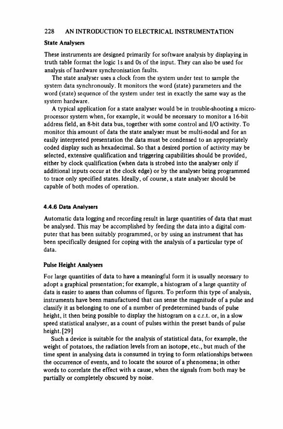
228 AN INTRODUCTION TO ELECTRICAL INSTRUMENTATION
State Analysers
These instruments are designed primarily for software analysis by displaying in truth table format the logic 1 s and 0s of the input. They can also be used for analysis of hardware synchronisation faults.
The state analyser uses a clock from the system under test to sample the system data synchronously. It monitors the word (state) parameters and the word (state) sequence of the system under test in exactly the same way as the system hardware.
A typical application for a state analyser would be in trouble-shooting a micro processor system when, for example, it would be necessary to monitor a 16-bit address field, an 8-bit data bus, together with some control and I/O activity. To monitor this amount of data the state analyser must be multi-nodal and for an easily interpreted presentation the data must be condensed to an appropriately coded display such as hexadecimal. So that a desired portion of activity may be selected, extensive qualification and triggering capabilities should be provided, either by clock qualification (when data is strobed into the analyser only if additional inputs occur at the clock edge) or by the analyser being programmed to trace only specified states. Ideally, of course, a state analyser should be capable of both modes of operation.
4.4.6 Data Analysers
Automatic data logging and recording result in large quantities of data that must be analysed. This may be accomplished by feeding the data into a digital com-puter that has been suitably programmed, or by using an instrument that has been specifically designed for coping with the analysis of a particular type of data.
Pulse Height Analysers
For large quantities of data to have a meaningful form it is usually necessary to adopt a graphical presentation; for example, a histogram of a large quantity of data is easier to assess than columns of figures. To perform this type of analysis, instruments have been manufactured that can sense the magnitude of a pulse and classify it as belonging to one of a number of predetermined bands of pulse height, it then being possible to display the histogram on a c.r.t. or, in a slow speed statistical analyser, as a count of pulses within the preset bands of pulse height. [29]
Such a device is suitable for the analysis of statistical data, for example, the weight of potatoes, the radiation levels from an isotope, etc., but much of the time spent in analysing data is consumed in trying to form relationships between the occurrence of events, and to locate the source of a phenomena; in other words to correlate the effect with a cause, when the signals from both may be partially or completely obscured by noise.
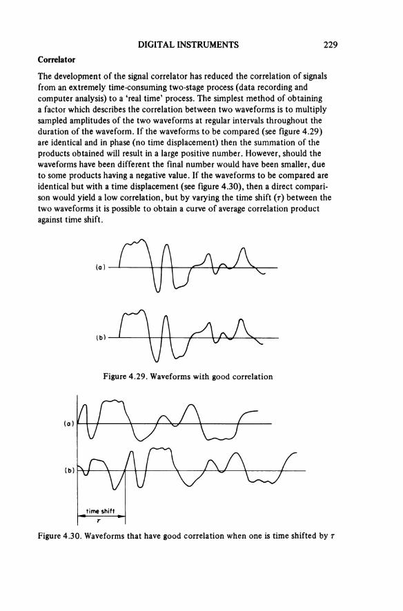
DIGITAL INSTRUMENTS 229
Correlator
The development of the signal correlator has reduced the correlation of signals from an extremely time-consuming two-stage process (data recording and computer analysis) to a ‘real time’ process. The simplest method of obtaining a factor which describes the correlation between two waveforms is to multiply sampled amplitudes of the two waveforms at regular intervals throughout the duration of the waveform. If the waveforms to be compared (see figure 4.29) are identical and in phase (no time displacement) then the summation of the products obtained will result in a large positive number. However, should the waveforms have been different the final number would have been smaller, due to some products having a negative value. If the waveforms to be compared are identical but with a time displacement (see figure 4.30), then a direct compari-son would yield a low correlation, but by varying the time shift (τ) between the two waveforms it is possible to obtain a curve of average correlation product against time shift.
Figure 4.29. Waveforms with good correlation
(a)
(b)
Figure 4.30. Waveforms that have good correlation when one is time shifted by τ
(o)
(b)
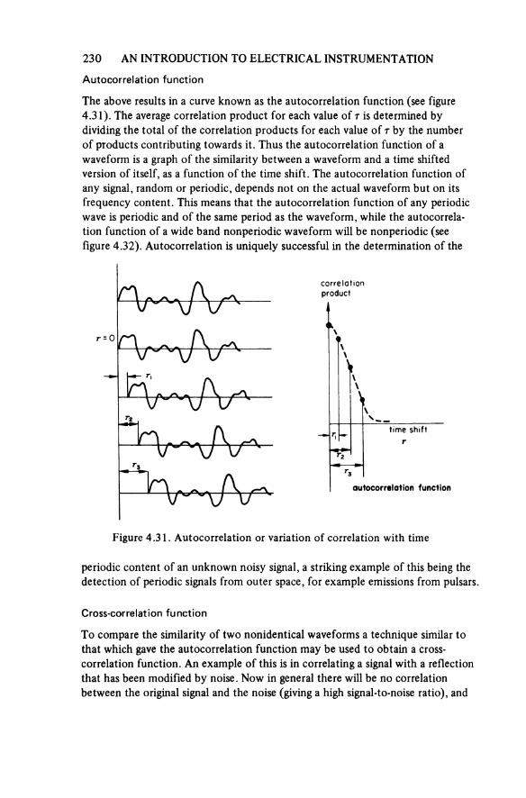
230 AN INTRODUCTION TO ELECTRICAL INSTRUMENTATION
Autocorrelation function
The above results in a curve known as the autocorrelation function (see figure 4.31). The average correlation product for each value of τ is determined by dividing the total of the correlation products for each value of τ by the number of products contributing towards it. Thus the autocorrelation function of a waveform is a graph of the similarity between a waveform and a time shifted version of itself, as a function of the time shift. The autocorrelation function of any signal, random or periodic, depends not on the actual waveform but on its frequency content. This means that the autocorrelation function of any periodic wave is periodic and of the same period as the waveform, while the autocorrela-tion function of a wide band nonperiodic waveform will be nonperiodic (see figure 4.32). Autocorrelation is uniquely successful in the determination of the
Figure 4.31. Autocorrelation or variation of correlation with time
correlationproduct
time shift
autocorrelation function
periodic content of an unknown noisy signal, a striking example of this being the detection of periodic signals from outer space, for example emissions from pulsars.
Cross-correlation function
To compare the similarity of two nonidentical waveforms a technique similar to that which gave the autocorrelation function may be used to obtain a cross-correlation function. An example of this is in correlating a signal with a reflection that has been modified by noise. Now in general there will be no correlation between the original signal and the noise (giving a high signal-to-noise ratio), and
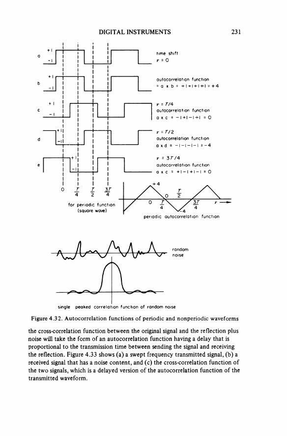
DIGITAL INSTRUMENTS 231
single peaked correlation function of random noise
time shift
autocorrelation function
autocorrelation function
autocorrelation function
autocorrelation function
for periodic function (square wave)
periodic autocorrelation function
randomnoise
Figure 4.32. Autocorrelation functions of periodic and nonperiodic waveforms
the cross-correlation function between the original signal and the reflection plus noise will take the form of an autocorrelation function having a delay that is proportional to the transmission time between sending the signal and receiving the reflection. Figure 4.33 shows (a) a swept frequency transmitted signal, (b) a received signal that has a noise content, and (c) the cross-correlation function of the two signals, which is a delayed version of the autocorrelation function of the transmitted waveform.
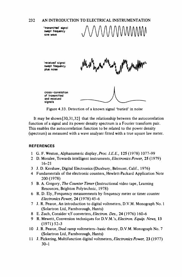
232 AN INTRODUCTION TO ELECTRICAL INSTRUMENTATION
Figure 4.33. Detection of a known signal ‘buried’ in noise
'transmitted' signal swept frequency sine wave
'received' signal swept frequency plus noise
cross-correlation of transmitted and received signals
It may be shown [30, 31, 32] that the relationship between the autocorrelation function of a signal and its power density spectrum is a Fourier transform pair. This enables the autocorrelation function to be related to the power density (spectrum) as measured with a wave analyser fitted with a true square law meter.
REFERENCES
1 G. F. Weston, Alphanumeric display, Proc. I.E.E., 125 (1978) 1077-992 D. Moralee, Towards intelligent instruments, Electronics Power, 25 (1979)
16-213 J. D. Kershaw, Digital Electronics (Duxbury, Belmont, Calif., 1976)4 Fundamentals of the electronic counters, Hewlett-Packard Application Note
200 (1978)5 B. A. Gregory, The Counter Timer (Instructional video tape, Learning
Resources, Brighton Polytechnic, 1978)6 R. D. Ely, Frequency measurements by frequency meter or timer counter
Electronics Power, 24 (1978) 45-67 J. R. Pearce, An introduction to digital voltmeters, D.V.M. Monograph No. 1
(Solartron Ltd, Farnborough, Hants)8 E. Zuch, Consider v/f converters, Electron. Des., 24 (1976) 160-69 R. Mewett, Conversion techniques for D N.M.’s, Electron. Equip. News, 13
(1971) 52-310 J. R. Pearce, Dual ramp voltmeters—basic theory, D.V.M. Monograph No. 7
(Solartron Ltd, Farnborough, Hants)11 J. Pickering, Multifunction digital voltmeters. Electronics Power, 23 (1977)
30-1
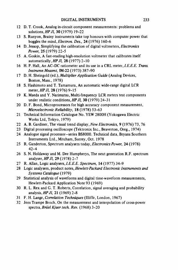
DIGITAL INSTRUMENTS 233
12 D. T. Crook, Analog in-circuit component measurements: problems andsolutions, HP Jl, 30 (1979) 19-22
13 S. Runyon, Brainy instruments take top honours with computer power thatboggles the mind, Electron. Des., 24 (1976) 160-6
14 D. Jessop, Simplifying the calibration of digital voltmeters. ElectronicsPower, 25 (1979) 22-5
15 A. Goskin, A fast-reading high-resolution voltmeter that calibrates itselfautomatically, HP Jl, 28 (1977) 2-10
16 H. P. Hall, An AC-DC ratiometer and its use in a CRL meter, I.E.E.E. Trans.Instrumn Measmt, IM-22 (1973) 387-90
17 D. H. Sheingold (ed.). Multiplier Application Guide (Analog Devices,Boston, Mass., 1978)
18 S. Hashimoto and T. Tamamura, An automatic wide-range digital LCRmeter, HP Jl, 28 (1976) 9-15
19 K. Maeda and Y. Narimatsu, Multi-frequency LCR meters test componentsunder realistic conditions, HP Jl, 30 (1979) 24-31
20 D. F. Bond, Microprocessors for high accuracy component measurement.Microelectronic Reliability, 18 (1978) 53-63
21 Technical Information Catalogue No. YEW 2800H (Yokogawa ElectricWorks Ltd, Tokyo, 1979)
22 A. B. Gardiner, The visual trend display. New Electronics, 9 (1976) 73, 7623 Digital processing oscilloscope (Tektronix Inc., Beaverton, Oreg., 1974)24 Analogue signal processor-series BS8000. Technical data, Bryans Southern
Instruments Ltd., Mitcham, Surrey, Oct. 197825 R. Ganderton, Spectrum analysers today. Electronics Power, 24 (1978)
42-426 S. N. Holdaway and M. Dee Humpherys, The next generation R.F. spectrum
analyser,HP Jl, 29 (1978) 2-727 R. Allan, Logic analysers, I.E.E.E. Spectrum, 14 (1977) 34-928 Logic analysers, product notes, Hewlett-Packard Electronic Instruments and
Systems Catalogue (1979)29 Statistical analysis of waveforms and digital time-waveform measurements,
Hewlett-Packard Application Note 93 (1969)30 R. L. Rex and G. T. Roberts, Correlation, signal averaging and probability
analysis,HPJl, 21 (1969) 2-831 F. H. Lange, Correlation Techniques (Illiffe, London, 1967)32 Jens Trampe Broch, On the measurement and interpolation of cross-power
spectra,Brüel Kjaer tech. Rev. (1968) 3-20

5Transducers
Definitions
Transducers
These devices have been defined as components that may be used to interconnect like or unlike systems and transmit energy between them. Although such a definition can be justified, a more generally acceptable definition to electrical engineers is that a transducer is a device used to convert a physical phenomenon into an electrical signal.
In many cases the conversion may be via an intermediate stage, that is, the measurand (for example, pressure) is first converted to a mechanical displace-ment which in turn is converted to an electrical signal. The mechanical conver-sion is accomplished by one of two fundamentally different methods, as follows.
Fixed reference devices
In these devices one part of the transducer is attached to a reference surface, and the other part connected, either directly or via a linking mechanism, to the variable as in figure 5.1. Should the displacement be small, some means of mech-anical magnification or electrical amplification must be used to obtain a satisfactory sensitivity.
Figure 5.1. Fixed reference transducer
wiper displacement
resistive track
fixed base
Vout
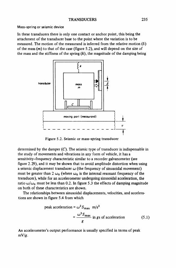
TRANSDUCERS 235
Mass-spring or seismic device
In these transducers there is only one contact or anchor point, this being theattachment of the transducer base to the point where the variation is to be measured. The motion of the measurand is inferred from the relative motion (δ) of the mass (m) to that of the case (figure 5.2), and will depend on the size of the mass and the stiffness of the spring (k) the magnitude of the damping being
Figure 5.2. Seismic or mass-spring transducer
transducer mass
moving part (measurand)
determined by the damper (C). The seismic type of transducer is indispensable in the study of movements and vibrations in any form of vehicle, it has a sensitivity-frequency characteristic similar to a recorder galvanometer (see figure 2.29), and it may be shown that to avoid amplitude distortion when using a seismic displacement transducer ω (the frequency of sinusoidal movement) must be greater than 2ω0 (where ω0 is the internal resonant frequency of the transducer), while for an accelerometer undergoing sinusoidal acceleration, the ratio ω/ω0 must be less than 0.2. In figure 5.3 the effects of damping magnitude on both of these characteristics are shown.
The relationships between sinusoidal displacements, velocities, and accelera-tions are shown in figure 5.4 from which
peak acceleration
in gs of acceleration (5.1)
An accelerometer’s output performance is usually specified in terms of peak mV/g.

Figure 5.3. Characteristic curves for seismic transducers showing the effect of damping magnitude on displacement amplitude of internal mass: (a) response to sinusoidal displacement of transducer case, (b) res-ponse to sinusoidal acceleration of transducer case
(a)
7 = fraction of critical damping
(b)

TRANSDUCERS 237
Figure 5.4. Relationships of oscillatory motions
displacement
velocity
time
acceleration
Transducer classification
A detailed study of transducers is more suited to specialised books [1, 2, 3] ratherthan this introductory text on instrumentation. However, because they form such an important part of any instrumentation system it is desirable to examine the transduction methods used to convert physical phenomena into electrical signals. Transducers may be classified either by the transduction method used, or by the function they are capable of measuring, for example acceleration, displace ment, etc. In table 5.1 are tabulated the more common measurands and the possible methods of transduction. The method of classification adopted in this
Table 5.1. Table of measurands against transduction methods
Resistancechange
Reactancechange
Electro-magnetic
Semi-conductor
Digital Thermo-electric
Acceleration * * * * *Displacement * * * * *Flow * * *Force * * *Humidity *Level * * *Pressure * * * *Temperature * * * *Thickness * *Velocity * * * * *
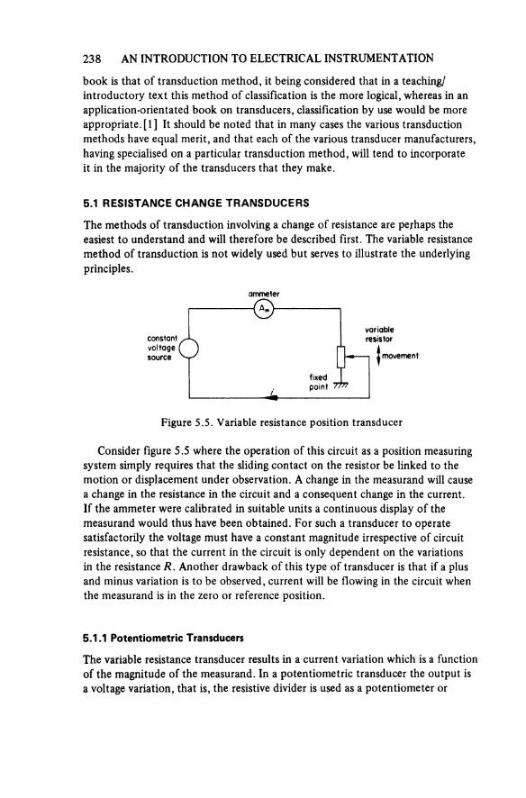
238 AN INTRODUCTION TO ELECTRICAL INSTRUMENTATION
book is that of transduction method, it being considered that in a teaching/ introductory text this method of classification is the more logical, whereas in an application-orientated book on transducers, classification by use would be more appropriate. [1] It should be noted that in many cases the various transduction methods have equal merit, and that each of the various transducer manufacturers, having specialised on a particular transduction method, will tend to incorporate it in the majority of the transducers that they make.
5.1 RESISTANCE CHANGE TRANSDUCERS
The methods of transduction involving a change of resistance are perhaps the easiest to understand and will therefore be described first. The variable resistance method of transduction is not widely used but serves to illustrate the underlying principles.
Figure 5.5. Variable resistance position transducer
ammeter
constantvoltagesource
variableresistor
movement
fixedpoint
Consider figure 5.5 where the operation of this circuit as a position measuring system simply requires that the sliding contact on the resistor be linked to the motion or displacement under observation. A change in the measurand will causea change in the resistance in the circuit and a consequent change in the current. If the ammeter were calibrated in suitable units a continuous display of the measurand would thus have been obtained. For such a transducer to operate satisfactorily the voltage must have a constant magnitude irrespective of circuit resistance, so that the current in the circuit is only dependent on the variations in the resistance R. Another drawback of this type of transducer is that if a plus and minus variation is to be observed, current will be flowing in the circuit when the measurand is in the zero or reference position.
5.1.1 Potentiometric Transducers
The variable resistance transducer results in a current variation which is a function of the magnitude of the measurand. In a potentiometric transducer the output is a voltage variation, that is, the resistive divider is used as a potentiometer or
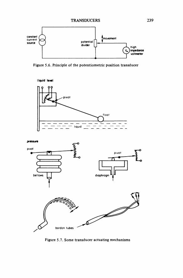
TRANSDUCERS 239
Figure 5.6. Principle of the potentiometric position transducer
constantcurrentsource potential
divider
movement
highimpedancevoltmeter
Figure 5.7. Some transducer actuating mechanisms
liquid level
pivot
float
liquid
pressure
pivot
bellows
pivot
diaphragm
bordon tubes
240 AN INTRODUCTION TO ELECTRICAL INSTRUMENTATION
potential divider (figure 5.6) and is in general a more satisfactory arrangement. A potentiometric transducer should be supplied from a constant current source, thetransducer output being monitored by a high impedance instrument so that the loading effects across the potentiometer are negligible. It will be seen that mechanically coupling the measurand to the sliding contact of the potentiometer will result in an output voltage that will be proportional to the displacement ofthe wiper from one end of the resistive path.
Since the resistance potentiometer may be used to convert a displacement into a proportional electrical signal, the measurement of quantities such as flow,force, pressure, humidity, etc., can be performed by a fixed reference potentio-metric sensor when a suitable quantity to displacement converter is positioned between the sliding contact and the measurand. Figure 5.7 illustrates some of the techniques used to convert physical properties to displacements suitable for applying to the sliding contact.
To obtain measurements of velocity or acceleration from a fixed reference potentiometric transducer, requires that the output voltage proportional to dis-placement is electrically differentiated once to obtain velocity and differentiated twice to produce an electrical signal proportional to acceleration (see section 6.7.2). A signal proportional to acceleration can however be obtained directly from a seismic potentiometric transducer (see figure 5.2) provided its mechanical resonant frequency ω0 is much higher than the frequency of the acceleration (ω), that is ω/ω0 < 0.2.
Both the variable resistance and the resistance potentiometer types of trans-ducer have a resistive element which may be wire wound, deposited carbon film, platinum film, or a resistive compound such as conductive plastics. Since the operation of an these transducers depends on the contact between a slider and the resistance element, their life is related to the wear of this contact, and the frequency of operation limited to a few cycles of displacement per second. The typical life expectancy of this type of transducer is around 3 × 10⁶ cycles of operation; they are comparatively inexpensive, and the circuitry associated with their use is simple although instrument loading effects must be considered, it should also be remembered that if displacement is the quantity being measured, a force has to be provided to overcome the friction of the sliding contact and this may affect the magnitude of the observed displacement.
Example
A potentiometric displacement transducer with a 20 mm travel has a resistance of 10 kΩ. If it is connected to a 10 V d.c. source of negligible output resistance, calculate the error in position if the output is measured as 5 V (that is, ≡ 10 mm)on an instrument that has an input resistance of 20 kΩ.
The circuit appropriate to this example is figure 5.6. The wiper divides thepotentiometer resistance into R and (10 kΩ — R), then
TRANSDUCERS 241
or
Hence
or
This is 615 Ω from the mid position and means an error of (615 × 100/5000) or 12.3 per cent.
5J.2 Resistance Strain Gauges
An important series of transducers is derived from the use of resistance strain gauges, and before considering such transducers the principles and applications of resistance strain gauges should be understood.
If a length of electrical wire is subjected to a tensile force it will stretch, its length being increased by an amount of δL (say), and provided that the elastic limit of the material is not exceeded, the change in length is proportional to the load and the wire will revert to its original length when the load is removed. Corresponding to this increase in length there will be a slight decrease in the cross-sectional area of the wire (the increased length has to come from some-where), and since resistance of a conductor = ρL/A, where p = resistivity of the material, L = length and A = cross-sectional area, the increase in length and the decrease in area will both contribute to an increase in the resistance of the stretched wire. In addition to the dimensional changes the resistivity of the material changes, this effect (termed piezoresistivity) is small for metals but does make a contribution to the change in resistance. Obviously, it is inconvenient to have long lengths of resistance wire attached to a test object so the general arrangement of a strain gauge is one in which the resistance wire (which typically has a 0.025 mm diameter) is folded into a grid and mounted on a backing of paper or Bakelite. A development from this is the foil gauge (see figure 5.8), which is manufactured by techniques similar to those used in the production of printed circuits. Such a process readily lends itself to the production of shaped, special purpose, strain gauges. The size of a strain gauge will depend on the

242 AN INTRODUCTION TO ELECTRICAL INSTRUMENTATION
Figure 5.8. Resistance foil gauges (courtesy of Philips)
I II
II IV
intended application but resistance gauges are available in a variety of lengths from around 3 mm to 150 mm, there being a range of nominal resistance values,preferred magnitudes of which are 120 Ω and 600 Ω.
It was stated above that the electrical resistance (R) of a straight wire willchange when it is stretched; let this change in resistance be δR. The definition of mechanical strain is the ratio ‘change in length/the original length’ or δL/L and is denoted by the symbol ε. To relate these two quantities, a factor known as the strain sensitivity is used such that
strain sensitivity = (5.2)
and has a characteristic value dependent on the type of resistance wire. Note: ε is often quoted as microstrain (με), for example, micrometres per metre.
When the wire is bent into a grid to form a strain gauge there are small lengths of the wire at each bend that are no longer acted on by the strain parallel to theaxis of the gauge. This part of the gauge resistance is termed ‘dead resistance’ and the ratio of dead resistance to total gauge resistance will depend on the type of fold and length of the gauge.
When a gauge is attached to an object that is stressed parallel to the axis of
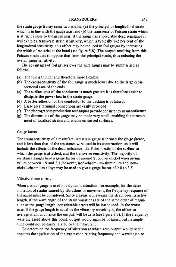
TRANSDUCERS 243
the strain gauge it may sense two strains: (a) the principal or longitudinal strain which is in line with the gauge axis, and (b) the transverse or Poisson strain which is at right angles to the gauge axis. If the gauge has appreciable dead resistance it will exhibit a transverse strain sensitivity, which is typically 1-2 per cent of the longitudinal sensitivity; this effect may be reduced in foil gauges by increasing the width of material at the bend (see figure 5.8). The output resulting from this Poisson strain acts to oppose that from the principal strain, thus reducing the overall gauge sensitivity.
The advantages of foil gauges over the wire gauges may be summarised as follows.
(a) The foil is thinner and therefore more flexible.(b) The cross-sensitivity of the foil gauge is much lower due to the large cross-
sectional area of the ends.(c) The surface area of the conductor is much greater; it is therefore easier to
dissipate the power loss in the strain gauge.(d) A better adhesion of the conductor to the backing is obtained.(e) Large area terminal connections are easily provided.(f) The photographic production techniques provide consistency in manufacture.(g) The dimensions of the gauge may be made very small, enabling the measure-
ment of localised strains and strains on curved surfaces.
Gauge factor
The strain sensitivity of a manufactured strain gauge is termed the gauge factor, and is less than that of the resistance wire used in its construction, as it will include the effects of the dead resistance, the Poisson ratio of the surface to which the gauge is attached, and the transverse sensitivity. The majority of resistance gauges have a gauge factor of around 2, copper-nickel wires giving values between 1.9 and 2.1; however, iron-chromium-aluminium and iron- nickel-chromium alloys may be used to give a gauge factor of 2.8 to 3.5.
Vibratory movement
When a strain gauge is used in a dynamic situation, for example, for the deter-mination of strains caused by vibrations or movement, the frequency response of the gauge must be considered. Since a gauge will average the strain over its active length, if the wavelength of the strain variations are of the same order of magni-tude as the gauge length, considerable errors will be introduced. In the worst case, if the gauge length is equal to the vibratory wavelength, the effective average strain and hence the output, will be zero (see figure 5.9). If the frequency were increased above this point, output would again be obtained but its ampli-tude could not be easily related to the measurand.
To determine the frequency of vibration at which zero output would occur requires the application of the expression relating frequency and wavelength to
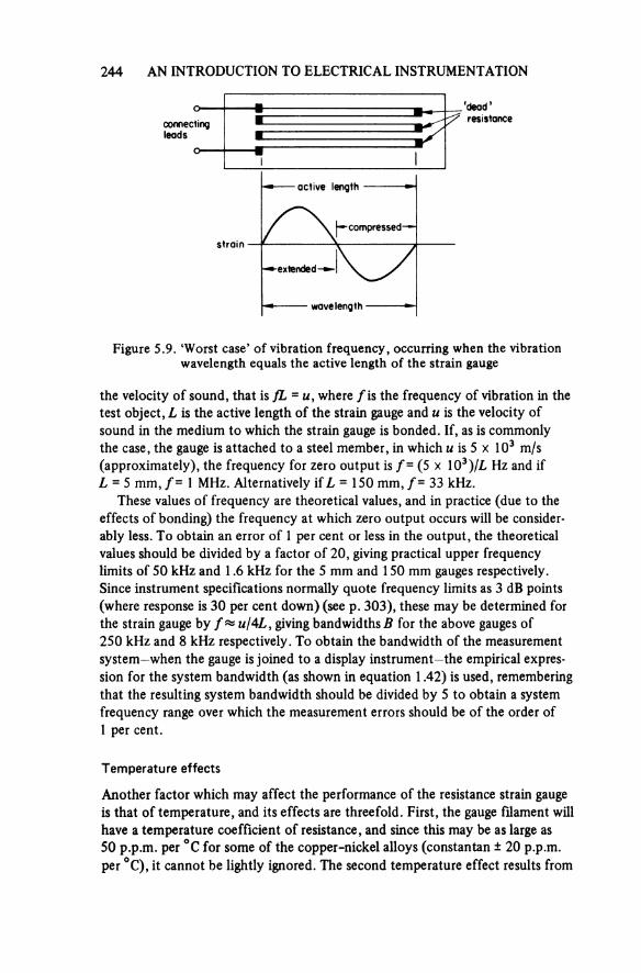
244 AN INTRODUCTION TO ELECTRICAL INSTRUMENTATION
Figure 5.9. ‘Worst case’ of vibration frequency, occurring when the vibration wavelength equals the active length of the strain gauge
connectingleads
'dead'resistance
active length
strain
compressed
extended
wavelength
the velocity of sound, that is fL = u, where / is the frequency of vibration in the test object, L is the active length of the strain gauge and u is the velocity of sound in the medium to which the strain gauge is bonded. If, as is commonly the case, the gauge is attached to a steel member, in which u is 5 × 10³ m/s (approximately), the frequency for zero output is /= (5 × 10³)/L Hz and if L = 5 mm, /= 1 MHz. Alternatively if L = 150 mm, /= 33 kHz.
These values of frequency are theoretical values, and in practice (due to the effects of bonding) the frequency at which zero output occurs will be consider-ably less. To obtain an error of 1 per cent or less in the output, the theoretical values should be divided by a factor of 20, giving practical upper frequency limits of 50 kHz and 1.6 kHz for the 5 mm and 1 50 mm gauges respectively. Since instrument specifications normally quote frequency limits as 3 dB points(where response is 30 per cent down) (see p. 303), these may be determined for the strain gauge by f = u/4L, giving bandwidths B for the above gauges of 250 kHz and 8 kHz respectively. To obtain the bandwidth of the measurement system—when the gauge is joined to a display instrument—the empirical expres-sion for the system bandwidth (as shown in equation 1.42) is used, remembering that the resulting system bandwidth should be divided by 5 to obtain a system frequency range over which the measurement errors should be of the order of 1 per cent.
Temperature effects
Another factor which may affect the performance of the resistance strain gauge is that of temperature, and its effects are threefold. First, the gauge filament will have a temperature coefficient of resistance, and since this may be as large as 50 p.p.m. per °C for some of the copper-nickel alloys (constantan ± 20 p.p.m. per °C), it cannot be lightly ignored. The second temperature effect results from
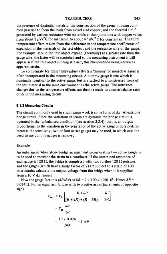
TRANSDUCERS 245
the presence of dissimilar metals in the construction of the gauge, it being com-mon practice to form the leads from nickel clad copper, and the thermal e.m.f. generated by various resistance wire materials at their junctions with copper varies from about 2 μV/°C for manganin to about 47 μV/°C for constantan. The third temperature effect results from the difference in the temperature coefficients of expansion of the materials of the test object and the resistance wire of the gauge. For example, should the test object expand (thermally) at a greater rate than the gauge wire, the latter will be stretched and to the measuring instrument it will appear as if the test object is being stressed, this phenomenon being known as apparent strain.
To compensate for these temperature effects a ‘dummy’ or nonactive gauge is often incorporated in the measuring circuit. A dummy gauge is one which is nominally identical to the active gauge, but is attached to a nonstressed piece of the test material in the same environment as the active gauge. The resistance changes due to the temperature effects can then be made to counterbalance each other in the measuring circuit.
5.L3 Measuring Circuits
The circuit commonly used in strain gauge work is some form of d.c. Wheatstonebridge circuit. Since the variations in strain are dynamic the bridge circuit is operated in the ‘unbalanced condition’ (see section 3.3.4), that is, an output proportional to the variation in the resistance of the active gauge is obtained. To increase the sensitivity, two or four active gauges may be used, in which case the need to use dummy gauges is removed.
Example
An unbalanced Wheatstone bridge arrangement incorporating two active gauges is to be used to monitor the strain in a cantilever. If the unstrained resistance of each gauge is 120 Ω, the bridge is completed with two further 120 Ω resistors,and the gauges (which have a gauge factor of 2) are subject to a strain of 100 microstrain; calculate the output voltage from the bridge when it is supplied from a 10 V d.c. source.
Now the gauge factor is (δR/Rε) or δR = 2 × 100 × 120/106. Hence δR = 0.024 Ω. For an equal arm bridge with two active arms (increments of opposite sign)
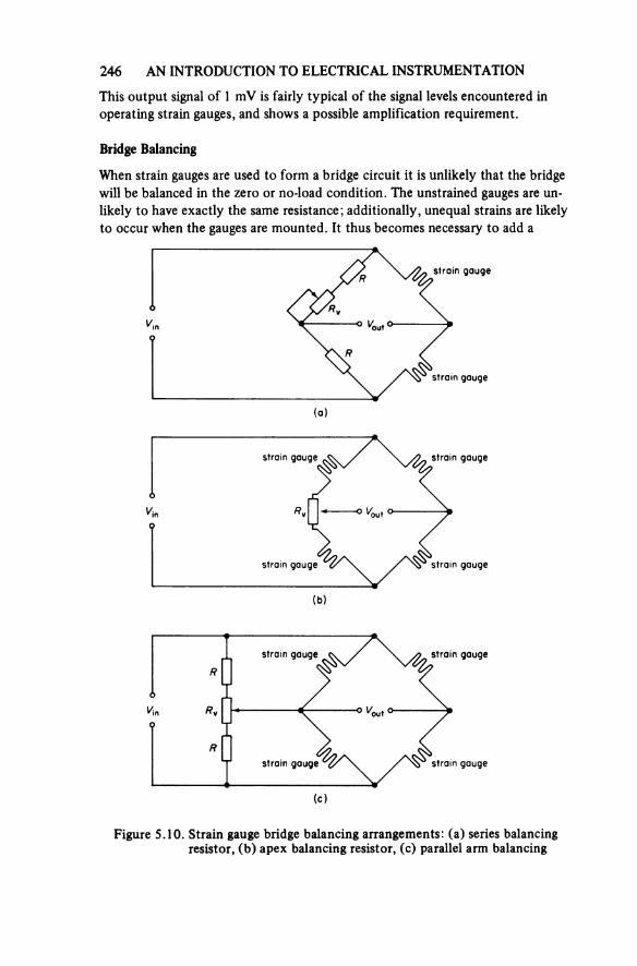
246 AN INTRODUCTION TO ELECTRICAL INSTRUMENTATION
This output signal of 1 mV is fairly typical of the signal levels encountered in operating strain gauges, and shows a possible amplification requirement.
Bridge Balancing
When strain gauges are used to form a bridge circuit it is unlikely that the bridge will be balanced in the zero or no-load condition. The unstrained gauges are un-likely to have exactly the same resistance; additionally, unequal strains are likely to occur when the gauges are mounted. It thus becomes necessary to add a
Figure 5.10. Strain gauge bridge balancing arrangements: (a) series balancing resistor, (b) apex balancing resistor, (c) parallel arm balancing
(a)
strain gauge
strain gauge
(b)
strain gauge strain gauge
strain gauge strain gauge
(c)
strain gauge strain gauge
strain gauge strain gauge
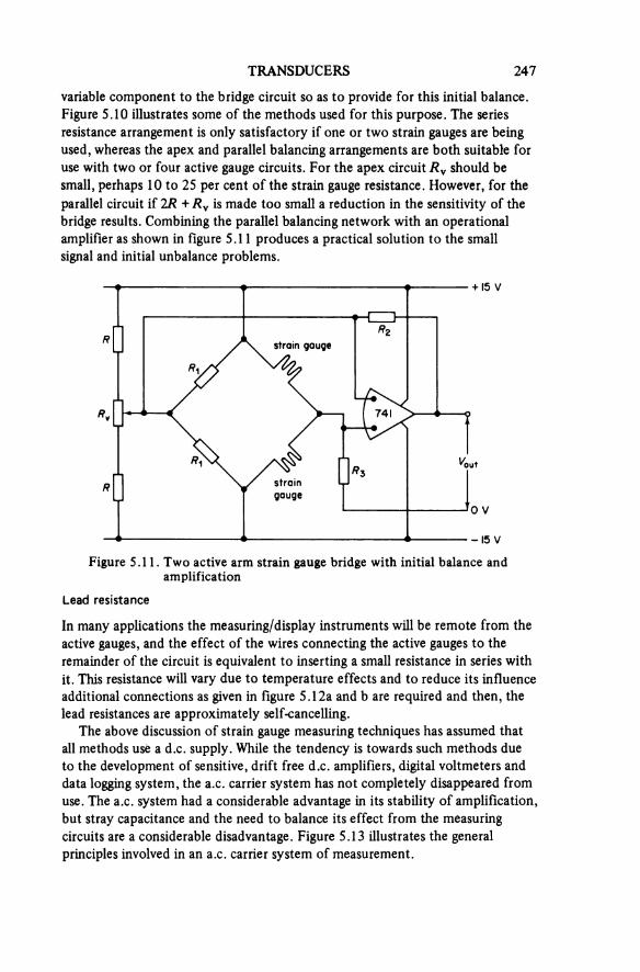
TRANSDUCERS 247
variable component to the bridge circuit so as to provide for this initial balance. Figure 5.10 illustrates some of the methods used for this purpose. The series resistance arrangement is only satisfactory if one or two strain gauges are being used, whereas the apex and parallel balancing arrangements are both suitable for use with two or four active gauge circuits. For the apex circuit Rv should be small, perhaps 10 to 25 per cent of the strain gauge resistance. However, for the parallel circuit if 2R + AV is made too small a reduction in the sensitivity of the bridge results. Combining the parallel balancing network with an operational amplifier as shown in figure 5.11 produces a practical solution to the small signal and initial unbalance problems.
Figure 5.11. Two active arm strain gauge bridge with initial balance and amplification
strain gauge
Lead resistance
In many applications the measuring/display instruments will be remote from theactive gauges, and the effect of the wires connecting the active gauges to the remainder of the circuit is equivalent to inserting a small resistance in series with it. This resistance will vary due to temperature effects and to reduce its influence additional connections as given in figure 5.12a and b are required and then, the lead resistances are approximately self-cancelling.
The above discussion of strain gauge measuring techniques has assumed that all methods use a d.c. supply. While the tendency is towards such methods due to the development of sensitive, drift free d.c. amplifiers, digital voltmeters and data logging system, the a.c. carrier system has not completely disappeared from use. The a.c. system had a considerable advantage in its stability of amplification, but stray capacitance and the need to balance its effect from the measuring circuits are a considerable disadvantage. Figure 5.13 illustrates the general principles involved in an a.c. carrier system of measurement.
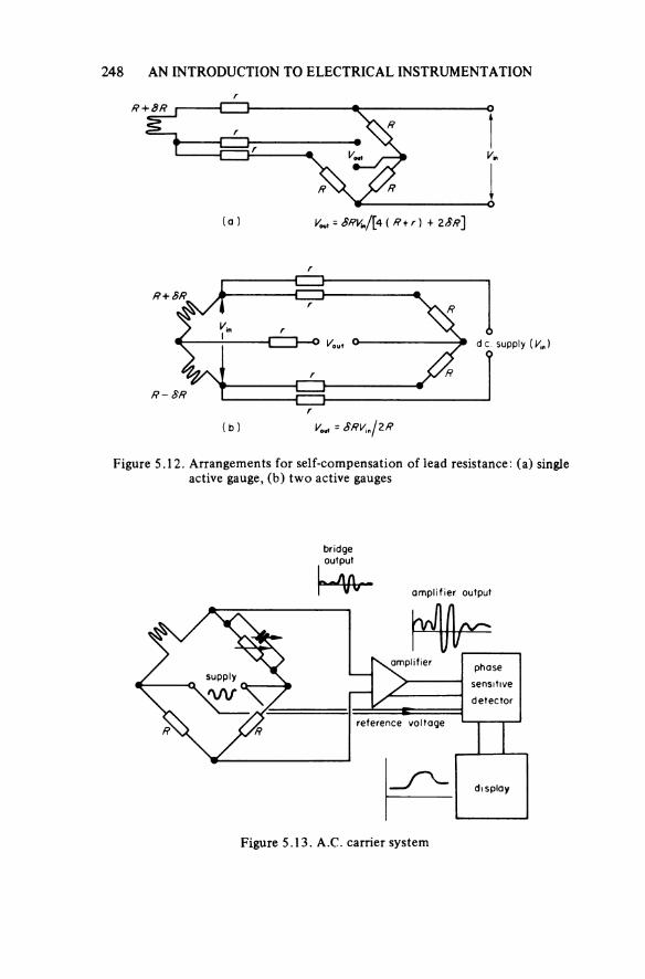
248 AN INTRODUCTION TO ELECTRICAL INSTRUMENTATION
Figure 5.12. Arrangements for self-compensation of lead resistance: (a) single active gauge, (b) two active gauges
(a)
(b)
Figure 5.13. A.C. carrier system
bridgeoutput
amplifier output
amplifiersupply
phasesensitivedetector
reference voltage
display
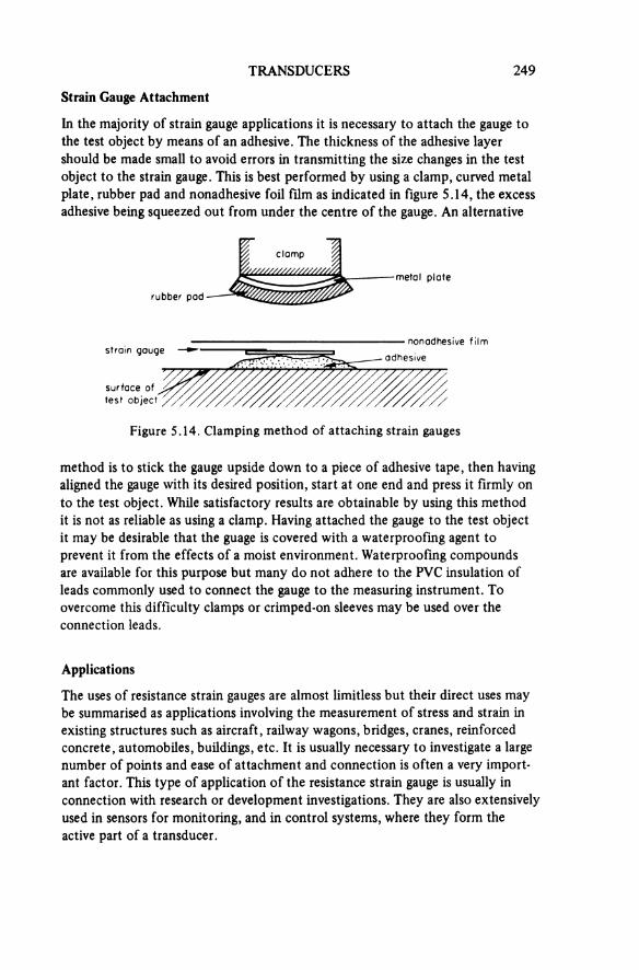
TRANSDUCERS 249
Strain Gauge Attachment
In the majority of strain gauge applications it is necessary to attach the gauge to the test object by means of an adhesive. The thickness of the adhesive layer should be made small to avoid errors in transmitting the size changes in the test object to the strain gauge. This is best performed by using a clamp, curved metal plate, rubber pad and nonadhesive foil film as indicated in figure 5.14, the excess adhesive being squeezed out from under the centre of the gauge. An alternative
Figure 5.14. Clamping method of attaching strain gauges
clamp
metal plate
rubber pad
strain gaugenonadhesive film
adhesive
surface of test object
method is to stick the gauge upside down to a piece of adhesive tape, then having aligned the gauge with its desired position, start at one end and press it firmly on to the test object. While satisfactory results are obtainable by using this method it is not as reliable as using a clamp. Having attached the gauge to the test object it may be desirable that the guage is covered with a waterproofing agent to prevent it from the effects of a moist environment. Waterproofing compounds are available for this purpose but many do not adhere to the PVC insulation of leads commonly used to connect the gauge to the measuring instrument. To overcome this difficulty clamps or crimped-on sleeves may be used over the connection leads.
Applications
The uses of resistance strain gauges are almost limitless but their direct uses may be summarised as applications involving the measurement of stress and strain in existing structures such as aircraft, railway wagons, bridges, cranes, reinforced concrete, automobiles, buildings, etc. It is usually necessary to investigate a largenumber of points and ease of attachment and connection is often a very import-ant factor. This type of application of the resistance strain gauge is usually in connection with research or development investigations. They are also extensively used in sensors for monitoring, and in control systems, where they form the active part of a transducer.
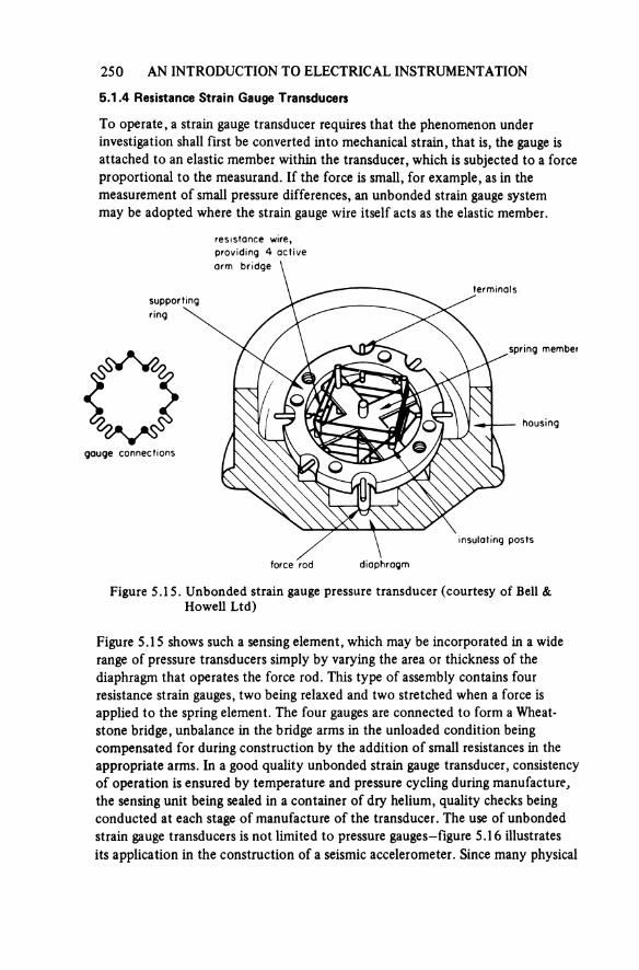
250 AN INTRODUCTION TO ELECTRICAL INSTRUMENTATION
5.1.4 Resistance Strain Gauge Transducers
To operate, a strain gauge transducer requires that the phenomenon under investigation shall first be converted into mechanical strain, that is, the gauge is attached to an elastic member within the transducer, which is subjected to a force proportional to the measurand. If the force is small, for example, as in the measurement of small pressure differences, an unbonded strain gauge system may be adopted where the strain gauge wire itself acts as the elastic member.
Figure 5.15. Unbonded strain gauge pressure transducer (courtesy of Bell & Howell Ltd)
resistance wire, providing 4 active arm bridge
supporting ring
terminals
spring member
housing
gauge connections
insulating posts
force rod diaphragm
Figure 5.15 shows such a sensing element, which may be incorporated in a wide range of pressure transducers simply by varying the area or thickness of the diaphragm that operates the force rod. This type of assembly contains four resistance strain gauges, two being relaxed and two stretched when a force is applied to the spring element. The four gauges are connected to form a Wheat-stone bridge, unbalance in the bridge arms in the unloaded condition being compensated for during construction by the addition of small resistances in the appropriate arms. In a good quality unbonded strain gauge transducer, consistency of operation is ensured by temperature and pressure cycling during manufacture,, the sensing unit being sealed in a container of dry helium, quality checks beingconducted at each stage of manufacture of the transducer. The use of unbonded strain gauge transducers is not limited to pressure gauges—figure 5.16 illustrates its application in the construction of a seismic accelerometer. Since many physical
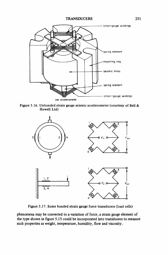
TRANSDUCERS 251
Figure 5.16. Unbonded strain gauge seismic accelerometer (courtesy of Bell & Howell Ltd)
strain-gauge windings
spring element
mounting
seismic mass
spring element
strain-gauge windingscec accelerometer
Figure 5.17. Some bonded strain gauge force transducers (load cells)
phenomena may be converted to a variation of force, a strain gauge element of the type shown in figure 5.15 could be incorporated into transducers to measure such properties as weight, temperature, humidity, flow and viscosity.
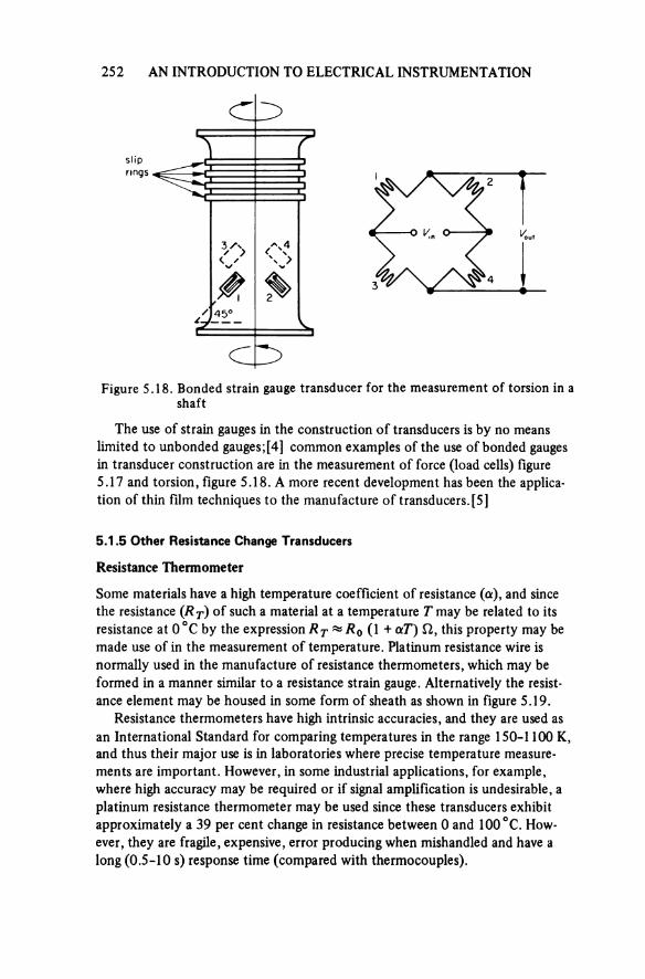
252 AN INTRODUCTION TO ELECTRICAL INSTRUMENTATION
Figure 5.18. Bonded strain gauge transducer for the measurement of torsion in a shaft
sliprings
The use of strain gauges in the construction of transducers is by no means limited to unbonded gauges;[4] common examples of the use of bonded gauges in transducer construction are in the measurement of force (load cells) figure 5.17 and torsion, figure 5.18. A more recent development has been the applica-tion of thin film techniques to the manufacture of transducers. [5]
5.1.5 Other Resistance Change Transducers
Resistance Thermometer
Some materials have a high temperature coefficient of resistance (α), and since the resistance (RT) of such a material at a temperature T may be related to its resistance at 0°C by the expression RT ~ R0 (1 + αT) Ω, this property may be made use of in the measurement of temperature. Platinum resistance wire is normally used in the manufacture of resistance thermometers, which may be formed in a manner similar to a resistance strain gauge. Alternatively the resist-ance element may be housed in some form of sheath as shown in figure 5.19.
Resistance thermometers have high intrinsic accuracies, and they are used as an International Standard for comparing temperatures in the range 150-1100 K, and thus their major use is in laboratories where precise temperature measure-ments are important. However, in some industrial applications, for example, where high accuracy may be required or if signal amplification is undesirable, a platinum resistance thermometer may be used since these transducers exhibit approximately a 39 per cent change in resistance between 0 and 100 °C. How-ever, they are fragile, expensive, error producing when mishandled and have a long (0.5-10 s) response time (compared with thermocouples).
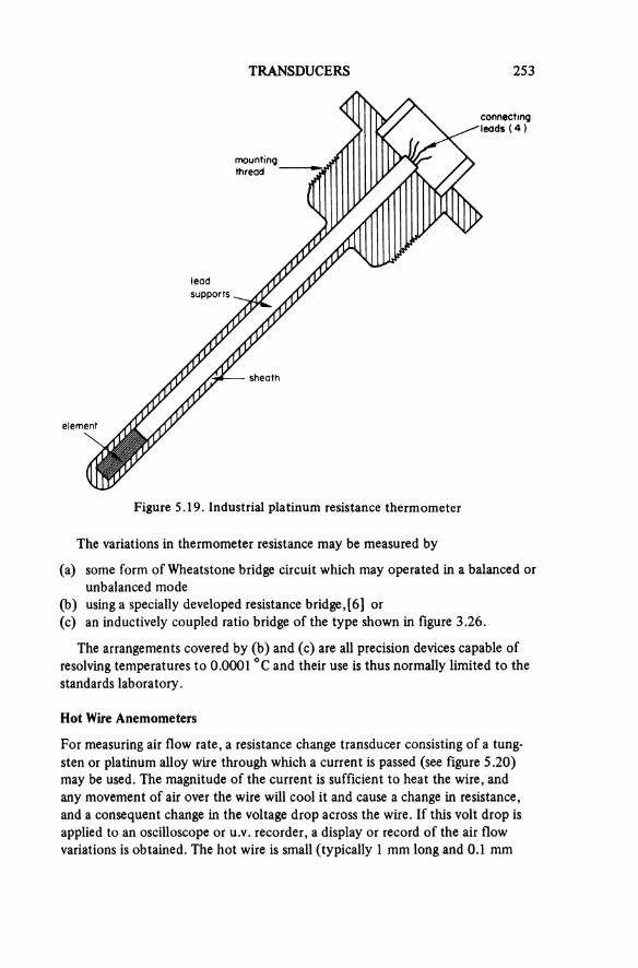
TRANSDUCERS 253
Figure 5.19. Industrial platinum resistance thermometer
connecting leads (4)
mountingthread
leadsupports
sheath
element
The variations in thermometer resistance may be measured by
(a) some form of Wheatstone bridge circuit which may operated in a balanced or unbalanced mode
(b) using a specially developed resistance bridge, [6] or(c) an inductively coupled ratio bridge of the type shown in figure 3.26.
The arrangements covered by (b) and (c) are all precision devices capable of resolving temperatures to 0.0001 °C and their use is thus normally limited to the standards laboratory.
Hot Wire Anemometers
For measuring air flow rate, a resistance change transducer consisting of a tung-sten or platinum alloy wire through which a current is passed (see figure 5.20) may be used. The magnitude of the current is sufficient to heat the wire, and any movement of air over the wire will cool it and cause a change in resistance, and a consequent change in the voltage drop across the wire. If this volt drop is applied to an oscilloscope or u.v. recorder, a display or record of the air flow variations is obtained. The hot wire is small (typically 1 mm long and 0.1 mm
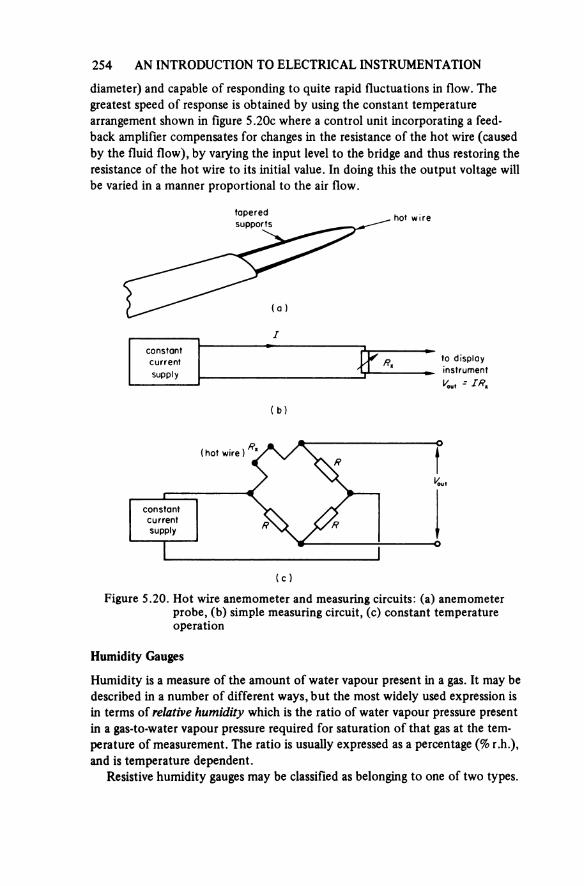
254 AN INTRODUCTION TO ELECTRICAL INSTRUMENTATION
diameter) and capable of responding to quite rapid fluctuations in flow. Thegreatest speed of response is obtained by using the constant temperature arrangement shown in figure 5.20c where a control unit incorporating a feed-back amplifier compensates for changes in the resistance of the hot wire (caused by the fluid flow), by varying the input level to the bridge and thus restoring the resistance of the hot wire to its initial value, in doing this the output voltage win be varied in a manner proportional to the air flow.
Figure 5.20. Hot wire anemometer and measuring circuits: (a) anemometer probe, (b) simple measuring circuit, (c) constant temperature operation
(a)
taperedsupports
hot wire
(b)
constantcurrentsupply
to display instrument
(c)
(hot wire)
constantcurrentsupply
Humidity Gauges
Humidity is a measure of the amount of water vapour present in a gas. It may be described in a number of different ways, but the most widely used expression is in terms of relative humidity which is the ratio of water vapour pressure present in a gas-to-water vapour pressure required for saturation of that gas at the tem-perature of measurement. The ratio is usually expressed as a percentage (% r.h.), and is temperature dependent.
Resistive humidity gauges may be classified as belonging to one of two types.

TRANSDUCERS 255
One type is those having a resistive sensing element, that is, a variation in the ambient humidity causes a variation in the resistance of the element that is usually a mixture of a hygroscopic salt, for example, lithium chloride and carbon on an insulating substrate between metal electrodes as shown in figure 5.21. The other form of resistance change humidity gauge is one in which the length change with humidity of a human hair or strip of animal gut is used to operate a displacement sensor which could be either potentiometric or strain gauge. [7]
Figure 5.21. Resistive sensing element humidity transducers
electrodes
conducting film
5.2 REACTANCE CHANGE TRANSDUCERS
This is a group of transducers in which a displacement is used to modulate either a capacitive or inductive reactance. Since variations in reactance may only be measured when the supply is an alternating voltage (or current) the excitation source for reactance change transducers must be alternating. This may, however, make the transducer incompatible with the remainder of the measuring system,and to overcome this a number of reactance change transducers are manufactured with an internal d.c. to a.c. converter and an output demodulator so that both the transducer input and output are d.c. while the internal excitation is a.c. [1]
5.2.1 Capacitance Variation
It has been indicated that a change in almost any physical phenomenon may be converted to a displacement and as the capacitance between two parallel con-ducting plates is approximately proportional to εA/d, (where ε is the dielectric constant of the material between the plates of area A, separated by a distance cI) varying any of these quantities will result in a change in the capacitance between the plates.
Variable dielectric
Figure 5.22 shows diagrammatically two types of dielectric variation transducer, one in which a dielectric sleeve is slid between coaxial electrodes to vary capaci-tance, the other being a device for measuring the height of a liquid in a container.
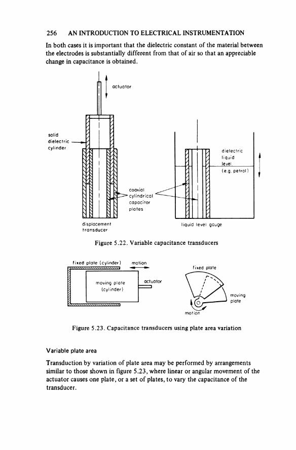
256 AN INTRODUCTION TO ELECTRICAL INSTRUMENTATION
In both cases it is important that the dielectric constant of the material between the electrodes is substantially different from that of air so that an appreciable change in capacitance is obtained.
Figure 5.22. Variable capacitance transducers
actuator
soliddielectriccylinder dielectric
liquidlevel(e.g. petrol)
coaxialcylindricalcapacitorplates
displacementtransducer
liquid level gauge
Figure 5.23. Capacitance transducers using plate area variation
fixed plate (cylinder) motion
moving plate (cylinder)
actuator
fixed plate
movingplate
motion
Variable plate area
Transduction by variation of plate area may be performed by arrangements similar to those shown in figure 5.23, where linear or angular movement of the actuator causes one plate, or a set of plates, to vary the capacitance of the transducer.

TRANSDUCERS 257
Variable plate separation
The third form of variation, namely that involving a change in the electrode separation (see figure 5.24) is perhaps the most widely used for the construction of such devices and is comparatively simple, as the forces required to move one plate in relation to another may be made exceedingly small, and the alignment of
Figure 5.24. Capacitance transducers using plate separation
motionfixed plate
fixedplate
diaphragm (moving plate)
the fixed and moving parts may not be as critical as it is when some other forms of transducer are used. Figure 5.25 illustrates the use of this technique to produce a capacitance strain gauge, a major advantage of this being its potential use at elevated temperatures. [8,9]
Figure 5.25. Capacitance strain gauge
electrode movement
weld weld
testpieceapplied strain
Measuring techniques
The measuring circuitry associated with capacitance change transducers usually involves some form of bridge. The simplest form would have two resistive and two capacitive arms. A slightly more sophisticated form of bridge is shown in figure 3.28, where a ratio transformer is incorporated together with a resistance circuit to compensate for any leakage resistance effects associated with the capacitance of the transducer. Either circuit may be used in the balanced or un-balanced condition provided that for the latter mode of operation the unbalance is less than 10 per cent.
Some capacitance change transducers are produced with internal signal con-ditioning equipment which uses a d.c. input to supply an oscillator, for operation of the capacitance bridge, and conversion of the bridge output to d.c. Alternat-ively an oscillator circuit may be used so that a change in capacitance causes a change in output frequency.
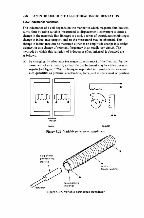
258 AN INTRODUCTION TO ELECTRICAL INSTRUMENTATION
5.2.2 Inductance Variation
The inductance of a coil depends on the manner in which magnetic flux links its turns, thus by using suitable ‘measurand to displacement’ converters to cause a change in the magnetic flux linkages in a coil, a series of transducers exhibiting a change in inductance proportional to the measurand may be obtained. This change in inductance can be measured either as an amplitude change in a bridge balance, or as a change of resonant frequency in an oscillatory circuit. The methods by which this variation of inductance (flux linkages) is obtained are as follows.
(a) By changing the reluctance (or magnetic resistance) of the flux path by the movement of an armature, so that the displacement may be either linear or angular (see figure 5.26) this being incorporated in transducers to measure such quantities as pressure, acceleration, force, and displacement or position.
Figure 5.26. Variable reluctance transducers
motion
linear angular
Figure 5.27. Variable permeance transducer
slug of highpermeabilitymaterial
centretapped windings
ferromagneticmaterial
actuator

TRANSDUCERS 259
(b) By the displacement of a slug of material having a high magnetic permeance that is constrained to move inside a centre-tapped coil which is wound on a ferromagnetic core (see figure 5.27). When the slug is positioned centrally the inductance of the two halves will be equal; on movement to one side the inductance of one half will increase while that of the other decreases.
Figure 5.28. Inductive change transducer measuring circuits—arrangements for: (a) d.c. output, (b) frequency output
(a)
inductancechangetransducer
phaseshiftingcircuit
supplyoscillator
phase sensitive detector d.c. output
(b)
transducer
i.c. operational amp
output
The inductor may form the arms of a bridge circuit, or be incorporated in an oscillator circuit (see figure 5.28a and b). The phase sensitive detector (see section 2.1.1) is included so that the d.c. output has a sign corresponding to the direction of the displacement. The phase shift circuit between the oscillator and the p.s.d. is necessary because at zero displacement there will be a phase angle between the reference voltage and the centre tap on the inductor (see also p. 316).

260 AN INTRODUCTION TO ELECTRICAL INSTRUMENTATION
5.2.3 Linear Variable Differential Transformer (L.V.D.T.)
In this type of transducer, the change of inductance is a variation of mutal coupling between windings rather than a variation of self inductance. This varia-tion of mutual inductance is obtained by the movement of a ferromagnetic core within a coil arrangement of the type shown in figure 5.29. There is usually one primary and two secondary coils. For a linear device the coils are wound on a nonmagnetic and insulating former while in angular devices of this type a ferro-magnetic core for the coils may be used. The operational circuits used for the differential transformer range from those such as that in figure 5.30a which has an a.c. output voltage that increases in magnitude for displacement either side of the centre or zero position. This circuit can easily be modified so that a d.c. output is obtained having a polarity dependent on the direction of displacement (see figure 5.30b). More complex arrangements are available commercially, in which a d.c. input is converted to an a.c. voltage, that is, varied by the transducer operation and then restored to d.c. so that the output voltage has a magnitude and direction proportional to displacement.
Figure 5.29. Linear variable differential transformer
secondaries
displacementprimary
corenonmagneticformer
linear movement
Figure 5.30. Operational circuits for use with differential transformer transducers
(a)displacement
(b)
displacement
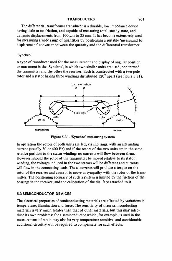
TRANSDUCERS 261
The differential transformer transducer is a durable, low impedance device, having little or no friction, and capable of measuring total, steady state, and dynamic displacements from 100 μm to 25 mm. It has become extensively used for measuring a wide range of quantities by positioning a suitable ‘measurand to displacement’ converter between the quantity and the differential transformer.
'Synchro'
A type of transducer used for the measurement and display of angular position or movement is the ‘Synchro’, in which two similar units are used, one termed the transmitter and the other the receiver. Each is constructed with a two-pole rotor and a stator having three windings distributed 120° apart (see figure 5.31).
Figure 5.31. ‘Synchro’ measuring system
a.c. excitation
slip ringsrotor rotor
stator stator
transmitter receiver
In operation the rotors of both units are fed, via slip rings, with an alternating current (usually 50 or 400 Hz) and if the rotors of the two units are in the same relative position to the stator windings no currents will flow between them. However, should the rotor of the transmitter be moved relative to its stator winding, the voltages induced in the two stators will be different and currents will flow in the connecting leads. These currents will produce a torque on therotor of the receiver and cause it to move in sympathy with the rotor of the trans mitter. The positioning accuracy of such a system is limited by the friction of the bearings in the receiver, and the calibration of the dial face attached to it.
5.3 SEMICONDUCTOR DEVICES
The electrical properties of semiconducting materials are affected by variations in temperature, illumination and force. The sensitivity of these semiconducting materials is very much greater than that of other materials, but this may intro-duce its own problems: for a semiconductor which, for example, is used in the measurement of strain may also be very temperature sensitive, and considerable additional circuitry will be required to compensate for such effects.
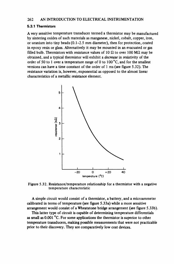
262 AN INTRODUCTION TO ELECTRICAL INSTRUMENTATION
5.3.1 Thermistors
A very sensitive temperature transducer termed a thermistor may be manufactured by sintering oxides of such materials as manganese, nickel, cobalt, copper, iron, or uranium into tiny beads (0.1-2.5 mm diameter), then for protection, coated in epoxy resin or glass. Alternatively it may be mounted in an evacuated or gas filled bulb. Thermistors with resistance values of 10 Ω to over 100 MΩ may be obtained, and a typical thermistor will exhibit a decrease in resistivity of the order of 50 to 1 over a temperature range of 0 to 100 °C, and for the smallest versions can have a time constant of the order of 1 ms (see figure 5.32). The resistance variation is, however, exponential as opposed to the almost linear characteristics of a metallic resistance element.
Figure 5.32. Resistance/temperature relationship for a thermistor with a negative temperature characteristic
resis
tanc
e (kΩ
)
temperature (°C)
A simple circuit would consist of a thermistor, a battery, and a microammeter calibrated in terms of temperature (see figure 5.33a) while a more sensitive arrangement would consist of a Wheatstone bridge arrangement (see figure 5.33b).
This latter type of circuit is capable of determining temperature differentials as small as 0.001 °C. For some applications the thermistor is superior to other temperature transducers, making possible measurements that were not practicable prior to their discovery. They are comparatively low cost devices.
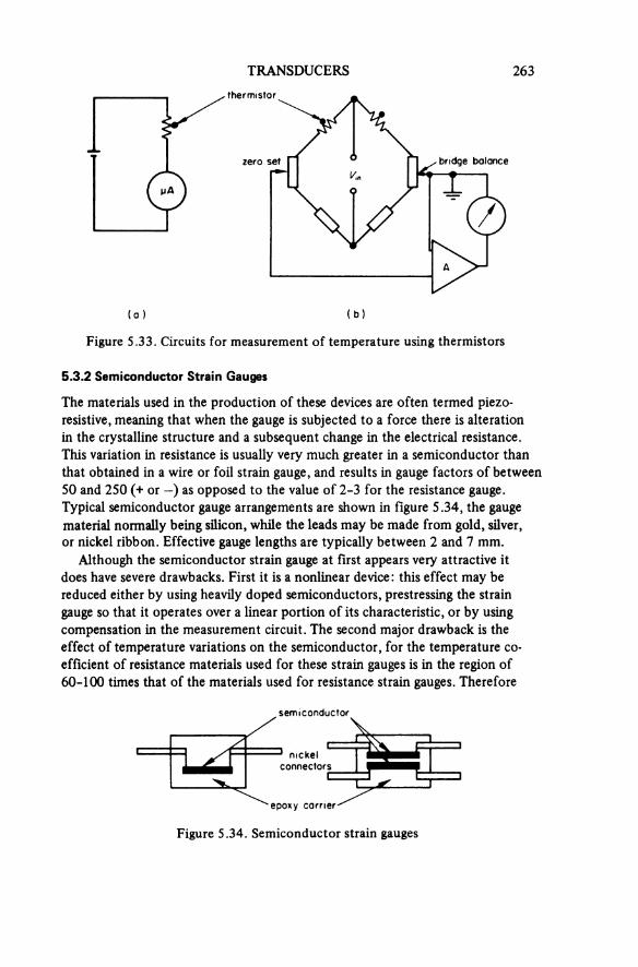
TRANSDUCERS 263
Figure 5.33. Circuits for measurement of temperature using thermistors
(a)
thermistor
(b)
zero set bridge balance
5.3.2 Semiconductor Strain Gauges
The materials used in the production of these devices are often termed piezo- resistive, meaning that when the gauge is subjected to a force there is alteration in the crystalline structure and a subsequent change in the electrical resistance. This variation in resistance is usually very much greater in a semiconductor than that obtained in a wire or foil strain gauge, and results in gauge factors of between 50 and 250 (+ or —) as opposed to the value of 2-3 for the resistance gauge. Typical semiconductor gauge arrangements are shown in figure 5.34, the gauge material normally being silicon, while the leads may be made from gold, silver, or nickel ribbon. Effective gauge lengths are typically between 2 and 7 mm.
Although the semiconductor strain gauge at first appears very attractive it does have severe drawbacks. First it is a nonlinear device: this effect may be reduced either by using heavily doped semiconductors, prestressing the strain gauge so that it operates over a linear portion of its characteristic, or by using compensation in the measurement circuit. The second major drawback is the effect of temperature variations on the semiconductor, for the temperature co-efficient of resistance materials used for these strain gauges is in the region of 60-100 times that of the materials used for resistance strain gauges. Therefore
Figure 5.34. Semiconductor strain gauges
semiconductor
nickel connectors
epoxy carrier

264 AN INTRODUCTION TO ELECTRICAL INSTRUMENTATION
when semiconductor strain gauges are used, temperature compensation must be incorporated in the measuring circuit. This may take the form of a ‘dummy’ gauge (see section 3.3.4) or be obtained by connecting a thermistor with the appropriate temperature/resistance characteristics in series or parallel with the semi-conductor gauge, in each active arm of the bridge circuit (see figure 5.35)or by using a pair of gauges so that one is subject to a positive strain and the other a negative strain.
Figure 5.35. Semiconductor strain gauge bridge
matched gauges for compensation of nonlinearities
thermistorfor temperaturecompensation
5.3.3 Photodiodes and Phototransistors
The electrical characteristics of most diodes and transistors are affected by light, hence it is normal to prevent light from acting on the semiconductor junction of these devices, by enclosing it in a screening can or other opaque container. If this container is removed from a transistor (or diode) incident light falling on the junction will affect the output of the device. Photodiodes and phototransistors are constructed so that this normally undesirable property is enhanced. [3] The majority of light sensing semiconductors are silicon, but when optimum responsein the infrared region is required germanium devices may be used. Both diodes and transistor are usually sealed in a metal can, there being a lens or window fitted to admit light to the junctions. Time constants of the order of 1 μs or less are common.
5.4 SELF-GENERATING TRANSDUCERS
Transducers in this group do not in theory require an external supply, for the electrical signal is produced either by the movement of a magnetic flux field in relation to a coil system, or by the application of force, heat or light to particular materials.
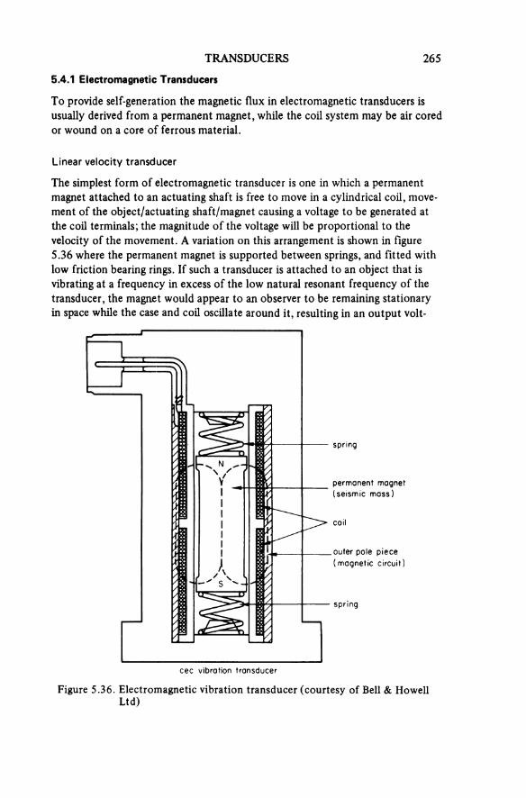
TRANSDUCERS 265
5.4.1 Electromagnetic Transducers
To provide self-generation the magnetic flux in electromagnetic transducers is usually derived from a permanent magnet, while the coil system may be air cored or wound on a core of ferrous material.
Linear velocity transducer
The simplest form of electromagnetic transducer is one in which a permanent magnet attached to an actuating shaft is free to move in a cylindrical coil, move-ment of the object/actuating shaft/magnet causing a voltage to be generated at the coil terminals; the magnitude of the voltage will be proportional to the velocity of the movement. A variation on this arrangement is shown in figure 5.36 where the permanent magnet is supported between springs, and fitted with low friction bearing rings. If such a transducer is attached to an object that is vibrating at a frequency in excess of the low natural resonant frequency of the transducer, the magnet would appear to an observer to be remaining stationary in space while the case and coil oscillate around it, resulting in an output volt-
Figure 5.36. Electromagnetic vibration transducer (courtesy of Bell & Howell Ltd)
spring
permanent magnet (seismic mass)
coil
outer pole piece (magnetic circuit)
spring
cec vibration transducer
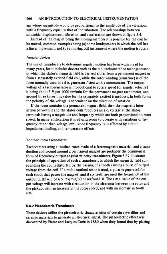
266 AN INTRODUCTION TO ELECTRICAL INSTRUMENTATION
age whose magnitude would be proportional to the amplitude of the vibration, with a frequency equal to that of the vibration. The relationships between sinusoidal displacement, vibration, and acceleration are shown in figure 5.4.
Instead of the magnet being the moving member it is possible for the coil to be moved, common examples being (a) some loudspeakers in which the coil has a linear movement, and (b) a moving coil instrument where the motion is rotary.
Angular devices
The use of transducers to determine angular motion has been widespread for many years, for it includes devices such as the d.c. tachometer or tachogenerator, in which the stator’s magnetic field is derived either from a permanent magnet or from a separately excited field coil, while the rotor winding (armature) is of the form normally used in a d.c. generator fitted with a commutator. The output voltage of a tachogenerator is proportional to rotary speed (or angular velocity) it being about 5 V per 1000 rev/min for the permanent magnet tachometer, and around three times this value for the separately excited transducer. In both forms the polarity of the voltage is dependent on the direction of rotation.
If the rotor contains the permanent magnet field, then the magnetic inter-action between it and the stator coils produces an a.c. voltage at the stator terminals having a magnitude and frequency which are both proportional to rotor speed. In many applications it is advantageous to operate with variations of fre-quency rather than voltage level, since frequency is unaffected by circuit impedance, loading, and temperature effects.
Toothed rotor tachometer
Tachometers using a toothed rotor made of a ferromagnetic material, and a trans-duction coil wound around a permanent magnet are probably the commonest form of frequency output angular velocity transducers. Figure 5.37 illustrates the principle of operation of such a transducer, in which the magnetic field sur-rounding the coil is distorted by the passing of a tooth causing a pulse of output voltage from the coil. If a multi-toothed rotor is used, a pulse is generated for each tooth that passes the magnet, and if six teeth are used the frequency of the output in Hz will be 6 × rev/min/60 or rev/min/10. The r.m.s. value of the out-put voltage will increase with a reduction in the clearance between the rotor and the pickup, with an increase in the rotor speed, and with an increase in tooth size.
5.4.2 Piezoelectric Transducers
These devices utilise the piezoelectric characteristics of certain crystalline and ceramic materials to generate an electrical signal. The piezoelectric effect was discovered by Pierre and Jacques Curie in 1880 when they found that by placing
TRANSDUCERS 267
Figure 5.37. Operation of a toothed wheel tachometer
output waveform
mild steel wheel permanent magnet
output waveform
weights on to a quartz crystal an electrical charge could be generated. Subsequent researchers have shown that there are about 40 crystalline materials which when subjected to a ‘squeeze’ (the Greek word ‘piezein’ means to squeeze) generate an electrical charge. The Curie brothers also discovered the reverse effect, that is, a dimension change is obtained when an electric stress is applied to a quartz crystal.
The crystal materials are of two basic types, natural crystals and synthetic crystals, the latter type being mainly ceramic ‘crystals’ of which barium titanate was the first to be commercially used. The addition of controlled impurities such as calcium titanate was found to improve some of the ‘crystal’s’ characteristics. Research on this and other synthetic ‘crystals’ has led to them being used more frequently than natural crystals in the production of piezoelectric transducers.
The force applied to the crystal may be that of shear, compression, or bend-ing, depending on the particular application for which the transducer has been designed. The merits of operating the crystal with the various force modes will not be discussed here—they are described in detail in reference 1. It must, how-ever, be remembered that since piezoelectric transducers belong to the self-generating category their use is predominantly in dynamic applications, a common form being as seismic accelerometers, although the piezoelectric principle may be effectively used in any situation where the measurand can be converted to a force that results in the stressing of a suitable crystal.
All piezoelectric crystals have a high output impedance, and for this reason the instrumentation to which the piezoelectric transducer is connected must have a high input impedance, or for most applications a charge amplifier (see section 6.7.1) must be connected between the transducer and the display instru-ment. A disadvantage is the additional expense involved. The equivalent circuit of a piezoelectric transducer is shown in figure 5.38, and this in practice may for simplicity be considered as a voltage source whose series impedance is a capaci-tor having a value of a few picofarads. The internal resistance (Ri) will normally
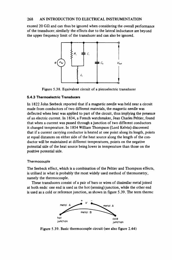
268 AN INTRODUCTION TO ELECTRICAL INSTRUMENTATION
exceed 20 GΩ and can thus be ignored when considering the overall performance of the transducer; similarly the effects due to the lateral inductance are beyond the upper frequency limit of the transducer and can also be ignored.
Figure 5.38. Equivalent circuit of a piezoelectric transducer
5.4.3 Thermoelectric Transducers
In 1822 John Seebeck reported that if a magnetic needle was held near a circuit made from conductors of two different materials, the magnetic needle was deflected when heat was applied to part of the circuit, thus implying the presence of an electric current. In 1834, a French watchmaker, Jean Charles Peltier, foundthat when a current was passed through a junction of two different conductors it changed temperature. In 1854 William Thompson (Lord Kelvin) discovered that if a current carrying conductor is heated at one point along its length, points at equal distances on either side of the heat source along the length of the con-ductor will be maintained at different temperatures, points on the negative potential side of the heat source being lower in temperature than those on the positive potential side.
Thermocouple
The Seebeck effect, which is a combination of the Peltier and Thompson effects, is utilised in what is probably the most widely used method of thermometry, namely the thermocouple.
These transducers consist of a pair of bars or wires of dissimilar metal joined at both ends: one end is used as the hot (sensing) junction, while the other end is used as a cold or reference junction, as shown in figure 5.39. The term thermo
Figure 5.39. Basic thermocouple circuit (see also figure 2.44)
metal A metal A
metal B
hotjunction
coldjunction
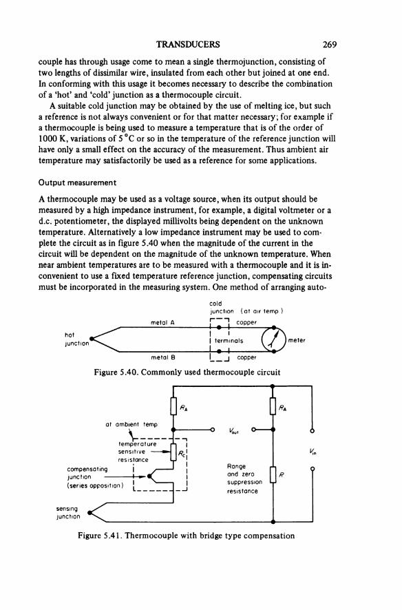
TRANSDUCERS 269
couple has through usage come to mean a single thermojunction, consisting of two lengths of dissimilar wire, insulated from each other but joined at one end. In conforming with this usage it becomes necessary to describe the combination of a ‘hot’ and ‘cold’ junction as a thermocouple circuit.
A suitable cold junction may be obtained by the use of melting ice, but such a reference is not always convenient or for that matter necessary; for example if a thermocouple is being used to measure a temperature that is of the order of 1000 K, variations of 5 °C or so in the temperature of the reference junction will have only a small effect on the accuracy of the measurement. Thus ambient air temperature may satisfactorily be used as a reference for some applications.
Output measurement
A thermocouple may be used as a voltage source, when its output should be measured by a high impedance instrument, for example, a digital voltmeter or a d.c. potentiometer, the displayed millivolts being dependent on the unknown temperature. Alternatively a low impedance instrument may be used to com-plete the circuit as in figure 5.40 when the magnitude of the current in the circuit will be dependent on the magnitude of the unknown temperature. When near ambient temperatures are to be measured with a thermocouple and it is in-convenient to use a fixed temperature reference junction, compensating circuits must be incorporated in the measuring system. One method of arranging auto-
Figure 5.40. Commonly used thermocouple circuit
coldjunction (at air temp )
metal A
hot junction
metal B
copper
terminals meter
copper
Figure 5.41. Thermocouple with bridge type compensation
at ambient temp.
compensating junction (series opposition)
temperature sensitive resistance
Range and zero suppression resistance
sensingjunction
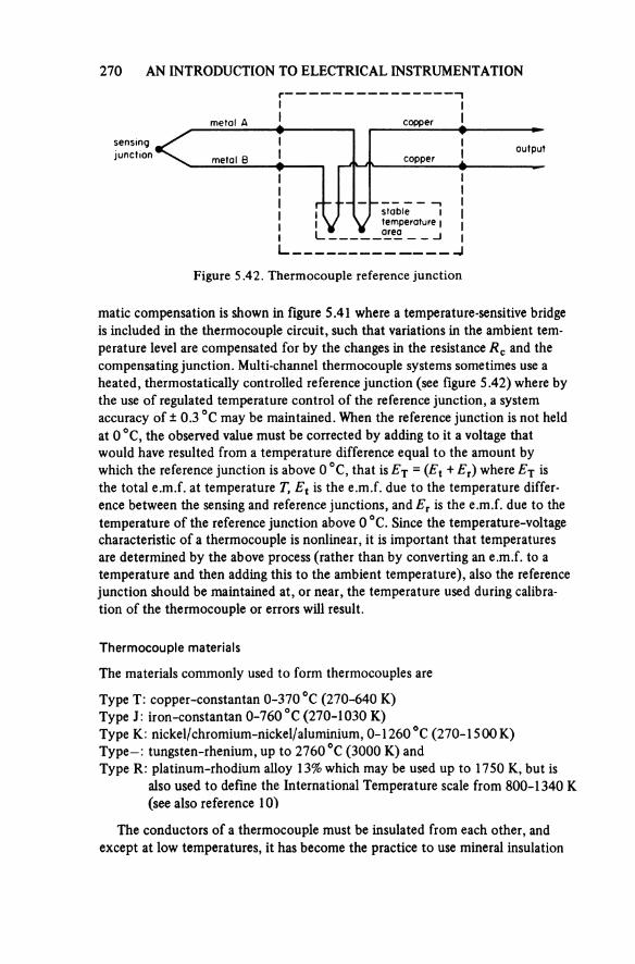
270 AN INTRODUCTION TO ELECTRICAL INSTRUMENTATION
Figure 5.42. Thermocouple reference junction
sensingjunction
metal A
metal B
copper
copperoutput
stabletemperaturearea
made compensation is shown in figure 5.41 where a temperature-sensitive bridge is included in the thermocouple circuit, such that variations in the ambient tem-perature level are compensated for by the changes in the resistance Rc and the compensating junction. Multi-channel thermocouple systems sometimes use a heated, thermostatically controlled reference junction (see figure 5.42) where by the use of regulated temperature control of the reference junction, a system accuracy of ± 0.3 °C may be maintained. When the reference junction is not held at 0 °C, the observed value must be corrected by adding to it a voltage that would have resulted from a temperature difference equal to the amount bywhich the reference junction is above 0 °C, that is ET = (Et + Er) where ET is the total e.m.f. at temperature Tf Et is the e.m.f. due to the temperature differ-ence between the sensing and reference junctions, and Er is the e.m.f. due to the temperature of the reference junction above 0 °C. Since the temperature-voltage characteristic of a thermocouple is nonlinear, it is important that temperaturesare determined by the above process (rather than by converting an e.m.f. to a temperature and then adding this to the ambient temperature), also the reference junction should be maintained at, or near, the temperature used during calibra-tion of the thermocouple or errors will result.
Thermocouple materials
The materials commonly used to form thermocouples are
Type T: copper-constantan 0-370 °C (270-640 K)Type J: iron-constantan 0-760 °C (270-1030 K)Type K: nickel/chromium-nickel/aluminium, 0-1260°C (270-1500K)Type—: tungsten-rhenium, up to 2760 °C (3000 K) andType R: platinum-rhodium alloy 13% which may be used up to 1750 K, but is
also used to define the International Temperature scale from 800-1340 K (see also reference 10)
The conductors of a thermocouple must be insulated from each other, and except at low temperatures, it has become the practice to use mineral insulation
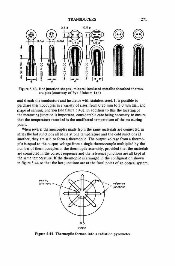
TRANSDUCERS 271
Figure 5.43. Hot junction shapes-mineral insulated metallic sheathed thermo couples (courtesy of Pye-Unicam Ltd)
50 to 150 mm
50 to 150
mm
50 to 80 m
m
50 to 80 mm
and sheath the conductors and insulator with stainless steel. It is possible to purchase thermocouples in a variety of sizes, from 0.25 mm to 3.0 mm dia., and shape of sensing junction (see figure 5.43). In addition to this the locating of the measuring junction is important, considerable care being necessary to ensurethat the temperature recorded is the unaffected temperature of the measuring point.
When several thermocouples made from the same materials are connected in series the hot junctions all being at one temperature and the cold junctions at another, they are said to form a thermopile. The output voltage from a thermo-pile is equal to the output voltage from a single thermocouple multiplied by the number of thermocouples in the thermopile assembly, provided that the materials are connected in the correct sequence and the reference junctions are all kept at the same temperature. If the thermopile is arranged in the configuration shown in figure 5.44 so that the hot junctions are at the focal point of an optical system.
Figure 5.44. Thermopile formed into a radiation pyrometer
sensingjunctions reference
junctions
output
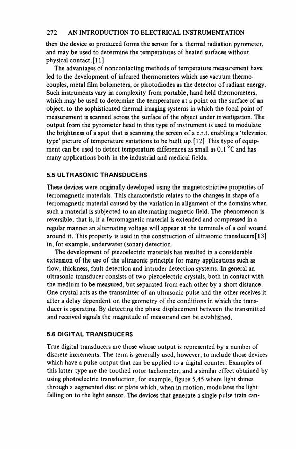
272 AN INTRODUCTION TO ELECTRICAL INSTRUMENTATIONthen the device so produced forms the sensor for a thermal radiation pyrometer,and may be used to determine the temperatures of heated surfaces without physical contact. [11]
The advantages of noncontacting methods of temperature measurement have led to the development of infrared thermometers which use vacuum thermo-couples, metal film bolometers, or photodiodes as the detector of radiant energy. Such instruments vary in complexity from portable, hand held thermometers,which may be used to determine the temperature at a point on the surface of an object, to the sophisticated thermal imaging systems in which the focal point ofmeasurement is scanned across the surface of the object under investigation. The output from the pyrometer head in this type of instrument is used to modulate the brightness of a spot that is scanning the screen of a c.r.t. enabling a ‘television type’ picture of temperature variations to be built up. [12] This type of equip-ment can be used to detect temperature differences as small as 0.1 °C and has many applications both in the industrial and medical fields.
5.5 ULTRASONIC TRANSDUCERS
These devices were originally developed using the magnetostrictive properties of ferromagnetic materials. This characteristic relates to the changes in shape of a ferromagnetic material caused by the variation in alignment of the domains when such a material is subjected to an alternating magnetic field. The phenomenon is reversible, that is, if a ferromagnetic material is extended and compressed in a regular manner an alternating voltage will appear at the terminals of a coil wound around it. This property is used in the construction of ultrasonic transducers [13] in, for example, underwater (sonar) detection.
The development of piezoelectric materials has resulted in a considerable extension of the use of the ultrasonic principle for many applications such as flow, thickness, fault detection and intruder detection systems. In general an ultrasonic transducer consists of two piezoelectric crystals, both in contact withthe medium to be measured, but separated from each other by a short distance. One crystal acts as the transmitter of an ultrasonic pulse and the other receives it after a delay dependent on the geometry of the conditions in which the trans-ducer is operating. By detecting the phase displacement between the transmitted and received signals the magnitude of measurand can be established.
5.6 DIGITAL TRANSDUCERS
True digital transducers are those whose output is represented by a number of discrete increments. The term is generally used, however, to include those devices which have a pulse output that can be applied to a digital counter. Examples of this latter type are the toothed rotor tachometer, and a similar effect obtained by using photoelectric transduction, for example, figure 5.45 where light shines through a segmented disc or plate which, when in motion, modulates the light falling on to the light sensor. The devices that generate a single pulse train can-
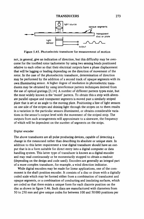
TRANSDUCERS 273
Figure 5.45. Photoelectric transducer for measurement of motion
light sourceopaque
transparent disc or plate
lightsensor
output
not, in general, give an indication of direction, but this difficulty may be over-come for the toothed rotor tachometer by using two sensing heads positioned relative to each other so that their electrical outputs have a phase displacement that will be lagging or leading depending on the direction of movement of the rotor. In the case of the photoelectric transducer, determination of directionmay be performed by the addition of a second track of opaque segments with its own illuminating sensor. A higher degree of resolution in photoelectric trans-ducers may be obtained by using interference pattern techniques derived from the use of optical gratings. [3, 14] A number of different pattern types exist, but the most widely known is the ‘moiré’ pattern. To obtain this a strip with altern-ate parallel opaque and transparent segments is moved past a similarly striped plate that is set at an angle to the moving plate. Positioning a line of light sensors on one side of the stripes and shining light through the stripes on to them results in a variation in the particular sensors illuminated, or obtains considerable varia-tions in the sensor’s output level with the movement of the striped strip. The outputs from such arrangements will approximate to a sinewave, the frequency of which will be dependent on the number of segments on the strips.
Digital encoder
The above transducers are all pulse producing devices, capable of detecting a change in the measurand rather than describing its absolute or unique state. In addition to this latter requirement a true digital transducer should have an out-put that is in a form suitable for direct entry into a digital computer or data handling system. This latter type of transducer is known as a digital encoder and may read continuously or be momentarily stopped to obtain a readout (depending on the design and code used). Encoders are generally an integral part of a more complex transducer, for example, a wind direction indicator.
While digital encoders may be made for linear applications, one of the com-monest is the shaft position encoder. It consists of a disc or drum with a digitally coded scale which may be formed either from a combination of translucent and opaque segments, or a combination of conducting and insulating surfaces, whichare coded so that there exists a unique form for each discrete position on the disc as shown in figure 5.46. Such discs are manufactured with diameters from 50 to 250 mm and give unique codes for between 100 and 50 000 positions per
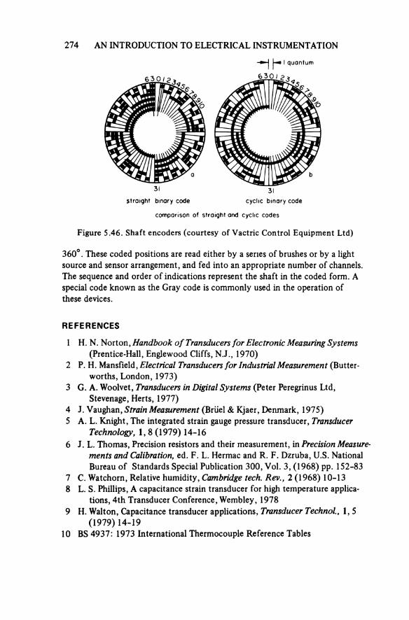
274 AN INTRODUCTION TO ELECTRICAL INSTRUMENTATION
Figure 5.46. Shaft encoders (courtesy of Vactric Control Equipment Ltd)
comparison of straight and cyclic codes
straight binary code cyclic binary code
1 quantum
360°. These coded positions are read either by a senes of brushes or by a light source and sensor arrangement, and fed into an appropriate number of channels. The sequence and order of indications represent the shaft in the coded form. A special code known as the Gray code is commonly used in the operation of these devices.
REFERENCES
1 H. N. Norton, Handbook of Transducers for Electronic Measuring Systems(Prentice-Hall, Englewood Cliffs, N.J., 1970)
2 P. H. Mansfield, Electrical Transducers for Industrial Measurement (Butter-worths, London, 1973)
3 G. A. Woolvet, Transducers in Digital Systems (Peter Peregrinus Ltd,Stevenage, Herts, 1977)
4 J. Vaughan, Strain Measurement (Brüel & Kjaer, Denmark, 1975)5 A. L. Knight, The integrated strain gauge pressure transducer, Transducer
Technology, 1, 8 (1979) 14-166 J. L. Thomas, Precision resistors and their measurement, in Precision Measure-
ments and Calibration, ed. F. L. Hermac and R. F. Dzruba, U.S. National Bureau of Standards Special Publication 300, Vol. 3, (1968) pp. 152-83
7 C. Watchorn, Relative humidity, Cambridge tech. Rev., 2 (1968) 10-138 L. S. Phillips, A capacitance strain transducer for high temperature applica-
tions, 4th Transducer Conference, Wembley, 19789 H. Walton, Capacitance transducer applications. Transducer Technol., 1, 5
(1979) 14-1910 BS 4937: 1973 International Thermocouple Reference Tables
TRANSDUCERS 275
11 H. D. Baker, E. A. Ryder and N. H. Baker, Temperature Measurement inEngineering, Vol. II (Wiley, New York, 1961)
12 D. F. Cassidy, Age of temperature monitoring by non-contacting methods,Control Instrumn, 4 (1972) 26-7
13 M. L. Gayford, Electroacoustics (Butterworth, London, 1970)14 D. K. Ewing, Measurement of speed transients using optical gratings, N.E.L.
Report No. 247 (1966)
6Signal Conditioning
In many instances the values of electrical quantities (voltage, current and power) are too large or too small to be connected directly to the available instrument. It therefore becomes necessary to suitably reduce, or amplify, the magnitude of the measurand so that it has a value compatible with the measuring instrument to be used. In addition to these requirements, the effects of the instrument’s impedance must always be considered for this may affect the value indicated foi the measurand, (see p. 27). The disturbance resulting from the insertion of a measuring instrument should be minimal, that is to say the device used in measuring a current should have as low an impedance as possible, while for volt-age measurement the requirement is a high impedance. In both cases the ideal instrument’s performance will be independent of frequency.
The simple current and voltage situations do not, however, apply in every case. For example, sometimes it is necessary to ensure that the maximum amount of power contained in the output signal from a sensor is conveyed to a display orrecording instrument, so as to obtain a maximum deflection; it is then necessary to match (see section 1.4.3) the output impedance of the signal source to the input impedance of the instrument.
6.1 VOLTAGE SCALING
Voltage dividers are an important aspect of scaling and have been mentioned in connection with the range extension of voltmeters and for use with, and within, potentiometers and multimeters. Voltage dividing resistors are sometimes con-fusingly termed potentiometers as an abbreviation of the term potential or potentiometric divider.

SIGNAL CONDITIONING 277
6.1.1 Resistance Divider
Resistance chain
The resistance chain is the simplest form of divider, the voltage division being due to the total voltage drop across the chain in comparison with the volt drop across the end unit. The chain may be connected in series with a pointer instru-ment (see figure 2.7) when the resistance of the measuring instrument forms part of the chain, or the measuring instrument is connected across the low voltage end of the divider. If the latter method of operation is used it is extremely important that the input impedance of the measuring instrument should be very much greater than the chain resistor across which it is connected, or a large error in the measurement will result. Consequently, this form of divider should only be used with potentiometers or electronic voltmeters which have a high input impedance. A further alternative, commonly used in electronic (both analogue and digital) voltmeters is that shown in figure 2.18 where the input voltage is connected across the whole chain and the high input impedance measuring circuits are switched across an increasing number of sections of the resistance chain as the sensitivity is increased.
All these voltage dividers are of course suitable for d.c. use, but may be usedon a.c. provided they are pure resistance (see section 7.2.2), that is, the imped-ance remains constant irrespective of frequency. The range of d.c. voltages over which this type of divider is used is limited by power dissipation and earth leakage path resistance.
Kelvin-Varley divider
The Kelvin-Varley divider was mentioned in chapter 3 in connection with its use in potentiometers. It is an inherently more precise method of voltage division than the simple resistance chain and finds extensive application in the standards laboratory. Considering the Kelvin-Varley divider in detail, it is seen to consist of several decades of resistors interconnected as in figure 6.1. Each voltage division decade is made up of 11 equal resistors, successive division decades having a total resistance equal to twice the value of a unit resistor in the previous decade. For example, if in a four-decade divider the first decade is constructed using 11 ×10 kΩ resistors, the second decade will have 11 × 2 kΩ resistors, the next decade 11 × 400 Ω resistors and the fourth decade or final division will have 10 × 80 Ω resistors. The use of 11 resistors to obtain a decade voltage division enables the Kelvin-Varley divider to have a constant input impedance (strictly with the out-put open circuited) irrespective of which switch positions are connected on the various decades. For example, decade 3 will have a constant impedance of
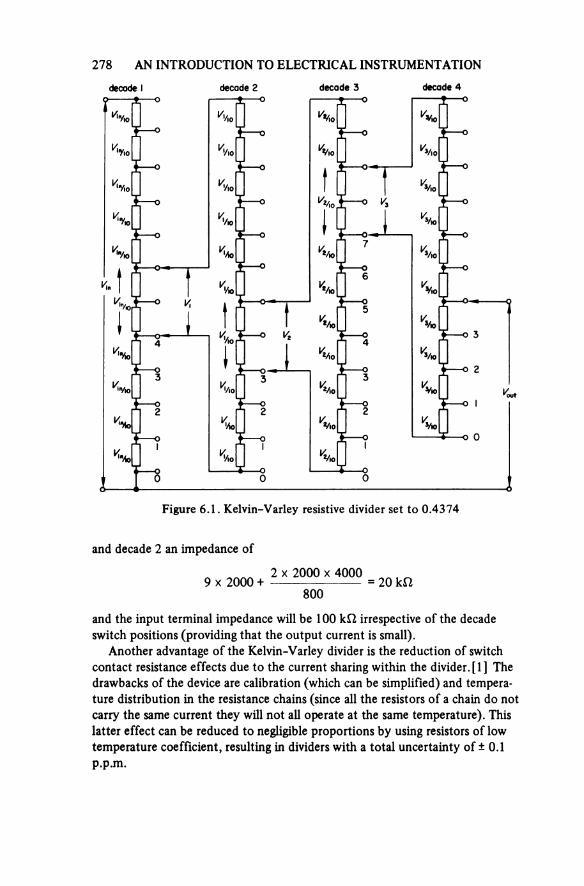
278 AN INTRODUCTION TO ELECTRICAL INSTRUMENTATION
Figure 6.1. Kelvin-Varley resistive divider set to 0.4374
decode 1 decade 2 decade 3 decade 4
and decade 2 an impedance of
and the input terminal impedance will be 100 kΩ irrespective of the decade switch positions (providing that the output current is small).
Another advantage of the Kelvin-Varley divider is the reduction of switchcontact resistance effects due to the current sharing within the divider. [1] The drawbacks of the device are calibration (which can be simplified) and tempera-ture distribution in the resistance chains (since all the resistors of a chain do not carry the same current they will not all operate at the same temperature). This latter effect can be reduced to negligible proportions by using resistors of low temperature coefficient, resulting in dividers with a total uncertainty of ± 0.1 p.p.m.
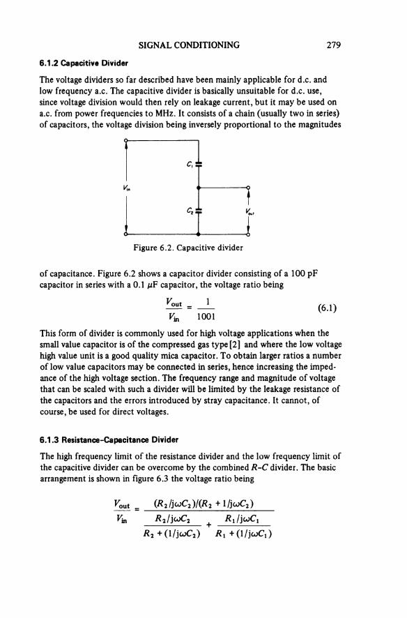
SIGNAL CONDITIONING 279
6.1.2 Capacitive Divider
The voltage dividers so far described have been mainly applicable for d.c. and low frequency a.c. The capacitive divider is basically unsuitable for d.c. use, since voltage division would then rely on leakage current, but it may be used on a.c. from power frequencies to MHz. It consists of a chain (usually two in series) of capacitors, the voltage division being inversely proportional to the magnitudes
Figure 6.2. Capacitive divider
of capacitance. Figure 6.2 shows a capacitor divider consisting of a 100 pF capacitor in series with a 0.1 μF capacitor, the voltage ratio being
(6.1)
This form of divider is commonly used for high voltage applications when the small value capacitor is of the compressed gas type [2] and where the low voltage high value unit is a good quality mica capacitor. To obtain larger ratios a number of low value capacitors may be connected in series, hence increasing the imped-ance of the high voltage section. The frequency range and magnitude of voltage that can be scaled with such a divider will be limited by the leakage resistance of the capacitors and the errors introduced by stray capacitance. It cannot, of course, be used for direct voltages.
6.1.3 Resistance-Capacitance Divider
The high frequency limit of the resistance divider and the low frequency limit of the capacitive divider can be overcome by the combined R-C divider. The basic arrangement is shown in figure 6.3 the voltage ratio being
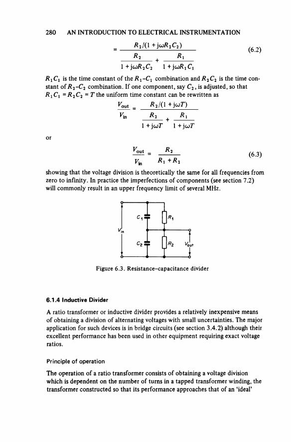
280 AN INTRODUCTION TO ELECTRICAL INSTRUMENTATION
(6.2)
R1C1 is the time constant of the R1-C1 combination and R2C2 is the time con-stant of R2-C2 combination. If one component, say C2, is adjusted, so thatR1C1 =R2C2 = T the uniform time constant can be rewritten as
or
(6.3)
showing that the voltage division is theoretically the same for an frequencies from zero to infinity, in practice the imperfections of components (see section 7.2) will commonly result in an upper frequency limit of several MHz.
Figure 6.3. Resistance-capacitance divider
6.1.4 Inductive Divider
A ratio transformer or inductive divider provides a relatively inexpensive means of obtaining a division of alternating voltages with small uncertainties. The major application for such devices is in bridge circuits (see section 3.4.2) although their excellent performance has been used in other equipment requiring exact voltage ratios.
Principle of operation
The operation of a ratio transformer consists of obtaining a voltage division which is dependent on the number of turns in a tapped transformer winding, the transformer constructed so that its performance approaches that of an ‘ideal’
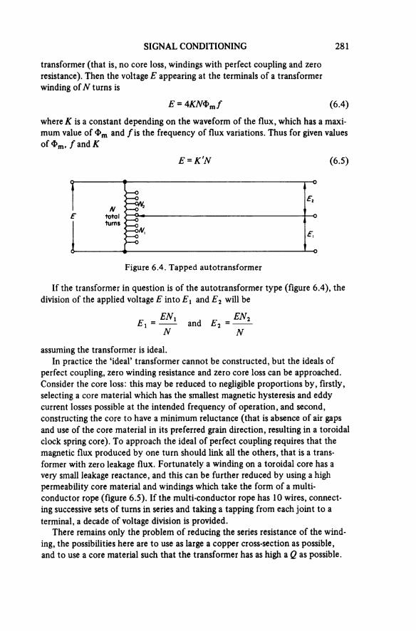
SIGNAL CONDITIONING 281
transformer (that is, no core loss, windings with perfect coupling and zero resistance). Then the voltage E appearing at the terminals of a transformer winding of N turns is
(6.4)
where K is a constant depending on the waveform of the flux, which has a maxi-mum value of Φm and f is the frequency of flux variations. Thus for given values of Φm, f and K
(6.5)
Figure 6.4. Tapped autotransformer
If the transformer in question is of the autotransformer type (figure 6.4), the division of the applied voltage E into Ex and E2 will be
assuming the transformer is ideal.In practice the ‘ideal’ transformer cannot be constructed, but the ideals of
perfect coupling, zero winding resistance and zero core loss can be approached. Consider the core loss: this may be reduced to negligible proportions by, firstly, selecting a core material which has the smallest magnetic hysteresis and eddy current losses possible at the intended frequency of operation, and second, constructing the core to have a minimum reluctance (that is absence of air gaps and use of the core material in its preferred grain direction, resulting in a toroidal clock spring core). To approach the ideal of perfect coupling requires that the magnetic flux produced by one turn should link all the others, that is a trans-former with zero leakage flux. Fortunately a winding on a toroidal core has a very small leakage reactance, and this can be further reduced by using a high permeability core material and windings which take the form of a multi-conductor rope (figure 6.5). If the multi-conductor rope has 10 wires, connect-ing successive sets of turns in series and taking a tapping from each joint to a terminal, a decade of voltage division is provided.
There remains only the problem of reducing the series resistance of the wind-ing, the possibilities here are to use as large a copper cross-section as possible, and to use a core material such that the transformer has as high a Q as possible.
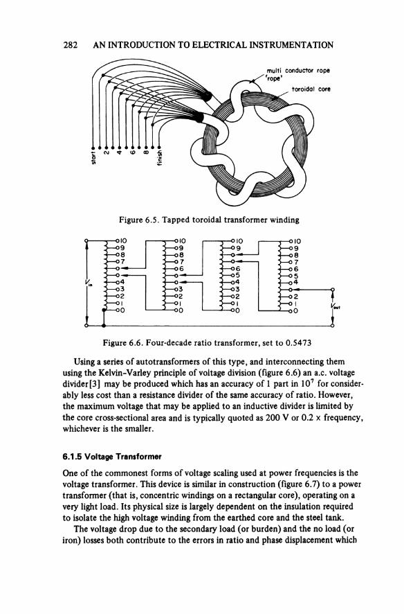
282 AN INTRODUCTION TO ELECTRICAL INSTRUMENTATION
Figure 6.5. Tapped toroidal transformer winding
multi conductor rope 'rope'
toroidal corest
art
finis
h
Figure 6.6. Four-decade ratio transformer, set to 0.5473
Using a series of autotransformers of this type, and interconnecting them using the Kelvin-Varley principle of voltage division (figure 6.6) an a.c. voltage divider [3] may be produced which has an accuracy of 1 part in 107 for consider-ably less cost than a resistance divider of the same accuracy of ratio. However, the maximum voltage that may be applied to an inductive divider is limited by the core cross-sectional area and is typically quoted as 200 V or 0.2 × frequency, whichever is the smaller.
6.1.5 Voltage Transformer
One of the commonest forms of voltage scaling used at power frequencies is the voltage transformer. This device is similar in construction (figure 6.7) to a power transformer (that is, concentric windings on a rectangular core), operating on a very light load. Its physical size is largely dependent on the insulation required to isolate the high voltage winding from the earthed core and the steel tank.
The voltage drop due to the secondary load (or burden) and the no load (or iron) losses both contribute to the errors in ratio and phase displacement which
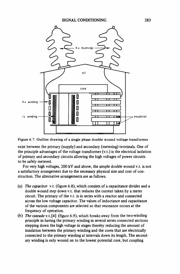
SIGNAL CONDITIONING 283
Figure 6.7. Outline drawing of a single phase double wound voltage transformer
h.v. bushings
oil
core
h.v. winding
l.v. winding insulation
exist between the primary (supply) and secondary (metering) terminals. One of the principle advantages of the voltage transformer (v.t.) is the electrical isolation of primary and secondary circuits allowing the high voltages of power circuits to be safely metered.
For very high voltages, 200 kV and above, the simple double wound v.t. is not a satisfactory arrangement due to the necessary physical size and cost of con-struction. The alternative arrangements are as follows.
(a) The capacitor v.t. (figure 6.8), which consists of a capacitance divider and a double wound step down v.t. that reduces the current taken by a metercircuit. The primary of the v.t. is in series with a reactor and connected across the low voltage capacitor. The values of inductance and capacitance of the various components are selected so that resonance occurs at the frequency of operation.
(b) The cascade v.t. [4] (figure 6.9), which breaks away from the two-winding principle in having the primary winding in several series connected sections stepping down the high voltage in stages thereby reducing the amount of insulation between the primary winding and the cores that are electrically connected to the primary winding at intervals down its length. The second-ary winding is only wound on to the lowest potential core, but coupling
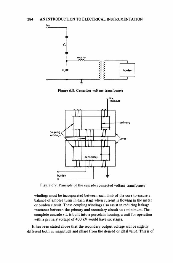
284 AN INTRODUCTION TO ELECTRICAL INSTRUMENTATION
Figure 6.8. Capacitor voltage transformer
h.v.
reactor
burden
Figure 6.9. Principle of the cascade connected voltage transformer
h.v.terminal
primary
couplingwindings
cores
secondary
burden
windings must be incorporated between each limb of the core to ensure a balance of ampere turns in each stage when current is flowing in the meter or burden circuit. These coupling windings also assist in reducing leakagereactance between the primary and secondary circuit to a minimum. The complete cascade v.t. is built into a porcelain housing; a unit for operation with a primary voltage of 400 kV would have six stages.
It has been stated above that the secondary output voltage will be slightly different both in magnitude and phase from the desired or ideal value. This is of
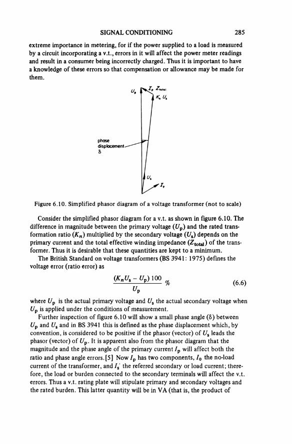
SIGNAL CONDITIONING 285
extreme importance in metering, for if the power supplied to a load is measured by a circuit incorporating a v.t., errors in it will affect the power meter readings and result in a consumer being incorrectly charged. Thus it is important to have a knowledge of these errors so that compensation or allowance may be made for them.
Figure 6.10. Simplified phasor diagram of a voltage transformer (not to scale)
phasedisplacementδ
Consider the simplified phasor diagram for a v.t. as shown in figure 6.10. The difference in magnitude between the primary voltage (Up) and the rated trans-formation ratio (Kn) multiplied by the secondary voltage (Us) depends on the primary current and the total effective winding impedance (Ztotal) of the trans-former. Thus it is desirable that these quantities are kept to a minimum.
The British Standard on voltage transformers (BS 3941: 1975) defines the voltage error (ratio error) as
(6.6)
where Up is the actual primary voltage and Us the actual secondary voltage when Up is applied under the conditions of measurement.
Further inspection of figure 6.10 will show a small phase angle (δ) between Up and Us and in BS 3941 this is defined as the phase displacement which, by convention, is considered to be positive if the phasor (vector) of Us leads the phasor (vector) of Up. It is apparent also from the phasor diagram that themagnitude and the phase angle of the primary current IP will affect both theratio and phase angle errors. [5] Now Ip has two components, I0 the no-load current of the transformer, and Is' the referred secondary or load current; there-fore, the load or burden connected to the secondary terminals will affect the v.t. errors. Thus a v.t. rating plate will stipulate primary and secondary voltages and the rated burden. This latter quantity will be in vA (that is, the product of
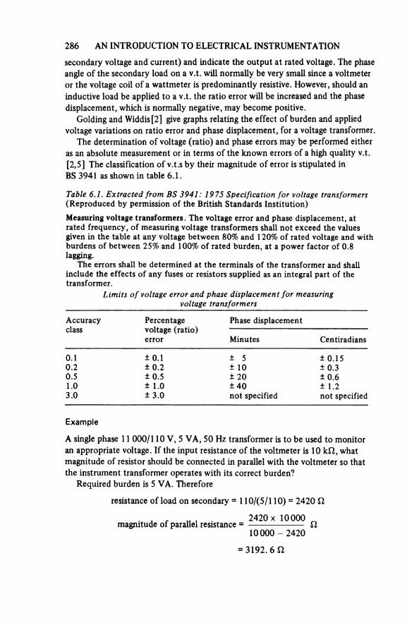
286 AN INTRODUCTION TO ELECTRICAL INSTRUMENTATION
secondary voltage and current) and indicate the output at rated voltage. The phase angle of the secondary load on a v.t. will normally be very small since a voltmeter or the voltage coil of a wattmeter is predominantly resistive. However, should an inductive load be applied to a v.t. the ratio error will be increased and the phase displacement, which is normally negative, may become positive.
Golding and Widdis [2] give graphs relating the effect of burden and applied voltage variations on ratio error and phase displacement, for a voltage transformer.
The determination of voltage (ratio) and phase errors may be performed either as an absolute measurement or in terms of the known errors of a high quality v.t. [2, 5] The classification of v.t.s by their magnitude of error is stipulated in BS 3941 as shown in table 6.1.
Table 6.1. Extracted from BS 3941: 1975 Specification for voltage transformers (Reproduced by permission of the British Standards Institution)Measuring voltage transformers. The voltage error and phase displacement, at rated frequency, of measuring voltage transformers shall not exceed the values given in the table at any voltage between 80% and 1 20% of rated voltage and with burdens of between 25% and 100% of rated burden, at a power factor of 0.8 lagging.
The errors shall be determined at the terminals of the transformer and shall include the effects of any fuses or resistors supplied as an integral part of the transformer.
Limits of voltage error and phase displacement for measuring voltage transformers
Accuracyclass
Percentage voltage (ratio) error
Phase displacement
Minutes Centiradians
0.1 ±0.1 ± 5 ± 0.150.2 ±0.2 ± 10 ±0.30.5 ±0.5 ±20 ±0.61.0 ± 1.0 ±40 ± 1.23.0 ±3.0 not specified not specified
Example
A single phase 11 000/110 V, 5 VA, 50 Hz transformer is to be used to monitor an appropriate voltage. If the input resistance of the voltmeter is 10 kΩ, what magnitude of resistor should be connected in parallel with the voltmeter so that the instrument transformer operates with its correct burden?
Required burden is 5 VA. Therefore
resistance of load on secondary =
magnitude of parallel resistance =

SIGNAL CONDITIONING 287
6.2 CURRENT SCALING
The majority of current measuring instruments are only capable of measuring directly milliamperes or at the most a few amperes, the exceptions being some dynamometer ammeters and moving iron ammeters which are specially con-structed to measure currents of the order of 100 A. Since currents of several thousands of amperes are used in many applications current scaling and voltage scaling are of equal importance.
6.2.1 Current Shunts
Current shunts have already been mentioned in connection with moving coil multi-meters (see section 2.1.2), and the use of a potentiometer, both of which with the aid of shunts may be used for measuring large direct currents. The use of current shunts is, however, not limited to d.c. provided that a shunt used for alternating current measurements is nonreactive. Its principal disadvantages arepower consumption and the fact that the metering current must be operated at the same potential to earth as the current carrying line and therefore limits its use to low voltage applications. [6, 7, 8]
Four-terminal Shunts
A current shunt (figure 6.11) is in general a four-terminal resistance the current to be measured being connected to the current terminals. The potential terminals are arranged so that an accurately known resistance and voltage drop existsbetween them, and situated so that they are unaffected by any heating which may occur at the current terminals.
The application of current shunts lies in the extension of ammeter range (where the volt drop across the shunt drives a proportion of the current through the ammeter); measurement of current by potentiometer; recording of current wave-forms and the measurement of low voltage power. It should be appreciated that with the increasing use of electronic measuring instruments with a high input resistance, the measurement of current as a voltage drop across a known resistance is tending to become a much used method of measurement.
Figure 6.11. A four-terminal current shunt
current terminals
terminals
heat sink
base (insulation)

288 AN INTRODUCTION TO ELECTRICAL INSTRUMENTATION
Universal Shunt
This is a device that may be incorporated into a galvanometer as a sensitivity control and is very useful when such an instrument is used as a null detector. Probably a wider use is in providing current ranges in multi-meters (see section 2.1.2). Figure 6.12 shows the basic arrangement for a universal shunt of resist-ance R shunting a galvanometer of resistance Rg. With the switch on contact a the galvanometer current
(6.7)
and if R >> Rg
Similarly with the switch at point b
at point c
and at point d
Figure 6.12. Universal shunt
galvanometer of resistance
For satisfactory operation of the galvanometer, R should be at least 10 times greater than Rg. If R is nearly equal or less in magnitude than Rg the galvano-meter movement will become overdamped, but irrespective of this the ratio of galvanometer sensitivities for the switch positions will remain constant. Let Rg = R, then for position a
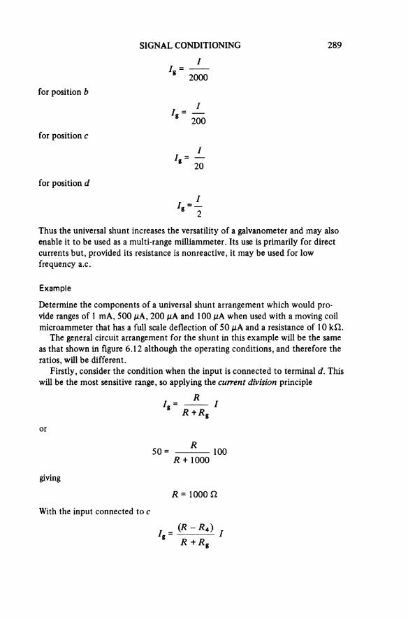
SIGNAL CONDITIONING 289
for position b
for position c
for position d
Thus the universal shunt increases the versatility of a galvanometer and may also enable it to be used as a multi-range miniammeter. its use is primarily for direct currents but, provided its resistance is nonreactive, it may be used for low frequency a.c.
Example
Determine the components of a universal shunt arrangement which would pro-vide ranges of 1 mA, 500 μA, 200 μA and 100 μA when used with a moving coil microammeter that has a full scale deflection of 50 μA and a resistance of 10 kΩ.
The general circuit arrangement for the shunt in this example will be the same as that shown in figure 6.12 although the operating conditions, and therefore the ratios, will be different.
Firstly, consider the condition when the input is connected to terminal d. This will be the most sensitive range, so applying the current division principle
or
giving
With the input connected to c
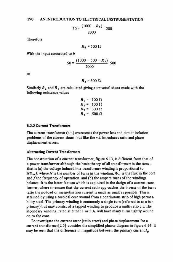
290 AN INTRODUCTION TO ELECTRICAL INSTRUMENTATION
Therefore
With the input connected to b
so
Similarly R2 and R1 are calculated giving a universal shunt made with the following resistance values
6.2.2 Current Transformers
The current transformer (c.t.) overcomes the power loss and circuit isolation problems of the current shunt, but like the v.t. introduces ratio and phase displacement errors.
Alternating Current Transformers
The construction of a current transformer, figure 6.13, is different from that of a power transformer although the basic theory of all transformers is the same, that is (a) the voltage induced in a transformer winding is proportional to NΦmf, where N is the number of turns in the winding, Φm is the flux in the core and f the frequency of operation, and (b) the ampere turns of the windings balance. It is the latter feature which is exploited in the design of a current trans-former, where to ensure that the current ratio approaches the inverse of the turns ratio the no-load or magnetisation current is made as small as possible. This is attained by using a toroidal core wound from a continuous strip of high permea-bility steel. The primary winding is commonly a single turn (referred to as a bar primary) but may consist of a tapped winding to produce a multi-ratio c.t. The secondary winding, rated at either 1 or 5 A, will have many turns tightly wound on to the core.
To investigate the current error (ratio error) and phase displacement for a current transformer [2, 5] consider the simplified phasor diagram in figure 6.14. It may be seen that the difference in magnitude between the primary current Ip
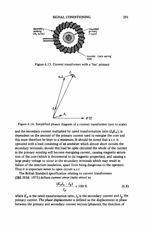
SIGNAL CONDITIONING 291
Figure 6.13. Current transformer with a ‘bar’ primary
secondary winding (N2 turns)
insulated primary (1 turn)
toroidal clock spring core
Figure 6.14. Simplified phasor diagram of a current transformer (not to scale)
and the secondary current multiplied by rated transformation ratio (IsKn), is dependent on the amount of the primary current used to energise the core and this must therefore be kept to a minimum. It should be noted that a c.t. is operated with a load consisting of an ammeter which almost short circuits the secondary terminals; should this load be open circuited the whole of the current in the primary winding will become energising current, causing magnetic satura-tion of the core (which is detrimental to its magnetic properties), and causing a large peaky voltage to occur at the secondary terminals which may result in failure of the interturn insulation, apart from being dangerous to the operator. Thus it is important never to open circuit a.c.t.
The British Standard specification relating to current transformers (IBS 3938: 1973) defines current error (ratio error) as
(6.8)
where Kn is the rated transformation ratio, Is is the secondary current and IP the primary current. The phase displacement is defined as the displacement in phase between the primary and secondary current vectors (phasors), the direction of
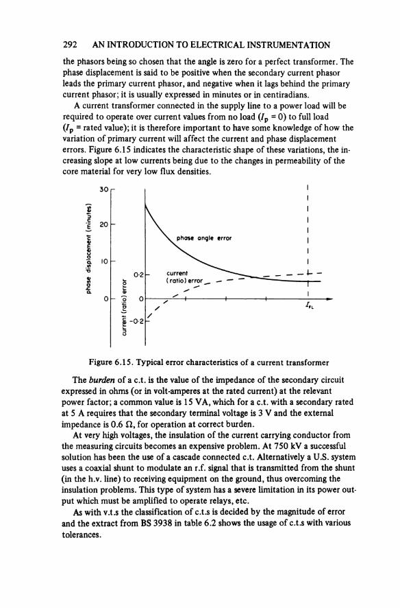
292 AN INTRODUCTION TO ELECTRICAL INSTRUMENTATION
the phasors being so chosen that the angle is zero for a perfect transformer. The phase displacement is said to be positive when the secondary current phasor leads the primary current phasor, and negative when it lags behind the primary current phasor; it is usually expressed in minutes or in centiradians.
A current transformer connected in the supply line to a power load will be required to operate over current values from no load (Ip = 0) to full load (Ip - rated value); it is therefore important to have some knowledge of how the variation of primary current will affect the current and phase displacementerrors. Figure 6.15 indicates the characteristic shape of these variations, the in-creasing slope at low currents being due to the changes in permeability of the core material for very low flux densities.
Figure 6.15. Typical error characteristics of a current transformer
phas
e disp
lace
men
t (min
utes
)
curr
ent (
ratio
) err
or
phase angle error
current (ratio) error
The burden of a c.t. is the value of the impedance of the secondary circuit expressed in ohms (or in volt-amperes at the rated current) at the relevant power factor; a common value is 1 5 VA, which for a c.t. with a secondary rated at 5 A requires that the secondary terminal voltage is 3 V and the external impedance is 0.6 Ω, for operation at correct burden.
At very high voltages, the insulation of the current carrying conductor from the measuring circuits becomes an expensive problem. At 750 kV a successful solution has been the use of a cascade connected c.t. Alternatively a U.S. system uses a coaxial shunt to modulate an r.f. signal that is transmitted from the shunt (in the h.v. line) to receiving equipment on the ground, thus overcoming the insulation problems. This type of system has a severe limitation in its power out-put which must be amplified to operate relays, etc.
As with v.t.s the classification of c.t.s is decided by the magnitude of error and the extract from BS 3938 in table 6.2 shows the usage of c.t.s with various tolerances.
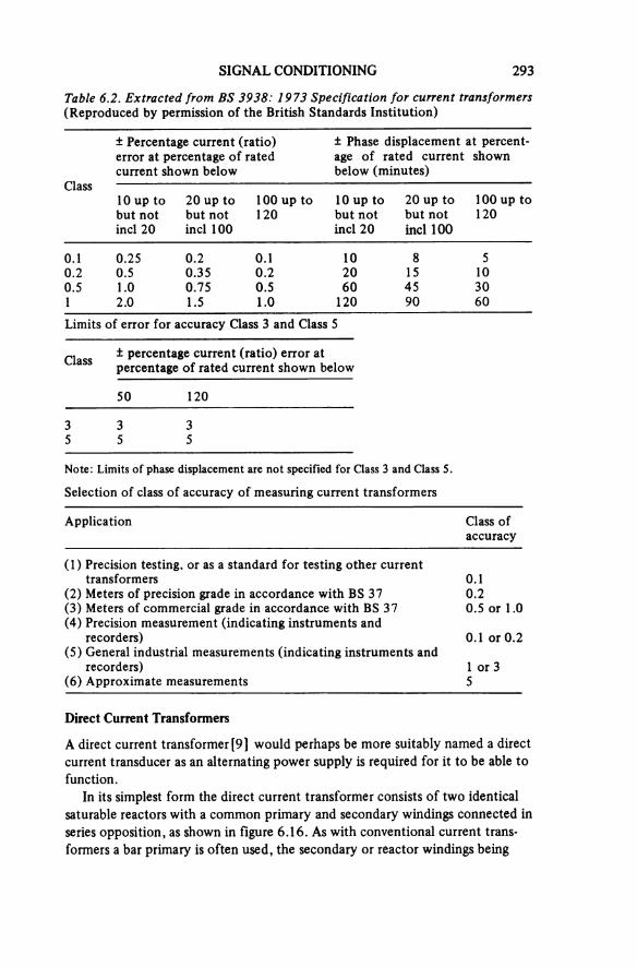
SIGNAL CONDITIONING 293
Table 6.2. Extracted from BS 3938: 1973 Specification for current transformers (Reproduced by permission of the British Standards Institution)
Class
± Percentage current (ratio)error at percentage of rated current shown below
± Phase displacement at percent-age of rated current shown below (minutes)
10 up to but not incl 20
20 up to but not incl 100
1 00 up to 120
10 up to but not incl 20
20 up to but not incl 100
100 up to 120
0.1 0.25 0.2 0.1 10 8 50.2 0.5 0.35 0.2 20 15 100.5 1.0 0.75 0.5 60 45 301 2.0 1.5 1.0 120 90 60Limits of error for accuracy Class 3 and Class 5
Class ± percentage current (ratio) error at percentage of rated current shown below
50 120
3 3 35 5 5
Note: Limits of phase displacement are not specified for Class 3 and Class 5.
Selection of class of accuracy of measuring current transformers
Application Class ofaccuracy
(1) Precision testing, or as a standard for testing other currenttransformers 0.1
(2) Meters of precision grade in accordance with BS 37 0.2(3) Meters of commercial grade in accordance with BS 37 0.5 or 1.0(4) Precision measurement (indicating instruments and
recorders) 0.1 or 0.2(5) General industrial measurements (indicating instruments and
recorders) 1 or 3(6) Approximate measurements 5
Direct Current Transformers
A direct current transformer [9] would perhaps be more suitably named a direct current transducer as an alternating power supply is required for it to be able to function.
In its simplest form the direct current transformer consists of two identical saturable reactors with a common primary and secondary windings connected in series opposition, as shown in figure 6.16. As with conventional current trans-formers a bar primary is often used, the secondary or reactor windings being
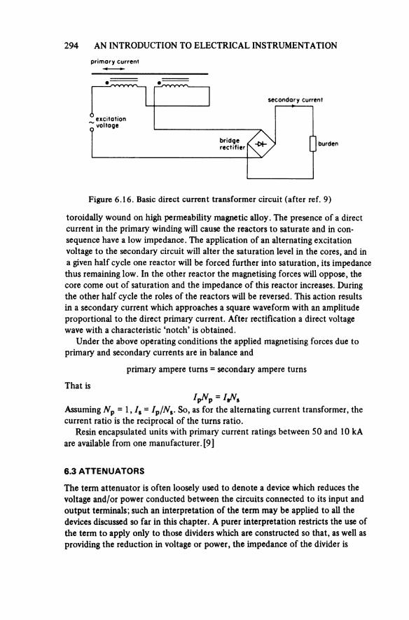
294 AN INTRODUCTION TO ELECTRICAL INSTRUMENTATION
Figure 6.16. Basic direct current transformer circuit (after ref. 9)
primary current
secondary current
excitationvoltage
bridgerectifier burden
toroidally wound on high permeability magnetic alloy. The presence of a direct current in the primary winding will cause the reactors to saturate and in con-sequence have a low impedance. The application of an alternating excitation voltage to the secondary circuit will alter the saturation level in the cores, and in a given half cycle one reactor will be forced further into saturation, its impedance thus remaining low. In the other reactor the magnetising forces will oppose, thecore come out of saturation and the impedance of this reactor increases. During the other half cycle the roles of the reactors will be reversed. This action results in a secondary current which approaches a square waveform with an amplitude proportional to the direct primary current. After rectification a direct voltage wave with a characteristic ‘notch’ is obtained.
Under the above operating conditions the applied magnetising forces due to primary and secondary currents are in balance and
primary ampere turns = secondary ampere turns
That is
Assuming Np = 1, Is = Ip/Ns. So, as for the alternating current transformer, the current ratio is the reciprocal of the turns ratio.
Resin encapsulated units with primary current ratings between 50 and 10 kA are available from one manufacturer. [9]
6.3 ATTENUATORS
The term attenuator is often loosely used to denote a device which reduces the voltage and/or power conducted between the circuits connected to its input and output terminals; such an interpretation of the term may be applied to all thedevices discussed so far in this chapter. A purer interpretation restricts the use of the term to apply only to those dividers which are constructed so that, as well as providing the reduction in voltage or power, the impedance of the divider is
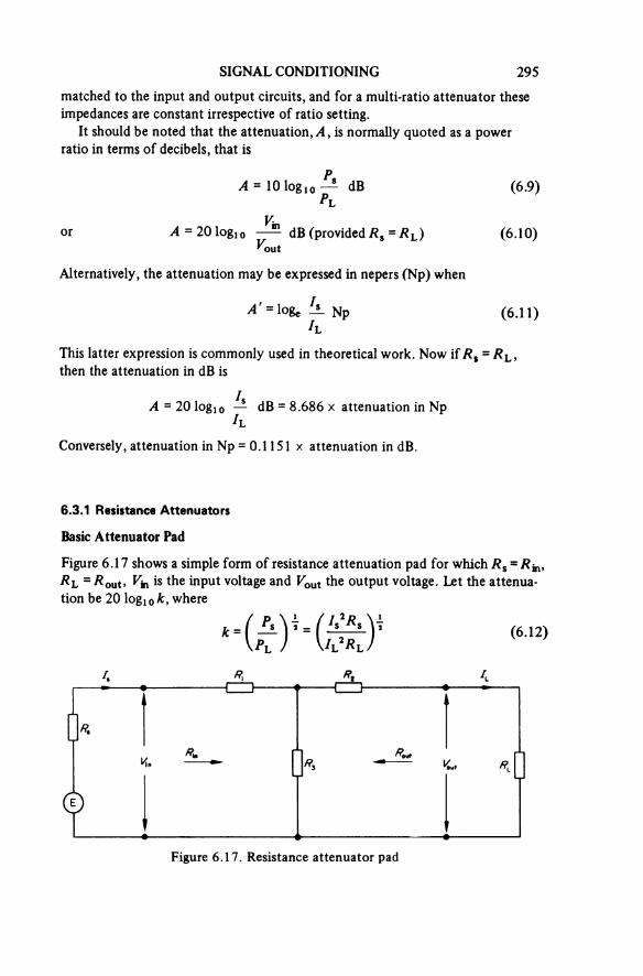
SIGNAL CONDITIONING 295matched to the input and output circuits, and for a multi-ratio attenuator theseimpedances are constant irrespective of ratio setting.
It should be noted that the attenuation, A, is normally quoted as a powerratio in terms of decibels, that is
(6.9)
or (provided Rs = RL) (6.10)
Alternatively, the attenuation may be expressed in nepers (Np) when
(6.11)
This latter expression is commonly used in theoretical work. Now if Rs = RL, then the attenuation in dB is
× attenuation in Np
Conversely, attenuation in Np = 0.1151 × attenuation in dB.
6.3.1 Resistance Attenuators
Basic Attenuator Pad
Figure 6.17 shows a simple form of resistance attenuation pad for which Rs = Rin, RL = Rout, Vin is the input voltage and Vout the output voltage. Let the attenua-tion be 20 log10 k, where
(6.12)
Figure 6.17. Resistance attenuator pad
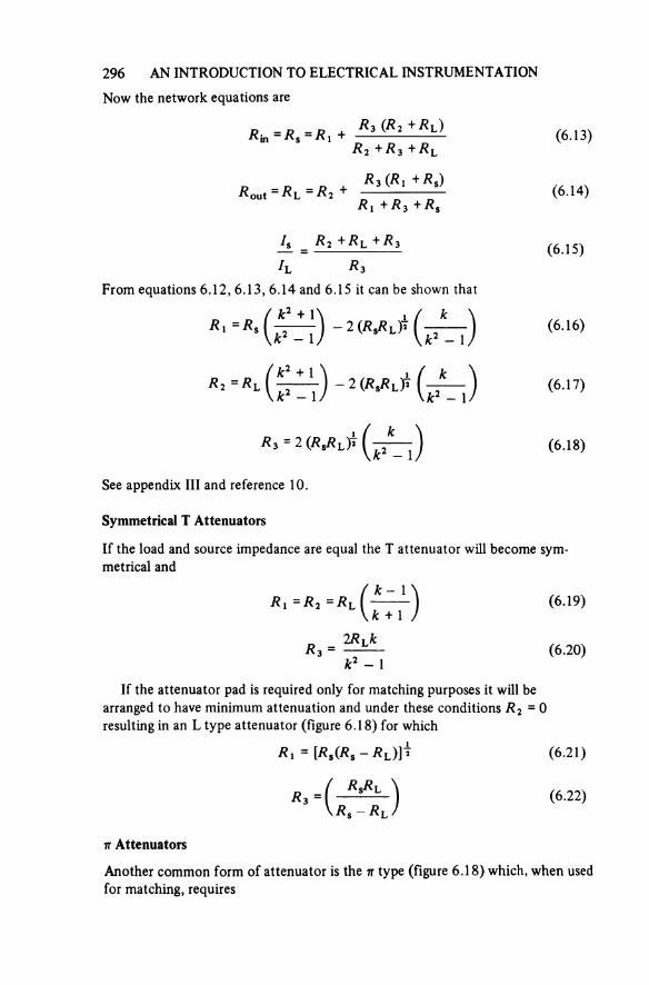
296 AN INTRODUCTION TO ELECTRICAL INSTRUMENTATION
Now the network equations are
(6.13)
(6.14)
(6.15)
From equations 6.12, 6.13, 6.14 and 6.15 it can be shown that
(6.16)
(6.17)
(6.18)
See appendix III and reference 10.
Symmetrical T Attenuators
If the load and source impedance are equal the T attenuator will become sym-metrical and
(6.19)
(6.20)
If the attenuator pad is required only for matching purposes it will be arranged to have minimum attenuation and under these conditions = 0 resulting in an L type attenuator (figure 6.18) for which
(6.21)
(6.22)
π Attenuators
Another common form of attenuator is the π type (figure 6.18) which, when used for matching, requires
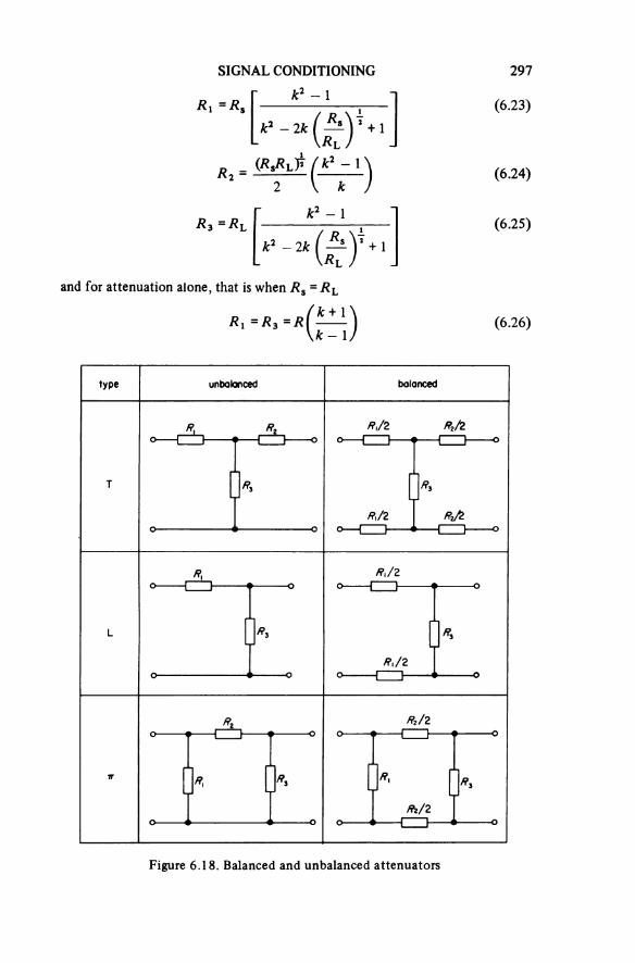
SIGNAL CONDITIONING 297
(6.23)
(6.24)
(6.25)
and for attenuation alone, that is when Rs = RL
(6.26)
Figure 6.18. Balanced and unbalanced attenuators
type unbalanced balanced
T
L
π
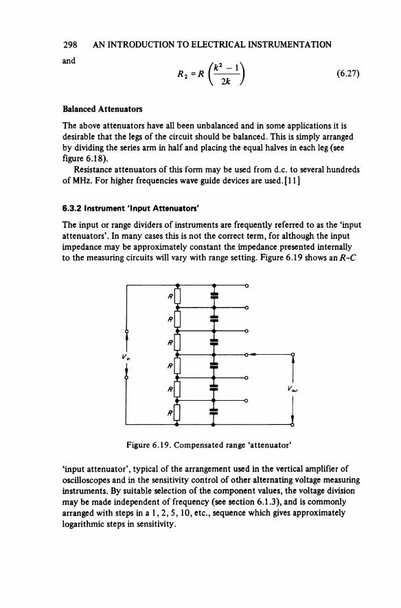
298 AN INTRODUCTION TO ELECTRICAL INSTRUMENTATION
and(6.27)
Balanced Attenuators
The above attenuators have all been unbalanced and in some applications it is desirable that the legs of the circuit should be balanced. This is simply arranged by dividing the series arm in half and placing the equal halves in each leg (see figure 6.18).
Resistance attenuators of this form may be used from d.c. to several hundreds of MHz. For higher frequencies wave guide devices are used. [11]
6.3.2 Instrument 'Input Attenuators'
The input or range dividers of instruments are frequently referred to as the ‘input attenuators’. In many cases this is not the correct term, for although the input impedance may be approximately constant the impedance presented internally to the measuring circuits will vary with range setting. Figure 6.19 shows an R-C
Figure 6.19. Compensated range ‘attenuator’
‘input attenuator’, typical of the arrangement used in the vertical amplifier of oscilloscopes and in the sensitivity control of other alternating voltage measuring instruments. By suitable selection of the component values, the voltage division may be made independent of frequency (see section 6.1.3), and is commonly arranged with steps in a 1, 2, 5, 10, etc., sequence which gives approximately logarithmic steps in sensitivity.
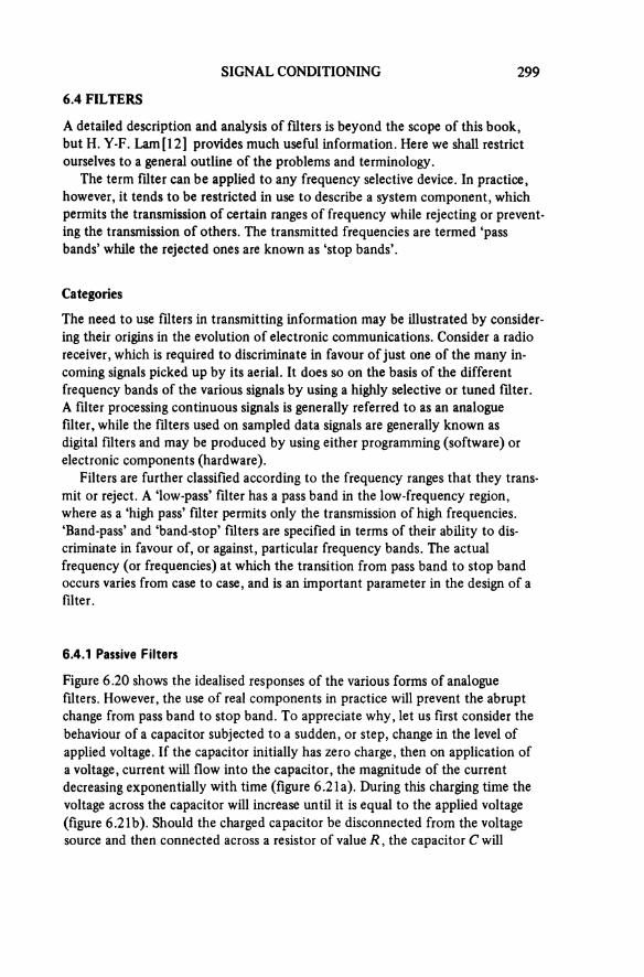
SIGNAL CONDITIONING 299
6.4 FILTERS
A detailed description and analysis of filters is beyond the scope of this book, but H. Y-F. Lam [12] provides much useful information. Here we shall restrict ourselves to a general outline of the problems and terminology.
The term filter can be applied to any frequency selective device. In practice, however, it tends to be restricted in use to describe a system component, which permits the transmission of certain ranges of frequency while rejecting or prevent ing the transmission of others. The transmitted frequencies are termed ‘pass bands’ while the rejected ones are known as ‘stop bands’.
Categories
The need to use filters in transmitting information may be illustrated by consider-ing their origins in the evolution of electronic communications. Consider a radioreceiver, which is required to discriminate in favour of just one of the many in-coming signals picked up by its aerial. It does so on the basis of the different frequency bands of the various signals by using a highly selective or tuned filter.A filter processing continuous signals is generally referred to as an analogue filter, while the filters used on sampled data signals are generally known as digital filters and may be produced by using either programming (software) or electronic components (hardware).
Filters are further classified according to the frequency ranges that they trans-mit or reject. A ‘low-pass’ filter has a pass band in the low-frequency region, where as a ‘high pass’ filter permits only the transmission of high frequencies. ‘Band-pass’ and ‘band-stop’ filters are specified in terms of their ability to dis-criminate in favour of, or against, particular frequency bands. The actual frequency (or frequencies) at which the transition from pass band to stop band occurs varies from case to case, and is an important parameter in the design of a filter.
6.4.1 Passive Filters
Figure 6.20 shows the idealised responses of the various forms of analogue filters. However, the use of real components in practice will prevent the abrupt change from pass band to stop band. To appreciate why, let us first consider the behaviour of a capacitor subjected to a sudden, or step, change in the level of applied voltage. If the capacitor initially has zero charge, then on application of a voltage, current will flow into the capacitor, the magnitude of the current decreasing exponentially with time (figure 6.21a). During this charging time the voltage across the capacitor will increase until it is equal to the applied voltage (figure 6.21b). Should the charged capacitor be disconnected from the voltage source and then connected across a resistor of value R, the capacitor C will
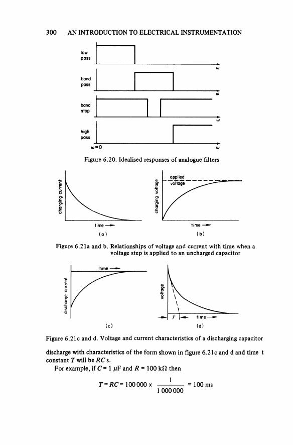
300 AN INTRODUCTION TO ELECTRICAL INSTRUMENTATION
Figure 6.20. Idealised responses of analogue filters
lowpass
bandpass
bandstop
highpass
Figure 6.21a and b. Relationships of voltage and current with time when a voltage step is applied to an uncharged capacitor
(a)
char
ging
curr
ent
time
(b)
char
ging
volta
ge
appliedvoltage
time
Figure 6.21c and d. Voltage and current characteristics of a discharging capacitor
(c)
disc
harg
e cur
rent
time
(d)
volta
ge
time
discharge with characteristics of the form shown in figure 6.21c and d and time t constant T will be RC s.
For example, if C = 1 μF and R = 100 kΩ then

SIGNAL CONDITIONING 301The expression for the current at any instant, t, is
(6.28)
so when t = T =RC
That is, i is 36.8 per cent of Im, or has decayed by 63.2 per cent. If t is made equal to 5T then
or i has reduced to 0.67 per cent of Im. Hence, for the 1 μF 100 kΩ combination, 0.5 s is required for the current to decay to less than 1 per cent of its initial value. Similarly the same time is required for the voltage to rise to be within 1 per cent of its final value. Similar response characteristics are obtained when a step change in voltage is applied to an inductor, figure 6.22, it being noted that for the inductive case the time constant of the circuit is T = L/R.
Figure 6.22. Transient response of an inductive circuit to a step function of voltage
(a)
curr
ent
time
(b)
volta
ge resistive volt drop
time
Thus it will be apparent that any system for recording transients must contain a minimum of reactive impedance or distortion of the measurand will result. This property is made use of in filters, for the time constant of a circuit is directly related to the frequency response or bandwidth of a circuit (this is shown by the analysis that follows).
High Pass Filters
Consider the circuit in figure 6.23 which has open circuited output terminals (that is, RL = ∞). Then

302 AN INTRODUCTION TO ELECTRICAL INSTRUMENTATION
Figure 6.23. ‘High pass’ filter circuit
Now CR = T, the time constant, therefore
or
(6.29)
Now when ω = 1/7
(6.30)
and this defines the —3 dB point, for by definition gain in dB = 10 1og10 (Pout/ Pin) Which by convention is taken as
gain in dB =
Therefore, if
= —3.01 dB
The circuit in figure 6.23 will prevent the passage of direct and low frequency signals while allowing high frequency signals to flow. The frequency output characteristic of the circuit is shown in figure 6.24a and in figure 6.24b, a sketch of the phase angle against frequency characteristic is drawn and shows that at ω = 1/T there will be a 45° phase shift between Vs and that is
phase angle ϕ =
(6.31)
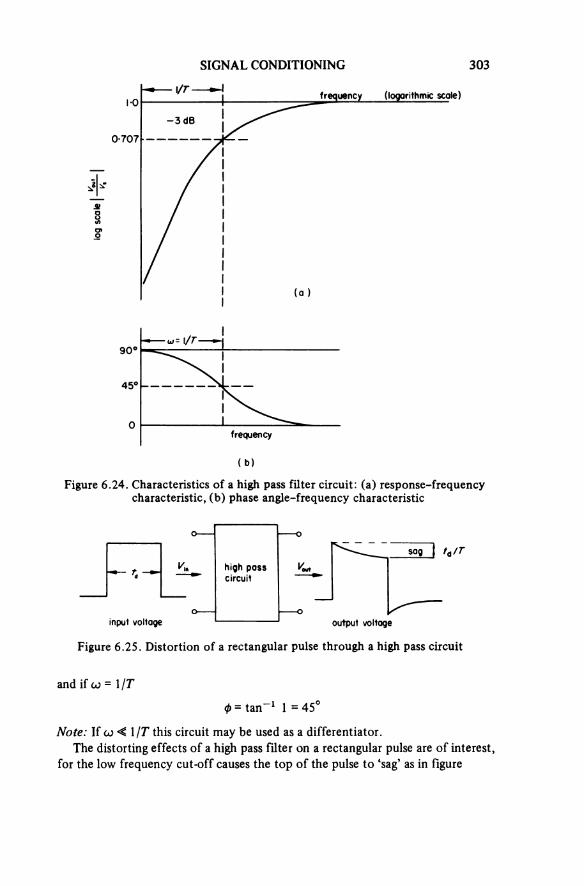
SIGNAL CONDITIONING 303
Figure 6.24. Characteristics of a high pass filter circuit: (a) response-frequency characteristic, (b) phase angle-frequency characteristic
(a)
frequency (logarithmic scale)lo
g sca
le
(b)
frequency
Figure 6.25. Distortion of a rectangular pulse through a high pass circuit
input voltage
high pass circuit
output voltage
and if ω = 1/T
Note: If ω << 1/T this circuit may be used as a differentiator.The distorting effects of a high pass filter on a rectangular pulse are of interest,
for the low frequency cut-off causes the top of the pulse to ‘sag’ as in figure
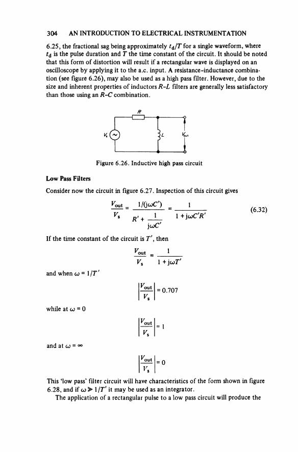
304 AN INTRODUCTION TO ELECTRICAL INSTRUMENTATION
6.25, the fractional sag being approximately td/T for a single waveform, where td is the pulse duration and T the time constant of the circuit. It should be noted that this form of distortion will result if a rectangular wave is displayed on an oscilloscope by applying it to the a.c. input. A resistance-inductance combina-tion (see figure 6.26), may also be used as a high pass filter. However, due to the size and inherent properties of inductors R-L filters are generally less satisfactory than those using an R-C combination.
Figure 6.26. Inductive high pass circuit
Low Pass Filters
Consider now the circuit in figure 6.27. Inspection of this circuit gives
(6.32)
if the time constant of the circuit is T', then
and when ω = 1/T'
while at ω = 0
and at ω = ∞
This ‘low pass’ filter circuit will have characteristics of the form shown in figure 6.28, and if ω >> 1/T' it may be used as an integrator.
The application of a rectangular pulse to a low pass circuit will produce the

SIGNAL CONDITIONING 305
Figure 6.27. ‘Low pass’ filter circuit
Figure 6.28. Characteristics of low pass filter circuit
frequency
phas
e ang
le
type of distortion illustrated in figure 6.29, the rise time of the distorted wave being defined as the time interval from 10 per cent to 90 per cent of the maxi-mum value. If T = CR (or L/R) is the time constant of the circuit, v1 the voltage of t1, v2 the voltage of t2 and Vm the total or final voltage, then
(6.33)
(6.34)
from equations 6.33 and 6.34
hence
Therefore
(6.35)
This rise time tr = (t2 - t1) is usually taken as 2.2T.
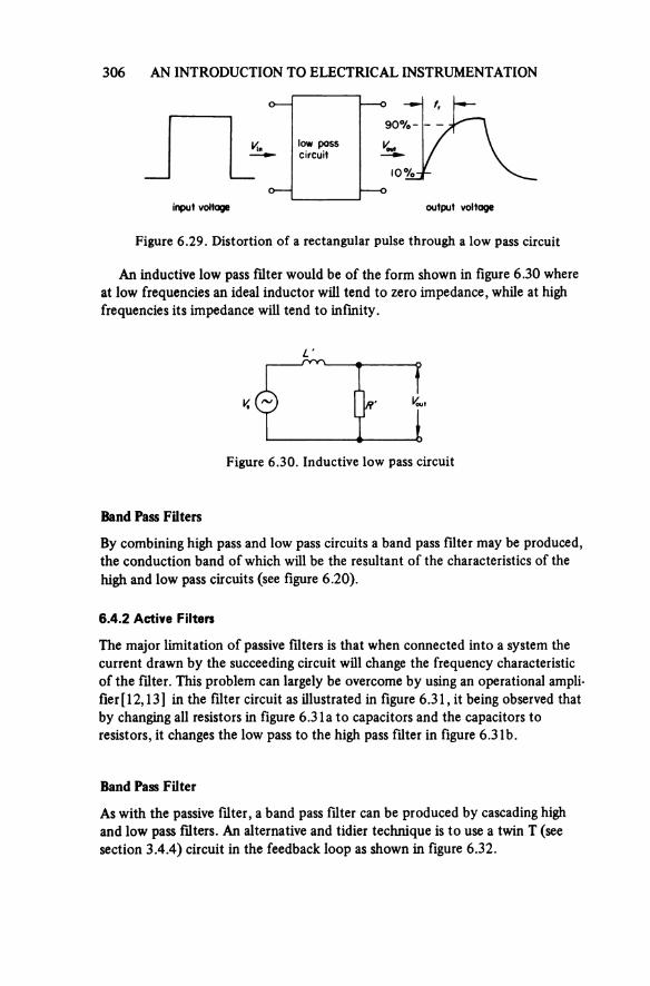
306 AN INTRODUCTION TO ELECTRICAL INSTRUMENTATION
Figure 6.29. Distortion of a rectangular pulse through a low pass circuit
input voltage
low pass circuit
output voltage
An inductive low pass filter would be of the form shown in figure 6.30 where at low frequencies an ideal inductor will tend to zero impedance, while at high frequencies its impedance will tend to infinity.
Figure 6.30. Inductive low pass circuit
Band Pass Filters
By combining high pass and low pass circuits a band pass filter may be produced, the conduction band of which will be the resultant of the characteristics of the high and low pass circuits (see figure 6.20).
6.4.2 Active Filters
The major limitation of passive filters is that when connected into a system the current drawn by the succeeding circuit will change the frequency characteristic of the filter. This problem can largely be overcome by using an operational ampli-fier [12, 13] in the filter circuit as illustrated in figure 6.31, it being observed that by changing all resistors in figure 6.31a to capacitors and the capacitors to resistors, it changes the low pass to the high pass filter in figure 6.31b.
Band Pass Filter
As with the passive filter, a band pass filter can be produced by cascading high and low pass filters. An alternative and tidier technique is to use a twin T (see section 3.4.4) circuit in the feedback loop as shown in figure 6.32.
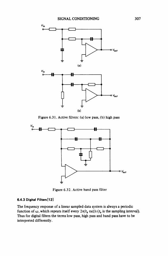
SIGNAL CONDITIONING 307
Figure 6.31. Active filters: (a) low pass, (b) high pass
(a)
(b)
Figure 6.32. Active band pass filter
6.4.3 Digital Filters [12]
The frequency response of a linear sampled-data system is always a periodic function of ω, which repeats itself every 2π/ts rad/s (ts is the sampling interval). Thus for digital filters the terms low pass, high pass and band pass have to be interpreted differently.
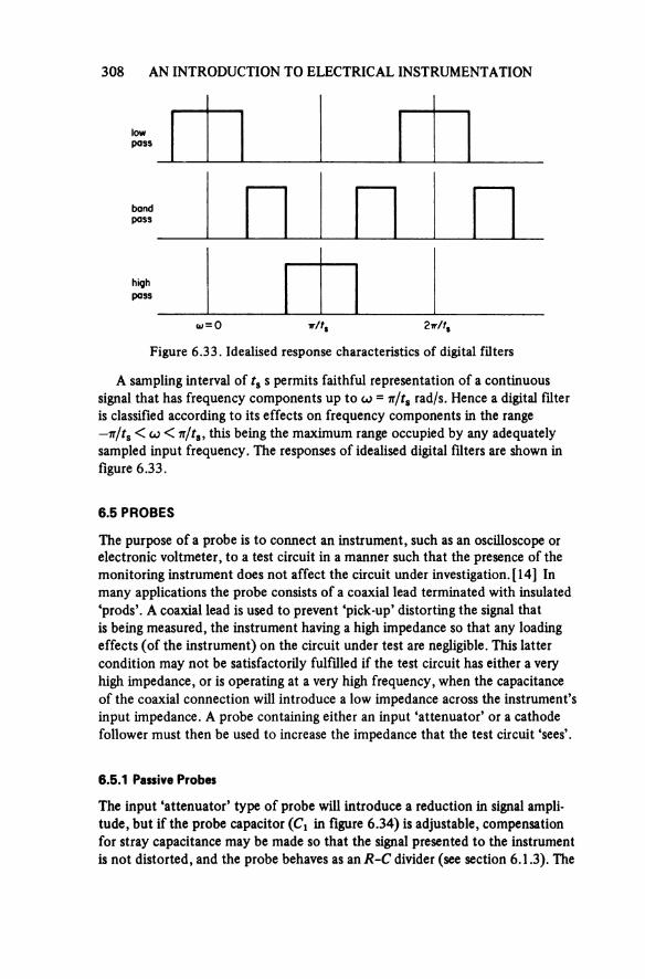
308 AN INTRODUCTION TO ELECTRICAL INSTRUMENTATION
Figure 6.33. Idealised response characteristics of digital filters
lowpass
bandpass
highpass
A sampling interval of t3 permits faithful representation of a continuous signal that has frequency components up to ω = π/ts rad/s. Hence a digital filter is classified according to its effects on frequency components in the range —π/ts < ω < π/ts, this being the maximum range occupied by any adequately sampled input frequency. The responses of idealised digital filters are shown in figure 6.33.
6.5 PROBES
The purpose of a probe is to connect an instrument, such as an oscilloscope or electronic voltmeter, to a test circuit in a manner such that the presence of the monitoring instrument does not affect the circuit under investigation. [14] In many applications the probe consists of a coaxial lead terminated with insulated ‘prods’. A coaxial lead is used to prevent ‘pick-up’ distorting the signal that is being measured, the instrument having a high impedance so that any loading effects (of the instrument) on the circuit under test are negligible. This latter condition may not be satisfactorily fulfilled if the test circuit has either a very high impedance, or is operating at a very high frequency, when the capacitance of the coaxial connection will introduce a low impedance across the instrument’s input impedance. A probe containing either an input ‘attenuator’ or a cathode follower must then be used to increase the impedance that the test circuit ‘sees’.
6.5.1 Passive Probes
The input ‘attenuator’ type of probe will introduce a reduction in signal ampli-tude, but if the probe capacitor (C1 in figure 6.34) is adjustable, compensation for stray capacitance may be made so that the signal presented to the instrument is not distorted, and the probe behaves as an R-C divider (see section 6.1.3). The

SIGNAL CONDITIONING 309
Figure 6.34. R-C passive probe
probe
connection c.r.o.
Figure 6.35. Effects of probe adjustment on the displayed square wave: (a) mis-adjustment- high frequency attenuation, (b) misadjustment— accentuated high frequency response, (c) correct adjustment giving optimum high frequency response
(a)
C1 too small
(b)
C1 too large
(c)
adjustment of C1 is normally provided by the longitudinal movement of one of a pair of concentric cylindrical conductors relative to the other. The effects of this adjustment are shown diagrammatically in figure 6.35. The reduction in signal level for passive probes, used between d.c. and 300 MHz is typically 1/10 from equation 6.3
This signal reduction is commonly specified as a 10× attenuation.
Input Impedance Effects
The objective of using a probe is to reduce the loading of the instrument on the signal source. Consider, therefore, the effective input impedance of an oscillo-scope connected to a signal via a probe as in figure 6.36
R1 = probe resistance = 9 MΩ R2 = ’scope input resistance = 1 MΩ C1 = adjustable probe capacitance

310 AN INTRODUCTION TO ELECTRICAL INSTRUMENTATION
Figure 6.36. Equivalent circuit of oscilloscope and probe combination
signalsource
oscilloscope
Figure 6.37. Effective circuit of oscilloscope and probe combination
C2 = ’scope input capacitance ≈ 20 pF C3 = cable capacitance ≈ 23 pF/mC4 = environmental capacitance ≈ 1.5-2 pF
Assuming a 1 m cable is used, c3 = 23 pF. For correct compensation
or
The effective input capacitance
and since the effective input resistance is (1 + 9) MΩ the effective circuit becomes that shown by figure 6.37.
It should be observed that care must be taken to ensure that the probe imped-ance is compatible with the input impedance of the instrument it is to be used with.
Signal Response
The rise time (10 per cent to 90 per cent of final value) specified for a passive probe is commonly quoted for the situation in which the probe alone is con-nected to a matched 50 Ω source. Thus the instrument’s response will depend
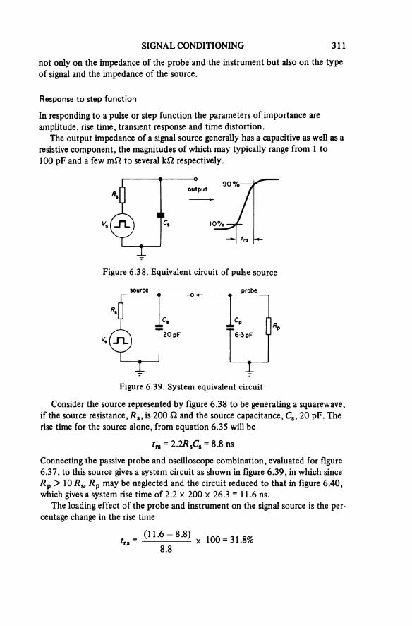
SIGNAL CONDITIONING 311
not only on the impedance of the probe and the instrument but also on the type of signal and the impedance of the source.
Response to step function
In responding to a pulse or step function the parameters of importance are amplitude, rise time, transient response and time distortion.
The output impedance of a signal source generally has a capacitive as well as a resistive component, the magnitudes of which may typically range from 1 to 100 pF and a few mΩ to several kΩ respectively.
Figure 6.38. Equivalent circuit of pulse source
output
Figure 6.39. System equivalent circuit
source probe
Consider the source represented by figure 6.38 to be generating a squarewave, if the source resistance, Rs, is 200 Ω and the source capacitance, Cs, 20 pF. The rise time for the source alone, from equation 6.35 will be
Connecting the passive probe and oscilloscope combination, evaluated for figure 6.37, to this source gives a system circuit as shown in figure 6.39, in which since Rp > 10 Rs, Rp may be neglected and the circuit reduced to that in figure 6.40, which gives a system rise time of 2.2 × 200 × 26.3 = 11.6 ns.
The loading effect of the probe and instrument on the signal source is the per-centage change in the rise time
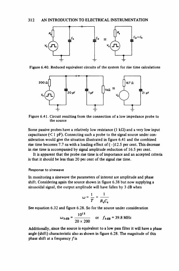
312 AN INTRODUCTION TO ELECTRICAL INSTRUMENTATION
Figure 6.40. Reduced equivalent circuits of the system for rise time calculations
Figure 6.41. Circuit resulting from the connection of a low impedance probe to the source
Some passive probes have a relatively low resistance (1 kΩ) and a very low input capacitance (< 1 pF). Connecting such a probe to the signal source under con-sideration would give the situation illustrated in figure 6.41 and the combined rise time becomes 7.7 ns with a loading effect of (—)12.5 per cent. This decrease in rise time is accompanied by signal amplitude reduction of 16.5 per cent.
It is apparent that the probe rise time is of importance and an accepted criteria is that it should be less than 20 per cent of the signal rise time.
Response to sinewave
In monitoring a sinewave the parameters of interest are amplitude and phase shift. Considering again the source shown in figure 6.38 but now supplying a sinusoidal signal, the output amplitude will have fallen by 3 dB when
See equation 6.32 and figure 6.28. So for the source under consideration
Additionally, since the source is equivalent to a low pass filter it will have a phase angle (shift) characteristic also as shown in figure 6.28. The magnitude of this phase shift at a frequency f is
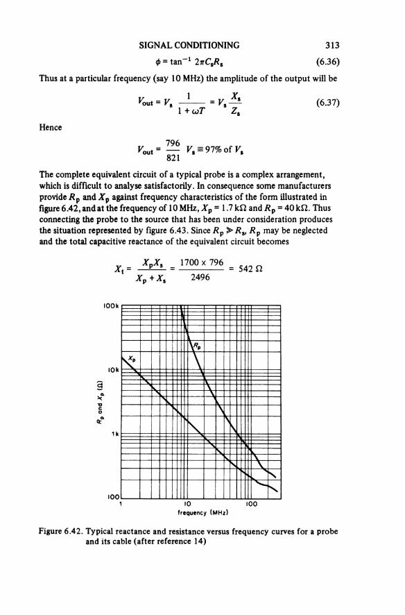
SIGNAL CONDITIONING 313
(6.36)
Thus at a particular frequency (say 10 MHz) the amplitude of the output will be
(637)
Hence
The complete equivalent circuit of a typical probe is a complex arrangement, which is difficult to analyse satisfactorily. In consequence some manufacturers provide λ p and XP against frequency characteristics of the form illustrated in figure 6.42, and at the frequency of 10 MHz, XP = 1.7 kΩ and Rp - 40 kΩ. Thus connecting the probe to the source that has been under consideration produces the situation represented by figure 6.43. Since Rp >RS, Rp may be neglected and the total capacitive reactance of the equivalent circuit becomes
Figure 6.42. Typical reactance and resistance versus frequency curves for a probe and its cable (after reference 14)
R, αn
d Xp M
)
frequency (MHz)

314 AN INTRODUCTION TO ELECTRICAL INSTRUMENTATION
Thus
and
phase shift =
While the reduction in amplitude is relatively small the phase shift is appreciable, and to reduce the phase shift a low impedance probe may be used, [14] but such a procedure will result in considerable signal reduction.
Figure 6.43. Probe connected to source: (a) values for f = 10 MHz, (b) reduced equivalent circuit of (a)
(a) (b)
6.5.2 Active Voltage Probes
Although the passive probe is by far the most commonly used voltage probe, it is apparent from the previous section that low capacitive loading (and phase shift) can only be obtained at the expense of considerable attenuation. These prob-lems can be overcome by using an active (FET) probe[15] which may have a loading effect as small as 10 MΩ in parallel with 2 pF, a bandwidth from d.c. to 500 MHz, and a × 1 attenuation.
Active voltage probes obtain the necessary power either from the designated source available on the front panel of the instrument or from a separate (probe accessory) power unit. To keep the probe small and easy to handle, and to meet the impedance requirements, a miniaturised amplifier, with an FET input stage is built into the tip of the probe.
Figure 6.44 is a simplified block diagram of an FET probe in which the alternating and direct voltage components are separated, amplified and then com-bined. This split-band amplification technique enables the optimum use of the device characteristics. To maintain a probe attenuation of × 1, the output signal is compared with the input signal via a feedback inverter and resistor R2. If the
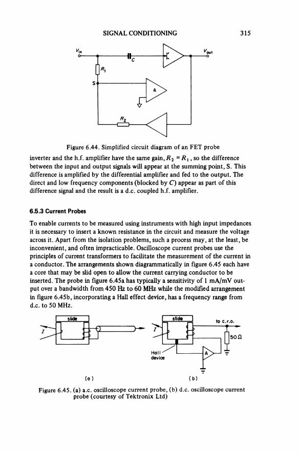
SIGNAL CONDITIONING 315
Figure 6.44. Simplified circuit diagram of an FET probeinverter and the h.L amplifier have the same gain, R2 = Rx, so the difference between the input and output signals will appear at the summing point, S. This difference is amplified by the differential amplifier and fed to the output. The direct and low frequency components (blocked by C) appear as part of this difference signal and the result is a d.c. coupled h.f. amplifier.
6.5.3 Current Probes
To enable currents to be measured using instruments with high input impedances it is necessary to insert a known resistance in the circuit and measure the voltage across it. Apart from the isolation problems, such a process may, at the least, be inconvenient, and often impracticable. Oscilloscope current probes use the principles of current transformers to facilitate the measurement of the current in a conductor. The arrangements shown diagrammatically in figure 6.45 each have a core that may be slid open to allow the current carrying conductor to be inserted. The probe in figure 6.45a has typically a sensitivity of 1 mA/mv out-put over a bandwidth from 450 Hz to 60 MHz while the modified arrangement in figure 6.45b, incorporating a Hall effect device, has a frequency range from d.c. to 50 MHz.
Figure 6.45. (a) a.c. oscilloscope current probe, (b) d.c. oscilloscope current probe (courtesy of Tektronix Ltd)
(a)
slide
(b)
slide to c.r.o.
Halldevice
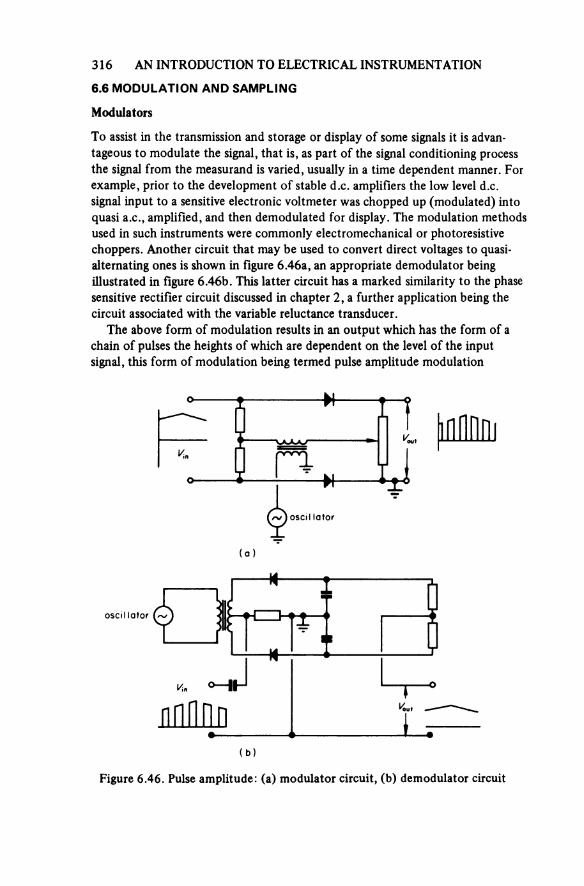
316 AN INTRODUCTION TO ELECTRICAL INSTRUMENTATION
6.6 MODULATION AND SAMPLING
Modulators
To assist in the transmission and storage or display of some signals it is advan-tageous to modulate the signal, that is, as part of the signal conditioning process the signal from the measurand is varied, usually in a time dependent manner. For example, prior to the development of stable d.c. amplifiers the low level d.c. signal input to a sensitive electronic voltmeter was chopped up (modulated) into quasi a.c., amplified, and then demodulated for display. The modulation methods used in such instruments were commonly electromechanical or photoresistive choppers. Another circuit that may be used to convert direct voltages to quasi- alternating ones is shown in figure 6.46a, an appropriate demodulator being illustrated in figure 6.46b. This latter circuit has a marked similarity to the phase sensitive rectifier circuit discussed in chapter 2, a further application being the circuit associated with the variable reluctance transducer.
The above form of modulation results in an output which has the form of a chain of pulses the heights of which are dependent on the level of the input signal, this form of modulation being termed pulse amplitude modulation
Figure 6.46. Pulse amplitude: (a) modulator circuit, (b) demodulator circuit
(a)
oscillator
(b)
oscillator
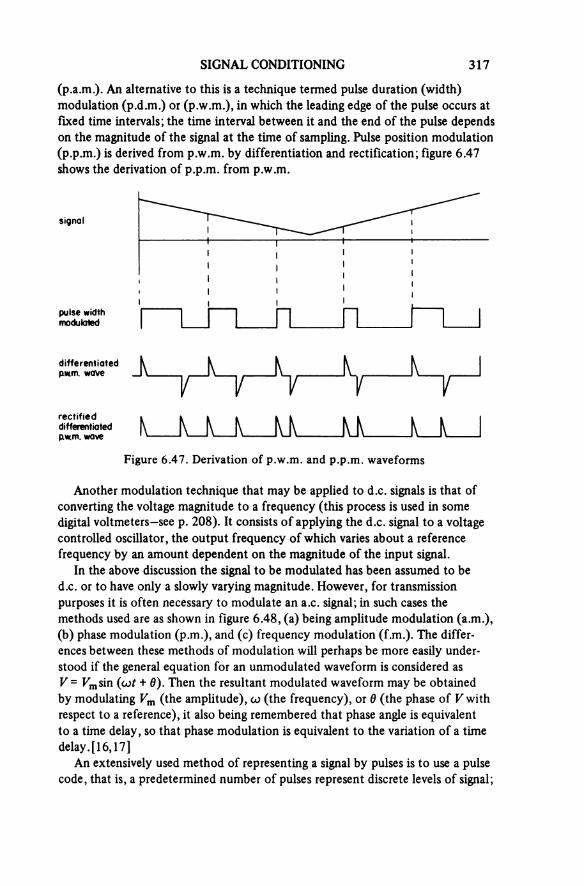
SIGNAL CONDITIONING 317
(p.a.m.). An alternative to this is a technique termed pulse duration (width) modulation (p.d.m.) or (p.w.m.), in which the leading edge of the pulse occurs at fixed time intervals; the time interval between it and the end of the pulse depends on the magnitude of the signal at the time of sampling. Pulse position modulation (p.p.m.) is derived from p.w.m. by differentiation and rectification; figure 6.47 shows the derivation of p.p.m. from p.w.m.
Figure 6.47. Derivation of p.w.m. and p.p.m. waveforms
signal
pulse width modulated
differentiated p.w.m. wave
rectified differentiated p.w.m. wave
Another modulation technique that may be applied to d.c. signals is that of converting the voltage magnitude to a frequency (this process is used in some digital voltmeters—see p. 208). It consists of applying the d.c. signal to a voltage controlled oscillator, the output frequency of which varies about a reference frequency by an amount dependent on the magnitude of the input signal.
In the above discussion the signal to be modulated has been assumed to be d.c. or to have only a slowly varying magnitude. However, for transmission purposes it is often necessary to modulate an a.c. signal; in such cases the methods used are as shown in figure 6.48, (a) being amplitude modulation (a.m.), (b) phase modulation (p.m.), and (c) frequency modulation (f.m.). The differ-ences between these methods of modulation will perhaps be more easily under-stood if the general equation for an unmodulated waveform is considered as V = Vmsin (ωt + θ). Then the resultant modulated waveform may be obtained by modulating Vm (the amplitude), ω (the frequency), or θ (the phase of V with respect to a reference), it also being remembered that phase angle is equivalent to a time delay, so that phase modulation is equivalent to the variation of a time delay. [16, 17]
An extensively used method of representing a signal by pulses is to use a pulse code, that is, a predetermined number of pulses represent discrete levels of signal;
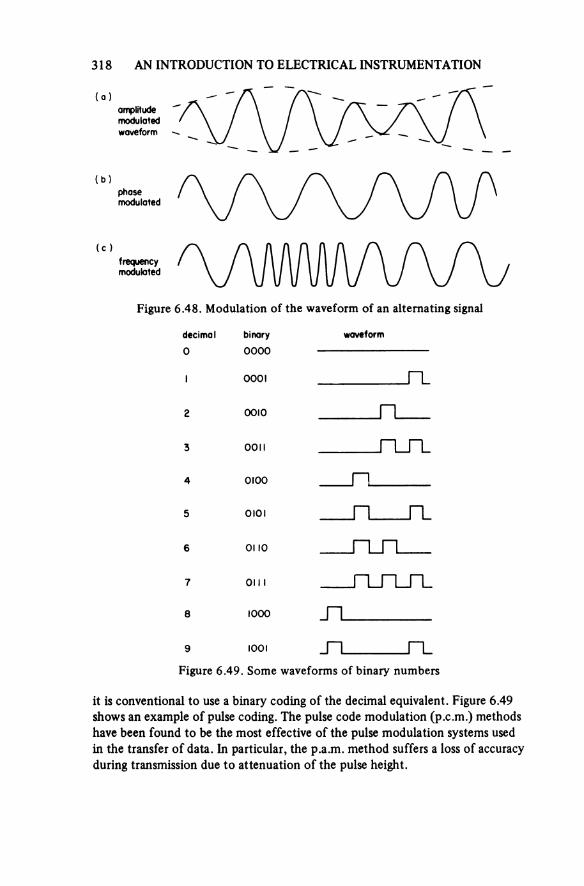
318 AN INTRODUCTION TO ELECTRICAL INSTRUMENTATION
Figure 6.48. Modulation of the waveform of an alternating signal
(a)amplitudemodulatedwaveform
(b)phasemodulated
(c)frequencymodulated
Figure 6.49. Some waveforms of binary numbers
decimal binary waveform
0 0000
1 0001
2 0010
3 0011
4 0100
5 0101
6 0110
7 0111
8 1000
9 1001
it is conventional to use a binary coding of the decimal equivalent. Figure 6.49 shows an example of pulse coding. The pulse code modulation (p.c.m.) methods have been found to be the most effective of the pulse modulation systems used in the transfer of data. In particular, the p.a.m. method suffers a loss of accuracy during transmission due to attenuation of the pulse height.

SIGNAL CONDITIONING 319
Sampling
When a continuous signal is to be represented by a set of samples, care must be taken to ensure that the scanning rate is sufficiently fast for all the variations in the measurand to be reconstructed from the record. The limiting requirement of sampling is that the frequency of sampling [17] shall be at least twice the highest frequency component of the signal being sampled in order that it may be recon-structed in its original form. An alternative method of looking at this is to consider a system which has a pass band of (say) d.c. to f Hz, then the sampling frequency must be at least 2/ However, the sampling theory assumes the presence of signal reconstruction equipment and a more practical sampling rate for many instrumentation applications is six times the highest frequency component of the signal.
6.7 ANALOGUE PROCESSING
In many measuring situations the signal must be ‘processed’ in order to obtain a reading that is a meaningful representation of the measurand. The developments in digital electronics are continually extending the range of what it is possible to do in a digital instrument but for some situations analogue signal processing will remain the most satisfactory.
6.7.1 Amplification
The use of amplifiers in instrumentation is extensive, and in such an application they can be thought of as ‘black boxes’ or building bricks, their function being to operate in some manner on the signal from the measurand. This operation may simply be to increase the magnitude of the signal or it may be to perform a mathematical function on it, for example, to differentiate or integrate the signal; other possibilities are the summation of a number of signals, or the removal (filtering) of unwanted components. Figure 6.50 shows the accepted symbols for operational amplifiers which are known as (a) single-ended and (b) differential input amplifiers. The normal method of construction used for an operational amplifier is as an integrated circuit with a differential input, a single- ended amplifier being created by suitable connection of one input. In either case, as an operational amplifier, it will have a high gain, typically 106, it will invert (there will be a reversal of polarity between input and output), and it will have a large input impedance, typically 100 kΩ. It should also have a bandwidth which extends from d.c. upwards, together with low offset and drift properties. The symbol in figure 6.50c represents an operational amplifier with feedback.
The gain of an amplifier is the ratio Vout/Vin; thus, for an operational amplifier this should be a large negative number. However, conventionally the gain is con-sidered as the modulus of the voltage ratio and is therefore positive, that is
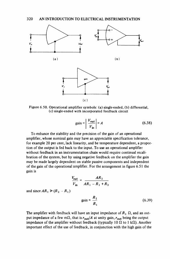
320 AN INTRODUCTION TO ELECTRICAL INSTRUMENTATION
Figure 6.50. Operational amplifier symbols: (a) single-ended, (b) differential, (c) single-ended with incorporated feedback circuit
(a) (b)
(c)
(6.38)
To enhance the stability and the precision of the gain of an operational amplifier, whose nominal gain may have an appreciable specification tolerance, for example 20 per cent, lack linearity, and be temperature dependent, a propor-tion of the output is fed back to the input. To use an operational amplifier without feedback in an instrumentation chain would require continual recali-bration of the system, but by using negative feedback on the amplifier the gain may be made largely dependent on stable passive components and independent of the gain of the operational amplifier. For the arrangement in figure 6.51 the gain is
and since AR1 >> (R2 — R1 )
(6.39)
The amplifier with feedback will have an input impedance of R1 Ω, and an out-put impedance of a few mΩ, that is rout/A at unity gain, rOut being the output impedance of the amplifier without feedback (typically 10 Ω to 1 kΩ). Another important effect of the use of feedback, in conjunction with the high gain of the
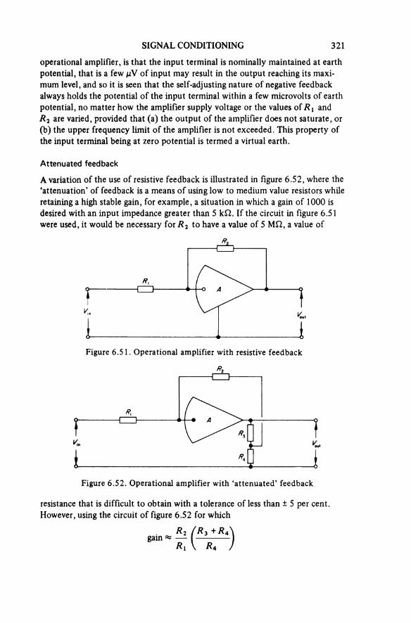
SIGNAL CONDITIONING 321
operational amplifier, is that the input terminal is nominally maintained at earth potential, that is a few μV of input may result in the output reaching its maxi-mum level, and so it is seen that the self-adjusting nature of negative feedback always holds the potential of the input terminal within a few microvolts of earth potential, no matter how the amplifier supply voltage or the values of R1 and R2 are varied, provided that (a) the output of the amplifier does not saturate, or (b) the upper frequency limit of the amplifier is not exceeded. This property of the input terminal being at zero potential is termed a virtual earth.
Attenuated feedback
A variation of the use of resistive feedback is illustrated in figure 6.52, where the ‘attenuation’ of feedback is a means of using low to medium value resistors while retaining a high stable gain, for example, a situation in which a gain of 1000 is desired with an input impedance greater than 5 kΩ. If the circuit in figure 6.51 were used, it would be necessary for R2 to have a value of 5 MΩ, a value of
Figure 6.51. Operational amplifier with resistive feedback
Figure 6.52. Operational amplifier with ‘attenuated’ feedback
resistance that is difficult to obtain with a tolerance of less than ± 5 per cent. However, using the circuit of figure 6.52 for which
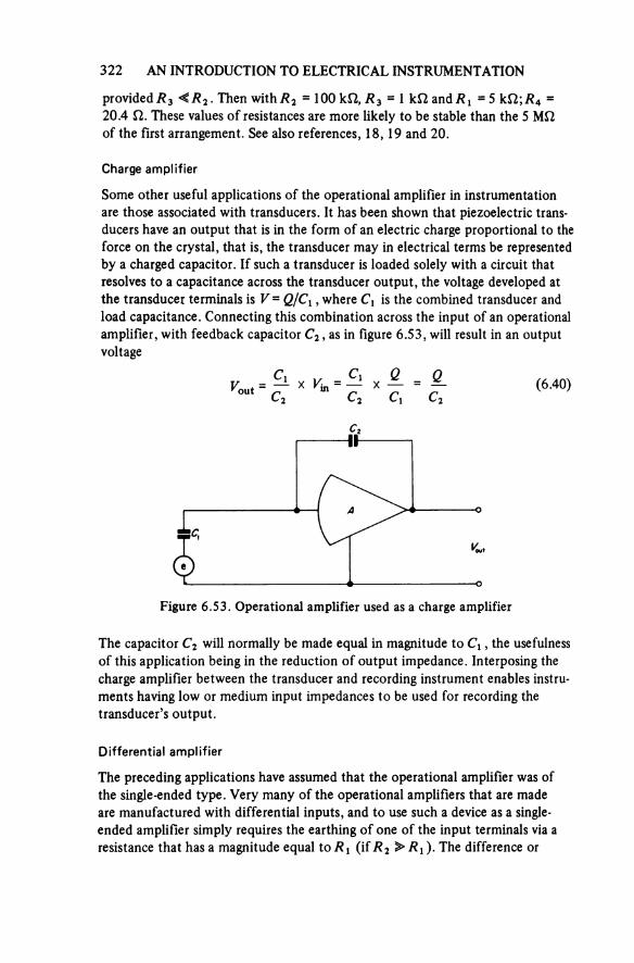
322 AN INTRODUCTION TO ELECTRICAL INSTRUMENTATION
provided R3 << R2. Then with R2 = 100 kΩ, R3 = 1 kΩ and R1 = 5 kΩ; R4 = 20.4 Ω. These values of resistances are more likely to be stable than the 5 MΩ of the first arrangement. See also references, 18, 19 and 20.
Charge amplifier
Some other useful applications of the operational amplifier in instrumentation are those associated with transducers. It has been shown that piezoelectric trans-ducers have an output that is in the form of an electric charge proportional to the force on the crystal, that is, the transducer may in electrical terms be represented by a charged capacitor. If such a transducer is loaded solely with a circuit that resolves to a capacitance across the transducer output, the voltage developed at the transducer terminals is V = Q/C1 , where C1 is the combined transducer and load capacitance. Connecting this combination across the input of an operational amplifier, with feedback capacitor C2, as in figure 6.53, will result in an output voltage
(6.40)
Figure 6.53. Operational amplifier used as a charge amplifier
The capacitor C2 will normally be made equal in magnitude to C1, the usefulness of this application being in the reduction of output impedance. Interposing the charge amplifier between the transducer and recording instrument enables instru-ments having low or medium input impedances to be used for recording the transducer’s output.
Differential amplifier
The preceding applications have assumed that the operational amplifier was of the single-ended type. Very many of the operational amplifiers that are made are manufactured with differential inputs, and to use such a device as a single- ended amplifier simply requires the earthing of one of the input terminals via a resistance that has a magnitude equal to R1 (if R2 >> R1). The difference or
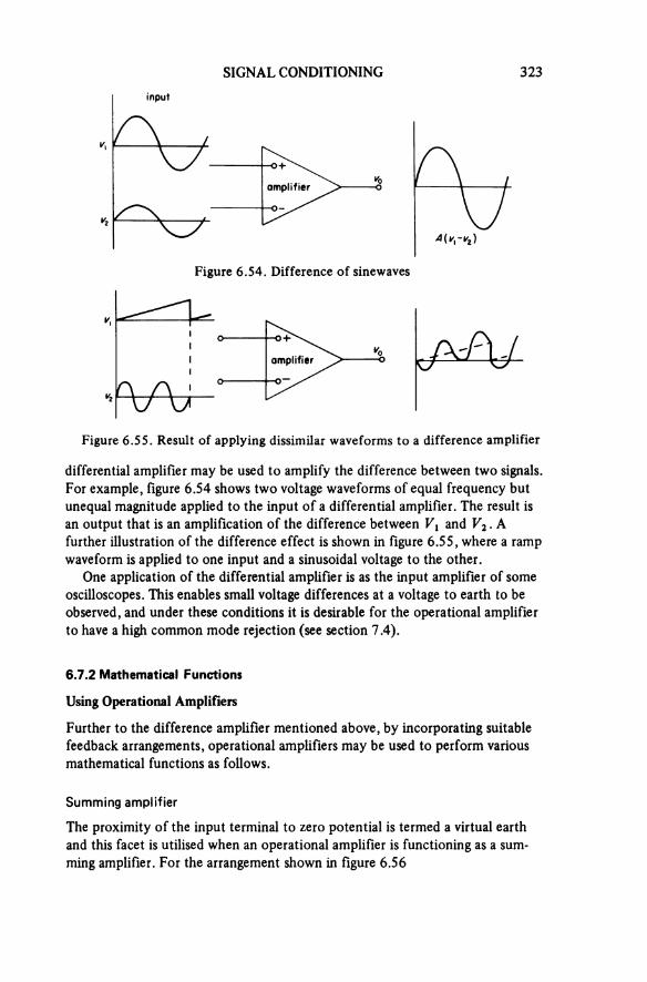
SIGNAL CONDITIONING 323
Figure 6.54. Difference of sinewaves
input
amplifier
Figure 6.55. Result of applying dissimilar waveforms to a difference amplifier
amplifier
differential amplifier may be used to amplify the difference between two signals. For example, figure 6.54 shows two voltage waveforms of equal frequency but unequal magnitude applied to the input of a differential amplifier. The result is an output that is an amplification of the difference between V1 and V2. A further illustration of the difference effect is shown in figure 6.55, where a ramp waveform is applied to one input and a sinusoidal voltage to the other.
One application of the differential amplifier is as the input amplifier of some oscilloscopes. This enables small voltage differences at a voltage to earth to be observed, and under these conditions it is desirable for the operational amplifier to have a high common mode rejection (see section 7.4).
6.7.2 Mathematical Functions
Using Operational Amplifiers
Further to the difference amplifier mentioned above, by incorporating suitable feedback arrangements, operational amplifiers may be used to perform various mathematical functions as follows.
Summing amplifier
The proximity of the input terminal to zero potential is termed a virtual earth and this facet is utilised when an operational amplifier is functioning as a sum-ming amplifier. For the arrangement shown in figure 6.56
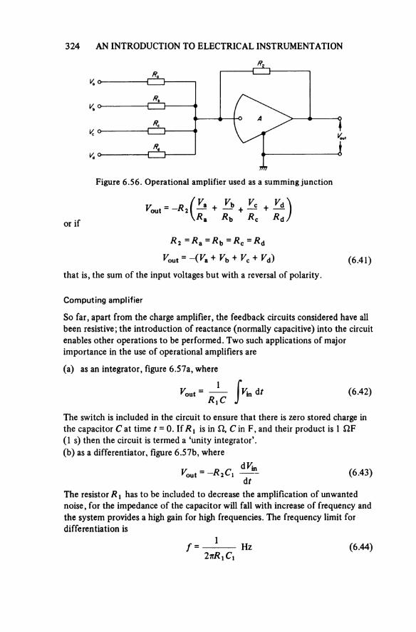
324 AN INTRODUCTION TO ELECTRICAL INSTRUMENTATION
Figure 6.56. Operational amplifier used as a summing junction
or if
(6.41)that is, the sum of the input voltages but with a reversal of polarity.
Computing amplifier
So far, apart from the charge amplifier, the feedback circuits considered have all been resistive; the introduction of reactance (normally capacitive) into the circuit enables other operations to be performed. Two such applications of major importance in the use of operational amplifiers are
(a) as an integrator, figure 6.57a, where
(6.42)
The switch is included in the circuit to ensure that there is zero stored charge in the capacitor C at time t = 0. If R1 is in Ω, C in F, and their product is 1 ΩF (1 s) then the circuit is termed a ‘unity integrator’.(b) as a differentiator, figure 6.57b, where
(6.43)
The resistor R1 has to be included to decrease the amplification of unwanted noise, for the impedance of the capacitor will fall with increase of frequency and the system provides a high gain for high frequencies. The frequency limit for differentiation is
(6.44)
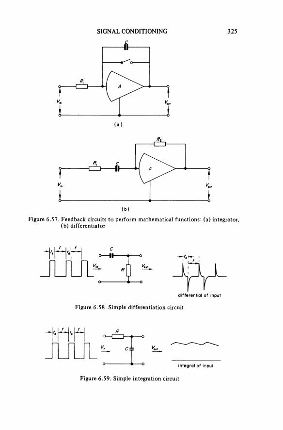
SIGNAL CONDITIONING 325
Figure 6.57. Feedback circuits to perform mathematical functions: (a) integrator, (b) differentiator
(a)
(b)
Figure 6.58. Simple differentiation circuit
differential of input
Figure 6.59. Simple integration circuit
integral of input
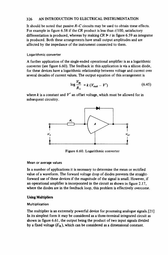
326 AN INTRODUCTION TO ELECTRICAL INSTRUMENTATION
It should be noted that passive R-C circuits may be used to obtain these effects. For example in figure 6.58 if the CR product is less than t/100, satisfactory differentiation is produced, whereas by making CR >> tin figure 6.59 an integrator is produced. Both these arrangements have small output amplitudes and are affected by the impedance of the instrument connected to them.
Logarithmic converter
A further application of the single-ended operational amplifier is as a logarithmic converter (see figure 6.60). The feedback in this application is via a silicon diode, for these devices have a logarithmic relationship between voltage and current over several decades of current values. The output equation of this arrangement is
(6.45)
where k is a constant and V' an offset voltage, which must be allowed for in subsequent circuitry.
Figure 6.60. Logarithmic converter
Mean or average values
In a number of applications it is necessary to determine the mean or rectified value of a waveform. The forward voltage drop of diodes prevents the straight-forward use of these devices if the magnitude of the signal is small. However, if an operational amplifier is incorporated in the circuit as shown in figure 2.17, where the diodes are in the feedback loop, this problem is effectively overcome.
Using Multipliers
Multiplication
The multiplier is an extremely powerful device for processing analogue signals. [21] In its simplest form it may be considered as a three-terminal integrated circuit as shown in figure 6.61, the output being the product of two input signals divided by a fixed voltage (ER), which can be considered as a dimensional constant.
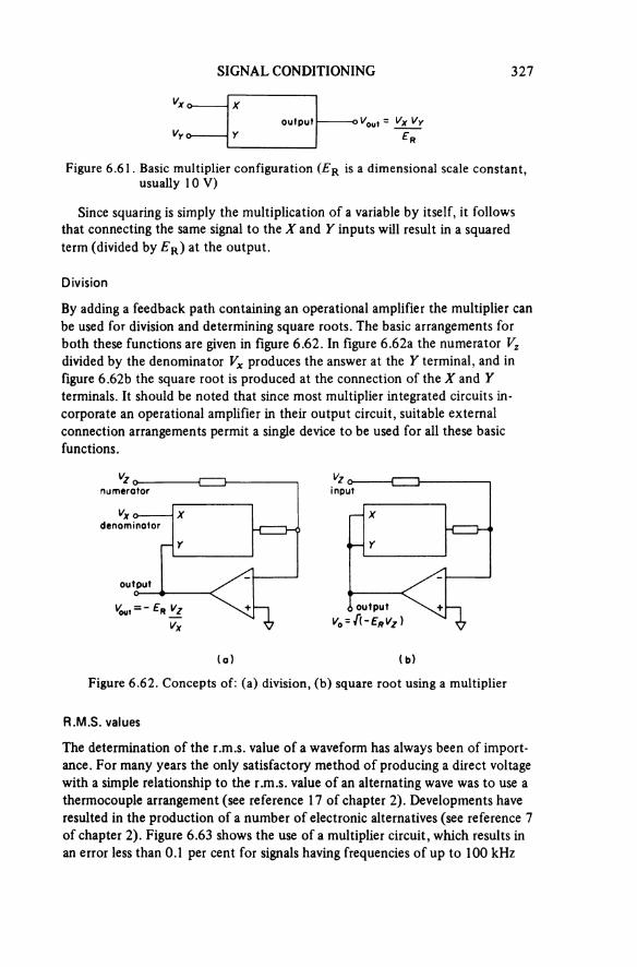
SIGNAL CONDITIONING 327
Figure 6.61. Basic multiplier configuration (ER is a dimensional scale constant, usually 10 V)
output
Since squaring is simply the multiplication of a variable by itself, it follows that connecting the same signal to the X and Y inputs will result in a squared term (divided by ER) at the output.
Division
By adding a feedback path containing an operational amplifier the multiplier can be used for division and determining square roots. The basic arrangements for both these functions are given in figure 6.62. In figure 6.62a the numerator Vz divided by the denominator Vx produces the answer at the Y terminal, and in figure 6.62b the square root is produced at the connection of the X and Y terminals. It should be noted that since most multiplier integrated circuits in-corporate an operational amplifier in their output circuit, suitable external connection arrangements permit a single device to be used for all these basic functions.
Figure 6.62. Concepts of: (a) division, (b) square root using a multiplier
(a)
vznumerator
Vxdenominator
output
(b)
input
output
R.M.S. values
The determination of the r.m.s. value of a waveform has always been of import-ance. For many years the only satisfactory method of producing a direct voltage with a simple relationship to the r.m.s. value of an alternating wave was to use a thermocouple arrangement (see reference 17 of chapter 2). Developments have resulted in the production of a number of electronic alternatives (see reference 7 of chapter 2). Figure 6.63 shows the use of a multiplier circuit, which results in an error less than 0.1 per cent for signals having frequencies of up to 100 kHz
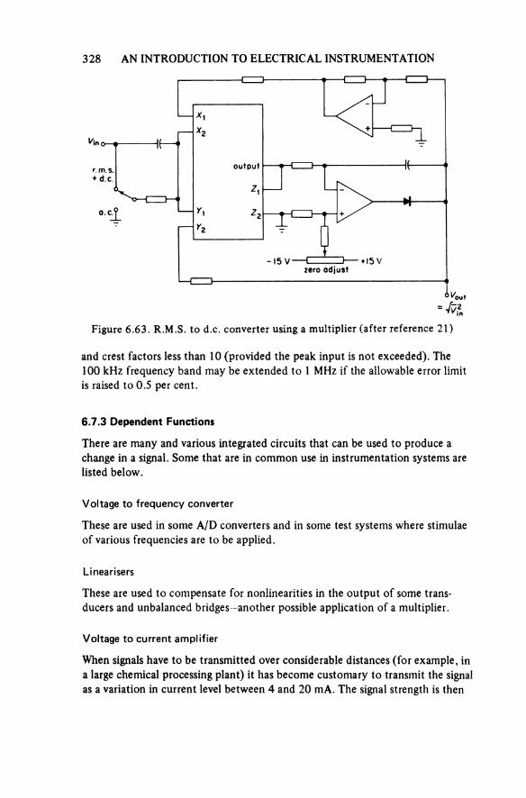
328 AN INTRODUCTION TO ELECTRICAL INSTRUMENTATION
Figure 6.63. R.M.S. to d.c. converter using a multiplier (after reference 21)
r.m.s. + d.c.
output
zero adjust
and crest factors less than 10 (provided the peak input is not exceeded). The 100 kHz frequency band may be extended to 1 MHz if the allowable error limit is raised to 0.5 per cent.
6.7.3 Dependent Functions
There are many and various integrated circuits that can be used to produce a change in a signal. Some that are in common use in instrumentation systems are listed below.
Voltage to frequency converter
These are used in some A/D converters and in some test systems where stimulae of various frequencies are to be applied.
Linearisers
These are used to compensate for nonlinearities in the output of some trans-ducers and unbalanced bridges—another possible application of a multiplier.
Voltage to current amplifier
When signals have to be transmitted over considerable distances (for example, in a large chemical processing plant) it has become customary to transmit the signal as a variation in current level between 4 and 20 mA. The signal strength is then

SIGNAL CONDITIONING 329
independent of variations in circuit resistance, a fault is normally apparent as a zero current condition and the signal simply reconverted to a voltage by passing the current through a known stable resistance.
6.8 DIGITAL-ANALOGUE CONVERSION
The use of digital displays has undisputed advantages of clarity, reduction of operator fatigue, etc., over an analogue display, and a number of analogue to digital conversion techniques are described in connection with the operation of digital voltmeters (see section 4.2.1). However, it is sometimes advantageous to convert digital signals to analogue ones for display purposes, for example, present ing computer output in graphical form. The process of digital to analogue (D/A) conversion is illustrated in principle in figure 6.64, where the summation proper-ties of an operational amplifier are used to form an analogue voltage from digital
Figure 6.64. Digital to analogue converter
switches
information. The summing resistors, R, have values in a binary progression and are connected to a fixed voltage source via switches (bistable circuits) which are controlled by the digital information. The voltage source must have a precisely known value, and the summing resistors must be stable. The scale of the output voltage will be dependent on the value of the feedback resistor R2.
REFERENCES
1 Jan Slyper, Advanced d.c. calibration techniques, E.E.E. European Seminar(Fluke Manufacturing Co., Seattle, Wash., 1969)
2 E. W. Golding and F. C. Widdis, Electrical Measurements and MeasuringInstruments (Pitman, London, 1963)
3 J. J. Hill and A. P. Miller, A seven decade adjustable ratio inductivelycoupled voltage divider with 0.1 ppm accuracy, Proc. I.E.E., 109B (1962) 157-62
4 Britain’s first 400 kV cascade-voltage transformers. Electronics Power, 13(1967) 470-1
330 AN INTRODUCTION TO ELECTRICAL INSTRUMENTATION
5 B. D. Jenkins, Introduction to Instrument Transformers (Newnes, London,1967)
6 F. E. Terman and J. M. Petit, Electronic Measurements (McGraw-Hill, NewYork, 1952)
7 F. K. Harris, Electrical Measurements (Wiley, New York, 1962)8 J. H. Parks, Shunts and inductors for surge current measurements,/. Res.
natn. Bur. Stand., 39 (1947) 1919 S. J. Turner, The operation and application of direct current transformers,
Electl Equip., 17 (1978) 71-6I 0 The Royal Signals Handbook of Line Communications, Vol. 1 (H.M.S.O.,
1947)II M. Sucher and J. Fox (ed.). Handbook of Microwave Measurements (Wiley,
New York, 1965)12 H. Y-F. Lam, Analog and Digital Filters; Design and Realisation (Prentice-
Hall, Englewood Cliffs, N.J., 1979)13 R. W. Henry, Electronic Systems and Instrumentation (Wiley, Chichester,
1978)14 —, Probes, parts I and U, Tekscope, 6 No. 2, 8-11, No. 3, 10-14 (1974)15 R. Lang, A new and low-cost 500 MHz probe, Tekscope, 8 (1976) 11-1316 P. A. Lynn, An Introduction to the Analysis and Processing of Signals
(Macmillan, London and Basingstoke, 1973)17 S. Stein and J. Jay Jones, Modern Communication Principles (McGraw-Hill,
New York, 1967)18 R. Morrison, D.C. Amplifiers in Instrumentation (Wiley, New York, 1970)19 G. B. Clayton, Operational Amplifiers (Butterworth, London, 1971)20 R. J. Isaacs, Optimising op. amps. Wireless Wld, 79 (1973) 185-621 D. H. Sheingold (ed.), Multiplier Application Guide (Analog Devices Inc.,
New York, 1978)

7Interference and Screening
In practical engineering the conduction of an electrical signal from the measurand to a measuring instrument can be affected by a number of forms of interference. These may, broadly speaking, be divided into
(a) the effects of the environment on the component parts of an instrument, or measurement system;
(b) impurities in individual components and their effects on the measuring system; and
(c) injection of unwanted signals from unrelated electrical circuits and fields into the measuring system.
7.1 ENVIRONMENTAL EFFECTS
The resultant effect of environmental interference is usually apparent as a gradual change, or drift, in the output from part of the measuring system when there is no change in the input.
7.1.1 Thermal Effects
These are undoubtedly the most common causes of drift and may be due to heat-ing of components within an instrument, or due to changes in the ambient temperature.
Expansion coefficient
Temperature changes will cause dimension changes dependent on the thermal coefficient of expansion of the material from which components are constructed. This causes, for example, changes in the dimensions of inductors which in turn

332 AN INTRODUCTION TO ELECTRICAL INSTRUMENTATION
cause a change of magnitude. If a number of different materials, each with its own coefficient of expansion, are involved in the construction of a component, mechanical stresses will result and these can also cause a change in value particularly if semiconductor devices are involved.
Resistance coefficient
Conductive materials and those used in the construction of resistors have, in addition to the temperature coefficient of expansion, a temperature coefficient of resistance, that is, their resistance is temperature dependent. Hence in sensitive instrumentation systems it is essential for components with small temperature coefficients to be used in a constant temperature environment. This latter requirement explains why it is necessary to provide in the measurement uncer-tainty specification an allowance for the effects of temperature, should a particular instrument be operated outside a specified temperature range.
Thermoelectric generation
The production of voltage by this process has been described elsewhere (section 5.4.3) and since junctions between dissimilar materials are inevitable, for example, at the ends of a resistor, care may be necessary to ensure that components arearranged so that pairs of junctions are at the same temperature, that is, a resistor should be mounted horizontally rather than vertically; also it is necessaryto ensure that excessive heating of components is avoided by arranging that they are operated well below their rated capacity.
7.1.2 Humidity Effects
The effects of the moisture content of air generally tend to be small although some materials used in the construction of components are hygroscopic and this will affect the value of the component when the humidity changes. This may be due to a variation in conduction or in the dielectric properties [1] of materials. Alternatively, it may be due to the absorption of moisture in materials (for example, wood) causing a dimensional change and a consequent change in component value, this latter effect being one reason for stipulating an allowable humidity band in the operation of a standards laboratory. [2]
The combination of high humidity, causing condensation, and dirt on surfaces may have two results, as follows.
Leakage resistance
The surface resistance between terminals of an instrument with a high (say 100 MΩ) input resistance, must be very much greater than the specified value. However, should the surface become contaminated with dirt and moisture, a reduction in the surface resistance will result, eventually leading to a situation
INTERFERENCE AND SCREENING 333
in which the instrument’s input resistance specification is no longer met. The same result can also be obtained by irresponsible use—do not handle surfaces that have to provide a large surface resistance, except in a clean room with recommended procedures and equipment.
Galvanic voltages
The use of electronic production techniques in instruments is now so extensive that it is evident that few, if any, contemporary sensitive instruments do not have a printed circuit in their construction. A problem that might arise from this situation, particularly after a repair or modification involving soldering, is that a condition may be created in which a copper strip is linked via a dried flux path to a soldered joint. If the flux is acid based and becomes damp, the constituent parts of a battery (copper plus acid plus zinc) are present and a galvanic voltage is produced which can add to (or subtract from) the measurand.
7.1.3 Pressure
The effects of environmental pressure changes are most likely to occur in the instances that involve the dielectric properties of air at atmospheric pressure. A situation where this is possible is one in which an air vane capacitor is in use, but fortunately the change in capacitance due to the small changes in dielectric will be very small and therefore normally negligible.
Of greater consequence is the effect of pressure in the method used for measur-ing a high voltage by the breakdown of an air gap between spheres. In setting a gap length for a particular voltage, an allowance must be made for any deviation from a pressure of 760 mm of mercury (see BS 358: 1960). Should relatively rapid changes in pressure occur due, say, to unsettled weather conditions, inconsist-ency in measurement will result.
7.1.4 Multiple Earths and Earth Loops
Ideally all the earth connections in a system are at the same (zero) potential but this can only be true if the earth path has zero resistance and inductance. This is not possible in a practical case, and any circuits which use the earth connections as a current return path will cause a voltage gradient to exist along the earth path. Two effects result from this. First, capacitive coupling between the earth path and the signal conductor may result in electrostatic interference being added to the signal. Secondly, if the return current is added to earth currents from shields and other circuits, these will appear to the measuring circuit as an increase in signal level.
To reduce this type of interference it is vital to avoid using the earth path as a signal return path, and also to make sure that a circuit is only earthed at one point—if more than one point is used and currents are flowing in the earth path,

334 AN INTRODUCTION TO ELECTRICAL INSTRUMENTATION
Figure 7.1. Earth loop and circulating current
sourceinstrument
a current i will circulate through the signal circuit (see figure 7.1), the magnitude of i depending on v, the volt drop between earth points and the lead resistances. [3, 4] This circulatory path is termed an earth loop.
7.1.5 Inherent Noise
Some noise or unwanted signals that are present in a sensitive measuring system are generated within the components or parts of the system. One such source of electrical noise results from poor connections, which may be due to bad solder-ing or dirt on switch contacts. It is therefore vital when dealing with small signal levels that great care is taken in forming joints and contacts. Another source of noise (normally at twice power frequency) is that which results from insufficient smoothing of direct voltage supplies to such items as amplifiers.
Voltage and current noise also result from the energy fluctuations generated by the random movement of free electrons within a conductor (Brownian move-ment). The spectrum of this noise covers all frequencies and is the limiting level to which noise may be reduced in a sensitive measuring system. Its effect may only be limited by making the system bandwidth as narrow as is acceptable in relation to the bandwidth of the signal.
7.2 COMPONENT IMPURITIES
It is almost impossible to manufacture a component so that it has only one property: for example, a resistance will have an associated reactance, a capacitor will have a leakage resistance and an inductor will have a resistance per turn and an interturn capacitance. However, a particular quantity may be made dominant, and it is possible to design ‘pure’ components for specified limits of operation.
Under zero frequency conditions of operation the quantity most likely to cause interference is the leakage resistance of insulating materials, where con-duction may be either through the material or across its surface. When compon-ents have, for isolation purposes, to be mounted on insulating supports, the insulation should be of good quality and have sufficient length so that the conduction paths between the terminals of the component and between the

INTERFERENCE AND SCREENING 335
component and earth are of negligible consequence. This is of particular impor-tance when high voltages are in use, or when high resolution measurements are being made.
7.2.1 Frequency Effects
The effects of frequency on the permittivity and dielectric loss of an insulating material are of consequence and figure 7.2 shows typical characteristics. These variations are largely due to polarisation effects, of which there are two types— dipole and interfacial. Dipole polarisation occurs in dielectrics having polar
Figure 7.2. Frequency characteristics of some insulating materials (see reference 7)
rela
tive p
erm
ittiv
ity er
loss
angl
e
Frequency ( Hz)
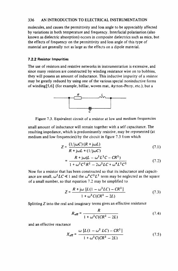
336 AN INTRODUCTION TO ELECTRICAL INSTRUMENTATION
molecules, and causes the permittivity and loss angle to be appreciably affected by variations in both temperature and frequency. Interfacial polarisation (also known as dielectric absorption) occurs in composite dielectrics such as mica, but the effects of frequency on the permittivity and loss angle of this type of material are generally not as large as the effects on a dipole material.
7.2.2 Resistor Impurities
The use of resistors and resistive networks in instrumentation is extensive, and since many resistors are constructed by winding resistance wire on to bobbins, they will possess an amount of inductance. This inductive impurity of a resistor may be greatly reduced by using one of the various special noninductive forms of winding [5, 6] (for example, bifilar, woven mat, Ayrton-Perry, etc.), but a
Figure 7.3. Equivalent circuit of a resistor at low and medium frequencies
small amount of inductance will remain together with a self capacitance. The resulting impedance, which is predominantly resistive, may be represented (at medium and low frequencies) by the circuit in figure 7.3 from which
(7.1)
(7.2)
Now for a resistor that has been constructed so that its inductance and capacit-ance are small, ω2LC << 1 and the ω4C2L2 term may be neglected as the square of a small number, so that equation 7.2 may be simplified to
(7.3)
Splitting Z into the real and imaginary terms gives an effective resistance
(7.4)
and an effective reactance
(7.5)
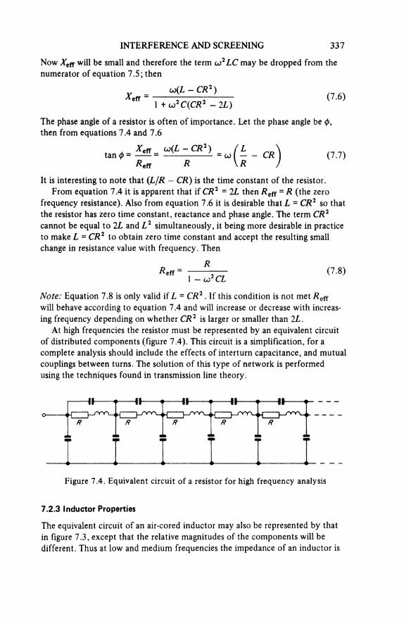
INTERFERENCE AND SCREENING 337
Now Xeff will be small and therefore the term ω2LC may be dropped from the numerator of equation 7.5; then
(7.6)
The phase angle of a resistor is often of importance. Let the phase angle be 0, then from equations 7.4 and 7.6
(7.7)
It is interesting to note that (L/R - CR) is the time constant of the resistor.From equation 7.4 it is apparent that if CR2 = 2L then Reff = R (the zero
frequency resistance). Also from equation 7.6 it is desirable that L = CR2 so that the resistor has zero time constant, reactance and phase angle. The term CR2 cannot be equal to 2L and L2 simultaneously, it being more desirable in practice to make L = CR2 to obtain zero time constant and accept the resulting small change in resistance value with frequency. Then
(7.8)
Note: Equation 7.8 is only valid if L = CR2. If this condition is not met Reff will behave according to equation 7.4 and will increase or decrease with increas-ing frequency depending on whether CR2 is larger or smaller than 2L.
At high frequencies the resistor must be represented by an equivalent circuit of distributed components (figure 7.4). This circuit is a simplification, for a complete analysis should include the effects of interturn capacitance, and mutual couplings between turns. The solution of this type of network is performed using the techniques found in transmission line theory.
Figure 7.4. Equivalent circuit of a resistor for high frequency analysis
7.2.3 Inductor Properties
The equivalent circuit of an air-cored inductor may also be represented by that in figure 7.3, except that the relative magnitudes of the components will be different. Thus at low and medium frequencies the impedance of an inductor is
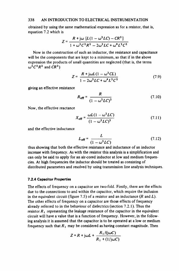
338 AN INTRODUCTION TO ELECTRICAL INSTRUMENTATION
obtained by using the same mathematical expression as for a resistor, that is equation 7.2 which is
Now in the construction of such an inductor, the resistance and capacitance will be the components that are kept to a minimum, so that if in the above expression the products of small quantities are neglected (that is, the terms ω2C2/R2 and CR2)
(7.9)
giving an effective resistance
(7.10)
Now, the effective reactance
(7.11)
and the effective inductance
(7.12)
thus showing that both the effective resistance and inductance of an inductor increase with frequency. As with the resistor this analysis is a simplification and can only be said to apply for an air-cored inductor at low and medium frequen-cies. At high frequencies the inductor should be treated as consisting of distributed parameters and resolved by using transmission line analysis techniques.
7.2.4 Capacitor Properties
The effects of frequency on a capacitor are two-fold. Firstly, there are the effects due to the connections to and within the capacitor, which require the inclusion in the equivalent circuit (figure 7.5) of a resistor and an inductance (R and L).The other effects of frequency on a capacitor are those effects of frequency already referred to in the behaviour of dielectrics (section 7.2.1). Thus the resistor R1 representing the leakage resistance of the capacitor in the equivalent circuit will have a value that is a function of frequency. However, in the follow-ing analysis it is assumed that the capacitor is to be operated at a low or mediumfrequency such that R1 may be considered as having constant magnitude. Then

INTERFERENCE AND SCREENING 339
Figure 7.5. Equivalent circuit of a capacitor
lead impedance
(7.13)Also
effective reactance =
or
(7.14)
and provided that ω2/R12C2 is large compared with 1
The effective capacitance (medium frequencies) is
(7.15)Note: At the frequency ω = l/(LC)1/2 a resonant condition will be produced; it is therefore important that the inductance of leads is kept to a minimum so thatthe resonant frequency is high.
The effective series resistance (medium frequency) is
(7.16)
The loss angle δ is obtained from
(7.17)
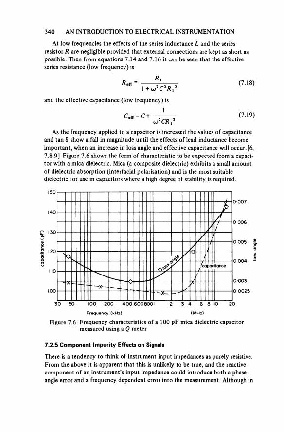
340 AN INTRODUCTION TO ELECTRICAL INSTRUMENTATION
At low frequencies the effects of the series inductance L and the series resistor R are negligible provided that external connections are kept as short as possible. Then from equations 7.14 and 7.16 it can be seen that the effective series resistance (low frequency) is
(7.18)
and the effective capacitance (low frequency) is
(7.19)
As the frequency applied to a capacitor is increased the values of capacitance and tan δ show a fan in magnitude until the effects of lead inductance become important, when an increase in loss angle and effective capacitance will occur. [6, 7, 8, 9] Figure 7.6 shows the form of characteristic to be expected from a capaci-tor with a mica dielectric. Mica (a composite dielectric) exhibits a small amount of dielectric absorption (interfacial polarisation) and is the most suitable dielectric for use in capacitors where a high degree of stability is required.
Figure 7.6. Frequency characteristics of a 100 pF mica dielectric capacitor measured using a Q meter
capa
citan
ce (p
F)
loss
angl
e
Frequency (kHz) (MHz)
7.2.5 Component Impurity Effects on Signals
There is a tendency to think of instrument input impedances as purely resistive. From the above it is apparent that this is unlikely to be true, and the reactive component of an instrument’s input impedance could introduce both a phase angle error and a frequency dependent error into the measurement. Although in
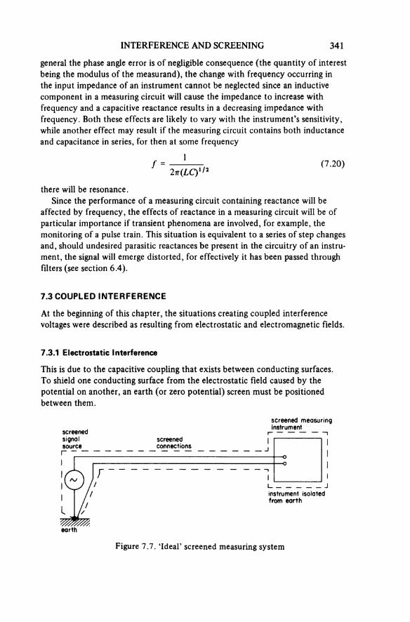
INTERFERENCE AND SCREENING 341
general the phase angle error is of negligible consequence (the quantity of interest being the modulus of the measurand), the change with frequency occurring in the input impedance of an instrument cannot be neglected since an inductive component in a measuring circuit will cause the impedance to increase with frequency and a capacitive reactance results in a decreasing impedance with frequency. Both these effects are likely to vary with the instrument’s sensitivity, while another effect may result if the measuring circuit contains both inductance and capacitance in series, for then at some frequency
(7.20)
there will be resonance.Since the performance of a measuring circuit containing reactance will be
affected by frequency, the effects of reactance in a measuring circuit will be of particular importance if transient phenomena are involved, for example, the monitoring of a pulse train. This situation is equivalent to a series of step changes and, should undesired parasitic reactances be present in the circuitry of an instru-ment, the signal will emerge distorted, for effectively it has been passed through filters (see section 6.4).
7.3 COUPLED INTERFERENCE
At the beginning of this chapter, the situations creating coupled interference voltages were described as resulting from electrostatic and electromagnetic fields.
7.3.1 Electrostatic Interference
This is due to the capacitive coupling that exists between conducting surfaces. To shield one conducting surface from the electrostatic field caused by the potential on another, an earth (or zero potential) screen must be positioned between them.
Figure 7.7. ‘Ideal’ screened measuring system
screenedsignalsource
screenedconnections
screened measuring instrument
instrument isolated from earth
earth
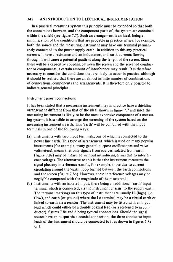
342 AN INTRODUCTION TO ELECTRICAL INSTRUMENTATION
In a practical measuring system this principle must be extended so that boththe connections between, and the component parts of, the system are contained within the shield (see figure 7.7). Such an arrangement is an ideal, being a simplification of the conditions that are probable in practice where, for example, both the source and the measuring instrument may have one terminal perman-ently connected to the power supply earth. In addition to this any practical screen will have a resistance and an inductance, and earth currents flowing through it will cause a potential gradient along the length of the screen. Since there will be a capacitive coupling between the screen and the screened conduc-tor or components, a certain amount of interference may result. It is therefore necessary to consider the conditions that are likely to occur in practice, although it should be realised that there are an almost infinite number of combinations of connections, components and arrangements. It is therefore only possible to indicate general principles.
Instrument screen connections
It has been stated that a measuring instrument may in practice have a shielding arrangement different from that of the ideal shown in figure 7.7 and since the measuring instrument is likely to be the most expensive component of a measur-ing system, it is sensible to arrange the screening of the system based on the measuring instrument’s earth. This ‘earth’ will be combined with the input terminals in one of the following ways.
(a) Instruments with two input terminals, one of which is connected to the power line earth. This type of arrangement, which is used on many popular instruments (for example, many general purpose oscilloscopes and valve voltmeters), means that only signals from sources isolated from earth (figure 7.8a) may be measured without introducing errors due to interfer-ence voltages. The alternative to this is that the instrument measures the signal plus any interference e.m.f.s, for example, those due to current circulating around the ‘earth’ loop formed between the earth connections and the screen (figure 7.8b). However, these interference voltages may be negligible compared with the magnitude of the measurand.
(b) Instruments with an isolated input, there being an additional ‘earth’ input terminal which is connected, via the instrument chassis, to the supply earth. The terminal markings on this type of instrument are usually Hi (high), Lo (low), and earth (or ground) where the Lo terminal may be a virtual earth or linked to earth via a resistor. The instrument may be fitted with an input lead which could either be a double coaxial lead (or a screened twin con-ductor), figures 7.8c and d being typical connections. Should the signal source have an output via a coaxial connection, the three conductor input leads of the instrument should be connected to it as shown in figures 7.8e or f.
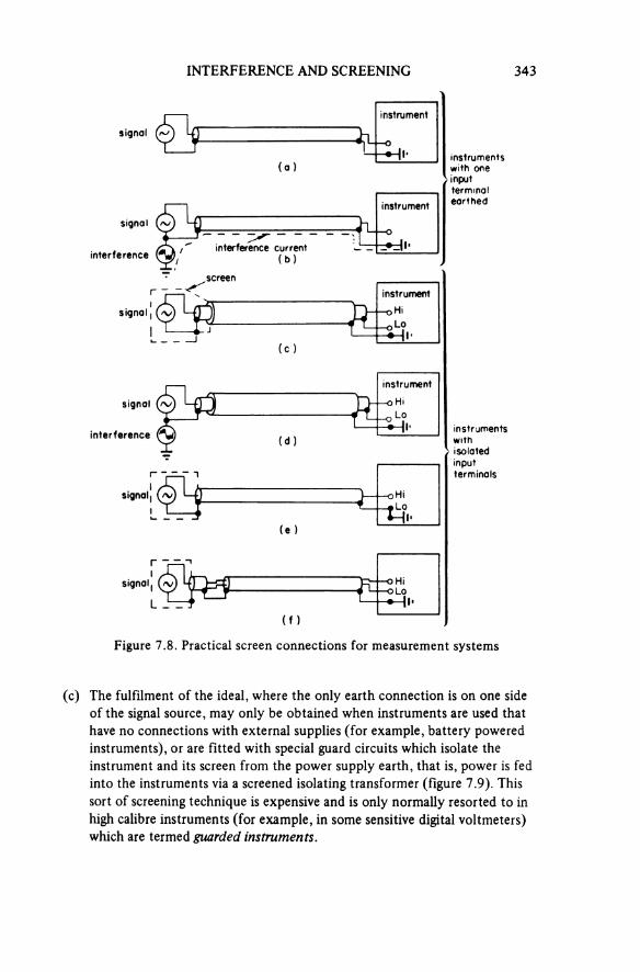
INTERFERENCE AND SCREENING 343
Figure 7.8. Practical screen connections for measurement systems
(a)
signal
instrument
(b)
signal
instrument
interferenceinterference current
(c )
signal
instrument
(d)
signal
instrument
interference
(e)
signal HiLo
(f )
signal HiLo
instrumentswithisolatedinputterminals
(c) The fulfilment of the ideal, where the only earth connection is on one side of the signal source, may only be obtained when instruments are used that have no connections with external supplies (for example, battery powered instruments), or are fitted with special guard circuits which isolate the instrument and its screen from the power supply earth, that is, power is fed into the instruments via a screened isolating transformer (figure 7.9). This sort of screening technique is expensive and is only normally resorted to in high calibre instruments (for example, in some sensitive digital voltmeters) which are termed guarded instruments.
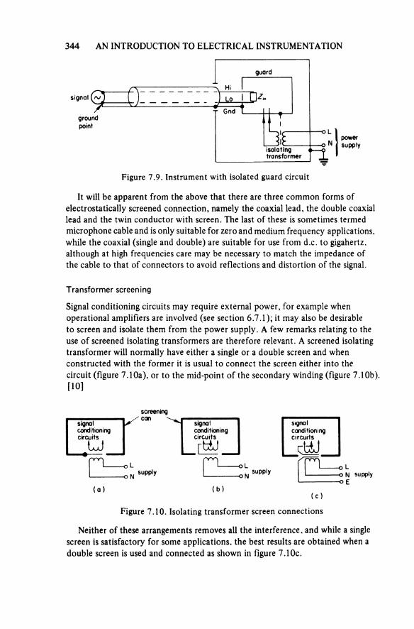
344 AN INTRODUCTION TO ELECTRICAL INSTRUMENTATION
Figure 7.9. Instrument with isolated guard circuit
guard
signal
groundpoint
Hi
Lo
Gnd
isolatingtransformer
powersupply
It will be apparent from the above that there are three common forms of electrostatically screened connection, namely the coaxial lead, the double coaxial lead and the twin conductor with screen. The last of these is sometimes termed microphone cable and is only suitable for zero and medium frequency applications, while the coaxial (single and double) are suitable for use from d.c. to gigahertz, although at high frequencies care may be necessary to match the impedance of the cable to that of connectors to avoid reflections and distortion of the signal.
Transformer screening
Signal conditioning circuits may require external power, for example when operational amplifiers are involved (see section 6.7.1); it may also be desirable to screen and isolate them from the power supply. A few remarks relating to the use of screened isolating transformers are therefore relevant. A screened isolating transformer will normally have either a single or a double screen and when constructed with the former it is usual to connect the screen either into the circuit (figure 7.10a), or to the mid-point of the secondary winding (figure 7.10b). [10]
Figure 7.10. Isolating transformer screen connections
(a)
signal conditioning circuits
supply
screening can
(b)
signalconditioningcircuits
supply
(c)
signalconditioningcircuits
supply
Neither of these arrangements removes all the interference, and while a single screen is satisfactory for some applications, the best results are obtained when a double screen is used and connected as shown in figure 7.10c.
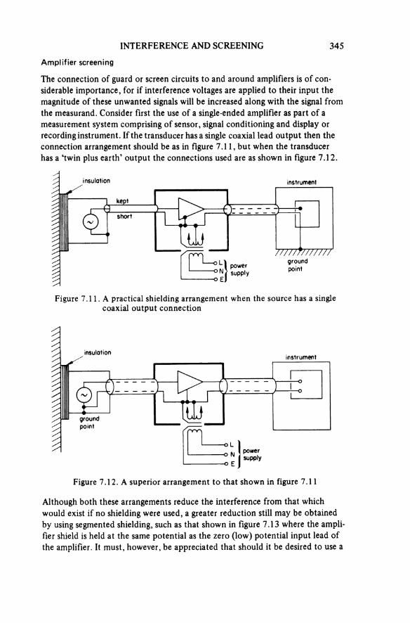
INTERFERENCE AND SCREENING 345
Amplifier screening
The connection of guard or screen circuits to and around amplifiers is of con-siderable importance, for if interference voltages are applied to their input the magnitude of these unwanted signals will be increased along with the signal from the measurand. Consider first the use of a single-ended amplifier as part of a measurement system comprising of sensor, signal conditioning and display or recording instrument. If the transducer has a single coaxial lead output then the connection arrangement should be as in figure 7.11, but when the transducer has a ‘twin plus earth’ output the connections used are as shown in figure 7.12.
Figure 7.11. A practical shielding arrangement when the source has a single coaxial output connection
insulation
kept
short
instrument
powersupply
groundpoint
Figure 7.12. A superior arrangement to that shown in figure 7.11
insulation
groundpoint
instrument
powersupply
Although both these arrangements reduce the interference from that which would exist if no shielding were used, a greater reduction still may be obtained by using segmented shielding, such as that shown in figure 7.13 where the ampli-fier shield is held at the same potential as the zero (low) potential input lead of the amplifier. It must, however, be appreciated that should it be desired to use a
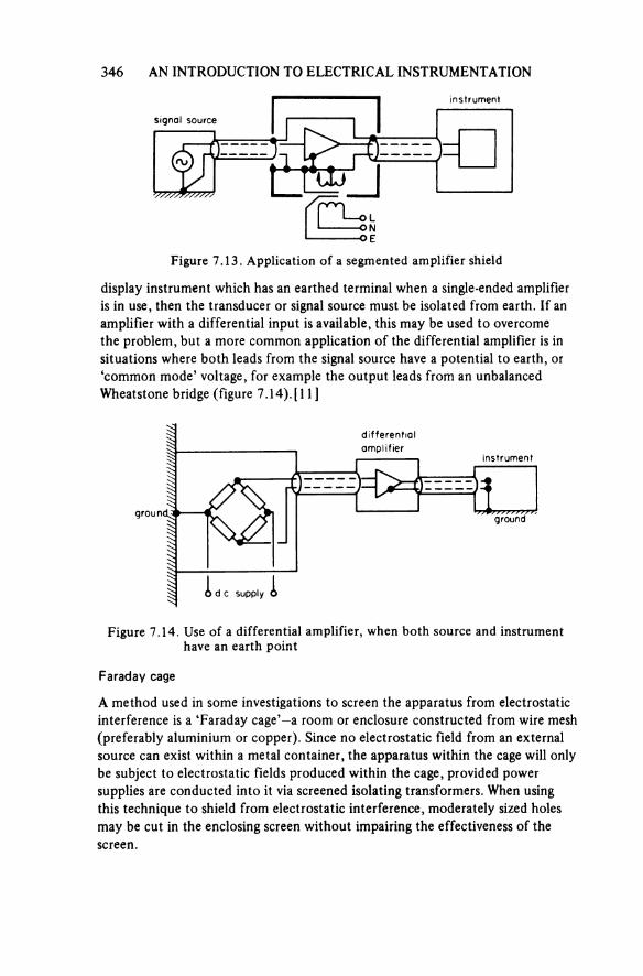
346 AN INTRODUCTION TO ELECTRICAL INSTRUMENTATION
Figure 7.13. Application of a segmented amplifier shield
signal source
instrument
display instrument which has an earthed terminal when a single-ended amplifier is in use, then the transducer or signal source must be isolated from earth. If an amplifier with a differential input is available, this may be used to overcome the problem, but a more common application of the differential amplifier is in situations where both leads from the signal source have a potential to earth, or ‘common mode’ voltage, for example the output leads from an unbalanced Wheatstone bridge (figure 7.14). [11]
Figure 7.14. Use of a differential amplifier, when both source and instrument have an earth point
differentialamplifier
instrument
ground ground
d c supply
Faraday cage
A method used in some investigations to screen the apparatus from electrostatic interference is a ‘Faraday cage’—a room or enclosure constructed from wire mesh (preferably aluminium or copper). Since no electrostatic field from an external source can exist within a metal container, the apparatus within the cage will only be subject to electrostatic fields produced within the cage, provided power supplies are conducted into it via screened isolating transformers. When using this technique to shield from electrostatic interference, moderately sized holes may be cut in the enclosing screen without impairing the effectiveness of the screen.
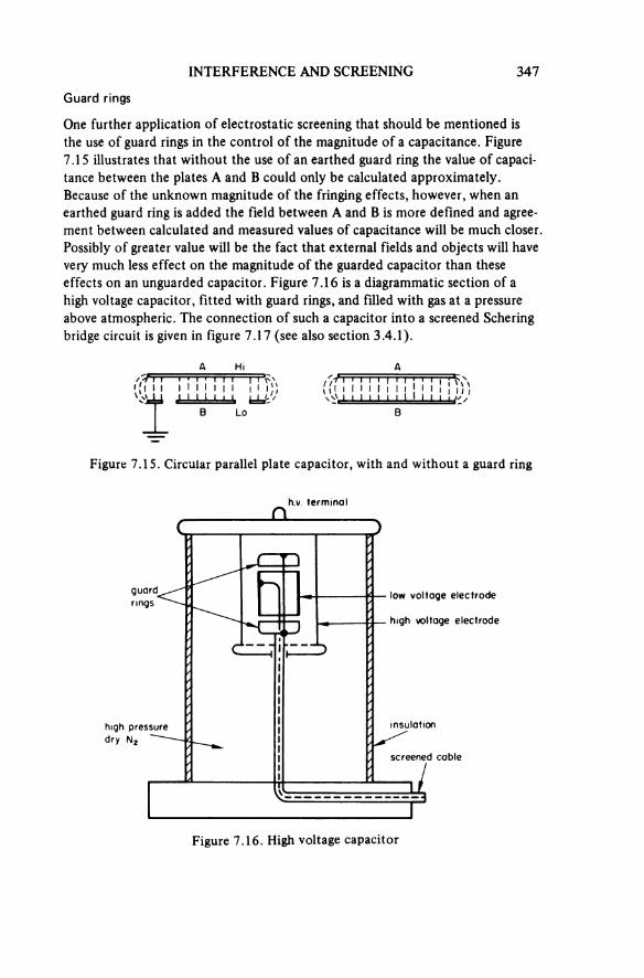
INTERFERENCE AND SCREENING 347
Guard rings
One further application of electrostatic screening that should be mentioned is the use of guard rings in the control of the magnitude of a capacitance. Figure 7.15 illustrates that without the use of an earthed guard ring the value of capaci-tance between the plates A and B could only be calculated approximately.Because of the unknown magnitude of the fringing effects, however, when an earthed guard ring is added the field between A and B is more defined and agree-ment between calculated and measured values of capacitance will be much closer. Possibly of greater value will be the fact that external fields and objects will have very much less effect on the magnitude of the guarded capacitor than theseeffects on an unguarded capacitor. Figure 7.16 is a diagrammatic section of a high voltage capacitor, fitted with guard rings, and filled with gas at a pressureabove atmospheric. The connection of such a capacitor into a screened Schering bridge circuit is given in figure 7.17 (see also section 3.4.1).
Figure 7.15. Circular parallel plate capacitor, with and without a guard ring
Figure 7.16. High voltage capacitor
h.v. terminal
guardrings
low voltage electrode
high voltage electrode
high pressure dry N2
insulation
screened cable

348 AN INTRODUCTION TO ELECTRICAL INSTRUMENTATION
Figure 7.17. Shielding arrangement of a high voltage Schering bridge
h.v.transformer
supply
sample standard
protectivegap
7.3.2 Electromagnetic Interference
Since this form of interference results from the electromagnetic coupling of a current carrying conductor with other conductors, the most likely sources of this type of interference are power supply connections and transformers. It is evident that signal carrying conductors should be kept well clear of such items, and if necessary screened from them by using a shield made from a high permea-bility material.
To eliminate the effects of r.f. electromagnetic interference it may be necessary to place equipment subject to r.f. interference in a screened enclosure or room. The shield material used for such a construction is usually copper sheet, and since the prevention of electromagnetic interference is only possible if the screen is complete, all joints must be electrically continuous and of low resistance, that is, there must not be any open circuits at doors, etc. Power supplied into such an enclosure should be filtered and screened, the filter having a shunt capacitor (low impedance at high frequency) followed by a series inductor (high imped-ance at high frequency).
Electrostatically screened conductors [3, 4] (for example, coaxial connections) afford a certain amount of protection from electromagnetic interference, and provided the magnetic field strength is not too large, satisfactory shielding from electromagnetic fields may be obtained by using screening intended for shielding from electrostatic fields. Similarly a shield designed for shielding from electro-magnetic interference will afford an amount of electrostatic screening.
7.3.3 Cross Talk
When several signal carrying circuits are routed via a ribbon conductor or a multi-conductor cable, interference or cross talk between circuits may occur. The magnitude of this form of interference, which appears as a mixing of signals, is dependent on a combination of electrostatic and electromagnetic coupling and results from the size and spacing of conductors, the strength of the signals and
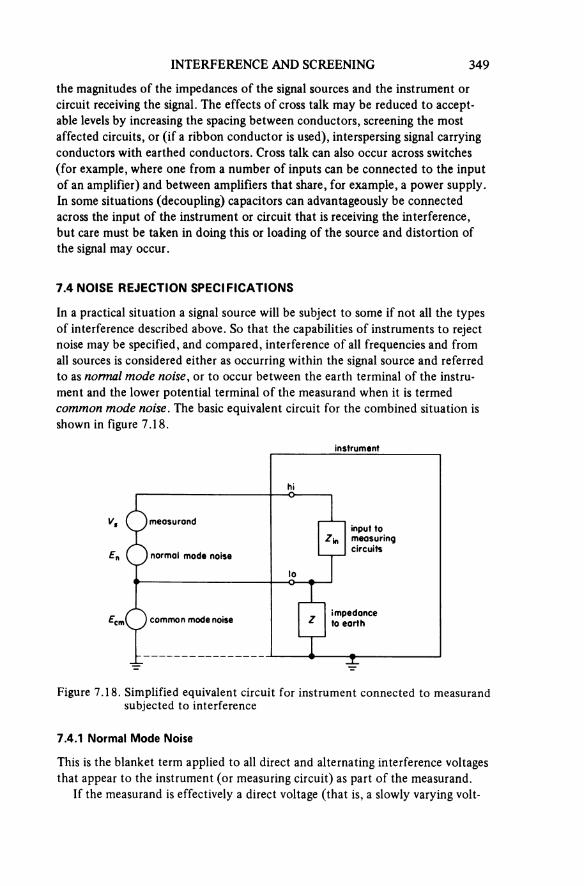
INTERFERENCE AND SCREENING 349
the magnitudes of the impedances of the signal sources and the instrument or circuit receiving the signal. The effects of cross talk may be reduced to accept-able levels by increasing the spacing between conductors, screening the most affected circuits, or (if a ribbon conductor is used), interspersing signal carrying conductors with earthed conductors. Cross talk can also occur across switches (for example, where one from a number of inputs can be connected to the input of an amplifier) and between amplifiers that share, for example, a power supply. In some situations (decoupling) capacitors can advantageously be connectedacross the input of the instrument or circuit that is receiving the interference, but care must be taken in doing this or loading of the source and distortion of the signal may occur.
7.4 NOISE REJECTION SPECIFICATIONS
In a practical situation a signal source will be subject to some if not all the types of interference described above. So that the capabilities of instruments to reject noise may be specified, and compared, interference of an frequencies and from an sources is considered either as occurring within the signal source and referred to as normal mode noise, or to occur between the earth terminal of the instru-ment and the lower potential terminal of the measurand when it is termed common mode noise. The basic equivalent circuit for the combined situation is shown in figure 7.18.
Figure 7.18. Simplified equivalent circuit for instrument connected to measurand subjected to interference
instrument
measurand
normal mode noise
input tomeasuringcircuits
common mode noiseimpedance to earth
7.4.1 Normal Mode Noise
This is the blanket term applied to all direct and alternating interference voltages that appear to the instrument (or measuring circuit) as part of the measurand.
If the measurand is effectively a direct voltage (that is, a slowly varying volt-
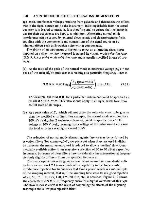
350 AN INTRODUCTION TO ELECTRICAL INSTRUMENTATION
age level), interference voltages resulting from galvanic and thermoelectric effects within the signal source are, to the instrument, indistinguishable from the actual quantity it is desired to measure. It is therefore vital to ensure that the possibili-ties for their occurrence are kept to a minimum. Alternating normal mode interference can be caused by external electrostatic and electromagnetic fields coupling with the components and connections of the signal source or byinherent effects such as Brownian noise within components.
The ability of an instrument or system to reject an alternating signal super-imposed on a direct voltage measured is termed its normal mode rejection ratio (N.M.R.R.) or series mode rejection ratio and is usually specified in one of two ways.
(a) As the ratio of the peak of the normal mode interference voltage (En) to the peak of the error (Ee) it produces in a reading at a particular frequency. That is
(7.21)
For example, the N.M.R.R. for a particular instrument could be specified as 60 dB at 50 Hz. Note: This ratio should apply to all signal levels from zero to full scale of all ranges.
(b) As a peak value of En, which will not cause the voltmeter error to be greater than the specified error limit. For example, the normal mode rejection for a 100 mV f.s.d., class 2 analogue voltmeter, could be specified as a 50 Hz voltage of 200 V peak, meaning that a voltage of this value would not cause the total error in a reading to exceed 2 mV.
The reduction of normal mode alternating interference may be performed by rejection filters (for example, L-C, low pass) but when these are used in digital instruments, the measurement speed is reduced to allow a ‘settling’ time. Com-mercially available active filters may give a rejection of 30 to 70 dB at a specified frequency, but some of these filters have considerably less attenuation at frequen-cies only slightly different from the specified frequency.
The dual slope or integrating conversion technique used in some digital volt-meters (see section 4.2.1) owes much of its popularity to its characteristic interference rejection for frequencies that have a period which is a sub-multiple of the sampling interval, that is, if the sampling time were 40 ms, good rejection of 25, 50, 75, 100, 125, 150, 175, 200 Hz, etc., is obtained. Figure 7.19 shows the characteristic N.M.R.R./frequency curve for a digital voltmeter of this type. The slow response curve is the result of combining the effects of the digitising technique and a low pass rejection filter.
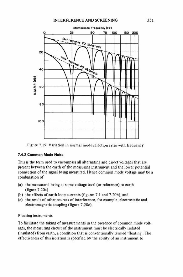
INTERFERENCE AND SCREENING 351
Figure 7.19. Variation in normal mode rejection ratio with frequency
Interference frequency (Hz)
N.M
.R.R
.(dB
)
7.4.2 Common Mode Noise
This is the term used to encompass all alternating and direct voltages that are present between the earth of the measuring instrument and the lower potential connection of the signal being measured. Hence common mode voltage may be a combination of
(a) the measurand being at some voltage level (or reference) to earth (figure 7.20a)
(b) the effects of earth loop currents (figures 7.1 and 7.20b), and(c) the result of other sources of interference, for example, electrostatic and
electromagnetic coupling (figure 7.20c).
Floating instruments
To facilitate the taking of measurements in the presence of common mode volt-ages, the measuring circuit of the instrument must be electrically isolated (insulated) from earth, a condition that is conventionally termed ‘floating’. The effectiveness of this isolation is specified by the ability of an instrument to
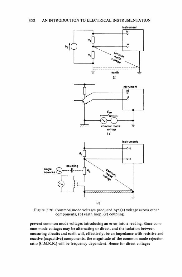
352 AN INTRODUCTION TO ELECTRICAL INSTRUMENTATION
Figure 7.20. Common mode voltages produced by: (a) voltage across other components, (b) earth loop, (c) coupling
(a)
instrument
earth
(b)
instrument
common mode voltage
(c)
instruments
singlesources
coupling
prevent common mode voltages introducing an error into a reading. Since com-mon mode voltages may be alternating or direct, and the isolation between measuring circuits and earth will, effectively, be an impedance with resistive and reactive (capacitive) components, the magnitude of the common mode rejection ratio (C.M.R.R.) will be frequency dependent. Hence for direct voltages
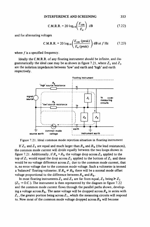
INTERFERENCE AND SCREENING 353
(7.22)
and for alternating voltages
(7.23)
where f is a specified frequency.
Ideally the C.M.R.R. of any floating instrument should be infinite, and dia-grammatically the ideal case may be as shown in figure 7.21, where Z2 and Z3 are the isolation impedances between ‘low’ and earth and ‘high’ and earth respectively.
Figure 7.21. Ideal common mode rejection situation in floating instrument
floating instrument
high source resistance
signalsource
low source resistance
tomeasuringcircuits
source earthcommon mode
voltage
earth
instrument earth
If Z3 and Z2 are equal and much larger than Ra and Rb (the lead resistances), the common mode current will divide equally between the two loops shown in figure 7.21. Additionally, if Ra = Rb the voltage drop across Z3 applied to the top of Z1 would equal the drop across Z2 applied to the bottom of Z1 and there would be no voltage difference across Z1 due to the common mode current, that is, no error voltage due to the common mode voltage. Such a voltmeter is termed a ‘balanced’ floating voltmeter. If Ra ≠ Rb there will be a normal mode offset voltage proportional to the difference between RB and Rb.
In most floating instruments Z2 and Z3 are far from equal, Z3 being >> Z2 (Z3 → O.C.). The instrument is then represented by the diagram in figure 7.22 and the common mode current flows through the parallel paths shown, develop-ing a voltage across Rb. The same voltage will be dropped across Ra in series with Z1, the greater portion being across Z1, which the measuring circuits will respond to. Now most of the common mode voltage dropped across Rb will become

354 AN INTRODUCTION TO ELECTRICAL INSTRUMENTATION
Figure 7.22. Practical common mode rejection situation in floating instrument
floating instrument
signalsource
tomeasuringcircuits
earth
Figure 7.23. Measurement of common mode rejection
floatinginstrument
commonmode
voltage
normal mode offset, so the common mode error depends almost entirely on the relationship between Z2 and Rb. Rb is usually lead resistance and Z2 the isolation impedance between two metallic chassis (108 -1 010 Ω) shunted by a capacitance of a few pF to fractions of a μF. At d.c. Z2 > Rb but as frequency rises Z2 falls, giving poorer immunity to common mode signals at high frequencies. Z2 is also very dependent on the environment, high humidity and dust causing a decrease in its value.
For conformity of specifications, instrument manufacturers have agreed that C.M.R.R. should normally be specified with an unbalance of 1 kΩ in source resistance (for example Rb = 1 kΩ, Ra = 0). An arrangement suitable for measuring the C.M.R.R. of an instrument with a floating input is shown in figure 7.23. For the conditions in that diagram, Ecm is the applied common mode voltage (alternating or direct as appropriate) and Ee is the error it causes in the voltage reading on the instrument.
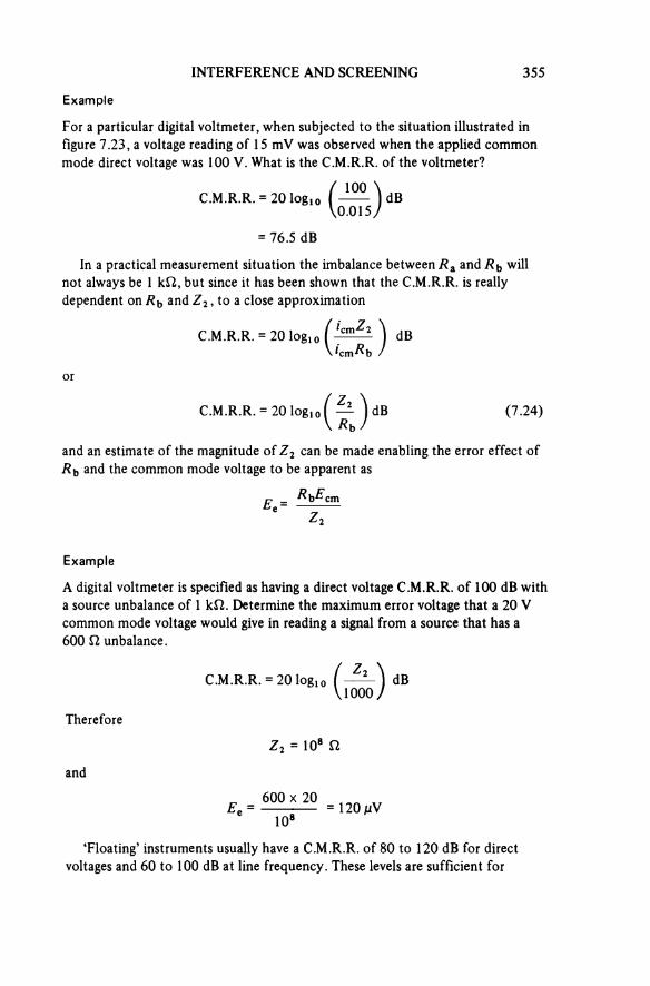
INTERFERENCE AND SCREENING 355
Example
For a particular digital voltmeter, when subjected to the situation illustrated in figure 7.23, a voltage reading of 15 mV was observed when the applied common mode direct voltage was 100 V. What is the C.M.R.R. of the voltmeter?
In a practical measurement situation the imbalance between R3 and will not always be 1 kΩ, but since it has been shown that the C.M.R.R. is really dependent on Rb and Z2, to a close approximation
or
(7.24)
and an estimate of the magnitude of Z2 can be made enabling the error effect of Rb and the common mode voltage to be apparent as
Example
A digital voltmeter is specified as having a direct voltage C.M.R.R. of 100 dB with a source unbalance of 1 kΩ. Determine the maximum error voltage that a 20 V common mode voltage would give in reading a signal from a source that has a 600 Ω unbalance.
Therefore
and
‘Floating’ instruments usually have a C.M.R.R. of 80 to 120 dB for direct voltages and 60 to 100 dB at line frequency. These levels are sufficient for
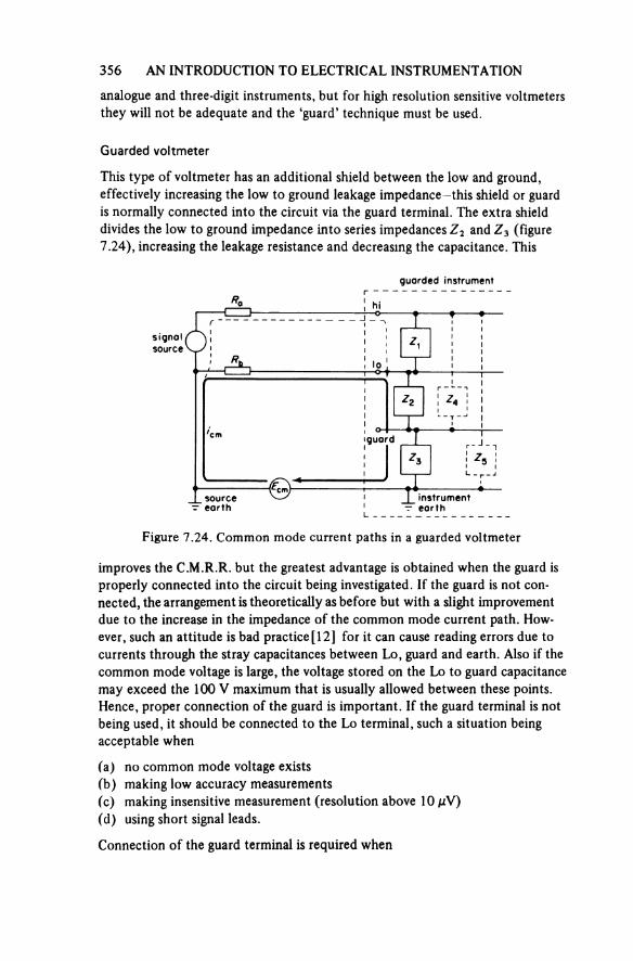
356 AN INTRODUCTION TO ELECTRICAL INSTRUMENTATION
analogue and three-digit instruments, but for high resolution sensitive voltmeters they will not be adequate and the ‘guard’ technique must be used.
Guarded voltmeter
This type of voltmeter has an additional shield between the low and ground, effectively increasing the low to ground leakage impedance—this shield or guard is normally connected into the circuit via the guard terminal. The extra shield divides the low to ground impedance into series impedances Z2 and Z3 (figure 7.24), increasing the leakage resistance and decreasing the capacitance. This
Figure 7.24. Common mode current paths in a guarded voltmeter
instrument
signalsource
guard
sourceearth
instrumentearth
improves the C.M.R.R. but the greatest advantage is obtained when the guard is properly connected into the circuit being investigated. If the guard is not con-nected, the arrangement is theoretically as before but with a slight improvement due to the increase in the impedance of the common mode current path. How-ever, such an attitude is bad practice [12] for it can cause reading errors due to currents through the stray capacitances between Lo, guard and earth. Also if the common mode voltage is large, the voltage stored on the Lo to guard capacitance may exceed the 100 V maximum that is usually allowed between these points. Hence, proper connection of the guard is important. If the guard terminal is not being used, it should be connected to the Lo terminal, such a situation being acceptable when
(a) no common mode voltage exists(b) making low accuracy measurements(c) making insensitive measurement (resolution above 10 μV)(d) using short signal leads.
Connection of the guard terminal is required when
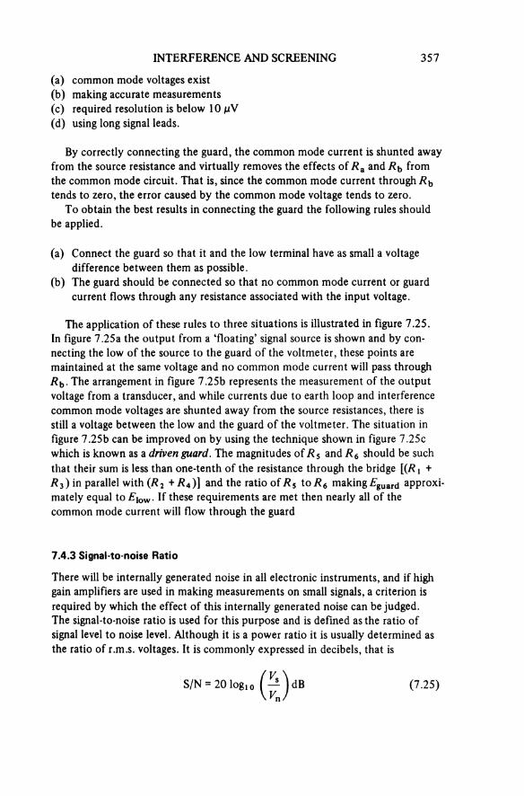
INTERFERENCE AND SCREENING 357
(a) common mode voltages exist(b) making accurate measurements(c) required resolution is below 10 μV(d) using long signal leads.
By correctly connecting the guard, the common mode current is shunted away from the source resistance and virtually removes the effects of Ra and Rb from the common mode circuit. That is, since the common mode current through Rb tends to zero, the error caused by the common mode voltage tends to zero.
To obtain the best results in connecting the guard the following rules should be applied.
(a) Connect the guard so that it and the low terminal have as small a voltage difference between them as possible.
(b) The guard should be connected so that no common mode current or guard current flows through any resistance associated with the input voltage.
The application of these rules to three situations is illustrated in figure 7.25.In figure 7.25a the output from a ‘floating’ signal source is shown and by con-necting the low of the source to the guard of the voltmeter, these points are maintained at the same voltage and no common mode current will pass through Rb. The arrangement in figure 7.25b represents the measurement of the output voltage from a transducer, and while currents due to earth loop and interference common mode voltages are shunted away from the source resistances, there is still a voltage between the low and the guard of the voltmeter. The situation in figure 7.25b can be improved on by using the technique shown in figure 7.25c which is known as a driven guard. The magnitudes of R5 and R6 should be such that their sum is less than one-tenth of the resistance through the bridge [(R1 + R3) in parallel with (R2 + R4)] and the ratio of R5 to R6 making Eguard approxi-mately equal to Elow. If these requirements are met then nearly all of the common mode current will flow through the guard
7.4.3 Signal-to-noise Ratio
There will be internally generated noise in all electronic instruments, and if high gain amplifiers are used in making measurements on small signals, a criterion is required by which the effect of this internally generated noise can be judged. The signal-to-noise ratio is used for this purpose and is defined as the ratio of signal level to noise level. Although it is a power ratio it is usually determined as the ratio of r.m.s. voltages. It is commonly expressed in decibels, that is
(7.25)
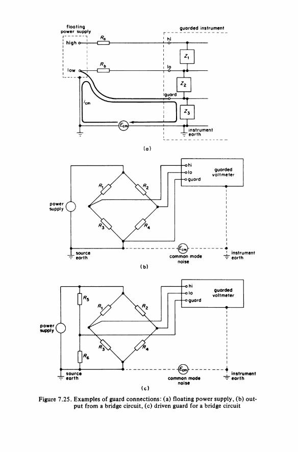
Figure 7.25. Examples of guard connections: (a) floating power supply, (b) out put from a bridge circuit, (c) driven guard for a bridge circuit
(a)
floating power supply
guarded instrument
high
low
hi
Io
guard
instrumentearth
(b)
hiIoguard
guardedvoltmeter
powersupply
sourceearth common mode
noise
instrumentearth
(c)
hiIoguard
guardedvoltmeter
powersupply
sourceearth common mode
noise
instrumentearth
INTERFERENCE AND SCREENING 359
A method of determining this ratio is to measure, with a suitable r.m.s. res ponding instrument, the value of the signal plus the noise giving
then measuring the noise alone, so that the signal can be evaluated.
1 N. Channon, The design and analysis of a novel dielectric paste and its use ina thick film humidity transducer (PhD Thesis, Brighton Polytechnic, 1977)
2 British Calibration Service, General Criteria for Laboratory Approval(London, 1967)
3 B. A. Gregory, An experiment in shielding and screening, Int. J. electlengng Educ., 9 (1971) 31-5
4 B. A. Gregory, Interference, A teaching package (Brighton Polytechnic,1979)
5 B. Hauge and T. R. Foord, A. C. Bridge Methods, 6th Ed. (Pitman, London,1971)
6 F. E. Terman and J. M. Pettit, Electronic Measurements (McGraw-Hill, NewYork, 1952)
7 A. R. Von Hippel (ed.), Dielectric Materials and Applications (M.I.T. Press,Cambridge, Mass., 1954)
8 J. V. L. Parry, E.R.A. Technical Reports L/T 275 and 325 (Leatherhead,Surrey)
9 H. Frohlich, Theory of Dielectrics, 2nd Ed. (Clarendon, Oxford, 1958)10 R. Morrison, Grounding and Shielding Techniques in Instrumentation
(Wiley, New York, 1967)11 Floating measurements and guarding, Hewlett-Packard Application Note
123 (1970)12 Calibration-philosophy in practice, Guarding of Digital Voltmeters, Applica-
tion Bulletin 20 (John Fluke Manufacturing Co., Seattle, Wash. 1977)
REFERENCES
8Instrument Selection and
Specification Analysis
The considerations for selecting an instrument may be regarded as falling into two categories: either an engineer is selecting the most suitable instrument from those within a department or establishment to perform a particular measurement, or he is undertaking the purchase of a new instrument to perform a particular measurement and possibly at the same time extend the measurement capabilities of the department or establishment in which he works. Many of the criteria in selecting an instrument are the same, whether the engineer is selecting an instru-ment off the shelf or purchasing new equipment. In either case a major pitfall is to ‘acquire’ the newest and most sophisticated pieces of equipment in the department, or on the market, simply as a prestige exercise. This is of little value if within a week, justifiable pressure is brought to bear by one’s colleagues and the prestige instrumentation system is reduced to its minimum requirements— which could be two suspect multimeters and the oldest oscilloscope in the department!
8.1 INSTRUMENT SELECTION
The general criteria for selecting an instrument may be summarised by the follow-ing check list, which although it may be more suitable when considering a moderately sophisticated instrument, could prove valuable as a guide in selecting the ‘right’ instrument on every occasion.
Ranges
(a) What are the maximum and minimum magnitudes of the values to be measured?
(b) Will a single range, or multi-range instrument be the most suitable?
Accuracy
(a) What is the maximum tolerance acceptable?(b) Is the resolution of the instrument consistent with its specified errors?
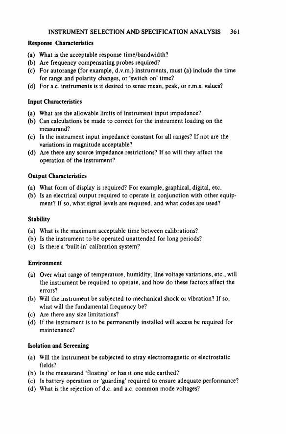
INSTRUMENT SELECTION AND SPECIFICATION ANALYSIS 36 1
Response Characteristics
(a) What is the acceptable response time/bandwidth?(b) Are frequency compensating probes required?(c) For autorange (for example, d.v.m.) instruments, must (a) include the time
for range and polarity changes, or ‘switch on’ time?(d) For a.c. instruments is it desired to sense mean, peak, or r.m.s. values?
Input Characteristics
(a) What are the allowable limits of instrument input impedance?(b) Can calculations be made to correct for the instrument loading on the
measurand?(c) Is the instrument input impedance constant for all ranges? If not are the
variations in magnitude acceptable?(d) Are there any source impedance restrictions? If so will they affect the
operation of the instrument?
Output Characteristics
(a) What form of display is required? For example, graphical, digital, etc.(b) Is an electrical output required to operate in conjunction with other equip-
ment? If so, what signal levels are required, and what codes are used?
Stability
(a) What is the maximum acceptable time between calibrations?(b) Is the instrument to be operated unattended for long periods?(c) Is there a ‘built-in’ calibration system?
Environment
(a) Over what range of temperature, humidity, line voltage variations, etc., will the instrument be required to operate, and how do these factors affect the errors?
(b) Will the instrument be subjected to mechanical shock or vibration? If so, what will the fundamental frequency be?
(c) Are there any size limitations?(d) If the instrument is to be permanently installed will access be required for
maintenance?
Isolation and Screening
(a) Will the instrument be subjected to stray electromagnetic or electrostatic fields?
(b) Is the measurand ‘floating’ or has it one side earthed?(c) Is battery operation or ‘guarding’ required to ensure adequate performance?(d) What is the rejection of d.c. and a.c. common mode voltages?
362 AN INTRODUCTION TO ELECTRICAL INSTRUMENTATION
Operation
(a) Is remote control required?(b) Is automatic or programmed operation required?(c) What are the effects of intermittent energisation?(d) Will multi-function operation be advantageous?(e) Will operator fatigue cause reading interpretation problems?(f) What power supplies will be required?
Reliability
(a) What is the specified operational life?(b) What will the consequences of failure be?(c) Is duplication or standby instrumentation required?(d) Will special spares and maintenance equipment be required?(e) Does the instrument incorporate any limit detection or alarm facilities? If
so, must a ‘fail safe’ arrangement be incorporated?
On completion of the above check list for a particular application, the derived specification for the desired instrument may not be possible in practical terms, and a compromise between that which is available within an organisation, or can be afforded, will have to be adopted.
If a new instrument is to be purchased it is essential to ensure that the ‘right’ instrument is being purchased. This is particularly relevant if the instrument is for a permanent installation although it may be considered as ‘good practice’ to purchase to a slightly higher specification if the proposed instrument is for use in a laboratory where the measurement requirements may change with experience and time. The problem here, of course, is over-specification resulting in thepurchase of an instrument that is much more sophisticated (and expensive) than is really necessary.
The following list is a rough guide to the factors that will increase the cost of an instrument.
(a) reduction of error magnitudes(b) increasing the speed of reading(c) increasing the sensitivity(d) improving the stability(e) improvement of isolation/guarding (except for battery operation)(f) the addition of input/output facilities(g) the addition of programmable capabilities(h) the extension of operating conditions.
Thus having decided on the requirements of the instrument it is desirable to purchase, it is necessary to study manufacturers’ literature and decide on a ‘best buy’.
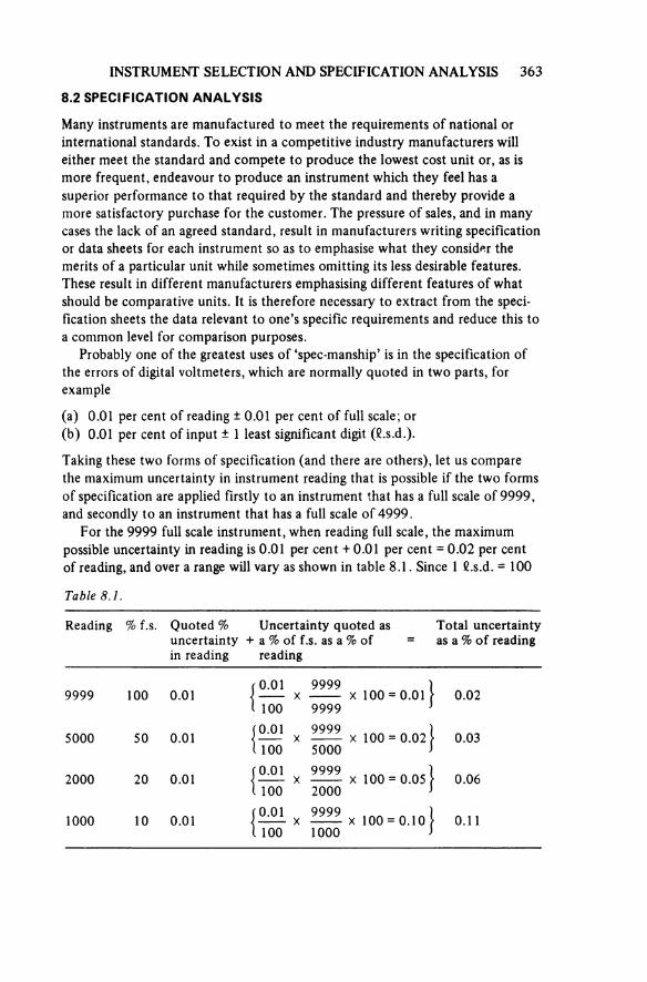
INSTRUMENT SELECTION AND SPECIFICATION ANALYSIS 363
8.2 SPECIFICATION ANALYSIS
Many instruments are manufactured to meet the requirements of national or international standards. To exist in a competitive industry manufacturers will either meet the standard and compete to produce the lowest cost unit or, as is more frequent, endeavour to produce an instrument which they feel has asuperior performance to that required by the standard and thereby provide a more satisfactory purchase for the customer. The pressure of sales, and in many cases the lack of an agreed standard, result in manufacturers writing specification or data sheets for each instrument so as to emphasise what they consider the merits of a particular unit while sometimes omitting its less desirable features. These result in different manufacturers emphasising different features of what should be comparative units. It is therefore necessary to extract from the speci-fication sheets the data relevant to one’s specific requirements and reduce this to a common level for comparison purposes.
Probably one of the greatest uses of ‘spec-manship’ is in the specification of the errors of digital voltmeters, which are normally quoted in two parts, for example
(a) 0.01 per cent of reading ± 0.01 per cent of full scale; or(b) 0.01 per cent of input ± 1 least significant digit (l.s.d.).
Taking these two forms of specification (and there are others), let us compare the maximum uncertainty in instrument reading that is possible if the two forms of specification are applied firstly to an instrument that has a full scale of 9999, and secondly to an instrument that has a full scale of 4999.
For the 9999 full scale instrument, when reading full scale, the maximum possible uncertainty in reading is 0.01 per cent + 0.01 per cent = 0.02 per cent of reading, and over a range will vary as shown in table 8.1. Since 1 l.s.d. = 100
Reading % Ls. Quoted % uncertainty + in reading
Uncertainty quoted as a % of f.s. as a % of = reading
Total uncertainty as a % of reading
9999 100 0.01 0.01 9999V \< 100 = 0.01 J 0.02
100 9999
5000 50 0.01 0.01 9999V \< 100 = 0.02 | 0.03
100 5000
2000 20 0.01 0.01 9999V )( 100 = 0.05 | 0.06
100 2000
1000 10 0.01 0.01 9999 × >: 100 = 0.10 J 0.11
100 1000
Table 8.1.
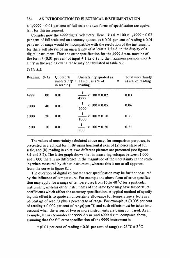
364 AN INTRODUCTION TO ELECTRICAL INSTRUMENTATION
× 1/9999 = 0.01 per cent of full scale the two forms of specification are equiva-lent for this instrument.
Consider now the 4999 digital voltmeter. Here 1 l.s.d. = 100 × 1/4999 = 0.02 per cent of full scale and an accuracy quoted as ± 0.01 per cent of reading ± 0.01 per cent of range would be incompatible with the resolution of the instrument, for there will always be an uncertainty of at least ± 1 l.s.d. in the display of a digital instrument. Thus the error specification for the 4999 d.v.m. must be of the form ± (0.01 per cent of input + 1 l.s.d.) and the maximum possible uncert-ainty in the reading over a range may be tabulated in table 8.2.
Table 8.2.
Reading % f.s. Quoted % uncertainty + in reading
Uncertainty quoted as1 l.s.d., as a % Of =reading
Total uncertainty as a % of reading
4999 100 0.01 1 × 100 = 0.024999
0.03
2000 40 0.01 1 x 100 = 0.052000
0.06
1000 20 0.01 1 X 100 = 0.101000
0.11
500 10 0.01 — x 100 = 0.20500
0.21
The values of uncertainty tabulated above may, for comparison purposes, be presented in graphical form. By using horizontal axes of (a) percentage of full scale, and (b) reading in volts, two different pictures are presented (see figures 8.1 and 8.2). The latter graph shows that in measuring voltages between 1.000and 5.000 there is no difference in the magnitude of the uncertainty in the read-ing when measured by either instrument, whereas this is not at all apparent from the curve in figure 8.1.
The question of digital voltmeter error specification may be further obscured by the influence of temperature. For example the above form of error specifica-tion may apply for a range of temperatures from 15 .to 40 °C for a particularinstrument, whereas other instruments of the same type may have temperature coefficients which affect the accuracy specification. A typical method of specify ing this effect is to quote an uncertainty allowance for temperature effects as a percentage of reading plus a percentage of range. For example, ± (0.005 per cent of reading + 0.002 per cent of range) per °C and such effects must be taken into account when the errors of two or more instruments are being compared. As an example, let us reconsider the 9999 d.v.m. and 4999 d.v.m. compared above, assuming that the full error specification of the 9999 instrument is
± (0.01 per cent of reading + 0.01 per cent of range) at 23 °C ± 2 °C
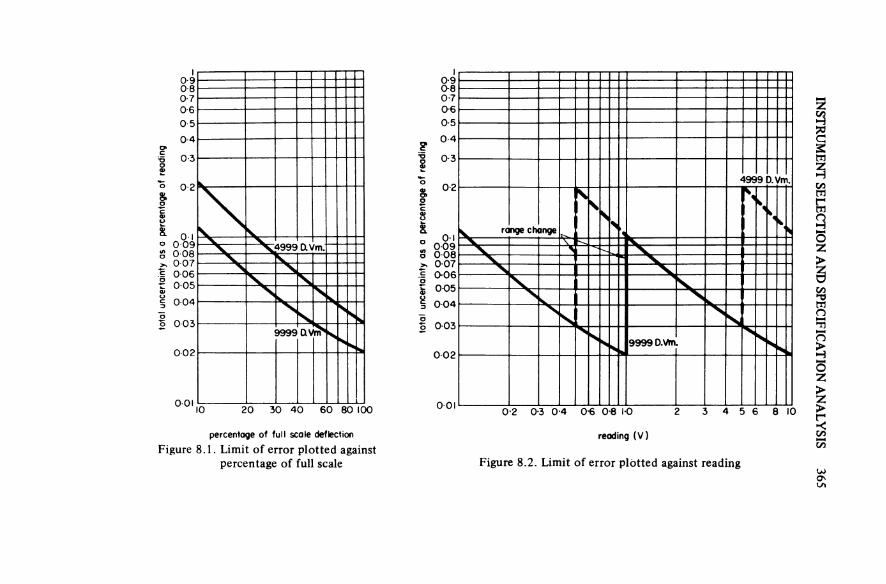
INSTR
UM
ENT SELECTIO
N AN
D SPECIFIC
ATION
AN
ALY
SIS 365
Figure 8.1. Limit of error plotted against percentage of full scale
tota
l unc
erta
inty
as a p
erce
ntag
e of re
adin
g
percentage of full scale deflection
Figure 8.2. Limit of error plotted against reading
tota
l unce
rtai
nty a
s a per
cent
age o
f rea
ding
reading (V)
range change
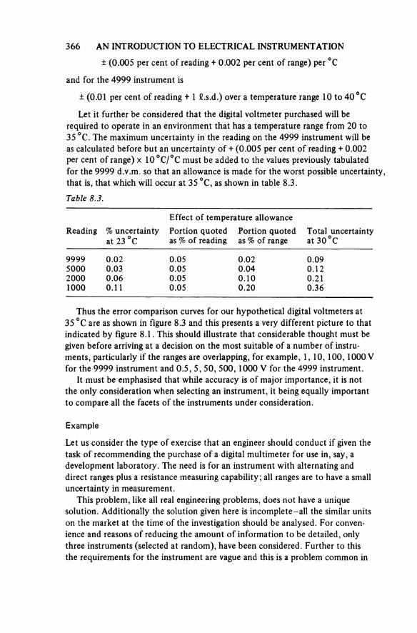
366 AN INTRODUCTION TO ELECTRICAL INSTRUMENTATION
± (0.005 per cent of reading + 0.002 per cent of range) per °C
and for the 4999 instrument is
± (0.01 per cent of reading + 1 l.s.d.) over a temperature range 10 to 40 °C
Let it further be considered that the digital voltmeter purchased will berequired to operate in an environment that has a temperature range from 20 to 35 °C. The maximum uncertainty in the reading on the 4999 instrument will be as calculated before but an uncertainty of +(0.005 per cent of reading + 0.002 per cent of range) × 10 °C/°C must be added to the values previously tabulated for the 9999 d.v.m. so that an allowance is made for the worst possible uncertainty, that is, that which will occur at 35 °C, as shown in table 8.3.
Table 8.3.
Reading % uncertainty at 23 °C
Effect of temperature allowancePortion quoted as % Of reading
Portion quoted as % of range
Total uncertainty at 30 °C
9999 0.02 0.05 0.02 0.095000 0.03 0.05 0.04 0.122000 0.06 0.05 0.10 0.211000 0.11 0.05 0.20 0.36
Thus the error comparison curves for our hypothetical digital voltmeters at 35 °C are as shown in figure 8.3 and this presents a very different picture to that indicated by figure 8.1. This should illustrate that considerable thought must be given before arriving at a decision on the most suitable of a number of instru-ments, particularly if the ranges are overlapping, for example, 1, 10, 100, 1000 V for the 9999 instrument and 0.5, 5, 50, 500, 1000 V for the 4999 instrument.
It must be emphasised that while accuracy is of major importance, it is not the only consideration when selecting an instrument, it being equally important to compare all the facets of the instruments under consideration.
Example
Let us consider the type of exercise that an engineer should conduct if given the task of recommending the purchase of a digital multimeter for use in, say, a development laboratory. The need is for an instrument with alternating and direct ranges plus a resistance measuring capability; all ranges are to have a small uncertainty in measurement.
This problem, like all real engineering problems, does not have a unique solution. Additionally the solution given here is incomplete—all the similar units on the market at the time of the investigation should be analysed. For conven-ience and reasons of reducing the amount of information to be detailed, only three instruments (selected at random), have been considered. Further to this the requirements for the instrument are vague and this is a problem common in
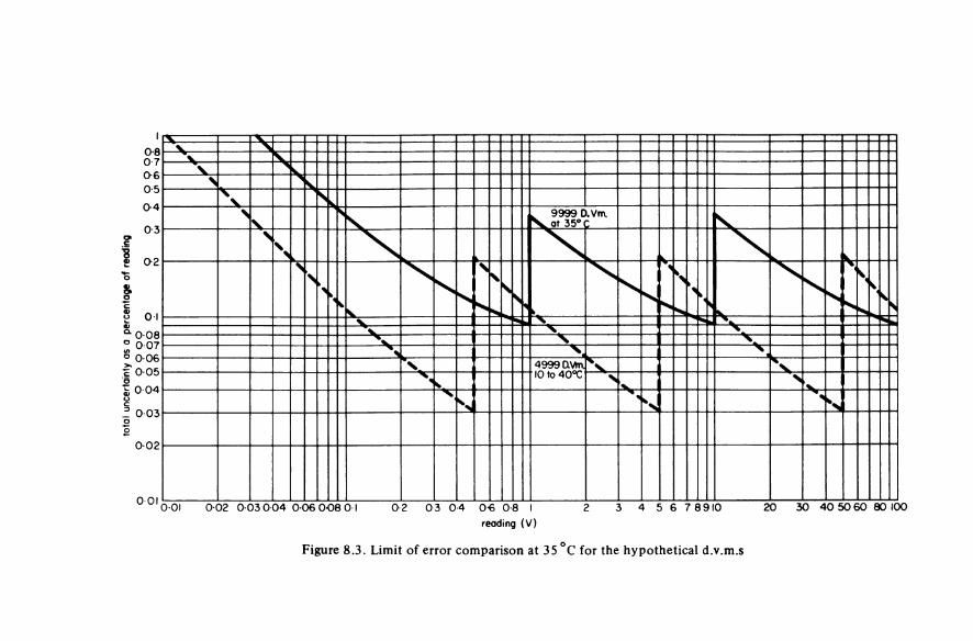
Figure 8.3. Limit of error comparison at 35 °C for the hypothetical d.v.m.s
tota
l unc
erta
inty
as a p
erce
ntag
e of r
eadi
ng
reading (V)
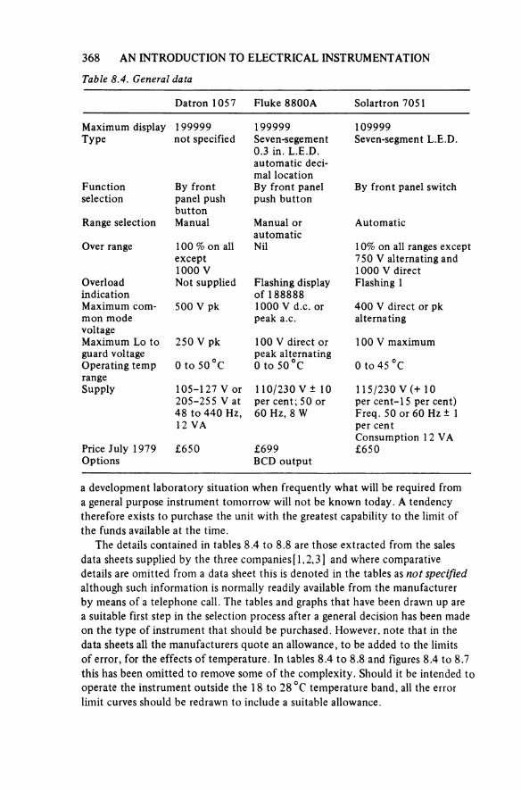
368 AN INTRODUCTION TO ELECTRICAL INSTRUMENTATION
Table 8.4. General data
Datron 1057 Fluke 8800A Solartron 7051
Maximum display 199999 199999 109999Type not specified Seven-segment
0.3 in. L.E.D. automatic deci-mal location
Seven-segment L.E.D.
Functionselection
By front panel push button
By front panel push button
By front panel switch
Range selection Manual Manual or automatic
Automatic
Over range 100 % on all except1000 V
Nil 10% on all ranges except 750 V alternating and 1000 V direct
Overloadindication
Not supplied Flashing display of 188888
Flashing 1
Maximum com-mon mode voltage
500 V pk 1000 V d.c. or peak a.c.
400 V direct or pk alternating
Maximum Lo to guard voltage
250 Vpk 100 V direct or peak alternating
100 V maximum
Operating temp range
0 to 50 °C 0 to 50 °C 0 to 45 °C
Supply 105-127 V or 205-255 V at 48 to 440 Hz, 12 VA
110/230 V± 10 per cent; 50 or60 Hz, 8 W
115/230 V(+10 per cent—15 per cent) Freq. 50 or 60 Hz ± 1 per centConsumption 12 VA
Price July 1979 1650 1699 1650Options BCD Output
a development laboratory situation when frequently what will be required from a general purpose instrument tomorrow will not be known today. A tendency therefore exists to purchase the unit with the greatest capability to the limit of the funds available at the time.
The details contained in tables 8.4 to 8.8 are those extracted from the sales data sheets supplied by the three companies [1, 2, 3] and where comparative details are omitted from a data sheet this is denoted in the tables as not specified although such information is normally readily available from the manufacturer by means of a telephone call. The tables and graphs that have been drawn up are a suitable first step in the selection process after a general decision has been made on the type of instrument that should be purchased. However, note that in the data sheets all the manufacturers quote an allowance, to be added to the limits of error, for the effects of temperature. In tables 8.4 to 8.8 and figures 8.4 to 8.7 this has been omitted to remove some of the complexity. Should it be intended to operate the instrument outside the 18 to 28 °C temperature band, all the error limit curves should be redrawn to include a suitable allowance.
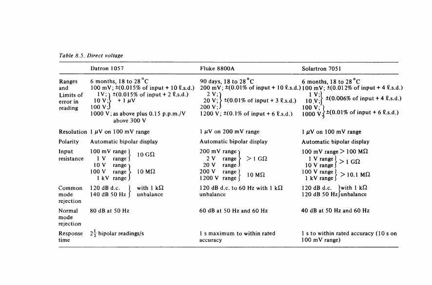
Table 8.5. Direct voltage
Datron 1057 Fluke 8800A Solartron 7051
RangesandLimits of error in reading
6 months, 18 to 28 °C 90 days, 18 to 28 °C 6 months, 18 to 28 °C100 mV; ±(0.015% of input + 10 δ.s.d.) 200 mV; ±(0.01% of input + 10 l.s.d.) 100 mV; ±(0.012% of input + 4 δ.s.d.)
IV; | ±(0.015% of input + 2 C.s.d.)!> + 1 μV
2V;1 1 V;1 ±(0.006% of input + 4 l.s.d.)10 V; 20 V; ±(0.01% of input + 3 l.s.d.) 10.V;|100 200 V;J 100 V;
r±(0.01% of input + 6 l.s.d.)1000 V ; as above plus 0.1 5 p.p.m./V above 300 V
1200 V; ±(0.1% of input + 6 δ.s.d.) 1000 V;
Resolution 1 μV on 1 00 mV range 1 μV on 200 mV range 1 μV on 100 mV rangePolarity Automatic bipolar display Automatic bipolar display Automatic bipolar displayInputresistance
1 00 mV range 1 10 GΩ 200 mV range ?1 100 mV range > 100 MΩ1 V range ’ 2 V range | > 1 GΩ 1 V range 1[• > 1 GΩ
1 0 V range 'I 20 V range J1 1 0 V range J100 V range I 10 MΩ 200 V range ] 10 MΩ 100 V range |[ > 10,1 MΩ
1 kV range,1 1200 V range J 1 kV range JCommonmoderejection
120 dB d.c. 1 with 1 kΩ | unbalance
120 dB d.c. to 60 Hz with 1 kΩ unbalance
120 dB d.c. 11 with 1 kΩ [unbalance140 dB 50 Hz ; 120 dB 50 HzJ
Normalmoderejection
80 dB at 50 Hz 60 dB at 50 Hz and 60 Hz 40 dB at 50 Hz and 60 Hz
Responsetime
2y bipolar readings/s 1 s maximum to within rated accuracy
1 s to within rated accuracy (10 s on1 00 mV range)
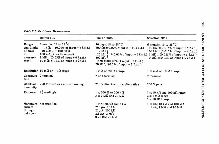
370 A
N INTR
ODU
CTIO
N TO ELEC
TRICA
L INSTR
UM
ENTATIO
N
Table 8.6. Resistance Measurement
Datron 1057 Fluke 8800A Solartron 7051
Ranges and Limits of error inmeasure-ment
6 months, 18 to 28 °C 90 days, 18 to 28 °C 6 months, 1 8 to 28 °C1 kΩ;i| ±(0.01% of input + 4 l.s.d.)
+100 mΩ)1 (can be zeroed)
200 Ω;±(0.02% of input + 10 l.s.d.) 10 kΩ; ±(0.01 5% of input + 5 l.s.d.)lOkΩJ 2 kΩ '1 100 kΩ; ±(0.015% of input + 4 l.s.d.)
100 kΩ;J 20 kΩ f ±(0.01% of input + 3 δ.s.d.) 1 MΩ; ±(0.025% of input + 5 l.s.d.)1 MΩ; ±(0.03% of input + 4 l.s.d.) 200 kΩ -1 10 MΩ; ±(0.05% of input + 5 l.s.d.)10 MΩ; ±(0.5% of input + 4 l.s.d.) 2 MΩ; ±(0.05% of input + 3 l.s.d.)
20 MΩ; ±(0.2% of input + 3 l.s.d.)
Resolution 1 0 mΩ on 1 kΩ range 1 mΩ on 200 Ω range 1 00 mΩ on 1 0 kΩ rangeConfigura-tion
2 terminal 2 or 4 terminal 2 terminal
Overloadimmunity
250 V direct or r.m.s. alternating 250 V direct or r.m.s. alternating 200 V peak
Response 2| reading/s 1 s; 200 Ω to 200 kΩ 1 s; 10 kΩ and 100 kΩ range3 s; 2 MΩ and 20 MΩ 2 s; 1 MΩ range
5 s; 10 MΩ rangeMaximumcurrentthroughunknown
not specified 1 mA; 200 Ω and 2 kΩ 100 μA; 10 kΩ and 100 kΩ250 μA; 20 kΩ 1 μA; 1 MΩ and 10 MΩ25 μA; 200 kΩ2,5 μA; 2 MΩ0.25 μA; 20 MΩ

INSTRUMENT SELECTION AND SPECIFICATION ANALYSIS 37 1
Table 8.7. Direct current
Datron 1057 Fluke 8800A Solartron 7051
Ranges and error limit
Nil-currents measured as voltage drop across known resistance
Nil-currents measured as voltage drop across known resistance
6 months, 18 to 28 °C100 μA ± (0.04% of input
+ 5 l.s.d.)1 mA ± (0.04% of input
+ 5 l.s.d.)100 mA ± (0.05% of input
+ 50 l.s.d.)1 A ± (0.05% of input
+ 5 l.s.d.)Input resistance As used As used 100 μA
1 mA < 5Ω
100 mA 1 A
< 2Ω
Resolution 1 μV on100 mV range
1 μV on200 mV range
1 nA on 1 00 μA range
It must also be remembered that the error curves for the three instruments are not strictly comparable. The Fluke error limit specification is for any time up to 90 days after calibration, while the specifications for the Datron and Solartron instruments are for 6 months.
General data
The general properties of the instruments have been summarised in table 8.4. All instruments have a display of seven-segment numerals. The maximum indications of the Datron and Fluke instruments are 199999, while the Solartron instrument has a maximum of 109999.
The Datron unit has a purely manual range selection, the Solartron has only an automatic range selection while the Fluke instrument can be operated in either mode.
The Fluke unit can sustain the largest common mode voltage (1000 V) where-as the Datron instrument is capable of coping with a Lo to guard voltage verymuch greater than either of the others.
The only unit capable of being fitted with an output would appear to be the Fluke 8800A.
Direct voltage measurement
Table 8.5 shows a comparison between the direct voltage measuring capabilities of the three instruments. The accuracy specifications (or limits of error in read-ing) have been modified from the data sheets to a common form in an attempt to ease the comparison. This is further assisted by the curves in figure 8.4. All the instruments have five ranges and a resolution of 1 μV on the most sensitive

Table 8.8. Alternating voltage measurement
Datron 1057 Fluke 8800A Solartron 7051
Senses r.m.s. (crest factor 5:1) Senses mean value Senses mean value
Ranges 1 V, 10 V, 100 V, 700 V 2 V, 20 V, 200 V, 1200 V 1 V, 10 V, 100 V, 750 VResolution 10 μV on 1 V range 1 0 μV on 2 V range 10 μV on 1 V rangeLimits of error in measure-ment
All ranges: 6 months, 18 to 28 °C 2 V to 200 V: 90 days, 18 to 28 °C 1 V range: 6 months, 18 to 28 °C30 Hz-50 Hz; ±(1,0% of input+ 60
l.s.d.)40 Hz-3 kHz; ±(0.1% of input +
100 C.s.d.)50 Hz-1 00 Hz; ±(0.25% of input + 40 Hz-20 kHz; ±(0.1% of input +
30 l.s.d.)20 C.s.d.)100 Hz-10 kHz; ±(0.1% of input +
10 C.s.d.)3 kHz-30 kHz; ±(0.2% of input +
200 l.s.d.)10 kHz-20 kHz; ±(0.25% of input + 10 V to 750 V: 6 months, 18 to 28 °C
20 C.s.d.)20 kHz-100 kHz; ±( 1.0% of input +
60 C.s.d.)700 V range: to the above specification add 0.2 p.p.m./V above 300 V
1200 V range: 90 days, 18 to 28 °C 40 Hz-20 kHz; ±(0.2% of input + 30 C.s.d.)30 Hz-100 Hz; ±(0.5% of input +
40 C.s.d.)100 Hz-10 kHz; ±(0.3% of input +
20 C.s.d.)10 kHz-20 kHz; ±(0.5% of input +
40 C.s.d.)Inputimpedance
1 V range: 1 GΩ shunted by 150 pF10 V to 700 V ranges; 10 MΩ
All ranges: 2 MΩ shunted by 100 pF All ranges: 1 MΩ shunted by 100 pF
Commonmoderejection
d.c. to 60 Hz; 1 kΩ unbalance signal Lo, 60 dB signal Hi, 1 00 dB
d.c. > 120 dBnot specified 50 Hz >40 dB
60 Hz > 40 dB
Responsetime
1 s 1.5 s to within rated accuracy 3 s to within rated accuracy
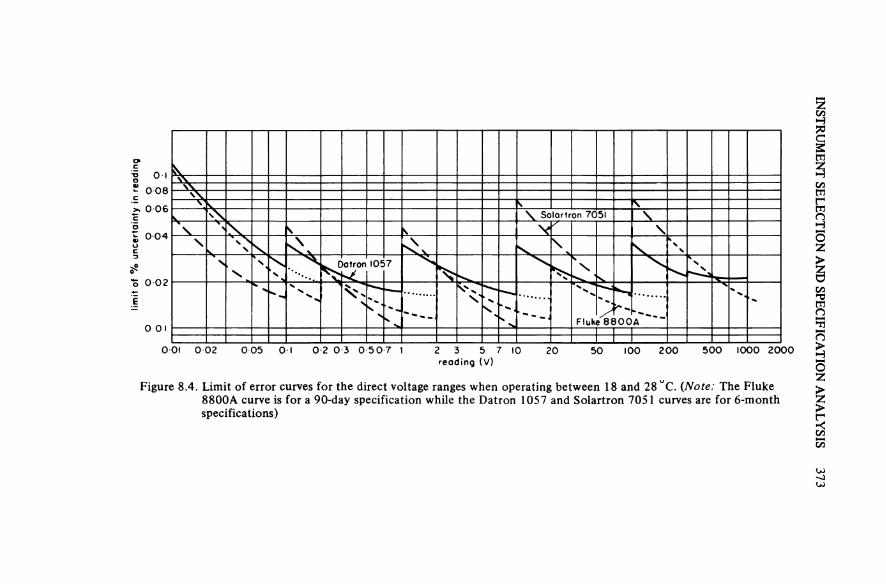
INSTR
UM
ENT SELEC
TION
AN
D SPECIFIC
ATIO
N AN
ALY
SIS 373
Figure 8.4. Limit of error curves for the direct voltage ranges when operating between 18 and 28 WC. [Note: The Fluke 8800A curve is for a 90-day specification while the Datron 1057 and Solartron 7051 curves are for 6-month specifications)
limit
of %
unce
rtai
nty i
n rea
ding
reading (V)
Datron 1057
Solartron 7051
Fluke 8800A
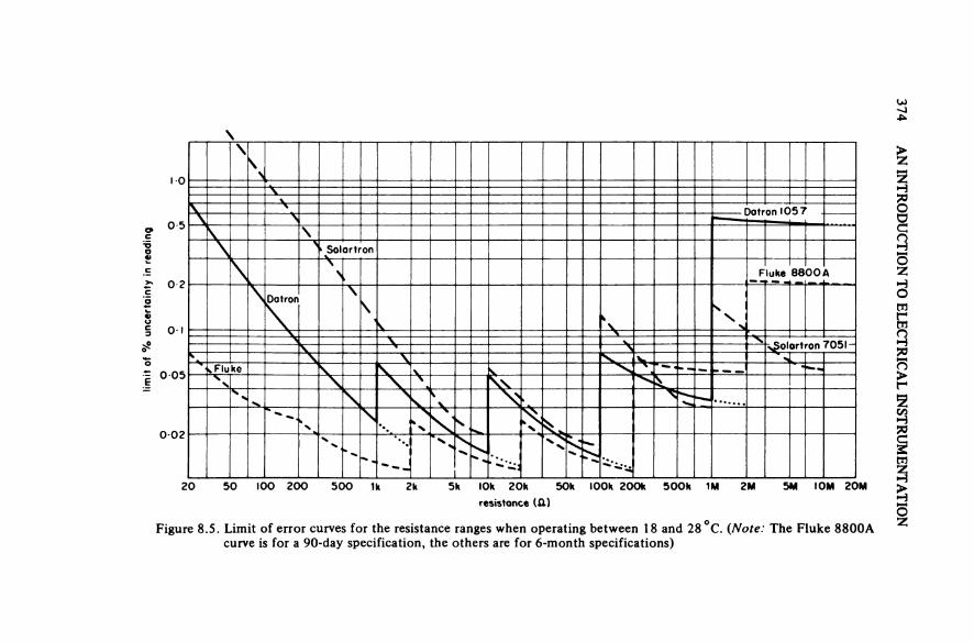
374 A
N INTR
ODU
CTIO
N TO ELEC
TRICA
L INSTR
UM
ENTA
TION
Figure 8.5. Limit of error curves for the resistance ranges when operating between 18 and 28 °C. (Note: The Fluke 8800A curve is for a 90-day specification, the others are for 6-month specifications)
limit
of %
unce
rtai
nty i
n rea
ding
resistance (&)
Fluke
Datron
Solartron
Datron 1057
Fluke 8800A
Solartron 7051
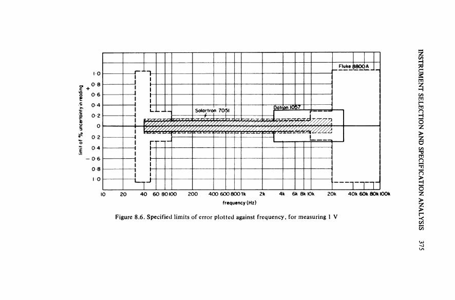
INSTR
UM
ENT SELEC
TION A
ND SPEC
IFICA
TION A
NA
LYSIS
375
Figure 8.6. Specified limits of error plotted against frequency, for measuring 1 V
limit o
f % un
cert
aint
y in
rea
ding
frequency (Hz)
Solartron 7051Datron 1057
Fluke 8800A
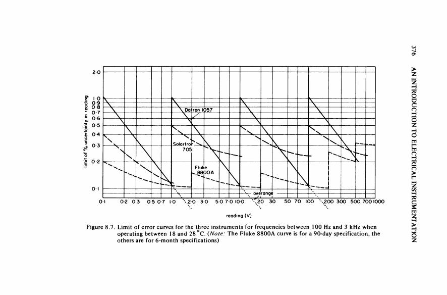
376 A
N INTR
ODU
CTIO
N TO ELEC
TRICA
L INSTR
UM
ENTATIO
N
Figure 8.7. Limit of error curves for the three instruments for frequencies between 100 Hz and 3 kHz when operating between 18 and 28 °C. (Note: The Fluke 8800A curve is for a 90-day specification, the others are for 6-month specifications)
limit
of %
unc
erta
inty
in re
adin
g
reading (V)
Dotron 1057
Solartron7051
Fluke 8800A
overange
INSTRUMENT SELECTION AND SPECIFICATION ANALYSIS 377
range. The 8800A is capable of measuring the highest voltage (1200 V). The curves show that it is not true to say that one instrument has smaller errors than the others; for example, the Solartron 7051 has the least uncertainty for voltages below 100 mV but the largest limit of error between 10 V and 200 V. So unlessit is known that the purpose of the exercise is to purchase an instrument for use at a particular level of voltage, the uncertainty in measuring direct voltages can-not be used as a means of deciding on the most desirable instrument.
The Datron 1057 has the highest input resistance on the low voltage ranges and has the highest normal mode rejection figure both of which are points in its favour.
Resistance measurement
Perusal of table 8.6 shows that the Fluke 8800A has six resistance ranges as opposed to the five of the Datron and four of the Solartron instrument. Figure 8.5 indicates that below 200 kΩ the Fluke multimeter has the smallest uncert-ainty in measurement (if calibrated twice as often as the others); it is also the only instrument capable of being used to make four terminal resistance measure-ments—an essential property when measuring resistances with a 1 mΩ resolution! The specification of the possible current through the unknown is useful informa-tion and indicates another plus for the Fluke 8800A.
Current measurement
The Solartron 705 1 is the only instrument of the three compared that has inter-nal current ranges and this is therefore a feature in its favour. To measure currents using either of the other instruments, a resistor with a very small tolerance (± 0.01 per cent or less) must be used and the unknown current measured as a voltage drop.
Alternating voltage measurement
Table 8.8 indicates that each of the instruments has four ranges, the maximum resolution in each case being 10 μV. However, the maximum voltages measurable vary, 700 V on the Datron, 750 V on the Solartron and 1200 V on the Fluke instrument. The Datron is the only r.m.s. sensing instrument, although all three are calibrated in terms of r.m.s. values.
In an attempt to compare the frequency ranges of the three instruments, figure 8.6 has been drawn, and this shows that (in measuring 1 V) the 8800A hasthe widest frequency range and the 7051 the narrowest frequency range.
Figure 8.7 shows the limit of error curves for the three instruments forfrequencies between 100 Hz and 3 kHz, it being apparent that except for operat-ing the Datron 1057 in an overrange condition, the Fluke 8800A gives the smallest uncertainty of measurement. As on the direct voltage ranges the Datron instrument has the highest input impedance. The a.c. common mode rejection of
378 AN INTRODUCTION TO ELECTRICAL INSTRUMENTATION
this instrument is better than the Solartron although the d.c. common mode rejection is poorer; somewhat surprisingly the C.M.R. figures are not specified for the Fluke instrument.
Best buy decision
Before reaching a decision on which of these instruments would be the ‘best buy’, two further procedures would be necessary. Firstly, an attempt should be madeto reassess the requirements of the proposed use of the instrument, paying particular attention to such aspects as the likely operational common mode voltages, the frequency range necessary and the requirements for current and resistance measurements. After establishing these needs the second step wouldbe to request from each manufacturer a demonstration of their instrument. At the demonstration particular performance aspects and omissions from the data sheet can be clarified, for example
(a) Are the quoted response times of the Datron instrument to within rated accuracy?
(b) What is the C.M.R. of the Fluke instrument on the alternating voltage ranges?(c) Is it possible for the Solartron instrument to be supplied with an output?
On completion of such procedures for all the instruments available a decision can be made.
Note: The above comparison was drawn up in the summer of 1979. The rate of electronic development is such that by the date of publication of this book these instruments may well have been superseded. The reader should realise that the above exercise is an example of procedure and not intended as a ‘state of the art’ comparison.
REFERENCES
1 1057 Multimeter Data Sheet (Datron Electronics Ltd., Norwich, 1979)2 Fluke 8800A Digital Multimeter (John Fluke Manufacturing Co., Seattle,
Wash.)3 Digital Voltmeter 7051 (Solartron Ltd, Farnborough, Hants, 1979)
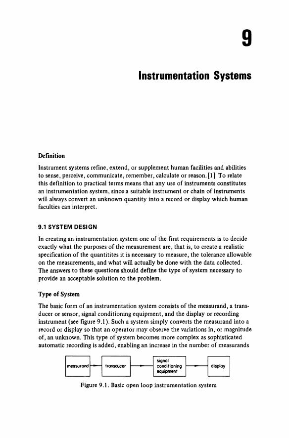
9Instrumentation Systems
Definition
Instrument systems refine, extend, or supplement human facilities and abilities to sense, perceive, communicate, remember, calculate or reason. [1] To relate this definition to practical terms means that any use of instruments constitutes an instrumentation system, since a suitable instrument or chain of instruments will always convert an unknown quantity into a record or display which human faculties can interpret.
9.1 SYSTEM DESIGN
In creating an instrumentation system one of the first requirements is to decide exactly what the purposes of the measurement are, that is, to create a realistic specification of the quantities it is necessary to measure, the tolerance allowable on the measurements, and what will actually be done with the data collected.The answers to these questions should define the type of system necessary to provide an acceptable solution to the problem.
Type of System
The basic form of an instrumentation system consists of the measurand, a trans-ducer or sensor, signal conditioning equipment, and the display or recording instrument (see figure 9.1). Such a system simply converts the measurand into a record or display so that an operator may observe the variations in, or magnitude of, an unknown. This type of system becomes more complex as sophisticated automatic recording is added, enabling an increase in the number of measurands
Figure 9.1. Basic open loop instrumentation system
measurand transducersignalconditioningequipment
display
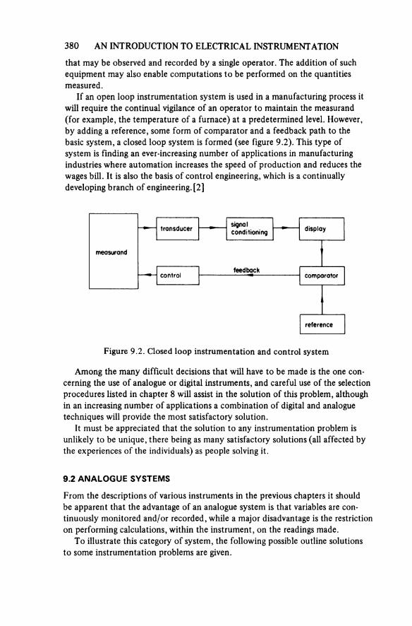
380 AN INTRODUCTION TO ELECTRICAL INSTRUMENTATION
that may be observed and recorded by a single operator. The addition of such equipment may also enable computations to be performed on the quantities measured.
If an open loop instrumentation system is used in a manufacturing process it will require the continual vigilance of an operator to maintain the measurand (for example, the temperature of a furnace) at a predetermined level. However,by adding a reference, some form of comparator and a feedback path to the basic system, a closed loop system is formed (see figure 9.2). This type of system is finding an ever-increasing number of applications in manufacturingindustries where automation increases the speed of production and reduces the wages bill. It is also the basis of control engineering, which is a continually developing branch of engineering. [2]
Figure 9.2. Closed loop instrumentation and control system
measurand
transducer signalconditioning display
controlfeedback
comparator
reference
Among the many difficult decisions that will have to be made is the one con-cerning the use of analogue or digital instruments, and careful use of the selection procedures listed in chapter 8 will assist in the solution of this problem, although in an increasing number of applications a combination of digital and analogue techniques will provide the most satisfactory solution.
It must be appreciated that the solution to any instrumentation problem is unlikely to be unique, there being as many satisfactory solutions (all affected by the experiences of the individuals) as people solving it.
9.2 ANALOGUE SYSTEMS
From the descriptions of various instruments in the previous chapters it should be apparent that the advantage of an analogue system is that variables are con-tinuously monitored and/or recorded, while a major disadvantage is the restriction on performing calculations, within the instrument, on the readings made.
To illustrate this category of system, the following possible outline solutions to some instrumentation problems are given.

INSTRUMENTATION SYSTEMS 381
9.2.1 Open Loop Systems
Since this type of system does not exert any control, it merely monitors, or may-be records, the events as they occur. There are very many applications for which an open loop system is suitable. The following are but two examples, for which possible outline solutions are given; the detailed solution requires an appraisal of the manufacturers’ literature on instruments that are currently available.
Problem 1
To facilitate an investigation of the magnitude and waveform of the in-rush current, when a 500 VA, 240/20 V, single phase, 50 Hz transformer is connec-ted to both a 240 V, 50 Hz supply, and loads of various magnitudes and phase angles.
An outline solution
Perusal of appropriate books and literature will show that, depending on thedesign, the construction, the magnetised state of the transformer core and the instant in the cycle of the closure of the switch connecting the transformer to the supply, a transient current wave having peaks of decaying amplitude in alternate half cycles will occur. It will therefore seem reasonable to record
(a) the supply voltage(b) the voltage across the 240 V winding of the transformer(c) the current through the 240 V winding, and possibly(d) the voltage produced at the 20 V terminals(e) the current to the load on the 20 V winding.
As possibly five waveforms are to be recorded simultaneously the use of a u.v. recorder seems appropriate with suitable matching circuits connecting the measurands to galvanometers of sufficient sensitivity and frequency response.The use of scaling circuits or signal conditioning amplifiers should be investigated from an impedance loading point of view. The final decision on the use of the latter may depend on the availability of funds (that is, can the extra expense be justified as essential to the operation of the system).
Figure 9.3 shows the general arrangement of a suitable system that would permit the peak values and wave shapes of in-rush currents to be investigated for various conditions from no load to full load.
The instrument requirements for the system are
(a) a u.v. recorder, with a minimum capability of six channels(b) six galvanometers (one spare) with a flat frequency response from d.c. to at
least 550 Hz as this caters for the eleventh harmonic (this will require fluid damped galvanometers)
(c) recording paper(d) two nonreactive current shunts, rated at 25 A

382 AN INTRODUCTION TO ELECTRICAL INSTRUMENTATION
Figure 9.3. System for recording in-rush values
240 : 20 V
50 Hz 240 V supply
load
u.v. recorder
(e) nonreactive resistors for the divider networks and/or signal conditioning amplifiers
(f) calibration source and instruments—so that the system may be calibrated as a whole.
The next stage must be a careful analysis of manufacturers’ literature (or the handbooks of instruments previously purchased) to establish the most suitable equipment for the system bearing in mind the criteria laid down in chapter 8. Resulting from the searches of data sheets the details of the system are resolved, for example, whether or not signal conditioning amplifiers are essential, the cost of the system, uncertainty of measurement, calibration requirements, etc. Another point that should perhaps be considered is that in the system as out-lined, the closure of the switch will occur at random instances on the supply waveform. Many recordings would therefore be required to provide a satisfactory analysis of the effect of the instant of switch closure. Hence a useful addition to the system would be a ‘point on wave’ selector so that the transformer could be connected to the supply at predetermined instances of the supply waveform.
Problem 2
To produce in graphical form the gain frequency response curve for an audio amplifier which has the following specification
voltage gain: 100 input signal: 100 mV pk bandwidth (3 dB): 30 Hz to 10 kHz load impedance: 50 Ω input impedance: 1 kΩ
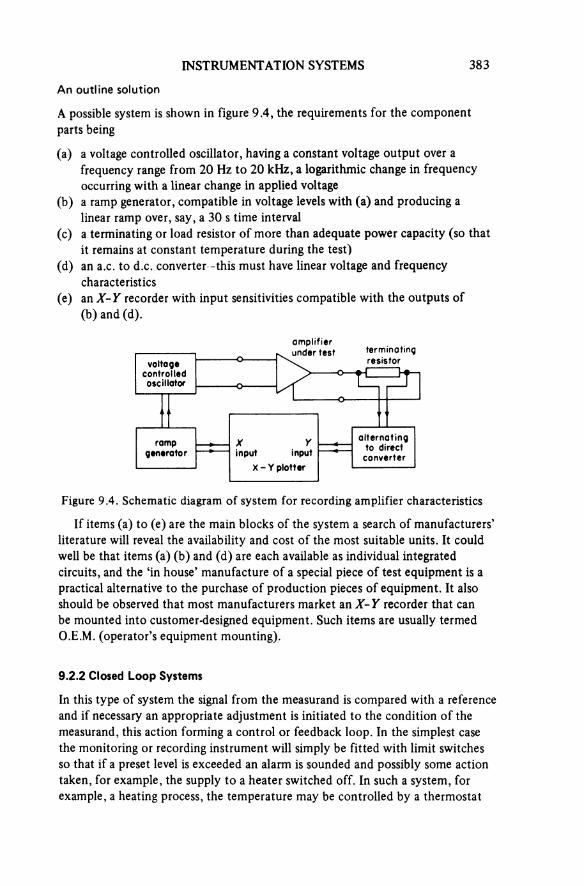
INSTRUMENTATION SYSTEMS 383
An outline solution
A possible system is shown in figure 9.4, the requirements for the component parts being
(a) a voltage controlled oscillator, having a constant voltage output over a frequency range from 20 Hz to 20 kHz, a logarithmic change in frequency occurring with a linear change in applied voltage
(b) a ramp generator, compatible in voltage levels with (a) and producing a linear ramp over, say, a 30 s time interval
(c) a terminating or load resistor of more than adequate power capacity (so thatit remains at constant temperature during the test)
(d) an a.c. to d.c. converter -this must have linear voltage and frequency characteristics
(e) an X-Y recorder with input sensitivities compatible with the outputs of (b) and (d).
Figure 9.4. Schematic diagram of system for recording amplifier characteristics
amplifier under test terminating
resistorvoltagecontrolledoscillator
rampgenerator
Xinput
Yinput
X-Y plotter
alternating to direct
converter
If items (a) to (e) are the main blocks of the system a search of manufacturers’ literature will reveal the availability and cost of the most suitable units. It could well be that items (a) (b) and (d) are each available as individual integrated circuits, and the ‘in house’ manufacture of a special piece of test equipment is a practical alternative to the purchase of production pieces of equipment. It also should be observed that most manufacturers market an X-Y recorder that can be mounted into customer-designed equipment. Such items are usually termed O.E.M. (operator’s equipment mounting).
9.2.2 Closed Loop Systems
In this type of system the signal from the measurand is compared with a reference and if necessary an appropriate adjustment is initiated to the condition of the measurand, this action forming a control or feedback loop. In the simplest case the monitoring or recording instrument will simply be fitted with limit switches so that if a preset level is exceeded an alarm is sounded and possibly some action taken, for example, the supply to a heater switched off. In such a system, for example, a heating process, the temperature may be controlled by a thermostat
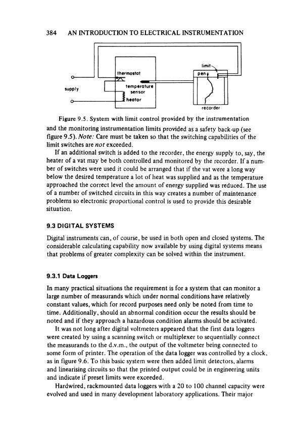
384 AN INTRODUCTION TO ELECTRICAL INSTRUMENTATION
Figure 9.5. System with limit control provided by the instrumentation
supply
thermostat
temperaturesensor
heater
limitpen
recorder
and the monitoring instrumentation limits provided as a safety back-up (see figure 9.5). Note: Care must be taken so that the switching capabilities of the limit switches are not exceeded.
If an additional switch is added to the recorder, the energy supply to, say, the heater of a vat may be both controlled and monitored by the recorder. If a num-ber of switches were used it could be arranged that if the vat were a long way below the desired temperature a lot of heat was supplied and as the temperature approached the correct level the amount of energy supplied was reduced. The useof a number of switched circuits in this way creates a number of maintenance problems so electronic proportional control is used to provide this desirable situation.
9.3 DIGITAL SYSTEMS
Digital instruments can, of course, be used in both open and closed systems. The considerable calculating capability now available by using digital systems means that problems of greater complexity can be solved within the instrument.
9.3.1 Data Loggers
In many practical situations the requirement is for a system that can monitor a large number of measurands which under normal conditions have relatively constant values, which for record purposes need only be noted from time to time. Additionally, should an abnormal condition occur the results should be noted and if they approach a hazardous condition alarms should be activated.
It was not long after digital voltmeters appeared that the first data loggers were created by using a scanning switch or multiplexer to sequentially connect the measurands to the d.v.m., the output of the voltmeter being connected to some form of printer. The operation of the data logger was controlled by a clock, as in figure 9.6. To this basic system were then added limit detectors, alarms and linearising circuits so that the printed output could be in engineering units and indicate if preset limits were exceeded.
Hardwired, rackmounted data loggers with a 20 to 100 channel capacity were evolved and used in many development laboratory applications. Their major
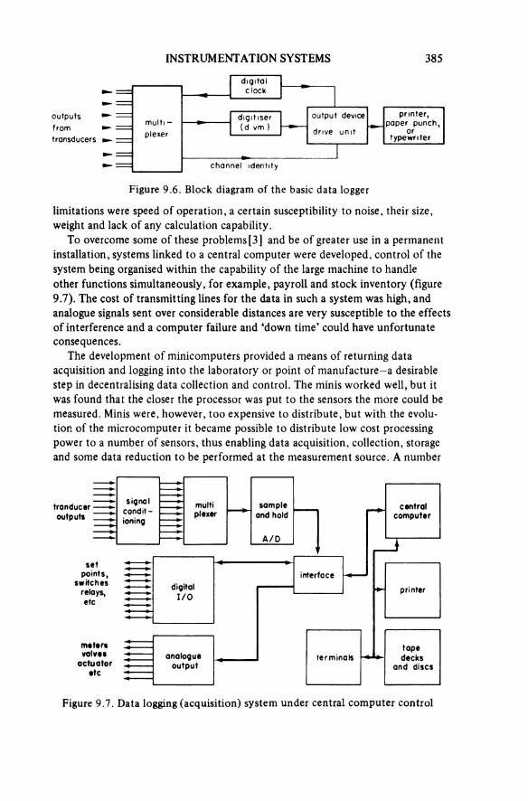
INSTRUMENTATION SYSTEMS 385
Figure 9.6. Block diagram of the basic data logger
outputsfromtransducers
multi - plexer
digitalclock
digitiser (d vm )
output device
drive unit
printer, paper punch
ortypewriter
limitations were speed of operation, a certain susceptibility to noise, their size, weight and lack of any calculation capability.
To overcome some of these problems [3] and be of greater use in a permanent installation, systems linked to a central computer were developed, control of the system being organised within the capability of the large machine to handle other functions simultaneously, for example, payroll and stock inventory (figure 9.7). The cost of transmitting lines for the data in such a system was high, and analogue signals sent over considerable distances are very susceptible to the effects of interference and a computer failure and ‘down time’ could have unfortunate consequences.
The development of minicomputers provided a means of returning data acquisition and logging into the laboratory or point of manufacture—a desirable step in decentralising data collection and control. The minis worked weH, but it was found that the closer the processor was put to the sensors the more could be measured. Minis were, however, too expensive to distribute, but with the evolu-tion of the microcomputer it became possible to distribute low cost processing power to a number of sensors, thus enabling data acquisition, collection, storage and some data reduction to be performed at the measurement source. A number
Figure 9.7. Data logging (acquisition) system under central computer control
transduceroutputs
signalcondit-ioning
multiplexer
sample and hold
A/D
centralcomputer
setpoints,
switchesrelays,etc
digitalI/O
interface
printer
metersvalves
actuatoretc
analogueoutput
terminalstape decks
and discs

386 AN INTRODUCTION TO ELECTRICAL INSTRUMENTATION
Figure 9.8. Distributed data acquisition system incorporating microcomputers linked to central computer
system 1
transduceroutputs
signalcondit-ioning
multi-plexer
sample and hold
A/D
setpoints,
switchesrelaysetc
digitalI/O microcomputer
centralcomputer
metersvalves
actuatoretc
analogueoutput
memory
dedicated software communicationlines
system 2 system 3
Figure 9.9. Programmable datalogger (courtesy of John Fluke Manufacturing Co.)
Dual Interval Scan
INSTRUMENTATION SYSTEMS 387
of microcomputer controlled stations, or process loops are then linked via a serial communications line to a central management computer, which oversees the total system (figure 9.8).
Such an arrangement is suitable for a large installation such as a chemical process plant or a ship. On a smaller scale such as that encountered in most research investigation, the use of microprocessors [4, 5] has resulted in self- contained data loggers with fairly extensive programmable and preprogrammed capabilities. For example, the instrument illustrated in figure 9.9 has a 1000 channel capability, an interactive keyboard programming capability for range, function, skip and limits selection for each channel, signal conditioning for the standard thermocouple types, a reading resolution of 1 μV or 0.1 °C, selectable scan rates, a clock to monitor real or elapsed time in days, hours, minutes and seconds, an internal printer to record the data and, if required, a printout of the complete program.
9.3.2 Bus-connected Systems
The possibilities of programmably controlling instruments and printing or graphically presenting the results of measurements are very desirable features in any measurement system. The cost of producing a single instrument capable of satisfying every requirement for all measurement situations would be so high that few, if any, organisations would be able to justify the purchase. In the mid to late 1960s a number of manufacturers began producing modular instruments so that customers could select suitable units and plug them into a main frame to form a system tailored to their particular requirements. The limitations of com-patibility between manufacturers resulted in the CAMAC (computer automated measurement and control) system of standard instrumentation interface [6]. Thisis an arrangement that provides for the use of units from different manufacturers within a common main frame.
At much the same time discussions took place in Europe and the United States on the feasibility of a standard interface between complete instruments, so that instrumentation systems could be designed and assembled using severalseparate instruments of different manufacture. The interface concepts then under development by Hewlett-Packard were selected as a model, and have resulted in the arrangement known variously as the IEC BUS, IEEE Standard 488-1975, HP-IB, GBIB, Plus Bus and ANSI std MCl-l (see reference 7, 8, 9 and 10).
Both the CAMAC and HP-IB systems have their applications (although the latter seems to be gaining greater acceptance) and were evolved in response to the rising need to minimise the resources repeatedly expended on unique solu-tions to the problem of interconnection of system components. Prior to their adoption, system design engineers were tending to select interface methods to satisfy specific and immediate needs. The development costs were high, each solution being a somewhat unique selection of codes, logic sense, levels and timing protocols for each application.
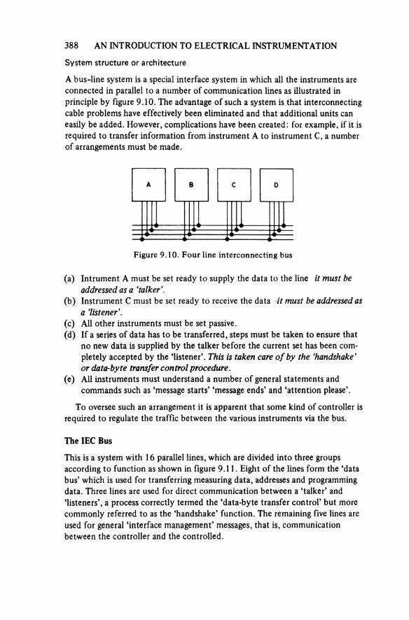
388 AN INTRODUCTION TO ELECTRICAL INSTRUMENTATION
System structure or architecture
A bus-line system is a special interface system in which all the instruments are connected in parallel to a number of communication lines as illustrated in principle by figure 9.10. The advantage of such a system is that interconnecting cable problems have effectively been eliminated and that additional units can easily be added. However, complications have been created: for example, if it is required to transfer information from instrument A to instrument C, a number of arrangements must be made.
Figure 9.10. Four line interconnecting bus
(a) Instrument A must be set ready to supply the data to the line it must be addressed as a ‘talker’.
(b) Instrument C must be set ready to receive the data it must be addressed as a ‘listener’.
(c) All other instruments must be set passive.(d) If a series of data has to be transferred, steps must be taken to ensure that
no new data is supplied by the talker before the current set has been com-pletely accepted by the ‘listener’. This is taken care of by the ‘handshake’ or data-byte transfer control procedure.
(e) All instruments must understand a number of general statements and commands such as ‘message starts’ ‘message ends’ and ‘attention please’.
To oversee such an arrangement it is apparent that some kind of controller is required to regulate the traffic between the various instruments via the bus.
The IEC Bus
This is a system with 16 parallel lines, which are divided into three groups according to function as shown in figure 9.11. Eight of the lines form the ‘databus’ which is used for transferring measuring data, addresses and programming data. Three lines are used for direct communication between a ‘talker’ and ‘listeners’, a process correctly termed the ‘data-byte transfer control’ but more commonly referred to as the ‘handshake’ function. The remaining five lines are used for general ‘interface management’ messages, that is, communication between the controller and the controlled.
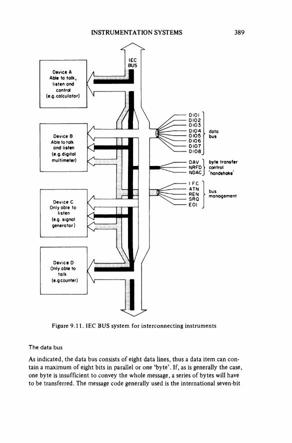
INSTRUMENTATION SYSTEMS 389
Figure 9.11. IEC BUS system for interconnecting instruments
Device A Able to talk,
listen and control
(e.g. calculator)
IEC BUS
Device BAble to talk and listen
(e.g. digital multimeter)
databus
byte transfercontrol'handshake'
Device C Only able to
listen (e.g. signal generator)
busmanagement
Device D Only able to
talk(e.g counter)
The data bus
As indicated, the data bus consists of eight data lines, thus a data item can con-tain a maximum of eight bits in parallel or one ‘byte’. If, as is generally the case one byte is insufficient to convey the whole message, a series of bytes will have to be transferred. The message code generally used is the international seven-bit
390 AN INTRODUCTION TO ELECTRICAL INSTRUMENTATION
ISO code, which covers nearly all the figures, letters and signs required in practice.The type of information transferred via the data bus can be subdivided as
follows.
(a) Addresses, that is, information offered by the controller to all the instru-ments in parallel. Each compares the address on the data bus with its own address and the one that identifies itself reacts.
(b) Data-this may be programming or measurement data communicated by the instrument addressed as a talker and received by those addressed as listeners. For example, the selection of a voltmeter range and the magnitude of the reading respectively.
The 'handshake' function
When a multiple-byte message has to be transferred from one instrument toanother, it is apparent that an organisation structure is required to ensure that the talker does not talk if the listener is not listening, and that the talker does not operate for a shorter time than the slowest listener can accept the informa-tion. These requirements are met with the aid of the data-byte transfer control or ‘handshake’ function embodied in the three lines set aside for the purpose. Each of the lines has its own specific function as follows.
DAV (Data valid): a ‘low’ signal from the talker on this line indicates that the data on the data lines is correct and suitable for acceptance.NRFD (not ready for data): the listeners indicate via this line if they are ready to listen to (new) information—‘High’ if ready, ‘Low’ if not ready for data.NDAC (Data not accepted): the listeners indicate their acceptance of the message via this line, a ‘high’ indicating acceptance and a ‘low’ being not accepted.
Both the NRFD and NDAC lines are ‘wired-OR’ that is these lines can only be ‘high’ if all instruments programmed as listeners have a ‘high’ output. This ensures that the line is only ‘high’ when all the listeners, (including the slowest) are ready for new data or have accepted the data.
The sequence of operations on the handshake lines, when involved in transfer-ring each data byte across the interface, can be represented by the timing diagram in figure 9.12, as follows.
T.1: initial conditions are set up in all the talkers and listenersthe DAVline is set highthe NRFDline is set low, andthe NDACline is set low.T.2: The talker checks the line conditions, and puts a data byte on the lines.
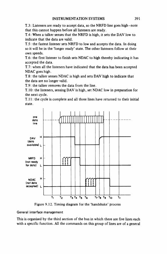
INSTRUMENTATION SYSTEMS 391
T.3: Listeners are ready to accept data, so the NRFD line goes high-note that this cannot happen before all listeners are ready.T.4: When a talker senses that the NRFD is high, it sets the DAV low to indicate that the data are valid.T.5: the fastest listener sets NRFD to low and accepts the data. In doing so it will be in the ‘longer ready’ state. The other listeners follow at their own speeds.T.6: the first listener to finish sets NDAC to high thereby indicating it has accepted the data.T.7: when all the listeners have indicated that the data has been accepted NDAC goes high.T.8: the talker senses NDAC is high and sets DAV high to indicate that the data are no longer valid.T.9: the talker removes the data from the line.T.10: the listeners, sensing DAV is high, set NDAC low in preparation for the next cycle.T.11: the cycle is complete and all three lines have returned to their initial state.
Figure 9.12. Timing diagram for the ‘handshake’ process
onedataline
DAV(data
available)
NRFD (not ready for data)
NDAC (not data accepted)
General interface management
This is organised by the third section of the bus in which there are five lines each with a specific function. All the commands on this group of lines are of a general
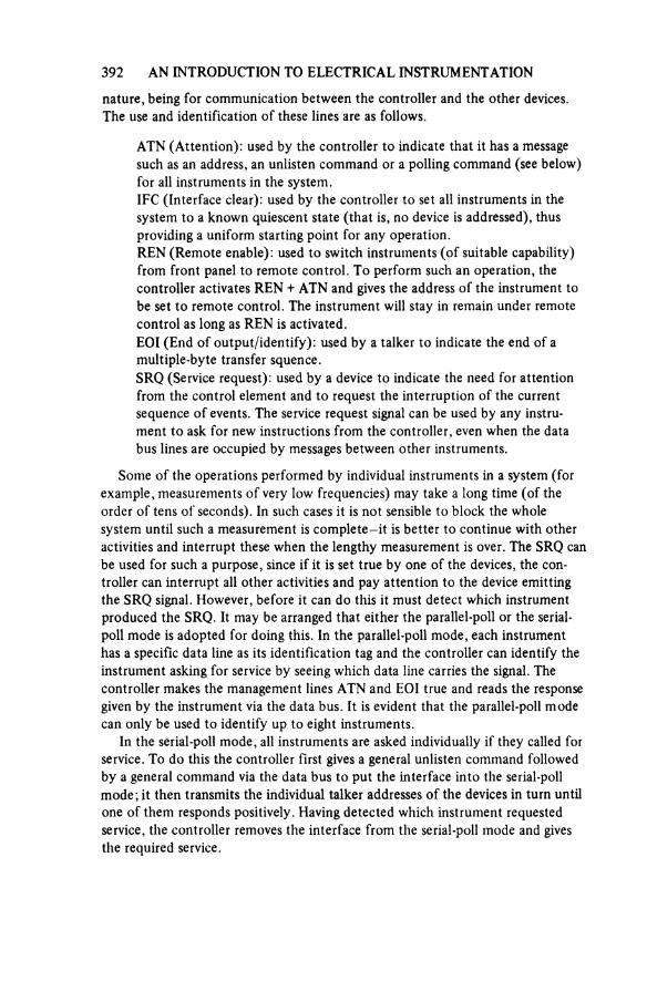
392 AN INTRODUCTION TO ELECTRICAL INSTRUMENTATION
nature, being for communication between the controller and the other devices. The use and identification of these lines are as follows.
ATN (Attention): used by the controller to indicate that it has a message such as an address, an unlisten command or a polling command (see below) for an instruments in the system.IFC (interface clear): used by the controller to set an instruments in the system to a known quiescent state (that is, no device is addressed), thus providing a uniform starting point for any operation.REN (Remote enable): used to switch instruments (of suitable capability) from front panel to remote control. To perform such an operation, the controller activates REN + ATN and gives the address of the instrument to be set to remote control. The instrument will stay in remain under remote control as long as REN is activated.EOI (End of output/identify): used by a talker to indicate the end of a multiple-byte transfer sequence.SRQ (Service request): used by a device to indicate the need for attention from the control element and to request the interruption of the current sequence of events. The service request signal can be used by any instru-ment to ask for new instructions from the controller, even when the data bus lines are occupied by messages between other instruments.
Some of the operations performed by individual instruments in a system (for example, measurements of very low frequencies) may take a long time (of the order of tens of seconds). In such cases it is not sensible to block the whole system until such a measurement is complete—it is better to continue with other activities and interrupt these when the lengthy measurement is over. The SRQ canbe used for such a purpose, since if it is set true by one of the devices, the con-troller can interrupt all other activities and pay attention to the device emitting the SRQ signal. However, before it can do this it must detect which instrument produced the SRQ. It may be arranged that either the parallel-poll or the serial- poll mode is adopted for doing this. In the paranei-pon mode, each instrument has a specific data line as its identification tag and the controller can identify the instrument asking for service by seeing which data line carries the signal. The controller makes the management lines ATN and EOI true and reads the response given by the instrument via the data bus. It is evident that the parallel-poll mode can only be used to identify up to eight instruments.
In the serial-poll mode, all instruments are asked individually if they called for service. To do this the controller first gives a general unlisten command followed by a general command via the data bus to put the interface into the serial-poll mode; it then transmits the individual talker addresses of the devices in turn until one of them responds positively. Having detected which instrument requested service, the controller removes the interface from the serial-poll mode and gives the required service.
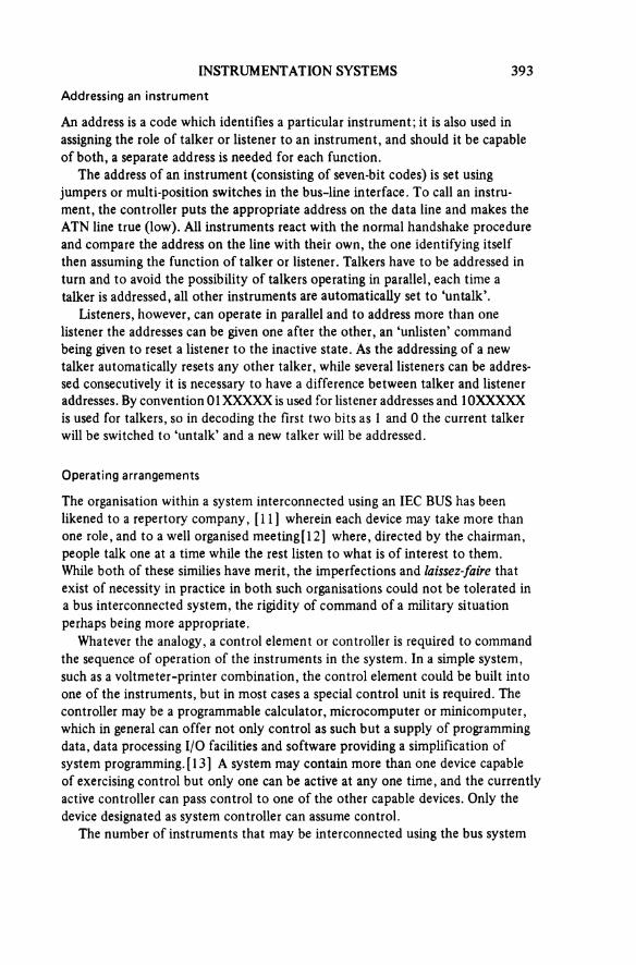
INSTRUMENTATION SYSTEMS 393
Addressing an instrument
An address is a code which identifies a particular instrument; it is also used in assigning the role of talker or listener to an instrument, and should it be capable of both, a separate address is needed for each function.
The address of an instrument (consisting of seven-bit codes) is set using jumpers or multi-position switches in the bus-line interface. To call an instru-ment, the controller puts the appropriate address on the data line and makes the ATN line true (low). All instruments react with the normal handshake procedure and compare the address on the line with their own, the one identifying itself then assuming the function of talker or listener. Talkers have to be addressed in turn and to avoid the possibility of talkers operating in parallel, each time a talker is addressed, all other instruments are automatically set to ‘untalk’.
Listeners, however, can operate in parallel and to address more than one listener the addresses can be given one after the other, an ‘unlisten’ command being given to reset a listener to the inactive state. As the addressing of a new talker automatically resets any other talker, while several listeners can be addres-sed consecutively it is necessary to have a difference between talker and listener addresses. By convention 01 XXXXX is used for listener addresses and 10XXXXX is used for talkers, so in decoding the first two bits as 1 and 0 the current talker will be switched to ‘untalk’ and a new talker will be addressed.
Operating arrangements
The organisation within a system interconnected using an IEC BUS has been likened to a repertory company, [11] wherein each device may take more than one role, and to a well organised meeting [2] where, directed by the chairman, people talk one at a time while the rest listen to what is of interest to them.While both of these similes have merit, the imperfections and laissez-faire that exist of necessity in practice in both such organisations could not be tolerated in a bus interconnected system, the rigidity of command of a military situation perhaps being more appropriate.
Whatever the analogy, a control element or controller is required to command the sequence of operation of the instruments in the system. In a simple system, such as a voltmeter-printer combination, the control element could be built into one of the instruments, but in most cases a special control unit is required. The controller may be a programmable calculator, microcomputer or minicomputer, which in general can offer not only control as such but a supply of programming data, data processing I/O facilities and software providing a simplification of system programming. [13] A system may contain more than one device capable of exercising control but only one can be active at any one time, and the currently active controller can pass control to one of the other capable devices. Only the device designated as system controller can assume control.
The number of instruments that may be interconnected using the bus system
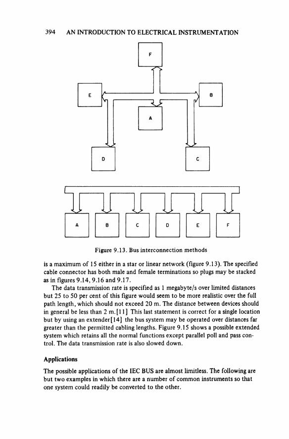
394 AN INTRODUCTION TO ELECTRICAL INSTRUMENTATION
Figure 9.13. Bus interconnection methods
is a maximum of 15 either in a star or linear network (figure 9.13). The specified cable connector has both male and female terminations so plugs may be stacked as in figures 9.14, 9.16 and 9.17.
The data transmission rate is specified as 1 megabyte/s over limited distances but 25 to 50 per cent of this figure would seem to be more realistic over the full path length, which should not exceed 20 m. The distance between devices should in general be less than 2 m. [11] This last statement is correct for a single locationbut by using an extender [14] the bus system may be operated over distances far greater than the permitted cabling lengths. Figure 9.15 shows a possible extended system which retains an the normal functions except parallel poll and pass con-trol. The data transmission rate is also slowed down.
Applications
The possible applications of the IEC BUS are almost limitless. The following are but two examples in which there are a number of common instruments so that one system could readily be converted to the other.
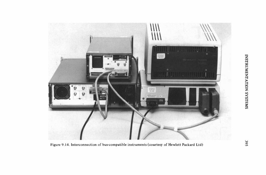
INSTR
UM
ENTA
TION SY
STEMS
395Figure 9.14. Interconnection of bus-compatible instruments (courtesy of Hewlett Packard Ltd)
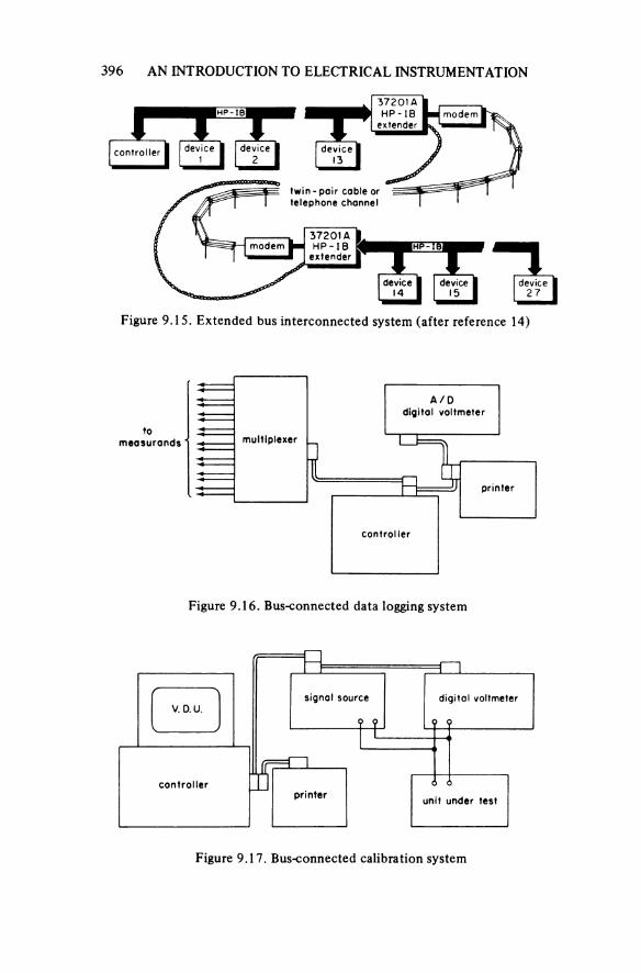
396 AN INTRODUCTION TO ELECTRICAL INSTRUMENTATION
Figure 9.15. Extended bus interconnected system (after reference 14)
HP-IB37201 AHP-IB
extendermodern
controller device device2
device13
twin-pair cable or telephone channel
modem37201 A HP-IB
extenderHl
device14
device15
device27
Figure 9.16. Bus-connected data logging system
tomeasurands multiplexer
A/Ddigital voltmeter
printer
controller
Figure 9.17. Bus-connected calibration system
V. D. U.signal source digital voltmeter
controllerprinter unit under test
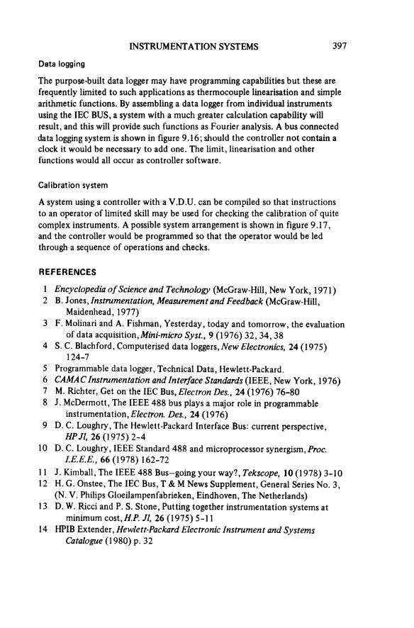
INSTRUMENTATION SYSTEMS 397
Data logging
The purpose-built data logger may have programming capabilities but these are frequently limited to such applications as thermocouple linearisation and simple arithmetic functions. By assembling a data logger from individual instruments using the IEC BUS, a system with a much greater calculation capability will result, and this will provide such functions as Fourier analysis. A bus connected data logging system is shown in figure 9.16; should the controller not contain a clock it would be necessary to add one. The limit, linearisation and other functions would all occur as controller software.
Calibration system
A system using a controller with a V.D.U. can be compiled so that instructions to an operator of limited skill may be used for checking the calibration of quite complex instruments. A possible system arrangement is shown in figure 9.17, and the controller would be programmed so that the operator would be led through a sequence of operations and checks.
REFERENCES
1 Encyclopedia of Science and Technology (McGraw-Hill, New York, 1 97 1)2 B. J ones, Instrumentation, Measurement and Feedback (McGraw-Hill,
Maidenhead, 1977)3 F. Molinari and A. Fishman, Yesterday, today and tomorrow, the evaluation
of data acquisition, Mini-micro Syst., 9 (1976) 32, 34, 384 S. C. Blachford, Computerised data loggers, New Electronics, 24 (1975)
124-75 Programmable data logger, Technical Data, Hewlett-Packard.6 CAMAC Instrumentation and Interface Standards (IEEE, New York, 1976)7 M. Richter, Get on the IEC Bus, Electron Des., 24 (1976) 76-808 J. McDermott, The IEEE 488 bus plays a major role in programmable
instrumentation, Electron. Des., 24 (1976)9 D. C. Loughry, The Hewlett-Packard Interface Bus: current perspective,
HP Jl, 26 (1975) 2-410 D. C. Loughry, IEEE Standard 488 and microprocessor synergism, Proc.
I.E.E.E., 66 (1978) 162-7211 J. Kimball, The IEEE 488 Bus-going your way?, Tekscope, 10 (1978) 3-1012 H. G. Onstee, The IEC Bus, T & M News Supplement, General Series No. 3,
(N. V. Philips Gloeilampenfabrieken, Eindhoven, The Netherlands)13 D. W. Ricci and P. S. Stone, Putting together instrumentation systems at
minimum cost, H.P. Jl, 26 (1975) 5-1114 HPIB Extender, Hewlett-Packard Electronic Instrument and Systems
Catalogue (1980) p. 32

10Problems and Exercises
10.1 PRINCIPLES
1. Discuss the differences between(a) substitution and null methods of measurement(b) analogue and digital instruments.
2. Write brief notes explaining(a) the methods used to reduce the possibility of parallax error in reading an
analogue instrument(b) the techniques used to produce alpha-numeric displays.
3. A resistor was measured, using a Wheatstone bridge as having a value of 1243 Ω ± 0.1%. The same resistor was remeasured, under identical environmental conditions using a digital multimeter and purported to have a value of 1244.5 Ω ± (0.05% of reading + 2 l.s.d.). Postulate a value for the resistance and a tolerance within which the actual value must lie.
4. A resistance box has the following components and tolerances10 resistors each of 100 kΩ ± 0.05%10 resistors each of 10 kΩ ± 0.05%10 resistors each of 1 kΩ ± 0.05%10 resistors each of 100 Ω ± 0.1%10 resistors each of 10 Ω ± 0.5%
Determine, both in ohms and as a percentage, the limit of uncertainty in a setting of 453.72 kΩ.
5. The value of a capacitor was to be evaluated using a circuit which resolved to the expression

PROBLEMS AND EXERCISES 399
Given that ω = 104 ± 0.01%, R = 100 kΩ ± 0.05% and C1 = 500 pF ± 1 pF, determine the value of Cx and the limit of uncertainty in the measurement.
6. A class 0.5 ammeter (fiducial value 1 A), and a class 0.2 voltmeter (fiducial value 10 V) were used to determine the value of a resistor. If the readings on the instruments were 0.72 A and 9.5 V respectively, calculate the value of the resistor and the limit of uncertainty in the measurement. (Neglect the impedance effects of the instruments.)
7. A 3½-digit panel meter has a full scale indication of 1.999 V. Draw a limit of error curve from 0.1 to 2 V, given that the accuracy specification is ± (0.05% of reading + 1 l.s.d.) when the instrument is operated between 10 and 35 °C.
8. A multimeter was used to measure the current in a circuit. When the 300 μArange was used a reading 90 μA was observed, however on changing to the 100 μA range the reading became 60 μA. Given that the voltage drop across the meter is 500 mV when full scale is indicated on either of these ranges, calculate the effective series resistance of the circuit under investigation.
9. A direct voltage source that has an ouput resistance of 125 Ω is connected to a circuit that has an input resistance of 3000 Ω. If the magnitude of the input voltage to the circuit is set at 10 V using a voltmeter that has a full scale of 10 V and an internal resistance of 500 Ω/V, calculate the magnitude of the voltage that will be applied to the circuit when the voltmeter is removed.
10. A resistor is connected in series with a 10 mA full scale ammeter across a variable direct voltage supply that has an internal resistance of Rs Ω. When a 10 v full scale voltmeter (internal resistance 1000 Ω/v) is connected across the terminals of the supply, which is then adjusted so that the voltmeter indicates 10 V, the current through the ammeter is 9.80 mA. On reconnecting the circuit so that the voltmeter is connected across the unknown resistor only, and the supply adjusted so that the milliammeter indicates full scale, the reading on the voltmeter is 5.05 V. Calculate the value of the unknown resistor and the resist-ance of the milliammeter.
11. In measuring the magnitude of a 2 kHz signal a reading on a mean sensing (but r.m.s. calibrated) voltmeter was 7.5 V, while on a r.m.s. sensing instrument the indication was 7.8 V. Determine the form factor of the signal and the contribu-tion of the distorted waveform to the error in measurement that would be present when using the mean sensing instrument.
12. Evaluate the mean, peak and r.m.s. values of the waveform v = 5 + 3 sin θ.
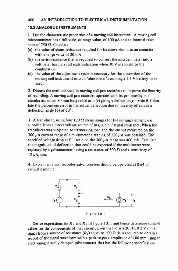
400 AN INTRODUCTION TO ELECTRICAL INSTRUMENTATION
10.2 ANALOGUE INSTRUMENTS
1. List the characteristic properties of a moving coil instrument. A moving coil microammeter has a full scale, or range value, of 100 μA and an internal resist-ance of 750 Ω. Calculate(a) the value of shunt resistance required for its conversion into an ammeter
with a range value of 20 mA(b) the series resistance that is required to convert the microammeter into a
voltmeter having a full scale indication when 30 V is applied to the combination
(c) the value of the adjustment resistor necessary for the conversion of the moving coil instrument into an ‘ohm-meter’ assuming a 1.5 V battery to be used.
2. Discuss the methods used in moving coil pen recorders to improve the linearity of recording. A moving coil pen recorder operates with its pen moving in a circular arc on an 80 mm long radial arm (r) giving a deflection y = r sin θ. Calcu-late the percentage error in the actual deflection due to linearity effects at a deflection angle (θ) of 20°.
3. A transducer, using four 120 Ω strain gauges for the sensing element, was supplied from a direct voltage source of negligible internal resistance. When the transducer was subjected to its working load and the output measured on the 300 μA current range of a multimeter a reading of 120 μA was obtained. The specified voltage drop at full scale on the 300 μA range was 400 mV. Calculate the magnitude of deflection that could be expected if the multimeter were replaced by a galvanometer having a resistance of 500 Ω and a sensitivity of 12 μA/mm.
4. Explain why u.v. recorder galvanometers should be operated at 0.64 of critical damping.
Figure 10.1.
Derive expressions for R1 and R2 of figure 10.1, and hence determine suitable values for the components of that circuit, given that Vs is a 20 Hz, 0.2 V r.m.s. signal from a source of resistance (Rs) equal to 100 Ω. It is required to obtain a record of the signal waveform with a peak-to-peak amplitude of 100 mm using an electromagnetically damped galvanometer that has the following specification
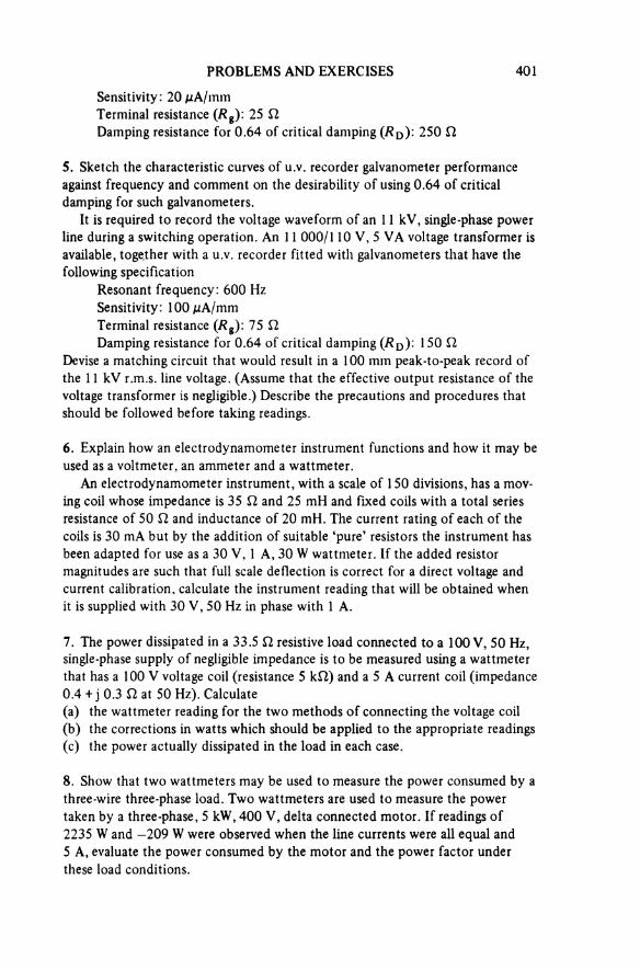
PROBLEMS AND EXERCISES 401
Sensitivity: 20 μA/mm Terminal resistance (Rg): 25 ΩDamping resistance for 0.64 of critical damping (RD): 250 Ω
5. Sketch the characteristic curves of u.v. recorder galvanometer performance against frequency and comment on the desirability of using 0.64 of critical damping for such galvanometers.
It is required to record the voltage waveform of an 11 kV, single-phase power line during a switching operation. An 11 000/110 V, 5 VA voltage transformer is available, together with a u.v. recorder fitted with galvanometers that have the following specification
Resonant frequency: 600 Hz Sensitivity: 100 μA/mm Terminal resistance (Rg): 75 ΩDamping resistance for 0.64 of critical damping (RD): 150 Ω
Devise a matching circuit that would result in a 100 mm peak-to-peak record of the 11 kV r.m.s. line voltage. (Assume that the effective output resistance of the voltage transformer is negligible.) Describe the precautions and procedures that should be followed before taking readings.
6. Explain how an electrodynamometer instrument functions and how it may be used as a voltmeter, an ammeter and a wattmeter.
An electrodynamometer instrument, with a scale of 150 divisions, has a mov-ing coil whose impedance is 35 Ω and 25 mH and fixed coils with a total series resistance of 50 Ω and inductance of 20 mH. The current rating of each of the coils is 30 mA but by the addition of suitable ‘pure’ resistors the instrument has been adapted for use as a 30 V, 1 A, 30 W wattmeter. If the added resistor magnitudes are such that full scale deflection is correct for a direct voltage and current calibration, calculate the instrument reading that will be obtained when it is supplied with 30 V, 50 Hz in phase with 1 A.
7. The power dissipated in a 33.5 Ω resistive load connected to a 100 V, 50 Hz, single-phase supply of negligible impedance is to be measured using a wattmeter that has a 100 V voltage coil (resistance 5 kΩ) and a 5 A current coil (impedance 0.4 +j 0.3 Ω at 50 Hz). Calculate(a) the wattmeter reading for the two methods of connecting the voltage coil(b) the corrections in watts which should be applied to the appropriate readings(c) the power actually dissipated in the load in each case.
8. Show that two wattmeters may be used to measure the power consumed by a three-wire three-phase load. Two wattmeters are used to measure the power taken by a three-phase, 5 kW, 400 V, delta connected motor. If readings of 2235 W and —209 W were observed when the line currents were all equal and5 A, evaluate the power consumed by the motor and the power factor under these load conditions.
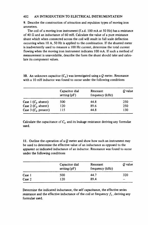
402 AN INTRODUCTION TO ELECTRICAL INSTRUMENTATION
9. Describe the construction of attraction and repulsion types of moving iron ammeters.
The coil of a moving iron instrument (f.s.d. 100 mA at 50 Hz) has a resistance of 40 Ω and an inductance of 60 mH. Calculate the value of a pure resistance shunt which when connected across the coil will result in full scale deflection occurring when 10 A, 50 Hz is applied to the combination. If the shunted meter is inadvertently used to measure a 100 Hz current, determine the total current flowing when the moving iron instrument indicates 100 mA. If such a method of measurement is unavoidable, describe the form the shunt should take and calcu-late its component values.
10. An unknown capacitor (Cx) was investigated using a Q meter. Resonance with a 10 mH inductor was found to occur under the following conditions
Capacitor dial setting (pF)
Resonant frequency (kHz)
Q value
Case 1 (Cx absent) 500 44.8 250Case 2 (Cx absent) 120 89.6 250Case 3 (Cx present) 115 44.8 130
Calculate the capacitance of Cx and its leakage resistance deriving any formulae used.
11. Outline the operation of a Q meter and show how such an instrument may be used to determine the effective value of an inductance as opposed to the apparent or indicated inductance of an inductor. Resonance was found to occur under the following conditions
Capacitor dial setting (pF)
Resonant frequency (kHz)
Q value
Case 1 500 44.7 320Case 2 120 89.4 —
Determine the indicated inductance, the self capacitance, the effective series resistance and the effective inductance of the coil at frequency f1, deriving any formulae used.

PROBLEMS AND EXERCISES 403
12. The sets of readings given below were obtained when an inductor that has a ferrite core was connected to a Q meter.
Capacitor dial setting (pF)
Resonant frequency (kHz)
Q value
Measurement 1 500 20.7 220Measurement 2 350 23.9 180Measurement 3 300 25.4 160Measurement 4 200 29.4 137Measurement 5 60 41.4 51
Calculate the effective resistance and effective inductance of the coil and show graphically the variation of these quantities with frequency. Hence determine the true inductance of the coil.
Explain why the graph of effective resistance against frequency does not conform to the expression
(7.10)
13. Describe the operation of a cathode ray oscilloscope, with particular refer-ence to the timebase, the vertical amplifiers, the deflection system, and the triggering of the trace.
The input ‘attenuator’ of an oscilloscope is set to 100 mV/div. If a sinusoidal trace has a peak-to-peak amplitude of 6.4 div. what is its r.m.s. value? For the same waveform the horizontal distance between identical points is four divisions when the timebase is set to a speed of 0.1 ms/div. Evaluate the frequency of the signal.
The above signal is the voltage across a capacitive impedance Z. A second waveform (the voltage drop across a pure 10 Ω resistor in series with Z) has a peak-to-peak amplitude of 4.8 div. (vertical amplifier sensitivity 1 mV/div.) and is displaced from the first wave by 0.8 div. What are the magnitudes of the series components of Z?
14. Describe methods by which a c.r.o. may be used to measure(a) the r.m.s. value of a sinewave(b) the frequency of a sinewave.
For the trace in figure 10.2a deduce an expression for the phase angle between the sinusoids that result in such a display and hence determine the phase angle for the given display.
Describe the procedure by which a trace of the type shown in figure 10.2b is obtained and then calculate the rise time of the voltage step shown in figure 10.2b given that the oscilloscope timebase when this display was obtained was set to 1 μs/div. and the × 5 condition had been applied.

404 AN INTRODUCTION TO ELECTRICAL INSTRUMENTATION
Figure 10.2.
(a) (b)
10.3 NULL OR COMPARISON MEASUREMENTS
1. A d.c. potentiometer is used to compare the voltage drop across an unknown resistance with that across a 1000 Ω ± 0.01% resistor. Given that the following readings were taken at the same temperature, calculate a value for the unknown and a tolerance in ohms on the measured value.
Forwardcurrent
Reversedcurrent
Voltage across 1 kΩ resistor (V) 0.9325 0.9400Voltage across unknown resistor (V) 1.5672 1.5678
Assume a tolerance of ± 0.2 mV on each potentiometer reading.
2. Discuss the use of the potentiometric principle in pen recorders and indicate the types of application appropriate to the various forms (flat-bed, circular, etc.) of recorder.
An X-Y recorder has a specified slewing speed of 1.8 m/s and equal X and Y maximum velocities. If its maximum Y acceleration from rest is 40 m/s2 deter-mine the peak amplitudes possible for the display of 3 Hz and 8 Hz waveforms.
Figure 10.3.
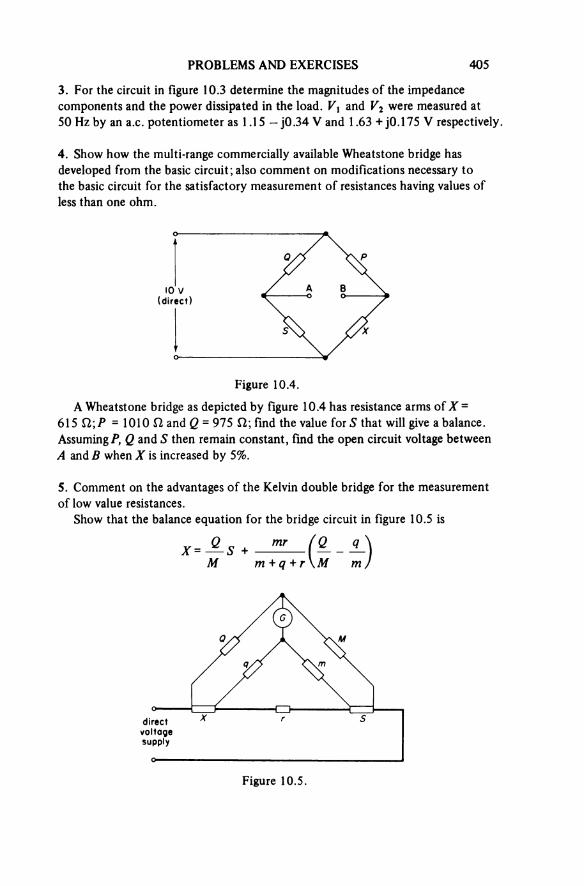
PROBLEMS AND EXERCISES 405
3. For the circuit in figure 10.3 determine the magnitudes of the impedance components and the power dissipated in the load. V1 and V2 were measured at 50 Hz by an a.c. potentiometer as 1.15 — j0.34 V and 1.63 + j0.175 V respectively
4. Show how the multi-range commercially available Wheatstone bridge has developed from the basic circuit ; also comment on modifications necessary to the basic circuit for the satisfactory measurement of resistances having values of less than one ohm.
Figure 10.4.
io V (direct)
A Wheatstone bridge as depicted by figure 10.4 has resistance arms of X =615 Ω; P = 1010 Ω and Q = 975 Ω; find the value for S that will give a balance. Assuming P, Q and S then remain constant, find the open circuit voltage between A and B when X is increased by 5%.
5. Comment on the advantages of the Kelvin double bridge for the measurement of low value resistances.
Show that the balance equation for the bridge circuit in figure 10.5 is
Figure 10.5.
directvoltagesupply
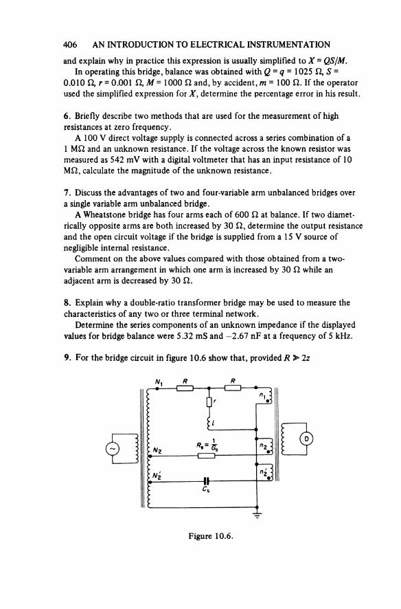
406 AN INTRODUCTION TO ELECTRICAL INSTRUMENTATION
and explain why in practice this expression is usually simplified to X = QS/M.In operating this bridge, balance was obtained with Q = q = 1025 Ω, S =
0.010 Ω, r = 0.001 Ω, M = 1000 Ω and, by accident, m = 100 Ω. If the operator used the simplified expression for X, determine the percentage error in his result.
6. Briefly describe two methods that are used for the measurement of high resistances at zero frequency.
A 100 V direct voltage supply is connected across a series combination of a 1 MΩ and an unknown resistance. If the voltage across the known resistor was measured as 542 mV with a digital voltmeter that has an input resistance of 10 MΩ, calculate the magnitude of the unknown resistance.
7. Discuss the advantages of two and four-variable arm unbalanced bridges over a single variable arm unbalanced bridge.
A Wheatstone bridge has four arms each of 600 Ω at balance. If two diamet-rically opposite arms are both increased by 30 Ω, determine the output resistance and the open circuit voltage if the bridge is supplied from a 1 5 V source of negligible internal resistance.
Comment on the above values compared with those obtained from a two- variable arm arrangement in which one arm is increased by 30 Ω while an adjacent arm is decreased by 30 Ω.
8. Explain why a double-ratio transformer bridge may be used to measure the characteristics of any two or three terminal network.
Determine the series components of an unknown impedance if the displayed values for bridge balance were 5.32 mS and —2.67 nF at a frequency of 5 kHz.
9. For the bridge circuit in figure 10.6 show that, provided R >> 2z
Figure 10.6.
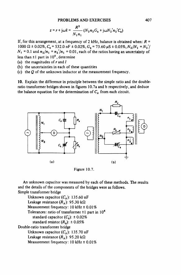
PROBLEMS AND EXERCISES 407
If, for this arrangement, at a frequency of 2 kHz, balance is obtained when: R = 1000 Ω ± 0.02%, Cs = 532.0 nF ± 0.02%, Gs = 73.60 μS ± 0.05%, N2/N1 = N2'/ N1 = 0.1 and n2/n1 = n2'/n1 = 0.01, each of the ratios having an uncertainty of less than ±1 part in 105, determine(a) the magnitudes of r and l(b) the uncertainties in each of these quantities(c) the Q of the unknown inductor at the measurement frequency.
10. Explain the difference in principle between the simple ratio and the double-ratio transformer bridges shown in figures 10.7a and b respectively, and deduce the balance equation for the determination of Cx from each circuit.
Figure 10.7.
(o) (b)
An unknown capacitor was measured by each of these methods. The results and the details of the components of the bridges were as follows.Simple transformer bridge
Unknown capacitor (Cx): 135.60 nFLeakage resistance (Rx) 95.30 kΩ Measurement frequency: 10 kHz ± 0.01%Tolerances: ratio of transformer ±1 part in 104
standard capacitor (Cs): ± 0.02% standard resistor (Rs): ± 0.05%
Double-ratio transformer bridgeUnknown capacitor (Cx): 135.70 nFLeakage resistance (Rx) 95.20 kΩ Measurement frequency: 10 kHz ± 0.01%
408 AN INTRODUCTION TO ELECTRICAL INSTRUMENTATION
Tolerances: ratios of voltage and current transformers ± 5 parts in 10sstandard capacitor (Cs): ± 0.05% standard resistor (Rs): ± 0.07%
Assuming that in each case the determination errors could be neglected, postu-late magnitudes and tolerances for the unknown capacitor and its leakage resistance.
10.4 DIGITAL INSTRUMENTS
1. Discuss briefly the advantages and disadvantages of using a counter-timer to measure frequencies in the 2 to 9 kHz band: (a) by frequency measurement; and (b) by multi-period measurement. Given that the timebase oscillator in a counter-timer is known to have an uncertainty in value of less than 5 p.p.m., evaluate the total possible uncertainty in determining the magnitude of a frequency from each of the following readings(i) 07.3560 kHz (using a 10 s time interval)(ii) 1 35.943 μs for 1 000 periods (assume that the trigger error is less than 03/n%,
where n is the number of periods averaged).Describe a method by which a counter-timer could be used to determine the
drift in the output frequency of a 4 kHz oscillator.
2. Sketch the total uncertainty in reading against frequency characteristics forthe ‘frequency’ and ‘multi-period’ modes of operation for a counter-timer. A six-digit (999999) counter-timer which has a 1 MHz reference oscillator (stability better than 9 p.p.m.) is to be used to measure a sinewave frequency of approximately 11 kHz. In the frequency mode of operation gate time intervals of 1 ms, 10 ms, 100 ms, 1 s and 10 s are available while in the multi-period mode, where 1 count = 1 μs, and n values of 1, 10, 102, . . ., 106 are possible.Determine the measurement method and range that will result in a minimum of uncertainty in the measurement of the unknown frequency. Assume that the reading determination error = 1 l.s.d., an eight-digit calculator is available, and for a sinewave the trigger error = 0.3%/n. Briefly describe a method of checking that the sensitivity of a counter timer is within its specification.
3. Describe in outline the dual-slope conversion technique used in digital volt-meters and comment on the ability of this technique to provide rejection of supply frequency interference.
A dual-slope 3½-digit voltmeter has an accuracy specification on its 20 mV range of ± (0.05% of reading + 0.05% of range) at 23 °C, a temperature allowance of ± (0.01% of reading + 5 μV) per °C and a d.c. common-mode rejection ratio of 120 dB. Calculate the total possible uncertainty in reading the voltage drop across R1 in figure 10.8 at 20 °C, given that R1 = 1 kΩ, R2 = 10 MΩ and Vs = 100 V.
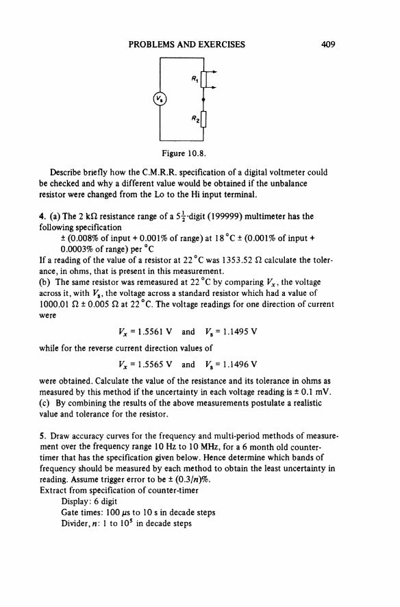
PROBLEMS AND EXERCISES 409
Figure 10.8.
Describe briefly how the C.M.R.R. specification of a digital voltmeter could be checked and why a different value would be obtained if the unbalance resistor were changed from the Lo to the Hi input terminal.
4. (a) The 2 kΩ resistance range of a 5½-digit (199999) multimeter has the following specification
± (0.008% of input + 0.001% of range) at 1 8 °C ± (0.001% of input + 0.0003% of range) per °C
If a reading of the value of a resistor at 22 °C was 1353.52 Ω calculate the toler-ance, in ohms, that is present in this measurement.(b) The same resistor was remeasured at 22 °C by comparing Vx, the voltage across it, with Vs, the voltage across a standard resistor which had a value of 1000.01 Ω ± 0.005 Ω at 22 °C. The voltage readings for one direction of current were
VX = 1.5561 V and Vs= 1.1495 V
while for the reverse current direction values of
Vx = 1.5565 V and Vs = 1.1496 V
were obtained. Calculate the value of the resistance and its tolerance in ohms as measured by this method if the uncertainty in each voltage reading is ± 0.1 mV. (c) By combining the results of the above measurements postulate a realistic value and tolerance for the resistor.
5. Draw accuracy curves for the frequency and multi-period methods of measure-ment over the frequency range 10 Hz to 10 MHz, for a 6 month old counter-timer that has the specification given below. Hence determine which bands of frequency should be measured by each method to obtain the least uncertainty in reading. Assume trigger error to be ± (0.3/n)%.Extract from specification of counter-timer
Display: 6 digitGate times: 100 μs to 10 s in decade steps Divider, n: 1 to 105 in decade steps
410 AN INTRODUCTION TO ELECTRICAL INSTRUMENTATION
Timebase: frequency—5 MHz (1 MHz output); accuracy-determined at any given time by the deviation from the initial setting caused by ageing and environmental effects as defined by the specified stability; stability/ ambient temperature effect, ± 3 parts in 106 between 20 and 40 °C; ageing, ± 1 part in 106 per month (after 3 months).
10.5 TRANSDUCERS
1. The output signal from a potentiometric displacement transducer is to be recorded using a fluid damped galvanometer in a u.v. recorder. The transducer, which has an output resistance that may be varied from 0 to 1000 Ω, is supplied with direct current from a 20 mA constant current source. If the galvanometer has a terminal resistance of 26 Ω, a sensitivity of 90 μA/mm and requires a damping resistance of between 50 Ω and 2 kΩ for operation at 0.64 of critical damping, calculate the value of resistance that must be placed in series with the galvanometer so that the maximum deflection is limited to 50 mm. Assuming that the constant current source has an infinite output impedance draw a graph relating displacement as a percentage of that possible at the transducer with deflection of the recorder trace.
How could the linearity be improved?
2. Show how resistance strain gauges may be incorporated in transducers to measure force, acceleration, pressure, temperature and humidity.
Discuss the use of unbalanced bridges in such devices and describe suitable methods of recording steady state and transient changes in the measurand.
Four strain gauges each having a resistance of 125 Ω are connected to form a Wheatstone bridge, so that adjacent arms have a resistance change of opposite sense (that is, increase and decrease). If this resistance change has a maximum value of 5 Ω, calculate the peak open circuit output voltage from the bridge when it is supplied from a 10 V direct source of negligible internal resistance.
If two galvanometers A and B are available for measuring the strain gauge bridge output, determine which should be used to obtain the largest deflection given that galvanometer A has a sensitivity of 10 μA/mm and terminal resistance of 500 Ω, and that galvanometer B has a sensitivity of 15 μA/mm and terminal resistance of 200 Ω.
3. Explain why initial balancing circuits are necessary when using strain gauges in bridge circuits.
A recorder galvanometer with the specification given below is to be used to measure the output from the strain gauge bridge arrangement shown in figure 10.9. Find(a) The value of Rp that provides the galvanometer with the damping resistance
for optimum performance.(b) The peak open circuit value of VOut which, if the bridge were connected to
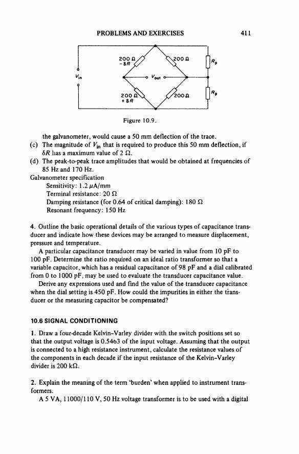
PROBLEMS AND EXERCISES 411
Figure 10.9
the galvanometer, would cause a 50 mm deflection of the trace.(c) The magnitude of Vin that is required to produce this 50 mm deflection, if
δR has a maximum value of 2 Ω.(d) The peak-to-peak trace amplitudes that would be obtained at frequencies of
85 Hz and 170 Hz.Galvanometer specification
Sensitivity: 1.2 μA/mm Terminal resistance: 20 ΩDamping resistance (for 0.64 of critical damping): 180 Ω Resonant frequency: 150 Hz
4. Outline the basic operational details of the various types of capacitance trans-ducer and indicate how these devices may be arranged to measure displacement, pressure and temperature.
A particular capacitance transducer may be varied in value from 10 pF to 100 pF. Determine the ratio required on an ideal ratio transformer so that a variable capacitor, which has a residual capacitance of 98 pF and a dial calibrated from 0 to 1000 pF, may be used to evaluate the transducer capacitance value.
Derive any expressions used and find the value of the transducer capacitance when the dial setting is 450 pF. How could the impurities in either the trans-ducer or the measuring capacitor be compensated?
10.6 SIGNAL CONDITIONING
1. Draw a four-decade Kelvin-Varley divider with the switch positions set so that the output voltage is 0.5403 of the input voltage. Assuming that the output is connected to a high resistance instrument, calculate the resistance values of the components in each decade if the input resistance of the Kelvin-Varley divider is 200 kΩ.
2. Explain the meaning of the term ‘burden’ when applied to instrument trans-formers.
A 5 VA, 11000/110 V, 50 Hz voltage transformer is to be used with a digital
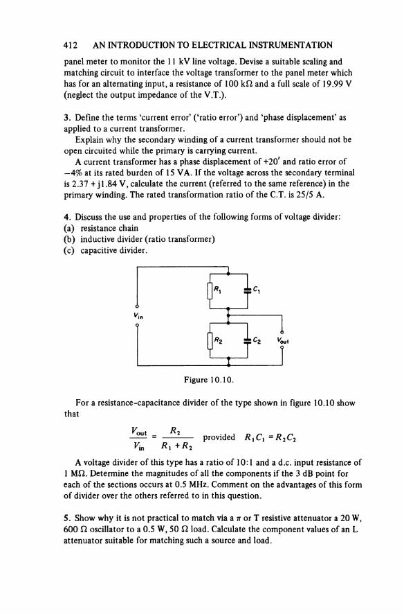
412 AN INTRODUCTION TO ELECTRICAL INSTRUMENTATION
panel meter to monitor the 11 kV line voltage. Devise a suitable scaling and matching circuit to interface the voltage transformer to the panel meter which has for an alternating input, a resistance of 100 kΩ and a full scale of 19.99 V (neglect the output impedance of the V.T.).
3. Define the terms ‘current error’ (‘ratio error’) and ‘phase displacement’ as applied to a current transformer.
Explain why the secondary winding of a current transformer should not be open circuited while the primary is carrying current.
A current transformer has a phase displacement of +20' and ratio error of —4% at its rated burden of 15 VA. If the voltage across the secondary terminal is 2.37 +j1.84 V, calculate the current (referred to the same reference) in the primary winding. The rated transformation ratio of the C.T. is 25/5 A.
4. Discuss the use and properties of the following forms of voltage divider:(a) resistance chain(b) inductive divider (ratio transformer)(c) capacitive divider.
Figure 10.10.
For a resistance-capacitance divider of the type shown in figure 10.10 show that
provided R1 C1 = R2C2
A voltage divider of this type has a ratio of 10: 1 and a d.c. input resistance of 1 MΩ. Determine the magnitudes of all the components if the 3 dB point for each of the sections occurs at 0.5 MHz. Comment on the advantages of this form of divider over the others referred to in this question.
5. Show why it is not practical to match via a π or T resistive attenuator a 20 W, 600 Ω oscillator to a 0.5 W, 50 Ω load. Calculate the component values of an L attenuator suitable for matching such a source and load.
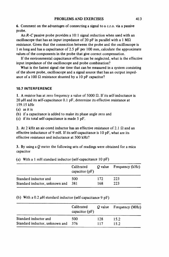
PROBLEMS AND EXERCISES 413
6. Comment on the advantages of connecting a signal to a c.r.o. via a passive probe.
An R-C passive probe provides a 10:1 signal reduction when used with an oscilloscope that has an input impedance of 20 pF in parallel with a 1 MΩ resistance. Given that the connection between the probe and the oscilloscope is 1 m long and has a capacitance of 2.5 pF per 100 mm, calculate the approximate values of the components in the probe that give correct compensation.
If the environmental capacitance effects can be neglected, what is the effective input impedance of the oscilloscope and probe combination?
What is the fastest signal rise time that can be measured in a system consisting of the above probe, oscilloscope and a signal source that has an output imped-ance of a 100 Ω resistance shunted by a 10 pF capacitor?
10.7 INTERFERENCE
1. A resistor has at zero frequency a value of 5000 Ω. If its self-inductance is 20 μH and its self-capacitance 0.1 pF, determine its effective resistance at 159.15 kHz(a) as it is(b) if a capacitance is added to make its phase angle zero and(c) if its total self-capacitance is made 5 pF.
2. At 2 kHz an air-cored inductor has an effective resistance of 2.1 Ω and an effective inductance of 9 mH. If its self-capacitance is 10 pF, what are its effective resistance and inductance at 500 kHz?
3. By using a Q meter the following sets of readings were obtained for a mica capacitor
(a) With a 1 mH standard inductor (self-capacitance 10 pF)
Calibrated capacitor (pF)
Q value Frequency (kHz)
Standard inductor and 500 172 223Standard inductor, unknown and 381 168 223
(b) With a 0.2 μH standard inductor (self-capacitance 9 pF)
Calibrated capacitor (pF)
Q value Frequency (MHz)
Standard inductor and 500 128 15.2Standard inductor, unknown and 376 117 15.2
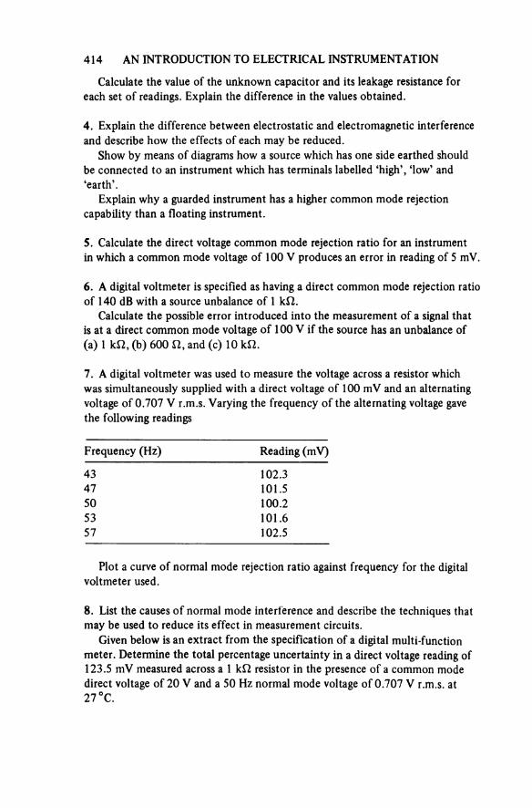
414 AN INTRODUCTION TO ELECTRICAL INSTRUMENTATION
Calculate the value of the unknown capacitor and its leakage resistance for each set of readings. Explain the difference in the values obtained.
4. Explain the difference between electrostatic and electromagnetic interferenceand describe how the effects of each may be reduced.
Show by means of diagrams how a source which has one side earthed should be connected to an instrument which has terminals labelled ‘high’, ‘low’ and ‘earth’.
Explain why a guarded instrument has a higher common mode rejection capability than a floating instrument.
5. Calculate the direct voltage common mode rejection ratio for an instrument in which a common mode voltage of 100 V produces an error in reading of 5 mV.
6. A digital voltmeter is specified as having a direct common mode rejection ratio of 140 dB with a source unbalance of 1 kΩ.
Calculate the possible error introduced into the measurement of a signal that is at a direct common mode voltage of 100 V if the source has an unbalance of (a) 1 kΩ, (b) 600 Ω, and (c) 10 kΩ.
7. A digital voltmeter was used to measure the voltage across a resistor which was simultaneously supplied with a direct voltage of 100 mV and an alternating voltage of 0.707 V r.m.s. Varying the frequency of the alternating voltage gave the following readings
Frequency (Hz) Reading (mV)
43 102.347 101.550 100.253 101.657 102.5
Plot a curve of normal mode rejection ratio against frequency for the digital voltmeter used.
8. List the causes of normal mode interference and describe the techniques that may be used to reduce its effect in measurement circuits.
Given below is an extract from the specification of a digital multi-function meter. Determine the total percentage uncertainty in a direct voltage reading of 123.5 mV measured across a 1 kΩ resistor in the presence of a common mode direct voltage of 20 V and a 50 Hz normal mode voltage of 0.707 V r.m.s. at 27 °C.
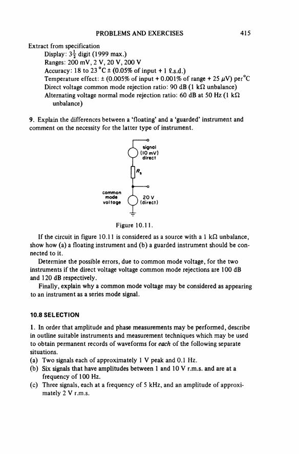
PROBLEMS AND EXERCISES 415
Extract from specificationDisplay: 3½ digit (1999 max.)Ranges: 200 mV, 2 V, 20 V, 200 V Accuracy: 18 to 23 °C ± (0.05% of input + 1 l.s.d.)Temperature effect: ± (0.005% of input + 0.001% of range + 25 μV) per°C Direct voltage common mode rejection ratio: 90 dB (1 kΩ unbalance) Alternating voltage normal mode rejection ratio: 60 dB at 50 Hz (1 kΩ
unbalance)
9. Explain the differences between a ‘floating’ and a ‘guarded’ instrument and comment on the necessity for the latter type of instrument.
Figure 10.11.
signal(10 mV) direct
commonmode
voltage20 V
(direct)
If the circuit in figure 10.11 is considered as a source with a 1 kΩ unbalance, show how (a) a floating instrument and (b) a guarded instrument should be con-nected to it.
Determine the possible errors, due to common mode voltage, for the two instruments if the direct voltage voltage common mode rejections are 100 dB and 120 dB respectively.
Finally, explain why a common mode voltage may be considered as appearing to an instrument as a series mode signal.
10.8 SELECTION
1. In order that amplitude and phase measurements may be performed, describe in outline suitable instruments and measurement techniques which may be used to obtain permanent records of waveforms for each of the following separate situations.(a) Two signals each of approximately 1 V peak and 0.1 Hz.(b) Six signals that have amplitudes between 1 and 10 V r.m.s. and are at a
frequency of 100 Hz.(c) Three signals, each at a frequency of 5 kHz, and an amplitude of approxi-
mately 2 V r.m.s.

Figure 10.12. Digital multimeters: (a) AVO Model DA116 (courtesy of AVO Ltd), (b) Keithley Model 169 (courtesy of Keithley Instruments Ltd)
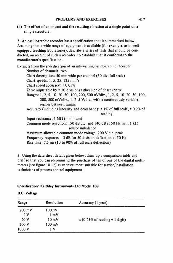
PROBLEMS AND EXERCISES 417
(d) The effect of an impact and the resulting vibration at a single point on a simple structure.
2. An oscillographic recorder has a specification that is summarised below. Assuming that a wide range of equipment is available (for example, as in well- equipped teaching laboratories), describe a series of tests that should be con-ducted, on receipt of such a recorder, to establish that it conforms to the manufacturer’s specification.
Extracts from the specification of an ink-writing oscillographic recorder Number of channels: twoChart description: 50 mm wide per channel (50 div. full scale)Chart speeds: 1, 5, 25, 125 mm/s Chart speed accuracy: ± 0.05%Zero: adjustable by ± 30 divisions either side of chart centreRanges: 1, 2, 5, 10, 20, 50, 100, 200, 500 μV/div., 1, 2, 5, 10, 20, 50, 100,
200, 500 mV/div., 1, 2, 5 V/div., with a continuously variable vernier between ranges
Accuracy (including linearity and dead band): ± 1% of full scale, ± 0.2% of reading
Input resistance: 1 MΩ (minimum)Common mode rejection: 150 dB d.c. and 140 dB at 50 Hz with 1 kΩ
source unbalanceMaximum allowable common mode voltage: 200 V d.c. peakFrequency response: —3 dB for 50 division deflection at 50 Hz Rise time: 7.5 ms (10 to 90% of full scale deflection)
3. Using the data sheet details given below, draw up a comparison table and brief so that you can recommend the purchase of ten of one of the digital multi-meters (see figure 10.12) as an instrument suitable for service/installation technicians of process control equipment.
Specification: Keithley Instruments Ltd Model 169
D.C. Voltage
Range Resolution Accuracy (1 year)
200 mV 100 μV2 V 1 mV
20 V 10 mV ± (0.25% of reading + 1 digit)200 V 100 mV
1000 V 1 V
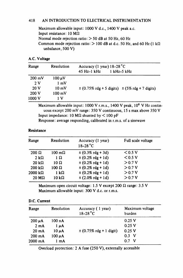
418 AN INTRODUCTION TO ELECTRICAL INSTRUMENTATION
Maximum allowable input: 1000 V d.c., 1400 V peak a.c.Input resistance: 10 MΩNormal mode rejection ratio: > 50 dB at 50 Hz, 60 HzCommon mode rejection ratio: > 100 dB at d.c. 50 Hz, and 60 Hz (1 kΩ
unbalance, 500 V)
A.C. Voltage
Range Resolution Accuracy (1 year) 18-28°C45 Hz-1 kHz 1 kHz-5 kHz
200 mV 100 μV2 V 1 mV
20 V 10 mV ± (0.75% rdg + 5 digits) ± (5% rdg + 7 digits)200 V 100 mV
1000 V 1 V
Maximum allowable input: 1000 V r.m.s., 1400 V peak, 106 V Hz contin-uous except 200 mV range: 350 V continuous, 15 s max above 350 V
Input impedance: 10 MΩ shunted by < 100 pFResponse: average responding, calibrated in r.m.s. of a sinewave
Resistance
Range Resolution Accuracy (1 year) 18-28 °C
Full scale voltage
200 Ω 100 mΩ ± (0.3% rdg + 3d) <0.5 V2 kΩ 1 Ω ± (0.2% rdg + 1d) <0.5 V
20 kΩ 10 Ω ± (0.2% rdg + 1d) >0.7 V200 kΩ 100 Ω ± (0.2% rdg + 1d) >0.7 V
2000 kΩ 1 kΩ ± (0.2% rdg + 1d) >0.7 V20 MΩ 10 kΩ ± (2.0% rdg + 1d) >0.7 V
Maximum open circuit voltage: 1.5 V except 200 Ω range: 3.5 V Maximum allowable input: 300 V d.c. or r.m.s.
D.C. Current
Range Resolution Accuracy ( 1 year)18-28 °C
Maximum voltage burden
200 μA 100 nA 0,25 V2 mA 1 μA 0,25 V
20 mA 10 μA ± (0.75% rdg + 1 digit) 0,25 V200 mA 100 μA 0,3 V
2000 mA 1 mA 0,7 V
Overload protection: 2 A fuse (250 V), externally accessible
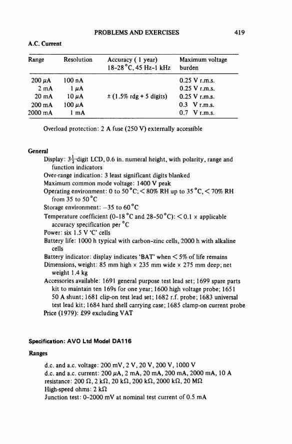
PROBLEMS AND EXERCISES 419
A.C. Current
Range Resolution Accuracy (1 year)18-28 °C, 45 Hz-1 kHz
Maximum voltage burden
200 μA 100 nA 0.25 V r.m.s.2 mA 1 μA 0.25 V r.m.s.
20 mA 10 μA ± (1.5% rdg + 5 digits) 0.25 V r.m.s.200 mA 100 μA 0.3 V r.m.s.
2000 mA 1 mA 0.7 V r.m.s.
Overload protection: 2 A fuse (250 V) externally accessible
GeneralDisplay: 3½-digit LCD, 0.6 in. numeral height, with polarity, range and
function indicatorsOver-range indication: 3 least significant digits blankedMaximum common mode voltage: 1 400 V peakOperating environment: 0 to 50°C; < 80% RH up to 35 °C, < 70% RH
from 35 to 50 °CStorage environment: —35 to 60°CTemperature coefficient (0-18 °C and 28-50 °C): < 0.1 × applicable
accuracy specification per °CPower: six 1.5 V ‘C’ cellsBattery life: 1000 h typical with carbon-zinc cells, 2000 h with alkaline
cellsBattery indicator: display indicates ‘BAT’ when < 5% of life remains Dimensions, weight: 85 mm high × 235 mm wide × 275 mm deep; net
weight 1.4 kgAccessories available: 1691 general purpose test lead set; 1699 spare parts
kit to maintain ten 169s for one year; 1600 high voltage probe; 165 1 50 A shunt; 1681 clip-on test lead set; 1682 r.f. probe; 1683 universal test lead kit; 1684 hard shell carrying case; 1685 clamp-on current probe
Price (1979): £99 excluding VAT
Specification: AVO Ltd Model DA116
Ranges
d.c. and a.c. voltage: 200 mV, 2 V, 20 V, 200 V, 1000 V d.c. and a.c. current: 200 μA, 2 mA, 20 mA, 200 mA, 2000 mA, 10 A resistance: 200 Ω, 2 kΩ, 20 kΩ, 200 kΩ, 2000 kΩ, 20 MΩ High-speed ohms: 2 kΩJunction test: 0-2000 mV at nominal test current of 0.5 mA

420 AN INTRODUCTION TO ELECTRICAL INSTRUMENTATION
Accuracy (20 °C)
d.c. voltage ranges 200 mV, 2 V: ± 0.2% of reading ± 1 digit; other ranges ± 0.5% of reading ± 1 digit
a.c. voltage ranges 200 mV: ± 1% of reading ± 4 digits; other ranges ± 1% of reading ± 2 digits
d.c. current ranges: ± 1% of reading ± 1 digit a.c. current ranges: ± 3% of reading ± 4 digits resistance ranges 20 MΩ, high-speed ohms: ± 3% of reading ± 1 digit;
other ranges ± 1% of reading ± 1 digit temperature effect: d.c. ranges ± 0.03%/°C; a.c. ranges ± 0.05%/°C; resist-
ance ranges ± 0.05%/°Cfrequency effect: for operation at frequencies other than 50 Hz or 60 Hz
an additional error of ± 1% of reading must be allowed between 40 Hz and 5 kHz (200 V range and below)
Input Characteristics
voltage ranges: 10 MΩ in shunt with not more than 100 pF current ranges: voltage drop of 200 mv nominal for full range, plus the
voltage drop across the fuseresistance ranges: 150 mV nominal voltage on 200 Ω range, 1.5 V-3 v
nominal voltage on other ranges
Temperature Range
0 to 40 °C
Long-term Stability
Not normally expected to require recalibration over extended periods. Good stability is assured in the design and only two adjustments are pro-vided for internal references. For critical requirements confirmation of accuracy is recommended annually.
Input Overload Ratings
a.c. and d.c. voltage ranges: 200 mV 2 V 500 V r.m.s. or d.c.; other ranges 1500 V peak or d.c.
a.c. and d.c. current ranges: 10 A range not protected; other ranges 2 A (250 V) fuse protected
resistance ranges: 350 V peak or d.c. junction test range: 250 V a.c. r.m.s.
Series Mode Noise Rejection
Greater than 40 dB at 50 Hz and 60 Hz
PROBLEMS AND EXERCISES 421
Display
3½-digit liquid crystal display, autopolarity. Over-range and battery low indications. Characters 1 3 mm high
Batteries
type: four 1.5 V cells, IEC R14, ‘C’ size (SP11, HP11, 214, 114C, U11MJ); batteries not supplied with instrument
life: 500 h approx.
Fuse
20 × 5 mm ceramic cartridge 2 A 250 V. IEC 127/1
Dimensions
instrument only: 185 × 147 × 87 mm with protective cover: 185 × 150 × 106 mm
Weight
1.0 kg (approx.)
Accessories
Supplied with instrument: Lead, prods and insulated clips, instruction booklet, Top cover with lead compartment, Battery divider, Key to remove fuse, Two spare fuses
Accessories
Available at extra cost: Multi-range current transformer (Part No.) 6330- 259, 30 kV d.c. probe 6310-525, r.f probe 6310-531, lightweight lead set, (max. 50 V) 6320-134, carrying case-ever-ready leather 6320-136
Price (1979)
£106.90
10.9 SYSTEMS
1. Describe a measurement system that could be used to investigate and record the relevant parameters during the 2 s following the connection of a 400 V supply to a 10 kVA, three-phase, 400/50 V, star-delta transformer. Your solution should contain a list of the parameters it is desirable to measure, a diagram of the proposed system and brief notes on the relevance and operation of each of the

422 AN INTRODUCTION TO ELECTRICAL INSTRUMENTATION
component parts. (Assume that the star point connection may be made by external connections.)
2. Describe and explain, with the aid of a schematic diagram, the technique used in one form of automatic digital impedance (L.C.R.) meter currently available.
Discuss the benefits (to an employer) of such instruments relative to the manually operated bridge techniques they supersede.
3. (a) Explain, with the aid of diagrams, the function of the IEC BUS.(b) Describe the operation of a data logging system produced by using such a
bus to interconnect suitable equipment.(c) Comment on the versatility of the bus interconnected system compared
with a traditional purely hardware data logging system.
4. By using data sheets of currently available equipment write a report in the form of a recommendation to a senior executive on one of the following topics. (Note: The report should include an analysis of the cost of purchase and opera-tion, your reasoning for the selection of particular instruments and an analysis of the accuracy and reliability of the results that it will produce.)(a) Devise an instrumentation/recording system to monitor the vibration and
stresses in the chassis of a lorry when it is driven over rough ground at 65 km/h.
(b) Devise an automated test and record system to quality check audio ampli-fiers on a production line. The amplifier specification is
Voltage gain: 40 dB3 dB bandwidth: 0 to 100 kHzSupply voltage: —12 V, 0, +12 VOutput current: 3 A continuous; 4 A maximum
(c) Devise an instrumentation system to record over an extended period (at least 1 year) the variables associated with and within a small tidal river at a point approximately 0.5 km from the shore line. Assume that a single phase 240 V power supply and suitable buildings to house equipment are available 25 m from the river bank. For one possible solution see figure 10.13!
10.10 ANSWERS
10.10.1 Principles
3. 1243.96 Ω± 0.283 Ω or ±0.023%. 4. ± 227.3 Ω, ± 0.05(01)%. 5.4.0 nF ±0.32%. 6. 13.19(5) Ω ± 0.120 Ω or ± 0.90(5)%. 7. 1.999 V ± 0.1%, 1.000 V ± 0.15%, 0.500 V ± 0.25%, 0.200 V ± 0.55%, 0.100 V ± 1.05%. 8. 5000 Ω. 9.10.24 V. 10. 531.9 Ω, 488.5 Ω. 11.1.154,-4%. 12. 5 V, 8 V, 5.43 V.
Figure 10.13. An anonymously suggested solution to the problem 4(c) of section 10.9.
TO MEASURE VARIATIONS ASSOCIATEDWITH AN ESTUARY
APPARATUS:1 PAIR OF WELLINGTON BOOTS 1 METRE RULE 1 THERMOMETER 1 YEAR’S SUPPLY OF TEA BAGS
HOW CAN I FIND TIME TO DO MY
OTHER LAB REPORTS WHEN I'VE GOT TO STAND HERE AND
MEASURE THIS FOR A YEAR!
THINKS:IT S A GOOD JOB I DID A COURSE IN ELECTRICAL
INSTRUMENTATION

424 AN INTRODUCTION TO ELECTRICAL INSTRUMENTATION
10.10.2 Analogue Instruments
1. 3.769 Ω, 299.25 kΩ, 14.25 kΩ. 2.-2.06%. 3.23.4 mm. 4.157 Ω,9016 Ω. 5. 2404 Ω, 17.5 Ω, 133 Ω. 6. 1.546 Ω, 965 Ω, 147.9(5) divisions.7. 295 W, 293.3 W, 3.5 W, 2 W, 291.5 W, 291.4 W. 8. 2026 W, 0.585.9. 0.4463 Ω, 12.42 A, 606 μH, 0.404 Ω. 10. 385 pF, 1.9 MΩ. 11. 25.34 mH, 6.67 pF, 21.7 Ω, 25.02 mH. 12. 100.8 mH, 51 Ω; 101.5 mH, 68 Ω; 101.5 mH, 79 Ω; 102 mH, 96 Ω; 102 mH, 210 Ω; 100 mH, ferrite core. 13. 226.7 mV,2.5 kHz; 414.5 Ω, 49.9 nF. 14. 72° 36', 0.96 μs.
10.10. 3 Null Methods
1. 1674.23 Ω± 0.74 Ω. 2. 67.5 mm pk, 15.8 mm pk. 3.171.5 Ω, 323 mH, 1.41 W. 4. 593.69 Ω, 115 mV. 5. + 8%. 6. 166.8 MΩ. 7. 614.6 Ω,366 mV; 599.6 Ω, 375 mV 8. 188 Ω, 94.3 μH. 9. 73.6 mΩ ± 0.092%;532 μH ± 0.062%; 90.8. 10. 135.63 nF ± 0.012 nF;95.26 kΩ ± 0.018 kΩ.
10.10.4 Digital Instruments
1. ±0.00186%, ± 0.00154%. 2. ± 0.00181%, ± 0.00105%. 3. ±1.33%.4. ± 0.2064 Ω, 1353.848 Ω ± 0.2115 Ω, 1353.68 Ω ± 0.047 Ω. 5. See figure 4.12. Hence by frequency mode 35-100 Hz, 0.3-1, 2.2-10, 30-100 and above 300 kHz; by multi-period mode 10-35, 100-300 Hz, 1-2.2, 10-30 and 100- 300 kHz.
10.10.5 Transducers
1. 3418.4 Ω; 100%, 50 mm; 75%, 39.7 mm; 50%, 28.2 mm; 25%, 15 mm; 10%,6.3 mm. 2. 400 mV pk, A gives 64 mm, B gives 82 mm. 3. 133 Ω; 12 mV;2.4 V; 100.7 mm, 67.6 mm. 4. 10,45 pF.
10.10.6 Signal Conditioning
1. 20 kΩ, 4 kΩ, 800 Ω, 160 Ω. 2. 2.18 kΩ, 243 Ω. 3. 26.04 Az37° 29'. 4. 100 kΩ, 900 kΩ, 0.35 pF, 3.18 pF. 5. 575 Ω, 55 Ω. 6.9 MΩ, 5 pF; 10 MΩ, 4.5 pF; 3.2 ns.
10.10.7 Interference
1. 5000.019 Ω, 5000.08 Ω, 4997.88 Ω. 2. 168.2 Ω, 80.5 mH. 3. 119 pF, 101 MΩ; 124 pF, 28 kΩ. 5. 86 dB. 6.10 μV, 6 μV, 100 μV. 7.-53 dB, -56.5 dB, -74 dB, -55.9 dB, -52 dB. 8. ±1.56%. 9. 200 μV, 20 μV.
10.10.8 Selection
1. Two pen recorders, u.v. recorder, tape recorder plus u.v. recorder, digital transient recorder and pen recorder.

Appendix I
UNITS, SYMBOLS AND CONVERSION FACTORS
The international system of units (Systeme International d’Unités — SI) has been established by international agreement to provide a logical and interconnected framework for all measurements in science and industry. It is based on six units: the metre (length), the second (time), the kilogram (mass), the ampere (electric current), the kelvin (temperature) and the candela (luminous intensity). The majority of the world’s population already use the SI system of units and it is possible that by 1985 the only major countries who have not changed will be Canada and the U.S.A.
In addition to the defining of the six basic units the SI establishes a set of factors that should be applied to all quantities so that their magnitude may always be written with less than four numerals before the decimal point, thus removing some of the difficulties associated with manipulating very large and very small numbers (see table A.1). Table A.2 lists the units in the SI system.
Table A. 1 Multiples
Prefix Symbol Factor by which the unit is to be multiplied
tera T 1012giga G 109mega M 106kilo k 103milli m 10-3micro μ 10-6nano n 10-9pico p 10-12femto f 10-15atto a 10-18
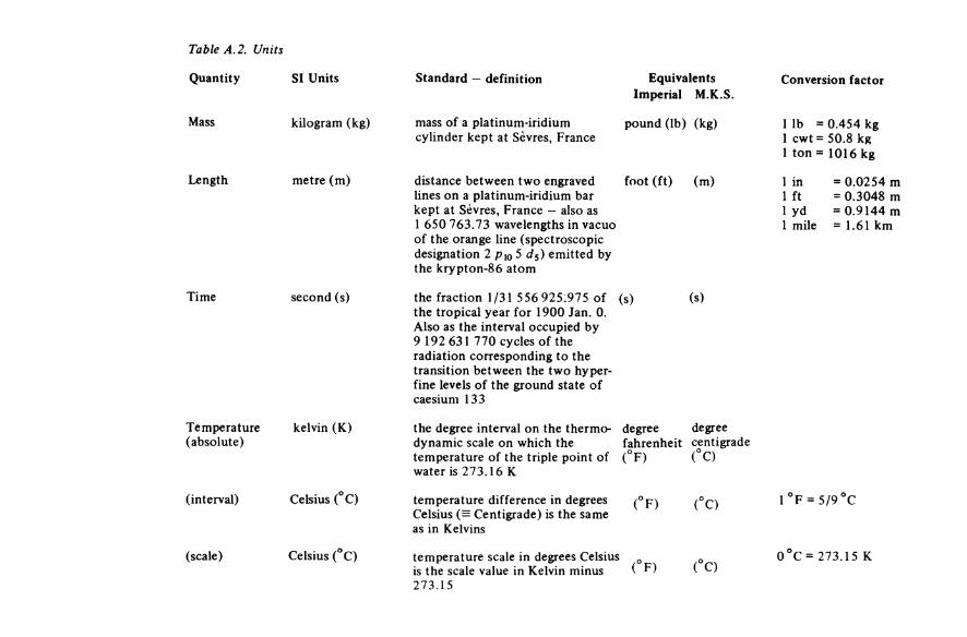
Table A.2. Units
Quantity SI Units Standard — definition Equivalents Conversion factorImperial M.K.S.
Mass kilogram (kg) mass of a platinum-iridium cylinder kept at Sevres, France
pound (lb) (kg) 1 lb = 0.454 kg1 cwt= 50.8 kg1 ton = 1016 kg
Length metre (m) distance between two engraved lines on a platinum-iridium bar kept at Sèvres, France — also as1 650 763.73 wavelengths in vacuo of the orange line (spectroscopic designation 2 p1o 5 ds) emitted by the krypton-86 atom
foot (ft) (m) 1 in = 0.0254 m1 ft = 0.3048 m1 yd = 0.9144 m1 mile =1.61 km
Time second (s) the fraction 1/31 556 925.975 of the tropical year for 1900 Jan. 0. Also as the interval occupied by9 192 631 770 cycles of the radiation corresponding to the transition between the two hyper- fine levels of the ground state of caesium 133
(S) (s)
Temperature(absolute)
kelvin (K) the degree interval on the thermo-dynamic scale on which the temperature of the triple point of water is 273.16 K
degreefahrenheit(°F)
degreecentigrade(°O
(interval) Celsius (°C) temperature difference in degrees Celsius (≡ Centigrade) is the same as in Kelvins
(°F) (°O 1 °F = 5/9 °C
(scale) Celsius (°C) temperature scale in degrees Celsius is the scale value in Kelvin minus 273.15
‘ (°F) (°O0°C = 273.15 K
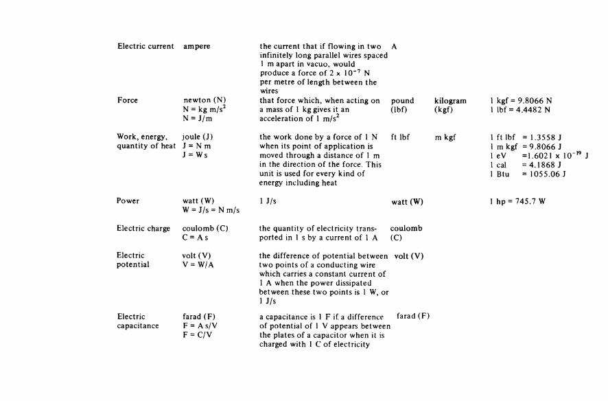
Electric current
Force
ampere
newton (N)N = kg m/s2N = J/m
the current that if flowing in two infinitely long parallel wires spaced1 m apart in vacuo, would produce a force of 2 x 10~7 N per metre of length between the wiresthat force which, when acting on a mass of 1 kg gives it an acceleration of 1 m/s2
A
pound(lbf)
1 kgf = 9.8066 N1 lbf =4.4482 N
kilogram(kgf)
Work, energy, quantity of heat
joule (J)J = NmJ = Ws
the work done by a force of 1 N when its point of application is moved through a distance of 1 m in the direction of the force. This unit is used for every kind of energy including heat
ft lbf m kgf 1 ft lbf = 1.3558 J1 m kgf =9.8066 J1 eV =1.6021 × 10*19 Jleal =4.1868 J1 Btu = 1055.06 J
Power watt (W)W = J/s = N m/s
1 J/s watt (W) 1 hp= 745.7 W
Electric charge coulomb (C)C = As
the quantity of electricity trans-ported in 1 s by a current of 1 A
coulomb(C)
Electricpotential
volt (V)V = W/A
the difference of potential between two points of a conducting wire which carries a constant current of1 A when the power dissipated between these two points is 1 W, or 1 J/s
volt (V)
Electriccapacitance
farad (F)F = A s/VF = C/V
a capacitance is 1 F if a difference of potential of 1 V appears between the plates of a capacitor when it is charged with 1 C of electricity
farad (F)
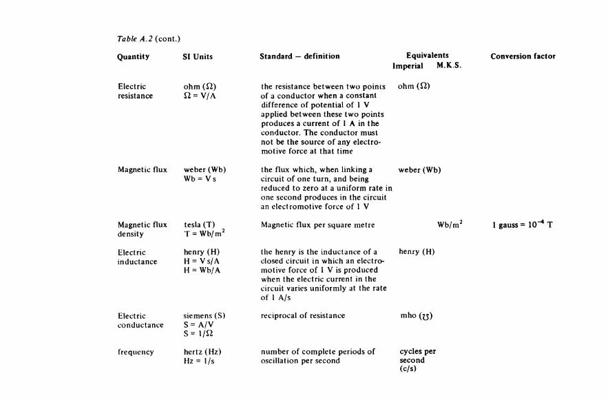
Table A.2 (cont.)
Quantity SI Units Standard — definition Equivalents Imperial M.K.S.
Conversion factor
Electricresistance
ohm (Ω)Ω = V/A
the resistance between two poincs of a conductor when a constant difference of potential of 1 V applied between these two points produces a current of 1 A in the conductor. The conductor must not be the source of any electro-motive force at that time
ohm (Ω)
Magnetic flux weber (Wb)Wb = Vs
the flux which, when linking a circuit of one turn, and being reduced to zero at a uniform rate in one second produces in the circuit an electromotive force of 1 V
weber (Wb)
Magnetic flux density
tesla (T) T=Wb/m2
Magnetic flux per square metre Wb/m5 1 gauss = 10-4 T
Electricinductance
henry (H)H = Vs/AH = Wb/A
the henry is the inductance of a closed circuit in which an electro-motive force of 1 V is produced when the electric current in the circuit varies uniformly at the rate of 1 A/s
henry (H)
Electricconductance
siemens (S)S= A/VS= 1/Ω
reciprocal of resistance mho (u)
frequency hertz (Hz)Hz = 1/s
number of complete periods of oscillation per second
cycles persecond(c/s)

APPENDIX I 429
For fuller details see:
1. Symbols and Abbreviations for use in Electrical and Electronic EngineeringCourses (Institution of Electrical Engineers, London, 1979)
2. BS 1991, Letter Symbols, Signs and Abbreviations3. BS 3763: 1970 International System (SI) Units4. PD 5686, The Use of SI Units (British Standards Institution, London, 1972)
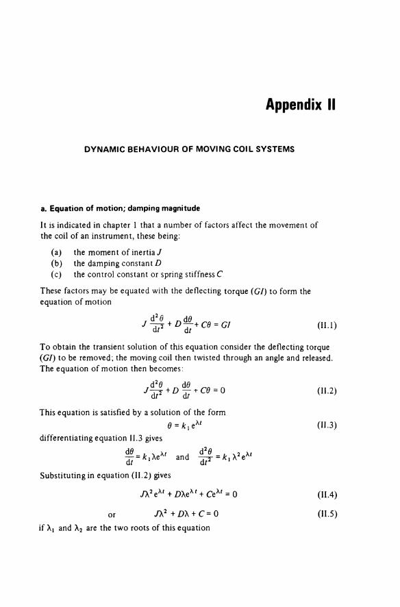
Appendix II
DYNAMIC BEHAVIOUR OF MOVING COIL SYSTEMS
a. Equation of motion; damping magnitude
It is indicated in chapter 1 that a number of factors affect the movement of the coil of an instrument, these being:
(a) the moment of inertia J(b) the damping constant D(c) the control constant or spring stiffness C
These factors may be equated with the deflecting torque (GI) to form the equation of motion
(II.1)
To obtain the transient solution of this equation consider the deflecting torque (GI) to be removed; the moving coil then twisted through an angle and released. The equation of motion then becomes:
(11.2)
This equation is satisfied by a solution of the form(11.3)
differentiating equation 11.3 gives
Substituting in equation (11.2) gives
(II.4)
or (II.5)if λ1 and λ2 are the two roots of this equation

APPENDIX II 431
and
As two arbitrary constants are required in the solution of a second order differential equation, the complete solution of (II.2) is
(II.6)
where A and B are the arbitrary constants, the values of which may be obtained from the conditions of motion.
It is necessary to consider three cases:
(1) Overdamped
D2 > 4CJ - the roots are real and unequal, the solution taking the form of the sum of two quantities both of which diminish exponentially.
(II.7)
being the curve (a) in figure A.1.
(2) Critically damped
D2 = 4CJ — the roots being equal and real. The curve (b) in figure A.1 is com puted from the equation
(II.8)
(where λ = -D/2J). This is a special case, being termed critical damping, and is the condition in which an instrument coil will change from one position to another in a minimum of time without overshoot.
(3) Underdamped
D2 < 4CJ - the roots becoming conjugate — complex
Substituting these values of λ1 and λ2 in H.6 gives
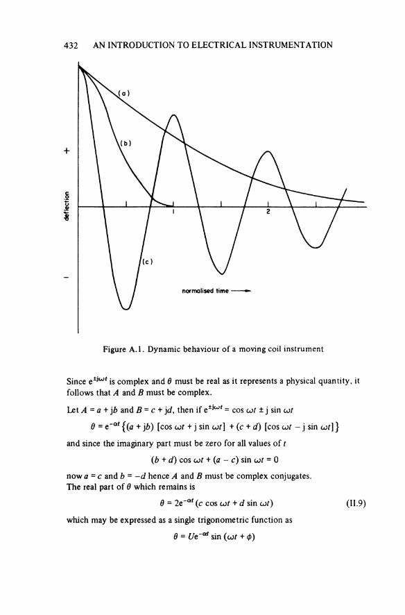
432 AN INTRODUCTION TO ELECTRICAL INSTRUMENTATION
Figure A.1. Dynamic behaviour of a moving coil instrument
defle
ctio
n
normalised time
Since e±jωf is complex and θ must be real as it represents a physical quantity, it follows that A and B must be complex.
Let A = a + jb and B = c + jd, then if e±jωt = cos ωt ± j sin ωt
θ = e-αt {(a + jb) [cos ωt + j sin ωt] + (c + d) [cos ωt — j sin ωt]}
and since the imaginary part must be zero for all values of t
(b + d) cos ωt + (a - c) sin ωt = 0
now a = c and b = -d hence A and B must be complex conjugates.The real part of θ which remains is
(II.9)
which may be expressed as a single trigonometric function as
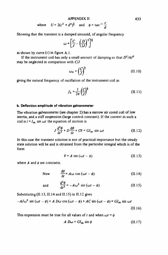
APPENDIX II 433where and
Showing that the transient is a damped sinusoid, of angular frequency
as shown by curve (c) in figure A.1.If the instrument coil has only a small amount of damping so that D2/4J2
may be neglected in comparison with C/J
(II.10)
giving the natural frequency of oscillation of the instrument coil as
(II.11)
b. Deflection amplitude of vibration galvanometer
The vibration galvanometer (see chapter 2) has a narrow air cored coil of low inertia, and a stiff suspension (large control constant). If the current in such a coil is i = Im sin ωt the equation of motion is
(II.12)
In this case the transient solution is not of practical importance but the steady state solution will be and is obtained from the particular integral which is of the form
(II.13)
where A and ϕ are constants.
Now (II.14)
and (II.15)
Substituting (II.13, II.14 and II.15) in II.12 gives
(II.16)
This expression must be true for all values of t and when ωt = ϕ
(II.17)
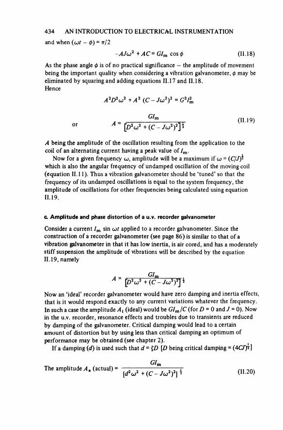
434 AN INTRODUCTION TO ELECTRICAL INSTRUMENTATION
and when (ωt — Φ) = π/2
(II.18)
As the phase angle ϕ is of no practical significance — the amplitude of movement being the important quality when considering a vibration galvanometer, ϕ may be eliminated by squaring and adding equations II.17 and II.18.Hence
or (II.19)
A being the amplitude of the oscillation resulting from the application to the coil of an alternating current having a peak value of Im.
Now for a given frequency ω, amplitude will be a maximum if ω = (C/J)½ which is also the angular frequency of undamped oscillation of the moving coil (equation II.11). Thus a vibration galvanometer should be ‘tuned’ so that the frequency of its undamped oscillations is equal to the system frequency, the amplitude of oscillations for other frequencies being calculated using equation II.19.
c. Amplitude and phase distortion of a u.v. recorder galvanometer
Consider a current Im sin ωt applied to a recorder galvanometer. Since the construction of a recorder galvanometer (see page 86) is similar to that of a vibration galvanometer in that it has low inertia, is air cored, and has a moderately stiff suspension the amplitude of vibrations will be described by the equation II.19, namely
Now an ‘ideal’ recorder galvanometer would have zero damping and inertia effects, that is it would respond exactly to any current variations whatever the frequency. In such a case the amplitude Ai (ideal) would be GIm/C (for D - 0 and J = 0). Now in the u.v. recorder, resonance effects and troubles due to transients are reduced by damping of the galvanometer. Critical damping would lead to a certain amount of distortion but by using less than critical damping an optimum ofperformance may be obtained (see chapter 2).
If a damping (d) is used such that d = ζD [D being critical damping = (4CZ)½]
The amplitude Aa (actual) = (II.20)
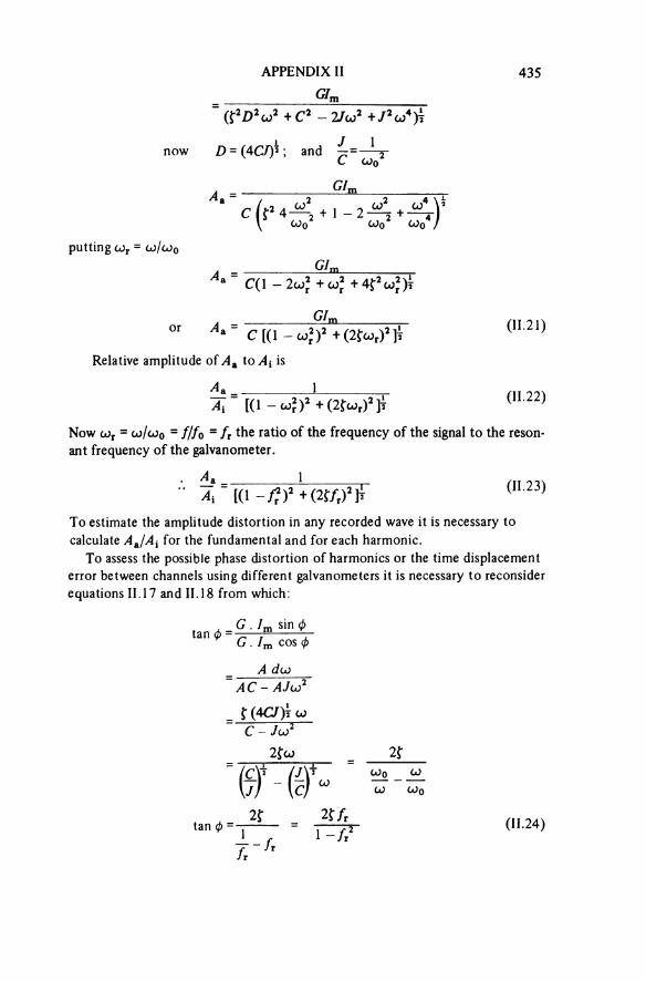
APPENDIX II 435
now and
putting ωr = ω/ω0
or (II.21)Relative amplitude of Aa to Ai is
(II.22)
Now ωτ = ω/ω0 = f/f0 = fr the ratio of the frequency of the signal to the reson-ant frequency of the galvanometer.
(II.23)
To estimate the amplitude distortion in any recorded wave it is necessary to calculate Aa/Ai for the fundamental and for each harmonic.
To assess the possible phase distortion of harmonics or the time displacement error between channels using different galvanometers it is necessary to reconsider equations II.17 and II.18 from which:
(II.24)
436 AN INTRODUCTION TO ELECTRICAL INSTRUMENTATION
Note. This expression gives the phase displacement of the recorded frequency with respect to its true position, measured on its own time scale of angular frequency. To estimate the distortion produced in a recorded wave it is necessary to calculate the phase displacement of the fundamental and each harmonic, and to allow for the different angular frequency scales of the various harmonics.For example a 25° displacement of a 5th harmonic on its own time scale represents 5° displacement on the angular frequency scale of the fundamental or vice versa.
For further analytical work see:E. Frank, Electrical Measurement Analysis (McGraw-Hill, New York, 1959)
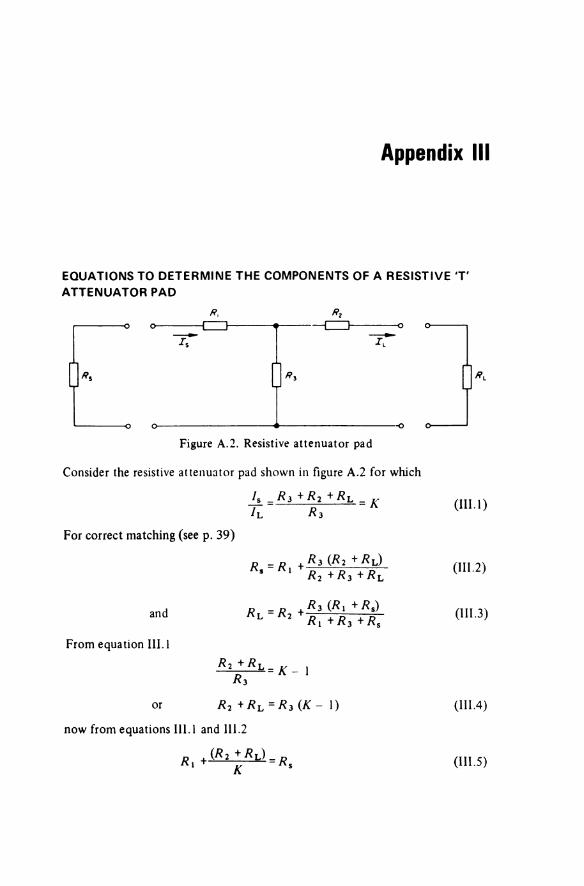
Appendix III
EQUATIONS TO DETERMINE THE COMPONENTS OF A RESISTIVE 'T' ATTENUATOR PAD
Figure A.2. Resistive attenuator pad
Consider the resistive attenuator pad shown in figure A.2 for which
(III.1)
For correct matching (see p. 39)
(III.2)
and (III.3)
From equation III.1
or (III.4)
now from equations III.1 and III.2
(III.5)

438 AN INTRODUCTION TO ELECTRICAL INSTRUMENTATION
Substituting equation III.4 in III.5 gives:
or (III.6)
Now substituting equations III.4 and III.6 in III.3 gives:
or
and (III.7)
Now from equations III.1 and 5.11
or (III.8)
Substituting equation III.8 in 111.7 gives
(III.9)
Substituting equations III.8 and III.9 in III.4 gives
(III.10)
and substituting equations III.8 and 1H.9 in III.6 gives
(III.11)
Note, k = (PS/PL)½ ; and attenuation, A = 10 log10(Ps/PL) dB
Hence or where A is in dB
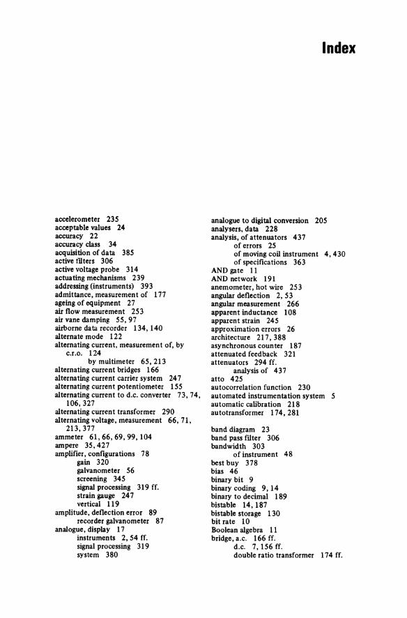
Index
accelerometer 235acceptable values 24accuracy 22accuracy class 34acquisition of data 385active filters 306active voltage probe 314actuating mechanisms 239addressing (instruments) 393admittance, measurement of 177ageing of equipment 27air flow measurement 253air vane damping 55, 97airborne data recorder 134,140alternate mode 122alternating current, measurement of, by
c.r.o. 124by multimeter 65,213
alternating current bridges 166 alternating current carrier system 247 alternating current potentiometer 155 alternating current to d.c. converter 73, 74,
106, 327alternating current transformer 290 alternating voltage, measurement 66, 7L
213,377ammeter 61,66,69,99,104ampere 35,427amplifier, configurations 78
gain 320 galvanometer 56 screening 345 signal processing 319 ff. strain gauge 247 vertical 119
amplitude, deflection error 89 recorder galvanometer 87
analogue, display 17instruments 2, 54 ff. signal processing 319 system 380
analogue to digital conversion 205 analysers, data 228 analysis, of attenuators 437
of errors 25of moving coil instrument 4, 430 of specifications 363
AND gate 11AND network 191anemometer, hot wire 253angular deflection 2, 53angular measurement 266apparent inductance 108apparent strain 245approximation errors 26architecture 217,388asynchronous counter 187attenuated feedback 321attenuators 294 ff.
analysis of 437atto 425autocorrelation function 230 automated instrumentation system 5 automatic calibration 218 autotransformer 174,281
band diagram 23band pass filter 306bandwidth 303
of instrument 48best buy 378bias 46binary bit 9binary coding 9,14binary to decimal 189bistable 14,187bistable storage 130bit rate 10Boolean algebra 11bridge, a.c. 166 ff.
d.c. 7,156 ff.double ratio transformer 174 ff.

440 INDEX
bridge, (conf.)output 161, 164 strain gauge 246 Wheatstone 8, 156, 161
British Calibration Service 36 Brownian movement 334 burden 285, 292 bus connected system 387
cable capacitance 310calculation errors 26calibration 36, 96calibration systems 396calibrator 37, 122cameras 123capacitance 427
effective 339measurement, by Q meter 111
by Schering bridge 167 by transformer bridge 173, 178
capacitive divider 279capacitive transducer 255capacitor, compressed gas 347
frequency characteristics of 340 high voltage 347properties 338
capacitor voltage transformer 283 carrier frequency 136, 247 cascade voltage transformer 283 cathode ray oscilloscope 115 ff. cathode ray tube 21, 115 Celsius 426central processing unit (CPU) 15charge, electric 427charge amplifier 322chopped mode 1 22circular chart recorder 151classification, of current transformers 293
of instruments 18, 34 of transducers 237 of voltage transformers 286
clock spring suspension 54closed loop system 383codes, digital 14, 189, 318common mode rejection 351, see also
sample specificationscomparators 175comparison (null) methods 5, 146 compensated wattmeter 102 compensating thermocouple 269 compensation, of lead resistance 248
of strain gauge 245 component impurities 334 ff.
measurements of 108, 177, 221 computer controlled system 15, 385 computing amplifier 324 conductance 176conducting shield 50
connection errors 27connections, screened 341 ff. constructional errors 26 control torque 2, 54 controller 15, 388 conventional true value 25 conversion, A to D 205
D to A 329coordinate potentiometer 155 correlator 229 coulomb 427 counters, digital 186 ff. coupled interference 49, 341 crest factor 45,213 critical damping 5, 87 cross-correlation function 229 cross talk 348current error (ratio error) 291 current measurement, by c.r.o. 124
by d.c. potentiometer 148 by digital multimeter 377 by electrodynamometer 99 by electronic multimeter 69 by moving coil multimeter 60
current probe 315current shunts 40, 287current transformer 66, 290
D to A converter 329damping 4, 55, 86, 97, 235damping resistance 92damping torque 4, 86data analysers 228data bus 389data logger 384, 396data transmission 9, 316, 384, 394dead resistance 242decade resistance box, errors 30 ff.deflection plates 117deflection torque 2, 54, 97demodulator 316dependent functions 328De Sauty bridge 167detectors, null a.c. 59, 167
d.c. 56phase sensitive 59
determination error 26 deviation, standard 33 dielectric loss 335 differential amplifier 320 differentiator 303, 324 diffraction (optical) grating 273 digital counter 1 86 ff.
displays 20 encoder 273 filter 307instruments 2, 8, 186 ff. multimeter 210 ff.

INDEX 441
digital counter (cont.) recorders 224 systems 384 tape recording 142 techniques 8, 74 transducers 272 wattmeter 224
direct acting galvanometer 56 multimeter 66 recorder 76
direct current transformer 293 direct recording 1 36 displacement transducers 240 display, choice 22
digital 20distortion 91, 120, 142, 305 divider (decade) 193, 277 ff. methods 16multiple trace 122 stored 20 X-Y 120,125
drift 143drivenguard 357dropouts 1 37dual beam oscilloscope 122dual slope d.v.m. 209dummy strain gauge 245dynamic behaviour, of moving coil system
5,430dynamic skew 143dynamometer see electrodynamometer
earphones 167earth connections 341earth loop 333eddy current damping 4, 54 effective capacitance 339 effective inductance 338 effective range 18 effective resistance 336 electric capacitance 427 electric charge 427 electric current 427 electric potential 427 electrodynamometer 97 electromagnetic damping 86, 92 electromagnetic interference 50, 348 electromagnetic transducer 265 electrometer valve 70, 160 electron gun 117, 122 electronic galvanometer 56 electronic instruments 107 electronic multimeter 69 electronic pen recorder 78 electronic signal conditioning 94 electrostatic instruments 107 electrostatic interference 49, 341
electrostatic stylus 80encoder, digital 273energy 427energy meters 113environmental errors 26environmental interference 49, 331 equalisation 135 equation of motion 4, 430 equivalent circuit capacitance 339 equivalent circuit resistance 336 errors, analysis of 25 ff.
correction (wattmeter) 99 current (ratio) 291 digital multimeter 34, 363 ff. linearity 77 phase 88pointer instruments 34 random 32 timing 143 voltage ratio 285
expansion coefficient 331
farad 35Faraday cage 346femto 425fibre optic 132fiducial value 18filter 299 fffirmware 16five terminal resistance measurement 215 fixed reference transducer 234 flat bed recorder 153 flip-flop 14floating instruments 351fluid damped galvanometer 92fluid damping 86flutter 143flyback 117foil strain gauge 244force 427force measurement 251form factor 44four-terminal resistance measurement 215 frequency characteristics, of capacitor 340
of insulating materials 335 of multimeters 375 of recorder galvanometers 87 of strain gauges 244 of transducers 236
frequency effects 335frequency equalisation 135frequency measurement, by counter 196,
203by c.r.o. 125
frequency-modulated recording 137 frequency selective detector 167 frequency standard 426 front gap 134
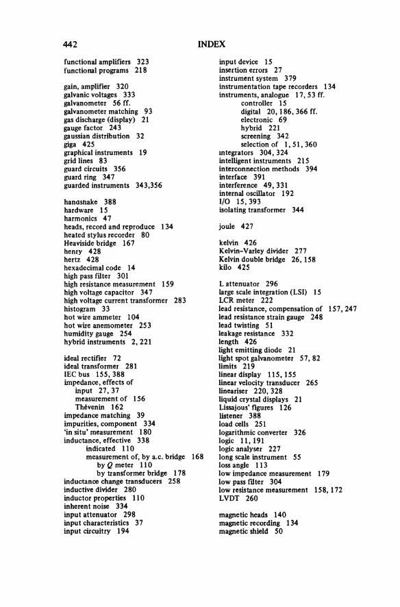
442 INDEX
functional amplifiers 323functional programs 218
gain, amplifier 320galvanic voltages 333galvanometer 56 ff.galvanometer matching 93gas discharge (display) 21gauge factor 243gaussian distribution 32giga 425graphical instruments 19grid lines 83guard circuits 356guard ring 347guarded instruments 343, 356
handshake 388hardware 15harmonics 47heads, record and reproduce 134 heated stylus recorder 80 Heaviside bridge 167 henry 428hertz 428hexadecimal code 14high pass filter 301high resistance measurement 159high voltage capacitor 347high voltage current transformer 283histogram 33hot wire ammeter 104hot wire anemometer 25 3humidity gauge 254hybrid instruments 2, 221
ideal rectifier 72ideal transformer 281IEC bus 155, 388impedance, effects of
input 27, 37 measurement of 156 Thévenin 162
impedance matching 39impurities, component 334‘in situ’ measurement 180inductance, effective 338
indicated 110measurement of, by a.c. bridge 168
by Q meter 110 by transformer bridge 178
inductance change transducers 258inductive divider 280inductor properties 110inherent noise 334input attenuator 298input characteristics 37input circuitry 194
input device 15insertion errors 27instrument system 379instrumentation tape recorders 134 instruments, analogue 17, 53 ff.
controller 15 digital 20, 186, 366 ff. electronic 69 hybrid 221 screening 342 selection of 1, 51, 360
integrators 304, 324intelligent instruments 215interconnection methods 394 interface 391 interference 49, 331 internal oscillator 192 I/O 15, 393isolating transformer 344
joule 427
kelvin 426Kelvin-Varley divider 277Kelvin double bridge 26, 158 kilo 425
L attenuator 296large scale integration (LSI) 15 LCR meter 222lead resistance, compensation of 157, 247 lead resistance strain gauge 248 lead twisting 51leakage resistance 332length 426light emitting diode 21light spot galvanometer 57, 82 limits 219linear display 115, 155linear velocity transducer 265 lineariser 220, 328 liquid crystal displays 21 Lissajous' figures 126 listener 388 load cells 251 logarithmic converter 326 logic 11,191 logic analyser 227 long scale instrument 55 loss angle 113low impedance measurement 179 low pass filter 304 low resistance measurement 158, 172 LVDT 260
magnetic heads 140magnetic recording 134magnetic shield 50

INDEX 443
magnetic tape 134magnetostriction transducers 272 main gate 193 mass 426mass spring transducer 235 matching impedances 39, 295 matching transformer 40 matching u.v. galvanometers 93 material standards 425 maximum power transfer 41 Maxwell bridge 167 mean value 42measurand 2measurement criteria 1measurement methods 2mega 425memories 14mesh storage 131metre 425micro 425microprocessor 15microstrain 242milli 425minicomputer 385minimum impurity (of resistance) 336 modulator 316 Moiré pattern 273 MOSFET 71moving coil instrument 55 ff. moving coil recorder 76 ff moving iron instrument 104 multi-channel recorder 79, 82, 134, 152 multi-function d.v.m. 205 multimeter, electronic 69
moving coil 60 multiple earths 333 multiple period measurement 197 multiple trace displays 122 multiples 425 multiplexer 140, 385 multiplication 219, 326 multiplier 326 multipoint recorder 152 multitrack heads 142
NAND 13nano 425national standards 35, 426nepers 294network characteristics 181 newton 427 noise, electrical 334
rejection 349 nominal value 23 nonlinearity 77 nonvolatile memory 15 NOR 13normal distribution 32
normal mode noise 349normal mode rejection 208, 350 null detector 56 null methods 6, 146
OEM 383offset 219ohm 35open loop system 381operational amplifiers 320operator costs 5optical grating 273optimum performance (galvanometer) 88 OR 12oscilloscope 115 ff.output characteristics 164, 361 overdamping, analysis of 4, 430 overflow 200overshoot 90, 127Owen bridge 167
parallax error 17parallel data transmission 9passive filters 299passive probes 308peak acceleration 235peak responding voltmeter 73 pen recorders 76, 150 ff. pencil galvanometers 84 period measurement 197 permanent display 20 permanising 83phase angle measurement, by c.r.o. 124
by u.v. recorder 97phase angle of a resistor 337 phase displacement 285, 291 phase error 89phase modulation 317phase relationships 45phosphors (c.r.t.) 121, 130photodevelopment 83photodiodes 264phototransistors 264pi (π) attenuator 296pico 425piezoelectric transducer 267 platinum resistance thermometer 252 playback 135plotters, X-Y 154pneumatic damping 4pointer instrument 17, 34Poisson strain 243polarisation of dielectric 335 potentiometer, d.c. 6, 146 potentiometric recorder 150 potentiometric transducer 238 power 45power density spectrum 232
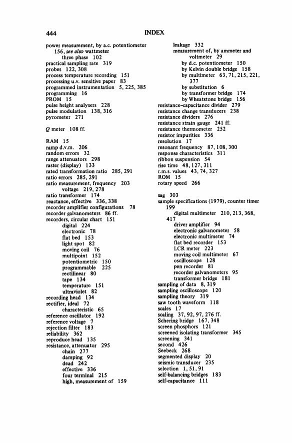
444 INDEX
power measurement, by a.c. potentiometer 156, see also wattmeter
three phase 102 practical sampling rate 319 probes 122, 308process temperature recording 151 processing u.v. sensitive paper 83 programmed instrumentation 5, 225, 385 programming 16PROM 15pulse height analysers 228pulse modulation 138, 316pyrometer 271
Q meter 108 ff
RAM 15ramp d.v.m. 206random errors 32range attenuators 298raster (display) 133rated transformation ratio 285, 291ratio errors 285, 291ratio measurement, frequency 203
voltage 219, 278 ratio transformer 174 reactance, effective 336, 338 recorder amplifier configurations 78 recorder galvanometers 86 ff. recorders, circular chart 151
digital 224 electronic 78 flatbed 153 light spot 82 moving coil 76 multipoint 152 potentiometric 150 programmable 225 rectilinear 80 tape 134 temperature 151 ultraviolet 82
recording head 1 34rectifier, ideal 72
characteristic 65reference oscillator 192reference voltage 7rejection filter 183reliability 362reproduce head 135resistance, attenuator 295
chain 277 damping 92 dead 242 effective 336 four terminal 215 high, measurement of 159
leakage 332measurement of, by ammeter and
voltmeter 29by d.c. potentiometer 150 by Kelvin double bridge 158 by multimeter 63, 71, 215, 221,
377by substitution 6 by transformer bridge 174 by Wheatstone bridge 156
resistance-capacitance divider 279 resistance change transducers 238 resistance dividers 276 resistance strain gauge 241 ff. resistance thermometer 252 resistor impurities 336 resolution 17resonant frequency 87, 108, 300 response characteristics 311 ribbon suspension 54 rise time 48, 127, 311 r.m.s. values 43, 74, 327 ROM 15rotary speed 266
sag 303sample specifications (1979), counter timer
199digital multimeter 210, 213, 368,
417driver amplifier 94 electronic galvanometer 58 electronic multimeter 74 flat bed recorder 153 LCR meter 223 moving coil multimeter 67 oscilloscope 128 pen recorder 81 recorder galvanometers 95 transformer bridge 181
sampling of data 8, 319sampling oscilloscope 120sampling theory 319saw tooth waveform 118scales 17scaling 37, 92, 97, 276 ff.Schering bridge 167, 348screen phosphors 121screened isolating transformer 345 screening 341 second 426 Seebeck 268 segmented display 20 seismic transducer 235 selection 1,51,91 self-balancing bridges 183 self-capacitance 111

INDEX 445
self-generating transducers 264 semiconductor transducers 261 sensitivity 37serial data transmission 9series mode noise 350series resistance of an inductor 111, 336 shaft position encoder 274 shield 50shunt 287
universal 288SI units 425siemen 428signal conditioning 93, 276 ff. signal response 311 signal to noise ratio 357 simple transformer bridge 171 sinewave 42 skew 143 slewing speed 155 software 16solid state display 20, 115sources of error 25specification analysis 33, 363 specifications see sample specifications spectrum analyser 226standard cell 7, 146standard deviation 33standard of temperature 252, 426 standardisation 146 standards 6,35,426 state analysers 228 statistical analyser 228 statistics 220 storage oscilloscope 1 30 strain gauge 241
attachment of 249 bridge 164,245 semiconductor 263 transducer 250
strain sensitivity 242strays and residuals 27stretching (tape) 143substitution measurements 6, 108 successive approximation d.v.m. 205 summation of errors 28 summing amplifier 323 suspension 54sweep delay 118symbols 13, 425synchro 261synchronous counter 187system bandwidth 48system instrumentation 379 system operation 16
T attenuator 296tachometer 267
talker 388tan δ (loss angle) 113tape recorders 1 34tape transport 142temperature 426temperature effects in strain gauges 245 temperature measurement 252, 268 temperature recorder 150 tera 425thermal effects 331thermal e.m.f. 332thermistors 262thermocouple 268thermocouple instrument 74, 105 thermometer, platinum resistance 252 thermopile 271Thévenin impedance 162three dB point 302time 426time constant 300, 305time interval measurement 204 time shift 89 timebase (c.r.o.) 117 timers (counters) 186 ff. timing analyser 227 timing bus system 390 timing lines 83 tolerance 23tooth rotor tachometer 266toroidal core 282torsion measurement 252totalising 1 95trace identification 83transducers, capacitive 255
classification of 237 digital 273 electromagnetic 265 fixed reference 234 inductive 258 linear velocity 265 magnetostriction 272 mass-spring 235 piezoelectric 266 potentiometric 238 resistance change 238 resistance strain gauge 24 1 seismic 235 semiconductor 261 thermoelectric 268 ultrasonic 272
transfer instrument 155transformation ratio 285, 291transformer bridge 171transient distortion 91transient response 90, 301transient solution (moving coil instrument)
4, 430
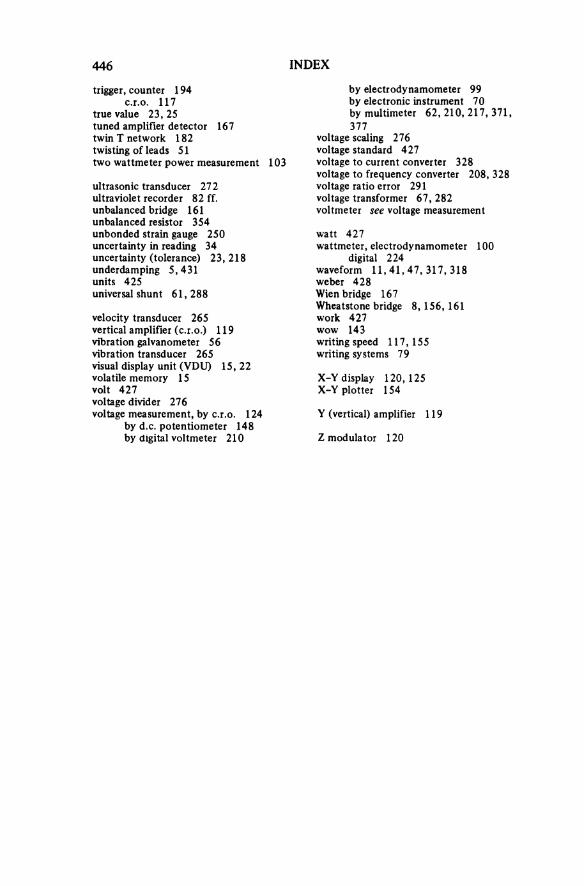
446 INDEX
trigger, counter 1 94 c.r.o. 117
true value 23, 25tuned amplifier detector 167 twin T network 182 twisting of leads 51two wattmeter power measurement 103
ultrasonic transducer 272ultraviolet recorder 82 ff.unbalanced bridge 161unbalanced resistor 354unbonded strain gauge 250 uncertainty in reading 34 uncertainty (tolerance) 23, 218 underdamping 5, 431 units 425universal shunt 61,288
velocity transducer 265vertical amplifier (c.r.o.) 119 vibration galvanometer 56 vibration transducer 265 visual display unit (VDU) 15, 22 volatile memory 1 5 volt 427voltage divider 276voltage measurement, by c.r.o. 124
by d.c. potentiometer 148 by digital voltmeter 210
by electrodynamometer 99 by electronic instrument 70 by multimeter 62, 210, 217, 371, 377
voltage scaling 276voltage standard 427voltage to current converter 328 voltage to frequency converter 208, 328 voltage ratio error 291voltage transformer 67, 282 voltmeter see voltage measurement
watt 427wattmeter, electrodynamometer 100
digital 224waveform 11, 41, 47, 317, 318weber 428Wien bridge 167Wheatstone bridge 8, 156, 161work 427wow 143writing speed 117, 155writing systems 79
X-Y display 120, 125X-Y plotter 154
Y (vertical) amplifier 119
Z modulator 120

In this second edition of his book Introduction to Electrical Instru-mentation, the author has considerably reorganised and extended his coverage to take account of the developments in integrated circuits, particularly the microprocessor, which have made possible the incor-poration of programmable and calculating facilities within instruments.
As in the first edition, the aim is to assist the student of electrical or electronic engineering to adopt a systematic and practical approach to his measurement problems. It will also be of value to the engineer or technician who needs to select the right type of instrument for a particular application from among the ranges now offered by many manufacturers.
Some of the important changes in the new edition are: additional material on accuracy and methods of display; the inclusion of intelligent instruments and hybrids in the chapter on digital instruments; increased coverage of interference and screening. In addition, in response to requests from users of the first edition the author has provided a final chapter consisting of problems and exercises (with answers), which will be of great value where the book is used as a course textbook.
Before becoming a lecturer, B.A. Gregory spent more than thirteen years in industry working in the field of instrumentation and measure-ment. For a number of years he has been a Senior Lecturer, specialising in electrical instrumentation, in the Department of Electrical and Electronic Engineering at Brighton Polytechnic.
ISBN 0 470-27092-6

An Introduction to
EL
EC
TR
ICAL INS
TRU
ME
NT
AT
ION
A
ND M
EA
SUR
EM
EN
T SYSTEM
SB
. A. G
regory
SECONDEDITION
HALSTEDPRESS