University of Memphis University of Memphis

University of Memphis Digital Commons University of Memphis Digital Commons

Electronic Theses and Dissertations

4-14-2017

An Inquiry into the Political, Socio-economic, Geographic, and An Inquiry into the Political, Socio-economic, Geographic, and

Educational Factors that Predict Race to the Top Winners and Educational Factors that Predict Race to the Top Winners and

Losers Losers

Brian Wade Brewer

Follow this and additional works at: https://digitalcommons.memphis.edu/etd

Recommended Citation Recommended Citation Brewer, Brian Wade, "An Inquiry into the Political, Socio-economic, Geographic, and Educational Factors that Predict Race to the Top Winners and Losers" (2017). Electronic Theses and Dissertations. 1598. https://digitalcommons.memphis.edu/etd/1598

This Dissertation is brought to you for free and open access by University of Memphis Digital Commons. It has been accepted for inclusion in Electronic Theses and Dissertations by an authorized administrator of University of Memphis Digital Commons. For more information, please contact khggerty@memphis.edu.

AN INQUIRY INTO THE POLITICAL, SOCIO-ECONOMIC, GEOGRAPHIC, AND

EDUCATIONAL FACTORS THAT PREDICT RACE TO THE TOP WINNERS AND

LOSERS

by

Brian Brewer

A Dissertation

Submitted in Partial Fulfillment of the

Requirement for the Degree of

Doctor of Education

Major: Leadership and Policy Studies

The University of Memphis

May 2017

ii

Abstract

Brewer, Brian Wade. EdD. The University of Memphis. May, 2017. An Inquiry into the Political, Socio-economic, Geographic, and Educational Factors that Predict Race to the Top Winners and Losers. Major Professor: Dr. Charisse Gulosino. This research investigated the effect of political, economic, racial, academic, geographic data,

and the components of the Race to the Top grant against the Race to the Top grant awards. Data

for all 50 states and the District of Columbia was compiled from the federal Race to the Top

documents, the Georgetown University Stateminder dataset, and the U.S. Census Bureau to

create a combined dataset. The combined dataset included a combination of the 2009 scores

from Delaware and Tennessee and the 2010 scores of all other states. Since the scores from

2009 only resulted in two winners, and the 2010 scores resulted in seventeen winners, the 2010

data became the basis for the dataset while including the 2009 data for the two first-round

winners. Predictor data for states that did not apply for Race to the Top also was included in the

dataset for an extended analysis of self-exclusion of the non-applying states. The analysis used

multiple comparison of means, a standard regression model and the Heckman selection

regression model to determine if any of the predictors affected the Race to the Top awards. The

comparison of means analyzed the differences in averages for Race to the Top Winners and

Applicants. The means and the significance of the means for the predictor values, and the means

of the scores of the Race to the Top components were calculated. A comparison of number and

percentage of significant predictor occurrence, and the means of the Race to the Top components

by geographic location was compiled. The standard regression was calculated using the 38

applying states. Since all states did not apply for Race to the Top, and the standard regression

model did not account for these exclusions, a secondary regression model, The Heckman

Selection Model, was used in conjunction with the standard regression to determine if the

iii

excluded states would influence predictor effect. The results demonstrated that several

predictors did have a significant effect on Race to the Top application scores and, ultimately, the

winning and losing states. Specifically, political affiliation of the state legislative process, race,

and academics were significant.

iv

Table of Contents

Chapter Page 1 Introduction 1 Recognition of the Problem 1 Emergence of the Problem 2 Historical Perspective 3 Within the Educational Leadership Discipline 9 Within Contemporary and Local Experience 9 Statement of the Problem 10 Previous Research Related to this Problem 10 Purpose of this Study 13 Significance of the Study 13 Research Questions 14 Scope and Delimitations of the Study 14 Limitations of the Study 15 Definition of Terms 16 Organization of this Study 19 2 Literature Review 19 Federalism 19 Federalism in Education 21 New Policy Implementation 28 Carrot Theory and Intergovernmental Grant Process 30 Race to the Top Development 32 Race to the Top Criteria Design 38 Race and Population Change 51 3 Methodologies and Data 52 Variables 52 Race to the Top Variables 53 Stateminder 57 Method of Analysis 58 4 Analysis 64 Discussion 64 Descriptive Statistics 64 Research Question 1 65 Research Question 2 69 Research Question 3 77 Summary of Findings 84

v

Table of Contents (cont.)

Chapter Page 5 Summary and Conclusions 85 Impact on Winning States Compared to All Applicants (Questions 1 and 2) 88 Impact on Final Scores (Question 3) 89 Recommendations 98 Recommendations for Further Research 99

References 101 Appendices

A: Variable Definitions 109

B: Award Winning States (By Region) 113

C: Research Dataset 115

IRB Approval/Waiver 125

vi

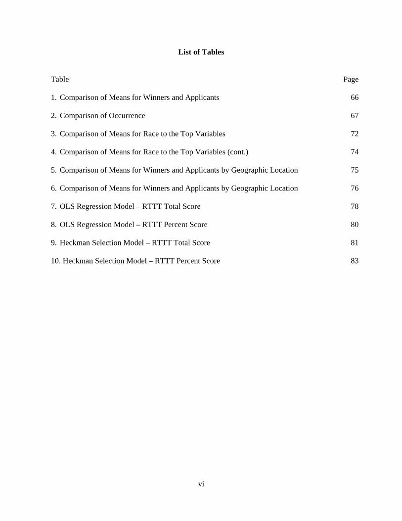
List of Tables

Table Page 1. Comparison of Means for Winners and Applicants 66 2. Comparison of Occurrence 67 3. Comparison of Means for Race to the Top Variables 72 4. Comparison of Means for Race to the Top Variables (cont.) 74 5. Comparison of Means for Winners and Applicants by Geographic Location 75 6. Comparison of Means for Winners and Applicants by Geographic Location 76 7. OLS Regression Model – RTTT Total Score 78 8. OLS Regression Model – RTTT Percent Score 80 9. Heckman Selection Model – RTTT Total Score 81 10. Heckman Selection Model – RTTT Percent Score 83

1

Chapter 1

Introduction

Recognition of the Problem

Education in the United States has seen multiple interjections from the federal

government. National and international events have spurred action by Congress and the

President to redirect or reform the states’ educational systems to address the educational gaps

evidenced through these events. America’s education system has been considered inferior to

other countries, and therefore, needs to be redirected. Government programs designed to modify

the educational landscape in America have appeared with increasing frequency, and the

requirements on the states have become more stringent as well. Federal programs that were

introduced, typically, offered equitable funding to states based upon predetermined criteria

(Anderson, 2007). This meant that there was no competition for grant money, and the states

simply had to implement the changes required from the federal government to receive the grant.

Race to the Top (RTTT) changed that paradigm. States competed against each other by

responding to a grant proposal and promising sweeping changes in their educational policies and

processes to receive additional grant funding. States that were not willing to implement

sweeping educational reform or were not able to meet the criteria at a high level based upon rater

review received less or no funding. This created a disparity between states, and spurred debate

among education leaders about the grant award process. The rating and award process was

objective in nature and left opportunity for outside influence in final decisions. Exterior

influence may have affected the scoring and awards process. Analysis of the section scores and

how those sections were weighted may have significant influence in the grant awards.

2

Emergence of the Problem

In 1983, a debated report on whether American education was failing was presented, “A

Nation at Risk” (Berliner, 1995). This report detailed a disturbing trend in the educational

landscape and what correction was needed became the fulcrum of a shift in educational progress

and policy in the United States (Berliner, 1995). Educational initiatives from the state and

federal levels began to define how students were educated and what made effective classroom

teachers. Student testing started to become the norm for public education as school leaders and

politicians struggled to identify track key student performance indicators. Many public school

students were evaluated using standardized tests created by states like Iowa or California, but as

student performance became more scrutinized, states began to move toward testing processes

that included high-stakes, end-of-course testing in core subject areas including English,

Mathematics, Science, and History.

One of the indicators used to define how American students compared to the rest of the

world’s students has been the Unites States’ performance on international standardized tests.

Every three years, Program for International Student Assessment (PISA), an international

standardized test, is given to 15-yesr-old students. Thirty-two countries participated in 2000, and

65 countries participated in 2012 (Kelly et al., 2013). In 2006, the United States scored 35th out

of the top 40 countries in mathematics and 31st in science. There was a decline in ranking and

raw score from the tests given 3 years earlier (Darling-Hammond & McCloskey, 2008). Reading

scores for United States’ students were closer to the PISA average in 2000. American students

had an average score of 504 compared to the PISA average of 500 (Office of Ecuational

Research and Improvement, U.S. Department of Education, 2001). In 2012, the United States

3

scored at the PISA average of 496 (OECD, 2013). The results of the mathematics assessment

showed a considerable deficiency in the competitive ability of American students in the global

job market, especially in the Science, Technology, Engineering, and Math (STEM) jobs that are

expected to see the highest job growth. Even with the reading scores at the PISA average, the

results showed that the U.S. students were not reading the highest levels, compared with their

international peers.

Historical Perspective

According to the tenth amendment, education is a responsibility of the states to fund and

maintain. However, there is an arguable belief throughout the history of the United States that

the federal government has consistently attempted to influence education (see e.g., (Sunderman

& Kim, 2007)). The U.S. Constitution does not mention education, therefore, by extension, the

federal government has no direct control or funding responsibility. However, the federal

government can pass legislation and influence the educational process through distributed and

competitive grants. As early as the late 1700s, legislation to inject federal dollars and influence

in the education system were being introduced in Congress. One of the first was the Ordinance

of 1785 and the Northwest Ordinance of 1787 that divided townships into 36-square-mile

sections and then subdivided into 1-acre lots where the 16th and eventually 36th lot was set aside

for education and the money raised from renting the lots and their eventual sale was earmarked

for education. These early ordinances created an immediate debate over federal influence on

education (Anderson, 2007). Other land-grant styled legislation, specifically the Morrill Act of

1862, created higher-education institutes and all of the land-grant legislations set a precedent for

categorical aid that still exists today (Anderson, 2007).

4

Further legislative attempts were made to provide federal funding to public education. In

the 1880s, the Blair Bill would have required states to educate all children without exception

(Anderson, 2007). The bill allowed for segregation, but would have forced states to educate

children of all races and economic backgrounds. The bill was thought to garner support from the

Southern states since the money allocations would be based upon illiteracy rates, which were

high in the South, but the requirement of educating all students as well as other influences on

Southern Congressmen did not garner the expected support (Going, 1957). The bill passed the

Senate several times, but never made it through the House of Representatives (Evans, 1960).

The Blair Bill was also unique because it would have provided education funding based upon

illiteracy rates and number of school-age children giving money directly to states rather than

through the land-grant systems previously implemented (Anderson, 2007). The bill met strong

resistance from groups who did not want the federal government’s influence or potential

takeover of schools as well as the Catholic Church that argued the funding should have been

extended to parochial schools as well (Evans, 1960). The Blair Bill failed its fourth reading in

the Senate and was not reintroduced (Evans, 1960).

Prior to World War I, the Smith-Hughes Act of 1917 provided funding for vocational

programs in public schools (Hillison, 1995). The Smith-Hughes Act was the first categorical

funding act for federal education dollars (Anderson, 2007). The act received support from

powerful lobbyists including the American Federation of Labor (AFL), the National Education

Association (NEA), the National Association of Manufacturers (NAM), the U.S. Chamber of

Commerce, and the National Democratic Party (Hillison, 1995). The act directed the use of

federal dollars to increase American education’s competitiveness on the international market

(Anderson, 2007). After World War I and during the depression, tax dollars for education were

5

scarce, but federal relief acts of the time did provide funding to maintain educational systems by

providing funding to keep teachers employed and build schools (Anderson, 2007). The

government also implemented the Lanham Act in 1941 and the Impact Aid laws of 1950 that

provided incentives and compensation to local schools that supported military bases (U.S.

Department of Education, 2016). The 1994 “G.I. Bill” expanded the federal government’s role

in education by providing post-secondary funding for World War II veterans (U.S. Department

of Education, 2016). The political strategies introduced with the Smith-Hughes Act and

military-based legislation set the methodology for the current federal education grant policies

(Anderson, 2007).

A rudimentary Department of Education was created in 1867 to gather data and monitor

the nation’s education (U.S. Department of Education, 2016), but it was not a part of the

Presidential cabinet or an official government office until the Elementary and Secondary

Education Act (ESEA), signed by President Johnson in 1965, created the federal Department of

Education (Anderson, 2007). The civil rights laws of the 1960s and 1970s expanded the focus of

the Department of Education to manage equal access to education as set forth by the new laws

(U.S. Department of Education, 2016). It was not until 1980 that Congress made the Department

of Education a Cabinet level position (U.S. Department of Education, 2016).

Two significant international events between the 1950s and the 1980s further defined the

federal government’s role in education and set the baseline for further federal education policies.

The first was the launch of Sputnik by the Soviet Union, which led to the introduction of the

National Defense Education Act of 1958 (NDEA) (U.S. Department of Education, 2016). The

NDEA was an effort to help American students compete with the Soviet Union in scientific and

technical fields. It also provided loans to college students, provided graduate fellowships, and

6

increased foreign language education at the secondary level (U.S. Department of Education,

2016). The second major event was the “Nation at Risk Report,” which was commissioned by

President Reagan’s administration and released in 1983 (Editoral Projects in Education Research

Center, 2004). The report used statistical data to show inadequate educational performance and

linked the need for improvement to the success of America’s economy (Editoral Projects in

Education Research Center, 2004). The report generated a “crisis” in education and the proposed

reforms largely focused on raising academic standards and increasing learning time (Anderson,

2007). The recommended changes in education from the report have been the basis of the

curriculum secondary students follow, even today. Over time, scholars have rebutted the validity

of the report saying that the statistics were flawed and the report was a way for political

influence to change the course of public education (Editoral Projects in Education Research

Center, 2004). Twenty years after the Nation at Risk report, data showed that American

education has not improved (Peterson, 2003).

In 1989, the National Governors’ Association’s held an “Education Summit” in

Charlottesville, Virginia. President George H.W. Bush, the nation’s governors, and business

leaders determined that education needed to move to a business-style accountability system

(Klein, 2014). States were still responsible for the implementation, but the federal government

started advocating for standards and accountability that made the federal role give the sense of a

larger entity. In 1994, when the ESEA was reauthorized under President Bill Clinton, it was

called the Improving America’s Schools Act (IASA). States were required to adopt academic

standards and assessments, and states’ compliance to these new requirements were tied to Title I

funding (Cantrell, 2013), and as part of President Clinton’s “Goals 2000” initiative, states were

asked for voluntary participation in setting national education standards. However, like “Nation

7

at Risk” and the “Education Summit,” no legislation resulted that would fundamentally alter the

behavior of the states (Klein, 2014).

Since each state controlled how their students were educated, including the funding

students received and tracking students’ academic progress, each state was not held to a common

standard or achievement expectation for students (Klein, 2014). To persuade a more consistent

educational process across the states, the federal government created two educational policies.

In 2001, No Child Left Behind (NCLB) was introduced by President George W. Bush’s

administration that included financial penalties in Title 1 funding (Hess & Petrilli, 2006). NCLB

created a more forceful induction by the federal government into public education (Hess &

Petrilli, 2006). Like IASA, NCLB put states’ Title I funding at risk for non-compliance, but the

legislation had the support to enforce it. Therefore, more pressure was put on the states to meet

requirements on assessments, student achievement, equal access to education, and other things

(Ahn & Vigdor, 2013).

In 2007, NCLB was not reauthorized and President Barak Obama, in his first term,

initiated the Race to the Top (RTTT) initiative as part of the American Recovery and

Reinvestment Act (ARRA) (J. Weiss, 2015). RTTT offered grant money through the Title 1

system as well as a competitive process for additional funds to coerce change in the states’

educational models. All states accepted money from NCLB, but the states were not required to

create a common accountability system, therefore, the result was a widely varying set of

educational accountability systems among all of the states and the District of Columbia (Linn,

Baker, & Betebenner, 2002). Before NCLB, state participation in any federal initiative was

strictly voluntary and did not lead to consensus among the states’ education departments.

8

To try and combat the issue of low performance among graduating students, initiatives

like No Child Left Behind (NCLB) and Race to the Top (RTTT) have become larger parts of our

educational landscape (Thomas, 2013). States, through federal programs, have initiated more

changes in public education to increase accountability in education and improve student

performance (Thomas, 2013). However, the standards that were currently in place to measure

student performance were deemed inadequate to ensure American students were prepared to

compete on a global scale. Therefore, the standards and their accompanying assessments

became more rigorous. Schools were expected to meet these new standards immediately with

teachers and students who have never been held to these higher standards or been exposed to the

technology being implemented.

When RTTT was introduced, the states were in the middle of a budgetary crisis due to the

recession America was experiencing (J. Weiss, 2015). Most of the states’ and districts’ budgets

were consumed in operating expenses which means that the funding for any additional initiatives

had to be taken from existing programs which was unpopular or difficult depending on the needs

of the districts and their students. The lack of discretionary money for improvement initiatives

made the RTTT grant appealing to lawmakers and state leaders. Increasing taxes to fund

existing educational needs from the state or local level has been difficult if not impossible due to

the economic and political climate that existed, which meant little or no funding for

improvement initiatives. Considering the economic and educational situation of the states and the

country, refusing additional educational funding to improve student achievement made states

willing to make concessions in their educational processes to show their support for

improvement in the education of the state’s children (E. Weiss, 2013).

9

Within the Educational Leadership Discipline

Education leaders have struggled with how to improve student learning. Federal

initiatives to improve American education have largely been ineffective in changing the overall

performance of students (Peterson, 2003). Federal initiatives like Race to the Top have

introduced significant changes in the educational landscape of the states that applied and won the

competitive grant funding. Leaders at the state and local levels scrambled to meet the new

requirements through policy and procedural changes that did not garner support from many

people in the educational system including teachers and teacher unions. The relationship

between local educators and state leaders become more strained as the states implemented new

teacher evaluation systems, testing systems, educator preparation and licensing requirements,

and legislation allowing the growth of charter management organizations.

Within Contemporary and Local Experience

New testing requirements pushed local technical systems to the limit. Teachers and

leaders tried to implement new classroom pedagogy to address the new tests with limited

resources and exposure to the new requirements. Students who have never been required to

perform to these new standards were working to meet the new benchmarks with limited success.

Schools, facing the possibility of closure or state takeover, were uncertain of their future. The

loss of students to state and charter associations affected school district funding, especially in

large urban districts. Less state funding led to budget shortfalls and an increased pressure on

local governments to close the funding gaps.

10

Statement of the Problem

The Race to the Top competitive grant proposal was a subjective rating process. Multiple

“raters” read the responses from the states and assigned a score to each section and sub-section.

The scores were totaled, and in a perfect process, the highest scoring states would receive some

level of funding. Since the scoring process was subjective, and the final award system was not

clearly defined, an analysis of the states’ responses and the ratings assigned to those responses

could help clarify what parts of the grant proposal were weighted heavier than others. The

analysis between ratings and awards will lead to a better understanding of what components of

Race to the Top truly influenced the grant awards and if any outside influence may have changed

the final awards.

Previous Research Related to this Problem

Several research strands exist in relationship to Race to the Top. The most common

research was about the policy changes that the states implemented to receive the grant funding.

In the research about policies, the authors discussed the grant proposal process and the potential

political influence involved, but the research does not delve into the components of the grant

proposal. The second most common research strand was the impact of Race to the Top on

student achievement. Like the policy research strands, these strands of research were not

focused on the grant proposal process, but more about the outcomes of the implementation by the

states. Other, less numerous, research strands focused on varying impacts of the grant and its

implementation exist, but again do not focus on the grant process directly.

Two research articles focusing on the grant proposal process were found. Though they

do not focus on each of the section and sub-section ratings, they do address the rating process

and provide insight into the awards process from the lens of their research. The first was a report

11

by Daniel H. Bowen in September, 2010. His research focused on the Race to the Top grant

awards through a lens of political influence. The purpose of the research was to apply

quantifiable value to the political climate of the states that won a RTTT grant. The author

performed a regression analysis by assigning values to a state’s projected Race to the Top score,

a measurement of a state’s competitiveness in the 2008 presidential election, whether a Senate

seat was contested in the 2010 election, and whether the state’s Governor seat was contested in

the 2010 election (Bowen, 2010). The fist finding of the analysis showed that states with highly-

contested Senate and Governor seats increased the round one scores by 35 to 75 points (Bowen,

2010). The second finding was the state’s political circumstances and education reform record

helped predict the first round scores (Bowen, 2010). Analyzing the results led to the

determination that the specific researched political climates of states like Delaware, Tennessee,

and Illinois were higher than projected due to the approaching contested elections and states like

Louisiana, North Carolina, and South Carolina scored lower than projected (Bowen, 2010).

The second research was a policy brief by The New Teacher Project in December, 2010.

This research focused on the review process and how it allowed the reviewers too much freedom

in assigning and deducting points, and the refusal of the Department of Education to intervene in

the final results (The New Teacher Project, 2010). Specifically, the analysis was trying to

determine if states’ scores were too inconsistent based upon the harshness or leniency of the

raters (The New Teacher Project, 2010). The raters were given basic guidance on scoring but

made their own interpretations of the scoring rubric, and scoring feedback from The Department

of Education did not force the raters to adjust their scoring (The New Teacher Project, 2010).

The analysis also revealed that raters also artificially inflated scores of the states that were

identified as finalists after the first round awards were made to Delaware and Tennessee (The

12

New Teacher Project, 2010). A third part of the analysis showed that the subjectivity of the

rating process may have affected the results where raters who had a more positive view of an

application may have freely given too many points (The New Teacher Project, 2010). Finally,

the analysis determined that states who made significant changes in laws and policies as part of

the application process did not always receive favorable scores compared to states that were

more ambiguous in their plans, especially related to the more poignant sections of the application

which means that states with intention to change were given equal or greater consideration as

states who made the changes to show commitment to their application (The New Teacher

Project, 2010).

Reviewing the results of the research by Bowen and The New Teacher Project compared

to the methodology of this research gives some insight into external influences of analyzing the

Race to the Top data and applications. The political impact on a process as large as Race to the

Top was evidenced by Bowen’s (2010) research. Largely contested state and federal elections

and political climate could have influenced the flow of grant money to states that may not have

scored the most points on the grading rubric (Bowen, 2010). Scoring qualitative data into a

quantitative measurement, as was done by the Race to the Top raters and in this research, brings

in a level of subjectivity. When multiple raters are used to score documents, a consistent,

repeatable process has to be implemented to try and ensure equal opportunity to all participants

(The New Teacher Project, 2010). According to The New Teacher Project’s (2010) research, the

consistency between raters was not evident, and may have affected the final outcomes of the

grant award process. Beyond the rating discrepancies, the U.S. Department of Education did not

correct or adjust the raters’ actions to ensure equity in the process. Also, the Department of

13

Education did not intervene in the selection process if scoring bias was suspected (The New

Teacher Project, 2010).

Purpose of this Study

This research will investigate how states’ responses to the Race to the Top (RTTT)

proposal, if specific focus areas of the requirements may have garnered a greater influence on

those awards, and any influence that political, economic, racial, social, and geography may have

influenced the Race to the Top (RTTT) grant awards. The purpose of this study is to collect the

states’ RTTT applications, the federal raters’ scoring documents, and the Stateminder dataset to

identify variables and assign values to perform a quantitative analysis. Using multiple

predictors, the researcher will be able to determine what factors had influence on the grant

awards, and if any outside influence may have affected the outcomes. Prior work on local grant

competitions and competitive federal grants, which has shown that the capacity of potential grant

recipients to administer grant-funded programs, is an important factor that helps to explain how

these competitive grants unfold (Berry, Burden, & Howell, 2010; Bickers & Stein, 2004; Manna

& Ryan, 2011).

Significance of the Study

This research can be valuable to educational leaders looking for guidance on federal

education policy foci that may better align local and state initiatives. The authorization of Every

Student Succeeds Act (ESSA) changes the landscape of federal Race to the Top education

policy. However, as supporters of federalism continue to attempt influence of federal education

policy, or if the federal government returns to offering competitive grant funding, knowing the

key indicators may allow states to align their proposals closer to the federal expectations.

Political leaders may be able to use this research to identify factors that would keep states from

14

applying for grants, and perform internal reviews to ensure equity among applicants. Groups

may find the results of this study useful as other influences of the process come to light. Other

areas of federal funding may also use the foundational structure of Race to the Top to provide

state funding (J. Weiss, 2015), therefore, the findings of this research may have a broader impact

than federal educational funding.

Research Questions

After analyzing the rater and state application documents and performing the coding

process to create a composite dataset, the research is divided into four questions.

1. What are the political, social, economic, educational, and geographic

patterns/characteristics of winning states and applying states in the national Race to the

Top (RTTT) competition?

2. Do the scores across different sections of the RTTT application differ between winning

and applying states?

3. What political, social, economic, educational, and geographic characteristics may have

influenced states' final scores on the RTTT grant competition, controlling for potential

selection bias between applicants and non-applicants of RTTT?

Question 1 took the information in the dataset to see patterns between the predictor values and

grant awards. Question 2 analyzed the dataset for differences in the scoring between winning

and losing states across the different sections of the Race to the Top application. Question 3

used the output from a standard and Heckman selection multiple regression models to determine

which predictors had significant influence in the scores.

Scope and Delimitations of the Study

15

The study includes the Race to the Top states that applied for tier one or tier two funding

in 2009 and 2010. The 50 states and the District of Columbia were invited to apply for the race

to the Top grant. Only two states won funding in 2009. Therefore, the data from 2009 was

combined with 2010 to overcome the small sample size created by the 2009 winning states. Ten

states did not apply for phase one funding, and 13 states did not apply for the phase two. The

applicants were able to resubmit their applications in 2010 and earned a different score from

2009. Since the winners from 2009 were combined with the 2010 data to have a larger sample,

the 13 states that did not reapply in 2010 were excluded from the standard analysis. Therefore,

38 applicants had data available for this research. States’ applications along with the the rater

documents and scores for each application will be used to code the data for the analysis.

Political, social, economic, racial, and geographic data from Stateminder along with the criteria

used in the Race to the Top application were placed into column headers. The existing data from

Stateminder and the numerical values provided by the federal rater documents were combined

into a single dataset used to perform statistical analyses to determine effects the variables on the

final award decisions. Prior research on political influence and the federal government’s rating

processes and procedures will not part of the research analysis. Although, those strands of

research will be used to develop possible explanations of the research results that were outside of

the current research.

Limitations of the Study

The scoring documents from the federal Race to the Top rating process were an average

of the scores provided by five different individuals using a scoring rubric. A level of bias and

inconsistency that can exist within that process could influence the results of the research. A

study that codes qualitative data into quantitative data will have opportunities for influence

16

outside of the researcher’s control. Any bias within the research documents will not be filtered

through the research processes which could have influenced the research outcomes. Other

criterion that may have influenced scoring outside of the scope of this study were not considered.

Definition of Terms

Carrot hypothesis is the granting authority placing a temptation in front of the receiving

authority that is good enough to entice the receiving authority to do what is required to try and

earn the temptation.

Coding is a process that takes information presented in language and converts it into a

numerical value.

Federalism is government where the same territory is controlled by two different levels

of the government. In the context of this research, the territory is education, and the two

different levels of government are the federal and state governments.

Intergovernmental grants are cooperative grants provided to the states by the federal

government. Some of the grants have specific requirements/restrictions for how the money can

be spent, and other grants are unrestricted in how the money is spent.

Local Education Associations (LEA’s) are local school districts responsible for the

public education of students within their governance boundary

Quantitative research uses numerical values along with statistical methods to identify

patterns in the data that assist in the identification of relationships and causality in the research.

Rater is a person or group of people who score a document using a pre-developed set of

criteria.

Rubric is a guide created to try and provide a consistent scoring process.

17

Strands of Research refer to alternative methods of defining and studying events that

differ from the current research methodology.

Organization of this Study

This study is designed for the reader to follow the thought process of the researcher.

Each component of the study gives insight into the development of the study. Five chapters will

be used to develop the structure of the study. The first chapter is the introduction to the study

document. The beginning of chapter one describes the recognition and emergence of the

research problem along with the historical perspective of federal intervention into the states’

educational process. An understanding of the history of federal education policy develops an

understanding of why the federal government became involved in education and gives insight

into the policy development process that led to the current Race to the Top initiative. Chapter

one continues to identify the research problem and the previous research that is similar to the

research being conducted in this study. The purpose and significance of the study are discussed

along with the research questions that drive this study. The scope, delimitations, and limitations

of the study are defined. Finally, chapter 1 concludes with a definition of terms to help the

reader understand any words or phrases used in the study.

Chapter 2 is the literature review section of the study. Published literature related to

federalism, federal education policy formation, and the Race to the Top criteria are discussed.

The theories of state and federal educational responsibility and management are discussed, and

the structure of the Race to the Top grant are discussed. Federal involvement in state educational

matters has sparked debate on both sides of the debate, and the desire to have more federal

involvement in education is believed to be the driving force behind the Race to the Top design.

18

The literature review set the context and background of the research to reach an understanding of

the issues and policies developed.

Chapter 3 discusses the methodology being implemented to perform this research. The

problem and research questions presented in chapter one are discussed in depth, and the theories

employed as part of the research are detailed. This study addresses existing data from the states’

Race to the Top applications and the rater documents from the U.S. Department of Education,

therefore, no survey instrument is required. However, the population of the study is discussed,

and the IRB review and approval will be included in the final document. The data collection and

coding process, statistical research methods and techniques, variable definition, and the

hypothesis to be tested conclude chapter three.

The findings and observations of the research will be reported in chapter 4. The trends in

the dataset will be identified and discussed using a descriptive analysis. The statistical analysis

that was performed will be detailed, and any significance will be identified. The result of the

significance calculations will be important in determining if the hypothesis being tested is valid.

After any significance is determined through the statistical program, SPSS, an analysis of the

significant data will be performed. Finally, a summary of the research findings will be presented

to give an overall understanding of the research.

The final chapters of the study, chapters 5, 6, and 7, complete the study. Chapter 5

includes the discussion of the study with conclusions reached and recommendations for future

research. A complete discussion of the significant findings and a final summary of the research

results are in chapter 5. Chapters 6 and 7 are the references and supporting appendixes of the

research. In the appendixes, the variable definitions, coding tables, and analysis tables will be

included for readers and other researchers to review.

19

Chapter 2

Literature Review

Federalism

The United States’ style of governance includes a federal government that is responsible

for national concerns and operations, and a state governance system that is responsible for local

concerns (Legal Information Institute, 2016). The roles of the federal and state governments,

though distinct, based upon the Constitution, do not operate autonomous of each other. Issues

that are primarily the responsibilities of the states may have cross-responsibility to the larger

concerns of the federal government. Federalism is the relationship between the federal and state

governments where both entities have jurisdictional authority (Legal Information Institute,

2016). Since the inception of the United States’ Constitution, critics and supporters of federal

involvement in state-level affairs have voiced their opinions in the federal government’s

increasing encroachment.

Frank Baumgartner and Bryan Jones (2009) traced and discussed the theoretical,

structural, and contextual changes in American politics using a term “punctuated equilibrium.”

They argued that the political process is not a stable and incremental process, but rather

disjointed and varying based upon external influence (Baumgartner & Jones, 2009). Policies are

defined and changed though sub-systems of content specialists within different federal agencies

and external special interest groups (Baumgartner & Jones, 2009). Policies and the processes to

create them would vary over time and not become focused or effective to the issues they were

designed to address (Baumgartner & Jones, 2009). However, moments in political or cultural

turmoil would leap the policies forward and into action to address the issues (Baumgartner &

20

Jones, 2009). However, the resulting policies may not have followed the direction hoped by the

activists attempting to enact the change (Baumgartner & Jones, 2009).

Political decision-making processes have not used a rational approach where the logical

approach to a decision is based upon a tally of the costs and benefits of said decision upon the

population (Baumgartner & Jones, 2009). Instead, a narrowed, incomplete attention toward an

issue determined its policy outcome without the input of most stakeholders. Enthusiasm for an

idea would turn to criticism without weighing the cost or benefit of the implemented policy

(Baumgartner & Jones, 2009). Because of the limited focus afforded people and groups of

people on issues, especially on a national scale, many decisions required the action of the

political subsystems (Baumgartner & Jones, 2009). Activists can redirect policy when the

possibility of error or subjectivity in the process is defined and highlighted as inappropriate for

the entire citizenship or a subgroup of citizens (Baumgartner & Jones, 2009).

The overlaps of authority between federal and state governments can inhibit or influence

change within the political landscape (Baumgartner & Jones, 2009). Due to the separation of

powers defined within the Constitution, avenues of appeal exist within the political and legal

frameworks. The avenues allow issues to be addressed in multiple venues where the opportunity

for feedback, reflection, and correction are possible (Baumgartner & Jones, 2009). Without

these structures, one group would be able to monopolize control without the possibility of losing

that control (Baumgartner & Jones, 2009). The actions of multiple groups upon an issue provide

stability and opportunity for policy change within the society by addressing the components of a

problem individually ultimately reaching a comprehensive solution (Baumgartner & Jones,

2009). Therefore, the overlap of federal and state jurisdiction allows the political process to

21

address the needs of all citizens, to the extent possible, while the separation of powers does not

allow one part of the system to dominate (Manna, 2006).

Two types of federalism have been defined by contemporary scholars, cooperative and

coercive federalism (McGovern, 2011). The cooperative model was described as collaboration

between state and federal governments where shared interests exist (Robinson, 2013). This

collaboration includes state implementation of federal policy through federal grants that are

distributed to the states either equally or, normally, through an algorithm of need based upon

population (McGovern, 2011). Coercive federalism is described as the federal government’s use

of conditional grants and statutory mandates to force state compliance (McGovern, 2011).

Cooperative federalism is a voluntary act between the federal and state governments, where

coercive federalism is forced action by the states to meet federal requirements. These

relationships are defined by the courts where the limit of federal authority is interpreted (Martin,

2012).

Federalism in Education

Public education in America has been the responsibility of the States since its formation.

The U.S. Constitution does not address public education as a responsibility of the federal

government, nor has public education been made a right under the Bill of Rights. Therefore,

under the tenth amendment, which states “the powers not delegated to the United States by the

Constitution, nor prohibited by it to the states, are reserved to the states respectively, or to the

people” (Legal Information Institute, 2016), the states were responsible for providing public

education to its citizens. However, since the federal government has no direct authority over

public education, the relationship is complex. A level of cooperative federalism existed where

the initiatives of the federal government in regards to education were more guidance than

22

mandate (Manna, 2006). The directives of the federal government were voluntarily implemented

by the states (Manna, 2006). Over time, that cooperative model has given way to a more

coercive one (Martin, 2012).

Federal intervention in education dates back to the 1700s, where the proceeds from the

sale of land in the Northwest Territories were used for public education (Anderson, 2007). At

the time, the Supreme Court did not believe that Congress had violated the Commerce Clause,

which defines the government’s ability to regulate interstate commerce, nor the Tenth

Amendment (Martin, 2012). Therefore, no laws were struck down by the Supreme Court

(Martin, 2012). At the conclusion of the Civil War in 1865, Congress required the new Union

states to provide free education and established a limited Department of Education (Martin,

2012). This expansion of federal involvement spurred the Supreme Court limited Congressional

power by prohibiting federal taxation and spending power into state responsibilities (Martin,

2012). Over time, the Supreme Court took a more “nationalist” view and relaxed the restrictions

on Congress and their interjection into state education, and saw the Tenth Amendment as a

restriction on legislative power (Martin, 2012).

The event that helped shape current federal education policy was enacting the Elementary

and Secondary Education Act (ESEA) in 1965 (Manna, 2006). The ESEA legislation was the

first federal program to offer funding to schools with specific guidelines for the allocation of

federal grant money. The act was comprised of six area or “titles” that defined the purpose and

limitations of the act. Title I, the most financially significant part of the act, provided funding to

schools with high concentrations of low-income students (Carleton, 2002). In 2004, Title I was

responsible for 23% of the U.S. Department of Education’s discretionary budget (Manna, 2006).

The second part of the act, Title II, was for instructional materials, and Title III included funding

23

for counseling secondary and adult students, specialized instruction for advanced students, and

remedial instruction for other students (Carleton, 2002). Title IV focused on educational

research, and Title V provided funding for states to improve their educational infrastructures and

agencies (Carleton, 2002). Title VI provided a significant component to the act in regards to

federalism in education. Section 604 of Title VI stated “Nothing contained in this Act shall be

construed to authorize any department, agency, officer, or employee of the United States to

exercise any direction, supervision, or control over the curriculum, program of instruction,

administration, or personnel of any educational institution or school system, or over the selection

of library resources, textbooks, or other printed or published instructional materials by any

educational institution or school system” (Carleton, 2002). This section was significant because

it showed the authors of ESEA recognized the division of educational power between the federal

and state governments even as the federal government was increasing its role in education

(Manna, 2006).

An increase in federal involvement in education continued into the 1980s and 1990s,

especially after the release of the “Nation at Risk” report in 1983 (Manna, 2006). During that

time, federal education dollars were decreasing or remaining stagnate, and state governors asked

for the federal government’s involvement in education monitoring (Manna, 2006; Pinder, 2010).

The conservative Supreme Court of the 1980s and 1990s resumed constraints against increased

federal roles in non-commercial, state focused policies (Martin, 2012). Despite the continued

role of the Supreme Court upholding states’ rights, the federal government continued to provide

extensive funding public education (Martin, 2012). To overcome the constraints imposed by the

Supreme Court, Congress passed educational policy containing stipulations for states to receive

24

funding (Martin, 2012). If states did not meet the federal requirements, their funding would be

reduced or removed (Martin, 2012).

Schools are an integral function of the democratic society (Robinson, 2013). Public

education gives children the equal opportunity to learn and grow to their potential despite the

circumstances into which they were born (Robinson, 2013). Education also prepares students to

participate in the political systems by giving them access to information and knowledge as well

as an understanding of social norms and actions (Robinson, 2013). Schools, in the United States,

are expected to address the role of inequality formed by socio-economic inequality that exists

with the poor and minority populations (Pinder, 2010). Low graduation rates and inconsistent

schooling between socio-economic groups have cost the United States billions of dollars in lost

tax revenue as well as the cost of welfare systems like food and housing assistance (Robinson,

2013). Some political groups believe that the states are incapable of providing these essential

functions, and since the country needs a citizenship that is prepared to participate politically and

financially, the federal government must regulate the nation’s educational system (Robinson,

2013).

Anti-Federalism has hindered the equality of education in the United States (Pinder,

2010; Robinson, 2013). Moments of education equity momentum within the country were

stymied by the election of Presidential and Congressional leaders that constrained the federalism

agenda (Robinson, 2015). One of the areas of educational equity battled in the state and federal

courts was equal funding laws (Pinder, 2010). In 1971, the California Supreme Court case

Serrano v. Priest held that the state’s funding law created an educational, economic disparity for

students and violated the Equal Protection Clause (Pinder, 2010). Two years later, San Antonio

Independent School District v. Rodriguez established that the federal courts were unwilling to

25

recognize education as a fundamental right, which, until No Child Left Behind, returned the

burden to the state courts. This left the federal government out of educational funding

concerning equal access issues (Pinder, 2010).

Another area of educational equity was in the desegregation cases (Robinson, 2013). The

federal courts ruled in Brown I and Brown II that the states had to desegregate their schools, but

the desegregation process was left as a state and local district matter, which allowed states to

extend the desegregation process (Robinson, 2013). In 1974, the Supreme Court decided in

Milliken v. Bradley (Milliken I), that the desegregation plan for Detroit public schools, which

would have created inter-district schools, was invalid, determining that the inter-district system

could not be implemented unless the state or neighboring districts had committed intentional acts

of segregation (Robinson, 2013). Other cases, Dowell, Freeman, and Jenkins, though different

in scope to Milliken I, saw the same result as Milliken I, where the Supreme Court ruled in favor

of local education control over federalism (Robinson, 2013). The lack of federal influence over

state education has led to renewed segregation of schools where the percentages of Hispanic and

African-American students attending 90% to 100% minority schools has increased (Robinson,

2013).

In 1990, President George H.W. Bush called the first national education summit in

response to an increasing number of states asking the federal government to get involved in the

creation of national education standards (Pinder, 2010). Within this collaborative effort,

President Bush promised to limit the federal government’s role in education, and the America

2000 plan, a six-goal plan to achieve educational equality, was created (Pinder, 2010). President

Clinton, in 1994, took the America 2000 plan a step further, creating the Improving America’s

Schools Amendment (IASA) (Wong, 2008). IASA tied ESEA Title I funding to states adopting

26

education standards, along with assessments to measure progress towards the standards (Wong,

2008). In both efforts to achieve educational standards, the federal government could not levee

any consequences upon the states for non-compliance (Wong, 2008), therefore, federalism still

was not making significant inroads.

With the introduction of No Child Left Behind (NCLB), a reauthorization of ESEA, by

President George W. Bush’s administration in 2001, the federal government had its first

educational policy that had enforceable consequences for state non-compliance (Wong, 2008).

States and districts receiving Title I funding were now required to create academic standards and

annually test children from elementary to high school (McGuinn, 2016). States had to track

student progress, especially in high-poverty schools, and ensure students were meeting an

“annual yearly progress” benchmark (Wong, 2008). Schools not meeting the benchmarks were

at the mercy of the state governments to realign the schools through closure, takeover, or school-

options programs (Wong, 2008). NCLB also enforced teacher qualifications and special

education requirements that ensure equal access or “least restrictive environment” to students

who, in the past, may have been placed in non-traditional classrooms rather than general

education classes (Wong, 2008). Unlike prior federal legislation, NCLB gave federal

departments authority to withhold Title I funding from states that did not meet the requirements

of the law (McGuinn, 2016). Even though the success or failure of NCLB has been widely

debated and many groups including the National Education Association (NEA) and civil rights

groups were against the implementation, federalism had finally become part of the national

educational landscape which expanded under Race to the Top (RTTT) (McGuinn, 2016).

President Obama’s response to NCLB was uncertain since so many democratic party

supporting groups were unhappy with its implementation (McGuinn, 2016). Surprising many,

27

the Obama administration introduced the Race to the Top (RTTT) legislation as part of the

American Recovery and Reinvestment Act (ARRA) of 2009. Race to the Top continued the

premises of NCLB and added a competitive grant process that offered states additional funding

by meeting a predetermined set of educational reforms (Robinson, 2015). The administration

was very aggressive in their push to implement RTTT, and the efforts by many states to

implement or show gains led to a backlash (McGuinn, 2016). The educational policies that the

administration was trying to enact were not being embraced by state or federal legislators, and

Presidential decree would not effectively implement them (Howell, 2015).

In 2015, the ESEA was reauthorized again into Every Student Succeeds Act (ESSA)

(McGuinn, 2016). ESSA rolled-back many of the authorizations of RTTT, returning education

control in favor of the states with federal oversight (Education Week, 2015). States still have to

create accountability plans, systems, and goals reported to the U.S. Department of Education

(Education Week, 2015). States also have to manage and intervene in low-performing, non-

improving schools using the same processes from NCLB (Education Week, 2015). State testing,

educational standards, English learners, special education, and school choice were part of the

ESSA design (Education Week, 2015). An interesting component of ESSA was the removal of

the requirement for student outcomes included in teacher evaluation models, which was the same

as the NCLB waivers before RTTT (Education Week, 2015).

Groups that support the separation of federal and state jurisdictions point to education as

a Constitutional right given to the citizens through state, not the federal, Constitutions (Lawson,

2013). Every state Constitution includes a guarantee of free public education to its citizens

(Lawson, 2013). The state courts administer these guarantees by evaluating the educational

policies under Equal Protection or adequacy laws where education is a civil right (Lawson,

28

2013). By the existence of these evaluation processes, state courts are able to legislate

educational requirements to benefit the children of the state (Lawson, 2013). When the federal

government begins to regulate education, the states become constrained in their ability to

properly protect children’s rights to education (Lawson, 2013). These constraints prevent the

state legislature and courts from effectively operating in tandem (Lawson, 2013). In contrast,

states have no remedy or jurisdiction upon federal laws and cannot efficiently address federal

education policies (Lawson, 2013).

With the authorization of ESSA, the federal and state jurisdictional lines are more

separated than during Race to the Top, though not as distinct as before No Child Left Behind.

Federal education supporters will certainly continue to lobby for increased federal influence in

education, and groups that want less federal influence in state responsibilities will lobby for less

federal interference. The goal should be the improvement of education for the nation’s students,

and the results have not shown that any of the programs, regardless of who drives them, have

shown marked improvement.

New Policy Implementation

Due to the complexity and extensive stakeholder involvement of educational reform, state

educational reform moved from the mandate model of No Child Left Behind to the collaborative

redesign process of Race to the Top (Russell et al., 2015). States with lower capacity to

influence educational practice networked with inter-agency and private sector organizations to

implement policy changes (Russell et al., 2015). Private foundations like The Gates Foundation

became more involved in states with limited capacity or high urban poverty to help bolster

educational change (Russell et al., 2015). Several states rejected Race to the Top to protect their

state educational interests, and did not participate in any part of the process (Vergari, 2012).

29

Other states, after receiving feedback from federal raters in the phase one application, decided

that it was not in their state’s best interest to reapply (Vergari, 2012). Other states experienced

political turmoil over issue like Common Core and clashes with teacher unions (Vergari, 2012).

As states applied, their responses were tailored to the capacities and abilities of the state, which

allowed the implementations to vary (Adler, 2012). This variation allowed the states and federal

government to watch, recognize, and implement others’ successful processes, which is a

different result from mandated policies (Adler, 2012).

Before the implementation of Race to the Top, state implementation of new policies was

slowly increasing, and accountability systems were decreasing (Howell, 2015). The states that

won Race to the Top funding, obviously, saw the largest increase in new policy implementation

(Howell, 2015). States that did not win funding, partially part of the application process, saw

significant increases in new policies (Howell, 2015). Interestingly, states that did not apply for

funding also saw a significant increase in new educational legislation compared to policy

changes prior to 2009 (Howell, 2015). The non-applying states did see the importance of

keeping pace with other states even if they did not approve of the federal policies (Howell,

2015).

States passed legislation that allowed public school vouchers, state takeover of poor

performing schools, and increased implementation of charter schools (Wong & Shen, 2002).

States implemented takeover systems that intervened in local schools that were not meeting

educational expectations (Arsen & Mason, 2013). Michigan implemented emergency managers

that could perform any act it deemed necessary to turn around schools including cancelling

contracts, opening and closing schools, and modifying academic programs (Arsen & Mason,

2013). These actions have been praised by supporters (Arsen & Mason, 2013). Opponents saw

30

these actions as a mechanism to diminish or undermine local district authority (Arsen & Mason,

2013). Charter school access and the expanded involvement of private foundations increased in

many states, especially in winning states (Finch, 2015). Even though charter schools have

increased more in winning states than non-winning states, the rate of increase maintained the

trend that existed before Race to the top (Howell, 2015).

Twenty-nine states created statewide teacher evaluation systems (Russell et al., 2015).

The expanded role of the federal government in educational policies raised concerns in federal

over-extension into a state-controlled process (Superfine et al., 2012). Teacher evaluations were

a significant part of Race to the Top (Bleiberg & Harbatkin, 2016). The changes in teacher

evaluation and governance policies related to the Race to the Top grant process found approval

and dissent (Superfine et al., 2012). States removed teacher union bargaining rights, since

unions were seen as a barrier to educational reform (Bleiberg & Harbatkin, 2016). Private

education foundations, like the Gates Foundation, found footing in states that were willing to

make changes to teacher evaluation and other education policies in exchange for additional

funding (Bleiberg & Harbatkin, 2016).

Carrot Theory and Intergovernmental Grant Process

The federal government has struggled to enforce educational policies, even under

enforceable acts like No Child Left Behind (Vergari, 2012). Withholding federal money to the

states as a means of enforcement ultimately punishes students who have no control over the

policies of the state (Vergari, 2012). Race to the Top was an effort by the Obama administration

to overcome the forced-compliance model of education reform to a model of innovation coerced

by a substantial infusion of money to implement reforms (McGuinn, 2012). The federal

government offered $650 million through a competitive application process that required states

31

to change their educational practices for the opportunity to win (Grisson & Herrington, 2012).

States may not have agreed with the stipulations placed upon them as a requirement for winning

Race to the Top funding, but passing the opportunity for additional federal dollars was not easy

for many states (Vergari, 2012). Once the grant money was exhausted, and the states were no

longer financially obligated to the change initiatives attributed to Race to the Top, the concern

for continued implementation increased (Vergari, 2012).

Race to the top was not the first federal program that dangled money in front of the states

to advance policy. The welfare system in the United States is a contractual system that

reimburses the states for money they spend on welfare (Albritton, 1989). States take advantage

of untethered federal dollars in entrepreneurial manners that expand the influence of the dollars

within the state, but outside of the initial expectations of the federal government’s program

design (Albritton, 1989). President Clinton, under the Goals 2000 initiative, introduced a bill

that provided $300 million to states to implement school-to-work programs and increase

cooperation between secondary and post-secondary education (Fuhrman, 1994). Goals 2000 also

was intended to promote standards, but the regulations to enforce the usage of the funds were

removed by Congress due to pressure by the states claiming too much federal intervention

(Mintrom & Vergari, 1997). This left the states to use the money as they wanted, even if they

usage was not part of the intention (Mintrom & Vergari, 1997).

The intergovernmental grant process is identified by four main process steps (Volden,

2007). First, the national government’s policymakers must decide if and how to grant the money

(Volden, 2007). Second, the conditions attached to the grant must be determined (Volden,

2007). Third, the governmental agency receiving the grant must decide whether to seek or

accept the grant (Volden, 2007). Fourth, the receiving agency must set the policies to spend the

32

funds (Volden, 2007). The conditions set upon the funds can be directly attached to programs or

unfunded mandates that the receiver must meet to earn the funds (Volden, 2007). The national

government can decide whether to allow the receiving agency, the states, to direct the money on

its own or can direct the receiving agency to use the money as directed by attaching strings to the

money (Volden, 2007). States become reliant upon the national funding, even with strings

attached (Shelly, 2008). This fact makes states less willing to oppose the national government’s

programs (Shelly, 2008). Once the states accept the national funding, they are constrained by the

restrictions applied to the funding, which reduce the states’ ability to creatively use the funds

(Shelly, 2008).

Race to the Top Development

The Elementary and Secondary Education Act (ESEA) of 1965 used “child benefit

theory,” funding provided for students instead to institutions, as a way to support its funding

stance through the courts (Viteritti, 2012). The original language of ESEA provided funding to

poor students whether they attended public or parochial schools (Viteritti, 2012). To avoid the

Establishment Clause, separation of Church and State, the Title I funding from ESEA would be

provided to all low-income students through the public education systems (Viteritti, 2012).

Teachers from public schools would go to parochial schools to provide remedial services to the

low-income students until 1985, when the Supreme Court ruled that public education teacher

could not provide the remedial services at the parochial schools (Viteritti, 2012). This led to

public school systems renting space that was considered “neutral” for the remedial services to be

provided (Viteritti, 2012). This ruling was overturned in 1997, which led to the end of the

remedial program for low-income students in parochial schools (Viteritti, 2012). By 1984,

studies showed that students supported through ESEA saw improvement compared to their peers,

33

but the improvements were not maintained over time (Editoral Projects in Education Research

Center, 2004).

The “Nation at Risk” report not only reported on the decline of public elementary and

secondary education, but also documented the rising rates of adult illiteracy and remedial

programs being implemented in business, universities, and the military (Viteritti, 2012). Political

leaders, though at the time not interested in direct federal intervention in state educational

matters, were forced to address the “education crisis” that was formed by the report (Editoral

Projects in Education Research Center, 2004). Presidents, since the Nation at Risk report, have

implemented federal programs to try and persuade states to increase the rigor of their educational

systems and implement standards and assessments that would support the increased rigor. The

results of these initiatives, up to and including No Child Left Behind (NCLB), did not show a

marked improvement in student achievement, nor a significant closing of the achievement gap

between minority African American and Hispanic students compared to their White and Asian

counterparts (Ahn & Vigdor, 2013). The coercive nature of NCLB left a strained relationship

between the states and federal education agendas (McGuinn, 2016). To try and overcome the

shortcomings of prior educational reform efforts, then Secretary of Education Arne Duncan,

developed Race to the Top (RTTT) competitive grant process (J. Weiss, 2015).

The U.S. Department of Education manages about 150 competitive grants per year (J.

Weiss, 2015). These grants are broken into seven main categories, educational science,

elementary and secondary education, innovation and improvement, postsecondary education,

special education and rehabilitative services, career and technical education, and English

language learners (U.S. Department of Education, 2016). The grants provide funding for

education research, student assistance programs, school innovation programs (magnet and

34

charter schools), teacher improvement programs, minority education improvement programs,

technical and special services programs for special needs students, the improvement of career

and technical education programs, and assistance programs for students learning English as a

secondary language (U.S. Department of Education, 2016). These grant programs provide

funding to students and educational institutions through a competitive process, but they have not

initiated an overarching change in educational practices like RTTT (J. Weiss, 2015).

Joanne Weiss(2015), one of the architects and leaders of Race to the Top from its

inception to its funding end, described the development and design of the program. Race to the

Top was a plan to use the funding approved by Congress in the American Recovery and

Reinvestment Act (ARRA) to invest in states that had educational improvement ideals and the

ability to implement them (J. Weiss, 2015). Most of the ARRA funding for education, $100

billion, was used to save teacher jobs and fund existing programs using the same need-based

calculations through Title I funding (McGuinn, 2016). However, Congress set aside $4.35

billion for state incentive programs that would become the Race to the Top program (McGuinn,

2016). This secondary funding would be part of the competitive grant process to empower states

to implement statewide educational reform that conformed to a common, federal framework (J.

Weiss, 2015). Weiss(2015) described eight fundamental design principals of RTTT that may

apply to other federal policy initiatives.

The first principal of the RTTT grant was to create a real competition that would have

winners and losers (J. Weiss, 2015). The notion of winners and losers in federal grant money

was unheard of before the RTTT grant was initiated. States were awarded some amount of

money, even though it may not have been equal to all states (Viteritti, 2012). To achieve a true

competitive environment, the government had to ensure that each state would receive equal

35

opportunity to win funding (J. Weiss, 2015). This meant that politics would have to be removed

from the process by not allowing state legislators and lobbyists the ability or access to influence

the outcome (J. Weiss, 2015). A panel of “education experts” was formed to review and rate the

states’ applications using a “blind” system so the raters would not know which states were being

evaluated (J. Weiss, 2015). Even though this process was ideal in design and intention, some

believe that bias still existed in the process (Bowen, 2010).

The second guiding principal was to provide clear goals for the states to pursue through

their applications (J. Weiss, 2015). Prior reform efforts focused on a single-solution process to

improve education, but the RTTT grant focused on four different areas: standards and

assessments, teachers and leaders, data, and turning around low-performing schools (J. Weiss,

2015). By providing four different areas of focus, implementation would be designed into

multiple areas of impact, and poor performance in one area would not derail the entire state

reform process (J. Weiss, 2015). Since each state was unique, the goals were flexible to allow

states to meet the desired outcome using the state’s own processes which allowed individualized

state implementation (J. Weiss, 2015). This flexibility did lead to a bloated design that including

many primary categories with several sub-categories underneath (J. Weiss, 2015).

Developers of the RTTT grant proposal wanted the states to achieve educational

alignment throughout the state improving academics and supporting disadvantaged and minority

students (J. Weiss, 2015). This meant that every level of the state’s educational process would

need to be involved to design, support, and implement the state’s plan (J. Weiss, 2015). In many

states, the Department of Education did not take a leadership role in education and allowed the

local districts to operate independently (J. Weiss, 2015). The RTTT designers felt that all levels

of education leadership needed to be involved and required that a binding Memorandum of

36

Understanding (MOU) be executed throughout the state (U.S. Department of Education, 2009).

These MOU’s were intended to increase cooperation and discussion between the state and local

agencies, which they did, but also led to difficult interactions where the state may have

threatened local funding to gain compliance with the final implementation (J. Weiss, 2015).

Stakeholder support for the proposal was another key design element (U.S. Department

of Education, 2009). The application required the signatures of the three highest-ranking state

education officials, the governor, the chief state school officer, and the head of the state board of

education, along with signatures of the local school districts’ superintendents, school board

president, and head of the local teacher’s union (J. Weiss, 2015). The designers felt that the

signature of all of these stakeholders would give all of them ownership of the process (U.S.

Department of Education, 2009). In some states like Tennessee, Wisconsin, and Ohio, the

collective bargaining rights of the unions were removed to make way for the reforms to be

implemented (Ghianni, 2011). States with the most buy-in by their stakeholders received

additional points on their application (J. Weiss, 2015). Also, states that reached the final group

of applicants had to meet with the reviewers to answer questions related to their application to

ensure the state leaders understood the commitments being made (J. Weiss, 2015).

States were implementing changes before the U.S. Department of Education awarded any

grant money (J. Weiss, 2015). States were changing laws, adopting new standards, and joining

national consortiums to meet the grant requirements (E. Weiss, 2013). The RTTT application

required states to remove any laws that prohibited the linkage of teacher and principal

evaluations with test scores before the state could enter the competition (J. Weiss, 2015). States

received points for how much reform had occurred before the RTTT application was reviewed as

well as the steps the state would take after the grant award (U.S. Department of Education,

37

2010). States that did not win initial funding, only Delaware and Tennessee won first-round

funding, had an opportunity to revise their applications to try and win second, and ultimately,

third-round funding (U.S. Department of Education, 2009).

Transparency was another key guiding principal of the RTTT design (J. Weiss, 2015).

Race to the Top received a large amount of scrutiny because of its new design and opportunity

for corruption (Bowen, 2010). Therefore, all of the information that was not restricted under the

Freedom of Information Act was made available for public review (J. Weiss, 2015). All of the

federal documents related to RTTT were placed on the Department of Education website,

including applications, guidance materials, rater documents, answers to questions, and videos of

face-to-face interviews with state leaders (U.S. Department of Education, 2009). The public

nature of the process led to improved applications, collaboration, and information sharing (J.

Weiss, 2015). It also allowed for watchdog groups to monitor the process and help keep the

process as honest as possible (J. Weiss, 2015).

Support was a key component for the states to complete the application and

implementation process (J. Weiss, 2015). Previous state correspondence was more compliance

in nature and related to benefits or consequences to actions states would take (McGuinn, 2016).

To change this mindset, a support structure had to be created that helped the states develop a

program that was best for the state (J. Weiss, 2015). Experts assisted the states in developing

roadmaps, a step-by-step application was created, and support was provided by the federal

government through webinars and onsite visits to the states (J. Weiss, 2015). A response system

of teams was developed to ensure that all questions were answered quickly and were provided in

terms the states could understand and implement (J. Weiss, 2015).

38

Finally, accountability was built into the design to avoid the overpromising and under-

delivery that would be within the states’ applications, given the competitive nature of the process

(J. Weiss, 2015). To maintain accountability, targets had to be ambitious, but attainable, and

states had to provide specific evidence to support any claims made in the application (U.S.

Department of Education, 2009). State Attorney Generals were required to sign the state

application verifying the laws were interpreted correctly (J. Weiss, 2015). Reviewers were not

capable of verifying state laws, so this component was critical to the overall accountability of the

process (J. Weiss, 2015).

Race to the Top Criteria Design

State success factors, section A, had 125 points available. Standards and assessments,

section B, had 70 points available. Great teachers and leaders, Section D, had 138 points

available. Section C, data systems section, held 47 possible points within the 500 total points

available for the entire application. In comparison to the other sections of Race to the Top, data

systems had the least number of points available. Turning around the lowest-achieving schools,

Section E, had 50 points available. The final section, section F, which contained the “other”

miscellaneous parts of the application, had 55 points available. According to the points scoring

rubric, data systems was the least impactful. However, data systems impacted the criterion of the

other sections of the application. Within state success factors, subsections 2 (building strong

statewide capacity to implement, scale up, and sustain proposed gains) and 3 (demonstrating

significant progress in raising achievement and closing gaps) both required the implementation

of the data systems. Subsection 2 of great teachers and leaders (improving teacher and principal

effectiveness based on performance) contained four other subtopics that were impacted by data

systems. Subtopic i (measuring student growth), subtopic ii (developing evaluation systems),

39

subtopic iii (conducting annual evaluations), and subtopic iv (using evaluations to inform key

decisions) all required the outputs of the data systems. Turning around the lowest-achieving

schools, subsection 1 (intervening in the lowest-achieving schools) and subsection 2 (turning

around the lowest-achieving schools) also required outputs from the data systems (U.S.

Department of Education, 2012).

A. State Success Factors. The Race to the Top grant was divided into five main sections

with sub-sections beneath. The first component, section A, required states to respond to what the

grant referred to as “State Success Factors” that demonstrated to the federal government that the

state was prepared to make radical improvements in its educational system (U.S. Department of

Education, 2009). Section A was valued at 125 points, divided into three educational areas: state

reform agendas and Local Educational Agency (LEA) participation, building statewide capacity

to implement and sustain plans, and demonstrating significant progress in improving

achievement and closing gaps (U.S. Department of Education, 2010). States articulated how

prepared they were for the new initiatives and what steps they would take to improve education

(J. Weiss, 2015).

The states were required to have the support of the stakeholders including LEA leaders,

teacher unions, and other educational support groups to demonstrate the agreement to implement

(U.S. Department of Education, 2010). The agreement percentage of state leaders and local

districts was a determining factor in how well states met the requirement. States were required

to use the National Assessment of Education Progress (NAEP) scoring benchmark, along with

whatever state-based assessments were currently implemented, to determine student success and

the closing of the achievement gap (U.S. Department of Education, 2010). Using NAEP and

local test scores, states were expected to show increases in student achievement in

40

reading/language arts (ELA) and mathematics, at a minimum, and decrease the achievement gap

(U.S. Department of Education, 2009). Increased graduation rates and college enrollment were

other criteria (U.S. Department of Education, 2009).

A 2009 Education Next study examined the relationship between students’ proficiency

scores on the National Assessment of Educational Progress (NAEP) assessment, given to fourth

and eighth grade math and reading students and managed by the U.S. Department of Education’s

National Center for Educational Statistics (NCES) (National Center for Educational Statistics,

2016), and the reported efficiency of the same students based upon the state’s internal

proficiency standards on each state’s own assessments (Peterson & Lastra-Anadon, 2010). The

study calculated the difference between the NAEP score and the states’ internal assessments’

proficiency scores, giving each state a letter grade between an “A” and “F.” The average

difference between the state and NAEP scores was calculated, and states were graded based upon

the number of standard deviations from the average. An “A” rating meant that the states’

difference was considerably above the average, the number of standard deviations from the

norm/average was low, and an “F” was considerably below average, the number of standard

deviations from the norm/average was high. States were graded based upon their calculated

difference in 2003, 2005, 2007, and 2009 with a final average score across those four years.

Tennessee was graded an “F” in each of the four years and in the final average. Tennessee,

based upon the math used in the study, actually saw a decline in the proficiency comparison over

the seven years investigated in the analysis (Peterson & Lastra-Anadon, 2010).

States were provided the flexibility to design their success factors to benefit and align to

their existing state’s educational processes (U.S. Department of Education, 2009). States were

encouraged to use existing, successful systems to build their Race to the Top implementation

41

plans (U.S. Department of Education, 2010). If states implemented key areas of section A before

submitting their application, they received “bonus points” during the review process (J. Weiss,

2015). States quickly began changing laws and policies to earn the bonus points being offered to

applicants (Viteritti, 2012). It was believed that a state building upon a solid foundation, based

upon the RTTT guidance, would be more likely to succeed (U.S. Department of Education,

2010).

B. Standards and Assessments. The standards and assessments components of section

B, 70 points, were used to determine a state’s commitment to moving towards common standards

and assessments that were comparable or in concert with national standards groups or

consortiums (U.S. Department of Education, 2010). The type of assessments and standards used

by the states was not defined, but whatever option the states chose, it had to be nationally based

with a “significant” number of states involved (U.S. Department of Education, 2010). By joining

and supporting the consortium, states would work together to develop common assessments that

were more rigorous (U.S. Department of Education, 2009). As part of the application document,

states described how they used their existing standards and assessments to improve student

achievement along with supporting statistics (U.S. Department of Education, 2010).

Since section B, required the states to address how common standards would be

implemented, and that they supported the common core initiative, states needed to be members

of consortiums that were dedicated to the creation and implementation of more rigorous

assessments that included summative and formative processes (U.S. Department of Education,

2009). A plan was required for how the state would make the transition to the more rigorous

standards and assessments that would build commitment among stakeholders and get educator

buy-in (U.S. Department of Education, 2010). The use of standards mapping between high

42

school exit and college entrance criteria, the introduction of common formative assessments

(CFA), and high-quality professional development were important qualities of the states’

application responses (U.S. Department of Education, 2009).

C. Data Systems. The data systems model designed for RTTT was developed from an

industry and manufacturing process called “Data-driven decision making” (Marsh, Pane, &

Hamilton, 2006). Data-driven decision making is an effort to make continuous improvement

models that enhance decisions and improve responsiveness by using costs, production rates,

employee perceptions, customer needs, and product outputs that business leaders can use to

effect change (Marsh et al., 2006). One of the early implementers of data-driven decision

making in education was Dr. William Sanders, who was widely credited as the person who made

Value-Added models (VAMs) popular in education. In the 1980s, while at the University of

Tennessee, Sanders and his colleagues developed the Education Value-Added Assessment

System (EVAAS) (Amrein-Beardsley, 2014). Sanders was a statistics professor who concluded

that he could help systematically, and “objectively” link student achievement with teachers using

a model similar to the ones he developed for agricultural genetics (Amrein-Beardsley, 2014).

The EVAAS system was adopted by the State of Tennessee in 1993, and eventually four other

states. In Tennessee, the name was changed to the Tennessee Value-Added Assessment System

(TVAAS), which became the benchmark for educational data systems. Before Race to the Top,

TVAAS, and EVAAS in other states, was not used to track a direct relationship between student

achievement and teacher evaluations (TN Department of Education, 2009). State Longitudinal

Data Systems’ (SLDS) inclusions in state accountability systems were a point of emphasis in No

Child Left Behind (NCLB). With Race to the Top, SLDS requirements were expanded requiring

student achievement and accountability tied to teacher and administrator evaluations.

43

The “Data Systems to Support Instruction” portion of the grant, section C, had impact on

several other main sections of the grant. States were required to have a statewide longitudinal

data system that met the 12 elements of the America Competes Act, and the system had to

contain a process for educators to access and interpret the data it contained (U.S. Department of

Education, 2009). Transparency was a vital component of the grant’s design (J. Weiss, 2015).

The state also had to use the data from the SLDS to make data-driven instructional changes

which included a percentage of teacher and administrator evaluations be tied to the SLDS output

(U.S. Department of Education, 2010). The information obtained through the SLDS would

affect classroom instruction, teacher evaluation, and would be part of the evaluation of the

districts and the states’ implementation success.

In the late 1980s, educational accountability became an important topic as state and

federal governments began discussions on how to improve student academic performance. Some

states began to implement longitudinal data systems to track measures including student

attendance, testing performance, and dropout rates to track academic performance (Sanders &

Horn, 1998). The data systems were provided correlation between state educational goals and

school performance, giving school leadership a comprehensive dataset to help identify

opportunities for improvement (Sanders & Horn, 1998). Value-added data systems were

expected to provide actionable information to educational professionals on how to create and

evaluate improvement plans for teachers and administrators (Sanders & Horn, 1998).

States receiving RTTT funds were required to incorporate data system results into teacher

and administrator evaluation models. Tracking educational improvement within the Race to the

Top design by student achievement scores became fundamental requirement (U.S. Department of

Education, 2009). Student performance on standardized testing, test achievement, and

44

improvements in students’ knowledge or “growth” were to be used to determine if teachers and

schools were effectively educating their students (David, 2010). Historically, the data and

calculations within longitudinal data systems were not transparent to educators who were being

rated (Smith, 2006). States accepting RTTT funds were required to provide access to the data

system through dashboards accessible to educators for tracking their students’ past and present

performance. This information would give educators the ability to differentiate classroom

instruction (U.S. Department of Education, 2009).

Six priorities were established in the development of Race to the Top, section C.

Priorities 4 and 5 were for the “expansion and adaptation of statewide longitudinal data systems”

and “P-20 coordination, vertical and horizontal alignment” which were major components of the

data system requirements (U.S. Department of Education, 2009). Priority 4 was designed to

incorporate “special education programs, English language learner programs, early childhood

programs, at-risk and dropout prevention programs, and school climate and culture programs”

into the data structure and calculations (U.S. Department of Education, 2009). Student mobility,

human resources (i.e., information on teachers, principals, and other staff), school finance,

student health, postsecondary education, and other relevant information was used to generate

usable decision-focused data for continuous improvement initiatives (U.S. Department of

Education, 2009).

States that had SLDS data available did not make the system’s output readily available to

education professionals, and the SLDS systems were not well integrated with other data

collection systems (Smith, 2006). Because the information was not part of teacher evaluation,

statewide access to the data was not considered as important as the proper interpretation of the

output. The resulting educational modifications that should have been generated were the focus

45

of the system’s output (Smith, 2006). With RTTT’s requirement for teacher evaluations to be

linked to the SLDS results, greater visibility was required. Subsection 2 of the data systems

portion of the RTTT application required states to improve data access and its usage (U.S.

Department of Education, 2009). Subtopic i of subsection 2 included a P-20 (20 data points)

expansion that was designed to track additional predictors for improving workforce and college-

ready preparation (Data Quality Campaign, 2011). Subtopic ii required 100% teacher access to

the data, and subtopic iii required the development of a data dashboard for users across the state

to easily access and use the data (U.S. Department of Education, 2009). These enhancements to

the SLDS provided more visibility into the accountability system. Educators, whose evaluations

were directly affected by the outputs of the SLDS, could use the information to actively improve

educational practices (U.S. Department of Education, 2009).

Subsection 3 of the data systems application required states to use the SLDS data to

improve instruction (U.S. Department of Education, 2012). To achieve this goal, subsection 3(i)

required states to use the data system as part of evaluations. The intention for using SLDS data

as part of evaluations, was to provide more accountability of student outcomes to the teachers

and administrators who were responsible for student education. This link between educator and

student is similar to how businesses use value-added systems to evaluate their workforce (Marsh

et al. 2006). For educators to effectively use the data, subsection 3(ii) required training to allow

the information to be properly interpreted and implemented. Subsection 3(iii) required data

access to researchers to evaluate overall effectiveness and recommend modifications to provide

continuous improvement (U.S. Department of Education, 2009).

Researchers have been working to determine the effectiveness of the new SLDS models’

ties to student achievement and educator evaluations (David, 2010). One of the concerns was the

46

correlation between principals’ teacher evaluation ratings and the value-added scores. In any

statistical model, there is a measurement of error that must be accounted (Yettick, 2014).

Teacher evaluations, affected by student achievement numbers, were also influenced by

additional factors outside of the classroom that were not accounted in the SLDS models (David,

2010). One factor that can affect teacher evaluations is between-subject teacher performance. A

teacher may teach more than one subject (i.e., Algebra I and Geometry) where students in one

subject may have performed considerably better than the other. Another factor is student type,

high or low achieving, within the classroom population. In this scenario, one teacher may have

classes with a high percentage of higher performing students who do not have a large growth

opportunity. However, with the growth model calculations in the SLDS, the teacher may be

scored lower than a teacher with a high percentage of low performing students who have a large

growth opportunity (Yettick, 2014). The discrepancy was caused by the inability of one teacher

to show significant test score gains for a set of high-achieving students who may have little to no

room to improve their test scores. Most agree that accountability is needed, but perhaps the

methodology of using the data to improve instruction within the states needs to be changed

(Yettick, 2014).

Race to the Top, through the SLDS systems, assigns a performance and growth score for

each student based upon their testing scores. States who agree to receive the RTTT grant must

take this data and connect teacher and leader evaluations with their student achievement (U.S.

Department of Education, 2009). States also use performance on the National Assessment of

Educational Progress (NAEP) program to determine how well a State’s students are performing

compared to their counterparts across the country (National Center for Educational Statistics,

2015). This information is not part of an SLDS input and is an indicator of how each state

47

performs in comparison to the other states. It shows how far apart states are in terms of internal

educational standards since one state could show gains in achievement within their state but

show little to no improvement on the NAEP.

American companies have leveraged technology, data collection, and reporting processes

in the workplace as a way to gain efficiencies (Boser, 2013). Since the introduction of

technology in the workplace, companies have seen a 2% gain in annual productivity (Boser,

2013). Business spends time and money on training for any new implementation so that the

users of any new technology understand the proper usage and expected improvements.

Companies realize that training maximizes the return on investment, and that training is a

continuous process for existing and new employees. Race to the Top has included an undefined

training requirement for the new SLDS systems, therefore the individual states determine their

training requirements (U.S. Department of Education, 2009). Since each state is responsible for

their students’ achievement and data systems vary between states, it is difficult to make a single

training model, however, variations in training levels even within the states will affect the data

systems’ effectiveness (Smith, 2006).

D. Great Teachers and Leaders. This section, required states to provide alternative

pathways for teacher and administrator licensing (U.S. Department of Education, 2009).

Effectiveness of teachers and principals had to be measured by the performance of their students

(U.S. Department of Education, 2009). This required the use of the information with the SLDS

to measure student growth along with an evaluation process that used the data to make key

decisions. States had to provide a plan that would ensure high-poverty or high-minority schools

received an equitable number of highly-effective teachers and administrators compared to other

schools (U.S. Department of Education, 2010). Teacher preparation programs within higher

48

education had to link student achievement and growth to their graduating students to determine

program effectiveness, and a data-driven professional development and coaching model had to

be developed (U.S. Department of Education, 2009).

Section D had a 138 point value assigned to it (U.S. Department of Education, 2009).

This was the largest point value section of the application. To provide more effective alternative

routes for teachers and principals, states would have to develop alternative routes through

providers outside of higher education institutions (E. Weiss, 2013). Existing alternative

licensure opportunities were identified, along with a process for identifying shortages in teachers

and principals (U.S. Department of Education, 2009). Plans for filling teacher and principal

shortages were provided by the states (U.S. Department of Education, 2009). States had to

provide a plan to ensure the equitable distribution of highly-effective teachers and administrators

to high-need schools and subject areas (U.S. Department of Education, 2009).

Performance-based evaluation systems for teachers and administrators were the largest

component of section D, 58 points (U.S. Department of Education, 2009). States had to define

and measure a consistent student achievement and growth model using value-added data systems

(E. Weiss, 2013) that would allow evaluations of teachers and administrators to be transparent,

fair, and constructive (U.S. Department of Education, 2009). A support structure of professional

development and coaching had to be designed along with process for removing ineffective

teachers and administrators, tenured and untenured, after they have had ample opportunity to

improve (U.S. Department of Education, 2009). States were encouraged to offer new

compensation models that tied pay increases to performance as a tool to retain high-performing

teachers and administrators (U.S. Department of Education, 2009).

49

Educator preparation programs had to be rated based upon the effectiveness of their

graduates (U.S. Department of Education, 2009). Higher education institutions’ funding was

affected by these ratings (Wright, 2012), and states were required to publish the results for all

state-funded institutions (U.S. Department of Education, 2009). Race to the top also required

states to develop an alternative licensing model outside of the state institutions (E. Weiss, 2013),

which created opportunity for groups like Teach for America to increase their presence in the

educational landscape.

E. Turning Around the Lowest Achieving Schools. Section E, “Turning Around the

Lowest Achieving Schools,” 50 points, required the states to identify and intervene in the lowest

performing schools. Intervention could include state takeover of a school, a set of schools, or an

entire LEA if deemed appropriate (U.S. Department of Education, 2010). This section of the

grant proposal made the state more accountable to the performance of the local schools and

districts it supports, but it also put the state in the business of managing the education of

students, which it previously had not been directly responsible. Many state LEA’s protested

their state’s intervention into local educational matters (E. Weiss, 2013). The process for how

states would perform school-level interventions required one of four school intervention models:

turnaround model, restart model, school closure, or the transformation model. State laws and

regulations would have to support such actions (U.S. Department of Education, 2009).

50

F. Other. The final section of the tier 1 application, section F, 55 points, included how

the states would make education funding a priority, ensuring conditions for successful charter

and innovative schools, and any other relevant laws or regulations the state had in place in

relationship to educational reform. The state had to show that their year-to-year educational

budget was higher, that an equitable funding formula was in place, and provide the state’s

financial data. Laws and regulations regarding charter school approval, management, oversight,

and accountability had to be in place along with an equitable funding formula compared to

traditional schools (U.S. Department of Education, 2009).

The Race to the Top application set school funding requirements that the states had to

meet or exceed prior year’s funding (U.S. Department of Education, 2009). Funding for high-

need districts within the state, and high-need schools within the LEA’s had to be a priority (U.S.

Department of Education, 2009). States were required to remove any laws that restricted the

operation of charter schools, and rules for their authorization, operation, and governance of the

charter schools had to be created (U.S. Department of Education, 2009). Funding for charter

schools had to equitable to state-funded schools, which meant that funding that normally would

have been allocated to public schools inside an LEA would have to be equally shared with the

charter schools (E. Weiss, 2013). Beyond basic funding, LEA’s also had to provide support

services and extra-curricular access to charter students that took additional funding and resources

from the public schools the LEA’s were required to service (E. Weiss, 2013). School funding

with the implementation of No Child Left Behind, Race to the Top, Common Core State

Standards, and more initiatives over last decade which have additional, sometimes unfunded,

costs leave the local districts to either cut services or increase taxes to fund the shortfall (Brown,

2015).

51

Race and Population Change

According to the National Center for Education Statistics (2016), the racial makeup of

public schools will change significantly. Students identified as Non-Hispanic – White decreased

from 59% of public education students in 2003 to 50% in 2013, and the percentage is expected to

decrease to 46% by 2025 (National Center for Education Statistics, 2016). The percentage of

African American students is expected to decrease slightly from 17% in 2003 to 16% in 2013

and 15% in 2025 (National Center for Education Statistics, 2016). The Hispanic population in

public education is expected to rise in the same time period. Nineteen percent of public

education student in 2003 were Hispanic (National Center for Education Statistics, 2016). That

percentage increased to 25% in 2013, and the percentage is expected to increase to 29% in 2025

(National Center for Education Statistics, 2016). Asian/Pacific Islander students will increase

slightly from 4% in 2003 to 5% in 2013, and is expected to increase to 6% in 2025 (National

Center for Education Statistics, 2016). These patterns indicate that the United States will not

have a single race over 50% of the overall population, which means that all races in the United

States will be a minority, by percentage (Center for Public Education, 2012).

52

Chapter 3

Methodologies and Data

After analyzing the rater and state application documents and performing the coding

process to create a composite dataset, the research was divided into three questions.

1. What are the political, social, economic, educational, and geographic

patterns/characteristics of winning states and applying states in the national Race to the

Top (RTTT) competition?

2. Do the scores across different sections of the RTTT application differ between winning

and applying states?

3. What political, social, economic, educational, and geographic characteristics may have

influenced states' final scores on the RTTT grant competition, controlling for potential

selection bias between applicants and non-applicants of RTTT?

Question 1 took the information in the dataset to see patterns between the predictor values and

grant awards. Question 2 analyzed the dataset for differences in the scoring between winning

and losing states across the different sections of the Race to the Top application. Question 3

used the output from a standard and Heckman selection multiple regression models to determine

which predictors had significant influence in the scores. By examining these questions,

improved insight could be gleaned into any influences in the scoring and award process.

Variables

The variables for this study were divided into two primary groups with multiple sub-

groups. The variables for the Race to the Top grant were the components and sub-components

of the application. The states answered these sections in their applications, and the federal raters

scored the states’ applications based upon the definitions provide by the U.S. Department of

53

Education. The Stateminder variables were assembled by Georgetown University researchers

using national databases. Stateminder data was retrieved from the U.S. Census Bureau, the

National Center for Education Statistics (NCES), and from the National Assessment of

Educational Progress (NAEP). A complete list of the variables for this study and their

definitions is provided in Appendix A.

Race to the Top Variables

The Race to the Top (RTTT) variables for this study were the six groups, or sections, of

the grant application along with the sub-sections that are part of the rater’s rubric document. The

components of each section or sub-section of the rating document were broken into separate

variables to maximize the analysis process. The original grouping of the variables was part of

the federal application development process, and the additional criterion variable creation will be

performed by the researcher using the federal application support documents. The six primary

groups were state success factors, standards and assessments, data systems to support instruction,

great teachers and leaders, turning around the lowest-achieving schools, and general selection

criteria. Each of these primary groups, or sections, were divided into sub-groups that include

guidance definitions for the states to follow while completing the application. The primary and

secondary groups within the RTTT application allowed the federal government to develop what

was considered a comprehensive education reform package. The states, in turn, had an education

reform manual that was intended to bring America’s disparate educational systems (each state’s

educational programs) to a more national structure (U.S. Department of Education, 2009).

Section A, “state success factors,” contained three sub-sections that define what the

federal government considers a successful state educational system. The first sub-section,

articulating state’s education reform agenda and LEA’s participation in it, is about setting goals

54

and agendas for implementing reforms (U.S. Department of Education, 2009). States had to

articulate a comprehensive, coherent reform agenda (U.S. Department of Education, 2010).

They had to secure commitment from their local education associations (LEA’s), and translate

the LEA participation into a statewide impact (U.S. Department of Education, 2010). To

maximize implementation impact, states had to use the national assessment data from NAEP to

show increases in student achievement and closure of the achievement gaps, and graduation and

college placement rates had to increase (U.S. Department of Education, 2009). The second sub-

section, building strong statewide capacity to implement, scale up, and sustain proposed plans,

was about the structure of the state’s educational reform process. States had to ensure their fiscal

capacity and use broad stakeholder support to implement and maintain the reforms (U.S.

Department of Education, 2010). The third sub-section, demonstrating significant progress in

raising achievement and closing gaps, required states to show they were making progress in each

reform area and how they were improving student outcomes (U.S. Department of Education,

2010)

Section B, “standards and assessment,” includes three sub-sections defining how states

were to improve their educational standards and assessments to be more consistent among the

states. The sub-sections included “developing and adopting common standards,” “developing

and implementing common, high-quality assessments,” and “supporting the transition to

enhanced standards and high-quality assessments” (U.S. Department of Education, 2010). States

were expected to join a consortium that included a “significant number” of partnering states to

develop and implement common standards and assessments (U.S. Department of Education,

2010). Once these common assessments were developed, states had to implement these new

55

standards and support the continued transition to more enhanced and high-quality assessments

(U.S. Department of Education, 2010).

Section C, “data systems to support instruction,” includes three sub-sections. The first

section, “fully implementing a statewide longitudinal data system,” required states to have a data

collection system that met, as a minimum, the twelve data points in the America Competes Act

(U.S. Department of Education, 2009). The data system had to be accessible by educators and

researchers (U.S. Department of Education, 2009), which was not normal at the time for many

state data systems. Finally, the states had to use the data collected to improve instruction, which

included the use of student achievement data in educator evaluations (U.S. Department of

Education, 2009). This meant the States that did not have a longitudinal data system (LDS) in

place at the time of the application had to describe the development and implementation of the

system to meet the grant requirements (U.S. Department of Education, 2009).

Section D, “great teachers and leaders,” includes five primary sections. States were

required to develop a “high-quality pathway for aspiring teachers and principals” that would give

alternative licensing opportunities (U.S. Department of Education, 2009). Teacher and principal

effectiveness would be based upon student performance which would require the states to

measure student growth, develop rigorous evaluation systems, conduct annual evaluations, and

use those evaluations to inform key employment decisions (U.S. Department of Education,

2010). States had to develop and implement a plan for equitable distribution of effective teacher

and principals into high-poverty, high-minority schools, hard-to-fill subjects, and specialty areas

(U.S. Department of Education, 2010). The effectiveness of educational preparation programs

had to be addressed, and proper support structures had to be in place for educators who would be

affected by these new requirements (U.S. Department of Education, 2009).

56

Section E, “turning around the lowest achieving schools,” had two primary subsections.

They required states to develop a plan to improve the performance of schools and districts

operating at the lowest levels (U.S. Department of Education, 2009). States would have to

follow a predefined set of interventions to improve low performing schools through

administration change, charter or state takeover, or closure (U.S. Department of Education,

2009). Using the output of the longitudinal data systems or other data collection means, the low-

performing schools would have to be identified and placed on an improvement plan. Persistently

low-performing schools would require intervention from the state.

Section F, “general,” was a group of requirements that had components of the other

sections, but were placed in their own section for emphasis (U.S. Department of Education,

2009). Three sub-sections included requirements for states to make educational funding a

priority, meaning that the state had to fund education at an equal or greater amount than in the

prior year (U.S. Department of Education, 2009). Charter and other “innovative” schools had to

be given opportunity to be successful (U.S. Department of Education, 2010). Finally, the state

had to demonstrate “other” reform conditions were addressed (U.S. Department of Education,

2009).

All of the primary sections, sub-sections, and defining criterion of the Race to the Top

application were used to develop a comprehensive variable set for analysis. The variables were

directly connected with the federal rater documents and state applications. The sectional scoring

from the Race to the Top rater documents gave an overall numeric score to the six primary

sections as well as scores for the sub-sections that were identified in the application. If a variable

required coding, a review of the state’s application language and the raters’ comments would

allow a determination whether a state met the requirements of that variable. If the state met that

57

variable’s requirement the state will be given a “1” in the spreadsheet. Otherwise, a “0” will be

entered.

Stateminder

The Stateminder data was a collection of information gathered from several sources (see

Appendix B). The structure of the dataset used actual numbers from the U.S. Census data, the

National Center for Education Statistics (NCES), SAT, and the National Assessment of

Educational Progress (NAEP). Some variables did not have numbers, and they were designed as

binary entries. The binary data will be entered as a “0” for negative or “1” for positive. The data

started with basic information. The opening information included the year the data was

collected, a unique identification number created for each state in alphabetical order, each state’s

postal, two-letter abbreviation code, and the full name of the state.

The next section of the dataset included the political structure of the state. The first

variable was a binary identifying if the state had a democratic governor the year the data was

collected, 2009 and 2010. The next two variables reflected the percentage of Republican

legislators in the upper and lower state houses. Two more sections of the dataset addressed the

student SAT data and educational expenditures of the states. The average SAT composite and

component scores in reading, math, and writing were collected from the SAT administrators, the

College Board. The financial expenditures and economic output of the state, gross state output,

represented in millions of dollars were included. Expenditure dollars for education per capita,

also represented in millions of dollars, and median household income represented in thousands of

dollars were included. The state financial numbers were collected from the National Center for

Educational Statistics (NCES).

58

Most of the remaining variables in the dataset were student and state demographic

related. The dataset included the number and percentage of Black and Hispanic public education

students, and the log of the Black and Hispanic population numbers. The dataset also included

the number and percentage of students on free or reduced lunch, along with secondary

calculations, completed the demographic variables. State region codes were included and were

important data used in the analysis. The region number where the state resides was the first

regional variable. A binary, dummy variable for the four regions was included. If a state was

included in one of the region dummy variables, it received a “1.” If a state was not included in

one of the region dummy variables, it received a “0.”

Method of Analysis

Descriptive analysis was used to look for trends in the dataset. The data was combined in

an Excel spreadsheet based upon variables related to political climate, socio-economic status,

student population, race, geographic location, and the six Race to the Top sections (see Appendix

A). After assembling the dataset, the variable data from the Race to the Top winners and

applicants were entered into a statistical model using multiple regression calculations. The

comparison of means tables from the regression output were used to identify any significant

differences in means and to analyze the trends in the means between winning and applying state

data. Other tables were created manually to analyze other trends in the data. A table to observe

the trends in the frequency and percentage of occurrence in the binary variables was created.

Another table was created in conjunction with the comparison of means output table for the Race

to the Top components. This new, adjoining table reported the comparison of means for the

Race to the Top components using the geographic locations of the states.

59

To perform the analysis of the predictors’ influence on the Race to the Top scoring, the

predictors were loaded into a statistical software to generate multiple regression outputs. The

dataset included states that applied and did not apply. The standard regression removed the non-

applying states to determine significant variables that affected the total and percentage scores.

Because these non-applying states may have scored well and won funding, their exclusion could

have altered the regression analysis. To overcome the exclusion of the states and their potential

effect on the regression results, a second analysis was run using the Heckman selection model

that accounts for the state exclusions.

For the main research question 3, the main OLS equation of interest takes the form:

Yi = β0 + β1Xi + εi (1)

where Yi is the dependent variable (total scores and/or percentage score on RTTT), Xi is the set of

independent variables and e is a normally distributed error term. In building the main equation

(Equation 1), this study considered the influence of pre-determined state characteristics (i.e.,

political variables) used in prior research that was likely to influence the decision to apply to the

RTTT program. Following the literature, this study identified several variables that may influence

this outcome: namely, political, socio-economic, educational and geographic.

In estimating the above regression equation, the study was concerned that the factors that

affected the decision to apply to the RTTT program were different for winners, losers, and non-

applicants. These factors (observed and unobserved characteristics) were likely to influence the

states' decision to apply. Sample selection occurs when a researcher is working with a non-random

sub-sample from a larger population of interest. In this study, the premise of the sample selection

problem was that we would not actually capture all 51 observations, but rather a subset (i.e.,

winners and losers). Simple OLS theory states that a random sample of a population will allow us

60

to make unbiased inference about the coefficients of interest. Specifically, the concern that the

non-random nature of participation on RTTT may bias the estimated states' final scores on RTTT

was evident throughout the entire literature on self-selection bias in observational studies.

Education researchers have long recognized that self-selection can have important effects on

program participation.

To resolve the extent of the bias that results from non-random participation, this study

utilized the Heckman two-step correction for selection (Heckman, 1976, 1979). The precise

form of the Heckman two-step method presented in equations below was the selection equation

and the substantive equation of interest.

Selection Equation: z* (unobserved) = γ’ω+μ μ ~ N(0,1) z = 1 if z* > 0 z = 0 if z* ≤ 0 Regression or Observation Equation:

y = β’x + e e ~ N(0,σ2)

where y was observed if and only if z = 2. The variance of u was normalized to 1 because only z,

not z*, was observed. The error terms, u and e, were assumed to be bivariate, normally

distributed with correlation coefficient, 𝜌𝜌, 𝛾𝛾,𝛽𝛽 were the parameter vectors. The Heckman

selection model involved two equations: (1) the regression equation considering mechanisms

determining the outcome variable and (2) the selection equation considering a portion of the

sample whose outcome was observed and mechanisms determining the selection process

(Heckman, 1976, 1979). The selection equation was estimated by maximum likelihood as an

independent probit model to determine the decision to apply or not to apply using information

61

from the whole sample of RTTT applicants and non-applicants. A vector of inverse Mills ratios

(estimated expected error) can be generated from the parameter estimates (Greene, 1995).

Effectively controlling for sample selectivity bias required the selection of at least one

variable that uniquely determined the discrete choice of applying to the Race to the Top (RTTT)

grant but not the continuous variable of states' final scores on RTTT. In the present study, the

selection of such identifying variables was informed by consideration of the factors that were

likely to impact the choice to apply or not to apply to the Race to the Top Fund program. In

theory, exclusion restrictions are not necessary in Heckman’s two-step method because the

model is identified by non-linearity (Heckman & Navarro-Lozano, 2004). However, in practice,

the identification issue was less clear-cut (Li & Prabhala, 2007). Considering Heckman’s two-

step method, this study imposed exclusion restriction for model identification. Exclusion

restrictions, like instrumental variables, are variables that affect the selection process but not the

substantive equation of interest. Models with exclusion restrictions are superior to models

without exclusion restrictions because they lend themselves to a more explicitly causal approach

to the problem of selection bias.

The Heckman selection equation model included two identifying variables: the amount of

federal money provided to the state Department of Education and the number of private

foundations. In the dataset, thirteen states did not apply for Race to the Top funding. Because

these states excluded themselves from the process, even though they could have won funding,

they had to be accounted in the analysis. Variables that predicted a state’s likelihood to exclude

themselves were required. This study assumed that states that were less dependent upon federal

education dollars or had less influence from private educational foundations were less likely to

apply for the Race to the Top grant. The U.S. Census Bureau (2010) published a federal aid to

62

states report. Inside that report, the amount of federal dollars given to the states was reported

(U.S. Census Bureau, 2010). That amount was divided by the total state education expenditures

reported in the Stateminder dataset to create the percentage federal education dollars represented

in the overall state educational expenditures (pct_fed_doe). The National Center for Charitable

Statistics reported the number of charitable organizations working in each state (National Center

for Charitable Statistics, 2013). Within that dataset was the number of private foundations

working in each state (pvt_fnd). Finally, a continuous control variable was added (applied09) for

the analysis that identified which states did or did not apply for funding in 2009.

As noted above, two explanatory variables in the Heckman selection equation were used

to predict why states did not apply in the 2010 application process. The importance of these

variables was justified in the literature. The first variable, private foundations (prv_fnd), related

to the number of private foundations operating in the state at the time of Race to the Top

applications. Private foundations have become more active in city and state educational systems

(Strauss, 2011). Educational systems, desperate for improvement, were willing to make changes

in their educational programs to receive money from the private foundations. Additionally,

private foundations were willing to assist states with their applications (Strauss, 2011). States

that were willing to meet the requirements of private foundation grants were expected to be more

willing to apply for Race to the Top. Therefore, private foundations were used in the selection

model to determine whether a particular state would apply for Race to the Top funding.

The second variable, percentage of Federal Department of Education (pct_fed_doe),

related to the percentage of federal dollars from the U.S. Department of Education in state

education revenue. All states receive some level of federal education funding, but the state’s

dependence on federal funding could be a significant variable in determining state participation.

63

States use the federal education funding to extend programs to students, and the ability to

provide additional programs is restricted by excess funding in the state’s budget (Albritton,

1989). With under-funded state budgets at the time of Race to the Top, states were more reliant

on federal dollars to bolster state budgets (Wilson, 2013). It is logical to expect that states with

high percentage of federal dollars in their education revenue would be more apt to apply for Race

to the Top funding.

When self-selection is present, the Heckman two-step method presented is the

appropriate model to use as opposed to the OLS. When self-selection is not present, the

Heckman two-step method converges to the OLS estimates (Eq. 1).

64

Chapter 4

Analysis

Discussion

The purpose of this study was to examine the Race to the Top grant applications to

determine if political, economic, educational, or geographic patterns affected the winning or

losing of the grant award. A dataset that included political, economic, educational, and

geographic information was combined with the scores from the rating documents used by the

United States Department of Education to scores the state’s applications. The new dataset was

used to perform a descriptive and inferential statistical analysis. The research was guided by the

following three questions:

1. What are the political, social, economic, educational, and geographic

patterns/characteristics of winning states and applying states in the national Race to the

Top (RTTT) competition?

2. Do the scores across different sections of the RTTT application differ between winning

and applying states?

3. What political, social, economic, educational, and geographic characteristics may have

influenced states' final scores on the RTTT grant competition, controlling for potential

selection bias between applicants and non-applicants of RTTT?

Descriptive Statistics

Three different mean comparisons were performed to answer research questions one and

two. Using the political, social, economic, and geographical variables, the mean and mean

difference for each variable as they related to data for Race to the Top winners and total

applicants was calculated. The mean and mean difference in the Race to the Top components for

65

the winners and total applicants was calculated. Finally, the mean and mean difference in the

Race to the Top scored sections based upon geographical characteristics were calculated. Using

the tables created from the calculations, differences in scores were observed.

Research Question 1

The comparison of means for the analysis variables in the context of Race to the Top

winners and total applicants is shown in Table 1. The relationships described in Table 1 and 2

addressed the first research question: What are the political, social, economic, educational, and

geographic patterns/characteristics of winning states and applying states in the national Race to

the Top (RTTT) competition?

Significant Predictors. At the α = .05 level, the means for pct_repL, pct_black, and sat

were significant. The mean for winners for pct_repL was 0.369, p = .039, and 0.469, p = .039

for Applicants. The mean for pct_black for the states that won Race to the Top was 0.257, p =

.004, and the mean for all states that applied was 0.117, p = .004. The mean percentage of

African American students was significantly higher in states that won Race to the Top compared

to the mean percentage of African American students for all of the applicants. The mean for

SAT scores in states that won Race to the Top grants was 1495.750, p = .002, and the mean for

SAT scores in all applying states was 1615.949, p = .002. The states that won the grants had a

significantly lower average SAT score compared to all of the states that applied.

The variables dem_gov, Midwest, South, and West were significant at α = .10. The state

Governors’ political affiliation was represented by a “0” for Republican and a “1” for Democrat.

After the mean calculation, a value closer to “1” represented a higher Democratic population,

and a value closer to “0” represented a higher Republican population. The mean for grant

winners was .513, and the mean for the overall grant applicant group was .667 with a mean

66

difference of –0.154. The mean for Midwest states that were grant winners was .083, and the

mean for the application group was .333 with a mean difference of .250. The mean for Southern

states that were grant winners was .333, and the mean for the application group was .231 with a

mean difference of -0.103. The mean for Western states that were grant winners was .083, and

the mean for the application group was .282 with a mean difference of .199.

Frequency and Percentage of Significant Predictors. Table 2 provided a summary of

the frequency of occurrence in the variables used in the analysis. The average occurrence of a

Democratic Governor in the states that won Race to the Top grants was .632 compared to .605

for all of the states that applied. States that were grant winners had a higher occurrence of

Democratic Governor compared to the overall applicants. The mean of winning states in the

Table 1 Comparison of Means

VariablesMean for RTT

Grant WinnersMean for RTT

Grant Applicants Difference p -valuedem_gov* 0.513 0.667 -0.154 0.359

dem_gov_cont 0.694 0.575 -0.120 0.331

pct_repU 0.400 0.487 0.087 0.119pct_repL 0.369 0.469 0.100 0.039log_exp_percap 2.630 2.479 -0.151 0.077log_medinc 10.863 10.833 -0.030 0.543students 1,134,363 912,055 -222,307 0.561pct_black 0.257 0.117 -0.140 0.004

pct_hisp 0.136 0.148 0.012 0.796pct_lunch 0.492 0.455 -0.037 0.277

sat 1495.750 1615.949 120.199 0.002Midwest* 0.083 0.333 0.250 0.093South* 0.333 0.231 -0.103 0.486West* 0.083 0.282 0.199 0.162N = 51

***Sig. at the 0.01 level; **Sig. at the 0.05 level; *Sig at the 0.10 level.

This table presents the comparison of means for the variables that are used in the analyses. Variables are described in Appendix A.

67

Northwest was .421 compared to .211 for total applicants. Midwest winning states had a mean

of .158 compared to a mean of .179 for all applicants. The mean for Southern states was .316

compared to a mean of .282 for all applicants. Western states had a mean of .105 for winners,

compared to .231 for non-winning states. Northwestern and Southern states had a higher

frequency within the winning states compared to the overall applicants. Midwestern and

Western states were underrepresented in the winning states compared to the overall applicant

group.

Significant Political Predictors. Nineteen of the 37 states, and District of Columbia,

that applied for Race to the Top received Race to the Top funding in one of the three phases.

Twelve of the nineteen winning states, 63%, had a Democratic Governor when they received the

grant award. Of the 12 states with a Democratic Governor, 11 of them had democratic control

Table 2Comparison of Occurrence

VariablesF for RTT Grant

Winners% for RTT Grant

WinnersF for RTT Grant

Applicants% for RTT Grant

Applicantsdem_gov 12 0.632 23 0.605dem_gov_cont N/A N/A N/A N/Apct_repU N/A N/A N/A N/Apct_repL N/A N/A N/A N/Alog_exp_percap N/A N/A N/A N/Alog_medinc N/A N/A N/A N/Astudents N/A N/A N/A N/Apct_black N/A N/A N/A N/Apct_hisp N/A N/A N/A N/Apct_lunch N/A N/A N/A N/Asat N/A N/A N/A N/ANortheast 8 0.421 11 0.289Midwest 3 0.158 7 0.184South 6 0.316 11 0.289West 2 0.105 9 0.237N = 38

This table presents the number occurrence (F) and percent occurrence (%) for the variables that are used in the analyses. Variables are described in Appendix A.

68

over the legislative process. Fourteen of the nineteen states, 68%, had a Democratic majority

controlling the legislative process by having at least two of the three legislative areas;

Democratic Governor, Senate majority, or House of Representative majority. Three states,

Hawaii, New Jersey, and Rhode Island, had a Republican Governor during the award process,

but their State House and Senate were Democratic controlled. Twenty-seven of the 38 applying

states, 71%, were Democrat controlled, with a Democratic Governor in 25 of the 38 applying

states, 66%.

Significant Racial Preditors. The percentage of African American (pct_black in the

dataset) students in the winning states was significant M = .257, p = .004, or a 25.7% average

compared to 11.7% for the total applicants. Delaware and Tennessee had 33% and 24%,

respectively, African American students. District of Columbia had 79% African American

students, and Maryland and Georgia were at 38% and 37%, respectively. North Carolina was

31%, and Florida was at 23% African American students. Six other states, New York had 19%,

and Ohio had 16%, Louisiana had 46%, Illinois had 19%, and New Jersey had 17%.

Pennsylvania, 15%, was near the average percentage.

Significant Academic Predictors. SAT score for the winning states, M = 1495.750, p =

.002, and the overall applicants, M = 1615.949, p = .002 was significant. Only 5 of the 19 states

that won the Race to the Top award had a score higher than the 1616 all-applicant average.

Tennessee had an average SAT of 1712. Louisiana (M = 1652), Colorado (M = 1695), Kentucky

(M = 1713), and Illinois (M = 1762) had an SAT score over the average for all applicants. In

comparison, 11 of the 19 non-winning states had an overall SAT score above the 1616 average.

Twelve of the 19 states that won grant awards, 63%, scored below the 1616 average, compared

to 19 of 38 applying states, 50%.

69

Significant Geographic Predictors. Geographic location was identified in the dataset

by values ranging from 0 to 3 using the National Geographic Regional Map, but combining

Southwest and West due to the small number of states in the Southwest (National Geographic,

2012). Zero representing the Northeastern states, 1 representing the Midwestern states, 2

representing the Southeastern states, 3 representing the combined Southwestern and Western

states. Thirteen States (Alaska, Idaho, Indiana, Kansas, Minnesota, North Dakota, Oregon,

South Dakota, Texas, Vermont, Washington, West Virginia, and Wyoming) did not apply for

phase 2 of the Race to the Top (RTTT) funding. The states that did apply and received funding

(see Appendix B) had a significant regional breakdown. Of the Northeastern states that applied

for RTTT, 8 of the 11 states received funding (see Appendix B, Table B1), which is a 73%

success rate in the region, a 42% success rate among the winning states, and an 21% success rate

among all of the applicants. In the Midwest, only 2 of the 7 states that applied for RTTT

received funding which is a 29% regional success rate and 11% overall success rate among

winning states, and an 5% success rate among all applicants (see Appendix B, Table B2).

Eleven states in the Southeast applied for RTTT funding, and only 55%, 6 of the 11 southeastern

states (see Appendix B, Table B3), received funding. The Southeastern states that won funding

was 32% of the award-winning states, and 16% of the applying states. The Western states had

the lowest representation among the winning states. Three of the 10 applying states received

funding reflecting a 20% regional success rate, 16% success rate among winning states, and 8%

success rate among all applicants (see Appendix B, Table B4).

Research Question 2

Tables 3 and 4 show the comparison of means for the Race to the Top scoring variables,

and Tables 5 and 6 show the comparison of means of the Race to the Top scoring variables based

70

on geographic location. The relationships described in Tables 3, 4, 5, and 6 will address the

second research question: Do the scores across different sections of the RTTT application differ

between winning and applying states?

Components A and B. The comparison of means of the Race to the Top scored

variables, at the α = .05 significance level, revealed several significant variables from Table 3.

Component B, standards and assessments, was significant for the total category score, but only

sub-component B3, supporting the transition to enhanced standards and high-quality

assessments, was significant. Sub-components B1, developing and adopting common standards,

and B2, developing and implementing high-quality assessments, were not significant. All of the

Component A, state success factors, variables were significant. The mean of the total

Component A scores for grant winners was 111.350, p < .001, and the mean for all applicants

was 91.438, p < .001. The mean for sub-component A1, articulating state’s education reform

agenda and LEA’s participation in it, for grant winners was 58.683, p = .001, and 48.523, p =

.001, for all applicants. Sub-component A2, building strong statewide capacity to implement,

scale up, and sustain proposed plans, had a mean of 27.483, p = .001, for grant winners, and

23.123, p = .001 for all applicants. Sub-component A3, demonstrating significant progress in

raising achievement and closing gaps, had a mean of 25.183, p < .001, for grant winners and

19.792, p < .001 for all applicants. The mean for the overall Component B score was 69.050, p =

.009, for grant winners compared to 62.885 p = .009 for all applicants. Sub-component B3 had a

mean of 19.167, p = .002, for grant winners compared to a mean of 16.138, p = .002, for all

applicants. All of the means for the winners were significantly higher than the means of all

applicants.

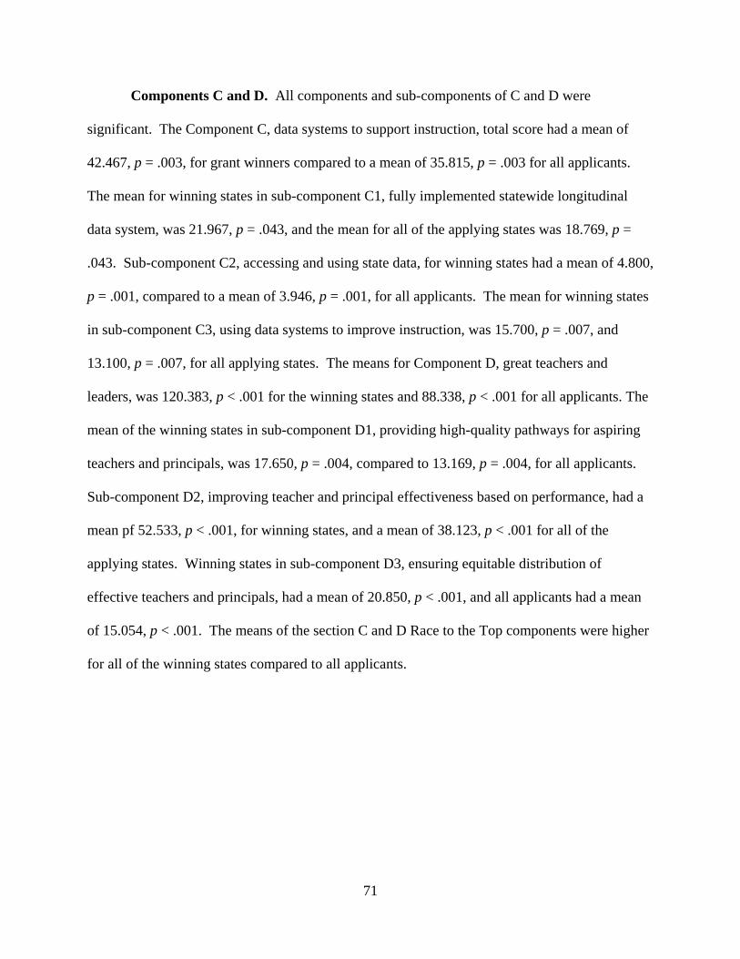
71

Components C and D. All components and sub-components of C and D were

significant. The Component C, data systems to support instruction, total score had a mean of

42.467, p = .003, for grant winners compared to a mean of 35.815, p = .003 for all applicants.

The mean for winning states in sub-component C1, fully implemented statewide longitudinal

data system, was 21.967, p = .043, and the mean for all of the applying states was 18.769, p =

.043. Sub-component C2, accessing and using state data, for winning states had a mean of 4.800,

p = .001, compared to a mean of 3.946, p = .001, for all applicants. The mean for winning states

in sub-component C3, using data systems to improve instruction, was 15.700, p = .007, and

13.100, p = .007, for all applying states. The means for Component D, great teachers and

leaders, was 120.383, p < .001 for the winning states and 88.338, p < .001 for all applicants. The

mean of the winning states in sub-component D1, providing high-quality pathways for aspiring

teachers and principals, was 17.650, p = .004, compared to 13.169, p = .004, for all applicants.

Sub-component D2, improving teacher and principal effectiveness based on performance, had a

mean pf 52.533, p < .001, for winning states, and a mean of 38.123, p < .001 for all of the

applying states. Winning states in sub-component D3, ensuring equitable distribution of

effective teachers and principals, had a mean of 20.850, p < .001, and all applicants had a mean

of 15.054, p < .001. The means of the section C and D Race to the Top components were higher

for all of the winning states compared to all applicants.

72

Table 3Comparison of Means

VariablesMean for RTT Grant

WinnersMean for RTT

Grant Applicants Difference p -valueComponent A 111.350 91.438 -19.912 0.000

[4.822] [15.254]A1 58.683 48.523 -10.160 0.001

[4.468] [9.230]A2 27.483 23.123 -4.360 0.001

[1.443] [3.860]

A3 25.183 19.792 -5.391 0.000

[2.693] [3.97]

Component B 69.050 62.885 -6.165 0.009[.763] [7.682]

B1 39.950 37.000 -2.950 0.101[.124] [6.026]

B2 9.933 9.746 -0.187 0.420

[.130] [.785]

B3 19.167 16.138 -3.028 0.002

[.781] [3.062]

Component C 42.467 35.815 -6.651 0.003[3.607] [6.745]

C1 21.967 18.769 -3.197 0.043[3.193] [4.786]

C2 4.800 3.946 -0.854 0.001[.295] [.799]

C3 15.700 13.100 -2.600 0.007[1.567] [2.939]

Component D 120.383 88.338 -32.045 0.000[4.508] [23.128]

D1 17.650 13.169 -4.481 0.004[2.240] [4.848]

D2 52.533 38.123 -14.410 0.000[2.175] [11.362]

D3 20.850 15.054 -5.796 0.000[1.874] [5.000]

***Sig. at the 0.01 level; **Sig. at the 0.05 level; *Sig at the 0.10 level.

This table presents the comparison of means for the Race to the Top variables that are used in the analyses. Variables are described in Appendix A.

73

Components E, F, and STEM. Component E, F, and the STEM component were

significant for the overall category score, but one sub-component of E and F was not significant.

Sub-components E1, intervening in the lowest-achieving schools and LEA’s, F1, making

education funding a priority, and F3, other significant reform conditions, were not significant.

The mean for Race to the Top winners in Component E, turning around the lowest-achieving

schools, was 46.917, p = .01, and 40.469, p = .01 for all applicants. For sub-component E2,

turning around the lowest-achieving schools, the mean for award winners was 36.917, p = .02,

and 31.738, p = .02 for all applicants. The mean for grant winners in sub-component F2,

ensuring successful conditions for high-performing charters and other innovative schools, was

33.600, p = .02, and the mean for all applicants was 24.315, p = .02. The mean in the STEM

component for winners was 15.000, p = .02, and 9.808, p = .02 for all applicants. In section E

and F, turning around lowest-achieving schools and allowing charter schools were the significant

components of those sections. Maintaining funding and intervention in lowest-achieving schools

and LEA’s were not significant in the award decision process.

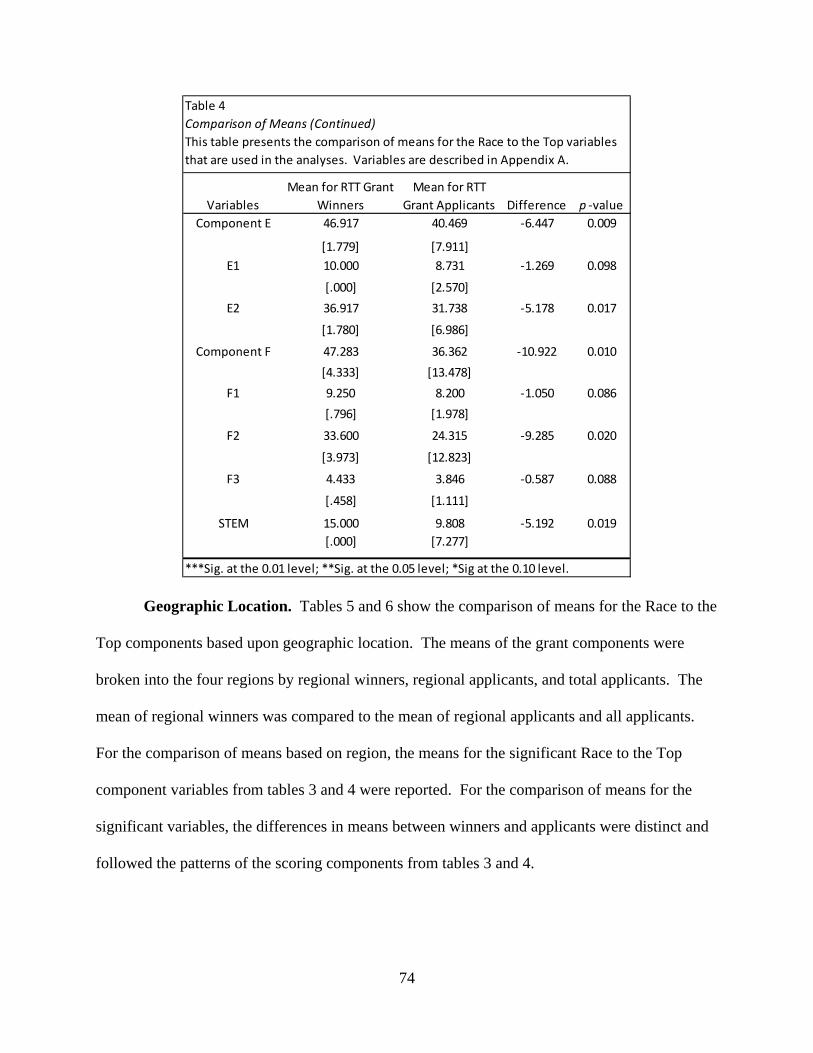
74

Geographic Location. Tables 5 and 6 show the comparison of means for the Race to the

Top components based upon geographic location. The means of the grant components were

broken into the four regions by regional winners, regional applicants, and total applicants. The

mean of regional winners was compared to the mean of regional applicants and all applicants.

For the comparison of means based on region, the means for the significant Race to the Top

component variables from tables 3 and 4 were reported. For the comparison of means for the

significant variables, the differences in means between winners and applicants were distinct and

followed the patterns of the scoring components from tables 3 and 4.

Table 4Comparison of Means (Continued)

VariablesMean for RTT Grant

WinnersMean for RTT

Grant Applicants Difference p -valueComponent E 46.917 40.469 -6.447 0.009

[1.779] [7.911]E1 10.000 8.731 -1.269 0.098

[.000] [2.570]E2 36.917 31.738 -5.178 0.017

[1.780] [6.986]

Component F 47.283 36.362 -10.922 0.010[4.333] [13.478]

F1 9.250 8.200 -1.050 0.086[.796] [1.978]

F2 33.600 24.315 -9.285 0.020

[3.973] [12.823]

F3 4.433 3.846 -0.587 0.088

[.458] [1.111]

STEM 15.000 9.808 -5.192 0.019[.000] [7.277]

***Sig. at the 0.01 level; **Sig. at the 0.05 level; *Sig at the 0.10 level.

This table presents the comparison of means for the Race to the Top variables that are used in the analyses. Variables are described in Appendix A.

75

Table 5Comparison of Means

Variables

Mean for RTT Grant

Winners NorthEast

Mean for RTT Grant

Applicants NorthEast

Mean for RTT Grant

Winners MidWest

Mean for RTT Grant

Applicants MidWest

Mean for RTT Grant

Applicants (ALL)

Component A 109.525 102.418 103.733 98.000 97.726A1 55.975 52.436 54.533 50.971 51.732A2 27.550 25.836 26.067 25.457 24.500A3 26.000 24.145 23.133 21.571 21.495

Component B 69.350 68.145 66.133 65.343 64.832B1 39.975 39.818 39.867 39.114 37.932B2 9.925 9.927 9.800 9.343 9.805B3 19.450 18.400 16.467 16.886 17.095

Component C 42.100 39.255 40.400 36.086 37.916C1 21.000 19.636 20.133 17.886 19.779C2 4.750 4.473 4.800 4.429 4.216C3 16.350 15.145 15.467 13.771 13.921

Component D 119.625 106.182 111.800 94.600 98.458D1 17.750 16.145 16.733 13.657 14.584D2 51.750 45.018 48.267 41.771 42.674D3 21.175 18.909 18.333 16.629 16.884D4 11.775 10.309 11.400 8.400 9.668D5 17.175 15.800 17.067 14.143 14.647

Component E 46.650 45.418 44.800 42.429 42.505E1 10.000 10.000 10.000 8.000 9.132E2 36.650 35.418 34.800 34.429 33.374

Component F 47.375 44.000 47.333 40.857 39.811F1 8.475 8.509 9.667 9.229 8.532F2 34.575 31.309 33.133 27.314 27.247F3 4.325 4.182 4.533 4.314 4.032

STEM 15.000 12.273 15.000 10.714 11.447Total 449.625 417.691 429.200 388.029 392.695

This table presents the comparison of means for the Race to the Top variables that are used in the analyses by geographic location. Variables are described in Appendix A.

76

Table 6Comparison of Means

Variables

Mean for RTT Grant

Winners SouthEast

Mean for RTT Grant

Applicants SouthEast

Mean for RTT Grant

Winners West

Mean for RTT Grant

Applicants West

Mean for RTT Grant

Applicants (ALL)

Component A 109.067 95.382 110.500 94.644 97.726A1 59.333 52.382 59.900 50.667 51.732A2 26.400 23.291 27.800 23.600 24.500A3 23.333 19.709 22.800 20.378 21.495

Component B 67.900 63.418 68.100 62.111 64.832B1 39.933 37.164 39.800 35.644 37.932B2 9.933 9.891 10.000 9.911 9.805B3 18.033 16.364 18.300 16.556 17.095

Component C 42.500 40.473 39.900 34.578 37.916C1 23.333 22.218 20.000 18.444 19.779C2 4.500 4.109 4.600 3.867 4.216C3 14.667 14.145 15.300 12.267 13.921

Component D 114.867 98.218 118.400 92.311 98.458D1 17.233 13.945 14.400 14.178 14.584D2 50.433 43.873 53.200 39.044 42.674D3 18.600 15.709 21.800 16.044 16.884D4 11.800 10.291 11.200 9.111 9.668D5 16.800 14.400 17.800 13.933 14.647

Component E 46.633 42.055 47.800 39.556 42.505E1 9.167 9.545 10.000 8.444 9.132E2 37.467 32.509 37.800 31.111 33.374

Component F 42.533 35.273 49.200 39.422 39.811F1 9.000 8.127 9.600 8.511 8.532F2 29.267 23.564 35.000 26.733 27.247F3 4.267 3.582 4.600 4.178 4.032

STEM 15.000 10.909 15.000 11.667 11.447Total 438.500 385.727 448.900 374.289 392.695

This table presents the comparison of means for the Race to the Top variables that are used in the analyses by geographic location. Variables are described in Appendix A.

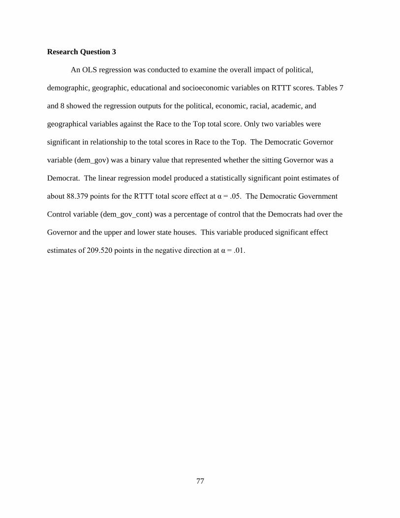
77

Research Question 3

An OLS regression was conducted to examine the overall impact of political,

demographic, geographic, educational and socioeconomic variables on RTTT scores. Tables 7

and 8 showed the regression outputs for the political, economic, racial, academic, and

geographical variables against the Race to the Top total score. Only two variables were

significant in relationship to the total scores in Race to the Top. The Democratic Governor

variable (dem_gov) was a binary value that represented whether the sitting Governor was a

Democrat. The linear regression model produced a statistically significant point estimates of

about 88.379 points for the RTTT total score effect at α = .05. The Democratic Government

Control variable (dem_gov_cont) was a percentage of control that the Democrats had over the

Governor and the upper and lower state houses. This variable produced significant effect

estimates of 209.520 points in the negative direction at α = .01.

78

Table 7OLS Regression Model

Variables Coefficientsdem_gov 88.379

[0.015]**dem_gov_cont -209.520

[0.002]***pct_repU -229.994

[0.111]pct_repL -86.245

[0.575]log_medinc 165.530

[0.205]students 0.000

[0.311]pct_black 91.292

[0.493]pct_hisp 179.843

[0.110]pct_lunch 52.899

[0.803]sat -0.160

[0.200]Midwest 72.328

[0.152]South 44.808

[0.446]West -19.177

[0.677]_cons -1.2e+03

[0.427]N 38R-sq 0.585adj. R-sq 0.321

Dependent variable = RTTT Total Score

***Sig. at the 0.01 level; **Sig. at the 0.05 level; *Sig at the 0.10 level.

This table presents the regression calculations for RTTT Total Score. Variables are described in Appendix A.

79

Democratic Governor. Based on the regression results in Table 8, the Democratic-

related political coefficients on RTTT percent score generally followed the same statistical

significance. The Democratic Governor variable (dem_gov) produced a statistically significant

point estimates of about .184 for the RTTT percent score. On the other hand, the Democratic

Government control variable (dem_gov_cont) produced significant effect estimates of .326

points but in the negative direction at α = .01.

It should be noted, however, that the results in Tables 7 and 8 are the uncorrected OLS

regressions on the states that won and lost the Race to the Top money (a total of 38 states in the

second round). The resulting beta-coefficients from OLS failed to account for the potential

threat of selection bias against those states that did not apply to the competition. Employing

OLS in the presence of potential selection bias can result in biased and inconsistent, or inefficient

parameter estimates. By correcting for the potential threat of selection bias, the final regression

estimates (see Tables 9 and 10) aimed to obtain the best linear unbiased predictors of RTTT

total/percent scores.

80

Table 8

OLS Regression Model

Variables Coefficientsdem_gov 0.184

[ 0.020]**dem_gov_cont -0.326

[0.014]**pct_repU -0.38

[0.230]pct_repL -.223

[0.487]log_medinc 0.274

[0.331]students 2.99E-08

[0.188]pct_black 0.29

[0.289]pct_hisp 0.327

[0.178]pct_lunch -0.003

[0.999]sat -.003

[0.148]Midwest 0.086

[ 0.384]South 0.055

[0.596]West -0.045

[0.609]_cons -1.36

[0.672]N 38R-sq 0.487adj. R-sq 0.21

Dependent variable = Total RTTT Percent score

***Sig. at the 0.01 level; **Sig. at the 0.05 level; *Sig at the 0.10 level.

This table presents the regression calculations for RTTT Percent Score. Variables are described in Appendix A.

81

Heckman Selection Model. To apply the Heckman sample selection to the RTTT

model, the analysis was split into two parts: an outcome equation, which described the

relationship between RTTT scores and a set of explanatory variables, and a selection equation,

which described the relationship between the probability of applying for RTTT grant and a set of

Table 9Heckman Selection model (Two-step estimates)

PANEL A. First stage PANEL B. Selection equationTotal RTTT Score Total RTTT Score(I) (I)

dem_gov 101.250 pvt_fnd 0.002[0.001]*** [0.057]*

dem_gov_cont -177.119 pct_fed_doe 22.402[0.001]*** [0.077]*

pct_repU -176.826 applied09 -.253[0.143] [0.756]

pct_repL -198.596 dem_gov 1.5220.221] [0.171]

log_medinc 93.572 dem_gov_cont -2.45[0.434] [0.275]

students 0.000 pct_repU 1.71[0.097]* [0.644]

pct_black 219.055 pct_repL -10.053[0.107]* [0.073]*

pct_hisp 222.530 students -3.28e-06[0.054]* [0.051]*

pct_lunch -70.266 pct_black 0.129[0.722] [0.063]*

sat -0.221 pct_hisp 0.129[0.043]** [0.095]*

Midwest 59.339 pct_lunch 7.512[0.168] [ 0.496]

South 34.447 sat 0.001[0.411] [0.723]

West -16.566 Constant 0.983[0.634] [0.874]

_cons -136.0272 λ 33.778[0.922] ρ 0.677

σ 49.916Number of observations 51Censored obsrvations 38Uncensored observations 13Wald χ2 (df) 31.01*** (13)

*** Significant at the 0.01 level, ** Significant at the 0.05 level, * Significant at the 0.10 level.

This table presents the regression results with sample selection Dependent variable: Total RTTT score

82

explanatory variables. Unlike Tables 7 and 8, the results from the selection equation in Tables 9

and 10 were estimated by maximum likelihood as an independent prohibit model to determine

factors influencing the decision whether to participate or not in RTTT grant among from the

entire 51 states (including the District of Columbia). The inclusion of two additional variables

(pvt_fnd and pct_fed_doe) is assumed to affect the probability of applying to RTTT, but is

assumed not to influence RTTT total/percent scores. These are known as instrumental variables

or exclusion restriction in the econometric literature.

Significant Predictors. Of the political variables, the Democratic governor and the

Democratic Government control variables were again most strongly related to the total RTTT

scores and percent scores. Geography and socio-economic indicators did not influence the final

scores on RTTT. The remaining significant explanatory variables were demographic- and

education-related.

The total number of public school students, the percentage of African American, and the

percentage of Hispanic students were positive and statistically significant at α = .01. The

education variable, SAT scores, was also a significant predictor at α = .05 but in the negative

direction.

Significant Selection Variables. The two instrumental variables in the selection

equation were significant. An increase in the number of private foundations (pvt_fnd variable)

raised the probability of states applying to the Race to the Top program by .2 percentage points,

a small but significant marginal effect. In addition, a one-unit increase in federal funding as a

percentage of state education revenue increased the probability of applying to the RTTT grant by

22.402 points. The Heckman model in Tables 9 and 10 revealed that the coefficients were much

larger but similarly-significant as the estimates in the OLS model. These results coincided with

83

results obtained with the Inverse Mills ratio (lambda). In particular, the non-significance of the

coefficient of the Inverse Mills ratio revealed that any selection bias in the data was not

statistically significant. Because there is no such evidence of selection bias found, the standard

OLS regression would suffice.

TABLE 10

Heckman Selection model (Two-step estimates)

PANEL A. First stage PANEL B. Selection equationTotal RTTT Percent Score Total RTTT Percent Score(I) (I)

dem_gov 0.202 pvt_fnd 0.002[0.001]*** [0.057]*

dem_gov_cont -0.354 pct_fed_doe 22.402[0.001]*** [0.077]*

pct_repU -0.354 applied09 -0.253[0.143] [0.756]

pct_repL -0.397 dem_gov 1.5220.221] [0.171]

log_medinc 0.187 dem_gov_cont -2.45[0.434] [0.275]

students 0.000 pct_repU 1.71[0.097]* [0.644]

pct_black 219.055 pct_repL -10.053[0.107] [0.073]*

pct_hisp 222.530 students -3.28e-06[0.054]* [0.051]*

pct_lunch -70.266 pct_black 0.129[0.722] [0.063]*

sat -0.221 pct_hisp 0.129[0.043]** [0.095]*

Midwest 59.339 pct_lunch 7.512[0.168] [ 0.496]

South 34.447 sat 0.001[0.411] [0.723]

West -16.566 Constant 0.983[0.634] [0.874]

_cons -0.272 λ 33.778[0.922] ρ 0.677

σ 0.0998Number of observations 51Censored obsrvations 38Uncensored observations 13Wald χ2 (df) 31.01*** (13)Wald χ2 (df) 31.01*** (13)

This table presents the regression results with sample selection Dependent variable: Total RTTT percent score

*** Significant at the 0.01 level, ** Significant at the 0.05 level, * Significant at the 0.10 level.

84

Summary of Findings

The descriptive statistics confirm that there was evidence of external influence on the

Race to the Top scoring and award process. First, the comparison of means results (Tables 1 to

6) reveal that at the α = .05 level, a statistically significant relationship between the mean scores

of winning states compared to applicants for race (pct_black) and states’ SAT scores was

significant. Also, at α = .10, Democratic Governor (dem_gov) and geographic region (Midwest,

South, and West) were significant to the differences in the mean scores between Race to the Top

winners compared to all applicants. Second, the OLS regression results (Tables 7 and 8) showed

a significant relationship between the Democratic control of the State Governor and legislative

decision process and Race top the Top total scores and percentage of scores. However, none of

the geographic and socioeconomic variables showed up as statistically significant. Third, using

the Heckman two-step selection model, the study found no significant evidence of self-section

between applicants and non-applicants of the RTTT grant. The direction and significance of the

coefficients remained virtually unchanged, and the Inverse Mills Ratio was not significant,

suggesting that the RTTT grant program was unlikely to be driven by selection bias. Finally, two

instrumental variables (pvt_fnd and pct_fed_doe) in the selection equation were found significant.

85

Chapter 5

Summary and Conclusions

The Race to the Top competitive grant was an opportunity for the United States

government to influence the states’ educational processes. States responded to a grant proposal

document provided by the United States Department of Education in an attempt to win additional

funding outside of the regular Title I distribution process. To win the grant, states had to be

willing to change different aspects of their educational system to match the expectations of the

grant writers. After states submitted their applications, the Department of Education had raters

score the applications to determine grant winners.

The 50 states and the District of Columbia were invited to respond to the grant proposal.

The first phase of the grant process occurred in 2009, and 41 responded to the proposal. Only

two states, Delaware and Tennessee, won the first round funding. States that did not win in the

first round, had an opportunity in 2010 to reapply and have their applications re-scored. In the

second phase, 13 of the 49 states available to re-apply did not. However, one state that did not

apply in phase one, Maryland, did apply in phase two. Of the 36 states that reapplied in 2010, 17

won funding.

The purpose of this study was to determine what predictors may have influenced the

award decisions. Using a political, socio-economic, race, academic, and geographic database

along with the Race to the Top scoring documents, a spreadsheet was created to perform a

descriptive analysis of the data. The variables used in the spreadsheet were put into statistical

analysis software to perform a logistic regression, using the Heckman model. The Heckman

model accounted for the exclusionary restrictions in the selection where states chose not to

participate in the 2010 application process. The statistical outputs were used to determine which

86

variables had a significant influence on grant awards. Combing the results of the descriptive and

inferential statistics, answers to the research questions could be assembled.

The research questions being answered by this study:

1. What are the political, social, economic, educational, and geographic

patterns/characteristics of winning states and applying states in the national Race to the

Top (RTTT) competition?

2. Do the scores across different sections of the RTTT application differ between winning

and applying states?

3. What political, social, economic, educational, and geographic characteristics may have

influenced states' final scores on the RTTT grant competition, controlling for potential

selection bias between applicants and non-applicants of RTTT?

The literature focusing on federal involvement, federalism, in state-run affairs is a

dominate theme. States do not have the capacity to implement all of the programs they would

like, so they rely on federal grants to bolster the state’s ability. Federal involvement in state

policies have been designed to encourage states to comply with federal policy changes. Some

federal involvement comes in the form of mandates that states must adhere. Other federal

programs come in the form of cooperative grants that give the state leeway in the money’s

allocation under an umbrella of a specific program like education. To influence state policy and

practice, the federal government creates grants with stipulations to direct how the money is used.

Race to the Top was a cooperative grant process that encouraged states make policy changes that

fell under a regulatory umbrella but giving the states opportunity to make the implementation

specific to the needs of the state.

87

In the case of Race to the Top, the designers created a program that encouraged states to

make changes in their educational practices by offering a monetary reward, a carrot. The

applications made by the states included implementation plans that would meet the requirements

of the grant, but were unique to the needs of each state. The federal government used the grant

money as an incentive to get the states to make the educational changes the designers felt were

the right ways to improve education. All of the states that applied for the Race to the Top grant

made significant changes in policies in an attempt to win the grant. Interestingly, even the states

that did not apply still had an increase in education policy changes.

States have the option to participate in federal grants, and in Race to the Top, thirteen

states decided not to participate in the 2010 process. Some of those states applied in the initial

2009 process, but after initial scoring feedback and internal strife over funding requirements,

decided not to continue to seek funding. By excluding themselves, the non-participating states

did not want the strings attached to the grant. Since states made a choice not to participate, the

regression model had to account for their exclusion. To accommodate their non-participation,

the Heckman exclusion model was used so that the non-participants would not influence the

significance of the variables in the study.

The ultimate goals of this study were to (1) identify patterns in the political, economic,

racial, academic, and geographic data between the winning and applying states that led to states

winning a grant award, (2) identify the patterns in the Race to the Top scoring data that would

reveal the sections of the grant that were more important to the grant award, and (3) the political,

economic, racial, academic, and geographic data that may have influenced the final scores. The

statistical techniques used in this research were found to be statistically sound and reliable. The

findings are summarized in the next two sections.

88

Impact on Winning States Compared to All Applicants (Questions 1 and 2)

The t-test for the comparison of means was conducted for the political, economic, racial,

academic, and geographical variables along with the Race to the Top application component

scores was analyzed. The dataset combined 2009 data for Delaware and Tennessee and the 2010

data for all other states that applied in the second round. For all states, political control of the

Governor’s seat was a significant factor between winning and applying states. The means of

race, percentage of African American students, average SAT scores, and states’ geographic

location had a significant comparison of the means. Political and racial structures along with

average SAT scores of the winning states showed that the award process favored states with

Democrat control of the Governorship, high percentages of African American students, and

lower than average SAT scores.

Comparing the means of the Race to the Top variables showed that most components

were significant in the application process (Note: a description of all Race to the Top

components is available in Appendix A). All of components A, C, and D were significant in the

award process. Sub-component B2, Developing and implementing common, high-quality

assessments, and sub-component E1, intervening in the lowest-achieving schools and LEAs,

were not significant. Two of the three sub-components of component F, F1, making education

funding a priority, and F3, other significant reform conditions, were not significant, but the

overall component F was significant. The means for the winning states compared to the

applicants did not show a significant difference in these four sub-components. This reflects that

the average scores between the winning and applying states for implementing high-quality

assessments, intervening in lowest-achieving schools and LEA’s, and education funding were

not important for determining winning states.

89

The comparison of the geographic means of the winning and applying states also were

significant. States in the Northeast and Southeast had higher average scores than states in the

Midwest or West. The average score percentage of winning and applying states in the

Northwest and Southeast were higher than the Western states where more states elected not to

apply than any other region of the country. Geographic showed an influence in the scoring

rubrics. States from the Northeast and Southeast consistently showed higher scores than the

Midwestern or Western states.

Impact on Final Scores (Questions 3)

A standard regression that did not account for the states’ selection to not apply in 2010

and a Heckman regression that did account for the states’ selection was used to determine factors

that affected the Race to the Top scoring. In both regression models, states that had a

Democratic Governor and/or Democratic control of the state’s legislative process had significant

effect on Race to the Top application scores. When accounting for the states that chose not to

apply in 2010, using the Heckman selection regression model, other factors became clear.

Average SAT scores had a significant influence on scoring. States with lower than average SAT

scores were more likely to receive Race to the Top funds. Also, through the Heckman model,

states with a higher percentage of African American and Hispanic students along with a higher

total number of students in the state’s public education system has a lesser but still significant

effect on the final scores.

Federalism is reflected by the national government trying to influence the states through

regulated or unregulated funding programs. The federal government’s involvement in

education was a key factor in the outcome of this research. To better understand the influence of

the federal government in the scoring and award process, the research investigated the

90

relationship between state political affiliation and scoring. The first significant variable was the

State Governor’s political affiliation and the effect on the Race to the Top scores, and ultimately,

winning and losing. The President of the United States during Race to the Top, Barak Obama,

was a Democrat. The Governor variable showed that states with Democratic Governors had a

positive coefficient. States with Governors of the same political affiliation as the President had a

greater possibility of higher rater scores and winning grant funds.

Governors are in a unique position in education. Their position gives them the authority

to align all levels of education to meet the goals of the administration. In many states, early

childhood education, K-12 education, and higher education are managed by different

departments (National Governors Association, 2012). The goals and objectives of each

educational group may not align with each other to create a coherent and comprehensive

educational strategy (National Governors Association, 2012). The Governor has the authority to

align these departments into a common path (National Governors Association, 2012). Executive

staffs are appointed to implement the Governor’s agenda, and the Governor’s office tries to

mobilize the public and special interest groups to work in favor of the agenda (National

Governors Association, 2017). Therefore, it is important for the President to gain the favor of

the Governors to help enact proposed federal initiatives.

When Race to the Top was created, the United States was trying to recover from the

“Great Recession” which placed a strain on state budgets, including education (Cavanagh,

2012). The Obama administration used this opportunity to make a political statement in

education by dangling the additional funding carrot in front of the state Governors (Cavanagh,

2012). States that applied for the funding were willing to meet the stipulations of the grant, even

though the states would have to fund the new programs after the grant funding expired (Vergari,

91

2012). Race to the Top was funded by the American Recovery and Reinvestment Act of 2009,

but the development of the grant process was driven by the Obama administration (Howell,

2015). The educational policies that the administration was trying to enact were not being

enacted by state or federal legislators, and Presidential decree would not effectively implement

them (Howell, 2015). The policies set in the grant process, which aligned with the

administrations educational agenda, were weighted to ensure compliance with that agenda

(Howell, 2015).

The role and importance of the Governor in extending federal initiatives to the states has

been seen in several federalism initiatives in education. President George H.W. Bush brought

the Governors together at the “educational summit” to discuss educational improvement and try

to gain acceptance of a national education plan (Klein, 2014). President Clinton tried to force

compliance to educational reform by threatening Title I funding, but the Governors, through

their legislators, removed the non-compliance portion of the America 2000 bill (Fuhrman, 1994).

The implementation plan for Race to the Top needed the support of the state Governors to

change state educational policy, and Democratic Governors were more willing to make those

changes because of inter-governmental grant relationships. By restricting the money available to

the Race to the Top grant, President Obama’s administration increased the competitive nature of

the process, which would lead to more state-level educational policy changes (Wong & Shen,

2002). By placing this competitive process and the potential money involved, Governors had to

weigh the risks and rewards of participating in the process (Vergari, 2012).

The second significant variable was the major political affiliation of the state’s legislative

control; Governor, Senate, and House of Representatives. Legislative control had a negative

coefficient on the total scores. As the Democratic control of the state’s legislative process

92

increased, the total scores decreased. This reverse phenomenon in legislative control compared

to the Governor could be tied to the bipartisan agenda that President Obama was trying to push

during the 2008 election (Wogan, 2012). During the formation of Race to the Top in 2009, the

political environment in Washington, D.C. was polarized along party lines. Legislation was not

getting passed due to gridlock in the political system. Race to the Top passed Congress with

bipartisan support coupled with President Obama’s desire for bipartisanship (Strauss, 2013),

would explain why states with larger percentages of Democratic control of the legislative

process received lower scores. A polarized legislative process did not require bipartisanship and

undermined the cooperative agenda that President Obama wanted for Race to the Top.

Student population had a significant effect on the Race to the Top total and percentage

score. The total number of public school students, the percentage of African American, and the

percentage of Hispanic students were significant. Total number of public school students had a

negligible coefficient, but the percentage of African American and Hispanic had positive

coefficients reflecting an increased possibility of higher rating scores as these numbers and

percentages increased. States with high total student populations require more funding than

states with lower total student populations. The increased funding need for these high student-

population states made Race to the Top enticing. African American and Hispanic students have,

historically, performed worse than their Caucasian and Asian counterparts on national exams

like NAEP (Hochschild & Shen, 2014). Barriers to success in these student populations include

socio-economics, parental education level/attainment, and language (Hochschild & Shen, 2014).

Schools with high percentages of African American and Hispanic students have struggled to

meet Annual Yearly Progress (AYP), and these students are more likely to be pushed out or drop

out of school (Hochschild & Shen, 2014). Race to the Top was designed to improve academics

93

and bolster minority populations (J. Weiss, 2015), so these factors having significant influence

are explained.

The state average SAT scores showed a negative coefficient in the regression

calculations. The negative coefficient represented a decrease in scores as states’ average SAT

scores increased. As states continued to see their educational success compared to others, the

opportunity Race to the Top presented was integral to states’ plans. Most states’ had reported

proficiency results below the “basic” level defined by NAEP (Bandeira de Mello, 2011). NAEP

scores and the PISA results continued to show the need for improved academics. One of the

benchmarks of success in Race to the Top was changes in NAEP scores over time (Gewertz,

2013). Academic improvement being an ultimate goal of Race to the Top (J. Weiss, 2015), an

academic influence in scores and awards make sense.

In the Heckman selection model, selected variables were used to determine why states

selected to exclude themselves from the grant. Private foundations and percentage of federal,

Department of Education funds, were significant predictors in state participation. Research has

shown that applying states had more private foundation involvement (Bleiberg & Harbatkin,

2016). Private foundations found an opportunity to influence public education when local and

state education was desperate for additional funding (Strauss, 2011). School districts and states

were making concessions to earn grants from these private foundations years before Race to the

Top (Strauss, 2011). In the eight years before Race to the Top was created, private foundations

granted $684 million to school districts (Strauss, 2011). The Gates Foundation gave over $78

million in local district grants in that timeframe (Strauss, 2011). Beyond the local district grants,

the Gates Foundation granted millions of dollars to states to assist in their Race to the Top

applications (Strauss, 2011). The research correlates with the involvement of private

94

foundations in the Race to the Top grant applications. Lower involvement of private

foundations, the more likely the state would not participate.

The federal funding as a percentage of percentage of state educational revenue also had a

positive effect on participation. Some states are more reliant upon federal education dollars, and

therefore are more likely to seek additional funding when available. Federal money coming into

the states allows the states to provide services to their citizens that would not have been possible

under the regular state’s budget (Albritton, 1989). States become dependent upon the additional

funding to maintain the level of service the citizens have been receiving (Albritton, 1989). Road

construction and infrastructure, and welfare systems have received high levels of federal funding

for decades, and the states rely on those dollars. Race to the Top was introduced when states

were more reliant on federal stimulus money than at any time in the past (Wilson, 2013). The

“Great Recession” reduced state tax revenues, and the American Recovery and Reinvestment

Act of 2009 was giving states additional funding that allowed the states to balance their budgets

(Wilson, 2013). Additional funding to bolster state budgets tempted states to apply and meet the

stipulations of the grant. The research supports the finding that a higher percentage of federal

education dollars as part of state education expenditures, the more likely the states participated.

The higher the percentage of Republicans in the state House of Representatives, the less

likely a state participated. Conversely, the higher the percentage of African American and

Hispanic students, the more likely a state participated. The results showed that many of the

variables that affected Race to the Top scores, were the same variables that affected state

participation. This supports the research that Race to the Top was designed for specific state

factors.

95

This study adds to the literature on federalism, carrot hypothesis, and intergovernmental

grants. Federalism is the intervention of the national government in the responsibilities of the

states. One way that the federal government influences state action is by gaining the support of

the Governors. The role and influence of the Governor made their participation in Race to the

Top critical to the implementation of the federal agenda. The Democratic Governor’s

significance shows that political affiliation between the state Governors and the President

influenced scores. The research showed that federal and state legislators were struggling to

implement President Obama’s education agenda. To get the states to enact the agenda, through

the Race to the Top grant, Governors had to promote and support the plan. Governors of the

same political party as the President, Democrats, were more likely to provide that promotion and

support.

The carrot hypothesis is defined by the granting authority placing a temptation in front of

the receiving authority that is good enough to entice the receiving authority to do what is

required to try and earn the temptation. In particular, the negative impact of Democrat-

controlled legislatures on RTTT final total/percent scores indicated that the grant competition

attempted to offer something for all sides—a carrot approach that might appease advocates of a

bipartisan approach to education reform. Under the RTTT grant, the federal government placed

the opportunity for a large amount of money in front of the states in exchange for making

changes in their educational policies. The budgetary crisis after the “Great Recession” made

states more willing to make law and policy changes for an infusion of money. The possibility of

millions of dollars in additional education dollars caused the applying states to implement many

of the requirements of Race to the Top, even before applying for the grant, without a guarantee

96

of funding. The significance of all but five of the Race to the Top grant sub-components showed

how much the states were willing to change their educational policies to try and win the money.

Intergovernmental grants are defined by a four-step process. First, the federal

government decided how to grant the money to the states, done through the implementation of

the American Recovery and Reinvestment Act. Second, the conditions of the grant had to be

established, which was the Race to the Top program. Third, the states had to decide to

participate in the program, which was indicated by the states that completed the applying

process. Fourth, the states had to decide how to spend the funds. Since the funds were

contingent upon the educational policies being re-shaped to meet the application, the spending

was set when the states applied. Like the carrot hypothesis, the significance of the application

criterion, along with the states’ willingness to meet those requirements in the hope of winning

the funding supports the intergovernmental grant hypothesis.

The findings of this research show that the federal government will use its political and

economic resources to influence the states to follow the federal agenda. Political and economic

pressures make the states more reliant on federal dollars, and therefore more accepting of federal

influence during poor economic periods. Also, continued state reliance on federal grants, like

welfare, education, and highway grants, maintain an open link between the federal and state

levels of government. By maintaining this open link, opportunities for federal government

influence continue.

While interpreting the results of this research, several limitations need to be

acknowledged. The variables used in this research are not a comprehensive list of possible

factors that may have influenced the Race to the Top scores, award decisions, or state

participation. Even though the variables used in this research came from literature, factors that

97

could explain other areas of Race to the Top’s policy prescriptions and reforms were not

examined. Bias that may have existed in the Race to the Top scoring process were not part of

the research. Inconsistencies in the Race to the Top documents were not filtered to

adjust/equalize scoring.

Another limitation of the study was the extent to which some states were leading others

in promoting one or more policy prescriptions, like Value Added Models (VAM’s), endorsed by

the Obama administration. VAM’s are statistical techniques used to estimate a teacher, school,

and district’s effectiveness in student learning (McCaffrey, Lockwood, Koretz, & Hamilton,

2004). One of the requirements of Race to the Top was the implementation of VAM’s to

evaluate teachers and schools. Research has shown that states providing less education funding

than the national average, have higher rates of students in poverty, and have higher percentages

of racial and language minorities are more likely to implement VAM’s (Amrein-Beardsley,

2014). In particular, a variable that could explain the effect of integration of VAMs in the state’s

educational processes on grant awards was not included in this research.

The study’s findings have several implications for state-federal relations in the realm of

education. As the federal government continues to try and improve the educational process

throughout the country, federal influence in state education policies and processes will continue.

As Race to the Top changed the face of education in many states, many others decided that the

requirements were too much sacrifice for the potential funding opportunity. Several states have

moved away from some of the requirements of Race to the Top, like Common Core State

Standards, because of the backlash within the state. The strain being experienced within the

states led federal legislators to enact ESSA which restricted the influence of the federal

government in state education affairs. To continue influencing the country’s educational

98

process, the federal government will experience more resistance from the states. If the

intergovernmental funding process for education is reduced, states will be required to fund

additional programs through their own budgets or through private foundation donations. Private

foundations and state agendas may conflict with the federal agenda. These conflicts may widen

the gap between the state educational systems and the federal agenda.

Recommendations

There are three recommendations resulting from this study. The first recommendation

addresses the process by which the federal government approaches states to apply for

competitive grants. The second recommendation addresses the rating process that the federal

government uses to score state applications. The third recommendation addresses the

willingness of the states to meet the requirements of the grant proposals. Both sides of the grant

process, provider and receiver, have to work together to create an opportunity that provides

maximum benefit to the students. Excluding federal money from students, from both sides, is

not improving all of America’s education system.

The Race to the Top competitive grant process could be considered a success in terms of

states, even those that did not apply, changing their educational laws and practices. However,

the funding opportunity was limited to 19 states. Nineteen other states that applied in 2010 were

excluded. The non-winning states, even though they may have made changes to their education

laws and practices in an attempt to win funding, did not see any financial benefit of their efforts.

It is possible that non-winning states may have lost money in their efforts to convince the raters

that they deserved funding. Race to the Top was a competitive process that resulted in winners

and losers, a “zero-sum” process. Instead of providing funding for a few states, the federal

government could have provided a funding opportunity to all applying states using a scaled

99

approach. The scale could be based upon a scoring rubric or other criterion, but allows every

state access to funding.

To provide a fair and equitable scoring process for the states to apply for a grant, the

rating and scoring system has to be unbiased. No grouping of variables can be a significant

predictor of scoring or winning. States that are not led by a specific political party, have a low

minority population, have high academic results, or are select regions of the country need to feel

like they have a reasonable opportunity to win funding. Even if funding was not provided to all

applying states, the rating and scoring process should not weigh any of these factors more than

the others. The grant managers must select a rater pool that is balanced, and any bias that

appears in the results must be addressed immediately. Also, the rating process needs to be as

blind as possible so that the raters do not have an opportunity to identify the applicants as they

are rating their applications.

Finally, states have to address the needs of their constituents compared to the

requirements of the grant proposal. States that are not willing or able to meet the requirements of

the grant proposal should work with government leaders to address their concerns. Valuable

resources, time and money, should not be spent by the states in the hopes of winning grant

money. Resources spent on these efforts should benefit the state regardless of winning grant

funding. Also, states that apply for federal grants need to weigh the internal cost of meeting

grant requirements after the grant money is exhausted. If changes made by the states to win

funding are worthwhile, long-term solutions, the state must plan to continue funding. Changing

the laws and practices of the state for short-term funding without maintaining change after the

funding expires does not create an atmosphere of improvement.

Recommendations for Further Research

100

The recommendations for further research, based upon the results of this study, are based

within the areas of non-application and state application content. The researcher recommends

another study that examines the factors that caused thirteen states to exclude themselves from the

grant process. Studying what political and social issues the non-applying states faced could

provide insight into the barriers for future grant opportunities with the states. In conjunction to

the political and social research, a study of what requirements of Race to the Top played a role in

the states not applying could improve any future grant process. What influence did political

figures have in the award process? Vice President Joe Biden, represented Delaware before

becoming Vice President, and Lamar Alexander, a former Secretary of Education, represents

Tennessee, both first round winners. Further, the researcher recommends a study of the costs the

states incurred to apply for the Race to the Top grant. If states incurred a high level of expense

without receiving grant funds, how will the states respond if another competitive grant

opportunity arose? Finally, future research should examine to what extent there is a correlation

between winning RTTT and the extent to which states were leading other states in promoting one

or more policy prescriptions (i.e., VAMs, charter schools, and teacher evaluation) endorsed by

the Obama administration.

101

List of References

Adler, J. H. (2012). Interstate competition and the race to the top. Faculty Publications, 89-99. Ahn, T., & Vigdor, J. L. (2013, May 21). Were all those standardized tests for nothing? The

lessons of no child left behind. Retrieved February 6, 2014, from American Enterprise Institute: http://www.aei.org/papers/education/k-12/accountability/were-all-those-standardized-tests-for-nothing-the-lessons-of-no-child-left-behind/

Albritton, R. B. (1989). Impacts of intergovernmental financial incentives on state welfare

policymaking and interstate equity. The Journal of Federalism, 127-141. Amrein-Beardsley, A. (2014). Rethinking value-added models in education. New York, NY:

Routledge. Anderson, L. (2007). Congress and the classroom: From the cold war to 'no child left behind'.

University Park, PA: Penn State University Press. Arsen, D., & Mason, M. L. (2013). Seeking accountibility through state-appointed emergency

district management. Educational Policy, 27(2), 248-278. Bandeira de Mello, V. (2011). Mapping state proficiency standards onto the naep scales:

Variation and change in state standards for reading and mathematics, 2005–2009 (NCES 2011-458). Washington, DC: National Center for Education Statistics, Institute of Education Sciences, U.S. Department of Education.

Baumgartner, F., & Jones, B. (2009). Agendas and instability in american politics, second

edition. Chicago, IL: The University of Chicago Press. Berry, C. R., Burden, B. C., & Howell, W. G. (2010). After enactment: The lives and deaths of

federal programs. American Journal of Political Science, 54(1), 1-17. Bickers, K. N., & Stein, R. M. (2004). Interlocal cooperation and the distribution of federal grant

awards. The Journal of Politics, 66(3), 800-822. Bleiberg, J., & Harbatkin, E. (2016, November 5). Teacher evaluation reform innovation and

diffusion: A story of federalism and foundations. Retrieved from appam.confex.com: https://appam.confex.com/appam/2016/webprogram/Paper16535.html

Boser, U. (2013, June 14). Are schools getting a big enough bang for their educational

technoology buck? Retrieved from www.americanprogress.org: https://www.americanprogress.org/issues/education/report/2013/06/14/66485/are-schools-getting-a-big-enough-bang-for-their-education-technology-buck/

102

Bowen, D. H. (2010, September). Politics and the scoring of race to the top applications. Retrieved from Amwrican Enterpirse Institute: https://www.aei.org/wp-content/uploads/2011/10/ESW-Report-4.pdf

Brown, E. (2015, March 27). Tennessee school districts sue state over what they say is

inadequate funding. Retrieved from The Washington Post: http://www.washingtonpost.com/news/local/wp/2015/03/27/tennessee-school-districts-sue-state-over-what-they-say-is-inadequate-funding/

Cantrell, M. (2013). TCAP scores and per pupil expenditures: Statewaide changes before and

after tennessee's first to the top act. Retrieved from Electronic Theses and Dissertations: http://dc.etsu.edu/etd/1779

Carleton, D. (2002). Student's guide to landmark congressional laws on education. Westport,

CT: Greenwood Press. Cavanagh, S. (2012, February 25). Governor talk funding, federal role in education. Retrieved

from blogs.edweek.org: http://blogs.edweek.org/edweek/state_edwatch/2012/02/governor_talk_funding_federal_role_in_education.html

Center for Public Education. (2012, May). The united states of education: The changing

demographics of the united states and their schools. Retrieved from www.centerforpubliceducation.com: http://www.centerforpubliceducation.org/You-May-Also-Be-Interested-In-landing-page-level/Organizing-a-School-YMABI/The-United-States-of-education-The-changing-demographics-of-the-United-States-and-their-schools.html

Darling-Hammond, L., & McCloskey, L. (2008). Assessment for learning around the world:

What would it mean to be internationally competitive? Phi Delta Kappan, 90(4), 263-272.

Data Quality Campaign. (2011, May). Leveraging the power of state longitudinal data systems:

Building capacity to turn data into useful information. Retrieved from www.dataqualitycampaign.org: http://www.dataqualitycampaign.org/wp-content/uploads/files/1303_DQC-Research%20capacity%20May17.pdf

David, J. L. (2010). What research says about... /Using value-added measures to evaluate

teachers. Educational Leadership, 67(8), 81-82. Retrieved from www.ascd.org. Editoral Projects in Education Research Center. (2004, August 3). A nation at risk. Retrieved

from Education Week: https://www.edweek.org/ew/issues/a-nation-at-risk/ Education Week. (2015, Dececmber 7). The every student succeeds act: Explained. Retrieved

from Opposing Viewpoints in Context: http://ic.galegroup.com/ic/ovic/MagazinesDetailsPage/MagazinesDetailsWindow?disable

103

Highlighting=false&displayGroupName=Magazines&currPage=&scanId=&query=&prodId=OVIC&search_within_results=&p=OVIC&mode=view&catId=&limiter=&display-query=&displayGroups=&con

Evans, J. W. (1960). Catholics and the blair education bill. The Catholic Historical Review,

46(3), 273-298. Finch, M. A. (2015). Tennessee to the top: One state's pursuit to win race to the top. Educational

Policy, 1-37. Fuhrman, S. H. (1994). Clinton's education policy and intergovernmental relations in the 1990's.

The Journal of Federalism, 83-97. Gewertz, C. (2013, November 7). Secretary duncan links federal race to top investments to naep

gains. Retrieved from blogs.edweek.com: http://blogs.edweek.org/edweek/curriculum/2013/11/ed_sec_duncan_links_rtt_invest.html

Ghianni, T. (2011, June 1). Tennessee limits collective bargaining rights for teachers. Retrieved

from www.reuters.com: http://www.reuters.com/article/2011/06/01/us-unions-states-tennessee-idUSTRE75071I20110601

Going, A. J. (1957). The south and the blair education bill. The Mississippi Valley Hostorical

review, 44(2), 267-290. Greene, W. H. (1995, May 8). Sample selection in the poisson regression model. Retrieved from

web-docs.stern.nyu.edu: http://web-docs.stern.nyu.edu/old_web/emplibrary/Sample_Selection_in_the_Poisson_Regression_Model.pdf

Grisson, J. A., & Herrington, C. D. (2012). Struggling for coherence and control: The new

politics of intergovernmental realtions in education. Educational Policy, 26(1), 3-14. Heckman, J. J. (1976). The common structure of statistical models of truncation, sample

selection and limited dependent variables and a sample estimator for such models. National Bureau of Econmic Research, 475-492.

Heckman, J. J. (1979). Sample selection bias as a specification error. Econometric Society, 47(1),

153-161. Heckman, J. J., & Navarro-Lozano, S. (2004). Using matching, instrumental variables, and

control functions to estimate econmic choice models. The Review of Economics and Statistics, 30-57.

Hess, F., & Petrilli, M. (2006). No child left behind primer. New York, NY: Peter Lang

Publishing.

104

Hillison, J. (1995). The coalition that supported the smith-hughes act or a case for strange bedfellows. Retrieved from files.eric.ed.gov: http://files.eric.ed.gov/fulltext/EJ504569.pdf

Hochschild, J. L., & Shen, F. X. (2014). Race, ethnicity, and education policy. New York:

Oxford University Press. Howell, W. (2015). Results of president obama's race to the top: Win or lose, states enacted

education reforms. Education Next, 15(4), 1-10. Kelly, D., Xie, H., Nord, C. W., Jenkins, F., Chan, J. Y., & Kastberg, D. (2013). Performance of

U.S. 15-year-old students in mathematics, science, and reading literacy in an international context. Washington, DC: U.S. Department of Education.

Klein, A. (2014, September 23). historic summit fueld push for k-12 standards. Retrieved from

Education Week: http://www.edweek.org/ew/articles/2014/09/24/05summit.h34.html Lawson, A. (2013). Educational federalism: A new case for reduced federal involvement in k-12

edcuation. B.Y.U. Edication & Law Journal, 2, 281-318. Legal Information Institute. (2016). Tenth amendment. Retrieved from www.law.cornell.edu:

https://www.law.cornell.edu/constitution/tenth_amendment Li, K., & Prabhala, N. (2007). Self-selection models in corporate finance. Handbook of

Corporate Finance, Espen Eckbo ed. Linn, R. L., Baker, E. L., & Betebenner, D. W. (2002). Accountibility systems: implications of

requirements of no child left behind act of 2001. Educational Researcher, 31(6), 3-16. Manna, P. (2006). School's in: Federalism and the national education agenda. Washington, DC:

Georgetown University Press. Manna, P., & Ryan, L. (2011). Competitive grants and educational federalism: President obama's

race to the top program in theory and practice. The Journal of Federalism, 41(3), 522-546. Retrieved from pmanna.people.wm.edu.

Marsh, J. A., Pane, J. F., & Hamilton, L. S. (2006). Making sense of data-driven decison making

in education. Retrieved from www.rand.org: http://www.rand.org/content/dam/rand/pubs/occasional_papers/2006/RAND_OP170.pdf

Martin, B. (2012). Increased role for the department of education in addressing federalism

concerns. Brigham Young Univerity Education and Law Journal, 2012(1), 79-110. McCaffrey, D. F., Lockwood, J. R., Koretz, D. M., & Hamilton, L. S. (2004). Evaluating value-

added models for teacher accountability. Santa Monica, CA: RAND Corporation.

105

McGovern, S. (2011). New model for states as laboratories for reform: How federalism informs education policy. New York University Law Review, 86(5), 1519-1555.

McGuinn, P. (2012). Stimulating reform: Race to the top competitive grants and the obama

education agenda. Educational Policy, 26(1), 136-159. McGuinn, P. (2016). From no child left behind to every student succeeds act: Federalism and the

education legacy of the obama administration. Publis: The Journal of Federalism, 46(3), 392-415.

Mintrom, M., & Vergari, S. (1997). Education reform and accountibility issues in an

intergovernmental context. The Journal of Federalism, 143-166. National Center for Charitable Statistics. (2013). State summary reports. Retrieved from

nccs.orban.org: http://nccs.urban.org/data-statistics/us-and-state-profiles National Center for Educational Statistics. (2015). NAEP overview. Retrieved from nces.ed.gov:

http://nces.ed.gov/nationsreportcard/about/ National Center for Educational Statistics. (2016, March 30). National assessment for

educational progress (NAEP). Retrieved from nces.ed.gov: http://nces.ed.gov/nationsreportcard/about/

National Center for Education Statistics. (2016, May). Racial/ethnic enrollment in public

schools. Retrieved from nces.ed.gov: https://nces.ed.gov/programs/coe/indicator_cge.asp National Geographic. (2012, January 3). United states regions. Retrieved from National

Geographic Society: http://www.nationalgeographic.org/maps/united-states-regions/ National Governors Association. (2012, October). Givernor's role in aligning early education

and k-12 reforms: Challenges, opportunities, and benefits for children. Retrieved from www.nga.org: https://www.nga.org/files/live/sites/NGA/files/pdf/1210AligningEarlyEducationPaper.pdf

National Governors Association. (2017). Governors' powers and authority. Retrieved from

www.nga.gov: https://www.nga.org/cms/home/management-resources/governors-powers-and-authority.html

OECD. (2013). PISA 2012 results: What 15-year-olds know. Retrieved April 1, 2014, from

www.oecd.org: http://www.oecd.org/pisa/keyfindings/pisa-2012-results-overview.pdf Office of Ecuational Research and Improvement, U.S. Department of Education. (2001).

Highlights from the 2000 program for international students assessment. Retrieved from nces.ed.gov: http://nces.ed.gov/pubs2002/2002116.pdf

106

Peterson, P. (2003, Spring). Ticket to nowhere. Retrieved from Education Next: http://educationnext.org/tickettonowhere/

Peterson, P., & Lastra-Anadon, C. (2010, Fall). State standards rise in reading, fall in math.

Education Next, 10(4), 12-16. Pinder, K. A. (2010). Federal demand and local choice: Safeguarding the notion of federalism in

education law and policy. Journal of Law & Education, 39(1), 1-36. Robinson, K. J. (2013). The high cost of education federalism. Wake forest law review, 48, 287-

331. Robinson, K. J. (2015). Disrupting educational federalism. Washington University Law Review,

92, 960-1018. Russell, J. L., Meredith, J., Childs, J., Stein, M. K., & Prine, D. W. (2015). Designing inter-

organizational networks to implement education reform: An analysis of state race to the top applications. Educational Evaluation and Policy Analysis, 37(1), 92-112.

Sanders, W., & Horn, S. (1998). Research findings from the tennessee value-added assessment

(tvaas) database: Implications for educational evaluation and research. Jounral of Personnel Evaluation in Education, 12(3), 247-256.

Shelly, B. (2008). Rebels and their causes: State resistance to no child left behind. The Journal of

Federalism, 38(3), 444-468. Smith, N. J. (2006, November). Increasing returns on investment in data systems:Lessons

learned from recipients of ies statewide longitudinal data systems grants. Retrieved from http://dataqualitycampaign.org/wp-content/uploads/2015/07/Meetings-DQC_Quarterly_Issue_Brief_112906.pdf

Strauss, V. (2011, July 25). Where private foundations award education cash. Retrieved from

www.washingtonpost.com: https://www.washingtonpost.com/blogs/answer-sheet/post/where-private-foundations-award-education-cash/2011/07/24/gIQA0M0mYI_blog.html?utm_term=.2f9efb011665

Strauss, V. (2013, April 28). Obama’s big second-term education problem. Retrieved from

www. washingtonpost.com: https://www.washingtonpost.com/news/answer-sheet/wp/2013/04/28/obamas-big-second-term-education-problem/?utm_term=.cba792a58691

Sunderman, G. L., & Kim, J. S. (2007). The expansion od federal power and the politics of

implementing the no child left behind act. Teachers College Record, 109, 1057-1085. Superfine, B. M., Gottlieb, J. J., & Smylie, M. A. (2012). The expanding federal role in teacher

workforce policy. Educational Policy, 26(1), 58-78.

107

The New Teacher Project. (2010, December). Resetting race to the top. Retrieved from The New Teacher Project: http://tntp.org/assets/documents/Resetting_R2T_Dec6F.pdf

Thomas, P. L. (2013). Corporate education reform and the rise of state schools. Journal for

Critical Education Policy Studies (JCEPS), 11(1), 204-239. TN Department of Education. (2009, January 18). Race to the top initial funding application -

Tennessee. Retrieved from www2.ed.gov: http://www2.ed.gov/programs/racetothetop/phase1-applications/tennessee.pdf

U.S. Census Bureau. (2010, August). Federal aid to states for fiscal year 2009. Retrieved from

www.census.gov: http://www.census.gov/prod/2010pubs/fas-09.pdf U.S. Department of Education. (2009, November). Race to the topexecutive summary. Retrieved

from ww2.ed.gov: https://www2.ed.gov/programs/racetothetop/executive-summary.pdf U.S. Department of Education. (2010). Race to the top technical review form. Washington, DC:

U.S. Department of Education. U.S. Department of Education. (2010, January). Appendix b: Scoring rubric. Retrieved from

www2.ed.gov: http://www2.ed.gov/programs/racetothetop/scoringrubric.pdf U.S. Department of Education. (2010, February 7). Race to the top delware application.

Retrieved from www2.ed.gov: http://www2.ed.gov/programs/racetothetop/phase1-applications/comments/delaware.pdf

U.S. Department of Education. (2010, May 27). Race to the top program guidance and

frequently asked questions. Retrieved from www2.ed.gov: http://www2.ed.gov/programs/racetothetop/faq.pdf

U.S. Department of Education. (2012, February 15). Resources - Race to the top fund. Retrieved

from www2.ed.gov: http://www2.ed.gov/programs/racetothetop/phase1-applications/index.html

U.S. Department of Education. (2016, July 21). The federal role in education. Retrieved from

www2.ed.gov: http://www2.ed.gov/about/overview/fed/role.html Vergari, S. (2012). The limits of federal activism in education policy. Educational Policy, 26(1),

15-34. Viteritti, J. (2012). The federal role in school reform: Obama's race to the top. Notre Dame Law

Review, 87(5), 2087-2121. Volden, C. (2007). Intergovernmental grants: A formal model of interrealated national and

subnational political decisions. The Journal of Federalism, 37(2), 209-243.

108

Weiss, E. (2013, September 12). Mismatches in race to the top limit educational improvement. Retrieved from Economic Policy Institute: http://www.epi.org/publication/race-to-the-top-goals/

Weiss, J. (2015, Fall). Competing principals: Race to the top, a $4 billion us education reform

effort, produced valuable lessons on designing a competition-based program. Stanford Social Innovation Review, pp. 57 - 60.

Wilson, R. (2013, September 23). State reliance on federal dollars near all-time high. Retrieved

from www.washingtonpost.com: https://www.washingtonpost.com/blogs/govbeat/wp/2013/09/23/state-reliance-on-federal-dollars-near-all-time-high/?utm_term=.43901abe9514

Wogan, J. B. (2012, August 21). Bring democrate and republicans together to pass an agenda.

Retrieved from www.politifact.com: http://www.politifact.com/truth-o-meter/promises/obameter/promise/522/bring-democrats-and-republicans-together-pass-agen/

Wong, K. (2008). Federalism revised: The promise and challenge of no child left behind act.

Public Administration Review, 175-185. Wong, K., & Shen, F. (2002). Politics of state-led reform in education: Market competition and

electoral dynamics. Educational Policy, 16(1), 161-192. Wright, R. (2012, March). Recent teacher policy changes in tennessee: teacher evaluations.

Retrieved from OREA: http://www.comptroller.tn.gov/Repository/RE/Teacher%20Evaluations.pdf

Yettick, H. (2014). Researchers advise caution on value-added models. Education Week(33), 10-

11.

109

Appendix A

Variable Definitions

Variable Definition Source Year Year data was retrieved State Full state name dem_gov Did the state have a Democratic Governor? Census dem_gov_cont A percentage of Democratic control of

Senate, House, and Governor Census

pct_repU Percentage of Republicans in Upper House (Senate)

Census

pct_repL Percentage of Republicans in Lower House (House of Representatives)

Census

sat_reading Average state SAT reading score SAT sat_math Average state SAT math score SAT sat_writing Average state SAT writing score SAT SAT Average state overall SAT score SAT students Number of students in K-12 Census Black Number of African American students in

K-12 Census

Hispanic Number of Hispanic students in K-12 Census freelunch Number of students on free lunch in K-12 Census pct_black Percentage of Black students in state Census pct_hisp Percentage of Hispanic students in state Census pct_lunch Percentage of Free Lunch students in state Census expend State educational expenditures NCES log_expend The log calculation of state expenditures Calculated log_medinc Log calculation of med_inc Calculated Region Region of the country Census Midwest Dummy variable for region Census South Dummy variable for region Census West Dummy variable for region Census Northeast Dummy variable for region Census pvt_fnd Number of private foundations National Center for Charitable

Statistics (NCCS) pct_fed_doe Percentage of federal dollars in state

education revenues Census

award_tier

The award tier that the state received funding (1st, 2nd, 3rd, or none)

Race to the Top Scoring Rubric

score_pct

The percentage of points received compared to the points available

Race to the Top Scoring Rubric

110

Variable Definition Source RTTT Criterion A

A

Overall score for “State Success Factors”

Race to the Top Scoring Rubric

A1

Articulating State's education reform agenda and LEA's participation in it

Race to the Top Scoring Rubric

A1_agenda

The state's articulation of their reform agenda

Race to the Top Scoring Rubric

A1_commit

State LEA commitment level

Race to the Top Scoring Rubric

A1_impact

The statewide impact of the education reform agenda

Race to the Top Scoring Rubric

A2

Building strong statewide capacity to implement, scale up, and sustain proposed plans

Race to the Top Scoring Rubric

A2_capacity

The state's capacity to implement the reforms

Race to the Top Scoring Rubric

A2_stakehold

The level of stakeholder support

Race to the Top Scoring Rubric

A3

Demonstrating significant progress in raising achievement and closing gaps

Race to the Top Scoring Rubric

A3_progress

The state's progress in improving key indicators

Race to the Top Scoring Rubric

A3_outcomes

The state's outcomes in improving student achievement

Race to the Top Scoring Rubric

RTTT Criterion B B

Overall score for “Standards and Assessments”

Race to the Top Scoring Rubric

B1

Developing and adopting common standards

Race to the Top Scoring Rubric

B1_consort

The state's participation in a consortium

Race to the Top Scoring Rubric

B1_standards

Adopting common standards

Race to the Top Scoring Rubric

B2

Developing and implementing common, high-quality assessments

Race to the Top Scoring Rubric

B3

Supporting the transition to enhanced standards and high-quality assessments

Race to the Top Scoring Rubric

111

Variable Definition Source RTTT Criterion C

C

Overall score for “Data Systems to Support Instruction”

Race to the Top Scoring Rubric

C1

Fully Implemented Statewide Longitudinal Data System

Race to the Top Scoring Rubric

C2

Accessing and Using State Data

Race to the Top Scoring Rubric

C3

Using Data Systems to improve instruction

Race to the Top Scoring Rubric

RTTT Criterion D D

Overall score for “Great Teachers and Leaders”

Race to the Top Scoring Rubric

D1

Providing high-quality pathways for aspiring teachers and principals

Race to the Top Scoring Rubric

D2

Improving teacher and principal effectiveness based on performance

Race to the Top Scoring Rubric

D2_growth

Student growth measurement

Race to the Top Scoring Rubric

D2_eval_process

Common teacher/admin evaluation process

Race to the Top Scoring Rubric

D2_eval

Conducting annual teacher/admin evaluations

Race to the Top Scoring Rubric

D2_data_eval

Data being used to inform key employment decisions

Race to the Top Scoring Rubric

D3

Ensuring equitable distribution of effective teachers and principals

Race to the Top Scoring Rubric

D3_eq_dist_schoo

Equitable distribution of highly-effective teachers and administrators in high-

Race to the Top Scoring Rubric

D3_eq_dist_subj

Equitable distribution of highly-effective teachers in high-need subjects

Race to the Top Scoring Rubric

D4

Improving the effectiveness of teacher and principal preparation programs

Race to the Top Scoring Rubric

D5

Providing effective support to teachers and principals

Race to the Top Scoring Rubric

112

Variable Definition Source RTTT Criterion E

E

Overall score for “ Turning Around the Lowest-Achieving Schools”

Race to the Top Scoring Rubric

E1

Intervening in the lowest-achieving schools and LEAs

Race to the Top Scoring Rubric

E2

Turning around the lowest-achieving schools

Race to the Top Scoring Rubric

E2_turn_schools

Process to identify the lowest performing schools

Race to the Top Scoring Rubric

E2_Support_lea

Process to support LEA's in turning around low-performing schools.

Race to the Top Scoring Rubric

RTTT Criterion F F

Overall Score for “Other”

Race to the Top Scoring Rubric

F1_funding

Making education funding a priority

Race to the Top Scoring Rubric

F2_conditions

Ensuring successful conditions for high- performing charters and other innovative schools

Race to the Top Scoring Rubric

F3_reforms

Other significant reform conditions

Race to the Top Scoring Rubric

Miscellaneous

STEM

Did the state meet the STEM requirements?

Race to the Top Scoring Rubric

Total

Total Score

Race to the Top Scoring Rubric

applied_09 Dummy variable identifying states that applied for RTTT funding

Race to the Top Scoring Rubric

113

Appendix B

Award Winning States (By Region) Table B1 Phase 1 Scores RTTT Award Winners (Adjusted) – Northeastern U.S. Section Possible DE DC MA MD NJ NY PA RI A. State Success Factors 125 119 113 115 111 104 108 103 102 B. Standards and Assessments 70 69 68 70 70 69 70 69 70 C. Data Systems to Support Instruction 47 47 35 44 41 31 46 45 47

D. Great Teachers and Leaders 138 119 118 127 126 124 128 95 120 E. Turning Around the Lowest-Achieving Schools 50 43 48 50 46 49 48 44 46

F. General 55 42 53 50 41 45 50 46 52 A. STEM 15 15 15 15 15 15 15 15 15 Total 500 455 450 471 450 438 465 418 451

Source: (U.S. Department of Education, 2012) Table B2 Phase 1 Scores RTTT Award Winners (Adjusted) – Midwestern U.S. Section Possible IL OH A. State Success Factors 125 103 111 B. Standards and Assessments 70 65 68 C. Data Systems to Support Instruction 47 42 37

D. Great Teachers and Leaders 138 111 120 E. Turning Around the Lowest-Achieving Schools 50 46 45

F. General 55 45 45 B. STEM 15 15 15 Total 500 330 356

Source: (U.S. Department of Education, 2012)

114

Table B3 Phase 1 Scores RTTT Award Winners (Adjusted) – Southeastern U.S. Section Possible FL GA KY LA NC TN A. State Success Factors 125 112 104 108 106 112 112 B. Standards and Assessments 70 68 70 67 66 68 68 C. Data Systems to Support Instruction 47 41 43 43 43 40 44

D. Great Teachers and Leaders 138 116 120 113 111 116 114 E. Turning Around the Lowest-Achieving Schools 50 47 48 45 45 46 48

F. General 55 53 46 21 48 43 43 C. STEM 15 15 15 15 15 15 15 Total 500 452 446 412 434 442 444

Source: (U.S. Department of Education, 2012) Table B4 Phase 1 Scores RTTT Award Winners (Adjusted) – Western U.S. Section Possible AZ CO HI A. State Success Factors 125 105 98 116 B. Standards and Assessments 70 67 66 69 C. Data Systems to Support Instruction 47 36 42 44

D. Great Teachers and Leaders 138 114 105 122 E. Turning Around the Lowest-Achieving Schools 50 47 43 48

F. General 55 50 52 48 D. STEM 15 15 15 15 Total 500 435 420 462

Source: (U.S. Department of Education, 2012)

115

Appendix C

Research Dataset

year state dem_gov dem_gov_cont pct_repU pct_repL sat_reading sat_math sat_writing sat2010 Alabama 0 0.666666687 0.4 0.428571 546 541 536 16232010 Alaska 0 0.166666701 0.5 0.55 515 511 487 15132010 Arizona 0 0 0.6 0.583333 517 523 499 15392010 Arkansas 1 1 0.228571 0.282828 568 570 554 16922010 California 0 0.666666687 0.358974 0.371795 499 515 499 15132010 Colorado 1 1 0.4 0.415385 570 573 556 16992010 Connecticut 0 0.666666687 0.333333 0.245033 509 513 513 15352010 Delaware 1 1 0.285714 0.414634 489 490 476 14552010 District of Columbia 1 1 0.55 0.531034 469 457 459 13852010 Florida 0 0 0.65 0.633333 487 489 471 14472010 Georgia 0 0 0.607143 0.586592 485 487 473 14452010 Hawaii 0 0.666666687 0.08 0.117647 479 500 469 14482010 Idaho 0 0 0.8 0.742857 542 539 517 15982010 Illinois 1 1 0.372881 0.40678 599 617 591 18072010 Indiana 0 0.333333313 0.66 0.48 493 501 475 14692010 Iowa 1 1 0.36 0.44 596 606 575 17772010 Kansas 1 0.333333313 0.775 0.608 580 591 563 17342010 Kentucky 1 0.666666687 0.540541 0.35 576 572 563 17112010 Louisiana 0 0.5 0.384615 0.490196 555 550 546 16512010 Maine 1 1 0.428571 0.36 469 469 453 13912010 Maryland 1 1 0.297872 0.257143 499 502 491 14922010 Massachusetts 1 1 0.125 0.100629 513 527 509 15492010 Michigan 1 0.666666687 0.578947 0.394495 583 604 573 17602010 Minnesota 0 0.666666687 0.313433 0.350746 593 608 577 17782010 Mississippi 0 0.666666687 0.490196 0.393443 564 543 553 16602010 Missouri 1 0.333333313 0.676471 0.54321 592 593 579 17642010 Montana 1 0.5 0.54 0.5 539 537 516 15922010 Nebraska 0 0 0.5 0.5 585 591 569 17452010 Nevada 0 0.666666687 0.428571 0.333333 494 496 470 14602010 New Hampshire 1 1 0.416667 0.4375 523 525 511 15592010 New Jersey 0 0.666666687 0.425 0.4125 495 516 497 15082010 New Mexico 1 1 0.357143 0.357143 548 541 529 16182010 New York 1 1 0.483871 0.290541 485 499 476 14602010 North Carolina 1 1 0.4 0.433333 493 508 474 14752010 North Dakota 0 0 0.553191 0.617021 586 612 561 17592010 Ohio 1 0.666666687 0.636364 0.464646 539 545 522 16062010 Oklahoma 1 0.333333313 0.541667 0.60396 571 565 547 16832010 Oregon 1 1 0.4 0.4 520 521 499 15402010 Pennsylvania 1 0.666666687 0.6 0.485 493 501 479 14732010 Rhode Island 0 0.666666687 0.108108 0.08 495 493 489 14772010 South Carolina 0 0 0.586957 0.572581 482 490 464 14362010 South Dakota 0 0 0.6 0.657143 584 591 562 17372010 Tennessee 1 0.333333313 0.575758 0.515152 575 568 567 17102010 Texas 0 0 0.612903 0.513333 479 502 465 14462010 Utah 0 0 0.724138 0.706667 563 559 545 16672010 Vermont 0 0.666666687 0.233333 0.335664 515 518 505 15382010 Virginia 1 0.666666687 0.45 0.602041 512 509 495 15162010 Washington 1 1 0.367347 0.377551 523 529 508 15602010 West Virginia 1 1 0.235294 0.29 514 501 497 15122010 Wisconsin 1 1 0.454545 0.469388 590 602 575 17672010 Wyoming 1 0.333333313 0.766667 0.683333 572 569 551 1692

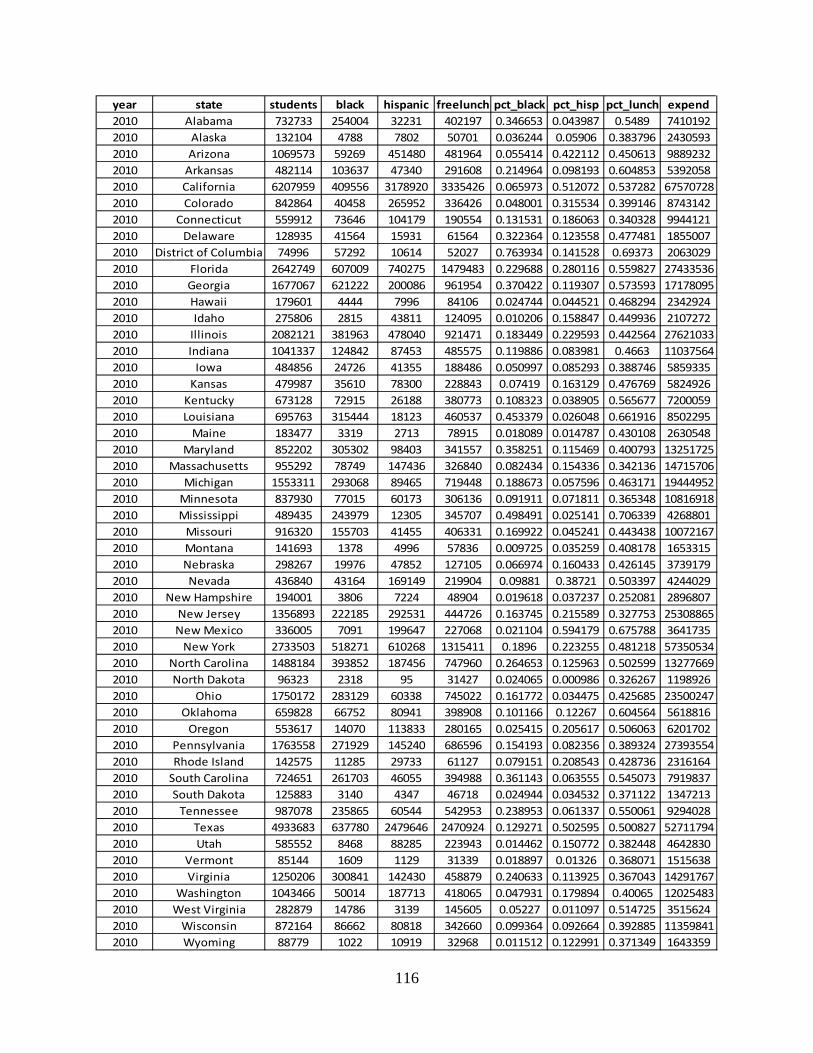
116

year state students black hispanic freelunch pct_black pct_hisp pct_lunch expend2010 Alabama 732733 254004 32231 402197 0.346653 0.043987 0.5489 74101922010 Alaska 132104 4788 7802 50701 0.036244 0.05906 0.383796 24305932010 Arizona 1069573 59269 451480 481964 0.055414 0.422112 0.450613 98892322010 Arkansas 482114 103637 47340 291608 0.214964 0.098193 0.604853 53920582010 California 6207959 409556 3178920 3335426 0.065973 0.512072 0.537282 675707282010 Colorado 842864 40458 265952 336426 0.048001 0.315534 0.399146 87431422010 Connecticut 559912 73646 104179 190554 0.131531 0.186063 0.340328 99441212010 Delaware 128935 41564 15931 61564 0.322364 0.123558 0.477481 18550072010 District of Columbia 74996 57292 10614 52027 0.763934 0.141528 0.69373 20630292010 Florida 2642749 607009 740275 1479483 0.229688 0.280116 0.559827 274335362010 Georgia 1677067 621222 200086 961954 0.370422 0.119307 0.573593 171780952010 Hawaii 179601 4444 7996 84106 0.024744 0.044521 0.468294 23429242010 Idaho 275806 2815 43811 124095 0.010206 0.158847 0.449936 21072722010 Illinois 2082121 381963 478040 921471 0.183449 0.229593 0.442564 276210332010 Indiana 1041337 124842 87453 485575 0.119886 0.083981 0.4663 110375642010 Iowa 484856 24726 41355 188486 0.050997 0.085293 0.388746 58593352010 Kansas 479987 35610 78300 228843 0.07419 0.163129 0.476769 58249262010 Kentucky 673128 72915 26188 380773 0.108323 0.038905 0.565677 72000592010 Louisiana 695763 315444 18123 460537 0.453379 0.026048 0.661916 85022952010 Maine 183477 3319 2713 78915 0.018089 0.014787 0.430108 26305482010 Maryland 852202 305302 98403 341557 0.358251 0.115469 0.400793 132517252010 Massachusetts 955292 78749 147436 326840 0.082434 0.154336 0.342136 147157062010 Michigan 1553311 293068 89465 719448 0.188673 0.057596 0.463171 194449522010 Minnesota 837930 77015 60173 306136 0.091911 0.071811 0.365348 108169182010 Mississippi 489435 243979 12305 345707 0.498491 0.025141 0.706339 42688012010 Missouri 916320 155703 41455 406331 0.169922 0.045241 0.443438 100721672010 Montana 141693 1378 4996 57836 0.009725 0.035259 0.408178 16533152010 Nebraska 298267 19976 47852 127105 0.066974 0.160433 0.426145 37391792010 Nevada 436840 43164 169149 219904 0.09881 0.38721 0.503397 42440292010 New Hampshire 194001 3806 7224 48904 0.019618 0.037237 0.252081 28968072010 New Jersey 1356893 222185 292531 444726 0.163745 0.215589 0.327753 253088652010 New Mexico 336005 7091 199647 227068 0.021104 0.594179 0.675788 36417352010 New York 2733503 518271 610268 1315411 0.1896 0.223255 0.481218 573505342010 North Carolina 1488184 393852 187456 747960 0.264653 0.125963 0.502599 132776692010 North Dakota 96323 2318 95 31427 0.024065 0.000986 0.326267 11989262010 Ohio 1750172 283129 60338 745022 0.161772 0.034475 0.425685 235002472010 Oklahoma 659828 66752 80941 398908 0.101166 0.12267 0.604564 56188162010 Oregon 553617 14070 113833 280165 0.025415 0.205617 0.506063 62017022010 Pennsylvania 1763558 271929 145240 686596 0.154193 0.082356 0.389324 273935542010 Rhode Island 142575 11285 29733 61127 0.079151 0.208543 0.428736 23161642010 South Carolina 724651 261703 46055 394988 0.361143 0.063555 0.545073 79198372010 South Dakota 125883 3140 4347 46718 0.024944 0.034532 0.371122 13472132010 Tennessee 987078 235865 60544 542953 0.238953 0.061337 0.550061 92940282010 Texas 4933683 637780 2479646 2470924 0.129271 0.502595 0.500827 527117942010 Utah 585552 8468 88285 223943 0.014462 0.150772 0.382448 46428302010 Vermont 85144 1609 1129 31339 0.018897 0.01326 0.368071 15156382010 Virginia 1250206 300841 142430 458879 0.240633 0.113925 0.367043 142917672010 Washington 1043466 50014 187713 418065 0.047931 0.179894 0.40065 120254832010 West Virginia 282879 14786 3139 145605 0.05227 0.011097 0.514725 35156242010 Wisconsin 872164 86662 80818 342660 0.099364 0.092664 0.392885 113598412010 Wyoming 88779 1022 10919 32968 0.011512 0.122991 0.371349 1643359

117

year state med_inc log_exp_percap log_expend log_medinc region Midwest South West2010 Alabama 42224 2.313830137 15.818367 10.65074444 2 0 1 02010 Alaska 59672 2.912301064 14.70364571 10.99661827 4 0 0 12010 Arizona 48375 2.224187136 16.10695648 10.7867384 3 0 0 12010 Arkansas 39804 2.414501905 15.50043774 10.59172249 2 0 1 02010 California 55995 2.387342691 18.02868462 10.93301773 4 0 0 12010 Colorado 62133 2.339219332 15.98377991 11.03703213 1 1 0 02010 Connecticut 68080 2.876957178 16.11249161 11.12843895 0 0 0 02010 Delaware 56956 2.666335344 14.4333992 10.95003414 0 0 0 02010 District of Columbia 58724 3.314495802 14.5396862 10.98060417 0 0 0 02010 Florida 45456 2.339946508 17.12727737 10.7244997 2 0 1 02010 Georgia 45509 2.326588631 16.65914536 10.72566509 2 0 1 02010 Hawaii 61417 2.568417311 14.66691017 11.02544212 4 0 0 12010 Idaho 48535 2.033451796 14.5609045 10.79004002 4 0 0 12010 Illinois 52328 2.585190535 17.13408852 10.86528683 1 1 0 02010 Indiana 47595 2.360798836 16.21681404 10.77048302 1 1 0 02010 Iowa 50562 2.491939545 15.58354664 10.83095551 1 1 0 02010 Kansas 47506 2.496142626 15.57765675 10.76861095 1 1 0 02010 Kentucky 42401 2.369909048 15.78959942 10.65492725 2 0 1 02010 Louisiana 40540 2.503082275 15.95584679 10.61004448 2 0 1 02010 Maine 49442 2.662858248 14.78270245 10.8085556 0 0 0 02010 Maryland 66226 2.744059324 16.39963913 11.10082817 0 0 0 02010 Massachusetts 62856 2.734653711 16.50442505 11.0486021 0 0 0 02010 Michigan 47736 2.527198792 16.78309822 10.77344131 1 1 0 02010 Minnesota 53972 2.557932138 16.19662285 10.89622021 1 1 0 02010 Mississippi 39363 2.165836573 15.2668438 10.58058167 2 0 1 02010 Missouri 47262 2.397165537 16.1252861 10.76346207 2 0 1 02010 Montana 42582 2.456874847 14.31829262 10.65918732 4 0 0 12010 Nebraska 54160 2.528632402 15.13437653 10.89969826 1 1 0 02010 Nevada 52815 2.273701429 15.26102352 10.87455082 4 0 0 12010 New Hampshire 68735 2.703500986 14.87911987 11.13801384 0 0 0 02010 New Jersey 64954 2.925957203 17.04666519 11.08143425 0 0 0 02010 New Mexico 46558 2.383089542 15.10797119 10.74845409 3 0 0 12010 New York 51351 3.043598175 17.86469269 10.84643936 0 0 0 02010 North Carolina 45213 2.188526869 16.40159416 10.71914005 2 0 1 02010 North Dakota 52614 2.521474361 13.9969368 10.87073708 1 1 0 02010 Ohio 47333 2.597296953 16.97252083 10.76496315 1 1 0 02010 Oklahoma 44463 2.141896963 15.5416317 10.70241261 3 1 0 02010 Oregon 52198 2.416105986 15.64033413 10.86279964 4 0 0 12010 Pennsylvania 49838 2.742974281 17.12581825 10.81653309 0 0 0 02010 Rhode Island 53252 2.787799358 14.65542316 10.88279057 0 0 0 02010 South Carolina 43014 2.391435862 15.88488102 10.66928101 2 0 1 02010 South Dakota 46783 2.370440483 14.11354828 10.75327492 1 1 0 02010 Tennessee 39809 2.242378235 16.04488182 10.59184837 2 0 1 02010 Texas 48757 2.368753433 17.78034973 10.7946043 3 1 0 02010 Utah 58489 2.070524454 15.35083485 10.97659397 4 0 0 12010 Vermont 57692 2.879247904 14.23134708 10.96287346 0 0 0 02010 Virginia 62271 2.43637538 16.47519493 11.03925133 2 0 1 02010 Washington 57934 2.444480181 16.30253792 10.96706009 4 0 0 12010 West Virginia 44126 2.519953012 15.0727272 10.69480419 2 0 1 02010 Wisconsin 51939 2.566862106 16.24559402 10.85782528 1 1 0 02010 Wyoming 53847 2.918347359 14.312253 10.89390182 4 0 0 1

118

year state Northeast all_np public_char pvt_fnd np_org pct_fed_doe award_tier score_pct2010 Alabama 0 18374 12264 1062 5048 0.072478433 0.4242010 Alaska 0 4784 3389 113 1282 0.0604654112010 Arizona 0 19796 14394 1086 4316 0.063897308 3 0.87082010 Arkansas 0 12083 8174 422 3487 0.031100993 0.77842010 California 0 144728 105876 10000 28852 0.052450741 0.84722010 Colorado 0 25560 17901 1662 5997 0.081593707 3 0.84042010 Connecticut 1 18602 11860 1770 4972 0.052083384 0.7582010 Delaware 1 5523 3050 1226 1247 0.04390106 1 0.90922010 District of Columbia 1 12367 8024 497 3846 0.091371422 2 0.92010 Florida 0 69310 50655 5960 12695 0.097906596 2 0.90482010 Georgia 0 37384 28334 1910 7140 0.059604937 2 0.89282010 Hawaii 0 6861 5032 444 1385 0.039086813 2 0.92482010 Idaho 0 7002 4584 311 2107 0.0101991272010 Illinois 0 60277 36801 5337 18139 0.093300555 3 0.85322010 Indiana 0 32993 21159 1305 10529 0.1082354892010 Iowa 0 26361 11551 983 13827 0.050179522 0.76562010 Kansas 0 15471 9535 846 5090 0.0509920662010 Kentucky 0 16785 11224 681 4880 0.116352796 3 0.82482010 Louisiana 0 17001 11028 730 5243 0.122318113 3 0.8682010 Maine 1 8508 5467 449 2592 0.133939042 0.56682010 Maryland 1 27654 17290 2307 8057 0.066850236 2 0.92010 Massachusetts 1 33722 22718 3515 7489 0.117189932 2 0.9422010 Michigan 0 42886 28270 2566 12050 0.096799622 0.76322010 Minnesota 0 31528 20636 1680 9212 0.0885491272010 Mississippi 0 11805 7891 355 3559 0.095065993 0.52682010 Missouri 0 34819 18599 1857 14363 0.090003223 0.63282010 Montana 0 9230 6127 323 2780 0.042725867 0.47682010 Nebraska 0 11916 6901 666 4349 0.080248168 0.59162010 Nevada 0 7254 4870 682 1702 0.091152586 0.76242010 New Hampshire 1 7498 4903 513 2082 0.007625706 0.67042010 New Jersey 1 38825 25925 3347 9553 0.061003863 3 0.87562010 New Mexico 0 9104 6500 380 2224 0.079838174 0.73242010 New York 1 91758 61691 11529 18538 0.083685011 2 0.92962010 North Carolina 0 39587 27777 2420 9390 0.116562707 2 0.88322010 North Dakota 0 5318 3010 117 2191 0.0258615652010 Ohio 0 59897 37267 3851 18779 0.088591777 2 0.88162010 Oklahoma 0 16953 11960 958 4035 0.08075002 0.78362010 Oregon 0 21050 14773 1016 5261 0.1193504362010 Pennsylvania 1 63345 37600 6208 19537 0.096833303 3 0.83522010 Rhode Island 1 7687 3364 1743 2580 0.067859709 2 0.90242010 South Carolina 0 21931 17062 659 4210 0.074204114 0.8622010 South Dakota 0 6031 3544 173 2314 0.083630542010 Tennessee 0 27623 20577 1034 6012 0.088378244 1 0.88842010 Texas 0 92734 65048 5711 21975 0.1078868352010 Utah 0 7855 5235 807 1813 0.146225613 0.7582010 Vermont 1 5363 3602 274 1487 0.0976468892010 Virginia 0 37860 26283 1827 9750 0.1435799152010 Washington 0 32084 22343 1515 8226 0.122284253 0.58122010 West Virginia 0 9381 5905 339 3137 0.0950745152010 Wisconsin 0 30854 18725 2074 10055 0.124235248 0.73682010 Wyoming 0 4156 2518 286 1352 0.083853618

119

year state A A1 A1_agenda A1_commit A1_impact A2 A2_capacity A2_stakehold2010 Alabama 42.8 21.2 3 10.2 8 10.6 7.8 2.82010 Alaska2010 Arizona 105.4 57.6 4.6 40.2 12.8 26 17.8 8.22010 Arkansas 94.4 47.6 4.4 33.6 9.6 23.2 14.6 8.62010 California 100 51 4.8 34.6 11.6 25 18 72010 Colorado 97.6 52.2 4.4 37.2 10.6 24.2 17 7.22010 Connecticut 96 51 4.8 34.2 12 24.2 15.2 92010 Delaware 119.4 64.6 5 45 14.6 28 18.2 9.82010 District of Columbia 113 59.4 5 41 13.4 26.8 18.4 8.42010 Florida 112.2 59.8 4.4 42.4 13 24.8 17.8 72010 Georgia 104.4 54.6 4.8 37.4 12.4 25 18.4 6.62010 Hawaii 115.6 62.2 4.8 43.4 14 29.6 19.6 102010 Idaho2010 Illinois 102.6 52.8 4.8 34.6 13.4 26.2 17 9.22010 Indiana2010 Iowa 97.6 53.2 4.4 37.2 11.6 26.6 17.8 8.82010 Kansas2010 Kentucky 107.6 57.4 5 40.4 12 27.8 17.8 102010 Louisiana 106.2 56.8 4.8 39.8 12.2 25.4 17.2 8.22010 Maine 74 36 4.4 23.2 8.4 19 13.4 5.62010 Maryland 111.2 55.4 5 38 12.4 27.6 20 7.62010 Massachusetts 115.4 57.4 5 39 13.4 29 20 92010 Michigan 106.2 55.4 5 39.4 11 27.2 17.4 9.82010 Minnesota2010 Mississippi 80.4 48 3.6 35.8 8.6 19.6 12.8 6.82010 Missouri 74.4 39.4 4.2 26.8 8.4 18.4 14.4 42010 Montana 86 46.4 3.8 33.4 9.2 21.4 13.6 7.82010 Nebraska 75.8 33.2 3.8 22.2 7.2 22.8 15.6 7.22010 Nevada 108.6 59.8 4.8 41 14 26 16.8 9.22010 New Hampshire 80.4 42 4.8 26.6 10.6 20.6 14 6.62010 New Jersey 104 50.6 5 33.8 11.8 27.4 20 7.42010 New Mexico 88.2 49 4 34.6 10.4 20.2 13.6 6.62010 New York 108.4 54.8 5 39 10.8 28.6 19 9.62010 North Carolina 112 64.2 4.4 45 14.8 27.2 18.2 92010 North Dakota2010 Ohio 111 58.6 4.6 41.4 12.6 27.8 18 9.82010 Oklahoma 91.8 45.4 4.2 31.4 9.8 24.2 16 8.22010 Oregon2010 Pennsylvania 103.2 55.6 4.2 41 10.4 25.8 18.2 7.62010 Rhode Island 101.6 50 4.4 34 11.6 27.2 19.4 7.82010 South Carolina 102.8 64 4.8 44.6 14.6 26 17.2 8.82010 South Dakota2010 Tennessee 112 63.2 4.8 44.2 14.2 28.2 18.4 9.82010 Texas2010 Utah 82.8 42.8 3.4 30.6 8.8 21.4 17 4.42010 Vermont2010 Virginia2010 Washington 73.4 41.8 3 30.6 8.2 18.6 11.4 7.22010 West Virginia2010 Wisconsin 95.2 51.4 4.4 34.8 12.2 23.4 15.2 8.22010 Wyoming

120

year state A3 A3_progress A3_outcomes B B1 B1_consort B1_standards B22010 Alabama 11 2.6 8.4 43.2 24.2 20 4.2 9.22010 Alaska2010 Arizona 21.8 4.4 17.4 67 40 20 20 102010 Arkansas 23.6 4.8 18.8 69 40 20 20 102010 California 24 4.6 19.4 69.2 40 20 20 102010 Colorado 21.2 4.6 16.6 65.8 40 20 20 9.62010 Connecticut 20.8 4.4 16.4 68.4 40 20 20 102010 Delaware 26.8 4.6 22.2 68.8 39.8 20 19.8 9.62010 District of Columbia 26.8 4.6 22.2 68.4 40 20 20 102010 Florida 27.6 5 22.6 68.2 40 20 20 102010 Georgia 24.8 4.8 20 69.6 40 20 20 102010 Hawaii 23.8 4.4 19.4 69.2 39.6 19.6 20 102010 Idaho2010 Illinois 23.6 5 18.6 64.6 39.6 20 19.6 9.82010 Indiana2010 Iowa 17.8 4.8 13 69.6 40 20 20 102010 Kansas2010 Kentucky 22.4 4.2 18.2 67 40 20 20 9.82010 Louisiana 24 5 19 65.8 39.6 20 19.6 102010 Maine 19 3.8 15.2 60.2 38.2 20 18.2 9.82010 Maryland 28.2 5 23.2 69.8 40 20 20 9.82010 Massachusetts 29 5 24 69.8 40 20 20 102010 Michigan 23.6 4.8 18.8 67.6 40 20 20 102010 Minnesota2010 Mississippi 12.8 4.4 8.4 56.6 40 20 20 102010 Missouri 16.6 4 12.6 54.8 25 20 5 102010 Montana 18.2 2.8 15.4 44.8 20 20 0 102010 Nebraska 19.8 4.4 15.4 56.2 35.2 19.6 15.6 62010 Nevada 22.8 4.8 18 66.6 40 20 20 9.82010 New Hampshire 17.8 4.2 13.6 66.2 40 20 20 102010 New Jersey 26 4.8 21.2 69.2 40 20 20 102010 New Mexico 19 4.6 14.4 62.8 36.2 20 16.2 9.82010 New York 25 4.6 20.4 70 40 20 20 102010 North Carolina 20.6 4.6 16 68.4 40 20 20 102010 North Dakota2010 Ohio 24.6 4.6 20 68 40 20 20 102010 Oklahoma 22.2 4.8 17.4 64.8 40 20 20 102010 Oregon2010 Pennsylvania 21.8 4.4 17.4 68.8 40 20 20 102010 Rhode Island 24.4 5 19.4 70 40 20 20 102010 South Carolina 12.8 4.2 8.6 66.6 40 20 20 102010 South Dakota2010 Tennessee 20.6 4.8 15.8 68.4 40 20 20 9.82010 Texas2010 Utah 18.6 4.4 14.2 67 40 20 20 9.82010 Vermont2010 Virginia2010 Washington 13 3.8 9.2 47.6 25 20 5 9.82010 West Virginia2010 Wisconsin 20.4 4.6 15.8 65.6 39 20 19 102010 Wyoming

121

year state B3 C C1 C2 C3 D D1 D2 D2_growth2010 Alabama 9.8 32 20 2 10 38.8 1.6 13.2 2.62010 Alaska2010 Arizona 17 36.2 18 4.2 14 114.4 15 51.8 4.62010 Arkansas 19 44 24 4.6 15.4 101.6 15.8 44.2 52010 California 19.2 30.8 10 4.6 16.2 110.4 13 48.6 4.42010 Colorado 16.2 41.6 22 4.6 15 105.2 16.6 43.4 4.42010 Connecticut 18.4 27.4 10 3.6 13.8 88.6 19 30.2 2.62010 Delaware 19.4 47 24 5 18 119.2 17.2 50.4 4.42010 District of Columbia 18.4 35.4 14 4.6 16.8 117.8 20.2 54.2 52010 Florida 18.2 41.4 24 4 13.4 115.6 18.4 48 42010 Georgia 19.6 43.2 24 4.8 14.4 119.8 16.6 54.8 52010 Hawaii 19.6 43.6 22 5 16.6 122.4 13.8 54.6 4.82010 Idaho2010 Illinois 15.2 42.4 20.4 4.8 17.2 110.6 18.2 47.4 3.22010 Indiana2010 Iowa 19.6 36.6 18 5 13.6 95.4 15.2 41 3.42010 Kansas2010 Kentucky 17.2 43.2 22.4 4.4 16.4 113.2 18.2 48.2 4.62010 Louisiana 16.2 43.2 24 4.2 15 110.6 17 47.8 4.42010 Maine 12.2 33.2 22 3.8 7.4 51.8 5 25.6 1.62010 Maryland 20 40.8 20 5 15.8 126.2 19.8 53 52010 Massachusetts 19.8 44.4 24 5 15.4 126.8 21 53 4.62010 Michigan 17.6 34.2 18 4.2 12 77.2 5.2 41.4 42010 Minnesota2010 Mississippi 6.6 26.4 14 2.2 10.2 55.4 10.2 29.4 3.82010 Missouri 19.8 45.2 24 5 16.2 84.2 8.6 41 4.22010 Montana 14.8 22.4 12 2.6 7.8 54.6 14.6 20 3.82010 Nebraska 15 22.6 9.2 3 10.4 72 5.8 40.2 3.22010 Nevada 16.8 38 22 3.4 12.6 84.6 9.6 39 4.42010 New Hampshire 16.2 34.4 16 3.8 14.6 70.6 11.6 25.4 2.82010 New Jersey 19.2 31.4 14 4 13.4 124.4 17.2 53.6 4.22010 New Mexico 16.8 33.2 18.8 3.6 10.8 78.6 15.6 31.2 2.82010 New York 20 45.8 24 4.6 17.2 127.6 19.4 54.4 4.82010 North Carolina 18.4 40.4 21.6 4.8 14 116 18.2 50.8 4.62010 North Dakota2010 Ohio 18 37.2 18 5 14.2 119.6 15.4 54 3.62010 Oklahoma 14.8 31.2 16 3.8 11.4 106.4 13.4 47.8 4.22010 Oregon2010 Pennsylvania 18.8 45.2 24 4.8 16.4 95.4 10.4 45.2 3.42010 Rhode Island 20 46.8 24 5 17.8 119.6 16.8 50.2 42010 South Carolina 16.6 42.6 22.4 4.4 15.8 111.2 13.8 52.2 4.22010 South Dakota2010 Tennessee 18.6 43.6 24 4.8 14.8 114 15 53 52010 Texas2010 Utah 17.2 34 23.2 3.8 7 100.4 18.6 38.8 42010 Vermont2010 Virginia2010 Washington 12.8 41.8 24 3.8 14 59 14 19.6 1.42010 West Virginia2010 Wisconsin 16.6 38 19.6 4.4 14 82.2 19.2 25 2.82010 Wyoming

122

year state D2_eval_process D2_eval D2_data_eval D3 D3_eq_dist_schools D3_eq_dist_subj D42010 Alabama 4.6 2.2 3.8 5.8 2.4 3.4 7.42010 Alaska2010 Arizona 13.6 9 24.6 20 12.4 7.6 10.82010 Arkansas 11.8 7 20.4 17.2 8.4 8.8 10.62010 California 14.4 7.4 22.4 20.4 12.6 7.8 13.22010 Colorado 10.4 8.4 20.2 16.6 9 7.6 11.62010 Connecticut 9.4 6.8 11.4 17.4 10.2 7.2 7.42010 Delaware 12.8 9.2 24 21.2 12.4 8.8 11.42010 District of Columbia 13 9.2 27 19.2 12.2 7 9.82010 Florida 11.8 7.4 24.8 20 12.2 7.8 11.62010 Georgia 14 9.4 26.4 18.6 12 6.6 10.82010 Hawaii 13.8 10 26 23.6 14.4 9.2 11.62010 Idaho2010 Illinois 12.2 7.4 24.6 18.6 11.6 7 10.82010 Indiana2010 Iowa 12 8.4 17.2 18.2 11.4 6.8 6.62010 Kansas2010 Kentucky 10.4 8.8 24.4 15.8 9.4 6.4 12.82010 Louisiana 12.2 8.6 22.6 19.6 11.6 8 12.42010 Maine 7.4 4.6 12 7.6 5.2 2.4 4.62010 Maryland 15 8.4 24.6 22.4 13.6 8.8 12.22010 Massachusetts 15 9.2 24.2 23.2 13.8 9.4 12.62010 Michigan 12 7.8 17.6 12 8.6 3.4 62010 Minnesota2010 Mississippi 8.2 7.6 9.8 4.4 2.2 2.2 52010 Missouri 12.6 8.6 15.6 10 6.2 3.8 9.62010 Montana 6.4 2.8 7 8.6 5.4 3.2 42010 Nebraska 12.2 6.6 18.2 12.8 8.8 4 52010 Nevada 12.4 7.4 14.8 12.4 6.8 5.6 82010 New Hampshire 7.4 5 10.2 13.6 8.8 4.8 7.22010 New Jersey 14.8 9.4 25.2 22 13.4 8.6 13.62010 New Mexico 9.6 5.2 13.6 13.6 7.2 6.4 7.42010 New York 12.6 9 28 21.8 13 8.8 13.62010 North Carolina 13.8 9.6 22.8 19.2 11.6 7.6 10.62010 North Dakota2010 Ohio 14.8 8.6 27 19.8 11.6 8.2 11.82010 Oklahoma 12.6 8.8 22.2 18.8 11.4 7.4 112010 Oregon2010 Pennsylvania 13.8 8 20 16.8 10.2 6.6 92010 Rhode Island 10.6 9.6 26 22.8 13 9.8 122010 South Carolina 13.6 9.2 25.2 23.8 14 9.8 9.82010 South Dakota2010 Tennessee 13.6 10 24.4 18.4 10.2 8.2 12.62010 Texas2010 Utah 10.8 7.8 16.2 15.8 9.4 6.4 112010 Vermont2010 Virginia2010 Washington 7.4 5.2 5.6 11.2 7.2 4 52010 West Virginia2010 Wisconsin 5.6 4.4 12.2 18.4 10 8.4 72010 Wyoming

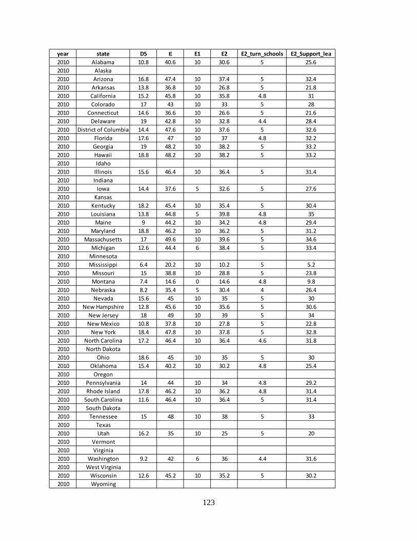
123

year state D5 E E1 E2 E2_turn_schools E2_Support_lea2010 Alabama 10.8 40.6 10 30.6 5 25.62010 Alaska2010 Arizona 16.8 47.4 10 37.4 5 32.42010 Arkansas 13.8 36.8 10 26.8 5 21.82010 California 15.2 45.8 10 35.8 4.8 312010 Colorado 17 43 10 33 5 282010 Connecticut 14.6 36.6 10 26.6 5 21.62010 Delaware 19 42.8 10 32.8 4.4 28.42010 District of Columbia 14.4 47.6 10 37.6 5 32.62010 Florida 17.6 47 10 37 4.8 32.22010 Georgia 19 48.2 10 38.2 5 33.22010 Hawaii 18.8 48.2 10 38.2 5 33.22010 Idaho2010 Illinois 15.6 46.4 10 36.4 5 31.42010 Indiana2010 Iowa 14.4 37.6 5 32.6 5 27.62010 Kansas2010 Kentucky 18.2 45.4 10 35.4 5 30.42010 Louisiana 13.8 44.8 5 39.8 4.8 352010 Maine 9 44.2 10 34.2 4.8 29.42010 Maryland 18.8 46.2 10 36.2 5 31.22010 Massachusetts 17 49.6 10 39.6 5 34.62010 Michigan 12.6 44.4 6 38.4 5 33.42010 Minnesota2010 Mississippi 6.4 20.2 10 10.2 5 5.22010 Missouri 15 38.8 10 28.8 5 23.82010 Montana 7.4 14.6 0 14.6 4.8 9.82010 Nebraska 8.2 35.4 5 30.4 4 26.42010 Nevada 15.6 45 10 35 5 302010 New Hampshire 12.8 45.6 10 35.6 5 30.62010 New Jersey 18 49 10 39 5 342010 New Mexico 10.8 37.8 10 27.8 5 22.82010 New York 18.4 47.8 10 37.8 5 32.82010 North Carolina 17.2 46.4 10 36.4 4.6 31.82010 North Dakota2010 Ohio 18.6 45 10 35 5 302010 Oklahoma 15.4 40.2 10 30.2 4.8 25.42010 Oregon2010 Pennsylvania 14 44 10 34 4.8 29.22010 Rhode Island 17.8 46.2 10 36.2 4.8 31.42010 South Carolina 11.6 46.4 10 36.4 5 31.42010 South Dakota2010 Tennessee 15 48 10 38 5 332010 Texas2010 Utah 16.2 35 10 25 5 202010 Vermont2010 Virginia2010 Washington 9.2 42 6 36 4.4 31.62010 West Virginia2010 Wisconsin 12.6 45.2 10 35.2 5 30.22010 Wyoming

124

year state F F1_funding F2_conditions F3_reforms stem Total applied092010 Alabama 14.6 9.4 1.8 3.4 0 212 12010 Alaska 02010 Arizona 50 9.4 36.2 4.4 15 435.4 12010 Arkansas 28.4 6.6 18.8 3 15 389.2 12010 California 52.4 9 38.6 4.8 15 423.6 12010 Colorado 52 9.6 38.4 4 15 420.2 12010 Connecticut 47 7.8 36.6 2.6 15 379 12010 Delaware 42.4 7.6 31 3.8 15 454.6 12010 District of Columbia 52.8 9.6 39.4 3.8 15 450 12010 Florida 53 8.8 39.4 4.8 15 452.4 12010 Georgia 46.2 9.8 32.8 3.6 15 446.4 12010 Hawaii 48.4 9.8 33.8 4.8 15 462.4 12010 Idaho 12010 Illinois 45 9.6 30.4 5 15 426.6 12010 Indiana 12010 Iowa 46 8.6 34.6 2.8 0 382.8 12010 Kansas 12010 Kentucky 21 8.2 8 4.8 15 412.4 12010 Louisiana 48.4 9.6 35.8 3 15 434 12010 Maine 20 8.8 7 4.2 0 283.4 02010 Maryland 40.8 8.2 27.6 5 15 450 02010 Massachusetts 50 10 35.4 4.6 15 471 12010 Michigan 37 10 22 5 15 381.6 12010 Minnesota 12010 Mississippi 24.4 7.8 14.6 2 0 263.4 02010 Missouri 19 1.8 16.8 0.4 0 316.4 12010 Montana 16 8.8 3.8 3.4 0 238.4 02010 Nebraska 18.8 8.4 6.2 4.2 15 295.8 12010 Nevada 38.4 6.4 27 5 0 381.2 02010 New Hampshire 38 9.2 24.2 4.6 0 335.2 12010 New Jersey 44.8 3.4 37.4 4 15 437.8 12010 New Mexico 50.6 9.6 36.4 4.6 15 366.2 12010 New York 50.2 9.8 36 4.4 15 464.8 12010 North Carolina 43.4 9 29.6 4.8 15 441.6 12010 North Dakota 02010 Ohio 45 9.8 30.6 4.6 15 440.8 12010 Oklahoma 42.4 6.4 32 4 15 391.8 12010 Oregon 12010 Pennsylvania 46 9.2 32.2 4.6 15 417.6 12010 Rhode Island 52 10 37.6 4.4 15 451.2 12010 South Carolina 46.4 9.8 31.6 5 15 431 12010 South Dakota 12010 Tennessee 43.2 8.6 30 4.6 15 444.2 12010 Texas 02010 Utah 44.8 10 32 2.8 15 379 12010 Vermont 02010 Virginia 12010 Washington 11.8 7.2 0.8 3.8 15 290.6 02010 West Virginia 12010 Wisconsin 42.2 8.6 29 4.6 0 368.4 12010 Wyoming 1

125

IRB Approval/Waiver

PRO-FY2017-275 - Admin Withdrawal: Not Human Subject Research - irb@memphis.edu

Institutional Review Board Office of Sponsored Programs University of Memphis 315 Admin Bldg Memphis, TN 38152-3370 Jan 26, 2017 PI Name: Brian Brewer Co-Investigators: Advisor and/or Co-PI: Charisse Gulosino Submission Type: Admin Withdrawal Title: Analysis of the Race to the Top application scores with state demographic, economic, political and social data examining Race to the Top grant awards IRB ID: #PRO-FY2017-275 From the information provided on your determination review request for “Analysis of the Race to the Top application scores with state demographic, economic, political and social data examining Race to the Top grant awards”, the IRB has determined that your activity does not meet the Office of Human Subjects Research Protections definition of human subjects research and 45 CFR part 46 does not apply. This study does not require IRB approval nor review. Your determination will be administratively withdrawn from Cayuse IRB and you will receive an email similar to this correspondence from irb@memphis.edu. THANKS, IRB Administrator Research Compliance Division of Research & Sponsored Programs The University of Memphis 315 Administration Building Memphis, TN 38152-3370 P: 901.678.2705

126

F: 901.678.4409 memphis.edu/rsp/compliance