An exponential random graph modeling approach to creating group-

based representative whole-brain connectivity networks

Sean L. Simpsona,*

, Malaak N. Moussab, Paul J. Laurienti

c

a Department of Biostatistical Sciences, Wake Forest University School of Medicine Winston-Salem, NC, USA

b Neuroscience Program, Wake Forest University School of Medicine Winston-Salem, NC, USA

c Department of Radiology, Wake Forest University School of Medicine Winston-Salem, NC, USA

*Corresponding author. Department of Biostatistical Sciences, Wake Forest University

School of Medicine, Medical Center Boulevard, Winston-Salem, NC 27157, USA. Fax:

+1 336 716 6427.

E-mail address: slsimpso@wakehealth.edu (S. Simpson).

ABSTRACT

Group-based brain connectivity networks have great appeal for researchers interested in gaining

further insight into complex brain function and how it changes across different mental states and

disease conditions. Accurately constructing these networks presents a daunting challenge given

the difficulties associated with accounting for inter-subject topological variability. Viable

approaches to this task must engender networks that capture the constitutive topological

properties of the group of subjects’ networks that it is aiming to represent. The conventional

approach has been to use a mean or median correlation network (Achard et al., 2006; Song et al.,

2009) to embody a group of networks. However, the degree to which their topological properties

conform with those of the groups that they are purported to represent has yet to be explored.

Here we investigate the performance of these mean and median correlation networks. We also

propose an alternative approach based on an exponential random graph modeling framework and

compare its performance to that of the aforementioned conventional approach. Simpson et al.

(2011) illustrated the utility of exponential random graph models (ERGMs) for creating brain

networks that capture the topological characteristics of a single subject’s brain network.

However, their advantageousness in the context of producing a brain network that “represents” a

group of brain networks has yet to be examined. Here we show that our proposed ERGM

approach outperforms the conventional mean and median correlation based approaches and

provides an accurate and flexible method for constructing group-based representative brain

networks.

Keywords: ERGM; p-star; Connectivity; Network; Graph analysis; fMRI.

Introduction

Whole-brain connectivity analysis is a burgeoning area in neuroscience which is gaining

prominence due to the need to understand how various regions of the brain interact with one

another. The application of network and graph theory has facilitated these analyses and enabled

examining the brain as an integrated system rather than a collection of individual components

(Bullmore and Sporns, 2009). Despite the utility of network science in providing insight into the

infrastructural properties of a given subject’s brain, capturing and understanding these properties

in a group of subjects presents challenges that impede research focusing on changes in complex

brain function across different cognitive and disease states.

As noted in Rubinov and Sporns (2010), comparing brain networks across subjects and

groups of subjects necessitates the development of accurate statistical comparison tools. Despite

this need, the amount of work done in this area has not been commensurate with its level of

importance (van Wijk et al., 2010). Developing a systematic approach to capture the network

characteristics from a group of subjects’ brain networks has great appeal and would help to fill

the gap in the group comparison literature. Evaluating individual networks and combining the

information limits studies to exploring features that can be distilled into simple quantitative

metrics such as the commonly used clustering coefficient (C) and path length (L). While

obtaining average measures of metrics such as these in a group is valuable, it only gives a global

view of the system and does not capture the complex organization within a population of

networks. However, a group-based representative brain connectivity network provides a graph

that typifies the complex structure of a set of brain networks. These representative brain

networks could serve as null networks against which other networks and network models could

be compared, as visualization tools (Song et al., 2009), as a way to topologically map and assess

a collection of networks (Achard et al., 2006), as a way to represent an individual’s network

based on several experimental runs, as a means to conduct group-based modularity analyses

(Meunier et al., 2009a,b; Valencia et al., 2009; Joyce et al., 2010), and as an instrument for

identifying hub/node types in a modularity analysis (functional cartography) (Joyce et al., 2010).

In addition to their utility in the previously mentioned contexts, the most important use for these

representative networks is in the nascent area of brain dynamics which requires representative

group-based networks for simulating and assessing information flow on a network. Simulating

dynamics on large groups of brain networks in order to understand how their topology supports

brain activity is infeasible computationally, necessitating an accurate summary network (Jirsa et

al., 2010). A representative network provides a central tendency for a set of complex systems

that allows determining the type of dynamic information transfer a population of brain networks

can support in various cognitive and disease states. Consequently, deeper insight can be gained

on brain-behavior and brain-disease relationships. This needed reduction of many systems to a

single system cannot be performed by simple manipulations of the average network metrics in a

group. Also, as novel network metrics are developed whose computational burden increases with

the number of subjects being analyzed, these representative networks will prove valuable.

However, creating these group-based “representative” networks is a daunting challenge given the

difficulties associated with accounting for the inter-subject topological variability.

There has been a lot of previous work on multivariate group models for functional networks;

however, their foci have been different from those here. Varoquaux et al. (2010) developed a

modeling approach to improve the estimation of a subject’s network based on group time series

data. Cecchi et al. (2009) proposed methods to extract features with high discriminative power

from subject-level time series data. Ramsey et al. (2010) discussed difficulties in inferring causal

relations from fMRI time series. Rădulescu and Mujica-Parodi (2009) applied principal

component network analysis to time series data from a limited number of ROIs in the brain. Our

goal here is not to fit models to time series data, but to fit them to already constructed binary

network data. That is, the approaches we examine are independent of how connections are

determined from time series data. We start from correlation matrices here, but some of the

aforementioned approaches could be used to construct subject-level binary networks from time

series data that could then be embedded within methods that produce a group representative

network based on the individual networks. The goal of these representative network techniques is

to take a set of already constructed networks and produce a group network that typifies the

topological structure of the individual graphs. Hence, these methods are independent of how the

initial subject-level networks are constructed.

Thus far, researchers have taken one of three general approaches to generating a group-based

representative functional network. The most common method has been to take the mean of the

functional connectivity matrices of the subjects in a group and threshold this group mean matrix

to get a mean network (Achard et al., 2006; Meunier et al., 2009a,b; Valencia et al., 2009).

Although this approach is intuitive and computationally straight forward, as with use of the mean

in any context, the resulting network may be unduly influenced by one or more outlying

functional connectivity values. Additionally, this approach is edge-based since the averaging is

done across the individual entries of the connectivity matrices; and thus, it ignores the

topological properties of each subject’s network. Another similar approach taken by researchers

is to take the median of the functional connectivity matrices of the subjects and threshold this

group median matrix to get a median network (Song et al., 2009). While this approach provides

more robustness to outlying connectivity values, it is still edge-based and ignores the topological

dependence among edges within each subject’s network. A third, and more contrasting approach,

was taken by Meunier et al. (2009b) and Joyce et al. (2010). They used a best subject network to

represent the group by assessing between subject differences in network organization (using an

information-based measure and the Jaccard index respectively) and identifying the most

representative subject in the sample. The network of the most representative subject is not likely

to best capture all topological metrics simultaneously, but provides a balance among all of the

variables. It would be ideal to have a method that incorporates the data from all subjects directly,

like the mean and median edge-based network approaches, while also having each metric

maximally optimized within the representative network rather than balancing properties by

selecting a typical subject. Toward this end, we propose an approach to creating group-based

representative networks that utilizes exponential random graph models (ERGMs), also known as

p* models (Frank and Strauss, 1986; Wasserman and Pattison, 1996; Pattison and Wasserman,

1999; Robins et al., 1999). These models enable achieving an efficient representation of complex

network data structures by modeling a network's global structure as a function of local

topological features.

Simpson et al. (2011) showed the utility of ERGMs for simulating a brain network that retains

the constitutive properties of a single subject’s original network. However, their usefulness in

producing a brain network that “represents” the topological characteristics of a group of

networks has yet to be explored. Also, despite the frequent use of mean and median group-based

networks, the amount to which their topological properties coincide with those of the groups that

they are purported to represent has yet to be investigated. Here we make use of resting-state

fMRI data from ten normal subjects to 1) examine how well the mean and median approaches

capture important topological properties of the group and 2) compare their performances to our

ERGM approach.

Materials and methods

Data and network construction

Our analysis included fMRI data from 10 normal subjects (5 female, average age 27.7 years

old [4.7 SD]). For each subject, 120 images were acquired during 5 minutes of resting using a

gradient echo echoplanar imaging (EPI) protocol with TR/TE=2500/40 ms on a 1.5 T GE twin-

speed LX scanner with a birdcage head coil (GE Medical Systems, Milwaukee, WI). The

acquired images were motion corrected, spatially normalized to the MNI (Montreal Neurological

Institute) space and re-sliced to 4×4×5 mm voxel size using an in-house processing script based

on SPM99 package (Wellcome Trust Centre for Neuroimaging, London, UK). The resulting

images were not smoothed in order to avoid artificially introducing local spatial correlation (van

den Heuvel et al., 2008). These subjects were part of a larger study with further details provided

in Peiffer et al. (2009).

The first step in performing the network construction was to calculate Pearson partial

correlation coefficients between the time courses of all node pairs adjusted for motion and

physiological noises (see Hayasaka and Laurienti, 2010 for further details). These node time

courses were obtained by averaging the voxel time courses in the 90 distinct anatomical regions

(90 ROIs-Regions of Interest) defined by the Automated Anatomical Labeling atlas (AAL;

Tzourio-Mazoyer et al., 2002). Three types of networks were then generated based on the

resulting 90×90 correlation matrices. Unweighted, undirected subject-specific networks were

created by thresholding the correlation matrices for each subject to yield a set of adjacency

matrices (Aij) with 1 indicating the presence and 0 indicating the absence of an edge between two

nodes. A group-based mean network was constructed by averaging the correlation matrices of

the 10 subjects (i.e., averaging element (i,j) across matrices) and then thresholding the resulting

matrix to yield a mean adjacency matrix. Similarly, a group-based median network was produced

by computing the median of element (i,j) across the 10 correlation matrices and then

thresholding the resulting matrix. All networks were defined (thresholded) so that the

relationship (denoted by S) between the number of nodes n and the average node degree K is the

same across networks. In particular, the networks were defined so that S = log(n)/log(K) = 2.8.

This relationship is based on the path length of a random network with n nodes and average

degree K, and can be rewritten as n = KS (see Hayasaka and Laurienti, 2010 for further details on

this thresholding approach and the reasons for choosing such a value).

Model definition

Exponential random graph models (ERGMs) have the following form (Handcock, 2002):

( ) ( ) { }1exp ( )T

P κ−

= =Y y g yθθθθθ θθ θθ θθ θ (1)

Here Y is an n×n (n nodes) random symmetric adjacency matrix representing a brain network

from a particular class of networks, with Yij = 1 if an edge exists between nodes i and j and Yij =

0 otherwise. We statistically model the probability mass function (pmf) ( )( )P =Y yθθθθ of this class

of networks as a function of the prespecified network features defined by the p-dimensional

vector g(y), where y is the observed network. This vector of explanatory metrics can contain any

graph statistic (e.g., number of edges) or node statistic (e.g., brain location of the node). The goal

in defining g(y) is to identify local metrics that concisely summarize the global (whole-brain)

structure. A subset of statistically compatible metrics for ERGMs is defined in Table 1 (Morris et

al., 2008). By statistically compatible we mean that the metrics do not generally induce

degeneracy issues discussed in Rinaldo et al. (2009). These issues concern the shape of the

estimated pmf (e.g., a pmf in which only a few graphs have nonzero probability) and can lead to

lack of model convergence and unreliable results. The parameter vector p∈θθθθ R (which must be

estimated), associated with g(y), quantifies the relative significance of each network feature in

explaining the structure of the network after accounting for the contribution of all other network

features in the model. More specifically,θ indicates the change in the log odds of an edge

existing for each unit increase in the corresponding explanatory metric. If theθ value

corresponding to a given metric is large and positive, then that metric plays a considerable role in

explaining the network architecture and is more prevalent than in the null model (random

network with the probability of an edge existing (p) = 0.5). Conversely, if the value is large and

negative, then that metric still plays a considerable role in explaining the network architecture

but is less prevalent than in the null model. The normalizing constant ( )κ θθθθ ensures that the

probabilities sum to one. This approach allows representing the global network structure (y) by

locally specified explanatory metrics (g(y)), and is capable of capturing several important

topological properties of brain networks simultaneously (Simpson et al., 2011). The fitted

parameter values ( )θθθθ can then be utilized to understand particular emergent behaviors of the

network (how local features give rise to the global structure).

Estimation of the model parameters θθθθ is normally done with either Markov chain Monte

Carlo maximum likelihood estimation (MCMC MLE) or maximum pseudo-likelihood estimation

(MPLE) (van Duijn et al., 2009 contains details). Model fits with MPLE are much simpler

computationally than MCMC MLE fits and afford higher convergence rates with large networks.

However, properties of the MPLE estimators are not well understood, and the estimates tend to

be less accurate than those of MCMC MLE. Here we employ MCMC MLE to fit the model in

equation 1 given that there were no convergence issues, though convergence could become an

obstacle in more spatially resolved networks (e.g., voxel-based). Hunter et al. (2008b) provides

further details about this estimation approach which can be implemented in the statnet package

(Handcock et al., 2008) for the R statistical computing environment which we used here.

Representative network creation

In order to create a group-based representative network via ERGMs, it is necessary to get a

group-based summary measure of the fitted parameter values ( )θθθθ for all subjects. The first step in

this process involves identifying the most important explanatory metrics (g(y)) for each subject’s

network as done in Simpson et al. (2011). They implemented a graphical goodness of fit (GOF)

approach (Hunter et al., 2008a) to select the “best” metrics from the set of potential metrics listed

by category in Table 2 for each of the 10 networks (10 subjects). These categories were chosen

based on properties of brain networks that are regarded as important in the literature (Bullmore

and Sporns, 2009). These metrics were chosen because they are analogous to typical brain

network metrics (e.g., clustering coefficient (C)) but have been developed to be statistically

compatible with ERGMs. Figure 1 exemplifies the calculation of GWESP, GWNSP, and

GWDSP, on a six-node example network as these metrics are not classically used in graph

analysis. The distribution of the unweighted analogues of these metrics (ESP, NSP, and DSP) is

given for simplicity. The weighted versions simply sum the values of the distribution giving less

weight to those with more shared partners. For this example we note that the network has 1 set of

connected nodes with 0 shared partners (ESP0), 5 sets with 1 shared partner (ESP1), 2 sets with 2

shared partners (ESP2), and 0 sets with 3 or 4 shared partners (ESP3 and ESP4). Further details on

the metrics are provided in Table 1 and Morris et al. (2008). Theτ parameters associated with

GWESP, GWDSP, GWNSP, and GWD were set toτ = 0.75 for reasons mentioned in Simpson et

al. (2011). The metrics in bold font (Edges, GWESP, and GWNSP) in Table 2 were those

contained in at least half (> 5) of these 10 best models/best sets of explanatory metrics.

Examining the uniformity of the selected explanatory metrics across subjects in this way is

important due to metric interdependencies. In other words, for example, the fitted parameter

value ( )edgeθ associated with the Edge metric in a given subject’s model is statistically dependent

upon/accounts for all other fitted parameter values in the model. Thus, an appropriate statistical

comparison or summary ofedge

θ across subjects requires that the fitted ERGMs for all subjects

contain the same set of metrics (g(y)). A detailed exposition of the aforementioned model

selection approach is presented in Simpson et al. (2011) and partially reproduced in the

Appendix.

Given the metrics in bold font in Table 2, the second step in creating our group-based

representative networks was to refit the networks of all 10 subjects with the “best” group model

( ) ( ) { }1

1 2 3exp .P Edges GWESP GWNSPκ θ θ θ−

= = + +Y yθθθθθθθθ (2)

An example set of graphical GOF plots for the best group model fitted to a subject’s network are

given in Figure 2. For good-fitting models, the plot of the observed network should closely

match that of the simulated networks. We can see that in this figure the model does a good job of

capturing the geodesic (global efficiency), degree, and triad census (motifs) distributions, but

does not do as well at capturing the shared partner (local efficiency) distribution. However, the

model likely fits well enough to still justify conclusions about local efficiency (as is shown later

in the results). The precise implications of these GOF plots for conclusions drawn from the

model have yet to be thoroughly examined in the literature. The estimated parameter values

( )1 2 3, ,θ θ θ for the best group model fitted to each subject are displayed in Table 3 along with the

mean and median of those values across subjects. The third step in creating our group-based

representative networks was to employ these mean ( )1 2 3, ,θ θ θ and median values

to simulate random realizations of networks from their corresponding probability mass functions

(pmfs) below:

( ) ( ) { }1

1 2 3expP Edges GWESP GWNSPκ θ θ θ−

= = + +Y yθθθθθθθθ (3)

(4)

Five mean ERGM and five median ERGM based networks were simulated based on equations 3

and 4 respectively. Additionally, five more networks were simulated from each probability mass

function (in equations 3 and 4) where the degree distributions (distribution of the number of

connections; see next section) were constrained to have the same distribution as subject 16 whom

we deemed to be most representative of the group in terms of this metric. In other words, for

these degree-constrained simulations, the probability mass functions in equations 3 and 4 were

constrained so that only networks whose overall degree distribution was the same as subject 16’s

had a non-zero probability. This approach is equivalent to (though much more efficient than)

simulating networks from the unconstrained pmfs in equations 3 and 4 as before, and then

choosing only those simulated networks with the same degree distribution as subject 16.

Accurately capturing the degree distribution of a set of networks proved difficult; thus, given its

importance in conferring vital properties to brain networks, this constrained simulation approach

was taken to examine whether we could fix the degree distribution while still being able to

properly represent other topological properties of the group. In total, then, we had 20 potential

group-based representative networks generated from these simulations.

Network assessment

Neurobiologically relevant network metrics were calculated for all subjects’ networks, the

mean and median correlation networks, and all ERGM derived mean and median simulated

networks. Unless otherwise noted, these metrics were calculated and evaluated using in-house

processing scripts. A more detailed review of the metrics used in these analyses can be found in

the literature (Rubinov and Sporns, 2010).

A commonly used measure of network connectivity, degree (K), was determined for each

network. The degree for each node (ki) in a network was computed as the total number of

functional links that were associated with a node i. The characteristic path length (L) is a

measure of the functional integration within a network and was calculated using Dijkstra’s

algorithm (Dijkstra, 1959) in the MatlabBGL package (David Gleich; Stanford University,

Standford, CA). It is equivalent to the average shortest path length in a network and was found

by generating a matrix of the geodesic distances between all node pairs. However, in the case of

isolated nodes and subgraphs this value is infinitely distant from the largest network component

(Nc). Because of this, the harmonic mean of the geodesic distances was used to calculate L:

( 1)

1i j

ij

N NL =

d≠

−

∑ (5)

where dij is equal to the harmonic mean of the geodesic distance between nodes i and j (Latora

and Marchiori, 2001; Newman, 2002, 2003). Global efficiency (Eglob), which is the reciprocal of

the characteristic path length (Latora and Marchiori, 2001), captures the level of distributive

processing in a network. Unlike the characteristic path length, global efficiency is scaled and

ranges in value from zero to one, where the latter represents maximal distributed processing.

Clustering coefficient (C) is defined as the fraction of triangles around a particular node in a

network and is thus a measure of local network segregation (Watts and Strogatz, 1998). Akin to

the clustering coefficient is local efficiency (Eloc). For each node in a network, this value

represents the average local sub-graph efficiencies of its neighboring nodes (Latora and

Marchiori, 2001). Like Eglob, it is a scaled value that ranges from zero to one. Nodes within a

network with values closer to one are those with connections that are predominately local.

Assortativity (Rjk) captures the likelihood a node is connected with other like nodes in a

network (Newman, 2002, 2003). In this study assortativity was based on similarity of node

degree. Networks with values closer to 1 were defined as assortative and exhibited high-high

and low-low degree connections. Values that were closer to -1 were indicative of disassortative

networks with high-low degree connections.

Statistical assessments of group-based networks

The following analyses were done to compare original subject data to the mean and median

correlation networks as well as the degree-constrained and unconstrained mean ERGM and

median ERGM simulation-based networks. First, values from each of the 90-nodes of a subject’s

network were used to calculate whole-network means for each metric discussed in the previous

subsection. The mean and median of these whole-network metric values were then computed

across all subjects and compared with the corresponding metric values for the mean and median

correlation networks and degree-constrained and unconstrained mean ERGM and median ERGM

simulation-based networks. We also calculated the Euclidean distance between metric values of

the networks in order to assess how well the representative networks captured all of the group

mean and median topological values simultaneously. That is, we evaluated the square root of the

squared distances between the group mean and median metric values and those of the mean and

median correlation networks and degree-constrained and unconstrained mean ERGM and median

ERGM simulation-based networks. Second, with the exception of degree and assortativity, the

nodal cumulative distributions of each metric were generated for each network. These were made

in order to evaluate which of the representative networks best captured the metric distributions of

the subjects’ data. Finally, to assess how well each representative network captured the nodal

connectivity (degree) of the original subjects’ networks, degree distributions were made. These

distributions show the likelihood with which a particular node in a network displays a certain

degree (Lima-Mendez and van Helden, 2009). Additionally, to visually assess whether or not

representative networks could capture the overall topology of the original subjects’ networks,

Harel-Koren Fast Multiscale graphs (Harel and Koren, 2001) were plotted using NodeXL.

Results

We implemented the network assessment procedure delineated in the previous section for the

20 mean ERGM and median ERGM simulation-based representative networks and compared the

results to those of the frequently used mean and median networks based on the subjects’

correlation matrices. Table 4 shows the results of this assessment and comparison for the 10

unconstrained and 10 degree-constrained simulated networks. As evidenced by the results in this

table, the 10 unconstrained mean ERGM and median ERGM simulation-based representative

networks more accurately capture the group mean and median values for path length (L), size of

the giant component (Nc), mean degree (K), and global efficiency (Eglob) than the corresponding

mean and median correlation networks. There are minimal differences in accuracy for clustering

coefficient (C) and local efficiency (Eloc), with the mean and median correlation networks only

being decisively more accurate for assortativity (Rjk). When assessing the accuracy in capturing

all of the group mean and median topological values simultaneously via the distance metric, all

five of the unconstrained mean ERGM simulation-based networks outperform the mean

correlation network, while four of the five median ERGM simulation-based networks outperform

the median correlation network. However, since our ultimate goal is to select a network that is

most representative of the group, only one simulation-based network need outperform the mean

and median correlation networks for our approach to be useful. Thus, the anomalous

underperforming median ERGM simulation-based network is of little relevance in our context.

An examination of the degree distributions for the subjects’ networks, unconstrained mean

ERGM and median ERGM simulation-based networks, and mean and median correlation

networks in Figure 3a illustrates the fact that the mean and median correlation networks tend to

overestimate this distribution while the unconstrained mean ERGM and median ERGM

simulation-based networks generally underestimate it.

Table 4 also displays the results for the 10 degree-constrained mean ERGM and median

ERGM simulation-based networks. As was the case with the unconstrained networks, these

degree-constrained networks also more accurately capture the group mean and median values for

path length (L) (though 4 of the 10 simulations do a fairly poor job), size of the giant component

(Nc), mean degree (K) (by construction), and global efficiency (Eglob) than the corresponding

mean and median correlation networks. Moreover, they are also more faithful to the group mean

and median values for local efficiency (Eloc). There are minimal differences in accuracy for

clustering coefficient (C), with the mean and median correlation networks again only being

decisively more accurate for assortativity (Rjk); nevertheless, the mean ERGM and median

ERGM simulation-based networks qualitatively capture the assortative behavior of the brain

networks, but just overestimate it quantitatively. As evidenced by the distance metric, the 10

degree-constrained mean ERGM and median ERGM simulation-based representative networks

uniformly outperform the corresponding mean and median correlation networks. Additionally,

we calculated the Euclidean distance over all metrics except the mean degree (K) in order to

highlight the contribution of constraining the degree distribution (Table 4). The degree-

constrained simulation-based networks maintain their uniform outperformance of the mean and

median correlation networks, with the most accurate ones, degree-constrained mean ERGM

network #5 and median ERGM network #4, still besting all of the unconstrained networks.

Figure 3b depicts the degree distributions of the degree-constrained mean ERGM and median

ERGM simulation-based networks along with those of the mean and median correlation networks

and subjects’ networks. By construction, the mean ERGM and median ERGM simulation-based

networks have degree distributions which are all the same and that well represent (fall near the

middle of) those of the group. Given this, and based on the results of Table 4, degree-constrained

mean ERGM network #5 and median ERGM network #4 serve as the two best candidates for the

group-based representative network.

In addition to capturing mean nodal properties as demonstrated in Table 4, it was also of

interest to examine how well the best ERGM simulation-based representative networks (mean

ERGM network #5 and median ERGM network #4) typified the distribution of these nodal

properties. Figure 4 displays the nodal distributions of path length (L), clustering coefficient (C),

global efficiency (Eglob), and local efficiency (Eloc) for the 10 subjects’ networks, mean and

median correlation networks, and the most representative ERGM networks. The ERGM

networks preserve the distribution of the nodal properties extremely well, clearly outperforming

the mean and median correlation networks. The Harel-Koren Fast Multiscale graphs (Harel and

Koren, 2001) in Figure 5 help to visualize the networks in two dimensions and provide further

visual evidence of the topological discrepancies between the most representative ERGM

networks and the mean and median correlation networks. Most notably, the ERGM based

networks have denser, more cohesive clusters than the mean and median correlation networks.

This architectural difference has major implications for examining the dynamics of brain

networks. These tighter clusters also seem characteristic of the individual subjects’ Harel-Koren

Fast Multiscale graphs which are shown in Supplementary Figure 1. Examining graphs such as

these is important in brain network analysis as they aid in discerning whether there are

qualitative differences in networks that are not being captured by the quantitative measures being

used. In other words, if two networks have equivalent metric values (C, L, etc.) but their

topology appears different in the Harel-Koren Fast Multiscale graphs, then it is possible that an

important property is not being quantitatively measured.

In addition to the original 20 mean ERGM and median ERGM simulation-based

representative networks, we also simulated another 50 degree-constrained mean ERGM networks

in order to assess how much better the “best” representative network would be when drawn from

a larger pool. The mean Euclidean distance of these 50 simulations was 4.53 with the best

network having a distance of 0.31 (compared with 0.45 for the best network from the original set

(Table 4)). As expected, selecting a network from a larger set of simulations leads to a better

representative network. However, this network is only slightly better than the one from the

original set. Thus, if an accurate representative network is found in a smaller set of simulations,

there are diminishing returns with higher numbers of simulations. The optimal number of

simulations to conduct will vary by context and assessment metrics.

Discussion and Conclusion

The construction of representative group-based networks is of paramount importance for brain

network scientists. The need for these representative networks in current areas of research is well

documented (Song et al., 2009; Achard et al., 2006; Meunier et al., 2009a,b; Valencia et al.,

2009; Joyce et al., 2010; Jirsa et al., 2010), and their potential utility for future areas is

promising. When examining complex systems it is frequently important to examine features that

cannot be distilled into a single quantitative metric. For example, if one wants to determine the

modular or community structure that represents the population this cannot readily be done by

combining the communities of the individual subjects. Each subject’s communities are complex

and there is no methodology or algorithm available to produce a community representation that

is typical of the group. Similarly, if one would like to evaluate how information flows on a

network with certain characteristics, it is not feasible to model information flow on each

individual network and then combine these flow patterns. Our approach produces a connectivity

graph that provides a central tendency for a set of complex systems that allows determining the

type of dynamic information flow a population of brain networks can support in various

cognitive and disease states (Jirsa et al., 2010). Another possible use of a representative network

would be to evaluate how assault and failure of nodes or edges alters the emergent properties of

the system. Performing assaults on the networks from individual subjects can be done, but the

assessment of the group outcomes must be limited to relatively simple metrics such as clustering

and path length. It is unlikely that such metrics capture the vital changes that occur within the

complex organization of the system. Planned work aimed at further refining our approach to

explicitly incorporate anatomical information will also allow comprehensively assessing which

brain areas are consistently connected across large populations of subjects.

This list of potential uses for a representative network is not exhaustive but points out several

methods currently used to examine networks that would benefit from such a representative

network. As the field of network science advances it is anticipated that new methodologies will

frequently be designed to assess single realizations of a complex system. In fact, the vast

majority of the methodological advances being produced are coming from fields like statistical

physics. These investigators most often use networks that do not have multiple representations

(like the internet or a particular social system). We must develop methods to capitalize on the

advances that are occurring in network science if we intend to use them to study normal and

abnormal brain function.

The work herein illustrates the utility of the ERGM framework for producing group-based

representative networks that capture both important average topological properties and nodal

distributions of those properties in a group of networks better than the commonly used mean and

median correlation networks. Of the 20 networks simulated based on our approach, 19

outperformed the mean and median correlation networks as assessed by our distance metric, with

the best two being an order of magnitude more accurate; though, again, only one network (the

one with the smallest distance) would ultimately be chosen. The representative network

produced within this framework has the potential to be further improved by simply increasing the

number of simulations and thereby increasing the probability of producing a network with an

even smaller distance value. Moreover, this approach can be further refined by developing and

assessing additional explanatory metrics that may lead to a more descriptive group model

(equation 2). For example, as mentioned previously, incorporating anatomical information will

prove useful given that the approach accounts only for topological properties of the graphs and

may not enable coming to any conclusions about specific sets of edges or nodes since the

anatomical locations in the ERGM simulated networks are lost without Nodematch in the model.

The general failure of the mean and median correlation approach to create appropriate group-

based networks is likely due to the fact that each edge is treated as independent from all others,

thus ignoring the dependence structure of the networks. Additionally, the clear inability of these

approaches to capture the path length of the individual networks may be the result of long

distance connections having more variability across subjects than local connections. Thus, these

long distance connections may simply average out and fall below the threshold value. The fact

that the mean and median correlation networks have a larger average degree than the individual

networks (Table 4) may also contribute to their shorter path length (and higher clustering). This

larger average degree may be the result of local connections having less variability across

subjects than other connections. Thus, these local connections may average above the threshold

even though not all of the subjects have a given connection. A plausible alternative explanation

for the disparate metric values is that the size of the giant component (Nc) may be driving the

differences in the other metric values (Alexander-Bloch et al., 2010; Dorogovtsev et al., 2008).

Whatever the mechanism may be that is driving the failure of the mean and median correlation

approach to capture these network metrics, metric interdependencies make it likely that just one

or two of them are driving the results.

The other approach used to construct group-based representative networks (mentioned in the

Introduction) not contrasted in detail with our ERGM approach here selects the network of the

“best subject” to represent the group (Meunier et al., 2009b; Joyce et al., 2010). While this

method would produce equally good results for the data assessed here, it suffers from the

conceptual drawback that it does not incorporate data from all other subjects. Thus, it would

preclude comprehensively assessing which brain areas are consistently connected across large

populations of subjects. Additionally, the network of the selected representative subject may

accurately capture the mean and distribution of some metrics but be quite atypical for others in

groups with large inter-subject variability. Although ERGM based networks could also suffer

from this problem, it is less likely given that the network represents a central tendency based on

the data from all subjects. That is, there may not be a single subject’s network that is

representative across all network measures, whereas ERGM based networks are more likely to be

(and can be tailored to be) so.

There are several limitations of the ERGM approach that may serve as the focus of future

work. The computational intensiveness of fitting ERGMs may preclude their use in the

construction of group-based representative networks with more spatially resolved networks than

those based on the AAL atlas due to convergence issues. It is important to note that our approach

is ad hoc, and may not work in all cases. Also, the amount of programming work increases

linearly with the number of subjects in the group since ERGMs must be fitted and assessed for

each subject individually. However, in contexts where the method appears feasible, like the one

presented here, our approach is clearly more appealing than the current methods. For situations

in which the ERGM approach appears infeasible, the development of modified mean/median

correlation approaches that incorporate network dependencies will prove useful.

Currently, our ERGM based approach provides an excellent method for creating group-based

representative whole-brain connectivity networks that surpasses the methods in current use. Our

approach affords a way to gain insight into the “average” complex internal connectivity structure

of brains from a group and how this structure is altered in groups with various diseases and

disorders. The generation of a representative network for a population will enable investigators

to evaluate complex properties that are typical of the study population. These properties can give

greater insight into the organization and function of the network than that achieved by relying on

global metrics such as clustering and path length. To fully understand the brain it will be vital

that we study the emergent properties that arise given the network topology. It is also important

to be able to evaluate changes in emergent properties when the topology is specifically altered.

The generation of population-based representative networks will enable comparing complex

processes between study populations and evaluating how these processes change for various

brain disorders.

Appendix: Graphical GOF model selection procedure (partially reproduced from Simpson et

al., 2011)

Steps 1 and 2 aim to select the best Connectedness and Local Efficiency metrics respectively

from the two options in Table 2. We opted to select one of each to avoid potential collinearity

issues that may arise given that metrics within the same category attempt to capture the same

properties. We started with selection of the Connectedness metric first as inclusion of both Edges

and Two-Path in the model generally led to non-convergence. The location metric Nodematch

was assessed last as we wanted to examine whether we could capture nodal information after

accounting for topological structure. This set of steps merely provides a needed ad hoc procedure

for metric selection in this context and is only one of many possible approaches. Fitting all

possible models is generally infeasible (especially as more explanatory metrics are considered);

thus, parsimonious approaches like the one outlined here are needed.

Step 1 – Selection of Connectedness metric.

Fit ( ) ( ) { }1

1 2 3 4 5expP Edges GWESP GWDSP GWNSP GWDκ θ θ θ θ θ−

= = + + + +Y yθθθθθθθθ and

( ) ( ) { }1

1 2 3 4 5exp - .P Two Path GWESP GWDSP GWNSP GWDκ θ θ θ θ θ−

= = + + + +Y yθθθθθθθθ Retain

Connectedness metric (Edges or Two-Path) from the model with the better graphical GOF plots

(Hunter et al., 2008a), which we will denote as C.

Step 2 – Selection of Local Efficiency metric.

Fit ( ) ( ) { }1

1 2 3 4expP C GWESP GWNSP GWDκ θ θ θ θ−

= = + + +Y yθθθθθθθθ and

( ) ( ) { }1

1 2 3 4exp .P C GWDSP GWNSP GWDκ θ θ θ θ−

= = + + +Y yθθθθθθθθ Retain Local Efficiency metric

(GWESP or GWDSP) from the model with the better graphical GOF plots, which we will denote

as LE.

Step 3 – Graphical GOF selection.

Fit ( ) ( ) { }1

1 2 3 4expP C LE GWNSP GWDκ θ θ θ θ−

= = + + +Y yθθθθθθθθ and all 4 possible models

containing three explanatory metrics (see Simpson et al., 2011). Compare the 5 models and

select the one with the best GOF plots. This model will be denoted as

( ) ( ) { }1exp ( ) .T

r rP κ−

= =Y y g yθθθθθ θθ θθ θθ θ

Step 4 – Selection of final model.

Fit ( ) ( ) { }1

1exp ( )T

r r rP Nodematchκ θ−

+= = +Y y g yθθθθ

θ θθ θθ θθ θ to determine whether adding information

about nodal location in the brain in this manner leads to a “better” model. The final model is the

one with the better GOF plots between ( ) ( ) { }1

1exp ( )T

r r rP Nodematchκ θ−

+= = +Y y g yθθθθ

θ θθ θθ θθ θ and

( ) ( ) { }1exp ( ) .T

r rP κ−

= =Y y g yθθθθθ θθ θθ θθ θ

Acknowledgements

This work was supported by the Translational Science Institute of Wake Forest University

(Translational Scholar Award) and the National Institute of Neurological Disorders and Stroke

(NS070917).

References

Achard, S., Salvador, R., Whitcher, B., Suckling, J., Bullmore, E., 2006. A resilient, low-

frequency, small-world human brain functional network with highly connected

association cortical hubs. Journal of Neuroscience 26 (1), 63-72.

Alexander-Bloch, A.F., Gogtay, N., Meunier, D., Birn, R., Clasen, L., Lalonde, F., Lenroot, R.,

Giedd, J., Bullmore, E.T., 2010. Disrupted modularity and local connectivity of

brain functional networks in childhood-onset schizophrenia. Front. Syst.

Neurosci. 4, 147.

Bullmore, E., Sporns, O., 2009. Complex brain networks: graph theoretical analysis of structural

and functional systems. Nat. Rev. Neurosci 10 (3), 186-198.

Cecchi, G.A., Rish, I., Thyreau, B., Thirion, F.B., Plaze, M., Paillere-Martinot, M.L., Martelli,

C., Martinot, J., Poline, J., 2009. Discriminative network models of schizophrenia. Neural

Information Processing Systems.

Dijkstra, E., 1959. A note on two problems in connexion with graphs. Numer. Math. 1, 269-271.

Dorogovtsev, S.N., Goltsev, A.V., Mendes, J.F.F., 2008. Critical phenomena in complex

networks. Rev. Mod. Phys. 80 (4), 1275.

Frank, O., Strauss, D., 1986. Markov Graphs. Journal of the American Statistical Association 81

(395), 832-842.

Handcock, M.S., Hunter, D.R., Butts, C.T., Goodreau, S.M., Morris, M., 2008. statnet: Software

Tools for the Representation, Visualization, Analysis and Simulation of Network Data. J

Stat Softw 24 (1), 1548-7660.

Harel, D., Koren, Y., 2001. A fast multi-scale method for drawing large graphs, in: Graph

drawing. pp. 235–287.

Hayasaka, S., Laurienti, P.J., 2010. Comparison of characteristics between region-and voxel-

based network analyses in resting-state fMRI data. Neuroimage 50 (2), 499-508.

Hunter, D., Goodreau, S., Handcock, M., 2008a. Goodness of fit of social network models.

Journal of the American Statistical Association 103 (481), 248-258.

Hunter, D.R., Handcock, M.S., Butts, C.T., Goodreau, S.M., Morris, M., 2008b. ergm: A

Package to Fit, Simulate and Diagnose Exponential-Family Models for Networks. J Stat

Softw 24 (3), nihpa54860.

Jirsa, V.K., Sporns, O., Breakspear, M., Deco, G., McIntosh, A.R., 2010. Towards the virtual

brain: network modeling of the intact and the damaged brain. Arch Ital Biol 148 (3), 189-

205.

Joyce, K.E., Laurienti, P.J., Burdette, J.H., Hayasaka, S., 2010. A new measure of centrality for

brain networks. PLoS ONE 5 (8), e12200.

Latora, V., Marchiori, M., 2001. Efficient behavior of small-world networks. Phys. Rev. Lett 87

(19), 198701.

Lima-Mendez, G., van Helden, J., 2009. The powerful law of the power law and other myths in

network biology. Mol Biosyst 5 (12), 1482-1493.

Meunier, D., Achard, S., Morcom, A., Bullmore, E., 2009a. Age-related changes in modular

organization of human brain functional networks. Neuroimage 44 (3), 715-723.

Meunier, D., Lambiotte, R., Fornito, A., Ersche, K.D., Bullmore, E.T., 2009b. Hierarchical

modularity in human brain functional networks. Front Neuroinformatics 3, 37.

Morris, M., Handcock, M.S., Hunter, D.R., 2008. Specification of Exponential-Family Random

Graph Models: Terms and Computational Aspects. J Stat Softw 24 (4), 1548-7660.

Newman, M.E.J., 2002. Assortative mixing in networks. Phys. Rev. Lett 89 (20), 208701.

Newman, M.E.J., 2003. Mixing patterns in networks. Phys Rev E Stat Nonlin Soft Matter Phys

67 (2 Pt 2), 026126.

Pattison, P., Wasserman, S., 1999. Logit models and logistic regressions for social networks: II.

Multivariate relations. British Journal of Mathematical & Statistical Psychology 52, 169-

193.

Peiffer, A.M., Hugenschmidt, C.E., Maldjian, J.A., Casanova, R., Srikanth, R., Hayasaka, S.,

Burdette, J.H., Kraft, R.A., Laurienti, P.J., 2009. Aging and the interaction of sensory

cortical function and structure. Hum Brain Mapp 30 (1), 228-240.

Rădulescu, A.R., Mujica-Parodi, L.R., 2009. A principal component network analysis of

prefrontal-limbic functional magnetic resonance imaging time series in schizophrenia

patients and healthy controls. Psychiatry Res 174 (3), 184-194.

Ramsey, J.D., Hanson, S.J., Hanson, C., Halchenko, Y.O., Poldrack, R.A., Glymour, C., 2010.

Six problems for causal inference from fMRI. Neuroimage 49 (2), 1545-1558.

Rinaldo, A., 2009. On the geometry of discrete exponential families with application to

exponential random graph models. Electron. J. Statist. 3, 446-484.

Robins, G., Pattison, P., Wasserman, S., 1999. Logit models and logistic regressions for social

networks: III. Valued relations. Psychometrika 64 (3), 371-394.

Rubinov, M., Sporns, O., 2010. Complex network measures of brain connectivity: uses and

interpretations. Neuroimage 52 (3), 1059-1069.

Simpson, S.L., Hayasaka, S., Laurienti, P.J., 2011. Exponential Random Graph Modeling for

Complex Brain Networks. PLoS ONE 6 (5), e20039.

Song, M., Liu, Y., Zhou, Y., Wang, K., Yu, C., Jiang, T., 2009. Default network and intelligence

difference. Conf Proc IEEE Eng Med Biol Soc 2009, 2212-2215.

Tzourio-Mazoyer, N., Landeau, B., Papathanassiou, D., Crivello, F., Etard, O., Delcroix, N.,

Mazoyer, B., Joliot, M., 2002. Automated anatomical labeling of activations in SPM

using a macroscopic anatomical parcellation of the MNI MRI single-subject brain.

Neuroimage 15 (1), 273-289.

Valencia, M., Pastor, M.A., Fernández-Seara, M.A., Artieda, J., Martinerie, J., Chavez, M.,

2009. Complex modular structure of large-scale brain networks. Chaos 19 (2), 023119.

Varoquaux, G., Gramfort, A., Poline, J.B., Thirion, B., 2010. Brain covariance selection: better

individual functional connectivity models using population prior. 1008.5071.

van den Heuvel, M.P., Stam, C.J., Boersma, M., Hulshoff Pol, H.E., 2008. Small-world and

scale-free organization of voxel-based resting-state functional connectivity in the human

brain. Neuroimage 43 (3), 528-539.

van Duijn, M., Gile, K., Handcock, M., 2009. A framework for the comparison of maximum

pseudo-likelihood and maximum likelihood estimation of exponential family random

graph models. Social Networks 31 (1), 52-62.

van Wijk, B.C.M., Stam, C.J., Daffertshofer, A., 2010. Comparing brain networks of different

size and connectivity density using graph theory. PLoS ONE 5 (10), e13701.

Wasserman, S., Pattison, P., 1996. Logit models and logistic regressions for social networks .1.

An introduction to Markov graphs and p*. Psychometrika 61 (3), 401-425.

Watts, D.J., Strogatz, S.H., 1998. Collective dynamics of 'small-world' networks. Nature 393

(6684), 440-442.

Table 1

Subset of ERGM explanatory metrics

Metric Description

Edges Number of edges in the network

Two-Path Number of paths of length 2 in the network

k-Cycle Number of k-cycles in network

k-Degree Number of nodes with degree k

Geometrically weighted degree

(GWD) Weighted sum of the counts of each degree ( i )

weighted by the geometric sequence ( )1 exp{ }i

τ− − ,

whereτ is a decay parameter

Geometrically weighted edge-wise

shared partner (GWESP)

Weighted sum of the number of connected nodes having

exactly i shared partners weighted by the geometric

sequence ( )1 exp{ }i

τ− − , whereτ is a decay parameter

Geometrically weighted non-edge-

wise shared partner (GWNSP)

Weighted sum of the number of non-connected nodes

having exactly i shared partners weighted by the

geometric sequence ( )1 exp{ }i

τ− − , whereτ is a decay

parameter

Geometrically weighted dyad-wise

shared partner (GWDSP) Weighted sum of the number of dyads

a having exactly i

shared partners weighted by the geometric sequence

( )1 exp{ }i

τ− − , whereτ is a decay parameter

Nodematch Number of edges (i,j) for which nodal attribute i equals

nodal attribute j (e.g., brain location of node i = brain

location of node j)

anode pair with or without edge

Table 2

Explanatory network metrics by category

Category Metric(s)b

1) Connectedness Edges, Two-Path

2) Local Clustering/Efficiency GWESP, GWDSP

3) Global Efficiency GWNSPa

4) Degree Distribution GWD

5) Location (in the brain) Nodematch

aNot inherently global, but helps produce models that

accurately capture the global efficiency of our networks

bMetrics in bold font were those contained in at least half of the

"best" subject network models

Table 3

Group model parameter estimates

Subject 1

θ (Edges)

2θ (GWESP) 3

θ (GWNSP)

002 -2.562 0.966 -0.293

003 -1.842 0.745 -0.329

005 -2.789 1.016 -0.279

008 -3.367 1.311 -0.266

009 -3.287 1.092 -0.180

010 -3.666 1.335 -0.204

012 -2.549 0.973 -0.266

013 -2.791 1.044 -0.301

016 -2.525 0.951 -0.308

021 -2.316 0.704 -0.365

Mean -2.769 1.014 -0.279

Median -2.676 0.994 -0.286

Table 4

Network assessment results for the subjects’ networks, edge-based mean and median correlation

networks, and mean ERGM and median ERGM simulation-based networks.

Note: “Distance” denotes the Euclidean distance between metric values of the potential

representative networks and the corresponding mean or median metric values of the subjects’

networks.

“Distance w/o K” denotes the same distance with mean degree (K) left out of the calculation.

Fig. 1. Six-node example network (reproduced from Simpson et al., 2011). The edgewise,

nonedgewise, and dyadwise shared partner distributions are (ESP0,…, ESP4) = (1, 5, 2, 0, 0),

(NSP0,…, NSP4) = (1, 4, 2, 0, 0), and (DSP0,…, DSP4) = (2, 9, 4, 0, 0) respectively.

1 2

3

4

56

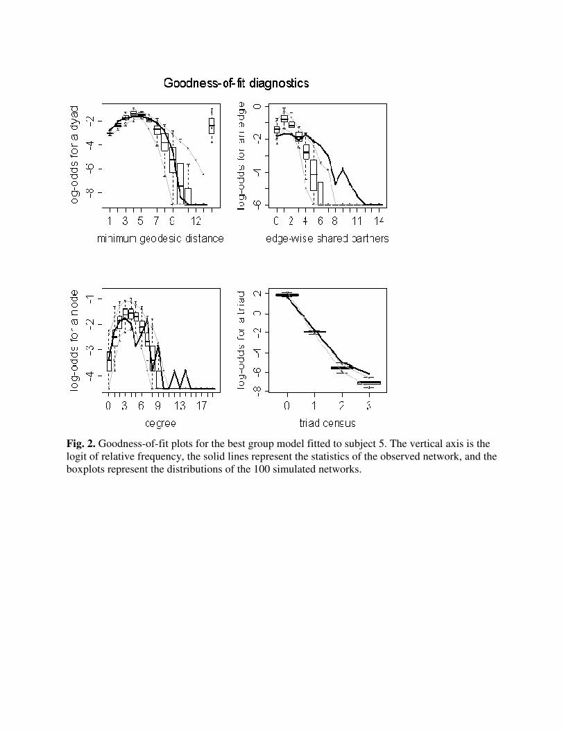
Fig. 2. Goodness-of-fit plots for the best group model fitted to subject 5. The vertical axis is the

logit of relative frequency, the solid lines represent the statistics of the observed network, and the

boxplots represent the distributions of the 100 simulated networks.

Fig. 3. Degree distribution plots for the 10 subjects’ networks, the edge-based mean and median

correlation networks, and a) the unconstrained mean ERGM and median ERGM simulation-

based networks and b) the degree-constrained mean ERGM and median ERGM simulation-based

networks. The upper panels show the mean networks and the lower panels the median networks.

Fig. 4. Nodal distributions of path length (L), clustering coefficient (C), global efficiency (Eglob),

and local efficiency (Eloc) for the 10 subjects’ networks, mean and median correlation networks,

and degree-constrained mean ERGM network #5 and median ERGM network #4.

Fig. 5. Harel-Koren Fast Multiscale graphs for

degree-constrained mean ERGM

Koren Fast Multiscale graphs for the mean and median correlation

ERGM network #5, and degree-constrained median ERGM

networks,

median ERGM network #4.