An Exploratory Model to Investigate the Dynamics of the World Energy System A Biophysical Economics Perspective

M.Sc. Thesis

S. Ahmad Reza Mir Mohammadi K.

August 2013

M.Sc. Thesis

An Exploratory Model to Investigate the Dynamics of the World Energy System: A Biophysical Economics Perspective

Author Seyed Ahmad Reza Mir Mohammadi Kooshknow Student No. 4183452 University Delft University of Technology Program Systems Engineering, Policy Analysis and Management Faculty Technology, Policy and Management Graduation Section Energy & Industry Company Energy For One World Co.

Graduation Committee Prof. Dr. Ir. P. M. Herder, Section Energy & Industry

Dr. Ir. G. P. J. Dijkema, Section Energy & Industry Dr. Ir. A. F. Correlje, Section Economics of Infrastructures Dr. A. Ghorbani, Section Energy & Industry Ir. A. Kamp, Energy For One World Co.

I

Acknowledgments

In the name of God, the Compassionate, the Merciful

This document is the main result of my M.Sc. Thesis project for the master’s program Systems Engineering, Policy Analysis and Management (SEPAM) at Delft University of Technology. The project was conducted as an internship in “Energy for One World” program.

First of all, I would like to express my deepest gratitude to God for all His helps and supports in every single moment of my life and in this project. “…Peerless He is, and His kingdom is eternal...The bird of thought cannot soar to the height of His presence, nor the hand of understanding reach to the skirt of His praise” (Saadi 1184-1283 EC)

Second, I would like to thank the faculty of Technology, Policy and Management (TPM) of TU Delft for awarding me a scholarship for master program SEPAM. In addition, I would like to thanks the Energy for One World Company for providing financial support for this research project.

During this project, I was honored to work with a number of TPM staffs. Surely, it is difficult to acknowledge the efforts they have made by just saying words, but I will try. I am deeply grateful to Professor Paulien Herder for her supervision and constructive comments. I owe a great deal of gratitude to her for all her helps not only in this project, but during my two-year graduate education in TU Delft. Besides, I am truly thankful to my first supervisor, Dr. Gerard Dijkema, for his brilliant supervision and advices during this research. His comments and opinions helped me a lot to learn how to behave as a researcher and manage this research. Moreover, I was lucky to work with my second supervisor, Dr. Aad Correlje, in this research project. His critical and constructive comments helped me a lot in framing and conducting this research. In addition, I am greatly Indebted to my daily supervisor, Dr. Amineh Ghorbani. Like others, I believe that she is eager to help people and she compassionately spends time for her students and provides detailed comments. I would like to express my special thanks to her for all her supports, motivations, compassion and comments.

In this project, I was honored to work with Mr. Adriaan Kamp, the founder of “Energy for One World” program and the author of a book with the same name. He initiated the idea of developing a model for the world energy system and pursued this idea. I learnt many things from his book and from our frequent meetings during this journey. I hope this research can be one step forward in helping his program and his objective of “having a world in which all people enjoy sufficient energy at affordable price”.

I am also thankful to Michael Dale for the providing details of his interesting model, GEMBA, for me. Details of GEMBA really enhanced the speed of this research in some implementation steps. GEMBA is a great model and I believe more works can be done on its basis.

II

I also would like to thank Dr. Igor Nikolic for his instructions in the courses of agent-based modeling in TPM faculty. I believe he played an important role in my interest in agent-based modeling. I also like to thank Andrew Bollinger for our scientific discussions and his comments on some parts of this research.

Moreover, during my life in Delft, I have been blessed with many great friends. I would like to thank them all here; however I cannot mention the name of all my friends one by one. Among my friends at TPM, I would like to thank Amir Ahmad Bornaee, Hamed Aboolhadi, Mohammadbashir Sedighi, Yashar Araghi, and Maryam Hashemi Ahmadi who were always available when I needed them. Also, I would like to thank Guy, Bert, Reinier, Panagiotis, Jane, Jeroen(s), Ruben(s), Rutger, Robert Jan and Trung who helped me a lot during the master program.

Last but not least, my deepest gratitude goes to my beloved parents and also to my lovely sisters Fatemeh, Zahra, and Marzieh for their emotional supports, prayers and encouragements during all stages of life and my education.

S. Ahmad Reza Mir Mohammadi K. Delft, August 2013

III

Abstract Energy is inherent part of our current life. No one can imagine living without it. It has changed the lifestyle of people and it will continue to do so in future. About 80% of current global total primary energy supply belongs to non-renewable resources. It is also expected that non-renewable resources dominate in total primary energy supply in next decades. The world is moving towards scarcity in non-renewable energy resources. Most studies about the world energy-economy system use standard economic theories. These theories do not include limitations of natural resources and the environment.

Biophysical economics theory considers the relation between economy and natural resources. It has been used as the basis of various energy-economy models. However, those models have a global view on this system. They do not sufficiently provide insights into the properties and international trading behaviors of energy suppliers and consumers. So, they do not provide insight on the effects of these interactions on the emergent behavior of the global energy system. Biophysical economics has high potential for providing insights into the world energy system. However, the current biophysical models are not capable of representing the world energy system considering trade and other interactions among regions.

Considering this problem the main research question in this thesis is stated as follow:

What can be learnt from biophysical economics theory when it is used for the modeling of the world energy system considering energy trade?

In order to answer this question, the objective of this research is set to develop a model for exploring the behaviors of the world energy system with multiple interacting regions. The theory of complex adaptive systems (CAS) is used to enable biophysical economics theory to consider trade and other interactions among regions. In order to model and analyze the world energy system from both biophysical economics and CAS perspective, agent-based modeling is identified as the most appropriate paradigm.

This thesis provides an analysis of the world energy system from both technical and actor perspectives. The technical analysis aims at describing the main characteristics of and activities in the world energy system. It also identifies the main uncertainties within this system. Actor analysis aims at providing a regional decomposition for the world energy system. To achieve this goal, a number of current regional decompositions are identified. One of those is selected on the basis of a number of criteria. This research uses the 11-region decomposition of (IIASA, 2012b)

To develop the objective model, a two-step approach is used. In the first step, the aggregated world energy model is developed without considering energy trade. In the second step, the multi-region world energy model is developed considering energy trade. The aggregated world energy model is the implementation of the most recent biophysical economics model in the literature, GEMBA by (M. A. J. Dale, 2010), in NetLogo. The multi-region model inherits all characteristics of the first model. However,

IV

it considers each world region as a world and facilitates the energy trade among them. The models are evaluated by comparison with historical data and literature.

The multi-region model shows that the energy trade can be modeled and explored using the biophysical economics perspective. Since it includes energy price as a parameter, it also shows that energy trade can be an interface between biophysical economics and standard economics as well.

In addition, exploratory experiments show that size of energy trade for regions is low in comparison to their total production/consumption. Moreover, they show that the size of total energy trade will peak and decline. It is because energy trade mostly belongs to non-renewable energy and the production of non-renewables will peak and decline in the future. In addition, it shows that lower energy trade can increase the share of production of energy.

Key Words: Biophysical economics, Agent-based modeling, world energy system, world regions, exploratory modeling

V

Table of Contents Abstract ........................................................................................................................................................ III

List of Figures ............................................................................................................................................. VIII

List of Tables ................................................................................................................................................. X

1 Introduction .......................................................................................................................................... 1

1.1 Research Problem ......................................................................................................................... 1

1.1.1 State of the World Energy System ........................................................................................ 1

1.1.2 End of Easy Oil ....................................................................................................................... 2

1.1.3 Biophysical Economics .......................................................................................................... 3

1.2 Research Questions....................................................................................................................... 4

1.3 Research Objective ....................................................................................................................... 5

1.4 Research Approach ....................................................................................................................... 5

1.4.1 Research Process................................................................................................................... 7

1.5 Outline of Thesis ......................................................................................................................... 10

2 Theoretical Perspective....................................................................................................................... 11

2.1 Economic world views................................................................................................................. 11

2.1.1 Standard economics ............................................................................................................ 11

2.1.2 Biophysical Economics ........................................................................................................ 13

2.2 Complex Adaptive System .......................................................................................................... 17

2.2.1 Characteristics of CAS ......................................................................................................... 18

2.2.2 Modeling ............................................................................................................................. 20

2.3 Conclusion ................................................................................................................................... 24

3 Analysis of the World Energy System ................................................................................................. 26

3.1 System Perspective ..................................................................................................................... 26

3.1.1 World Energy system .......................................................................................................... 27

3.1.2 World Energy Resources ..................................................................................................... 28

3.1.3 End of Easy oil ..................................................................................................................... 34

3.1.4 Conclusion ........................................................................................................................... 36

3.2 Actor Perspective ........................................................................................................................ 38

3.2.1 Micro Analysis ..................................................................................................................... 38

3.2.2 Macro Analysis .................................................................................................................... 40

VI

3.2.3 Conclusion ........................................................................................................................... 49

4 The First Model: Aggregated World Energy Model ............................................................................ 50

4.1 Model Development ................................................................................................................... 50

4.1.1 Introduction to GEMBA ....................................................................................................... 50

4.1.2 Formalization of Concept and Model ................................................................................. 57

4.1.3 Implementation .................................................................................................................. 76

4.1.4 Evaluation ........................................................................................................................... 77

4.2 Experimentation ......................................................................................................................... 79

4.2.1 Design of Experiments ........................................................................................................ 79

4.2.2 Results ................................................................................................................................. 80

4.3 Conclusion ................................................................................................................................... 88

5 The Second Model: Multi-Region World Energy Model ..................................................................... 90

5.1 Model Development ................................................................................................................... 91

5.1.1 Formalization of Concept and Model ................................................................................. 91

5.1.2 Implementation ................................................................................................................ 101

5.1.3 Evaluation of the multi-region model ............................................................................... 104

5.2 Experimentation ....................................................................................................................... 105

5.2.1 Design of Experiments ...................................................................................................... 105

5.2.2 Experiments Results .......................................................................................................... 107

5.3 Conclusion ................................................................................................................................. 113

6 Conclusion ......................................................................................................................................... 115

6.1 Overview ................................................................................................................................... 115

6.2 Research Outcomes .................................................................................................................. 116

6.2.1 Using biophysical economics to develop models ............................................................. 117

6.2.2 Main characteristics of the world energy system ............................................................. 117

6.2.3 Decomposing the world energy system ............................................................................ 118

6.2.4 Modeling Requirements to explore the world energy system ......................................... 119

6.2.5 Biophysical economics theory for the modeling of the world energy system ................. 120

6.3 Reflection .................................................................................................................................. 121

6.3.1 Adoption of biophysical economics as theoretical perspective ....................................... 121

6.3.2 Combination of biophysical economics and CAS in ABM ................................................. 123

6.3.3 Combination of ABM and SD ............................................................................................ 123

VII

6.3.4 Assumption is the design of the Multi-Region World Energy Model ............................... 124

6.3.5 Policy Implications of Outcomes ....................................................................................... 126

6.4 Future Work .............................................................................................................................. 126

6.4.1 Make some parameters endogenous ............................................................................... 126

6.4.2 Automating calibration of the model ............................................................................... 126

6.4.3 Link the model to other models ........................................................................................ 127

Appendix I. USGS/USBM System for classification of Resources .............................................................. 128

Appendix II. Energy Circuit Language ........................................................................................................ 130

References ................................................................................................................................................ 131

VIII

List of Figures Figure 1 Total Primary Energy Supply in Mtoe - Picture from (IEA, 2012a) .................................................. 2 Figure 2 Conceptual view of relation of economic concepts and the Hubbert curve for global oil use – Picture from (C. A. S. Hall & Klitgaard, 2012) ................................................................................................ 3 Figure 3 Conceptual Framework for Complex Adaptive Systems – Picture from (Van Der Lei et al., 2010) 6 Figure 4 Research Methodology ................................................................................................................... 8 Figure 5 The neoclassical view of economics - Picture from (C. A. S. Hall & Klitgaard, 2012) .................... 12 Figure 6 The biophysical systems model of the economy from (Gilliland, 1975) – Picture from (M. Dale, 2010) ........................................................................................................................................................... 16 Figure 7 Approaches (Paradigms) in Simulation Modeling on Abstraction Level Scale- picture from (Borshchev & Filippov, 2004) ...................................................................................................................... 21 Figure 8 Population in WROLD3 .................................................................................................................. 22 Figure 9 Structure of an Agent-based Model - Picture from (van Dam et al., 2013) .................................. 23 Figure 10 Functional and Product decomposition of the world energy system – picture from (GEA, 2012) .................................................................................................................................................................... 27 Figure 11 Energy flow across the energy system- Picture from (C. A. S. Hall, Cleveland, & Kaufmann, 1992) ........................................................................................................................................................... 28 Figure 12 World Primary Energy Consumption in 2011 ............................................................................. 29 Figure 13 Share of resources in total primary energy production in US- Source IEA- Picture from (Koonin, 2005) ........................................................................................................................................................... 29 Figure 14 Global energy flows (in EJ) from primary to useful energy by primary resource input, energy carrier (fuels), and end-use sector applications in 2005, Picture from (GEA, 2012), ALS= Auto consumption, losses, stock changes, OTF= Other transformation to secondary fuels............................... 30 Figure 15 Simple Representation of Resource Envelope - Picture from (JAFFE et al., 2011) ..................... 31 Figure 16 USGS/USBM System (USGS, 1981) .............................................................................................. 31 Figure 17 Distribution of estimates for URR of various non-renewable sources ....................................... 32 Figure 18 A field-by-field plot of Norwegian oil production - picture from (Aleklett et al., 2010) ............. 35 Figure 19 Distribution of actors over energy value chain ........................................................................... 40 Figure 20 IIASA 11 Regions - data from (IIASA, 2012b) ............................................................................... 43 Figure 21 IEA World Energy Model Regions – data from (IEA, 2012b) ....................................................... 43 Figure 22 Distribution of oil reserves over the world (numbers in billions of barrels) – Picture from (EIA) .................................................................................................................................................................... 44 Figure 23 Diversity in GDP per capita across the world - data from (CIA, 2012) - picture from (indexmundi), data for Russia in not included ............................................................................................ 45 Figure 24 Diversity in energy consumption over the world - Picture from (eia, 2013) .............................. 46 Figure 25 Energy use per capita vs. GNI per capita PPP of 126 countries in 2010 - data from (WorldBank) .................................................................................................................................................................... 46 Figure 26 Relationship between the energy sector and the rest of economy - Picture from (M. A. J. Dale, 2010) ........................................................................................................................................................... 51 Figure 27 Causal Loop diagram in GEMBA .................................................................................................. 52

IX

Figure 28 Structure of the GEMBA energy-economy model as an energy circuit diagram – Picture from (M. A. J. Dale, 2010) .................................................................................................................................... 54 Figure 29 Dynamic EROI function and its components: A. the technological progression function B. Resource quality function C. Dynamic EROI function - Picture From (Michael Dale et al., 2011) .............. 57 Figure 30 Overview of the Global Energy system ....................................................................................... 59 Figure 31 Information inputs and Outputs of Renewable Suppliers .......................................................... 61 Figure 32 Information inputs and outputs of Non-Renewable Suppliers ................................................... 63 Figure 33 Information inputs and outputs of Energy Consumers .............................................................. 64 Figure 34 Information inputs and outputs of Energy Dispatchers .............................................................. 66 Figure 35 Sequence Diagram ...................................................................................................................... 68 Figure 36 Results of GEMBA ....................................................................................................................... 77 Figure 37 Results of Aggregated World Energy Model ............................................................................... 77 Figure 38 Aggregated World Energy Model - Energy Yield in years 1800-2200 ......................................... 81 Figure 39 Aggregated World Energy Model - Capital stock in years 1800-2200 ........................................ 82 Figure 40 Changes in Energy Yield of renewable resources and conventional non-renewable resoruces with respect to uncertain Peak EROI .......................................................................................................... 82 Figure 41 Total capital of Energy sector and Consumer sector with respect to uncertain Peak EROI ....... 83 Figure 42 Distribution of Total Renewable Production in 2030 under URR-TP uncertainty ...................... 84 Figure 43 Distribution of Total Conventional Non-Renewable Production in 2030 under URR-TP uncertainty .................................................................................................................................................. 85 Figure 44 Distribution of Total Unconventional Renewable Production in 2030 under URR-TP uncertainty .................................................................................................................................................................... 85 Figure 45 Distribution of Total Renewable Production in 2030 ................................................................. 87 Figure 46 Total Energy Yield under URR-TP uncertainty ............................................................................ 88 Figure 47 Blocks for calculating the qualitative geographical distance – The Map from (IIASA, 2012a) ... 92 Figure 48 Agents in Multi-Region World Energy Model ............................................................................. 93 Figure 49 Information inputs and outputs of Energy Dispatchers .............................................................. 95 Figure 50 Total global renewable production _ Comparison of historical data and multi-region model output ....................................................................................................................................................... 104 Figure 51 Total global non-renewable production _ Comparison of historical data and multi-region model output ............................................................................................................................................ 105 Figure 52 Multi-Region model output ...................................................................................................... 107 Figure 53 Trajectory of energy trade during 1950-2150 .......................................................................... 108 Figure 54 Energy export of regions ........................................................................................................... 109 Figure 55 Total Energy trade with respect to price and trust ................................................................... 110 Figure 56 Distribution of Total Conventional Non-Renewable Energy Yield with respect to price and Trust in 2030 ...................................................................................................................................................... 111 Figure 57 Distribution of Total Unconventional Non-renewable Energy Yield with respect to price and trust in 2030 .............................................................................................................................................. 112 Figure 58 Distribution of Total Renewable Net Energy Yield with respect to price and Trust in 2030 .... 113

X

List of Tables Table 1 Comparison of system dynamics modeling and agent based modeling – From (Bollinger, 2010) 24 Table 2 summary of distribution parameters for various non-renewable sources – Data from (Michael Dale, 2012) .................................................................................................................................................. 32 Table 3 Fossil Fuels and Uranium Reserves and Resources - Data from (GEA, 2012) – Resource data is not cumulative and do not include reserves ..................................................................................................... 33 Table 4 Renewable energy flows, potentials and utilization – data from (GEA, 2012) - data are energy input-data, not output ................................................................................................................................ 34 Table 5 IIASA 11 regions in Bradshaw framework ...................................................................................... 47 Table 6 Attributes of Renewable Suppliers ................................................................................................. 59 Table 7 States and Attributes of Non-Renewable Suppliers ....................................................................... 61 Table 8 States and attributes of Energy Consuemrs ................................................................................... 63 Table 9 States and Attributes of Energy Dispatchers ................................................................................. 65 Table 10 Action Sequence ........................................................................................................................... 66 Table 11 GEMBA Parameters from (M. Dale et al., 2012) .......................................................................... 76 Table 12 Uncertainties in Aggregated World Energy Model and their ranges ........................................... 80 Table 13 States and Attributes of Energy Dispatchers ............................................................................... 94 Table 14 States and Attributes of Contracts ............................................................................................... 95 Table 15 States and Attributes of the Environment ................................................................................... 96 Table 16 Share of regions from global URR .............................................................................................. 101 Table 17 Share of regions from global TP ................................................................................................. 102 Table 18 Trust Coefficient ......................................................................................................................... 103 Table 19 Geographical Distance................................................................................................................ 104 Table 20 Uncertainties and their ranges in experiments of multi-region model ..................................... 106

1

1 Introduction Energy is an inherent part of human life. No one can imagine living without it. Different types of energy are being used all over the world for warming, lighting, transportation, manufacturing, and other purposes. Without energy, even the basic needs of human beings cannot be provided completely.

People deserve to have a life at a reasonable quality level and energy is essential for such a life. No one has more right than the others. So, from ethical point of view, everyone has right to have access to sufficient and affordable energy. But, it is doubtful whether the current energy system in the world can provide such energy for people.

Currently, substantial part of global energy demand is supplied from the fossil fuels. Many infrastructures and industries have been developed on the basis of these fuels all over the world. On the other hand, reserves of fossil fuels are diminishing. Many scientists believe that production rate of conventional oil is reaching its peak. At the same time, the world’s population is increasing and energy-hungry modern lifestyle is getting popular. Therefore, the global demand for the energy is expected to increase. Any gap between energy supply and demand can influence the availability and accessibility of the energy. So, it seems that conventional non-renewable sources of energy cannot supply the world’s demand in future.

Helping future generations to enjoy energy at sufficient quantity and affordable price is the motivation of this research. In order to achieve such goals, deliberate policies should be developed and adopted. Development of policies requires appropriate images about the functioning of systems. This research aims at design and development of a model which may provide one of these images.

1.1 Research Problem

1.1.1 State of the World Energy System Energy is one of the essential factors of human life. People use energy to cook their foods, to warm up or cool down their houses, to move their vehicles, etc. Energy is “the go of things” (Maxwell, 1950) and no work can be done without it.

The level of energy production and consumption has changed during years. The level of energy consumption is different from one country to another. In general, it has changed the lifestyle of people and it will continue to do so in future. People use machines to get their jobs done instead of using their body or animals like before. It is because the work which can be done by a machine and a little fuel is equal to the work which can be done by many human beings at the same time. For example, the refined product from one barrel of oil can produce as much work as one can get from 12 people all working for a year. Surprisingly, the average production cost for that barrel of oil is about 1 dollar in a country like Iraq (Gelpke, McCormack, & Caduff, 2006). The energy system has evolved significantly all over the world during the last century. It also has shaped the life of human beings.

2

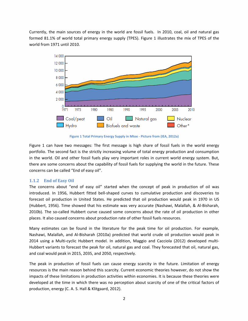
Currently, the main sources of energy in the world are fossil fuels. In 2010, coal, oil and natural gas formed 81.1% of world total primary energy supply (TPES). Figure 1 illustrates the mix of TPES of the world from 1971 until 2010.

Figure 1 Total Primary Energy Supply in Mtoe - Picture from (IEA, 2012a)

Figure 1 can have two messages: The first message is high share of fossil fuels in the world energy portfolio. The second fact is the strictly increasing volume of total energy production and consumption in the world. Oil and other fossil fuels play very important roles in current world energy system. But, there are some concerns about the capability of fossil fuels for supplying the world in the future. These concerns can be called “End of easy oil”.

1.1.2 End of Easy Oil The concerns about “end of easy oil” started when the concept of peak in production of oil was introduced. In 1956, Hubbert fitted bell-shaped curves to cumulative production and discoveries to forecast oil production in United States. He predicted that oil production would peak in 1970 in US (Hubbert, 1956). Time showed that his estimate was very accurate (Nashawi, Malallah, & Al-Bisharah, 2010b). The so-called Hubbert curve caused some concerns about the rate of oil production in other places. It also caused concerns about production rate of other fossil fuels resources.

Many estimates can be found in the literature for the peak time for oil production. For example, Nashawi, Malallah, and Al-Bisharah (2010a) predicted that world crude oil production would peak in 2014 using a Multi-cyclic Hubbert model. In addition, Maggio and Cacciola (2012) developed multi-Hubbert variants to forecast the peak for oil, natural gas and coal. They forecasted that oil, natural gas, and coal would peak in 2015, 2035, and 2050, respectively.

The peak in production of fossil fuels can cause energy scarcity in the future. Limitation of energy resources is the main reason behind this scarcity. Current economic theories however, do not show the impacts of these limitations in production activities within economies. It is because these theories were developed at the time in which there was no perception about scarcity of one of the critical factors of production, energy (C. A. S. Hall & Klitgaard, 2012).

3

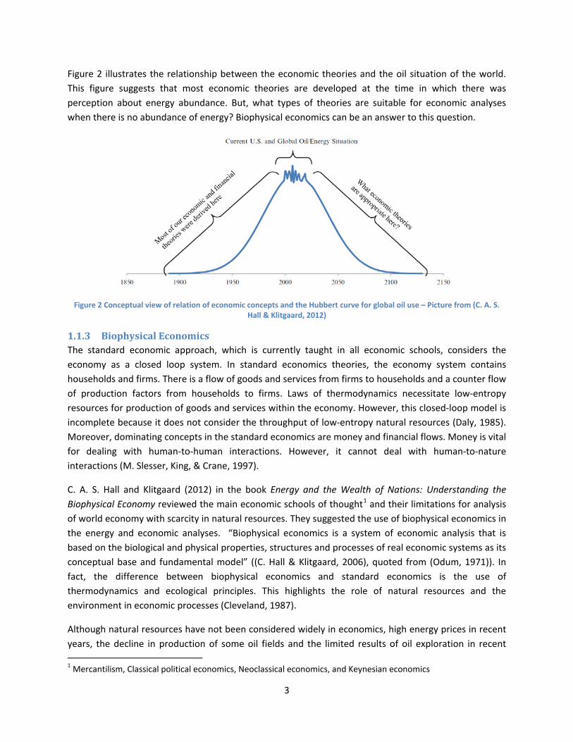
Figure 2 illustrates the relationship between the economic theories and the oil situation of the world. This figure suggests that most economic theories are developed at the time in which there was perception about energy abundance. But, what types of theories are suitable for economic analyses when there is no abundance of energy? Biophysical economics can be an answer to this question.

Figure 2 Conceptual view of relation of economic concepts and the Hubbert curve for global oil use – Picture from (C. A. S. Hall & Klitgaard, 2012)

1.1.3 Biophysical Economics The standard economic approach, which is currently taught in all economic schools, considers the economy as a closed loop system. In standard economics theories, the economy system contains households and firms. There is a flow of goods and services from firms to households and a counter flow of production factors from households to firms. Laws of thermodynamics necessitate low-entropy resources for production of goods and services within the economy. However, this closed-loop model is incomplete because it does not consider the throughput of low-entropy natural resources (Daly, 1985). Moreover, dominating concepts in the standard economics are money and financial flows. Money is vital for dealing with human-to-human interactions. However, it cannot deal with human-to-nature interactions (M. Slesser, King, & Crane, 1997).

C. A. S. Hall and Klitgaard (2012) in the book Energy and the Wealth of Nations: Understanding the Biophysical Economy reviewed the main economic schools of thought1 and their limitations for analysis of world economy with scarcity in natural resources. They suggested the use of biophysical economics in the energy and economic analyses. “Biophysical economics is a system of economic analysis that is based on the biological and physical properties, structures and processes of real economic systems as its conceptual base and fundamental model” ((C. Hall & Klitgaard, 2006), quoted from (Odum, 1971)). In fact, the difference between biophysical economics and standard economics is the use of thermodynamics and ecological principles. This highlights the role of natural resources and the environment in economic processes (Cleveland, 1987).

Although natural resources have not been considered widely in economics, high energy prices in recent years, the decline in production of some oil fields and the limited results of oil exploration in recent 1 Mercantilism, Classical political economics, Neoclassical economics, and Keynesian economics

4

years show the importance of the role of natural resources in economics. Therefore, biophysical economics can be considered as a relevant backbone to deal with these problems.

To better understand the world energy system, biophysical economics has been used in a number of energy supply models. In his classification of the global energy supply models, M. Dale (2010) classified models into three categories: “deterministic models with growth curves”, “energy-economy optimization models”, and “physical resource accounting models”. The renowned example of models in the first category is the Hubbert curve. The famous examples of the energy-economy optimization models are MESSAGE (Schrattenholzer, 1981), MARKAL (Hamilton et al., 1992) and, WEM (IEA, 2012b).

Also, famous examples of the third category are WORLD3 (D. H. Meadows, 1972), ECCO (Malcolm Slesser, 1992), and Dynamic Energy (J. T. Baines & Peet, 1983). WROLD3, ECCO, and Dynamic Energy model are system dynamics model which use biophysical perspective. Recently, M. Dale, Krumdieck, and Bodger (2012) developed a system dynamics model (GEMBA) for analysis of the global energy system from biophysical economic perspective. GEMBA simulates the energy yield of different energy sources from 1800 until 2200.

Although these models provide valuable insights into the world energy system, there is one thing in common among all resource accounting models. Their level of abstraction and aggregation is the “world”. These models cannot show the (geographical) distribution of energy production (or consumption) across the world. Instead, they provide aggregated information for the whole world. The geographical diversity of the world energy system can influence its behaviors. Some regions own large reserves of fossil fuels and flow of renewable resources whereas they consume little energy. On the other hand, some regions consume too much energy whereas they do not have sufficient energy endowments. Consequently, energy trade has emerged among regions and countries. One of the drawbacks of the current models is that they do not consider energy trade and other types of interaction among countries.

Following the stated arguments, the research problem can be stated as follows:

Biophysical economics can be a useful theory to analyze the world energy system which is why it is used as the basis of various biophysical models. However, the current models are all process oriented and only have a global view on this system. They do not sufficiently provide insights into the properties and trading behaviors of energy suppliers and consumers. Consequently, they don’t provide insight about the effects of these interactions on the emergent behaviors of the global energy system.

1.2 Research Questions Considering the stated problem, the main research question can be formulated as follow:

What can be learnt from biophysical economics theory when it is used for the modeling of the world energy system considering energy trade?

In order to answer this question, the following sub-questions need to be answered:

5

1. To what extent can biophysical economics theory be used to develop models for exploring trade in the global energy system?

2. What are the main characteristics and activities in the world energy system from biophysical economics perspective?

3. How can the world energy system be decomposed into different trading regions? 4. What are the requirements to design a model to explore the world energy system considering

energy trade?

1.3 Research Objective Considering the stated research problem and the research questions, the objective of this research can be stated as follows:

To develop a model using the biophysical economics theory in order to explore the behaviors of the world energy system with multiple interacting regions

1.4 Research Approach As it is stated in the research objective, this research aims at including interactions and trade among different world regions in biophysical economics analysis. In such analysis, the holistic behavior of the world energy system depends not only on the behavior of each country or region, but also on the interactions and trade among them.

All regions produce and consume energy. But, there is considerable diversity among world regions regarding the energy production capabilities, and energy requirements. There is no central control or governance over energy sector of the world. Nonetheless, the aforementioned disparities among regions have caused the emergence of global energy trade and other types of interactions among them. These characteristics of the world energy system can classify it as a complex adaptive system.

J. H. Holland defines complex adaptive systems as:

“… a dynamic network of many agents (which may represent cells, species, individuals, firms, nations) acting in parallel, constantly acting and reacting to what the other agents are doing. The control of a CAS tends to be highly dispersed and decentralized. If there is to be any coherent behavior in the system, it has to arise from competition and cooperation among the agents themselves. The overall behavior of the system is the result of a huge number of decisions made every moment by many individual agents.” (Waldorp, 1992)

Currently, the global energy system can be considered as a dynamic network of many regions, institutions and actors. Actors and regions can produce and consume energy. If they have surplus of energy production, they can export it to regions or actor who require that energy. The behaviors of the whole global energy system emerge from the interactions among all the agents. Being a complex adaptive system (CAS), the world energy system owns the common characteristics of CASs. Dynamics and instability are some examples of such characteristics (Van Der Lei, Bekebrede, & Nikolic, 2010). Therefore, in addition to biophysical economics theory, the theory of CAS can add insights into analysis and modeling of the world energy system.

6

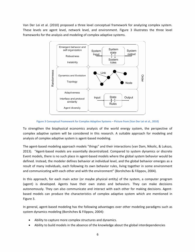
Van Der Lei et al. (2010) proposed a three level conceptual framework for analyzing complex system. These levels are agent level, network level, and environment. Figure 3 illustrates the three level frameworks for the analysis and modeling of complex adaptive systems.

Figure 3 Conceptual Framework for Complex Adaptive Systems – Picture from (Van Der Lei et al., 2010)

To strengthen the biophysical economics analysis of the world energy system, the perspective of complex adaptive system will be considered in this research. A suitable approach for modeling and analysis of complex adaptive system is agent-based modeling.

The agent-based modeling approach models “things” and their interactions (van Dam, Nikolic, & Lukszo, 2013). “Agent-based models are essentially decentralized. Compared to system dynamics or discrete Event models, there is no such place in agent-based models where the global system behavior would be defined. Instead, the modeler defines behavior at individual level, and the global behavior emerges as a result of many individuals, each following its own behavior rules, living together in some environment and communicating with each other and with the environment” (Borshchev & Filippov, 2004).

In this approach, for each main actor (or maybe physical entity) of the system, a computer program (agent) is developed. Agents have their own states and behaviors. They can make decisions autonomously. They can also communicate and interact with each other for making decisions. Agent-based models can produce the characteristics of complex adaptive system which are mentioned in Figure 3.

In general, agent-based modeling has the following advantages over other modeling paradigms such as system dynamics modeling (Borshchev & Filippov, 2004):

• Ability to capture more complex structures and dynamics. • Ability to build models in the absence of the knowledge about the global interdependencies

7

• Higher maintainability (model refinements normally result in very local, not global changes)

Because of these advantages and capabilities, agent-based modeling will be considered as the main modeling approach in this research. Details of modeling paradigms such as system dynamics, agent-based modeling and their comparison will be provided in Chapter 2.

1.4.1 Research Process In order to develop an agent-based model and answer the research questions, a number of phases should be completed. The research process in this research can be divided into five main phases. Each phase consists of a number of steps in the research. The main research phases in this research are:

• Theoretical Perspective • System Analysis • Model Development • Experimentation • Exploration and conclusion

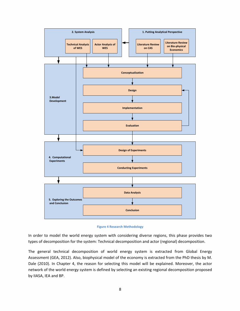
The research process is depicted in Figure 4.

Theoretical perspective The objective of Phase 1 is elaborating on the theories which are used in this research. In this phase, the theoretical perspectives of the research are delineated. Combination of “biophysical economics” theory and “complex adaptive systems” theory constitute the theoretical foundations of this research. So, literature review on these two theories is the dominating part of this phase. For each theory, the relevant tools and techniques will be explained and introduced. So, literature review on, and comparison between relevant modeling paradigms is one of the important steps in this phase.

System Analysis In phase 2, the research questions “What are the main characteristics and activities in the world energy system from biophysical economics perspective?” and “How can the world energy system be decomposed into different trading regions?” will be answered. In this phase, different characteristics of the world energy system as a socio-technical system will be analyzed. Socio-technical system can be seen from “System” (also called technical) and “Actor” perspectives (de Bruijn & Herder, 2009). For both analyses, literature review is the dominating method.

8

2. System Analysis 1. Putting Analytical Perspective

3.Model Development

5. Exploring the Outcomes and Conclusion

4. Computational Experiments

Conclusion

Literature Review on CAS

Literature Review on Bio-physical

Economics

Technical Analysis of WES

Actor Analysis of WES

Conceptualization

Design

Implementation

Evaluation

Design of Experiments

Conducting Experiments

Data Analysis

Figure 4 Research Methodology

In order to model the world energy system with considering diverse regions, this phase provides two types of decomposition for the system: Technical decomposition and actor (regional) decomposition.

The general technical decomposition of world energy system is extracted from Global Energy Assessment (GEA, 2012). Also, biophysical model of the economy is extracted from the PhD thesis by M. Dale (2010). In Chapter 4, the reason for selecting this model will be explained. Moreover, the actor network of the world energy system is defined by selecting an existing regional decomposition proposed by IIASA, IEA and BP.

9

The outputs of this phase are technical and regional decomposition of the world energy system and the data on ultimately recoverable resources of non-renewables and technical potential of renewables.

Model Development In this phase, the research question “What are the requirements to design a model to explore the world energy system with considering energy trade?” will be answered. The objective of this research is exploratory modeling of the world energy system. Exploratory modeling and Analysis (EMA) is a method for researching complex and uncertain systems using computational models (Steve Bankes, 1993). The method is founded on the fact that there is no model fully explaining all behavior of a system correctly and uses uncertainty exploration for making sure that all possibilities are taken into account when researching a particular problem (S Bankes, Walker, & Kwakkel, 2010).

Phase 3 aims at developing such a model. In order to develop such a model, 4 steps are followed. These steps are:

• Conceptualization • Design • Implementation • Evaluation

The implementation step is done in NetLogo software. NetLogo provides the possibility for both agent-based modeling and system dynamics modeling. Being user-friendly and comprehensive documentation were main reasons for selecting this software. In addition, NetLogo can easily be controlled in Java which gives possibility for the use of algorithms for calibration of the model.

The initial concept of global energy modeling from biophysical perspective is obtained from GEMBA model by M. Dale (2010). So, all the steps in Phase 3 are followed twice. First, they are followed for redevelopment of GEMBA model. Then, they are followed for development of a multi-region model.

Computational Experiments Phase 4 consists of two main steps: “Design of experiments” and “Experimentation”. Design of experiments in exploratory modeling is done by considering different ranges for uncertain variables. The uncertain variables are obtained from Phase 2. They are also obtained from definition of trade EROI function in Phase 3. The aim of Phase 4 is studying the emerging pattern in the behavior of system under different ranges of uncertainties.

Exploring outcomes and conclusion Phase 5 aims at recognizing informative patterns in results of the model. The information will be used for answering the main research question. It consists of two main steps: exploring outcomes and drawing conclusions. For the exploration of outcomes, data analysis is the dominating method. For data analysis, R Studio is used. The reasons for using R studio are: 1) capability to handle large volumes of data, 2) being open source software, and 3) comprehensive online documentation.

10

1.5 Outline of Thesis This chapter has introduced the research problem, research questions, and the research approach. The rest of this report is structured as follows:

Chapter 2 elaborates on the first phase of the research process, the theoretical perspectives. First, the biophysical economics theory will be explained. The standard economics and its limitations will be elaborated on and the biophysical view of world economics will be presented. In addition, since this research aims at incorporating energy trade into analysis, the concept of energy trade in biophysical economics will be introduced and explained. Next, the theory of complex adaptive systems (CAS) will be explained. First, the characteristics of CAS will be introduced and its relevant examples in the energy systems will be explained. Then, the relevant modeling approaches for this research will be introduced and compared.

Chapter 3 elaborates on the second phase of the research approach 4, the analysis of the world energy system. This chapter answers two questions “What are the main characteristics and activities in the world energy system from biophysical economics perspective?” and “How can the world energy system be decomposed into different trading regions?” First, the technical analysis will be provided. The world energy system will be defined, and its main characteristics and uncertainties will be elaborated on. Next, the actors of the world energy system will be introduced and a regional decomposition will be suggested for the modeling process.

In this research, two models will be developed. Chapter 4 elaborates on third, fourth and a part of fifth phases in the research methodology for the first model. The development process, experimentation process, and the data analysis for the aggregated world energy model will be provided in this chapter.

Chapter 5 elaborates on third, fourth and the first part of the fifth phases of the research approach for the second model of the research. The Multi-Region World Energy Model is the main model in this research. It will be developed on the basis of aggregated world energy model. The development, experimentation and data analysis for the multi-region model will be presented in chapter 5.

Finally, in Chapter 6, the research process and the main outcomes will be reviewed and the main conclusions will be drawn. In this chapter a number of features in this research will be reflected on and suggestions for future work will be presented.

11

2 Theoretical Perspective In Chapter 1 , the research problem, research questions, and research approach were presented and explained. In this chapter, the theoretical perspectives of this research namely biophysical economics and complex adaptive systems (CAS) and their analytical tools will be explained.

In section 2.1, two different economic worldviews will be explained and compared. The first world view is called standard economics which is widely taught in universities and business schools. In this section, the limitations of standard economic will be explained and biophysical economics, as a different perspective, will be introduced. In this section, the history of biophysical economics will also be reviewed. Then the biophysical economic model will be presented and explained. Finally, since the research questions address energy trade, the current tools and technique for assessment of the energy trade from biophysical perspective will be introduced and explained.

In section 2.2, the theory of complex adaptive systems will be introduced and reviewed. Afterwards, the relevant modeling paradigms to model the world energy system from the aforementioned perspectives will be introduced and analyzed. Since agent-based modeling (ABM) is the main simulation approach used to analyze CAS, it will be explained in more detail. Further justification will also be provided on why ABM is more appropriate than system dynamics for this particular research.

Finally, in section 2.3, this chapter will be wrapped up and concluded.

2.1 Economic world views As mentioned in Chapter 1, the main theoretical perspective in this research is biophysical economics. In this section, first, the standard world view of economics will be presented. The term “standard economics” refers to concepts and models which are currently taught in economic schools all over the world. With reviewing the limitations of standard economics, the essence of biophysical economics becomes clear.

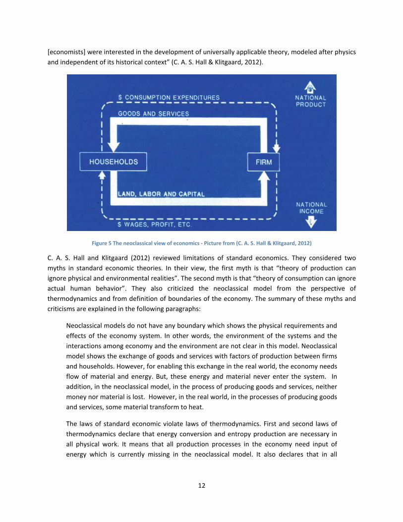
2.1.1 Standard economics The current standard view of the economy is based on neoclassical economics theories. In this view, the economy is divided into two groups: firms and households (Sloman, 2006). Firms produced goods and services while they employ labor, land, and capital. Households are consumers of goods and services. They also supply factors of production to the firms (Sloman, 2006). In neoclassical view, the economy is a self-maintaining circular flow among firms and households (C. A. S. Hall & Klitgaard, 2012). Figure 5 illustrates the neo-classical view on the economy. In this figure, the outflow of firms is the income of the economy. Similarly, the inflow of firms is expenditure of the economy. In this model, the value of expenditure and income of the economy are equal. This refers to equilibrium which is obtained through product and factor markets.

In neoclassical model, the economic relations within the economy can be expressed with a system of mathematical equations. This is one of the main advantages of this model. “The neoclassical

12

[economists] were interested in the development of universally applicable theory, modeled after physics and independent of its historical context” (C. A. S. Hall & Klitgaard, 2012).

Figure 5 The neoclassical view of economics - Picture from (C. A. S. Hall & Klitgaard, 2012)

C. A. S. Hall and Klitgaard (2012) reviewed limitations of standard economics. They considered two myths in standard economic theories. In their view, the first myth is that “theory of production can ignore physical and environmental realities”. The second myth is that “theory of consumption can ignore actual human behavior”. They also criticized the neoclassical model from the perspective of thermodynamics and from definition of boundaries of the economy. The summary of these myths and criticisms are explained in the following paragraphs:

Neoclassical models do not have any boundary which shows the physical requirements and effects of the economy system. In other words, the environment of the systems and the interactions among economy and the environment are not clear in this model. Neoclassical model shows the exchange of goods and services with factors of production between firms and households. However, for enabling this exchange in the real world, the economy needs flow of material and energy. But, these energy and material never enter the system. In addition, in the neoclassical model, in the process of producing goods and services, neither money nor material is lost. However, in the real world, in the processes of producing goods and services, some material transform to heat.

The laws of standard economic violate laws of thermodynamics. First and second laws of thermodynamics declare that energy conversion and entropy production are necessary in all physical work. It means that all production processes in the economy need input of energy which is currently missing in the neoclassical model. It also declares that in all

13

production processes low entropy and useful material is transformed to high entropy and useless material and heat. This fact is missing in the neoclassical model.

Moreover, in the production theory of neoclassical economics, the production model shows the distribution of productive inputs. However, no input can be critical. So, in this model, in the case of limitations in a resource, the resource can be substituted with other inputs. Consequently, the economy can experience scarcity and infinite growth at the same time.

Another criticism about neoclassical economics is about production functions. In the Cobb-Douglas production function ( αβ KALQ = ), the “technology” (A) is independent of factors

of production(Cobb & Douglas, 1928). It is calculated in as a residual in calculation of multi-factor productivity of the economy (Kim, 1990). So, one of the usual assumptions in the standard economics is that there is no diminishing return on the technology. Therefore, technology can compensate deficiencies in factors of production in Cobb-Douglas function. As a result, scarcity in resources itself cannot harm the production. On the other hand, in physics, energy is “the go of things”(Maxwell, 1950) and it is a critical factor of production. C. Hall, Lindenberger, Kümmel, Kroeger, and Eichhorn (2001) used an econometric model to analyze the role of energy next to labor and capital in the economic production in U.S., Germany and Japan. They showed that in all 3 cases, the productive power of energy was more important than labor or capital and nearly an order of magnitude larger than the 5% share of energy cost in the total cost.

These fundamental criticisms about standard economics necessitate seeking for new theories which consider the environment and natural resources in economics.

2.1.2 Biophysical Economics “Biophysical economics is a system of economic analysis that is based on the biological and physical properties, structures and processes of real economic systems as its conceptual base and fundamental model” ((C. Hall & Klitgaard, 2006), quoted from (Odum, 1971)). The difference between biophysical economics and standard economics is the use of thermodynamics and ecological principles. This highlights the role of natural resources and the environment in economic processes (Cleveland, 1987).

2.1.2.1 Literature Review on Biophysical Economics Cleveland (1987) reviewed the evolution of biophysical economics thoughts and trends from the physiocracy era in 1750s until 1980s. He argued that absence of biophysical basis in the modern economic theory has two reasons. The first reason is U.S. had been endowed with enormous volumes of renewables and non-renewable natural resources until then. The second reason is the strong anthropocentric bias of economic theory since the 18th century.

Although biophysical thoughts roots in 1750s, Cleveland (1987) declared that “natural resources” was not considered as a distinct field of analysis economic abstracts or journals until 1960s. The book Limits to Growth by D. H. Meadows (1972) and oil price shocks in 1970s called attention to natural resources. Also, high energy prices in recent years, the decline in production of some oil fields and the limited

14

results of oil exploration in recent years can emphasize on the importance of role of natural resources in economies. Biophysical economics is a candidate theory to deal with these problems.

The main milestones identified by Cleveland (1987) in history of biophysical economics can be classified intro three groups: 1) authors who highlighted the role of natural resources in the economy, 2) authors who highlighted the role of relationship between economy and thermodynamics, and 3) authors who emphasized on importance of energy in economic processes. These three groups can be summarized as summarized as follow:

The role of “Natural resources” was, first, highlighted in the physiocrats’ economic school. Physiocrats believed that the agricultural productivity was the key factor for understanding economic processes. They introduced natural laws, including physical and moral laws, which influenced the economic processes. However, the influence of physiocrats declined after 1760s (Cleveland, 1987).

Criticizing standard economics by means of physics and thermodynamics was done by several scientists. Podolinsky (1883) was the first author who used a thermodynamic perspective for investigating economic processes. He concluded that limits to economic growth lay in physical and ecological laws.

Also, Fredrick Soddy criticized the laws of standard economic with thermodynamics. He believed that theory of economic wealth has biophysical laws as first principles (Soddy, 1922). He also maintained that the flaw in the standard economics was confusion of wealth with debts. He believed that wealth has distinct physical dimension whereas debts is a virtual and imaginary mathematical quantity (Soddy, 1926).

Robert Ayres also used thermodynamics to criticize the standard economics. He mentioned that according to the first law of thermodynamics, low entropy resources which enter the economy system should be degraded and leave it as waste. It was in contradiction with the closed system of standard economics. He also used the second law of thermodynamics to investigate the quality of energy resources. He found that high quality resources are formed by stocks of low entropic value. He also maintained that the positive feedback between decreasing resource quality and the rate of extraction of resources is missing in standard economics (Ayres, 1978) (Ayres & Kneese, 1969) .

Moreover, Georgescu-Roegen (1971) in the book The Entropy Law and the Economic Process mentioned that thermodynamics is the physics of economic value. He called the laws of thermodynamics the "most economic of all physical laws". In his view, standard economics focuses only on the circular exchange of goods and services. He believed that it leaded to the lack of sensitivity of standard economics to changes in the quality of low-entropy stocks of resources.

The third group of moments which are identified by Cleveland (1987) belongs to authors who highlighted the role of energy in economies. Cottrell (1955) performed a comprehensive investigation about the role of energy in human societies. He emphasized two points which influenced the relation between energy quality, economy and social development: 1) surplus energy2, and 2) connection

2 The difference between the energy delivered by a process and the energy invested in the delivery process

15

between amounts of energy used to subsidize the efforts of labor and productivity of labor. He mentioned that economic and social growth after industrial revolution is mainly because the energy surplus provided by fossil fuels.

Moreover, Odum (1971) analyzed the system of humans and nature with using of energy flows. He had two major contributions to biophysical economics: 1) energy quality3, and 2) counter-flow of energy and money. He argued that because of variety in energy quality of fuels, societies with access to fuels with higher quality have economic advantage over others.

M. Dale (2010) developed a system dynamics global energy model using biophysical economics theory. He developed a new function for presenting energy return on investment. Initially, the concept of energy return on investment (EROI) was first introduced (Bullard Iii & Herendeen, 1975). However, M. Dale (2010) developed a dynamic EROI function with two components of technological progress and resource quality. He explored the behavior of the global energy system during years 1800 – 2200 from biophysical economics perspective.

Energy and the Wealth of Nations: Understanding the Biophysical Economy by C. A. S. Hall and Klitgaard (2012) is the most comprehensive textbook in biophysical economics. The authors introduced the state of the world economy with respect to state of the world energy supply (Hubbert Curve). The provided a comprehensive assessment about four main economics schools of thought in the history4 and analyzed to what extent they can answer the main economic problem. They provided extensive theory about how to incorporate energy in the economic analysis. They also provided a scientific framework for performing biophysical economic analysis for nations.

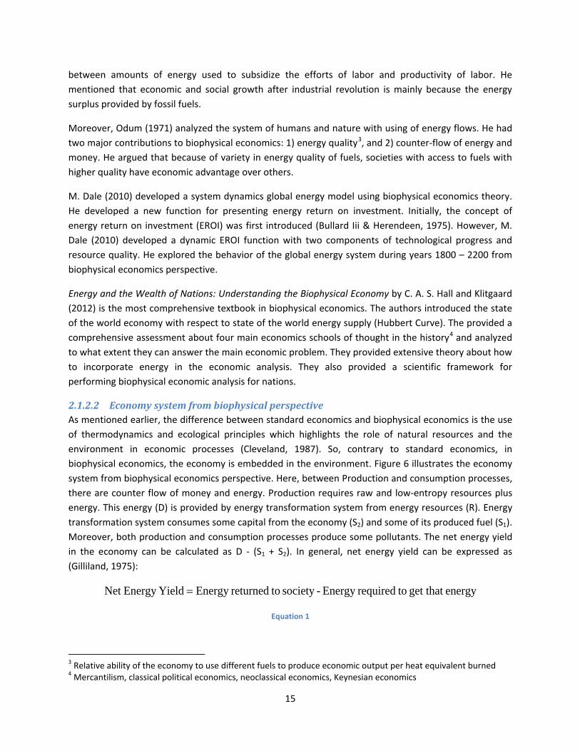
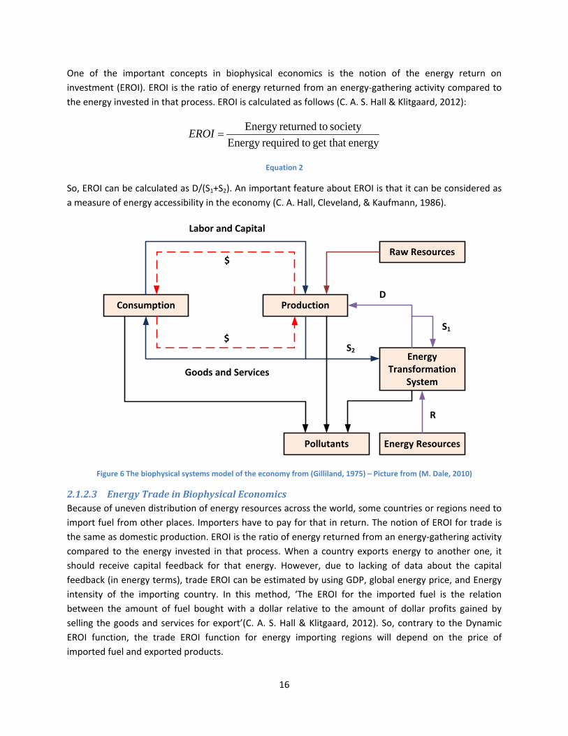
2.1.2.2 Economy system from biophysical perspective As mentioned earlier, the difference between standard economics and biophysical economics is the use of thermodynamics and ecological principles which highlights the role of natural resources and the environment in economic processes (Cleveland, 1987). So, contrary to standard economics, in biophysical economics, the economy is embedded in the environment. Figure 6 illustrates the economy system from biophysical economics perspective. Here, between Production and consumption processes, there are counter flow of money and energy. Production requires raw and low-entropy resources plus energy. This energy (D) is provided by energy transformation system from energy resources (R). Energy transformation system consumes some capital from the economy (S2) and some of its produced fuel (S1). Moreover, both production and consumption processes produce some pollutants. The net energy yield in the economy can be calculated as D - (S1 + S2). In general, net energy yield can be expressed as (Gilliland, 1975):

energyget that torequiredEnergy -society toreturnedEnergy YieldEnergy Net =

Equation 1

3 Relative ability of the economy to use different fuels to produce economic output per heat equivalent burned 4 Mercantilism, classical political economics, neoclassical economics, Keynesian economics

16

One of the important concepts in biophysical economics is the notion of the energy return on investment (EROI). EROI is the ratio of energy returned from an energy-gathering activity compared to the energy invested in that process. EROI is calculated as follows (C. A. S. Hall & Klitgaard, 2012):

energyget that torequiredEnergy society toreturnedEnergy

=EROI

Equation 2

So, EROI can be calculated as D/(S1+S2). An important feature about EROI is that it can be considered as a measure of energy accessibility in the economy (C. A. Hall, Cleveland, & Kaufmann, 1986).

Raw Resources

Energy ResourcesPollutants

ProductionConsumption

Energy Transformation

System

Labor and Capital

$

Goods and Services

$S2

S1

D

R

Figure 6 The biophysical systems model of the economy from (Gilliland, 1975) – Picture from (M. Dale, 2010)

2.1.2.3 Energy Trade in Biophysical Economics Because of uneven distribution of energy resources across the world, some countries or regions need to import fuel from other places. Importers have to pay for that in return. The notion of EROI for trade is the same as domestic production. EROI is the ratio of energy returned from an energy-gathering activity compared to the energy invested in that process. When a country exports energy to another one, it should receive capital feedback for that energy. However, due to lacking of data about the capital feedback (in energy terms), trade EROI can be estimated by using GDP, global energy price, and Energy intensity of the importing country. In this method, ‘The EROI for the imported fuel is the relation between the amount of fuel bought with a dollar relative to the amount of dollar profits gained by selling the goods and services for export’(C. A. S. Hall & Klitgaard, 2012). So, contrary to the Dynamic EROI function, the trade EROI function for energy importing regions will depend on the price of imported fuel and exported products.

17

(R. Kauffman, 1986.) proposed a formula to calculate the EROI of imported oil of U.S.

tboe

boet PE

EEROI,tintensity, *

=

Equation 3

where boeE is energy content of a barrel of oil equivalent (6164 MJ/boe), yintensity,E is energy intensity of

the economy in year t ( MJ/USD/y), and tboeP , is the price of a barrel of oil equivalent in year t (USD).

Energy intensity can be calculated by dividing the whole energy consumption of the economy by the GDP of the country (R. Kauffman, 1986.).

t

tConsumed

GDPE

E ,tintensity, =

Equation 4

The same formulas can be used for all other types of energies such as natural gas and coal. Trade EROI for energy importers is inversely proportional to global energy price and energy intensity. So, when energy price increases, the trade EROI can drop. For example, ‘the EROI for imported oil of U.S. was about 25:1 before 1970s which was very favorable. It dropped to about 9:1 after the first price hike in 1973. It dropped to 3:1 following the second price hike in 1979. This ratio returned to a more favorable level from 1985 to about 2000 as the price of exported goods increased through inflation more rapidly than the price of oil’ ((R. Kauffman, 1986.) quoted from (C. A. S. Hall & Klitgaard, 2012)).

2.2 Complex Adaptive System In the previous section, the necessity of biophysical economics in economic analyses was explained and the overall scope of the economy was presented. This overall presentation can help to analyze the economic and energy problems with a top-down view. In top-down view, some overall rules are defined which influence all elements of the system. In other words, there is a kind of central control over the behavior of different elements of the system. However, in reality, in a large and complex system such as the world economy or the world energy system, there are many elements and actors who behave autonomously without any centralized control. Furthermore, even with the presence of control, actors make autonomous decisions that result in emergent properties of the system that are not directly related to the initial top-down rules. So, limiting analyses to top-down view can ignore how those actors really behave.

A remedy for this problem is bottom-up analysis. In the bottom-up view, the analysis is done at lower level (the level of elements and actors of the system) and the behavior of the system is the result of the states and behaviors at lower levels.

As mentioned in Chapter 1, J. H. Holland defines complex adaptive systems (CAS) as:

18

“… a dynamic network of many agents (which may represent cells, species, individuals, firms, nations) acting in parallel, constantly acting and reacting to what the other agents are doing. The control of a CAS tends to be highly dispersed and decentralized. If there is to be any coherent behavior in the system, it has to arise from competition and cooperation among the agents themselves. The overall behavior of the system is the result of a huge number of decisions made every moment by many individual agents.” (Waldorp, 1992)

On the basis of this definition, the world economy system can be considered as a complex adaptitve system. The agents who influence the emergent behavior of the system are very diverse. Agents could be small firms to countries or regions .

Beinhocker (2006) in the book The Origin of Wealth: Evolution, Complexity, And the Radical Remaking of Economics mentioned that tradition economics considered the economy as a closed equilibrium system which is in contradition with the laws of physics. He suggested “complexity economics” as an alternative for anlaysis of the economy. In his view, considerign the economy as a complex adaptive system can provide new tools and theories for analysis of the economy.

Therefore, in order to add advantages of bottom-up analysis to analyze the world energy system, this reseach combines the theory of biophysical economics and complex adaptive system.

2.2.1 Characteristics of CAS The main generic characteristics of complex adaptive system were mentioned in Figure 3. Here, these characteristics will be elaborated on. As mentioned in Chapter 1, Van Der Lei et al. (2010) proposed a three-level framework for analysis of complex adaptive systems. These levels are: agent level, network level, and system level. Complex adaptive system have different characteristic in each level.

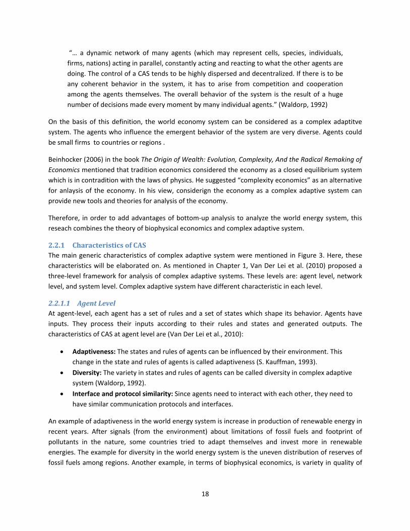
2.2.1.1 Agent Level At agent-level, each agent has a set of rules and a set of states which shape its behavior. Agents have inputs. They process their inputs according to their rules and states and generated outputs. The characteristics of CAS at agent level are (Van Der Lei et al., 2010):

• Adaptiveness: The states and rules of agents can be influenced by their environment. This change in the state and rules of agents is called adaptiveness (S. Kauffman, 1993).

• Diversity: The variety in states and rules of agents can be called diversity in complex adaptive system (Waldorp, 1992).

• Interface and protocol similarity: Since agents need to interact with each other, they need to have similar communication protocols and interfaces.

An example of adaptiveness in the world energy system is increase in production of renewable energy in recent years. After signals (from the environment) about limitations of fossil fuels and footprint of pollutants in the nature, some countries tried to adapt themselves and invest more in renewable energies. The example for diversity in the world energy system is the uneven distribution of reserves of fossil fuels among regions. Another example, in terms of biophysical economics, is variety in quality of

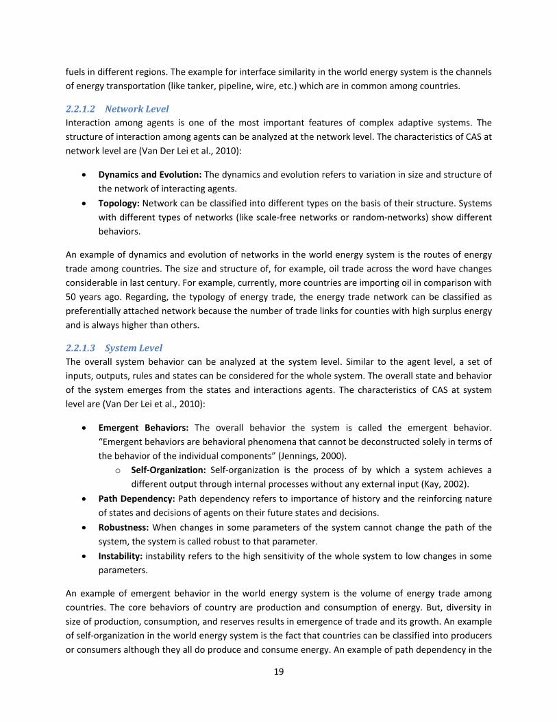
19

fuels in different regions. The example for interface similarity in the world energy system is the channels of energy transportation (like tanker, pipeline, wire, etc.) which are in common among countries.

2.2.1.2 Network Level Interaction among agents is one of the most important features of complex adaptive systems. The structure of interaction among agents can be analyzed at the network level. The characteristics of CAS at network level are (Van Der Lei et al., 2010):

• Dynamics and Evolution: The dynamics and evolution refers to variation in size and structure of the network of interacting agents.

• Topology: Network can be classified into different types on the basis of their structure. Systems with different types of networks (like scale-free networks or random-networks) show different behaviors.

An example of dynamics and evolution of networks in the world energy system is the routes of energy trade among countries. The size and structure of, for example, oil trade across the word have changes considerable in last century. For example, currently, more countries are importing oil in comparison with 50 years ago. Regarding, the typology of energy trade, the energy trade network can be classified as preferentially attached network because the number of trade links for counties with high surplus energy and is always higher than others.

2.2.1.3 System Level The overall system behavior can be analyzed at the system level. Similar to the agent level, a set of inputs, outputs, rules and states can be considered for the whole system. The overall state and behavior of the system emerges from the states and interactions agents. The characteristics of CAS at system level are (Van Der Lei et al., 2010):

• Emergent Behaviors: The overall behavior the system is called the emergent behavior. “Emergent behaviors are behavioral phenomena that cannot be deconstructed solely in terms of the behavior of the individual components” (Jennings, 2000).

o Self-Organization: Self-organization is the process of by which a system achieves a different output through internal processes without any external input (Kay, 2002).

• Path Dependency: Path dependency refers to importance of history and the reinforcing nature of states and decisions of agents on their future states and decisions.

• Robustness: When changes in some parameters of the system cannot change the path of the system, the system is called robust to that parameter.

• Instability: instability refers to the high sensitivity of the whole system to low changes in some parameters.

An example of emergent behavior in the world energy system is the volume of energy trade among countries. The core behaviors of country are production and consumption of energy. But, diversity in size of production, consumption, and reserves results in emergence of trade and its growth. An example of self-organization in the world energy system is the fact that countries can be classified into producers or consumers although they all do produce and consume energy. An example of path dependency in the

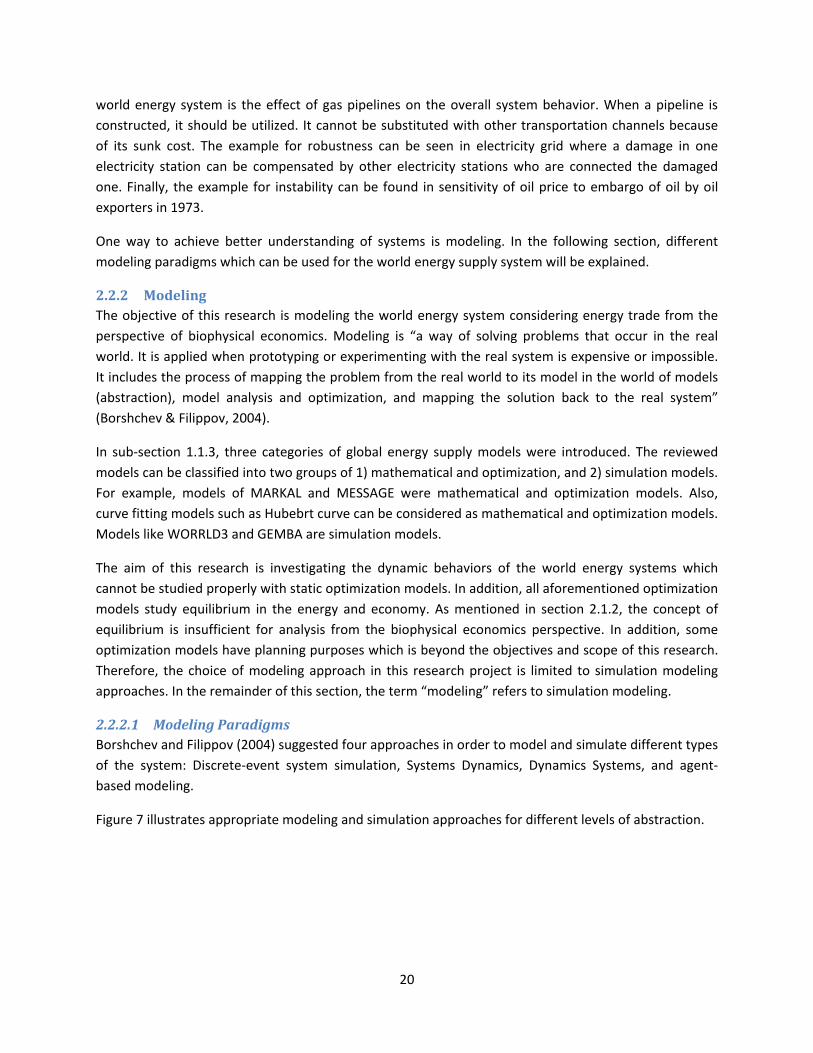
20

world energy system is the effect of gas pipelines on the overall system behavior. When a pipeline is constructed, it should be utilized. It cannot be substituted with other transportation channels because of its sunk cost. The example for robustness can be seen in electricity grid where a damage in one electricity station can be compensated by other electricity stations who are connected the damaged one. Finally, the example for instability can be found in sensitivity of oil price to embargo of oil by oil exporters in 1973.

One way to achieve better understanding of systems is modeling. In the following section, different modeling paradigms which can be used for the world energy supply system will be explained.

2.2.2 Modeling The objective of this research is modeling the world energy system considering energy trade from the perspective of biophysical economics. Modeling is “a way of solving problems that occur in the real world. It is applied when prototyping or experimenting with the real system is expensive or impossible. It includes the process of mapping the problem from the real world to its model in the world of models (abstraction), model analysis and optimization, and mapping the solution back to the real system” (Borshchev & Filippov, 2004).

In sub-section 1.1.3, three categories of global energy supply models were introduced. The reviewed models can be classified into two groups of 1) mathematical and optimization, and 2) simulation models. For example, models of MARKAL and MESSAGE were mathematical and optimization models. Also, curve fitting models such as Hubebrt curve can be considered as mathematical and optimization models. Models like WORRLD3 and GEMBA are simulation models.

The aim of this research is investigating the dynamic behaviors of the world energy systems which cannot be studied properly with static optimization models. In addition, all aforementioned optimization models study equilibrium in the energy and economy. As mentioned in section 2.1.2, the concept of equilibrium is insufficient for analysis from the biophysical economics perspective. In addition, some optimization models have planning purposes which is beyond the objectives and scope of this research. Therefore, the choice of modeling approach in this research project is limited to simulation modeling approaches. In the remainder of this section, the term “modeling” refers to simulation modeling.

2.2.2.1 Modeling Paradigms Borshchev and Filippov (2004) suggested four approaches in order to model and simulate different types of the system: Discrete-event system simulation, Systems Dynamics, Dynamics Systems, and agent-based modeling.

Figure 7 illustrates appropriate modeling and simulation approaches for different levels of abstraction.

21

Figure 7 Approaches (Paradigms) in Simulation Modeling on Abstraction Level Scale- picture from (Borshchev & Filippov, 2004)

Because of the size and complexity of the world energy system, the modeling of this system necessitates high level of abstraction. Therefore, systems dynamics and agent-based modeling can be considered as main candidates for modeling of the world energy system. As it is illustrated in Figure 7, system dynamics mainly model continuous processes whereas agent-base modeling mainly deals with discrete processes. However, depending of the definition of the system, there can be no strict boundary between continuous and discrete systems.

2.2.2.2 System Dynamics “System dynamics is a perspective and set of conceptual tools that enable us to understand the structure and dynamics of complex systems. System dynamics is also a rigorous modeling method that enables us to build formal computer simulations of complex systems and use them to design more effective policies and organizations” (Sterman, 2000).

System dynamics has very broad area of application. It employs a top-down view for modeling of system. It identifies the main variables of the system and causal relations among them. Groups of causal relations among variable form the structure of feedback loops. These structures drive the behavior of the system.

For example, in WORLD3 model by D. H. Meadows (1972), population system is one of the sub-system of the world system. Figure 8 illustrates part of population system in this model. Here, population is a stock variable. In addition, birth and death are flow variables which are influenced by rate of fertility and mortality respectively. There is a positive feedback loop between population and birth whereas there is a negative feedback loop between population and death.

22

Figure 8 Population in WROLD3

These different loops in the system drive the dynamics within the system. These loops can explain why the world population is exponentially growing and how it might overshoot and collapse. So, the focus of system dynamics is on analysis of the structure of the system.

2.2.2.3 Agent-based Modeling “Agent-based modeling (ABM) is the computational study of social agents as evolving systems of autonomous interacting agents. It is a tool for the study of social systems from the complex adaptive system perspective”(Janssen, 2005).

Bonabeau (2002) maintained that general agent-based models have two benefits over other modeling paradigms. Firstly, they can capture emergent behaviors of the system in the model. Secondly, they provide more natural description about a system because it can show more details about the behaviors of each element of the system. Page (2005) mentioned the benefits of using agent-based models in economic analyses. He considered learning, networks, externalities, and heterogeneity as four primary features of agent-based models which are missing in neoclassical economic.

Agent-based models have an environment and a number of agents. A set of rules and parameters define the behavior of agents (Reynolds, 1999). Figure 9 illustrates the generic structure of agent-based models.

PopulationBirth Death

Fertility Mortality

+ +

+ +

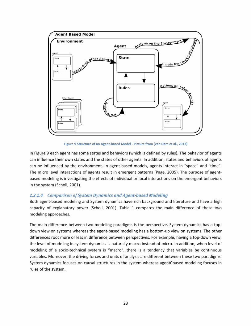
23

Figure 9 Structure of an Agent-based Model - Picture from (van Dam et al., 2013)

In Figure 9 each agent has some states and behaviors (which is defined by rules). The behavior of agents can influence their own states and the states of other agents. In addition, states and behaviors of agents can be influenced by the environment. In agent-based models, agents interact in “space” and “time”. The micro level interactions of agents result in emergent patterns (Page, 2005). The purpose of agent-based modeling is investigating the effects of individual or local interactions on the emergent behaviors in the system (Scholl, 2001).

2.2.2.4 Comparison of System Dynamics and Agent-based Modeling Both agent-based modeling and System dynamics have rich background and literature and have a high capacity of explanatory power (Scholl, 2001). Table 1 compares the main difference of these two modeling approaches.

The main difference between two modeling paradigms is the perspective. System dynamics has a top-down view on systems whereas the agent-based modeling has a bottom-up view on systems. The other differences root more or less in difference between perspectives. For example, having a top-down view, the level of modeling in system dynamics is naturally macro instead of micro. In addition, when level of modeling of a socio-technical system is “macro”, there is a tendency that variables be continuous variables. Moreover, the driving forces and units of analysis are different between these two paradigms. System dynamics focuses on causal structures in the system whereas agent0based modeling focuses in rules of the system.

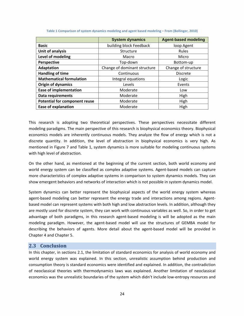
24

Table 1 Comparison of system dynamics modeling and agent based modeling – From (Bollinger, 2010)

System dynamics Agent-based modeling Basic building block Feedback loop Agent Unit of analysis Structure Rules Level of modeling Macro Micro Perspective Top-down Bottom-up Adaptation Change of dominant structure Change of structure Handling of time Continuous Discrete Mathematical formulation Integral equations Logic Origin of dynamics Levels Events Ease of implementation Moderate Low Data requirements Moderate High Potential for component reuse Moderate High Ease of explanation Moderate High

This research is adopting two theoretical perspectives. These perspectives necessitate different modeling paradigms. The main perspective of this research is biophysical economics theory. Biophysical economics models are inherently continuous models. They analyze the flow of energy which is not a discrete quantity. In addition, the level of abstraction in biophysical economics is very high. As mentioned in Figure 7 and Table 1, system dynamics is more suitable for modeling continuous systems with high level of abstraction.

On the other hand, as mentioned at the beginning of the current section, both world economy and world energy system can be classified as complex adaptive systems. Agent-based models can capture more characteristics of complex adaptive systems in comparison to system dynamics models. They can show emergent behaviors and networks of interaction which is not possible in system dynamics model.

System dynamics can better represent the biophysical aspects of the world energy system whereas agent-based modeling can better represent the energy trade and interactions among regions. Agent-based model can represent systems with both high and low abstraction levels. In addition, although they are mostly used for discrete system, they can work with continuous variables as well. So, in order to get advantage of both paradigms, in this research agent-based modeling is will be adopted as the main modeling paradigm. However, the agent-based model will use the structures of GEMBA model for describing the behaviors of agents. More detail about the agent-based model will be provided in Chapter 4 and Chapter 5.

2.3 Conclusion In this chapter, in sections 2.1, the limitation of standard economics for analysis of world economy and world energy system was explained. In this section, unrealistic assumption behind production and consumption theory is standard economics were identified and explained. In addition, the contradiction of neoclassical theories with thermodynamics laws was explained. Another limitation of neoclassical economics was the unrealistic boundaries of the system which didn’t include low-entropy resources and

25

high-entropy wastes. These limitations lead us to explore the potential of biophysical economics for analyzing the world energy system.

In order to address the aforementioned limitations, the biophysical economic theory was introduced. The evolution of biophysical thought in the literature was reviewed. Afterwards, the biophysical view of economy presented. In the biophysical view, the role of natural resources, wastes, and counter flow of money and energy were realized. In addition, the concept of energy trade from biophysical economics perspective was introduced and explained.

Although analysis of energy trade (among countries) was not common in the literature, bio physical economics can explain energy trade. The most important step for taking energy trade into account in biophysical analysis is defining trade EROI. It was mentioned that EROI for the imported fuel can be estimated with using energy intensity of nations and global energy price.

In section 2.2, the next theoretical perspective of this research, complex adaptive systems, was introduced. It was explained why the world energy system is a complex adaptive system and examples of generic characteristics of CAS in the world energy system were provided. Modeling can be used to analyze CAS. Therefore, two modeling paradigms, system dynamics and agent-based modeling, were introduced, explained, and compared. In general, While system dynamics modeling has advantage for modeling of continuous biophysical economics system, agent-based modeling has advantage of presenting network of agents and the emergent behavior of the system.

Energy trade within the world energy system can be considered as an interaction among countries. One of the main advantages of agent-based models over systems dynamics models was incorporating interactions among individuals and agents. So, the network of energy trade among countries and regions can be modeled effectively using agent-based modeling. Furthermore, if EROI of energy trade can be defined as a rule in agents of the world energy system, the emergent energy trade can be analyzed from both biophysical perspective and complex adaptive systems perspective.

In the next chapter the world energy system will be analyzed from technical and actor perspectives.

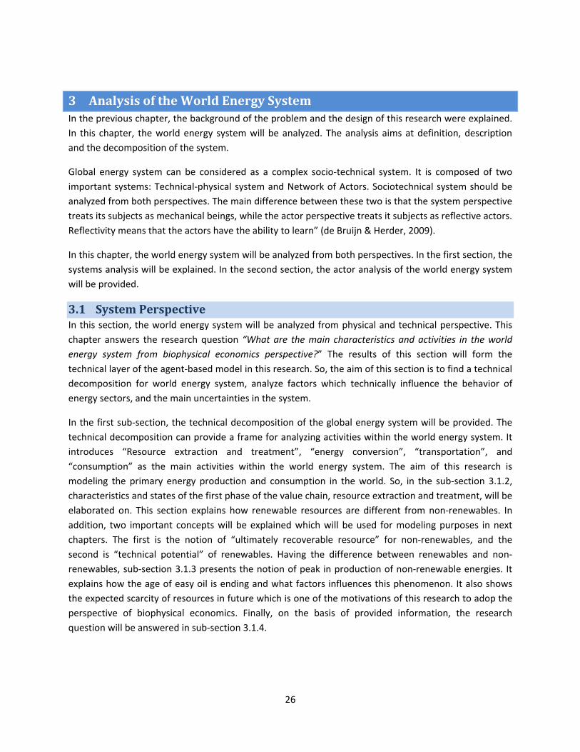
26

3 Analysis of the World Energy System In the previous chapter, the background of the problem and the design of this research were explained. In this chapter, the world energy system will be analyzed. The analysis aims at definition, description and the decomposition of the system.

Global energy system can be considered as a complex socio-technical system. It is composed of two important systems: Technical-physical system and Network of Actors. Sociotechnical system should be analyzed from both perspectives. The main difference between these two is that the system perspective treats its subjects as mechanical beings, while the actor perspective treats it subjects as reflective actors. Reflectivity means that the actors have the ability to learn” (de Bruijn & Herder, 2009).

In this chapter, the world energy system will be analyzed from both perspectives. In the first section, the systems analysis will be explained. In the second section, the actor analysis of the world energy system will be provided.

3.1 System Perspective In this section, the world energy system will be analyzed from physical and technical perspective. This chapter answers the research question “What are the main characteristics and activities in the world energy system from biophysical economics perspective?” The results of this section will form the technical layer of the agent-based model in this research. So, the aim of this section is to find a technical decomposition for world energy system, analyze factors which technically influence the behavior of energy sectors, and the main uncertainties in the system.

In the first sub-section, the technical decomposition of the global energy system will be provided. The technical decomposition can provide a frame for analyzing activities within the world energy system. It introduces “Resource extraction and treatment”, “energy conversion”, “transportation”, and “consumption” as the main activities within the world energy system. The aim of this research is modeling the primary energy production and consumption in the world. So, in the sub-section 3.1.2, characteristics and states of the first phase of the value chain, resource extraction and treatment, will be elaborated on. This section explains how renewable resources are different from non-renewables. In addition, two important concepts will be explained which will be used for modeling purposes in next chapters. The first is the notion of “ultimately recoverable resource” for non-renewables, and the second is “technical potential” of renewables. Having the difference between renewables and non-renewables, sub-section 3.1.3 presents the notion of peak in production of non-renewable energies. It explains how the age of easy oil is ending and what factors influences this phenomenon. It also shows the expected scarcity of resources in future which is one of the motivations of this research to adop the perspective of biophysical economics. Finally, on the basis of provided information, the research question will be answered in sub-section 3.1.4.

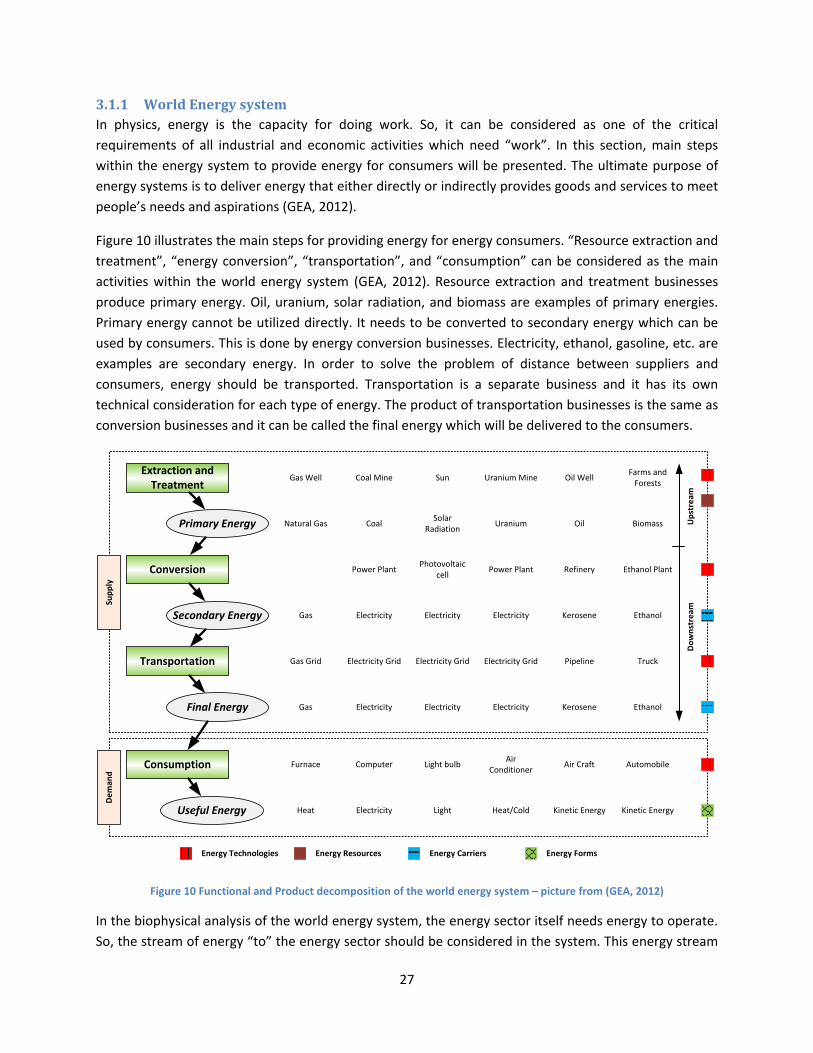
27

3.1.1 World Energy system In physics, energy is the capacity for doing work. So, it can be considered as one of the critical requirements of all industrial and economic activities which need “work”. In this section, main steps within the energy system to provide energy for consumers will be presented. The ultimate purpose of energy systems is to deliver energy that either directly or indirectly provides goods and services to meet people’s needs and aspirations (GEA, 2012).

Figure 10 illustrates the main steps for providing energy for energy consumers. “Resource extraction and treatment”, “energy conversion”, “transportation”, and “consumption” can be considered as the main activities within the world energy system (GEA, 2012). Resource extraction and treatment businesses produce primary energy. Oil, uranium, solar radiation, and biomass are examples of primary energies. Primary energy cannot be utilized directly. It needs to be converted to secondary energy which can be used by consumers. This is done by energy conversion businesses. Electricity, ethanol, gasoline, etc. are examples are secondary energy. In order to solve the problem of distance between suppliers and consumers, energy should be transported. Transportation is a separate business and it has its own technical consideration for each type of energy. The product of transportation businesses is the same as conversion businesses and it can be called the final energy which will be delivered to the consumers.

Extraction and Treatment

Conversion

Transportation

Consumption

Primary Energy

Secondary Energy

Final Energy

Useful Energy

Gas Well Coal Mine Sun Uranium Mine Oil Well Farms and Forests

Natural Gas Coal Solar Radiation Uranium Oil Biomass

Power Plant Photovoltaic cell Power Plant Refinery Ethanol Plant

Gas Electricity Electricity Electricity Kerosene Ethanol

Gas Grid Electricity Grid Electricity Grid Electricity Grid Pipeline Truck

Gas Electricity Electricity Electricity Kerosene Ethanol

Furnace Computer Light bulb Air Conditioner Air Craft Automobile

Heat Electricity Light Heat/Cold Kinetic Energy Kinetic Energy

Supp

lyD

eman

d

Ups

trea

mD

owns

trea

m

Energy Technologies Energy Resources Energy Carriers Energy Forms

Figure 10 Functional and Product decomposition of the world energy system – picture from (GEA, 2012)

In the biophysical analysis of the world energy system, the energy sector itself needs energy to operate. So, the stream of energy “to” the energy sector should be considered in the system. This energy stream

28

is called “energy feedback”. Energy feedback has two types. The first type is fuel feedback which will be consumed by facilities in the energy sector in order to produce, covert, or transport energy. The second type is energy of energy equivalent of capital, labor, or services which are required by the energy sector.

Figure 11 illustrates the fuel and capital feedbacks to the energy sector. Fuel feedback is part of final energy and capital feedback is part of useful energy. In this figure, all energy activities lose some energy which goes to environment.

Extraction and Treatment Conversion Transportation ConsumptionPrimary Energy Secondary

Energy Final Energy Useful EnergyJ5Resource

J4 J3 J2

Figure 11 Energy flow across the energy system- Picture from (C. A. S. Hall, Cleveland, & Kaufmann, 1992)

Net energy yield which is delivered to the economy can be calculated by subtracting volume of fuel and capital feedbacks from final energy (C. A. Hall et al., 1986).

( )4325YieldEnergy Net JJJJ ++−=

Equation 5

Energy return on investment (EROI) is the ratio of energy returned from an energy-gathering activity compared to the energy invested in that process. It can be calculated as follow (C. A. Hall et al., 1986):

432

5

EnergyGet that toRequiredEnergy Society toReturnedEnergy EROI

JJJJ

++==

Equation 6

3.1.2 World Energy Resources In this research, the concentration of analysis and modeling is on production of primary energy in the energy sector. Production of secondary energy and final energy mainly depends on volume of primary energy production and the energy conversion efficiency5. So, for the sake of simplicity, only primary energy production will be elaborated on.

In general, primary energy resources can be classified into two groups: Renewables resources and Non-Renewable resources. Non-renewable resources are stocks of energy with finite size. Renewable energy resources comprise the harvesting of naturally occurring energy flows (GEA, 2012) The main difference between renewable resources and non-renewable resources can be found in ratio of regeneration of the 5 Energy conversion efficiency is the ratio between the useful output of an energy conversion system and the input, in energy terms. In a power plan, the plant’s input is primary energy and the output is secondary. So the energy conversion ratio and the volume of primary energy input can determine the volume of output.

29

source. The rate of regeneration of non-renewable resources is extremely low, whereas the rate of regeneration of renewable resources is much higher.

Figure 12 World Primary Energy Consumption in 2011

Figure 12 illustrates the composition of the world primary energy consumption by fuel in 2011. In this figure, it is obvious that non-renewable resources are dominant in the world energy consumption.

Figure 13 Share of resources in total primary energy production in US- Source IEA- Picture from (Koonin, 2005)

Figure 13 complements the previous figure with illustrating the evolution of share of different resources in U.S. energy portfolio. An interesting thing in Figure 13Figure 13 Share of resources in total primary energy production in US- Source IEA- Picture from (Koonin, 2005) is that the actual size of wood consumption in 1850 is the same as 2000. Figure 14 illustrates the share each primary resource in primary consumption sector. It shows that most of crude oil is consumed as fuel for the transportation

33%

24%

30%

5% 6%

2%

Oil

Natural gas

Coal

Nuclear energy

Hydro electricity

Renewables

30

sector or as feedstock for special industries. Other types of energies are consumers in industry, residential and commercial uses.

Figure 14 Global energy flows (in EJ) from primary to useful energy by primary resource input, energy carrier (fuels), and end-use sector applications in 2005, Picture from (GEA, 2012), ALS= Auto consumption, losses, stock changes, OTF= Other

transformation to secondary fuels

3.1.2.1 Non-Renewable Resources One of the most interesting issues in analysis of global energy system is the classification and size of non-renewable resources. There is wide range of estimations about the ultimately recoverable resources (URR) of non-renewable sources (GEA, 2012). Debates surrounding an impending peak in production , which will be explained in the next section, are centered on the scale of recoverable resources (JAFFE, MEDLOCK, & SOLIGO, 2011). Michael Dale (2012) performed meta-analysis of non-renewable energy resource estimates. His analysis reveals high variations and uncertainty about ultimately recoverable resources. The concept of reserves is generally not well understood(Hirsch, Bezdek, & Wendling, 2005). Here, two exemplar approaches will be introduced.

Figure 15 illustrates the difference among different terms for measurement of recoverable resources. From the total resource in place, some part can technically be recovered. Size of Economic recoverable resource is dynamic and it depends on resource in place, technology, and field development costs (JAFFE et al., 2011). Proved reserves are subset of economically recoverable resources.

31

Figure 15 Simple Representation of Resource Envelope - Picture from (JAFFE et al., 2011)

More standard terms for classification of resources can be found in USGS/USBM system (USGS, 1981). Figure 16 illustrates classification of resources. In this system, resources are either identified, or undiscovered. Identified resources are resources whose location, grade, quality, and quantity are known or estimated from specific geologic evidence. Undiscovered resources are resources, the existence of which are only postulated, comprising deposits that are separate from identified resources. More information on USGS/USBM system can be found in the Appendix I.

Cumulative Production

Identified Resources Undiscovered Resources

Demonstrated Inferred Probability Range

Measured Indicated Hypothetical Speculative

Economic Reserves Inferred Reserves

Marginally Economic

Marginal Reserves Inferred Marginal Reserves

Sub-Economic Demonstrated Sub-economic

Resources

Inferred Sub-economic Resources

Other Occurrences

Include non-conventional and low grade resources

Figure 16 USGS/USBM System (USGS, 1981)

Michael Dale (2012) fitted distribution functions to various estimated of URR for non-renewables. Table 2 illustrates the summary of distribution parameters for various non-renewable sources.

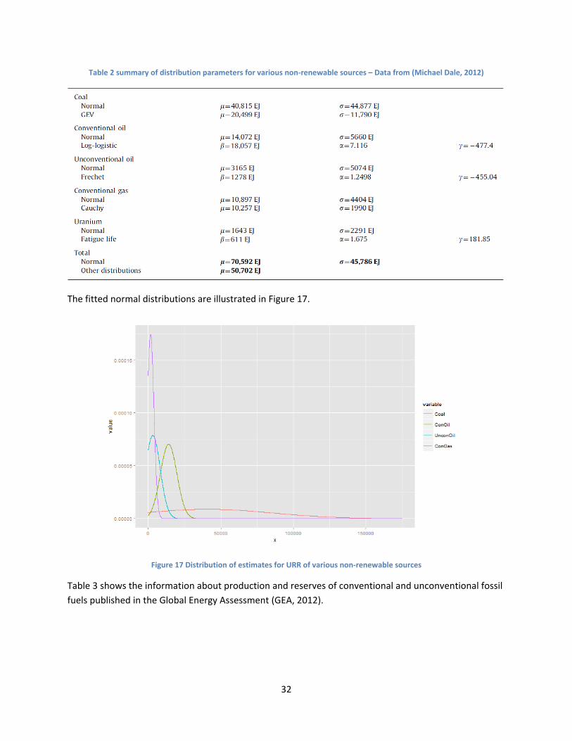
32

Table 2 summary of distribution parameters for various non-renewable sources – Data from (Michael Dale, 2012)

The fitted normal distributions are illustrated in Figure 17.

Figure 17 Distribution of estimates for URR of various non-renewable sources

Table 3 shows the information about production and reserves of conventional and unconventional fossil fuels published in the Global Energy Assessment (GEA, 2012).

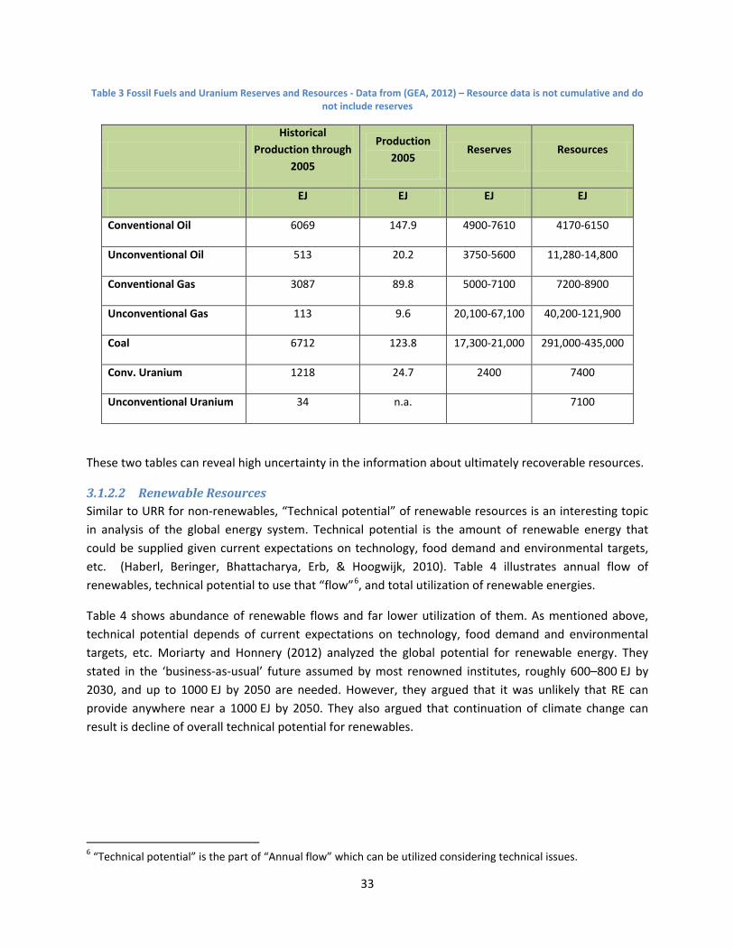
33

Table 3 Fossil Fuels and Uranium Reserves and Resources - Data from (GEA, 2012) – Resource data is not cumulative and do not include reserves

Historical

Production through 2005

Production 2005

Reserves Resources

EJ EJ EJ EJ

Conventional Oil 6069 147.9 4900-7610 4170-6150

Unconventional Oil 513 20.2 3750-5600 11,280-14,800

Conventional Gas 3087 89.8 5000-7100 7200-8900

Unconventional Gas 113 9.6 20,100-67,100 40,200-121,900

Coal 6712 123.8 17,300-21,000 291,000-435,000

Conv. Uranium 1218 24.7 2400 7400

Unconventional Uranium 34 n.a. 7100

These two tables can reveal high uncertainty in the information about ultimately recoverable resources.

3.1.2.2 Renewable Resources Similar to URR for non-renewables, “Technical potential” of renewable resources is an interesting topic in analysis of the global energy system. Technical potential is the amount of renewable energy that could be supplied given current expectations on technology, food demand and environmental targets, etc. (Haberl, Beringer, Bhattacharya, Erb, & Hoogwijk, 2010). Table 4 illustrates annual flow of renewables, technical potential to use that “flow”6, and total utilization of renewable energies.

Table 4 shows abundance of renewable flows and far lower utilization of them. As mentioned above, technical potential depends of current expectations on technology, food demand and environmental targets, etc. Moriarty and Honnery (2012) analyzed the global potential for renewable energy. They stated in the ‘business-as-usual’ future assumed by most renowned institutes, roughly 600–800 EJ by 2030, and up to 1000 EJ by 2050 are needed. However, they argued that it was unlikely that RE can provide anywhere near a 1000 EJ by 2050. They also argued that continuation of climate change can result is decline of overall technical potential for renewables.

6 “Technical potential” is the part of “Annual flow” which can be utilized considering technical issues.

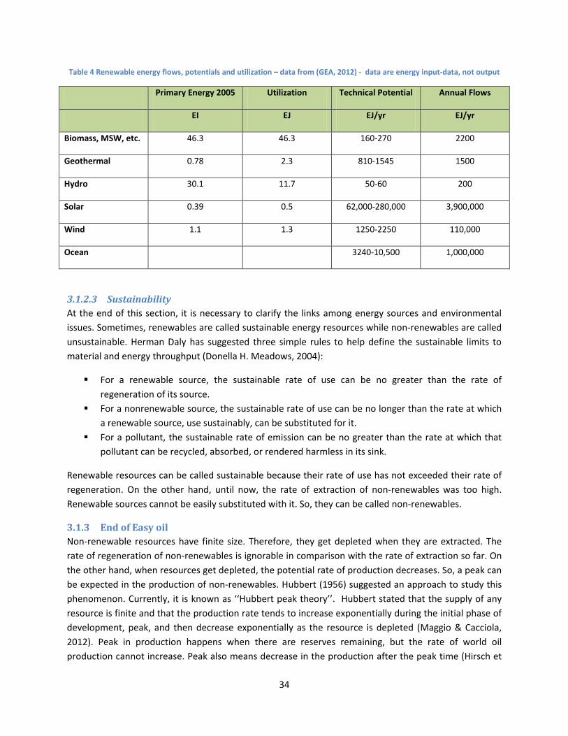
34

Table 4 Renewable energy flows, potentials and utilization – data from (GEA, 2012) - data are energy input-data, not output

Primary Energy 2005 Utilization Technical Potential Annual Flows

EI EJ EJ/yr EJ/yr

Biomass, MSW, etc. 46.3 46.3 160-270 2200

Geothermal 0.78 2.3 810-1545 1500

Hydro 30.1 11.7 50-60 200

Solar 0.39 0.5 62,000-280,000 3,900,000

Wind 1.1 1.3 1250-2250 110,000

Ocean 3240-10,500 1,000,000

3.1.2.3 Sustainability At the end of this section, it is necessary to clarify the links among energy sources and environmental issues. Sometimes, renewables are called sustainable energy resources while non-renewables are called unsustainable. Herman Daly has suggested three simple rules to help define the sustainable limits to material and energy throughput (Donella H. Meadows, 2004):

For a renewable source, the sustainable rate of use can be no greater than the rate of regeneration of its source.

For a nonrenewable source, the sustainable rate of use can be no longer than the rate at which a renewable source, use sustainably, can be substituted for it.

For a pollutant, the sustainable rate of emission can be no greater than the rate at which that pollutant can be recycled, absorbed, or rendered harmless in its sink.

Renewable resources can be called sustainable because their rate of use has not exceeded their rate of regeneration. On the other hand, until now, the rate of extraction of non-renewables was too high. Renewable sources cannot be easily substituted with it. So, they can be called non-renewables.

3.1.3 End of Easy oil Non-renewable resources have finite size. Therefore, they get depleted when they are extracted. The rate of regeneration of non-renewables is ignorable in comparison with the rate of extraction so far. On the other hand, when resources get depleted, the potential rate of production decreases. So, a peak can be expected in the production of non-renewables. Hubbert (1956) suggested an approach to study this phenomenon. Currently, it is known as ‘‘Hubbert peak theory’’. Hubbert stated that the supply of any resource is finite and that the production rate tends to increase exponentially during the initial phase of development, peak, and then decrease exponentially as the resource is depleted (Maggio & Cacciola, 2012). Peak in production happens when there are reserves remaining, but the rate of world oil production cannot increase. Peak also means decrease in the production after the peak time (Hirsch et

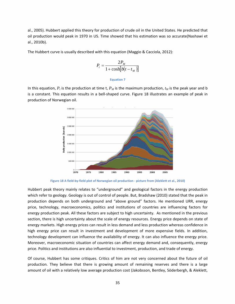
35

al., 2005). Hubbert applied this theory for production of crude oil in the United States. He predicted that oil production would peak in 1970 in US. Time showed that his estimation was so accurate(Nashawi et al., 2010b).

The Hubbert curve is usually described with this equation (Maggio & Cacciola, 2012):

( )[ ]M

Mt ttb

PP−+

=cosh1

2

Equation 7

In this equation, Pt is the production at time t, PM is the maximum production, tM is the peak year and b is a constant. This equation results in a bell-shaped curve. Figure 18 illustrates an example of peak in production of Norwegian oil.

Figure 18 A field-by-field plot of Norwegian oil production - picture from (Aleklett et al., 2010)

Hubbert peak theory mainly relates to “underground” and geological factors in the energy production which refer to geology. Geology is out of control of people. But, Bradshaw (2010) stated that the peak in production depends on both underground and “above ground” factors. He mentioned URR, energy price, technology, macroeconomics, politics and institutions of countries are influencing factors for energy production peak. All these factors are subject to high uncertainty. As mentioned in the previous section, there is high uncertainty about the scale of energy resources. Energy price depends on state of energy markets. High energy prices can result in less demand and less production whereas confidence in high energy price can result in investment and development of more expensive fields. In addition, technology development can influence the availability of energy. It can also influence the energy price. Moreover, macroeconomic situation of countries can affect energy demand and, consequently, energy price. Politics and institutions are also influential to investment, production, and trade of energy.

Of course, Hubbert has some critiques. Critics of him are not very concerned about the future of oil production. They believe that there is growing amount of remaining reserves and there is a large amount of oil with a relatively low average production cost (Jakobsson, Bentley, Söderbergh, & Aleklett,

36

2012). Critics also believe that Hubbert method forecasts depend on knowing how much oil can be discovered and produced, and the forecasted number is just a guess (Towler, 2011). Of course, in general, uncertainty is proved to be very high for estimation of the world conventional oil reserves(Tien & McVay, 2010). Nonetheless, Hubbert has so many advocates as well who are concerned about the future of oil production.

Due to aforementioned uncertainty in factors of production peak, there is wide range of estimation about the peak time for different resources. UK Energy Research Center announced that the time for peak in production of crude oil is between 2009 and 2009 (Sorrell, Speirs, Bentley, Brandt, & Miller, 2009). Nashawi et al. (2010a) predicted that world crude oil production would peak in 2014 at the rate of 79 MMSTB/D with a Multi-cyclic Hubbert model. Maggio and Cacciola (2012) developed multi-Hubbert variants to forecast the peak for oil, natural gas and coal. They Forecasted that peak values were 30 Gb/year for oil in 2015, 132 Tcf/year for natural gas in 2035, and 4.5 Gtoe/year for coal in 2052.

Hubbert adopted a top-down modeling approach for forecasting the peak in production of U.S. oil. Jakobsson et al. (2012) developed a bottom-up model which leads to qualitatively the same results as Hubbert’s model. Getting the same result from higher resolution models (like bottom-up models) can be considered as validation of lower resolution models (like Hubbert’s). Having concerns about proving affordable energy for the entire world, signals from Hubebrt’s models cannot be ignored. Here, the concerned view is selected in order to prepare our world even for the unfavorable cases.

Oil production is reaching to its peak. At the same time, the population of the world is increasing. It can be symptom of higher energy demand in future. In addition, as new economies like China and India are emerging, the welfare and lifestyle of their people are also changing and improving. Economic growth is essential for improving welfare. And, energy is essential for economic growth. Just high economic growth of China and India can cause exponential growth in the future global energy demand (Gelpke et al., 2006). Regardless of risk (probability) of near-peak time, impact of peak in production of non-renewables can be very high for the world economy and security. Great share of the world primary energy supply is from non-renewables and any shortage can have significant impacts.

3.1.4 Conclusion In this chapter the general characteristics of the world energy system, primary energy resources, production peak and EROI were presented and discussed. Now, it is possible to answer the question at the beginning of the chapter “What are the main characteristics and activities in the world energy system from biophysical economics perspective?”

Given the information and arguments in this chapter, it can be concluded that the world energy system is the system of all facilities, technology, businesses and actor which aims at delivering energy that either directly or indirectly provides goods and services to meet people’s needs and aspirations. The world energy system can be decomposed into for sub-systems: “extraction and treatment”, “conversion”, “transportation”, and “consumption”.

The first sub-system produced primary energy supply from either renewable or non-renewable resources. These two types of resources have different characteristics. Non-renewables have finite size

37

and they diminish as they get extracted. Renewables have technical potential which is the maximum possible production per year. The estimates for non-renewable and renewable resource were provided from different literature and from different standards. It showed lack of unique definition about energy resources and high uncertainty about scale of resources.

Non-renewables will experience peak and decline in their production. It depends on many underground factors and above-ground factors. The main underground factor is URR whereas the main above-ground factors are energy price, macroeconomics, technology, politics and institutions. Peak in production identified as a credible statement however there are many uncertainties and debates around it.

38

3.2 Actor Perspective As mentioned at the beginning of this chapter, the world energy system will be analyzed from system and actor perspectives. Technical and physical aspects of the system were analyzed in the previous section. In this section, the system will be analyzed from actor perspective.

The aim of this section is answering the research question “How can the world energy system be decomposed into different trading regions?” The purpose of this section is to find suitable actor decomposition for the world energy system in order to use in the agent-based model in Chapter 5.

The analysis will be done at two levels: Micro analysis and Macro analysis. Micro analysis will be presented in sub-section 3.2.1. Micro actor analysis describes the network of companies and institutes along energy value chain which influence the functioning the energy sector of countries. This analysis can help aggregated actor analysis at international and global scale. Such analysis can be called macro actor analysis.

Macro analysis will be provided in sub-section 3.2.2. The aim of macro analysis is decomposition of the world energy system into groups of countries. Actor decomposition will be limited to selection of one of existing decompositions in the literature. In order to select such a decomposition, in sub-section 3.2.2.1.1, alternative decompositions and criteria for selection will be provided. Consequently, in sub-section 3.2.2.1.2, the selection will be done. The selected decomposition will be used later as decomposition of the agent-based model.

In addition, in sub-section 3.2.2.2, main international energy-related institutes will be introduced. These international institutes can influence the degree of trust and cooperation among regions which will be considered in Chapter 5.

3.2.1 Micro Analysis Analysis of main actors at national level necessitates revisiting value chain of energy systems. As presented in the previous chapter, the main sections of energy value chain are: “Extraction and Treatment”, “Conversion”, “Transportation”, and “Consumption”7. Each of these sections is owned and controlled by specific set of actors. Sometimes, actors controlling different sections are vertically integrated. For example, in oil industry, different companies serve different functions such as exploration, production, refining, and distribution. They can be strategically controlled by one large company. In other cases, different sections of energy value chain can be unbundled. For example, after legislation of Third Energy Package8, member states of European Union are obliged to unbundle ownership across energy value chain. It means that if, for example, a company produces natural gas, it should not operate the gas pipelines as well. Things like operation of gas pipelines or electricity grid are 7 Energy Storage can be considered as a part of energy Transportation. 8 Third Energy Package consists of:

• Regulation (EC) No 713/2009 • Regulation (EC) No 714/2009 • Regulation (EC) No 715/2009 • Directive 2009/72/EC • Directive 2009/73/EC

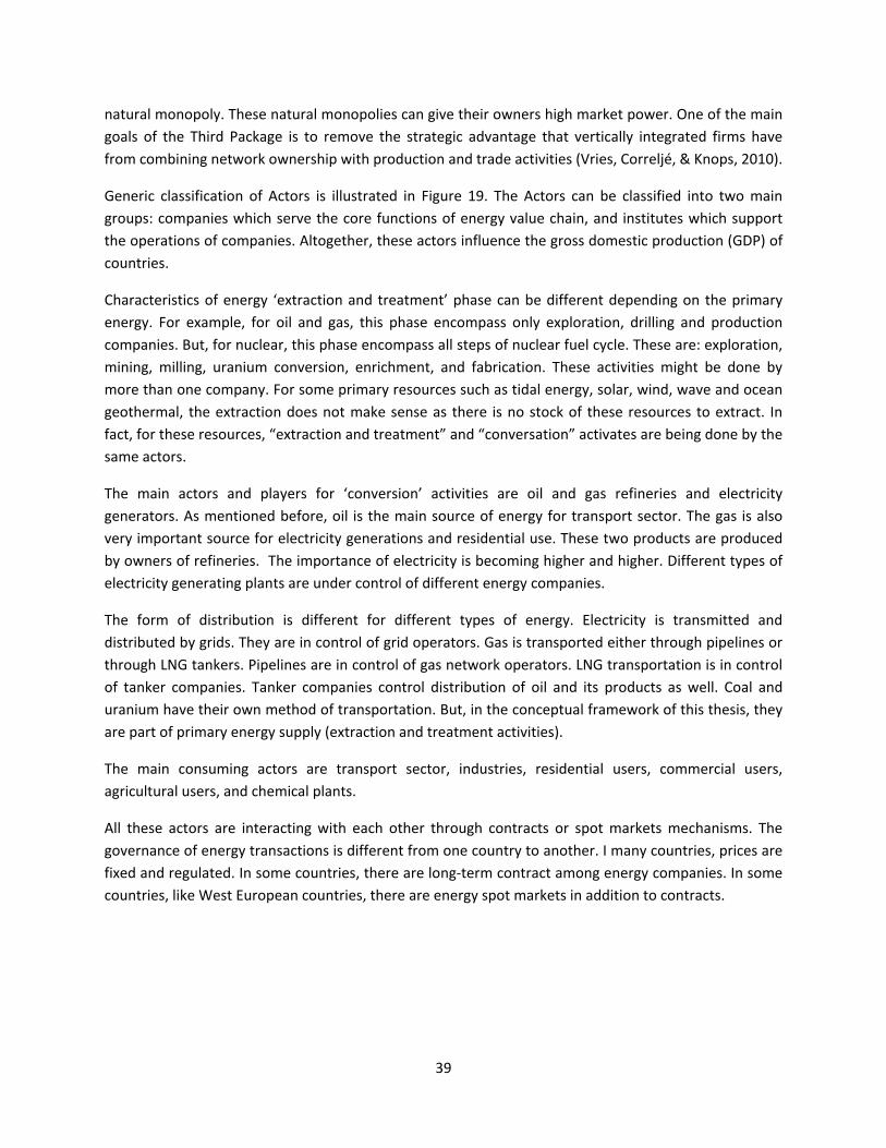
39

natural monopoly. These natural monopolies can give their owners high market power. One of the main goals of the Third Package is to remove the strategic advantage that vertically integrated firms have from combining network ownership with production and trade activities (Vries, Correljé, & Knops, 2010).

Generic classification of Actors is illustrated in Figure 19. The Actors can be classified into two main groups: companies which serve the core functions of energy value chain, and institutes which support the operations of companies. Altogether, these actors influence the gross domestic production (GDP) of countries.

Characteristics of energy ‘extraction and treatment’ phase can be different depending on the primary energy. For example, for oil and gas, this phase encompass only exploration, drilling and production companies. But, for nuclear, this phase encompass all steps of nuclear fuel cycle. These are: exploration, mining, milling, uranium conversion, enrichment, and fabrication. These activities might be done by more than one company. For some primary resources such as tidal energy, solar, wind, wave and ocean geothermal, the extraction does not make sense as there is no stock of these resources to extract. In fact, for these resources, “extraction and treatment” and “conversation” activates are being done by the same actors.

The main actors and players for ‘conversion’ activities are oil and gas refineries and electricity generators. As mentioned before, oil is the main source of energy for transport sector. The gas is also very important source for electricity generations and residential use. These two products are produced by owners of refineries. The importance of electricity is becoming higher and higher. Different types of electricity generating plants are under control of different energy companies.

The form of distribution is different for different types of energy. Electricity is transmitted and distributed by grids. They are in control of grid operators. Gas is transported either through pipelines or through LNG tankers. Pipelines are in control of gas network operators. LNG transportation is in control of tanker companies. Tanker companies control distribution of oil and its products as well. Coal and uranium have their own method of transportation. But, in the conceptual framework of this thesis, they are part of primary energy supply (extraction and treatment activities).

The main consuming actors are transport sector, industries, residential users, commercial users, agricultural users, and chemical plants.

All these actors are interacting with each other through contracts or spot markets mechanisms. The governance of energy transactions is different from one country to another. I many countries, prices are fixed and regulated. In some countries, there are long-term contract among energy companies. In some countries, like West European countries, there are energy spot markets in addition to contracts.

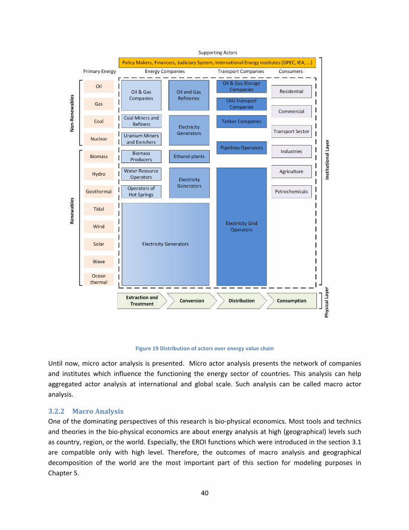
40

Figure 19 Distribution of actors over energy value chain

Until now, micro actor analysis is presented. Micro actor analysis presents the network of companies and institutes which influence the functioning the energy sector of countries. This analysis can help aggregated actor analysis at international and global scale. Such analysis can be called macro actor analysis.

3.2.2 Macro Analysis One of the dominating perspectives of this research is bio-physical economics. Most tools and technics and theories in the bio-physical economics are about energy analysis at high (geographical) levels such as country, region, or the world. Especially, the EROI functions which were introduced in the section 3.1 are compatible only with high level. Therefore, the outcomes of macro analysis and geographical decomposition of the world are the most important part of this section for modeling purposes in Chapter 5.

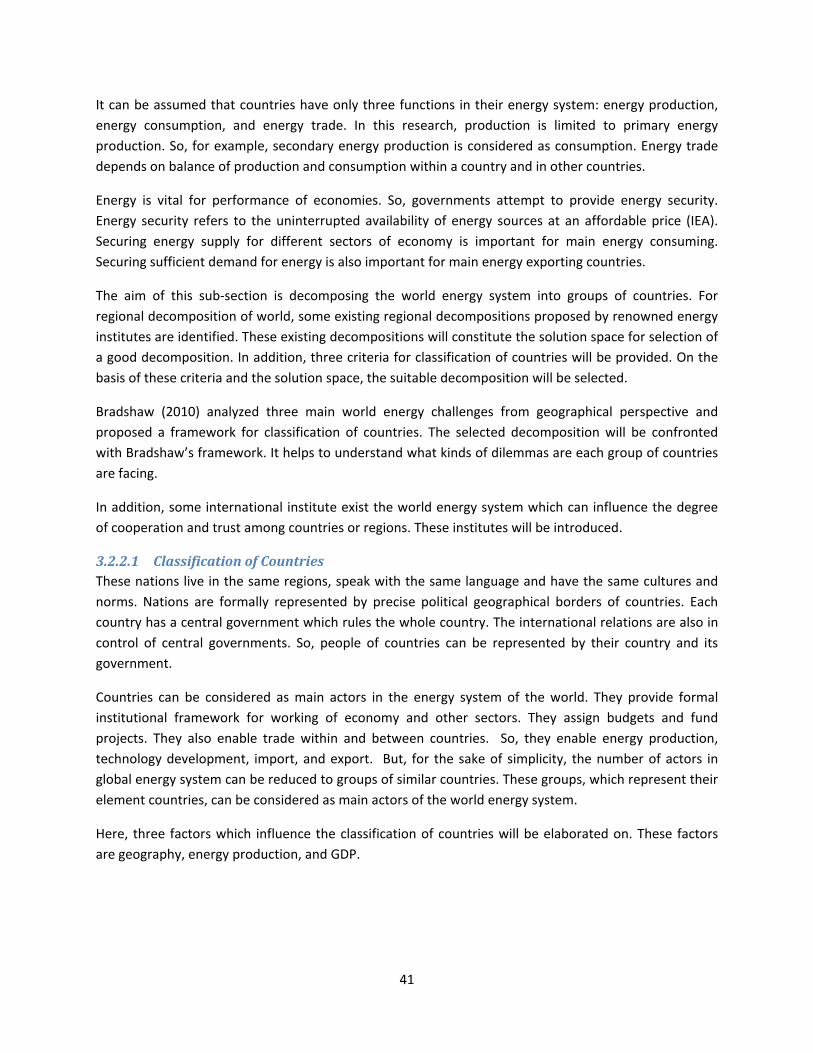
41

It can be assumed that countries have only three functions in their energy system: energy production, energy consumption, and energy trade. In this research, production is limited to primary energy production. So, for example, secondary energy production is considered as consumption. Energy trade depends on balance of production and consumption within a country and in other countries.

Energy is vital for performance of economies. So, governments attempt to provide energy security. Energy security refers to the uninterrupted availability of energy sources at an affordable price (IEA). Securing energy supply for different sectors of economy is important for main energy consuming. Securing sufficient demand for energy is also important for main energy exporting countries.

The aim of this sub-section is decomposing the world energy system into groups of countries. For regional decomposition of world, some existing regional decompositions proposed by renowned energy institutes are identified. These existing decompositions will constitute the solution space for selection of a good decomposition. In addition, three criteria for classification of countries will be provided. On the basis of these criteria and the solution space, the suitable decomposition will be selected.

Bradshaw (2010) analyzed three main world energy challenges from geographical perspective and proposed a framework for classification of countries. The selected decomposition will be confronted with Bradshaw’s framework. It helps to understand what kinds of dilemmas are each group of countries are facing.

In addition, some international institute exist the world energy system which can influence the degree of cooperation and trust among countries or regions. These institutes will be introduced.

3.2.2.1 Classification of Countries These nations live in the same regions, speak with the same language and have the same cultures and norms. Nations are formally represented by precise political geographical borders of countries. Each country has a central government which rules the whole country. The international relations are also in control of central governments. So, people of countries can be represented by their country and its government.

Countries can be considered as main actors in the energy system of the world. They provide formal institutional framework for working of economy and other sectors. They assign budgets and fund projects. They also enable trade within and between countries. So, they enable energy production, technology development, import, and export. But, for the sake of simplicity, the number of actors in global energy system can be reduced to groups of similar countries. These groups, which represent their element countries, can be considered as main actors of the world energy system.

Here, three factors which influence the classification of countries will be elaborated on. These factors are geography, energy production, and GDP.

42

3.2.2.1.1 Alternatives and Criteria for Classification

3.2.2.1.1.1 Geography Bradshaw (2010) identified geography central to understanding different energy challenges. So, here, it is considered as one of the main factors. The next two factors (energy production and GDP) will be investigated from geographical perspective as well. Neighboring countries are likely to have the same culture, resources, interests, institutional frameworks, etc. So, the main actors of global energy system can be considered as a number of geographical regions. These regions are consisting of neighboring countries.

Decomposition of the world into a number of regions is quite common in energy literature. For example, Correljé and van der Linde (2006) considered two storylines for such characterizations of the way in which energy producing and consuming countries and regions would manifest themselves in the global energy markets. These storylines are “Markets and Institutions” and “Regions and Empires”. In the former, the international interactions and flows are influenced by market forces. In addition, all activities are regulated by international institutes. In the latter, political and military strategy, bilateralism and regionalism divide the world into competing spheres. They analyzed security of energy supply from European perspective. They, specifically, considered Persian Gulf, Russia, the Caspian Sea, US, China, Japan, and India as main blocks which influence EU energy security. Similarly, Kamp (2011) considered five hands in the global energy game. He considered OECD, energy producers (originally, OPEC and GasPEC), BRICS, emerging developing countries, very poor countries.

Decomposition of the world into regions is also common in the reports of international organizations. They classify countries into different regions for aggregating their information. International Institute of Applied Systems Analysis (IIASA) uses 11 regions9 for data aggregation in its global energy assessment (GEA). Figure 20 illustrates 11 regions of GEA. It also provides 5-region10 and 2-region11 aggregation levels(IIASA, 2012b). Moreover, International Energy Agency uses 25 country and regional models12 in its world energy model (WEM) (IEA, 2012b). However, in IEA model, some regions are sometimes composed of non-neighbor countries in the same continents Figure 21 illustrates 25 country and regions of WEM. Similarly, BP uses 5-region 13 model for aggregation in its statistical review of the world energy (BP, 2012a) and energy outlook 2030 (BP, 2012b).

9 Sub-Saharan Africa, Centrally planned Asia and China, Central and Eastern Europe, Former Soviet Union, Latin America and the Caribbean, Middle East and North Africa, North America, Pacific OECD, Other Pacific Asia, South Asia, Western Europe 10 OECD 90, Reforming Economies, Asia, Middle East and Africa, Latin America and the Caribbean 11 North (Industrialized countries, i.e. countries that make up the OECD 90 and Reforming Economies regions), South (Developing countries, i.e. countries that make up the Middle East and Africa, Asia and Latin America and the Caribbean regions.) 12 OECD Americas (4 country), OECD Europe (3 regions), OECD Asia Oceania (2 country, 1 region), Eastern Europe/Eurasia10 (1 country, 3 regions), Non-OECD Asia (3 country, 2 regions), Latin America (1 country, 1 region), Middle East (1 region), Africa (1 country, 2 regions) 13 North America, Central and South America, Europe and Eurasia, Middle East, Africa, Asia Pacific

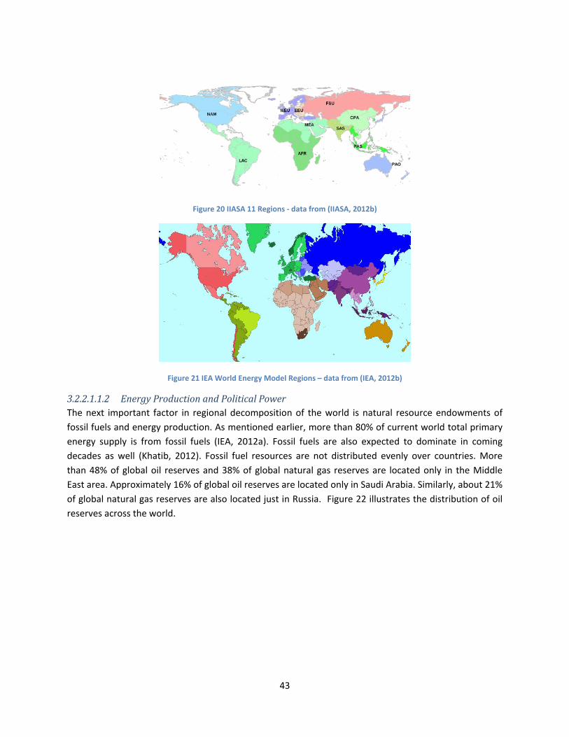
43

Figure 20 IIASA 11 Regions - data from (IIASA, 2012b)

Figure 21 IEA World Energy Model Regions – data from (IEA, 2012b)

3.2.2.1.1.2 Energy Production and Political Power The next important factor in regional decomposition of the world is natural resource endowments of fossil fuels and energy production. As mentioned earlier, more than 80% of current world total primary energy supply is from fossil fuels (IEA, 2012a). Fossil fuels are also expected to dominate in coming decades as well (Khatib, 2012). Fossil fuel resources are not distributed evenly over countries. More than 48% of global oil reserves and 38% of global natural gas reserves are located only in the Middle East area. Approximately 16% of global oil reserves are located only in Saudi Arabia. Similarly, about 21% of global natural gas reserves are also located just in Russia. Figure 22 illustrates the distribution of oil reserves across the world.

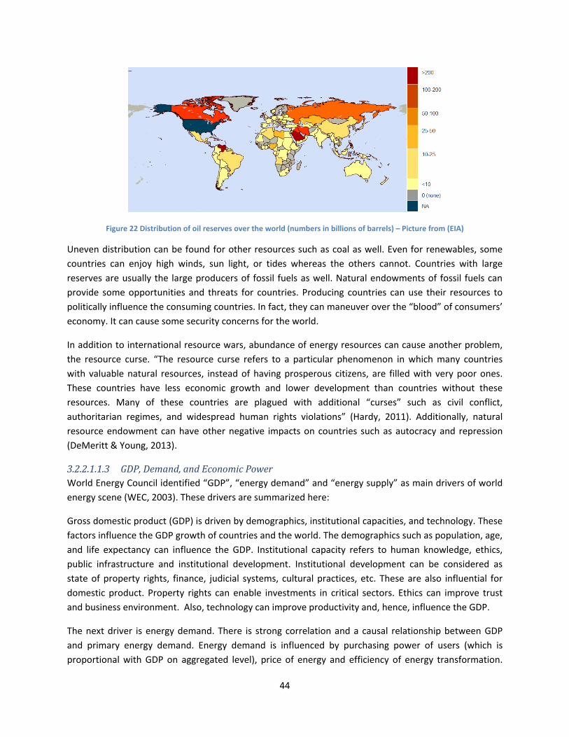
44

Figure 22 Distribution of oil reserves over the world (numbers in billions of barrels) – Picture from (EIA)

Uneven distribution can be found for other resources such as coal as well. Even for renewables, some countries can enjoy high winds, sun light, or tides whereas the others cannot. Countries with large reserves are usually the large producers of fossil fuels as well. Natural endowments of fossil fuels can provide some opportunities and threats for countries. Producing countries can use their resources to politically influence the consuming countries. In fact, they can maneuver over the “blood” of consumers’ economy. It can cause some security concerns for the world.

In addition to international resource wars, abundance of energy resources can cause another problem, the resource curse. “The resource curse refers to a particular phenomenon in which many countries with valuable natural resources, instead of having prosperous citizens, are filled with very poor ones. These countries have less economic growth and lower development than countries without these resources. Many of these countries are plagued with additional “curses” such as civil conflict, authoritarian regimes, and widespread human rights violations” (Hardy, 2011). Additionally, natural resource endowment can have other negative impacts on countries such as autocracy and repression (DeMeritt & Young, 2013).

3.2.2.1.1.3 GDP, Demand, and Economic Power World Energy Council identified “GDP”, “energy demand” and “energy supply” as main drivers of world energy scene (WEC, 2003). These drivers are summarized here:

Gross domestic product (GDP) is driven by demographics, institutional capacities, and technology. These factors influence the GDP growth of countries and the world. The demographics such as population, age, and life expectancy can influence the GDP. Institutional capacity refers to human knowledge, ethics, public infrastructure and institutional development. Institutional development can be considered as state of property rights, finance, judicial systems, cultural practices, etc. These are also influential for domestic product. Property rights can enable investments in critical sectors. Ethics can improve trust and business environment. Also, technology can improve productivity and, hence, influence the GDP.

The next driver is energy demand. There is strong correlation and a causal relationship between GDP and primary energy demand. Energy demand is influenced by purchasing power of users (which is proportional with GDP on aggregated level), price of energy and efficiency of energy transformation.

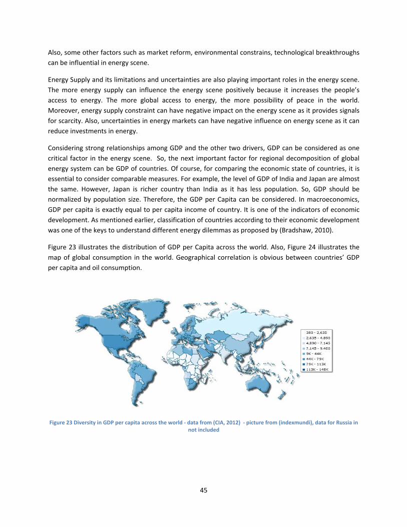
45

Also, some other factors such as market reform, environmental constrains, technological breakthroughs can be influential in energy scene.

Energy Supply and its limitations and uncertainties are also playing important roles in the energy scene. The more energy supply can influence the energy scene positively because it increases the people’s access to energy. The more global access to energy, the more possibility of peace in the world. Moreover, energy supply constraint can have negative impact on the energy scene as it provides signals for scarcity. Also, uncertainties in energy markets can have negative influence on energy scene as it can reduce investments in energy.

Considering strong relationships among GDP and the other two drivers, GDP can be considered as one critical factor in the energy scene. So, the next important factor for regional decomposition of global energy system can be GDP of countries. Of course, for comparing the economic state of countries, it is essential to consider comparable measures. For example, the level of GDP of India and Japan are almost the same. However, Japan is richer country than India as it has less population. So, GDP should be normalized by population size. Therefore, the GDP per Capita can be considered. In macroeconomics, GDP per capita is exactly equal to per capita income of country. It is one of the indicators of economic development. As mentioned earlier, classification of countries according to their economic development was one of the keys to understand different energy dilemmas as proposed by (Bradshaw, 2010).

Figure 23 illustrates the distribution of GDP per Capita across the world. Also, Figure 24 illustrates the map of global consumption in the world. Geographical correlation is obvious between countries’ GDP per capita and oil consumption.

Figure 23 Diversity in GDP per capita across the world - data from (CIA, 2012) - picture from (indexmundi), data for Russia in not included

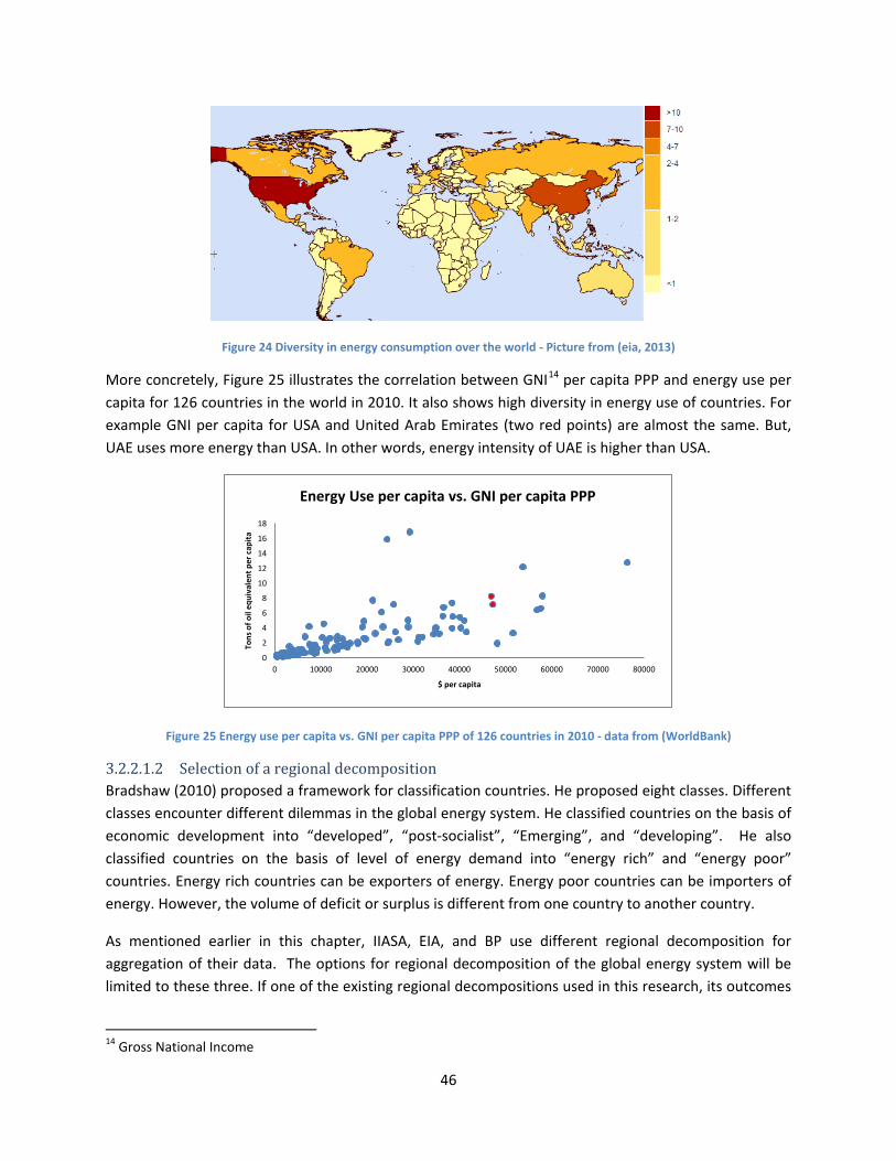
46

Figure 24 Diversity in energy consumption over the world - Picture from (eia, 2013)

More concretely, Figure 25 illustrates the correlation between GNI14 per capita PPP and energy use per capita for 126 countries in the world in 2010. It also shows high diversity in energy use of countries. For example GNI per capita for USA and United Arab Emirates (two red points) are almost the same. But, UAE uses more energy than USA. In other words, energy intensity of UAE is higher than USA.

Figure 25 Energy use per capita vs. GNI per capita PPP of 126 countries in 2010 - data from (WorldBank)

3.2.2.1.2 Selection of a regional decomposition Bradshaw (2010) proposed a framework for classification countries. He proposed eight classes. Different classes encounter different dilemmas in the global energy system. He classified countries on the basis of economic development into “developed”, “post-socialist”, “Emerging”, and “developing”. He also classified countries on the basis of level of energy demand into “energy rich” and “energy poor” countries. Energy rich countries can be exporters of energy. Energy poor countries can be importers of energy. However, the volume of deficit or surplus is different from one country to another country.

As mentioned earlier in this chapter, IIASA, EIA, and BP use different regional decomposition for aggregation of their data. The options for regional decomposition of the global energy system will be limited to these three. If one of the existing regional decompositions used in this research, its outcomes

14 Gross National Income

0

2

4

6

8

10

12

14

16

18

0 10000 20000 30000 40000 50000 60000 70000 80000

Tons

of o

il eq

uiva

lent

per

cap

ita

$ per capita

Energy Use per capita vs. GNI per capita PPP

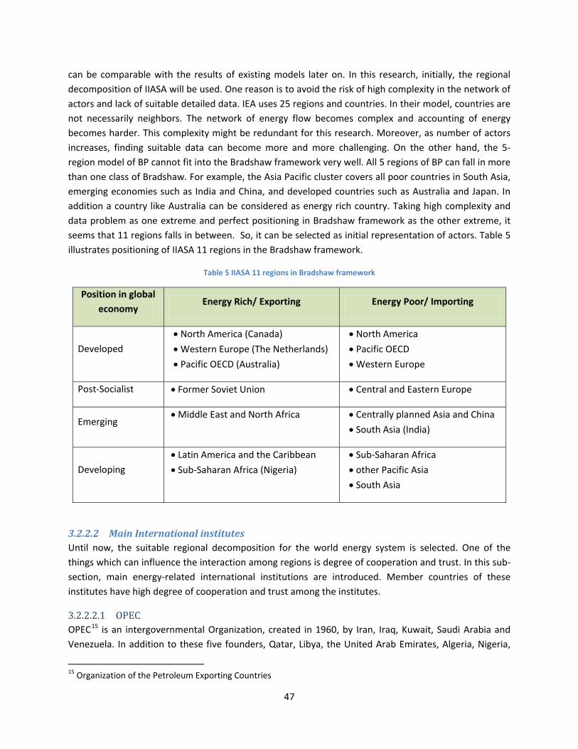
47

can be comparable with the results of existing models later on. In this research, initially, the regional decomposition of IIASA will be used. One reason is to avoid the risk of high complexity in the network of actors and lack of suitable detailed data. IEA uses 25 regions and countries. In their model, countries are not necessarily neighbors. The network of energy flow becomes complex and accounting of energy becomes harder. This complexity might be redundant for this research. Moreover, as number of actors increases, finding suitable data can become more and more challenging. On the other hand, the 5-region model of BP cannot fit into the Bradshaw framework very well. All 5 regions of BP can fall in more than one class of Bradshaw. For example, the Asia Pacific cluster covers all poor countries in South Asia, emerging economies such as India and China, and developed countries such as Australia and Japan. In addition a country like Australia can be considered as energy rich country. Taking high complexity and data problem as one extreme and perfect positioning in Bradshaw framework as the other extreme, it seems that 11 regions falls in between. So, it can be selected as initial representation of actors. Table 5 illustrates positioning of IIASA 11 regions in the Bradshaw framework.

Table 5 IIASA 11 regions in Bradshaw framework

Position in global economy

Energy Rich/ Exporting Energy Poor/ Importing

Developed • North America (Canada) • Western Europe (The Netherlands) • Pacific OECD (Australia)

• North America • Pacific OECD • Western Europe

Post-Socialist • Former Soviet Union • Central and Eastern Europe

Emerging • Middle East and North Africa • Centrally planned Asia and China

• South Asia (India)

Developing • Latin America and the Caribbean • Sub-Saharan Africa (Nigeria)

• Sub-Saharan Africa • other Pacific Asia • South Asia

3.2.2.2 Main International institutes Until now, the suitable regional decomposition for the world energy system is selected. One of the things which can influence the interaction among regions is degree of cooperation and trust. In this sub-section, main energy-related international institutions are introduced. Member countries of these institutes have high degree of cooperation and trust among the institutes.

3.2.2.2.1 OPEC OPEC15 is an intergovernmental Organization, created in 1960, by Iran, Iraq, Kuwait, Saudi Arabia and Venezuela. In addition to these five founders, Qatar, Libya, the United Arab Emirates, Algeria, Nigeria,

15 Organization of the Petroleum Exporting Countries

48

Ecuador, and Angola joined OPEC later. OPEC's objective is to co-ordinate and unify petroleum policies among Member Countries, in order to secure fair and stable prices for petroleum producers; an efficient, economic and regular supply of petroleum to consuming nations; and a fair return on capital to those investing in the industry (OPEC). Currently, OPEC has 72.4% of global proved oil reserves and 42.4% global oil production (BP, 2012a).

3.2.2.2.2 OECD OECD16 was established in September 1961 (OECD). Its mission is to promote policies that will improve the economic and social well-being of people around the world. The common thread of OECD work is a shared commitment to market economies backed by democratic institutions (OECD). 34 countries have joined OECD. These countries are industrialized North American, European and Pacific countries. These countries are committed for democracy and free-market systems. Currently, OECD consumes 45% of global primary energy (BP, 2012a). After 1973 oil crisis, OECD countries established IEA17 which acts as policy advisor for member states.

3.2.2.2.3 EU EU18 is a union of 27 member European states. Rooted in the European Coal and Steel Community (ECSC) and the European Economic Community (EEC), EU establish with Maastricht Treaty in 1993. EU has developed a single market and a monetary Euro zone (Steiner & Woods, 2009). Currently, EU has 13% global primary energy consumption.

3.2.2.2.4 BRICS BRICS refers to set of emerging economies. Brazil, Russia, Indonesia, China, and South Africa are fast growing economies. They will be important consumers of energy in future. The solidarity of this group is not like aforementioned ones yet. However, their relations are getting stronger. In fifth summit of BRICS in March 2013, they agreed to found a bank for funding infrastructures. this bank is expected to be a competitor for the World Bank (Smith, 2013).

3.2.2.2.5 GECF GECF19 is a gathering of the world’s leading gas producers. It was established in 2008. Its objective is to increase the level of coordination and strengthen the collaboration among Member countries. The Member Countries of the Forum are: Algeria, Bolivia, Egypt, Equatorial Guinea, Iran, Libya, Nigeria, Oman, Qatar, Russia, Trinidad and Tobago, United Arab Emirates and Venezuela. Kazakhstan, Iraq, the Netherlands and Norway have the status of Observer Members. Its potential rests on the enormous natural gas reserves of the Member Countries all together accumulating 62% of the world proved natural gas reserves (GECF).

16 Organization for Economic Cooperation and Development 17 International Energy Agency 18 European Union 19 Gas Exporting Countries Forum

49

3.2.2.2.6 Sphere of influence Each international institute has limited sphere of influence in IIASA regional model. OPEC mainly influences the Middle East and North Africa (MEA). It can partially influence Sub-Saharan Africa (AFR) and Latin America and Caribbean (LAB). GECF can mainly influence MEA and FSU.

OECD influences the North America (NAM), Western Europe (WEU) and Pacific OECD (PAO). The Sphere of influence of EU is Western Europe (WEU) and Central and Eastern Europe (EEU). BRICS has the most diverse influence in this model. It can influence the Latin America and the Caribbean (LAB), Former Soviet (FSU), South Asia (SAS), Centrally planned Asia and China (CPA).

3.2.3 Conclusion This section aimed at answering the research question “How can the world energy system be decomposed into different trading regions?”. The purpose of this question is to determine the decomposition of the future agent-based model.

In order to find suitable decomposition, micro and macro analysis of actors in the global energy system were provided. In the micro analysis, the network of energy-related companies along the value chain was analyzed. Micro analysis showed who work in the energy sector of a country and how governments and policy makers interact with them. It showed diversity of actors within each country. Diversity of actor can make system complex.

Since the focus of this research is on modeling of primary energy supply, in the macro analysis, the main energy activates in a country were considered to be production, consumption, and trade. Considerable diversity was found among regions in term of economic state and energy state. Despite all diversities within and between countries, an attempt was made to put countries with similar energy and economic states into the same groups.

In this research, instead of real actor decomposition of the world, an existing one was selected. Selecting one of the existing regional decomposition among what renowned international institute use in their reports, enables comparison of the outcomes of the future agent-based model with those report.

In order to select a suitable decomposition, some criteria were set. The geography played the most important role among all criteria. It could encompass the geology, culture, economy and politics of countries and regions.

The 11 regions of IIASA were selected as the actor decomposition of for the future agent-based model. The advantage of IIASA over other alternative was the moderate level of abstraction and availability of most required data in the GEA scenario database.

In addition to regional decomposition of the world, main international energy-related institutes were introduced in order to identify the level of cooperation and trust among selected regions.

50

4 The First Model: Aggregated World Energy Model In the previous chapters, the energy problem, the research design, and the world energy system were explained. In the current chapter a hybrid system dynamics and agent-based model will be developed without considering regional decomposition of the world. In the next chapter, an agent-based model will be developed considering world regions.

In this chapter, in section 4.1, the phases of model development will be presented. Then, in section 4.2, the design and the results of the experimentation phases will be provided.

4.1 Model Development The objective of this research is development of a model to explore the behaviors of the world energy system from biophysical economics perspective and with considering energy trade among countries and regions. This research follows two steps for development of such model. The first step is to develop a model without considering energy trade. The second step will be development of a model with considering energy trade. This two-step approach can enable the use of current biophysical economics models of the world energy-economy system. There are already some biophysical economics models in the literature which ignore energy trade and geographical movements of energy in their assumptions. So, if the equivalent of a current model can be designed and developed in the first step, the objective model of this research can be designed and developed by adding some modules and modification the first model. So, one of the advantages of this approach would be scientific foundations and validity of the first model.

As mentioned in Chapter 1, the most recent biophysical economic model for the world energy system, GEMBA, is developed by M. Dale et al. (2012). He developed a system dynamics model (GEMBA) to explore the global energy system from biophysical perspective. In this section equivalent of GEMBA will be designed and developed. Here, the equivalent model is called “Aggregated World Energy Model”. The aggregated world energy model uses the same functions as GEMBA. Later, with incorporating the regional decomposition of the world, “Multi-Region World Energy Model” will be design and developed.

In this section, in sub-section 4.1.1, an introduction to the reference system dynamics model (GEMBA) will be provided. Afterwards, in sub-section 4.1.3, the conceptual design of the model will be explained. The details of implementation and evaluation phases will be provided in sub-sections 4.1.3 and 4.1.4.

4.1.1 Introduction to GEMBA

4.1.1.1 GEMBA Overview The Global Energy Model using a Biophysical Approach (GEMBA) is developed by M. A. J. Dale (2010). GEMBA is a system dynamics model to explore the global energy supply. In Figure 6, the general biophysical view of economy was introduced. More abstracted, Figure 26 illustrates the relationship between the energy sector and the rest of the economy. GEMBA analyzes the relationship between energy sector and the rest of economy as depicted in Figure 26.

51

Raw Resources

Energy ResourcesPollutants

Rest of the Economy

Energy Transformation

System

S2

S1

D

R

Figure 26 Relationship between the energy sector and the rest of economy - Picture from (M. A. J. Dale, 2010)

In GEMBA, main physical elements in the system are energy sector capital stock the industrial sector capital stock. These capital stocks refer to infrastructures in their host sector and they can be measured in exajoules (EJ). Both energy sector (energy transformation system) and industrial sector (the rest of economy) have important outputs. The main outputs of energy sector are total energy yield and net energy yield. The main output of industrial sector can be called industrial output which is the physical capital output of the rest of economy.

Energy sector capital stock is measured separately for each energy resource. In GEMBA, the energy resources are classified into two groups of renewables and non-renewables. Renewable resources include biomass, hydro, geothermal, tidal, wind, solar, wave, and ocean thermal energy conversion (OTEC). Non-renewable resources include coal, conventional oil, conventional gas, unconventional oil, unconventional gas, uranium20. In this classification, the distinction between “conventional” and “unconventional” non-renewable resources is because of different EROI of resources.

As mentioned in 2, the focus of system dynamics models is on the structure of causal relations and feedbacks in the system. The general causal relationships in GEMBA are depicted in Figure 27.

20 In GEMBA, uranium is assumed to be burner reactor

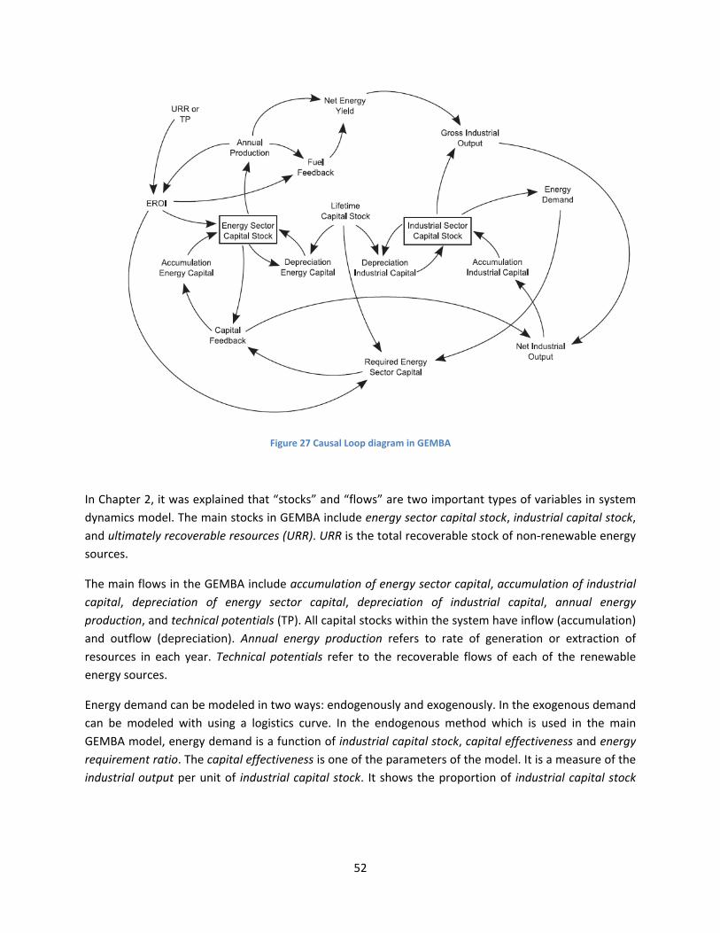
52

Figure 27 Causal Loop diagram in GEMBA

In Chapter 2, it was explained that “stocks” and “flows” are two important types of variables in system dynamics model. The main stocks in GEMBA include energy sector capital stock, industrial capital stock, and ultimately recoverable resources (URR). URR is the total recoverable stock of non-renewable energy sources.

The main flows in the GEMBA include accumulation of energy sector capital, accumulation of industrial capital, depreciation of energy sector capital, depreciation of industrial capital, annual energy production, and technical potentials (TP). All capital stocks within the system have inflow (accumulation) and outflow (depreciation). Annual energy production refers to rate of generation or extraction of resources in each year. Technical potentials refer to the recoverable flows of each of the renewable energy sources.

Energy demand can be modeled in two ways: endogenously and exogenously. In the exogenous demand can be modeled with using a logistics curve. In the endogenous method which is used in the main GEMBA model, energy demand is a function of industrial capital stock, capital effectiveness and energy requirement ratio. The capital effectiveness is one of the parameters of the model. It is a measure of the industrial output per unit of industrial capital stock. It shows the proportion of industrial capital stock

53

that is itself capable of producing industrial output. Also, energy intensity of the economy, which is defined as energy requirement ratio, is a measure of industrial output per unit of net energy yield21.

The variable for allocating energy demand to energy resources is called favorability of the resource. Favorability is function of resource EROI and resource availability. The resource availability is dependent on (annual or cumulative) energy production and URR/TP of resources. Since there is a delay from perception of favorability for one resource and capital accumulation in that resource, the first order exponential smoothing22 is employed to capture the delay.

4.1.1.2 GEMBA Assumptions GEMBA is developed on the basis of a set of assumptions. In the following paragraphs the main assumptions of GEMBA will be introduced and elaborated on.

On the basis of work of J.T. Baines and Peet (1986) and Bodger and Baines (1989), M. A. J. Dale (2010) used three fundamental variables (incept date, availability, accessibility) in development of GEMBA. He also used the variable “capital intensity” in GEMBA. The “Incept date” is the year that energy source enters the market. The variable “availability” shows how much energy is available in for specific resource. The variable “accessibility” can be measured with the energy-return-on-investment (EROI)23. One of the model parameters which influence the annual energy production is capital intensity. In GEMBA, it is defined as capital factor. Capital factor is the ratio of capital input to total input of energy sector in order to extract and produce energy.

In GEMBA, the distinction between energy carriers and transportation options is ignored. So, the only distinction is about source of energy. In addition, all phases of extraction, transformation and transportation are aggregated into “the energy sector”. The energy losses in these phases are aggregated as well.

Moreover, in GEMBA, the distinction among consuming sectors (industry, households, etc.) is ignored. So, it is assumed that the only energy consumer is the rest of economy. In addition, considering long time frame of the simulation and low availability of data, the energy demand is assumed to be homogenous which means that demand is just for energy, not for a particular type of resource.

In GEMBA, both energy sector and the rest of economy have capital requirements. Another assumption about the GEMBA is priority of capital requirements of energy sector to capital requirements of the rest of the economy.

Finally, in GEMBA, the energy resources such as fission with “breeder” and nuclear fusion are ignored in this model. M. A. J. Dale (2010) argued that these options can be considered infeasible in terms of schedule, budget and competitiveness with other options.

21 Energy requirement ratio is not a measure of the efficiency of energy use. Such a measure would not be possible since energy is the only metric used within the GEMBA.

22 SMOOTH function in Vensim 23 It can be calculated by energy yield ratio (Equation 2)

54

4.1.1.3 GEMBA in Energy Circuit Language In Figure 26, the relationship between energy sector and the rest of the economy was illustrated. Also, Figure 27 showed the causal relationship within the GEMBA model. Combination of these two views can be seen with energy circuit language in Figure 28. Energy circuit language was developed by (Odum, 1976). Using this language can ensure the adherence of model to physical laws such as thermodynamics. The symbols of energy circuit language are explained in Appendix 2.

Figure 28 Structure of the GEMBA energy-economy model as an energy circuit diagram – Picture from (M. A. J. Dale, 2010)

In Figure 28, the dashed lines show the boundaries of energy sector and the rest of the economy. There are “tanks” (stocks) of non-renewables with specific URR24. There are also “sources” (flows) of renewable energy with specific TP. Both energy and economy sectors have capital tanks. There are also “interaction” segments in both sectors which produce outflow of energy or capital from more than one inflow. The hexagonal in the economy shows the fact that it consume energy. All arrowed lines show the flow of energy (or flow of capital in terms of exajoules). Both sectors have “heat sinks” in which their capital is depreciated or the energy is lost.

As it is illustrated in Figure 28, EROI is a function of the energy availability of resources (which is function

of energy production ∑ kPand URR/TP of resources). EROI influenced the fuel feedback to energy

sector, ∑ kS ,1 . The net energy yield ( Net ) is function of energy production and fuel feedback. The 24 “k” is the index of the resource (like coal, conventional oil, etc.)

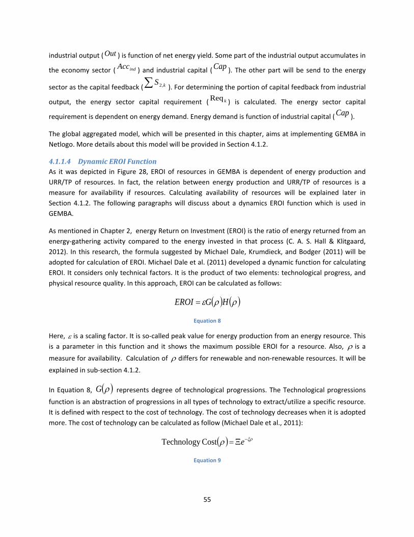
55

industrial output ( Out ) is function of net energy yield. Some part of the industrial output accumulates in

the economy sector ( indAcc ) and industrial capital ( Cap ). The other part will be send to the energy

sector as the capital feedback (∑ kS ,2 ). For determining the portion of capital feedback from industrial

output, the energy sector capital requirement ( kReq ) is calculated. The energy sector capital

requirement is dependent on energy demand. Energy demand is function of industrial capital ( Cap ).

The global aggregated model, which will be presented in this chapter, aims at implementing GEMBA in Netlogo. More details about this model will be provided in Section 4.1.2.

4.1.1.4 Dynamic EROI Function As it was depicted in Figure 28, EROI of resources in GEMBA is dependent of energy production and URR/TP of resources. In fact, the relation between energy production and URR/TP of resources is a measure for availability if resources. Calculating availability of resources will be explained later in Section 4.1.2. The following paragraphs will discuss about a dynamics EROI function which is used in GEMBA.

As mentioned in Chapter 2, energy Return on Investment (EROI) is the ratio of energy returned from an energy-gathering activity compared to the energy invested in that process (C. A. S. Hall & Klitgaard, 2012). In this research, the formula suggested by Michael Dale, Krumdieck, and Bodger (2011) will be adopted for calculation of EROI. Michael Dale et al. (2011) developed a dynamic function for calculating EROI. It considers only technical factors. It is the product of two elements: technological progress, and physical resource quality. In this approach, EROI can be calculated as follows:

( ) ( )ρρε HGEROI =

Equation 8

Here, ε is a scaling factor. It is so-called peak value for energy production from an energy resource. This is a parameter in this function and it shows the maximum possible EROI for a resource. Also, ρ is a

measure for availability. Calculation of ρ differs for renewable and non-renewable resources. It will be

explained in sub-section 4.1.2.

In Equation 8, ( )ρG represents degree of technological progressions. The Technological progressions

function is an abstraction of progressions in all types of technology to extract/utilize a specific resource. It is defined with respect to the cost of technology. The cost of technology decreases when it is adopted more. The cost of technology can be calculated as follow (Michael Dale et al., 2011):

( ) ξρρ −Ξ= eCost Technology

Equation 9

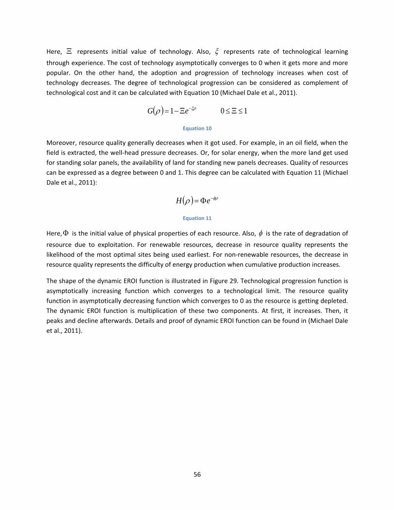
56

Here, Ξ represents initial value of technology. Also, ξ represents rate of technological learning

through experience. The cost of technology asymptotically converges to 0 when it gets more and more popular. On the other hand, the adoption and progression of technology increases when cost of technology decreases. The degree of technological progression can be considered as complement of technological cost and it can be calculated with Equation 10 (Michael Dale et al., 2011).

( ) 101 ≤Ξ≤Ξ−= −ξρρ eG

Equation 10

Moreover, resource quality generally decreases when it got used. For example, in an oil field, when the field is extracted, the well-head pressure decreases. Or, for solar energy, when the more land get used for standing solar panels, the availability of land for standing new panels decreases. Quality of resources can be expressed as a degree between 0 and 1. This degree can be calculated with Equation 11 (Michael Dale et al., 2011):

( ) φρρ −Φ= eH

Equation 11

Here,Φ is the initial value of physical properties of each resource. Also, φ is the rate of degradation of

resource due to exploitation. For renewable resources, decrease in resource quality represents the likelihood of the most optimal sites being used earliest. For non-renewable resources, the decrease in resource quality represents the difficulty of energy production when cumulative production increases.

The shape of the dynamic EROI function is illustrated in Figure 29. Technological progression function is asymptotically increasing function which converges to a technological limit. The resource quality function in asymptotically decreasing function which converges to 0 as the resource is getting depleted. The dynamic EROI function is multiplication of these two components. At first, it increases. Then, it peaks and decline afterwards. Details and proof of dynamic EROI function can be found in (Michael Dale et al., 2011).

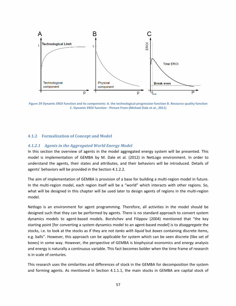
57

Figure 29 Dynamic EROI function and its components: A. the technological progression function B. Resource quality function C. Dynamic EROI function - Picture From (Michael Dale et al., 2011)

4.1.2 Formalization of Concept and Model

4.1.2.1 Agents in the Aggregated World Energy Model In this section the overview of agents in the model aggregated energy system will be presented. This model is implementation of GEMBA by M. Dale et al. (2012) in NetLogo environment. In order to understand the agents, their states and attributes, and their behaviors will be introduced. Details of agents’ behaviors will be provided in the Section 4.1.2.2.

The aim of implementation of GEMBA is provision of a base for building a multi-region model in future. In the multi-region model, each region itself will be a “world” which interacts with other regions. So, what will be designed in this chapter will be used later to design agents of regions in the multi-region model.

Netlogo is an environment for agent programming. Therefore, all activities in the model should be designed such that they can be performed by agents. There is no standard approach to convert system dynamics models to agent-based models. Borshchev and Filippov (2004) mentioned that “the key starting point [for converting a system dynamics model to an agent-based model] is to disaggregate the stocks, i.e. to look at the stocks as if they are not tanks with liquid but boxes containing discrete items, e.g. balls”. However, this approach can be applicable for system which can be seen discrete (like set of boxes) in some way. However, the perspective of GEMBA is biophysical economics and energy analysis and energy is naturally a continuous variable. This fact becomes bolder when the time frame of research is in scale of centuries.

This research uses the similarities and differences of stock in the GEMBA for decomposition the system and forming agents. As mentioned in Section 4.1.1.1, the main stocks in GEMBA are capital stock of

58

energy sector, capital stock of the economy, and stocks of non-renewable resources. These stocks can be assigned to three groups:

1. The economy: The main economy consumes energy and has “capital stock of the economy” 2. The renewable energy sector: It produces renewable energy and has “capital stock of energy

sector” 3. The non-renewable energy sector: It produces non-renewable energy and has “capital stock of

energy sector” and “stock of non-renewables energy”.

In each of these groups, the stocks influence different variables. Also, they are themselves treated differently. For example, the stock of capital in the economy influences the energy demand whereas other stocks do not influence it. In addition, the stocks of non-renewable energy influence the EROI of non-renewable resources whereas the renewable resources do not have any stock at all. On the basis of these differences and similarities, in this research, three aforementioned groups form the basis of three of agents in the model. The agent “Energy Consumer” represents the group of the economy. The agent “Renewable Supplier” represents the group of renewable energy sector. Also, the agent “non-renewable supplier” represents the group of non-renewable energy sector.

The function of ‘aggregating net energy yield of different resources’ and ‘allocating energy demand to energy sectors can be done by “Energy Consumers”. However, in order to provide more flexibility for future development of the model, these functions are assigned to a new agent called “Energy Dispatcher”. In fact, while other agents are representing the technical aspects of the world energy system, “Energy Dispatcher” represents more managerial and business aspects in the system. So, having energy dispatchers as distinct agent can help future development of model and improving business aspects.

So, the main agents in the model are: Renewable Suppliers, Non-Renewable Suppliers, Energy Consumers, and Energy Dispatchers. Energy Suppliers (renewable and non-renewable) take care of all extraction, conversion and distribution activities which are discussed in Section 3.1. Energy consumers are the main economy excluding the energy sector. Energy dispatchers are virtual entities who allocate total energy demand over different energy resources. They also connect energy suppliers to energy consumers and facilitate (information of) flow of energy and capital. The overview of the system is illustrated in Figure 30. Here, flow of capital, energy, and information are depicted.

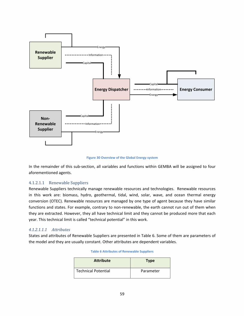
59

Energy ConsumerEnergy

Capital

Energy Dispatcher

Renewable Supplier

Non-Renewable

Supplier

Energy

Energy

Capital

Capital

Information

Information

Information

Figure 30 Overview of the Global Energy system

In the remainder of this sub-section, all variables and functions within GEMBA will be assigned to four aforementioned agents.

4.1.2.1.1 Renewable Suppliers Renewable Suppliers technically manage renewable resources and technologies. Renewable resources in this work are: biomass, hydro, geothermal, tidal, wind, solar, wave, and ocean thermal energy conversion (OTEC). Renewable resources are managed by one type of agent because they have similar functions and states. For example, contrary to non-renewable, the earth cannot run out of them when they are extracted. However, they all have technical limit and they cannot be produced more that each year. This technical limit is called “technical potential” in this work.

4.1.2.1.1.1 Attributes States and attributes of Renewable Suppliers are presented in Table 6. Some of them are parameters of the model and they are usually constant. Other attributes are dependent variables.

Table 6 Attributes of Renewable Suppliers

Attribute Type

Technical Potential Parameter

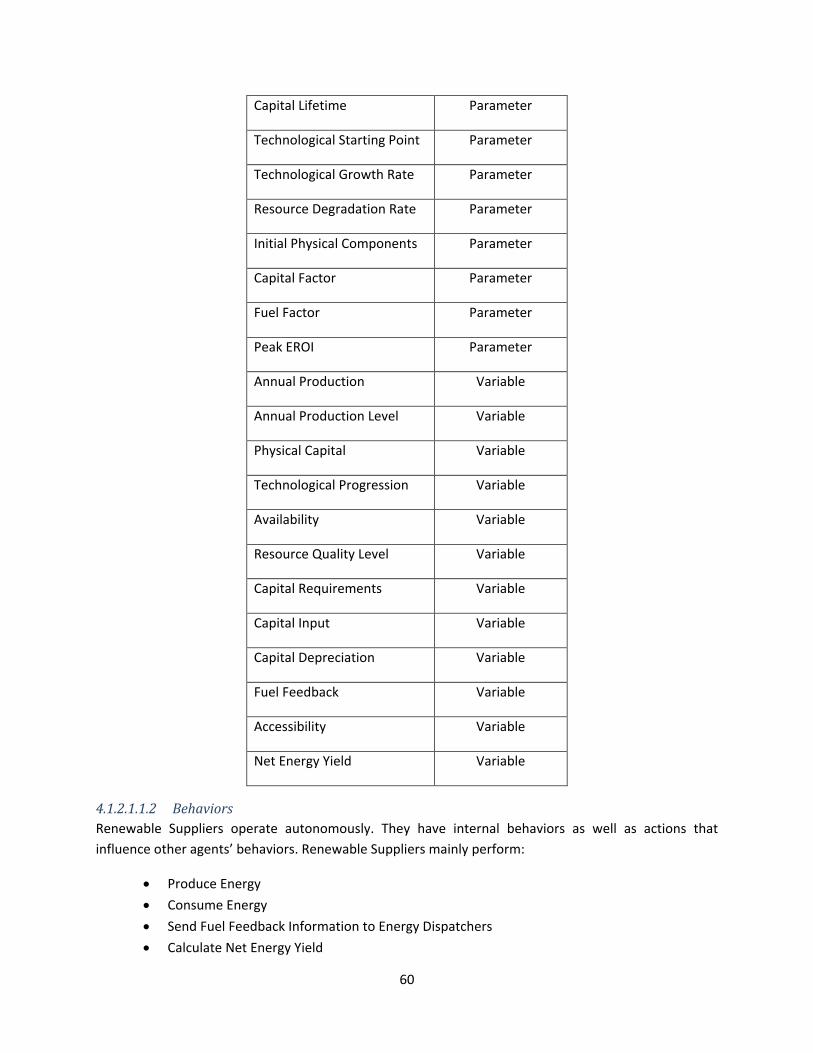
60

Capital Lifetime Parameter

Technological Starting Point Parameter

Technological Growth Rate Parameter

Resource Degradation Rate Parameter

Initial Physical Components Parameter

Capital Factor Parameter

Fuel Factor Parameter

Peak EROI Parameter

Annual Production Variable

Annual Production Level Variable

Physical Capital Variable

Technological Progression Variable

Availability Variable

Resource Quality Level Variable

Capital Requirements Variable

Capital Input Variable

Capital Depreciation Variable

Fuel Feedback Variable

Accessibility Variable

Net Energy Yield Variable

4.1.2.1.1.2 Behaviors Renewable Suppliers operate autonomously. They have internal behaviors as well as actions that influence other agents’ behaviors. Renewable Suppliers mainly perform:

• Produce Energy • Consume Energy • Send Fuel Feedback Information to Energy Dispatchers • Calculate Net Energy Yield

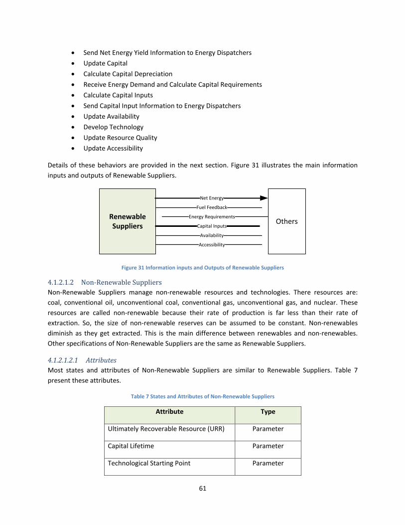
61

• Send Net Energy Yield Information to Energy Dispatchers • Update Capital • Calculate Capital Depreciation • Receive Energy Demand and Calculate Capital Requirements • Calculate Capital Inputs • Send Capital Input Information to Energy Dispatchers • Update Availability • Develop Technology • Update Resource Quality • Update Accessibility

Details of these behaviors are provided in the next section. Figure 31 illustrates the main information inputs and outputs of Renewable Suppliers.

Renewable Suppliers

Net Energy

Fuel Feedback

Energy Requirements

Capital Inputs

Availability

Accessibility

Others

Figure 31 Information inputs and Outputs of Renewable Suppliers

4.1.2.1.2 Non-Renewable Suppliers Non-Renewable Suppliers manage non-renewable resources and technologies. There resources are: coal, conventional oil, unconventional coal, conventional gas, unconventional gas, and nuclear. These resources are called non-renewable because their rate of production is far less than their rate of extraction. So, the size of non-renewable reserves can be assumed to be constant. Non-renewables diminish as they get extracted. This is the main difference between renewables and non-renewables. Other specifications of Non-Renewable Suppliers are the same as Renewable Suppliers.

4.1.2.1.2.1 Attributes Most states and attributes of Non-Renewable Suppliers are similar to Renewable Suppliers. Table 7 present these attributes.

Table 7 States and Attributes of Non-Renewable Suppliers

Attribute Type

Ultimately Recoverable Resource (URR) Parameter

Capital Lifetime Parameter

Technological Starting Point Parameter

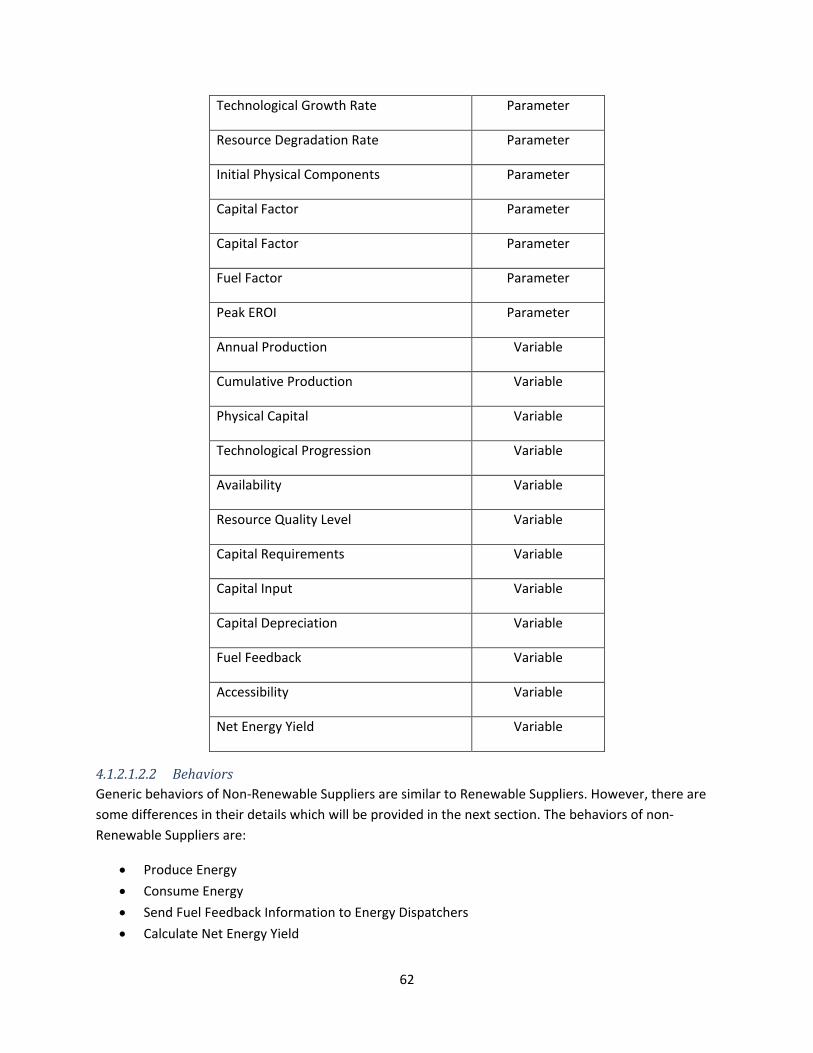
62

Technological Growth Rate Parameter

Resource Degradation Rate Parameter

Initial Physical Components Parameter

Capital Factor Parameter

Capital Factor Parameter

Fuel Factor Parameter

Peak EROI Parameter

Annual Production Variable

Cumulative Production Variable

Physical Capital Variable

Technological Progression Variable

Availability Variable

Resource Quality Level Variable

Capital Requirements Variable

Capital Input Variable

Capital Depreciation Variable

Fuel Feedback Variable

Accessibility Variable

Net Energy Yield Variable

4.1.2.1.2.2 Behaviors Generic behaviors of Non-Renewable Suppliers are similar to Renewable Suppliers. However, there are some differences in their details which will be provided in the next section. The behaviors of non-Renewable Suppliers are:

• Produce Energy • Consume Energy • Send Fuel Feedback Information to Energy Dispatchers • Calculate Net Energy Yield

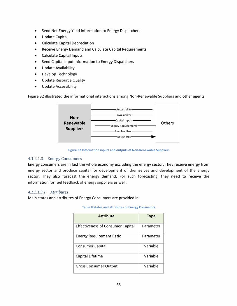
63

• Send Net Energy Yield Information to Energy Dispatchers • Update Capital • Calculate Capital Depreciation • Receive Energy Demand and Calculate Capital Requirements • Calculate Capital Inputs • Send Capital Input Information to Energy Dispatchers • Update Availability • Develop Technology • Update Resource Quality • Update Accessibility

Figure 32 illustrated the informational interactions among Non-Renewable Suppliers and other agents.

Non-Renewable Suppliers

Net Energy

Fuel Feedback

Energy Requirements

Capital Inputs

Availability

Accessibility

Others

Figure 32 Information inputs and outputs of Non-Renewable Suppliers

4.1.2.1.3 Energy Consumers Energy consumers are in fact the whole economy excluding the energy sector. They receive energy from energy sector and produce capital for development of themselves and development of the energy sector. They also forecast the energy demand. For such forecasting, they need to receive the information for fuel feedback of energy suppliers as well.

4.1.2.1.3.1 Attributes Main states and attributes of Energy Consumers are provided in

Table 8 States and attributes of Energy Consuemrs

Attribute Type

Effectiveness of Consumer Capital Parameter

Energy Requirement Ratio Parameter

Consumer Capital Variable

Capital Lifetime Variable

Gross Consumer Output Variable

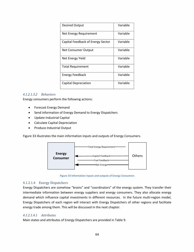
64

Desired Output Variable

Net Energy Requirement Variable

Capital Feedback of Energy Sector Variable

Net Consumer Output Variable

Net Energy Yield Variable

Total Requirement Variable

Energy Feedback Variable

Capital Depreciation Variable

4.1.2.1.3.2 Behaviors Energy consumers perform the following actions:

• Forecast Energy Demand • Send information of Energy Demand to Energy Dispatchers • Update Industrial Capital • Calculate Capital Depreciation • Produce Industrial Output

Figure 33 illustrates the main information inputs and outputs of Energy Consumers.

Energy Consumer

Net Energy

Fuel Feedback

Total Energy Requirement

OthersCapital Feedback

Figure 33 Information inputs and outputs of Energy Consumers

4.1.2.1.4 Energy Dispatchers Energy Dispatchers are somehow “brains” and “coordinators” of the energy system. They transfer their intermediate information between energy suppliers and energy consumers. They also allocate energy demand which influence capital investments in different resources. In the future multi-region model, Energy Dispatchers of each region will interact with Energy Dispatchers of other regions and facilitate energy trade among them. This will be discussed in the next chapter.

4.1.2.1.4.1 Attributes Main states and attributes of Energy Dispatchers are provided in Table 9.

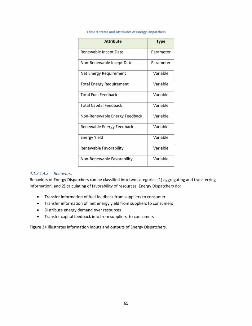
65

Table 9 States and Attributes of Energy Dispatchers

Attribute Type

Renewable Incept Date Parameter

Non-Renewable Incept Date Parameter

Net Energy Requirement Variable

Total Energy Requirement Variable

Total Fuel Feedback Variable

Total Capital Feedback Variable

Non-Renewable Energy Feedback Variable

Renewable Energy Feedback Variable

Energy Yield Variable

Renewable Favorability Variable

Non-Renewable Favorability Variable

4.1.2.1.4.2 Behaviors Behaviors of Energy Dispatchers can be classified into two categories: 1) aggregating and transferring information, and 2) calculating of favorability of resources. Energy Dispatchers do:

• Transfer information of fuel feedback from suppliers to consumer • Transfer information of net energy yield from suppliers to consumers • Distribute energy demand over resources • Transfer capital feedback info from suppliers to consumers

Figure 34 illustrates information inputs and outputs of Energy Dispatchers.

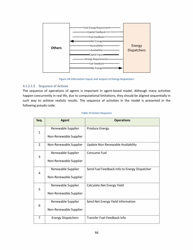
66

Others

Net Energy

Fuel Feedback

Energy Requirements

Capital Inputs

Availability

Accessibility Energy Dispatchers

Net Energy

Fuel Feedback

Total Energy Requirement

Capital Feedback

Figure 34 Information inputs and outputs of Energy Dispatchers

4.1.2.1.5 Sequence of Actions The sequence of operations of agents is important in agent-based model. Although many activities happen concurrently in real life, due to computational limitations, they should be aligned sequentially in such way to achieve realistic results. The sequence of activities in the model is presented in the following pseudo code:

Table 10 Action Sequence

Seq. Agent Operations

1 Renewable Supplier

Non-Renewable Supplier

Produce Energy

2 Non-Renewable Supplier Update Non Renewable Availability

3 Renewable Supplier

Non-Renewable Supplier

Consume Fuel

4 Renewable Supplier

Non-Renewable Supplier

Send Fuel Feedback Info to Energy Dispatcher

5 Renewable Supplier

Non-Renewable Supplier

Calculate Net Energy Yield

6 Renewable Supplier

Non-Renewable Supplier

Send Net Energy Yield Information

7 Energy Dispatchers Transfer Fuel Feedback Info

67

8 Energy Consumers Forecast Energy Demand

9 Energy Consumers Send Energy Demand Info

10 Renewable Supplier

Non-Renewable Supplier

Update Supplier Capital

11 Renewable Supplier

Non-Renewable Supplier

Calculate Suppliers Capital Depreciation

12 Non-Renewable Supplier Calculate Non-Renewable Capital Requirements

13 Energy Dispatchers Transfer Energy Capital Info

14 Energy Dispatchers Transfer Net Energy Yield Info

15 Energy Consumers Update Industrial Capital

16 Energy Consumers Produce Industrial Output

17 Energy Dispatchers Distribute Energy Requirements over Resources

18 Renewable Supplier Update Renewable Availability

19 Renewable Supplier

Non-Renewable Supplier

Develop Technology

20 Renewable Supplier

Non-Renewable Supplier

Update Resource Quality

21 Renewable Supplier

Non-Renewable Supplier

Update Accessibility

22 Renewable Supplier Calculate Renewable Capital Requirements

23 Renewable Supplier

Non-Renewable Supplier

Calculate Capital Inputs

24 Renewable Supplier

Non-Renewable Supplier

Send Capital Input Info

68

Figure 35 illustrates the sequence diagram of model’s four agents. In this figure, the sequence exchange of information among agents is depicted.

Renewable Supplier Non-Renewable Supplier Energy Dispatcher Energy Consumer

Net Renewable

Net Non-Renewable

Renewable Fuel Feedback

Non-Renewable Fuel Feedback

Non-Renewable Availability

Total Energy Requirements

Fuel Feedback

Non-Renewable Energy Requirements

Renewable Energy Requirements

Non-Renewable Capital Input

Renewable Capital Input

Total Capital Feedback

Net Energy Yield

Renewable Availability

NonRenewable Availability

Renewable Accessibility

NonRenewable Accessibility

Figure 35 Sequence Diagram

4.1.2.2 Operational Details of the Aggregated World Energy Model25 In this section, the operational details of each agent will be explained. To this aim, mathematical formulations of activities will be presented. All formulas and equations in this section are extracted from (M. A. J. Dale, 2010).

4.1.2.2.1 Renewable Suppliers Renewable suppliers manage renewable resources. Each resource has a technical potential (TP). It shows how much of a particular energy source, such as wind, is available for human purposes. (M. A. J.

25 All formulas and equation in section 4.1.2.2 are extracted from Vensim version of GEMBA model by (M. A. J. Dale, 2010) and adapted to NetLogo version

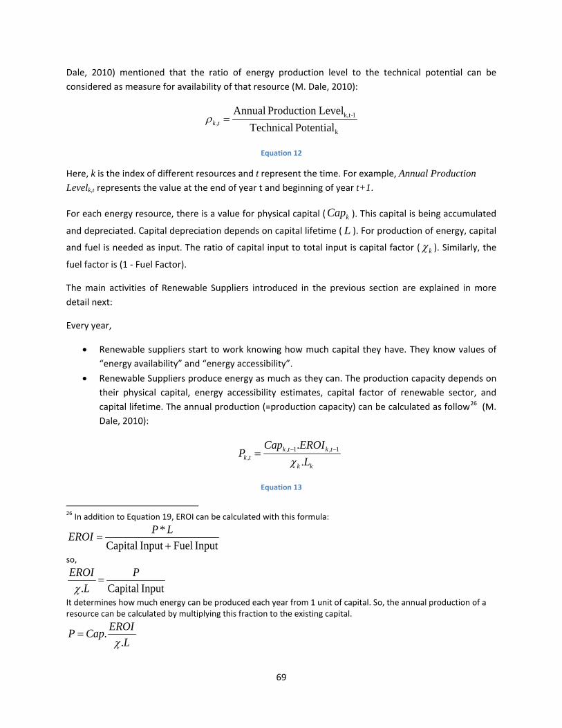
69

Dale, 2010) mentioned that the ratio of energy production level to the technical potential can be considered as measure for availability of that resource (M. Dale, 2010):

k

1-tk,, Potential Technical

Level Production Annual=tkρ

Equation 12

Here, k is the index of different resources and t represent the time. For example, Annual Production Levelk,t represents the value at the end of year t and beginning of year t+1.

For each energy resource, there is a value for physical capital ( kCap ). This capital is being accumulated

and depreciated. Capital depreciation depends on capital lifetime ( L ). For production of energy, capital

and fuel is needed as input. The ratio of capital input to total input is capital factor ( kχ ). Similarly, the

fuel factor is (1 - Fuel Factor).

The main activities of Renewable Suppliers introduced in the previous section are explained in more detail next:

Every year,

• Renewable suppliers start to work knowing how much capital they have. They know values of “energy availability” and “energy accessibility”.

• Renewable Suppliers produce energy as much as they can. The production capacity depends on their physical capital, energy accessibility estimates, capital factor of renewable sector, and capital lifetime. The annual production (=production capacity) can be calculated as follow26 (M. Dale, 2010):

kk

tktktk L

EROICapP

.. 1,1,

, χ−−=

Equation 13

26 In addition to Equation 19, EROI can be calculated with this formula:

Input FuelInput Capital*+

=LPEROI

so,

Input Capital.P

LEROI

=χ

It determines how much energy can be produced each year from 1 unit of capital. So, the annual production of a resource can be calculated by multiplying this fraction to the existing capital.

LEROICapP

..χ

=

70

Renewable Suppliers send information of produced energy to Renewable Links. • Renewable Suppliers consume part of their energy production. Here, it is called “Fuel

Feedback”. Fuel feedback can be calculated with using EROI and capital factor as defined by (M. A. J. Dale, 2010):

( )1,

,, 1Feedback Fuel

−

−=tk

tkktk EROI

Pχ

Equation 14

Renewable Suppliers send information of fuel feedback to Energy Dispatchers. • Renewable Suppliers send the information of net energy production and fuel feedback to

Renewable Links.

tktkt k PNet ,,, Feedback Fuel-=

Equation 15

Renewable Suppliers send information to net energy yield to Energy Dispatchers. • Renewables Suppliers update size of their physical capital. Physical capital changes according to

this formula (M. Dale, 2010):

1,1,1,, onDepreciati-Input Capital −−− += tktktktk CapCap

Equation 16

• Renewables Suppliers calculate how much physical capital should be eliminated due to depreciation. The value of depreciation is calculated as follows (M. Dale, 2010):

LCap tktk /onDepreciati ,, =

Equation 17

• Renewable suppliers calculate the size of physical capital input. They receive information about energy demand (energy requirements) of each resource from Renewable Links. They calculate how much capital should be added to the system in order to meet the requirements. The capital requirement for each resource is calculated as follows (M. Dale, 2010):

tk

ktktk EROI

L

,

,,

..tRequiremenEnergy tRequiremen Capital

χ=

Equation 18

M. Dale (2010) used first order exponential smoothing for calculation of capital requirement. Because of high correlation between capital requirements of consecutive years and because it takes many years for capital to be developed, these values can be smoothed:

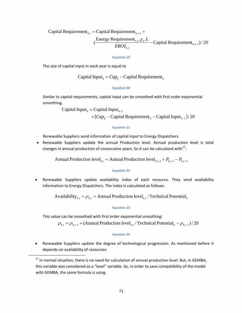
71

20/)tRequiremen Capital..tRequiremenEnergy

(

tRequiremen CapitaltRequiremen Capital

1,,

,

1,,

−

−

−

+=

tktk

ktk

tktk

EROILχ

Equation 19

The size of capital input in each year is equal to

kkk Cap tRequiremen CapitalInput Capital −=

Equation 20

Similar to capital requirements, capital input can be smoothed with first order exponential smoothing.

( ) 20/Input CapitaltRequiremen CapitalInput CapitalInput Capital

1

1

−

−

−−+=

kkk

kk

Cap

Equation 21

Renewable Suppliers send information of capital input to Energy Dispatchers. • Renewable Suppliers update the annual Production level. Annual production level is total

changes in annual production of consecutive years. So it can be calculated with27:

2,1,1,, level Production Annuallevel Production Annual −−− −+= tktktktk PP

Equation 22

• Renewable Suppliers update availability index of each resource. They send availability information to Energy Dispatchers. The index is calculated as follows:

ktktktk Potential Technical/level Production AnnualtyAvailabili ,,, == ρ

Equation 23

This value can be smoothed with first order exponential smoothing: 20/)Potential Technical/level Production (Annual 1,,1,, −− −+= tkktktktk ρρρ

Equation 24

• Renewable Suppliers update the degree of technological progression. As mentioned before it depends on availability of resources:

27 In normal situation, there is no need for calculation of annual production level. But, in GEMBA, this variable was considered as a “level” variable. So, in order to save compatibility of the model with GEMBA, the same formula is using.

72

( ) tkkeG ktk,.1,

ρξρ −Ξ−=

Equation 25

• Renewable Suppliers update the degree of Resource Quality. As mentioned before it depends on availability of resources:

( ) tkkeH ktk,

,ρφρ −Φ=

Equation 26

• Renewable Suppliers update the degree of energy accessibility. As mentioned before it depends on degree of technological progression, degree of resource quality, and estimation of production peak:

( ) ( )tktkktk HGEROI ,,, ρρε=

Equation 27

EROI can be smoothed with exponential smoothing. ( ) ( ) 20/)( 1,,,1,, −− −+= tktktkktktk EROIHGEROIEROI ρρε

Equation 28

Information of accessibility will be sent to Energy Dispatchers.

4.1.2.2.2 Non-Renewable Suppliers Non-Renewable suppliers develop non-renewable resources. Each resource has a capacity. It is called ultimate recoverable resource (URR). M. A. J. Dale (2010) maintained with comparing the cumulative production of each resource to the URR, the degree of energy availability can be determined.

k

tk,, URR

Production Cumulative=tkρ

Equation 29

Similar to renewables, each energy resource has a value for physical capital ( kCap ). Capital lifetime ( L )

is being incorporated to model as well. For production of energy, capital and fuel is needed as input.

As mentioned before, main activities of Non-Renewable Suppliers are the same as Renewable Suppliers. But, there are some minor differences in some formulas. Here, these activities are explained in more details:

Every year,

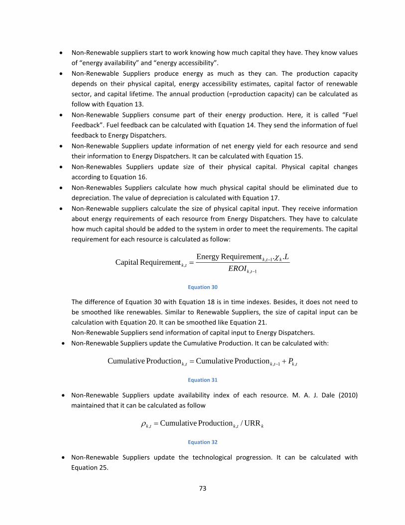
73

• Non-Renewable suppliers start to work knowing how much capital they have. They know values of “energy availability” and “energy accessibility”.

• Non-Renewable Suppliers produce energy as much as they can. The production capacity depends on their physical capital, energy accessibility estimates, capital factor of renewable sector, and capital lifetime. The annual production (=production capacity) can be calculated as follow with Equation 13.

• Non-Renewable Suppliers consume part of their energy production. Here, it is called “Fuel Feedback”. Fuel feedback can be calculated with Equation 14. They send the information of fuel feedback to Energy Dispatchers.

• Non-Renewable Suppliers update information of net energy yield for each resource and send their information to Energy Dispatchers. It can be calculated with Equation 15.

• Non-Renewables Suppliers update size of their physical capital. Physical capital changes according to Equation 16.

• Non-Renewables Suppliers calculate how much physical capital should be eliminated due to depreciation. The value of depreciation is calculated with Equation 17.

• Non-Renewable suppliers calculate the size of physical capital input. They receive information about energy requirements of each resource from Energy Dispatchers. They have to calculate how much capital should be added to the system in order to meet the requirements. The capital requirement for each resource is calculated as follow:

1,

1,,

..tRequiremenEnergy tRequiremen Capital

−

−=tk

ktktk EROI

Lχ

Equation 30

The difference of Equation 30 with Equation 18 is in time indexes. Besides, it does not need to be smoothed like renewables. Similar to Renewable Suppliers, the size of capital input can be calculation with Equation 20. It can be smoothed like Equation 21. Non-Renewable Suppliers send information of capital input to Energy Dispatchers.

• Non-Renewable Suppliers update the Cumulative Production. It can be calculated with:

tktktk P ,1,, Production CumulativeProduction Cumulative += −

Equation 31

• Non-Renewable Suppliers update availability index of each resource. M. A. J. Dale (2010) maintained that it can be calculated as follow

ktktk URR/Production Cumulative ,, =ρ

Equation 32

• Non-Renewable Suppliers update the technological progression. It can be calculated with Equation 25.

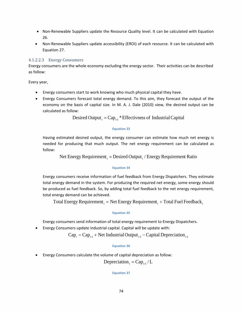
74

• Non-Renewable Suppliers update the Resource Quality level. It can be calculated with Equation 26.

• Non-Renewable Suppliers update accessibility (EROI) of each resource. It can be calculated with Equation 27.

4.1.2.2.3 Energy Consumers Energy consumers are the whole economy excluding the energy sector. Their activities can be described as follow:

Every year,

• Energy consumers start to work knowing who much physical capital they have. • Energy Consumers forecast total energy demand. To this aim, they forecast the output of the

economy on the basis of capital size. In M. A. J. Dale (2010) view, the desired output can be calculated as follow:

Capital Industrial of ssEffectivne*CapOutput Desired 1-tt =

Equation 33

Having estimated desired output, the energy consumer can estimate how much net energy is needed for producing that much output. The net energy requirement can be calculated as follow:

Ratiot RequiremenEnergy /Output Desired tRequiremenEnergy Net tt =

Equation 34

Energy consumers receive information of fuel feedback from Energy Dispatchers. They estimate total energy demand in the system. For producing the required net energy, some energy should be produced as fuel feedback. So, by adding total fuel feedback to the net energy requirement, total energy demand can be achieved.

ttt Feedback Fuel Total tRequiremenEnergy Net tRequiremenEnergy Total +=

Equation 35

Energy consumers send information of total energy requirement to Energy Dispatchers. • Energy Consumers update industrial capital. Capital will be update with:

1-t1-t1-tt onDepreciati Capital Output IndustrialNet CapCap −+=

Equation 36

• Energy Consumers calculate the volume of capital depreciation as follow:

L/CaponDepreciati 1-tt =

Equation 37

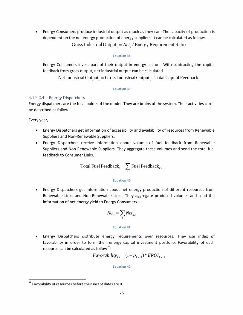
75

• Energy Consumers produce industrial output as much as they can. The capacity of production is dependent on the net energy production of energy suppliers. It can be calculated as follow:

Ratiot RequiremenEnergy / Output Industrial Gross tt Net=

Equation 38

Energy Consumers invest part of their output in energy sectors. With subtracting the capital feedback from gross output, net industrial output can be calculated

ttt Feedback Capital Total- Output Industrial GrossOutput IndustrialNet =

Equation 39

4.1.2.2.4 Energy Dispatchers Energy dispatchers are the focal points of the model. They are brains of the system. Their activities can be described as follow:

Every year,

• Energy Dispatchers get information of accessibility and availability of resources from Renewable Suppliers and Non-Renewable Suppliers.

• Energy Dispatchers receive information about volume of fuel feedback from Renewable Suppliers and Non-Renewable Suppliers. They aggregate these volumes and send the total fuel feedback to Consumer Links.

∑=k

tk ,t Feedback FuelFeedback Fuel Total

Equation 40

• Energy Dispatchers get information about net energy production of different resources from Renewable Links and Non-Renewable Links. They aggregate produced volumes and send the information of net energy yield to Energy Consumers.

∑=k

tkt NetNet ,

Equation 41

• Energy Dispatchers distribute energy requirements over resources. They use index of favorability in order to form their energy capital investment portfolio. Favorability of each resource can be calculated as follow28:

1,1,, *)1( −−−= tktktk EROItyFavorabili ρ

Equation 42

28 Favorability of resources before their incept dates are 0.

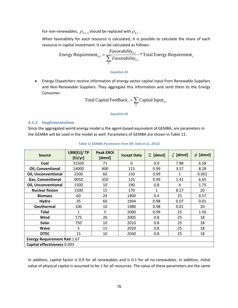
76

For non-renewables, 1, −tkρ should be replaced with tk ,ρ .

When favorability for each resource is calculated, it is possible to calculate the share of each resource in capital investment. It can be calculated as follows:

t,

,, tRequiremenEnergy Total*tRequiremenEnergy ∑

=

ktk

tktk tyFavorabili

tyFavorabili

Equation 43

• Energy Dispatchers receive information of energy sector capital input from Renewable Suppliers and Non-Renewable Suppliers. They aggregate this information and send them to the Energy Consumer.

∑=k

tk ,t Input CapitalFeedback Capital Total

Equation 44

4.1.3 Implementation Since the aggregated world energy model is the agent-based equivalent of GEMBA, are parameters in the GEMBA will be used in the model as well. Parameters of GEMBA are shown in Table 11:

Table 11 GEMBA Parameters from (M. Dale et al., 2012)

Source URR[EJ]/ TP [EJ/yr]

Peak EROI [dmnl] Incept Date Ξ [dmnl] ξ [dmnl] φ [dmnl]

Coal 31500 71 0 0.9 7.88 6.58 Oil, Conventional 14000 400 115 0.99 3.57 8.28

Oil, Unconventional 2500 60 150 0.99 1 0.001 Gas, Conventional 9050 350 125 0.99 1.41 6.65

Oil, Unconventional 1500 10 190 0.8 4 1.75 Nuclear fission 1500 15 170 1 8.27 20

Biomass 60 24 1800 0.4 25 0.57 Hydro 35 60 1904 0.98 0.07 0.01

Geothermal 100 10 1980 0.98 0.01 20 Tidal 1 5 2000 0.99 25 1.56 Wind 175 20 2005 0.8 25 18 Solar 750 10 2010 0.8 25 18 Wave 5 15 2020 0.8 25 18 OTEC 15 10 2040 0.8 25 18

Energy Requirement Rati 1.67 Capital effectiveness 0.093

In addition, capital factor is 0.9 for all renewables and is 0.1 for all no-renewables. In addition, initial value of physical capital is assumed to be 1 for all resources. The value of these parameters are the same

77

as parameters of GEMAB in (M. Dale et al., 2012). The model will be run for 400 ticks. The tick 0 show the year 1800 and tick 400 shows 2200.

4.1.4 Evaluation As discussed at the beginning of this chapter, this research follows two steps for developments of the objective model. The first step which is explained in chapter aimed at developing an equivalent of GEMBA in NetLogo. So, the evaluation phase for this model is done by confrontation of its results with result of GEMBA model. GEMBA model was validated by confrontation of model results with historical data about global energy production from different resources.

Variables renewable energy yield, non-renewable energy yield, and total energy yield were three variable used by (M. Dale et al., 2012) to show the behaviors of the world energy system. So, here, the comparison between models is illustrated using these three variables. Outputs of GEMBA model and Aggregated World Energy Model are illustrated in Figure 36 and Figure 37 respectively.

Figure 36 Results of GEMBA

Figure 37 Results of Aggregated World Energy Model

78

The emerging patterns in both models are the same. With tracing all important variables in the aggregated world energy model during some consecutive time steps (years), it was verified and assured that the global aggregated model behaves correctly. However, some differences can be seen in the results in Figure 36 and Figure 37. These differences are found to be results of difference in precision of Vensim (where GEMBA is implemented) and NetLogo. In Vensim, the precision of numbers are not pre-set. So, sometime numbers have precision of two decimals, and sometimes they have precision of three decimals or more. These minor differences in precision of the models results in the minor discrepancy in the results of two models.

These differences necessitate re-calibration of the model in order to achieve more precision. However, this model is not the main model of the research. It will be used later in Chapter 5 in the Multi-Region model. The main calibration process will be done for that model.

79

4.2 Experimentation In this section, a number of experiments will be done in the aggregated world energy model. The main purpose of the experiments is to explore the effects of diffident ranges of uncertain parameters on the behavior of the model. This exploration can gives insight about both behaviors of the system and sensitivity of the model against uncertain parameters.

In GEMBA and the aggregated world energy model, “URR”, “TP”, “Peak EROI”, “Energy Requirement Ratio”, and “Effectiveness of consumer capital” are the main uncertainties. There is high uncertainty about value of URR and TP as discussed in Section 3.1.2. In addition, values such as Peak EROI, energy Requirement ration and Effectiveness of Consumer Capital were set with using calibration algorithms. So, the can influence the behavior of the system.

In this section, in sub-section 4.2.1, the design of experiments will be explained. Then, in sub-section 4.2.2, the results of experiments will be presented. Finally, in sub-section 0, a number of conclusions about experiments results will be provided.

4.2.1 Design of Experiments The objective of this research is to develop a model in order to explore the world energy system from perspectives of biophysical economics theory and complex adaptive systems. In other world, the aim of this research is exploring how the world works using biophysical economics theory (and more specifically, regularities maintained by M. A. J. Dale (2010) in GEMBA) and what are impacts of uncertainties on the behaviors of the system.

To design the experiments, the variables have to be defined in such way to capture the range of behaviors, results and system level regularities that emerge with the available parameters (van Dam et al., 2013). Therefore, the following variables can be defined:

• Total net energy yield from renewables • Total net energy yield from conventional non-renewables • Total net energy yield from unconventional non-renewables

It is interesting to explore the state of these variables during the time period 1800-2200 (and more specifically 2030).

This variables are interesting for explore because they are the main components to total energy supply. The summation of these variables shows the total energy supply in the world. In addition, they can show the state of their resources. There is obvious distinction between renewables resources and non-renewable resources. The renewable are flow of energy while non-renewables are stocks of energy in the world. In addition capital intensity of these sectors is significantly different. Within non-renewable resources, there is difference between parameters of the dynamic EROI function for conventional and unconventional resources. For example, the technological progress of unconventional technology is slower than conventional resource technologies. Because of these differences, studying these three variables is expected to provide some insights about the world energy supply.

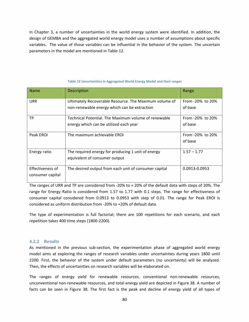
80

In Chapter 3, a number of uncertainties in the world energy system were identified. In addition, the design of GEMBA and the aggregated world energy model uses a number of assumptions about specific variables. The value of those variables can be influential in the behavior of the system. The uncertain parameters in the model are mentioned in Table 12.

Table 12 Uncertainties in Aggregated World Energy Model and their ranges

Name Description Range

URR Ultimately Recoverable Resource. The Maximum volume of non-renewable energy which can be extraction

From -20% to 20% of base

TP Technical Potential. The Maximum volume of renewable energy which can be utilized each year

From -20% to 20% of base

Peak EROI The maximum achievable EROI From -20% to 20% of base

Energy ratio The required energy for producing 1 unit of energy equivalent of consumer output

1.57 – 1.77

Effectiveness of consumer capital

The desired output from each unit of consumer capital 0.0913-0.0953

The ranges of URR and TP are considered from -20% to + 20% of the default data with steps of 20%. The range for Energy Ratio is considered from 1.57 to 1.77 with 0.1 steps. The range for effectiveness of consumer capital considered from 0.0913 to 0.0953 with step of 0.01. The range for Peak EROI is considered as uniform distribution from -20% to +20% of default data.

The type of experimentation is full factorial; there are 100 repetitions for each scenario, and each repetition takes 400 time steps (1800-2200).

4.2.2 Results As mentioned in the previous sub-section, the experimentation phase of aggregated world energy model aims at exploring the ranges of research variables under uncertainties during years 1800 until 2200. First, the behavior of the system under default parameters (no uncertainty) will be analyzed. Then, the effects of uncertainties on research variables will be elaborated on.

The ranges of energy yield for renewable resources, conventional non-renewable resources, unconventional non-renewable resources, and total energy yield are depicted in Figure 38. A number of facts can be seen in Figure 38. The first fact is the peak and decline of energy yield of all types of

81

resources in the time frame of the research. This peak can be a signal about scarcity of energy resources in the future. Remember the EROI function which was explained in section 4.1.1.4. EROI function has two components: technological progress and resource quality. Technological progress asymptotically increases when resources get extracted. On the other hand, resource quality decreases when it get extracted. So, when the decline in resource quality prevail growth of technological progress, the EROI decline. Here, the peak and decline can be explained by the nature of EROI function. When resources get extracted/utilized, first the EROI is high and the energy yield grows. But, when extraction/utilized exceed the threshold, the EROI declines and influence the energy yield negatively.

Figure 38 Aggregated World Energy Model - Energy Yield in years 1800-2200

It also shows that when both conventional and unconventional energy yield decline, growth of renewable energy yield cannot compensate this decline and the total energy yield declines as well. This can be explained by investigating the role of capital in energy production. The energy production is proportional to capital of energy sector. However, renewable sector requires much more capital than non-renewable sector for producing 1 joules of energy. In other words, capital intensity of renewable sector (capital factor) is too high. The fact that renewable energy yield cannot compensate the decline in non-renewables is because the rest of the economy cannot provide sufficient capital.

Accumulation of capital in the energy sector needs industrial output which is proportional with total net energy yield. Figure 39 illustrates the range of capital in different sectors during years 1800 – 2200. It is obvious that the decline in total energy yield results in decline in the size of consumer (economy) capital as the industrial output declines. After this decline, the economy has to invest more capital in energy sector because the investments go to renewable sector which has very high capital intensity.

82

Figure 39 Aggregated World Energy Model - Capital stock in years 1800-2200

Contrary to EROI of non-renewable which usually converge to 0 when they extracted, EROI of renewables converge to a constant level. It is because renewable resources are flow and they do not diminish when they get extracted. There is only a limit for utilization of renewables each year. So, because of structure of dynamic EROI function, EROI of renewables converge to a constant level. Therefore, the decline in renewables is far less than non-renewables and they tend to form a plateau after their peak. In that case, the total energy yield and renewable energy yield become equal.

The behaviors which were illustrated in Figure 38 and Figure 39 were based on the default parameters of the model. No randomness was is the system parameters. In order to better understand the behaviors of the model, it is necessary to observe its behaviors under variation of parameters.

4.2.2.1 Uncertain Peak EROI In this sub-section the effect of different ranges of Peak EROI on each research variable.

Figure 40 Changes in Energy Yield of renewable resources and conventional non-renewable resoruces with respect to uncertain Peak EROI

One of the parameters in the EROI function in GEMBA (and in the aggregated world energy model) is the Peak EROI. It is a scaling factor and defined the maximum EROI of resources. So, this parameter is expected to influence the behavior of the system. Figure 40 illustrates the effects of uncertain Peak EROI on the energy yield of renewable and conventional non-renewable resources. The curve of unconventional non-renewables is not depicted here. However, all analyses for conventional non-renewables in the following paragraphs apply for unconventional non-renewables as well. As mentioned

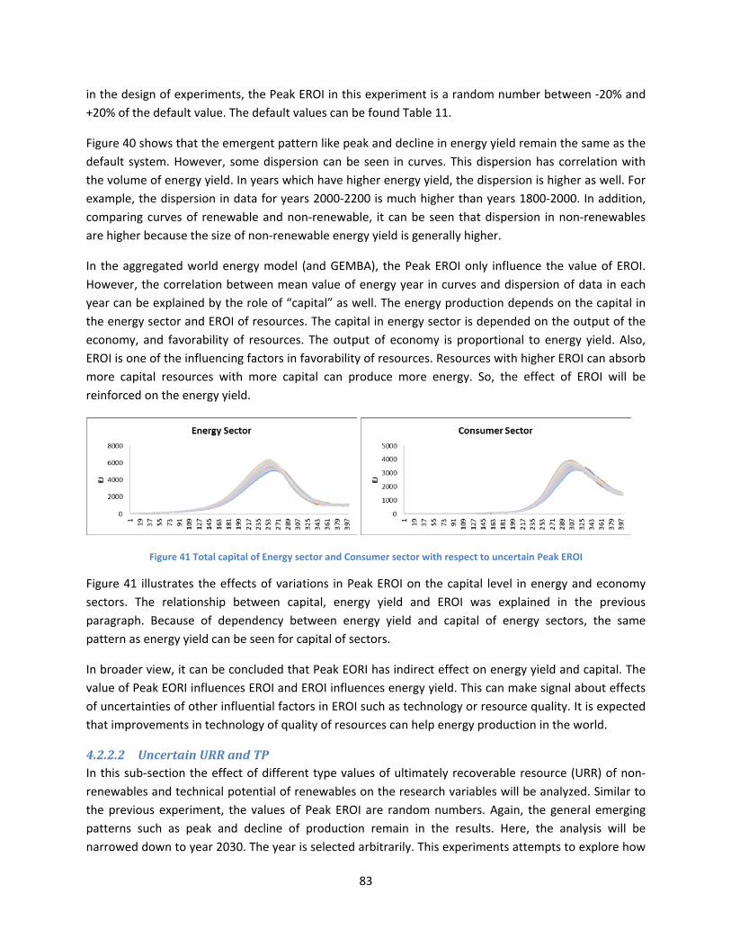
83

in the design of experiments, the Peak EROI in this experiment is a random number between -20% and +20% of the default value. The default values can be found Table 11.

Figure 40 shows that the emergent pattern like peak and decline in energy yield remain the same as the default system. However, some dispersion can be seen in curves. This dispersion has correlation with the volume of energy yield. In years which have higher energy yield, the dispersion is higher as well. For example, the dispersion in data for years 2000-2200 is much higher than years 1800-2000. In addition, comparing curves of renewable and non-renewable, it can be seen that dispersion in non-renewables are higher because the size of non-renewable energy yield is generally higher.

In the aggregated world energy model (and GEMBA), the Peak EROI only influence the value of EROI. However, the correlation between mean value of energy year in curves and dispersion of data in each year can be explained by the role of “capital” as well. The energy production depends on the capital in the energy sector and EROI of resources. The capital in energy sector is depended on the output of the economy, and favorability of resources. The output of economy is proportional to energy yield. Also, EROI is one of the influencing factors in favorability of resources. Resources with higher EROI can absorb more capital resources with more capital can produce more energy. So, the effect of EROI will be reinforced on the energy yield.

Figure 41 Total capital of Energy sector and Consumer sector with respect to uncertain Peak EROI

Figure 41 illustrates the effects of variations in Peak EROI on the capital level in energy and economy sectors. The relationship between capital, energy yield and EROI was explained in the previous paragraph. Because of dependency between energy yield and capital of energy sectors, the same pattern as energy yield can be seen for capital of sectors.

In broader view, it can be concluded that Peak EORI has indirect effect on energy yield and capital. The value of Peak EORI influences EROI and EROI influences energy yield. This can make signal about effects of uncertainties of other influential factors in EROI such as technology or resource quality. It is expected that improvements in technology of quality of resources can help energy production in the world.

4.2.2.2 Uncertain URR and TP In this sub-section the effect of different type values of ultimately recoverable resource (URR) of non-renewables and technical potential of renewables on the research variables will be analyzed. Similar to the previous experiment, the values of Peak EROI are random numbers. Again, the general emerging patterns such as peak and decline of production remain in the results. Here, the analysis will be narrowed down to year 2030. The year is selected arbitrarily. This experiments attempts to explore how

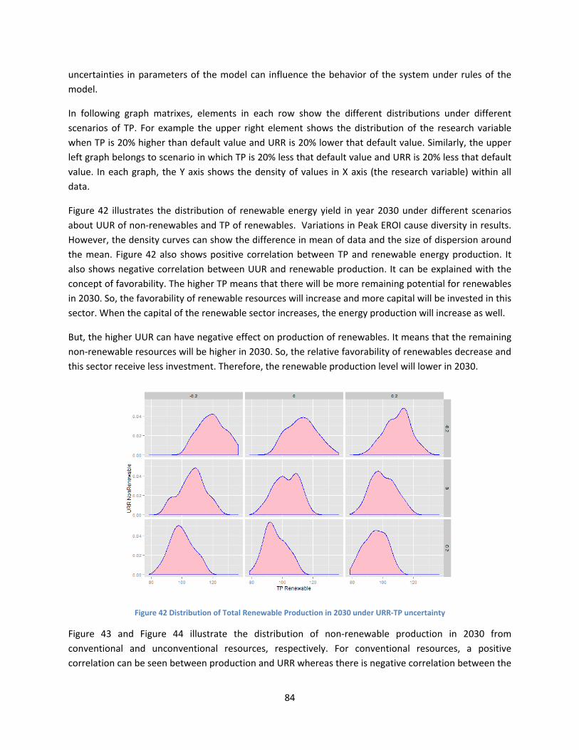
84

uncertainties in parameters of the model can influence the behavior of the system under rules of the model.

In following graph matrixes, elements in each row show the different distributions under different scenarios of TP. For example the upper right element shows the distribution of the research variable when TP is 20% higher than default value and URR is 20% lower that default value. Similarly, the upper left graph belongs to scenario in which TP is 20% less that default value and URR is 20% less that default value. In each graph, the Y axis shows the density of values in X axis (the research variable) within all data.

Figure 42 illustrates the distribution of renewable energy yield in year 2030 under different scenarios about UUR of non-renewables and TP of renewables. Variations in Peak EROI cause diversity in results. However, the density curves can show the difference in mean of data and the size of dispersion around the mean. Figure 42 also shows positive correlation between TP and renewable energy production. It also shows negative correlation between UUR and renewable production. It can be explained with the concept of favorability. The higher TP means that there will be more remaining potential for renewables in 2030. So, the favorability of renewable resources will increase and more capital will be invested in this sector. When the capital of the renewable sector increases, the energy production will increase as well.

But, the higher UUR can have negative effect on production of renewables. It means that the remaining non-renewable resources will be higher in 2030. So, the relative favorability of renewables decrease and this sector receive less investment. Therefore, the renewable production level will lower in 2030.

Figure 42 Distribution of Total Renewable Production in 2030 under URR-TP uncertainty

Figure 43 and Figure 44 illustrate the distribution of non-renewable production in 2030 from conventional and unconventional resources, respectively. For conventional resources, a positive correlation can be seen between production and URR whereas there is negative correlation between the

85

production and TP. These correlations can be explained with the effects of UUR and TP on favorably of non-renewable resources and renewables which was explained previously.

Figure 43 Distribution of Total Conventional Non-Renewable Production in 2030 under URR-TP uncertainty

For unconventional non-renewables, new type of pattern can be seen. Here, there is negative correlation between production of unconventional energy in 2030 with both URR and TP.

Figure 44 Distribution of Total Unconventional Renewable Production in 2030 under URR-TP uncertainty

The explanation of correlation between TP and unconventional production is the same as the explanation for conventional resources. But, the negative correlation between URR and unconventional production lay in the EROI function of unconventional. The technological learning for unconventional

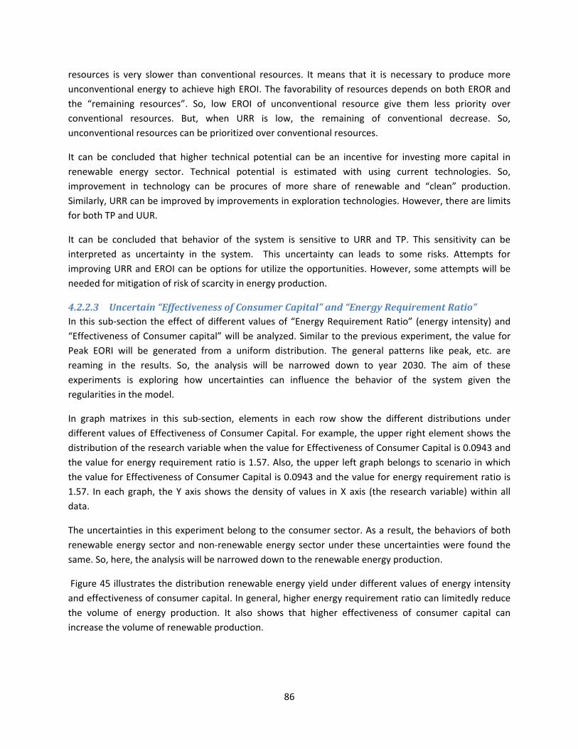
86

resources is very slower than conventional resources. It means that it is necessary to produce more unconventional energy to achieve high EROI. The favorability of resources depends on both EROR and the “remaining resources”. So, low EROI of unconventional resource give them less priority over conventional resources. But, when URR is low, the remaining of conventional decrease. So, unconventional resources can be prioritized over conventional resources.

It can be concluded that higher technical potential can be an incentive for investing more capital in renewable energy sector. Technical potential is estimated with using current technologies. So, improvement in technology can be procures of more share of renewable and “clean” production. Similarly, URR can be improved by improvements in exploration technologies. However, there are limits for both TP and UUR.

It can be concluded that behavior of the system is sensitive to URR and TP. This sensitivity can be interpreted as uncertainty in the system. This uncertainty can leads to some risks. Attempts for improving URR and EROI can be options for utilize the opportunities. However, some attempts will be needed for mitigation of risk of scarcity in energy production.

4.2.2.3 Uncertain “Effectiveness of Consumer Capital” and “Energy Requirement Ratio” In this sub-section the effect of different values of “Energy Requirement Ratio” (energy intensity) and “Effectiveness of Consumer capital” will be analyzed. Similar to the previous experiment, the value for Peak EORI will be generated from a uniform distribution. The general patterns like peak, etc. are reaming in the results. So, the analysis will be narrowed down to year 2030. The aim of these experiments is exploring how uncertainties can influence the behavior of the system given the regularities in the model.

In graph matrixes in this sub-section, elements in each row show the different distributions under different values of Effectiveness of Consumer Capital. For example, the upper right element shows the distribution of the research variable when the value for Effectiveness of Consumer Capital is 0.0943 and the value for energy requirement ratio is 1.57. Also, the upper left graph belongs to scenario in which the value for Effectiveness of Consumer Capital is 0.0943 and the value for energy requirement ratio is 1.57. In each graph, the Y axis shows the density of values in X axis (the research variable) within all data.

The uncertainties in this experiment belong to the consumer sector. As a result, the behaviors of both renewable energy sector and non-renewable energy sector under these uncertainties were found the same. So, here, the analysis will be narrowed down to the renewable energy production.

Figure 45 illustrates the distribution renewable energy yield under different values of energy intensity and effectiveness of consumer capital. In general, higher energy requirement ratio can limitedly reduce the volume of energy production. It also shows that higher effectiveness of consumer capital can increase the volume of renewable production.

87

Figure 45 Distribution of Total Renewable Production in 2030

The limited influence of energy requirement ration can be explained as follows. Energy requirement ratio has double effect on the behavior of the system. Energy demand is positively proportional to energy requirement ratio. So, higher values of energy requirement ratio can results in higher demand and higher capital investment in energy sector. As mentioned earlier, higher capital of energy sector can increase the energy production. Higher energy production increases the industrial output and, consequently, the consumer capital and energy demand. On the other hand, industrial output is inversely proportional to energy requirement ration. So, higher energy requirement ratio can reduce the industrial output, consumer capital and energy demand. Therefore, there is no reinforcing relation between energy requirement ratio and energy production.

However, the effectiveness of consumer capital can have significant effect of the energy production. This parameter shows the productive proportion of industrial capital. So, when it increases, the energy demand increases as well. Increase in energy demand can result is increase in energy production as it is explained in the previous paragraph.

From this experiment, it can be concluded that productivity of capital in the economy can increase the energy production. However, the growth in energy production is limited by the nature. The faster growth in energy production before the production peak can results in faster decline after peak. This can give signal to policy makers to seek for proper level of productivity in the economy. In addition, here, it was assumed that productivity of the economy is independent variable. However, in the real world, it can be influenced by many factors including energy. Considering productivity of the economy as a dependent variable in the system can be future research.

88

4.2.2.4 Discussion on validity of inferences Conclusions of this section in based on the behavior of the model under different parameters which do not change during the simulation. The GEMBA model and Aggregated World Energy model use fixed parameters such as URR which influence the behavior of the model from 1800 to 2200.

When parameters are fixed and set in the beginning of simulation, they influence the behavior of the system before the current year (2013). For example, Figure 46 illustrates the whole view of total energy yield over years of 1800-2200 with respect to different URR and TP. This picture shows that the behavior (for example, the value for year 2000) of the system in past years (1800-2012) is not the same. It can influence the validity of the model and inferences.

Figure 46 Total Energy Yield under URR-TP uncertainty

However, the conclusions drawn in this section are explaining the patterns and influences and details of value do not influence their validity.

4.3 Conclusion In this chapter, the two-steps approach for building the objective model of this research was explained. The first step of this approach was covered in this chapter. It aimed at development of a biophysical economics model for the world energy system in Netlogo without considering energy trade. Because a number of biophysical economic models were found in the literature, an attempt was made to develop an agent-based equivalent of the most recent biophysical economics model in the literature, GEMBA by (M. A. J. Dale, 2010).

An overview of GEMBA was provided to clarify the assumptions, variables and rules within the model. Consequently, an agent-based model was developed in NetLogo environment to mimic the behaviors of GEMBA. The system was decomposed into four agents: renewable supplier, non-renewable supplier,

89

energy consumer and energy dispatcher. The agents used the same differential equations as GEMBA in order to be compatible with the continuous nature of biophysical economics problems.

The model was implemented in NetLogo using the same values for parameters as GEMBA. The microscopic and macroscopic behaviors of aggregated world energy model and GEMBA were compared in order to evaluate the new model. The evaluation process showed that the emergent patterns in both model are the same. However, due to difference in precision of NetLogo and Vensim, in which GEMBA was developed, there were some differences in values of variables.

In order to explore the behavior of the model under different scenarios in parameters, a number of experiments were designed. The experiments explored the behavior of the system in years 1800-2200 and a specific year (2030).

Result showed that the world energy supply system can experience peak and decline in production as a result of decline in energy-return-on-investment of resources and decline in their favorability. The behavior of the system proved to be sensitive towards the parameters of dynamic EROI function such as Peak EROI. It was also concluded that having different perceptions about ultimately recoverable resources (URR) on non-renewables and technical potential (TP) of renewables can be influential to energy production in the world. Since estimates of technical potential of renewables are based on current technologies, it can be suggested that improvements is technology can increase the perception of technical potential and production of renewables.

In addition to URR and TP, productivity of the economics proved to be influential on level of energy production in the world. It was observed that higher levels of productivity resulted in higher energy demand and higher energy production. However, because of limitations of nature, it is suggested to seek for a “proper” level for productivity of the economy. In addition, it is suggested that productivity of the economy can be considered as a dependent variable in the system in future research.

Because of the scientific foundation and validity of GEMBA, it can be concluded that its equivalent (aggregated world energy model) can provide a good basis to develop an agent-based model and explore the world energy system considering energy trade in Chapter 5.

90

5 The Second Model: Multi-Region World Energy Model This chapter introduces the main model of this research. One of the objectives of this research was incorporating energy trade into the model of global energy system. Energy trade refers to movement of energy among countries and difference geographical regions. So, it is necessary to find these regions. As mentioned before in section 3.2, the world can be clustered into a number of regions. These regions are groups of neighboring countries which have common characteristics from energy, economic and institutional perspectives. In addition to geography, endowment of energy resources and reserves is one of those characteristics. Another characteristic is the level of GDP and per capita income of countries. The other common characteristic can be international agreements and institutions such as OPEC and OECD which make countries similar to each other and put them in the same cluster.

In the multi-region world energy model, the world will be considered as a composition of number of regions. Each region produces and consumes energy. In addition, if regions face energy scarcity, they can import surplus of energy in other regions. In the aggregated world energy model, “the world” was just producing and consuming energy. So, regions themselves can be considered as “worlds” (which produce and consume energy) and trade energy with “other worlds”. With this perspective, most agents of the aggregated world energy model can be utilized here for regions and new features can be added to them.

So, in addition to regional decomposition of the world, similar to the aggregated world energy model, each region can be decomposed into four agents: Renewable Suppliers, Non-Renewable Suppliers, Energy Consumers, and Energy Dispatchers. For the first three agents, rules and behaviors are the same as aggregated model agents. In those agents, only parameters will be adjusted to regional level. But, for Energy Dispatchers, some new rules and behaviors will be introduced to the model. In the multi-regions model, Energy Dispatchers interact with each other and facilitate energy trade among regions. The interactions are done through links called “Contracts”. Contracts calculate the EROI of imported energy on the basis of energy price.

Trade among regions depends of EROI of trade which was explained in Section 2.1.2.3. Trade EROI depends of the ratio of monetary value of imported energy to the monetary value of exchanged capital for getting that energy. So, price can play an important role in the calculation of trade EROI.

In this chapter, in section 5.1, three phases of model development for the multi-region model will be provided. Afterward, in section 5.2, the design and results of experiments will be presented.

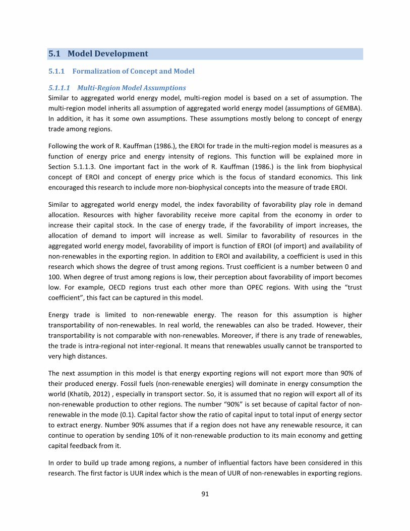
91

5.1 Model Development

5.1.1 Formalization of Concept and Model

5.1.1.1 Multi-Region Model Assumptions Similar to aggregated world energy model, multi-region model is based on a set of assumption. The multi-region model inherits all assumption of aggregated world energy model (assumptions of GEMBA). In addition, it has it some own assumptions. These assumptions mostly belong to concept of energy trade among regions.

Following the work of R. Kauffman (1986.), the EROI for trade in the multi-region model is measures as a function of energy price and energy intensity of regions. This function will be explained more in Section 5.1.1.3. One important fact in the work of R. Kauffman (1986.) is the link from biophysical concept of EROI and concept of energy price which is the focus of standard economics. This link encouraged this research to include more non-biophysical concepts into the measure of trade EROI.

Similar to aggregated world energy model, the index favorability of favorability play role in demand allocation. Resources with higher favorability receive more capital from the economy in order to increase their capital stock. In the case of energy trade, if the favorability of import increases, the allocation of demand to import will increase as well. Similar to favorability of resources in the aggregated world energy model, favorability of import is function of EROI (of import) and availability of non-renewables in the exporting region. In addition to EROI and availability, a coefficient is used in this research which shows the degree of trust among regions. Trust coefficient is a number between 0 and 100. When degree of trust among regions is low, their perception about favorability of import becomes low. For example, OECD regions trust each other more than OPEC regions. With using the “trust coefficient”, this fact can be captured in this model.

Energy trade is limited to non-renewable energy. The reason for this assumption is higher transportability of non-renewables. In real world, the renewables can also be traded. However, their transportability is not comparable with non-renewables. Moreover, if there is any trade of renewables, the trade is intra-regional not inter-regional. It means that renewables usually cannot be transported to very high distances.

The next assumption in this model is that energy exporting regions will not export more than 90% of their produced energy. Fossil fuels (non-renewable energies) will dominate in energy consumption the world (Khatib, 2012) , especially in transport sector. So, it is assumed that no region will export all of its non-renewable production to other regions. The number “90%” is set because of capital factor of non-renewable in the mode (0.1). Capital factor show the ratio of capital input to total input of energy sector to extract energy. Number 90% assumes that if a region does not have any renewable resource, it can continue to operation by sending 10% of it non-renewable production to its main economy and getting capital feedback from it.

In order to build up trade among regions, a number of influential factors have been considered in this research. The first factor is UUR index which is the mean of UUR of non-renewables in exporting regions.

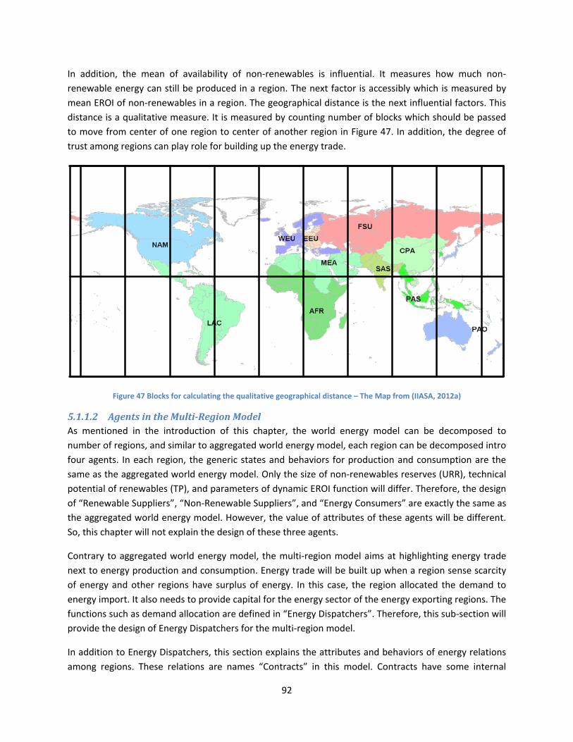
92

In addition, the mean of availability of non-renewables is influential. It measures how much non-renewable energy can still be produced in a region. The next factor is accessibly which is measured by mean EROI of non-renewables in a region. The geographical distance is the next influential factors. This distance is a qualitative measure. It is measured by counting number of blocks which should be passed to move from center of one region to center of another region in Figure 47. In addition, the degree of trust among regions can play role for building up the energy trade.

Figure 47 Blocks for calculating the qualitative geographical distance – The Map from (IIASA, 2012a)

5.1.1.2 Agents in the Multi-Region Model As mentioned in the introduction of this chapter, the world energy model can be decomposed to number of regions, and similar to aggregated world energy model, each region can be decomposed intro four agents. In each region, the generic states and behaviors for production and consumption are the same as the aggregated world energy model. Only the size of non-renewables reserves (URR), technical potential of renewables (TP), and parameters of dynamic EROI function will differ. Therefore, the design of “Renewable Suppliers”, “Non-Renewable Suppliers”, and “Energy Consumers” are exactly the same as the aggregated world energy model. However, the value of attributes of these agents will be different. So, this chapter will not explain the design of these three agents.

Contrary to aggregated world energy model, the multi-region model aims at highlighting energy trade next to energy production and consumption. Energy trade will be built up when a region sense scarcity of energy and other regions have surplus of energy. In this case, the region allocated the demand to energy import. It also needs to provide capital for the energy sector of the energy exporting regions. The functions such as demand allocation are defined in “Energy Dispatchers”. Therefore, this sub-section will provide the design of Energy Dispatchers for the multi-region model.

In addition to Energy Dispatchers, this section explains the attributes and behaviors of energy relations among regions. These relations are names “Contracts” in this model. Contracts have some internal

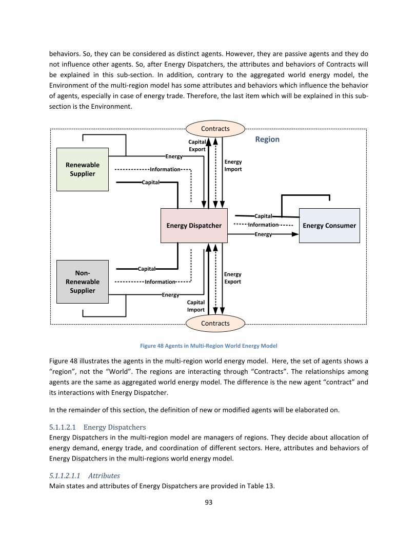
93

behaviors. So, they can be considered as distinct agents. However, they are passive agents and they do not influence other agents. So, after Energy Dispatchers, the attributes and behaviors of Contracts will be explained in this sub-section. In addition, contrary to the aggregated world energy model, the Environment of the multi-region model has some attributes and behaviors which influence the behavior of agents, especially in case of energy trade. Therefore, the last item which will be explained in this sub-section is the Environment.

Energy ConsumerEnergy

Capital

Energy Dispatcher

Renewable Supplier

Non-Renewable

Supplier

Energy

Energy

Capital

Capital

Information

Information

Information

Region

Energy Import

Energy Export

Capital Import

Capital Export

Contracts

Contracts

Figure 48 Agents in Multi-Region World Energy Model

Figure 48 illustrates the agents in the multi-region world energy model. Here, the set of agents shows a “region”, not the “World”. The regions are interacting through “Contracts”. The relationships among agents are the same as aggregated world energy model. The difference is the new agent “contract” and its interactions with Energy Dispatcher.

In the remainder of this section, the definition of new or modified agents will be elaborated on.

5.1.1.2.1 Energy Dispatchers Energy Dispatchers in the multi-region model are managers of regions. They decide about allocation of energy demand, energy trade, and coordination of different sectors. Here, attributes and behaviors of Energy Dispatchers in the multi-regions world energy model.

5.1.1.2.1.1 Attributes Main states and attributes of Energy Dispatchers are provided in Table 13.

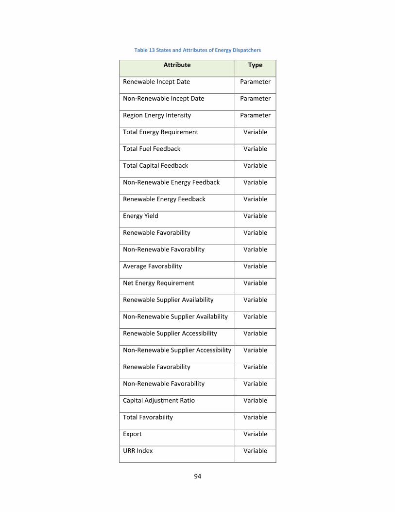
94

Table 13 States and Attributes of Energy Dispatchers

Attribute Type

Renewable Incept Date Parameter

Non-Renewable Incept Date Parameter

Region Energy Intensity Parameter

Total Energy Requirement Variable

Total Fuel Feedback Variable

Total Capital Feedback Variable

Non-Renewable Energy Feedback Variable

Renewable Energy Feedback Variable

Energy Yield Variable

Renewable Favorability Variable

Non-Renewable Favorability Variable

Average Favorability Variable

Net Energy Requirement Variable

Renewable Supplier Availability Variable

Non-Renewable Supplier Availability Variable

Renewable Supplier Accessibility Variable

Non-Renewable Supplier Accessibility Variable

Renewable Favorability Variable

Non-Renewable Favorability Variable

Capital Adjustment Ratio Variable

Total Favorability Variable

Export Variable

URR Index Variable

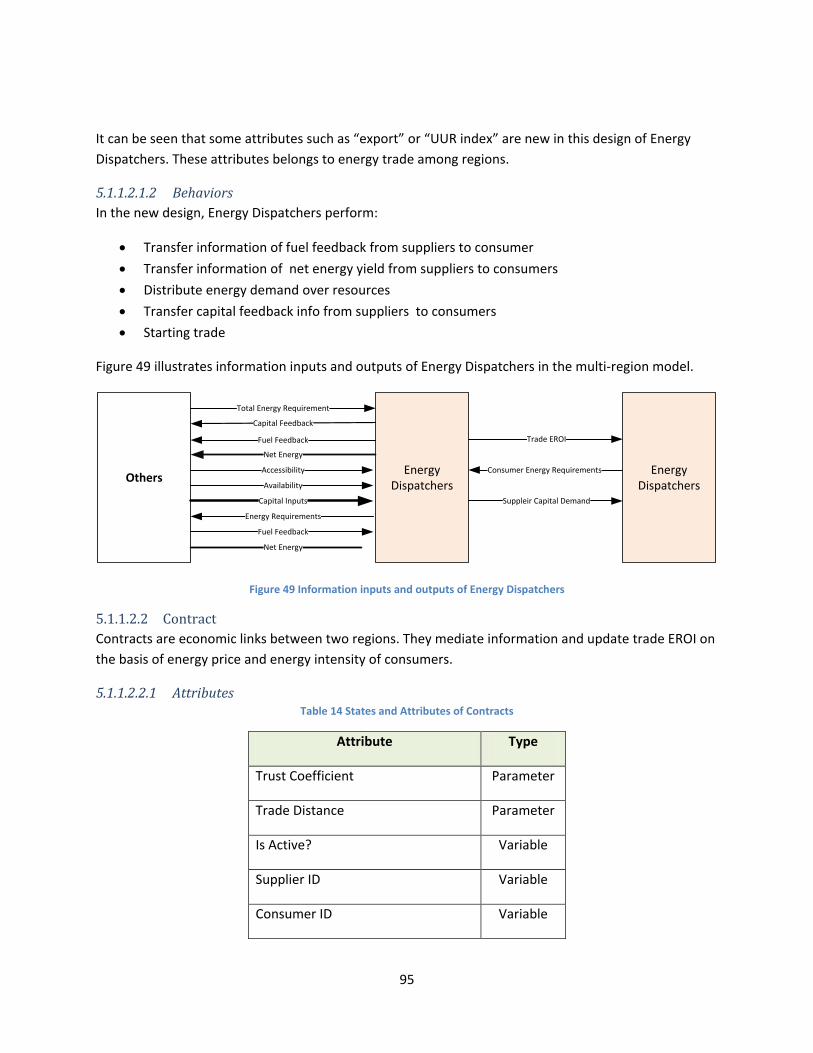
95

It can be seen that some attributes such as “export” or “UUR index” are new in this design of Energy Dispatchers. These attributes belongs to energy trade among regions.

5.1.1.2.1.2 Behaviors In the new design, Energy Dispatchers perform:

• Transfer information of fuel feedback from suppliers to consumer • Transfer information of net energy yield from suppliers to consumers • Distribute energy demand over resources • Transfer capital feedback info from suppliers to consumers • Starting trade

Figure 49 illustrates information inputs and outputs of Energy Dispatchers in the multi-region model.

Others

Net Energy

Fuel Feedback

Energy Requirements

Capital Inputs

Availability

Accessibility Energy Dispatchers

Net Energy

Fuel Feedback

Total Energy Requirement

Capital Feedback

Energy Dispatchers

Consumer Energy Requirements

Suppleir Capital Demand

Trade EROI

Figure 49 Information inputs and outputs of Energy Dispatchers

5.1.1.2.2 Contract Contracts are economic links between two regions. They mediate information and update trade EROI on the basis of energy price and energy intensity of consumers.

5.1.1.2.2.1 Attributes Table 14 States and Attributes of Contracts

Attribute Type

Trust Coefficient Parameter

Trade Distance Parameter

Is Active? Variable

Supplier ID Variable

Consumer ID Variable

96

Consumer Net Energy Requirement Variable

Supplier Capital Demand Variable

Trade EROI Variable

Net Energy Trade Variable

Trade Accessibility Variable

Trade Favorability Variable

Requirement Fraction Variable

5.1.1.2.2.2 Behaviors Contracts are kind of passive agents. Their only active behavior is:

• Updating Trade EROI • Update Trade Availability • Update Trade Favorability • Update Contracting Signals

5.1.1.2.3 Environment The Environment represents the world in which the world energy system is living in. It enables regions to form energy trade networks. It is an abstraction of (political, economic, etc.) relations among regions. The states of the Environment can influence the favorability of energy trade among regions.

5.1.1.2.3.1 Attributes Table 15 States and Attributes of the Environment

Attribute Type

Global energy price Parameter

Coefficient of Trade EROI Parameter

5.1.1.2.3.2 Behaviors The Environment’s behavior is:

• Update Global Energy Price

5.1.1.3 Operational details of the Multi-Regions Energy Model In section 5.1.1.2, the general attributes and behaviors of Energy Dispatchers and Contracts were explained. In this section, the operational details of these two agents will be presented.

97

5.1.1.3.1 Energy Dispatchers Some behaviors of Energy Dispatchers in the Multi-Region model are the same as aggregated world energy model. However, they perform some new actions in order to facilitate trade among themselves.

Every year,

• Energy Dispatchers get information of accessibility and availability of resources from Renewable Suppliers and Non-Renewable Suppliers.

• Energy Dispatchers receive information about volume of fuel feedback from Renewable Suppliers and Non-Renewable Suppliers. They aggregate these volumes and send the total fuel feedback to Energy Consumer. Total Fuel feedback can be calculated with Equation 40.

• Energy Dispatchers get information about net energy production of different resources from Renewable Supplier and Non-Renewable Supplier. They aggregate produced volumes and send the information of net energy yield with Equation 41. After calculation of net energy yield, if the region is an exporting region, it calculates the volume of the export. The volume of export can be calculated as follow:

20/tRequiremenEnergy Total

tRequiremenEnergy Net Consumer * 1

t

linksexport 1

−

+= −−

∑tttt ExportNetExportExport

Equation 45

This equation implies that volume of export is perceived by exporters with delay as it is necessary to develop capital for it. In order to prevent the condition in which regions export all of their energy production to other regions, a corrective rule is added to the behavior of the Energy Dispatchers.

tnewableNonttnewableNont NetExportNetExportif ,Re,Re *8.0,*9.0 −− =>

Equation 46

The net energy yield should be updated after calculation of the export.

ttt ExportNetNet −=

Equation 47

In addition, energy dispatcher should set the “net energy trade” of their export contracts as follow:

=

∑ i

i, tRequiremenEnergyNetConsumer

tRequiremenEnergyNetConsumer*tti ExportTradeEnergyNet

Equation 48

98

where i is the index of export contract. In case there is any energy import, the aggregated net energy yield can be calculated with:

∑∑ +=c

tck

tkt NetNetNet ,,

Equation 49

Finally, the value of net energy yield will be transferred to Energy Consumers. • Energy Dispatchers distribute energy requirements over resources. They use index of

favorability in order to form their energy capital investment portfolio. Favorability of each resource can be calculated with Equation 42. The total favorability, for regions without any energy import, can be calculated as follow:

∑=k

tktk tyFavorabilityFavorabiliotal ,,T

Equation 50

For regions which import energy, the total favorability can be calculated with:

∑∑ +=i

tik

tktk tyFavorabiliTradetyFavorabilityFavorabiliotal ,,,T

Equation 51

where i is the index of import contract. When favorability for each resource is calculated, it is possible to calculate the share of each resource in capital investment. For regions without any energy trade, it can be calculated with Equation 43. For Energy Exporting regions, energy requirements of resources can be calculated with:

+

=

∑

∑

ctc,t

,

,,

tRequiremenEnergy tRequiremenEnergy Total

*tRequiremenEnergy

ktk

tktk tyFavorabili

tyFavorabili

Equation 52

For energy importing regions, energy requirements can be calculated as follow:

t

,,

,,

tRequiremenEnergy Total

*tRequiremenEnergy ∑∑ +

=

ctc

ktk

tktk tyFavorabilityFavorabili

tyFavorabili

Equation 53

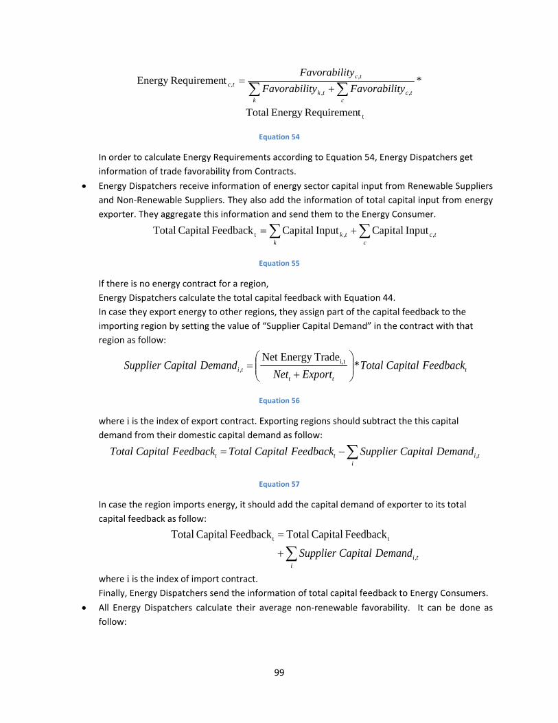
99

t

,,

,,

tRequiremenEnergy Total

*tRequiremenEnergy ∑∑ +

=

ctc

ktk

tctc tyFavorabilityFavorabili

tyFavorabili

Equation 54

In order to calculate Energy Requirements according to Equation 54, Energy Dispatchers get information of trade favorability from Contracts.

• Energy Dispatchers receive information of energy sector capital input from Renewable Suppliers and Non-Renewable Suppliers. They also add the information of total capital input from energy exporter. They aggregate this information and send them to the Energy Consumer.

∑∑ +=c

tck

tk ,,t Input CapitalInput CapitalFeedback Capital Total

Equation 55

If there is no energy contract for a region, Energy Dispatchers calculate the total capital feedback with Equation 44. In case they export energy to other regions, they assign part of the capital feedback to the importing region by setting the value of “Supplier Capital Demand” in the contract with that region as follow:

ttt

ti FeedbackCapitalTotalExportNet

DemandCapitalSupplier *TradeEnergyNet ti,

,

+

=

Equation 56

where i is the index of export contract. Exporting regions should subtract the this capital demand from their domestic capital demand as follow:

∑−=i

titt DemandCapitalSupplierFeedbackCapitalTotalFeedbackCapitalTotal ,

Equation 57

In case the region imports energy, it should add the capital demand of exporter to its total capital feedback as follow:

∑+=

itiDemandCapitalSupplier ,

tt Feedback Capital TotalFeedback Capital Total

where i is the index of import contract. Finally, Energy Dispatchers send the information of total capital feedback to Energy Consumers.

• All Energy Dispatchers calculate their average non-renewable favorability. It can be done as follow:

100

∑−=

=renewablenonk

tkmean tyFavorabilin

tyFavorabili ,*1

Equation 58

• Energy Dispatchers search for energy partners. If they can find other dispatchers with higher average non-renewable favorability than themselves, they sign a contract with them. This contract last forever. However, the volume of trade can be ignorable. When a contract is signed, the variable “is Active?” in the contract becomes TRUE. The rules for starting trade and sign contract is as follow:

PendingisActiveThen

meofEROIDisparcherEnergyothertheofEROIicientTrustCoeffIf

ANDmeofDisparcherEnergyothertheofIf

ANDmeofIndexURRDisparcherEnergyothertheofIndexURRIf

newableNonmean

newableNonmean

renewalbenonmeanrenewalbenonmean

=

>

−>−

>

−

−

−−

?,*4.0

*

)1(*5.1)1(

*3.1

Re,

Re,

,, ρρ

Equation 59

Now, candidates for trade are determined. The candidate with short distance and high favorability will be selected.

( ) ( )

eStart trad,

ty)favorabili*distance ical1/geograph(ty)favorabili*distance ical1/geograph( if maxpendingi

then=∈

Equation 60

5.1.1.3.2 Contracts Contracts are passive agents.

Each year,

• contracts update the trade EROI. The approach for calculation of trade EROI is based in Equation 3 and Equation 4. Trade EROI can be updated as follow29:

29 According to America physical Society (APS), each boe equals to 5.8 MBtu. Mean Btu equals 1055.87 J. So, 1 boe is 6126.046 MJ.

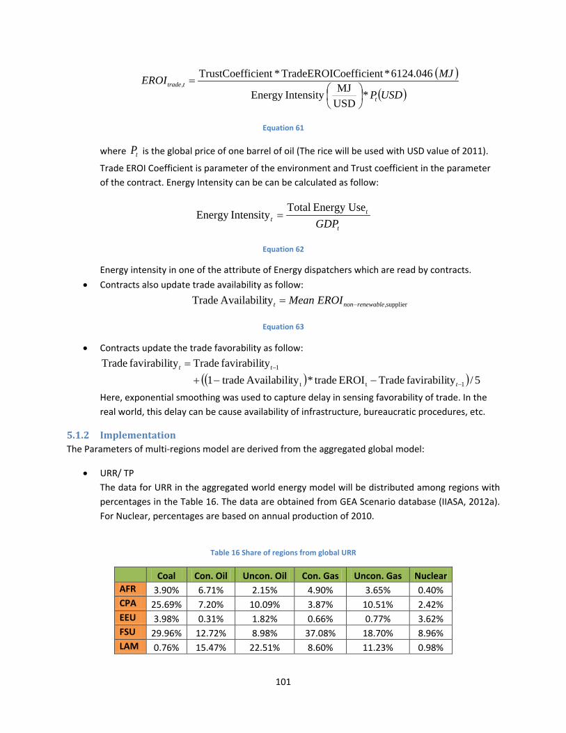
101

( )( )USDP

MJEROIt

ttrade

*USDMJIntensityEnergy

046.6124*oefficientTradeEROIC *icient TrustCoeff,

=

Equation 61

where tP is the global price of one barrel of oil (The rice will be used with USD value of 2011).

Trade EROI Coefficient is parameter of the environment and Trust coefficient in the parameter of the contract. Energy Intensity can be can be calculated as follow:

t

tt GDP

Energy Use TotalIntensityEnergy =

Equation 62

Energy intensity in one of the attribute of Energy dispatchers which are read by contracts. • Contracts also update trade availability as follow:

supplier,tyAvailabili Trade renewablenont EROIMean −=

Equation 63

• Contracts update the trade favorability as follow:

( )( ) 5/tyfavirabili TradeEROI trade*tyAvailabili trade1tyfavirabili Tradetyfavirabili Trade

1tt

1

−

−

−−+=

t

tt

Here, exponential smoothing was used to capture delay in sensing favorability of trade. In the real world, this delay can be cause availability of infrastructure, bureaucratic procedures, etc.

5.1.2 Implementation The Parameters of multi-regions model are derived from the aggregated global model:

• URR/ TP The data for URR in the aggregated world energy model will be distributed among regions with percentages in the Table 16. The data are obtained from GEA Scenario database (IIASA, 2012a). For Nuclear, percentages are based on annual production of 2010.

Table 16 Share of regions from global URR

Coal Con. Oil Uncon. Oil Con. Gas Uncon. Gas Nuclear

AFR 3.90% 6.71% 2.15% 4.90% 3.65% 0.40% CPA 25.69% 7.20% 10.09% 3.87% 10.51% 2.42% EEU 3.98% 0.31% 1.82% 0.66% 0.77% 3.62% FSU 29.96% 12.72% 8.98% 37.08% 18.70% 8.96% LAM 0.76% 15.47% 22.51% 8.60% 11.23% 0.98%

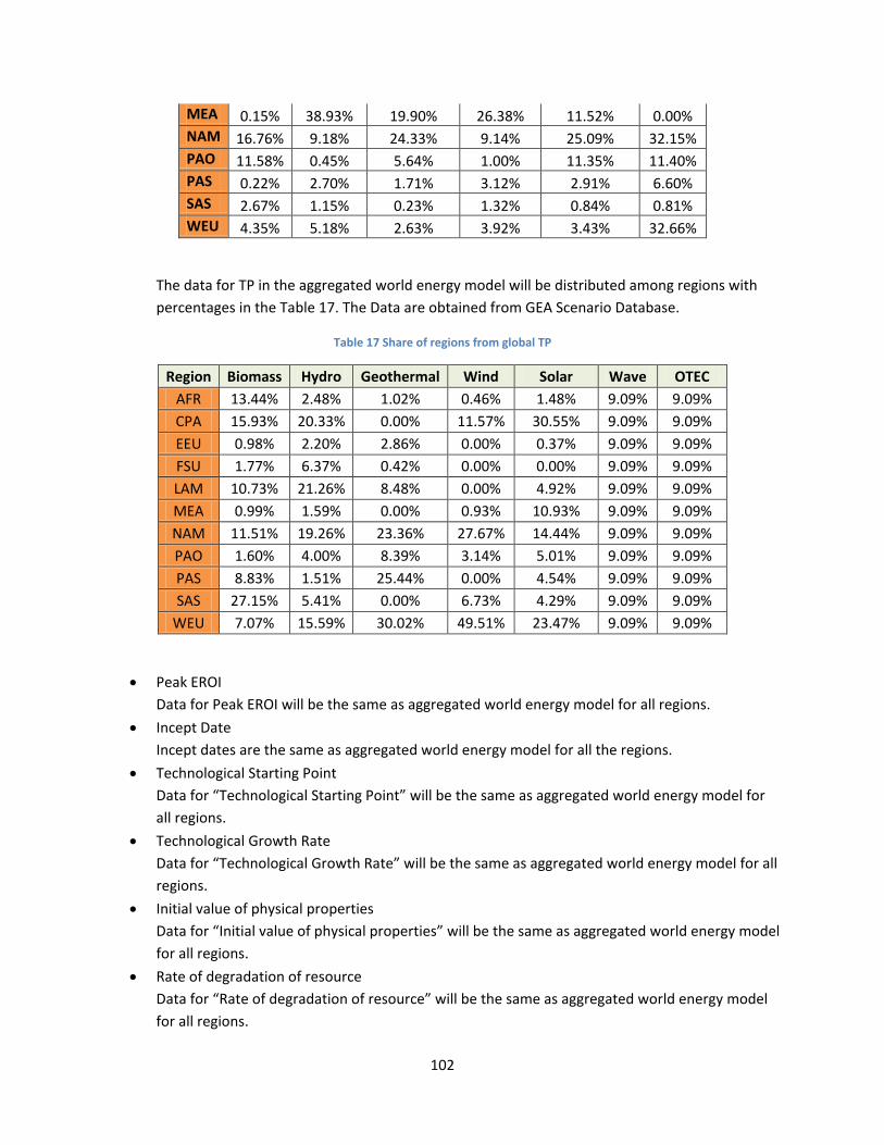
102

MEA 0.15% 38.93% 19.90% 26.38% 11.52% 0.00% NAM 16.76% 9.18% 24.33% 9.14% 25.09% 32.15% PAO 11.58% 0.45% 5.64% 1.00% 11.35% 11.40% PAS 0.22% 2.70% 1.71% 3.12% 2.91% 6.60% SAS 2.67% 1.15% 0.23% 1.32% 0.84% 0.81% WEU 4.35% 5.18% 2.63% 3.92% 3.43% 32.66%

The data for TP in the aggregated world energy model will be distributed among regions with percentages in the Table 17. The Data are obtained from GEA Scenario Database.

Table 17 Share of regions from global TP

Region Biomass Hydro Geothermal Wind Solar Wave OTEC AFR 13.44% 2.48% 1.02% 0.46% 1.48% 9.09% 9.09% CPA 15.93% 20.33% 0.00% 11.57% 30.55% 9.09% 9.09% EEU 0.98% 2.20% 2.86% 0.00% 0.37% 9.09% 9.09% FSU 1.77% 6.37% 0.42% 0.00% 0.00% 9.09% 9.09% LAM 10.73% 21.26% 8.48% 0.00% 4.92% 9.09% 9.09% MEA 0.99% 1.59% 0.00% 0.93% 10.93% 9.09% 9.09% NAM 11.51% 19.26% 23.36% 27.67% 14.44% 9.09% 9.09% PAO 1.60% 4.00% 8.39% 3.14% 5.01% 9.09% 9.09% PAS 8.83% 1.51% 25.44% 0.00% 4.54% 9.09% 9.09% SAS 27.15% 5.41% 0.00% 6.73% 4.29% 9.09% 9.09%

WEU 7.07% 15.59% 30.02% 49.51% 23.47% 9.09% 9.09%

• Peak EROI Data for Peak EROI will be the same as aggregated world energy model for all regions.

• Incept Date Incept dates are the same as aggregated world energy model for all the regions.

• Technological Starting Point Data for “Technological Starting Point” will be the same as aggregated world energy model for all regions.

• Technological Growth Rate Data for “Technological Growth Rate” will be the same as aggregated world energy model for all regions.

• Initial value of physical properties Data for “Initial value of physical properties” will be the same as aggregated world energy model for all regions.

• Rate of degradation of resource Data for “Rate of degradation of resource” will be the same as aggregated world energy model for all regions.

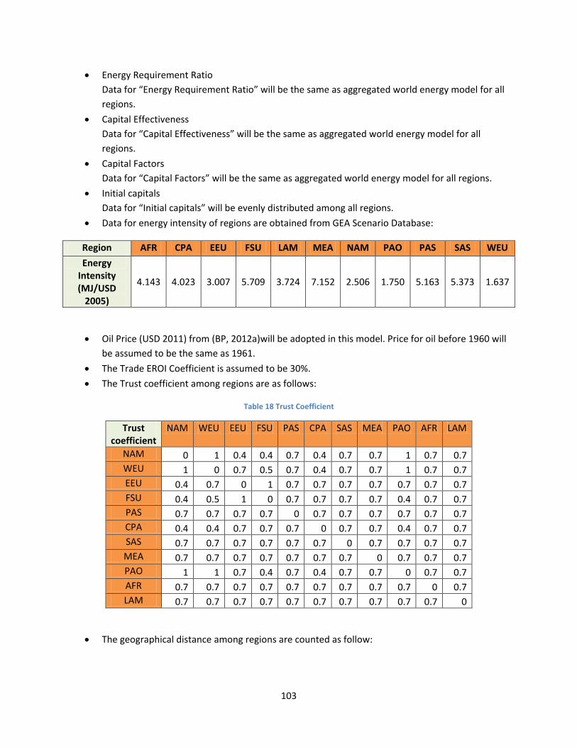
103

• Energy Requirement Ratio Data for “Energy Requirement Ratio” will be the same as aggregated world energy model for all regions.

• Capital Effectiveness Data for “Capital Effectiveness” will be the same as aggregated world energy model for all regions.

• Capital Factors Data for “Capital Factors” will be the same as aggregated world energy model for all regions.

• Initial capitals Data for “Initial capitals” will be evenly distributed among all regions.

• Data for energy intensity of regions are obtained from GEA Scenario Database:

Region AFR CPA EEU FSU LAM MEA NAM PAO PAS SAS WEU Energy

Intensity (MJ/USD

2005)

4.143 4.023 3.007 5.709 3.724 7.152 2.506 1.750 5.163 5.373 1.637

• Oil Price (USD 2011) from (BP, 2012a)will be adopted in this model. Price for oil before 1960 will be assumed to be the same as 1961.

• The Trade EROI Coefficient is assumed to be 30%. • The Trust coefficient among regions are as follows:

Table 18 Trust Coefficient

Trust coefficient

NAM WEU EEU FSU PAS CPA SAS MEA PAO AFR LAM

NAM 0 1 0.4 0.4 0.7 0.4 0.7 0.7 1 0.7 0.7 WEU 1 0 0.7 0.5 0.7 0.4 0.7 0.7 1 0.7 0.7 EEU 0.4 0.7 0 1 0.7 0.7 0.7 0.7 0.7 0.7 0.7 FSU 0.4 0.5 1 0 0.7 0.7 0.7 0.7 0.4 0.7 0.7 PAS 0.7 0.7 0.7 0.7 0 0.7 0.7 0.7 0.7 0.7 0.7 CPA 0.4 0.4 0.7 0.7 0.7 0 0.7 0.7 0.4 0.7 0.7 SAS 0.7 0.7 0.7 0.7 0.7 0.7 0 0.7 0.7 0.7 0.7 MEA 0.7 0.7 0.7 0.7 0.7 0.7 0.7 0 0.7 0.7 0.7 PAO 1 1 0.7 0.4 0.7 0.4 0.7 0.7 0 0.7 0.7 AFR 0.7 0.7 0.7 0.7 0.7 0.7 0.7 0.7 0.7 0 0.7 LAM 0.7 0.7 0.7 0.7 0.7 0.7 0.7 0.7 0.7 0.7 0

• The geographical distance among regions are counted as follow:

104

Table 19 Geographical Distance

Distance NAM WEU EEU FSU PAS CPA SAS MEA PAO AFR LAM NAM 0 3 4 3 3 4 5 5 3 3 1 WEU 3 0 1 2 5 5 4 2 4 3 4 EEU 4 1 0 1 5 5 4 2 4 3 5 FSU 3 2 1 0 2 1 2 1 2 5 5 PAS 3 5 5 2 0 1 2 4 1 5 3 CPA 4 5 5 1 1 0 1 2 2 4 4 SAS 5 4 4 2 2 1 0 1 3 3 5 MEA 5 2 2 1 4 2 1 0 4 1 5 PAO 3 4 4 2 1 2 3 4 0 5 3 AFR 3 3 3 5 5 4 3 1 5 0 3 LAM 1 4 5 5 3 4 5 5 3 3 0

5.1.3 Evaluation of the multi-region model The evaluation of the model was done by comparison of values of “total renewable net energy yield”, and “total non-renewable net energy yield” with historical data. The historical data is the same as historical data from PhD thesis by (M. Dale, 2010).

The validation process was done by calibration of model parameters such as URR, TP, parameters of dynamic EROI function, energy trade coefficients, and trust matrix. The model was manually run 100 times with different combinations of the parameters and the best combination of parameters was selected.

Figure 50 and Figure 51 illustrate the comparison of model output and the historical data. The fitting quality for renewable production is R2=0.951895 and for non-renewable production is R2=0.986616.

Figure 50 Total global renewable production _ Comparison of historical data and multi-region model output

0

10

20

30

40

50

60

70

1851

1860

1869

1878

1887

1896

1905

1914

1923

1932

1941

1950

1959

1968

1977

1986

1995

2004

EJ

Renewable Energy Yield

Historical Renewable

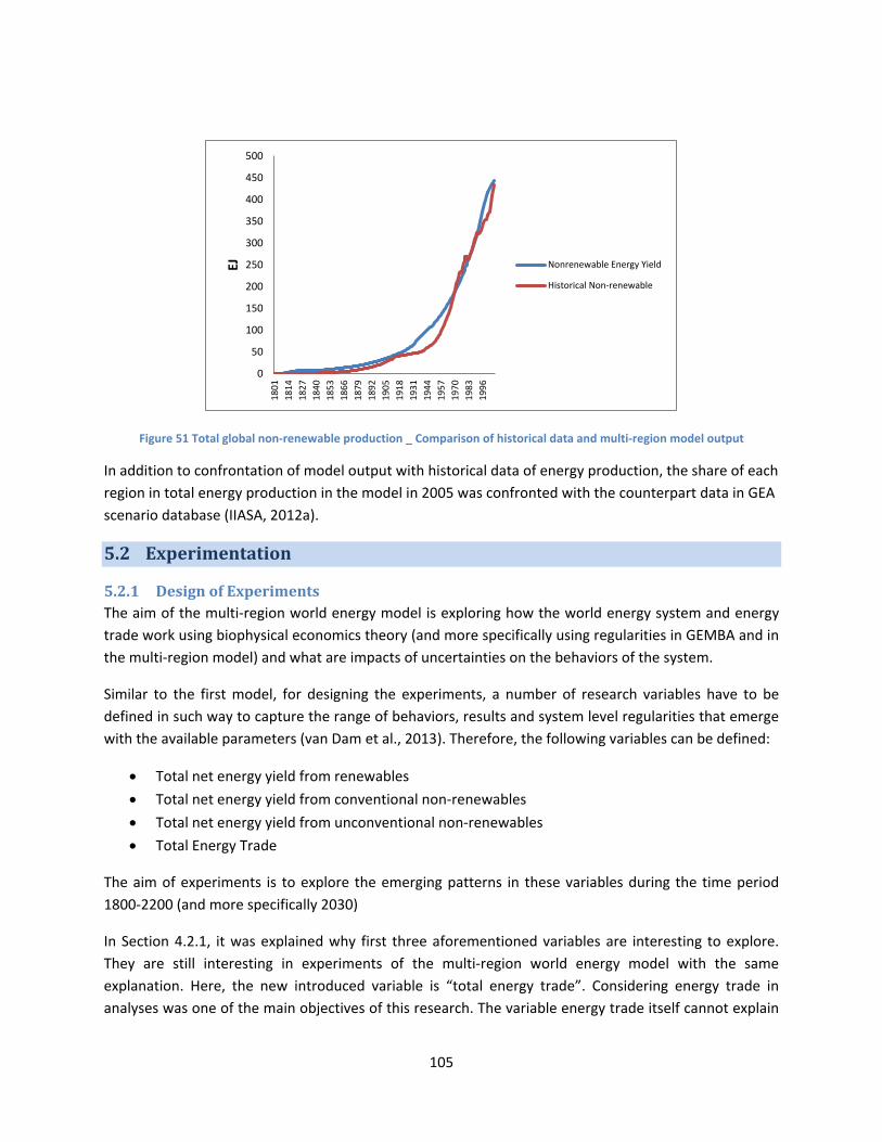
105

Figure 51 Total global non-renewable production _ Comparison of historical data and multi-region model output

In addition to confrontation of model output with historical data of energy production, the share of each region in total energy production in the model in 2005 was confronted with the counterpart data in GEA scenario database (IIASA, 2012a).

5.2 Experimentation

5.2.1 Design of Experiments The aim of the multi-region world energy model is exploring how the world energy system and energy trade work using biophysical economics theory (and more specifically using regularities in GEMBA and in the multi-region model) and what are impacts of uncertainties on the behaviors of the system.

Similar to the first model, for designing the experiments, a number of research variables have to be defined in such way to capture the range of behaviors, results and system level regularities that emerge with the available parameters (van Dam et al., 2013). Therefore, the following variables can be defined:

• Total net energy yield from renewables • Total net energy yield from conventional non-renewables • Total net energy yield from unconventional non-renewables • Total Energy Trade

The aim of experiments is to explore the emerging patterns in these variables during the time period 1800-2200 (and more specifically 2030)

In Section 4.2.1, it was explained why first three aforementioned variables are interesting to explore. They are still interesting in experiments of the multi-region world energy model with the same explanation. Here, the new introduced variable is “total energy trade”. Considering energy trade in analyses was one of the main objectives of this research. The variable energy trade itself cannot explain

0

50

100

150

200

250

300

350

400

450

500

1801

1814

1827

1840

1853

1866

1879

1892

1905

1918

1931

1944

1957

1970

1983

1996

EJ

Nonrenewable Energy Yield

Historical Non-renewable

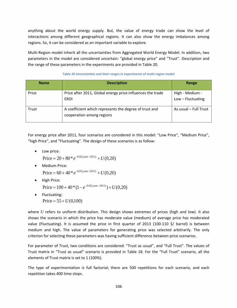
106

anything about the world energy supply. But, the value of energy trade can show the level of interactions among different geographical regions. It can also show the energy imbalances among regions. So, it can be considered as an important variable to explore.

Multi-Region model inherit all the uncertainties from Aggregated World Energy Model. In addition, two parameters in the model are considered uncertain: “global energy price” and “Trust”. Description and the range of these parameters in the experiments are provided in Table 20.

Table 20 Uncertainties and their ranges in experiments of multi-region model

Name Description Range

Price Price after 2011, Global energy price influences the trade EROI

High - Medium - Low – Fluctuating

Trust A coefficient which represents the degree of trust and cooperation among regions

As usual – Full Trust

For energy price after 2011, four scenarios are considered in this model: “Low Price”, “Medium Price”, “high Price”, and “Fluctuating”. The design of these scenarios is as follow:

• Low price:

)20,0(*8020Price )2011(02.0 Ue year ++= −−

• Medium Price:

)20,0(*4060Price )2011(01.0 Ue year ++= −−

• High Price:

)20,0()1(*40100Price )2011(02.0 Ue year +−+= −−

• Fluctuating: )100,0(55Price U+=

where U refers to uniform distribution. This design shows extremes of prices (high and low). It also shows the scenario in which the price has moderate value (medium) of average price has moderated value (Fluctuating). It is assumed the price in first quarter of 2013 (100-110 $/ barrel) is between medium and high. The value of parameters for generating price was selected arbitrarily. The only criterion for selecting these parameters was having sufficient difference between price scenarios.

For parameter of Trust, two conditions are considered: “Trust as usual”, and “Full Trust”. The values of Trust matrix in “Trust as usual” scenario is provided in Table 18. For the “Full Trust” scenario, all the elements of Trust matrix is set to 1 (100%).

The type of experimentation is full factorial; there are 500 repetitions for each scenario, and each repetition takes 400 time steps.

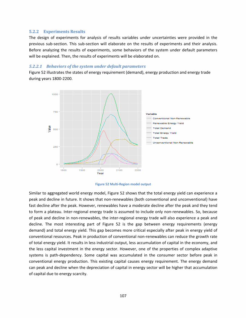
107

5.2.2 Experiments Results The design of experiments for analysis of results variables under uncertainties were provided in the previous sub-section. This sub-section will elaborate on the results of experiments and their analysis. Before analyzing the results of experiments, some behaviors of the system under default parameters will be explained. Then, the results of experiments will be elaborated on.

5.2.2.1 Behaviors of the system under default parameters Figure 52 illustrates the states of energy requirement (demand), energy production and energy trade during years 1800-2200.

Figure 52 Multi-Region model output

Similar to aggregated world energy model, Figure 52 shows that the total energy yield can experience a peak and decline in future. It shows that non-renewables (both conventional and unconventional) have fast decline after the peak. However, renewables have a moderate decline after the peak and they tend to form a plateau. Inter-regional energy trade is assumed to include only non-renewables. So, because of peak and decline in non-renewables, the inter-regional energy trade will also experience a peak and decline. The most interesting part of Figure 52 is the gap between energy requirements (energy demand) and total energy yield. This gap becomes more critical especially after peak in energy yield of conventional resources. Peak in production of conventional non-renewables can reduce the growth rate of total energy yield. It results in less industrial output, less accumulation of capital in the economy, and the less capital investment in the energy sector. However, one of the properties of complex adaptive systems is path-dependency. Some capital was accumulated in the consumer sector before peak in conventional energy production. This existing capital causes energy requirement. The energy demand can peak and decline when the depreciation of capital in energy sector will be higher that accumulation of capital due to energy scarcity.

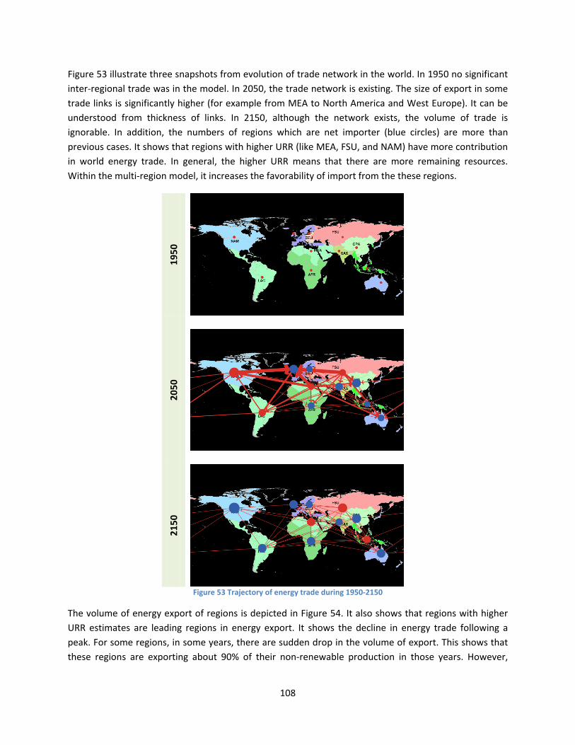
108

Figure 53 illustrate three snapshots from evolution of trade network in the world. In 1950 no significant inter-regional trade was in the model. In 2050, the trade network is existing. The size of export in some trade links is significantly higher (for example from MEA to North America and West Europe). It can be understood from thickness of links. In 2150, although the network exists, the volume of trade is ignorable. In addition, the numbers of regions which are net importer (blue circles) are more than previous cases. It shows that regions with higher URR (like MEA, FSU, and NAM) have more contribution in world energy trade. In general, the higher URR means that there are more remaining resources. Within the multi-region model, it increases the favorability of import from the these regions.

Figure 53 Trajectory of energy trade during 1950-2150

The volume of energy export of regions is depicted in Figure 54. It also shows that regions with higher URR estimates are leading regions in energy export. It shows the decline in energy trade following a peak. For some regions, in some years, there are sudden drop in the volume of export. This shows that these regions are exporting about 90% of their non-renewable production in those years. However,

1950

2050

2150

109

because it is assumed that the regions are not allowed to export more than 90% of their non-renewable production, they have to reduce the volume of export.

Figure 54 Energy export of regions

After investigating the behavior of the model under default parameters, the behavior of the model under uncertainty in parameters will be explored.

5.2.2.2 Total Energy Trade Since the new feature in the multi-region model in energy trade, before analyzing other research variables, energy trade will be explored. In this sub-section, the effects of different trust and energy price condition on the energy trade will be analyzed.

Figure 55 illustrated the effects of energy price and trust on the energy trade over years 1800-2200. In this graph matrix, elements in each row show the time series of total energy trade during 1800-2200 under different scenarios for energy price. For example the upper right element shows the time series total energy trade when the energy price in “medium” and trust among regions in “false” (“trust as usual”). Similarly, the upper left element shows the time series of total energy yield when energy price is “fluctuating” and trust is “as usual”. The second two belongs to scenarios in which there is full trust among regions. In each element graph, the Y axis shows the total energy yield in (EJ) and axis X shows time.

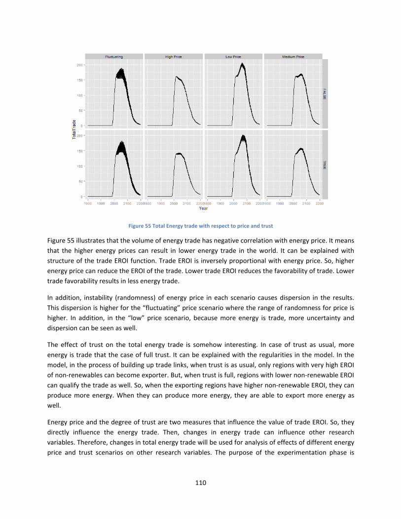
110

Figure 55 Total Energy trade with respect to price and trust

Figure 55 illustrates that the volume of energy trade has negative correlation with energy price. It means that the higher energy prices can result in lower energy trade in the world. It can be explained with structure of the trade EROI function. Trade EROI is inversely proportional with energy price. So, higher energy price can reduce the EROI of the trade. Lower trade EROI reduces the favorability of trade. Lower trade favorability results in less energy trade.

In addition, instability (randomness) of energy price in each scenario causes dispersion in the results. This dispersion is higher for the “fluctuating” price scenario where the range of randomness for price is higher. In addition, in the “low” price scenario, because more energy is trade, more uncertainty and dispersion can be seen as well.

The effect of trust on the total energy trade is somehow interesting. In case of trust as usual, more energy is trade that the case of full trust. It can be explained with the regularities in the model. In the model, in the process of building up trade links, when trust is as usual, only regions with very high EROI of non-renewables can become exporter. But, when trust is full, regions with lower non-renewable EROI can qualify the trade as well. So, when the exporting regions have higher non-renewable EROI, they can produce more energy. When they can produce more energy, they are able to export more energy as well.

Energy price and the degree of trust are two measures that influence the value of trade EROI. So, they directly influence the energy trade. Then, changes in energy trade can influence other research variables. Therefore, changes in total energy trade will be used for analysis of effects of different energy price and trust scenarios on other research variables. The purpose of the experimentation phase is

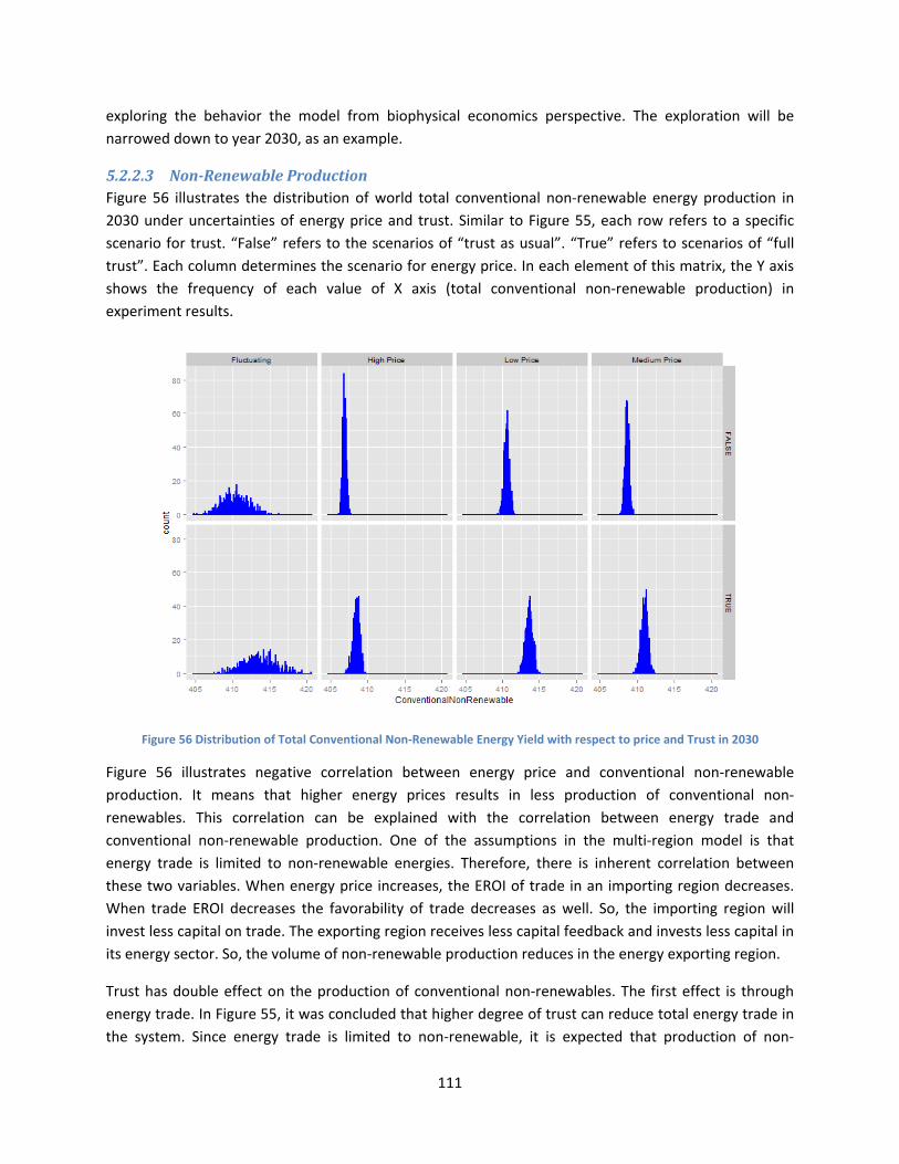
111

exploring the behavior the model from biophysical economics perspective. The exploration will be narrowed down to year 2030, as an example.

5.2.2.3 Non-Renewable Production Figure 56 illustrates the distribution of world total conventional non-renewable energy production in 2030 under uncertainties of energy price and trust. Similar to Figure 55, each row refers to a specific scenario for trust. “False” refers to the scenarios of “trust as usual”. “True” refers to scenarios of “full trust”. Each column determines the scenario for energy price. In each element of this matrix, the Y axis shows the frequency of each value of X axis (total conventional non-renewable production) in experiment results.

Figure 56 Distribution of Total Conventional Non-Renewable Energy Yield with respect to price and Trust in 2030

Figure 56 illustrates negative correlation between energy price and conventional non-renewable production. It means that higher energy prices results in less production of conventional non-renewables. This correlation can be explained with the correlation between energy trade and conventional non-renewable production. One of the assumptions in the multi-region model is that energy trade is limited to non-renewable energies. Therefore, there is inherent correlation between these two variables. When energy price increases, the EROI of trade in an importing region decreases. When trade EROI decreases the favorability of trade decreases as well. So, the importing region will invest less capital on trade. The exporting region receives less capital feedback and invests less capital in its energy sector. So, the volume of non-renewable production reduces in the energy exporting region.

Trust has double effect on the production of conventional non-renewables. The first effect is through energy trade. In Figure 55, it was concluded that higher degree of trust can reduce total energy trade in the system. Since energy trade is limited to non-renewable, it is expected that production of non-

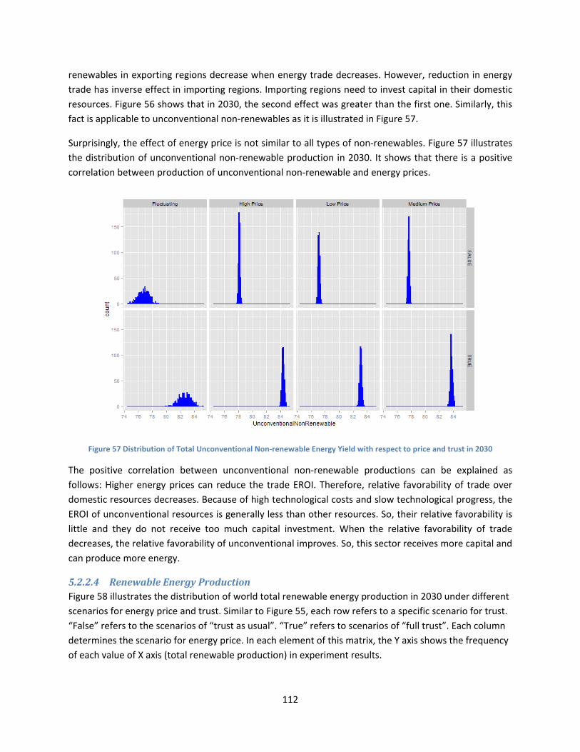
112

renewables in exporting regions decrease when energy trade decreases. However, reduction in energy trade has inverse effect in importing regions. Importing regions need to invest capital in their domestic resources. Figure 56 shows that in 2030, the second effect was greater than the first one. Similarly, this fact is applicable to unconventional non-renewables as it is illustrated in Figure 57.

Surprisingly, the effect of energy price is not similar to all types of non-renewables. Figure 57 illustrates the distribution of unconventional non-renewable production in 2030. It shows that there is a positive correlation between production of unconventional non-renewable and energy prices.

Figure 57 Distribution of Total Unconventional Non-renewable Energy Yield with respect to price and trust in 2030

The positive correlation between unconventional non-renewable productions can be explained as follows: Higher energy prices can reduce the trade EROI. Therefore, relative favorability of trade over domestic resources decreases. Because of high technological costs and slow technological progress, the EROI of unconventional resources is generally less than other resources. So, their relative favorability is little and they do not receive too much capital investment. When the relative favorability of trade decreases, the relative favorability of unconventional improves. So, this sector receives more capital and can produce more energy.

5.2.2.4 Renewable Energy Production Figure 58 illustrates the distribution of world total renewable energy production in 2030 under different scenarios for energy price and trust. Similar to Figure 55, each row refers to a specific scenario for trust. “False” refers to the scenarios of “trust as usual”. “True” refers to scenarios of “full trust”. Each column determines the scenario for energy price. In each element of this matrix, the Y axis shows the frequency of each value of X axis (total renewable production) in experiment results.

113

Figure 58 Distribution of Total Renewable Net Energy Yield with respect to price and Trust in 2030

Figure 58 illustrates positive correlation between total world renewable energy production and energy price. Similar to non-renewables, this correlation can also be explained with energy trade. In the previous analyses, it was concluded that higher energy prices can reduce EROI and favorability of energy trade. Reduction in trade can motivate importing regions to invest more capital in renewables. More investment in renewables can increase the production of renewables as it is depicted in Figure 58. On the other hand, since energy trade is limited to non-renewables, less energy trade can result in fewer requirements for non-renewables. In energy exporting regions, this can increase relative favorability of renewables. So, it can results in more production of renewables. Moreover, the effect of trust on the energy production can be explained the same as on non-renewables.

5.3 27BConclusion In Chapter 4, the two-step approach for development of the objective model of this research was explained. In this chapter, the multi-region world energy model, the second model of this research, was developed. The multi-region model uses the aggregated world energy model as the basis and incorporated new concepts such as trade EROI into analysis.

After clarifying the main assumptions of the model (see Section 5.1.1.1), the conceptual design of the model was presented. Multi-region model inherits all characteristics of the aggregated world energy model. So, the agents “Renewable Supplier”, “Non-Renewable Supplier”, and “Energy Consumer” remained the same. However, new set of rules was added to energy dispatchers in order to be able to manage the energy trade. In the multi-region model, all 11 regions have these four agents. However, energy dispatcher acts and brains of the region. The EROI function provided by R. Kauffman (1986.) was used in the analyses of energy trade in the multi-region model. In addition, the trade links among regions (“Contracts”) were defined and specified.

114

Similar to aggregated world energy model, the multi region was implemented in NetLogo environment. The model was calibrated manually and evaluated by confrontation model results with the historical data.

For exploring the behaviors of the model under defined uncertainties, a number of experiments were designed. The experiments explored the behavior of the system in years 1800-2200 and s specific year (2030).

All emergent patterns in the aggregated world energy model (such as peak, decline, etc.) were repeating in the multi-region model. Next to that, multi-region models provides possibility to study the behaviors of agents, the network of energy trade and the effects of energy trade on other behaviors of the system. Results of experiments showed that, from biophysical economics perspective, in alignment with non-renewables, energy trade can experience peak and decline.

Contrary to aggregated world energy model in which energy price was not influential at all, the multi-region model used energy price for measuring the trade EROI. Also, a scaling coefficient was added to the measure in order to correct perceptions of trade favorability among regions. Results of experiments show that both parameters could directly the energy trade influence and energy production indirectly.

Because the multi-region mode used GEMBA as its basis, and because of similarity of model output with historical data, it can be concluded that the multi-region model can provide some insights about the world energy system. More explanation about the insights will be provided in Chapter 6

115

6 Conclusion

6.1 Overview The world is moving towards scarcity in non-renewable energy resources. Therefore, new studies need to be taken to provide solutions for future generations. These studies mostly use standard economic theories which do not consider limitations of natural resources even though these resources are the main subject of the studies.

Biophysical economics as an economic theory considers the relation between economy and limited natural resources. Therefore, it was selected as a theoretical perspective for this research. Biophysical economics theory has been used as the basis of a number of biophysical models. However, those models are all process oriented and only have a global view on this system. They do not sufficiently provide insights into the geographical properties and trading behaviors of energy suppliers and consumers. So, they do not provide insight on the effects of these interactions on the emergent behavior of the global energy system.

Biophysical economics has high potential for providing insights into the world energy system by considering the natural resources. However, the current biophysical models are not capable of representing the world energy system considering its bottom-up complexities. This lead to the following research question:

What can be learnt from biophysical economics theory when it is used for the modeling of the world energy system considering trade?

In order to answer this question, the research objective was set to develop a model using the biophysical economics theory in order to explore the behaviors of the world energy system with multiple interacting regions.

For the development of the model, some preliminary steps were followed. In the first step, theoretical perspectives of this research were explained. The first theoretical perspective in this research was biophysical economics. The literature review on biophysical economic was provided and this theory was compared with standard economics theories. Also, the general model of relation between energy sector, the main economy, and the environment was presented. Since the objective of this research was to consider energy interactions among world regions in the modeling practice, complex adaptive systems (CAS) theory was taken as the second theoretical perspective of this research. The main characteristics of CAS were explained to show why and how the world energy system is classified as a CAS. Afterwards, among different modeling paradigms, agent-based modeling was identified as the most suitable approach for modeling the world energy system with aforementioned theoretical perspectives.

In the next step, the world energy system was analyzed from two perspectives. The first perspective was technical and system perspective. The analysis provided the technical decomposition of the world energy system into its main processes. The definition of reserves, resources, ultimately recoverable

116

resource, technical potential and other uncertain factors which can influence the state of the world energy system were provided. In addition, having these uncertainties, the concept of peak in energy production was reviewed. For the second perspective, actor analysis was provided to describe the main players in the world energy system at micro level and macro level. The micro level studied the generic network of energy-related companies and institutions. Macro analysis studied the current regional decompositions of the world energy system. It provided some criteria to find a suitable regional decomposition of the world. This analysis found the IIASA 11-region model as the suitable regional decomposition for modeling purposes.

Following the theoretical perspectives and system description, a two-step approach was taken to develop the objective model of this research. In the first step, a model was developed without considering interacting regions. In the second step a model was developed considering interacting regions. The first model was developed as an agent-based equivalent of the most recent biophysical economics model in the literature, GEMBA. GEMBA is a system dynamics model developed by M. A. J. Dale (2010). The second model was developed by expanding the first model. The validation of both models was done by confrontation of model outputs with the historical data or the outputs of GEMBA. After the development of each model, a set of experiments were done in order to explore the behavior of the model under defined and assumed regularities in the models and biophysical economics. Finally, the results of experiments were analyzed and discussed.

In section 6.2, the outcomes of the research will be explained and the research questions will be answered.

6.2 Research Outcomes The main outcome of this research is the multi-region world energy agent-based model. The model observes the world from biophysical economics perspective and considers the energy interactions among different world regions. Two facts support the scientific basis and validity of this model. First, the basis of the multi-region model is the aggregated world energy model. The aggregated world energy model was the agent-based implementation of the most recent biophysical economics model in the literature, GEMBA by M. Dale (2010). GEMBA is a validated model with comprehensive biophysical economics background. The multi-region world energy model adapts and incorporates the rules of energy trade with the functions of GEMBA and functions of the aggregated word energy model. Second, in the evaluation process, the global behaviors of the multi-region model were compared with historical data. Similarity with historical data also supports the validity of the model.

Having the objective model, the research questions can be answered. The main research question was:

What can be learnt from biophysical economics theory when it is used for the modeling of the world energy system considering energy trade?

In order to answer this question, a number of sub-questions were asked in the introduction of the thesis. Answering these sub-questions can help answering the main research question.

117

6.2.1 Using biophysical economics to develop models The first research sub-question was “To what extent can biophysical economics theory be used to develop models for exploring trade in the global energy system?” This question can be answered as follows: Energy trade can be considered in biophysical economics models as far as it can be explained with biophysical measures such as EROI. In addition, combination with complex adaptive systems theory enables biophysical economics models to incorporate the concept of trade in analyses more effectively. This conclusion will be elaborated on in following paragraphs.

The biophysical view of economics (see Figure 6) talks about the “world” which obtains energy only from energy transformation system. In the standard economic, when the level of abstraction is the “world”, no import or export is considered in the model. However, when the level of abstraction is reduced to countries, imports/exports can enter the model as injections/withdrawals. Similarly, when the level of abstraction in the biophysical view is reduced from the “world” to “regions”, energy trade can emerge from the model as a type of injection/withdrawal. In biophysical economics, EROI can provide signal for investments in energy sector. So, in order to include energy trade into biophysical economics analyses, it is necessary to measure the EROI of the trade. Following the work of R. Kauffman (1986.), measuring EROI for imported energy became possible. So, it can be concluded that the analysis of trade is possible in biophysical economics theory.

Another feature of energy trade among world regions is the geographical movement of energy. These movements create a network of interactions among regions. Although in biophysical economics, the EROI for trade can be measured, it does not provide specific tools for studying these interactions. However, biophysical economics theory can be strengthened if it is combined with the theory of complex adaptive system (CAS) (see Section 2.2). In CAS, the behaviors of the system emerge from the states and behaviors of individuals (agents) and interactions among them. So, adoption of this theory can improve capabilities of the biophysical economics models to analyze energy trade. Agent-based modeling is a leading tool for CAS analysis. The multi-region world energy model, as an agent-based model, defines the favorability of energy trade such that it is compatible with definition of favorability of resources in GEMBA. Because of this compatibility, the model is able to work and represent the energy trade properly. Therefore, the multi-region world energy model and its exploratory experiments are evidences for the capability of biophysical economics and CAS for exploring and analyzing the energy trade in the system.

6.2.2 59BMain characteristics of the world energy system The next research sub-question was “What are the main characteristics and activities in the world energy system from biophysical economics perspective?” The main features of the world energy system can be explained as follows:

Following the analyses and discussions in Section 3.1, the purpose of the world energy system can be considered as “delivering energy that either directly or indirectly provides goods and services to meet people’s needs and aspirations”(GEA, 2012). The main activities within the world energy system can be classified into four groups of “extraction and treatment”, “conversion”, “transportation”, and “consumption”. The first group receives energy resource as feed and produces primary energy. The

118

second group receives primary energy and produces the secondary energy. Other activities are not (energy) producing activities. They belong to movement and consumption of energy. From the biophysical economics perspective, all groups of activities have inputs of fuel and capital. Also, they all have energy losses.

Primary energy resources are obtained from two groups of renewable resources and non-renewables. Non-renewables can be classified into two groups of conventional and unconventional resources. Non-renewable resources are stocks of energy with finite size whereas renewables are flows of energy in the world with finite potentials. For non-renewables, the measure of “ultimately recoverable resource” shows this finite “size”. For renewables, the measure “technical potential” shows this maximum size of flow. One of the characteristics of the world energy system is that there is no standard and unique definition about these measures and they are subject to very high uncertainty (see Table 2, Table 3, and Table 4).

Another characteristic of the world energy system is the expectations for peak in production of non-renewables resources. The finite size of non-renewable stocks causes such expectations. The factors influences the peak can be classified into underground factors (geological factors) and above-ground factors (such as macroeconomics, technology, etc) (see Section 3.1.3). High uncertainty in these factors causes high uncertainties about the time and value of peak in non-renewables.

The other characteristic of the world energy system from biophysical economics perspective is the EROI. In biophysical economics, EROI is the driving force for functioning of the energy supply system. The EROI depends on several factors. Following the work of Michael Dale et al. (2011), two main factors can be considered influential in EROI: 1) quality of resources and 2) progress of technology. Quality of resources decreases with production of energy whereas technology progresses with production of more energy. Therefore, a growth, peak and decline can be expected for EROI of energy resources in their productive lifecycles.

All in all, the world energy system is a very large and complex system and it owns too many characteristics and features. Here, the analysis is limited to aforementioned characteristics as they can be influential in modeling process.

6.2.3 Decomposing the world energy system The third research sub-question was “How can the world energy system be decomposed into different trading regions?”

For decomposition of the world energy system two approaches could be followed: 1) clustering of the world into regions, and 2) selection one of current decomposition. In order to improve comparability of the objective model with existing models and data, it was decided to select one of the existing regional decomposition.

Following the literature review, the regional decompositions of IIASA, IEA, and BP can be considered as the main candidates. The criteria for selection of the best candidate can be limited to geography, resources and production power, and energy demand. Geography is the most important factor because

119

it could encompass the geology, culture, economy and politics of countries and regions. Using these criteria, the 11 regions of IIASA can be selected as the regional decomposition for the future agent-based model. The advantage of IIASA over other alternative is the moderate level of abstraction and availability of most required data in the GEA scenario database.

6.2.4 Modeling Requirements to explore the world energy system The last research sub-question was “What are the requirements to design a model to explore the world energy system with considering energy trade?”

The main requirements for design and development of models can be explained in a number of steps which should be followed. Different modeling paradigms can influence the reaming path of modeling. So, the preliminary step for modeling a system is selecting the right modeling paradigms (see Section 2.2.2). Since the selected modeling paradigm for this research is agent-based modeling, the steps will be explained for development of an agent-based model.

The first step in model development was understanding the problem which was going to be modeled (see Section 1.1). In this research, the problem was lack of insight about energy trade and interaction among world regions from biophysical economics perspective.

The second step in development of a world energy model was decomposition of the system. Decomposition of a large-scale socio-technical system can be done with both system perspective (see Section 3.1) and actor perspective (see Section 3.2). The system decomposition provided insights about processes and rules of the system. Also, actor decomposition helped in defining agents in the agent-based model.

Conceptual modeling was the next step in the modeling process. In conceptual modeling, the main variables, attributes and functions of the system should be defined (see Section 4.1.2 and Section 5.1.1). This process defined what each agent has and what it does. In this research, there were four generic agents in each region for the world energy system. “Renewable suppliers” were responsible for functioning of the renewable energy sectors. “Non-Renewable suppliers” were responsible for functioning of the non-renewable energy sectors. “Energy Consumers” were responsible for functioning of the rest of the economy. “Energy Dispatchers” were responsible to intermediate the energy and capital flow from the energy sector and the economy. They were also responsible for managing energy trade with energy dispatchers of other regions.

The next step is implementation of the model in software and consequently, the evaluation of the model. The model needed to be verified. Verification in this research was done by comparison of the code and the results with the operational details of the model design (see Section 4.1.2.2 and Section 5.1.1.3). The model needed to be validated as well. Validation was done by literature comparison (see Section 4.1.4) or comparison with historical data (see Section 5.1.3)

The next step was to learn from the model through experimentation. A set of experiments were designed in order to investigate the behavior of the system (see Section 4.2.1 and Section 5.2.1). The

120

next step, which was the last step in this research, was data analysis. Data analysis search for patterns in the behaviors of the model (see Section 4.2.2 and Section 5.2.2).

6.2.5 62BBiophysical economics theory for the modeling of the world energy system In this research, all the required steps were followed in order to learn from the model and modeling process and answer the main research question. Having the model and the answers of all research sub-question and results of experiments, it is possible to answer the main research question “What can be learnt from biophysical economics theory when it is used for the modeling of the world energy system?”

Considering the multi-region model in this research (and GEMBA in the literature), it can be concluded that biophysical economics models can provide additional insights about the possible emerging patterns in the world energy system as compared to standard economic theories. Biophysical economic theory enables models to systematically incorporate the limitations of resources into the analysis. The details of biophysical analyses are subject to high uncertainty in size of resources. However, the general emerging pattern is robust.

Biophysical economics analysis is not compatible with the traditional paradigm in economic analysis. It does not work with equilibrium concept. In this theory, the role of price in allocation of demand is replaced with EROI. EROI is not as tangible as price. So, measuring EROI for biophysical analysis needs more precise energy accounting.

Another fact about biophysical economics is the continuous nature of variables in this theory. Continuous nature of variables and low degree of details (resolution) of models cause tendency in continuous modeling such as system dynamics. For example, WORLD 3 and GEMBA are system dynamics model. Also, in the multi-region model, the agents think and make decisions using system dynamics formalism.

In the multi-region model some aspects of the energy trade were modeled and explored using the biophysical economics perspective. In the multi-region model, the EROI for energy trade is a function of energy price and energy intensity of regions. So, the multi-region model showed that that energy trade can be an interface between biophysical economics and standard economics as well. Standard economics can explore the state of price while biophysical economics explore the states of trade EROI. In addition to standard economics, some other theories such as politics can be incorporated in the perceptions of trade EROI in biophysical economics model. This was done in the multi-region model using the concept “degree of trust”.

Like GEMBA, multi-region model shows the peak and decline in production of non-renewables in future. It also shows a peak and a moderate decline in future of renewables. Similar to GEMBA, it shows that the gap between the energy demand and the energy production will increase in future and most part of energy demand will be supplied by renewables afterwards. The gap will start to increase when the production of non-renewables start to decline. Also, the multi-region shows that size of energy trade for regions is very small in comparison to their total production/consumption. In addition, in the multi-region model, energy trade experiences a peak and decline as it is assumed to be only the trade of non-renewables. Multi-region model also shows that lower energy trade can increase the share of

121

renewable production in energy portfolio of the world. Decrease in energy trade can happen, for example, when the energy price is too high.

6.3 Reflection In this section, three important items in the process of this research and their implications will be reflected on.

6.3.1 Adoption of biophysical economics as theoretical perspective One of the main features of this research is adoption of biophysical economics instead of standard economics. The main reason for selecting biophysical economics was the concept of “end of easy oil” and concerns about limitations of natural resources. Contrary to standard economics, in biophysical economics, the economy is systematically considered within the nature and the environment. In this theory, any economic activity begins from the nature and ends in the nature. This paradigm was as interesting option to deal with limitation of natural resources inF the economic analyses. So, it was selected as the theoretical perspective. For adoption of biophysical economics, this research attempted to employ and extend the most novel biophysical economics model in the literature, GEMBA. It also used the concept of EROI for imported fuel for extension of GEMBA.

There were a number of challenges in process of adopting biophysical economics, and more specifically employing and extending GEMBA:

• The first challenge was limited documentation and literature for biophysical economics models. There are few biophysical economics models in the literature and most of them belong are quite old. The theory was not paid attention to, among policy makers and economists for long time until very recent years.

• The next challenge in adoption of biophysical economics is that it needs energy accounting in countries. Energy accounting is not limited to fuels, but it also considers the energy equivalent (work) of goods and services in the economy. Lack of such accounting systems and accurate data can be considered as a problem in adoption of biophysical economics.

• Another challenge with biophysical economics is that EROI is not as tangible as price in standard economics. In addition, it is not easy to measure compared to price. More specifically, the dynamic EROI function which was developed by Michael Dale et al. (2011) considers only the resource quality and the technology development for calculation of GEMBA. However, in practice, it is expected that many social, political and economic factors can be influential in the EROI. Another difficulty of the dynamic EROI function is the estimation of its parameters.

• The next challenge is about the resolution of biophysical economics models. EROI can be calculated for resources which are usually owned by countries. So, biophysical economics become useful for level of at least a country. So, contrary to standard macroeconomics that can be linked with microeconomics, the low-resolution biophysical economics model cannot be easily linked with higher resolution models.

• Finally, because the GEMBA approach focuses on the “energy” as the only metric in the analysis, it is not compatible with most existing policy instruments in economies. In turn, the policy

122

recommendations on the basis of biophysical economics models are usually more abstract and have a very long-term scale.

The alternative economic world view for development of a model for the world energy system was standard economics. In this research, a model based on standard economics could have been developed. With that approach, the focus of analysis would have been shifted to the main economy. Then, the impacts of the economic activities on the environment could be assessed in order to consider limitations of natural resources. Taking that approach, energy could be considered as a commodity which is traded and priced. Adoption of standard economics concepts could have some advantages:

• The first advantage was extensive literature of the standard economics. The literature of standard economics provides a comprehensive set of concepts, rules, tools and models (e.g. WEM, MESSAGE) for analysis of various economic-energy problems. Such a literature could have support the modeling process.

• In addition, since it is “standard” economics, much more economic data would have been available. There are many national and international institutes (e.g. IEA, IIASA, UN, EIA, WEC, etc.) which publish energy-related data regularly.

• The other advantage of standard economics model over the current biophysical economics model could have been its tangible concepts such as price, etc. which are not the case in the current biophysical economics model. In addition, since policy making processes at national and international levels are based on standard economics, results of such a model could have been more compatible with policy instruments.

Although standard economics world view could have provided some advantages in the model, the current model has some valuable features which are lacking in standard economics model:

• The first advantage of the multi-region model (and GEMBA) is the boundary of the system in this model. In section 2.1.1, it was discussed how the boundary of the economic model in standard economics is problematic. In standard economic, there is always a circular flow in the system and no channel considered for input of material and energy from the environment and dispose of waste to the environment. Although the multi-region model (and GEMBA) abstracts the natural resources (like mineral) as their energy equivalent, the channels of energy resources and waste are considered in the model.

• The next scientific advantage of the adoption of biophysical economics in the multi-region model is its compliance with laws of physics and thermodynamics. In section 2.1.1, it was explained how the processes in standard economics are in contradiction with laws of thermodynamics. But, in multi-region model (and GEMBA), the low-entropy energy resources and the high-entropy wastes are clearly defined I in the model. In Multi-region model (and GEMBA), the main economy has inputs and outputs is not a self-maintaining circular loop anymore.

• The other advantage of adoption of biophysical economics in the multi-region model is the fact that it used energy price in the trade EROI function. In this model, the energy price is considered

123

as an exogenous variable. However, it can provide an interface to systematically link standard economics models with the multi-region model.

All in all, the multi-region model has aforementioned advantages and limitations. The biophysical economics is not as mature as standard economics. Multi-region model can be considered as a step forward for development of biophysical economics. It provides insights about energy trade and it introduced opportunities for linking biophysical and standard economics models.

6.3.2 Combination of biophysical economics and CAS in ABM One of the contributions of this research is combination of biophysical economics theory and the theory of complex adaptive systems for development of an exploratory model. Biophysical economics (as it is currently documented) is a completely process oriented theory. However, the CAS theory focuses on the behaviors of units and their interactions in a network.

Biophysical economics puts emphasis on energy analysis within the world. It also measure variables at level of countries and in low resolution time frame. So, biophysical systems are naturally continuous systems. In addition, biophysical economics inherently adopts a top-down view on the economy. The best modeling paradigm for such a condition is system dynamics as it was used in GEMBA, WROLD3, etc. In this research, agent-based modeling paradigm was used to develop the multi-region model. Agent-based modeling is the most appropriate paradigm for modeling complex adaptive system. It adopts bottom-up view to the world. In the multi-region model, the level of abstraction was reduced from “the world” to “regions”. So, the model attempts to explore the effects of changes in regional level on the global variables. In order to keep compatibility with biophysical economics, the multi-region model was developed as a kind of hybrid model in which agents think in system dynamics formalism (the smooth curves in the results of the model shows) whereas they interact with each other in a discrete energy trade network.

The current agent-based model has some advantages over its equivalent system dynamics model. Most of the advantages can be utilized in the future works. The first advantage is the flexibility of the model. All changes in the model can be done at the level of agents. There is no need to change the structure of the whole model as it is in system dynamics models. An example of flexibility is about the number of regions. The current model adopts the 11 regions of IIASA. It can adopt other decomposition after calibration of few parameters. The next advantage of this model is its maintainability. The next advantage of this agent-based model is its capability to work with other agent-based models as long as they share a communication protocol. This can help the expansion of the model in the future. In addition, typical advantages of agent-based models over system dynamics model like maintainability is applicable here as well.

6.3.3 Combination of ABM and SD One of the features of this research is combination of system dynamics and agent-based modeling. This combination is different from so-called multi-paradigm modeling in which a number of models with different paradigms interact with each other in a meta-model. Here, SD becomes the rule-base of agents in agent-based model.

124

In the literature, most problems with low level of abstraction are modeled with either SD, or ABM. The scientific research is usually concentrated to selecting and implementing the better paradigm or to comparison of these paradigms. In other words, because of different characteristics of these two paradigms (see Table 1), a strict boundary is usually considered between these two paradigms. In addition to difference in characteristics of these two approaches, it seems that using professional software applications (e.g. Vensim) navigate research models to be pure SD or ABM. In addition, it seems that the high cost of multi-paradigm modeling software programs (e.g. AnyLogic) prevents researcher to consider ABM and SD together.

Nonetheless, in this research, the multi-region world energy model showed that combination of these two approaches can be insightful. In this research, the world energy system was analyzed. The level of abstraction in such a system is extremely high. It seems that in such a condition, the differences between SD and ABM (the top-down perspective and the bottom-up perspective) decreases. It enables the combination of ABM and SD. Moreover, in this research, the model was implemented in NetLogo. All properties of the GEMBA were implemented by converting differential equations to “nlogo” codes. So, there was no pressure by the software to move towards a pure SD of ABM. In other words, it can be concluded that there was no hard boundary between SD and ABM as long as they can be programmed in programming languages without being trapped in regularities of software applications.

So, this research can have a message that in very abstract and high level systems, combined ABM and SD models can be developed by using programming languages instead of existing applications and such a combination might be insightful.

6.3.4 Assumption is the design of the Multi-Region World Energy Model In the design of the multi-region model a set of assumption were used. Some assumptions were inherited from GEMBA. Those assumptions are mentioned in section 4.1.1.2 and are extensively discussed and reflected on in (M. Dale, 2010). Here, the discussion will be narrowed down to new assumptions which are used in the design of the multi-region model. In the following paragraphs a number of these assumptions will be reflected on.

Comparability of EROI functions One of the explicit assumption in the multi-region model is that trade EROI and EROI of energy resource are comparable. The EROI of resources and EROI of trade are calculated differently in the multi-region model. Trade EROI is a function of price and energy intensity which are completely exogenous parameters to the model. EROI of resources are function of energy production and URR/TP. Although URR/TP is a parameter of the model, the production is an endogenous variable. This might be a question how these two values are comparable when they are calculated on the basis of two different approaches?

Both trade EROI function and dynamics EROI function are methods to estimate the EROI in the real world. The trade EROI function attempts to calculate the EROI on the basis of classic definition of EROI. It calculates the ratio of energy value of imported fuel to energy value of exported products (investments). The dynamic EROI function estimates value of EROI in relation with capital and annual

125

energy production. Since the variable they are estimating is the same, they are technically comparable. The only problem is that the value of the dynamic EROI function is scaled and bounded to a parameter (peak EROI) whereas it is not scaled. In order to make these two functions comparable, a coefficient is added to the trade EROI function to scale it and make it comparable with EROI of resources. This coefficient is calibrated using historical data. It does not have a physical meaning. It is added to the model for making harmony in the results.

The fact that the scaling factor in trade EROI function is not meaningful in physics does not influence the analysis. It is because the value of EROI itself is not interesting in this model, but its value in harmony with other variables is expected to produce plausible results.

Limiting energy trade to non-renewables The next assumption in this model is that energy trade is limited to non-renewables resources. In other words, it is assumed that all produced renewable energy will be consumed within the producer region. In addition, it is assumed that no more that 90% of non-renewable energy production can be exported by regions.

This assumption is a simplifying assumption in the model. However, it has foundations in the real world. In general, renewable energy resources cannot be transported for long distances. Most of them should be converted to electricity. The loss of electricity in long distances is significant. But, non-renewables such as oil or LNG can be easily transported among continents. In addition, usually, the export/import of electricity takes place between neighbor countries. The level of abstraction in this research is “region” and TP of renewables is usually low. So, neglecting the movements of electricity among regions is not expected to influence the behavior of the world energy system.

In addition, it is expected that non-renewables continue to dominate the world energy supply in the next decade. Especially, in transportation sector, it is expected that fossil fuels cannot be easily replaced with other types of fuels in early future. So, the size of trade is bounded to maximum 90% of the non-renewable production. This is an arbitrary value and shows the extreme point of energy trade. This constraint can be criticized; however it does not become active in conducted simulations until later years. So, it does not influence the generic behavior of the model and the drawn conclusions.

Lack of dependency between energy price, supply and demand The next assumption is that there is no link between energy price in the multi-region to the production and consumption of energy. This is true criticism about this model. However, since the perspective of this research is biophysical economics, there is no mechanism for setting price. Even the production and consumption of energy within the model are not linked with price. So, in order to set the price endogenously, another module should be added to the model which uses the standard economics theories to set the price.

Incorporation of “Trust” Another assumption in this model is incorporation of the concept “political trust” in the biophysical economic model. Biophysical economics is naturally incompatible with politics. However, the trust coefficient is cooperating with the trade EROI coefficient in scaling trade EROI for regions. In fact it is

126

assumed that biophysical rationality of regions is bounded with politics. Some regions such as OECD regions can sense the trade EROI as it is. But some regions with dispute sense less import favorability from high EROI exporters. An example can be found in the fact that although most of the oil reserves in the world are located in OPEC countries, considerable production oil is currently done outside OPEC. Therefore, it can be assumed that the sense of trade EROI among OECD regions are complete whereas is the sense of EROI between OECD regions and OPEC regions is less.

6.3.5 Policy Implications of Outcomes As mentioned earlier in this section, because the multi-region model (and GEMBA) focuses on the “energy” as the only metric in the analysis, it is not compatible with most existing policy instruments in economies. So, the policy recommendations on the basis of biophysical economics models are usually abstract and have a very long-term scale. Nonetheless, a number of policy implications are mentioned in the following paragraphs.

One of the interesting emergent patterns in both GEMBA and multi-region model is the increasing gap between global energy supply and energy requirements. In standard economics terms, increasing gap between supply and demand means scarcity and it leads to very high energy prices. On the other hand, higher energy prices can reduce the GDP of countries and slow down their developments. Such high process can increase the gap and disparities among countries. In very long term, it can also results in political disputes or even wars for energy. Therefore, policy makers need to take this possibility into account. They need to rethink about energy production, consumption and trade. This scarcity would be a constraint for some future policies. So, some mitigation measures need to be planned to that time. For example, change in lifestyle, change in regulations, and change in energy intensity of regions can mitigate the effects of this gap.

Another policy implication is the technology policy. As it was discussed in Chapter 4, the behavior of the system is sensitive to the estimates of technical potential of renewables. On the other hand, these estimates are based on the current technologies. So, technology improvements in renewable sector can increase the production of renewables. In addition, technological improvements can increase the estimate of ultimately recoverable resources as well. It can increase the production of non-renewables.

6.4 Future Work This research can be extended with the following suggestions:

6.4.1 Make some parameters endogenous Currently, some parameters in the model are fixed. For example, the “energy requirement ratio” which is an index for energy intensity is fixed. Another example is “effectiveness of consumer capital” which is the proportion of productive capital in the economy. In the real world, these parameters can change due to changes in technology, population, etc. so, the future work could be making these fixed parameters endogenous.

6.4.2 Automating calibration of the model As discussed in Section 4.2.2.4, changes in parameters of the model can influence the validity of the details of results. A future work can be developing a heuristic or meta-heuristic algorithm for

127

automating the calibration and validation process in this research. Examples of meta-heuristic algorithms are genetic algorithm, simulated annealing, Tabu search, ant colony, etc. These algorithms can test different combination of parameters and find a set of parameters which has good fitting quality (R2). Although such algorithms cannot reach to the optimal solution, they might lead to “good” solution. The calibration algorithm can be added to an additional module.

6.4.3 Link the model to other models The current structure in the model provides a great opportunity for linking the model to other models. First of all, this model adopts biophysical economics perspective. It limits the analysis to energy sector and the rest of the economy. However, like WORLD3, it can incorporate other systems such as “population” in the analyses.

In addition, the fact that energy price is included in the model for calculation of trade EROI can make it possible to link this model to other models which can determine the price as an endogenous variable.

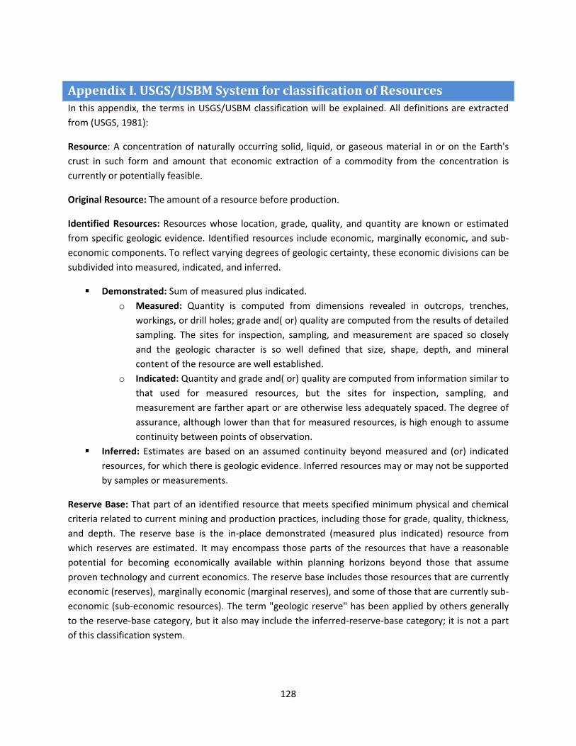
128

Appendix I. USGS/USBM System for classification of Resources In this appendix, the terms in USGS/USBM classification will be explained. All definitions are extracted from (USGS, 1981):

Resource: A concentration of naturally occurring solid, liquid, or gaseous material in or on the Earth's crust in such form and amount that economic extraction of a commodity from the concentration is currently or potentially feasible.

Original Resource: The amount of a resource before production.

Identified Resources: Resources whose location, grade, quality, and quantity are known or estimated from specific geologic evidence. Identified resources include economic, marginally economic, and sub-economic components. To reflect varying degrees of geologic certainty, these economic divisions can be subdivided into measured, indicated, and inferred.

Demonstrated: Sum of measured plus indicated. o Measured: Quantity is computed from dimensions revealed in outcrops, trenches,

workings, or drill holes; grade and( or) quality are computed from the results of detailed sampling. The sites for inspection, sampling, and measurement are spaced so closely and the geologic character is so well defined that size, shape, depth, and mineral content of the resource are well established.

o Indicated: Quantity and grade and( or) quality are computed from information similar to that used for measured resources, but the sites for inspection, sampling, and measurement are farther apart or are otherwise less adequately spaced. The degree of assurance, although lower than that for measured resources, is high enough to assume continuity between points of observation.

Inferred: Estimates are based on an assumed continuity beyond measured and (or) indicated resources, for which there is geologic evidence. Inferred resources may or may not be supported by samples or measurements.

Reserve Base: That part of an identified resource that meets specified minimum physical and chemical criteria related to current mining and production practices, including those for grade, quality, thickness, and depth. The reserve base is the in-place demonstrated (measured plus indicated) resource from which reserves are estimated. It may encompass those parts of the resources that have a reasonable potential for becoming economically available within planning horizons beyond those that assume proven technology and current economics. The reserve base includes those resources that are currently economic (reserves), marginally economic (marginal reserves), and some of those that are currently sub-economic (sub-economic resources). The term "geologic reserve" has been applied by others generally to the reserve-base category, but it also may include the inferred-reserve-base category; it is not a part of this classification system.

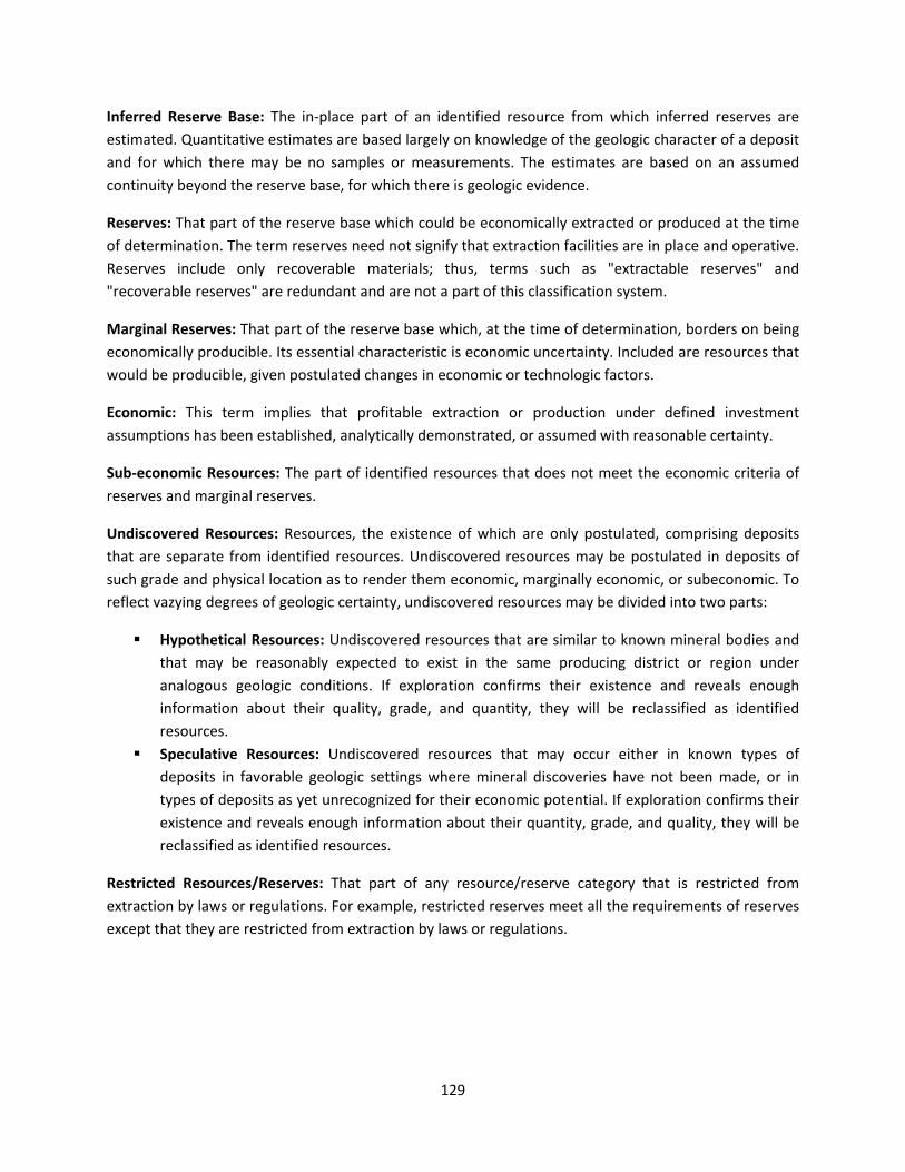
129

Inferred Reserve Base: The in-place part of an identified resource from which inferred reserves are estimated. Quantitative estimates are based largely on knowledge of the geologic character of a deposit and for which there may be no samples or measurements. The estimates are based on an assumed continuity beyond the reserve base, for which there is geologic evidence.

Reserves: That part of the reserve base which could be economically extracted or produced at the time of determination. The term reserves need not signify that extraction facilities are in place and operative. Reserves include only recoverable materials; thus, terms such as "extractable reserves" and "recoverable reserves" are redundant and are not a part of this classification system.

Marginal Reserves: That part of the reserve base which, at the time of determination, borders on being economically producible. Its essential characteristic is economic uncertainty. Included are resources that would be producible, given postulated changes in economic or technologic factors.

Economic: This term implies that profitable extraction or production under defined investment assumptions has been established, analytically demonstrated, or assumed with reasonable certainty.

Sub-economic Resources: The part of identified resources that does not meet the economic criteria of reserves and marginal reserves.

Undiscovered Resources: Resources, the existence of which are only postulated, comprising deposits that are separate from identified resources. Undiscovered resources may be postulated in deposits of such grade and physical location as to render them economic, marginally economic, or subeconomic. To reflect vazying degrees of geologic certainty, undiscovered resources may be divided into two parts:

Hypothetical Resources: Undiscovered resources that are similar to known mineral bodies and that may be reasonably expected to exist in the same producing district or region under analogous geologic conditions. If exploration confirms their existence and reveals enough information about their quality, grade, and quantity, they will be reclassified as identified resources.

Speculative Resources: Undiscovered resources that may occur either in known types of deposits in favorable geologic settings where mineral discoveries have not been made, or in types of deposits as yet unrecognized for their economic potential. If exploration confirms their existence and reveals enough information about their quantity, grade, and quality, they will be reclassified as identified resources.

Restricted Resources/Reserves: That part of any resource/reserve category that is restricted from extraction by laws or regulations. For example, restricted reserves meet all the requirements of reserves except that they are restricted from extraction by laws or regulations.

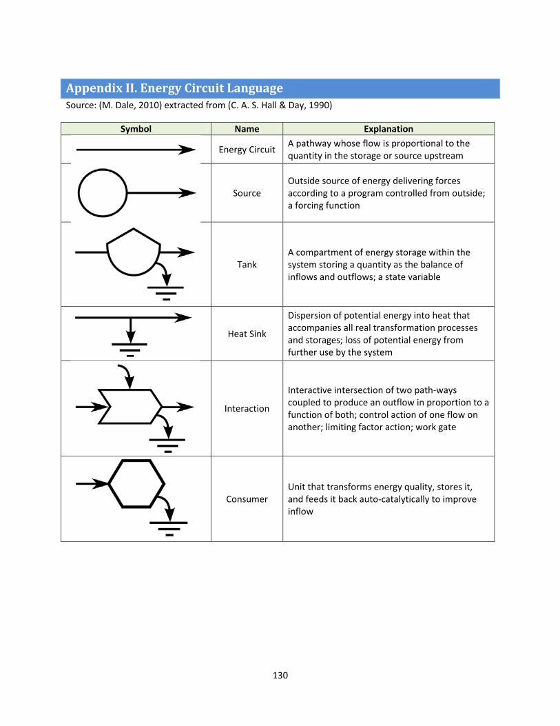
130

Appendix II. Energy Circuit Language Source: (M. Dale, 2010) extracted from (C. A. S. Hall & Day, 1990)

Symbol Name Explanation

Energy Circuit A pathway whose flow is proportional to the

quantity in the storage or source upstream

Source Outside source of energy delivering forces according to a program controlled from outside; a forcing function

Tank A compartment of energy storage within the system storing a quantity as the balance of inflows and outflows; a state variable

Heat Sink

Dispersion of potential energy into heat that accompanies all real transformation processes and storages; loss of potential energy from further use by the system

Interaction

Interactive intersection of two path-ways coupled to produce an outflow in proportion to a function of both; control action of one flow on another; limiting factor action; work gate

Consumer Unit that transforms energy quality, stores it, and feeds it back auto-catalytically to improve inflow

131

References Aleklett, K., Höök, M., Jakobsson, K., Lardelli, M., Snowden, S., & Söderbergh, B. (2010). The Peak of the

Oil Age – Analyzing the world oil production Reference Scenario in World Energy Outlook 2008. Energy Policy, 38(3), 1398-1414. doi: http://dx.doi.org/10.1016/j.enpol.2009.11.021

APS. Energy Units Retrieved 7 June, 2013, from http://www.aps.org/policy/reports/popa-reports/energy/units.cfm

Ayres, R. U. (1978). Resources, environment, and economics: applications of the materials/energy balance principle: Wiley.

Ayres, R. U., & Kneese, A. V. (1969). Production, Consumption, and Externalities: Resources for the Future.

Baines, J. T., & Peet, N. J. (1983). The dynamics of energy consumption: changing expectations for the supply of goods and services: Department of Chemical Engineering.

Baines, J. T., & Peet, N. J. (1986). The Dynamics of Energy Consumption: Changing Expectations for the Supply of Goods and Services: New Zealand Energy Research and Development Committee.

Bankes, S. (1993). Exploratory Modeling for Policy Analysis. Operations Research, 41(3), 435-449. doi: 10.2307/171847

Bankes, S., Walker, W., & Kwakkel, J. (2010). Encyclopedia of OR (upcoming 3th edition ed.)., Chapter Exploratory Modeling and Analysis (Vol. 3): Boston: Kluwer Academic Publishers.[forthcoming].

Beinhocker, E. D. (2006). The Origin of Wealth: Evolution, Complexity, And the Radical Remaking of Economics: Harvard Business School Press.

Bodger, P., & Baines, J. (1989). Dynamics of an energy-economic system subject to an energy substitution sequence. Energy systems and policy, 12(3), 167-178.

Bollinger, L. A. (2010). Growing cradle-to-cradle metal flow systems: An application of agent-based modeling and system dynamics to the study of global flows of metals in mobile phones. M.Sc., Delft University of Technology, Leiden University.

Bonabeau, E. (2002). Agent-based modeling: Methods and techniques for simulating human systems. Proceedings of the National Academy of Sciences of the United States of America, 99(SUPPL. 3), 7280-7287.

Borshchev, A., & Filippov, A. (2004). From System Dynamics and Discrete Event to Practical Agent Based Modeling: Reasons, Techniques, Tools. Paper presented at the The 22nd International Conference of the System Dynamics Society, Oxford, England.

BP. (2012a). 2012 Statistical Review of World energy. In B. Petroleum (Ed.). BP. (2012b). BP Energy Outlook 2030: British Petroleum. Bradshaw, M. J. (2010). Global energy dilemmas: A geographical perspective. Geographical Journal,

176(4), 275-290. Bullard Iii, C. W., & Herendeen, R. A. (1975). The energy cost of goods and services. Energy Policy, 3(4),

268-278. doi: http://dx.doi.org/10.1016/0301-4215(75)90035-X CIA. (2012). The World Factbook: U.S. Central Intelligence Agency. Cleveland, C. J. (1987). Biophysical economics —historical-perspective and current research trends.

Ecological Modelling, 38, 47–73. Cobb, C. W., & Douglas, P. H. (1928). A Theory of Production. The American Economic Review, 18(1),

139-165. doi: 10.2307/1811556 Correljé, A., & van der Linde, C. (2006). Energy supply security and geopolitics: A European perspective.

Energy Policy, 34(5), 532-543. doi: http://dx.doi.org/10.1016/j.enpol.2005.11.008 Cottrell, F. (1955). Energy and Society: The Relations Between Energy, Social Change and Economic

Development: McGraw-Hill.

132

D. H. Meadows, D. L. M., J. Randers, W. W. Behrens III. (1972). The Limits to Growth. New York: Universe.

Dale, M. (2010). GLOBAL ENERGY MODELLING:A BIOPHYSICAL APPROACH. Doctor of Philosophy in Mechanical Engineering, University of Canterbury. Retrieved from http://ir.canterbury.ac.nz/bitstream/10092/5156/1/Dale2011GlobalEnergyModelling-ABiophysicalApproach.pdf

Dale, M. (2012). Meta-analysis of non-renewable energy resource estimates. Energy Policy, 43(0), 102-122. doi: http://dx.doi.org/10.1016/j.enpol.2011.12.039

Dale, M., Krumdieck, S., & Bodger, P. (2011). A Dynamic Function for Energy Return on Investment. Sustainability, 3(10), 1972-1985.

Dale, M., Krumdieck, S., & Bodger, P. (2012). Global energy modelling — A biophysical approach (GEMBA) Part 2: Methodology. Ecological Economics, 73(0), 158-167. doi: http://dx.doi.org/10.1016/j.ecolecon.2011.10.028

Dale, M. A. J. (2010). GLOBAL ENERGY MODELLING:A BIOPHYSICAL APPROACH. Doctor of Philosophy in Mechanical Engineering, University of Canterbury. Retrieved from http://ir.canterbury.ac.nz/bitstream/10092/5156/1/Dale2011GlobalEnergyModelling-ABiophysicalApproach.pdf

Daly, H. E. (1985). The circular flow of exchange value and the linear throughput of matter-energy: a case of misplaced concreteness. Review of Social Economy, 43(3), 279-297.

de Bruijn, H., & Herder, P. M. (2009). System and actor perspectives on sociotechnical systems. IEEE Transactions on Systems, Man, and Cybernetics Part A:Systems and Humans, 39(5), 981-992.

DeMeritt, J. H. R., & Young, J. K. (2013). A political economy of human rights: Oil, natural gas, and state incentives to repress1. Conflict Management and Peace Science, 30(2), 99-120.

Donella H. Meadows, J. R. D. L. M. (2004). The Limits to Growth: Earthscan. EIA. Countries: Proved Oil Reserves Retrieved 20 March, 2013, from

http://www.eia.gov/countries/index.cfm?view=reserves eia. (2013). Countries :Oil Consumption Retrieved 15 April, 2013, from

http://www.eia.gov/countries/index.cfm?view=consumption GEA. (2012). Global Energy Assessment Toward a Sustainable Future: International Institute for Applied

Systems Analysis. GECF. GECF: About us Retrieved 18 April, 2013, from http://www.gecf.org/aboutus/about-gecf Gelpke, B., McCormack, R., & Caduff, R. (Writers). (2006). A Crude Awakening: The Oil Crash. In L.

Productions (Producer). Georgescu-Roegen, N. (1971). The Entropy Law and the Economic Process: Harvard University Press. Gilliland, M. W. (1975). Energy Analysis and Public Policy: The energy unit measures environmental

consequences, economic costs, material needs, and resource availability. Science, 189(4208), 1051-1056. doi: 10.1126/science.189.4208.1051

Haberl, H., Beringer, T., Bhattacharya, S. C., Erb, K.-H., & Hoogwijk, M. (2010). The global technical potential of bio-energy in 2050 considering sustainability constraints. Current Opinion in Environmental Sustainability, 2(5–6), 394-403. doi: http://dx.doi.org/10.1016/j.cosust.2010.10.007

Hall, C., & Klitgaard, K. (2006). The need for a new, biophysical-based paradigm in economics for the second half of the age of oil. International Journal of Transdisciplinary Research, 1(1), 4-22.

Hall, C., Lindenberger, D., Kümmel, R., Kroeger, T., & Eichhorn, W. (2001). The Need to Reintegrate the Natural Sciences with Economics: Neoclassical economics, the dominant form of economics today, has at least three fundamental flaws from the perspective of the natural sciences, but it is possible to develop a different, biophysical basis for economics that can serve as a supplement to, or a replacement for, neoclassical economics. BioScience, 51(8), 663-673.

133

Hall, C. A., Cleveland, C. J., & Kaufmann, R. (1986). Energy and resource quality: the ecology of the economic process.

Hall, C. A. S., Cleveland, C. J., & Kaufmann, R. K. (1992). Energy and resource quality: the ecology of the economic process: University Press of Colorado.

Hall, C. A. S., & Day, J. W. (1990). Ecosystem Modeling in Theory and Practice: An Introduction With Case Histories: University Press of Colorado.

Hall, C. A. S., & Klitgaard, K. A. (2012). Energy and the Wealth of Nations: Understanding the Biophysical Economy: Springer New York.

Hamilton, L. D., Goldstein, G. A., Lee, J., Marcuse, W., Morris, S. C., Manne, A. S., & Wene, C. O. (1992). MARKAL-MACRO: An overview (pp. Medium: ED; Size: Pages: (55 p)).

Hardy, J. (2011). Resource Curse. In D. Chatterjee (Ed.), Encyclopedia of Global Justice (pp. 946-948): Springer Netherlands.

Hirsch, R. L., Bezdek, R., & Wendling, R. (2005). PEAKING OF WORLD OIL PRODUCTION: IMPACTS, MITIGATION, & RISK MANAGEMENT Retrieved from http://www.netl.doe.gov/publications/others/pdf/Oil_Peaking_NETL.pdf.

Hubbert, M. K. (1956). Nuclear energy and the fossil fuel. Drilling and production practice. IEA. Energy Security Retrieved 10 April, 2013, from http://www.iea.org/topics/energysecurity/ IEA. (2012a). 2012 Key World Energy Statistics: International Energy Agency. IEA. (2012b). World Energy Model Documentation: International Energy Agency. IIASA. (2012a). GEA Scenario Database. In IIASA (Ed.). IIASA. (2012b). Public GEA Scenario Database Retrieved April 4, 2013, from http://www.iiasa.ac.at/web-

apps/ene/geadb/dsd?Action=htmlpage&page=about indexmundi. Thematic Map: GDP - per capita (PPP) - World, from

http://www.indexmundi.com/map/?t=0&v=67&r=xx&l=en JAFFE, A. M., MEDLOCK, K. B., & SOLIGO, R. (2011). The Status of World Oil Reserves: Conventional and

Unconventional Resources in the Future Supply Mix. RICE UNIVERSITY: James A. Baker III Institute for Public Policy.

Jakobsson, K., Bentley, R., Söderbergh, B., & Aleklett, K. (2012). The end of cheap oil: Bottom-up economic and geologic modeling of aggregate oil production curves. Energy Policy, 41(0), 860-870. doi: http://dx.doi.org/10.1016/j.enpol.2011.11.073

Janssen, M. A. (2005). Agent-based modelling. Modelling in ecological economics, 155-172. Jennings, N. R. (2000). On agent-based software engineering. Artificial Intelligence, 117(2), 277-296. doi:

http://dx.doi.org/10.1016/S0004-3702(99)00107-1 Kamp, A. (2011). Energy for One World: CreateSpace. Kauffman, R. (1986.). Energy return on investment for imported petroleum. Kauffman, S. (1993). The origins of order: Self organization and selection in evolution: Oxford University

Press. Kay, J. (2002). On Complexity Theory, Exergy and Industrial Ecology: Some Implications for Construction

Ecology. In C. J. Kibert (Ed.), Construction Ecology: Nature as a Basis for Green Buildings: Taylor & Francis.

Khatib, H. (2012). IEA World Energy Outlook 2011-A comment. Energy Policy, 48, 737-743. Kim, H. Y. (1990). Estimates of Productivity Change by Industry: An Evaluation and Alternative. Southern

Economic Journal, 57(1), 261-263. doi: 10.2307/1060504 Koonin, S. E. (2005). Energy for the Coming Decades: Trends and Technologies, from

http://video.mit.edu/watch/steven-koonin-on-energy-for-the-coming-decades-trends-and-technologies-9956/

Maggio, G., & Cacciola, G. (2012). When will oil, natural gas, and coal peak? Fuel, 98(0), 111-123. doi: http://dx.doi.org/10.1016/j.fuel.2012.03.021

134

Maxwell, J. C. (1950, 31 August). The Times. Moriarty, P., & Honnery, D. (2012). What is the global potential for renewable energy? Renewable and

Sustainable Energy Reviews, 16(1), 244-252. doi: http://dx.doi.org/10.1016/j.rser.2011.07.151 Nashawi, I. S., Malallah, A., & Al-Bisharah, M. (2010a). Forecasting world crude oil production using

multicyclic Hubbert model. Energy and Fuels, 24(3), 1788-1800. Nashawi, I. S., Malallah, A., & Al-Bisharah, M. (2010b). Modeling world oil supply: Its peak production

rate and time - Model validation. Odum, H. T. (1971). Environment, power and society: New York, USA, Wiley-Interscience. Odum, H. T. (1976). Energy analysis and net energy. Paper presented at the Proceedings of NSF

Workshop on Net Energy, Stanford, Cal. Institute for Energy Studies, Stanford Univ. and TRW. OECD. About the OECD Retrieved 18 April, 2013, from http://www.oecd.org/about/ OECD. OECD: History Retrieved 18 April, 2013, from http://www.oecd.org/about/history/ OPEC. OPEC: Brief Histpry Retrieved 18 April, 2013, from

http://www.opec.org/opec_web/en/about_us/24.htm Page, S. E. (2005). Agent based models. The New Palgrave Dictionary of Economics. Palgrave MacMillan,

New York. Podolinsky, S. (1883). Menschliche Arbeit und Einheit der Kraft. Die Neue Zeit, 1. Reynolds, C. (1999). Individual-based models. red3d. com [online article], October. Scholl, H. J. (2001). Agent-based and system dynamics modeling: a call for cross study and joint research.

Paper presented at the System Sciences, 2001. Proceedings of the 34th Annual Hawaii International Conference on.

Schrattenholzer, L. (1981). The energy supply model MESSAGE: IIASA Laxenburg, Austria. Slesser, M. (1992). ECCO: User's Manual. Resource Use Institute (Ed.). Edinburgh, Scotland. Slesser, M., King, J., & Crane, D. C. (1997). The Management of Greed: A Bio-physical Appraisal of

Economic and Environmental Potential: RUI Publishing. Sloman, J. (2006). Economics: Financial Times Prentice Hall. Smith, D. (2013, 28 March 2013). Brics eye infrastructure funding through new development bank,

Guardian. Retrieved from http://www.guardian.co.uk/global-development/2013/mar/28/brics-countries-infrastructure-spending-development-bank

Soddy, F. (1922). Cartesian Economics: The Bearing of Physical Science Upon State Stewardship: Hendersons.

Soddy, F. (1926). Wealth, virtual wealth and debt: the solution of the economic paradox. Sorrell, S., Speirs, J., Bentley, R., Brandt, A., & Miller, R. (2009). Global Oil Depletion: An assessment of

the evidence for a near-term peak in global oil production: UK Energy Research Centre. Steiner, J., & Woods, L. (2009). EU Law: Oxford University Press, Incorporated. Sterman, J. (2000). Business Dynamics: Systems Thinking and Modeling for a Complex World with CD-

ROM: McGraw-Hill Education. Tien, C. M., & McVay, D. A. (2010). Quantifying the uncertainty in estimates of world conventional oil

resources. Towler, B. (2011). World peak oil production still years away. Oil and Gas Journal, 109(18), 90-97. USGS. (1981). Principles of a Resource/Reserve Classification for Minerals: US Geological Survey

US Bureau of Mines. van Dam, K. H., Nikolic, I., & Lukszo, Z. (2013). Agent-Based Modelling of Socio-Technical Systems:

Springer London, Limited. Van Der Lei, T. E., Bekebrede, G., & Nikolic, I. (2010). Critical infrastructures: a review from a complex

adaptive systems perspective. International Journal of Critical Infrastructures, 6(4), 380-401. doi: 10.1504/ijcis.2010.037454

135

Vries, L. J. d., Correljé, A. F., & Knops, H. P. A. (2010). Electricity: Market design and policy choices. Delft University of Technology.

Waldorp, M. M. (1992). Complexity: The Emerging Science at the Edge of Order and Chaos. New York: Simon and Schuster.

WEC. (2003). Drivers of Energy Scene: World Energy Council. WorldBank. Data. Website of the World Bank: The World Bank.