MSER Exploratory Research - The University of Virginia
231
-
Upload
khangminh22 -
Category
Documents
-
view
2 -
download
0
Transcript of MSER Exploratory Research - The University of Virginia
MSER Exploratory Research: Implementations,Virtual Laboratory Development, and
Parameterization Analysis
A Dissertation
Presented to
the faculty of the School of Engineering and Applied Science
University of Virginia
in partial ful�llment
of the requirements for the degree
Doctor of Philosophy
by
Sung Nam Hwang
May 2017

APPROVAL SHEET
This Dissertation
is submitted in partial ful�llment of the requirements
for the degree of
Doctor of Philosophy
Author Signature:
This Dissertation has been read and approved by the examining committee:
Advisor: Prof. K. Preston White, Jr
Committee Member: Prof. Michael C. Smith
Committee Member: Prof. James W. Lark III
Committee Member: Prof. William T. Scherer
Committee Member: Dr. Paul J. Sanchez
Committee Member:
Accepted for the School of Engineering and Applied Science:
Craig H. Benson, School of Engineering and Applied Science
May 2017
ii
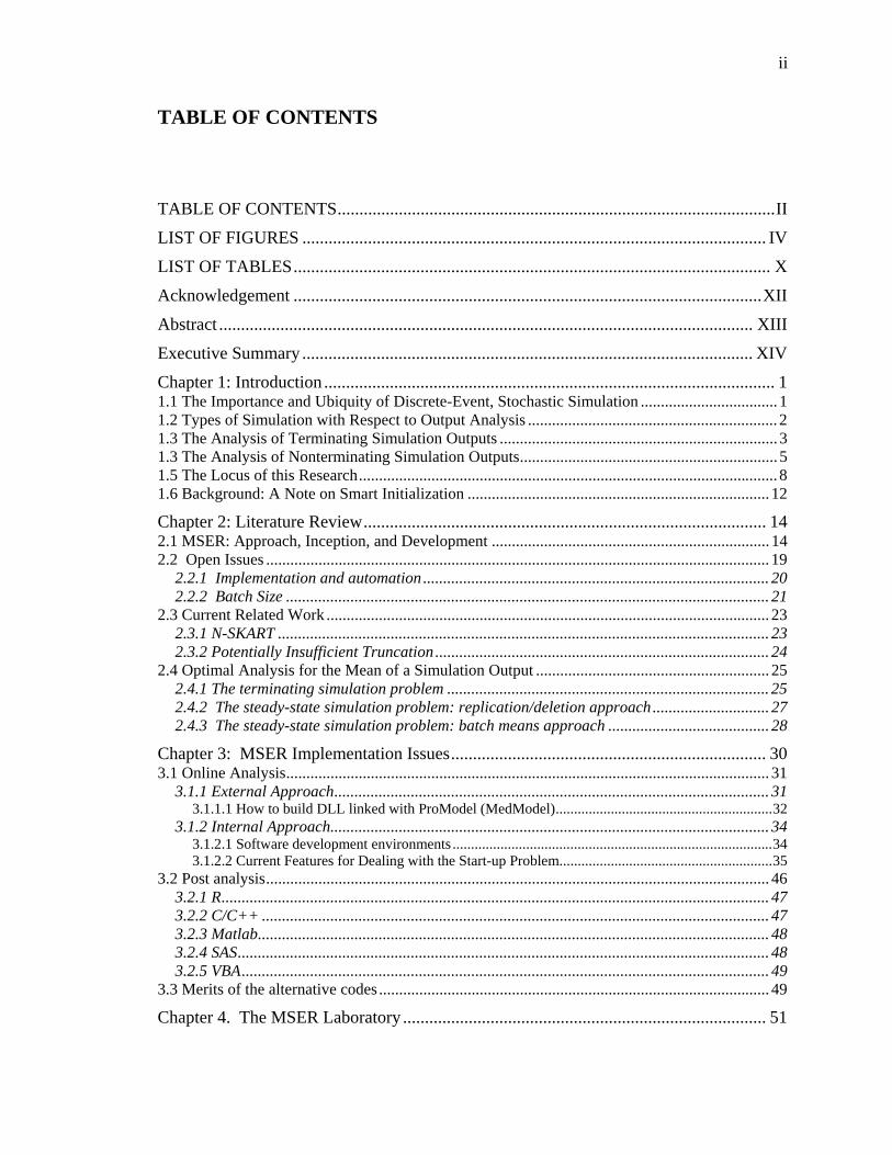
TABLE OF CONTENTS
TABLE OF CONTENTS .................................................................................................... II
LIST OF FIGURES .......................................................................................................... IV
LIST OF TABLES ............................................................................................................. X
Acknowledgement ........................................................................................................... XII
Abstract .......................................................................................................................... XIII
Executive Summary ....................................................................................................... XIV
Chapter 1: Introduction ....................................................................................................... 1 1.1 The Importance and Ubiquity of Discrete-Event, Stochastic Simulation .................................. 1 1.2 Types of Simulation with Respect to Output Analysis .............................................................. 2 1.3 The Analysis of Terminating Simulation Outputs ..................................................................... 3 1.3 The Analysis of Nonterminating Simulation Outputs ................................................................ 5 1.5 The Locus of this Research ........................................................................................................ 8 1.6 Background: A Note on Smart Initialization ........................................................................... 12
Chapter 2: Literature Review ............................................................................................ 14 2.1 MSER: Approach, Inception, and Development ..................................................................... 14 2.2 Open Issues ............................................................................................................................. 19
2.2.1 Implementation and automation ...................................................................................... 20 2.2.2 Batch Size ........................................................................................................................ 21
2.3 Current Related Work .............................................................................................................. 23 2.3.1 N-SKART .......................................................................................................................... 23 2.3.2 Potentially Insufficient Truncation ................................................................................... 24
2.4 Optimal Analysis for the Mean of a Simulation Output .......................................................... 25 2.4.1 The terminating simulation problem ................................................................................ 25 2.4.2 The steady-state simulation problem: replication/deletion approach ............................. 27 2.4.3 The steady-state simulation problem: batch means approach ........................................ 28
Chapter 3: MSER Implementation Issues ........................................................................ 30 3.1 Online Analysis ........................................................................................................................ 31
3.1.1 External Approach ............................................................................................................ 31 3.1.1.1 How to build DLL linked with ProModel (MedModel) ........................................................... 32
3.1.2 Internal Approach............................................................................................................. 34 3.1.2.1 Software development environments ....................................................................................... 34 3.1.2.2 Current Features for Dealing with the Start-up Problem.......................................................... 35
3.2 Post analysis ............................................................................................................................. 46 3.2.1 R ........................................................................................................................................ 47 3.2.2 C/C++ .............................................................................................................................. 47 3.2.3 Matlab ............................................................................................................................... 48 3.2.4 SAS .................................................................................................................................... 48 3.2.5 VBA ................................................................................................................................... 49
3.3 Merits of the alternative codes ................................................................................................. 49
Chapter 4. The MSER Laboratory ................................................................................... 51

iii
Chapter 5. Implementation of MSER in Commercial Software ...................................... 57 5.1 ExtendSim Implementation ..................................................................................................... 57
5.1.1 ExtendSim Process Flow .................................................................................................. 58 5.1.2. ExtendSim Code .............................................................................................................. 59
5.2 Arena Submodel Implementation ............................................................................................ 63 5.2.1 Arena Process Flow .......................................................................................................... 64 5.2.2 Arena MSER Modules ..................................................................................................... 66
5.3 Promodel/Medmodel Implementation ..................................................................................... 66 5.3.1 Promodel/Medmodel Process Flow .................................................................................. 67 5.3.2 ProModel DLL Code ........................................................................................................ 68
Chapter 6. Implementation in Post Analysis Codes ......................................................... 72 6.1. R Source Code ........................................................................................................................ 72 6.2. The SAS Source Code ............................................................................................................ 74 6.3. Matlab Source Code ................................................................................................................ 75 6.4. VBA Source Code ................................................................................................................... 76 6.5. C Source Code ........................................................................................................................ 80 6.6. C++ Source Code .................................................................................................................... 84
Chapter 7. Parameterization Issues, Analyses, and Results ............................................. 90 7.1 Choosing the Run Length of a Nonterminating Simulation ..................................................... 90 7.2 Test Models and Results ......................................................................................................... 94
7.2.1 Model 1: Uniform Distribution with Superimposed Deterministic Bias .......................... 95 7.2.1.1 Model Description ................................................................................................................... 95 7.2.1.2 Results: Batch size effects for long runs .................................................................................. 97 7.2.1.3 Results: Batch size effects for short runs ............................................................................... 105 7.2.1.4 Results: Overlapping Batch Means ........................................................................................ 113
7.2.2 Model 2: Waiting Time in an M/M/1 .............................................................................. 116 7.2.2.1 Results for Model 2 with traffic intensity of 0.90 .................................................................. 117 7.2.2.2 Results for Model 2 with traffic intensity of 0.80 .................................................................. 124 7.2.2.3 Results for Model 2 with traffic intensity of 0.70 .................................................................. 129 7.2.2.4 Results for Model 2 with traffic intensity of 0.60 .................................................................. 134 7.2.2.5 Result for Model 2: Simulation run length effect................................................................... 139 7.2.2.6 Result for Model 2: Traffic intensity effect ........................................................................... 140 7.2.2.7 Results: Overlapping Batch Means for M/M/1 with Traffic Intensity of 0.90. ...................... 141 7.2.2.8 Results: Initialization Bias ..................................................................................................... 149 7.2.2.9 Summary Results for Model 2 ............................................................................................... 153
7.2.3 Model 3: EAR(1) ............................................................................................................. 155 7.2.3.1 Results for Model 3 with =0.99 ........................................................................................... 158 7.3.3.2 Results for Model 3 with =0.90 ........................................................................................... 165 7.3.3.3 Results for Model 3 with =0.80 ........................................................................................... 170 7.3.3.4 Results for Model 3 with =0.70 ........................................................................................... 175 7.3.3.5 Results Using OBM for Model 3 with =0.70 ....................................................................... 180
Chapter 8. Conclusion and future research .................................................................... 184
References ....................................................................................................................... 191
Appendix I. Arena MSER Submodel User Guide .......................................................... 196
Appendix II. Personal reflections on the importance of the warm-up problem and undergraduate simulation curriculum survey .................................................................. 207 II.1 Anecdotal case to emphasize the importance of warm-up period ......................................... 207 II.2 Undergraduate curriculum survey ......................................................................................... 207

iv
LIST OF FIGURES
Figure 1.1 Types of simulation (Law 2015) ....................................................................... 3Figure 1.2 Example of transient and steady-state density functions (after Law 2015) ....... 6Figure 2.1 Testing Module for identifying optimal truncation points in SIMUL8. .......... 20Figure 2.2 Output Analysis Tree for Wilson and Students ............................................... 24Figure 3.1 Example of DLL usage in ProModel ............................................................... 33Figure 3.2 Specifying Warm-up Period in Arena’s Run Setup Dialogue ......................... 37Figure 3.3 Warm-Up Period Determination in AutoMod ................................................. 38Figure 3.4 Warm-Up Period in SIMUL8 .......................................................................... 39Figure 3.5 Output Analysis Support in SIMUL8 .............................................................. 39Figure 3.6 Specifying a Warm-Up Period in ProModel ................................................... 40Figure 3.7 Specifying a Warm-Up Period in FlexSim ...................................................... 41Figure 3.8 Specifying a Warm-Up Period in Simio .......................................................... 42Figure 3.9 Warm-Up Period in ExtendSim using Clear Statistics under Statistics library44Figure 3.10 GUI of SimCAD ............................................................................................ 45Figure 4.1. Introduction of MSER Laboratory Web page ................................................ 53Figure 4.2. History of MSER Laboratory Web page ........................................................ 54Figure 4.3. Sample Codes of MSER Laboratory Web page ............................................. 55Figure 4.4. Math of MSER Laboratory Web page ............................................................ 56Figure 5.1 MSER Implementation and GUI in ExtendSim .............................................. 59Figure 5.2 Main model of an M/M/1 queue in Arena with the MSER module included to
collect statistics on the waiting time in Service queue ............................................... 64Figure 5.3 Details of the MSER calculation in the Arena ................................................ 65Figure 5.4 M/M/1 Model in ProModel ............................................................................. 67Figure 5.5 DLL Usage in ProModel ................................................................................. 68Figure 6.1 Output and MSER Plot in R ............................................................................ 74Figure 6.2 Output and MSER Plot in SAS ...................................................................... 75Figure 6.3 Output and MSER Plot in Matlab ................................................................... 76Figure 6.4 Output and MSER Plot in Excel VBA ............................................................ 80Figure 6.5 Output Results in Console by C/C++ .............................................................. 89Figure 7.1 Hypothetical simulation output sequences illustrating one potential consequence
of an inadequate run length ........................................................................................ 93Figure 7.2 Hypothetical extensions of the simulation output sequences in Figure 7.1
illustrating further potential consequences of an inadequate run length .................... 94Figure 7.3 Output for a representative replication of the first model ............................... 96Figure 7.4 95% confidence intervals for (a) the truncated means for run lengths n=10000
and batch sizes b=1, 5, 10 and (b) the sample standard deviation in the estimated means for run lengths n=10000 and batch sizes b=1, 5, 10 ................................................... 98

v
Figure 7.5 Fits to the steady-state sampling distributions of the mean for 1000 replications for run length n=10,000. Fits for all three batch sizes tested are nearly identical for batch sizes b=1, 5, and 10 .......................................................................................... 99
Figure 7.6 95% confidence intervals for (a) the MSER mean and (b) the standard deviation in the MSER truncation point for run lengths n=10000 and batch sizes b=1, 5, 10 .. 99
Figure 7.7 Scatterplots of the truncated mean vs. the number of observations truncated for batch sizes b=1, 5, and 10 for run length n=10,000 ................................................. 100
Figure 7.8 Frequency distribution of the total number of observations truncated as a function of batch size for batch sizes b=1, 5, and 10 for run length n=10,000 ........ 101
Figure 7.9 Batched means and MSER statistic for the first 500 observations for replication 958 for batch sizes b=1, 5, and 10 for run length n=10,000 .................................... 102
Figure 7.10 Batch means and MSER statistic for the first 1500 observations for replication 958 for batch sizes b=10 and run length n=10,000 .................................................. 103
Figure 7.11 Estimated steady-state distribution (after truncation) for a single representative replication for run length n=10,000, with uniform fit for batch size b=1 and normal fits for batch sizes b=5 and 10 ........................................................................................ 104
Figure 7.12 Scatterplots of the truncated mean vs. the number of observations truncated batch sizes b=1, 5, and 10 for run lengths n=175, 200, 500, and 500 ...................... 109
Figure 7.13 Frequency distribution of the total number of observations truncated as a function of batch size for batch sizes b=1, 5, and 10 for run lengths of n=175, 200, 500, 500 .................................................................................................................... 110
Figure 7.14 95% confidence intervals of the mean for the truncated mean output as a function of batch size for batch sizes b=1, 5, and 10 for run lengths of n=175, 200, 300, 500 ............................................................................................................................ 111
Figure 7.15 95% confidence intervals for the mean for the number of observations truncated for batch sizes b=1, 5, and 10 for run lengths of n=175, 200, 300, 500 ... 112
Figure 7.16 Representative Output, Overlapping Batch Mean, and MSER Statistic of Model 1 (b= 10, 35, 75, and 150) ............................................................................. 113
Figure 7.17 95% confidence intervals for Model 1 on (a) the truncated mean for overlapping and non-overlapping batches and (b) the standard deviation for overlapping and non-overlapping batches ................................................................ 114
Figure 7.18 Scatterplots of the truncated mean vs. the number of observations truncated for OBM sizes b=10, 35, 75 and 150 for run length of n=500 for Model 1 (including NOBM batch size of 10) .......................................................................................... 115
Figure 7.19 Frequency distribution of the number of observations truncated as a function of OBM sizes b=10, 35, 75, and 150 for run length of n=500 for Model 1 (including NOBM batch size of 10) .......................................................................................... 115
Figure 7.20 Representative Output of Waiting-Time in an M/M/1 with Traffic Intensity of 0.9 (n = 64000; Blue line: E(Wq)=81) ...................................................................... 117
Figure 7.21 95% confidence intervals for the mean and the truncated mean as a function of batch size (b= 1, 5, and 10) and run length (n=1000, 2000, 4000, 8000, 16000, 32000, and 64000) for Model 2 with traffic intensity of 0.9 (Theoretical mean of 81, Blue line) .................................................................................................................................. 119
Figure 7.22 95% confidence intervals for the mean number of observations truncated as a function of batch size (b= 1, 5, and 10) and run length (n=1000, 2000, 4000, 8000, 16000, 32000, and 64000) for Model 2 with traffic intensity of 0.9 ........................ 120

vi
Figure 7.23 Scatterplots of the truncated mean vs. the number of observations truncated for batch sizes b=1, 5, and 10 for run length of n=1000, 2000, 4000, 8000, 16000, 32000, and 64000 for Model 2 with traffic intensity of 0.9 ................................................. 121
Figure 7.24 Frequency distribution of the number of observations truncated as a function of batch sizes b=1, 5, and 10 for run length of n=1000, 2000, 4000, 8000, 16000, 32000, and 64000 for Model 2 with traffic intensity of 0.9 ..................................... 123
Figure 7.25 Example of M/M/1 with traffic intensity of 0.8 (n = 16000, Blue line: E(X)) .................................................................................................................................. 124
Figure 7.26 95% confidence intervals of the mean for the truncated mean output as a function of batch size (b= 1, 5, and 10) and run length (n=1000, 2000, 4000, 8000, and 16,000) for Model 2 with traffic intensity of 0.80 (Theoretical mean of 32, Blue line) .................................................................................................................................. 124
Figure 7.27 95% confidence intervals for the mean number of observations truncated as a function of batch size (b= 1, 5, and 10) and run length (n= 1000, 2000, 4000, 8000, and 16,000) for Model 2 with traffic intensity of 0.80 ............................................. 125
Figure 7.28 Scatterplots of the truncated mean vs. the number of observations truncated for batch sizes b=1, 5, and 10 for run length of n=1000, 2000, 4000, 8000, and 16,000 Model 2 with traffic intensity of 0.80 ...................................................................... 126
Figure 7.29 Frequency distribution of the number of observations truncated as a function of batch sizes b=1, 5, and 10 for run length of n=1000, 2000, 4000, 8000, and 16,000 for Model 2 with traffic intensity of 0.80 ................................................................. 128
Figure 7.30 Example of M/M/1 with traffic intensity of 0.70 (n = 16000, Blue line: E(X)) .................................................................................................................................. 129
Figure 7.31 95% confidence intervals of the mean for the truncated mean output as a function of batch size (b= 1, 5, and 10) and run length (n=1000, 2000, 4000, 8000, and 16,000) for Model 2 with traffic intensity of 0.70 (Theoretical mean of 16.33, Blue line) ........................................................................................................................... 129
Figure 7.32 95% confidence intervals for the mean number of observations truncated as a function of batch size (b= 1, 5, and 10) and run length (n= 1000, 2000, 4000, 8000, and 16,000) for Model 2 with traffic intensity of 0.70 ............................................. 130
Figure 7.33 Scatterplots of the truncated mean vs. the number of observations truncated for batch sizes b=1, 5, and 10 for run length of n=1000, 2000, 4000, 8000, and 16,000 Model 2 with traffic intensity of 0.7 ........................................................................ 131
Figure 7.34 Frequency distribution of the number of observations truncated as a function of batch sizes b=1, 5, and 10 for run length of n=1000, 2000, 4000, 8000, and 16,000 for Model 2 with traffic intensity of 0.70 ................................................................. 133
Figure 7.35 Example of M/M/1 with traffic intensity of 0.60 (n = 16000, Blue line: E(X)) .................................................................................................................................. 134
Figure.7.36 95% confidence intervals of the mean for the truncated mean output as a function of batch size (b= 1, 5, and 10) and run length (n=1000, 2000, 4000, 8000, and 16,000) for Model 2 with traffic intensity of 0.60 (Theoretical mean of 9, Blue line) .................................................................................................................................. 134
Figure 7.37 95% confidence intervals for the mean number of observations truncated as a function of batch size (b= 1, 5, and 10) and run length (n=1000, 2000, 4000, 8000, and 16,000) for Model 2 with traffic intensity of 0.60 ................................................... 135

vii
Figure 7.38 Scatterplots of the truncated mean vs. the number of observations truncated for batch sizes b=1, 5, and 10 for run length of n=1000, 2000, 4000, 8000, and 16,000 Model 2 with traffic intensity of 0.60 ...................................................................... 136
Figure 7.39 Frequency distribution of the number of observations truncated as a function of batch sizes b=1, 5, and 10 for run length of n=1000, 2000, 4000, 8000, and 16,000 for Model 2 with traffic intensity of 0.60 ................................................................. 138
Figure 7.40 Correlation between truncated means and observations truncated as a function of run length and traffic intensity ............................................................................. 139
Figure 7.41 Correlation between truncated means and observations truncated by different traffic intensity (Run length of 16000) ..................................................................... 140
Figure 7.42 Correlation between truncated means and observations truncated by different traffic intensity (Run length of 8000, 4000, 2000, and 100) .................................... 141
Figure 7.43 Representative Output, Overlapping Batch Mean, and MSER Statistic of Model 2 with traffic intensity of 0.90 (b= 10, 50, 100, and 200) ............................. 142
Figure 7.44 95% confidence intervals for Model 3 on (a) the truncated mean for overlapping and non-overlapping batches and (b) the standard deviation for overlapping and non-overlapping batches ................................................................ 143
Figure 7.45 Scatterplots of the truncated mean vs. the number of observations truncated for OBM sizes b=10, 50, 100 and 200 for run length of n=64,000 with traffic intensity of 0.90 for Model 2 (including NOBM batch size of 10) ............................................. 144
Figure 7.46 Frequency distribution of the number of observations truncated as a function of OBM sizes b=10, 50, 100, and 200 for run length of n=64,000 with traffic intensity of 0.90 for Model 2 (including NOBM batch size of 10) ........................................ 145
Figure 7.47 95% confidence intervals for M/M/1 with traffic intensity of 0.90 about the truncated mean for overlapping and non-overlapping batches (n = 1000, 2000, 4000, 8000, 16000, 32000, and 64000.) ............................................................................. 148
Figure 7.48 Output time series with traffic intensity of 0.90 with b =1 and n = 32,000 149Figure 7.49 Confidence interval for Mean and Standard Deviation, Scatter Plot for
Truncation points and Truncated Mean, Frequency Distribution of the Number of Observations Truncated with Traffic Intensity of 0.90 with b =1, 5, and 10 and n = 64,000 and 32,000 .................................................................................................... 150
Figure 7.50 Representative output for EAR(1) for run length n=500 and batch size b=1, illustrating the dependency of the steady-state mean and rate of convergence on the parameter for ={0.7, 0.8, 0.9, 0.99} ....................................................................... 156
Figure 7.51 Example of Model 3 with =0.99 (n = 16000, Brown line: E(X)) .............. 158Figure 7.52 95% confidence intervals of the mean for the truncated mean output as a
function of batch size (b= 1, 5, and 10) and run length (n=100, 150, 300, 500, 1000, 2000, 4000, 8000, and 16,000) for Model 3 with =0.99 (Theoretical mean of 100, Blue line) .................................................................................................................. 160
Figure 7.53 95% confidence intervals for the mean number of observations truncated as a function of batch size (b= 1, 5, and 10) and run length (n=100, 150, 300, 500, 1000, 2000, 4000, 8000, and 16,000) for Model 3 with =0.99 ........................................ 161
Figure 7.54 Scatterplots of the truncated mean vs. the number of observations truncated for batch sizes b=1, 5, and 10 for run length of n=100, 150, 300, 500, 1000, 2000, 4000, 8000, and 16,000 Model 3 with =0.99 ................................................................... 162
viii
Figure 7.55 Frequency distribution of the number of observations truncated as a function of batch sizes b=1, 5, and 10 for run length of n=100, 150, 300, 500, 1000, 2000, 4000, 8000, and 16,000 for Model 3 with of 0.99............................................................ 164
Figure 7.56 Example of EAR(1) with ϕ of 0.9 (n = 16000, Blue line: E(X)) ................ 165Figure 7.57 95% confidence intervals of the mean for the truncated mean output as a
function of batch size (b= 1, 5, and 10) and run length (n=100, 150, 300, 500, 1000, 2000, 4000, 8000, and 16,000) for Model 3 with ϕ =0.90 (Theoretical mean of 10, Blue line) .................................................................................................................. 165
Figure 7.58 95% confidence intervals for the mean number of observations truncated as a function of batch size (b= 1, 5, and 10) and run length (n=100, 150, 300, 500, 1000, 2000, 4000, 8000, and 16,000) for Model 3 with =0.90 ........................................ 166
Figure 7.59 Scatterplots of the truncated mean vs. the number of observations truncated for batch sizes b=1, 5, and 10 for run length of n=100, 150, 300, 500, 1000, 2000, 4000, 8000, and 16,000 Model 3 with =0.90 ................................................................... 167
Figure 7.60 Frequency distribution of the number of observations truncated as a function of batch sizes b=1, 5, and 10 for run length of n=100, 150, 300, 500, 1000, 2000, 4000, 8000, and 16,000 for Model 3 with of 0.90 .......................................................... 169
Figure 7.61 Example of EAR(1) with of 0.8 (n = 16000, Green line: E(X)) .............. 170Figure 7.62 95% confidence intervals of the mean for the truncated mean output as a
function of batch size (b= 1, 5, and 10) and run length (n=100, 150, 300, 500, 1000, 2000, 4000, 8000, and 16,000) for Model 3 with =0.80 (Theoretical mean of 5, Blue line) ........................................................................................................................... 170
Figure 7.63 95% confidence intervals for the mean number of observations truncated as a function of batch size (b= 1, 5, and 10) and run length (n=100, 150, 300, 500, 1000, 2000, 4000, 8000, and 16,000) for Model 3 with =0.80 ........................................ 171
Figure 7.64 Scatterplots of the truncated mean vs. the number of observations truncated for batch sizes b=1, 5, and 10 for run length of n=100, 150, 300, 500, 1000, 2000, 4000, 8000, and 16,000 Model 3 with =0.80 ................................................................... 172
Figure 7.65 Frequency distribution of the number of observations truncated as a function of batch sizes b=1, 5, and 10 for run length of n=100, 150, 300, 500, 1000, 2000, 4000, 8000, and 16,000 for Model 3 with of 0.80 .......................................................... 174
Figure 7.66 Example of EAR(1) with ϕ of 0.7 (n = 16000, Blue line: E(X)) ................ 175Figure 7.67 95% confidence intervals of the mean for the truncated mean output as a
function of batch size (b= 1, 5, and 10) and run length (n=100, 150, 300, 500, 1000, 2000, 4000, 8000, and 16,000) for Model 3 with =0.70 (Theoretical mean of 3.33, Blue line) .................................................................................................................. 175
Figure 7.68 95% confidence intervals for the mean number of observations truncated as a function of batch size (b= 1, 5, and 10) and run length (n=100, 150, 300, 500, 1000, 2000, 4000, 8000, and 16,000) for Model 3 with =0.70 ........................................ 176
Figure 7.69 Scatterplots of the truncated mean vs. the number of observations truncated for batch sizes b=1, 5, and 10 for run length of n=100, 150, 300, 500, 1000, 2000, 4000, 8000, and 16,000 Model 3 with =0.70 ................................................................... 177
Figure 7.70 Frequency distribution of the number of observations truncated as a function of batch sizes b=1, 5, and 10 for run length of n=100, 150, 300, 500, 1000, 2000, 4000, 8000, and 16,000 for Model 3 with of 0.70 .......................................................... 179

ix
Figure 7.71 Representative Output, Overlapping Batch Mean, and MSER Statistic of Model 3 (b= 10, 50, 100, and 200) ........................................................................... 180
Figure 7.72 95% confidence intervals for Model 3 on (a) the truncated mean for overlapping and non-overlapping batches and (b) the standard deviation for overlapping and non-overlapping batches ................................................................ 181
Figure 7.73 Scatterplots of the truncated mean vs. the number of observations truncated for OBM sizes b=10, 50, 100 and 200 for run length of n=1000 with ϕ of 0.70 for Model 3 (including NOBM batch size of 10) ...................................................................... 182
Figure 7.74 Frequency distribution of the number of observations truncated as a function of OBM sizes b=10, 50, 100, and 200 for run length of n=1000 with ϕ of 0.70 for Model 3 (including NOBM batch size of 10) .......................................................... 182

x
LIST OF TABLES
Table 2.1 Methods for Determining Start-up Periods (after Hoad et al. (2008)) .............. 18Table 3.1 Properties of Warm-Up Period Control in Simio ............................................. 43Table 7.1 95% confidence intervals for the mean and variance for the truncated mean
output as a function of batch size for batch sizes b=1, 5, and 10 for run length n=10,000 .................................................................................................................................... 98
Table 7.2 . 95% confidence intervals for the mean and variance for the number of observations truncated for batch sizes b=1, 5, and 10 for run length n=10,000 ........ 99
Table 7.3 Correlation between the truncated mean and the number of observations truncated for batch sizes b=1, 5, and 10 for run length n=10,000. ........................... 101
Table 7.4 Summary statistics for the steady-state data given in Figure 7.11. ................. 105Table 7.5 95% confidence intervals for Model 1 on the truncated mean and the standard
deviation for overlapping and non-overlapping batches .......................................... 114Table 7.6. Correlation between the truncated mean and the number of observations
truncated for OBM sizes b=10, 35, 75, 150 for run length of n=500 for Model 1 .. 116Table 7.7. Theoretical Waiting Time in Queue by Traffic Intensity .............................. 117Table 7.8 Correlation between the truncated mean and the number of observations
truncated for batch sizes b=1, 5, and 10 for run length of n=1000, 2000, 4000, 8000, 16000, 32000, and 64000 for Model 2 with traffic intensity of 0.9. ........................ 122
Table 7.9 Correlation between the truncated mean and the number of observations truncated for batch sizes b=1, 5, and 10 for run length of n=1000, 2000, 4000, 8000, and 16,000 for Model 2 with traffic intensity of 0.80 .............................................. 127
Table 7.10 Correlation between the truncated mean and the number of observations truncated for batch sizes b=1, 5, and 10 for run length of n=1000, 2000, 4000, 8000, and 16,000 for Model 2 with traffic intensity of 0.70 .............................................. 132
Table 7.11 Correlation between the truncated mean and the number of observations truncated for batch sizes b=1, 5, and 10 for run length of n=1000, 2000, 4000, 8000, and 16,000 for Model 2 with traffic intensity of 0.60 .............................................. 137
Table 7.12 95% confidence intervals for Model 2 on the truncated mean and the standard deviation for overlapping and non-overlapping batches .......................................... 143
Table 7.13 Correlation between the truncated mean and the number of observations truncated for OBM sizes b=10, 50, 100, and 200 for run length of n=64,000 for Model 2 ................................................................................................................................ 145
Table7.14 Confidence Intervals for M/M/1 with traffic intensity of 0.90 on the truncated mean and the standard deviation for overlapping and non-overlapping batches with traffic intensity of 0.90 (n = 1000, 2000, 4000, 8000, 16000, 32000, and 64000) .. 146
Table 7.15 Correlation between the truncated mean and the number of observations truncated for b=1, 5, and 10 for run length of n=32,000 with initial bias of 100 .... 151
Table 7.16 95% confidence intervals for Model 2 on the observation truncated and the standard deviation for run length of n=32,000 with initial bias of 100 .................... 151
Table 7.17 95% confidence intervals for Model 2 on the truncated mean and the standard deviation for run length of n=32,000 with initial bias of 100 .................................. 151

xi
Table7.18 95% confidence intervals for Model 2 on the mean without truncation and the standard deviation for run length of n=32,000 with initial bias of 100 .................... 152
Table 7.19 Correlation between the truncated mean and the number of observations truncated for b=1, 5, and 10 for run length of n=64,000 with initial bias of 100 .... 152
Table 7.20 95% confidence intervals for Model 2 on the observation truncated and the standard deviation for run length of n=64,000 with initial bias of 100 .................... 152
Table 7.21 95% confidence intervals for Model 2 on the truncated mean and the standard deviation for run length of n=64,000 with initial bias of 100 .................................. 152
Table 7.22 95% confidence intervals for Model 2 on the mean without truncation and the standard deviation for run length of n=64,000 with initial bias of 100 .................... 153
Table 7.23 Expected Value of the Steady-State Mean as a function of ....................... 155Table 7.24 Expected -percent settling time as a function of and ......................... 157Table 7.25 Correlation between the truncated mean and the number of observations
truncated for batch sizes b=1, 5, and 10 for run length of n=100, 150, 300, 500, 1000, 2000, 4000, 8000, and 16,000 for Model 3 with =0.99.......................................... 163
Table 7.26 Correlation between the truncated mean and the number of observations truncated for batch sizes b=1, 5, and 10 for run length of n=100, 150, 300, 500, 1000, 2000, 4000, 8000, and 16,000 for Model 3 with =0.90.......................................... 168
Table 7.27 Correlation between the truncated mean and the number of observations truncated for batch sizes b=1, 5, and 10 for run length of n=100, 150, 300, 500, 1000, 2000, 4000, 8000, and 16,000 for Model 3 with =0.80.......................................... 173
Table 7.28 Correlation between the truncated mean and the number of observations truncated for batch sizes b=1, 5, and 10 for run length of n=100, 150, 300, 500, 1000, 2000, 4000, 8000, and 16,000 for Model 3 with =0.70.......................................... 178
Table 7.29 95% confidence intervals for Model 3 on the truncated mean and the standard deviation for overlapping and non-overlapping batches .......................................... 181
Table 7.30 Correlation between the truncated mean and the number of observations truncated for OBM sizes b=10, 50, 100, and 200 for run length of n=16,000 with ϕ of 0.70 for Model 3 ....................................................................................................... 183
Table AII.1 Twenty Undergraduate Curricula of Simulation ......................................... 209

xii
Acknowledgement
The journey of my PhD study is finally heading towards the last train station. However,
this won’t be the end of my learning process but a start of a new journey. I believe my one
small step into the world of simulation is trivial, yet very meaningful for it will enlighten
a person to be like me and have courage to work hard with intelligent people at University
of Virginia.
I admit that my advisor, Prof. White Jr., is my first and final beacon in staying in the U.S.
Without his considerate support and help, I wouldn’t have come this far with only my
contribution in discrete event simulation. In addition, I won’t forget all the constructive
and encouraging comments and guidance from other committee members for my life at the
University of Virginia.
I would like to express my most sincere gratitude to my wife, Eun Hye Kwon, who has
fully supported and believed me both mentally and emotionally throughout this journey. I
also thank my son, Edward and daughter, Claire for understanding a busy father as well as
my parents and my parents-in-law encouraging my unexpected long journey.

xiii
Abstract
It is well known that the Mean Squared Error Rule (MSER) is an efficient and effective
method for mitigating initialization bias in the output analysis of steady-state, discrete-
event simulation. However, the application of this method in research and practice has been
delayed or misunderstood even by experienced simulation modelers. To address this issue,
we develop the MSER Laboratory—a permanent website that provides user-friendly
sample codes, as well as information needed to apply MSER intelligently. MSER modules
for three commercial software packages, and standalone MSER codes in five popular
programming languages, have been written, validated, and made publically available via
the Laboratory.
In addition, we use these codes to address open issues in the selection of the parameters
needed to apply MSER. These issues include the selection of the MSER truncation
threshold, batch size, and batching scheme (overlapping or non-overlapping batch means),
in conjunction with the determination of an initial run length for simulation replications.
Experiments are conducted using three test models that pose differing challenges for the
successful determination of a warm-up period. We confirm that, given adequate run
lengths, MSER is both effective and robust in all cases. We also illustrate various
consequences of foreshortened replications for each of the three models.

xiv
Executive Summary
This research addresses a practical shortcoming in the output analysis of non-terminating,
stochastic, discrete-event simulations (DES). Specifically, our concern is the application
of MSER, an algorithm for determining an optimal warm-up period when estimating the
steady-state mean of an output based on a sequence of simulated output values. It is
noteworthy that MSER:
is proven to yield a near-optimal estimate (under mild assumptions) in the sense of
minimum mean-squared error (MSE) that cannot be improved upon a priori,
is widely accepted in the academic literature as the preferred approach to mitigating
bias associated with the arbitrary specification of initial conditions,
is presented in detail and recommended in the current editions of many standard
texts on DES, and
is effective, efficient, robust, and intuitive.
In spite of these considerable merits, the application of MSER in practice appears far
from universal. We speculate the unaided application of MSER can be inconvenient and
potentially consuming of both analyst and computing time, especially when a large number
of output sequences must be initialized. An obvious solution is to imbed MSER in an
automated, dynamic, run-time procedure that requires minimal analyst interaction.

xv
However, the only reported effort to build MSER into a commercial simulation suite
(SIMUL8) led to the suggestion that there are significant barriers to implementation (Hoad
and Robinson, 2011). These include:
the selection of run length,
sequential data collection from multiple replications,
output types associated with cumulative values and extrema, and
data associated with entities.
Conventionally, MSER has been implemented as a data-driven postprocessor and, as
such, requires that an output sequence be simulated before application. There is no
guarantee that MSER will converge if the run length for this sequence is insufficient to
capture a useful trailing segment of steady-state behavior, even for a stable system.
Determination of an optimal warm-up period therefore is, in fact, confounded with problem
of determining an adequate run length, which is most often resolved only by trial and error.
In this research we demonstrate that in application MSER typically will flag instances
in which the run length is inadequate by truncating all (or at least a very large fraction) of
the output sequence to which it is applied. However, we further demonstrate that there are
pathological instances for which this is not the case. While Hoad et al. (2008) provide
useful guidance, determining an appropriate run length a priori remains an open and
perhaps intractable problem.
With this caveat, we demonstrate both theoretically and by application that the
remaining barriers are readily overcome. Specifically, we:
cast estimation of an output mean as an iterative optimization problem from which
we derive the memory requirements for run-time implementation,

xvi
develop runtime versions of MSER for ExtendSim (as a static library), Arena (as a
submodel), Promodel (as a DLL),
develop MSER postprocessing codes in several popular programming languages,
including the open-source languages R and C/C++, as well as the proprietary
languages Matlab, SAS, and VBA, and
create a prototype MSER Laboratory—a website to facilitate the distribution of
MSER codes and supporting research online available at
http://faculty.virginia.edu/MSER/.
MSER automation, the distribution of codes, and the creation of the Lab are principal
contributions of this research.
Additionally, during the course of this research we encountered multiple instances of a
perhaps obvious, but seemingly pervasive misconception regarding the application and
evaluation initialization procedures related to MSER. At least two alternative approaches
appear in the literature. The first applies MSER to individual output sequences, truncates
each sequence accordingly, calculates the truncated mean for each sequence, and then
averages the truncated means with weighting to estimate the steady-state mean. The
second determines the output sequences for multiple replications, averages these
sequences, applies MSER to the average sequence to determine a single warm-up period,
and then estimates the steady-state mean based on the average sequence truncated by this
period.
The first approach is preferred. MSER determines the optimal truncation point for the
specific output sequence to which it is applied and will return an optimal estimate of the
mean for each sequence when this exists. The second approach is almost certainly

xvii
suboptimal. There is no reason to believe that the truncation point for the average sequence
is optimal for each of the individual runs. The aggregate result is over-truncation for some
of the sequences and under-truncation for the remainder.
The second approach has led to misgivings regarding the efficacy of MSER. These
doubts surfaced most notably in Law (2015), who compares the average of the sample of
individual truncation points with a theoretical mean truncation point. He erroneously
concludes that MSER may not truncate an appropriately large number of observations.
Wang and Glynn (2014) offer an argument that is similarly flawed.
A further contribution of this research is to highlight and correct this misconception
with a set of three simple examples: (1) the response of a uniform white-noise process in
steady-state with a superimposed linearly-decreasing deterministic transient, (2) the delay
times in an M/M/1 queue, and (3) the response of an EAR(1) process. For these test cases
we show that, given adequate run lengths, the MSER estimate of the steady-state mean is
uncorrelated with the MSER-optimal truncation point and therefore the success of a
truncation procedure in terms of the accuracy of the estimate cannot be imputed from the
truncation point alone. Indeed, we show that even modest correlation is a symptom of
inadequate run lengths. We reiterate that the purpose of truncation is to determine the
warm-up period that yields the most accurate and precise estimate of the steady-state mean.
Other proposed measures of performance are at best irrelevant and at worse seriously
misleading.
We use these same examples to explore the sensitivity of the estimated mean to run
length n and to the choice of the MSER parameters b (batch size) and dmax (the maximum
acceptable optimal truncation point on the range of a given run length [0≤ dmax ≤n]). We

xviii
show that longer run lengths and smaller batch sizes in general better serve to find
acceptable truncation points in all models. For all experiments with sufficient runs lengths
and small batches, however, MSER is consistently effective in yielding near-optimal
truncation points, irrespective of the character of the response. For models with strong
negative or positive trends in the transient sequences, such as Models 1 and 3, MSER
remains highly effective even with relatively short runs for which dmax is greater than n/2,
a maximum threshold suggested in the literature. This is especially true for models in
which there is a sharp transition from the transient to the steady-state operating regimes,
such as Model 1.
Models that are characterized by oscillatory responses, including such regenerative
processes such as queues, represent the greatest challenge for MSER among the three test
cases. In particular, the specification of dmax becomes an issue. For long runs, the
proportion of runs that violate the dmax≤n/2 threshold is comparatively small and the
truncated mean and the truncation point are independent. MSER has ample data
representative of steady-state with which to work.
As n decreases, this is no longer the case. The number of violations increases
dramatically and the correlation becomes increasingly negative, even becoming significant
at =0.3 in the most extreme cases. This implies that smaller (biased) mean estimates are
associated with the greater truncation. Since the average error in the estimates seems
always to be negative when starting queuing systems from empty and idle, violations of
the threshold cause greater estimation error. Enforcing the stringent rule of n/2 improves
the estimates dramatically.

xix
Batching rarely improves MSER performance and, as might be guessed, is
contraindicated for short runs. We speculate (but do not attempt to confirm) that the
superior performance of MSER-5 reported in the literature is a consequence of the central
limit theorem and results from normalizing the geometric sampling distribution of mean
number in system for an M/M/1 queue, with the effect of improving coverage.
The batching scheme conventionally applied in MSER-b uses non-overlapping batches
each with batch size b. We also explored the application of overlapping batch means
(OBM) as an alternative, as suggested by Pasupathy and Schmeiser (2010), for a range of
alternative batch sizes. We find that with mild noise amplitudes, OBM tends to outperform
NOBM. However, the performance of OBM appears to be more sensitive to batch size and
simulation run lengths in comparison to NOBM.
This dissertation is organized as follows:
Chapter 1: Introduction
Chapter 2: Literature review
Chapter 3: MSER Implementation Issues
Chapter 4: MSER Laboratory
Chapter 5: MSER implementation in commercial languages
Chapter 6: MSER implementation in Post-Analysis Codes
Chapter 7: Parameterization Issues, Analyses, and Results
Chapter 8: Conclusion and future research
References
Appendix I: Arena MSER Submodel User’s Guide

xx
Appendix II: Personal reflections on the importance of the warm-up problem and
undergraduate simulation curriculum survey

1
Chapter 1: Introduction
This research addresses a practical shortcoming in the output analysis of non-
terminating, stochastic, discrete-event simulations (DES). Specifically, our concern is the
application of MSER, an algorithm for determining an optimal warm-up period when
estimating the steady-state mean of an output based on a sequence of simulated output
values. In this chapter we briefly review the importance of stochastic simulation, the types
of simulation with respect to output analysis, the analysis of terminating and
nonterminating simulations, introduce the warm-up problem, and outline the research
issues and contributions.
1.1 The Importance and Ubiquity of Discrete-Event, Stochastic Simulation
Stochastic simulation has emerged as a critical tool for analysis, especially for complex
systems that reflect current sophisticated and interacting real-time technologies. While
developments in information technology and computer science promoted the use of
simulation in various fields of academia and industry, remarkable advances computing
power reduced the computational burdens in terms of both time and money. Students,
engineers, analysts, practitioners and decision-makers are more and more dependent upon
simulation because analytical solutions are rarely available for the design or
implementation of complex systems.

2
Simulation is widely applied in engineering, health, management, manufacturing,
service industries, public systems, and almost all systems imaginable (Fishman, 2001).
While simulation may be regarded as computational programming to replicate and imitate
a real system with a reasonable model based on succinct assumptions, stochastic simulation
more broadly is a computational sampling experiment and should be supported by sound
statistical notions (Law 2015). Statistical output analysis provides the foundation needed
to verify and validate the model simulating the system of interest.
1.2 Types of Simulation with Respect to Output Analysis
With respect to output analysis, simulations largely can be categorized into two groups,
as shown in Figure 1.1: (1) terminating (or finite horizon) simulations and (2) non-
terminating (or infinite horizon) simulations. For terminating simulations, initial and
terminating run conditions are usually known (at least approximately) so that initial
transients are a part of the natural behavior under investigation. In contrast, for non-
terminating simulations, neither initial nor terminating conditions are specified and these
must be invented for analysis. Serial correlation in output observations can lead to
significant bias in performance estimators with a “poor” selection of initial conditions.
Understanding and mitigating such biases is essential.
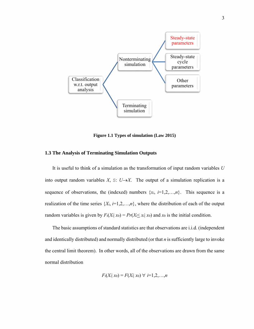
3
Figure 1.1 Types of simulation (Law 2015)
1.3 The Analysis of Terminating Simulation Outputs
It is useful to think of a simulation as the transformation of input random variables U
into output random variables X, S: UX. The output of a simulation replication is a
sequence of observations, the (indexed) numbers {xi, i=1,2,…,n}. This sequence is a
realization of the time series {Xi, i=1,2,…,n}, where the distribution of each of the output
random variables is given by Fi(Xi| x0) = Pr(Xi< xi| x0) and x0 is the initial condition.
The basic assumptions of standard statistics are that observations are i.i.d. (independent
and identically distributed) and normally distributed (or that n is sufficiently large to invoke
the central limit theorem). In other words, all of the observations are drawn from the same
normal distribution
Fi(Xi| x0) = F(Xi| x0) i=1,2,…,n
Classification w.r.t. output
analysis
Nonterminatingsimulation
Steady-state parameters
Steady-state cycle
parameters
Other parameters
Terminating simulation

4
These assumptions are not met by observations within the series. First, the observations
typically are sequentially correlated and therefore not independent. Second, the transient
distributions Fi(Xi,| x0) typically are different for each observation index i and therefore the
observations are not identically distributed. Third, there is no guarantee that these
distributions are normal.
For terminating simulations, this difficulty is easily overcome. Each replication,
j=1,2,…,N, yields one observation of the statistic of interest Yj, such as the sample mean
n
iijj X
nXY
1
1
Running N independent replications of the simulation yields a set observations drawn from
the sampling distribution for this statistic, {Yi, i=1,2,…,N}. These observations are i.i.d.
and therefore the mean across replications
is an unbiased estimator for the output statistic
Moreover, because the sampling distribution of Yj is approximately normal (by the central
limit theorem for sufficiently large N), the precision of the estimate of X can be estimated
as confidence interval by the standard formula
where the sample variance of Yj is an unbiased estimator for the variance of Yj
Y 1
NYj
j1
N
limN
Y E X X
Y tN1,1 /2
SN2
N

5
.
Thus the basic assumptions of standard statistics are satisfied for summary statistics across
replications.
1.3 The Analysis of Nonterminating Simulation Outputs
The approach described above works because the transient response is the object of our
analysis for terminating simulations. This is not the case for nonterminating systems,
however, and performing independent replications alone is inadequate. For nonterminating
simulations, all of the observations within each replication must be drawn from the steady-
state distribution F(X)=Pr(X< x) otherwise the estimator for the statistic is biased. Because
F(X) is not independent of the initial conditions at the beginning, the difficulty posed is
variously referred to as the problem of the initial transient, the start-up problem, or the
warm-up problem.
While there are many proposed alternatives, the most common approach to resolving
the warm-up problem is based on the idea that the transient distributions converge to the
steady-state distribution as the index gets large
F(Xi| x0) F(X) as i .
As suggested in Figure 1.2, after some number of observations d, the transient distribution
is sufficiently close to the steady-state distribution to mitigate bias in the output statistic,
i.e.,
F(Xi| x0) F(X) i d+1.
limN
SN2 Y

6
Figure 1.2 Example of transient and steady-state density functions (after Law 2015)
By allowing the simulation to “warm up”–-discarding all observations prior to Xd+1 within
the output series when computing the statistic—the problem can be overcome. On each
replication we observe the truncated sample mean
Yj,d X j,d 1
n dXi
id1
n
. (1)
The warm-up problem then reduces to that of determining the best truncation point d for
each replication j. As a matter of convenience, very often a single, conservatively large
value of d is selected and used for all replications.
It should be noted that the requirement for convergence in distribution can be relaxed
in some cases. If our interest is estimating the steady-state mean, for example, it is
sufficient that the process is covariance stationary, i.e., that

7
(1) the mean exists niXE i ,,2,1
(2) the variance exists niXVar i ,,2,12 , and
(3) the autocovariance function of order r
,
is not a function of i.
In other words, the means and variances of all observations are constant and the correlation
between any two observations in the series depends only on the number of intervening
observations and not on the location of these points in the series.
For a covariance stationary process, it can be shown that the variance of the sample
mean (within-run) is
(2)
where R(r) is the order r autocovariance function defined above (Pawlikowski, 1990). For
uncorrelated observations, R(r)=0 for all lags r>0, and therefore the variance reduces to the
standard formula for i.i.d. observations
. (3)
From this we can see that if the correlation is strong and positive, ignoring it will lead to
serious underestimation of the true variation.
R(r) cov(Xi, Xir ) k, 0 r n1
1
2
1
(0) 2 1 ( )n
k
kR k n
nnX R
22
1
( 1/ˆ )n
ii
X x Xn n nn

8
1.5 The Locus of this Research
As will be discussed in Chapter 2, many alternative approaches to determining d have
been proposed. Until the introduction of the MSER algorithm (White and Minnox, 1994),
mitigating initialization bias in the mean was considered an open problem. All of the prior
approaches where found wanting for various reasons. Over the past two decades, however,
increasingly MSER has been accepted as a solution to the warm-up problem.
It is noteworthy that MSER:
is proven to yield a near-optimal estimate (under mild assumptions) in the sense of
minimum mean-squared error (MSE) that cannot be improved upon a priori,
is widely accepted in the academic literature as the preferred approach to mitigating
bias associated with the arbitrary specification of initial conditions,
is presented in detail and recommended in the current editions of many standard
texts on DES, and
is effective, efficient, robust, and intuitive.
In spite of these considerable merits, the application of MSER in practice appears far
from universal. We speculate the unaided application of MSER can be inconvenient and
potentially consuming of both analyst and computing time, especially when a large number
of output sequences must be initialized. An obvious solution is to imbed MSER in an
automated, dynamic, run-time procedure that requires minimal analyst interaction.
However, the only reported effort to build MSER into a commercial simulation suite
(SIMUL8) led to the suggestion that there are significant barriers to implementation (Hoad
and Robinson, 2011). These include:
the selection of run length,

9
sequential data collection from multiple replications,
output types associated with cumulative values and extrema, and
data associated with entities.
Conventionally, MSER is a data-driven postprocessor and, as such, requires that an
output sequence be simulated before application. There is no guarantee that MSER will
converge if the run length for this sequence is insufficient to capture a useful trailing
segment of steady-state behavior. Determination of an optimal warm-up period therefore
is in fact confounded with problem of determining an adequate run length, which is most
often resolved by trial and error.
In this research we demonstrate that in application MSER typically will flag instances
in which the run length is inadequate by truncating all (or at least a very large fraction) of
the output sequence to which it is applied. However, we further demonstrate that there are
pathological instances for which this is not the case. While Hoad et al. (2008) provide
useful guidance, determining an appropriate run length a priori remains an open and
perhaps intractable problem.
With this caveat, we demonstrate both analytically and by application that the
remaining barriers are readily overcome. Specifically, we:
cast estimation of an output mean as an iterative optimization problem from which
we derive the memory requirements for run-time implementation (see the literature
review in Chapter 2),
describe and resolve MSER implementation issues (Chapter 3)

10
create a prototype MSER Laboratory (Chapter 4)—a website to facilitate the
distribution of MSER codes and supporting research online (available at
http://faculty.virginia.edu/MSER/).
develop runtime versions of MSER in an ExtendSim static library, a Promodel
DLL, and an Arena submodel (Chapter 5), and
develop MSER post-processing codes in several popular programming languages,
including the open-source languages R and C/C++, as well as the proprietary
languages Matlab, SAS, and VBA (Chapter 6).
Additionally, during the course of this research we encountered multiple instances of a
perhaps obvious, but seemingly pervasive, misconception regarding the application and
evaluation initialization procedures such as MSER. At least two alternative approaches
appear in the literature. The first applies MSER to individual output sequences, truncates
each sequence accordingly, calculates the truncated mean for each sequence, and then
averages the weighted truncated means to estimate the steady-state mean. The second
determines the output sequences for multiple replications, averages these sequences,
applies MSER to the average sequence to determine a single warm-up period, and then
estimates the steady-state mean based on the average sequence truncated by this period.
The first approach is preferred. MSER determines the optimal truncation point for the
specific output sequence to which it is applied and will return an optimal estimate of the
mean for each sequence. The second approach is almost certainly suboptimal. There is no
reason to believe that the truncation point for the average sequence is optimal for each of
the individual runs. The aggregate result is over-truncation for some of the sequences and
under-truncation for the remainder. A proof is provided.

11
The second approach has led to misgivings regarding the efficacy of MSER. These
doubts surfaced most notably in Law (2015), who compares the average of the sample of
individual truncation points with a theoretical mean average truncation point. He
erroneously concludes that MSER may not truncate an appropriately large number of
observations. Wang and Glynn (2014) offer an argument similarly flawed.
A further contribution of this research (see Chapter 7) is to highlight and correct his
misconception with a set of three simple examples: (1) the response of a uniform white-
noise process in steady-state with a superimposed linearly-decreasing deterministic
transient, (2) the delay times in an M/M/1 queue, and (3) the response of an EAR(1)
process. For these test cases, we show that the MSER estimate of the steady state mean is
uncorrelated with the MSER-optimal truncation point and therefore the success of a
truncation procedure in terms of the accuracy of the estimate cannot be imputed from the
truncation point alone. We reiterate that the purpose of truncation is to determine the
warm-up period that yields the most accurate and precise estimate of the steady-state mean.
Other proposed measures of performance are at best irrelevant and at worse seriously
misleading. Also in Chapter 7 we use these same examples to explore the sensitivity of the
estimate mean to run length n and to the choice of the MSER parameters b (batch size) and
dmax (the maximum acceptable optimal truncation point on the range of a given run length
[0≤ dmax ≤n]).
The final Chapter discusses the conclusions of this effort, together with potentially
useful directions for further research. A User’s Guide for application of the Arena
submodel is provided in the Appendix I. Appendix II includes an anecdotal case with some

12
personal reflections on the simulation enterprise and the importance of the warm-up
problem, as well as a survey of undergraduate simulation curricula.
1.6 Background: A Note on Smart Initialization
One of the strengths of MSER is that it demands only that an optimal truncation point
exists for a simulated model (i.e., stationary or weak convergence). In the past, some
researchers have suggested that truncating or deleting an initial data series is not the best
way to improve the estimate with respect to mean squared error (MSE). Blomqvist (1970),
Wilson and Pritsker (1978), Turnquist and Sussman (1977), and Grassmann (2009, 2011)
instead advocated the “smart” choice of an initial condition to mitigate biases and generate
a robust result.
However, it is rather difficult to search for an optimal starting point unless the
characteristics of simulation are known a priori. Do we still need to recognize the existence
of initialization bias? We firmly believe that the answer should be “yes”. We will be better
off by presuming almost every probabilistic non-terminating simulation has unavoidable
initialization bias, and then testing this presumption. Furthermore, consider the tradeoff
between precision and computational budget associated with truncation points. It is
common that more data will support a better analysis by obtaining a robust estimate of
descriptive statistics in output analysis. However, truncation clearly implies that less data
is available.
To compensate the loss of precision, faster analysis is possible with automated
truncation identification, rather than human intervention or post-analysis. This kind of
trade-off can be applied to the comparison between a batch means method and a
replication/deletion method. However, both methodologies can be performed well after we

13
find a right truncation point. We will mention the list of numerous approaches of truncating
initially biased data sets in the next section, but the explanation of each method cannot be
studied here unless the methods are closely related to the topic of MSER.
We might think of another aspect to investigate the characteristic of transient states prior
to the steady-state in simulation output. In order to understand the path during the transient
period, artificial intervention during simulation would be desirable or feasible. If so, we
would like to monitor the differentiated simulation paths to an expected pre-specified
steady state or a newly designated steady state from the modification of simulation input
conditions.

14
Chapter 2: Literature Review
The start-up problem has been the subject of research and debate for over 60 years.
Early work by Morse (1955), Conway (1963), Tocher (1963), and Cohen (1982) proposed
heuristics for determining the presence and persistence of an initial transient in a simulation
output series. Pawlikowski (1990) reviewed eleven such rules and illustrated the strengths
and weaknesses of these different approaches. He distinguished between methods based on
the convergence of estimators for the sample mean and sample variance. The first set of
methods included those from Emshoff and Sission (1970), Fishman (1973), Wilson and
Pritsker (1978), Kelton and Law (1983), and Solomon (1983); the second set included those
from Billingsley (1968), Gordon (1969), Fishman (1971), and Schruben (1982, 1983).
Pawlikowski’s comprehensive review subsequently has been updated by Hoad et al.
(2008) and by Pasupathy and Schmeiser (2010) to include newer approaches. The
interested reader is referred to these works. In the remainder of this chapter, therefore, we
focus on the literature directly related MSER.
2.1 MSER: Approach, Inception, and Development
At the University of Virginia (UVA), MSER was devised by Maclarnon (1990) and
called the Minimal Confidence interval Rule (MCR). White and Minnox (1994), White
(1995), White (1997), Rossetti et al. (1995), Spratt (1998), Cobb (2000), White et al.

15
(2000), and Franklin (2009) all improved and/or further tested the approach. We begin by
describing the MSER concept.
White and Minnox (1994) suggested that the optimal truncation should minimize the
half-width of the marginal confidence interval about the truncated sample mean. Given
the output of a simulation, a finite stochastic sequence {Xi, i=1,2,…,n}, they defined the
optimal truncation point as
(4)
where is the z-score of standard normal distribution associated with a 100(1-)%
confidence interval. The marginal standard error in the mean of the reserved sequence (i.e.,
the sequence remaining after truncation) is
, (5)
and the truncated sample mean is
.
While recognizing that, for a correlated sequence, the sample standard deviation is
biased estimator of the steady-state standard deviation, they reasoned that this statistic
could be interpreted instead as capturing the homogeneity of a sequence—initial sequences
with larger sample standard deviations could be flagged as including transient
observations. Franklin and White (2008) subsequently confirmed this intuition.
For a preconditioned confidence level, is a constant and Eq. 4 reduces to
/ 2
0
* arg minn d
z s dd
n d
/ 2z
s(d)Xi Xn,d 2
id1
n
n d 1
n
diidi X
dnX
1,
1
/2z
16
d* argminnd0
1
n d 2 n d X 2 n d Xn,d
2
id1
n
. (6)
For a given output sequence from one replication of simulation, (if it exists) minimizes
the constrained optimization problem in either Eq. (4) or Eq. (6). Thus, the truncation
algorithm has a simple interpretation and does not require the specification of unknown
parameter settings.
Spratt (1998) introduced MSER-b, using the means of batches of size k as output
variables to which MSER is applied. Batching prewhitens the output series, which is widely
believed to improve the visualization of a transient (Welch, 1981). The formula was the
same as Eq. (6), replacing Xi with Zj (White et al., 2000),
Z j 1 b Yb( j1)p
p1
b
(7)
where { , j=1,…,m} represent a series of batch means each with the size of batches b, n
is the number of observations of Yi, and is the number of batches, where is a
maximum integer or floor function.
Independent research outside of UVA has affirmed the effectiveness of MSER-5. For
example, Mahajan and Ingalls (2004) noted the efficiency and robustness of MSER-5. Oh
and Park (2006) compared their exponential variation rate (EVR) rule with MSER-5 and
acknowledged that the EVR only converged to the path of MSER-5. Bertoli, Casale, and
Serazzi (2007, 2009) implemented MSER-5 into their Java Modeling toolkit.
In the U.K., Hoad et al. (2008) performed a comprehensive and detailed survey on
start-up approaches, identifying over forty-six different methods as indicated in
*d
jZ
m n / k

17
Table 2.1. One of the key performance indicators was whether or not an approach
supported automation in order that it might be incorporated in commercial simulation
software. This requirement eliminated approaches requiring a priori specification of
unknown parameter settings. Among the remaining approaches, they found that MSER-5
performed exceptionally well on a wide variety of test cases. They concluded that MSER-
5 was consistently the best approach across the board, in terms of accuracy, robustness,
simplicity, and ease of automation.
Franklin et al. (2009) demonstrated empirically that the effect of MSER is to
(approximately) minimize the mean-squared error (MSE) in the estimated sample mean,
which is a widely accepted criterion for a quality of a point estimate. This observation
subsequently was proven analytically (under mild assumptions) by Pasupathy and
Schmeiser (2010). White and Robinson (2010) reiterated the strength of MSER-5 with the
basic but fundamental example of an M/M/1 queue, while White and Franklin (2010)
demonstrated a parametric function which gives rise to a close-form solution accounting
for geometrically decaying bias of the AR(1) process. Sanchez and White (2011) identified
adjustments needed to account for differing sample sizes when applying MSER using a
replication/deletion approach for interval estimation of the steady-state mean.
The theoretical work undertaken by Pasupathy and Schmeiser (2010) represents an
important advance over previous empirical research. They verified analytically that the
MSER statistic is asymptotically proportional to the MSE and the minima of each tend to
lie close to the same truncation point. In a more recent presentation, Pasupathy and
Schmeiser (2014) demonstrated analytically that MSER outperforms even two ideal

18
methodologies (i.e., ideal deletion and optimal constant deletion) with uncertainty in output
analysis.
Table 2.1 Methods for Determining Start-up Periods (after Hoad et al. (2008)) Method Type Method
Graphical Simple Time Series Inspection Ensemble (Batch) Average Plots Cumulative-Mean Rule Deleting-The-Cumulative-Mean Rule CUSUM Plots Welch’s Method Variance Plots (or Gordon Rule) Exponentially Weighted Moving Average Control Charts Statistical Process Control Method (SPC)
Heuristic Ensemble (Batch) Average Plots with Schribner’s Rule Conway Rue or Forward Data-Interval Rule Modified Conway Rule or Backward Data-Interval Rule Crossing-Of-The-Mean Rule Autocorrelation Estimator Rule Marginal Confidence Rule or Marginal Standard Error Rule (MSER) Marginal Standard Error Rule m, (e.g. m = 5, MSER-5) Telephone Network Rule Relaxation Heuristics Beck’s Approach for Cycle output Tocher’s Cycle Rule Kimbler’s Double exponential smoothing method Euclidean Distance (ED) Method Neural Networks (NN) Method
Statistical Goodness-Of-Fit Test Algorithm for a Static Dataset (ASD) Algorithm for a Dynamic Dataset (ADD) Kelton and Law Regression Method Glynn & Iglehart Bias Deletion Rule Wavelet-based spectral method (WASSP) Queueing approximations method (MSEASVT) Chase Theory Method (methods M1 and M2) Kalman Filter method Randomization Tests For Initialization Bias
Initialization bias test Schruben’s Maximum Test (STS) Schruben’s Modified Test Optimal Test (Brownian bridge process) Rank Test Batch Means Based Tests – Max Test Batch Mean Based Test – Batch Means Test Batch Means Based Test – Area Test Ockerman & Goldsman Students t-test Method Ockerman & Goldsman (t-test) Compound Tests
Hybrid Pawlikowski’s Sequential Method Scale Invariant Truncation Method

19
In its original form (Eqns. 4 and 6), the MSER criterion suggests the choice of a
truncation point is the global minimum of the MSER statistic on n>d>0. (This choice we
shall denote as MSER-GM.) It was recommended in practice, however, that the choice of
a truncation point be constrained to the first half of the output sequence, d<n/2. (This choice
we shall denote as MSER-Half.) The reasoning was that, if a minimum is not found on
this interval, the run length is insufficiently long to provide a tight interval estimate,
possibly because the simulation is unstable and no suitable truncation point exists.
Pasupathy and Schmeiser (2014) proposed and tested two additional alternatives: the
leftmost local minimum of the MSER statistic (MSER-LLM) and the left-most local
minimum of the local minima of the MSER statistic (MSER-LLM2).
They suggested that MSER-LLM was the best choice. However, their intention to use
the most left local minimum also confirmed the notion of checking the minimum value
prior to the first half of output series in MSER-Half when the sample size is enough to
obtain a steady-state mean estimate after preprocessing data from simulation with a
reasonable batch size. That is, the relationship among the truncation points is
bLLM bLLM 2 bGM (Pasupathy and Schmeiser, 2010), where bGM is the truncation point
that yields a globally minimum MSER statistic. After properly batching output and
generating a sufficient sample size, bLLM would be equivalent to bGM or bHalf.
2.2 Open Issues
The motivation for this research stems from a range of issues that have been raised
regarding various aspects of MSER. Insight on how to resolve these issues is the subject
of the subsequent chapters and a contribution of this research.

20
2.2.1 Implementation and automation
As noted in the Chapter 1, Hoad and Robinson (2008) explored the practical
implementation in commercial simulation software and Hoad et al. (2011) provided a
framework to automate an output analyzer incorporating the logic of MSER-5. They
identified four obstacles to implementation. However, as we demonstrate in this research,
these appear to be specific to limitations of the simulation software they employed
(SIMUL8, see Figure 2.1) and not innate difficulties caused by MSER-5.
Figure 2.1 Testing Module for identifying optimal truncation points in SIMUL8.
The difficulties identified were:
(1) selection of the simulation run length selection,
(2) sequential data collection from multiple replications,
(3) output types associated with cumulative values and extrema,
(4) data associated with entities.
The first difficulty is fundamental in simulation (and sampling more generally) and not
unique to the question of automating a warm-up procedure for steady-state simulation. We

21
illustrate this difficulty specifically as it relates to MSER in Chapter 7 and acknowledge
the run-length selection remains an open and perhaps unavoidable problem. However, to
present this difficulty as an absolute barrier to automation is disingenuous, insomuch as it
denies the practicality and usefulness of any form of automated output analysis, which
clearly is not the case. With this caveat, in Chapters 5 and 6 we demonstrate both
theoretically and by application that the remaining barriers are readily overcome.
The second (and fourth) difficulties easily can be handled by storing vectors of raw
output data with time stamps. If the software application enables a modeler to save
variables of his/her interest, these issues should not be regarded as any obstacle. Visual
Logic Editor in SIMUL8 might also provide the functionality to export raw data after each
replication, or any state change, and exporting data or saving online output in memory
would alleviate the second issue. Moreover, MSER is best applied to individual output
sequences and there is no need to save within-run observations across replications (see
Section 2.4).
The third difficulty arises in the desire to avoid malpractice by novice simulationists—
a difficulty that will never arise in a well-conceived output analysis. A cumulative statistic
is derived from an underlying output sequence {Xi, i=1,2,…,n}, and it
is this latter sequence to which MSER is applied to determine a truncation point, not to the
former. The same is true of extrema.
2.2.2 Batch Size
Spratt (1998), White, Cobb, and Spratt (2000), and most recent papers advocate MSER-
b, which prewhitens the output sequence by creating averages of non-overlapping batches
{ 1, 2,: , }iY i n

22
of size b. Their empirical results suggest that MSER–5 is modestly better than MSER
without prewhitening. However, Pasupathy and Schmeiser (2010) note
that any one-size-fits-all preprocessing, however, leads to a contradiction: if the
preprocessed data are better in some sense, then why not preprocess the preprocessed
data? If preprocessing is to make sense, then its form needs to be based on an analysis
of the given data {X1,X2,...,Xn}. Another point is that the use of non-overlapping batches
is suboptimal to using overlapping batches, which leave no orphaned observations at
the end of the data series, which cause no graininess in the analysis, and which still
requires only O(n) computation.
Their logic appears unassailable and the question of an optimal batch size b, its
relationship to given data, and the overlapping batch means (OBM) approach will be
further explored in Chapter 7. Originally proposed by Meketon and Schmeiser (1984),
OBM replaces Equation (7) with
OBMk 1 b Ybp1
p1
b
(8)
where {OBMk, k=1,…,(n-b+1)} represents a series of batch means for overlapping batches
of size b, where n is the number of observations of Yi. In general, the OBMk are highly
correlated. The correlation is accounted by computing the variance estimator as
))(1(
21
,2
bnbn
XXb
S
bn
kdk
OBM
(9)
and the (100-)% confidence interval as
221,, OBMfkn StX (10)

23
where tf is distributed Student-t distribution with f degrees of freedom (see Law, 2015).
In this regard, the literature on batch means also may provide some insights. The batch-
means method is aimed at mitigating serial correlation between output data in simulation
by batching the output data sequentially and using the means and of these batches in the
construction of interval estimates of the true steady-state mean. Schmeiser (1982)
investigated batch size effects. In other words, given a sequence in steady-state (after first
truncating any transient), how many batches are required and how wide must the batches
be in order to obtain an unbiased estimate to meet any prescribed condition for a simulation
model? Goldsman and Meketon (1986), Schmeiser and Song (1987), Song and Schmeiser
(1993, 1995), Song (1996), and Nelson (2011) have discussed the batch size effect and
optimality condition in batch mean methods.
2.3 Current Related Work
2.3.1 N-SKART
Comparatively recently, James Wilson and his students at North Carolina State
University have developed new truncation algorithms that appear to show modestly better
performance than MSER on select problem instances. These methods derive from WASP,
SBatch, and SKART, and include N-SKART, and MSER5Y (see Figure 2.2). In particular,
Mokashi et al. (2010) compared N-SKART to MSER in terms of performance criteria such
as the success rates of finding truncation points, the minimal MSE values, and confidence
interval coverage.
We do not pursue direct empirical comparisons with NSKART or MSER-5Y in this
research, at least in part because of the extreme complexity of these methods. We simply

24
note in passing that, where improvements over MSER were in fact demonstrated, the test
cases employed appear inherently unrealistic. Moreover, improvements were at best
marginal and required vastly greater computational effort. Further, their algorithm has an
innate weakness in that it does not detect any bias in the moving average of output series.
Figure 2.2 Output Analysis Tree for Wilson and Students
2.3.2 Potentially Insufficient Truncation
Recent work by Law (2015) and Wang and Glynn (2014) suggests that MSER may not
truncate an appropriate number of observations. Both studies apply theoretical constructs
that focus on the average truncation points that should be obtained given an infinite number
of replications. As demonstrated by White and Hwang (2015), this suggestion appears to
contradict both the theoretical results obtained by Pasupathy and Schmeiser (2010) and the
very substantial body of empirical evidence accumulated over the past twenty-five years.
Nevertheless the suggestion merits investigation and further discussion is undertaken
Chapter 7.
James Wilson
Emily Lada (2003, 2008) (WASSP, SBatch)
Ali Tafazzoli (2009) (SKART, N-SKART)
Mokashi et al. (2010)
Youserif (2011)
MSER-5Y

25
2.4 Optimal Analysis for the Mean of a Simulation Output
White (2012) demonstrates how output analysis can be formulated as a constrained
optimization problem. We include his formalism here because it not only provides a
notation for the overall problem, but also a means to determine memory requirements for
implementing MSER. The objective is to achieve an estimate of the mean for a simulation
output with a given precision using the least number of observations. We consider three
cases—terminating simulations, nonterminating simulations using the replication/deletion
approach, and nonterminating simulations using the batch means approach.
2.4.1 The terminating simulation problem
We are given user-defined values for:
HW and , where HW is the maximum desired half-width of the 100(1-)%
confidence interval on the sample mean of the simulation output;
r0, the initial number of replications; and
R, the maximum number of replications.
The problem is then:
Find
where r is the number of replications required, such that
(11)
minr{r0,r1,}
r
r R
26
. (12)
Here HW(r) is the estimated half-width derived from r replications,
(13)
is the variance of mean of the sample means,
; j=0,1,2,…,r (14)
are the sample means, and
(15)
is the grand mean.
Note that this optimization problem may be infeasible for a given choice of HW, , and R.
If this is the case, the user has the option of relaxing any or all of these three parameters,
i.e., increasing the number of replications and/or settling for a less precise estimate. Note
also that an estimate for the number of additional runs required at any stage i+1 is
(16)
If ri+1>R, then let ri+1=R. This is likely a more efficient approach than incrementing r by
a fixed amount. Note finally that the data required to solve this optimization problem is
essentially the r-dimensional array of sample means X j nj .
HW (r) tr1,1 /2
S2 r r
HW
S2 r 1
r 1X j (nj ) X r
j1
r
X j (nj ) 1
nj
Xij
i1
nj
X(r) 1
rX j (nj )
j1
r
ri1 HW (r)
HW
2
ri ri

27
2.4.2 The steady-state simulation problem: replication/deletion approach
This is the same as the terminating simulation problem, except that we must now
determine suitable initial and terminating conditions for each replication by solving a
second set of optimization problems. We are given user-defined values for HW, , R, and
n0, the initial run length for each replication
I, the MSER re-computation interval
N, the maximum number of such intervals (corresponding to a tentative stopping
condition for a maximum run length of n0+NI)
For each replication j=1,…, r, first solve the following problem:
Find
jNInInnn
nj 000 ,,,
min
where nj is the run length required on the jth replication, such that
(17)
Here dj*(nj) is the MSER-optimal truncation point for replication j with run length
nj, where is the floor function,
(18)
is the truncated sample variance, and
(19)
dj *(nj ) argminnj /k d0
Sj2 nj, dj nj dj
nj / k
.
Sj2 nj, dj 1
nj dj
Xij X j nj, dj 2
id j1
n0nj
X j (nj, dj ) 1
nj dj
Xij
injdj1
nj

28
is the truncated sample mean.
Note that constraint Eq. (17) implies the existence of an optimal MSER truncation point
on the output series knnXXX /21 0,,, . The best choice for k is unclear, but we have
achieved good results by requiring the truncation point to be within the first half of the
output time series, i.e., k=2.
Furthermore, note that failure to satisfy constraint Eq. (17) implies that the run length
is insufficient, or that the output is unstable. Without some insight into the nature of the
output, there is no way of knowing which is the case. If constraint Eq. (17) is not satisfied,
the user may choose to increase the value of N, or conclude the output is unstable and stop.
There is no need to evaluate constraints Eq. (11) and Eq. (12) if constraint Eq. (17) is not
satisfied.
Note also that when computing the confidence interval using this approach, one needs
to account for that fact that MSER will yield replications of unequal sample size. See
Sanchez, P. J., and White, K. P., Jr. (2011) for one approach this issue. If the desired HW
constraint is not achieved, additional runs may be attempted. Note finally that the data
required is the output time series X0, X1,…, Xn+n0. For time-persistent statistics, we can
construct this from the array of pairs{xi, ti}.
2.4.3 The steady-state simulation problem: batch means approach
This is the same as the replication/deletion problem, except that we must now
implement batching. By construction, r0=R=1, constraint Eq. (11) is automatically

29
satisfied, and the subscript j in constraint Eq. (17) is superfluous. Constraint Eq. (12) is
replaced by
(12a)
where
(20)
is the standard deviation of the batch means using B batches, given by
(21)
Note that Arena has a well-documented algorithm for adjusting the batch size B as a
function of the run length that maintains 40>B>20. See Kelton et al. (2010, pp.326-327),
for the algorithm and rationale.
HW (n, d*) tnd*1,1 /2
SB2 n / B, d *
n / B HW
SB2 n d * / B 1
n d * / B (Z j Z n d * / B
j1
nd* /B
Z j 1
BXi
i j1
jB

30
Chapter 3: MSER Implementation Issues
In this chapter we consider various options for implementing MSER truncation logic
within alternative software environments. Broadly, we distinguish between two such
options. One is to compute and update a truncation point while simulating a model (i.e.,
online analysis). The other is to analyze the output data obtained after simulating the model
(i.e., post-analysis).
With respect to online analysis, we distinguish between external and internal
implementation approaches. We provide an example of the external approach by outlining
development of a dynamic linked library (DLL) that performs MSER calculations. This
DLL can be called from within models built in Windows-based commercial languages such
as ProModel and MedModel. For internal implementations, we identify the software
development environments associated with a wide range of the most popular commercial
DES languages, including Arena, AutoMod, SIMUL8, ProModel (MedModel), FlexSim,
Simio, ExtendSim, and SimCAD. With respect to post-analysis, we review five different
languages in which we have written standalone programs in which we implement MSER:
R, C++, Matlab, SAS, and VBA.
This chapter provides background leading to several selective implementations. These
implementations were developed as part of this research and are distributed online via the
MSER Laboratory. The details of these implementations and the Lab are provided in
Chapters 4-6 and the Appendices.

31
3.1 Online Analysis
Using online analysis, MSER statistics are continuously updated during each
simulation run. These statistics are used to determine a truncation point following the logic
provided in Section 2.4. If such a point exists, the simulation terminates and output
statistics are reported, allowing comparison of the estimated steady-state mean and
corresponding confidence interval with and without truncation. If such a point does not
exist, this fact is reported instead. Online analysis can be implemented in two different
ways.
3.1.1 External Approach
DES software increasingly is extendable using external modules, such as dynamic
linked libraries (DLL) and Component Object Models (COM). In particular, on a Windows
operating system DLL’s have the flexibility to provide new functions and variables in order
to obtain intended simulation objectives (e.g., additional complex computation). A single
DLL can contain multiple new functions and multiple programs can share the same DLL.
We note, however, that DLL’s must be used with caution. Any modification to an existing
DLL must not adversely affect a previously linked application. Therefore, we need to
emphasize the careful documentation of the DLL. This is essential to maintain
programming intent and any logic to consist of inside functions. Without this practice, it is
difficult to use DLL across different applications, as a compiled file does not demonstrate
how it works or what it accomplishes.

32
3.1.1.1 How to build DLL linked with ProModel (MedModel)
ProModel (http://www.promodel.com/) has a function, XSUB( ), which is used call
external DLL files. This command provides modelers with more versatile power to control
simulation models, such as performing a complex calculation separately without burdening
simulating a model. Furthermore, one standard and representative DLL will be portable to
additional simulation models. To use this feature, the modeler must know how to code
DLL files in a high-level programming language. The exemplar DLL file is written in
C/C++, but it can be written in other programming languages as well. Furthermore, its
portability will be very useful to be foster reusability continuously (ProModel, 2011).
Those who are new to Promodel and the usage of XSUB( ) can refer to the manual in
Promodel. However, this command is considered as an advanced option so that we would
like to explain general ideas here. One of the strengths of an XSUB( ) external subroutine
call is in enhancing the capability of ProModel through the users’ programming skills. That
is, as long as the programing language (i.e., C/C++, VB, and Pascal) is supportive, the logic
called with XSUB() enables a modeler to test every intention, such as complex file IO and
statistical analysis.
Its principal limitation is that, while XSUB() is being executed, the simulation is
temporarily halted so it is important that the computation inside the external subroutine
doesn’t take too long. A Windows 32-bit compiler must compile the logic inside the DLL
and a user must understand Windows platform knowledge.
The function representing the logic only takes one parameter, a void pointer (a generic
pointer). However, it may access multiple parameters through structure. That is why the
function should include a structure. This is a strict condition to implement a user’s

33
intention. In addition to MSER DLL in a following chapter, a basic example of DLL usage
is explained (ProModel, 2011).
Syntax:
XSUB(<file ID>, <ordinal function number> or <function name> {,
<parameter1>, <parameter2>...})
Example
XSUB(MSER, 1, 5) or XSUB(MSER_raw, “Log_B_of_Output”, 10, 5)
The components of the four elements in XSUB() are briefly explained in syntax. The
argument <file ID> is an identifier to build a simulation model and link its output with a
DLL file. Figure 3.1 shows how to designate a file ID and set up its type as DLL. When
DLL is ready, we need to specify it into “File Name”.
Figure 3.1 Example of DLL usage in ProModel
The argument <ordinal function number> or <function name> is used to set up which
function inside a DLL file becomes interactive with ProModel. As we build a DLL file,
multiple functions can be constructed to perform output analysis. For example, we want to
find a truncation point, MSER statistics, or a truncated mean value. If we build different
functions to compute them, we need to remember their order and then use the ordinal

34
number for relevant components of XSUB(). As an alternative, we can use the defined
names inside DLL for XSUB() components. The argument <parameters> is any set of input
values generated from ProModel to a DLL file. It will be passed to the function of DLL.
3.1.2 Internal Approach
The internal approach can be achieved in several different ways. First, the software
developer can incorporate MSER logic for release in a version upgrade. This clearly is the
best approach, but is limited by the ability and willingness of the software house to provide
internal developers’ time to create and test the upgrade. Second, a static library can be
written in a software language specific to the commercial simulation suite. This is the
second best approach, but at present is officially supported by only one software company,
ExtendSim. Third, a submodel or subprocess can be developed to compute the MSER
truncation point and associate statistics, such as in Arena. Such a submodel is reusable
given in-detail explanations of submodel inputs, outputs, and operation. We pursue the
second two approaches in Chapters 5.
3.1.2.1 Software development environments
The main purpose of this session is review how commercial DES are created and which
languages would be used in an internal approach. We include the most popular software
adopted in academia as well as industry. Most software environments are built on object-
oriented programming languages such as C++, C#, and Java. However, simulation-specific
languages also are employed (Arena, for example, is built in the simulation language
SIMAN, which itself was originally programmed in Fortran and then later reprogrammed
in C). We determined which development language has been used in each simulation suite

35
based on information in the suites’ users manuals. Where these manuals are inadequate to
make this determination, we also consulted each company’s job postings. As most of
software houses need to hire new programmers, we can infer which language is used for
specific simulation software. We list the languages for each simulation environment as
follows:
Arena – SIMAN
AutoMod – proprietary language
SIMUL8 – proprietary language
ProModel (MedModel) – MS Studio GUI and its proprietary language
FlexSim – C++ based proprietary language
Simio – C#
ExtendSim – C-based proprietary language, ModL
SimCAD – C#
All of these DES software applications run only on MS Windows OS (and the same is
true of all but a few agent-based simulation applications and open-source simulation
languages). That is why more and more simulation GUIs have adopted the Window’s
ribbon-style interfaces. Thus, we expect that a single versatile DLL in a single object-
oriented programming language to be usable across the majority of these environments.
3.1.2.2 Current Features for Dealing with the Start-up Problem
After understanding basic and fundamental structure of each software suite, we observe
different approaches to deal with a warm-up period across multiple simulation software

36
environments. We test Arena, AutoMod, SIMUL8, ProModel, FlexSim, Simio, and
SimCAD. Almost all of these have features for specifying a warm-up period during run
setup. The specifics for each language are summarized, as well as the corresponding
interface.
3.1.2.2.1 Arena
Arena (https://www.arenasimulation.com/) was originally developed by Dennis Pegden at
Systems Modeling Corporation and later acquired by Rockwell Software (Banks 1998;
Kelton et al., 2010). It is an extensible simulation and animation software package that
provides a complete simulation environment supporting all steps in a simulation study.
Arena combines the modeling power and flexibility of the SIMAN simulation language
with a GUI interface for drag-and-drop model building as well as simulation run animation.
In Arena, the warm-up period is defaulted to zero unless otherwise specified on the
“Replications Parameters” tab in “Run Setup” menu shown in Figure 3.2. Arena has a good
feature to take advantage of both replication/deletion and batch means approaches to
steady-state simulation by using “Initialize Between Replication”, a feature which is not
seen in other software by default.

37
Figure 3.2 Specifying Warm-up Period in Arena’s Run Setup Dialogue
3.1.2.2.2 AutoMod
AutoMod is a graphical simulation software environment providing true-to-scale 3D
simulation developed by Applied Materials (http://www.appliedmaterials.com/global-
services/automation-software/automod). Its application focuses on manufacturing and
distribution operations (i.e., semiconductor industry). AutoMod puts much importance on
output analysis and clearly promotes using replication/deletion method to compute its
confidence interval. Comprehensive explanations of determining warm-up period are
followed inside its manual—an entire chapter is devoted to addressing the warm-up
problem—which is a rare case among current simulation software manuals. The AutoMod

38
suite includes a companion program, AutoStat, designed specifically to implement Welch’s
procedure, in particular.
Figure 3.3 Warm-Up Period Determination in AutoMod
3.1.2.2.3 SIMUL8
SIMUL8 (http://www.simul8.com/) is a process-based DES that helps an analyst to
build high-level simulation model, widely adopted as a teaching language by educational
institutions in the UK. Like Arena, it has an option to specify warm-up period, as shown
in Figure 3.4. As shown in Figure 3.5, SIMUL8 also includes a routine to estimate the
number of simulation replications required to achieve a specified minimum precision in
specified output statistics (KPI’s). It is noteworthy that Hoad and Robinson (2011) relate
lessons learned in their effort to implement MSER in SIMUL8.

39
Figure 3.4 Warm-Up Period in SIMUL8
Figure 3.5 Output Analysis Support in SIMUL8
3.1.2.2.4 ProModel and MedModel
ProModel is an older DES suite that aims to provide insights on planning, designing,
and improving existing or new manufacturing, supply chain, and other discrete-event
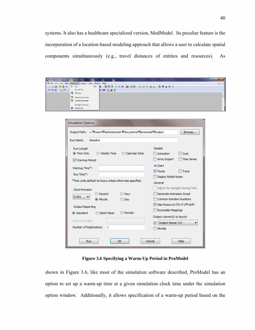
40
systems. It also has a healthcare specialized version, MedModel. Its peculiar feature is the
incorporation of a location-based modeling approach that allows a user to calculate spatial
components simultaneously (e.g., travel distances of entities and resources). As
Figure 3.6 Specifying a Warm-Up Period in ProModel
shown in Figure 3.6, like most of the simulation software described, ProModel has an
option to set up a warm-up time at a given simulation clock time under the simulation
option window. Additionally, it allows specification of a warm-up period based on the

41
number of processed entities (e.g., WARMUP). Thus, it provides dual modes to control a
warm-up period.
3.1.2.2.5 FlexSim
FlexSim was founded in 1993 by Bill Nordgren (Co-Founder Promodel Corporation,
1988) along with Roger Hullinger and Cliff King. Its strength lies in 3D-modeling
capability. Most of the features inside FlexSim are similar to ProModel. It supports its own
language, Flexscript, as well as C++ when a modeler builds a simulation model. Figure
3.7 shows the dialog for setting a warm-up period in FlexSim
Figure 3.7 Specifying a Warm-Up Period in FlexSim
3.1.2.2.6 Simio
Developed in 2006 by Dennis Pegden, Arena users can easily adopt Simio. The major
difference is that Simio is a 3D object-based modeling environment simulation package
which is written in a C# and .NET environment (http://www.simio.com/products/ and
Simio Reference Guide). Compared to Arena, it helps a user to build 3D simulation models
easily. Its 3D library is directly linked with Google Warehouse and allows any relevant 3D
symbols to be added in a simulation model.

42
Most features in Arena also are available in Simio and, as shown in Figure 3.8, a warm-
up period is implemented in “Experiments” after building a model. The Experiment
Properties asks a user to determine a warm-up period as well as a confidence level. To
access this option, the user can select the “Navigation window” first and then choose
“Experiments”. To specify the warm-up period, Simio provides related properties of the
“Experiment” in Table 3.1.
Figure 3.8 Specifying a Warm-Up Period in Simio

43
Table 3.1 Properties of Warm-Up Period Control in Simio
Property Valid Entry
Description
Warm-up Period
Real By default, Simio removes the information before a warm-up period in order to obtain an estimate unaffected by an initial condition.
Default Replications
Integer
This feature is useful to obtain results from multiple simulation runs. It can specify the different replication numbers of each different scenario. If a user does not change any value, the default replication is 1.
Confidence Level
90%, 95%, 98%, 99%
After running multiple replications, Simio will calculate confidence interval of half-width statistics of average results across replications.
3.1.2.2.7 ExtendSim
ExtendSim (http://www.extendsim.com/) has an open structure to help users modify its
library (Banks, 1998), a feature which attracts us to focus on this package in
implementation of an automatic MSER calculation. Additionally, the syntax of its
programming language, ModL, is very similar to C, and allows the modeler to save output
data in memory instead of a hard disk, facilitating faster computation time. As shown in
Figure 3.9, a warm-up period can be implemented in ExtendSim using the “Clear Statistics”
option in the statistics library.
3.1.2.2.8 SimCAD
SimCAD (https://www.createasoft.com/) is a DES environment that provides user-
friendly features to create a model. It advertises that even simulation novices can build a
model without spending a long time to figure it out. However, it appears that a user tends
to follow built-in functions exclusively. Even though it can foster model building, some
features do not reflect the notion of statistics or methodologies from systems engineering.

44
Figure 3.9 Warm-Up Period in ExtendSim using Clear Statistics under Statistics library
Furthermore, it does not clearly include a warm-up period as a basic option. We observed
that an application specialist in SimCAD did not know how to handle a warm-up period.
When we had a later conversation with a lead development engineer, he suggested how to
achieve the same functionality of a warm-up period. Apparently, it can deal with the warm-
up period, but requires the end user to write additional code. The SimCAD GUI is shown
in Figure 3.10.

45
Figure 3.10 GUI of SimCAD

46
3.2 Post analysis
Heretofore MSER logic has been implemented by individuals in custom-built, data-
driven postprocessors. In contrast to the Arena and ExtendSim online implementations
provided in Chapter 4, these codes operate on output sequences generated by prior
simulation runs, rather than continuously while simulating a model. Law (2015) provides
a notable example in his test applications of MSER. In these examples, Law imported
simulation output to an Excel spreadsheet developed by Katy Hoad of the University of
Warwick. This spreadsheet incorporates a VBA macro to perform all MSER calculations.
To promote more widespread adoption of MSER, we developed MSER codes in several
popular programming languages. These codes are given in Chapter 6 and also are available
online at the MSER Laboratory. Each code required us to implement logic using alternate
programming syntax and built-in functions. While run times varied on test cases, all of the
applications yielded identical results and the identical cases, as expected.
Five different applications were written: two in the open-source code applications, R
and C/C++, and three in the proprietary software applications, Matlab, SAS, and VBA.
Each implementation has its own strength of computing an optimal truncation point by
using the concept of an array, which makes these distinct from each other. Once we
understand the common workflow to calculate MSER, the difference in what language it
is written is minor. That is, we just need to know and exchange specific built-in functions
inside each and follow language specific syntax. Using these built-in functions may or may
not be efficient computationally. If the data sets are not large, however, the functions tend
to work better than using user-defined functions based on loop and conditional statements.

47
An overview of these computing languages is provided in the following section. We
describe each pertinent programming language or application to implement and run MSER
so it is useful to illustrate key features before accounting for syntax in different codes. The
following part will explain the history, background, and features from each programming
language.
3.2.1 R
R is known as a statistical computing language that supports publication-quality
graphics. Based on the S language, R is part of the GNU freeware project, an open source-
programming environment. Because it is freeware, more academic institutions tend to use
R rather than commercial alternatives. In addition, R can run on a wide variety of popular
operating systems such as Windows, Linux, and MacOS. User contributions to R enrich its
functionalities along with research development and it is very flexible to interact with other
languages such as C, C++, and FORTAN. Source: What is R?: Introduction to R
(http://www.r-project.org/)
3.2.2 C/C++
Dennis Ritchie created C in 1972 at Bell Laboratories and Bjarne Stroustrup developed
C++ in the early 1980s, also at Bell Laboratories. Among the programming languages
discussed here, C/C++ are the only languages to compile the code before running the logic.
Generally speaking, C++ is superset of C. Thus codes written in C can usually be
transported to C++(some exceptions exist). Both C and C++ demand very rigorous and
strict coding, but are very fast to execute (Prata, 2003 and 2005).

48
3.2.3 Matlab
As the name suggests, Matlab is useful to manipulate matrix operations for numerical
computations and visual representations. Matlab is intended to support technical
computing. It advertises that the mastery of its language, tools, and built-in functions can
help users obtain the results efficiently. We also witness that more and more engineers and
students areadopting this technical language. Source: Matlab primer
(http://www.mathworks.com/help/pdf_doc/matlab/getstart.pdf)
3.2.4 SAS
SAS is proprietary software to solve problems from real business to academic research. Its
exemplar tasks include file IO (data entry, retrieval, and management), ODS (output
delivery system for presentation of report and pertinent graphics), statistical and
mathematical analysis, and functionality for operations management/research problems
such as business planning, forecasting, decision, and others.
To perform MSER calculation, we use a specific module to support array and matrix
manipulation, SAS/IML (Interactive Matrix Language). This is a complete programming
language with a dynamic, interactive environment for programmers, statisticians,
researchers, and high-end analysts. After obtaining data or processed information, this
interactive language is designated for more complex and sophisticated analysis to explore
target data sets. Its user interface is similar to SAS, as well as Matlab. However, creating
one’s own SAS/IML modules becomes much easier than using SAS by itself. Every

49
application can be run either interactively or in batch. Furthermore, it can adopt R code via
the IML server. Source: SAS 9.3 Language Reference
(http://support.sas.com/documentation/cdl/en/lrcon/65287/PDF/default/lrcon.pdf) and
SAS/IML fact sheet
(http://www.sas.com/resources/factsheet/sas-iml-factsheet.pdf)
3.2.5 VBA
Excel, the spreadsheet included in MS Office, is equipped with the Visual Basic for
Applications (VBA) language. Whenever extra analysis or calculation cannot be performed
by built-in functions, VBA is the last source to count on. VBA is based on the Basic
programming language and relatively easy to learn. However, its speed of execution is
sacrificed for the stake of simplicity. VBA also supports an array format and its dynamic
properties can be used for the development of MSER inside Excel. When a user opens the
Excel workbook, the user can open Visual Basic Editor on the Developer Tab and build
various functions to meet the objectives of a modeler.
3.3 Merits of the alternative codes
In summary, needless to say, the application written in C/C++ is more error prone and
time consuming because we can only depend on their basic math library. In addition to this
effort, we have to define types of all variables with care. However, it is cost effective and
very fast to process long time series, which is a general benefit in high-level programming
language. VBA is a more user-friendly interface to interact with end users, but demands
more time to compute MSER statistics. We acknowledge that there might be room to
optimize code performance in Visual Basic as we just use VBA to compute MSER. Three

50
other applications will help whoever has some expertise or experiences among R, Matlab,
and SAS to be familiar with MSER logic. These three applications develop their own array
manipulation tools and use built-in functions to code MSER logic in simple ways. As long
as the user knows and uses the right functions, it would reduce the time and effort to write
applications with these.

51
Chapter 4. The MSER Laboratory
Ideally, simulationists from industry and the academy collaborate to keep abreast of
developments reported in the simulation literature. Commercial simulation software
continues to incorporate new research findings, but typically lags in the pace of adoption
because of the considerable investment required to revise current codes or to add new logic
in a current version of software. One of the main goals of this research is to spur the
implementation of MSER in commercial software and practical application.
To this end we have created a web-based laboratory that is an open and accessible
resource for those who are interested in improving, applying, and extending the use of
MSER. Included in the MSER Laboratory are (1) an archive of key research articles, (2)
a repository of MSER codes that may be freely downloaded, and (3) a set of concrete and
user-friendly examples that illustrate the application of these codes. The MSER Laboratory
is hosted at the University of Virginia at http://faculty.virginia.edu/MSER/.
We have observed that increasingly researchers are publishing their sample data sets as
well as their codes. However, it is not an easy task to decipher code written in a language
with which one is not familiar. That is why we facilitate the implementation of MSER in
well-known simulation software such as ExtendSim, Arena, and ProModel/MedModel (see
Chapter 5), as well provide MSER postprocessors in written in R, SAS, Matlab, VBA, and
C/C++ (see Chapter 6). We seek continuity of this beginning by maintaining an up-to-date

52
development in MSER from those who make progress. Furthermore, we appreciate
receiving any constructive comments to improve the quality of this site.
In this chapter we take a very brief guided tour through screen shots of the Lab as it
currently is configured, while additional details are provided in later chapters. The content
in this site gives the general idea of MSER (Figure 4.1), its history related to research
articles (Figure 4.2), sample codes as well as sample test sets (Figure 4.3) and the basic
math derivation of the MSER statistic (Figure 4.4).
These implementations in commercial simulation software are distinct from the
current, arbitrary warm-up determination because these:
Determine a truncation point automatically
Minimize unnecessary user input
Provide figures and tables to support this determination
All information is downloadable by any interested users and the site will help researchers
exchange and update any new developments.

53
Figure 4.1. Introduction of MSER Laboratory Web page

54
Figure 4.2. History of MSER Laboratory Web page

55
Figure 4.3. Sample Codes of MSER Laboratory Web page

56
Figure 4.4. Math of MSER Laboratory Web page

57
Chapter 5. Implementation of MSER in Commercial Software
Before selecting appropriate simulation software suites, we must check whether the
software package can update the MSER-statistic in a designated way while it saves the
output to memory. After reviewing current discrete-event simulation software (see Chapter
3), we chose three representative software packages—ExtendSim, Arena, and ProModel—
with which we can calculate the MSER statistic online. In this Chapter we present examples
of the incorporation of MSER logic in the model process flow diagrams, together with the
corresponding source code or module structure needed to support implementation for each
of these languages.
5.1 ExtendSim Implementation
ExtendSim (originally named “Extend”), from Imagine That, Inc., is a general-purpose
software suite for continuous, discrete-event, and hybrid simulation (Banks 1998, Krahl
2012). After we confirmed its capability to store output data sets, we collaborated with
Dave Krahl at Imagine That and appreciated his efforts and time, even under his tight
schedule, on the creation of a MSER library in ExtendSim. The MSER algorithm is
implemented in ExtendSim’s C-based ModL language. Only minor modifications relating
to the user interface and variable initialization were required to convert the algorithm from
ANSII C to ModL. The MSER block is fully integrated into ExtendSim and can be used in
any ExtendSim model in the future.

58
The library collects data continuously from any relevant blocks and is designed to
compute a MSER statistic, a truncation point, and a mean estimate associated with the
truncation point. Another feature in this library includes the function to set up the
computing frequency via a user input. The default batch size is 5 and batch size can be
varied via setting different dialog parameters.
5.1.1 ExtendSim Process Flow
Figure 6.1 depicts a tandem queue model in ExtendSim, with the MSER module
included to collect statics on the waiting time in Queue 2 tied with the GUI for the MSER
calculator.
Create
R L
Queue 1D F
Activ ity A
R L
W
Queue 2
D F
U
Activ ity BMSER
9928
Exit
Right click and select
open structure to edit
ModL code
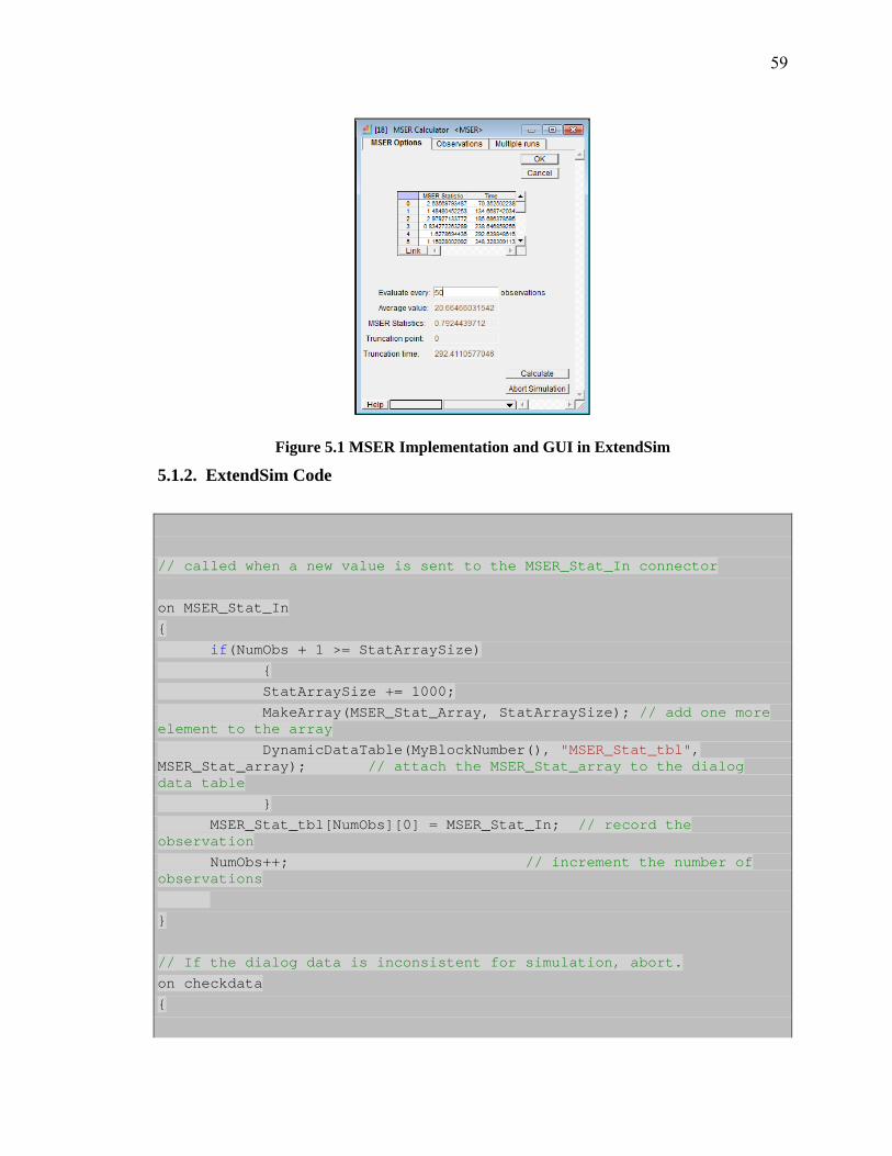
59
Figure 5.1 MSER Implementation and GUI in ExtendSim
5.1.2. ExtendSim Code
// called when a new value is sent to the MSER_Stat_In connector
on MSER_Stat_In
{
if(NumObs + 1 >= StatArraySize)
{
StatArraySize += 1000;
MakeArray(MSER_Stat_Array, StatArraySize); // add one more element to the array
DynamicDataTable(MyBlockNumber(), "MSER_Stat_tbl", MSER_Stat_array); // attach the MSER_Stat_array to the dialog data table
}
MSER_Stat_tbl[NumObs][0] = MSER_Stat_In; // record the observation
NumObs++; // increment the number of observations
}
// If the dialog data is inconsistent for simulation, abort.
on checkdata
{
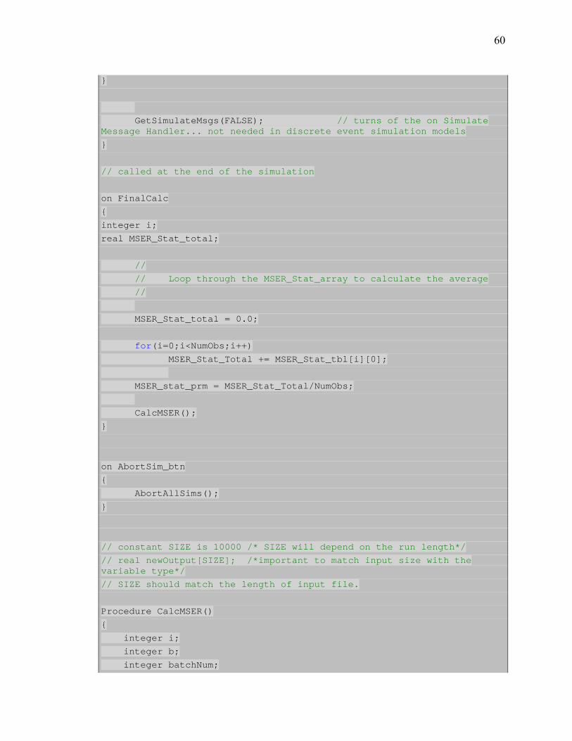
60 }
GetSimulateMsgs(FALSE); // turns of the on Simulate Message Handler... not needed in discrete event simulation models
}
// called at the end of the simulation
on FinalCalc
{
integer i;
real MSER_Stat_total;
//
// Loop through the MSER_Stat_array to calculate the average
//
MSER_Stat_total = 0.0;
for(i=0;i<NumObs;i++)
MSER_Stat_Total += MSER_Stat_tbl[i][0];
MSER_stat_prm = MSER_Stat_Total/NumObs;
CalcMSER();
}
on AbortSim_btn
{
AbortAllSims();
}
// constant SIZE is 10000 /* SIZE will depend on the run length*/
// real newOutput[SIZE]; /*important to match input size with the variable type*/
// SIZE should match the length of input file.
Procedure CalcMSER()
{
integer i;
integer b;
integer batchNum;

61 integer m; /*Batch output length*/
integer d, j;
integer mser, d_final, n, k, threshold, j_final;
real min_MSER;
integer min_Index;
integer ReportOutput;
MakeArray(Sum, NumObs);
MakeArray(MSER_array, NumObs);
MakeArray(mean_array, NumObs);
MakeArray(sumMean, NumObs);
MakeArray(sum, NumObs);
MakeArray(average, NumObs);
MakeArray(squared_sum, NumObs);
ReportOutput = FALSE;
for (i = 0; i < NumObs; i++)
{
if (i == 0)
{
sum[i] = MSER_Stat_tbl[i][0];
squared_sum[i] = sum[i]*sum[i];
}
else
{
sum[i] = sum[i-1]+MSER_Stat_tbl[i][0];
squared_sum[i] = squared_sum[i-1] + sum[i]*sum[i];
}
average[i] = sum[i]/(i+1);
}
// Batch mean generation part
bigB = 20;
n = NumObs;
batchNum = floor(n/bigB);
real interimSum;
MakeArray(z, NumObs);
for (m = 0; m < batchNum; m++)

62 {
interimSum = 0.0;
for (b =0; b < bigB; b++)
{
interimSum += MSER_Stat_tbl[bigB*m + b][0];
if (b == (bigB-1)){
z[m] = interimSum/bigB;
// printf("\t\t%f\n", z[m]);
}
}
}
//before computing d and MSER-statistic, we need to store mean_array
for (d = 0; d < batchNum; d++)
{
for (j = 0; j < batchNum; j++)
{
if (j+d >= batchNum)
break;
else
{
sumMean[d] += z[j+d];
}
}
mean_array[d]= sumMean[d]/(batchNum - d + 1);
}
//redefine run length n to batchNum;
n = batchNum; /* run length of each replication*/
k = 2; /* try to find a truncation within the first half of output series*/
threshold = n/k;
Makearray(sampleVariance, batchNum);
Makearray(mserSum, batchNum);
Makearray(MSER_array, batchNum);
for(i=0;i<batchNum;i++)
{
sampleVariance[i] = 0;
mserSum[i] = 0;

63 MSER_array[i] = 0;
}
min_MSER = BLANK;
for (d_final = 0; d_final < threshold; d_final++)
{
for (mser = 0; mser <= n; mser++)
{
if (mser + d_final > batchNum)
break;
else
{
mserSum[d_final] += (z[mser + d_final] - mean_array [d_final]) * (z[mser + d_final] - mean_array [d_final]);
}
}
sampleVariance[d_final] = mserSum[d_final]/(n - d_final - 1);
MSER_array[d_final] = sampleVariance[d_final]/(n - d_final);
if (MSER_array[ d_final ] < min_MSER || NoValue(min_MSER))
{
min_MSER = MSER_array[d_final];
min_Index = d_final;
}
}
{
MSER_Statistic_prm = min_MSER;
Min_Index_prm = min_Index;
MSerOut = min_MSER;
SendMsgToInputs(MSerOut);
}
}
on CREATEBLOCK
{
NumObsEvaluate_prm = 100;
}
5.2 Arena Submodel Implementation

64
Although it is desirable to develop MSER as a built-in function in Arena, as has done
in ExtendSim, we have as yet been unable to persuade Rockwell Software to invest in this
functionality. As an immediate alternative, we chose to implement the MSER calculation
logic inside an Arena submodel (Kelton, et al. 2010). This submodel is generic and can be
inserted in any Arena project. The MSER-optimal point can be calculated for any output
by assigning this attribute as the input to the MSER submodel.
5.2.1 Arena Process Flow
Figure 5.2 depicts an M/M/1 queue in Arena with a MSER submodel included to collect
statistics on the waiting time in queue defined in the “Service” process module. The wait
time in queue is assigned to an attribute before the corresponding entity enters the
submodel named “MSER Module”. In models more complex than this simple queue, we
can add copies of the submodel to compute MSER statistics for multiple attributes or
variables anywhere in the process flow. For instance, if a researcher wants to compute the
wait time in both queues in a tandem queue model, she/he needs to include these two
submodels, one for the output of each service process.
Figure 5.2 Main model of an M/M/1 queue in Arena with the MSER module included to collect statistics on the waiting time in Service queue
M SER M oduleArriv al Serv ice
M/M/1 w ith traffic intensity of 0.9
Ex it
0 0
0

65
Figure 5.3 Details of the MSER calculation in the Arena

66
5.2.2 Arena MSER Modules
Figure 5.3 shows the Arena process flow that implements the MSER computation.
Table 5.1 lists the global and local variables and arrays used by the submodel. The User’s
Guide in Appendix I provides more details and a fully worked-out example.
Table 5.1. Global, Local variables and Arrays
No. Variable (array) name Location of block Usage
1 v_Counter Index Record entity number
v_Counter + 1
2 v_X InterimData Generation
Record entity wait time
3 v_X2 InterimData Generation
Record (entity waiting time)2
4 v_inter_cumX InterimData Generation
Holder for summation of v_X
5 v_inter_cumX2 InterimData Holder for summation of v_X2
6 v_Mean DataGeneration v_cumX(v_Counter)/v_Counter
7 v_ cumX DataGeneration v_inter_cumX(v_counter)
8 v_ cumX2 DataGeneration v_inter_cumX2(v_counter)
9 v_MSER_test MSER Without Trucation
(v_cumX2(v_Counter) - v_Counter * v_Mean(v_Counter) * v_Mean(v_Counter))/ ((v_counter - 0) * (v_counter - 0))
10 StopRule End of Simulation
(Decision block)
Global variable to check the end of simulation, 10000 that confirm
StopRule = v_Counter
11 v_Truncation Truncation Index v_Truncation + 1
12 v_MSER_final MSER WithTruncation ((v_cumX2(StopRule) - v_cumX(v_Truncation)) - (StopRule -v_Truncation) * v_Mean(StopRule) * v_Mean(StopRule))/ ((StopRule - v_Truncation) * (StopRule - v_Truncation - 1))
5.3 Promodel/Medmodel Implementation
Promodel/Medmodel is equipped with a function call to use DLL so computing
additional statistic can be feasible as mentioned previously. We test M/M/1 with traffic

67
intensity of 0.9. As shown in Figure 5.4, this simple model consists of three nodes
representing entity arrival, processing, and exit, as well as a waiting queue for processing.
5.3.1 Promodel/Medmodel Process Flow
After compiling the DLL to compute MSER statistic, this file is listed in “External Files”
as “DLL”. It is saved in a working directory, or the model needs to be told the directory
where it is compiled. XSUB() uses Med.dll to compute MSER the statistic aDuration that
records time in system, as shown in Figure 5.5.
Figure 5.4 M/M/1 Model in ProModel

68
Figure 5.5 DLL Usage in ProModel
5.3.2 ProModel DLL Code
* DLL.cpp *
* Author: Sung Nam Hwang *
* Topic: DLL of Promodel(Medmodel) to generate MSER *
* Date: Dec. 16, 2013 */
#include "Med.h"
#include <cmath>
struct TEST_SUB_PARAMS
{
double basic;
//double time; If a modeler selects time weighted variable, this variable needs to be redefined.
};
extern "C"
{
double _export BatchTest (void *p)
{
static double batchOutput[100000] ;
static double Batchsum = 0.0;
static int b = 5; //batch size of 5
static int j = 0; //batch output index
static int m = 0; //execution index to make batch output (i.e., m = 1 means the first raw output
//m = 2 means the second one and so on.

69 static double holder = 0.0; //temporary value holder
static double test3 = 0.0; //temporary value holder
TEST_SUB_PARAMS * param;
param = (TEST_SUB_PARAMS*) p; //type conversion from void to TEST_SUB_PARAMS
Batchsum += param->basic; //Add up the raw outputs
m +=1;
if (m == b)
{
if (j == 0) //the first batch output generation
{
batchOutput[j] = Batchsum/b; //batch output with batch size of b
m = 0; //after making one batch output need to reset m for the next batch output
j += 1; //increase the batch output index for the next batch output
}
else //except the first batch output generation
{
for (int _temp_ = 0; _temp_ < j; _temp_ ++) //automatic variable of _temp_
{
holder +=batchOutput[_temp_];
}
batchOutput[j] = (Batchsum - (holder * b))/b;
m = 0;
j +=1;
holder = 0.0;
}
}
//if the vector of batch output is created and reaches at a certain number (i.e., j = 5)
//Compute truncated mean of batch outputs such as average of z_0, z_1, z_2, and so on
static double trunBatchSum = 0.0;
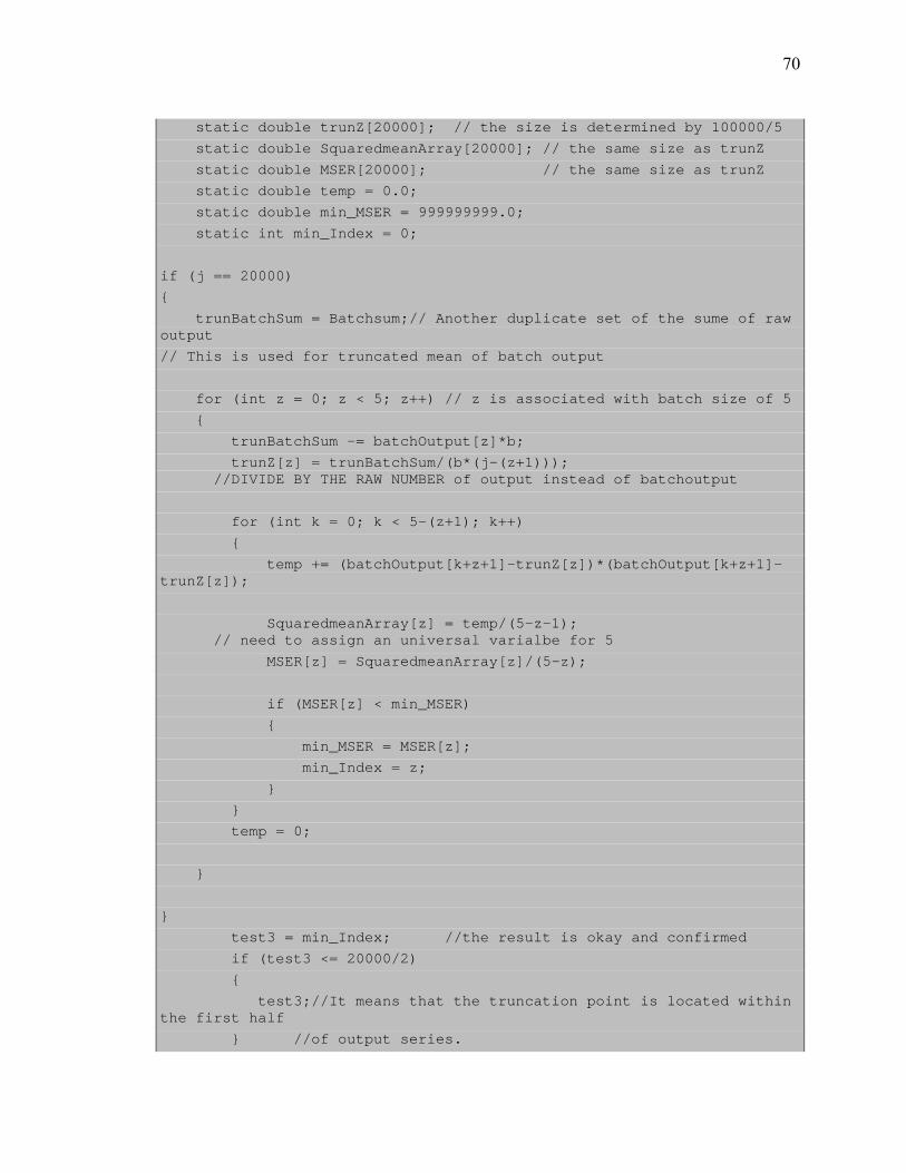
70 static double trunZ[20000]; // the size is determined by 100000/5
static double SquaredmeanArray[20000]; // the same size as trunZ
static double MSER[20000]; // the same size as trunZ
static double temp = 0.0;
static double min_MSER = 999999999.0;
static int min_Index = 0;
if (j == 20000)
{
trunBatchSum = Batchsum;// Another duplicate set of the sume of raw output
// This is used for truncated mean of batch output
for (int z = 0; z < 5; z++) // z is associated with batch size of 5
{
trunBatchSum -= batchOutput[z]*b;
trunZ[z] = trunBatchSum/(b*(j-(z+1))); //DIVIDE BY THE RAW NUMBER of output instead of batchoutput
for (int k = 0; k < 5-(z+1); k++)
{
temp += (batchOutput[k+z+1]-trunZ[z])*(batchOutput[k+z+1]-trunZ[z]);
SquaredmeanArray[z] = temp/(5-z-1); // need to assign an universal varialbe for 5
MSER[z] = SquaredmeanArray[z]/(5-z);
if (MSER[z] < min_MSER)
{
min_MSER = MSER[z];
min_Index = z;
}
}
temp = 0;
}
}
test3 = min_Index; //the result is okay and confirmed
if (test3 <= 20000/2)
{
test3;//It means that the truncation point is located within the first half
} //of output series.

71 else
{
test3 = 9999999; //Indicator that urges the more simulation run to achieve steady state.
}
return test3;//the value indicates minimal truncation point.
}
}
//Header file of DLL_MSER.cpp
#ifndef __MED_H__
#define __MED_H__
#include <windows.h>
#ifdef BUILD_DLL
#define _EXPORT __declspec(dllexport)
#else
#define DLL_EXPORT __declspec(dllimport)
#endif // BUILD_DLL
#ifdef __cplusplus
extern "C"
{
#endif
double _export BatchTest (void *p);
#ifdef __cplusplus
}
#endif
#endif
/* Promodel (Medmodel) code using xsub that execute dll*/
aDuration = clock() - aEnter
real endvalue
endValue = XSUB(TEST2, 1, aDuration)

72
Chapter 6. Implementation in Post Analysis Codes
The MSER Laboratory currently includes five post-analysis codes written in R, SAS,
Matlab, VBA, and C/C++. In this Chapter, we demonstrate the application of each of these
codes on a simple example. The corresponding outputs also are provided.
Each code reads data from a file (either Simple2.csv or simple2.txt). These data are
the output of one replication of a normal white noise process with superimposed
deterministic bias initialized at declining from 15 to 0 with a slope of -0.1. The batch size
is set at b=5 and the run length is n=10,000 observations. The results from all five
applications are identical. The sample mean without truncation is 0.106268, the MSER-
optimal truncated mean is -0.005395563, and the MSER truncation point is d*=30.
6.1. R Source Code
# Set up a working directory
setwd("~/Documents/MSER") #change this working directory as your R and data file are located
newOutput <- read.table("simple2.csv", sep = ",", header = F) #change the input file name
# Generating batch mean
# Set up parameter for the array of batch mean
dataLength <- dim(newOutput)[1]
batchSize <- k <- 5
batchNumber <- floor(dataLength/batchSize)
batchMean = rep(0, batchNumber)

73
for ( i in 1:batchNumber) {
batchMean[i] = sum (newOutput [((i-1)*batchSize +1):(i*batchSize),])/batchSize
}
# MSER-Statistic
# Generating placeholders for updating series
sampleMSE <- rep(0, batchNumber)
sampleMean <- rep(0, batchNumber)
batchMean2 <- batchMean^2
for ( d in 1:batchNumber) {
sampleMean[d] <- mean(batchMean[d: (length(batchMean))]);
sampleMSE[d] =(sum(batchMean2[d: length(batchMean)])-(batchNumber- d)*(sampleMean[d]^2))/((batchNumber - d)*(batchNumber - d - 1))
}
# Find the minimal value of MSER statistic and the location
trun <- which(sampleMSE == min(sampleMSE[1:(batchNumber-batchSize)]))
sampleMSE[trun]
# Plotting an initial raw data sets and MSER Graph including a truncating point par(mfrow=c(1,2))
ts.plot(newOutput, ylab="Raw output")
ts.plot(sampleMSE[1:dataLength/batchSize], gpars=list(xlab="d", ylab="MSER Statistic", lty=c(1:3)))
abline(v = trun, lty = 2, col = "red")
par(mfrow=c(1,1))
# Raw mean vs. truncated mean and a truncating point
cat("mean without truncation: ", sampleMean[1], "\n")
cat("truncated mean: ", sampleMean[trun], "\n")
cat(“truncating point: ", trun, "\n")
cat(“minimal MSER: ", sampleMSE[trun], "\n")

74
Figure 6.1 Output and MSER Plot in R
6.2. The SAS Source Code
libname MSER 'C:\Users\Administrator\Documents\SAS'; proc import datafile='C:\Users\Administrator\Documents\SAS\simple2.txt' dbms = dlm out = MSER.raw replace;
delimiter =" ";
getnames = no; run;
proc iml;
use MSER.raw;
read all into check;
dataLength = nrow(check);
close MSER.raw;
* Batch mean generation; k = 5;
batchSize = k;
batchNumber = floor(dataLength/batchSize); batchMean = j(batchNumber, 1, 0);
/*do statement*/ do i = 1 to batchNumber;
batchMean[i] = sum (check[((i-1)*batchSize +1) : (i*batchSize)])/batchSize;
end;
/*MSER Statistic Generation*/ sampleMSE = j(batchNumber, 1, 0);
sampleMean = j(batchNumber, 1, 0);
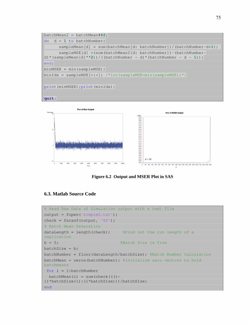
75 batchMean2 = batchMean##2;
do d = 1 to batchNumber;
sampleMean[d] = sum(batchMean[d: batchNumber])/(batchNumber-d+1);
sampleMSE[d] =(sum(batchMean2[d: batchNumber])-(batchNumber- d)*(sampleMean[d]**2))/((batchNumber - d)*(batchNumber - d - 1));
end;
minMSER = min(sampleMSE);
minIdx = sampleMSE[>:<]; /*loc(sampleMSE=min(sampleMSE))*/
print(minMSER);print(minIdx);
quit;
Figure 6.2 Output and MSER Plot in SAS
6.3. Matlab Source Code
% Read Raw Data of Simulation output with a text file
output = fopen('simple2.txt');
check = fscanf(output, '%f');
% Batch Mean Generation
dataLength = length(check); %Find out the run length of a replication
b = 5; %Batch Size is five
batchSize = b;
batchNumber = floor(dataLength/batchSize); %Batch Number Calculation
batchMean = zeros(batchNumber); %initialize zero vectors to hold batchmeans
for i = 1:batchNumber
batchMean(i) = sum(check(((i-1)*batchSize+1):(i*batchSize)))/batchSize;
end

76 % MSER-Statistic
sampleMSE = zeros(0, batchNumber);
sampleMean = zeros(0, batchNumber);
batchMean2 = batchMean.^2;
for d = 1:batchNumber
sampleMean(d) = mean(batchMean(d:(length(batchMean))));
sampleMSE(d) = (sum(batchMean2(d:length(batchMean)))...
-(batchNumber - d)*(sampleMean(d)^2))/((batchNumber - d)*(batchNumber - d - 1));
end
% Find a truncation point whose MSER statistic is minimum except the last
% few output series. Consider one or two points to compute sample variance.
% Thus, we need to exclude those erratic points.
trun = find(sampleMSE == min(sampleMSE(1:(batchNumber-batchSize))));
% Add a graph showing the trend of MSER statistics
% Match dimensions between x and y axis
plot(1:(batchNumber-batchSize), sampleMSE(1:batchNumber-batchSize));
title 'Truncation Point with Batch Mean';
xlabel 'Batch Numbers';
ylabel 'MSER Statistic';
hold all;
Figure 6.3 Output and MSER Plot in Matlab
6.4. VBA Source Code
Option Explicit
Option Base 1
Sub Main()
Dim batchSize As Integer
Dim dataLength As Long, batchNumber As Double
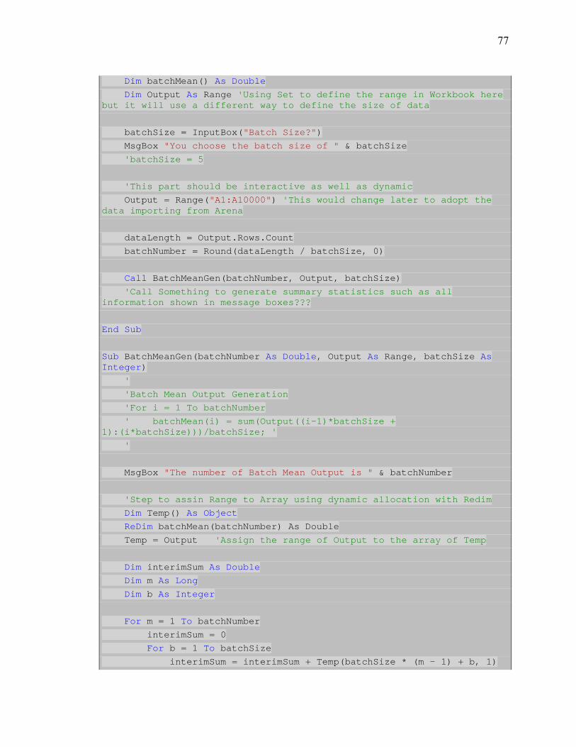
77 Dim batchMean() As Double
Dim Output As Range 'Using Set to define the range in Workbook here but it will use a different way to define the size of data
batchSize = InputBox("Batch Size?")
MsgBox "You choose the batch size of " & batchSize
'batchSize = 5
'This part should be interactive as well as dynamic
Output = Range("A1:A10000") 'This would change later to adopt the data importing from Arena
dataLength = Output.Rows.Count
batchNumber = Round(dataLength / batchSize, 0)
Call BatchMeanGen(batchNumber, Output, batchSize)
'Call Something to generate summary statistics such as all information shown in message boxes???
End Sub
Sub BatchMeanGen(batchNumber As Double, Output As Range, batchSize As Integer)
'
'Batch Mean Output Generation
'For i = 1 To batchNumber
' batchMean(i) = sum(Output((i-1)*batchSize + 1):(i*batchSize)))/batchSize; '
'
MsgBox "The number of Batch Mean Output is " & batchNumber
'Step to assin Range to Array using dynamic allocation with Redim
Dim Temp() As Object
ReDim batchMean(batchNumber) As Double
Temp = Output 'Assign the range of Output to the array of Temp
Dim interimSum As Double
Dim m As Long
Dim b As Integer
For m = 1 To batchNumber
interimSum = 0
For b = 1 To batchSize
interimSum = interimSum + Temp(batchSize * (m - 1) + b, 1)

78 If b = batchSize Then
batchMean(m) = interimSum / batchSize
End If
Next b
Next m
'batchMean Generation is definitely correct
Dim bNumber As Double
Dim bMean() As Double
bNumber = batchNumber
bMean = batchMean
Call MSERGen(bNumber, bMean())
End Sub
Sub MSERGen(batchNumber As Double, batchMean() As Double)
'MSER Generation
ReDim SampleMean(batchNumber) As Double, SampleMSE(batchNumber) As Double
Dim d As Double, j As Long
ReDim meanArray(batchNumber) As Double
'
'check SampleMean and meanArray
'
For d = 1 To batchNumber
SampleMean(d) = 0
For j = 1 To batchNumber
If (j + d - 1) > batchNumber Then 'Use (j+d-1) instead of (j+d)
Exit For
Else
SampleMean(d) = SampleMean(d) + batchMean(j + d - 1)
End If
Next j
meanArray(d) = SampleMean(d) / (batchNumber - d + 1)
Next d
' Let's consider For j = 1 To (batchNumber - d) in the future trial
' SampleMean and meanArray are correct

79 Dim k As Integer, threshold As Long
k = 2
threshold = Round(batchNumber / k, 0)
Dim min_MSER As Double
ReDim sampleVariance(batchNumber) As Double
ReDim mserSum(batchNumber) As Double
ReDim MSER_array(batchNumber) As Double
Dim min_Index As Double
min_MSER = 999999999.0#
Dim d_final As Double
Dim mser As Long
'd_final = 1
For d_final = 1 To threshold
For mser = 1 To batchNumber
If (mser + d_final - 1) > batchNumber Then
Exit For
Else
mserSum(d_final) = mserSum(d_final) + (batchMean(mser + d_final - 1) - meanArray(d_final)) * (batchMean(mser + d_final - 1) - meanArray(d_final))
End If
Next mser
sampleVariance(d_final) = mserSum(d_final) / (batchNumber - d_final - 1)
MSER_array(d_final) = sampleVariance(d_final) / (batchNumber - d_final)
If MSER_array(d_final) < min_MSER Then
min_MSER = MSER_array(d_final)
min_Index = d_final
End If
Next d_final
MsgBox "Minimum of MSER " & MSER
MsgBox "The truncation point is " & (min_Index)
MsgBox "Before truncatinig, we have a mean of " & meanArray(1)
MsgBox "The trucated mean is " & meanArray(min_Index)
End Sub
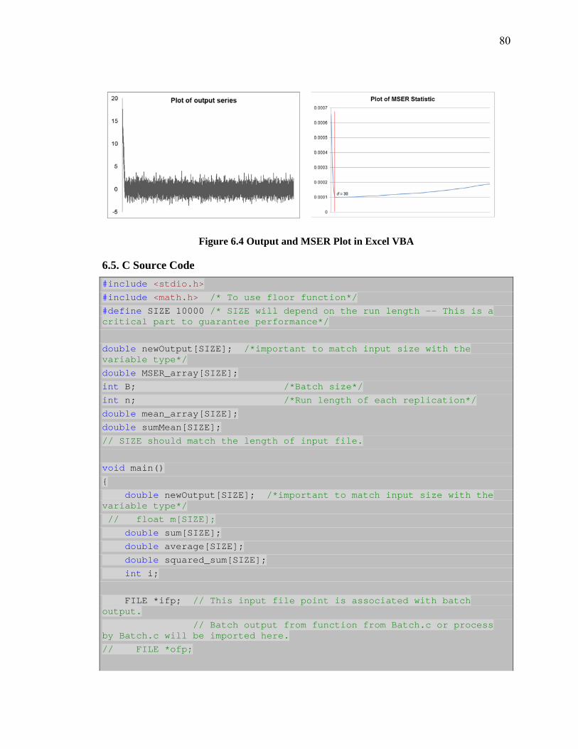
80
Figure 6.4 Output and MSER Plot in Excel VBA
6.5. C Source Code
#include <stdio.h>
#include <math.h> /* To use floor function*/
#define SIZE 10000 /* SIZE will depend on the run length -- This is a critical part to guarantee performance*/
double newOutput[SIZE]; /*important to match input size with the variable type*/
double MSER_array[SIZE];
int B; /*Batch size*/
int n; /*Run length of each replication*/
double mean_array[SIZE];
double sumMean[SIZE];
// SIZE should match the length of input file.
void main()
{
double newOutput[SIZE]; /*important to match input size with the variable type*/
// float m[SIZE];
double sum[SIZE];
double average[SIZE];
double squared_sum[SIZE];
int i;
FILE *ifp; // This input file point is associated with batch output.
// Batch output from function from Batch.c or process by Batch.c will be imported here.
// FILE *ofp;
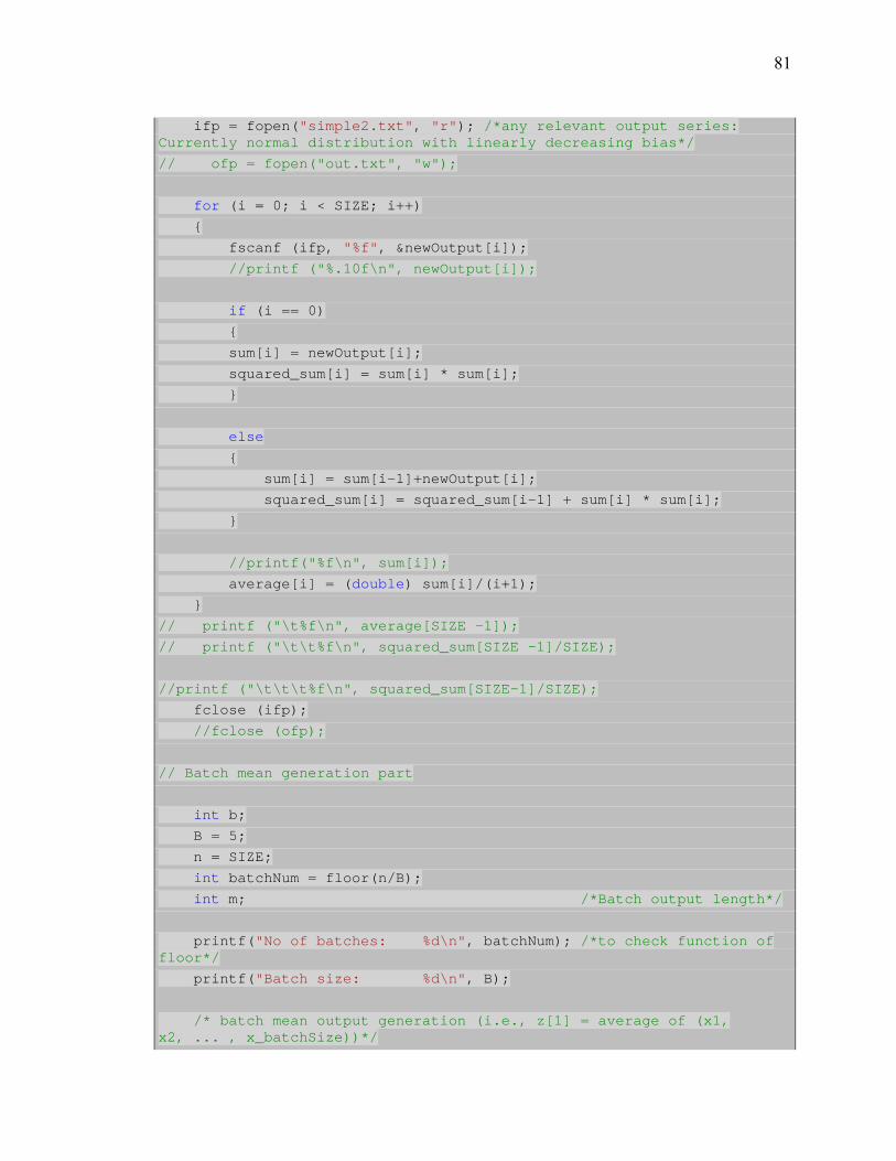
81 ifp = fopen("simple2.txt", "r"); /*any relevant output series: Currently normal distribution with linearly decreasing bias*/
// ofp = fopen("out.txt", "w");
for (i = 0; i < SIZE; i++)
{
fscanf (ifp, "%f", &newOutput[i]);
//printf ("%.10f\n", newOutput[i]);
if (i == 0)
{
sum[i] = newOutput[i];
squared_sum[i] = sum[i] * sum[i];
}
else
{
sum[i] = sum[i-1]+newOutput[i];
squared_sum[i] = squared_sum[i-1] + sum[i] * sum[i];
}
//printf("%f\n", sum[i]);
average[i] = (double) sum[i]/(i+1);
}
// printf ("\t%f\n", average[SIZE -1]);
// printf ("\t\t%f\n", squared_sum[SIZE -1]/SIZE);
//printf ("\t\t\t%f\n", squared_sum[SIZE-1]/SIZE);
fclose (ifp);
//fclose (ofp);
// Batch mean generation part
int b;
B = 5;
n = SIZE;
int batchNum = floor(n/B);
int m; /*Batch output length*/
printf("No of batches: %d\n", batchNum); /*to check function of floor*/
printf("Batch size: %d\n", B);
/* batch mean output generation (i.e., z[1] = average of (x1, x2, ... , x_batchSize))*/
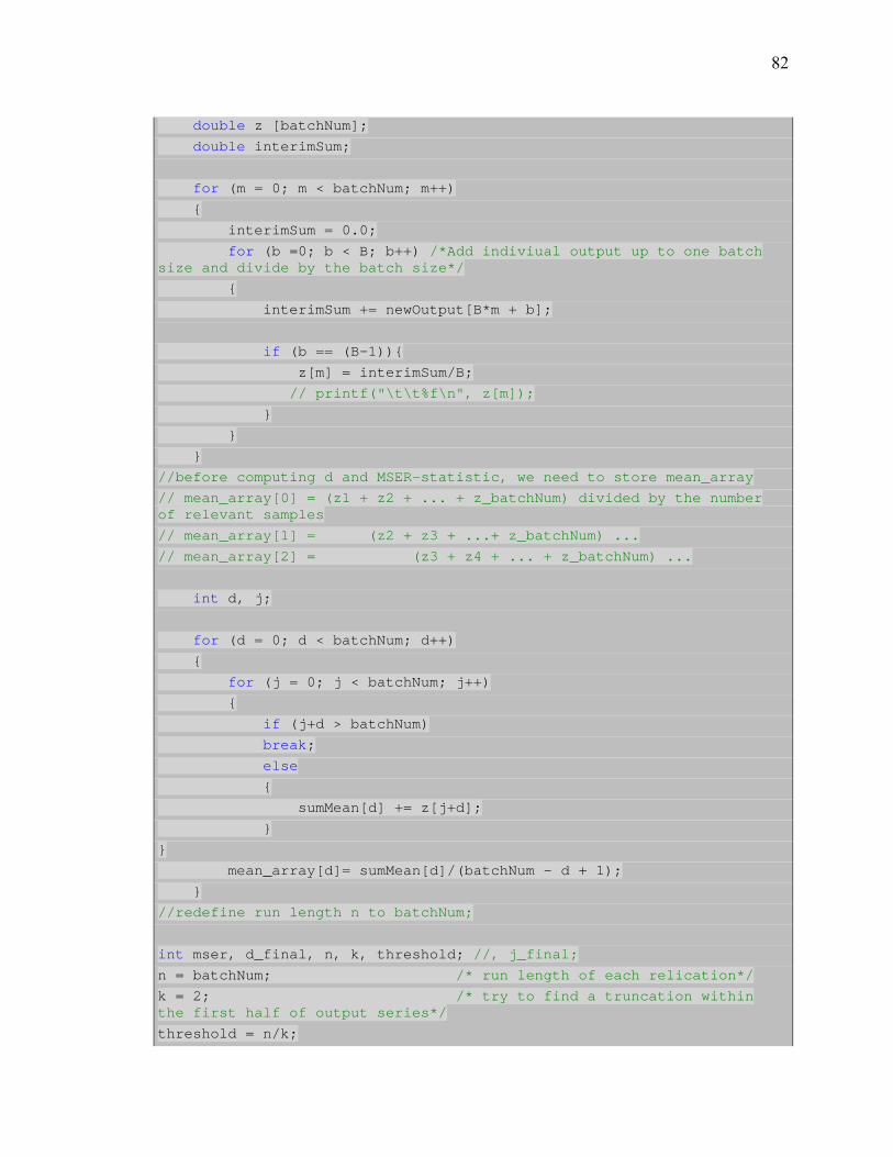
82 double z [batchNum];
double interimSum;
for (m = 0; m < batchNum; m++)
{
interimSum = 0.0;
for (b =0; b < B; b++) /*Add indiviual output up to one batch size and divide by the batch size*/
{
interimSum += newOutput[B*m + b];
if (b == (B-1)){
z[m] = interimSum/B;
// printf("\t\t%f\n", z[m]);
}
}
}
//before computing d and MSER-statistic, we need to store mean_array
// mean_array[0] = (z1 + z2 + ... + z_batchNum) divided by the number of relevant samples
// mean_array[1] = (z2 + z3 + ...+ z_batchNum) ...
// mean_array[2] = (z3 + z4 + ... + z_batchNum) ...
int d, j;
for (d = 0; d < batchNum; d++)
{
for (j = 0; j < batchNum; j++)
{
if (j+d > batchNum)
break;
else
{
sumMean[d] += z[j+d];
}
}
mean_array[d]= sumMean[d]/(batchNum - d + 1);
}
//redefine run length n to batchNum;
int mser, d_final, n, k, threshold; //, j_final;
n = batchNum; /* run length of each relication*/
k = 2; /* try to find a truncation within the first half of output series*/
threshold = n/k;

83
double min_MSER;
double sampleVariance[batchNum];
double mserSum [batchNum];
double MSER_array [batchNum];
int min_Index;
min_MSER = 999999999.0;
for (d_final = 0; d_final < threshold; d_final++)
{
for (mser = 0; mser <= n; mser++)
{
if (mser + d_final > batchNum)
break;
else
{
mserSum[d_final] += (z[mser + d_final] - mean_array [d_final]) * (z[mser + d_final] - mean_array [d_final]);
}
}
sampleVariance[d_final] = mserSum[d_final]/(n - d_final - 1);
MSER_array[d_final] = sampleVariance[d_final]/(n - d_final);
if (MSER_array[ d_final ] < min_MSER)
{
min_MSER = MSER_array[d_final];
min_Index = d_final;
//printf("%d\n", min_Index);
}
}
printf("%s\n"," ");
printf("MSER statistics:\t%f\n", min_MSER);
printf("Truncation point:\t%d\n", min_Index );
double rawAverage;
double trunAverage;
rawAverage = mean_array[0];
trunAverage = mean_array[min_Index];
printf("Raw average:\t%f\n", rawAverage);
printf("Average after truncating:\t%f\n", trunAverage);
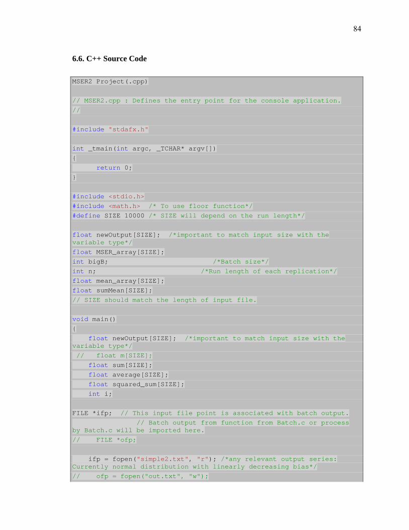
84
6.6. C++ Source Code
MSER2 Project(.cpp)
// MSER2.cpp : Defines the entry point for the console application.
//
#include "stdafx.h"
int _tmain(int argc, _TCHAR* argv[])
{
return 0;
}
#include <stdio.h>
#include <math.h> /* To use floor function*/
#define SIZE 10000 /* SIZE will depend on the run length*/
float newOutput[SIZE]; /*important to match input size with the variable type*/
float MSER_array[SIZE];
int bigB; /*Batch size*/
int n; /*Run length of each replication*/
float mean_array[SIZE];
float sumMean[SIZE];
// SIZE should match the length of input file.
void main()
{
float newOutput[SIZE]; /*important to match input size with the variable type*/
// float m[SIZE];
float sum[SIZE];
float average[SIZE];
float squared_sum[SIZE];
int i;
FILE *ifp; // This input file point is associated with batch output.
// Batch output from function from Batch.c or process by Batch.c will be imported here.
// FILE *ofp;
ifp = fopen("simple2.txt", "r"); /*any relevant output series: Currently normal distribution with linearly decreasing bias*/
// ofp = fopen("out.txt", "w");

85
for (i = 0; i < SIZE; i++)
{
fscanf (ifp, "%f", &newOutput[i]);
//printf ("%.10f\n", n[i]);
if (i == 0)
{
sum[i] = newOutput[i];
squared_sum[i] = sum[i]*sum[i];
}
else
{
sum[i] = sum[i-1]+newOutput[i];
squared_sum[i] = squared_sum[i-1] + sum[i]*sum[i];
}
//printf("%f\n", sum[i]);
average[i] = (float) sum[i]/(i+1);
}
// printf ("\t%f\n", average[SIZE -1]);
// printf ("\t\t%f\n", squared_sum[SIZE -1]/SIZE);
//printf ("\t\t\t%f\n", squared_sum[SIZE-1]/SIZE);
fclose (ifp);
//fclose (ofp);
// Batch mean generation part
int b;
bigB = 20;
n = SIZE;
int batchNum = floor((double) n/bigB);
int m; /*Batch output length*/
printf("No of batches: %d\n", batchNum); /*to check function of floor*/
printf("Batch size: %d\n", bigB);
float z [SIZE];
float interimSum;
for (m = 0; m < batchNum; m++)
{
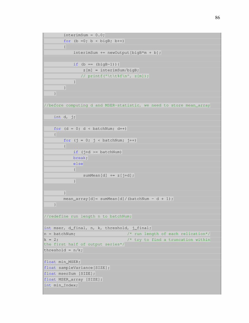
86 interimSum = 0.0;
for (b =0; b < bigB; b++)
{
interimSum += newOutput[bigB*m + b];
if (b == (bigB-1)){
z[m] = interimSum/bigB;
// printf("\t\t%f\n", z[m]);
}
}
}
//before computing d and MSER-statistic, we need to store mean_array
int d, j;
for (d = 0; d < batchNum; d++)
{
for (j = 0; j < batchNum; j++)
{
if (j+d >= batchNum)
break;
else
{
sumMean[d] += z[j+d];
}
}
mean_array[d]= sumMean[d]/(batchNum - d + 1);
}
//redefine run length n to batchNum;
int mser, d_final, n, k, threshold, j_final;
n = batchNum; /* run length of each relication*/
k = 2; /* try to find a truncation within the first half of output series*/
threshold = n/k;
float min_MSER;
float sampleVariance[SIZE];
float mserSum [SIZE];
float MSER_array [SIZE];
int min_Index;

87 min_MSER = 999999999.0;
for(i=0;i<SIZE;i++)
mserSum[i] = 0.0;
for (d_final = 0; d_final < threshold; d_final++)
{
// for (mser = 0; mser <= n; mser++)
for (mser = 0; mser < n; mser++)
{
if (mser + d_final >= batchNum)
break;
else
{
mserSum[d_final] += (z[mser + d_final] - mean_array [d_final]) * (z[mser + d_final] - mean_array [d_final]);
}
}
sampleVariance[d_final] = mserSum[d_final]/(n - d_final - 1);
MSER_array[d_final] = sampleVariance[d_final]/(n - d_final);
if (MSER_array[ d_final ] < min_MSER)
{
min_MSER = MSER_array[d_final];
min_Index = d_final;
//printf("%d\n", min_Index);
}
}
printf("%s\n"," ");
printf("MSER statistics:\t%f\n", min_MSER);
printf("Truncation point:\t%d\n", min_Index );
//printf("\t\t%f\n", MSER_array[100]);
}
stadfx.cpp
// stdafx.cpp : source file that includes just the standard includes
// MSER2.pch will be the pre-compiled header
// stdafx.obj will contain the pre-compiled type information
#include "stdafx.h"
// TODO: reference any additional headers you need in STDAFX.H
// and not in this file
88
Header files
stdafx.h
// stdafx.h : include file for standard system include files,
// or project specific include files that are used frequently, but
// are changed infrequently
//
#pragma once
#include "targetver.h"
#include <stdio.h>
#include <tchar.h>
// TODO: reference additional headers your program requires here
targetver.h
#pragma once
// The following macros define the minimum required platform. The minimum required platform
// is the earliest version of Windows, Internet Explorer etc. that has the necessary features to run
// your application. The macros work by enabling all features available on platform versions up to and
// including the version specified.
// Modify the following defines if you have to target a platform prior to the ones specified below.
// Refer to MSDN for the latest info on corresponding values for different platforms.
#ifndef _WIN32_WINNT // Specifies that the minimum required platform is Windows Vista.
#define _WIN32_WINNT 0x0600 // Change this to the appropriate value to target other versions of Windows.
#endif
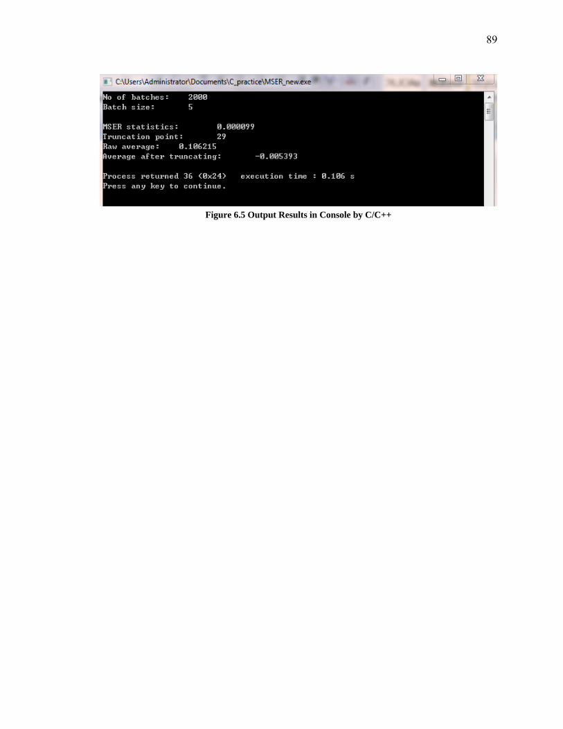
89
Figure 6.5 Output Results in Console by C/C++

90
Chapter 7. Parameterization Issues, Analyses, and Results
While MSER is widely accepted as the most robust approach to initializing steady-state
simulations, there remain a number of open questions regarding its application. These
include:
the choice of simulation run length n,
the choice of batch size b, and
the maximum acceptable optimal truncation point dmax on the range of a given run
length [0≤ dmax ≤n]
the incorporation of the overlapping batch means.
One purpose of this research is to provide insight on the relationships among these
parameters and guidance regarding their selection. To this end, we explore these
relationships empirically on a selection of test problems using a replication/deletion
analysis framework. We estimate the sampling distributions of the truncated means and
corresponding truncation points, test for correlation, and compare response surfaces for
varying batch sizes and run lengths. Before proceeding to the test problems, however, we
consider a fundamental and perhaps unresolvable difficulty inherent in choosing an
adequate run length (see White and Hwang, 2015).
7.1 Choosing the Run Length of a Nonterminating Simulation
While intuition may derive from the system being simulated and/or the purpose of the
simulation study, determining an appropriate run length for a nonterminating simulation

91
typically is a process of trial and error. Framed as an optimization problem in Chapter 2,
the global objective is to discover the number of observations needed to achieve both the
accuracy and precision desired in the estimated steady-state simulation outputs with the
minimum computing effort. For output series that are potentially nonstationary or cyclical,
run lengths must first and foremost be long enough to convince one that this is or is not the
case; for output series that are slow to converge in distribution, practical constraints on
time and computing budgets may necessitate settling for shorter run lengths and confidence
intervals wider than desired.
We distinguish between the two typical output analysis frameworks. If batch-means is
adopted for output analysis then the run length should be sufficient to provide a sample of
steady-state observations (after truncation sufficient to mediate initialization bias) large
enough to form nearly uncorrelated batch means yielding a desired level of confidence in
the grand mean. If replication/deletion is adopted, then each of the replication run lengths
should be adequate to guarantee that MSER can determine an appropriate truncation point.
In this case, the accuracy and precision of the estimate is a function of the number of
replications run. The interested reader should see Hoad, et al. (2007) for a review of the
literature and an empirical comparison of alternative procedures for determining the
number of replications required.
The replication/deletion framework provides the insights we seek regarding MSER
parameterization. MSER works by successively considering the leading observation xd in
the output series {xd, …, xn}, i.e., the sequence remaining after the initial d-1 observations
have been truncated. This observation is a candidate for deletion if the MSE in the estimate
of the steady-state mean decreases for the reserved sequence {xd+1, …, xn}. For MSER to

92
succeed in determining an optimal truncation point for any single replication, however, the
algorithm has to “see” enough of the steady-state response in the reserved sequence in order
to make a correct determination. We note that, symptomatically, as the sample size n-d
becomes small with continued truncation, the MSER statistic can behave erratically
(Rossetti, Delaney, and White, 1995; Spratt, 1998; and Hoad et al., 2008). In other words,
there is some shortest sequence {xdmax,…, xn} that is “sufficiently large and representative”
of a sample drawn from the steady-state distribution of Xt for use in determining a
truncation point.
If MSER determines that d*>dmax, then by construction the algorithm should return a
message that an optimal truncation point cannot be determined for the given output
sequence. In such cases the MSER statistic decreases over entire range [0, dmax], indicating
that the output sequence increases (in trend) or decreases over this same range. This will
be the case for one of two reasons. Either (1) the output is inherently unstable (such as a
queue with traffic intensity ρ≥1) and MSER will not converge irrespective of run length,
or (2) the process is stable, but the run length n is insufficient to achieve a detectable steady
state. Without addition computing, it is impossible to tell which is the case based on the
output alone.
To illustrate the inherent problem, consider output sequences for two different systems
given in Figure 7.1. First, consider run lengths of n≤500. The MSER statistic will have a
minimum value in the neighborhood of n for both Output A (Red) and Output B (Blue).
MSER therefore will fail to return a truncation point for either output.

93
Figure 7.1 Hypothetical simulation output sequences illustrating one potential consequence
of an inadequate run length
Second, consider run lengths of n≥500. MSER will still fail to return a truncation point
for Output A. However, if n is sufficiently large, MSER will return optimal truncation point
in the neighborhood of d*=500 for Output B. It is unlikely that MSER will find an optimal
truncation for values all values of n≥500 and the question is, “What is the minimum run
length n* such that MSER finds a correct truncation point for Output B?” This almost
certainly will depend on the unique properties of the specific output sequence under
consideration, most especially the degree of sequential correlation.
Now consider output sequences for two different systems given in Figure 7.2. These
are possible extensions of the outputs in Figure 7.1. Obviously, MSER will yield the same
results for run lengths n≤800. If n is sufficiently large, however, MSER will conclude (1)
that Output A (Red) has stabilized, and will return optimal truncation point in the
neighborhood of d*=800; and (2) Output B (Blue) is unstable and fail to return a truncation
point for this output. Again, the question of how large is sufficient to draw either
conclusion remains unclear.

94
Figure 7.2 Hypothetical extensions of the simulation output sequences in Figure 7.1 illustrating further potential consequences of an inadequate run length
From these examples we see that MSER can potentially change its determinations
regarding the location and the even the existence of a suitable truncation point depending
on the run length chosen. While in our experience Output B in the second example is a
pathological case, the conclusion remains that the performance of MSER depends on
choosing a sufficient run length. And without knowledge beyond the output sequences
alone, there are no guarantees that this is or is not the case.
7.2 Test Models and Results
We performed empirical tests with differing batch sizes to determine if any discernable
trends or correlations exist among mean estimates, truncation points, batch sizes, and run
lengths, using three different forms of output. These test outputs included (1) the response
of a uniform white-noise process in steady-state with a superimposed linearly-decreasing
deterministic transient, (2) the delay times in an M/M/1 queue, and (3) the response of an
EAR(1) process.
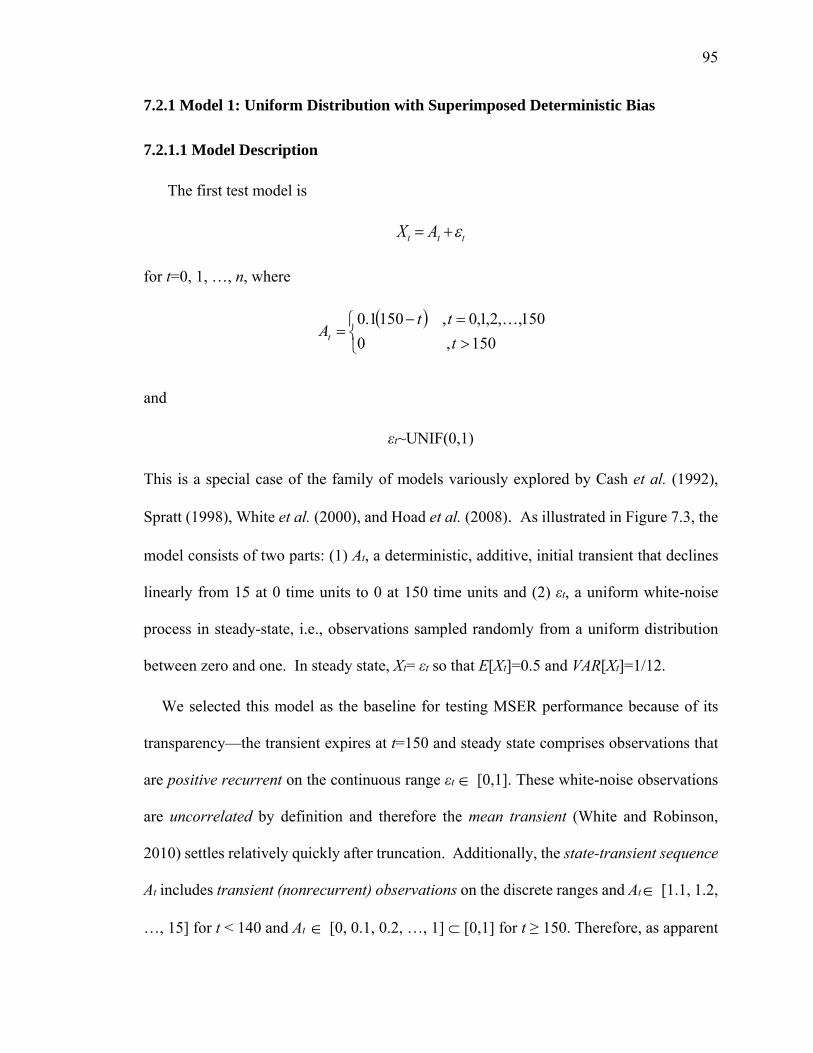
95
7.2.1 Model 1: Uniform Distribution with Superimposed Deterministic Bias
7.2.1.1 Model Description
The first test model is
for t=0, 1, …, n, where
150,0
150,,2,1,0,1501.0
t
ttAt
and
εt~UNIF(0,1)
This is a special case of the family of models variously explored by Cash et al. (1992),
Spratt (1998), White et al. (2000), and Hoad et al. (2008). As illustrated in Figure 7.3, the
model consists of two parts: (1) At, a deterministic, additive, initial transient that declines
linearly from 15 at 0 time units to 0 at 150 time units and (2) εt, a uniform white-noise
process in steady-state, i.e., observations sampled randomly from a uniform distribution
between zero and one. In steady state, Xt= εt so that E[Xt]=0.5 and VAR[Xt]=1/12.
We selected this model as the baseline for testing MSER performance because of its
transparency—the transient expires at t=150 and steady state comprises observations that
are positive recurrent on the continuous range εt [0,1]. These white-noise observations
are uncorrelated by definition and therefore the mean transient (White and Robinson,
2010) settles relatively quickly after truncation. Additionally, the state-transient sequence
At includes transient (nonrecurrent) observations on the discrete ranges and At [1.1, 1.2,
…, 15] for t < 140 and At [0, 0.1, 0.2, …, 1] [0,1] for t ≥ 150. Therefore, as apparent
Xt At t
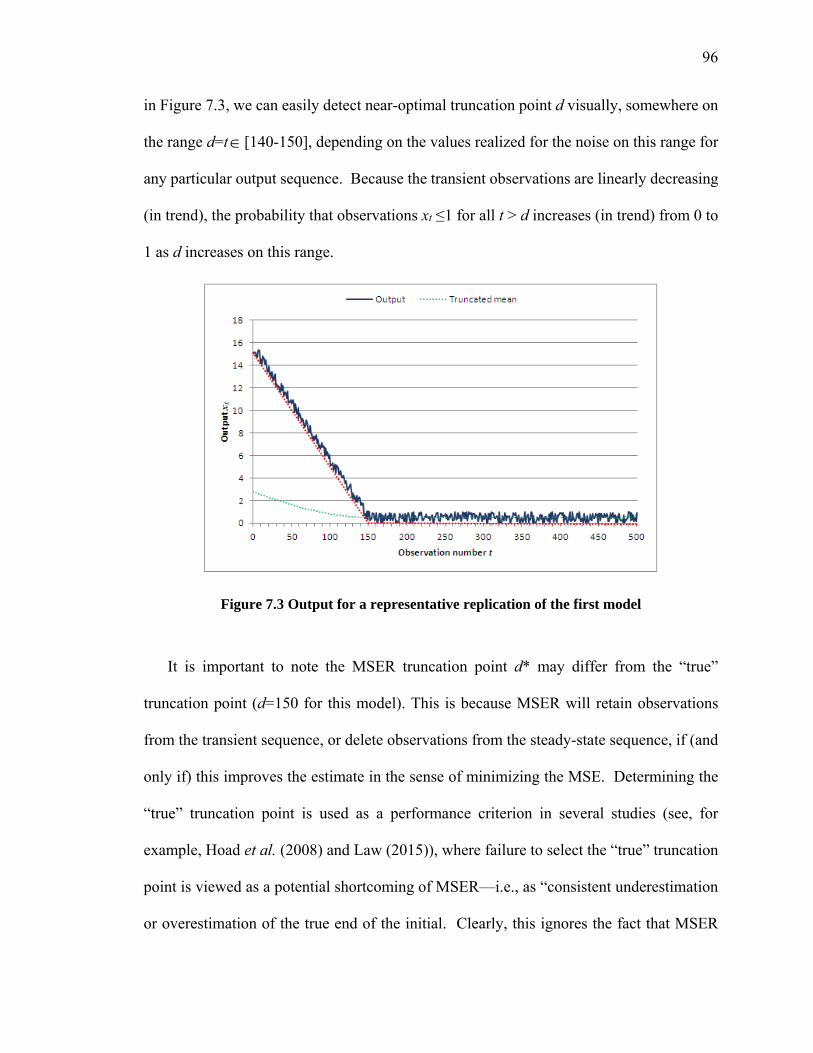
96
in Figure 7.3, we can easily detect near-optimal truncation point d visually, somewhere on
the range d=t [140-150], depending on the values realized for the noise on this range for
any particular output sequence. Because the transient observations are linearly decreasing
(in trend), the probability that observations xt ≤1 for all t > d increases (in trend) from 0 to
1 as d increases on this range.
Figure 7.3 Output for a representative replication of the first model
It is important to note the MSER truncation point d* may differ from the “true”
truncation point (d=150 for this model). This is because MSER will retain observations
from the transient sequence, or delete observations from the steady-state sequence, if (and
only if) this improves the estimate in the sense of minimizing the MSE. Determining the
“true” truncation point is used as a performance criterion in several studies (see, for
example, Hoad et al. (2008) and Law (2015)), where failure to select the “true” truncation
point is viewed as a potential shortcoming of MSER—i.e., as “consistent underestimation
or overestimation of the true end of the initial. Clearly, this ignores the fact that MSER

97
leads to superior estimates in the sense of MSE by not selecting the “true” point (White
and Hwang, 2015).
7.2.1.2 Results: Batch size effects for long runs
To explore the combined effect of batching and run length on MSER performance, we
ran 1,000 independent replications of Model 1 with batch sizes b=1, 5, and 10. Initially,
we chose a run length of n=10,000 observations, noting that this run length should be
several orders of magnitude longer than the state-transient sequence regardless of the batch
size.
Table 7.1 and Figure 7.4 confirm the effectiveness of MSER truncation for the first
model in terms of both the accuracy and precision of the estimated steady-state mean.
While the confidence intervals for batch sizes of 5 and 10 do not quite cover the true mean,
all of the estimates are accurate to three significant figures. Note, also, that the small errors
in the estimates are all negative, while the biasing observations are greater than the steady-
state mean. From this we conclude that for this instance
(1) all batch sizes remove all of the transient observations, and
(2) estimation errors are an artifact of sampling after the biasing effect of the initial
transient has been removed.
As shown in Figure 7.5, the sampling distributions of the mean are nearly normal, as
predicted by the Central Limit Theorem, and nearly identical for all batch sizes. From this
we conclude that for this instance
(3) modest batching has no significant effect on the quality of estimates.

98
Table 7.1 95% confidence intervals for the mean and variance for the truncated mean output as a function of batch size for batch sizes b=1, 5, and 10 for run length n=10,000
Truncated Mean Batch Size 1 Batch Size 5 Batch Size 10 Sample Mean 0.499825 0.499789 0.499777 Upper limit 0.500000 0.499965 0.499955 Lower limit 0.499649 0.499614 0.499602
Sample Std Dev 0.002850 0.002851 0.002829 Upper limit 0.002960 0.002961 0.002959 Lower limit 0.002711 0.002712 0.002711
Table 7.2 shows that the mean number of observations truncated (as distinct from the
number of batches truncated) is an increasing function of batch size. For batch size of b=1,
the mean truncation is between t=145 and t=150, as anticipated. For batch sizes of b=5
and 10, the means are modestly larger. These differences are statistically significant at the
95% confidence level with greater truncation for larger batches on average.
(a)
(b)
Figure 7.4 95% confidence intervals for (a) the truncated means for run lengths n=10000 and batch sizes b=1, 5, 10 and (b) the sample standard deviation in the estimated means for run lengths n=10000 and batch sizes b=1, 5, 10
0.4994
0.4995
0.4996
0.4997
0.4998
0.4999
0.5
0.5001
b=1 b=5 b=100.00255
0.0026
0.00265
0.0027
0.00275
0.0028
0.00285
0.0029
0.00295
0.003
b=1 b=5 b=10

99
Figure 7.5 Fits to the steady-state sampling distributions of the mean for 1000 replications for run length n=10,000. Fits for all three batch sizes tested are nearly identical for batch
sizes b=1, 5, and 10
Table 7.2 . 95% confidence intervals for the mean and variance for the number of observations truncated for batch sizes b=1, 5, and 10 for run length n=10,000
Observations Truncated Batch Size 1 Batch Size 5 Batch Size 10
Sample Mean 146.9190 152.5950 157.8500
Upper limit 147.0289 155.2085 159.1441
Lower limit 146.8091 151.9817 156.5159
Sample Std Dev 1.7708 9.8858 21.1764
Upper limit 1.8520 10.5571 22.1477
Lower limit 1.6964 9.4688 20.2872
(a)
(b)
Figure 7.6 95% confidence intervals for (a) the MSER mean and (b) the standard deviation in the MSER truncation point for run lengths n=10000 and batch sizes b=1, 5, 10
146
148
150
152
154
156
158
160
b=1 b=5 b=100
5
10
15
20
25
b=1 b=5 b=10

100
The scatter diagram in Figure 7.7, the frequency histogram in Figure 7.8, and the
correlation coefficients in Table 7.3 illustrate the relationship between the truncated means
and the corresponding total number of observations truncated. We conclude that for this
instance
(4) increasing batch sizes increases both the variance and spread of the truncated
observations, without systematically affecting the accuracy of the estimated mean,
(5) the mean estimate is uncorrelated with the number of observations truncated for
all the batch sizes, and
(6) the success of a truncation procedure in terms of the accuracy of the estimate
cannot be imputed from the truncation point alone.
Figure 7.7 Scatterplots of the truncated mean vs. the number of observations truncated for
batch sizes b=1, 5, and 10 for run length n=10,000
0.3
0.5
0.7
0.9
1.1
100 150 200 250 300 350 400
Tru
nca
ted
Mea
n
Number of Observations Truncated
Batch Size of 1 Batch Size of 5 Batch Size of 10

101
Figure 7.8 Frequency distribution of the total number of observations truncated as a
function of batch size for batch sizes b=1, 5, and 10 for run length n=10,000
Table 7.3 Correlation between the truncated mean and the number of observations truncated for batch sizes b=1, 5, and 10 for run length n=10,000.
Linear Correlation Table Trunc Batch=1 Trunc Batch=5 Trunc Batch=10
Mean Batch=1 -0.054 -0.011 0.075
Mean Batch=5 -0.046 -0.015 0.072
Mean Batch=10 -0.045 -0.014 0.076
As can be seen in Figure 7.8, increasing the batch size tends to increase the number of
observations truncated in part because of the increased granularity—with larger batches
there are fewer candidate truncation points to consider. But this trend also reflects the
difference between the “true” and MSER truncation points. To further explore, consider
output for replication 958. The MSER truncation points for batches of b=1, 5, and 10 are
d*=148, 190, and 590 respectively, where 590 is the largest truncation point observed
across all replications of with all batch sizes.

102
The batch means and MSER statistic for that replication are plotted against the first 500
observations in Figure 7.9. Figure 7.10 provides a closer look these data for b=10 on the
range t [100, 1500], i.e., batches 10 through 150. The mean for batch number 59 is
0.1524185, which is nearly 4 standard deviations below the steady-state mean. Given the
length of the reserved sequence for this truncation point (941 batches), MSER can improve
the estimate of the mean by deleting this observation.
Finally, we note that in general there are two effects of batching. First, the sequence is
whitened, decreasing any serial correlation in the batch means. Second, the sequence is
smoothed, altering the form of the steady-state distribution, decreasing any skew, and
making the resulting distribution more nearly normal. These effects are consequences of
the Central Limit Theorem.
Figure 7.9 Batched means and MSER statistic for the first 500 observations for replication 958 for batch sizes b=1, 5, and 10 for run length n=10,000
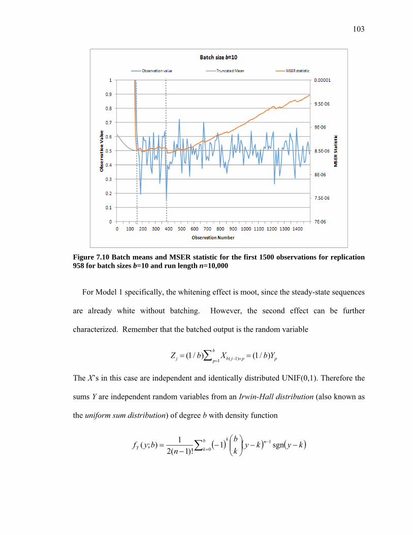
103
Figure 7.10 Batch means and MSER statistic for the first 1500 observations for replication 958 for batch sizes b=10 and run length n=10,000
For Model 1 specifically, the whitening effect is moot, since the steady-state sequences
are already white without batching. However, the second effect can be further
characterized. Remember that the batched output is the random variable
The X’s in this case are independent and identically distributed UNIF(0,1). Therefore the
sums Y are independent random variables from an Irwin-Hall distribution (also known as
the uniform sum distribution) of degree b with density function
kykyk
b
nbyf nkb
kY
sgn1)!1(2
1);( 1
0
Z j (1 / b) Xb( j1)pp1
b (1 / b)Yp
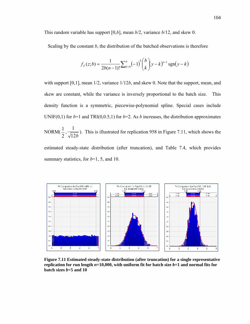
104
This random variable has support [0,b], mean b/2, variance b/12, and skew 0.
Scaling by the constant b, the distribution of the batched observations is therefore
kykyk
b
nbbzf nkb
kZ
sgn1)!1(2
1);( 1
0
with support [0,1], mean 1/2, variance 1/12b, and skew 0. Note that the support, mean, and
skew are constant, while the variance is inversely proportional to the batch size. This
density function is a symmetric, piecewise-polynomial spline. Special cases include
UNIF(0,1) for b=1 and TRI(0,0.5,1) for b=2. As b increases, the distribution approximates
NORM( , ). This is illustrated for replication 958 in Figure 7.11, which shows the
estimated steady-state distribution (after truncation), and Table 7.4, which provides
summary statistics, for b=1, 5, and 10.
Figure 7.11 Estimated steady-state distribution (after truncation) for a single representative replication for run length n=10,000, with uniform fit for batch size b=1 and normal fits for batch sizes b=5 and 10
1
2
1
12b

105
Table 7.4 Summary statistics for the steady-state data given in Figure 7.11.
b=1 b=5 b=10 Mean 0.50246 0.50267 0.50511 Mode ≈0.85641 ≈0.55255 ≈0.48050 Median 0.50874 0.50217 0.50017 Std Dev 0.28949 0.12662 0.08857 Variance 0.085804 0.016055 0.007845 b*Var 0.085804 0.080165 0.078446 1/12 0.085555 0.085555 0.085555 Skewness -0.0271 -0.0582 0.1771 Kurtosis 1.7926 2.8118 2.8455
Interestingly, we can show that for this model the MSER statistic itself is independent
of the batch size and decreases linearly as a function of run length. Let nb=n/b be the
number of batches in the reserved sequence and let Varb=1/12b be the variance for this
sequence. The MSER statistic is then
MSER(n,b)= Varb/nb= (1/12b)/(n/b)=1/12n.
7.2.1.3 Results: Batch size effects for short runs
The preceding results suggest that mean estimates are both empirically and
theoretically insensitive to batch size for Model 1. These results are derived using a run
length that is several orders of magnitude longer than the state-transient sequence,
however, and one might anticipate that results for much shorter runs will differ. To explore
this intuition, we repeated the analysis with run lengths of n=175, 200, 300, and 500
observations.

106
Results are displayed in Figures 7.12-7.15. The overall effect of reducing runs lengths
is to rotate the centerline of the scatter plots from one that is essentially horizontal to one
that is increasingly vertical, implying an increasingly negative correlation between the
number of observations truncated and the run length. The average and spread of the
number of observations deleted both decrease; the average and spread of the estimated
steady-state mean both increase. The strength of this effect increases as the batch size
increases.
For n=500, the larger batch sizes continue to yield additional truncation beyond the
[140,150] range in some instances, for the same reasons illustrated earlier. The difference
is that the largest truncation points are now for b=5, instead of b=10.
For n=500 and n=200, the results are essentially identical. Nearly all of the truncation
points are on the anticipated range [140,150], none are less than 140, and comparatively
few are greater than 150. The smallest truncation points are now associated with the
largest batch sizes—a complete reversal from the results obtained with long runs. Indeed,
for b=5 almost all of the truncation points are 145 or 150; for b=10 the truncation point is
140 for all 1000 replications.
For n=175, the effects of very short sequences are most pronounced. The truncation
points for b=1 rarely exceed 150. For b=5 all of the truncation points are 145. For b=10
almost all are 140, with a very few at 150.
Note that for n=175 and b=10, all of the estimates suffer from the effect of bias, some
acutely. This is because algorithm sees very little data—a total of 17 batches, only two of
which are in steady state. Depending on the realization of the noise process, MSER bases
its estimate on either two or three batch means. For those few replications where a third

107
(nonrecurrant) observation is retained, estimates are about twice the steady-state mean. For
this combination of batching and run length, correlation between the truncation point and
error in the mean estimate is strongest, with greater truncation leading to greater error in
the mean estimates.
All of the effects noted are consequences of the relative weight MSER gives the sample
size of the reserved sequence (nb-d) and the residuals of the observations . For
larger samples, MSER is relatively less sensitive to the sample size; for small samples
MSER is relatively more sensitive to the sample size. Therefore, we conclude for Model
1 that
(1) to the degree that batching reduces the effective sample size, it is not
recommended for small samples and provides no discernable benefit for large
samples, and
(2) even with very little steady-state data, the MSER-indicated truncation points are
themselves very reasonable and indeed optimal in terms of the mean estimates
for most cases.
(3) the choice of dmax is a binding concern only if (n-d)/n is close to 1—the choice of
n is likely dominated by the need for estimates with acceptable accuracy and
precision.
Finally, and perhaps most importantly, all of the results above use all of the simulation
replications, which is equivalent to setting the maximum truncation point at dmax=n. What
happens if, instead, we impose the recommend threshold dmax=n/2 and discard replications
for which d*>dmax? We can see from the results that (1) for n=10,000 and 500, the
threshold has no effect on the results; (2) for n=300, however, a significant number of
(xt x )

108
replications are discarded for b=5 and 10; and (3) for n=200 and 175, all of the replications
will be discarded! We conclude that, for this model,
(4) the d*≤dmax=n/2 threshold provides significant protection against estimation
errors resulting from run lengths that are too short’ without over-truncation of
replications with adequate run lengths. For run lengths that are approximately the
same as ideal truncation point, however, the protection may be inadequate. A
modestly lower threshold would be preferred.

109
Figure 7.12 Scatterplots of the truncated mean vs. the number of observations truncated
batch sizes b=1, 5, and 10 for run lengths n=175, 200, 500, and 500
0.3
0.4
0.5
0.6
0.7
0.8
0.9
1
1.1
1.2
130 180
TruncatedMean
ObservationsTruncated
RunLengthn=500
BatchSizeof1 BatchSizeof5 BatchSizeof10
0.3
0.4
0.5
0.6
0.7
0.8
0.9
1
1.1
1.2
130 150 170 190
TruncatedMean
ObservationsTruncated
RunLengthn=300
BatchSizeof1 BatchSizeof5 BatchSizeof10
0.3
0.4
0.5
0.6
0.7
0.8
0.9
1
1.1
1.2
130 150 170 190
TruncatedMean
ObservationsTruncated
RunLengthn=200
BatchSizeof1 BatchSizeof5 BatchSizeof10
0.3
0.4
0.5
0.6
0.7
0.8
0.9
1
1.1
1.2
130 150 170 190
TruncatedMean
ObservationsTruncated
RunLengthn=175
BatchSizeof1 BatchSizeof5 BatchSizeof10

110
Figure 7.13 Frequency distribution of the total number of observations truncated as a function of batch size for batch sizes b=1, 5, and 10 for run lengths of n=175, 200, 500, 500
020040060080010001200
130
132
134
136
138
140
142
144
146
148
150
152
154
156
158
160
162
164
>165
NumberofReplications
NumberofObservationsTruncated
RunLengthn=500
BatchSizeof1 BatchSizeof5 BatchSizeof10
020040060080010001200
130
132
134
136
138
140
142
144
146
148
150
152
154
156
158
160
162
164
>165
NumberofReplications
NumberofObservationsTruncated
RunLengthn=300
BatchSizeof1 BatchSizeof5 BatchSizeof10
020040060080010001200
130
132
134
136
138
140
142
144
146
148
150
152
154
156
158
160
162
164
>165
NumberofReplications
NumberofObservationsTruncated
RunLengthn=200
BatchSizeof1 BatchSizeof5 BatchSizeof10
020040060080010001200
130
132
134
136
138
140
142
144
146
148
150
152
154
156
158
160
162
164
>165
NumberofReplications
NumberofObservationsTruncated
RunLengthn=175
BatchSizeof1 BatchSizeof5 BatchSizeof10

111
n = 175
n = 200
n = 300
n = 500
Figure 7.14 95% confidence intervals of the mean for the truncated mean output as a function of batch size for batch sizes b=1, 5, and 10 for run lengths of n=175, 200, 300, 500

112
n = 175
n = 200
n = 300
n = 500
Figure 7.15 95% confidence intervals for the mean for the number of observations truncated for batch sizes b=1, 5, and 10 for run lengths of n=175, 200, 300, 500
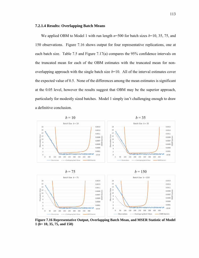
113
7.2.1.4 Results: Overlapping Batch Means
We applied OBM to Model 1 with run length n=500 for batch sizes b=10, 35, 75, and
150 observations. Figure 7.16 shows output for four representative replications, one at
each batch size. Table 7.5 and Figure 7.17(a) compares the 95% confidence intervals on
the truncated mean for each of the OBM estimates with the truncated mean for non-
overlapping approach with the single batch size b=10. All of the interval estimates cover
the expected value of 0.5. None of the differences among the mean estimates is significant
at the 0.05 level, however the results suggest that OBM may be the superior approach,
particularly for modestly sized batches. Model 1 simply isn’t challenging enough to draw
a definitive conclusion.
b = 10 b = 35
b = 75
b = 150
Figure 7.16 Representative Output, Overlapping Batch Mean, and MSER Statistic of Model 1 (b= 10, 35, 75, and 150)

114
Table 7.5 95% confidence intervals for Model 1 on the truncated mean and the standard deviation for overlapping and non-overlapping batches
OBM NOBM
OBM b=10 OBM b=35 OBM b=75 OBM b=150 NOBM b=10
Sample Mean 0.50005 0.49993 0.49965 0.50028 0.49934
Upper limit 0.50104 0.50096 0.50071 0.50138 0.50082
Lower limit 0.49906 0.4989 0.4986 0.49919 0.49786
Sample Std D 0.01602 0.01661 0.017 0.01762 0.02383
Upper limit 0.01675 0.01737 0.01777 0.01843 0.02492
Lower limit 0.01534 0.01591 0.01628 0.01688 0.02283
(a)
(b)
Figure 7.17 95% confidence intervals for Model 1 on (a) the truncated mean for overlapping and non-overlapping batches and (b) the standard deviation for overlapping and non-overlapping batches
In contrast, Figure 7.17(b) compares the 95% confidence intervals on the standard
deviation in estimates for the same replications. While the differences among OBM
estimates are not significant, OBM outperforms the non-overlapping approach in all cases.
At least for this test case, OBM provides significantly greater precision in the estimate.
This reflects the considerably larger sample size afforded by overlapping batches.
0.497
0.498
0.499
0.5
0.501
0.502
OBMb=10
OBMb=35
OBMb=75
OBMb=150
NOBMb=10
0.01
0.015
0.02
0.025
OBMb=10
OBMb=35
OBMb=75
OBMb=150
NOBMb=10

115
Figure 7.18 Scatterplots of the truncated mean vs. the number of observations truncated for OBM sizes b=10, 35, 75 and 150 for run length of n=500 for Model 1 (including NOBM batch size of 10)
Figure 7.19 Frequency distribution of the number of observations truncated as a function of OBM sizes b=10, 35, 75, and 150 for run length of n=500 for Model 1 (including NOBM batch size of 10)

116
Table 7.6. Correlation between the truncated mean and the number of observations truncated for OBM sizes b=10, 35, 75, 150 for run length of n=500 for Model 1
Trunc Batch =10 Trunc Batch =35 Trunc Batch =75 Trun Batch = 150
Mean Batch = 10 -0.006655114 0.001668587 0.002054254 -0.177174472
Mean Batch = 35 0.000478214 -0.0644325 -0.087803961 -0.282730256
Mean Batch = 75 -0.003975614 -0.073941266 -0.156501886 -0.302717128
Mean Batch = 150 -0.027110964 -0.046266742 -0.076909778 -0.346795267
7.2.2 Model 2: Waiting Time in an M/M/1
The second test model is an M/M/1 queue where our interest is in estimating the mean
waiting-time in queue. This is the problem examined by Law (2015) and reexamined by
White and Hwang (2015). We used this second model to ascertain the performance of
MSER with the same batch sizes used in Model 1. In addition, we explored the sensitivity
of estimates to changes in traffic intensity, the quotient
where is arrival rate, is service rate, and the expected waiting time in queue is
.
The theoretical expected values of waiting time in queue for four different traffic
intensities are summarized in Table 7.7. Clearly, the autocorrelation of successive
observations of the waiting time is a function of the traffic intensity. For very low ,
customers typically arrive at an empty and idle queue and do not have to wait for service.
As the traffic intensity increases, customers experience increasingly longer waits on
average. For 1, the demand for service exceeds the supply, the queue is unstable, and
average waiting times become infinite. One might anticipate the effects of decreasing to
be similar to those encountered by increasing the run length n.
)( qWE

117
Table 7.7. Theoretical Waiting Time in Queue by Traffic Intensity Traffic Intensity
0.6 0.7 0.8 0.9
Waiting Time in Queue 9 16.33 32 81
7.2.2.1 Results for Model 2 with traffic intensity of 0.90
Figure 7.20 Representative Output of Waiting-Time in an M/M/1 with Traffic Intensity of
0.9 (n = 64000; Blue line: E(Wq)=81)
Figure 7.20 provides a typical output series from M/M/1 queue with traffic intensity of
=0.9, initialized empty and idle (x0=0), for a run length of n=64,000. The output is said to
be regenerative, in that it comprises independent cycles each beginning with a customer
that experiences zero waiting. The system regenerates at when it returns to this same zero
state and a new cycle begins. The duration of each cycle is random, as is the peak waiting
time. Decreasing the traffic intensity will result in an increasing number of cycles and
generally shorter peak waiting times.
We begin our analysis with the application of MSER to Model 2 and explore the
combined impact of alternative batch sizes (b=1, 5, and 10) and run lengths (n=64,000,
32,000, 16,000, 8,000, 4,000, 2000, and 1,000). Our analysis follows the same steps
( )

118
introduced in the analysis of Model 1. For M/M/1 with =0.9, Figure 7.21 compares the
confidence intervals on the sample means, Figure 7.22 compares the confidence intervals
on the MSER truncation points, Figure 7.23 compares scatterplots of the truncated mean
vs. the number of observations truncated, Table 7.8 provides the corresponding correlation
coefficients, and Figure 7.24 compares the frequency histograms of the number of
observations truncated.
Without truncation, the raw sample mean is 80.75 and insensitive to batch size. While
the raw estimate does not provide coverage, the absolute estimation error is less than 1%.
The truncated is mean 79.39 and also insensitive to batch size. While the truncated estimate
likewise does not provide coverage, the absolute estimation error is less than 2%. The
improvement result from truncation is very modest, but the difference in estimates is
statistically significant at =0.05.
As the run length deceases, the raw estimate decreases more slowly than the truncated
estimate. For run lengths of n=8,000 and below, the truncated means are exceptionally
poor and far worse than the raw estimates. In general, the number of observations truncated
decreases with as the run length decreases.
For the larger run lengths, we see that the mean estimates for this problem are quite good
without truncation. Truncation improves on these estimates only for n=64,000 and then
only very modestly. Truncation is contraindicated for smaller n. While there is negative
trend in the estimated mean for larger truncation points, the correlation is negligible, but
increasing in decreasing run length and increasing batch size.

119
n = 64000
n = 32000
n = 16000
n = 8000
n = 4000
n=2000
n = 1000
Figure 7.21 95% confidence intervals for the mean and the truncated mean as a function of batch size (b= 1, 5, and 10) and run length (n=1000, 2000, 4000, 8000, 16000, 32000, and 64000) for Model 2 with traffic intensity of 0.9 (Theoretical mean of 81, Blue line)
40
50
60
70
80
90
MSER b= 1
Raw b =1
MSER b= 5
Raw b =5
MSER b= 10
Raw b =10
40
50
60
70
80
90
MSER b= 1
Raw b =1
MSER b= 5
Raw b =5
MSER b= 10
Raw b =10
40
50
60
70
80
90
MSER b= 1
Raw b =1
MSER b= 5
Raw b =5
MSER b= 10
Raw b =10
40
50
60
70
80
90
MSER b= 1
Raw b =1
MSER b= 5
Raw b =5
MSER b= 10
Raw b =10
40
50
60
70
80
90
MSER b= 1
Raw b =1
MSER b= 5
Raw b =5
MSER b= 10
Raw b =10
40
50
60
70
80
90
MSER b= 1
Raw b =1
MSER b= 5
Raw b =5
MSER b= 10
Raw b =10
40
50
60
70
80
90
MSERb = 1
Raw b= 1
MSERb = 5
Raw b= 5
MSERb = 10
Raw b= 10

120
n = 64000
n = 32000
n = 16000
n = 8000
n = 4000
n = 2000
n = 1000
Figure 7.22 95% confidence intervals for the mean number of observations truncated as a function of batch size (b= 1, 5, and 10) and run length (n=1000, 2000, 4000, 8000, 16000, 32000, and 64000) for Model 2 with traffic intensity of 0.9
0
500
1000
1500
2000
2500
MSER b = 1 MSER b = 5 MSER b = 100
500
1000
1500
2000
2500
MSER b = 1 MSER b = 5 MSER b = 100
500
1000
1500
2000
2500
MSER b = 1 MSER b = 5 MSER b = 10
0
400
800
1200
1600
MSER b = 1 MSER b = 5 MSER b = 100
400
800
1200
1600
MSER b = 1 MSER b = 5 MSER b = 100
400
800
1200
1600
MSER b = 1 MSER b = 5 MSER b = 10
0
200
400
600
800
MSER b = 1 MSER b = 5 MSER b = 10

121
n = 64000
n=32000
n=16000
n=8000
n=4000
n=2000
n=1000
Figure 7.23 Scatterplots of the truncated mean vs. the number of observations truncated for batch sizes b=1, 5, and 10 for run length of n=1000, 2000, 4000, 8000, 16000, 32000, and 64000 for Model 2 with traffic intensity of 0.9

122
Table 7.8 Correlation between the truncated mean and the number of observations truncated for batch sizes b=1, 5, and 10 for run length of n=1000, 2000, 4000, 8000, 16000, 32000, and 64000 for Model 2 with traffic intensity of 0.9.
Trunc
Batch =1
Trunc
Batch =5
Trunc
Batch =10
Mean
Batch = 1
-0.3053 -0.3019 -0.2748
Mean
Batch = 5
-0.3043 -0.3084 -0.2809
Mean
Batch = 10
-0.3003 -0.3044 -0.3170
Trunc
Batch =1
Trunc
Batch =5
Trunc
Batch =10
Mean
Batch = 1
-0.3966 -0.3687 -0.3455
Mean
Batch = 5
-0.4007 -0.4169 -0.3976
Mean
Batch = 10
-0.3854 -0.4271 -0.4542
Trunc
Batch =1
Trunc
Batch =5
Trunc
Batch =10
Mean
Batch = 1
-0.4969 -0.4433 -0.4129
Mean
Batch = 5
-0.4701 -0.5512 -0.5107
Mean
Batch = 10
-0.4570 -0.5315 -0.6101
n = 64000 n = 32000 n = 16000
Trunc
Batch =1
Trunc
Batch =5
Trunc
Batch =10
Mean
Batch = 1
-0.6038 -0.5261 -0.4629
Mean
Batch = 5
-0.5114 -0.6093 -0.5238
Mean
Batch = 10
-0.4389 -0.5163 -0.6100
Trunc
Batch =1
Trunc
Batch =5
Trunc
Batch =10
Mean
Batch = 1
-0.6189 -0.5190 -0.4686
Mean
Batch = 5
-0.4419 -0.5714 -0.5130
Mean
Batch = 10
-0.2854 -0.3969 -0.5295
Trunc
Batch =1
Trunc
Batch =5
Trunc
Batch =10
Mean
Batch = 1
-0.3427 -0.3867 -0.4123
Mean
Batch = 5
-0.3770 -0.4592 -0.4741
Mean
Batch = 10
-0.3774 -0.4446 -0.5150
n = 8000 n = 4000 n = 2000
Trunc
Batch =1
Trunc
Batch =5
Trunc
Batch =10
Mean
Batch = 1
-0.0820 -0.2141 -0.2591
Mean
Batch = 5
-0.1102 -0.2270 -0.2725
Mean
Batch = 10
-0.1215 -0.2397 -0.2805
n = 1000

123
n = 64000
n = 32000
n = 16000
n = 8000
n = 4000
n = 2000
n = 1000
Figure 7.24 Frequency distribution of the number of observations truncated as a function of batch sizes b=1, 5, and 10 for run length of n=1000, 2000, 4000, 8000, 16000, 32000, and 64000 for Model 2 with traffic intensity of 0.9
0
200
400
600
800
Num
ber
of R
eplic
atio
ns
Number of Observations Truncated
Batch Size of 1 Batch Size of 5 Batch Size of 10
0100200300400500600700
Num
ber
of R
eplic
atio
ns
Number of Observations Truncated
Batch Size of 1 Batch Size of 5 Batch Size of 10
0100200300400500600700
Num
ber
of R
eplic
atio
ns
Number of Observations Truncated
Batch Size of 1 Batch Size of 5 Batch Size of 10
0
200
400
600
800
0 250 500 1000 2000 4000 8000
Num
ber
of R
eplic
atio
ns
Number of Observations Truncated
Batch Size of 1 Batch Size of 5 Batch Size of 10
0
200
400
600
0 250 500 1000 2000 4000
Num
ber
of R
eplic
atio
ns
Number of Observations Truncated
Batch Size of 1 Batch Size of 5 Batch Size of 10
0
200
400
600
0 250 500 1000 2000
Num
ber
of R
eplic
atio
ns
Number of Observations Truncated
Batch Size of 1 Batch Size of 5
Batch Size of 10
0
200
400
600
0 250 500 <1000
Num
ber
of R
eplic
atio
ns
Number of Observations Truncated
Batch Size of 1 Batch Size of 5 Batch Size of 10

124
7.2.2.2 Results for Model 2 with traffic intensity of 0.80
Figure 7.25 Example of M/M/1 with traffic intensity of 0.8 (n = 16000, Blue line: E(X))
n = 16000
n = 8000
n = 4000
n = 2000
n = 1000
Figure 7.26 95% confidence intervals of the mean for the truncated mean output as a function of batch size (b= 1, 5, and 10) and run length (n=1000, 2000, 4000, 8000, and 16,000) for Model 2 with traffic intensity of 0.80 (Theoretical mean of 32, Blue line)
7
12
17
22
27
32
37
MSERb = 1
Rawb = 1
MSERb = 5
Rawb = 5
MSERb = 10
Rawb = 10
7
12
17
22
27
32
37
MSERb = 1
Rawb = 1
MSERb = 5
Rawb = 5
MSERb = 10
Rawb = 10
7
12
17
22
27
32
37
MSERb = 1
Rawb = 1
MSERb = 5
Rawb = 5
MSERb = 10
Rawb = 10
7
12
17
22
27
32
37
MSERb = 1
Rawb = 1
MSERb = 5
Rawb = 5
MSERb = 10
Rawb = 10
7
12
17
22
27
32
37
MSERb = 1
Rawb = 1
MSERb = 5
Rawb = 5
MSERb = 10
Rawb = 10

125
n = 16000
n = 8000
n = 4000
n = 2000
n = 1000
Figure 7.27 95% confidence intervals for the mean number of observations truncated as a function of batch size (b= 1, 5, and 10) and run length (n= 1000, 2000, 4000, 8000, and 16,000) for Model 2 with traffic intensity of 0.80
0
100
200
300
400
500
600
MSER b = 1 MSER b = 5 MSER b = 100
100
200
300
400
500
600
MSER b = 1 MSER b = 5 MSER b = 100
100
200
300
400
500
600
MSER b = 1 MSER b = 5 MSER b = 10
0
100
200
300
400
500
600
MSER b = 1 MSER b = 5 MSER b = 100
100
200
300
400
500
600
MSER b = 1 MSER b = 5 MSER b = 10
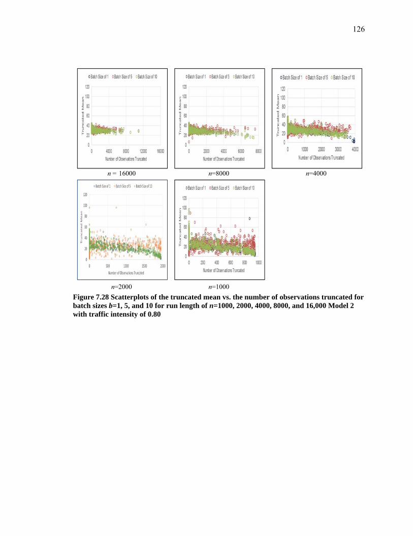
126
n = 16000
n=8000
n=4000
n=2000
n=1000
Figure 7.28 Scatterplots of the truncated mean vs. the number of observations truncated for batch sizes b=1, 5, and 10 for run length of n=1000, 2000, 4000, 8000, and 16,000 Model 2 with traffic intensity of 0.80

127
Table 7.9 Correlation between the truncated mean and the number of observations truncated for batch sizes b=1, 5, and 10 for run length of n=1000, 2000, 4000, 8000, and 16,000 for Model 2 with traffic intensity of 0.80
Trunc
Batch =1
Trunc
Batch =5
Trunc
Batch =10
Mean
Batch = 1
-0.2309 -0.2198 -0.1629
Mean
Batch = 5
-0.2305 -0.2509 -0.1892
Mean
Batch = 10
-0.2270 -0.2467 -0.2718
Trunc
Batch =1
Trunc
Batch =5
Trunc
Batch =10
Mean
Batch = 1
-0.3575 -0.2954 -0.1696
Mean
Batch = 5
-0.3339 -0.4310 -0.2472
Mean
Batch = 10
-0.3162 -0.3654 -0.4741
Trunc
Batch =1
Trunc
Batch =5
Trunc
Batch =10
Mean
Batch = 1
-0.5712 -0.3760 -0.3494
Mean
Batch = 5
-0.4004 -0.5596 -0.4806
Mean
Batch = 10
-0.3643 -0.4781 -0.5627
n = 16000 n = 8000 n = 4000
Trunc
Batch =1
Trunc
Batch =5
Trunc
Batch =10
Mean
Batch = 1
-0.6450 -0.0322 -0.0362
Mean
Batch = 5
0.0895 -0.7072 -0.6257
Mean
Batch = 10
0.1010 -0.6245 -0.7147
Trunc
Batch =1
Trunc
Batch =5
Trunc
Batch =10
Mean
Batch = 1
-0.5840 -0.5342 -0.5021
Mean
Batch = 5
-0.5326 -0.6471 -0.6008
Mean
Batch = 10
-0.4800 -0.5831 -0.6486
n = 2000 n = 1000
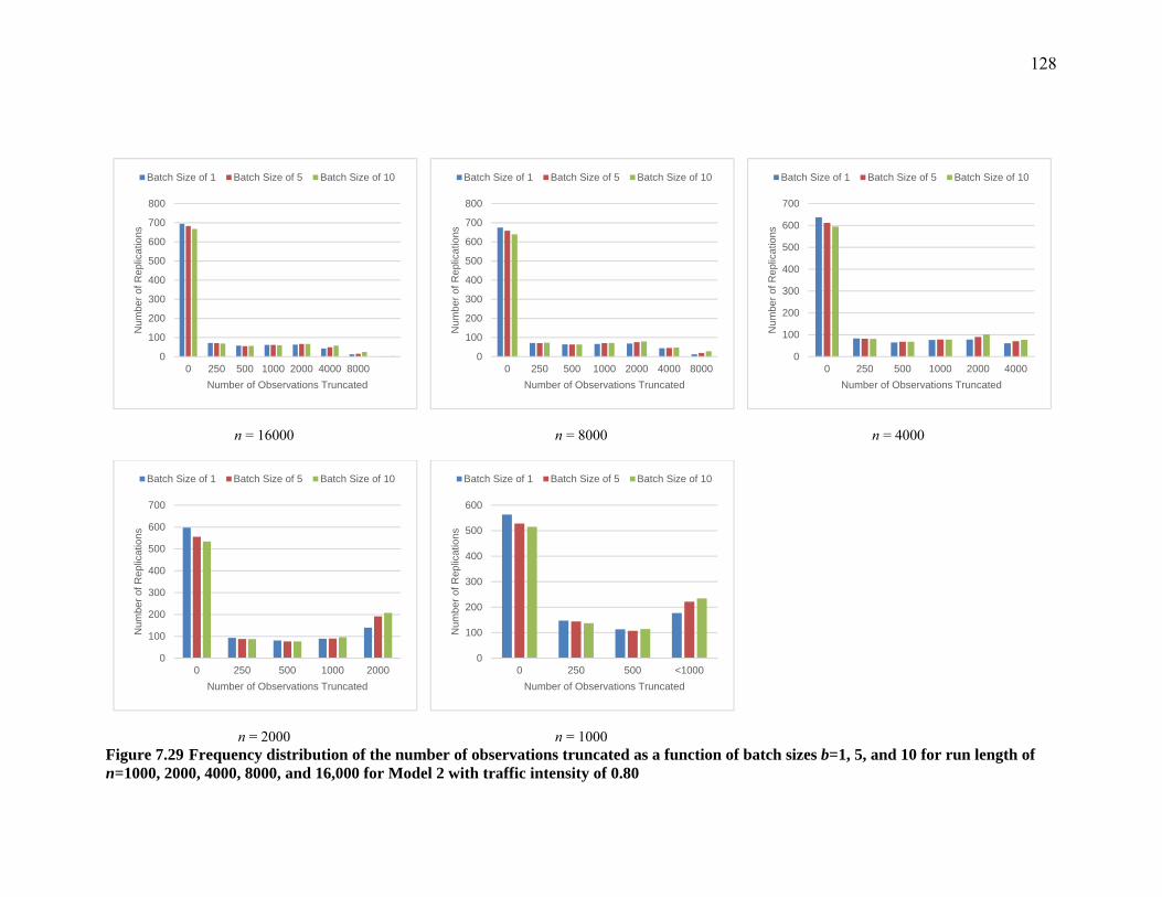
128
n = 16000 n = 8000 n = 4000
n = 2000 n = 1000 Figure 7.29 Frequency distribution of the number of observations truncated as a function of batch sizes b=1, 5, and 10 for run length of n=1000, 2000, 4000, 8000, and 16,000 for Model 2 with traffic intensity of 0.80
0
100
200
300
400
500
600
700
800
0 250 500 1000 2000 4000 8000
Num
ber
of R
eplic
atio
ns
Number of Observations Truncated
Batch Size of 1 Batch Size of 5 Batch Size of 10
0
100
200
300
400
500
600
700
800
0 250 500 1000 2000 4000 8000
Num
ber
of R
eplic
atio
ns
Number of Observations Truncated
Batch Size of 1 Batch Size of 5 Batch Size of 10
0
100
200
300
400
500
600
700
0 250 500 1000 2000 4000
Num
ber
of R
eplic
atio
ns
Number of Observations Truncated
Batch Size of 1 Batch Size of 5 Batch Size of 10
0
100
200
300
400
500
600
700
0 250 500 1000 2000
Num
ber
of R
eplic
atio
ns
Number of Observations Truncated
Batch Size of 1 Batch Size of 5 Batch Size of 10
0
100
200
300
400
500
600
0 250 500 <1000
Num
ber
of R
eplic
atio
ns
Number of Observations Truncated
Batch Size of 1 Batch Size of 5 Batch Size of 10
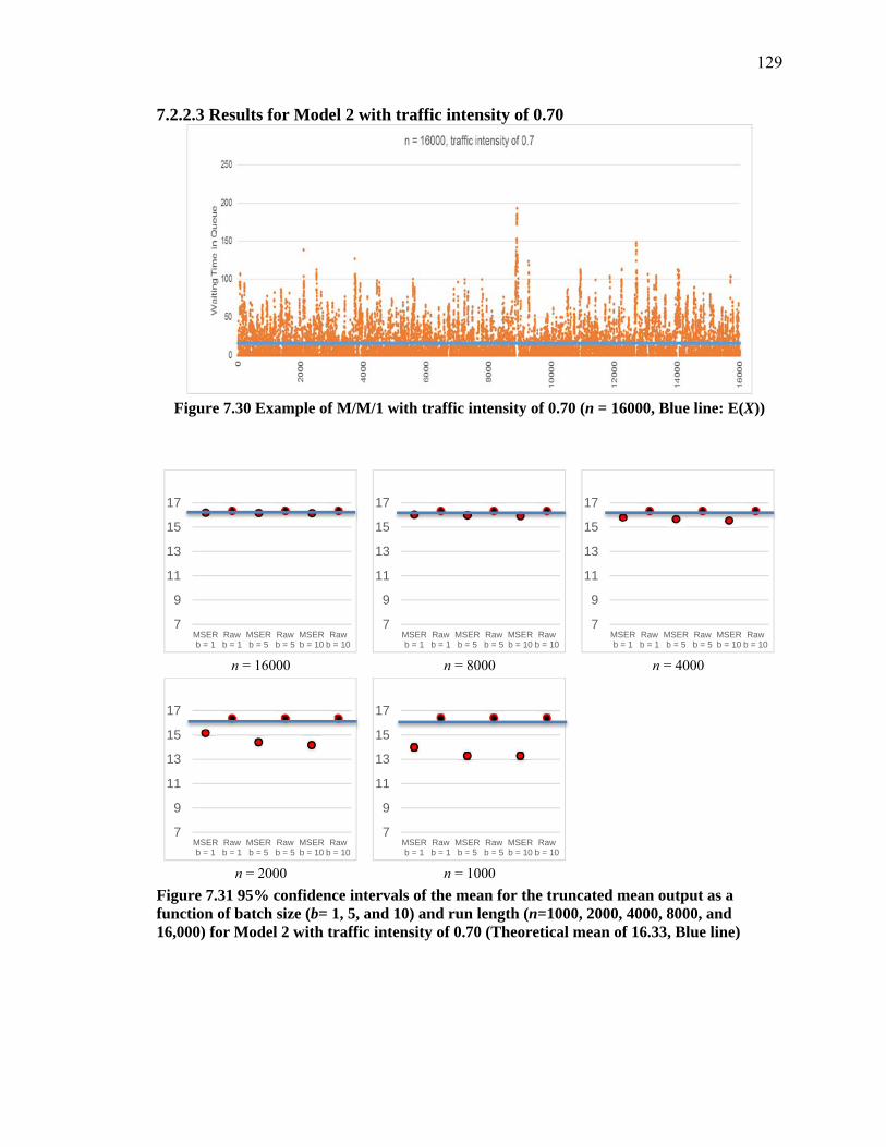
129
7.2.2.3 Results for Model 2 with traffic intensity of 0.70
Figure 7.30 Example of M/M/1 with traffic intensity of 0.70 (n = 16000, Blue line: E(X))
n = 16000
n = 8000
n = 4000
n = 2000
n = 1000
Figure 7.31 95% confidence intervals of the mean for the truncated mean output as a function of batch size (b= 1, 5, and 10) and run length (n=1000, 2000, 4000, 8000, and 16,000) for Model 2 with traffic intensity of 0.70 (Theoretical mean of 16.33, Blue line)
7
9
11
13
15
17
MSERb = 1
Rawb = 1
MSERb = 5
Rawb = 5
MSERb = 10
Rawb = 10
7
9
11
13
15
17
MSERb = 1
Rawb = 1
MSERb = 5
Rawb = 5
MSERb = 10
Rawb = 10
7
9
11
13
15
17
MSERb = 1
Rawb = 1
MSERb = 5
Rawb = 5
MSERb = 10
Rawb = 10
7
9
11
13
15
17
MSERb = 1
Rawb = 1
MSERb = 5
Rawb = 5
MSERb = 10
Rawb = 10
7
9
11
13
15
17
MSERb = 1
Rawb = 1
MSERb = 5
Rawb = 5
MSERb = 10
Rawb = 10

130
n = 16000
n = 8000
n = 4000
n = 2000
n = 1000
Figure 7.32 95% confidence intervals for the mean number of observations truncated as a function of batch size (b= 1, 5, and 10) and run length (n= 1000, 2000, 4000, 8000, and 16,000) for Model 2 with traffic intensity of 0.70
050
100150200250300350400450
MSER b =1
MSER b =5
MSER b =10
050
100150200250300350400450
MSER b =1
MSER b =5
MSER b =10
050
100150200250300350400450
MSER b =1
MSER b =5
MSER b =10
050
100150200250300350400450
MSER b =1
MSER b =5
MSER b =10
050
100150200250300350400450
MSER b =1
MSER b =5
MSER b =10

131
n = 16000
n=8000
n=4000
n=2000
n=1000
Figure 7.33 Scatterplots of the truncated mean vs. the number of observations truncated for batch sizes b=1, 5, and 10 for run length of n=1000, 2000, 4000, 8000, and 16,000 Model 2 with traffic intensity of 0.7

132
Table 7.10 Correlation between the truncated mean and the number of observations truncated for batch sizes b=1, 5, and 10 for run length of n=1000, 2000, 4000, 8000, and 16,000 for Model 2 with traffic intensity of 0.70
Trunc
Batch =1
Trunc
Batch =5
Trunc
Batch =10
Mean
Batch = 1
-0.2111 -0.1440 -0.1260
Mean
Batch = 5
-0.2043 -0.2309 -0.2020
Mean
Batch = 10
-0.2032 -0.2288 -0.2547
Trunc
Batch =1
Trunc
Batch =5
Trunc
Batch =10
Mean
Batch = 1
-0.2798 -0.1877 -0.0755
Mean
Batch = 5
-0.2774 -0.3459 -0.2021
Mean
Batch = 10
-0.2628 -0.3292 -0.3816
Trunc
Batch =1
Trunc
Batch =5
Trunc
Batch =10
Mean
Batch = 1
-0.3720 -0.1779 -0.1079
Mean
Batch = 5
-0.3015 -0.4755 -0.2573
Mean
Batch = 10
-0.2865 -0.3195 -0.4833
n = 16000 n = 8000 n = 4000
Trunc
Batch =1
Trunc
Batch =5
Trunc
Batch =10
Mean
Batch = 1
-0.5000 -0.2143 -0.1666
Mean
Batch = 5
-0.3846 -0.7016 -0.5412
Mean
Batch = 10
-0.3682 -0.5999 -0.7216
Trunc
Batch =1
Trunc
Batch =5
Trunc
Batch =10
Mean
Batch = 1
-0.6094 -0.4215 -0.4041
Mean
Batch = 5
-0.4924 -0.6921 -0.6256
Mean
Batch = 10
-0.4924 -0.6921 -0.6256
n = 2000 n = 1000
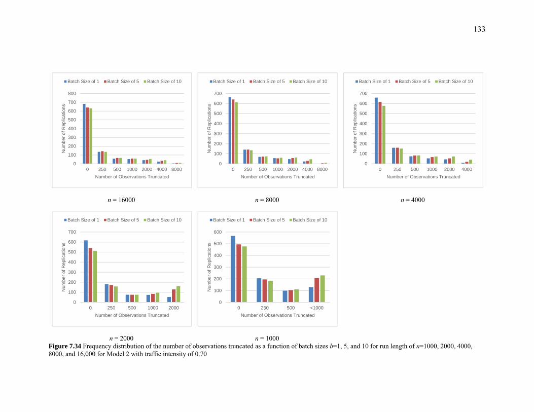
133
n = 16000 n = 8000 n = 4000
n = 2000 n = 1000 Figure 7.34 Frequency distribution of the number of observations truncated as a function of batch sizes b=1, 5, and 10 for run length of n=1000, 2000, 4000, 8000, and 16,000 for Model 2 with traffic intensity of 0.70
0
100
200
300
400
500
600
700
800
0 250 500 1000 2000 4000 8000
Num
ber
of R
eplic
atio
ns
Number of Observations Truncated
Batch Size of 1 Batch Size of 5 Batch Size of 10
0
100
200
300
400
500
600
700
0 250 500 1000 2000 4000 8000
Num
ber
of R
eplic
atio
ns
Number of Observations Truncated
Batch Size of 1 Batch Size of 5 Batch Size of 10
0
100
200
300
400
500
600
700
0 250 500 1000 2000 4000
Num
ber
of R
eplic
atio
ns
Number of Observations Truncated
Batch Size of 1 Batch Size of 5 Batch Size of 10
0
100
200
300
400
500
600
700
0 250 500 1000 2000
Num
ber
of R
eplic
atio
ns
Number of Observations Truncated
Batch Size of 1 Batch Size of 5 Batch Size of 10
0
100
200
300
400
500
600
0 250 500 <1000
Num
ber
of R
eplic
atio
ns
Number of Observations Truncated
Batch Size of 1 Batch Size of 5 Batch Size of 10

134
7.2.2.4 Results for Model 2 with traffic intensity of 0.60
Figure 7.35 Example of M/M/1 with traffic intensity of 0.60 (n = 16000, Blue line: E(X))
n = 16000
n = 8000
n = 4000
n = 2000
n = 1000
Figure.7.36 95% confidence intervals of the mean for the truncated mean output as a function of batch size (b= 1, 5, and 10) and run length (n=1000, 2000, 4000, 8000, and 16,000) for Model 2 with traffic intensity of 0.60 (Theoretical mean of 9, Blue line)
7
7.5
8
8.5
9
9.5
MSERb = 1
Rawb = 1
MSERb = 5
Rawb = 5
MSERb = 10
Rawb = 10
7
7.5
8
8.5
9
9.5
MSERb = 1
Rawb = 1
MSERb = 5
Rawb = 5
MSERb = 10
Rawb = 10
7
7.5
8
8.5
9
9.5
MSERb = 1
Rawb = 1
MSERb = 5
Rawb = 5
MSERb = 10
Rawb = 10
7
7.5
8
8.5
9
9.5
MSERb = 1
Rawb = 1
MSERb = 5
Rawb = 5
MSERb = 10
Rawb = 10
7
7.5
8
8.5
9
9.5
MSERb = 1
Rawb = 1
MSERb = 5
Rawb = 5
MSERb = 10
Rawb = 10

135
n = 16000
n = 8000
n = 4000
n = 2000
n = 1000
Figure 7.37 95% confidence intervals for the mean number of observations truncated as a function of batch size (b= 1, 5, and 10) and run length (n=1000, 2000, 4000, 8000, and 16,000) for Model 2 with traffic intensity of 0.60
0
50
100150
200
250300
350
MSER b =1
MSER b =5
MSER b =10
0
50
100150
200
250300
350
MSER b =1
MSER b =5
MSER b =10
0
50
100150
200
250300
350
MSER b =1
MSER b =5
MSER b =10
050
100
150200
250
300
350
MSER b =1
MSER b =5
MSER b =10
050
100
150200
250
300
350
MSER b =1
MSER b =5
MSER b =10
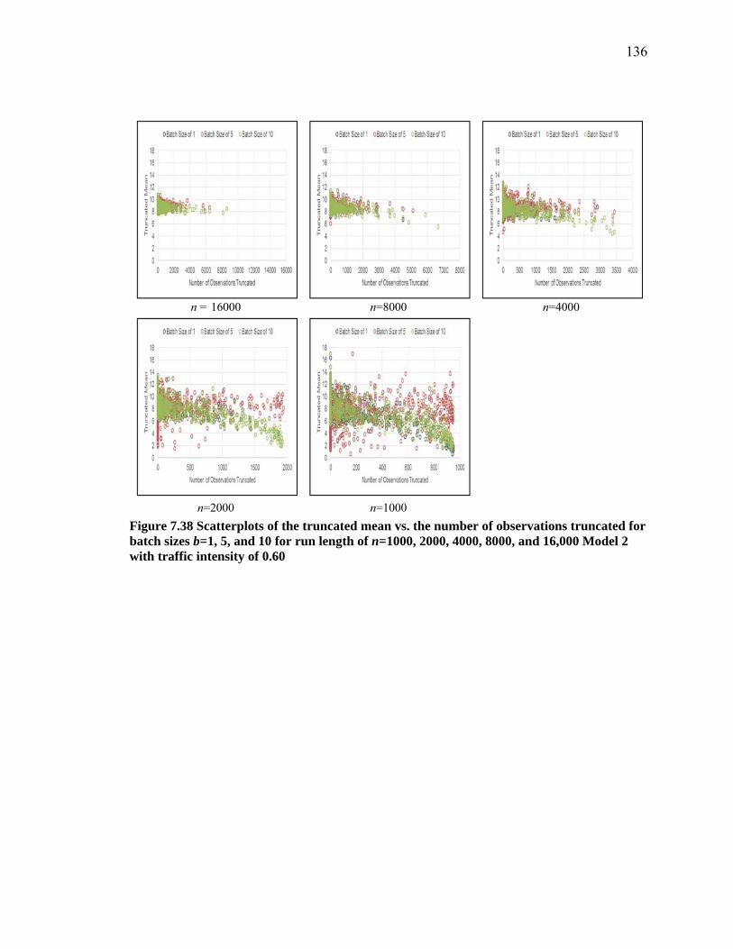
136
n = 16000
n=8000
n=4000
n=2000
n=1000
Figure 7.38 Scatterplots of the truncated mean vs. the number of observations truncated for batch sizes b=1, 5, and 10 for run length of n=1000, 2000, 4000, 8000, and 16,000 Model 2 with traffic intensity of 0.60

137
Table 7.11 Correlation between the truncated mean and the number of observations truncated for batch sizes b=1, 5, and 10 for run length of n=1000, 2000, 4000, 8000, and 16,000 for Model 2 with traffic intensity of 0.60
Trunc
Batch =1
Trunc
Batch =5
Trunc
Batch =10
Mean
Batch = 1
-0.1597 -0.1056 -0.0320
Mean
Batch = 5
-0.1599 -0.2199 -0.1122
Mean
Batch = 10
-0.1553 -0.2128 -0.2509
Trunc
Batch =1
Trunc
Batch =5
Trunc
Batch =10
Mean
Batch = 1
-0.2120 -0.1465 -0.0421
Mean
Batch = 5
-0.2130 -0.2720 -0.1367
Mean
Batch = 10
-0.1965 -0.2565 -0.3522
Trunc
Batch =1
Trunc
Batch =5
Trunc
Batch =10
Mean
Batch = 1
-0.2819 -0.1425 -0.1271
Mean
Batch = 5
-0.2939 -0.4185 -0.3418
Mean
Batch = 10
-0.2920 -0.4008 -0.5182
n = 16000 n = 8000 n = 4000
Trunc
Batch =1
Trunc
Batch =5
Trunc
Batch =10
Mean
Batch = 1
-0.4056 -0.1680 -0.0967
Mean
Batch = 5
-0.3121 -0.6541 -0.4410
Mean
Batch = 10
-0.2541 -0.5291 -0.7204
Trunc
Batch =1
Trunc
Batch =5
Trunc
Batch =10
Mean
Batch = 1
-0.6309 -0.3548 -0.2981
Mean
Batch = 5
-0.4903 -0.7493 -0.5802
Mean
Batch = 10
-0.4631 -0.6305 -0.7329
n = 2000 n = 1000

138
n = 16000 n = 8000 n = 4000
n = 2000 n = 1000 n = 500 Figure 7.39 Frequency distribution of the number of observations truncated as a function of batch sizes b=1, 5, and 10 for run length of n=1000, 2000, 4000, 8000, and 16,000 for Model 2 with traffic intensity of 0.60
0
100
200
300
400
500
600
700
800
0 250 500 1000 2000 4000 8000
Num
ber
of R
eplic
atio
ns
Number of Observations Truncated
Batch Size of 1 Batch Size of 5 Batch Size of 10
0
100
200
300
400
500
600
700
800
0 250 500 1000 2000 4000 8000
Num
ber
of R
eplic
atio
ns
Number of Observations Truncated
Batch Size of 1 Batch Size of 5 Batch Size of 10
0
100
200
300
400
500
600
700
800
0 250 500 1000 2000 4000
Num
ber
of R
eplic
atio
ns
Number of Observations Truncated
Batch Size of 1 Batch Size of 5 Batch Size of 10
0
100
200
300
400
500
600
700
0 250 500 1000 2000
Num
ber
of R
eplic
atio
ns
Number of Observations Truncated
Batch Size of 1 Batch Size of 5 Batch Size of 10
0
100
200
300
400
500
600
700
0 250 500 <1000
Num
ber
of R
eplic
atio
ns
Number of Observations Truncated
Batch Size of 1 Batch Size of 5 Batch Size of 10
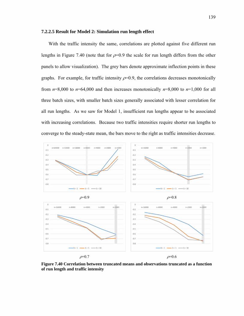
139
7.2.2.5 Result for Model 2: Simulation run length effect
With the traffic intensity the same, correlations are plotted against five different run
lengths in Figure 7.40 (note that for =0.9 the scale for run length differs from the other
panels to allow visualization). The grey bars denote approximate inflection points in these
graphs. For example, for traffic intensity =0.9, the correlations decreases monotonically
from n=8,000 to n=64,000 and then increases monotonically n=8,000 to n=1,000 for all
three batch sizes, with smaller batch sizes generally associated with lesser correlation for
all run lengths. As we saw for Model 1, insufficient run lengths appear to be associated
with increasing correlations. Because two traffic intensities require shorter run lengths to
converge to the steady-state mean, the bars move to the right as traffic intensities decrease.
=0.9
=0.8
=0.7 =0.6
Figure 7.40 Correlation between truncated means and observations truncated as a function of run length and traffic intensity

140
7.2.2.6 Result for Model 2: Traffic intensity effect
We also consider how traffic intensities (i.e., 0.6, 0.7, 0.8 and 0.9) affect correlation while
the simulation length stays the same.
(1) n = 16000
Under the same condition of simulation lengths, correlations from the smaller traffic
intensities tend to become weaker. That is applicable for all three batch sizes tested.
Figure 7.41 Correlation between truncated means and observations truncated by different
traffic intensity (Run length of 16000)
(2) n = 8000, 4000, 2000, and 1000
The same patterns are shown in the case of n = 8000 compared to n = 16000. However, the
run lengths of 2000 and 1000 do not conform the same trends as the run lengths of 16000
and 8000, while n = 4000 shows mixed trends between the two groups where n is 16000
and 8000, vs. n is 2000 and 1000.
We note that the run lengths of 16000 and 8000 ascertain that the longer run length can
mitigate influences of traffic intensities except for traffic intensity of 0.9, regardless of batch
sizes. Thus, we can conclude that traffic intensity of 0.9 would benefit from increasing the
-0.8
-0.7
-0.6
-0.5
-0.4
-0.3
-0.2
-0.1
00.6 0.7 0.8 0.9
n = 16000
Batch 1 Batch 5 Batch 10

141
run length. For the run lengths of 2000 and 1000, the correlations between truncated means
and observations truncated appear to be counterintuitive as the higher traffic intensity is
associated with the lower correlations. However, these trends might be true when long
waiting times are infrequently realized during the relatively short simulation runs in the
lower traffic intensity such as 0.6, 0.7, and 0.8. On the other hand, the traffic intensity of
0.9 might build up longer queues even for short runs.
Figure 7.42 Correlation between truncated means and observations truncated by different traffic intensity (Run length of 8000, 4000, 2000, and 100)
7.2.2.7 Results: Overlapping Batch Means for M/M/1 with Traffic Intensity of 0.90.
We applied OBM to Model 2 with run length n=64000 with the highest traffic intensity
of 0.9 among M/M/1 models for batch sizes b=10, 50, 100, and 200 observation and Figure
7.43 shows four representative cases with original outputs, OBM, and MSER statistic. By
increasing batch sizes of OBM, we observed different trends among the four tested cases:

142
Small batch size of 10: The result is almost identical to NOBM because the pre-
processed net output series takes closest resemblance for an original output
series.
Batch sizes larger than 10 (i.e., 50, 100, and 200): Based on the results, the
difference from a theoretical mean value becomes apparent by increasing batch
sizes. This finding can be attributable to (1) regenerative cycles in M/M/1 and
(2) irregular peaks to influence multiple OBM. Impacts from any outliers in
waiting time can remain strong because OBM keeps using these values multiple
times compared to NOBM’s one usage and go property that any big or small
number can influence only one batch mean.
b = 10 b = 50
b = 100 b = 200
Figure 7.43 Representative Output, Overlapping Batch Mean, and MSER Statistic of Model 2 with traffic intensity of 0.90 (b= 10, 50, 100, and 200)

143
We summarize the confidence intervals of the mean estimates and truncation points in
Table 7.12 and Figure 7.44 that accounts for our finding. For Model 1 and 3 (following
section), OBM tends to outperform NOBM because both cases the output clearly converges
to certain mean estimates. However, Models 2 here provides another aspects to be
considered. As long as the output takes on a regenerative pattern, OBM might lead to a
wrong conclusion about mean estimate for testing models.
Table 7.12 95% confidence intervals for Model 2 on the truncated mean and the standard deviation for overlapping and non-overlapping batches
OBM NOBM
OBM b=10 OBM b=50 OBM b=100 OBM b=200 NOBM b=10
Sample Mean 79.162030 76.821921 74.199907 74.199907 79.310097
Upper limit 79.635371 77.633984 75.211400 75.211400 79.736781
Lower limit 78.688690 76.009859 73.188415 73.188415 78.883414
Sample Std D 7.627800 13.086239 16.300019 16.300019 6.875926
Upper limit 7.977651 13.686444 17.047626 17.047626 7.191293
Lower limit 7.307526 12.536779 15.615620 15.615620 6.587222
(a)
(b)
Figure 7.44 95% confidence intervals for Model 3 on (a) the truncated mean for overlapping and non-overlapping batches and (b) the standard deviation for overlapping and non-overlapping batches
68
70
72
74
76
78
80
82
OBMb = 10
OBMb = 50
OBMb = 100
OBMb = 200
MSERb = 10
0
2
4
6
8
10
12
14
16
18
OBMb = 10
OBMb = 50
OBMb = 100
OBMb = 200
MSERb = 10

144
Figure 7.45 and 7.46 and Table 7.13 below reiterate the inefficiency of bigger OBM to
find accurate mean estimate and significant loss in output series is observed since truncation
points pass the first half even with run length of 64000. That is, “batch size of 200” indeed
uses less than 10% of total output and estimates quite smaller mean estimates.
Figure 7.45 Scatterplots of the truncated mean vs. the number of observations truncated for OBM sizes b=10, 50, 100 and 200 for run length of n=64,000 with traffic intensity of 0.90 for Model 2 (including NOBM batch size of 10)

145
Figure 7.46 Frequency distribution of the number of observations truncated as a function of OBM sizes b=10, 50, 100, and 200 for run length of n=64,000 with traffic intensity of 0.90 for Model 2 (including NOBM batch size of 10)
Table 7.13 Correlation between the truncated mean and the number of observations truncated for OBM sizes b=10, 50, 100, and 200 for run length of n=64,000 for Model 2
Trunc Batch =10 Trunc Batch =50 Trunc Batch =100 Trun Batch = 200
Mean Batch = 10 0.043 -0.053 -0.890 0.082
Mean Batch = 50 -0.198 -0.829 -0.299 -0.114
Mean Batch = 100 -0.120 -0.333 -0.890 0.017
Mean Batch = 200 -0.113 -0.210 -0.422 -0.914
As we observe, without applying d*<n/2 rule, the results for OBM have been deteriorated
compared to NOBM as well as raw output series without any truncation. Thus, we try to
capture the characteristics of truncations satisfying d*<n/2 rule for OBM and the results are
summarized in Table 7.14 and Figure 7.45. The disadvantage following this rule is that some
of replications need to be omitted to obtain mean estimates. First, the set of mean estimates
are tabulated according to different run lengths from n = 64000 to 1000. Short lengths of n
such as 1000, 2000, and 4000 do not show accuracy of means compared to NOBM estimates
but longer run lengths apparently show improved convergence to a theoretical estimate.

146
Table7.14 Confidence Intervals for M/M/1 with traffic intensity of 0.90 on the truncated mean and the standard deviation for overlapping and non-overlapping batches with traffic intensity of 0.90 (n = 1000, 2000, 4000, 8000, 16000, 32000, and 64000)
n =64000 OBM NOBM
Mean with truncation Batch Size of 10 Batch Size of 50 Batch Size of 100 Batch Size of 200 Batch Size of 10
Sample Mean 79.42 79.09 78.85 78.42 79.42
Upper limit 79.84 79.51 79.29 78.87 79.84
Lower limit 79.00 78.66 78.41 77.97 79.00
Sample Std Dev 6.77 6.68 6.67 6.53 6.77
Upper limit 7.09 6.98 6.98 6.83 7.08
Lower limit 6.49 6.40 6.39 6.25 6.49
n =32000 OBM NOBM
Mean with truncation Batch Size of 10 Batch Size of 50 Batch Size of 100 Batch Size of 200 Batch Size of 10
Sample Mean 78.28 77.73 77.22 76.55 78.37
Upper limit 78.85 78.32 77.84 77.22 78.93
Lower limit 77.71 77.13 76.59 75.89 77.80
Sample Std Dev 8.95 8.89 8.91 8.69 8.99
Upper limit 9.36 9.30 9.31 9.08 9.41
Lower limit 8.57 8.51 8.53 8.32 8.62
n = 16000 OBM NOBM
Mean with truncation Batch Size of 10 Batch Size of 50 Batch Size of 100 Batch Size of 200 Batch Size of 10
Sample Mean 76.64 76.16 75.82 75.98 76.72
Upper limit 77.47 77.07 76.80 77.07 77.53
Lower limit 75.82 75.25 74.84 74.89 75.91
Sample Std Dev 12.63 12.71 12.68 12.79 12.60
Upper limit 13.21 13.29 13.26 13.38 13.18
Lower limit 12.10 12.17 12.15 12.25 12.07
n =8000 OBM NOBM
Mean with truncation Batch Size of 10 Batch Size of 50 Batch Size of 100 Batch Size of 200 Batch Size of 10
Sample Mean 72.13 71.93 72.13 71.85 72.78
Upper limit 73.20 73.15 73.52 73.41 73.83
Lower limit 71.06 70.71 70.74 70.28 71.72
Sample Std Dev 15.48 15.30 15.63 15.90 15.84
Upper limit 16.19 16.00 16.34 16.63 16.56
Lower limit 14.83 14.65 14.97 15.23 15.17

147
n = 4000 OBM NOBM
Mean with truncation Batch Size of 10 Batch Size of 50 Batch Size of 100 Batch Size of 200 Batch Size of 10
Sample Mean 69.21 69.47 68.50 68.91 70.50
Upper limit 70.70 71.21 70.34 70.85 71.97
Lower limit 67.71 67.72 66.67 66.97 69.03
Sample Std Dev 20.39 20.87 20.32 20.15 21.50
Upper limit 21.33 21.83 21.25 21.08 22.48
Lower limit 19.53 20.00 19.47 19.31 20.59
n = 2000 OBM NOBM
Mean with truncation Batch Size of 10 Batch Size of 50 Batch Size of 100 Batch Size of 200 Batch Size of 10
Sample Mean 64.64 65.23 65.97 67.59 66.16
Upper limit 66.55 67.75 68.74 70.33 68.15
Lower limit 62.73 62.71 63.21 64.86 64.16
Sample Std Dev 24.71 27.95 28.78 28.11 27.06
Upper limit 25.84 29.24 30.10 29.39 28.30
Lower limit 23.67 26.78 27.57 26.93 25.93
n = 1000 OBM NOBM
Mean with truncation Batch Size of 10 Batch Size of 50 Batch Size of 100 Batch Size of 200 Batch Size of 10
Sample Mean 63.58 66.00 66.41 69.56 68.07
Upper limit 66.69 69.76 70.34 73.68 71.58
Lower limit 60.46 62.24 62.48 65.44 64.55
Sample Std Dev 39.52 42.39 43.35 47.31 44.58
Upper limit 41.33 44.33 45.34 49.47 46.63
Lower limit 37.86 40.61 41.53 45.32 42.71

148
n= 64000
n= 32000
n= 16000
n= 8000 n= 4000 n= 2000
n= 1000
Figure 7.47 95% confidence intervals for M/M/1 with traffic intensity of 0.90 about the truncated mean for overlapping and non-overlapping batches (n = 1000, 2000, 4000, 8000, 16000, 32000, and 64000.)
74
75
76
77
78
79
80
OBMb = 10
OBMb = 50
OBMb = 100
OBMb = 200
MSERb = 10
74
75
76
77
78
79
80
OBMb = 10
OBMb = 50
OBMb = 100
OBMb = 200
MSERb = 10
74
75
76
77
78
79
80
OBMb = 10
OBMb = 50
OBMb = 100
OBMb = 200
MSERb = 10
58
63
68
73
78
OBMb = 10
OBMb = 50
OBMb = 100
OBMb = 200
MSERb = 10
58
63
68
73
78
OBMb = 10
OBMb = 50
OBMb = 100
OBMb = 200
MSERb = 10
58
63
68
73
78
OBMb = 10
OBMb = 50
OBMb = 100
OBMb = 200
MSERb = 10
58
63
68
73
78
OBMb = 10
OBMb = 50
OBMb = 100
OBMb = 200
MSERb = 10

149
7.2.2.8 Results: Initialization Bias
To test the assertion that the errors in the output are the result of inadequate run lengths
and unrepresentative initial conditions (note that x0=0 is the mode of the steady-state
distribution and hardly representative!), we ran two more experiments. Each comprised 100
replications of Model 2 with traffic intensity of 0.9 and initial condition x0=100. We used
and compared three different batch sizes, b=1, 5, and 10, and two different run lengths,
n=64,000 and 32,000.
Figure 7.48 shows the output time series for one representative replication with b=1 and
n=32,000. Clearly, the initial condition results in a large initial spike in waiting times. Just
as clearly, MSER removes much or this entire initial spike.
Figure 7.48 Output time series with traffic intensity of 0.90 with b =1 and n = 32,000
In contrast to the prior experiments without initialization bias, MSER truncation
provides significantly improved estimates over those obtained without truncation in Figure
7.49. These results appear to be relatively insensitive to batch size (although smaller batches
appear to perform modestly better) and, again, the error in the estimates is relatively
uncorrelated to the MSER truncation points. The effect of run length is apparent and for

150
the longer runs coverage is achieved for every batch size. We speculate that this may be
attributable to the significant reduction in sample variance for longer runs.
95% confidence intervals on the mean
95% confidence intervals on Sample Std Dev.
Scatterplots indicting the correlation between truncated mean and truncation point
Frequency distribution
of the number of observations truncated
n=64,000 n=32,000
Figure 7.49 Confidence interval for Mean and Standard Deviation, Scatter Plot for Truncation points and Truncated Mean, Frequency Distribution of the Number of Observations Truncated with Traffic Intensity of 0.90 with b =1, 5, and 10 and n = 64,000 and 32,000

151
Note that this example appears to suggest that “smart initialization” may not be the solution
to the warm-up problem that has been widely recommendation. The initial condition of
x0=100 certainly is much closer to the theoretical steady-state mean of 81 than x0=0 in the
prior examples. However, truncation is still required to eliminate the initial spike in waiting
times. The same would be true if we had made the very lucky guess of x0=81! Warm-up
appears to be required. In this instance smart initialization appears to suggest
foreknowledge of the entire steady-state distribution, in particular the mode, rather than the
steady state mean.
Table 7.15 Correlation between the truncated mean and the number of observations truncated for b=1, 5, and 10 for run length of n=32,000 with initial bias of 100
Trunc Batch =1 Trunc Batch =5 Trunc Batch =10
Mean Batch = 1 -0.4147 -0.4050 -0.4050 Mean Batch = 5 -0.4308 -0.4232 -0.4233 Mean Batch = 10 -0.4308 -0.4232 -0.4233
Table 7.16 95% confidence intervals for Model 2 on the observation truncated and the standard deviation for run length of n=32,000 with initial bias of 100
Truncation Point batch = 1 batch = 5 batch = 10
Sample Mean 2878.4400 2900.7000 2901.3000
Upper limit 3735.0552 3772.1267 3772.7876
Lower limit 2021.8248 2029.2733 2029.8124
Sample Std Dev 4317.1446 4391.7915 4392.0984
Upper limit 4515.1520 4593.2226 4593.5436
Lower limit 4135.8779 4207.3905 4207.6845 Table 7.17 95% confidence intervals for Model 2 on the truncated mean and the standard deviation for run length of n=32,000 with initial bias of 100
Mean with truncation batch = 1 batch = 5 batch = 10
Sample Mean 78.036849 77.993410 77.992041
Upper limit 79.770945 79.725121 79.723891
Lower limit 76.302752 76.261699 76.260191
Sample Std Dev 8.739450 8.727426 8.728127
Upper limit 9.140288 9.127712 9.128446
Lower limit 8.372501 8.360982 8.361653

152
Table7.18 95% confidence intervals for Model 2 on the mean without truncation and the standard deviation for run length of n=32,000 with initial bias of 100
Mean w/o truncation batch = 1 batch = 5 batch = 10
Sample Mean 94.087628 94.0876 94.0876
Upper limit 96.269303 96.2693 96.2693
Lower limit 91.905953 91.9060 91.9060
Sample Std Dev 10.995146 10.9951 10.9951
Upper limit 11.499442 11.4994 11.4994
Lower limit 10.533485 10.5335 10.5335
Table 7.19 Correlation between the truncated mean and the number of observations truncated for b=1, 5, and 10 for run length of n=64,000 with initial bias of 100
Trunc Batch =1 Trunc Batch =5 Trunc Batch =10
Mean Batch = 1 -0.3940 -0.3588 -0.3491
Mean Batch = 5 -0.3811 -0.4295 -0.4191
Mean Batch = 10 -0.3782 -0.4269 -0.4268
Table 7.20 95% confidence intervals for Model 2 on the observation truncated and the standard deviation for run length of n=64,000 with initial bias of 100
Truncation Point batch = 1 batch = 5 batch = 10
Sample Mean 2738.4600 2995.2500 3092.4000
Upper limit 3624.6425 3999.8582 4105.6587
Lower limit 1852.2775 1990.6418 2079.1413
Sample Std Dev 4466.1572 5062.9956 5106.5923
Upper limit 4670.9991 5295.2117 5340.8080
Lower limit 4278.6337 4850.4123 4892.1785
Table 7.21 95% confidence intervals for Model 2 on the truncated mean and the standard deviation for run length of n=64,000 with initial bias of 100
Mean with truncation batch = 1 batch = 5 batch = 10
Sample Mean 79.395610 79.281469 79.243732
Upper limit 80.761263 80.670545 80.632182
Lower limit 78.029956 77.892394 77.855283
Sample Std Dev 6.882581 7.000622 6.997469
Upper limit 7.198253 7.321708 7.318410
Lower limit 6.593598 6.706682 6.703661

153
Table 7.22 95% confidence intervals for Model 2 on the mean without truncation and the standard deviation for run length of n=64,000 with initial bias of 100
Mean w/o truncation batch = 1 batch = 5 batch = 10
Sample Mean 87.175809 87.1758 87.1758
Upper limit 88.607643 88.6076 88.6076
Lower limit 85.743975 85.7440 85.7440
Sample Std Dev 7.216117 7.2161 7.2161
Upper limit 7.547086 7.5471 7.5471
Lower limit 6.913129 6.9131 6.9131
7.2.2.9 Summary Results for Model 2
We chose this model initially because it allows comparison with the results obtained by
Law (2015) and by White and Hwang (2015) for long runs. This prior research addressed
the performance of MSER for a single batch size (b=5), single run length (n=65,000), and
single traffic intensity (=0.9) with respect to a range of different initial conditions {x0=0,
5, 10, 12, 15, 18, 20}. The results obtained by White and Hwang (2015) demonstrated that
truncation points and the error in the truncated mean estimates are essentially independent.
Further, while the mean estimates for this problem are quite good without truncation,
applying MSER-5 truncation modestly improves the accuracy of these estimates.
(1) The results obtained in the present research for n=64,000 and =0.9 are entirely
consistent with those reported earlier.
Our objective here was to explore the performance of MSER for a single initial condition,
empty and idle {x0=0}, with respect to alternative run lengths, batch sizes, and model traffic

154
intensities. We speculated the effects of decreasing to be similar to those encountered by
increasing the run length n.
(2) The results of our experiments suggest that this speculation is largely untrue and
decreasing traffic intensity cannot altogether compensate for short run lengths.
(3) The d*≤dmax=n/2 truncation rule likewise cannot altogether compensate for short
run lengths
For smaller run lengths and traffic intensities, MSER appears to overestimate the amount
truncation warranted, reducing the sample variance by truncating early regenerative cycles
with large peak waiting times while the MSER statistic is relatively less sensitive to the
accompanying reduction in sample size. The result is underestimation of the steady-state
mean.
In the final analysis, our analysis demonstrates that
(4) The difficulty in estimating the steady-state mean has little or nothing to do with bias
resulting from a poor choice of initial conditions for Model 2. The empty-and-idle
condition regenerates frequently, more frequently for lower traffic intensities and
smaller batches.
(5) The fundamental issue is determining an initial run length that is sufficiently long to
capture observations that, taken together, are representative of the steady-state
distribution.
(6) The new initial bias of x0=100 apparently vindicates the efficacy of MSER to detect
steady state mean(s) and truncation point(s) compared to smart initialization
approach.

155
7.2.3 Model 3: EAR(1)
The third test model is AR(1)
ttt XX 1
for t = 0, 1, …, n, with exponentially decaying error
where =1. This model differs from a typical AR(1) with normally distributed white noise
because the error term is exponentially distributed. It is stable if and only if
0 <1
For stable processes, the expected steady-mean is
Table 7.23 provides this expectation for parameter values ={0.7, 0.8, 0.9, 0.99}. Note that
the rate of convergence to steady state also depends , with the rate increasing in decreasing
. In terms of the average warm-up period required, therefore, we would anticipate that the
effect of decreasing is similar to that of increasing the run length n.
Table 7.23 Expected Value of the Steady-State Mean as a function of
0.7 0.8 0.9 0.99
3.33 5.00 10 100
Both of these dependencies are illustrated in Figure 7.50 for a run length of n=500. (Note
the scale for the ordinate in the panel for =0.99 differs from the other three panels, in order
to allow visualization.) In each panel, the response Xt is plotted in blue, while the expected
response
t ~ et
E X 1
1
E X

156
11 tt XEXE
is plotted in red.
=0.99
=0.9
=0.8
=0.7
Figure 7.50 Representative output for EAR(1) for run length n=500 and batch size b=1, illustrating the dependency of the steady-state mean and rate of convergence on the parameter for ={0.7, 0.8, 0.9, 0.99}
Determining the “true” truncation point for this model is problematic. This is because
the process converges to steady state only in the limit. Which observation to choose as the
“true” truncation point is inherently subjective and open to second-guessing. In classical
control engineering, the point where the response is “close enough” to steady state is called
the settling time. The expected -percent settling time is implicitly defined by

157
Common choices for the settling time are observations at which the responses are within
5% and 2% of their steady-state values. Table 7.24 provides settling times as a function of
the parameter for a wide range of potential choices for .
Note that MSER is data driven and does not suffer from this ambiguity. On any
replication, the process is deemed to have settled into steady state when the MSER statistic
is minimized on the initial segment of observations. The expected settling time is
approximately the average of these individual settling times over a very large number of
replications. Note that this is the point argued by White and Hwang (2015) in response to
Law (2015).
Table 7.24 Expected -percent settling time as a function of and 0.7 0.8 0.9 0.99 9 14 29 299 11 18 38 390 13 21 44 459 0.1 20 31 66 688 0.01 26 42 88 917 0.001 33 52 110 1146
In this chapter we explore the sensitivity of the estimated steady-state mean and
truncation point with respect to the model parameter ={0.7, 0.8, 0.9, 0.99} for batch sizes
b={1, 5, 10} and eight different run lengths:
long run lengths of n=16000, 8000, 4000
E X 100100
E X 1
100
100
1
1
1
100100 1

158
medium run lengths of n=2000, 1000
short run lengths of n=500, 300, 150, 100
We distinguish among these categories of run length experimentally, based on coverage of
the mean by the truncated and/or raw 95% confidence intervals for =0.99.
7.2.3.1 Results for Model 3 with =0.99
Figure 7.51 shows the response of one of 1000 replications for =0.99 and n=16000.,
together with the expected mean .Visually, this output appears to settle into a
steady-state operating regime after approximately 300-400 observations after which
observations remain relatively stable about the mean. This corresponds to the traditional
choice of a 2% to 5% settling time as applied control engineering.
Figure 7.51 Example of Model 3 with =0.99 (n = 16000, Brown line: E(X))
By halving the run length sequentially, the relationships among the variables—run length,
batch size, and model parameter —and key metrics—means without truncation, truncated
means, truncation points, the correlation between truncated means and truncation points—
begin to emerge.
As can be seen in Figure 7.52, MSER yields superior estimates for all run lengths, with
the difference in accuracy increasing as the run lengths as the decrease. For the long runs
E X 100

159
(n=16000, 8000, 4000), both the MSER-truncated and the raw confidence intervals cover
the true mean. The comparatively large number of observations in steady state appears to
be sufficient to overwhelm the initial transient. For medium-length runs (n=2000, 1000),
only the MSER-truncated estimates provide coverage; for short-runs (n=500, 300, 150,
100), neither the MSER-truncated nor the raw confidence intervals cover the true mean. As
the run length continues to decline, the ranges of truncated means become wider and
estimation for every batch size increases.
This suggests that MSER needs to “see” at most 1000 observations on average in order
to provide coverage for this system. As shown in Figure 7.53, this is approximately three
times the length of the MSER-determined warm-up period. Batching is contraindicated
below about n=500 with larger batches on average yielding smaller estimates and greater
estimation error.
Larger batches are associated with greater truncation for every run length. The average
MSER truncation point is reasonably consistent across large runs, on range 250<d*<400, as
well as across medium-length runs, on the range 150<d*<300, and across short runs, on the
range 0<d*<200. Restricting the optimal truncation point to d*<n/2 does not consistently
appear to provide the desired indication that runs are too short to yield accurate estimates
on average. However, the same is not true when the restriction is applied on a replication-
by-replication basis, as recommended.
Figures 7.54 and Table 7.25 demonstrate that truncated mean estimates are relatively
independent of the observations truncated. For long runs, the correlation is essentially zero.
For medium and short runs, there appears to be a modest positive correlation, with the

160
magnitude of this correlation generally increasing as run length decreases. As is perhaps
intuitive, the shortest runs tend to induce greater truncation on average.
n = 16000
n = 8000
n = 4000
n = 2000
n = 1000
n=500
n = 300
n = 150
n = 100
Figure 7.52 95% confidence intervals of the mean for the truncated mean output as a function of batch size (b= 1, 5, and 10) and run length (n=100, 150, 300, 500, 1000, 2000, 4000, 8000, and 16,000) for Model 3 with =0.99 (Theoretical mean of 100, Blue line)
0
20
40
60
80
100
MSERb = 1
Rawb = 1
MSERb = 5
Rawb = 5
MSERb = 10
Rawb = 10
0
20
40
60
80
100
MSERb = 1
Rawb = 1
MSERb = 5
Rawb = 5
MSERb = 10
Rawb = 10
0
20
40
60
80
100
MSERb = 1
Rawb = 1
MSERb = 5
Rawb = 5
MSERb = 10
Rawb = 10
0
20
40
60
80
100
MSERb = 1
Rawb = 1
MSERb = 5
Rawb = 5
MSERb = 10
Rawb = 10
0
20
40
60
80
100
MSERb = 1
Rawb = 1
MSERb = 5
Rawb = 5
MSERb = 10
Rawb = 10
0
20
40
60
80
100
MSERb = 1
Rawb = 1
MSERb = 5
Rawb = 5
MSERb = 10
Rawb = 10
0
20
40
60
80
100
MSERb = 1
Rawb = 1
MSERb = 5
Rawb = 5
MSERb = 10
Rawb = 10
0
20
40
60
80
100
MSERb = 1
Rawb = 1
MSERb = 5
Rawb = 5
MSERb = 10
Rawb = 10
0
20
40
60
80
100
MSERb = 1
Rawb = 1
MSERb = 5
Rawb = 5
MSERb = 10
Raw b =10
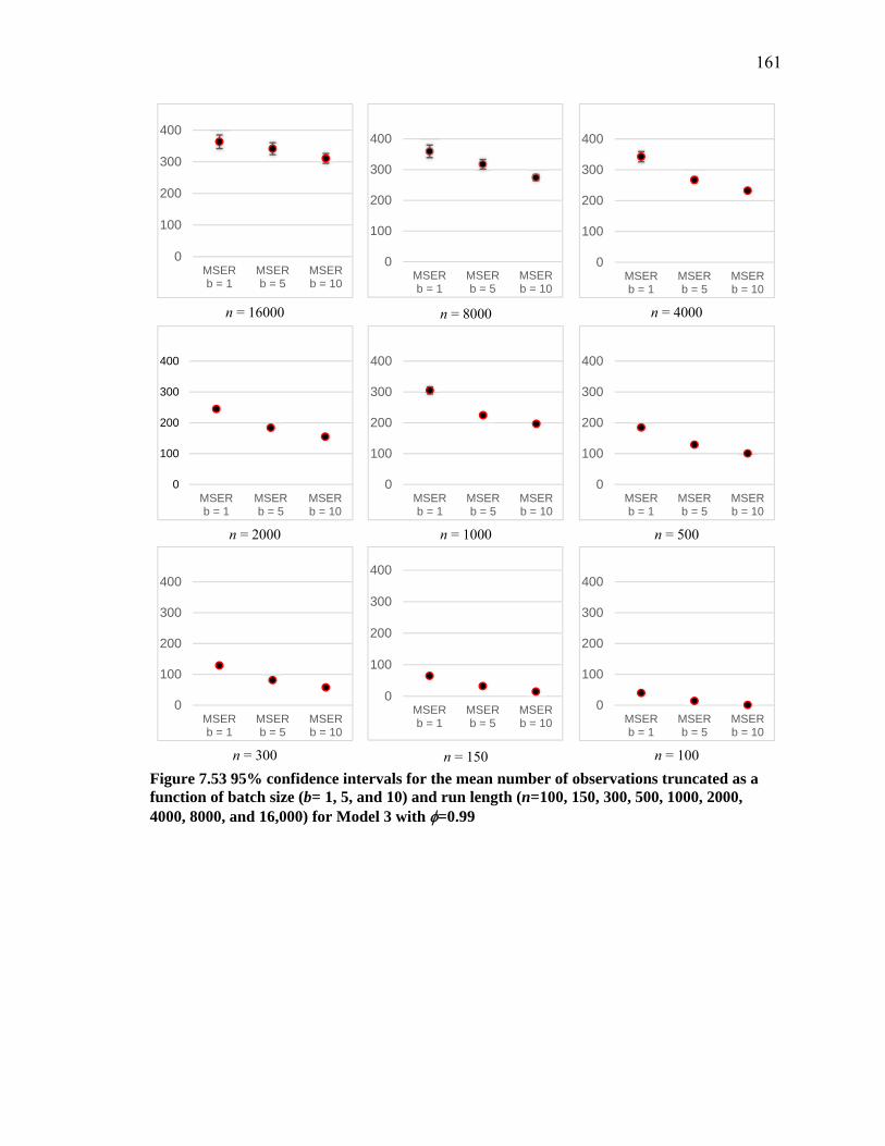
161
n = 16000
n = 8000
n = 4000
n = 2000
n = 1000
n = 500
n = 300
n = 150
n = 100
Figure 7.53 95% confidence intervals for the mean number of observations truncated as a function of batch size (b= 1, 5, and 10) and run length (n=100, 150, 300, 500, 1000, 2000, 4000, 8000, and 16,000) for Model 3 with =0.99
0
100
200
300
400
MSERb = 1
MSERb = 5
MSERb = 10
0
100
200
300
400
MSERb = 1
MSERb = 5
MSERb = 10
0
100
200
300
400
MSERb = 1
MSERb = 5
MSERb = 10
0
100
200
300
400
MSERb = 1
MSERb = 5
MSERb = 10
0
100
200
300
400
MSERb = 1
MSERb = 5
MSERb = 10
0
100
200
300
400
MSERb = 1
MSERb = 5
MSERb = 10
0
100
200
300
400
MSERb = 1
MSERb = 5
MSERb = 10
0
100
200
300
400
MSERb = 1
MSERb = 5
MSERb = 10
0
100
200
300
400
MSERb = 1
MSERb = 5
MSERb = 10

162
n = 16000
n=8000
n=4000
n=2000
n=1000
n=500
n=300
n=150
n=100
Figure 7.54 Scatterplots of the truncated mean vs. the number of observations truncated for batch sizes b=1, 5, and 10 for run length of n=100, 150, 300, 500, 1000, 2000, 4000, 8000, and 16,000 Model 3 with =0.99

163
Table 7.25 Correlation between the truncated mean and the number of observations truncated for batch sizes b=1, 5, and 10 for run length of n=100, 150, 300, 500, 1000, 2000, 4000, 8000, and 16,000 for Model 3 with =0.99
Trunc
Batch =1
Trunc
Batch =5
Trunc
Batch =10
Mean
Batch = 1
-0.0527 -0.0557 -0.0163
Mean
Batch = 5
-0.0424 -0.0558 -0.0167
Mean
Batch = 10
-0.0278 -0.0393 -0.0155
Trunc
Batch =1
Trunc
Batch =5
Trunc
Batch =10
Mean
Batch = 1
-0.0735 -0.0108 0.0453
Mean
Batch = 5
-0.0427 -0.0175 0.0365
Mean
Batch = 10
-0.0097 0.0248 0.0429
Trunc
Batch =1
Trunc
Batch =5
Trunc
Batch =10
Mean
Batch = 1
-0.0458 0.1113 0.1575
Mean
Batch = 5
0.0149 0.1157 0.1733
Mean
Batch = 10
0.0255 0.1242 0.1687
n = 16000 n = 8000 n = 4000
Trunc
Batch =1
Trunc
Batch =5
Trunc
Batch =10
Mean
Batch = 1
0.1117 0.1870 0.1989
Mean
Batch = 5
0.1116 0.2078 0.2194
Mean
Batch = 10
0.0812 0.1333 0.2168
Trunc
Batch =1
Trunc
Batch =5
Trunc
Batch =10
Mean
Batch = 1
0.2822 0.2843 0.2641
Mean
Batch = 5
0.1160 0.3102 0.2861
Mean
Batch = 10
0.0348 0.1456 0.3094
Trunc
Batch =1
Trunc
Batch =5
Trunc
Batch =10
Mean
Batch = 1
0.4864 0.3049 0.2182
Mean
Batch = 5
0.1363 0.4254 0.3383
Mean
Batch = 10
0.0348 0.2258 0.3924
n = 2000 n = 1000 n = 500
Trunc
Batch =1
Trunc
Batch =5
Trunc
Batch =10
Mean
Batch = 1
0.5040 0.2615 0.1539
Mean
Batch = 5
0.0708 0.4444 0.2953
Mean
Batch = 10
-0.0267 0.2004 0.3906
Trunc
Batch =1
Trunc
Batch =5
Trunc
Batch =10
Mean
Batch = 1
0.4771 0.1246 -0.0443
Mean
Batch = 5
0.0104 0.4455 0.2406
Mean
Batch = 10
-0.1133 0.1392 0.4748
Trunc
Batch =1
Trunc
Batch =5
Trunc
Batch =10
Mean
Batch = 1
0.4557 0.1240 -0.0240
Mean
Batch = 5
-0.0149 0.5077 0.1365
Mean
Batch = 10
-0.0693 0.1651 0.3193
n = 300 n = 150 n = 100

164
n = 16000
n = 8000
n = 4000
n = 2000
n = 1000
n = 500
n = 300
n = 150
n = 100
Figure 7.55 Frequency distribution of the number of observations truncated as a function of batch sizes b=1, 5, and 10 for run length of n=100, 150, 300, 500, 1000, 2000, 4000, 8000, and 16,000 for Model 3 with of 0.99
0200400600800
0 25 50 75 125
250
500
100
015
00
200
025
00
300
035
00
< 4
000
Num
ber
of R
eplic
atio
ns
Number of Observations Truncated
Batch Size of 1 Batch Size of 5 Batch Size of 10
0200400600800
0 25 50 75 125
250
500
100
015
00
200
025
00
300
0<
3500
Num
ber
of R
eplic
atio
ns
Number of Observations Truncated
Batch Size of 1 Batch Size of 5 Batch Size of 10
0
200
400
600
800
Num
ber
of R
eplic
atio
ns
Number of Observations Truncated
Batch Size of 1 Batch Size of 5 Batch Size of 10
0
500
1000
Num
ber
of
Rep
licat
ions
Number of Observations Truncated
Batch Size of 1 Batch Size of 5 Batch Size of 10
0
500
1000
Num
ber
of
Rep
licat
ions
Number of Observations Truncated
Batch Size of 1 Batch Size of 5 Batch Size of 10
0
500
1000
Num
ber
of
Rep
licat
ions
Number of Observations Truncated
Batch Size of 1 Batch Size of 5 Batch Size of 10
0200400600800
Num
ber
of R
eplic
atio
ns
Number of Observations Truncated
Batch Size of 1 Batch Size of 5 Batch Size of 10
0
500
1000
Num
ber
of R
eplic
atio
ns
Number of Observations Truncated
Batch Size of 1 Batch Size of 5 Batch Size of 10
0500
10001500
Num
ber
of R
eplic
atio
ns
Number of Observations Truncated
Batch Size of 1 Batch Size of 5 Batch Size of 10

165
7.3.3.2 Results for Model 3 with =0.90
Figure 7.56 Example of EAR(1) with ϕ of 0.9 (n = 16000, Blue line: E(X))
n = 16000
n = 8000
n = 4000
n = 2000
n = 1000
n=500
n = 300
n = 150
n = 100
Figure 7.57 95% confidence intervals of the mean for the truncated mean output as a function of batch size (b= 1, 5, and 10) and run length (n=100, 150, 300, 500, 1000, 2000, 4000, 8000, and 16,000) for Model 3 with ϕ =0.90 (Theoretical mean of 10, Blue line)
8.8
9
9.2
9.4
9.6
9.8
10
MSERb = 1
Rawb = 1
MSERb = 5
Rawb = 5
MSERb = 10
Raw b = 10
8.8
9
9.2
9.4
9.6
9.8
10
MSERb = 1
Rawb = 1
MSERb = 5
Rawb = 5
MSERb = 10
Raw b = 10
8.8
9
9.2
9.4
9.6
9.8
10
MSERb = 1
Rawb = 1
MSERb = 5
Rawb = 5
MSERb = 10
Raw b = 10
8.8
9
9.2
9.4
9.6
9.8
10
MSERb = 1
Rawb = 1
MSERb = 5
Rawb = 5
MSERb = 10
Raw b = 10
8.8
9
9.2
9.4
9.6
9.8
10
MSERb = 1
Rawb = 1
MSERb = 5
Rawb = 5
MSERb = 10
Raw b = 10
8.8
9
9.2
9.4
9.6
9.8
10
MSERb = 1
Rawb = 1
MSERb = 5
Rawb = 5
MSERb = 10
Raw b = 10
8.8
9
9.2
9.4
9.6
9.8
10
MSERb = 1
Rawb = 1
MSERb = 5
Rawb = 5
MSERb = 10
Raw b = 10
8.8
9
9.2
9.4
9.6
9.8
10
MSERb = 1
Rawb = 1
MSERb = 5
Rawb = 5
MSERb = 10
Raw b = 10
8.8
9
9.2
9.4
9.6
9.8
10
MSERb = 1
Rawb = 1
MSERb = 5
Rawb = 5
MSERb = 10
Raw b = 10

166
n = 16000
n = 8000
n = 4000
n = 2000
n = 1000
n = 500
n = 300
n = 150
n = 100
Figure 7.58 95% confidence intervals for the mean number of observations truncated as a function of batch size (b= 1, 5, and 10) and run length (n=100, 150, 300, 500, 1000, 2000, 4000, 8000, and 16,000) for Model 3 with =0.90
0
5
10
15
20
25
30
35
MSER b =1
MSER b =5
MSER b =10
0
5
10
15
20
25
30
35
MSER b =1
MSER b =5
MSER b =10
0
5
10
15
20
25
30
35
MSER b =1
MSER b =5
MSER b =10
0
5
10
15
20
25
30
35
MSER b =1
MSER b =5
MSER b =10
0
5
10
15
20
25
30
35
MSER b =1
MSER b =5
MSER b =10
0
5
10
15
20
25
30
35
MSER b =1
MSER b =5
MSER b =10
0
5
10
15
20
25
30
35
MSER b =1
MSER b =5
MSER b =10
0
5
10
15
20
25
30
35
MSER b =1
MSER b =5
MSER b =10
0
5
10
15
20
25
30
35
MSER b =1
MSER b =5
MSER b =10

167
n = 16000
n=8000
n=4000
n=2000
n=1000
n=500
n=300
n=150
n=100
Figure 7.59 Scatterplots of the truncated mean vs. the number of observations truncated for batch sizes b=1, 5, and 10 for run length of n=100, 150, 300, 500, 1000, 2000, 4000, 8000, and 16,000 Model 3 with =0.90

168
Table 7.26 Correlation between the truncated mean and the number of observations truncated for batch sizes b=1, 5, and 10 for run length of n=100, 150, 300, 500, 1000, 2000, 4000, 8000, and 16,000 for Model 3 with =0.90
Trunc
Batch =1
Trunc
Batch =5
Trunc
Batch =10
Mean
Batch = 1
0.0094 -0.0087 0.0276
Mean
Batch = 5
0.0089 -0.0111 0.0261
Mean
Batch = 10
0.0076 -0.0119 0.0198
Trunc
Batch =1
Trunc
Batch =5
Trunc
Batch =10
Mean
Batch = 1
-0.0329 -0.0314 0.0107
Mean
Batch = 5
-0.0328 -0.0467 -0.0026
Mean
Batch = 10
-0.0327 -0.0468 -0.0032
Trunc
Batch =1
Trunc
Batch =5
Trunc
Batch =10
Mean
Batch = 1
-0.0277 -0.0166 0.0038
Mean
Batch = 5
-0.0267 -0.0347 -0.0110
Mean
Batch = 10
-0.0263 -0.0337 -0.0149
n = 16000 n = 8000 n = 4000
Trunc
Batch =1
Trunc
Batch =5
Trunc
Batch =10
Mean
Batch = 1
-0.1249 -0.1247 -0.1125
Mean
Batch = 5
-0.1251 -0.1220 -0.1107
Mean
Batch = 10
-0.1152 -0.1134 -0.1121
Trunc
Batch =1
Trunc
Batch =5
Trunc
Batch =10
Mean
Batch = 1
-0.1194 -0.1071 -0.0355
Mean
Batch = 5
-0.1025 -0.1044 -0.0354
Mean
Batch = 10
-0.0457 -0.0442 -0.0344
Trunc
Batch =1
Trunc
Batch =5
Trunc
Batch =10
Mean
Batch = 1
-0.1609 -0.0987 -0.0565
Mean
Batch = 5
-0.0776 -0.0945 -0.0507
Mean
Batch = 10
-0.0460 -0.0417 -0.0418
n = 2000 n = 1000 n = 500
Trunc
Batch =1
Trunc
Batch =5
Trunc
Batch =10
Mean
Batch = 1
-0.1213 -0.0715 -0.0633
Mean
Batch = 5
-0.0001 -0.0528 -0.0731
Mean
Batch = 10
0.0172 -0.0193 -0.0558
Trunc
Batch =1
Trunc
Batch =5
Trunc
Batch =10
Mean
Batch = 1
-0.1776 0.0518 0.2247
Mean
Batch = 5
0.0080 0.0640 0.2239
Mean
Batch = 10
0.0299 0.1226 0.3203
Trunc
Batch =1
Trunc
Batch =5
Trunc
Batch =10
Mean
Batch = 1
0.0356 0.1800 0.1167
Mean
Batch = 5
0.1101 0.2034 0.1250
Mean
Batch = 10
0.0835 0.1562 0.2702
n = 300 n = 150 n = 100

169
n = 16000
n = 8000
n = 4000
n = 2000
n = 1000
n = 500
n = 300
n = 150
n = 100
Figure 7.60 Frequency distribution of the number of observations truncated as a function of batch sizes b=1, 5, and 10 for run length of n=100, 150, 300, 500, 1000, 2000, 4000, 8000, and 16,000 for Model 3 with of 0.90
0200400600800
1000
0 25 50 75 125 250 500 <1000
Num
ber
of R
eplic
atio
ns
Number of Observations Truncated
Batch Size of 1 Batch Size of 5 Batch Size of 10
0200400600800
1000
0 25 50 75 125 250 500 <1000
Num
ber
of R
eplic
atio
ns
Number of Observations Truncated
Batch Size of 1 Batch Size of 5 Batch Size of 10
0200400600800
1000
0 25 50 75 125 250 500 <1000
Num
ber
of R
eplic
atio
ns
Number of Observations Truncated
Batch Size of 1 Batch Size of 5 Batch Size of 10
0
500
1000
0 25 50 75 125 250 500 <1000
Num
ber
of R
eplic
atio
ns
Number of Observations Truncated
Batch Size of 1 Batch Size of 5 Batch Size of 10
0
500
1000
0 25 50 75 125 250 500 <1000
Num
ber
of R
eplic
atio
ns
Number of Observations Truncated
Batch Size of 1 Batch Size of 5 Batch Size of 10
0
500
1000
0 25 50 75 125 250 500 <1000
Num
ber
of R
eplic
atio
ns
Number of Observations Truncated
Batch Size of 1 Batch Size of 5 Batch Size of 10
0200400600800
1000
0 25 50 75 125 250 500 <1000
Num
ber
of R
eplic
atio
ns
Number of Observations Truncated
Batch Size of 1 Batch Size of 5 Batch Size of 10
0200400600800
10001200
0 25 50 75 125 250 500 <1000
Num
ber
of R
eplic
atio
ns
Number of Observations Truncated
Batch Size of 1 Batch Size of 5 Batch Size of 10
0
200
400
600
800
1000
0 25 50 75 125 250 500 <1000N
um
be
r o
f R
ep
lica
tion
s
Number of Observations Truncated
Batch Size of 1 Batch Size of 5 Batch Size of 10

170
7.3.3.3 Results for Model 3 with =0.80
Figure 7.61 Example of EAR(1) with of 0.8 (n = 16000, Green line: E(X))
n = 16000
n = 8000
n = 4000
n = 2000
n = 1000
n=500
n = 300
n = 150
n = 100
Figure 7.62 95% confidence intervals of the mean for the truncated mean output as a function of batch size (b= 1, 5, and 10) and run length (n=100, 150, 300, 500, 1000, 2000, 4000, 8000, and 16,000) for Model 3 with =0.80 (Theoretical mean of 5, Blue line)
4.65
4.7
4.75
4.8
4.85
4.9
4.95
5
MSERb = 1
Rawb = 1
MSERb = 5
Rawb = 5
MSERb = 10
Rawb = 10
4.65
4.7
4.75
4.8
4.85
4.9
4.95
5
MSERb = 1
Rawb = 1
MSERb = 5
Rawb = 5
MSERb = 10
Rawb = 10
4.65
4.7
4.75
4.8
4.85
4.9
4.95
5
MSERb = 1
Rawb = 1
MSERb = 5
Rawb = 5
MSERb = 10
Rawb = 10
4.65
4.7
4.75
4.8
4.85
4.9
4.95
5
MSERb = 1
Rawb = 1
MSERb = 5
Rawb = 5
MSERb = 10
Rawb = 10
4.65
4.7
4.75
4.8
4.85
4.9
4.95
5
MSERb = 1
Rawb = 1
MSERb = 5
Rawb = 5
MSERb = 10
Rawb = 10
4.65
4.7
4.75
4.8
4.85
4.9
4.95
5
MSERb = 1
Rawb = 1
MSERb = 5
Rawb = 5
MSERb = 10
Rawb = 10
4.65
4.7
4.75
4.8
4.85
4.9
4.95
5
MSERb = 1
Rawb = 1
MSERb = 5
Rawb = 5
MSERb = 10
Rawb = 10
4.65
4.7
4.75
4.8
4.85
4.9
4.95
5
MSERb = 1
Rawb = 1
MSERb = 5
Rawb = 5
MSERb = 10
Rawb = 10
4.65
4.7
4.75
4.8
4.85
4.9
4.95
5
MSERb = 1
Rawb = 1
MSERb = 5
Rawb = 5
MSERb = 10
Rawb = 10

171
n = 16000
n = 8000
n = 4000
n = 2000
n = 1000
n = 500
n = 300
n = 150
n = 100
Figure 7.63 95% confidence intervals for the mean number of observations truncated as a function of batch size (b= 1, 5, and 10) and run length (n=100, 150, 300, 500, 1000, 2000, 4000, 8000, and 16,000) for Model 3 with =0.80
0
5
10
15
20
MSER b =1
MSER b =5
MSER b =10
0
5
10
15
20
MSER b =1
MSER b =5
MSER b =10
0
5
10
15
20
MSER b =1
MSER b =5
MSER b =10
0
5
10
15
20
MSER b =1
MSER b =5
MSER b =10
0
5
10
15
20
MSER b =1
MSER b =5
MSER b =10
0
5
10
15
20
MSER b =1
MSER b =5
MSER b =10
0
5
10
15
20
MSER b =1
MSER b =5
MSER b =10
0
5
10
15
20
MSER b =1
MSER b =5
MSER b =10
0
5
10
15
20
MSER b =1
MSER b =5
MSER b =10

172
n = 16000
n=8000
n=4000
n=2000
n=1000
n=500
n=300
n=150
n=100
Figure 7.64 Scatterplots of the truncated mean vs. the number of observations truncated for batch sizes b=1, 5, and 10 for run length of n=100, 150, 300, 500, 1000, 2000, 4000, 8000, and 16,000 Model 3 with =0.80

173
Table 7.27 Correlation between the truncated mean and the number of observations truncated for batch sizes b=1, 5, and 10 for run length of n=100, 150, 300, 500, 1000, 2000, 4000, 8000, and 16,000 for Model 3 with =0.80
Trunc
Batch =1
Trunc
Batch =5
Trunc
Batch =10
Mean
Batch = 1
0.0519 0.0491 0.0431
Mean
Batch = 5
0.0508 0.0419 0.0387
Mean
Batch = 10
0.0509 0.0437 0.0338
Trunc
Batch =1
Trunc
Batch =5
Trunc
Batch =10
Mean
Batch = 1
0.0245 0.0221 -0.0122
Mean
Batch = 5
0.0237 0.0097 0.0024
Mean
Batch = 10
0.0241 0.0165 -0.0233
Trunc
Batch =1
Trunc
Batch =5
Trunc
Batch =10
Mean
Batch = 1
0.0023 0.0051 0.0102
Mean
Batch = 5
0.0015 -0.0088 0.0004
Mean
Batch = 10
0.0010 -0.0058 -0.0114
n = 16000 n = 8000 n = 4000
Trunc
Batch =1
Trunc
Batch =5
Trunc
Batch =10
Mean
Batch = 1
-0.0264 -0.0447 -0.0443
Mean
Batch = 5
-0.0302 -0.0799 -0.0725
Mean
Batch = 10
-0.0272 -0.0725 -0.0736
Trunc
Batch =1
Trunc
Batch =5
Trunc
Batch =10
Mean
Batch = 1
-0.0566 -0.0549 -0.0201
Mean
Batch = 5
-0.0595 -0.0755 -0.0307
Mean
Batch = 10
-0.0037 -0.0193 -0.0420
Trunc
Batch =1
Trunc
Batch =5
Trunc
Batch =10
Mean
Batch = 1
-0.1855 -0.1398 -0.0686
Mean
Batch = 5
-0.1211 -0.1418 -0.0677
Mean
Batch = 10
-0.0647 -0.0736 -0.0439
n = 2000 n = 1000 n = 500
Trunc
Batch =1
Trunc
Batch =5
Trunc
Batch =10
Mean
Batch = 1
-0.1854 -0.1782 -0.0958
Mean
Batch = 5
-0.0969 -0.1531 -0.0767
Mean
Batch = 10
-0.0268 -0.0685 -0.0344
Trunc
Batch =1
Trunc
Batch =5
Trunc
Batch =10
Mean
Batch = 1
-0.3738 -0.1403 0.0159
Mean
Batch = 5
-0.0987 -0.1463 0.0115
Mean
Batch = 10
-0.0165 0.0275 0.0946
Trunc
Batch =1
Trunc
Batch =5
Trunc
Batch =10
Mean
Batch = 1
-0.2847 -0.0222 0.0204
Mean
Batch = 5
0.0231 -0.0132 0.0129
Mean
Batch = 10
0.0452 0.0239 0.0474
n = 300 n = 150 n = 100
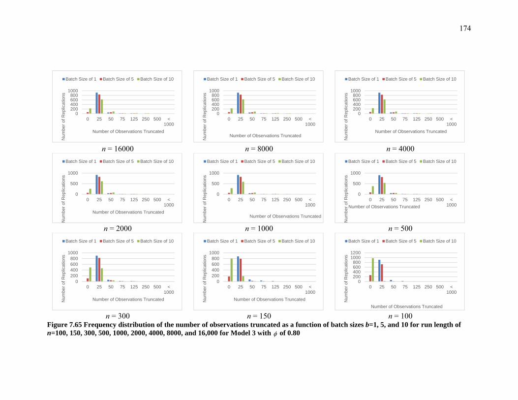
174
n = 16000
n = 8000
n = 4000
n = 2000
n = 1000
n = 500
n = 300
n = 150
n = 100
Figure 7.65 Frequency distribution of the number of observations truncated as a function of batch sizes b=1, 5, and 10 for run length of n=100, 150, 300, 500, 1000, 2000, 4000, 8000, and 16,000 for Model 3 with of 0.80
0200400600800
1000
0 25 50 75 125 250 500 <1000
Num
ber
of R
eplic
atio
ns
Number of Observations Truncated
Batch Size of 1 Batch Size of 5 Batch Size of 10
0200400600800
1000
0 25 50 75 125 250 500 <1000
Num
ber
of R
eplic
atio
ns
Number of Observations Truncated
Batch Size of 1 Batch Size of 5 Batch Size of 10
0200400600800
1000
0 25 50 75 125 250 500 <1000
Num
ber
of R
eplic
atio
ns
Number of Observations Truncated
Batch Size of 1 Batch Size of 5 Batch Size of 10
0
500
1000
0 25 50 75 125 250 500 <1000
Num
ber
of R
eplic
atio
ns
Number of Observations Truncated
Batch Size of 1 Batch Size of 5 Batch Size of 10
0
500
1000
0 25 50 75 125 250 500 <1000
Num
ber
of R
eplic
atio
ns
Number of Observations Truncated
Batch Size of 1 Batch Size of 5 Batch Size of 10
0
500
1000
0 25 50 75 125 250 500 <1000
Num
ber
of R
eplic
atio
ns
Number of Observations Truncated
Batch Size of 1 Batch Size of 5 Batch Size of 10
0200400600800
1000
0 25 50 75 125 250 500 <1000
Num
ber
of R
eplic
atio
ns
Number of Observations Truncated
Batch Size of 1 Batch Size of 5 Batch Size of 10
0200400600800
1000
0 25 50 75 125 250 500 <1000
Num
ber
of R
eplic
atio
ns
Number of Observations Truncated
Batch Size of 1 Batch Size of 5 Batch Size of 10
0200400600800
10001200
0 25 50 75 125 250 500 <1000
Num
ber
of R
eplic
atio
ns
Number of Observations Truncated
Batch Size of 1 Batch Size of 5 Batch Size of 10
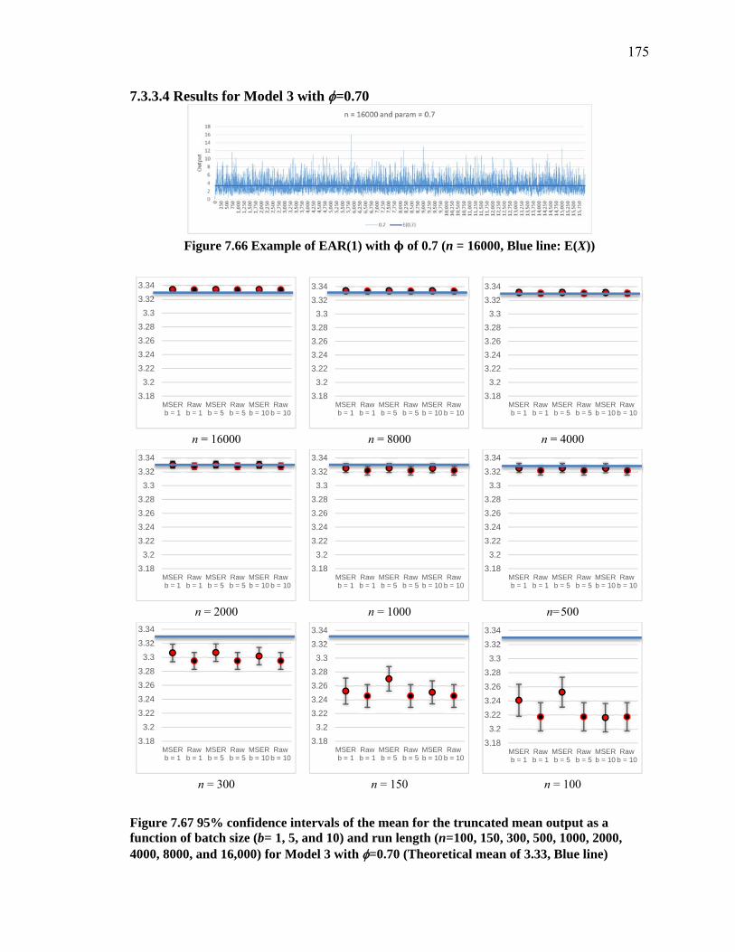
175
7.3.3.4 Results for Model 3 with =0.70
Figure 7.66 Example of EAR(1) with ϕ of 0.7 (n = 16000, Blue line: E(X))
n = 16000
n = 8000
n = 4000
n = 2000
n = 1000
n=500
n = 300
n = 150
n = 100
Figure 7.67 95% confidence intervals of the mean for the truncated mean output as a function of batch size (b= 1, 5, and 10) and run length (n=100, 150, 300, 500, 1000, 2000, 4000, 8000, and 16,000) for Model 3 with =0.70 (Theoretical mean of 3.33, Blue line)
3.18
3.2
3.22
3.24
3.26
3.28
3.3
3.32
3.34
MSERb = 1
Rawb = 1
MSERb = 5
Rawb = 5
MSERb = 10
Rawb = 10
3.18
3.2
3.22
3.24
3.26
3.28
3.3
3.32
3.34
MSERb = 1
Rawb = 1
MSERb = 5
Rawb = 5
MSERb = 10
Rawb = 10
3.18
3.2
3.22
3.24
3.26
3.28
3.3
3.32
3.34
MSERb = 1
Rawb = 1
MSERb = 5
Rawb = 5
MSERb = 10
Rawb = 10
3.18
3.2
3.22
3.24
3.26
3.28
3.3
3.32
3.34
MSERb = 1
Rawb = 1
MSERb = 5
Rawb = 5
MSERb = 10
Rawb = 10
3.18
3.2
3.22
3.24
3.26
3.28
3.3
3.32
3.34
MSERb = 1
Rawb = 1
MSERb = 5
Rawb = 5
MSERb = 10
Rawb = 10
3.18
3.2
3.22
3.24
3.26
3.28
3.3
3.32
3.34
MSERb = 1
Rawb = 1
MSERb = 5
Rawb = 5
MSERb = 10
Rawb = 10
3.18
3.2
3.22
3.24
3.26
3.28
3.3
3.32
3.34
MSERb = 1
Rawb = 1
MSERb = 5
Rawb = 5
MSERb = 10
Rawb = 10
3.18
3.2
3.22
3.24
3.26
3.28
3.3
3.32
3.34
MSERb = 1
Rawb = 1
MSERb = 5
Rawb = 5
MSERb = 10
Rawb = 10
3.18
3.2
3.22
3.24
3.26
3.28
3.3
3.32
3.34
MSERb = 1
Rawb = 1
MSERb = 5
Rawb = 5
MSERb = 10
Rawb = 10

176
n = 16000
n = 8000
n = 4000
n = 2000
n = 1000
n = 500
n = 300
n = 150
n = 100
Figure 7.68 95% confidence intervals for the mean number of observations truncated as a function of batch size (b= 1, 5, and 10) and run length (n=100, 150, 300, 500, 1000, 2000, 4000, 8000, and 16,000) for Model 3 with =0.70
0
5
10
15
20
MSER b =1
MSER b =5
MSER b =10
0
5
10
15
20
MSER b =1
MSER b =5
MSER b =10
0
5
10
15
20
MSER b =1
MSER b =5
MSER b =10
0
5
10
15
20
MSER b =1
MSER b =5
MSER b =10
0
5
10
15
20
MSER b =1
MSER b =5
MSER b =10
0
2
4
6
8
10
12
MSER b =1
MSER b =5
MSER b =10
0
2
4
6
8
10
12
MSER b =1
MSER b =5
MSER b =10
0
2
4
6
8
10
12
MSER b =1
MSER b =5
MSER b =10
0
2
4
6
8
10
12
MSER b =1
MSER b =5
MSER b =10

177
n = 16000
n=8000
n=4000
n=2000
n=1000
n=500
n=300
n=150
n=100
Figure 7.69 Scatterplots of the truncated mean vs. the number of observations truncated for batch sizes b=1, 5, and 10 for run length of n=100, 150, 300, 500, 1000, 2000, 4000, 8000, and 16,000 Model 3 with =0.70

178
Table 7.28 Correlation between the truncated mean and the number of observations truncated for batch sizes b=1, 5, and 10 for run length of n=100, 150, 300, 500, 1000, 2000, 4000, 8000, and 16,000 for Model 3 with =0.70
Trunc
Batch =1
Trunc
Batch =5
Trunc
Batch =10
Mean
Batch = 1
0.0533 0.0414 0.0544
Mean
Batch = 5
0.0534 0.0320 0.0496
Mean
Batch = 10
0.0549 0.0362 0.0445
Trunc
Batch =1
Trunc
Batch =5
Trunc
Batch =10
Mean
Batch = 1
0.0322 0.0211 0.0171
Mean
Batch = 5
0.0324 0.0108 0.0101
Mean
Batch = 10
0.0353 0.0159 0.0046
Trunc
Batch =1
Trunc
Batch =5
Trunc
Batch =10
Mean
Batch = 1
-0.0248 0.0189 0.0068
Mean
Batch = 5
-0.0238 0.0025 -0.0054
Mean
Batch = 10
-0.0196 0.0093 -0.0086
n = 16000 n = 8000 n = 4000
Trunc
Batch =1
Trunc
Batch =5
Trunc
Batch =10
Mean
Batch = 1
-0.01590 0.00987 -0.01131
Mean
Batch = 5
-0.01121 -0.01420 -0.02741
Mean
Batch = 10
-0.01241 -0.00999 -0.04313
Trunc
Batch =1
Trunc
Batch =5
Trunc
Batch =10
Mean
Batch = 1
-0.0489 -0.0357 -0.0050
Mean
Batch = 5
-0.0433 -0.0707 -0.0243
Mean
Batch = 10
0.0036 -0.0122 -0.0235
Trunc
Batch =1
Trunc
Batch =5
Trunc
Batch =10
Mean
Batch = 1
-0.1123 -0.0845 -0.0460
Mean
Batch = 5
-0.0980 -0.1320 -0.0551
Mean
Batch = 10
-0.0548 -0.0555 -0.0396
n = 2000 n = 1000 n = 500
Trunc
Batch =1
Trunc
Batch =5
Trunc
Batch =10
Mean
Batch = 1
-0.1889 -0.1540 -0.1375
Mean
Batch = 5
-0.1520 -0.1642 -0.1320
Mean
Batch = 10
-0.0862 -0.0812 -0.1175
Trunc
Batch =1
Trunc
Batch =5
Trunc
Batch =10
Mean
Batch = 1
-0.4042 -0.1781 -0.0367
Mean
Batch = 5
-0.1494 -0.1855 -0.0261
Mean
Batch = 10
-0.0409 0.0120 -0.0015
Trunc
Batch =1
Trunc
Batch =5
Trunc
Batch =10
Mean
Batch
= 1
-0.3479 -0.1125 -0.0772
Mean
Batch = 5
-0.0362 -0.0818 -0.0866
Mean
Batch = 10
0.0228 -0.0025 -0.0667
n = 300 n = 150 n = 100

179
n = 16000
n = 8000
n = 4000
n = 2000
n = 1000
n = 500
n = 300
n = 150
n = 100
Figure 7.70 Frequency distribution of the number of observations truncated as a function of batch sizes b=1, 5, and 10 for run length of
n=100, 150, 300, 500, 1000, 2000, 4000, 8000, and 16,000 for Model 3 with of 0.70
0200400600800
1000
0 25 50 75 125 250 500 <1000
Num
ber
of
Rep
licat
ions
Number of Observations Truncated
Batch Size of 1 Batch Size of 5 Batch Size of 10
0200400600800
1000
0 25 50 75 125 250 500 <1000
Num
ber
of R
eplic
atio
ns
Number of Observations Truncated
Batch Size of 1 Batch Size of 5 Batch Size of 10
0200400600800
1000
0 25 50 75 125 250 500 <1000
Num
ber
of R
eplic
atio
ns
Number of Observations Truncated
Batch Size of 1 Batch Size of 5 Batch Size of 10
0200400600800
1000
0 25 50 75 125 250 500 <1000
Num
ber
of R
eplic
atio
ns
Number of Observations Truncated
Batch Size of 1 Batch Size of 5 Batch Size of 10
0200400600800
1000
0 25 50 75 125 250 500 <1000
Num
ber
of R
eplic
atio
ns
Number of Observations Truncated
Batch Size of 1 Batch Size of 5 Batch Size of 10
0200400600800
1000
0 25 50 75 125 250 500 <1000
Num
ber
of R
eplic
atio
ns
Number of Observations Truncated
Batch Size of 1 Batch Size of 5 Batch Size of 10
0200400600800
1000
0 25 50 75 125 250 500 <1000
Num
ber
of R
eplic
atio
ns
Number of Observations Truncated
Batch Size of 1 Batch Size of 5 Batch Size of 10
0200400600800
1000
0 25 50 75 125 250 500 <1000
Num
ber
of R
eplic
atio
ns
Number of Observations Truncated
Batch Size of 1 Batch Size of 5 Batch Size of 10
0
500
1000
1500
0 25 50 75 125 250 500 <1000
Num
ber
of R
eplic
atio
ns
Number of Observations Truncated
Batch Size of 1 Batch Size of 5 Batch Size of 10

180
7.3.3.5 Results Using OBM for Model 3 with =0.70
We applied OBM to Model 3 with run length n=1000 for batch sizes b=10, 50, 100,
and 200 observations. Figure 7.71 shows output for four representative replications, one
at each batch size. Table 7.29 and Figure 7.72(a) compares the 95% confidence intervals
on the truncated mean for each of the OBM estimates with the truncated mean for non-
overlapping approach with the single batch size b=10. None of the interval estimates cover
the expected value of 3.33 except OBM b = 100 and NOBM. However, all the mean
estimates are within 0.3% of the theoretical mean and the differences among these
estimates are not statistically significant.
b = 10 b = 50
b = 100 b = 200
Figure 7.71 Representative Output, Overlapping Batch Mean, and MSER Statistic of Model 3 (b= 10, 50, 100, and 200)

181
Table 7.29 95% confidence intervals for Model 3 on the truncated mean and the standard deviation for overlapping and non-overlapping batches
OBM NOBM
OBM b=10 OBM b=50 OBM b=100 OBM b=200 NOBM b=10
Sample Mean 3.322456 3.320894 3.323329 3.322423 3.325367
Upper limit 3.329200 3.327986 3.330414 3.329345 3.332040
Lower limit 3.315712 3.313801 3.316244 3.315501 3.318693
Sample Std D 0.108683 0.114299 0.114175 0.111547 0.107546
Upper limit 0.113668 0.119542 0.119412 0.116663 0.112479
Lower limit 0.104120 0.109500 0.109381 0.106863 0.103031
(a)
(b)
Figure 7.72 95% confidence intervals for Model 3 on (a) the truncated mean for overlapping and non-overlapping batches and (b) the standard deviation for overlapping and non-overlapping batches
Figure 7.73, 7.74, and Table 7.29 suggest an interesting finding of how OBM does act
compared to NOBM. As we see in Model 2, this approach keeps looking for the minimal
MSER statistic over d*<n/2 and this tendency causes violation of the half run rule. Thus,
imposing this rule for OBM should be recommended. In addition, OBM b=10 and NOBM
b=10 perform similar patterns as the pre-processed output from OBM follows NOBM’s
output trend.
3.3
3.305
3.31
3.315
3.32
3.325
3.33
3.335
OBMb = 10
OBMb = 50
OBMb = 100
OBMb = 200
MSERb = 10
0.09
0.095
0.1
0.105
0.11
0.115
0.12
0.125
OBMb = 10
OBMb = 50
OBMb = 100
OBMb = 200
MSERb = 10
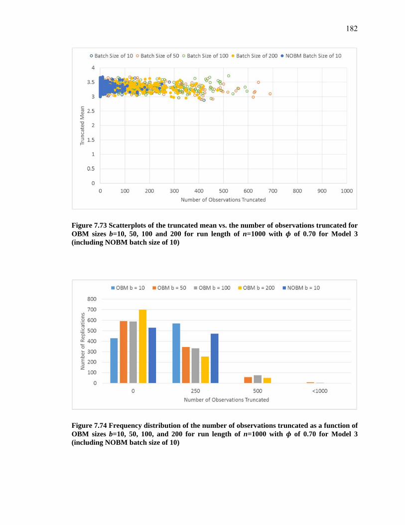
182
Figure 7.73 Scatterplots of the truncated mean vs. the number of observations truncated for OBM sizes b=10, 50, 100 and 200 for run length of n=1000 with ϕ of 0.70 for Model 3 (including NOBM batch size of 10)
Figure 7.74 Frequency distribution of the number of observations truncated as a function of OBM sizes b=10, 50, 100, and 200 for run length of n=1000 with ϕ of 0.70 for Model 3 (including NOBM batch size of 10)

183
Table 7.30 Correlation between the truncated mean and the number of observations truncated for OBM sizes b=10, 50, 100, and 200 for run length of n=16,000 with ϕ of 0.70 for Model 3
Trunc Batch =10 Trunc Batch =50 Trunc Batch =100 Trun Batch = 200
Mean Batch = 10 -0.105123784 0.024183645 -0.007825651 -0.041654617
Mean Batch = 50 0.005546592 -0.144419915 -0.01367133 -0.069917161
Mean Batch = 100 -0.062115342 0.031223516 -0.036393455 -0.036956424
Mean Batch = 200 -0.018985329 -0.022951969 -0.003507772 -0.103548868

184
Chapter 8. Conclusion and future research
One measure of the effectiveness of applied research on DES is the degree to which
research findings are incorporated into standard practice. A major purpose of our research
was to enhance the effectiveness of MSER in just this way. Two different approaches to
improving MSER accessibly were implemented and thoroughly tested.
The first was to integrate MSER logic in commercial simulation software in the form
of a static library, a DLL, and a submodel (subroutine); the second was to provide
standalone codes a variety of programming language to use as MSER post-analysis. After
extensive reviews, we chose the commercial simulation software ExtendSim,
ProModel/MedModel, and Arena to realize this first approach; we chose R, SAS, Matlab,
VBA, and C/C++ to implement the second.
To make these codes public and facilitate distribution, we created the MSER
Laboratory hosted at the University of Virginia. In addition to the sample codes, this web
site currently includes information on the mathematical and historical development of
MSER, as well as references into the literature. Our intention is to maintain and support
the continued development and expansion of the Lab.
In the future, we will explore modifications to the laboratory site which will make it
interactive, such that a warm-up period can be determined automatically simply by
importing a data set to be analyzed. We also intend to include codes in additional
programming languages, such as the scripting languages Python and Perl, as well as

185
incorporate useful suggestions and related research findings from the simulation
community. We are very anxious to work with developers of commercial simulation
software houses to incorporate MSER in future releases of their products, as we have done
previously with Dave Krahl at Imagine That (to whom we reiterate our sincere thanks and
appreciation). We also intend to pursue research to advance the MSER logic module,
particularly with regard to integrating MSER with the notion of automatic stopping rules.
The second major purpose of our research was to address a number of open questions
regarding MSER application and provide guidance in the selection of MSER parameters.
These include:
the choice of simulation run length n,
the choice of batch size b,
the maximum acceptable optimal truncation point dmax on the range of a given run
length [0≤ dmax ≤n], and
the incorporation of the overlapping batch means.
To this end we first develop a hypothetical case which demonstrated that MSER can
potentially change its determinations regarding the location and the even the existence of
a suitable truncation point depending on the run length chosen. We concluded that
performance of MSER does in fact depend fundamentally on choosing a sufficient run
length. Without knowledge beyond the output sequences alone, this choice remains an open
problem and the subject for future research.
To develop insight regarding the remaining questions, we tested MSER using non-
overlapping batch means (NOBM) with batch sizes of b= 1, 5, and 10 and selected run
lengths for three simulation models: (1) a uniform white noise process with superimposed

186
linearly decreasing bias, (2) the delay time in M/M/1 with four different traffic intensities,
and (3) EAR(1) with four different parameters. We also tested MSER using overlapping
batch means (OBM) with selected batch sizes run lengths.
We selected Model 1 as the baseline for testing MSER performance because of its
transparency—the range of optimal truncation points is clear, both visually and
analytically. We showed that for long runs:
(1) all batch sizes remove all of the transient observations,
(2) estimation errors are an artifact of sampling after the biasing effect of the initial
transient has been removed,
(3) modest batching has no significant effect on the quality of estimates, and
(4) the mean estimate is uncorrelated with the number of observations truncated for
all the batch sizes and the success of a truncation procedure in terms of the
accuracy of the estimate cannot be imputed from the truncation point alone.
For shorter runs, we showed conclusion (4) also holds. In addition:
(5) even with very little steady-state data, the MSER-indicated truncation points are
themselves very reasonable and indeed optimal in terms of the mean estimates for
most cases,
(6) increasing batch sizes increases both the variance and spread of the truncated
observations, without systematically affecting the accuracy of the estimated mean,
(7) to the degree that batching reduces the effective sample size, it is not recommended
for small samples and provides no discernable benefit for large samples,

187
(8) the choice of dmax is a binding concern only if (n-d)/n is close to 1—the choice of
n is likely dominated by the need for estimates with acceptable accuracy and
precision,
(9) the d*≤dmax=n/2 threshold provides significant protection against estimation errors
resulting from run lengths that are too short without over-truncation of replications
with adequate run lengths,
(10) for run lengths that are approximately the same as ideal truncation point, however,
the protection may be inadequate and a modestly lower threshold would be
preferred, and
(11) OBM outperforms the non-overlapping approach in all cases and OBM offers
significantly greater precision in the estimate.
We selected Model 2 because it allows comparison with the results obtained by Law
(2015) and by White and Hwang (2015) for long runs. The results obtained by White and
Hwang (2015) demonstrated that truncation points and the error in the truncated mean
estimates are essentially independent. Further that, while the mean estimates for this
problem are quite good without truncation, applying MSER-5 truncation modestly
improves the accuracy of these estimates.
Our objective here was to explore the performance of MSER for a single initial
condition, empty and idle {x0=0}, with respect to alternative run lengths, batch sizes, and
model traffic intensities. We found that:
(1) the results obtained in the present research for n=64,000 and =0.9 are entirely
consistent with those reported earlier.

188
(2) while we speculated that the effects of decreasing would be similar to those
encountered by increasing the run length n, the results of our experiments suggest
that this speculation is largely untrue and decreasing traffic intensity cannot
altogether compensate for short run length,
(3) the d*≤dmax=n/2 truncation rule likewise does not altogether compensate for short
run lengths, and
(4) for smaller run lengths and traffic intensities, MSER appears to overestimate the
amount of truncation warranted and underestimate the steady-state mean.
We speculate that conclusion (4) obtains because truncating early regenerative cycles
with large peak waiting times, when these exist, reduces the sample variance. Early in the
run, the MSER statistic is relatively less sensitive to the accompanying reduction in sample
size than to the reduction of sample variance. This speculation remains open for future
research.
In the final analysis, our research demonstrates that
(5) the difficulty in estimating the steady-state mean has little or nothing to do with bias
resulting from a poor choice of initial conditions for Model 2. The empty-and-idle
condition regenerates frequently, more frequently for lower traffic intensities and
smaller batches, and
(6) instead, the fundamental issue here is determining an initial run length that is
sufficiently long to capture observations that, taken together, are representative of
the steady-state distribution.
In other words,

189
(7) for regenerative processes with irregular cyclical outputs and inadequate run lengths,
MSER may suggest truncation points when truncation is contraindicated.
Future research might extend these results by testing the effect of alternate initial conditions
other than x0=0 or 100, where truncation is actually required to mitigate initialization bias.
We selected Model 3 because determining the “true” truncation point for this model is
problematic. Unlike Model 1, the process converges to steady state only in the limit and
which observation to choose as the “true” truncation point is inherently subjective. We
noted that MSER is data driven and does not suffer from this ambiguity. We also suggested
the expected -percent settling time as a measure for the degree of truncation.
We found that:
(1) MSER yields superior estimates for all run lengths, with the difference in accuracy
increasing as the run lengths as the decrease,
(2) restricting the optimal truncation point to d*<n/2 does not consistently appear to
provide the desired indication that runs are too short to yield accurate estimates on
average.
However, we speculate the same is not true when the threshold is applied on a replication-
by-replication basis, as recommended. This speculation warrants future research.
(3) Truncated mean estimates are relatively independent of the number of observations
truncated—for long runs, the correlation is essentially zero; for medium and short
runs, there appears to be a modest positive correlation, with the magnitude of this
correlation generally increasing as run length decreases. The shortest runs tend to
induce greater truncation on average, and

190
(4) NOBM provides better accuracy and precision at b=10.
It is unclear whether or not conclusion (4) holds for other batch sizes. Adding clarity on
the relative performance of OBM and NOBM is a potentially fruitful subject for future
research.
The conclusion consistently obtained in this research—that batching, in general, does
not improve estimates and can, in some instances, result in a loss of precision seemingly
contradicts a long-standing result in the literature (White, Cobb, and Spratt, 2000) but
agrees with Schmeiser’s discussion and recommendation
The MSER-5 is the most attractive general-purpose heuristic for mitigating the effects
of the startup problem evaluated in this research. It is the most sensitive rule in
detecting bias and the most consistent rule in mitigating its effects.
This result was obtained based using models not considered in the current research. Future
research should attempt to reproduce the results reported in the literature using the methods
developed in this research. Future research should also test MSER performance on
additional, more complex processes models, such as SS7 model examined by Law. The
MSER laboratory, we hope, will facilitate these future research efforts.

191
References
Applied Material, Introduction of Automod, accessed Aug. 19, 2016, http://www.appliedmaterials.com/global-services/automation-software/automod
Arena Simulation Software, What is Simulation Software?, accessed Aug. 19, 2016, https://www.arenasimulation.com/
Banks, J., (Editor), 1998, Handbook of Simulation: Principles, Methodology, Advances, Applications, and Practice, Wiley
Bertoli, M., G. Casale, and G. Serazzi, 2007, The JMT Simulator for Performance Evaluation of NonProduct-Form Queueing Networks. Proceedings of the 40thAnnual Simulation Symposium, pp. 3-10
Bertoli, M., G. Casale, and G. Serazzi, 2009, JMT: Performance Engineering Tools for System Modeling. ACM Metrics Performance Evaluation Review, 36(4)10-15.
Billingsley, P., 1968, Convergence of Probability Measures. Wiley, New York.
Blomqvist, N., 1967, The Covariance Function of the M/G/1 Queueing system. Skandinavisk Aktuarietidskrift, 6:157-174
Cash, C. R., D. G. Dippold, J. M. Long, B. L. Nelson, and W. P. Pollard., 1992, Evaluation of tests for initial condition bias. In Proceedings of the 1992 Winter Simulation Conference, ed. J. J. Swain, D. Goldsman, R. C. Crain, and J. R. Wilson, Institute of Electrical and Electronics Engineers, Piscataway, NJ, 577-585
Cobb, M. J., 2000, Eliminating Initialization Bias while Controlling Simulation Run Length, Master Thesis, Department of Systems and Information Engineering, University of Virginia, Charlottesville, Virginia
Cohen, J. W., 1982, The Single Server Queue. North- Holland, Amsterdam
Conway, R. W., 1963, Some Tactical Problems in Digital Simulation, Management Science, 10(1)47-61
CreateaSoft, SimCAD Process Simulator, accessed Aug. 20, 2016, https://www.createasoft.com/
Emshoff, J. R., and R. L. Sission, 1970, Design and Use of Computer Simulation Models, Macmillan, New York
Fishman, G.S., 1971, Estimating Sampling Size in Computing Simulation Experiments, Management Science, 18(1)21-38
Fishman, G.S., 1973, Statistical analysis for queueing simulation, Management Science, 20:363-369
Fishman, G.S., 2001, Discrete-Event Simulation: Modeling, Programming, and Analysis, Springer-Verlag, New York
Franklin, W. W., and K. P. White, Jr., 2008, Stationarity Tests and MSER-5: Exploring the Intuition Behind Mean-Squared-Error-Reduction in Detecting and Correcting Initialization Bias, Proceedings of the 2008 Winter Simulation Conference, 541-546

192
Franklin, W. W., K. P. White, Jr., and K. A. Hoad, 2009, Comparing Warm-up Methods using Mean-Squared Error, Working paper, Department of Systems and Information, University of Virginia, Charlottesville, VA. Available from the authors.
Franklin, W.W., 2009, The Theoretical Foundation of the MSER Algorithm, Ph.D. Dissertation, Department of Systems and Information Engineering, University of Virginia, Charlottesville, VA
Goldsman, D. and M.S. Meketon, 1986, A Comparison of Several Variance Estimators, Tech. Report #J-85-12, School of ISyE, Georgia Tech, Atlanta.
Gordon, G., 1969, System Simulation, Prentice Hall PTR, Upper Saddle River, NJ
Grassmann, W.K., 2009, When, and when not to Use Warm-up Periods in Discrete Event Simulation. SimuTools 2009, Rome, 1-6
Grassmann, W.K., 2011, Rethinking the Initialization Bias Problem in Steady-State Discrete Event Simulation, Proceedings of the 2011 Winter Simulation Conference, 593-599
Hoad, K., and S. Robinson, 2011, Implementing Mser-5 in Commercial Simulation Software and Its Wider Implications, Proceedings of the 2011 Winter Simulation Conference, pp.495-503
Hoad, K., Robinson, S., and Davies, R., 2008, Automating Warm-up Length Estimation, Proceedings of the 2008 Winter Simulation Conference, 532-540
Hoad, K., Robinson. S., and Davies, R., 2011, AutoSimOA: a framework for automated analysis of simulation output, Journal of Simulation 5:9-24
Imagine That, Introduction of ExtendSim, accessed Aug. 20, 2016, http://www.extendsim.com/
Kelton, W. D., and A. M. Law, 1983, A New Approach for Dealing with the Startup Problem in Discrete Event Simulation, Naval Research Logistics Quarterly 30, pp. 641-658
Kelton, W. D., R. P. Sadowski, and N. Swets, 2010, Simulation with Arena, 5th edition, McGraw-Hill, New York
Krahl, D., 2012, ExtendSim: a history of innovation, Proceedings of the Winter Simulation Conference.
Lada, E. K., and J. R. Wilson, 2008, SBatch: A spaced batch means procedure for steady-state simulation analysis. Journal of Simulation 2:170–185.
Lada, E.K., 2003, A wavelet-based procedure for steady-state simulation output analysis, Ph.D Dissertation, available online via www.lib.ncsu.edu/theses/available/etd-04032003-141616/unrestricted/etd.pdf
Law, M. A., 2015, Simulation Modeling and Analysis, 5th edition, McGraw-Hill, New York
Mahajan, P. S., and R.G. Ingalls, 2004, Evaluation of methods used to detect warm-up period in steady state simulation, Proceedings of the 2004 Winter Simulation Conference, pp. 663-671
McClarnon, M. A., 1990, Detection of steady state in discrete event dynamic systems: An analysis of heuristics. M.S. thesis, School of Engineering and Applied Science,

193
University of Virginia, Charlottesville, Virginia. Available from University of Viginia Library, [email protected], 434–982–3094.
Meketon, M. S., and Schmeiser, B. W., 1984, Overlapping batch means: Something for nothing? Proceedings of the 1984 Winter Simulation Conference, 227-230.
Mokashi, A. C., J. J. Tejada, S. Yousefi, T. Xu, J. R. Wilson, A. Tafazzoli, and N. M. Steigher, 2010, Performance Comparison of MSER-5 and N-Skart on the Simulation Start-up Problem, Proceedings of the 2010 Winter Simulation Conference, pp.971-982
Morse, P. M., 1955, Stochastic properties of waiting lines. Operations Research, 3(3) pp.1255-1261
Nelson, B.L., 2011, Thirty Years of Batch Size Effects, Proceedings in the 2011 Winter Simulation Conference, 392-400
Nelson, B. 2013, Foundations and Methods of Stochastic Simulation: A First Course. Springer Science, New York.
Pasupathy, R. and B. Schmeiser, 2010, The Initial Transient in State-State Point Estimation: Contexts, A Bibliography, The MSE Criterion, and The MSER Statistic, Proceedings of the 2010 Winter Simulation Conference, 184-197
Pasupathy, R., and B. Schmeiser. 2014. “MSER: Algorithms for the Initial-Transient Problem.” Presented at the INFORMS Annual Meeting, 12 November
Pawliskowski, K., 1990, Steady-State Simulation of Queuing Processes: A Survey of Problems and Solutions, ACM Computing Surveys, 22(2)123-170
Peng, L., and Q. Yao, 2003, Least Absolute Deviation Estimation for ARCH and GARCH models, Biometria 90(4)967-975
Pollard, D., 1991, Asymptotics for least absolute deviation regression estimators, Econometric Theory 7:186-199
ProModel, 2011, ProModel tutorial accessed via https://www.promodel.com/solutionscafe/webinars/ProModel%202011%20Tutorial/PM2011Tutorial.html
Rossetti, M. D., P. J. Delaney, and K. P. White, Jr. 1995, Generalizing the half-width minimization heuristic for mitigating initialization bias, In Proceedings of International Conference on Systems, Man, and Cybernetics. Piscataway, New Jersey: Institute of Electrical and Electronics Engineers, Inc. pp. 212–216
Sanchez, P., and K.P. White, Jr. 2011, Interval Estimation Using Replication/Deletion and MSER Truncation, Proceedings of the 2011 Winter Simulation Conference, 488-494
Schmeiser, B., 1982, Batch size effects in the analysis of simulation output, Operations Research 30:556–568
Schmeiser. B., and W.T. Song., 1987, Correlation among estimators of the variance of the sample mean. Proceedings of the Winter Simulation Conference, pp.309–317
Schruben, L.W., 1982, Detecting Initialization Bias in Simulation Output, Operation Research 30(3)569-590
Schruben, L. W., 1983, Confidence interval estimation using standardized time series. Operations research, 30:1090-1108

194
Simio Release 2 - Sprint 41 - July 21, 2010 to implement the research logic, accessed Aug. 20, 2016, http://www.simio.com/products/ and Simio Reference Guide
SIMUL8 Software, Simul8 Introduction, accessed Aug. 19, 2016, http://www.simul8.com/
Solomon, S. L., 1983, Simulation of Waiting-Line Systems. Prentice-Hall, Englewood Cliffs, N.J.
Song, W. T., 1996, On the Estimation of Optimal Batch Sizes in the Analysis of Simulation Output, European Journal of Operational Research, 88:304-319
Song, W. T., and B. Schmeiser, 1993, Variance of the Sample Mean: Properties and Graphs of Quadratic-Form Estimators, Operations Research 41:501-517
Song, W.T., and B. Schmeiser, 1995, Optimal Mean-Squared-Error Batch Sizes, Management Science 41:110–123.
Spratt, S. C., 1998, An Evaluation of Heuristics for the Startup Problem
Tafazzoli, A., 2009, Skart: A skewness- and autoregression-adjusted batch-means procedure for simulation analysis. PhD Dissertation, Department of Industrial and Systems Engineering, North Carolina State University, Raleigh, North Carolina. Available via www.lib.ncsu.edu/theses/available/etd-01122009-153054/unrestricted/etd.pdf [accessed March 3, 2012].
Tafazzoli, A., and J. R. Wilson, 2009, N-Skart: A Nonsequential Skewness-and Autoregression-adjusted Batch-means Procedure for Simulation Analysis. Proceedings of the 2009 Winter Simulation Conference, pp.652-662
Tocher, K. D.,1963, The Art of Simulation, English Universities Press
Turnquist, M. A., and J. M. Sussman, 1977, Toward Guidelines for Designing Experiments in Queuing Simulation. Simulation, 28:137-144
Wang, R. J., and P. W. Glynn, 2014, On the Marginal Standard Error Rule and the Testing of Initial Transient Deletion Methods, working paper, Department of Management Science and Engineering, Stanford University. Stanford, CA. Accessed 30 April 2015. http://web.stanford.edu/~glynn/papers/2014/WangG14.pdf
Welch, P. D., 1981, On the Problem of the Initial Transient in Steady-State Simulation, IBM Watson Research Center, Yorktown Heights, New York.
White, K. P., Jr. 1995, A simple rule for mitigating initialization bias in simulation output: Comparative results. In Proceedings of the International Conference on Systems, Man, and Cybernetics, Piscataway, New Jersey: Institute of Electrical and Electronics Engineers, Inc., pp. 206–211.
White, K.P. Jr., 1997, An Effective Truncation Heuristic for Bias Reduction in Simulation Output, Simulation 69(6),323-334
White, K. P., Jr., 2012, Optimal analysis for the mean of a simulation output, Department of Systems and Information Engineering, University of Virginia, working paper
White, K. P. Jr., M. J. Cobb, and S. C. Spratt, 2000, A Comparison of Five Steady-State Truncation Heuristics for Simulation, Proceedings of the 2000 Winter Simulation Conference, pp.755-760

195
White, K. P. Jr., and W. W. Franklin, 2010, Parametric Expression For MSER with Geometrically Decaying Bias, Proceedings of the 2010 Winter Simulation Conference, 957- 964
White, K. P., Jr., and Hwang, S. N., 2015, Delay times in an M/M/1 queue: estimating the sampling distribution for the MSER-truncated steady-state mean using replication/deletion, Proceedings of the 2015 Winter Simulation Conference, pp. 493-504
White, K. P., and M. A. Minnox, 1994, Minimizing initialization bias in simulation output using a simple heuristic. In Proceedings of International Conference on Systems, Man, and Cybernetics, Piscataway, New Jersey: Institute of Electrical and Electronics Engineers, Inc., pp. 215–220.
White, K. P., Jr., and S. Robinson, 2010, The initial transient problem (again), or why MSER works, Journal of Simulation, 4(3)268-272
Wilson, J. R., and A. A. B. Pritsker, 1978, Evaluation of startup policies in simulation experiments. Simulation, 31:79-89
Yousefi, S., 2011, MSER-5Y: An Improved Version of MSER-5 with Automatic Confidence Interval Estimation, Master thesis, North Carolina State University, Raleigh, NC

196
Appendix I. Arena MSER Submodel User Guide
This appendix provides guidance that will allow you to incorporate the purpose-built MSER submodel in your Arena simulation model.
Variable definition
After building a model, you can choose entity’s attribute(s) of interest that are passed to a Arena MSER submodel.
1. General simulation variables: a. X: Attribute of interest (i.e., entity waiting time) b. StopRule: User input to end simulation c. Counter: Number of entities
2. MSER related variables: You need to define the following additional variables to
store temporary values and compute MSER statistics associated with each entity. a. Truncation: Truncation index b. MSER_test: MSER statistics without truncation c. MSER_final: MSER statistics related to each truncation index d. X2: Squared values of attribute X e. inter_cumX: Summation of X associated with each entity
f. inter_cumX2: Summation of X2 associated with each entity
g. cumX: Storage for summation of X associated with each entity h. cumX2: Storage for summation of X associated with each entity i. Mean: Average value from the first X to the current one by dividing cumX
by Counter
To avoid confusion, all of variables are preceded with “v_” inside the Arena submodel with the exception StopRule. Equations 2b and 2c are used to compute MSER statistic.
2b:
2c:
0011 1
2
CounterCounterXXCounterXCounter
ii
Counter
i
Counter
iii
111 11
22
TruncationStopRuleTruncationStopRuleXXTruncationStopRuleXXStopRule
ii
StopRule
i
StopRule
ii
truncation
iii

197
All required variables are listed in Table I.1. For example, if you were interested in entity wait time, choose its wait time attribute as a global variable, v_X. In this table, the “Location of block” column indicates where the corresponding variables are located in building blocks in Arena model.
Table I.1. Global, Local variables and Arrays
No. Variable (array) name
Location of block Usage
1 v_Counter Index Record entity number
v_Counter + 1
2 v_X InterimData Generation
Record entity wait time
3 v_X2 InterimData Generation
Record (entity waiting time)2
4 v_inter_cumX InterimData Generation
Holder for summation of v_X
5 v_inter_cumX2 InterimData Holder for summation of v_X2
6 v_Mean DataGeneration v_cumX(v_Counter)/v_Counter
7 v_ cumX DataGeneration v_inter_cumX(v_counter)
8 v_ cumX2 DataGeneration v_inter_cumX2(v_counter)
9 v_MSER_test MSER Without Truncation
(v_cumX2(v_Counter) - v_Counter * v_Mean(v_Counter) * v_Mean(v_Counter))/ ((v_counter - 0) * (v_counter - 0))
10 StopRule End of Simulation
(Decision block)
Global variable to check the end of simulation, 10000 that confirm
StopRule = v_Counter
11 v_Truncation Truncation Index v_Truncation + 1
12 v_MSER_final MSER
With Truncation
((v_cumX2(StopRule) - v_cumX(v_Truncation)) - (StopRule -v_Truncation) * v_Mean(StopRule) * v_Mean(StopRule))/ ((StopRule - v_Truncation) * (StopRule - v_Truncation - 1))

198
Run length control
As shown in Figure I.1, the global variable StopRule must be defined before running a model. After assign a value to StopRule, such as 10000 entities, you need to use this variable as the terminating condition on the Replication Parameters tab of the Arena Run Setup menu.
Figure I.1. Setting the Simulation Length using the variable StopRule.

199
Usage of MSER Submodel
As an example, consider the case where the output of interest is the mean entity waiting-time for an M/M/1 queue in steady state. When building the model, include the MSER submodel as shown in Figure I.2.
Figure I.2. Main model for the example.
As shown in Figure I.3, the MSER submodel consists of three major parts: (1) Data preprocessing, (2) MSER test generation, and (3) MSER statistics generation. The second part is included simply to test whether or not the calculations are performed correctly and can be ignored after completing the model.
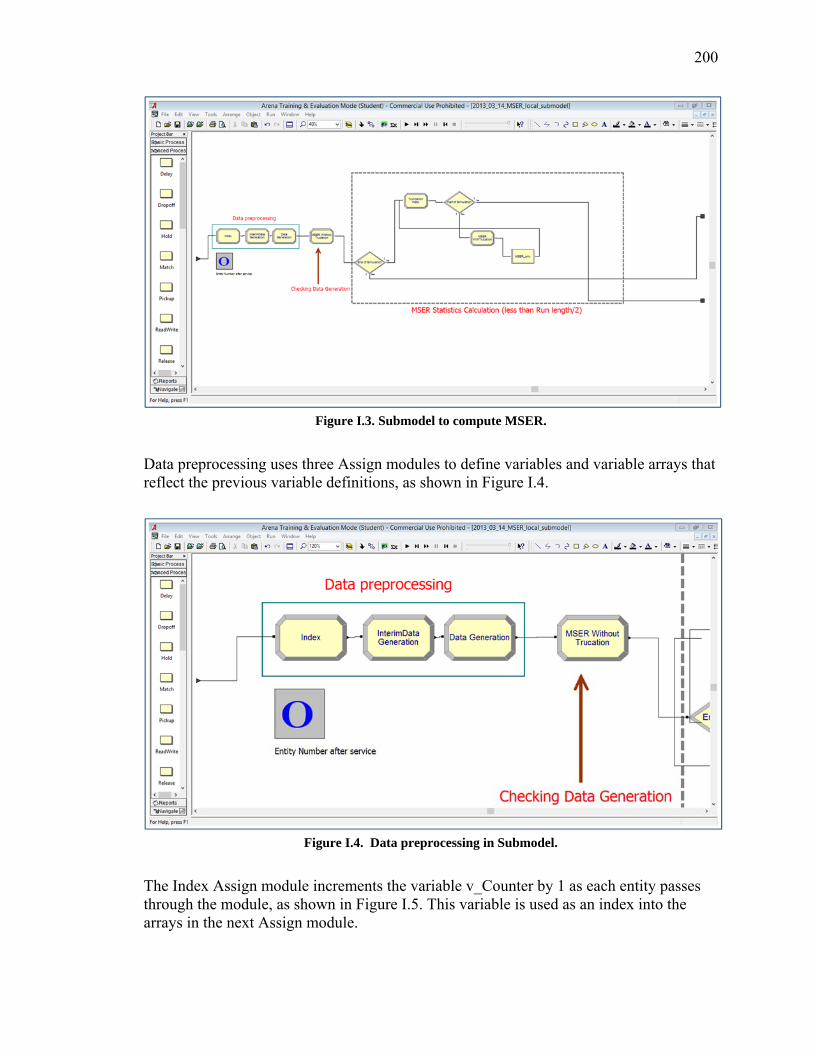
200
Figure I.3. Submodel to compute MSER.
Data preprocessing uses three Assign modules to define variables and variable arrays that reflect the previous variable definitions, as shown in Figure I.4.
Figure I.4. Data preprocessing in Submodel.
The Index Assign module increments the variable v_Counter by 1 as each entity passes through the module, as shown in Figure I.5. This variable is used as an index into the arrays in the next Assign module.

201
Figure I.5. Index incremented in an Assign module.
As shown in Figure I.6, the Interim Data Generation Assign module assigns values to the elements of two variable arrays, X and X2, using V_Counter as the index into these arrays. This module also assigns a value to the variable inter_cumX. These variables are subsequently used to update the MSER statistic.
Figure I.6. Interim Data Generation Assignments.
As shown in Figure I.7, the Data Generation assignment module assigns three variable arrays that also used to update the MSER statistic.

202
Figure I.7. Data Generation in Assignment.
As noted previously, this assignment shown in Figure I.8 is included to test whether or not the calculations are performed correctly and can be removed after performing the test satisfactorily.
Figure I.8. MSER without Truncation in Assignment.
Figure I.9 shows the core building blocks used to compute MSER statistics.

203
Figure I.9. MSER Statistics calculation in Submodel.
The decide module in Figure I.10 compares the value of the variable V_Counter to the value of the variable StopRule to determine whether or not the stopping condition has been met. If not, the entity exits the Arena MSER submodel.
Figure I.10. End of Simulation in Decision Node.
Once the stopping condition is met, the entity proceeds to the Truncation Index assignment module shown in Figure I.11. Here the index variable v_Truncation is incremented by 1.

204
Figure I. 11 Truncation Index in Assignment.
This decision node shown in Figure I.12 checks whether or not the half of simulation run is completed.
Figure I.12. Half of Simulation in Decision Node.
If not, then the MSER statistics are calculated in the MSER With Truncation Assign module as shown in Figure I.13. The logic in Equation 2c is incorporated in the New Value field for the current truncation index to assign the value calculated for the MSER statistic, an element of the global variable array v_MSER_final.
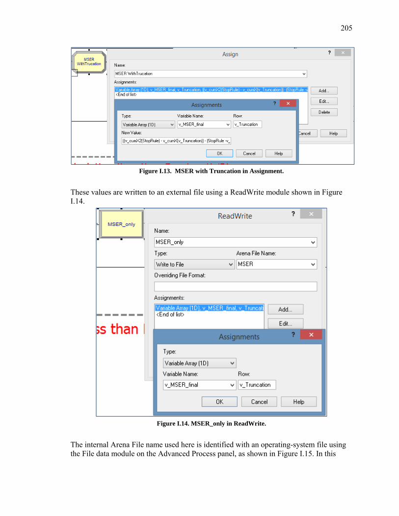
205
Figure I.13. MSER with Truncation in Assignment.
These values are written to an external file using a ReadWrite module shown in Figure I.14.
Figure I.14. MSER_only in ReadWrite.
The internal Arena File name used here is identified with an operating-system file using the File data module on the Advanced Process panel, as shown in Figure I.15. In this
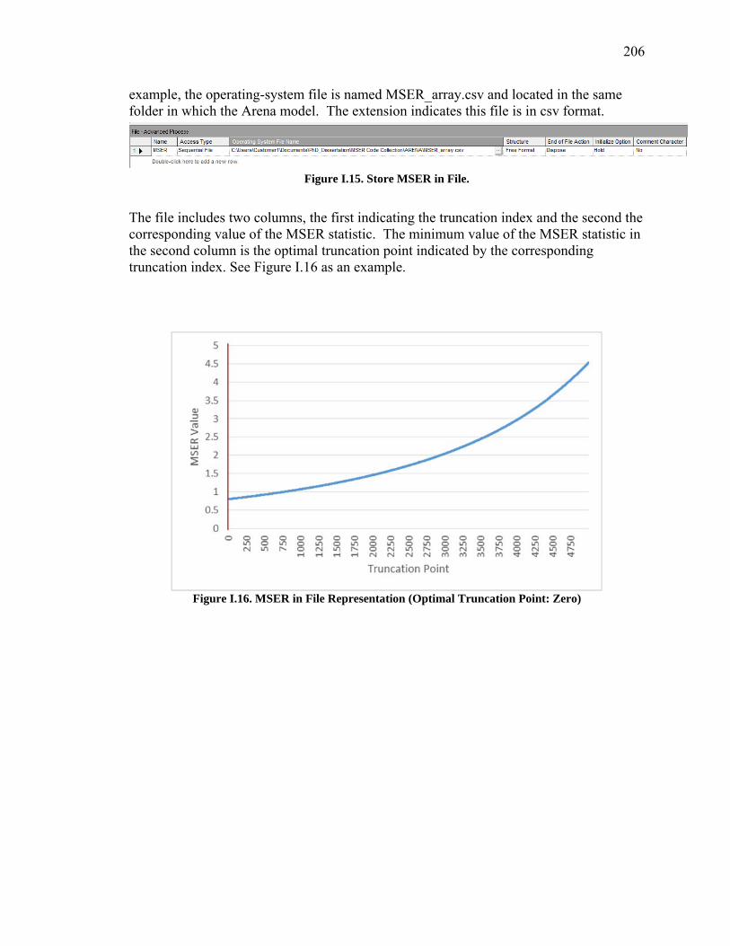
206
example, the operating-system file is named MSER_array.csv and located in the same folder in which the Arena model. The extension indicates this file is in csv format.
Figure I.15. Store MSER in File.
The file includes two columns, the first indicating the truncation index and the second the corresponding value of the MSER statistic. The minimum value of the MSER statistic in the second column is the optimal truncation point indicated by the corresponding truncation index. See Figure I.16 as an example.
Figure I.16. MSER in File Representation (Optimal Truncation Point: Zero)

207
Appendix II. Personal reflections on the importance of the warm-up problem and undergraduate simulation curriculum survey
II.1 Anecdotal case to emphasize the importance of warm-up period
Some of working professionals representing simulation specialists do not have in-depth
knowledge and fundamental understanding of discrete event simulation. In fact, they are
likely to build models based on a specific software environment. Thus, as long as its built-
in functionalities are enough to reflect key characteristics of the system, only potential
minor error might occur. For example, when a modeler sets up the travel distance of
moving resources, she or he should acknowledge the behavior of returning resources
imposed by some software application. However, we seldom see a simulation professional
using warm-up periods with a solid understanding.
II.2 Undergraduate curriculum survey
We reviewed the twenty curricula or handbooks in industrial or systems engineering
departments in the U.S. colleges. Thirteen out of twenty universities apparently mandate
undergraduates to take credits of simulation course for graduation. Six other universities
also describe simulation as a key methodology to learn before graduation. Even though one
school does not have undergraduate programs, that school provides simulation courses for
graduates. Most courses are 3 or 4 credits which are recommended to take during the third
year. Table AII.1 summarizes detailed information about the survey.
This requirement apparently emphasizes the importance and the difficulty of simulation
courses. However, this tendency does not guarantee those students taking simulation

208
classes to be confident in building complex and sophisticated models. First, it only takes
one semester to fulfill this credit. After finishing the course as a junior student, she or he
might lose the insight and lessons learned over time.
Second, they might have to re-learn using other specific simulation package after their
graduation if the worksite’s tool is different from what they learned. Third, with respect to
output analysis, its contents tend to be addressed near the end of the course. Sometimes,
students are overwhelmed by the last minute pressures while instructors might not have
enough time to provide in-depth lessons. These are the reasons that students and even
experienced modelers do not fully appreciate the criticality of analyzing output statistics.
Furthermore, most of simulation software applications provide 95 or 90% confidence
interval by merely clicking an option.
Additionally, simulation software training courses from software vendors consist of
two parts: Basic/introductory course and the following advanced course. The first course
usually provides the brief review of simulation methodology and teaches how to build
reasonable size models using built-in functions. Its major intents lie in familiarizing how
to use that specific software. By completing this course, the course taker will likely know
how to build relatively formulated models. However, they might fail to incorporate some
key ingredients of a problem.
As the beginners and intermediate modelers encounter more complex situations, they
will turn to their software vendors for additional support. These needs will urge them to
take an advanced course to learn how to use optimization add-ins and to code inside or
outside extensions. Both of these courses usually require two or three day boot camps,

209
TableAII.1 Twenty Undergraduate Curricula of Simulation
but they never exceed more than one week. Thus, less than two weeks and a semester
exposure to simulation is where college graduates start work as simulation analysts.
We also meet many simulation modelers whose backgrounds are not as industrial or
systems engineers. They just take two courses from software vendors and then learn the
methodologies further while they work. In fact, I have been somewhat surprised to witness
many mistakes and misusage even with simple built-in functions and add-ons. For instance,
one input analyzer (i.e., Stat:fit) indicates that there is no good fit for the collected data,
but the modeler just used the first distribution that was addressed. If she or he decides to
use it as a second best option after carefully comparing it with other distributions, it might
be acceptable even though this practice is not recommended. However, if the modeler just
chooses the first one listed out of input analyzer, this attitude should be remedied.
In addition, building a simulation model as a team is sometimes considered a norm, but
this process should be checked by another modeler. At least another input analyzer such as
Undergraduate No. of
Mandatory Credit
1 Columbia University (Fu Foundation) Yes 4
2 Cornell University Yes 4 http://www.orie.cornell.edu/orie/academics/undergraduate/requirements.cfm
3 Georgia Institute of Technology Yes 3 http://www.isye.gatech.edu/academics/undergraduate/courses/
4 Lehigh University (Rossin) Yes 3 http://www.lehigh.edu/ise/documents/IE%20Major%20Requirements%2009_10.pdf
5 North Carolina State University Yes 3 https://portalsp.acs.ncsu.edu/psp/EP91PRD/EMPLOYEE/PCS900PRD/c/NC_SSS_MENU.NC_AA_REQMNT_RPT.GBL
6 Northwestern University (McCormick) Yes 3 http://www.iems.northwestern.edu/docs/undergraduate/AY%2013‐14%20BSIE%20Degree%20Requirements.pdf
7 Purdue University‐West Lafayette Not clear 3 https://engineering.purdue.edu/IE/Academics/Undergrad/Curriculum
8 Stanford University Optional 3 http://exploredegrees.stanford.edu/schoolofengineering/managementscienceandengineering/#bachelorstext
9 Texas A&M University‐College Station (Look) Not clear 3 http://engineering.tamu.edu/industrial/academics/courses/course‐descriptions
10 University of Arkansas‐Fayetteville Yes 3 http://www.ineg.uark.edu/Undergrad_Handbook_Spring_20140423.pdf
11 University of California‐Berkeley Not clear 3 http://ieor.berkeley.edu/AcademicPrograms/Ugrad/Courses/index.htm
12 University of California‐Santa Barbara Not clear 3 http://engineering.ucsb.edu/current_undergraduates/pdf/00‐01Announce.pdf
13 University of Florida Yes 3 https://catalog.ufl.edu/ugrad/current/engineering/majors/industrial‐and‐systems‐engineering.aspx
14 University of Illinois‐Urbana‐Champaign Yes 3 http://provost.illinois.edu/programsofstudy/2014/fall/programs/undergrad/engin/ind_engin.html
15 University of Michigan‐Ann Arbor Yes 4 http://ioe.engin.umich.edu/degrees/ugrad/ugdocs/UndergradStudentGuide.2013.2014.pdf
16 University of Pittsburgh (Swanson) Yes 3 http://www.engineering.pitt.edu/Industrial/Undergraduate/Curriculum_Effective_as_of_Fall_2014/
17 University of Southern California (Viterbi) Not clear 3 http://ise.usc.edu/academics/undergrad/undergrad.htm
18 University of Texas‐Austin (Cockrell) No 0 No undergraduate program
19 University of Wisconsin‐‐Madison Yes 4 http://www.engr.wisc.edu/cmsdocuments/isye‐curriculum‐2014.pdf
20 Virginia Tech Yes 3 http://www.ise.vt.edu/UndergradProgram/ImportantDocuments/2013_14_UG_Handbook.pdf
SourceNo. School name

210
Expert:fit provides qualitative statements indicating that considering empirical distribution
or expertise knowledge is a better solution. However, some software just implement their
own function to assign input distributions that are seemingly workable but does not assure
proper fitting of input data. The reason why I address the cases of input analysis is that
while people believe they follow the standard and reliable steps to analyze input data, many
errors prevail. Thus, the right usage of output analysis must be strictly enforced as there is
no standard method across software environments. We will take a look at different
approaches to deal with warm-up period across multiple simulation software to apply
MSER methodology to their output analysis.