An experiment management component for the WBCSim problem solving environment

AN EXPERIMENT MANAGEMENT COMPONENT FOR THE

WBCSIM PROBLEM SOLVING ENVIRONMENT

by

Jiang Shu

Thesis submitted to the Faculty of the

Virginia Polytechnic Institute and State University

in partial fulfillment of the requirements for the degree of

MASTER OF SCIENCE

in

Computer Science

APPROVED:

Layne T. Watson

Chair of Advisory Committee

Frederick A. Kamke Naren Ramakrishnan

October 1, 2002

Blacksburg, Virginia

Key words: Experiment management, problem solving environment, computing envi-

ronment, wood-based composite materials, database management, visualization, optimiza-

tion.

Copyright 2002, Jiang Shu

AN EXPERIMENT MANAGEMENT COMPONENT FOR THE

WBCSIM PROBLEM SOLVING ENVIRONMENT

by

Jiang Shu

(ABSTRACT)

This thesis describes a computing environment WBCSim and its experiment man-

agement component. WBCSim is a web-based simulation system used to increase the

productivity of wood scientists conducting research on wood-based composite and material

manufacturing processes. This experiment management component integrates a web-based

graphical front end, server scripts, and a database management system to allow scientists

to easily save, retrieve, and perform customized operations on experimental data. A de-

tailed description of the system architecture and the experiment management component

is presented, along with a typical scenario of usage.

ACKNOWLEDGEMENTS

I would like to express my appreciation for the support and guidance that I received

from my advisor Dr. Layne T. Watson in the past two years. Also, I want to thank the

other two members of my advisory committee, Dr. Frederick A. Kamke and Dr. Naren

Ramakrishnan, for their sincere support and advice.

Furthermore, I would like to thank Balazs G. Zombori for his work on mat formation

modeling, hot compression modeling, and composite material analysis modeling (documented

in Chapter 2). Moreover, I thank Alex Verstak for his work on the telnet server (documented in

Chapter 5) in WBCSim. I would also thank Dr. Clifford A. Shaffer and Dr. Calvin J. Ribbens

for their effort in organizing research meetings to help students collaborate with each other.

This work was supported in part by a Virginia Polytechnic Institute and State University

1997 ASPIRES grant, USDA Grant 97-35504-4697, and DOE contract DE-AC04-95AL97273-

91830.

iii

TABLE OF CONTENTS

1. Introduction . . . . . . . . . . . . . . . . . . . . . . . . . . . . . . . . . . . . . . . . . . . . . . . . . . . . . . . . . . . . . . . . . . . . . . 1

1.1 WBCSim Introduction . . . . . . . . . . . . . . . . . . . . . . . . . . . . . . . . . . . . . . . . . . . . . . . . . . . 1

1.2 Experiment Management Component Introduction . . . . . . . . . . . . . . . . . . . . . . . 2

1.3 Organization . . . . . . . . . . . . . . . . . . . . . . . . . . . . . . . . . . . . . . . . . . . . . . . . . . . . . . . . . . . . 2

2. Related Work . . . . . . . . . . . . . . . . . . . . . . . . . . . . . . . . . . . . . . . . . . . . . . . . . . . . . . . . . . . . . . . . . . . . .3

2.1 Problem Solving Environments . . . . . . . . . . . . . . . . . . . . . . . . . . . . . . . . . . . . . . . . . . 3

2.2 WBC Computer-based Systems . . . . . . . . . . . . . . . . . . . . . . . . . . . . . . . . . . . . . . . . . . 3

2.3 Experiment Management Systems . . . . . . . . . . . . . . . . . . . . . . . . . . . . . . . . . . . . . . . . 5

3. Simulation Models . . . . . . . . . . . . . . . . . . . . . . . . . . . . . . . . . . . . . . . . . . . . . . . . . . . . . . . . . . . . . . . . 7

3.1 Rotary Dryer Simulation (RDS) . . . . . . . . . . . . . . . . . . . . . . . . . . . . . . . . . . . . . . . . . 7

3.2 Radio-Frequency Pressing (RFP) . . . . . . . . . . . . . . . . . . . . . . . . . . . . . . . . . . . . . . . . 7

3.3 Oriented Strandboard Mat Formation (OSB) . . . . . . . . . . . . . . . . . . . . . . . . . . . . . 8

3.4 Hot Compression (HC) . . . . . . . . . . . . . . . . . . . . . . . . . . . . . . . . . . . . . . . . . . . . . . . . . . 8

3.5 Composite Material Analysis (CMA) . . . . . . . . . . . . . . . . . . . . . . . . . . . . . . . . . . . . . 9

4. Simulation Model User Interfaces . . . . . . . . . . . . . . . . . . . . . . . . . . . . . . . . . . . . . . . . . . . . . . . . 10

5. WBCSim Architecture . . . . . . . . . . . . . . . . . . . . . . . . . . . . . . . . . . . . . . . . . . . . . . . . . . . . . . . . . . . 14

5.1 Client Layer . . . . . . . . . . . . . . . . . . . . . . . . . . . . . . . . . . . . . . . . . . . . . . . . . . . . . . . . . . . . 14

5.2 Server Layer . . . . . . . . . . . . . . . . . . . . . . . . . . . . . . . . . . . . . . . . . . . . . . . . . . . . . . . . . . . . 15

5.3 Developer Layer . . . . . . . . . . . . . . . . . . . . . . . . . . . . . . . . . . . . . . . . . . . . . . . . . . . . . . . . 16

6. Optimization And Visualization . . . . . . . . . . . . . . . . . . . . . . . . . . . . . . . . . . . . . . . . . . . . . . . . . 17

6.1 Optimization . . . . . . . . . . . . . . . . . . . . . . . . . . . . . . . . . . . . . . . . . . . . . . . . . . . . . . . . . . . 17

6.2 Visualization . . . . . . . . . . . . . . . . . . . . . . . . . . . . . . . . . . . . . . . . . . . . . . . . . . . . . . . . . . . 17

7. Rationale For Experiment Management . . . . . . . . . . . . . . . . . . . . . . . . . . . . . . . . . . . . . . . . . . 21

8. Experiment Management Component Architecture . . . . . . . . . . . . . . . . . . . . . . . . . . . . . . . 22

8.1 Client Layer . . . . . . . . . . . . . . . . . . . . . . . . . . . . . . . . . . . . . . . . . . . . . . . . . . . . . . . . . . . . 22

8.2 Server Layer . . . . . . . . . . . . . . . . . . . . . . . . . . . . . . . . . . . . . . . . . . . . . . . . . . . . . . . . . . . . 24

8.3 Developer Layer . . . . . . . . . . . . . . . . . . . . . . . . . . . . . . . . . . . . . . . . . . . . . . . . . . . . . . . . 24

9. Simulation Scenario . . . . . . . . . . . . . . . . . . . . . . . . . . . . . . . . . . . . . . . . . . . . . . . . . . . . . . . . . . . . . 25

10. Future Work And Conclusions . . . . . . . . . . . . . . . . . . . . . . . . . . . . . . . . . . . . . . . . . . . . . . . . . . . 28

10.1 Experiment Management . . . . . . . . . . . . . . . . . . . . . . . . . . . . . . . . . . . . . . . . . . . . . . . 28

10.2 Collaboration Support . . . . . . . . . . . . . . . . . . . . . . . . . . . . . . . . . . . . . . . . . . . . . . . . . . 29

10.3 High Performance Computing . . . . . . . . . . . . . . . . . . . . . . . . . . . . . . . . . . . . . . . . . . 29

iv

10.4 Conclusions . . . . . . . . . . . . . . . . . . . . . . . . . . . . . . . . . . . . . . . . . . . . . . . . . . . . . . . . . . . . 29

References . . . . . . . . . . . . . . . . . . . . . . . . . . . . . . . . . . . . . . . . . . . . . . . . . . . . . . . . . . . . . . . . . . . . . . . 31

Appendix A: Perl Subroutine gencontourplot . . . . . . . . . . . . . . . . . . . . . . . . . . . . . . . . . . . 34

Appendix B: Perl Code Example of WhirlGif from gen3Dplot . . . . . . . . . . . . . . . . . . . 36

Appendix C: Perl OSB Save Wrapper osbsave.pl . . . . . . . . . . . . . . . . . . . . . . . . . . . . . . . 38

Appendix D: Perl OSB Load Wrapper osbload.pl . . . . . . . . . . . . . . . . . . . . . . . . . . . . . . 47

Vita . . . . . . . . . . . . . . . . . . . . . . . . . . . . . . . . . . . . . . . . . . . . . . . . . . . . . . . . . . . . . . . . . . . . . . . . . . . . . 50

LIST OF FIGURES

Figure 4.1. The RDS model user interface. . . . . . . . . . . . . . . . . . . . . . . . . . . . . . . . . . . . . . . 11

Figure 4.2. The OSB model user interface. . . . . . . . . . . . . . . . . . . . . . . . . . . . . . . . . . . . . . . 12

Figure 4.3. The HC model user interface. . . . . . . . . . . . . . . . . . . . . . . . . . . . . . . . . . . . . . . . . 13

Figure 5.1. WBCSim architecture overview. . . . . . . . . . . . . . . . . . . . . . . . . . . . . . . . . . . . . . 14

Figure 6.1. VRML pressure graph showing the variation of pressure with increasing

distance from the laminate surface and with time (the receding axis) . . . . . . . . . . . . . 18

Figure 6.2. Visualization of the three-layer random flake mat: the area of the mat is

450× 450 mm. Only a fraction of the flakes are shown, and the shading designates the

density of the flakes. . . . . . . . . . . . . . . . . . . . . . . . . . . . . . . . . . . . . . . . . . . . . . . . . . . . . . . . . . . . . 19

Figure 8.1. The OSB retrieval user interface. . . . . . . . . . . . . . . . . . . . . . . . . . . . . . . . . . . . . 23

Figure 8.2. The OSB Void Fractions/Contact Area comparison detail user interface.

23

Figure 9.1. The OSB Void Fraction/ContactArea comparison result from two simulation

runs. It shows “space/mat” (SM) volume and “contact area” (CA) from those two

simulation runs. . . . . . . . . . . . . . . . . . . . . . . . . . . . . . . . . . . . . . . . . . . . . . . . . . . . . . . . . . . . . . . . . . 27

v

Chapter 1: INTRODUCTION

Over the past few years, increased attention has been given to the way scientists

generate, store, and manage experimental data. Usually, scientists are easily able to

generate and store several megabytes of data per experiment. However, they often lack

adequate experiment management tools that are not only powerful enough to capture the

complexity of the experiments but, at the same time, are natural and intuitive to the

non-expert [18]. Therefore, scientists often rely on tagged folders and directory hierarchies

to separate and organize experiment data; some scientists have even gone back to the use

of paper notebooks to track their data. This situation obviously hinders the productivity

of many experimental groups.

In order to address this problem, an experiment management component has been

developed for the WBCSim problem solving environment (PSE). This experiment man-

agement (EM) component integrates a web-based graphical front end, server scripts, and

a database management system to allow scientists to easily save, retrieve, and perform

customized operations on experimental data.

1.1 WBCSim Introduction

WBCSim is a problem solving environment that increases the productivity of wood

scientists conducting research on wood-based composite (WBC) materials and manufacturing

processes. It integrates Fortran 90 simulation codes with a Web-based graphical front end,

an optimization tool, and various visualization tools. The WBCSim project was begun in

1997 with support from USDA, Department of Energy, and Virginia Polytechnic Institute

and State University (VPI). It has since been used by students in several wood science

classes, by graduate students and faculty, and by researchers at several forest products

companies. User feedback has resulted in numerous changes to the interface and underlying

models, and was the major impetus for adding experiment management. Replacing the

batch file mode of use by the Web interface, and supporting optimization for manufacturing

process design, have had a major impact on the productivity of wood scientists using the

analysis codes in WBCSim.

Goel et al. [14], [13] describe an early version of WBCSim. Since then, WBCSim has

evolved, taking different approaches to its architecture, adding more sophisticated models,

and switching from an experiment-oriented to manufacturer-oriented approach. However,

the application’s original goals remain the same: (1) to increase the productivity of WBC

research and manufacturing groups by improving their software environment, and (2) to

continue serving as an example for the design, construction, and evaluation of small-scale

PSEs.

Goel et al. [14] give a more complete description of what constitutes a PSE and why

WBCSim is a PSE. In general, a PSE provides an integrated set of high-level facilities

1

that support users engaged in solving problems from a proscribed domain [11]. Also,

a PSE commonly addresses the following issues: Internet accessibility to legacy codes,

visualization, experiment management, multidisciplinary support, collaboration support,

optimization, high performance computing, usage documentation, preservation of expert

knowledge, recommender systems, and integration [27]. WBCSim qualifies as a PSE for

the following reasons: it makes legacy simulation codes available via the World Wide

Web; it is equipped with visualization and optimization tools; it is multidisciplinary; it

has an experiment management component; furthermore it will soon be augmented with

collaboration support and high performance computing.

1.2 Experiment Management Component Introduction

Despite its multifunctional ability of running simulation experiments and generating

and storing data, WBCSim needs an adequate tool to manage its execution and experiment

data, and to provide additional features such as experiment searching, comparison, and

other data mining techniques. Therefore, such an experiment management component was

developed for WBCSim. In short, the intent was to implement a database management

system (DBMS) to store simulation inputs and outputs at the server end, provide helpful

graphical interfaces to facilitate user access at the client side, and then use some scripts to

connect all of these various components.

1.3 Organization

Chapters are organized as follows. Chapter 2 reviews some related work in PSEs, WBC

computer-based systems, and some experiment management systems. Chapter 3 describes

the five simulation models currently supported by WBCSim. Chapter 4 elaborates on the

WBCSim user interface, the model interface similarities, and also the unique aspects of each.

Chapter 5 explains the various architecture layers of WBCSim, and also the new WBCSim

telnet communication connection scheme. Chapter 6 explains the WBCSim optimization

tool and the visualization tools involved. Chapter 7 gives the motivation for developing the

EM component. Chapter 8 elaborates on the EM component and how the EM component

fits in the WBCSim architecture. Chapter 9 demonstrates a typical scenario using this

EM component. Chapter 10 outlines some future directions for this EM component and

WBCSim, and also draws conclusions.

2

Chapter 2: RELATED WORK

There are a dozen or so problem-specific PSEs developed for various application domains,

and several computer-based mathematical models were developed to solve particular problems

in the wood-based composites industry. However, no work known to the authors addresses

the integration of WBC mathematical models with a problem solving environment. WBCSim

is meant to fill this gap and provide a valuable tool for the wood-based composites industry.

2.1 Problem Solving Environments

Goel et al. [14] describe some early PSEs such as ELLPACK and its descendents [3] for

solving two and three dimensional elliptic partial differential equations (PDE), SCIRun [25]

developed to interactively compose, execute, and control a large-scale computer simulation,

and Linear System Analyzer [7] for manipulating and solving large-scale sparse linear systems

of equations. Since then, several new PSEs have been introduced. Gismo [8], created at

Washington University, is an object-oriented Monte Carlo package for modeling all aspects

of a satellite’s design and performance. It has played a significant role in the design of

the Gamma Ray Large Area Space Telescope, the successor to the Compton Gamma Ray

Observatory that was launched into space in 1991 to explore the gamma ray portion of

the electromagnetic spectrum in astrophysics. VizCraft [12], developed at VPI, provides

a graphical user interface for a widely-used suite of analysis and optimization codes that

aid aircraft designers during the conceptual design of high-speed civil transport. VizCraft

combines visualization and computation, encouraging the designer to think in terms of the

overall problem-solving task, not simply using the visualization to view the computation’s

results. Also, a computing environment developed by Chen et al. [9], that combines

particle systems, rigid-body particle dynamics, computational fluid dynamics, rendering,

and visualization techniques to simulate physically realistic, complex dust behavior has

been shown to be useful in interactive graphics applications for education, entertainment,

or training.

2.2 WBC Computer-based Systems

In the wood composites industry, mathematical models may be used to describe the

pertinent relationships among various manufacturing parameters and final composite prop-

erties. The most influential stages of composites production are the mat formation and the

hot-pressing processes; therefore, the modeling effort is concentrated on these two areas.

However, most of the mathematical models were implemented as command line based pro-

grams with standard text input and output, and only a few attempts were made to create

more user friendly environments.

A mat formation model is required to establish the critical relationships between the

structure of the composite and the dynamic change of certain physical properties during mat

3

consolidation. One of the most notable examples of such an approach is the commercially

available mat formation software developed by Forintek Canada Corporation. The software,

based on Dai’s mathematical model [10], incorporates geometric probability theory and

simulation techniques for describing characteristics observable on the surface of the flake

mat. The basis of the model is an idealized, randomly formed, flake layer network, where

the dimensions of the flakes are uniform, and the number of the flakes is limited in a

manner that the sum of the areas of the flakes is equal to the area of the layer. Given these

assumptions, several properties of the flake network are mathematically definable using

probability distributions and random field theory. The composite mat is constructed from

these single layers of flakes. The model can calculate the horizontal density distribution

of the mat, the flake-to-flake contact area, and the void volume fraction. The commercial

software version of the model is only accessible for a fee.

Another mat formation model created by Lu [24], called WinMat, works as a stand

alone application in all Windows operating systems. Besides the major objective of WinMat

to generate commands for an industrial robot, which is capable of putting together mat

structures from uniform size flakes, several additional features were included in the program.

It can create a single or a three-layer OSB structure from flakes either with fixed dimensions

or with dimensions described by a normal, uniform, Poisson, or binomial distribution.

Additionally, the orientation of the flakes can follow a uniform or a vonMises distribution.

Although the interface to the program is easy to use, several aspects of the model are

deficient. The density of the flakes is constant, not allowing mats built from mixed wood

species. Additionally, the number of the deposited flakes in each layer is controlled by the

actual flake number instead of the more realistic cumulative flake weight.

Less computer based than the above, another mathematical modeling approach to

characterize the spatial structure of randomly formed wood flake composites is referred to

as the edge model [21], [22], [23]. This model subdivides the mat into imaginary flake columns

of finite size. The geometrical properties of the columns are determined by experiments

and measured at the edge of the mat. Probability density functions are then fit to the data.

The columns are reproduced in the simulation model by sampling the fitted probability

distributions. Although the edge modeling approach is unique, no attempt was made to

include a graphical user interface or advanced result visualization.

Zombori et al. [34] developed a more realistic model of the mat structure, where

the mat formation includes the geometry of the wood elements as random variables with

certain limitations imposed on the orientation of the elements. Additionally, a density

value is assigned to each individual strand, allowing the simulation of the horizontal density

distribution of composites made out of mixed species. The mat formation process model was

developed based on data obtained from commercial strand measurements and was validated

by comparison of the simulated horizontal density distribution to a measured horizontal

4

density distribution. None of the previous models could predict the real structure and

horizontal density distribution of a commercial, three-layer OSB mat, based on geometry

and density measurements of industrial strands.

A hot-pressing model describes the heat and mass transfer during the hot-pressing

process of wood-based composite panels. The first of a series of models was published by

Humphrey and Bolton et al. [4], [5], [6], followed by a more sophisticated model, including

steam injection, by Haselein [15]. This was further improved by Thomen [28], who modeled

the internal environment in a continuous hot-press.

All these models had inherent limitations; either they were one-dimensional, or gross

simplifications were made about the transfer mechanisms. Additionally, important modeling

efforts to date were either not computer based or did not include an integrated environ-

ment. The hot-compression model of Zombori [33] allowed a comprehensive two-dimensional

description of the heat and mass transfer phenomena during the mat consolidation. All

conceivable simultaneous heat and mass transfer mechanisms were considered, together with

phase balancing sorption isotherms. By numerically solving the governing partial differential

equations, the evolution of moisture and temperature profiles in the vertical midplane of

the board could be predicted.

The oriented strandboard mat formation and hot-compression simulation models pro-

vided in the PSE WBCSim are a logical continuation of the previously described models.

Generally, both of the models implement a wider range of functionalities than any of the

mathematical models used in the wood-based composites industry. WBCSim supports

these models with intuitive graphical user interfaces, from a large selection of model input

variables to sophisticated visualization and optimization techniques.

2.3 Experiment Management Systems

The topic of experiment management has become very popular in the research com-

munity. Workflow management systems (WFMSs) created at the University of Wisconsin

[1] use a database management system (DBMS) to store task descriptions and implement

all workflow functionality in modules that run on top of the DBMS. The Desktop Experi-

ment Management Environment (DEME), also called Zoo [18], which comes from the same

university, emphasizes generic experiment management technology. Zoo has been used by

many domain scientists in fields as diverse as soil sciences to biochemistry, demonstrating

that new technology can be continuously transferred among laboratories. At the same time,

feedback from installed software can be tested and evaluated in real-life settings that can also

affect research directions and decisions. The Site-Specific Systems Simulator for Wireless

Communications [31] at VPI uses a subset of XML-based markup languages to support a

high performance execution environment, experiment management, and reasoning about

model sequences. PYTHIA-II [16] is a modular framework and system that combines a

5

general knowledge discovery in database methodology and recommender system technologies

to give advice about scientific software/hardware artifacts. It provides all of the facilities

needed to set up database schemas for testing suites and associated performance data in

order to test suites of software.

6

Chapter 3: SIMULATION MODELS

WBCSim currently supports five simulation models that help wood scientists studying

wood-based composite material manufacturing. Each of these models is described next.

3.1 Rotary Dryer Simulation (RDS)

The rotary dryer simulation model assists in the design and operation of the most

common type of system used for the drying of wood particles [19], [20]. The rotary dryer is

an integral part of the processes to manufacture particleboard and strandboard products. It

consists of a large, horizontally oriented, rotating drum (typically 3 to 5 m in diameter and

20 to 30 m in length). The wet wood particles are mixed directly with hot combustion gases,

in a co-current flow pattern, at the inlet to the rotating drum. The gas flow provides the

thermal energy for drying, as well as the medium for pneumatic transport of the particles

through the length of the drum. Interior lifting flanges serve to agitate and produce a

cascade of particles through the hot gases.

The RDS model consists of coupled material and energy balance equations for each

segment along the length of the drum. Each drum segment is defined by the cascading

pattern of particle travel. The segment, or cycle, begins when a particle drops off a lifting

flange and falls to the bottom of the drum. This is followed by travel along the periphery

of the drum, where the particle is caught by a lifting flange. The segment ends when the

particle attains its maximum angle of repose and tumbles off of the lifting flange. The

user must supply the inlet conditions of the hot gases and wet wood particles, as well as

the physical dimensions of the drum and lifting flanges, flow rates, and thermal loss factor

for the dryer. The RDS model predicts the particle moisture content, temperature, gas

composition, and energy consumption.

3.2 Radio-Frequency Pressing (RFP)

The radio-frequency pressing model [26] was developed to simulate the consolidation

of wood veneer into a laminated composite using high frequency energy. The energy needed

for cure of the thermosetting adhesive is supplied by a high-frequency electric field. Radio-

frequency pressing is commonly used for thick composites and for nonplanar laminated

composites. The model may be used to help design alternative pressing schedules.

The RFP model consists of a collection of nonlinear PDEs that describe the heat and

mass transfer within the veneer layers. The primary variables are temperature and moisture

content. The moisture content is further divided into three phases: bound water, liquid

water, and water vapor. These water phases must satisfy a criterion of local thermodynamic

equilibrium as represented by a nonlinear algebraic equation. The model is one-dimensional,

with a fixed resistance to heat and mass flux at the boundary. The RFP model predicts

the time-dependent temperature and moisture content profiles in the veneer layers, as well

7

as the extent of adhesive cure. Among the user-supplied input data are the initial density,

thickness, moisture content, and temperature of the veneer, as well as the electric field

strength.

3.3 Oriented Strandboard Mat Formation (OSB)

The mat formation model creates a three-dimensional spatial structure of a layered

wood-based composite (e.g., oriented strandboard and waferboard); it also calculates certain

mat properties by superimposing a mesh on the mat structure. The model is based on a

Monte Carlo simulation technique. It is assumed that the dimensions of the constituents (e.g.,

strands) of the mat follow certain probability distribution functions. The parameters of the

probability distribution functions have to be determined on a subsample by measurement.

The user inputs the number of layers. The total number of strands is determined by

specifying that number, or specifying the weight, volume, or area of each layer. The

probability distribution functions of the length, width, thickness, and density of the strands

are given by the user.

Output from the mat formation model includes the horizontal density distribution,

proportion of void space, and potential bonded surface area. Output data is available in a

numerical format and two- or three-dimensional visualizations. The output from the mat

formation model is required for the hot compression model.

3.4 Hot Compression (HC)

The hot compression model simulates the mat consolidation and adhesive cure that occurs

during industrial hot-pressing of wood-based panels. The model is based on fundamental

engineering principles and uses the output from the mat formation model to establish the

starting spatial structure of the mat. Six primary variables are considered: mat density,

air content, vapor content, bound water content, and temperature within the mat, and the

extent of the cure of the adhesive system characterized by the cure index. The heat is

transported by conduction and bulk flow, while the water phases are transported by bulk

flow and diffusion. A nonlinear viscoelastic relationship was used to describe the compression

behavior of the mat. This relationship separates the geometric nonlinear response of the

cellular structure of the wood elements from the linear viscoelastic response of the wood cell

wall polymers. The behavior of the cellular structure is modeled with a modified Hooke’s

Law. The viscoelastic properties of the flakes are described by the time-temperature-moisture

equivalence principle of polymers.

The resulting differential-algebraic system of equations is solved by a semicontinuous

finite difference method. The spatial derivatives of the conduction terms are discretized

according to a central difference scheme, while the spatial derivatives of the bulk flow terms

are discretized according to an upwind scheme. The resulting ordinary differential equations

8

(ODEs) in the time variable are solved by DDASSL, a freely available differential-algebraic

system solver. The model predicts temperature, moisture content, partial air and vapor

pressures, total pressure, relative humidity, extent of adhesive cure, and the spatial density

profiles within the mat. A set of three-dimensional graphical profiles illustrate the evolution

of these variables with time, in the thickness and width dimensions of the mat. The model

assists users in the understanding of the interacting mechanisms involved in a complex

production process. The model may also be used to optimize the hot-pressing parameters

for improved quality of wood-based panel products, while minimizing processing cost.

3.5 Composite Material Analysis (CMA)

The composite material analysis model was developed to assess the stress and strain

behavior and strength properties of laminated materials (e.g., plywood and fiber-reinforced

composites). The user defines the layer sequence of the laminate. The graphical user

interface was designed to allow easy specification of the material, thickness, and orientation

at each layer. The mechanical and failure properties of the layer materials may be selected

from a predefined list. The model can perform design and analysis functions, where the

user either defines the loading condition, or defines the deformation.

The calculations are based on the classical lamination theory (CLT) and the Tsai-Wu

failure criteria. The “Design” and “Analysis” models calculate the induced stresses and

strains in the primary laminate (x, y) and principal fiber (1, 2) directions within each layer

based on the CLT, and check for the integrity of the layers of the laminate by the Tsai-Wu

failure criteria. In the design mode, the model calculates the stresses and strains caused

by the combination of different loading conditions, such as tension, moment, torque, or

shear. In the analysis mode, the normal and shear stresses, together with the strains and

curvatures induced by a user-defined deformed shape, are calculated. The model predicts

the tensile strength, bending strength, and shear strength of the composite material.

9

Chapter 4: SIMULATION MODEL USER INTERFACES

WBCSim is Web-based; therefore, its user interface is composed of a Web browser

and Java applets. A user launches the WBCSim Web page from a browser window, and

then invokes applets from the Web page. The very first applet allows the selection of a

simulation model. From that point on, all user interaction with the system is via applets.

There are some common features among all the model interfaces (see Figure. 4.1). At the

top left corner of a model interface, there is a “Usage Instructions” button, whose pop-out

window explains the model behavior at an abstract level, and also gives general directions

about how to use the model. The middle region of each model interface is model-dependent,

allowing a user to specify simulation parameters in any number of text boxes, drop down

lists, radio buttons, or plain buttons, which possibly open pop-out windows for editing even

more simulation parameters. Near the bottom of the interface, there is a long text box

where a user can describe the simulation; this description is saved when the simulation

data is saved. At the very bottom of an interface, there is a row of buttons, which control

model-level actions for a simulation. Among those buttons are the four: “Retrieve Problem”,

“Run Simulation”, “Store Problem”, and “Dismiss”. The “Store Problem” button is used

to store the current set of input values (along with the simulation description text), which

can be retrieved later using the “Retrieve Problem” button. (The user interface related to

the EM component are described in Chapter 8.) Clicking on the “Run Simulation” button

fires input values defined in the interface through a telnet connection to the WBCSim

server, which in turn calls a UNIX or Perl script to execute compiled FORTRAN code, and

additional optimization or visualization codes. (The details of this communication process

are described in the Chapter 5.) The “Dismiss” button dismisses the interface without

saving any input. Other than these four main control buttons, there are some other buttons

varying from model to model that may appear in the same row, such as the “Simulation

Constants” button (lists some simulation parameters not accessible by the user), and the

“Set Default” button (sets all the model variables to a predefined set of values). The results

from running a simulation model are usually available in both textual (normally tables of

numbers) and graphical (VRML files, GIF files) forms, and displayable in browser windows.

The RDS (Figure. 4.1) and RFP models have the simplest user interfaces in WBCSim.

The user simply enters values for various input parameters through text boxes, then runs

the simulation. The CMA model has evolved. Depending on the context, “model” refers

to the computer simulation code itself, or the interface to that code. The previous CMA

model [14] supported five calculations: “analysis”, “design”, “tensile strength”, “bending

strength”, and “shear strength”. When the user selected any of the five, the user was

locked to that calculation and could not switch from one calculation to another without

returning to the beginning. Also, in each calculation interface, many parameters were fixed or

10

Figure 4.1. The RDS model user interface.

assumed, whereas the current CMA model interface provides text boxes for those previously

fixed parameters. The current CMA model has a new calculation “general strength”, and

integrates all the calculations into one interface, allowing the user to select a dynamically

loaded calculation from a drop down list. The current CMA model also includes two sets

of defaults, structure and loading (both in drop down lists). This new integrated interface

allows the user to cross-reference different sets of defaults by setting one structure parameter

set and then running any calculation with any loadings.

The OSB model (Figure. 4.2) is similar to the CMA model with rows of input data

representing layers of the wood composite. The user activates a layer by selecting the

leftmost checkbox for that layer. Also as in the CMA model, the OSB model provides a

set of defaults rather than a single default like most of the other models. However, the

rest of the OSB model is more complex than that of CMA, since it involves many pop-out

windows when the user chooses an item from a drop down list or clicks on a button. For

example, selecting the “Empirical” distribution in the “Length Distribution” drop down

list, a pop-out window containing forty-two text boxes appears, allowing the user to define

the number of intervals and each interval’s starting and ending points. The OSB interface

can also save the values defined in pop-out windows, which means those pop-out windows

can be closed and then opened again for editing.

The HC model (Figure. 4.3) interface differs from the other models’ interfaces by dividing

the simulation parameters into three groups partitioned into columns: (1) model input, (2)

11

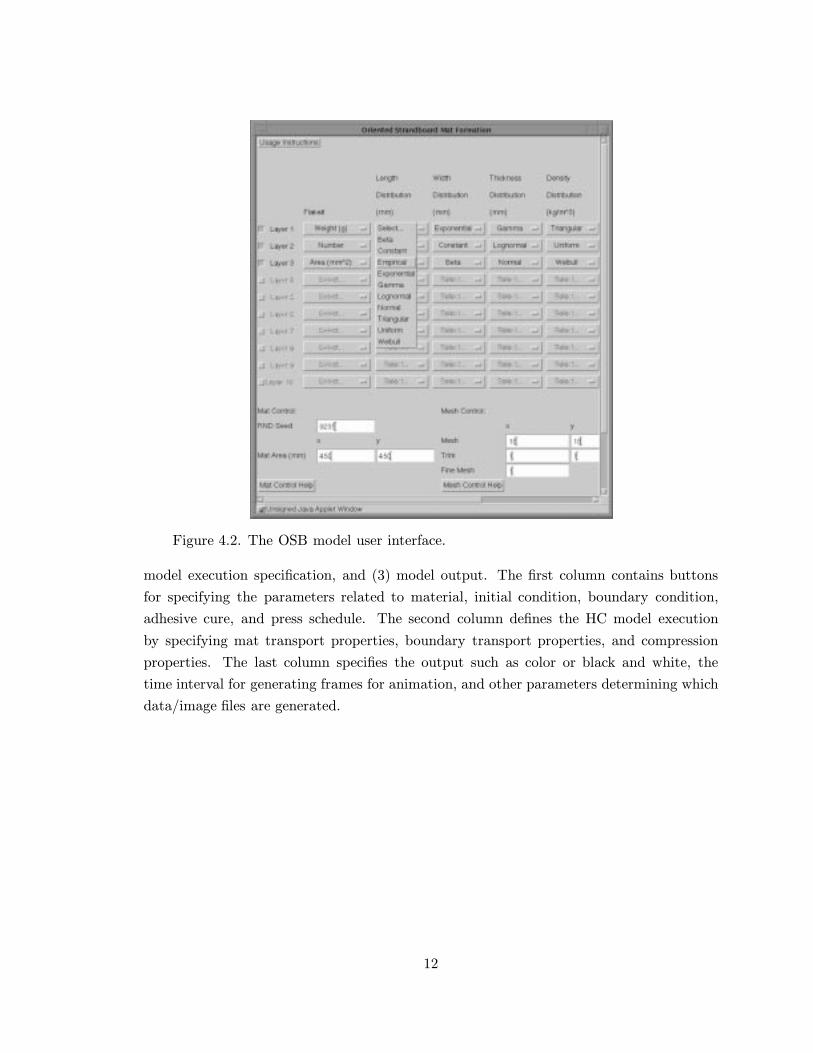
Figure 4.2. The OSB model user interface.

model execution specification, and (3) model output. The first column contains buttons

for specifying the parameters related to material, initial condition, boundary condition,

adhesive cure, and press schedule. The second column defines the HC model execution

by specifying mat transport properties, boundary transport properties, and compression

properties. The last column specifies the output such as color or black and white, the

time interval for generating frames for animation, and other parameters determining which

data/image files are generated.

12

Figure 4.3. The HC model user interface.

13

Chapter 5: WBCSIM ARCHITECTURE

The current software architecture of WBCSim follows the three-tier model described

by Goel et al. [14], for which the tiers are (1) the client layer—user interface, (2) the server

layer—telnet server and a custom shell, and (3) the developer layer—legacy simulation

codes and various optimization and visualization tools running on the server. These layers

are shown in Figure. 5.1. (The elements related to the EM component are discussed in

Chapter 8.)

Developer Layer

Client Layer

Server Layer

��

��

��

��

��

��

WrapperSimulation

��

��

��

��

��

��

��

��

��

��

��

��

��

��

��

��

��

VRML Translator

Results

Simulation

SQL Query

Telnet Server

WhirlGif

YAPS

Interface

Database

Input Data

Mathematica HTML

Figure 5.1. WBCSim architecture overview.

5.1 Client Layer

The client layer is the only layer visible to end-users and typically the only layer running

on the local machine. Besides the user interfaces described in Chapter 4, the client layer

also contains viewers for one of the visualization tools—the VRML Translator. WBCSim

requires a VRML 2.0 viewer for the RFP model. The VRML viewer serves as a plug-in to

the Web browsers.

The client layer also handles the communication with the server layer. After the user

enters all the necessary parameters and triggers the “Run Simulation” button, the client

sends those parameters along with a request for executing the corresponding simulation to

the server layer via a telnet connection. When the simulation terminates, the client takes

the URLs returned by the server layer, and directs them into the user’s browser. Of course,

the client may also send requests for save and retrieve operations.

The telnet connection method replaces the old Javamatic server and socket communi-

cation paradigm described in [14], and facilitates setting up WBCSim guest accounts on the

14

server machine that do not require full account privileges. The guest account and normal

user accounts (for commercial, paying users) permit users to save and track their different

simulation runs, and protect their data from being removed or overwritten by others. The

client side of this telnet connection manages the pool of connections and provides a means

for executing remote commands on the server.

5.2 Server Layer

By separating the legacy simulation codes from the user interface, the server layer

functions as the key to how WBCSim can run a text-only application from a Web browser.

The server layer consists of two components: a telnet server and a custom shell to facilitate

server-client communication.

The telnet server is not a replacement for a standard telnet server, implementing only

enough of the telnet protocol to work with the WBCSim telnet client. The telnet server

supports guest and regular logins and all the operations provided by the previous Javamatic

server, which could direct execution of multiple simulations and accept multiple requests

from the client concurrently [14].

Yet Another PSE Shell (YAPS) is a simple Perl script that the client invokes when

it logs in via the telnet connection. Therefore, the client talks to this shell instead of the

UNIX login shell of the account. Among the commands that YAPS supports, the following

four are most important.

(1) The store command is used to permanently store a problem (input parameters,

text description, simulation output) in the database on the server. Notice that it is possible

to store problem parameters without running the simulation, in which case there is no

simulation output.

(2) The remove command removes one or more stored problems. It actually removes

entries from the database, so the results are irreversible.

(3) The load command retrieves all stored problems from the database. This command

prints a collection of problem IDs (each problem definition or simulation run has a unique

problem ID), parameters, descriptions, and URLs, which could be picked up by the telnet

client.

(4) The clean command deletes temporary files. Normally cleanup is requested when

the “simulation results” window is dismissed. However, cleanup requests are only executed

if there is an idle connection. If no idle connection exists, cleanup requests are queued until

a connection becomes available. The goal of this policy is to clean up only when doing

so incurs no extra connection. Making an extra connection involves a lengthy bootstrap

process and possibly passing the user password again.

There is no command to run a simulation because the simulation wrapper can be

invoked directly by YAPS based on the requests coming from the telnet client.

15

5.3 Developer Layer

As its name suggests, the developer layer consists of legacy programs created by

researchers to model wood-based composite materials and manufacturing processes. These

legacy programs are the heart of WBCSim. In general, WBCSim supports legacy programs

written in any programming language as long as the program takes its input parameters from

UNIX stdin. The input parameters can be a few numbers or a large data file. In particular,

WBCSim supports five FORTRAN 77 and Fortran 90 simulation programs, corresponding

to the five models described in Chapter 3.

While each Fortran program has its own input format (stdin could be redirected to a

file), the server layer communicates data with the developer layer via strings of parameters

separated by white space (spaces, tabs, newlines). In order to cope with this string format,

each legacy program is “wrapped” with a customized Perl script. The script receives this

string of parameters from the server, and converts those parameters into an appropriate

format for the Fortran program. Then the script calls the legacy program into action,

feeding it the input, invoking any required optimization and visualization tools, packing

all Fortran output in HTML files, and passing their URLs, first to the server layer, and

then to the client layer. With this architecture, the developer layer is independent of the

other layers, which makes the process of designing, and integrating new simulation codes

relatively easy.

The developer layer also includes optimization and visualization tools, which are de-

scribed in the next chapter.

16

Chapter 6: OPTIMIZATION AND VISUALIZATION

As mentioned in Chapter 5, there are optimization and visualization tools residing in

the developer layer to maximize the simulation’s value to the user. Here optimization and

visualization are described, respectively.

6.1 Optimization

Scientists typically use a PSE like WBCSim iteratively with some design or system

behavior goal in mind. Their exploration is by trial and error, guided by intuition that

improves as more computational experiments are performed. Mathematical optimization

is a powerful tool for automating this tedious search process. Currently the optimization

tool provided with WBCSim is the program DOT (Design Optimization Tool) [29], based

on sequential quadratic programming and the method of feasible directions. DOT is a

robust sophisticated FORTRAN 77 subroutine for nonlinear constrained optimization, and

is widely used in engineering.

WBCSim supports two models, RDS and RFP, that are linked to DOT. Each has

a different interface for optimization than for analysis. Comparing the interface without

the optimization option to the one with optimization, the former provides only one text

box for every simulation parameter, while the latter provides three, one for specifying

the initial value for that parameter, one for specifying the maximum value, and one for

specifying the minimum value. The optimization interface also allows the user to specify

which parameters are fixed and which are to be varied. The optimization interface also

supplies a number of predefined objective functions (typically computed physical quantities,

such as temperature or pressure), for which the user can specify either maximization or

minimization. The optimization interfaces necessarily provide parameters to control the

convergence of the optimizer, such as “Maximum absolute change in the objective function”,

“Maximum relative change in the objective function”, “Relative finite difference step for

gradients”, and “Maximum number of iterations”.

6.2 Visualization

In principle, WBCSim supports the addition of any visualization tools to convert

simulation output to a format meaningful to the user. However, it does require the user

to have the corresponding viewer for the format of that visualization result installed and

accessible from the Web browser. An example is the VRML viewer described in Chapter 5.2.

WBCSim currently uses three visualization tools: VRML [2], Mathematica [32], and

the UNIX utility WhirlGif. With a VRML viewer, the output converted to VRML can be

viewed from various directions in the three-dimensional viewspace. Mathematica is only

used to generate static two or three-dimensional graphs of simulation results. WhirlGif is

17

Figure 6.1. VRML pressure graph showing the variation of pressure with increasing

distance from the laminate surface and with time (the receding axis)

a GIF to animation converter, which simply picks up the GIF format frames generated by

Mathematica and converts them into an animation file, also in GIF format.

VRML was chosen to interactively visualize some WBCSim simulation output, because

VRML is a well-accepted standard for three-dimensional visualization, available on many

platforms, easy to use, and easily generated. A custom VRML translator was built to

provide better control over the description of the three-dimensional output than third party

translators could provide. WBCSim generates VRML code for the RFP model output.

In the RFP model, the output data is a matrix of numbers where each row contains two

independent variables and the corresponding dependent variable. This three-dimensional

data is conveniently modeled as a VRML ElevationGrid. Each row in the matrix can be

represented either as a point or a square that is colored based on its height, where blue

denotes the lowest point on the grid, red the highest, and the rest are colored by linearly

interpolating between blue and red (HSB) hues, as shown in Figure. 6.1.

Mathematica was chosen to generate static two or three-dimensional graphs of WBCSim

simulation results, because Mathematica has sophisticated graphics tools, and is commonly

used by wood scientists for graphic representations. When Mathematica was first used

in conjunction with WBCSim, the Mathematica commands were hard coded (in Perl) in

the wrapper. Every time a simulation was invoked that required Mathematica’s services,

the wrapper would write the Mathematica commands into a text file embedded with the

dynamically generated filenames for the GIF output files (using the simulation ID) . Then,

the wrapper would give this file as input to Mathematica, which would generate the GIF

18

files accordingly. However, as more complex simulations such as CMA were added to the

system, the Mathematica input file became large and unwieldy. Compounding this size

problem was the fact that every time the Mathematica code changed, the Perl wrapper

also had to be changed. The current WBCSim approach keeps the Mathematica code as

a blueprint external to the wrapper. Then in every simulation run, the wrapper makes a

copy of that blueprint code, uses sed to insert the dynamic graphics output filenames, and

then feeds it directly to the Mathematica kernel. Figure. 6.2 (are explained in Chapter 9)

is an image file generated by Mathematica from the OSB model.

Figure 6.2. Visualization of the three-layer random flake mat: the area of the

mat is 450× 450 mm. Only a fraction of the flakes are shown, and the shading

designates the density of the flakes.

Since some simulation results, such as the CMA model’s stress and strain distributions,

are time series, WBCSim also provides time animation of those results by using WhirlGif.

WhirlGif is a small UNIX utility for generating a single animated GIF image file from a

sequence of GIF image files. The reason Mathematica is not used for generating those

animation files is that the time to generate an animation in Mathematica is significantly

longer than the time by using WhirlGif. Because the number of frames may change from one

simulation run to another, the wrapper reads the number of frames from a data file. Then

the wrapper constructs a command like “WhirlGif -loop 1000 frame1.gif frame2.gif

19

frame3.gif frame4.gif . . . > animation.gif”, where frame*.gif are the frame images

generated by Mathematica. Then this WhirlGif command is fired off to the UNIX shell by

the wrapper to generate the animation file. By embedding each frame into a HTML file,

another option is also provided whereby the user can use hyperlinks such as “Next” and

“Previous” to view the frames one at a time.

20

Chapter 7: RATIONALE FOR EXPERIMENT MANAGEMENT

Before the experiment management component was added, WBCSim had a file-based

save and retrieve system that operated as follows. Upon saving, the input parameters were

packed into a file with a filename identified by the current run ID. This file, along with the

possible output files (data files generated by the FORTRAN code, pictures generated by the

Mathematica or VRML translator, and HTML files generated by the scripts), was stored

in a permanent directory (depending on the login account). An optional description of the

simulation was also stored. Upon retrieving the simulation, a user chose to either load the

input parameters in the proper model interface or load the stored simulation results.

This approach is not sufficient as WBCSim evolves from being experiment-oriented to

being manufacturer-oriented. Manufacturers like to see how the product properties could

be optimized while the profit is maximized. However, any given simulation run is just

an evaluation of a single point in a multidimensional space, and optimization can only

search this space for an optimal point with respect to an objective function [27]. While

WBCSim supports automated optimization, often it is not possible to precisely articulate an

objective function, and there may be multiple conflicting objectives. Furthermore, design

trends and data patterns are unlikely to be revealed by a few isolated runs or by automatic

optimization. What is required is that the results of simulation runs be stored automatically

in a systematic way. This approach would permit annotating the parameters that define a

run as well as its results, and would further allow searching, comparison, and other data

mining of a database of numerical experiments.

Toward this end, a special tailored experiment management component is being added

to WBCSim, which consists of customized user interfaces, server scripts, and an open

source database management system (DBMS)—Postgres. The details of this component

are explained in Chapter 8. This experiment management component not only supports all

of the previous features from the file-based save and retrieve system, it also significantly

increases WBCSim user productivity and usability in the following ways.

(1) The new user interface allows a user to filter the stored simulation runs by their

description or date.

(2) The new user interface provides customized comparison functions that can compare

multiple simulation runs.

(3) The server script searches the database for each simulation run. If the simulation

has been run before and saved, the script retrieves the simulation results from the database

rather than run the FORTRAN program, which normally requires a longer execution time.

(4) The database stores simulation inputs and outputs. Only distinct inputs and outputs

are saved. In case there is a duplicate simulation run (with a distinctive annotation), its

inputs and outputs are not stored but will point to those from the previously stored simulation

run.

21

Chapter 8: EXPERIMENT MANAGEMENT COMPONENT ARCHITECTURE

Chapter 5 explained the WBCSim three-tier model. Here, only the elements related

to the experiment management component are discussed.

8.1 Client Layer

Chapter 4 described how all the models have a row of buttons at the very bottom of the

interface (shown in Figure. 4.1) that control model-level actions for a simulation. Among

those buttons are two, “Store Problem” and “Retrieve Problem”, which are related to the

experiment management component. When the “Store Problem” button is triggered, the

current set of input values (along with the simulation description, which can be specified

in the long text box near the bottom of the interface) is sent to the server and stored. The

interface are updated with a run ID at the upper right-hand corner to indicate that the

save occurred. The “Retrieve Problem” button is used to retrieve stored simulation runs.

Upon activation of the “Retrieve Problem” button, a window (shown in Figure. 8.1) will

open with a list of all the simulation runs for this particular model stored in the database.

This window is the portal for a user to access the stored simulation runs. At the top of

this window, there is some text describing the use of this window. There are also a set of

dropdown lists, and text fields and buttons, which allow the user to filter the simulation

runs displayed. By selecting either “Description” or “Date” from the “Options” dropdown

list, the user can narrow the filter process to either field. Then the user can input a regular

expression (in UNIX grep style) in the text field, and press the “Filter” button to execute

the filter process, which will reload this window with the simulation runs that meet the

filter criteria. The next portion of the window is a scrollbar panel with all of the simulation

runs listed. Each simulation takes a row, which has a “Show Input” button, “Show Output”

button, a check box, the date that it was stored, and its description. The “Show Input”

button launches the model interface with the set of stored input values. The user can make

changes to those parameters, and run the simulation again. Clicking on the “Show Results”

button opens another window with buttons that point to the simulation results, displayable

in browser windows. The checkbox allows the user to either delete the simulation run from

the database (by clicking the “Remove” button at the very bottom of the window), or

apply the comparison functions (by selecting an item from the “Compare Marked Runs”

dropdown list). Each model of WBCSim has its own comparison functions. For example,

the OSB model has three, which allow the user to compare “Void Fractions/Contact Area”,

“Density”, and “Coefficient of Variation” among the simulation runs marked.

If “Void Fractions/Contact Area” is selected from the “Compare Marked Runs” drop-

down list, a window (shown in Figure. 8.2) opens with more options that allow comparisons

among “space/mat”, “lumen/mat”, “void/mat”, “lumen/flake”, and “contact area”. The

user can also specify the interval of the Y axis in order to narrow the comparison.

Depending on the choices made in the detail comparison window, the user gets a result

window, which has links pointing to the results that can be displayed in a browser window.

22

Figure 8.1. The OSB retrieval user interface.

Figure 8.2. The OSB Void Fractions/ContactArea comparison detail user interface.

8.2 Server Layer

Chapter 5.2 described the common commands supported by YAPS. Those commands

23

were previously working with the file system, but are now calling the corresponding save

and retrieve wrappers to interact with the database. These save and retrieve wrappers are

explained next.

8.3 Developer Layer

With the addition of the experiment management component, the simulation wrapper

(described in Chapter 5) performs one more operation before it calls the Fortran program

to execute the simulation. The simulation wrapper checks if a simulation with the current

set of inputs has already been executed. If the simulation was executed before and the

results were saved, the wrapper constructs the output data files from the database instead

of running the Fortran program. The wrapper then feeds the output data files into any

required optimization and visualization tools. This operation is transparent to the user; it

can significantly reduce the response run time if the output is found in the database.

There are other wrappers associated with the save, retrieve, and compare functions

from the user interface at the client layer. Like the simulation wrapper, these wrappers

receive data from the server layer, and convert those input values into an appropriate format

(SQL queries typically) for the database. Moreover, they also perform some extra checks

in order to optimize database usage and storage. For example, the save wrapper checks if

the current set of values is already saved. If that is the case, only a pointer to that set

of values is saved. If the current set of the input that the user is saving is matched with

the previous stored inputs whose output was not saved, the wrapper automatically updates

those previously stored inputs in order to point to the current set of output values.

Postgres is the database system being used. Postgres is a sophisticated object-relational

database management system (DBMS) that supports almost all SQL constructs, including

subselects, transactions, and user-defined types and functions. Moreover, it is open source.

In this architecture, the wrappers communicate with Postgres by Pgsql-perl5, which is

an interface between Perl version 5 and Postgres. This interface uses the Perl version 5

application programming interface for C extensions, which calls the Postgres programmer’s

interface LIBPQ.

24

Chapter 9: SIMULATION SCENARIO

Describing a typical usage scenario of WBCSim is instructive. Consider research into

the properties of oriented strand board products, which would use the OSB model. First,

a scientist samples a subset of the face and core layer flakes from an industrial production

line. The scientist measures the geometry and the weight of each flake. The flake property

data sets are then used to estimate the statistical probability density functions of the flake

properties. Then, the scientist opens a browser window and launches WBCSim. The

guest account is the default login option, which stores all the input and output data in

a temporary directory that is purged periodically. The scientist selects the OSB model

from a dropdown list of all the available models, and launches the OSB model interface

(shown in Figure. 4.2). By specifying the probability density functions of the flake properties

obtained offline earlier, the scientist can create a statistically valid model instance of the

spatial structure of multiple layers of flakes, each with various parameters defining the

number of flakes, length distribution, width distribution, thickness distribution, density

distribution, orientation, flake color, and number of flakes shown. The latter two are solely

for visualization.

Next, the input parameters (Boolean, numeric, or alphanumeric) are sent to the WBCSim

server as a long string (parameters are separated by white space) via a telnet connection.

Then, the OSB wrapper converts this string into a SQL query, and checks if this set of

input parameters is stored in the database.

If the output does not exist in the database, the OSB wrapper converts this input string

into a data file designated for the OSB Fortran 90 simulation program. Since the OSB

simulation code has its own text-based user interface taking input from stdin, a temporary

file is generated to contain all of the appropriate commands. Stdin is then redirected to this

temporary data file for the simulation. The OSB wrapper then calls the OSB simulation

code with this temporary file as stdin along with the properly formatted data file. When

the simulation code is executing, the OSB wrapper monitors to the simulation output

stream for strings indicating execution milestones. The OSB wrapper uses the standard

error stream for sending these messages to the client, because Java buffers the standard

output stream until the process terminates. The contents of the standard error stream are

sent immediately. The OSB wrapper also sends other messages (such as when visualization

or optimization tools are invoked) to the client, displaying the simulation status for the

scientist. However, due to network delay, a group of messages generated at different times

can arrive at the client at the same time, in which case the client only displays the latest

message and discards any old ones.

If the output exists in the database, the OSB wrapper extracts the outputs from the

database and places them into data files in the same format as they would have been written

by the OSB Fortran 90 simulation code.

25

When those output data files are ready (no matter whether they come from the

Fortran 90 simulation program or the database), the OSB wrapper calls Mathematica

to read those data files and generate plots with various Mathematica commands such as

ListContourPlot, ListPlot3D, MultipleListPlot, and Graphics3D. Mathematica also converts

these internal graphics data structures into GIF format so that they can be viewed in a

browser. Figure. 6.2 shows a three-dimensional visualization of a three-layer random flake

mat created with Graphics3D by Mathematica. Finally, the OSB wrapper embeds these

GIF files in HTML files and returns the URLs of these HTML files to the client.

Upon closing the interface windows, the scientist has a choice of storing this particular

run’s input values and results, or discarding this run (the default). If the scientist chooses

to store this run, he enters a description such as “Smith 2” and presses the “Store Problem”

button. The entire interface is then updated with the run ID to indicate that the save

occurred. To further compare this run with any previous runs, the scientist can click the

“Retrieve Problem” button to launch the retrieve problem interface (shown in Figure. 4.1).

The scientist can use the filter (described in Chapter 8) to narrow the list of simulation runs

displayed in the scrollbar panel. By marking two simulation runs, for example, “Smith 2”

and “Smith 1, ” the scientist can compare their “Void Fractions/Contact Area” by selecting

that item from the “Compare Marked Runs” dropdown list. The comparison detail window

(shown in Figure. 8.2) allows the scientist to choose among “space/mat ”, “lumen/mat”,

“void/mat”, “lumen/flake”, and “contact area” to view the comparison result. Figure. 9.1

shows the comparison result created with MultipleListPlot by Mathematica. The scientist

can go back to the comparison detail window to make other selections or change the Y axis

interval to get different results or views.

26

0 0.1 0.2 0.3 0.4 0.5 0.6 0.7Compression Strain

0

0.2

0.4

0.6

0.8

1

Vo

id V

olu

me

or

Co

nta

ct A

rea

Fra

ctio

n

CA-Run2

SM-Run2

CA-Run1

SM-Run1

Figure 9.1. The OSB Void Fraction/Contact Area comparison result from two

simulation runs. It shows “space/mat” (SM) volume and “contact area” (CA)

from those two simulation runs.

27

Chapter 10: FUTURE WORK AND CONCLUSIONS

Of the PSE characteristics mentioned in Chapter 1, experiment management (EM), collab-

oration support, and high performance computing are the most appealing at the current

stage of WBCSim development.

10.1 Experiment Management

The development track for the EM component intends to support all simulation models, be

more DBMS centric, and be general enough for use in other PSE projects.

(1) Support All Models

Currently, this EM component is only available for two models, RDS and OSB, among

the five models described in Chapter 3. RDS was used as the first application of this EM

component, since RDS has the smallest number of input and output parameters. Application

of the EM component to the OSB model has proved that it can handle the complex OSB

model as well. EM support for the other three models (RFP, HC, and CMA) is in progress.

Each model will have its own customized comparison functions.

(2) More DBMS Centric Architecture

Chapter 8 describes the current architecture of WBCSim along with the EM component’s

role. However, a more database management system-centric architecture (DBMSCA) could

provide much more scientific workflow management system functionality. The DBMSCA

can define a workflow for the conduct of a WBCSim simulation: preparing the input file,

validating the input, invoking the simulation code or submitting a job, formatting files,

monitoring the status of a job, and retrieving results. The DBMSCA can then define a

schema for the workflow, use a workflow management system that summarizes, keeps track

of the status of different jobs, determines what is to be done, triggers upon abnormal

conditions (e.g., divide by zero, file not found), etc. A (Postgres) user-defined function looks

for records specified in the query. If these records exist, it gets them from the database.

If they do not, it “places” some new records into a table called “requests”. The workflow

manager periodically scans the “requests” table and schedules jobs. When experiments are

finished, the manager places appropriate entries in the output tables. This idea has been

explored in the S4W PSE for wireless system design [30].

(3) Generalization

The EM component is specially designed for WBCSim. At VPI, there are currently

PSE groups working on cell cycle modeling, wireless communication systems, aircraft design,

microarray experiments, and land use change analysis. The usefulness of the EM component

for other PSE projects is currently being explored.

28

10.2 Collaboration Support

Even though the current telnet server and YAPS allow user/guest logins and multiple users

at multiple workstations working on WBCSim simultaneously, more sophisticated real-time

collaboration support (e.g., Sieve [17]) is needed. This would allow multiple geographically

distributed users to jointly modify the same model interface, and concurrently view and

annotate the same simulation output. Other features indirectly supporting collaboration

are user control over where their data is stored (locally on the client machine vs. remotely

on the server), and support for exchanging data with other researchers.

10.3 High Performance Computing

Simulation codes used by wood scientists often require access to significant computing

resources such as a parallel supercomputer. WBCSim is no exception. The more advanced

models in WBCSim, such as the HC Fortran 90 core or its visualization/optimization tools,

can take hours to run on a fast (AXP 21064) workstation. By utilizing either parallel

or distributed computing, WBCSim can reduce the turnaround time to minutes, making

interactive use feasible even for complex three-dimensional models. A planned next step is

to use a 200 node Beowulf cluster as a compute engine for WBCSim, transparent to the

user, when a requested simulation can be estimated to require such resources.

10.4 Conclusions

WBCSim has evolved steadily from a prototype PSE, intended as a tool for computer

science PSE research and a Web-based interface for a few legacy computer programs, to a

manufacture-oriented near commercial quality PSE that is seriously used by wood science

researchers in industry and academia. Since interesting computational capabilities are still

lacking (cf. Chapters 10.1–10.3), WBCSim will remain an object of computer science research

for some time to come. Yet the program’s interfaces, models, and output visualizations are

now good enough to be used as production tools by wood scientists. The directions in which

computer scientists would like to take WBCSim (collaboration, data mining, grid computing)

are quite different from the directions that wood scientists would prefer for WBCSim (new

models, refining existing models, more interface and visualization options). The present

layered architecture of WBCSim supports these divergent development directions well.

With the addition of the EM component, WBCSim now has a much more efficient

tool to manage its simulation execution and experiment data. From the user perspective,

the EM component allows a user to easily save, retrieve, compare simulation runs, and

further investigate the inter-relationships among multiple parameters. From the developer

perspective, the simulation runs are stored in a more systematic manner—a database that

permits further annotation and data mining possibilities. Adding a different compare

29

function (comparison between simulation outputs) is easy, since only (high level script)

wrappers need to be modified.

The original stated goal [14] of WBCSim was to provide “an integrated set of facilities

allowing wood scientists to concentrate on high-level problem solving rather than on low-level

programming details and application scheduling/execution, allowing users to define, record,

and modify problems, and visualize and optimize simulation results”. This now seems much

closer with the addition of an experiment management capability.

30

REFERENCES

[1] A. Ailamaki, Y.E. Ioannidis, M. Livny, “Scientific workflow management by databasemanagement”, in Proc. 10th International Conference on Scientific and StatisticalDatabase Management, Capri, Italy, July 1998.

[2] A.L. Ames, D.R. Nadeau, J.L. Moreland, VRML 2.0 Sourcebook, 2nd ed, (John Wiley& Sons, Inc., New York, 1996).

[3] R.F. Boisvert, J.R. Rice, Solving elliptic problems using ELLPACK, (Springer-Verlag,New York, 1985).

[4] A.J. Bolton, P.E. Humphrey, P.K. Kavvouras, “The hot-pressing of dry-formed wood-based composites. Part III. Predicted vapour pressure and temperature variation withtime, compared with experimental data for laboratory boards”, Holzforschung, 43 (1989)265–274.

[5] A.J. Bolton, P.E. Humphrey, P.K. Kavvouras, “The hot-pressing of dry-formed wood-based composites. Part IV. Predicted variation of mattress moisture content with time”,Holzforschung, 43 (1989) 345–349.

[6] A.J. Bolton, P.E. Humphrey, P.K. Kavvouras, “The hot-pressing of dry-formed wood-based composites. Part VI. The importance of stresses in the pressed mattress and theirrelevance to the minimization of pressing time, and the variability of board properties”,Holzforschung, 43 (1989) 406–410.

[7] R. Bramley, D. Gannon, T. Stuckey, J. Villacis, E. Akman, J. Balasubramanian, F. Breg,S. Diwan, M. Govindaraju, “The linear system analyzer”, Technical Report TR-511,Computer Science Department, Indiana University, Bloomington, IN, 1998.

[8] T. Burnett, C. Chaput, H. Arrighi, J. Norris, D.J. Suson, “Simulating the Glast satellitewith Gismo”, IEEE Computing in Science and Engineering, 2 (2000) 9–18.

[9] J.X. Chen, X. Fu, “Integrating physics-based computing and visualization: modelingdust behavior”, IEEE Computing in Science and Engineering, 1 (1999) 12–16.

[10] C. Dai, P.R. Steiner, “Spatial structure of wood composites in relation to processing andperformance characteristics. Part III. Modeling the formation of multi-layered randomflake mats”, Wood Science and Technology, 28 (1994) 229–239.

[11] E. Gallopoulos, E. Houstis, J.R. Rice, “Computer as thinker/doer: Problem-solvingenvironments for computational science”, IEEE Computational Science & Engineering,1 (1994) 11–23.

[12] A. Goel, C.A. Baker, C.A. Shaffer, B. Grossman, W.H. Mason, L.T. Watson, R.T.Haftka, “VizCraft: a problem-solving environment for aircraft configuration design”,IEEE Computing in Science and Engineering, 3 (2001) 56–66.

[13] A. Goel, C. Phanouriou, F.A. Kamke, C.J. Ribbens, C.A. Shaffer, L.T. Watson, “WBC-Sim: a prototype problem solving environment for wood-based composites simulations”,Technical Report TR98-25, Computer Science Department, Virginia Polytechnic Insti-tute and State University, Blacksburg, VA, 1998.

[14] A. Goel, C. Phanouriou, F.A. Kamke, C.J. Ribbens, C.A. Shaffer, L.T. Watson, “WBC-Sim: a prototype problem solving environment for wood-based composites simulations”,Engineering with Computers, 15 (1999) 198–210.

[15] C.R. Haselein, “Numerical simulation of pressing wood-fiber composites”, Ph.D. Dis-sertation, Forest Products Dept., Oregon State University, Corvallis, OR, 1998.

31

[16] E.N. Houstis, A.C. Catlin, J.R. Rice, V.S. Verykios, N. Ramakrishnan, C.E. Houstis,“PYTHIA-II: a knowledge/database system for managing performance data and recom-mending scientific software”, ACM Transactions on Mathematical Software, 26 (2000)227–253.

[17] P.L. Isenhour, J. Begole, W.S. Heagy, C.A. Shaffer, “Sieve: A Java-based collabo-rative visualization environment”, in Late Breaking Hot Topics Proceedings, IEEEVisualization ’97, (Phoenix, AZ, 1997) 13–16.

[18] Y.E. Ioannidis, M. Livny, S. Gupta, N. Ponnekanti, “Zoo: a desktop experimentmanagement environment”, in Proc. 22nd International VLDB Conference, Bombay,India, September 1996, 274–285.

[19] F.A. Kamke, J.B. Wilson, “Computer simulation of a rotary dryer: retention time”,American Institute of Chemical Engineers J., 32 (1985) 263–268.

[20] F.A. Kamke, J.B. Wilson, “Computer simulation of a rotary dryer: heat and masstransfer”, American Institute of Chemical Engineers J., 32 (1985) 269–275.

[21] M.E. Lang, M.P. Wolcott, “Modeling the consolidation of wood-strand mat”, Mechanicsof Cellulosic Materials, ASME AMD 209/MD 60 (1995) 153–176.

[22] M.E. Lang, M.P. Wolcott, “A model for viscoelastic consolidation of wood-strand mats.Part I. Structural characterization of the mat via Monte Carlo Simulation”, Wood andFiber Science, 28 (1996) 100–109.

[23] M.E. Lang, M.P. Wolcott, “A model for viscoelastic consolidation of wood-strand mats.Part II. Static stress-strain behavior of the mat”, Wood and Fiber Science, 28 (1996)369–379.

[24] C. Lu, “Organization of wood elements in partially oriented flakeboard mats”, Ph.D.Dissertation. Dept. of Forestry, University of British Columbia, Vancouver, BC, 1999.

[25] S.G. Parker, D.M. Weinstein, C.R. Johnson, “The SCIRun computational steeringsoftware system”, in Modern Software Tools in Scientific Computing, E. Arge, A. M.Bruaset, H. P. Langtangen (eds.), (Birkhauser Press, 1997) 1–40.

[26] J. Resnik, F.A. Kamke, “Modeling the cure of adhesive-wood bonds using high fre-quency energy”, Final Report, U.S.-Slovene Joint Board on Scientific and TechnologicalCooperation, Project 95-AES10, University of Ljubljana, Ljubljana, Slovenia, 1998.

[27] C.A. Shaffer, L.T. Watson, D.G. Kafura, N. Ramakrishnan, “Features of problem solvingenvironments for computational science”, in Proc. High Performance Computing Symp.2000, A. Tentner (ed.), (Soc. for Computer Simulation Interna, San Diego, CA, 2000)242–247.

[28] H. Thoemen, “Modeling the physical processes in natural fiber composites during batchand continuous pressing”, Ph.D. dissertation. Forest Products Dept., Oregon StateUniversity, Corvallis, OR, 2000.

[29] Vanderplaats Research & Development, Inc., DOT Users Manual, Version 4.20, (Col-orado Springs, CO, 1985).

[30] A. Verstak, “Data and Computation Modeling for Scientific PSEs”, M.S. Thesis, VirginiaPolytechnic Institute and State University (CS), Aug 2002.

[31] A. Verstak, M. Vass, N. Ramakrishnan, C. Shaffer, L. Watson, K.K. Bae, J. Jiang, W. H.Tranter, T.S. Rappaport, “Lightweight data management for compositional modelingin problem solving environments”, Proc. High Performance Computing Symp. 2001,A. Tentner (ed.), (Soc. for Computer Simulation Int., San Diego, CA, 2001) 148–153.

32

[32] S. Wolfram, The Mathematica Book, 3rd ed., (Wolfram Media/Cambridge UniversityPress, 1996).

[33] B.G. Zombori, “Modeling the transient effects during the hot-pressing of wood-basedcomposites”, Ph.D. Dissertation, Virginia Polytechnic Institute and State University,Blacksburg, VA, 2001.

[34] B.G. Zombori, F.A. Kamke, L.T. Watson, “Simulation of the mat formation process”,Wood Fiber Science, 33 (2001) 564–580.

33

Appendix A: Perl Subroutine gencontourplot

The following subroutine gencontourplot is one of the subroutines in the Perl script

OSBsub.pl called by the OSB Wrapper OSB.pl. This subroutine illustrates that the current

WBCSim approach keeps the Mathematica code as a blueprint external to the wrapper.

Then in every simulation run, the wrapper makes a copy of that blueprint code, uses sed to

insert the dynamic graphics output directory, and then feeds it directly to the Mathematica

kernel, which is discussed in Chapter 6.

# This subroutine generates contour plot GIF files.

sub gencontourplot

{

# Output status message to stdin.

print "STEP Use Mathematica to Generate Graphics\n";

# Define contour plot’s blueprint of Mathematica script.

$MATH_SCRIPT = "/d/pse/WWW/bin/osb_math1_contour.script";

# Define a working copy of the blueprint.

$MATH_SCRIPT_COPY = "$INPUT_DIR/$$/OSB_$$.redirect";

# Define complete working directory in a format required by Mathematica.

$IN_DIR = "\\/d\\/pse\\/WWW\\/data\\/tmp\\/$$\\/";

# Substitute "inputdirectory" (in the blueprint) by the working directory.

print("PSE: Change Directory Location In Math Script.\n"), return

if system "sed ’s/inputdirectory/$IN_DIR/’ $MATH_SCRIPT > $MATH_SCRIPT_COPY";


print "STEP Generate GIF Files - Contour Plot via Mathematica\n";

# Runs Mathematica.

print("PSE:WARNING Could Not Execute Mathematica.\n"), return

if system "$MATHEMATICA < $MATH_SCRIPT_COPY";

# Embed the GIF files in a HTML file.

$RESULT_CONTOUR_PLOT_FILE = "$OUTPUT_DIR/$$/$RESULT_ID.contourplot.html";

open(FILE_OUT, ">$RESULT_CONTOUR_PLOT_FILE")

or print("PSE:WARN Could Not Write Contour Plot HTML.\n"), return;

print FILE_OUT "<html><head>\n";

print FILE_OUT "<title>Mat Formation - Contour Plot</title></head>\n";

print FILE_OUT "<body bgcolor=\"#ffffff\" text=\"#102030\" link=\"#B00909\"

vlink=\"#502020\">\n";

print FILE_OUT "<center><h1>Mat Formation</h1>\n";

print FILE_OUT "<h2>Simulation Results - Contour Plot</h2></center><hr>\n";

print FILE_OUT "<a href=\"\#Density\">Density Distribution</a><br> ";

print FILE_OUT "<a href=\"\#Thickness\">Thickness Distribution</a><br>";

print FILE_OUT "<a href=\"\#Number\">Number Distribution</a><br>";

print FILE_OUT "\n";

print FILE_OUT "\n";

print FILE_OUT "<hr><h3><A NAME=\"Density\"></A>Density Distribution</h3>\n";

print FILE_OUT "<table border=0 cellpadding=0 cellspacing=5><tr><th><img

src=\"density.gif\"></th></tr></table>\n";

print FILE_OUT "<hr><h3><A NAME=\"Thickness\"></A>Thickness Distribution</h3>\n";


src=\"thickness.gif\"></th></tr></table>\n";

print FILE_OUT "<hr><h3><A NAME=\"Number\"></A>Number Distribution</h3>\n";

34


src=\"number.gif\"></th></tr></table>\n";

print FILE_OUT "<hr></body></html>\n";

close(FILE_OUT)

or print("PSE:WARN Could Not Write Graph HTML.\n"), return;

# Output result HTML filename and related info.

&PrintURL("$RESULT_CONTOUR_PLOT_FILE", "text/html", "Contour Plot");

}

35

Appendix B: Perl Code Example of WhirlGif from gen3Dplot

The following segment of code is from the subroutine gen3Dplot, which is one of the

subroutines in the Perl script HOTsub.pl called by the HOT wrapper HOT.pl.

The code illustrates how WBCSim uses the the UNIX utility WhirlGif to generate a

single animated GIF image file from a sequence of GIF image files, as described in Chapter 6.

# Because the number of frames may change from one simulation

# run to another, the code reads the number of frames from a

# data file generated by a Fortran program. Then the wrapper

# constructs a command like "WhirlGif -loop 1000 frame1.gif

# frame2.gif frame3.gif frame4.gif > animation.gif",

# where frame*.gif are the frame images generated by

# Mathematica.

# $COUNT stores the number of frames, which was readin earlier.

if ($COUNT != 1)

{

# Define WhirlGif.

$WHIRLGIF = "$PSE_HOME/bin/whirlgif";

# Construct the command.

# -loop defines the number of animation loop.

# -time defines the animation speed.

$MOVIE = "$WHIRLGIF -loop 1000 -time 25";

# Continue to construct the command depending on the $COUNT

for $k (1..$COUNT)

{

$MOVIE = "$MOVIE $INPUT_DIR/$$/Movie$k.gif "; $k = $k + 1;

}

# Continue to construct the command.

$MOVIE = "$MOVIE > $INPUT_DIR/$$/Movie.gif";


print "STEP Generate GIF Files - 3D Movie via WhirlGif\n";

# Runs WhirlGif.

print("PSE:WARN Could Not Execute WhirlGif.\n"), return

if system "$MOVIE";

# Embed the GIF files in a HTML file.

$RESULT_PLOT_FILE = "$OUTPUT_DIR/$$/$RESULT_ID.plot3D.html";

open(FILE_OUT, ">$RESULT_PLOT_FILE")


print FILE_OUT "<html><head>\n";

print FILE_OUT "<title>Hot Compression</title></head>\n";

print FILE_OUT "<body bgcolor=\"#ffffff\" text=\"#102030\" link=\"#B00909\"

vlink=\"#502020\">\n";

print FILE_OUT "<center><h1>Hot Compression</h1>\n";

print FILE_OUT "<h2>Simulation Results - 3D Profiles (Animation)</h2></center><hr>\n";

print FILE_OUT "<h3><A NAME=\"movie\"></A></h3>\n";


src=\"Movie.gif\"></th></tr></table>\n";

print FILE_OUT "<hr></body></html>\n";

36

close(FILE_OUT)


# Output result HTML filename and related info.

&PrintURL("$RESULT_PLOT_FILE", "text/html", "3D Profiles (Animation)");

} # End of if

37

Appendix C: Perl OSB Save Wrapper osbsave.pl

The following Perl script is the OSB save wrapper osbsave.pl, which illustrates how

WBCSim interacts with the database to save inputs and outputs, as discussed in Chapter 8.

#!/usr/local/bin/perl -w

#

# Author: Jiang Shu

# Last Modification: 11/11/2002

#

# config.pl defines system specific variables such as

# $MATHEMATICA = "/usr/local/bin/math";

require "config.pl";

# dbutil.pl defines some common used database operations

# such as subroutine CheckDB, which takes

# 1) target value

# 2) table name

# 3) condition

# 4) database name

# and check if with this condition the target value is in

# the table of that database.

require "dbutil.pl";

# Pg(Pgsql_perl5) is an interface between Larry Wall’s language

# Perl Version 5 and the database PostgreSQL (previously

# Postgres95). This has been done by using the Perl5 application

# programming interface for C extensions which calls the

# Postgres programmer’s interface LIBPQ.

use Pg;

# This subroutine stores OSB inputs and outputs to database.

sub OSBStoreDB

{

# Prepare inputs.

# Name, ID

# This is the case that the simulate has been run.

# User clicks "Store Results" from output window.

# System saves both inputs and outputs.

# Run ID is already generated, and is passed in here.

if ($#ARGV==1 && $ARGV[1] = /PSE/)

{

# Set run ID.

$run_id = $ARGV[1];

# Use the run ID as input ID.

$input_id = $run_id;

# Output ID is the same as the input ID.

$output_id = $input_id;


print "PSE:ID $input_id $PROBLEM_NAME\n";

# Get the actual inputs from the $input_id.input file.

38

open(INPUT, "$OUTPUT_DIR/$input_id.input")

or print("PSE:ERROR Cannot Open input_id.input!\n"), return;

# Skip the first entry = Problem Description.

# Then get the inputs.

$_ = <INPUT>; $_ = <INPUT>;

# Close $input_id.input file.

close(INPUT)

or die "PSE:ERROR Closes $input_id.input!";

# Separate the inputs (a string) into an array of elements.

@IN = split;

# Call OSBConstructInputs to construct two types of inputs.

($inputs, $inputs2) = &OSBConstructInputs(@IN);

}

# Name, parameters

# This is the case that the simulate has NOT been run.

# User clicks the "Store Problem" from input window.

# System only saves the inputs.

# Run ID is not generated so far.

else

{

# Output input parameters to stdin.

print @ARGV, "\n";

# Shift out the first entry = Problem Description.

shift(@ARGV);

# Generate a Run ID.

$run_id = &GenerateFile();

# Use the run ID as input ID.

$input_id = $run_id;

# Output ID is null (there is no output).

$output_id = "null";

# Call OSBConstructInputs to construct two types of inputs.

($inputs, $inputs2) = &OSBConstructInputs(@ARGV);

}

# Start actual logic/operation.

# Initialize the parameters.

# UPPER CASE VARIABLES are constants and defined in STORE.pl,

# which calls this subroutine.

$dbmain = $DATABASE;

$null = "null";

$date = &GetDate2();

# Check database for inputs.

@temp = &CheckDB("input_id", $SIM_INPUTS, "$inputs2");

$inputfound = $temp[0];

# Connect to database.

$conn = Pg::connectdb("dbname=$dbmain");

die $conn->errorMessage unless PGRES_CONNECTION_OK eq $conn->status;

39

print "Connected to $dbmain for Saving.\n";

# Inputs do not exist.

if ($inputfound eq $null)

{


print "Save - Input Not Found\n";

# Save inputs in TABLE - osb_inputs.


print "Save - Save the Input\n";

$inputs = "(’$input_id’, $inputs)";

$result = $conn->exec("INSERT INTO $SIM_INPUTS VALUES $inputs");

die $conn->errorMessage unless PGRES_COMMAND_OK eq $result->resultStatus;

print "Save Inputs, status = ", $result->cmdStatus, "\n";

# Save outputs (if there is any) in TABLE - osb_outputs.

if ($output_id ne $null)

{


print "Save - Save the Output\n";

# Construct outputs.

$outputs = &OSBConstructOutputs();

$outputs = "(’$output_id’, $outputs)";

$result = $conn->exec("INSERT INTO $SIM_OUTPUTS VALUES $outputs");


print "Save Outputs, status = ", $result->cmdStatus, "\n";

# Some files are stored, outside of database.

&OSBStoreFiles($input_id);

}

else

{


print "Save - Output is NOT found, so NO outputs saved\n";

}

# Store the run.


print "Save - Save Run\n";

$result = $conn->exec("INSERT INTO $SIM_RUNS VALUES (’$run_id’, ’$PROBLEM_NAME’,

’$USERNAME’, ’$date’, ’$input_id’, ’$output_id’)");


print "Save Runs - run_id = $run_id, input_id = $input_id, output_id = $output_id, status

= ", $result->cmdStatus, "\n";

}

# Inputs do exist.

else

{


print "Input Found - $inputfound\n";

# NOT save inputs.

40


print "Save - Not Save the Inputs\n";

# Check if the outputs are in the database.

@temp = &CheckDB("output_id", $SIM_OUTPUTS, "output_id=\’$inputfound\’");

$outputfound = $temp[0];

# No output is found in the database.

if ($outputfound eq $null)

{

# Output was generated.

if ($output_id ne $null)

{


print "Save - Output Not Found, But Output is Available -> Save the Outputs\n";


$outputs = &OSBConstructOutputs();

$outputs = "(’$inputfound’, $outputs)";

# Save the outputs in the database.

$result = $conn->exec("INSERT INTO $SIM_OUTPUTS VALUES $outputs");


print "Save Outputs, status = ", $result->cmdStatus, "\n";

$outputfound = $inputfound;

# Some files are stored, outside of database.

&OSBStoreFiles($inputfound);

# Smart Update.

# Update the old runs to point to the newly saved outputs.

$result = $conn->exec("UPDATE $SIM_RUNS SET output_id=\’$outputfound\’ WHERE

input_id=\’$inputfound\’");


print "Smart Update, status = ", $result->cmdStatus, "\n";

}

# Output was NOT generated.

else

{


print "Save - Output is NOT found, NOT Save the Outputs\n";

}

}

# Outputs are found in the database.

else

{


print "Save - Output Found - $outputfound, NOT Save the Outputs\n";

}

# Store the run.

print "Save - Save Run\n";

$result = $conn->exec("INSERT INTO $SIM_RUNS VALUES (’$run_id’, ’$PROBLEM_NAME’,

’$USERNAME’, ’$date’, ’$inputfound’, ’$outputfound’)");


41

print "Save Runs - run_id = $run_id, input_id = $inputfound, output_id = $outputfound,

status = ", $result->cmdStatus, "\n";

}

} # End of OSBStoreDBsub

# This subroutine constructs two types of inputs.

# 1) $inputs = just the parameters

# 2) $inputs2 = inputs with column names for the query

sub OSBConstructInputs

{


$i = 0;

$inputs = "";

$inputs2 = "";

# First few column names in the table.

@p = ("dimension", "layers", "seed", "mat_d1", "mat_d2", "nmp1", "nmp2", "cut1", "cut2",

"noi", "pn");

# Get @p data.

for $i (0..10)

{

$a = shift(@_);

$inputs = "$inputs$a, ";

$inputs2 = "$inputs2$p[$i]=$a and ";

# Get dimension (2D or 3D).

if ($i == 0)

{

$dimension = $a;

}

# Get number of layers.

if ($i == 1)

{

$number_of_layers = $a;

}

$i++;

}

# Get number of press.

$pn = 2*$a;

$pndata = "{";

$i = 1;

for $i (1..$pn)

{

$a = shift(@_);

$pndata = "$pndata\"$a\", ";

$i++;

}

chop($pndata); chop($pndata);

$pndata = "$pndata}";

$inputs = "$inputs\’$pndata\’, ";

$x = "pressdata";

$inputs2 = "$inputs2$x=\’$pndata\’ and ";

42

# Get layers data.

$layers = "{";

$i = 1;

for $i (1..$number_of_layers)

{

$one_layer = "\"";

$j = 0;

for $j (1..7)

{

$a = shift(@_);

$one_layer = "$one_layer$a ";

$j++;

}

$j = 0;

for $j (1..4)

{

$a = shift(@_);


$type = $a;

$a = shift(@_);


$number_of_parameters = $a;

if ($type == 3)

{

$number_of_parameters = $number_of_parameters * 2 + 1;

}

$k = 1;

for $k (1..$number_of_parameters)

{

$a = shift(@_);


$k++;

}

$j++;

}

chop($one_layer);

$one_layer = "$one_layer\"";

$layers = "$layers$one_layer, ";

$i++;

}

chop($layers); chop($layers);

$layers= "$layers}";

$inputs = "$inputs\’$layers\’";

$x = "layerdata";

$inputs2 = "$inputs2$x=\’$layers\’";

return ($inputs, $inputs2);

} # End of ConstructInput

# This subroutine constructs outputs.

sub OSBConstructOutputs

43

{


$all_outputs = "";

# The data files will be saved.

@datafiles = ("osb_Azoned.dat", "osb_Azoned.dat", "osb_Azoned.dat", "osb_Azoned.dat",

"osb_voidcont.dat", "osb_stat.dat");

foreach (@datafiles)

{

# Process one data file at a time.

$one_data_file = &OSBConstructOutputsSub1($_);

$all_outputs = "$all_outputs\’$one_data_file\’, ";

}

# One additional data file for Hot Compression, which has

# different format from the above ones.

$one_data_file = &OSBConstructOutputsSub2("osb_matform.dat");

$all_outputs = "$all_outputs\’$one_data_file\’";

return $all_outputs;

} # End of OSBConstructOutputs

# This subroutine constructs outputs for @datafiles defined in

# OSBConstructOutputs.

sub OSBConstructOutputsSub1

{

# Receive the data file name as argument.

$datafile = $_[0];

# Parse the folder name.

($_, $_, $_, $_, $_, $folder) = split /-/, $run_id;

open(OUTPUT, "$OUTPUT_DIR/$folder/$datafile")

or print("PSE:ERROR Cannot Open $datafile!\n"), return;


$matrix = "";

foreach (<OUTPUT>)

{

@one_row = split;

$a_row = "{";

foreach (@one_row)

{

$a_row = "$a_row$_, ";

}

chop($a_row); chop($a_row);

$a_row = "$a_row}, ";

$matrix = "$matrix$a_row";

}

chop($matrix); chop($matrix);

close(OUTPUT)

or die "PSE:ERROR Cannot Close $datafile!";

44

return "{$matrix}";

} # End of OSBConstructOutputsSub1

# This subroutine constructs outputs for osb_matform.dat,

# which has different format from the other files.

sub OSBConstructOutputsSub2

{

# Receive the data file name as argument.

$datafile = $_[0];


($_, $_, $_, $_, $_, $folder) = split /-/, $run_id;

open(OUTPUT, "$OUTPUT_DIR/$folder/$datafile")

or print("PSE:ERROR Cannot Open $datafile!\n"), return;


$one_line = "";

<OUTPUT>;

foreach (<OUTPUT>)

{

@one_row = split;

if ($one_row[0] ne "/")

{

$one_line = "$one_line$one_row[1], ";

}

}

chop($one_line); chop($one_line);

close(OUTPUT)

or die "PSE:ERROR Cannot Close $datafile!";

return "{$one_line}";

} # End of OSBConstructOutputsSub2

# Some files are stored outside of the database such as:

# 1) The descriptive input file, which only helps a user to

# understand the input file.

# 2) 2D and 3D layer images, which are only for visual effect.

# datafiles (containing coordinates of flakes)

# are not saved in the database.

sub OSBStoreFiles

{

# Receive ID as argument.

$id = $_[0];


($_, $_, $_, $_, $_, $folder) = split /-/, $output_id;

# Save the descriptive input file.

print("PSE:ERROR Copying 2D pictures.\n"), exit 2

if system "$CP $OUTPUT_DIR/$folder/osb_input.dat $SIMDIR/$id.osb_input.dat";

# Save 2D Gif Files.

45

for $i (1..$number_of_layers)

{


if system "$CP $OUTPUT_DIR/$folder/layer$i.gif $SIMDIR/$id.layer$i.gif";

}


if system "$CP $OUTPUT_DIR/$folder/layer_all.gif $SIMDIR/$id.layer_all.gif";

# Save 3D Gif File.

if ($dimension == 2)

{


if system "$CP $OUTPUT_DIR/$folder/3D.gif $SIMDIR/$id.3D.gif";

}

} # End of OSBStoreFiles

1; # It will fail without this line

# End of file

46

Appendix D: Perl OSB Load Wrapper osbload.pl

The following Perl script is the OSB load wrapper osbload.pl, which illustrates how

WBCSim interacts with the database to load saved simulation runs, as discussed in Chapter 8.

#!/usr/local/bin/perl -w

#

# Author: Jiang Shu

# Last Modification: 11/11/2002

#

# config.pl defines system specific variables such as

# $MATHEMATICA = "/usr/local/bin/math";

require "config.pl";

# dbutil.pl defines some common used database operations

# such as subroutine CheckDB, which takes

# 1) target value

# 2) table name

# 3) condition

# 4) database name

# and check if with this condition the target value is in

# the table of that database.

require "dbutil.pl";

# Pg(Pgsql_perl5) is an interface between Larry Wall’s language

# Perl Version 5 and the database PostgreSQL (previously

# Postgres95). This has been done by using the Perl5 application

# programming interface for C extensions which calls the

# Postgres programmer’s interface LIBPQ.

use Pg;

sub OSBLoadDB

{

# UPPER CASE VARIABLES are constants and defined in LOAD.pl,

# which calls this subroutine.

$dbmain = $DATABASE;

# Connect to database.

$conn = Pg::connectdb("dbname=$dbmain");

die $conn->errorMessage unless PGRES_CONNECTION_OK eq $conn->status;

print "Connected to $dbmain for Loading\n";

# Retrieve all the runs from OSB Runs table.

$result2 = $conn->exec("SELECT * FROM $SIM_RUNS");

die $conn->errorMessage unless PGRES_TUPLES_OK eq $result2->resultStatus;

print "Retrieve all the runs from - $SIM_RUNS, status = ", $result2->cmdStatus, "\n";

while (@row = $result2->fetchrow)

{

$ID = $row[0];


print "PSE:ID $ID***$row[1]***$row[3]\n";

47

# Print archive URL.

print "PSE:URL http://wbc.forprod.vt.edu/ pse/data/tmp/$ID.input x-wbc/x-archive

Archive File\n";

# Print parameters, have to split long lines.

# Prepare target string.

$target = "";

@p = ("dimension", "layers", "seed", "mat_d1", "mat_d2", "nmp1", "nmp2", "cut1",

"cut2", "noi", "pn", "pressdata", "layerdata");

foreach (@p)

{

$target = "$target$_, ";

}

chop($target); chop($target);

# Get the inputs.

$para = $conn->exec("SELECT $target FROM $SIM_INPUTS WHERE input_id=\’$row[4]\’");

@temp = $para->fetchrow;

print "PSE:PARAM ";

$param = "";

# Print out the single values.

$i = 1;

for $i (1..11)

{

$_ = shift(@temp);

$param = "$param$_ ";

if ($i == 1)

{

$dimension = $_;

}

$i++;

}

# Print out press data.

$_ = shift(@temp);

@x = split /{|}|,|"/, $_;

$space = $x[0];

foreach (@x)

{

if ($_ ne $space)

{


}

}

# Print out layer data.

$_ = shift(@temp);

@x = split /{|}|,|"/, $_;

$space = $x[0];

foreach (@x)

{

if ($_ ne $space)

{

48


}

}

chop($param);

while (length($param) > 66)

{

print substr($param, 0, 66), "\\\n";

$param = substr($param, 66);

}

print $param, "\n";

# Print output URLs.

$null = "null";

@temp = &CheckDB("output_id", $SIM_OUTPUTS, "output_id=\’$row[4]\’");

$outputfound = $temp[0];

if ($outputfound ne $null)

{

($_, $_, $_, $_, $_, $folder) = split /-/, $outputfound;

print "PSE:URL http://wbc.forprod.vt.edu/ pse/data/tmp/$folder/$ID.input.txt

text/plain Namelist Input Data\n";

print "PSE:URL http://wbc.forprod.vt.edu/ pse/data/tmp/$folder/$ID.contourplot.html

text/html Contour Plot\n";

print "PSE:URL http://wbc.forprod.vt.edu/ pse/data/tmp/$folder/$ID.surfaceplot.htmll

text/html Surface Plot\n";

print "PSE:URL

http://wbc.forprod.vt.edu/ pse/data/tmp/$folder/$ID.compressionplot.html text/html

Compression Plot\n";

print "PSE:URL http://wbc.forprod.vt.edu/ pse/data/tmp/$folder/$ID.layerplot.html

text/html Layer Plot\n";

if ($dimension == 2)

{

print "PSE:URL http://wbc.forprod.vt.edu/ pse/data/tmp/$folder/$ID.3D.html

text/html 3D Plot\n";

}

print "PSE:URL http://wbc.forprod.vt.edu/ pse/data/tmp/$folder/$ID.outputfiles.html

text/html Text Output Files\n";

}

}

} # End of OSBLoadDB

1; # It will fail without this line

# End of file

49

VITA

Jiang Shu was born in Wuhan, P. R. China, on July 3rd, 1976. He earned two bachelor’s

degrees, in Computer Science and Mathematics, in May 2000 from University of Louisiana at

Monroe, Monroe, Louisiana, USA. In August 2000, he started graduate study in computer

science at Virginia Polytechnic Institute and State University. In October 2002, he received

the Master of Science degree in computer science from Virginia Polytechnic Institute and

State University. He will continue his study in pursuit of the Doctor of Philosophy degree

in computer science.

50

An experiment management component for the WBCSim problem solving environment

Documents

Transcript of An experiment management component for the WBCSim problem solving environment