(This is a sample cover image for this issue. The actual cover is not yet available at this time.)

This article appeared in a journal published by Elsevier. The attachedcopy is furnished to the author for internal non-commercial researchand education use, including for instruction at the authors institution

and sharing with colleagues.

Other uses, including reproduction and distribution, or selling orlicensing copies, or posting to personal, institutional or third party

websites are prohibited.

In most cases authors are permitted to post their version of thearticle (e.g. in Word or Tex form) to their personal website orinstitutional repository. Authors requiring further information

regarding Elsevier’s archiving and manuscript policies areencouraged to visit:

http://www.elsevier.com/copyright

Author's personal copy

Agricultural and Forest Meteorology 161 (2012) 15– 25

Contents lists available at SciVerse ScienceDirect

Agricultural and Forest Meteorology

jou rn al h om epa g e: www.elsev ier .com/ locate /agr formet

An evaluation of MODIS 8- and 16-day composite products for monitoring maizegreen leaf area index

Noemi Guindin-Garciaa, Anatoly A. Gitelsonb,∗, Timothy J. Arkebauera, John Shanahanc,Albert Weissd

a Department of Agronomy and Horticulture, University of Nebraska-Lincoln, 203 KCR, Lincoln, NE 68583-0817, USAb Center for Advanced Land Management Information Technologies (CALMIT), School of Natural Resources, 303 Hardin Hall, University of Nebraska-Lincoln, Lincoln, NE 68583-0973,USAc Pioneer Hi-Bred, Johnston, IA 50131-1000, USAd School of Natural Resources, 507 Hardin Hall, University of Nebraska-Lincoln, Lincoln, NE 68583-0995, USA

a r t i c l e i n f o

Article history:Received 22 June 2011Received in revised form 1 March 2012Accepted 18 March 2012

Key words:MODISTemporal resolutionVegetation indicesMaizeGreen leaf area index

a b s t r a c t

The seasonal patterns of green leaf area index (GLAI) can be used to assess crop physiological and pheno-logical status, to assess yield potential, and to incorporate in crop simulation models. This study focusedon examining the potential capabilities and limitations of satellite data retrieved from the moderate reso-lution imaging spectroradiometer (MODIS) 8- and 16-day composite products to quantitatively estimateGLAI over maize (Zea mays L.) fields. Results, based on the nine years of data used in this study, indicateda wide variability of temporal resolution obtained from MODIS 8- and 16-day composite periods andhighlighted the importance of information about day of MODIS products pixel composite for monitoringagricultural crops. Due to high maize GLAI temporal variability, the inclusion of day of pixel compositeis necessary to decrease substantial uncertainties in estimating GLAI. Results also indicated that maizeGLAI can be accurately retrieved from the 250-m resolution MODIS products (MOD13Q1 and MOD09Q1)by a wide dynamic range vegetation index with root mean square error (RMSE) below 0.60 m2 m−2 or bythe enhanced vegetation index with RMSE below 0.70 m2 m−2.

© 2012 Elsevier B.V. All rights reserved.

1. Introduction

Remote sensing has been used to estimate crop biophysicalparameters (CBP) such as green leaf area index (GLAI), canopychlorophyll content, the fraction of photosynthetically active radi-ation absorbed by the crop, biomass, vegetation cover, and grossprimary production using different vegetation indices, VIs (e.g.,Hatfield et al., 2008). Most of the VIs are combinations of reflectancein the visible or photosynthetically active radiation spectral range(400–700 nm), especially red reflectance (620–700 nm), and thenear infrared range (NIR; 750–1300 nm). The most widely used VIin agricultural applications is the normalized difference vegetationindex, NDVI (Rouse et al., 1974). Myneni et al. (1997) developed aphysically based algorithm for the estimation of GLAI from NDVIobservations. As the authors noted, “the algorithm must be viewedwithin a framework dominated largely by practical considerationand to a lesser extent by accuracy”. The relationship betweenNDVI and GLAI is essentially nonlinear and exhibits significantvariations among various vegetation types. When GLAI exceeds

∗ Corresponding author. Tel.: +1 402 472 8386.E-mail address: agitelson2@unl.edu (A.A. Gitelson).

2 m2 m−2, NDVI is generally insensitive for assessing changes inGLAI in grasses, cereal crops, and broadleaf crops (Myneni et al.,1997; Gitelson, 2004). New approaches have been proposed usingspectral regions in the green and red edge (Buschman and Nagel,1993; Gitelson et al., 1996; Dash and Curran, 2004; Gitelson, 2004).However, data from the red edge spectral region are not availablefrom the widely used the moderate resolution imaging spectrora-diometer (MODIS) sensor and the green band is only available inthe 500-m resolution MODIS product.

Huete et al. (1997) introduced the enhanced vegetation index(EVI), which has a higher sensitivity to moderate-to-high vegeta-tion biomass; EVI is a widely used product of the MODIS system:

EVI = 2.5 × (�NIR − �red)1 + �NIR + 6 × �red − 7.5 × �blue

(1a)

The modification of EVI, EVI2, uses only red and NIR bands (Jianget al., 2008):

EVI2 = 2.5 × (�NIR − �red)1 + �NIR + 2.4 × �red

(1b)

0168-1923/$ – see front matter © 2012 Elsevier B.V. All rights reserved.doi:10.1016/j.agrformet.2012.03.012

Author's personal copy

16 N. Guindin-Garcia et al. / Agricultural and Forest Meteorology 161 (2012) 15– 25

Gitelson (2004) proposed a nonlinear transformation of NDVI,called the wide dynamic range vegetation index (WDRVI), in theform:

WDRVI = ˛ × �NIR − �red

× �NIR + �red(2a)

The weighting coefficient, is introduced to attenuate the contribu-tion of the NIR reflectance at moderate-to-high green biomass, andto make it comparable to that of the red reflectance. It was shownthat WDRVI retrieved from close range (6 m above the canopy) andfrom MODIS data is linearly related to GLAI (Gitelson et al., 2007;Gitelson, 2011). WDRVI can be calculated using MODIS red and NIRreflectances (Eq. (2a)) or directly from NDVI (Vina and Gitelson,2005):

WDRVI = ( + 1) × NDVI + ( − 1)( − 1) × NDVI + ( + 1)

(2b)

The accuracy of CBP estimates depends on the satellite system’stemporal and spatial resolutions, and the quality of the data dueto appearance of clouds, low viewing angles, and poor geometry(Chen et al., 2002, 2003; Duchemin and Maisongrande, 2002). Ithas been demonstrated that without cloud contamination NDVI isable to quite accurately detect maximum values of maize GLAI (e.g.,Chen et al., 2003). In addition to atmospheric interference (e.g.,clouds, haze, etc.), NDVI also could be affected by contaminationfrom surrounding areas due to limited spatial resolution. Smooth-ing the data obtained from VIs over study areas reduces effects ofcontaminated signals (Swets et al., 1999; Funk and Budde, 2009).An alternative to reduce or eliminate pixel contamination is theselection of finer spatial resolution. Data obtained from a spatialresolution of 250-m (area is about 6.25 ha) allow quite accurateidentification of pixels covered by specific crops (Gitelson et al.,2007).

The estimation of CBP and the detection of developmental stagesof agricultural crops are important for government agencies, pri-vate industry, and researchers. MODIS products offer high qualitydata at consistent spatial resolutions and temporal resolutionsderived every 8 or 16 days (Huete et al., 1999, 2002; Didan andHuete, 2006). MODIS 8- and 16-day composites contain the bestpossible observations obtained during the composite period basedon several parameters such as view angle, absence of clouds orcloud shadows and aerosols (Vermote and Kotchennova, 2008).MODIS 8- and 16-day composite data have been used in manyagricultural applications to develop land cover/land use products(Lobell and Asner, 2004; Sedano et al., 2005; Lunetta et al., 2006),monitor phenology (Zhang et al., 2003; Sakamoto et al., 2005;Wardlow et al., 2006), and estimate CBP (Zhu et al., 2005; Chenet al., 2006; Rochdi and Fernandes, 2010).

MODIS products have also been used to estimate GLAI for cropmodeling applications. Fang et al. (2008) utilized the MODIS LAI1000-m product to incorporate into a maize crop simulation model.Doraiswamy et al. (2004) used data retrieved from MODIS 250-msurface reflectance 8-day composite in a radiative transfer modelto estimate GLAI during the growing season and then incorporatedGLAI into a maize crop simulation model. Chen et al. (2006) evalu-ated the potential use of data retrieved from MODIS at 250-, 500-and 1000-m resolutions to track maize GLAI and phenology forcrop modeling applications. However, a detailed evaluation of theeffects of MODIS temporal resolution on the accuracy of crop GLAIestimates has not been reported to date.

Monitoring of maize GLAI requires a good understanding of GLAIchanges at each phenological stage in order to evaluate poten-tial capabilities and limitations of the satellite data retrieved fromMODIS 8- and 16-day composite periods. A period of 8 and/or 16days may represent significant changes in maize GLAI especiallyduring the vegetative stage. For example, maximum observed rate

of maize GLAI change during the period of this study was as largeas 0.30 m2 m−2 day−1. Consequently, information on day of pixelcomposite (DPC), included in some MODIS products, would appearto be very useful for accurately estimating GLAI in maize.

The main goal of this study was to evaluate the accuracy of maizeGLAI estimates from three MODIS products: (a) MODIS vegetationindex 16-day composite 250-m (MOD13Q1), (b) MODIS surfacereflectance 8-day composite 250-m (MOD09Q1), and (c) MODISsurface reflectance 8-day composite 500-m (MOD09A1). Specifi-cally, we (i) investigated real temporal resolution of 8- and 16-daycomposite periods and demonstrated the importance of the day ofpixel composite information for increasing the accuracy of maizeGLAI estimates; and (ii) calibrated and validated models for esti-mating maize GLAI.

2. Materials and methods

2.1. Field measurements

This research used field data from the Carbon Sequestra-tion Project at the University of Nebraska-Lincoln located atthe Agricultural Research and Development Center in SaundersCounty, Nebraska, USA. Field data were collected over three largestudy sites with different cropping systems. Site 1 (41◦09′54.2′′N,96◦28′35.9′′W, 361 m) was 48.7 ha planted in continuous maizefrom 2001 until 2009 under irrigated (center pivot) conditions.Site 2 (41◦09′53.5′′N, 96◦28′12.3′′W, 362 m) was planted in maize-soybean rotation over an area of 52.4 ha under center pivotirrigation. Site 3 (41◦10′46.8′′N, 96◦26′22.7′′W, 362 m) was 65.4 haplanted in a maize-soybean rotation under rainfed conditions. Thesoils at the three sites are deep silty clay loams consisting of foursoil series: Yutan (fine-silty, mixed, superactive, mesic Mollic Hap-ludalfs), Tomek (fine, smectitic, mesic Pachic Argialbolls), Filbert(fine, smectitic, mesic Vertic Argialbolls), and Filmore (fine, smec-titic, mesic Vertic Argialbolls). Nitrogen (N) was applied in oneapplication at the rainfed site (site 3) and three applications atthe irrigated sites (sites 1 and 2) according to guidelines recom-mended in Shapiro et al. (2001). This study used nine years of data(2001–2009) from site 1 and five years of data (2001, 2003, 2005,2007, and 2009) from sites 2 and 3. Within each site, six plot areas(20 m × 20 m) were established and called intensive managementzones (IMZs) for detailed process-level studies (details in Vermaet al., 2005). Destructive samples consisting of five or more contin-uous plants were collected from a 1 m linear row section in the sixIMZs for each site at 10- to 14-day intervals until maturity. Leaveswere separated into green and non-green portions and total andgreen leaf areas harvested per plant (m2 plant−1) were measuredwith an area meter (Model LI-3100, LI-COR, Inc., Lincoln, NE). Ineach IMZ, the total and green LAI were calculated using the plantpopulation density (plants m−2) by:

Total LAI = plant population × total leaf areaplant

(3)

GLAI = plant population × green leaf areaplant

(4)

Total LAI and green LAI were obtained by averaging all six IMZmeasurements at each site. The mean standard error of GLAI mea-surements was less than 0.15 m2 m−2 during the nine years ofstudy. Cubic spline interpolation (in MATLAB®) was used to esti-mate daily values of total LAI and GLAI.

2.2. Remote sensing data

A time series of MODIS Terra vegetation index 16-day com-posite 250-m (MOD13Q1), MODIS surface reflectance 8-day

Author's personal copy

N. Guindin-Garcia et al. / Agricultural and Forest Meteorology 161 (2012) 15– 25 17

Fig. 1. MODIS 250-m 16-day composite (MOD13Q1) pixel locations superimposedover study sites in Mead, Nebraska.

composite 250-m (MOD09Q1), and MODIS surface reflectance8-day composite 500-m (MOD09A1) images were downloadedfrom the National Aeronautic and Space Administration (NASA)Land Process Distributed Active Archive Center (LPDAAC)(https://lpdaac.usgs.gov/lpdaac/get data/data pool) for the studyarea for the April through October period from 2001 until 2009(MODIS tile h10v04). All MODIS images were processed, repro-jected, and converted to the GeoTIFF format using the MODISReprojection Tool Version 4.0 (MRT) downloaded from LPAAC(https://lpdaac.usgs.gov/lpdaac/tools). The day of year (DOY) foreach MODIS image represents the first day of the period of the 8- or16-day composite. The day during the composite period when thebest observation is recorded is called the day of pixel composite.Information on DPC is included in the MOD09A1 and MOD13Q1products but it is not available in the MOD09Q1 product. Weassumed that the DPC during the 8-day composite periods for theMOD09Q1 product were the same as for the MOD09A1 product.

MOD09A1 provides surface reflectance in 7 bands (band1 = 620–670 nm; band 2 = 841–876 nm; band 3 = 459–479 nm; band4 = 545–565 nm; band 5 = 1230–1250 nm; band 6 = 1628–1652 nm;band 7 = 2105–2155 nm) with resolution of 500-m. MOD09Q1 pro-vides reflectance values for bands 1 and 2. MOD13Q1 included datafor NDVI and EVI, and surface reflectances from bands 1, 2, 3, and7 with 250-m resolution. Each study site was geolocated on eachMOD13Q1 (Fig. 1). To avoid pixel contamination, we used NDVI andEVI from pixels located as close as possible to the center of the field.Because the spatial resolution of MOD13Q1 and MOD09Q1 is thesame (250-m), the locations of selected pixels from MOD13Q1 werealso used to retrieve reflectance data from MOD09Q1 over the studysites. A similar technique was used to retrieve data from MOD09A1

Fig. 2. MODIS 500-m 8-day composite (MOD09A1) pixel locations superimposedover study sites in Mead, Nebraska.

(Fig. 2). However, due to the size of the field sites, it was not pos-sible to select an uncontaminated pixel in each 500-m resolutionimage.

Surface reflectances from bands 1 and 2 were extracted fromMOD09Q1 and MOD09A1 products and NDVI and WDRVI werecalculated for the selected pixels in each study site from 2001until 2009. EVI and EVI2 (Jiang et al., 2008) were calculated usingMOD09A1 and MOD09Q1 products. Average values of NDVI, EVI,and WDRVI of the selected pixels were used for further analysis.

EVI and EVI2 were very closely related: determination coeffi-cient, R2, was above 0.96 for MOD09A1 and 0.99 for MOD13Q1.Thus, from this point onward EVI2 will be referred to as EVI fordata retrieved from the MOD09Q1 product.

Direct measurements of GLAI under rainfed and irrigated condi-tions from 2001 until 2004 were used to calibrate models for GLAIestimation using NDVI, EVI, and WDRVI. The WDRVI was calculatedusing Eqs. (2a) and (2b) with two weighting coefficients = 0.1 and0.2. The models were validated with independent field data takenfrom 2005 to 2009 under rainfed and irrigated conditions and theroot mean square error (RMSE) of GLAI prediction was found foreach model.

To test the applicability of VIs to estimate GLAI using differ-ent MODIS products with no re-parameterization of the GLAI vs.VIs relationship, we performed an analysis of variance (ANOVA)between the coefficients of the best-fit functions for three prod-ucts (8- and 16-day composites with 250-m resolution and 8-daycomposite with 500-m resolution) combined vs. the coefficientsobtained for each individual product (Ritz and Streibig, 2008).

Author's personal copy

18 N. Guindin-Garcia et al. / Agricultural and Forest Meteorology 161 (2012) 15– 25

(b) 2001

113 12 9 145 16 1 177 19 3 209 22 5 24 1 25 7 27 3 28 9

GL

AI

(m2 m

-2)

0

1

2

3

4

5

6

7

MOD09 A1

Site 1

(d) 2003

DOY

113 12 9 145 16 1 177 19 3 209 22 5 24 1 25 7 27 3 28 9

GL

AI

(m2 m

-2)

0

1

2

3

4

5

6

7

MOD09A1

Site 1

(a) 200 1

113 12 9 14 5 16 1 17 7 193 20 9 225 24 1 257 27 3 289

GL

AI

(m2 m

-2)

0

1

2

3

4

5

6

7

MOD13 Q1

Sit e 1

(c) 2003

DOY

113 12 9 145 16 1 177 19 3 209 22 5 24 1 25 7 27 3 289

GL

AI

(m2 m

-2)

0

1

2

3

4

5

6

7

MOD13Q1

Site 1

V6 V11

V7 V10

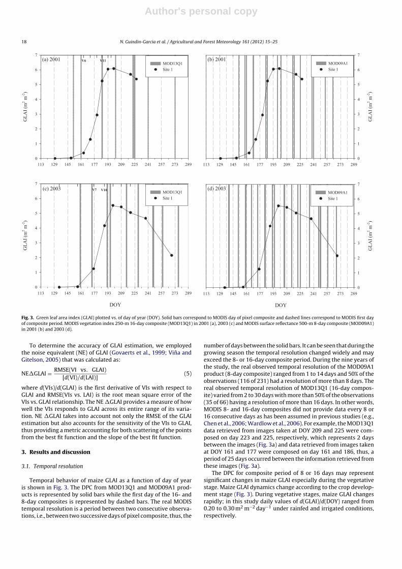
Fig. 3. Green leaf area index (GLAI) plotted vs. of day of year (DOY). Solid bars correspond to MODIS day of pixel composite and dashed lines correspond to MODIS first dayof composite period. MODIS vegetation index 250-m 16-day composite (MOD13Q1) in 2001 (a), 2003 (c) and MODIS surface reflectance 500-m 8-day composite (MOD09A1)in 2001 (b) and 2003 (d).

To determine the accuracy of GLAI estimation, we employedthe noise equivalent (NE) of GLAI (Govaerts et al., 1999; Vina andGitelson, 2005) that was calculated as:

NE�GLAI = RMSE(VI vs. GLAI)[d(VI)/d(LAI)]

(5)

where d(VIs)/d(GLAI) is the first derivative of VIs with respect toGLAI and RMSE(VIs vs. LAI) is the root mean square error of theVIs vs. GLAI relationship. The NE �GLAI provides a measure of howwell the VIs responds to GLAI across its entire range of its varia-tion. NE �GLAI takes into account not only the RMSE of the GLAIestimation but also accounts for the sensitivity of the VIs to GLAI,thus providing a metric accounting for both scattering of the pointsfrom the best fit function and the slope of the best fit function.

3. Results and discussion

3.1. Temporal resolution

Temporal behavior of maize GLAI as a function of day of yearis shown in Fig. 3. The DPC from MOD13Q1 and MOD09A1 prod-ucts is represented by solid bars while the first day of the 16- and8-day composites is represented by dashed bars. The real MODIStemporal resolution is a period between two consecutive observa-tions, i.e., between two successive days of pixel composite, thus, the

number of days between the solid bars. It can be seen that during thegrowing season the temporal resolution changed widely and mayexceed the 8- or 16-day composite period. During the nine years ofthe study, the real observed temporal resolution of the MOD09A1product (8-day composite) ranged from 1 to 14 days and 50% of theobservations (116 of 231) had a resolution of more than 8 days. Thereal observed temporal resolution of MOD13Q1 (16-day compos-ite) varied from 2 to 30 days with more than 50% of the observations(35 of 66) having a resolution of more than 16 days. In other words,MODIS 8- and 16-day composites did not provide data every 8 or16 consecutive days as has been assumed in previous studies (e.g.,Chen et al., 2006; Wardlow et al., 2006). For example, the MOD13Q1data retrieved from images taken at DOY 209 and 225 were com-posed on day 223 and 225, respectively, which represents 2 daysbetween the images (Fig. 3a) and data retrieved from images takenat DOY 161 and 177 were composed on day 161 and 186, thus, aperiod of 25 days occurred between the information retrieved fromthese images (Fig. 3a).

The DPC for composite period of 8 or 16 days may representsignificant changes in maize GLAI especially during the vegetativestage. Maize GLAI dynamics change according to the crop develop-ment stage (Fig. 3). During vegetative stages, maize GLAI changesrapidly; in this study daily values of d(GLAI)/d(DOY) ranged from0.20 to 0.30 m2 m−2 day−1 under rainfed and irrigated conditions,respectively.

Author's personal copy

N. Guindin-Garcia et al. / Agricultural and Forest Meteorology 161 (2012) 15– 25 19

(a)

First DOY of MODIS composite period

12

9

14

5

16

1

17

7

19

3

20

9

22

5

24

1

25

7

27

3

Nu

mb

er o

f d

ays

bet

wee

n t

wo

co

nse

cuti

ve

ob

serv

atio

ns

0

5

10

15

20

25

30

35

(b)

Days b etween two c onse cut ive o bserv ati ons

0 2 4 6 8 10 12 14 16 18 20 22 24 26 28 30 32

Ch

ang

e in

GL

AI

(m2

m-2

)

-6

-5

-4

-3

-2

-1

0

1

2

3

4

5

6

Veget ati ve

Reproducti ve

Fig. 4. (a) Number of days between two consecutive observations plotted vs. thefirst day of MODIS composite period (DOY) for MODIS vegetation index 250-m 16-day composite period data (MOD13Q1). (b) Changes in green leaf area index (GLAI)plotted vs. number of days between two consecutive observations.

The real temporal resolution of MOD09A1 and MOD13Q1 prod-ucts varies for each pixel in the image. It can be seen that theDPC changed without any predictable pattern (Figs. 4 and 5a). Thiscontradicts assumptions of previous studies that assumed eitherthe first, last, or mean day of the composite period was appropri-ate (Chen et al., 2006; Wardlow et al., 2006). The real temporalresolution has significant implications in detecting phenology ofagricultural crops. Due to the variability in the first derivative ofGLAI with respect to DOY, d(GLAI)/d(DOY), during growing season,differences in GLAI values in a period between two consecutiveobservations might vary widely depending on the developmentstage (Figs. 4b and 5b). For example, during a 9-day period betweentwo consecutive observations (16-day composite data), change inGLAI may be up to 4 m2 m−2 during the vegetative stages while itcould be less than 1 m2 m−2 during reproductive stages (Fig. 4b).Similar results were observed for the 8-day composite data wherechanges in maize GLAI were larger during vegetative stages com-pare to reproductive stages (Fig. 5b). However, even using the 8-daycomposite data, one cannot avoid large uncertainties in GLAI values,ranging from 1 to 3.5 m2 m−2, when the real temporal resolution– the period between successive observations – exceeds 7 days(Fig. 5b). These results highlight that the real temporal resolutionof MODIS composite products must be taken into account when

(a)

First DOY of MO DIS co mposite perio d

12

9

13

7

14

5

15

3

16

1

16

9

17

7

18

5

19

3

20

1

20

9

21

7

22

5

23

3

24

1

24

9

25

7

26

5

27

3

Nu

mb

er o

f d

ays

bet

wee

n t

wo

con

secu

tiv

e o

bse

rvat

ion

s

0

2

4

6

8

10

12

14

16

(b)

Days bet ween two consecutive observ ation s

0 1 2 3 4 5 6 7 8 9 10 11 12 13 14 15 16

Ch

ang

e in

GL

AI

(m2

m-2

)

-6

-5

-4

-3

-2

-1

0

1

2

3

4

5

6

Vegetati ve

Reproductiv e

Fig. 5. (a) Number of days between two consecutive observations plotted vs. firstday of MODIS composite period (DOY) for MODIS surface reflectance 250-m 8-daycomposite period data (MOD09Q1). (b) Changes in green leaf area index (GLAI)plotted vs. number of days between two consecutive observations.

MODIS data are used to estimate rapidly changing biophysical char-acteristics (e.g., GLAI) of agricultural crops such as maize.

MODIS VIs 16-day composites have been used in many agricul-tural applications such as phenology detection (Zhang et al., 2003;Sakamoto et al., 2005; Wardlow et al., 2006); however, none ofthese studies mentioned the importance of a period of 16 days onagricultural crop dynamics especially during the vegetative stage.The MODIS 16-day composite (MOD13Q1) data might not be ableto detect critical developmental stages of agricultural crops due toperiods between observations of up to 30 days (Fig. 4a). To evalu-ate crop condition and yield, a technique comparing NDVI valuesobtained in a current growing season with historical NDVI valuesfor the same study site has been widely used (e.g., Kastens et al.,2005; Li et al., 2007). However, analyses of historical NDVI data thatdo not consider DPC may also lead to erroneous interpretations. Forinstance, during the nine years of observation in our study, NDVIvalues obtained from MODIS 16-day composite over site 1 on DOY161 ranged from 0.31 to 0.85.

3.2. Estimation of maize green leaf area index

The first step in testing performance of vegetation indicesretrieved from MODIS products was to understand how spatialand temporal resolutions affect the accuracy of GLAI estimation by

Author's personal copy

20 N. Guindin-Garcia et al. / Agricultural and Forest Meteorology 161 (2012) 15– 25

Table 1Root mean square error (RMSE), coefficient of variation (CV = RMSE/mean GLAI), and determination coefficient (R2) of the relationships between vegetation indices, VIs (EVI,WDRVI˛=0.2 and WDRVI˛=0.1) and green leaf area index (GLAI). VIs were retrieved at the first day of the period of the 8- or 16-day composite (defined here as DOY) and at theday during the composite period when the best observation was recorded (defined here as day of pixel composite, DPC).

Vegetation index and day of VIs retrieval MOD09A1, 500 m, 8 d MOD13Q1, 250 m, 16 d; MOD09Q1, 250 m, 8 d

RMSE (m2 m−2) CV (%) R2 RMSE (m2 m−2) CV (%) R2

EVIDOY 1.04 29.02 0.72 1.01 29.54 0.75DPC 0.80 21.79 0.82 0.58 16.31 0.91

WDRVI˛=0.2DOY 1.03 28.73 0.72 0.92 26.96 0.79DPC 0.84 22.94 0.80 0.50 13.95 0.94

WDRVI˛=0.1DOY 1.07 29.91 0.70 0.92 26.91 0.79DPC 0.90 24.50 0.77 0.50 14.08 0.93

different VIs. We compared relationships of VIs vs. GLAI, in whichGLAI corresponded to (a) the first day of composite period (denotedas DOY), and (b) the day of pixel composite (denoted as DPC). TheGLAI values were obtained by cubic spline interpolation of the rela-tionship between destructively measured GLAI and DOY (Fig. 3). InTable 1, determination coefficients (R2), root mean square errorsof GLAI estimation, and coefficients of variation (CV) are presentedfor relationships between GLAI and three vegetation indices, EVIand WDRVI˛=0.2 and WDRVI˛=0.1, retrieved from three MODIS prod-ucts. Data taken in 2001 through 2004 under irrigated and rainfedconditions were used in the analyses.

The main results of the analyses are as follows.

(i) When GLAI at day of pixel composite was used, RMSE of GLAIestimation decreased considerably compared with the use ofGLAI taken at the first day of the composite. For 250-m 16-daycomposite data RMSE decreases two-fold.

(ii) An increase in spatial resolution (250-m vs. 500-m) led toincreasing accuracy; RMSE decrease was 40% for EVI and 46%for WDRVI.

These findings help to explain results presented by Chen et al.(2006) who reported that data obtained from MODIS 250-m did notprovide more accurate GLAI estimation over maize fields comparedwith MODIS 500-m resolution data. Our analysis showed similarRMSE of maize GLAI estimation using 250-m and 500-m resolutionwithout the incorporation of DPC data. However, the results pre-sented in Table 1 with the incorporation of DPC data clearly showthat MODIS 250-m resolution did provide estimates that are moreaccurate over agricultural crops compared with MODIS 500-m res-olution.

Relationships were established between vegetation indices andGLAI, taken at day of pixel composite, for all three MODIS prod-ucts. Fig. 6 presents the relationships between vegetation indices(NDVI, EVI, WDRVI˛=0.2 and WDRVI˛=0.1) and GLAI under rainfedand irrigated conditions in 2001–2004. The relationships betweenNDVI and GLAI were essentially nonlinear for all three MODIS prod-ucts. While having high sensitivity to GLAI below 3 m2 m−2, NDVItends to saturate as GLAI exceeds 3 m2 m−2. As GLAI varied from

4 to 6 m2 m−2, NDVI changed from 0.84 to 0.86. This result is inaccord with results of previous studies (Maas, 1993; Buschman andNagel, 1993; Myneni et al., 1997; Gitelson et al., 2003). The rela-tionships of EVI and WDRVI˛=0.2 with GLAI were also nonlinear;however, decreases in sensitivity of VIs to GLAI >3 m2 m−2 wereless pronounced than with NDVI. For all three MODIS products,WDRVI˛=0.1 had linear relationships with GLAI and determinationcoefficient above 0.93 for 250 m data and above 0.77 for 500 mdata (Table 2).

An analysis of variance between the coefficients of the best-fitfunctions for three products (250-m 8- and 16-day composites and500-m 8-day composite) combined vs. the coefficients obtainedfor each individual product showed that for 8- and 16-day 250-m products the relationships between all VIs used (NDVI, EVI andWDRVIs) and GLAI are statistically similar (NDVI: p > 0.58; EVI:p > 0.5, WDRVI˛=0.2: p > 0.63; WDRVI˛=0.1: p > 0.80). Thus, estab-lished equations (Table 2) can be applied to MODIS 250-m productswith no re-parameterization. However, relationships between GLAIand VIs for 250-m and 500-m resolution products are statisticallydifferent with � < 0.01 (Table 2). Important to note, for the sameGLAI, all VIs are consistently higher for 250-m products than for500-m products (Fig. 6e–h). This is understandable taking intoaccount that 500-m data is contaminated by surrounding areaswith no vegetation (roads) or less vegetation than in the fields as isseen in Fig. 2.

The determination coefficient, R2, and RMSE of GLAI estimationrepresent the dispersion of the points from the best-fit regressionlines. They constitute measures of how good the regression model(best-fit function) is in capturing the relationship between GLAIand VIs. However, when the best-fit function is nonlinear, as incase of NDVI, EVI and WDRVI˛=0.2 (Fig. 6), both R2 and RMSE val-ues may be misleading. For example, although the relationshipof NDVI vs. GLAI showed values of R2 above 0.90 (Table 2 andFig. 6a), the slope of the relationship decreased drastically as GLAIexceeded 3 m2 m−2. The relationships of GLAI vs. VIs had similarR2 and RMSE (Table 2) but very different shapes (e.g., asymptoticbehavior in NDVI vs. linear in WDRVI˛=0.1). Therefore, a differentaccuracy metric was needed to compare the performance of VIs inestimating GLAI over the whole range of its variation. We applied

Table 2Established relationships between green leaf area index (GLAI) and vegetation indices retrieved from three MODIS products. Root mean square error (RMSE), coefficient ofvariation, CV (RMSE/mean GLAI), and determination coefficients (R2) are also presented.

Vegetation index Model equation RMSE (m2 m−2) CV (%) R2

MOD13Q1, 250-m, 16 d;MOD09Q1, 250-m, 8 d

NDVI GLAI = 1.94 − 10.84 × NDVI + 16.53 × NDVI2 0.49 13.80 0.94EVI GLAI = −1.84 + 9.05 × EVI + 0.94 × EVI2 0.58 16.31 0.91WDRVI˛=0.2 GLAI = 2.12 + 5.29 × WDRVI˛=0.2 + 1.29 × WDRVI2

˛=0.2 0.50 13.95 0.94WDRVI˛=0.1 GLAI = 3.96 + 5.69 × WDRVI˛=0.1 0.50 14.08 0.93

MOD09A1, 500-m 8 d

NDVI GLAI = −0.82 − 1.56 × NDVI + 9.79 × NDVI2 1.02 27.79 0.73EVI GLAI = 11.25 × EVI − 2.47 0.80 21.79 0.82WDRVI˛=0.2 GLAI = 5.80 × WDRVI˛=0.2 + 2.63 0.84 22.88 0.80WDRVI˛=0.1 GLAI = 5.81 × WDRVI˛=0.1 + 4.46 0.90 24.52 0.77

Author's personal copy

N. Guindin-Garcia et al. / Agricultural and Forest Meteorology 161 (2012) 15– 25 21

(a) y = -0.0176x2 + 0. 196 5x + 0.3308

R2 = 0.96

0 1 2 3 4 5 6 7

ND

VI

0.0

0.2

0.4

0.6

0.8

1.0

250- m 16 d

250- m 8d

(b) y = -0.0 081 x2 + 0.14 02x + 0.1955

R2 = 0. 93

0 1 2 3 4 5 6 7

EV

I

0.0

0.2

0.4

0.6

0.8

1.0

250- m 16 d

250- m 8d

(c) y = -0. 017 x2+ 0. 271 5x - 0.45 47

R2= 0. 96

0 1 2 3 4 5 6 7

WD

RV

Iα=

0.2

-0.8

-0.6

-0.4

-0.2

0.0

0.2

0.4

0.6

0.8

250-m 16d

250-m 8d

(d) y = 0.16 41x - 0.65 46

R2= 0. 93

GLAI (m2 m

-2)

0 1 2 3 4 5 6 7

WD

RV

Iα=

0.1

-0.8

-0.6

-0.4

-0.2

0.0

0.2

0.4

0.6

0.8

250- m 16 d

250- m 8d

(e) y = -0. 011 x2 + 0.14 2x + 0.3945

R2 = 0. 85

0 1 2 3 4 5 6 7

ND

VI

0.0

0.2

0.4

0.6

0.8

1.0

500- m 8d

(f) y = -0.04 4x2 + 0.1003x + 0 .2516

R2 = 0.83

0 1 2 3 4 5 6 7

EV

I

0.0

0.2

0.4

0.6

0.8

1.0

500- m 8d

(h) y = 0. 132 7x - 0.62 26

R2 = 0. 77

GLAI (m2 m

-2)

0 1 2 3 4 5 6 7

WD

RV

Iα=0.1

-0.8

-0.6

-0.4

-0.2

0.0

0.2

0.4

0.6

0.8

500- m 8d

(g) y = -0. 009 1x2 + 0.1947 x - 0.3 82

R2 = 0. 81

0 1 2 3 4 5 6 7

WD

RV

I α

=0

.2

-0.8

-0.6

-0.4

-0.2

0.0

0.2

0.4

0.6

0.8

500- m 8d

Fig. 6. Vegetation indices plotted vs. green leaf area index (GLAI) for 250-m resolution data (left column) and 500-m resolution (right column); solid lines are best-fitfunctions. Dashed lines are best-fit functions for 8- and 16-day 250-m resolution data plotted for comparison with 500-m data. (a) and (e) normalized difference vegetationindex (NDVI), (b) and (f) enhanced vegetation index (EVI), (c) and (g) wide dynamic range vegetation index (WDRVI) with = 0.2, (d) and (h) wide dynamic range vegetationindex (WDRVI) with = 0.1.

the noise equivalent as an indicator of the accuracy of GLAI esti-mation that provides a metric accounting for both scattering ofthe points from the best-fit function and the slope of the best-fitfunction.

Fig. 7 shows noise equivalent of GLAI estimation by differentindices retrieved from MODIS 250-m 8- and 16-day composites.NDVI had the lowest NE (highest accuracy) when GLAI < 2.5 m2 m−2,while NE increased drastically when GLAI was above 3 m2 m−2.

Author's personal copy

22 N. Guindin-Garcia et al. / Agricultural and Forest Meteorology 161 (2012) 15– 25

Fig. 7. Noise equivalent of green LAI estimated by NDVI, EVI, WDRVI with = 0.1and = 0.2, retrieved from MODIS surface reflectance 250-m 8-day composite(MOD09Q1) and MODIS vegetation index 250-m 16-day composite (MOD13Q1).

The behavior of the NE of WDRVI˛=0.2 was almost the same asNDVI for GLAI < 2.5 m2 m−2, however, the rate of NE increase forGLAI > 3 m2 m−2 was much lower. The relationship WDRVI˛=0.1 vs.GLAI was linear (Fig. 6d and h, Table 2), thus, NE remained constantover the whole dynamic range of GLAI (Fig. 7). It was the lowestamong the VIs used for LAI > 3 m2 m−2. In Table 3 we presented NEvalues for different VIs corresponding to GLAI from 1 to 6 m2 m−2.It can be seen that NDVI was superior in estimating GLAI overthe range from 0 to 2.5 m2 m−2 (NE was below 0.46 m2 m−2) andWDRVI˛=0.1 had the highest accuracy (NE below 0.49 m2 m−2) whenGLAI > 3 m2 m−2. Thus, applying the NE metric allows direct quan-titative comparison among different indices with different scalesand dynamic ranges.

We validated the models for GLAI estimation using EVI andWDRVI ( = 0.1 and = 0.2) with independent data sets taken from2005 through 2009. We did not validate the NDVI model due toits very low accuracy for estimating GLAI > 3 m2 m−2. VIs valuesfrom the validation data sets were used to calculate GLAI employingestablished calibrated equations (Table 2) and these predicted GLAIvalues were compared to GLAI measured destructively. Figs. 8–10show the results of the validations. The GLAI vs. EVI model wasable to estimate GLAI with RMSE below 0.9 m2 m−2 for all MODISproducts. The linear models of GLAI vs. WDRVI˛=0.1 and polynomialmodels of GLAI vs. WDRVI˛=0.2 brought RMSE below 0.87 for the500-m resolution product and were much more accurate in GLAIestimation using the 250-m resolution products: RMSE was below0.60 m2 m−2 (Fig. 11). Validation results confirmed that more accu-rate estimates of maize GLAI can be obtained using data taken withhigher spatial resolution: the 250-m (MOD13Q1 and MOD09Q1),compared to the MODIS product 500-m resolution (MOD09A1).The reason for higher uncertainties of GLAI estimation using 500-mresolution data is most likely signal contamination by surroundingareas (Fig. 2).

Table 3Noise equivalent in m2 m−2 of green leaf area index (GLAI) estimation by vegetationindices calculated using 250-m 8- and 16-day composite MODIS products.

GLAI (m2 m−2) NDVI EVI WDRVI = 0.2 WDRVI = 0.1

1 0.31 0.48 0.38 0.492 0.4 0.56 0.44 0.492.5 0.46 0.6 0.48 0.493 0.55 0.66 0.53 0.494 0.90 0.8 0.67 0.495 2.43 1.01 0.89 0.496 1.39 1.36 0.49

(a) EVI

RMSE=0.5 8 m2 m

-2

CV=16 % n=78

Measured GLAI (m2 m

-2)

0 1 2 3 4 5 6 7 8

Pre

dic

ted G

LA

I (m

2 m

-2)

0

1

2

3

4

5

6

7

8

Irrigated

Rainfed

(b) WDRV Iα=0.1

RMSE=0.5 7 m2 m

-2

CV=16 % n=78

Measured GLAI (m2 m

-2)

0 1 2 3 4 5 6 7 8

Pre

dic

ted G

LA

I (m

2 m

-2)

0

1

2

3

4

5

6

7

8

Irrigate d

Rainf ed

(c) WDRV Iα=0.2

RMSE=0.5 7 m2 m

-2

CV=16 % n=78

Mea sured GLAI ( m2 m

-2)

0 1 2 3 4 5 6 7 8

Pre

dic

ted G

LA

I (m

2 m

-2)

0

1

2

3

4

5

6

7

8

Irrigated

Rainf ed

Fig. 8. Green leaf area index (GLAI) predicted by established algorithms (Table 2)(a) enhanced vegetation index (EVI), and wide dynamic range vegetation index(WDRVI) with (b) = 0.1 and (c) = 0.2 plotted vs. measured GLAI of maize grownunder irrigated and rainfed conditions from 2005 to 2009. VIs were retrieved fromMODIS vegetation index 250-m 16-day product (MOD13Q1).

WDRVI ( = 0.1 and = 0.2) and EVI allowed more accurate esti-mation of GLAI taken at DPC than has been reported in previousstudies using MODIS 250-m resolution products. Doraiswamy et al.(2004) estimated maize GLAI with a RMSE of 1.11 and 0.63 m2 m−2

using MODIS 250-m and field canopy reflectance, respectively.They attributed the difference in RMSE between field and satellite

Author's personal copy

N. Guindin-Garcia et al. / Agricultural and Forest Meteorology 161 (2012) 15– 25 23

(a) EVI

RMSE=0.6 7 m2 m -2

CV=18 % n=145

Meas ured GLAI (m2 m

-2)

0 1 2 3 4 5 6 7 8

Pre

dic

ted

GL

AI

(m2 m

-2)

0

1

2

3

4

5

6

7

8

Irr iga ted

Rainfed

(c) WDRVIα-0.2

RMSE=0.59 m2 m -2

CV=16% n=145

Meas ured GLAI (m2 m

-2)

0 1 2 3 4 5 6 7 8

Pre

dic

ted G

LA

I (m

2 m

-2)

0

1

2

3

4

5

6

7

8

Irrig ated

Rainfed

(b) WDRVIα-0 .1

RMSE=0.59 m2 m -2

CV=16% n=145

Meas ured GLAI (m2 m

-2)

0 1 2 3 4 5 6 7 8

Pre

dic

ted

GL

AI

(m2 m

-2)

0

1

2

3

4

5

6

7

8

Irrig ated

Rainfed

Fig. 9. Green leaf area index (GLAI) predicted by established algorithms (Table 2)(a) enhanced vegetation index (EVI), and wide dynamic range vegetation index(WDRVI) with (b) = 0.1 and (c) = 0.2 plotted vs. measured GLAI of maize grownunder irrigated and rainfed conditions from 2005 to 2009. VIs were retrieved fromMODIS surface reflectance 250-m 8-day product (MOD09Q1).

estimation to potential errors associated with MODIS atmosphericcorrection. On the other hand, Zhu et al. (2005) reported a lin-ear relationship in grass between GLAI and 250-m resolutionMODIS-retrieved EVI and NDVI with R2 = 0.82 and 0.78, respec-tively. Neither of these studies mentioned whether information onDPC was included in their analyses.

The results presented in this study clearly show that MODIS250-m spatial resolution products (MOD13Q1 and MOD09Q1)

(a) EVI

RMSE=0.8 0 m2m

-2

CV=21% n=13 6

Mea sured GLAI (m2 m

-2)

0 1 2 3 4 5 6 7 8

Pre

dic

ted G

LA

I (m

2 m

-2)

0

1

2

3

4

5

6

7

8

Irriga ted

Rainfed

(c) WDRVIα=0.2

RMSE= 0.83 m2

m-2

CV=22% n=136

Measured GLAI (m2 m

-2)

0 1 2 3 4 5 6 7 8

Pre

dic

ted G

LA

I (m

2 m

-2)

0

1

2

3

4

5

6

7

8

Irrig ated

Rain fed

(b) WDRVIα=0.1

RMSE=0.87 m2m

-2

CV=23% n=136

Measured GLAI (m2 m

-2)

0 1 2 3 4 5 6 7 8

Pre

dic

ted G

LA

I (m

2 m

-2)

0

1

2

3

4

5

6

7

8

Irrigated

Rain fed

Fig. 10. Green leaf area index (GLAI) predicted by established algorithms (Table 2)(a) enhanced vegetation index (EVI), and wide dynamic range vegetation index(WDRVI) with (b) = 0.1 and (c) = 0.2 plotted vs. measured GLAI of maize grownunder irrigated and rainfed conditions from 2005 to 2009. VIs were retrieved fromMODIS surface reflectance 500-m 8-day product (MOD009A1).

can provide more accurate estimates of critical growth stagesand GLAI for crop modeling applications than the MODIS 500-m spatial resolution product (MOD09A1). Results obtained duringnine years of observation showed that maize GLAI can be mon-itored during the entire growing season using the EVI and theWDRVI˛=0.2 quadratic models and WDRVI˛=0.1 linear models using

Author's personal copy

24 N. Guindin-Garcia et al. / Agricultural and Forest Meteorology 161 (2012) 15– 25

RM

SE

(m

2 m

-2)

0.0

0.2

0.4

0.6

0.8

1.0

MOD13Q1

MOD09Q1

MOD09A1

WDRVI α=0.1 WDRVI α=0.2EVI

Fig. 11. Root mean square error (RMSE) of green leaf area index prediction by estab-lished algorithms (Table 2) using MODIS 250-m 16-day (MOD13Q1), 250-m 8-day(MOD09Q1), and 500-m 8-day (MOD09A1) products.

data retrieved from the MODIS VIs 16-day composite product(MOD13Q1). The MODIS surface reflectance 8-day composite 250-m product (MOD09Q1) brings more frequent observations thatshould provide an opportunity for better estimation of crop crit-ical stages; however, knowledge of the DPC would dramaticallyenhance its utility in many agricultural applications.

The relationships of GLAI vs. VIs (Table 2) were developed onthe basis of results obtained in three Nebraska sites during fouryears of observation in 2001–2004. The algorithms were vali-dated using data obtained in 2005–2009. We cannot answer thequestion whether these equations can be applied with no re-parameterization to estimate GLAI in maize grown in differentclimatic conditions. However, the algorithms were developed andvalidated for maize grown under both irrigation management andrainfed conditions. The nine-year study period represents wet yearsas well as normal and dry years, in which the maize in the rain-fed site might suffer from water stress to different degrees, whilethe maize in irrigated sites was relatively stress-free. In addi-tion, the density of planting in the rainfed site was much lowerthan in the irrigated sites in order to account for differences inwater-limited attainable yield. Thus, during the nine years of obser-vations the physiological conditions of crops varied drastically.Despite all these differences, as well as wide changes in weatherconditions, in composition of incident irradiation, and in viewingzenith angle among others, the models presented in the paper wereable to accurately estimate GLAI with RMSE below 0.60 m2 m−2.Thus, the models as presented may likely be applied for maizegrown in different climatic conditions. However, further studiesshould address questions about whether the algorithms requirere-parameterization or not.

4. Conclusions

This study evaluated performance of three MODIS products(MOD13Q1, MOD09A1, and MOD09Q1) to quantify green leaf areaindex in maize. The temporal resolution of MODIS data (periodbetween two consecutive observations) for this study varied widelyand reached 15 days for 8-day composites and 30 days for 16-daycomposites. Due to maize leaf area index dynamics and unpre-dictable changes in MODIS real temporal resolution, the inclusionof day of pixel composite is necessary to increase the accuracyof green leaf area index estimates in agricultural crops. Analysisof noise equivalent of established relationships between VIs andgreen leaf area index showed that accuracy of green leaf area indexestimation by NDVI, EVI and WDRVI˛=0.2 varied significantly for

different canopy densities. Among the vegetation indices studied,only WDRVI˛=0.1 had a linear relationship with green leaf areaindex and, thus, a constant noise equivalent value below 0.5 m2 m−2

over the whole range of green leaf area index from 0 to morethan 6 m2 m−2. The established relationships using day of pixelcomposite data were validated by independent data sets takenin 2005–2009. Using MODIS 250-m resolution data, maize greenLAI was predicted by EVI with RMSE below 0.7 m2 m−2 and byboth WDRVIs with RMSE below 0.6 m2 m−2. Results also showedthat MODIS 250-m resolution provides more accurate estimates ofmaize green leaf area index compared to MODIS 500-m resolution.Using MODIS 500-m resolution data allows estimates of green leafarea index with RMSE around 0.80 m2 m−2 by both EVI and WDRVI.Results from this study also suggested that the MOD09Q1 prod-uct could be the better product to monitor agricultural crops dueto higher spatial and temporal resolutions; however, this productdoes not include information on day of pixel composite (collection5).

Acknowledgments

We would like to thank Dave Scoby who led the field LAI mea-surements and two anonymous reviewers for excellent and veryhelpful comments and suggestions.

References

Buschman, C., Nagel, E., 1993. In vivo spectroscopy and internal optics of leaves asbasis for remote sensing of vegetation. Int. J. Remote Sens. 14, 711–722.

Chen, P.Y., Fedosejevs, G., Tiscareno-López, M., Arnold, J.G., 2006. Assessment ofMODIS-EVI, MODIS NDVI and vegetation-NDVI composite data using agricul-tural measurements: an example at corn fields in Western Mexico. Environ.Monit. Assess. 119, 69–82.

Chen, P.Y., Srinivasan, R., Fedosejevs, G., Kiniry, J.R., 2003. Evaluating different NDVIcomposite techniques using NOAA-14 AVHRR data. Int. J. Remote Sens. 24 (17),3403–3412.

Chen, P.Y., Srinivasan, R., Fedosejevs, G., Narasimhan, B., 2002. An automated clouddetection method for daily NOAA-14 AVRR data for Texas, USA. Int. J. RemoteSens. 23 (15), 2939–2950.

Dash, J., Curran, P.J., 2004. The MERIS terrestrial chlorophyll index. Int. J. RemoteSens. 25, 5003–5013.

Didan, K., Huete, A., 2006. MODIS Vegetation Index Product Series Collection 5Change Summary, retrieved from http://landweb.nascom.nasa.gov/QA WWW/forPage/MOD13 VI C5 Changes Document 06 28 06.pdf.

Doraiswamy, P.C., Hatfield, J.L., Jackson, T.J., Akhmedov, B., Prueger, J., Stern, A., 2004.Crop condition and yield simulations using Landsat and MODIS. Remote Sens.Environ. 92, 548–559.

Duchemin, B., Maisongrande, P., 2002. Normalisation of directional effects in 10-dayglobal syntheses derived from VEGETATION/SPOT: I. Investigation of conceptsbased on simulation. Remote Sens. Environ. 81, 90–100.

Fang, H., Liang, S., Hoogenboom, G., Teasdale, J., Cavigelli, M., 2008. Corn-yield esti-mation through assimilation of remotely sensed data into the CSM-CERES-Maizemodel. Int. J. Remote Sens. 29 (10), 3011–3032.

Funk, C., Budde, M., 2009. Phenologically-tuned MODIS NDVI-based productionanomaly estimates for Zimbabwe. Remote Sens. Environ. 113 (1), 115–125.

Gitelson, A.A., 2011. Remote sensing estimation of crop biophysical characteristicsat various scales. In: Thenkabail, P.S., Lyon, J.G., Huete, A. (Eds.), HyperspectralRemote Sensing of Vegetation. Taylor and Francis, pp. 329–358 (chapter 15).

Gitelson, A.A., 2004. Wide dynamic range vegetation index for remote quantificationof biophysical characteristics of vegetation. J. Plant Physiol. 161, 165–173.

Gitelson, A.A., Wardlow, B.D., Keydan, G.P., Leavitt, B., 2007. Evaluation of MODIS250-m data for green LAI estimation in crops. Geophys. Res. Lett. 34, L20403,doi:10.1029/2007GL031620.

Gitelson, A.A., Kaufman, Y., Merzlyak, M.N., 1996. Use of green channel in remotesensing of global vegetation from EOS-MODIS. Remote Sens. Environ. 58,289–298.

Gitelson, A.A., Vina, A., Arkebauer, T.J., Rundquist, D.C., Keydan, G., Leavitt, B., 2003.Remote estimation of leaf area index and green leaf biomass in maize canopies.Geophys. Res. Lett. 30 (5), 1248.

Govaerts, Y.M., Verstraete, M.M., Pinty, B., Gobron, N., 1999. Designing optimal spec-tral indices: a feasibility and proof of concept study. Int. J. Remote Sens. 20,1853–1873.

Hatfield, J.L., Gitelson, A.A., Schepers, J.S., Walthall, C.L., 2008. Application of spectralremote sensing for agronomic decisions. Agron. J. 100, 117–131.

Huete, A.R., Liu, H.Q., Batchily, K., van Leeuwen, W.J.D., 1997. A comparison of veg-etation indices over a global set of TM images for EOS-MODIS. Remote Sens.Environ. 59, 440–451.

Author's personal copy

N. Guindin-Garcia et al. / Agricultural and Forest Meteorology 161 (2012) 15– 25 25

Huete, A., Didan, K., Miura, T., Rodriguez, E.P., Gao, X., Ferreira, L.G., 2002. Overview ofthe radiometric and biophysical performance of the MODIS vegetation indices.Remote Sens. Environ. 83, 195–213.

Huete, A., Justice, C.O., van Leeuwen, W.J., 1999. MODIS Vegetation Index (MOD13),retrieved from http://modis.gsfc.nasa.gov/data/atbd/atbd mod13.pdf.

Kastens, J.H., Kastens, T.L., Kastens, D.L., Price, K.P., Martinko, E.A., Lee, R.Y., 2005.Image masking for crop yield forecasting using AVHRR NDVI time series imagery.Remote Sens. Environ. 99, 341–356.

Jiang, Z., Huete, A.R., Didan, K.A., Miura, T., 2008. Development of a two-bandenhanced vegetation index without a blue band. Remote Sens. Environ. 112,3833–3845.

Li, A., Liang, S., Wang, A., Qin, J., 2007. Estimating crop yield from multi-temporalsatellite data using multivariate regression and neural network techniques. Pho-togramm. Eng. Remote Sens. 73 (10), 1149–1157.

Lobell, D.B., Asner, G.P., 2004. Cropland distributions from temporal unmixing ofMODIS data. Remote Sens. Environ. 93, 412–422.

Lunetta, R.L., Knight, F.K., Ediriwickrema, J., Lyon, J.G., Worthly, L.D., 2006. Land-cover change detection using multi-temporal MODIS NDVI data. Remote Sens.Environ. 105, 142–154.

Maas, S.J., 1993. Within-season calibration of modeled wheat growth using remotesensing and field sampling. Agron. J. 85, 669–672.

Myneni, R.B., Nemani, R.R., Running, S.W., 1997. Estimation of global leaf area indexand absorbed PAR using radiative transfer models. IEEE Trans. Geosci. RemoteSens. 35, 1380–1393.

Ritz, C., Streibig, J.C., 2008. Grouped data. In: Ritz, C., Streibig, J.C. (Eds.), NonlinearRegression with R. Springer Science+Business Media, LLC, New York, NY, pp.109–131.

Rochdi, N., Fernandes, R., 2010. Systematic mapping of leaf area index across Canadausing 250-meter MODIS data. Remote Sens. Environ. 114, 1130–1135.

Rouse, J.W., Haas, R.H., Schell, J.A., Deering, D.W., 1974. Monitoring vegetation sys-tems in the Great Plains with ERTS. In: Proc. Third Earth Resources TechnologySatellite-1 Symposium, SP-351, Greenbelt, MD, pp. 309–317.

Sakamoto, T., Yokozawa, M., Toritani, H., Shibayama, M., Ishitsuka, N., Ohno, H., 2005.A crop phenology detection method using time-series MODIS data. Remote Sens.Environ. 95, 366–374.

Sedano, F., Gong, P., Ferrao, M., 2005. Land cover assessment with MODIS imagery insouthern African Miombo ecosystems. Remote Sens. Environ. 98, pp. 429–441.

Shapiro, C.A., Ferguson, R.B., Hergert, G.W., Dobermann, A., Wortmann, C.S., 2001.Fertilizer suggestions for corn. Neb-Guide G74-174-A. Cooperative Extension,Institute of Agriculture and Natural Resources. University of Nebraska-Lincoln,Lincoln, NE.

Swets, D.L., Reed, B.C., Rowland, J.R., Marko, S.E., 1999. A weighted least-squaresapproach to temporal smoothing of NDVI. In: ASPRS Annual Conference, Portand,Oregon, pp. 17–21.

Verma, S.B., Dobermann, A., Cassman, K.G., Walters, D.T., Knops, J.M., Arkebauer,T.J., Suyker, A.E., Burba, G.G., Amos, B., Yang, H., Ginting, D., Hubbard, K.G.,Gitelson, A.A., Walter-Shea, E.A., 2005. Annual carbon dioxide exchange inirrigated and rainfed maize-based agroecosystems. Agric. For. Meteorol. 131,77–96.

Vermote, E.F., Kotchennova, S.Y., 2008. MOD09 (Surface Reflectance) User’s Guide,retrieved from http://modis-sr.ltdri.org.

Vina, A., Gitelson, A.A., 2005. New developments in the remote estimation of thefraction of absorbed photosynthetically active radiation in crops. Geophys. Res.Lett. 32, L17403, doi:10.1029/2005GL023647.

Wardlow, B.D., Kastens, J.H., Egbert, S.L., 2006. Using USDA crop progress data forthe evaluation of greenup onset date calculated from MODIS 250-meter data.Photogramm. Eng. Remote Sens. 72 (11), 1225–1234.

Zhang, X., Friedl, M.A., Schaaf, C.B., Strahler, A.H., Hodges, J.C., Gao, F., Reed, B.C.,Huete, A., 2003. Monitoring vegetation phenology using MODIS. Remote Sens.Environ. 84, 471–475.

Zhu, H., Luo, T., Yang, Y., 2005. MODIS-based seasonality and distribution of leafarea index of grassland of Gonghe Basin in Qinghai-Tibet plateau. Proc. SPIE5976, 324–331.