An evaluation of alternativescoring models in private banking

Hussein A. AbdouSalford Business School, Salford University, Salford, UK

Abstract

Purpose – This paper aims to investigate the efficiency and effectiveness of alternativecredit-scoring models for consumer loans in the banking sector. In particular, the focus is upon thefinancial risks associated with both the efficiency of alternative models in terms of correctclassification rates, and their effectiveness in terms of misclassification costs (MCs).

Design/methodology/approach – A data set of 630 loan applicants was provided by an Egyptianprivate bank. A two-thirds training sample was selected for building the proposed models, leaving aone-third testing sample to evaluate the predictive ability of the models. In this paper, an investigationis conducted into both neural nets (NNs), such as probabilistic and multi-layer feed-forward neuralnets, and conventional techniques, such as the weight of evidence measure, discriminant analysis andlogistic regression.

Findings – The results revealed that a best net search, which selected a multi-layer feed-forward netwith five nodes, generated both the most efficient classification rate and the most effective MC. Ingeneral, NNs gave better average correct classification rates and lower MCs than traditional techniques.

Practical implications – By reducing the financial risks associated with loan defaults, banks canachieve a more effective management of such a crucial component of their operations, namely, theprovision of consumer loans.

Originality/value – The use of NNs and conventional techniques in evaluating consumer loanswithin the Egyptian private banking sector utilizes rigorous techniques in an environment whichmerits investigation.

Keywords Banking, Financial risk, Scoring procedures (tests)

Paper type Research paper

IntroductionRecently, the role of effective management of different financial and operational risks isespecially important for bankers who have come to realize that banking operationsaffect and are affected by economic and social environmental risks that they face. It isbelieved that the Egyptian banking sector has been “tough” since 1999, and is “expectedto remain so” for the performance of the banking sector in Egypt has shown an “ongoingprofitability weakness due to revenue pressure” and a high incidence of problem loans(Oldham and Young, 2004; CBE, 2006/2007). Therefore, the role that scoring techniquescan play is critical in helping to reduce the current and/or the expected risk they face,because of an inadequate risk-reduction through efficient diversification.

Especially, with the fast growth in the credit industry and the huge loan portfoliomanagement, credit scoring is regarded as a one the most important techniques in banksand has become a very critical tool during recent decades. A number of credit-scoringmodels have been developed to evaluate the credit risk process of both new and existingloan clients. Scoring techniques assess, and therefore help to decide, “who will get credit,how much credit they should get, and what operational strategies will maintain theprofitability of the borrowers to the lenders” (Thomas et al., 2002; Hand and Jacka, 1998).

The current issue and full text archive of this journal is available at

www.emeraldinsight.com/1526-5943.htm

JRF10,1

38

The Journal of Risk FinanceVol. 10 No. 1, 2009pp. 38-53q Emerald Group Publishing Limited1526-5943DOI 10.1108/15265940910924481

Statistical techniques, such as discriminant analysis (DA), regression analysis, andlogistic regression (LR), used in building the scoring models have been examined(Crook et al., 2007; Greene, 1998; Altman et al., 1994; Orgler, 1971). A few studies haveexplored the scoring models using the weight of evidence (WOE) measure, or in termsof poor as good or good and bad credit, also results were comparable with those fromother techniques (Banasik et al., 2003; Bailey, 2001; Siddiqi, 2006). The evaluation ofnew client’s loans has attracted some attention in the last ten decades and it isconsidered as one of the most critical applications of credit-scoring models (Sarlija et al.,2004; Chen and Huang, 2003; Malhotra and Malhotra, 2003).

The neural network models have the highest average correct classification (ACC)rate when compared with other traditional techniques, such as DA and LR, taking intoaccounts that results were very close. A few credit-scoring models have investigatedthe use probabilistic neural nets (PNNs) (Ganchev et al., 2007; Zekic-Susac et al., 2004;Masters, 1995), whilst many scoring models applying multi-layer feed-forward nets(MLFNs) have been used (Erbas and Stefanou, 2008; Dimla and Lister, 2000; West,2000; Reed and Marks, 1999; Desai et al., 1996; Bishop, 1995).

Other statistical models, as well as neural networks and fuzzy algorithms have beenused in building scoring models (Tsai and Wu, 2008; Anderson, 2007; Crook et al., 2007;Nur Ozkan-Gunay and Ozkan, 2007; Yu et al., 2007; Seow and Thomas, 2006; Handet al., 2005; Zhang and Bhattacharyya, 2004). Furthermore, comparisons betweenconventional and advanced statistical scoring techniques have been investigated aswell (Lee and Chen, 2005; Ong et al., 2005; Lee et al., 2002; Desai et al., 1997).Comparisons have also been extended to include other neural networks, such asback-propagation and feed-forward nets (Min and Lee, 2008; Malhotra and Malhotra,2003; Arminger et al., 1997). Neural network models are better representations of datathan LR and CART, as shown by the statistical association measures (Zekic-Susac et al.,2004; Zhang et al., 1999), while other traditional techniques, such as DA, in general, asnoted by Liang (2003) has a better classification ability but worse prediction ability,whereas LR has a moderately better prediction ability.

The chosen environment is the Egyptian banking sector. Indeed, from the review ofliterature to date, the author was not aware of other studies in Egypt in coveringcredit-scoring techniques. Therefore, the intention was to cover this gap, which was foundin the Egyptian banking sector. This paper is organized as follows: part two details theresearch methodology and data collection. Part three explains the results. Finally, partfour concludes the results of the study and suggests areas for future research.

Methodology and data collectionThis part begins with a description of four statistical techniques used in building creditscoring. The first model is the WOE measure, which is one of the earliest techniques usedin credit scoring. The second model is the DA model, which was first proposed by Fisher(1936) as a discrimination and classification technique. Third, the LR model, unlike otherconventional statistical techniques, can suit different kinds of distribution functions andis more suitable for credit-scoring problems. Then, neural nets (NNs), one of the beststatistical techniques used in building the scoring models, is regarded as a practicaltechnology, with successful applications in many fields in financial institutionsespecially banks (Bishop, 1995; Masters, 1995). Here, two different nets, PNNs andMLFNs with four nodes (selected automatically by the software design) were utilized in

Alternativescoring models

39

this paper and the best net search (BNS), from a MLFN with two to six nodes and from aPNN as well, was an option selected in the current package. The advantage of selectingthe BNS, current package tests all checked net configurations, including PNNs andMLFNs with node counts in the entered minimum-maximum range, from two to sixnodes, which means more alternative models in the training and testing process.

Later, the data collection method and the identification of variables will bediscussed. The applied validation technique used in this paper is based on a trainingsample (389 cases; 67 per cent) and a testing sample (192 cases; 33 per cent). The testingsample tests the predictive effectiveness of the fitted model.

Weight of evidence measureOne of the earliest measures used in credit-scoring models is WOE measure. It dependson the odds ratio of good scores expressed as a proportion of bad scores. Informationodds (IO) are the ratio of the proportions; therefore, it is used to make inferences aboutthe difference between two distributions without the effect of changes to the overallpopulation. Therefore, we have the first equation:

IO ¼ Goods sub-classification as percent=Bads sub-classification as percentage:

WOE can be calculated from the IO using the logarithmic function, which can beconsidered as raw scores, as follows:

WOE ¼ lnðIOÞ:

To determine the Point Score, or WOE Score, the following equation might be used:

Point Score ¼X P

lnð2Þ£ Rw

� �£ ½WOE þ c�

� �;

where, P – is the score at which the odds are doubled; Rw – is the correlation coefficient(from a multiple regression) between the respective variable and the WOE for thevariable; c – is a constant applied to each variable (Bailey, 2001; Siddiqi, 2006).

Discriminant analysisHowever, as to the statistical assumptions implicit in implementation, DA requires thedata to be independent and normally distributed. Consequently, the general formulaof DA is as follows:

Z ¼ aþ b1X1 þ b2X2 þ · · · þ bnXn;

where Z represents the discriminant Z-score, a is the intercept term, and bi representsthe respective coefficient in the linear combination of explanatory variables, Xi, fori ¼ 1, . . . , n (Lee et al., 2002).

Logistic regressionLR is a widely used statistical modeling technique in which the probability of a binaryoutcome (zero or one) is related to a set of potential predictor variables in the form:

lnp

1 2 p

� �¼ aþ b1X1 þ b2X2 þ · · · þ bnXn;

JRF10,1

40

where p is the probability of the outcome of interest, a is the intercept term, and bi

represents the respective coefficient in the linear combination of explanatory variables,Xi, for i ¼ 1, . . . , n. The dependent variable is the logarithm of the odds{ln½p=ð1 2 pÞ�}, which is the logarithm of the ratio of two probabilities of theoutcome of interest (Lee et al., 2002).

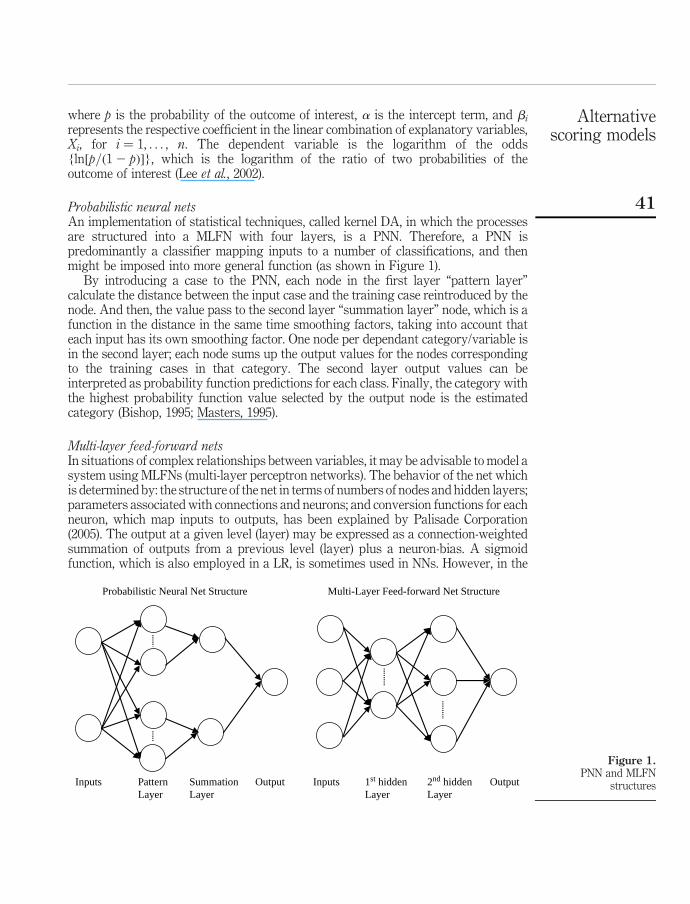
Probabilistic neural netsAn implementation of statistical techniques, called kernel DA, in which the processesare structured into a MLFN with four layers, is a PNN. Therefore, a PNN ispredominantly a classifier mapping inputs to a number of classifications, and thenmight be imposed into more general function (as shown in Figure 1).

By introducing a case to the PNN, each node in the first layer “pattern layer”calculate the distance between the input case and the training case reintroduced by thenode. And then, the value pass to the second layer “summation layer” node, which is afunction in the distance in the same time smoothing factors, taking into account thateach input has its own smoothing factor. One node per dependant category/variable isin the second layer; each node sums up the output values for the nodes correspondingto the training cases in that category. The second layer output values can beinterpreted as probability function predictions for each class. Finally, the category withthe highest probability function value selected by the output node is the estimatedcategory (Bishop, 1995; Masters, 1995).

Multi-layer feed-forward netsIn situations of complex relationships between variables, it may be advisable to model asystem using MLFNs (multi-layer perceptron networks). The behavior of the net whichis determined by: the structure of the net in terms of numbers of nodes and hidden layers;parameters associated with connections and neurons; and conversion functions for eachneuron, which map inputs to outputs, has been explained by Palisade Corporation(2005). The output at a given level (layer) may be expressed as a connection-weightedsummation of outputs from a previous level (layer) plus a neuron-bias. A sigmoidfunction, which is also employed in a LR, is sometimes used in NNs. However, in the

Figure 1.PNN and MLFN

structuresInputs PatternLayer

SummationLayer

Output

Probabilistic Neural Net Structure

Inputs 1st hiddenLayer

2nd hiddenLayer

Output

Multi-Layer Feed-forward Net Structure

Alternativescoring models

41

Neural Tools software the sigmoid function is not utilized (Figure 1). The reason is toavoid a restriction on outputs values, to create a superb model for training purposes.

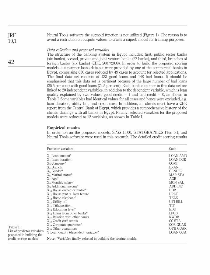
Data collection and proposed variablesThe structure of the banking system in Egypt includes: first, public sector banks(six banks), second, private and joint venture banks (27 banks), and third, branches offoreign banks (six banks) (CBE, 2007/2008). In order to build the proposed scoringmodels, a consumer loans data-set were provided by one of the commercial banks inEgypt, comprising 630 cases reduced by 49 cases to account for rejected applications.The final data set consists of 433 good loans and 148 bad loans. It should beemphasized that this data set is pertinent because of the large number of bad loans(25.5 per cent) with good loans (74.5 per cent). Each bank customer in this data-set arelinked to 20 independent variables, in addition to the dependent variable, which is loanquality explained by two values, good credit – 1 and bad credit – 0, as shown inTable I. Some variables had identical values for all cases and hence were excluded, e.g.loan duration, utility bill, and credit card. In addition, all clients must have a CBEreport from the Central Bank of Egypt, which provides a comprehensive history of theclients’ dealings with all banks in Egypt. Finally, selected variables for the proposedmodels were reduced to 12 variables, as shown in Table I.

Empirical resultsIn order to run the proposed models, SPSS 15.00, STATGRAPHICS Plus 5.1, andNeural Tools software were used in this research. The detailed credit scoring results

Predictor variables Code

X1 Loan amounta LOAN AMOX2 Loan duration LOAN DURX3 Companya COMPX4 Branch BRANX5 Gendera GENDERX6 Marital statusa MAR STAX7 Agea AGEX8 Monthly salarya MON SALX9 Additional incomea ADD INCX10 House owned or renteda HORX11 House rent . loan tenure HRLTX12 Home telephonea TELEX13 Utility bill UTI BILLX14 Title/position TITX15 Education levela EDUX16 Loans from other banksa LFOBX17 Relation with other banks RWOBX18 Credit card status CC STAX19 Corporate guaranteea COR GUARX20 Other guarantors OTH GUARY Loan quality (dependent variable)a LOAN QUA

Note: aVariables finally selected in building the scoring models

Table I.List of predictor variablesproposed in building thecredit-scoring models

JRF10,1

42

using the above-mentioned modeling techniques can be summarized as follows.Because of the high correlation between the loan amount and monthly salary, 0.963, anorthogonalization test has been used to keep the effect of both in the proposed modelsbecause of their potential importance. The revised correlation, after running the test,was 0.269; all other variables had correlations within an acceptable range.

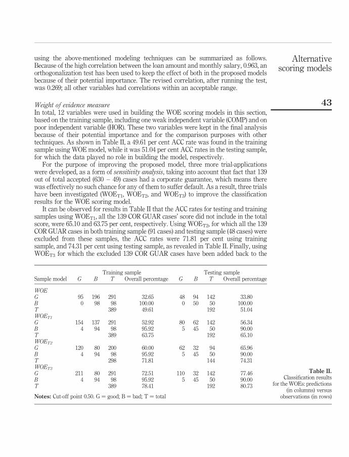
Weight of evidence measureIn total, 12 variables were used in building the WOE scoring models in this section,based on the training sample, including one weak independent variable (COMP) and onpoor independent variable (HOR). These two variables were kept in the final analysisbecause of their potential importance and for the comparison purposes with othertechniques. As shown in Table II, a 49.61 per cent ACC rate was found in the trainingsample using WOE model, while it was 51.04 per cent ACC rates in the testing sample,for which the data played no role in building the model, respectively.

For the purpose of improving the proposed model, three more trial-applicationswere developed, as a form of sensitivity analysis, taking into account that fact that 139out of total accepted (630 – 49) cases had a corporate guarantee, which means therewas effectively no such chance for any of them to suffer default. As a result, three trialshave been investigated (WOET1, WOET2, and WOET3) to improve the classificationresults for the WOE scoring model.

It can be observed for results in Table II that the ACC rates for testing and trainingsamples using WOET1, all the 139 COR GUAR cases’ score did not include in the totalscore, were 65.10 and 63.75 per cent, respectively. Using WOET2, for which all the 139COR GUAR cases in both training sample (91 cases) and testing sample (48 cases) wereexcluded from these samples, the ACC rates were 71.81 per cent using trainingsample, and 74.31 per cent using testing sample, as revealed in Table II. Finally, usingWOET3 for which the excluded 139 COR GUAR cases have been added back to the

Training sample Testing sampleSample model G B T Overall percentage G B T Overall percentage

WOEG 95 196 291 32.65 48 94 142 33.80B 0 98 98 100.00 0 50 50 100.00T 389 49.61 192 51.04WOET1

G 154 137 291 52.92 80 62 142 56.34B 4 94 98 95.92 5 45 50 90.00T 389 63.75 192 65.10WOET2

G 120 80 200 60.00 62 32 94 65.96B 4 94 98 95.92 5 45 50 90.00T 298 71.81 144 74.31WOET3

G 211 80 291 72.51 110 32 142 77.46B 4 94 98 95.92 5 45 50 90.00T 389 78.41 192 80.73

Notes: Cut-off point 0.50. G ¼ good; B ¼ bad; T ¼ total

Table II.Classification results

for the WOEs: predictions(in columns) versus

observations (in rows)

Alternativescoring models

43

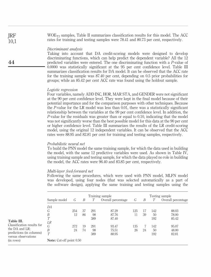
WOET2 samples, Table II summarizes classification results for this model. The ACCrates for training and testing samples were 78.41 and 80.73 per cent, respectively.

Discriminant analysisTaking into account that DA credit-scoring models were designed to developdiscriminating functions, which can help predict the dependent variable? All the 12predicted variables were entered. The one discriminating function with a P-value of0.0000 was statistically significant at the 95 per cent confidence level. Table IIIsummarizes classification results for DA model. It can be observed that the ACC ratefor the training sample was 87.40 per cent, depending on 0.5 prior probabilities forgroups; while an 85.42 per cent ACC rate was found using the holdout sample.

Logistic regressionFour variables, namely ADD INC, HOR, MAR STA, and GENDER were not significantat the 90 per cent confidence level. They were kept in the final model because of theirpotential importance and for the comparison purposes with other techniques. Becausethe P-value for the LR model was less than 0.01, there was a statistically significantrelationship between the variables at the 99 per cent confidence level. In addition, theP-value for the residuals was greater than or equal to 0.10, indicating that the modelwas not significantly worse than the best possible model for this data at the 90 per centor higher confidence level. Table III summarizes the results of the LR credit-scoringmodel, using the original 12 independent variables. It can be observed that the ACCrates were 88.95 and 82.81 per cent for training and testing samples, respectively.

Probabilistic neural netTo build the PNN model the same training sample, for which the data used in buildingthe model, with the same 12 predictive variables were used. As shown in Table IV,using training sample and testing sample, for which the data played no role in buildingthe model, the ACC rates were 96.40 and 83.85 per cent, respectively.

Multi-layer feed-forward netFollowing the same procedures, which were used with PNN model, MLFN modelwas developed, using four nodes (that was selected automatically as a part ofthe software design), applying the same training and testing samples using the

Training sample Testing sampleSample model G B T Overall percentage G B T Overall percentage

DAG 254 37 291 87.29 125 17 142 88.03B 12 86 98 87.76 11 39 50 78.00T 389 87.40 192 85.42LRG 272 19 291 93.47 135 7 142 95.07B 24 74 98 75.51 26 24 50 48.00T 389 88.95 192 82.81

Note: Cut-off point 0.50

Table III.Classification results forthe DA and LR;predictions (in columns)versus observations(in rows)

JRF10,1

44

same predictor variables. A 97.69 and 89.06 per cent ACC rates were foundapplying training and testing samples, respectively, as revealed in Table IV.

Powerful neural net modelsThe main difference between PNN and MLFN and powerful NN models was that for theformer, the data cases in both training and testing samples were selected judgmentallyby dividing the whole data-set into a 33 per cent testing sample and a 67 per cent trainingsample (the same samples data-sets were used with other scoring techniques used in thispaper namely, WOE, DA, and LR). By contrast, for the later, the data cases in the testingand the training samples were automatically selected by the Neural Tools software,applying a different 33 per cent data-set as a testing sample and a different 67 per centdata-set as a training sample for each trial.

The experiment was repeated several times, the reason for repeating the process wasto investigate whether different results, in terms of average correct classification rate,were being achieved because of the random selection procedure as part of the softwaredesign. Finally, there is evidence of significant differences between the powerful neuralnet models, as described below. Following are the classification results for the bestpowerful NN models under each of the 20 PNN, MLFN and BNS models, respectively.

From results revealed in Table V, PNN3 was (trial number three applying PNNs) thebest model (based on the highest overall testing ACC rate), between all the 20 powerfulPNN models, achieving a 94.09 per cent and an 89.58 per cent ACC rates applyingtraining and testing samples, respectively. While three different MLFNs were the best(based on the highest predictive ability) between the 20 powerful NN models, MLFN5,MLFN7 and MLFN10. ACC rates in the training samples were 95.12, 96.66 and 96.40 percent for MLFN5, MLFN7 and MLFN10, respectively; and an 86.98 per cent ACC rate forthe three nets in the testing samples, as shown in Table V.

As explained earlier PNN and MLFN from two to six nodes, this was an optionunder BNS, as a part of the currently used software, were applied in this paper as well.It can be observed from Table V that BNS4-MLFN-5N (BNS4-MLFN-5N means trialnumber four under the BNS with MLFN selecting five nodes as a best net) was the bestmodel, between all the 20 powerful BNS models. A 94.60 and 91.15 per cent ACC rateswere found in the training and testing samples, respectively, (for more detailsregarding all models including all trials, see the Appendix).

As it shown in Table VI, there is evidence of significant differences between NNmodels; the ANOVA F-ratio was 13.04. It was significant at 99 per cent confidence level.

Training sample Testing sampleSample model G B T Overall percentage G B T Overall percentage

PNNG 288 3 291 98.97 135 7 142 95.07B 11 87 98 88.78 24 26 50 52.00T 389 96.40 192 83.85MLFNG 287 4 291 98.63 133 9 142 93.66B 5 93 98 94.90 12 38 50 76.00T 389 97.69 192 89.06

Table IV.Classification results

for the PNN and MLFN;predictions (in columns)

versus observations(in rows)

Alternativescoring models

45

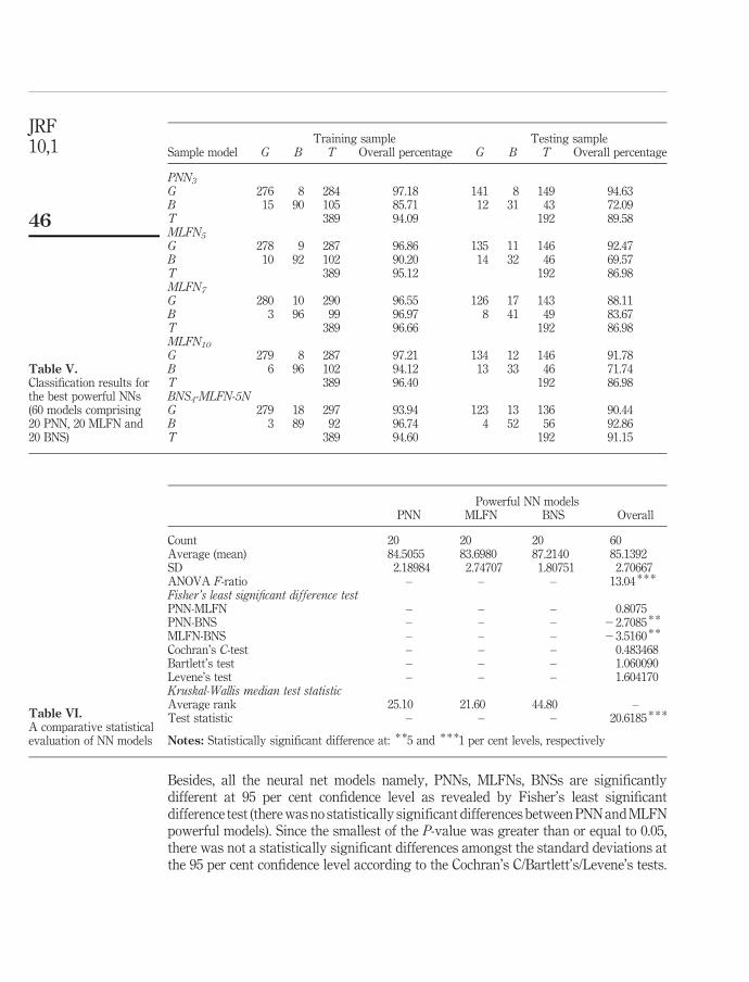
Besides, all the neural net models namely, PNNs, MLFNs, BNSs are significantlydifferent at 95 per cent confidence level as revealed by Fisher’s least significantdifference test (there was no statistically significant differences between PNN and MLFNpowerful models). Since the smallest of the P-value was greater than or equal to 0.05,there was not a statistically significant differences amongst the standard deviations atthe 95 per cent confidence level according to the Cochran’s C/Bartlett’s/Levene’s tests.

Training sample Testing sampleSample model G B T Overall percentage G B T Overall percentage

PNN3

G 276 8 284 97.18 141 8 149 94.63B 15 90 105 85.71 12 31 43 72.09T 389 94.09 192 89.58MLFN5

G 278 9 287 96.86 135 11 146 92.47B 10 92 102 90.20 14 32 46 69.57T 389 95.12 192 86.98MLFN7

G 280 10 290 96.55 126 17 143 88.11B 3 96 99 96.97 8 41 49 83.67T 389 96.66 192 86.98MLFN10

G 279 8 287 97.21 134 12 146 91.78B 6 96 102 94.12 13 33 46 71.74T 389 96.40 192 86.98BNS4-MLFN-5NG 279 18 297 93.94 123 13 136 90.44B 3 89 92 96.74 4 52 56 92.86T 389 94.60 192 91.15

Table V.Classification results forthe best powerful NNs(60 models comprising20 PNN, 20 MLFN and20 BNS)

Powerful NN modelsPNN MLFN BNS Overall

Count 20 20 20 60Average (mean) 84.5055 83.6980 87.2140 85.1392SD 2.18984 2.74707 1.80751 2.70667ANOVA F-ratio – – – 13.04 * * *

Fisher’s least significant difference testPNN-MLFN – – – 0.8075PNN-BNS – – – 22.7085 * *

MLFN-BNS – – – 23.5160 * *

Cochran’s C-test – – – 0.483468Bartlett’s test – – – 1.060090Levene’s test – – – 1.604170Kruskal-Wallis median test statisticAverage rank 25.10 21.60 44.80 –Test statistic – – – 20.6185 * * *

Notes: Statistically significant difference at: * *5 and * * *1 per cent levels, respectively

Table VI.A comparative statisticalevaluation of NN models

JRF10,1

46

Moreover, the Kruskal-Wallis median test statistic shows statistically significantdifferences at 99 per cent confidence level for NNs models with test statistics 20.62,which means that the average correct classification rates are significantly different ineach neural net.

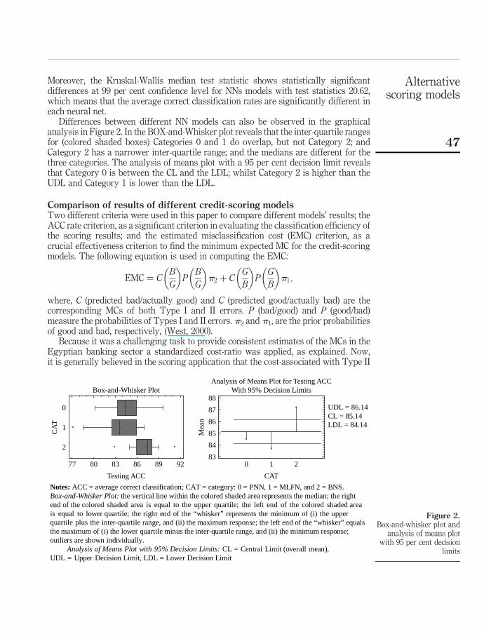
Differences between different NN models can also be observed in the graphicalanalysis in Figure 2. In the BOX-and-Whisker plot reveals that the inter-quartile rangesfor (colored shaded boxes) Categories 0 and 1 do overlap, but not Category 2; andCategory 2 has a narrower inter-quartile range; and the medians are different for thethree categories. The analysis of means plot with a 95 per cent decision limit revealsthat Category 0 is between the CL and the LDL; whilst Category 2 is higher than theUDL and Category 1 is lower than the LDL.

Comparison of results of different credit-scoring modelsTwo different criteria were used in this paper to compare different models’ results; theACC rate criterion, as a significant criterion in evaluating the classification efficiency ofthe scoring results; and the estimated misclassification cost (EMC) criterion, as acrucial effectiveness criterion to find the minimum expected MC for the credit-scoringmodels. The following equation is used in computing the EMC:

EMC ¼ CB

G

� �P

B

G

� �p2 þ C

G

B

� �P

G

B

� �p1;

where, C (predicted bad/actually good) and C (predicted good/actually bad) are thecorresponding MCs of both Type I and II errors. P (bad/good) and P (good/bad)measure the probabilities of Types I and II errors. p2 and p1, are the prior probabilitiesof good and bad, respectively, (West, 2000).

Because it was a challenging task to provide consistent estimates of the MCs in theEgyptian banking sector a standardized cost-ratio was applied, as explained. Now,it is generally believed in the scoring application that the cost-associated with Type II

Figure 2.Box-and-whisker plot and

analysis of means plotwith 95 per cent decision

limits

Box-and-Whisker Plot

Testing ACC

CA

T

0

1

2

77 80 83 86 89 92

CAT

Analysis of Means Plot for Testing ACCWith 95% Decision Limits

Mea

n

UDL = 86.14CL = 85.14LDL = 84.14

0 1 283

84

85

86

87

88

Notes: ACC = average correct classification; CAT = category: 0 = PNN, 1 = MLFN, and 2 = BNS. Box-and-Whisker Plot: the vertical line within the colored shaded area represents the median; the rightend of the colored shaded area is equal to the upper quartile; the left end of the colored shaded areais equal to lower quartile; the right end of the “whisker” represents the minimum of (i) the upperquartile plus the inter-quartile range, and (ii) the maximum response; the left end of the “whisker” equalsthe maximum of (i) the lower quartile minus the inter-quartile range, and (ii) the minimum response;outliers are shown individually. Analysis of Means Plot with 95% Decision Limits: CL = Central Limit (overall mean),UDL = Upper Decision Limit, LDL = Lower Decision Limit

Alternativescoring models

47

(bad credit is misclassified as good credit) error is much higher than the MC associatedwith Type I (good credit is misclassified as bad credit) error, which is also true in othercase studies based on housing loans (Lee and Chen, 2005). Hofmann, who compiled hisGerman credit data, reported that the ratio of MCs associated with Types II and I is 5:1,as noted by West (2000). In this paper, this relative cost ratio will be used to calculatethe EMC for the proposed models (MCs have been calculated for all models includingall trial-applications, see the Appendix). The prior probabilities of good and bad creditare set as 74.5 and 25.5 per cent, respectively, using the ratio of good and bad credit inthe Egyptian data-set.

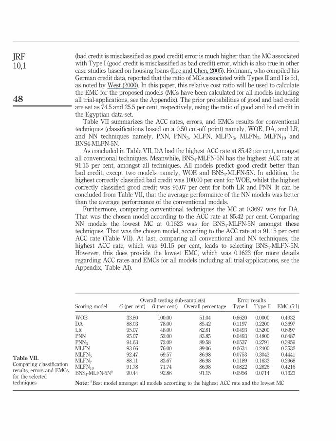
Table VII summarizes the ACC rates, errors, and EMCs results for conventionaltechniques (classifications based on a 0.50 cut-off point) namely, WOE, DA, and LR,and NN techniques namely, PNN, PNN3, MLFN, MLFN5, MLFN7, MLFN10 andBNS4-MLFN-5N.

As concluded in Table VII, DA had the highest ACC rate at 85.42 per cent, amongstall conventional techniques. Meanwhile, BNS4-MLFN-5N has the highest ACC rate at91.15 per cent, amongst all techniques. All models predict good credit better thanbad credit, except two models namely, WOE and BNS4-MLFN-5N. In addition, thehighest correctly classified bad credit was 100.00 per cent for WOE, whilst the highestcorrectly classified good credit was 95.07 per cent for both LR and PNN. It can beconcluded from Table VII, that the average performance of the NN models was betterthan the average performance of the conventional models.

Furthermore, comparing conventional techniques the MC at 0.3697 was for DA.That was the chosen model according to the ACC rate at 85.42 per cent. ComparingNN models the lowest MC at 0.1623 was for BNS4-MLFN-5N amongst thesetechniques. That was the chosen model, according to the ACC rate at a 91.15 per centACC rate (Table VII). At last, comparing all conventional and NN techniques, thehighest ACC rate, which was 91.15 per cent, leads to selecting BNS4-MLFN-5N.However, this does provide the lowest EMC, which was 0.1623 (for more detailsregarding ACC rates and EMCs for all models including all trial-applications, see theAppendix, Table AI).

Overall testing sub-sample(s) Error resultsScoring model G (per cent) B (per cent) Overall percentage Type I Type II EMC (5:1)

WOE 33.80 100.00 51.04 0.6620 0.0000 0.4932DA 88.03 78.00 85.42 0.1197 0.2200 0.3697LR 95.07 48.00 82.81 0.0493 0.5200 0.6997PNN 95.07 52.00 83.85 0.0493 0.4800 0.6487PNN3 94.63 72.09 89.58 0.0537 0.2791 0.3959MLFN 93.66 76.00 89.06 0.0634 0.2400 0.3532MLFN5 92.47 69.57 86.98 0.0753 0.3043 0.4441MLFN7 88.11 83.67 86.98 0.1189 0.1633 0.2968MLFN10 91.78 71.74 86.98 0.0822 0.2826 0.4216BNS4-MLFN-5Na 90.44 92.86 91.15 0.0956 0.0714 0.1623

Note: aBest model amongst all models according to the highest ACC rate and the lowest MC

Table VII.Comparing classificationresults, errors and EMCsfor the selectedtechniques

JRF10,1

48

Conclusions and directions for future researchCredit scoring is regarded as one of the effective management tools to reduce bothfinancial and operational risks facing banks. Furthermore, credit scoring is regarded asone of the basic applications of misclassification problems that have attractedmore-and-more attention during the past decades. This research presents an evaluationof personal loans to help strengthen the financial and operational risks evaluationprocess in the Egyptian banking sector using four credit scoring statistical techniques:WOE, DA, LR and NNs. The intention in this paper has been to investigate both theclassification efficiency rate of consumer loans and the cost effectiveness associatedwith misclassification errors.

The ranking of the models did not vary according to the decision criterion. Usingboth the highest ACC rate and the lowest EMC, BNS4-MLFN-5N is preferred.Correspondingly, it has been suggested that the ACC rate is more reliable, while theEMC calculated in this paper is more subjective. Some of the predictor variables havenot normally been used in published studies of credit-scoring models, for example:COR GUAR and LFOB. They are particularly appropriate within the Egyptianbanking sector.

Future studies should aim to use other advanced statistical scoring techniques, suchas genetic algorithms, besides the NNs and traditional scoring models which were usedin the current paper, and perhaps integrated with other techniques, such as fuzzyDA. Finally, future research would use more evaluation criteria such as, area underthe ROC.

References

Altman, E.I., Marco, G. and Varetto, F. (1994), “Corporate distress diagnosis: comparisons usinglinear discriminant analysis and neural networks (the Italian experience)”, Journal ofBanking & Finance, Vol. 18 No. 3, pp. 505-29.

Anderson, R. (2007), The Credit Scoring Toolkit: Theory and Practice for Retail Credit RiskManagement and Decision Automation, Oxford University Press, New York, NY.

Arminger, G., Enache, D. and Bonne, T. (1997), “Analyzing credit risk data: a comparison oflogistic discriminant, classification tree analysis, and feedforward networks”,Computational Statistics, Vol. 12 No. 2, pp. 293-310.

Bailey, M. (2001), Credit Scoring: The Principles and Practicalities, White Box Publishing, Bristol.

Banasik, J., Crook, J. and Thomas, L. (2003), “Sample selection bias in credit scoring models”,Journal of the Operational Research Society, Vol. 54 No. 8, pp. 822-32.

Bishop, C.M. (1995), Neural Networks for Pattern Recognition, Oxford University Press,New York, NY.

CBE (2006/2007), “Banking developments”, Economic Review, Vol. 47 No. 3, pp. 32-56.

CBE (2007/2008), “Structure of the Egyptian banking system”, Economic Review, Vol. 48 No. 3,p. 93.

Chen, M. and Huang, S. (2003), “Credit scoring and rejected instances reassigning throughevolutionary computation techniques”, Expert Systems with Applications, Vol. 24 No. 4,pp. 433-41.

Crook, J., Edelman, D. and Thomas, L. (2007), “Recent developments in consumer credit riskassessment”, European Journal of Operational Research, Vol. 183 No. 3, pp. 1447-65.

Alternativescoring models

49

Desai, V.S., Crook, J.N. and Overstreet, G.A. (1996), “A comparison of neural networks and linearscoring models in the credit union environment”, European Journal of OperationalResearch, Vol. 95 No. 1, pp. 24-37.

Desai, V.S., Conway, D.G., Crook, J.N. and Overstreet, G.A. (1997), “Credit scoring models in thecredit union environment using neural networks and genetic algorithms”, IMA Journal ofMathematics Applied in Business and Industry, Vol. 8 No. 4, pp. 323-3463.

Dimla, D.E. and Lister, P.M. (2000), “On-line metal cutting tool condition monitoring: II: tool-stateclassification using multi-layer perceptron neural networks”, International Journal ofMachine Tools & Manufacture, Vol. 40 No. 5, pp. 769-81.

Erbas, B. and Stefanou, S. (2008), “An application of neural networks in microeconomics:input-output mapping in a power generation subsector of the US electricity industry”,Expert Systems with Applications, Vol. 36 No. 2, pp. 2317-26.

Fisher, R.A. (1936), “The use of multiple measurements in taxonomic problems”, Annals ofEugenics, Vol. 7 No. 2, pp. 179-88.

Ganchev, T., Tasoulis, D., Varhatis, M. and Fakotakis, N. (2007), “Generalized locally recurrentprobabilistic neural network with application to text-independent speaker verification”,Neurocomputing, Vol. 70 Nos 7/9, pp. 1424-38.

Greene, W. (1998), “Sample selection in credit-scoring models”, Japan and the World Economy,Vol. 10 No. 3, pp. 299-316.

Hand, D.J. and Jacka, S.D. (1998), Statistics in Finance, Arnold Applications of Statistics, London.

Hand, D.J., Sohn, S.Y. and Kim, Y. (2005), “Optimal bipartite scorecards”, Expert Systems withApplications, Vol. 29 No. 3, pp. 684-90.

Lee, T. and Chen, I. (2005), “A two-stage hybrid credit scoring model using artificial neuralnetworks and multivariate adaptive regression splines”, Expert Systems with Applications,Vol. 28 No. 4, pp. 743-52.

Lee, T., Chiu, C., Lu, C. and Chen, I. (2002), “Credit scoring using the hybrid neural discriminanttechnique”, Expert Systems with Applications, Vol. 23 No. 3, pp. 245-54.

Liang, Q. (2003), “Corporate financial distress diagnosis in china: empirical analysis using creditscoring models”, Hitotsubashi Journal of Commerce and Management, Vol. 38 No. 1,pp. 13-28.

Malhotra, R. and Malhotra, D.K. (2003), “Evaluating consumer loans using neural networks”,Omega the International Journal of Management Science, Vol. 31 No. 2, pp. 83-96.

Masters, T. (1995), Advanced Algorithms for Neural Networks: ACþþ Sourcebook, Wiley,New York, NY.

Min, J.H. and Lee, Y-C. (2008), “A practical approach to credit scoring”, Expert Systems withApplications, Vol. 35 No. 4, pp. 1762-70.

Nur Ozkan-Gunay, E. and Ozkan, M. (2007), “Prediction of bank failures in emerging financialmarkets: an ANN approach”, Journal of Risk Finance, Vol. 8 No. 5, pp. 465-80.

Oldham, M. and Young, M. (2004), “Egypt: difficult times remains for the banking sector”,Special Report, FitchRatings, New York, NY.

Ong, C., Huang, J. and Tzeng, G. (2005), “Building credit scoring models using geneticprogramming”, Expert Systems with Applications, Vol. 29 No. 1, pp. 41-7.

Orgler, Y.E. (1971), “Evaluation of bank consumer loans with credit scoring models”, Journal ofBank Research, Vol. 2 No. 1, pp. 31-7.

Palisade Corporation (2005), Neural Tools: Neural Networks Add-in for Microsoft Excel,Version 1.0, Palisade Corporation, New York, NY.

JRF10,1

50

Reed, R.D. and Marks, R.J. (1999), Neural Smithing: Supervised Learning in FeedforwardArtificial Neural Networks, The MIT Press, London.

Sarlija, N., Bensic, M. and Bohacek, Z. (2004), “Multinomial model in consumer credit scoring”,paper presented at the 10th International Conference on Operational Research, Trogir.

Seow, H. and Thomas, L.C. (2006), “Using adaptive learning in credit scoring to estimate take-upprobability distribution”, European Journal of Operational Research, Vol. 173 No. 3,pp. 880-92.

Siddiqi, N. (2006), Credit Risk Scorecards: Developing and Implementing Intelligent Credit Scoring,Wiley, Hoboken, NJ.

Thomas, L.C., Edelman, D.B. and Crook, L.N. (2002), Credit Scoring and Its Applications, Societyfor Industrial and Applied Mathematics, Philadelphia, PA.

Tsai, C. and Wu, J. (2008), “Using neural network ensembles for bankruptcy prediction and creditscoring”, Expert Systems with Applications, Vol. 34 No. 4, pp. 2639-49.

West, D. (2000), “Neural network credit scoring models”, Computers & Operations Research,Vol. 27 Nos 11/12, pp. 1131-52.

Yu, L., Wang, S. and Lai, K. (2007), “An intelligent-agent-based fuzzy group decision makingmodel for financial multicriteria decision support: the case of credit scoring”, EuropeanJournal of Operational Research, July.

Zekic-Susac, M., Sarlija, N. and Bensic, M. (2004), “Small business credit scoring: a comparison oflogistic regression, neural networks, and decision tree models”, paper presented at the26th International Conference on Information Technology Interfaces, Dubrovnik.

Zhang, G., Hu, M.Y., Patuwo, B.E. and Indro, D.C. (1999), “Artificial neural networks inbankruptcy prediction: general framework and cross-validation analysis”, EuropeanJournal of Operational Research, Vol. 116 No. 1, pp. 16-32.

Zhang, Y. and Bhattacharyya, S. (2004), “Genetic programming in classifying large-scale data:an ensemble method”, Information Sciences, Vol. 163 Nos 1/3, pp. 85-101.

(The Appendix follows overleaf.)

Alternativescoring models

51

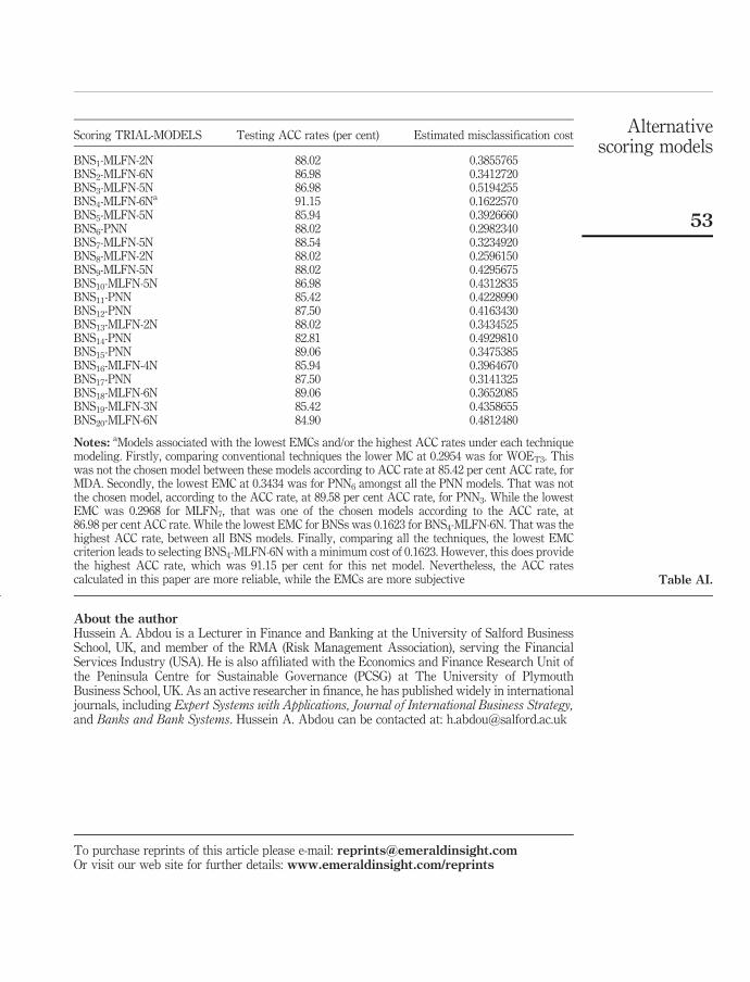
Appendix. ACC rates and EMCs for all the proposed models based on the testingresults

Scoring TRIAL-MODELS Testing ACC rates (per cent) Estimated misclassification cost

WOE 51.04 0.4931900WOET1 65.10 0.4527670WOET2 74.31 0.3810980WOET3

a 80.73 0.2954230MDAa 85.42 0.3696765LR 82.81 0.6997285PNN 83.85 0.6487285PNN1 84.38 0.5627485PNN2 80.21 0.5478655PNN3

a 89.58 0.3958590PNN4 84.38 0.4881895PNN5 87.50 0.3486675PNN6

a 85.94 0.3433690PNN7 86.46 0.4891580PNN8 83.85 0.4599020PNN9 85.94 0.5033080PNN10 83.85 0.4792355PNN11 83.33 0.5159050PNN12 84.38 0.5279940PNN13 85.42 0.5838990PNN14 86.46 0.4729960PNN15 83.33 0.5576850PNN16 81.25 0.3872680PNN17 83.85 0.4812070PNN18 82.29 0.4735590PNN19 82.29 0.6142950PNN20 85.42 0.5096840MLFN 89.06 0.3532330MLFN1 82.81 0.4055805MLFN2 84.38 0.3852480MLFN3 85.42 0.4709525MLFN4 83.33 0.4650425MLFN5

a 86.98 0.4440810MLFN6 82.29 0.4824780MLFN7

a 86.98 0.2967880MLFN8 77.08 0.6070260MLFN9 80.73 0.5028725MLFN10

a 86.98 0.4215540MLFN11 82.81 0.5376720MLFN12 83.85 0.3412575MLFN13 85.42 0.4506675MLFN14 82.81 0.3800235MLFN15 85.42 0.5422965MLFN16 86.46 0.5139520MLFN17 81.77 0.4934140MLFN18 78.65 0.6591290MLFN19 83.33 0.4435355MLFN20 86.46 0.4572215

(continued )Table AI.

JRF10,1

52

About the authorHussein A. Abdou is a Lecturer in Finance and Banking at the University of Salford BusinessSchool, UK, and member of the RMA (Risk Management Association), serving the FinancialServices Industry (USA). He is also affiliated with the Economics and Finance Research Unit ofthe Peninsula Centre for Sustainable Governance (PCSG) at The University of PlymouthBusiness School, UK. As an active researcher in finance, he has published widely in internationaljournals, including Expert Systems with Applications, Journal of International Business Strategy,and Banks and Bank Systems. Hussein A. Abdou can be contacted at: h.abdou@salford.ac.uk

Scoring TRIAL-MODELS Testing ACC rates (per cent) Estimated misclassification cost

BNS1-MLFN-2N 88.02 0.3855765BNS2-MLFN-6N 86.98 0.3412720BNS3-MLFN-5N 86.98 0.5194255BNS4-MLFN-6Na 91.15 0.1622570BNS5-MLFN-5N 85.94 0.3926660BNS6-PNN 88.02 0.2982340BNS7-MLFN-5N 88.54 0.3234920BNS8-MLFN-2N 88.02 0.2596150BNS9-MLFN-5N 88.02 0.4295675BNS10-MLFN-5N 86.98 0.4312835BNS11-PNN 85.42 0.4228990BNS12-PNN 87.50 0.4163430BNS13-MLFN-2N 88.02 0.3434525BNS14-PNN 82.81 0.4929810BNS15-PNN 89.06 0.3475385BNS16-MLFN-4N 85.94 0.3964670BNS17-PNN 87.50 0.3141325BNS18-MLFN-6N 89.06 0.3652085BNS19-MLFN-3N 85.42 0.4358655BNS20-MLFN-6N 84.90 0.4812480

Notes: aModels associated with the lowest EMCs and/or the highest ACC rates under each techniquemodeling. Firstly, comparing conventional techniques the lower MC at 0.2954 was for WOET3. Thiswas not the chosen model between these models according to ACC rate at 85.42 per cent ACC rate, forMDA. Secondly, the lowest EMC at 0.3434 was for PNN6 amongst all the PNN models. That was notthe chosen model, according to the ACC rate, at 89.58 per cent ACC rate, for PNN3. While the lowestEMC was 0.2968 for MLFN7, that was one of the chosen models according to the ACC rate, at86.98 per cent ACC rate. While the lowest EMC for BNSs was 0.1623 for BNS4-MLFN-6N. That was thehighest ACC rate, between all BNS models. Finally, comparing all the techniques, the lowest EMCcriterion leads to selecting BNS4-MLFN-6N with a minimum cost of 0.1623. However, this does providethe highest ACC rate, which was 91.15 per cent for this net model. Nevertheless, the ACC ratescalculated in this paper are more reliable, while the EMCs are more subjective Table AI.

Alternativescoring models

53

To purchase reprints of this article please e-mail: reprints@emeraldinsight.comOr visit our web site for further details: www.emeraldinsight.com/reprints