Estuaries Vol. 20, No. 1, p. 149-158 March 1997

An Estuarine Benthic Index of

Biotic Integrity (B-IBI) for

Chesapeake Bay

STEPHEN B. WEISBER@ LINDA C. SCIIAPPNER J. ANANDA RANASINGHE ROBERT J. DIAL V&al; Inc. School of Marine Science 9200 Rumsey Road The College of William and Mary Columbia, Maryland 21045 Gloucester Point, Virginia 23062

DANIEL M. DAUER JEFFREY B. FRITHSEN Department of Biological Sciences Versar; Inc. Old Dominion University 9200 Rumsey Road Norfolk, Virginia 23529 Columbia, Maryland 21045

AJBTRACT: A multbnetric benthic index of biotic integrity (B-IBI) was developed using data from five Chesapeake Bay sampling programs conducted between 1972 and 1991. Attributes of the index were selected by comparing the response of 17 candidate measures of bentbic condition (metrics) between a set of miniially affected reference sites and at all other sites for which data were available. This procedure was conducted independently for each of seven habitats defined by salinity and substrate. Fifteen of the 17 candidate metics differed significantly between reference sites and other sites for at least one habitat. No metric differed significantly in all seven habitats, however, four metrics, species diversity, abundance, biomass, and percent of abundance as pollution-indicative taxa, differed in six habitats. The index was calculated by scoring each selected metric as 5, 3, or 1 depending on whether its value at a site approx- imated, deviated slightly from, or deviated greatly from conditions at the best reference sites. Validation based on independent data collected between 1992 and 1994 indicated that tbe index correctly distinguished stressed sites from reference sites 93% of the time, with the highest validation rates occurring in high salmity habitats.

Introduction Benthic invertebrates are used extensively as in-

dicators of estuarine environmental status and trends because numerous studies have demonstrat- ed that benthos respond predictably to many kinds of natural and anthropogenic stress (Pearson and Rosenberg 1978; Dauer 1993; Tapp et al. 1993; Wil- son and Jeffrey 1994). Many characteristics of ben- thic assemblages make them useful indicators (Bil- yard 1987), the most important of which are relat- ed to their exposure to stress and the diversity of their response. Exposure to hypoxia is typically greatest in near-bottom waters and anthropogenic contaminants often accumulate in sediments where benthos live. Benthic organisms generally have limited mobility and cannot avoid these ad- verse conditions (Wass 1967). This immobility is advantageous in environmental assessments be-

1 Corresponding author. 2Present address: Southern California Coastal Water Re-

search Program, 7171 Fenwick Lane, Westminster, California 92683; tele 714/8942222; fax 714/8949699; e-mail stevew@ sccwrp.org.

0 1997 Estuarine Research Federation 149

cause, unlike most pelagic fauna, benthic assem- blages reflect local environmental conditions (Gray 1979). The structure of benthic assemblages responds to many kinds of stress because these as- semblages typically include organisms with a wide range of physiological tolerances, feeding modes, and trophic interactions (Pearson and Rosenberg 1978; Rhoads et al. 1978; Boesch and Rosenberg 1981).

Although descriptions of benthic assemblages have been useful for characterizing environmental conditions and gradients at local scales, benthic as- semblages have not yet been used to their full po- tential as indicators in regional-scale studies or studies of entire estuaries because the structure of benthic assemblages also reflects natural variation related to salinity, sediment type, latitude, and depth (Boesch 1973, 1977; Dauer et al. 1984,1987; Holland et al. 1987; Schaffner et al. 1987; Snel- grove and Butman 1994; Heip and Craeymeersch 1995). Benthic assemblages rarely are used to as- sess ecological condition across habitats because of the difficulty in separating variation in the condi- tion of the assemblage caused by habitat differ-

This single electronic copy was made for your private study or research within the Auckland Regional Council. It is not to be redistributed. The Copyright Act 1994 prohibits the sale, letting for hire or copying of this work.

150 S. B. Weisberg et al.

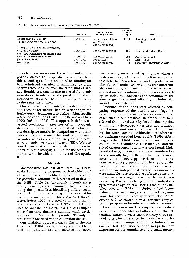
TABLE 1. Data sources used in developing the Chesapeake Bay EIBI.

Data Source Time Period Sampling Gear and Summer Sampling Area (m’) Samclles References

Chesapeake Bay Benthic Monitoring Program, Maryland

Chesapeake Bay Benthic Monitoring Program, Virginia EPA’s Environmental Monitoring and Assessment Program (EMAP) James River Study Wolf Trap

1984-1994

1985-1994

1990-1993 1971-1972 1987-1991

Petite Ponar (0.025) Van Veen (0.1) Box Corer (0.022)

Box Corer (0.0184)

Van Veen (0.044) Ponar (0.05) Box Corer (0.063)

1,814 Ranasinghe et al. (1994a)

180 Dauer and Alden (1995)

293 Paul et al. (1992) 28 Diaz (1989)

4 Schaffner (unpublished data)

ences from variation caused by natural and anthro- pogenic stresses. In site-specific assessments of ben- thic assemblages, the problem of accounting for habitat-induced variation is minimized by using nearby reference sites from the same kind of hab- itat. Benthic assessments also are used frequently in studies of trends, where the problem of habitat- induced variation can be minimized by returning to the same site or area.

One approach used to integrate biotic responses and account for natural habitat variations in the freshwater environment is to define habitat-specific reference conditions (Karr 1991; Kerans and Karr 1994; DeShon 1995). This approach defines ex- pected conditions at sites free of anthropogenic stress, and then assigns categorical values for vari- ous descriptive metrics by comparison with obser- vations at reference sites. The result is a multi-met- ric index of biotic condition, frequently referred to as an index of biotic integrity (IBI). We bor- rowed from that approach to develop a benthic index of biotic integrity (B-IBI) for use with sum- mer estuarine benthic communities of Chesapeake Bay.

Methods Macrobenthic infaunal data from five Chesa-

peake Bay sampling programs, each of which used a 0.5-mm sieve and identified organisms to the low- est possible taxonomic level, were used to develop the B-IBI (Table 1). Taxonomic inconsistencies among programs were eliminated by cross-corre- lating the species lists, identifying differences in nomenclature, and consulting the taxonomist for each program to resolve discrepancies. Data col- lected before 1992 were used to calibrate the in- dex; data collected between 1992 and 1994 were used to validate the index. If a site was sampled more than once during a summer, which we de- fined as July 15 through September 30, only the first sample was used in the calibration dataset.

Our analytical approach was similar to the one Karr et al. (1986) used to develop comparable in- dices for freshwater fish and involved four activi-

ties: selecting measures of benthic macroinverte- brate assemblages (referred to by Karr as metrics) that differ between references and degraded areas; identifying quantitative thresholds that differenti- ate between degraded and reference areas for each selected metric; combining metric scores to devel- op an index that identifies the condition of the assemblage at a site; and validating the index with an independent dataset.

Attributes of the index were selected by com- paring response of the benthic assemblage be- tween minimally affected reference sites and all other sites in our database. Reference sites were selected from our dataset by first eliminating sites within highly developed watersheds and locations near known point-source discharges. The remain- ing sites were examined to identify those where no contaminant exceeded Long et al.‘s (1995) effects range-median (ER-M) concentration, total organic content of the sediment was less than 2%, and dis- solved oxygen concentration was consistently high. Dissolved oxygen concentration was considered to be consistently high if the site had no recorded measurement below 2 ppm, 90% of the observa- tions were above 3 ppm, and at least 80% of the measurements were above 5 ppm. Sites for which less than five independent oxygen measurements were available were selected as reference sites only if they were in a region classified by the Chesa- peake Bay Program as being free of dissolved ox- ygen stress (Magnien et al. 1995). One of the sam- pling programs (EMAP) included a 10-d, acute sediment bioassay using the amphipod Ampelisca abdita for each site. Bioassay survival also had to exceed 80% of control survival for sites sampled by this program to be selected as reference sites.

Two criteria were used to compare metric values between reference sites and other sites in the cal- ibration dataset. First, a Mann-Whitney U-test was used to test for differences in mean. Second, dis- tributions were compared using a Kolmogorov- Smirnov test. The latter criterion was particularly important for the abundance and biomass metrics

Benthic lndexforchesapeake Bay 151

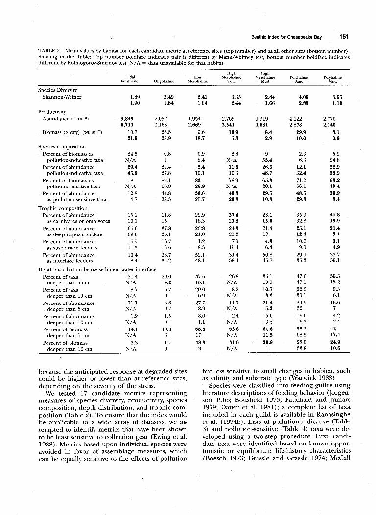
TABLE 2. Mean values by habitat for each candidate metric at reference sites (top number) and at all other sites (bottom number). Shading in the Table: Top number boldface indicates pair is different by Mann-Whitney test; bottom number boldface indicates different by Kolmogorov-Smirnov test. N/A = data unavailable for that habitat.

Tidal Freshwater Oligohaline

LOW Mesohaline

High Mesohzdine

High Mesohaline

Sand Mud Polyhaline Polyhaline

Sand Mud

Species Diversity Shannon-Weiner 1.89 2.49

1.90 1.84

Productivity Abundance (# me2) 3,849 2,052

6,713 3,163 Biomass (g dry) (wt m-*) 10.7 26.5

21.9 28.9

Species composition Percent of biomass as 24.5 0.8

pollution-indicative taxa N/A 1 Percent of abundance 29.4 22.4

pollution-indicative taxa 45.9 27.8 Percent of biomass as 18 89.1

pollution-sensitive taxa N/A 66.9 Percent of abundance 12.8 44.8

as pollution-sensitive taxa 4.7 28.3

Trophic composition Percent of abundance 15.1 11.8

as carnivores or omnivores 10.1 15 Percent of abundance 66.6 37.8

as deep deposit feeders 69.6 35.1 Percent of abundance 6.5 16.7

as suspension feeders 11.3 13.6 Percent of abundance 10.4 33.7

as interface feeders 8.4 35.2

Depth distribution below sediment-water interface Percent of taxa 31.4 20.0

deeper than 5 cm N/A 4.2 Percent of taxa 8.7 6.7

deeper than 10 cm N/A 0 Percent of abundance 11.1 8.6

deeper than 5 cm N/A 0.7 Percent of abundance 1.9 1.5

deeper than 10 cm N/A 0 Percent of biomass 14.1 10.0

deeper than 5 cm N/A 3 Percent of biomass 3.3 1.7

deeper than 10 cm N/A 0

2.41 3.35 2.84 4.06 3.55 1.84 2.44 1.66 2.88 1.10

1,954 2,765 1,319 4,122 2,770 2,669 3,541 1,681 2,878 2,140

9.6 19.9 8.4 29.9 8.1 18.7 5.8 2.9 10.0 0.9

0.9 2.8 9 2.3 5.9 8.4 N/A 55.4 6.3 24.8 2.4 11.6 26.5 12.1 22.9

19.1 19.3 48.7 32.4 58.9 83 78.9 65.3 71.2 63.2 26.9 N/A 20.1 66.1 40.4 30.6 40.3 29.5 48.5 39.9 25.7 20.8 10.3 29.3 8.4

22.9 37.4 23.1 35.3 41.8 18.3 23.8 15.6 32.8 19.9 23.8 24.3 21.4 25.1 21.4 21.8 21.3 18 12.4 9.4

1.2 7.0 4.8 10.6 3.1 8.3 15.4 6.4 9.0 4.9

52.1 31.4 50.8 29.0 33.7 48.1 39.4 46.7 35.3 39.1

37.6 26.8 35.1 47.6 35.5 18.1 N/A 19.9 47.1 15.2 20.0 8.2 10.7 22.0 9.3

6.9 N/A 3.3 30.1 6.1 27.7 11.7 21.4 34.9 16.6

8.9 N/A 5.2 32 7 8.0 2.4 5.6 16.6 4.2 1.1 N/A 0.8 16.3 2.4

68.8 63.6 61.6 58.3 42 17 N/A 11.5 68.5 17.4 48.3 31.6 29.9 28.5 24.9

3 N/A 1 33.8 10.6

because the anticipated response at degraded sites could be higher or lower than at reference sites, depending on the severity of the stress.

We tested 17 candidate metrics representing measures of species diversity, productivity, species composition, depth distribution, and trophic com- position (Table 2). To ensure that the index would be applicable to a wide array of datasets, we at- tempted to identify metrics that have been shown to be least sensitive to collection gear (Ewing et al. 1988). Metrics based upon individual species were avoided in favor of assemblage measures, which can be equally sensitive to the effects of pollution

but less sensitive to small changes in habitat, such as salinity and substrate type (Warwick 1988).

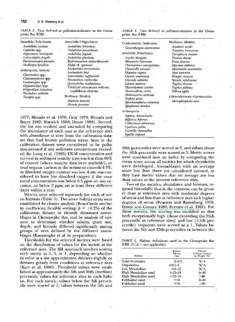
Species were classified into feeding guilds using literature descriptions of feeding behavior (Jorgen- sen 1966; Bousfield 1973; Fauchald and Jumars 1979; Dauer et al. 1981); a complete list of taxa included in each guild is available in Ranasinghe et al. (1994b). Lists of pollution-indicative (Table 3) and pollution-sensitive (Table 4) taxa were de- veloped using a two-step procedure. First, candi- date taxa were identified based on known oppor- tunistic or equilibrium life-history characteristics (Boesch 1973; Grassle and Grassle 1974; McCall

152 S. B. Weisberg et al.

TABLE 3. Taxa defined as pollution-indicative in the Chesa- peake Bay B-IBI.

Annelida : Polychaeta Asabellides oculata Capitella spp. Hypereteone heteropoda Leitoscolqplossragilis Parapionospio pinnata Streblosfiio benedicti

Arthropoda : Insecta Chironomus spp. Cladotanytarsus spp. Coelotanypus spp. Glyptotendipes spp. Polypedilum tripodura Procladius sublet&i Tanypus spp.

Atmelida : Oligochaeta Aulodtilus limnobius Aulodrilus paucichaeta Aulodrilus pigueti Aulodtilus pluriseta Bothrionewum vejdovskyanum Haber cf. sfieciosus Isochaetidei curvosetosus Isochaetides freyi Limnodrilus hoffmeistti Potamothrix vejdovskyi Quistadrilus multisetosus Tubificid immatures without

capilliform chaetae

Mollusca : Bivalvia Mulinia lateralis Nucula proxima

1977; Rhoads et al. 1978; Gray 1979; Rhoads and Boyer 1982; Warwick 1986; Dauer 1993). Second, the list was verified and amended by comparing the abundance of each taxa at the reference sites with abundance at sites from the calibration data- set that had known pollution stress. Sites in the calibration dataset were considered to be pollu- tion-stressed if any sediment contaminant exceed- ed the Long et al. (1995) ER-M concentration and survival in sediment toxicity tests was less than 80% of control (where toxicity data were available), or total organic carbon in the sediment exceeded 3%, or dissolved oxygen content was low. A site was con- sidered to have low dissolved oxygen if the mea- sured concentration was below 0.5 ppm on any oc- casion, or below 2 ppm on at least three different dates within a year.

Metrics were selected separately for each of sev- en habitats (Table 5). The seven habitat strata were established by cluster analysis (Bray-Curtis similar- ity coefficient; flexible sorting; B = -0.25) of the calibration dataset to identify dominant assem- blages in Chesapeake Bay, and by analysis of vari- ance to determine whether salinity, grain size, depth, and latitude differed significantly among groups of sites defined by the different assem- blages (Ranasinghe et al. in preparation).

Thresholds for the selected metrics were based on the distribution of values for the metric at the reference sites. The IBI approach involves scoring each metric as 5, 3, or 1, depending on whether its value at a site approximates, deviates slightly, or deviates greatly from conditions at reference sites (Karr et al. 1986). Threshold values were estab- lished as approximately the 5th and 50th (median) percentile values for reference sites in each habi- tat. For each metric, values below the 5th percen- tile were scored as 1; values between the 5th and

TABLE 4. Taxa defined as pollution-sensitive in the Chesa- peake Bay B-IBI.

Coelenterata : Anthozoa Ceriantheopsis americanus

Aunelida : Polychaeta Asychis elongata Bhawania heteroseta Chaetoptemcs variopedatus Clymenella toruata Diopatra cupea Glycera americana Glycinde solitatia Loimia medusa Macroclymene zonalis Marenzelleria virdis Mediomastus ambiseta Nqhtys picta Spiochaetopterus costarurn Spiophanes bombyx

Arthropoda A1phe-w heterochaelis Biffan’us hfwmis Callianassa setimanus Cyathura polita Listriella clymenellae Squilla emjrusa

Mollusca : Bivalvia Anadara ovalis Anadara transversa CyrtOpleura costata Dosinia discus Ensis directus Macoma balthica Mercenaria mercenaria Mya arenatia Rangia cuneata Spisula solidissima Tagelus divisus Tageus plebeius Tellina agilis

Echinodermata: Ophiuroidea Microphiopholis atra

50th percentiles were scored as 3, and values above the 50th percentile were scored as 5. Metric scores were combined into an index by computing the mean score across all metrics for which thresholds were developed. Assemblages with an average score less than three are considered stressed, as they have metric values that on average are less than values at the poorest reference sites.

Two of the metrics, abundance and biomass, re- spond bimodally; that is, the response can be great- er than at reference sites with moderate degrees of stress and less than at reference sites with higher degrees of stress (Pearson and Rosenberg 1978; Dauer and Conner 1980; Ferraro et al. 1991). For these metrics, the scoring was modified so that both exceptionally high (those exceeding the 95th percentile at reference sites) and low (<5th per- centile) responses were scored as a 1. Values be- tween the 5th and 25th percentiles or between the

TABLE 5. Habitat definitions used in the Chesapeake Bay RIB1 (N/A = not applicable).

Habitat

Silt-clay (<63 p) Content

by Weight (%)

Tidal freshwater Oligohaline Low Mesohaline High Mesohaline sand High Mesohaline mud Polyhaline sand Polvhaline mud

o-o.5 N/A 20.5-5 N/A

~5-12 N/A 212-18 O-40 212-18 >40

~18 O-40 218 >40

Benthic Index for Chesapeake Bay 153

75th and 95th percentiles were scored as 3, and values between the 25th and 75th percentiles of the values at reference sites were scored as 5.

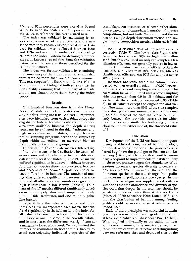
The index was validated by examining its re- sponse at a new set of reference sites and a new set of sites with known environmental stress. Data used for validation were collected between 1992 and 1994 and were independent of data used to calibrate the index. Criteria for defining reference sites and known stressed sites from the validation dataset were the same as those described for the calibration dataset.

The index was further validated by examining the consistency of the index response at sites that were sampled more than once during a summer. This test, suggested by Stewart and Loar (1994) as a prerequisite for biological indices, examines in- dex stability assuming that the quality of the site should not change appreciably during the index period.

Results One hundred fourteen sites from the Chesa-

peake Bay database met our criteria as reference sites for developing the B-IBI. At least 10 reference sites were identified from each habitat except the oligohaline habitat, for which only seven reference sites were available. Biomass and depth metrics could not be evaluated in the tidal freshwater and high mesohaline sand habitats, though, because not all sampling programs partitioned samples by depth within the sediment or measured biomass individually by taxonomic groups.

Fifteen of the 17 candidate metrics differed sig- nificantly in mean or in distribution between ref- erence sites and all other sites in the calibration dataset for at least one habitat (Table 2). No metric differed significantly in all seven habitats; however, four metrics, species diversity, abundance, biomass and percent of abundance as pollution-indicative taxa, differed in six habitats. The number of met- rics that differed significantly between reference sites and all other sites was considerably greater in high salinity than in low salinity (Table 2). Four- teen of the 17 metrics differed significantly at ref- erence sites in polyhaline mud compared with only three in tidal freshwater, and one in the oligoha- line habitat.

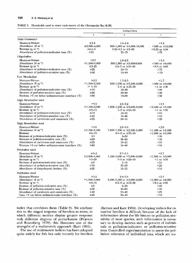
Table 6 lists the selected metrics and their thresholds. We incorporated each metric that dif- fered significantly in six habitats into the index for all habitats because in each case the direction of the response was the same in the seventh habitat and in most cases the difference was significant at a marginally lower alpha level. We also limited the number of redundant metrics within a habitat to avoid over-weighting individual properties of the

assemblage. For instance, we selected either abun- dance-based or biomass-based metrics of species composition, but not both. We also limited the in- dex to a single depth-distribution metric, and sin- gle trophic composition metric, within each habi- tat.

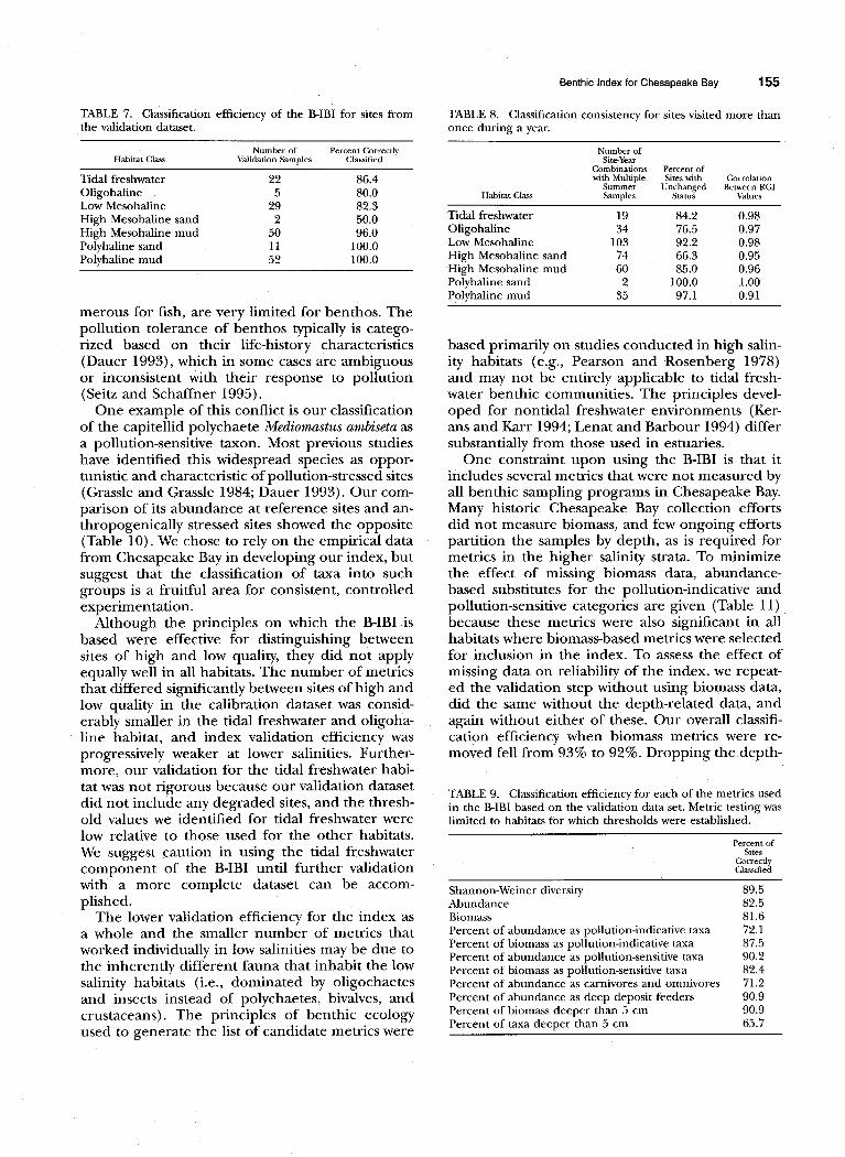
The B-IBI classified 93% of the validation sites correctly (Table 7). The lowest classification effi- ciency by habitat was 50% in high mesohaline sand, but this was based on only two samples. Clas- sification efficiency was generally poorer in low sa- linities. Cumulative classification efficiency for hab- itats with salinity less than 18%0 was 84%, whereas classification efficiency was 97% for salinities above 18%0 (Table 7).

The index was stable within the summer index period, with an overall correlation of 0.97 between the first and second sampling visits to a site. The correlation between the first and second sampling visits was greater than 0.9 in all habitats, and for six habitats the correlation exceeded 0.95 (Table 8). In all habitats except the oligohaline and me- sohaline sand, more than 80% of the sites sampled twice during the same summer classified the same (Table 8). Most of the sites that classified differ- ently between the two visits were sites for which index values were similar for both visits but were close to, and on either side of, the threshold value of 3.

Discussion Development of the B-IBI was based upon quan-

tifying established principles of benthic ecology, not on developing new ones. The principles were based largely on the paradigm of Pearson and Ro- senberg (1978)) which holds that benthic assem- blages respond to improvements in habitat quality in three progressive stages: the abundance of or- ganisms increases; species diversity increases as new taxa are able to survive at the site; and the dominant species at the site change from pollu- tion-tolerant to pollution-sensitive species. In our work, this paradigm was supplemented with as- sumptions that the abundance and diversity of spe- cies occurring deeper in the sediment should be greater at reference sites than at degraded sites (Warwick 1986; Schaffner 1990; Dauer 1993) and that the distribution of benthos among feeding guilds should be more diverse at reference sites (Word 1978).

Each of these principles was successful at distin- guishing reference sites from degraded sites within at least some habitats of Chesapeake Bay (Table 2). When applied individually to the validation data- set, however, none of the metrics derived from these principles were as effective at distinguishing between reference sites and degraded sites as the

154 S. B. Weisberg et al.

TABLE 6. Thresholds used to score each metric of the Chesapeake Bay B-IBI.

Scoring Criteria

5 3 1

Tidal Freshwater Shannon-Weiner Abundance (# m-2) Biomass (g rnm2) Abundance of pollution-indicative taxa (%)

Oligohaline Shannon-Weiner Abundance (# m-*) Biomass (g mm*) Abundance of pollution-indicative taxa (%) Abundance of pollution-sensitive taxa (%)

Low Mesohaline Shannon-Weiner Abundance (# m-*) Biomass (g m-2) Abundance of pollution-indicative taxa (%) Biomass of pollution-sensitive taxa (%) Biomass >5 cm below sediment-water interface (%)

High Mesohaline sand Shannon-Weiner Abundance (# rne2) Biomass (g m-*) Abundance of pollution-indicative taxa (%) Abundance of pollution-sensitive taxa (%) Abundance of carnivores and omnivores (%)

High Mesohaline mud Shannon-Weiner Abundance (# m-*) Biomass Biomass of pollution-indicative taxa (% ) Biomass of pollution-sensitive taxa (%) Abundance of carnivores and omnivores (%) Biomass >5 cm below sediment-water interface (%)

Polyhaline sand Shannon-Weiner Abundance (# m-*) Biomass (g m-*) Biomass of pollution-indicative taxa (%) Abundance of pollution-sensitive taxa (%) Abundance of deep-deposit feeders (%)

Polyhaline mud Shannon-Weiner Abundance (# rnm2) Biomass (g m-2) Biomass of pollution-indicative taxa (%) Biomass of pollution-sensitive taxa (Or,) Abundance of carnivores and omnivores (%) Taxa >5 cm below sediment-water interface (%)

21.8 ~1,000-4,000

20.5-3 525

~2.5 1.9-2.5 <1.9 21,500-3,000 500-1,500 or ?3,000-8,000 <500 or ?8,000

23-25 0.5-3 or 225-60 CO.5 or ~60 525 25-75 >75 240 10-40 <lo

22.5 1.7-2.5 ?1,500-2,500 500-1,500 or ?2,500-6,000

2 5-10 l-5 or ZlO-30 510 10-20 280 40-80 280 10-80

~3.2 2.5-3.2 <2.5 ?1,500-3,000 l,OOO-1,500 or ?3,000-5,000 <l,OOO or Z5,OOO

23-15 l-3 or 215-50 <1 or 250 510 lo-25 >25 240 1 O-40 <lo 235 20-35 <20

23.0 2.0-3.0 ?1,500-2,500 l,OOO-1,500 or ?2,500-5,000

22-10 0.5-2 or ~10-50 55 5-30

260 30-60 525 lo-25 260 lo-60

23-5 2.7-3.5 <2.7 ?3,000-5,000 1,500-3,000 or ?5,000-8,000 cl,500 or 28,000

25-20 l-5 or 220-50 <I or 250 =5 5-15 >15

250 25-50 <25 225 10-25 <IO

23.3 2.4-3.3 <2.4 ?1,500-3,000 l,OOO-1,500 or ?3,000-8,000 <l,OOO or Z8,OOO

23-10 0.5-3 or ZlO-30 CO.5 or 230 55 5-20 >20

260 30-60 <30 240 25-40 <25 240 1040 <lo

1.0-1.8 Cl.0 500-1,000 or S4,000-10,000 <500 or 210,000

0.25-0.5 or 23-50 CO.25 or 250 25-75 >75

Cl.7 <500 or 26,000

<l or 230 >20 <40 <lo

<2.0 <l,OOO or 25,000 <l,OOO or Z5,OOO

>30 <30 <lo <lo

index that combines them (Table 9). We attribute this to the staged response of benthos to stress, in which different metrics display greater response with different degrees of perturbation (Pearson and Rosenberg 1978); this illustrates one of the strengths of a multimetric approach (Karr 1991).

The use of multimetric indices has been adopted quite widely for fish but only recently for benthos

(Kerans and Karr 1994). Developing indices for es- tuarine benthos is difficult because of the lack of information about the life history or pollution sen- sitivity of most species; such information is neces- sary to develop metrics such as percent of individ- uals as pollution-indicative or pollution-sensitive taxa. Controlled experimentation to assess the pol- lution tolerance of individual taxa, which are nu-

Benthic index for Chesapeake Bay 155

TABLE 7. Classification efficiency of the B-IBI for sites from the validation dataset.

Habitat Class Number of

Validation Samples Percent Correctly

Classified

Tidal freshwater 22 86.4 Oligohaline 5 80.0 Low Mesohaline 29 82.3 High Mesohaline sand 2 50.0 High Mesohaline mud 50 96.0 Polyhaline sand 11 100.0 Polyhaline mud 52 100.0

merous for fish, are very limited for benthos. The pollution tolerance of benthos typically is catego- rized based on their life-history characteristics (Dauer 1993), which in some cases are ambiguous or inconsistent with their response to pollution (Seitz and Schaffner 1995).

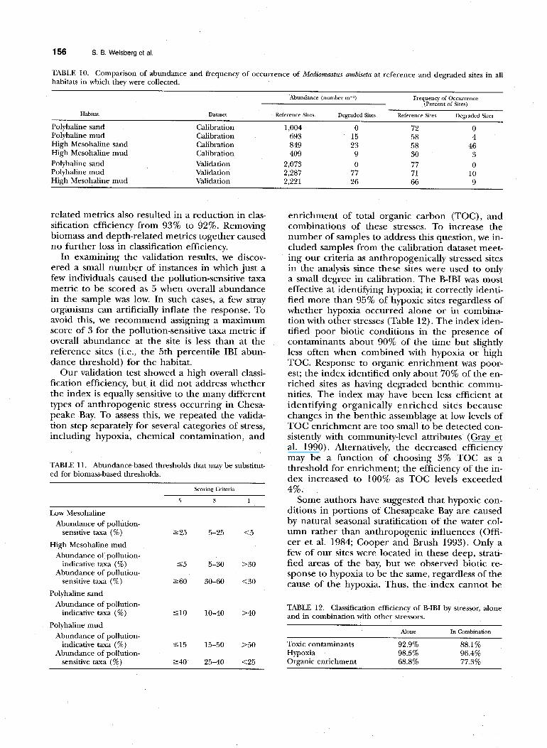
One example of this conflict is our classification of the capitellid polychaete Mediomastus am&eta as a pollution-sensitive taxon. Most previous studies have identified this widespread species as oppor- tunistic and characteristic of pollution-stressed sites (Grassle and Grassle 1984; Dauer 1993). Our com- parison of its abundance at reference sites and an- thropogenically stressed sites showed the opposite (Table 10). We chose to rely on the empirical data from Chesapeake Bay in developing our index, but suggest that the classification of taxa into such groups is a fruitful area for consistent, controlled experimentation.

Although the principles on which the B-IBI is based were effective for distinguishing between sites of high and low quality, they did not apply equally well in all habitats. The number of metrics that differed significantly between sites of high and low quality in the calibration dataset was consid- erably smaller in the tidal freshwater and oligoha- line habitat, and index validation efficiency was progressively weaker at lower salinities. Further- more, our validation for the tidal freshwater habi- tat was not rigorous because our validation dataset did not include any degraded sites, and the thresh- old values we identified for tidal freshwater were low relative to those used for the other habitats. We suggest caution in using the tidal freshwater component of the B-IBI until further validation with a more complete dataset can be accom- plished.

The lower validation efficiency for the index as a whole and the smaller number of metrics that worked individually in low salinities may be due to the inherently different fauna that inhabit the low salinity habitats (i.e., dominated by oligochaetes and insects instead of polychaetes, bivalves, and crustaceans). The principles of benthic ecology used to generate the list of candidate metrics were

TABLE 8. Classification consistency for sites visited more than once during a year.

Habitat Class

Number of Site-Year

Combinations Percent of with Multiple Sites with C0rr&ti0n

Summer Unchanged Between RGI Samples StatUS V.3llles

Tidal freshwater 19 84.2 0.98 Oligohaline 34 76.5 0.97 Low Mesohaline 103 92.2 0.98 High Mesohaline sand 74 66.3 0.95 High Mesohaline mud 60 85.0 0.96 Polyhaline sand 2 100.0 1.00 Polvhaline mud 35 97.1 0.91

based primarily on studies conducted in high salin- ity habitats (e.g., Pearson and Rosenberg 19’78) and may not be entirely applicable to tidal fresh- water benthic communities. The principles devel- oped for nontidal freshwater environments (Ker- ans and Karr 1994; Lenat and Barbour 1994) differ substantially from those used in estuaries.

One constraint upon using the B-IBI is that it includes several metrics that were not measured by all benthic sampling programs in Chesapeake Bay. Many historic Chesapeake Bay collection efforts did not measure biomass, and few ongoing efforts partition the samples by depth, as is required for metrics in the higher salinity strata. To minimize the effect of missing biomass data, abundance- based substitutes for the pollution-indicative and pollution-sensitive categories are given (Table 11) because these metrics were also significant in all habitats where biomass-based metrics were selected for inclusion in the index. To assess the effect of missing data on reliability of the index, we repeat- ed the validation step without using biomass data, did the same without the depth-related data, and again without either of these. Our overall classifi- cation efficiency when biomass metrics were re- moved fell from 93% to 92%. Dropping the depth-

TABLE 9. Classification efficiency for each of the metrics used in the RIB1 based on the validation data set. Metric testing was limited to habitats for which thresholds were established.

Percent of Sites

Correcdy Classified

Shannon-Weiner diversity Abundance Biomass Percent of abundance as pollution-indicative taxa Percent of biomass as pollution-indicative taxa Percent of abundance as pollution-sensitive taxa Percent of biomass as pollution-sensitive taxa Percent of abundance as carnivores and omnivores Percent of abundance as deep deposit feeders Percent of biomass deeper than 5 cm Percent of taxa deeper than 5 cm

89.5 82.5 81.6 72.1 87.5 90.2 82.4 71.2 90.9 90.9 65.7

156 S. B. Weisberg et al.

TABLE 10. Comparison of abundance and frequency of occurrence of Mediomastus ambiseta at reference and degraded sites in all habitats in which they were collected.

Abundance (number m-‘) Frequency of Occurrence (Percent of Sites)

Habitat D&lS.% Reference Sites Degraded Sites Reference Sites Degraded Sites

Polyhaline sand Calibration 1,004 0 72 0 Polyhaline mud Calibration 693 15 58 4 High Mesohaline sand Calibration 849 23 58 46 High Mesohaline mud Calibration 409 9 30 3

Polyhaline sand Validation 2,073 0 77 0 Polyhaline mud Validation 2,287 77 71 10 High Mesohaline mud Validation 2,221 26 66 9

related metrics also resulted in a reduction in clas- sification efficiency from 93% to 92%. Removing biomass and depth-related metrics together caused no further loss in classification efficiency.

In examining the validation results, we discov- ered a small number of instances in which just a few individuals caused the pollution-sensitive taxa metric to be scored as 5 when overall abundance in the sample was low. In such cases, a few stray organisms can artificially inflate the response. To avoid this, we recommend assigning a maximum score of 3 for the pollution-sensitive taxa metric if overall abundance at the site is less than at the reference sites (i.e., the 5th percentile IBI abun- dance threshold) for the habitat.

Our validation test showed a high overall classi- fication efficiency, but it did not address whether the index is equally sensitive to the many different types of anthropogenic stress occurring in Chesa- peake Bay. To assess this, we repeated the valida- tion step separately for several categories of stress, including hypoxia, chemical contamination, and

TABLE 11. Abundance-based thresholds that may be substitut- ed for biomass-based thresholds.

Low Mesohaline Abundance of pollution-

sensitive taxa (%)

High Mesohaline mud Abundance of pollution-

indicative taxa (%) Abundance of pollution-

sensitive taxa (%)

Polyhaline sand Abundance of pollution-

indicative taxa (%)

Polyhaline mud Abundance of pollution-

indicative taxa (%) Abundance of pollution-

sensitive taxa (%)

Scoring Criteria

5 3 1

225 5-25 <5

55 5-30 >30

260 30-60 <30

510 10-40 >40

515 15-50 >50

240 25-40 <25

enrichment of total organic carbon (TOC), and combinations of these stresses. To increase the number of samples to address this question, we in- cluded samples from the calibration dataset meet- ing our criteria as anthropogenically stressed sites in the analysis since these sites were used to only a small degree in calibration. The B-IBI was most effective at identifying hypoxia; it correctly identi- fied more than 95% of hypoxic sites regardless of whether hypoxia occurred alone or in combina- tion with other stresses (Table 12). The index iden- tified poor biotic conditions in the presence of contaminants about 90% of the time but slightly less often when combined with hypoxia or high TOC. Response to organic enrichment was poor- est; the index identified only about 70% of the en- riched sites as having degraded benthic commu- nities. The index may have been less efficient at identifying organically enriched sites because changes in the benthic assemblage at low levels of TOC enrichment are too small to be detected con- sistently with community-level attributes (Gray et al. 1990). Alternatively, the decreased efficiency may be a function of choosing 3% TOC as a threshold for enrichment; the efficiency of the in- dex increased to 100% as TOC levels exceeded 4%.

Some authors have suggested that hypoxic con- ditions in portions of Chesapeake Bay are caused by natural seasonal stratification of the water col- umn rather than anthropogenic influences (Offi- cer et al. 1984; Cooper and Brush 1993). Only a few of our sites were located in these deep, strati- fied areas of the bay, but we observed biotic re- sponse to hypoxia to be the same, regardless of the cause of the hypoxia. Thus, the index cannot be

TABLE 12. Classification efficiency of RIB1 by stressor, alone and in combination with other stressors.

Alone In Combination

Toxic contaminants Hypoxia Organic enrichment

92.9% 88.1% 98.5% 96.4% 68.8% 77.3%

Benthic Index for Chesapeake Bay 157

used to distinguish natural from anthropogenic R. Rosenberg (eds.), Stress Effects on Natural Ecosystems. stress. John Wiley & Sons, New York.

Although factors like natural stress must be con- sidered in interpreting results, the B-IBI allows sci- entists to analyze and interpret benthic data in ways not previously possible by providing a uni- form scale for comparing the quality of the benthic assemblage across habitats. This kind of informa- tion can be used to identify areas of the bay most in need of management action or to evaluate prog- ress toward a set of environmental goals. The B-IBI is an extension of an effort to establish benthic restoration goals for Chesapeake Bay (Ranasinghe et al. 1994b).

BOUSFIELD, E. L. 1973. Shallow-water Gammaridean Amphipo- da of New England. Cornell University Press, .Ithaca, New York.

COOPER, S. R AND G. S. BRUSH. 1993. A 2500-year history of anoxia and eutrophication in Chesapeake Bay. Estuaries 16: 617-626.

DAUER, D. M. 1993. Biological criteria, environmental health and estuarine macrobenthic community structure. Matine Pol- lution Bulletin 26:249-257.

The B-IBI also facilitates communication of com- plex benthic data. Many tools used previously to summarize benthic data, such as graphical models (Warwick 1986; Dauer 1993) or multivariate tech- niques (Warwick and Clarke 1991; Norris 1995), are robust but require detailed explanations and complex analytical techniques (McManus and Pau- ly 1990). Some scientists have expressed concern about indices that summarize too much informa- tion into a single number (Elliot 1994). The simple additive scaling and equal weighting of metrics in the B-IBI allow users to examine its component parts easily and to identify how each metric con- tributes to the overall score. Also, use of the B-IBI does not preclude examining and interpreting spe- cies composition data, particularly for sites classi- fied near the threshold of 3, if this is considered necessary, desirable, or expedient.

DAUER, D. M. AND R. W. ALDEN. 1995. Long-term trends in the macrobenthos and water quality of the lower Chesapeake Bay (1985-1991). Marine Pollution Bulletin 30:840-850.

DAUER, D. M. AND W. G. CONNER. 1980. Effects of moderate sewage on benthic polychaete populations. Estuatine and Coastal Marine Science 10:335-346.

DAUER, D. M., R. M. EWING, AND A. J. RODI, JR. 1987. Macro- benthic distribution within the sediment along an estuarine salinity gradient. Znternationale Revue der Gesamten Hydrobiologie 72:529-538.

DAUER, D. M., C. A. MA~URY, AND R. M. EWING. 1981. Feeding behavior and general ecology of several spionid polychaetes from Chesapeake Bay. Journal of Experimental Marine Biology and Ecology 54:21-38.

DAUER, D. M., T. L. STOKES, JR., H. R. BARKER, JR., R. M. EWING, AND J. W. SOURBEER. 1984. Macrobenthic communities of the lower Chesapeake Bay. lV. Baywide transects and the inner continental shelf. Znte-rnationale Revue der Gesamten Hydrobiologie 69:1-22.

DESHON, J. E. 1995. Development and application of the inver- tebrate community index, p. 217-243. In W. P. Davis and T. P. Simon (eds.), Biological Assessment and Criteria. Lewis Publishers, Boca Raton, Florida.

ACKNOWLEDGMENTS

We gratefully acknowledge the contributions of T. Morris, N. Mountford, and A. Rodi in helping identify and resolve taxo- nomic conflicts among the many Chesapeake Bay datasets. We thank K. Summers for access to the EMAP data, which was an important part of our calibration and validation datasets. We also thank L. Scott, F. Holland, M. Southerland, R. Eskin, R. Magnien, M. Luckenbach, K. Mountford, and C. DeLisle for their comments on drafts of the manuscript. Portions of this work were supported by contract no. 68-D9-0166 from the Unit- ed States Environmental Protection Agency Chesapeake Bay Program and by contract no. CB92-006-004 from the Maryland Governor’s Council on Chesapeake Bay Research; we thank our contract officers, R. Batiuk and P. Miller, for their assistance.

DIAZ, R. J. 1989. Pollution and tidal benthic communities of the James River Estuary, Virginia. Hydrobiologia 180:195-211.

ELLIOTT, M. 1994. The analysis of macrobenthic community data. Marine Pollution Bulletin 28:62-64.

EWING, R. M., J. A. RANASNGHE, AND D. M. DAUER. 1988. Com- parison of five benthic sampling devices. Prepared for the Virginia Water Control Board, Richmond, Virginia.

FAUCHALD, K. AND P. A. JUMARS. 1979. The diet of worms. A study of polychaete feeding guilds. Oceanography and Matine Biology Annual Reuiew 17~193-284.

FERRARO, S. P., R. C. SWARTZ, F. A. COLE, AND D. W. SCHULTS. 1991. Temporal changes in the benthos along a pollution gradient: Discriminating the effects of natural phenomena from sewage-industrial wastewater effects. Estuarine Coastal and Shelf Science 33:383-407.

LITEMTURF CITED

BILYARD, G. R. 1987. The value of benthic infauna in marine pollution monitoring studies. Marine Pollution Bulletin l&581- 585.

BOESCH, D. F. 1973. Classification and community structure of macrobenthos in the Hampton Roads area, Virginia. Matine Biology 21:226-244.

GRASSLE, J. F. AND J. P. GRASSLE. 1974. Opportunistic life his- tories and genetic systems in marine benthic polychaetes. Jour- nal of Marine Research 32:253-284.

GRASSLE, J. P. AND J. F. GRASSLE. 1984. The utility of studying the effects of pollutants on single species populations in ben- thos of mesocosms and coastal ecosystems, p. 621-642. In H. H. White (ed.), Concepts in Marine Pollution Measurements, Maryland Sea Grant College, College Park, Maryland.

GRAY, J. S. 1979. Pollution-induced changes in populations. Transactions of the Royal Philosophical Society of London (B) 286: 545-561.

BOESCH, D. F. 1977. A new look at the zonation of benthos along the estuarine gradient, p. 245-266. In B. C. Coull (ed.), Ecology of Marine Benthos. University of South Carolina Press, Columbia, South Carolina.

BOESCH, D. F. AND R. ROSENBERG. 1981. Response to stress in marine benthic communities, p. 179-200. In G. W. Barret and

GRAY, J. S., K. R. CLARKE, R. M. WARWICK, AND G. HOBBS. 1990. Detection of initial effects of pollution on marine benthos: An example from the Ekofisk and Eldfisk oilfields, North Sea. Matine Ecolqp Progress Series 66285-299.

HEIP, C. AND J. A. CRAEYMEERSCH. 1995. Benthic community structures in the North Sea. Helgolander Meeresuntersuchungen 49:313-328.

HOLLAND, A. F., A. SHAUGHNESSEY, AND M. H. HEIGEL. 1987.

158 S. B. Weisberg et al.

Long-term variation in mesohaline Chesapeake Bay benthos: Spatial and temporal patterns. Estuaries 10:227-245.

JORGENSEN, C. B. 1966. Biology of Suspension Feeding. Perga- mon Press, Oxford, England.

KARR, .J. R. 1991. Biological integrity: A long-neglected aspect of water resource man~gement.~Ec&$cal A~plic&ons 1:68-84.

KARR, 1. R., K. D. FAUSCH, P. L. ANGERMEIER. P. R YANT. AND I. ., J. SCHLOSSER. 1986. Assessing biological integrity in running waters: A method and its rationale. Special Publication 5. Il- linois Natural History Survey, Champaign, Illinois.

JCERANS, B. L. AND I. R. KARR. 1994. A benthic index of biotic integrity (B-IBI) “for rivers of the Tennessee Valley. Ecological Applications 4~768-785.

LENAT, D. R. AND M. T. BARBOUR. 1994. Using benthic macro- invertebrate community structure for rapid, costeffective, wa- ter-quality monitoring: Rapid bioassessment, p. 187-216. In S. L. Loeb and A. Spacie (eds.), Biological Monitoring of Aquat- ic Systems. Lewis Publishers, Boca Raton, Florida.

LONG, E. R., D. D. MCDONALD, S. L. SMITH, AND F. D. CALDER. 1995. Incidence of adverse biological effects within ranges of chemical concentrations in marine and estuarine sediments. Environmental Management 19:81-95.

MAGNIEN, R., D. BOWARD, AND S. BIEBER. 1995. The state of the Chesapeake Bay 1995. Report by the United States Environ- mental Protection Agency Chesapeake Bay Program, Annap olis, Maryland.

MCCALL, P. L. 1977. Community patterns and adaptive strate- gies of the infaunal benthos of Long Island Sound. Journal of Marine Research 35:221-266.

MCMANUS J. W. AND D. PAULY. 1990. Measuring ecological stress: Variations on a theme by R. M. Warwick. Marine Biology 106:305-308.

NORRIS, R. H. 1995. Biological monitoring: The dilemna of data analysis. Journal of the North American Biological Society 14: 440-450.

OFFICER, C. B., R. B. BIGGS, J. L. TAFT, L. E. CRONIN, M. A. TYLER, AND W. R. BOWTON. 1984. Chesapeake Bay anoxia: Origin, development and significance. Science 223:22-27.

PAUL, J. F., K. J. SCOTT, A. F. HOLLAND, S. B. WEISBERG, J. K. SUMMERS, AND A. ROBERTSON. 1992. The estuarine compo- nent of the U.S. EPA’s Environmental Monitoring and As- sessment Program. Chemistry and Ecology 7:93-l 16.

PEARSON, T. H. AND R. ROSENBERG. 1978. Macrobenthic succes- sion in relation to organic enrichment and pollution of the marine environment. Oceanography and Marine Biology Annual Review 16:229-311.

RANASINGHE, J. A., L. C. SCOTT, R. NEWPORT, AND S. B. WEISBERG. 1994a. Chesapeake Bay Water Quality Monitoring Program, Long-Term Benthic Monitoring and Assessment Component. Level,1 Comprehensive Report, July 1984-December 1993. Prepared for the Maryland Department of the E&ironment, Baltimore, Maryland.

RANASINGHE, J. A., S. B. WEISBERG, J. B. FRITHSEN, D. M. DAUER, L. C. SCHAFFNER, AND R. J. DIAZ. 1994b. Chesapeake Bay Ben- thic Community Restoration Goals. Report CBP/TRS 107/94.

United States Environmental Protection Agency, Chesapeake Bay Program. Annapolis, Maryland.

RHOADS, D. C. AND L. F. BOYER. 1982. The effects of marine benthos on physical properties of sediments: A successional perspective, p. 3-52. In P. L. McCall and M. S. Tevesz (eds.), Animal-Sediment Relations. Plenum Press, New York.

RHOADS, D. C., P. L. MCCALL, AND J. Y YINGST. 1978. Distur- bance and production on the estuarine sea floor. American Scientist 66:577-586.

SCHAFFNER, L. C. 1990. Small-scale organism distributions and patterns of species diversity: Evidence for positive interactions in an estuarine benthic community. Marine Ecology Progress Se- ries 61:107-117.

SCHAFFNER, L. C., R. J. DIAZ, C. R. OLSON, AND I. L. LARSEN. 1987. Fauna1 characteristics and sediment accumulation pro- cesses in the James River Estuary, Virginia. Estuarine Coastal and Shelf Science 25:211-226.

SEITZ, R. D. AND L. C. SCHAFFNER. 1995. Population ecology and secondary production of the polychaete Loimia medusa (Ter- ebellidae). Marine Biology 121:701-711.

SNELGROVE, P. V. AND C. A. BUTMAN. 1994. Animal-sediment relationships revisited: Cause vs. effect. Oceanography and Ma- rine Biology Annual Reoiew 32:ll l-l 77.

STEWART, A. J. AND J. M. LOAR. 1994. Spatial and temporal vari- ation in biological monitoring data, p. 91-124. In S. L. Loeb and A. Spacie (eds.), Biological Monitoring of Aquatic Sys- tems. Lewis Publishers, Boca Raton, Florida.

TAPP, J. F., N. SHILLABEER, AND C. M. ASHMAN. 1993. Continued observation of the benthic fauna of the industrialised Tees estuary, 1979-1990. Journal of Experimental Make Biology and Ecology 172:67-80.

WARWICK, R. M. 1986. A new method for detecting pollution effects on marine macrobenthic communities. Marine BioZoa 92:557-562.

WARWICK, R. M. 1988. The level of taxonomic discrimination required to detect pollution effects on marine macrobenthic communities. Marine Pollution Bulletin 19:259-268.

WARWICK, R. M. AND K. R. CLARKE. 1991. A comparison of some methods for analysing changes in benthic community struc- ture. Journal of the Marine Biological Association of the United Kingdom 71:225-244.

WASS, M. L. 1967. Indicators of pollution, p. 271-183. In T. A. Olsen and F. Burgess (eds.), Pollution and Marine Ecology. John Wiley and Sons, New York.

WILSON, J. G. AND D. W. JEFFREY. 1994. Benthic biological pol- lution indices in estuaries, p. 31 l-327. In J. M. Kramer (ed.), Biomonitoring of Coastal Waters and Estuaries. CRC Press, Boca Raton, Florida.

WORD, J. Q. 1978. The infaunal trophic index, p. 19-39. In W. Bascom (ed.), Coastal Water Research Project, Annual Report for the Year 1978. Southern California Coastal Water Re- search Project, El Segunda, California.

Rec&ed for consideration, January 1 I, 1995 Accepted for publication, April 8, 1996