Discussion

Paper

|D

iscussionP

aper

|D

iscussionP

aper|

Discussion

Paper

|

Ocean Sci. Discuss., 12, 275–313, 2015www.ocean-sci-discuss.net/12/275/2015/doi:10.5194/osd-12-275-2015© Author(s) 2015. CC Attribution 3.0 License.

This discussion paper is/has been under review for the journal Ocean Science (OS).Please refer to the corresponding final paper in OS if available.

An estimate of the Sunda Shelf and theStrait of Malacca transports: a numericalstudy

F. Daryabor1,2, A. A. Samah1,2, S. H. Ooi1, and S. N. Chenoli1

1National Antarctic Research Center, Institute of Postgraduate Studies, University of Malaya,50603, Kuala Lumpur, Malaysia2Institute of Ocean and Earth Sciences, Institute of Postgraduate Studies, University ofMalaya, 50603 Kuala Lumpur, Malaysia

Received: 18 December 2014 – Accepted: 3 February 2015 – Published: 17 February 2015

Correspondence to: F. Daryabor (fdaryabor@um.edu.my, farshiddaryabor@gmail.com)

Published by Copernicus Publications on behalf of the European Geosciences Union.

275

Discussion

Paper

|D

iscussionP

aper|

Discussion

Paper

|D

iscussionP

aper|

Abstract

Using the Regional Ocean Modeling System (ROMS), this study aims to provide anestimate of the volume, freshwater, heat, and salt transports through the Sunda Shelfand the Strait of Malacca in the southern region of the South China Sea (SSCS). Themodeling system is configured with two one-way nested domains representing par-5

ent and child with resolutions of 1/2 and 1/12◦, respectively. The simulated currents,sea surface salinity, temperature and various transports (e.g., volume, heat, etc) agreewell with the observed values as well as those estimated from the Simple Ocean DataAssimilation (SODA) re-analysis product. The ROMS estimated seasonal and meanannual transports are in accord with those calculated from SODA and those of limited10

observations. The ROMS estimates of mean annual volume, freshwater, heat and salttransports through the Sunda Shelf into the Java Sea are 0.32 Sv (1Sv = 106 m3 s−1),0.023 Sv, 0.032 PW (1PW = 1015 j s−1), and 0.010×109 kgs−1 respectively. The corre-sponding ROMS estimates for mean annual transports through the Strait of Malaccainto Andaman Sea are 0.14, 0.009 Sv, 0.014 PW, and 0.0043×109 kgs−1 respectively.15

The relative percentages of mean annual transports computed individually from thoseof volume, heat, salinity, and freshwater between the Strait of Malacca and the SundaShelf range from 39 to 43.8 %. This reflects that the Strait of Malacca plays an equallysignificant role in the annual transports from the SSCS into the Andaman Sea.

1 Introduction20

The southern region of the South China Sea (SSCS) has complex bathymetry and wa-ter circulation near the equator in which the monsoon plays a dominant role (Daryaboret al., 2010, 2014, 2015). The SSCS connects to the Java Sea, which is a source oflow-salinity water mass (Wyrtki, 1961) through the Sunda Shelf and Karimata Strait, aswell as the Andaman Sea through the Strait of Malacca (Fig. 1). Therefore, the SSCS25

is important for water exchange through these Straits.

276

Discussion

Paper

|D

iscussionP

aper

|D

iscussionP

aper|

Discussion

Paper

|

The SSCS receives heat mostly from the sun and the atmosphere, as well as fresh-water from precipitation, which can significantly affect the climate system of the region(Gong and Wang, 1999; Zhang et al., 2003). The Asian–Australian monsoon systemlargely influences the general current circulation in the South China Sea (SCS), partic-ularly in the southern region (Wyrtki, 1961; Chu et al., 1999; Daryabor et al., 2015) and5

hence regulates various transports across the Sunda Shelf/Karimata Strait and Straitof Malacca. A better estimation of transports across the SSCS is important for under-standing inter-ocean exchanges, particularly between the Indian and Pacific Oceans.Numerous studies have estimated volume, freshwater, heat and salt transports in theSCS from surface observations and numerical models. Wyrtki (1961), based on the10

ship drift data, observed that outflow from the SCS into Java Sea through the Kari-mata Strait is 4.5 Sv during winter and noted an inflow of 3 Sv into the SCS duringsummer (1Sv = 106 m3 s−1). Cai et al. (2002), using the State Key Laboratory of Nu-merical Modeling for Atmospheric Sciences and Geophysical Fluid Dynamics/Instituteof Atmospheric Physics Climate Ocean Model (LICOM) with horizontal resolution of15

1/2◦, estimated the mean annual volume transport through the Sunda Shelf into theJava Sea is 0.93 Sv. In another study using the same model but with different config-uration, Cai et al. (2005a) estimated 2.26 Sv from the Sunda Shelf to the Java Sea.Song (2006), using sea surface height from satellites and ocean bottom pressuredata, estimated a mean transport of 7.5 Sv flowed out of the SSCS into the Java Sea20

through the Karimata Strait for winter season. Furthermore, Fang et al. (2003), usingthe Princeton/NOAA GFDL Modular Ocean Model (MOM2) with a resolution of 1/6◦

for the SCS and adjacent seas and 3◦ for the global ocean, estimated the mean an-nual volume (3.1 Sv), salt (0.110×109 kgs−1), and heat (0.35 PW) transports throughSunda Shelf into the Java Sea (1PW = 1015 j s−1). For the Strait of Malacca the cor-25

responding estimates are 0.5 Sv, 0.017×109 kgs−1, and 0.06 PW respectively. Fanget al. (2009), using the same model but with different configuration, estimated the an-nual volume, heat and salt tansports from the Sunda Shelf into the Java Sea to be1.16 Sv, 0.113 PW, 0.039×109 kgs−1 respectively, while those into the Strait of Malacca

277

Discussion

Paper

|D

iscussionP

aper|

Discussion

Paper

|D

iscussionP

aper|

are 0.16 Sv, 0.016 PW, 0.005×109 kgs−1. Recently, Fang et al. (2010), based on theAcoustic Doppler current profiler observations, estimated a mean volume transport of3.6 Sv from the SSCS into the Java Sea for a period of 13 January to 12 February 2008.

The numerical estimates of various transports in the SSCS as mentioned above varywidely mainly due to the differences in model configuration and resolution. Also, obser-5

vations of the SSCS transports remain limited compared with those in the northernregion of the SCS. Owing to the complexity of bathymetry and flow patterns in theSSCS region, a high-resolution regional ocean model may be required for a better es-timation of the transports. Hence, the motivation of this work is to use the RegionalOcean Modeling System (ROMS) with finer horizontal and vertical resolutions to com-10

pute the volume, freshwater, salt, and heat transports for the Sunda Shelf and Strait ofMalacca. This study also estimates the transports in the Strait of Malacca, which havenot been in previous studies (e.g., Cai et al., 2005a; Qingye et al., 2009). Section 2 dis-cusses the model setup and data. Section 3 describes the analysis method. Section 4discusses the modeled transports in the SSCS and Sect. 5 summarizes the findings.15

2 Model description and data sources

The IRD (the Institut de Recherche pour le Développement (http://www.romsagrif.org))version of the ROMS with two-nested domains is employed in this study. The coarsegrid has horizontal spacing of resolution of 1/2◦ and 30 vertical S-levels. The coarsemodel domain covers 20◦ S to 30◦N and 90 to 140◦ E, encompassing the eastern In-20

dian Ocean and western Pacific Ocean. The horizontal resolution of the fine grid is1/12◦, with 30 vertical S-levels also. The fine model domain is from 2.7◦ S to 15◦N and97.2 to 116.7◦ E (Fig. 1). Thus, the model comprises 99×103×30 and 234×210×30fixed grid points for the parent and child domains, respectively. This model solves in-compressible primitive equations in a split-explicit, free-surface, topography-following25

coordinate system with Boussinesq and hydrostatic approximations (Shchepetkin and

278

Discussion

Paper

|D

iscussionP

aper

|D

iscussionP

aper|

Discussion

Paper

|

McWilliams, 2003, 2005) which are described as follows:

∂u∂t

+U · ∇u− f v = − 1ρ0

∂p∂x− ∂∂z

(−KM

∂u∂z− ν∂u

∂z

)+ Fu +Du (1)

∂v∂t

+U · ∇v + f u = − 1ρ0

∂p∂y− ∂∂z

(−KM

∂v∂z− ν∂v

∂z

)+ Fv +Dv (2)

where U (u,v ,w) is the velocity vector; f is the Coriolis parameter calculated with theformula 2ωsinϕ, in which ω is the rotational angular velocity of the Earth and ϕ is5

latitude; ρ0 a reference density of the sea water (approximately 1023 kgm−3); p, thetotal pressure (∼= −ρ0gz); KM , the vertical eddy viscosity; ν, the molecular viscosity; Fuand Fv , the frictional terms; Du and Dv , the diffusive terms; and t, the time variable.The hydrostatic equation is given by:

∂ρ∂z

= −ρg (3)10

Whereby ρ is the density and g = 9.8ms−2 is acceleration due to gravity. The continuityequation for an incompressible fluid is expressed as follows:

∇ ·U = 0 (4)

The primitive equations for temperature and salinity are advection diffusion equationsgiven as follows:15

∂C∂t

+U · ∇C = − ∂∂z

(−KC

∂C∂z− νθ

∂C∂z

)+ FC +DC (5)

The Symbol C is the tracer field (such as temperature and salinity); KC is the verticaleddy diffusivity in m2 s−1; νθ is the molecular diffusivity coefficient in m2 s−1; FC and DCare friction and diffusive terms, respectively.

279

Discussion

Paper

|D

iscussionP

aper|

Discussion

Paper

|D

iscussionP

aper|

Lateral tracer and momentum advection in the model is associated with the third-order upstream-biased scheme (Shchepetkin and McWilliams, 1998). The advection–diffusion split resolves spurious diapycnal mixing in S-coordinate models caused by theimplementation of higher-order diffusive advection schemes (Marchesiello et al., 2009).The method used in this nested simulation maintains the low dispersion and diffusion5

capabilities of the original scheme. Moreover, vertical mixing is based on a non-localK-Profile Parameterization (KPP) scheme proposed by Large et al. (1994). The bot-tom boundary layer is generated by KPP bottom-boundary layer parameterization anda quadratic bottom drag (Veitch et al., 2010).

The nested model is implemented based on the parallel runs of the parent and child10

domains. This configuration is necessary to achieve interaction when more than onedomain is used (Spall and Holland, 1991). The parent and child bathymetry is basedon the ETOPO2 (http://www.ngdc.noaa.gov) of 1/30◦ horizontal resolution. ETOPO2 isderived from depth soundings and satellite gravity observations (Smith and Sandwell,1997). The topography is smoothed to reduce the pressure gradient error with a max-15

imum relative topographic gradient (r = ∇hh ) no larger than 0.2 (Daryabor et al., 2015).The vertical axis is resolved using 30 vertical fine-resolution layers from the bottomto the surface for both parent and child domains. The four lateral boundaries, A, B,C, and D, are specified at the Karimata Strait, the east of Luzon and Taiwan, thenorth of Taiwan, and east of the Andaman Sea at the northern tip of the Strait of20

Malacca, respectively (see Fig. 1). Open boundary conditions are prescribed in thelateral boundaries where an active, implicit, upstream-biased, radiation condition is im-plemented (Marchesiello et al., 2001).The boundary conditions are supplied by theclimatological monthly mean salinity and temperature of the World Ocean Atlas 2005(WOA 2005) (refer to http://www.nodc.noaa.gov/OC5/WOA05/pubwoa05.html) recom-25

mended by Antonov et al. (2006) and Locarnini et al. (2006), respectively. More-over, hydrostatic and geostrophic equations (Eqs. 3 and 6) prescribed by Marchesiello

280

Discussion

Paper

|D

iscussionP

aper

|D

iscussionP

aper|

Discussion

Paper

|

et al. (2001) are used to compute the elevation and velocity at the boundaries.{u = − 1

ρf∂∂y

∫0zρgdz− g

f∂ζ∂y

v = 1ρf

∂∂x

∫0zρgdz+ g

f∂ζ∂x

(6)

The term (u, v) on the left side of Eq. (6) is baroclinic velocity components in ms−1,and the symbol ζ in meters is sea surface height. Radiation boundary conditions ofFlather’s (1976) and Chapman’s (1985) are used for the 2-D momentum and eleva-5

tion fields respectively. However, the Orlanski (1976) radiative boundary condition isused for the 3-D fields. The time steps for the parent and child domains are 18 and3 min respectively. Climatological monthly mean surface forces (wind stress, fresh-water, and net heat) from the Comprehensive Ocean–Atmosphere Data Set (COADSfrom http://iridl.ldeo.columbia.edu/SOURCES/.DASILVA/.SMD94/.climatology/) recom-10

mended by Da Silva et al. (1994) are used to force the parent and child domains. Themodel also includes a relaxation to COADS climatological temperature and salinity.The model is initialized by using climatological values of temperature and salinity fieldsfrom the WOA 2005. The model is run for 10 years in total with three years spin-uptime estimated from the surface and volume averaged kinetic energy (Daryabor et al.,15

2015). The analysis is then based on the data from Year 4 to Year 10 of the model run.Seasonal and monthly climatology is computed based on this period. The modeledcurrents and estimation of mass transports are compared with the Simple Ocean DataAssimilation (SODA) Version 2.2.6 (Carton and Giese, 2008). The SODA is a globalocean reanalysis data set with 1/2◦ horizontal resolution spanning from 1865 to 2008.20

There are 40 levels in the vertical direction from 5 to 5375 m with a finer resolution inthe upper ocean. Fang et al. (2012) indicated that SODA is a reasonable product formodel validation in the SCS. Apart from the SODA, the monthly mean of Ocean SurfaceCurrent Analyses-Real (OSCAR) time with a horizontal resolution of 1/3 ◦ derived fromsatellite altimeter and scatterometer data (available from http://www.oscar.noaa.gov/)25

for the period 2000 to 2006 is used as a secondary dataset for validation. In addi-tion, the model simulated climatological Sea Surface Temperature (SST) is compared

281

Discussion

Paper

|D

iscussionP

aper|

Discussion

Paper

|D

iscussionP

aper|

with that from the Group for High Resolution Sea Surface Temperature (GHRSST) witha horizontal resolution of 0.05◦ for the period 2000 to 2006 (refer to http://podaac.jpl.nasa.gov/dataset/NCDC-L4LRblend-GLOB-AVHRR_OI). This product uses optimal in-terpolation (OI) using data from the 4 km Advanced Very High Resolution Radiometer(AVHRR) Pathfinder Version 5 (Reynolds et al., 2007), and in situ ship and buoy obser-5

vations. Hydrographic climatological data “HydroBase” version 2 with 1◦ horizontal res-olution from http://www.whoi.edu/science/PO/hydrobase/php/index.php for the period2000 to 2006 is also used to validate the model simulated climatological Sea SurfaceSalinity (SSS).

3 Methods of analysis10

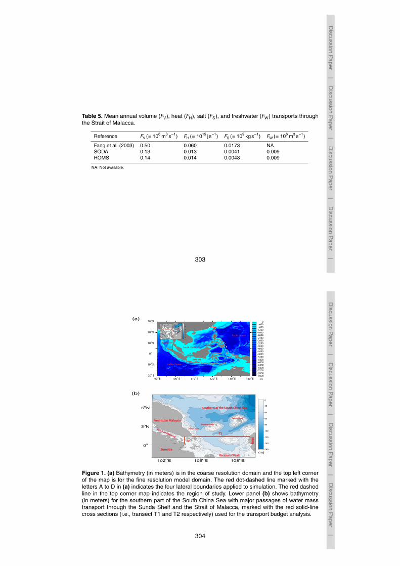
This section presents the calculations on the inter-ocean transport between the SundaShelf in the SSCS and the Strait of Malacca. The present study uses prognostic-modemomentum components and tracer field to calculate and analyze the transport. Thecross-sections of the Sunda Shelf (transect T1) and Strait of Malacca (transect T2) arespecified by heavy red solid lines from the southern end of the Peninsular Malaysia to15

western Borneo (1.5◦N from 104 to 109◦ E) and from the east coast of Sumatra to thesouthern end of Peninsular Malaysia (103.7◦ E from 0.2 to 1.5◦N), respectively (Fig. 1).The SCS is a marginal sea with a depth of about 4000–5000 m in the central regionand becoming shallower towards the southern region with depths of 50–70 m in theSunda Shelf. The Strait of Malacca is located between the east coast of Sumatra and20

the west coast of Peninsular Malaysia, connecting the SSCS and the Andaman Sea.The minimum depth of the Strait of Malacca (≤ 20 m) is in the southern part of theStrait connected to the Sunda Shelf whereas the maximum depth is in the northernpart (Fig. 1). The transports in these sections are calculated from the surface to the

282

Discussion

Paper

|D

iscussionP

aper

|D

iscussionP

aper|

Discussion

Paper

|

bottom in the z coordinate. For the volume transport the following equation is used:

FV =∫

A

v · n̂dA (7)

Where A represents the transect from the surface to the desired depth, dA denotes thearea element, v is the velocity component, and n̂ indicates the normal vector perpen-dicular to the transect. Thus, the direction of the normal velocity component relative to5

the normal vector is considered as the direction of transports. Hereafter, positive andnegative values are referred to as “outflow” form and “inflow” to the SSCS, respectively.The heat transport FH is calculated using:

FH = ρcp

∫

A

(T − T0)v · n̂dA (8)

The symbol ρ is the water density with a mean temperature of 28 ◦C and a mean10

salinity of 33 psu, taken as 1023 kgm−3. The specific heat cp for the above tempera-ture and salinity is determined based on the calculation by Millero et al. (1973). T de-notes the water temperature, and T0 represents the reference temperature of 3.72 ◦C(Schiller et al., 1998; Fang et al., 2009, 2010). The salinity and freshwater transportsare evaluated according to Eqs. (9) and (10), respectively, where S is the salinity (unit15

of psu), and S0 is the reference salinity set to 34.544 (Fang et al., 2009, 2010).

FS = ρ∫

A

Sv · n̂dA (9)

FW =∫

A

(S0 −SS0

)v · n̂dA (10)

283

Discussion

Paper

|D

iscussionP

aper|

Discussion

Paper

|D

iscussionP

aper|

4 Results and discussion

Generally, the modeled SST, SSS and circulation pattern in the SSCS are in goodagreement with observations and previous studies (e.g., Chu et al., 1999; Xie et al.,2003; Daryabor et al., 2014, 2015). During winter (December-January-February) andsummer (June-July-August), the model simulated the circulation patterns and major5

features including the western boundary currents along the Peninsular Malaysia’s east-ern continental shelf (PMECS) reasonably.

4.1 Sea surface temperature and salinity

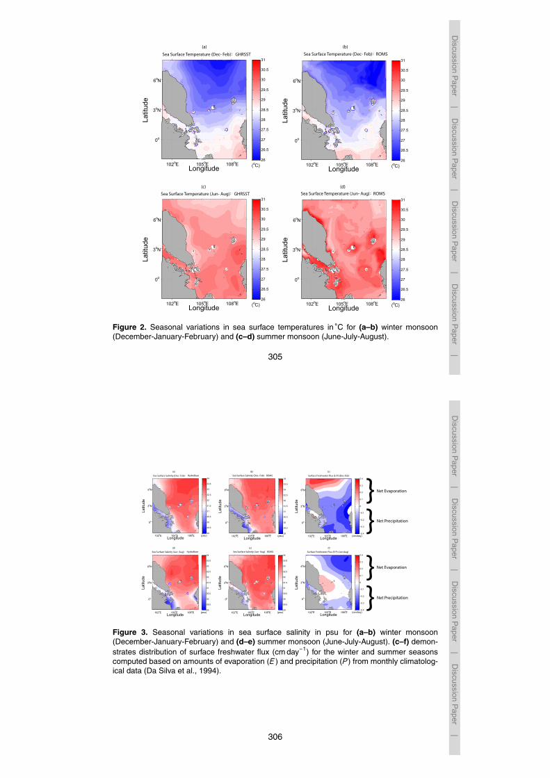
The patterns of model simulated SST (Fig. 2) and SSS (Fig. 3) compare well with theobservations of GHRSST and those of HydroBase climatological data, respectively.10

The seasonal variations in the modeled SST show that the SSTs are relatively lowerduring winter with an average of 26.5 ◦C north of 1.5◦N. Because of the advection ofcold waters from the north to the SSCS and relatively warmer through the Sunda Shelffrom the south of 1.5◦N towards the Java Sea with an average temperature of approxi-mately 29 ◦C these well agree with the GHRSST (Fig. 2) and previous studies (Hu et al.,15

2000; Morimoto et al., 2000; Cai et al., 2005b, 2007; Daryabor et al., 2014, 2015). Themodeld SSTs in the basin are relatively warmer with the average temperature 30 ◦Cduring summer because of increased solar radiation and the advection of warm wa-ters from the southern region, especially from the Java Sea (Yanagi et al., 2001; Caiet al., 2005b; Daryabor et al., 2014, 2015). The major feature during summer is the20

“cold tongue” along the PMECS with the temperature range of 28.5 ◦C due to the ex-istence of upwelling filament (Daryabor et al., 2014, 2015), which is also simulated bythe model. Model output can be different from the observation due to several possi-ble sources, particularly during summer monsoon because of the interaction of strongmonsoon wind flow direction with bathymetry and topography at different entry points.25

In addition, characteristic turbulent diffusion times due to vertical turbulent diffusionand the vertical advection/convection in the upper layer during the strong southwest-

284

Discussion

Paper

|D

iscussionP

aper

|D

iscussionP

aper|

Discussion

Paper

|

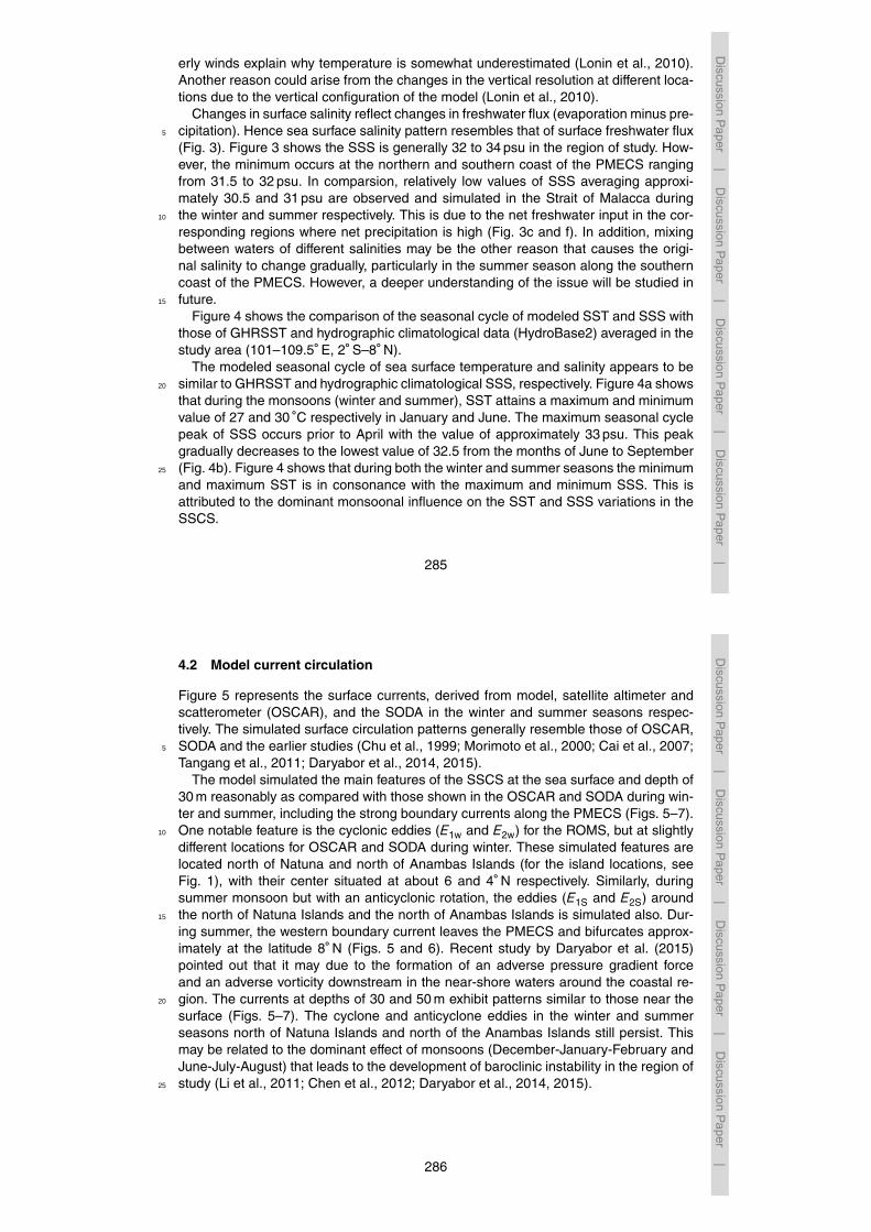
erly winds explain why temperature is somewhat underestimated (Lonin et al., 2010).Another reason could arise from the changes in the vertical resolution at different loca-tions due to the vertical configuration of the model (Lonin et al., 2010).

Changes in surface salinity reflect changes in freshwater flux (evaporation minus pre-cipitation). Hence sea surface salinity pattern resembles that of surface freshwater flux5

(Fig. 3). Figure 3 shows the SSS is generally 32 to 34 psu in the region of study. How-ever, the minimum occurs at the northern and southern coast of the PMECS rangingfrom 31.5 to 32 psu. In comparsion, relatively low values of SSS averaging approxi-mately 30.5 and 31 psu are observed and simulated in the Strait of Malacca duringthe winter and summer respectively. This is due to the net freshwater input in the cor-10

responding regions where net precipitation is high (Fig. 3c and f). In addition, mixingbetween waters of different salinities may be the other reason that causes the origi-nal salinity to change gradually, particularly in the summer season along the southerncoast of the PMECS. However, a deeper understanding of the issue will be studied infuture.15

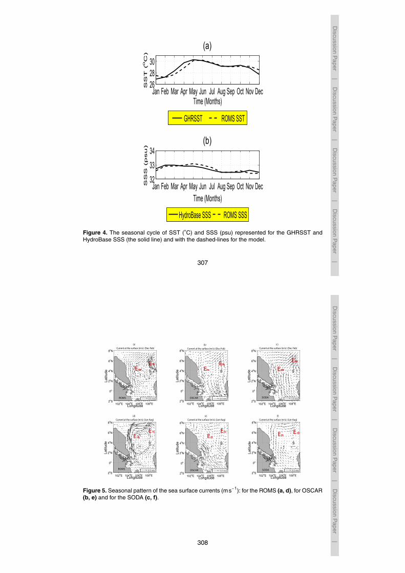
Figure 4 shows the comparison of the seasonal cycle of modeled SST and SSS withthose of GHRSST and hydrographic climatological data (HydroBase2) averaged in thestudy area (101–109.5◦ E, 2◦ S–8◦N).

The modeled seasonal cycle of sea surface temperature and salinity appears to besimilar to GHRSST and hydrographic climatological SSS, respectively. Figure 4a shows20

that during the monsoons (winter and summer), SST attains a maximum and minimumvalue of 27 and 30 ◦C respectively in January and June. The maximum seasonal cyclepeak of SSS occurs prior to April with the value of approximately 33 psu. This peakgradually decreases to the lowest value of 32.5 from the months of June to September(Fig. 4b). Figure 4 shows that during both the winter and summer seasons the minimum25

and maximum SST is in consonance with the maximum and minimum SSS. This isattributed to the dominant monsoonal influence on the SST and SSS variations in theSSCS.

285

Discussion

Paper

|D

iscussionP

aper|

Discussion

Paper

|D

iscussionP

aper|

4.2 Model current circulation

Figure 5 represents the surface currents, derived from model, satellite altimeter andscatterometer (OSCAR), and the SODA in the winter and summer seasons respec-tively. The simulated surface circulation patterns generally resemble those of OSCAR,SODA and the earlier studies (Chu et al., 1999; Morimoto et al., 2000; Cai et al., 2007;5

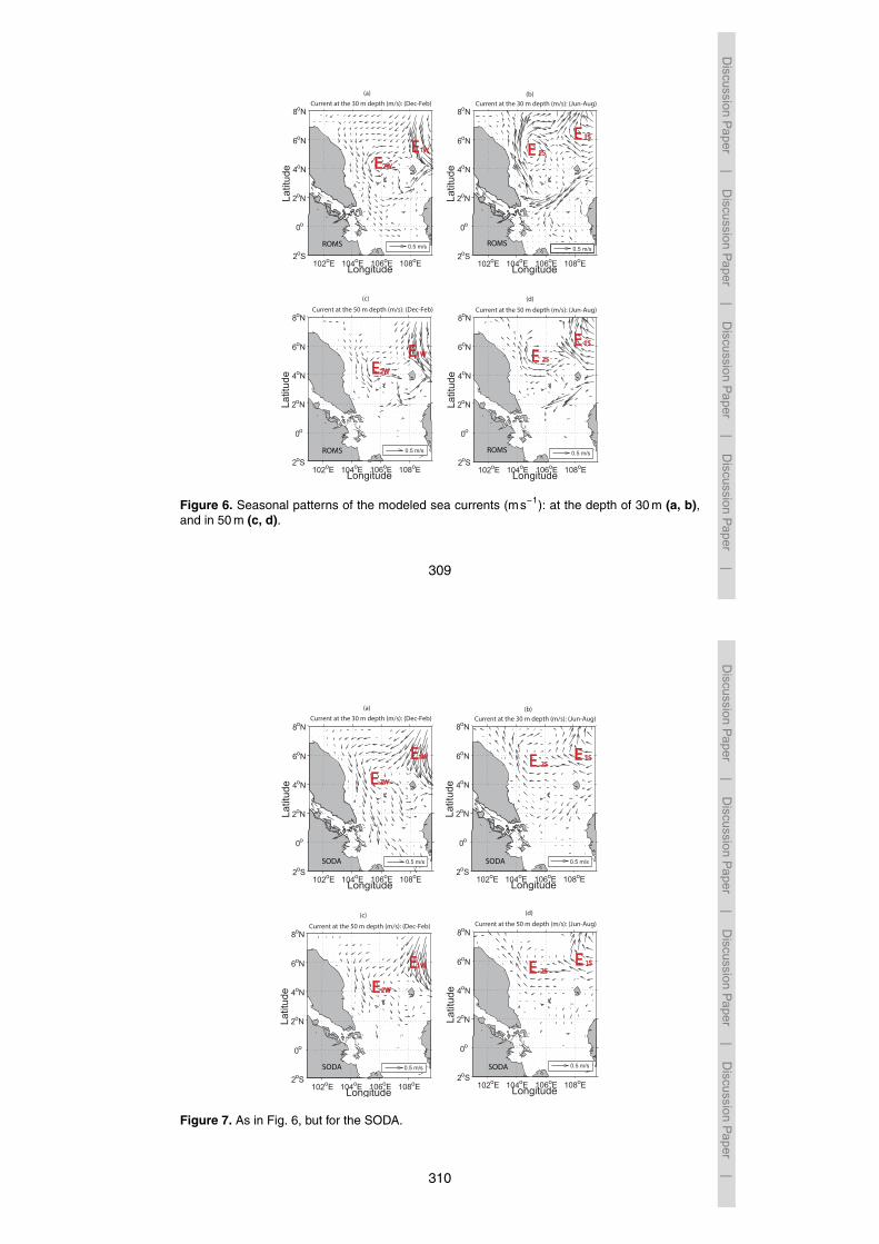
Tangang et al., 2011; Daryabor et al., 2014, 2015).The model simulated the main features of the SSCS at the sea surface and depth of

30 m reasonably as compared with those shown in the OSCAR and SODA during win-ter and summer, including the strong boundary currents along the PMECS (Figs. 5–7).One notable feature is the cyclonic eddies (E1w and E2w) for the ROMS, but at slightly10

different locations for OSCAR and SODA during winter. These simulated features arelocated north of Natuna and north of Anambas Islands (for the island locations, seeFig. 1), with their center situated at about 6 and 4◦N respectively. Similarly, duringsummer monsoon but with an anticyclonic rotation, the eddies (E1S and E2S) aroundthe north of Natuna Islands and the north of Anambas Islands is simulated also. Dur-15

ing summer, the western boundary current leaves the PMECS and bifurcates approx-imately at the latitude 8◦N (Figs. 5 and 6). Recent study by Daryabor et al. (2015)pointed out that it may due to the formation of an adverse pressure gradient forceand an adverse vorticity downstream in the near-shore waters around the coastal re-gion. The currents at depths of 30 and 50 m exhibit patterns similar to those near the20

surface (Figs. 5–7). The cyclone and anticyclone eddies in the winter and summerseasons north of Natuna Islands and north of the Anambas Islands still persist. Thismay be related to the dominant effect of monsoons (December-January-February andJune-July-August) that leads to the development of baroclinic instability in the region ofstudy (Li et al., 2011; Chen et al., 2012; Daryabor et al., 2014, 2015).25

286

Discussion

Paper

|D

iscussionP

aper

|D

iscussionP

aper|

Discussion

Paper

|

4.3 Seasonal and mean annual transports

This section discusses the seasonal and annual exchange of transports of volume,freshwater, heat, and salt between the SSCS and the Java Sea as well as their effectson distribution of temperature and salinity in the region of study. The same is also dealtwith for the Strait of Malacca. Further transports and the effects of these exchanges5

through the main passages in the SSCS, their roles in the mechanism and the for-mation of thermohaline circulation in the upper SSCS as well as the changes of theocean’s ventilation rates and pathways are elaborated.

4.3.1 Seasonal transports

(a) Sunda Shelf10

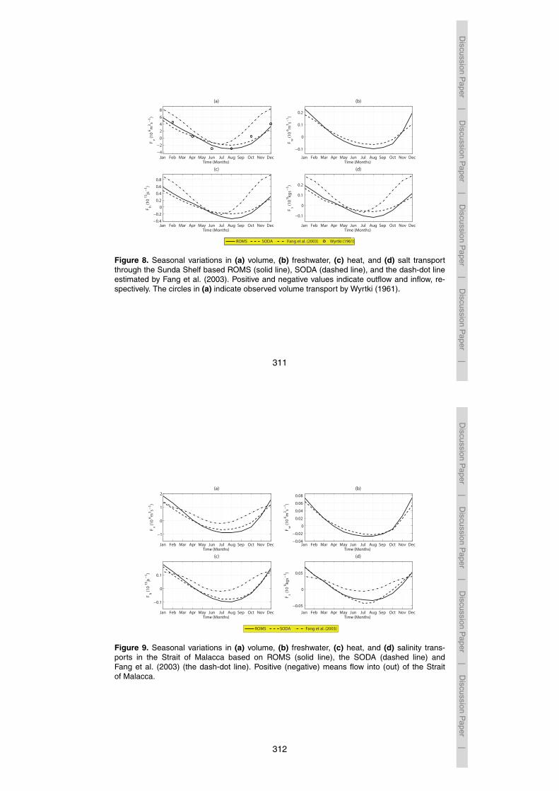
The seasonal cycles of various transports calculated from the sea surface to the bottomin the pathway of the Sunda Shelf indicated by transect T1 are depicted in Fig. 8. TheROMS estimated seasonal cycle of volume transport agrees well with those of SODA.In addition, both estimates are in good agreement with the observed values of Wyrtki(1961). In early January, the SODA and ROMS volume transports from the SSCS into15

the Java Sea are 4.9 and 5.7 Sv, respectively (Fig. 8a). These estimates of outflows intothe Java Sea are consistent with the mostly southward flow in the Sunda Shelf duringwinter (Figs. 5–7). Meanwhile, the volume transport estimate of Fang et al. (2003)during January appears to be higher as compared to the ROMS estimated values byabout 2 Sv. This higher estimate may be due to the coarse resolution of the Fang’s20

model which is configured with the horizontal resolution of the coarse grid 3◦ and thefine grid of approximately 1/6◦ with 15 vertical levels.

The ROMS estimated outflow in February is 4.5 Sv, which is comparable with the ob-served value of Wyrtki (1961). The volume transport gradually reduces to zero aroundApril–May and becomes negative (inflow into the SSCS) starting from June to October25

when the flow becomes dominantly northwards. By early June, transport switches to

287

Discussion

Paper

|D

iscussionP

aper|

Discussion

Paper

|D

iscussionP

aper|

inflow and continues throughout the summer with a maximum of about 3.0 Sv in Au-gust. This estimate is in good agreement with the observed volume transport of 3 Svby Wyrtki (1961). The inflow then decreases in September and switches back to out-flow in early winter with estimated volume transports of 3.3 and 2.5 Sv in Decemberfor ROMS and SODA, respectively. Hence, the volume transport in the Sunda Shelf5

seems to depend largely on the monsoon cycle. The good agreement between ROMS,SODA and observed values of Wyrtki (1961) seems to suggest the advantage of usinga high-resolution regional ocean model for better estimation of transports in complexregion such as the SSCS. In fact, Fang et al. (2003) using a global ocean circulationmodel with coarse resolution of 1/6◦ overestimated the volume transport in winter but10

underestimated it in summer. Furthermore, the switching of transport from outflow toinflow occurs in the middle of August, much earlier than those of ROMS, SODA andobserved values of Wyrtki (1961) (Fig. 8a).

Table 1 provides another comparison of volume transport of this study with two pre-vious modeling studies based on the coarser global ocean model during the months15

of December, January, and June. Cai et al. (2005a), based on LICOM global modelof 1/2◦ horizontal resolution and 12 uniform vertical levels, estimated 3.4 and 0.2 Svof volume transport during December and June, respectively. The positive values ofvolume transports during both December and June indicate no reversal of the volumetransports from winter to summer. Qingye et al. (2009), using HYCOM global model of20

1/2◦ horizontal resolution and 20 uniform levels with bathymetry from ETOPO5, esti-mated volume transport of 2.1 and −1.0 Sv during January and June respectively. Theestimates from these two modeling studies are not consistent with the modeled andobserved values from ROMS, SODA and Wyrtki (1961).

Table 2 shows a comparison of transports from the SSCS into Java Sea through the25

Sunda Shelf in the months of January and February between estimates of a morerecent observational study of Fang et al. (2010) and those estimated from ROMSand SODA. Fang et al.’s estimates are based on the Acoustic Doppler current pro-filer deployed for a period of 13 January to 12 February 2008. The corresponding vol-

288

Discussion

Paper

|D

iscussionP

aper

|D

iscussionP

aper|

Discussion

Paper

|

ume transports of ROMS and SODA are consistent with the observed value of Fanget al. (2010).

The seasonal cycle of freshwater, heat, and salt transport derived from ROMS andSODA generally follows that of the volume transport (Fig. 8). During the peak of thewinter monsoon in January, freshwater transport enters the Java Sea at 0.23 Sv while5

in August the transport is into the Sunda Shelf at 0.099 Sv. These estimates are inaccord with the values of 0.19 and 0.066 Sv for the respective months of January andAugust obtained from SODA (Fig. 8b). However, there has been no direct observationof the seasonal cycle of freshwater transport that can be compared with these values.Nevertheless, Fang et al. (2010), based on observation for a period of 13 January to10

12 February 2008, provided an estimate of freshwater transport of 0.14 Sv into the JavaSea through the Sunda Shelf (see Table 2). This value is comparable with both SODAand ROMS estimates of 0.15 and 0.18 Sv, even though observed value representsa transport only for a very specific period of measurement. The ROMS and SODAestimated seasonal cycles of heat transport through the Sunda Shelf are similar to15

each other (Fig. 8c). However, the estimates of Fang et al. (2003), which are basedon the global ocean model, are much higher during winter and lower during summer.Nevertheless, the ROMS and SODA estimated heat transport in one month duringJanuary and February are consistent with observed values of Fang et al. (2010) (seeTable 2). Similarly, the seasonal cycle of the salt transport (Fig. 8d) through the Sunda20

Shelf follows the pattern of volume transport. The ROMS estimated amounts of salttransport out of and into the Sunda Shelf in January and August are 0.2×109 and0.11×109 kgs−1 respectively. The corresponding values for SODA are 0.16×109 and0.06×109 kgs−1 respectively. The ROMS estimated value in summer is slightly highercompared with that from SODA. However, the ROMS estimated salt transport for the25

months of January and February is in accordance with the observed value (Fang et al.,2010) as shown in Table 2.

289

Discussion

Paper

|D

iscussionP

aper|

Discussion

Paper

|D

iscussionP

aper|

(b) Strait of Malacca

Figure 9 compares the seasonal cycle of various transports estimated based on ROMS,SODA for the pathway of the Strait of Malacca indicated by transect T2 and those ofFang et al. (2003). As in the Sunda Shelf, ROMS and SODA estimates of transportsin the Strait of Malacca are in good agreement with each other. However, in contrast5

to Sunda Shelf, Fang et al.’s estimates of transports during winter are lower than theROMS estimates. The ROMS estimated volume transport through the Strait of Malaccain early January is approximately 1.8 Sv towards the Andaman Sea, which is slightlyhigher than the 1.4 Sv from SODA. As in the Sunda Shelf, the volume transport de-creases and becomes zero in April. The volume transport switches to an inflow in late10

May and continues throughout the summer up to October with maximum values inAuguest of approximately 0.9 and 0.6 Sv for ROMS and SODA respectively.

The inflow decreases further in autumn and switches back to outflow in Novemberwith a maximum rate of approximately 1.6 and 1.2 Sv for ROMS and SODA in Decem-ber respectively (Fig. 9). In general, the volume transport estimates of the ROMS and15

SODA are in good agreement throughout the years. In contrast, Fang’s study underes-timated the volume transports in summer (Fig. 9a).

The seasonal cycle of freshwater transport (Fig. 9b) generally follows that of the vol-ume transport. During the peak of the winter monsoon in January, freshwater transportenters the Strait of Malacca at a maximum rate of 0.073 and 0.065 Sv for the ROMS20

and SODA respectively. However, during summer, the inflow of the freshwater trans-ports into the Strait of Malacca is estimated to be approximately 0.28 and 0.23 Sv forROMS and SODA respectively. This inflow reverses its direction at the end of autumn.The seasonal cycle of heat (Fig. 9c) is also very similar to the seasonal cycle of volumetransport. Estimates from ROMS and SODA are in accordance with each other. On the25

other hand, Fang’s study underestimated the heat transport during the summer. DuringJanuary the heat is transported into the Andaman Sea through the Strait of Malaccawith an estimate of 0.18 PW for ROMS and 0.16 PW for SODA. In the summer season,

290

Discussion

Paper

|D

iscussionP

aper

|D

iscussionP

aper|

Discussion

Paper

|

the heat is transported into the corresponding area with an estimate of 0.096 PW forROMS and 0.079 PW for SODA. For salt transport (Fig. 9d), ROMS and SODA esti-mate are also in good agreement. During winter, salt is transported into the Strait ofMalacca with estimates of 0.068×109 and 0.067×109 kgs−1 for ROMS and SODA re-spectively. During summer the salt transport is into the Strait of Malacca with estimates5

of 0.034×109 and 0.041×109 kgs−1 for ROMS and SODA respectively. In contrast,Fang’s study underestimated the salt transport during both summer and winter.

4.3.2 Mean annual transports

(a) Sunda Shelf

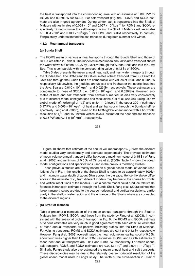
The ROMS mean of various annual transports through the Sunda Shelf and those of10

SODA are listed in Table 3. The model estimated mean annual volume transport showsthe water flows out of the SSCS by 0.32 Sv through the Sunda Shelf and into the JavaSea. This is comparable with the corresponding value of 0.42 Sv of SODA.

Table 3 also presents the mean annual heat, salt, and freshwater transports throughthe Sunda Shelf. The ROMS and SODA estimates of heat transport from SSCS into the15

Java Sea through the Sunda Shelf are comparable with values of 0.032 and 0.042 PWrespectively. Meanwhile, the modeled annual salt and freshwater transports flows intothe Java Sea are 0.010×109 kgs−1 and 0.023 Sv, respectively. These estimates arecomparable to those of SODA (i.e., 0.016×109 kgs−1 and 0.026 Sv). However, esti-mates of heat and salt transports from several numerical studies vary considerably20

due to different model configurations and resolutions. Cai et al. (2005a), using LICOMglobal model of horizontal of 1/2◦ and uniform 12 levels in the upper 300 m estimated0.17 PW and 0.066×109 kgs−1 of heat and salt transports through the Sunda shelf re-spectively. Fang et al. (2003), based on the MOM global ocean model with a horizontalresolution of 1/6◦ and 15 uniform vertical levels, estimated the heat and salt transport25

of 0.35 PW and 0.11×109 kgs−1, respectively.

291

Discussion

Paper

|D

iscussionP

aper|

Discussion

Paper

|D

iscussionP

aper|

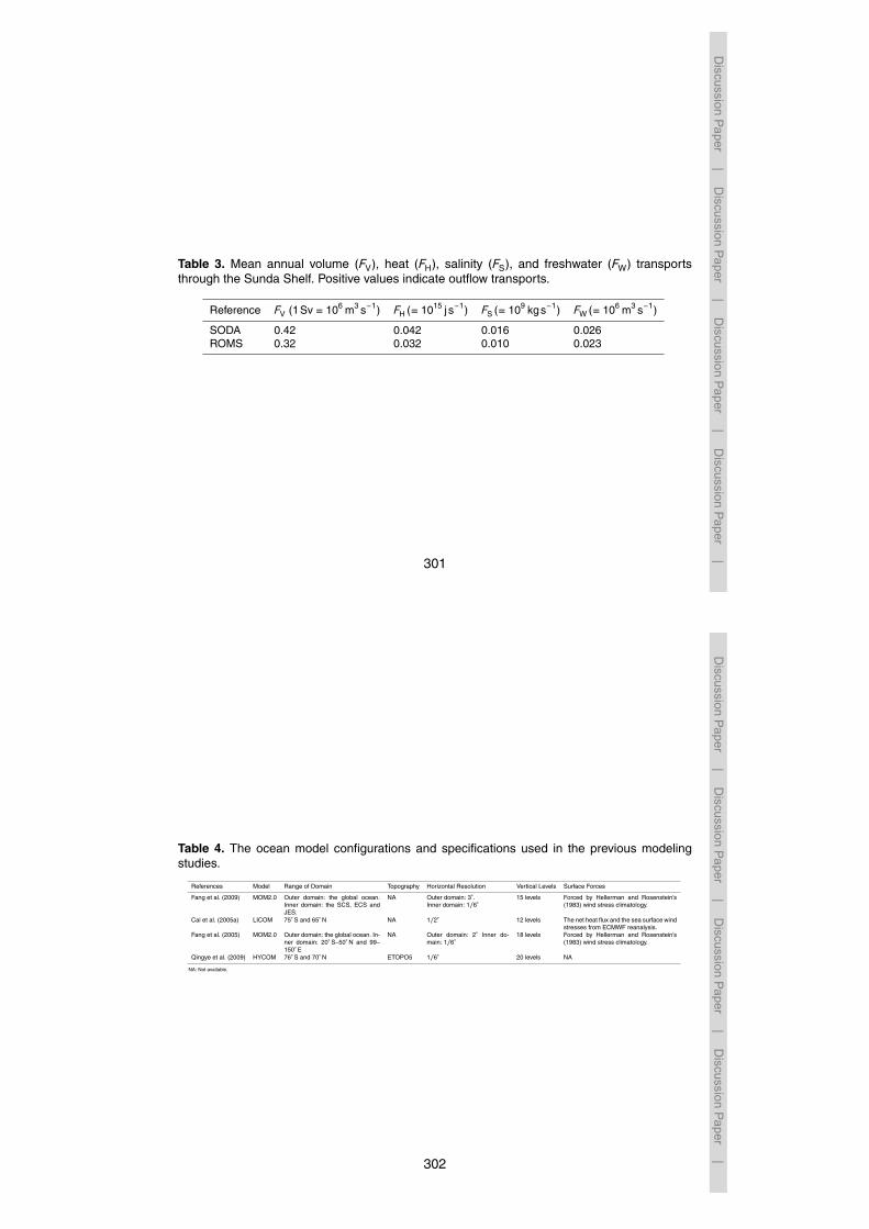
Figure 10 shows that estimate of the annual volume transport (FV) from the differentmodel studies vary considerably and decrease exponentially. The previous estimatesof mean volume annual transport differ between a maximum value of 3.15 Sv of Fanget al. (2003) and minimum of 0.5 Sv of Qingye et al. (2009). Table 4 shows the oceanmodel configurations and specifications used in the previous modeling studies.5

These previous studies are mostly based on a global ocean model of various reso-lutions. As in Fig. 1 the length of the Sunda Shelf is noted to be approximately 500 kmand maximum water depth of about 50 m across the passage. Hence the above differ-ences in the estimate of FV from different models may be due to the coarse horizontaland vertical resolutions of the models. Such a coarse model could produce relative dif-10

ferences in transport estimates through the Sunda Shelf. Fang et al. (2005) pointed thatlarge transport values are due to the coarse horizontal and vertical resolutions, partic-ularly in the shallow water region and the entrance of the Straits where are connectedto the different regions.

(b) Strait of Malacca15

Table 5 presents a comparison of the mean annual transports through the Strait ofMalacca from ROMS, SODA, and those from the study by Fang et al. (2003). In con-sistent with the seasonal cycle of transport in Fig. 9, the ROMS and SODA estimateof various estimates are very much in good agreement with each other. All estimatesof mean annual transports are positive indicating outflow into the Strait of Malacca.20

For volume transports, ROMS and SODA estimates are 0.14 and 0.13 Sv respectively.However, Fang et al. (2003) overestimated the mean volume annual transport of 0.5 Sv,about four times higher than that of ROMS estimates. ROMS and SODA estimates ofmean heat annual transports are 0.014 and 0.013 PW respectively. For mean annualsalt transport, ROMS and SODA estimates are 0.0043×109 and 0.0041×109 kgs−1.25

Similarly, Fang’s study also overestimated the mean annual heat and salt transports.These discrepancies may be due to the relatively coarse horizontal resolution of theglobal ocean model used in Fang’s study. The width of the cross-section in Strait of

292

Discussion

Paper

|D

iscussionP

aper

|D

iscussionP

aper|

Discussion

Paper

|

Malacca (see Fig. 1) is about 140 km with depths of ≤ 20 m. With such a narrow andshallow Strait, using a global ocean model for transports estimation may be inaccurate.

The cross-section in the Strait of Malacca is narrower than the Sunda Shelf pas-sage and hence lesser transports flow through it. The maximum outflow volume trans-port through the Sunda Shelf during January is 5.7 Sv, which is much higher than the5

corresponding outflow volume transport of 1.8 Sv for the Strait of Malacca. Owing tothis shallow depth, the Strait of Malacca is often not captured in the simulation usinga coarse global ocean model (Fang et al., 2005; Cai et al., 2005a; Qingye et al., 2009).However, in spite of the high value of outflow and inflow transports throughout the year,the outflow mean annual transports through the Sunda Shelf are relatively small. Inter-10

estingly, the outflow mean annual transports through the Strait of Malacca are equallysignificant compared to those of the Sunda Shelf. For mean volume and heat annualtransports, the estimate for Strait of Malacca is about 43.8 % of the Sunda Shelf. Forsalt and freshwater, the percentages are about 43 and 39 %, respectively. This reflectsthat the Strait of Malacca plays equally important role in the annual transports from the15

Strait of Malacca into the Andaman Sea.

5 Summary and conclusion

Based on the results of ROMS simulation, transports of volume, freshwater, heat, andsalt, through the inter-ocean passages are estimated in the SSCS for the Sunda Shelfand the Strait of Malacca. The simulated patterns of SST and current circulation are in20

good agreement with observations, re-analysis product of SODA, near-real time globalocean surface currents derived from satellite altimeter and scatterometer data (OS-CAR). The estimated ROMS and SODA seasonal transports across both the SundaShelf and the Strait of Malacca are almost comparable to each other (Figs. 8 and 9).The ROMS estimated transports are also consistent with the observed values of Fang25

et al. (2010) for one-month duration of 13 January and 12 February 2008. However,estimates of transports from coarser global ocean model (Fang et al., 2003) are often

293

Discussion

Paper

|D

iscussionP

aper|

Discussion

Paper

|D

iscussionP

aper|

higher during winter and lower during summer. This could be due to the inability ofthe coarser global ocean model in resolving the complexity in the SSCS region due torapid changes by interaction with bathymetry and topography. This study shows thatthe mean annual transports in the Sunda Shelf are outflow transports into the JavaSea. Similarly, the mean annual transports in the Strait of Malacca are outflow trans-5

ports from the Straits of Malacca towards the Andaman Sea. Owing to the relativelylarge area of the cross-section in the Sunda Shelf as compared to that in the Strait ofMalacca, the seasonal transports in the Sunda Shelf are higher and vary considerably.However, in terms of mean annual transports, ROMS estimated transports indicate theimportance of both passages in the Sunda Shelf and the Strait of Malacca. The per-10

centages of estimated mean annual transports through the Strait of Malacca to those ofthe Sunda Shelf range from 39 to 43.8 %. These percentages reiterate the equally im-portance of the Strait of Malacca as an inter-ocean transport passage from the SSCSinto the Andaman Sea. Overall, this study provides estimates of various transportsthrough inter-ocean passages in the SSCS. Nevertheless, a better estimate of trans-15

port is necessary to understand the changes in the ocean circulation as well as toenhance our knowledge on the role of transport distribution such as heat and freshwa-ter which in turn affect the changes of the ocean’s ventilation rates and pathways. Thisprovides a better picture to assess the changes in the net uptake of gases such as O2,CO2 which influence the distribution of the nutrient balance in regulation changes in20

the marine ecosystem.

Acknowledgements. This research study is funded by the Higher Institution Center of Excel-lence (HICOE), IOES-2014A and Fundamental Research Grant Scheme (FRGS), FP 049-2013A. It is also strongly supported by the Vice Chancellor of the University of Malaya.

294

Discussion

Paper

|D

iscussionP

aper

|D

iscussionP

aper|

Discussion

Paper

|

References

Antonov, J. I., Locarnini, R. A., Boyer, T. P., Mishonov, A. V., and Garcia, H. E.: World OceanAtlas 2005, Volume 2, Salinity, US Government Printing Office 62, NOAA Atlas NESDIS,Washington, D.C., 182 pp., 2006.

Cai, S. Q., Liu, H. L., and Li, W.: Water transport exchange between the South China Sea and5

its adjacent seas, Adv. Marine Sci., 20, 29–34, 2002 (in Chinese).Cai, S. Q., Liu, H. L., and Li, W.: Application of LICOM to the numerical study of water ex-

change between the South China Sea and its adjacent oceans, Acta Oceanol. Sin., 24,10–19, 2005a.

Cai, S. Q., Su, J., Long, X., Wang, S., and Huang, Q.: Numerical study on summer circulation10

and its stablishment of the upper South China Sea, Acta Oceanol. Sin., 24, 31–38, 2005b.Cai, S. Q., Long, X., and Wang, S.: A model study of the summer Southeast Vietnam offshore

current in the Southern South China Sea, Cont. Shelf Res., 27, 2357–2372, 2007.Carton, J. A. and Giese, B. S.: A reanalysis of ocean climate using Simple Ocean Data Assim-

ilation (SODA), Mon. Weather Rev., 136, 2999–3017, 2008.15

Chapman, D. C.: Numerical treatment of cross-shelf open boundaries in a barotropic coastalmodel, J. Phys. Oceanogr., 15, 1060–1075, 1985.

Chen, G., Gan, J., Xie, Q., Chu, X., Wang, D., and Hou, Y.: Eddy heat and salt transportsin the South China Sea and their seasonal modulations, J. Geophys. Res., 117, C05021,doi:10.1029/2011JC007724, 2012.20

Chu, P. C., Edmons, N. L., and Fan, C. W.: Dynamical mechanisms for the South China Seaseasonal circulation and thermohaline variability, J. Phys. Oceanogr., 29, 2971–2989, 1999.

Daryabor, F., Tangang, F., and Juneng, L.: Hydrodynamic and Thermohaline Seasonal Struc-tures of Peninsular Malaysia’s eastern continental shelf sea, in: EGU General AssemblyConference Abstracts, Geophysical Research Abstracts., 12, 778 pp., 2010.25

Daryabor, F., Tangang, F., and Juneng, L.: Simulation of southwest monsoon current circulationand temperature in the east coast of Peninsular Malaysia, Sains Malays., 43, 389–398, 2014.

Daryabor, F., Samah, A. A., and Ooi, S. H.: Dynamical Structure of the Sea off the East Coastof Peninsular Malaysia, Ocean Dynam., 65, 93–106, 2015.

Da Silva, A. M., Young, C. C., and Levitus, S.: Atlas of Surface Marine Data 1994, Vol. 1,30

Algorithms and Procedures, technical report. Technical report, National Oceanographic andAtmospheric Administration, Silver Spring, Md, 1994.

295

Discussion

Paper

|D

iscussionP

aper|

Discussion

Paper

|D

iscussionP

aper|

Fang, G. H., Wei, Z. X., Choi, B. H., Wang, K., Fang, Y., and Li, W.: Interbasin freshwater, heatand salt transport through the boundaries of the East and South China Sea from a variable-grid ocean circulation model, Science China, 46, 149–161, 2003.

Fang, G. H., Susanto, D., Soesilo, I., Zheng, Q., Fangli, Q., and Zexun, W.: A note on the SouthChina Sea shallow interocean circulation, Adv. Atmos. Sci., 22, 946–954, 2005.5

Fang, G. H., Wang, Y., Wei, Z. X., Fang, Y., Qiao, F., and Hu, X.: Interocean circulation, heatand freshwater budgets of the South China Sea based on a numerical model, Dynam. Atmos.Oceans, 47, 55–72, 2009.

Fang, G. H., Susant, R. D., Wirasantosa, S., Qiao, F., Supangat, A., Fan, B., Wei, Z. X., Sulis-tiyo, B., and Li, S.: Volume, heat and freshwater transports from the South China Sea10

to Indonesian seas in the boreal winter of 2007–2008, J. Geophys. Res., 115, C12020,doi:10.1029/2010JC006225, 2010.

Fang, G. H., Wang, G., Fang, Y., and Fang, W.: A review on the South China Sea westernboundary current, Acta Oceanol. Sin., 31, 1–10, 2012.

Flather, R. A.: A tidal model of the north-west European continental shelf, Mem. S. R. Sci.15

Liege, 6, 141–164, 1976.Gong, D. and Wang, S.: The warmest year on record of the century in China, Meteorology, 25,

3–5, 1999.Hellerman, S. and Rosenstein, M.: Normal monthly wind stress over the World Ocean with error

estimates, J. Phys. Oceanogr., 13, 1093–1104, 1983.20

Hu, J. Y., Kawamura, H., Hong, H., and Qi, Y. Q.: A review on the currents in the SouthChina Sea: seasonal circulation, South China Sea warm current and Kuroshio intrusion, J.Oceanogr., 56, 607–624, 2000.

Jiaxun Li, Ren Zhang, and Baogang Jin: Eddy characteristics in the northern South ChinaSea as inferred from Lagrangian drifter data, Ocean Sci., 7, 661–669, doi:10.5194/os-7-661-25

2011, 2011.Large, W. J., McWilliams, J. C., and Doney, S. C.: Oceanic vertical mixing: a review and a model

with nonlocal boundary layer parameterization, Rev. Geophys., 32, 363–403, 1994.Locarnini, R. A., Mishonov, A. V., Antonov, J. I., Boyer, T. P., and Garcia, H. E.: World Ocean

Atlas 2005, Volume 1: Temperature, edited by: Levitus, S., NOAA Atlas NESDIS 61, US30

Government Printing Office, Washington, D.C, 182 pp., 2006.

296

Discussion

Paper

|D

iscussionP

aper

|D

iscussionP

aper|

Discussion

Paper

|

Lonin, S. A., Hernandez, J. L., and Palacios, D. M.: Atmospheric events disruptingcoastal upwelling in the southwestern Caribbean, J. Geophys. Res., 115, C06030,doi:10.1029/2008JC005100, 2010.

Marchesiello, P., McWilliams, J. C., and Shchepetkin, A.: Open boundary condition for long-termintegration of regional oceanic models, Ocean Model., 3, 1–21, 2001.5

Marchesiello, P., Debreu, L., and Couvelard, X.: Spurious diapycnal mixing in terrain followingcoordinate models: advection problem and solution, Ocean Model., 26, 156–169, 2009.

Millero, F. J., Perron, G., and Desnoyers, J. E.: Heat capacity of seawater solution, J. Geophys.Res., 78, 4499–4507, 1973.

Morimoto, A., Yoshimoto, K., and Yanagi, T.: Characteristics of sea surface circulation and eddy10

field in the South China Sea revealed by satellite altimetric data, J. Oceanogr., 56, 331–344,2000.

Orlanski, I.: A simple boundary condition for unbounded hyperbolic flows, J. Comput. Phys., 21,252–269, 1976.

Qingye, W., Hong, C., and Shuwen, Z.: Water transport through the four main straits around the15

South China Sea, Chin. J. Oceanol. Limn., 27, 229–236, 2009.Reynolds, R. W., Smith, T. M., Liu, C., Chelton, D. B., Casey, K. S., and Schlax, M. G.: Daily

high-resolution blended analyses for sea surface temperature, J. Climate, 20, 5473–5496,2007.

Schiller, A., Godfrey, I. S., McIntosh, P. C., Meyers, G., and Wijffels, S. E.: Seasonal near-20

surface dynamics and thermodynamics of the Indian Ocean and Indonesian Throughflow ina global ocean general circulation model, J. Phys. Oceanogr., 28, 2288–2312, 1998.

Shchepetkin, A. and McWilliams, J. C.: Quasi-monotone advection schemes based on explicitlocally adaptive dissipation, Mon. Weather Rev., 126, 1541–1580, 1998.

Shchepetkin, A. and McWilliams, J. C.: A method for computing horizontal pressure gradient25

force in an oceanic model with a nonaligned vertical coordinate, J. Geophys. Res., 108,1978–2012, 2003.

Shchepetkin, A. and McWilliams, J. C.: The Regional Oceanic Modeling System (ROMS):a split-explicit, free-surface, topography-following-coordinate oceanic model, Ocean Model.,9, 347–404, 2005.30

Smith, W. H. F. and Sandwell, D. T.: Global seafloor topography from satellite altimetry and shipdepth soundings, Science, 277, 1957–1962, 1997.

297

Discussion

Paper

|D

iscussionP

aper|

Discussion

Paper

|D

iscussionP

aper|

Song, Y. T.: Estimation of interbasin transport using ocean bottom pressure: theory and modelfor Asian marginal seas, J. Geophys. Res., 111, C11S19, doi:10.1029/2005JC003189, 2006.

Spall, M. A. and Holland, W. R.: A nested primitive equation model for oceanic applications, J.Phys. Oceanogr., 21, 205–220, 1991.

Tangang, F., Xia, C., Qiao, F., Juneng, L., and Shan, F.: Seasonal circulations in the Malay5

Peninsula Eastern continental shelf from a wave–tide–circulation coupled model, Ocean Dy-nam., 61, 1317–1328, 2011.

Veitch, J., Penven, P., and Shillington, F.: Modeling equilibrium dynamics of the Benguela cur-rent system, J. Phys. Oceanogr., 40, 1942–1964, 2010.

Wyrtki, K.: Scientific results of marine investigations of the South China Sea and the Gulf of10

Thailand 1959–1961, Naga Report 2, Technical Report, Scripps Institute of Oceanography,195 pp., 1961.

Xie, S. P., Xie, Q., Wang, D. X., and Liu, W. T.: Summer upwelling in the South China Sea andits role in regional climate variations, J. Geophys. Res., 108, 1978–2012, 2003.

Yanagi, T., Sachoemar, I. S., Takao, T., and Fujiwara, S.: Seasonal variation of stratification in15

the Gulf of Thailand, J. Oceanogr., 57, 461–470, 2001.Zhang, J., Liu, P., and Wu, G.: The relationship between the flood and drought over the lower

reach of the Yangtze River Valley and the SST over the Indian Ocean and the South ChinaSea, Chinese J. Atmos. Sci., 27, 992–1006, 2003.

298

Discussion

Paper

|D

iscussionP

aper

|D

iscussionP

aper|

Discussion

Paper

|

Table 1. Seasonal volume transport (1Sv = 106 m3 s−1) out of and into the SSCS through theSunda Shelf obtained from previous modeling studies.

Winter Summer

Dec Jan JunCai et al. (2005a) 3.4 NA 0.2Qingye et al. (2009) NA 2.1 −1.0Present Study 3.3 5.7 −2.0

NA: Not available.

299

Discussion

Paper

|D

iscussionP

aper|

Discussion

Paper

|D

iscussionP

aper|

Table 2. Estimates of mean volume (FV), heat (FH), salt (FS), and freshwater (FW) transportsduring winter (January and February) from observation (Fang et al., 2010), the SODA andROMS.

Reference FV (1Sv = 106 m3 s−1) FH (1PW1015 j s−1) FS (= 109 kgs−1) FW(1Sv = 106 m3 s−1)

Fang et al. (2010) 3.6±0.8 0.36±0.08 0.12±0.03 0.14±0.04SODA 3.9 0.39 0.13 0.15ROMS 4.8 0.48 0.16 0.18

300

Discussion

Paper

|D

iscussionP

aper

|D

iscussionP

aper|

Discussion

Paper

|

Table 3. Mean annual volume (FV), heat (FH), salinity (FS), and freshwater (FW) transportsthrough the Sunda Shelf. Positive values indicate outflow transports.

Reference FV (1Sv = 106 m3 s−1) FH (= 1015 j s−1) FS (= 109 kgs−1) FW (= 106 m3 s−1)

SODA 0.42 0.042 0.016 0.026ROMS 0.32 0.032 0.010 0.023

301

Discussion

Paper

|D

iscussionP

aper|

Discussion

Paper

|D

iscussionP

aper|

Table 4. The ocean model configurations and specifications used in the previous modelingstudies.

References Model Range of Domain Topography Horizontal Resolution Vertical Levels Surface Forces

Fang et al. (2009) MOM2.0 Outer domain: the global ocean.Inner domain: the SCS, ECS andJES.

NA Outer domain: 3◦.Inner domain: 1/6◦

15 levels Forced by Hellerman and Rosenstein’s(1983) wind stress climatology.

Cai et al. (2005a) LICOM 75◦ S and 65◦ N NA 1/2◦ 12 levels The net heat flux and the sea surface windstresses from ECMWF reanalysis.

Fang et al. (2005) MOM2.0 Outer domain: the global ocean. In-ner domain: 20◦ S–50◦ N and 99–150◦ E

NA Outer domain: 2◦ Inner do-main: 1/6◦

18 levels Forced by Hellerman and Rosenstein’s(1983) wind stress climatology.

Qingye et al. (2009) HYCOM 76◦ S and 70◦ N ETOPO5 1/6◦ 20 levels NA

NA: Not available.

302

Discussion

Paper

|D

iscussionP

aper

|D

iscussionP

aper|

Discussion

Paper

|

Table 5. Mean annual volume (FV), heat (FH), salt (FS), and freshwater (FW) transports throughthe Strait of Malacca.

Reference FV (= 106 m3 s−1) FH (= 1015 j s−1) FS (= 109 kgs−1) FW (= 106 m3 s−1)

Fang et al. (2003) 0.50 0.060 0.0173 NASODA 0.13 0.013 0.0041 0.009ROMS 0.14 0.014 0.0043 0.009

NA: Not available.

303

Discussion

Paper

|D

iscussionP

aper|

Discussion

Paper

|D

iscussionP

aper|

90o E 100o E 110o E 120o E 130o E 140o E20o S

10o S

0o

10oN

20oN

30oN 0-400-800

-1200-1600-2000-2400-2800-3200-3600-4000-4400-4800-5200-5800-6000-6400-6800-7200-7600-8000

(m)

102oE 105oE 108oE

0o

3oN

6oN

(m)

Peninsular Malaysia

Strait of Malacca

Southern of the South China Sea

Natuna Islands

T1

Sumatra

Karimata Strait

Borneo

(b)

Tioman Island

Anambas Islands

T2

(a)

Indian Ocean

Paci�c Ocean

Andaman Sea

Java Sea

South China Sea

KarimataA

Balabac Island

Mindoro

Luzo

nTa

iwan

B

C

D

0

-20

-40

-60

-80

-100

-120

-140

-160

30

60

102oE 108oE 114oE

0o

6oN

12oN

(m)

0

-500

-1000

-1500

-2000

-2500

-3000

-3500

-4000

-4500

-5000

Figure 1. (a) Bathymetry (in meters) is in the coarse resolution domain and the top left cornerof the map is for the fine resolution model domain. The red dot-dashed line marked with theletters A to D in (a) indicates the four lateral boundaries applied to simulation. The red dashedline in the top corner map indicates the region of study. Lower panel (b) shows bathymetry(in meters) for the southern part of the South China Sea with major passages of water masstransport through the Sunda Shelf and the Strait of Malacca, marked with the red solid-linecross sections (i.e., transect T1 and T2 respectively) used for the transport budget analysis.

304

Discussion

Paper

|D

iscussionP

aper

|D

iscussionP

aper|

Discussion

Paper

|

102oE 105oE 108oE

0o

3oN

6oN

Longitude

Latit

ude

(oC)26

26.5

27

27.5

28

28.5

29

29.5

30

30.5

31

102oE 105oE 108oE

0o

3oN

6oN

Longitude

Latit

ude

(oC)26

26.5

27

27.5

28

28.5

29

29.5

30

30.5

31

102oE 105oE 108oE

0o

3oN

6oN

Longitude

Latit

ude

(oC)26

26.5

27

27.5

28

28.5

29

29.5

30

30.5

31

102oE 105oE 108oE

0o

3oN

6oN

Longitude

Latit

ude

(oC)26

26.5

27

27.5

28

28.5

29

29.5

30

30.5

31

Sea Surface Temperature (Dec- Feb) GHRSST: Sea Surface Temperature (Dec- Feb) ROMS:(a) (b)

Sea Surface Temperature (Jun- Aug) ROMS:(c) (d)

Sea Surface Temperature (Jun- Aug) GHRSST:

Figure 2. Seasonal variations in sea surface temperatures in ◦C for (a–b) winter monsoon(December-January-February) and (c–d) summer monsoon (June-July-August).

305

Discussion

Paper

|D

iscussionP

aper|

Discussion

Paper

|D

iscussionP

aper|

102oE 105oE 108oE

0o

3oN

6oN

Longitude

Latit

ude

(psu)29

29.5

30

30.5

31

31.5

32

32.5

33

33.5

34

102oE 105oE 108oE

0o

3oN

6oN

Longitude

Latit

ude

(psu)29

29.5

30

30.5

31

31.5

32

32.5

33

33.5

34

102oE 105oE 108oE

0o

3oN

6oN

Longitude

Latit

ude

(psu)29

29.5

30

30.5

31

31.5

32

32.5

33

33.5

34

102oE 105oE 108oE

0o

3oN

6oN

Longitude

Latit

ude

(psu)29

29.5

30

30.5

31

31.5

32

32.5

33

33.5

34

Sea Surface Salinity (Dec- Feb) :

(a)

Sea Surface Salinity (Dec- Feb) ROMS:(b)

(d)Sea Surface Salinity (Jun- Aug) ROMS:

(e)

HydroBase

Sea Surface Salinity (Jun- Aug) : HydroBase

102oE 105oE 108oE

0o

3oN

6oN

Longitude

Latit

ude

(cm/day)−0.4

−0.3

−0.2

−0.1

0

0.1

0.2

0.3

0.4

102oE 105oE 108oE

0o

3oN

6oN

Longitude

Latit

ude

(cm/day)−0.4

−0.3

−0.2

−0.1

0

0.1

0.2

0.3

0.4

Surface Freshwater Flux (E-P):(Dec-Feb)

Surface Freshwater Flux (E-P):(Jun-Aug)

(c)

(f)

}}

}}

Net Evaporation

Net Precipitation

Net Evaporation

Net Precipitation

Figure 3. Seasonal variations in sea surface salinity in psu for (a–b) winter monsoon(December-January-February) and (d–e) summer monsoon (June-July-August). (c–f) demon-strates distribution of surface freshwater flux (cm day−1) for the winter and summer seasonscomputed based on amounts of evaporation (E ) and precipitation (P ) from monthly climatolog-ical data (Da Silva et al., 1994).

306

Discussion

Paper

|D

iscussionP

aper

|D

iscussionP

aper|

Discussion

Paper

|

Jan Feb Mar Apr May Jun Jul Aug Sep Oct Nov Dec262830

Time (Months)

SS

T (

oC

)

(a)

GHRSST ROMS SST

Jan Feb Mar Apr May Jun Jul Aug Sep Oct Nov Dec323334

Time (Months)

SS

S (

psu

)(b)

HydroBase SSS ROMS SSS

Figure 4. The seasonal cycle of SST (◦C) and SSS (psu) represented for the GHRSST andHydroBase SSS (the solid line) and with the dashed-lines for the model.

307

Discussion

Paper

|D

iscussionP

aper|

Discussion

Paper

|D

iscussionP

aper|

102oE 104oE 106oE 108oE 2oS

0o

2oN

4oN

6oN

8oN

Longitude

Latit

ude

0.5 m/s

102oE 104oE 106oE 108oE 2oS

0o

2oN

4oN

6oN

8oN

Longitude

Latit

ude

0.5 m/s

Current at the surface (m/s): (Jun-Aug)(d)

E 1S

E 2S

102oE 104oE 106oE 108oE 2oS

0o

2oN

4oN

6oN

8oN

Longitude

Latit

ude

Current at the surface (m/s): (Dec-Feb)

0.5 m/s

(a)

E1W

E2W

Current at the surface (m/s): (Dec-Feb)(b)

102oE 104oE 106oE 108oE 2oS

0o

2oN

4oN

6oN

8oN

Longitude

Latit

ude

0.5 m/s

102oE 104oE 106oE 108oE 2oS

0o

2oN

4oN

6oN

8oN

Longitude

Latit

ude

Current at the surface (m/s): (Dec-Feb)

0.5 m/s

(c)

102oE 104oE 106oE 108oE 2oS

0o

2oN

4oN

6oN

8oN

Longitude

Latit

ude

Current at the surface (m/s): (Jun-Aug)

0.5 m/s

(f)

1WE2WE

1SE2SE

2wE

2SE1SE

1wE

Current at the surface (m/s): (Jun-Aug)(e)

ROMS

ROMS

OSCAR

OSCAR

SODA

SODA

Figure 5. Seasonal pattern of the sea surface currents (ms−1): for the ROMS (a, d), for OSCAR(b, e) and for the SODA (c, f).

308

Discussion

Paper

|D

iscussionP

aper

|D

iscussionP

aper|

Discussion

Paper

|

102oE 104oE 106oE 108oE 2oS

0o

2oN

4oN

6oN

8oN

Longitude

Latit

ude

Current at the 30 m depth (m/s): (Jun-Aug)

0.5 m/s

(b)

102oE 104oE 106oE 108oE 2oS

0o

2oN

4oN

6oN

8oN

Longitude

Latit

ude

Current at the 50 m depth (m/s): (Jun-Aug)

(d)

0.5 m/s

E 1S

E 1S

E 2S

E 2S

102oE 104oE 106oE 108oE 2oS

0o

2oN

4oN

6oN

8oN

LongitudeLa

titud

e

Current at the 30 m depth (m/s): (Dec-Feb)

(a)

0.5 m/s

102oE 104oE 106oE 108oE 2oS

0o

2oN

4oN

6oN

8oN

Longitude

Latit

ude

Current at the 50 m depth (m/s): (Dec-Feb)

(c)

0.5 m/s

E1W

E1W

E2W

E2W

ROMS ROMS

ROMSROMS

Figure 6. Seasonal patterns of the modeled sea currents (ms−1): at the depth of 30 m (a, b),and in 50 m (c, d).

309

Discussion

Paper

|D

iscussionP

aper|

Discussion

Paper

|D

iscussionP

aper|

102oE 104oE 106oE 108oE 2oS

0o

2oN

4oN

6oN

8oN

Longitude

Latit

ude

Current at the 30 m depth (m/s): (Dec-Feb)

(a)

0.5 m/s

102oE 104oE 106oE 108oE 2oS

0o

2oN

4oN

6oN

8oN

Longitude

Latit

ude

Current at the 30 m depth (m/s): (Jun-Aug)(b)

0.5 m/s

102oE 104oE 106oE 108oE 2oS

0o

2oN

4oN

6oN

8oN

Longitude

Latit

ude

Current at the 50 m depth (m/s): (Dec-Feb)

102oE 104oE 106oE 108oE 2oS

0o

2oN

4oN

6oN

8oN

Longitude

Latit

ude

Current at the 50 m depth (m/s): (Jun-Aug)(c) (d)

0.5 m/s 0.5 m/s

1WE

1WE

2WE

2WE

2SE

2SE

1SE

1SE

SODA SODA

SODASODA

Figure 7. As in Fig. 6, but for the SODA.

310

Discussion

Paper

|D

iscussionP

aper

|D

iscussionP

aper|

Discussion

Paper

|

Jan Feb Mar Apr May Jun Jul Aug Sep Oct Nov Dec−4

−2

0

2

4

6

8

Time (Months)

Fv (1

06 m

3 s−1)

(a)

Jan Feb Mar Apr May Jun Jul Aug Sep Oct Nov Dec

−0.1

0

0.1

0.2

Time (Months)

Fw

(10

6 m3 s−1

)

(b)

Jan Feb Mar Apr May Jun Jul Aug Sep Oct Nov Dec−0.4

−0.2

0

0.2

0.4

0.6

0.8

Time (Months)

Fh (1

015

js−1

)

(c)

Jan Feb Mar Apr May Jun Jul Aug Sep Oct Nov Dec

−0.1

0

0.1

0.2

Time (Months)

Fs (1

09 kg

s−1)

(d)

ROMS SODA Fang et al. (2003) Wyrtki (1961)

Figure 8. Seasonal variations in (a) volume, (b) freshwater, (c) heat, and (d) salt transportthrough the Sunda Shelf based ROMS (solid line), SODA (dashed line), and the dash-dot lineestimated by Fang et al. (2003). Positive and negative values indicate outflow and inflow, re-spectively. The circles in (a) indicate observed volume transport by Wyrtki (1961).

311

Discussion

Paper

|D

iscussionP

aper|

Discussion

Paper

|D

iscussionP

aper|

Jan Feb Mar Apr May Jun Jul Aug Sep Oct Nov Dec

−1

0

1

2

Time (Months)

Fv (1

06 m

3 s−1)

(a)

Jan Feb Mar Apr May Jun Jul Aug Sep Oct Nov Dec−0.04

−0.02

0

0.02

0.04

0.06

0.08

Time (Months)

Fw

(10

6 m3 s−1

)

(b)

Jan Feb Mar Apr May Jun Jul Aug Sep Oct Nov Dec

−0.1

0

0.1

Time (Months)

Fh (1

015

js−1

)

(c)

Jan Feb Mar Apr May Jun Jul Aug Sep Oct Nov Dec

−0.05

0

0.05

Time (Months)

Fs (1

09 kg

s−1)

(d)

ROMS SODA Fang et al. (2003)

Figure 9. Seasonal variations in (a) volume, (b) freshwater, (c) heat, and (d) salinity trans-ports in the Strait of Malacca based on ROMS (solid line), the SODA (dashed line) andFang et al. (2003) (the dash-dot line). Positive (negative) means flow into (out) of the Straitof Malacca.

312

Discussion

Paper

|D

iscussionP

aper

|D

iscussionP

aper|

Discussion

Paper

|

1 2 3 4 5 60

0.5

1

1.5

2

2.5

3

3.5

F v (106 m

3 s−1 )

1: Fang et al. (2003)2: Cai et al. (2005a)3: Fang et al. (2005)4: Qingye et al. (2009)5: SODA6: ROMS

3.15

1.86

1.32

0.5 0.420.32

Figure 10. Results of different models for the mean volume annual transport (in 1Sv =106 m3 s−1) for the SSCS through the Sunda Shelf into the Java Sea.

313